Elasticsearch: A Guide Elasticsearch
Elasticsearch%20-%20A%20%20Guide
User Manual:
Open the PDF directly: View PDF ![]() .
.
Page Count: 798 [warning: Documents this large are best viewed by clicking the View PDF Link!]
- Cover
- Copyright
- Credits
- Preface
- Table of Content
- Module 1
- Chapter 1: Getting Started with Elasticsearch
- Chapter 2: Understanding Document Analysis and Creating Mappings
- Chapter 3: Putting Elasticsearch into Action
- Chapter 4: Aggregations for Analytics
- Chapter 5: Data Looks Better on Maps: Master Geo-Spatiality
- Chapter 6: Document Relationships in NoSQL World
- Chapter 7: Different Methods of Search and Bulk Operations
- Chapter 8: Controlling Relevancy
- Chapter 9: Cluster Scaling in Production Deployments
- Chapter 10: Backups and Security
- Module 2
- Chapter 1: Introduction to Elasticsearch
- Chapter 2: Power User Query DSL
- Chapter 3: Not Only Full Text Search
- Chapter 4: Improving the User Search Experience
- Chapter 5: The Index Distribution Architecture
- Chapter 6: Low-level Index Control
- Chapter 7: Elasticsearch Administration
- Chapter 8: Improving Performance
- Chapter 9: Developing Elasticsearch Plugins
- Module 3
- Chapter 1: Introduction to ELK Stack
- Chapter 2: Building Your First Data Pipeline with ELK
- Chapter 3: Collect, Parse and Transform Data with Logstash
- Chapter 4: Creating Custom Logstash Plugins
- Chapter 5: Why Do We Need Elasticsearch in ELK?
- Chapter 6: Finding Insights with Kibana
- Chapter 7: Kibana – Visualization and Dashboard
- Chapter 8: Putting It All Together
- Chapter 9: ELK Stack in Production
- Chapter 10: Expanding Horizons with ELK
- Bibliography


Elasticsearch:
A Complete Guide
End-to-end Search and Analytics
A course in three modules
BIRMINGHAM - MUMBAI
Elasticsearch: A Complete Guide
Copyright © 2017 Packt Publishing
All rights reserved. No part of this course may be reproduced, stored in a retrieval
system, or transmitted in any form or by any means, without the prior written
permission of the publisher, except in the case of brief quotations embedded in
critical articles or reviews.
Every effort has been made in the preparation of this course to ensure the accuracy
of the information presented. However, the information contained in this course
is sold without warranty, either express or implied. Neither the authors, nor Packt
Publishing, and its dealers and distributors will be held liable for any damages
caused or alleged to be caused directly or indirectly by this course.
Packt Publishing has endeavored to provide trademark information about all of the
companies and products mentioned in this course by the appropriate use of capitals.
However, Packt Publishing cannot guarantee the accuracy of this information.
Published on: January 2017
Production reference: 1190117
Published by Packt Publishing Ltd.
Livery Place
35 Livery Street
Birmingham B3 2PB, UK.
ISBN 978-1-78728-854-6
www.packtpub.com

Credits
Authors
Bharvi Dixit
Rafał Kuć
Marek Rogoziński
Saurabh Chhajed
Reviewers
Alberto Paro
Hüseyin Akdoğan
Julien Duponchelle
Marcelo Ochoa
Isra El Isa
Anthony Lapenna
Blake Praharaj
Content Development Editor
Mayur Pawanikar
Production Coordinator
Nilesh Mohite

[ i ]
Preface
Elasticsearch is a modern, fast, distributed, scalable, fault tolerant, open source
search and analytics engine. It provides a new level of control over how you can
index and search even huge sets of data. This course will take you from basics
of Elasticsearch to using Elasticsearch in the Elastic stack, and in production.
You will start with very basics of understanding Elasticsearch terminologies and
installation & conguration. After this, you will understand the basic analytics and
indexing, search, and querying. You will also learn about creating various maps
and visualization. You will also get a quick understanding of cluster scaling, search
and bulk operations, and more. You will also learn about backups and security.
After this, you will dig your teeth deeper into Elasticsearch's internal functionalities
including caches, Apache Lucene library, and its monitoring capabilities. You'll
learn about practical usage of Elasticsearch conguration parameters and how to use
the monitoring API. You will learn how to improve user search experience, index
distribution, segment statistics, merging, and more. Once you are a master, it would
be time to move on. You will dive into end-to-end visualize-analyze-log techniques
with Elastic Stack (also known as the ELK stack). You will look at Elasticsearch,
Logstash, and Kibana, and how to make them work together to build amazing
insights and business metrics out of data. You will know how to effectively use
Elasticsearch with other De facto components and get the most out of Elasticsearch.
You will have developed a full-edged data pipeline by the end of this course.

Preface
[ ii ]
What this learning path covers
Module 1, Elasticsearch Essentials, this module provides a complete coverage of
working with Elasticsearch using Python and as well as Java APIs to perform CRUD
operations, aggregation-based analytics, handling document relationships, working
with geospatial data, and controlling search relevancy.
Module 2, Mastering Elasticsearch, in this module we start with an introduction
to the world of Lucene and Elasticsearch. We will discuss topics such as different
scoring algorithms, choosing the right store mechanism, what the differences
between them are, and why choosing the proper one matters. We touch the
administration part of Elasticsearch by discussing discovery and recovery modules
and the human-friendly Cat API.
Module 3, Learning ELK Stack, this module is aimed at introducing building
your own ELK Stack data pipeline using the open source technologies stack of
Elasticsearch, Logstash, and Kibana. This module covers the core concepts of each
of the components of the stack and quickly using them to build your own log
analytics solutions.
What you need for this learning path
Module 1:
This book was written using Elasticsearch version 2.0.0, and all the examples and
functions should work with it. Using Oracle Java 1.7u55 and above is recommended
for creating Elasticsearch clusters. In addition to this, you'll need a command
that allows you to send HTTP requests, such as curl, which is available for most
operating systems. In addition to this, this book covers all the examples using Python
and Java.
For Java examples, you will need to have Java JDK (Java Development Kit) installed
and an editor that will allow you to develop your code (or a Java IDE such as
Eclipse). Apache Maven have been used to build Java codes.
For running Python examples, you will need Python 2.7 and above and also need to
install Elasticsearch-Py, the ofcial Python client for Elasticsearch.
In addition to this, some chapters may require additional software such as
Elasticsearch plugins and other software but it has been explicitly mentioned when
certain types of software are needed.

Preface
[ iii ]
Module 2:
This book was written for Elasticsearch users and enthusiasts who are already
familiar with the basics concepts of this great search server and want to extend their
knowledge when it comes to Elasticsearch itself as well as topics such as how Apache
Lucene or the JVM garbage collector works. In addition to that, readers who want to
see how to improve their query relevancy and learn how to extend Elasticsearch with
their own plugin may nd this book interesting and useful.
If you are new to Elasticsearch and you are not familiar with basic concepts such as
querying and data indexing, you may nd it hard to use this book, as most of the
chapters assume that you have this knowledge already. In such cases, we suggest
that you look at our previous book about Elasticsearch— Elasticsearch Server,
Second Edition, Packt Publishing.
Module 3:
You will need the following as a requisite for this module:
Unix Operating System (Any avor)
Elasticsearch 1.5.2
Logstash 1.5.0
Kibana 4.0.2
Who this learning path is for
This course appeals to anyone who wants to build efcient search and analytics
applications. Some development experience is expected.
Reader feedback
Feedback from our readers is always welcome. Let us know what you think about
this course—what you liked or disliked. Reader feedback is important for us as it
helps us develop titles that you will really get the most out of.
To send us general feedback, simply e-mail feedback@packtpub.com, and mention
the course's title in the subject of your message.
If there is a topic that you have expertise in and you are interested in either writing
or contributing to a course, see our author guide at www.packtpub.com/authors.

Preface
[ iv ]
Customer support
Now that you are the proud owner of a Packt course, we have a number of things to
help you to get the most from your purchase.
Downloading the example code
You can download the example code les for this course from your account at
http://www.packtpub.com. If you purchased this course elsewhere, you can
visit http://www.packtpub.com/support and register to have the les e-mailed
directly to you.
You can download the code les by following these steps:
1. Log in or register to our website using your e-mail address and password.
2. Hover the mouse pointer on the SUPPORT tab at the top.
3. Click on Code Downloads & Errata.
4. Enter the name of the course in the Search box.
5. Select the course for which you're looking to download the code les.
6. Choose from the drop-down menu where you purchased this course from.
7. Click on Code Download.
You can also download the code les by clicking on the Code Files button on the
course's webpage at the Packt Publishing website. This page can be accessed by
entering the course's name in the Search box. Please note that you need to be logged
in to your Packt account.
Once the le is downloaded, please make sure that you unzip or extract the folder
using the latest version of:
• WinRAR / 7-Zip for Windows
• Zipeg / iZip / UnRarX for Mac
• 7-Zip / PeaZip for Linux
The code bundle for the course is also hosted on GitHub at https://github.com/
PacktPublishing/ElasticSearch-A-Complete-Guide. We also have other
code bundles from our rich catalog of books, videos and courses available at
https://github.com/PacktPublishing/. Check them out!

Preface
[ v ]
Errata
Although we have taken every care to ensure the accuracy of our content, mistakes
do happen. If you nd a mistake in one of our books—maybe a mistake in the text or
the code—we would be grateful if you could report this to us. By doing so, you can
save other readers from frustration and help us improve subsequent versions of this
course. If you nd any errata, please report them by visiting http://www.packtpub.
com/submit-errata, selecting your course, clicking on the Errata Submission Form
link, and entering the details of your errata. Once your errata are veried, your
submission will be accepted and the errata will be uploaded to our website or added
to any list of existing errata under the Errata section of that title.
To view the previously submitted errata, go to https://www.packtpub.com/books/
content/support and enter the name of the book in the search eld. The required
information will appear under the Errata section.
Piracy
Piracy of copyrighted material on the Internet is an ongoing problem across all
media. At Packt, we take the protection of our copyright and licenses very seriously.
If you come across any illegal copies of our works in any form on the Internet, please
provide us with the location address or website name immediately so that we can
pursue a remedy.
Please contact us at copyright@packtpub.com with a link to the suspected
pirated material.
We appreciate your help in protecting our authors and our ability to bring you
valuable content.
Questions
If you have a problem with any aspect of this course, you can contact us at
questions@packtpub.com, and we will do our best to address the problem.

[ i ]
Module 1 1
Chapter 1: Getting Started with Elasticsearch 3
Introducing Elasticsearch 3
Installing and conguring Elasticsearch 9
Basic operations with Elasticsearch 15
Summary 22
Chapter 2: Understanding Document Analysis and Creating
Mappings 23
Text search 24
Document analysis 26
Elasticsearch mapping 31
Summary 42
Chapter 3: Putting Elasticsearch into Action 43
CRUD operations using elasticsearch-py 43
CRUD operations using Java 50
Creating a search database 53
Elasticsearch Query-DSL 55
Understanding Query-DSL parameters 56
Search requests using Python 66
Search requests using Java 67
Sorting your data 69
Document routing 71
Summary 71
Chapter 4: Aggregations for Analytics 73
Introducing the aggregation framework 73
Metric aggregations 77

Table of Contents
[ ii ]
Bucket aggregations 84
Combining search, buckets, and metrics 96
Memory pressure and implications 100
Summary 101
Chapter 5: Data Looks Better on Maps: Master Geo-Spatiality 103
Introducing geo-spatial data 103
Working with geo-point data 104
Geo-aggregations 112
Geo-shapes 116
Summary 123
Chapter 6: Document Relationships in NoSQL World 125
Relational data in the document-oriented NoSQL world 126
Working with nested objects 129
Parent-child relationships 137
Considerations for using document relationships 142
Summary 143
Chapter 7: Different Methods of Search and Bulk Operations 145
Introducing search types in Elasticsearch 145
Cheaper bulk operations 147
Multi get and multi search APIs 152
Data pagination 156
Practical considerations for bulk processing 161
Summary 162
Chapter 8: Controlling Relevancy 163
Introducing relevant searches 163
The Elasticsearch out-of-the-box tools 164
Controlling relevancy with custom scoring 167
Summary 177
Chapter 9: Cluster Scaling in Production Deployments 179
Node types in Elasticsearch 180
Introducing Zen-Discovery 182
Node upgrades without downtime 184
Upgrading Elasticsearch version 185
Best Elasticsearch practices in production 186
Creating a cluster 188
Scaling your clusters 190
Summary 194

Table of Contents
[ iii ]
Chapter 10: Backups and Security 195
Introducing backup and restore mechanisms 195
Securing Elasticsearch 204
Summary 210
Module 2 211
Chapter 1: Introduction to Elasticsearch 213
Introducing Apache Lucene 214
Introducing Elasticsearch 221
The story 230
Summary 232
Chapter 2: Power User Query DSL 233
Default Apache Lucene scoring explained 233
Query rewrite explained 240
Query templates 248
Handling lters and why it matters 255
Choosing the right query for the job 265
Summary 289
Chapter 3: Not Only Full Text Search 291
Query rescoring 291
Controlling multimatching 297
Signicant terms aggregation 306
Documents grouping 320
Relations between documents 326
Scripting changes between Elasticsearch versions 336
Summary 355
Chapter 4: Improving the User Search Experience 357
Correcting user spelling mistakes 358
Improving the query relevance 387
Summary 406
Chapter 5: The Index Distribution Architecture 409
Choosing the right amount of shards and replicas 410
Routing explained 413
Altering the default shard allocation behavior 424
Query execution preference 434
Summary 437

Table of Contents
[ iv ]
Chapter 6: Low-level Index Control 439
Altering Apache Lucene scoring 439
Choosing the right directory implementation – the store module 446
NRT, ush, refresh, and transaction log 450
Segment merging under control 455
When it is too much for I/O – throttling explained 462
Understanding Elasticsearch caching 465
Summary 481
Chapter 7: Elasticsearch Administration 483
Discovery and recovery modules 483
The human-friendly status API – using the Cat API 501
Backing up 506
Federated search 511
Summary 518
Chapter 8: Improving Performance 519
Using doc values to optimize your queries 520
Knowing about garbage collector 524
Benchmarking queries 535
Very hot threads 542
Scaling Elasticsearch 545
Summary 573
Chapter 9: Developing Elasticsearch Plugins 575
Creating the Apache Maven project structure 575
Understanding the basics 576
Creating custom REST action 581
Creating the custom analysis plugin 589
Summary 600
Module 3 603
Chapter 1: Introduction to ELK Stack 605
The need for log analysis 605
Challenges in log analysis 607
The ELK Stack 609
ELK data pipeline 612
ELK Stack installation 612
Summary 626
Chapter 2: Building Your First Data Pipeline with ELK 627
Input dataset 627
Conguring Logstash input 629

Table of Contents
[ v ]
Filtering and processing input 630
Putting data to Elasticsearch 633
Visualizing with Kibana 636
Summary 645
Chapter 3: Collect, Parse and Transform Data with Logstash 647
Conguring Logstash 648
Logstash plugins 649
Summary 676
Chapter 4: Creating Custom Logstash Plugins 677
Logstash plugin management 677
Plugin lifecycle management 678
Structure of a Logstash plugin 680
Summary 689
Chapter 5: Why Do We Need Elasticsearch in ELK? 691
Why Elasticsearch? 691
Elasticsearch basic concepts 692
Document 692
Exploring the Elasticsearch API 694
Elasticsearch Query DSL 700
Elasticsearch plugins 707
Summary 709
Chapter 6: Finding Insights with Kibana 711
Kibana 4 features 711
Kibana interface 713
Summary 721
Chapter 7: Kibana – Visualization and Dashboard 723
Visualize page 723
Dashboard page 735
Summary 737
Chapter 8: Putting It All Together 739
Input dataset 739
Conguring Logstash input 740
Visualizing with Kibana 743
Summary 753
Chapter 9: ELK Stack in Production 755
Prevention of data loss 755
Data protection 756
System scalability 758
Data retention 759

Module 1
Elasticsearch Essentials
Harness the power of ElasticSearch to build and manage scalable
search and analytics solutions with this fast-paced guide

[ 3 ]
Getting Started with
Elasticsearch
Nowadays, search is one of the primary functionalities needed in every
application; it can be fullled by Elasticsearch, which also has many other extra
features. Elasticsearch, which is built on top of Apache Lucene, is an open source,
distributable, and highly scalable search engine. It provides extremely fast searches
and makes data discovery easy.
In this chapter, we will cover the following topics:
• Concepts and terminologies related to Elasticsearch
• Rest API and the JSON data structure
• Installing and configuring Elasticsearch
• Installing the Elasticsearch plugins
• Basic operations with Elasticsearch
Introducing Elasticsearch
Elasticsearch is a distributed, full text search and analytic engine that is build on top
of Lucene, a search engine library written in Java, and is also a base for Solr. After its
rst release in 2010, Elasticsearch has been widely adopted by large as well as small
organizations, including NASA, Wikipedia, and GitHub, for different use cases.
The latest releases of Elasticsearch are focusing more on resiliency, which builds
condence in users being able to use Elasticsearch as a data storeage tool, apart
from using it as a full text search engine. Elasticsearch ships with sensible default
congurations and settings, and also hides all the complexities from beginners,
which lets everyone become productive very quickly by just learning the basics.

Getting Started with Elasticsearch
[ 4 ]
The primary features of Elasticsearch
Lucene is a blazing fast search library but it is tough to use directly and has very
limited features to scale beyond a single machine. Elasticsearch comes to the rescue
to overcome all the limitations of Lucene. Apart from providing a simple HTTP/
JSON API, which enables language interoperability in comparison to Lucene's bare
Java API, it has the following main features:
• Distributed: Elasticsearch is distributed in nature from day one, and has
been designed for scaling horizontally and not vertically. You can start with
a single-node Elasticsearch cluster on your laptop and can scale that cluster
to hundreds or thousands of nodes without worrying about the internal
complexities that come with distributed computing, distributed document
storage, and searches.
• High Availability: Data replication means having multiple copies of data in
your cluster. This feature enables users to create highly available clusters by
keeping more than one copy of data. You just need to issue a simple command,
and it automatically creates redundant copies of the data to provide higher
availabilities and avoid data loss in the case of machine failure.
• REST-based: Elasticsearch is based on REST architecture and provides API
endpoints to not only perform CRUD operations over HTTP API calls, but
also to enable users to perform cluster monitoring tasks using REST APIs.
REST endpoints also enable users to make changes to clusters and indices
settings dynamically, rather than manually pushing configuration updates
to all the nodes in a cluster by editing the elasticsearch.yml file and
restarting the node. This is possible because each resource (index, document,
node, and so on) in Elasticsearch is accessible via a simple URI.
• Powerful Query DSL: Query DSL (domain-specific language) is a JSON
interface provided by Elasticsearch to expose the power of Lucene to write
and read queries in a very easy way. Thanks to the Query DSL, developers
who are not aware of Lucene query syntaxes can also start writing complex
queries in Elasticsearch.
• Schemaless: Being schemaless means that you do not have to create
a schema with field names and data types before indexing the data in
Elasticsearch. Though it is one of the most misunderstood concepts, this is
one of the biggest advantages we have seen in many organizations, especially
in e-commerce sectors where it's difficult to define the schema in advance
in some cases. When you send your first document to Elasticsearch, it tries
its best to parse every field in the document and creates a schema itself.
Next time, if you send another document with a different data type for the
same field, it will discard the document. So, Elasticsearch is not completely
schemaless but its dynamic behavior of creating a schema is very useful.

Chapter 1
[ 5 ]
There are many more features available in Elasticsearch,
such as multitenancy and percolation, which will be
discussed in detail in the next chapters.
Understanding REST and JSON
Elasticsearch is based on a REST design pattern and all the operations, for example,
document insertion, deletion, updating, searching, and various monitoring and
management tasks, can be performed using the REST endpoints provided by
Elasticsearch.
What is REST?
In a REST-based web API, data and services are exposed as resources with URLs. All
the requests are routed to a resource that is represented by a path. Each resource has a
resource identier, which is called as URI. All the potential actions on this resource can
be done using simple request types provided by the HTTP protocol. The following are
examples that describe how CRUD operations are done with REST API:
• To create the user, use the following:
POST /user
fname=Bharvi&lname=Dixit&age=28&id=123
• The following command is used for retrieval:
GET /user/123
• Use the following to update the user information:
PUT /user/123
fname=Lavleen
• To delete the user, use this:
DELETE /user/123
Many Elasticsearch users get confused between the POST and
PUT request types. The difference is simple. POST is used to
create a new resource, while PUT is used to update an existing
resource. The PUT request is used during resource creation in
some cases but it must have the complete URI available for this.

Getting Started with Elasticsearch
[ 6 ]
What is JSON?
All the real-world data comes in object form. Every entity (object) has some
properties. These properties can be in the form of simple key value pairs or they
can be in the form of complex data structures. One property can have properties
nested into it, and so on.
Elasticsearch is a document-oriented data store where objects, which are called
as documents, are stored and retrieved in the form of JSON. These objects are not
only stored, but also the content of these documents gets indexed to make them
searchable.
JavaScript Object Notation (JSON) is a lightweight data interchange format and,
in the NoSQL world, it has become a standard data serialization format. The primary
reason behind using it as a standard format is the language independency and complex
nested data structure that it supports. JSON has the following data type support:
Array, Boolean, Null, Number, Object, and String
The following is an example of a JSON object, which is self-explanatory about how
these data types are stored in key value pairs:
{
"int_array": [1, 2,3],
"string_array": ["Lucene" ,"Elasticsearch","NoSQL"],
"boolean": true,
"null": null,
"number": 123,
"object": {
"a": "b",
"c": "d",
"e": "f"
},
"string": "Learning Elasticsearch"
}
Elasticsearch common terms
The following are the most common terms that are very important to know when
starting with Elasticsearch:
• Node: A single instance of Elasticsearch running on a machine.
• Cluster: A cluster is the single name under which one or more nodes/
instances of Elasticsearch are connected to each other.
• Document: A document is a JSON object that contains the actual data in key
value pairs.
Chapter 1
[ 7 ]
• Index: A logical namespace under which Elasticsearch stores data, and may
be built with more than one Lucene index using shards and replicas.
• Doc types: A doc type in Elasticsearch represents a class of similar
documents. A type consists of a name, such as a user or a blog post, and a
mapping, including data types and the Lucene configurations for each field.
(An index can contain more than one type.)
• Shard: Shards are containers that can be stored on a single node or multiple
nodes and are composed of Lucene segments. An index is divided into one
or more shards to make the data distributable.
A shard can be either primary or secondary. A primary shard is the one
where all the operations that change the index are directed. A secondary
shard is the one that contains duplicate data of the primary shard and
helps in quickly searching the data as well as for high availability; in a
case where the machine that holds the primary shard goes down, then
the secondary shard becomes the primary automatically.
• Replica: A duplicate copy of the data living in a shard for high availability.
Understanding Elasticsearch structure with
respect to relational databases
Elasticsearch is a search engine in the rst place but, because of its rich functionality
offerings, organizations have started using it as a NoSQL data store as well. However,
it has not been made for maintaining the complex relationships that are offered by
traditional relational databases.
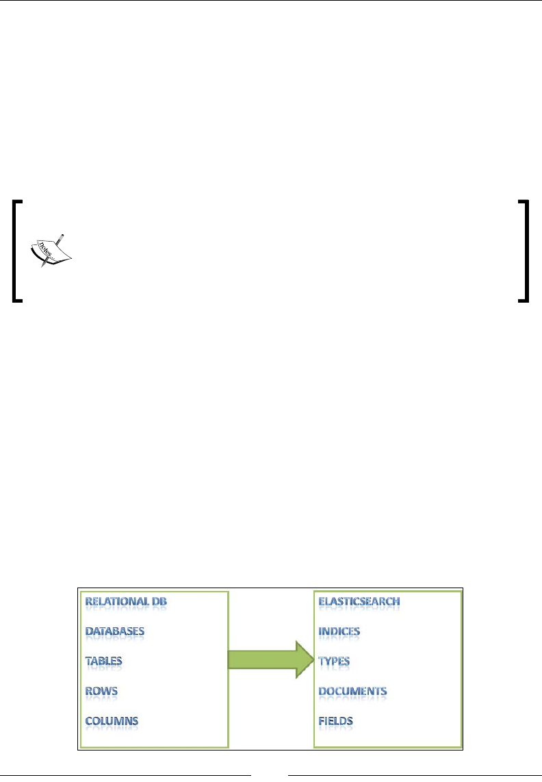
If you want to understand Elasticsearch in relational database terms then, as shown
in the following image, an index in Elasticsearch is similar to a database that consists
of multiple types. A single row is represented as a document, and columns are
similar to elds.

Getting Started with Elasticsearch
[ 8 ]
Elasticsearch does not have the concept of referential integrity constraints such
as foreign keys. But, despite being a search engine and NoSQL data store, it does
allow us to maintain some relationships among different documents, which will
be discussed in the upcoming chapters.
With these theoretical concepts, we are good to go with learning the practical steps
with Elasticsearch.
First of all, you need to be aware of the basic requirements to install and run
Elasticsearch, which are listed as follows:
• Java (Oracle Java 1.7u55 and above)
• RAM: Minimum 2 GB
• Root permission to install and configure program libraries
Please go through the following URL to check the JVM and OS
dependencies of Elasticsearch: https://www.elastic.co/
subscriptions/matrix.
The most common error that comes up if you are using an incompatible Java version
with Elasticsearch, is the following:
Exception in thread "main" java.lang.UnsupportedClassVersionError: org/
elasticsearch/bootstrap/Elasticsearch : Unsupported major.minor version
51.0
at java.lang.ClassLoader.defineClass1(Native Method)
at java.lang.ClassLoader.defineClassCond(ClassLoader.java:637)
at java.lang.ClassLoader.defineClass(ClassLoader.java:621)
at java.security.SecureClassLoader.defineClass(SecureClassLoader.
java:141)
at java.net.URLClassLoader.defineClass(URLClassLoader.java:283)
at java.net.URLClassLoader.access$000(URLClassLoader.java:58)
at java.net.URLClassLoader$1.run(URLClassLoader.java:197)
at java.security.AccessController.doPrivileged(Native Method)
at java.net.URLClassLoader.findClass(URLClassLoader.java:190)
at java.lang.ClassLoader.loadClass(ClassLoader.java:306)
at sun.misc.Launcher$AppClassLoader.loadClass(Launcher.java:301)
at java.lang.ClassLoader.loadClass(ClassLoader.java:247)

Chapter 1
[ 9 ]
If you see the preceding error while installing/working with Elasticsearch, it is most
probably because you have an incompatible version of JAVA set as the JAVA_HOME
variable or not set at all. Many users install the latest version of JAVA but forget to
set the JAVA_HOME variable to the latest installation. If this variable is not set, then
Elasticsearch looks into the following listed directories to nd the JAVA and the
rst existing directory is used:
/usr/lib/jvm/jdk-7-oracle-x64, /usr/lib/jvm/java-7-oracle, /usr/lib/
jvm/java-7-openjdk, /usr/lib/jvm/java-7-openjdk-amd64/, /usr/lib/jvm/
java-7-openjdk-armhf, /usr/lib/jvm/java-7-openjdk-i386/, /usr/lib/jvm/
default-java
Installing and conguring Elasticsearch
I have used the Elasticsearch Version 2.0.0 in this book; you can choose to install
other versions, if you wish to. You just need to replace the version number with
2.0.0. You need to have an administrative account to perform the installations
and congurations.
Installing Elasticsearch on Ubuntu through
Debian package
Let's get started with installing Elasticsearch on Ubuntu Linux. The steps will be the
same for all Ubuntu versions:
1. Download the Elasticsearch Version 2.0.0 Debian package:
wget https://download.elastic.co/elasticsearch/elasticsearch/
elasticsearch-2.0.0.deb
2. Install Elasticsearch, as follows:
sudo dpkg -i elasticsearch-2.0.0.deb
3. To run Elasticsearch as a service (to ensure Elasticsearch starts automatically
when the system is booted), do the following:
sudo update-rc.d elasticsearch defaults 95 10

Getting Started with Elasticsearch
[ 10 ]
Installing Elasticsearch on Centos through
the RPM package
Follow these steps to install Elasticsearch on Centos machines. If you are using any
other Red Hat Linux distribution, you can use the same commands, as follows:
1. Download the Elasticsearch Version 2.0.0 RPM package:
wget https://download.elastic.co/elasticsearch/elasticsearch/
elasticsearch-2.0.0.rpm
2. Install Elasticsearch, using this command:
sudo rpm -i elasticsearch-2.0.0.rpm
3. To run Elasticsearch as a service (to ensure Elasticsearch starts automatically
when the system is booted), use the following:
sudo systemctl daemon-reload
sudo systemctl enable elasticsearch.service
Understanding the Elasticsearch installation
directory layout
The following table shows the directory layout of Elasticsearch that is created after
installation. These directories, have some minor differences in paths depending upon
the Linux distribution you are using.
Description Path on Debian/Ubuntu Path on RHEL/
Centos
Elasticsearch home
directory
/usr/share/elasticsearch /usr/share/
elasticsearch
Elasticsearch and
Lucene jar files
/usr/share/elasticsearch/lib /usr/share/
elasticsearch/
lib
Contains plugins /usr/share/elasticsearch/
plugins
/usr/share/
elasticsearch/
plugins
The locations of the
binary scripts that are
used to start an ES node
and download plugins
usr/share/elasticsearch/bin usr/share/
elasticsearch/
bin

Chapter 1
[ 11 ]
Description Path on Debian/Ubuntu Path on RHEL/
Centos
Contains the
Elasticsearch
configuration files:
(elasticsearch.yml
and logging.yml)
/etc/elasticsearch /etc/
elasticsearch
Contains the data files
of the index/shard
allocated on that node
/var/lib/elasticsearch/data /var/lib/
elasticsearch/
data
The startup script for
Elasticsearch (contains
environment variables
including HEAP SIZE
and file descriptors)
/etc/init.d/elasticsearch /etc/sysconfig/
elasticsearch
Or /etc/init.d/
elasticsearch
Contains the log files of
Elasticsearch.
/var/log/elasticsearch/ /var/log/
elasticsearch/
During installation, a user and a group with the elasticsearch name are created
by default. Elasticsearch does not get started automatically just after installation.
It is prevented from an automatic startup to avoid a connection to an already
running node with the same cluster name.
It is recommended to change the cluster name before starting
Elasticsearch for the rst time.
Conguring basic parameters
1. Open the elasticsearch.yml le, which contains most of the Elasticsearch
conguration options:
sudo vim /etc/elasticsearch/elasticsearch.yml
2. Now, edit the following ones:
°cluster.name: The name of your cluster
°node.name: The name of the node
°path.data: The path where the data for the ES will be stored

Getting Started with Elasticsearch
[ 12 ]
Similar to path.data, we can change path.logs and
path.plugins as well. Make sure all these parameters
values are inside double quotes.
3. After saving the elasticsearch.yml le, start Elasticsearch:
sudo service elasticsearch start
Elasticsearch will start on two ports, as follows:
°9200: This is used to create HTTP connections
°9300: This is used to create a TCP connection through a JAVA client
and the node's interconnection inside a cluster
Do not forget to uncomment the lines you have edited. Please
note that if you are using a new data path instead of the default
one, then you first need to change the owner and the group of
that data path to the user, elasticsearch.
The command to change the directory ownership to elasticsearch
is as follows:
sudo chown –R elasticsearch:elasticsearch data_
directory_path
4. Run the following command to check whether Elasticsearch has been
started properly:
sudo service elasticsearch status
If the output of the preceding command is shown as elasticsearch is not
running, then there must be some configuration issue. You can open the
log file and see what is causing the error.
The list of possible issues that might prevent Elasticsearch from starting is:
• A Java issue, as discussed previously
• Indention issues in the elasticsearch.yml file
• At least 1 GB of RAM is not free to be used by Elasticsearch
• The ownership of the data directory path is not changed to elasticsearch
• Something is already running on port 9200 or 9300

Chapter 1
[ 13 ]
Adding another node to the cluster
Adding another node in a cluster is very simple. You just need to follow all the steps
for installation on another system to install a new instance of Elasticsearch. However,
keep the following in mind:
• In the elasticsearch.yml file, cluster.name is set to be the same on both
the nodes
• Both the systems should be reachable from each other over the network.
• There is no firewall rule set for Elasticsearch port blocking
• The Elasticsearch and JAVA versions are the same on both the nodes
You can optionally set the network.host parameter to the IP address of the system
to which you want Elasticsearch to be bound and the other nodes to communicate.
Installing Elasticsearch plugins
Plugins provide extra functionalities in a customized manner. They can be used
to query, monitor, and manage tasks. Thanks to the wide Elasticsearch community,
there are several easy-to-use plugins available. In this book, I will be discussing
some of them.
The Elasticsearch plugins come in two avors:
• Site plugins: These are the plugins that have a site (web app) in them and do
not contain any Java-related content. After installation, they are moved to the
site directory and can be accessed using es_ip:port/_plugin/plugin_name.
• Java plugins: These mainly contain .jar files and are used to extend the
functionalities of Elasticsearch. For example, the Carrot2 plugin that is used
for text-clustering purposes.
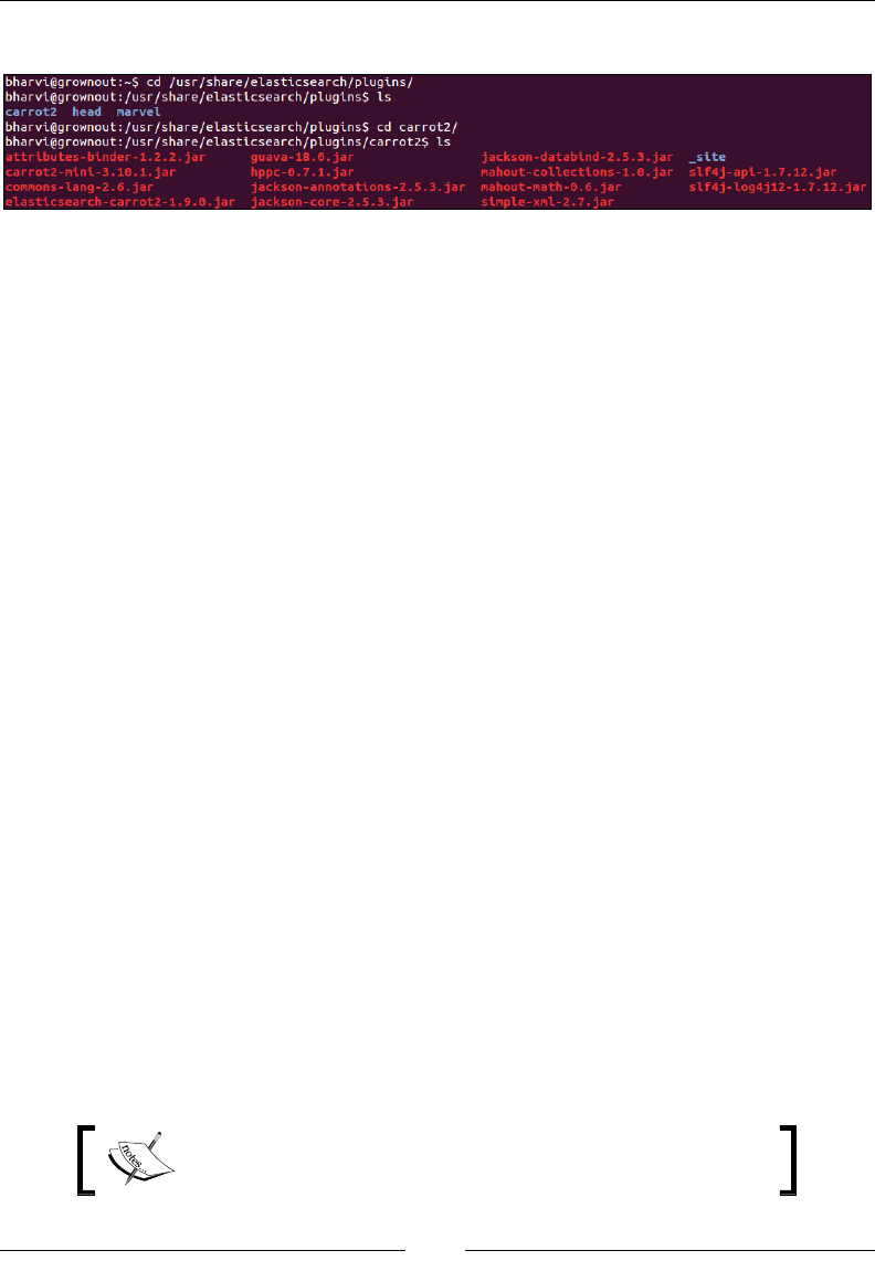
Elasticsearch ships with a plugin script that is located in the /user/share/
elasticsearch/bin directory, and any plugin can be installed using this script
in the following format:
bin/plugin --install plugin_url
Once the plugin is installed, you need to restart that node to
make it active. In the following image, you can see the different
plugins installed inside the Elasticsearch node. Plugins need to
be installed separately on each node of the cluster.
Getting Started with Elasticsearch
[ 14 ]
The following is the layout of the plugin directory of Elasticsearch:
Checking for installed plugins
You can check the log of your node that shows the following line at start up time:
[2015-09-06 14:16:02,606][INFO ][plugins ] [Matt
Murdock] loaded [clustering-carrot2, marvel], sites [marvel, carrot2,
head]
Alternatively, you can use the following command:
curl XGET 'localhost:9200/_nodes/plugins'?pretty
Another option is to use the following URL in your browser:
http://localhost:9200/_nodes/plugins
Installing the Head plugin for Elasticsearch
The Head plugin is a web front for the Elasticsearch cluster that is very easy to use.
This plugin offers various features such as showing the graphical representations of
shards, the cluster state, easy query creations, and downloading query-based data in
the CSV format.
The following is the command to install the Head plugin:
sudo /usr/share/elasticsearch/bin/plugin -install mobz/elasticsearch-head
Restart the Elasticsearch node with the following command to load the plugin:
sudo service elasticsearch restart
Once Elasticsearch is restarted, open the browser and type the following URL to
access it through the Head plugin:
http://localhost:9200/_plugin/head
More information about the Head plugin can be found here:
https://github.com/mobz/elasticsearch-head

Chapter 1
[ 15 ]
Installing Sense for Elasticsearch
Sense is an awesome tool to query Elasticsearch. You can add it to your latest version
of Chrome, Safari, or Firefox browsers as an extension.
Now, when Elasticsearch is installed and running in your system, and you have
also installed the plugins, you are good to go with creating your rst index and
performing some basic operations.
Basic operations with Elasticsearch
We have already seen how Elasticsearch stores data and provides REST APIs to
perform the operations. In next few sections, we will be performing some basic
actions using the command line tool called CURL. Once you have grasped the
basics, you will start programming and implementing these concepts using
Python and Java in upcoming chapters.
When we create an index, Elasticsearch by default creates ve
shards and one replica for each shard (this means ve primary
and ve replica shards). This setting can be controlled in the
elasticsearch.yml le by changing the index.number_
of_shards properties and the index.number_of_replicas
settings, or it can also be provided while creating the index.
Once the index is created, the number of shards can't be increased or decreased;
however, you can increase or decrease the number of replicas at any time after
index creation. So it is better to choose the number of required shards for an index
at the time of index creation.

Getting Started with Elasticsearch
[ 16 ]
Creating an Index
Let's begin by creating our rst index and give this index a name, which is book
in this case. After executing the following command, an index with ve shards
and one replica will be created:
curl –XPUT 'localhost:9200/books/'
Uppercase letters and blank spaces are not allowed in index names.
Indexing a document in Elasticsearch
Similar to all databases, Elasticsearch has the concept of having a unique identier
for each document that is known as _id. This identier is created in two ways,
either you can provide your own unique ID while indexing the data, or if you don't
provide any id, Elasticsearch creates a default id for that document. The following
are the examples:
curl -XPUT 'localhost:9200/books/elasticsearch/1' -d '{
"name":"Elasticsearch Essentials",
"author":"Bharvi Dixit",
"tags":["Data Analytics","Text Search","Elasticsearch"],
"content":"Added with PUT request"
}'
On executing above command, Elasticsearch will give the following response:
{"_index":"books","_type":"elasticsearch","_id":"1","_
version":1,"created":true}
However, if you do not provide an id, which is 1 in our case, then you will get the
following error:
No handler found for uri [/books/elasticsearch] and method [PUT]
The reason behind the preceding error is that we are using a PUT request to create
a document. However, Elasticsearch has no idea where to store this document
(no existing URI for the document is available).
Chapter 1
[ 17 ]
If you want the _id to be auto generated, you have to use a POST request. For example:
curl -XPOST 'localhost:9200/books/elasticsearch' -d '{
"name":"Elasticsearch Essentials",
"author":"Bharvi Dixit",
"tags":["Data Anlytics","Text Search","Elasticsearch"],
"content":"Added with POST request"
}'
The response from the preceding request will be as follows:
{"_index":"books","_type":"elasticsearch","_id":"AU-ityC8xdEEi6V7cMV5","_
version":1,"created":true}
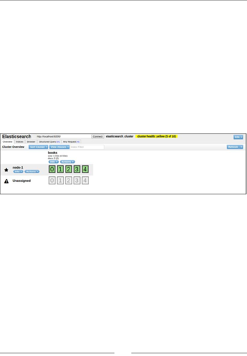
If you open the localhost:9200/_plugin/head URL, you can perform all the
CRUD operations using the HEAD plugin as well:
Some of the stats that you can see in the preceding image are these:
• Cluster name: elasticsearch_cluster
• Node name: node-1
• Index name: books
• No. of primary shards: 5
• No. of docs in the index: 2
• No. of unassigned shards (replica shards): 5

Getting Started with Elasticsearch
[ 18 ]
Cluster states in Elasticsearch
An Elasticsearch cluster can be in one of the three states: GREEN,
YELLOW, or RED. If all the shards, meaning primary as well as
replicas, are assigned in the cluster, it will be in the GREEN state.
If any one of the replica shards is not assigned because of any
problem, then the cluster will be in the YELLOW state. If any one
of the primary shards is not assigned on a node, then the cluster
will be in the RED state. We will see more on these states in the
upcoming chapters. Elasticsearch never assigns a primary and its
replica shard on the same node.
Fetching documents
We have stored documents in Elasticsearch. Now we can fetch them using their
unique ids with a simple GET request.
Get a complete document
We have already indexed our document. Now, we can get the document using its
document identier by executing the following command:
curl -XGET 'localhost:9200/books/elasticsearch/1'?pretty
The output of the preceding command is as follows:
{
"_index" : "books",
"_type" : "elasticsearch",
"_id" : "1",
"_version" : 1,
"found" : true,
"_source":{"name":"Elasticsearch Essentials","author":"Bharvi Dixit",
"tags":["Data Anlytics","Text Search","ELasticsearch"],"content":"Added
with PUT request"}
}
pretty is used in the preceding request to make the response
nicer and more readable.

Chapter 1
[ 19 ]
As you can see, there is a _source eld in the response. This is a special eld
reserved by Elasticsearch to store all the JSON data. There are options available to
not store the data in this eld since it comes with an extra disk space requirement.
However, this also helps in many ways while returning data from ES, re-indexing
data, or doing partial document updates. We will see more on this eld in the next
chapters.
If the document did not exist in the index, the _found eld would have been marked
as false.
Getting part of a document
Sometimes you need only some of the elds to be returned instead of returning the
complete document. For these scenarios, you can send the names of the elds to be
returned inside the _source parameter with the GET request:
curl -XGET 'localhost:9200/books/elasticsearch/1'?_source=name,author
The response of Elasticsearch will be as follows:
{
"_index":"books",
"_type":"elasticsearch",
"_id":"1",
"_version":1,
"found":true,
"_source":{"author":"Bharvi Dixit","name":"Elasticsearch Essentials"}
}
Updating documents
It is possible to update documents in Elasticsearch, which can be done either
completely or partially, but updates come with some limitations and costs. In the
next sections, we will see how these operations can be performed and how things
work behind the scenes.

Getting Started with Elasticsearch
[ 20 ]
Updating a whole document
To update a whole document, you can use a similar PUT/POST request, which we had
used to create a new document:
curl -XPUT 'localhost:9200/books/elasticsearch/1' -d '{
"name":"Elasticsearch Essentials",
"author":"Bharvi Dixit",
"tags":["Data Analytics","Text Search","Elasticsearch"],
"content":"Updated document",
"publisher":"pact-pub"
}'
The response of Elasticsearch looks like this:
{"_index":"books","_type":"elasticsearch","_id":"1","_
version":2,"created":false}
If you look at the response, it shows _version is 2 and created is false, meaning
the document is updated.
Updating documents partially
Instead of updating the whole document, we can use the _update API to do partial
updates. As shown in the following example, we will add a new eld, updated_time,
to the document for which a script parameter has been used. Elasticsearch uses Groovy
scripting by default.
Scripting is by default disabled in Elasticsearch, so to use a script
you need to enable it by adding the following parameter to your
elasticsearch.yml le:
script.inline: on
curl -XPOST 'localhost:9200/books/elasticsearch/1/_update' -d '{
"script" : "ctx._source.updated_time= \"2015-09-09T00:00:00\""
}'
The response of the preceding request will be this:
{"_index":"books","_type":"elasticsearch","_id":"1","_version":3}
It shows that a new version has been created in Elasticsearch.

Chapter 1
[ 21 ]
Elasticsearch stores data in indexes that are composed of Lucene segments.
These segments are immutable in nature, meaning that, once created, they can't
be changed. So, when we send an update request to Elasticsearch, it does the
following things in the background:
• Fetches the JSON data from the _source field for that document
• Makes changes in the _source field
• Deletes old documents
• Creates a new document
All these data re-indexing tasks can be done by the user; however, if you are using
the UPDATE method, it is done using only one request. These processes are the same
when doing a whole document update as for a partial update. The benet of a partial
update is that all operations are done within a single shard, which avoids network
overhead.
Deleting documents
To delete a document using its identier, we need to use the DELETE request:
curl -XDELETE 'localhost:9200/books/elasticsearch/1'
The following is the response of Elasticsearch:
{"found":true,"_index":"books","_type":"elasticsearch","_id":"1","_
version":4}
If you are from a Lucene background, then you must know how segment merging
is done and how new segments are created in the background with more documents
getting indexed. Whenever we delete a document from Elasticsearch, it does not get
deleted from the le system right away. Rather, Elasticsearch just marks that document
as deleted, and when you index more data, segment merging is done. At the same
time, the documents that are marked as deleted are indeed deleted based on a merge
policy. This process is also applied while the document is updated.
The space from deleted documents can also be reclaimed with the _optimize API by
executing the following command:
curl –XPOST http://localhost:9200/_optimize?only_expunge_deletes=true'

Getting Started with Elasticsearch
[ 22 ]
Checking documents' existence
While developing applications, some scenarios require you to check whether a
document exists or not in Elasticsearch. In these scenarios, rather than querying
the documents with a GET request, you have the option of using another HTTP
request method called HEAD:
curl -i -XHEAD 'localhost:9200/books/elasticsearch/1'
The following is the response of the preceding command:
HTTP/1.1 200 OK
Content-Type: text/plain; charset=UTF-8
Content-Length: 0
In the preceding command, I have used the -i parameter that is used to show the
header information of an HTTP response. It has been used because the HEAD request
only returns headers and not any content. If the document is found, then status code
will be 200, and if not, then it will be 400.
Summary
A lot of things have been covered in this chapter. You have got to know about
the Elasticsearch architecture and its workings. Then, you have learned about
the installations of Elasticsearch and its plugins. Finally, basic operations with
Elasticsearch were done.
With all these, you are ready to learn about data analysis phases and mappings
in the next chapter.

[ 23 ]
Understanding
Document Analysis and
Creating Mappings
Search is hard, and it becomes harder when both speed and relevancy are required
together. There are lots of congurable options Elasticsearch provides out-of-the-box
to take control before you start putting the data into it. Elasticsearch is schemaless. I
gave a brief idea in the previous chapter of why it is not completely schemaless and
how it creates a schema right after indexing the very rst document for all the elds
existing in that document. However, the schema matters a lot for a better and more
relevant search. Equally important is understanding the theory behind the phases of
document indexing and search.
In this chapter, we will cover the following topics:
• Full text search and inverted indices
• Document analysis
• Introducing Lucene analyzers
• Creating custom analyzers
• Elasticsearch mappings

Understanding Document Analysis and Creating Mappings
[ 24 ]
Text search
Searching is broadly divided into two types: exact term search and full text search.
An exact term search is something in which we look out for the exact terms; for
example, any named entity such as the name of a person, location, or organization
or date. These searches are easier to make since the search engine simply looks out
for a yes or no and returns the documents.
However, full text search is different as well as challenging. Full text search refers to
the search within text elds, where the text can be unstructured as well as structured.
The text data can be in the form of any human language and based on the natural
languages, which are very hard for a machine to understand and give relevant
results. The following are some examples of full text searches:
• Find all the documents with search in the title or content fields, and return the
results with matches in titles with the higher score
• Find all the tweets in which people are talking about terrorism and killing and
return the results sorted by the tweet creation time
While doing these kinds of searches, we not only want relevant results but also
expect that the search for a keyword matches all of its synonyms, root words, and
spelling mistakes. For example, terrorism should match terorism and terror, while
killing should match kills, kill, and killed.
To serve all these queries, the text-based elds go through an analysis phase
before indexing, and based on this analysis, inverted indexes are built. At the time
of querying, the same analysis process is applied to the terms that are sent within
the queries to match those terms stored in the inverted indexes.
TF-IDF
TF-IDF stands for term frequencies-inverse document frequencies, and it is an
important parameter used inside Lucene's standard similarity algorithm, Vector
Space Model (VSM). The weight calculated by TF-IDF is the statistical measure
to evaluate how important a word is to a document in a collection of documents.
Let's see how a TF-IDF weight is calculated to nd our term's relevancy:
• TF (term): (The number of times a term appears in a document) /
(The total number of terms in the document)
• IDF (term): log_e (The total number of documents / The number of
documents with the t term in it)

Chapter 2
[ 25 ]
While calculating IDF, the log is taken because terms such as the,
that, and is may appear too many times, and we need to weigh
down these frequently appearing terms while increasing the
importance of rare terms.
The weight of TF-IDF is a product of TF(term)*IDF(term).
In information retrieval, one of the simplest relevancy ranking functions is
implemented by summing the TF-IDF weight for each query term. Based on
the combined weights for all the terms appearing in a single query, a score is
calculated that is used to return the results in a sorted order.
Inverted indexes
Inverted index is the heart of search engines. The primary goal of a search engine is
to provide speedy searches while nding the documents in which our search terms
occur. Relevancy comes second.
Let's see with an example how inverted indexes are created and why they are so
fast. In this example, we have two documents with each content eld containing
the following texts:
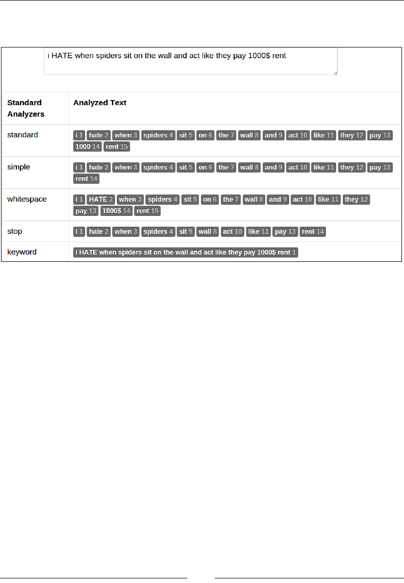
• I hate when spiders sit on the wall and act like they pay rent
• I hate when spider just sit there
While indexing, these texts are tokenized into separate terms and all the unique
terms are stored inside the index with information such as in which document
this term appears and what is the term position in that document.
The inverted index built with the preceding document texts looks like this:
Term Document:Position
I 1:1, 2:1
Hate 1:2, 2:2
When 1:3, 2:3
Spiders 1:4
Sit 1:5, 2:5
On 1:6
Wall 1:7
Spider 2:4
Understanding Document Analysis and Creating Mappings
[ 26 ]
Term Document:Position
Just 2:5
There 2:6
When you search for the term spider OR spiders, the query is executed against the
inverted index and the terms are looked out for, and the documents where these
terms appear are quickly identied. If you search for spider AND spiders, you will
not get any results because when we use AND queries, both the terms used in the
queries must be present in the document. However, spiders and spider are different
for the search engine unless they are normalized into their root forms. For all these
term normalizations, Elasticsearch has a document analysis phase that we will see
in the upcoming sections.
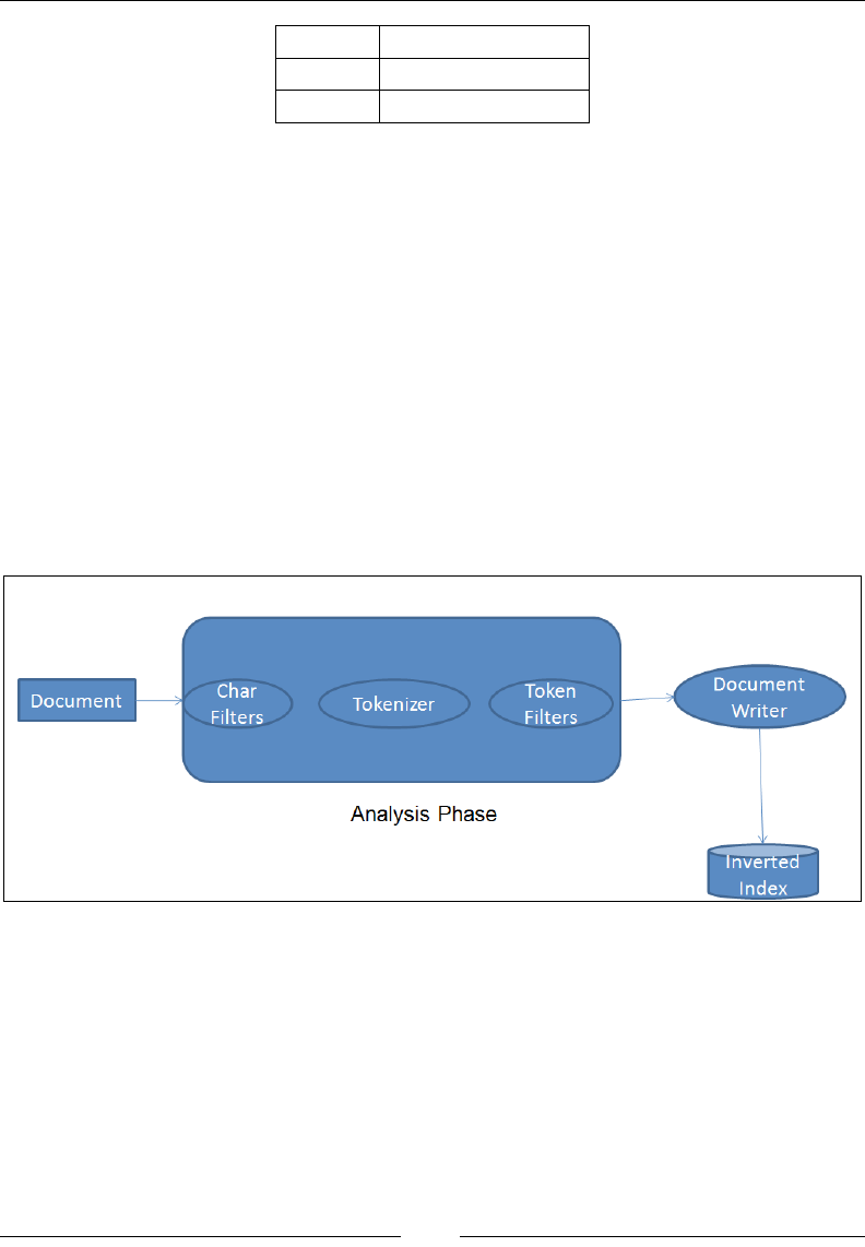
Document analysis
When we index documents into Elasticsearch, it goes through an analysis phase that
is necessary in order to create inverted indexes. It is a series of steps performed by
Lucene, which is depicted in the following image:
The analysis phase is performed by analyzers that are composed of one or more
char lters, a single tokenizer, and one or more token lters. You can declare separate
analyzers for each eld in your document depending on the need. For the same eld,
the analyzers can be the same for both indexing and searching or they can be different.
• Character Filters: The job of character filters is to do cleanup tasks such as
stripping out HTML tags.

Chapter 2
[ 27 ]
• Tokenizers: The next step is to split the text into terms that are called
tokens. This is done by a tokenizer. The splitting can be done based on
any rule such as whitespace. More details about tokenizers can be found
at this URL: https://www.elastic.co/guide/en/elasticsearch/
reference/current/analysis-tokenizers.html.
• Token filters: Once the tokens are created, they are passed to token filters
that normalize the tokens. Token filters can change the tokens, remove the
terms, or add terms to new tokens.
The most used token lters are: the lowercase token lter, which converts a token
into lowercase: the stop token lter, which removes the stop word tokens such as to,
be, a, an, the, and so on: and the ASCII folding token lter, which converts Unicode
characters into their ASCII equivalent. A long list of token lters can be found here:
https://www.elastic.co/guide/en/elasticsearch/reference/current/
analysis-tokenfilters.html.
Introducing Lucene analyzers
Lucene has a wide range of built-in analyzers. We will see the most important
ones here:
• Standard analyzer: This is the default analyzer used by Elasticsearch unless
you mention any other analyzer to be used explicitly. This is best suited for
any language. A standard analyzer is composed of a standard tokenizer
(which splits the text as defined by Unicode Standard Annex), a standard
token filter, a lowercase token filter, and a stop token filter.
A standard tokenizer uses a stop token filter but it defaults to an empty
stopword list, so it does not remove any stop words by default. If you
need to remove stopwords, you can either use the stop analyzer or you
can provide a stopword list to the standard analyzer setting.
• Simple analyzer: A simple analyzer splits the token wherever it finds
a non-letter character and lowercases all the terms using the lowercase
token filter.
• Whitespace analyzer: As the name suggests, it splits the text at white spaces.
However, unlike simple and standard analyzers, it does not lowercase tokens.
• Keyword analyzer: A keyword analyzer creates a single token of the entire
stream. Similar to the whitespace analyzer, it also does not lowercase tokens.
This analyzer is good for fields such as zip codes and phone numbers. It is
mainly used for either exact terms matching, or while doing aggregations.
However, it is beneficial to use not_analyzed for these kinds of fields.

Understanding Document Analysis and Creating Mappings
[ 28 ]
• Language analyzer: There are lots of ready-made analyzers available for
many languages. These analyzers understand the grammatical rules and
the stop words of corresponding languages, and create tokens accordingly.
To know more about language specific analyzers, visit the following URL:
https://www.elastic.co/guide/en/elasticsearch/reference/
current/analysis-lang-analyzer.html.
Elasticsearch provides an easy way to test the analyzers with the _analyze REST
endpoint. Just create a test index, as follows:
curl –XPUT 'localhost:9200/test'
Use the following command by passing the text through the _analyze API to test
the analyzer regarding how your tokens will be created:
curl –XGET 'localhost:9200/test/_analyze?analyzer=whitespace&text=testi
ng, Analyzers&pretty'
You will get the following response:
{
"tokens" : [ {
"token" : "testing,",
"start_offset" : 0,
"end_offset" : 8,
"type" : "word",
"position" : 1
}, {
"token" : "Analyzers",
"start_offset" : 9,
"end_offset" : 18,
"type" : "word",
"position" : 2
} ]
}
You can see in the response how Elasticsearch splits the testing and Analyzers
text into two tokens based on white spaces. It also returns the token positions and
the offsets. You can hit the preceding request in your favorite browser too using
this: localhost:9200/test/_analyze?analyzer=whitespace&text=testing,
Analyzers&pretty.
Chapter 2
[ 29 ]
The following image explains how different analyzers split a token and how many
tokens they produce for the same stream of text:
Creating custom analyzers
In the previous section, we saw in-built analyzers. Sometimes, they are not good
enough to serve our purpose. We need to customize the analyzers using built-in
tokenizers and token/char lters. For example, the keyword analyzer by default
does not use a lowercase lter, but we need it so that data is indexed in the
lowercase form and is searched using either lowercase or uppercase.
To achieve this purpose, Elasticsearch provides a custom analyzer that's type is
custom and can be combined with one tokenizer with zero or more token lters
and zero or more char lters.
Custom analyzers always take the following form:
{
"analysis": {
"analyzer": {}, //Where we put our custom analyzers
"filters": {} //where we put our custom filters.
}
}

Understanding Document Analysis and Creating Mappings
[ 30 ]
Let's create a custom analyzer now with the name keyword_tokenizer using the
keyword tokenizer and lowercase and asciifolding token lters:
"keyword_tokenizer": {
"type": "custom",
"filter": [
"lowercase",
"asciifolding"
],
"tokenizer": "keyword"
}
Similarly, we can create one more custom analyzer with the name url_analyzer for
creating tokens of URLs and e-mail addresses:
"url_analyzer": {
"type": "custom",
"filter": [
"lowercase",
"stop"
],
"tokenizer": "uax_url_email"
}
Changing a default analyzer
You have all the control to dene the type of analyzer to be used for each eld
while creating mapping. However, what about those dynamic elds that you do
not know about while creating mappings. By default, these elds will be indexed
with a standard analyzer. But in case you want to change this default behavior,
you can do it in the following way.
A default analyzer always has the name default and is created using a custom type:
"default": {
"filter": [
"standard",
"lowercase",
"asciifolding"
],
"type": "custom",
"tokenizer": "keyword"
}
In the preceding setting, the name of the analyzer is default, which is created with
the keyword tokenizer.

Chapter 2
[ 31 ]
Putting custom analyzers into action
We have learned to create custom analyzers but we have to tell Elasticsearch about
our custom analyzers so that they can be used. This can be done via the _settings
API of Elasticsearch, as shown in the following example:
curl –XPUT 'localhost/index_name/_settings' –d '{
"analysis": {
"analyzer": {
"default": {
"filter": [
"standard",
"lowercase",
"asciifolding"
],
"type": "custom",
"tokenizer": "keyword"
}
},
"keyword_tokenizer": {
"filter": [
"lowercase",
"asciifolding"
],
"type": "custom",
"tokenizer": "keyword"
}
}
}'
If an index already exists and needs to be updated with new custom
analyzers, then the index rst needs to be closed before updating the
analyzers. It can be done using curl –XPOST 'localhost:9200/
index_name/_close'. After updating, the index can be opened again
using curl –XPOST 'localhost:9200/index_name/_open'.
Elasticsearch mapping
We have seen in the previous chapter how an index can have one or more types
and each type has its own mapping.
Mappings are like database schemas that describe the elds or properties that the
documents of that type may have. For example, the data type of each eld, such as a
string, integer, or date, and how these elds should be indexed and stored by Lucene.

Understanding Document Analysis and Creating Mappings
[ 32 ]
One more thing to consider is that unlike a database, you cannot have a eld with
the same name with different types in the same index; otherwise, you will break
doc_values, and the sorting/searching is also broken. For example, create myIndex
and also index a document with a valid eld that contains an integer value inside
the type1 document type:
curl –XPOST localhost:9200/myIndex/type1/1 –d '{"valid":5}'
Now, index another document inside type2 in the same index with the valid eld.
This time the valid eld contains a string value:
curl –XPOST localhost/myIndex/type2/1 –d '{"valid":"40"}'
In this scenario, the sort and aggregations on the valid eld are broken because they
are both indexed as valid elds in the same index!
Document metadata elds
When a document is indexed into Elasticsearch, there are several metadata elds
maintained by Elasticsearch for that document. The following are the most important
metadata elds you need to know in order to control your index structure:
• _id: _id is a unique identifier for the document and can be either
auto-generated or can be set while indexing or can be configured in
the mapping to be parsed automatically from a field.
• _source: This is a special field generated by Elasticsearch that contains the
actual JSON data in it. Whenever we execute a search request, the _source
field is returned by default. By default, it is enabled, but it can be disabled
using the following configuration while creating a mapping:
PUT index_name/_mapping/doc_type
{"_source":{"enabled":false}}
Be careful while disabling the _source field, as there
are lots of features you can't with it disabled. For example,
highlighting is dependent on the _source field. Documents
can only be searched and not returned; documents can't be
re-indexed and can't be updated.

Chapter 2
[ 33 ]
• _all: When a document is indexed, values from all the fields are indexed
separately as well as in a special field called _all. This is done by Elasticsearch
by default to make a search request on the content of the document without
specifying the field name. It comes with an extra storage cost and should be
disabled if searches need to be made against field names. For disabling it
completely, use the following configuration in you mapping file:
PUT index_name/_mapping/doc_type
{"_all": { "enabled": true }}
However, there are some cases where you do not want to include all the
fields to be included in _all where only certain fields. You can achieve it
by setting the include_in_all parameter to false:
PUT index_name/_mapping/doc_type
{
"_all": {
"enabled": true
},
"properties": {
"first_name": {
"type": "string",
"include_in_all": false
},
"last_name": {
"type": "string"
}
}
}
In the preceding example, only the last name will be included inside the
_all field.
• _ttl: There are some cases when you want the documents to be automatically
deleted from the index. For example, the logs. _ttl (time to live) field provides
the options you can set when the documents should be deleted automatically.
By default, it is disabled and can be enabled using the following configuration:
PUT index_name/_mapping/doc_type
{
"_ttl": {
"enabled": true,
"default": "1w"
}
}

Understanding Document Analysis and Creating Mappings
[ 34 ]
Inside the default field, you can use time units such as m (minutes), d (days),
w (weeks), M (months), and ms (milliseconds). The default is milliseconds.
Please note that the __ttl field has been deprecated since the
Elasticsearch 2.0.0 beta 2 release and might be removed from the
upcoming versions. Elasticsearch will provide a new replacement
for this field in future versions.
• dynamic: There are some scenarios in which you want to restrict the dynamic
fields to be indexed. You only allow the fields that are defined by you in the
mapping. This can be done by setting the dynamic property to be strict, in
the following way:
PUT index_name/_mapping/doc_type
{
"dynamic": "strict",
"properties": {
"first_name": {
"type": "string"
},
"last_name": {
"type": "string"
}
}
}
Data types and index analysis options
Lucene provides several options to congure each and every eld separately
depending on the use case. These options slightly differ based on the data types
for a eld.
Conguring data types
Data types in Elasticsearch are segregated in two forms:
• Core types: These include string, number, date, boolean, and binary
• Complex data types: These include arrays, objects, multi fields, geo points,
geo shapes, nested, attachment, and IP
Since Elasticsearch understands JSON, all the data types supported
by JSON are also supported in Elasticsearch, along with some extra
data types such as geopoint and attachment.

Chapter 2
[ 35 ]
The following are the common attributes for the core data types:
• index: The values can be from analyzed, no, or not_analyzed. If set to
analyzed, the text for that field is analyzed using a specified analyzer.
If set to no, the values for that field do not get indexed and thus, are not
searchable. If set to not_analyzed, the values are indexed as it is; for
example, Elasticsearch Essentials will be indexed as a single term
and thus, only exact matches can be done while querying.
• store: This takes values as either yes or no (default is no but _source is
an exception). Apart from indexing the values, Lucene does have an option
to store the data, which comes in handy when you want to extract the data
from the field. However, since Elasticsearch has an option to store all the
data inside the _source field, it is usually not required to store individual
fields in Lucene.
• boost: This defaults to 1. This specifies the importance of the field inside doc.
• null_value: Using this attribute, you can set a default value to be indexed
if a document contains a null value for that field. The default behavior is to
omit the field that contains null.
One should be careful while configuring default values for null.
The default value should always be of the type corresponding to
the data type configured for that field, and it also should not be
a real value that might appear in some other document.
Let's start with the conguration of the core as well as complex data types.
String
In addition to the common attributes, the following attributes can also be set for
string-based elds:
• term_vector: This property defines whether the Lucene term vectors should
be calculated for that field or not. The values can be no (the default one), yes,
with_offsets, with_positions, and with_positions_offsets.
A term vector is the list of terms in the document and their number
of occurrences in that document. Term vectors are mainly used for
Highlighting and MorelikeThis (searching for similar documents)
queries. A very nice blog on term vectors has been written by Adrien
Grand, which can be read here: http://blog.jpountz.net/
post/41301889664/putting-term-vectors-on-a-diet.

Understanding Document Analysis and Creating Mappings
[ 36 ]
• omit_norms: This takes values as true or false. The default value is false.
When this attribute is set to true, it disables the Lucene norms calculation
for that field (and thus you can't use index-time boosting).
• analyzer: A globally defined analyzer name for the index is used for
indexing and searching. It defaults to the standard analyzer, but can be
controlled also, which we will see in the upcoming section.
• index_analyzer: The name of the analyzer used for indexing. This is not
required if the analyzer attribute is set.
• search_analyzer: The name of the analyzer used for searching. This is not
required if the analyzer attribute is set.
• ignore_above: This specifies the maximum size of the field. If the character
count is above the specified limit, that field won't be indexed. This setting
is mainly used for the not_analyzed fields. Lucene has a term byte-length
limit of 32,766. This means a single term cannot contain more than 10,922
characters (one UTF-8 character contains at most 3 bytes).
An example mapping for two string elds, content and author_name, is as follows:
{
"contents": {
"type": "string",
"store": "yes",
"index": "analyzed",
"include_in_all": false,
"analyzer": "simple"
},
"author_name": {
"type": "string",
"index": "not_analyzed",
"ignore_above": 50
}
}
Number
The number data types are: byte, short, integer, long, floats, and double.
The elds that contain numeric values need to be congured with the appropriate
data type. Please go through the storage type requirements for all the types under a
number before deciding which type you should actually use. In case the eld does
not contain bigger values, choosing long instead of integer is a waste of space.

Chapter 2
[ 37 ]
An example of conguring numeric elds is shown here:
{"price":{"type":"float"},"age":{"type":"integer"}}
Date
Working with dates usually comes with some extra challenges because there are
so many data formats available and you need to decide the correct format while
creating a mapping. Date elds usually take two parameters: type and format.
However, you can use other analysis options too.
Elasticsearch provides a list of formats to choose from depending on the date format
of your data. You can visit the following URL to learn more about it: http://www.
elasticsearch.org/guide/reference/mapping/date-format.html.
The following is an example of conguring date elds:
{
"creation_time": {
"type": "date",
"format": "YYYY-MM-dd"
},
"updation_time": {
"type": "date",
"format": "yyyy/MM/dd HH:mm:ss||yyyy/MM/dd"
},
"indexing_time": {
"type": "date",
"format": "date_optional_time"
}
}
Please note the different date formats used for different date elds in the preceding
mapping. The updation_time eld contains a special format with an || operator,
which species that it will work for both yyyy/MM/dd HH:mm:ss and yyyy/MM/dd
date formats. Elasticsearch uses date_optional_time as the default date parsing
format, which is an ISO datetime parser.
Boolean
While indexing data, a Boolean type eld can contain only two values: true or
false, and it can be congured in a mapping in the following way:
{"is_verified":{"type":"boolean"}}

Understanding Document Analysis and Creating Mappings
[ 38 ]
Arrays
By default, all the elds in Lucene and thus in Elasticsearch are multivalued, which
means that they can store multiple values. In order to send such elds for indexing
to Elasticsearch, we use the JSON array type, which is nested within opening and
closing square brackets []. Some considerations need to be taken care of while
working with array data types:
• All the values of an array must be of the same data type.
• If the data type of a field is not explicitly defined in a mapping, then the data
type of the first value inside the array is used as the type of that field.
• The order of the elements is not maintained inside the index, so do not get
upset if you do not find the desired results while querying. However, this
order is maintained inside the _source field, so when you return the data
after querying, you get the same JSON as you had indexed.
Objects
JSON documents are hierarchical in nature, which allows them to dene inner objects.
Elasticsearch completely understands the nature of these inner objects and can map
them easily by providing query support for their inner elds.
Once a eld is declared as an object type, you can't put any
other type of data into it. If you try to do so, Elasticsearch
will throw an exception.
{
"features": {
"type": "object",
"properties": {
"name": {
"type": "string"
},
"sub_features": {
"dynamic": false,
"type": "object",
"properties": {
"name": {
"type": "string"
},
"description": {
"type": "string"

Chapter 2
[ 39 ]
}
}
}
}
}
}
If you look carefully in the previous mapping, there is a features root object eld and
it contains two properties: name and sub_features. Further, sub_features, which
is an inner object, also contains two properties: name and description, but it has an
extra setting: dynamic: false. Setting this property to false for an object changes the
dynamic behavior of Elasticsearch, and you cannot index any other elds inside that
object apart from the one that is declared inside the mapping. Therefore, you can index
more elds in future inside the features object, but not inside the sub_features object.
Indexing the same eld in different ways
If you need to index the same eld in different ways, the following is the way to
create a mapping for it. You can dene as many elds with the fields parameter
as you want:
{
"name": {
"type": "string",
"fields": {
"raw": {
"type": "string",
"index": "not_analyzed"
}
}
}
}
With the preceding mapping, you just need to index data into the name eld, and
Elasticsearch will index the data into the name eld using the standard analyzer
that can be used for a full text search, and the data in the name.raw eld without
analyzing the tokens; which can be used for an exact term matching. You do not
have to send data into the name.raw eld explicitly.
Please note that this option is only available for core data types
and not for the objects.

Understanding Document Analysis and Creating Mappings
[ 40 ]
Putting mappings in an index
There are two ways of putting mappings inside an index:
• Using a post request at the time of index creation:
curl –XPOST 'localhost:9200/index_name' -d '{
"settings": {
"number_of_shards": 1,
"number_of_replicas": 0
},
"mappings": {
"type1": {
"_all": {
"enabled": false
},
"properties": {
"field1": {
"type": "string",
"index": "not_analyzed"
}
}
},
"type2": {
"properties": {
"field2": {
"type": "string",
"index": "analyzed",
"analyzer":"keyword"
}
}
}
}
}'
• Using a PUT request using the _mapping API. The index must exist before
creating a mapping in this way:
curl –XPUT 'localhost:9200/index_name/index_type/_mapping' –d '{
"_all": {
"enabled": false
},
"properties": {
"field1": {
"type": "integer"
}
}
}'

Chapter 2
[ 41 ]
The mappings for the fields are enclosed inside the properties object, while
all the metadata fields will appear outside the properties object.
It is highly recommended to use the same configuration for the
same field names across different types and indexes in a cluster.
For instance, the data types and analysis options must be the same;
otherwise, you will face weird outputs.
Viewing mappings
Mappings can be viewed easily with the _mapping API:
• To view the mapping of all the types in an index, use the following URL:
curl –XGET localhost:9200/index_name/_mapping?pretty
• To view the mapping of a single type, use the following URL: curl –XGET
localhost:9200/index_name/type_name/_mapping?pretty
Updating mappings
If you want to add mapping for some new elds in the mapping of an existing type,
or create a mapping for a new type, you can do it later using the same _mapping API.
For example, to add a new eld in our existing type, we only need to specify the
mapping for the new eld in the following way:
curl –XPUT 'localhost:9200/index_name/index_type/_mapping' –d '{
"properties": {
"new_field_name": {
"type": "integer"
}
}
}'
Please note that the mapping denition of an existing eld cannot be changed.

Understanding Document Analysis and Creating Mappings
[ 42 ]
Dealing with a long JSON data to be sent in request body
While creating indexes with settings, custom analyzers, and mappings,
you must have noted that all the JSON congurations are passed using
–d, which stands for data. This is used to send a request body. While
creating settings and mappings, it usually happens that the JSON
data becomes so large that it gets difcult to use them in a command
line using curl. The easy solution is to create a le with the .json
extension and provide the path of the le while working with those
settings or mappings. The following is an example command:
curl –XPUT 'localhost:9200/index_name/_settings' –d @
path/setting.json
curl –XPUT 'localhost:9200/index_name/index_type/_
mapping' –d @path/mapping.json
Summary
In this chapter, we covered a lot of ground involving inverted indexes, document
analysis phases, the working of analyzers, and creating custom analyzers. We also
learned about creating and working with mappings of different data types.
In the next chapter, we will start pushing data into Elasticsearch and will learn how
to perform operations with Elasticsearch using Python and Java API.

[ 43 ]
Putting Elasticsearch
into Action
We have covered a lot of ground on Elasticsearch architecture, indexes, analyzers,
and mappings. It's time to start learning about the indexing of data and the querying
of Elasticsearch using its rich Query-DSL.
In this chapter, we will cover the following topics:
• CRUD operations using the Elasticsearch Python client
• CRUD operations using the Elasticsearch Java client
• Creating a search database
• Introducing Query-DSL
• Search requests using Python
• Search requests using Java
• Sorting data
• Document routing
CRUD operations using elasticsearch-py
Elasticsearch is written in Java but it is interoperable with non-JVM languages too.
In this book, we will use its Python client, elasticsearch-py, as well as its Java
client to perform all the operations. The best part of this Python client library is
that it communicates over HTTP and gives you the freedom to write your settings,
mappings, and queries using plain JSON objects, and allows them to pass into the
body parameters of the requests. To read more about this client, you can visit this
URL: http://elasticsearch-py.readthedocs.org/en/master/.

Putting Elasticsearch into Action
[ 44 ]
All the examples used in this book are based on Python 2.7. However, they are
compatible with Python version 3 also.
Setting up the environment
In this section, you will learn how to set up Python environments on Ubuntu using
pip and virtualenv.
Installing Pip
Pip is a package installer for Python modules. It can be installed using the
following commands:
sudo apt-get install python-pip python-dev build-essential
sudo pip install --upgrade pip
Installing virtualenv
While developing programs using Python, it is good practice to create virtualenv.
A virtualenv command creates a directory that stores a private copy of Python
and all the default Python packages. Virtual environments are of great help while
working with several projects and different versions of Python on a single system.
You can create separate virtual environments for each project and enable them for
each corresponding project. To install virtualenv, use the following command:
sudo pip install --upgrade virtualenv
Once the virtual environment is installed, you can create a directory and copy
existing Python packages to it using this command:
mkdir venv
virtualenv venv
After this, you can activate this environment with the following command:
source venv
Once this environment is activated, all the packages that you install will be inside
this venv directory. A virtual environment can be deactivated using just the
deactivate command.

Chapter 3
[ 45 ]
Installing elasticsearch-py
elasticsearch-py can be easily installed using pip in the following way:
pip install elasticsearch
You can verify the installation using the following command:
pip freeze | grep elasticsearch
You will get to know which version of the Elasticsearch client has been installed:
elasticsearch==1.6.0
The version can be different depending on the latest release. The
preceding command installs the latest version. If you want to install a
specic version, then you can specify the version using the == operator.
For example, pip install elasticsearch==1.5.
Performing CRUD operations
You will learn to perform CRUD operations in the upcoming sections, but before
that, let's start with the creation of indexes using Python code.
Since elasticsearch-py communicates over HTTP, it takes JSON data
(setting, mapping, and queries) in the body parameters of the requests.
It is advisable to use a sense plugin (which comes with Marvel or as an
extension too) to write queries, settings, mappings, and all other requests,
because sense offers a lot of help with its autosuggestion functionality.
Once the correct JSON data is created, you can simply store it inside a
variable in your Python code and use it inside a function's body parameter.
Request timeouts
The default timeout for any request sent to Elasticsearch is 10 seconds but there are
chances for requests not to get completed within 10 seconds due to the complexity of
the queries, the load on Elasticsearch, or network latencies. You have two options to
control the timeouts:
• Global timeout: This involves using the timeout parameter while creating
a connection.
• Per-request timeout: This involves using the request_timeout parameter
(in seconds) while hitting separate requests. When request_timeout is used,
it overrides the global timeout value for that particular request.

Putting Elasticsearch into Action
[ 46 ]
Creating indexes with settings and mappings
Create a Python le with index settings and mappings and save it with the name
config.py. It will have two variables, index_settings and doc_mappings:
index_settings = {
"number_of_shards": 1,
"number_of_replicas": 1,
"index": {
"analysis": {
"analyzer": {
"keyword_analyzed": {
"type": "custom",
"filter": [
"lowercase",
"asciifolding"
],
"tokenizer": "keyword"
}
}
}
}
}
doc_mapping = {
"_all": {
"enabled": False
},
"properties": {
"skills": {
"type": "string",
"index": "analyzed",
"analyzer": "standard",
}
}
}
Now create another le, es_operations.py, and follow these steps:
1. Import the Elasticsearch module to your Python le:
from elasticsearch import Elasticsearch
from time import time
2. Import the index_setting and mapping variables from the config le:
from config import index_settings, doc_mapping

Chapter 3
[ 47 ]
3. Initialize the client:
es = Elasticsearch('localhost:9200')
4. Declare variables for the index name, doc type, and body. The body will
contain the settings and the mapping:
index_name='books'
doc_type='search'
body = {}
mapping = {}
mapping[doc_type] = doc_mapping
body['settings'] = index_settings
body['mappings'] = mapping
5. Check whether the index exists; otherwise, create the index:
if not es.indices.exists(index = index_name):
print 'index does not exist, creating the index'
es.indices.create(index = index_name, body = body)
time.sleep(2)
print 'index created successfully'
else:
print 'An index with this name already exists'
Indexing documents
Let's create a document and store it inside a doc1 variable, which is a dictionary:
doc1 = {
'name' : 'Elasticsearch Essentials',
'category' : ['Big Data', 'search engines', 'Analytics'],
'Publication' : 'Packt-Pub',
'Publishing Date' : '2015-31-12'
}
Once the document is created, it can be indexed using the index function:
es.index(index = index_name, doc_type = doc_type, body = doc1, id =
'123')
If you want the unique ID to be autogenerated, use the
None keyword inside the id parameter.

Putting Elasticsearch into Action
[ 48 ]
Retrieving documents
Document retrieval is done using a GET request that takes the following parameter:
response = es.get(index=index_name, doc_type=doc_type, id='1',
ignore=404)
print response
The ignore parameter is used to avoid exceptions in case the document does not
exist in the index. The response will look as follows:
In the response, all the eld names start with u that denotes Unicode. In
normal scenarios, this format does not affect when any task is performed
with the response data. However, in some cases, you might require this to
be in the form of a plain JSON format. To do this, simply import the JSON
module of Python in your code and call the json.dumps(response)
function with the response object inside its parameter.
All the elds are returned inside the _source object and a particular eld can be
accessed using this:
response.get('_source').get(field_name)
Updating documents
As we have seen in Chapter 1, Getting Started with Elasticsearch, a partial document
update can be done using scripts with the _update API. With a Python client, it can
be done using the update function. We can do an update in two scenarios; either to
completely replace the value for a eld, or to append the value inside that eld. To
use scripts to update the documents, make sure you have dynamic scripting enabled.
Replacing the value of a eld completely
To replace the value of an existing eld, you need to simply pass the new value
inside the _source of the document in the following way:
script ={"script" : "ctx._source.category= \"data analytics\""}
es.update(index=index_name, doc_type=doc_type, body=script, id='1',
ignore=404)
After this request, the category eld will contain only one value, data analytics.

Chapter 3
[ 49 ]
Appending a value in an array
Sometimes you need to preserve the original value and append some new data
inside it. Groovy scripting supports the use of parameters with the param attribute
inside scripts, which helps us to achieve this task:
script = {"script" : "ctx._source.category += tag",
"params" : {
"tag" : "Python"
}
}
es.update(index=index_name, doc_type=doc_type, body=script, id='1',
ignore=404)
After this request, the category eld will contain two values: data analytics
and Python.
Updates using doc
Partial updates can be done using the doc parameter instead of body, where doc
is a dictionary object that holds the partial elds that are to be updated. This is the
preferable method to do partial updates. It can be done as shown in the following
example:
es.update(index=index_name, doc_type=doc_type, 'doc': {'new_field':
'doing partial update with a new field'}, id='1', ignore=404)
In most cases, where many documents need to be updated,
document re-indexing makes more sense than updating it
through a script or with doc.
Checking document existence
If it is required to check whether a document exists, you can use the exists function
that returns either true or false in its response:
es.exists(index=index_name, doc_type=doc_type, id='1'):
Deleting a document
Document deletion can be done using the delete function in the following way:
es.delete(index=index_name, doc_type=doc_type, id='1', ignore=404)

Putting Elasticsearch into Action
[ 50 ]
CRUD operations using Java
In this section, we will go through the Elasticsearch Java client to perform the
CRUD operations. To use a Java client of Elasticsearch, you can either build a
Maven project (recommended) or simply add Elasticsearch jar les, which ship
with the Elasticsearch installation le, into your project classpath.
You can include an Elasticsearch dependency in your Maven project by adding
the following code to the project's pom.xml le:
<dependency>
<groupId>org.elasticsearch</groupId>
<artifactId>elasticsearch</artifactId>
<version>2.0.0</version>
</dependency>
Connecting with Elasticsearch
To connect with Elasticsearch using its transport client, you need to add the
following imports:
import org.elasticsearch.client.Client;
import org.elasticsearch.client.transport.TransportClient;
import org.elasticsearch.common.settings.Settings;
import org.elasticsearch.common.transport.InetSocketTransportAddress;
After this, a connection can be created with the following code snippet:
static Client client;
static Settings settings;
public static Client getEsConnection()
{
settings = Settings.settingsBuilder().put("cluster.name",
"elasticsearch").put("path.home", "/").put("client.transport.ping_
timeout","10s").build();
try {
client = TransportClient.builder().settings(settings)
.addTransportAddress(new InetSocketTransportAddress(InetAddr
ess.getByName("localhost"), 9300));
} catch (UnknownHostException e) {
e.printStackTrace();
}
return client;
}

Chapter 3
[ 51 ]
To connect with more than one node of a single cluster, you can add more transport
addresses in this way:
client = TransportClient.builder().settings(settings).build()
.addTransportAddress(new InetSocketTransportAddress(InetAddr
ess.getByName("localhost"), 9300))
.addTransportAddress(new InetSocketTransportAddress(InetAddress.
getByName("some_other_host"), 9300));
Note that to create a connection with Elasticsearch using Java API, you need to rst
create settings by specifying the cluster name and can optionally provide a timeout
that defaults to 5s.
This setting is then used by the transport client to create a connection with the
Elasticsearch cluster over the TCP port 9300.
Indexing a document
To index a single document at once (sequential indexing), you can create documents in
multiple ways, such as using plain JSON strings, or using Jackson API or your familiar
HashMap. The following example shows the use of HashMap to create a document:
1. The rst import will be as follows:
import org.elasticsearch.action.index.IndexResponse;
2. Then create the document:
Map<String, Object> document1= new HashMap<String, Object>();
document1.put("screen_name", "d_bharvi");
document1.put("followers_count", 2000);
document1.put("create_at", "2015-09-20");
3. The preceding document can be indexed with the following code, assuming
you have an object of the client available in your code:
IndexResponse response = client.prepareIndex()
.setIndex("IndexName").setType("docType")
.setId("1").setSource(document1)
.execute().actionGet();
In the preceding code, the setIndex and setType methods take the index
name and the name of the document type correspondingly.
°The setSource method takes the actual data for indexing.
°The setId method takes the unique document identifier. This is
optional; Elasticsearch will generate it dynamically if it is not set.
There are many other methods available, which will see in the upcoming chapter.

Putting Elasticsearch into Action
[ 52 ]
Fetching a document
To fetch a document from Elasticsearch, you need its document ID. Once you know
the document ID, it is simple to fetch it. Just add the following import:
import org.elasticsearch.action.get.GetResponse;
Then, you can get the document using prepareGet:
GetResponse response = client.prepareGet()
.setIndex(indexName).setType(docType)
.setId("1").execute().actionGet();
Updating a document
As you are aware, documents can be updated in two ways; rst using doc, and
the other way is to use script. In both cases, you need to import UpdateResponse
to you, code:
import org.elasticsearch.action.delete.UpdateResponse;
Updating a document using doc
To do a partial update, you can create the object to be appended or replace an
existing value for a eld:
Map<String, Object> partialDoc1= new HashMap<String, Object>();
partialDoc1.put("user_name", "Bharvi Dixit");
Then, you can send it to Elasticsearch using the prepareUpdate method by setting
the partial document inside the setDoc method:
UpdateResponse response = client.prepareUpdate()
.setIndex(indexName).setType(docType)
.setId("1").setDoc(partialDoc1)
.execute().actionGet();
Updating a document using script
To use scripts for updating, rst you need to make sure that you have enabled
dynamic scripting in your elasticsearch.yml le. Then, you need to import
the following classes into your code:
import org.elasticsearch.script.Script;
import org.elasticsearch.script.ScriptService.ScriptType;

Chapter 3
[ 53 ]
Once the import is done, you can do the update in the following way:
String script = "ctx._source.user_name = \"Alberto Paro\"";
UpdateResponse response = client.prepareUpdate()
.setIndex(indexName).setType(docType)
.setScript(new Script(script, ScriptType.INLINE, "groovy", null)).
setId("1").execute().actionGet();
Note that in this example, the INLINE scripts have been used. You can also use le
scripts or indexed scripts . You can nd more about scripting here: https://www.
elastic.co/guide/en/elasticsearch/reference/2.0/modules-scripting.html.
Deleting documents
To delete a single document in a single request, import the following line of code:
import org.elasticsearch.action.delete.DeleteResponse;
You can delete the document with the prepareDelete method using the document ID:
DeleteResponse response = client.prepareDelete()
.setIndex(indexName).setType(docType)
.setId("1").execute().actionGet();
Creating a search database
It's always good to have some practical examples with real data sets, and what could
be better than real-time social media data? In this section, we will write the code that
will fetch tweets from Twitter in real time based on the search keywords provided.
There are three dependencies of the code written in this section:
• tweepy is a Python client for Twitter.
• elasticsearch is a Python client for Elasticsearch that we have
already installed.
• For Twitter API access token keys, please follow the instructions at this
link. https://dev.twitter.com/oauth/overview/application-owner-
access-tokens, to create a sample Twitter application and get all the four
keys that are needed to interact with the Twitter API. These four tokens
are named: Access Token, Access Token Secret, Consumer Key, and
Consumer Secret.

Putting Elasticsearch into Action
[ 54 ]
After generating the auth tokens and keys stored it inside config.py with the
variable names: consumer_key, consumer_secret, access_token, and access_
token_secret. The next step is to install tweepy using this command:
pip install tweepy
If you get any error during the installation of tweepy, the version of
pip may need to be upgraded. To upgrade the pip version use the
following command: pip install 'pip>1.5' --upgrade.
It's good to do some hands-on while creating mappings. For this, rst you need to
understand the JSON data of Twitter. You can view a sample on the following URL
and accordingly create mappings with the appropriate eld types and analyzers:
https://gist.github.com/bharvidixit/0d35b7ac907127860e58.
Once the mapping is created, write the code to start fetching tweets and indexing
them in our index with the name twitter, and type tweet:
from tweepy import OAuthHandler
from tweepy import Stream
from tweepy.streaming import StreamListener
from elasticsearch import Elasticsearch
import config
import json
es = Elasticsearch('localhost:9200')
class StdOutListener(StreamListener):
"""A listener handles tweets that are received from the stream.
This listener dumps the tweets into elasticsearch
"""
counter = 0
total_docs_to_be_indexed = 10000
def on_data(self, data):
print data
while self.total_docs_to_be_indexed > self.counter:
tweet = json.loads(data)
self.index_tweet(tweet)
self.counter += 1
return True
def index_tweet(self, tweet):

Chapter 3
[ 55 ]
es.index(index='twitter', doc_type='tweets',id=tweet['id_str'],
body=tweet)
def on_error(self, status):
print status
pass
#code execution starts here
if __name__ == '__main__':
listener = StdOutListener()
auth = OAuthHandler(config.consumer_key, config.consumer_secret)
auth.set_access_token(config.access_token, config.access_token_
secret)
stream = Stream(auth, listener)
#set the terms for tracking and fetching tweets from Twitter
stream.filter(track=['crime', 'blast', 'earthquake', 'riot',
'politics'])
Elasticsearch Query-DSL
Query-DSL is a JSON interface provided by Elasticsearch to write queries in the
JSON format. It allows you to write any query that you may write in Lucene. The
queries can be as simple as just matching simple terms, or they can be very complex.
Until now, to retrieve documents from Elasticsearch we used a GET request that
was dependent on the ID to search and retrieve the document. You can extend the
searches in similar way; for example: localhost:9200/index_name/doc_type/_
search?q=category:databases.
The preceding query is a typical Lucene query string that searches for the
databases word inside the category eld. Submitting queries to Elasticsearch
in this way is very limited, so you will learn about Query-DSL now.
Syntax:
The Query-DSL follows the following syntax:
{
"query": {},
"from": 0,
"size": 20,
"_source": ["field1","field2"]
}

Putting Elasticsearch into Action
[ 56 ]
Understanding Query-DSL parameters
• query: The query object contains all the queries that need to be passed to
Elasticsearch. For example, the query to find all the documents that belong
to a search category can written as follows:
GET index_name/doc_type/_search
{
"query": {
"query_string": {
"default_field": "category",
"query": "search"
}
}
}
• from and size: These parameters control the pagination and the result size to
be returned after querying. The from parameter is used to specify the starting
point from which document the results will be returned. It defaults to 0. The
size parameter, which defaults to 10, specifies how many top documents
will be returned from the total matched documents in a corpus.
• _source: This is an optional parameter that takes field names in an array
format, which are to be returned in the query results. It by default returns
all the fields stored inside the _source field. If you do not want to return
any field, you can specify _source: false.
Elasticsearch queries majorly fall into two categories:
• Basic Queries: These queries include normal keyword searching
inside indexes.
• Compound Queries: These queries combine multiple basic queries
together with Boolean clauses.
We will be using our Twitter dataset to perform all the queries
in this and the upcoming chapters.

Chapter 3
[ 57 ]
Query types
At the abstract level, there are two major categories of queries in Elasticsearch:
• Full-Text Search Queries: These are the queries that usually run over text
fields like a tweet text. These queries understand the field mapping, and
depending on the field type and analyzer used for that field and query,
the text goes through an analysis phase (similar to indexing) to find the
relevant documents.
• Term-based search queries: Unlike full-text queries, term-based queries
do not go through an analysis process. These queries are used to match the
exact terms stored inside an inverted index.
There exist a few other categories of queries such as Compound
Queries, Geo Queries, and Relational Queries. We will cover
Compound Queries in this chapter and the rest will be covered
in the subsequent chapters.
Full-text search queries
The most important queries in this category are the following:
• match_all
• match
• match_phrase
• multi_match
• query_string
match_all
The simplest query in Elasticsearch is match_all query that matches all the
documents. It gives a generous _score of 1.0 to each document in the index.
The syntax of the match_all query is as follows:
{
"query": {
"match_all": {}
}
}

Putting Elasticsearch into Action
[ 58 ]
match query
The text passed inside a match query goes through the analysis phase and,
depending on the operator (which defaults to OR), documents are matched.
For example:
{
"query": {
"match": {
"text": "Build Great Web Apps",
"operator" : "and"
}
}
}
The preceding query will match the documents that contain the Build, Great, Web,
and Apps terms in the text eld. If we had used the OR operator, it would have
matched the documents containing any of these terms.
If you want the exact matches, you need to pass the text in the
following way so that the text is not broken into tokens:
{
"query": {
"match": {
"text": "\"Build Great Web Apps\""
}
}
}
The preceding query will match the documents in which Build
Great Web Apps appear together exactly in the same order.
Phrase search
Match query provides an option to search phrases with the type parameter in the
following way:
{
"query": {
"match": {
"text": "Build Great Web Apps",
"type" : "phrase"
}
}
}

Chapter 3
[ 59 ]
multi match
The multi_match query is similar to the match query but it provides options to
search the same terms in more than one eld at one go. For example:
{
"query": {
"multi_match": {
"query": "Build Great Web Apps",
"fields": ["text","retweeted_status.text"]
}
}
}
The preceding query will search the words Build, Great, Web, and Apps inside the
two elds text and retweeted_status.text, and will return the relevant results
in a sorted order based on the score each document gets. If you want to match only
those documents in which all the terms are present, then use the and keyword in the
operator parameter.
query_string
In comparison to all the other queries available in Elasticsearch, the query_string
query provides a full Lucene syntax to be used in it. It uses a query parser to construct
an actual query out of the provided text. Similar to the match query, it also goes
through the analysis phase. The following is the syntax for query_string:
{
"query": {
"query_string": {
"default_field": "text",
"query": "text:analytics^2 +text:data -user.name:d_bharvi"
}
}
}
The match query that we used in the previous section can be written using a query
string in the following way:
{
"query": {
"query_string": {
"default_field": "text",
"query": "Build Great Web Apps"
}
}
}

Putting Elasticsearch into Action
[ 60 ]
Term-based search queries
The most important queries in this category are the following:
• Term query
• Terms query
• Range query
• Exists query
• Missing query
Term query
The term query does an exact term matching in a given eld. So, you need to provide
the exact term to get the correct results. For example, if you have used a lowercase
lter while indexing, you need to pass the terms in lowercase while querying with
the term query.
The syntax for a term query is as follows:
{
"query": {
"term": {
"text": "elasticsearch"
}
}
}
Terms query
If you want to search more than one term in a single eld, you can use the terms
query. For example, to search all the tweets in which the hashtags used are either
bomb or blast, you can write a query like this:
{
"query": {
"terms": {
"entities.hashtags": [
"bomb",
"blast"
],
"minimum_match": 1
}
}
}

Chapter 3
[ 61 ]
The minimum_match species the number of minimum terms that should match in
each document. This parameter is optional.
Range queries
Range queries are used to nd data within a certain range. The syntax of a range
query is as follows and is the same for date elds as well as number elds such as
integer, long, and so on:
{
"query": {
"range": {
"user.followers_count": {
"gte": 100,
"lte": 200
}
}
}
}
The preceding query will nd all the tweets created by users whose follower count is
between 100 and 200. The parameters supported in the range queries are: gt, lt, gte,
and lte.
Please note that if you use range queries on string elds, you
will get weird results as strings. String ranges are calculated
lexicographically or alphabetically, so a string stored as 50 will
be lesser than 6. In addition, doing range queries on strings is
a heavier operation in comparison to numbers.
Range queries on dates allow date math operations. So, for example, if you want to
nd all the tweets from the last one hour, you can use the following query:
{
"query": {
"range": {
"created_at": {
"gt": "now-1h"
}
}
}
}
Similarly, months (M), minutes (m), years (y), and seconds (s) are allowed in the query.

Putting Elasticsearch into Action
[ 62 ]
Exists queries
The exists query matches documents that have at least one non-value in a given
eld. For example, the following query will nd all the tweets that are replies to
any other tweet:
{
"query":{
"constant_score":{
"filter":{
"exists":{"field":"in_reply_to_user_id"}
}
}
}
}
Missing queries
Missing queries are the opposite of exists queries. They are used to nd the
documents that contain null values. For instance, the following query nds all
the tweets that do not contain any hashtags:
{
"query":{
"constant_score":{
"filter":{
"missing":{"field":"hashtags"}
}
}
}
}

Chapter 3
[ 63 ]
The story of lters
Before version 2.0.0, Elasticsearch used to have two different
objects for querying data: Queries and Filters. Both used to
differ in functionality and performance.
Queries were used to nd out how relevant a document was
to a particular query by calculating a score for each document,
whereas lters were used to match certain criteria and were
cacheable to enable faster execution. This means that if a lter
matched 1,000 documents, with the help of bloom lters,
Elasticsearch used to cache them in the memory to get them
quickly in case the same lter was executed again.
However, with the release of Lucene 5.0, which is used by
Elasticsearch version 2.0.0, things have completely changed
and both the queries and lters are now the same internal
object. Users need not worry about caching and performance
anymore, as Elasticsearch will take care of it. However, one
must be aware of the contextual difference between a query
and a lter that was listed in the previous paragraph.
In the query context, put the queries that ask the questions
about document relevance and score calculations, while in the
lter context, put the queries that need to match a simple yes/
no question.
If you have been using an Elasticsearch version below 2.0.0,
please go through the breaking changes here: https://
www.elastic.co/guide/en/elasticsearch/
reference/2.0/breaking-changes-2.0.html, and
migrate your application code accordingly since there have
been a lot of changes, including the removal of various lters.
Compound queries
Compound queries are offered by Elasticsearch to connect multiple simple
queries together to make your search better. A compound query clause can
combine any number of queries including compound ones that allow you to
write very complex logic for your searches. You will need them at every step
while creating any search application.
In the previous chapter, we saw how Lucene calculates a score based
on the TF/IDF formula. This score is calculated for each and every
query we send to Elasticsearch. Thus, when we combine queries
in a compound form, the scores of all the queries are combined to
calculate the overall score of the document.

Putting Elasticsearch into Action
[ 64 ]
The primary compound queries are as follows:
• Bool query
• Not query
• Function score query (will be discussed in Chapter 8, Controlling Relevancy)
Bool queries
Bool queries allow us to wrap up many queries clauses together including bool
clauses. The documents are matched based on the combinations of these Boolean
clauses that are listed as follows:
• must: The queries that are written inside this clause must match in order to
return the documents.
• should: The queries written inside the should clause may or may not have
a match but if the bool query has no must clause inside it, then at least one
should condition needs to be matched in order to return the documents.
• must_not: The queries wrapped inside this clause must not appear in the
matching documents.
• filter: A query wrapped inside this clause must appear in the matching
documents. However, this does not contribute to scoring. The structure of
bool queries is as follows:
{
"query":{
"bool":{
"must":[{}],
"should":[{}],
"must_not":[{}]
"filter":[{}]
}
}
}
There are some additional parameters supported by bool queries that are listed here:
• boost: This parameter controls the score of each query, which is wrapped
inside the must or should clause.
• minimum_should_match: This is only used for the should clauses. Using this,
we can specify how many should clauses must match in order to return a
document.

Chapter 3
[ 65 ]
• disable_coord: The bool queries by default use query coordination for
all the should clauses; it is a good thing to have since the more clauses get
matched, the higher the score a document will get. However, look at the
following example where we may need to disable this:
{
"query":{
"bool":{
"disable_coord":true,
"should":[
{"term":{"text":{"value":"turmoil"}}},
{"term":{"text":{"value":"riot"}}}
]
}
}
}
In the preceding example, inside the text eld, we are looking for the terms turmoil
and riot, which are synonyms of each other. In these cases, we do not care how
many synonyms are present in the document since all have the same meaning. In
these kinds of scenarios, we can disable query coordination by setting disable_
coord to true, so that similar clauses do not impact the score factor computation.
Not queries
The not query is used to lter out the documents that match the query. For example,
we can use the following to get the tweets that are not created within a certain range
of time:
{
"filter": {
"not": {
"filter": {
"range": {
"created_at": {
"from": "2015-10-01",
"to": "2010-10-30"
}
}
}
}
}
}
Please note that any lter can be used inside bool queries with the must, must_not,
or should blocks.

Putting Elasticsearch into Action
[ 66 ]
Search requests using Python
All the queries that we have discussed can be performed with the Elasticsearch
Python client using the search function. To do this, rst store the query inside
a variable that is query in the following example:
query = {
"query": {
"match_all": {}
},
}
Call the search function with all the parameters including the index name, document
type, and query. The size parameter used in the following search request can also be
included inside the query itself:
response = es.search(index='twitter', doc_type='tweets', body=query,
size=2, request_timeout=20)
To search against more than one index, instead of using a string
value, you need to use a list of index names. The same applies
for document types too.
The response data comes in the following format:
{
"hits": {
"hits": [
{
"_score": 1,
"_type": "tweets",
"_id": "649956033515773953",
"_source": {
"contributors": null,
"truncated": false,
"text": "RT @lexcanroar: \"No mass shootings in the past 30
years have been stopped by an armed civilian.\""
.
.
},
{
...

Chapter 3
[ 67 ]
}
"_index": "twitter"
}
],
"total": 124,
"max_score": 1
},
"_shards": {
"successful": 5,
"failed": 0,
"total": 5
},
"took": 5,
"timed_out": false
}
The response contains an object hit that has an array of hits containing all the
documents. Further, each hit inside an array of hits contains the following elds in it:
• _score: The document score with respect to the query
• _index: The index name to which the document belongs
• _type: The document type to which the document belongs
• _id: The unique ID of the document
• _source: This contains all the fields and values
The documents inside _source can be accessed with the following code:
for hit in response['hits']['hits']:
print hit.get('_source')
Search requests using Java
While it's easy to write a JSON query and directly use it with the Python client, using
Java client requires a bit of expertise to create queries using Elasticsearch Java APIs.
In Java, there is the QueryBuilder class that helps you in constructing queries.
Once the queries are created, you can execute that query with the client's
prepareSearch method.
First of all, you need the following imports in your code:
import org.elasticsearch.index.query.QueryBuilder;
import org.elasticsearch.index.query.QueryBuilders;
import org.elasticsearch.search.SearchHit;

Putting Elasticsearch into Action
[ 68 ]
Then you can start building queries and executing them:
QueryBuilder query = QueryBuilders.termQuery("screen_name", "d_
bharvi");
SearchResponse response = client.prepareSearch()
.setIndices(indexName).setTypes(docType)
.setQuery(query).setFrom(0).setSize(10)
.execute().actionGet();
The preceding code shows an example of creating term queries where we search for
a term, d_bharvi, inside the screen_name eld.
Similarly, you can create all types of query against the QueryBuilders class. To take
another example, a match_all query can be created by this:
QueryBuilders.matchAllQuery();
The other parameters are as follows:
• setIndices: This is required as search requests support a single search
query to be executed against more than one index. You can specify
comma-separated index names if you want to do so.
• setTypes: Similar to searching inside more than one index, a search can
be executed inside more than one document type. Here, you can provide
comma-separated type names if needed.
• setQuery: This method takes the actual query built using QueryBuilder.
• setFrom and setSize: These parameters are used for pagination purposes
and to specify the number of documents that need to be returned.
Parsing search responses
A search response contains multiple document hits inside it that can be iterated by
converting the response hits into a SearchHit array:
SearchHit[] results = response.getHits().getHits();
for (SearchHit hit : results) {
System.out.println(hit.getSource());
//process documents
}
There are many other methods supported for search requests. A full list can be found
at this gist: https://gist.github.com/bharvidixit/357367e30cea59bb5d62.

Chapter 3
[ 69 ]
Sorting your data
Data in Elasticsearch is by default sorted by a relevance score, which is computed
using the Lucene scoring formula, TF/IDF. This relevance score is a oating point
value that is returned with search results inside the _score parameter. By default,
results are sorted in descending order.
Sorting on nested and geo-points elds will be covered
in the upcoming chapters.
See the following query for an example:
{
"query": {
"match": {
"text": "data analytics"
}
}
}
We are searching for tweets that contain the data or analytics terms in their
text elds. In some cases, however, we do not want the results to be sorted based
on _score. Elasticsearch provides a way to sort documents in various ways.
Let's explore how this can be done.
Sorting documents by eld values
This section covers the sorting of documents based on the elds that contain a single
value such as created_at, or followers_count. Please note that we are not talking
about sorting string-based elds here.
Suppose we want to sort tweets that contain data or analytics in their text eld
based on their creation time in ascending order:
{
"query":{
"match":{"text":"data analytics"}
},
"sort":[
{"created_at":{"order":"asc"}}
]
}

Putting Elasticsearch into Action
[ 70 ]
In the response of the preceding query, max_score and _score will have null as
values. They are not calculated because _score is not used for sorting. You will
see an additional eld, sort. This eld contains the date value in the long format,
which has been used for sorting.
Sorting on more than one eld
In scenarios where it is required to sort documents based on more than one eld,
one can use the following syntax for sorting:
"sort": [
{"created_at":{"order":"asc"},"followers_count":{"order":"asc"}}
]
With the above query, the results will be sorted rst using tweet creation time, and
if two tweets have the same tweet creation time, then they will be sorted using the
followers count.
Sorting multivalued elds
Multivalued elds such as arrays of dates contain more than one value, and you
cannot specify on which value to sort. So in this case, the single value needs to be
calculated rst using mode parameter that takes min, max, avg, median, or sum as a
value. For example, in the following query the sorting will be done on the maximum
value inside the price eld of each document:
"sort" : [
{"price" : {"order" : "asc", "mode" : "max"}}
]
Sorting on string elds
The analyzed string elds are also multivalued elds since they contain multiple
tokens and because of performance considerations; do not use sorting on analyzed
elds.
The string eld on which sorting is to be done must be not_analyzed or keyword
tokenized so that the eld contains only one single token.

Chapter 3
[ 71 ]
Sorting is an expensive process. All the values for the eld on which
sorting is to be performed are loaded into memory. So, you should
have an ample amount of memory on the node to perform sorting.
The data type of the eld should also be chosen carefully while
creating mapping. For example, short can be used in place of
integer or long if the value is not going to be bigger.
Document routing
Document routing is the concept of indexing a document to a particular shard.
By default, Elasticsearch tries to evenly distribute the documents among all the
shards in an index. For this, it uses the following formula:
shard = hash(routing) % number_of_primary_shards
Here, shard is the shard number in which the document will be indexed and
routing is the _id of a document.
We can explicitly specify the routing value while indexing, updating, fetching,
or searching data in Elasticsearch. Custom routing yields faster indexing as well
as faster searches. However, it is more about designing for scale that we will study
in the following chapters.
Summary
In this chapter, you learned how to use Python and Java clients for Elasticsearch
and perform CRUD operations using it. We also covered Elasticsearch Query-DSL,
various queries, and data sorting techniques in this chapter.
In the next chapter, we will take a deep dive into the Elasticsearch aggregation
framework.

[ 73 ]
Aggregations for Analytics
Elasticsearch is a search engine at the core but what makes it more usable is its
ability to make complex data analytics in an easy and simple way. The volume of
data is growing rapidly and companies want to perform analysis on data in real
time. Whether it is log, real-time streaming of data, or static data, Elasticsearch
works wonderfully in getting a summarization of data through its aggregation
capabilities.
In this chapter, we will cover the following topics:
• Introducing the aggregation framework
• Metric and bucket aggregations
• Combining search, buckets, and metrics
• Memory pressure and implications
Introducing the aggregation framework
The aggregation functionality is completely different from search and enables
you to ask sophisticated questions of the data. The use cases of aggregation vary
from building analytical reports to getting real-time analysis of data and taking
quick actions.
Also, despite being different in functionality, aggregations can operate along the usual
search requests. Therefore, you can search or lter your data, and at the same time, you
can also perform aggregation on the same datasets matched by search/lter criteria
in a single request. A simple example can be to nd the maximum number of hashtags
used by users related to tweets that has crime in the text eld. Aggregations enable you to
calculate and summarize data about the current query on the y. They can be used for
all sorts of tasks such as dynamic counting of result values to building a histogram.

Aggregations for Analytics
[ 74 ]
Aggregations come in two avors: metrics and buckets.
• Metrics: Metrics are used to do statistics calculations, such as min, max,
average, on a field of a document that falls into a certain criteria. An example
of a metric can be to find the maximum count of followers among the user's
follower counts.
• Buckets: Buckets are simply the grouping of documents that meet a certain
criteria. They are used to categorize documents, for example:
°The category of loans can fall into the buckets of home loan or
personal loan
°The category of an employee can be either male or female
Elasticsearch offers a wide variety of buckets to categorize documents in many ways
such as by days, age range, popular terms, or locations. However, all of them work
on the same principle: document categorization based on some criteria.
The most interesting part is that bucket aggregations can be nested within each
other. This means that a bucket can contain other buckets within it. Since each of
the buckets denes a set of documents, one can create another aggregation on that
bucket, which will be executed in the context of its parent bucket. For example, a
country-wise bucket can include a state-wise bucket, which can further include a
city-wise bucket.
In SQL terms, metrics are simply functions such as MIN(),
MAX(), SUM(), COUNT(), and AVG(), where buckets group
the results using GROUP BY queries.
Aggregation syntax
Aggregation follows the following syntax:
"aggregations" : {
"<aggregation_name>" : {
"<aggregation_type>" : {
<aggregation_body>
}
[,"aggregations" : { [<sub_aggregation>]+ } ]?
}
[,"<aggregation_name_2>" : { ... } ]*
}

Chapter 4
[ 75 ]
Let's understand how the preceding structure works:
• aggregations: The aggregations objects (which can also be replaced with agg)
in the preceding structure holds the aggregations that have to be computed.
There can be more than one aggregation inside this object.
• <aggregation_name>: This is a user-defined logical name for the
aggregations that are held by the aggregations object (for example, if you
want to compute the average age of users in the index, it makes sense
to give the name as avg_age). These logical names will also be used to
uniquely identify the aggregations in the response.
• <aggregation_type>: Each aggregation has a specific type, for example,
terms, sum, avg, min, and so on.
• <aggregation_body>: Each type of aggregation defines its own body
depending on the nature of the aggregation (for example, an avg
aggregation on a specific field will define the field on which the
average will be calculated).
• <sub_aggregation>: The sub aggregations are defined on the bucketing
aggregation level and are computed for all the buckets built by the bucket
aggregation. For example, if you define a set of aggregations under the range
aggregation, the sub aggregations will be computed for the range buckets
that are defined.
Look at the following JSON structure to understand a more simple structure of
aggregations:
{
"aggs": {
"NAME1": {
"AGG_TYPE": {},
"aggs": {
"NAME": {
"AGG_TYPE": {}
}
}
},
"NAME2": {
"AGG_TYPE": {}
}
}
}

Aggregations for Analytics
[ 76 ]
Extracting values
Aggregations typically work on the values extracted from the aggregated document
set. These values can be extracted either from a specic eld using the eld key
inside the aggregation body or can also be extracted using a script.
While it's easy to dene a eld to be used to aggregate data, the syntax of using
scripts needs some special understanding. The benet of using scripts is that one
can combine the values from more than one eld to use as a single value inside
an aggregation.
Using scripting requires much more computation power and
slows down the performance on bigger datasets.
The following are the examples of extracting values from a script:
Extracting a value from a single eld:
{ "script" : "doc['field_name'].value" }
Extracting and combining values from more than one eld:
"script": "doc['author.first_name'].value + ' ' +
doc['author.last_name'].value"
The scripts also support the use of parameters using the param keyword. For example:
{
"avg": {
"field": "price",
"script": {
"inline": "_value * correction",
"params": {
"correction": 1.5
}
}
}
}
The preceding aggregation calculates the average price after multiplying each value
of the price eld with 1.5, which is used as an inline function parameter.

Chapter 4
[ 77 ]
Returning only aggregation results
Elasticsearch by default computes aggregations on a complete set of documents
using the match_all query and returns 10 documents by default along with the
output of the aggregation results.
If you do not want to include the documents in the response, you need to set the
value of the size parameter to 0 inside your query. Note that you do not need to use
the from parameter in this case. This is a very useful parameter because it avoids
document relevancy calculation and the inclusion of documents in the response,
and only returns the aggregated data.
Metric aggregations
As explained in the previous sections, metric aggregations allow you to nd out the
statistical measurement of the data, which includes the following:
• Computing basic statistics
°Computing in a combined way: stats aggregation
°Computing separately : min, max, sum, value_count, aggregations
• Computing extended statistics: extended_stats aggregation
• Computing distinct counts: cardinality aggregation
Metric aggregations are fundamentally categorized in two forms:
• single-value metric: min, max, sum, value_count, avg,
and cardinality aggregations
• multi-value metric: stats and extended_stats
aggregations

Aggregations for Analytics
[ 78 ]
Computing basic stats
The basic statistics include: min, max, sum, count, and avg. These statistics can be
computed in the following two ways and can only be performed on numeric elds.
Combined stats
All the stats mentioned previously can be calculated with a single aggregation query.
Python example
query = {
"aggs": {
"follower_counts_stats": {
"stats": {
"field": "user.followers_count"
}
}
}
}
res = es.search(index='twitter', doc_type='tweets', body=query)
print resp
The response would be as follows:
"aggregations": {
"follower_counts_stats": {
"count": 124,
"min": 2,
"max": 38121,
"avg": 2102.814516129032,
"sum": 260749
}
}
In the preceding response, count is the total values on which the aggregation
is executed.
• min is the minimum follower count of a user
• max is the maximum follower count of a user
• avg is the average count of followers
• Sum is the addition of all the followers count

Chapter 4
[ 79 ]
Java example
In Java, all the metric aggregations can be created using the
MetricsAggregationBuilder and AggregationBuilders
classes. However, you need to import a specic package into
your code to parse the results.
To build and execute a stats aggregation in Java, rst do the following imports in
the code:
import org.elasticsearch.search.aggregations.metrics.stats.Stats;
Then build the aggregation in the following way:
MetricsAggregationBuilder aggregation =
AggregationBuilders
.stats("follower_counts_stats")
.field("user.followers_count");
This aggregation can be executed with the following code snippet:
SearchResponse response = client.prepareSearch(indexName).
setTypes(docType).setQuery(QueryBuilders.matchAllQuery())
.addAggregation(aggregation)
.execute().actionGet();
The stats aggregation response can be parsed as follows:
Stats agg = sr.getAggregations().get("follower_counts_stats");
long min = agg.getMin();
long max = agg.getMax();
double avg = agg.getAvg();
long sum = agg.getSum();
long count = agg.getCount();
Computing stats separately
In addition to computing these basic stats in a single query, Elasticsearch provides
multiple aggregations to compute them one by one. The following are the aggregation
types that fall into this category:
• value_count: This counts the number of values that are extracted from the
aggregated documents
• min: This finds the minimum value among the numeric values extracted from
the aggregated documents

Aggregations for Analytics
[ 80 ]
• max: This finds the maximum value among the numeric values extracted
from the aggregated documents
• avg: This finds the average value among the numeric values extracted from
the aggregated documents
• sum: This finds the sum of all the numeric values extracted from the
aggregated documents
To perform these aggregations, you just need to use the following syntax:
{
"aggs": {
"aggaregation_name": {
"aggrigation_type": {
"field": "name_of_the_field"
}
}
}
}
Python example
query = {
"aggs": {
"follower_counts_stats": {
"sum": {
"field": "user.followers_count"
}
}
},"size": 0
}
res = es.search(index='twitter', doc_type='tweets', body=query)
We used the sum aggregation type in the preceding query; for other aggregations
such as min, max, avg, and value_count, just replace the type of aggregation in
the query.
Java example
To perform these aggregations using the Java client, you need to follow this syntax:
MetricsAggregationBuilder aggregation =
AggregationBuilders
.sum("follower_counts_stats")
.field("user.followers_count");

Chapter 4
[ 81 ]
Note that in the preceding aggregation, instead of sum, you just need to call the
corresponding aggregation type to build other types of metric aggregations such as,
min, max, count, and avg. The rest of the syntax remains the same.
For parsing the responses, you need to import the correct package according to the
aggregation type. The following are the imports that you will need:
• For min aggregation:
import org.elasticsearch.search.aggregations.metrics.min.Min;
The parsing response will be as follows:
Min agg = response.getAggregations().get("follower_counts_stats");
double value = agg.getValue();
• For max aggregation:
import org.elasticsearch.search.aggregations.metrics.min.Max;
The parsing response will be:
Max agg = response.getAggregations().get("follower_counts_stats");
double value = agg.getValue();
• For avg aggregation:
import org.elasticsearch.search.aggregations.metrics.min.Avg;
The parsing response will be this:
Avg agg = response.getAggregations().get("follower_counts_stats");
double value = agg.getValue();
• For sum aggregation:
import org.elasticsearch.search.aggregations.metrics.min.Sum;
This will be the parsing response:
Sum agg = response.getAggregations().get("follower_counts_stats");
double value = agg.getValue();
Stats aggregations cannot contain sub aggregations. However,
they can be a part of the sub aggregations of buckets.

Aggregations for Analytics
[ 82 ]
Computing extended stats
The extended_stats aggregation is the extended version of stats aggregation
and provides advanced statistics of the data, which include sum of square, variance,
standard deviation, and standard deviation bounds.
So, if we hit the query with the extended_stats aggregation on the followers count
eld, we will get the following data:
"aggregations": {
"follower_counts_stats": {
"count": 124,
"min": 2,
"max": 38121,
"avg": 2102.814516129032,
"sum": 260749,
"sum_of_squares": 3334927837,
"variance": 22472750.441402186,
"std_deviation": 4740.543264374051,
"std_deviation_bounds": {
"upper": 11583.901044877135,
"lower": -7378.272012619071
}
}
}
}
Python example
query = {
"aggs": {
"follower_counts_stats": {
"extended_stats": {
"field": "user.followers_count"
}
}
}
},"size": 0
res = es.search(index='twitter', doc_type='tweets', body=query)

Chapter 4
[ 83 ]
Java example
An extended aggregation is build using the Java client in the following way:
MetricsAggregationBuilder aggregation =
AggregationBuilders
.extendedStats("agg_name")
.field("user.follower_count");
To parse the response of the extended_stats aggregation in Java, you need to have
the following import statement:
import org.elasticsearch.search.aggregations.metrics.stats.extended.
ExtendedStats;
Then the response can parsed in the following way:
ExtendedStats agg = response.getAggregations().get("agg_name");
double min = agg.getMin();
double max = agg.getMax();
double avg = agg.getAvg();
double sum = agg.getSum();
long count = agg.getCount();
double stdDeviation = agg.getStdDeviation();
double sumOfSquares = agg.getSumOfSquares();
double variance = agg.getVariance();
Finding distinct counts
The count of a distinct value of a eld can be calculated using the cardinality
aggregation. For example, we can use this to calculate unique users:
{
"aggs": {
"unique_users": {
"cardinality": {
"field": "user.screen_name"
}
}
}
}

Aggregations for Analytics
[ 84 ]
The response will be as follows:
"aggregations": {
"unique_users": {
"value": 122
}
}
Java example
Cardinality aggregation is built using the Java client in the following way:
MetricsAggregationBuilder aggregation =
AggregationBuilders
.cardinality("unique_users")
.field("user.screen_name");
To parse the response of the cardinality aggregation in Java, you need to have the
following import statement:
import org.elasticsearch.search.aggregations.metrics.cardinality.
Cardinality;
Then the response can parsed in the following way:
Cardinality agg = response.getAggregations().get("unique_users");
long value = agg.getValue();
Bucket aggregations
Similar to metric aggregations, bucket aggregations are also categorized into two
forms: Single buckets that contain only a single bucket in the response, and multi
buckets that contain more than one bucket in the response.
The following are the most important aggregations that are used to create buckets:
• Multi bucket aggregations
°Terms aggregation
°Range aggregation
°Date range aggregation
°Histogram aggregation
°Date histogram aggregation

Chapter 4
[ 85 ]
• Single bucket aggregation
°Filter-based aggregation
We will cover a few more aggregations such as nested and
geo aggregations in subsequent chapters.
Buckets aggregation response formats are different from the response formats of
metric aggregations. The response of a bucket aggregation usually comes in the
following format:
"aggregations": {
"aggregation_name": {
"buckets": [
{
"key": value,
"doc_count": value
},
......
]
}
}
All the bucket aggregations can be created in Java using the
AggregationBuilder and AggregationBuilders classes.
You need to have the following classes imported inside your
code for the same:
org.elasticsearch.search.aggregations.
AggregationBuilder;
org.elasticsearch.search.aggregations.
AggregationBuilders;
Also, all the aggregation queries can be executed with the
following code snippet:
SearchResponse response = client.
prepareSearch(indexName).setTypes(docType)
.setQuery(QueryBuilders.matchAllQuery())
.addAggregation(aggregation)
.execute().actionGet();
The setQuery() method can take any type of Elasticsearch
query, whereas the addAggregation() method takes the
aggregation built using AggregationBuilder.

Aggregations for Analytics
[ 86 ]
Terms aggregation
Terms aggregation is the most widely used aggregation type and returns the buckets
that are dynamically built using one per unique value.
Let's see how to nd the top 10 hashtags used in our Twitter index in descending order.
Python example
query = {
"aggs": {
"top_hashtags": {
"terms": {
"field": "entities.hashtags.text",
"size": 10,
"order": {
"_term": "desc"
}
}
}
}
}
In the preceding example, the size parameter controls how many buckets are to be
returned (defaults to 10) and the order parameter controls the sorting of the bucket
terms (defaults to asc):
res = es.search(index='twitter', doc_type='tweets', body=query)
The response would look like this:
"aggregations": {
"top_hashtags": {
"doc_count_error_upper_bound": 0,
"sum_other_doc_count": 44,
"buckets": [
{
"key": "politics",
"doc_count": 2
},
….............
]
}
}

Chapter 4
[ 87 ]
Java example
Terms aggregation can be built as follows:
AggregationBuilder aggregation =
AggregationBuilders.terms("agg").field(fieldName)
.size(10);
Here, agg is the aggregation bucket name and fieldName is the eld on which the
aggregation is performed.
The response object can be parsed as follows:
To parse the terms aggregation response, you need to import the following class:
import org.elasticsearch.search.aggregations.bucket.terms.Terms;
Then, the response can be parsed with the following code snippet:
Terms screen_names = response.getAggregations().get("agg");
for (Terms.Bucket entry : screen_names.getBuckets()) {
entry.getKey(); // Term
entry.getDocCount(); // Doc count
}
Range aggregation
With range aggregation, a user can specify a set of ranges, where each range
represents a bucket. Elasticsearch will put the document sets into the correct
buckets by extracting the value from each document and matching it against
the specied ranges.
Python example
query = "aggs": {
"status_count_ranges": {
"range": {
"field": "user.statuses_count",
"ranges": [
{
"to": 50
},
{
"from": 50,
"to": 100
}

Aggregations for Analytics
[ 88 ]
]
}
}
},"size": 0
}
res = es.search(index='twitter', doc_type='tweets', body=query)
The range aggregation always discards the to value for each range
and only includes the from value.
The response for the preceding query request would look like this:
"aggregations": {
"status_count_ranges": {
"buckets": [
{
"key": "*-50.0",
"to": 50,
"to_as_string": "50.0",
"doc_count": 3
},
{
"key": "50.0-100.0",
"from": 50,
"from_as_string": "50.0",
"to": 100,
"to_as_string": "100.0",
"doc_count": 3
}
]
}
}
Java example
Building range aggregation:
AggregationBuilder aggregation =
AggregationBuilders
.range("agg")
.field(fieldName)
.addUnboundedTo(1) // from -infinity to 1 (excluded)
.addRange(1, 100) // from 1 to 100(excluded)
.addUnboundedFrom(100); // from 100 to +infinity

Chapter 4
[ 89 ]
Here, agg is the aggregation bucket name and fieldName is the eld on which the
aggregation is performed. The addUnboundedTo method is used when you do not
specify the from parameter and the addUnboundedFrom method is used when you
don't specify the to parameter.
Parsing the response
To parse the range aggregation response, you need to import the following class:
import org.elasticsearch.search.aggregations.bucket.range.Range;
Then, the response can be parsed with the following code snippet:
Range agg = response.getAggregations().get("agg");
for (Range.Bucket entry : agg.getBuckets()) {
String key = entry.getKeyAsString(); // Range as key
Number from = (Number) entry.getFrom(); // Bucket from
Number to = (Number) entry.getTo(); // Bucket to
long docCount = entry.getDocCount(); // Doc count
}
Date range aggregation
The date range aggregation is dedicated for date elds and is similar to range
aggregation. The only difference between range and date range aggregation is that
the latter allows you to use a date math expression inside the from and to elds.
The following table shows an example of using math operations in Elasticsearch.
The supported time units for the math operations are: y (year), M (month), w (week),
d (day), h (hour), m (minute), and s (second):
Operation Description
Now Current time
Now+1h Current time plus 1 hour
Now-1M Current time minus 1 month
Now+1h+1m Current time plus 1 hour plus one minute
Now+1h/d Current time plus 1 hour rounded to the nearest day
2016-01-01||+1M/d 2016-01-01 plus 1 month rounded to the nearest day
Python example
query = {
"aggs": {
"tweets_creation_interval": {

Aggregations for Analytics
[ 90 ]
"range": {
"field": "created_at",
"format": "yyyy",
"ranges": [
{
"to": 2000
},
{
"from": 2000,
"to": 2005
},
{
"from": 2005
}
]
}
}
},"size": 0
}
res = es.search(index='twitter', doc_type='tweets', body=query)
print res
Java example
Building date range aggregation:
AggregationBuilder aggregation =
AggregationBuilders
.dateRange("agg")
.field(fieldName)
.format("yyyy")
.addUnboundedTo("2000") // from -infinity to 2000 (excluded)
.addRange("2000", "2005") // from 2000 to 2005 (excluded)
.addUnboundedFrom("2005"); // from 2005 to +infinity
Here, agg is the aggregation bucket name and fieldName is the eld on which the
aggregation is performed. The addUnboundedTo method is used when you do not
specify the from parameter and the addUnboundedFrom method is used when you
don't specify the to parameter.
Parsing the response:
To parse the date range aggregation response, you need to import the
following class:
import org.elasticsearch.search.aggregations.bucket.range.Range;
import org.joda.time.DateTime;

Chapter 4
[ 91 ]
Then, the response can be parsed with the following code snippet:
Range agg = response.getAggregations().get("agg");
for (Range.Bucket entry : agg.getBuckets()) {
String key = entry.getKeyAsString(); // Date range as key
DateTime fromAsDate = (DateTime) entry.getFrom(); // Date bucket
from as a Date
DateTime toAsDate = (DateTime) entry.getTo(); // Date bucket to as a
Date
long docCount = entry.getDocCount(); // Doc count
}
Histogram aggregation
A histogram aggregation works on numeric values extracted from documents and
creates xed-sized buckets based on those values. Let's see an example for creating
buckets of a user's favorite tweet counts:
Python example
query = {
"aggs": {
"favorite_tweets": {
"histogram": {
"field": "user.favourites_count",
"interval": 20000
}
}
},"size": 0
}
res = es.search(index='twitter', doc_type='tweets', body=query)
for bucket in res['aggregations']['favorite_tweets']['buckets']:
print bucket['key'], bucket['doc_count']
The response for the preceding query will look like the following, which says that
114 users have favorite tweets between 0 to 20000 and 8 users have more than 20000
as their favorite tweets:
"aggregations": {
"favorite_tweets": {
"buckets": [
{
"key": 0,
"doc_count": 114
},

Aggregations for Analytics
[ 92 ]
{
"key": 20000,
"doc_count": 8
}
]
}
}
While executing the histogram aggregation, the values of the
documents are rounded off and they fall into the closest bucket;
for example, if the favorite tweet count is 72 and the bucket size
is set to 5, it will fall into the bucket with the key 70.
Java example
Building histogram aggregation:
AggregationBuilder aggregation =
AggregationBuilders
.histogram("agg")
.field(fieldName)
.interval(5);
Here, agg is the aggregation bucket name and fieldName is the eld on which
aggregation is performed. The interval method is used to pass the interval for
generating the buckets.
Parsing the response:
To parse the histogram aggregation response, you need to import the following class:
import org.elasticsearch.search.aggregations.bucket.histogram.
Histogram;
Then, the response can be parsed with the following code snippet:
Range agg = response.getAggregations().get("agg");
for (Histogram.Bucket entry : agg.getBuckets()) {
Long key = (Long) entry.getKey(); // Key
long docCount = entry.getDocCount(); // Doc coun
}

Chapter 4
[ 93 ]
Date histogram aggregation
Date histogram is similar to the histogram aggregation but it can only be applied
to date elds. The difference between the two is that date histogram allows you to
specify intervals using date/time expressions.
The following values can be used for intervals:
• year, quarter, month, week, day, hour, minute, and second
You can also specify fractional values, such as 1h (1 hour), 1m (1 minute) and so on.
Date histograms are mostly used to generate time-series graphs in many applications.
Python example
query = {
"aggs": {
"tweet_histogram": {
"date_histogram": {
"field": "created_at",
"interval": "hour"
}
}
}, "size": 0
}
The preceding aggregation will generate an hourly-based tweet timeline on the eld,
created_at:
res = es.search(index='twitter', doc_type='tweets', body=query)
for bucket in res['aggregations']['tweet_histogram']['buckets']:
print bucket['key'], bucket['key_as_string'], bucket['doc_count']
Java example
Building date histogram aggregation:
AggregationBuilder aggregation =
AggregationBuilders
.histogram("agg")
.field(fieldName)
.interval(DateHistogramInterval.YEAR);

Aggregations for Analytics
[ 94 ]
Here, agg is the aggregation bucket name and fieldname is the eld
on which the aggregation is performed. The interval method is used to
pass the interval to generate buckets. For interval in days, you can do this:
DateHistogramInterval.days(10)
Parsing the response:
To parse the date histogram aggregation response, you need to import the
following class:
import org.elasticsearch.search.aggregations.bucket.histogram.
DateHistogramInterval;
The response can be parsed with this code snippet:
Histogram agg = response.getAggregations().get("agg");
for (Histogram.Bucket entry : agg.getBuckets()) {
DateTime key = (DateTime) entry.getKey(); // Key
String keyAsString = entry.getKeyAsString(); // Key as String
long docCount = entry.getDocCount(); // Doc count
}
Filter-based aggregation
Elasticsearch allows lters to be used as aggregations too. Filters preserve their
behavior in the aggregation context as well and are usually used to narrow down
the current aggregation context to a specic set of documents. You can use any lter
such as range, term, geo, and so on.
To get the count of all the tweets done by the user, d_bharvi, use the following code:
Python example
query = {
"aggs": {
"screename_filter": {
"filter": {
"term": {
"user.screen_name": "d_bharvi"
}
}
}
},"size": 0
}

Chapter 4
[ 95 ]
In the preceding request, we have used a term lter to narrow down the bucket of
tweets done by a particular user:
res = es.search(index='twitter', doc_type='tweets', body=query)
for bucket in res['aggregations']['screename_filter']['buckets']:
print bucket['doc_count']
The response would look like this:
"aggregations": {
"screename_filter": {
"doc_count": 100
}
}
}
Java example
Building lter-based aggregation:
AggregationBuilder aggregation =
AggregationBuilders
.filter("agg")
.filter(QueryBuilders.termQuery("user.screen_name ", "d_bharvi"));
Here, agg is the aggregation bucket name under the rst lter method and the
second lter method takes a query to apply the lter.
Parsing the response:
To parse a lter-based aggregation response, you need to import the following class:
import org.elasticsearch.search.aggregations.bucket.histogram.
DateHistogramInterval;
The response can be parsed with the following code snippet:
Filter agg = response.getAggregations().get("agg");
agg.getDocCount(); // Doc count

Aggregations for Analytics
[ 96 ]
Combining search, buckets, and metrics
We can always combine searches, lters bucket aggregations, and metric aggregations
to get a more and more complex analysis. Until now, we have seen single levels of
aggregations; however, as explained in the aggregation syntax section earlier, an
aggregation can contain multiple levels of aggregations within. However, metric
aggregations cannot contain further aggregations within themselves. Also, when you
run an aggregation, it is executed on all the documents in the index for a document
type if specied on a match_all query context, but you can always use any type of
Elasticsearch query with an aggregation. Let's see how we can do this in Python and
Java clients.
Python example
query = {
"query": {
"match": {
"text": "crime"
}
},
"aggs": {
"hourly_timeline": {
"date_histogram": {
"field": "created_at",
"interval": "hour"
},
"aggs": {
"top_hashtags": {
"terms": {
"field": "entities.hashtags.text",
"size": 1
},
"aggs": {
"top_users": {
"terms": {
"field": "user.screen_name",
"size": 1
},
"aggs": {
"average_tweets": {
"avg": {
"field": "user.statuses_count"
}
}

Chapter 4
[ 97 ]
}
}
}
}
}
}
} ,"size": 0
}
res = es.search(index='twitter', doc_type='tweets', body=query)
Parsing the response data:
for timeline_bucket in res['aggregations']['hourly_timeline']
['buckets']:
print 'time range', timeline_bucket['key_as_string']
print 'tweet count ',timeline_bucket['doc_count']
for hashtag_bucket in timeline_bucket['top_hashtags']['buckets']:
print 'hashtag key ', hashtag_bucket['key']
print 'hashtag count ', hashtag_bucket['doc_count']
for user_bucket in hashtag_bucket['top_users']['buckets']:
print 'screen_name ', user_bucket['key']
print 'count', user_bucket['doc_count']
print 'average tweets', user_bucket['average_tweets']
['value']
And you will nd the output as below:
time_range 2015-10-14T10:00:00.000Z
tweet_count 1563
hashtag_key crime
hashtag_count 42
screen_name andresenior
count 2
average_tweets 9239.0
............
Understanding the response in the context of our search of the term crime in a
text eld:
• time_range: The key of the daywise_timeline bucket
• tweet_count: The number of tweets happening per hour
• hashtag_key: The name of the hashtag used by users within the specified
time bucket

Aggregations for Analytics
[ 98 ]
• hashtag_count: The count of each hashtag within the specified time bucket
• screen_name: The screen name of the user who has tweeted using that hashtag
• count: The number of times that user tweeted using a corresponding hashtag
• average_tweets: The average number of tweets done by users in their lifetime
who have used this particular hashtag
Java example
Writing multilevel aggregation queries (as we just saw) in Java seems quite complex,
but once you learn the basics of structuring aggregations, it becomes fun.
Let's see how we write the previous query in Java:
Building the query using QueryBuilder:
QueryBuilder query = QueryBuilders.matchQuery("text", "crime");
Building the aggregation:
The syntax for a multilevel aggregation in Java is as follows:
AggregationBuilders
.aggType("aggs_name")
//aggregation_definition
.subAggregation(AggregationBuilders
.aggType("aggs_name")
//aggregation_definition
.subAggregation(AggregationBuilders
.aggType("aggs_name")
//aggregation_definition……..
You can relate the preceding syntax with the aggregation syntax you learned in the
beginning of this chapter.
The exact aggregation for our Python example will be as follows:
AggregationBuilder aggregation =
AggregationBuilders
.dateHistogram("hourly_timeline")
.field("@timestamp")
.interval(DateHistogramInterval.YEAR)
.subAggregation(AggregationBuilders
.terms("top_hashtags")
.field("entities.hashtags.text")
.subAggregation(AggregationBuilders

Chapter 4
[ 99 ]
.terms("top_users")
.field("user.screen_name")
.subAggregation(AggregationBuilders
.avg("average_status_count")
.field("user.statuses_count"))));
Let's execute the request by combining the query and aggregation we have built:
SearchResponse response = client.prepareSearch(indexName).
setTypes(docType)
.setQuery(query).addAggregation(aggregation)
.setSize(0)
.execute().actionGet();
Parsing multilevel aggregation responses:
Since multilevel aggregations are nested inside each other, you need to iterate
accordingly to parse each level of aggregation response in loops.
The response for our request can be parsed with the following code:
//Get first level of aggregation data
Histogram agg = response.getAggregations().get("hourly_timeline");
//for each entry of hourly histogram
for (Histogram.Bucket entry : agg.getBuckets()) {
DateTime key = (DateTime) entry.getKey();
String keyAsString = entry.getKeyAsString();
long docCount = entry.getDocCount();
System.out.println(key);
System.out.println(docCount);
//Get second level of aggregation data
Terms topHashtags = entry.getAggregations().get("top_hashtags");
//for each entry of top hashtags
for (Terms.Bucket hashTagEntry : topHashtags.getBuckets()) {
String hashtag = hashTagEntry.getKey().toString();
long hashtagCount = hashTagEntry.getDocCount();
System.out.println(hashtag);
System.out.println(hashtagCount);
//Get 3rd level of aggregation data
Terms topUsers = hashTagEntry.getAggregations()
.get("top_users");
//for each entry of top users
for (Terms.Bucket usersEntry : topUsers.getBuckets()) {

Aggregations for Analytics
[ 100 ]
String screenName = usersEntry.getKey().toString();
long userCount = usersEntry.getDocCount(); System.out.
println(screenName);
System.out.println(userCount);
//Get 4th level of aggregation data
Avg average_status_count = usersEntry
.getAggregations()
.get("average_status_count");
double max = average_status_count.getValue();
System.out.println(max);
}
}
}
As you saw, building these types of aggregations and going for a drill down on
data sets to do complex analytics can be fun. However, one has to keep in mind the
pressure on memory that Elasticsearch bears while doing these complex calculations.
The next section covers how we can avoid these memory implications.
Memory pressure and implications
Aggregations are awesome! However, they bring a lot of memory pressure on
Elasticsearch. They work on an in-memory data structure called elddata, which
is the biggest consumer of HEAP memory in a Elasticsearch cluster. Fielddata is not
only used for aggregations, but also used for sorting and scripts. The in-memory
elddata is slow to load, as it has to read the whole inverted index and un-invert
it. If the elddata cache lls up, old data is evicted causing heap churn and bad
performance (as elddata is reloaded and evicted again.)
The more unique terms exist in the index, the more terms will be loaded into memory
and the more pressure it will have. If you are using an Elasticsearch version below 2.0.0
and above 1.0.0, then you can use the doc_vlaues parameter inside the mapping while
creating the index to avoid the use of elddata using the following syntax:
PUT /index_name/_mapping/index_type
{
"properties": {
"field_name": {
"type": "string",
"index": "not_analyzed",
"doc_values": true
}
}
}

Chapter 4
[ 101 ]
doc_values have been enabled by default from Elasticsearch
version 2.0.0 onwards.
The advantages of using doc_values are as follows:
• Less heap usage and faster garbage collections
• No longer limited by the amount of fielddata that can fit into a given
amount of heap—instead the file system caches can make use of all the
available RAM
• Fewer latency spikes caused by reloading a large segment into memory
The other important consideration to keep in mind is not to have a huge number
of buckets in a nested aggregation. For example, nding the total order value for
a country during a year with an interval of one week will generate 100*51 buckets
with the sum value. It is a big overhead that is not only calculated in data nodes,
but also in the co-ordinating node that aggregates them. A big JSON also gives
problems on parsing and loading on the "frontend". It will easily kill a server with
wide aggregations.
Summary
In this chapter, we learned about one of the most powerful features of Elasticsearch,
that is, aggregation frameworks. We went through the most important metric and
bucket aggregations along with examples of doing analytics on our Twitter dataset
with Python and Java API.
This chapter covered many fundamental as well complex examples of the different
facets of analytics, which can be built using a combination of full-text searches,
term-based searches, and multilevel aggregations. Elasticsearch is awesome for
analytics but one should always keep in mind the memory implications, which
we covered in the last section of this chapter, to avoid the over killing of nodes.
In the next chapter, we will learn to work with geo spatial data in Elasticsearch and
we will also cover analytics with geo aggregations.

[ 103 ]
Data Looks Better on Maps:
Master Geo-Spatiality
The world is getting smarter day by day and searches based on locations have
become an integral part of our daily life. Be it searching for shopping centers,
hospitals, restaurants, or any locations, we always look out for information such as
distance and other information about the area. Elasticsearch is helpful in combining
geo-location data with full-text search, structured search, and also in doing analytics.
In this chapter, we will cover the following topics:
• Introducing geo-spatial data
• Geo-location data types
• Working with geo-point data
• Geo aggregations
• Working with geo-shapes
Introducing geo-spatial data
Geo-spatial data is information of any object on the earth and is presented by
numeric values called latitude-longitude (lat-lon) that are presented on geographical
systems. Apart from lat-lon, a geo-spatial object also contains other information
about that object such as name, size, and shape. Elasticsearch is very helpful when
working with such kinds of data. It doesn't only provide powerful geo-location
searches, but also has functionalities such as sorting with geo distance, creating geo
clusters, scoring based on location, and working with arbitrary geo-shapes.

Data Looks Better on Maps: Master Geo-Spatiality
[ 104 ]
Elasticsearch has two data types to solely work on geo-spatial data; they are as follows:
• geo_point: This is a combination of latitude-longitude pairs that defines a
single location point
• geo_shape: This works on latitude-longitudes, but with complex shapes such
as points, multi-points, lines, circles, polygons, and multi-polygons defined
by a geo-JSON data structure
Working with geo-point data
Geo-points are single location points dened by a latitude-longitude pair on the
surface of the earth. Using geo-points you can do the following things:
• Calculate the distance between two points
• Find the document that falls in a specified rectangular area
• Sort documents based on distance and score results based on it
• Create clusters of geo-points using aggregations
Mapping geo-point elds
Unlike all the data types in Elasticsearch, geo-point elds can't be determined
dynamically. So, you have to dene the mapping in advance before indexing data.
The mapping for a geo-point eld can be dened in the following format:
"location": {
"type": "geo_point"
}
A geo_point mapping indexes a single eld (the location in our example) in the
lat-lon format. You can optionally index .lat and .lon separately by setting the
lat-lon parameter to true.
Indexing geo-point data
Elasticsearch supports the following three formats to index geo_point data with the
same mapping that we dened in the previous section:
lat-lon as a string : "location" : "28.61, 77.23"
lat-lon as an object : "location": {
"lat": 28.61,
"lon": 77.23
}
lat-lon as an array : "location" : [77.23, 28.61]

Chapter 5
[ 105 ]
The order of latitude-longitude differs in an array format. It takes longitude rst and
then latitude.
Python example
In this section, we will see how to index the geo_point data in all the three formats
using Python:
• Using string format:
doc ={"location": "28.61, 77.23"}
es.index(index=index_name, doc_type=doc_type, body=doc)
• Using object format:
location = dict()
location['lat'] = 28.61
location['lon'] = 77.23
doc['location'] = location
es.index(index=index_name, doc_type=doc_type, body=doc)
• Using array format:
location = list()
location.append(77.23)
location.append(28.6)
doc['location'] = location
es.index(index=index_name, doc_type=doc_type, body=doc)
Java example
• Using string format:
Map<String, Object> document1= new HashMap<String, Object>();
document1.put("location", "29.9560, 78.1700");
document1.put("name", "delhi");
document1.put("dish_name", "chinese");
client.prepareIndex().setIndex(indexName).setType(docType)
.setSource(document1).execute().actionGet();
• Using object format:
Map<String, Object> document3 = new HashMap<String, Object>();
Map<String, Object> locationMap = new HashMap<String, Object>();
locationMap.put("lat", 29.9560);
locationMap.put("lon", 78.1700);
document3.put("location", locationMap);
document3.put("name", "delhi");
document3.put("dish_name", "chinese");
client.prepareIndex().setIndex(indexName).setType(docType)
.setSource(document3).execute().actionGet();

Data Looks Better on Maps: Master Geo-Spatiality
[ 106 ]
• Using array format:
Map<String, Object> document2= new HashMap<String, Object>();
List<Double> geoPoints = new ArrayList<Double>();
geoPoints.add(77.42);
geoPoints.add(28.67);
document2.put("location", geoPoints);
document2.put("name", "delhi");
document2.put("dish_name", "chinese");
client.prepareIndex().setIndex(indexName).setType(docType)
.setSource(document2).execute().actionGet();
Querying geo-point data
The following are the query types available to query data with the geo_point
eld type:
• Geo distance query
• Geo distance range query
• Geo bounding box query
Geo distance query
The geo distance query is used to lter documents that exist within a specied
distance from a given eld. Let's see an example of how can we nd out the best
places to visit within a 200 km distance from Delhi.
Python example
query = {
"query": {
"bool": {
"must": {
"match_all": {}
},
"filter": {
"geo_distance": {
"distance": "200km",
"location": {
"lat": 28.67,
"lon": 77.42
}
}
}

Chapter 5
[ 107 ]
}
}
}
response = es.search(index=index_name, doc_type=doc_type, body=query)
In the preceding query, we have used locations lat-lon in the object form; however,
you always have an option to use string or array formats in the query without
worrying about the format in which your data has been indexed.
The distance can be specied in various time-unit formats, such as the following:
• mi or miles for mile
• yd or yards for yard
• ft or feet for feet
• in or inch for inch
• km or kilometers for kilometer
• m or meters for meter
• cm or centimeters for centimeter
• mm or millimeters for millimeter
• NM, nmi or nauticalmiles for nautical mile
Java example
Apart from importing QueryBuilders, you need to have the following import in
you code:
import org.elasticsearch.common.unit.DistanceUnit;
DistanceUnit is an Enum type that provides all the distance units that can be used.
Build the search query as follows:
QueryBuilder query = QueryBuilders.matchAllQuery();
Now, the geo distance query can be built like this:
QueryBuilder geoDistanceQuery =
QueryBuilders.geoDistanceQuery("location")
.lat(28.67).lon(77.42)
.distance(12, DistanceUnit.KILOMETERS);
Combine both the queries to make a nal query. Note that our geo distance query is
part of a boolQuery that comes under the must block:
QueryBuilder finalQuery = QueryBuilders.boolQuery()
.must(query).filter(geoDistanceQuery);

Data Looks Better on Maps: Master Geo-Spatiality
[ 108 ]
Here is the nal execution:
SearchResponse response =
client.prepareSearch(indexName).setTypes(docType)
.setQuery(finalQuery)
.execute().actionGet();
Geo distance range query
In Chapter 3, Putting Elasticsearch into Action we saw range and date range queries.
The geo distance range query has the same concept. It is used to lter out documents
that fall in a specied range with respect to a given point of location. For example,
with the following query, you can nd out the documents that fall in the range of
2,000 to 400 km from Delhi:
{
"query": {
"bool": {
"must": {
"match_all": {}
},
"filter": {
"geo_distance_range": {
"from": "200km",
"to": "400km",
"location": [77.42,28.67]
}
}
}
}
}
All the distance units that we have seen for the geo_distance query can be applied
to this query too. This query also supports the common parameters for a range (lt,
lte, gt, gte, from, to, include_upper, and include_lower).
Java example
The following example is an implementation of the same JSON query that we have
seen for Python:
QueryBuilder query = QueryBuilders.matchAllQuery();
QueryBuilder geoDistanceRangeQuery =
QueryBuilders.geoDistanceRangeQuery("location")
.lon(28.67).lat(77.42)
.from("100km").to("4000km");
QueryBuilder finalQuery = QueryBuilders.boolQuery()

Chapter 5
[ 109 ]
.must(query).filter(geoDistanceRangeQuery);
SearchResponse response =
client.prepareSearch(indexName).setTypes(docType)
.setQuery(finalQuery).execute().actionGet();
Geo bounding box query
This query works based on the points of a rectangle also called as bounding box.
You provide the top, bottom, left, and right coordinates of the rectangle and the
query compares the latitude with the left and right coordinates and the longitude
with the top and bottom coordinates:
{
"query": {
"bool": {
"must": {
"match_all": {}
},
"filter": {
"geo_bounding_box": {
"location": {
"top_left": {
"lat":76.9771,
"lon": 28.7965
},
"bottom_right": {
"lat": 28.4301,
"lon": 77.5717
}
}
}
}
}
}
}
See the special parameters, top_left and bottom_right, that are points of a
rectangle.
These keys can also be used in an array format:
"top_left" : [28.7965,76.9771],
"bottom_right" : [77.5717, 28.4301]
Data Looks Better on Maps: Master Geo-Spatiality
[ 110 ]
They can be used in a string format as well:
"top_left" : "76.9771, 28.7965",
"bottom_right" : "28.4301, 77.5717"
Understanding bounding boxes
Initially it could be a little hard to understand and create the bounding boxes but this
section will guide you in understanding and creating bounding boxes to enable you
to use them in queries.
Please visit http://www.openstreetmap.org/ and on the top–left corner, click the
Export button.
Now you can either search for a place or can manually select an area (Delhi and
related areas in our example) using the corners, as shown in the following image:
In the preceding image, you can see four points that depict the corners of the
rectangle that we have drawn. The top_left point in the preceding image is
76.9771, 28.7965, whereas the bottom_right point is 28.4301, 77.5717.
Java example
You need to import the following additional classes in your code rst:
import org.elasticsearch.common.geo.GeoPoint;
Note that Geopoint is a class in Elasticsearch that is used to create geo-points. If you
do not choose to use it, you always have the lat() and lon() methods available to
set the latitude and longitude points in the queries, as we have seen in the previous
examples. However, for your knowledge, this example uses the GeoPoint class:

Chapter 5
[ 111 ]
GeoPoint topLeft= new GeoPoint(68.91,35.60);
GeoPoint bottomRight= new GeoPoint(7.80,97.29);
QueryBuilder query = QueryBuilders.matchAllQuery();
QueryBuilder geoDistanceRangeQuery =
QueryBuilders.geoBoundingBoxQuery("location")
.topLeft(topLeft).bottomRight(bottomRight);
QueryBuilder finalQuery = QueryBuilders.boolQuery()
.must(query).filter(geoDistanceRangeQuery);
SearchResponse response =
client.prepareSearch(indexName).setTypes(docType)
.setQuery(finalQuery)
.execute().actionGet();
Sorting by distance
In the previous chapters, we saw how default sorting works on _score calculated
by Elasticsearch, and we also saw how we can use the values of a eld to inuence
the sorting of documents. Elasticsearch allows the sorting of documents by distance
using the _geo_distance parameter.
For example, you want to nd all the restaurants in a sorted order with respect to
your current location and those that have Chinese cuisine in a list of restaurants
available in your index.
Python example
query = {
"query": {
"term": {
"dish_name": {
"value": "chinese"
}
}
},
"sort": [
{
"_geo_distance": {
"location": [
28.67,
77
],
"order": "asc",
"unit": "km"
}

Data Looks Better on Maps: Master Geo-Spatiality
[ 112 ]
}
]
}
response = es.search(index=index_name, doc_type=doc_type, body=query)
Java example
The same preceding query can be written in Java in the following way; however, rst
you need to import some extra classes:
import org.elasticsearch.search.sort.SortBuilder;
import org.elasticsearch.search.sort.SortBuilders;
import org.elasticsearch.search.sort.SortOrder;
import org.elasticsearch.common.unit.DistanceUnit;
We have already covered the explanation of DistanceUnit. SortOrder is also an
Enum that provides different values such as ASC and DESC that can be used for
sorting purposes.
Our other import, SortBuilder, is not only used for gro sorting, but can be also used
to do sorting on other types of elds:
QueryBuilder query = QueryBuilders.termQuery("dish_name", "chinese");
SortBuilder sortingQuery = SortBuilders.geoDistanceSort("location")
.point(28.67, 77).unit(DistanceUnit.KILOMETERS)
.order(SortOrder.ASC);
SearchResponse response =
client.prepareSearch(indexName).setTypes(docType)
.setQuery(query)
.addSort(sortingQuery)
.execute().actionGet();
Please note that sorting by distance is a memory- and CPU-intensive
task, so if you have a lot of documents in your index, it's better to use
lters such as bounding box or queries to minimize the search context.
Geo-aggregations
Sometimes searches may return too many results but you might be just interested in
nding out how many documents exist in a particular range of a location. A simple
example can be to see how many news events related to crime occurred in an area by
plotting them on a map or by generating a heatmap cluster of the events on the map,
as shown in the following image:

Chapter 5
[ 113 ]
Elasticsearch offers both metric and bucket aggregations for geo_point elds.
Geo distance aggregation
Geo distance aggregation is an extension of range aggregation. It allows you to create
buckets of documents based on specied ranges. Let's see how this can be done using
an example.
Python example
query = {
"aggs": {
"news_hotspots": {
"geo_distance": {
"field": "location",
"origin": "28.61, 77.23",
"unit": "km",
"distance_type": "plane",
"ranges": [
{
"to": 50
},
{
"from": 50, "to": 200
},
{
"from": 200
}
]
}

Data Looks Better on Maps: Master Geo-Spatiality
[ 114 ]
}
}
}
Executing the query, as follows:
response = es.search(index=index_name, doc_type=doc_type, body=query,
search_type='count')
The preceding query creates buckets of documents with the following ranges with
respect to the specied origin point:
• The count of the news events that happened in 0 to 50 km of range
• The count of the news events that happened in 50 to 200 km of range
• The count of the news events that happened outside the 200 km range
The query parameters are as follows:
• origin: This accepts lat-lon in all three formats: object, string or array.
• unit: This defaults to m (meters), but accepts other distance units as well,
such as km.
• distance_type: This is used to specify how the distance needs to be
calculated. It is an optional parameter, which defaults to sloppy_arc (faster
but less accurate), but can also be set to arc (slower but most accurate)
or plane (fastest but least accurate). Because of high error margins, plane
should be used only for small geographic areas.
Java example
We covered aggregation in detail in the previous chapter, where you saw range
aggregation. Geo distance aggregation is similar to it and only takes the following
extra parameters:
Point, distance unit, and distance type, which we have already covered in the
previous section.
For the distance type, import org.elasticsearch.common.geo.GeoDistance;.
AggregationBuilder aggregation =
AggregationBuilders.geoDistance("news_hotspots").field(fieldName).
point(new GeoPoint(28.61, 77.23))
.unit(DistanceUnit.KILOMETERS)
.distanceType(GeoDistance.PLANE)
.addUnboundedTo(50)
.addRange(50, 100)
.addUnboundedFrom(200);

Chapter 5
[ 115 ]
SearchResponse response = client.prepareSearch(indexName).
setTypes(docType)
.setQuery(QueryBuilders.matchAllQuery())
.addAggregation(aggregation)
.setSize(0).execute().actionGet();
Range agg = response.getAggregations().get("news_hotspots");
for (Range.Bucket entry : agg.getBuckets()) {
String key = entry.getKeyAsString();
Number from = (Number) entry.getFrom();
Number to = (Number) entry.getTo();
long docCount = entry.getDocCount(); System.out.
println("key: "+key + " from: "+from+" to: "+to+" doc count:
"+docCount);
}
Using bounding boxes with geo distance
aggregation
The following is an example of using a bounding box query to limit the scope of our
searches and then performing aggregation.
Python example
query= {
"query": {
"bool": {
"must": {
"match_all": {}
},
"filter": {
"geo_bounding_box": {
"location": {
"top_left": {"lat": 68.91, "lon": 35.6},
"bottom_right": {"lat": 7.8, "lon": 97.29}
}
}
}
}
},
"aggs": {
"news_hotspots": {
"geo_distance": {
"field": "location",

Data Looks Better on Maps: Master Geo-Spatiality
[ 116 ]
"origin": "28.61, 77.23",
"unit": "km",
"distance_type": "plane",
"ranges": [
{"from": 0, "to": 50 },
{"from": 50, "to": 200 }
]
}
}
}
}
response = es.search(index=index_name, doc_type=doc_type, body=query)
print 'total documents found', response['hits']['total']
for hit in response['hits']['hits']:
print hit.get('_source')
The preceding query nds all the news documents within India (specied using the
bounding box query) and creates buckets from 0 to 50 km and from 50 to 200 km in
the national capital region of Delhi.
To build this query in Java, you can use the geo bounding box query in combination
with geo distance aggregation examples.
Geo-shapes
Geo-shapes are completely different from geo-points. Until now we have worked
with simple geo-location and rectangle searches. However, with geo-shapes, the
sky is the limit. On a map, you can simply draw a line, polygon, or circle and ask
Elasticsearch to populate the data according to the co-ordinates of your queries, as
seen in the following image:

Chapter 5
[ 117 ]
Let's see some of the most important geo-shapes.
Point
A point is a single geographical coordinate, such as your current location shown by
your smart-phone. A point in Elasticsearch is represented as follows:
{
"location" : {
"type" : "point",
"coordinates" : [28.498564, 77.0812823]
}
}
Linestring
A linestring can be dened in two ways. If it contains two coordinates, it will be a
straight line, but if it contains more than two points, it will be an arbitrary path:
{
"location" : {
"type" : "linestring",
"coordinates" : [[-77.03653, 38.897676], [-77.009051,
38.889939]]
}
}

Data Looks Better on Maps: Master Geo-Spatiality
[ 118 ]
Circles
A circle contains a coordinate as its centre point and a radius. For example:
{
"location" : {
"type" : "circle",
"coordinates" : [-45.0, 45.0],
"radius" : "500m"
}
}
Polygons
A polygon is composed of a list of points with the condition that its rst and last
points are the same, to make it closed. For example:
{
"location": {
"type": "polygon",
"coordinates": [
[
[-5.756836, 49.991408],
[-7.250977, 55.124723],
[1.845703, 51.500194],
[-5.756836, 49.991408]
]
]
}
}
Envelops
An envelope is a bounding rectangle and is created by specifying only the top-left
and bottom-right points. For example:
{"location":
{
"type":"envelope",
"coordinates":[[-45,45],[45,-45]]
}
}

Chapter 5
[ 119 ]
Mappings geo-shape elds
Similar to geo-points, geo-shapes are also not dynamically identied by
Elasticsearch, and a mapping needs to be dened before putting in the data.
The mapping for a geo-point eld can be dened in the following format:
"location": {
"type": "geo_shape",
"tree": " quadtree "
}
The tree parameter denes which kind of grid encoding is to be used for geo-
shapes. It defaults to geo_hash, but can also be set to quadtree.
Geohash versus Quadtree
Geohashes transform a two-dimension spatial point (latitude-longitude)
into an alphanumerical string or hash and is used by Elasticsearch as a
default encoding scheme for geo-point data. Geohashes divide the world
into a grid of 32 cells, and each cell is given an alphanumeric character.
Quadtrees are similar to geohashes, except that they are built on a
quadrant that is, there are only four cells at each level instead of 32. As
per my experience with geo data, quadtrees are faster and provide more
performance in comparison to geohashes.
Indexing geo-shape data
Indexing a geo-shape value in a point form is easier and follows this syntax:
location": {
"type": "Point",
"coordinates": [13.400544, 52.530286]
}
Python example
The same previous location data can be used for indexing with Python in the
following way:
doc = dict()
location = dict()
location['coordinates'] = [13.400544, 52.530286]
doc['location'] = location
doc['location']['type'] = 'Point'
es.index(index=index_name, doc_type=doc_type, body=doc)

Data Looks Better on Maps: Master Geo-Spatiality
[ 120 ]
Java example
List<Double> coordinates = new ArrayList<Double>();
coordinates.add(13.400544);
coordinates.add(52.530286);
Map<String, Object> location = new HashMap<String, Object>();
location.put("coordinates", coordinates);
location.put("type", "Point");
Map<String, Object> document = new HashMap<String, Object>();
document.put("location", location);
IndexResponse response = client.prepareIndex().setIndex(indexName).
setType(docType)
.setSource(document).setId("1").execute().actionGet();
Querying geo-shape data
Java programmers need to add the following dependencies in the pom.
xml le to be able to work with geo-spatial data. If you are using Jar
les in your class path, the Spatial4J and JTS Jar les can be found
under Elasticsearch home's lib directory:
<dependency>
<groupId>com.spatial4j</groupId>
<artifactId>spatial4j</artifactId>
<version>0.4.1</version>
</dependency>
<dependency>
<groupId>com.vividsolutions</groupId>
<artifactId>jts</artifactId>
<version>1.13</version>
<exclusions>
<exclusion>
<groupId>xerces</groupId>
<artifactId>xercesImpl</artifactId>
</exclusion>
</exclusions></dependency>
The data we have stored previously can be queried using any geo shape type.
Let's see a few examples to search the previous document in both Python and Java
languages.

Chapter 5
[ 121 ]
Python example
Searching on linestring is done as follows:
query = {
"query": {
"bool": {
"must": {
"match_all": {}
},
"filter": {
"geo_shape": {
"location": {
"shape": {
"type": "linestring",
"coordinates": [[ 13.400544,52.530286],[13.4006,52.
5303]]
}
}
}
}
}
}
}
response = es.search(index=index_name, doc_type=doc_type, body=query)
Searching inside an envelope is done like this:
query = {
"query": {
"bool": {
"must": {
"match_all": {}
},
"filter": {
"geo_shape": {
"location": {
"shape": {
"type": "envelope",
"coordinates": [[13,53],[14,52]]
}
}
}
}
}

Data Looks Better on Maps: Master Geo-Spatiality
[ 122 ]
}
}
response = es.search(index=index_name, doc_type=doc_type,
body=query)
Similarly, you can search all type of shapes by specifying the type and the
corresponding coordinates for that shape.
Java example
To search using linestring:
Apart from QueryBuilder, you also need to import the following statement that is
used to build various geo shape queries:
import org.elasticsearch.common.geo.builders.ShapeBuilder;
Then you can build the query, as follows:
QueryBuilder lineStringQuery =
QueryBuilders.boolQuery()
.must(QueryBuilders.matchAllQuery())
.filter(QueryBuilders.geoShapeQuery(geoShapeFieldName,
ShapeBuilder.newLineString()
.point(13.400544, 52.530286)
.point(13.4006, 52.5303)));
SearchResponse response =
client.prepareSearch(indexName)
.setTypes(docType)
.setQuery(lineStringQuery)
.execute().actionGet();
To search using Envelope:
QueryBuilder envelopQuery =
QueryBuilders.boolQuery()
.must(QueryBuilders.matchAllQuery())
.filter(QueryBuilders.geoShapeQuery(geoShapeFieldName,
ShapeBuilder.newEnvelope()
.topLeft(13.0, 53.0)
.bottomRight(14.0, 52.0)));
As shown in the preceding code, an envelope takes top-left and bottom-right points
similar to what we saw for bounding box queries:
SearchResponse response =
client.prepareSearch(indexName).setTypes(docType)
.setQuery(envelopQuery)
.execute().actionGet();

Chapter 5
[ 123 ]
Summary
In this chapter, we learned about geo data concepts and covered the rich geo search
functionalities offered by Elasticsearch, including creating mappings for geo-points
and geo-shapes, indexing documents, geo-aggregations, and sorting data based on
geo-distance. We also covered code examples for the most widely used geo-queries
in both Python and Java.
In the next chapter, you will learn how document relationships can be managed in
Elasticsearch using nested and parent-child relationships.

[ 125 ]
Document Relationships
in NoSQL World
We have all grown up learning about relational data and databases. However,
relational databases have their limitations, especially when providing full-text
searches. Because of the limitations faced with relational databases, the world is
adapting quickly to NoSQL solutions, and despite of there being so many NoSQL
databases in the market, Elasticsearch has an upper hand because it offers the
handling of relationships among different entities in combination with a powerful
full-text search.
In this chapter, we will cover the following topics:
• Managing relational data in Elasticsearch
• Working with nested objects
• Introducing parent-child relationships
• Considerations for using document relationships

Document Relationships in NoSQL World
[ 126 ]
Relational data in the document-oriented
NoSQL world
Relational databases have a lot of problems when it comes to dealing with a massive
amount of data. Be it speed, efcient processing, effective parallelization, scalability,
or costs, relational databases fail when the volume of data starts growing. The
other challenge of relational databases is that relationships and schemas must be
dened upfront. To overcome these problems, people started with normalizing
data, dropping constraints, and relaxing transactional guarantees. Eventually, by
compromising on these features, relational databases started resembling a NoSQL
product. NoSQL is a combination of two terms, No and SQL. Some people say that it
means no relational or no RDBMS, whereas other people say that it is "not only SQL".
Whatever the meaning is, one thing is for sure, NoSQL is all about not following the
rules of relational databases.
There is no doubt that document-oriented NoSQL databases have succeeded a lot in
overcoming the issues faced in relational databases, but one thing cannot be missed
out while working with any kind of data: relationships.
Managing relational data in Elasticsearch
Elasticsearch is also a NoSQL document data store. However, despite being a
NoSQL data store, Elasticsearch offers a lot of help in managing relational data
to an extent. It does support SQL-like joins and works awesomely on nested and
related data entities.
For blog posts and comments, or an employee and their experiences, the data is
always relational. With Elasticsearch, you can work very easily by preserving
the association with different entities along with a powerful full-text search and
analytics. Elasticsearch makes this possible by introducing two types of document
relation models:
• Nested relationships
• Parent-child relationships
Both types of relationship work on the same model, one to many relationship.
There is one root/parent object that can have one or more child objects.
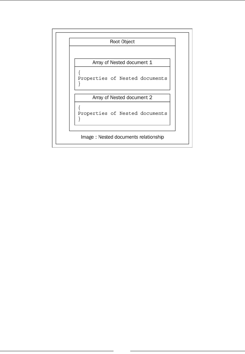
Chapter 6
[ 127 ]
The following image is a visual representation of how nested and parent-child
documents look into Elasticsearch:
As shown in the preceding image, in a nested relationship, there is a one root object,
which is the main document that we have, and it contains an array of sub-documents
called nested documents. There is no limit to the level of nesting of documents inside
a root object. For example, look at the following JSON for a multilevel nesting:
{
"location_id": "axdbyu",
"location_name": "gurgaon",
"company": [
{
"name": "honda",
"modelName": [
{ "name": "honda cr-v", "price": "2 million" }
]
},
{
"name": "bmw",
"modelName": [
{ "name": "BMW 3 Series", "price": "2 million"},
{ "name": "BMW 1 Series", "price": "3 million" }
]
}
]
}
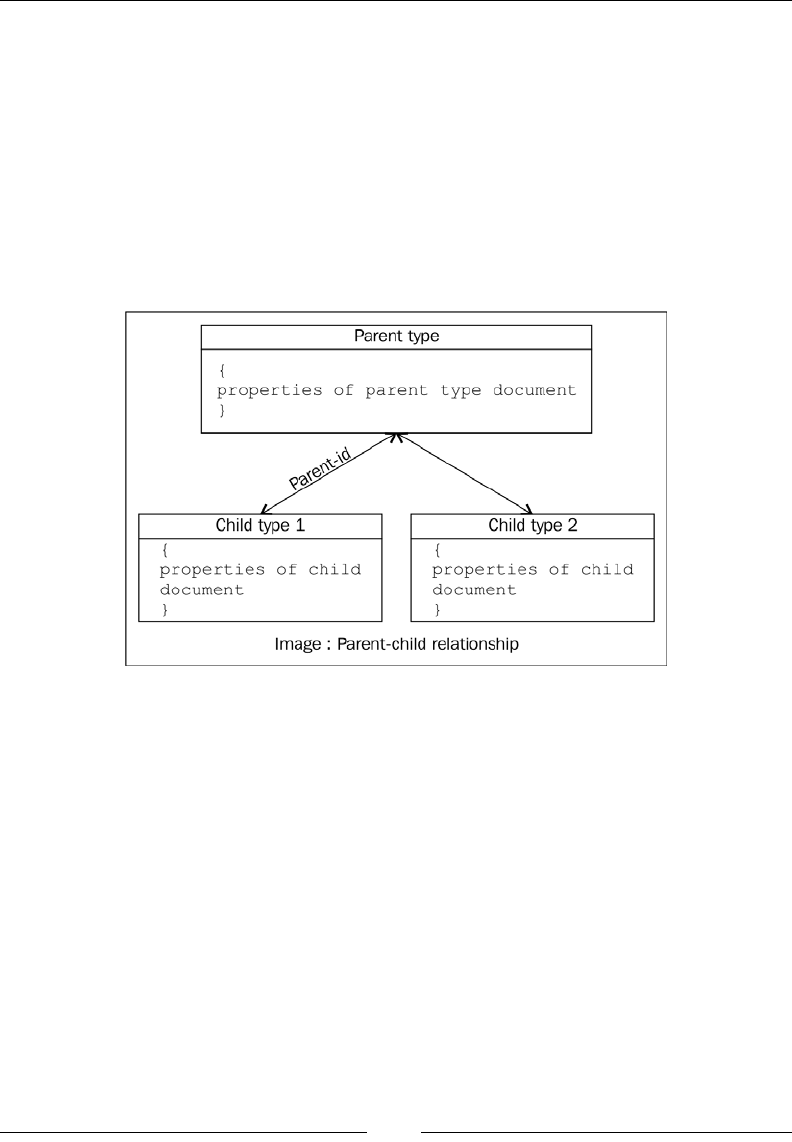
Document Relationships in NoSQL World
[ 128 ]
The preceding example shows that we are dealing with data in which each location
can have multiple companies and each company has different models. So, indexing
this kind of data without a nested type will not solve our purpose if we have to
nd a particular model with the name or price of a particular company at a given
location. This type of relational data with a one to many relationship can be handled
in Elasticsearch using nested types.
Nested elds are used to index arrays of objects, in which each object can be queried
(with the nested query) as an independent document; however, in a nested structure,
everything is stored in the same Lucene block. This has the advantage of fast joins
while querying, but also a disadvantage of the storage of the data.
The parent-child relational model overcomes the storage problems of a nested model
as the related documents here are not stored in the same lucene block, rather they are
stored in the same shard. The parent and child are completely different documents.
Elasticsearch maintains an internal data structure by mapping child document IDs
to parent document IDs (similar to a foreign key that we use to dene in relational
databases).

Chapter 6
[ 129 ]
Working with nested objects
Nested objects look similar to plain objects but they differ in mapping and the way
they are stored internally in Elasticsearch.
We will work with the same Twitter data but this time we will index it in a nested
structure. We will have a user as our root object and every user can have multiple
tweets as nested documents. Indexing this kind of data without using nested
mapping will lead to problems, as shown in the following example:
PUT /twitter/tweet/1
{
"user": {
"screen_name": "d_bharvi",
"followers_count": "2000",
"created_at": "2012-06-05"
},
"tweets": [
{
"id": "121223221",
"text": "understanding nested relationships",
"created_at": "2015-09-05"
},
{
"id": "121223222",
"text": "NoSQL databases are awesome",
"created_at": "2015-06-05"
}
]
}
PUT /twitter/tweet/2
{
"user": {
"screen_name": "d_bharvi",
"followers_count": "2000",
"created_at": "2012-06-05"
},
"tweets": [
{
"id": "121223223",
"text": "understanding nested relationships",
"created_at": "2015-09-05"
},

Document Relationships in NoSQL World
[ 130 ]
{
"id": "121223224",
"text": "NoSQL databases are awesome",
"created_at": "2015-09-05"
}
]
}
Now, if we want to query all the tweets that are about NoSQL and have been created
on 2015-09-05, we would use the following code:
GET twitter/tweets/_search
{
"query": {
"bool": {
"must": [
{
"match": {
"tweets.text": "NoSQL"
}
},
{
"term": {
"tweets.created_at": "2015-09-05"
}
}
]
}
}
}
The preceding query will return both the documents in the response. The reason is
that Elasticsearch internally stores objects in the following way:
{tweets.id : ["121223221","121223222","121223223","121223224"],
tweets.text : ["understanding nested relationships",........],
tweets.created_at : ["2015-09-05","2015-06-05","2015-09-05","2015-09-
05"]}
All the elds of the tweet objects are attened into an array format, which leads to
loosing the association between the tweet texts and tweet creation dates, and because
of this, the previous query returned the wrong results.

Chapter 6
[ 131 ]
Creating nested mappings
The mapping for nested objects can be dened in the following way:
PUT twitter_nested/users/_mapping
{
"properties": {
"user": {
"type": "object",
"properties": {
"screen_name": {
"type": "string"
},
"followers_count": {
"type": "integer"
},
"created_at": {
"type": "date"
}
}
},
"tweets": {
"type": "nested",
"properties": {
"id": {
"type": "string"
},
"text": {
"type": "string"
},
"created_at": {
"type": "date"
}
}
}
}
}
In the previous mapping, user is a simple object eld but the tweets eld is dened
as a nested type object, which contains id, text, and created_at as its properties.

Document Relationships in NoSQL World
[ 132 ]
Indexing nested data
You can use the same JSON documents that we used in the previous section to index
users and their tweets, as indexing nested elds is similar to indexing object elds
and does not require any extra effort in the code. However, Elasticsearch considers
all the nested documents as separate documents and stores them internally in the
following format, which preserves the relationships between tweet texts and dates:
{tweets.id : "121223221",tweets.text : "understanding nested
relationships", tweets.created_at : "2015-09-05"}
{tweets.id : "121223221",tweets.text : "understanding nested
relationships", tweets.created_at : "2015-09-05"}
{tweets.id : "121223221",tweets.text : "understanding nested
relationships", tweets.date : "2015-09-05"}
Querying nested type data
To query a nested eld, Elasticsearch offers a nested query, which has the
following syntax:
"query": {
"nested": {
"path": "path_to_nested_doc",
"query": {}
}
}
Let's understand the nested query syntax:
• The top most query parameter wraps all the queries inside it.
• The nested parameter tells Elasticsearch that this query is of the nested type
• The path parameter specifies the path of the nested field
• The internal query object contains all the queries supported by Elasticsearch
Now let's run the nested query to search all the tweets that are about NoSQL and
have been created on 2015-09-05.
Python example
query = {
"query": {
"nested": {
"path": "tweets",
"query": {

Chapter 6
[ 133 ]
"bool": {
"must": [
{
"match": {
"tweets.text": "NoSQL"
}
},
{
"term": {
"tweets.created_at": "2015-09-05"
}
}
]
}
}
}
}
}
res = es.search(index='twitter_nested', doc_type= 'users', body=query)
Java example
SearchResponse response = client.prepareSearch("twitter_nested")
.setTypes("users")
.setQuery(QueryBuilders
.nestedQuery(nestedField, QueryBuilders
.boolQuery()
.must(QueryBuilders
.matchQuery("tweets.text", "Nosql Databases"))
.must(QueryBuilders
.termQuery("tweets.created_at", "2015-09-05"))))
.execute().actionGet();
The response object contains the output returned from Elasticsearch, which will have
one matching document in the response this time.
Nested aggregations
Nested aggregations allow you to perform aggregations on nested elds. There are
two types of nested aggregations available in Elasticsearch. The rst one (nested
aggregation) allows you to aggregate the nested elds, whereas the second one
(reverse nested aggregation) allows you to aggregate the elds that fall outside
the nested scope.

Document Relationships in NoSQL World
[ 134 ]
Nested aggregation
A nested aggregation allows you to perform all the aggregations on the elds inside
a nested object. The syntax is as follows:
{
"aggs": {
"NAME": {
"nested": {
"path": "path_to_nested_field"
},
"aggs": {}
}
}
}
Understanding nested aggregation syntax:
The syntax of a nested aggregation is similar to the other aggregations but here we
need to specify the path of the topmost nested eld as we have learnt to do in the
nested queries. Once the path is specied, you can perform any aggregation on the
nested documents using the inner aggs object. Let's see an example of how to do it:
Python example
query = {
"aggs": {
"NESTED_DOCS": {
"nested": {
"path": "tweets"
},"aggs": {
"TWEET_TIMELINE": {
"date_histogram": {
"field": "tweets.created_at",
"interval": "day"
}
}
}
}
}
}
res = es.search(index='twitter_nested', doc_type= 'users', body=query,
size=0)

Chapter 6
[ 135 ]
The preceding aggregation query creates a bucket of nested aggregation, which
further contains the date histogram of tweets (the number of tweets created per day).
Please note that we can combine nested aggregation with full-text search queries in
a similar way to how we saw in Chapter 4, Aggregations for Analytics.
Java example
The following example requires this extra import in your code:
org.elasticsearch.search.aggregations.bucket.histogram.
DateHistogramInterval
You can build the aggregation in the following way:
SearchResponse response = client.prepareSearch("twitter_nested")
.setTypes("users")
.addAggregation(AggregationBuilders.nested("NESTED_DOCS")
.path(nestedField)
.subAggregation(AggregationBuilders
.dateHistogram("TWEET_TIMELINE")
.field("tweets.created_at")
.interval(DateHistogramInterval.DAY)
)).setSize(0).execute().actionGet();
The DateHistogramInterval class offers the nal static variables
(DAY in our example) to dene the intervals of buckets. The possible values
are SECOND, MINUTE, HOUR, DAY, WEEK, MONTH, QUARTER, and YEAR.
The output for the preceding query will look like the following:
"aggregations" : {
"NESTED_DOCS" : {
"doc_count" : 2,
"TWEET_TIMELINE" : {
"buckets" : [ {
"key_as_string" : "2015-09-05T00:00:00.000Z",
"key" : 1441411200000,
"doc_count" : 2
} ]
}
}
}
In the output, NESTED_DOCS is the name of our nested aggregations that shows doc_
count as 2 because our document was composed using an array of two nested tweet
documents. The TWEET_TIMELINE buckets show two documents because we have
two tweets in one document.

Document Relationships in NoSQL World
[ 136 ]
Reverse nested aggregation
Nested aggregation has the limitation that it can only access the elds within
the nested scope. Reverse nested aggregations overcome this scenario and allow
you to look beyond the nested scope and go back to the root document or other
nested documents.
For example, we can nd all the unique users who have tweeted in a particular
date range with the following reverse nested aggregation:
Python example
query = {
"aggs": {
"NESTED_DOCS": {
"nested": {
"path": "tweets"
},
"aggs": {
"TWEET_TIMELINE": {
"date_histogram": {
"field": "tweets.created_at",
"interval": "day"
},
"aggs": {
"USERS": {
"reverse_nested": {},
"aggs": {
"UNIQUE_USERS": {
"cardinality": {
"field": "user.screen_name"
}
}
}
}
}
}
}
}
}
}
resp = es.search(index='twitter_nested', doc_type= 'users',
body=query, size=0)

Chapter 6
[ 137 ]
Java example
SearchResponse response =
client.prepareSearch(indexName).setTypes(docType)
.addAggregation(AggregationBuilders.nested("NESTED_DOCS")
.path(nestedField)
.subAggregation(AggregationBuilders.dateHistogram("TWEET_TIMELINE")
.field("tweets.created_at").interval(DateHistogramInterval.DAY)
.subAggregation(AggregationBuilders.reverseNested("USERS")
.subAggregation(AggregationBuilders.cardinality("UNIQUE_USERS")
.field("user.screen_name")))))
.setSize(0).execute().actionGet();
The output for the preceding aggregation will be as follows:
{ "aggregations": {
"NESTED_DOCS": {
"doc_count": 2,
"TWEET_TIMELINE": {
"buckets": [
{
"key_as_string": "2015-09-05T00:00:00.000Z",
"key": 1441411200000,
"doc_count": 2,
"USERS": {
"doc_count": 1,
"UNIQUE_USERS": {
"value": 1
}
}
} ] } } } }
The preceding output shows the nested docs count as 2, whereas the USERS key
species that there is only one root document that exists in the given time range.
UNIQUE_USERS shows the cardinality aggregation output for the unique users in
the index.
Parent-child relationships
Similar to nested types, parent-child relationships also allow you to relate
different entities together but they differ in the implementation and behavior.
Unlike nested documents, they are not present within the same document, rather
parent-child documents are completely separate documents. They follow the one
to many relationship principle and allow you to dene one type as parent and one
or more as the child type.

Document Relationships in NoSQL World
[ 138 ]
Creating parent-child mappings
To create a parent-child mapping, you just need to specify which type should be the
parent of the child type. You do not need to dene anything extra in the parent type
mapping but before indexing the data in the child type, you need to specify in the
child's mapping who will be its parent.
Let's create a new index, twitter_parent_child:
PUT /twitter_parent_child
Now, put the mapping of the tweets type by specifying that the user will be its
parent. This is done using the _parent keyword inside the mapping, but outside
the properties:
PUT /twitter_parent_child/tweets/_mapping
{
"_parent": {
"type": "users"
},
"properties": {
"text":{"type": "string"},
"created_at":{"type": "date"}
}
}
Next, put the mapping of the users type:
PUT /twitter_parent_child/users/_mapping
{
"properties": {
"screen_name":{"type": "string"},
"created_at":{"type": "date"}
}
}
One parent can have multiple child types but one child can have
only one parent type. It's also important to know the fact that you
have to create the mappings for child type and specify the parent
before creating the parent type. If you do it in reverse, you will get
the exception: "Can't add a _parent eld that points to an already
existing type". Also, note that parents cannot be updated for any
child type.

Chapter 6
[ 139 ]
Indexing parent-child documents
Indexing parent documents is similar to what we have followed till now. However,
while indexing children, you need to specify the unique ID of the parent document
so that Elasticsearch can know which document is the parent of this document.
Python example
Indexing parent document:
A parent document is indexed in a similar way to any other document:
parent_doc = {}
parent_doc['screen_name'] = 'd_bharvi'
parent_doc['followers_count"'] = 2000
parent_doc['create_at"'] = '2012-05-30'
es.index(index='twitter_parent_child', doc_type= users, body=parent_
doc, id='64995604')
Indexing a child document:
Indexing a child document requires specifying the _id of the parent document type.
In Python, it is done using the id parameter inside the index function:
child_doc = {}
child_doc['text'] = 'learning parent-child concepts'
child_doc['created_at'] = '2015-10-30'
es.index(index='twitter_parent_child', doc_type= 'tweets', body=child_
doc, id = '2333', parent='64995604')
Java example
Include the following import statements:
import org.elasticsearch.action.index.IndexRequestBuilder;
The parent document can be indexed in the following way:
IndexRequestBuilder index = client.prepareIndex(
"twitter_parent_child", "users");
Map<String, Object> parentDoc= new HashMap<String, Object>();
parentDoc.put("screen_name", "d_bharvi");
parentDoc.put("followers_count", 2000);
parentDoc.put("create_at", "2012-05-30");
index.setId("64995604").setSource(parentDoc)
.execute().actionGet();

Document Relationships in NoSQL World
[ 140 ]
The child document can be indexed in the following way:
IndexRequestBuilder index=client.prepareIndex("twitter_parent_child",
"tweets");
Map<String, Object> childDoc= new HashMap<String, Object>();
childDoc.put("text", "learning parent-child concepts in
elasticsearch");
childDoc.put("create_at", "2015-05-30");
index.setParent("64995604").setId("2333")
.setSource(childDoc).execute().actionGet();
Please note that while indexing the child document, we have used the setParent
method and passed the _id of the parent document.
By specifying the parent ID, we not only create an association
between the parent and child documents but also make sure
that they reside in the same shard.
Querying parent-child documents
Elasticsearch offers two queries to search parent-child documents:
• The has_child query
• The has_parent query
has_child query
The has_child query allows you to nd and return parent documents by
querying the child type. For example, we can nd all the users who have
tweeted about Elasticsearch.
Python example
query = {
"query": {
"has_child": {
"type": "tweets",
"query": {
"match": {
"text": "elasticsearch"
}
}
}

Chapter 6
[ 141 ]
}
}
resp = es.search(index='twitter_parent_child', doc_type= 'users',
body=query)
Java example
The same query can be applied using Java with the following code:
SearchResponse response = client.prepareSearch("twitter_parent_
child").setTypes("users")
.setQuery(QueryBuilders.hasChildQuery(childType, QueryBuilders.mat
chQuery("text","elasticsearch")))
.execute().actionGet();
Please see carefully that while using the has_child query, it is
applied to the parent type because we have to return the parent
documents, while the has_child parameter contains the name
of the child type.
has_parent query
The has_parent query works in reverse compared to the has_child query and
allows you to nd and return child documents by querying on the parent type.
For example, we can nd all the tweets tweeted by users who have a followers
count greater than 200.
Python example
query = {
"query": {
"has_parent": {
"type": "users",
"query": {
"range": {
"followers_count": {
"gte": 200
}
}
}
}
}
}
resp = es.search(index='twitter_parent_child', doc_type= 'tweets',
body=query)

Document Relationships in NoSQL World
[ 142 ]
Java example
The same query can be applied using Java with the following code:
SearchResponse response = client.prepareSearch("twitter_parent_child")
.setTypes("tweets")
.setQuery(QueryBuilders
.hasParentQuery(parentType, QueryBuilders.rangeQuery("followers_
count")
.gt(200))).execute().actionGet();
Considerations for using document
relationships
Over the years, Elasticsearch has improved a lot in reducing memory pressure by
introducing doc_values, which is a little slower than the in-memory data structure,
elddata, but still offer reasonable speed and performance. However, because of the
way nested and parent-child documents are stored and searched, you should keep
the pros and cons in mind before modeling your data. The following is a comparison
of nested versus parent-child types, which is nicely outlined by Zachary Tong in one
of his articles:
Nested Parent-Child
Stored in the same Lucene block as each
other, which helps in a faster read/query
performance. Reading a nested doc is faster
than the equivalent parent/child.
Children are stored separately from
the parent, but are routed to the same
shard. So parent/children performance is
slightly less on read/query than nested.
Updating a single field in a nested document
(parent or nested children) forces ES to
re-index the entire nested document. This
can be very expensive for large nested docs.
If you are not using doc_values (which
is by default since version 2.0.0), parent/
child mappings have a bit extra memory
overhead since ES maintains a "join" list
in the memory.
This is best suited for data that does not
change frequently.
Updating a child doc does not affect
the parent or any other children, which
can potentially save a lot of indexing on
large docs.

Chapter 6
[ 143 ]
Summary
This chapter covered the concepts of handling relational data in Elasticsearch with
the help of nested and parent-child types. We learned about creating mappings,
indexing, and querying data using Java and Python. This chapter also covered
the pros and cons of using these relationships in Elasticsearch.
In the next chapter, we will learn about the different types of search execution
offered by Elasticsearch and write code to re-index data from one index to other.

[ 145 ]
Different Methods of Search
and Bulk Operations
The use cases of different searches differ according to scenarios, and Elasticsearch
provides a lot of exibility regarding how a user can perform search requests and
return the data for efcient processing. The other most important thing to know is
the execution of bulk operations, which enables you to nish your tasks quickly
and do some other important work in your life.
In this chapter, we will cover the following topics:
• Introducing search types in Elasticsearch
• Cheaper CRUD bulk operations
• Multi get and multi search APIs
• Data pagination and re-indexing
• Practical considerations for bulk processing
Introducing search types in Elasticsearch
Elasticsearch provides the following search types to be executed:
• query_then_fetch: This is the default search type available in Elasticsearch.
It follows a two-phase search execution. In the first phase (query), the
query goes to a coordinating node that further forwards the query to all the
relevant shards. Each shard searches the documents, sorts them locally, and
returns the results to the coordinating node. The coordinating node further
merges all the results, sorts them, and returns the result to the caller. The
final results are of the maximum size specified in the size parameter with the
search request.

Different Methods of Search and Bulk Operations
[ 146 ]
• dfs_query_then_fetch: This is similar to the query_then_fetch search
type, but asks Elasticsearch to do some extra processing for more accurate
scoring of documents. In the fetch phase, all the shards compute the
distributed term frequencies.
• scan: The scan search type differs from normal search requests because it
does not involve any scoring and sorting processing of the documents. scan
is used for the scenarios where scoring is not required and you need to iterate
over a large number of documents from Elasticsearch.
The deprecated search type: count
There used to be another search type, count, that was used to return
just the count of documents for a given query. It was also used while
doing aggregation for excluding documents in a result and only
returning the aggregation results. Count has been deprecated from
Elasticsearch version 2.0 and will be removed in upcoming releases.
You just need to use the size parameter of 0 in your query instead
of using the count search type.
Search types can be specied while executing your search with the search_type
parameter in the following way:
• Using REST endpoint:
GET /search/search_type=scan
• Using Python client:
es.search(index=index_name, doc_type=doc_type, body=query, search_
type='scan'
• Using Java client, first import SearchType using the following import
statement:
import org.elasticsearch.action.search.SearchType;
• Then, do the following:
client.prepareSearch("index_name")
.setTypes("doc_type")
.setSearchType(SearchType.SCAN)
.setQuery(QueryBuilders.matchAllQuery())
.execute().actionGet();

Chapter 7
[ 147 ]
Cheaper bulk operations
There are times when you need to perform more than one request on Elasticsearch.
For this, Elasticsearch offers a bulk API with the _bulk endpoint that allows you
to perform bulk operations in a single request, be it indexing, updating, or deleting
more than one document, getting more than one document using more than one
document ID, or executing more than one query in a single request. The best part
is that bulk operations can be executed on more than one index and doc type in a
single request. The Elasticsearch Java client also offers a BulkProcessor class,
which will be covered in a later section of this chapter. For now, let's explore the
bulk requests.
The Python client provides a helper module to create bulk operations.
You need to import this module from elasticsearch.helpers
import bulk.
Bulk create
Bulk create allows to create documents only if they do not already exist in the
index. It expects _source for each document to be separated with new lines.
Python example:
1. Declare a list to hold the document set, as follows:
docs = []
2. Create documents with the following:
doc1 = dict()
doc1['text'] = 'checking out search types in elasticsearch'
doc1['created_at'] = datetime.datetime.utcnow()
doc2 = dict()
doc2['text'] = 'bulk API is awesome'
doc2['created_at'] = datetime.datetime.utcnow()
3. Add both the documents to a list of documents:
docs.append(doc1)
docs.append(doc2)
4. Declare a list that will hold the actions to be executed in the bulk:
actions = list()

Different Methods of Search and Bulk Operations
[ 148 ]
5. Create an action for each document and append it to the list of bulk actions:
for doc in docs:
action = {
'_index': index_name,
'_type': doc_type,
'_op_type': 'create',
'_source': doc
}
actions.append(action)
Please note that if you use _op_type as index, it will be of the index type bulk
request. Now, execute the bulk method of the Elasticsearch helpers module to
index the documents in a single request:
try:
bulk_response = helpers.bulk(es, actions,request_timeout=100)
print "bulk response:",bulk_response
except Exception as e:
print str(e)
If the bulk size is more than 500, the Python module of Elasticsearch
internally breaks the bulk requests into chunks of 500 documents and
then indexes them.
Java example:
1. Create an object of the BulkRequestBuilder class:
BulkRequestBuilder bulkRequests = client.prepareBulk();
2. Create two documents using hashmap, as follows:
Map<String, Object> document1= new HashMap<String, Object>();
Map<String, Object> document2= new HashMap<String, Object>();
document1.put("screen_name", "d_bharvi");
document1.put("followers_count", 2000);
document1.put("create_at", "2015-09-20");
document2.put("screen_name", "b44nz0r");
document2.put("followers_count", 6000);
document2.put("create_at", "2019-09-20");

Chapter 7
[ 149 ]
3. Create individual index requests and add them to the bulk request:
bulkRequests.add(new IndexRequest().index(indexName).
type(docType).source(document1).opType("create").id("125"));
bulkRequests.add(new IndexRequest().index(indexName).
type(docType).source(document1).opType("index").id("123"));
4. Execute the bulk request, as shown here:
BulkResponse bulkResponse =bulkRequests.execute().actionGet();
if (bulkResponse.hasFailures())
{
//handle the failure scenarios
for (BulkItemResponse bulkItemResponse : bulkResponse) {
}
}
Bulk indexing
Bulk indexing allows you to index multiple documents in a single request, which is
similar to indexing a single document as we have seen until now. If the document
already exists, it deletes the document and indexes a new document in its place, and
if the document does not already exist, it creates a new document. It also expects
_source for each document to be separated with new lines.
The code for bulk index is the same as for bulk create, with only one difference:
in Python, you just need to set the _op_type value to index, and in Java opType
will take index as its parameter. The difference between index and create is: when
the operation is set to index, documents get over-ridden if they already exist in the
index, whereas a create operation is useful when you want to skip the indexing of
documents that already exist. Therefore, the create operation gives a performance
boost in comparison to index.
Bulk updating
Bulk updating allows you to perform partial updates on one or more than one
document in a single request. Instead of _source, it requires either a script
parameter or a doc parameter to update the documents.

Different Methods of Search and Bulk Operations
[ 150 ]
Python example:
1. Declare a list that will hold the actions to be executed in the bulk:
actions = list()
2. Create an action for each document and append it to the list of bulk actions:
for doc in docs:
action = {
'_index': index_name,
'_type': doc_type,
'_id': doc_id,
'_op_type': 'update',
'doc': {'new_field': 'doing partial update with a new field'}
}
actions.append(action)
As mentioned earlier, a partial update requires doc instead of _source as a new
eld to be updated when an ID for the existing documents is provided. The same
is shown in the preceding example. For every document, we have created an inline
partial doc with the eld name as new field, and once the actions are created, we
are all set to execute a bulk update as follows:
try:
bulk_indexed = helpers.bulk(es, actions,request_timeout=100)
print "bulk response:",bulk_indexed
except Exception as e:
print str(e)
You will get a missing document exception if the document ID does not exist in
the index.
Java example
In Java, you can create individual bulk requests using UpdateRequest and add them
to the object of BulkRequestBuilder, using the following code:
bulkRequests.add(new UpdateRequest().index(indexName).type(docType).
doc(partialDoc1).id("125"));
bulkRequests.add(new UpdateRequest().index(indexName).type(docType).
doc(partialDoc2).id("123"));

Chapter 7
[ 151 ]
Finally, bulk updates can be executed similarly to what we saw for bulk indexing:
BulkResponse bulkResponse = bulkRequests.execute().actionGet();
if (bulkResponse.hasFailures())
{
//handle the failure scenarios
for (BulkItemResponse bulkItemResponse : bulkResponse) {
}
}
Bulk deleting
Bulk deleting allows you to delete one or more than one document in a single
request. It does not require any source in the request body and follows the same
semantic as a standard delete request.
Python example:
Bulk deleting needs the IDs of documents to be deleted, which you can do as follows:
del_complete_batch = []
for id in ids_to_delete:
del_complete_batch.append({
'_op_type': 'delete',
'_index': index_name,
'_type': doc_type,
'_id': id,
})
try:
helpers.bulk(es, del_complete_batch, request_timeout=100)
except Exception as e:
print str(e)
Java example:
Bulk delete requests can be built by creating individual DeleteRequest and adding
them to the BulkRequestBuilder object:
bulkRequests.add(new DeleteRequest().index(indexName).type(docType).
id("1252"));
bulkRequests.add(new UpdateRequest().index(indexName).type(docType).
id("123"));
And once the bulk is ready, then can be executed.
BulkResponse bulkResponse = bulkRequests.execute().actionGet();

Different Methods of Search and Bulk Operations
[ 152 ]
Please note that the execution might return an exception similar to bulk updates if
the documents do not exist in the index.
Multi get and multi search APIs
Until now, you have seen the execution of a single get request to fetch a document
and hit a single query at a time to search for documents. However, life will be easier
with the following two APIs offered by Elasticsearch.
Multi get
Multi get is all about combining more than one get request in a single request.
I remember once I had a requirement to check the existence of multiple documents
in an index and create a bulk update request against only those IDs that did not
already exist. The one way to do this was by hitting a single HEAD request for
each document ID, and based on the response of Elasticsearch, create a bulk update
request for the documents that did not exist. However, multi get requests can solve
this problem in a single API call instead of multiple HEAD requests.
All you need to do is create an array of document IDs and hit them on Elasticsearch
using the _mget endpoint of Elasticsearch. The following is a simple curl request to
show how you can do this:
curl 'localhost:9200/index_name/doc_type/_mget' -d '{
"ids" : ["1", "2"]
}'
Here, IDs are the _id of the documents to be fetched.
If an ID does not exist in the index, Elasticsearch returns found=false
for that document ID.
You have additional options to decide whether you want to return the data of the
document or not. If it is not required, just set _source : false while hitting the
mget request. For example:
curl 'localhost:9200/index_name/doc_type/_mget' -d '{
"ids" : ["1", "2"], "_source" : false
}'

Chapter 7
[ 153 ]
If you are interested in only returning a particular eld, you can do it like this:
curl 'localhost:9200/index_name/doc_type/_mget' -d '{
"ids" : ["1", "2"], "_source" : ["field1", "field2"]
}
Here, field1 and field2 are the names of the elds required to be returned.
Python example:
Declare an array of IDs to be fetched:
document_ids_to_get = ['1','4','12','54','123','543']
Create a query by passing an array of doc IDs to the ID parameter:
query = {"ids": document_ids_to_get}
#Exceute the query using mget endpoint:
exists_resp = es.mget(index=index_name,doc_type=doc_type, body=query,
_source=False, request_timeout=100)
Java example:
Import the following packages into your source code:
import org.elasticsearch.action.get.MultiGetItemResponse;
import org.elasticsearch.action.get.MultiGetResponse;
Create a multi get request in the following way:
MultiGetResponse responses = client.prepareMultiGet()
.add(indexName, docType, ids_to_be_fetched)
.execute().actionGet();
The multi get response is parsed in the following way:
for (MultiGetItemResponse itemResponse : responses) {
GetResponse response = itemResponse.getResponse();
if (response.isExists()) {
String json = response.getSourceAsString();
System.out.println(json);
}
}
The id_to_be_fetched function is a list of document IDs that need to be fetched.

Different Methods of Search and Bulk Operations
[ 154 ]
Multi searches
You might have worked with many databases and search engines, but none of
them provides the functionality to hit more than one query in a single request.
Elasticsearch can do this with its _msearch REST API. For this, it follows a specic
request format as shown here:
header\n
body\n
………
………
header\n
body\n
Understanding the preceding search request structure:
• header: This includes the name of the index/indices to be searched upon
and optionally includes the search type, search preference nodes (primary,
secondary, and so on), and routing
• body: This includes the search request queries
Let's see an example:
1. Create a le, multi_requests, with the following content. Please note that
each line is separated with \n (new line):
{"index" : "users"}
{"query" : {"match_all" : {}}, "from" : 0, "size" : 10}
{"index" : "twitter", "search_type" : "dfs_query_then_fetch"}
{"query" : {"match_all" : {}}}
2. Now execute the search request using the _msearch API:
curl -XGET localhost:9200/_msearch --data-binary "@ multi _
requests"
In the preceding curl command, we have used the –data-binary flag to
load the multiline content from the file. This is required while executing bulk
data indexing too.
Searches executed with the _msearch API return responses in the
responses array form, which includes the search response for each
search request that matches its order in the original multi search
request. If there is a complete failure for that specific search request, an
object with an error message will be returned in the place of the actual
search response.

Chapter 7
[ 155 ]
Python example:
1. Create an individual request head with an index name and doc type in the
following way:
req_head1 = {'index': index_name1, 'type': doc_type1}
2. Create a query_request_array list, which contains the actual queries and
the head part of those queries:
query_request_array = []
query_1 = {"query" : {"match_all" : {}}}
query_request_array.append(req_head1)
query_request_array.append(query_1)
3. Create another request with a head and body:
req_head2 = {'index': index_name2, 'type': doc_typ2}
query_2 = {"query" : {"match_all" : {}}}
query_request_array.append(req_head2)
query_request_array.append(query_2)
4. Execute the request using a msearch endpoint by passing query_request_
array into the body; you can optionally set request_timeout too:
response = es.msearch(body=query_request_array)
5. The response of a multi search can be parsed in the following way:
for resp in response["responses"]:
if resp.get("hits"):
for hit in resp.get("hits").get('hits'):
print hit["_source"]
Java example:
1. To execute a multi search using Java, you need to import the following
packages into your code:
import org.elasticsearch.action.search.MultiSearchResponse;
import org.elasticsearch.action.search.SearchRequestBuilder;
2. Then, you can create an individual search request using the
SearchRequestBuilder class:
SearchRequestBuilder searchRequest1 = client.
prepareSearch().setIndices(indexName).setTypes(docType)
.setQuery(QueryBuilders.queryStringQuery("elasticsearch").
defaultField("text")).setSize(1);
SearchRequestBuilder searchRequest2 =

Different Methods of Search and Bulk Operations
[ 156 ]
client.prepareSearch().setIndices(indexName).setTypes(docType)
.setQuery(QueryBuilders.matchQuery("screen_name", "d_
bharvi")).setSize(1);
3. These individual search requests can be added to a multi search request and
executed in the following way:
MultiSearchResponse sr = client.prepareMultiSearch()
.add(searchRequest1)
.add(searchRequest1)
.execute().actionGet();
4. You will get all the individual responses from MultiSearchResponse,
as follows:
long nbHits = 0;
for (MultiSearchResponse.Item item : sr.getResponses()) {
SearchResponse response = item.getResponse();
nbHits += response.getHits().getTotalHits();
}
}
Data pagination
We have seen that for any query, Elasticsearch by default returns only the top 10
documents after scoring and sorting them. However, they are not always enough
to serve the purpose. A user always needs more and more data either to render on
a page or to process in the backend. Let's see how we can do this.
Pagination with scoring
In the previous chapters, we discussed how Elasticsearch offers the from and to
parameters to be passed with search requests. So, you always have an option to
either increase the size parameter to load more results from Elasticsearch or send
another query with the changed from and size values to get more data.
This pagination approach makes sense when you have to fetch a limited number of
documents from Elasticsearch. As this approach is too costly and can kill Elasticsearch
if you are hitting a request, for example, where from = 100000 and size = 100010 to
get 10 documents, which have less score than those 1 lac documents in the index.

Chapter 7
[ 157 ]
Pagination without scoring
While working with Elasticsearch, a functionality that is needed most of the time
is: returning a large set of data to process or to simply re-index from one index to
another. This type of data fetching does not require any document scoring or sorting.
Elasticsearch offers a scan search type to full this requirement.
Scrolling and re-indexing documents using
scan-scroll
A scan search type works in the same manner as how you scan a Facebook or
Twitter web page with your eyes and scroll to see more content.
Python example:
You can dene a query for which you want all the documents to be returned,
as follows:
query = {"query":{"match_all":{}}}
Also, you can create a list that will hold the returned documents:
documents = []
Then execute the following request to get the scroll ID from Elasticsearch, which will
be used to get the actual data in subsequent requests. The scroll parameter (timeout
for scrolling) in the following request species for how long the scroll will be open.
It can be dened using 100s (100 seconds) or 2m (two minutes):
resp = es.search(index=source_index, doc_type=source_doc_type,
body=query, search_type="scan", scroll='100s', size=100)
Once scroll_id is returned with the preceding request, you can use it inside
a while loop, which will run until Elasticsearch returns the entire document for
your query:
while True:
print 'scrolling for ',str(scroll_count)+' time'
#A new scroll id generated for each request. Scroll parameter is
also need to be set for each request.
resp = es.scroll(resp['_scroll_id'], scroll='100s')
if len(resp['hits']['hits']) == 0:
print 'data re-indexing completed..!!'
break
else:
#add the documents to the documents list
documents.extend(resp['hits']['hits'])

Different Methods of Search and Bulk Operations
[ 158 ]
#send the documens to for re-indexing
perform_bulk_index(destination_index, destination_doc_type,
documents)
#Empty your documents list so that it can hold another batch of
response
documents = []
The perform_bulk_index function can be implemented in the same way as we have
seen in bulk indexing. It will take a set of documents and will be sent to Elasticsearch
in bulk:
actions = []
for document in documents:
actions.append({
'_op_type': 'create',
'_index': destination_index,
'_type': destination_doc_type,
'_id': document['_id'],
'_source': document['_source']
})
try:
helpers.bulk(es, actions, request_timeout=100)
except Exception as e:
print "bulk index raised exception", str(e)
Java Example (using bulk processor):
We have already seen how bulk indexing can be done using BulkRequestBuilder.
You will now learn how to do bulk indexing using the BulkProcessor class.
As mentioned in the Elasticsearch documentation:
"A bulk processor is a thread safe bulk processing class, allowing you to easily set
when to "ush a new bulk request (either based on number of actions, based on the
size, or time), and to easily control the number of concurrent bulk requests allowed
to be executed in parallel."
The most important parameters offered by BulkProcessor are as follows:
• Bulk actions: This defaults to 1,000. This sets the number of operations to be
processed in a single bulk request.
• Flush interval: The default for this is not set. Flush is a process of performing
a Lucene commit on the disk. Before doing a flush, Elasticsearch stores the
data inside a special file called translog to prevent data loss.

Chapter 7
[ 159 ]
• Bulk size: This defaults to 5 MB. This specifies how much data should be
flushed at once. It should be increased wisely according to the capacity of the
Elasticsearch cluster.
• Concurrent Requests: The default value is 1. (It should not be set to more
than the number of available CPU cores where code is running because each
concurrent request starts a new thread.)
Let's import the packages into our code to get data through scan-scroll and bulk
processing:
import static org.elasticsearch.index.query.QueryBuilders.
matchAllQuery;
import java.util.concurrent.TimeUnit;
import org.elasticsearch.action.bulk.BulkProcessor;
import org.elasticsearch.action.bulk.BulkRequest;
import org.elasticsearch.action.bulk.BulkResponse;
import org.elasticsearch.action.index.IndexRequest;
import org.elasticsearch.action.search.SearchResponse;
import org.elasticsearch.action.search.SearchType;
import org.elasticsearch.client.Client;
import org.elasticsearch.common.unit.TimeValue;
import org.elasticsearch.search.SearchHit;
The following are the main variables you need to declare to index using a bulk
processor:
//The maximum time to wait for the bulk requests to complete
public static final int SCROLL_TIMEOUT_SECONDS = 30;
//Number of documents to be returned, maximum would be scroll_
size*number of shards
public static final int SCROLL_SIZE = 10;
//Sets when to flush a new bulk request based on the number of
actions currently added. defaults to 1000
public static final int BULK_ACTIONS_THRESHOLD = 10000;
//Sets the number of concurrent requests allowed to be executed.
public static final int BULK_CONCURRENT_REQUESTS = 2;
//Sets a flush interval flushing (specified in seconds)
public static final int BULK_FLUSH_DURATION = 30;
Create an instance of the Bulk Processor class using the previous variables:
BulkProcessor bulkProcessor = BulkProcessor.builder(clientTo,
createLoggingBulkProcessorListener()).
setBulkActions(BULK_ACTIONS_THRESHOLD).setConcurrentRequests(BULK_
CONCURRENT_REQUESTS)
.setFlushInterval(createFlushIntervalTime().build();

Different Methods of Search and Bulk Operations
[ 160 ]
Getting the data from scan-scroll can be done as follows:
SearchResponse searchResponse = clientFrom.prepareSearch(fromIndex)
.setTypes(sourceDocType)
.setQuery(matchAllQuery())
.setSearchType(SearchType.SCAN)
.setScroll(createScrollTimeoutValue())
.setSize(SCROLL_SIZE).execute().actionGet();
This will return a scroll ID, which will be used to scroll the documents and return
them for processing:
while (true) {
searchResponse = clientFrom.prepareSearchScroll(searchResp
onse.getScrollId())
.setScroll(createScrollTimeoutValue()).execute().
actionGet();
if (searchResponse.getHits().getHits().length == 0) {
System.out.println("Closing the bulk processor");
bulkProcessor.close();
break; //Break condition: No hits are returned
}
//Add the documents to the bulk processor and depending on
the bulk threshold they will be flushed to ES
for (SearchHit hit : searchResponse.getHits()) {
IndexRequest request = new IndexRequest(toIndex,
destinationDocType, hit.id());
request.source(hit.getSource());
bulkProcessor.add(request);
}
}
The bulk processor has a listener, which ushes the request index depending on the
bulk threshold. This listener can be dened in the following way:
private BulkProcessor.Listener createLoggingBulkProcessorListener() {
return new BulkProcessor.Listener() {
@Override
public void beforeBulk(long executionId, BulkRequest request)
{

Chapter 7
[ 161 ]
System.out.println("Going to execute new bulk composed "+
request.numberOfActions()+" no. of actions");
}
@Override
public void afterBulk(long executionId, BulkRequest request,
BulkResponse response) {
System.out.println("Executed bulk composed "+ request.
numberOfActions()+" no. of actions");
}
@Override
public void afterBulk(long executionId, BulkRequest request,
Throwable failure) {
System.out.println("Error executing bulk "+ failure);
}
};
}
You also need to dene the following helper function to create time units to be used
by bulk processing:
private TimeValue createFlushIntervalTime() {
return new TimeValue(BULK_FLUSH_DURATION, TimeUnit.SECONDS);
}
private TimeValue createScrollTimeoutValue() {
return new TimeValue(SCROLL_TIMEOUT_SECONDS, TimeUnit.
SECONDS);
}
Practical considerations for bulk
processing
It's awesome to minimize the requests using the search types and bulk APIs we saw
in this chapter, but you also need to think that for a large amount of processing to be
done by Elasticsearch, you need to take care of resource utilization and control the
size of your requests accordingly. The following are some points that will help you
while working with the things you have learned in this chapter.

Different Methods of Search and Bulk Operations
[ 162 ]
The most important factor to be taken care of is the size of your documents. Fetching
or indexing 1 KB of 1,000 documents in a single request is damn easier than 100 KB
of 1,000 documents:
• Multisearch: While querying with multi search requests, you should take
care of how many queries you are hitting in a single request. You just can't
combine 1,000 queries in a single query and execute them in one go. Also,
the number of queries should be minimized according to the complexity of
queries. So, you can break your query set into multiple multi-search requests
in batches of, for example, 100 queries per batch, and execute them. You can
combine the results after all the batches are executed. The same rule applies
while querying with the mget API too.
• Scan-scroll: A search with scan and scroll is highly beneficial for performing
deep paginations, but the number of documents returned in a single request
is usually scroll_size*number_of_shards. We have also seen that we need to
pass the timeout using a scroll parameter because it tells Elasticsearch for
how long a search context needs to be open on the server to serve a particular
scroll request. Scroll timeouts do not need to be long enough to process all
the data — they just need to be long enough to process the previous batch of
results. Each scroll request (with the scroll parameter) sets a new expiry
time. So, you need to set the scroll timeout wisely so that there are not too
many open search contexts existing at the same time on your Elasticsearch
server. This heavily affects the background merge process of Lucene indexes.
Also, the scroll time should not be so small that your request gets a timeout.
• Bulk indexing and bulk updates: Sending too much data in a single request
can harm your Elasticsearch node if you do not have the optimal resources
available. Remember that while data indexing or updating, the merging of
Lucene segments is done in the background, and with a large amount of data
merging and flushing on the disk, a very high amount of CPU and disk IO is
required. So, choose the numbers wisely by benchmarking your requests.
Summary
This chapter provided you some very important functionalities of Elasticsearch,
which every programmer needs to know while developing applications in real-time
scenarios and working with a large number of datasets. We covered the bulk APIs
by combining multiple requests into a single one to reduce the time and number
of requests to process large datasets. We also saw some best practices to be kept in
mind while working with these APIs, and most importantly, you got practical code
examples that will help you through your journey with Elasticsearch.
In the next chapter, you are going to learn about search relevancy and how to control
the scoring of your searches.

[ 163 ]
Controlling Relevancy
Getting a search engine to behave can be very hard. It does not matter if you are
a newbie or have years of experience with Elasticsearch or Solr, you must have
denitely struggled with low-quality search results in your application. The default
algorithm of Lucene does not come close to meeting your requirements, and there is
always a struggle to deliver the relevant search results.
In this chapter, we will cover the following topics:
• Introducing relevant searches
• Out-of-the-box tools from Elasticsearch
• Controlling relevancy with custom scoring
Introducing relevant searches
Relevancy is the root of a search engine's value proposition and can be dened
as the art of ranking content for a user's search based on how much that content
satises the needs of the user or the business.
In an application, it does not matter how beautiful your user interface looks or
how many functionalities you are providing to the user; search relevancy cannot be
avoided at any cost. So, despite of the mystical behavior of search engines, you have
to nd a solution to get relevant results. The relevancy becomes more important
because a user does not care about the whole bunch of documents that you have.
The user enters their keywords, selects lters, and focuses on a very small amount
of data—the relevant results. And if your search engine fails to deliver according to
expectations, the user might be annoyed, which might be a loss for your business.

Controlling Relevancy
[ 164 ]
A search engine like Elasticsearch comes with a built-in intelligence. You enter the
keyword and within the blink of an eye, it returns to you the results that it thinks are
relevant according to its intelligence. However, Elasticsearch does not have a built-
in intelligence according to your application domain. The relevancy is not dened
by a search engine; rather it is dened by your users, their business needs, and the
domains. Take an example of Google or Twitter; they have put in years of engineering
experience, but still fail occasionally while providing relevancy. Don't they?
Further, the challenges of searching differ with the domain: the search on an
e-commerce platform is about driving sales and bringing positive customer outcomes,
whereas in elds such as medicine, it is about the matter of life and death. The lives of
search engineers become more complicated because they do not have domain-specic
knowledge, which can be used to understand the semantics of user queries.
However, despite of all the challenges, the implementation of search relevancy is
up to you, and it depends on what information you can extract from the users, their
queries, and the content they see. We continuously take feedback from users, create
funnels, or enable loggings to capture the search behavior of users so that we can
improve our algorithms to provide relevant results.
The Elasticsearch out-of-the-box tools
Elasticsearch primarily works with two models of information retrieval: the Boolean
model and the Vector Space model. In addition to these, there are other scoring
algorithms available in Elasticsearch as well, such as Okapi BM25, Divergence from
Randomness (DFR), and Information Based (IB). Working with these three models
requires extensive mathematical knowledge and needs some extra congurations in
Elasticsearch, which are beyond the scope of this book.
The Boolean model uses the AND, OR, and NOT conditions in a query to nd all
the matching documents. This Boolean model can be further combined with the
Lucene scoring formula, TF/IDF (which we have already discussed in Chapter 2,
Understanding Document Analysis and Creating Mappings), to rank documents.
The vector space model works differently from the Boolean model, as it represents
both queries and documents as vectors. In the vector space model, each number in
the vector is the weight of a term that is calculated using TF/IDF.
The queries and documents are compared using a cosine similarity in which angles
between two vectors are compared to nd the similarity, which ultimately leads to
nding the relevancy of the documents.

Chapter 8
[ 165 ]
An example: why defaults are not enough
Let's build an index with sample documents to understand the examples in a
better way.
First, create an index with the name profiles:
curl -XPUT 'localhost:9200/profiles'
Then, put the mapping with the document type as candidate:
curl -XPUT 'localhost:9200/profiles/candidate'
{
"properties": {
"geo_code": {
"type": "geo_point",
"lat_lon": true
}
}
}
Please note that in the preceding mapping, we are putting mapping only for the geo
data type. The rest of the elds will be indexed dynamically.
Now, you can create a data.json le with the following content in it:
{ "index" : { "_index" : "profiles", "_type" : "candidate", "_id" : 1 }}
{ "name" : "Sam", "geo_code" : "12.9545163,77.3500487", "total_
experience":5, "skills":["java","python"] }
{ "index" : { "_index" : "profiles", "_type" : "candidate", "_id" : 2 }}
{ "name" : "Robert", "geo_code" : "28.6619678,77.225706", "total_
experience":2, "skills":["java"] }
{ "index" : { "_index" : "profiles", "_type" : "candidate", "_id" : 3 }}
{ "name" : "Lavleen", "geo_code" : "28.6619678,77.225706", "total_
experience":4, "skills":["java","Elasticsearch"] }
{ "index" : { "_index" : "profiles", "_type" : "candidate", "_id" : 4 }}
{ "name" : "Bharvi", "geo_code" : "28.6619678,77.225706", "total_
experience":3, "skills":["java","lucene"] }
{ "index" : { "_index" : "profiles", "_type" : "candidate", "_id" : 5 }}
{ "name" : "Nips", "geo_code" : "12.9545163,77.3500487", "total_
experience":7, "skills":["grails","python"] }
{ "index" : { "_index" : "profiles", "_type" : "candidate", "_id" : 6 }}
{ "name" : "Shikha", "geo_code" : "28.4250666,76.8493508", "total_
experience":10, "skills":["c","java"] }

Controlling Relevancy
[ 166 ]
If you are indexing skills, which are separated by spaces or which
include non-English characters, that is, C++, C#, or Core Java, you
need to create mapping for the skills eld as not_analyzed in
advance to have exact term matching.
Once the le is created, execute the following command to put the data inside the
index we have just created:
curl -XPOST 'localhost:9200' --data-binary @data.json
If you look carefully at the example, the documents contain the data of the candidates
who might be looking for jobs. For hiring candidates, a recruiter can have the
following criteria:
• Candidates should know about Java
• Candidates should have experience of 3 to 5 years
• Candidates should fall in the distance range of 100 kilometers from the office
of the recruiter
You can construct a simple bool query in combination with a term query on the
skills eld along with geo_distance and range lters on the geo_code and
total_experience elds respectively. However, does this give a relevant set of
results? The answer would be NO.
The problem is that if you are restricting the range of experience and distance, you
might even get zero results or no suitable candidates. For example, you can put a
range of 0 to 100 kilometers of distance but your perfect candidate might be at a
distance of 101 kilometers. At the same time, if you dene a wide range, you might
get a huge number of non-relevant results.
The other problem is that if you search for candidates who know Java, there is a
chance that a person who knows only Java and not any other programming language
will be at the top, while a person who knows other languages apart from Java will be
at the bottom. This happens because during the ranking of documents with TF/IDF,
the lengths of the elds are taken into account. If the length of a eld is small, the
document is more relevant.
Elasticsearch is not intelligent enough to understand the semantic meaning of your
queries, but for these scenarios, it offers you the full power to redene how scoring
and document ranking should be done.

Chapter 8
[ 167 ]
Controlling relevancy with custom scoring
In most cases, you are good to go with the default scoring algorithms of Elasticsearch
to return the most relevant results. However, some cases require you to have more
control on the calculation of a score. This is especially required while implementing
domain-specic logic such as nding the relevant candidates for a job, where you
need to implement a very specic scoring formula. Elasticsearch provides you with
the function_score query to take control of all these things.
This chapter covers the code examples only in Java because a
Python client gives you the exibility to pass the query inside
the body parameter of a search function as you have learned
in the previous chapters. Python programmers can simply use
the example queries in the same way. There is no extra module
required to execute these queries. You can still download the
Python code for this chapter from the Packt website.
The function_score query
The function_score query allows you to take the complete control of how a score
needs to be calculated for a particular query.
The syntax of a function_score query:
{
"query": {"function_score": {
"query": {},
"boost": "boost for the whole query",
"functions": [
{}
],
"max_boost": number,
"score_mode": "(multiply|max|...)",
"boost_mode": "(multiply|replace|...)",
"min_score" : number
}}
}
The function_score query has two parts: the rst is the base query that nds
the overall pool of results you want. The second part is the list of functions, which
are used to adjust the scoring. These functions can be applied to each document
that matches the main query in order to alter or completely replace the original
query _score.

Controlling Relevancy
[ 168 ]
In a function_score query, each function is composed of
an optional lter that tells Elasticsearch which records should
have their scores adjusted (this defaults to "all records") and a
description of how to adjust the score.
The other parameters that can be used with a functions_score query are as follows:
• boost: An optional parameter that defines the boost for the entire query.
• max_boost: The maximum boost that will be applied by a function score.
• boost_mode: An optional parameter, which defaults to multiply. The score
mode defines how the combined result of the score functions will influence
the final score together with the subquery score. This can be replace (only the
function_score is used; the query score is ignored), max (the maximum of
the query score and the function score), min (the minimum of the query score
and the function score), sum (the query score and the function score are added),
avg, or multiply (the query score and the function score are multiplied).
• score_mode: This parameter specifies how the results of individual
score functions will be aggregated. The possible values can be first
(the first function that has a matching filter is applied), avg, max, sum,
min, and multiply.
• min_score: The minimum score to be used.
Excluding non-relevant documents with min_score
To exclude documents that do not meet a certain score
threshold, the min_score parameter can be set to the
desired score threshold.
The following are the built-in functions that are available to be used with the
function score query:
• weight
• field_value_factor
• script_score
• The decay functions—linear, exp, and gauss
Let's see them one by one and then you will learn how to combine them in a
single query.

Chapter 8
[ 169 ]
weight
A weight function allows you to apply a simple boost to each document without the
boost being normalized: a weight of 2 results in 2 * _score. For example:
GET profiles/candidate/_search
{
"query": {
"function_score": {
"query": {
"term": {
"skills": {
"value": "java"
}
}
},
"functions": [
{
"filter": {
"term": {
"skills": "python"
}
},
"weight": 2
}
],
"boost_mode": "replace"
}
}
}
The preceding query will match all the candidates who know Java, but will give a
higher score to the candidates who also know Python. Please note that boost_mode
is set to replace, which will cause _score to be calculated by a query that is to be
overridden by the weight function for our particular lter clause. The query output
will contain the candidates on top with a _score of 2 who know both Java and Python.
Java example:
The previous query can be implemented in Java in the following way:
1. First, you need to import the following classes into your code:
import org.elasticsearch.action.search.SearchResponse;
import org.elasticsearch.client.Client;

Controlling Relevancy
[ 170 ]
import org.elasticsearch.index.query.QueryBuilders;
import org.elasticsearch.index.query.functionscore.
FunctionScoreQueryBuilder;
import org.elasticsearch.index.query.functionscore.
ScoreFunctionBuilders;
2. Then the following code snippets can be used to implement the query:
FunctionScoreQueryBuilder functionQuery = new FunctionScoreQueryBu
ilder(QueryBuilders.termQuery("skills", "java"))
.add(QueryBuilders.termQuery("skills", "python"),
ScoreFunctionBuilders.weightFactorFunction(2)).
boostMode("replace");
SearchResponse response =
client.prepareSearch().setIndices(indexName)
.setTypes(docType).setQuery(functionQuery)
.execute().actionGet();
eld_value_factor
This uses the value of a eld in the document to alter the _score:
GET profiles/candidate/_search
{
"query": {
"function_score": {
"query": {
"term": {
"skills": {
"value": "java"
}
}
},
"functions": [
{
"field_value_factor": {
"field": "total_experience"
}
}
],
"boost_mode": "multiply"
}
}
}

Chapter 8
[ 171 ]
The preceding query nds all the candidates with Java in their skills, but inuences the
total score depending on the total experience of the candidate. So, the more experience
the candidate has, the higher the ranking they will get. Please note that boost_mode is
set to multiply, which will yield the following formula for the nal scoring:
_score = _score * doc['total_experience'].value
However, there are two issues with the preceding approach: rst is the documents
that have the total experience value as 0 and will reset the nal score to 0. Second,
Lucene _score usually falls between 0 and 10, so a candidate with an experience of
more than 10 years will completely swamp the effect of the full text search score.
To get rid of this problem, apart from using the field parameter, the field_value_
factor function provides you with the following extra parameters to be used:
• factor: This is an optional factor to multiply the field value with. This
defaults to 1.
• modifier: This is a mathematical modifier to apply to the field value.
This can be: none, log, log1p, log2p, ln, ln1p, ln2p, square, sqrt,
or reciprocal. It defaults to none.
Java example:
The preceding query can be implemented in Java in the following way:
1. First, you need to import the following classes into your code:
import org.elasticsearch.action.search.SearchResponse;
import org.elasticsearch.client.Client;
import org.elasticsearch.index.query.QueryBuilders;
import org.elasticsearch.index.query.functionscore*;
2. Then the following code snippets can be used to implement the query:
FunctionScoreQueryBuilder functionQuery = new FunctionScoreQueryBu
ilder(QueryBuilders.termQuery("skills", "java"))
.add(new FieldValueFactorFunctionBuilder("total_experience")).
boostMode("multiply");
SearchResponse response = client.prepareSearch().
setIndices("profiles")
.setTypes("candidate").setQuery(functionQuery)
.execute().actionGet();

Controlling Relevancy
[ 172 ]
script_score
script_score is the most powerful function available in Elasticsearch. It uses a
custom script to take complete control of the scoring logic. You can write a custom
script to implement the logic you need. Scripting allows you to write from a simple
to very complex logic. Scripts are cached, too, to allow faster executions of repetitive
queries. Let's see an example:
{
"script_score": {
"script": "doc['total_experience'].value"
}
}
Look at the special syntax to access the eld values inside the script parameter.
This is how the value of the elds is accessed using Groovy scripting language.
Scripting is, by default, disabled in Elasticsearch, so to use
script score functions, rst you need to add this line in your
elasticsearch.yml le: script.inline: on.
To see some of the power of this function, look at the following example:
GET profiles/candidate/_search
{
"query": {
"function_score": {
"query": {
"term": {
"skills": {
"value": "java"
}
}
},
"functions": [
{
"script_score": {
"params": {
"skill_array_provided": [
"java",
"python"
]
},

Chapter 8
[ 173 ]
"script": "final_score=0; skill_array = doc['skills'].
toArray(); counter=0; while(counter<skill_array.size()){for(skill in
skill_array_provided){if(skill_array[counter]==skill){final_score =
final_score+doc['total_experience'].value};};counter=counter+1;};retu
rn final_score"
}
}
],
"boost_mode": "replace"
}
}
}
Let's understand the preceding query:
• params is the placeholder where you can pass the parameters to your
function, similar to how you use parameters inside a method signature in
other languages. Inside the script parameter, you write your complete logic.
• This script iterates through each document that has Java mentioned in the
skills, and for each document it fetches all the skills and stores them inside
the skill_array variable. Finally, each skill that we have passed inside
the params section is compared with the skills inside skill_array. If this
matches, the value of the final_score variable is incremented with the
value of the total_experience field of that document. The score calculated
by the script score will be used to rank the documents because boost_mode is
set to replace the original _score value.
Do not try to work with the analyzed elds while writing the scripts. You might get
weird results. This is because, had our skills eld contained a value such as "core java",
you could not have got the exact matching for it inside the script section. So, the elds
with space-separated values need to be set as not_analyzed or the keyword has to be
analyzed in advance.
To write these script functions, you need to have some command over
groovy scripting. However, if you nd it complex, you can write these
scripts in other languages, such as Python, using the language plugin
of Elasticsearch. More on this can be found here: https://github.
com/elastic/elasticsearch-lang-python.
For fast performance, use Groovy or Java functions. Python and
JavaScript code requires the marshalling and unmarshalling of values
that kill performance due to more CPU/memory usage.

Controlling Relevancy
[ 174 ]
Java example:
The previous query can be implemented in Java in the following way:
1. First, you need to import the following classes into your code:
import org.elasticsearch.action.search.SearchResponse;
import org.elasticsearch.client.Client;
import org.elasticsearch.index.query.QueryBuilders;
import org.elasticsearch.index.query.functionscore.*;
import org.elasticsearch.script.Script;
2. Then, the following code snippets can be used to implement the query:
String script = "final_score=0; skill_array =
doc['skills'].toArray(); "
+ "counter=0; while(counter<skill_array.size())"
+ "{for(skill in skill_array_provided)"
+ "{if(skill_array[counter]==skill)"
+ "{final_score = final_score+doc['total_experience'].
value};};"
+ "counter=counter+1;};return final_score";
ArrayList<String> skills = new ArrayList<String>();
skills.add("java");
skills.add("python");
Map<String, Object> params = new HashMap<String, Object>();
params.put("skill_array_provided",skills);
FunctionScoreQueryBuilder functionQuery = new
FunctionScoreQueryBuilder(QueryBuilders.termQuery("skills",
"java"))
.add(new ScriptScoreFunctionBuilder(new Script(script,
ScriptType.INLINE, "groovy", params))).boostMode("replace");
SearchResponse response = client.prepareSearch().
setIndices(indexName)
.setTypes(docType).setQuery(functionQuery)
.execute().actionGet();
As you can see, the script logic is a simple string that is used to instantiate the
Script class constructor inside ScriptScoreFunctionBuilder.

Chapter 8
[ 175 ]
Decay functions - linear, exp, and gauss
We have seen the problems of restricting the range of experience and distance that
could result in getting zero results or no suitable candidates. Maybe a recruiter
would like to hire a candidate from a different province because of a good candidate
prole. So, instead of completely restricting with the range lters, we can incorporate
sliding-scale values such as geo_location or dates into _score to prefer documents
near a latitude/longitude point or recently published documents.
function_score provide to work with this sliding scale with the help of three decay
functions: linear, exp (that is, exponential), and gauss (that is, Gaussian). All three
functions take the same parameter, as shown in the following code and are required
to control the shape of the curve created for the decay function: origin, scale,
decay, and offset.
The point of origin is used to calculate distance. For date elds, the default is the
current timestamp. The scale parameter denes the distance from the origin at
which the computed score will be equal to the decay parameter.
The origin and scale parameters can be thought of as your min and max that dene
a bounding box within which the curve will be dened. If we wanted to give more
boosts to the documents that have been published in the past 10 days, it would be
best to dene the origin as the current timestamp and the scale as 10d.
The offset species that the decay function will only compute the decay function of
documents with a distance greater that the dened offset. The default is 0.
Finally, the decay option alters how severely the document is demoted based on its
position. The default decay value is 0.5.
All three decay functions work only on numeric, date,
and geo-point elds.
GET profiles/candidate/_search
{
"query": {
"function_score": {
"query": {
"match_all": {}
},
"functions": [
{
"exp": {
"geo_code": {

Controlling Relevancy
[ 176 ]
"origin": {
"lat": 28.66,
"lon": 77.22
},
"scale": "100km"
}
}
}
],"boost_mode": "multiply"
}
}
}
In the preceding query, we have used the exponential decay function that tells
Elasticsearch to start decaying the score calculation after a distance of 100 km from
the given origin. So, the candidates who are at a distance of greater than 100 km
from the given origin will be ranked low, but not discarded. These candidates can
still get a higher rank if we combine other function score queries such as weight
or field_value_factor with the decay function and combine the result of all the
functions together.
Java example:
The preceding query can be implemented in Java in the following way:
1. First, you need to import the following classes into your code:
import org.elasticsearch.action.search.SearchResponse;
import org.elasticsearch.client.Client;
import org.elasticsearch.index.query.QueryBuilders;
import org.elasticsearch.index.query.functionscore.*;
2. Then, the following code snippets can be used to implement the query:
Map<String, Object> origin = new HashMap<String, Object>();
String scale = "100km";
origin.put("lat", "28.66");
origin.put("lon", "77.22");
FunctionScoreQueryBuilder functionQuery = new
FunctionScoreQueryBuilder()
.add(new ExponentialDecayFunctionBuilder("geo_code",origin,
scale)).boostMode("multiply");
//For Linear Decay Function use below syntax
//.add(new LinearDecayFunctionBuilder("geo_code",origin,
scale)).boostMode("multiply");
//For Gauss Decay Function use below syntax

Chapter 8
[ 177 ]
//.add(new GaussDecayFunctionBuilder("geo_code",origin,
scale)).boostMode("multiply");
SearchResponse response =
client.prepareSearch().setIndices(indexName)
.setTypes(docType).setQuery(functionQuery)
.execute().actionGet();
In the preceding example, we have used the exp decay function but, the commented
lines show examples of how other decay functions can be used.
Last, as always, remember that Elasticsearch lets you use multiple functions in
a single function_score query to calculate a score that combines the results of
each function.
Summary
This chapter covered the most important aspects of search engines; that is, relevancy.
We discussed the powerful scoring capabilities available in Elasticsearch and the
practical examples to show how you can control the scoring process according
to your needs. Despite the relevancy challenges faced while working with search
engines, the out-of-the-box features such as function scores and custom scoring
always allow us to tackle challenges with ease.
In the next chapter, you will learn how to set up an Elasticsearch cluster and
congure different types of node for production deployments.

[ 179 ]
Cluster Scaling in
Production Deployments
Until now, we have been more focused about the search and data analytics
capabilities of Elasticsearch. Now is the time to learn about taking Elasticsearch
clusters in production while focusing on best practices.
In this chapter, we will cover the following topics:
• Node types in Elasticsearch
• Introducing Zen-Discovery
• Best Elasticsearch practices in production
• Cluster creation
• Scaling your clusters
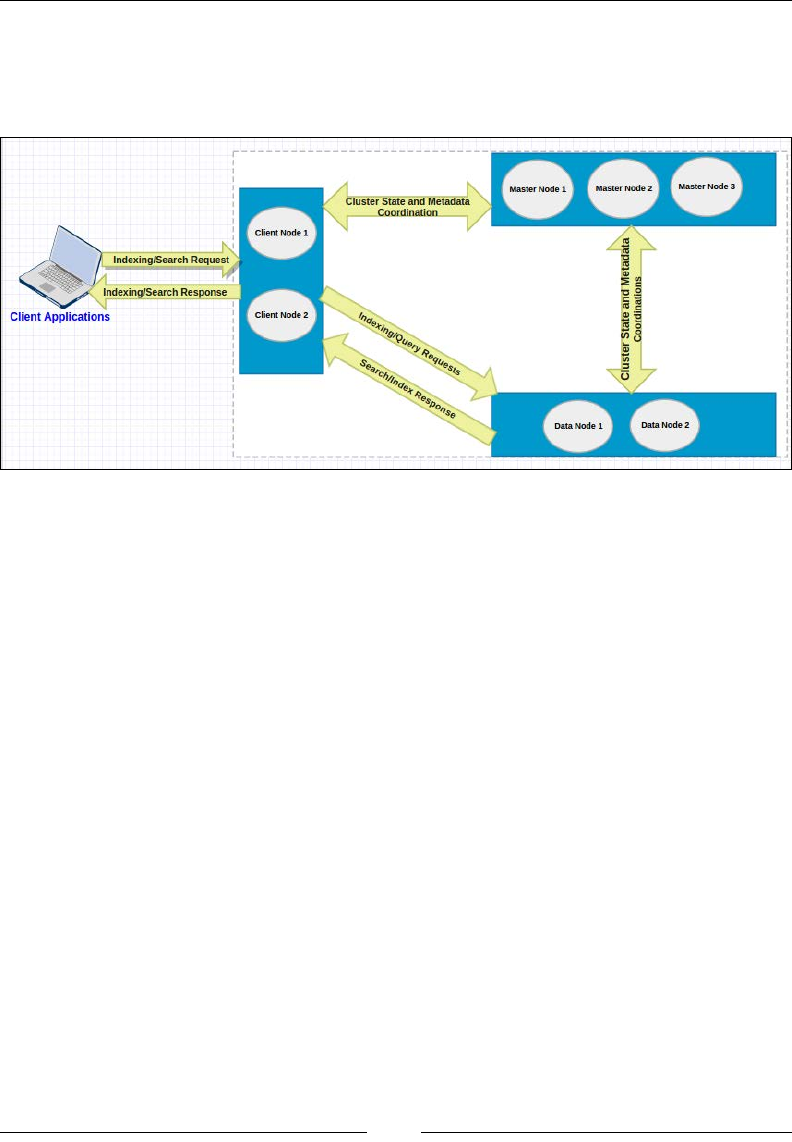
Cluster Scaling in Production Deployments
[ 180 ]
Node types in Elasticsearch
In Elasticsearch, you can congure three types of nodes, as shown in the
following cluster:
In the preceding cluster diagram, there are two client nodes, three master nodes,
and two data nodes. Let's understand how these node types differ in Elasticsearch
and how to congure them.
Client node
A client node in Elasticsearch acts as a query router and a load balancer. It does
not hold any data. A client node can be used to query as well as index processes.
It takes queries and distributes the search to data nodes. Once the data nodes return
their respective results, the client node combines all the data to give the nal results.
Similarly, when you send the data to a client node for indexing, it calculates the
sharding key for each document and sends the documents for the respective shards.
A client node can be congured by adding the following lines to the
elasticsearch.yml le:
• node.data: false
• node.master: false

Chapter 9
[ 181 ]
Data node
A data node in the Elasticsearch is responsible for holding the data, merging
segments, and executing queries. Data nodes are the real work horses of your
cluster and need a higher conguration than any other type of node in the cluster.
A data node can be congured by adding the following lines to the
elasticsearch.yml le:
• node.data: true
• node.master: false
Master node
A master node is responsible for the management of the complete cluster. It holds
the states of all the nodes and periodically distributes the cluster state to all the other
nodes in the cluster to make them aware of any new node that has joined the cluster
and which nodes have left. A master node periodically sends a ping to all the other
nodes to see whether they are alive (other nodes also send pings to the master node).
The nal major task of the master node is conguration management. It holds the
complete meta-data and the mapping of all the indexes in the cluster. If a master
leaves, a new master node is chosen from the rest of the master-eligible nodes.
If there is no master-eligible node left, the cluster cannot operate at all.
A master node can be congured by adding the following lines to the
elasticsearch.yml le.
• node.data: false
• node.master: true
By default, every node is configured as node.data: true and node.
master: true, which means every node is a data node and can also
act as a master node.

Cluster Scaling in Production Deployments
[ 182 ]
Introducing Zen-Discovery
Elasticsearch is highly scalable and distributed in nature. This scalability would
not have been possible without a reliable centralized co-ordination system. In fact,
every distributed system requires a coordination system to maintain conguration
information' and provide distributed synchronizations to all the nodes connected
in the cluster. If you have worked with SolrCloud, you will know that it uses a
coordination service known as Zookeeper. Zookeeper is an awesome open source
project as a whole and can be used with many distributed systems, even with
Elasticsearch by installing the plugin.
At the heart of Elasticsearch, there is no third-party coordination service. However,
Elasticsearch does have a built-in centralized coordination mechanism—Zen
Discovery. One of the primary tasks of Discovery is to choose a master node that
looks after the entire cluster.
When you start a node in an Elasticsearch cluster, the rst thing that happens is that
a node searches for the master node that has the same cluster name. If it nds one,
it simply joins the cluster, and if there is no master node available and this newly
started node is master eligible (we will see what it means), then it becomes the
master node. This process of cluster formation is known as discovery.
Zen-Discovery allows you to have two types of discovery mechanisms: Multicasting
and Unicasting.
Multicasting discovery
In the versions before 2.0, mulitcast used to be the default discovery type in
Elasticsearch. However, since version 2.0, this has been changed to unicast discovery.
The reason was that multicasting is good to go in a development environment, but
comes with added disadvantages. In multicasting, every node in the cluster sends
message packets to all the other nodes for communication and health checks. This
not only makes the network congested because of too many message transmissions
in the network, it also makes it less secure. Any node that is unwanted and has the
same cluster name can automatically join the cluster.
To enable the multicasting discovery type, add the following parameter in all the
nodes of your cluster and restart them:
• discovery.zen.ping.multicast.enabled: true

Chapter 9
[ 183 ]
Unicasting discovery
In unicasting discovery, the transmission of a single message is sent over the
network to a single host at once. Here, you congure a set of nodes that can receive
the messages from the node that wants to join the cluster. The unicasting mechanism
is secure too since a node that wants to join the cluster must know the address and
port of the master nodes that are responsible for deciding who will join the cluster.
Conguring unicasting discovery
To congure unicasting discovery, there are four properties that need to be congured
inside the elasticsearch.yml le.
Minimum number of master nodes: preventing split-brain
A split-brain is the situation in which one Elasticsearch cluster divides itself into
two clusters, and each cluster has a separate master node. This is mainly caused by
network issues or when a cluster becomes unstable because nodes experience long
pauses due to slow garbage collections. The subsets of nodes attempt to form their
own clusters, and this is known as a Split-Brain situation. In this situation, the
nodes are diverged and cannot form a single cluster again until you kill the other
half of the cluster. Split-brain can be very dangerous and can incur potential data
loss. Luckily, the Elasticsearch team has worked hard to prevent the worst scenarios
of handling split-brain situations, but the implementation is up to you.
To avoid split-brain, you need to decide the minimum number of master nodes
that must be operational in the cluster to keep the cluster running. The size of the
minimum number of master nodes depends on the total number of master nodes you
have in your cluster. It can be set using the discovery.zen.minimum_master_nodes
property inside the elasticsearch.yml le:
• discovery.zen.minimum_master_nodes: n
Here, n is the integer value of the minimum number of master nodes. As per
recommendation, this value should be decided based on the formula, N/2+1, where
N is the total number of master nodes in the cluster. So, if you have three master
nodes, this parameter can be set as 3/2+1 = 2 (rounding off to the nearest integer).

Cluster Scaling in Production Deployments
[ 184 ]
An initial list of hosts to ping
Unicasting requires an initial list of hosts to be pinged when a new node is started to
form a cluster. Here you need to provide the list of all your master nodes along with
an optional TCP port number in the following format:
discovery.zen.ping.unicast.hosts: ["masternode1IPAddress:TCP-
Port","masternode2IPAddress:TCP-Port", "masternode3IPAddress:TCP-
Port"]
The TCP port defaults to 9300.
Ping timeout
This, by default, has 3s; within this time the nodes will ping to the master node
and the master node will ping back to the other nodes to ensure that all nodes are
up. This property should be set to a higher value in a slow network or a congested
cluster. It can be congured in the following way:
• discovery.zen.ping.timeout: 5s
Node upgrades without downtime
To achieve SLAs, you need highly available systems. However, at the same time, you
may need to upgrade or downgrade your machines or even upgrade Elasticsearch to
its upgraded release. Both cases require some best practices to be followed because one
wrong step can incur data loss or a delay in the completion of the required changes.
In both the cases, one thing is for sure, nodes must be stopped one by one. While it's
easy to stop the client or the master node and perform maintenance tasks, data nodes
require special considerations because they might need a higher shard recovery time.
Every time a data node is restarted, shard re-balancing is done by Elasticsearch,
which takes too much time because of some unnecessary data movement and
synchronization inside the cluster. To avoid this scenario and for a faster recovery
of the data nodes, follow these steps.
Before stopping a data node, set the shard routing allocation to none with the
following command:
PUT _cluster/settings
{
"transient" : {
"cluster.routing.allocation.enable" : "none"
}
}

Chapter 9
[ 185 ]
After starting the data node, set back the shard routing allocation to all with
this command:
PUT _cluster/settings
{
"transient" : {
"cluster.routing.allocation.enable" : "all"
}
}
An Elasticsearch version can't be downgraded to a lower release. So, take data
backups before going for a version upgrade. Backup and restores are covered
in the next chapter.
Upgrading Elasticsearch version
An Elasticsearch cluster can be upgraded to a higher version in two ways:
• Rolling upgrade: This requires one node to stop at once and perform
the upgradation.
• Full cluster restart: This requires a complete cluster shutdown before
proceeding with the upgrade task.
You need to go through the following URL for more information on the supported
versions to choose the type of upgrade you need to perform:
https://www.elastic.co/guide/en/elasticsearch/reference/current/
setup-upgrade.html
In both cases, to upgrade a node, the following are the easiest steps to upgrade a
version node by node:
1. Disable the routing allocation, as discussed in the previous section.
2. Stop the node.
3. Take a backup of the data.
4. Take a backup of the conguration les.
5. Remove Elasticsearch (you can simply purge it to complete the uninstallation
of Elasticsearch from the server by running this command: sudo apt-get
purge Elasticsearch)
6. Install Elasticsearch with the latest release.
7. Change the conguration les according to the previous settings.
8. Upgrade the plugins.
9. Restart the node.

Cluster Scaling in Production Deployments
[ 186 ]
Best Elasticsearch practices in
production
This section is dedicated to guide you on following the best practices and
considerations to keep in mind when going into production.
Memory
• Always choose ES_HEAP_SIZE 50% of the total available memory. Sorting
and aggregations both can be memory hungry, so enough heap space to
accommodate these is required. This property is set inside the /etc/init.d/
elasticsearch file.
• A machine with 64 GB of RAM is ideal; however, 32 GB and 16 GB machines
are also common. Less than 8 GB tends to be counterproductive (you end
up needing smaller machines), and greater than 64 GB has problems in
pointer compression.
CPU
Choose a modern processor with multiple cores. If you need to choose between
faster CPUs or more cores, choose more cores. The extra concurrency that multiple
cores offer will far outweigh a slightly faster clock speed. The number of threads is
dependent on the number of cores. The more cores you have, the more threads you
get for indexing, searching, merging, bulk, or other operations.
Disks
• If you can afford SSDs, they are far superior to any spinning media.
SSD-backed nodes see boosts in both querying and indexing performance.
• Avoid network-attached storage (NAS) to store data.
Network
• The faster the network you have, the more performance you will get in a
distributed system. Low latency helps to ensure that nodes communicate
easily, while a high bandwidth helps in shard movement and recovery.
• Avoid clusters that span multiple data centers even if the data centers are
collocated in close proximity. Definitely avoid clusters that span large
geographic distances.

Chapter 9
[ 187 ]
General consideration
• It is better to prefer medium-to-large boxes. Avoid small machines because
you don't want to manage a cluster with a thousand nodes, and the overhead
of simply running Elasticsearch is more apparent on such small boxes.
• Always use a Java version greater than JDK1.7 Update 55 from Oracle and
avoid using Open JDK.
• A master node does not require much resources. In a cluster with 2 Terabytes
of data having 100s of indexes, 2 GB of RAM, 1 Core CPU, and 10 GB of disk
space is good enough for the master nodes. In the same scenario, the client
nodes with 8 GB of RAM each and 2 Core CPUs is a very good configuration
to handle millions of requests. The configuration of data nodes is completely
dependent on the speed of indexing, the type of queries, and aggregations.
However, they usually need very high configurations such as 64 GB of RAM
and 8 Core CPUs.
Some other important conguration changes
• Assign Names: Assign the cluster name and node name.
• Assign Paths: Assign the log path and data path.
• Recovery Settings: Avoid shard shuffles during recovery. The recovery
throttling section should be tweaked in large clusters only; otherwise,
it comes with very good defaults.
Disable the deletion of all the indices by a single command:
action.disable_delete_all_indices: false
• Ensure by setting the following property that you do not run more than one
Elasticsearch instance from a single installation:
max_local_storage_nodes: "1"
Disable HTTP requests on all the data and master nodes in the following way:
http.enabled: false
• Plugins installations: Always prefer to install the compatible plugin version
according to the Elasticsearch version you are using and after the installation
of the plugin, do not forget to restart the node.

Cluster Scaling in Production Deployments
[ 188 ]
• Avoid storing Marvel indexes in the production cluster.
• Clear the cache if the heap fills up when the node start-up and shards refuse
to get initialized after going into red state This can be done by executing the
following command:
°To clear the cache of the complete cluster:
curl -XPOST 'http://localhost:9200/_cache/clear'
°To clear the cache of a single index:
curl -XPOST 'http://localhost:9200/index_name/_cache/clear'
• Use routing wherever beneficial for faster indexing and querying.
Creating a cluster
Since you have learned a major part of cluster conguration, let's begin to create
a full-blown production-ready cluster. In this example, we will congure a cluster
with three master, two client nodes, and two data nodes.
The example shows a conguration of one master, one data, and one client node.
On the rest of nodes, all the conguration will remain the same according to the
node category, but only four parameters will be changed:
node.name, path.data, path.log and network.host.
If you are conguring a new data or log path, make sure that
Elasticsearch has the full permission of that directory. You can
set the permission with the following command:
sudo chown -R elasticsearch:elasticsearch
path_of_the_data_directory
Conguring master nodes
cluster.name: "production-cluster"
node.name: "es-master-01"
node.data: false
node.master: true
path.data: "path_to_data_directory"
network.host: "192.168.1.10" (should be changed to a private IP
address of this machine or can be left out too, because Elasticsearch,
by default, binds itself to the 0.0.0.0 address)
http.enabled: false
transport.tcp.port: 9300

Chapter 9
[ 189 ]
discovery.zen.minimum_master_nodes: 3
discovery.zen.ping.unicast.hosts: ["es-master-01:6300","es-
master-02:6300", "es-master-03:6300"]
discovery.zen.ping.timeout: 5s
bootstrap.mlockall: true
action.destructive_requires_name: true
#For allowing script execution
script.inline: on
Conguring client nodes
cluster.name: "production-cluster"
node.name: "es-client-01"
node.data: false
node.master: false
network.host: "192.168.1.10" (should be changed to the private IP
address of this machine)
http.enabled: true
http.port: 9200
transport.tcp.port: 9300
discovery.zen.minimum_master_nodes: 3
discovery.zen.ping.unicast.hosts: ["es-master-01:9300","es-
master-02:9300", "es-master-03:9300"]
discovery.zen.ping.timeout: 5s
bootstrap.mlockall: true
action.destructive_requires_name: true
action.disable_delete_all_indices: false
script.inline: on
#To allow sense and marvel to query elasticsearch
http.cors.enabled: true
http.cors.allow-origin: /http:\/\/localhost(:[0-9]+)?/
http.cors.allow-credentials: true
Conguring data nodes
cluster.name: "production-cluster"
node.name: "es-data-01"
node.data: true
node.master: false
network.host: "192.168.1.10" (should be changed to the private IP
address of this machine)
http.enabled: false
transport.tcp.port: 9300
discovery.zen.minimum_master_nodes: 3

Cluster Scaling in Production Deployments
[ 190 ]
discovery.zen.ping.unicast.hosts: ["es-master-01:9300","es-
master-02:9300", "es-master-03:9300"]
discovery.zen.ping.timeout: 5s
bootstrap.mlockall: true
action.destructive_requires_name: true
script.inline: on
Scaling your clusters
While it's easy to get started with the launching of nodes and the forming of
Elasticsearch clusters, the real challenge comes when the indexing and searching
requests increase and your server encounters real pressure. In this section, we will
discuss when and how to scale your Elasticsearch clusters.
Cluster scaling is only possible if you have done some capacity
planning in advance and have decided on an optimal number
of shards. Always remember that once an index is created,
you cannot increase or decrease the number of shards but can
always change the number of replicas.
When to scale
Elasticsearch is very good at giving you hints in advance when it starts getting
overloaded. The problems can arise in many areas such as slow searches, disk space
utilizations, JVM issues, memory pressure, or high CPU utilizations. In any case,
scaling should be done before your servers crash.
For timely scaling, the best thing to do is keep a close eye on the monitoring of the
metrics provided by Elasticsearch for all resource utilizations. Your biggest friend
would be Marvel. It provides very granular statistics of your clusters. However, in
case you can't opt for Marvel due to any reason, you can use a combination of three
approaches: use monitoring plugins such as Bigdesk, HQ; keep watching the logs
and use the monitoring REST APIs to get a clear idea of what is causing the problem;
and taking decisions about when to scale.
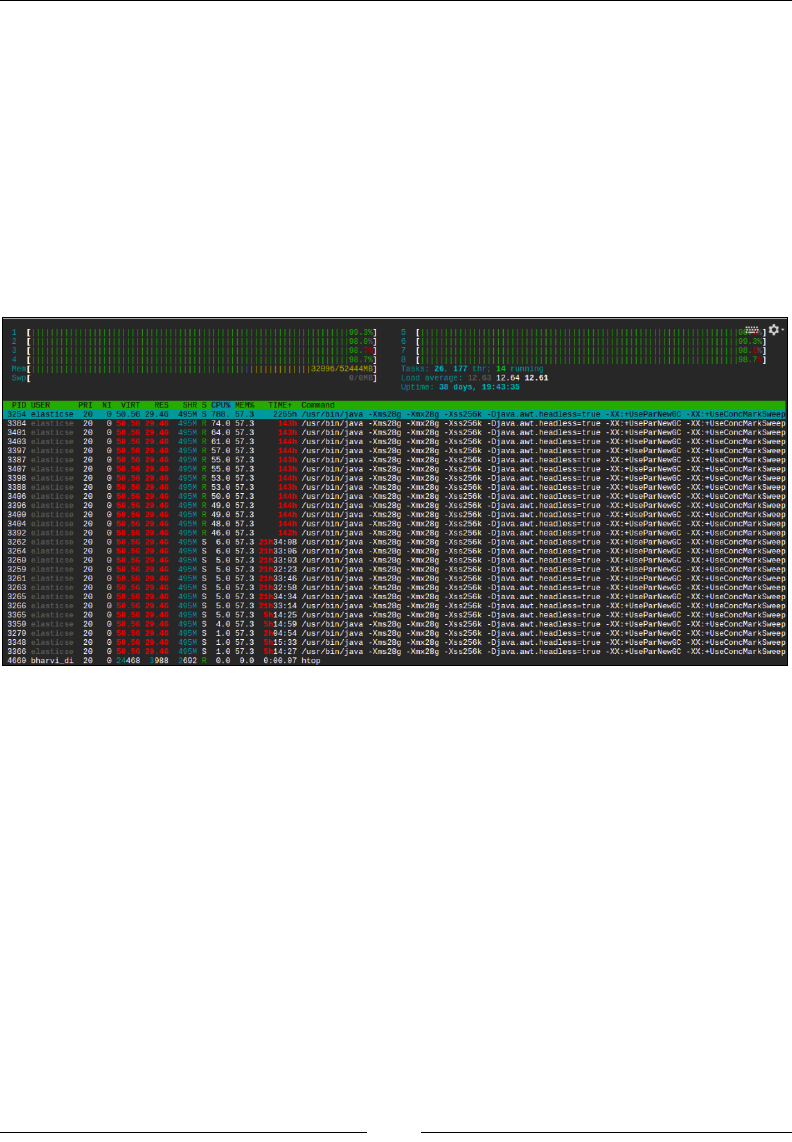
Chapter 9
[ 191 ]
Metrics to watch
The following are the most important metrics that you need to continuously watch
out for in Elasticsearch.
CPU utilization
The performance of Elasticsearch is highly dependent on the type of server on which it
has been installed. There are many reasons for spikes in high CPU utilizations, such as
higher indexing speed that causes a lot of segment merges in the background or higher
garbage collection activities. Look at the following images that have been taken after
running the htop command on a Ubuntu system:
The preceding screenshot is from my server, which has eight CPU cores and 32 GB
of RAM (16 GB dedicated to Elasticsearch). You can see Elasticsearch is using almost
800% of CPU because of a higher indexing rate of almost 3,000 documents per second
(with a size of 20 KB per document). We were required to increase the indexing rate,
but we were not able to because there was no room in the CPU.
The only solution in this scenario was to scale, either vertically (increasing CPU of
this server) or horizontally (adding more nodes to allocate some of the shards on a
new node), to distribute the load.
Cluster Scaling in Production Deployments
[ 192 ]
The same CPU utilization can be viewed with the help of the Bigdesk plugin:
Memory utilization
Elasticsearch is a memory extensive process. It runs in JVM and requires a lot
of memory holding objects while performing aggregation, sorting, and caching
different kinds of data, such as eld cache and lter cache, to give you faster
search executions. Many people are worried when they see that Elasticsearch is
using almost all the memory of the server. However, this is not always correct.
In Elasticsearch, it is good if your server is utilizing all the memory. The actual
thing to look for is whether there is any free buffer or cached memory available.
When there is too much memory pressure on an Elasticsearch node, it starts giving
warnings in the logs of that particular node, similar to the following one:
[2015-11-25 18:13:53,166][WARN ][monitor.jvm] [es-data-1] [gc][ParNew]
[1135087][11248] duration [2.6m], collections [1]/[2.7m], total [2.6m]/
[6.8m], memory [2.4gb]->[2.3gb]/[3.8gb], all_pools {[Code Cache]
[13.7mb]->[13.7mb]/[48mb]}{[Par Eden Space] [109.6mb]->[15.4mb]/[1gb]}
{[Par Survivor Space] [136.5mb]->[0b]/[136.5mb]}{[CMS Old Gen] [2.1gb]-
>[2.3gb]/[2.6gb]}{[CMS Perm Gen] [35.1mb]->[34.9mb]/[82mb]}
If you start getting these kinds of warnings in your logs, its time to add more resources.

Chapter 9
[ 193 ]
Disk I/O utilization
If you are working on applications having high writes such as logging and real-time
data indexing, you need very high disk I/Ops. Elasticsearch provides options for
tuning store-level throttling for segment merging; however, spinning media disks
cannot cope with heavy writes. It is best to use SSD for write heavy applications. In
our applications, we have seen an almost 10x performance boost after opting for SSD.
Disk low watermark
Look at the following lines of log, which have been taken from the master node of
the cluster:
[2015-11-21 15:22:52,656][INFO ][cluster.routing.allocation.decider] [es-
master-1] low disk watermark [15%] exceeded on [ujhOO-MzR22bJHPUGLtyQA]
[es-data-1] free: 36.6gb[14.8%], replicas will not be assigned to this
node
It clearly says that one of the data nodes has less than 15% of disk space available
and new shards won't be assigned to this node anymore. This can even be worse
if 90% of the disk is full. In this case, your shards will be automatically assigned to
other nodes, and if the other nodes also have the same disk space, your cluster will
go into hang mode.
However, you can increase the thresholds for low and high watermarks in the
following way:
curl -XPUT client_node_ip:9200/_cluster/settings -d '{
"transient" : {
"cluster.routing.allocation.disk.watermark.low" : "90%",
"cluster.routing.allocation.disk.watermark.high" : "10gb"
}
}'
As you can see, these parameters take values in the form of percentage as well as
gigabytes or megabytes. However, if this is still not enough, you need to add more
nodes to move the shards or increase the disk space.

Cluster Scaling in Production Deployments
[ 194 ]
How to scale
Distributed systems such as Elasticsearch, Cassandra, or Mongodb are built for
higher scalability. However, it is very important to consider one thing: how you
scale your clusters. Scaling can be done either vertically or horizontally. Vertical
scaling is the one in which you keep adding more resources to existing machines,
whereas in horizontal scaling, you dynamically add more nodes to the cluster.
Elasticsearch is built for horizontal scaling. You keep adding more nodes to your
cluster, and it can automatically balance the shards/load on the new nodes.
To add new nodes to Elasticsearch, simply launch a new server with Elasticsearch
installed on it and similar conguration (cluster name and discovery parameters).
It will automatically connect to the existing cluster, if it is able to connect with your
master nodes.
There are still some scenarios in which it will be required to go for vertical scaling, such
as cost optimizations. In this case, you need to stop the node and increase the resources
on it. However, you need to have enough nodes to keep the cluster operational, such
as having two client nodes or two data nodes and three master nodes.
Summary
In this chapter, you learned how to congure different types of nodes in Elasticsearch,
along with keeping best practices in mind when going for the production deployments
of an Elasticsearch cluster. The chapter covered one of the most important aspects of
cluster sizing—resource allocation and conguration for different types of nodes.
Finally, we saw some key metrics such as CPU, disk I/Ops, RAM, and utilizations
to watch out for when your cluster needs scaling and the best practices to follow for
scaling without downtime.
In the next chapter, we will learn about securing clusters and creating data backups.

[ 195 ]
Backups and Security
Data backups and data security are the most important aspects of any organization.
It is even more important to design and implement business continuity plans to
tackle data loss because of various factors. While Elasticsearch is not a database
and it does not provide the backup and security functionalities that you can get in
databases, it still offers some way around this. Let's learn how you can create cost
effective and robust backup plans for your Elasticsearch clusters.
In this chapter, we will cover the following topics:
• Introducing backup and restore mechanisms
• Securing an Elasticsearch cluster
• Load balancing using Nginx
Introducing backup and restore
mechanisms
In Elasticsearch, you can implement a backup and restore functionality in two
different ways depending on the requirements and efforts put in. You can either
create a script to create manual backups and restoration or you can opt for a more
automated and functionality-rich Backup-Restore API offered by Elasticsearch.
Backup using snapshot API
A snapshot is the backup of a complete cluster or selected indices. The best thing
about snapshots is that they are incremental in nature. So, only data that has been
changed since the last snapshot will be taken in the next snapshot.

Backups and Security
[ 196 ]
Life was not so easy before the release of Elasticsearch Version 1.0.0. This release
not only introduced powerful aggregation functionalities to Elasticsearch, but also
brought in the Snapshot Restore API to create backups and restore them on the y.
Initially, only a shared le system was supported by this API, but gradually it has
been possible to use this API on AWS to create backups on AWS buckets, Hadoop
to create backups inside Hadoop clusters, and Microsoft Azure to create backups on
Azure Storage with the help of plugins. In the upcoming section, you will learn how
to create backups using a shared le system repository. To use cloud and Hadoop
plugins, have a look at the following URLs:
https://github.com/elastic/elasticsearch-cloud-aws#s3-repository
https://github.com/elastic/elasticsearch-hadoop/tree/master/
repository-hdfs
https://github.com/elastic/elasticsearch-cloud-azure#azure-repository
Creating snapshots using le system repositories requires the repository to be
accessible from all the data and master nodes in the cluster. For this, we will be
creating an network le system (NFS) drive in the next section.
Creating an NFS drive
NFS is a distributed le system protocol, which allows you to mount remote
directories on your server. The mounted directories look like the local directory of
the server, therefore using NFS, multiple servers can write to the same directory.
Let's take an example to create a shared directory using NFS. For this example, there
is one host server, which can also be viewed as a backup server of Elasticsearch data,
two data nodes, and three master nodes.
The following are the IP addresses of all these nodes:
• Host Server: 10.240.131.44
• Data node 1: 10.240.251.58
• Data node 1: 10.240.251.59
• Master Node 1: 10.240.80.41
• Master Node 2: 10.240.80.42
• Master Node 3: 10.240.80.43

Chapter 10
[ 197 ]
Conguring the NFS host server
The very rst step is to install the nfs-kernel-server package after updating the
local package index:
sudo apt-get update
sudo apt-get install nfs-kernel-server
Once the package is installed, you can create a directory that can be shared among
all the clients. Let's create a directory:
sudo mkdir /mnt/shared-directory
Give the access permission of this directory to the nobody user and the nogroup
group. They are a special reserved user and group in the Linux operating system
that do not need any special permission to run things:
sudo chown –R nobody:nogroup /mnt/shared-directory
The next step is to congure the NFS Exports, where we can specify with which
machine this directory will be shared. For this, open the /etc/exports le with
root permissions:
sudo nano /etc/exports
Add the following line, which contains the directory to be shared and the space-
separated client IP lists:
/mnt/shared-directory 10.240.251.58(rw,sync,no_subtree_check)
10.240.251.59(rw,sync,no_subtree_check) 10.240.80.41(rw,sync,no_subtree_
check) 10.240.80.42(rw,sync,no_subtree_check) 10.240.80.43(rw,sync,no_
subtree_check)
Once done, save the le and exit.
The next step is to create an NFS table, which holds the exports of your share by
running the following command:
sudo exportfs –a
Now start the NFS service by running this command:
sudo service nfs-kernel-server start
After this, your shared directory is available to the clients you have congured on
your host machine. It's time to do the congurations on the client machines.
Backups and Security
[ 198 ]
Conguring client machines
First of all, your need to install the NFS client after updating the local package index:
sudo apt-get update
sudo apt-get install nfs-common
Now, create a directory on the client machine that will be used to mount the remote
shared directory:
sudo mkdir /mnt/nfs
Mount the shared directory (by specifying the nfs server host ip:shared directory
name) on the client machine by using the following command:
sudo mount 10.240.131.44:/mnt/shared-directory /mnt/nfs
To check whether the mount is successfully done, you can use the following command:
df -h
You will see an extra drive mounted on your system, as shown in the following
screenshot, which shows the mounted shared directory:
Please note that mounting the directories/devices using the mount command only
mounts them temporarily. For a permanent mount, open the /etc/fstab le:
sudo nano /etc/fstab
Add these lines to this le:
host.domain.com:/mnt/shared-directory /mnt/nfs/ nfs auto,noatime,nol
ock,bg,nfsvers=4,sec=krb5p,intr,tcp,actimeo=1800 0 0
Perform similar steps on all the data and master nodes to mount the shared directory
on all of them using NFS.

Chapter 10
[ 199 ]
Creating a snapshot
The following subsections cover the various steps that are performed to create
a snapshot.
Registering the repository path
Add the following line inside the elasticsearch.yml le, to register the path.repo
setting on all the master and data nodes:
path.repo: ["/mnt/nfs"]
After this, restart the nodes one by one to reload the conguration.
Registering the shared le system repository
in Elasticsearch
Register the shared le system repository with the name es-backup:
curl -XPUT 'http://localhost:9200/_snapshot/es-backup' -d '{
"type": "fs",
"settings": {
"location": "/mnt/nfs/es-backup",
"compress": true
}
}'
In preceding request, the location parameter species the path of the snapshots and
the compress parameter turns on the compression of the snapshot les. Compression
is applied only to the index metadata les (mappings and settings) and not to the
data les.
Create your rst snapshot
You can create multiple snapshots of the same cluster within a repository.
The following is the command that is used to create a snapshot_1 snapshot
inside the es-snapshot repository:
curl -XPUT 'http://localhost:9200/_snapshot/es-backup/snapshot_1?wait_
for_completion=true'
The wait_for_completion parameter tells whether the request should return
immediately after snapshot initialization (defaults to true) or wait for snapshot
completion. During snapshot initialization, information about all previous
snapshots is loaded into the memory, which means that in large repositories,
it may take several seconds (or even minutes) for this command to return even
if the wait_for_completion parameter is set to false.

Backups and Security
[ 200 ]
By default, a snapshot of all the open and started indices in the cluster is created.
This behavior can be changed by specifying the list of indices in the body of the
snapshot request:
curl -XPUT 'http://localhost:9200/_snapshot/es-backup/snapshot_1?wait_
for_completion=true' -d '{
"indices": "index_1,index_2",
"ignore_unavailable": "true",
"include_global_state": false
}'
In the preceding request, the indices parameter species the names of the indices
that need to be included inside the snapshot. The ignore_unavailable parameter,
if set to true, enables a snapshot request to not fail if any index is not available in the
snapshot creation request. The third parameter, include_global_state, when set
to false, avoids the global cluster state to be stored as a part of the snapshot.
Getting snapshot information
To get the details of a single snapshot, you can run the following command:
curl -XPUT 'http://localhost:9200/_snapshot /es-backup/snapshot_1
Use comma-separated snapshot names to get the details of more than one snapshot:
curl -XPUT 'http://localhost:9200/_snapshot /es-backup/snapshot_1
To get the details of all the snapshots, use _all in the end, like this:
curl -XPUT 'http://localhost:9200/_snapshot /es-backup/_all
Deleting snapshots
A snapshot can be deleted using the following command:
curl -XDELETE 'http://localhost:9200/_snapshot /es-backup/snapshot_1
Restoring snapshots
Restoring a snapshot is very easy and a snapshot can be restored to other clusters
too, provided the cluster in which you are restoring is version compatible. You
cannot restore a snapshot to a lower version of Elasticsearch.

Chapter 10
[ 201 ]
While restoring snapshots, if the index does not already exist, a new index will be
created with the same index name and all the mappings for that index, which was
there before creating the snapshot. If the index already exists, then it must be in the
closed state and must have the same number of shards as the index snapshot. The
restore operation automatically opens the indexes after a successful completion:
Example: restoring a snapshot
To take an example of restoring a snapshot from the es-backup repository and the
snapshot_1 snapshot, run the following command against the _restore endpoint
on the client node:
curl -XPOST localhost:9200/_snapshot/es-backup/snapshot_1/_restore
This command will restore all the indices of the snapshot.
Elasticsearch offers several options while restoring the snapshots. The following are
some of the important ones.
Restoring multiple indices
There might be a scenario in which you do not want to restore all the indices of a
snapshot and only a few indices. For this, you can use the following command:
curl -XPOST 'localhost:9200/_snapshot/es-backup/snapshot_1/_restore' -d
'{
"indices": "index_1,index_2",
"ignore_unavailable": "true"
}'
Renaming indices
Elasticsearch does not have any option to rename an index once it has been created,
apart from setting aliases. However, it provides you with an option to rename the
indices while restoring from the snapshot. For example:
curl -XPOST 'localhost:9200/_snapshot/es-backup/snapshot_1/_restore' -d
'{
"indices": "index_1",
"ignore_unavailable": "true",
"rename_replacement": "restored_index"
}'

Backups and Security
[ 202 ]
Partial restore
Partial restore is a very useful feature. It comes in handy in scenarios such
as creating snapshots, if the snapshots can not be created for some of the
shards. In this case, the entire restore process will fail if one or more indices
does not have a snapshot of all the shards. In this case, you can use the
following command to restore such indices back into cluster:
curl -XPOST 'localhost:9200/_snapshot/es-backup/snapshot_1/_restore' -d
'{
"partial": true
}'
Note that you will lose the data of the missing shard in this case, and
those missing shards will be created as empty ones after the completion
of the restore process.
Changing index settings during restore
During restoration, many of the index settings can be changed, such as the
number of replicas and refresh intervals. For example, to restore an index
named my_index with a replica size of 0 (for a faster restore process) and a
default refresh interval rate, you can run this command:
curl -XPOST 'localhost:9200/_snapshot/es-backup/snapshot_1/_restore' -d
'{
"indices": "my_index",
"index_settings": {
"index.number_of_replicas": 0
},
"ignore_index_settings": [
"index.refresh_interval"
]
}'

Chapter 10
[ 203 ]
The indices parameter can contain more than one comma separated index_name.
Once restored, the replicas can be increased with the following command:
curl -XPUT 'localhost:9200/my_index/_settings' -d '
{
"index" : {
"number_of_replicas" : 1
}
}'
Restoring to a different cluster
To restore a snapshot to a different cluster, you rst need to register the repository
from where the snapshot needs to be restored to a new cluster.
There are some additional considerations that you need to take in this process:
• The version of the new cluster must be the same or greater than the cluster
from which the snapshot had been taken
• Index settings can be applied during snapshot restoration
• The new cluster need not be of the same size (the number of nodes and so on)
as the old cluster
• An appropriate disk size and memory must be available for restoration
• The plugins that create additional mapping types must be installed on both
the clusters (that is, attachment plugins); otherwise, the index will fail to
open due to mapping problems.

Backups and Security
[ 204 ]
Manual backups
Manual backups are simple to understand, but difcult to manage with growing
datasets and the number of machines inside the cluster. However, you can still give
a thought to creating manual backups in small clusters. The following are the steps
needed to be performed to create backups:
• Shut down the node.
• Copy the data to a backup directory. You can either take a backup of all the
indices available on a node by navigating to the path_to_data_directory/
cluster_name/nodes/0/ directory and copy the complete indices folder or
can take a backup of the individual indices too.
• Start the node.
Manual restoration
Manual restorations also require steps similar to those used when the creating backups:
• Shut down the node
• Copy the data from a backup directory to the indices directory of datapath
• Start the node
Securing Elasticsearch
Elasticsearch does not have any default security mechanisms. Anyone can destroy
your entire data collection with just a single command. However, with the increasing
demand of securing Elasticsearch clusters, the Elastic team has launched a new
product called shield that provides you with a complete security solution including
authentication, encryption, role-based access control, IP ltering, eld- and document-
level security, and audit logging. However, if you cannot afford shield, there are other
ways to protect Elasticsearch. One way can be to not expose Elasticsearch publicly
and put a rewall in front of it to allow access to only a limited number of IPs. The
other way is to wrap Elasticsearch in a reverse proxy to enable access control and SSL
encryption. In this chapter, we will see how you can secure your Elasticsearch cluster
using a basic HTTP authentication behind a reverse proxy.
In the remaining sections, we will go on to learn how to use Nginx to secure an
Elasticsearch cluster. The commands used to set up Nginx and Basic Auth work
on Ubuntu 12.04 and above. To set up the same on Centos systems, you can get
the installation guide at the following URL:
https://gist.github.com/bharvidixit/8b00fdc85f8d31391876
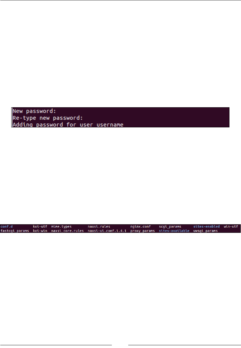
Chapter 10
[ 205 ]
Setting up basic HTTP authentication
HTTP authentication allows you to secure Elasticsearch using username- and
password-based access. You can do this by installing the apache-utils package:
sudo apt-get update
sudo apt-get install apache-utils
Now, let's create a password le with this command:
sudo htpasswd -c /etc/nginx/.htpasswd username
The preceding command will prompt you to create a password for the username
user, as shown in the following screenshot:
Once you create the password, a le with the .htpasswd name will be created inside
the /etc/nginx directory in the format of login:password.
Setting up Nginx
Run the following command to install Nginx on Ubuntu machines:
sudo apt-get install nginx
You can nd the conguration directory of Nginx inside the /etc/nginx directory,
which looks similar to this:
Proxy templates are usually created inside the sites-available directory. This can be
created with the following command:
sudo vi /etc/nginx/sites-available/elastic_proxy
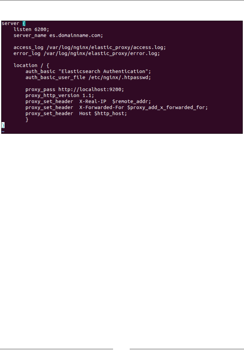
Backups and Security
[ 206 ]
Enter the following conguration lines inside this le:
As you can see, we have congured the Nginx server to listen to port 6200, which is
just a custom port number to connect with Elasticsearch. You are no longer required
to connect Elasticsearch on its default port 9200 because it is running on localhost.
It's also good if you can create a subdomain for your Elasticsearch cluster (es.
domainname.com, in this example), which points to the public IP of this server.
If you do not have any subdomain, but have a public IP available on this server,
you can omit the server_name parameter.
The main things are written inside the location directive, where we have used the
HTTP authentication le you had created. Now only those users who have this user
name and password can access this Elasticsearch cluster.
When you are done with the conguration of your template, create a symbolic link
of the template to make it available inside the /etc/sites-enabled directory that
will be nally loaded by Nginx. To do this, run the following command:
sudo ln -s /etc/nginx/sites-available/elastic_proxy /etc/nginx/sites-
enabled/
You also need to create a log directory to store all the access and error logs. You can
do it using these commands:
sudo mkdir /var/log/nginx/elastic_proxy
sudo touch /var/log/nginx/elastic_proxy/access.log
sudo touch /var/log/nginx/elastic_proxy/error.log
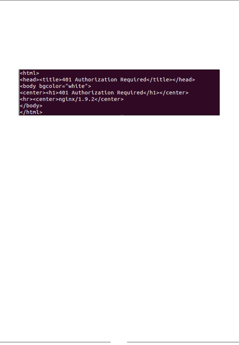
Chapter 10
[ 207 ]
Once done, start the Nginx server with the following command:
sudo service nginx start
Now, try to access Elasticsearch with this command:
curl localhost:6200
You will get the following response:
This clearly tells you that to access this URL, you need a valid user name and
password. So, it can be accessed using the following command:
curl username:password@localhost:6200
Here, the username and password are the ones you have created in the
previous section.
Securing critical access
You know very well that Elasticsearch is based on REST and provides the HTTP
endpoints for all the tasks, such as _search, _delete, _update, _stats, _settings,
and so on, which essentially works on the HTTP verbs such as GET, PUT, POST, and
DELETE.
Nginx is very good for rule-based access by getting the request parameters and
putting constraints on the requests. Let's see how you can do this.
Restricting DELETE requests
To keep your data safe by avoiding DELETE requests, you can do the following
congurations inside your proxy template:
if ($request_method ~ "DELETE") {
return 403;
break;
}
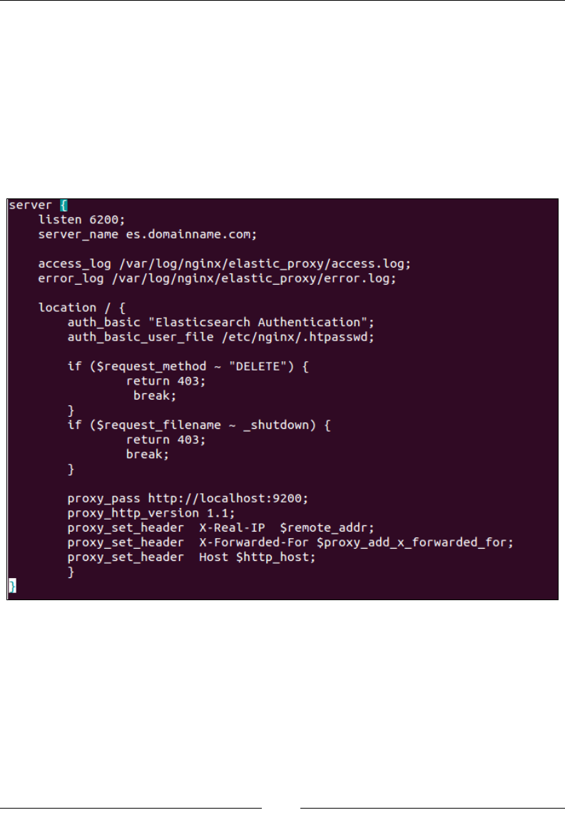
Backups and Security
[ 208 ]
Restricting endpoints
To restrict endpoints, such as _shutdown, you can use the following conguration:
if ($request_filename ~ _shutdown) {
return 403;
break;
}
A nal conguration would look like this:
You can add many other constraints using similar if statements as shown in the
preceding template. Whenever you edit the template inside /etc/sites-available,
it will automatically reect the changes inside sites-enabled; however, make sure to
reload the changed congurations by running this command:
sudo service nginx reload
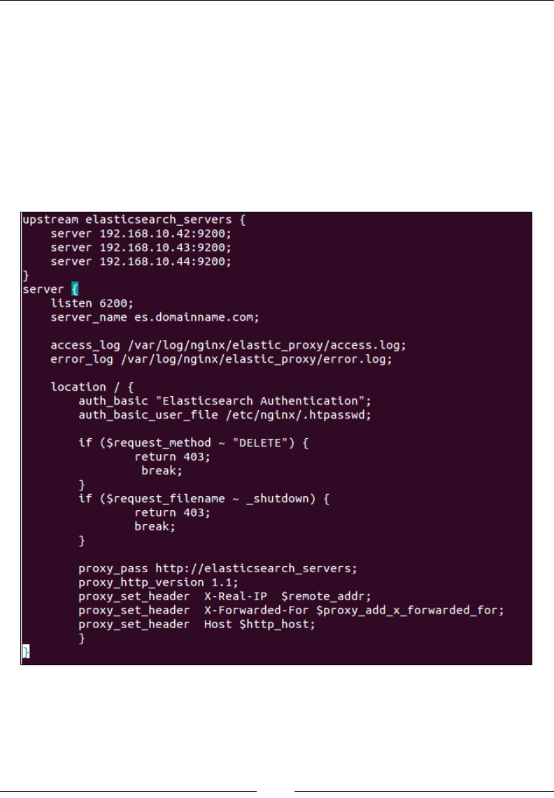
Chapter 10
[ 209 ]
Load balancing using Nginx
If you have more than one client node in your Elasticsearch cluster, you can create
connections to all of the client nodes for high availability. However, to load balance
the requests in addition to cluster security, you can use the power of Nginx.
For example, you have three client nodes with the IP addresses, 192.168.10.42,
192.168.10.43, and 192.168.10.44. The following is a sample conguration that will
listen to your proxy server subdomain or the public IP address (can be a private IP
if not an Internet-facing ES) and will distribute the load to the Elasticsearch clients
in a round-robin fashion:
See the upstream directive in the preceding conguration template that holds all the
IP and ports of the Elasticsearch clients using the elasticsearch_servers name.
The proxy_pass directive now contains the name of the upstream directive instead
of a single client address.

Backups and Security
[ 210 ]
Nginx also provides options to load balance requests such as least connected,
weighted, and session persistence. To use them, you can go through the load balancing
guide of Nginx at http://nginx.org/en/docs/http/load_balancing.html and
utilize them to give more power to your Elasticsearch cluster.
Summary
In this chapter, you learned how to create data backups of an Elasticsearch cluster
and restore them back into the same or another cluster. You also learned how to
secure Elasticsearch clusters and load balance them using Nginx.
Finally, we have reached the end of the book, and we hope that you have had a
pleasant reading experience. Elasticsearch is vast, and covering every tiny detail
in this book was not possible. However, as per the goal, it covers almost every
"essential" topic of Elasticsearch for developers to start from scratch and to be
able to manage and scale an Elasticsearch cluster on their own. Most interestingly,
this book serves both Java and Python programmers under one hood.
Not only has Elasticsearch matured, but the community around this technology is
also much more mature now. If you face any issue, you can post your questions to
the ofcial user discussion group: https://discuss.elastic.co.
We also suggest you keep visiting the ofcial blog of Elasticsearch at https://www.
elastic.co/blog to keep yourself updated with the latest and greatest news around
this technology.
With all this knowledge and everything you have learned throughout this book,
you are now fully equipped to create and manage a full-blown search and analytics
solutions based on Elasticsearch. We wish you the best!
Module 2
Mastering Elasticsearch
Further your knowledge of ElasticSearch server by learning more
about its internals, querying, and data handling

Introduction to Elasticsearch
Before going further into the book, we would like to emphasize that we are treating
this book as an extension to the Elasticsearch Server Second Edition book we've written,
also published by Packt Publishing. Of course, we start with a brief introduction
to both Apache Lucene and Elasticsearch, but this book is not for a person who
doesn't know Elasticsearch at all. We treat Mastering Elasticsearch as a book that will
systematize your knowledge about Elasticsearch and extend it by showing some
examples of how to leverage your knowledge in certain situations. If you are looking
for a book that will help you start your journey into the world of Elasticsearch, please
take a look at Elasticsearch Server Second Edition mentioned previously.
That said, we hope that by reading this book, you want to extend and build on basic
Elasticsearch knowledge. We assume that you already know how to index data to
Elasticsearch using single requests as well as bulk indexing. You should also know
how to send queries to get the documents you are interested in, how to narrow down
the results of your queries by using ltering, and how to calculate statistics for your
data with the use of the faceting/aggregation mechanism. However, before getting
to the exciting functionality that Elasticsearch offers, we think we should start with a
quick tour of Apache Lucene, which is a full text search library that Elasticsearch uses
to build and search its indices, as well as the basic concepts on which Elasticsearch
is built. In order to move forward and extend our learning, we need to ensure that
we don't forget the basics. This is easy to do. We also need to make sure that we
understand Lucene correctly as Mastering Elasticsearch requires this understanding. By
the end of this chapter, we will have covered the following topics:
• What Apache Lucene is
• What overall Lucene architecture looks like
• How the analysis process is done
• What Apache Lucene query language is and how to use it
• What are the basic concepts of Elasticsearch
• How Elasticsearch communicates internally

Introduction to Elasticsearch
[ 214 ]
Introducing Apache Lucene
In order to fully understand how Elasticsearch works, especially when it comes
to indexing and query processing, it is crucial to understand how Apache Lucene
library works. Under the hood, Elasticsearch uses Lucene to handle document
indexing. The same library is also used to perform a search against the indexed
documents. In the next few pages, we will try to show you the basics of Apache
Lucene, just in case you've never used it.
Getting familiar with Lucene
You may wonder why Elasticsearch creators decided to use Apache Lucene instead
of developing their own functionality. We don't know for sure since we were not the
ones who made the decision, but we assume that it was because Lucene is mature,
open-source, highly performing, scalable, light and, yet, very powerful. It also has a
very strong community that supports it. Its core comes as a single le of Java library
with no dependencies, and allows you to index documents and search them with
its out-of-the-box full text search capabilities. Of course, there are extensions to
Apache Lucene that allow different language handling, and enable spellchecking,
highlighting, and much more, but if you don't need those features, you can
download a single le and use it in your application.
Overall architecture
Although I would like to jump straight to Apache Lucene architecture, there are
some things we need to know rst in order to fully understand it, and those are
as follows:
• Document: It is a main data carrier used during indexing and search,
containing one or more elds, that contain the data we put and get from
Lucene.
• Field: It is a section of the document which is built of two parts: the name
and the value.
• Term: It is a unit of search representing a word from the text.
• Token: It is an occurrence of a term from the text of the eld. It consists of
term text, start and end offset, and a type.
Apache Lucene writes all the information to the structure called inverted index. It is
a data structure that maps the terms in the index to the documents, not the other way
round like the relational database does. You can think of an inverted index as a data
structure, where data is term oriented rather than document oriented.

Chapter 1
[ 215 ]
Let's see how a simple inverted index can look. For example, let's assume that
we have the documents with only title eld to be indexed and they look like the
following:
• Elasticsearch Server (document 1)
• Mastering Elasticsearch (document 2)
• Apache Solr 4 Cookbook (document 3)
So, the index (in a very simple way) could be visualized as shown in the
following gure:
4
Apache
Cooking
Elasticsearch
Mastering
Server
Solr
Term Count Docs
1
1
1
2
1
1
1
<3>
<3>
<3>
<1><2>
<1>
<1>
<3>
As you can see, each term points to the number of documents it is present in. This
allows for a very efcient and fast search such as the term-based queries. In addition
to this, each term has a number connected to it: the count, telling Lucene how often it
occurs.
Each index is divided into multiple write once and read many time segments. When
indexing, after a single segment is written to disk, it can't be updated. For example,
the information about deleted documents is stored in a separate le, but the segment
itself is not updated.
However, multiple segments can be merged together in a process called segments
merge. After forcing, segments are merged, or after Lucene decides it is time for
merging to be performed, segments are merged together by Lucene to create
larger ones. This can be I/O demanding; however, it is needed to clean up some
information because during that time some information that is not needed anymore
is deleted, for example the deleted documents. In addition to this, searching with
the use of one larger segment is faster than searching against multiple smaller ones
holding the same data. However, once again, remember that segments merging is
an I/O demanding operation and you shouldn't force merging, just congure your
merge policy carefully.

Introduction to Elasticsearch
[ 216 ]
If you want to know what les are building the segments and what
information is stored inside them, please take a look at Apache
Lucene documentation available at http://lucene.apache.
org/core/4_10_3/core/org/apache/lucene/codecs/
lucene410/package-summary.html.
Getting deeper into Lucene index
Of course, the actual index created by Lucene is much more complicated and
advanced, and consists of more than the terms their counts and documents in which
they are present. We would like to tell you about a few of those additional index
pieces because even though they are internal, it is usually good to know about them
as they can be very handy.
Norms
A norm is a factor associated with each indexed document and stores normalization
factors used to compute the score relative to the query. Norms are computed on
the basis of index time boosts and are indexed along with the documents. With the
use of norms, Lucene is able to provide an index time-boosting functionality at the
cost of a certain amount of additional space needed for norms indexation and some
amount of additional memory.
Term vectors
Term vectors are small inverted indices per document. They consist of pairs—a term
and its frequency—and can optionally include information about term position.
By default, Lucene and Elasticsearch don't enable term vectors indexing, but some
functionality such as the fast vector highlighting requires them to be present.
Posting formats
With the release of Lucene 4.0, the library introduced the so-called codec
architecture, giving developers control over how the index les are written onto the
disk. One of the parts of the index is the posting format, which stores elds, terms,
documents, terms positions and offsets, and, nally, the payloads (a byte array
stored at an arbitrary position in Lucene index, which can contain any information
we want). Lucene contains different posting formats for different purposes, for
example one that is optimized for high cardinality elds like the unique identier.

Chapter 1
[ 217 ]
Doc values
As we already mentioned, Lucene index is the so-called inverted index. However,
for certain features, such as faceting or aggregations, such architecture is not the best
one. The mentioned functionality operates on the document level and not the term
level and because Elasticsearch needs to uninvert the index before calculations can
be done. Because of that, doc values were introduced and additional structure used
for faceting, sorting and aggregations. The doc values store uninverted data for a
eld they are turned on for. Both Lucene and Elasticsearch allow us to congure the
implementation used to store them, giving us the possibility of memory-based doc
values, disk-based doc values, and a combination of the two.
Analyzing your data
Of course, the question arises of how the data passed in the documents is
transformed into the inverted index and how the query text is changed into terms to
allow searching. The process of transforming this data is called analysis.
Analysis is done by the analyzer, which is built of tokenizer and zero or more lters,
and can also have zero or more character mappers.
A tokenizer in Lucene is used to divide the text into tokens, which are basically terms
with additional information, such as its position in the original text and its length.
The result of the tokenizer work is a so-called token stream, where the tokens are put
one by one and are ready to be processed by lters.
Apart from tokenizer, Lucene analyzer is built of zero or more lters that are used
to process tokens in the token stream. For example, it can remove tokens from the
stream, change them or even produce new ones. There are numerous lters and you
can easily create new ones. Some examples of lters are as follows:
• Lowercase lter: It makes all the tokens lowercase
• ASCII folding lter: It removes non ASCII parts from tokens
• Synonyms lter: It is responsible for changing one token to another on the
basis of synonym rules
• Multiple language stemming lters: These are responsible for reducing
tokens (actually the text part that they provide) into their root or base forms,
the stem
Filters are processed one after another, so we have almost unlimited analysis
possibilities with adding multiple lters one after another.

Introduction to Elasticsearch
[ 218 ]
The last thing is the character mappings, which is used before tokenizer and is
responsible for processing text before any analysis is done. One of the examples of
character mapper is the HTML tags removal process.
Indexing and querying
We may wonder how that all affects indexing and querying when using Lucene
and all the software that is built on top of it. During indexing, Lucene will use an
analyzer of your choice to process the contents of your document; different analyzers
can be used for different elds, so the title eld of your document can be analyzed
differently compared to the description eld.
During query time, if you use one of the provided query parsers, your query will
be analyzed. However, you can also choose the other path and not analyze your
queries. This is crucial to remember because some of the Elasticsearch queries are
being analyzed and some are not. For example, the prex query is not analyzed and
the match query is analyzed.
What you should remember about indexing and querying analysis is that the index
should be matched by the query term. If they don't match, Lucene won't return the
desired documents. For example, if you are using stemming and lowercasing during
indexing, you need to be sure that the terms in the query are also lowercased and
stemmed, or your queries will return no results at all.
Lucene query language
Some of the query types provided by Elasticsearch support Apache Lucene query
parser syntax. Because of this, it is crucial to understand the Lucene query language.
Understanding the basics
A query is divided by Apache Lucene into terms and operators. A term, in Lucene,
can be a single word or a phrase (group of words surrounded by double quote
characters). If the query is set to be analyzed, the dened analyzer will be used on
each of the terms that form the query.
A query can also contain Boolean operators that connect terms to each other forming
clauses. The list of Boolean operators is as follows:
• AND: It means that the given two terms (left and right operand) need to
match in order for the clause to be matched. For example, we would run a
query, such as apache AND lucene, to match documents with both apache and
lucene terms in a document eld.

Chapter 1
[ 219 ]
• OR: It means that any of the given terms may match in order for the clause to
be matched. For example, we would run a query, such as apache OR lucene,
to match documents with apache or lucene (or both) terms in a document
eld.
• NOT: It means that in order for the document to be considered a match,
the term appearing after the NOT operator must not match. For example, we
would run a query lucene NOT Elasticsearch to match documents that contain
lucene term, but not the Elasticsearch term in the document eld.
In addition to these, we may use the following operators:
• +: It means that the given term needs to be matched in order for the
document to be considered as a match. For example, in order to nd
documents that match lucene term and may match apache term, we would
run a query such as +lucene apache.
• -: It means that the given term can't be matched in order for the document to
be considered a match. For example, in order to nd a document with lucene
term, but not Elasticsearch term, we would run a query such as +lucene
-Elasticsearch.
When not specifying any of the previous operators, the default OR operator will be
used.
In addition to all these, there is one more thing: you can use parenthesis to group
clauses together for example, with something like the following query:
Elasticsearch AND (mastering OR book)
Querying elds
Of course, just like in Elasticsearch, in Lucene all your data is stored in elds that
build the document. In order to run a query against a eld, you need to provide
the eld name, add the colon character, and provide the clause that should be run
against that eld. For example, if you would like to match documents with the term
Elasticsearch in the title eld, you would run the following query:
title:Elasticsearch
You can also group multiple clauses. For example, if you would like your query to
match all the documents having the Elasticsearch term and the mastering book
phrase in the title eld, you could run a query like the following code:
title:(+Elasticsearch +"mastering book")

Introduction to Elasticsearch
[ 220 ]
The previous query can also be expressed in the following way:
+title:Elasticsearch +title:"mastering book"
Term modiers
In addition to the standard eld query with a simple term or clause, Lucene allows
us to modify the terms we pass in the query with modiers. The most common
modiers, which you will be familiar with, are wildcards. There are two wildcards
supported by Lucene, the ? and * terms. The rst one will match any character and
the second one will match multiple characters.
Please note that by default these wildcard characters can't be used as
the rst character in a term because of performance reasons.
In addition to this, Lucene supports fuzzy and proximity searches with the use of the
~ character and an integer following it. When used with a single word term, it means
that we want to search for terms that are similar to the one we've modied (the so-
called fuzzy search). The integer after the ~ character species the maximum number
of edits that can be done to consider the term similar. For example, if we would run a
query, such as writer~2, both the terms writer and writers would be considered a
match.
When the ~ character is used on a phrase, the integer number we provide is telling
Lucene how much distance between the words is acceptable. For example, let's take
the following query:
title:"mastering Elasticsearch"
It would match the document with the title eld containing mastering
Elasticsearch, but not mastering book Elasticsearch. However, if we would
run a query, such as title:"mastering Elasticsearch"~2, it would result in both
example documents matched.
We can also use boosting to increase our term importance by using the ^ character
and providing a oat number. Boosts lower than one would result in decreasing
the document importance. Boosts higher than one will result in increasing the
importance. The default boost value is 1. Please refer to the Default Apache Lucene
scoring explained section in Chapter 2, Power User Query DSL, for further information
on what boosting is and how it is taken into consideration during document scoring.

Chapter 1
[ 221 ]
In addition to all these, we can use square and curly brackets to allow range
searching. For example, if we would like to run a range search on a numeric eld, we
could run the following query:
price:[10.00 TO 15.00]
The preceding query would result in all documents with the price eld between
10.00 and 15.00 inclusive.
In case of string-based elds, we also can run a range query, for example name:[Adam
TO Adria].
The preceding query would result in all documents containing all the terms between
Adam and Adria in the name eld including them.
If you would like your range bound or bounds to be exclusive, use curly brackets
instead of the square ones. For example, in order to nd documents with the price
eld between 10.00 inclusive and 15.00 exclusive, we would run the following query:
price:[10.00 TO 15.00}
If you would like your range bound from one side and not bound by the other, for
example querying for documents with a price higher than 10.00, we would run the
following query:
price:[10.00 TO *]
Handling special characters
In case you want to search for one of the special characters (which are +, -, &&, ||, !,
(, ), { }, [ ], ^, ", ~, *, ?, :, \, /), you need to escape it with the use of the backslash
(\) character. For example, to search for the abc"efg term you need to do something
like abc\"efg.
Introducing Elasticsearch
Although we've said that we expect the reader to be familiar with Elasticsearch, we
would really like you to fully understand Elasticsearch; therefore, we've decided to
include a short introduction to the concepts of this great search engine.
As you probably know, Elasticsearch is production-ready software to build search
and analysis-oriented applications. It was originally started by Shay Banon and
published in February 2010. Since then, it has rapidly gained popularity just within
a few years and has become an important alternative to other open source and
commercial solutions. It is one of the most downloaded open source projects.

Introduction to Elasticsearch
[ 222 ]
Basic concepts
There are a few concepts that come with Elasticsearch and their understanding is
crucial to fully understand how Elasticsearch works and operates.
Index
Elasticsearch stores its data in one or more indices. Using analogies from the SQL
world, index is something similar to a database. It is used to store the documents
and read them from it. As already mentioned, under the hood, Elasticsearch uses
Apache Lucene library to write and read the data from the index. What you should
remember is that a single Elasticsearch index may be built of more than a single
Apache Lucene index—by using shards.
Document
Document is the main entity in the Elasticsearch world (and also in the Lucene
world). At the end, all use cases of using Elasticsearch can be brought at a point
where it is all about searching for documents and analyzing them. Document
consists of elds, and each eld is identied by its name and can contain one or
multiple values. Each document may have a different set of elds; there is no schema
or imposed structure—this is because Elasticsearch documents are in fact Lucene
ones. From the client point of view, Elasticsearch document is a JSON object (see
more on the JSON format at http://en.wikipedia.org/wiki/JSON).
Type
Each document in Elasticsearch has its type dened. This allows us to store various
document types in one index and have different mappings for different document
types. If you would like to compare it to an SQL world, a type in Elasticsearch is
something similar to a database table.
Mapping
As already mentioned in the Introducing Apache Lucene section, all documents are
analyzed before being indexed. We can congure how the input text is divided into
tokens, which tokens should be ltered out, or what additional processing, such as
removing HTML tags, is needed. This is where mapping comes into play—it holds
all the information about the analysis chain. Besides the fact that Elasticsearch can
automatically discover eld type by looking at its value, in most cases we will want
to congure the mappings ourselves to avoid unpleasant surprises.

Chapter 1
[ 223 ]
Node
The single instance of the Elasticsearch server is called a node. A single node in
Elasticsearch deployment can be sufcient for many simple use cases, but when you
have to think about fault tolerance or you have lots of data that cannot t in a single
server, you should think about multi-node Elasticsearch cluster.
Elasticsearch nodes can serve different purposes. Of course, Elasticsearch is designed
to index and search our data, so the rst type of node is the data node. Such nodes
hold the data and search on them. The second type of node is the master node—a
node that works as a supervisor of the cluster controlling other nodes' work. The
third node type is the tribe node, which is new and was introduced in Elasticsearch
1.0. The tribe node can join multiple clusters and thus act as a bridge between them,
allowing us to execute almost all Elasticsearch functionalities on multiple clusters
just like we would be using a single cluster.
Cluster
Cluster is a set of Elasticsearch nodes that work together. The distributed nature
of Elasticsearch allows us to easily handle data that is too large for a single node to
handle (both in terms of handling queries and documents). By using multi-node
clusters, we can also achieve uninterrupted work of our application, even if several
machines (nodes) are not available due to outage or administration tasks such
as upgrade. Elasticsearch provides clustering almost seamlessly. In our opinion,
this is one of the major advantages over competition; setting up a cluster in the
Elasticsearch world is really easy.
Shard
As we said previously, clustering allows us to store information volumes that exceed
abilities of a single server (but it is not the only need for clustering). To achieve this
requirement, Elasticsearch spreads data to several physical Lucene indices. Those
Lucene indices are called shards, and the process of dividing the index is called
sharding. Elasticsearch can do this automatically and all the parts of the index
(shards) are visible to the user as one big index. Note that besides this automation,
it is crucial to tune this mechanism for particular use cases because the number of
shard index is built or congured during index creation and cannot be changed
without creating a new index and re-indexing the whole data.

Introduction to Elasticsearch
[ 224 ]
Replica
Sharding allows us to push more data into Elasticsearch that is possible for a single
node to handle. Replicas can help us in situations where the load increases and
a single node is not able to handle all the requests. The idea is simple—create an
additional copy of a shard, which can be used for queries just as original, primary
shard. Note that we get safety for free. If the server with the primary shard is gone,
Elasticsearch will take one of the available replicas of that shard and promote it to the
leader, so the service work is not interrupted. Replicas can be added and removed at
any time, so you can adjust their numbers when needed. Of course, the content of the
replica is updated in real time and is done automatically by Elasticsearch.
Key concepts behind Elasticsearch
architecture
Elasticsearch was built with a few concepts in mind. The development team wanted
to make it easy to use and highly scalable. These core features are visible in every
corner of Elasticsearch. From the architectural perspective, the main features are as
follows:
• Reasonable default values that allow users to start using Elasticsearch just
after installing it, without any additional tuning. This includes built-in
discovery (for example, eld types) and auto-conguration.
• Working in distributed mode by default. Nodes assume that they are or will
be a part of the cluster.
• Peer-to-peer architecture without single point of failure (SPOF). Nodes
automatically connect to other machines in the cluster for data interchange
and mutual monitoring. This covers automatic replication of shards.
• Easily scalable both in terms of capacity and the amount of data by adding
new nodes to the cluster.
• Elasticsearch does not impose restrictions on data organization in the index.
This allows users to adjust to the existing data model. As we noted in type
description, Elasticsearch supports multiple data types in a single index, and
adjustment to the business model includes handling relationships between
documents (although, this functionality is rather limited).
• Near Real Time (NRT) searching and versioning. Because of the distributed
nature of Elasticsearch, it is impossible to avoid delays and temporary
differences between data located on the different nodes. Elasticsearch tries to
reduce these issues and provide additional mechanisms as versioning.
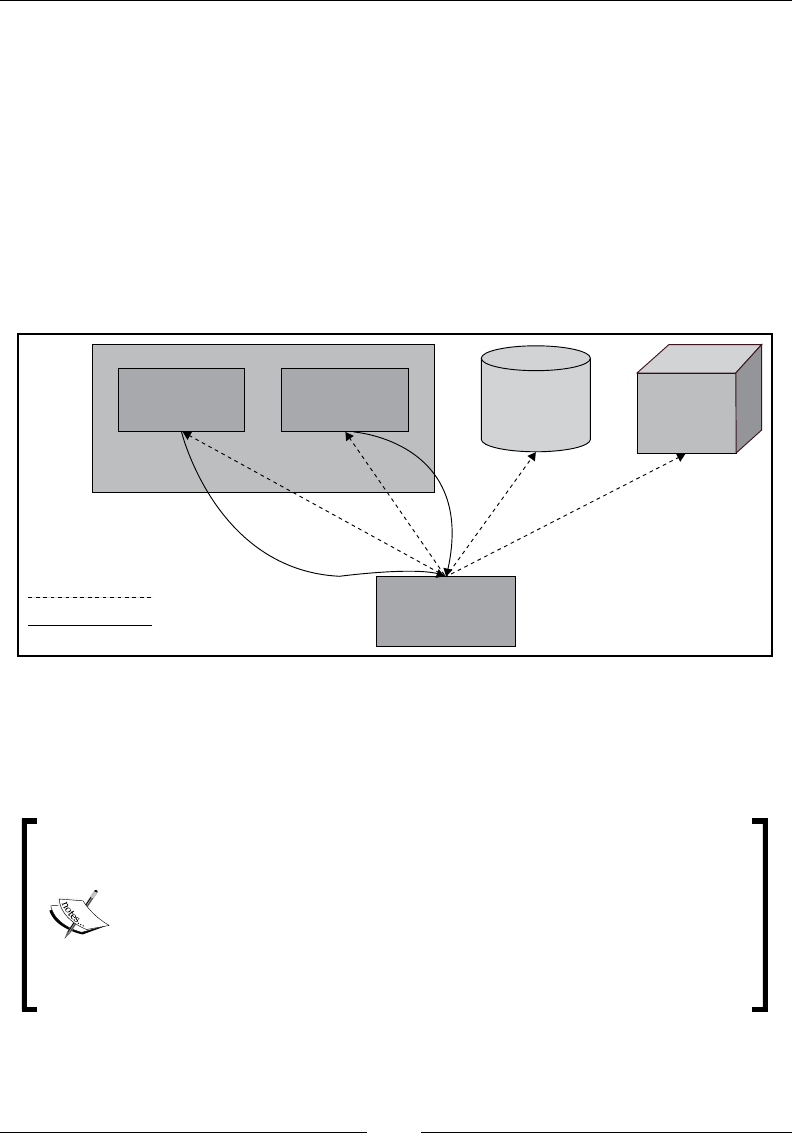
Chapter 1
[ 225 ]
Workings of Elasticsearch
The following section will include information on key Elasticsearch features, such as
bootstrap, failure detection, data indexing, querying, and so on.
The startup process
When Elasticsearch node starts, it uses the discovery module to nd the other nodes
in the same cluster (the key here is the cluster name dened in the conguration)
and connect to them. By default the multicast request is broadcast to the network to
nd other Elasticsearch nodes with the same cluster name. You can see the process
illustrated in the following gure:
Application
Database
Elasticsearch
Node
Elasticsearch
Node
Elasticsearch Cluster
New
Elasticsearch
Node
Multicast request
Multicast response
In the preceding gure, the cluster, one of the nodes that is master eligible is elected
as master node (by default all nodes are master eligible). This node is responsible for
managing the cluster state and the process of assigning shards to nodes in reaction to
changes in cluster topology.
Note that a master node in Elasticsearch has no importance from the
user perspective, which is different from other systems available (such
as the databases). In practice, you do not need to know which node is
a master node; all operations can be sent to any node, and internally
Elasticsearch will do all the magic. If necessary, any node can send
sub-queries in parallel to other nodes and merge responses to return
the full response to the user. All of this is done without accessing the
master node (nodes operates in peer-to-peer architecture).

Introduction to Elasticsearch
[ 226 ]
The master node reads the cluster state and, if necessary, goes into the recovery
process. During this state, it checks which shards are available and decides which
shards will be the primary shards. After this, the whole cluster enters into a yellow
state.
This means that a cluster is able to run queries, but full throughput and all
possibilities are not achieved yet (it basically means that all primary shards are
allocated, but not all replicas are). The next thing to do is to nd duplicated shards
and treat them as replicas. When a shard has too few replicas, the master node
decides where to put missing shards and additional replicas are created based on a
primary shard (if possible). If everything goes well, the cluster enters into a green
state (which means that all primary shards and all their replicas are allocated).
Failure detection
During normal cluster work, the master node monitors all the available nodes and
checks whether they are working. If any of them are not available for the congured
amount of time, the node is treated as broken and the process of handling failure
starts. For example, this may mean rebalancing of shards, choosing new leaders,
and so on. As another example, for every primary shard that is present on the
failed nodes, a new primary shard should be elected from the remaining replicas of
this shard. The whole process of placing new shards and replicas can (and usually
should) be congured to match our needs. More information about it can be found in
Chapter 7, Elasticsearch Administration.
Just to illustrate how it works, let's take an example of a three nodes cluster. One
of the nodes is the master node, and all of the nodes can hold data. The master
node will send the ping requests to other nodes and wait for the response. If the
response doesn't come (actually how many ping requests may fail depends on the
conguration), such a node will be removed from the cluster. The same goes in the
opposite way—each node will ping the master node to see whether it is working.
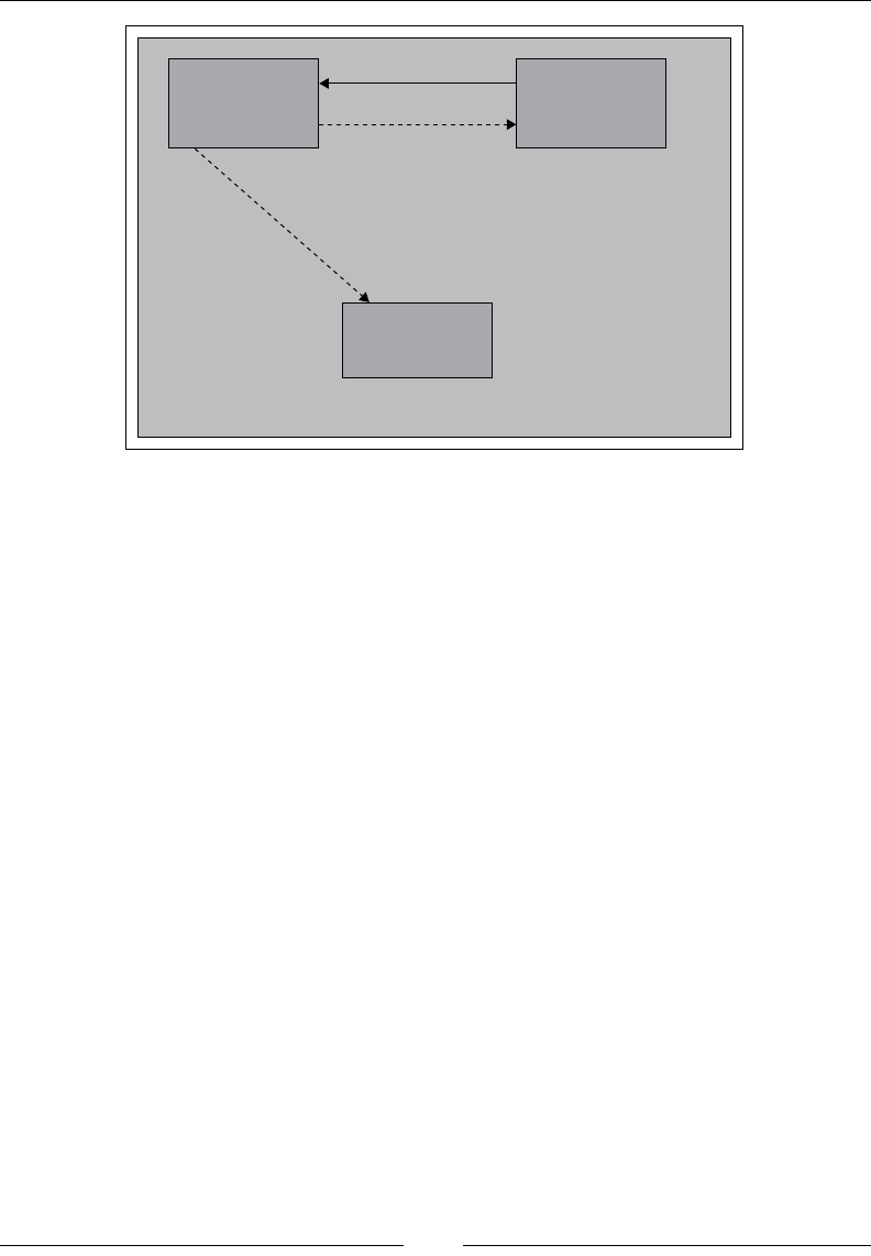
Chapter 1
[ 227 ]
Elasticsearch
Node 1
Elasticsearch
Node 2
Elasticsearch
Master Node
Ping request
Ping response
Elasticsearch Cluster
Ping request
Communicating with Elasticsearch
We talked about how Elasticsearch is built, but, after all, the most important part
for us is how to feed it with data and how to build queries. In order to do that,
Elasticsearch exposes a sophisticated Application Program Interface (API). In
general, it wouldn't be a surprise if we would say that every feature of Elasticsearch
has an API. The primary API is REST based (see http://en.wikipedia.org/wiki/
Representational_state_transfer) and is easy to integrate with practically any
system that can send HTTP requests.
Elasticsearch assumes that data is sent in the URL or in the request body as a JSON
document (see http://en.wikipedia.org/wiki/JSON). If you use Java or language
based on Java Virtual Machine (JVM), you should look at the Java API, which, in
addition to everything that is offered by the REST API, has built-in cluster discovery.
It is worth mentioning that the Java API is also internally used by Elasticsearch itself
to do all the node-to-node communication. Because of this, the Java API exposes all
the features available through the REST API calls.
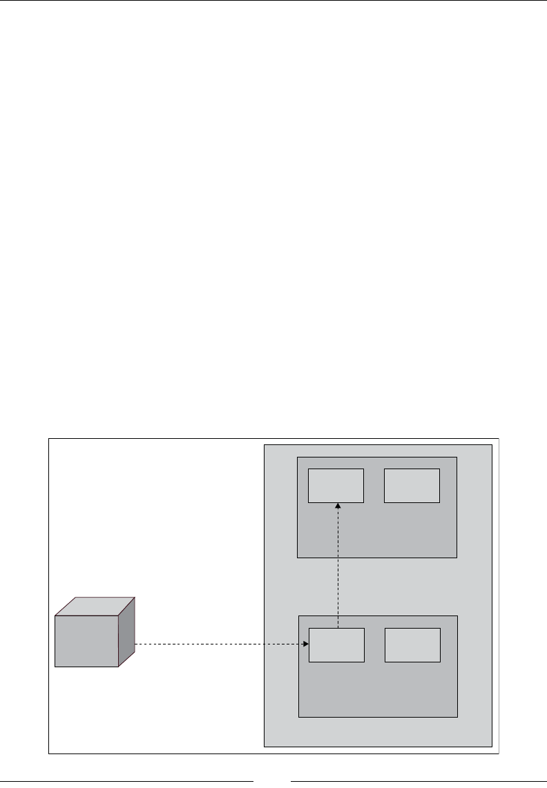
Introduction to Elasticsearch
[ 228 ]
Indexing data
There are a few ways to send data to Elasticsearch. The easiest way is using the index
API, which allows sending a single document to a particular index. For example, by
using the curl tool (see http://curl.haxx.se/). An example command that would
create a new document would look as follows:
curl -XPUT http://localhost:9200/blog/article/1 -d '{"title": "New
version of Elastic Search released!", "tags": ["announce",
"Elasticsearch", "release"] }'
The second way allows us to send many documents using the bulk API and the UDP
bulk API. The difference between these methods is the connection type. Common
bulk command sends documents by HTTP protocol and UDP bulk sends this using
connection less datagram protocol. This is faster but not so reliable. The last method
uses plugins, called rivers, but let's not discuss them as the rivers will be removed in
future versions of Elasticsearch.
One very important thing to remember is that the indexing will always be rst
executed at the primary shard, not on the replica. If the indexing request is sent to a
node that doesn't have the correct shard or contains a replica, it will be forwarded to
the primary shard. Then, the leader will send the indexing request to all the replicas,
wait for their acknowledgement (this can be controlled), and nalize the indexation
if the requirements were met (like the replica quorum being updated).
The following illustration shows the process we just discussed:
Application
Shade 2
primary
Shade 1
primary
Elasticsearch Node
Elasticsearch Cluster
Shade 2
replica
Shade 1
replica
Elasticsearch Node
Forward to
leader
Indexing request

Chapter 1
[ 229 ]
Querying data
The Query API is a big part of Elasticsearch API. Using the Query DSL (JSON-based
language for building complex queries), we can do the following:
• Use various query types including simple term query, phrase, range,
Boolean, fuzzy, span, wildcard, spatial, and function queries for human
readable scoring control
• Build complex queries by combining the simple queries together
• Filter documents, throwing away ones that do not match selected criteria
without inuencing the scoring, which is very efcient when it comes
to performance
• Find documents similar to a given document
• Find suggestions and corrections of a given phrase
• Build dynamic navigation and calculate statistics using aggregations
• Use prospective search and nd queries matching a given document
When talking about querying, the important thing is that query is not a simple,
single-stage process. In general, the process can be divided into two phases: the
scatter phase and the gather phase. The scatter phase is about querying all the
relevant shards of your index. The gather phase is about gathering the results from
the relevant shards, combining them, sorting, processing, and returning to the client.
The following illustration shows that process:
Application
Elasticsearch Cluster
Results
Shade 1
Elasticsearch Node
Shade 2
Elasticsearch Node
Query
Scatter phase
Gather phase

Introduction to Elasticsearch
[ 230 ]
You can control the scatter and gather phases by specifying the search
type to one of the six values currently exposed by Elasticsearch. We've
talked about query scope in our previous book Elasticsearch Server
Second Edition by Packt Publishing.
The story
As we said in the beginning of this chapter, we treat the book you are holding in your
hands as a continuation of the Elasticsearch Server Second Edition book. Because of
this, we would like to continue the story that we've used in that book. In general, we
assume that we are implementing and running an online book store, as simple as that.
The mappings for our library index look like the following:
{
"book" : {
"_index" : {
"enabled" : true
},
"_id" : {
"index": "not_analyzed",
"store" : "yes"
},
"properties" : {
"author" : {
"type" : "string"
},
"characters" : {
"type" : "string"
},
"copies" : {
"type" : "long",
"ignore_malformed" : false
},
"otitle" : {
"type" : "string"
},
"tags" : {
"type" : "string",
"index" : "not_analyzed"
},
"title" : {
"type" : "string"

Chapter 1
[ 231 ]
},
"year" : {
"type" : "long",
"ignore_malformed" : false
},
"available" : {
"type" : "boolean"
},
"review" : {
"type" : "nested",
"properties" : {
"nickname" : {
"type" : "string"
},
"text" : {
"type" : "string"
},
"stars" : {
"type" : "integer"
}
}
}
}
}
}
The mappings can be found in the library.json le provided with the book.
The data that we will use is provided with the book in the books.json le. The
example documents from that le look like the following:
{ "index": {"_index": "library", "_type": "book", "_id": "1"}}
{ "title": "All Quiet on the Western Front","otitle": "Im Westen
nichts
Neues","author": "Erich Maria Remarque","year": 1929,"characters":
["Paul
Bäumer", "Albert Kropp", "Haie Westhus", "Fredrich Müller",
"Stanislaus
Katczinsky", "Tjaden"],"tags": ["novel"],"copies": 1, "available":
true,
"section" : 3}
{ "index": {"_index": "library", "_type": "book", "_id": "2"}}
{ "title": "Catch-22","author": "Joseph Heller","year":
1961,"characters":

Introduction to Elasticsearch
[ 232 ]
["John Yossarian", "Captain Aardvark", "Chaplain Tappman", "Colonel
Cathcart", "Doctor Daneeka"],"tags": ["novel"],"copies": 6,
"available" :
false, "section" : 1}
{ "index": {"_index": "library", "_type": "book", "_id": "3"}}
{ "title": "The Complete Sherlock Holmes","author": "Arthur Conan
Doyle","year": 1936,"characters": ["Sherlock Holmes","Dr. Watson",
"G.
Lestrade"],"tags": [],"copies": 0, "available" : false, "section" :
12}
{ "index": {"_index": "library", "_type": "book", "_id": "4"}}
{ "title": "Crime and Punishment","otitle": "Преступлéние и
наказáние","author": "Fyodor Dostoevsky","year": 1886,"characters":
["Raskolnikov", "Sofia Semyonovna Marmeladova"],"tags": [],"copies":
0,
"available" : true}
Downloading the example code
You can download the example code les for all Packt books you have
purchased from your account at http://www.packtpub.com. If you
purchased this book elsewhere, you can visit http://www.packtpub.
com/support and register to have the les e-mailed directly to you.
To create the index using the provided mappings and to index the data, we would
run the following commands:
curl -XPOST 'localhost:9200/library'
curl -XPUT 'localhost:9200/library/book/_mapping' -d @library.json
curl -s -XPOST 'localhost:9200/_bulk' --data-binary @books.json
Summary
In this chapter, we looked at the general architecture of Apache Lucene: how it
works, how the analysis process is done, and how to use Apache Lucene query
language. In addition to that, we discussed the basic concepts of Elasticsearch, its
architecture, and internal communication.
In the next chapter, you'll learn about the default scoring formula Apache Lucene
uses, what the query rewrite process is, and how it works. In addition to that, we'll
discuss some of the Elasticsearch functionality, such as query templates, lters, and
how they affect performance, what we can do with that, and how we can choose the
right query to get the job done.

Power User Query DSL
In the previous chapter, we looked at what Apache Lucene is, how its architecture
looks, and how the analysis process is handled. In addition to these, we saw what
Lucene query language is and how to use it. We also discussed Elasticsearch, its
architecture, and core concepts. In this chapter, we will dive deep into Elasticsearch
focusing on the Query DSL. We will rst go through how Lucene scoring formula
works before turning to advanced queries. By the end of this chapter, we will have
covered the following topics:
• How the default Apache Lucene scoring formula works
• What query rewrite is
• What query templates are and how to use them
• How to leverage complicated Boolean queries
• What are the performance implications of large Boolean queries
• Which query you should use for your particular use case
Default Apache Lucene scoring explained
A very important part of the querying process in Apache Lucene is scoring. Scoring
is the process of calculating the score property of a document in a scope of a given
query. What is a score? A score is a factor that describes how well the document
matched the query. In this section, we'll look at the default Apache Lucene scoring
mechanism: the TF/IDF (term frequency/inverse document frequency) algorithm
and how it affects the returned document. Knowing how this works is valuable
when designing complicated queries and choosing which queries parts should be
more relevant than the others. Knowing the basics of how scoring works in Lucene
allows us to tune queries more easily and the results retuned by them to match our
use case.

Power User Query DSL
[ 234 ]
When a document is matched
When a document is returned by Lucene, it means that it matched the query we've
sent. In such a case, the document is given a score. Sometimes, the score is the same
for all the documents (like for the constant_score query), but usually this won't be
the case. The higher the score value, the more relevant the document is, at least at the
Apache Lucene level and from the scoring formula point of view. Because the score
is dependent on the matched documents, query, and the contents of the index, it is
natural that the score calculated for the same document returned by two different
queries will be different. Because of this, one should remember that not only should
we avoid comparing the scores of individual documents returned by different
queries, but we should also avoid comparing the maximum score calculated for
different queries. This is because the score depends on multiple factors, not only on
the boosts and query structure, but also on how many terms were matched, in which
elds, the type of matching that was used on query normalization, and so on. In
extreme cases, a similar query may result in totally different scores for a document,
only because we've used a custom score query or the number of matched terms
increased dramatically.
For now, let's get back to the scoring. In order to calculate the score property for a
document, multiple factors are taken into account, which are as follows:
• Document boost: The boost value given for a document during indexing.
• Field boost: The boost value given for a eld during querying.
• Coord: The coordination factor that is based on the number of terms the
document has. It is responsible for giving more value to the documents that
contain more search terms compared to other documents.
• Inverse document frequency: Term-based factor telling the scoring formula
how rare the given term is. The higher the inverse document frequency, the
rarer the term is. The scoring formula uses this factor to boost documents
that contain rare terms.
• Length norm: A eld-based factor for normalization based on the number
of terms given eld contains (calculated during indexing and stored in the
index). The longer the eld, the lesser boost this factor will give, which
means that the Apache Lucene scoring formula will favor documents with
elds containing lower terms.
• Term frequency: Term-based factor describing how many times a given term
occurs in a document. The higher the term frequency, the higher the score of
the document will be.

Chapter 2
[ 235 ]
• Query norm: Query-based normalization factor that is calculated as a sum
of a squared weight of each of the query terms. Query norm is used to allow
score comparison between queries, which, as we said, is not always easy and
possible.
TF/IDF scoring formula
Since the Lucene version 4.0, contains different scoring formulas and you are
probably aware of them. However, we would like to discuss the default TF/IDF
formula in greater detail. Please keep in mind that in order to adjust your query
relevance, you don't need to understand the following equations, but it is very
important to at least know how it works as it simplies the relevancy tuning process.
Lucene conceptual scoring formula
The conceptual version of the TF/IDF formula looks as follows:
The presented formula is a representation of a Boolean Model of Information
Retrieval combined with a Vector Space Model of Information Retrieval. Let's not
discuss this and let's just jump into the practical formula, which is implemented by
Apache Lucene and is actually used.
The information about the Boolean Model and Vector Space Model
of Information Retrieval are far beyond the scope of this book. You
can read more about it at http://en.wikipedia.org/wiki/
Standard_Boolean_model and http://en.wikipedia.org/
wiki/Vector_Space_Model.
Lucene practical scoring formula
Now, let's look at the following practical scoring formula used by the default Apache
Lucene scoring mechanism:

Power User Query DSL
[ 236 ]
As you can see, the score factor for the document is a function of query q and
document d, as we have already discussed. There are two factors that are not
dependent directly on query terms, coord and queryNorm. These two elements of the
formula are multiplied by the sum calculated for each term in the query.
The sum, on the other hand, is calculated by multiplying the term frequency for the
given term, its inverse document frequency, term boost, and the norm, which is the
length norm we've discussed previously.
Sounds a bit complicated, right? Don't worry, you don't need to remember all of
that. What you should be aware of is what matters when it comes to document score.
Basically, there are a few rules, as follows, which come from the previous equations:
• The rarer the matched term, the higher the score the document will have.
Lucene treats documents with unique words as more important than the
ones containing common words.
• The smaller the document elds (contain less terms), the higher the score
the document will have. In general, Lucene emphasizes shorter documents
because there is a greater possibility that those documents are exactly about
the topic we are searching for.
• The higher the boost (both given during indexing and querying), the
higher the score the document will have because higher boost means more
importance of the particular data (document, term, phrase, and so on).
As we can see, Lucene will give the highest score for the documents that have many
uncommon query terms matched in the document contents, have shorter elds (less
terms indexed), and will also favor rarer terms instead of the common ones.
If you want to read more about the Apache Lucene TF/IDF
scoring formula, please visit Apache Lucene Javadocs for the
TFIDFSimilarity class available at http://lucene.apache.
org/core/4_9_0/core/org/apache/lucene/search/
similarities/TFIDFSimilarity.html.
Elasticsearch point of view
On top of all this is Elasticsearch that leverages Apache Lucene and thankfully
allows us to change the default scoring algorithm by specifying one of the available
similarities or by implementing your own. But remember, Elasticsearch is more than
just Lucene because we are not bound to rely only on Apache Lucene scoring.

Chapter 2
[ 237 ]
We have different types of queries, where we can strictly control how the score of
the documents is calculated, for example, by using the function_score query, we
are allowed to use scripting to alter score of the documents; we can use the rescore
functionality introduced in Elasticsearch 0.90 to recalculate the score of the returned
documents, by another query run against top N documents, and so on.
For more information about the queries from Apache Lucene point
of view, please refer to Javadocs, for example, the one available at
http://lucene.apache.org/core/4_9_0/queries/org/
apache/lucene/queries/package-summary.html.
An example
Till now we've seen how scoring works. Now we would like to show you a simple
example of how the scoring works in real life. To do this, we will create a new index
called scoring. We do that by running the following command:
curl -XPUT 'localhost:9200/scoring' -d '{
"settings" : {
"index" : {
"number_of_shards" : 1,
"number_of_replicas" : 0
}
}
}'
We will use an index with a single physical shard and no replicas to keep it as simple
as it can be (we don't need to bother about distributed document frequency in such a
case). Let's start with indexing a very simple document that looks as follows:
curl -XPOST 'localhost:9200/scoring/doc/1' -d '{"name":"first
document"}'
Let's run a simple match query that searches for the document term:
curl -XGET 'localhost:9200/scoring/_search?pretty' -d '{
"query" : {
"match" : { "name" : "document" }
}
}'

Power User Query DSL
[ 238 ]
The result returned by Elasticsearch would be as follows:
{
"took" : 1,
"timed_out" : false,
"_shards" : {
"total" : 1,
"successful" : 1,
"failed" : 0
},
"hits" : {
"total" : 1,
"max_score" : 0.19178301,
"hits" : [ {
"_index" : "scoring",
"_type" : "doc",
"_id" : "1",
"_score" : 0.19178301,
"_source":{"name":"first document"}
} ]
}
}
Of course, our document was matched and it was given a score. We can also check
how the score was calculated by running the following command:
curl -XGET 'localhost:9200/scoring/doc/1/_explain?pretty' -d '{
"query" : {
"match" : { "name" : "document" }
}
}'
The results returned by Elasticsearch would be as follows:
{
"_index" : "scoring",
"_type" : "doc",
"_id" : "1",
"matched" : true,
"explanation" : {
"value" : 0.19178301,
"description" : "weight(name:document in 0)
[PerFieldSimilarity], result of:",
"details" : [ {
"value" : 0.19178301,

Chapter 2
[ 239 ]
"description" : "fieldWeight in 0, product of:",
"details" : [ {
"value" : 1.0,
"description" : "tf(freq=1.0), with freq of:",
"details" : [ {
"value" : 1.0,
"description" : "termFreq=1.0"
} ]
}, {
"value" : 0.30685282,
"description" : "idf(docFreq=1, maxDocs=1)"
}, {
"value" : 0.625,
"description" : "fieldNorm(doc=0)"
} ]
} ]
}
}
As we can see, we've got detailed information on how the score has been calculated
for our query and the given document. We can see that the score is a product
of the term frequency (which is 1 in this case), the inverse document frequency
(0.30685282), and the eld norm (0.625).
Now, let's add another document to our index:
curl -XPOST 'localhost:9200/scoring/doc/2' -d '{"name":"second
example document"}'
If we run our initial query again, we will see the following response:
{
"took" : 6,
"timed_out" : false,
"_shards" : {
"total" : 1,
"successful" : 1,
"failed" : 0
},
"hits" : {
"total" : 2,
"max_score" : 0.37158427,
"hits" : [ {
"_index" : "scoring",
"_type" : "doc",
"_id" : "1",

Power User Query DSL
[ 240 ]
"_score" : 0.37158427,
"_source":{"name":"first document"}
}, {
"_index" : "scoring",
"_type" : "doc",
"_id" : "2",
"_score" : 0.2972674,
"_source":{"name":"second example document"}
} ]
}
}
We can now compare how the TF/IDF scoring formula works in real life. After
indexing the second document to the same shard (remember that we created our
index with a single shard and no replicas), the score changed, even though the query
is still the same. That's because different factors changed. For example, the inverse
document frequency changed and thus the score is different. The other thing to notice
is the scores of both the documents. We search for a single word (the document),
and the query match was against the same term in the same eld in case of both the
documents. The reason why the second document has a lower score is that it has one
more term in the name eld compared to the rst document. As you will remember, we
already know that Lucene will give a higher score to the shorter documents.
Hopefully, this short introduction will give you better insight into how scoring
works and will help you understand how your queries work when you are in need
of relevancy tuning.
Query rewrite explained
We have already talked about scoring, which is valuable knowledge, especially when
trying to improve the relevance of our queries. We also think that when debugging
your queries, it is valuable to know how all the queries are executed; therefore, it is
because of this we decided to include this section on how query rewrite works in
Elasticsearch, why it is used, and how to control it.
If you have ever used queries, such as the prex query and the wildcard query,
basically any query that is said to be multiterm, you've probably heard about query
rewriting. Elasticsearch does that because of performance reasons. The rewrite
process is about changing the original, expensive query to a set of queries that are far
less expensive from Lucene's point of view and thus speed up the query execution.
The rewrite process is not visible to the client, but it is good to know that we can alter
the rewrite process behavior. For example, let's look at what Elasticsearch does with
a prex query.

Chapter 2
[ 241 ]
Prex query as an example
The best way to illustrate how the rewrite process is done internally is to look at an
example and see what terms are used instead of the original query term. Let's say we
have the following data in our index:
curl -XPUT 'localhost:9200/clients/client/1' -d '{
"id":"1", "name":"Joe"
}'
curl -XPUT 'localhost:9200/clients/client/2' -d '{
"id":"2", "name":"Jane"
}'
curl -XPUT 'localhost:9200/clients/client/3' -d '{
"id":"3", "name":"Jack"
}'
curl -XPUT 'localhost:9200/clients/client/4' -d '{
"id":"4", "name":"Rob"
}'
We would like to nd all the documents that start with the j letter. As simple as that,
we run the following query against our clients index:
curl -XGET 'localhost:9200/clients/_search?pretty' -d '{
"query" : {
"prefix" : {
"name" : {
"prefix" : "j",
"rewrite" : "constant_score_boolean"
}
}
}
}'
We've used a simple prefix query; we've said that we would like to nd all the
documents with the j letter in the name eld. We've also used the rewrite property
to specify the query rewrite method, but let's skip it for now, as we will discuss the
possible values of this parameter in the later part of this section.
As the response to the previous query, we've got the following:
{
"took" : 2,
"timed_out" : false,
"_shards" : {

Power User Query DSL
[ 242 ]
"total" : 5,
"successful" : 5,
"failed" : 0
},
"hits" : {
"total" : 3,
"max_score" : 1.0,
"hits" : [ {
"_index" : "clients",
"_type" : "client",
"_id" : "3",
"_score" : 1.0,
"_source":{
"id":"3", "name":"Jack"
}
}, {
"_index" : "clients",
"_type" : "client",
"_id" : "2",
"_score" : 1.0,
"_source":{
"id":"2", "name":"Jane"
}
}, {
"_index" : "clients",
"_type" : "client",
"_id" : "1",
"_score" : 1.0,
"_source":{
"id":"1", "name":"Joe"
}
} ]
}
}
As you can see, in response we've got the three documents that have the contents of
the name eld starting with the desired character. We didn't specify the mappings
explicitly, so Elasticsearch has guessed the name eld mapping and has set it to
string-based and analyzed. You can check this by running the following command:
curl -XGET 'localhost:9200/clients/client/_mapping?pretty'
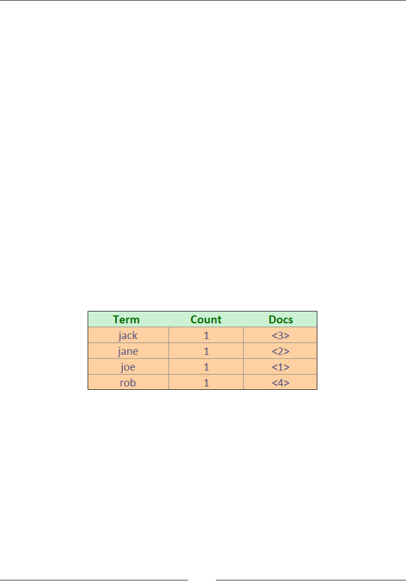
Chapter 2
[ 243 ]
Elasticsearch response will be similar to the following code:
{
"client" : {
"properties" : {
"id" : {
"type" : "string"
},
"name" : {
"type" : "string"
}
}
}
}
Getting back to Apache Lucene
Now let's take a step back and look at Apache Lucene again. If you recall what
Lucene inverted index is built of, you can tell that it contains a term, a count, and a
document pointer (if you can't recall, please refer to the Introduction to Apache Lucene
section in Chapter 1, Introduction to Elasticsearch). So, let's see how the simplied
view of the index may look for the previous data we've put to the clients index, as
shown in the following gure:
What you see in the column with the term text is quite important. If we look at
Elasticsearch and Apache Lucene internals, you can see that our prex query was
rewritten to the following Lucene query:
ConstantScore(name:jack name:jane name:joe)
We can check the portions of the rewrite using the Elasticsearch API. First of all, we
can use the Explain API by running the following command:
curl -XGET 'localhost:9200/clients/client/1/_explain?pretty' -d '{
"query" : {
"prefix" : {
"name" : {

Power User Query DSL
[ 244 ]
"prefix" : "j",
"rewrite" : "constant_score_boolean"
}
}
}
}'
The result would be as follows:
{
"_index" : "clients",
"_type" : "client",
"_id" : "1",
"matched" : true,
"explanation" : {
"value" : 1.0,
"description" : "ConstantScore(name:joe), product of:",
"details" : [ {
"value" : 1.0,
"description" : "boost"
}, {
"value" : 1.0,
"description" : "queryNorm"
} ]
}
}
We can see that Elasticsearch used a constant score query with the joe term against
the name eld. Of course, this is on Lucene level; Elasticsearch actually used a cache
to get the terms. We can see this by using the Validate Query API with a command
that looks as follows:
curl -XGET 'localhost:9200/clients/client/_validate/query?explain&pretty'
-d '{
"query" : {
"prefix" : {
"name" : {
"prefix" : "j",
"rewrite" : "constant_score_boolean"
}
}
}
}'

Chapter 2
[ 245 ]
The result returned by Elasticsearch would look like the following:
{
"valid" : true,
"_shards" : {
"total" : 1,
"successful" : 1,
"failed" : 0
},
"explanations" : [ {
"index" : "clients",
"valid" : true,
"explanation" : "filtered(name:j*)->cache(_type:client)"
} ]
}
Query rewrite properties
Of course, the rewrite property of multiterm queries can take more than a single
constant_score_boolean value. We can control how the queries are rewritten
internally. To do that, we place the rewrite parameter inside the JSON object
responsible for the actual query, for example, like the following code:
{
"query" : {
"prefix" : {
"name" : "j",
"rewrite" : "constant_score_boolean"
}
}
}
The rewrite property can take the following values:
• scoring_boolean: This rewrite method translates each generated term into
a Boolean should clause in a Boolean query. This rewrite method causes the
score to be calculated for each document. Because of that, this method may
be CPU demanding and for queries that many terms may exceed the Boolean
query limit, which is set to 1024. The default Boolean query limit can be
changed by setting the index.query.bool.max_clause_count property
in the elasticsearch.yml le. However, please remember that the more
Boolean queries are produced, the lower the query performance may be.

Power User Query DSL
[ 246 ]
• constant_score_boolean: This rewrite method is similar to the scoring_
boolean rewrite method described previously, but is less CPU demanding
because scoring is not computed, and instead of that, each term receives a
score equal to the query boost (one by default and can be set using the boost
property). Because this rewrite method also results in Boolean should clauses
being created, similar to the scoring_boolean rewrite method, this method
can also hit the maximum Boolean clauses limit.
• constant_score_filter: As Apache Lucene Javadocs state, this rewrite
method rewrites the query by creating a private lter by visiting each term
in a sequence and marking all documents for that term. Matching documents
are given a constant score equal to the query boost. This method is faster than
the scoring_boolean and constant_score_boolean methods, when the
number of matching terms or documents is not small.
• top_terms_N: A rewrite method that translates each generated term into a
Boolean should clause in a Boolean query and keeps the scores as computed
by the query. However, unlike the scoring_boolean rewrite method, it
only keeps the N number of top scoring terms to avoid hitting the maximum
Boolean clauses limit and increase the nal query performance.
• top_terms_boost_N: It is a rewrite method similar to the top_terms_N one,
but the scores are not computed, but instead the documents are given the
score equal to the value of the boost property (one by default).
When the rewrite property is set to constant_score_auto
value or not set at all, the value of constant_score_filter or
constant_score_boolean will be used depending on the query
and how it is constructed.
For example, if we would like our example query to use the top_terms_N with N
equal to 2, our query would look like the following:
{
"query" : {
"prefix" : {
"name" : {
"prefix" :"j",
"rewrite" : "top_terms_2"
}
}
}
}

Chapter 2
[ 247 ]
If you look at the results returned by Elasticsearch, you'll notice that unlike our initial
query, the documents were given a score different than the default 1.0:
{
"took" : 3,
"timed_out" : false,
"_shards" : {
"total" : 5,
"successful" : 5,
"failed" : 0
},
"hits" : {
"total" : 3,
"max_score" : 0.30685282,
"hits" : [ {
"_index" : "clients",
"_type" : "client",
"_id" : "3",
"_score" : 0.30685282,
"_source":{
"id":"3", "name":"Jack"
}
}, {
"_index" : "clients",
"_type" : "client",
"_id" : "2",
"_score" : 0.30685282,
"_source":{
"id":"2", "name":"Jane"
}
}, {
"_index" : "clients",
"_type" : "client",
"_id" : "1",
"_score" : 0.30685282,
"_source":{
"id":"1", "name":"Joe"
}
} ]
}
}
This is because the top_terms_N keeps the score for N top scoring terms.

Power User Query DSL
[ 248 ]
Before we nish the query rewrite section of this chapter, we should ask ourselves
one last question: when to use which rewrite types? The answer to this question
greatly depends on your use case, but to summarize, if you can live with lower
precision and relevancy (but higher performance), you can go for the top N rewrite
method. If you need high precision and thus more relevant queries (but lower
performance), choose the Boolean approach.
Query templates
When the application grows, it is very probable that the environment will start to be
more and more complicated. In your organization, you probably have developers
who specialize in particular layers of the application—for example, you have at least
one frontend designer and an engineer responsible for the database layer. It is very
convenient to have the development divided into several modules because you can
work on different parts of the application in parallel without the need of constant
synchronization between individuals and the whole team. Of course, the book you
are currently reading is not a book about project management, but search, so let's
stick to that topic. In general, it would be useful, at least sometimes, to be able to
extract all queries generated by the application, give them to a search engineer,
and let him/her optimize them, in terms of both performance and relevance. In
such a case, the application developers would only have to pass the query itself to
Elasticsearch and not care about the structure, query DSL, ltering, and so on.
Introducing query templates
With the release of Elasticsearch 1.1.0, we were given the possibility of dening a
template. Let's get back to our example library e-commerce store that we started
working on in the beginning of this book. Let's assume that we already know what
type of queries should be sent to Elasticsearch, but the query structure is not nal—
we will still work on the queries and improve them. By using the query templates,
we can quickly supply the basic version of the query, let application specify
the parameters, and modify the query on the Elasticsearch side until the query
parameters change.
Let's assume that one of our queries needs to return the most relevant books from
our library index. We also allow users to choose whether they are interested in
books that are available or the ones that are not available. In such a case, we will
need to provide two parameters—the phrase itself and the Boolean that species the
availability. The rst, simplied example of our query could looks as follows:
{
"query": {
"filtered": {

Chapter 2
[ 249 ]
"query": {
"match": {
"_all": "QUERY"
}
},
"filter": {
"term": {
"available": BOOLEAN
}
}
}
}
}
The QUERY and BOOLEAN are placeholders for variables that will be passed to the
query by the application. Of course, this query is too simple for our use case, but as
we already said, this is only its rst version—we will improve it in just a second.
Having our rst query, we can now create our rst template. Let's change our query
a bit so that it looks as follows:
{
"template": {
"query": {
"filtered": {
"query": {
"match": {
"_all": "{{phrase}}"
}
},
"filter": {
"term": {
"available": "{{avail}}"
}
}
}
}
},
"params": {
"phrase": "front",
"avail": true
}
}

Power User Query DSL
[ 250 ]
You can see that our placeholders were replaced by {{phrase}} and {{avail}}, and
a new section params was introduced. When encountering a section like {{phrase}},
Elasticsearch will go to the params section and look for a parameter called phrase and
use it. In general, we've moved the parameter values to the params section, and in the
query itself we use references using the {{var}} notation, where var is the name of
the parameter from the params section. In addition, the query itself is nested in the
template element. This way we can parameterize our queries.
Let's now send the preceding query to the /library/_search/template REST
endpoint (not the /library/_search as we usually do) using the GET HTTP
method. To do this, we will use the following command:
curl -XGET 'localhost:9200/library/_search/template?pretty' -d '{
"template": {
"query": {
"filtered": {
"query": {
"match": {
"_all": "{{phrase}}"
}
},
"filter": {
"term": {
"available": "{{avail}}"
}
}
}
}
},
"params": {
"phrase": "front",
"avail": true
}
}'

Chapter 2
[ 251 ]
Templates as strings
The template can also be provided as a string value. In such a case, our template will
look like the following:
{
"template": "{ \"query\": { \"filtered\": { \"query\": {
\"match\": { \"_all\": \"{{phrase}}\" } }, \"filter\": {
\"term\": { \"available\": \"{{avail}}\" } } } } }",
"params": {
"phrase": "front",
"avail": true
}
}
As you can see, this is not very readable or comfortable to write—every quotation
needs to be escaped, and new line characters are also problematic and should be
avoided. However, you'll be forced to use this notation (at least in Elasticsearch from
1.1.0 to 1.4.0 inclusive) when you want to use Mustache (a template engine we will
talk about in the next section) features.
There is a gotcha in the Elasticsearch version used during the
writing of this book. If you prepare an incorrect template, the
engine detects an error and writes info into the server logs, but
from the API point of view, the query is silently ignored and all
documents are returned, just like you would send the match_all
query. You should remember to double-check your template
queries until that is changed.
The Mustache template engine
Elasticsearch uses Mustache templates (see: http://mustache.github.io/) to
generate resulting queries from templates. As you have already seen, every variable
is surrounded by double curly brackets and this is specic to Mustache and is a
method of dereferencing variables in this template engine. The full syntax of the
Mustache template engine is beyond the scope of this book, but we would like to
briey introduce you to the most interesting parts of it: conditional expression, loops,
and default values.
The detailed information about Mustache syntax can be found
at http://mustache.github.io/mustache.5.html.

Power User Query DSL
[ 252 ]
Conditional expressions
The {{val}} expression results in inserting the value of the val variable. The
{{#val}} and {{/val}} expressions inserts the values placed between them if the
variable called val computes to true.
Let's take a look at the following example:
curl -XGET 'localhost:9200/library/_search/template?pretty' -d '{
"template": "{ {{#limit}}\"size\": 2 {{/limit}}}",
"params": {
"limit": false
}
}'
The preceding command returns all documents indexed in the library index.
However, if we change the limit parameter to true and send the query once again,
we would only get two documents. That's because the conditional would be true and
the template would be activated.
Unfortunately, it seems that versions of Elasticsearch available
during the writing of this book have problems with conditional
expressions inside templates. For example, one of the issues related
to that is available at https://github.com/elasticsearch/
elasticsearch/issues/8308. We decided to leave the section
about conditional expressions with the hope that the issues will be
resolved soon. The query templates can be a very handy functionality
when used with conditional expressions.
Loops
Loops are dened between exactly the same as conditionals—between expression
{{#val}} and {{/val}}. If the variable from the expression is an array, you can
insert current values using the {{.}} expression.
For example, if we would like the template engine to iterate through an array of
terms and create a terms query using them, we could run a query using the following
command:
curl -XGET 'localhost:9200/library/_search/template?pretty' -d '{
"template": {
"query": {
"terms": {

Chapter 2
[ 253 ]
"title": [
"{{#title}}",
"{{.}}",
"{{/title}}"
]
}
}
},
"params": {
"title": [ "front", "crime" ]
}
}'
Default values
The default value tag allows us to dene what value (or whole part of the template)
should be used if the given parameter is not dened. The syntax for dening the
default value for a variable called var is as follows:
{{var}}{{^var}}default value{{/var}}
For example, if we would like to have the default value of crime for the phrase
parameter in our template query, we could send a query using the following
command:
curl -XGET 'localhost:9200/library/_search/template?pretty' -d '{
"template": {
"query": {
"term": {
"title": "{{phrase}}{{^phrase}}crime{{/phrase}}"
}
}
},
"params": {
"phrase": "front"
}
}'

Power User Query DSL
[ 254 ]
The preceding command will result in Elasticsearch nding all documents with term
front in the title eld. However, if the phrase parameter was not dened in the
params section, the term crime will be used instead.
Storing templates in les
Regardless of the way we dened our templates previously, we were still a long
way from decoupling them from the application. We still needed to store the whole
query in the application, we were only able to parameterize the query. Fortunately,
there is a simple way to change the query denition so it can be read dynamically by
Elasticsearch from the config/scripts directory.
For example, let's create a le called bookList.mustache (in the config/scripts/
directory) with the following contents:
{
"query": {
"filtered": {
"query": {
"match": {
"_all": "{{phrase}}"
}
},
"filter": {
"term": {
"available": "{{avail}}"
}
}
}
}
}
We can now use the contents of that le in a query by specifying the template name
(the name of the template is the name of the le without the .mustache extension).
For example, if we would like to use our bookList template, we would send the
following command:
curl -XGET 'localhost:9200/library/_search/template?pretty' -d '{
"template": "bookList",
"params": {
"phrase": "front",
"avail": true
}
}'

Chapter 2
[ 255 ]
The very convenient fact is that Elasticsearch can see the changes in
the le without the need of a node restart. Of course, we still need to
have the template le stored on all Elasticsearch nodes that are capable
of handling the query execution. Starting from Elasticsearch 1.4.0, you
can also store templates in a special index called .scripts. For more
information please refer to the ofcial Elasticsearch documentation
available at http://www.elasticsearch.org/guide/en/
elasticsearch/reference/current/search-template.html.
Handling lters and why it matters
Let's have a look at the ltering functionality provided by Elasticsearch. At rst it
may seem like a redundant functionality because almost all the lters have their
query counterpart present in Elasticsearch Query DSL. But there must be something
special about those lters because they are commonly used and they are advised
when it comes to query performance. This section will discuss why ltering is
important, how lters work, and what type of ltering is exposed by Elasticsearch.
Filters and query relevance
The rst difference when comparing queries to lters is the inuence on the
document score. Let's compare queries and lters to see what to expect. We will start
with the following query:
curl -XGET "http://127.0.0.1:9200/library/_search?pretty" -d'
{
"query": {
"term": {
"title": {
"value": "front"
}
}
}
}'
The results for that query are as follows:
{
"took" : 1,
"timed_out" : false,
"_shards" : {

Power User Query DSL
[ 256 ]
"total" : 5,
"successful" : 5,
"failed" : 0
},
"hits" : {
"total" : 1,
"max_score" : 0.11506981,
"hits" : [ {
"_index" : "library",
"_type" : "book",
"_id" : "1",
"_score" : 0.11506981,
"_source":{ "title": "All Quiet on the Western
Front","otitle": "Im Westen nichts Neues","author": "Erich
Maria Remarque","year": 1929,"characters": ["Paul Bäumer",
"Albert Kropp", "Haie Westhus", "Fredrich Müller",
"Stanislaus Katczinsky", "Tjaden"],"tags":
["novel"],"copies": 1,
"available": true, "section" : 3}
} ]
}
}
There is nothing special about the preceding query. Elasticsearch will return all the
documents having the front value in the title eld. What's more, each document
matching the query will have its score calculated and the top scoring documents will
be returned as the search results. In our case, the query returned one document with
the score equal to 0.11506981. This is normal behavior when it comes to querying.
Now let's compare a query and a lter. In case of both query and lter cases, we
will add a fragment narrowing the documents to the ones having a single copy (the
copies eld equal to 1). The query that doesn't use ltering looks as follows:
curl -XGET "http://127.0.0.1:9200/library/_search?pretty" -d'
{
"query": {
"bool": {
"must": [
{
"term": {
"title": {
"value": "front"
}

Chapter 2
[ 257 ]
}
},
{
"term": {
"copies": {
"value": "1"
}
}
}
]
}
}
}'
The results returned by Elasticsearch are very similar and look as follows:
{
"took" : 1,
"timed_out" : false,
"_shards" : {
"total" : 5,
"successful" : 5,
"failed" : 0
},
"hits" : {
"total" : 1,
"max_score" : 0.98976034,
"hits" : [ {
"_index" : "library",
"_type" : "book",
"_id" : "1",
"_score" : 0.98976034,
"_source":{ "title": "All Quiet on the Western
Front","otitle": "Im Westen nichts Neues","author": "Erich
Maria Remarque","year": 1929,"characters": ["Paul Bäumer",
"Albert Kropp", "Haie Westhus", "Fredrich Müller",
"Stanislaus Katczinsky", "Tjaden"],"tags":
["novel"],"copies": 1,
"available": true, "section" : 3}
} ]
}
}

Power User Query DSL
[ 258 ]
The bool query in the preceding code is built of two term queries, which have to
be matched in the document for it to be a match. In the response we again have the
same document returned, but the score of the document is 0.98976034 now. This is
exactly what we suspected after reading the Default Apache Lucene scoring explained
section of this chapter—both terms inuenced the score calculation.
Now let's look at the second case—the query for the value front in the title eld
and a lter for the copies eld:
curl -XGET "http://127.0.0.1:9200/library/_search?pretty" -d'
{
"query": {
"term": {
"title": {
"value": "front"
}
}
},
"post_filter": {
"term": {
"copies": {
"value": "1"
}
}
}
}'
Now we have the simple term query, but in addition we are using the term lter.
The results are the same when it comes to the documents returned, but the score is
different now, as we can look in the following code:
{
"took" : 1,
"timed_out" : false,
"_shards" : {
"total" : 5,
"successful" : 5,
"failed" : 0
},
"hits" : {
"total" : 1,

Chapter 2
[ 259 ]
"max_score" : 0.11506981,
"hits" : [ {
"_index" : "library",
"_type" : "book",
"_id" : "1",
"_score" : 0.11506981,
"_source":{ "title": "All Quiet on the Western
Front","otitle": "Im Westen nichts Neues","author": "Erich
Maria Remarque","year": 1929,"characters": ["Paul Bäumer",
"Albert Kropp", "Haie Westhus", "Fredrich Müller",
"Stanislaus Katczinsky", "Tjaden"],"tags":
["novel"],"copies": 1,
"available": true, "section" : 3}
} ]
}
}
Our single document has got a score of 0.11506981 now—exactly as the base query
we started with. This leads to the main conclusion—ltering does not affect the score.
Please note that previous Elasticsearch versions were using filter for
the lters section instead of the post_filter used in the preceding
query. In the 1.x versions of Elasticsearch, both versions can be used,
but please remember that filter can be removed in the future.
In general, there is a single main difference between how queries and lters work.
The only purpose of lters is to narrow down results with certain criteria. The
queries not only narrow down the results, but also care about their score, which
is very important when it comes to relevancy, but also has a cost—the CPU cycles
required to calculate the document score. Of course, you should remember that this
is not the only difference between them, and the rest of this section will focus on how
lters work and what is the difference between different ltering methods available
in Elasticsearch.
How lters work
We already mentioned that lters do not affect the score of the documents
they match. This is very important because of two reasons. The rst reason is
performance. Applying a lter to a set of documents hold in the index is simple
and can be very efcient. The only signicant information lter holds about the
document is whether the document matches the lter or not—a simple ag.
Filters provide this information by returning a structure called DocIdSet (org.
Power User Query DSL
[ 260 ]
apache.lucene.search.DocIdSet). The purpose of this structure is to provide
the view of the index segment with the lter applied on the data. It is possible by
providing implementation of the Bits interface (org.apache.lucene.util.Bits),
which is responsible for random access to information about documents in the lter
(basically allows to check whether the document inside a segment matches the lter
or not). The Bits structure is very effective because CPU can perform ltering using
bitwise operations (and there is a dedicated CPU piece to handle such operations,
you can read more about circular shifts at http://en.wikipedia.org/wiki/
Circular_shift). We can also use the DocIdSetIterator on an ordered set of
internal document identiers, also provided by the DocIdSet.
The following gure shows how the classes using the Bits work:
Lucene (and Elasticsearch) have various implementation of DocIdSet suitable for
various cases. Each of the implementations differs when it comes to performance.
However, choosing the correct implementation is the task of Lucene and Elasticsearch
and we don't have to care about it, unless we extend the functionality of them.
Please remember that not all lters use the Bits structure. The lters
that don't do that are numeric range lters, script ones, and the whole
group of geographical lters. Instead, those lters put data into the
eld data cache and iterate over documents ltering as they operate on
a document. This means that the next lter in the chain will only get
documents allowed by the previous lters. Because of this, those lters
allow optimizations, such as putting the heaviest lters on the end of
the lters, execution chain.

Chapter 2
[ 261 ]
Bool or and/or/not lters
We talked about lters in Elasticsearch Server Second Edition, but we wanted to remind
you about one thing. You should remember that and, or, and not lters don't use
Bits, while the bool lter does. Because of that you should use the bool lter
when possible. The and, or, and not lters should be used for scripts, geographical
ltering, and numeric range lters. Also, remember that if you nest any lter that is
not using Bits inside the and, or, or not lter, Bits won't be used.
Basically, you should use the and, or, and not lters when you combine lters that
are not using Bits with other lters. And if all your lters use Bits, then use the
bool lter to combine them.
Performance considerations
In general, lters are fast. There are multiple reasons for this—rst of all, the parts
of the query handled by lters don't need to have a score calculated. As we have
already said, scoring is strongly connected to a given query and the set of indexed
documents.
There is one thing when it comes to ltering. With the release of
Elasticsearch 1.4.0, the bitsets used for nested queries execution are loaded
eagerly by default. This is done to allow faster nested queries execution,
but can lead to memory problems. To disable this behavior we can set the
index.load_fixed_bitset_filters_eagerly to false. The size of
memory used for xed bitsets can be checked by using the curl -XGET
'localhost:9200/_cluster/stats?human&pretty' command
and looking at the fixed_bit_set_memory_in_bytes property in the
response.
When using a lter, the result of the lter does not depend on the query, so the result
of the lter can be easily cached and used in the subsequent queries. What's more, the
lter cache is stored as per Lucene segment, which means that the cache doesn't have
to be rebuilt with every commit, but only on segment creation and segment merge.
Of course, as with everything, there are also downsides of using
lters. Not all lters can be cached. Think about lters that depend on
the current time, caching them wouldn't make much sense. Sometimes
caching is not worth it because of too many unique values that can be
used and poor cache hit ratio, an example of this can be lters based
on geographical location.
Power User Query DSL
[ 262 ]
Post ltering and ltered query
If someone would say that the lter will be quicker comparing to the same query, it
wouldn't be true. Filters have fewer things to care about and can be reused between
queries, but Lucene is already highly optimized and the queries are very fast, even
considering that scoring has to be performed. Of course, for a large number of results,
lter will be faster, but there is always something we didn't tell you yet. Sometimes,
when using post_filter, the query sent to Elasticsearch won't be as fast and efcient
as we would want it to be. Let's assume that we have the following query:
curl -XGET 'http://127.0.0.1:9200/library/_search?pretty' -d '{
"query": {
"terms": {
"title": [ "crime", "punishment", "complete", "front" ]
}
},
"post_filter" : {
"term": {
"available": {
"value": true,
"_cache": true
}
}
}
}'
The following gure shows what is going on during query execution:

Chapter 2
[ 263 ]
Of course, ltering matters for higher amounts of data, but for the purpose of this
example, we've used our data. In the preceding gure, our index contains four
documents. Our example terms query matches three documents: Doc1, Doc3, and
Doc4. Each of them is scored and ordered on the basis of the calculated score. After
that, our post_filter starts its work. From all of our documents in the whole
index, it passes only two of them—Doc1 and Doc4. As you can see from the three
documents passed to the lter, only two of them were returned as the search result.
So why are we bothering about calculating the score for the Doc3? In this case, we
lost some CPU cycles for scoring a document that are not valid in terms of query. For
a large number of documents returned, this can become a performance problem.
Please note that in the example we've used the term lter, which
was cached by default until Elasticsearch 1.5. That behavior changed
starting with Elasticsearch 1.5 (see https://github.com/
elasticsearch/elasticsearch/pull/7583). Because of that,
we decided to use the term lter in the example, but with forced
caching.
Let's modify our query and let's lter the documents before the Scorer calculates the
score for each document. The query that does that looks as follows:
curl -XGET 'http://127.0.0.1:9200/library/_search?pretty' -d '{
"query": {
"filtered": {
"query": {
"terms": {
"title": [ "crime", "punishment", "complete", "front" ]
}
},
"filter": {
"term": {
"available": {
"value": true,
"_cache": true
}
}
}
}
}
}'
Power User Query DSL
[ 264 ]
In the preceding example, we have used the filtered query. The results returned by
the preceding query will be exactly the same, but the execution of the query will be
a little bit different, especially when it comes to ltering. Let's look at the following
gure showing the logical execution of the query:
Now the initial work is done by the term lter. If it was already used, it will be
loaded from the cache, and the whole document set will be narrowed down to
only two documents. Finally, those documents are scored, but now the scoring
mechanism has less work to do. Of course, in the example, our query matches the
documents returned by the lter, but this is not always true.
Technically, our lter is wrapped by query, and internally Lucene library collects
results only from documents that meet the enclosed lter criteria. And, of course,
only the documents matching the lter are forwarded to the main query. Thanks to
lter, the scoring process has fewer documents to look at.
Choosing the right ltering method
If you read the preceding explanations, you may think that you should always use
the filtered query and run away from post ltering. Such statement will be true for
most use cases, but there are exceptions to this rule. The rule of thumb says that the
most expensive operations should be moved to the end of query processing. If the
lter is fast, cheap, and easily cacheable, then the situation is simple—use filtered
query. On the other hand, if the lter is slow, CPU-intensive, and hard to cache (i.e.,
because of too many distinct values), use post ltering or try to optimize the lter
by simplifying it and making it more cache friendly, for example by reducing the
resolution in case of time-based lters.

Chapter 2
[ 265 ]
Choosing the right query for the job
In our Elasticsearch Server Second Edition, we described the full query language, the
so-called Query DSL provided by Elasticsearch. A JSON structured query language
that allows us to virtually build as complex queries as we can imagine. What we
didn't talk about is when the queries can be used and when they should be used.
For a person who doesn't have much prior experience with a full text search engine,
the number of queries exposed by Elasticsearch can be overwhelming and very
confusing. Because of that, we decided to extend what we wrote in the second
edition of our rst Elasticsearch book and show you, the reader, what you can do
with Elasticsearch.
We decided to divide the following section into two distinct parts. The rst part
will try to categorize the queries and tell you what to expect from a query in that
category. The second part will show you an example usage of queries from each
group and will discuss the differences. Please take into consideration that the
following section is not a full reference for the Elasticsearch Query DSL, for such
reference please see Elasticsearch Server Second Edition from Packt Publishing or
ofcial Elasticsearch documentation available at http://www.elasticsearch.org/
guide/en/elasticsearch/reference/current/query-dsl.html.
Query categorization
Of course, categorizing queries is a hard task and we don't say that the following list
of categories is the only correct one. We would even say that if you would ask other
Elasticsearch users, they would provide their own categories or say that each query
can be assigned to more than a single category. What's funny—they would be right.
We also think that there is no single way of categorizing the queries; however, in our
opinion, each Elasticsearch query can be assigned to one (or more) of the following
categories:
• Basic queries: Category that groups queries allowing searching for a part of
the index, either in an analyzed or a non-analysed manner. The key point in
this category is that you can nest queries inside a basic query. An example of
a basic query is the term query.
• Compound queries: Category grouping queries that allow us to combine
multiple queries or lters inside them, for example a bool or dismax queries.
• Not analyzed queries: Category for queries that don't analyze the input and
send it as is to Lucene index. An example of such query is the term query.
• Full text search queries: Quite a large group of queries supporting full text
searching, analysing their content, and possibly providing Lucene query
syntax. An example of such query is the match query.

Power User Query DSL
[ 266 ]
• Pattern queries: Group of queries providing support for various wildcards
in queries. For example, a prefix query can be assigned to this particular
group.
• Similarity supporting queries: Group of queries sharing a common
feature—support for match of similar words of documents. An example of
such query is the fuzzy_like_this or the more_like_this query.
• Score altering queries: Very important group of queries, especially when
combined with full text searching. This group includes queries that allow us
to modify the score calculation during query execution. An example query
that we can assign to this group is the function_score query, which we will
talk about in detail in Chapter 3, Not Only Full Text Search.
• Position aware queries: Queries that allow us to use term position
information stored in the index. A very good example of such queries is the
span_term query.
• Structure aware queries: Group of queries that can work on structured data
such as the parent–child documents. An example query from this group is
the nested one.
Of course, we didn't talk about the lters at all, but you can use the same logic as for
queries, so let's put the lters aside for now. Before going into examples for each type
of query, let's briey describe the purpose of each of the query category.
Basic queries
Queries that are not able to group any other queries, but instead they are used for
searching the index only. Queries in this group are usually used as parts of the more
complex queries or as single queries sent against Elasticsearch. You can think about
those queries as bricks for building structures—more complex queries. For example,
when you need to match a certain phrase in a document without any additional
requirements, you should look at the basic queries—in such a case, the match query
will be a good opportunity for this requirement and it doesn't need to be added by
any other query.
Some examples of the queries from basic category are as follows:
• Match: A Query (actually multiple types of queries) used when you need a
full text search query that will analyze the provided input. Usually, it is used
when you need analysis of the provided text, but you don't need full Lucene
syntax support. Because this query doesn't go through the query parsing
process, it has a low chance of resulting in a parsing error, and because of
this it is a good candidate for handling text entered by the user.

Chapter 2
[ 267 ]
• match_all: A simple query matching all documents useful for situations
when we need all the whole index contents returned for aggregations.
• term: A simple, not analyzed query that allows us to search for an exact
word. An example use case for the term query is searching against non-
analyzed elds, like ones storing tags in our example data. The term query
is also used commonly combined with ltering, for example ltering on
category eld from our example data.
The queries from the complex category are: match, multi_match, common, fuzzy_
like_this, fuzzy_like_this_field, geoshape, ids, match_all, query_string,
simple_query_string, range, prefix, regexp, span_term, term, terms, wildcard.
Compound queries
Compound queries are the ones that we can use for grouping other queries together
and this is their only purpose. If the simple queries were bricks for building houses,
the complex queries are joints for those bricks. Because we can create a virtually
indenite level of nesting of the compound queries, we are able to produce very
complex queries, and the only thing that limits us is performance.
Some examples of the compound queries and their usage are as follows:
• bool: One of the most common compound query that is able to group
multiple queries with Boolean logical operator that allows us to control
which part of the query must match, which can and which should not match.
For example, if we would like to nd and group together queries matching
different criteria, then the bool query is a good candidate. The bool query
should also be used when we want the score of the documents to be a sum of
all the scores calculated by the partial queries.
• dis_max: A very useful query when we want the score of the document to
be mostly associated with the highest boosting partial query, not the sum of
all the partial queries (like in the bool query). The dis_max query generates
the union of the documents returned by all the subqueries and scores the
documents by the simple equation max (score of the matching clauses) +
tie_breaker * (sum of scores of all the other clauses that are not max scoring
ones). If you want the max scoring subquery to dominate the score of your
documents, then the dis_max query is the way to go.
The queries from that category are: bool, boosting, constant_score, dis_max,
filtered, function_score, has_child, has_parent, indices, nested, span_
first, span_multi, span_first, span_multi, span_near, span_not, span_or,
span_term, top_children.

Power User Query DSL
[ 268 ]
Not analyzed queries
These are queries that are not analyzed and instead the text we provide to them is
sent directly to Lucene index. This means that we either need to be aware exactly
how the analysis process is done and provide a proper term, or we need to run the
searches against the non-analyzed elds. If you plan to use Elasticsearch as NoSQL
store this is probably the group of queries you'll be using, they search for the exact
terms without analysing them, i.e., with language analyzers.
The following examples should help you understand the purpose of not
analyzed queries:
• term: When talking about the not analyzed queries, the term query will
be the one most commonly used. It provides us with the ability to match
documents having a certain value in a eld. For example, if we would like
to match documents with a certain tag (tags eld in our example data), we
would use the term query.
• Prefix: Another type of query that is not analyzed. The prex query is
commonly used for autocomplete functionality, where the user provides a
text and we need to nd all the documents having terms that start with the
given text. It is good to remember that even though the prex query is not
analyzed, it is rewritten by Elasticsearch so that its execution is fast.
The queries from that category are: common, ids, prefix, span_term, term, terms,
wildcard.
Full text search queries
A group that can be used when you are building your Google-like search interface.
Those queries analyze the provided input using the information from the mappings,
support Lucene query syntax, support scoring capabilities, and so on. In general, if
some part of the query you are sending comes from a user entering some text, you'll
want to use one of the full text search queries such as the query_string, match or
simple_query_string queries.
A Simple example of the full text search queries use case can be as follows:
• simple_query_string: A query built on top of Lucene SimpleQueryParser
(http://lucene.apache.org/core/4_9_0/queryparser/org/apache/
lucene/queryparser/simple/SimpleQueryParser.html) that was
designed to parse human readable queries. In general, if you want your
queries not to fail when a query parsing error occurs and instead gure out
what the user wanted to achieve, this is a good query to consider.
The queries from that category are: match, multi_match, query_string, simple_
query_string.

Chapter 2
[ 269 ]
Pattern queries
Elasticsearch provides us with a few queries that can handle wildcards directly or
indirectly, for example the wildcard query and the prefix query. In addition to
that, we are allowed to use the regexp query that can nd documents that have
terms matching given patterns.
We've already discussed an example using the prefix query, so let's focus a bit
on the regexp query. If you want a query that will nd documents having terms
matching a certain pattern, then the regexp query is probably the only solution for
you. For example, if you store logs in your Elasticsearch indices and you would
like to nd all the logs that have terms starting with the err prex, then having any
number of characters and ending with memory, the regexp query will be the one to
look for. However, remember that all the wildcard queries that have expressions
matching large number of terms will be expensive when it comes to performance.
The queries from that category are: prefix, regexp, wildcard.
Similarity supporting queries
We like to think that the similarity supporting queries is a family of queries that allow
us to search for similar terms or documents to the one we passed to the query. For
example, if we would like to nd documents that have terms similar to crimea term,
we could run a fuzzy query. Another use case for this group of queries is providing us
with "did you mean" like functionality. If we would like to nd documents that have
titles similar to the input we've provided, we would use the more_like_this query. In
general, you would use a query from this group whenever you need to nd documents
having terms or elds similar to the provided input.
The queries from that category are: fuzzy_like_this, fuzzy_like_this_field,
fuzzy, more_like_this, more_like_this_field.
Score altering queries
A group of queries used for improving search precision and relevance. They allow
us to modify the score of the returned documents by providing not only a custom
boost factor, but also some additional logic. A very good example of a query from
this group is the function_score query that provides us with a possibility of using
functions, which result in document score modication based on mathematical
equations. For example, if you would like the documents that are closer to a given
geographical point to be scored higher, then using the function_score query
provides you with such a possibility.
The queries from that category are: boosting, constant_score, function_score,
indices.

Power User Query DSL
[ 270 ]
Position aware queries
These are a family of queries that allow us to match not only certain terms but also
the information about the terms' positions. The most signicant queries from this
group are all the span queries in Elasticsearch. We can also say that the match_
phrase query can be assigned to this group as it also looks at the position of the
indexed terms, at least to some extent. If you want to nd groups of words that are
a certain distance in the index from other words, like "nd me the documents that
have mastering and Elasticsearch terms near each other and are followed by
second and edition terms no further than three positions away," then span queries
is the way to go. However, you should remember that span queries will be removed
in future versions of Lucene library and thus from Elasticsearch as well. This is
because those queries are resource-intensive and require vast amount of CPU to be
properly handled.
The queries from that category are: match_phrase, span_first, span_multi, span_
near, span_not, span_or, span_term.
Structure aware queries
The last group of queries is the structure aware queries. The queries that can be
assigned to this group are as follows:
• nested
• has_child
• has_parent
• top_children
Basically, all the queries that allow us to search inside structured documents and
don't require us to atten the data can be classied as the structure aware queries.
If you are looking for a query that will allow you to search inside the children
document, nested documents, or for children having certain parents, then you need
to use one of the queries that are mentioned in the preceding terms. If you want to
handle relationships in the data, this is the group of queries you should look for;
however, remember that although Elasticsearch can handle relations, it is still not a
relational database.
The use cases
As we already know which groups of queries can be responsible for which tasks and
what can we achieve using queries from each group, let's have a look at example use
cases for each of the groups so that we can have a better view of what the queries are
useful for. Please note that this is not a full and comprehensive guide to all the queries
available in Elasticsearch, but instead a simple example of what can be achieved.

Chapter 2
[ 271 ]
Example data
For the purpose of the examples in this section, we've indexed two additional
documents to our library index.
First, we need to alter the index structure a bit so that it contains nested documents (we
will need them for some queries). To do that, we will run the following command:
curl -XPUT 'http://localhost:9200/library/_mapping/book' -d '{
"book" : {
"properties" : {
"review" : {
"type" : "nested",
"properties": {
"nickname" : { "type" : "string" },
"text" : { "type" : "string" },
"stars" : { "type" : "integer" }
}
}
}
}
}'
The commands used for indexing two additional documents are as follows:
curl -XPOST 'localhost:9200/library/book/5' -d '{
"title" : "The Sorrows of Young Werther",
"author" : "Johann Wolfgang von Goethe",
"available" : true,
"characters" : ["Werther",
"Lotte","Albert",
" Fräulein von B"],
"copies" : 1,
"otitle" : "Die Leiden des jungen Werthers",
"section" : 4,
"tags" : ["novel", "classics"],
"year" : 1774,
"review" : [{"nickname" : "Anna","text" : "Could be good, but not
my style","stars" : 3}]
}'

Power User Query DSL
[ 272 ]
curl -XPOST 'localhost:9200/library/book/6' -d '{
"title" : "The Peasants",
"author" : "Władysław Reymont",
"available" : true,
"characters" : ["Maciej Boryna","Jankiel","Jagna Paczesiówna",
"Antek Boryna"],
"copies" : 4,
"otitle" : "Chłopi",
"section" : 4,
"tags" : ["novel", "polish", "classics"],
"year" : 1904,
"review" : [{"nickname" : "anonymous","text" : "awsome
book","stars" : 5},{"nickname" : "Jane","text" : "Great book, but
too long","stars" : 4},{"nickname" : "Rick","text" : "Why bother,
when you can find it on the internet","stars" : 3}]
}'
Basic queries use cases
Let's look at simple use cases for the basic queries group.
Searching for values in range
One of the simplest queries that can be run is a query matching documents in a
given range of values. Usually, such queries are a part of a larger query or a lter.
For example, a query that would return books with the number of copies from 1 to 3
inclusive would look as follows:
curl -XGET 'localhost:9200/library/_search?pretty' -d '{
"query" : {
"range" : {
"copies" : {
"gte" : 1,
"lte" : 3
}
}
}
}'

Chapter 2
[ 273 ]
Simplied query for multiple terms
Imagine a situation where your users can show a number of tags the books returned
by what the query should contain. The thing is that we require only 75 percent of
the provided tags to be matched if the number of tags provided by the user is higher
than three, and all the provided tags to be matched if the number of tags is three or
less. We could run a bool query to allow that, but Elasticsearch provides us with the
terms query that we can use to achieve the same requirement. The command that
sends such query looks as follows:
curl -XGET 'localhost:9200/library/_search?pretty' -d '{
"query" : {
"terms" : {
"tags" : [ "novel", "polish", "classics", "criminal", "new" ],
"minimum_should_match" : "3<75%"
}
}
}'
Compound queries use cases
Let's now see how we can use compound queries to group other queries together.
Boosting some of the matched documents
One of the simplest examples is using the bool query to boost some documents by
including not mandatory query part that is used for boosting. For example, if we
would like to nd all the books that have at least a single copy and boost the ones
that are published after 1950, we could use the following query:
curl -XGET 'localhost:9200/library/_search?pretty' -d '{
"query" : {
"bool" : {
"must" : [
{
"range" : {
"copies" : {
"gte" : 1
}
}
}

Power User Query DSL
[ 274 ]
],
"should" : [
{
"range" : {
"year" : {
"gt" : 1950
}
}
}
]
}
}
}'
Ignoring lower scoring partial queries
The dis_max query, as we have already covered, allows us to control how inuential
the lower scoring partial queries are. For example, if we only want to assign the score
of the highest scoring partial query for the documents matching crime punishment
in the title eld or raskolnikov in the characters eld, we would run the
following query:
curl -XGET 'localhost:9200/library/_search?pretty' -d '{
"fields" : [ "_id", "_score" ],
"query" : {
"dis_max" : {
"tie_breaker" : 0.0,
"queries" : [
{
"match" : {
"title" : "crime punishment"
}
},
{
"match" : {
"characters" : "raskolnikov"
}
}

Chapter 2
[ 275 ]
]
}
}
}'
The result for the preceding query should look as follows:
{
"took" : 3,
"timed_out" : false,
"_shards" : {
"total" : 5,
"successful" : 5,
"failed" : 0
},
"hits" : {
"total" : 1,
"max_score" : 0.2169777,
"hits" : [ {
"_index" : "library",
"_type" : "book",
"_id" : "4",
"_score" : 0.2169777,
"fields" : {
"_id" : "4"
}
} ]
}
}
Now let's see the score of the partial queries alone. To do that we will run the partial
queries using the following commands:
curl -XGET 'localhost:9200/library/_search?pretty' -d '{
"fields" : [ "_id", "_score" ],
"query" : {
"match" : {
"title" : "crime punishment"
}
}
}'

Power User Query DSL
[ 276 ]
The response for the preceding query is as follows:
{
"took" : 2,
"timed_out" : false,
"_shards" : {
"total" : 5,
"successful" : 5,
"failed" : 0
},
"hits" : {
"total" : 1,
"max_score" : 0.2169777,
"hits" : [ {
"_index" : "library",
"_type" : "book",
"_id" : "4",
"_score" : 0.2169777,
"fields" : {
"_id" : "4"
}
} ]
}
}
And the next command is as follows:
curl -XGET 'localhost:9200/library/_search?pretty' -d '{
"fields" : [ "_id", "_score" ],
"query" : {
"match" : {
"characters" : "raskolnikov"
}
}
}'
And the response is as follows:
{
"took" : 1,
"timed_out" : false,
"_shards" : {
"total" : 5,
"successful" : 5,

Chapter 2
[ 277 ]
"failed" : 0
},
"hits" : {
"total" : 1,
"max_score" : 0.15342641,
"hits" : [ {
"_index" : "library",
"_type" : "book",
"_id" : "4",
"_score" : 0.15342641,
"fields" : {
"_id" : "4"
}
} ]
}
}
As you can see, the score of the document returned by our dis_max query is equal to
the score of the highest scoring partial query (the rst partial query). That is because
we've set the tie_breaker property to 0.0.
Not analyzed queries use cases
Let's look at two example use cases for queries that are not processed by any of the
dened analyzers.
Limiting results to given tags
One of the simplest examples of the not analyzed query is the term query provided
by Elasticsearch. You'll probably very rarely use the term query alone; however, it
may be commonly used in compound queries. For example, let's assume that we
would like to search for all the books with the novel value in the tags eld. To do
that, we would run the following command:
curl -XGET 'localhost:9200/library/_search?pretty' -d '{
"query" : {
"term" : {
"tags" : "novel"
}
}
}'

Power User Query DSL
[ 278 ]
Efcient query time stopwords handling
Elasticsearch provides the common terms query, which allows us to handle query
time stopwords in an efcient way. It divides the query terms into two groups—
more important terms and less important terms. The more important terms are
the ones that have a lower frequency; the less important terms are the opposite.
Elasticsearch rst executes the query with important terms and calculates the score
for those documents. Then, a second query with the less important terms is executed,
but the score is not calculated and thus the query is faster.
For example, the following two queries should be similar in terms of results, but not
in terms of score computation. Please also note that to see the differences in scoring
we would have to use a larger data sample and not use index time stopwords:
curl -XGET 'localhost:9200/library/_search?pretty' -d '{
"query" : {
"common" : {
"title" : {
"query" : "the western front",
"cutoff_frequency" : 0.1,
"low_freq_operator": "and"
}
}
}
}'
And the second query would be as follows:
curl -XGET 'localhost:9200/library/_search?pretty' -d '{
"query" : {
"bool" : {
"must" : [
{
"term" : { "title" : "western" }
},
{
"term" : { "title" : "front" }
}
],
"should" : [
{
"term" : { "title" : "the" }
}
]
}
}
}'

Chapter 2
[ 279 ]
Full text search queries use cases
Full text search is a broad topic and so are the use cases for the full text queries.
However, let's look at two simple examples of queries from that group.
Using Lucene query syntax in queries
Sometimes, it is good to be able to use Lucene query syntax as it is. We talked
about this syntax in the Lucene query language section in Chapter 1, Introduction to
Elasticsearch. For example, if we would like to nd books having sorrows and young
terms in their title, von goethe phrase in the author eld and not having more than
ve copies we could run the following query:
curl -XGET 'localhost:9200/library/_search?pretty' -d '{
"query" : {
"query_string" : {
"query" : "+title:sorrows +title:young +author:\"von goethe\" -
copies:{5 TO *]"
}
}
}'
As you can see, we've used the Lucene query syntax to pass all the matching
requirements and we've let query parser construct the appropriate query.
Handling user queries without errors
Sometimes, queries coming from users can contain errors. For example, let's look at
the following query:
curl -XGET 'localhost:9200/library/_search?pretty' -d '{
"query" : {
"query_string" : {
"query" : "+sorrows +young \"",
"default_field" : "title"
}
}
}'
The response would contain the following:
"error" : "SearchPhaseExecutionException[Failed to execute phase
[query]

Power User Query DSL
[ 280 ]
This means that the query was not properly constructed and parse error happened.
That's why the simple_query_string query was introduced. It uses a query parser
that tries to handle user mistakes and tries to guess how the query should look. Our
query using that parser would look as follows:
curl -XGET 'localhost:9200/library/_search?pretty' -d '{
"query" : {
"simple_query_string" : {
"query" : "+sorrows +young \"",
"fields" : [ "title" ]
}
}
}'
If you run the preceding query, you would see that the proper document has been
returned by Elasticsearch, even though the query is not properly constructed.
Pattern queries use cases
There are multiple use cases for the wildcard queries; however, we wanted to show
you the following two.
Autocomplete using prexes
A very common use case provides autocomplete functionality on the indexed
data. As we know, the prex query is not analyzed and works on the basis of
terms indexed in the eld. So the actual functionality depends on what tokens are
produced during indexing. For example, let's assume that we would like to provide
autocomplete functionality on any token in the title eld and the user provided
wes prex. A query that would match such a requirement looks as follows:
curl -XGET 'localhost:9200/library/_search?pretty' -d '{
"query" : {
"prefix" : {
"title" : "wes"
}
}
}'

Chapter 2
[ 281 ]
Pattern matching
If we need to match a certain pattern and our analysis chain is not producing tokens
that allow us to do so, we can turn into the regexp query. One should remember,
though, that this kind of query can be expensive during execution and thus should
be avoided. Of course, this is not always possible. One thing to remember is that the
performance of the regexp query depends on the chosen regular expression. If you
choose a regular expression that will be rewritten into a high number of terms, then
performance will suffer.
Let's now see the example usage of the regexp query. Let's assume that we would
like to nd documents that have a term starting with wat, then followed by two
characters and ending with the n character, and those terms should be in the
characters eld. To match this requirement, we could use a regexp query like the
one used in the following command:
curl -XGET 'localhost:9200/library/_search?pretty' -d '{
"query" : {
"regexp" : {
"characters" : "wat..n"
}
}
}'
Similarity supporting queries use cases
Let's look at a couple of simple use cases about how we can nd similar documents
and terms.
Finding terms similar to a given one
A very simple example is using the fuzzy query to nd documents having a term
similar to a given one. For example, if we would like to nd all the documents
having a value similar to crimea, we could run the following query:
curl -XGET 'localhost:9200/library/_search?pretty' -d '{
"query" : {
"fuzzy" : {
"title" : {
"value" : "crimea",
"fuzziness" : 3,
"max_expansions" : 50
}

Power User Query DSL
[ 282 ]
}
}
}'
Finding documents with similar eld values
Another example of similarity queries is a use case when we want to nd all the
documents having eld values similar to what we provided in a query. For example,
if we would like to nd books having a title similar to the western front battles
name, we could run the following query:
curl -XGET 'localhost:9200/library/_search?pretty' -d '{
"query" : {
"fuzzy_like_this_field" : {
"title" : {
"like_text" : "western front battles",
"max_query_terms" : 5
}
}
}
}'
The result of the preceding query would be as follows:
{
"took" : 10,
"timed_out" : false,
"_shards" : {
"total" : 5,
"successful" : 5,
"failed" : 0
},
"hits" : {
"total" : 2,
"max_score" : 1.0162667,
"hits" : [ {
"_index" : "library",
"_type" : "book",
"_id" : "1",
"_score" : 1.0162667,

Chapter 2
[ 283 ]
"_source":{ "title": "All Quiet on the Western
Front","otitle": "Im Westen nichts Neues","author": "Erich
Maria Remarque","year": 1929,"characters": ["Paul B├Ąumer",
"Albert Kropp", "Haie Westhus", "Fredrich M├╝ller",
"Stanislaus Katczinsky", "Tjaden"],"tags":
["novel"],"copies": 1,
"available": true, "section" : 3}
}, {
"_index" : "library",
"_type" : "book",
"_id" : "5",
"_score" : 0.4375,
"_source":{"title" : "The Sorrows of Young Werther","author"
: "Johann Wolfgang von Goethe","available" :
true,"characters" : ["Werther","Lotte","Albert","Fraulein
von B"],"copies" : 1, "otitle" : "Die Leiden des jungen
Werthers","section" : 4,"tags" : ["novel",
"classics"],"year" : 1774,"review" : [{"nickname" :
"Anna","text" : "Could be good, but not my style","stars" :
3}]}
} ]
}
}
As you can see, sometimes the results are not as obvious as we would expect (look
at the second book title). This is because of what Elasticsearch thinks is similar to
each other. In the case of the preceding query, Elasticsearch will take all the terms,
run a fuzzy search on them, and choose a number of best differentiating terms for
documents matching.
Score altering queries use cases
When it comes to relevancy, Elasticsearch provides us with a few queries that we
can use to alter the score as per our need. Of course, in addition to this, most queries
allow us to provide boost, which gives us even more control. Let's now look at two
example use cases of score altering queries.
Favoring newer books
Let's assume that we would like to favor books that are newer, so that a book from
the year 1986 is higher in the results list than a book from 1870. The query that would
match that requirement looks as follows:
curl -XGET 'localhost:9200/library/_search?pretty' -d '{
"query" : {
"function_score" : {

Power User Query DSL
[ 284 ]
"query" : {
"match_all" : {}
},
"score_mode" : "multiply",
"functions" : [
{
"gauss" : {
"year" : {
"origin" : 2014,
"scale" : 2014,
"offset" : 0,
"decay": 0.5
}
}
}
]
}
}
}'
We will discuss the function_score query in Chapter 3, Not Only Full Text Search.
For now, if you look at the results returned by the preceding query, you can see that
the newer the book, the higher in the results it will be.
Decreasing importance of books with certain value
Sometimes, it is good to be able to decrease the importance of certain documents,
while still showing them in the results list. For example, we may want to show all
books, but put the ones that are not available on the bottom of the results list by
lowering their score. We don't want sorting on availability because sometimes use
may know what he or she is looking for and the score of a full text search query
should be also important. However, if our use case is that we want the books that are
not available on the bottom of the results list, we could use the following command
to get them:
curl -XGET 'localhost:9200/library/_search?pretty' -d '{
"query" : {
"boosting" : {
"positive" : {

Chapter 2
[ 285 ]
"match_all" : {}
},
"negative" : {
"term" : {
"available" : false
}
},
"negative_boost" : 0.2
}
}
}'
Pattern queries use cases
Not very commonly used because of how resource hungry they are, pattern aware
queries allow us to match documents having phrases and terms in the right order.
Let's look at some examples.
Matching phrases
The simplest position aware query possible and the most performing one from
the queries assigned in this group. For example, a query that would only match
document leiden des jungen phrase in the otitle eld would look as follows:
curl -XGET 'localhost:9200/library/_search?pretty' -d '{
"query" : {
"match_phrase" : {
"otitle" : "leiden des jungen"
}
}
}'
Spans, spans everywhere
Of course, the phrase query is very simple when it comes to position handling. What
if we would like to run a query to nd documents that have des jungen phrase not
more than two positions after the die term and just before the werthers term? This
can be done with span queries, and the following command shows how such a query
could look:
curl -XGET 'localhost:9200/library/_search?pretty' -d '{
"query" : {
"span_near" : {

Power User Query DSL
[ 286 ]
"clauses" : [
{
"span_near" : {
"clauses" : [
{
"span_term" : {
"otitle" : "die"
}
},
{
"span_near" : {
"clauses" : [
{
"span_term" : {
"otitle" : "des"
}
},
{
"span_term" : {
"otitle" : "jungen"
}
}
],
"slop" : 0,
"in_order" : true
}
}
],
"slop" : 2,
"in_order" : false
}
},
{
"span_term" : {
"otitle" : "werthers"
}
}
],
"slop" : 0,
"in_order" : true

Chapter 2
[ 287 ]
}
}
}'
Please note that span queries are not analyzed. We can see that by looking at the
response of the Explain API. To see that response, we should run the same request
body (our query) to the /library/book/5/_explain REST endpoint. The interesting
part of the output looks as follows:
"description" : "weight(spanNear([spanNear([otitle:die,
spanNear([otitle:des, otitle:jungen], 0, true)], 2, false),
otitle:werthers], 0, true) in 1) [PerFieldSimilarity], result
of:",
Structure aware queries use cases
When it comes to the nested documents or the parent–child relationship, structure
aware queries are the ones that will be needed sooner or later. Let's look at the
following two examples of where the structure query can be used.
Returning parent documents having a certain nested
document
The rst example will be a very simple one. Let's return all the books that have at
least a single review that was given four stars or more. The query that does that
looks as follows:
curl -XGET 'localhost:9200/library/_search?pretty' -d '{
"query" : {
"nested" : {
"path" : "review",
"query" : {
"range" : {
"stars" : {
"gte" : 4
}
}
}
}
}
}'

Power User Query DSL
[ 288 ]
Affecting parent document score with the score of nested
documents
Let's assume that we want to nd all the available books that have reviews and let's
sort them on the maximum number of stars given in the review. The query that
would ll such a requirement looks as follows:
curl -XGET 'localhost:9200/library/_search?pretty' -d '{
"query" : {
"nested" : {
"path" : "review",
"score_mode" : "max",
"query" : {
"function_score" : {
"query" : { "match_all" : {} },
"score_mode" : "max",
"boost_mode" : "replace",
"field_value_factor" : {
"field" : "stars",
"factor" : 1,
"modifier" : "none"
}
}
}
}
}
}'

Chapter 2
[ 289 ]
Summary
In this chapter, we've looked at how the default Apache Lucene scoring works and
we've discussed the query rewrite process—how it is done and why is it needed.
We've discussed how query templates work and how they can simplify your
queries. We've also looked at different query ltering methods, how they differ
in comparison to each other, and when they can be used. Finally, we've assigned
queries to different groups, we've learned when which query group can be used, and
we've seen some example queries for each of the groups.
In the next chapter, we'll step away from full text search and focus on other search
functionalities. We will start by extending our knowledge about the rescore
functionality and the ability to recalculate the score for top documents in the results.
After that we will look at how to load signicant terms and add documents grouping
using aggregations. We will also compare parent–child relationships to the nested
documents, we will use function queries and, nally, we will learn how to efciently
page documents.

Not Only Full Text Search
In the previous chapter, we extensively talked about querying in Elasticsearch.
We started by looking at how default Apache Lucene scoring works, through how
ltering works, and we've nished with looking at which query to use in a particular
situation. In this chapter, we will continue with discussions regarding some of the
Elasticsearch functionalities connected to both querying and data analysis. By the
end of this chapter, we will have covered the following areas:
• What query rescoring is and how you can use it to optimize your queries
and recalculate the score for some documents
• Controlling multimatch queries
• Analyzing your data to get signicant terms from it
• Grouping your documents in buckets using Elasticsearch
• Differences in relationship handling when using object, nested documents,
and parent–child functionality
• Extended information regarding Elasticsearch scripting such as
Groovy usage and Lucene expressions
Query rescoring
One of the great features provided by Elasticsearch is the ability to change the
ordering of documents after they were returned by a query. Actually, Elasticsearch
does a simple trick—it recalculates the score of top matching documents, so only part
of the document in the response is reordered. The reasons why we want to do that
can vary. One of the reasons may be performance—for example, calculating target
ordering is very costly because scripts are used and we would like to do this on the
subset of documents returned by the original query. You can imagine that rescore
gives us many great opportunities for business use cases. Now, let's look at this
functionality and how we can benet from using it.

Not Only Full Text Search
[ 292 ]
What is query rescoring?
Rescore in Elasticsearch is the process of recalculating the score for a dened number
of documents returned by the query. This means that Elasticsearch rst takes N
documents for a given query (or the post_filter phase) and calculates their score
using a provided rescore denition. For example, if we would take a term query
and ask for all the documents that are available, we can use rescore to recalculate the
score for 100 documents only, not for all documents returned by the query. Please
note that the rescore phase will not be executed when using search_type of scan or
count. This means that rescore won't be taken into consideration in such cases.
An example query
Let's start with a simple query that looks as follows:
{
"fields" : ["title", "available"],
"query" : {
"match_all" : {}
}
}
It returns all the documents from the index the query is run against. Every document
returned by the query will have the score equal to 1.0 because of the match_all
query. This is enough to show how rescore affects our result set.
Structure of the rescore query
Let's now modify our query so that it uses the rescore functionality. Basically, let's
assume that we want the score of the document to be equal to the value of the year
eld. The query that does that would look as follows:
{
"fields": ["title", "available"],
"query": {
"match_all": {}
},
"rescore": {
"query": {
"rescore_query": {
"function_score": {
"query": {
"match_all": {}
},

Chapter 3
[ 293 ]
"script_score": {
"script": "doc['year'].value"
}
}
}
}
}
}
Please note that you need to specify the lang property with the groovy
value in the preceding query if you are using Elasticsearch 1.4 or older.
What's more, the preceding example uses dynamic scripting which was
enabled in Elasticsearch until versions 1.3.8 and 1.4.3 for groovy and till
1.2 for MVEL. If you would like to use dynamic scripting with groovy
you should add script.groovy.sandbox.enabled property and
set it to true in your elasticsearch.yml le. However, please
remember that this is a security risk.
Let's now look at the preceding query in more detail. The rst thing you may have
noticed is the rescore object. The mentioned object holds the query that will affect
the scoring of the documents returned by the query. In our case, the logic is very
simple—just assign the value of the year eld as the score of the document. Please
also note, that when using curl you need to escape the script value, so the
doc['year'].value would look like doc[\"year\"].value
In the preceding example, in the rescore object, you can see a
query object. When this book was written, a query object was the
only option, but in future versions, we may expect other ways to
affect the resulting score.
If we save this query in the query.json le and send it using the following command:
curl localhost:9200/library/book/_search?pretty -d @query.json
The document that Elasticsearch should return should be as follows (please note that
we've omitted the structure of the response so that it is as simple as it can be):
{
"took" : 1,
"timed_out" : false,
"_shards" : {
"total" : 5,
"successful" : 5,
"failed" : 0
},

Not Only Full Text Search
[ 294 ]
"hits" : {
"total" : 6,
"max_score" : 1962.0,
"hits" : [ {
"_index" : "library",
"_type" : "book",
"_id" : "2",
"_score" : 1962.0,
"fields" : {
"title" : [ "Catch-22" ],
"available" : [ false ]
}
}, {
"_index" : "library",
"_type" : "book",
"_id" : "3",
"_score" : 1937.0,
"fields" : {
"title" : [ "The Complete Sherlock Holmes" ],
"available" : [ false ]
}
}, {
"_index" : "library",
"_type" : "book",
"_id" : "1",
"_score" : 1930.0,
"fields" : {
"title" : [ "All Quiet on the Western Front" ],
"available" : [ true ]
}
}, {
"_index" : "library",
"_type" : "book",
"_id" : "6",
"_score" : 1905.0,
"fields" : {
"title" : [ "The Peasants" ],
"available" : [ true ]
}
}, {
"_index" : "library",
"_type" : "book",
"_id" : "4",
"_score" : 1887.0,
"fields" : {
"title" : [ "Crime and Punishment" ],
"available" : [ true ]
}

Chapter 3
[ 295 ]
}, {
"_index" : "library",
"_type" : "book",
"_id" : "5",
"_score" : 1775.0,
"fields" : {
"title" : [ "The Sorrows of Young Werther" ],
"available" : [ true ]
}
} ]
}
}
As we can see, Elasticsearch found all the documents from the original query. Now
look at the score of the documents. Elasticsearch took the rst N documents and
applied the second query to them. In the result, the score of those documents is the
sum of the score from the rst and second queries.
As you know, scripts execution can be demanding when it comes to performance.
That's why we've used it in the rescore phase of the query. If our initial match_all
query would return thousands of results, calculating script-based scoring for all
those can affect query performance. Rescore gave us the possibility to only calculate
such scoring on the top N documents and thus reduce the performance impact.
In our example, we have only seen a single rescore denition. Since
Elasticsearch 1.1.0, there is a possibility of dening multiple rescore
queries for a single result set. Thanks to this, you can build multilevel
queries when the top N documents are reordered and this result is an
input for the next reordering.
Now let's see how to tune rescore functionality behavior and what parameters
are available.
Rescore parameters
In the query under the rescore object, we are allowed to use the following
parameters:
• window_size (defaults to the sum of the from and size parameters): The
number of documents used for rescoring on every shard

Not Only Full Text Search
[ 296 ]
• query_weight (defaults to 1): The resulting score of the original query will
be multiplied by this value before adding the score generated by rescore
• rescore_query_weight (defaults to 1): The resulting score of the rescore
will be multiplied by this value before adding the score generated by the
original query
To sum up, the target score for the document is equal to:
original_query_score * query_weight + rescore_query_score *
rescore_query_weight
Choosing the scoring mode
By default, the score from the original query part and the score from the rescored
part are added together. However, we can control that by specifying the score_mode
parameter. The available values for it are as follows:
• total: Score values are added together (the default behavior)
• multiply: Values are multiplied by each other
• avg: The result score is an average of enclosed scores
• max: The result is equals of greater score value
• min: The result is equals of lower score value
To sum up
Sometimes, we want to show results, where the ordering of the rst documents on
the page is affected by some additional rules. Unfortunately, this cannot be achieved
by the rescore functionality. The rst idea points to the window_size parameter, but
this parameter, in fact, is not connected with the rst documents on the result list but
with the number of results returned on every shard. In addition, the window_size
value cannot be less than page size (Elasticsearch will set the window_size value to
the value of the size property, when window_size is lower than size). Also, one
very important thing, rescoring cannot be combined with sorting because sorting
is done before the changes to the documents, score are done by rescoring, and thus
sorting won't take the newly calculated score into consideration.

Chapter 3
[ 297 ]
Controlling multimatching
Until Elasticsearch 1.1, we had limited control over the multi_match query. Of
course, we had the possibility to specify the elds we want our query to be run
against; we could use disjunction max queries (by setting the use_dis_max property
to true). Finally, we could inform Elasticsearch about the importance of each eld by
using boosting. Our example query run against multiple elds could look as follows:
curl -XGET 'localhost:9200/library/_search?pretty' -d '{
"query" : {
"multi_match" : {
"query" : "complete conan doyle",
"fields" : [ "title^20", "author^10", "characters" ]
}
}
}'
A simple query that will match documents having given tokens in any of the
mentioned elds. In addition to that required query, the title eld is more
important than the author eld, and nally the characters eld.
Of course, we could also use the disjunction max query:
curl -XGET 'localhost:9200/library/_search?pretty' -d '{
"query" : {
"multi_match" : {
"query" : "complete conan doyle",
"fields" : [ "title^20", "author^10", "characters" ],
"use_dis_max" : true
}
}
}'
But apart from the score calculation for the resulting documents, using disjunction
max didn't change much.

Not Only Full Text Search
[ 298 ]
Multimatch types
With the release of Elasticsearch 1.1, the use_dis_max property was deprecated and
Elasticsearch developers introduced a new property—the type. This property allows
control over how the multi_match query is internally executed. Let's now look at the
possibilities of controlling how Elasticsearch runs queries against multiple elds.
Please note that the tie_breaker property was not deprecated and
we can still use it without worrying about future compatibility.
Best elds matching
To use the best elds type matching, one should set the type property of the multi_
match query to the best_fields query. This type of multimatching will generate
a match query for each eld specied in the fields property and it is best used for
searching for multiple words in the same, best matching eld. For example, let's look
at the following query:
curl -XGET 'localhost:9200/library/_search?pretty' -d '{
"query" : {
"multi_match" : {
"query" : "complete conan doyle",
"fields" : [ "title", "author", "characters" ],
"type" : "best_fields",
"tie_breaker" : 0.8
}
}
}'
The preceding query would be translated into a query similar to the following one:
curl -XGET 'localhost:9200/library/_search?pretty' -d '{
"query" : {
"dis_max" : {
"queries" : [
{
"match" : {
"title" : "complete conan doyle"
}

Chapter 3
[ 299 ]
},
{
"match" : {
"author" : "complete conan doyle"
}
},
{
"match" : {
"characters" : "complete conan doyle"
}
}
],
"tie_breaker" : 0.8
}
}
}'
If you would look at the results for both of the preceding queries, you would notice
the following:
{
"took" : 1,
"timed_out" : false,
"_shards" : {
"total" : 5,
"successful" : 5,
"failed" : 0
},
"hits" : {
"total" : 1,
"max_score" : 0.033352755,
"hits" : [ {
"_index" : "library",
"_type" : "book",
"_id" : "3",
"_score" : 0.033352755,
"_source":{ "title": "The Complete Sherlock
Holmes","author": "Arthur Conan Doyle","year":
1936,"characters": ["Sherlock Holmes","Dr. Watson", "G.
Lestrade"],"tags": [],"copies": 0, "available" : false,
"section" : 12}

Not Only Full Text Search
[ 300 ]
} ]
}
}
Both queries resulted in exactly the same results and the same scores calculated for
the document. One thing to remember is how the score is calculated. If the tie_
breaker value is present, the score for each document is the sum of the score for the
best matching eld and the score of the other matching elds multiplied by the tie_
breaker value. If the tie_breaker value is not present, the document is assigned
the score equal to the score of the best matching eld.
There is one more question when it comes to the best_fields matching: what
happens when we would like to use the AND operator or the minimum_should_match
property? The answer is simple: the best_fields matching is translated into many
match queries and both the operator property and the minimum_should_match
property are applied to each of the generated match queries. Because of that, a query
as follows wouldn't return any documents in our case:
curl -XGET 'localhost:9200/library/_search?pretty' -d '{
"query" : {
"multi_match" : {
"query" : "complete conan doyle",
"fields" : [ "title", "author", "characters" ],
"type" : "best_fields",
"operator" : "and"
}
}
}'
This is because the preceding query would be translated into:
curl -XGET 'localhost:9200/library/_search?pretty' -d '{
"query" : {
"dis_max" : {
"queries" : [
{
"match" : {
"title" : {
"query" : "complete conan doyle",
"operator" : "and"
}

Chapter 3
[ 301 ]
}
},
{
"match" : {
"author" : {
"query" : "complete conan doyle",
"operator" : "and"
}
}
},
{
"match" : {
"characters" : {
"query" : "complete conan doyle",
"operator" : "and"
}
}
}
]
}
}
}'
And the preceding query looks as follows on the Lucene level:
(+title:complete +title:conan +title:doyle) | (+author:complete
+author:conan +author:doyle) | (+characters:complete
+characters:conan +characters:doyle)
We don't have any document in the index that has the complete, conan, and doyle
terms in a single eld. However, if we would like to match the terms in a different
eld, we can use the cross-eld matching.
Cross elds matching
The cross_fields type matching is perfect when we want all the terms from the
query to be found in the mentioned elds inside the same document. Let's recall
our previous query, but this time instead of the best_fields matching, let's use the
cross_fields matching type:
curl -XGET 'localhost:9200/library/_search?pretty' -d '{

Not Only Full Text Search
[ 302 ]
"query" : {
"multi_match" : {
"query" : "complete conan doyle",
"fields" : [ "title", "author", "characters" ],
"type" : "cross_fields",
"operator" : "and"
}
}
}'
This time, the results returned by Elasticsearch were as follows:
{
"took" : 1,
"timed_out" : false,
"_shards" : {
"total" : 5,
"successful" : 5,
"failed" : 0
},
"hits" : {
"total" : 1,
"max_score" : 0.08154379,
"hits" : [ {
"_index" : "library",
"_type" : "book",
"_id" : "3",
"_score" : 0.08154379,
"_source":{ "title": "The Complete Sherlock
Holmes","author": "Arthur Conan Doyle","year":
1936,"characters": ["Sherlock Holmes","Dr. Watson", "G.
Lestrade"],"tags": [],"copies": 0, "available" : false,
"section" : 12}
} ]
}
}
This is because our query was translated into the following Lucene query:
+(title:complete author:complete characters:complete)
+(title:conan author:conan characters:conan) +(title:doyle
author:doyle characters:doyle)

Chapter 3
[ 303 ]
The results will only contain documents having all the terms in any of the mentioned
elds. Of course, this is only the case when we use the AND Boolean operator. With
the OR operator, we will get documents having at least a single match in any of
the elds.
One more thing that is taken care of when using the cross_fields type is the
problem of different term frequencies for each eld. Elasticsearch handles that by
blending the term frequencies for all the elds that are mentioned in a query. To put
it simply, Elasticsearch gives almost the same weight to all the terms in the elds that
are used in a query.
Most elds matching
Another type of multi_field conguration is the most_fields type. As the ofcial
documentation states, it was designed to help run queries against documents that
contain the same text analyzed in different ways. One of the examples is having
multiple languages in different elds. For example, if we would like to search for
books that have die leiden terms in their title or original title, we could run the
following query:
curl -XGET 'localhost:9200/library/_search?pretty' -d '{
"query" : {
"multi_match" : {
"query" : "Die Leiden",
"fields" : [ "title", "otitle" ],
"type" : "most_fields"
}
}
}'
Internally, the preceding request would be translated to the following query:
curl -XGET 'localhost:9200/library/_search?pretty' -d '{
"query" : {
"bool" : {
"should" : [
{
"match" : {
"title" : "die leiden"
}
},

Not Only Full Text Search
[ 304 ]
{
"match" : {
"otitle" : "die leiden"
}
}
]
}
}
}'
The resulting documents are given a score equal to the sum of scores from each
match query divided by the number of matching match clauses.
Phrase matching
The phrase matching is very similar to the best_fields matching we already
discussed. However, instead of translating the query using match queries, it uses
match_phrase queries. Let's take a look at the following query:
curl -XGET 'localhost:9200/library/_search?pretty' -d '{
"query" : {
"multi_match" : {
"query" : "sherlock holmes",
"fields" : [ "title", "author" ],
"type" : "phrase"
}
}
}'
Because we use the phrase matching, it would be translated into the following:
curl -XGET 'localhost:9200/library/_search?pretty' -d '{
"query" : {
"dis_max" : {
"queries" : [
{
"match_phrase" : {
"title" : "sherlock holmes"
}

Chapter 3
[ 305 ]
},
{
"match_phrase" : {
"author" : "sherlock holmes"
}
}
]
}
}
}'
Phrase with prexes matching
This is exactly the same as the phrase matching, but instead of using match_phrase
query, the match_phrase_prefix query is used. Let's assume we run the
following query:
curl -XGET 'localhost:9200/library/_search?pretty' -d '{
"query" : {
"multi_match" : {
"query" : "sherlock hol",
"fields" : [ "title", "author" ],
"type" : "phrase_prefix"
}
}
}'
What Elasticsearch would do internally is run a query similar to the following one:
curl -XGET 'localhost:9200/library/_search?pretty' -d '{
"query" : {
"dis_max" : {
"queries" : [
{
"match_phrase_prefix" : {
"title" : "sherlock hol"
}
},
{

Not Only Full Text Search
[ 306 ]
"match_phrase_prefix" : {
"author" : "sherlock hol"
}
}
]
}
}
}'
As you can see, by using the type property of the multi_match query, you can
achieve different results without the need of writing complicated queries. What's
more, Elasticsearch will also take care of the scoring and problems related to it.
Signicant terms aggregation
One of the aggregations introduced after the release of Elasticsearch 1.0 is the
significant_terms aggregation that we can use starting from release 1.1. It allows
us to get the terms that are relevant and probably the most signicant for a given
query. The good thing is that it doesn't only show the top terms from the results of
the given query, but also shows the one that seems to be the most important one.
The use cases for this aggregation type can vary from nding the most troublesome
server working in your application environment to suggesting nicknames from the
text. Whenever Elasticsearch can see a signicant change in the popularity of a term,
such a term is a candidate for being signicant.
Please remember that the significant_terms aggregation is
marked as experimental and can change or even be removed in the
future versions of Elasticsearch.
An example
The best way to describe the significant_terms aggregation type will be through
an example. Let's start with indexing 12 simple documents, which represent reviews
of work done by interns (commands are also provided in a significant.sh script
for easier execution on Linux-based systems):
curl -XPOST 'localhost:9200/interns/review/1' -d '{"intern" :
"Richard", "grade" : "bad", "type" : "grade"}'
curl -XPOST 'localhost:9200/interns/review/2' -d '{"intern" : "Ralf",
"grade" : "perfect", "type" : "grade"}'

Chapter 3
[ 307 ]
curl -XPOST 'localhost:9200/interns/review/3' -d '{"intern" :
"Richard", "grade" : "bad", "type" : "grade"}'
curl -XPOST 'localhost:9200/interns/review/4' -d '{"intern" :
"Richard", "grade" : "bad", "type" : "review"}'
curl -XPOST 'localhost:9200/interns/review/5' -d '{"intern" :
"Richard", "grade" : "good", "type" : "grade"}'
curl -XPOST 'localhost:9200/interns/review/6' -d '{"intern" : "Ralf",
"grade" : "good", "type" : "grade"}'
curl -XPOST 'localhost:9200/interns/review/7' -d '{"intern" : "Ralf",
"grade" : "perfect", "type" : "review"}'
curl -XPOST 'localhost:9200/interns/review/8' -d '{"intern" :
"Richard", "grade" : "medium", "type" : "review"}'
curl -XPOST 'localhost:9200/interns/review/9' -d '{"intern" :
"Monica", "grade" : "medium", "type" : "grade"}'
curl -XPOST 'localhost:9200/interns/review/10' -d '{"intern" :
"Monica", "grade" : "medium", "type" : "grade"}'
curl -XPOST 'localhost:9200/interns/review/11' -d '{"intern" :
"Ralf", "grade" : "good", "type" : "grade"}'
curl -XPOST 'localhost:9200/interns/review/12' -d '{"intern" :
"Ralf", "grade" : "good", "type" : "grade"}'
Of course, to show the real power of the significant_terms aggregation, we
should use a way larger dataset. However, for the purpose of this book, we will
concentrate on this example, so it is easier to illustrate how this aggregation works.
Now let's try nding the most signicant grade for Richard. To do that we will use
the following query:
curl -XGET 'localhost:9200/interns/_search?pretty' -d '{
"query" : {
"match" : {
"intern" : "Richard"
}
},
"aggregations" : {
"description" : {
"significant_terms" : {
"field" : "grade"
}
}
}
}'

Not Only Full Text Search
[ 308 ]
The result of the preceding query looks as follows:
{
"took" : 2,
"timed_out" : false,
"_shards" : {
"total" : 5,
"successful" : 5,
"failed" : 0
},
"hits" : {
"total" : 5,
"max_score" : 1.4054651,
"hits" : [ {
"_index" : "interns",
"_type" : "review",
"_id" : "4",
"_score" : 1.4054651,
"_source":{"intern" : "Richard", "grade" : "bad"}
}, {
"_index" : "interns",
"_type" : "review",
"_id" : "3",
"_score" : 1.0,
"_source":{"intern" : "Richard", "grade" : "bad"}
}, {
"_index" : "interns",
"_type" : "review",
"_id" : "8",
"_score" : 1.0,
"_source":{"intern" : "Richard", "grade" : "medium"}
}, {
"_index" : "interns",
"_type" : "review",
"_id" : "1",
"_score" : 1.0,
"_source":{"intern" : "Richard", "grade" : "bad"}
}, {
"_index" : "interns",
"_type" : "review",
"_id" : "5",
"_score" : 1.0,
"_source":{"intern" : "Richard", "grade" : "good"}
} ]

Chapter 3
[ 309 ]
},
"aggregations" : {
"description" : {
"doc_count" : 5,
"buckets" : [ {
"key" : "bad",
"doc_count" : 3,
"score" : 0.84,
"bg_count" : 3
} ]
}
}
}
As you can see, for our query, Elasticsearch informed us that the most signicant
grade for Richard is bad. Maybe it wasn't the best internship for him, who knows.
Choosing signicant terms
To calculate signicant terms, Elasticsearch looks for data that reports signicant
changes in their popularity between two sets of data: the foreground set and the
background set. The foreground set is the data returned by our query, while the
background set is the data in our index (or indices, depending on how we run our
queries). If a term exists in 10 documents out of 1 million indexed documents, but
appears in ve documents from 10 returned, such a term is denitely signicant and
worth concentrating on.
Let's get back to our preceding example now to analyze it a bit. Richard got three
grades from the reviewers: bad three times, medium one time, and good one time.
From those three, the bad value appears in three out of ve documents matching the
query. In general, the bad grade appears in three documents (the bg_count property)
out of the 12 documents in the index (this is our background set). This gives us 25
percent of the indexed documents. On the other hand, the bad grade appears in three
out of ve documents matching the query (this is our foreground set), which gives us
60 percent of the documents. As you can see, the change in popularity is signicant
for the bad grade and that's why Elasticsearch have chosen it to be returned in the
significant_terms aggregation results.

Not Only Full Text Search
[ 310 ]
Multiple values analysis
Of course, the significant_terms aggregation can be nested and provide us with
nice data analysis capabilities that connect two multiple sets of data. For example,
let's try to nd a signicant grade for each of the interns that we have information
about. To do that, we will nest the significant_terms aggregation inside the
terms aggregation and the query that does that looks as follows:
curl -XGET 'localhost:9200/interns/_search?size=0&pretty' -d '{
"aggregations" : {
"grades" : {
"terms" : {
"field" : "intern"
},
"aggregations" : {
"significantGrades" : {
"significant_terms" : {
"field" : "grade"
}
}
}
}
}
}'
The results returned by Elasticsearch for that query are as follows:
{
"took" : 71,
"timed_out" : false,
"_shards" : {
"total" : 5,
"successful" : 5,
"failed" : 0
},
"hits" : {
"total" : 12,
"max_score" : 0.0,
"hits" : [ ]
},
"aggregations" : {

Chapter 3
[ 311 ]
"grades" : {
"doc_count_error_upper_bound" : 0,
"sum_other_doc_count" : 0,
"buckets" : [ {
"key" : "ralf",
"doc_count" : 5,
"significantGrades" : {
"doc_count" : 5,
"buckets" : [ {
"key" : "good",
"doc_count" : 3,
"score" : 0.21000000000000002,
"bg_count" : 4
} ]
}
}, {
"key" : "richard",
"doc_count" : 5,
"significantGrades" : {
"doc_count" : 5,
"buckets" : [ {
"key" : "bad",
"doc_count" : 3,
"score" : 0.6,
"bg_count" : 3
} ]
}
}, {
"key" : "monica",
"doc_count" : 2,
"significantGrades" : {
"doc_count" : 2,
"buckets" : [ ]
}
} ]
}
}
}
As you can see, we got the results for interns Ralf (key property equals ralf) and
Richard (key property equals richard). We didn't get information for Monica
though. That's because there wasn't a signicant change for the term in the grade
eld associated with the monica value in the intern eld.

Not Only Full Text Search
[ 312 ]
Signicant terms aggregation and full text
search elds
Of course, the significant_terms aggregation can also be used on full text search
elds, practically useful for identifying text keywords. The thing is that, running
this aggregation of analyzed elds may require a large amount of memory because
Elasticsearch will attempt to load every term into the memory.
For example, we could run the significant_terms aggregation against the title
eld in our library index like the following:
curl -XGET 'localhost:9200/library/_search?size=0&pretty' -d '{
"query" : {
"term" : {
"available" : true
}
},
"aggregations" : {
"description" : {
"significant_terms" : {
"field" : "title"
}
}
}
}'
However, the results wouldn't bring us any useful insight in this case:
{
"took" : 2,
"timed_out" : false,
"_shards" : {
"total" : 5,
"successful" : 5,
"failed" : 0
},
"hits" : {
"total" : 4,
"max_score" : 0.0,
"hits" : [ ]
},

Chapter 3
[ 313 ]
"aggregations" : {
"description" : {
"doc_count" : 4,
"buckets" : [ {
"key" : "the",
"doc_count" : 3,
"score" : 1.125,
"bg_count" : 3
} ]
}
}
}
The reason for this is that we don't have large enough data for the results to be
meaningful. However, from a logical point of view, the the term is signicant for
the title eld.
Additional conguration options
We could stop here and let you play with the significant_terms aggregation,
but we will not. Instead, we will show you a few of the vast conguration options
available for this aggregation type so that you can congure internal calculations and
adjust it to your needs.
Controlling the number of returned buckets
Elasticsearch allows, how many buckets at maximum we want to have returned in
the results. We can control it by using the size property. However, the nal bucket
list may contain more buckets than we set the size property to. This is the case when
the number of unique terms is larger than the specied size property.
If you want to have even more control over the number of returned buckets, you
can use the shard_size property. This property species how many candidates for
signicant terms will be returned by each shard. The thing to consider is that usually
the low-frequency terms are the ones turning out to be the most interested ones,
but Elasticsearch can't see that before merging the results on the aggregation node.
Because of this, it is good to keep the shard_size property value higher than the
value of the size property.
There is one more thing to remember: if you set the shard_size property lower than
the size property, then Elasticsearch will replace the shard_size property with the
value of the size property.

Not Only Full Text Search
[ 314 ]
Please note that starting from Elasticsearch 1.2.0, if the size or
shard_size property is set to 0, Elasticsearch will change that
and set it to Integer.MAX_VALUE.
Background set ltering
If you remember, we said that the background set of term frequencies used by the
significant_terms aggregation is the whole index or indices. We can alter that
behavior by using lter (using the background_filter property) to narrow down
the background set. This is useful when we want to nd signicant terms in a
given context.
For example, if we would like to narrow down the background set from our rst
example only to documents that are the real grades, not reviews, we would add the
following term lter to our query:
curl -XGET 'localhost:9200/interns/_search?pretty&size=0' -d '{
"query" : {
"match" : {
"intern" : "Richard"
}
},
"aggregations" : {
"description" : {
"significant_terms" : {
"field" : "grade",
"background_filter" : {
"term" : {
"type" : "grade"
}
}
}
}
}
}'

Chapter 3
[ 315 ]
If you would look more closely at the results, you would notice that Elasticsearch
calculated the signicant terms for a smaller number of documents:
{
"took" : 4,
"timed_out" : false,
"_shards" : {
"total" : 5,
"successful" : 5,
"failed" : 0
},
"hits" : {
"total" : 5,
"max_score" : 0.0,
"hits" : [ ]
},
"aggregations" : {
"description" : {
"doc_count" : 5,
"buckets" : [ {
"key" : "bad",
"doc_count" : 3,
"score" : 1.02,
"bg_count" : 2
} ]
}
}
}
Notice that bg_count is now 2 instead of 3 in the initial example. That's because
there are only two documents having the bad value in the grade eld and matching
our lter specied in background_filter.
Minimum document count
A good thing about the significant_terms aggregation is that we can control
the minimum number of documents a term needs to be present in to be included
as a bucket. We do that by adding the min_doc_count property with the count of
our choice.

Not Only Full Text Search
[ 316 ]
For example, let's add this parameter to our query that resulted in signicant grades
for each of our interns. Let's lower the default value of 3 that the min_doc_count
property is set to and let's set it to 2. Our modied query would look as follows:
curl -XGET 'localhost:9200/interns/_search?size=0&pretty' -d '{
"aggregations" : {
"grades" : {
"terms" : {
"field" : "intern"
},
"aggregations" : {
"significantGrades" : {
"significant_terms" : {
"field" : "grade",
"min_doc_count" : 2
}
}
}
}
}
}'
The results of the preceding query would be as follows:
{
"took" : 3,
"timed_out" : false,
"_shards" : {
"total" : 5,
"successful" : 5,
"failed" : 0
},
"hits" : {
"total" : 12,
"max_score" : 0.0,
"hits" : [ ]
},
"aggregations" : {
"grades" : {
"doc_count_error_upper_bound" : 0,

Chapter 3
[ 317 ]
"sum_other_doc_count" : 0,
"buckets" : [ {
"key" : "ralf",
"doc_count" : 5,
"significantGrades" : {
"doc_count" : 5,
"buckets" : [ {
"key" : "perfect",
"doc_count" : 2,
"score" : 0.3200000000000001,
"bg_count" : 2
}, {
"key" : "good",
"doc_count" : 3,
"score" : 0.21000000000000002,
"bg_count" : 4
} ]
}
}, {
"key" : "richard",
"doc_count" : 5,
"significantGrades" : {
"doc_count" : 5,
"buckets" : [ {
"key" : "bad",
"doc_count" : 3,
"score" : 0.6,
"bg_count" : 3
} ]
}
}, {
"key" : "monica",
"doc_count" : 2,
"significantGrades" : {
"doc_count" : 2,
"buckets" : [ {
"key" : "medium",
"doc_count" : 2,
"score" : 1.0,
"bg_count" : 3
} ]
}
} ]
}
}
}

Not Only Full Text Search
[ 318 ]
As you can see, the results differ from the original example—this is because the
constraints on the signicant terms have been lowered. Of course, that also means
that our results may be worse now. Setting this parameter to 1 may result in typos
and strange words being included in the results and is generally not advised.
There is one thing to remember when it comes to using the min_doc_count property.
During the rst phase of aggregation calculation, Elasticsearch will collect the
highest scoring terms on each shard included in the process. However, because shard
doesn't have the information about the global term frequencies, the decision about
term being a candidate to a signicant terms list is based on shard term frequencies.
The min_doc_count property is applied during the nal stage of the query, once all
the results are merged from the shards. Because of this, it may happen that high-
frequency terms are missing in the signicant terms list and the list is populated by
high-scoring terms instead. To avoid this, you can increase the shard_size property
and the cost of memory consumption and higher network usage.
Execution hint
Elasticsearch allows us to specify execution mode, which should be used to calculate
the significant_terms aggregation. Depending on the situation, we can either set
the execution_hint property to map or to ordinal. The rst execution type tells
Elasticsearch to aggregate the data per bucket using the values themselves. The
second value tells Elasticsearch to use ordinals of the values instead of the values
themselves. In most situations, setting the execution_hint property to ordinal
should result in slightly faster execution, but the data we are working on must
expose the ordinals. However, if the elds you calculate the significant_terms
aggregation on is high cardinality one (if it contains a high number of unique terms),
then using map is, in most cases, a better choice.
Please note that Elasticsearch will ignore the execution_hint
property if it can't be applied.
More options
Because Elasticsearch is constantly being developed and changed, we decided not to
include all the options that are possible to set. We also omitted the options that we
think are very rarely used by the users so that we are able to write in further detail
about more commonly used features. See the full list of options at http://www.
elasticsearch.org/guide/en/elasticsearch/reference/current/search-
aggregations-bucket-significantterms-aggregation.html.

Chapter 3
[ 319 ]
There are limits
While we were working on this book, there were a few limitations when it comes
to the significant_terms aggregation. Of course, those are no showstoppers
that will force you to totally forget about that aggregation, but it is useful to
know about them.
Memory consumption
Because the significant_terms aggregation works on indexed values, it needs to
load all the unique terms into the memory to be able to do its job. Because of this,
you have to be careful when using this aggregation on large indices and on elds
that are analyzed. In addition to this, we can't lower the memory consumption by
using doc values elds because the significant_terms aggregation doesn't
support them.
Shouldn't be used as top-level aggregation
The significant_terms aggregation shouldn't be used as a top-level aggregation
whenever you are using the match_all query, its equivalent returning all the
documents or no query at all. In such cases, the foreground and background sets
will be the same, and Elasticsearch won't be able to calculate the differences in
frequencies. This means that no signicant terms will be found.
Counts are approximated
Elasticsearch approximates the counts of how many documents contain a term based
on the information returned for each shard. You have to be aware of that because
this means that those counts can be miscalculated in certain situations (for example,
count can be approximated too low when shards didn't include data for a given term
in the top samples returned). As the documentation states, this was a design decision
to allow faster execution at the cost of potentially small inaccuracies.
Floating point elds are not allowed
Fields that are oating point type-based ones are not allowed as the subject of
calculation of the significant_terms aggregation. You can use the long or integer
based elds though.

Not Only Full Text Search
[ 320 ]
Documents grouping
One of the most desired functionalities in Elasticsearch was always a feature called
document folding or document grouping. This functionality was the most +1 marked
issue for Elasticsearch. It is not surprising at all. It is sometimes very convenient to
show a list of documents grouped by a particular value, especially when the number
of results is very big. In this case, instead of showing all the documents one by one,
we would return only one (or a few) documents from every group. For example, in
our library, we could prepare a query returning all the documents about wildlife
sorted by publishing date, but limit the list to two books from every year. The other
useful use case, where grouping can become very handy, is counting and showing
distinct values in a eld. An example of such behavior is returning only a single book
that had many editions.
Top hits aggregation
The top_hits aggregation was introduced in Elasticsearch 1.3 along with the
changes to scripting about which we will talk in the Scripting changes section later
in this chapter. What is interesting is that we can force Elasticsearch to provide
grouping functionality with this aggregation. In fact, it seems that a document
folding is more or less a side effect and only one of the possible usage examples of
the top_hits aggregation. In this section, we will only focus on how this particular
aggregation works, and we assumed that you already know the basic rules that rule
the world of the Elasticsearch aggregation framework.
If you don't have any experience with this Elasticsearch functionality,
please considering looking at Elasticsearch Server Second Edition
published by Packt Publishing or reading the Elasticsearch
documentation page available at http://www.elasticsearch.
org/guide/en/elasticsearch/reference/current/search-
aggregations.html.
The idea behind the top_hits aggregation is simple. Every document that is
assigned to a particular bucket can be also remembered. By default, only three
documents per bucket are remembered. Let's see how it works using our example
library index.

Chapter 3
[ 321 ]
An example
To show you a potential use case that leverages the top_hits aggregation, we
decided to use the following query:
curl -XGET "http://127.0.0.1:9200/library/_search?pretty" -d'
{
"size": 0,
"aggs": {
"when": {
"histogram": {
"field": "year",
"interval": 100
},
"aggs": {
"book": {
"top_hits": {
"_source": {
"include": [
"title",
"available"
]
},
"size": 1
}
}
}
}
}
}'
In the preceding example, we did the histogram aggregation on year ranges.
Every bucket is created for every 100 years. The nested top_hits aggregations will
remember a single document with the greatest score from each bucket (because of the
size property set to 1). We added the include option only for simplicity of the results,
so that we only return the title and available elds for every aggregated document.
The response returned by Elasticsearch should be similar to the following one:
{
"took": 2,
"timed_out": false,

Not Only Full Text Search
[ 322 ]
"_shards": {
"total": 5,
"successful": 5,
"failed": 0
},
"hits": {
"total": 4,
"max_score": 0,
"hits": []
},
"aggregations": {
"when": {
"buckets": [
{
"key_as_string": "1800",
"key": 1800,
"doc_count": 1,
"book": {
"hits": {
"total": 1,
"max_score": 1,
"hits": [
{
"_index": "library",
"_type": "book",
"_id": "4",
"_score": 1,
"_source": {
"title": "Crime and Punishment",
"available": true
}
}
]
}
}
},
{
"key_as_string": "1900",
"key": 1900,
"doc_count": 3,
"book": {
"hits": {
"total": 3,

Chapter 3
[ 323 ]
"max_score": 1,
"hits": [
{
"_index": "library",
"_type": "book",
"_id": "3",
"_score": 1,
"_source": {
"title": "The Complete Sherlock
Holmes",
"available": false
}
}
]
}
}
}
]
}
}
}
The interesting parts of the response are highlighted. We can see that because of
the top_hits aggregation, we have the most scoring document (from each bucket)
included in the response. In our particular case, the query was the match_all one
and all the documents have the same score, so the top scoring document for every
bucket is more or less random. Elasticsearch used the match_all query because we
didn't specify any query at all—this is the default behavior. If we want to have a
custom sorting, this is not a problem for Elasticsearch. For example, we can return
the rst book from a given century. What we just need to do is add a proper sorting
option, just like in the following query:
curl -XGET 'http://127.0.0.1:9200/library/_search?pretty' -d '{
"size": 0,
"aggs": {
"when": {
"histogram": {
"field": "year",
"interval": 100
},
"aggs": {
"book": {

Not Only Full Text Search
[ 324 ]
"top_hits": {
"sort": {
"year": "asc"
},
"_source": {
"include": [
"title",
"available"
]
},
"size": 1
}
}
}
}
}
}'
Please take a look at the highlighted fragment of the preceding query. We've added
sorting to the top_hits aggregation, so the results are sorted on the basis of the year
eld. This means that the rst document will be the one with the lowest value in that
eld and this is the document that is going to be returned for each bucket.
Additional parameters
However, sorting and eld inclusion is not everything that we can we do inside
the top_hits aggregation. Elasticsearch allows using several other functionalities
related to documents retrieval. We don't want to discuss them all in detail because
you should be familiar with most of them if you are familiar with the Elasticsearch
aggregation module. However, for the purpose of this chapter, let's look at the
following example:
curl -XGET 'http://127.0.0.1:9200/library/_search?pretty' -d '{
"query": {
"filtered": {
"query": {
"match": {
"_all": "quiet"
}

Chapter 3
[ 325 ]
},
"filter": {
"term": {
"copies": 1,
"_name": "copies_filter"
}
}
}
},
"size": 0,
"aggs": {
"when": {
"histogram": {
"field": "year",
"interval": 100
},
"aggs": {
"book": {
"top_hits": {
"highlight": {
"fields": {
"title": {}
}
},
"explain": true,
"version": true,
"_source": {
"include": [
"title",
"available"
]
},
"fielddata_fields" : ["title"],
"script_fields": {
"century": {

Not Only Full Text Search
[ 326 ]
"script": "(doc[\"year\"].value /
100).intValue()"
}
},
"size": 1
}
}
}
}
}
}'
As you can see, our query contains the following functionalities:
• Named lters and queries (in our example the lter is named copies_
filter)
• Document version inclusion
• Document source ltering (choosing elds that should be returned)
• Using eld-data elds and script elds
• Inclusion of explained information that tells us why a given document was
matched and included
• Highlighting usage
Relations between documents
While Elasticsearch is gaining more and more attention, it is no longer used as a
search engine only. It is seen as a data analysis solution and sometimes as a primary
data store. Having a single data store that enables fast and efcient full text searching
often seems like a good idea. We not only can store documents, but we can also
search them and analyze their contents bringing meaning to the data. This is usually
more than we could expect from traditional SQL databases. However, if you have
any experience with SQL databases, when dealing with Elasticsearch, you soon
realize the necessity of modeling relationships between documents. Unfortunately,
it is not easy and many of the habits and good practices from relation databases
won't work in the world of the inverted index that Elasticsearch uses. You should
already be familiar with how Elasticsearch handles relationships because we already
mentioned nested objects and parent–child functionality in our Elasticsearch Server
Second Edition book, but let's go through available possibilities and look closer at the
traps connected with them.

Chapter 3
[ 327 ]
The object type
Elasticsearch tries to interfere as little as possible when modeling your data and
turning it into an inverted index. Unlike the relation databases, Elasticsearch can
index structured objects and it is natural to it. It means that if you have any JSON
document, you can index it without problems and Elasticsearch adapts to it. Let's
look at the following document:
{
"title": "Title",
"quantity": 100,
"edition": {
"isbn": "1234567890",
"circulation": 50000
}
}
As you can see, the preceding document has two simple properties and a nested
object inside it (the edition one) with additional properties. The mapping for our
example is simple and looks as follows (it is also stored in the relations.json le
provided with the book):
{
"book" : {
"properties" : {
"title" : {"type": "string" },
"quantity" : {"type": "integer" },
"edition" : {
"type" : "object",
"properties" : {
"isbn" : {"type" : "string", "index" : "not_analyzed" },
"circulation" : {"type" : "integer" }
}
}
}
}
}

Not Only Full Text Search
[ 328 ]
Unfortunately, everything will work only when the inner object is connected to
its parent with a one-to-one relation. If you add the second object, for example, like
the following:
{
"title": "Title",
"quantity": 100,
"edition": [
{
"isbn": "1234567890",
"circulation": 50000
},
{
"isbn": "9876543210",
"circulation": 2000
}
]
}
Elasticsearch will atten it. To Elasticsearch, the preceding document will look more
or less like the following one (of course, the _source eld will still look like the
preceding document):
{
"title": "Title",
"quantity": 100,
"edition": {
"isbn": [ "1234567890", "9876543210" ],
"circulation": [50000, 2000 ]
}
}
This is not exactly what we want, and such representation will cause problems
when you search for books containing editions with given ISBN numbers and given
circulation. Simply, cross-matches will happen—Elasticsearch will return books
containing editions with given ISBNs and any circulation.
We can test this by indexing our document by using the following command:
curl -XPOST 'localhost:9200/object/doc/1' -d '{
"title": "Title",
"quantity": 100,
"edition": [

Chapter 3
[ 329 ]
{
"isbn": "1234567890",
"circulation": 50000
},
{
"isbn": "9876543210",
"circulation": 2000
}
]
}'
Now, if we would run a simple query to return documents with the isbn eld
equal to 1234567890 and the circulation eld equal to 2000, we shouldn't get any
documents. Let's test that by running the following query:
curl -XGET 'localhost:9200/object/_search?pretty' -d '{
"fields" : [ "_id", "title" ],
"query" : {
"bool" : {
"must" : [
{
"term" : {
"isbn" : "1234567890"
}
},
{
"term" : {
"circulation" : 2000
}
}
]
}
}
}'

Not Only Full Text Search
[ 330 ]
What we got as a result from Elasticsearch is as follows:
{
"took" : 5,
"timed_out" : false,
"_shards" : {
"total" : 5,
"successful" : 5,
"failed" : 0
},
"hits" : {
"total" : 1,
"max_score" : 1.0122644,
"hits" : [ {
"_index" : "object",
"_type" : "doc",
"_id" : "1",
"_score" : 1.0122644,
"fields" : {
"title" : [ "Title" ]
}
} ]
}
}
This cross-nding can be avoided by rearranging the mapping and document so that
the source document looks like the following:
{
"title": "Title",
"quantity": 100,
"edition": {
"isbn": ["1234567890", "9876543210"],
"circulation_1234567890": 50000,
"circulation_9876543210": 2000
}
}

Chapter 3
[ 331 ]
Now, you can use the preceding mentioned query, which use the relationships
between elds by the cost of greater complexity of query building. The important
problem is that the mappings would have to contain information about all the
possible values of the elds—this is not something that we would like to go for when
having more than a couple of possible values. From the other side, this still does not
allow us to create more complicated queries such as all books with a circulation of
more than 10 000 and ISBN number starting with 23. In such cases, a better solution
would be to use nested objects.
To summarize, the object type could be handy only for the simplest cases when
problems with cross-eld searching does not exist—for example, when you don't
want to search inside nested objects or you only need to search on one of the elds
without matching on the others.
The nested documents
From the mapping point of view, the denition of a nested document differs only
in the use of nested type instead of object (which Elasticsearch will use by default
when guessing types). For example, let's modify our previous example so that it uses
nested documents:
{
"book" : {
"properties" : {
"title" : {"type": "string" },
"quantity" : {"type": "integer" },
"edition" : {
"type" : "nested",
"properties" : {
"isbn" : {"type" : "string", "index" : "not_analyzed" },
"circulation" : {"type" : "integer" }
}
}
}
}
}

Not Only Full Text Search
[ 332 ]
When we are using the nested documents, Elasticsearch, in fact, creates one
document for the main object (we can call it a parent one, but that can bring
confusion when talking about the parent–child functionality) and additional
documents for inner objects. During normal queries, these additional documents are
automatically ltered out and not searched or displayed. This is called a block join
in Apache Lucene (you can read more about Apache Lucene block join queries at a
blog post written by Lucene committer Mike McCandless, available at http://blog.
mikemccandless.com/2012/01/searching-relational-content-with.html).
For performance reasons, Lucene keeps these documents together with the main
document, in the same segment block.
This is why the nested documents have to be indexed at the same time as the main
document. Because both sides of the relation are prepared before storing them in
the index and both sides are indexed at the same time. Some people refer to nested
objects as an index-time join. This strong connection between documents is not a big
problem when the documents are small and the data are easily available from the
main data store. But what if documents are quite big, one of the relationship parts
changes a lot, and reindexing the second part is not an option? The next problem
is what if a nested document belongs to more than one main document? These
problems do not exist in the parent–child functionality.
If we would get back to our example, and we would change our index to use
the nested objects and we would change our query to use the nested query, no
documents would be returned because there is no match for such a query in a single
nested document.
Parent–child relationship
When talking about the parent–child functionality, we have to start with its main
advantage—the true separation between documents— and each part of the relation
can be indexed independently. The rst cost of this advantage is more complicated
queries and thus slower queries. Elasticsearch provides special query and lter types,
which allow us to use this relation. This is why it is sometimes called a query-time
join. The second disadvantage, which is more signicant, is present in the bigger
applications and multi-node Elasticsearch setups. Let's see how the parent–child
relationship works in the Elasticsearch cluster that contains multiple nodes.
Please note that unlike nested documents, the children documents
can be queried without the context of the parent document, which is
not possible with nested documents.

Chapter 3
[ 333 ]
Parent–child relationship in the cluster
To better show the problem, let's create two indices: the rel_pch_m index
holding documents being the parents and the rel_pch_s index with documents
that are children:
curl -XPUT localhost:9200/rel_pch_m -d '{ "settings" : {
"number_of_replicas" : 0 } }'
curl -XPUT localhost:9200/rel_pch_s -d '{ "settings" : {
"number_of_replicas" : 0 } }'
Our mappings for the rel_pch_m index are simple and they can be sent to
Elasticsearch by using the following command:
curl -XPOST localhost:9200/rel_pch_m/book/_mapping?pretty -d '{
"book" : {
"properties" : {
"title" : { "type": "string" },
"quantity" : { "type": "integer" }
}
}
}'
The mappings for the rel_pch_s index are simple as well, but we have to inform
Elasticsearch what type of documents should be treated as parents. We can use the
following command to send the mappings for the second index to Elasticsearch:
curl -XPOST localhost:9200/rel_pch_s/edition/_mapping?pretty -d '{
"edition" : {
"_parent" : {
"type" : "book"
},
"properties" : {
"isbn" : { "type" : "string", "index" : "not_analyzed" },
"circulation" : { "type" : "integer" }
}
}
}'
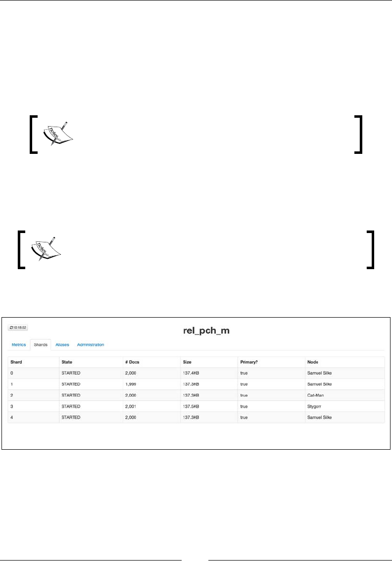
Not Only Full Text Search
[ 334 ]
The last step is to import data to these indices. We generated about 10000 records; an
example document looks as follows:
{"index": {"_index": "rel_pch_m", "_type": "book", "_id": "1"}}
{"title" : "Doc no 1", "quantity" : 101}
{"index": {"_index": "rel_pch_s", "_type": "edition", "_id": "1",
"_parent": "1"}}
{"isbn" : "no1", "circulation" : 501}
If you are curious and want to experiment, you will nd the
simple bash script create_relation_indices.sh used to
generate the example data.
The assumption is simple: we have 10000 documents of each type (book and
edition). The key is the _parent eld. In our example, it will always be set to 1, so
we have 10 000 books but our 10 000 edition belongs to that one particular book.
This example is rather extreme, but it lets us point out an important thing.
For visualization, we have used the ElasticHQ plugin available at
http://www.elastichq.org/.
First let's look at the parent part of the relation and the index storing the parent
documents, as shown in the following screenshot:
As we can see, the ve shards of the index are located on three different nodes.
Every shard has more or less the same number of documents. This is what we would
expect—Elasticsearch used hashing to calculate the shard on which documents
should be placed.

Chapter 3
[ 335 ]
Now, let's look at the second index, which contains our children documents, as
shown in the following screenshot:
The situation is different. We still have ve shards, but four of them are empty
and the last one contains all the 10,000 documents! So something is not right—all
the documents we indexed are located in one particular shard. This is because
Elasticsearch will always put documents with the same parent in the same shard (in
other words, the routing parameter value for children documents is always equal
to the parent parameter value). Our example shows that in situations when some
parent documents have substantially more children, we can end up with uneven
shards, which may cause performance and storage issues—for example, some shards
may be idling, while others will be constantly overloaded.
A few words about alternatives
As we have seen, the handling of relations between documents can cause different
problems to Elasticsearch. Of course, this is not only the case with Elasticsearch
because full text search solutions are extremely valuable for searching and data
analysis, and not for modeling relationships between data. If it is a big problem for
your application, and the full text capability is not a core part of it, you may consider
using an SQL database that allows full text searching to some extent. Of course, these
solutions won't be as exible and fast as Elasticsearch, but we have to pay the price if
we need full relationship support. However, in most other cases, the change of data
architecture and the elimination of relations by de-normalization will be sufcient.

Not Only Full Text Search
[ 336 ]
Scripting changes between Elasticsearch
versions
One of the great things in Elasticsearch is its scripting capabilities. You can use script
for calculating score, text-based scoring, data ltering, and data analysis. Although
scripting can be slow in some cases, such as calculating the score for each document,
we think that this part of Elasticsearch is important. Because of this, we decided that
this section should bring you the information about the changes and will extend the
information present in the Elasticsearch Server Second Edition book.
Scripting changes
Elasticsearch scripting has gone through a lot of refactoring in version 1.0 and in the
versions that came after that. Because of those changes, some users were lost as to
why their scripts stopped working when upgrading to version 1.2 of Elasticsearch
and what is happening in general. This section will try to give you an insight on
what to expect.
Security issues
During the lifetime of Elasticsearch 1.1, an exploit was published (see http://bouk.
co/blog/elasticsearch-rce/): it showed that with the default conguration,
Elasticsearch was not fully secure. Because of that, dynamic scripting was disabled
by default in Elasticsearch 1.2. Although, disabling dynamic scripting was enough to
make Elasticsearch secure, it made script usage far more complicated.
Groovy – the new default scripting language
With the release of Elasticsearch 1.3, we can use a new scripting language that
will become default in the next version: Groovy (see http://groovy.codehaus.
org/). The reason for this is that it can be closed in its own sandbox, preventing
dynamic scripts from doing any harm to the cluster and the operating system. In
addition to that, because Groovy can be sandboxed, Elasticsearch allows us to use
dynamic scripting when using it. Generally speaking, starting from version 1.3, if a
scripting language can be sandboxed, it can be used in dynamic scripts. However,
Groovy is not everything: Elasticsearch 1.3 allows us to use Lucene expressions,
which we will cover in this section. However, with the release of Elasticsearch 1.3.8
and 1.4.3 dynamic scripting was turned off even for Groovy. Because of that, if you
still want to use dynamic scripting for Groovy you need to add script.groovy.
sandbox.enabled property to elasticsearch.yml and set it to true or make your
Elasticsearch a bit less dynamic with stored scripts. Please be aware that enabling
dynamic scripting exposes security issues though and should be used with caution.

Chapter 3
[ 337 ]
Removal of MVEL language
Because of the security issues and introduction of Groovy, starting from Elasticsearch
1.4, MVEL will no longer be available by default with Elasticsearch distribution.
The default language will be Groovy, and MVEL will only be available as a plugin
installed on demand. Remember that if you want to drop MVEL scripts, it is really
easy to port them to Groovy. Of course, you will be able to install the MVEL plugin,
but still dynamic scripting will be forbidden.
Short Groovy introduction
Groovy is a dynamic language for the Java Virtual Machine. It was built on top of
Java, with some inspiration from languages such as Python, Ruby, or Smalltalk. Even
though Groovy is out of the context of this book, we decided to describe it because, as
you know, it is the default scripting language starting from Elasticsearch 1.4. If you
already know Groovy and you know how to use it in Elasticsearch, you can easily skip
this section and move to the Scripting in full text context section of this book.
The thing to remember is that Groovy is only sandboxed up to
Elasticsearch 1.3.8 and 1.4.3. Starting from the mentioned versions it
is not possible to run dynamic Groovy scripts unless Elasticsearch is
congured to allow such. All the queries in the examples that we will
show next require you to add script.groovy.sandbox.enabled
property to elasticsearch.yml and set it to true.
Using Groovy as your scripting language
Before we go into an introduction to Groovy, let's learn how to use it in Elasticsearch
scripts. To do this, check the version you are using. If you are using Elasticsearch older
than 1.4, you will need to add the lang property with the value groovy. For example:
curl -XGET 'localhost:9200/library/_search?pretty' -d '{
"fields" : [ "_id", "_score", "title" ],
"query" : {
"function_score" : {
"query" : {
"match_all" : {}
},
"script_score" : {
"lang" : "groovy",
"script" : "_index[\"title\"].docCount()"
}
}
}
}'

Not Only Full Text Search
[ 338 ]
If you are using Elasticsearch 1.4 or newer, you can easily skip the scripting language
denition because Elasticsearch will use Groovy by default.
Variable denition in scripts
Groovy allows us to dene variables in scripts used in Elasticsearch. To dene a new
variable, we use the def keyword followed by the variable name and its value. For
example, to dene a variable named sum and assign an initial value of 0, to it we
would use the following snippet of code:
def sum = 0
Of course, we are not only bound to simple variables denition. We can dene lists,
for example, a list of four values:
def listOfValues = [0, 1, 2, 3]
We can dene a range of values, for example, from 0 to 9:
def rangeOfValues = 0..9
Finally, we can dene maps:
def map = ['count':1, 'price':10, 'quantity': 12]
The preceding line of code will result in dening a map with three keys (count,
price, and quantity) and three values corresponding to those keys (1, 10, and 12).
Conditionals
We are also allowed to use conditional statements in scripts. For example, we can use
standard if - else if - else structures:
if (count > 1) {
return count
} else if (count == 1) {
return 1
} else {
return 0
}
We can use the ternary operator:
def isHigherThanZero = (count > 0) ? true : false

Chapter 3
[ 339 ]
The preceding code will assign a true value to the isHigherThanZero variable
if the count variable is higher than 0. Otherwise, the value assigned to the
isHigherThanZero variable will be false.
Of course, we are also allowed to use standard switch statements that allow us to use
an elegant way of choosing the execution path based on the value of the statement:
def isEqualToTenOrEleven = false;
switch (count) {
case 10:
isEqualToTenOrEleven = true
break
case 11:
isEqualToTenOrEleven = true
break
default:
isEqualToTenOrEleven = false
}
The preceding code will set the value of the isEqualToTenOrEleven variable
to true if the count variable is equal to 10 or 11. Otherwise, the value of the
isEqualToTenOrEleven variable will be set to false.
Loops
Of course, we can also use loops when using Elasticsearch scripts and Groovy as the
language in which scripts are written. Let's start with the while loop that is going to
be executed until the statement in the parenthesis is true:
def i = 2
def sum = 0
while (i > 0) {
sum = sum + i
i--
}
The preceding loop will be executed twice and ended. In the rst iteration, the i
variable will have the value of 2, which means that the i > 0 statement is true. In
the second iteration, the value of the i variable will be 1, which again makes the i >
0 statement true. In the third iteration, the i variable will be 0, which will cause the
while loop not to execute its body and exit.

Not Only Full Text Search
[ 340 ]
We can also use the for loop, which you are probably familiar with if you've used
programming languages before. For example, to iterate 10 times over the for loop
body, we could use the following code:
def sum = 0
for ( i = 0; i < 10; i++) {
sum += i
}
We can also iterate over a range of values:
def sum = 0
for ( i in 0..9 ) {
sum += i
}
Or iterate over a list of values:
def sum = 0
for ( i in [0, 1, 2, 3, 4, 5, 6, 7, 8, 9] ) {
sum += i
}
If we have a map, we can iterate over its entries:
def map = ['quantity':2, 'value':1, 'count':3]
def sum = 0
for ( entry in map ) {
sum += entry.value
}
An example
Now after seeing some basics of Groovy, let's try to run an example script that will
modify the score of our documents. We will implement the following algorithm for
score calculation:
• if the year eld holds the value lower than 1800, we will give the book a
score of 1.0
• if the year eld is between 1800 and 1900, we will give the book a score of 2.0
• the rest of the books should have the score equal to the value of the year
eld minus 1000

Chapter 3
[ 341 ]
The query that does the preceding example looks as follows:
curl -XGET 'localhost:9200/library/_search?pretty' -d '{
"fields" : [ "_id", "_score", "title", "year" ],
"query" : {
"function_score" : {
"query" : {
"match_all" : {}
},
"script_score" : {
"lang" : "groovy",
"script" : "def year = doc[\"year\"].value; if (year < 1800) {
return 1.0 } else if (year < 1900) { return 2.0 } else { return
year - 1000 }"
}
}
}
}'
You may have noticed that we've separated the def year =
doc[\"year\"].value statement in the script from the rest of it
using the ; character. We did it because we have the script in a single
line and we need to tell Groovy where our assign statement ends and
where another statement starts.
The result returned by Elasticsearch for the preceding query is as follows:
{
"took" : 4,
"timed_out" : false,
"_shards" : {
"total" : 5,
"successful" : 5,
"failed" : 0
},
"hits" : {
"total" : 6,
"max_score" : 961.0,
"hits" : [ {
"_index" : "library",
"_type" : "book",

Not Only Full Text Search
[ 342 ]
"_id" : "2",
"_score" : 961.0,
"fields" : {
"title" : [ "Catch-22" ],
"year" : [ 1961 ],
"_id" : "2"
}
}, {
"_index" : "library",
"_type" : "book",
"_id" : "3",
"_score" : 936.0,
"fields" : {
"title" : [ "The Complete Sherlock Holmes" ],
"year" : [ 1936 ],
"_id" : "3"
}
}, {
"_index" : "library",
"_type" : "book",
"_id" : "1",
"_score" : 929.0,
"fields" : {
"title" : [ "All Quiet on the Western Front" ],
"year" : [ 1929 ],
"_id" : "1"
}
}, {
"_index" : "library",
"_type" : "book",
"_id" : "6",
"_score" : 904.0,
"fields" : {
"title" : [ "The Peasants" ],
"year" : [ 1904 ],
"_id" : "6"
}
}, {
"_index" : "library",
"_type" : "book",
"_id" : "4",
"_score" : 2.0,
"fields" : {
"title" : [ "Crime and Punishment" ],

Chapter 3
[ 343 ]
"year" : [ 1886 ],
"_id" : "4"
}
}, {
"_index" : "library",
"_type" : "book",
"_id" : "5",
"_score" : 1.0,
"fields" : {
"title" : [ "The Sorrows of Young Werther" ],
"year" : [ 1774 ],
"_id" : "5"
}
} ]
}
}
As you can see, our script worked as we wanted it to.
There is more
Of course, the information we just gave is not a comprehensive guide to Groovy and
was never intended to be one. Groovy is out of the scope of this book and we wanted
to give you a glimpse of what to expect from it. If you are interested in Groovy and
you want to extend your knowledge beyond what you just read, we suggest going
to the ofcial Groovy web page and reading the documentation available at http://
groovy.codehaus.org/.
Scripting in full text context
Of course, scripts are not only about modifying the score on the basis of data.
In addition to this, we can use full text-specic statistics in our scripts, such as
document frequency or term frequency. Let's look at these possibilities.
Field-related information
The rst text-related information we can use in scripts we would like to talk about is
eld-related statistics. The eld-related information Elasticsearch allows us to use
is as follows:
• _index['field_name'].docCount(): Number of documents that contain a
given eld. This statistic doesn't take deleted documents into consideration.

Not Only Full Text Search
[ 344 ]
• _index['field_name'].sumttf(): Sum of the number of times all terms
appear in all documents in a given eld.
• _index['field_name'].sumdf(): Sum of document frequencies.
This shows the sum of the number of times all terms appear in a given eld
in all documents.
Please remember that the preceding information is given for
a single shard, not for the whole index, so they may differ
between shards.
For example, if we would like to give our documents a score equal to the number
of documents having the title eld living in a given shard, we could run the
following query:
curl -XGET 'localhost:9200/library/_search?pretty' -d '{
"fields" : [ "_id", "_score", "title" ],
"query" : {
"function_score" : {
"query" : {
"match_all" : {}
},
"script_score" : {
"lang" : "groovy",
"script" : "_index[\"title\"].docCount()"
}
}
}
}'
If we would look at the response, we would see the following:
{
"took" : 3,
"timed_out" : false,
"_shards" : {
"total" : 5,
"successful" : 5,
"failed" : 0
},
"hits" : {

Chapter 3
[ 345 ]
"total" : 6,
"max_score" : 2.0,
"hits" : [ {
"_index" : "library",
"_type" : "book",
"_id" : "1",
"_score" : 2.0,
"fields" : {
"title" : [ "All Quiet on the Western Front" ],
"_id" : "1"
}
}, {
"_index" : "library",
"_type" : "book",
"_id" : "6",
"_score" : 2.0,
"fields" : {
"title" : [ "The Peasants" ],
"_id" : "6"
}
}, {
"_index" : "library",
"_type" : "book",
"_id" : "4",
"_score" : 1.0,
"fields" : {
"title" : [ "Crime and Punishment" ],
"_id" : "4"
}
}, {
"_index" : "library",
"_type" : "book",
"_id" : "5",
"_score" : 1.0,
"fields" : {
"title" : [ "The Sorrows of Young Werther" ],
"_id" : "5"
}
}, {
"_index" : "library",
"_type" : "book",
"_id" : "2",
"_score" : 1.0,

Not Only Full Text Search
[ 346 ]
"fields" : {
"title" : [ "Catch-22" ],
"_id" : "2"
}
}, {
"_index" : "library",
"_type" : "book",
"_id" : "3",
"_score" : 1.0,
"fields" : {
"title" : [ "The Complete Sherlock Holmes" ],
"_id" : "3"
}
} ]
}
}
As you can see, we have ve documents that were queried to return the preceding
results. The rst two documents have a score of 2.0, which means that they are
probably living in the same shard because the four remaining documents have a
score of 1.0, which means that are alone in their shard.
Shard level information
The shard level information that we are allowed to use are as follows:
• _index.numDocs(): Number of documents in a shard
• _index.maxDoc(): Internal identier of the maximum number of
documents in a shard
• _index.numDeletedDocs(): Number of deleted documents in a given shard
Please remember that the preceding information is given for
a single shard, not for the whole index, so they may differ
between shards.
For example, if we would like to sort documents on the basis of the highest internal
identier each shard has, we could send the following query:
curl -XGET 'localhost:9200/library/_search?pretty' -d '{
"fields" : [ "_id", "_score", "title" ],
"query" : {
"function_score" : {
"query" : {

Chapter 3
[ 347 ]
"match_all" : {}
},
"script_score" : {
"lang" : "groovy",
"script" : "_index.maxDoc()"
}
}
}
}'
Of course, it doesn't make much sense to use those statistics alone, like we just did,
but with addition to other text-related information, they can be very useful.
Term level information
The next type of information that we can use in scripts is term level information.
Elasticsearch allows us to use the following:
• _index['field_name']['term'].df(): Returns the number of documents
the term appears in a given eld
• _index['field_name']['term'].ttf(): Returns the sum of the number of
times a given term appears in all documents in a given eld
• _index['field_name']['term'].tf(): Returns the information about the
number of times a given term appears in a given eld in a document
To give a good example of how we can use the preceding statistics, let's index two
documents by using the following commands:
curl -XPOST 'localhost:9200/scripts/doc/1' -d '{"name":"This is a
document"}'
curl -XPOST 'localhost:9200/scripts/doc/2' -d '{"name":"This is a
second document after the first document"}'
Now, let's try ltering documents on the basis of how many times a given term
appears in the name eld. For example, let's match only those documents that have in
the name eld the document term appearing at least twice. To do this, we could run
the following query:
curl -XGET 'localhost:9200/scripts/_search?pretty' -d '{
"query" : {
"filtered" : {

Not Only Full Text Search
[ 348 ]
"query" : {
"match_all" : {}
},
"filter" : {
"script" : {
"lang" : "groovy",
"script": "_index[\"name\"][\"document\"].tf() > 1"
}
}
}
}
}'
The result of the query would be as follows:
{
"took" : 1,
"timed_out" : false,
"_shards" : {
"total" : 5,
"successful" : 5,
"failed" : 0
},
"hits" : {
"total" : 1,
"max_score" : 1.0,
"hits" : [ {
"_index" : "scripts",
"_type" : "doc",
"_id" : "2",
"_score" : 1.0,
"_source":{"name":"This is a second document after the first
document"}
} ]
}
}
As we can see, Elasticsearch did exactly what we wanted.

Chapter 3
[ 349 ]
More advanced term information
In addition to already presented information, we can also use term positions, offsets,
and payloads in our scripts. To get those, we can use one the _index['field_
name'].get('term', OPTION) expression, where OPTION is one of the following:
• _OFFSETS: Term offsets
• _PAYLOADS: Term payloads
• _POSITIONS: Term positions
Please remember that the eld you want to get offsets or
positions for needs to have this enabled during indexing.
In addition to this, we can also use the _CACHE option. It allows us to iterate multiple
times over all the term positions. Options can also be combined using the | operator;
for example, if you would like to get term offsets and positions for the document
term in the title eld, you could use the following expression in your script:
_index['title'].get('document', _OFFSETS | _POSITIONS).
One thing to remember is that all the preceding options return an object called that,
depending on the options we have chosen, contains the following information:
• startOffset: Start offset for the term
• endOffset: End offset for the term
• payload: Payload for the term
• payloadAsInt(value): Returns payload for the term converted to integer or
the value in case the current position doesn't have a payload
• payloadAsFloat(value): Returns payload for the term converted to oat or
the value in case the current position doesn't have a payload
• payloadAsString(value): Returns payload for the term converted to string
or the value in case the current position doesn't have a payload
• position: Position of a term
To illustrate an example, let's create a new index with the following mappings:
curl -XPOST 'localhost:9200/scripts2' -d '{
"mappings" : {
"doc" : {
"properties" : {

Not Only Full Text Search
[ 350 ]
"name" : { "type" : "string", "index_options" : "offsets" }
}
}
}
}'
After this, we index two documents using the following commands:
curl -XPOST 'localhost:9200/scripts2/doc/1' -d '{"name":"This is the
first document"}'
curl -XPOST 'localhost:9200/scripts2/doc/2' -d '{"name":"This is a
second simple document"}'
Now, let's set the score of our documents to the sum of all the start positions for the
document term in the name eld. To do this, we run the following query:
curl -XGET 'localhost:9200/scripts2/_search?pretty' -d '{
"query" : {
"function_score" : {
"query" : {
"match_all" : {}
},
"script_score" : {
"lang" : "groovy",
"script": "def termInfo = _index[\"name\"].get(\"document\",_OFFSETS);
def sum = 0; for (offset in termInfo) { sum += offset.startOffset; };
return sum;"
}
}
}
}'
The results returned by Elasticsearch would be as follows:
{
"took" : 3,
"timed_out" : false,
"_shards" : {
"total" : 5,
"successful" : 5,
"failed" : 0
},

Chapter 3
[ 351 ]
"hits" : {
"total" : 2,
"max_score" : 24.0,
"hits" : [ {
"_index" : "scripts2",
"_type" : "doc",
"_id" : "2",
"_score" : 24.0,
"_source":{"name":"This is a second simple document"}
}, {
"_index" : "scripts2",
"_type" : "doc",
"_id" : "1",
"_score" : 18.0,
"_source":{"name":"This is the first document"}
} ]
}
}
As we can see, it works. If we look at the formatted script, we would see something
like the following:
def termInfo = _index['name'].get('document',_OFFSETS);
def sum = 0;
for (offset in termInfo) {
sum += offset.startOffset;
};
return sum;
As you can see, it is nothing sophisticated. First, we get the information about the
offsets in an object; next, we create a variable to hold our offsets sum. Then, we have
a loop for all the offsets information (we can have multiple instances of offsets for
different occurrences of the same term in a eld) and, nally, we return the sum that
makes our score for the document to be set to the returned value.
In addition to all what we talked about in the preceding section, we are
also able to get information about term vectors if we turned them on
during indexing. To do that, we can use the _index.termVectors()
expression, which will return Apache Lucene Fields object instance.
You can nd more about the Fields object in Lucene Javadocs
available at https://lucene.apache.org/core/4_9_0/core/
org/apache/lucene/index/Fields.html.

Not Only Full Text Search
[ 352 ]
Lucene expressions explained
Although marked as experimental, we decided to talk about it because this is a new
and very good feature. The reason that makes Lucene expressions very handy is
using them is very fast—their execution is as fast as native scripts, but yet they are
like dynamic scripts with some limitations. This section will show you what you can
do with Lucene expressions.
The basics
Lucene provides functionality to compile a JavaScript expression to a Java
bytecode. This is how Lucene expressions work and this is why they are as fast
as native Elasticsearch scripts. Lucene expressions can be used in the following
Elasticsearch functionalities:
• Scripts responsible for sorting
• Aggregations that work on numeric elds
• In the function_score query in the script_score query
• In queries using script_fields
In addition to this, you have to remember that:
• Lucene expressions can be only used on numeric elds
• Stored elds can't be accessed using Lucene expressions
• Missing values for a eld will be given a value of 0
• You can use _score to access the document score and doc['field_name'].
value to access the value of a single valued numeric eld in the document
• No loops are possible, only single statements
An example
Knowing the preceding information, we can try using Lucene expressions to modify
the score of our documents. Let's get back to our library index and try to increase
the score of the given document by 10% of the year it was originally released. To do
this, we could run the following query:
curl -XGET 'localhost:9200/library/_search?pretty' -d '{
"fields" : [ "_id", "_score", "title" ],
"query" : {
"function_score" : {

Chapter 3
[ 353 ]
"query" : {
"match_all" : {}
},
"script_score" : {
"lang" : "expression",
"script" : "_score + doc[\"year\"].value * percentage",
"params" : {
"percentage" : 0.1
}
}
}
}
}'
The query is very simple, but let's discuss its structure. First, we are using the match_
all query wrapped in the function_score query because we want all documents to
match and we want to use script for scoring. We are also setting the script language
to expression (by setting the lang property to expression) to tell Elasticsearch that
our script is a Lucene expressions script. Of course, we provide the script and we
parameterize it, just like we would with any other script. The results of the preceding
query look as follows:
{
"took" : 4,
"timed_out" : false,
"_shards" : {
"total" : 5,
"successful" : 5,
"failed" : 0
},
"hits" : {
"total" : 6,
"max_score" : 197.1,
"hits" : [ {
"_index" : "library",
"_type" : "book",
"_id" : "2",
"_score" : 197.1,
"fields" : {
"title" : [ "Catch-22" ],
"_id" : "2"

Not Only Full Text Search
[ 354 ]
}
}, {
"_index" : "library",
"_type" : "book",
"_id" : "3",
"_score" : 194.6,
"fields" : {
"title" : [ "The Complete Sherlock Holmes" ],
"_id" : "3"
}
}, {
"_index" : "library",
"_type" : "book",
"_id" : "1",
"_score" : 193.9,
"fields" : {
"title" : [ "All Quiet on the Western Front" ],
"_id" : "1"
}
}, {
"_index" : "library",
"_type" : "book",
"_id" : "6",
"_score" : 191.4,
"fields" : {
"title" : [ "The Peasants" ],
"_id" : "6"
}
}, {
"_index" : "library",
"_type" : "book",
"_id" : "4",
"_score" : 189.6,
"fields" : {
"title" : [ "Crime and Punishment" ],
"_id" : "4"
}
}, {
"_index" : "library",
"_type" : "book",
"_id" : "5",
"_score" : 178.4,
"fields" : {

Chapter 3
[ 355 ]
"title" : [ "The Sorrows of Young Werther" ],
"_id" : "5"
}
} ]
}
}
As we can see, Elasticsearch did what it was asked to do.
There is more
Of course, the provided example is a very simple one. If you are interested in what
Lucene expressions provide, please visit the ofcial Javadocs available at http://
lucene.apache.org/core/4_9_0/expressions/index.html?org/apache/lucene/
expressions/js/package-summary.html. The documents available at the given URL
provide more information about what Lucene exposes in expressions module.
Summary
In this chapter, we extended our knowledge about query handling and data
analysis. First of all, we discussed query rescore, which can help us when we need
to recalculate the score of the top documents returned by a query. We also learned
how to control multimatching queries. After that, we looked at two new aggregation
types—one allowing us to get signicant terms from a set of results and the other
allowing documents grouping: a highly anticipated feature. We also discussed
differences in relationship handling and approaches we can take when using
Elasticsearch. Finally, we extended our knowledge about the Elasticsearch scripting
module and we've learned what changes were introduced after Elasticsearch 1.0.
In the next chapter, we will try to improve our user query experience. We will start
with user spelling mistakes and how Elasticsearch can help us by turning mistakes
into good queries. We will also see what approaches we can take to handle user
spelling mistake situations. After that, we will discuss improving query relevance on
a given example. We will show you a query returning poor results and we will tune
the query to match our needs.

Improving the User
Search Experience
In the previous chapter, we extended our knowledge about query handling and data
analysis. We started by looking at the query rescore that can help us when we need
to recalculate the score of the top documents returned by a query. We controlled
multi matching in Elasticsearch queries and looked at two new exciting aggregation
types: signicant terms aggregation and top hits aggregation. We discussed the
differences in relationship handling and, nally, we extended our knowledge about
the Elasticsearch scripting module and learned what the changes introduced were
after the release of Elasticsearch 1.0. By the end of this chapter, we will have covered
the following topics:
• Using the Elasticsearch Suggest API to correct user spelling mistakes
• Using the term suggester to suggest single words
• Using the phrase suggester to suggest whole phrases
• Conguring suggest capabilities to match your needs
• Using the completion suggester for the autocomplete functionality
• Improving query relevance by using different Elasticsearch functionalities

Improving the User Search Experience
[ 358 ]
Correcting user spelling mistakes
One of the simplest ways to improve the user search experience is to correct their
spelling mistakes either automatically or by just showing the correct query phrase
and allowing the user to use it. For example, this is what Google shows us when we
type in elasticsaerch instead of Elasticsearch:
Starting from 0.90.0 Beta1, Elasticsearch allows us to use the Suggest API to correct
the user spelling mistakes. With the newer versions of Elasticsearch, the API was
changed, bringing new features and becoming more and more powerful. In this
section, we will try to bring you a comprehensive guide on how to use the Suggest
API provided by Elasticsearch, both in simple use cases and in ones that require
more conguration.
Testing data
For the purpose of this section, we decided that we need a bit more data than a few
documents. In order to get the data we need, we decided to use the Wikipedia river
plugin (https://github.com/elasticsearch/elasticsearch-river-wikipedia)
to index some public documents from Wikipedia. First, we need to install the plugin
by running the following command:
bin/plugin -install elasticsearch/elasticsearch-river-wikipedia/2.4.1
After that, we run the following command:
curl -XPUT 'localhost:9200/_river/wikipedia_river/_meta' -d '{
"type" : "wikipedia",
"index" : {
"index" : "wikipedia"
}
}'

Chapter 4
[ 359 ]
After that, Elasticsearch will start indexing the latest English dump from Wikipedia.
If you look at the logs, you should see something like this:
[2014-08-28 22:35:01,566][INFO ][river.wikipedia ] [Thing]
[wikipedia][Wikipedia_river] creating wikipedia stream river for
[http://download.wikimedia.org/enwiki/latest/enwiki-latest-pages-
articles.xml.bz2]
[2014-08-28 22:35:01,568][INFO ][river.wikipedia ] [Thing]
[wikipedia][Wikipedia_river] starting wikipedia stream
As you can see, the river has started its work. After some time, you will have the
data indexed in the index called wikipedia. If you want all data from the latest English
Wikipedia dump to be indexed, you have to be patient, and we are not. The number
of documents when we decided to cancel the indexation was 7080049. The index had
about 19 GB in total size (without replicas).
Getting into technical details
Introduced in Version 0.90.3, the Suggest API is not the simplest one available in
Elasticsearch. In order to get the desired suggest, we can either add a new suggest
section to the query, or we can use a specialized REST endpoint that Elasticsearch
exposes. In addition to this, we have multiple suggest implementations that allow us
to correct user spelling mistakes, create the autocomplete functionality, and so on.
All this gives us a powerful and exible mechanism that we can use in order to make
our search better.
Of course, the suggest functionality works on our data, so if we have a small set of
documents in the index, the proper suggestion may not be found. When dealing with
a smaller data set, Elasticsearch has fewer words in the index and, because of that, it
has fewer candidates for suggestions. On the other hand, the more data, the bigger
the possibility that we will have data that has some mistakes; however, we can
congure Elasticsearch internals to handle such situations.
Please note that the layout of this chapter is a bit different. We start by
showing you a simple example on how to query for suggestions and
how to interpret the Suggest API response without getting too much
into all the conguration options. We do this because we don't want to
overwhelm you with technical details, but we want to show you what
you can achieve. The nifty conguration parameters come later.

Improving the User Search Experience
[ 360 ]
Suggesters
Before we continue with querying and analyzing the responses, we would like to write
a few words about the available suggester types—the functionality responsible for
nding suggestions when using the Elasticsearch Suggest API. Elasticsearch allows us
to use three suggesters currently: the term one, the phrase one, and the completion one.
The rst two allow us to correct spelling mistakes, while the third one allows us to
develop a very fast autocomplete functionality. However, for now, let's not focus on
any particular suggester type, but let's look on the query possibilities and the responses
returned by Elasticsearch. We will try to show you the general principles, and then we
will get into more details about each of the available suggesters.
Using the _suggest REST endpoint
There is a possibility that we can get suggestions for a given text by using a
dedicated _suggest REST endpoint. What we need to provide is the text to
analyze and the type of used suggester (term or phrase). So if we would like to get
suggestions for the words graphics desiganer (note that we've misspelled the word
on purpose), we would run the following query:
curl -XPOST 'localhost:9200/wikipedia/_suggest?pretty' -d '{
"first_suggestion" : {
"text" : "wordl war ii",
"term" : {
"field" : "_all"
}
}
}'
As you can see, each suggestion request is send to Elasticsearch in its own object with
the name we chose (in the preceding case, it is first_suggestion). Next, we specify
the text for which we want the suggestion to be returned using the text parameter.
Finally, we add the suggester object, which is either term or phrase currently. The
suggester object contains its conguration, which for the term suggester used in the
preceding command, is the eld we want to use for suggestions (the field property).
We can also send more than one suggestion at a time by adding multiple suggestion
names. For example, if in addition to the preceding suggestion, we would also
include a suggestion for the word raceing, we would use the following command:
curl -XPOST 'localhost:9200/wikipedia/_suggest?pretty' -d '{
"first_suggestion" : {

Chapter 4
[ 361 ]
"text" : "wordl war ii",
"term" : {
"field" : "_all"
}
},
"second_suggestion" : {
"text" : "raceing",
"term" : {
"field" : "text"
}
}
}'
Understanding the REST endpoint suggester
response
Let's now look at the example response we can expect from the _suggest REST
endpoint call. Although the response will differ for each suggester type, let's look
at the response returned by Elasticsearch for the rst command we've sent in the
preceding code that used the term suggester:
{
"_shards" : {
"total" : 5,
"successful" : 5,
"failed" : 0
},
"first_suggestion" : [ {
"text" : "wordl",
"offset" : 0,
"length" : 5,
"options" : [ {
"text" : "world",
"score" : 0.8,
"freq" : 130828
}, {
"text" : "words",
"score" : 0.8,
"freq" : 20854
}, {

Improving the User Search Experience
[ 362 ]
"text" : "wordy",
"score" : 0.8,
"freq" : 210
}, {
"text" : "woudl",
"score" : 0.8,
"freq" : 29
}, {
"text" : "worde",
"score" : 0.8,
"freq" : 20
} ]
}, {
"text" : "war",
"offset" : 6,
"length" : 3,
"options" : [ ]
}, {
"text" : "ii",
"offset" : 10,
"length" : 2,
"options" : [ ]
} ]
}
As you can see in the preceding response, the term suggester returns a list of possible
suggestions for each term that was present in the text parameter of our first_
suggestion section. For each term, the term suggester will return an array of possible
suggestions with additional information. Looking at the data returned for the wordl
term, we can see the original word (the text parameter), its offset in the original text
parameter (the offset parameter), and its length (the length parameter).
The options array contains suggestions for the given word and will be empty if
Elasticsearch doesn't nd any suggestions. Each entry in this array is a suggestion
and is characterized by the following properties:
• text: This is the text of the suggestion.
• score: This is the suggestion score; the higher the score, the better the
suggestion will be.
• freq: This is the frequency of the suggestion. The frequency represents how
many times the word appears in documents in the index we are running the
suggestion query against. The higher the frequency, the more documents
will have the suggested word in its elds and the higher the chance that the
suggestion is the one we are looking for.

Chapter 4
[ 363 ]
Please remember that the phrase suggester response will differ from
the one returned by the terms suggester, and we will discuss the
response of the phrase suggester later in this section.
Including suggestion requests in query
In addition to using the _suggest REST endpoint, we can include the suggest
section in addition to the query section in the normal query sent to Elasticsearch. For
example, if we would like to get the same suggestion we've got in the rst example
but during query execution, we could send the following query:
curl -XGET 'localhost:9200/wikipedia/_search?pretty' -d '{
"query" : {
"match_all" : {}
},
"suggest" : {
"first_suggestion" : {
"text" : "wordl war ii",
"term" : {
"field" : "_all"
}
}
}
}'
As you would expect, the response for the preceding query would be the query
results and the suggestions as follows:
{
"took" : 5,
"timed_out" : false,
"_shards" : {
"total" : 5,
"successful" : 5,
"failed" : 0
},
"hits" : {
"total" : 7080049,
"max_score" : 1.0,
"hits" : [

Improving the User Search Experience
[ 364 ]
...
]
},
"suggest" : {
"first_suggestion" : [ {
"text" : "wordl",
"offset" : 0,
"length" : 5,
"options" : [ {
"text" : "world",
"score" : 0.8,
"freq" : 130828
}, {
"text" : "words",
"score" : 0.8,
"freq" : 20854
}, {
"text" : "wordy",
"score" : 0.8,
"freq" : 210
}, {
"text" : "woudl",
"score" : 0.8,
"freq" : 29
}, {
"text" : "worde",
"score" : 0.8,
"freq" : 20
} ]
}, {
"text" : "war",
"offset" : 6,
"length" : 3,
"options" : [ ]
}, {
"text" : "ii",
"offset" : 10,
"length" : 2,
"options" : [ ]
} ]
}
}

Chapter 4
[ 365 ]
As we can see, we've got both search results and the suggestions whose structure
we've already discussed earlier in this section.
There is one more possibility—if we have the same suggestion text, but we want
multiple suggestion types, we can embed our suggestions in the suggest object and
place the text property as the suggest object option. For example, if we would like
to get suggestions for the wordl war ii text for the text eld and for the _all eld,
we could run the following command:
curl -XGET 'localhost:9200/wikipedia/_search?pretty' -d '{
"query" : {
"match_all" : {}
},
"suggest" : {
"text" : "wordl war ii",
"first_suggestion" : {
"term" : {
"field" : "_all"
}
},
"second_suggestion" : {
"term" : {
"field" : "text"
}
}
}
}'
We now know how to make a query with suggestions returned or how to use the
_suggest REST endpoint. Let's now get into more details of each of the available
suggester types.

Improving the User Search Experience
[ 366 ]
The term suggester
The term suggester works on the basis of the edit distance, which means that the
suggestion with fewer characters that needs to be changed or removed to make the
suggestion look like the original word is the best one. For example, let's take the
words worl and work. In order to change the worl term to work, we need to change the l
letter to k, so it means a distance of one. Of course, the text provided to the suggester
is analyzed and then terms are chosen to be suggested. Let's now look at how we can
congure the Elasticsearch term suggester.
Conguration
The Elasticsearch term suggester supports multiple conguration properties
that allow us to tune its behavior to match our needs and to work with our data.
Of course, we've already seen how it works and what it can give us, so we will
concentrate on conguration now.
Common term suggester options
The common term suggester options can be used for all the suggester
implementations that are based on the term suggester. Currently, these are the phrase
suggester and, of course, the base term suggester. The available options are:
• text: This is the text we want to get the suggestions for. This parameter is
required in order for the suggester to work.
• field: This is another required parameter. The eld parameter allows us to set
which eld the suggestions should be generated for. For example, if we only
want to consider title eld terms in suggestions, we should set this parameter
value to the title.
• analyzer: This is the name of the analyzer that should be used to analyze
the text provided in the text parameter. If not set, Elasticsearch will use the
analyzer used for the eld provided by the eld parameter.
• size: This is the maximum number of suggestions that are allowed to be
returned by each term provided in the text parameter. It defaults to 5.
• sort: This allows us to specify how suggestions are sorted in the result
returned by Elasticsearch. By default, this is set to a score, which tells
Elasticsearch that the suggestions should be sorted by the suggestion score
rst, suggestion document frequency next, and nally, by the term. The
second possible value is the frequency, which means that the results are rst
sorted by the document frequency, then by score, and nally, by the term.

Chapter 4
[ 367 ]
• suggest_mode: This is another suggestion parameter that allows us to
control which suggestions will be included in the Elasticsearch response.
Currently, there are three values that can be passed to this parameter:
missing, popular, and always. The default missing value will tell
Elasticsearch to generate suggestions to only those words that are provided
in the text parameter that doesn't exist in the index. If this property will
be set to popular, then the term suggester will only suggest terms that are
more popular (exist in more documents) than the original term for which
the suggestion is generated. The last value, which is always, will result in a
suggestion generated for each of the words in the text parameter.
Additional term suggester options
In addition to the common term suggester options, Elasticsearch allows us to
use additional ones that will only make sense for the term suggester itself.
These options are as follows:
• lowercase_terms: When set to true, this will tell Elasticsearch to make all
terms that are produced from the text eld after analysis, lowercase.
• max_edits: This defaults to 2 and species the maximum edit distance
that the suggestion can have for it to be returned as a term suggestion.
Elasticsearch allows us to set this value to 1 or 2. Setting this value to 1 can
result in fewer suggestions or no suggestions at all for words with many
spelling mistakes. In general, if you see many suggestions that are not
correct, because of errors, you can try setting max_edits to 1.
• prefix_length: Because spelling mistakes usually don't appear at the
beginning of the word, Elasticsearch allows us to set how much of the
suggestion's initial characters must match with the initial characters of the
original term. By default, this property is set to 1. If we are struggling with
the suggester performance increasing, this value will improve the overall
performance, because less suggestions will be needed to be processed
by Elasticsearch.
• min_word_length: This defaults to 4 and species the minimum number
of characters a suggestion must have in order to be returned on the
suggestions list.
• shard_size: This defaults to the value specied by the size parameter
and allows us to set the maximum number of suggestions that should be
read from each shard. Setting this property to values higher than the size
parameter can result in more accurate document frequency (this is because
of the fact that terms are held in different shards for our indices unless we
have a single shard index created) being calculated but will also result in
degradation of the spellchecker's performance.

Improving the User Search Experience
[ 368 ]
• max_inspections: This defaults to 5 and species how many candidates
Elasticsearch will look at in order to nd the words that can be used as
suggestions. Elasticsearch will inspect a maximum of shard_size multiplied
by the max_inspections candidates for suggestions. Setting this property to
values higher than the default 5 may improve the suggester accuracy but can
also decrease the performance.
• min_doc_freq: This defaults to 0, which means not enabled. It allows us to
limit the returned suggestions to only those that appear in the number of
documents higher than the value of this parameter (this is a per-shard value
and not a globally counted one). For example, setting this parameter to 2
will result in suggestions that appear in at least two documents in a given
shard. Setting this property to values higher than 0 can improve the quality
of returned suggestions; however, it can also result in some suggestion
not being returned because it has a low shard document frequency. This
property can help us with removing suggestions that come from a low
number of documents and may be erroneous. This parameter can be
specied as a percentage; if we want to do this, its value must be less than 1.
For example, 0.01 means 1 percent, which again means that the minimum
frequency of the given suggestion needs to be higher than 1 percent of the
total term frequency (of course, per shard).
• max_term_freq: This defaults to 0.01 and species the maximum number
of documents the term from the text eld can exist for it to be considered a
candidate for spellchecking. Similar to the min_doc_freq parameter, it can
be either provided as an absolute number (such as 4 or 100), or it can be a
percentage value if it is beyond 1 (for example, 0.01 means 1 percent). Please
remember that this is also a per-shard frequency. The higher the value of
this property, the better the overall performance of the spellchecker will be.
In general, this property is very useful when we want to exclude terms that
appear in many documents from spellchecking, because they are usually
correct terms.
• accuracy: This defaults to 0.5 and can be a number from 0 to 1. It species
how similar the term should be when compared to the original one. The
higher the value, the more similar the terms need to be. This value is used in
comparison during string distance calculation for each of the terms from the
original input.

Chapter 4
[ 369 ]
• string_distance: This species which algorithm should be used to
compare how similar terms are when comparing them to each other. This
is an expert setting. These options are available: internal, which is the
default comparison algorithm based on an optimized implementation of the
Damerau Levenshtein similarity algorithm; damerau_levenshtein, which is
the implementation of the Damerau Levenshtein string distance algorithm
(http://en.wikipedia.org/wiki/Damerau%E2%80%93Levenshtein_
distance); levenstein, which is the implementation of the Levenshtein
distance (http://en.wikipedia.org/wiki/Levenshtein_distance),
jarowinkler, which is an implementation of the Jaro-Winkler distance
algorithm (http://en.wikipedia.org/wiki/Jaro%E2%80%93Winkler_
distance), and nally, ngram, which is an N-gram based distance algorithm.
Because of the fact that we've used the terms suggester during the
initial examples, we decided to skip showing you how to query term
suggesters and how the response looks. If you want to see how to query
this suggester and what the response looks like, please refer to the
beginning of the Suggesters section in this chapter.
The phrase suggester
The term suggester provides a great way to correct user spelling mistakes on a per-
term basis. However, if we would like to get back phrases, it is not possible to do
that when using this suggester. This is why the phrase suggester was introduced. It
is built on top of the term suggester and adds additional phrase calculation logic to
it so that whole phrases can be returned instead of individual terms. It uses N-gram
based language models to calculate how good the suggestion is and will probably be
a better choice to suggest whole phrases instead of the term suggester. The N-gram
approach divides terms in the index into grams—word fragments built of one or
more letters. For example, if we would like to divide the word mastering into bi-
grams (a two letter N-gram), it would look like this: ma as st te er ri in ng.
If you want to read more about N-gram language models,
refer to the Wikipedia article available at http://
en.wikipedia.org/wiki/Language_model#N-gram_
models and continue from there.

Improving the User Search Experience
[ 370 ]
Usage example
Before we continue with all the possibilities, we have to congure the phrase
suggester; let's start with showing you an example of how to use it. This time, we
will run a simple query to the _search endpoint with only the suggests section in
it. We do this by running the following command:
curl -XGET 'localhost:9200/wikipedia/_search?pretty' -d '{
"suggest" : {
"text" : "wordl war ii",
"our_suggestion" : {
"phrase" : {
"field" : "_all"
}
}
}
}'
As you can see in the preceding command, it is almost the same as we sent
when using the term suggester, but instead of specifying the term suggester
type, we've specied the phrase type. The response to the preceding command
will be as follows:
{
"took" : 58,
"timed_out" : false,
"_shards" : {
"total" : 5,
"successful" : 5,
"failed" : 0
},
"hits" : {
"total" : 7080049,
"max_score" : 1.0,
"hits" : [
...
]
},
"suggest" : {
"our_suggestion" : [ {
"text" : "wordl war ii",
"offset" : 0,

Chapter 4
[ 371 ]
"length" : 12,
"options" : [ {
"text" : "world war ii",
"score" : 7.055394E-5
}, {
"text" : "words war ii",
"score" : 2.3738032E-5
}, {
"text" : "wordy war ii",
"score" : 3.575829E-6
}, {
"text" : "worde war ii",
"score" : 1.1586584E-6
}, {
"text" : "woudl war ii",
"score" : 1.0753317E-6
} ]
} ]
}
}
As you can see, the response is very similar to the one returned by the term suggester,
but instead of a single word being returned as the suggestion for each term from the
text eld, it is already combined and Elasticsearch returns whole phrases. Of course,
we can congure additional parameters in the phrase section and, now, we will look
at what parameters are available for usage. Of course, the returned suggestions are
sorted by their score by default.
Conguration
The phrase suggester conguration parameter can be divided into three groups: basic
parameters that dene the general behavior, the smoothing models conguration
to balance N-grams' weights, and candidate generators that are responsible for
producing the list of terms suggestions that will be used to return nal suggestions.
Because the phrase suggester is based on the term suggester, it
can also use some of the conguration options provided by it. These
options are text, size, analyzer, and shard_size. Refer to the
term suggester description earlier in this chapter to nd out what
they mean.

Improving the User Search Experience
[ 372 ]
Basic conguration
In addition to properties mentioned in the preceding phrase, the suggester exposes
the following basic options:
• highlight: This allows us to use suggestions highlighting. With the use of
the pre_tag and post_tag properties, we can congure what prex and
postx should be used to highlight suggestions. For example, if we would
like to surround suggestions with the <b> and </b> tags, we should set pre_
tag to <b> and post_tag to </b>.
• gram_size: This is the maximum size of the N-gram that is stored in the
eld and is specied by the field property. If the given eld doesn't contain
N-grams, this property should be set to 1 or not passed with the suggestion
request at all. If not set, Elasticsearch will try to detect the proper value
of this parameter by itself. For example, for elds using a shingle lter
(http://www.elasticsearch.org/guide/en/elasticsearch/reference/
current/analysis-shingle-tokenfilter.html), the value of this
parameter will be set to the max_shingle_size property (of course, if not
set explicitly).
• confidence: This is the parameter that allows us to limit the suggestion based
on its score. The value of this parameter is applied to the score of the input
phrase (the score is multiplied by the value of this parameter), and this score
is used as a threshold for generated suggestions. If the suggestion score
is higher than the calculated threshold, it will be included in the returned
results; if not, then it will be dropped. For example, setting this parameter to
1.0 (which is the default value of it) will result in suggestions that are scored
higher than the original phrase. On the other hand, setting it to 0.0 will result
in the suggester returning all the suggestions (limited by the size parameter)
no matter what their score is.
• max_errors: This is the property that allows us to specify the maximum
number (or the percentage) of terms that can be erroneous (not correctly
spelled) in order to create a correction using it. The value of this property
can be either an integer number such as 1 or 5, or it can be a oat between 0
and 1, which will be treated as a percentage value. If we will set it as a oat,
it will specify the percentage of terms that can be erroneous. For example, a
value of 0.5 will mean 50 percent. If we specify an integer number, such as
1 or 5, Elasticsearch will treat it as a maximum number of erroneous terms.
By default, it is set to 1, which means that at most, a single term can be
misspelled in a given correction.
• separator: This defaults to a whitespace character and species the separator
that will be used to divide terms in the resulting bigram eld.

Chapter 4
[ 373 ]
• force_unigrams: This defaults to true and species whether the
spellchecker should be forced to use a gram size of 1 (unigram).
• token_limit: This defaults to 10 and species the maximum number of
tokens the corrections list can have in order for it to be returned. Setting this
property to a value higher than the default one may improve the suggester
accuracy at the cost of performance.
• collate: This allows us to check each suggestion against a specied query
(using the query property inside the collate object) or lter (using the
filter property inside the collate object). The provided query or lter
is run as a template query and exposes the {{suggestion}} variable that
represents the currently processed suggestion. By including an additional
parameter called prune (in the collate object) and setting it to true,
Elasticsearch will include the information if the suggestion matches the query
or lter (this information will be included in the collate_match property in
the results). In addition to this, the query preference can be included by using
the preference property (which can take the same values as the ones used
during the normal query processing).
• real_word_error_likehood: This is a percentage value, which defaults to
0.95 and species how likely it is that a term is misspelled even though it
exists in the dictionary (built of the index). The default value of 0.95 tells
Elasticsearch that 5% of all terms that exist in its dictionary are misspelled.
Lowering the value of this parameter will result in more terms being taken as
misspelled ones even though they may be correct.
Let's now look at an example of using some of the preceding mentioned parameters,
for example, suggestions highlighting. If we modify our initial phrase suggestion
query and add highlighting, the command would look as follows:
curl -XGET 'localhost:9200/wikipedia/_search?pretty' -d '{
"suggest" : {
"text" : "wordl war ii",
"our_suggestion" : {
"phrase" : {
"field" : "_all",
"highlight" : {
"pre_tag" : "<b>",
"post_tag" : "</b>"
},
"collate" : {

Improving the User Search Experience
[ 374 ]
"prune" : true,
"query" : {
"match" : {
"title" : "{{suggestion}}"
}
}
}
}
}
}
}'
The result returned by Elasticsearch for the preceding query would be as follows:
{
"took" : 3,
"timed_out" : false,
"_shards" : {
"total" : 5,
"successful" : 5,
"failed" : 0
},
"hits" : {
"total" : 7080049,
"max_score" : 1.0,
"hits" : [
...
]
},
"suggest" : {
"our_suggestion" : [ {
"text" : "wordl war ii",
"offset" : 0,
"length" : 12,
"options" : [ {
"text" : "world war ii",
"highlighted" : "<b>world</b> war ii",
"score" : 7.055394E-5,
"collate_match" : true
}, {
"text" : "words war ii",

Chapter 4
[ 375 ]
"highlighted" : "<b>words</b> war ii",
"score" : 2.3738032E-5,
"collate_match" : true
}, {
"text" : "wordy war ii",
"highlighted" : "<b>wordy</b> war ii",
"score" : 3.575829E-6,
"collate_match" : true
}, {
"text" : "worde war ii",
"highlighted" : "<b>worde</b> war ii",
"score" : 1.1586584E-6,
"collate_match" : true
}, {
"text" : "woudl war ii",
"highlighted" : "<b>woudl</b> war ii",
"score" : 1.0753317E-6,
"collate_match" : true
} ]
} ]
}
}
As you can see, the suggestions were highlighted.
Conguring smoothing models
A Smoothing model is a functionality of the phrase suggester whose responsibility
is to measure the balance between the weight of infrequent N-grams that don't exist
in the index and the frequent ones that exist in the index. It is rather an expert option
and if you want to modify these N-grams, you should check suggester responses
for your queries in order to see whether your suggestions are proper for your case.
Smoothing is used in language models to avoid situations where the probability of
a given term is equal to zero. The Elasticsearch phrase suggester supports multiple
smoothing models.
You can nd out more about language models at http://
en.wikipedia.org/wiki/Language_model.

Improving the User Search Experience
[ 376 ]
In order to set which smoothing model we want to use, we need to add an object
called smoothing and include a smoothing model name we want to use inside of
it. Of course, we can include the properties we need or want to set for the given
smoothing model. For example, we could run the following command:
curl -XGET 'localhost:9200/wikipedia/_search?pretty&size=0' -d '{
"suggest" : {
"text" : "wordl war ii",
"generators_example_suggestion" : {
"phrase" : {
"analyzer" : "standard",
"field" : "_all",
"smoothing" : {
"linear" : {
"trigram_lambda" : 0.1,
"bigram_lambda" : 0.6,
"unigram_lambda" : 0.3
}
}
}
}
}
}'
There are three smoothing models available in Elasticsearch. Let's now look at them.
Stupid backoff is the default smoothing model used by the Elasticsearch phrase
suggester. In order to alter it or force its usage, we need to use the stupid_backoff
name. The stupid backoff smoothing model is an implementation that will use a
lower ordered N-gram (and will give it a discount equal to the value of the discount
property) if the higher order N-gram count is equal to 0. To illustrate the example,
let's assume that we use the ab bigram and the c unigram, which are common and
exist in our index used by the suggester. However, we don't have the abc trigram
present. What the stupid backoff model will do is that it will use the ab bigram
model, because abc doesn't exist and, of course, the ab bigram model will be given a
discount equal to the value of the discount property.
The stupid backoff model provides a single property that we can alter: discount.
By default, it is set to 0.4, and it is used as a discount factor for the lower ordered
N-gram model.

Chapter 4
[ 377 ]
You can read more about N-gram smoothing models by looking at http://
en.wikipedia.org/wiki/N-gram#Smoothing_techniques and http://
en.wikipedia.org/wiki/Katz's_back-off_model (which is similar to the stupid
backoff model described).
The Laplace smoothing model is also called additive smoothing. When used (to use
it, we need to use the laplace value as its name), a constant value equal to the value
of the alpha parameter (which is by 0.5 default) will be added to counts to balance
weights of frequent and infrequent N-grams. As mentioned, the Laplace smoothing
model can be congured using the alpha property, which is set to 0.5 by default.
The usual values for this parameter are typically equal or below 1.0.
You can read more about additive smoothing at http://en.wikipedia.org/wiki/
Additive_smoothing.
Linear interpolation, the last smoothing model, takes the values of the lambdas
provided in the conguration and uses them to calculate weights of trigrams,
bigrams, and unigrams. In order to use the linear interpolation smoothing model, we
need to provide the name of linear in the smoothing object in the suggester query
and provide three parameters: trigram_lambda, bigram_lambda, and unigram_
lambda. The sum of the values of the three mentioned parameters must be equal to
1. Each of these parameters is a weight for a given type of N-gram; for example, the
bigram_lambda parameter value will be used as a weights for bigrams.
Conguring candidate generators
In order to return possible suggestions for a term from the text provided in the
text parameter, Elasticsearch uses so-called candidate generators. You can think of
candidate generators as term suggesters although they are not exactly the same—
they are similar, because they are used for every single term in the query provided
to suggester. After the candidate terms are returned, they are scored in combination
with suggestions for other terms from the text, and this way, the phrase suggestions
are built.
Currently, direct generators are the only candidate generators available in
Elasticsearch, although we can expect more of them to be present in the future.
Elasticsearch allows us to provide multiple direct generators in a single phrase
suggester request. We can do this by providing the list named direct_generators.
For example, we could run the following command:
curl -XGET 'localhost:9200/wikipedia/_search?pretty&size=0' -d '{
"suggest" : {
"text" : "wordl war ii",

Improving the User Search Experience
[ 378 ]
"generators_example_suggestion" : {
"phrase" : {
"analyzer" : "standard",
"field" : "_all",
"direct_generator" : [
{
"field" : "_all",
"suggest_mode" : "always",
"min_word_len" : 2
},
{
"field" : "_all",
"suggest_mode" : "always",
"min_word_len" : 3
}
]
}
}
}
}'
The response should be very similar to the one previously shown, so we decided to
omit it.
Conguring direct generators
Direct generators allow us to congure their behavior by using a parameter similar
to that exposed by the terms suggester. These common conguration parameters
are field (which is required), size, suggest_mode, max_edits, prefix_length,
min_word_length (in this case, it defaults to 4), max_inspections, min_doc_freq,
and max_term_freq. Refer to the term suggester description to see what these
parameters mean.
In addition to the mentioned properties, direct generators allow us to use the pre_
filter and post_filter properties. These two properties allow us to provide an
analyzer name that Elasticsearch will use. The analyzer specied by the pre_filter
property will be used for each term passed to the direct generator, and the lter
specied by the post_filter property will be used after it is returned by the direct
generator, just before these terms are passed to the phrase scorer for scoring.

Chapter 4
[ 379 ]
For example, we could use the ltering functionality of the direct generators to
include synonyms just before the suggestions are passed to the direct generator
using the pre_filter property. For example, let's update our wikipedia index
settings to include simple synonyms, and let's use them in ltering. To do this, we
start with updating the settings with the following commands:
curl -XPOST 'localhost:9200/wikipedia/_close'
curl -XPUT 'localhost:9200/wikipedia/_settings' -d '{
"settings" : {
"index" : {
"analysis": {
"analyzer" : {
"sample_synonyms_analyzer": {
"tokenizer": "standard",
"filter": [
"sample_synonyms"
]
}
},
"filter": {
"sample_synonyms": {
"type" : "synonym",
"synonyms" : [
"war => conflict"
]
}
}
}
}
}
}'
curl -XPOST 'localhost:9200/wikipedia/_open'

Improving the User Search Experience
[ 380 ]
First, we need to close the index, update the setting, and then open it again because
Elasticsearch won't allow us to change analysis settings on opened indices. Now we
can test our direct generator with synonyms with the following command:
curl -XGET 'localhost:9200/wikipedia/_search?pretty&size=0' -d '{
"suggest" : {
"text" : "wordl war ii",
"generators_with_synonyms" : {
"phrase" : {
"analyzer" : "standard",
"field" : "_all",
"direct_generator" : [
{
"field" : "_all",
"suggest_mode" : "always",
"post_filter" : "sample_synonyms_analyzer"
}
]
}
}
}
}'
The response to the preceding command should be as follows:
{
"took" : 47,
"timed_out" : false,
"_shards" : {
"total" : 5,
"successful" : 5,
"failed" : 0
},
"hits" : {
"total" : 7080049,
"max_score" : 0.0,
"hits" : [ ]
},
"suggest" : {
"generators_with_synonyms" : [ {
"text" : "wordl war ii",

Chapter 4
[ 381 ]
"offset" : 0,
"length" : 12,
"options" : [ {
"text" : "world war ii",
"score" : 7.055394E-5
}, {
"text" : "words war ii",
"score" : 2.4085322E-5
}, {
"text" : "world conflicts ii",
"score" : 1.4253577E-5
}, {
"text" : "words conflicts ii",
"score" : 4.8214292E-6
}, {
"text" : "wordy war ii",
"score" : 4.1216194E-6
} ]
} ]
}
}
As you can see, instead of the war term, the conflict term was returned for some
of the phrase suggester results. So, our synonyms' conguration was taken into
consideration. However, please remember that the synonyms were taken before the
scoring of the fragments, so it can happen that the suggestions with the synonyms
are not the ones that are scored the most, and you will not be able to see them in the
suggester results.
The completion suggester
With the release of Elasticsearch 0.90.3, we were given the possibility to use a prex-
based suggester. It allows us to create the autocomplete functionality in a very
performance-effective way because of storing complicated structures in the index
instead of calculating them during query time. Although this suggester is not about
correcting user spelling mistakes, we thought that it will be good to show at least a
simple example of this highly efcient suggester.

Improving the User Search Experience
[ 382 ]
The logic behind the completion suggester
The prex suggester is based on the data structure called Finite State Transducer
(FST) (http://en.wikipedia.org/wiki/Finite_state_transducer). Although it
is highly efcient, it may require signicant resources to build on systems with large
amounts of data in them: systems that Elasticsearch is perfectly suitable for. If we
would like to build such a structure on the nodes after each restart or cluster state
change, we may lose performance. Because of this, the Elasticsearch creators decided
to use an FST-like structure during index time and store it in the index so that it can
be loaded into the memory when needed.
Using the completion suggester
To use a prex-based suggester we need to properly index our data with a
dedicated eld type called completion. It stores the FST-like structure in the index.
In order to illustrate how to use this suggester, let's assume that we want to create
an autocomplete feature to allow us to show book authors, which we store in an
additional index. In addition to authors' names, we want to return the identiers of
the books they wrote in order to search for them with an additional query. We start
with creating the authors index by running the following command:
curl -XPOST 'localhost:9200/authors' -d '{
"mappings" : {
"author" : {
"properties" : {
"name" : { "type" : "string" },
"ac" : {
"type" : "completion",
"index_analyzer" : "simple",
"search_analyzer" : "simple",
"payloads" : true
}
}
}
}
}'

Chapter 4
[ 383 ]
Our index will contain a single type called author. Each document will have two
elds: the name eld, which is the name of the author, and the ac eld, which is the
eld we will use for autocomplete. The ac eld is the one we are interested in; we've
dened it using the completion type, which will result in storing the FST-like structure
in the index. In addition to this, we've used the simple analyzer for both index and
query time. The last thing is payload, which is the additional information we will
return along with the suggestion; in our case, it will be an array of
book identiers.
The type property for the eld we will use for autocomplete is
mandatory and should be set to completion. By default, the search_
analyzer and index_analyzer properties will be set to simple and
the payloads property will be set to false.
Indexing data
To index the data, we need to provide some additional information in addition to
what we usually provide during indexing. Let's look at the following commands that
index two documents describing authors:
curl -XPOST 'localhost:9200/authors/author/1' -d '{
"name" : "Fyodor Dostoevsky",
"ac" : {
"input" : [ "fyodor", "dostoevsky" ],
"output" : "Fyodor Dostoevsky",
"payload" : { "books" : [ "123456", "123457" ] }
}
}'
curl -XPOST 'localhost:9200/authors/author/2' -d '{
"name" : "Joseph Conrad",
"ac" : {
"input" : [ "joseph", "conrad" ],
"output" : "Joseph Conrad",
"payload" : { "books" : [ "121211" ] }
}
}'

Improving the User Search Experience
[ 384 ]
Notice the structure of the data for the ac eld. We provide the input, output, and
payload properties. The payload property is used to provide additional information
that will be returned. The input property is used to provide input information that
will be used to build the FST-like structure and will be used to match the user input
to decide whether the document should be returned by the suggester. The output
property is used to tell the suggester which data should be returned for
the document.
Please remember that the payload property must be a JSON object
that starts with a { character and ends with a } character.
If the input and output property is the same in your case and you don't want to
store payloads, you may index the documents just like you usually index your data.
For example, the command to index our rst document would look like this:
curl -XPOST 'localhost:9200/authors/author/3' -d '{
"name" : "Stanislaw Lem",
"ac" : [ "Stanislaw Lem" ]
}'
Querying data
Finally, let's look at how to query our indexed data. If we would like to nd
documents that have authors starting with fyo, we would run the following
command:
curl -XGET 'localhost:9200/authors/_suggest?pretty' -d '{
"authorsAutocomplete" : {
"text" : "fyo",
"completion" : {
"field" : "ac"
}
}
}'
Before we look at the results, let's discuss the query. As you can see, we've run the
command to the _suggest endpoint, because we don't want to run a standard query;
we are just interested in autocomplete results. The rest of the query is exactly the
same as the standard suggester query run against the _suggest endpoint, with the
query type set to completion.

Chapter 4
[ 385 ]
The results returned by Elasticsearch for the preceding query look as follows:
{
"_shards" : {
"total" : 5,
"successful" : 5,
"failed" : 0
},
"authorsAutocomplete" : [ {
"text" : "fyo",
"offset" : 0,
"length" : 3,
"options" : [ {
"text" : "Fyodor Dostoevsky",
"score" : 1.0,
"payload":{"books":["123456","123457"]}
} ]
} ]
}
As you can see, in response, we've got the document we were looking for along with
the payload information, which is the identier of the books for that author.
Custom weights
By default, the term frequency will be used to determine the weight of the document
returned by the prex suggester. However, this may not be the best solution when
you have multiple shards for your index, or your index is composed of multiple
segments. In such cases, it is useful to dene the weight of the suggestion by
specifying the weight property for the eld dened as completion; the weight property
should be set to a positive integer value and not a oat one like the boost for queries
and documents. The higher the weight property value, the more important the
suggestion is. This gives us plenty of opportunities to control how the returned
suggestions will be sorted.
For example, if we would like to specify a weight for the rst document in our
example, we would run the following command:
curl -XPOST 'localhost:9200/authors/author/1' -d '{
"name" : "Fyodor Dostoevsky",
"ac" : {
"input" : [ "fyodor", "dostoevsky" ],
"output" : "Fyodor Dostoevsky",

Improving the User Search Experience
[ 386 ]
"payload" : { "books" : [ "123456", "123457" ] },
"weight" : 80
}
}'
Now, if we would run our example query, the results would be as follows:
{
"_shards" : {
"total" : 5,
"successful" : 5,
"failed" : 0
},
"authorsAutocomplete" : [ {
"text" : "fyo",
"offset" : 0,
"length" : 3,
"options" : [ {
"text" : "Fyodor Dostoevsky",
"score" : 80.0,
"payload":{"books":["123456","123457"]}
} ]
} ]
}
See how the score of the result changed. In our initial example, it was 1.0 and, now,
it is 80.0; this is because we've set the weight parameter to 80 during the indexing.
Additional parameters
There are three additional parameters supported by the suggester that we didn't
mention till now. They are max_input_length, preserve_separators, and
preserve_position_increments. Both preserve_separators and preserve_
position_increments can be set to true or false. When setting the preserve_
separators parameter to false, the suggester will omit separators such as
whitespace (of course, proper analysis is required). Setting the preserve_position_
increments parameter to false is needed if the rst word in the suggestion is a stop
word and we are using an analyzer that throws stop words away. For example, if we
have The Clue as our document and the The word will be discarded by the analyzer
by setting preserve_position_increments to false, the suggester will be able to
return our document by specifying c as text.
The max_input_length property is set to 50 by default and species the maximum
input length in UTF-16 characters. This limit is used at indexing time to limit the total
number of characters stored in the internal structures.

Chapter 4
[ 387 ]
Improving the query relevance
Elasticsearch and search engines in general are used for searching. Of course, some
use cases may require browsing some portion of the indexed data; sometimes, it
is even needed to export whole query results. However, in most cases, scoring is
one of the factors that play a major role in the search process. As we said in the
Default Apache Lucene scoring explained section of Chapter 2, Power User Query DSL,
Elasticsearch leverages the Apache Lucene library document scoring capabilities and
allows you to use different query types to manipulate the score of results returned by
our queries. What's more, we can change the low-level algorithm used to calculate
the score that we will describe in the Altering Apache Lucene scoring section of Chapter
6, Low-level Index Control.
Given all this, when we start designing our queries, we usually go for the simplest
query that returns the documents we want. However, given all the things we can
do in Elasticsearch when it comes to scoring control, such queries return results
that are not the best when it comes to the user search experience. This is because
Elasticsearch can't guess what our business logic is and what documents are the ones
that are the best from our point of view when running a query. In this section, we
will try to follow a real-life example of query relevance tuning. We want to make
this chapter a bit different compared to the other ones. Instead of only giving you
an insight, we have decided to give you a full example of when the query tuning
process may look like. Of course, remember that this is only an example and you
should adjust this process to match your organization needs. Some of the examples
you nd in this section may be general purpose ones, and when using them in your
own application, make sure that they make sense to you.
Just to give you a little insight into what is coming, we will start with a simple query
that returns the results we want, we will alter the query by introducing different
Elasticsearch queries to make the results better, we will use lters, we will lower
the score of the documents we think of as garbage, and nally, we will introduce
faceting to render drill-down menus for users to allow the narrowing of results.
Data
Of course, in order to show you the results of the query modications that we
perform, we need data. We would love to show you the real-life data we were
working with, but we can't, as our clients wouldn't like this. However, there is a
solution to that: for the purpose of this section, we have decided to index Wikipedia
data. To do that, we will reuse the installed Wikipedia river plugin that we installed
in the Correcting user spelling mistakes section earlier in this chapter.

Improving the User Search Experience
[ 388 ]
The Wikipedia river will create the wikipedia index for us if there is not an existing
one. Because we already have such an index, we will delete it. We could go with the
same index, but we know that we will need to adjust the index elds, because we
need some additional analysis logic, and in order to not reindex the data, we create
the index upfront.
Remember to remove the old river before adding the
new one. To remove the old river, you should just run
the following command:
curl -XDELETE 'localhost:9200/_river/
wikipedia_river'
In order to reimport documents, we use the following commands:
curl -XDELETE 'localhost:9200/wikipedia'
curl -XPOST 'localhost:9200/wikipedia' -d'{
"settings": {
"index": {
"analysis": {
"analyzer": {
"keyword_ngram": {
"filter": [
"lowercase"
],
"tokenizer": "ngram"
}
}
}
}
},
"mappings": {
"page": {
"properties": {
"category": {
"type": "string",
"fields": {
"untouched": {

Chapter 4
[ 389 ]
"type": "string",
"index": "not_analyzed"
}
}
},
"disambiguation": {
"type": "boolean"
},
"link": {
"type": "string",
"index": "not_analyzed"
},
"redirect": {
"type": "boolean"
},
"redirect_page": {
"type": "string"
},
"special": {
"type": "boolean"
},
"stub": {
"type": "boolean"
},
"text": {
"type": "string"
},
"title": {
"type": "string",
"fields": {
"ngram": {
"type": "string",
"analyzer": "keyword_ngram"
},
"simple": {

Improving the User Search Experience
[ 390 ]
"type": "string",
"analyzer": "simple"
}
}
}
}
}
}
}'
For now, what we have to know is that we have a page type that we are interested in
and whether that represents a Wikipedia page. We will use two elds for searching:
the text and title elds. The rst one holds the content of the page and the second one
is responsible for holding its title.
What we have to do next is start the Wikipedia river. Because we were interested
in the latest data in order to instantiate the river and start indexing, we've used the
following command:
curl -XPUT 'localhost:9200/_river/wikipedia/_meta' -d '{
"type" : "wikipedia"
}'
That's all; Elasticsearch will index the newest Wikipedia dump available to the index
called wikipedia. All we have to do is wait. We were not patient, and we decided
that we'll only index the rst 10 million documents and, after our Wikipedia river hit
that number of documents, we deleted it. We checked the nal number of documents
by running the following command:
curl -XGET 'localhost:9200/wikipedia/_search?q=*&size=0&pretty'
The response was as follows:
{
"took" : 5,
"timed_out" : false,
"_shards" : {
"total" : 5,
"successful" : 5,
"failed" : 0
},
"hits" : {
"total" : 10425136,

Chapter 4
[ 391 ]
"max_score" : 0.0,
"hits" : [ ]
}
}
We can see that we have 10,425,136 documents in the index.
When running examples from this chapter, please consider
the fact that the data we've indexed changes over time, so
the examples shown in this chapter may result in a different
document if we run it after some time.
The quest for relevance improvement
After we have our indexed data, we are ready to begin the process of searching. We
will start from the beginning using a simple query that will return the results we are
interested in. After that, we will try to improve the query relevance. We will also try
to pay attention to performance and notice the performance changes when they are
most likely to happen.
The standard query
As you know, Elasticsearch includes the content of the documents in the _all eld
by default. So, why do we need to bother with specifying multiple elds in a query
when we can use a single one, right? Going in that direction, let's assume that we've
constructed the following query and now we send it to Elasticsearch to retrieve our
precious documents using the following command:
curl -XGET 'localhost:9200/wikipedia/_search?fields=title&pretty' -d'
{
"query": {
"match": {
"_all": {
"query": "australian system",
"operator": "OR"
}
}
}
}'

Improving the User Search Experience
[ 392 ]
Because we are only interested in getting the title eld (Elasticsearch will use the _
source eld to return the title eld, because the title eld is not stored), we've added
the fields=title request parameter and, of course, we want it to be in a human-
friendly formatting, so we added the pretty parameter as well.
However, the results were not as perfect as we would like them to be. The rst
page of documents were as follows (the whole JSON response can be found in the
response_query_standard.json le provided with the book):
Australian Honours System
List of Australian Awards
Australian soccer league
Australian football league system
AANBUS
Australia Day Honours
Australian rating system
TAAATS
Australian Arbitration system
Western Australian Land Information System (WALIS)
While looking at the title of the documents, it seems that some of these that
contain both words from the query have a lower rank than the others. Let's try
to improve things.
The multi match query
What we can do rst is not use the _all eld at all. The reason for this is that we
need to tell Elasticsearch what importance each of the elds has. For example, in
our case, the title eld is more important than the content of the eld, which is
stored in the text eld. In order to inform this to ElasticSearch, we will use the
multi_match query. To send such a query to Elasticsearch, we will use the
following command:
curl -XGET 'localhost:9200/wikipedia/_search?fields=title&pretty' -d'
{
"query": {
"multi_match": {
"query": "australian system",
"fields": [
"title^100",
"text^10",
"_all"
]

Chapter 4
[ 393 ]
}
}
}'
The rst page of results of the preceding query was as follows (the whole JSON
response can be found in the response_query_multi_match.json le provided
with the book):
Australian Antarctic Building System
Australian rating system
Australian Series System
Australian Arbitration system
Australian university system
Australian Integrated Forecast System
Australian Education System
The Australian electoral system
Australian preferential voting system
Australian Honours System
Instead of running the query against a single _all eld, we chose to run it against
the title, text, and _all elds. In addition to this, we introduced boosting: the
higher the boost value, the more important the eld will be (the default boost value
for a eld is 1.0). So, we said that the title eld is more important than the text
eld, and the text eld is more important than _all.
If you look at the results now, they seem to be a bit more relevant but still not
as good as we would like them to be. For example, look at the rst and second
documents on the results list. The rst document's title is Australian Antarctic
Building System, the second document's title is Australian rating system, and
so on. I would like the second document to be higher than the rst one.
Phrases comes into play
The next idea that should come into our minds is the introduction of phrase queries
so that we can overcome the problem that was described previously. However, we
still need the documents that don't have phrases included in the results just below
the ones with the phrases present. So, we need to modify our query by adding the
bool query on top. Our current query will come into the must section and the phrase
query will go into the should section. An example command that sends the modied
query would look as follows:
curl -XGET 'localhost:9200/wikipedia/_search?fields=title&pretty' -d'
{
"query": {

Improving the User Search Experience
[ 394 ]
"bool": {
"must": [
{
"multi_match": {
"query": "australian system",
"fields": [
"title^100",
"text^10",
"_all"
]
}
}
],
"should": [
{
"match_phrase": {
"title": "australian system"
}
},
{
"match_phrase": {
"text": "australian system"
}
}
]
}
}
}'
Now, if we look at the top results, they are as follows (the whole response can be
found in the response_query_phrase.json le provided with the book):
Australian honours system
Australian Antarctic Building System
Australian rating system
Australian Series System
Australian Arbitration system

Chapter 4
[ 395 ]
Australian university system
Australian Integrated Forecast System
Australian Education System
The Australian electoral system
Australian preferential voting system
We would really like to stop further query optimization, but our results are still not
as good as we would like them to be, although they are a bit better. This is because
we don't have all the phrases matched. What we can do is introduce the slop
parameter, which will allow us to dene how many words in between can be present
for a match to be considered a phrase match. For example, our australian system
query will be considered a phrase match for a document with the australian
education system title and with a slop parameter of 1 or more. So, let's send our
query with the slop parameter present by using the following command:
curl -XGET 'localhost:9200/wikipedia/_search?fields=title&pretty' -d'
{
"query": {
"bool": {
"must": [
{
"multi_match": {
"query": "australian system",
"fields": [
"title^100",
"text^10",
"_all"
]
}
}
],
"should": [
{
"match_phrase": {
"title": {
"query": "australian system",
"slop": 1
}
}

Improving the User Search Experience
[ 396 ]
},
{
"match_phrase": {
"text": {
"query": "australian system",
"slop": 1
}
}
}
]
}
}
}'
Now, let's look at the results (the whole response can be found in the response_
query_phrase_slop.json le provided with the book):
Australian Honours System
Australian honours system
Wikipedia:Articles for deletion/Australian university system
Australian rating system
Australian Series System
Australian Arbitration system
Australian university system
Australian Education System
The Australian electoral system
Australian Legal System
It seems that the results are now better. However, we can always do some more
tweaking and see whether we can get some more improvements.
Let's throw the garbage away
What we can do now is that we can remove the garbage from our results. We can do
this by removing redirect documents and special documents (for example, the ones
that are marked for deletion). To do this, we will introduce a lter so that it doesn't
mess with the scoring of other results (because lters are not scored). What's more,
Elasticsearch will be able to cache lter results and reuse them in our queries and speed
up their execution. The command that sends our query with lters will look as follows:
curl -XGET 'localhost:9200/wikipedia/_search?fields=title&pretty' -d'
{

Chapter 4
[ 397 ]
"query": {
"filtered": {
"query": {
"bool": {
"must": [
{
"multi_match": {
"query": "australian system",
"fields": [
"title^100",
"text^10",
"_all"
]
}
}
],
"should": [
{
"match_phrase": {
"title": {
"query": "australian system",
"slop": 1
}
}
},
{
"match_phrase": {
"text": {
"query": "australian system",
"slop": 1
}
}
}
]
}
},

Improving the User Search Experience
[ 398 ]
"filter": {
"bool": {
"must_not": [
{
"term": {
"redirect": "true"
}
},
{
"term": {
"special": "true"
}
}
]
}
}
}
}
}'
The results returned by it will look as follows:
Australian honours system
Australian Series System
Australian soccer league system
Australian Antarctic Building System
Australian Integrated Forecast System
Australian Defence Air Traffic System
Western Australian Land Information System
The Australian Advanced Air Traffic System
Australian archaeology
Australian Democrats
Isn't it better now? We think it is, but we can still make even more improvements.

Chapter 4
[ 399 ]
Now, we boost
If you ever need to boost the importance of the phrase queries that we've introduced,
we can do that by wrapping a phrase query with the function_score query. For
example, if we want to have a phrase for the title eld to have a boost of 1000, we
need to change the following part of the preceding query:
...
{
"match_phrase": {
"title": {
"query": "australian system",
"slop": 1
}
}
}
...
We need to replace the preceding part of the query with the following one:
...
{
"function_score": {
"boost_factor": 1000,
"query": {
"match_phrase": {
"title": {
"query": "australian system",
"slop": 1
}
}
}
}
}
...
After introducing the preceding change, the documents with phrases will be scored
even higher than before, but we will leave it for you to test.

Improving the User Search Experience
[ 400 ]
Performing a misspelling-proof search
If you look back at the mappings, you will see that we have the title eld dened
as multi eld and one of the elds is analyzed with a dened ngram analyzer. By
default, it will create bigrams, so from the system word, it will create the sy ys st
te em bigrams. Imagine that we could drop some of them during searches to make
our search misspelling-proof. For the purpose of showing how we can do this, let's
take a simple misspelled query sent with the following command:
curl -XGET 'localhost:9200/wikipedia/_search?fields=title&pretty' -d'
{
"query": {
"query_string": {
"query": "austrelia",
"default_field": "title",
"minimum_should_match": "100%"
}
}
}'
The results returned by Elasticsearch would be as follows:
{
"took" : 10,
"timed_out" : false,
"_shards" : {
"total" : 5,
"successful" : 5,
"failed" : 0
},
"hits" : {
"total" : 0,
"max_score" : null,
"hits" : [ ]
}
}

Chapter 4
[ 401 ]
We've sent a query that is misspelled against the title eld and because there is no
document with the misspelled term, we didn't get any results. So now, let's leverage
the title.ngram eld capabilities and omit some of the bigrams so that Elasticsearch
can nd some documents. Our command with a modied query looks as follows:
curl -XGET 'localhost:9200/wikipedia/_search?fields=title&pretty' -d'
{
"query": {
"query_string": {
"query": "austrelia",
"default_field": "title.ngram",
"minimum_should_match": "85%"
}
}
}'
We changed the default_field property from title to title.ngram in order
to inform Elasticsearch, the one with bigrams indexed. In addition to that, we've
introduced the minimum_should_match property, and we've set it to 85 percent.
This allows us to inform Elasticsearch that we don't want all the terms produced by
the analysis process to match but only a percentage of them, and we don't care which
terms these are.
Lowering the value of the minimum_should_match property will give
us more documents but a less accurate search. Setting the value of the
minimum_should_match property to a higher one will result in the
decrease of the documents returned, but they will have more bigrams
similar to the query ones and, thus, they will be more relevant.
The top results returned by the preceding query are as follows (the whole result's
response can be found in a le called response_ngram.json provided with the book):
Aurelia (Australia)
Australian Kestrel
Austrlia
Australian-Austrian relations
Australia-Austria relations
Australia–Austria relations
Australian religion
CARE Australia
Care Australia
Felix Austria

Improving the User Search Experience
[ 402 ]
If you would like to see how to use the Elasticsearch suggester to handle
spellchecking, refer to the Correcting user spelling mistakes section in this chapter.
Drill downs with faceting
The last thing we want to mention is faceting and aggregations. You can do multiple
things with it, for example, calculating histograms, statistics for elds, geo distance
ranges, and so on. However, one thing that can help your users get the data they are
interested in is terms faceting. For example, if you go to amazon.com and enter the
kids shoes query, you would see the following screenshot:
You can narrow down the results by the brand (the left-hand side of the page). The
list of brands is not static and is generated on the basis of the results returned. We
can achieve the same with terms faceting in Elasticsearch.

Chapter 4
[ 403 ]
Please note that we are showing both queries with faceting and
with aggregations. Faceting is deprecated and will be removed from
Elasticsearch at some point. However, we know that our readers still
use it and for that, we show different variants of the same query.
So now, let's get back to our Wikipedia data. Let's assume that we like to allow our
users to choose the category of documents they want to see after the initial search.
In order to do that, we add the facets section to our query (however, in order to
simplify the example, let's use the match_all query instead of our complicated one)
and send the new query with the following command:
curl -XGET 'localhost:9200/wikipedia/_search?fields=title&pretty' -d '{
"query": {
"match_all": {}
},
"facets": {
"category_facet": {
"terms": {
"field": "category.untouched",
"size": 10
}
}
}
}'
As you can see, we've run the facet calculation on the category.untouched eld,
because terms faceting is calculated on the indexed data. If we run it on the category
eld, we will get a single term in the faceting result, and we want the whole category
to be present. The faceting section of the results returned by the preceding query
looks as follows (the entire result's response can be found in a le called response_
query_facets.json provided with the book):
"facets" : {
"category_facet" : {
"_type" : "terms",
"missing" : 6175806,
"total" : 16732022,
"other" : 16091291,
"terms" : [ {
"term" : "Living people",

Improving the User Search Experience
[ 404 ]
"count" : 483501
}, {
"term" : "Year of birth missing (living people)",
"count" : 39413
}, {
"term" : "English-language films",
"count" : 22917
}, {
"term" : "American films",
"count" : 16139
}, {
"term" : "Year of birth unknown",
"count" : 15561
}, {
"term" : "The Football League players",
"count" : 14020
}, {
"term" : "Main Belt asteroids",
"count" : 13968
}, {
"term" : "Black-and-white films",
"count" : 12945
}, {
"term" : "Year of birth missing",
"count" : 12442
}, {
"term" : "English footballers",
"count" : 9825
} ]
}
}
By default, we've got the faceting results sorted on the basis of the count property,
which tells us how many documents belong to that particular category. Of course,
we can do the same with aggregations by using the following query:
curl -XGET 'localhost:9200/wikipedia/_search?fields=title&pretty' -d '{
"query": {
"match_all": {}
},
"aggs": {
"category_agg": {

Chapter 4
[ 405 ]
"terms": {
"field": "category.untouched",
"size": 10
}
}
}
}'
Now, if our user wants to narrow down its results to the English-language films
category, we need to send the following query:
curl -XGET 'localhost:9200/wikipedia/_search?fields=title&pretty' -d '{
"query": {
"filtered": {
"query" : {
"match_all" : {}
},
"filter" : {
"term": {
"category.untouched": "English-language films"
}
}
}
},
"facets": {
"category_facet": {
"terms": {
"field": "category.untouched",
"size": 10
}
}
}
}'
We've changed our query to include a lter and, thus, we've ltered down the
documents set on which the faceting will be calculated.

Improving the User Search Experience
[ 406 ]
Of course, we can do the same with aggregations by using the following query:
curl -XGET 'localhost:9200/wikipedia/_search?fields=title&pretty' -d '{
"query": {
"filtered": {
"query" : {
"match_all" : {}
},
"filter" : {
"term": {
"category.untouched": "English-language films"
}
}
}
},
"aggs": {
"category_agg": {
"terms": {
"field": "category.untouched",
"size": 10
}
}
}
}'
Summary
In this chapter, we learned how to correct user spelling mistakes both by using the
terms suggester and the phrase suggester, so now we know what to do in order to
avoid empty pages that are a result of misspelling. In addition to that, we improved
our users' query experience by improving the query relevance. We started with a
simple query; we added multi match queries, phrase queries, boosts, and used query
slops. We saw how to lter our garbage results and how to improve the phrase
match importance. We used N-grams to avoid misspellings as an alternate method to
using Elasticsearch suggesters. We've also discussed how to use faceting to allow our
users to narrow down search results and thus simplify the way in which they can
nd the desired documents or products.

Chapter 4
[ 407 ]
In the next chapter, we will nally get into performance-related topics, starting with
discussions about Elasticsearch scaling. Then, we will discuss how to choose the
right amount of shards and replicas for our deployment, and how routing can help
us in our deployment. We will alter the default shard allocation logic, and we will
adjust it to match our needs. Finally, we will see what Elasticsearch gives us when
it comes to query execution logic and how we can control that to best match our
deployment and indices architecture.

The Index Distribution
Architecture
In the previous chapter, we were focused on improving the user search experience.
We started with using the terms and phrase suggester to correct typos in user
queries. In addition to that, we used the completion suggester to create an efcient,
index time-calculated autocomplete functionality. Finally, we saw what Elasticsearch
tuning may look like. We started with a simple query; we added multi match
queries, phrase queries, boosts, and used query slops. We saw how to lter our
garbage results and how to improve phrase match importance. We used n-grams to
avoid misspellings as an alternate method to using Elasticsearch suggesters. We also
discussed how to use faceting to allow our users to narrow down search results and
thus simplify the way in which they can nd the desired documents or products. By
the end of this chapter, we will have covered:
• Choosing the right amount of shards and replicas
• Routing
• Shard allocation behavior adjustments
• Using query execution preference

The Index Distribution Architecture
[ 410 ]
Choosing the right amount of shards and
replicas
In the beginning, when you started using Elasticsearch, you probably began by
creating the index, importing your data to it and, after that, you started sending
queries. We are pretty sure all worked well—at least in the beginning when
the amount of data and the number of queries per second were not high. In the
background, Elasticsearch created some shards and probably replicas as well (if you
are using the default conguration, for example), and you didn't pay much attention
to this part of the deployment.
When your application grows, you have to index more and more data and handle
more and more queries per second. This is the point where everything changes.
Problems start to appear (you can read about how we can handle the application's
growth in Chapter 8, Improving Performance). It's now time to think about how you
should plan your index and its conguration to rise with your application. In this
chapter, we will give you some guidelines on how to handle this. Unfortunately,
there is no exact recipe; each application has different characteristics and
requirements, based on which, not only does the index structure depend, but also the
conguration. For example, these factors can be ones like the size of the document or
the whole index, query types, and the desired throughput.
Sharding and overallocation
You already know from the Introducing Elasticsearch section in Chapter 1, Introduction
to Elasticsearch, what sharding is, but let's recall it. Sharding is the splitting of an
Elasticsearch index to a set of smaller indices, which allows us to spread them
among multiple nodes in the same cluster. While querying, the result is a sum of all
the results that were returned by each shard of an index (although it's not really a
sum, because a single shard may hold all the data we are interested in). By default,
Elasticsearch creates ve shards for every index even in a single-node environment.
This redundancy is called overallocation: it seems to be totally not needed at this
point and only leads to more complexity when indexing (spreading document to
shards) and handling queries (querying shards and merging the results). Happily,
this complexity is handled automatically, but why does Elasticsearch do this?
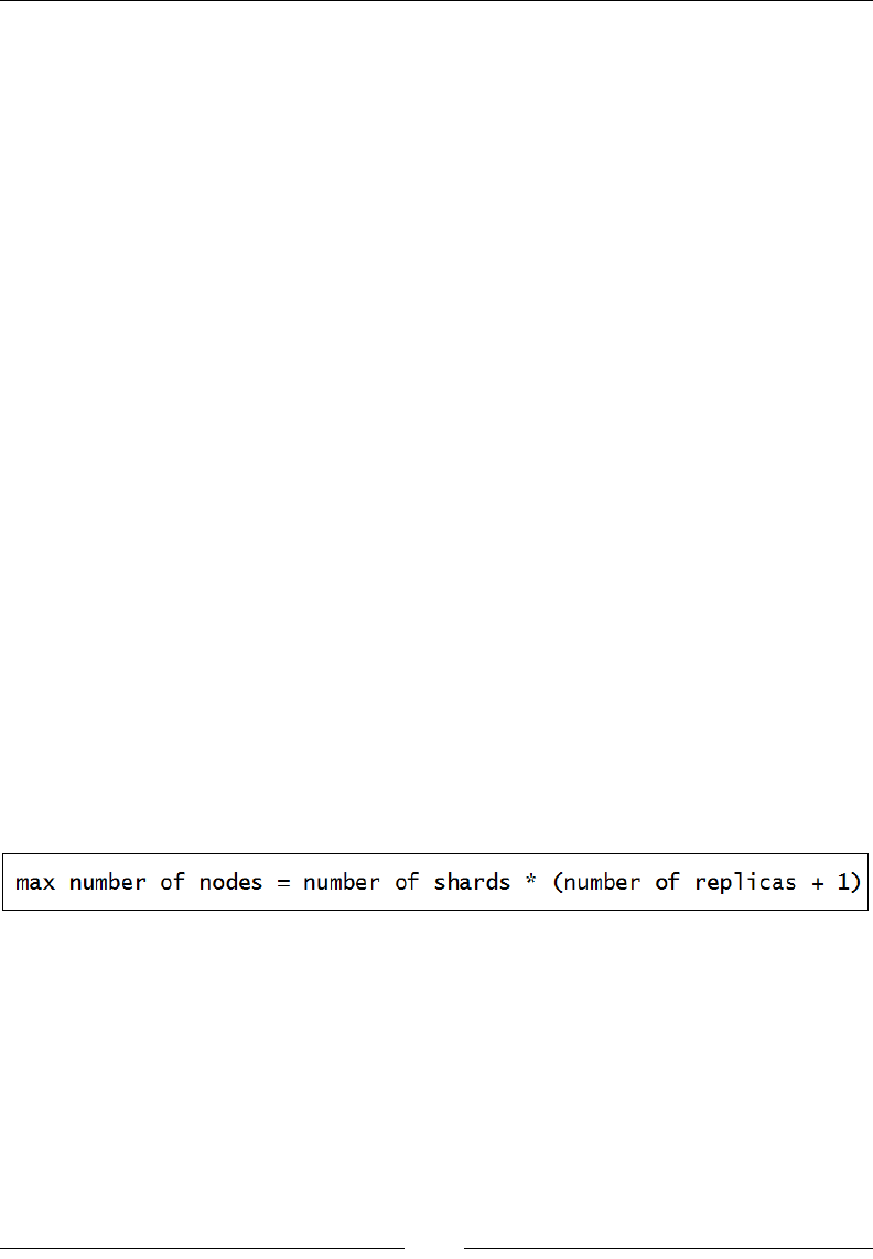
Chapter 5
[ 411 ]
Let's say that we have an index that is built only of a single shard. This means that if
our application grows above the capacity of a single machine, we will face a problem.
In the current version of Elasticsearch, there is no possibility of splitting the index
into multiple, smaller parts: we need to say how many shards the index should be
built of when we create that index. What we can do is prepare a new index with more
shards and reindex the data. However, such an operation requires additional time
and server resources, such as CPU time, RAM, and mass storage. When it comes to
the production environment, we don't always have the required time and mentioned
resources. On the other hand, while using overallocation, we can just add a new server
with Elasticsearch installed, and Elasticsearch will rebalance the cluster by moving
parts of the index to the new machine without the additional cost of reindexing. The
default conguration (which means ve shards and one replica) chosen by the authors
of Elasticsearch is the balance between the possibilities of growing and overhead
resulting from the need to merge results from a different shard.
The default shard number of ve is chosen for standard use cases. So now, this
question arises: when should we start with more shards or, on the contrary, try to
keep the number of shards as low as possible?
The rst answer is obvious. If you have a limited and strongly dened data set,
you can use only a single shard. If you do not, however, the rule of thumb dictates
that the optimal number of shards be dependent on the target number of nodes.
So, if you plan to use 10 nodes in the future, you need to congure the index to
have 10 shards. One important thing to remember is that for high availability and
query throughput, we should also congure replicas, and it also takes up room on
the nodes just like the normal shard. If you have one additional copy of each shard
(number_of_replicas equal to one), you end up with 20 shards—10 with the main
data and 10 with its replicas.
To sum up, our simple formula can be presented as follows:
In other words, if you have planned to use 10 shards and you like to have two replicas,
the maximum number of nodes that will hold the data for this setup will be 30.

The Index Distribution Architecture
[ 412 ]
A positive example of overallocation
If you carefully read the previous part of this chapter, you will have a strong
conviction that you should use the minimal number of shards. However, sometimes,
having more shards is handy, because a shard is, in fact, an Apache Lucene index,
and more shards means that every operation executed on a single, smaller Lucene
index (especially indexing) will be faster. Sometimes, this is a good enough reason
to use many shards. Of course, there is the possible cost of splitting a query into
multiple requests to each and every shard and merge the response from it. This can
be avoided for particular types of applications where the queries are always ltered
by the concrete parameter. This is the case with multitenant systems, where every
query is run in the context of the dened user. The idea is simple; we can index the
data of this user in a single shard and use only that shard during querying. This
is in place when routing should be used (we will discuss it in detail in the Routing
explained section in this chapter).
Multiple shards versus multiple indices
You may wonder whether, if a shard is the de-facto of a small Lucene index, what
about true Elasticsearch indices? What is the difference between having multiple
small shards and having multiple indices? Technically, the difference is not that
great and, for some use cases, having more than a single index is the right approach
(for example, to store time-based data such as logs in time-sliced indices). When you
are using a single index with many shards, you can limit your operations to a single
shard when using routing, for example. When dealing with indices, you may choose
which data you are interested in; for example, choose only a few of your time-
based indices using the logs_2014-10-10,logs_2014-10-11,... notation. More
differences can be spotted in the shard and index-balancing logic, although we can
congure both balancing logics.
Replicas
While sharding lets us store more data than we can t on a single node, replicas are
there to handle increasing throughput and, of course, for high availability and fault
tolerance. When a node with the primary shard is lost, Elasticsearch can promote
one of the available replicas to be a new primary shard. In the default conguration,
Elasticsearch creates a single replica for each of the shards in the index. However,
the number of replicas can be changed at any time using the Settings API. This is
very convenient when we are at a point where we need more query throughput;
increasing the number of replicas allows us to spread the querying load on more
machine, which basically allows us to handle more parallel queries.

Chapter 5
[ 413 ]
The drawback of using more replicas is obvious: the cost of additional space used by
additional copies of each shard, the cost of indexing on nodes that host the replicas,
and, of course, the cost of data copy between the primary shard and all the replicas.
While choosing the number of shards, you should also consider how many replicas
need to be present. If you select too many replicas, you can end up using disk space
and Elasticsearch resources, when in fact, they won't be used. On the other hand,
choosing to have none of the replicas may result in the data being lost if something
bad happens to the primary shard.
Routing explained
In the Choosing the right amount of shards and replicas section in this chapter, we
mentioned routing as a solution for the shards on which queries will be executed on
a single one. Now it's time to look closer at this functionality.
Shards and data
Usually, it is not important how Elasticsearch divides data into shards and which
shard holds the particular document. During query time, the query will be sent to
all the shards of a particular index, so the only crucial thing is to use the algorithm
that spreads our data evenly so that each shard contains similar amounts of data. We
don't want one shard to hold 99 percent of the data while the other shard holds the
rest—it is not efcient.
The situation complicates slightly when we want to remove or add a newer version
of the document. Elasticsearch must be able to determine which shard should be
updated. Although it may seem troublesome, in practice, it is not a huge problem. It
is enough to use the sharding algorithm, which will always generate the same value
for the same document identier. If we have such an algorithm, Elasticsearch will
know which shard to point to when dealing with a document.
However, there are times when it would be nice to be able to hit the same shard for
some portion of data. For example, we would like to store every book of a particular
type only on a particular shard and, while searching for that kind of book, we could
avoid searching on many shards and merging results from them. Instead, because we
know the value we used for routing, we could point Elasticsearch to the same shard
we used during indexing. This is exactly what routing does. It allows us to provide
information that will be used by Elasticsearch to determine which shard should be
used for document storage and for querying; the same routing value will always
result in the same shard. It's basically something like saying "search for documents
on the shard where you've put the documents by using the provided routing value".

The Index Distribution Architecture
[ 414 ]
Let's test routing
To show you an example that will illustrate how Elasticsearch allocates shards and
which documents are placed on the particular shard, we will use an additional
plugin. It will help us visualize what Elasticsearch did with our data. Let's install the
Paramedic plugin using the following command:
bin/plugin -install karmi/elasticsearch-paramedic
After restarting Elasticsearch, we can point our browser to http://
localhost:9200/_plugin/paramedic/index.html and we will able to see a page
with various statistics and information about indices. For our example, the most
interesting information is the cluster color that indicates the cluster state and the list
of shards and replicas next to every index.
Let's start two Elasticsearch nodes and create an index by running the
following command:
curl -XPUT 'localhost:9200/documents' -d '{
"settings": {
"number_of_replicas": 0,
"number_of_shards": 2
}
}'
We've created an index without replicas, which is built of two shards. This means that
the largest cluster can have only two nodes, and each next node cannot be lled with
data unless we increase the number of replicas (you can read about this in the Choosing
the right amount of shards and replicas section of this chapter). The next operation is to
index some documents; we will do that by using the following commands:
curl -XPUT localhost:9200/documents/doc/1 -d '{ "title" : "Document
No. 1" }'
curl -XPUT localhost:9200/documents/doc/2 -d '{ "title" : "Document
No. 2" }'
curl -XPUT localhost:9200/documents/doc/3 -d '{ "title" : "Document
No. 3" }'
curl -XPUT localhost:9200/documents/doc/4 -d '{ "title" : "Document
No. 4" }'
After that, if we would look at the installed Paramedic plugin, we would see our two
primary shards created and assigned.
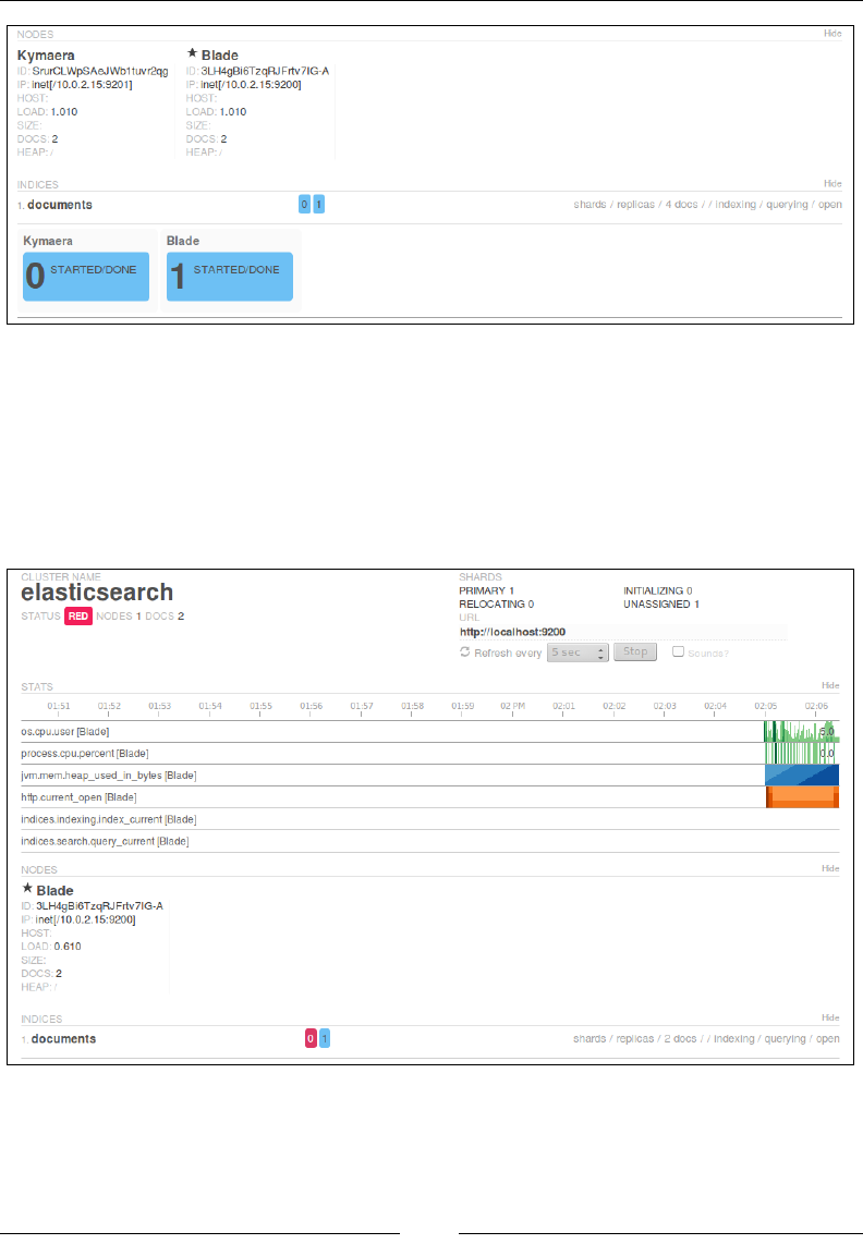
Chapter 5
[ 415 ]
In the information about nodes, we can also nd the information that we are currently
interested in. Each of the nodes in the cluster holds exactly two documents. This leads
us to the conclusion that the sharding algorithm did its work perfectly, and we have an
index that is built of shards that have evenly redistributed documents.
Now, let's create some chaos and let's shut down the second node. Now, using
Paramedic, we should see something like this:

The Index Distribution Architecture
[ 416 ]
The rst information we see is that the cluster is now in the red state. This means
that at least one primary shard is missing, which tells us that some of the data is not
available and some parts of the index are not available. Nevertheless, Elasticsearch
allows us to execute queries; it is our decision as to what applications should
do—inform the user about the possibility of incomplete results or block querying
attempts. Let's try to run a simple query by using the following command:
curl -XGET 'localhost:9200/documents/_search?pretty'
The response returned by Elasticsearch will look as follows:
{
"took" : 26,
"timed_out" : false,
"_shards" : {
"total" : 2,
"successful" : 1,
"failed" : 0
},
"hits" : {
"total" : 2,
"max_score" : 1.0,
"hits" : [ {
"_index" : "documents",
"_type" : "doc",
"_id" : "2",
"_score" : 1.0,
"_source":{ "title" : "Document No. 2" }
}, {
"_index" : "documents",
"_type" : "doc",
"_id" : "4",
"_score" : 1.0,
"_source":{ "title" : "Document No. 4" }
} ]
}
}

Chapter 5
[ 417 ]
As you can see, Elasticsearch returned the information about failures; we can see
that one of the shards is not available. In the returned result set, we can only see the
documents with identiers of 2 and 4. Other documents have been lost, at least until
the failed primary shard is back online. If you start the second node, after a while
(depending on the network and gateway module settings), the cluster should return to
the green state and all documents should be available. Now, we will try to do the same
using routing, and we will try to observe the difference in the Elasticsearch behavior.
Indexing with routing
With routing, we can control the target shard Elasticsearch will choose to send
the documents to by specifying the routing parameter. The value of the routing
parameter is irrelevant; you can use whatever value you choose. The important thing
is that the same value of the routing parameter should be used to place different
documents together in the same shard. To say it simply, using the same routing
value for different documents will ensure us that these documents will be placed in
the same shard.
There are a few possibilities as to how we can provide the routing information to
Elasticsearch. The simplest way is add the routing URI parameter when indexing a
document, for example:
curl -XPUT localhost:9200/books/doc/1?routing=A -d '{ "title" :
"Document" }'
Of course, we can also provide the routing value when using bulk indexing. In such
cases, routing is given in the metadata for each document by using the _routing
property, for example:
curl -XPUT localhost:9200/_bulk --data-binary '
{ "index" : { "_index" : "books", "_type" : "doc", "_routing" : "A"
}}
{ "title" : "Document" }
'
Another option is to place a _routing eld inside the document. However, this
will work properly only when the _routing eld is dened in the mappings.
For example, let's create an index called books_routing by using the following
command:
curl -XPUT 'localhost:9200/books_routing' -d '{
"mappings": {
"doc": {

The Index Distribution Architecture
[ 418 ]
"_routing": {
"required": true,
"path": "_routing"
},
"properties": {
"title" : {"type": "string" }
}
}
}
}'
Now we can use _routing inside the document body, for example, like this:
curl -XPUT localhost:9200/books_routing/doc/1 -d '{ "title" :
"Document", "_routing" : "A" }'
In the preceding example, we used a _routing eld. It is worth mentioning that the
path parameter can point to any eld that's not analyzed from the document. This is
a very powerful feature and one of the main advantages of the routing feature. For
example, if we extend our document with the library_id eld's indicated library
where the book is available, it is logical that all queries based on library can be more
effective when we set up routing based on this library_id eld. However, you have
to remember that getting the routing value from a eld requires additional parsing.
Routing in practice
Now let's get back to our initial example and do the same as what we did but now
using routing. The rst thing is to delete the old documents. If we do not do this and
add documents with the same identier, routing may cause that same document
to now be placed in the other shard. Therefore, we run the following command to
delete all the documents from our index:
curl -XDELETE 'localhost:9200/documents/_query?q=*:*'
After that, we index our data again, but this time, we add the routing information.
The commands used to index our documents now look as follows:
curl -XPUT localhost:9200/documents/doc/1?routing=A -d '{ "title" :
"Document No. 1" }'
curl -XPUT localhost:9200/documents/doc/2?routing=B -d '{ "title" :
"Document No. 2" }'

Chapter 5
[ 419 ]
curl -XPUT localhost:9200/documents/doc/3?routing=A -d '{ "title" :
"Document No. 3" }'
curl -XPUT localhost:9200/documents/doc/4?routing=A -d '{ "title" :
"Document No. 4" }'
As we said, the routing parameter tells Elasticsearch in which shard the document
should be placed. Of course, it may happen that more than a single document will be
placed in the same shard. That's because you usually have less shards than routing
values. If we now kill one node, Paramedic will again show you the red cluster and
the state. If we query for all the documents, Elasticsearch will return the following
response (of course, it depends which node you kill):
curl -XGET 'localhost:9200/documents/_search?q=*&pretty'
The response from Elasticsearch would be as follows:
{
"took" : 24,
"timed_out" : false,
"_shards" : {
"total" : 2,
"successful" : 1,
"failed" : 0
},
"hits" : {
"total" : 3,
"max_score" : 1.0,
"hits" : [ {
"_index" : "documents",
"_type" : "doc",
"_id" : "1",
"_score" : 1.0,
"_source":{ "title" : "Document No. 1" }
}, {
"_index" : "documents",
"_type" : "doc",
"_id" : "3",
"_score" : 1.0,
"_source":{ "title" : "Document No. 3" }
}, {
"_index" : "documents",
"_type" : "doc",
"_id" : "4",
"_score" : 1.0,

The Index Distribution Architecture
[ 420 ]
"_source":{ "title" : "Document No. 4" }
} ]
}
}
In our case, the document with the identier 2 is missing. We lost a node with the
documents that had the routing value of B. If we were less lucky, we could lose
three documents!
Querying
Routing allows us to tell Elasticsearch which shards should be used for querying.
Why send queries to all the shards that build the index if we want to get data from
a particular subset of the whole index? For example, to get the data from a shard
where routing A was used, we can run the following query:
curl -XGET 'localhost:9200/documents/_search?pretty&q=*&routing=A'
We just added a routing parameter with the value we are interested in. Elasticsearch
replied with the following result:
{
"took" : 0,
"timed_out" : false,
"_shards" : {
"total" : 1,
"successful" : 1,
"failed" : 0
},
"hits" : {
"total" : 3,
"max_score" : 1.0,
"hits" : [ {
"_index" : "documents",
"_type" : "doc",
"_id" : "1",
"_score" : 1.0, "_source" : { "title" : "Document No. 1" }
}, {
"_index" : "documents",
"_type" : "doc",
"_id" : "3",
"_score" : 1.0, "_source" : { "title" : "Document No. 3" }
}, {
"_index" : "documents",

Chapter 5
[ 421 ]
"_type" : "doc",
"_id" : "4",
"_score" : 1.0, "_source" : { "title" : "Document No. 4" }
} ]
}
}
Everything works like a charm. But look closer! We forgot to start the node that
holds the shard with the documents that were indexed with the routing value of B.
Even though we didn't have a full index view, the reply from Elasticsearch doesn't
contain information about shard failures. This is proof that queries with routing hit
only a chosen shard and ignore the rest. If we run the same query with routing=B,
we will get an exception like the following one:
{
"error" : "SearchPhaseExecutionException[Failed to execute phase
[query_fetch], all shards failed]",
"status" : 503
}
We can test the preceding behavior by using the Search Shard API. For example, let's
run the following command:
curl -XGET 'localhost:9200/documents/_search_shards?pretty&routing=A'
-d '{"query":"match_all":{}}'
The response from Elasticsearch would be as follows:
{
"nodes" : {
"QK5r_d5CSfaV1Wx78k633w" : {
"name" : "Western Kid",
"transport_address" : "inet[/10.0.2.15:9301]"
}
},
"shards" : [ [ {
"state" : "STARTED",
"primary" : true,
"node" : "QK5r_d5CSfaV1Wx78k633w",
"relocating_node" : null,
"shard" : 0,
"index" : "documents"
} ] ]
}
As we can see, only a single node will be queried.

The Index Distribution Architecture
[ 422 ]
There is one important thing that we would like to repeat. Routing ensures us
that, during indexing, documents with the same routing value are indexed in the
same shard. However, you need to remember that a given shard may have many
documents with different routing values. Routing allows you to limit the number of
shards used during queries, but it cannot replace ltering! This means that a query
with routing and without routing should have the same set of lters. For example, if
we use user identiers as routing values if we search for that user's data, we should
also include lters on that identier.
Aliases
If you work as a search engine specialist, you probably want to hide some
conguration details from programmers in order to allow them to work faster and
not care about search details. In an ideal world, they should not worry about routing,
shards, and replicas. Aliases allow us to use shards with routing as ordinary indices.
For example, let's create an alias by running the following command:
curl -XPOST 'http://localhost:9200/_aliases' -d '{
"actions" : [
{
"add" : {
"index" : "documents",
"alias" : "documentsA",
"routing" : "A"
}
}
]
}'
In the preceding example, we created a named documentsA alias from the documents
index. However, in addition to that, searching will be limited to the shard used when
routing value A is used. Thanks to this approach, you can give information about the
documentsA alias to developers, and they may use it for querying and indexing like
any other index.

Chapter 5
[ 423 ]
Multiple routing values
Elasticsearch gives us the possibility to search with several routing values in a single
query. Depending on which shard documents with given routing values are placed,
it could mean searching on one or more shards. Let's look at the following query:
curl -XGET 'localhost:9200/documents/_search?routing=A,B'
After executing it, Elasticsearch will send the search request to two shards in our
index (which in our case, happens to be the whole index), because the routing value
of A covers one of two shards of our index and the routing value of B covers the
second shard of our index.
Of course, multiple routing values are supported in aliases as well. The following
example shows you the usage of these features:
curl -XPOST 'http://localhost:9200/_aliases' -d '{
"actions" : [
{
"add" : {
"index" : "documents",
"alias" : "documentsA",
"search_routing" : "A,B",
"index_routing" : "A"
}
}
]
}'
The preceding example shows you two additional conguration parameters we
didn't talk about until now—we can dene different values of routing for searching
and indexing. In the preceding case, we've dened that during querying (the
search_routing parameter) two values of routing (A and B) will be applied. When
indexing (index_routing parameter), only one value (A) will be used. Note that
indexing doesn't support multiple routing values, and you should also remember
proper ltering (you can add it to your alias).
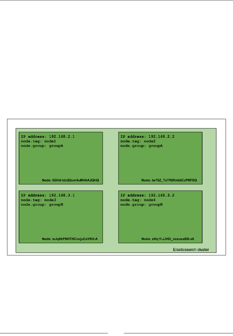
The Index Distribution Architecture
[ 424 ]
Altering the default shard allocation
behavior
In Elasticsearch Server Second Edition, published by Packt Publishing, we talked
about a number of things related to the shard allocation functionality provided by
Elasticsearch. We discussed the Cluster Reroute API, shard rebalancing, and shard
awareness. Although now very commonly used, these topics are very important
if you want to be in full control of your Elasticsearch cluster. Because of that, we
decided to extend the examples provided in Elasticsearch Server Second Edition and
provide you with guidance on how to use Elasticsearch shards awareness and alter
the default shard allocation mechanism.
Let's start with a simple example. We assume that we have a cluster built of four
nodes that looks as follows:
As you can see, our cluster is built of four nodes. Each node was bound to a specic
IP address, and each node was given the tag property and a group property (added
to elasticsearch.yml as node.tag and node.group properties). This cluster will
serve the purpose of showing you how shard allocation ltering works. The group
and tag properties can be given whatever names you want; you just need to prex
your desired property name with the node name; for example, if you would like
to use a party property name, you would just add node.party: party1 to your
elasticsearch.yml le.
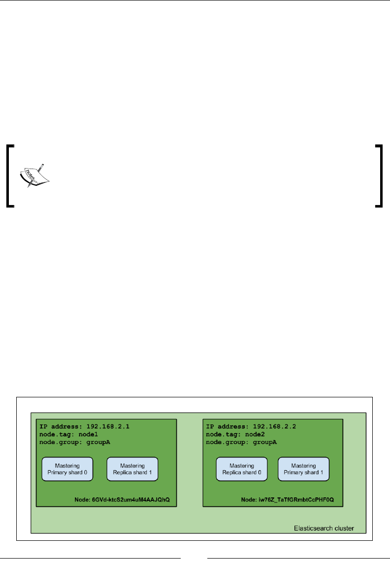
Chapter 5
[ 425 ]
Allocation awareness
Allocation awareness allows us to congure shards and their replicas' allocation
with the use of generic parameters. In order to illustrate how allocation awareness
works, we will use our example cluster. For the example to work, we should add the
following property to the elasticsearch.yml le:
cluster.routing.allocation.awareness.attributes: group
This will tell Elasticsearch to use the node.group property as the
awareness parameter.
One can specify multiple attributes when setting the cluster.routing.
allocation.awareness.attributes property, for example:
cluster.routing.allocation.awareness.attributes:
group,
node
After this, let's start the rst two nodes, the ones with the node.group parameter
equal to groupA, and let's create an index by running the following command:
curl -XPOST 'localhost:9200/mastering' -d '{
"settings" : {
"index" : {
"number_of_shards" : 2,
"number_of_replicas" : 1
}
}
}'
After this command, our two nodes' cluster will look more or less like this:
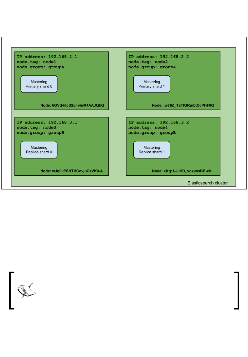
The Index Distribution Architecture
[ 426 ]
As you can see, the index was divided evenly between two nodes. Now let's
see what happens when we launch the rest of the nodes (the ones with node.group
set to groupB):
Notice the difference: the primary shards were not moved from their original
allocation nodes, but the replica shards were moved to the nodes with a different
node.group value. That's exactly right—when using shard allocation awareness,
Elasticsearch won't allocate shards and replicas to the nodes with the same value
of the property used to determine the allocation awareness (which, in our case, is
node.group). One of the example usages of this functionality is to divide the cluster
topology between virtual machines or physical locations in order to be sure that you
don't have a single point of failure.
Please remember that when using allocation awareness, shards will
not be allocated to the node that doesn't have the expected attributes
set. So, in our example, a node without the node.group property set
will not be taken into consideration by the allocation mechanism.

Chapter 5
[ 427 ]
Forcing allocation awareness
Forcing allocation awareness can come in handy when we know, in advance, how
many values our awareness attributes can take, and we don't want more replicas
than needed to be allocated in our cluster, for example, not to overload our cluster
with too many replicas. To do this, we can force allocation awareness to be active
only for certain attributes. We can specify these values using the cluster.routing.
allocation.awareness.force.zone.values property and providing a list of
comma-separated values to it. For example, if we would like allocation awareness to
only use the groupA and groupB values of the node.group property, we would add
the following to the elasticsearch.yml le:
cluster.routing.allocation.awareness.attributes: group
cluster.routing.allocation.awareness.force.zone.values: groupA,
groupB
Filtering
Elasticsearch allows us to congure the allocation for the whole cluster or for the
index level. In the case of cluster allocation, we can use the properties prexes:
• cluster.routing.allocation.include
• cluster.routing.allocation.require
• cluster.routing.allocation.exclude
When it comes to index-specic allocation, we can use the following
properties prexes:
• index.routing.allocation.include
• index.routing.allocation.require
• index.routing.allocation.exclude
The previously mentioned prexes can be used with the properties that we've
dened in the elasticsearch.yml le (our tag and group properties) and with a
special property called _ip that allows us to match or exclude IPs using nodes' IP
address, for example, like this:
cluster.routing.allocation.include._ip: 192.168.2.1
If we would like to include nodes with a group property matching the groupA value,
we would set the following property:
cluster.routing.allocation.include.group: groupA
Notice that we've used the cluster.routing.allocation.include prex, and
we've concatenated it with the name of the property, which is group in our case.

The Index Distribution Architecture
[ 428 ]
What include, exclude, and require mean
If you look closely at the parameters mentioned previously, you would notice that
there are three kinds:
• include: This type will result in the inclusion of all the nodes with this
parameter dened. If multiple include conditions are visible, then all
the nodes that match at least one of these conditions will be taken into
consideration when allocating shards. For example, if we would add
two cluster.routing.allocation.include.tag parameters to our
conguration, one with a property to the value of node1 and the second with
the node2 value, we would end up with indices (actually, their shards) being
allocated to the rst and second node (counting from left to right). To sum
up, the nodes that have the include allocation parameter type will be taken
into consideration by Elasticsearch when choosing the nodes to place shards
on, but that doesn't mean that Elasticsearch will put shards on them.
• require: This was introduced in the Elasticsearch 0.90 type of allocation
lter, and it requires all the nodes to have the value that matches the value
of this property. For example, if we would add one cluster.routing.
allocation.require.tag parameter to our conguration with the value of
node1 and a cluster.routing.allocation.require.group parameter, the
value of groupA would end up with shards allocated only to the rst node
(the one with the IP address of 192.168.2.1).
• exclude: This allows us to exclude nodes with given properties from the
allocation process. For example, if we set cluster.routing.allocation.
include.tag to groupA, we would end up with indices being allocated only
to nodes with IP addresses 192.168.3.1 and 192.168.3.2 (the third and
fourth node in our example).
Property values can use simple wildcard characters. For example, if
we would like to include all the nodes that have the group parameter
value beginning with group, we could set the cluster.routing.
allocation.include.group property to group*. In the example
cluster case, it would result in matching nodes with the groupA and
groupB group parameter values.
Runtime allocation updating
In addition to setting all discussed properties in the elasticsearch.yml le, we
can also use the update API to update these settings in real-time when the cluster is
already running.

Chapter 5
[ 429 ]
Index level updates
In order to update settings for a given index (for example, our mastering index), we
could run the following command:
curl -XPUT 'localhost:9200/mastering/_settings' -d '{
"index.routing.allocation.require.group": "groupA"
}'
As you can see, the command was sent to the _settings end-point for a given index.
You can include multiple properties in a single call.
Cluster level updates
In order to update settings for the whole cluster, we could run the following
command:
curl -XPUT 'localhost:9200/_cluster/settings' -d '{
"transient" : {
"cluster.routing.allocation.require.group": "groupA"
}
}'
As you can see, the command was sent to the cluster/_settings end-point. You
can include multiple properties in a single call. Please remember that the transient
name in the preceding command means that the property will be forgotten after the
cluster restart. If you want to avoid this and set this property as a permanent one,
use persistent instead of the transient one. An example command, which will
keep the settings between restarts, could look like this:
curl -XPUT 'localhost:9200/_cluster/settings' -d '{
"persistent" : {
"cluster.routing.allocation.require.group": "groupA"
}
}'
Please note that running the preceding commands, depending on
the command and where your indices are located, can result in
shards being moved between nodes.

The Index Distribution Architecture
[ 430 ]
Dening total shards allowed per node
In addition to the previously mentioned properties, we are also allowed to dene
how many shards (primaries and replicas) for an index can by allocated per node. In
order to do that, one should set the index.routing.allocation.total_shards_
per_node property to a desired value. For example, in elasticsearch.yml we
could set this:
index.routing.allocation.total_shards_per_node: 4
This would result in a maximum of four shards per index being allocated to a
single node.
This property can also be updated on a live cluster using the Update API, for
example, like this:
curl -XPUT 'localhost:9200/mastering/_settings' -d '{
"index.routing.allocation.total_shards_per_node": "4"
}'
Now, let's see a few examples of what the cluster would look like when creating a
single index and having the allocation properties used in the elasticsearch.yml le.
Dening total shards allowed per physical
server
One of the properties that can be useful when having multiple nodes on a single
physical server is cluster.routing.allocation.same_shard.host. When set
to true, it prevents Elasticsearch from placing a primary shard and its replica (or
replicas) on the same physical host. We really advise that you set this property to
true if you have very powerful servers and that you go for multiple Elasticsearch
nodes per physical server.
Inclusion
Now, let's use our example cluster to see how the allocation inclusion works.
Let's start by deleting and recreating the mastering index by using the
following commands:
curl -XDELETE 'localhost:9200/mastering'
curl -XPOST 'localhost:9200/mastering' -d '{
"settings" : {
"index" : {
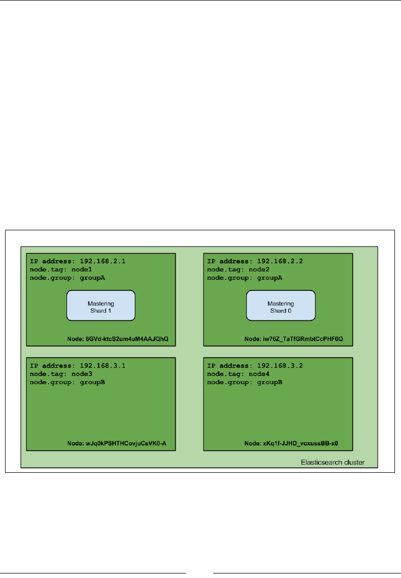
Chapter 5
[ 431 ]
"number_of_shards" : 2,
"number_of_replicas" : 0
}
}
}'
After this, let's try to run the following command:
curl -XPUT 'localhost:9200/mastering/_settings' -d '{
"index.routing.allocation.include.tag": "node1",
"index.routing.allocation.include.group": "groupA",
"index.routing.allocation.total_shards_per_node": 1
}'
If we visualize the response of the index status, we would see that the cluster looks
like the one in the following image:
As you can see, the mastering index shards are allocated to nodes with the tag
property set to node1 or the group property set to groupA.
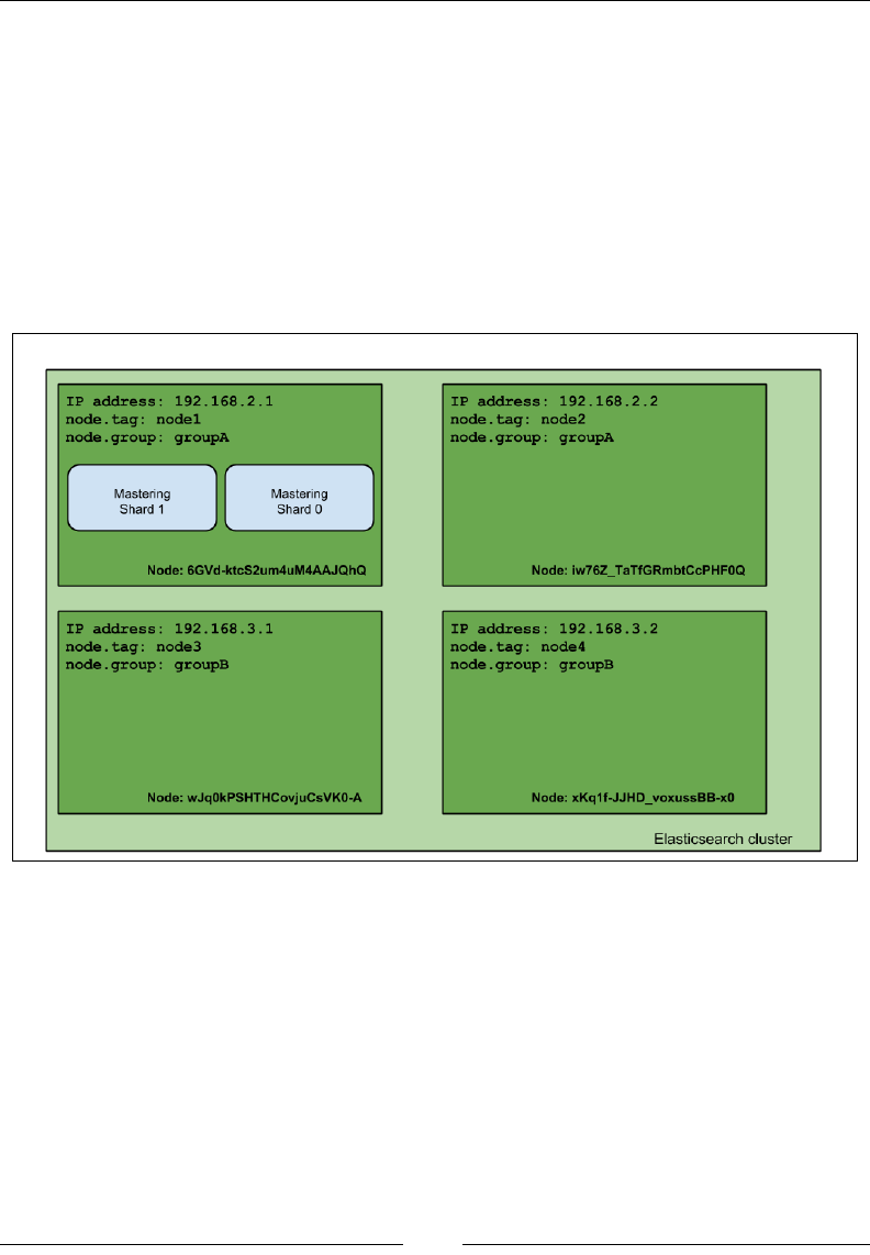
The Index Distribution Architecture
[ 432 ]
Requirement
Now, let's reuse our example cluster and try running the following command:
curl -XPUT 'localhost:9200/mastering/_settings' -d '{
"index.routing.allocation.require.tag": "node1",
"index.routing.allocation.require.group": "groupA"
}'
If we visualize the response of the index status command, we would see that the
cluster looks like this:
As you can see, the view is different than the one when using include. This is
because we tell Elasticsearch to allocate shards of the mastering index only to the
nodes that match both the require parameters, and in our case, the only node that
matches both is the rst node.
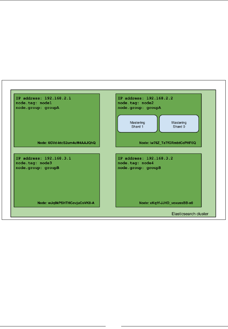
Chapter 5
[ 433 ]
Exclusion
Let's now look at exclusions. To test it, we try to run the following command:
curl -XPUT 'localhost:9200/mastering/_settings' -d '{
"index.routing.allocation.exclude.tag": "node1",
"index.routing.allocation.require.group": "groupA"
}'
Again, let's look at our cluster now:
As you can see, we said that we require the group property to be equal to groupA,
and we want to exclude the node with a tag equal to node1. This resulted in the
shard of the mastering index being allocated to the node with the 192.168.2.2 IP
address, which is what we wanted.
Disk-based allocation
Of course, the mentioned properties are not the only ones that can be used. With the
release of Elasticsearch 1.3.0 we got the ability to congure awareness on the basis of
the disk usage. By default, disk-based allocation is turned on, and if we want, we can
turn it off by setting the cluster.routing.allocation.disk.threshold_enabled
property to false.
The Index Distribution Architecture
[ 434 ]
There are three additional properties that can help us congure disk-based
allocation. The cluster.routing.allocation.disk.watermark.low cluster
controls when Elasticsearch does not allow you to allocate new shards on the node.
By default, it is set to 85 percent and it means that when the disk usage is equal or
higher than 85 percent, no new shards will be allocated on that node. The second
property is cluster.routing.allocation.disk.watermark.high, which controls
when Elasticsearch will try to move the shards out of the node and is set to 90
percent by default. This means that Elasticsearch will try to move the shard out of
the node if the disk usage is 90 percent or higher.
Both cluster.routing.allocation.disk.watermark.low and cluster.routing.
allocation.disk.watermark.high can be set to absolute values, for example, 1024mb.
Query execution preference
Let's forget about the shard placement and how to congure it—at least for a
moment. In addition to all the fancy stuff that Elasticsearch allows us to set for
shards and replicas, we also have the possibility to specify where our queries
(and other operations, for example, the real-time GET) should be executed.
Before we get into the details, let's look at our example cluster:

Chapter 5
[ 435 ]
As you can see, we have three nodes and a single index called mastering. Our index
is divided into two primary shards, and there is one replica for each primary shard.
Introducing the preference parameter
In order to control where the query (and other operations) we are sending will be
executed, we can use the preference parameter, which can be set to one of the
following values:
• _primary: Using this property, the operations we are sending will only be
executed on primary shards. So, if we send a query against mastering index
with the preference parameter set to the _primary value, we would have it
executed on the nodes with the names node1 and node2. For example, if you
know that your primary shards are in one rack and the replicas are in other
racks, you may want to execute the operation on primary shards to avoid
network trafc.
• _primary_first: This option is similar to the _primary value's behavior but
with a failover mechanism. If we ran a query against the mastering index
with the preference parameter set to the _primary_first value, we would
have it executed on the nodes with the names node1 and node2; however, if
one (or more) of the primary shards fails, the query will be executed against
the other shard, which in our case is allocated to a node named node3. As we
said, this is very similar to the _primary value but with additional fallback to
replicas if the primary shard is not available for some reason.
• _local: Elasticsearch will prefer to execute the operation on a local node,
if possible. For example, if we send a query to node3 with the preference
parameter set to _local, we would end up having that query executed
on that node. However, if we send the same query to node2, we would
end up with one query executed against the primary shard numbered 1
(which is located on that node) and the second part of the query will be
executed against node1 or node3 where the shard numbered 0 resides. This
is especially useful while trying to minimize the network latency; while
using the _local preference, we ensure that our queries are executed locally
whenever possible (for example, when running a client connection from a
local node or sending a query to a node).

The Index Distribution Architecture
[ 436 ]
• _only_node:wJq0kPSHTHCovjuCsVK0-A: This operation will be
only executed against a node with the provided identier (which is
wJq0kPSHTHCovjuCsVK0-A in this case). So in our case, the query would be
executed against two replicas located on node3. Please remember that if there
aren't enough shards to cover all the index data, the query will be executed
against only the shard available in the specied node. For example, if we set
the preference parameter to _only_node:6GVd-ktcS2um4uM4AAJQhQ, we
would end up having our query executed against a single shard. This can be
useful for examples where we know that one of our nodes is more powerful
than the other ones and we want some of the queries to be executed only on
that node.
• _prefer_node:wJq0kPSHTHCovjuCsVK0-A: This option sets the preference
parameter to _prefer_node: the value followed by a node identier
(which is wJq0kPSHTHCovjuCsVK0-A in our case) will result in Elasticsearch
preferring the mentioned node while executing the query, but if some
shards are not available on the preferred node, Elasticsearch will send the
appropriate query parts to nodes where the shards are available. Similar
to the _only_node option, _prefer_node can be used while choosing a
particular node, with a fall back to other nodes, however.
• _shards:0,1: This is the preference value that allows us to identify which
shards the operation should be executed against (in our case, it will be all the
shards, because we only have shards 0 and 1 in the mastering index). This
is the only preference parameter value that can be combined with the other
mentioned values. For example, in order to locally execute our query against
the 0 and 1 shard, we should concatenate the 0,1 value with _local using the
; character, so the nal value of the preference parameter should look like
this: 0,1;_local. Allowing us to execute the operation against a single shard
can be useful for diagnosis purposes.
• custom, string value: Setting the _preference parameter to a custom
value will guarantee that the query with the same custom value will be
executed against the same shards. For example, if we send a query with the _
preference parameter set to the mastering_elasticsearch value, we would
end up having the query executed against primary shards located on nodes
named node1 and node2. If we send another query with the same preference
parameter value, then the second query will again be executed against the
shards located on nodes named node1 and node2. This functionality can
help us in cases where we have different refresh rates and we don't want our
users to see different results while repeating requests. There is one more thing
missing, which is the default behavior. What Elasticsearch will do by default
is that it will randomize the operation between shards and replicas. If we sent
many queries, we would end up having the same (or almost the same) number
of queries run against each of the shards and replicas.

Chapter 5
[ 437 ]
Summary
In this chapter, we talked about general shards and the index architecture. We chose
the right amount of shards and replicas for our deployment, and we used routing
during indexing and querying and in conjunction with aliases. We also discussed
shard-allocation behavior adjustments, and nally, we looked at what query
execution preference can bring us.
In the next chapter, we will take a deeper look, altering the Apache Lucene scoring
mechanism by providing different similarity models. We will adjust our inverted
index format by using codecs. We will discuss near real-time indexing and querying,
ush and refresh operations, and transaction log conguration. We will talk about
throttling and segment merges. Finally, we will discuss Elasticsearch caching—eld
data, lter, and query shard caches.

Low-level Index Control
In the previous chapter, we talked about general shards and the index architecture.
We started by learning how to choose the right amount of shards and replicas, and
we used routing during indexing and querying, and in conjunction with aliases. We
also discussed shard allocation behavior adjustments, and nally, we looked at what
query execution preference can bring us.
In this chapter, we will take a deeper dive into more low-level aspects of handling
shards in Elasticsearch. By the end of this chapter, you will have learned:
• Altering the Apache Lucene scoring by using different similarity models
• Altering index writing by using codes
• Near real-time indexing and querying
• Data ushing, index refresh, and transaction log handling
• I/O throttling
• Segment merge control and visualization
• Elasticsearch caching
Altering Apache Lucene scoring
With the release of Apache Lucene 4.0 in 2012, all the users of this great full text
search library were given the opportunity to alter the default TF/IDF-based
algorithm. The Lucene API was changed to allow easier modication and extension
of the scoring formula. However, this was not the only change that was made to
Lucene when it comes to documents' score calculation. Lucene 4.0 was shipped with
additional similarity models, which basically allows us to use a different scoring
formula for our documents. In this section, we will take a deeper look at what
Lucene 4.0 brings and how these features were incorporated into Elasticsearch.

Low-level Index Control
[ 440 ]
Available similarity models
As already mentioned, the original and default similarity model available before
Apache Lucene 4.0 was the TF/IDF model. We already discussed it in detail in the
Default Apache Lucene scoring explained section in Chapter 2, Power User Query DSL.
The ve new similarity models that we can use are:
• Okapi BM25: This similarity model is based on a probabilistic model that
estimates the probability of nding a document for a given query. In order
to use this similarity in Elasticsearch, you need to use the BM25 name. The
Okapi BM25 similarity is said to perform best when dealing with short
text documents where term repetitions are especially hurtful to the overall
document score.
• Divergence from randomness (DFR): This similarity model is based on
the probabilistic model of the same name. In order to use this similarity in
Elasticsearch, you need to use the DFR name. It is said that the divergence
from the randomness similarity model performs well on text similar to
natural language text.
• Information-based: This is very similar to the model used by Divergence
from randomness. In order to use this similarity in Elasticsearch, you need to
use the IB name. Similar to the DFR similarity, it is said that the information-
based model performs well on data similar to natural language text.
• LM Dirichlet: This similarity model uses Bayesian smoothing with Dirichlet
priors. To use this similarity, we need to use the LMDirichlet name.
More information about it can be found at https://lucene.apache.
org/core/4_9_0/core/org/apache/lucene/search/similarities/
LMDirichletSimilarity.html.
• LM Jelinek Mercer: This similarity model is based on the Jelinek
Mercer smoothing method. To use this similarity, we need to use the
LMJelinekMercer name. More information about it can be found at
https://lucene.apache.org/core/4_9_0/core/org/apache/lucene/
search/similarities/LMJelinekMercerSimilarity.html.
All the mentioned similarity models require mathematical knowledge
to fully understand them and a deep explanation of these models is far
beyond the scope of this book. However, if you would like to explore
these models and increase your knowledge about them, please go to
http://en.wikipedia.org/wiki/Okapi_BM25 for the Okapi
BM25 similarity and http://terrier.org/docs/v3.5/dfr_
description.html for divergence from the randomness similarity.

Chapter 6
[ 441 ]
Setting a per-eld similarity
Since Elasticsearch 0.90, we are allowed to set a different similarity for each of
the elds we have in our mappings. For example, let's assume that we have the
following simple mappings that we use in order to index blog posts (stored in the
posts_no_similarity.json le):
{
"mappings" : {
"post" : {
"properties" : {
"id" : { "type" : "long", "store" : "yes" },
"name" : { "type" : "string", "store" : "yes", "index" :
"analyzed" },
"contents" : { "type" : "string", "store" : "no", "index" :
"analyzed" }
}
}
}
}
What we would like to do is use the BM25 similarity model for the name eld and the
contents eld. In order to do this, we need to extend our eld denitions and add
the similarity property with the value of the chosen similarity name. Our changed
mappings (stored in the posts_similarity.json le) would look like this:
{
"mappings" : {
"post" : {
"properties" : {
"id" : { "type" : "long", "store" : "yes" },
"name" : { "type" : "string", "store" : "yes", "index" :
"analyzed", "similarity" : "BM25" },
"contents" : { "type" : "string", "store" : "no", "index" :
"analyzed", "similarity" : "BM25" }
}
}
}
}
That's all; nothing more is needed. After the preceding change, Apache Lucene will
use the BM25 similarity to calculate the score factor for the name and contents elds.

Low-level Index Control
[ 442 ]
Please note that in the case of the Divergence from randomness and
Information-based similarities, we need to congure some additional
properties to specify these similarities' behavior. How to do that is
covered in the next part of the current section.
Similarity model conguration
As we now know how to set the desired similarity for each eld in our index, it's
time to see how to congure them if we need them, which is actually pretty easy.
What we need to do is use the index settings section to provide an additional
similarity section, for example, like this (this example is stored in the posts_custom_
similarity.json le):
{
"settings" : {
"index" : {
"similarity" : {
"mastering_similarity" : {
"type" : "default",
"discount_overlaps" : false
}
}
}
},
"mappings" : {
"post" : {
"properties" : {
"id" : { "type" : "long", "store" : "yes" },
"name" : { "type" : "string", "store" : "yes", "index" :
"analyzed", "similarity" : "mastering_similarity" },
"contents" : { "type" : "string", "store" : "no", "index" :
"analyzed" }
}
}
}
}
You can, of course, have more than one similarity conguration, but let's focus on
the preceding example. We've dened a new similarity model named mastering_
similarity, which is based on the default similarity, which is the TF/IDF one.
We've set the discount_overlaps property to false for this similarity, and we've
used it as the similarity for the name eld. We'll talk about what properties can be
used for different similarities further in this section. Now, let's see how to change the
default similarity model Elasticsearch will use.

Chapter 6
[ 443 ]
Choosing the default similarity model
In order to change the similarity model used by default, we need to provide a
conguration of a similarity model that will be called default. For example, if we
would like to use our mastering_similarity "name" as the default one, we would
have to change the preceding conguration to the following one (the whole example
is stored in the posts_default_similarity.json le):
{
"settings" : {
"index" : {
"similarity" : {
"default" : {
"type" : "default",
"discount_overlaps" : false
}
}
}
},
...
}
Because of the fact that the query norm and coordination factors (which were
explained in the Default Apache Lucene scoring explained section in Chapter 2, Power
User Query DSL) are used by all similarity models globally and are taken from the
default similarity, Elasticsearch allows us to change them when needed. To do this,
we need to dene another similarity—one called base. It is dened exactly the same
as what we've shown previously, but instead of setting its name to default, we set it
to base, just like this (the whole example is stored in the posts_base_similarity.
json le):
{
"settings" : {
"index" : {
"similarity" : {
"base" : {
"type" : "default",
"discount_overlaps" : false
}
}
}
},
...
}

Low-level Index Control
[ 444 ]
If the base similarity is present in the index conguration, Elasticsearch will use it
to calculate the query norm and coord factors when calculating the score using other
similarity models.
Conguring the chosen similarity model
Each of the newly introduced similarity models can be congured to match our
needs. Elasticsearch allows us to use the default and BM25 similarities without any
conguration, because they are precongured for us. In the case of DFR and IB, we
need to provide the conguration in order to use them. Let's now see what properties
each of the similarity models' implementation provides.
Conguring the TF/IDF similarity
In the case of the TF/IDF similarity, we are allowed to set only a single parameter—
discount_overlaps, which defaults to true. By default, the tokens that have their
position increment set to 0 (and therefore, are placed at the same position as the one
before them) will not be taken into consideration when calculating the score. If we
want them to be taken into consideration, we need to congure the similarity with
the discount_overlaps property set to false.
Conguring the Okapi BM25 similarity
In the case of the Okapi BM25 similarity, we have these parameters: we can congure
k1 (controls the saturation—nonlinear term frequency normalization) as a oat value, b
(controls how the document length affects the term frequency values) as a oat value,
and discount_overlaps, which is exactly the same as in TF/IDF similarity.
Conguring the DFR similarity
In the case of the DFR similarity, we have these parameters that we can congure:
basic_model (which can take the value be, d, g, if, in, or ine), after_effect (with
values of no, b, and l), and the normalization (which can be no, h1, h2, h3, or z). If
we choose a normalization other than no, we need to set the normalization factor.
Depending on the chosen normalization, we should use normalization.h1.c (the
oat value) for the h1 normalization, normalization.h2.c (the oat value) for the
h2 normalization, normalization.h3.c (the oat value) for the h3 normalization,
and normalization.z.z (the oat value) for the z normalization. For example, this
is what the example similarity conguration could look like:
"similarity" : {
"esserverbook_dfr_similarity" : {
"type" : "DFR",
"basic_model" : "g",

Chapter 6
[ 445 ]
"after_effect" : "l",
"normalization" : "h2",
"normalization.h2.c" : "2.0"
}
}
Conguring the IB similarity
In the case of the IB similarity, we have these parameters that we can congure:
the distribution property (which can take the value of ll or spl) and the lambda
property (which can take the value of df or tff). In addition to this, we can choose the
normalization factor, which is the same as the one used for the DFR similarity, so
we'll omit describing it for the second time. This is what the example IB similarity
conguration could look like:
"similarity" : {
"esserverbook_ib_similarity" : {
"type" : "IB",
"distribution" : "ll",
"lambda" : "df",
"normalization" : "z",
"normalization.z.z" : "0.25"
}
}
Conguring the LM Dirichlet similarity
In the case of the LM Dirichlet similarity, we have the mu property that we can
congure the mu property, which is by default set to 2000. An example conguration
of this could look as follows:
"similarity" : {
"esserverbook_lm_dirichlet_similarity" : {
"type" : "LMDirichlet",
"mu" : "1000"
}
}
Conguring the LM Jelinek Mercer similarity
When it comes to the LM Jelinek Mercer similarity, we can congure the lambda
property, which is set to 0.1 by default. An example conguration of this could look
as follows:
"similarity" : {
"esserverbook_lm_jelinek_mercer_similarity" : {
"type" : "LMJelinekMercer",

Low-level Index Control
[ 446 ]
"lambda" : "0.7"
}
}
It is said that for short elds (like the document title) the
optimal lambda value is around 0.1, while for long elds
the lambda should be set to 0.7.
Choosing the right directory
implementation – the store module
The store module is one of the modules that we usually don't pay much attention
to when conguring our cluster; however, it is very important. It is an abstraction
between the I/O subsystem and Apache Lucene itself. All the operation that Lucene
does with the hard disk drive is done using the store module. Most of the store
types in Elasticsearch are mapped to an appropriate Apache Lucene Directory class
(http://lucene.apache.org/core/4_9_0/core/org/apache/lucene/store/
Directory.html). The directory is used to access all the les the index is built of, so
it is crucial to properly congure it.
The store type
Elasticsearch exposes ve store types that we can use. Let's see what they provide
and how we can leverage their features.
The simple lesystem store
The simplest implementation of the Directory class that is available is implemented
using a random access le (Java RandomAccessFile—http://docs.oracle.
com/javase/7/docs/api/java/io/RandomAccessFile.html) and maps to
SimpleFSDirectory (http://lucene.apache.org/core/4_9_0/core/org/
apache/lucene/store/SimpleFSDirectory.html) in Apache Lucene. It is
sufcient for very simple applications. However, the main bottleneck will be
multithreaded access, which has poor performance. In the case of Elasticsearch, it is
usually better to use the new I/O-based system store instead of the Simple lesystem
store. However, if you would like to use this system store, you should set index.
store.type to simplefs.

Chapter 6
[ 447 ]
The new I/O lesystem store
This store type uses the Directory class implementation based on the FileChannel
class (http://docs.oracle.com/javase/7/docs/api/java/nio/channels/
FileChannel.html) from java.nio package and maps to NIOFSDirectory in
Apache Lucene (http://lucene.apache.org/core/4_9_0/core/org/apache/
lucene/store/NIOFSDirectory.html). The discussed implementation allows
multiple threads to access the same les concurrently without performance
degradation. In order to use this store, one should set index.store.type to niofs.
Please remember that because of some bugs that exist in the JVM
machine for Microsoft Windows, it is very probable that the new I/O
lesystem store will suffer from performance problems when running
on Microsoft Windows. More information about this bug can be found
at http://bugs.sun.com/bugdatabase/view_bug.do?bug_
id=6265734.
The MMap lesystem store
This store type uses Apache Lucene's MMapDirectory (http://lucene.apache.
org/core/4_9_0/core/org/apache/lucene/store/MMapDirectory.html)
implementation. It uses the mmap system call (http://en.wikipedia.org/wiki/
Mmap) for reading, and it uses random access les for writing. It uses a portion of
the available virtual memory address space in the process equal to the size of the
le being mapped. It doesn't have any locking, so it is scalable when it comes to
multithread access. When using mmap to read index les for the operating system, it
looks like it is already cached (it was mapped to the virtual space). Because of this,
when reading a le from the Apache Lucene index, this le doesn't need to be loaded
into the operating system cache and thus, the access is faster. This basically allows
Lucene and thus Elasticsearch to directly access the I/O cache, which should result
in fast access to index les.
It is worth noting that the MMap lesystem store works best on 64-bit environments
and should only be used on 32-bit machines when you are sure that the index is
small enough and the virtual address space is sufcient. In order to use this store,
one should set index.store.type to mmapfs.

Low-level Index Control
[ 448 ]
The hybrid lesystem store
Introduced in Elasticsearch 1.3.0, the hybrid le store uses both NIO and MMap
access depending on the le type. A the time of writing this, only term dictionary
and doc values were read and written using MMap, and all the other les of the
index were opened using NIOFSDirectory. In order to use this store, one should set
index.store.type to default.
The memory store
This is the second store type that is not based on the Apache Lucene Directory (the
rst one is the hybrid lesystem store). The memory store allows us to store all
the index les in the memory, so the les are not stored on the disk. This is crucial,
because it means that the index data is not persistent—it will be removed whenever
a full cluster restart will happen. However, if you need a small, very fast index that
can have multiple shards and replicas and can be rebuilt very fast, the memory store
type may be the thing you are looking for. In order to use this store, one should set
index.store.type to memory.
The data stored in the memory store, like all the other stores, is
replicated among all the nodes that can hold data.
Additional properties
When using the memory store type, we also have some degree of control over the
caches, which are very important when using the memory store. Please remember
that all the following settings are set per node:
• cache.memory.direct: This defaults to true and species whether the
memory store should be allocated outside of the JVM heap memory. It is
usually a good idea to leave it to the default value so that the heap is not
overloaded with data.
• cache.memory.small_buffer_size: This defaults to 1kb and denes a
small buffer size—the internal memory structure used to hold segments'
information and deleted documents' information.
• cache.memory.large_buffer_size: This defaults to 1mb and denes a large
buffer size—the internal memory structure used to hold index les other
than segments' information and deleted documents.

Chapter 6
[ 449 ]
• cache.memory.small_cache_size: The objects' small cache size—the
internal memory structure used for the caching of index segments'
information and deleted documents' information. It defaults to 10mb.
• cache.memory.large_cache_size: The objects' large cache size—the
internal memory structure used to cache information about the index other
than the index segments' information and deleted documents' information. It
defaults to 500mb.
The default store type
There are differences when it comes to the default store of Elasticsearch 1.3.0 and the
newer and older versions.
The default store type for Elasticsearch 1.3.0
and higher
Starting from Elasticsearch 1.3.0, the new default Elasticsearch store type is the
hybrid one that we can choose by setting index.store.type to default.
The default store type for Elasticsearch versions
older than 1.3.0
By default, Elasticsearch versions older than 1.3.0 use lesystem-based storage.
However different store types are chosen for different operating systems. For
example, for a 32-bit Microsoft Windows system, the simplefs type will be used;
mmapfs will be used when Elasticsearch is running on Solaris and Microsoft Windows
64 bit, and niofs will be used for the rest of the world.
If you are looking for some information from experts on how they see
which Directory implementation to use, please look at the http://
blog.thetaphi.de/2012/07/use-lucenes-mmapdirectory-
on-64bit.html post written by Uwe Schindler and http://
jprante.github.io/lessons/2012/07/26/Mmap-with-
Lucene.html by Jörg Prante.
Usually, the default store type will be the one that you want to use. However,
sometimes, it is worth considering using the MMap le system store type, especially
when you have plenty of memory and your indices are big. This is because when
using mmap to access the index le, it will cause the index les to be cached only once
and be reused both by Apache Lucene and the operating system.

Low-level Index Control
[ 450 ]
NRT, ush, refresh, and transaction log
In an ideal search solution, when new data is indexed, it is instantly available
for searching. When you start Elasticsearch, this is exactly how it works even in
distributed environments. However, this is not the whole truth, and we will show
you why it is like this.
Let's start by indexing an example document to the newly created index using the
following command:
curl -XPOST localhost:9200/test/test/1 -d '{ "title": "test" }'
Now, let's replace this document, and let's try to nd it immediately. In order to do
this, we'll use the following command chain:
curl -XPOST localhost:9200/test/test/1 -d '{ "title": "test2" }' ;
curl -XGET 'localhost:9200/test/test/_search?pretty'
The preceding command will probably result in a response that is very similar to the
following one:
{"_index":"test","_type":"test","_id":"1","_version":2,"created":f
alse}{
"took" : 1,
"timed_out" : false,
"_shards" : {
"total" : 5,
"successful" : 5,
"failed" : 0
},
"hits" : {
"total" : 1,
"max_score" : 1.0,
"hits" : [ {
"_index" : "test",
"_type" : "test",
"_id" : "1",
"_score" : 1.0,
"_source":{ "title": "test" }
} ]
}
}

Chapter 6
[ 451 ]
We see two responses glued together. The rst line starts with a response to the
indexing command—the rst command we've sent. As you can see, everything
is correct—we've updated the document (look at _version). With the second
command, our search query should return the document with the title eld set
to test2; however, as you can see, it returned the rst document. What happened?
Before we give you the answer to this question, we will take a step back and discuss
how the underlying Apache Lucene library makes the newly indexed documents
available for searching.
Updating the index and committing changes
As we already know from the Introducing Apache Lucene section in Chapter 1,
Introduction to Elasticsearch, during the indexing process, new documents are written
into segments. The segments are independent indices, which means that queries that
are run in parallel to indexing should add newly created segments from time to time
to the set of these segments that are used for searching. Apache Lucene does this by
creating subsequent (because of the write-once nature of the index) segments_N les,
which list segments in the index. This process is called committing. Lucene can do
this in a secure way—we are sure that all changes or none of them hit the index. If a
failure happens, we can be sure that the index will be in a consistent state.
Let's return to our example. The rst operation adds the document to the index but
doesn't run the commit command to Lucene. This is exactly how it works. However,
a commit is not enough for the data to be available for searching. The Lucene library
uses an abstraction class called Searcher to access the index, and this class needs to
be refreshed.
After a commit operation, the Searcher object should be reopened in order for it to
be able to see the newly created segments. This whole process is called refresh. For
performance reasons, Elasticsearch tries to postpone costly refreshes and, by default,
refresh is not performed after indexing a single document (or a batch of them), but
the Searcher is refreshed every second. This happens quite often, but sometimes,
applications require the refresh operation to be performed more often than once
every second. When this happens, you can consider using another technology, or
the requirements should be veried. If required, there is a possibility of forcing the
refresh by using the Elasticsearch API. For example, in our example, we can add the
following command:
curl -XGET localhost:9200/test/_refresh
If we add the preceding command before the search, Elasticsearch would respond as
we had expected.

Low-level Index Control
[ 452 ]
Changing the default refresh time
The time between automatic Searcher refresh operations can be changed by using the
index.refresh_interval parameter either in the Elasticsearch conguration le or
by using the Update Settings API, for example:
curl -XPUT localhost:9200/test/_settings -d '{
"index" : {
"refresh_interval" : "5m"
}
}'
The preceding command will change the automatic refresh to be performed every 5
minutes. Please remember that the data that is indexed between refreshes won't be
visible by queries.
As we said, the refresh operation is costly when it comes to resources.
The longer the period of the refresh, the faster your indexing will be. If
you are planning for a very high indexing procedure when you don't
need your data to be visible until the indexing ends, you can consider
disabling the refresh operation by setting the index.refresh_
interval parameter to -1 and setting it back to its original value after
the indexing is done.
The transaction log
Apache Lucene can guarantee index consistency and all or nothing indexing, which
is great. However, this fact cannot ensure us that there will be no data loss when
failure happens while writing data to the index (for example, when there isn't
enough space on the device, the device is faulty, or there aren't enough le handlers
available to create new index les). Another problem is that frequent commit is
costly in terms of performance (as you may recall, a single commit will trigger a
new segment creation, and this can trigger the segments to merge). Elasticsearch
solves these issues by implementing the transaction log. The transaction log holds
all uncommitted transactions and, from time to time, Elasticsearch creates a new
log for subsequent changes. When something goes wrong, the transaction log can
be replayed to make sure that none of the changes were lost. All of these tasks are
happening automatically, so the user may not be aware of the fact that the commit
was triggered at a particular moment. In Elasticsearch, the moment where the
information from the transaction log is synchronized with the storage (which is the
Apache Lucene index) and the transaction log is cleared is called ushing.

Chapter 6
[ 453 ]
Please note the difference between ush and refresh operations. In
most of the cases, refresh is exactly what you want. It is all about
making new data available for searching. On the other hand, the
ush operation is used to make sure that all the data is correctly
stored in the index and the transaction log can be cleared.
In addition to automatic ushing, it can be forced manually using the ush API. For
example, we can run a command to ush all the data stored in the transaction log for
all indices by running the following command:
curl -XGET localhost:9200/_flush
Or, we can run the flush command for the particular index, which in our case is the
one called library:
curl -XGET localhost:9200/library/_flush
curl -XGET localhost:9200/library/_refresh
In the second example, we used it together with the refresh, which after ushing the
data, opens a new searcher.
The transaction log conguration
If the default behavior of the transaction log is not enough, Elasticsearch allows us to
congure its behavior when it comes to the transaction log handling. The following
parameters can be set in the elasticsearch.yml le as well as using index settings'
Update API to control the transaction log behavior:
• index.translog.flush_threshold_period: This defaults to 30 minutes
(30m). It controls the time after which the ush will be forced automatically
even if no new data was being written to it. In some cases, this can cause a
lot of I/O operation, so sometimes it's better to perform the ush more often
with less data stored in it.
• index.translog.flush_threshold_ops: This species the maximum
number of operations after which the ush operation will be performed. By
default, Elasticsearch does not limit these operations.
• index.translog.flush_threshold_size: This species the maximum size of
the transaction log. If the size of the transaction log is equal to or greater than
the parameter, the ush operation will be performed. It defaults to 200 MB.

Low-level Index Control
[ 454 ]
• index.translog.interval: This defaults to 5s and describes the period
between consecutive checks if the ush is needed. Elasticsearch randomizes
this value to be greater than the dened one and less than double of it.
• index.gateway.local.sync: This denes how often the transaction log
should be sent to the disk using the fsync system call. The default is 5s.
• index.translog.disable_flush: This option allows us to disable the
automatic ush. By default, ushing is enabled, but sometimes, it is handy
to disable it temporarily, for example, during the import of a large amount
of documents.
All of the mentioned parameters are specied for an index of our
choice, but they dene the behavior of the transaction log for each
of the index shards.
In addition to setting the previously mentioned properties in the elasticsearch.
yml le, we can also set them by using the Settings Update API. For example, the
following command will result in disabling ushing for the test index:
curl -XPUT localhost:9200/test/_settings -d '{
"index" : {
"translog.disable_flush" : true
}
}'
The previous command was run before the import of a large amount of data, which
gave us a performance boost for indexing. However, one should remember to turn
on ushing when the import is done.
Near real-time GET
Transaction logs give us one more feature for free, that is, the real-time GET
operation, which provides us with the possibility of returning the previous version
of the document, including noncommitted versions. The real-time GET operation
fetches data from the index, but rst, it checks whether a newer version of this
document is available in the transaction log. If there is no ushed document, the data
from the index is ignored and a newer version of the document is returned—the one
from the transaction log.

Chapter 6
[ 455 ]
In order to see how it works, you can replace the search operation in our example
with the following command:
curl -XGET localhost:9200/test/test/1?pretty
Elasticsearch should return a result similar to the following:
{
"_index" : "test",
"_type" : "test",
"_id" : "1",
"_version" : 2,
"exists" : true, "_source" : { "title": "test2" }
}
If you look at the result, you would see that, again, the result was just as we expected
and no trick with refresh was required to obtain the newest version of the document.
Segment merging under control
As you already know (we've discussed it throughout Chapter 1, Introduction to
Elasticsearch), every Elasticsearch index is built out of one or more shards and can
have zero or more replicas. You also know that each of the shards and replicas
are actual Apache Lucene indices that are built of multiple segments (at least one
segment). If you recall, the segments are written once and read many times, and data
structures, apart from the information about the deleted documents that are held in
one of the les, can be changed. After some time, when certain conditions are met,
the contents of some segments can be copied to a bigger segment, and the original
segments are discarded and thus deleted from the disk. Such an operation is called
segment merging.
You may ask yourself, why bother about segment merging? There are a few reasons.
First of all, the more segments the index is built of, the slower the search will be and
the more memory Lucene will need. In addition to this, segments are immutable, so
the information is not deleted from it. If you happen to delete many documents from
your index, until the merge happens, these documents are only marked as deleted
and are not deleted physically. So, when segment merging happens, the documents
that are marked as deleted are not written into the new segment, and this way, they
are removed, which decreases the nal segment size.
Many small changes can result in a large number of small segments,
which can lead to problems with a large number of opened les. We
should always be prepared to handle such situations, for example, by
having the appropriate opened les' limit set.

Low-level Index Control
[ 456 ]
So, just to quickly summarize, segments merging takes place and from the user's
point of view, it will result in two effects:
• It will reduce the number of segments in order to allow faster searching
when a few segments are merged into a single one
• It will reduce the size of the index because of removing the deleted
documents when the merge is nalized
However, you have to remember that segment merging comes with a price: the price
of I/O operations, which can affect performance on slower systems. Because of this,
Elasticsearch allows us to choose the merge policy and the store level throttling.
Choosing the right merge policy
Although segment merging is Apache Lucene's duty, Elasticsearch allows us to
congure which merge policy we would like to use. There are three policies that we
are currently allowed to use:
• tiered (the default one)
• log_byte_size
• log_doc
Each of the preceding mentioned policies have their own parameters, which dene
their behavior and the default values that we can override (please look at the section
dedicated to the policy of your choice to see what those parameters are).
In order to tell Elasticsearch which merge policy we want to use, we should set
index.merge.policy.type to the desired type, shown as follows:
index.merge.policy.type: tiered
Once the index is created with the specied merge policy type, it can't
be changed. However, all the properties dening the merge policy
behavior can be changed using the Index Update API.
Let's now look at the different merge policies and the functionality that they provide.
After this, we will discuss all the conguration options provided by the policies.

Chapter 6
[ 457 ]
The tiered merge policy
The tiered merge policy is the default merge policy that Elasticsearch uses. It
merges segments of approximately similar size, taking into account the maximum
number of segments allowed per tier. It is also possible to differentiate the number
of segments that are allowed to be merged at once from how many segments are
allowed to be present per tier. During indexing, this merge policy will compute how
many segments are allowed to be present in the index, which is called budget. If the
number of segments the index is built of is higher than the computed budget, the
tiered policy will rst sort the segments by the decreasing order of their size (taking
into account the deleted documents). After that, it will nd the merge that has the
lowest cost. The merge cost is calculated in a way that merges are reclaiming more
deletions, and having a smaller size is favored.
If the merge produces a segment that is larger than the value specied by the
index.merge.policy.max_merged_segment property, the policy will merge fewer
segments to keep the segment size under the budget. This means that for indices
that have large shards, the default value of the index.merge.policy.max_merged_
segment property may be too low and will result in the creation of many segments,
slowing down your queries. Depending on the volume of your data, you should
monitor your segments and adjust the merge policy setting to match your needs.
The log byte size merge policy
The log byte size merge policy is a merge policy, which over time, will produce an
index that will be built of a logarithmic size of indices. There will be a few large
segments, then there will be a few merge factor smaller segments, and so on. You
can imagine that there will be a few segments of the same level of size when the
number of segments will be lower than the merge factor. When an extra segment is
encountered, all the segments within that level are merged. The number of segments
an index will contain is proportional to the logarithm of the next size in bytes. This
merge policy is generally able to keep the low number of segments in your index
while minimizing the cost of segments merging.
The log doc merge policy
The log doc merge policy is similar to the log_byte_size merge policy, but instead
of operating on the actual segment size in bytes, it operates on the number of
documents in the index. This merge policy will perform well when the documents
are similar in terms of size or if you want segments of similar sizes in terms of the
number of documents.

Low-level Index Control
[ 458 ]
Merge policies' conguration
We now know how merge policies work, but we lack the knowledge about the
conguration options. So now, let's discuss each of the merge policies and see what
options are exposed to us. Please remember that the default values will usually be
OK for most of the deployments and they should be changed only when needed.
The tiered merge policy
When using the tiered merge policy, the following options can be altered:
• index.merge.policy.expunge_deletes_allowed: This defaults to 10 and
species the percentage of deleted documents in a segment in order for it to
be considered to be merged when running expungeDeletes.
• index.merge.policy.floor_segment: This is a property that enables us to
prevent the frequent ushing of very small segments. Segments smaller than
the size dened by this property are treated by the merge mechanism, as they
would have the size equal to the value of this property. It defaults to 2MB.
• index.merge.policy.max_merge_at_once: This species the maximum
number of segments that will be merged at the same time during indexing.
By default, it is set to 10. Setting the value of this property to higher values
can result in multiple segments being merged at once, which will need more
I/O resources.
• index.merge.policy.max_merge_at_once_explicit: This species the
maximum number of segments that will be merged at the same time during
the optimize operation or expungeDeletes. By default, this is set to 30. This
setting will not affect the maximum number of segments that will be merged
during indexing.
• index.merge.policy.max_merged_segment: This defaults to 5GB and
species the maximum size of a single segment that will be produced
during segment merging when indexing. This setting is an approximate
value, because the merged segment size is calculated by summing the
size of segments that are going to be merged minus the size of the deleted
documents in these segments.
• index.merge.policy.segments_per_tier: This species the allowed
number of segments per tier. Smaller values of this property result in less
segments, which means more merging and lower indexing performance. It
defaults to 10 and should be set to a value higher than or equal to index.
merge.policy.max_merge_at_once, or you'll be facing too many merges
and performance issues.

Chapter 6
[ 459 ]
• index.reclaim_deletes_weight: This defaults to 2.0 and species how
many merges that reclaim deletes are favored. When setting this value to
0.0, the reclaim deletes will not affect the merge selection. The higher the
value, the more favored the merge that reclaims deletes will be.
• index.compund_format: This is a Boolean value that species whether the
index should be stored in a compound format or not. It defaults to false. If
set to true, Lucene will store all the les that build the index in a single le.
Sometimes, this is useful for systems running constantly out of le handlers,
but it will decrease the searching and indexing performance.
The log byte size merge policy
When using the log_byte_size merge policy, the following options can be used to
congure its behavior:
• merge_factor: This species how often segments are merged during
indexing. With a smaller merge_factor value, the searches are faster and less
memory is used, but this comes with the cost of slower indexing. With larger
merge_factor values, it is the opposite—the indexing is faster (because of
less merging being done), but the searches are slower and more memory is
used. By default, merge_factor is given the value of 10. It is advised to use
larger values of merge_factor for batch indexing and lower values of this
parameter for normal index maintenance.
• min_merge_size: This denes the size (the total size of the segment les in
bytes) of the smallest segment possible. If a segment is lower in size than the
number specied by this property, it will be merged if the merge_factor
property allows us to do that. This property defaults to 1.6MB and is very
useful in order to avoid having many very small segments. However, one
should remember that setting this property to a large value will increase the
merging cost.
• max_merge_size: This denes the maximum size (the total size of the
segment les in bytes) of the segment that can be merged with other
segments. By default, it is not set, so there is no limit on the maximum size a
segment can be in order to be merged.
• maxMergeDocs: This denes the maximum number of documents a segment
can have in order to be merged with other segments. By default, it is not set,
so there is no limit to the maximum number of documents a segment
can have.
• calibrate_size_by_deletes: This is a Boolean value, which is set to true
and species whether the size of the deleted documents should be taken into
consideration when calculating the segment size.

Low-level Index Control
[ 460 ]
The mentioned properties we just saw should be prexed with the index.merge.
policy prex. So if we would like to set the min_merge_docs property, we should
use the index.merge.policy.min_merge_docs property.
In addition to this, the log_byte_size merge policy accepts the index.merge.async
and index.merge.async_interval properties just like the tiered merge
policy does.
The log doc merge policy
When using the log_doc merge policy, the following options can be used to
congure its behavior:
• merge_factor: This is same as the property that is present in the log_byte_
size merge policy, so please refer to this policy for the explanation.
• min_merge_docs: This denes the minimum number of documents for the
smallest segment. If a segment contains a lower document count than the
number specied by this property, it will be merged if the merge_factor
property allows this. This property defaults to 1000 and is very useful in order
to avoid having many very small segments. However, one should remember
that setting this property to a large value will increase the merging cost.
• max_merge_docs: This denes the maximum number of documents a
segment can have in order to be merged with other segments. By default, it is
not set, so there is no limit to the maximum number of documents a segment
can have.
• calibrate_size_by_deletes: This is a Boolean value that defaults to true
and species whether the size of deleted documents should be taken into
consideration when calculating the segment size.
Similar to the previous merge policy, the previously mentioned properties should
be prexed with the index.merge.policy prex. So if we would like to set the
min_merge_docs property, we should use the index.merge.policy.min_merge_
docs property.
Scheduling
In addition to having control over how the merge policy is behaving, Elasticsearch
allows us to dene the execution of the merge policy once a merge is needed. There
are two merge schedulers available, with the default being ConcurrentMergeScheduler.

Chapter 6
[ 461 ]
The concurrent merge scheduler
This is a merge scheduler that will use multiple threads in order to perform
segments' merging. This scheduler will create a new thread until the maximum
number of threads is reached. If the maximum number of threads is reached and
a new thread is needed (because segments' merge needs to be performed), all the
indexing will be paused until at least one merge is completed.
In order to control the maximum threads allowed, we can alter the index.merge.
scheduler.max_thread_count property. By default, it is set to the value calculated
by the following equation:
maximum_value(1, minimum_value(3, available_processors / 2)
So, if our system has eight processors available, the maximum number of threads
that the concurrent merge scheduler is allowed to use will be equal to four.
You should also remember that this is especially not good for spinning disks. You
want to be sure that merging won't saturate your disks' throughput. Because of this,
if you see extensive merging, you should lower the number of merging threads. It is
usually said that for spinning disks, the number of threads used by the concurrent
merge scheduler should be set to 1.
The serial merge scheduler
A simple merge scheduler uses the same thread for merging. It results in a merge
that stops all the other document processing that was happening on the same
thread, which in this case, means the stopping of indexing. This merge scheduler is
only provided for backwards compatibility and, in fact, uses the concurrent merge
scheduler with the number of threads equal to one.
Setting the desired merge scheduler
In order to set the desired merge scheduler, one should set the index.merge.
scheduler.type property to the value of concurrent or serial. For example, in
order to use the concurrent merge scheduler, one should set the following property:
index.merge.scheduler.type: concurrent
In order to use the serial merge scheduler, one should set the following property:
index.merge.scheduler.type: serial

Low-level Index Control
[ 462 ]
When talking about the merge policy and merge schedulers,
it would be nice to visualize them. If one needs to see how the
merges are done in the underlying Apache Lucene library, we
suggest that you visit Mike McCandless' blog post at http://
blog.mikemccandless.com/2011/02/visualizing-
lucenes-segment-merges.html.
In addition to this, there is a plugin that allows us to see what
is happening to the segments called SegmentSpy. Refer to the
following URL for more information:
https://github.com/polyfractal/elasticsearch-
segmentspy
When it is too much for I/O – throttling
explained
In the Choosing the right directory implementation section, we've talked about the store
type, which means we are now able to congure the store module to match our
needs. However, we didn't write everything about the store module—we didn't
write about throttling.
Controlling I/O throttling
As you remember from the Segment merging under control section, Apache Lucene
stores the data in immutable segment les that can be read many times but can be
written only once. The merge process is asynchronous and, in general, it should
not interfere with indexing and searching, looking from the Lucene point of view.
However, problems may occur because merging is expensive when it comes to
I/O—it requires you to read the segments that are going to be merged and write new
ones. If searching and indexing happen concurrently, this can be too much for the
I/O subsystem, especially on systems with low I/O. This is where throttling kicks
in—we can control how much I/O Elasticsearch will use.
Conguration
Throttling can be congured both on a node-level and on the index-level, so you can
either congure how many resources a node will use or how many resources will be
used for the index.

Chapter 6
[ 463 ]
The throttling type
In order to congure the throttling type on the node-level, one should use the
indices.store.throttle.type property, which can take the value of none, merge,
and all. The none value will tell Elasticsearch that no limiting should take place. The
merge value tells Elasticsearch that we want to limit the I/O usage for the merging
of nodes (and it is the default value) and the all value species that we want to limit
all store module-based operations.
In order to congure the throttling type on the index-level, one should use the
index.store.throttle.type property, which can take the same values as the
indices.store.throttle.type property with an additional one— node. The node
value will tell Elasticsearch that instead of using per-index throttling limiting, we
will use the node-level conguration. This is the default value.
Maximum throughput per second
In both cases, when using index or node-level throttling, we are able to set the
maximum bytes per second that I/O can use. For the value of this property, we can
use 10mb, 500mb, or anything that we need. For the index-level conguration, we
should use the index.store.throttle.max_bytes_per_sec property and for the
node-level conguration, we should use indices.store.throttle.max_bytes_
per_sec.
The previously mentioned properties can be set both in the
elasticsearch.yml le and can also be updated dynamically using
the cluster update settings for the node-level conguration and using
the index update settings for the index-level conguration.
Node throttling defaults
On the node-level, since Elasticsearch 0.90.1, throttling is enabled by default. The
indices.store.throttle.type property is set to merge and the indices.store.
throttle.max_bytes_per_sec property is set to 20mb. Elasticsearch versions before
0.90.1 don't have throttling enabled by default.
Performance considerations
When using SSD (solid state drives) or when query speed matters only a little (or
you are not searching when you index your data), it is worth considering disabling
throttling completely. We can do this by setting the indices.store.throttle.type
property to none. This causes Elasticsearch to not use any store-level throttling and
use full disk throughput for store-based operations.

Low-level Index Control
[ 464 ]
The conguration example
Now, let's imagine that we have a cluster that consists of four Elasticsearch nodes
and we want to congure throttling for the whole cluster. By default, we want the
merge operation not to process more than 50 megabytes per second for a node. We
know that we can handle such operations without affecting the search performance,
and this is what we are aiming at. In order to achieve this, we would run the
following request:
curl -XPUT 'localhost:9200/_cluster/settings' -d '{
"persistent" : {
"indices.store.throttle.type" : "merge",
"indices.store.throttle.max_bytes_per_sec" : "50mb"
}
}'
In addition to this, we have a single index called payments that is very rarely used,
and we've placed it in the smallest machine in the cluster. This index doesn't have
replicas and is built of a single shard. What we would like to do for this index is limit
the merges to process a maximum of 10 megabytes per second. So, in addition to the
preceding command, we would run one like this:
curl -XPUT 'localhost:9200/payments/_settings' -d '{
"index.store.throttle.type" : "merge",
"index.store.throttle.max_bytes_per_sec" : "10mb"
}'
After running the preceding commands, we can check our index settings by running
the following command:
curl -XGET 'localhost:9200/payments/_settings?pretty'
In response, we should get the following JSON:
{
"payments" : {
"settings" : {
"index" : {
"creation_date" : "1414072648520",
"store" : {
"throttle" : {
"type" : "merge",
"max_bytes_per_sec" : "10mb"

Chapter 6
[ 465 ]
}
},
"number_of_shards" : "5",
"number_of_replicas" : "1",
"version" : {
"created" : "1040001"
},
"uuid" : "M3lePTOvSN2jnDz1J0t4Uw"
}
}
}
}
As you can see, after updating the index setting, closing the index, and opening it
again, we've nally got our settings working.
Understanding Elasticsearch caching
One of the very important parts of Elasticsearch, although not always visible to the
users, is caching. It allows Elasticsearch to store commonly used data in memory
and reuse it on demand. Of course, we can't cache everything—we usually have way
more data than we have memory, and creating caches may be quite expensive when
it comes to performance. In this chapter, we will look at the different caches exposed
by Elasticsearch, and we will discuss how they are used and how we can control
their usage. Hopefully, such information will allow you to better understand how
this great search server works internally.
The lter cache
The lter cache is the simplest of all the caches available in Elasticsearch. It is used
during query time to cache the results of lters that are used in queries. We already
talked about lters in section Handling lters and why it matters of Chapter 2, Power
User Query DSL, but let's look at a simple example. Let's assume that we have the
following query:
{
"query" : {
"filtered" : {
"query" : {
"match_all" : {}
},
"filter" : {
"term" : {

Low-level Index Control
[ 466 ]
"category" : "romance"
}
}
}
}
}
The preceding query will return all the documents that have the romance term in the
category eld. As you can see, we've used the match_all query combined with a
lter. Now, after the initial query, every query with the same lter present in it will
reuse the results of our lter and save the precious I/O and CPU resources.
Filter cache types
There are two types of lter caches available in Elasticsearch: node-level and index-
level lter caches. This gives us the possibility of choosing the lter cache to be
dependent on the index or on a node (which is the default behavior). As we can't
always predict where the given index will be allocated (actually, its shards and
replicas), it is not recommended that you use the index-level lter cache because we
can't predict the memory usage in such cases.
Node-level lter cache conguration
The default and recommended lter cache type is congured for all shards allocated
to a given node (set using the index.cache.filter.type property to the node
value or not setting that property at all). Elasticsearch allows us to use the indices.
cache.filter.size property to congure the size of this cache. We can either use
a percentage value as 10% (which is the default value), or a static memory value as
1024mb. If we use the percentage value, Elasticsearch will calculate it as a percentage
of the maximum heap memory given to a node.
The node-level lter cache is a Least Recently Used cache type (LRU), which means
that while removing cache entries, the ones that were used the least number of times
will be thrown away in order to make place for the newer entries.

Chapter 6
[ 467 ]
Index-level lter cache conguration
The second type of lter cache that Elasticsearch allows us to use is the index-level
lter cache. We can congure its behavior by conguring the following properties:
• index.cache.filter.type: This property sets the type of the cache, which
can take the values of resident, soft, weak, and node (the default one). By
using this property, Elasticsearch allows us to choose the implementation
of the cache. The entries in the resident cache can't be removed by JVM
unless we want them to be removed (either by using the API or by setting
the maximum size or expiration time) and is basically recommended because
of this (lling up the lter cache can be expensive). The soft and weak lter
cache types can be cleared by JVM when it lacks memory, with the difference
that when clearing up memory, JVM will choose the weaker reference objects
rst and then choose the one that uses the soft reference. The node value tells
Elasticsearch to use the node-level lter cache.
• index.cache.filter.max_size: This property species the maximum
number of cache entries that can be stored in the lter cache (the default is
-1, which means unbounded). You need to remember that this setting is
not applied for the whole index but for a single segment of a shard for the
index, so the memory usage will differ depending on how many shards (and
replicas) there are (for the given index) and how many segments the index
contains. Generally, the default, unbounded lter cache is ne with the soft
type and the proper queries that are paying attention in order to make the
caches reusable.
• index.cache.filter.expire: This property species the expiration time
of an entry in the lter cache, which is unbounded (set to -1) by default. If
we want our lter cache to expire if not accessed, we can set the maximum
time of inactivity. For example, if we would like our cache to expire after 60
minutes, we should set this property to 60m.
If you want to read more about the soft and weak references in Java,
please refer to the Java documentation, especially the Javadocs, for these
two types: http://docs.oracle.com/javase/8/docs/api/java/
lang/ref/SoftReference.html and http://docs.oracle.com/
javase/8/docs/api/java/lang/ref/WeakReference.html.

Low-level Index Control
[ 468 ]
The eld data cache
The eld data cache is used when we want to send queries that involve operations
that work on uninverted data. What Elasticsearch needs to do is load all the values
for a given eld and store that in the memory—you can call this eld data cache.
This cache is used by Elasticsearch when we use faceting, aggregations, scripting,
or sorting on the eld value. When rst executing an operation that requires data
uninverting, Elasticsearch loads all the data for that eld into the memory. Yes, that's
right; all the data from a given eld is loaded into the memory by default and is
never removed from it. Elasticsearch does this to be able to provide fast document-
based access to values in a eld. Remember that the eld data cache is usually
expensive to build from the hardware resource's point of view, because the data
for the whole eld needs to be loaded into the memory, and this requires both I/O
operations and CPU resources.
One should remember that for every eld that we sort on or use faceting
on, the data needs to be loaded into the memory each and every term.
This can be expensive, especially for the elds that are high cardinality
ones: the ones with numerous different terms in them.
Field data or doc values
Lucene doc values and their implementation in Elasticsearch is getting better and
better with each release. With the release of Elasticsearch 1.4.0, they are almost, or
as fast as, the eld data cache. The thing is that doc values are calculated during
indexing time and are stored on the disk along with the index, and they don't require
as much memory as the eld data cache. In fact, they require very little heap space
and are almost as fast as the eld data cache. If you are using operations that require
large amounts of eld data cache, you should consider using doc values for such
elds. You only need to add the doc_values property and set it to true for such
elds, and Elasticsearch will do the rest.
At the time of writing this, Elasticsearch does not allow using doc
values on analyzed string elds. You can use doc values with all
the other eld types.
For example, if we would like to set our year eld to use doc values, we would
change its conguration to the following one:
"year" : {
"type" : "long",
"ignore_malformed" : false,

Chapter 6
[ 469 ]
"index" : "analyzed",
"doc_values" : true
}
If you reindex your data, Elasticsearch would use the doc values (instead of the eld
data cache) for the operations that require uninverted data in the year eld, for
example, aggregations.
Node-level eld data cache conguration
Since Elasticsearch 0.90.0, we are allowed to use the following properties to congure
the node-level eld data cache, which is the default eld data cache if we don't alter
the conguration:
• indices.fielddata.cache.size: This species the maximum size of the
eld data cache either as a percentage value such as 20%, or an absolute
memory size such as 10gb. If we use the percentage value, Elasticsearch will
calculate it as a percentage of the maximum heap memory given to a node.
By default, the eld data cache size is unbounded and should be monitored,
as it can consume a vast amount of memory given to the JVM.
• indices.fielddata.cache.expire: This property species the expiration
time of an entry in the eld data cache, which is set to -1 by default, which
means that the entries in the cache won't be expired. If we want our eld data
cache to expire if not accessed, we can set the maximum time of inactivity. For
example, if we like our cache to expire after 60 minutes, we should set this
property to 60m. Please remember that the eld data cache is very expensive to
rebuild, and the expiration should be considered with caution.
If we want to be sure that Elasticsearch will use the node-level eld
data cache, we should set the index.fielddata.cache.type
property to the node value or not set that property at all.
Index-level eld data cache conguration
Similar to index-level lter cache, we can also use the index-level eld data cache,
but again, it is not recommended that you do because of the same reasons: it is hard
to predict which shards or which indices will be allocated to which nodes. Because of
this, we can't predict the amount of memory that will be used for the eld data cache
for each index, and we can run into memory-related issues when Elasticsearch does
the rebalancing, for example.

Low-level Index Control
[ 470 ]
However, if you know what you are doing and what you want to use—resident
or soft eld data cache—you can use the index.fielddata.cache.type property
and set it to resident or soft. As we already discussed during the lter cache's
description, the entries in the resident cache can't be removed by JVM unless we
want them to be, and it is basically recommended that you use this cache type when
we want to use the index-level eld data cache. Rebuilding the eld data cache is
expensive and will affect the Elasticsearch query's performance. The soft eld data
cache types can be cleared by JVM when it lacks memory.
The eld data cache ltering
In addition to the previously mentioned conguration options, Elasticsearch
allows us to choose which eld values are loaded into the eld data cache. This
can be useful in some cases, especially if you remember that sorting, faceting, and
aggregations use the eld data cache to calculate the results. Elasticsearch allows us
to use three types of eld data loading ltering: by term frequency, by using regex, or
a combination of both methods.
Let's talk about one of the examples where eld data ltering can be useful and where
you may want to exclude the terms with lower frequency from the results of faceting.
For example, we may need to do this because we know that we have some terms in the
index that have spelling mistakes, and these are lower cardinality terms for sure. We
don't want to bother calculating aggregations for them, so we can remove them from
the data, correct them in our data source, or remove them from the eld data cache by
ltering. This will not only exclude them from the results returned by Elasticsearch,
but it will also make the eld data memory footprint lower, because less data will be
stored in the memory. Now let's look at the ltering possibilities.
Adding eld data ltering information
In order to introduce the eld data cache ltering information, we need to add an
additional object to our mappings eld denition: the fielddata object with its child
object—filter. So our extended eld denition for some abstract tag eld would look
as follows:
"tag" : {
"type" : "string",
"index" : "not_analyzed",
"fielddata" : {
"filter" : {
...
}
}
}
We will see what to put in the filter object in the upcoming sections.

Chapter 6
[ 471 ]
Filtering by term frequency
Filtering by term frequency allows us to only load the terms that have a frequency
higher than the specied minimum (the min parameter) and lower than the specied
maximum (the max parameter). The term frequency bounded by the min and max
parameters is not specied for the whole index but per segment, which is very
important, because these frequencies will differ. The min and max parameters can be
specied either as a percentage (for example, 1 percent is 0.01 and 50 percent is 0.5),
or as an absolute number.
In addition to this, we can include the min_segment_size property that species the
minimum number of documents a segment should contain in order to be taken into
consideration while building the eld data cache.
For example, if we would like to store only the terms that come from segments with
at least 100 documents and the terms that have a segment term frequency between 1
percent to 20 percent in the eld data cache, we should have mappings similar to the
following ones:
{
"book" : {
"properties" : {
"tag" : {
"type" : "string",
"index" : "not_analyzed",
"fielddata" : {
"filter" : {
"frequency" : {
"min" : 0.01,
"max" : 0.2,
"min_segment_size" : 100
}
}
}
}
}
}
}

Low-level Index Control
[ 472 ]
Filtering by regex
In addition to ltering by the term frequency, we can also lter by the regex
expression. In such a case, only the terms that match the specied regex will be
loaded into the eld data cache. For example, if we only want to load the data from
the tag eld, which probably has Twitter tags (starting with the # character), we
should have the following mappings:
{
"book" : {
"properties" : {
"tag" : {
"type" : "string",
"index" : "not_analyzed",
"fielddata" : {
"filter" : {
"regex" : "^#.*"
}
}
}
}
}
}
Filtering by regex and term frequency
Of course, we can combine the previously discussed ltering methods. So, if we want
to have the eld data cache responsible for holding the tag eld data of only those
terms that start with the # character, this comes from a segment with at least 100
documents and has a segment term frequency between 1 to 20 percent; we should
have the following mappings:
{
"book" : {
"properties" : {
"tag" : {
"type" : "string",
"index" : "not_analyzed",
"fielddata" : {
"filter" : {
"frequency" : {
"min" : 0.1,
"max" : 0.2,

Chapter 6
[ 473 ]
"min_segment_size" : 100
},
"regex" : "^#.*"
}
}
}
}
}
}
Remember that the eld data cache is not built during indexing but
can be rebuilt while querying and, because of that, we can change
ltering during runtime by updating the fieldata section using the
Mappings API. However, one has to remember that after changing
the eld data loading ltering settings, the cache should be cleared
using the clear cache API described in the Clearing the caches section
in this chapter.
The ltering example
So now, let's go back to the example from the beginning of the ltering section. What
we want to do is exclude the terms with the lowest frequency from faceting results.
In our case, the lowest ones are the ones that have the frequency lower than 50
percent. Of course, this frequency is very high, but in our example, we only use four
documents. In production, you'd like to have different values: lower ones. In order to
do this, we will create a books index with the following commands:
curl -XPOST 'localhost:9200/books' -d '{
"settings" : {
"number_of_shards" : 1,
"number_of_replicas" : 0
},
"mappings" : {
"book" : {
"properties" : {
"tag" : {
"type" : "string",
"index" : "not_analyzed",
"fielddata" : {
"filter" : {
"frequency" : {
"min" : 0.5,
"max" : 0.99

Low-level Index Control
[ 474 ]
}
}
}
}
}
}
}
}'
Now, let's index some sample documents using the bulk API (the code is stored in
the regex.json le provided with the book):
curl -s -XPOST 'localhost:9200/_bulk' --data-binary '
{ "index": {"_index": "books", "_type": "book", "_id": "1"}}
{"tag":["one"]}
{ "index": {"_index": "books", "_type": "book", "_id": "2"}}
{"tag":["one"]}
{ "index": {"_index": "books", "_type": "book", "_id": "3"}}
{"tag":["one"]}
{ "index": {"_index": "books", "_type": "book", "_id": "4"}}
{"tag":["four"]}
'
Now, let's check a simple term's faceting by running the following query (because as
we already discussed, faceting and aggregations use the eld data cache to operate):
curl -XGET 'localhost:9200/books/_search?pretty' -d ' {
"query" : {
"match_all" : {}
},
"aggregations" : {
"tag" : {
"terms" : {
"field" : "tag"
}
}
}
}'

Chapter 6
[ 475 ]
The response for the preceding query would be as follows:
{
"took" : 1,
"timed_out" : false,
"_shards" : {
"total" : 1,
"successful" : 1,
"failed" : 0
},
.
.
.
"aggregations" : {
"tag" : {
"doc_count_error_upper_bound" : 0,
"sum_other_doc_count" : 0,
"buckets" : [ {
"key" : "one",
"doc_count" : 3 }]
}
}
As you can see, the terms aggregation was only calculated for the one term, and the
four term was omitted. If we assume that the four term was misspelled, then we have
achieved what we wanted.
Field data formats
Field data cache is not a simple functionality and is implemented to save as much
memory as possible. Because of this, Elasticsearch exposes a few formats for the eld
data cache depending on the data type. We can set the format of the internal data
stored in the eld data cache by specifying the format property inside a fielddata object
for a eld, for example:
"tag" : {
"type" : "string",
"fielddata" : {
"format" : "paged_bytes"
}
}
Let's now look at the possible formats.

Low-level Index Control
[ 476 ]
String-based elds
For string-based elds, Elasticsearch exposes three formats of the eld data cache.
The default format is paged_bytes, which stores unique occurrences of the terms
sequentially and maps documents to these terms. This data is stored in the memory.
The second format is fst, which stores the eld data cache in a structure called
Finite State Transducer (FST—http://en.wikipedia.org/wiki/Finite_state_
transducer), which results in lower memory usage compared to the default format,
but it is also slower compared to it. Finally, the third format is doc_values, which
results in computing the eld data cache entries during indexing and storing them
on the disk along with the index les. This format is almost as fast as the default one,
but its memory footprint is very low. However, it can't be used with analyzed string
elds. Field data ltering is not supported for the doc_values format.
Numeric elds
For numeric-based elds, we have two options when it comes to the format of the
eld data cache. The default array format stores the data in an in-memory array. The
second type of format is doc_values, which uses doc values to store the eld data,
which means that the eld data cache entries will be computed during indexing and
stored on the disk along with the index les. Field data ltering is not supported for
the doc_values format.
Geographical-based elds
For geo-point based elds, we have options similar to the numeric elds: the default
array format, which stores longitudes and latitudes in an array, or doc_values,
which uses doc values to store the eld data. Of course, eld data ltering is not
supported for the doc_values format.
Field data loading
In addition to what we wrote already, Elasticsearch allows us to congure how the
eld data cache is loaded. As we already mentioned, the eld data cache is loaded by
default when the cache is needed for the rst time—during the rst query execution
that needs uninverted data. We can change this behavior by including the loading
property and setting it to eager. This will make Elasticsearch load the eld data cache
eagerly whenever new data appears to be loaded into the cache. Therefore, to make
the eld data cache for the tag eld to be loaded eagerly, we would congure it the
following way:
"tag" : {
"type" : "string",
"fielddata" : {

Chapter 6
[ 477 ]
"loading" : "eager"
}
}
We can also completely disable the eld data cache loading by setting the format
property to disabled. For example, to disable loading the eld data cache for our tag
eld, we can change its conguration to the following one:
"tag" : {
"type" : "string",
"fielddata" : {
"format" : "disabled"
}
}
Please note that functionalities that require uninverted data (such as aggregations)
won't work on such dened elds.
The shard query cache
A new cache introduced in Elasticsearch 1.4.0 can help with query performance.
The shard query cache is responsible for caching local results for each shard. As you
remember, when Elasticsearch executes a query, it is sent to all the relevant shards
and is executed on them. The results are returned to the node that requested them
and are combined. The shard query cache is about caching these partial results on
the shard level.
At the time of writing this, the only cached search_type query
was count. Therefore, the documents returned by the query will
not be cached, but the total number of hits, aggregations, and
suggestions returned by each shard will be cached, speeding up
proceeding queries. Note that this is likely to be changed in future
versions of Elasticsearch.
The shard query cache is not enabled by default. However, we have two options
that show you how to enable it. We can do this by adding the index.cache.query.
enable property and setting it to true in the settings of our index or by updating the
indices settings in real-time with a command like this:
curl -XPUT 'localhost:9200/mastering/_settings' -d '{
"index.cache.query.enable" : true
}'

Low-level Index Control
[ 478 ]
The second option is to enable the shard query cache per request. We can do this by
using the query_cache URI parameter set to true on a per-query basis. The thing
to remember is that passing this parameter overwrites the index-level settings. An
example request could look as follows:
curl -XGET
'localhost:9200/books/_search?search_type=count&query_cache=true' -d
'{
"query" : {
"match_all" : {}
},
"aggregations" : {
"tags" : {
"terms" : {
"field" : "tag"
}
}
}
}'
The good thing about shard query cache is that it is invalidated and updated
automatically. Whenever a shard's contents changes, Elasticsearch will update the
contents of the cache automatically, so the results of the cached and not cached query
will always be the same.
Setting up the shard query cache
By default, Elasticsearch will use up to 1 percent of the heap size given to a node for
the shard query cache. This means that all indices present on a node can use up to 1
percent of the total heap memory for the query cache. We can change this by setting
the indices.cache.query.size property in the elasticsearch.yml le.
In addition to this, we can control the expiration time of the cache by setting the
indices.cache.query.expire property. For example, if we would like the cache to
be automatically expired after 60 minutes, we should set the property to 60m.

Chapter 6
[ 479 ]
Using circuit breakers
Because queries can put a lot of pressure on Elasticsearch resources, they allow us
to use so-called circuit breakers that prevent Elasticsearch from using too much
memory in certain functionalities. Elasticsearch estimates the memory usage and
rejects the query execution if certain thresholds are met. Let's look at the available
circuit breakers and what they can help us with.
The eld data circuit breaker
The eld data circuit breaker will prevent request execution if the estimated memory
usage for the request is higher than the congured values. By default, Elasticsearch
sets indices.breaker.fielddata.limit to 60%, which means that no more than 60
percent of the JVM heap is allowed to be used for the eld data cache.
We can also congure the multiplier that Elasticsearch uses for estimates (the
estimated values are multiplied by this property value) by using the indices.
breaker.fielddata.overhead property. By default, it is set to 1.03.
Please note than before Elasticsearch 1.4.0, indices.breaker.
fielddata.limit was called indices.fielddata.breaker.
limit and indices.breaker.fielddata.overhead was called
indices.fielddatabreaker.overhead.
The request circuit breaker
Introduced in Elasticsearch 1.4.0, the request circuit breaker allows us to congure
Elasticsearch to reject the execution of the request if the total estimated memory used
by it will be higher than the indices.breaker.request.limit property (set to 40%
of the total heap memory assigned to the JVM by default).
Similar to the eld data circuit breaker, we can set the overhead by using the
indices.breaker.request.overhead property, which defaults to 1.
The total circuit breaker
In addition to the previously described circuit breakers, Elasticsearch 1.4.0
introduced a notion of the total circuit breaker, which denes the total amount of
memory that can be used along all the other circuit breakers. We can congure it
using indices.breaker.total.limit, and it defaults to 70% of the JVM heap.

Low-level Index Control
[ 480 ]
Please remember that all the circuit breakers can be
dynamically changed on a working cluster using the Cluster
Update Settings API.
Clearing the caches
As we've mentioned earlier, sometimes it is necessary to clear the caches.
Elasticsearch allows us to clear the caches using the _cache REST endpoint.
Let's look at the usage possibilities.
Index, indices, and all caches clearing
The simplest thing we can do is just clear all the caches by running the
following command:
curl -XPOST 'localhost:9200/_cache/clear'
Of course, as we are used to, we can choose a single index or multiple indices to
clear the caches for them. For example, if we want to clear the cache for the mastering
index, we should run the following command:
curl -XPOST 'localhost:9200/mastering/_cache/clear'
If we want to clear caches for the mastering and books indices, we should run the
following command:
curl -XPOST 'localhost:9200/mastering,books/_cache/clear'
Clearing specic caches
By default, Elasticsearch clears all the caches when running the cache clear request.
However, we are allowed to choose which caches should be cleared and which ones
should be left alone. Elasticsearch allows us to choose the following behavior:
• Filter caches can be cleared by setting the filter parameter to true. In order
to exclude this cache type from the clearing one, we should set this parameter
to false. Note that the lter cache is not cleared immediately, but it is
scheduled by Elasticsearch to be cleared in the next 60 seconds.
• The eld data cache can be cleared by setting the field_data parameter to
true. In order to exclude this cache type from the clearing one, we should set
this parameter to false.

Chapter 6
[ 481 ]
• To clear the caches of identiers used for parent-child relationships, we
can set the id_cache parameter to true. Setting this property to false will
exclude that cache from being cleared.
• The shard query cache can be cleared by setting the query_cache parameter
to true. Setting this parameter to false will exclude the shard query cache
from being cleared.
For example, if we want all caches apart from the lter and shard query caches for
the mastering index, we could run the following command:
curl -XPOST
'localhost:9200/mastering/_cache/clear?field_data=true&filter=false&q
uery_cache=false'
Summary
In this chapter, we started by discussing how to alter the Apache Lucene scoring by
using different similarity methods. We altered our index postings format writing by
using codecs. We indexed and searched our data in a near real-time manner, and we
also learned how to ush and refresh our data. We congured the transaction log and
throttled the I/O subsystem. We talked about segment merging and how to visualize
it. Finally, we discussed federated search and the usage of tribe nodes in Elasticsearch.
In the next chapter, we will focus on the Elasticsearch administration. We will
congure discovery and recovery, and we will use the human-friendly Cat API. In
addition to this, we will back up and restore our indices, nalizing what federated
search is, and how to search and index data to multiple clusters while still using all
the functionalities of Elasticsearch.

Elasticsearch Administration
In the previous chapter, we discussed how to alter the Apache Lucene scoring by
using different similarity methods. We indexed and searched our data in a near real-
time manner, and we also learned how to ush and refresh our data. We congured
the transaction log and the throttled I/O subsystem. We talked about segment
merging and how to visualize it. Finally, we discussed federated search and the
usage of tribe nodes in Elasticsearch.
In this chapter, we will talk more about the Elasticsearch conguration and new
features introduced in Elasticsearch 1.0 and higher. By the end of this chapter,
you will have learned:
• Conguring the discovery and recovery modules
• Using the Cat API that allows a human-readable insight into the
cluster status
• The backup and restore functionality
• Federated search
Discovery and recovery modules
When starting your Elasticsearch node, one of the rst things that Elasticsearch
does is look for a master node that has the same cluster name and is visible in the
network. If a master node is found, the starting node gets joined into an already
formed cluster. If no master is found, then the node itself is selected as a master (of
course, if the conguration allows such behavior). The process of forming a cluster
and nding nodes is called discovery. The module responsible for discovery has two
main purposes—electing a master and discovering new nodes within a cluster.

Elasticsearch Administration
[ 484 ]
After the cluster is formed, a process called recovery is started. During the recovery
process, Elasticsearch reads the metadata and the indices from the gateway, and
prepares the shards that are stored there to be used. After the recovery of the
primary shards is done, Elasticsearch should be ready for work and should continue
with the recovery of all the replicas (if they are present).
In this section, we will take a deeper look at these two modules and discuss the
possibilities of conguration Elasticsearch gives us and what the consequences
of changing them are.
Note that the information provided in the Discovery and recovery modules
section is an extension of what we already wrote in Elasticsearch Server
Second Edition, published by Packt Publishing.
Discovery conguration
As we have already mentioned multiple times, Elasticsearch was designed to work in
a distributed environment. This is the main difference when comparing Elasticsearch
to other open source search and analytics solutions available. With such assumptions,
Elasticsearch is very easy to set up in a distributed environment, and we are not
forced to set up additional software to make it work like this. By default, Elasticsearch
assumes that the cluster is automatically formed by the nodes that declare the same
cluster.name setting and can communicate with each other using multicast requests.
This allows us to have several independent clusters in the same network.
There are a few implementations of the discovery module that we can use, so let's see
what the options are.
Zen discovery
Zen discovery is the default mechanism that's responsible for discovery in
Elasticsearch and is available by default. The default Zen discovery conguration
uses multicast to nd other nodes. This is a very convenient solution: just start
a new Elasticsearch node and everything works—this node will be joined to the
cluster if it has the same cluster name and is visible by other nodes in that cluster.
This discovery method is perfectly suited for development time, because you don't
need to care about the conguration; however, it is not advised that you use it in
production environments. Relying only on the cluster name is handy but can also
lead to potential problems and mistakes, such as the accidental joining of nodes.
Sometimes, multicast is not available for various reasons or you don't want to use it
for these mentioned reasons. In the case of bigger clusters, the multicast discovery
may generate too much unnecessary trafc, and this is another valid reason why it
shouldn't be used for production.

Chapter 7
[ 485 ]
For these cases, Zen discovery allows us to use the unicast mode. When using the
unicast Zen discovery, a node that is not a part of the cluster will send a ping request
to all the addresses specied in the conguration. By doing this, it informs all the
specied nodes that it is ready to be a part of the cluster and can be either joined to
an existing cluster or can form a new one. Of course, after the node joins the cluster,
it gets the cluster topology information, but the initial connection is only done to the
specied list of hosts. Remember that even when using unicast Zen discovery, the
Elasticsearch node still needs to have the same cluster name as the other nodes.
If you want to know more about the differences between multicast
and unicast ping methods, refer to these URLs: http://
en.wikipedia.org/wiki/Multicast and http://
en.wikipedia.org/wiki/Unicast.
If you still want to learn about the conguration properties of multicast Zen
discovery, let's look at them.
Multicast Zen discovery conguration
The multicast part of the Zen discovery module exposes the following settings:
• discovery.zen.ping.multicast.address (the default: all available
interfaces): This is the interface used for the communication given as the
address or interface name.
• discovery.zen.ping.multicast.port (the default: 54328): This port is
used for communication.
• discovery.zen.ping.multicast.group (the default: 224.2.2.4): This is
the multicast address to send messages to.
• discovery.zen.ping.multicast.buffer_size (the default: 2048): This is
the size of the buffer used for multicast messages.
• discovery.zen.ping.multicast.ttl (the default: 3): This is the time for
which a multicast message lives. Every time a packet crosses the router, the
TTL is decreased. This allows for the limiting area where the transmission
can be received. Note that routers can have the threshold values assigned
compared to TTL, which causes that TTL value to not match exactly the
number of routers that a packet can jump over.
• discovery.zen.ping.multicast.enabled (the default: true): Setting this
property to false turns off the multicast. You should disable multicast if you
are planning to use the unicast discovery method.

Elasticsearch Administration
[ 486 ]
The unicast Zen discovery conguration
The unicast part of Zen discovery provides the following conguration options:
• discovery.zen.ping.unicats.hosts: This is the initial list of nodes in the
cluster. The list can be dened as a list or as an array of hosts. Every host
can be given a name (or an IP address) or have a port or port range added.
For example, the value of this property can look like this: ["master1",
"master2:8181", "master3[80000-81000]"]. So, basically, the hosts' list for
the unicast discovery doesn't need to be a complete list of Elasticsearch nodes
in your cluster, because once the node is connected to one of the mentioned
nodes, it will be informed about all the others that form the cluster.
• discovery.zen.ping.unicats.concurrent_connects (the default: 10):
This is the maximum number of concurrent connections unicast discoveries
will use. If you have a lot of nodes that the initial connection should be made
to, it is advised that you increase the default value.
Master node
One of the main purposes of discovery apart from connecting to other nodes is to
choose a master node—a node that will take care of and manage all the other nodes.
This process is called master election and is a part of the discovery module. No
matter how many master eligible nodes there are, each cluster will only have a single
master node active at a given time. If there is more than one master eligible node
present in the cluster, they can be elected as the master when the original master fails
and is removed from the cluster.
Conguring master and data nodes
By default, Elasticsearch allows every node to be a master node and a data node.
However, in certain situations, you may want to have worker nodes, which will only
hold the data or process the queries and the master nodes that will only be used as
cluster-managed nodes. One of these situations is to handle a massive amount of
data, where data nodes should be as performant as possible, and there shouldn't be
any delay in master nodes' responses.
Conguring data-only nodes
To set the node to only hold data, we need to instruct Elasticsearch that we don't
want such a node to be a master node. In order to do this, we add the following
properties to the elasticsearch.yml conguration le:
node.master: false
node.data: true

Chapter 7
[ 487 ]
Conguring master-only nodes
To set the node not to hold data and only to be a master node, we need to instruct
Elasticsearch that we don't want such a node to hold data. In order to do that, we
add the following properties to the elasticsearch.yml conguration le:
node.master: true
node.data: false
Conguring the query processing-only nodes
For large enough deployments, it is also wise to have nodes that are only responsible
for aggregating query results from other nodes. Such nodes should be congured
as nonmaster and nondata, so they should have the following properties in the
elasticsearch.yml conguration le:
node.master: false
node.data: false
Please note that the node.master and the node.data
properties are set to true by default, but we tend to include
them for conguration clarity.
The master election conguration
We already wrote about the master election conguration in Elasticsearch Server
Section Edition, but this topic is very important, so we decided to refresh our
knowledge about it.
Imagine that you have a cluster that is built of 10 nodes. Everything is working ne
until, one day, your network fails and three of your nodes are disconnected from
the cluster, but they still see each other. Because of the Zen discovery and the master
election process, the nodes that got disconnected elect a new master and you end
up with two clusters with the same name with two master nodes. Such a situation
is called a split-brain and you must avoid it as much as possible. When a split-brain
happens, you end up with two (or more) clusters that won't join each other until the
network (or any other) problems are xed. If you index your data during this time,
you may end up with data loss and unrecoverable situations when the nodes get
joined together after the network split.

Elasticsearch Administration
[ 488 ]
In order to prevent split-brain situations or at least minimize the possibility of their
occurrences, Elasticsearch provides a discovery.zen.minimum_master_nodes
property. This property denes a minimum amount of master eligible nodes that
should be connected to each other in order to form a cluster. So now, let's get back
to our cluster; if we set the discovery.zen.minimum_master_nodes property to 50
percent of the total nodes available plus one (which is six, in our case), we would end
up with a single cluster. Why is that? Before the network failure, we would have 10
nodes, which is more than six nodes, and these nodes would form a cluster. After
the disconnections of the three nodes, we would still have the rst cluster up and
running. However, because only three nodes disconnected and three is less than six,
these three nodes wouldn't be allowed to elect a new master and they would wait for
reconnection with the original cluster.
Zen discovery fault detection and conguration
Elasticsearch runs two detection processes while it is working. The rst process is to
send ping requests from the current master node to all the other nodes in the cluster
to check whether they are operational. The second process is a reverse of that—each
of the nodes sends ping requests to the master in order to verify that it is still up and
running and performing its duties. However, if we have a slow network or our nodes
are in different hosting locations, the default conguration may not be sufcient.
Because of this, the Elasticsearch discovery module exposes three properties that
we can change:
• discovery.zen.fd.ping_interval: This defaults to 1s and species the
interval of how often the node will send ping requests to the target node.
• discovery.zen.fd.ping_timeout: This defaults to 30s and species how
long the node will wait for the sent ping request to be responded to. If your
nodes are 100 percent utilized or your network is slow, you may consider
increasing that property value.
• discovery.zen.fd.ping_retries: This defaults to 3 and species the
number of ping request retries before the target node will be considered not
operational. You can increase this value if your network has a high number
of lost packets (or you can x your network).

Chapter 7
[ 489 ]
There is one more thing that we would like to mention. The master node is the
only node that can change the state of the cluster. To achieve a proper cluster state
updates sequence, Elasticsearch master nodes process single cluster state update
requests one at a time, make the changes locally, and send the request to all the other
nodes so that they can synchronize their state. The master nodes wait for the given
time for the nodes to respond, and if the time passes or all the nodes are returned,
with the current acknowledgment information, it proceeds with the next cluster
state update request processing. To change the time, the master node waits for all
the other nodes to respond, and you should modify the default 30 seconds time by
setting the discovery.zen.publish_timeout property. Increasing the value may be
needed for huge clusters working in an overloaded network.
The Amazon EC2 discovery
Amazon, in addition to selling goods, has a few popular services such as selling
storage or computing power in a pay-as-you-go model. So-called Amazon Elastic
Compute Cloud (EC2) provides server instances and, of course, they can be used
to install and run Elasticsearch clusters (among many other things, as these are
normal Linux machines). This is convenient—you pay for instances that are needed
in order to handle the current trafc or to speed up calculations, and you shut down
unnecessary instances when the trafc is lower. Elasticsearch works well on EC2, but
due to the nature of the environment, some features may work slightly differently.
One of these features that works differently is discovery, because Amazon EC2
doesn't support multicast discovery. Of course, we can switch to unicast discovery,
but sometimes, we want to be able to automatically discover nodes and, with unicast,
we need to at least provide the initial list of hosts. However, there is an alternative—
we can use the Amazon EC2 plugin, a plugin that combines the multicast and unicast
discovery methods using the Amazon EC2 API.
Make sure that during the set up of EC2 instances, you set up
communication between them (on port 9200 and 9300 by
default). This is crucial in order to have Elasticsearch nodes
communicate with each other and, thus, cluster functioning
is required. Of course, this communication depends on
network.bind_host and network.publish_host (or
network.host) settings.

Elasticsearch Administration
[ 490 ]
The EC2 plugin installation
The installation of a plugin is as simple as with most of the plugins. In order to install
it, we should run the following command:
bin/plugin install elasticsearch/elasticsearch-cloud-aws/2.4.0
The EC2 plugin's generic conguration
This plugin provides several conguration settings that we need to provide in order
for the EC2 discovery to work:
• cluster.aws.access_key: Amazon access key—one of the credential values
you can nd in the Amazon conguration panel
• cluster.aws.secret_key: Amazon secret key—similar to the previously
mentioned access_key setting, it can be found in the EC2 conguration panel
The last thing is to inform Elasticsearch that we want to use a new discovery type by
setting the discovery.type property to ec2 value and turn off multicast.
Optional EC2 discovery conguration options
The previously mentioned settings are sufcient to run the EC2 discovery, but in
order to control the EC2 discovery plugin behavior, Elasticsearch exposes
additional settings:
• cloud.aws.region: This region will be used to connect with Amazon EC2
web services. You can choose a region that's adequate for the region where
your instance resides, for example, eu-west-1 for Ireland. The possible
values during the writing of the book were eu-west, sa-east, us-east,
us-west-1, us-west-2, ap-southeast-1, and ap-southeast-1.
• cloud.aws.ec2.endpoint: If you are using EC2 API services, instead of
dening a region, you can provide an address of the AWS endpoint, for
example, ec2.eu-west-1.amazonaws.com.
• cloud.aws.protocol: This is the protocol that should be used by the plugin
to connect to Amazon Web Services endpoints. By default, Elasticsearch will
use the HTTPS protocol (which means setting the value of the property to
https). We can also change this behavior and set the property to http for the
plugin to use HTTP without encryption. We are also allowed to overwrite the
cloud.aws.protocol settings for each service by using the cloud.aws.ec2.
protocol and cloud.aws.s3.protocol properties (the possible values are
the same—https and http).

Chapter 7
[ 491 ]
• cloud.aws.proxy_host: Elasticsearch allows us to dene a proxy that will
be used to connect to AWS endpoints. The cloud.aws.proxy_host property
should be set to the address to the proxy that should be used.
• cloud.aws.proxy_port: The second property related to the AWS endpoints
proxy allows us to specify the port on which the proxy is listening. The
cloud.aws.proxy_port property should be set to the port on which the
proxy listens.
• discovery.ec2.ping_timeout (the default: 3s): This is the time to wait for
the response for the ping message sent to the other node. After this time, the
nonresponsive node will be considered dead and removed from the cluster.
Increasing this value makes sense when dealing with network issues or we
have a lot of EC2 nodes.
The EC2 nodes scanning conguration
The last group of settings we want to mention allows us to congure a very
important thing when building cluster working inside the EC2 environment—
the ability to lter available Elasticsearch nodes in our Amazon Elastic Cloud
Computing network. The Elasticsearch EC2 plugin exposes the following
properties that can help us congure its behavior:
• discovery.ec2.host_type: This allows us to choose the host type that
will be used to communicate with other nodes in the cluster. The values
we can use are private_ip (the default one; the private IP address will
be used for communication), public_ip (the public IP address will be used
for communication), private_dns (the private hostname will be used for
communication), and public_dns (the public hostname will be used
for communication).
• discovery.ec2.groups: This is a comma-separated list of security groups.
Only nodes that fall within these groups can be discovered and included in
the cluster.
• discovery.ec2.availability_zones: This is array or command-separated
list of availability zones. Only nodes with the specied availability zones will
be discovered and included in the cluster.
• discovery.ec2.any_group (this defaults to true): Setting this property to
false will force the EC2 discovery plugin to discover only those nodes that
reside in an Amazon instance that falls into all of the dened security groups.
The default value requires only a single group to be matched.

Elasticsearch Administration
[ 492 ]
• discovery.ec2.tag: This is a prex for a group of EC2-related settings.
When you launch your Amazon EC2 instances, you can dene tags, which
can describe the purpose of the instance, such as the customer name or
environment type. Then, you use these dened settings to limit discovery
nodes. Let's say you dene a tag named environment with a value of qa. In
the conguration, you can now specify the following:
°discovery.ec2.tag.environment: qa and only nodes running on
instances with this tag will be considered for discovery.
°cloud.node.auto_attributes: When this is set to true,
Elasticsearch will add EC2-related node attributes (such as the
availability zone or group) to the node properties and will allow
us to use them, adjusting the Elasticsearch shard allocation and
configuring the shard placement. You can find more about shard
placement in the Altering the default shard allocation behavior section of
Chapter 5, The Index Distribution Architecture.
Other discovery implementations
The Zen discovery and EC2 discovery are not the only discovery types that are
available. There are two more discovery types that are developed and maintained by
the Elasticsearch team, and these are:
• Azure discovery: https://github.com/elasticsearch/elasticsearch-
cloud-azure
• Google Compute Engine discovery: https://github.com/elasticsearch/
elasticsearch-cloud-gce
In addition to these, there are a few discovery implementations provided by the
community, such as the ZooKeeper discovery for older versions of Elasticsearch
(https://github.com/sonian/elasticsearch-zookeeper).
The gateway and recovery conguration
The gateway module allows us to store all the data that is needed for Elasticsearch
to work properly. This means that not only is the data in Apache Lucene indices
stored, but also all the metadata (for example, index allocation settings), along with
the mappings conguration for each index. Whenever the cluster state is changed,
for example, when the allocation properties are changed, the cluster state will be
persisted by using the gateway module. When the cluster is started up, its state will
be loaded using the gateway module and applied.

Chapter 7
[ 493 ]
One should remember that when conguring different nodes
and different gateway types, indices will use the gateway type
conguration present on the given node. If an index state should not
be stored using the gateway module, one should explicitly set the
index gateway type to none.
The gateway recovery process
Let's say explicitly that the recovery process is used by Elasticsearch to load the
data stored with the use of the gateway module in order for Elasticsearch to work.
Whenever a full cluster restart occurs, the gateway process kicks in to load all the
relevant information we've mentioned—the metadata, the mappings, and of course,
all the indices. When the recovery process starts, the primary shards are initialized
rst, and then, depending on the replica state, they are initialized using the gateway
data, or the data is copied from the primary shards if the replicas are out of sync.
Elasticsearch allows us to congure when the cluster data should be recovered
using the gateway module. We can tell Elasticsearch to wait for a certain number of
master eligible or data nodes to be present in the cluster before starting the recovery
process. However, one should remember that when the cluster is not recovered, all
the operations performed on it will not be allowed. This is done in order to avoid
modication conicts.
Conguration properties
Before we continue with the conguration, we would like to say one more thing.
As you know, Elasticsearch nodes can play different roles—they can have a role of
data nodes—the ones that hold data—they can have a master role, or they can be
only used for request handing, which means not holding data and not being master
eligible. Remembering all this, let's now look at the gateway conguration properties
that we are allowed to modify:
• gateway.recover_after_nodes: This is an integer number that species
how many nodes should be present in the cluster for the recovery to happen.
For example, when set to 5, at least 5 nodes (doesn't matter whether they
are data or master eligible nodes) must be present for the recovery process
to start.
• gateway.recover_after_data_nodes: This is an integer number that
allows us to set how many data nodes should be present in the cluster for the
recovery process to start.

Elasticsearch Administration
[ 494 ]
• gateway.recover_after_master_nodes: This is another gateway
conguration option that allows us to set how many master eligible nodes
should be present in the cluster for the recovery to start.
• gateway.recover_after_time: This allows us to set how much time
to wait before the recovery process starts after the conditions dened by
the preceding properties are met. If we set this property to 5m, we tell
Elasticsearch to start the recovery process 5 minutes after all the dened
conditions are met. The default value for this property is 5m, starting from
Elasticsearch 1.3.0.
Let's imagine that we have six nodes in our cluster, out of which four are data
eligible. We also have an index that is built of three shards, which are spread across
the cluster. The last two nodes are master eligible and they don't hold the data. What
we would like to congure is the recovery process to be delayed for 3 minutes after
the four data nodes are present. Our gateway conguration could look like this:
gateway.recover_after_data_nodes: 4
gateway.recover_after_time: 3m
Expectations on nodes
In addition to the already mentioned properties, we can also specify properties that
will force the recovery process of Elasticsearch. These properties are:
• gateway.expected_nodes: This is the number of nodes expected to be
present in the cluster for the recovery to start immediately. If you don't
need the recovery to be delayed, it is advised that you set this property to
the number of nodes (or at least most of them) with which the cluster will
be formed from, because that will guarantee that the latest cluster state
will be recovered.
• gateway.expected_data_nodes: This is the number of expected data
eligible nodes to be present in the cluster for the recovery process to
start immediately.
• gateway.expected_master_nodes: This is the number of expected
master eligible nodes to be present in the cluster for the recovery process
to start immediately.
Now, let's get back to our previous example. We know that when all six nodes are
connected and are in the cluster, we want the recovery to start. So, in addition to the
preceeding conguration, we would add the following property:
gateway.expected_nodes: 6

Chapter 7
[ 495 ]
So the whole conguration would look like this:
gateway.recover_after_data_nodes: 4
gateway.recover_after_time: 3m
gateway.expected_nodes: 6
The preceding conguration says that the recovery process will be delayed for 3
minutes once four data nodes join the cluster and will begin immediately after
six nodes are in the cluster (doesn't matter whether they are data nodes or master
eligible nodes).
The local gateway
With the release of Elasticsearch 0.20 (and some of the releases from 0.19 versions),
all the gateway types, apart from the default local gateway type, were deprecated.
It is advised that you do not use them, because they will be removed in future
versions of Elasticsearch. This is still not the case, but if you want to avoid full data
reindexation, you should only use the local gateway type, and this is why we won't
discuss all the other types.
The local gateway type uses a local storage available on a node to store the
metadata, mappings, and indices. In order to use this gateway type and the local
storage available on the node, there needs to be enough disk space to hold the data
with no memory caching.
The persistence to the local gateway is different from the other gateways that
are currently present (but deprecated). The writes to this gateway are done in a
synchronous manner in order to ensure that no data will be lost during the
write process.
In order to set the type of gateway that should be used, one
should use the gateway.type property, which is set to
local by default.
There is one additional thing regarding the local gateway of Elasticsearch that we
didn't talk about—dangling indices. When a node joins a cluster, all the shards
and indices that are present on the node, but are not present in the cluster, will be
included in the cluster state. Such indices are called dangling indices, and we are
allowed to choose how Elasticsearch should treat them.

Elasticsearch Administration
[ 496 ]
Elasticsearch exposes the gateway.local.auto_import_dangling property, which
can take the value of yes (the default value that results in importing all dangling
indices into the cluster), close (results in importing the dangling indices into the
cluster state but keeps them closed by default), and no (results in removing the
dangling indices). When setting the gateway.local.auto_import_dangling
property to no, we can also set the gateway.local.dangling_timeout property
(defaults to 2h) to specify how long Elasticsearch will wait while deleting the dangling
indices. The dangling indices feature can be nice when we restart old Elasticsearch
nodes, and we don't want old indices to be included in the cluster.
Low-level recovery conguration
We discussed that we can use the gateway to congure the behavior of the
Elasticsearch recovery process, but in addition to that, Elasticsearch allows us
to congure the recovery process itself. We mentioned some of the recovery
conguration options already when talking about shard allocation in the Altering The
default shard allocation behavior section of Chapter 5, The Index Distribution Architecture;
however, we decided that it would be good to mention the properties we can use in
the section dedicated to gateway and recovery.
Cluster-level recovery conguration
The recovery conguration is specied mostly on the cluster level and allows us to
set general rules for the recovery module to work with. These settings are:
• indices.recovery.concurrent_streams: This defaults to 3 and species
the number of concurrent streams that are allowed to be opened in order to
recover a shard from its source. The higher the value of this property, the
more pressure will be put on the networking layer; however, the recovery
may be faster, depending on your network usage and throughput.
• indices.recovery.max_bytes_per_sec: By default, this is set to 20MB and
species the maximum number of data that can be transferred during shard
recovery per second. In order to disable data transfer limiting, one should set
this property to 0. Similar to the number of concurrent streams, this property
allows us to control the network usage of the recovery process. Setting this
property to higher values may result in higher network utilization and a
faster recovery process.
• indices.recovery.compress: This is set to true by default and allows us
to dene whether ElasticSearch should compress the data that is transferred
during the recovery process. Setting this to false may lower the pressure
on the CPU, but it will also result in more data being transferred over
the network.

Chapter 7
[ 497 ]
• indices.recovery.file_chunk_size: This is the chunk size used to copy
the shard data from the source shard. By default, it is set to 512KB and is
compressed if the indices.recovery.compress property is set to true.
• indices.recovery.translog_ops: This defaults to 1000 and species how
many transaction log lines should be transferred between shards in a single
request during the recovery process.
• indices.recovery.translog_size: This is the chunk size used to copy
the shard transaction log data from the source shard. By default, it is set to
512KB and is compressed if the indices.recovery.compress property is
set to true.
In the versions prior to Elasticsearch 0.90.0, there was the
indices.recovery.max_size_per_sec property that
could be used, but it was deprecated, and it is suggested that
you use the indices.recovery.max_bytes_per_sec
property instead. However, if you are using an Elasticsearch
version older than 0.90.0, it may be worth remembering this.
All the previously mentioned settings can be updated using the Cluster Update API,
or they can be set in the elasticsearch.yml le.
Index-level recovery settings
In addition to the values mentioned previously, there is a single property that can
be set on a per-index basis. The property can be set both in the elasticsearch.yml
le and using the indices Update Settings API, and it is called index.recovery.
initial_shards. In general, Elasticsearch will only recover a particular shard when
there is a quorum of shards present and if that quorum can be allocated. A quorum is
50 percent of the shards for the given index plus one. By using the index.recovery.
initial_shards property, we can change what Elasticsearch will take as a quorum.
This property can be set to the one of the following values:
• quorum: 50 percent, plus one shard needs to be present and be allocable. This
is the default value.
• quorum-1: 50 percent of the shards for a given index need to be present and
be allocable.
• full: All of the shards for the given index need to be present and be
allocable.
• full-1: 100 percent minus one shards for the given index need to be present
and be allocable.

Elasticsearch Administration
[ 498 ]
• integer value: Any integer such as 1, 2, or 5 species the number of shards
that are needed to be present and that can be allocated. For example, setting
this value to 2 will mean that at least two shards need to be present and
Elasticsearch needs at least 2 shards to be allocable.
It is good to know about this property, but in most cases, the default value will be
sufcient for most deployments.
The indices recovery API
With the introduction of the indices recovery API, we are no longer limited to only
looking at the cluster state and the output similar to the following one:
curl 'localhost:9200/_cluster/health?pretty'
{
"cluster_name" : "mastering_elasticsearch",
"status" : "red",
"timed_out" : false,
"number_of_nodes" : 10,
"number_of_data_nodes" : 10,
"active_primary_shards" : 9,
"active_shards" : 9,
"relocating_shards" : 0,
"initializing_shards" : 0,
"unassigned_shards" : 1
}
By running an HTTP GET request to the _recovery endpoint (for all the indices
or for a particular one), we can get the information about the state of the indices'
recovery. For example, let's look at the following request:
curl -XGET 'localhost:9200/_recovery?pretty'
The preceding request will return information about ongoing and nished
recoveries of all the shards in the cluster. In our case, the response was as
follows (we had to cut it):
{
"test_index" : {
"shards" : [ {
"id" : 3,
"type" : "GATEWAY",

Chapter 7
[ 499 ]
"stage" : "START",
"primary" : true,
"start_time_in_millis" : 1414362635212,
"stop_time_in_millis" : 0,
"total_time_in_millis" : 175,
"source" : {
"id" : "3M_ErmCNTR-huTqOTv5smw",
"host" : "192.168.1.10",
"transport_address" : "inet[/192.168.1.10:9300]",
"ip" : "192.168.10",
"name" : "node1"
},
"target" : {
"id" : "3M_ErmCNTR-huTqOTv5smw",
"host" : "192.168.1.10",
"transport_address" : "inet[/192.168.1.10:9300]",
"ip" : "192.168.1.10",
"name" : "node1"
},
"index" : {
"files" : {
"total" : 400,
"reused" : 400,
"recovered" : 400,
"percent" : "100.0%"
},
"bytes" : {
"total" : 2455604486,
"reused" : 2455604486,
"recovered" : 2455604486,
"percent" : "100.0%"
},
"total_time_in_millis" : 28
},
"translog" : {
"recovered" : 0,
"total_time_in_millis" : 0
},
"start" : {
"check_index_time_in_millis" : 0,
"total_time_in_millis" : 0
}
}, {
"id" : 9,

Elasticsearch Administration
[ 500 ]
"type" : "GATEWAY",
"stage" : "DONE",
"primary" : true,
"start_time_in_millis" : 1414085189696,
"stop_time_in_millis" : 1414085189729,
"total_time_in_millis" : 33,
"source" : {
"id" : "nNw_k7_XSOivvPCJLHVE5A",
"host" : "192.168.1.11",
"transport_address" : "inet[/192.168.1.11:9300]",
"ip" : "192.168.1.11",
"name" : "node3"
},
"target" : {
"id" : "nNw_k7_XSOivvPCJLHVE5A",
"host" : "192.168.1.11",
"transport_address" : "inet[/192.168.1.11:9300]",
"ip" : "192.168.1.11",
"name" : "node3"
},
"index" : {
"files" : {
"total" : 0,
"reused" : 0,
"recovered" : 0,
"percent" : "0.0%"
},
"bytes" : {
"total" : 0,
"reused" : 0,
"recovered" : 0,
"percent" : "0.0%"
},
"total_time_in_millis" : 0
},
"translog" : {
"recovered" : 0,
"total_time_in_millis" : 0
},
"start" : {
"check_index_time_in_millis" : 0,
"total_time_in_millis" : 33
},
.

Chapter 7
[ 501 ]
.
.
]
}
}
The preceding response contains information about two shards for test_index (the
information for the rest of the shards was removed for clarity). We can see that one
of the shards is during the recovery process ("stage" : "START") and the second
one already nished the recovery process ("stage" : "DONE"). We can see a lot
of information about the recovery process, and the information is provided on the
index shard level, which allows us to clearly see at what stage our Elasticsearch
cluster is. We can also limit the information to only shards that are currently being
recovered by adding the active_only=true parameter to our request, so it would
look as follows:
curl -XGET 'localhost:9200/_recovery?active_only=true&pretty'
If we want to get even more detailed information, we can add the detailed=true
parameter to our request, so it would look like this:
curl -XGET 'localhost:9200/_recovery?detailed=true&pretty'
The human-friendly status API – using
the Cat API
The Elasticsearch Admin API is quite extensive and covers almost every part of its
architecture—from low-level information about Lucene to high-level information
about the cluster nodes and their health. All this information is available both
using the Elasticsearch Java API as well as using the REST API; however, the data
is returned in the JSON format. What's more—the returned data can sometimes
be hard to analyze without further parsing. For example, try to run the following
request on your Elasticsearch cluster:
curl -XGET 'localhost:9200/_stats?pretty'
On our local, single node cluster, Elasticsearch returns the following information
(we cut it down drastically; the full response can be found in the stats.json le
provided with the book):
{
"_shards" : {
"total" : 60,

Elasticsearch Administration
[ 502 ]
"successful" : 30,
"failed" : 0
},
"_all" : {
"primaries" : {
.
.
.
},
"total" : {
.
.
.
}
},
"indices" : {
.
.
.
}
}
If you look at the provided stats.json le, you would see that the response is
about 1,350 lines long. This isn't quite convenient for analysis by a human without
additional parsing. Because of this, Elasticsearch provides us with a more human-
friendly API—the Cat API. The special Cat API returns data in a simple text, tabular
format, and what's more, it provides aggregated data that is usually usable without
any further processing.
Remember that we've told you that Elasticsearch allows you
to get information not just in the JSON format? If you don't
remember this, please try to add the format=yaml request
parameter to your request.
The basics
The base endpoint for the Cat API is quite obvious—it is /_cat. Without any
parameters, it shows us all the available endpoints for that API. We can check this by
running the following command:
curl -XGET 'localhost:9200/_cat'

Chapter 7
[ 503 ]
The response returned by Elasticsearch should be similar or identical (depending on
your Elasticsearch version) to the following one:
=^.^=
/_cat/allocation
/_cat/shards
/_cat/shards/{index}
/_cat/master
/_cat/nodes
/_cat/indices
/_cat/indices/{index}
/_cat/segments
/_cat/segments/{index}
/_cat/count
/_cat/count/{index}
/_cat/recovery
/_cat/recovery/{index}
/_cat/health
/_cat/pending_tasks
/_cat/aliases
/_cat/aliases/{alias}
/_cat/thread_pool
/_cat/plugins
/_cat/fielddata
/_cat/fielddata/{fields}
So, looking for the top Elasticsearch allows us to get the following information using
the Cat API:
• Shard allocation-related information
• All shard-related information (limited to a given index)
• Nodes information, including elected master indication
• Indices' statistics (limited to a given index)
• Segments' statistics (limited to a given index)
• Documents' count (limited to a given index)
• Recovery information (limited to a given index)
• Cluster health
• Tasks pending execution
• Index aliases and indices for a given alias

Elasticsearch Administration
[ 504 ]
• The thread pool conguration
• Plugins installed on each node
• The eld data cache size and eld data cache sizes for individual elds
Using the Cat API
Let's start using the Cat API through an example. We can start with checking
the cluster health of our Elasticsearch cluster. To do this, we just run the
following command:
curl -XGET 'localhost:9200/_cat/health'
The response returned by Elasticsearch to the preceding command should be similar
to the following one:
1414347090 19:11:30 elasticsearch yellow 1 1 47 47 0 0 47
It is clean and nice. Because it is in a tabular format, it is also easier to use the
response in tools such as grep, awk, or sed—a standard set of tools for every
administrator. It is also more readable once you know what it is all about. To add
a header describing each column purpose, we just need to add an additional v
parameter just like this:
curl -XGET 'localhost:9200/_cat/health?v'
The response is very similar to what we've seen previously, but it now contains a
header describing each column:
epoch timestamp cluster status node.total node.data shards
pri relo init unassign
1414347107 19:11:47 elasticsearch yellow 1 1 47
47 0 0 47
Common arguments
Every Cat API endpoint has its own arguments, but there are a few common options
that are shared among all of them:
• v: This adds a header line to response with names of presented items.
• h: This allows us to show only chosen columns (refer to the next section).
• help: This lists all possible columns that this particular endpoint is able to
show. The command shows the name of the parameter, its abbreviation, and
the description.

Chapter 7
[ 505 ]
• bytes: This is the format for information representing values in bytes. As
we said, the Cat API is designed to be used by humans and, because of
that, these values are represented in a human-readable form by default, for
example, 3.5kB or 40GB. The bytes option allows us to set the same base for all
numbers, so sorting or numerical comparison will be easier. For example,
bytes=b presents all values in bytes, bytes=k in kilobytes, and so on.
For the full list of arguments for each Cat API endpoint, refer to
the ofcial Elasticsearch documentation available at http://www.
elasticsearch.org/guide/en/elasticsearch/reference/
current/cat.html.
The examples
When we wrote this book, the Cat API had 21 endpoints. We don't want to describe
them all—it would be a repetition of information contained in the documentation or
chapters about the administration API. However, we didn't want to leave this section
without any example regarding the usage of the Cat API. Because of this, we decided
to show you how easily you can get information using the Cat API compared to the
standard JSON API exposed by Elasticsearch.
Getting information about the master node
The rst example shows you how easy it is to get information about which node in
our cluster is the master node. By calling the /_cat/master REST endpoint, we can
get information about the nodes and which one of them is currently being elected as
a master. For example, let's run the following command:
curl -XGET 'localhost:9200/_cat/master?v'
The response returned by Elasticsearch for my local two nodes cluster looks as follows:
id host ip node
8gfdQlV-SxKB0uUxkjbxSg Banshee.local 10.0.1.3 Siege
As you can see in the response, we've got the information about which node is
currently elected as the master—we can see its identier, IP address, and name.

Elasticsearch Administration
[ 506 ]
Getting information about the nodes
The /_cat/nodes REST endpoint provides information about all the nodes
in the cluster. Let's see what Elasticsearch will return after running the
following command:
curl -XGET 'localhost:9200/_cat/nodes?v&h=name,node.role,load,uptime'
In the preceding example, we have used the possibility of choosing what information
we want to get from the approximately 70 options for this endpoint. We have chosen
to get only the node name, its role—whether a node is a data or client node— node
load, and its uptime.
The response returned by Elasticsearch looks as follows:
name node.role load uptime
Alicia Masters d 6.09 6.7m
Siege d 6.09 1h
As you can see the /_cat/nodes REST endpoint provides all requested information
about the nodes in the cluster.
Backing up
One of the most important tasks for the administrator is to make sure that no
data will be lost in the case of a system failure. Elasticsearch, in its assumptions,
is a resistant and well-congured cluster of nodes and can survive even a few
simultaneous disasters. However, even the most properly congured cluster is
vulnerable to network splits and network partitions, which in some very rare cases
can result in data corruption or loss. In such cases, being able to get data restored
from the backup is the only solution that can save us from recreating our indices.
You probably already know what we want to talk about: the snapshot / restore
functionality provided by Elasticsearch. However, as we said earlier, we don't want
to repeat ourselves—this is a book for more advanced Elasticsearch users, and
basics of the snapshot and restore API were already described in Elasticsearch Server
Second Edition by Packt Publishing and in the ofcial documentation. Now, we want
to focus on the functionalities that were added after the release of Elasticsearch 1.0
and thus omitted in the previous book—let's talk about the cloud capabilities of the
Elasticsearch backup functionality.

Chapter 7
[ 507 ]
Saving backups in the cloud
The central concept of the snapshot / restore functionality is a repository. It is a
place where the data—our indices and the related meta information—is safely stored
(assuming that the storage is reliable and highly available). The assumption is that
every node that is a part of the cluster has access to the repository and can both
write to it and read from it. Because of the need for high availability and reliability,
Elasticsearch, with the help of additional plugins, allows us to push our data outside
of the cluster—to the cloud. There are three possibilities where our repository can be
located, at least using ofcially supported plugins:
• The S3 repository: Amazon Web Services
• The HDFS repository: Hadoop clusters
• The Azure repository: Microsoft's cloud platform
Because we didn't discuss any of the plugins related to the snapshot / restore
functionality, let's get through them to see where we can push our backup data.
The S3 repository
The S3 repository is a part of the Elasticsearch AWS plugin, so to use S3 as the
repository for snapshotting, we need to install the plugin rst:
bin/plugin -install elasticsearch/elasticsearch-cloud-aws/2.4.0
After installing the plugin on every Elasticsearch node in the cluster, we need to alter
their conguration (the elasticsearch.yml le) so that the AWS access information
is available. The example conguration can look like this:
cloud:
aws:
access_key: YOUR_ACCESS_KEY
secret_key: YOUT_SECRET_KEY
To create the S3 repository that Elasticsearch will use for snapshotting, we need to
run a command similar to the following one:
curl -XPUT 'http://localhost:9200/_snapshot/s3_repository' -d '{
"type": "s3",
"settings": {
"bucket": "bucket_name"
}
}'

Elasticsearch Administration
[ 508 ]
The following settings are supported when dening an S3-based repository:
• bucket: This is the required parameter describing the Amazon S3 bucket to
which the Elasticsearch data will be written and from which Elasticsearch
will read the data.
• region: This is the name of the AWS region where the bucket resides. By
default, the US Standard region is used.
• base_path: By default, Elasticsearch puts the data in the root directory.
This parameter allows you to change it and alter the place where the data is
placed in the repository.
• server_side_encryption: By default, encryption is turned off. You can set
this parameter to true in order to use the AES256 algorithm to store data.
• chunk_size: By default, this is set to 100m and species the size of the data
chunk that will be sent. If the snapshot size is larger than chunk_size,
Elasticsearch will split the data into smaller chunks that are not larger than
the size specied in chunk_size.
• buffer_size: The size of this buffer is set to 5m (which is the lowest possible
value) by default. When the chunk size is greater than the value of buffer_
size, Elasticsearch will split it into buffer_size fragments and use the AWS
multipart API to send it.
• max_retries: This species the number of retries Elasticsearch will take before
giving up on storing or retrieving the snapshot. By default, it is set to 3.
In addition to the preceding properties, we are allowed to set two additional
properties that can overwrite the credentials stored in elasticserch.yml, which
will be used to connect to S3. This is especially handy when you want to use several
S3 repositories—each with its own security settings:
• access_key: This overwrites cloud.aws.access_key from
elasticsearch.yml
• secret_key: This overwrites cloud.aws.secret_key from
elasticsearch.yml
The HDFS repository
If you use Hadoop and its HDFS (http://wiki.apache.org/hadoop/HDFS)
lesystem, a good alternative to back up the Elasticsearch data is to store it in your
Hadoop cluster. As with the case of S3, there is a dedicated plugin for this. To install
it, we can use the following command:
bin/plugin -i elasticsearch/elasticsearch-repository-hdfs/2.0.2

Chapter 7
[ 509 ]
Note that there is an additional plugin version that supports Version 2 of Hadoop.
In this case, we should append hadoop2 to the plugin name in order to be able to
install the plugin. So for Hadoop 2, our command that installs the plugin would
look as follows:
bin/plugin -i elasticsearch/elasticsearch-repository-hdfs/2.0.2-hadoop2
There is also a lite version that can be used in a situation where Hadoop is installed
on the system with Elasticsearch. In this case, the plugin does not contain Hadoop
libraries and are already available to Elasticsearch. To install the lite version of the
plugin, the following command can be used:
bin/plugin -i elasticsearch/elasticsearch-repository-hdfs/2.0.2-light
After installing the plugin on each Elasticsearch (no matter which version of the
plugin was used) and restarting the cluster, we can use the following command to
create a repository in our Hadoop cluster:
curl -XPUT 'http://localhost:9200/_snapshot/hdfs_repository' -d '{
"type": "hdfs"
"settings": {
"path": "snapshots"
}
}'
The available settings that we can use are as follows:
• uri: This is the optional parameter that tells Elasticsearch where HDFS
resides. It should have a format like hdfs://HOST:PORT/.
• path: This is the information about the path where snapshot les should be
stored. It is a required parameter.
• load_default: This species whether the default parameters from the
Hadoop conguration should be loaded and set to false if the reading of the
settings should be disabled.
• conf_location: This is the name of the Hadoop conguration le to be
loaded. By default, it is set to extra-cfg.xml.
• chunk_size: This species the size of the chunk that Elasticsearch will
use to split the snapshot data; by default, it is set to 10m. If you want the
snapshotting to be faster, you can use smaller chunks and more streams to
push the data to HDFS.

Elasticsearch Administration
[ 510 ]
• conf.<key>: This is where key is any Hadoop argument. The value provided
using this property will be merged with the conguration.
• concurrent_streams: By default, this is set to 5 and species the number of
concurrent streams used by a single node to write and read to HDFS.
The Azure repository
The last of the repositories we wanted to mention is Microsoft's Azure cloud. Just
like Amazon S3, we are able to use a dedicated plugin to push our indices and
metadata to Microsoft cloud services. To do this, we need to install a plugin, which
we can do by running the following command:
bin/plugin -install elasticsearch/elasticsearch-cloud-azure/2.4.0
The conguration is also similar to the Amazon S3 plugin conguration. Our
elasticsearch.yml le should contain the following section:
cloud:
azure:
storage_account: YOUR_ACCOUNT
storage_key: YOUT_SECRET_KEY
After Elasticsearch is congured, we need to create the actual repository, which we
do by running the following command:
curl -XPUT 'http://localhost:9200/_snapshot/azure_repository' -d '{
"type": "azure"
}'
The following settings are supported by the Elasticsearch Azure plugin:
• container: As with the bucket in Amazon S3, every piece of information
must reside in the container. This setting denes the name of the container in
the Microsoft Azure space. The default value is elasticserch-snapshots.
• base_path: This allows us to change the place where Elasticsearch will put
the data. By default, Elasticsearch puts the data in the root directory.
• chunk_size: This is the maximum chunk size used by Elasticsearch (set to
64m by default, and this is also the maximum value allowed). You can change
it to change the size when the data should be split into smaller chunks.

Chapter 7
[ 511 ]
Federated search
Sometimes, having data in a single cluster is not enough. Imagine a situation where
you have multiple locations where you need to index and search your data—for
example, local company divisions that have their own clusters for their own data.
The main center of your company would also like to search the data—not in each
location but all at once. Of course, in your search application, you can connect to all
these clusters and merge the results manually, but from Elasticsearch 1.0, it is also
possible to use the so-called tribe node that works as a federated Elasticsearch client
and can provide access to more than a single Elasticsearch cluster. What the tribe
node does is fetch all the cluster states from the connected clusters and merge these
states into one global cluster state available on the tribe node. In this section, we will
take a look at tribe nodes and how to congure and use them.
Remember that the described functionality was introduced in
Elasticsearch 1.0 and is still marked as experimental. It can be changed
or even removed in future versions of Elasticsearch.
The test clusters
For the purpose of showing you how tribe nodes work, we will create two clusters
that hold data. The rst cluster is named mastering_one (as you remember to set the
cluster name, you need to specify the cluster.name property in the elasticsearch.
yml le) and the second cluster is named mastering_two. To keep it as simple as it
can get, each of the clusters contain only a single Elasticsearch node. The node in the
cluster named mastering_one is available at the 192.168.56.10 IP address and the
cluster named mastering_one is available at the 192.168.56.40 IP address.
Cluster one was indexed with the following documents:
curl -XPOST '192.168.56.10:9200/index_one/doc/1' -d '{"name" : "Test
document 1 cluster 1"}'
curl -XPOST '192.168.56.10:9200/index_one/doc/2' -d '{"name" : "Test
document 2 cluster 1"}'
For the second cluster the following data was indexed:
curl -XPOST '192.168.56.40:9200/index_two/doc/1' -d '{"name" : "Test
document 1 cluster 2"}'
curl -XPOST '192.168.56.40:9200/index_two/doc/2' -d '{"name" : "Test
document 2 cluster 2"}'

Elasticsearch Administration
[ 512 ]
Creating the tribe node
Now, let's try to create a simple tribe node that will use the multicast discovery
by default. To do this, we need a new Elasticsearch node. We also need to provide
a conguration for this node that will specify which clusters our tribe node
should connect together—in our case, these are our two clusters that we created
earlier. To congure our tribe node, we need the following conguration in the
elasticsearch.yml le:
tribe.mastering_one.cluster.name: mastering_one
tribe.mastering_two.cluster.name: mastering_two
All the congurations for the tribe node are prexed with the tribe prex. In the
preceding conguration, we told Elasticsearch that we will have two tribes: one
named mastering_one and the second one named mastering_two. These are
arbitrary names that are used to distinguish the clusters that are a part of the
tribe cluster.
We can start our tribe node, which we will start on a server with the 192.168.56.50
IP address. After starting Elasticsearch, we will try to use the default multicast
discovery to nd the mastering_one and mastering_two clusters and connect to
them. You should see the following in the logs of the tribe node:
[2014-10-30 17:28:04,377][INFO ][cluster.service ]
[Feron] added {[mastering_one_node_1][mGF6HHoORQGYkVTzuPd4Jw]
[ragnar][inet[/192.168.56.10:9300]]{tribe.name=mastering_one},},
reason: cluster event from mastering_one, zen-disco-receive(from
master [[mastering_one_node_1][mGF6HHoORQGYkVTzuPd4Jw][ragnar]
[inet[/192.168.56.10:9300]]])
[2014-10-30 17:28:08,288][INFO ][cluster.service ]
[Feron] added {[mastering_two_node_1][ZqvDAsY1RmylH46hqCTEnw]
[ragnar][inet[/192.168.56.40:9300]]{tribe.name=mastering_two},},
reason: cluster event from mastering_two, zen-disco-receive(from
master [[mastering_two_node_1][ZqvDAsY1RmylH46hqCTEnw][ragnar]
[inet[/192.168.56.40:9300]]])
As we can see, our tribe node joins two clusters together.
Using the unicast discovery for tribes
Of course, multicast discovery is not the only possibility to connect multiple clusters
together using the tribe node; we can also use the unicast discovery if needed. For
example, to change our tribe node conguration to use unicast, we would change the
elasticsearch.yml le to look as follows:
tribe.mastering_one.cluster.name: mastering_one
tribe.mastering_one.discovery.zen.ping.multicast.enabled: false

Chapter 7
[ 513 ]
tribe.mastering_one.discovery.zen.ping.unicast.hosts:
["192.168.56.10:9300"]
tribe.mastering_two.cluster.name: mastering_two
tribe.mastering_two.discovery.zen.ping.multicast.enabled: false
tribe.mastering_two.discovery.zen.ping.unicast.hosts:
["192.168.56.40:9300"]
As you can see, for each tribe cluster, we disabled the multicast and we specied the
unicast hosts. Also note the thing we already wrote about—each property for the
tribe node is prexed with the tribe prex.
Reading data with the tribe node
We said in the beginning that the tribe node fetches the cluster state from all the
connected clusters and merges it into a single cluster state. This is done in order
to enable read and write operations on all the clusters when using the tribe node.
Because the cluster state is merged, almost all operations work in the same way as
they would on a single cluster, for example, searching.
Let's try to run a single query against our tribe now to see what we can expect. To do
this, we use the following command:
curl -XGET '192.168.56.50:9200/_search?pretty'
The results of the preceding query look as follows:
{
"took" : 9,
"timed_out" : false,
"_shards" : {
"total" : 10,
"successful" : 10,
"failed" : 0
},
"hits" : {
"total" : 4,
"max_score" : 1.0,
"hits" : [ {
"_index" : "index_two",
"_type" : "doc",
"_id" : "1",
"_score" : 1.0,
"_source":{"name" : "Test document 1 cluster 2"}
}, {
"_index" : "index_one",

Elasticsearch Administration
[ 514 ]
"_type" : "doc",
"_id" : "2",
"_score" : 1.0,
"_source":{"name" : "Test document 2 cluster 1"}
}, {
"_index" : "index_two",
"_type" : "doc",
"_id" : "2",
"_score" : 1.0,
"_source":{"name" : "Test document 2 cluster 2"}
}, {
"_index" : "index_one",
"_type" : "doc",
"_id" : "1",
"_score" : 1.0,
"_source":{"name" : "Test document 1 cluster 1"}
} ]
}
}
As you can see, we have documents coming from both clusters—yes, that's right;
our tribe node was about to automatically get data from all the connected tribes and
return the relevant results. We can, of course, do the same with more sophisticated
queries; we can use percolation functionality, suggesters, and so on.
Master-level read operations
Read operations that require the master to be present, such as reading the cluster
state or cluster health, will be performed on the tribe cluster. For example, let's look
at what cluster health returns for our tribe node. We can check this by running the
following command:
curl -XGET '192.168.56.50:9200/_cluster/health?pretty'
The results of the preceding command will be similar to the following one:
{
"cluster_name" : "elasticsearch",
"status" : "yellow",
"timed_out" : false,
"number_of_nodes" : 5,
"number_of_data_nodes" : 2,
"active_primary_shards" : 10,
"active_shards" : 10,
"relocating_shards" : 0,

Chapter 7
[ 515 ]
"initializing_shards" : 0,
"unassigned_shards" : 10
}
As you can see, our tribe node reported 5 nodes to be present. We have a single node
for each of the connected clusters: one tribe node and two internal nodes that are
used to provide connectivity to the connected clusters. This is why there are 5 nodes
and not three of them.
Writing data with the tribe node
We talked about querying and master-level read operations, so it is time to write
some data to Elasticsearch using the tribe node. We won't say much; instead of
talking about indexing, let's just try to index additional documents to one of our
indices that are present on the connected clusters. We can do this by running the
following command:
curl -XPOST '192.168.56.50:9200/index_one/doc/3' -d '{"name" : "Test
document 3 cluster 1"}'
The execution of the preceding command will result in the following response:
{"_index":"index_one","_type":"doc","_id":"3","_
version":1,"created":true}
As we can see, the document has been created and, what's more, it was indexed
in the proper cluster. The tribe node just did its work by forwarding the request
internally to the proper cluster. All the write operations that don't require the cluster
state to change, such as indexing, will be properly executed using the tribe node.
Master-level write operations
Master-level write operations can't be executed on the tribe node—for example, we
won't be able to create a new index using the tribe node. Operations such as index
creation will fail when executed on the tribe node, because there is no global master
present. We can test this easily by running the following command:
curl -XPOST '192.168.56.50:9200/index_three'
The preceding command will return the following error after about 30 seconds
of waiting:
{"error":"MasterNotDiscoveredException[waited for
[30s]]","status":503}

Elasticsearch Administration
[ 516 ]
As we can see, the index was not created. We should run the master-level write
commands on the clusters that are a part of the tribe.
Handling indices conicts
One of the things that the tribe node can't handle properly is indices with the same
names present in multiple connected clusters. What the Elasticsearch tribe node will
do by default is that it will choose one and only one index with the same name. So, if
all your clusters have the same index, only a single one will be chosen.
Let's test this by creating the index called test_conflicts on the mastering_one
cluster and the same index on the mastering_two cluster. We can do this by running
the following commands:
curl -XPOST '192.168.56.10:9200/test_conflicts'
curl -XPOST '192.168.56.40:9200/test_conflicts'
In addition to this, let's index two documents—one to each cluster. We do this by
running the following commands:
curl -XPOST '192.168.56.10:9200/test_conflicts/doc/11' -d '{"name" :
"Test conflict cluster 1"}'
curl -XPOST '192.168.56.40:9201/test_conflicts/doc/21' -d '{"name" :
"Test conflict cluster 2"}'
Now, let's run our tribe node and try to run a simple search command:
curl -XGET '192.168.56.50:9202/test_conflicts/_search?pretty'
The output of the command will be as follows:
{
"took" : 1,
"timed_out" : false,
"_shards" : {
"total" : 5,
"successful" : 5,
"failed" : 0
},
"hits" : {
"total" : 1,
"max_score" : 1.0,
"hits" : [ {
"_index" : "test_conflicts",
"_type" : "doc",

Chapter 7
[ 517 ]
"_id" : "11",
"_score" : 1.0,
"_source":{"name" : "Test conflict cluster 1"}
} ]
}
}
As you can see, we only got a single document in the result. This is because the
Elasticsearch tribe node can't handle indices with the same names coming from
different clusters and will choose only one index. This is quite dangerous, because
we don't know what to expect.
The good thing is that we can control this behavior by specifying the tribe.on_
conflict property in elasticsearch.yml (introduced in Elasticsearch 1.2.0). We
can set it to one of the following values:
• any: This is the default value that results in Elasticsearch choosing one of the
indices from the connected tribe clusters.
• drop: Elasticsearch will ignore the index and won't include it in the global
cluster state. This means that the index won't be visible when using the
cluster node (both for write and read operations) but still will be present on
the connected clusters themselves.
• prefer_TRIBE_NAME: Elasticsearch allows us to choose the tribe cluster
from which the indices should be taken. For example, if we set our property
to prefer_mastering_one, it would mean that Elasticsearch will load the
conicting indices from the cluster named mastering_one.
Blocking write operations
The tribe node can also be congured to block all write operations and all the
metadata change requests. To block all the write operations, we need to set the
tribe.blocks.write property to true. To disallow metadata change requests,
we need to set the tribe.blocks.metadata property to true. By default, these
properties are set to false, which means that write and metadata altering operations
are allowed. Disallowing these operations can be useful when our tribe node should
only be used for searching and nothing else.
In addition to this, Elasticsearch 1.2.0 introduced the ability to block write operations
on dened indices. We do this by using the tribe.blocks.indices.write property
and setting its value to the name of the indices. For example, if we want our tribe
node to block write operations on all the indices starting with test and production,
we set the following property in the elasticsearch.yml le of the tribe node:
tribe.blocks.indices.write: test*, production*

Elasticsearch Administration
[ 518 ]
Summary
In this chapter, we focused more on the Elasticsearch conguration and new features
that were introduced in Elasticsearch 1.0. We congured discovery and recovery,
and we used the human-friendly Cat API. In addition to that, we used the backup
and restore functionality, which allowed easy backup and recovery of our indices.
Finally, we looked at what federated search is and how to search and index data to
multiple clusters, while still using all the functionalities of Elasticsearch and being
connected to a single node.
In the next chapter, we will focus on the performance side of Elasticsearch. We will
start by optimizing our queries with lters. We will discuss the garbage collector
work, and we will benchmark our queries with the new benchmarking capabilities
of Elasticsearch. We will use warming queries to speed up the query execution time,
and we will use the Hot Threads API to see what is happening inside Elasticsearch.
Finally, we will discuss Elasticsearch scaling and prepare Elasticsearch for high
indexing and querying use cases.

Improving Performance
In the previous chapter, we looked at the discovery and recovery modules'
conguration. We congured these modules and learned why they are important.
We also saw additional discovery implementations available through plugins.
We used the human-friendly Cat API to get information about the cluster in a
human-readable form. We backed up our data to the external cloud storage, and
we discussed tribe nodes—a federated search functionality allowing you to connect
several Elasticsearch clusters together. By the end of this chapter, you will have
learned the following things:
• What doc values can help us with when it comes to queries that are based
on eld data cache
• How garbage collector works
• How to benchmark your queries and x performance problems before
going to production
• What is the Hot Threads API and how it can help you with
problems' diagnosis
• How to scale Elasticsearch and what to look at when doing that
• Preparing Elasticsearch for high querying throughput use cases
• Preparing Elasticsearch for high indexing throughput use cases

Improving Performance
[ 520 ]
Using doc values to optimize your
queries
In the Understanding Elasticsearch caching section of Chapter 6, Low-level Index Control
we described caching: one of many ways that allow us to improve Elasticsearch's
outstanding performance. Unfortunately, caching is not a silver bullet and,
sometimes, it is better to avoid it. If your data is changing rapidly and your queries
are very unique and not repeatable, then caching won't really help and can even
make your performance worse sometimes.
The problem with eld data cache
Every cache is based on a simple principle. The main assumption is that to improve
performance, it is worth storing some part of the data in the memory instead of
fetching from slow sources such as spinning disks, or to save the system a need to
recalculate some processed data. However, caching is not free and it has its price—in
terms of Elasticsearch, the cost of caching is mostly memory. Depending on the cache
type, you may only need to store recently used data, but again, that's not always
possible. Sometimes, it is necessary to hold all the information at once, because
otherwise, the cache is just useless. For example, the eld data cache used for sorting
or aggregations—to make this functionality work, all values for a given eld must
be uninverted by Elasticsearch and placed in this cache. If we have a large number
of documents and our shards are very large, we can be in trouble. The signs of such
troubles may be something such as those in the response returned by Elasticsearch
when running queries:
{
"error": "ReduceSearchPhaseException[Failed to execute phase
[fetch], [reduce] ; shardFailures {[vWD3FNVoTy-
64r2vf6NwAw][dvt1][1]: ElasticsearchException[Java heap space];
nested: OutOfMemoryError[Java heap space]; }{[vWD3FNVoTy-
64r2vf6NwAw][dvt1][2]: ElasticsearchException[Java heap space];
nested: OutOfMemoryError[Java heap space]; }]; nested:
OutOfMemoryError[Java heap space]; ",
"status": 500
}
The other indications of memory-related problems may be present in Elasticsearch
logs and look as follows:
[2014-11-29 23:21:32,991][DEBUG][action.search.type ]
[Abigail Brand] [dvt1][2], node[vWD3FNVoTy-64r2vf6NwAw], [P],
s[STARTED]: Failed to execute
[org.elasticsearch.action.search.SearchRequest@49d609d3]
lastShard [true]

Chapter 8
[ 521 ]
org.elasticsearch.ElasticsearchException: Java heap space
at org.elasticsearch.ExceptionsHelper.convertToRuntime
(ExceptionsHelper.java:46)
at org.elasticsearch.search.SearchService.executeQueryPhase
(SearchService.java:304)
at org.elasticsearch.search.action.
SearchServiceTransportAction$5.call
(SearchServiceTransportAction.java:231)
at org.elasticsearch.search.action.
SearchServiceTransportAction$5.call
(SearchServiceTransportAction.java:228)
at org.elasticsearch.search.action.
SearchServiceTransportAction$23.run
(SearchServiceTransportAction.java:559)
at java.util.concurrent.ThreadPoolExecutor.runWorker
(ThreadPoolExecutor.java:1145)
at java.util.concurrent.ThreadPoolExecutor$Worker.run
(ThreadPoolExecutor.java:615)
at java.lang.Thread.run(Thread.java:744)
Caused by: java.lang.OutOfMemoryError: Java heap space
This is where doc values can help us. Doc values are data structures in Lucene that
are column-oriented, which means that they do not store the data in inverted index
but keep them in a document-oriented data structure that is stored on the disk
and calculated during the indexation. Because of this, doc values allow us to avoid
keeping uninverted data in the eld data cache and instead use doc values that
access the data from the index, and since Elasticsearch 1.4.0, values are as fast as you
would use in the memory eld data cache.
The example of doc values usage
To show you the difference in memory consumption between the doc values-based
approach and the eld data cache-based approach, we indexed some
simple documents into Elasticsearch. We indexed the same data to two indices:
dvt1 and dvt2. Their structure is identical; the only difference is highlighted in
the following code:
{
"t": {
"properties": {
"token": {
"type": "string",
"index": "not_analyzed",

Improving Performance
[ 522 ]
"doc_values": true
}
}
}
}
The dvt2 index uses doc_values, while dtv1 doesn't use it, so the queries run
against them (if they use sorting or aggregations) will use the eld data cache.
For the purpose of the tests, we've set the JVM heap lower
than the default values given to Elasticsearch. The example
Elasticsearch instance was run using:
bin/elasticsearch -Xmx16m -Xms16m
This seems somewhat insane for the rst sight, but who said that
we can't run Elasticsearch on the embedded device? The other
way to simulate this problem is, of course, to index way more
data. However, for the purpose of the test, keeping the memory
low is more than enough.
Let's now see how Elasticsearch behaves when hitting our example indices. The
query does not look complicated but shows the problem very well. We will try to
sort our data on the basis of our single eld in the document: the token type. As we
know, sorting requires uninverted data, so it will use either the eld data cache or
doc values if they are available. The query itself looks as follows:
{
"sort": [
{
"token": {
"order": "desc"
}
}
]
}
It is a simple sort, but it is sufcient to take down our server when we try to search
in the dvt1 index. At the same time, a query run against the dvt2 index returns the
expected results without any sign of problems.
The difference in memory usage is signicant. We can compare the memory usage
for both indices after restarting Elasticsearch and removing the memory limit from
the startup parameters. After running the query against both dvt1 and dvt2, we use
the following command to check the memory usage:
curl -XGET 'localhost:9200/dvt1,dvt2/_stats/fielddata?pretty'

Chapter 8
[ 523 ]
The response returned by Elasticsearch in our case was as follows:
{
"_shards" : {
"total" : 20,
"successful" : 10,
"failed" : 0
},
"_all" : {
"primaries" : {
"fielddata" : {
"memory_size_in_bytes" : 17321304,
"evictions" : 0
}
},
"total" : {
"fielddata" : {
"memory_size_in_bytes" : 17321304,
"evictions" : 0
}
}
},
"indices" : {
"dvt2" : {
"primaries" : {
"fielddata" : {
"memory_size_in_bytes" : 0,
"evictions" : 0
}
},
"total" : {
"fielddata" : {
"memory_size_in_bytes" : 0,
"evictions" : 0
}
}
},
"dvt1" : {
"primaries" : {
"fielddata" : {
"memory_size_in_bytes" : 17321304,
"evictions" : 0
}
},

Improving Performance
[ 524 ]
"total" : {
"fielddata" : {
"memory_size_in_bytes" : 17321304,
"evictions" : 0
}
}
}
}
}
The most interesting parts are highlighted. As we can see, the indexes without doc_
values use 17321304 bytes (16 MB) of memory for the eld data cache. At the same
time, the second index uses nothing; exactly no RAM memory is used to store the
uninverted data.
Of course, as with most optimizations, doc values are not free to use when it comes
to resources. Among the drawbacks of using doc values are speed—doc values are
slightly slower compared to eld data cache. The second drawback is the additional
space needed for doc_values. For example, in our simple test case, the index with
doc values was 41 MB, while the index without doc values was 34 MB. This gives us
a bit more than 20 percent increase in the index size, but that usually depends on the
data you have in your index. However, remember that if you have memory problems
related to queries and eld data cache, you may want to turn on doc values, reindex
your data, and not worry about out-of-memory exceptions related to the eld data
cache anymore.
Knowing about garbage collector
You know that Elasticsearch is a Java application and, because of that, it runs in
the Java Virtual Machine. Each Java application is compiled into a so-called byte
code, which can be executed by the JVM. In the most general way of thinking, you
can imagine that the JVM is just executing other programs and controlling their
behavior. However, this is not what you will care about unless you develop plugins
for Elasticsearch, which we will discuss in Chapter 9, Developing Elasticsearch Plugins.
What you will care about is the garbage collector—the piece of JVM that is responsible
for memory management. When objects are de-referenced, they can be removed from
the memory by the garbage collector. When the memory is running, the low garbage
collector starts working and tries to remove objects that are no longer referenced. In
this section, we will see how to congure the garbage collector, how to avoid memory
swapping, how to log the garbage collector behavior, how to diagnose problems, and
how to use some Java tools that will show you how it all works.

Chapter 8
[ 525 ]
You can learn more about the architecture of JVM in many places you
nd on the World Wide Web, for example, on Wikipedia: http://
en.wikipedia.org/wiki/Java_virtual_machine.
Java memory
When we specify the amount of memory using the Xms and Xmx parameters (or the
ES_MIN_MEM and ES_MAX_MEM properties), we specify the minimum and maximum
size of the JVM heap space. It is basically a reserved space of physical memory that
can be used by the Java program, which in our case, is Elasticsearch. A Java process
will never use more heap memory than what we've specied with the Xmx parameter
(or the ES_MAX_MEM property). When a new object is created in a Java application, it
is placed in the heap memory. After it is no longer used, the garbage collector will
try to remove that object from the heap to free the memory space and for JVM to be
able to reuse it in the future. You can imagine that if you don't have enough heap
memory for your application to create new objects on the heap, then bad things will
happen. JVM will throw an OutOfMemory exception, which is a sign that something
is wrong with the memory—either we don't have enough of it, or we have some
memory leak and we don't release the object that we don't use.
When running Elasticsearch on machines that are powerful and have a
lot of free RAM memory, we may ask ourselves whether it is better to
run a single large instance of Elasticsearch with plenty of RAM given to
the JVM or a few instances with a smaller heap size. Before we answer
this question, we need to remember that the more the heap memory is
given to the JVM, the harder the work for the garbage collector itself
gets. In addition to this, when setting the heap size to more than 31
GB, we don't benet from the compressed operators, and JVM will
need to use 64-bit pointers for the data, which means that we will use
more memory to address the same amount of data. Given these facts,
it is usually better to go for multiple smaller instances of Elasticsearch
instead of one big instance.
The JVM memory (in Java 7) is divided into the following regions:
• eden space: This is the part of the heap memory where the JVM initially
allocates most of the object types.
• survivor space: This is the part of the heap memory that stores objects that
survived the garbage collection of the eden space heap. The survivor space is
divided into survivor space 0 and survivor space 1.

Improving Performance
[ 526 ]
• tenured generation: This is the part of the heap memory that holds objects
that were living for some time in the survivor space heap part.
• permanent generation: This is the non-heap memory that stores all the data
for the virtual machine itself, such as classes and methods for objects.
• code cache: This is the non-heap memory that is present in the HotSpot JVM
that is used for the compilation and storage of native code.
The preceding classication can be simplied. The eden space and the survivor space
is called the young generation heap space, and the tenured generation is often called
old generation.
The life cycle of Java objects and garbage
collections
In order to see how the garbage collector works, let's go through the life cycle of a
sample Java object.
When a new object is created in a Java application, it is placed in the young
generation heap space inside the eden space part. Then, when the next young
generation garbage collection is run and the object survives that collection (basically,
if it was not a one-time used object and the application still needs it), it will be moved
to the survivor part of the young generation heap space (rst to survivor 0 and then,
after another young generation garbage collection, to survivor 1).
After living for sometime in the survivor 1 space, the object is moved to the tenured
generation heap space, so it will now be a part of the old generation. From now on,
the young generation garbage collector won't be able to move that object in the heap
space. Now, this object will be live in the old generation until our application decides
that it is not needed anymore. In such a case, when the next full garbage collection
comes in, it will be removed from the heap space and will make place for new
objects.
There is one thing to remember: what you usually try to aim to do
is smaller, but more garbage collections count rather than one but
longer. This is because you want your application to be running at the
same constant performance level and the garbage collector work to be
transparent for Elasticsearch. When a big garbage collection happens, it
can be a stop for the world garbage collection event, where Elasticsearch
will be frozen for a short period of time, which will make your queries
very slow and will stop your indexing process for some time.

Chapter 8
[ 527 ]
Based on the preceding information, we can say (and it is actually true) that at least
till now, Java used generational garbage collection; the more garbage collections
our object survives, the further it gets promoted. Because of this, we can say that
there are two types of garbage collectors working side by side: the young generation
garbage collector (also called minor) and the old generation garbage collector (also
called major).
With the update 9 of Java 7, Oracle introduced a new garbage collector
called G1. It is promised to be almost totally unaffected by stop the
world events and should be working faster compared to other garbage
collectors. To read more about G1, please refer to http://www.
oracle.com/technetwork/tutorials/tutorials-1876574.
html. Although Elasticsearch creators advise against using G1, numerous
companies use it with success, and it allowed them to overcome problems
with stop the world events when using Elasticsearch with large volumes
of data and heavy queries.
Dealing with garbage collection problems
When dealing with garbage collection problems, the rst thing you need to identify
is the source of the problem. It is not straightforward work and usually requires
some effort from the system administrator or the people responsible for handling the
cluster. In this section, we will show you two methods of observing and identifying
problems with the garbage collector; the rst is to turn on logging for the garbage
collector in Elasticsearch, and the second is to use the jstat command, which is
present in most Java distributions.
In addition to the presented methods, please note that there are tools out there that
can help you diagnose issues related to memory and the garbage collector. These
tools are usually provided in the form of monitoring software solutions such as
Sematext Group SPM (http://sematext.com/spm/index.html) or NewRelic
(http://newrelic.com/). Such solutions provide sophisticated information not
only related to garbage collection, but also the memory usage as a whole.
Improving Performance
[ 528 ]
An example dashboard from the mentioned SPM application showing the garbage
collector work looks as follows:
Turning on logging of garbage collection work
Elasticsearch allows us to observe periods when the garbage collector is working too
long. In the default elasticsearch.yml conguration le, you can see the following
entries, which are commented out by default:
monitor.jvm.gc.young.warn: 1000ms
monitor.jvm.gc.young.info: 700ms
monitor.jvm.gc.young.debug: 400ms
monitor.jvm.gc.old.warn: 10s
monitor.jvm.gc.old.info: 5s
monitor.jvm.gc.old.debug: 2s
As you can see, the conguration species three log levels and the thresholds for
each of them. For example, for the info logging level, if the young generation
collection takes 700 milliseconds or more, Elasticsearch will write the information
to logs. In the case of the old generation, it will be written to logs if it will take more
than ve seconds.

Chapter 8
[ 529 ]
Please note that in older Elasticsearch versions (before 1.0), the
prex to log information related to young generation garbage
collection was monitor.jvm.gc.ParNew.*, while the prex
to log old garbage collection information was monitor.jvm.
gc.ConcurrentMarkSweep.*.
What you'll see in the logs is something like this:
[2014-11-09 15:22:52,355][WARN ][monitor.jvm ]
[Lizard] [gc][old][964][1] duration [14.8s], collections
[1]/[15.8s], total [14.8s]/[14.8s], memory [8.6gb]-
>[3.4gb]/[11.9gb], all_pools {[Code Cache] [8.3mb]-
>[8.3mb]/[48mb]}{[young] [13.3mb]->[3.2mb]/[266.2mb]}{[survivor]
[29.5mb]->[0b]/[33.2mb]}{[old] [8.5gb]->[3.4gb]/[11.6gb]}
As you can see, the preceding line from the log le says that it is about the old garbage
collector work. We can see that the total collection time took 14.8 seconds. Before the
garbage collection operation, there was 8.6 GB of heap memory used (out of 11.9 GB).
After the garbage collection work, the amount of heap memory used was reduced to
3.4 GB. After this, you can see information in more detailed statistics about which parts
of the heap were taken into consideration by the garbage collector: the code cache,
young generation space, survivor space, or old generation heap space.
When turning on the logging of the garbage collector work at a certain threshold,
we can see when things don't run the way we would like by just looking at the logs.
However, if you would like to see more, Java comes with a tool for that: jstat.
Using JStat
Running the jstat command to look at how our garbage collector works is as simple
as running the following command:
jstat -gcutil 123456 2000 1000
The -gcutil switch tells the command to monitor the garbage collector work,
123456 is the virtual machine identier on which Elasticsearch is running, 2000 is
the interval in milliseconds between samples, and 1000 is the number of samples to
be taken. So, in our case, the preceding command will run for a little more than 33
minutes (2000 * 1000 / 1000 / 60).

Improving Performance
[ 530 ]
In most cases, the virtual machine identier will be similar to your process ID or even
the same but not always. In order to check which Java processes are running and
what their virtual machines identiers are, one can just run a jps command, which is
provided with most JDK distributions. A sample command would be like this:
jps
The result would be as follows:
16232 Jps
11684 ElasticSearch
In the result of the jps command, we see that each line contains the JVM identier,
followed by the process name. If you want to learn more about the jps command,
please refer to the Java documentation at http://docs.oracle.com/javase/7/
docs/technotes/tools/share/jps.html.
Please remember to run the jstat command from the same
account that Elasticsearch is running, or if that is not possible, run
jstat with administrator privileges (for example, using the sudo
command on Linux systems). It is crucial to have access rights to
the process running Elasticsearch, or the jstat command won't be
able to connect to that process.
Now, let's look at a sample output of the jstat command:
S0 S1 E O P YGC YGCT FGC FGCT GCT
12.44 0.00 27.20 9.49 96.70 78 0.176 5 0.495 0.672
12.44 0.00 62.16 9.49 96.70 78 0.176 5 0.495 0.672
12.44 0.00 83.97 9.49 96.70 78 0.176 5 0.495 0.672
0.00 7.74 0.00 9.51 96.70 79 0.177 5 0.495 0.673
0.00 7.74 23.37 9.51 96.70 79 0.177 5 0.495 0.673
0.00 7.74 43.82 9.51 96.70 79 0.177 5 0.495 0.673
0.00 7.74 58.11 9.51 96.71 79 0.177 5 0.495 0.673
The preceding example comes from the Java documentation and we decided to take
it because it nicely shows us what jstat is all about. Let's start by saying what each
of the columns mean:
• S0: This means that survivor space 0 utilization is a percentage of the
space capacity
• S1: This means that survivor space 1 utilization is a percentage of the
space capacity

Chapter 8
[ 531 ]
• E: This means that the eden space utilization is a percentage of the
space capacity
• O: This means that the old space utilization is a percentage of the
space capacity
• YGC: This refers to the number of young garbage collection events
• YGCT: This is the time of young garbage collections in seconds
• FGC: This is the number of full garbage collections
• FGCT: This is the time of full garbage collections in seconds
• GCT: This is the total garbage collection time in seconds
Now, let's get back to our example. As you can see, there was a young garbage
collection event after sample three and before sample four. We can see that the
collection took 0.001 of a second (0.177 YGCT in the fourth sample minus 0.176
YGCT in the third sample). We also know that the collection promoted objects from
the eden space (which is 0 percent in the fourth sample and was 83.97 percent in
the third sample) to the old generation heap space (which was increased from 9.49
percent in the third sample to 9.51 percent in the fourth sample). This example
shows you how you can analyze the output of jstat. Of course, it can be time
consuming and requires some knowledge about how garbage collector works,
and what is stored in the heap. However, sometimes, it is the only way to see why
Elasticsearch is stuck at certain moments.
Remember that if you ever see Elasticsearch not working correctly—the S0, S1 or E
columns at 100 percent and the garbage collector working and not being able to handle
these heap spaces—then either your young is too small and you should increase it
(of course, if you have sufcient physical memory available), or you have run into
some memory problems. These problems can be related to memory leaks when some
resources are not releasing the unused memory. On the other hand, when your old
generation space is at 100 percent and the garbage collector is struggling with releasing
it (frequent garbage collections) but it can't, then it probably means that you just don't
have enough heap space for your Elasticsearch node to operate properly. In such cases,
what you can do without changing your index architecture is to increase the heap
space that is available for the JVM that is running Elasticsearch (for more information
about JVM parameters, refer to http://www.oracle.com/technetwork/java/
javase/tech/vmoptions-jsp-140102.html).

Improving Performance
[ 532 ]
Creating memory dumps
One additional thing that we didn't mention till now is the ability to dump the heap
memory to a le. Java allows us to get a snapshot of the memory for a given point
in time, and we can use that snapshot to analyze what is stored in the memory and
nd problems. In order to dump the Java process memory, one can use the jmap
(http://docs.oracle.com/javase/7/docs/technotes/tools/share/jmap.html)
command, for example, like this:
jmap -dump:file=heap.dump 123456
The 123456 heap dump, in our case, is the identier of the Java process we want
to get the memory dump for, and -dump:file=heap.dump species that we want
the dump to be stored in the le named heap.dump. Such a dump can be further
analyzed by specialized software, such as jhat (http://docs.oracle.com/
javase/7/docs/technotes/tools/share/jhat.html), but the usage of such
programs are beyond the scope of this book.
More information on the garbage collector work
Tuning garbage collection is not a simple process. The default options set for us in
Elasticsearch deployment are usually sufcient for most cases, and the only thing
you'll need to do is adjust the amount of memory for your nodes. The topic of tuning
the garbage collector work is beyond the scope of the book; it is very broad and is
called black magic by some developers. However, if you would like to read more
about garbage collector, what the options are, and how they affect your application,
I can suggest a great article that can be found at http://www.oracle.com/
technetwork/java/javase/gc-tuning-6-140523.html. Although the article in the
link is concentrated on Java 6, most of the options, if not all, can be successfully used
with deployments running on Java 7.
Adjusting the garbage collector work in
Elasticsearch
We now know how the garbage collector works and how to diagnose problems with
it, so it would be nice to know how we can change Elasticsearch start up parameters
to change how garbage collector works. It depends on how you run Elasticsearch.
We will look at the two most common ones: standard start up script provided with
the Elasticsearch distribution package and when using the service wrapper.

Chapter 8
[ 533 ]
Using a standard start up script
When using a standard start up script in order to add additional JVM parameters,
we should include them in the JAVA_OPTS environment property. For example, if
we would like to include -XX:+UseParNewGC -XX:+UseConcMarkSweepGC in our
Elasticsearch start up parameters in Linux-like systems, we would do the following:
export JAVA_OPTS="-XX:+UseParNewGC -XX:+UseConcMarkSweepGC"
In order to check whether the property was properly considered, we can just run
another command:
echo $JAVA_OPTS
The preceding command should result in the following output in our case:
-XX:+UseParNewGC -XX:+UseConcMarkSweepGC
Service wrapper
Elasticsearch allows the user to install it as a service using the Java service wrapper
(https://github.com/elasticsearch/elasticsearch-servicewrapper). If
you are using the service wrapper, setting up JVM parameters is different when
compared to the method shown previously. What we need to do is modify the
elasticsearch.conf le, which will probably be located in /opt/elasticsearch/
bin/service/ (if your Elasticsearch was installed in /opt/elasticsearch). In the
mentioned le, you will see properties such as:
set.default.ES_HEAP_SIZE=1024
You will see properties such as these as well:
wrapper.java.additional.1=-Delasticsearch-service
wrapper.java.additional.2=-Des.path.home=%ES_HOME%
wrapper.java.additional.3=-Xss256k
wrapper.java.additional.4=-XX:+UseParNewGC
wrapper.java.additional.5=-XX:+UseConcMarkSweepGC
wrapper.java.additional.6=-XX:CMSInitiatingOccupancyFraction=75
wrapper.java.additional.7=-XX:+UseCMSInitiatingOccupancyOnly
wrapper.java.additional.8=-XX:+HeapDumpOnOutOfMemoryError
wrapper.java.additional.9=-Djava.awt.headless=true

Improving Performance
[ 534 ]
The rst property is responsible for setting the heap memory size for Elasticsearch,
while the rest are additional JVM parameters. If you would like to add another
parameter, you can just add another wrapper.java.additional property, followed
by a dot and the next available number, for example:
wrapper.java.additional.10=-server
One thing to remember is that tuning the garbage collector
work is not something that you do once and forget. It requires
experimenting, as it is very dependent on your data, queries and
all that combined. Don't fear making changes when something is
wrong, but also observe them and look how Elasticsearch works
after making changes.
Avoid swapping on Unix-like systems
Although this is not strict about garbage collection and heap memory usage, we
think that it is crucial to see how to disable swap. Swapping is the process of writing
memory pages to the disk (swap partition in Unix-based systems) when the amount
of physical memory is not sufcient or the operating system decides that for some
reason, it is better to have some part of the RAM memory written into the disk. If the
swapped memory pages will be needed again, the operating system will load them
from the swap partition and allow processes to use them. As you can imagine, such
processes take time and resources.
When using Elasticsearch, we want to avoid its process memory being swapped. You
can imagine that having parts of memory used by Elasticsearch written to the disk
and then again read from it can hurt the performance of both searching and indexing.
Because of this, Elasticsearch allows us to turn off swapping for it. In order to do that,
one should set bootstrap.mlockall to true in the elasticsearch.yml le.
However, the preceding setting is only the beginning. You also need to ensure that
the JVM won't resize the heap by setting the Xmx and Xms parameters to the same
values (you can do that by specifying the same values for the ES_MIN_MEM and ES_
MAX_MEM environment variables for Elasticsearch). Also remember that you need to
have enough physical memory to handle the settings you've set.
Now if we run Elasticsearch, we can run into the following message in the logs:
[2013-06-11 19:19:00,858][WARN ][common.jna ]
Unknown mlockall error 0
This means that our memory locking is not working. So now, let's modify two les
on our Linux operating system (this will require administration rights). We assume
that the user who will run Elasticsearch is elasticsearch.

Chapter 8
[ 535 ]
First, we modify /etc/security/limits.conf and add the following entries:
elasticsearch -nofile 64000
elasticsearch -memlock unlimited
The second thing is to modify the /etc/pam.d/common-session le and add
the following:
session required pam_limits.so
After re-logging to the elasticsearch user account, you should be able to start
Elasticsearch and not see the mlockall error message.
Benchmarking queries
There are a few important things when dealing with search or data analysis. We
need the results to be precise, we need them to be relevant, and we need them to be
returned as soon as possible. If you are a person responsible for designing queries
that are run against Elasticsearch, sooner or later, you will nd yourself in a position
where you will need to improve the performance of your queries. The reasons can
vary from hardware-based problems to bad data architecture to poor query design.
When writing this book, the benchmark API was only available in the trunk of
Elasticsearch, which means that it was not a part of ofcial Elasticsearch distribution.
For now we can either use tools like jMeter or ab (the Apache benchmark is http://
httpd.apache.org/docs/2.2/programs/ab.html) or use trunk version of
Elasticsearch. Please also note that the functionality we are describing can change
with the nal release, so keeping an eye on http://www.elasticsearch.org/
guide/en/elasticsearch/reference/master/search-benchmark.html is a good
idea if you want to use benchmarking functionality.
Preparing your cluster conguration for
benchmarking
By default, the benchmarking functionality is disabled. Any attempt to use
benchmarking on the Elasticsearch node that is not congured properly will lead to
an error similar to the following one:
{
"error" : "BenchmarkNodeMissingException[No available nodes for
executing benchmark [benchmark_name]]",
"status" : 503
}

Improving Performance
[ 536 ]
This is okay; no one wants to take a risk of running potentially dangerous
functionalities on production cluster. During performance testing and benchmarking,
you will want to run many complicated and heavy queries, so running such
benchmarks on the Elasticsearch cluster that is used by real users doesn't seem like
a good idea. It will lead to the slowness of the cluster, and it could result in crashes
and a bad user experience. To use benchmarking, you have to inform Elasticsearch
which nodes can run the generated queries. Every instance we want to use for
benchmarking should be run with the --node.bench option set to true. For
example, we could run an Elasticsearch instance like this:
bin/elasticsearch --node.bench true
The other possibility is to add the node.bench property to the elasticsearch.yml
le and, of course, set it to true. Whichever way we choose, we are now ready to run
our rst benchmark.
Running benchmarks
Elasticsearch provides the _bench REST endpoint, which allows you to dene the
task to run on benchmarking-enabled nodes in the cluster. Let's look at a simple
example to learn how to do that. We will show you something practical; in the
Handling lters and why it matters section in Chapter 2, Power User Query DSL, we
talked about ltering. We tried to convince you that, in most cases, post ltering is
bad. We can now check it ourselves and see whether the queries with post ltering
are really slower. The command that allows us to test this looks as follows (we have
used the Wikipedia database):
curl -XPUT 'localhost:9200/_bench/?pretty' -d '{
"name": "firstTest",
"competitors": [ {
"name": "post_filter",
"requests": [ {
"post_filter": {
"term": {
"link": "Toyota Corolla"
}
}
}]
},
{
"name": "filtered",

Chapter 8
[ 537 ]
"requests": [ {
"query": {
"filtered": {
"query": {
"match_all": {}
},
"filter": {
"term": {
"link": "Toyota Corolla"
}
}
}
}
}]
}]
}'
The structure of a request to the _bench REST endpoint is pretty simple. It contains
a list of competitors—queries or sets of queries (because each competitor can have
more than a single query)—that will be compared to each other by the Elasticsearch
benchmarking functionality. Each competitor has its name to allow easier results
analysis. Now, let's nally look at the results returned by the preceding request:
{
"status": "COMPLETE",
"errors": [],
"competitors": {
"filtered": {
"summary": {
"nodes": [
"Free Spirit"
],
"total_iterations": 5,
"completed_iterations": 5,
"total_queries": 5000,
"concurrency": 5,
"multiplier": 1000,
"avg_warmup_time": 6,
"statistics": {
"min": 1,

Improving Performance
[ 538 ]
"max": 5,
"mean": 1.9590000000000019,
"qps": 510.4645227156713,
"std_dev": 0.6143244085137575,
"millis_per_hit": 0.0009694501018329939,
"percentile_10": 1,
"percentile_25": 2,
"percentile_50": 2,
"percentile_75": 2,
"percentile_90": 3,
"percentile_99": 4
}
}
},
"post_filter": {
"summary": {
"nodes": [
"Free Spirit"
],
"total_iterations": 5,
"completed_iterations": 5,
"total_queries": 5000,
"concurrency": 5,
"multiplier": 1000,
"avg_warmup_time": 74,
"statistics": {
"min": 66,
"max": 217,
"mean": 120.88000000000022,
"qps": 8.272667107875579,
"std_dev": 18.487886855778815,
"millis_per_hit": 0.05085254582484725,
"percentile_10": 98,
"percentile_25": 109.26595744680851,
"percentile_50": 120.32258064516128,
"percentile_75": 131.3181818181818,
"percentile_90": 143,
"percentile_99": 171.01000000000022
}
}
}
}
}

Chapter 8
[ 539 ]
As you can see, the test was successful; Elasticsearch returned an empty errors
table. For every test we've run with both post_filter and filtered queries, only
a single node named Free Spirit was used for benchmarking. In both cases, the
same number of queries was used (5000) with the same number of simultaneous
requests (5). Comparing the warm-up time and statistics, you can easily draw
conclusions about which query is better. We would like to choose the ltered query;
what about you?
Our example was quite simple (actually it was very simple), but it shows you
the usefulness of benchmarking. Of course, our initial request didn't use all
the conguration options exposed by the Elasticsearch benchmarking API. To
summarize all the options, we've prepared a list of the available global options for
the _bench REST endpoint:
• name: This is the name of the benchmark, making it easy to distinguish
multiple benchmarks (refer to the Controlling currently run benchmarks
section).
• competitors: This is the denition of tests that Elasticsearch should perform.
It is the array of objects describing each test.
• num_executor_nodes: This is the maximum number of Elasticsearch nodes
that will be used during query tests as a source of queries. It defaults to 1.
• percentiles: This is an array dening percentiles Elasticsearch should
compute and return in results with the query execution time. The default
value is [10, 25, 50, 75, 90, 99].
• iteration: This defaults to 5 and denes the number of repetitions for each
competitor that Elasticsearch should perform.
• concurrency: This is the concurrency for each iteration and it defaults to 5,
which means that ve concurrent threads will be used by Elasticsearch.
• multiplier: This is the number of repetitions of each query in the given
iteration. By default, the query is run 1000 times.
• warmup: This informs you that Elasticsearch should perform the warm-up
of the query. By default, the warm-up is performed, which means that this
value is set to true.

Improving Performance
[ 540 ]
• clear_caches: By default, this is set to false, which means that before
each iteration, Elasticsearch will not clean the caches. We can change this
by setting the value to true. This parameter is connected with a series of
parameters saying which cache should or should not be cleared. These
additional parameters are clear_caches.filter (the lter cache), clear_
caches.field_data (the eld data cache), clear_caches.id (the ID cache),
and clear_caches.recycler (the recycler cache). In addition, there are two
parameters that can take an array of names: clear_caches.fields species
the names of elds and which cache should be cleared and clear_caches.
filter_keys species the names of lter keys to clear. For more information
about caches, refer to the Understanding Elasticsearch caching section in Chapter
6, Low-level Index Control.
In addition to the global options, each competitor is an object that can contain the
following parameters:
• name: Like its equivalent on the root level, this helps distinguish several
competitors from each other.
• requests: This is a table of objects dening queries that should be run within
given competitors. Each object is a standard Elasticsearch query that is
dened using the query DSL.
• num_slowest: This is the number of the slowest queries tracked. It defaults to
1. If we want Elasticsearch to track and record more than one slow query, we
should increase the value of that parameter.
• search_type: This indicates the type of searches that should be performed.
Few of the options are query_then_fetch, dfs_query_then_fetch, and
count. It defaults to query_then_fetch.
• indices: This is an array with indices names to which the queries should
be limited.
• types: This is an array with type names to which the queries should
be limited.
• iteration, concurrency, multiplier, warmup, clear_caches: These
parameters override their version dened on the global level.

Chapter 8
[ 541 ]
Controlling currently run benchmarks
Depending on the parameters we've used to execute our benchmark, a single
benchmarking command containing several queries with thousands of repeats can
run for several minutes or even hours. It is very handy to have a possibility to check
how the tests run and estimate how long it will take for the benchmark command to
end. As you can expect, Elasticsearch provides such information. To get this, the only
thing we need to do is run the following command:
curl -XGET 'localhost:9200/_bench?pretty'
The output generated for the preceding command can look as follows (it was taken
during the execution of our sample benchmark):
{
"active_benchmarks" : {
"firstTest" : {
"status" : "RUNNING",
"errors" : [ ],
"competitors" : {
"post_filter" : {
"summary" : {
"nodes" : [
"James Proudstar" ],
"total_iterations" : 5,
"completed_iterations" : 3,
"total_queries" : 3000,
"concurrency" : 5,
"multiplier" : 1000,
"avg_warmup_time" : 137.0,
"statistics" : {
"min" : 39,
"max" : 146,
"mean" : 78.95077720207264,
"qps" : 32.81378178835111,
"std_dev" : 17.42543552392229,
"millis_per_hit" : 0.031591310251188054,
"percentile_10" : 59.0,
"percentile_25" : 66.86363636363637,
"percentile_50" : 77.0,
"percentile_75" : 89.22727272727272,
"percentile_90" : 102.0,
"percentile_99" : 124.86000000000013

Improving Performance
[ 542 ]
}
}
}
}
}
}
}
Thanks to it, you can see the progress of tests and try to estimate how long you will
have to wait for the benchmark to nish and return the results. If you would like
to abort the currently running benchmark (for example, it takes too long and you
already see that the tested query is not optimal), Elasticsearch has a solution. For
example, to abort our benchmark called firstTest, we run a POST request to the
_bench/abort REST endpoint, just like this:
curl -XPOST 'localhost:9200/_bench/abort/firstTest?pretty'
The response returned by Elasticsearch will show you a partial result of the test. It is
almost the same as what we've seen in the preceding example, except that the status
of the benchmark will be set to ABORTED.
Very hot threads
When you are in trouble and your cluster works slower than usual and uses large
amounts of CPU power, you know you need to do something to make it work again.
This is the case when the Hot Threads API can give you the information necessary
to nd the root cause of problems. A hot thread in this case is a Java thread that
uses a high CPU volume and executes for longer periods of time. Such a thread
doesn't mean that there is something wrong with Elasticsearch itself; it gives you
information on what can be a possible hotspot and allows you to see which part of
your deployment you need to look more deeply at, such as query execution or Lucene
segments merging. The Hot Threads API returns information about which parts of the
Elasticsearch code are hot spots from the CPU side or where Elasticsearch is stuck for
some reason.
When using the Hot Threads API, you can examine all nodes, a selected few of
them, or a particular node using the /_nodes/hot_threads or /_nodes/{node
or nodes}/hot_threads endpoints. For example, to look at hot threads on all the
nodes, we would run the following command:
curl 'localhost:9200/_nodes/hot_threads'

Chapter 8
[ 543 ]
The API supports the following parameters:
• threads (the default: 3): This is the number of threads that should be
analyzed. Elasticsearch takes the specied number of the hottest threads by
looking at the information determined by the type parameter.
• interval (the default: 500ms): Elasticsearch checks threads twice to calculate
the percentage of time spent in a particular thread on an operation dened
by the type parameter. We can use the interval parameter to dene the
time between these checks.
• type (the default: cpu): This is the type of thread state to be examined. The
API can check the CPU time taken by the given thread (cpu), the time in the
blocked state (block), or the time in the waiting (wait) state. If you would
like to know more about the thread states, refer to http://docs.oracle.
com/javase/7/docs/api/java/lang/Thread.State.html.
• snapshots (the default: 10): This is the number of stack traces (a nested
sequence of method calls at a certain point of time) snapshots to take.
Using the Hot Threads API is very simple; for example, to look at hot threads on all
the nodes that are in the waiting state with check intervals of one second, we would
use the following command:
curl 'localhost:9200/_nodes/hot_threads?type=wait&interval=1s'
Usage clarication for the Hot Threads API
Unlike other Elasticsearch API responses where you can expect JSON to be returned,
the Hot Threads API returns formatted text, which contains several sections. Before we
discuss the response structure itself, we would like to tell you a bit about the logic that
is responsible for generating this response. Elasticsearch takes all the running threads
and collects various information about the CPU time spent in each thread, the number
of times the particular thread was blocked or was in the waiting state, how long it was
blocked or was in the waiting state, and so on. The next thing is to wait for a particular
amount of time (specied by the interval parameter), and after that time passes,
collect the same information again. After this is done, threads are sorted on the basis
of time each particular thread was running. The sort is done in a descending order so
that the threads running for the longest period of time are on top of the list. Of course,
the mentioned time is measured for a given operation type specied by the type
parameter. After this, the rst N threads (where N is the number of threads specied
by the threads parameter) are analyzed by Elasticsearch. What Elasticsearch does is
that, at every few milliseconds, it takes a few snapshots (the number of snapshots is
specied by the snapshot parameter) of stack traces of the threads that were selected
in the previous step. The last thing that needs to be done is the grouping of stack traces
in order to visualize changes in the thread state and return the response to the caller.
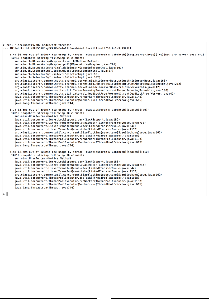
Improving Performance
[ 544 ]
The Hot Threads API response
Now, let's go through the sections of the response returned by the Hot Threads API.
For example, the following screenshot is a fragment of the Hot Threads API response
generated for Elasticsearch that was just started:
Now, let's discuss the sections of the response. To do that, we will use a slightly
different response compared to the one shown previously. We do this to better
visualize what is happening inside Elasticsearch. However, please remember that the
general structure of the response will not change.
The rst section of the Hot Threads API response shows us which node the thread is
located on. For example, the rst line of the response can look as follows:
::: [N'Gabthoth][aBb5552UQvyFCk1PNCaJnA][Banshee-
3.local][inet[/10.0.1.3:9300]]
Thanks to it, we can see which node the Hot Threads API returns information about
and which node is very handy when the Hot Threads API call goes to many nodes.

Chapter 8
[ 545 ]
The next lines of the Hot Threads API response can be divided into several sections,
each starting with a line similar to the following one:
0.5% (2.7ms out of 500ms) cpu usage by thread
'elasticsearch[N'Gabthoth][search][T#10]'
In our case, we see a thread named search, which takes 0.5 percent of all the
CPU time at the time when the measurement was done. The cpu usage part of
the preceding line indicates that we are using type equal to cpu (other values you
can expect here are block usage for threads in the blocked state and wait usage
for threads in the waiting states). The thread name is very important here, because
by looking at it, we can see which Elasticsearch functionality is the hot one. In our
example, we see that this thread is all about searching (the search value). Other
example values that you can expect to see are recovery_stream (for recovery
module events), cache (for caching events), merge (for segments merging threads),
index (for data indexing threads), and so on.
The next part of the Hot Threads API response is the section starting with the
following information:
10/10 snapshots sharing following 10 elements
This information will be followed by a stack trace. In our case, 10/10 means that 10
snapshots have been taken for the same stack trace. In general, this means that all the
examination time was spent in the same part of the Elasticsearch code.
Scaling Elasticsearch
As we already said multiple times both in this book and in Elasticsearch Server Second
Edition, Elasticsearch is a highly scalable search and analytics platform. We can scale
it both horizontally and vertically.
Vertical scaling
When we talk about vertical scaling, we often mean adding more resources to
the server Elasticsearch is running on: we can add memory and we can switch
to a machine with better CPU or faster disk storage. Of course, with better
machines, we can expect increase in performance; depending on our deployment
and its bottleneck, there can be smaller or higher improvement. However, there
are limitations when it comes to vertical scaling. For example, one of such is the
maximum amount of physical memory available for your servers or the total
memory required by the JVM to operate. When you have large enough data and
complicated queries, you can very soon run into memory issues, and adding new
memory may not be helpful at all.
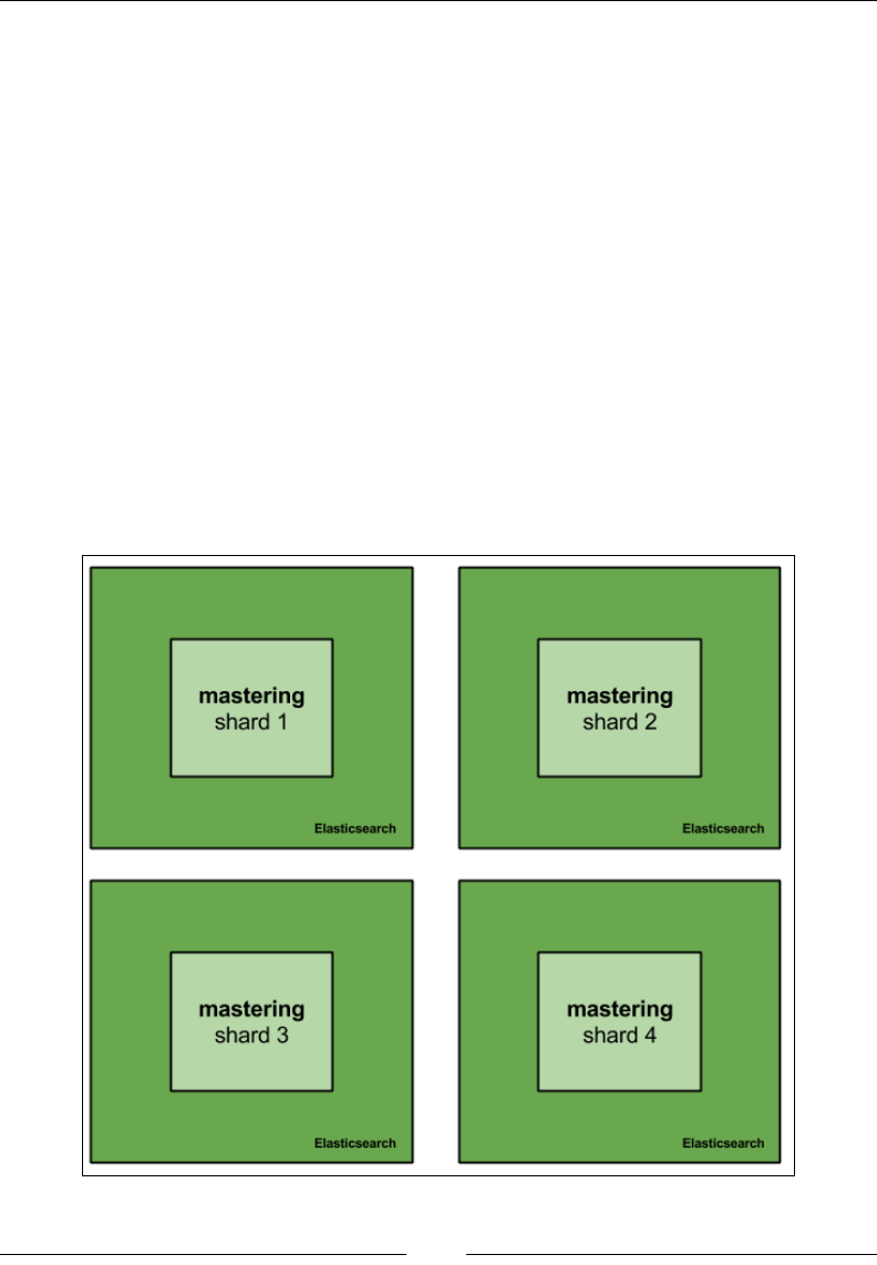
Improving Performance
[ 546 ]
For example, you may not want to go beyond 31 GB of physical memory given to the
JVM because of garbage collection and the inability to use compressed ops, which
basically means that to address the same memory space, JVM will need to use twice
the memory. Even though it seems like a very big issue, vertical scaling is not the
only solution we have.
Horizontal scaling
The other solution available to us Elasticsearch users is horizontal scaling. To give
you a comparison, vertical scaling is like building a sky scrapper, while horizontal
scaling is like having many houses in a residential area. Instead of investing in
hardware and having powerful machines, we choose to have multiple machines and
our data split between them. Horizontal scaling gives us virtually unlimited scaling
possibilities. Even with the most powerful hardware time, a single machine is not
enough to handle the data, the queries, or both of them. If a single machine is not
able to handle the amount of data, we have such cases where we divide our indices
into multiple shards and spread them across the cluster, just like what is shown in
the following gure:
Chapter 8
[ 547 ]
When we don't have enough processing power to handle queries, we can always
create more replicas of the shards we have. We have our cluster: four Elasticsearch
nodes with the mastering index created and running on it and built of four shards.
If we want to increase the querying capabilities of our cluster, we would just add
additional nodes, for example, four of them. After adding new nodes to the cluster,
we can either create new indices that will be built of more shards to spread the load
more evenly, or add replicas to already existing shards. Both options are viable. We
should go for more primary shards when our hardware is not enough to handle the
amount of data it holds. In such cases, we usually run into out-of-memory situations,
long shard query execution time, swapping, or high I/O waits. The second option—
having replicas—is a way to go when our hardware is happily handling the data
we have, but the trafc is so high that the nodes just can't keep up. The rst option
is simple, but let's look at the second case: having more replicas. So, with four
additional nodes, our cluster would look as follows:
Now, let's run the following command to add a single replica:
curl -XPUT 'localhost:9200/mastering/_settings' -d '{
"index" : {
"number_of_replicas" : 1
}
}'

Improving Performance
[ 548 ]
Our cluster view would look more or less as follows:
As you can see, each of the initial shards building the mastering index has a single
replica stored on another node. Because of this, Elasticsearch is able to round robin
the queries between the shard and its replicas so that the queries don't always hit one
node. Because of this, we are able to handle almost double the query load compared
to our initial deployment.
Automatically creating replicas
Elasticsearch allows us to automatically expand replicas when the cluster is big
enough. You might wonder where such functionality can be useful. Imagine a
situation where you have a small index that you would like to be present on every
node so that your plugins don't have to run distributed queries just to get data
from it. In addition to this, your cluster is dynamically changing; you add and
remove nodes from it. The simplest way to achieve such a functionality is to allow
Elasticsearch to automatically expand replicas. To do this, we would need to set
index.auto_expand_replicas to 0-all, which means that the index can have 0
replicas or be present on all the nodes. So if our small index is called mastering_
meta and we would like Elasticsearch to automatically expand its replicas, we would
use the following command to create the index:
curl -XPOST 'localhost:9200/mastering_meta/' -d '{
"settings" : {
"index" : {
"auto_expand_replicas" : "0-all"
}
}
}'
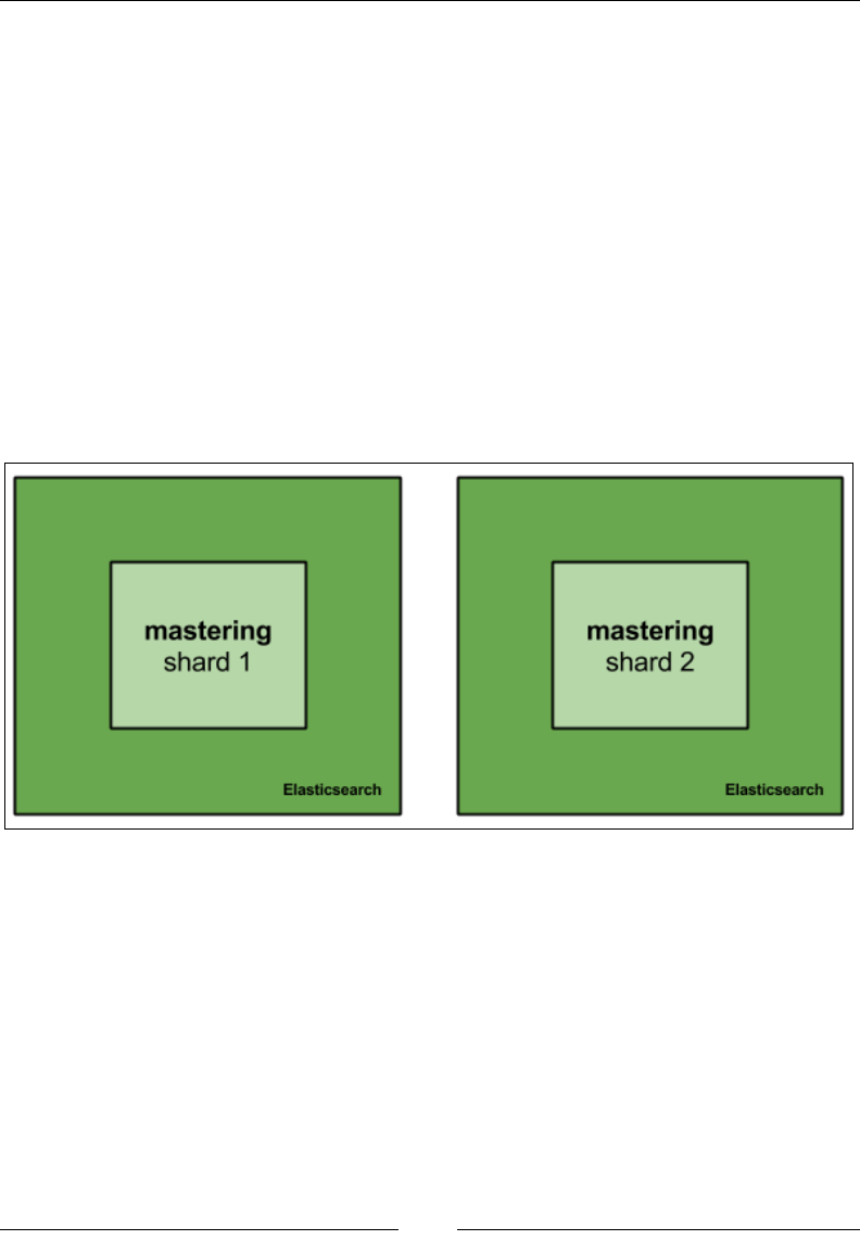
Chapter 8
[ 549 ]
We can also update the settings of that index if it is already created by running the
following command:
curl -XPUT 'localhost:9200/mastering_meta/_settings' -d '{
"index" : {
"auto_expand_replicas" : "0-all"
}
}'
Redundancy and high availability
The Elasticsearch replication mechanism not only gives us the ability to handle
higher query throughput, but also gives us redundancy and high availability.
Imagine an Elasticsearch cluster hosting a single index called mastering that is built
of 2 shards and 0 replicas. Such a cluster could look as follows:
Now, what would happen when one of the nodes fails? The simplest answer is that
we lose about 50 percent of the data, and if the failure is fatal, we lose that data
forever. Even when having backups, we would need to spin up another node and
restore the backup; this takes time. If your business relies on Elasticsearch, downtime
means money loss.
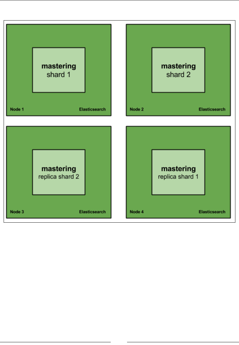
Improving Performance
[ 550 ]
Now let's look at the same cluster but with one replica:
Now, losing a single Elasticsearch node means that we still have the whole data
available and we can work on restoring the full cluster structure without downtime.
What's more, with such deployment, we can live with two nodes failing at the same
time in some cases, for example, Node 1 and Node 3 or Node 2 and Node 4. In both
the mentioned cases, we would still be able to access all the data. Of course, this will
lower performance because of less nodes in the cluster, but this is still better than not
handling queries at all.
Because of this, when designing your architecture and deciding on the number of
nodes, how many nodes indices will have, and the number of shards for each of
them, you should take into consideration how many nodes' failure you want to live
with. Of course, you can't forget about the performance part of the equation, but
redundancy and high availability should be one of the factors of the scaling equation.

Chapter 8
[ 551 ]
Cost and performance exibility
The default distributed nature of Elasticsearch and its ability to scale horizontally
allow us to be exible when it comes to performance and costs that we have when
running our environment. First of all, high-end servers with highly performant disks,
numerous CPU cores, and a lot of RAM are expensive. In addition to this, cloud
computing is getting more and more popular and it not only allows us to run our
deployment on rented machines, but it also allows us to scale on demand. We just
need to add more machines, which is a few clicks away or can even be automated
with some degree of work.
Getting this all together, we can say that having a horizontally scalable solution,
such as Elasticsearch, allows us to bring down the costs of running our clusters and
solutions. What's more, we can easily sacrice performance if costs are the most
crucial factor in our business plan. Of course, we can also go the other way. If we
can afford large clusters, we can push Elasticsearch to hundreds of terabytes of
data stored in the indices and still get decent performance (of course, with proper
hardware and property distributed).
Continuous upgrades
High availability, cost, performance exibility, and virtually endless growth are not
the only things worth saying when discussing the scalability side of Elasticsearch. At
some point in time, you will want to have your Elasticsearch cluster to be upgraded
to a new version. It can be because of bug xes, performance improvements, new
features, or anything that you can think of. The thing is that when having a single
instance of each shard, an upgrade without replicas means the unavailability of
Elasticsearch (or at least its parts), and that may mean downtime of the applications
that use Elasticsearch. This is another point why horizontal scaling is so important;
you can perform upgrades, at least to the point where software such as Elasticsearch
is supported. For example, you could take Elasticsearch 1.0 and upgrade it to
Elasticsearch 1.4 with only rolling restarts, thus having all the data still available for
searching and indexing happening at the same time.
Multiple Elasticsearch instances on a single
physical machine
Although we previously said that you shouldn't go for the most powerful machines
for different reasons (such as RAM consumption after going above 31 GB JVM heap),
we sometimes don't have much choice. This is out of the scope of the book, but
because we are talking about scaling, we thought it may be a good thing to mention
what can be done in such cases.
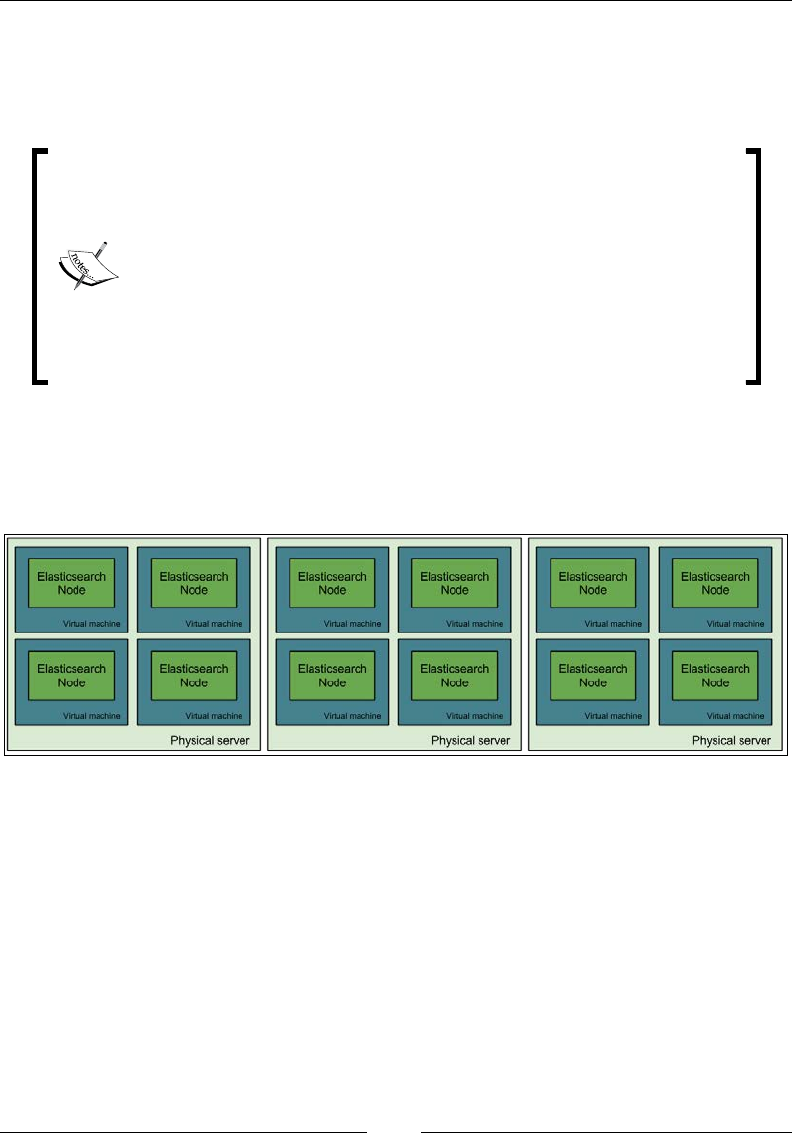
Improving Performance
[ 552 ]
In cases such as the ones we are discussing, when we have high-end hardware with
a lot of RAM memory, a lot of high speed disk, numerous CPU cores, among others,
we should think about diving the physical server into multiple virtual machines and
running a single Elasticsearch server on each of the virtual machines.
There is also a possibility of running multiple Elasticsearch servers
on a single physical machine without running multiple virtual
machines. Which road to take—virtual machines or multiple
instances—is really your choice; however, we like to keep things
separate and, because of that, we are usually going to divide any
large server into multiple virtual machines. When dividing a large
server into multiple smaller virtual machines, remember that the
I/O subsystem will be shared across these smaller virtual machines.
Because of this, it may be good to wisely divide the disks between
virtual machines.
To illustrate such a deployment, please look at the following provided gure. It
shows how you could run Elasticsearch on three large servers, each divided into four
separate virtual machines. Each virtual machine would be responsible for running a
single instance of Elasticsearch.
Preventing the shard and its replicas from being on the
same node
There is one additional thing worth mentioning. When having multiple physical
servers divided into virtual machines, it is crucial to ensure that the shard and its
replica won't end up on the same physical machine. This would be tragic if a server
crashes or is restarted. We can tell Elasticsearch to separate shards and replicas using
cluster allocation awareness. In our preceding case, we have three physical servers;
let's call them server1, server2, and server3.

Chapter 8
[ 553 ]
Now for each Elasticsearch on a physical server, we dene the node.server_name
property and we set it to the identier of the server. So, for the example of all
Elasticsearch nodes on the rst physical server, we would set the following property
in the elasticsearch.yml conguration le:
node.server_name: server1
In addition to this, each Elasticsearch node (no matter on which physical
server) needs to have the following property added to the elasticsearch.yml
conguration le:
cluster.routing.allocation.awareness.attributes: server_name
It tells Elasticsearch not to put the primary shard and its replicas on the nodes with
the same value in the node.server_name property. This is enough for us, and
Elasticsearch will take care of the rest.
Designated nodes' roles for larger clusters
There is one more thing that we wanted to tell you; actually, we already mentioned
that both in the book you are holding in your hands and in Elasticsearch Server Second
Edition, Packt Publishing. To have a fully fault-tolerant and highly available cluster,
we should divide the nodes and give each node a designated role. The roles we can
assign to each Elasticsearch node are as follows:
• The master eligible node
• The data node
• The query aggregator node
By default, each Elasticsearch node is master eligible (it can serve as a master node),
can hold data, and can work as a query aggregator node, which means that it can
send partial queries to other nodes, gather and merge the results, and respond to the
client sending the query. You may wonder why this is needed. Let's give you a simple
example: if the master node is under a lot of stress, it may not be able to handle the
cluster state-related command fast enough and the cluster can become unstable. This is
only a single, simple example, and you can think of numerous others.
Improving Performance
[ 554 ]
Because of this, most Elasticsearch clusters that are larger than a few nodes usually
look like the one presented in the following gure:
As you can see, our hypothetical cluster contains two aggregator nodes (because
we know that there will not be too many queries, but we want redundancy), a
dozen of data nodes because the amount of data will be large, and at least three
master eligible nodes that shouldn't be doing anything else. Why three master
nodes when Elasticsearch will only use a single one at any given time? Again, this
is because of redundancy and to be able to prevent split brain situations by setting
the discovery.zen.minimum_master_nodes to 2, which would allow us to easily
handle the failure of a single master eligible node in the cluster.
Let's now give you snippets of the conguration for each type of node in our cluster.
We already talked about this in the Discovery and recovery modules section in Chapter
7, Elasticsearch Administration, but we would like to mention it once again.
Query aggregator nodes
The query aggregator nodes' conguration is quite simple. To congure them,
we just need to tell Elasticsearch that we don't want these nodes to be master
eligible and hold data. This corresponds to the following conguration in the
elasticsearch.yml le:
node.master: false
node.data: false

Chapter 8
[ 555 ]
Data nodes
Data nodes are also very simple to congure; we just need to say that they should
not be master eligible. However, we are not big fans of default congurations
(because they tend to change) and, thus, our Elasticsearch data nodes' conguration
looks as follows:
node.master: false
node.data: true
Master eligible nodes
We've left the master eligible nodes for the end of the general scaling section. Of
course, such Elasticsearch nodes shouldn't be allowed to hold data, but in addition
to that, it is good practice to disable the HTTP protocol on such nodes. This is done
in order to avoid accidentally querying these nodes. Master eligible nodes can be
smaller in resources compared to data and query aggregator nodes, and because of
that, we should ensure that they are only used for master-related purposes. So, our
conguration for master eligible nodes looks more or less as follows:
node.master: true
node.data: false
http.enabled: false
Using Elasticsearch for high load scenarios
Now that we know the theory (and some examples of Elasticsearch scaling), we
are ready to discuss the different aspects of Elasticsearch preparation for high load.
We decided to split this part of the chapter into three sections: one dedicated to
preparing Elasticsearch for a high indexing load, one dedicated for the preparation
of Elasticsearch for a high query load, and one that can be taken into consideration in
both cases. This should give you an idea of what to think about when preparing your
cluster for your use case.
Please consider that performance testing should be done after preparing the cluster
for production use. Don't just take the values from the book and go for them; try
them with your data and your queries and try altering them, and see the differences.
Remember that giving general advices that works for everyone is not possible, so
treat the next two sections as general advices instead of ready for use recipes.

Improving Performance
[ 556 ]
General Elasticsearch-tuning advices
In this section, we will look at the general advices related to tuning Elasticsearch.
They are not connected to indexing performance only or querying performance only
but to both of them.
Choosing the right store
One of the crucial aspects of this is that we should choose the right store
implementation. This is mostly important when running an Elasticsearch version older
than 1.3.0. In general, if you are running a 64-bit operating system, you should again
go for mmapfs. If you are not running a 64-bit operating system, choose the niofs
store for Unix-based systems and simplefs for Windows-based ones. If you can allow
yourself to have a volatile store, but a very fast one, you can look at the memory store:
it will give you the best index access performance but requires enough memory to
handle not only all the index les, but also to handle indexing and querying.
With the release of Elasticsearch 1.3.0, we've got a new store type called default,
which is the new default store type. As Elasticsearch developers said, it is a hybrid
store type. It uses memory-mapped les to read term dictionaries and doc values,
while the rest of the les are accessed using the NIOFSDirectory implementation.
In most cases, when using Elasticsearch 1.3.0 or higher, the default store type
should be used.
The index refresh rate
The second thing we should pay attention to is the index refresh rate. We know that
the refresh rate species how fast documents will be visible for search operations.
The equation is quite simple: the faster the refresh rate, the slower the queries will
be and the lower the indexing throughput. If we can allow ourselves to have a
slower refresh rate, such as 10s or 30s, it may be a good thing to set it. This puts less
pressure on Elasticsearch, as the internal objects will have to be reopened at a slower
pace and, thus, more resources will be available both for indexing and querying.
Remember that, by default, the refresh rate is set to 1s, which basically means that
the index searcher object is reopened every second.

Chapter 8
[ 557 ]
To give you a bit of an insight into what performance gains we are talking about, we
did some performance tests, including Elasticsearch and a different refresh rate. With
a refresh rate of 1s, we were able to index about 1.000 documents per second using
a single Elasticsearch node. Increasing the refresh rate to 5s gave us an increase
in the indexing throughput of more than 25 percent, and we were able to index
about 1280 documents per second. Setting the refresh rate to 25s gave us about 70
percent of throughput more compared to a 1s refresh rate, which was about 1700
documents per second on the same infrastructure. It is also worth remembering that
increasing the time indenitely doesn't make much sense, because after a certain
point (depending on your data load and the amount of data you have), the increase
in performance is negligible.
Thread pools tuning
This is one of the things that is very dependent on your deployment. By default,
Elasticsearch comes with a very good default when it comes to all thread pools'
conguration. However, there are times when these defaults are not enough. You
should remember that tuning the default thread pools' conguration should be done
only when you really see that your nodes are lling up the queues and they still
have processing power left that could be designated to the processing of the
waiting operations.
For example, if you did your performance tests and you see your Elasticsearch
instances not being saturated 100 percent, but on the other hand, you've experienced
rejected execution errors, then this is a point where you should start adjusting the
thread pools. You can either increase the amount of threads that are allowed to be
executed at the same time, or you can increase the queue. Of course, you should
also remember that increasing the number of concurrently running threads to very
high numbers will lead to many CPU context switches (http://en.wikipedia.
org/wiki/Context_switch), which will result in a drop in performance. Of course,
having massive queues is also not a good idea; it is usually better to fail fast rather
than overwhelm Elasticsearch with several thousands of requests waiting in the
queue. However, this all depends on your particular deployment and use case. We
would really like to give you a precise number, but in this case, giving general
advice is rarely possible.

Improving Performance
[ 558 ]
Adjusting the merge process
Lucene segments' merging adjustments is another thing that is highly dependent on
your use case and several factors related to it, such as how much data you add, how
often you do that, and so on. There are two things to remember when it comes to
Lucene segments and merging. Queries run against an index with multiple segments
are slower than the ones with a smaller number of segments. Performance tests show
that queries run against an index built of several segments are about 10 to 15 percent
slower than the ones run against an index built of only a single segment. On the
other hand, though, merging is not free and the fewer segments we want to have in
our index, the more aggressive a merge policy should be congured.
Generally, if you want your queries to be faster, aim for fewer segments for your
indices. For example, for log_byte_size or log_doc merge policies, setting the
index.merge.policy.merge_factor property to a value lower than the default
of 10 will result in less segments, lower RAM consumption, faster queries, and
slower indexing. Setting the index.merge.policy.merge_factor property to a
value higher than 10 will result in more segments building the index, higher RAM
consumption, slower queries, and faster indexing.
There is one more thing: throttling. By default, Elasticsearch will throttle merging
to 20mb/s. Elasticsearch uses throttling so that your merging process doesn't affect
searching too much. What's more, if merging is not fast enough, Elasticsearch will
throttle the indexing to be single threaded so that the merging could actually nish
and not have an extensive number of segments. However, if you are running SSD
drives, the default 20mb/s throttling is probably too much and you can set it to 5 to
10 times more (at least). To adjust throttling, we need to set the indices.store.
throttle.max_bytes_per_sec property in elasticsearch.yml (or using the
Cluster Settings API) to the desired value, such as 200mb/s.
In general, if you want indexing to be faster, go for more segments for indices. If
you want your queries to be faster, your I/O can handle more work because of
merging, and you can live with Elasticsearch consuming a bit more RAM memory,
go for more aggressive merge policy settings. If you want Elasticsearch to index
more documents, go for a less aggressive merge policy, but remember that this will
affect your queries' performance. If you want both of these things, you need to nd a
golden spot between them so that the merging is not too often but also doesn't result
in an extensive number of segments.
Data distribution
As we know, each index in the Elasticsearch world can be divided into multiple
shards, and each shard can have multiple replicas. In cases where you have multiple
Elasticsearch nodes and indices divided into shards, proper data distribution may be
crucial to even the load the cluster and not have some nodes doing more work than
the other ones.
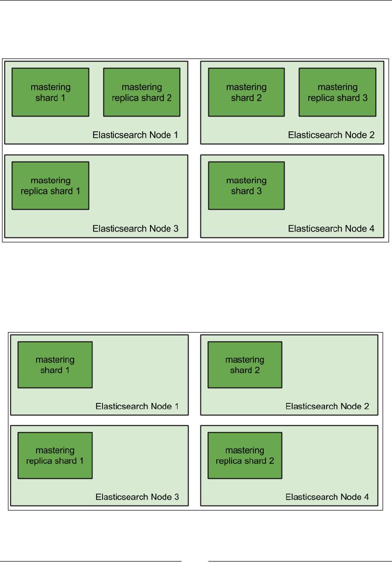
Chapter 8
[ 559 ]
Let's take the following example—imagine that we have a cluster that is built of four
nodes, and it has a single index built of three shards and one replica allocated. Such
deployment could look as follows:
As you can see, the rst two nodes have two physical shards allocated to them, while
the last two nodes have one shard each. So the actual data allocation is not even.
When sending the queries and indexing data, we will have the rst two nodes do
more work than the other two; this is what we want to avoid. We could make the
mastering index have two shards and one replica so that it would look like this:
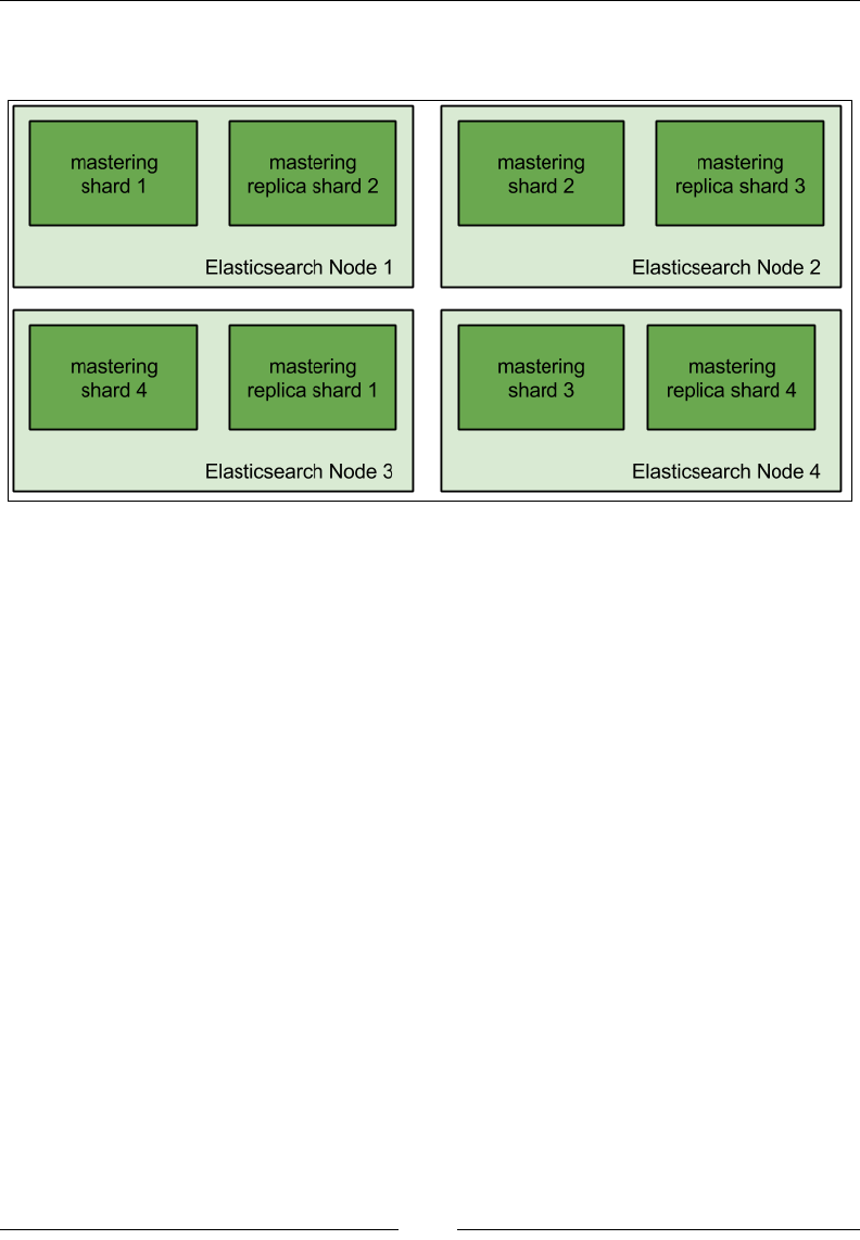
Improving Performance
[ 560 ]
Or, we could have the mastering index divided into four shards and have
one replica.
In both cases, we will end up with an even distribution of shards and replicas, with
Elasticsearch doing a similar amount of work on all the nodes. Of course, with
more indices (such as having daily indices), it may be trickier to get the data evenly
distributed, and it may not be possible to have evenly distributed shards, but we
should try to get to such a point.
One more thing to remember when it comes to data distribution, shards, and replicas
is that when designing your index architecture, you should remember what you
want to achieve. If you are going for a very high indexing use case, you may want
to spread the index into multiple shards to lower the pressure that is put on the
CPU and the I/O subsystem of the server. This is also true in order to run expensive
queries, because with more shards, you can lower the load on a single server.
However, with queries, there is one more thing: if your nodes can't keep up with
the load caused by queries, you can add more Elasticsearch nodes and increase the
number of replicas so that physical copies of the primary shards are placed on these
nodes. This will make the indexing a bit slower but will give you the capacity to
handle more queries at the same time.

Chapter 8
[ 561 ]
Advices for high query rate scenarios
One of the great features of Elasticsearch is its ability to search and analyze the data
that was indexed. However, sometimes, the user is needed to adjust Elasticsearch,
and our queries to not only get the results of the query, but also get them fast (or in a
reasonable amount of time). In this section, we will not only look at the possibilities
but also prepare Elasticsearch for high query throughput use cases. We will also look
at general performance tips when it comes to querying.
Filter caches and shard query caches
The rst cache that can help with query performance is the lter cache (if our queries
use lters, and if not, they should probably use lters). We talked about lters in the
Handling lters and why it matters section in Chapter 2, Power User Query DSL. What
we didn't talk about is the cache that is responsible for storing results of the lters:
the lter cache. By default, Elasticsearch uses the lter cache implementation that
is shared among all the indices on a single node, and we can control its size using
the indices.cache.filter.size property. It defaults to 10 percent by default and
species the total amount of memory that can be used by the lter cache on a given
node. In general, if your queries are already using lters, you should monitor the
size of the cache and evictions. If you see that you have many evictions, then you
probably have a cache that's too small, and you should consider having a larger one.
Having a cache that's too small may impact the query performance in a bad way.
The second cache that has been introduced in Elasticsearch is the shard query
cache. It was added to Elasticsearch in Version 1.4.0, and its purpose is to cache
aggregations, suggester results, and the number of hits (it will not cache the returned
documents and, thus, it only works with search_type=count). When your queries
are using aggregations or suggestions, it may be a good idea to enable this cache (it
is disabled by default) so that Elasticsearch can reuse the data stored there. The best
thing about the cache is that it promises the same near real-time search as search that
is not cached.
To enable the shard query cache, we need to set the index.cache.query.enable
property to true. For example, to enable the cache for our mastering index, we could
issue the following command:
curl -XPUT 'localhost:9200/mastering/_settings' -d '{
"index.cache.query.enable": true
}'

Improving Performance
[ 562 ]
Please remember that using the shard query cache doesn't make sense if we don't use
aggregations or suggesters.
One more thing to remember is that, by default, the shard query cache is allowed
to take no more than 1 percent of the JVM heap given to the Elasticsearch node. To
change the default value, we can use the indices.cache.query.size property. By
using the indices.cache.query.expire property, we can specify the expiration
date of the cache, but it is not needed, and in most cases, results stored in the cache
are invalidated with every index refresh operation.
Think about the queries
This is the most general advice we can actually give: you should always think about
optimal query structure, lter usage, and so on. We talked about it extensively in
the Handling lters and why it matters section in Chapter 2, Power User Query DSL, but
we would like to mention that once again, because we think it is very important. For
example, let's look at the following query:
{
"query" : {
"bool" : {
"must" : [
{
"query_string" : {
"query" : "name:mastering AND department:it AND
category:book"
}
},
{
"term" : {
"tag" : "popular"
}
},
{
"term" : {
"tag" : "2014"
}
}
]
}
}
}

Chapter 8
[ 563 ]
It returns the book name that matches a few conditions. However, there are a few
things we can improve in the preceding query. For example, we could move a few
things to ltering so that the next time we use some parts of the query, we save CPU
cycles and reuse the information stored in the cache. For example, this is what the
optimized query could look like:
{
"query" : {
"filtered" : {
"query" : {
"match" : {
"name" : "mastering"
}
},
"filter" : {
"bool" : {
"must" : [
{
"term" : {
"department" : "it"
}
},
{
"term" : {
"category" : "book"
}
},
{
"terms" : {
"tag" : [ "popular", "2014" ]
}
}
]
}
}
}
}
}
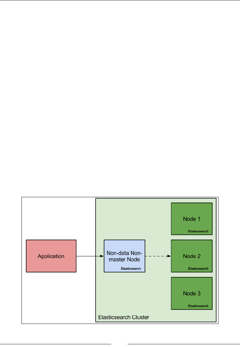
Improving Performance
[ 564 ]
As you can see, there are a few things that we did. First of all, we used the filtered
query to introduce lters and we moved most of the static, non-analyzed elds to
lters. This allows us to easily reuse the lters in the next queries that we execute.
Because of such query restructuring, we were able to simplify the main query, so
we changed query_string_query to the match query, because it is enough for our
use case. This is exactly what you should be doing when optimizing your queries or
designing them—have optimization and performance in mind and try to keep them
as optimal as they can be. This will result in faster query execution, lower resource
consumption, and better health of the whole Elasticsearch cluster.
However, performance is not the only difference when it comes to the outcome of
queries. As you know, lters don't affect the score of the documents returned and
are not taken into consideration when calculating the score. Because of this, if you
compare the scores returned by the preceding queries for the same documents, you
would notice that they are different. This is worth remembering.
Using routing
If your data allows routing, you should consider using it. The data with the same
routing value will always end up in the same shard. Because of this, we can save
ourselves the need to query all the shards when asking for certain data. For example,
if we store the data of our clients, we may use a client identier as the routing value.
This will allow us to store the data of a single client inside a single shard. This means
that during querying, Elasticsearch needs to fetch data from only a single shard, as
shown in the following gure:
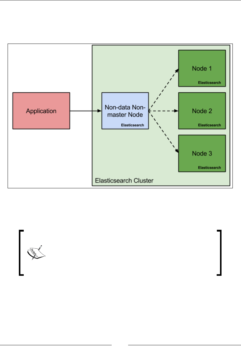
Chapter 8
[ 565 ]
If we assume that the data lives in a shard allocated to Node 2, we can see that
Elasticsearch only needed to run the query against that one particular node to get all
the data for the client. If we don't use routing, the simplied query execution could
look as follows:
In the case of nonrouting, Elasticsearch rst needs to query all the index shards.
If your index contains dozen of shards, the performance improvement will be
signicant as long as a single Elasticsearch instance can handle the shard size.
Please remember that not every use case is eligible to use
routing. To be able to use it, your data needs to be virtually
divided so that it is spread across the shards. For example,
it usually doesn't make sense to have dozens of very small
shards and one massive one, because for the massive one,
performance may not be decent.
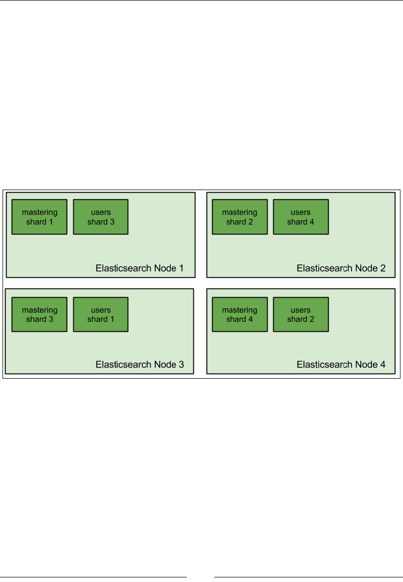
Improving Performance
[ 566 ]
Parallelize your queries
One thing that is usually forgotten is the need to parallelize queries. Imagine that
you have a dozen nodes in your cluster, but your index is built of a single shard.
If the index is large, your queries will perform worse than you would expect. Of
course, you can increase the number of replicas, but that won't help; a single query
will still go to a single shard in that index, because replicas are not more than the
copies of the primary shard, and they contain the same data (or at least they should).
One thing that will actually help is dividing your index into multiple shards—the
number of shards depends on the hardware and deployment. In general, it is advised
to have the data evenly divided so that nodes are equally loaded. For example, if you
have four Elasticsearch nodes and two indices, you may want to have four shards for
each index, just like what is shown in the following gure:
Field data cache and breaking the circuit
By default, the eld data cache in Elasticsearch is unbounded. This can be very
dangerous, especially when you are using faceting and sorting on many elds. If
these elds are high cardinality ones, then you can run into even more trouble. By
trouble, we mean running out of memory.
We have two different factors we can tune to be sure that we won't run into out-of-
memory errors. First of all, we can limit the size of the eld data cache. The second
thing is the circuit breaker, which we can easily congure to just throw an exception
instead of loading too much data. Combining these two things will ensure that we
don't run into memory issues.

Chapter 8
[ 567 ]
However, we should also remember that Elasticsearch will evict data from the eld
data cache if its size is not enough to handle faceting request or sorting. This will
affect the query performance, because loading eld data information is not very
efcient. However, we think that it is better to have our queries slower rather than
having our cluster blown up because of out-of-memory errors.
Finally, if your queries are using eld data cache extensively (such as aggregations
or sorting) and you are running into memory-related issues (such as OutOfMemory
exceptions or GC pauses), consider using doc values that we already talked about.
Doc values should give you performance that's similar to eld data cache, and
support for doc values is getting better and better with each Elasticsearch release
(improvements to doc values are made in Lucene itself).
Keeping size and shard_size under control
When dealing with queries that use aggregations, for some of them, we have the
possibility of using two properties: size and shard_size. The size parameter
denes how many buckets should be returned by the nal aggregation results; the
node that aggregates the nal results will get the top buckets from each shard that
returns the result and will only return the top size of them to the client. The shard_
size parameter tells Elasticsearch about the same but on the shard level. Increasing
the value of the shard_size parameter will lead to more accurate aggregations (such
as in the case of signicant terms' aggregation) at the cost of network trafc and
memory usage. Lowering this parameter will cause aggregation results to be less
precise, but we will benet from lower memory consumption and lower network
trafc. If we see that the memory usage is too large, we can lower the size and
shard_size properties of problematic queries and see whether the quality of the
results is still acceptable.
High indexing throughput scenarios and
Elasticsearch
In this section, we will discuss some optimizations that will allow us to concentrate
on the indexing throughput and speed. Some use cases are highly dependent on the
amount of data you can push to Elasticsearch every second, and the next few topics
should cover some information regarding indexing.
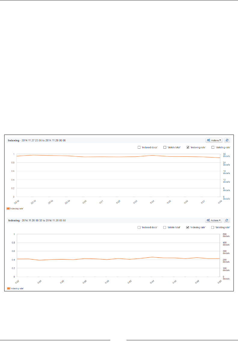
Improving Performance
[ 568 ]
Bulk indexing
This is very obvious advice, but you would be surprised by how many Elasticsearch
users forget about indexing data in bulk instead of sending the documents one
by one. The thing to remember, though, is to not overload Elasticsearch with too
many bulk requests. Remember about the bulk thread pool and its size (equal to the
number of CPU cores in the system by default with a queue of 50 requests), and try
to adjust your indexers so that they don't to go beyond it. Or, you will rst start to
queue their requests and if Elasticsearch is not able to process them, you will quickly
start seeing rejected execution exceptions, and your data won't be indexed. On the
other hand, remember that your bulk requests can't be too large, or Elasticsearch will
need a lot of memory to process them.
Just as an example, I would like to show you two types of indexing happening. In
the rst gure, we have indexing throughput when running the indexation one
document by one. In the second gure, we do the same, but instead of indexing
documents one by one, we index them in batches of 10 documents.

Chapter 8
[ 569 ]
As you can see, when indexing documents one by one, we were able to index
about 30 documents per second and it was stable. The situation changed with bulk
indexing and batches of 10 documents. We were able to index slightly more than 200
documents per second, so the difference can be clearly seen.
Of course, this is a very basic comparison of indexing speed, and in order to show
you the real difference, we should use dozens of threads and push Elasticsearch to
its limits. However, the preceding comparison should give you a basic view of the
indexing throughput gains when using bulk indexing.
Doc values versus indexing speed
When talking about indexing speed, we have to talk about doc values. As we
already said a few times in the book, doc values allows us to ght gigantic JVM
heap requirements when Elasticsearch needs to uninvert elds for functionalities
such as sorting, aggregations, or faceting. However, writing doc values requires
some additional work during the indexation. If we are all about the highest indexing
speed and the most indexing throughput, you should consider not going for doc
values. On the other hand, if you have a lot of data—and you probably have when
you are indexing fast—using doc values may be the only way that will allow using
aggregations or sorting on eld values without running into memory-related problems.
Keep your document elds under control
The amount of data you index makes the difference, which is understandable.
However, this is not the only factor; the size of the documents and their analysis
matters as well. With larger documents, you can expect not only your index to grow,
but also make the indexation slightly slower. This is why you may sometimes want
to look at all the elds you are indexing and storing. Keep your stored elds to a
minimum or don't use them at all; the only stored eld you need in most cases is the
_source eld.

Improving Performance
[ 570 ]
There is one more thing—apart from the _source eld, Elasticsearch indexes the
_all eld by default. Let's remind you: the _all eld is used by Elasticsearch to
gather data from all the other textual elds. In some cases, this eld is not used at all
and because of that, it is nice to turn it off. Turning it off is simple and the only thing
to do is add the following entry to the type mappings:
"_all" : {"enabled" : false}
We can do this during the index creation, for example, like this:
curl -XPOST 'localhost:9200/disabling_all' -d '{
"mappings" : {
"test_type" : {
"_all" : { "enabled" : false },
"properties" : {
"name" : { "type" : "string" },
"tag" : { "type" : "string", "index" : "not_analyzed" }
}
}
}
}'
The indexing should be slightly faster depending on the size of your documents and
the number of textual elds in it.
There is an additional thing, which is good practice when disabling the _all
eld: setting a new default search eld. We can do this by setting the index.
query.default_field property. For example, in our case, we can set it in the
elasticsearch.yml le and set it to the name eld from our preceding mappings:
index.query.default_field: name
The index architecture and replication
When designing the index architecture, one of the things you need to think about
is the number of shards and replicas that the index is built of. During that time, we
also need to we think about data distribution among Elasticsearch nodes, optimal
performance, high availability, reliability, and so on. First of all, distributing primary
shards of the index across all nodes we have will parallelize indexing operations and
will make them faster.
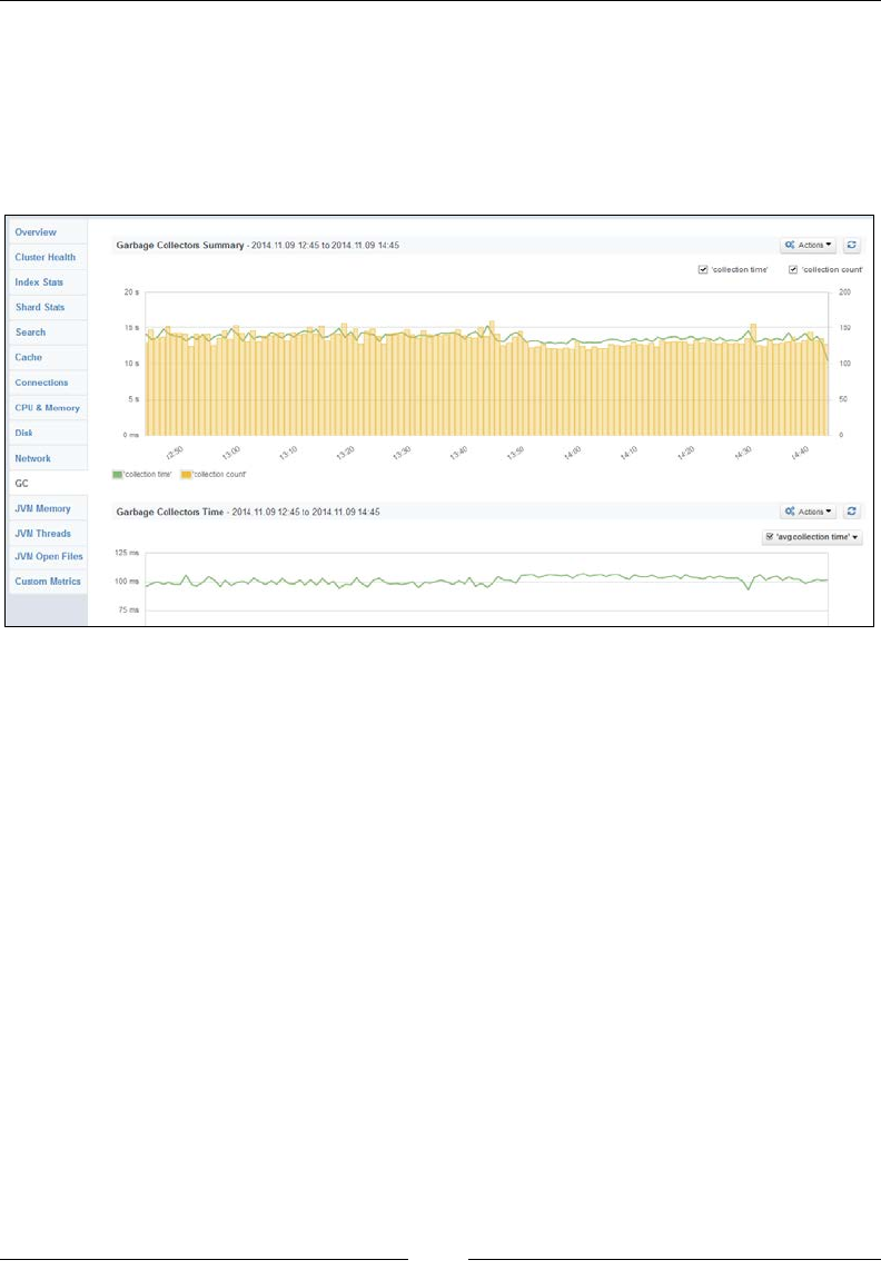
Chapter 8
[ 571 ]
The second thing is data replication. What we have to remember is that too many
replicas will cause the indexation speed to drop. This is because of several reasons.
First of all, you need to transfer the data between primary shards and replicas. The
second thing is that, usually, replicas and primary shards may live on the same
nodes (not primary shards and its replicas, of course, but replicas of other primaries).
For example, take a look at what is shown in the following gure:
Because of this, Elasticsearch will need the data for both primary shards and
replicas and, thus, it will use the disk. Depending on the cluster setup, the indexing
throughput may drop in such cases (depends on the disks, number of documents
indexed at the same time, and so on).
Tuning write-ahead log
We already talked about transaction logs in the Data ushing, index refresh and
transaction log handling section of Chapter 6, Low-level Index Control. Elasticsearch
has an internal module called translog (http://www.elasticsearch.org/guide/
en/elasticsearch/reference/current/index-modules-translog.html). It
is a per-shard structure that serves the purpose of write-ahead logging (http://
en.wikipedia.org/wiki/Write-ahead_logging). Basically, it allows Elasticsearch
to expose the newest updates for GET operations, ensure data durability, and
optimize writing to Lucene indices.

Improving Performance
[ 572 ]
By default, Elasticsearch keeps a maximum of 5000 operations in the transaction log
with a maximum size of 200 MB. However, if we can pay the price of data not being
available for search operations for longer periods of time but we want more indexing
throughput, we can increase these defaults. By specifying the index.translog.
flush_threshold_ops and index.translog.flush_threshold_size properties
(both are set per index and can be updated in real time using the Elasticsearch
API), we can set the maximum number of operations allowed to be stored in the
transaction log and its maximum size. We've seen deployments having this property
values set to 10 times the default values.
One thing to remember is that in case of failure, shard initialization will be slower—
of course on the ones that had large transaction logs. This is because Elasticsearch
needs to process all the information from the transaction log before the shard is
ready for use.
Think about storage
One of the crucial things when it comes to high indexing use cases is the storage
type and its conguration. If your organization can afford SSD disks (solid state
drives), go for them. They are superior in terms of speed compared to the traditional
spinning disks, but of course, that comes at the cost of price. If you can't afford SSD
drives, congure your spinning disks to work in RAID 0 (http://en.wikipedia.
org/wiki/RAID) or point Elasticsearch to use multiple data paths.
What's more, don't use shared or remote lesystems for Elasticsearch indices; use
local storage instead. Remote and shared lesystems are usually slower compared
to local disk drives and will cause Elasticsearch to wait for read and write, and thus
result in a general slowdown.
RAM buffer for indexing
Remember that the more the available RAM for the indexing buffer (the indices.
memory.index_buffer_size property), the more documents Elasticsearch can hold
in the memory, but of course, we don't want to occupy 100 percent of the available
memory only to Elasticsearch. By default, this is set to 10 percent, but if you really
need a high indexing rate, you can increase it. It is advisable to have approximately
512 MB of RAM for each active shard that takes part in the indexing process, but
remember that the indices.memory.index_buffer_size property is per node and
not per shard. So, if you have 20 GB of heap given to the Elasticsearch node and 10
shards active on the node, Elasticsearch will give each shard about 200 MB of RAM
for indexing buffering (10 percent of 20 GB / 10 shards) by default.

Chapter 8
[ 573 ]
Summary
In this chapter, we were focused on the performance and scaling of Elasticsearch.
We looked at how doc values can help us with improving the query performance,
how garbage collector works, and what to look at when changing its conguration.
We benchmarked our queries and we saw what the Hot Threads API is. Finally, we
discussed how to scale Elasticsearch and how to prepare it for high querying and
indexing use cases.
In the next chapter, we will write some code. We will create the Apache Maven
project used to write Elasticsearch plugins. We will write a custom REST action to
extend the Elasticsearch functionality. In addition to this, we will learn what needs
to be done in order to introduce new analysis plugins for Elasticsearch, and we will
create such plugins.

Developing
Elasticsearch Plugins
In the previous chapter, we were focused on the performance and scaling of our
Elasticsearch clusters. We looked at how doc values can help us improve query
performance and lower the memory for queries, which deals with eld data cache at
the cost of slightly slower indexing. We looked at how garbage collector works and
what to look at when changing its conguration. We've benchmarked our queries,
and we've seen what Hot Threads API gives us. Finally, we discussed how to scale
Elasticsearch. By the end of this chapter, you will have learned:
• How to set up the Apache Maven project for Elasticsearch
plugins' development
• How to develop a custom REST action plugin
• How to develop a custom analysis plugin extending Elasticsearch
analysis capabilities
Creating the Apache Maven project
structure
Before we start with showing you how to develop a custom Elasticsearch plugin, we
would like to discuss a way to package it so that it can be installed by Elasticsearch
using the plugin command. In order to do that, we will use Apache Maven
(http://maven.apache.org/), which is designed to simplify software projects'
management. It aims to make your build process easier, provide a unifying build
system, manage dependencies, and so on.
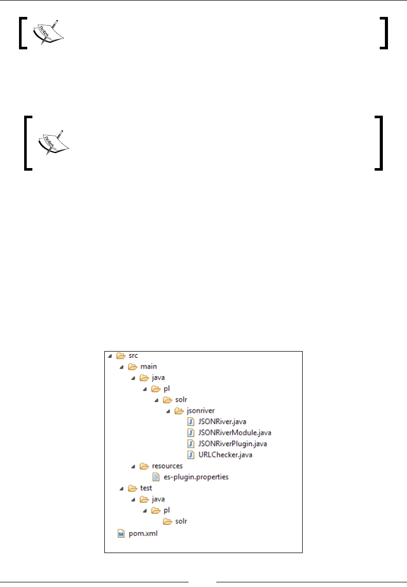
Developing Elasticsearch Plugins
[ 576 ]
Please note that the chapter you are currently reading was written
and tested using Elasticsearch 1.4.1.
Also remember that the book you are holding in your hands is not about
Maven but Elasticsearch, and we will keep Maven-related information to
the required minimum.
Installing Apache Maven is a straightforward task; we assume
that you already have it installed. However, if you have problems
with it, please consult http://maven.apache.org/ for more
information.
Understanding the basics
The result of a Maven build process is an artifact. Each artifact is dened by its
identier, its group, and its version. This is crucial when working with Maven,
because every dependency you'll use will need to be identied by these three
mentioned properties.
The structure of the Maven Java project
The idea behind Maven is quite simple—you create a project structure that
looks something like this:

Chapter 9
[ 577 ]
You can see that the code is placed in the src folder—the code is in the main folder
and the unit tests are located in the test folder. Although you can change the default
layout, Maven tends to work best with the default layout.
The idea of POM
In addition to the code, you can see a le named pom.xml that is located in the root
directory in the previous image. This is a project object model le that describes
the project, its properties, and its dependencies. That's right—you don't need to
manually download dependencies if they are present in one of the available Maven
repositories—during its work, Maven will download them, put them in your local
repository on your hard disk, and use it when needed. All you need to care about is
writing an appropriate pom.xml section that will inform Maven which dependencies
should be used.
For example, this is an example Maven pom.xml le:
<project xmlns="http://maven.apache.org/POM/4.0.0" xmlns:xsi="http://
www.w3.org/2001/XMLSchema-instance"
xsi:schemaLocation="http://maven.apache.org/POM/4.0.0 http://
maven.apache.org/xsd/maven-4.0.0.xsd">
<modelVersion>4.0.0</modelVersion>
<groupId>pl.solr</groupId>
<artifactId>analyzer</artifactId>
<version>1.0-SNAPSHOT</version>
<packaging>jar</packaging>
<name>analyzer</name>
<url>http://solr.pl</url>
<properties>
<elasticsearch.version>1.4.1</elasticsearch.version>
<project.build.sourceEncoding>UTF-8</project.build.
sourceEncoding>
</properties>
<dependencies>
<dependency>
<groupId>org.elasticsearch</groupId>
<artifactId>elasticsearch</artifactId>
<version>${elasticsearch.version}</version>
</dependency>

Developing Elasticsearch Plugins
[ 578 ]
</dependencies>
</project>
This is a simplied version of a pom.xml le that we will extend in the rest of the
chapter. You can see that it starts with the root project tag and then denes the
group identier, the artifact identier, the version, and the packaging method (in
our case, the standard build command will create a jar le). In addition to this, we've
specied a single dependency—the Elasticsearch library Version 1.4.1.
Running the build process
In order to run the build process, what we need to do is simply run the following
command in the directory where the pom.xml le is present:
mvn clean package
It will result in running Maven. It will clean all the generated content in the working
directory, compile and package our code. Of course, if we have unit tests, they will
have to pass in order for the package to be built. The built package will be written
into the target directory created by Maven.
If you want to learn more about the Maven life cycle, please refer
to http://maven.apache.org/guides/introduction/
introduction-to-the-lifecycle.html.
Introducing the assembly Maven plugin
In order to build the ZIP le that will contain our plugin code, we need to package
it. By default, Maven doesn't support pure ZIP les' packaging, so in order to make
it all work, we will use the Maven Assembly plugin (you can nd more about the
plugin at http://maven.apache.org/plugins/maven-assembly-plugin/). In
general, the described plugin allows us to aggregate the project output along with its
dependencies, documentations, and conguration les into a single archive.
In order for the plugin to work, we need to add the build section to our pom.xml
le that will contain information about the assembly plugin, the jar plugin (which is
responsible for creating the proper jar), and the compiler plugin, because we want to
be sure that the code will be readable by Java 7. In addition to this, let's assume that
we want our archive to be put into the target/release directory of our project. The
relevant section of the pom.xml le should look as follows:
<build>
<plugins>
<plugin>

Chapter 9
[ 579 ]
<groupId>org.apache.maven.plugins</groupId>
<artifactId>maven-jar-plugin</artifactId>
<version>2.3</version>
<configuration>
<finalName>elasticsearch-${project.name}-
${elasticsearch.version}</finalName>
</configuration>
</plugin>
<plugin>
<groupId>org.apache.maven.plugins</groupId>
<artifactId>maven-assembly-plugin</artifactId>
<version>2.2.1</version>
<configuration>
<finalName>elasticsearch-${project.name}-
${elasticsearch.version}</finalName>
<appendAssemblyId>false</appendAssemblyId>
<outputDirectory>${project.build.directory}/release/</
outputDirectory>
<descriptors>
<descriptor>assembly/release.xml</descriptor>
</descriptors>
</configuration>
<executions>
<execution>
<id>generate-release-plugin</id>
<phase>package</phase>
<goals>
<goal>single</goal>
</goals>
</execution>
</executions>
</plugin>
<plugin>
<artifactId>maven-compiler-plugin</artifactId>
<configuration>
<source>1.7</source>
<target>1.7</target>
</configuration>
</plugin>
</plugins>
</build>

Developing Elasticsearch Plugins
[ 580 ]
If you look closely at the assembly plugin conguration, you'll notice that we specify
the assembly descriptor called release.xml in the assembly directory. This le is
responsible for specifying what kind of archive we want to have as the output. Let's
put the following release.xml le in the assembly directory of our project:
<?xml version="1.0"?>
<assembly>
<id>bin</id>
<formats>
<format>zip</format>
</formats>
<includeBaseDirectory>false</includeBaseDirectory>
<dependencySets>
<dependencySet>
<unpack>false</unpack>
<outputDirectory>/</outputDirectory>
<useProjectArtifact>false</useProjectArtifact>
<useTransitiveFiltering>true</useTransitiveFiltering>
<excludes>
<exclude>org.elasticsearch:elasticsearch</exclude>
</excludes>
</dependencySet>
</dependencySets>
<fileSets>
<fileSet>
<directory>${project.build.directory}/</directory>
<outputDirectory>/</outputDirectory>
<includes>
<include>elasticsearch-${project.name}-
${elasticsearch.version}.jar</include>
</includes>
</fileSet>
</fileSets>
</assembly>
Again, we don't need to know all the details; however, it is nice to understand
what is going on, even on the general level. The preceding code le tells the Maven
Assembly plugin that we want our archive to be packed with ZIP (<format>zip</
format>), and we want Elasticsearch libraries to be excluded (the exclude section),
because they will already be present in Elasticsearch, where we will install the
plugin. In addition to this, we've specied that we want our project jar to be included
(the includes section).

Chapter 9
[ 581 ]
If you want to see the full project structure with the full pom.xml le
and all the needed les, please look at the code provided with the
book for Chapter 9, Developing Elasticsearch Plugins.
Creating custom REST action
Let's start the journey of extending Elasticsearch by creating a custom REST action.
We've chosen this as the rst extension, because we wanted to take the simplest
approach as the introduction to extending Elasticsearch.
We assume that you already have a Java project created and that you
are using Maven, just like we did in the Creating the Apache Maven project
structure section in the beginning of this chapter. If you would like
to use an already created and working example and start from there,
please look at the code for Chapter 9, Developing Elasticsearch Plugins that
is available with the book.
The assumptions
In order to illustrate how to develop a custom REST action, we need to have an
idea of how it should work. Our REST action will be really simple—it should return
names of all the nodes or names of the nodes that start with the given prex if the
prefix parameter is passed to it. In addition to that, it should only be available when
using the HTTP GET method, so POST requests, for example, shouldn't be allowed.
Implementation details
We will need to develop two Java classes:
• A class that extends the BaseRestHandler Elasticsearch abstract class from
the org.elasticsearch.rest package that will be responsible for handling
the REST action code—we will call it a CustomRestAction.
• A class that will be used by Elasticsearch to load the plugin—this class
needs to extend the Elasticsearch AbstractPlugin class from the org.
elasticsearch.plugin package—we will call it CustomRestActionPlugin.
In addition to the preceding two, we will need a simple text le that we will discuss
after implementing the two mentioned Java classes.

Developing Elasticsearch Plugins
[ 582 ]
Using the REST action class
The most interesting class is the one that will be used to handle the user's requests—
we will call it CustomRestAction. In order to work, it needs to extend the
BaseRestHandler class from the org.elasticsearch.rest package—the base class
for REST actions in Elasticsearch. In order to extend this class, we need to implement
the handleRequest method in which we will process the user request and a three
argument constructor that will be used to initialize the base class and register the
appropriate handler under which our REST action will be visible.
The whole code for the CustomRestAction class looks as follows:
public class CustomRestAction extends BaseRestHandler {
@Inject
public CustomRestAction(Settings settings, RestController
controller, Client client) {
super(settings, controller, client);
controller.registerHandler(Method.GET,"/_mastering/nodes", this);
}
@Override
public void handleRequest(RestRequest request, RestChannel
channel, Client client) {
final String prefix = request.param("prefix", "");
client.admin().cluster().prepareNodesInfo().all().execute(new
RestBuilderListener<NodesInfoResponse>(channel) {
@Override
public RestResponse buildResponse(
NodesInfoResponse response, XContentBuilder builder)
throws Exception {
List<String> nodes = new ArrayList<String>();
for (NodeInfo nodeInfo : response.getNodes()) {
String nodeName = nodeInfo.getNode().getName();
if (prefix.isEmpty()) {
nodes.add(nodeName);
} else if (nodeName.startsWith(prefix)) {
nodes.add(nodeName);
}
}
builder.startObject()
.field("nodes", nodes)

Chapter 9
[ 583 ]
.endObject();
return new BytesRestResponse(RestStatus.OK, builder);
}
});
}
}
The constructor
For each custom REST class, Elasticsearch will pass three arguments when creating
an object of such type: the Settings type object, which holds the settings; the
RestController type object that we will use to bind our REST action to the REST
endpoint; and the Client type object, which is an Elasticsearch client and entry point
for cooperation with it. All of these arguments are also required by the super class, so
we invoke the base class constructor and pass them.
There is one more thing: the @Inject annotation. It allows us to inform Elasticsearch
that it should put the objects in the constructor during the object creation. For more
information about it, please refer to the Javadoc of the mentioned annotation, which
is available at https://github.com/elasticsearch/elasticsearch/blob/
master/src/main/java/org/elasticsearch/common/inject/Inject.java.
Now, let's focus on the following code line:
controller.registerHandler(Method.GET, "/_mastering/nodes", this);
What it does is that it registers our custom REST action implementation and binds
it to the endpoint of our choice. The rst argument is the HTTP method type, the
REST action will be able to work with. As we said earlier, we only want to respond
to GET requests. If we would like to respond to multiple types of HTTP methods, we
should just include multiple registerHandler method invocations with each HTTP
method. The second argument species the actual REST endpoint our custom action
will be available at; in our case, it will available under the /_mastering/nodes
endpoint. The third argument tells Elasticsearch which class should be responsible
for handling the dened endpoint; in our case, this is the class we are developing,
thus we are passing this.

Developing Elasticsearch Plugins
[ 584 ]
Handling requests
Although the handleRequest method is the longest one in our code, it is not
complicated. We start by reading the request parameter with the following
line of code:
String prefix = request.param("prefix", "");
We store the prex request parameter in the variable called prefix. By default, we
want an empty String object to be assigned to the prefix variable if there is no
prex parameter passed to the request (the default value is dened by the second
parameter of the param method of the request object).
Next, we retrieve the NodesInfoResponse object using the Elasticsearch client object
and its abilities to run administrative commands. In this case, we have used the
possibility of sending queries to Elasticsearch in an asynchronous way. Instead of the
call execute().actionGet() part, which waits for a response and returns it, we have
used the execute() call, which takes a future object that will be informed when the
query nishes. So, the rest of the method is in the buildResponse() callback of the
RestBuilderListener object. The NodesInfoResponse object will contain an array of
NodeInfo objects, which we will use to get node names. What we need to do is return
all the node names that start with a given prex or all if the prefix parameter was not
present in the request. In order to do this, we create a new array:
List<String> nodes = new ArrayList<String>();
We iterate over the available nodes using the following for loop:
for (NodeInfo nodeInfo : response.getNodes())
We get the node name using the getName method of the DiscoveryNode object,
which is returned after invoking the getNode method of NodeInfo:
String nodeName = nodeInfo.getNode().getName();
If prefix is empty or if it starts with the given prex, we add the name of the node
to the array we've created. After we iterate through all the NodeInfo objects, we call
the are starting build the response and sent it through the HTTP.

Chapter 9
[ 585 ]
Writing response
The last thing regarding our CustomRestAction class is the response handling,
which is the responsibility of the last part of the buildResponse() method that we
created. It is simple because an appropriate response builder is already provided by
Elasticsearch under the builder argument. It takes into consideration the format
parameter used by the client in the call, so by default, we send the response in a
proper JSON format just like Elasticsearch does and also take the YAML (http://
en.wikipedia.org/wiki/YAML) format for free.
Now, we use the builder object we got to start the response object (using the
startObject method) and start a nodes eld (because the value of the eld is a
collection, it will automatically be formatted as an array). The nodes eld is created
inside the initial object, and we will use it to return matching nodes names. Finally,
we close the object using the endObject method.
After we have our object ready to be sent as a response, we return the
BytesRestResponse object. We do this in the following line:
return new BytesRestResponse(RestStatus.OK, builder);
As you can see, to create the object, we need to pass two parameters: RestStatus
and the XContentBuilder, which holds our response. The RestStatus class allows
us to specify the response code, which is RestStatus.OK in our case, because
everything went smoothly.
The plugin class
The CustomRestActionPlugin class will hold the code that is used by Elasticsearch
to initialize the plugin itself. It extends the AbstractPlugin class from the org.
elasticsearch.plugin package. Because we are creating an extension, we are
obliged to implement the following code parts:
• constructor: This is a standard constructor that will take a single argument; in
our case, it will be empty
• The onModule method: This is the method that includes the code that will
add our custom REST action so that Elasticsearch will know about it
• The name method: This is the name of our plugin
• The description method: This is a short description of our plugin

Developing Elasticsearch Plugins
[ 586 ]
The code of the whole class looks as follows:
public class CustomRestActionPlugin extends AbstractPlugin {
@Inject
public CustomRestActionPlugin(Settings settings) {
}
public void onModule(RestModule module) {
module.addRestAction(CustomRestAction.class);
}
@Override
public String name() {
return "CustomRestActionPlugin";
}
@Override
public String description() {
return "Custom REST action";
}
}
The constructor, name, and description methods are very simple, and we will just
skip discussing them, and we will focus on the onModule method. This method
takes a single argument: the RestModule class object, which is the class that
allows us to register our custom REST action. Elasticsearch will call the onModule
method for all the modules that are available and eligible (all REST actions). What
we do is just a simple call to the RestModule addRestAction method, passing
in our CustomRestAction class as an argument. That's all when it comes to Java
development.
Informing Elasticsearch about our REST action
We have our code ready, but we need one additional thing; we need to let
Elasticsearch know what the class registering our plugin is—the one we've called
CustomRestActionPlugin. In order to do this, we create an es-plugin.properties
le in the src/main/resources directory with the following content:
plugin=pl.solr.rest.CustomRestActionPlugin
We just specify the plugin property there, which should have a value of the class we
use to register our plugins (the one that extends the Elasticsearch AbstractPlugin
class). This le will be included in the jar le that will be created during the build
process and will be used by Elasticsearch during the plugin load process.

Chapter 9
[ 587 ]
Time for testing
Of course, we could leave it now and say that we are done, but we won't. We would
like to show you how to build each of the plugins, install it, and nally, test it to see
whether it actually works. Let's start with building our plugin.
Building the REST action plugin
We start with the easiest part—building our plugin. In order to do this, we run a
simple command:
mvn compile package
We tell Maven that we want the code to be compiled and packaged. After the
command nishes, we can nd the archive with the plugin in the target/release
directory (assuming you are using a project setup similar to the one we've described
at the beginning of the chapter).
Installing the REST action plugin
In order to install the plugin, we will use the plugin command that is located in the
bin directory of the Elasticsearch distributable package. Assuming that we have our
plugin archive stored in the /home/install/es/plugins directory, we will run the
following command (we run it from the Elasticsearch home directory):
bin/plugin --install rest --url
file:/home/install/es/plugins/elasticsearch-rest-1.4.1.zip
We need to install the plugin on all the nodes in our cluster, because we want to be
able to run our custom REST action on each Elasticsearch instance.
In order to learn more about installing Elasticsearch plugins, please
refer to our previous book, Elasticsearch Server Second Edition, or
check out the ofcial Elasticsearch documentation at http://www.
elasticsearch.org/guide/reference/modules/plugins/.
After we have the plugin installed, we need to restart our Elasticsearch instance we
were making the installation on. After the restart, we should see something like this
in the logs:
[2014-12-12 21:04:48,348][INFO ][plugins ]
[Archer] loaded [CustomRestActionPlugin], sites []
As you can see, Elasticsearch informed us that the plugin named
CustomRestActionPlugin was loaded.

Developing Elasticsearch Plugins
[ 588 ]
Checking whether the REST action plugin works
We can nally check whether the plugin works. In order to do that, we will run the
following command:
curl -XGET 'localhost:9200/_mastering/nodes?pretty'
As a result, we should get all the nodes in the cluster, because we didn't provide the
prefix parameter and this is exactly what we've got from Elasticsearch:
{
"nodes" : [ "Archer" ]
}
Because we only had one node in our Elasticsearch cluster, we've got the nodes array
with only a single entry.
Now, let's test what will happen if we add the prefix=Are parameter to our request.
The exact command we've used was as follows:
curl -XGET 'localhost:9200/_mastering/nodes?prefix=Are&pretty'
The response from Elasticsearch was as follows:
{
"nodes" : [ ]
}
As you can see, the nodes array is empty, because we don't have any node in the
cluster that would start with the Are prex. At the end, let's check another
format of response:
curl -XGET 'localhost:9200/_mastering/nodes?pretty&format=yaml'
Now the response is not in a JSON format. Look at the example output for a cluster
consisting of two nodes:
---
nodes:
- "Atalon"
- "Slapstick"
As we can see, our REST plugin is not so complicated but already has
several features.

Chapter 9
[ 589 ]
Creating the custom analysis plugin
The last thing we want to discuss when it comes to custom Elasticsearch plugins
is the analysis process extension. We've chosen to show how to develop a custom
analysis plugin because this is sometimes very useful, for example, when you want
to have the custom analysis process that you use in your company introduced, or
when you want to use the Lucene analyzer or lter that is not present in Elasticsearch
itself or as a plugin for it. Because creating an analysis extension is more complicated
compared to what we've seen when developing a custom REST action, we decided to
leave it until the end of the chapter.
Implementation details
Because developing a custom analysis plugin is the most complicated, at least from
the Elasticsearch point of view and the number of classes we need to develop,
we will have more things to do compared to previous examples. We will need to
develop the following things:
• The TokenFilter class extension (from the org.apache.lucene.analysis
package) implementation that will be responsible for handling token
reversing; we will call it CustomFilter
• The AbstractTokenFilterFactory extension (from the org.
elasticsearch.index.analysis package) that will be responsible for
providing our CustomFilter instance to Elasticsearch; we will call it
CustomFilterFactory
• The custom analyzer, which will extend the org.apache.lucene.analysis.
Analyzer class and provide the Lucene analyzer functionality; we will call it
CustomAnalyzer
• The analyzer provider, which we will call CustomAnalyzerProvider, which
extends AbstractIndexAnalyzerProvider from the org.elasticsearch.
index.analysis package, and which will be responsible for providing the
analzyer instance to Elasticsearch
• An extension of AnalysisModule.AnalysisBinderProcessor from the org.
elasticsearch.index.analysis package, which will have information
about the names under which our analyzer and token lter will be available
in Elasticsearch; we will call it CustomAnalysisBinderProcessor
• An extension of the AbstractComponent class from the org.
elasticsearch.common.component package, which will inform
Elasticsearch which factories should be used for our custom analyzer and
token lter; we will call it CustomAnalyzerIndicesComponent

Developing Elasticsearch Plugins
[ 590 ]
• The AbstractModule extension (from the org.elasticsearch.
common.inject package) that will inform Elasticsearch that our
CustomAnalyzerIndicesComponent module should be a singleton; we will
call it CustomAnalyzerModule
• Finally, the usual AbstractPlugin extension (from the org.
elasticsearch.plugins package) that will register our plugin; we will call
it CustomAnalyzerPlugin
So let's start discussing the code.
Implementing TokenFilter
The funniest thing about the currently discussed plugin is that the whole analysis
work is actually done on a Lucene level, and what we need to do is write the
org.apache.lucene.analysis.TokenFilter extension, which we will call
CustomFilter. In order to do this, we need to initialize the super class and override
the incrementToken method. Our class will be responsible for reversing the tokens,
so that's the logic we want our analyzer and lter to have. The whole implementation
of our CustomFilter class looks as follows:
public class CustomFilter extends TokenFilter {
private final CharTermAttribute termAttr =
addAttribute(CharTermAttribute.class);
protected CustomFilter(TokenStream input) {
super(input);
}
@Override
public boolean incrementToken() throws IOException {
if (input.incrementToken()) {
char[] originalTerm = termAttr.buffer();
if (originalTerm.length > 0) {
StringBuilder builder = new StringBuilder(new
String(originalTerm).trim()).reverse();
termAttr.setEmpty();
termAttr.append(builder.toString());
}
return true;
} else {
return false;
}
}
}

Chapter 9
[ 591 ]
The rst thing we see in the implementation is the following line:
private final CharTermAttribute termAttr =
addAttribute(CharTermAttribute.class);
It allows us to retrieve the text of the token we are currently processing. In order
to get access to the other token information, we need to use other attributes. The
list of attributes can be found by looking at the classes implementing Lucene's
org.apache.lucene.util.Attribute interface (http://lucene.apache.org/
core/4_10_0/core/org/apache/lucene/util/Attribute.html). What you need
to know now is that by using the static addAttribute method, we can bind different
attributes and use them during token processing.
Then, we have the constructor, which is only used for super class initialization, so we
can skip discussing it.
Finally, there is the incrementToken method, which returns true when there is a
token in the token stream left to be processed, and false if there is no token left to be
processed. So, what we do rst is we check whether there is a token to be processed
by calling the incrementToken method of input, which is the TokenStream instance
stored in the super class. Then, we get the term text by calling the buffer method of
the attribute we bind in the rst line of our class. If there is text in the term (its length
is higher than zero), we use a StringBuilder object to reverse the text, we clear the
term buffer (by calling setEmpty on the attribute), and we append the reversed text
to the already emptied term buffer (by calling the append method of the attribute).
After this, we return true, because our token is ready to be processed further—on a
token lter level, we don't know whether the token will be processed further or not,
so we need to be sure we return the correct information, just in case.
Implementing the TokenFilter factory
The factory for our token lter implementation is one of the simplest
classes in the case of the discussed plugins. What we need to do is create an
AbstractTokenFilterFactory (from the org.elasticsearch.index.analysis
package) extension that overrides a single create method in which we create our
token lter. The code of this class looks as follows:
public class CustomFilterFactory extends
AbstractTokenFilterFactory {
@Inject
public CustomFilterFactory(Index index, @IndexSettings Settings
indexSettings, @Assisted String name, @Assisted Settings settings)
{
super(index, indexSettings, name, settings);
}

Developing Elasticsearch Plugins
[ 592 ]
@Override
public TokenStream create(TokenStream tokenStream) {
return new CustomFilter(tokenStream);
}
}
As you can see, the class is very simple. We start with the constructor, which is
needed, because we need to initialize the parent class. In addition to this, we have
the create method, in which we create our CustomFilter class with the provided
TokenStream object.
Before we go on, we would like to mention two more things: the @IndexSettings
and @Assisted annotations. The rst one will result in index settings being injected
as the Settings class object to the constructor; of course, this is done automatically.
The @Assisted keyword results in the annotated parameter value to be injected
from the argument of the factory method.
Implementing the class custom analyzer
We wanted to keep the example implementation as simple as possible and, because
of that, we've decided not to complicate the analyzer implementation. To implement
our analyzer, we need to extend an abstract Analyzer class from Lucene's org.
apache.lucene.analysis package, and we did that. The whole code of our
CustomAnalyzer class looks as follows:
public class CustomAnalyzer extends Analyzer {
public CustomAnalyzer() {
}
@Override
protected TokenStreamComponents createComponents(String field,
Reader reader) {
final Tokenizer src = new WhitespaceTokenizer(reader);
return new TokenStreamComponents(src, new CustomFilter(src));
}
}
If you want to see more complicated analyzer implementations,
please look at the source code of Apache Lucene, Apache Solr,
and Elasticsearch.

Chapter 9
[ 593 ]
The createComponent method is the one we need to implement, and it should
return a TokenStreamComponents object (from the org.apache.lucene.analysis
package) for a given eld name (the String type object—the rst argument of
the method) and data (the Reader type object—the second method argument).
What we do is create a Tokenizer object using the WhitespaceTokenizer class
available in Lucene. This will result in the input data to be tokenized on whitespace
characters. Then, we create a Lucene TokenStreamComponents object, to which
we give the source of tokens (our previously created Tokenizer object) and our
CustomFilter object. This will result in our CustomFilter object to be used by
CustomAnalyzer.
Implementing the analyzer provider
Let's talk about another provider implementation in addition to the
token lter factory we've created earlier. This time, we need to extend
AbstractIndexAnalyzerProvider from the org.elasticsearch.index.
analysis package in order for Elasticsearch to be able to create our analyzer. The
implementation is very simple, as we only need to implement the get method in
which we should return our analyzer. The CustomAnalyzerProvider class code
looks as follows:
public class CustomAnalyzerProvider extends
AbstractIndexAnalyzerProvider<CustomAnalyzer> {
private final CustomAnalyzer analyzer;
@Inject
public CustomAnalyzerProvider(Index index, @IndexSettings
Settings indexSettings, Environment env, @Assisted String name,
@Assisted Settings settings) {
super(index, indexSettings, name, settings);
analyzer = new CustomAnalyzer();
}
@Override
public CustomAnalyzer get() {
return this.analyzer;
}
}

Developing Elasticsearch Plugins
[ 594 ]
As you can see, we've implemented the constructor in order to be able to initialize
the super class. In addition to that, we are creating a single instance of our analyzer,
which we will return when Elasticsearch requests it. We do this because we don't
want to create an analyzer every time Elasticsearch requests it; this is not efcient.
We don't need to worry about multithreading because our analyzer is thread-safe
and, thus, a single instance can be reused. In the get method, we are just returning
our analyzer.
Implementing the analysis binder
The binder is a part of our custom code that informs Elasticsearch about
the names under which our analyzer and token lter will be available.
Our CustomAnalysisBinderProcessor class extends AnalysisModule.
AnalysisBinderProcessor from org.elasticsearch.index.analysis, and we
override two methods of this class: processAnalyzers in which we will register our
analyzer and processTokenFilters in which we will register our token lter. If we
had only an analyzer or only a token lter, we would only override a single method.
The code of CustomAnalysisBinderProcessor looks as follows:
public class CustomAnalysisBinderProcessor extends
AnalysisModule.AnalysisBinderProcessor {
@Override
public void processAnalyzers(AnalyzersBindings
analyzersBindings) {
analyzersBindings.processAnalyzer("mastering_analyzer",
CustomAnalyzerProvider.class);
}
@Override
public void processTokenFilters(TokenFiltersBindings
tokenFiltersBindings) {
tokenFiltersBindings.processTokenFilter("mastering_filter",
CustomFilterFactory.class);
}
}
The rst method—processAnalyzers—takes a single AnalysisBinding object
type, which we can use to register our analyzer under a given name. We do this by
calling the processAnalyzer method of the AnalysisBinding object and pass in
the name under which our analyzer will be available and the implementation of
AbstractIndexAnalyzerProvider, which is responsible for creating our analyzer,
which in our case, is the CustomAnalyzerProvider class.

Chapter 9
[ 595 ]
The second method—procesTokenFilters—again takes a single
TokenFiltersBindings class, which enables us to register our token lter. We do
this by calling the processTokenFilter method and passing the name under which
our token lter will be available and the token lter factory class, which in our case,
is CustomFilterFactory.
Implementing the analyzer indices component
Now, we need to implement a node level component that will allow our analyzer
and token lter to be reused. However, we will tell Elasticsearch that our analyzer
should be reusable only on the indices level and not globally (just to show you how
to do it). What we need to do is extend the AbstractComponent class from the org.
elasticsearch.common.component package. In fact, we only need to develop a
constructor for the class we called CustomAnalyzerIndicesComponent. The whole
code for the mentioned class looks as follows:
public class CustomAnalyzerIndicesComponent extends
AbstractComponent {
@Inject
public CustomAnalyzerIndicesComponent(Settings settings,
IndicesAnalysisService indicesAnalysisService) {
super(settings);
indicesAnalysisService.analyzerProviderFactories().put(
"mastering_analyzer",
new PreBuiltAnalyzerProviderFactory("mastering_analyzer",
AnalyzerScope.INDICES, new CustomAnalyzer()));
indicesAnalysisService.tokenFilterFactories().put("mastering_filte
r",
new PreBuiltTokenFilterFactoryFactory(new
TokenFilterFactory() {
@Override
public String name() {
return "mastering_filter";
}
@Override
public TokenStream create(TokenStream tokenStream) {
return new CustomFilter(tokenStream);
}
}));
}
}

Developing Elasticsearch Plugins
[ 596 ]
First of all, we pass the constructor arguments to the super class in order to initialize
it. After that, we create a new analyzer, which is our CustomAnalyzer class, by
using the following code snippet:
indicesAnalysisService.analyzerProviderFactories().put(
"mastering_analyzer",
new PreBuiltAnalyzerProviderFactory("mastering_analyzer",
AnalyzerScope.INDICES, new CustomAnalyzer()));
As you can see, we've used the IndicesAnalysisService object
and its analyzerProviderFactories method to get the map of
PreBuiltAnalyzerProviderFactory (as a value and the name as a key in the
map), and we've put a newly created PreBuiltAnalyzerProviderFactory
object with the name of mastering_analyzer. In order to create the
PreBuiltAnalyzerProviderFactory we've used our CustomAnalyzer and
AnalyzerScope.INDICES enum values (from the org.elasticsearch.index.
analysis package). The other values of AnalyzerScope enum are GLOBAL and
INDEX. If you would like the analyzer to be globally shared, you should use
AnalyzerScope.GLOBAL and AnalyzerScope.INDEX, both of which should be
created for each index separately.
In a similar way, we add our token lter, but this time, we use the
tokenFilterFactories method of the IndicesAnalysisService object, which
returns a Map of PreBuiltTokenFilterFactoryFactory as a value and a name (a
String object) as a key. We put a newly created TokenFilterFactory object with
the name of mastering_filter.
Implementing the analyzer module
A simple class called CustomAnalyzerModule extends AbstractModule from the
org.elasticsearch.common.inject package. It is used to tell Elasticsearch that our
CustomAnalyzerIndicesComponent class should be used as a singleton; we do this
because it's enough to have a single instance of that class. Its code looks as follows:
public class CustomAnalyzerModule extends AbstractModule {
@Override
protected void configure() {
bind(CustomAnalyzerIndicesComponent.class).asEagerSingleton();
}
}
As you can see, we implement a single congure method, which tells you to bind the
CustomAnalyzerIndicesComponent class as a singleton.

Chapter 9
[ 597 ]
Implementing the analyzer plugin
Finally, we need to implement the plugin class so that Elasticsearch knows that
there is a plugin to be loaded. It should extend the AbstractPlugin class from the
org.elasticsearch.plugins package and thus implement at least the name and
descriptions methods. However, we want our plugin to be registered, and that's
why we implement two additional methods, which we can see in the following
code snippet:
public class CustomAnalyzerPlugin extends AbstractPlugin {
@Override
public Collection<Class<? extends Module>> modules() {
return ImmutableList.<Class<? extends
Module>>of(CustomAnalyzerModule.class);
}
public void onModule(AnalysisModule module) {
module.addProcessor(new CustomAnalysisBinderProcessor());
}
@Override
public String name() {
return "AnalyzerPlugin";
}
@Override
public String description() {
return "Custom analyzer plugin";
}
}
The name and description methods are quite obvious, as they are returning
the name of the plugin and its description. The onModule method adds our
CustomAnalysisBinderProcessor object to the AnalysisModule object
provided to it.
The last method is the one we are not yet familiar with: the modules method:
public Collection<Class<? extends Module>> modules() {
return ImmutableList.<Class<? extends
Module>>of(CustomAnalyzerModule.class);
}

Developing Elasticsearch Plugins
[ 598 ]
We override this method from the super class in order to return a collection of
modules that our plugin is registering. In this case, we are registering a single
module class—CustomAnalyzerModule—and we are returning a list with a
single entry.
Informing Elasticsearch about our custom analyzer
Once we have our code ready, we need to add one additional thing: we need to let
Elasticsearch know what the class registering our plugin is—the one we've called
CustonAnalyzerPlugin. In order to do that, we create an es-plugin.properties
le in the src/main/resources directory with the following content:
plugin=pl.solr.analyzer.CustomAnalyzerPlugin
We just specify the plugin property there, which should have a value of the class we
use to register our plugins (the one that extends the Elasticsearch AbstractPlugin
class). This le will be included in the JAR le that will be created during the build
process and will be used by Elasticsearch during the plugin load process.
Testing our custom analysis plugin
Now, we want to test our custom analysis plugin just to be sure that everything
works. In order to do that, we need to build our plugin, install it on all nodes in our
cluster, and nally, use the Admin Indices Analyze API to see how our analyzer
works. Let's do that.
Building our custom analysis plugin
We start with the easiest part: building our plugin. In order to do that, we run a
simple command:
mvn compile package
We tell Maven that we want the code to be compiled and packaged. After the
command nishes, we can nd the archive with the plugin in the target/release
directory (assuming you are using a project setup similar to the one we've described
at the beginning of the chapter).

Chapter 9
[ 599 ]
Installing the custom analysis plugin
To install the plugin, we will use the plugin command, just like we did previously.
Assuming that we have our plugin archive stored in the /home/install/es/
plugins directory, would run the following command (we run it from the
Elasticsearch home directory):
bin/plugin --install analyzer --url
file:/home/install/es/plugins/elasticsearch-analyzer-1.4.1.zip
We need to install the plugin on all the nodes in our cluster, because we want
Elasticsearch to be able to nd our analyzer and lter no matter on which node the
analysis process is done. If we don't install the plugin on all nodes, we can be certain
that we will run into issues.
In order to learn more about installing Elasticsearch plugins,
please refer to our previous book, Elasticsearch Server Section
Edition, by Packt Publishing or refer to the ofcial Elasticsearch
documentation.
After we have the plugin installed, we need to restart our Elasticsearch instance we
were creating the installation on. After the restart, we should see something like this
in the logs:
[2014-12-03 22:39:11,231][INFO ][plugins ]
[Tattletale] loaded [AnalyzerPlugin], sites []
With the preceding log line, Elasticsearch informs us that the plugin named
AnalyzerPlugin was successfully loaded.
Checking whether our analysis plugin works
We can nally check whether our custom analysis plugin works as it should. In order
to do that, we start with creating an empty index called analyzetest (the index
name doesn't matter). We do this by running the following command:
curl -XPOST 'localhost:9200/analyzetest/'
After this we use the Admin Indices Analyze API (http://www.elasticsearch.
org/guide/en/elasticsearch/reference/current/indices-analyze.html) to
see how our analyzer works. We do that by running the following command:
curl -XGET 'localhost:9200/analyzetest/_analyze?analyzer=mastering_
analyzer&pretty' -d 'mastering elasticsearch'

Developing Elasticsearch Plugins
[ 600 ]
So, what we should see in response is two tokens: one that should be reversed—
mastering—gniretsam and another one that should also be reversed—
elasticsearch—hcraescitsale. The response Elasticsearch returns looks as follows:
{
"tokens" : [ {
"token" : "gniretsam",
"start_offset" : 0,
"end_offset" : 9,
"type" : "word",
"position" : 1
}, {
"token" : "hcraescitsale",
"start_offset" : 10,
"end_offset" : 23,
"type" : "word",
"position" : 2
} ]
}
As you can see, we've got exactly what we expected, so it seems that our custom
analysis plugin works as intended.
Summary
In this chapter, we were focused on developing custom plugins for Elasticsearch.
We learned how to properly set up your Maven project to be able to automatically
build your Elasticsearch plugins. You saw how to develop a custom REST action
plugin, and we extended Elasticsearch analysis capabilities by creating a plugin that
included a custom token lter and new analyzer.
We've reached the end of the book, and we wanted to write a small summary and
say a few words to the brave reader who managed to get to the end. We decided to
write the second edition of Mastering Elasticsearch after writing Elasticsearch Server
Second Edition. We thought that we had left a number of topics uncovered, and we
wanted to write them in this book. We went from introducing Apache Lucene and
Elasticsearch to querying and data handling—both on the Lucene index and the
Elasticsearch level. We hope that, by now, you know how Lucene works and how
Elasticsearch uses it, and you will nd this knowledge worthy in your journey with
this great search engine. We talked about some topics that can be useful when things
are hot, such as I/O throttling, Hot Threads API, and how to speed up your queries.
We also concentrated on things such as choosing the right query for the use case and
Elasticsearch scaling.

Chapter 9
[ 601 ]
Finally, we dedicated one chapter to discussing Java development on how to
extend Elasticsearch with your own plugins. In the rst version of the book, we also
described the Java API briey, but we decided it doesn't make sense. The API would
require its own book and showing only some things regarding them just feels wrong.
Hopefully, you'll be able to write your own plugins and even though we didn't write
about all the possibilities, we hope that you'll be able to nd the things we didn't
write about.
Thank you for reading the book; we hope that you like it and that it brought you
some knowledge that you were seeking, and that you'll be able to use it whether you
use Elasticsearch professionally or just as a hobby.
Finally, please stop by at http://elasticsearchserverbook.com/ from time
to time. In addition to the usual posts we make, we will publish the book fragments
that didn't make it to the book or were cut down because the book would be
too broad.
Module 3
Learning ELK Stack
Build mesmerizing visualizations, analytics, and logs from your
data using Elasticsearch, Logstash, and Kibana

[ 605 ]
Introduction to ELK Stack
This chapter explains the importance of log analysis in today's data-driven world
and what are the challenges associated with log analysis. It introduces ELK stack
as a complete log analysis solution, and explains what ELK stack is and the role of
each of the open source components of the stack, namely, Elasticsearch, Logstash,
and Kibana. Also, it briey explains the key features of each of the components and
describes the installation and conguration steps for them.
The need for log analysis
Logs provide us with necessary information on how our system is behaving.
However, the content and format of the logs varies among different services or say,
among different components of the same system. For example, a scanner may log
error messages related to communication with other devices; on the other hand,
a web server logs information on all incoming requests, outgoing responses, time
taken for a response, and so on. Similarly, application logs for an e-commerce
website will log business-specic logs.
As the logs vary by their content, so will their uses. For example, the logs from a scanner
may be used for troubleshooting or for a simple status check or reporting while the web
server log is used to analyze trafc patterns across multiple products. Analysis of logs
from an e-commerce site can help gure out whether packages from a specic location
are returned repeatedly and the probable reasons for the same.
The following are some common use cases where log analysis is helpful:
• Issue debugging
• Performance analysis
• Security analysis
• Predictive analysis
• Internet of things (IoT) and logging

Introduction to ELK Stack
[ 606 ]
Issue debugging
Debugging is one of the most common reasons to enable logging within your
application. The simplest and most frequent use for a debug log is to grep for a
specic error message or event occurrence. If a system administrator believes that
a program crashed because of a network failure, then he or she will try to nd a
connection dropped message or a similar message in the server logs to analyze
what caused the issue. Once the bug or the issue is identied, log analysis solutions
help capture application information and snapshots of that particular time can be
easily passed across development teams to analyze it further.
Performance analysis
Log analysis helps optimize or debug system performance and give essential inputs
around bottlenecks in the system. Understanding a system's performance is often
about understanding resource usage in the system. Logs can help analyze individual
resource usage in the system, behavior of multiple threads in the application,
potential deadlock conditions, and so on. Logs also carry with them timestamp
information, which is essential to analyze how the system is behaving over time. For
instance, a web server log can help know how individual services are performing
based on response times, HTTP response codes, and so on.
Security analysis
Logs play a vital role in managing the application security for any organization. They
are particularly helpful to detect security breaches, application misuse, malicious
attacks, and so on. When users interact with the system, it generates log events,
which can help track user behavior, identify suspicious activities, and raise alarms or
security incidents for breaches.
The intrusion detection process involves session reconstruction from the logs itself.
For example, ssh login events in the system can be used to identify any breaches
on the machines.
Predictive analysis
Predictive analysis is one of the hot trends of recent times. Logs and events data
can be used for very accurate predictive analysis. Predictive analysis models help
in identifying potential customers, resource planning, inventory management and
optimization, workload efciency, and efcient resource scheduling. It also helps
guide the marketing strategy, user-segment targeting, ad-placement strategy,
and so on.

Chapter 1
[ 607 ]
Internet of things and logging
When it comes to IoT devices (devices or machines that interact with each other
without any human intervention), it is vital that the system is monitored and
managed to keep downtime to a minimum and resolve any important bugs or issues
swiftly. Since these devices should be able to work with little human intervention
and may exist on a large geographical scale, log data is expected to play a crucial role
in understanding system behavior and reducing downtime.
Challenges in log analysis
The current log analysis process mostly involves checking logs at multiple servers
that are written by different components and systems across your application. This
has various problems, which makes it a time-consuming and tedious job. Let's look
at some of the common problem scenarios:
• Non-consistent log format
• Decentralized logs
• Expert knowledge requirement
Non-consistent log format
Every application and device logs in its own special way, so each format needs its
own expert. Also, it is difcult to search across because of different formats.
Let's take a look at some of the common log formats. An interesting thing to observe
will be the way different logs represent different timestamp formats, different ways
to represent INFO, ERROR, and so on, and the order of these components with logs.
It's difcult to gure out just by seeing logs what is present at what location. This is
where tools such as Logstash help.
Tomcat logs
A typical tomcat server startup log entry will look like this:
May 24, 2015 3:56:26 PM org.apache.catalina.startup.HostConfig deployWAR
INFO: Deployment of web application archive \soft\apache-tomcat-7.0.62\
webapps\sample.war has finished in 253 ms

Introduction to ELK Stack
[ 608 ]
Apache access logs – combined log format
A typical Apache access log entry will look like this:
127.0.0.1 - - [24/May/2015:15:54:59 +0530] "GET /favicon.ico HTTP/1.1"
200 21630
IIS logs
A typical IIS log entry will look like this:
2012-05-02 17:42:15 172.24.255.255 - 172.20.255.255 80 GET /images/
favicon.ico - 200 Mozilla/4.0+(compatible;MSIE+5.5;+Windows+2000+Server)
Variety of time formats
Not only log formats, but timestamp formats are also different among different
types of applications, different types of events generated across multiple devices,
and so on. Different types of time formats across different components of your
system also make it difcult to correlate events occurring across multiple systems
at the same time:
• 142920788
• Oct 12 23:21:45
• [5/May/2015:08:09:10 +0000]
• Tue 01-01-2009 6:00
• 2015-05-30 T 05:45 UTC
• Sat Jul 23 02:16:57 2014
• 07:38, 11 December 2012 (UTC)
Decentralized logs
Logs are mostly spread across all the applications that may be across different
servers and different components. The complexity of log analysis increases with
multiple components logging at multiple locations. For one or two servers' setup,
nding out some information from logs involves running cat or tail commands
or piping these results to grep command. But what if you have 10, 20, or say,
100 servers? These kinds of searches are mostly not scalable for a huge cluster of
machines and need a centralized log management and an analysis solution.

Chapter 1
[ 609 ]
Expert knowledge requirement
People interested in getting the required business-centric information out of logs
generally don't have access to the logs or may not have the technical expertise to
gure out the appropriate information in the quickest possible way, which can make
analysis slower, and sometimes, impossible too.
The ELK Stack
The ELK platform is a complete log analytics solution, built on a combination of
three open source tools—Elasticsearch, Logstash, and Kibana. It tries to address all
the problems and challenges that we saw in the previous section. ELK utilizes the
open source stack of Elasticsearch for deep search and data analytics; Logstash for
centralized logging management, which includes shipping and forwarding the logs
from multiple servers, log enrichment, and parsing; and nally, Kibana for powerful
and beautiful data visualizations. ELK stack is currently maintained and actively
supported by the company called Elastic (formerly, Elasticsearch).
Let's look at a brief overview of each of these systems:
• Elasticsearch
• Logstash
• Kibana
Elasticsearch
Elasticsearch is a distributed open source search engine based on Apache Lucene,
and released under an Apache 2.0 license (which means that it can be downloaded,
used, and modied free of charge). It provides horizontal scalability, reliability,
and multitenant capability for real-time search. Elasticsearch features are available
through JSON over a RESTful API. The searching capabilities are backed by a
schema-less Apache Lucene Engine, which allows it to dynamically index data
without knowing the structure beforehand. Elasticsearch is able to achieve fast
search responses because it uses indexing to search over the texts.
Elasticsearch is used by many big companies, such as GitHub, SoundCloud,
FourSquare, Netix, and many others. Some of the use cases are as follows:
• Wikipedia: This uses Elasticsearch to provide a full text search, and provide
functionalities, such as search-as-you-type, and did-you-mean suggestions.

Introduction to ELK Stack
[ 610 ]
• The Guardian: This uses Elasticsearch to process 40 million documents per
day, provide real-time analytics of site-traffic across the organization, and
help understand audience engagement better.
• StumbleUpon: This uses Elasticsearch to power intelligent searches across its
platform and provide great recommendations to millions of customers.
• SoundCloud: This uses Elasticsearch to provide real-time search capabilities
for millions of users across geographies.
• GitHub: This uses Elasticsearch to index over 8 million code repositories,
and index multiple events across the platform, hence providing real-time
search capabilities across it.
Some of the key features of Elasticsearch are:
• It is an open source distributed, scalable, and highly available real-time
document store
• It provides real-time search and analysis capabilities
• It provides a sophisticated RESTful API to play around with lookup, and
various features, such as multilingual search, geolocation, autocomplete,
contextual did-you-mean suggestions, and result snippets
• It can be scaled horizontally easily and provides easy integrations with
cloud-based infrastructures, such as AWS and others
Logstash
Logstash is a data pipeline that helps collect, parse, and analyze a large variety of
structured and unstructured data and events generated across various systems. It
provides plugins to connect to various types of input sources and platforms, and
is designed to efciently process logs, events, and unstructured data sources for
distribution into a variety of outputs with the use of its output plugins, namely le,
stdout (as output on console running Logstash), or Elasticsearch.
It has the following key features:
• Centralized data processing: Logstash helps build a data pipeline that can
centralize data processing. With the use of a variety of plugins for input and
output, it can convert a lot of different input sources to a single common format.

Chapter 1
[ 611 ]
• Support for custom log formats: Logs written by different applications often
have particular formats specific to the application. Logstash helps parse and
process custom formats on a large scale. It provides support to write your
own filters for tokenization and also provides ready-to-use filters.
• Plugin development: Custom plugins can be developed and published, and
there is a large variety of custom developed plugins already available.
Kibana
Kibana is an open source Apache 2.0 licensed data visualization platform that helps
in visualizing any kind of structured and unstructured data stored in Elasticsearch
indexes. Kibana is entirely written in HTML and JavaScript. It uses the powerful
search and indexing capabilities of Elasticsearch exposed through its RESTful API
to display powerful graphics for the end users. From basic business intelligence to
real-time debugging, Kibana plays its role through exposing data through beautiful
histograms, geomaps, pie charts, graphs, tables, and so on.
Kibana makes it easy to understand large volumes of data. Its simple browser-based
interface enables you to quickly create and share dynamic dashboards that display
changes to Elasticsearch queries in real time.
Some of the key features of Kibana are as follows:
• It provides flexible analytics and a visualization platform for business
intelligence.
• It provides real-time analysis, summarization, charting, and debugging
capabilities.
• It provides an intuitive and user friendly interface, which is highly
customizable through some drag and drop features and alignments as and
when needed.
• It allows saving the dashboard, and managing more than one dashboard.
Dashboards can be easily shared and embedded within different systems.
• It allows sharing snapshots of logs that you have already searched through,
and isolates multiple problem transactions.
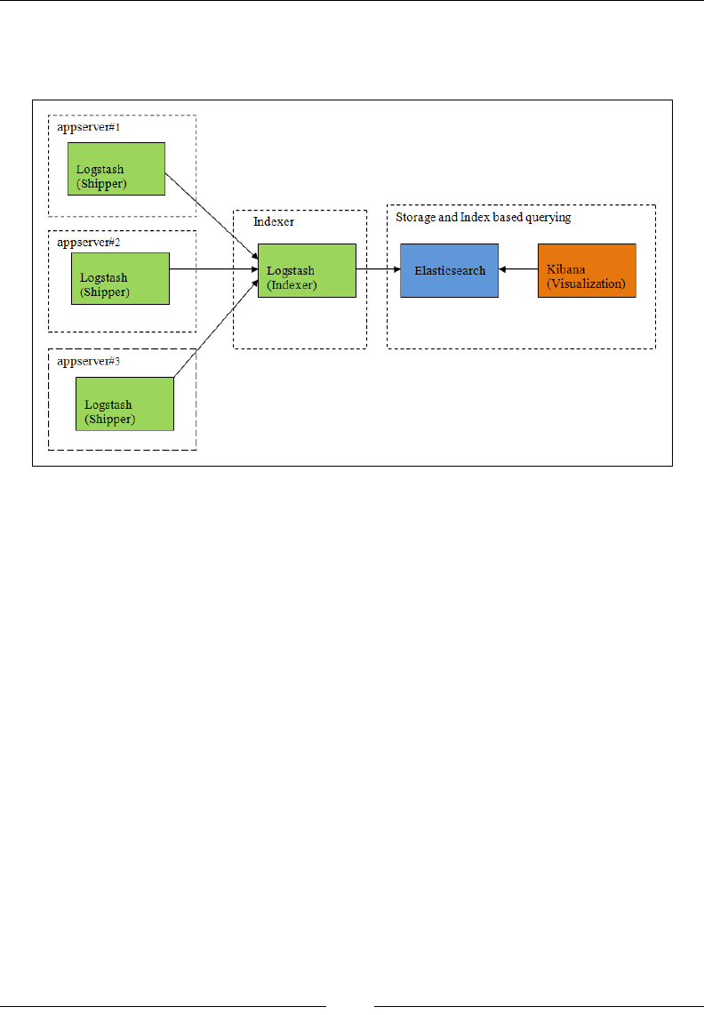
Introduction to ELK Stack
[ 612 ]
ELK data pipeline
A typical ELK stack data pipeline looks something like this:
In a typical ELK Stack data pipeline, logs from multiple application servers are
shipped through Logstash shipper to a centralized Logstash indexer. The Logstash
indexer will output data to an Elasticsearch cluster, which will be queried by Kibana
to display great visualizations and build dashboards over the log data.
ELK Stack installation
A Java runtime is required to run ELK Stack. The latest version of Java is
recommended for the installation. At the time of writing this book, the minimum
requirement is Java 7. You can use the ofcial Oracle distribution, or an open source
distribution, such as OpenJDK.
You can verify the Java installation by running the following command in your shell:
> java -version
java version "1.8.0_40"
Java(TM) SE Runtime Environment (build 1.8.0_40-b26)
Java HotSpot(TM) 64-Bit Server VM (build 25.40-b25, mixed mode)
If you have veried the Java installation in your system, we can proceed with the
ELK installation.

Chapter 1
[ 613 ]
Installing Elasticsearch
When installing Elasticsearch during production, you can use the method described
below, or the Debian or RPM packages provided on the download page.
You can download the latest version of Elasticsearch from
https://www.elastic.co/downloads/elasticsearch.
curl –O https://download.elastic.co/elasticsearch/elasticsearch/
elasticsearch-1.5.2.tar.gz
If you don't have cURL, you can use the following
command to install it:
sudo apt-get install curl
Then, unpack the zip le on your local lesystem:
tar -zxvf elasticsearch-1.5.2.tar.gz
And then, go to the installation directory:
cd elasticsearch-1.5.2
Elastic, the company behind Elasticsearch, recently launched
Elasticsearch 2.0 with some new aggregations, better
compression options, simplied query DSL by merging query
and lter concepts, and improved performance.
More details can be found in the ofcial documentation:
https://www.elastic.co/guide/en/elasticsearch/
reference/current/index.html.
Running Elasticsearch
In order to run Elasticsearch, execute the following command:
$ bin/elasticsearch
Add the -d ag to run it in the background as a daemon process.
We can test it by running the following command in another terminal window:
curl 'http://localhost:9200/?pretty'

Introduction to ELK Stack
[ 614 ]
This shows you an output similar to this:
{
"status" : 200,
"name" : "Master",
"cluster_name" : "elasticsearch",
"version" : {
"number" : "1.5.2",
"build_hash" : "c88f77ffc81301dfa9dfd81ca2232f09588bd512",
"build_timestamp" : "2015-05-13T13:05:36Z",
"build_snapshot" : false,
"lucene_version" : "4.10.3"
},
"tagline" : "You Know, for Search"
}
We can shut down Elasticsearch through the API as follows:
curl -XPOST 'http://localhost:9200/_shutdown'
Elasticsearch conguration
Elasticsearch conguration les are under the config folder in the Elasticsearch
installation directory. The config folder has two les, namely elasticsearch.yml
and logging.yml. The former will be used to specify conguration properties of
different Elasticsearch modules, such as network address, paths, and so on, while the
latter will specify logging-related congurations.
The conguration le is in the YAML format and the following sections are some of
the parameters that can be congured.
Network Address
To specify the address where all network-based modules will bind and publish to:
network :
host : 127.0.0.1
Paths
To specify paths for data and log les:
path:
logs: /var/log/elasticsearch
data: /var/data/elasticsearch

Chapter 1
[ 615 ]
The cluster name
To give a name to a production cluster, which is used to discover and auto
join nodes:
cluster:
name: <NAME OF YOUR CLUSTER>
The node name
To change the default name of each node:
node:
name: <NAME OF YOUR NODE>
Elasticsearch plugins
Elasticsearch has a variety of plugins that ease the task of managing indexes, cluster,
and so on. Some of the mostly used ones are the Kopf plugin, Marvel, Sense, Shield,
and so on, which will be covered in the subsequent chapters. Let's take a look at the
Kopf plugin here.
Kopf is a simple web administration tool for Elasticsearch that is written in
JavaScript, AngularJS, jQuery and Twitter bootstrap. It offers an easy way of
performing common tasks on an Elasticsearch cluster. Not every single API is
covered by this plugin, but it does offer a REST client, which allows you to explore
the full potential of the Elasticsearch API.
In order to install the elasticsearch-kopf plugin, execute the following command
from the Elasticsearch installation directory:
bin/plugin -install lmenezes/elasticsearch-kopf
Now, go to this address to see the interface: http://localhost:9200/_plugin/
kopf/.

Introduction to ELK Stack
[ 616 ]
You can see a page similar to this, which shows Elasticsearch nodes, shards, a
number of documents, size, and also enables querying the documents indexed.
Elasticsearch Kopf UI
Installing Logstash
First, download the latest Logstash TAR le from the download page.
Check for the latest Logstash release version at
https://www.elastic.co/downloads/logstash.
curl –O http://download.elastic.co/logstash/logstash/logstash-1.5.0.tar.
gz
Then, unpack the GZIP le on your local lesystem:
tar -zxvf logstash-1.5.0.tar.gz
Now, you can run Logstash with a basic conguration.

Chapter 1
[ 617 ]
Running Logstash
Run Logstash using -e ag, followed by the conguration of standard input
and output:
cd logstash-1.5.0
bin/logstash -e 'input { stdin { } } output { stdout {} }'
Now, when we type something in the command prompt, we will see its output in
Logstash as follows:
hello logstash
2015-05-15T03:34:30.111Z 0.0.0.0 hello logstash
Here, we are running Logstash with the stdin input and the stdout output as this
conguration prints whatever you type in a structured format as the output. The -e
ag allows you to quickly test the conguration from the command line.
Now, let's try the codec setting for output for a pretty formatted output. Exit from
the running Logstash by issuing a Ctrl + C command, and then we need to restart
Logstash with the following command:
bin/logstash -e 'input { stdin { } } output { stdout { codec => rubydebug
} }'
Now, enter some more test input:
Hello PacktPub
{
"message" => " Hello PacktPub",
"@timestamp" => "2015-05-20T23:48:05.335Z",
"@version" => "1",
"host" => "packtpub"
}
The output that you see is the most common output that we generally see
from Logstash:
• "message" includes the complete input message or the event line
• "@timestamp" will include the timestamp of the time when the event was
indexed; or if date filter is used, this value can also use one of the fields in the
message to get a timestamp specific to the event
• "host" will generally represent the machine where this event was generated

Introduction to ELK Stack
[ 618 ]
Logstash with le input
Logstash can be easily congured to read from a log le as input.
For example, to read Apache logs from a le and output to a standard output
console, the following conguration will be helpful:
input {
file {
type => "apache"
path => "/user/packtpub/intro-to-elk/elk.log"
}
}
output {
stdout {
codec => rubydebug
}
}
Logstash with Elasticsearch output
Logstash can be congured to output all inputs to an Elasticsearch instance. This is
the most common scenario in an ELK platform:
bin/logstash -e 'input { stdin { } } output { elasticsearch { host
= localhost } }'
Then type 'you know, for logs
You will be able to see indexes in Elasticsearch through
http://localhost:9200/_search.
Conguring Logstash
Logstash conguration les are in the JSON format. A Logstash cong le has a
separate section for each type of plugin that you want to add to the event processing
pipeline. For example:
# This is a comment. You should use comments to describe
# parts of your configuration.
input {
...
}
filter {
...

Chapter 1
[ 619 ]
}
output {
...
}
Each section contains the conguration options for one or more plugins. If you
specify multiple lters, they are applied in the order of their appearance in the
conguration le.
When you run logstash, you use the -flag to read congurations from a
conguration le or even from a folder containing multiple conguration les for
each type of plugin—input, lter, and output:
bin/logstash –f ../conf/logstash.conf
If you want to test your congurations for syntax errors
before running them, you can simply check with the
following command:
bin/logstash –configtest ../conf/logstash.conf
This command just checks the conguration without
running logstash.
Logstash runs on JVM and consumes a hefty amount of resources to do so. Logstash,
at times, has signicant memory consumption. Obviously, this could be a great
challenge when you want to send logs from a small machine without harming
application performance.
In order to save resources, you can use the Logstash forwarder (previously known
as Lumberjack). The forwarder uses Lumberjack's protocol, enabling you to securely
ship compressed logs, thus reducing resource consumption and bandwidth. The sole
input is le/s, while the output can be directed to multiple destinations.
Other options do exist as well, to send logs. You can use rsyslog on Linux machines,
and there are other agents for Windows machines, such as nxlog and syslog-ng.
There is another lightweight tool to ship logs called Log-Courier (https://github.
com/driskell/log-courier), which is an enhanced fork of the Logstash forwarder
with some improvements.

Introduction to ELK Stack
[ 620 ]
Installing Logstash forwarder
Download the latest Logstash forwarder release from the download page.
Check for the latest Logstash forwarder release version at
https://www.elastic.co/downloads/logstash.
Prepare a conguration le that contains input plugin details and ssl certicate
details to establish a secure communication between your forwarder and indexer
servers, and run it using the following command:
Logstash forwarder -config Logstash forwarder.conf
And in Logstash, we can use the Lumberjack plugin to get data from the forwarder:
input {
lumberjack {
# The port to listen on
port => 12345
# The paths to your ssl cert and key
ssl_certificate => "path/to/ssl.crt"
ssl_key => "path/to/ssl.key"
# Set the type of log.
type => "log type"
}
Logstash plugins
Some of the most popular Logstash plugins are:
• Input plugin
• Filters plugin
• Output plugin
Input plugin
Some of the most popular Logstash input plugins are:
• file: This streams log events from a file
• redis: This streams events from a redis instance
• stdin: This streams events from standard input

Chapter 1
[ 621 ]
• syslog: This streams syslog messages over the network
• ganglia: This streams ganglia packets over the network via udp
• lumberjack: This receives events using the lumberjack protocol
• eventlog: This receives events from Windows event log
• s3: This streams events from a file from an s3 bucket
• elasticsearch: This reads from the Elasticsearch cluster based on results of a
search query
Filters plugin
Some of the most popular Logstash lter plugins are as follows:
• date: This is used to parse date fields from incoming events, and use that as
Logstash timestamp fields, which can be later used for analytics
• drop: This drops everything from incoming events that matches the
filter condition
• grok: This is the most powerful filter to parse unstructured data from logs or
events to a structured format
• multiline: This helps parse multiple lines from a single source as one
Logstash event
• dns: This filter will resolve an IP address from any fields specified
• mutate: This helps rename, remove, modify, and replace fields in events
• geoip: This adds geographic information based on IP addresses that are
retrieved from Maxmind database
Output plugin
Some of the most popular Logstash output plugins are as follows:
• file: This writes events to a file on disk
• e-mail: This sends an e-mail based on some conditions whenever it receives
an output
• elasticsearch: This stores output to the Elasticsearch cluster, the most
common and recommended output for Logstash
• stdout: This writes events to standard output
• redis: This writes events to redis queue and is used as a broker for many ELK
implementations
• mongodb: This writes output to mongodb
• kafka: This writes events to Kafka topic

Introduction to ELK Stack
[ 622 ]
Installing Kibana
Before we can install and run Kibana, it has certain prerequisites:
• Elasticsearch should be installed, and its HTTP service should be running on
port 9200 (default).
• Kibana must be configured to use the host and port on which Elasticsearch is
running (check out the following Configuring Kibana section).
Download the latest Kibana release from the download page.
Check for the latest Kibana release version at
https://www.elastic.co/downloads/kibana.
curl –O https://download.elastic.co/kibana/kibana/kibana-4.0.2-linux-x64.
tar.gz
Then, unpack kibana-4.0.2-linux-x64.tar.gz on your local le system and
create a soft link to use a short name.
tar -zxvf kibana-4.0.2-linux-x64.tar.gz
ln -s kibana-4.0.2-linux-x64 kibana
Then, you can explore the kibana folder:
cd kibana
Conguring Kibana
The Kibana conguration le is present in the config folder inside the
kibana installation:
config/kibana.yml
Following are some of the important congurations for Kibana.
This controls which port to use.
port: 5601.

Chapter 1
[ 623 ]
Property to set the host to bind the server is:
host: "localhost".
Set the elasticsearch_url to point at your Elasticsearch instance, which is
localhost by default.
elasticsearch_url: http://localhost:9200
Running Kibana
Start Kibana manually by issuing the following command:
bin/kibana
You can verify the running Kibana instance on port 5601 by placing the following
URL in the browser:
http://localhost:5601
This should re up the Kibana UI for you.
Kibana UI

Introduction to ELK Stack
[ 624 ]
We need to specify Index name or pattern that has to be used to
show data indexed in Elasticsearch. By default, Kibana assumes the
default index as logstash-* as it is assuming that data is being fed
to Elasticsearch through Logstash. If you have changed the name of
the index in Logstash output plugin conguration, then we need to
change that accordingly.
Kibana 3 versus Kibana 4
Kibana 4 is a major upgrade over Kibana 3. Kibana 4 offers some
advanced tools, which provides more exibility in visualization
and helps us use some of the advanced features of Elasticsearch.
Kibana 3 had to be installed on a web server; Kibana 4 is released as
a standalone application. Some of the new features in Kibana 4 as
compared to Kibana 3 are as follows:
• Search results highlighting
• Shipping with its own web server and using Node.js on
the backend
• Advanced aggregation-based analytics features, for example,
unique counts, non-date histograms, ranges, and percentiles
Kibana interface
As you saw in the preceding screenshot of the Kibana UI, the Kibana interface
consists of four main components—Discover, Visualize, Dashboard, and Settings.
Discover
The Discover page helps to interactively explore the data matching the selected index
pattern. This page allows submitting search queries, ltering the search results, and
viewing document data. Also, it gives us the count of matching results and statistics
related to a eld. If the timestamp eld is congured in the indexed data, it will also
display, by default, a histogram showing distribution of documents over time.

Chapter 1
[ 625 ]
Kibana Discover Page
Visualize
The Visualize page is used to create new visualizations based on different
data sources—a new interactive search, a saved search, or an existing saved
visualization. Kibana 4 allows you to create the following visualizations in a
new visualization wizard:
• Area chart
• Data table
• Line chart
• Markdown widget
• Metric
• Pie chart
• Tile map
• Vertical bar chart

Introduction to ELK Stack
[ 626 ]
These visualizations can be saved, used individually, or can be used in dashboards.
Kibana Visualize Page
Dashboard
Dashboard is a collection of saved visualizations in different groups. These
visualizations can be arranged freely with a drag and drop kind of feature, and
can be ordered as per the importance of the data. Dashboards can be easily saved,
shared, and loaded at a later point in time.
Settings
The Settings page helps congure Elasticsearch indexes that we want to explore and
congures various index patterns. Also, this page shows various indexed elds in
one index pattern and data types of those elds. It also helps us create scripted elds,
which are computed on the y from the data.
Summary
In this chapter, we gathered a basic understanding of ELK stack, and also gured
out why we need log analysis, and why ELK stack specically. We also set up
Elasticsearch, Logstash, and Kibana.
In the next chapter, we will look at how we can use our ELK stack installation to
quickly build a data pipeline for analysis.

[ 627 ]
Building Your First Data
Pipeline with ELK
In the previous chapter, we got familiar with each component of ELK
Stack—Elasticsearch, Logstash, and Kibana. We got the components installed and
congured. In this chapter, we will build our rst basic data pipeline using ELK
Stack. This will help us understand how easy it is to get together the components of
ELK Stack to build an end-to-end analytics pipeline.
While running the example in this chapter, we assume that you already installed
Elasticsearch, Logstash, and Kibana as described in Chapter 1, Introduction to
ELK Stack.
Input dataset
For our example, the dataset that we are going to use here is the daily Google
(GOOG) Quotes price dataset over a 6 month period from July 1, 2014 to December
31, 2014. This is a good dataset to understand how we can quickly analyze simple
datasets, such as these, with ELK.
This dataset can be easily downloaded from the following source:
http://finance.yahoo.com/q/hp?s=GOOG
Data format for input dataset
The most signicant elds of this dataset are Date, Open Price, Close Price, High
Price, Volume, and Adjusted Price.

Building Your First Data Pipeline with ELK
[ 628 ]
The following table shows some of the sample data from the dataset. The actual
dataset is in the CSV format.
Date Open High Low Close Volume Adj Close
Dec 31, 2014 531.25 532.60 525.80 526.40 1,368,200 526.40
Dec 30, 2014 528.09 531.15 527.13 530.42 876,300 530.42
Dec 29, 2014 532.19 535.48 530.01 530.33 2,278,500 530.33
Dec 26, 2014 528.77 534.25 527.31 534.03 1,036,000 534.03
Dec 24, 2014 530.51 531.76 527.02 528.77 705,900 528.77
Dec 23, 2014 527.00 534.56 526.29 530.59 2,197,600 530.59
Dec 22, 2014 516.08 526.46 516.08 524.87 2,723,800 524.87
Dec 19, 2014 511.51 517.72 506.91 516.35 3,690,200 516.35
Dec 18, 2014 512.95 513.87 504.70 511.10 2,926,700 511.10
Dec 17, 2014 497.00 507.00 496.81 504.89 2,883,200 504.89
Dec 16, 2014 511.56 513.05 489.00 495.39 3,964,300 495.39
Dec 15, 2014 522.74 523.10 513.27 513.80 2,813,400 513.80
Dec 12, 2014 523.51 528.50 518.66 518.66 1,994,600 518.66
Dec 11, 2014 527.80 533.92 527.10 528.34 1,610,800 528.34
Dec 10, 2014 533.08 536.33 525.56 526.06 1,712,300 526.06
We need to put this data into a location from where ELK Stack can access it for
further analysis.
We will look at some of the top entries of the CSV le using the Unix head command
as follows:
$ head GOOG.csv
2014-12-31,531.25244,532.60236,525.80237,526.4024,1368200,526.4024
2014-12-30,528.09241,531.1524,527.13239,530.42242,876300,530.42242
2014-12-29,532.19244,535.48242,530.01337,530.3324,2278500,530.3324
2014-12-26,528.7724,534.25244,527.31238,534.03247,1036000,534.03247
2014-12-24,530.51245,531.76141,527.0224,528.7724,705900,528.7724
2014-12-23,527.00238,534.56244,526.29236,530.59241,2197600,530.59241
2014-12-22,516.08234,526.4624,516.08234,524.87238,2723800,524.87238
2014-12-19,511.51233,517.72235,506.9133,516.35229,3690200,516.35229
2014-12-18,512.95233,513.87231,504.7023,511.10233,2926700,511.10233
Each row represents the Quote price data for a particular date separated by a comma.
Now, when we are familiar with the data, we will set up the ELK Stack where we can
parse and process the data using Logstash, index it in Elasticsearch, and then build
beautiful visualizations in Kibana.

Chapter 2
[ 629 ]
Conguring Logstash input
As we already know, Logstash has a rich set of plugins for different types of inputs,
outputs and lters, which can read, parse, and lter data as per our needs. We will
utilize the file input plugin to read the source le.
A file input plugin streams events from the input le, and each event is assumed
as a single line. It automatically detects le rotation and handles it. It maintains
the location where it left reading, and will automatically detect the new data if
congured correctly. It reads les in a similar manner:
tail -0f
In general, a file input plugin conguration will look as follows:
input {
file {
path => #String (path of the files) (required)
start_position => #String (optional, default "end")
tags => #array (optional)
type => #string (optional)
}
}
• path: The path field is the only required field in file input plugin, which
represents the path of the file from where input events have to be processed.
• start_position: This defines from where Logstash starts reading input
files. Values can be "beginning" or "end". The default value is "end" which
caters to the needs of reading live streams. If we need to read some historic
data, it can be set to "beginning".
• tags: tags represents any number of strings as an array that can be utilized
later to filter and process events based on tags assigned to them.
• type: The type field can be used to mark a specific type of events, which
helps to filter and search them later. Type is added to the document that is
stored in Elasticsearch, and can later be viewed in Kibana under the _type
field. For example, we can assign type as "error_logs" or "info_logs".
Let's congure Logstash for our input dataset:
input{
file{
path =>"/opt/logstash/input/GOOG.csv"

Building Your First Data Pipeline with ELK
[ 630 ]
start_position =>"beginning"
}
}
We will provide the path of the CSV le in the path attribute, and as our dataset is
historic, we will use start_position as "beginning".
Filtering and processing input
Once we congure the input le, we need to lter the input based on our needs
so that we can identify which elds we need, and process them as per the required
analysis.
A filter plugin will perform the intermediary processing on the input event. We
can apply the lter conditionally based on certain elds.
Since our input le is a CSV le, we will use the csv lter for the same. The csv
lter takes an event eld that contains CSV formatted data, parses it, and stores it
as individual elds. It can also parse data with any separator other than commas. A
typical csv lter is as follows:
filter {
csv {
columns => #Array of column names.
separator => #String ; default -","
}
}
The attribute columns take the name of elds in our CSV le, which is optional. By
default, the columns will be named as column 1, column 2, and so on.
The attribute separator denes what character is used to separate the different
columns in the le. The default is a comma, but it can be any other separator too.
In our example, we can specify a simple csv lter as follows:
filter {
csv {
columns =>
["date_of_record","open","high","low","close","volume","adj_close"
]
separator => ","
}
}

Chapter 2
[ 631 ]
Here, we specied the column names as dened in our CSV le, and explicitly
dened the separator as a comma just to make it clear.
Now, we are done with csv lter conguration, but we still need to do some
intermediary processing on the columns to associate specic data types with
our columns.
First of all, we need to specify which column represents the date eld so that it can
be explicitly indexed as date type and can be used to lter based on date. Logstash
has a specic lter called date for the same. A typical date lter looks as follows:
filter {
date {
match => # array (optional), default: []
target => # string (optional), default: "@timestamp"
timezone => # string (optional)
}
}
Here, in the match attribute, we dene an array, which is in the [field, formats]
format; that is, eld, followed by a set of time formats that can be applied to that eld.
For example, if our log le has multiple formats, we can use the the following code:
match => [ "date_field", "MMM dd YYY HH:mm:ss",
"MMM d YYY HH:mm:ss", "MMddYYYY","ISO8601" ]
Date formats in Logstash: Date formats allowed are as per the
allowed JodaTime DateTimeFormat library:
http://joda-time.sourceforge.net/apidocs/org/
joda/time/format/DateTimeFormat.html
As per our date format, our date lter will be as follows:
date{
match => ["date_of_record", "yyyy-MM-dd"]
target => "@timestamp"
}
The target lter denes where to map the matching timestamp. By default, it maps
to @timestamp (the eld that represents the time stamp of the event, which defaults
to the time when the event was captured). In our case, since we are taking some
historic data, we don't want the event captured time to be in @timestamp, but the
date of record. We will map our date eld to @timestamp. It is not mandatory to
dene this, but recommended to use.

Building Your First Data Pipeline with ELK
[ 632 ]
After updating the data type of date elds, the next operation we require is updating
the data type of elds, which we need for numeric comparisons or operations. By
default, the value will be of string data type. We will convert them to integers so
that we can perform some aggregations and comparisons on the data.
We will use mutate lter for the conversion of elds to a specic data type. This lter
helps perform general mutations on the elds, which includes modications of data
types, renaming, replacing elds, and removing elds. It can also help merge two
elds, perform uppercase and lowercase conversions, split and strip elds, and so on.
A typical mutate lter looks like this:
filter {
mutate {
convert => # hash of field and data type (optional)
join => # hash of fields to be joined (optional)
lowercase => # array of fields to be converted (optional)
merge => # hash of fields to be merged (optional)
rename => # hash of original and rename field (optional)
replace => # hash of fields to replaced with (optional)
split => # hash of fields to be split (optional)
strip => # array of fields (optional)
uppercase => # array of fields (optional)
}
}
Let's see what our mutate lter looks like:
mutate {
convert => ["open","float"]
convert => ["high ","float"]
convert => ["low ","float"]
convert => ["close ","float"]
convert => ["volume","integer"]
convert => ["adj_close","float"]
}
We are using the convert functionality to convert our price and volume elds to
integer. Valid data types are "integer", "float", and "string".

Chapter 2
[ 633 ]
Putting data to Elasticsearch
Now that we have set up the data to be consumed by a CSV le into Logstash,
followed by parsing and processing based on the data type needed, we now need to
put the data in Elasticsearch so that we can index the different elds and consume
them later via the Kibana interface.
We will use the output plugin of Logstash for an elasticsearch output.
A typical elasticsearch plugin conguration looks like this:
output {
elasticsearch {
action => # string (optional), default: "index"
cluster => # string (optional)
host => # string (optional)
document_id => # string (optional), default: nil
index => # string (optional), default: "logstash-%{+YYYY.MM.dd}"
index_type => # string (optional)
port => # string (optional)
protocol => # string, one of ["node", "transport", "http"]
(optional)
}
}
• action: This specifies what action to perform on incoming documents.
The default is "index" and possible values are "index" or "delete". The
"index" value will index a document and "delete" will delete a document
based on document ID.
• cluster: This is the name of the cluster set in elasticsearch.
• host: This is the hostname or IP address of the elasticsearch.
• document_id: This is the document ID of the index; it is useful to delete or
overwrite the existing entries.
• index: This is the index name to which the incoming events have to
be written. By default, it is indexed based on each day, and named as
"logstash-%{+YYYY.MM.dd}".

Building Your First Data Pipeline with ELK
[ 634 ]
• index_type: This specifies the index type to write events to. This is to ensure
that you write similar types of events to the same index type.
• port: This specifies the port to be used for the elasticsearch service.
• protocol: This specifies the protocol to be used to connect with
Elasticsearch. The values are "http", "node", and "transport".
Now, let's take a look at our elasticsearch output conguration:
output{
elasticsearch {
host => "localhost"
}
}
We used the default value for index and most of the other settings.
Now, when we have seen how individual plugins are congured, let's take a look at
what the overall Logstash conguration looks like:
input{
file{
path =>"/opt/logstash/input/GOOG.csv"
start_position =>"beginning"
}
}
filter{
csv{
columns =>
["date_of_record","open","high","low","close","volume","adj_close"]
separator => ","
}
date {
match => ["date_of_record","yyyy-MM-dd"]

Chapter 2
[ 635 ]
}
mutate {
convert => ["open","float"]
convert => ["high","float"]
convert => ["low","float"]
convert => ["close","float"]
convert => ["volume","integer"]
convert => ["adj_close","float"]
}
}
output{
elasticsearch {
host => "localhost"
}
}
We will save this conguration in the Logstash installation folder with the name
logstash.conf, and as we saw earlier, we can run Logstash with this conguration
using the following command:
Before running Logstash with this conguration, make sure
the Elasticsearch is running as per the instructions in the
previous chapter.
$ bin/logstash –f logstash.conf
Logstash will start to run with the dened conguration and keep on indexing all
incoming events to the elasticsearch indexes. You may see an output similar to
this on the console:
May 31, 2015 4:04:54 PM org.elasticsearch.node.internal.InternalNode
start
INFO: [logstash-4004-9716] started
Logstash startup completed

Building Your First Data Pipeline with ELK
[ 636 ]
At this point, we can open the elasticsearch Kopf plugin console to verify
whether we have some documents indexed already, and we can also query
the documents.
Elasticsearch Kopf interface
As we can see that there are 129 documents indexed already, we veried that our
Logstash conguration worked well.
Visualizing with Kibana
Now when you verify that your data is indexed successfully in Elasticsearch, we can
go ahead and look at the Kibana interface to get some useful analytics from the data.
Running Kibana
As described in the previous chapter, we will start the Kibana service from the
Kibana installation directory.
$ bin/kibana
Now, let's see Kibana up and running similar to the following screenshot on the
browser, by going to the following URL:
http://localhost:5601

Chapter 2
[ 637 ]
Kibana Discover page
As we already set up Kibana to take logstash-* indexes by default, it displays the
indexed data as a histogram of counts, and the associated data as elds in the
JSON format.
First of all, we need to set the date lter to lter based on our date range so that we
can build our analysis on the same. Since we took data from July 1, 2014 to December
31, 2014, we will congure our date lter for the same.
Clicking on the Time Filter icon at the extreme top-right corner, we can set an
Absolute Time Filter based on our range as follows:
Kibana Time Filter
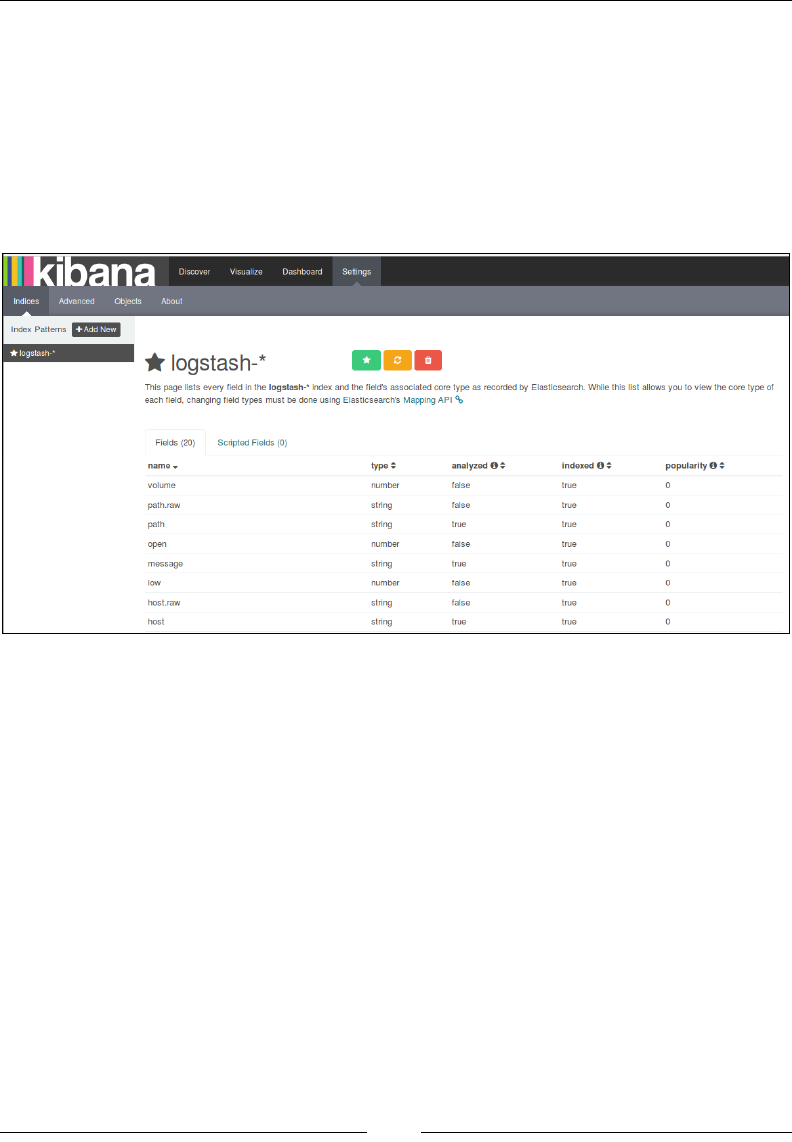
Building Your First Data Pipeline with ELK
[ 638 ]
Now, we are all set to build beautiful visualizations on the collected dataset using the
rich set of visualization features that Kibana provides.
Before we build the visualization, let's conrm whether all elds are indexed
properly with their associated data types so that we can perform the appropriate
operations on them.
For this, let's click on the Settings page at the top of the screen and select the
logstash-* index pattern on the left of the screen. The page looks something like this:
Kibana Settings page
It shows all our elds that were indexed, their data types, index status, and
popularity value.
Kibana visualizations
Let's build some basic visualizations from the Kibana visualizations page, and we
will use them later in dashboard.
Click on the visualization page link at the top of the Kibana home page, and click
on the new visualization icon.

Chapter 2
[ 639 ]
This page shows various types of visualizations that are possible with the
Kibana interface:
Kibana visualization menu
Building a line chart
The rst visualization that we will build is a line chart showing weekly close price
index movement for the GOOG script over a six month period.
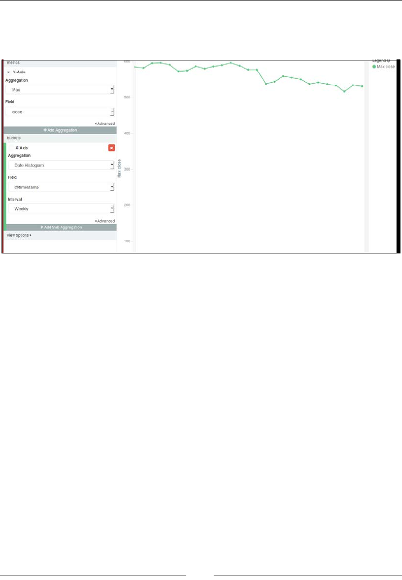
Building Your First Data Pipeline with ELK
[ 640 ]
Select Line Chart from the visualization menu, and then we'll select Y-Axis metrics as
Max, and Field as close. In the buckets section, select Aggregation as Date Histogram
based on the @timestamp eld, and Interval as Weekly, and click on Apply.
Kibana Line chart
Now, save the visualization using some name for the line chart, which we will pull
into the dashboard later.
Building a bar chart
We will build a vertical bar chart representing the movement of weekly traded
volumes over a six month period.
Select Vertical Bar Chart from the visualization menu, and select Y-Axis
Aggregation as Sum, and Field as volume. In the buckets section, select X-Axis
Aggregation as Date Histogram, and Field as @timestamp, and Interval as Weekly.
Click on Apply to see a vertical bar chart representing the weekly total volume
traded over a six month period.
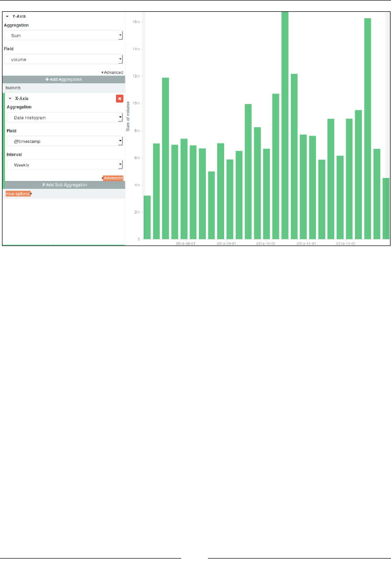
Chapter 2
[ 641 ]
Kibana Vertical Bar Chart
Now, save the visualization using some name for the bar chart, which we will pull
into the dashboard later.
Building a Metric
Metric represents one big number that we want to show as something special
about data.
We will show the Highest Volume Traded in a single day in a six month period
using Metric.

Building Your First Data Pipeline with ELK
[ 642 ]
Click on Metric in the visualization menu, and select Metric Aggregation as
Max, Field as volume. Click on Apply to see the result of visualization on the
right as follows:
Kibana Metric
Now, save the visualization using some name for the Metric, which we will pull into
the dashboard later.
Building a data table
Data tables are meant to show detailed breakdowns in a tabular format for results of
some composed aggregations.
We will create a data table of Monthly Average volume traded over six months.
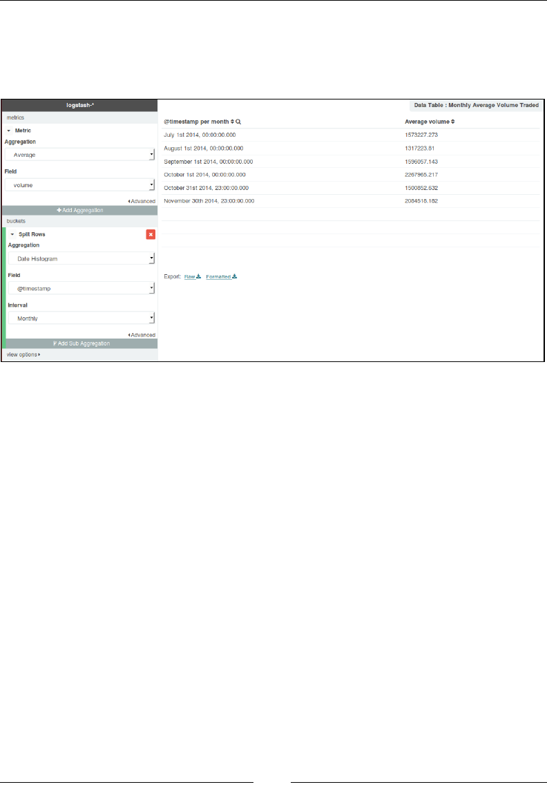
Chapter 2
[ 643 ]
Select Data table from the visualization menu, click on split rows and select
Aggregation as Average and Fields as volume. In the buckets section, select
Aggregation as Date Histogram, Fields as @timestamp, and Interval as Monthly.
Click on Apply to see the image as in the following screenshot:
Kibana Data table
Now, save the visualization using some name for the data table, which we will pull
into the dashboard later.
After we have built some visualizations, let's build a dashboard that includes these
visualizations.
Select the dashboard page link at top of the page, and click on the Add Visualization
link to select visualizations from your saved visualizations and arrange them.
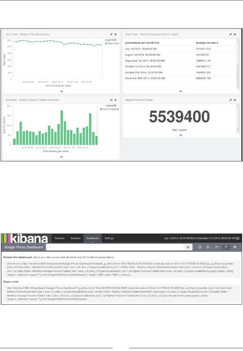
Building Your First Data Pipeline with ELK
[ 644 ]
The Dashboard, after including a line chart, bar chart, data table, and Metric, looks
like this:
Kibana Dashboard
Now, we can save this dashboard using the save button, and it can be pulled later
and shared easily.
Dashboards can be embedded as an IFrame in other systems or can be directly
shared as links.
Click on the share button to see the options to share:
Kibana Share options
If you have completed everything up to this point, then you have successfully set up
your rst ELK data pipeline.

Chapter 2
[ 645 ]
Summary
In this chapter, we saw how you can utilize different input, lter, and output plugins
in Logstash to gather, parse, and index data to Elasticsearch, and later utilize the
Kibana interface to query and visualize over Elasticsearch indexes. We also built
some visualizations, and a dashboard using those visualizations. We successfully
built our rst data pipeline using ELK Stack. In the coming chapters, we will look
at individual components in more detail.

[ 647 ]
Collect, Parse and Transform
Data with Logstash
By now, we should have a basic understanding of ELK Stack and what role it plays
in log analysis or event analysis systems. In Chapter 2, Building Your First Data
Pipeline with ELK, we built analytics over the GOOG stock price data with the
ELK Stack conguration, and also understood role of each component of the stack
in the pipeline.
In this chapter, we will get into more detail on Logstash, the most important
component of the ELK Stack, and see how Logstash helps collect, parse, and
transform any format and any type of data to a common format, which can be used
to build a wide variety of analytics systems across many applications.
We saw in Chapter 1, Introduction to ELK Stack, the importance of log analysis and
problem with log analysis methods. Also, there are a variety of log formats, and date
and time formats in logs. Often these logs are customized to each application and
require expert knowledge to gather essential information out of them. Now, we will
see how Logstash provides us with a variety of plugins that help us overcome all
of these problems and build easily-congurable and manageable visualizations on
top of it.
In this chapter, while explaining various congurations of Logstash plugins, we
assume that you have installed Logstash, as explained in Chapter 1, Introduction to
ELK Stack, and have the basic conguration set up and running. If you do not, you
should get Logstash installed and run a basic stdin, stdout conguration and then
resume this chapter so that you can try out some conguration options based on the
explanations.

Collect, Parse and Transform Data with Logstash
[ 648 ]
Conguring Logstash
As we have seen in previous chapters, a general Logstash plugin conguration looks
like this:
input {
}
filter {
}
output {
}
A Logstash conguration consists of a series of input, filter, and output plugins
and their corresponding properties. Each plugin plays an important role towards
parsing, processing, and nally putting the data in the required format. Input
plugins generate the event, lters modify them, and output will ship them to
other systems.
file, stdin, lumberjack, twitter etc.
grok, grep, mutate, drop, date etc.
elasticsearch, stdout, mongodb etc.
Input
Filter
Output
Logstash plugins

Chapter 3
[ 649 ]
Logstash plugins
Logstash has a variety of plugins to help integrate it with a variety of input and
output sources. Let's explore the various plugins available.
Listing all plugins in Logstash
You can execute the following command to list all available plugins in your installed
Logstash version:
bin/plugin list
Also, you can list all plugins containing a name fragment by executing this
command:
bin/plugin list <namefragment>
To list all plugins for group names, input, output, or lter, we can execute this
command:
bin/plugin list --group <group name>
bin/plugin list --group output
Before exploring various plugin congurations, let's take a look at the data types and
conditional expressions used in various Logstash congurations.
Data types for plugin properties
A Logstash plugin requires certain settings or properties to be set. Those properties
have certain values that belong to one of the following important data types.
Array
An array is collection of values for a property.
An example can be seen as follows:
path => ["value1","value2"]
The => sign is the assignment operator that is used for all
properties of conguration values in Logstash conguration.

Collect, Parse and Transform Data with Logstash
[ 650 ]
Boolean
A boolean value is either true or false (without quotes).
An example can be seen as follows:
periodic_flush => false
Codec
Codec is actually not a data type but a way to encode or decode data at input
or output.
An example can be seen as follows:
codec => "json"
This instance species that this codec, at output, will encode all output in
JSON format.
Hash
Hash is basically a key value pair collection. It is specied as "key" => "value" and
multiple values in a collection are separated by a space.
An example can be seen as follows:
match => {
"key1" => "value1" "key2" => "value2"}
String
String represents a sequence of characters enclosed in quotes.
An example can be seen as follows:
value => "Welcome to ELK"
Comments
Comments begin with the # character.
An example can be seen as follows:
#this represents a comment

Chapter 3
[ 651 ]
Field references
Fields can be referred to using [field_name] or nested elds using [level1][level2].
Logstash conditionals
Logstash conditionals are used to lter events or log lines under certain conditions.
Conditionals in Logstash are handled like other programming languages and work
with if, if else and else statements. Multiple if else blocks can be nested.
Syntax for conditionals is as follows:
if <conditional expression1>{
#some statements here.
}
else if <conditional expression2>{
#some statements here.
}
else{
#some statements here.
}
Conditionals work with comparison operators, boolean operators and unary
operators:
Comparison operators include:
• Equality operators: ==, !=, <, >, <=, >=
• Regular expressions: =~, !~
• Inclusion: in, not in
• Boolean operators include and, or, nand, xor
• Unary operators include !
Let's take a look at this with an example:
filter {
if [action] == "login" {
mutate { remove => "password" }
}
}
Multiple expressions can be specied in a single statement using boolean operators.

Collect, Parse and Transform Data with Logstash
[ 652 ]
An example can be seen as follows:
output {
# Send Email on Production Errors
if [loglevel] == "ERROR" and [deployment] == "production" {
email{
}
}
}
Types of Logstash plugins
The following are types of Logstash plugins:
• Input
• Filter
• Output
• Codec
Now let's take a look at some of the most important input, output, lter and codec
plugins, which will be useful for building most of the log analysis pipeline use cases.
Input plugins
An input plugin is used to congure a set of events to be fed to Logstash. Some of the
most important input plugins are:
le
The file plugin is used to stream events and log lines les to Logstash. It
automatically detects le rotations, and reads from the point last read by it.
The Logstash file plugin maintains sincedb les to track
the current positions in les being monitored. By default
it writes sincedb les at $HOME/.sincedb* path. The
location and frequency can be altered using sincedb_path
and sincedb_write_interval properties of the plugin.

Chapter 3
[ 653 ]
A most basic le conguration looks like this:
input{
file{
path => "/path/to/logfiles"
}
The only required conguration property is the path to the les. Let's look at how
we can make use of some of the conguration properties of the le plugin to read
different types of les.
Conguration options
The following conguration options are available for the le input plugin:
add_eld
It is used to add a eld to incoming events, its value type is Hash, and default value
is {}.
Let's take the following instance as an example:
add_field => { "input_time" => "%{@timestamp}" }
codec
It is used to specify a codec, which can decode a specic type of input.
For example: codec => "json" is used to decode the json type of input.
The default value of codec is "plain".
delimiter
It is used to specify a delimiter, which identies separate lines. By default, it is "\n".
exclude
To exclude certain types of les from the input path, the data type is array.
Let's take the following instance as an example:
path =>["/app/packtpub/logs/*"]
exclude => "*.gz"
This will exclude all gzip les from input.

Collect, Parse and Transform Data with Logstash
[ 654 ]
path
This is the only required conguration for the le plugin. It species an array of path
locations from where to read logs and events.
sincedb_path
It species the location where to write the sincedb les, which keeps track of the
current position of les being monitored. The default is $HOME/.sincedb*
sincedb_write_interval
It species how often (number in seconds), the sincedb les that keep track of the
current position of monitored les, are to be written. The default is 15 seconds.
start_position
It has two values: "beginning" and "end". It species where to start reading
incoming les from. The default value is "end", as in most situations this is used
for live streaming data. Although, if you are working on old data, it can be set
to "beginning".
This option has impact only when a le is being read for the rst
time, called "first contact", as it maintains the location in
the "sincedb" location. So for the next setting, this option has no
impact unless you decide to remove the sincedb les.
tags
It species the array of tags that can be added to incoming events. Adding tags to
your incoming events helps with processing later, when using conditionals. It is
often helpful to tag certain data as "processed" and use those tags to decide a future
course of action.
For example, if we specify "processed" in tags:
tags =>["processed"]
In lter, we can check in conditionals:
filter{
if "processed" in tags[]{
}
}

Chapter 3
[ 655 ]
type
The type option is really helpful to process the different type of incoming streams
using Logstash. You can congure multiple input paths for different type of events,
just give a type name, and then you can lter them separately and process.
Let's take the following instance as an example:
input {
file{
path => ["var/log/syslog/*"]
type => "syslog"
}
file{
path => ["var/log/apache/*"]
type => "apache"
}
}
In filter, we can lter based on type:
filter {
if [type] == "syslog" {
grok {
}
}
if [type] == "apache" {
grok {
}
}
}
As in the preceding example, we have congured a separate type for incoming les;
"syslog" and "apache". Later in ltering the stream, we can specify conditionals to
lter based on this type.
stdin
The stdin plugin is used to stream events and log lines from standard input.
A basic conguration for stdin looks like this:
stdin {
}

Collect, Parse and Transform Data with Logstash
[ 656 ]
When we congure stdin like this, whatever we type in the console will go as input
to the Logstash event pipeline. This is mostly used as the rst level of testing of
conguration before plugging in the actual le or event input.
Conguration options
The following conguration options are available for the stdin input plugin:
add_eld
The add_field conguration for stdin is the same as add_field in the file input
plugin and is used for similar purposes.
codec
It is used to decode incoming data before passing it on to the data pipeline. The
default value is "line".
tags
The tags conguration for stdin is the same as tags in the file input plugin and is
used for similar purposes.
type
The type conguration for stdin is the same as type in the file input plugin and is
used for similar purposes.
twitter
You may need to analyze a Twitter stream based on a topic of interest for various
purposes, such as sentiment analysis, trending topics analysis, and so on. The
twitter plugin is helpful to read events from the Twitter streaming API. This
requires a consumer key, consumer secret, keyword, oauth token, and oauth token
secret to work.
These details can be obtained by registering an application on the Twitter developer
API page (https://dev.twitter.com/apps/new):
twitter {
consumer_key => "your consumer key here"
keywords => "keywords which you want to filter on streams"
consumer_secret => "your consumer secret here"
oauth_token => "your oauth token here"
oauth_token_secret => "your oauth token secret here"
}

Chapter 3
[ 657 ]
Conguration options
The following conguration options are available for the twitter input plugin:
add_eld
The add_field conguration for the twitter plugin is the same as add_field in the
file input plugin and is used for similar purposes.
codec
The codec conguration for twitter is the same as the codec plugin in the file
input plugin and is used for similar purposes.
consumer_key
This is a required conguration with no default value. Its value can be obtained from
the Twitter app registration page. Its value is the String type.
consumer_secret
The same as consumer_key, its value can be obtained from the Twitter dev app
registration.
full_tweet
This is a boolean conguration with the default value; false. It species whether to
record a full tweet object obtained from the Twitter streaming API.
keywords
This is an array type required conguration, with no default value. It species a set
of keywords to track from the Twitter stream.
An example can be seen as follows:
keywords => ["elk","packtpub"]
oauth_token
The oauth_token option is also obtained from the Twitter dev API page.
After you get your consumer key and consumer secret, click
on Create My Access Token to create your oauth token and
oauth token secret.
oauth_token_secret
The oauth_token_secret option is obtained from the Twitter dev API page.

Collect, Parse and Transform Data with Logstash
[ 658 ]
tags
The tags conguration for the twitter input plugin is the same as tags in the file
input plugin and is used for similar purposes.
type
type conguration for twitter input plugins is the same as type in the file input
plugin and is used for similar purposes.
lumberjack
The lumberjack plugin is useful to receive events via the lumberjack protocol that
is used in Logstash forwarder.
The basic required conguration option for the lumberjack plugin looks like this:
lumberjack {
port =>
ssl_certificate =>
ssl_key =>
}
Lumberjack or Logstash forwarder is a light weight log shipper
used to ship log events from source systems. Logstash is quite a
memory consuming process, so installing it on every node from
where you want to ship data is not recommended. Logstash
forwarder is a light weight version of Logstash, which provides
low latency, secure and reliable transfer, and provides low
resource usage.
More details about Lumberjack or Logstash forwarder can be
found from here:
https://github.com/elastic/logstash-forwarder
Conguration options
The following conguration options are available for the lumberjack input plugin:
add_eld
The add_field conguration for the lumberjack plugin is the same as add_field in
the file input plugin and is used for similar purposes.
codec
The codec conguration for the lumberjack plugin is the same as the codec plugin
in the file input plugin and is used for similar purposes.

Chapter 3
[ 659 ]
host
It species the host on which to listen to. The default value: "0.0.0.0".
port
This is a number type required conguration and it species the port to listen to.
There is no default value.
ssl_certicate
It species the path to the SSL certicate to be used for the connection. It is a
required setting.
An example is as follows:
ssl_certificate => "/etc/ssl/logstash.pub"
ssl_key
It species the path to the SSL key that has to be used for the connection. It is also a
required setting.
An example is as follows:
ssl_key => "/etc/ssl/logstash.key"
ssl_key_passphrase
It species the SSL key passphrase that has to be used for the connection.
tags
The tags conguration for the lumberjack input plugin is the same as tags in the
file input plugin and is used for similar purposes.
type
The type conguration for the lumberjack input plugins is the same as type in the
file input plugin and is used for similar purposes.
redis
The redis plugin is used to read events and logs from the redis instance.
Redis is often used in ELK Stack as a broker for incoming log
data from the Logstash forwarder, which helps to queue data
until the time the indexer is ready to ingest logs. This helps to
keep the system in check under heavy load.

Collect, Parse and Transform Data with Logstash
[ 660 ]
The basic conguration of the redis input plugin looks like this:
redis {
}
Conguration options
The following conguration options are available for the redis input plugin:
add_eld
The add_field conguration for redis is the same as add_field in the file input
plugin and is used for similar purposes.
codec
The codec conguration for redis is the same as codec in the file input plugin and
is used for similar purposes.
data_type
The data_type option can have a value as either "list", "channel" or
"pattern_channel".
From the Logstash documentation for the redis plugin (https://www.elastic.co/
guide/en/logstash/current/plugins-inputs-redis.html):
"If redis_type is list, then we will BLPOP the key. If redis_type is
channel, then we will SUBSCRIBE to the key. If redis_type is pattern_
channel, then we will PSUBSCRIBE to the key."
While using redis on the consumer and publisher side, key
and data_type should be the same on both sides.
host
It species the hostname of the redis server. The default value is "127.0.0.1".
key
It species the key for redis; "list" or "channel".
password
It is a password type conguration that species the password to be used
for connection.

Chapter 3
[ 661 ]
port
It species the port on which the redis instance is running. The default is 6379.
An extensive list and latest documentation on all available Logstash input plugins
is available at https://www.elastic.co/guide/en/logstash/current/input-
plugins.html.
Now that we have seen some of the most important input plugins for Logstash, let's
have a look at some output plugins.
Output plugins
Logstash provides a wide variety of output plugins that help integrate incoming
events with almost any type of destination. Let's look at some of the most used
output plugins in detail.
csv
The csv plugin is used to write a CSV le as output, specifying the elds in csv and
the path of the le.
The basic conguration of the csv output plugin looks like this:
csv {
fields => ["date","open_price","close_price"]
path => "/path/to/file.csv"
}
Conguration options
The following are the conguration options available for the csv plugin:
codec
It is used to encode the data before it goes out of Logstash. The default value is
"plain", which will output data as it is.
csv_options
The csv_options option is used to specify advanced options for the csv output. It
includes changing the default column and row separator.
An example is as follows:
csv_options => {"col_sep" => "\t" "row_sep" => "\r\n"}

Collect, Parse and Transform Data with Logstash
[ 662 ]
elds
The fields setting is a required setting that is used to specify the elds for the
output CSV le. It is specied as an array of eld names and written in the same
order as in the array. There is no default value for this setting.
gzip
The gzip setting is a boolean type of setting that species whether to output as a
gzip compressed format or not. The default is false.
path
The path setting is a required setting and is used to specify the path to the CSV le.
le
The file output plugin, just like the file input plugin, will be used to write events
to a le in the le system.
The basic conguration of the file output plugin looks like this:
file
{
path = > "path/to/file"
}
Conguration options
The available conguration options are:
• codec
• gzip
• max_size
• path
Most of these conguration options have been covered earlier and are well
understood by their name.
email
The email plugin is a very important output plugin as it is very useful to send
e-mails for certain events and failure scenarios.
The basic required conguration looks like this:
email {
to => "abc@example.com"
}

Chapter 3
[ 663 ]
Conguration options
The following conguration options are available for the email plugin:
attachments
The attachments option is an array of le paths to be attached with the e-mail. The
default value is []
body
The body option species the body of the e-mail in plain text format. The default
value is "".
cc
The cc option species the list of e-mails to be included as the cc addresses in the
e-mail. It accepts multiple e-mail IDs in a comma separated format.
from
The from option species the e-mail address to be used as the sender address in
the e-mail. The default value is "logstash.alert@nowhere.com" and must be
overridden as per the type of alerts or system.
to
The to option is a required setting that species the receiver address for the e-mail. It
can also be expressed as a string of comma separated e-mail addresses.
htmlbody
The htmlbody option species the body of the e-mail in HTML format. It includes
HTML mark-up tags in the e-mail body.
replyto
The replyto option species the e-mail address to be used for the Reply-To eld for
the e-mail.
subject
The subject option species the subject for the e-mail. The default value is "".
elasticsearch
The elasticsearch plugin is the most important plugin used in ELK Stack, because
it is where you will want to write your output to be stored to analyze later in Kibana.

Collect, Parse and Transform Data with Logstash
[ 664 ]
We will take a look at ElasticSearch in more detail in Chapter 5, Why Do We Need
Elasticsearch in ELK?, but let's look at the conguration options for this plugin here:
The basic conguration for the elasticsearch plugin looks like this:
elasticsearch {
}
Conguration options
Some of the most important conguration options are mentioned as follows:
option data type required default value
action string N "index"
bind_host string N
bind_port number N
cacert a valid system path N
cluster string N
document_id string N
document_type string N
host array N
index string N "logstash-
%{+YYYY.
MM.dd}"
max_retries number N 3
node_name string N
password password N
port string N
user string N
ganglia
Ganglia is a monitoring tool that is used to monitor the performance of a cluster of
machines in a distributed computing environment. Ganglia makes uses of a daemon
called Gmond, which is a small service that is installed on each machine that needs
to be monitored.
The ganglia output plugin in Logstash is used to send metrics to the gmond service
based on events in logs.

Chapter 3
[ 665 ]
The basic ganglia output plugin conguration looks like this:
ganglia {
metric =>
value =>
}
Conguration options
The following conguration options are available for the ganglia plugin
metric
The metric option species the metric that is to be used for performance monitoring.
It can even take values from the event elds.
unit
The unit option species the unit like kb/s, ms for the metric used.
value
The value option species the value of metric used.
jira
The jira plugin doesn't come by default in Logstash installation but can be easily
installed by a plugin install command like this:
bin/plugin install logstash-output-jira
The jira plugin is used to send events to a JIRA instance, which can create JIRA
tickets based on certain events in your logs. To use this, the JIRA instance must
accept REST API calls, since it internally makes use of JIRA REST API to pass the
output events from Logstash to JIRA.
The basic conguration of the jira output plugin looks like this:
jira {
issuetypeid =>
password =>
priority =>
projectid =>
summary =>
username =>
}

Collect, Parse and Transform Data with Logstash
[ 666 ]
Conguration options
The following are the conguration options and their corresponding data types
available for the jira plugin:
Option Data type Required
assignee string N
issuetypeid string Y
password string Y
priority string Y
projectid string Y
reporter string N
summary string Y
username string Y
kafka
As explained on the Hortonworks Kafka page (http://hortonworks.com/hadoop/
kafka/):
"Apache™ Kafka is a fast, scalable, durable, and fault-tolerant publish-subscribe
messaging system."
The kafka output plugin is used to write certain events to a topic on kafka. It uses
the Kafka Producer API to write messages to a topic on the broker.
The basic kafka conguration looks like this:
kafka {
topic_id =>
}
Conguration options
There are many kafka specic conguration options that can be obtained from
ofcial documentation, but the only required conguration is topic_id.
topic_id
The topic_id option denes the topic to send messages to.
lumberjack
The lumberjack plugin is used to write output to a Logstash forwarder or
lumberjack.

Chapter 3
[ 667 ]
The basic conguration for the lumberjack plugin looks like this:
lumberjack {
hosts =>
port =>
ssl_certificate =>
}
Conguration options
The following conguration options are available for the lumberjack plugin:
hosts
The hosts option species the list of addresses where lumberjack can send
messages to.
port
The port option species the port to connect to the lumberjack communication.
ssl_certicate
It species the path to ssl_certificate to be used for communication.
redis
The redis plugin is used to send events to a redis instance.
Conguration options
Conguration options are similar to the ones dened for the redis input plugin.
rabbitmq
RabbitMQ is an open source message broker software
(sometimes called message-oriented middleware) that
implements the Advanced Message Queuing Protocol
(AMQP). More information is available in the ofcial
documentation at http://www.rabbitmq.com.
In RabbitMQ, the producer always sends messages to an exchange, and the exchange
decides what to do with the messages. There are various exchange types that denes
a further course of action for the messages, namely direct, topic, headers
and fanout.
The rabbitmq plugin pushes the events from logs to the RabbitMQ exchange.

Collect, Parse and Transform Data with Logstash
[ 668 ]
The basic conguration of the rabbitmq plugin looks like this:
rabbitmq {
exchange =>
exchange_type =>
host =>
}
stdout
The stdout plugin writes the output events to the console. It is used to debug
the conguration to test the event output from Logstash before integrating with
other systems.
The basic conguration looks like this:
output {
stdout {}
}
mongodb
MongoDB is a document-oriented NoSQL database, which stores data as
JSON documents.
Like the jira plugin, this is also a community maintained plugin and doesn't
ship with Logstash. It can be easily installed using the following plugin
install command:
bin/plugin install logstash-output-mongodb
The basic conguration for the mongodb output plugin is:
mongodb {
collection =>
database =>
uri =>
}
Conguration options
The following conguration options are available for the mongodb plugin:
collection
The collection option species which mongodb collection has to be used to
write data.

Chapter 3
[ 669 ]
database
The database option species the mongodb database to be used to store the data.
uri
The uri option species the connection string to be used to connect to mongodb.
An extensive list and latest documentation on all available Logstash output plugins
is available at https://www.elastic.co/guide/en/logstash/current/output-
plugins.html.
Filter plugins
Filter plugins are used to do intermediate processing on events read from an input
plugin and before passing them as output via an output plugin. They are often used
to identify the elds in input events, and to conditionally process certain parts of
input events.
Let's take a look at some of the most important lter plugins.
csv
The csv lter is used to parse the data from an incoming CSV le and assign values
to elds.
Conguration options
Conguration options for the csv lter plugin were covered in an example in Chapter
2, Building Your First Data Pipeline with ELK.
date
In ELK, it is very important to assign the correct timestamp to an event so that it
can be analyzed on the time lter in Kibana. The date lter is meant to assign the
appropriate timestamp based on elds in logs, or events, and assign a proper format
to the timestamp.
If the date lter is not set, Logstash will assign a timestamp as the rst time it sees
the event or when the le is read.
The basic conguration of the date lter looks like this:
date {
}

Collect, Parse and Transform Data with Logstash
[ 670 ]
Conguration options
Conguration options for the date lter are already covered in an example in
Chapter 2, Building Your First Data Pipeline with ELK.
drop
The drop lter is used to drop everything that matches the conditionals for this lter.
Let's take the following instance as an example:
filter {
if [fieldname == "test"] {
drop {
}
}
}
The preceding lter will cause all events having the test eldname to be dropped.
This is very helpful to lter out non useful information out of the incoming events.
Conguration options
The following conguration options are present for this lter:
• add_field
• add_tag
• remove_field
• remove_tag
geoip
The geoip lter is used to add the geographical location of the IP address present in
the incoming event. It fetches this information from the Maxmind database.
Maxmind is a company that specializes in products built to
get useful information from IP addresses. GeoIP is their IP
intelligence product that is used to trace the location of an IP
address. All Logstash releases have a Maxmind's GeoLite city
database shipped with them. It is also available at http://
dev.maxmind.com/geoip/legacy/geolite/.
The basic conguration of the geoip lter looks like this:
geoip {
source =>
}

Chapter 3
[ 671 ]
Conguration options
The following conguration option is available for the geoip plugin.
source
The source option is a required setting that is of the string type. It is used to
specify an IP address or a hostname that has to be mapped via the geoip service.
Any eld from events that contains the IP address or hostname can be provided, and
if the eld is of the array type, only the rst value is taken.
grok
The grok option is by far the most popular and most powerful plugin that Logstash
has. It can parse any unstructured log event and convert it into a structured set of
elds that can be processed further and used in analysis.
It is used to parse any type of logs, whether it be apache logs, mysql logs, custom
application logs, or just any unstructured text in events.
Logstash, by default, comes with a set of grok patterns that can be directly used to
tag certain types of elds, and custom regular expressions are also supported.
All available grok patterns are available at:
https://github.com/logstash-plugins/logstash-patterns-core/tree/
master/patterns
Some examples of the grok patterns are as follows:
HOSTNAME \b(?:[0-9A-Za-z][0-9A-Za-z-]{0,62})(?:\.(?:[0-9A-Za-z]
[0-9A-Za-z-]{0,62}))*(\.?|\b)
DAY (?:Mon(?:day)?|Tue(?:sday)?|Wed(?:nesday)?|Thu(?:rsday)?|Fri(?:day
)?|Sat(?:urday)?|Sun(?:day)?)
YEAR (?>\d\d){1,2}
HOUR (?:2[0123]|[01]?[0-9])
MINUTE (?:[0-5][0-9])
The preceding grok patterns can be directly used to tag elds of those types with an
operator like this:
%{HOSTNAME:host_name}
Here, host_name is the eld name that we want to assign to the part of the log event
that represents the hostname like string.
Let's try to look at grok in more detail:

Collect, Parse and Transform Data with Logstash
[ 672 ]
The grok patterns in logs are represented by this general format:
%{SYNTAX:SEMANTIC}
Here, SYNTAX is the name of the pattern that matches the text in log, and SEMANTIC is
the eld name that we want to assign to that pattern.
Let's take the following instance as an example:
Let's say you want to represent the number of bytes transferred in one event:
%{NUMBER:bytes_transferred}
Here, bytes_transferred will refer to the actual value of bytes transferred in the
log event.
Let's take a look at how we can represent a line from HTTP logs:
54.3.245.1 GET /index.html 14562 0.056
The grok pattern would be represented as:
%{IP:client_ip} %{WORD: request_method } %{URIPATHPARAM:uri_path}
%{NUMBER:bytes_transferred} %{NUMBER:duration}
The basic grok conguration for the preceding event will look like this:
filter{
grok{
match => { "message" =>"%{IP:client_ip} %{WORD:request_
method} %{URIPATHPARAM:uri_path} %{NUMBER:bytes_transferred}
%{NUMBER:duration}"}
}
}
After being processed with this grok lter, we can see the following elds added to
the event with the values:
• client_ip : 54.3.245.1
• request_method : GET
• uri_path :/index.html
• bytes_transferred :14562
• duration :0.056
Custom grok patterns
Custom grok patterns can be created based on a regular expression if not found in
the list of grok patterns available.

Chapter 3
[ 673 ]
These URLs are useful to design and test grok patterns for the matching text
as required:
http://grokdebug.herokuapp.com and http://grokconstructor.appspot.com/
mutate
The mutate lter is an important lter plugin that helps rename, remove, replace,
and modify elds in an incoming event. It is also specially used to convert the data
type of elds, merge two elds, and convert text from lower case to upper case and
vice versa.
The basic conguration of the mutate lter looks like this:
filter {
mutate {
}
}
Conguration options
There are various conguration options for mutate and most of them are understood
by the name:
Option Data type Required Default value
add_field hash N {}
add_tag array N []
convert hash N
join hash N
lowercase array N
merge hash N
remove_field array N []
remove_tag array N []
rename hash N
replace hash N
split hash N
strip array N
update hash N
uppercase array N

Collect, Parse and Transform Data with Logstash
[ 674 ]
sleep
The sleep option is used to put Logstash in sleep mode for the amount of time
specied. We can also specify the frequency of sleep intervals based on the number
of events.
Let's take the following instance as an example:
If we want to let Logstash sleep for 1 sec for every fth event processed, we can
congure it like this:
filter {
sleep {
time => "1" # Sleep 1 second
every => 5 # Sleep on every 5th event.
}
}
An extensive list and the latest documentation on all available Logstash lter plugins
is available at https://www.elastic.co/guide/en/logstash/current/filter-
plugins.html.
Codec plugins
Codec plugins are used to encode or decode incoming or outgoing events from
Logstash. They act as stream lters in input and output plugins.
Some of the most important codec plugins are:
• avro
• json
• line
• multiline
• plain
• rubydebug
• spool
Let's take a look at some details about some of the most commonly used ones.
json
If your input event or output event consists of full JSON documents, then the json
codec plugin is helpful. It can be dened as:
input{
stdin{

Chapter 3
[ 675 ]
codec => json{
}
}
}
Or it can be simply dened as:
input{
stdin{
codec => "json"
}
}
line
The line codec is used to read each line in an input as an event or to decode each
outgoing event as a line. It can be dened as:
input{
stdin{
codec => line{
}
}
}
Or it can be simply dened as:
input{
stdin{
codec => "line"
}
}
multiline
The multiline codec is very helpful for certain types of events where you like to
take more than one line as one event. This is really helpful in cases such as Java
Exceptions or stack traces.
For example, the following conguration can take a full stack trace as one event:
input {
file {
path => "/var/log/someapp.log"
codec => multiline {
pattern => "^%{TIMESTAMP_ISO8601} "
negate => true

Collect, Parse and Transform Data with Logstash
[ 676 ]
what => previous
}
}
}
This will take all lines that don't start with a timestamp as a part of the previous line
and consider everything as a single event.
plain
The plain plugin is used to specify that there is no encoding or decoding required
for events as it will be taken care of by corresponding input or output plugin
types itself. For many plugins, such as redis, mongodb and so on, this is the default
codec type.
rubydebug
The rubydebug plugin is used only with output event data, and it prints output
event data using the Ruby Awesome Print library.
An extensive list and latest documentation on all available Logstash codec plugins
is available at https://www.elastic.co/guide/en/logstash/current/codec-
plugins.html.
Summary
In this chapter, we saw various conguration options for Logstash plugins, namely
input, lter, output and codec plugins, and how these various plugins available with
Logstash can be used to help collect, parse, and transform various types of events
generated from multiple types of sources.
In the next chapter, we will see how we can create our own plugin to cater to the
needs for custom format or to handle special type of events not handled through
existing plugins.

[ 677 ]
Creating Custom
Logstash Plugins
In the previous chapter, we saw how we could use the various available Logstash
plugins for various types of input, processing and output requirements. But, if you
need to create your own plugins for some custom needs, we can do that too. In this
chapter, we will look at some of the following advanced concepts for Logstash plugins:
• Plugin management in Logstash.
• Downloading and installing community managed plugins.
• Creating custom Logstash plugins.
Logstash plugin management
From 1.5.0+ version onwards, Logstash plugins are separated from the core package
and are maintained as separate self-contained packages using RubyGems. It
facilitates the release of plugin updates separately from Logstash releases. Also, it
reduces the overall size of the Logstash core package.
Logstash plugins are developed in Ruby.
RubyGems is a package manager for the Ruby programming
language that provides a standard format to distribute Ruby
programs and libraries (in a self-contained format called a
"gem"). It is a tool designed to easily manage the installation of
gems, and a server to distribute them.

Creating Custom Logstash Plugins
[ 678 ]
Logstash core plugins and community plugins are published on https://rubygems.
org/, and can be easily downloaded from here and installed.
All Logstash plugins are stored in GitHub at the following repository:
https://github.com/logstash-plugins
Plugin lifecycle management
Logstash plugin management is done through the install script that is shipped with
the Logstash installation:
$LOGSTASH_HOME/bin/plugin
Installing a plugin
To install a plugin, we can issue the following command:
$bin/plugin install <plug_in_name>
plug_in_name is the name of the plugin as mentioned in the gem name in https://
rubygems.org/ or in the Logstash plugin repository.
Let's take the following command as an example:
$bin/plugin install logstash-input-rabbitmq
The preceding command will install the rabbitmq input plugin to the Logstash
installation. You can also specify the --version parameter to install a specic
version of the plugin.
RabbitMQ (https://www.rabbitmq.com) is a messaging broker,
a common platform to send and receive messages, which holds
messages until received.
Also, plugins downloaded from https://rubygems.org/ can be installed using the
le path as follows:
$bin/plugin install path/to/logstash-input-rabbitmq-0.1.0.gem

Chapter 4
[ 679 ]
You can also explore all available Logstash plugins by searching https://
rubygems.org/ for "logstash".
Plugin download page at https://rubygems.org/
Updating a plugin
To update a previously installed plugin, we can issue the command:
$bin/plugin update <plug_in_name>
Let's take the following command as an example:
$bin/plugin update logstash-input-rabbitmq
The preceding command will update the logstash-input-rabbitmq plugin to the
latest version. Please make sure to test the updates well before moving on to the
production environment.
Uninstalling a plugin
To uninstall a plugin, we can issue the following command:
$bin/plugin uninstall <plug_in_name>
Let's take the following command as an example:
$bin/plugin uninstall logstash-input-rabbitmq

Creating Custom Logstash Plugins
[ 680 ]
The preceding command will uninstall the logstash-input-rabbitmq plugin from
the Logstash installation.
Structure of a Logstash plugin
As already mentioned in Logstash plugin management, Logstash plugins are self-
contained RubyGems.
This section requires a little bit knowledge of the Ruby
programming language. If you are looking for a quick
overview, you can look at the ofcial Ruby tutorial here:
https://www.ruby-lang.org/en/documentation/
quickstart/
As extensive knowledge of Ruby is not expected from the readers, we will take a
look at some simple illustrations of how a plugin works, and how we can design
one simple plugin on our own. We will also cover some details of how the plugins
are bundled to gems. More information is available at https://www.elastic.co/
guide/en/logstash/current/contributing-to-logstash.html.
Let's look at the structure of a drop filter plugin, which is used to drop certain
events on certain conditions (https://github.com/logstash-plugins/logstash-
filter-drop):
# encoding: utf-8
require "logstash/filters/base"
require "logstash/namespace"
# Drop filter.
#
# Drops everything that gets to this filter.
#
# This is best used in combination with conditionals, for example:
# [source,ruby]
# filter {
# if [loglevel] == "debug" {
# drop { }
# }
# }
#
# The above will only pass events to the drop filter if the loglevel
field is
# `debug`. This will cause all events matching to be dropped.
class LogStash::Filters::Drop < LogStash::Filters::Base

Chapter 4
[ 681 ]
config_name "drop"
# Drop all the events within a pre-configured percentage.
#
# This is useful if you just need a percentage but not the whole.
#
# Example, to only drop around 40% of the events that have the field
loglevel wiht value "debug".
#
# filter {
# if [loglevel] == "debug" {
# drop {
# percentage => 40
# }
# }
# }
config :percentage, :validate => :number, :default => 100
public
def register
# nothing to do.
end
public
def filter(event)
event.cancel if (@percentage == 100 || rand < (@percentage /
100.0))
end # def filter
end # class LogStash::Filters::Drop
Now, let's try to break it down and look at each component of a plugin.
Required dependencies
The rst requirement actually loads the logstash/namespace.rb le, which denes
the modules namespaces for the input, lter, output, and codec plugins.
require "logstash/namespace"
Then, since this is a filter plugin, we will add dependency for the lter:
require "logstash/filters/base"
Similarly, for input, we can add /logstash/inputs/base, and for output /
logstash/outputs/base.

Creating Custom Logstash Plugins
[ 682 ]
Class declaration
Next, for each plugin, we need to declare a class for it, and it should include the
required Base class for the filter plugin as well:
class LogStash::Filters::Drop < LogStash::Filters::Base
So, as we have a drop lter, we will declare a class by its name.
Conguration name
Next, we need to specify the name of the plugin that will be used in the Logstash
conguration. We do this by declaring config_name:
config_name "drop"
So, it will be used like this:
filter {
drop {
}
}
Conguration options setting
We can dene as many conguration options as we need for the plugin with this
setting. It allows us to set the name of the option, its data type and default value, and
specify if it is required:
config :percentage, :validate => :number, :default => 100
The following are the congurations:
• : validate: It allows us to enforce the data type for the option. The possible
values can be :string, :number, :array, :hash, :boolean, and so on.
For the drop filter, we have a specified validation for the percentage option
to be of type : number.
• : default: It allows us to specify the default value for the option.
For the drop filter, we have specified the value 100 as the default for the
option named percentage.
• : required: It takes a boolean value as either true or false and specifies
whether the option is required or not.

Chapter 4
[ 683 ]
Plugin methods
Every plugin type (input, lter, output, and codec) has certain methods that they
need to implement to initialize instance variables and to execute actual operations
inside the plugin.
Plugin type Methods
Input plugin register and run(queue)
Filter plugin register and filter(event)
Output plugin register and receive
Codec plugin register, encode, decode
Input plugin
For the input plugin, the register and run(queue) methods need to be
implemented.
The register method is used to initialize the instance variables if any.
The run method converts the stream of incoming messages to events that can be
further transformed:
public
def run(queue)
#Code which converts messages to event here.
end # def run
Filter plugin
For the lter plugin, the register and filter (event) methods need to be
implemented:
public
def register
# nothing to do.
end
The register method is used to initialize instance variables if any. For drop lter,
we don't need to use any instance variables, so we will keep it empty.
public
def filter(event)
event.cancel if (@percentage == 100 || rand < (@percentage /
100.0))
end # def filter

Creating Custom Logstash Plugins
[ 684 ]
The filter method does the actual work of ltering the events. Inside the filter
method, we can use the config parameters set using an '@' prex, and we have
event properties available using event hashmap.
For example, we can get the message as event["message"].
Also, certain operations, such as event.cancel, are also available.
For example, in the drop lter, we will use event.cancel to cancel the event
matching this lter.
Output plugin
For the output plugin, the register and receive methods need to be implemented.
The register method is used to initialize the instance variables, if any.
The receive method processes the events before sending them to the output
destination, depending on the type of plugin.
public
def receive(event)
end # def event
Codec plugin
The codec plugin is used with input and output plugins to decode an input event or
encoding an outgoing event.
For the codec plugin, register, encode or decode methods need to be implemented.
The register method is used to initialize instance variables, if any.
The encode method is used to encode an event to another format.
An example is the json codec plugin, which transforms the events to json format:
public
def encode(event)
@on_event.call(event, event.to_json)
end
The decode method decodes the incoming data to an event. This method needs a
yield statement to return decoded events to a pipeline.

Chapter 4
[ 685 ]
For example, in the spool codec plugin, to send the messages to some buffer:
public
def decode(data)
data.each do |event|
yield event
end
end
Writing a Logstash lter plugin
Now, we have seen the structure of a plugin, which gives us a head start on
developing one of our own.
In this section, we will demonstrate building a simple lter plugin using the
knowledge of the structure of a plugin that we acquired in the previous section.
In this illustration, we will assume that we have a sequence of numbers coming in a
stream, and we want to denote them with certain currencies based on a name, which
we will pass as a parameter to the plugin. Let's see what our simple currency lter
plugin looks like:
# Adds a Currency Symbol to price field
#
#filter {
# currency{
# name => "$"
# }
#}
require "logstash/filters/base"
require "logstash/namespace"
class LogStash::Filters::Currency < LogStash::Filters::Base
config_name "currency"
config :name, :validate => :string, :default => "$"
public
def register
#do nothing
end
public

Creating Custom Logstash Plugins
[ 686 ]
def filter(event)
if @name
msg = @name + event["message"]
event["message"] = msg
end
end
end
Let's take a look at how the preceding lter is structured.
First, we have added the dependency for the required classes:
require "logstash/filters/base"
require "logstash/namespace"
Then, we have dened a class for the lter:
class LogStash::Filters::Currency < LogStash::Filters::Base
Next, we named the lter using config_name:
config_name "currency"
Now, we will specify the conguration option needed for this lter as we need
the name of the currency to be specied so we can add it to the message. We will
dene it as follows:
config :name, :validate => :string, :default => "$"
Then, as we don't need to set any instance variables, we have provided an empty
register method for the lter:
public
def register
#do nothing
end
Next, we will implement the filter method for the filter plugin, which will take
an event and apply the logic for currency:
public
def filter(event)
if @name
msg = @name + event["message"]
event["message"] = msg
end
end

Chapter 4
[ 687 ]
Here, we will rst check the value of the name lter and if it is present, we will add
the value in front of the message; otherwise, the lter will be ignored.
Now, filter can be used as follows:
filter {
currency{
name => "$"
}
}
Let's say if your input is 200 after using this lter, each incoming event's output from
the Logstash lter plugin will look like this:
{
"@timestamp" => "2015-06-21T14:21:54.123Z",
"message" => "$200",
}
Building the plugin
Now, when we have successfully created a plugin, save it as currency.rb in the
following folder structure:
logstash-filter-currency
└───lib
| └───logstash
| └───filters
| └───currency.rb
Gemfile
logstash-filter-currency.gemspec
Now, to create the RubyGem for the folder, we will require a gemle and a gemspec
le present in the logstash-filter-currency top folder.
gemle: A gemle describes the gem dependencies required
to execute associated Ruby code.
gemspec le: A gemspec le denes the specication of the
RubyGem that will be built.

Creating Custom Logstash Plugins
[ 688 ]
Let's add some specications to our gemspec le:
Gem::Specification.new do |s|
s.name = 'logstash-filter-currency'
s.version = '0.1.0'
s.licenses = ['Apache License (2.0)']
s.summary = "This plugin adds a currency name before message."
s.description = "This plugin is used to add core logstash available
plugin, to define a new functionality of adding currency
symbols for certain messages"
s.authors = ["Saurabh Chhajed"]
s.email = 'saurabh.chhajed@gmail.com'
s.homepage = "http://saurzcode.in"
s.require_paths = ["lib"]
# Files
s.files = ["lib/logstash/filters/currency.rb"]
# Special flag to let us know this is actually a logstash plugin
s.metadata = { "logstash_plugin" => "true", "logstash_group" =>
"filter" }
# Gem dependencies
s.add_runtime_dependency "logstash-core", '>= 1.4.0', '< 2.0.0'
s.add_development_dependency 'logstash-devutils'
end
Save this logstash-filter-currency.gemspec le under the root plugin folder as
shown in the folder structure.
It requires Ruby gem bundlers to build gems based on these les, which can be easily
installed on the Ruby console using:
$ gem install bundler
More information on using bundler can be found at http://bundler.io/.
Now, we can build the gem using:
$gem build logstash-filter-currency.gemspec
That's it! This should have created a gem named logstash-filter-currency-
0.1.0.gem in the same folder.

Chapter 4
[ 689 ]
It can be installed to the existing Logstash installation easily:
$ bin/plugin install /path/to/ logstash-filter-currency-0.1.0.gem
If successful, you should see the plugin listed in:
$bin/plugin list
We can quickly test the plugin using the logstash -e ag option:
bin/logstash -e 'input { stdin{} } filter { currency { name => "$" } }
output {stdout { codec => rubydebug }}'
For the filter plugin, any number that we write will be appended by the $ currency
name:
200
{
"message" => "$200"
"@version" => "1",
"@timestamp" => "2015-06-27T19:17:20.230Z",
"host" => "saurzcode"
}
We can see $ being added to the number 200 that we entered as standard input.
Now, we have successfully created our rst Logstash lter plugin and tested it
successfully.
Similarly, plugins of input and output types can be created and deployed.
Summary
In this chapter, we saw how to create a custom Logstash plugin for requirements that
were not fullled through the available plugins. By now, we've seen all the different
types of features and plugins supported by Logstash and how we can extend
Logstash for varying needs of input and output sources.
Next, we will take a detailed look at the features of the other two components of ELK
stack—Elasticsearch, and Kibana.

[ 691 ]
Why Do We Need
Elasticsearch in ELK?
In this chapter, we will look at the role of Elasticsearch in ELK Stack. It covers the
features of Elasticsearch, and why it is such a wonderful technology to enable fast
search responses for real time analytics. In the end, we will also briey look at some
of the plugins available for Elasticsearch, which make our lives much easier while
dealing with the Elasticsearch cluster.
Why Elasticsearch?
Elasticsearch is a search and analytics engine that enables fast and scalable searches
in a distributed environment. As we have already covered in Chapter 1, Introduction
to ELK Stack, some of the biggest distributed architectures, such as GitHub,
StackOverow, and Wikipedia, make use of the Elasticsearch full-text search,
structured search, and analytics capabilities for fast and relevant searches.
Elasticsearch is built on Apache Lucene. The denition of Lucene from its Apache
page (https://lucene.apache.org) is:
"Apache LuceneTM is a high-performance, full-featured text search engine library
written entirely in Java. It is a technology suitable for nearly any application that
requires full-text search, especially cross-platform"
Elasticsearch hides the complexity behind Lucene by providing a powerful RESTful
API built on top of it, which makes querying the indexed data easier, and makes
it available to any programming language. It extends the capabilities of Lucene by
providing real-time analytics built on structured and unstructured data of petabytes
of size distributed across many servers.
Before taking a deep dive into the various APIs that Elasticsearch provides, let's
understand some of the basic concepts of Elasticsearch.

Why Do We Need Elasticsearch in ELK?
[ 692 ]
Elasticsearch basic concepts
Let's look at some of the basic concepts of Elasticsearch, which explain how it stores
the indexed data.
Index
Index in Elasticsearch is a collection of documents that share some common
characteristics.
Each index contains multiple types, which in turn contains multiple documents, and
each document contains multiple elds. An index consists of multiple JSON documents
in Elasticsearch. There can be any number of indices in a cluster in Elasticsearch.
In ELK, when Logstash JSON documents are sent to Elasticsearch, they are sent as
the default index pattern "logstash-%{+YYYY.MM.dd}". It partitions indices by day
so that it can easily be searched and deleted if required. This pattern can be changed
in the Logstash output plugin conguration.
The URL to search and query the indices looks like this:
http://localhost:9200/[index]/[type]/[operation]
Document
A document in Elasticsearch is a JSON document stored in an index. Each document
has a type and corresponding ID, which represents it uniquely.
For example, a document stored in Elasticsearch would look similar to this:
{
"_index" : "packtpub",
"_type" : "elk",
"_id" : "1",
"_version" : 1,
"found" : true,
"_source":{
book_name : "learning elk"
}
}
Field
A eld is a basic unit inside a document. As in the preceding example, a basic eld is
a key value pair as follows:
book_name : "learning elk"

Chapter 5
[ 693 ]
Type
Type is used to provide a logical partition inside the indices. It basically represents
a class of similar types of documents. An index can have multiple types and we can
dene them as per the context.
For example, the index for Facebook can have post as one of the index types,
comments as another.
Mapping
Mapping is used to map each eld of the document with its corresponding data type,
such as string, integer, float, double, date, and so on. Elasticsearch creates a
mapping for the elds automatically during index creation, and those mappings can
be easily queried or modied based on specic types of needs.
Shard
A shard is the actual physical entity where the data for each index is stored. Each
index can have a number of primary and replica shards where it stores the data.
Shards are distributed among all the nodes in the cluster and can be moved from one
node to another in case of node failures or the addition of new nodes.
Primary shard and replica shard
Each document in an Elasticsearch index is stored on one primary shard and a
number of replica shards. While indexing, the document is rst stored on a primary
shard and then on the corresponding replica shard. By default, the number of
primary shards for each index is ve and can be congured as per our needs.
Replica shards will typically reside on a different node than the primary shard and
help in case of failover and load balancing to cater to multiple requests.
Cluster
A cluster is a collection of nodes that stores the indexed data. Elasticsearch provides
horizontal scalability with the help of data stored in the cluster. Each cluster is
represented by a cluster name, which different nodes join. The cluster name is set by
a property called cluster.name in the Elasticsearch conguration elasticsearch.
yml, which defaults to "elasticsearch":
cluster.name: elasticsearch

Why Do We Need Elasticsearch in ELK?
[ 694 ]
Node
A node is a single running instance of Elasticsearch, which belongs to one of
the clusters. By default, every node in Elasticsearch joins the cluster named
"elasticsearch". Each node can have its own conguration dened in
elasticsearch.yml, they can have different settings regarding memory and
resource allocations.
In Elasticsearch, nodes can play three types of roles:
• Data node: Data nodes index documents and perform searches on indexed
documents. It is always recommended to add more data nodes in order to
increase performance or scale the cluster. A node can be made a data node
by setting these properties in the elasticsearch.yml configuration for
the node:
node.master = false
node.data=true
• Master node: Master nodes are responsible for management of a cluster. For
large clusters, it is recommended to have three dedicated master nodes (one
primary and two backup), which only act as master nodes and do not store
indices or perform searches. A node can be configured to be a dedicated
master node with this configuration in elasticsearch.yml:
node.master =true
node.data=false
• Routing node or load balancer node: These nodes do not play the role of
either a master or data node, but just perform load balancing, or routing of
requests for searches, or indexing the document to appropriate nodes. This is
useful for high volume searches or index operations. A node can be configured
to be a routing node with this configuration in elasticsearch.yml:
node.master =false
node.data=false
Exploring the Elasticsearch API
In ELK, although Logstash and Kibana act as an interface to talk to Elasticsearch
indices, it's still necessary to understand how Logstash and Kibana makes use of
Elasticsearch RESTful APIs to perform various operations, such as creating and
managing indices, storing and retrieving the documents, and forming various types of
search queries around the indices. It is also often useful to know how to delete indices.

Chapter 5
[ 695 ]
As we already know, Elasticsearch provides an extensive API to perform various
operations. The generic syntax of querying the cluster from the command line is
as follows:
$curl -X<VERB>
'<PROTOCOL>://<HOST>:<PORT>/<PATH>/<OPERATION_NAME>?<QUERY_STRING>' -
d '<BODY>'
Let's understand various parts of this command:
• VERB: This can take values for the request method type: GET, POST, PUT,
DELETE, HEAD.
• PROTOCOL: This is either http or https.
• HOST: This is the hostname of the node in the cluster. For local installations,
this can be 'localhost' or '127.0.0.1'.
• PORT: This is the port on which the Elasticsearch instance is currently
running. The default is 9200.
• PATH: This corresponds to the name of the index, type, and ID to be queried,
for example: /index/type/id.
• OPERATION_NAME: This corresponds to the name of the operation to be
performed, for example: _search, _count, and so on.
• QUERY_STRING: This is an optional parameter to be specified for query string
parameters. For example, ?pretty for pretty print of JSON documents.
• BODY: This makes a request for body text.
Let's take the following command as an example:
curl –XGET 'http://localhost:9200/logstash-2014.08.04/_search?pretty'
This URL will search in the index named logstash-2014.08.04.
For the upcoming sections, it is assumed that you have already installed
Elasticsearch as explained in Chapter 1, Introduction to ELK Stack, and it is running.
In this section, we will make use of the indices created in our example in Chapter 2,
Building Your First Data Pipeline with ELK, and will try to perform some operations
on them.
Listing all available indices
Let's rst try to see all available indices in our cluster by executing the
following command:
curl –XGET 'localhost:9200/_cat/indices?v'

Why Do We Need Elasticsearch in ELK?
[ 696 ]
Upon executing this, we will get the following response:
health status index pri rep docs.count docs.deleted store.
size pri.store.size
green open logstash-2014.12.19 5 1 1 0
6.1kb 6.1kb
green open logstash-2014.12.08 5 1 1 0
6.1kb 6.1kb
green open logstash-2014.07.17 5 1 1 0
6kb 6kb
green open logstash-2014.08.04 5 1 1 0
6.1kb 6.1kb
green open logstash-2014.11.05 5 1 1 0
6.1kb 6.1kb
green open logstash-2014.07.27 5 1 1 0
6.1kb 6.1kb
green open logstash-2014.09.16 5 1 1 0
6.1kb 6.1kb
green open logstash-2014.12.15 5 1 1 0
6.1kb 6.1kb
green open logstash-2014.12.10 5 1 1 0
6.1kb 6.1kb
green open logstash-2014.09.18 5 1 1 0
6kb 6kb
green open logstash-2014.12.18 5 1 1 0
6.1kb 6.1kb
green open logstash-2014.07.08 5 1 1 0
6.1kb 6.1kb
This will show all the indices that are stored among all nodes in the cluster, and
some information about them such as health, index name, size, count of documents,
number of primary shards, and so on.
For example, the rst row in the preceding text shows that we have 5 primary and 1
replica shards of the index named logstash-2014.12.19 and it has 1 document in
it and 0 deleted documents.
Listing all nodes in a cluster
We can also see all nodes in a cluster by invoking the following command:
curl –XGET 'http://localhost:9200/_cat/nodes?v'

Chapter 5
[ 697 ]
The response is as follows:
host ip heap.percent ram.percent load node.role
master name
packtpub 127.0.1.1 18 35 0.27 d
* Animus
Since ours is a single node cluster on localhost, it shows one node and the memory
related characteristics of this node.
Checking the health of the cluster
We can check the health of a cluster by invoking the following command:
curl -XGET 'http://localhost:9200/_cluster/health?pretty=true'
{
"cluster_name" : "elasticsearch",
"status" : "yellow",
"timed_out" : false,
"number_of_nodes" : 1,
"number_of_data_nodes" : 1,
"active_primary_shards" : 11,
"active_shards" : 11,
"relocating_shards" : 0,
"initializing_shards" : 0,
"unassigned_shards" : 11
}
Health can be checked at cluster level, shard level, or indices level, using URLs that
are similar to the following ones:
curl -XGET 'http://localhost:9200/_cluster/health?level=cluster&pretty=tr
ue'
curl -XGET 'http://localhost:9200/_cluster/health?level=shards&pretty=tr
ue'
curl -XGET 'http://localhost:9200/_cluster/health?level=indices&pretty=tr
ue'

Why Do We Need Elasticsearch in ELK?
[ 698 ]
Health status of the cluster
Elasticsearch cluster health is indicated in three parameters:
• Red indicates that some or all primary shards are not ready to serve
the requests.
• Yellow indicates that all primary shards are allocated but some or all of the
replicas have not been allocated. Normally, single node clusters will have
their health status as yellow as no other node is available for replication.
• Green indicates that all shards and their replicas are well allocated and the
cluster is fully operational.
Creating an index
In ELK, index creation is automatically handled by providing the index name in the
Logstash elasticsearch output plugin. Still, let's take a look at how we can create
an index:
curl -XPUT 'localhost:9200/<index_name>?pretty'
For example, to create an index named packtpub, we can issue the following
command:
curl –XPUT 'localhost:9200/packtpub/?pretty'
We can also directly create an index while putting the document inside the index
as follows:
curl –xPUT 'localhost:9200/packtpub/elk/1?pretty' –d '
{
book_name : "learning elk"
}'
The response of the preceding command is:
{
"_index" : "packtpub",
"_type" : "elk",
"_id" : "1",
"_version" : 1,
"created" : true
}
With the preceding command, a new index named packtpub was created along with
type elk, and a document with ID 1 was stored in it.

Chapter 5
[ 699 ]
Retrieving the document
We will now retrieve the document that we just indexed:
curl -XGET 'localhost:9200/packtpub/elk/1?pretty'
The response of the preceding query will be:
{
"_index" : "packtpub",
"_type" : "elk",
"_id" : "1",
"_version" : 1,
"found" : true,
"_source":{
book_name : "learning elk"
}
}
The _source eld will contain a full document, which was indexed with ID as 1.
From our GOOG price indices example from Chapter 2, Building Your First Data Pipeline
with ELK, let's try to query for a document:
curl –XGET 'localhost:9200/logstash-2014.08.04/logs/_search?pretty'
This will give us the following response:
{
"took" : 3,
"timed_out" : false,
"_shards" : {
"total" : 5,
"successful" : 5,
"failed" : 0
},
"hits" : {
"total" : 1,
"max_score" : 1.0,
"hits" : [ {
"_index" : "logstash-2014.08.04",
"_type" : "logs",
"_id" : "AU2qgZixPoayDyQnreXd",
"_score" : 1.0,

Why Do We Need Elasticsearch in ELK?
[ 700 ]
"_source":{"message":["2014-08-05,570.05255,571.9826,562.61255,
565.07257,1551200,565.07257"],"@version":"1","@timestamp":"2014-08-
04T23:00:00.000Z","host":"packtpub","path":"/opt/logstash/input/
GOOG.csv","date_of_record":"2014-08-05","open":570.05255,"high":5
71.9826,"low":562.61255,"close":565.07257,"volume":1551200,"adj_
close":"565.07257"}
} ]
}
}
We got the complete message stored as the _source eld, which contains JSON
emitted from Logstash.
Deleting documents
In order to delete a document inside one index, we can issue the following
command:
curl -XDELETE 'localhost:9200/packtpub/elk/1?pretty'
Deleting an index
Let's delete the index that we created:
curl -XDELETE 'localhost:9200/packtpub?pretty'
The response is as follows:
{
"acknowledged" : true
}
This indicates that the index was successfully deleted.
Elasticsearch Query DSL
The queries that we saw until now were basic commands that were used to retrieve
data, but the actual power of Elasticsearch's querying lies in a robust Query
Domain Specic Language based on JSON also called Query DSL. Kibana makes
extensive use of Query DSL in order to get results in a desired format for you. You
almost never really have to worry about writing the query JSON, as Kibana will
automatically create and put the results in a nice format.

Chapter 5
[ 701 ]
For example, in order to get only three results out of all the matching ones, we can
specify it like this:
curl -XPOST 'localhost:9200/logstash-*/_search' -d '
{
"query": { "match_all": {} },
"size": 3
}'
The response is as follows, which contains three documents matching the search:
{
"took" : 390,
"timed_out" : false,
"_shards" : {
"total" : 640,
"successful" : 640,
"failed" : 0
},
"hits" : {
"total" : 128,
"max_score" : 1.0,
"hits" : [{
"_index" : "logstash-2014.07.01",
"_type" : "logs",
"_id" : "AU2qge3cPoayDyQnreX0",
"_score" : 1.0,
"_source" : {
"message" : ["2014-07-
02,583.3526,585.44269,580.39264,582.33765,1056400,582.33765"],
"@version" : "1",
"@timestamp" : "2014-07-01T23:00:00.000Z",
"host" : "packtpub",
"path" : "/opt/logstash/input/GOOG.csv",
"date_of_record" : "2014-07-02",
"open" : 583.3526,
"high" : 585.44269,
"low" : 580.39264,
"close" : 582.33765,
"volume" : 1056400,
"adj_close" : "582.33765"
}
}, {
"_index" : "logstash-2014.07.09",

Why Do We Need Elasticsearch in ELK?
[ 702 ]
"_type" : "logs",
"_id" : "AU2qge3cPoayDyQnreXv",
"_score" : 1.0,
"_source" : {
"message" : ["2014-07-
10,565.91254,576.59265,565.01257,571.10254,1356700,571.10254"],
"@version" : "1",
"@timestamp" : "2014-07-09T23:00:00.000Z",
"host" : "packtpub",
"path" : "/opt/logstash/input/GOOG.csv",
"date_of_record" : "2014-07-10",
"open" : 565.91254,
"high" : 576.59265,
"low" : 565.01257,
"close" : 571.10254,
"volume" : 1356700,
"adj_close" : "571.10254"
}
}, {
"_index" : "logstash-2014.07.21",
"_type" : "logs",
"_id" : "AU2qgZixPoayDyQnreXn",
"_score" : 1.0,
"_source" : {
"message" : ["2014-07-
22,590.72266,599.65271,590.60266,594.74268,1699200,594.74268"],
"@version" : "1",
"@timestamp" : "2014-07-21T23:00:00.000Z",
"host" : "packtpub",
"path" : "/opt/logstash/input/GOOG.csv",
"date_of_record" : "2014-07-22",
"open" : 590.72266,
"high" : 599.65271,
"low" : 590.60266,
"close" : 594.74268,
"volume" : 1699200,
"adj_close" : "594.74268"
}
}
]
}
}

Chapter 5
[ 703 ]
Similarly, the query to get results sorted by a eld will look similar to this:
curl -XPOST 'localhost:9200/logstash-*/_search' -d '
{
"query" : {
"match_all" :{}
},
"sort" : {"open" : { "order":"desc"}},
"size" :3
}'
You can see the response of the preceding query, sorted by the "open" eld in
a desc manner:
{
"took" : 356,
"timed_out" : false,
"_shards" : {
"total" : 640,
"successful" : 640,
"failed" : 0
},
"hits" : {
"total" : 128,
"max_score" : null,
"hits" : [{
"_index" : "logstash-2014.07.23",
"_type" : "logs",
"_id" : "AU2qgZixPoayDyQnreXl",
"_score" : null,
"_source" : {
"message" : ["2014-07-
24,596.4527,599.50269,591.77271,593.35266,1035100,593.35266"],
"@version" : "1",
"@timestamp" : "2014-07-23T23:00:00.000Z",
"host" : "packtpub",
"path" : "/opt/logstash/input/GOOG.csv",
"date_of_record" : "2014-07-24",
"open" : 596.4527,
"high" : 599.50269,
"low" : 591.77271,
"close" : 593.35266,
"volume" : 1035100,

Why Do We Need Elasticsearch in ELK?
[ 704 ]
"adj_close" : "593.35266"
},
"sort" : [596.4527]
}, {
"_index" : "logstash-2014.09.21",
"_type" : "logs",
"_id" : "AU2qgZioPoayDyQnreW8",
"_score" : null,
"_source" : {
"message" : ["2014-09-
22,593.82269,593.95166,583.46271,587.37262,1689500,587.37262"],
"@version" : "1",
"@timestamp" : "2014-09-21T23:00:00.000Z",
"host" : "packtpub",
"path" : "/opt/logstash/input/GOOG.csv",
"date_of_record" : "2014-09-22",
"open" : 593.82269,
"high" : 593.95166,
"low" : 583.46271,
"close" : 587.37262,
"volume" : 1689500,
"adj_close" : "587.37262"
},
"sort" : [593.82269]
}, {
"_index" : "logstash-2014.07.22",
"_type" : "logs",
"_id" : "AU2qgZixPoayDyQnreXm",
"_score" : null,
"_source" : {
"message" : ["2014-07-
23,593.23267,597.85266,592.50269,595.98267,1233200,595.98267"],
"@version" : "1",
"@timestamp" : "2014-07-22T23:00:00.000Z",
"host" : "packtpub",
"path" : "/opt/logstash/input/GOOG.csv",
"date_of_record" : "2014-07-23",
"open" : 593.23267,
"high" : 597.85266,
"low" : 592.50269,
"close" : 595.98267,
"volume" : 1233200,
"adj_close" : "595.98267"
},

Chapter 5
[ 705 ]
"sort" : [593.23267]
}
]
}
}
More details on Query DSL can be found at the Elasticsearch
ofcial documentation here:
https://www.elastic.co/guide/en/elasticsearch/
reference/current/query-dsl.html
Now when we have an understanding of Query DSL in Elasticsearch, let's look at
one of the queries automatically created by Kibana, in our example from Chapter 2,
Building Your First Data Pipeline with ELK.
Go to the Kibana Visualize page and open the Highest Traded Volume Visualization
that we created earlier. If we click on the arrow button at the bottom, it opens up
buttons for Request, Response like this:
Elasticsearch Request Body on Kibana UI

Why Do We Need Elasticsearch in ELK?
[ 706 ]
Here, we can easily see the request sent by Kibana to Elasticsearch as Elasticsearch
request body:
{
"query": {
"filtered": {
"query": {
"query_string": {
"analyze_wildcard": true,
"query": "*"
}
},
"filter": {
"bool": {
"must": [
{
"range": {
"@timestamp": {
"gte": 1403880285618,
"lte": 1419472695417
}
}
}
],
"must_not": []
}
}
}
},
"size": 0,
"aggs": {
"1": {
"max": {
"field": "volume"
}
}
}
}
The preceding query makes use of query lters to apply range on the @timestamp
eld, along with aggregations to nd the maximum value of the "Volume" eld.
Similarly, we can also check for other visualizations created. Kibana takes care of
creating queries for all the types of visualizations that you create.
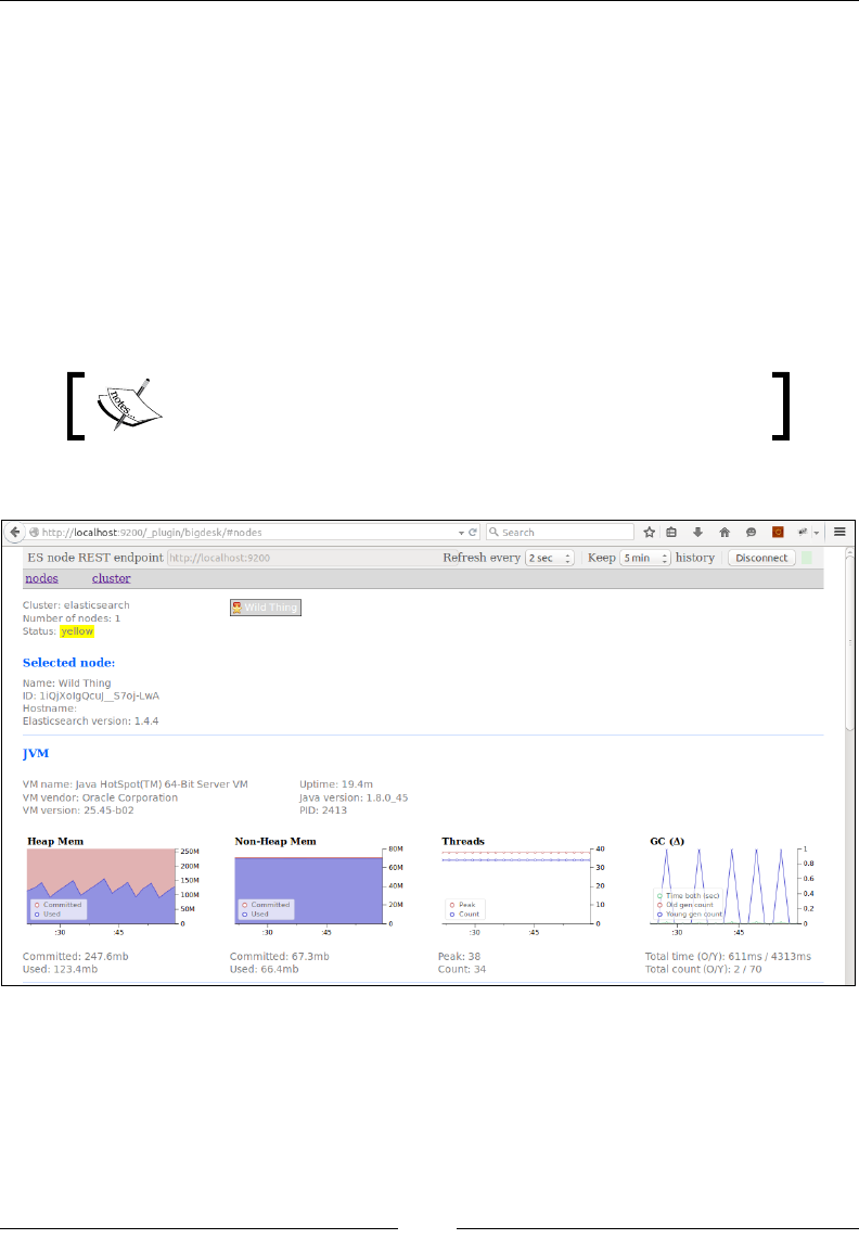
Chapter 5
[ 707 ]
Elasticsearch plugins
Elasticsearch has a very rich set of plugins, mainly community driven, which are
really helpful to analyze the cluster, and execute full-text structural queries easily.
Let's look at a few of the plugins.
Bigdesk plugin
This plugin was developed by Lukas Vlcek. It helps analyze the nodes across the
cluster with the help of live charts and various statistics related to JVM, CPU, and
OS, and about shards and their replicas.
More information is available at https://github.com/
lukas-vlcek/bigdesk.
The following screenshot shows the Bigdesk plugin:
BigDesk plugin
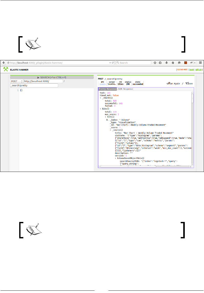
Why Do We Need Elasticsearch in ELK?
[ 708 ]
Elastic-Hammer plugin
The Elastic-Hammer plugin acts as a frontend for Elasticsearch. It helps query the
cluster and provides syntax checking while typing queries as well.
More details can be found here: https://github.com/
andrewvc/elastic-hammer.
Elasticsearch Elastic-Hammer plugin
Head plugin
Head plugins are capable of generating statistics of the cluster, as well as providing
browsing, and performing structured queries on Elasticsearch indices.
More details can be found here: https://github.com/
mobz/elasticsearch-head.
Chapter 5
[ 709 ]
Elasticsearch head plugin
There are many more plugins available that are supported by Elasticsearch or by the
community and they play an important role while interacting with Elasticsearch.
You can easily check the list of available plugins here:
https://www.elastic.co/guide/en/elasticsearch/
reference/current/modules-plugins.html#_plugins
Summary
In this chapter, we learned the basic concepts of Elasticsearch. We also gured
out how querying on a Elasticsearch index works, and how Kibana makes use
of Elasticsearch queries to efciently analyze indexed data and show beautiful
visualizations on top of it.
In the next chapter, we will look at Kibana's features in more detail to understand
how it helps perform some searches on data with querying on its Discover page.

[ 711 ]
Finding Insights with Kibana
In the previous chapter, we saw how Elasticsearch plays a role in ELK Stack to
support fast searches and a variety of aggregations. In this chapter, we will take a
look at how Kibana acts as the frontend of ELK, where it hides all the complexities
of data and presents beautiful visualizations, charts, and dashboards built over the
data, which helps gain essential insights into the data.
Kibana makes it easy to create and share dashboards consisting of various types
of charts and graphs. Kibana visualizations automatically display changes in data
over time based on Elasticsearch queries. It's easy to install and set up, and helps us
quickly explore and discover many aspects of data.
Kibana 4 features
Some of the unique features in Kibana 4 are as follows:

Finding Insights with Kibana
[ 712 ]
Search highlights
Search terms are highlighted in the list of documents shown after the search:
Search highlight in Kibana 4
Elasticsearch aggregations
Kibana 4 makes extensive use of Elasticsearch aggregations and sub aggregations to
provide more than one aggregation for visualizations. There are mainly two types
of aggregations—Bucketing and Metrics. Bucketing produces a list of buckets, each
one with a set of documents belonging to it, for example, terms, range, histograms,
and so on. Metrics calculate the compute metrics for a set of documents, for example,
min, max, sum, average, and so on. These types of computations can only be done on
numeric type of elds.
Scripted elds
Scripted elds are used to make computations on the y on indexed data.
For example, for a certain eld you always want to multiply by 100 before you show
it. You can save it as a scripted eld. Scripted elds, though, can't be searched.
Let's take the following script as an example: doc['volume'].value * 100.
This script will always multiply the value of volume by 100 before it shows it.

Chapter 6
[ 713 ]
Dynamic dashboards
Dashboards are very exible and dynamic as individual visualizations can be easily
arranged as per convenience, and data can be refreshed automatically.
Kibana interface
A Kibana interface consists of four main tabs:
• Discover: The Discover page enables free text searches, field-based searches,
range-based searches, and so on.
• Visualize: The Visualize page enables building many visualizations, such as
pie charts, bar charts, line charts, and so on, which can be saved and used in
dashboards later.
• Dashboard: The Dashboard represents collections of multiple visualizations
and searches, which can be used to easily apply filters based on click
interaction, and draw conclusions based on multiple data aggregations.
• Settings: Settings enables the configuration of index patterns, scripted fields,
the data types of fields, and so on.
Let's take a look at the Discover page in more detail.
Discover page
The Discover page is used to perform interactive searches on your indexed data.
It allows you to perform ad hoc searches based on elds, the ltering of data, and
allows you to view indexed documents as well.

Finding Insights with Kibana
[ 714 ]
A typical Kibana home page, which defaults to the Discover page, looks as follows:
Kibana Discover page
The Discover page shows all the indexed elds in the Index Pattern on the left, a
Time Filter at the top, and a Search Box to enter your search queries. Also, it shows
a default Histogram based on the @timestamp eld in the documents and displays
No. of Hits in the document corresponding to your search. It shows 500 documents
by default with the latest based on the timestamp at the top.
Time lter
Remember the time when your boss asked to nd some statistics from your data
for a specic time? The time lter is the answer for these kinds of searches. You can
lter data on any specic time period selected from the calendar, called Absolute,
or make it Relative based on current time. There are also some quick time lters
available for use.

Chapter 6
[ 715 ]
Quick time lter
A quick time lter helps lter quickly based on some already available time ranges:
Kibana Time Filter – Quick
Relative time lter
A relative time lter helps lter based on relative time from the current time. By
default, the time lter is set to Relative with 15 Minutes ago from Now:
Kibana Time Filter - Relative
Absolute time lter
The absolute time lter helps lter based on a range of dates selected for From and
To a date and time:
Kibana Time Filter – Absolute

Finding Insights with Kibana
[ 716 ]
Kibana Auto-refresh setting
The Auto-refresh setting can be set to set a refresh interval:
Kibana Auto-refresh setting
The time lter can also be specied using click and drag on an area of a histogram or
other charts:
Zoom-in to Set Time Filter
Querying and searching data
Kibana uses Lucene query syntax to search among indices stored in index patterns.
You can also specify an Elasticsearch query DSL, like we explained in Chapter 5,
Why Do We Need Elasticsearch in ELK? The eld list, index documents lists, and the
histogram are automatically refreshed based on the search and time lter settings.
Analyzed and Not Analyzed Fields
As mentioned in the Logstash index template for Elasticsearch
(https://github.com/logstash-plugins/logstash-
output-elasticsearch/blob/master/lib/logstash/
outputs/elasticsearch/elasticsearch-template.
json), when we index string elds, both analyzed (tokenized)
and non-analyzed versions are saved in indexes. All
non-analyzed elds appear with the .raw extension in the
Discover or Visualize pages.
Let's look at some examples of searches.

Chapter 6
[ 717 ]
Freetext search
The freetext search is aimed at ltering documents containing the search term. It
searches in all the documents for all the elds containing the searched term.
Let's take the following instance as an example:
You want to search for all the ELK books from an index pattern consisting of
PacktPub books collections. You can write 'ELK' in the search box, and it lters all
documents containing the term ELK.
Search syntax can be looked up here:
https://lucene.apache.org/core/2_9_4/
queryparsersyntax.html
Boolean searches can be performed on the following terms:
AND
"Learning" AND "ELK"
The preceding query will search for all documents that contain both terms:
"Learning" and "ELK".
OR
"Logstash" OR "ELK
The preceding query will search for all documents that contain the terms
"Logstash" or "ELK".
NOT
"Logstash" NOT "ELK"
The preceding query will search for documents that contain the term Logstash
but not "ELK".
Groupings
("Logstash" OR "ELK") AND "Kibana"
The preceding query will search for documents that contain "Kibana" and can
contain either "ELK" or "Logstash".

Finding Insights with Kibana
[ 718 ]
Wildcard searches
You can also perform wildcard searches using the following terms:
• plan*: will search for all documents that have terms, such as plans, or
plant, or planting, and so on
• plan?: will search for plant or plans
• ? and *: cannot be used as the first character in a search
Field searches
Field searches aim to search for specic values or ranges of values for elds in your
indexed document that displays on the left-hand side of the Discover page.
Field searches can be performed using the eld name and the : character, followed
by a value for the eld we want to lter on.
<field_name>: <field_value>
Let's take a look at some examples of eld searches:
title : "Learning ELK"
title : "Learning ELK" AND category : "technology"
Range searches
Range searches are used to search for a range of values for a eld.
For example, to search for a specic date range:
date_of_record : [20140701 TO 20141231]
To search for a range of values for the volume eld:
volume : [ 100000 TO 200000]
Range and eld searches can be combined using boolean operators like this:
publish_date : [20150701 TO 20151231] AND title : "Learning ELK"
Special characters escaping
The following is the list of special characters, which if we want to search for, need to
be escaped using the \ operator:
+ - && || ! ( ) { } [ ] ^ " ~ * ? : \
For example, to search for 1:2 it needs to be escaped as 1\:2.

Chapter 6
[ 719 ]
New search
You can start a new search by clicking on the New Search button on the
Discover toolbar:
Kibana New Search option
Saving the search
Searches can be saved and used in visualizations later using the Save Search
option on the Discover toolbar. Saved searches can also be added to a dashboard
in order to show the information in a traditional table format. This is very important
for real-world applications in identifying issues:
Kibana Save Search option
Loading a search
Previously saved searches can be loaded using the Load Saved Search option on the
Discover toolbar:
Loading a Saved Search
Finding Insights with Kibana
[ 720 ]
Field searches using eld list
Field searches can also be performed by clicking on the positive or negative lter icon
on certain values on the eld.
Positive and negative filter on fields using field list
In the preceding gure, if you click on the positive lter icon, it will lter all
documents having the http.code value as 200, and if you click on negative lter, it
will show all documents having the http.code value other than 200.
You can also add certain elds on the right-hand side panel by clicking on the add
button on the eld name in the eld list. This enables an easy view of elds as tables
based on your searches.
Field Searches in Kibana

Chapter 6
[ 721 ]
In this way, elds can be quickly added and documents can be sorted in elds, and
elds can be arranged in any order. This is especially helpful to build a table for a
quick search.
Summary
In this chapter, we saw how we can use Kibana's Discover page to gain insights into
the data with some quick searches, which can be saved and used later.
In the next chapter, we will see the Visualize, Dashboard, and Settings pages in
Kibana in detail.

[ 723 ]
Kibana – Visualization
and Dashboard
In the last chapter, we looked at the Discover page and how we could make some
quick searches across indexed documents. In this chapter, we will look at the
Visualize and Dashboard features in Kibana. We will see how we can leverage the
power of Kibana, built over Elasticsearch indexes, to build various types of charts
and graphs, and awesome dashboards covering various analytics, which can be
easily embedded or shared with others.
Visualize page
The Visualize page helps create visualizations in the form of graphs and charts.
These visualizations can be saved and viewed individually or can be used in
multiple dashboards, which act as a collection of visualizations.

Kibana – Visualization and Dashboard
[ 724 ]
All visualizations in Kibana are based on the aggregation feature of Elasticsearch.
Kibana also supports multilevel aggregations to come up with various useful data
analytics. Let's take a look at what a Visualize page looks like:
Kibana Visualize page
The Visualize page has two parts—either you can create a new visualization or open
an existing one from your saved list.
Creating a visualization
To create a new visualization, select Visualize from the top menu bar, which opens a
new Visualize page, and then click on the New Visualization button on tool bar.
Creating a new visualization is a three step process on the Visualize page:
1. Select a visualization type.
2. Select a data source (from a new search or an existing saved search).
3. Congure the aggregations (metrics and buckets) that are to be used for the
visualization on the Edit page.

Chapter 7
[ 725 ]
Visualization types
Kibana supports the following visualizations:
• Area chart
• Data table
• Line chart
• Markdown widget
• Metric
• Pie chart
• Tile map
• Vertical bar chart
Before we start building visualizations of various types, let's understand a bit
about Elasticsearch aggregations, which forms the backbone of the visualizations
in Kibana.
Metrics and buckets aggregations
The metrics and buckets concepts come from the aggregation functionality of
Elasticsearch, and they play a vital role when designing a visualization for your
dataset in Kibana.
Buckets
Buckets help distribute documents among multiple buckets containing a subset of
indexed documents. Buckets are very similar to the GROUP BY functionality in SQL.
They help group documents based on specied criteria, and metrics can be applied
on these documents.
Buckets usually represent the X-axis in Kibana charts and it is possible to add sub-
buckets to a bucket.
The following buckets are available for the X-axis in Kibana:
• Date Histogram
• Histogram
• Range
• Date Range

Kibana – Visualization and Dashboard
[ 726 ]
• IPV4 Range
• Terms
• Filters
• Significant Terms
Let's take a look at a few important visualizations here.
Date Histogram
Date Histogram requires a eld name of type date and interval for the conguration.
It groups documents as per the specied eld and interval specied. For example,
if you specify the eld bucket as @timestamp and Interval as weekly, documents
will be grouped based on weekly data, and then you can apply some metrics, such as
Count, Average, and so on, on top of the grouped documents.
Histogram
Histogram is similar to Date Histogram, except that it requires the eld of type
numbers and a numeric interval to be specied. It will bucket documents for the
particular interval specied in the chosen eld. This is like a range aggregation
with equal intervals.
Range
Range is like Histogram, but it allows you to congure different ranges as per the
requirements, manually. For example, for a eld count, you can choose the bucketing
range to be 0-1000, 1000-5000, 5000-15000, and so on.
Date Range
Date Range requires a date eld and a custom range to be specied for each bucket.
Terms
Terms help group documents by the value of any eld, which is very similar to the
GROUP BY statement in SQL. The Terms aggregation also lets you choose whether
you want Top N or Bottom N, or you can specify the order based on metrics too.
For example, you can choose to group by a product type and get the top ve spends
in that product type.
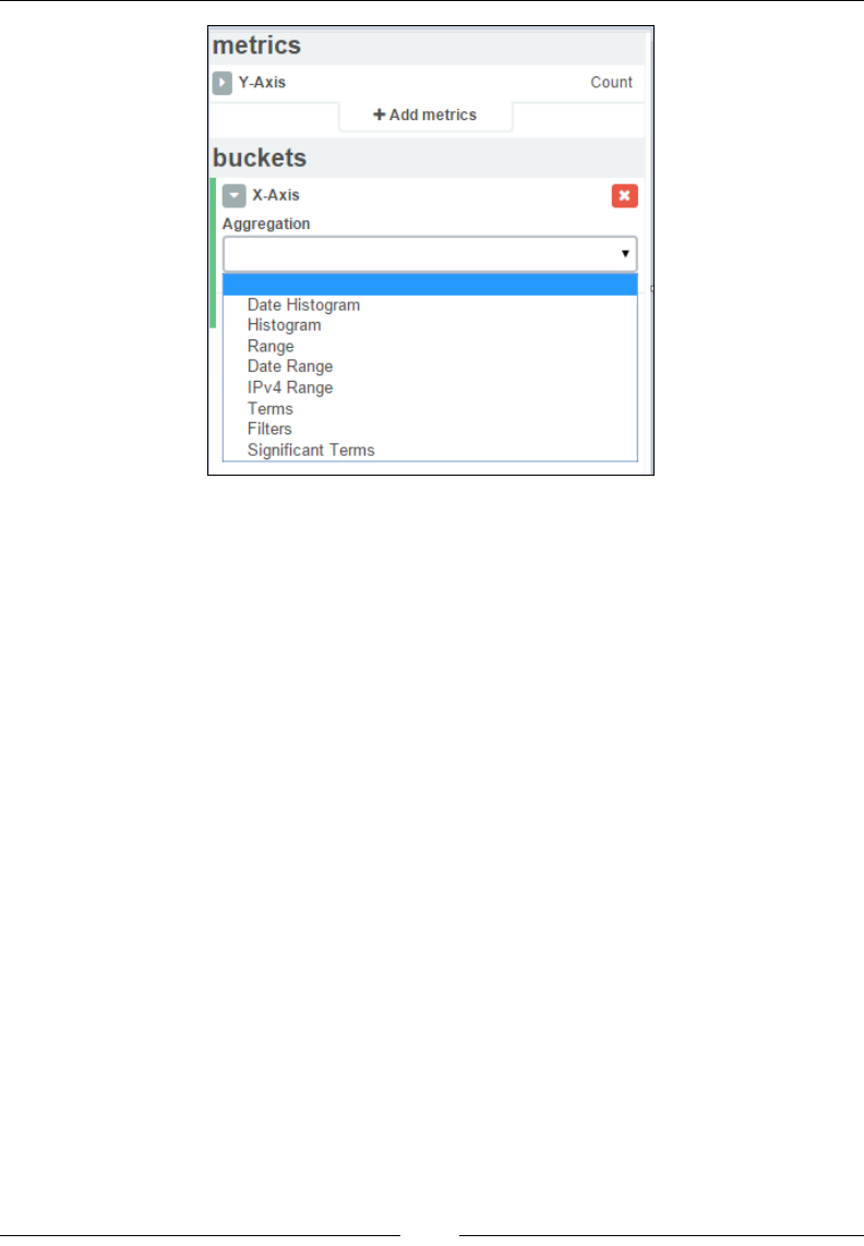
Chapter 7
[ 727 ]
Buckets in visualizations
Metrics
Metrics represents computations performed on values of elds in each bucket, for
example, computing the count, average, minimum, or maximum of a eld in the
document. Metrics usually represent the Y-axis in Area chart, Vertical bar chart,
and Line chart. The types of metrics available in Kibana are:
• Count
• Average
• Sum
• Unique Count
• Min
• Max
• Percentile
• Percentile Ranks
Let's take a look at a few of them.
Count
The Count metric aggregation is very important, and its main purpose is to calculate
the count of the number of elds in each bucket in a bucket aggregation.

Kibana – Visualization and Dashboard
[ 728 ]
For example, to count the number of visitors for each of the product categories, you can
specify the product category eld as bucket aggregation and count metric aggregation.
Average, Sum, Min, and Max
Similar to Count aggregation, Average, Sum, Min, and Max provide the average,
sum, minimum, and maximum, respectively, of all the values of a numeric eld
provided in the aggregation.
Unique Count
Unique Count is similar to the COUNT (DISTINCT eldname) functionality in SQL,
which counts number of unique values for a eld.
Kibana visualization metrics

Chapter 7
[ 729 ]
Advanced options
Buckets and metrics aggregations have Advanced options, which can take JSON
input as scripted elds, as described in Chapter 6, Finding Insights with Kibana. The
following script is an example:
{ "script" : "doc['volume'].value * 100"}
JSON Input Advanced option
Overall, a New Visualization page looks like this, with the toolbar at the top, metrics
and buckets conguration on the left and the preview pane on right-hand side:
Kibana New Visualization page

Kibana – Visualization and Dashboard
[ 730 ]
The toolbar at the top has the options to create a new visualization, save a
visualization, open a saved visualization, share a visualization, and refresh it.
Kibana Visualization toolbar
When creating a visualization, Kibana provides two options as a search source:
• From a saved search
• From a new search
Kibana search source selection
From a saved search uses searches that you saved in the Discover page.
From a new search is used to create a new visualization based on a new search.
Visualizations
Now, let's take a look at various visualization types and how they can be used.
Area chart
Area chart is especially useful to create stacked timelines or distribute data.
Area chart uses metrics as Y-axis and buckets for X-axis. We can also dene sub-
aggregations in buckets, which give you the functionality of Split Charts (multiple
charts based on different aggregations) or Split Area (Area chart split based on
different aggregations).
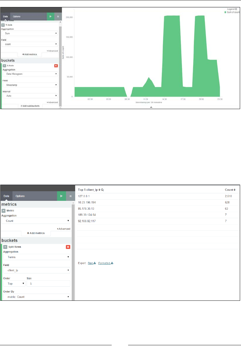
Chapter 7
[ 731 ]
Kibana Area chart
Data table
Data table is used to present aggregated data in a tabular format and helps identify
Top N kinds of aggregations.
For example, to get the top ve clients by the number of hits, the following data table
visualization can be used:
Kibana Data table
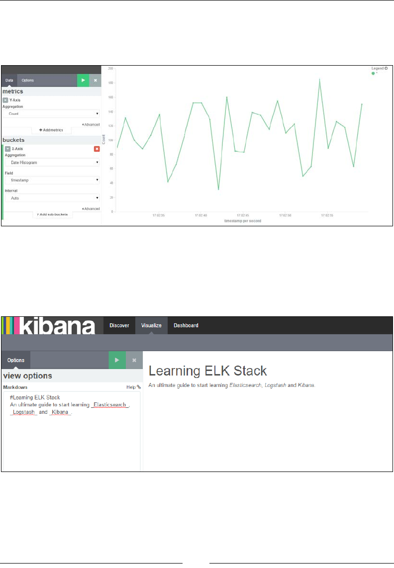
Kibana – Visualization and Dashboard
[ 732 ]
Line chart
Line charts are used for high density time series, and are often helpful when
comparing one series with another:
Kibana Line chart
Markdown widget
Markdown widget is used to display information or instructions on Dashboard and
can be used for any requirements for text on Dashboard.
Kibana Markdown widget
Metric
Metric is used to show a one number kind of analysis for your eld. It can be used to
compute the total number of hits or the sum or average of a eld.
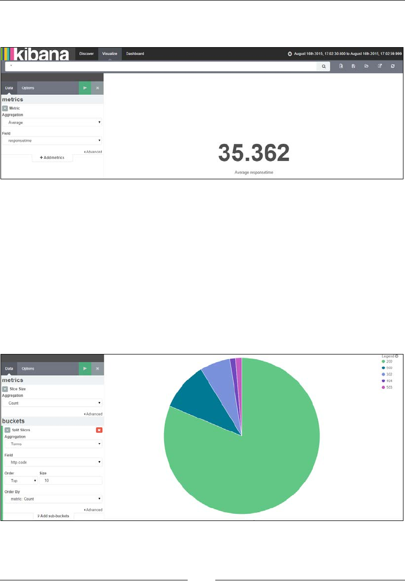
Chapter 7
[ 733 ]
For example, the following metric can be used to show the average response time of
the application over a period of time:
Kibana Metric
Pie chart
Pie charts are often used to show parts of a whole or a percentage relationship. It
represents the distribution of data over multiple slices in a pie chart.
A slice of the pie chart is determined by metrics aggregations, which can have the
values Count, Sum, or Unique Count. Bucket aggregation denes the type of data
that has to be represented in one chart.
For example, the following pie chart can be used to show the distribution of the
different response codes of an application:
Kibana Pie chart
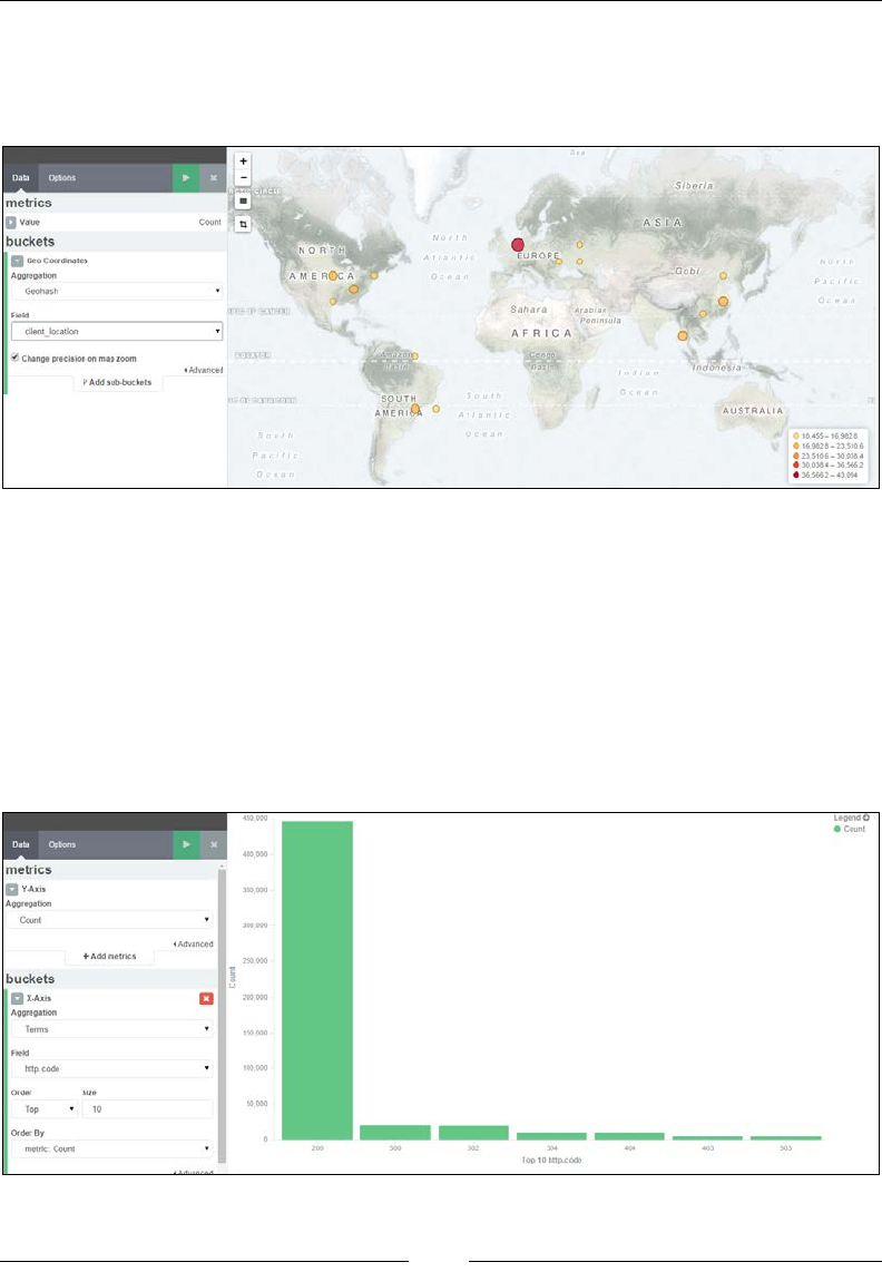
Kibana – Visualization and Dashboard
[ 734 ]
Tile map
Tile maps are used to locate geographic locations based on geo coordinates. It works on
the Geohash bucket aggregation, which groups multiple coordinates into one bucket.
Kibana Tile map
Vertical bar chart
Vertical bar chart is a chart that can be used for a variety of purposes and works well
with time- and non-time-based elds. It can be used as single bar or stacked as well.
Y-axis is metrics and X-axis is buckets aggregation.
For example, the following Vertical bar chart can be used to show a count of HTTP
response codes:
Kibana Vertical bar chart
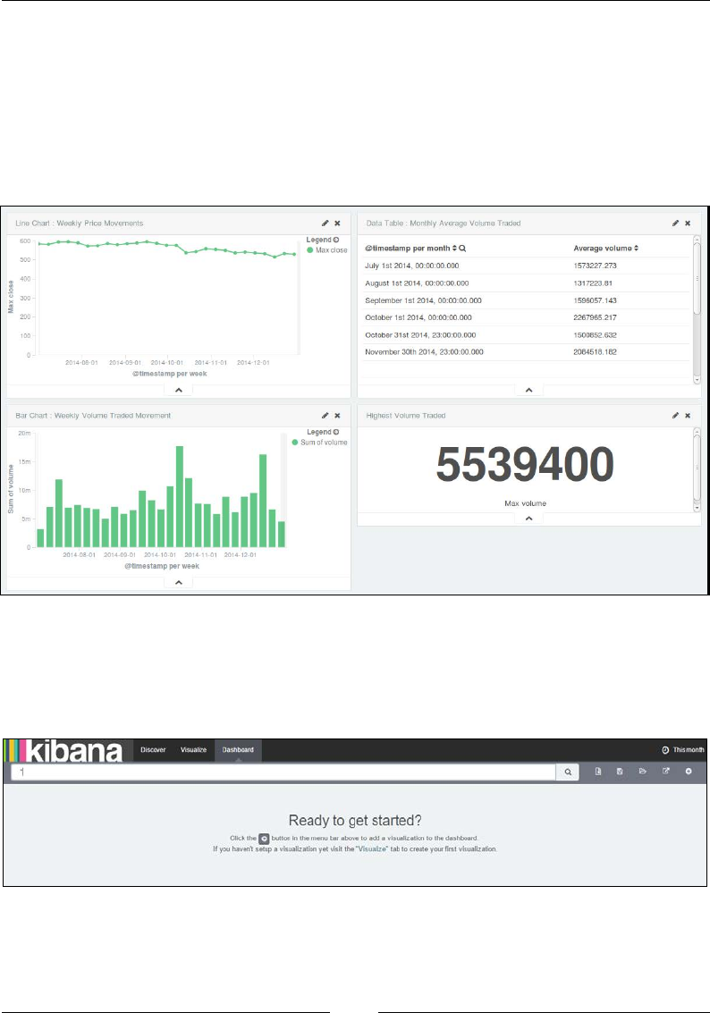
Chapter 7
[ 735 ]
Dashboard page
Kibana Dashboard is just a collection of saved visualizations or saved searches,
which can be arranged in any order. Visualizations can be used on multiple
dashboards and changes will reect to all of them automatically. A dashboard can
be saved and shared easily.
Let's look at what Dashboard will look like:
Building a new dashboard
When you click on the Kibana Dashboard page link at the top of the page for the rst
time, it displays an empty Kibana dashboard that is ready to add visualizations to:
Kibana New Dashboard screen

Kibana – Visualization and Dashboard
[ 736 ]
You can click on the + button with a circle on the extreme right-hand side toolbar
to add any saved visualizations or searches that you saved in the Discover page
in a tabular format. After you have added the visualizations, you can move the
individual visualizations around, edit them, or remove them. You can even resize
or drag and drop them as per your requirements.
Setting a refresh interval on the time lter at the top automatically refreshes the
dashboard with the latest values.
The click to lter feature in Kibana dashboards is very useful in scenarios where
you would like all visualizations and searches to reect events at a particular
time. For example, you can click on a specic bar in a histogram and all the other
visualizations and searches will reect the same automatically.
Saving and loading a dashboard
Once you are done with the arrangement of visualizations, to save a dashboard, click
on the Save Dashboard button on the toolbar and enter a name for the dashboard
and save.
Kibana provides the facility to save a dashboard, which reects values at a particular
time. To do this, there is an option to save time with the dashboard. This is useful to
provide snapshots of the system at a particular time.
Kibana Save Dashboard
To load a saved dashboard, click on the Load Dashboard button on the toolbar and
choose among a list of saved dashboards.

Chapter 7
[ 737 ]
Sharing a dashboard
Once completed and saved, you can share a link to a dashboard or embed it within
another application using the IFrame tag. To do so, click on the Share button on the
toolbar, which shows both a code to embed within another application, and a direct
link to the dashboard, which can be copied and shared.
Kibana Share screen
Summary
In this chapter, we've seen how to create different types of visualizations in Kibana
based on aggregations. We also saw how to arrange and share them using Kibana
Dashboards. In the next chapter, we'll see how we can put all the components of
ELK together to build a powerful data pipeline.

[ 739 ]
Putting It All Together
In the previous chapters, we looked at the basics of Elasticsearch, Kibana, and
Logstash. We saw the congurations and properties of each of them, and tried to
understand what role each of the components plays in building a data pipeline for
your data.
Now we will apply everything that we have learnt so far. We'll create an end-to-end
running solution to analyze logs using ELK Stack.
For demo purposes, we will use a sample web application that runs on the Tomcat
server. We'll set up ELK Stack, where we'll use Logstash to collect, parse and index
access logs to Elasticsearch. Finally, we'll see various searches and visualizations on
it in the Kibana interface.
Input dataset
The input dataset is a continuous stream of Tomcat access logs in the following format:
10.0.0.2 - - [08/Sep/2015:17:39:46 +0100] "GET /elk/demo/10 HTTP/1.1" 200
40
10.0.0.2 - - [08/Sep/2015:17:39:47 +0100] "GET /elk/demo/11 HTTP/1.1" 200
39
10.0.0.3 - - [08/Sep/2015:17:39:48 +0100] "GET /elk/demo/12 HTTP/1.1" 200
39
10.0.0.2 - - [08/Sep/2015:17:39:49 +0100] "GET /elk/demo/13 HTTP/1.1" 200
39
10.0.0.2 - - [08/Sep/2015:17:39:50 +0100] "GET /elk/demo/14 HTTP/1.1" 200
39
10.0.0.4 - - [08/Sep/2015:17:39:51 +0100] "GET /elk/demo/15 HTTP/1.1" 200
40
10.0.0.2 - - [08/Sep/2015:17:39:52 +0100] "GET /elk/demo/16 HTTP/1.1" 200
39

Putting It All Together
[ 740 ]
10.0.0.2 - - [08/Sep/2015:17:39:53 +0100] "GET /elk/demo/17 HTTP/1.1" 200
39
10.0.0.5 - - [08/Sep/2015:17:39:54 +0100] "GET /elk/demo/18 HTTP/1.1" 200
39
10.0.0.2 - - [08/Sep/2015:17:39:55 +0100] "GET /elk/demo/19 HTTP/1.1" 200
39
10.0.0.2 - - [08/Sep/2015:17:39:56 +0100] "GET /elk/demo/20 HTTP/1.1" 200
40
10.0.0.6 - - [08/Sep/2015:17:39:57 +0100] "GET /elk/demo/21 HTTP/1.1" 200
38
10.0.0.2 - - [08/Sep/2015:17:39:58 +0100] "GET /elk/demo/22 HTTP/1.1" 200
40
10.0.0.2 - - [08/Sep/2015:17:39:59 +0100] "GET /elk/demo/23 HTTP/1.1" 200
39
The preceding log format is a Common Apache log format, dened in the Tomcat
server.xml le in conf folder as follows:
<Valve className="org.apache.catalina.valves.AccessLogValve"
directory="logs"
prefix="localhost_access_log." suffix=".txt"
pattern="%h %l %u %t "%r" %s %b" />
The log pattern is in the following format:
%h %l %u %t "%r" %s %b
• %h: This represents the remote hostname (or IP address)
• %l: This represents the remote logical username
• %u: This represents the remote user that was authenticated
• %t: This specifies the date and time in common log format
• %r: This represents the request
• %s: This represents the response HTTP code
• %b: This represents the bytes sent in response, excluding HTTP headers
Conguring Logstash input
In this section, we'll congure Logstash to read data from access logs located on
Tomcat, and index it in Elasticsearch, making lters and tokenization of terms in
logs as per the grok pattern.

Chapter 8
[ 741 ]
Grok pattern for access logs
As we already saw, some of the commonly used grok patterns are already included
with the Logstash installation. Check out the list of Logstash grok patterns on
GitHub at https://github.com/logstash-plugins/logstash-patterns-core/
tree/master/patterns.
There is already a grok pattern for the Common Apache log format in the Logstash
installation as follows:
COMMONAPACHELOG %{IPORHOST:clientip} %{USER:ident} %{USER:auth}
\[%{HTTPDATE:timestamp}\] "(?:%{WORD:verb} %{NOTSPACE:request}(?:
HTTP/%{NUMBER:httpversion})?|%{DATA:rawrequest})"
%{NUMBER:response} (?:%{NUMBER:bytes}|-)
We can directly use COMMONAPACHELOG as a matching pattern for our incoming
messages to Logstash as follows:
input{
file{
path =>"/var/lib/tomcat7/logs/localhost_access_logs.txt"
start_position =>"beginning"
}
}
Next, we need to specify our grok pattern matching with the incoming message,
assign a timestamp eld from our message, and convert the data types of some of the
elds as per our needs:
filter{
grok {
match => { "message" => "%{COMMONAPACHELOG}" }
}
date{
match => ["timestamp","dd/MMM/yyyy:HH:mm:ss Z"]
}
mutate{
convert => ["response","integer"]
convert => ["bytes","integer"]
}
}

Putting It All Together
[ 742 ]
Finally, to congure the output plugin to send ltered messages to Elasticsearch,
we will not specify any port here as we are using the default port for Elasticsearch,
that is, 9200:
output{
elasticsearch {
host => "localhost"
}
}
Now that we have understood the individual conguration, let's see what the overall
conguration for Tomcat looks like:
input{
file{
path =>"/var/lib/tomcat7/logs/localhost_access_log.txt"
start_position =>"beginning"
}
}
filter{
grok {
match => { "message" => "%{COMMONAPACHELOG}" }
}
date{
match => ["timestamp","dd/MMM/yyyy:HH:mm:ss Z"]
}
mutate{
convert => ["response","integer"]
convert => ["bytes","integer"]
}
}
output{
elasticsearch {
host => "localhost"
}
}
*
Now, lets start logstash with this conguration:
$ bin/logstash –f logstash.conf

Chapter 8
[ 743 ]
Logstash will start to run with the dened conguration and keep on indexing all
incoming events to the Elasticsearch indexes. You may see an output that is similar
to this one on the console:
May 31, 2015 4:04:54 PM org.elasticsearch.node.internal.InternalNode
start
INFO: [logstash-4004-9716] started
Logstash startup completed
Now, you will see your Apache access logs data in Elasticsearch. Logstash was able
to parse the input line and break it into different pieces of information, based on the
grok patterns, for the Apache access logs. Now, we can easily set up analytics on
HTTP response codes, request methods, and different URLs.
At this point, we can open the Elasticsearch Kopf plugin console that we installed
in Chapter 1, Introduction to ELK Stack, to verify whether we have some documents
indexed already, and we can also query these documents.
Elasticsearch Kopf UI
If we can see some indexes for Logstash already in Elasticsearch, we have veried
that our Logstash conguration worked well.
Visualizing with Kibana
Now that you have veried that your data is indexed successfully in Elasticsearch, we
can go ahead and look at the Kibana interface to get some useful analytics from the data.
Running Kibana
As described in Chapter 1, Introduction to ELK Stack, we will start the Kibana service
from the Kibana installation directory:
$ bin/kibana
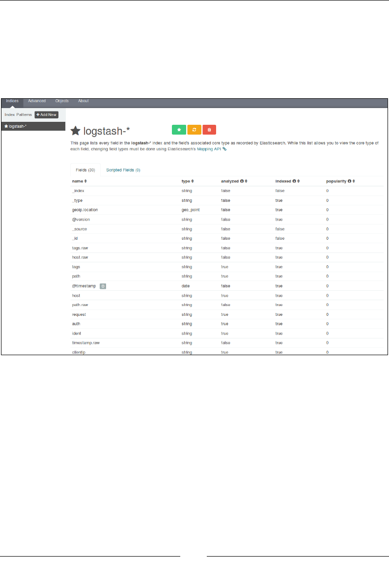
Putting It All Together
[ 744 ]
Now, let's see Kibana up and running with a screen similar to the following
screenshot on the browser with this URL:
http://localhost:5601
We can verify our index and elds in the Settings page under the indices tab
as follows:
Kibana Settings page
It shows all our elds that were indexed, their data types, index status, and
popularity value.
As we have already set up Kibana to take the logstash-* indexes by default, it
starts to display the indexed data as a histogram of counts, and the associated data
as elds in the JSON format as follows:
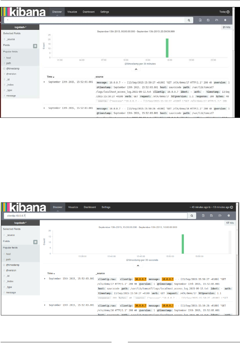
Chapter 8
[ 745 ]
The Kibana Discover page showing indexed values
Searching on the Discover page
After our data is indexed, we can perform some quick searches on our elds to
analyze some data.
To search for a specic client IP, we can type search command as
clientip: 10.0.0.7 and the indexed document on the page displays
matching highlighted values:
Search on fields in the Discover page
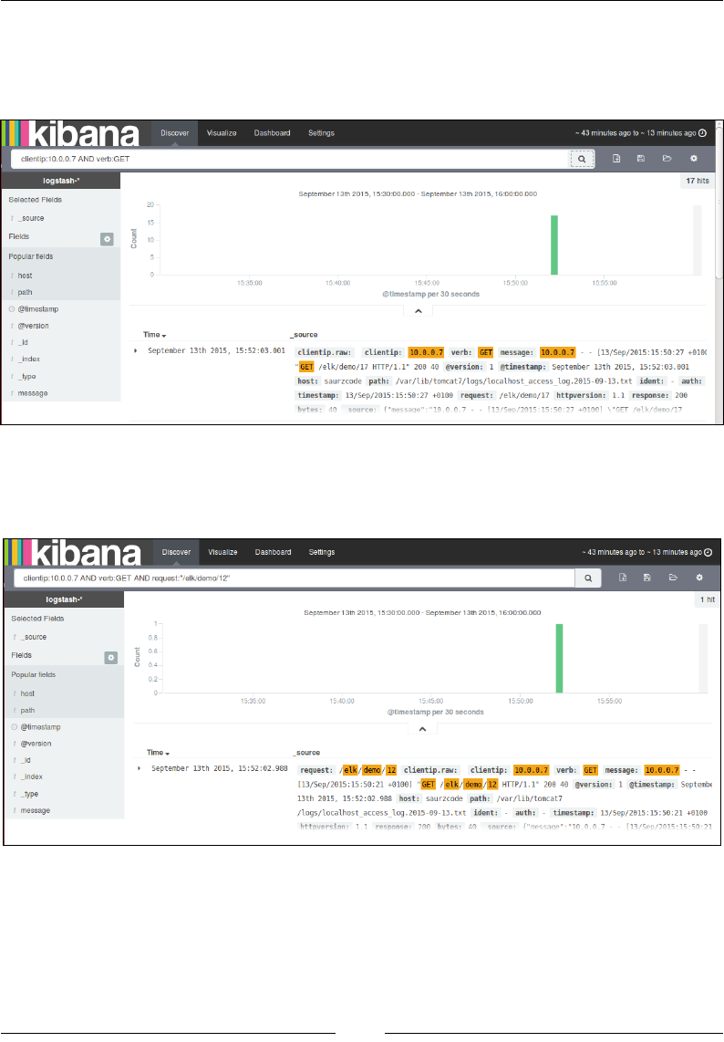
Putting It All Together
[ 746 ]
To search all GET requests coming from specic client IP, we can issue a query
like this:
clientip:10.0.0.7 AND verb:GET
Searching on fields
To search all instances of a particular GET request coming from a specic client IP we
can issue a query like the one shown in the following screenshot:
Searching on fields II
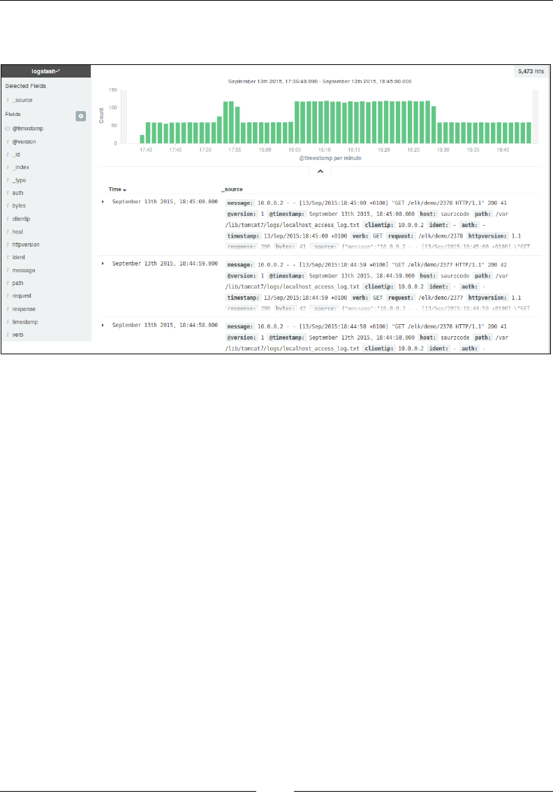
Chapter 8
[ 747 ]
Once our data is fully indexed, the Discover page will look something like this, with
a default histogram based on the count of documents over time:
The Discover page after full indexing
Visualizations – charts
Let's build some basic visualizations from the Kibana Visualize page, and we will
use them later in dashboard.
Click on the Visualize page link at the top of the Kibana home page and click on the
new visualization icon.

Putting It All Together
[ 748 ]
This page shows various types of visualizations that are possible with the
Kibana interface:
Kibana visualization menu
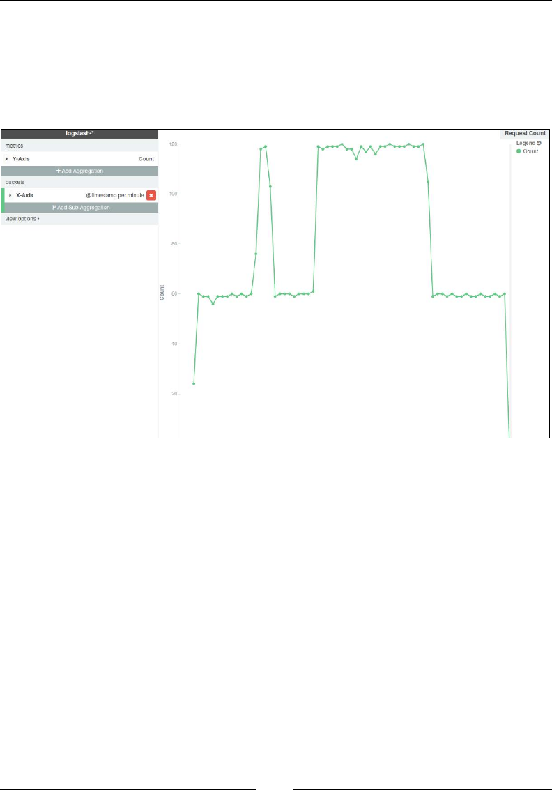
Chapter 8
[ 749 ]
Building a Line chart
The rst visualization that we will build is a Line chart showing the number of hits
over time for the application. To do this, we'll choose the Y-axis metrics as Count
and the X-axis bucket as Date Histogram, and then click on Apply. The resulting
Line chart looks like this:
Line Chart – Request Count
Now, save the visualization using any name for the Line chart, which we will pull in
Dashboard later.

Putting It All Together
[ 750 ]
Building an Area chart
We can build an Area chart based on the number of bytes transferred over time as
follows. To do this, we'll choose the Y-axis metrics as Average and choose Field as
bytes. The resulting Area chart looks like this:
Area Chart – Average Bytes
Now, save the visualization using any name for the Area chart, which we will pull in
Dashboard later.
Building a Bar chart
We'll build a vertical split bar chart showing the number of requests split across
multiple clients. For the Y-axis metrics, we will use Count, and for the X-axis
aggregation, we'll use Date Histogram. We'll use sub aggregation using the Split
Bars feature, and split it using the clientip term:
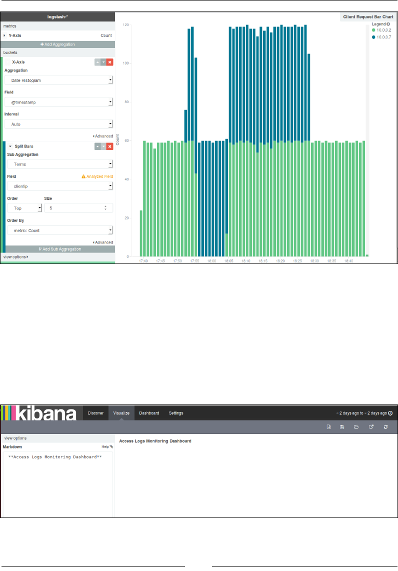
Chapter 8
[ 751 ]
Bar Chart – Requests by Clients
Now, save the visualization using any name for the Bar chart, which we will pull in
Dashboard later.
Building a Markdown
Markdown is lightweight markup language that has a simple formatting syntax for
various documentation needs. We'll build one Markdown to give an explanation of
our Dashboard:
Markdown

Putting It All Together
[ 752 ]
Dashboard page
On the Dashboard page, we can choose from our list of saved visualizations or
searches to include them in our Dashboard:
Add visualization or searches to Dashboard
After we have selected the visualizations that we want to include in our dashboard,
we can drag and drop and arrange them accordingly. The resulting dashboard looks
like this:
Dashboard – Access Logs Monitoring

Chapter 8
[ 753 ]
Once completed, we can choose to share the dashboard using the share button,
which also gives us the code to be used if we want to include it as an embedded
dashboard in some other application:
Share Dashboard
Summary
In this chapter, we saw how we could build an end-to-end data pipeline built over
our logs using ELK Stack, which helps us get useful analysis from our data. This
chapter helped us understand how the features of Elasticsearch, Logstash, and
Kibana come together to help build our own analytics pipeline.
In the next chapter, we'll take a look at some of the practical implementations of ELK
Stack and how it is helping the industry.

[ 755 ]
ELK Stack in Production
So far in the book, we saw how we could use ELK stack to gure out useful
information out of our logs, and build a centralized logging solution for multiple
data sources of an application.
In our end-to-end log pipeline, we congured ELK on our local machine to use local
Elasticsearch, Logstash, and Kibana instances.
In this chapter, we will take a look at how ELK Stack can be used in production with
huge amounts of data and a variety of data sources. Some of the biggest companies,
such as Bloomberg, LinkedIn, Netix, and so on, are successfully using ELK Stack in
production and ELK Stack is gaining popularity day by day.
When we talk about the production level implementation of ELK Stack, some of the
perquisites are:
• Prevention of data loss
• Data protection
• Scalability of the solution
• Data retention
Prevention of data loss
Data loss prevention is critical for a production system, as monitoring and
debugging is largely dependent on each and every log event to be present in the
system; otherwise, whole analytics or the debugging system will fail, and we end up
losing some of the important events in our system.
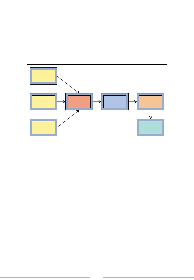
ELK Stack in Production
[ 756 ]
Data loss can be prevented using a message broker in front of the Logstash indexers.
Message brokers, such as Redis, prove to be useful when dealing with a large stream
of data, as Logstash may slow down while indexing data to Elasticsearch. Redis can
help in these situations where it can buffer the data while Logstash is busy indexing
to Elasticsearch. It also adds a layer of resiliency where if indexing fails, events are
held in a queue instead of getting lost. ZeroMQ, RabbitMQ, AMQP can also be used
as a broker in place of Redis.
For example, the following architecture can be useful:
Logstash
Shipper
Logstash
Shipper
Logstash
Shipper
Redis
(Broker)
Logstash
(Indexer) Elasticsearch
Kibana
ELK Architecture with message broker
Data protection
Since data is of immense value and carries a lot of condential information, it
is extremely important to protect the data at various points while in ELK Stack.
Elasticsearch indices must be prevented from unauthorized access, and Kibana
Dashboard should be protected too. We can also set up an Nginx reverse proxy
to access Kibana instances, which will put your Kibana console behind an
authentication page that requires a username and password.
Kibana supports SSL encryption for both client requests and the requests the Kibana
server sends to Elasticsearch.

Chapter 9
[ 757 ]
To encrypt communications between the browser and the Kibana server, we can
congure the ssl_key_file and ssl_cert_file properties in kibana.yml:
The following are SSL for outgoing requests from the Kibana server
(PEM formatted):
• ssl_key_file: /path/to/your/server.key
• ssl_cert_file: /path/to/your/server.crt
Elasticsearch shield can be used to provide index level access control to your data in
Elasticsearch. We can create a role for Kibana in shield, and determine what access
we want to grant to users of Kibana, as follows:
kibana4:
cluster:
- cluster:monitor/nodes/info
- cluster:monitor/health
indices:
'*':
- indices:admin/mappings/fields/get
- indices:admin/validate/query
- indices:data/read/search
- indices:data/read/msearch
- indices:admin/get
'.kibana':
- indices:admin/exists
- indices:admin/mapping/put
- indices:admin/mappings/fields/get
- indices:admin/refresh
- indices:admin/validate/query
- indices:data/read/get
- indices:data/read/mget
- indices:data/read/search
- indices:data/write/delete
- indices:data/write/index
- indices:data/write/update
- indices:admin/create

ELK Stack in Production
[ 758 ]
We can also give the Kibana server level roles, which gives access to the .kibana
index as follows:
kibana4_server:
cluster:
- cluster:monitor/nodes/info
- cluster:monitor/health
indices:
'.kibana':
- indices:admin/create
- indices:admin/exists
- indices:admin/mapping/put
- indices:admin/mappings/fields/get
- indices:admin/refresh
- indices:admin/validate/query
- indices:data/read/get
- indices:data/read/mget
- indices:data/read/search
- indices:data/write/delete
- indices:data/write/index
- indices:data/write/update
Please note that shield is not free and is a part of a paid service provided by Elastic.
Search Guard is another tool that is free and works well to secure your Elasticsearch
installation. More details are available at http://floragunn.com/searchguard.
System scalability
As the data in the application grows, it is essential that the log analytics system
should scale well with the system. Also, there are times when your systems are
under a heavy load, and you need your log analytics systems to analyze what
is going on with the application. ELK Stack provides that capability where you
can easily scale each component as per your needs. You can always add more
Elasticsearch nodes (master nodes and data nodes) in the cluster. It is recommended
that you have three master nodes (one primary and two backup) for large clusters.
Also, load balancing or routing nodes can be added for high volume searches and
indexing requirements. You can also get more Logstash and Redis instances, and add
more than one Kibana instance too. A typical scaled architecture may look like this:
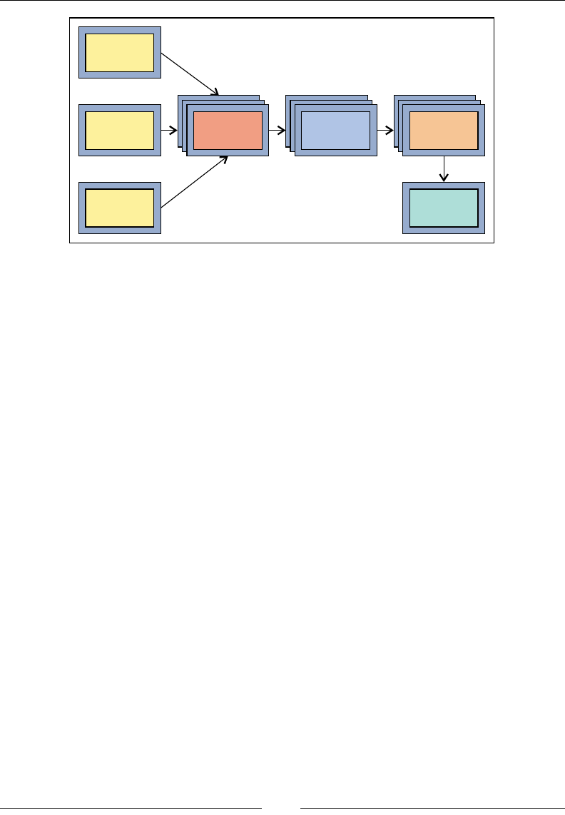
Chapter 9
[ 759 ]
Logstash
Shipper
Logstash
Shipper
Logstash
Shipper
Redis
(Cluster)
Logstash
(Cluster)
Elasticsearch
(Master and
Data Nodes)
Kibana
ELK Architecture with Cluster
Data retention
When setting up a log analytics system, it is extremely important to dene your data
retention policy as Elasticsearch can't hold all the data that you have, which may
result in data loss. There should be a process to automatically delete old indices after
a certain dened period.
The Elasticsearch Curator (https://github.com/elasticsearch/curator) is
especially useful to manage your indices. You can schedule Curator to delete old
indices based on your need. For example, the following command can be set up in a
crontab to delete indices older than 10 days at a specied time, daily:
curator --host 10.0.0.7 delete indices --older-than 10 --time-unit days \
--timestring '%Y.%m.%d'

ELK Stack in Production
[ 760 ]
ELK Stack implementations
The ELK community is quite large, and it's growing rapidly as it is gaining more
and more attention. Let's take a look at some of the already existing successful ELK
Stack implementations.
ELK Stack at LinkedIn
LinkedIn is a business oriented social networking site, which is mainly used for
professional networking. LinkedIn was launched in May 5, 2003. As of March 2015,
LinkedIn reports more than 364 million acquired users, in more than 200 countries
and territories.
Refer to http://www.slideshare.net/TinLe1/elk-atlinked-in.
Problem statement
LinkedIn has millions of multiple data centers, tens of thousands of servers,
hundreds of billions of log records. It is a challenge to log, index, search, store,
visualize, and analyze all of these logs all day, every day. Also, security in terms
of access control, storage, and transport has to be maintained. As data grows, the
system will scale to more data centers, more servers, and will produce even more
logs. It needs an efcient log analytics pipeline that can handle data at this scale.
Criteria for solution
The log analytics solution that LinkedIn is looking for, must meet the following:
• It is horizontally scalable, so that more nodes can be added when needed
• It is fast, and quick, and as close to real-time as possible
• It is inexpensive
• It is flexible
• It has a large user community and supports availability
• It is open source

Chapter 9
[ 761 ]
Solution
ELK Stack proved to match all these criteria. ELK is currently used across many
teams in LinkedIn. This is what the current ELK Stack implementation at LinkedIn
looks like:
• 100 plus ELK clusters across 20 plus teams and six data centers
• Some of the larger clusters have:
°Greater than 32 billion docs (30+ TB)
°Daily indices that average 3.0 billion docs (~3 TB)
The current architecture for ELK Stack at LinkedIn uses Elasticsearch, Logstash,
Kibana, and Kafka.
Apache Kafka: Kafka is a high throughput distributed
messaging system, which was invented by LinkedIn, and
open sourced in 2011. It is a fast, scalable, distributed, and
durable messaging system which proves useful for systems
that produce huge amounts of data. More details can be
found at the Kafka site http://kafka.apache.org.
Kafka at LinkedIn
Kafka is a common data-transport layer across LinkedIn. Kafka handles around
1.1 trillion messages per day, a 200 TB per day input, and a 700 TB per day output.
The architecture is spread across 1100 brokers, over 50 plus clusters, which includes
around 32000 topics and 350 thousands partitions.
Operational challenges
LinkedIn generates lots of data, so reliable transport, queuing, storing, and indexing
is very essential. It has to take data from various sources, such as Java, Scala, Python,
Node.js, Go, and so on. Obviously, the data format was different across these sources
so transformations were needed.

ELK Stack in Production
[ 762 ]
Logging using Kafka at LinkedIn
LinkedIn uses dedicated clusters for logs in each data center. They have individual
Kafka topics per application, and it acts as a common logging transport for all
services, languages, and frameworks. To ingest logs from Kafka to Logstash, they
used their own Kafka input plugin; later, they started using KCC (Kafka console
consumer) using a pipe input plugin.
Elasticsearch
(master)
Logstash Logstash
Kafka
Elasticsearch
(tribe)
Kibana
Users
Elasticsearch
(data node)
Elasticsearch
(data node)
ELK at LinkedIn
An example conguration of a Logstash pipe plugin using KCC is as follows:
pipe {
type => "mobile"
command => "/opt/bin/kafka-console-consumer/kafka-console-
consumer.sh \
--formatter
com.linkedin.avro.KafkaMessageJsonWithHexFormatter \
--property schema.registry.url=http://schema-
server.example.com:12250/schemaRegistry/schemas \
--autocommit.interval.ms=60000 \
--zookeeper zk.example.com:12913/kafka-metrics \
--topic log_stash_event \
--group logstash1"
codec => "json"
}

Chapter 9
[ 763 ]
ELK at SCA
SCA is a leading global hygiene and forest products company. The SCA group
companies develop and produce sustainable personal care, tissue, and forest products.
As we can see at https://www.elastic.co/blog/improving-user-intelligence-
with-the-elk-stack-at-sca:
"At SCA we use Elasticsearch, Logstash, and Kibana to record searches, clicks on
result documents and user feedback, on both the intranet and external sites. We
also collect qualitative metrics by asking our public users a question after showing
search results: "Did you nd what you were looking for?" The user has the option
to give a thumbs up or down and also write a comment."
How is ELK used in SCA?
All search parameters and results information are recorded for each search event:
the query string, paging, sorting, facets, the number of hits, search response time,
the date and time of the search, and so on. Clicking a result document also records
a multitude of information: the position of the document in the result list, the time
it took from search to click, and various document metadata (such as URL, source,
format, last modied, author, and more). A click event also gets connected with the
search event that generated it. This is also the case for feedback events.
Each event is written to a log le that is being monitored by Logstash, which then
creates a document from each event, and pushes them to Elasticsearch where the
data is visualized in Kibana.
How is it helping in analytics?
Since a lot of information is being indexed in the stack, a variety of analytics
can be performed from simple queries, such as "What are the ten most frequent
queries during the past week?" and "Users who click on document X, what do they
search for?", to the more complex ones, such as "What is the distribution of clicked
documents' last modied dates, coming from source S, on Wednesdays?"
Analysis like this helps them tune the search to meet the needs of the users and
deliver value to them. It helps adjust the relevance model, add new facets or remove
old ones, or change the layout of search and result pages.

ELK Stack in Production
[ 764 ]
What this means for SCA is that they get a search that is ever improving. The direct
feedback loop between the users and administrators of the system creates a sense
of community, especially when users see that their grievances are being tended to.
Users nd what they are looking for to a greater and greater extent, saving them time
and frustration.
ELK for monitoring at SCA
This setup is not only used to record information about user behavior, but also used
to monitor the health of the servers. In that context Elasticsearch, Logstash, and
Kibana are being used as a Time Series Database. Every few seconds, information
about each server's CPU, memory, and disk usage (time series data) is being indexed.
It also helps gain access to the historic aspect of data and to nd trends in the system.
This can, of course, be correlated with the user statistics. For example, a rise in CPU
usage can be correlated to an increase in query volume.
Refer to: https://www.elastic.co/blog/improving-user-intelligence-with-
the-elk-stack-at-sca.
ELK at Cliffhanger Solutions
Cliffhanger Solutions is an application and service provider for the utility and
telecom industry. It helps customers and utility companies with preventative
maintenance and reducing outage restoration times.
"At Cliffhanger Solutions, we index data in real time from various sources using
Elasticsearch and Logstash. Sources include GPS location data from maintenance
trucks or from tablets running our app, readings from smart meters and facility
data from GIS (geographical information systems)."
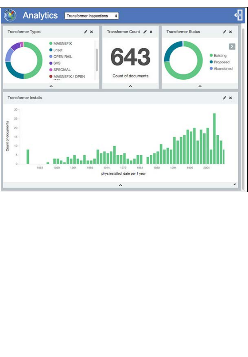
Chapter 9
[ 765 ]
Kibana dashboard at Cliffhanger
Operators can now quickly get answers to questions such as "Can I safely close this
switch and restore power to these 1500 customers?" or "A storm is coming in from
the South, how fast can I get my bucket trucks to the area where the storm will hit?"
As for preventative maintenance, engineers can seek answers to questions such
as "Transformers from vendor X have a higher than average MTBF (mean time
between failures). Find all of them and sort them by installation date, then send
them to the work order system for inspection or replacement." While it might not
sound like a big deal, this is actually pretty incredible, and this wasn't possible until
now without a heavy investments in consultancy or getting locked in with the few
one stop shop large vendors that offer a total solution. As we can see at https://www.
elastic.co/blog/using-elk-to-keep-the-lights-on:

ELK Stack in Production
[ 766 ]
"Cliffhanger Solutions is a small company, but the exibility of Elasticsearch allowed
us to focus on creating value for our customers instead of getting stuck in maintaining
different systems for different clients. And our clients are getting it as well. For
example, we serve a tiny utility on a Caribbean island, with only 1 guy in the IT
department. By using ATLAS (+Kibana) out of the box, we built them a dashboard
to show them outages on a map, color coded by customer density. This would never
have been possible even a few years ago. The ELK stack is pretty incredible at making
data searchable even if the source data is not clearly dened. Unlike traditional
databases you don't need to know your questions in advance, you can explore and nd
correlations you didn't even know existed. It reduces a lot of overhead.
Internally, at the Cliffhanger ofce, we use the ELK stack to monitor the status of
our clients' applications. We use it to improve search relevance, performance, nd
errors and prevent hack attacks. We share this data with our clients. They like this
level of transparency and it gives them condence that their data is safe."
Refer to https://www.elastic.co/blog/using-elk-to-keep-the-lights-on.
Kibana demo – Packetbeat dashboard
Finally, from ELK itself, there is a very good demo for the Kibana dashboard, which
shows various aspects of the stack, and shows the power and breadth of information
it gives. It is available at http://demo.elastic.co.
Packetbeat is a real-time network packet analytics provider,
and an open source data shipper that integrates with
Elasticsearch and Kibana to provide real-time analytics for
web, database, and other network protocols.
This demo is spread across multiple dashboards based on Packetbeat, such as the
MySQL dashboard, the MongoDB dashboard, the Web Transactions dashboard,
the Thrift-RPC and PostgreSQL dashboard. It helps us understand many advanced
searches and visualizations built on the Kibana platform. Here is what the dashboard
looks like:
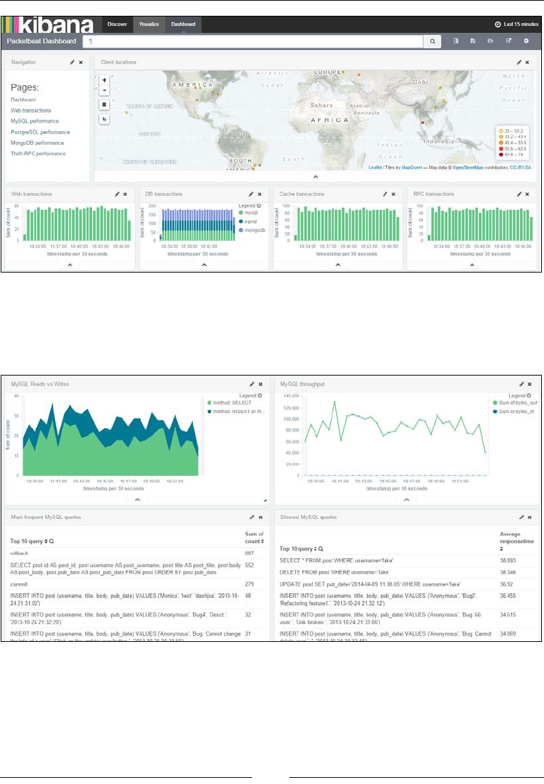
Chapter 9
[ 767 ]
Kibana Packetbeat Demo dashboard
As we can see on the left-hand side of the preceding screenshot, it displays links to
various dashboards. A MySQL performance dashboard, which displays the various
queries used, performance of queries, and so on, looks like this:
MySQL Performance dashboard
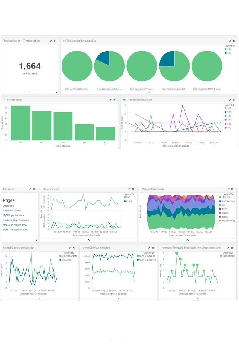
ELK Stack in Production
[ 768 ]
A Web Transactions dashboard, which displays various web transactions, which
includes the various HTTP methods used, total number of requests, error codes, and
so on, looks like this:
Web Transactions dashboard
A MongoDB dashboard, which dispays MongoDB throughput, errors, errors per
collections, input and output throughput, and so on, looks like this:
MongoDB Performance dashboard
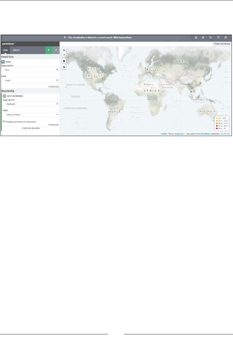
Chapter 9
[ 769 ]
We can also explore multiple visualizations built in each of these dashboards. For
example, a conguration of a GeoIP visualization, which plots clients across the
geography, looks like this:
Geo IP Visualization
Summary
In this chapter, we looked at some of the production level strategies for ELK Stack
and also looked at some of the implementations of the stack. ELK Stack is gaining
more popularity as the community of users evolves, and with a multitude of use
cases, which get benets from the stack.

[ 771 ]
Expanding Horizons with ELK
In all the previous chapters, we explored all the capabilities of ELK Stack, and how it
makes your life easier to analyze logs. Now, we will explore some of the plugins and
utilities that extend the capability of the stack and make it more wonderful, secure,
and easy to maintain. We'll also take a look at the roadmap for the components of
ELK Stack.
The following topics are covered in this chapter:
• Elasticsearch plugins and utilities
°Curator for index management
°Shield for security
°Marvel to monitor
• ELK roadmap
Elasticsearch plugins and utilities
Elasticsearch is a very important component of ELK Stack, so it's very important to
have a good management of the Elasticsearch cluster, and to maintain security. There
are a few plugins and utilities that are available.
Curator for index management
Curator is an important utility that helps manage the Elasticsearch indices. As your
data grows, it becomes important to manage the kind of information that you want
to retain and what information you can remove from your system. Curator can help
remove old indices and optimize the system.

Expanding Horizons with ELK
[ 772 ]
The following are some of the high level tasks that Curator can perform for your
Elasticsearch indices:
• Delete indices and snapshots
• Close indices
• Open closed indices
• Show indices and snapshots
• Add or remove indices from an alias
• Optimize indices
• Change the number of replicas per shard for indices
Curator commands
Curator can be easily congured as cron entries in your system, where you can
schedule the cleanup of indices regularly. Let's take a look at the command-line
syntax of Curator:
curator [FLAGS] COMMAND [FLAGS] SUBCOMMAND [FLAGS]
All available options can be explored using the help command:
curator --help
Let's look at some examples of how Curator can be used:
• Deleting the indices older than a certain period:
curator --host 10.0.0.X delete indices --older-than 180 --time-
unit days \ --timestring '%Y.%m.%d'
• Show all the indices matching a timestring:
curator --host 10.0.0.x show indices --timestring '%Y.%m.%d'
• Add indices older than 30 days to alias last_month:
curator alias --alias-older-than 30 --alias last_month
• Remove indices older than 60 days from alias last_month:
curator alias --unalias-older-than 60 --alias last_month
Curator installation
Curator installation is very easy and quick; it can be done via the python pip utility:
pip install elasticsearch-curator

Chapter 10
[ 773 ]
Curator is hosted at https://github.com/elastic/curator, and detailed
information about Curator can be found in its ofcial documentation at https://www.
elastic.co/guide/en/elasticsearch/client/curator/current/index.html.
Shield for security
Shield is an Elasticsearch plugin from Elastic that adds security to your Elasticsearch
cluster. Shield helps protect the data by adding a secure authentication or role-based
authorization process.
The following are high-level capabilities of shield:
• It adds authorization control to cluster by enabling password protection,
role-based access control, and IP filtering techniques
• It adds SSL/TLS encryption, and message authentication capability
• It adds auditing capabilities to maintain an audit trail of changes in data
More details on shield can be found in its ofcial
documentation here:
https://www.elastic.co/guide/en/shield/
current/index.html
Shield is available for 30 days with a trial license, and a subscription needs to be
purchased after that. There are open sources alternatives for shield for Elasticsearch
security, such as Search Guard (https://github.com/floragunncom/search-guard).
Shield installation
To install shield, you need to follow these steps from the Elasticsearch
installation directory:
1. Install the license plugin:
bin/plugin -i elasticsearch/license/latest
-> Installing elasticsearch/license/latest...
Tryinghttp://download.elasticsearch.org/elasticsearch/license/
license-latest.zip...
Downloading ....................................................
DONE
Installed elasticsearch/license/latest into /usr/share/
elasticsearch/plugins/license

Expanding Horizons with ELK
[ 774 ]
2. Install the shield plugin:
bin/plugin -i elasticsearch/shield/latest
-> Installing elasticsearch/shield/latest...
Tryinghttp://download.elasticsearch.org/elasticsearch/shield/
shield-latest.zip...
Downloading
DONE
Installed elasticsearch/shield/latest into /usr/share/
elasticsearch/plugins/shield
3. After installing plugin, start your Elasticsearch instance and check in the start
up logs for references of shield:
[2015-10-17 07:46:27,508][INFO ][transport ]
[Witchfire] Using [org.elasticsearch.shield.transport.
ShieldServerTransportService] as transport service, overridden by
[shield]
[2015-10-17 07:46:27,510][INFO ][transport ]
[Witchfire] Using [org.elasticsearch.shield.transport.netty.
ShieldNettyTransport] as transport, overridden by [shield]
[2015-10-17 07:46:27,511][INFO ][http ]
[Witchfire] Using [org.elasticsearch.shield.transport.netty.
ShieldNettyHttpServerTransport] as http transport, overridden by
[shield]
Once the shield plugin is added, your access to Elasticsearch at http://
localhost:9200 is restricted without a valid authentication.
Adding users and roles
You need to add users and roles in shield to access Elasticsearch. The following
simple command can help you add users with a role, and you can set a password
for each user:
bin/shield/esusers useradd es_admin -r admin
Adding roles in shield
Chapter 10
[ 775 ]
Once added, you can verify the user through a list command, or you can delete
users, change the password, and so on.
Listing and removing roles in shield
Please note that the license plugin that we installed enables the 30 day trial version of
shield, beyond which it is degraded to limited functionalities and the license needs to
be purchased to enable full functionality.
Using Kibana4 on shield protected Elasticsearch
If we need to use Kibana on top of Elasticsearch that is now protected using shield,
we need to add a kibana4-server role in shield, and provide a corresponding
conguration in the Kibana conguration le in the Kibana installation at config/
kibana.yml.
The following is the Kibana server role:
esusers useradd kibana4-server -r kibana4_server -p password
The following is the Kibana conguration:
kibana_elasticsearch_username: kibana4-server
kibana_elasticsearch_password: password
Marvel to monitor
Marvel is a product that helps monitor an Elasticsearch cluster. It provides a single
interface to view aggregated analytics on the cluster. You can view the essential
metrics for your cluster, such as health, state of nodes, and indices. Marvel can help
perform a root cause analysis of cluster-related issues so that you can anticipate
problems before they occur and x them. You can also analyze historical or real-time
data with it.
Marvel 2.0, supporting Elasticsearch 2.0, is a complete
rewrite as a Kibana plugin. It is free for use by everyone, but
multicluster support comes as a commercial feature. More on
Marvel 2.0 can be found here https://www.elastic.co/
guide/en/marvel/current/index.html.
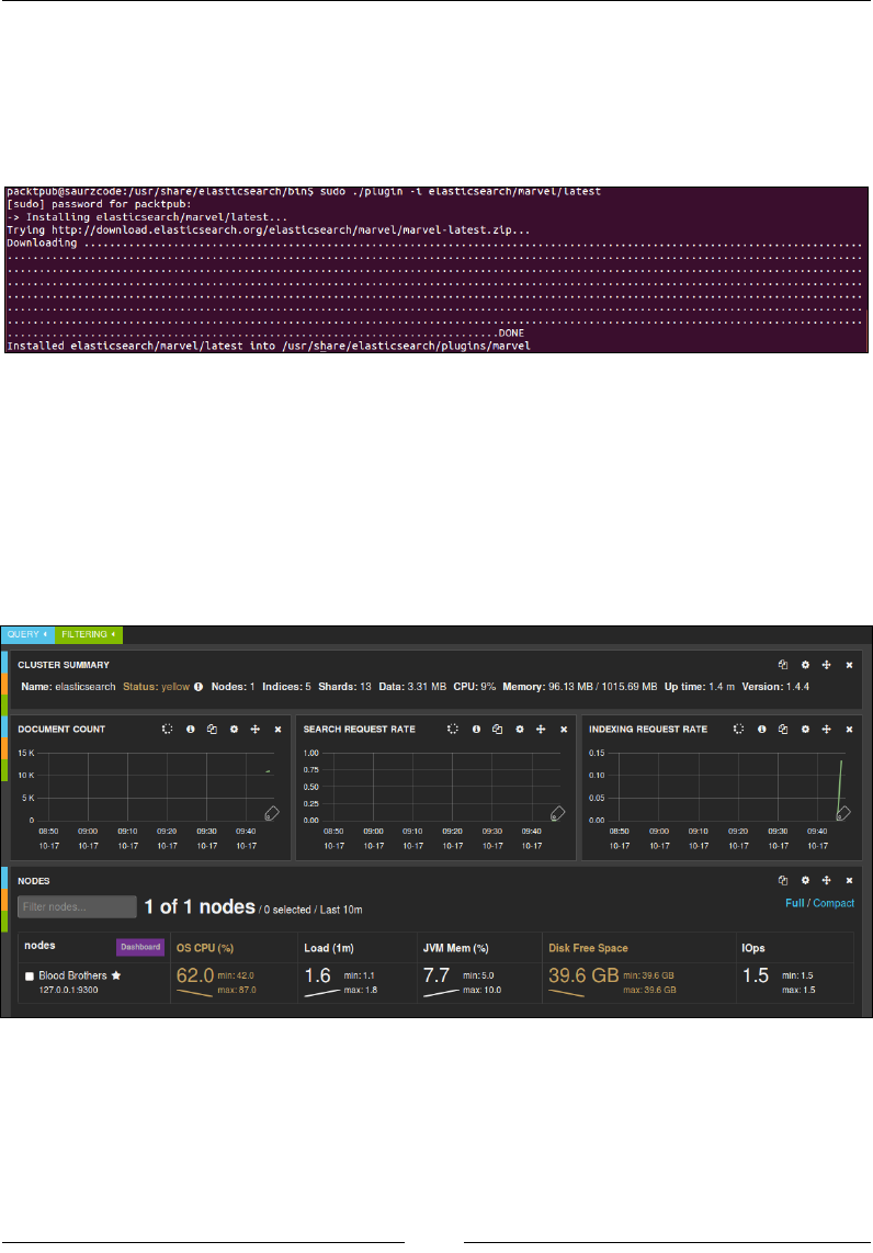
Expanding Horizons with ELK
[ 776 ]
Marvel installation
Just like shield, the Marvel installation is also a one step process. We need to execute
the following command from the Elasticsearch installation directory:
bin/plugin -i elasticsearch/marvel/latest
Marvel installation
The following are some of the features that Marvel provides.
Marvel dashboards
Looking quite similar to Kibana dashboards, Marvel dashboard gives you various
metrics about your Elasticsearch cluster, and various nodes and indices. Values in
yellow need your attention and have to be taken care of.
Marvel dashboard
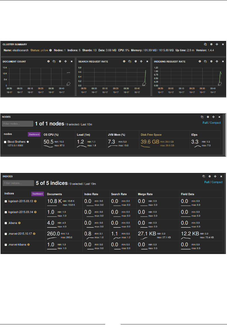
Chapter 10
[ 777 ]
It gives you the DOCUMENT COUNT, SEARCH REQUEST RATE, INDEXING
REQUEST RATE, various statistics on nodes and indexes, such as OS CPU,
Load, JVM Mem, Disk Free Space and IOps operations, as shown in the
following screenshots:
Marvel dashboard statistics
Marvel node metrics
Marvel indices metrics
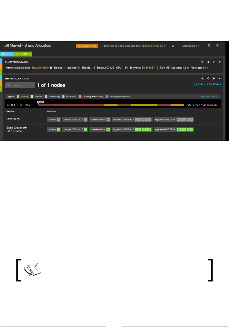
Expanding Horizons with ELK
[ 778 ]
There is also a very good dashboard that represents the Shard Allocation in your
cluster, and where different indices sit on various shards and replicas. It displays all
primary nodes and replica nodes with different color codes along with the state of
various nodes.
Marvel Shard Allocation dashboard
ELK roadmap
All the tools in ELK Stack and its ecosystem are in an active development phase, and
new updates are being pushed regularly. It's evolving rapidly to suit the needs of
modern enterprise applications.
Elasticsearch roadmap
Elasticsearch is widely used across companies in various use cases, and its ecosystem
and plugins are evolving very rapidly. With a wide range of plugins available for
various tasks involving Elasticsearch, it is becoming more and more adaptable to a
variety of use cases.
All plugins and integrations are documented here:
https://www.elastic.co/guide/en/elasticsearch/
plugins/current/index.html

Chapter 10
[ 779 ]
Logstash roadmap
Logstash is probably the most active development among ELK Stack tools. The
development team and community are working hard to make the tool more
enterprise grade by adding more resiliency, robustness, and maintainability features.
Logstash 1.5.x has already made signicant changes related to plugin management
and development. The following are the capabilities being added in coming versions
of Logstash.
Event persistence capability
Currently we need to use a message broker, such as Redis, and so on, to throttle the
event queue or to save losing the events in the pipeline. The upcoming versions of
Logstash are going to add the capability of persisting the events queue to disk to
avoid loss of data in case of plugin crash or restart.
End-to-end message acknowledgement
The current Logstash implementation lacks the capability of acknowledging the
message across end-to-end systems. The upcoming versions of Logstash are planned
to include notication of failed events, and so on, so that events can be replayed
or handled.
Logstash monitoring and management API
The Logstash process currently lacks the support to monitor the installation, and to
track event successes and failures, in the pipeline. Monitoring API planned in future
releases is aimed at providing these capabilities.
Also, currently, if you need to change any conguration, you need to change the
Logstash conguration le, and the system needs a restart to take the change in to
effect. The Logstash management API is planned to overcome this limitation so that
conguration can be updated dynamically without interrupting the pipeline.
More capabilities that are being added to Logstash
can be tracked at https://github.com/elastic/
logstash/labels/roadmap.

Expanding Horizons with ELK
[ 780 ]
Kibana roadmap
Kibana is getting more and more useful with a variety of use cases now utilizing
the tool with ELK Stack, and also the integration with many other systems. With
increasing use of analysis on a variety of data, new chart types, and aggregations are
being added. The following are some of the recent capabilities added to the platform
in version 4.1:
• The ability to build a bubble chart, derived from Line chart
• Field formatting options in Settings.
• Kibana objects (dashboards, charts and searches) can now be imported and
exported as well.
You can track more new enhancements in Kibana here
https://www.elastic.co/guide/en/kibana/
current/releasenotes.html.
Summary
In this chapter, we saw some of the tools and utilities that make your life easy while
using ELK Stack. Also, we explored how ELK Stack and its ecosystem are evolving
to the needs of modern enterprises to extend its support to multiple systems and
data sources.

[ 781 ]
Bibliography
This course is a blend of text and quizzes, all packaged up keeping your journey in
mind. It includes content from the following Packt products:
• Elasticsearch Essentials, Bharvi Dixit
• Mastering Elasticsearch - Second Edition, Rafał Kuć, and Marek Rogoziński
• Learning ELK Stack, Saurabh Chhajed
