D:\WPDOC\WPCURR\WP541\Engine_Sim\Engine Cycle Simulator User's Guide.wpd Engine Sim Guide

User Manual:

Open the PDF directly: View PDF .
Page Count: 10

1

Engine Cycle Simulator User’s Guide

This document describes the engine cycle simulator program Engine_Sim07.

Introduction

The Engine Cycle Simulator program was developed to let mechanical engineering students run

internal combustion engine cycle simulations with a variety of input settings and options for thermodynamic

treatment. The program enables the student to study the effect of cycle parameters on engine performance

as well as the effect of various thermodynamic simplifications on the engine cycle.

Installation

The Engine Cycle Simulator Program is designed to run on screen resolutions of 1024 x 768 or

greater. Please adjust your display settings accordingly.

The entire contents of the zip file Engine_Sim07.zip should be extracted to a directory in which

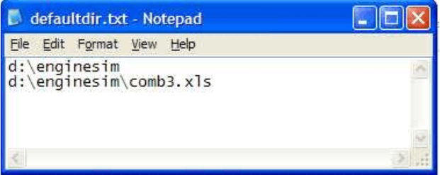
the program will be run. These contents should include a file named defaultdir.txt. The contents of this

file will look similar to:

To use EngineSim, you must Notepad or a similar text editor to modify this file so that the first line

identifies the installation directory on your computer and the second line identifies the Excel

spreadsheet containing thermodynamic data. The included file Comb3.sud contains information on

a few fuels as well as air and combustion products. Appendix A describes the thermodynamic data files in

more detail and might be useful if you want to use other fuels.

If Matlab version 7.0 with the compiler toolbox has been installed on your computer, (as in MecE

3-26 and 4-19), this will be sufficient to run the program. Otherwise, the matlab runtime components

need to be installed. These can be installed by downloading the software under "Runtime Routines

Installer", un-zipping it in a directory, running the MCRInstaller.exe program and following the prompts.

The program should now be ready to run. Open the installation directory in Windows Explorer

and open the Engine_sim.exe program.

2

User Interface

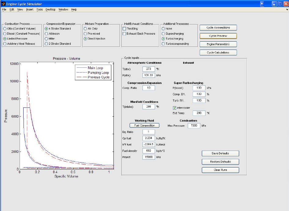
When the program starts, a screen similar to the following will be displayed:

Most user input is made on this screen. The fluid properties, intake and outlet conditions, and cycle

type are all defined on this page. Cycle assumptions can be changed by selecting the Cycle Assumptions

button. Parameters affecting the overall engine output can be changed by selecting the Engine Parameters

button. Various sections of the screen appear only if they are needed. A Combustion Process,

Compression/Expansion Process, and Mixture Preparation Option must be selected before a cycle

simulation can be run.

When the program is started, some of the fields will have default values entered in them already.

These values can be used or changed as required. New defaults can be saved by entering the new values

in the required fields and selecting the Save Defaults button. This button applies to the main input screen

as well as the Engine Parameters dialog box. If the original defaults need to be restored, the Restore

Defaults button can be used; however, the values will not change to the original defaults until the program

is restarted.

A couple of other buttons may become available depending on the cycle type selected. If the

mixture preparation is selected as Pre-mixed or Direct Injection, a fuel composition must be entered and

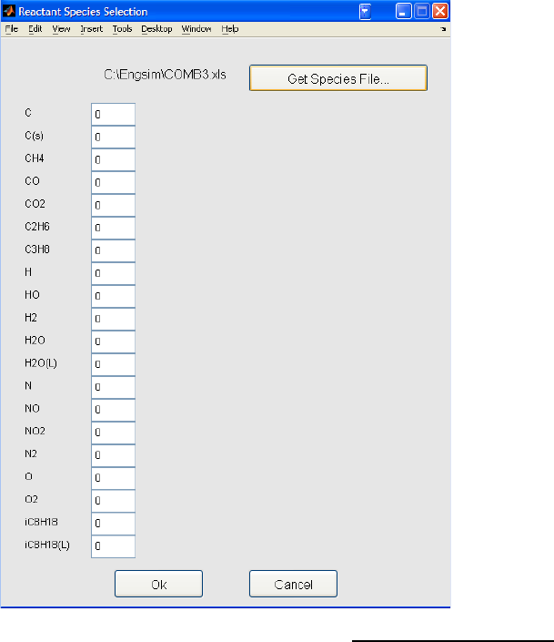
the fuel composition button appears. Selecting the fuel composition button which will display a window

3

like the following:

Note that you only enter the fuel composition in this window, not the fuel/air mixture. The

window has the full list of species from the Excel thermodynamic data spreadsheet so you can include fuels

that are mixtures. You enter the fuel composition as a number of moles of each species. For example, for

a natural gas that is 95% methane, 3% ethane, 2% carbon dioxide, you could enter 95, 2 and 3 in the

respective boxes for CH4, CO2 and C2H6 respectively. You could also enter 0.95, 0.02 and 0.03 ... the

program takes the inputs and calculates proportional amounts for the fuel composition. A different species

file can be used by selecting the Get Species File... button.

Once the fuel composition has been specified, you return to the program main window by hitting the

"Ok" button.

In the main screen, a cycle simulation can be run once a Combustion Process, Compression

/Expansion Process, and Mixture Preparation Option have been selected. When the Cycle Preview button

is pressed, the program plots a P-v diagram and pressure - crank angle trace diagram in the main screen plot

window. Pressing the Cycle Calculations button performs a full set of calculations and plots the current

cycle’s P-v diagram in the main screen’s plot window. Up to six cycles can be displayed at once. This

allows the user to quickly see the differences in cycle P-v diagram from recent changes. The current cycle

will be shown in blue, and the previous cycles shown in red. When a full cycle calculation is performed, the

numerical calculations are sent to an Excel spreadsheet named cycle_output.xls in the working directory.

Note: You can't write to cycle_output.xls while it's open in Excel. Remember to close this spreadsheet

before calculating any cycles!

4

All previously calculated runs stored in cycle_output.xls can be cleared by selecting the Clear Runs

button. This will bring up a prompt asking if the user would like to erase the Excel spreadsheet data. If NO

is selected, only the runs stored in the Engine Cycle Simulator program will be erased.

Previously calculated runs can also be replaced without deleting later runs. For example, if a user

has completed 6 runs, the next run can be entered as run 3 and only run 3 will be changed in the file

cycle_output.xls. However, the P-v and P-crank angle plots will only be completed up to the current run.

Description of User - Defined Inputs

Main Input Screen

Cycle Options

Combustion Process

Otto - Constant volume heat addition.

Diesel - Constant pressure heat addition.

Limited Pressure - Constant volume heat addition up a maximum pressure, then constant

pressure heat addition.

Arbitrary Heat Release - Heat addition modelled with a shape function to represent mass

of fuel burned. Currently only available with either 4 or 2 stroke standard

compression/expansion processes and air standard working fluid only.

Compression/Expansion Process

4 Stroke Standard - Standard cycle with pumping loop included. Compression ratio equals

expansion ratio, and intake valve closes at bottom dead center (BDC). 1 power stroke for

every 2 revolutions.

Atkinson Cycle - Intake/Compression stroke and Power/Exhaust strokes are of different

length. Compression ratio and expansion ratio are independent. 4 stroke cycle, includes

pumping loop.

Miller Cycle - Intake/Compression stroke are equal length, but intake valve is closed

sometime after BDC. 4 stroke cycle, pumping loop included.

2 Stroke Standard - Same as 4 stroke standard, but no pumping loop. One power stroke

per revolution.

Mixture Preparation

Air Only - No fuel considered. Heat input entered as a value in the Cycle Input window.

Can be changed from Air Standard to Real Air in the Cycle Assumptions window.

Pre-mixed - Fuel/air mixture considered perfectly mixed before it enters the engine. Fuel

is entered with the fuel composition button and equivalence ratio can be selected in the Cycle

Inputs section. Complete combustion or equilibrium combustion can be selected in the

Cycle Assumptions window.

Direct Injection - Fuel considered injected at top dead center (TDC) after compression

stroke. Fuel and equivalence ratio entered similarly to Pre-mixed mixture, but other fuel

properties entered in the Cycle Input window as well.

Inlet/Exhaust Conditions

Throttling - A throttled intake can be specified. Instead of using the atmospheric pressure

as the intake conditions, the manifold pressure can be specified.

Exhaust Back Pressure - Exhaust back pressure due to flow losses can be specified.

Instead of using the atmospheric pressure as the exhaust pressure, the pressure at the exhaust

valve can be specified.

5

Additional Processes

Supercharging - A supercharger can be added to the intake of the engine. Additionally, an

intercooler can then be specified.

Turbocharging - A turbocharger can be added to the intake of the engine. Additionally, an

intercooler can then be specified.

Turbocompounding - A turbine can be added to the engine to extract more power from the

exhaust gases.

Cycle Input Window

Atmospheric Conditions

T(atm) - Atmospheric Temperature, °K.

P(atm) - Atmospheric Pressure, kPa.

Compression/Expansion

Comp. Ratio - Compression ratio, required for all cycles.

Exp. Ratio - Expansion ratio, required for Atkinson cycle.

IVC Angle - Intake valve closed angle, degrees. Required for Miller cycle.

Manifold Conditions

T(manifold) - Manifold temperature, °K. If a supercharged or turbocharged cycle is

selected, this is the temperature before the compressor.

P(manifold) - Manifold pressure, kPa. Throttled cycles only.

Working Fluid

Cp - Working fluid constant pressure specific heat, kJ/kg°K. Air standard cycles only.

Cv - Working fluid constant volume specific heat, kJ/kg°K. Air standard cycles only.

qin - Heat added to cycle, kJ/kg. Air only cycles.

Fuel Composition - Select this button to enter the fuel composition. Pre-mixed, direct

injection cycles only.

Eq. Ratio - Equivalence ratio. Pre-mixed, direct injection cycles only.

Cp fuel - Fuel constant pressure specific heat, kJ/kg°K. Direct injection cycles only.

h°f fuel - Enthalpy of formation for fuel, kJ/kmol. Direct injection cycles only.

Fuel density - density of fuel, kg/m^3. Direct injection cycles only.

Pinject - Fuel injection pressure, kPa. Direct injection cycles only.

Exhaust

P(exhaust) - Exhaust back pressure, kPa (absolute). Cycles with exhaust back pressure

selected only.

Super/Turbocharging

P(boost) - Pressure increase during compression stage, kPa. Pressure added to atmospheric

pressure or manifold pressure if throttled. Supercharged/turbocharged cycles only.

Mech. Eff - Isentropic efficiency, %. For supercharged or turbocompounded cycles only.

Comp. Eff - Compressor isentropic efficiency, %. For turbocharged cycles only.

Turb. Eff - Turbine isentropic efficiency, %. For turbocharged cycles only.

Intercooler - Option button, allows an intercooler to be added to supercharged or

turbocharged cycles only.

Exit Temp - Temperature out from intercooler, °K. Intercooled cycles only.

6

Combustion

Max. Pressure - Maximum cycle pressure, kPa. Limited pressure cycles only.

Ignition - Crank angle where heat release begins, degrees. Arbitrary heat release cycles

only.

Burn Duration - Crank angle for duration of heat release, degrees. Arbitrary heat release

cycles only.

Knock Simulation - Button allows calculation of knock index for specified cycle. Dialog

box will pop up asking for octane number of fuel. Arbitrary heat release cycle only.

Cycle Assumptions Window

Heat Transfer - Not available in this version of the program.

Reversibility - Not available in this version of the program.

Mass Losses- Not available in this version of the program.

Working Fluid Assumptions, Air Only Cycle - Allows Air Standard or Real Air assumptions to

be made. Real air includes variable specific heats.

Working Fluid Assumptions, Pre-Mixed/Direct Injection Cycle - Allows complete combustion

products or equilibrium combustion products to be specified.

Engine Parameters Dialog Box

Bore - Diameter of an individual engine cylinder, mm.

Stroke - Twice the crankshaft throw, mm. With bore defines displacement of 1 cylinder.

Cylinders - Defines the total number of cylinders the engine has. With the bore and stroke, defines

the total engine displacement.

Engine Speed - Rotational engine speed, RPM. Defines power output, and affects knock simulation

calculations.

Con Rod/Crank Throw Ratio - Length of connecting rod divided by the length of the crank throw.

Has a small effect on the pressure - crank angle plot.

7

Excel Spreadsheet Output

The numerical values calculated for each cycle run are saved in an Excel spreadsheet named

cycle_output.xls. There are 3 sheets within this spreadsheet. The first contains all the raw data from the

Engine Cycle Simulator program. Included are the pressure, temperature, and specific volume points

calculated for the P-v diagram. The user can create any custom plots in Excel with this data. The second

sheet contains the formatted cycle calculations and a summary of the cycle configuration. An example of this

sheet can be seen below:

Run 1

Cycle Options

Combustion Type Otto

Expansion/Compression Process 4 stroke std.

Mixture Properties Pre-mixed

Additional Mixture Specification Equilibrium

Throttled No

Exhaust Back Pressure Atm.

Additional Processes None

Intercooler N/A

Cycle Inputs

Fuel (User Input) C3H8

Displacement (l) 1.952

Speed (RPM) 4000

Con rod / crank throw ratio 3

Tatm (K) 293

Patm (kPa) 101.325

Compression Ratio 9

Expansion Ratio 0

IVC Angle (° Crank Angle) 0

Tmanifold (K) 305

Pmanifold (K) 101.325

Cp (kJ/(kg.K)) N/A

Cv (kJ/(kg.K)) N/A

Qin (kJ/kg) N/A

Φ1

Cp fuel (kJ/(kg.K)) N/A

ηf fuel (kJ/kg) N/A

rfuel (kg/m3)N/A

Pinj (kPa) N/A

Pmax (kPa) N/A

Pexhaust (kPa) 101.325

dPcomp/turbine (kPa) N/A

ηmech comp/turbine N/A

ηmech turbine N/A

Tintercooled (K) N/A

Ts (° Crank Angle) N/A

Tb (° Crank Angle) N/A

State Properties

P1 (kPa) 101.33

T1 (K) 339.54

8

v1 (m3/kg) 0.947

P2(kPa) 1863.02

T2 (K) 693.76

v2 (m3/kg) 0.105

P3(kPa) 8090.41

T3 (K) 2853.27

v3 (m3/kg) 0.105

P4(kPa) 568.97

T4 (K) 1834.33

v4 (m3/kg) 0.947

P5(kPa) 101.33

T5(K) 1276.08

v5(m3/kg) 3.699

Cycle Calculations

wnet (kJ/kg) 1209.5

qin - LHV (kJ/kg) 46353

ηth 44.8%

IMEP (kPa) 1437.1

ηv95.8%

IP (kW) 93.51

ISFC g/(kW hr) 173.41

mfuel (g/sec) 4.504

residual 2.84%

Fuel/Air 0.0638

Mean Piston Speed (m/sec) 11.47

The third sheet lists the composition of the combustion products at the end of combustion and the end of the

expansion stroke. This sheet is only useful for fuel/air cycles with complete or equilibrium combustion

products.

9

Appendix A - Creating JANAF Excel Spreadsheets

The Engine Cycle Simulator program uses JANAF tables for fuels. Essentially, any molecule

consisting of carbon, hydrogen, nitrogen, and or oxygen can be used, as long as there is at least one carbon

or hydrogen atom in the molecule. This information is entered in a standard Excel spreadsheet which can be

accessed with the Engine Cycle Simulator program.

This procedure describes converting a JANAF table in STANJAN .sud or .dat format, but any format

can be used as long as enthalpy and entropy data is available for the temperature range of 200 to 6000°K.

STANJAN .dat files can be used directly. Unformatted .sud files must be converted to .dat files using

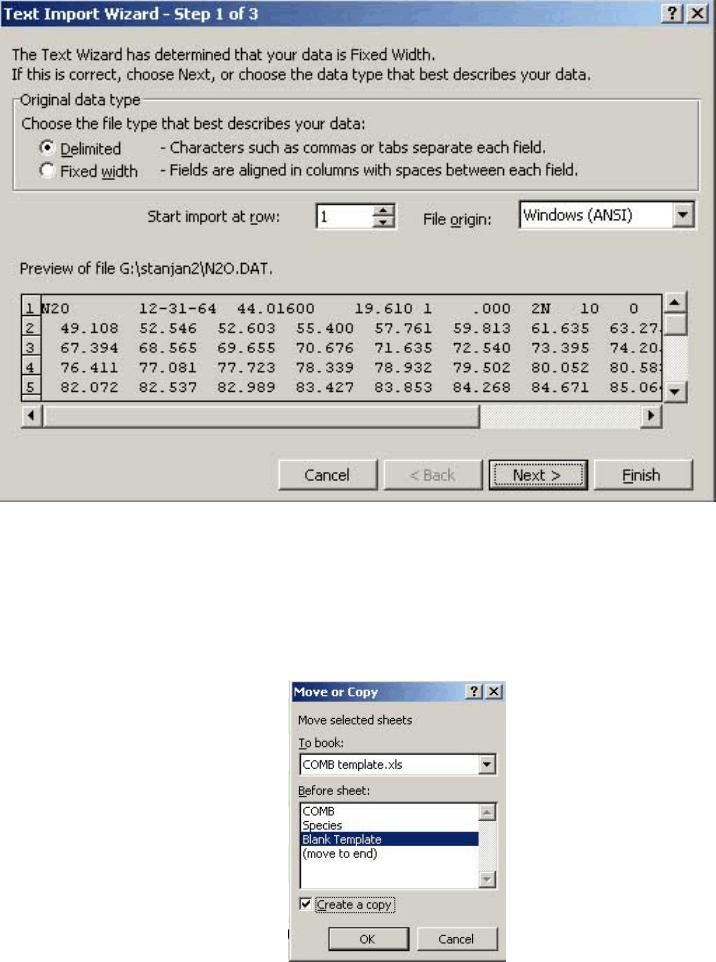
the JANFILE program included with STANJAN. Once the JANAF file is in STANJAN .dat format, open

Excel. Go to File, Open, and choose files of type, all files. Choose the .dat file that is to be converted. A

window will pop up as shown below.

Chose delimited and click next. Another window will pop up with an option for delimiters. Select only space

and click finish. The JANAF data is now in Excel.

Open the COMB_template.xls file. Paste the JANAF data into the COMB sheet, starting in cell A1.

Right click on the Blank Template sheet and select move or copy. Choose to place the new sheet before

Blank Template and select Create a Copy, as shown in the figure below. This will create a new worksheet

called Blank Template (2).

10

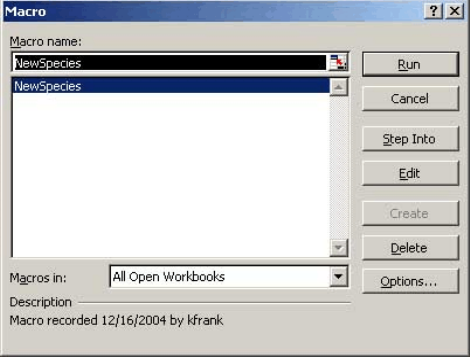
The next step is to go into the Tools menu and select Macro, Macros. A new window will pop up similar to

this one.

Select NewSpecies and run. This will place all of the entropy and enthalpy values in the Blank Template (2)

sheet. The top table with molar mass and number of atoms must be filled in manually. Now rename the

Blank Template (2) sheet to the name of the species, and add the name of the species to the list on the species

sheet. Save the Excel file to a different name and it will be ready to go.