Chapter Two Exercise Solutions Engineering Circuit Analysis (6th Edition, 2001) Hayt Solution Manual
User Manual:
Open the PDF directly: View PDF ![]() .
.
Page Count: 990 [warning: Documents this large are best viewed by clicking the View PDF Link!]
CHAPTER TWO SOLUTIONS
Engineering Circuit Analysis, 6th Edition Copyright ©2002 McGraw-Hill, Inc. All Rights Reserved.
1. (a) 12 µs (d) 3.5 Gbits (g) 39 pA
(b) 750 mJ (e) 6.5 nm (h) 49 kΩ
(c) 1.13 kΩ (f) 13.56 MHz (i) 11.73 pA
CHAPTER TWO SOLUTIONS
Engineering Circuit Analysis, 6th Edition Copyright ©2002 McGraw-Hill, Inc. All Rights Reserved.
2. (a) 1 MW (e) 33 µJ (i) 32 mm
(b) 12.35 mm (f) 5.33 nW
(c) 47. kW (g) 1 ns
(d) 5.46 mA (h) 5.555 MW
CHAPTER TWO SOLUTIONS
Engineering Circuit Analysis, 6th Edition Copyright ©2002 McGraw-Hill, Inc. All Rights Reserved.
3. Motor power = 175 Hp
(a) With 100% efficient mechanical to electrical power conversion,
(175 Hp)[1 W/ (1/745.7 Hp)] = 130.5 kW
(b) Running for 3 hours,
Energy = (130.5×10³ W)(3 hr)(60 min/hr)(60 s/min) = 1.409 GJ
(c) A single battery has 430 kW-hr capacity. We require
(130.5 kW)(3 hr) = 391.5 kW-hr therefore one battery is sufficient.
CHAPTER TWO SOLUTIONS
Engineering Circuit Analysis, 6th Edition Copyright ©2002 McGraw-Hill, Inc. All Rights Reserved.
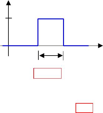
4. The 400-mJ pulse lasts 20 ns.
(a) To compute the peak power, we assume the pulse shape is square:
Then P = 400×10-3/20×10-9 = 20 MW.
(b) At 20 pulses per second, the average power is
Pavg = (20 pulses)(400 mJ/pulse)/(1 s) = 8 W.
400
Energy (mJ)
t (ns)
20
CHAPTER TWO SOLUTIONS
Engineering Circuit Analysis, 6th Edition Copyright ©2002 McGraw-Hill, Inc. All Rights Reserved.
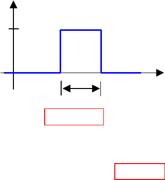
5. The 1-mJ pulse lasts 75 fs.
(c) To compute the peak power, we assume the pulse shape is square:
Then P = 1×10⁻³/75×10-15 = 13.33 GW.
(d) At 100 pulses per second, the average power is
Pavg = (100 pulses)(1 mJ/pulse)/(1 s) = 100 mW.
1
Energy (mJ)
t (fs)
75
CHAPTER TWO SOLUTIONS
Engineering Circuit Analysis, 6th Edition Copyright ©2002 McGraw-Hill, Inc. All Rights Reserved.
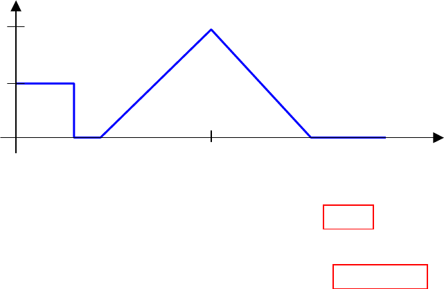
6. The power drawn from the battery is (not quite drawn to scale):
(a) Total energy (in J) expended is
[6(5) + 0(2) + 0.5(10)(10) + 0.5(10)(7)]60 = 6.9 kJ.
(b) The average power in Btu/hr is
(6900 J/24 min)(60 min/1 hr)(1 Btu/1055 J) = 16.35 Btu/hr.
5 7 17 24
P (W)
10
6
t (min)
CHAPTER TWO SOLUTIONS
Engineering Circuit Analysis, 6th Edition Copyright ©2002 McGraw-Hill, Inc. All Rights Reserved.
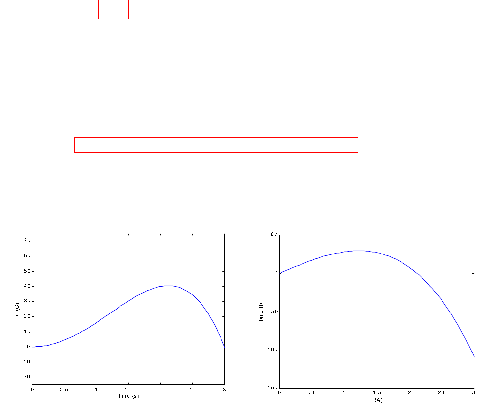
7. Total charge q = 18t2 – 2t4 C.
(a) q(2 s) = 40 C.
(b) To find the maximum charge within 0 ≤ t ≤ 3 s, we need to take the first and
second derivitives:
dq/dt = 36t – 8t3 = 0, leading to roots at 0, ± 2.121 s
d2q/dt2 = 36 – 24t2
substituting t = 2.121 s into the expression for d2q/dt2, we obtain a value of
–14.9, so that this root represents a maximum.
Thus, we find a maximum charge q = 40.5 C at t = 2.121 s.
(c) The rate of charge accumulation at t = 8 s is
dq/dt|t = 0.8 = 36(0.8) – 8(0.8)3 = 24.7 C/s.
(d) See Fig. (a) and (b).
(a) (b)
CHAPTER TWO SOLUTIONS
Engineering Circuit Analysis, 6th Edition Copyright ©2002 McGraw-Hill, Inc. All Rights Reserved.
8. Referring to Fig. 2.6c,
0 A, 3 2-
0 A, 3 2-
)( 3
5
1
>+
<+
=−
te
te
ti t
t
Thus,
(a) i1(-0.2) = 6.155 A
(b) i1 (0.2) = 3.466 A
(c) To determine the instants at which i1 = 0, we must consider t < 0 and t > 0 separately:
for t < 0, - 2 + 3e-5t = 0 leads to t = -0.2 ln (2/3) = +2.027 s (impossible)
for t > 0, -2 + 3e3t = 0 leads to t = (1/3) ln (2/3) = -0.135 s (impossible)
Therefore, the current is never negative.
(d) The total charge passed left to right in the interval 0.08 < t < 0.1 s is
q(t) = ∫−
1.0
08.0 1)( dtti
=
[][]
∫∫ +−++−
−
−1.0
0
3
0
08.0
532 32 dtedte tt
= 1.0
0
3
0
0.08-
532 32 tt ee +−++− −
= 0.1351 + 0.1499
= 285 mC
CHAPTER TWO SOLUTIONS
Engineering Circuit Analysis, 6th Edition Copyright ©2002 McGraw-Hill, Inc. All Rights Reserved.
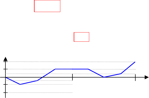
9. Referring to Fig. 2.28,
(a) The average current over one period (10 s) is
iavg = [-4(2) + 2(2) + 6(2) + 0(4)]/10 = 800 mA
(b) The total charge transferred over the interval 1 < t < 12 s is
∫
=12
1
total )( dttiq = -4(2) + 2(2) + 6(2) + 0(4) –4(2) = 0 C
(d) See Fig. below
2 4 6
8
10 12
16
q (C)
t(s)
-16
8
16
-8
14

CHAPTER TWO SOLUTIONS
Engineering Circuit Analysis, 6th Edition Copyright ©2002 McGraw-Hill, Inc. All Rights Reserved.
10. (a) Pabs = (+3.2 V)(-2 mA) = -6.4 mW (or +6.4 mW supplied)
(b) Pabs = (+6 V)(-20 A) = -120 W (or +120 W supplied)
(d) Pabs = (+6 V)(2 ix) = (+6 V)[(2)(5 A)] = +60 W
(e) Pabs = (4 sin 1000t V)(-8 cos 1000t mA)| t = 2 ms = +12.11 W
CHAPTER TWO SOLUTIONS
Engineering Circuit Analysis, 6th Edition Copyright ©2002 McGraw-Hill, Inc. All Rights Reserved.
11. i = 3te-100t mA and v = [6 – 600t] e-100t mV
(a) The power absorbed at t = 5 ms is
Pabs =
()
[
]
W 3 6006 5
100100
µ
mst
tt teet =
−− ⋅−
= 0.01655 µW = 16.55 nW
(b) The energy delivered over the interval 0 < t < ∞ is
()
∫∫
∞∞
−
−=
00
200 J 60063
µ
dtettdtP t
abs
Making use of the relationship
1
0
!
+
∞−=
∫n
axn
a
n
dxex where n is a positive integer and a > 0,
we find the energy delivered to be
= 18/(200)2 - 1800/(200)3
= 0
CHAPTER TWO SOLUTIONS
Engineering Circuit Analysis, 6th Edition Copyright ©2002 McGraw-Hill, Inc. All Rights Reserved.
12. (a) Pabs = (40i)(3e-100t)| t = 8 ms =
[]
2
8
100
360 mst
t
e=
− = 72.68 W
(b) Pabs =
[]
W36.34- 180- 2.0 2
8
100 ==
=
−mst
t
ei
dt
di
(c) Pabs =
()
mst
t
teidt
8
100
03 20 30
=
−
+
∫
=
mst
t
ttt etdee
8
100
0
100100 60 3 90
=
−
′
−−
+
′
∫ = 27.63 W
CHAPTER TWO SOLUTIONS
Engineering Circuit Analysis, 6th Edition Copyright ©2002 McGraw-Hill, Inc. All Rights Reserved.
13. (a) The short-circuit current is the value of the current at V = 0.
Reading from the graph, this corresponds to approximately 3.0 A.
(b) The open-circuit voltage is the value of the voltage at I = 0.
Reading from the graph, this corresponds to roughly 0.4875 V, estimating the curve as
hitting the x-axis 1 mm behind the 0.5 V mark.
(c) We see that the maximum current corresponds to zero voltage, and likewise, the
maximum voltage occurs at zero current. The maximum power point, therefore,
occurs somewhere between these two points. By trial and error,
Pmax is roughly (375 mV)(2.5 A) = 938 mW, or just under 1 W.
CHAPTER TWO SOLUTIONS
Engineering Circuit Analysis, 6th Edition Copyright ©2002 McGraw-Hill, Inc. All Rights Reserved.
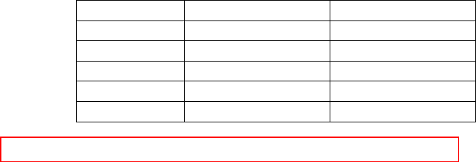
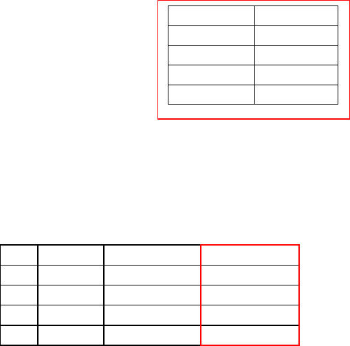
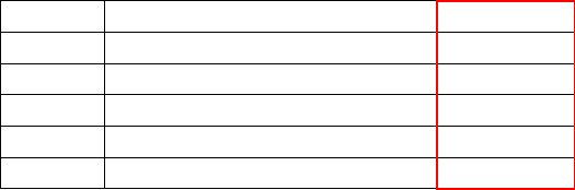
14. Note that in the table below, only the –4-A source and the –3-A source are actually
“absorbing” power; the remaining sources are supplying power to the circuit.
Source Absorbed Power Absorbed Power
2-V source (2 V)(-2 A) - 4 W
8-V source (8 V)(-2 A) - 16 W
-4-A source (10 V)[-(-4 A)] 40 W
10-V source (10 V)(-5 A) - 50 W
-3-A source (10 V)[-(-3 A)] 30 W
The 5 power quantities sum to –4 – 16 + 40 – 50 + 30 = 0, as demanded from
conservation of energy.

CHAPTER TWO SOLUTIONS
Engineering Circuit Analysis, 6th Edition Copyright ©2002 McGraw-Hill, Inc. All Rights Reserved.
15. We are told that Vx = 1 V, and from Fig. 2.33 we see that the current flowing through
the dependent source (and hence through each element of the circuit) is 5Vx = 5 A.
We will compute absorbed power by using the current flowing into the positive
reference terminal of the appropriate voltage (passive sign convention), and we will
compute supplied power by using the current flowing out of the positive reference
terminal of the appropriate voltage.
(a) The power absorbed by element “A” = (9 V)(5 A) = 45 W
(b) The power supplied by the 1-V source = (1 V)(5 A) = 5 W, and
the power supplied by the dependent source = (8 V)(5 A) = 40 W
(c) The sum of the supplied power = 5 + 40 = 45 W
The sum of the absorbed power is 45 W, so
yes, the sum of the power supplied = the sum of the power absorbed, as we
expect from the principle of conservation of energy.

CHAPTER TWO SOLUTIONS
Engineering Circuit Analysis, 6th Edition Copyright ©2002 McGraw-Hill, Inc. All Rights Reserved.
16. We are asked to determine the voltage vs, which is identical to the voltage labeled v1.
The only remaining reference to v1 is in the expression for the current flowing through
the dependent source, 5v1.
This current is equal to –i2.
Thus,
5 v1 = -i2 = - 5 mA
Therefore v1 = -1 mV
and so vs = v1 = -1 mV

CHAPTER TWO SOLUTIONS
Engineering Circuit Analysis, 6th Edition Copyright ©2002 McGraw-Hill, Inc. All Rights Reserved.
17. The battery delivers an energy of 460.8 W-hr over a period of 8 hrs.
(a) The power delivered to the headlight is therefore (460.8 W-hr)/(8 hr) = 57.6 W
(b) The current through the headlight is equal to the power it absorbs from the battery
divided by the voltage at which the power is supplied, or
I = (57.6 W)/(12 V) = 4.8 A

CHAPTER TWO SOLUTIONS
Engineering Circuit Analysis, 6th Edition Copyright ©2002 McGraw-Hill, Inc. All Rights Reserved.
18. The supply voltage is 110 V, and the maximum dissipated power is 500 W. The fuses
are specified in terms of current, so we need to determine the maximum current that
can flow through the fuse.
P = V I therefore Imax = Pmax/V = (500 W)/(110 V) = 4.545 A
If we choose the 5-A fuse, it will allow up to (110 V)(5 A) = 550 W of power to be
delivered to the application (we must assume here that the fuse absorbs zero power, a
reasonable assumption in practice). This exceeds the specified maximum power.
If we choose the 4.5-A fuse instead, we will have a maximum current of 4.5 A. This
leads to a maximum power of (110)(4.5) = 495 W delivered to the application.
Although 495 W is less than the maximum power allowed, this fuse will provide
adequate protection for the application circuitry. If a fault occurs and the application
circuitry attempts to draw too much power, 1000 W for example, the fuse will blow,
no current will flow, and the application circuitry will be protected. However, if the
application circuitry tries to draw its maximum rated power (500 W), the fuse will
also blow. In practice, most equipment will not draw its maximum rated power
continuously- although to be safe, we typically assume that it will.
CHAPTER TWO SOLUTIONS
Engineering Circuit Analysis, 6th Edition Copyright ©2002 McGraw-Hill, Inc. All Rights Reserved.
19. (a) Pabs = i2R = [20e-12t] 2 (1200) µW
= [20e-1.2] 2 (1200) µW
= 43.54 mW
(b) Pabs = v2/R = [40 cos 20t] 2 / 1200 W
= [40 cos 2] 2 / 1200 W
= 230.9 mW
(c) Pabs = v i = 8t 1.5 W
= 253.0 mW
keep in mind we
are using radians
CHAPTER TWO SOLUTIONS
Engineering Circuit Analysis, 6th Edition Copyright ©2002 McGraw-Hill, Inc. All Rights Reserved.
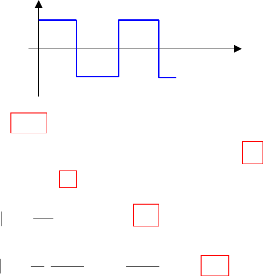
20. It’s probably best to begin this problem by sketching the voltage waveform:
(a) vmax = +10 V
(b) vavg = [(+10)(20×10-3) + (-10)(20×10-3)]/(40×10-3) = 0
(c) iavg = vavg /R = 0
(d) R
v
pabs
2
max
max = = (10)2 / 50 = 2 W
(e)
⋅
−
+⋅
+
=20
)10(
20
)10(
40
1
22
RR
pavg
abs = 2 W
60
40
20 t (ms)
v (V)
+10
-10

CHAPTER TWO SOLUTIONS
Engineering Circuit Analysis, 6th Edition Copyright ©2002 McGraw-Hill, Inc. All Rights Reserved.
21. We are given that the conductivity
σ
of copper is 5.8×10⁷ S/m.
(a) 50 ft of #18 (18 AWG) copper wire, which has a diameter of 1.024 mm, will have
a resistance of l/(
σ
A) ohms, where A = the cross-sectional area and l = 50 ft.
Converting the dimensional quantities to meters,
l = (50 ft)(12 in/ft)(2.54 cm/in)(1 m/100 cm) = 15.24 m
and
r = 0.5(1.024 mm)(1 m/1000 mm) = 5.12×10⁻⁴ m
so that
A =
π
r2 =
π
(5.12×10⁻⁴ m)2 = 8.236×10⁻⁷ m2
Thus, R = (15.24 m)/[( 5.8×10⁷)( 8.236×10⁻⁷)] = 319.0 mΩ
(b) We assume that the conductivity value specified also holds true at 50oC.
The cross-sectional area of the foil is
A = (33 µm)(500 µm)(1 m/106 µm)( 1 m/106 µm) = 1.65×10⁻⁸ m2
So that
R = (15 cm)(1 m/100 cm)/[( 5.8×10⁷)( 1.65×10⁻⁸)] = 156.7 mΩ
A 3-A current flowing through this copper in the direction specified would
lead to the dissipation of
I2R = (3)2 (156.7) mW = 1.410 W

CHAPTER TWO SOLUTIONS
Engineering Circuit Analysis, 6th Edition Copyright ©2002 McGraw-Hill, Inc. All Rights Reserved.
22. Since we are informed that the same current must flow through each component, we
begin by defining a current I flowing out of the positive reference terminal of the
voltage source.
The power supplied by the voltage source is Vs I.
The power absorbed by resistor R1 is I2R1.
The power absorbed by resistor R2 is I2R2.
Since we know that the total power supplied is equal to the total power absorbed,
we may write: Vs I = I2R1 + I2R2
or Vs = I R1 + I R2
Vs = I (R1 + R2)
By Ohm’s law,
I = 2
R
V/ R2
so that
Vs =
()
21
2
2RR
R
VR+
Solving for 2
R
Vwe find
()
21
2
s
2RR
R
VVR+
= Q.E.D.
CHAPTER TWO SOLUTIONS
Engineering Circuit Analysis, 6th Edition Copyright ©2002 McGraw-Hill, Inc. All Rights Reserved.
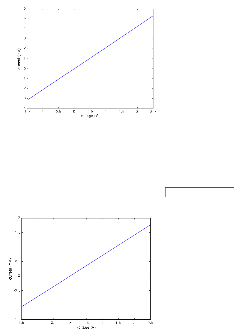
23. (a)
(b) We see from our answer to part (a) that this device has a reasonably linear
characteristic (a not unreasonable degree of experimental error is evident in the data).
Thus, we choose to estimate the resistance using the two extreme points:
Reff = [(2.5 – (-1.5)]/[5.23 – (-3.19)] kΩ = 475 Ω
Using the last two points instead, we find Reff = 469 Ω, so that we can state with some
certainty at least that a reasonable estimate of the resistance is approximately 470 Ω.
(c)
CHAPTER TWO SOLUTIONS
Engineering Circuit Analysis, 6th Edition Copyright ©2002 McGraw-Hill, Inc. All Rights Reserved.
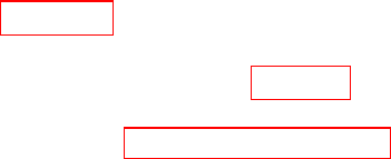
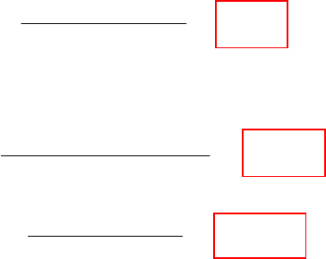
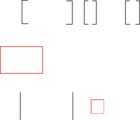
24. Top Left Circuit: I = (5/10) mA = 0.5 mA, and P10k = V2/10 mW = 2.5 mW
Top Right Circuit: I = -(5/10) mA = -0.5 mA, and P10k = V2/10 mW = 2.5 mW
Bottom Left Circuit: I = (-5/10) mA = -0.5 mA, and P10k = V2/10 mW = 2.5 mW
Bottom Right Circuit: I = -(-5/10) mA = 0.5 mA, and P10k = V2/10 mW = 2.5 mW

CHAPTER TWO SOLUTIONS
Engineering Circuit Analysis, 6th Edition Copyright ©2002 McGraw-Hill, Inc. All Rights Reserved.
25. The voltage vout is given by
vout = -10-3 vπ (1000)
= - vπ
Since vπ = vs = 0.01 cos 1000t V, we find that
vout = - vπ = -0.001 cos 1000t V

CHAPTER TWO SOLUTIONS
Engineering Circuit Analysis, 6th Edition Copyright ©2002 McGraw-Hill, Inc. All Rights Reserved.
26. 18 AWG wire has a resistance of 6.39 Ω / 1000 ft.
Thus, we require 1000 (53) / 6.39 = 8294 ft of wire.
(Or 1.57 miles. Or, 2.53 km).

CHAPTER TWO SOLUTIONS
Engineering Circuit Analysis, 6th Edition Copyright ©2002 McGraw-Hill, Inc. All Rights Reserved.
27. We need to create a 470-Ω resistor from 28 AWG wire, knowing that the ambient
temperature is 108oF, or 42.22oC.
Referring to Table 2.3, 28 AWG wire is 65.3 mΩ/ft at 20oC, and using the equation
provided we compute
R2/R1 = (234.5 + T2)/(234.5 + T1) = (234.5 + 42.22)/(234.5 + 20) = 1.087
We thus find that 28 AWG wire is (1.087)(65.3) = 71.0 mΩ/ft.
Thus, to repair the transmitter we will need
(470 Ω)/(71.0 × 10-3 Ω/ft) = 6620 ft (1.25 miles, or 2.02 km).
Note: This seems like a lot of wire to be washing up on shore. We may find we don’t
have enough. In that case, perhaps we should take our cue from Eq. [6], and try to
squash a piece of the wire flat so that it has a very small cross-sectional area…..
CHAPTER TWO SOLUTIONS
Engineering Circuit Analysis, 6th Edition Copyright ©2002 McGraw-Hill, Inc. All Rights Reserved.
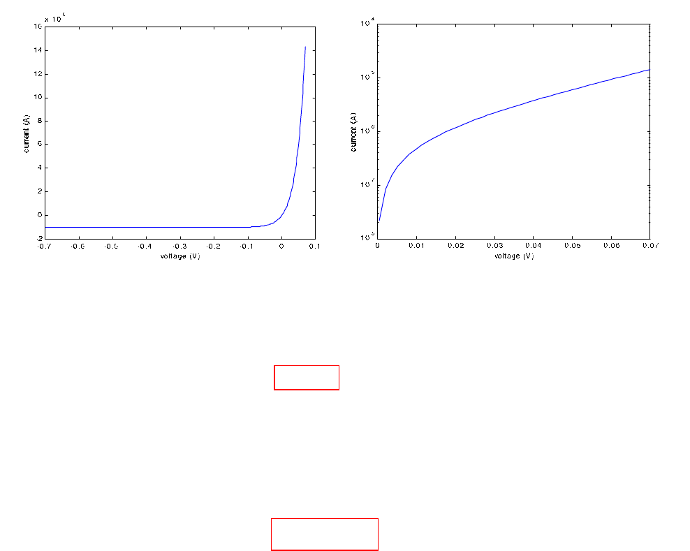
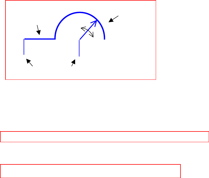
28. (a) We need to plot the negative and positive voltage ranges separately, as the positive
voltage range is, after all, exponential!
(b) To determine the resistance of the device at V = 550 mV, we compute the
corresponding current:
I = 10-6 [e39(0.55) – 1] = 2.068 A
Thus, R(0.55 V) = 0.55/2.068 = 266 mΩ
(c) R = 1 Ω corresponds to V = I. Thus, we need to solve the transcendental equation
I = 10-6 [e39I – 1]
Using a scientific calculator or the tried-and-true trial and error approach, we find that
I = 325.5 mA

CHAPTER TWO SOLUTIONS
Engineering Circuit Analysis, 6th Edition Copyright ©2002 McGraw-Hill, Inc. All Rights Reserved.
29. We require a 10-Ω resistor, and are told it is for a portable application, implying that
size, weight or both would be important to consider when selecting a wire gauge. We
have 10,000 ft of each of the gauges listed in Table 2.3 with which to work. Quick
inspection of the values listed eliminates 2, 4 and 6 AWG wire as their respective
resistances are too low for only 10,000 ft of wire.
Using 12-AWG wire would require (10 Ω) / (1.59 mΩ/ft) = 6290 ft.
Using 28-AWG wire, the narrowest available, would require
(10 Ω) / (65.3 mΩ/ft) = 153 ft.
Would the 28-AWG wire weight less? Again referring to Table 2.3, we see that the
cross-sectional area of 28-AWG wire is 0.0804 mm2, and that of 12-AWG wire is
3.31 mm2. The volume of 12-AWG wire required is therefore 6345900 mm3, and that
of 28-AWG wire required is only 3750 mm3.
The best (but not the only) choice for a portable application is clear: 28-AWG wire!
CHAPTER TWO SOLUTIONS
Engineering Circuit Analysis, 6th Edition Copyright ©2002 McGraw-Hill, Inc. All Rights Reserved.
30. Our target is a 100-Ω resistor. We see from the plot that at ND = 1015 cm-3, µn ~ 2x10³
cm2/V-s, yielding a resistivity of 3.121 Ω-cm.
At ND = 1018 cm-3, µn ~ 230 cm2/ V-s, yielding a resistivity of 0.02714 Ω-cm.
Thus, we see that the lower doping level clearly provides material with higher
resistivity, requiring less of the available area on the silicon wafer.
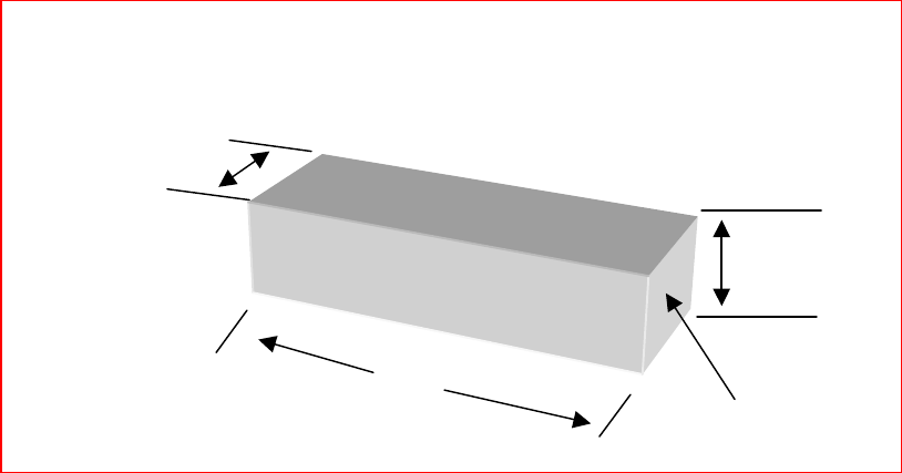
Since R = ρL/A, where we know R = 10 Ω and ρ = 3.121 Ω-cm, we need only define
the resistor geometry to complete the design.
We typically form contacts primarily on the surface of a silicon wafer, so that the
wafer thickness would be part of the factor A; L represents the distance between the
contacts. Thus, we may write
R = 3.121 L/(250x10-4 Y)
where L and Y are dimensions on the surface of the wafer.
If we make Y small (i.e. a narrow width as viewed from the top of the wafer), then L
can also be small. Seeking a value of 0.080103 then for L/Y, and choosing Y = 100
µm (a large dimension for silicon devices), we find a contact-to-contact length of L =
8 cm! While this easily fits onto a 6” diameter wafer, we could probably do a little
better. We are also assuming that the resistor is to be cut from the wafer, and the ends
made the contacts, as shown below in the figure.
Design summary (one possibility): ND = 1015 cm-3
L = 8 cm
Y = 100 µm
250 µm
8 cm contact
100
µ
m
CHAPTER THREE SOLUTIONS
Engineering Circuit Analysis, 6th Edition Copyright ©2002 McGraw-Hill, Inc. All Rights Reserved.
1.
CHAPTER THREE SOLUTIONS
Engineering Circuit Analysis, 6th Edition Copyright ©2002 McGraw-Hill, Inc. All Rights Reserved.
2. (a) six nodes; (b) nine branches.
CHAPTER THREE SOLUTIONS
Engineering Circuit Analysis, 6th Edition Copyright ©2002 McGraw-Hill, Inc. All Rights Reserved.
3. (a) Four nodes; (b) five branches; (c) path, yes – loop, no.
CHAPTER THREE SOLUTIONS
Engineering Circuit Analysis, 6th Edition Copyright ©2002 McGraw-Hill, Inc. All Rights Reserved.
4. (a) Five nodes; (b) seven branches; (c) path, yes – loop, no.
CHAPTER THREE SOLUTIONS
Engineering Circuit Analysis, 6th Edition Copyright ©2002 McGraw-Hill, Inc. All Rights Reserved.
5. (a) 3 A; (b) –3 A; (c) 0.
CHAPTER THREE SOLUTIONS
Engineering Circuit Analysis, 6th Edition Copyright ©2002 McGraw-Hill, Inc. All Rights Reserved.
6. By KCL, we may write: 5 + iy + iz = 3 + ix
(a) ix = 2 + iy + iz = 2 + 2 + 0 = 4 A
(b) iy = 3 + ix – 5 – iz
iy = –2 + 2 – 2 iy
Thus, we find that iy = 0.
(c) This situation is impossible, since ix and iz are in opposite directions. The only
possible value (zero), is also disallowed, as KCL will not be satisfied ( 5 ≠ 3).

CHAPTER THREE SOLUTIONS
Engineering Circuit Analysis, 6th Edition Copyright ©2002 McGraw-Hill, Inc. All Rights Reserved.
7. Focusing our attention on the bottom left node, we see that ix = 1 A.
Focusing our attention next on the top right node, we see that iy = 5A.

CHAPTER THREE SOLUTIONS
Engineering Circuit Analysis, 6th Edition Copyright ©2002 McGraw-Hill, Inc. All Rights Reserved.
8. (a) vy = 1(3vx + iz)
vx = 5 V and given that iz = –3 A, we find that
vy = 3(5) – 3 = 12 V
(b) vy = 1(3vx + iz) = –6 = 3vx + 0.5
Solving, we find that vx = (–6 – 0.5)/3 = –2.167 V.

CHAPTER THREE SOLUTIONS
Engineering Circuit Analysis, 6th Edition Copyright ©2002 McGraw-Hill, Inc. All Rights Reserved.
9. (a) ix = v1/10 + v1/10 = 5
2v1 = 50
so v1 = 25 V.
By Ohm’s law, we see that iy = v2/10
also, using Ohm’s law in combination with KCL, we may write
ix = v2/10 + v2/10 = iy + iy = 5 A
Thus, iy = 2.5 A.
(b) From part (a), ix = 2 v1/ 10. Substituting the new value for v1, we find that
ix = 6/10 = 600 mA.
Since we have found that iy = 0.5 ix, iy = 300 mA.
(c) no value – this is impossible.
CHAPTER THREE SOLUTIONS
Engineering Circuit Analysis, 6th Edition Copyright ©2002 McGraw-Hill, Inc. All Rights Reserved.
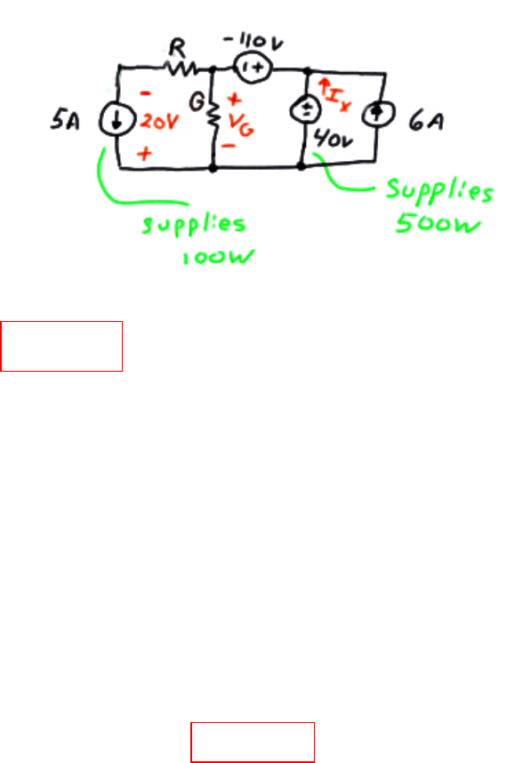
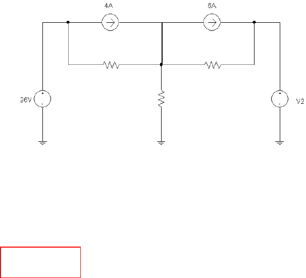
10. We begin by making use of the information given regarding the power generated by
the 5-A and the 40-V sources. The 5-A source supplies 100 W, so it must therefore
have a terminal voltage of 20 V. The 40-V source supplies 500 W, so it must therefore
provide a current of 12.5 A. These quantities are marked on our schematic below:
(1) By KVL, -40 – 110 + R(5) = 0
Thus, R = 30 Ω.
(2) By KVL, -VG – (-110) + 40 = 0
So VG = 150 V
Now that we know the voltage across the unknown conductance G, we need only to
find the current flowing through it to find its value by making use of Ohm’s law.
KCL provides us with the means to find this current: The current flowing into the “+”
terminal of the –110-V source is 12.5 + 6 = 18.5 A.
Then, Ix = 18.5 – 5 = 13.5 A
By Ohm’s law, Ix = G · VG
So G = 13.5/ 150 or G = 90 mS

CHAPTER THREE SOLUTIONS
Engineering Circuit Analysis, 6th Edition Copyright ©2002 McGraw-Hill, Inc. All Rights Reserved.
11. (a) -1 + 2 + 10i – 3.5 + 10i = 0
Solving, i = 125 mA
(b) +10 + 1i - 2 + 2i + 2 – 6 + i = 0
Solving, we find that 4i = -4 or i = - 1 A.
CHAPTER THREE SOLUTIONS
Engineering Circuit Analysis, 6th Edition Copyright ©2002 McGraw-Hill, Inc. All Rights Reserved.
12. (a) By KVL, -2 + vx + 8 = 0
so that vx = -6 V.
(b) By KCL at the top right node,
IS + 4 vx = 4 - vx/4
So IS = 29.5 A.
(c) By KCL at the top left node,
iin = 1 + IS + vx/4 – 6
or iin = 23 A
(d) The power provided by the dependent source is 8(4vx) = -192 W.
CHAPTER THREE SOLUTIONS
Engineering Circuit Analysis, 6th Edition Copyright ©2002 McGraw-Hill, Inc. All Rights Reserved.
13. (a) Working from left to right,
v1 = 60 V
v2 = 60 V
i2 = 60/20 = 3 A
i4 = v1/4 = 60/4 = 15 A
v3 = 5i2 = 15 V
By KVL, -60 + v3 + v5 = 0
v5 = 60 – 15 = 45 V
v4 = v5 = 45
i5 = v5/5 = 45/5 = 9 A
i3 = i4 + i5 = 15 + 9 = 24 A
i1 = i2 + i3 = 3 + 24 = 27
(b) It is now a simple matter to compute the power absorbed by each element:
p1 = -v1i1 = -(60)(27) = -1.62 kW
p2 = v2i2 = (60)(3) = 180 W
p3 = v3i3 = (15)(24) = 360 W
p4 = v4i4 = (45)(15) = 675 W
p5 = v5i5 = (45)(9) = 405 W
and it is a simple matter to check that these values indeed sum to zero as they should.
v1 = 60 V i1 = 27 A
v2 = 60 V i2 = 3 A
v3 = 15 V i3 = 24 A
v4 = 45 V i4 = 15 A
v5 = 45 V i5 = 9 A
CHAPTER THREE SOLUTIONS
Engineering Circuit Analysis, 6th Edition Copyright ©2002 McGraw-Hill, Inc. All Rights Reserved.
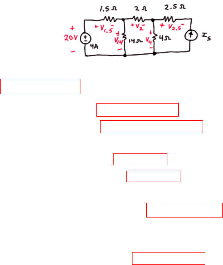
14. Refer to the labeled diagram below.
Beginning from the left, we find
p20V = -(20)(4) = -80 W
v1.5 = 4(1.5) = 6 V therefore p1.5 = (v1.5)2/ 1.5 = 24 W.
v14 = 20 – v1.5 = 20 – 6 = 14 V therefore p14 = 142/ 14 = 14 W.
i2 = v2/2 = v1.5/1.5 – v14/14 = 6/1.5 – 14/14 = 3 A
Therefore v2 = 2(3) = 6 V and p2 = 62/2 = 18 W.
v4 = v14 – v2 = 14 – 6 = 8 V therefore p4 = 82/4 = 16 W
i2.5 = v2.5/ 2.5 = v2/2 – v4/4 = 3 – 2 = 1 A
Therefore v2.5 = (2.5)(1) = 2.5 V and so p2.5 = (2.5)2/2.5 = 2.5 W.
I2.5 = - IS, thefore IS = -1 A.
KVL allows us to write -v4 + v2.5 + vIS = 0
so VIS = v4 – v2.5 = 8 – 2.5 = 5.5 V and pIS = -VIS IS = 5.5 W.
A quick check assures us that these power quantities sum to zero.
CHAPTER THREE SOLUTIONS
Engineering Circuit Analysis, 6th Edition Copyright ©2002 McGraw-Hill, Inc. All Rights Reserved.
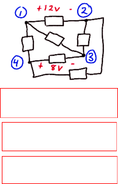
15. Sketching the circuit as described,
(a) v14 = 0. v13 = v43 = 8 V
v23 = -v12 – v34 = -12 + 8 = -4 V
v24 = v23 + v34 = -4 – 8 = -12 V
(b) v14 = 6 V. v13 = v14 + v43 = 6 + 8 = 14 V
v23 = v13 – v12 = 14 – 12 = 2 V
v24 = v23 + v34 = 2 – 8 = -6 V
(c) v14 = -6 V. v13 = v14 + v43 = -6 + 8 = 2 V
v23 = v13 – v12 = 2 – 12 = -10 V
v24 = v23 + v34 = -10 – 8 = -18 V

CHAPTER THREE SOLUTIONS
Engineering Circuit Analysis, 6th Edition Copyright ©2002 McGraw-Hill, Inc. All Rights Reserved.
16. (a) By KVL, -12 + 5000ID + VDS + 2000ID = 0
Therefore, VDS = 12 – 7(1.5) = 1.5 V.
(b) By KVL, - VG + VGS + 2000ID = 0
Therefore, VGS = VG – 2(2) = -1 V.
CHAPTER THREE SOLUTIONS
Engineering Circuit Analysis, 6th Edition Copyright ©2002 McGraw-Hill, Inc. All Rights Reserved.
17. Applying KVL around this series circuit,
-120 + 30ix + 40ix + 20ix + vx + 20 + 10ix = 0
where vx is defined across the unknown element X, with the “+” reference on top.
Simplifying, we find that 100ix + vx = 100
To solve further we require specific information about the element X and its
properties.
(a) if X is a 100-Ω resistor,
vx = 100ix so we find that 100 ix + 100 ix = 100.
Thus ix = 500 mA and px = vx ix = 25 W.
(b) If X is a 40-V independent voltage source such that vx = 40 V, we find that
ix = (100 – 40) / 100 = 600 mA and px = vx ix = 24 W
(c) If X is a dependent voltage source such that vx = 25ix,
ix = 100/125 = 800 mA and px = vx ix = 16 W.
(d) If X is a dependent voltage source so that vx = 0.8v1,
where v1 = 40ix, we have 100 ix + 0.8(40ix) = 100
or ix = 100/132 = 757.6 mA and px = vx ix = 0.8(40)(0.7576)2 = 18.37 W.
(e) If X is a 2-A independent current source, arrow up,
100(-2) + vx = 100
so that vx = 100 + 200 = 300 V and px = vx ix = -600 W
CHAPTER THREE SOLUTIONS
Engineering Circuit Analysis, 6th Edition Copyright ©2002 McGraw-Hill, Inc. All Rights Reserved.
18. (a) We first apply KVL:
-20 + 10i1 + 90 + 40i1 + 2v2 = 0
where v2 = 10i1. Substituting,
70 + 70 i1 = 0
or i1= -1 A.
(b) Applying KVL, -20 + 10i1 + 90 + 40i1 + 1.5v3 = 0 [1]
where v3 = -90 – 10i1 + 20 = -70 – 10 i1
alternatively, we could write v3 = 40i1 + 1.5v3 = -80i1
Using either expression in Eq. [1], we find i1 = 1 A.
(c) Applying KVL, -20 + 10i1 + 90 + 40i1 - 15 i1 = 0
Solving, i1 = - 2A.

CHAPTER THREE SOLUTIONS
Engineering Circuit Analysis, 6th Edition Copyright ©2002 McGraw-Hill, Inc. All Rights Reserved.
19. Applying KVL, we find that
-20 + 10i1 + 90 + 40i1 + 1.8v3 = 0 [1]
Also, KVL allows us to write v3 = 40i1 + 1.8v3
v3 = -50i1
So that we may write Eq. [1] as
50i1 – 1.8(50)i1 = -70
or i1 = -70/-40 = 1.75 A.
Since v3 = -50i1 = -87.5 V, no further information is required to determine its value.
The 90-V source is absorbing (90)(i1) = 157.5 W of power and the dependent source
is absorbing (1.8v3)(i1) = -275.6 W of power.
Therefore, none of the conditions specified in (a) to (d) can be met by this circuit.

CHAPTER THREE SOLUTIONS
Engineering Circuit Analysis, 6th Edition Copyright ©2002 McGraw-Hill, Inc. All Rights Reserved.
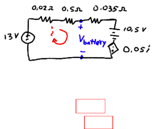
20. (a) Define the charging current i as flowing clockwise in the circuit provided.
By application of KVL,
-13 + 0.02i + Ri + 0.035i + 10.5 = 0
We know that we need a current i = 4 A, so we may calculate the necessary resistance
R = [13 – 10.5 – 0.055(4)]/ 4 = 570 mΩ
(b) The total power delivered to the battery consists of the power absorbed by the
0.035-Ω resistance (0.035i2), and the power absorbed by the 10.5-V ideal battery
(10.5i). Thus, we need to solve the quadratic equation
0.035i2 + 10.5i = 25
which has the solutions i = -302.4 A and i = 2.362 A.
In order to determine which of these two values should be used, we must recall that
the idea is to charge the battery, implying that it is absorbing power, or that i as
defined is positive. Thus, we choose i = 2.362 A, and, making use of the expression
developed in part (a), we find that
R = [13 – 10.5 – 0.055(2.362)]/ 2.362 = 1.003 Ω
(c) To obtain a voltage of 11 V across the battery, we apply KVL:
0.035i + 10.5 = 11 so that i = 14.29 A
From part (a), this means we need
R = [13 – 10.5 – 0.055(14.29)]/ 14.29 = 119.9 mW
CHAPTER THREE SOLUTIONS
Engineering Circuit Analysis, 6th Edition Copyright ©2002 McGraw-Hill, Inc. All Rights Reserved.
21. Drawing the circuit described, we also define a clockwise current i.
By KVL, we find that
-13 + (0.02 + 0.5 + 0.035)i + 10.5 – 0.05i = 0
or that i = (13 – 10.5)/0.505 = 4.950 A
and Vbattery = 13 – (0.02 + 0.5)i = 10.43 V.
CHAPTER THREE SOLUTIONS
Engineering Circuit Analysis, 6th Edition Copyright ©2002 McGraw-Hill, Inc. All Rights Reserved.
22. Applying KVL about this simple loop circuit (the dependent sources are still linear
elements, by the way, as they depend only upon a sum of voltages)
-40 + (5 + 25 + 20)i – (2v3 + v2) + (4v1 – v2) = 0 [1]
where we have defined i to be flowing in the clockwise direction, and
v1 = 5i, v2 = 25i, and v3 = 20i.
Performing the necessary substition, Eq. [1] becomes
50i - (40i + 25i) + (20i – 25i) = 40
so that i = 40/-20 = -2 A
Computing the absorbed power is now a straightforward matter:
p40V = (40)(-i) = 80 W
p5W = 5i2 = 20 W
p25W = 25i2 = 100 W
p20W = 20i2 = 80 W
pdepsrc1 = (2v3 + v2)(-i) = (40i + 25i) = -260 W
pdepsrc2 = (4v1 - v2)(-i) = (20i - 25i) = -20 W
and we can easily verify that these quantities indeed sum to zero as expected.
CHAPTER THREE SOLUTIONS
Engineering Circuit Analysis, 6th Edition Copyright ©2002 McGraw-Hill, Inc. All Rights Reserved.
23. We begin by defining a clockwise current i.
(a) i = 12/(40 + R) mA, with R expressed in kΩ.
We want i2 · 25 = 2
or 2 25
40
12 2
=⋅
+R
Rearranging, we find a quadratic expression involving R:
R2 + 80R – 200 = 0
which has the solutions R = -82.43 kΩ and R = 2.426 kΩ. Only the latter is a
physical solution, so
R = 2.426 kΩ.
(b) We require i · 12 = 3.6 or i = 0.3 mA
From the circuit, we also see that i = 12/(15 + R + 25) mA.
Substituting the desired value for i, we find that the required value of R is R = 0.
(c)

CHAPTER THREE SOLUTIONS
Engineering Circuit Analysis, 6th Edition Copyright ©2002 McGraw-Hill, Inc. All Rights Reserved.
24. By KVL, –12 + (1 + 2.3 + Rwire segment) i = 0
The wire segment is a 3000–ft section of 28–AWG solid copper wire. Using Table
2.3, we compute its resistance as
(16.2 mΩ/ft)(3000 ft) = 48.6 Ω
which is certainly not negligible compared to the other resistances in the circuit!
Thus, i = 12/(1 + 2.3 + 48.6) = 231.2 mA

CHAPTER THREE SOLUTIONS
Engineering Circuit Analysis, 6th Edition Copyright ©2002 McGraw-Hill, Inc. All Rights Reserved.
25. We can apply Ohm’s law to find an expression for vo:
vo = 1000(–gm vπ)
We do not have a value for vπ, but KVL will allow us to express that in terms of vo,
which we do know:
–10×10–3 cos 5t + (300 + 50×103) i = 0
where i is defined as flowing clockwise.
Thus, vπ = 50×103 i = 50×103 (10×10–3 cos 5t) / (300 + 50×103)
= 9.940×10⁻³ cos 5t V
and we by substitution we find that
vo = 1000(–25×10–3)( 9.940×10⁻³ cos 5t )
= –248.5 cos 5t mV
CHAPTER THREE SOLUTIONS
Engineering Circuit Analysis, 6th Edition Copyright ©2002 McGraw-Hill, Inc. All Rights Reserved.
26. By KVL, we find that
–3 + 100 ID + VD = 0
Substituting ID = 3×10⁻⁶(eVD
/ 27×10–3 – 1), we find that
–3 + 300×10–6(eVD
/ 27×10–3 – 1) + VD = 0
This is a transcendental equation. Using a scientific calculator or a numerical
software package such as MATLAB®, we find
VD = 246.4 mV
Let’s assume digital assistance is unavailable. In that case, we need to “guess” a value
for VD, substitute it into the right hand side of our equation, and see how close the
result is to the left hand side (in this case, zero).
GUESS RESULT
0 –3
1 3.648×10¹²
0.5 3.308×10⁴
0.25 0.4001
0.245 –0.1375
0.248 0.1732
0.246 –0.0377
oops
better
At this point, the error is
getting much smaller, and
our confidence is increasing
as to the value of VD.
CHAPTER THREE SOLUTIONS
Engineering Circuit Analysis, 6th Edition Copyright ©2002 McGraw-Hill, Inc. All Rights Reserved.
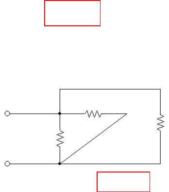
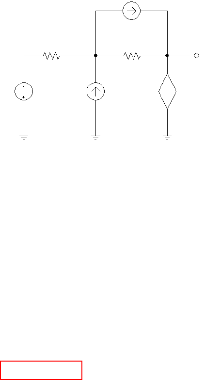
27. Define a voltage vx, “+” reference on the right, across the dependent current source.
Note that in fact vx appears across each of the four elements. We first convert the 10
mS conductance into a 100–Ω resistor, and the 40–mS conductance into a 25–Ω
resistor.
(a) Applying KCL, we sum the currents flowing into the right–hand node:
5 – vx / 100 – vx / 25 + 0.8 ix = 0 [1]
This represents one equation in two unknowns. A second equation to introduce at this
point is
ix = vx /25 so that Eq. [1] becomes
5 – vx / 100 – vx / 25 + 0.8 (vx / 25) = 0
Solving for vx, we find vx = 277.8 V. It is a simple matter now to compute the power
absorbed by each element:
P5A = –5 vx = –1.389 kW
P100Ω = (vx)2 / 100 = 771.7 W
P25Ω = (vx)2 / 25 = 3.087 kW
Pdep = –vx(0.8 ix) = –0.8 (vx)2 / 25 = –2.470 kW
A quick check assures us that the calculated values sum to zero, as they should.
(b) Again summing the currents into the right–hand node,
5 – vx / 100 – vx / 25 + 0.8 iy = 0 [2]
where iy = 5 – vx/100
Thus, Eq. [2] becomes
5 – vx / 100 – vx / 25 + 0.8(5) – 0.8 (iy) / 100 = 0
Solving, we find that vx x = 155.2 V and iy = 3.448 A
So that
P5A = –5 vx = –776.0 W
P100Ω = (vx)2 / 100 = 240.9 W
P25Ω = (vx)2 / 25 = 963.5 W
Pdep = –vx(0.8 iy) = –428.1 W
A quick check assures us that the calculated values sum to 0.3, which is reasonably
close to zero (small roundoff errors accumulate here).

CHAPTER THREE SOLUTIONS
Engineering Circuit Analysis, 6th Edition Copyright ©2002 McGraw-Hill, Inc. All Rights Reserved.
28. Define a voltage v with the “+” reference at the top node. Applying KCL and
summing the currents flowing out of the top node,
v/5,000 + 4×10⁻³ + 3i1 + v/20,000 = 0 [1]
This, unfortunately, is one equation in two unknowns, necessitating the search for a
second suitable equation. Returning to the circuit diagram, we observe that
i1 = 3 i1 + v/2,000
or i1 = –v/40,000 [2]
Upon substituting Eq. [2] into Eq. [1], Eq. [1] becomes,
v/5,000 + 4×10⁻³ – 3v/40,000 + v/20,000 = 0
Solving, we find that
v = –22.86 V
and
i1 = 571.4 µA
Since ix = i1, we find that ix = 571.4 µA.

CHAPTER THREE SOLUTIONS
Engineering Circuit Analysis, 6th Edition Copyright ©2002 McGraw-Hill, Inc. All Rights Reserved.
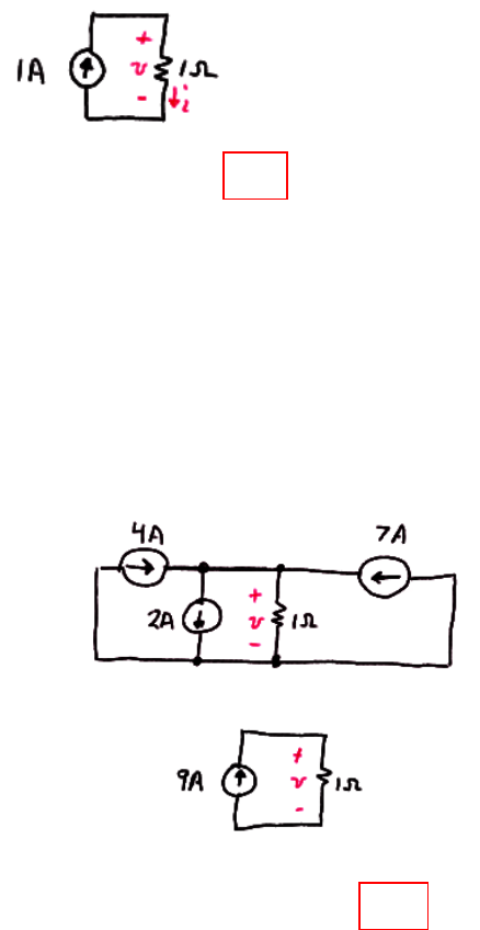
29. Define a voltage vx with its “+” reference at the center node. Applying KCL and
summing the currents into the center node,
8 – vx /6 + 7 – vx /12 – vx /4 = 0
Solving, vx = 30 V.
It is now a straightforward matter to compute the power absorbed by each element:
P8A = –8 vx = –240 W
P6Ω = (vx)2 / 6 = 150 W
P8A = –7 vx = –210 W
P12Ω = (vx)2 / 12 = 75 W
P4Ω = (vx)2 / 4 = 225 W
and a quick check verifies that the computed quantities sum to zero, as expected.

CHAPTER THREE SOLUTIONS
Engineering Circuit Analysis, 6th Edition Copyright ©2002 McGraw-Hill, Inc. All Rights Reserved.
30. (a) Define a voltage v across the 1–kΩ resistor with the “+” reference at the top node.
Applying KCL at this top node, we find that
80×10–3 – 30×10–3 = v/1000 + v/4000
Solving, v = (50×10–3)(4×10⁶ / 5×10³) = 40 V
and P4kΩ = v2/4000 = 400 mW
(b) Once again, we first define a voltage v across the 1–kΩ resistor with the “+”
reference at the top node. Applying KCL at this top node, we find that
80×10–3 – 30×10–3 – 20×10–3 = v/1000
Solving, v = 30 V
and P20mA = v · 20×10–3 = 600 mW
(c) Once again, we first define a voltage v across the 1–kΩ resistor with the “+”
reference at the top node. Applying KCL at this top node, we find that
80×10–3 – 30×10–3 – 2ix = v/1000
where ix = v/1000
so that 80×10–3 – 30×10–3 = 2v/1000 + v/1000
and v = 50×10–3 (1000)/3 = 16.67 V
Thus, Pdep = v · 2ix = 555.8 mW
(d) We note that ix = 60/1000 = 60 mA. KCL stipulates that (viewing currents
into and out of the top node)
80 – 30 + is = ix = 60
Thus, is = 10 mA
and P60V = 60(–10) mW = –600 mW

CHAPTER THREE SOLUTIONS
Engineering Circuit Analysis, 6th Edition Copyright ©2002 McGraw-Hill, Inc. All Rights Reserved.
31. (a) To cancel out the effects of both the 80-mA and 30-mA sources, iS must be set to
iS = –50 mA.
(b) Define a current is flowing out of the “+” reference terminal of the independent
voltage source. Interpret “no power” to mean “zero power.”
Summing the currents flowing into the top node and invoking KCL, we find that
80×10-3 - 30×10-3 - vS/1×103 + iS = 0
Simplifying slightly, this becomes
50 - vS + 103 iS = 0 [1]
We are seeking a value for vS such that vS · iS = 0. Clearly, setting vS = 0 will achieve
this. From Eq. [1], we also see that setting vS = 50 V will work as well.

CHAPTER THREE SOLUTIONS
Engineering Circuit Analysis, 6th Edition Copyright ©2002 McGraw-Hill, Inc. All Rights Reserved.
32. Define a voltage v9 across the 9-Ω resistor, with the “+” reference at the top node.
(a) Summing the currents into the right-hand node and applying KCL,
5 + 7 = v9 / 3 + v9 / 9
Solving, we find that v9 = 27 V. Since ix = v9 / 9, ix = 3 A.
(b) Again, we apply KCL, this time to the top left node:
2 – v8 / 8 + 2ix – 5 = 0
Since we know from part (a) that ix = 3 A, we may calculate v8 = 24 V.
(c) p5A = (v9 – v8) · 5 = 15 W.

CHAPTER THREE SOLUTIONS
Engineering Circuit Analysis, 6th Edition Copyright ©2002 McGraw-Hill, Inc. All Rights Reserved.
33. Define a voltage vx across the 5-A source, with the “+” reference on top.
Applying KCL at the top node then yields
5 + 5v1 - vx/ (1 + 2) – vx/ 5 = 0 [1]
where v1 = 2[vx /(1 + 2)] = 2 vx / 3.
Thus, Eq. [1] becomes 5 + 5(2 vx / 3) – vx / 3 – vx / 5 = 0
or 75 + 50 vx – 5 vx – 3 vx = 0, which, upon solving, yields vx = -1.786 V.
The power absorbed by the 5-Ω resistor is then simply (vx)2/5 = 638.0 mW.

CHAPTER THREE SOLUTIONS
Engineering Circuit Analysis, 6th Edition Copyright ©2002 McGraw-Hill, Inc. All Rights Reserved.
34. Despite the way it may appear at first glance, this is actually a simple node-pair
circuit. Define a voltage v across the elements, with the “+” reference at the top node.
Summing the currents leaving the top node and applying KCL, we find that
2 + 6 + 3 + v/5 + v/5 + v/5 = 0
or v = -55/3 = -18.33 V. The power supplied by each source is then computed as:
p2A = -v(2) = 36.67 W
p6A = -v(6) = 110 W
p3A = -v(3) = 55 W
We can check our results by first determining the power absorbed by each resistor,
which is simply v2/5 = 67.22 W for a total of 201.67 W, which is the total power
supplied by all sources.

CHAPTER THREE SOLUTIONS
Engineering Circuit Analysis, 6th Edition Copyright ©2002 McGraw-Hill, Inc. All Rights Reserved.
35. Defining a voltage Vx across the 10-A source with the “+” reference at the top node,
KCL tells us that 10 = 5 + I1Ω, where I1Ω is defined flowing downward through the
1-Ω resistor.
Solving, we find that I1Ω = 5 A, so that Vx = (1)(5) = 5 V.
So, we need to solve Vx = 5 = 5(0.5 + Rsegment)
with Rsegment = 500 mΩ.
From Table 2.3, we see that 28-AWG solid copper wire has a resistance of 65.3
mΩ/ft. Thus, the total number of miles needed of the wire is
miles 101.450
ft/mi) /ft)(5280m (65.3
m 500 3-
×=
Ω
Ω
CHAPTER THREE SOLUTIONS
Engineering Circuit Analysis, 6th Edition Copyright ©2002 McGraw-Hill, Inc. All Rights Reserved.
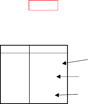
36. Since v = 6 V, we know the current through the 1-Ω resistor is 6 A, the current
through the 2-Ω resistor is 3 A, and the current through the 5-Ω resistor is 6/5
= 1.2 A, as shown below:
By KCL, 6 + 3 + 1.2 + iS = 0 or iS = -10.2 A.

CHAPTER THREE SOLUTIONS
Engineering Circuit Analysis, 6th Edition Copyright ©2002 McGraw-Hill, Inc. All Rights Reserved.
37. (a) Applying KCL, 1 – i – 3 + 3 = 0 so i = 1 A.
(b) The rightmost source should be labeled 3.5 A to satisfy KCL.
Then, looking at the left part of the circuit, we see 1 + 3 = 4 A flowing into the
unknown current source, which, by virtue of KCL, must therefore be a 4-A current
source. Thus, KCL at the node labeled with the “+” reference of the voltage v gives
4 – 2 + 7 – i = 0 or i = 9 A
CHAPTER THREE SOLUTIONS
Engineering Circuit Analysis, 6th Edition Copyright ©2002 McGraw-Hill, Inc. All Rights Reserved.
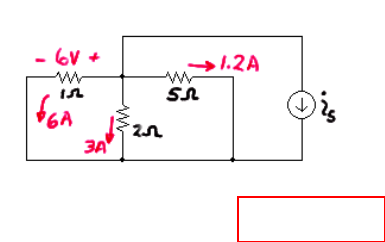
38. (a) We may redraw the circuit as
Then, we see that v = (1)(1) = 1 V.
(b) The current source at the far right should be labeled 3.5 A, or KCL is violated.
In that case, we may combine all sources to the right of the 1-Ω resistor into a single
7-A current source. On the left, the two 1-A sources in sereies reduce to a single 1-A
source.
The new 1-A source and the 3-A source combine to yield a 4-A source in series with
the unknown current source which, by KCL, must be a 4-A current source.
At this point we have reduced the circuit to
Further simplification is possible, resulting in
From which we see clearly that v = (9)(1) = 9 V.
CHAPTER THREE SOLUTIONS
Engineering Circuit Analysis, 6th Edition Copyright ©2002 McGraw-Hill, Inc. All Rights Reserved.
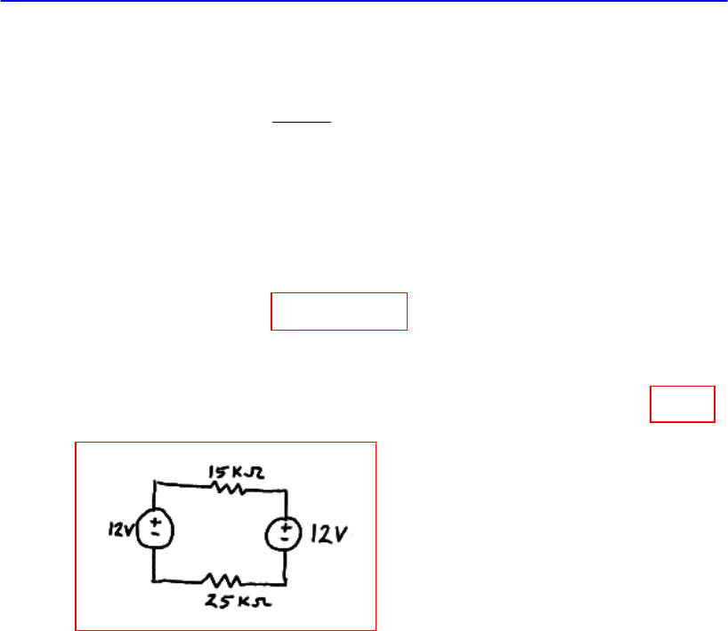
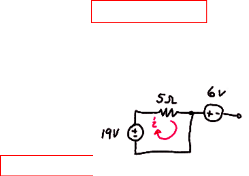
39. (a) Combine the 12-V and 2-V series connected sources to obtain a new 12 – 2 = 10 V
source, with the “+” reference terminal at the top. The result is two 10-V sources in
parallel, which is permitted by KVL. Therefore,
i = 10/1000 = 10 mA.
(b) No current flows through the 6-V source, so we may neglect it for this calculation.
The 12-V, 10-V and 3-V sources are connected in series as a result, so we replace
them with a 12 + 10 –3 = 19 V source as shown
Thus, i = 19/5 = 3.8 A.
CHAPTER THREE SOLUTIONS
Engineering Circuit Analysis, 6th Edition Copyright ©2002 McGraw-Hill, Inc. All Rights Reserved.
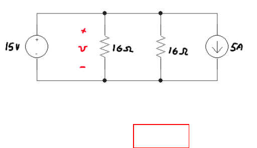
40. We first combine the 10-V and 5-V sources into a single 15-V source, with the “+”
reference on top. The 2-A and 7-A current sources combine into a 7 – 2 = 5 A current
source (arrow pointing down); although these two current sources may not appear to
be in parallel at first glance, they actually are.
Redrawing our circuit,
we see that v = 15 V (note that we can completely the ignore the 5-A source here,
since we have a voltage source directly across the resistor). Thus,
p16Ω = v2/16 = 14.06 W.
CHAPTER THREE SOLUTIONS
Engineering Circuit Analysis, 6th Edition Copyright ©2002 McGraw-Hill, Inc. All Rights Reserved.
41. We can combine the voltage sources such that
i = vS/ 14
(a) vS = 10 + 10 – 6 – 6 = 20 –12 = 8
Therefore i = 8/14 = 571.4 mA.
(b) vS = 3 + 2.5 – 3 – 2.5 = 0 Therefore i = 0.
(c) vS = -3 + 1.5 – (-0.5) – 0 = -1 V
Therefore i = -1/14 = -71.43 mA.
CHAPTER THREE SOLUTIONS
Engineering Circuit Analysis, 6th Edition Copyright ©2002 McGraw-Hill, Inc. All Rights Reserved.
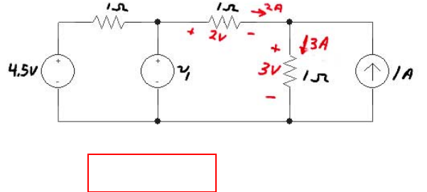
42. We first simplify as shown, making use of the fact that we are told ix = 2 A to find the
voltage across the middle and right-most 1-Ω resistors as labeled.
By KVL, then, we find that v1 = 2 + 3 = 5 V.

CHAPTER THREE SOLUTIONS
Engineering Circuit Analysis, 6th Edition Copyright ©2002 McGraw-Hill, Inc. All Rights Reserved.
43. We see that to determine the voltage v we will need vx due to the presence of the
dependent current soruce. So, let’s begin with the right-hand side, where we find that
vx = 1000(1 – 3) × 10-3 = -2 V.
Returning to the left-hand side of the circuit, and summing currents into the top node,
we find that
(12 – 3.5) ×10-3 + 0.03 vx = v/10×103
or v = -515 V.
CHAPTER THREE SOLUTIONS
Engineering Circuit Analysis, 6th Edition Copyright ©2002 McGraw-Hill, Inc. All Rights Reserved.
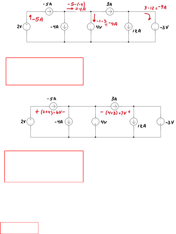
44. (a) We first label the circuit with a focus on determining the current flowing through
each voltage source:
Then the power absorbed by each voltage source is
P2V = -2(-5) = 10 W
P4V = -(-4)(4) = 16 W
P-3V = -(-9)(-3) = 27 W
For the current sources,
So that the absorbed power is
P
-5A = +(-5)(6) = -30 W
P-4A = -(-4)(4) = 16 W
P3A = -(3)(7) = -21 W
P12A = -(12)(-3) = 36 W
A quick check assures us that these absorbed powers sum to zero as they should.
(b) We need to change the 4-V source such that the voltage across the –5-A source
drops to zero. Define Vx across the –5-A source such that the “+” reference terminal is
on the left. Then, -2 + Vx – Vneeded = 0
or Vneeded = -2 V.

CHAPTER THREE SOLUTIONS
Engineering Circuit Analysis, 6th Edition Copyright ©2002 McGraw-Hill, Inc. All Rights Reserved.
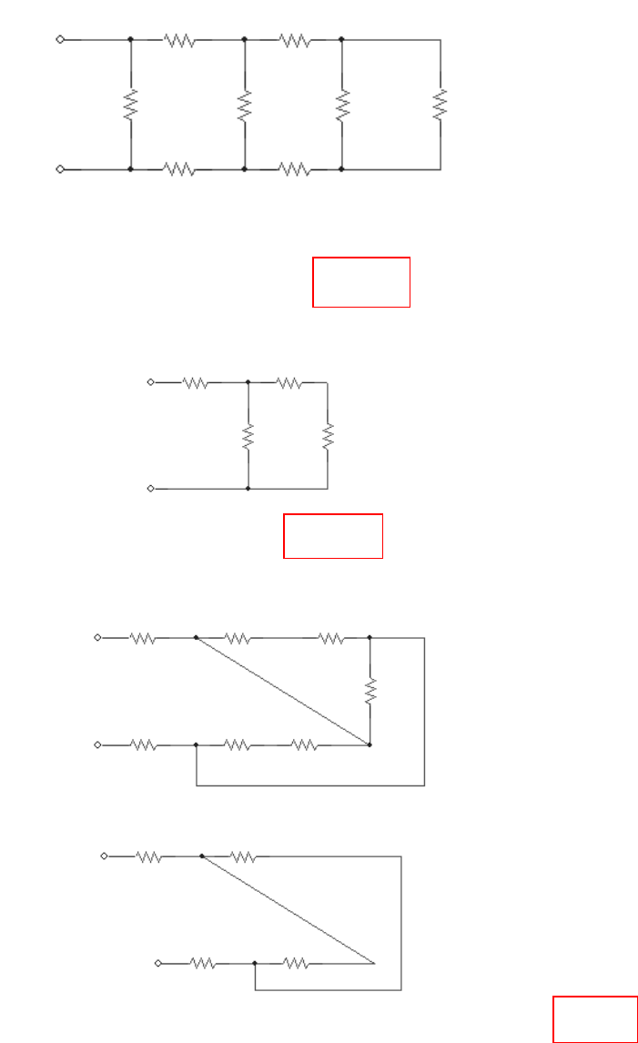
45. We begin by noting several things:
(1) The bottom resistor has been shorted out;
(2) the far-right resistor is only connected by one terminal and therefore does
not affect the equivalent resistance as seen from the indicated terminals;
(3) All resistors to the right of the top left resistor have been shorted.
Thus, from the indicated terminals, we only see the single 1-kΩ resistor, so that
Req = 1 kΩ.

CHAPTER THREE SOLUTIONS
Engineering Circuit Analysis, 6th Edition Copyright ©2002 McGraw-Hill, Inc. All Rights Reserved.
46. (a) We see 1Ω || (1 Ω + 1 Ω) || (1 Ω + 1 Ω + 1 Ω)
= 1Ω || 2 Ω || 3 Ω
= 545.5 mΩ
(b) 1/Req = 1 + 1/2 + 1/3 + … 1/N
Thus, Req = [1 + 1/2 + 1/3 + … 1/N]-1
CHAPTER THREE SOLUTIONS
Engineering Circuit Analysis, 6th Edition Copyright ©2002 McGraw-Hill, Inc. All Rights Reserved.
47. (a) 5 kΩ = 10 kΩ || 10 kΩ
(b) 57 333 Ω = 47 kΩ + 10 kΩ + 1 kΩ || 1kΩ || 1kΩ
(c) 29.5 kΩ = 47 kΩ || 47 kΩ + 10 kΩ || 10 kΩ + 1 kΩ
CHAPTER THREE SOLUTIONS
Engineering Circuit Analysis, 6th Edition Copyright ©2002 McGraw-Hill, Inc. All Rights Reserved.
0 V 1 A
5 Ω 7 Ω
5 Ω
1 A 2.917 Ω
48. (a) no simplification is possible using only source and/or resistor combination
techniques.
(b) We first simplify the circuit to
and then notice that the 0-V source is shorting out one of the 5-Ω resistors, so a
further simplification is possible, noting that 5 Ω || 7 Ω = 2.917 Ω:

CHAPTER THREE SOLUTIONS
Engineering Circuit Analysis, 6th Edition Copyright ©2002 McGraw-Hill, Inc. All Rights Reserved.
49. Req = 1 kΩ + 2 kΩ || 2 kΩ + 3 kΩ || 3 kΩ + 4 kΩ || 4 kΩ
= 1 kΩ + 1 k Ω + 1.5 kΩ + 2 kΩ
= 5.5 kΩ.
CHAPTER THREE SOLUTIONS
Engineering Circuit Analysis, 6th Edition Copyright ©2002 McGraw-Hill, Inc. All Rights Reserved.
Req →
100 Ω
100 Ω
100 Ω
100 Ω
100 Ω 250 Ω
100 Ω
100 Ω
10 Ω
20 Ω
5 Ω
14.4 Ω
Req →
2 Ω
15 Ω 10 Ω
50 Ω
8 Ω 20 Ω 30 Ω
2 Ω 16.67 Ω
8 Ω 50 Ω
50. (a) Working from right to left, we first see that we may combine several resistors as
100 Ω + 100 Ω || 100 Ω + 100 Ω = 250 Ω, yielding the following circuit:
Next, we see 100 Ω + 100 Ω || 250 Ω + 100 Ω = 271.4 Ω,
and subsequently 100 Ω + 100 Ω || 271.4 Ω + 100 Ω = 273.1 Ω,
and, finally,
Req = 100 Ω || 273.1 Ω = 73.20 Ω.
(b) First, we combine 24 Ω || (50 Ω + 40 Ω) || 60 Ω = 14.4 Ω, which leaves us with
Thus, Req = 10 Ω + 20 Ω || (5 + 14.4 Ω) = 19.85 Ω.
(c) First combine the 10-Ω and 40-Ω resistors and redraw the circuit:
We now see we have (10 Ω + 15 Ω) || 50 Ω = 16.67 Ω. Redrawing once again,
where the equivalent resistance is seen to be 2 Ω + 50 Ω || 16.67 Ω + 8 Ω = 22.5 Ω.

CHAPTER THREE SOLUTIONS
Engineering Circuit Analysis, 6th Edition Copyright ©2002 McGraw-Hill, Inc. All Rights Reserved.
51. (a) Req = [(40 Ω + 20 Ω) || 30 Ω + 80 Ω] || 100 Ω + 10 Ω = 60 Ω.
(b) Req = 80 Ω = [(40 Ω + 20 Ω) || 30 Ω + R] || 100 Ω + 10 Ω
70 Ω = [(60 Ω || 30 Ω) + R] || 100 Ω
1/70 = 1/(20 + R) + 0.01
20+ R = 233.3 Ω therefore R = 213.3 Ω.
(c) R = [(40 Ω + 20 Ω) || 30 Ω + R] || 100 Ω + 10 Ω
R – 10 Ω = [20 + R] || 100
1/(R – 10) = 1/(R + 20) + 1/ 100
3000 = R2 + 10R – 200
Solving, we find R = -61.79 Ω or R = 51.79 Ω.
Clearly, the first is not a physical solution, so R = 51.79 Ω.

CHAPTER THREE SOLUTIONS
Engineering Circuit Analysis, 6th Edition Copyright ©2002 McGraw-Hill, Inc. All Rights Reserved.
52. (a) 25 Ω = 100 Ω || 100 Ω || 100 Ω
(b) 60 Ω = [(100 Ω || 100 Ω) + 100 Ω] || 100 Ω
(c) 40 Ω = (100 Ω + 100 Ω) || 100 Ω || 100 Ω

CHAPTER THREE SOLUTIONS
Engineering Circuit Analysis, 6th Edition Copyright ©2002 McGraw-Hill, Inc. All Rights Reserved.
53. Req = [(5 Ω || 20 Ω) + 6 Ω] || 30 Ω + 2.5 Ω = 10 Ω
The source therefore provides a total of 1000 W and a current of 100/10 = 10 A.
P
2.5Ω = (10)2 · 2.5 = 250 W
V
30Ω = 100 - 2.5(10) = 75 V
P
30Ω = 752/ 30 = 187.5 W
I
6Ω = 10 – V30Ω /30 = 10 – 75/30 = 7.5 A
P
6Ω = (7.5)2 · 6 = 337.5 W
V
5Ω = 75 – 6(7.5) = 30 V
P
5Ω = 302/ 5 = 180 W
V
20Ω = V5Ω = 30 V
P
20Ω = 302/20 = 45 W
We check our results by verifying that the absorbed powers in fact add to 1000 W.
CHAPTER THREE SOLUTIONS
Engineering Circuit Analysis, 6th Edition Copyright ©2002 McGraw-Hill, Inc. All Rights Reserved.
- vx +
9 A
14 Ω 6 Ω
4 Ω 6 Ω
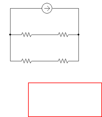
54. To begin with, the 10-Ω and 15-Ω resistors are in parallel ( = 6 Ω), and so are the
20-Ω and 5-Ω resistors (= 4 Ω).
Also, the 4-A, 1-A and 6-A current sources are in parallel, so they can be combined
into a single 4 + 6 – 1 = 9 A current source as shown:
Next, we note that (14 Ω + 6 Ω) || (4 Ω + 6 Ω) = 6.667 Ω
so that vx = 9(6.667) = 60 V
and ix = -60/10 = -6 A.
CHAPTER THREE SOLUTIONS
Engineering Circuit Analysis, 6th Edition Copyright ©2002 McGraw-Hill, Inc. All Rights Reserved.
13.64 mS
100 mS
22.22 mS
Gin →
55. (a) Working from right to left, and borrowing x || y notation from resistance
calculations to indicate the operation xy/(x + y),
Gin = {[(6 || 2 || 3) + 0.5] || 1.5 || 2.5 + 0.8} || 4 || 5 mS
= {[(1) + 0.5] || 1.5 || 2.5 + 0.8} || 4 || 5 mS
= {1.377} || 4 || 5
= 0.8502 mS = 850.2 mS
(b) The 50-mS and 40-mS conductances are in series, equivalent to (50(40)/90 =
22.22 mS. The 30-mS and 25-mS conductances are also in series, equivalent to 13.64
mS. Redrawing for clarity,
we see that Gin = 10 + 22.22 + 13.64 = 135.9 mS.

CHAPTER THREE SOLUTIONS
Engineering Circuit Analysis, 6th Edition Copyright ©2002 McGraw-Hill, Inc. All Rights Reserved.
56. The bottom four resistors between the 2-Ω resistor and the 30-V source are shorted
out. The 10-Ω and 40-Ω resistors are in parallel (= 8 Ω), as are the 15-Ω and 60-Ω
(=12 Ω) resistors. These combinations are in series.
Define a clockwise current I through the 1-Ω resistor:
I = (150 – 30)/(2 + 8 + 12 + 3 + 1 + 2) = 4.286 A
P1Ω = I2 · 1 = 18.37 W
To compute P10Ω, consider that since the 10-Ω and 40-Ω resistors are in parallel, the
same voltage Vx (“+” reference on the left) appears across both resistors. The current I
= 4.286 A flows into this combination. Thus, Vx = (8)(4.286) = 34.29 V and
P10Ω = (Vx)2 / 10 = 117.6 W.
P13Ω = 0 since no current flows through that resistor.
CHAPTER THREE SOLUTIONS
Engineering Circuit Analysis, 6th Edition Copyright ©2002 McGraw-Hill, Inc. All Rights Reserved.
57. One possible solution of many:
The basic concept is as shown
If we use 28-AWG soft copper wire, we see from Table 2.3 that 9-Ω would require
138 feet, which is somewhat impractical. Referring to p. 4-48 of the Standard
Handbook for Electrical Engineers (this should be available in most
engineering/science libraries), we see that 44-AWG soft copper wire has a resistance
of 2590 Ω per 1000 ft, or 0.08497 Ω/cm.
Thus, 1-Ω requires 11.8 cm of 44-AWG wire, and 9-Ω requires 105.9 cm. We decide
to make the wiper arm and leads out of 28-AWG wire, which will add a slight
resistance to the total value, but a negligible amount.
The radius of the wiper arm should be (105.9 cm)/
π
= 33.7 cm.
9-Ω wire
se
g
ment
1-Ω wire
se
g
ment
external contacts

CHAPTER THREE SOLUTIONS
Engineering Circuit Analysis, 6th Edition Copyright ©2002 McGraw-Hill, Inc. All Rights Reserved.
58. One possible solution of many:
vS = 2(5.5) = 11 V
R
1 = R2 = 1 kΩ.

CHAPTER THREE SOLUTIONS
Engineering Circuit Analysis, 6th Edition Copyright ©2002 McGraw-Hill, Inc. All Rights Reserved.
59. One possible solution of many:
iS = 11 mA
R
1 = R2 = 1 kΩ.

CHAPTER THREE SOLUTIONS
Engineering Circuit Analysis, 6th Edition Copyright ©2002 McGraw-Hill, Inc. All Rights Reserved.
60. p15Ω = (v15)2 / 15×103 A
v15 = 15×103 (-0.3 v1)
where v1 = [4 (5)/ (5 + 2)] · 2 = 5.714 V
Therefore v15 = -25714 V and p15 = 44.08 kW.

CHAPTER THREE SOLUTIONS
Engineering Circuit Analysis, 6th Edition Copyright ©2002 McGraw-Hill, Inc. All Rights Reserved.
61. Replace the top 10 kΩ, 4 kΩ and 47 kΩ resistors with 10 kΩ + 4 kΩ || 47 kΩ =
13.69 kΩ.
Define vx across the 10 kΩ resistor with its “+” reference at the top node: then
vx = 5 · (10 kΩ || 13.69 kΩ) / (15 kΩ + 10 || 13.69 kΩ) = 1.391 V
ix = vx/ 10 mA = 139.1 µA
v15 = 5 – 1.391 = 3.609 V and p15 = (v15)2/ 15×103 = 868.3 µW.

CHAPTER THREE SOLUTIONS
Engineering Circuit Analysis, 6th Edition Copyright ©2002 McGraw-Hill, Inc. All Rights Reserved.
62. We may combine the 12-A and 5-A current sources into a single 7-A current source
with its arrow oriented upwards. The left three resistors may be replaced by a 3 +
6 || 13 = 7.105 Ω resistor, and the right three resistors may be replaced by a 7 + 20 || 4
= 10.33 Ω resistor.
By current division, iy = 7 (7.105)/(7.105 + 10.33) = 2.853 A
We must now return to the original circuit. The current into the 6 Ω, 13 Ω parallel
combination is 7 – iy = 4.147 A. By current division,
ix = 4.147 . 13/ (13 + 6) = 2.837 A
and px = (4.147)2 · 3 = 51.59 W

CHAPTER THREE SOLUTIONS
Engineering Circuit Analysis, 6th Edition Copyright ©2002 McGraw-Hill, Inc. All Rights Reserved.
63. The controlling voltage v1, needed to obtain the power into the 47-kΩ resistor, can be
found separately as that network does not depend on the left-hand network.
The right-most 2 kΩ resistor can be neglected.
By current division, then, in combination with Ohm’s law,
v1 = 3000[5×10⁻³ (2000)/ (2000 + 3000 + 7000)] = 2.5 V
Voltage division gives the voltage across the 47-kΩ resistor:
V 0.9228
16.67 47
7)0.5(2.5)(4
20 ||100 47
47
5.0 1=
+
=
+
v
So that p47kΩ = (0.9928)2 / 47×103 = 18.12 µW

CHAPTER THREE SOLUTIONS
Engineering Circuit Analysis, 6th Edition Copyright ©2002 McGraw-Hill, Inc. All Rights Reserved.
64. The temptation to write an equation such as
v1 = 2020
20
10 +
must be fought!
Voltage division only applies to resistors connected in series, meaning that the same
current must flow through each resistor. In this circuit, i1 ≠ 0 , so we do not have the
same current flowing through both 20 kΩ resistors.
CHAPTER THREE SOLUTIONS
Engineering Circuit Analysis, 6th Edition Copyright ©2002 McGraw-Hill, Inc. All Rights Reserved.
65. (a) )]R (R || [R R
)R (R || R
V
4321
432
S2 ++
+
=v
=
()
()
4324321
432432
SR R R)R (R R R
R R R)R (R R
V ++++
+++
=
()
)R (RR R R RR
)R (R R
V
4324321
432
S++++
+
(b) )]R (R || [R R
R
V
4321
1
S1 ++
=v
=
()
4324321
1
SR R R)R (R R R
R
V ++++
=
()
)R (RR R R RR
)R R (R R
V
4324321
4321
S++++
++
(c)
++
=
432
2
1
1
4R R R
R
R
v
i
=
()
[]
)R R )(RR (RR )R R (RRR
R R R R R
V
43243243211
24321
S++++++
++
=
()
)R (RR R R RR
R
V
4324321
2
S++++
CHAPTER THREE SOLUTIONS
Engineering Circuit Analysis, 6th Edition Copyright ©2002 McGraw-Hill, Inc. All Rights Reserved.
66. (a) With the current source open-circuited, we find that
v1 = V 8-
6000 || 3000 500
500
40 =
+
−
(b) With the voltage source short-circuited, we find that
i2 =
()
mA 400
1/6000 1/3000 500/1
1/3000
103 3=
++
×−
i3 =
()
mA 600
6000 || 3000 500
500
103 3=
+
×−
CHAPTER THREE SOLUTIONS
Engineering Circuit Analysis, 6th Edition Copyright ©2002 McGraw-Hill, Inc. All Rights Reserved.
67. (a) The current through the 5-Ω resistor is 10/5 = 2 A. Define R as 3 || (4 + 5)
= 2.25 Ω. The current through the 2-Ω resistor then is given by
25.5
I
R) (2 1
1
I S
S=
++
The current through the 5-Ω resistor is
A 2
9 3
3
25.5
I
S=
+
so that IS = 42 A.
(b) Given that IS is now 50 A, the current through the 5-Ω resistor becomes
A 2.381
9 3
3
25.5
I
S=
+
Thus, vx = 5(2.381) = 11.90 V
(c) 0.2381
I
9 3
3
5.25
5I
I
S
S
S
=
+
=
x
v

CHAPTER THREE SOLUTIONS
Engineering Circuit Analysis, 6th Edition Copyright ©2002 McGraw-Hill, Inc. All Rights Reserved.
68. First combine the 1 kΩ and 3 kΩ resistors to obtain 750 Ω.
By current division, the current through resistor Rx is
IRx = 750 R 2000
2000
1010
x
3
++
×−
and we know that Rx · I
Rx = 9
so
x
x
R 2750
R 20
9 +
=
9 Rx + 24750 = 20 Rx or Rx = 2250 W. Thus,
PRx = 92/ Rx = 36 mW.
CHAPTER THREE SOLUTIONS
Engineering Circuit Analysis, 6th Edition Copyright ©2002 McGraw-Hill, Inc. All Rights Reserved.
69. Define R = R3 || (R4 + R5)
Then
+
=
2
SR R R
R
V v
=
()
()
++++
+++
2543543
543543
SR R R R)R (R R
R R R)R (R R
V
=
++++
+
)R (RR )R R(R R
)R (R R
V
54354 32
543
S
Thus,
+
=
54
5
R5 R R
R
vv
=
++++ )R (RR )R R(R R
R R
V
54354 32
53
S
CHAPTER THREE SOLUTIONS
Engineering Circuit Analysis, 6th Edition Copyright ©2002 McGraw-Hill, Inc. All Rights Reserved.
70. Define R1 = 10 + 15 || 30 = 20 Ω and R2 = 5 + 25 = 30 Ω.
(a) Ix = I1 . 15 / (15 + 30) = 4 mA
(b) I1 = Ix . 45/15 = 36 mA
(c) I2 = IS R1 / (R1 + R2) and I1 = IS R2 / (R1 + R2)
So I1/I2 = R2/R1
Therefore I1 = R2I2/R1 = 30(15)/20 = 22.5 mA
Thus, Ix = I1 . 15/ 45 = 7.5 mA
(d) I1 = IS R2/ (R1 + R2) = 60 (30)/ 50 = 36 A
Thus, Ix = I1 15/ 45 = 12 A.

CHAPTER THREE SOLUTIONS
Engineering Circuit Analysis, 6th Edition Copyright ©2002 McGraw-Hill, Inc. All Rights Reserved.
71. vout = -gm vπ (100 kΩ || 100 kΩ) = -4.762×10³ gm vπ
where vπ = (3 sin 10t) · 15/(15 + 0.3) = 2.941 sin 10t
Thus, vout = -56.02 sin 10t V

CHAPTER THREE SOLUTIONS
Engineering Circuit Analysis, 6th Edition Copyright ©2002 McGraw-Hill, Inc. All Rights Reserved.
72. vout = -1000gm vπ
where vπ = V 10sin 2.679
0.3 3) || (15
3 || 15
10sin 3 tt =
+
therefore
vout = -(2.679)(1000)(38×10-3) sin 10t = -101.8 sin 10t V.
CHAPTER FOUR SOLUTIONS
Engineering Circuit Analysis, 6th Edition Copyright ©2002 McGraw-Hill, Inc. All Rights Reserved.
1. (a) 0.1 -0.3 -0.4 v1 0
-0.5 0.1 0 v2 = 4
-0.2 -0.3 0.4 v3 6
Solving this matrix equation using a scientific calculator, v2 = -8.387 V
(b) Using a scientific calculator, the determinant is equal to 32.
CHAPTER FOUR SOLUTIONS
Engineering Circuit Analysis, 6th Edition Copyright ©2002 McGraw-Hill, Inc. All Rights Reserved.
2. (a) 1 1 1 vA 27
-1 2 3 vB = -16
2 0 4 vC -6
Solving this matrix equation using a scientific calculator,
vA = 19.57
vB = 18.71
vC = -11.29
(b) Using a scientific calculator,
1 1 1
-1 2 3 = 16
2 0 4

CHAPTER FOUR SOLUTIONS
Engineering Circuit Analysis, 6th Edition Copyright ©2002 McGraw-Hill, Inc. All Rights Reserved.
3. The bottom node has the largest number of branch connections, so we choose that as
our reference node. This also makes vP easier to find, as it will be a nodal voltage.
Working from left to right, we name our nodes 1, P, 2, and 3.
NODE 1: 10 = v1/ 20 + (v1 – vP)/ 40 [1]
NODE P: 0 = (vP – v1)/ 40 + vP/ 100 + (vP – v2)/ 50 [2]
NODE 2: -2.5 + 2 = (v2 – vP)/ 50 + (v2 – v3)/ 10 [3]
NODE 3: 5 – 2 = v3/ 200 + (v3 – v2)/ 10 [4]
Simplifying,
60v1 - 20vP = 8000 [1]
-50v1 + 110 vP - 40v2 = 0 [2]
- vP + 6v2 - 5v3 = -25 [3]
-200v2 + 210v3 = 6000 [4]
Solving,
vP = 171.6 V

CHAPTER FOUR SOLUTIONS
Engineering Circuit Analysis, 6th Edition Copyright ©2002 McGraw-Hill, Inc. All Rights Reserved.
4. The logical choice for a reference node is the bottom node, as then vx will
automatically become a nodal voltage.
NODE 1: 4 = v1/ 100 + (v1 – v2)/ 20 + (v1 – vx)/ 50 [1]
NODE x: 10 – 4 – (-2) = (vx – v1)/ 50 + (vx – v2)/ 40 [2]
NODE 2: -2 = v2 / 25 + (v2 – vx)/ 40 + (v2 – v1)/ 20 [3]
Simplifying,
4 = 0.0800v1 – 0.0500v2 – 0.0200vx [1]
8 = -0.0200v1 – 0.02500v2 + 0.04500vx [2]
-2 = -0.0500v1 + 0.1150v2 – 0.02500vx [3]
Solving, vx = 397.4 V.
CHAPTER FOUR SOLUTIONS
Engineering Circuit Analysis, 6th Edition Copyright ©2002 McGraw-Hill, Inc. All Rights Reserved.
5. Designate the node between the 3-Ω and 6-Ω resistors as node X, and the right-hand
node of the 6-Ω resistor as node Y. The bottom node is chosen as the reference node.
(a) Writing the two nodal equations, then
NODE X: –10 = (vX – 240)/ 3 + (vX – vY)/ 6 [1]
NODE Y: 0 = (vY – vX)/ 6 + vY/ 30 + (vY – 60)/ 12 [2]
Simplifying, -180 + 1440 = 9 vX – 3 vY [1]
10800 = - 360 vX + 612 vY [2]
Solving, vX = 181.5 V and vY = 124.4 V
Thus, v1 = 240 – vX = 58.50 V and v2 = vY – 60 = 64.40 V
(b) The power absorbed by the 6-Ω resistor is
(vX – vY)2 / 6 = 543.4 W

CHAPTER FOUR SOLUTIONS
Engineering Circuit Analysis, 6th Edition Copyright ©2002 McGraw-Hill, Inc. All Rights Reserved.
6. Only one nodal equation is required: At the node where three resistors join,
0.02v1 = (vx – 5 i2) / 45 + (vx – 100) / 30 + (vx – 0.2 v3) / 50 [1]
This, however, is one equation in four unknowns, the other three resulting from the
presence of the dependent sources. Thus, we require three additional equations:
i2 = (0.2 v3 - vx) / 50 [2]
v1 = 0.2 v3 - 100 [3]
v3 = 50i2 [4]
Simplifying,
v1 – 0.2v3 = -100 [3]
– v3 + 50 i2 = 0 [4]
–vx + 0.2v3 – 50 i2 = 0 [2]
0.07556vx – 0.02v1 – 0.004v3 – 0.111i2 = 33.33 [1]
Solving, we find that v1 = -103..8 V and i2 = -377.4 mA.
CHAPTER FOUR SOLUTIONS
Engineering Circuit Analysis, 6th Edition Copyright ©2002 McGraw-Hill, Inc. All Rights Reserved.
7. If v1 = 0, the dependent source is a short circuit and we may redraw the circuit as:
At NODE 1: 4 - 6 = v1/ 40 + (v1 – 96)/ 20 + (v1 – V2)/ 10
Since v1 = 0, this simplifies to
-2 = -96 / 20 - V2/ 10
so that V2 = -28 V.
20 Ω 10 Ω
40 Ω
+
v1 = 0
-
.

CHAPTER FOUR SOLUTIONS
Engineering Circuit Analysis, 6th Edition Copyright ©2002 McGraw-Hill, Inc. All Rights Reserved.
8. We choose the bottom node as ground to make calculation of i5 easier. The left-most
node is named “1”, the top node is named “2”, the central node is named “3” and the
node between the 4-Ω and 6-Ω resistors is named “4.”
NODE 1: - 3 = v1/2 + (v1 – v2)/ 1 [1]
NODE 2: 2 = (v2 – v1)/ 1 + (v2 – v3)/ 3 + (v2 – v4)/ 4 [2]
NODE 3: 3 = v3/ 5 + (v3 – v4)/ 7 + (v3 – v2)/ 3 [3]
NODE 4: 0 = v4/ 6 + (v4 – v3)/ 7 + (v4 – v2)/ 4 [4]
Rearranging and grouping terms,
3v1 – 2v2 = -6 [1]
-12v1 + 19v2 – 4v3 – 3v4 = 24 [2]
–35v2 + 71v3 – 15v4 = 315 [3]
-42v2 – 24v3 + 94v4 = 0 [4]
Solving, we find that v3 = 6.760 V and so i5 = v3/ 5 = 1.352 A.
CHAPTER FOUR SOLUTIONS
Engineering Circuit Analysis, 6th Edition Copyright ©2002 McGraw-Hill, Inc. All Rights Reserved.
9. We can redraw this circuit and eliminate the 2.2-kΩ resistor as no current flows
through it:
At NODE 2: 7×10⁻³ – 5×10-3 = (v2 + 9)/ 470 + (v2 – vx)/ 10×10-3 [1]
At NODE x: 5×10⁻³ – 0.2v1 = (vx – v2)/ 10×103 [2]
The additional equation required by the presence of the dependent source and the fact
that its controlling variable is not one of the nodal voltages:
v1 = v2 – vx [3]
Eliminating the variable v1 and grouping terms, we obtain:
10,470 v2 – 470 vx = –89,518
and 1999 v2 – 1999 vx = 50
Solving, we find vx = –8.086 V.
↓
9 V 7 mA
5 mA
0.2 v1
10 kΩ
470 Ω + v1 - vx
v2

CHAPTER FOUR SOLUTIONS
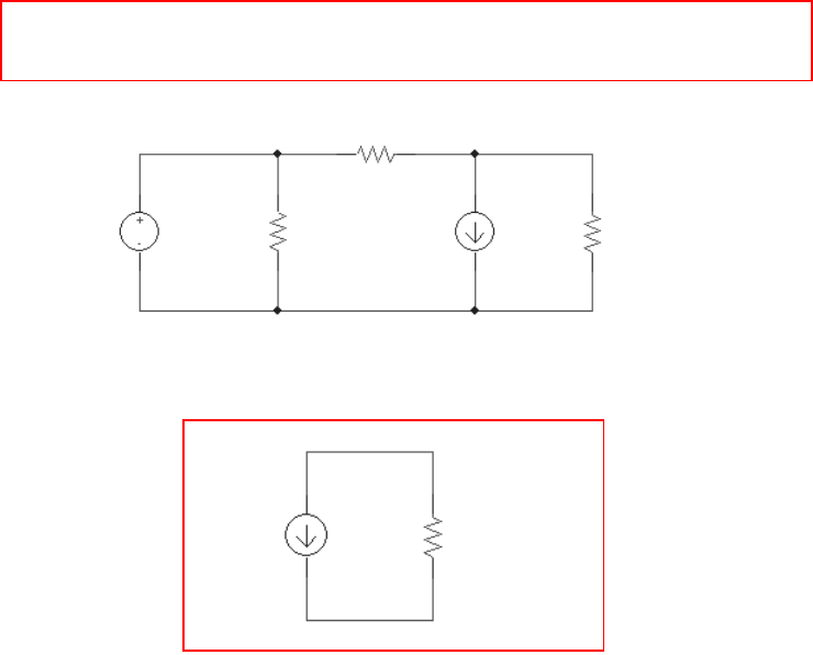
Engineering Circuit Analysis, 6th Edition Copyright ©2002 McGraw-Hill, Inc. All Rights Reserved.
10. We need concern ourselves with the bottom part of this circuit only. Writing a single
nodal equation, -4 + 2 = v/ 50
We find that v = -100 V.

CHAPTER FOUR SOLUTIONS
Engineering Circuit Analysis, 6th Edition Copyright ©2002 McGraw-Hill, Inc. All Rights Reserved.
11. We choose the center node for our common terminal, since it connects to the largest
number of branches. We name the left node “A”, the top node “B”, the right node
“C”, and the bottom node “D”. We next form a supernode between nodes A and B.
At the supernode: 5 = (VA – VB)/ 10 + VA/ 20 + (VB – VC)/ 12.5 [1]
At node C: VC = 150 [2]
At node D: -10 = VD/ 25 + (VD – VA)/ 10 [3]
Our supernode-related equation is VB – VA = 100 [4]
Simplifiying and grouping terms,
0.15 VA + 0.08 VB - 0.08 VC – 0.1 VD = 5 [1]
VC = 150 [2]
-25 VA + 35 VD = -2500 [3]
- VA + VB = 100 [4]
Solving, we find that VD = -63.06 V. Since v4 = - VD,
v4 = 63.06 V.

CHAPTER FOUR SOLUTIONS
Engineering Circuit Analysis, 6th Edition Copyright ©2002 McGraw-Hill, Inc. All Rights Reserved.
12. Choosing the bottom node as the reference terminal and naming the left node “1”, the
center node “2” and the right node “3”, we next form a supernode about nodes 1 and
2, encompassing the dependent voltage source.
At the supernode, 5 – 8 = (v1 – v2)/ 2 + v3/ 2.5 [1]
At node 2, 8 = v2 / 5 + (v2 – v1)/ 2 [2]
Our supernode equation is v1 - v3 = 0.8 vA [3]
Since vA = v2, we can rewrite [3] as v1 – v3 = 0.8v2
Simplifying and collecting terms,
0.5 v1 - 0.5 v2 + 0.4 v3 = -3 [1]
-0.5 v1 + 0.7 v2 = 8 [2]
v1 - 0.8 v2 - v3 = 0 [3]
(a) Solving for v2 = vA, we find that vA = 25.91 V
(b) The power absorbed by the 2.5-Ω resistor is
(v3)2/ 2.5 = (-0.4546)2/ 2.5 = 82.66 mW.

CHAPTER FOUR SOLUTIONS
Engineering Circuit Analysis, 6th Edition Copyright ©2002 McGraw-Hill, Inc. All Rights Reserved.
13. Selecting the bottom node as the reference terminal, we name the left node “1”, the
middle node “2” and the right node “3.”
NODE 1: 5 = (v1 – v2)/ 20 + (v1 – v3)/ 50 [1]
NODE 2: v2 = 0.4 v1 [2]
NODE 3: 0.01 v1 = (v3 – v2)/ 30 + (v3 – v1)/ 50 [3]
Simplifying and collecting terms, we obtain
0.07 v1 – 0.05 v2 – 0.02 v3 = 5 [1]
0.4 v1 – v2 = 0 [2]
-0.03 v1 – 0.03333 v2 + 0.05333 v3 = 0 [3]
Since our choice of reference terminal makes the controlling variable of both
dependent sources a nodal voltage, we have no need for an additional equation as we
might have expected.
Solving, we find that v1 = 148.2 V, v2 = 59.26 V, and v3 = 120.4 V.
The power supplied by the dependent current source is therefore
(0.01 v1) • v3 = 177.4 W.

CHAPTER FOUR SOLUTIONS
Engineering Circuit Analysis, 6th Edition Copyright ©2002 McGraw-Hill, Inc. All Rights Reserved.
14. At node x: vx/ 4 + (vx – vy)/ 2 + (vx – 6)/ 1 = 0 [1]
At node y: (vy – kvx)/ 3 + (vy – vx)/ 2 = 2 [2]
Our additional constraint is that vy = 0, so we may simplify Eqs. [1] and [2]:
14 vx = 48 [1]
-2k vx - 3 vx = 12 [2]
Since Eq. [1] yields vx = 48/14 = 3.429 V, we find that
k = (12 + 3 vx)/ (-2 vx) = -3.250

CHAPTER FOUR SOLUTIONS
Engineering Circuit Analysis, 6th Edition Copyright ©2002 McGraw-Hill, Inc. All Rights Reserved.
15. Choosing the bottom node joining the 4-Ω resistor, the 2-A current sourcee and the
4-V voltage source as our reference node, we next name the other node of the 4-Ω
resistor node “1”, and the node joining the 2-Ω resistor and the 2-A current source
node “2.” Finally, we create a supernode with nodes “1” and “2.”
At the supernode: –2 = v1/ 4 + (v2 – 4)/ 2 [1]
Our remaining equations: v1 – v2 = –3 – 0.5i1 [2]
and i1 = (v2 – 4)/ 2 [3]
Equation [1] simplifies to v1 + 2 v2 = 0 [1]
Combining Eqs. [2] and [3, 4 v1 – 3 v2 = –8 [4]
Solving these last two equations, we find that v2 = 727.3 mV. Making use of Eq. [3],
we therefore find that i1 = – 1.636 A.
CHAPTER FOUR SOLUTIONS
Engineering Circuit Analysis, 6th Edition Copyright ©2002 McGraw-Hill, Inc. All Rights Reserved.
16. We first number the nodes as 1, 2, 3, 4, and 5 moving left to right. We next select
node 5 as the reference terminal. To simplify the analysis, we form a supernode from
nodes 1, 2, and 3.
At the supernode,
-4 – 8 + 6 = v1/ 40 + (v1 – v3)/ 10 + (v3 – v1)/ 10 + v2/ 50 + (v3 – v4)/ 20 [1]
Note that since both ends of the 10-Ω resistor are connected to the supernode, the
related terms cancel each other out, and so could have been ignored.
At node 4: v4 = 200 [2]
Supernode KVL equation: v1 – v3 = 400 + 4v20 [3]
Where the controlling voltage v20 = v3 – v4 = v3 – 200 [4]
Thus, Eq. [1] becomes -6 = v1/ 40 + v2/ 50 + (v3 – 200)/ 20 or, more simply,
4 = v1/ 40 + v2/ 50 + v3/ 20 [1’]
and Eq. [3] becomes v1 – 5 v3 = -400 [3’]
Eqs. [1’], [3’], and [5] are not sufficient, however, as we have four unknowns. At this
point we need to seek an additional equation, possibly in terms of v2. Referring to the
circuit, v1 - v2 = 400 [5]
Rewriting as a matrix equation,
=
400
400-
4
0 1- 1
5- 0 1
20
1
50
1
40
1
3
2
1
v
v
v
Solving, we find that
v1 = 145.5 V, v2 = -254.5 V, and v3 = 109.1 V. Since v20 = v3 – 200, we find that
v20 = -90.9 V.
CHAPTER FOUR SOLUTIONS
Engineering Circuit Analysis, 6th Edition Copyright ©2002 McGraw-Hill, Inc. All Rights Reserved.
17. We begin by naming the top left node “1”, the top right node “2”, the bottom node of
the 6-V source “3” and the top node of the 2-Ω resistor “4.” The reference node has
already been selected, and designated using a ground symbol.
By inspection, v2 = 5 V.
Forming a supernode with nodes 1 & 3, we find
At the supernode: -2 = v3/ 1 + (v1 – 5)/ 10 [1]
At node 4: 2 = v4/ 2 + (v4 – 5)/ 4 [2]
Our supernode KVL equation: v1 – v3 = 6 [3]
Rearranging, simplifying and collecting terms,
v1 + 10 v3 = -20 + 5 = -15 [1]
and v1 - v3 = 6 [2]
Eq. [3] may be directly solved to obtain v4 = 4.333 V.
Solving Eqs. [1] and [2], we find that
v1 = 4.091 V and v3 = -1.909 V.
CHAPTER FOUR SOLUTIONS
Engineering Circuit Analysis, 6th Edition Copyright ©2002 McGraw-Hill, Inc. All Rights Reserved.
18. We begin by selecting the bottom node as the reference, naming the nodes as shown
below, and forming a supernode with nodes 5 & 6.
By inspection, v4 = 4 V.
By KVL, v3 – v4 = 1 so v3 = -1 + v4 = -1 + 4 or v3 = 3 V.
At the supernode, 2 = v6/ 1 + (v5 – 4)/ 2 [1]
At node 1, 4 = v1/ 3 therefore, v1 = 12 V.
At node 2, -4 – 2 = (v2 – 3)/ 4
Solving, we find that v2 = -21 V
Our supernode KVL equation is v5 - v6 = 3 [2]
Solving Eqs. [1] and [2], we find that
v5 = 4.667 V and v6 = 1.667 V.
The power supplied by the 2-A source therefore is (v6 – v2)(2) = 45.33 W.
4 A
2 A
1 V
4 V
3 V
4 Ω
3 Ω
2 Ω
1 Ω
v2
v1
v3 v4 v5 v6
CHAPTER FOUR SOLUTIONS
Engineering Circuit Analysis, 6th Edition Copyright ©2002 McGraw-Hill, Inc. All Rights Reserved.
19. We begin by selecting the bottom node as the reference, naming each node as shown
below, and forming two different supernodes as indicated.
By inspection, v7 = 4 V and v1 = (3)(4) = 12 V.
At node 2: -4 – 2 = (v2 – v3)/ 4 or v2 -v3 = -24 [1]
At the 3-4 supernode:
0 = (v3 – v2)/ 4 + (v4 – v5)/ 6 or -6v2 + 6v3 + 4v4 – 4v5 = 0 [2]
At node 5:
0 = (v5 – v4)/ 6 + (v5 – 4)/ 7 + (v5 – v6)/ 2 or -14v4 + 68v5 – 42v6 = 48 [3]
At the 6-8 supernode: 2 = (v6 – v5)/ 2 + v8/ 1 or -v5 + v6 + 2v8 = 4 [4]
3-4 supernode KVL equation: v3 - v4 = -1 [5]
6-8 supernode KVL equation: v6 – v8 = 3 [6]
Rewriting Eqs. [1] to [6] in matrix form,
=
3
1-
4
48
0
24-
1- 1 0 0 0 0
0 0 0 1- 1 0
2 1 1- 0 0 0
0 42- 68 14- 0 0
0 0 4- 4 6 6-
0 0 0 0 1- 1
8
6
5
4
3
2
v
v
v
v
v
v
Solving, we find that
v2 = -68.9 V, v3 = -44.9 V, v4 = -43.9 V, v5 = -7.9 V, v6 = 700 mV, v8 = -2.3 V.
The power generated by the 2-A source is therefore (v8 – v6)(2) = 133.2 W.
v1
v2 v3 v4
v5 v6
v7
v8
Voltages in
volts.
Currents in
amperes.
Resistances
in ohms.

CHAPTER FOUR SOLUTIONS
Engineering Circuit Analysis, 6th Edition Copyright ©2002 McGraw-Hill, Inc. All Rights Reserved.
20. With the reference terminal already specified, we name the bottom terminal of the
3-mA source node “1,” the right terminal of the bottom 2.2-kΩ resistor node “2,” the
top terminal of the 3-mA source node “3,” the “+” reference terminal of the 9-V
source node “4,” and the “-” terminal of the 9-V source node “5.”
Since we know that 1 mA flows through the top 2.2-kΩ resistor, v5 = -2.2 V.
Also, we see that v4 – v5 = 9, so that v4 = 9 – 2.2 = 6.8 V.
Proceeding with nodal analysis,
At node 1: -3×10-3 = v1/ 10x103 + (v1 – v2)/ 2.2×10³ [1]
At node 2: 0 = (v2 – v1)/ 2.2×10³ + (v2 – v3)/ 4.7×10³ [2]
At node 3: 1×10³ + 3×103 = (v3 – v2)/ 4.7×10³ + v3/3.3×103 [3]
Solving, v1 = -8.614 V, v2 = -3.909 V and v3 = 6.143 V.
Note that we could also have made use of the supernode approach here.

CHAPTER FOUR SOLUTIONS
Engineering Circuit Analysis, 6th Edition Copyright ©2002 McGraw-Hill, Inc. All Rights Reserved.
21. Moving from left to right, we name the bottom three meshes, mesh “1”, mesh “2,”
and mesh “3.” In each of these three meshes we define a clockwise current. The
remaining mesh current is clearly 8 A. We may then write:
MESH 1: 12 i1 - 4 i2 = 100
MESH 2: -4 i1 + 9 i2 - 3 i3 = 0
MESH 3: -3 i2 + 18 i3 = -80
Solving this system of three (independent) equations in three unknowns, we find that
i2 = ix = 2.791 A.

CHAPTER FOUR SOLUTIONS
Engineering Circuit Analysis, 6th Edition Copyright ©2002 McGraw-Hill, Inc. All Rights Reserved.
22. We define four clockwise mesh currents. The top mesh current is labeled i4. The
bottom left mesh current is labeled i1, the bottom right mesh current is labeled i3, and
the remaining mesh current is labeled i2. Define a voltage “v4A” across the 4-A current
source with the “+” reference terminal on the left.
By inspection, i3 = 5 A and ia = i4.
MESH 1: -60 + 2i1 – 2i4 + 6i4 = 0 or 2i1 + 4i4 = 60 [1]
MESH 2: -6i4 + v4A + 4i2 – 4(5) = 0 or 4i2 - 6i4 + v4A = 30 [2]
MESH 4: 2i4 – 2i1 + 5i4 + 3i4 – 3(5) – v4A = 0 or -2i1 + 10i4 - v4A = 15 [3]
At this point, we are short an equation. Returning to the circuit diagram, we note that
i2 – i4 = 4 [4]
Collecting these equations and writing in matrix form, we have
=
4
15
20
60
0 1- 1 0
1- 10 0 2-
1 6- 4 0
0 4 0 2
A4
4
2
1
v
i
i
i
Solving, i1 = 16.83 A, i2 = 10.58 A, i4 = 6.583 A and v4A = 17.17 V.
Thus, the power dissipated by the 2-Ω resistor is
(i1 – i4)2 • (2) = 210.0 W

CHAPTER FOUR SOLUTIONS
Engineering Circuit Analysis, 6th Edition Copyright ©2002 McGraw-Hill, Inc. All Rights Reserved.
23. We begin our analysis by defining three clockwise mesh currents. We will call the top
mesh current i3, the bottom left mesh current i1, and the bottom right mesh current i2.
By inspection, i1 = 5 A [1] and i2 = -0.01 v1 [2]
MESH 3: 50 i3 + 30 i3 – 30 i2 + 20 i3 – 20 i1 = 0
or -20 i1 – 30 i2 + 100 i3 = 0 [3]
These three equations are insufficient, however, to solve for the unknowns. It would
be nice to be able to express the dependent source controlling variable v1 in terms of
the mesh currents. Returning to the diagram, it can be seen that KVL around mesh 1
will yield - v1 + 20 i1 – 20 i3 + 0.4 v1 = 0
or v1 = 20 i1/ 0.6 – 20 i3/ 0.6 or v1 = (20(5)/ 0.6 - 20 i3/ 0.6 [4]
Substituting Eq. [4] into Eq. [2] and then the modified Eq. [2] into Eq. [3], we find
-20(5) – 30(-0.01)(20)(5)/0.6 + 30(-0.01)(20) i3/ 0.6 + 100 i3 = 0
Solving, we find that i3 = (100 – 50)/ 90 = 555.6 mA
Thus, v1 = 148.1 V, i2 = -1.481 A, and the power generated by the dependent voltage
source is 0.4 v1 (i2 – i1) = -383.9 W.

CHAPTER FOUR SOLUTIONS
Engineering Circuit Analysis, 6th Edition Copyright ©2002 McGraw-Hill, Inc. All Rights Reserved.
24. We begin by defining four clockwise mesh currents i1, i2, i3 and i4, in the meshes of
our circuit, starting at the left-most mesh. We also define a voltage vdep across the
dependent current source, with the “+” on the top.
By inspection, i1 = 2A and i4 = -5 A.
At Mesh 2: 10 i2 - 10(2) + 20 i2 + vdep = 0 [1]
At Mesh 3: - vdep + 25 i3 + 5 i3 –5(-5) = 0 [2]
Collecting terms, we rewrite Eqs. [1] and [2] as
30 i2 + vdep = 20 [1]
30 i3 – vdep = -25 [2]
This is only two equations but three unknowns, however, so we require an additional
equation. Returning to the circuit diagram, we note that it is possible to express the
current of the dependent source in terms of mesh currents. (We might also choose to
obtain an expression for vdep in terms of mesh currents using KVL around mesh 2 or
3.)
Thus, 1.5ix = i3 - i2 where ix = i1 – i2 so -0.5 i2 - i3 = -3 [3]
In matrix form,
=
3-
25-
20
0 1- 0.5-
1- 30 0
1 0 30
3
2
dep
v
i
i
Solving, we find that i2 = -6.333 A so that ix = i1 – i2 = 8.333 A.

CHAPTER FOUR SOLUTIONS
Engineering Circuit Analysis, 6th Edition Copyright ©2002 McGraw-Hill, Inc. All Rights Reserved.
25. We define a clockwise mesh current i1 in the bottom left mesh, a clockwise mesh
current i2 in the top left mesh, a clockwise mesh current i3 in the top right mesh, and a
clockwise mesh current i4 in the bottom right mesh.
MESH 1: -0.1 va + 4700 i1 – 4700 i2 + 4700 i1 – 4700 i4 = 0 [1]
MESH 2: 9400 i2 – 4700 i1 – 9 = 0 [2]
MESH 3: 9 + 9400 i3 – 4700 i4 = 0 [3]
MESH 4: 9400 i4 – 4700 i1 – 4700 i3 + 0.1 ix = 0 [4]
The presence of the two dependent sources has led to the introduction of two
additional unknowns (ix and va) besides our four mesh currents. In a perfect world, it
would simplify the solution if we could express these two quantities in terms of the
mesh currents.
Referring to the circuit diagram, we see that ix = i2 (easy enough) and that
va = 4700 i3 (also straightforward). Thus, substituting these expressions into our
four mesh equations and creating a matrix equation, we arrive at:
=
0
9-
9
0
9400 4700- 0.1 4700-
4700- 9400 0 0
0 0 9400 4700-
4700- 470- 4700- 9400
4
3
2
1
i
i
i
i
Solving,
i1 = 239.3 µA, i2 = 1.077 mA, i3 = -1.197 mA and i4 = -478.8 µA.
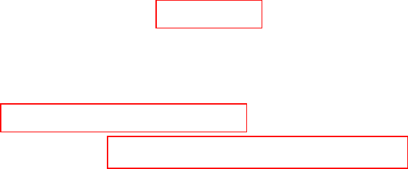
CHAPTER FOUR SOLUTIONS
Engineering Circuit Analysis, 6th Edition Copyright ©2002 McGraw-Hill, Inc. All Rights Reserved.
26. We define a clockwise mesh current i3 in the upper right mesh, a clockwise mesh
current i1 in the lower left mesh, and a clockwise mesh current i2 in the lower right
mesh.
MESH 1: -6 + 6 i1 - 2 = 0 [1]
MESH 2: 2 + 15 i2 – 12 i3 – 1.5 = 0 [2]
MESH 3: i3 = 0.1 vx [3]
Eq. [1] may be solved directly to obtain i1 = 1.333 A.
It would help in the solution of Eqs. [2] and [3] if we could express the dependent
source controlling variable vx in terms of mesh currents. Referring to the circuit
diagram, we see that vx = (1)( i1) = i1, so Eq. [3] reduces to
i3 = 0.1 vx = 0.1 i1 = 133.3 mA.
As a result, Eq. [1] reduces to i2 = [-0.5 + 12(0.1333)]/ 15 = 73.31 mA.

CHAPTER FOUR SOLUTIONS
Engineering Circuit Analysis, 6th Edition Copyright ©2002 McGraw-Hill, Inc. All Rights Reserved.
27. (a) Define a mesh current i2 in the second mesh. Then KVL allows us to write:
MESH 1: -9 + R i1 + 47000 i1 – 47000 i2 = 0 [1]
MESH 2: 67000 i2 – 47000 i1 – 5 = 0 [2]
Given that i1 = 1.5 mA, we may solve Eq. [2] to find that
mA 1.127 mA
67
47(1.5) 5
2=
+
=i
and so
3-
101.5
47(1.127) 47(1.5) - 9
×
+
=R = -5687 Ω.
(b) This value of R is unique; no other value will satisfy both Eqs. [1] and [2].

CHAPTER FOUR SOLUTIONS
Engineering Circuit Analysis, 6th Edition Copyright ©2002 McGraw-Hill, Inc. All Rights Reserved.
28. Define three clockwise mesh currents i1, i2 and i3. The bottom 1-kΩ resistor can be
ignored, as no current flows through it.
MESH 1: -4 + (2700 + 1000 + 5000) i1 – 1000 i2 = 0 [1]
MESH 2: (1000 + 1000 + 4400 + 3000) i2 – 1000 i1 – 4400 i3 + 2.2 – 3 = 0 [2]
MESH 3: (4400 + 4000 + 3000) i3 - 4400 i2 – 1.5 = 0 [3]
Combining terms,
8700 i1 – 1000 i2 = 4 [1]
–1000 i1 + 9400 i2 – 4400 i3 = 0.8 [2]
– 4400 i2 + 11400 i3 = 1.5 [3]
Solving,
i1 = 487.6 mA, i2 = 242.4 mA and i3 = 225.1 mA.
The power absorbed by each resistor may now be calculated:
P5k = 5000 (i1)2 = 1.189 mW
P2.7k = 2700 (i1)2 = 641.9 µW
P1ktop = 1000 (i1 – i2)2 = 60.12 µW
P1kmiddle = 1000 (i2)2 = 58.76 µW
P1kbottom = 0 = 0
P4.4k = 4400 (i2 – i3)2 = 1.317 µW
P3ktop = 3000 (i3)2 = 152.0 µW
P4k = 4000 (i3)2 = 202.7 µW
P3kbottom = 3000 (i2)2 = 176.3 µW
Check: The sources supply a total of
4(487.6) + (3 – 2.2)(242.4) + 1.5(225.1) = 2482 µW.
The absorbed powers add to 2482 µW.
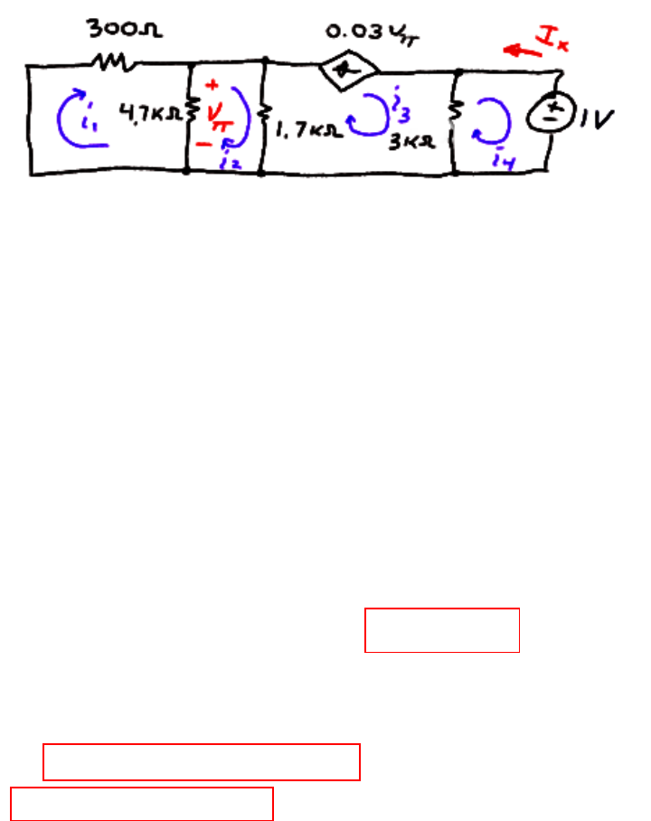
CHAPTER FOUR SOLUTIONS
Engineering Circuit Analysis, 6th Edition Copyright ©2002 McGraw-Hill, Inc. All Rights Reserved.
29. (a) We begin by naming four mesh currents as depicted below:
Proceeding with mesh analysis, then, keeping in mind that Ix = -i4,
MESH 1: (4700 + 300) i1 - 4700 i2 = 0 [1]
MESH 2: (4700 + 1700) i2 – 4700 i1 – 1700 i3 = 0 [2]
Since we have a current source on the perimeter of mesh 3, we do not require a KVL
equation for that mesh. Instead, we may simply write
i3 = -0.03 vπ [3a] where vπ = 4700(i1 – i2) [3b]
MESH 4: 3000 i4 – 3000 i3 + 1 = 0 [4]
Simplifying and combining Eqs. 3a and 3b,
5000 i1 – 4700 i2 = 0
–4700 i1 + 6400 i2 – 1700 i3 = 0
–141 i1 + 141 i2 – i3 = 0
– 3000 i3 + 3000 i4 = –1
Solving, we find that i4 = -333.3 mA, so Ix = 333.3 µA.
(b) At node “π” : 0.03 vπ = vπ / 300 + vπ / 4700 + vπ /1700
Solving, we find that vπ = 0, therefore no current flows through the dependent source.
Hence, Ix = 333.3 µA as found in part (a).
(c) Vs/ Ix has units of resistance. It can be thought of as the resistance “seen” by the
voltage source Vs…. more on this in Chap. 5….
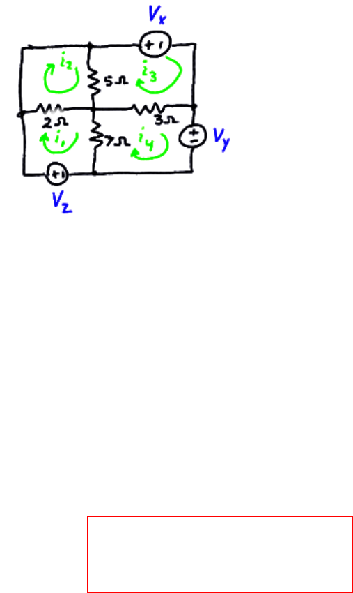
CHAPTER FOUR SOLUTIONS
Engineering Circuit Analysis, 6th Edition Copyright ©2002 McGraw-Hill, Inc. All Rights Reserved.
30. We begin by naming each mesh and the three undefined voltage sources as shown
below:
MESH 1: –Vz + 9i1 – 2i2 – 7i4 = 0
MESH 2: –2i1 + 7i2 – 5i3 = 0
MESH 3: Vx – 5i2 + 8i3 – 3i4 = 0
MESH 4: Vy – 7i1 – 3i3 + 10i4 = 0
Rearranging and setting i1 – i2 = 0, i2 – i3 = 0, i1 – i4 = 0 and i4 – i3 = 0,
9i1 - 2i2 -7i4 = Vz
-2i1 + 7i2 - 5i3 = 0
-5i2 + 8i3 – 3i4 = - Vx
-7i1 -3i3 + 10i4 = - Vy
Since i1 = i2 = i3 = i4, these equations produce:
V
z = 0
0 = 0
-V
x = 0
-V
y = 0
This is a unique solution. Therefore,
the request that nonzero values be
found cannot be satisfied.

CHAPTER FOUR SOLUTIONS
Engineering Circuit Analysis, 6th Edition Copyright ©2002 McGraw-Hill, Inc. All Rights Reserved.
31. The “supermesh” concept is not required (or helpful) in solving this problem, as there
are no current sources shared between meshes. Starting with the left-most mesh and
moving right, we define four clockwise mesh currents i1, i2, i3 and i4. By inspection,
we see that i1 = 2 mA.
MESH 2: -10 + 5000i2 + 4 + 1000i3 = 0 [1]
MESH 3: -1000i3 + 6 + 10,000 – 10,000i4 = 0 [2]
MESH 4: i4 = -0.5i2 [3]
Reorganising, we find
5000 i2 + 1000 i3 = 6 [1]
9000 i3 – 10,000 i4 = -6 [2]
0.5 i2 + i4 = 0 [3]
We could either subtitute Eq. [3] into Eq. [2] to reduce the number of equations, or
simply go ahead and solve the system of Eqs. [1-3]. Either way, we find that
i1 = 2 mA, i2 = 1.5 mA, i3 = -1.5 mA and i4 = -0.75 mA.
The power generated by each source is:
P2mA = 5000(i1 – i2)(i1) = 5 mW
P4V = 4 (-i2) = -6 mW
P6V = 6 (-i3) = 9 mW
PdepV = 1000 i3 (i3 – i2) = 4.5 mW
PdepI = 10,000(i3 – i4)(0.5 i2) = -5.625 mW
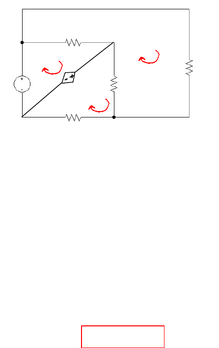
CHAPTER FOUR SOLUTIONS
Engineering Circuit Analysis, 6th Edition Copyright ©2002 McGraw-Hill, Inc. All Rights Reserved.
32. This circuit does not require the supermesh technique, as it does not contain any
current sources. Redrawing the circuit so its planar nature and mesh structure are
clear,
MESH 1: -20 + 2 i1 – 2 i2 + 2.5 iA = 0 [1]
MESH 2: 2 i2 + 3 i2 – 3 i3 + 2 i2 – 2 i1 = 0 [2]
MESH 3: -2.5 iA + 7 i3 – 3 i2 = 0 [3]
Combining terms and making use of the fact that iA = - i3,
2 i1 – 2 i2 – 2.5 i3 = 20 [1]
-2 i1 + 7i2 – 3 i3 = 0 [2]
–3 i2 + 9.5 i3 = 0 [3]
Solving, i1 = 18.55 A, i2 = 6.129 A, and i3 = 1.935 A. Since iA = - i3,
iA = -1.935 A.
20 V 2.5 iA
2 Ω
4 Ω
2 Ω
iA →
i2
i3
i1
•
•
3 Ω
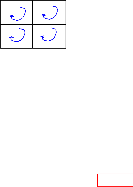
CHAPTER FOUR SOLUTIONS
Engineering Circuit Analysis, 6th Edition Copyright ©2002 McGraw-Hill, Inc. All Rights Reserved.
33. Define four mesh currents
By inspection, i1 = -4.5 A.
We form a supermesh with meshes 3 and 4 as defined above.
MESH 2: 2.2 + 3 i2 + 4 i2 + 5 – 4 i3 = 0 [1]
SUPERMESH: 3 i4 + 9 i4 – 9 i1 + 4 i3 – 4 i2 + 6 i3 + i3 – 3 = 0 [2]
Supermesh KCL equation: i4 - i3 = 2 [3]
Simplifying and combining terms, we may rewrite these three equations as:
7 i2 – 4 i3 = -7.2 [1]
-4 i2 + 11 i3 + 12 i4 = -37.5 [2]
- i3 + i4 = 2 [3]
Solving, we find that i2 = -2.839 A, i3 = -3.168 A, and i4 = -1.168 A.
The power supplied by the 2.2-V source is then 2.2 (i1 – i2) = -3.654 W.
i1 i2
i4
i3
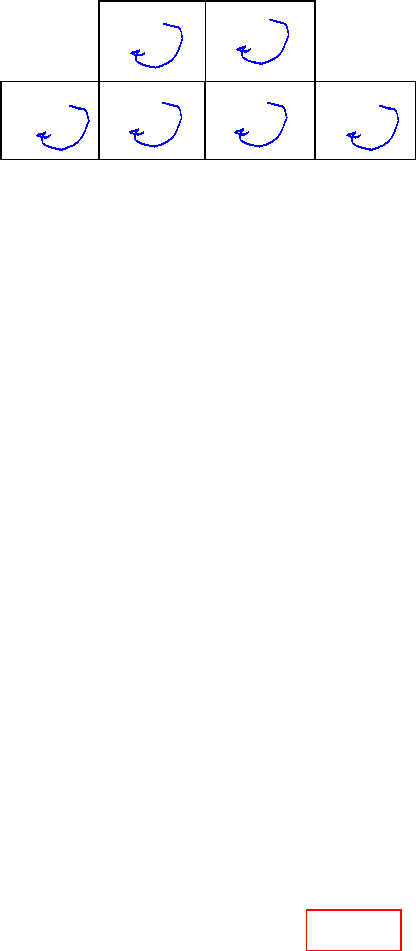
CHAPTER FOUR SOLUTIONS
Engineering Circuit Analysis, 6th Edition Copyright ©2002 McGraw-Hill, Inc. All Rights Reserved.
34. We begin by defining six mesh currents as depicted below:
• We form a supermesh with meshes 1 and 2 since they share a current source.
• We form a second supermesh with meshes 3 and 4 since they also share a current
source.
1, 2 Supermesh:
(4700 + 1000 + 10,000) i1 – 2200 i5 + (2200 + 1000 + 4700) i2 – 1000 i3 = 0 [1]
3, 4 Supermesh:
(4700 + 1000 + 2200) i3 – 1000 i2 – 2200 i6 + (4700 + 10,000 + 1000) i4 = 0 [2]
MESH 5: (2200 + 4700) i5 – 2200 i2 + 3.2 – 1.5 = 0 [3]
MESH 6: 1.5 + (4700 + 4700 + 2200) c – 2200 i3 = 0 [4]
1, 2 Supermesh KCL equation: i1 – i2 = 3×10⁻³ [5]
3, 4 Supermesh KCL equation: i4 – i3 = 2×10⁻³ [6]
We can simplify these equations prior to solution in several ways. Choosing to retain
six equations,
15,700 i1 + 7900 i2 - 1000 i3 -2200 i5 = 0 [1]
- 1000 i2 + 7900 i3 + 15,700 i4 -2200 i6 = 0 [2]
- 2200 i2 + 6900 i5 = -1.7 [3]
- 2200 i3 + 11,600 i6 = -1.5 [4]
i1 – i2 = 3×10⁻³ [5]
- i3 + i4 = 2×10⁻³ [6]
Solving, we find that i4 = 540.8 mA. Thus, the voltage across the 2-mA source is
(4700 + 10,000 + 1000) (540.8×10⁻⁶) = 8.491 V
i5 i6
i3 i2
i1 i4

CHAPTER FOUR SOLUTIONS
Engineering Circuit Analysis, 6th Edition Copyright ©2002 McGraw-Hill, Inc. All Rights Reserved.
35. We define a mesh current ia in the left-hand mesh, a mesh current i1 in the top right
mesh, and a mesh current i2 in the bottom right mesh.
The left-most mesh can be analysed separately to determine the controlling voltage va,
as KCL assures us that no current flows through either the 1-Ω or 6-Ω resistor.
Thus, -1.8 + 3 ia – 1.5 + 2 ia = 0, which may be solved to find ia = 0.66 A. Hence,
va = 3 ia = 1.98 V.
Forming one supermesh from the remaining two meshes, we may write:
-3 + 2.5 i1 + 3 i2 + 4 i2 = 0
and the supermesh KCL equation: i2 – i1 = 0.05 va = 0.05(1.98) = 99×10-3
Thus, we have two equations to solve:
2.5 i1 + 7 i2 = 3
-i1 + i2 = 99×10-3
Solving, we find that i1 = 242.8 mA and the voltage across the 2.5-Ω resistor
(arbitrarily assuming the left terminal is the “+” reference) is 2.5 i1 = 607 mV.

CHAPTER FOUR SOLUTIONS
Engineering Circuit Analysis, 6th Edition Copyright ©2002 McGraw-Hill, Inc. All Rights Reserved.
36. UNDEFINED RESISTOR VALUE IN FIGURE. Set to 10 mΩ.
There are only three meshes in this circuit, as the botton 22-mΩ resistor is not
connected connected at its left terminal. Thus, we define three mesh currents, i1, i2,
and i3, beginning with the left-most mesh.
We next create a supermesh from meshes 1 and 2 (note that mesh 3 is independent,
and can be analysed separately).
Thus, -11.8 + 10×10-3 i1 + 22×10-3 i2 + 10×10-3 i2 + 17×10-3 i1 = 0
and applying KCL to obtain an equation containing the current source,
i1 – i2 = 100
Combining terms and simplifying, we obtain
27×10-3 i1 + 32×10-3 i2 = 11.8
i1 – i2 = 100
Solving, we find that i1 = 254.2 A and i2 = 154.2 A.
The final mesh current is easily found: i3 = 13×103/ (14 + 11.6 + 15) = 320.2 A.

CHAPTER FOUR SOLUTIONS
Engineering Circuit Analysis, 6th Edition Copyright ©2002 McGraw-Hill, Inc. All Rights Reserved.
37. MESH 1: -7 + i1 – i2 = 0 [1]
MESH 2: i2 – i1 + 2i2 + 3i2 – 3i3 = 0 [2]
MESH 3: 3i3 – 3i2 + xi3 +2i3 – 7 = 0 [3]
Grouping terms, we find that
i1 – i2 = 7 [1]
-i1 + 6i2 – 3i3 = 0 [2]
-3i2 + (5 + x)i3 = 7 [3]
This, unfortunately, is four unknowns but only three equations. However, we have not
yet made use of the fact that we are trying to obtain i2 = 2.273 A. Solving these “four”
equations, we find that
x = (7 + 3 i2 – 5 i3)/ i3 = 4.498 Ω.
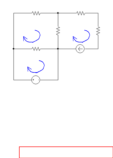
CHAPTER FOUR SOLUTIONS
Engineering Circuit Analysis, 6th Edition Copyright ©2002 McGraw-Hill, Inc. All Rights Reserved.
7 V
7 A
1 Ω
2 Ω
3 Ω
300 mΩ
2 Ω
i2 i3
i1
38. We begin by redrawing the circuit as instructed, and define three mesh currents:
By inspection, i3 = 7 A.
MESH 1: -7 + i1 – i2 = 0 or i1 – i2 = 7 [1]
MESH 2: (1 + 2 + 3) i2 – i1 –3(7) = 0 or -i1 + 6i2 = 21 [2]
There is no need for supermesh techniques for this situation, as the only current
source lies on the outside perimeter of a mesh- it is not shared between meshes.
Solving, we find that i1 = 12.6 A, i2 = 5.6 A and i3 = 7 A.

CHAPTER FOUR SOLUTIONS
Engineering Circuit Analysis, 6th Edition Copyright ©2002 McGraw-Hill, Inc. All Rights Reserved.
39. (a) We are asked for a voltage, and have one current source and one voltage source.
Nodal analysis is probably best then- the nodes can be named so that the desired
voltage is a nodal voltage, or, at worst, we have one supernode equation to solve.
Name the top left node “1” and the top right node “x”; designate the bottom node as
the reference terminal. Next, form a supernode with nodes “1” and “x.”
At the supernode: 11 = v1/ 2 + vx/ 9 [1]
and the KVL Eqn: v1 – vx = 22 [2]
Rearranging, 11(18) = 9 v1 + 2 vx [1]
22 = v1 – vx [2]
Solving, vx = 0
(b) We are asked for a voltage, and so may suspect that nodal analysis is preferrable;
with two current sources and only one voltage source (easily dealt with using the
supernode technique), nodal analysis does seem to have an edge over mesh analysis
here.
Name the top left node “x,” the top right node “y” and designate the bottom node as
the reference node. Forming a supernode from nodes “x” and “y,”
At the supernode: 6 + 9 = vx / 10 + vy/ 20 [1]
and the KVL Eqn: vy – vx = 12 [2]
Rearranging, 15(20) = 2 vx + vy [1]
and 12 = - vx + vy [2]
Solving, we find that vx = 96 V.
(c) We are asked for a voltage, but would have to subtract two nodal voltages (not
much harder than invoking Ohm’s law). On the other hand, the dependent current
source depends on the desired unknown, which would lead to the need for another
equation if invoking mesh analysis. Trying nodal analysis,
0.1 vx = (v1 – 50) / 2 + vx / 4 [1]
referring to the circuit we see that vx = v1 – 100. Rearranging so that we may
eliminate v1 in Eq. [1], we obtain v1 = vx + 100. Thus, Eq. [1] becomes
0.1 vx = (vx + 100 – 50)/ 2 + vx / 4
and a little algebra yields vx = -38.46 V.
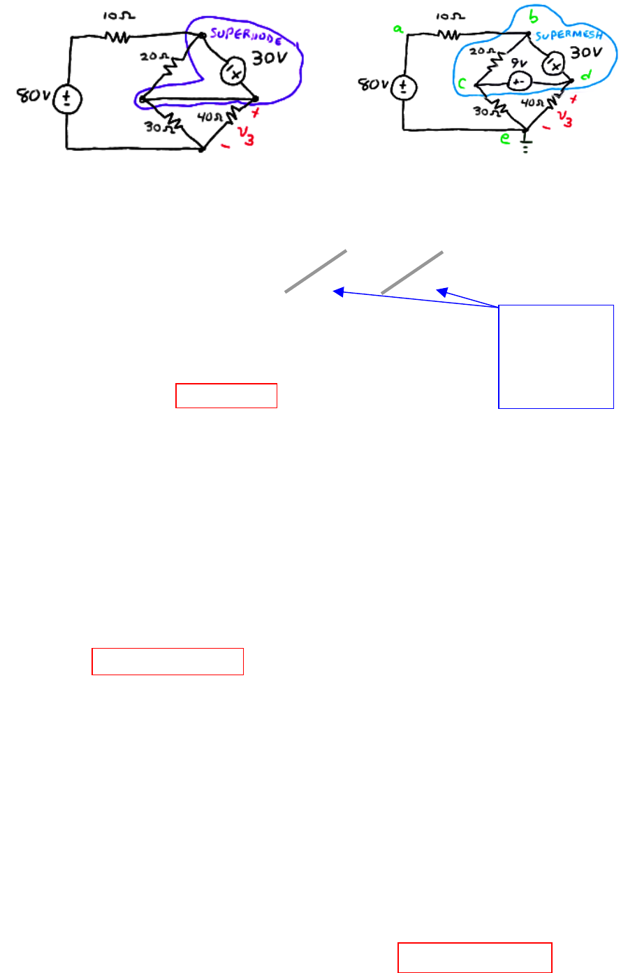
CHAPTER FOUR SOLUTIONS
Engineering Circuit Analysis, 6th Edition Copyright ©2002 McGraw-Hill, Inc. All Rights Reserved.
Both ends of the
resistor are
connected to the
supernode, so we
could actually just
ignore it…
(a) (b)
Ref.
v1
40.
(a) We begin by noting that it is a voltage that is required; no current values are
requested. This is a three-mesh circuit, or a four-node circuit, depending on your
perspective. Either approach requires three equations…. Except that applying the
supernode technique reduces the number of needed equations by one.
At the 1, 3 supernode:
0 = (v1 – 80)/ 10 + (v1 – v3)/ 20 + (v3 – v1)/ 20 + v3/ 40 + v3/ 30
and v3 - v1 = 30
We simplify these two equations and collect terms, yielding
0.1 v1 + 0.05833 v3 = 8
- v1 + v3 = 30
Solving, we find that v3 = 69.48 V
(b) Mesh analysis would be straightforward, requiring 3 equations and a (trivial)
application of Ohm’s law to obtain the final answer. Nodal analysis, on the other
hand, would require only two equations, and the desired voltage will be a nodal
voltage.
At the b, c, d supernode: 0 = (vb – 80)/ 10 + vd/ 40 + vc/ 30
and: vd – vb = 30 vc – vd = 9
Simplify and collect terms: 0.1 vb + 0.03333 vc + 0.025 vd = 80
-vb + vd = 30
vc - vd = 9
Solving, vd (= v3) = 67.58 V
(c) We are now faced with a dependent current source whose value depends on a
mesh current. Mesh analysis in this situation requires 1 supermesh, 1 KCL equation
and Ohm’s law. Nodal analysis requires 1 supernode, 1 KVL equation, 1 other nodal
equation, and one equation to express i1 in terms of nodal voltages. Thus, mesh
analysis has an edge here. Define the left mesh as “1,” the top mesh as “2”, and the
bottom mesh as “3.”
Mesh 1: -80 + 10 i1 + 20 i1 – 20 i2 + 30 i1 – 30 i3 = 0
2, 3 supermesh: 20 i2 – 20 i1 – 30 + 40 i3 + 30 i3 – 30 i1 = 0
and: i2 - i3 = 5 i1
Rewriting, 60 i1 – 20 i2 – 30 i3 = 80
-50 i1 + 20 i2 + 70 i3 = 30
5 i1 – i2 + i3 = 0
Solving, i3 = 4.727 A so v3 = 40 i3 = 189 V.

CHAPTER FOUR SOLUTIONS
Engineering Circuit Analysis, 6th Edition Copyright ©2002 McGraw-Hill, Inc. All Rights Reserved.
41. This circuit consists of 3 meshes, and no dependent sources. Therefore 3 simultaneous
equations and 1 subtraction operation would be required to solve for the two desired
currents. On the other hand, if we use nodal analysis, forming a supernode about the
30-V source would lead to 5 – 1 – 1 = 3 simulataneous equations as well, plus several
subtraction and division operations to find the currents. Thus, mesh analysis has a
slight edge here.
Define three clockwise mesh currents: ia in the left-most mesh, ib in the top right
mesh, and ic in the bottom right mesh. Then our mesh equations will be:
Mesh a: -80 + (10 + 20 + 30) ia – 20 ib – 30 ic = 0 [1]
Mesh b: -30 + (12 + 20) ib – 12 ic – 20 ia = 0 [2]
Mesh c: (12 + 40 + 30) ic – 12 ib – 30 ia = 0 [3]
Simplifying and collecting terms,
60 ia – 20 ib – 30 ic = 80 [1]
-20 ia + 32 ib – 12 ic = 30 [2]
-30 ia – 12 ib + 82 ic = 0 [3]
Solving, we find that ia = 3.549 A, ib = 3.854 A, and ic = 1.863 A. Thus,
i1 = ia = 3.549 A and i2 = ia – ic = 1.686 A.

CHAPTER FOUR SOLUTIONS
Engineering Circuit Analysis, 6th Edition Copyright ©2002 McGraw-Hill, Inc. All Rights Reserved.
42. Approaching this problem using nodal analysis would require 3 separate nodal
equations, plus one equation to deal with the dependent source, plus subtraction and
division steps to actually find the current i10. Mesh analysis, on the other hand, will
require 2 mesh/supermesh equations, 1 KCL equation, and one subtraction step to find
i10. Thus, mesh analysis has a clear edge. Define three clockwise mesh currents: i1 in
the bottom left mesh, i2 in the top mesh, and i3 in the bottom right mesh.
MESH 1: i1 = 5 mA by inspection [1]
SUPERMESH: i1 – i2 = 0.4 i10
i1 – i2 = 0.4(i3 – i2)
i1 – 0.6 i2 – 0.4 i3 = 0 [2]
MESH 3: -5000 i1 – 10000 i2 + 35000 i3 = 0 [3]
Simplify: 0.6 i2 + 0.4 i3 = 5×10⁻³ [2]
-10000 i2 + 35000 i3 = 25 [3]
Solving, we find i2 = 6.6 mA and i3 = 2.6 mA. Since i10 = i3 – i2, we find that
i10 = -4 mA.

CHAPTER FOUR SOLUTIONS
Engineering Circuit Analysis, 6th Edition Copyright ©2002 McGraw-Hill, Inc. All Rights Reserved.
43. For this circuit problem, nodal analysis will require 3 simultaneous nodal equations,
then subtraction/ division steps to obtain the desired currents. Mesh analysis requires
1 mesh equation, 1 supermesh equation, 2 simple KCL equations and one subtraction
step to determine the currents. If either technique has an edge in this situation, it’s
probably mesh analysis. Thus, define four clockwise mesh equations: ia in the bottom
left mesh, ib in the top left mesh, ic in the top right mesh, and id in the bottom right
mesh.
At the a, b, c supermesh: -100 + 6 ia + 20 ib + 4 ic + 10 ic – 10 id = 0 [1]
Mesh d: 100 + 10 id – 10 ic + 24 id = 0 [2]
KCL: - ia + ib = 2 [3]
and - ib + ic = 3 i3 = 3 ia [4]
Collecting terms & simplifying,
6 ia + 20 ib + 14 ic – 10 id = 100 [1]
-10 ic + 34 id = -100 [2]
- ia + ib = 2 [3]
-3 ia – ib + ic = 0 [4]
Solving,
ia = 0.1206 A, ib = 2.121 A, ic = 2.482 A, and id = -2.211 A. Thus,
i3 = ia = 120.6 mA and i10 = ic – id = 4.693 A.
CHAPTER FOUR SOLUTIONS
Engineering Circuit Analysis, 6th Edition Copyright ©2002 McGraw-Hill, Inc. All Rights Reserved.
44. With 7 nodes in this circuit, nodal analysis will require the solution of three
simultaneous nodal equations (assuming we make use of the supernode technique)
and one KVL equation. Mesh analysis will require the solution of three simultaneous
mesh equations (one mesh current can be found by inspection), plus several
subtraction and multiplication operations to finally determine the voltage at the
central node. Either will probably require a comparable amount of algebraic
manoeuvres, so we go with nodal analysis, as the desired unknown is a direct result of
solving the simultaneous equations. Define the nodes as:
NODE 1: -2×10-3 = (v1 – 1.3)/ 1.8×10³ → v1 = -2.84 V.
2, 4 Supernode:
2.3×10-3 = (v2 – v5)/ 1x10³ + (v4 – 1.3)/ 7.3×10³ + (v4 – v5)/ 1.3×10³ + v4/ 1.5×10³
KVL equation: -v2 + v4 = 5.2
Node 5: 0 = (v5 – v2)/ 1x10³ + (v5 – v4)/ 1.3x10³ + (v5 – 2.6)/ 6.3x10³
Simplifying and collecting terms,
14.235 v2 + 22.39 v4 – 25.185 v5 = 35.275 [1]
-v2 + v4 = 5.2 [2]
-8.19 v2 – 6.3 v4 + 15.79 v5 = 3.38 [3]
Solving, we find the voltage at the central node is v4 = 3.460 V.
v1 v2
v3
v4 v5
v6
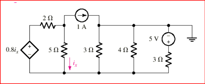
CHAPTER FOUR SOLUTIONS
Engineering Circuit Analysis, 6th Edition Copyright ©2002 McGraw-Hill, Inc. All Rights Reserved.
45. Mesh analysis yields current values directly, so use that approach. We therefore
define four clockwise mesh currents, starting with i1 in the left-most mesh, then i2, i3
and i4 moving towards the right.
Mesh 1: -0.8ix + (2 + 5) i1 – 5 i2 = 0 [1]
Mesh 2: i2 = 1 A by inspection [2]
Mesh 3: (3 + 4) i3 – 3(1) – 4(i4) = 0 [3]
Mesh 4: (4 + 3) i4 – 4 i3 – 5 = 0 [4]
Simplify and collect terms, noting that ix = i1 – i2 = i1 – 1
-0.8(i1 – 1) + 7 i1 – 5(1) = 0 yields i1 = 677.4 mA
Thus, [3] and [4] become: 7 i3 – 4 i4 = 3 [3]
-4 i3 + 7 i4 = 5 [4]
Solving, we find that i3 = 1.242 A and i4 = 1.424 A. A map of individual branch
currents can now be drawn:
↑
677.4 mA
677.4 mA
→
-322.6 mA
↓ -242.0 mA
↓
↑
182.0 mA
↑
-1.424 A

CHAPTER FOUR SOLUTIONS
Engineering Circuit Analysis, 6th Edition Copyright ©2002 McGraw-Hill, Inc. All Rights Reserved.
46. If we choose to perform mesh analysis, we require 2 simultaneous equations (there are
four meshes, but one mesh current is known, and we can employ the supermesh
technique around the left two meshes). In order to find the voltage across the 2-mA
source we will need to write a KVL equation, however. Using nodal analysis is less
desirable in this case, as there will be a large number of nodal equations needed.
Thus, we define four clockwise mesh currents i1, i2, i3 and i4 starting with the left-
most mesh and moving towards the right of the circuit.
At the 1,2 supermesh: 2000 i1 + 6000 i2 – 3 + 5000 i2 = 0 [1]
and i1 – i2 = 2×10⁻³ [2]
by inspection, i4 = -1 mA. However, this as well as any equation for mesh
four are unnecessary: we already have two equations in two unknowns and i1 and i2
are sufficient to enable us to find the voltage across the current source.
Simplifying, we obtain 2000 i1 + 11000 i2 = 3 [1]
1000 i1 - 1000 i2 = 2 [2]
Solving, i1 = 1.923 mA and i2 = -76.92 µA.
Thus, the voltage across the 2-mA source (“+” reference at the top of the source) is
v = -2000 i1 – 6000 (i1 – i2) = -15.85 V.

CHAPTER FOUR SOLUTIONS
Engineering Circuit Analysis, 6th Edition Copyright ©2002 McGraw-Hill, Inc. All Rights Reserved.
47. Nodal analysis will require 2 nodal equations (one being a “supernode” equation), 1
KVL equation, and subtraction/division operations to obtain the desired current. Mesh
analysis simply requires 2 “supermesh” equations and 2 KCL equations, with the
desired current being a mesh current. Thus, we define four clockwise mesh currents
ia, ib, ic, id starting with the left-most mesh and proceeding to the right of the circuit.
At the a, b supermesh: -5 + 2 ia + 2 ib + 3 ib – 3 ic = 0 [1]
At the c, d supermesh: 3 ic – 3 ib + 1 + 4 id = 0 [2]
and ia - ib = 3 [3]
ic - id = 2 [4]
Simplifying and collecting terms, we obtain
2 ia + 5 ib – 3 ic = 5 [1]
-3 ib + 3 ic + 4 id = -1 [2]
ia - ib = 3 [3]
ic - id = 2 [4]
Solving, we find ia = 3.35 A, ib = 350 mA, ic = 1.15 A, and id = -850 mA. As i1 = ib,
i1 = 350 mA.

CHAPTER FOUR SOLUTIONS
Engineering Circuit Analysis, 6th Edition Copyright ©2002 McGraw-Hill, Inc. All Rights Reserved.
48. Define a voltage vx at the top node of the current source I2, and a clockwise mesh
current ib in the right-most mesh.
We want 6 W dissipated in the 6-Ω resistor, which leads to the requirement ib = 1 A.
Applying nodal analysis to the circuit,
I
1 + I2 = (vx – v1)/ 6 = 1
so our requirement is I1 + I2 = 1. There is no constraint on the value of v1 other than
we are told to select a nonzero value.
Thus, we choose I1 = I2 = 500 mA and v1 = 3.1415 V.

CHAPTER FOUR SOLUTIONS
Engineering Circuit Analysis, 6th Edition Copyright ©2002 McGraw-Hill, Inc. All Rights Reserved.
49. Inserting the new 2-V source with “+” reference at the bottom, and the new 7-mA
source with the arrow pointing down, we define four clockwise mesh currents i1, i2, i3,
i4 starting with the left-most mesh and proceeding towards the right of the circuit.
Mesh 1: (2000 + 1000 + 5000) i1 – 6000 i2 – 2 = 0 [1]
2, 3 Supermesh:
2 + (5000 + 5000 + 1000 + 6000) i2 – 6000 i1 + (3000 + 4000 + 5000) i3 – 5000 i4
= 0 [2]
and i2 - i3 = 7×10⁻³ [3]
Mesh 4: i4 = -1 mA by inspection [4]
Simplifying and combining terms,
8000 i1 – 6000 i2 = 2 [1]
1000 i2 – 1000 i3 = 7 [4]
-6000 i1 + 17000 i2 + 12000 i3 = -7 [2]
Solving, we find that
i1 = 2.653 A, i2 = 3.204 A, i3 = -3.796 A, i4 = -1 mA

CHAPTER FOUR SOLUTIONS
Engineering Circuit Analysis, 6th Edition Copyright ©2002 McGraw-Hill, Inc. All Rights Reserved.
50. Define node 1 as the top left node, and node 2 as the node joining the three 2-Ω
resistors. Place the “+” reference terminal of the 2-V source at the right. The right-
most 2-Ω resistor has therefore been shorted out. Applying nodal analysis then,
Node 1: -5 i1 = (v1 – v2)/ 2 [1]
Node 2: 0 = (v2 – v1)/ 2 + v2/ 2 + (v2 – 2)/ 2 [2]
and, i1 = (v2 – 2)/ 2 [3]
Simplifying and collecting terms,
v1 + v2 = 10 [1]
-v1 + 3 v2 = 2 [2]
Solving, we find that v1 = 3.143 V and v2 = 1.714 V.
Defining clockwise mesh currents ia, ib, ic, id starting with the left-most mesh and
proceeding right, we may easily determine that
ia = -5 i1 = 714.3 mA
ib = -142.9 mA
ic = i1 – 2 = -2.143 A
id = 3 + ic = 857.1 mA
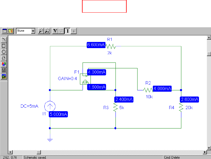
CHAPTER FOUR SOLUTIONS
Engineering Circuit Analysis, 6th Edition Copyright ©2002 McGraw-Hill, Inc. All Rights Reserved.
51. Hand analysis:
Define three clockwise mesh currents: i1 in the bottom left mesh, i2 in the top mesh,
and i3 in the bottom right mesh.
MESH 1: i1 = 5 mA by inspection [1]
SUPERMESH: i1 – i2 = 0.4 i10
i1 – i2 = 0.4(i3 – i2)
i1 – 0.6 i2 – 0.4 i3 = 0 [2]
MESH 3: -5000 i1 – 10000 i2 + 35000 i3 = 0 [3]
Simplify: 0.6 i2 + 0.4 i3 = 5×10⁻³ [2]
-10000 i2 + 35000 i3 = 25 [3]
Solving, we find i2 = 6.6 mA and i3 = 2.6 mA. Since i10 = i3 – i2, we find that
i10 = -4 mA.
PSpice simulation results:
Summary: The current entering the right-hand node of the 10-kΩ resistor R2 is
equal to 4.000 mA. Since this current is –i10, i10 = -4.000 mA as found by hand.
i10
→
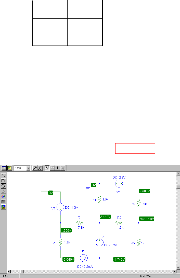
CHAPTER FOUR SOLUTIONS
Engineering Circuit Analysis, 6th Edition Copyright ©2002 McGraw-Hill, Inc. All Rights Reserved.
52. Hand analysis:
Define the nodes as:
NODE 1: -2×10-3 = (v1 – 1.3)/ 1.8×10³ → v1 = -2.84 V.
2, 4 Supernode:
2.3×10-3 = (v2 – v5)/ 1x10³ + (v4 – 1.3)/ 7.3×10³ + (v4 – v5)/ 1.3×10³ + v4/ 1.5×10³
KVL equation: -v2 + v4 = 5.2
Node 5: 0 = (v5 – v2)/ 1x10³ + (v5 – v4)/ 1.3x10³ + (v5 – 2.6)/ 6.3x10³
Simplifying and collecting terms,
14.235 v2 + 22.39 v4 – 25.185 v5 = 35.275 [1]
-v2 + v4 = 5.2 [2]
-8.19 v2 – 6.3 v4 + 15.79 v5 = 3.38 [3]
Solving, we find the voltage at the central node is v4 = 3.460 V.
PSpice simulation results:
Summary: The voltage at the center node is found to be 3.460 V, which is in
agreement with our hand calculation.
v1 v2
v3
v4 v5
v6
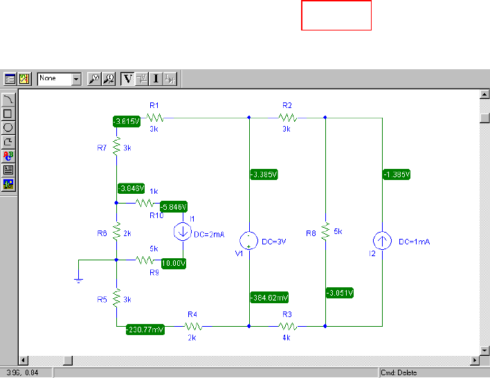
CHAPTER FOUR SOLUTIONS
Engineering Circuit Analysis, 6th Edition Copyright ©2002 McGraw-Hill, Inc. All Rights Reserved.
53. Hand analysis:
At the 1,2 supermesh: 2000 i1 + 6000 i2 – 3 + 5000 i2 = 0 [1]
and i1 – i2 = 2×10⁻³ [2]
by inspection, i4 = -1 mA. However, this as well as any equation for mesh
four are unnecessary: we already have two equations in two unknowns and i1 and i2
are sufficient to enable us to find the voltage across the current source.
Simplifying, we obtain 2000 i1 + 11000 i2 = 3 [1]
1000 i1 - 1000 i2 = 2 [2]
Solving, i1 = 1.923 mA and i2 = -76.92 µA.
Thus, the voltage across the 2-mA source (“+” reference at the top of the source) is
v = -2000 i1 – 6000 (i1 – i2) = -15.85 V.
PSpice simulation results:
Summary: Again arbitrarily selecting the “+” reference as the top node of the
2-mA current source, we find the voltage across it is –5.846 – 10 = -15.846 V, in
agreement with our hand calculation.
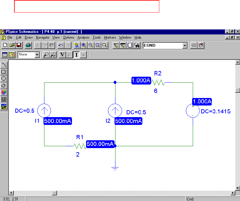
CHAPTER FOUR SOLUTIONS
Engineering Circuit Analysis, 6th Edition Copyright ©2002 McGraw-Hill, Inc. All Rights Reserved.
54. Hand analysis:
Define a voltage vx at the top node of the current source I2, and a clockwise mesh
current ib in the right-most mesh.
We want 6 W dissipated in the 6-Ω resistor, which leads to the requirement ib = 1 A.
Applying nodal analysis to the circuit,
I
1 + I2 = (vx – v1)/ 6 = 1
so our requirement is I1 + I2 = 1. There is no constraint on the value of v1 other than
we are told to select a nonzero value.
Thus, we choose I1 = I2 = 500 mA and v1 = 3.1415 V.
PSpice simulation results:
Summary: We see from the labeled schematic above that our choice for I1, I2 and
V1 lead to 1 A through the 6-Ω resistor, or 6 W dissipated in that resistor, as desired.
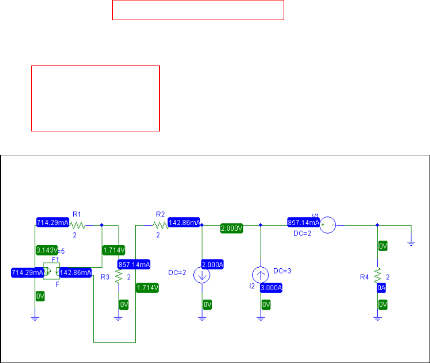
CHAPTER FOUR SOLUTIONS
Engineering Circuit Analysis, 6th Edition Copyright ©2002 McGraw-Hill, Inc. All Rights Reserved.
55. Hand analysis:
Define node 1 as the top left node, and node 2 as the node joining the three 2-Ω
resistors. Place the “+” reference terminal of the 2-V source at the right. The right-
most 2-Ω resistor has therefore been shorted out. Applying nodal analysis then,
Node 1: -5 i1 = (v1 – v2)/ 2 [1]
Node 2: 0 = (v2 – v1)/ 2 + v2/ 2 + (v2 – 2)/ 2 [2]
and, i1 = (v2 – 2)/ 2 [3]
Simplifying and collecting terms,
v1 + v2 = 10 [1]
-v1 + 3 v2 = 2 [2]
Solving, we find that v1 = 3.143 V and v2 = 1.714 V.
Defining clockwise mesh currents ia, ib, ic, id starting with the left-most mesh and
proceeding right, we may easily determine that
ia = -5 i1 = 714.3 mA
ib = -142.9 mA
ic = i1 – 2 = -2.143 A
id = 3 + ic = 857.1 mA
PSpice simulation results:
Summary: The simulation results agree with the hand calculations.
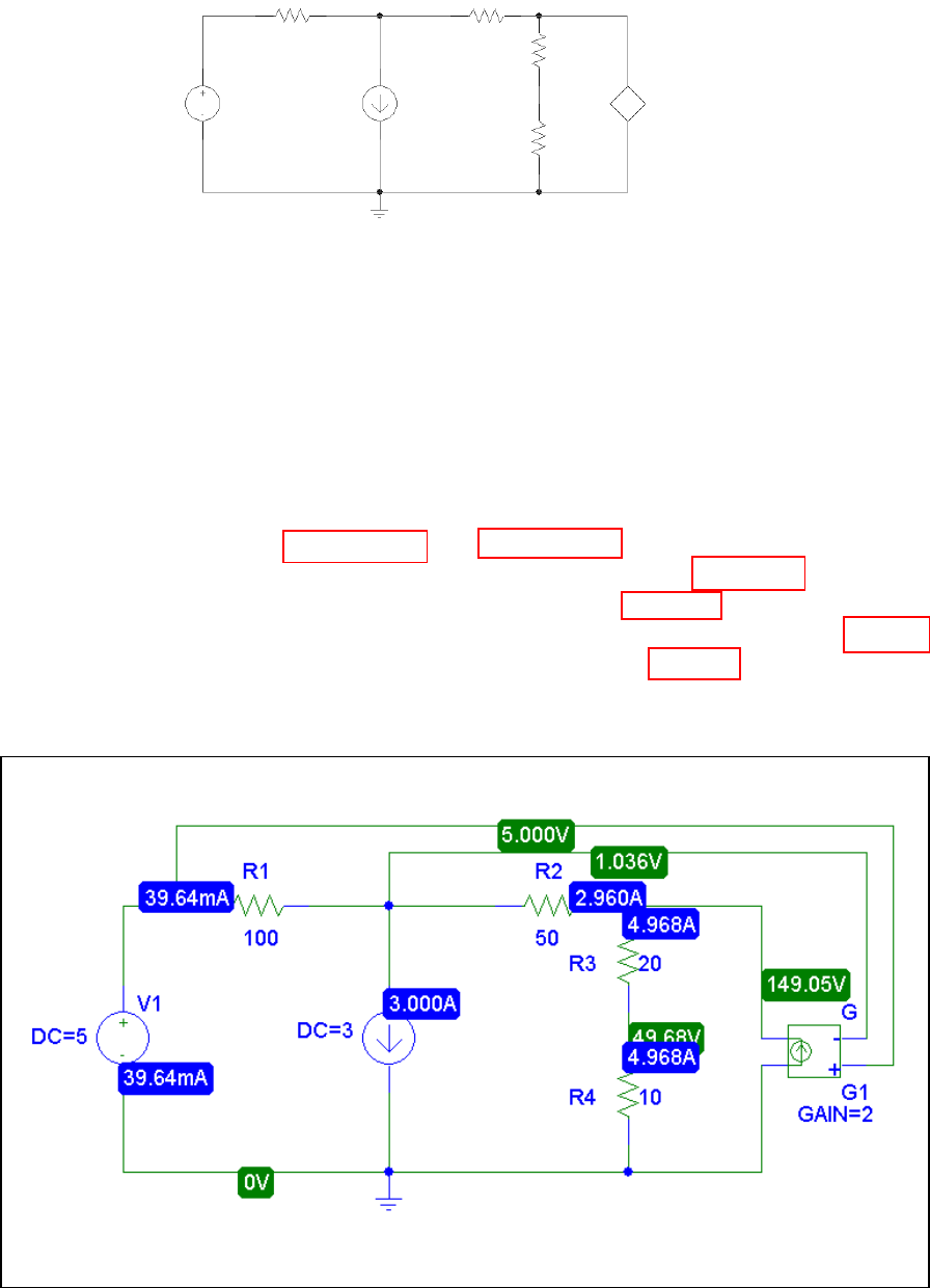
CHAPTER FOUR SOLUTIONS
Engineering Circuit Analysis, 6th Edition Copyright ©2002 McGraw-Hill, Inc. All Rights Reserved.
56. (a) One possible circuit configuration of many that would satisfy the requirements:
At node 1: -3 = (v1 – 5)/ 100 + (v1 – v2)/ 50 [1]
At node 2: 2 vx = (v2 – v1)/ 50 + v2/ 30 [2]
and, vx = 5 – v1 [3]
Simplifying and collecting terms,
150 v1 – 100 v2 = -14750 [1]
2970 v1 + 80 v2 = 15000 [2]
Solving, we find that v1 = 1.036 V and v2 = 149.1 V.
The current through the 100-Ω resistor is simply (5 – v1)/100 = 39.64 mA
The current through the 50-Ω resistor is (v1 – v2)/ 50 = -2.961 A,
and the current through the 20-Ω and 10-Ω series combination is v2/ 30 = 4.97 A.
Finally, the dependent source generates a current of 2 vx = 7.928 A.
(b) PSpice simulation results
Summary: The simulated results agree with the hand calculations.
↑
5 V 3 A 2 vx
100 Ω
50 Ω 20 Ω
10 Ω
+ vx -
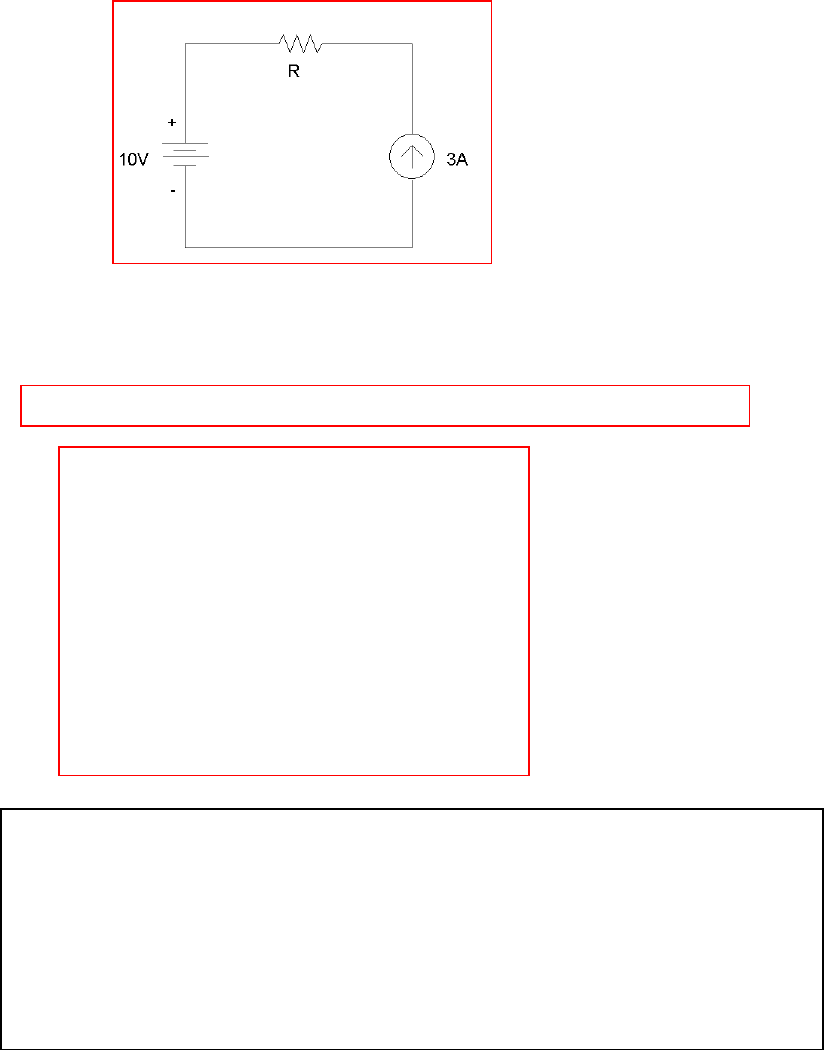
CHAPTER FOUR SOLUTIONS
Engineering Circuit Analysis, 6th Edition Copyright ©2002 McGraw-Hill, Inc. All Rights Reserved.
+ 5 V -
57. One possible solution of many:
Choose R so that 3R = 5; then the voltage across the current source will be 5 V, and
so will the voltage across the resistor R.
R = 5/3 Ω. To construct this from 1-Ω resistors, note that
5/3 Ω = 1 Ω + 2/3 Ω = 1 Ω + 1 Ω || 1Ω || 1Ω + 1Ω || 1Ω || 1Ω
* Solution to Problem 4.57
.OP
V1 1 0 DC 10
I1 0 4 DC 3
R1 1 2 1
R2 2 3 1
R3 2 3 1
R4 2 3 1
R5 3 4 1
R6 3 4 1
R7 3 4 1
.END
**** SMALL SIGNAL BIAS SOLUTION TEMPERATURE = 27.000 DEG C
******************************************************************************
NODE VOLTAGE NODE VOLTAGE NODE VOLTAGE NODE VOLTAGE
( 1) 10.0000 ( 2) 7.0000 ( 3) 6.0000 ( 4) 5.0000
VOLTAGE SOURCE CURRENTS
NAME CURRENT
V1 -3.000E+00
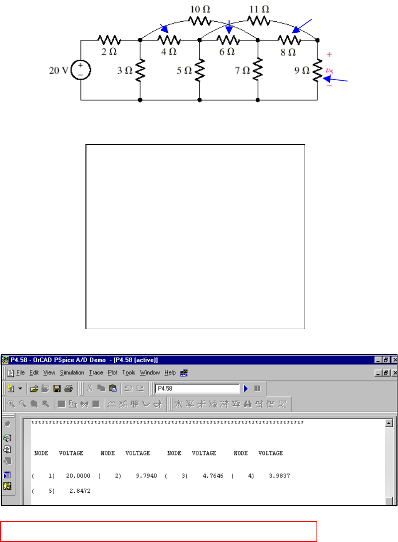
CHAPTER FOUR SOLUTIONS
Engineering Circuit Analysis, 6th Edition Copyright ©2002 McGraw-Hill, Inc. All Rights Reserved.
58. We first name each node, resistor and voltage source:
We next write an appropriate input deck for SPICE:
And obtain the following output:
We see from this simulation result that the voltage v5 = 2.847 V.
1 2 3
4
5
0
R1
R2
R3
R4
R5
R6
R7
R8
R9
R10
V1
* Solution to Problem 4.58
.OP
V1 1 0 DC 20
R1 1 2 2
R2 2 0 3
R3 2 3 4
R4 2 4 10
R5 3 0 5
R6 3 4 6
R7 3 5 11
R8 4 0 7
R9 4 5 8
R10 5 0 9
.END
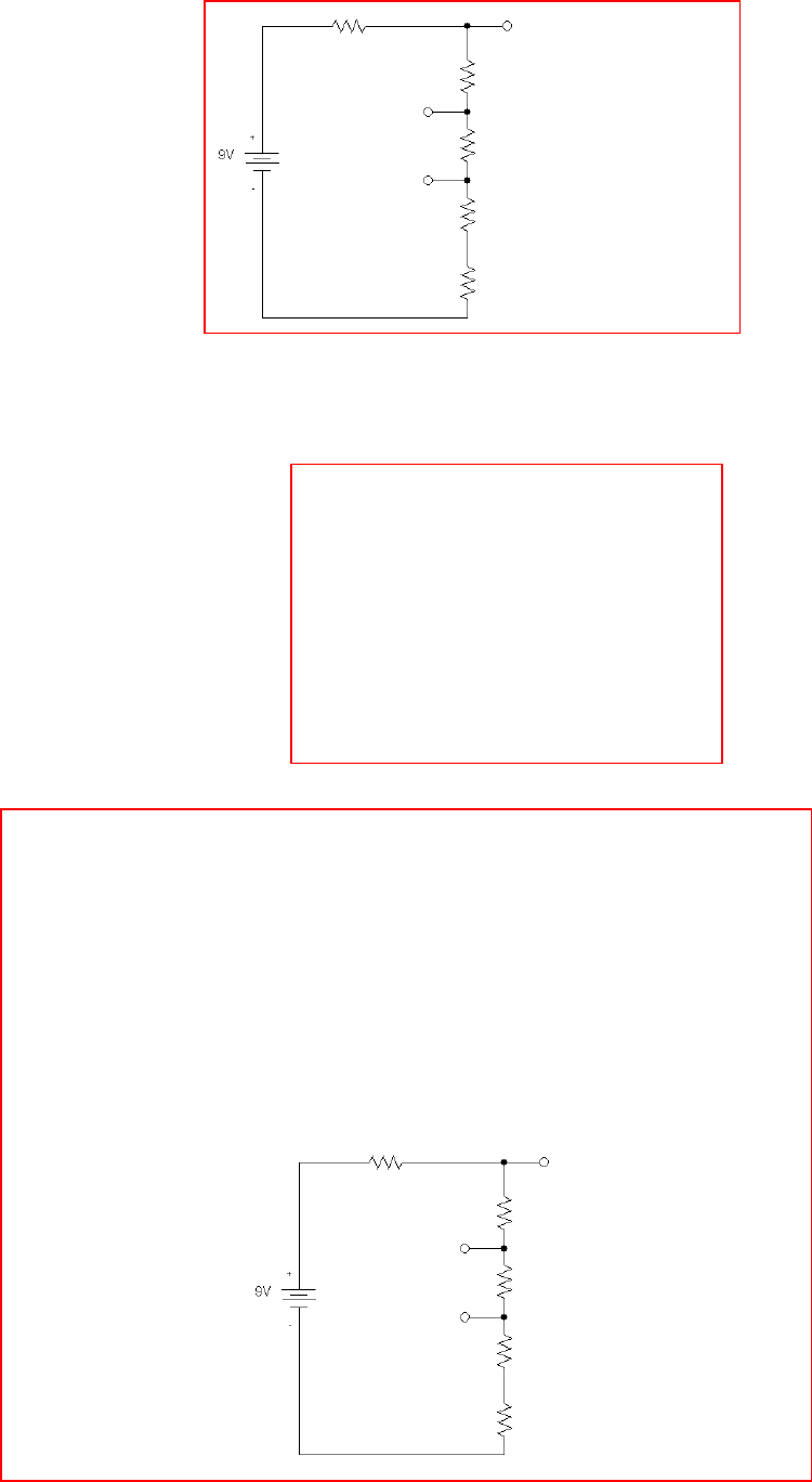
CHAPTER FOUR SOLUTIONS
Engineering Circuit Analysis, 6th Edition Copyright ©2002 McGraw-Hill, Inc. All Rights Reserved.
v1
v2
v3
All resistors are
1 Ω, except R1,
which represents
5 1-Ω resistors
in series.
59. One possible solution of many:
Verify: v1 = 9(4/9) = 4 V
v2 = 9(3/9) = 3 V
v3 = 9(2/9) = 2 V
SPICE INPUT DECK:
* Solution to Problem 4.59
.OP
V1 1 0 DC 9
R1 1 2 5
R2 2 3 1
R3 3 4 1
R4 4 5 1
R5 5 0 1
.END
R1 R2
R3
R4
R5
**** 07/29/01 21:36:26 *********** Evaluation PSpice (Nov 1999) **************
* Solution to Problem 4.59
**** SMALL SIGNAL BIAS SOLUTION TEMPERATURE = 27.000 DEG C
***********************************************************************
*******
NODE VOLTAGE NODE VOLTAGE NODE VOLTAGE NODE
VOLTAGE
( 1) 9.0000 ( 2) 4.0000 ( 3) 3.0000 ( 4) 2.0000
( 5) 1.0000 1 2
3
4
5
0
R1
R4
R5
R2
R3

CHAPTER FOUR SOLUTIONS
Engineering Circuit Analysis, 6th Edition Copyright ©2002 McGraw-Hill, Inc. All Rights Reserved.
60. (a) If only two bulbs are not lit (and thinking of each bulb as a resistor), the bulbs
must be in parallel- otherwise, the burned out bulbs, acting as short circuits, would
prevent current from flowing to the “good” bulbs.
(b) In a parallel connected circuit, each bulb “sees” 115 VAC. Therefore, the
individual bulb current is 1 W/ 115 V = 8.696 mA. The resistance of each “good”
bulb is V/I = 13.22 kΩ. A simplified, electrically-equivalent model for this circuit
would be a 115 VAC source connected in parallel to a resistor Req such that
1/Req = 1/13.22×103 + 1/13.22×103 + …. + 1/13.22×103 (400 – 2 = 398 terms)
or Req = 33.22 Ω. We expect the source to provide 398 W.
(c) The inherent series resistance of the wire connections leads to a voltage drop
which increases the further one is from the voltage source. Thus, the furthest bulbs
actually have less than 115 VAC across them, so they draw slightly less current and
glow more dimly.
* Solution to Problem 4.60
.OP
V1 1 0 AC 115 60
R1 1 0 33.22
.AC LIN 1 60 60
.PRINT AC VM(1)IM(V1)
.END
**** 07/29/01 21:09:32 *********** Evaluation PSpice (Nov 1999) **************
* Solution to Problem 4.60
**** SMALL SIGNAL BIAS SOLUTION TEMPERATURE = 27.000 DEG C
******************************************************************************
NODE VOLTAGE NODE VOLTAGE NODE VOLTAGE NODE VOLTAGE
( 1) 0.0000
VOLTAGE SOURCE CURRENTS
NAME CURRENT
V1 0.000E+00
TOTAL POWER DISSIPATION 0.00E+00 WATTS
**** 07/29/01 21:09:32 *********** Evaluation PSpice (Nov 1999) **************
* Solution to Problem 4.60
**** AC ANALYSIS TEMPERATURE = 27.000 DEG C
******************************************************************************
FREQ VM(1) IM(V1)
6.000E+01 1.150E+02 3.462E+00
This calculated power is not the value
sought. It is an artifact of the use o
f
an ac source, which requires that we
perform an ac analysis. The supplied
power is then separately computed as
(1.15×10²)(3.462) = 398.1 W.
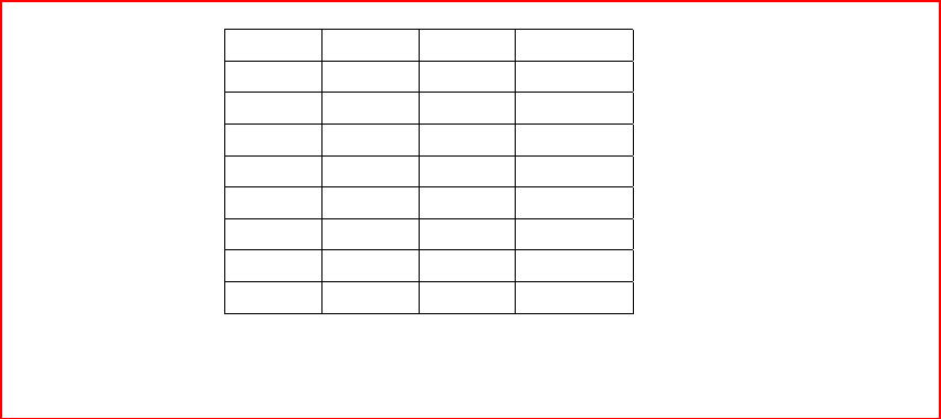
CHAPTER FIVE SOLUTIONS
Engineering Circuit Analysis, 6th Edition Copyright ©2002 McGraw-Hill, Inc. All Rights Reserved.
1. Define percent error as 100 [ex – (1 + x)]/ ex
x 1 + x ex % error
0.001 1.001 1.001 5×10⁻⁵
0.005 1.005 1.005 1×10⁻³
0.01 1.01 1.010 5×10⁻³
0.05 1.05 1.051 0.1
0.10 1.10 1.105 0.5
0.50 1.50 1.649 9
1.00 2.00 2.718 26
5.00 6.00 148.4 96
Of course, “reasonable” is a very subjective term. However, if we choose x < 0.1, we
ensure that the error is less than 1%.
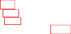
CHAPTER FIVE SOLUTIONS
Engineering Circuit Analysis, 6th Edition Copyright ©2002 McGraw-Hill, Inc. All Rights Reserved.
2. iA, vB “on”, vC = 0: ix = 20 A
iA, vC “on”, vB = 0: ix = -5 A
iA, vB, vC “on” : ix = 12 A
so, we can write ix’ + ix” + ix”’ = 12
ix’ + ix” = 20
ix’ + ix”’ = - 5
In matrix form,
=
′′′
′′
′
5-
20
12
1 0 1
0 1 1
1 1 1
x
x
x
i
i
i
(a) with iA on only, the response ix = ix’ = 3 A.
(b) with vB on only, the response ix = ix” = 17 A.
(c) with vC on only, the response ix = ix”’ = -8 A.
(d) iA and vC doubled, vB reversed: 2(3) + 2(-8) + (-1)(17) = -27 A.

CHAPTER FIVE SOLUTIONS
Engineering Circuit Analysis, 6th Edition Copyright ©2002 McGraw-Hill, Inc. All Rights Reserved.
3. One source at a time:
The contribution from the 24-V source may be found by shorting the 45-V source and
open-circuiting the 2-A source. Applying voltage division,
vx’ = V 10
182010
20
24
30||452010
20
24 =
++
=
++
We find the contribution of the 2-A source by shorting both voltage sources and
applying current division:
vx” = V 8.333
182010
10
220 =
++
Finally, the contribution from the 45-V source is found by open-circuiting the 2-A
source and shorting the 24-V source. Defining v30 across the 30-Ω resistor with the
“+” reference on top:
0 = v30/ 20 + v30/ (10 + 20) + (v30 – 45)/ 45
solving, v30 = 11.25 V and hence vx”’ = -11.25(20)/(10 + 20) = -7.5 V
Adding the individual contributions, we find that vx = vx’ + vx” + vx”’ = 10.83 V.
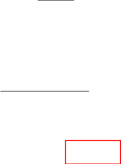
CHAPTER FIVE SOLUTIONS
Engineering Circuit Analysis, 6th Edition Copyright ©2002 McGraw-Hill, Inc. All Rights Reserved.
4. The contribution of the 8-A source is found by shorting out the two voltage sources
and employing simple current division:
i3' = A 5-
3050
50
8=
+
−
The contribution of the voltage sources may be found collectively or individually. The
contribution of the 100-V source is found by open-circuiting the 8-A source and
shorting the 60-V source. Then,
i3" = A 6.25
30||60||)3050(
100 =
+
The contribution of the 60-V source is found in a similar way as i3"' = -60/30 = -2 A.
The total response is i3 = i3' + i3" + i3"' = -750 mA.

CHAPTER FIVE SOLUTIONS
Engineering Circuit Analysis, 6th Edition Copyright ©2002 McGraw-Hill, Inc. All Rights Reserved.
5. (a) By current division, the contribution of the 1-A source i2’ is
i2’ = 1 (200)/ 250 = 800 mA.
The contribution of the 100-V source is i2” = 100/ 250 = 400 mA.
The contribution of the 0.5-A source is found by current division once the 1-A source
is open-circuited and the voltage source is shorted. Thus,
i2”’ = 0.5 (50)/ 250 = 100 mA
Thus, i2 = i2’ + i2” + i2”’ = 1.3 A
(b) P1A = (1) [(200)(1 – 1.3)] = 60 W
P200 = (1 – 1.3)2 (200) = 18 W
P100V = -(1.3)(100) = -130 W
P50 = (1.3 – 0.5)2 (50) = 32 W
P0.5A = (0.5) [(50)(1.3 – 0.5)] = 20 W
Check: 60 + 18 + 32 + 20 = +130.
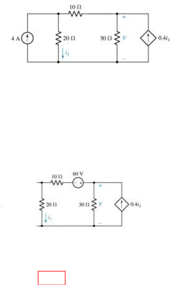
CHAPTER FIVE SOLUTIONS
Engineering Circuit Analysis, 6th Edition Copyright ©2002 McGraw-Hill, Inc. All Rights Reserved.
6. We find the contribution of the 4-A source by shorting out the 100-V source and
analysing the resulting circuit:
4 = V1' / 20 + (V1' – V')/ 10 [1]
0.4 i1' = V1'/ 30 + (V' – V1')/ 10 [2]
where i1' = V1'/ 20
Simplifying & collecting terms, we obtain 30 V1' – 20 V' = 800 [1]
-7.2 V1' + 8 V' = 0 [2]
Solving, we find that V' = 60 V. Proceeding to the contribution of the 60-V source, we
analyse the following circuit after defining a clockwise mesh current ia flowing in the
left mesh and a clockwise mesh current ib flowing in the right mesh.
30 ia – 60 + 30 ia – 30 ib = 0 [1]
ib = -0.4 i1" = +0.4 ia [2]
Solving, we find that ia = 1.25 A and so V" = 30(ia – ib) = 22.5 V.
Thus, V = V' + V" = 82.5 V.
'
'
"
"
'
"

CHAPTER FIVE SOLUTIONS
Engineering Circuit Analysis, 6th Edition Copyright ©2002 McGraw-Hill, Inc. All Rights Reserved.
7. (a) Linearity allows us to consider this by viewing each source as being scaled by
25/ 10. This means that the response (v3) will be scaled by the same factor:
25 iA'/ 10 + 25 iB'/ 10 = 25 v3'/ 10
∴ v3 = 25v3'/ 10 = 25(80)/ 10 = 200 V
(b) iA' = 10 A, iB' = 25 A → v4' = 100 V
iA" = 10 A, iB" = 25 A → v4" = -50 V
iA = 20 A, iB = -10 A → v4 = ?
We can view this in a somewhat abstract form: the currents iA and iB multiply
the same circuit parameters regardless of their value; the result is v4.
Writing in matrix form,
=
50-
100
b
a
10 25
25 10 , we can solve to find
a = -4.286 and b = 5.714, so that 20a – 10b leads to v4 = -142.9 V

CHAPTER FIVE SOLUTIONS
Engineering Circuit Analysis, 6th Edition Copyright ©2002 McGraw-Hill, Inc. All Rights Reserved.
8. With the current source open-circuited and the 7-V source shorted, we are left with
100k || (22k + 4.7k) = 21.07 kΩ.
Thus, V3V = 3 (21.07)/ (21.07 + 47) = 0.9286 V.
In a similar fashion, we find that the contribution of the 7-V source is:
V
7V = 7 (31.97) / (31.97 + 26.7) = 3.814 V
Finally, the contribution of the current source to the voltage V across it is:
V
5mA = (5×10⁻³) ( 47k || 100k || 26.7k) = 72.75 V.
Adding, we find that V = 0.9286 + 3.814 + 72.75 = 77.49 V.

CHAPTER FIVE SOLUTIONS
Engineering Circuit Analysis, 6th Edition Copyright ©2002 McGraw-Hill, Inc. All Rights Reserved.
9. We must find the current through the 500-kΩ resistor using superposition, and then
calculate the dissipated power.
The contribution from the current source may be calculated by first noting that
1M || 2.7M || 5M = 636.8 kΩ. Then,
i60µA = A 43.51
0.636830.5
3
1060 6
µ
=
++
×−
The contribution from the voltage source is found by first noting that 2.7M || 5M =
1.753 MΩ. The total current flowing from the voltage source (with the current source
open-circuited) is –1.5/ (3.5 || 1.753 + 1) µA = -0.6919 µA. The current flowing
through the 500-kΩ resistor due to the voltage source acting alone is then
i1.5V = 0.6919 (1.753)/ (1.753 + 3.5) mA = 230.9 nA.
The total current through the 500-kΩ resistor is then i60µA + i1.5V = 43.74 µA and the
dissipated power is (43.74×10⁻⁹)2 (500×103) = 956.6 µW.
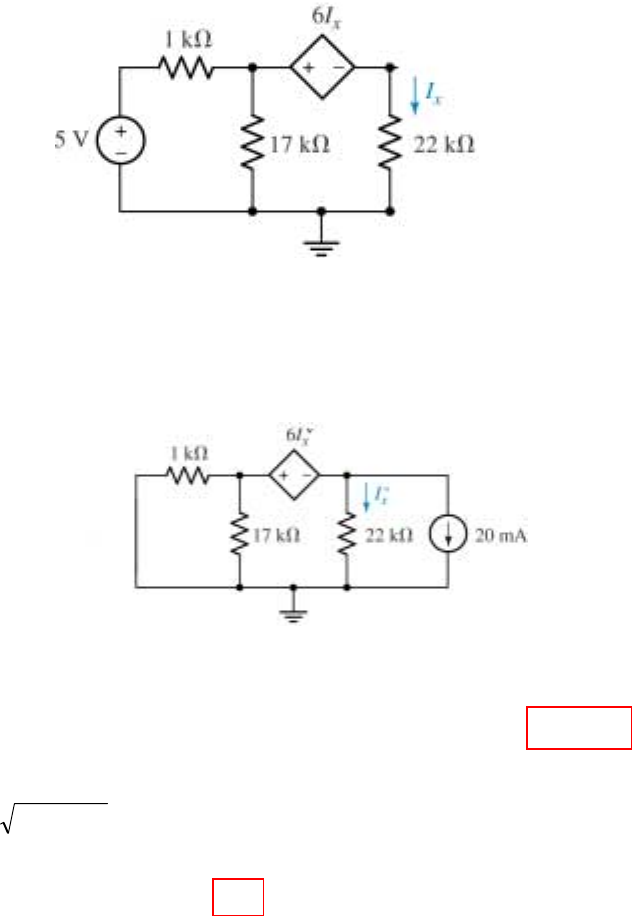
CHAPTER FIVE SOLUTIONS
Engineering Circuit Analysis, 6th Edition Copyright ©2002 McGraw-Hill, Inc. All Rights Reserved.
10. We first determine the contribution of the voltage source:
Via mesh analysis, we write: 5 = 18000 I1' – 17000 Ix'
-6 I
x' = -17000 Ix' + 39000 Ix'
Solving, we find I1' = 472.1 mA and Ix' = 205.8 mA, so V' = 17×103 (I1' - Ix')
= 4.527 V. We proceed to find the contribution of the current source:
Via supernode: -20×10-3 = Vx"/ 22×103 + V"/ 0.9444×10³ [1]
and V" – Vx" = 6Ix" or V" – Vx" = 6 Vx"/ 22×103 [2]
Solving, we find that V" = -18.11 V. Thus, V = V' + V" = -13.58 V.
The maximum power is V2/ 17×103 = V2/ 17 mW = 250 mW, so
V = 13.58 - V 65.19 )250)(17( ′
== . Solving, we find max
V′= 78.77 V.
The 5-V source may then be increased by a factor of 78.77/ 4.527, so that its
maximum positive value is 87 V; past this value, and the resistor will overheat.
'
↑
I1'
'
Vx"
V"
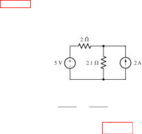
CHAPTER FIVE SOLUTIONS
Engineering Circuit Analysis, 6th Edition Copyright ©2002 McGraw-Hill, Inc. All Rights Reserved.
11. It is impossible to identify the individual contribution of each source to the power
dissipated in the resistor; superposition cannot be used for such a purpose.
Simplifying the circuit, we may at least determine the total power dissipated in the
resistor:
Via superposition in one step, we may write
i = mA 195.1
2.12
2.1
2 -
1.22
5=
++
Thus,
P2Ω = i2 . 2 = 76.15 mW
i →
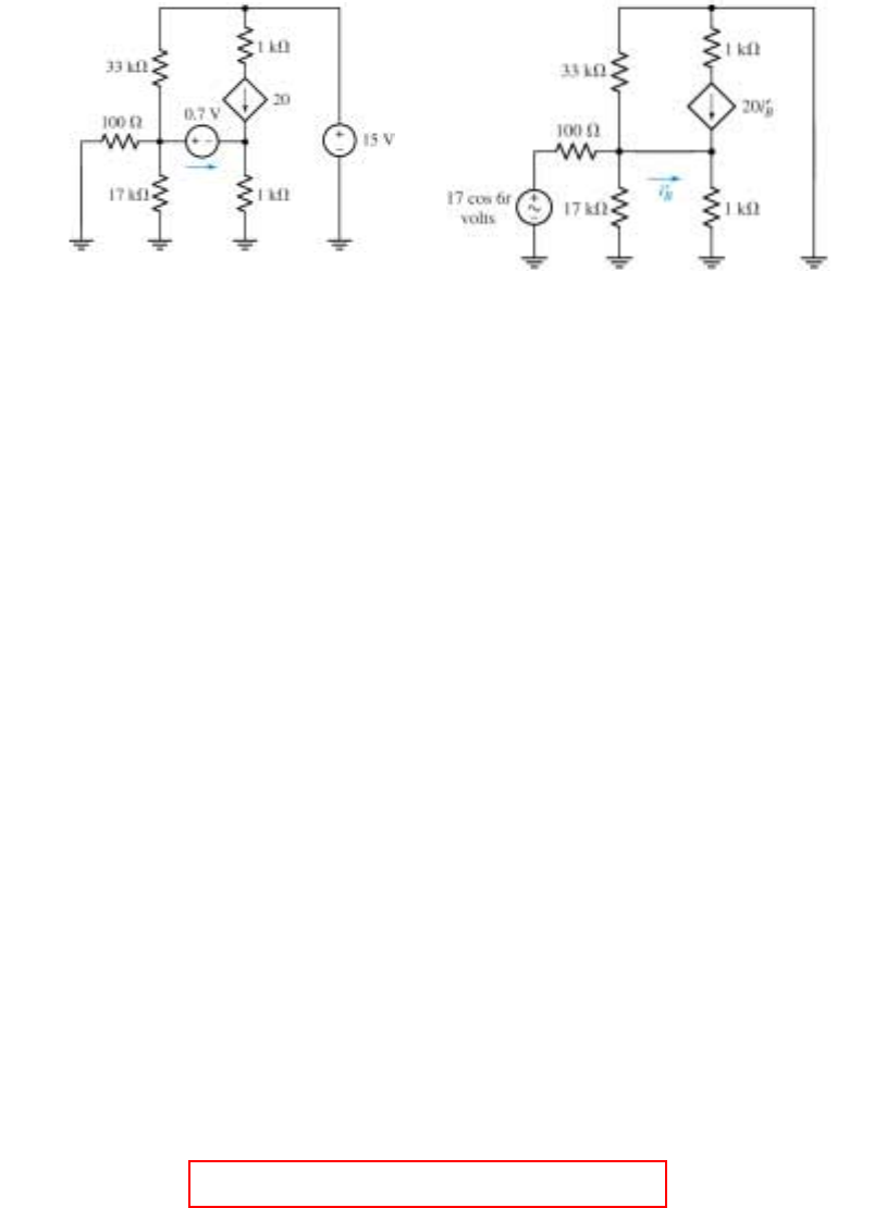
CHAPTER FIVE SOLUTIONS
Engineering Circuit Analysis, 6th Edition Copyright ©2002 McGraw-Hill, Inc. All Rights Reserved.
12. We will analyse this circuit by first considering the combined effect of both dc
sources (left), and then finding the effect of the single ac source acting alone (right).
1, 3 supernode: V1/ 100 + V1/ 17×103 + (V1 – 15)/ 33×103 + V3/ 103 = 20 IB [1]
and: V1 – V3 = 0.7 [2]
Node 2: -20 IB = (V2 – 15)/ 1000 [3]
We require one additional equation if we wish to have IB as an unknown:
20 IB + IB = V3/ 1000 [4]
Simplifying and collecting terms,
10.08912 V1 + V3 – 20×103 IB = 0.4545 [1]
V
1 - V3 = 0.7 [2]
V2 + 20×103 IB = 15 [3]
-V3 + 21×103 IB = 0 [4]
Solving, we find that IB = -31.04 µA.
To analyse the right-hand circuit, we first find the Thévenin equivalent to the left of
the wire marked iB', noting that the 33-kΩ and 17-kΩ resistors are now in parallel. We
find that VTH = 16.85 cos 6t V by voltage division, and RTH = 100 || 17k || 33k =
99.12 Ω. We may now proceed:
20 iB' = vx' / 1000 + (vx' – 16.85 cos 6t)/ 99.12 [1]
20 iB' + iB'' = vx'/ 1000 [2]
Solving, we find that iB' = 798.6 cos 6t mA. Thus, adding our two results, we find the
complete current is
iB = iB' + IB = -31.04 + 798.6 cos 6t µA.
IB
IB
V1
V2
V3 vx'
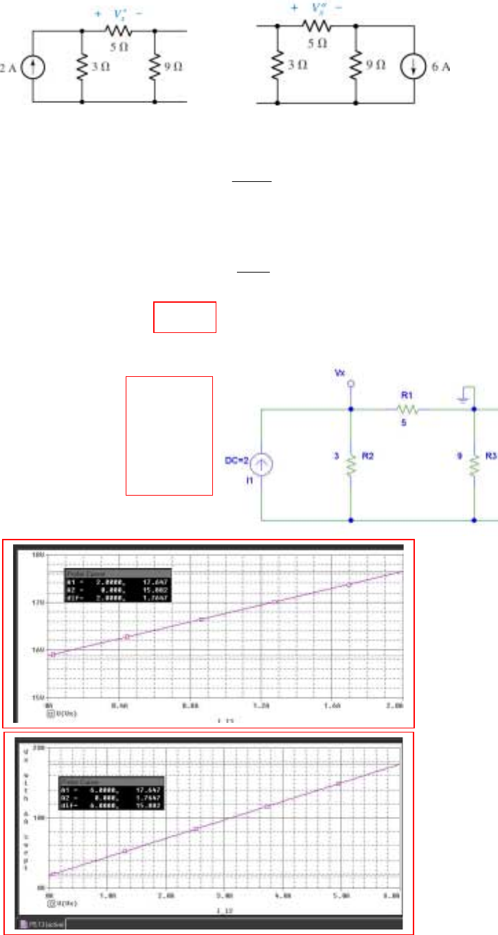
CHAPTER FIVE SOLUTIONS
Engineering Circuit Analysis, 6th Edition Copyright ©2002 McGraw-Hill, Inc. All Rights Reserved.
13.
We first consider the effect of the 2-A source separately, using the left circuit:
Vx' = V 1.765
143
3
2 5 =
+
Next we consider the effect of the 6-A source on its own using the right circuit:
Vx" = V 15.88
89
9
6 5 =
+
Thus, Vx = Vx' + Vx" = 17.65 V.
(b) PSpice verification (DC Sweep)
The DC
sweep
results
below
confirm
that Vx' =
1.765 V
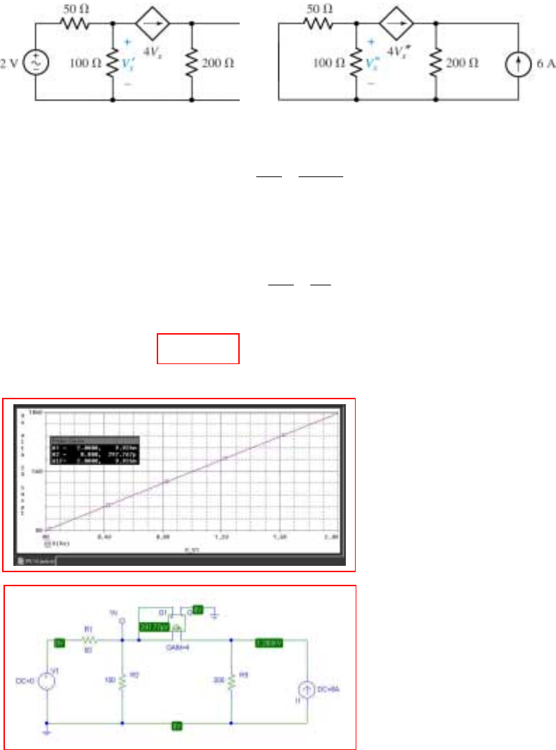
CHAPTER FIVE SOLUTIONS
Engineering Circuit Analysis, 6th Edition Copyright ©2002 McGraw-Hill, Inc. All Rights Reserved.
14.
(a) Beginning with the circuit on the left, we find the contribution of the 2-V source to
Vx:
50
2V
100
V
V4 xx
x
−
′
+
′
=
′
−
which leads to Vx' = 9.926 mV.
The circuit on the right yields the contribution of the 6-A source to Vx:
50
V
100
V
V4 xx
x
′′
+
′′
=
′′
−
which leads to Vx" = 0.
Thus, Vx = Vx' + Vx" = 9.926 mV.
(b) PSpice verification.
'
As can be seen from the two
separate PSpice simulations,
our hand calculations are
correct; the pV-scale voltage in
the second simulation is a result
of numerical inaccuracy.
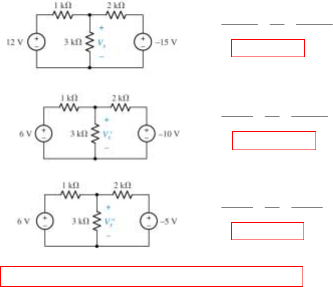
CHAPTER FIVE SOLUTIONS
Engineering Circuit Analysis, 6th Edition Copyright ©2002 McGraw-Hill, Inc. All Rights Reserved.
15.
V 2.455 V so
0
2
15V
3
V
1
12V
x
xxx
=
=
+
++
−
V 0.5455 V so
0
2
10V
3
V
1
6V
x
xxx
=
′
=
+
′
+
′
+
−
′
V 1.909 V so
0
2
5V
3
V
1
6V
x
xxx
=
′′
=
+
′′
+
′′
+
−
′′
Adding, we find that Vx' + Vx" = 2.455 V = Vx as promised.
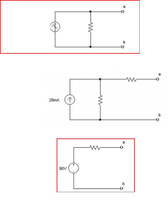
CHAPTER FIVE SOLUTIONS
Engineering Circuit Analysis, 6th Edition Copyright ©2002 McGraw-Hill, Inc. All Rights Reserved.
16. (a) [120 cos 400t] / 60 = 2 cos 400t A. 60 || 120 = 40 Ω.
[2 cos 400t] (40) = 80 cos 400t V. 40 + 10 = 50 Ω.
[80 cos 400t]/ 50 = 1.6 cos 400t A. 50 || 50 = 25 Ω.
(b) 2k || 3k + 6k = 7.2 kΩ. 7.2k || 12k = 4.5 kΩ
(20)(4.5) = 90 V.
25 Ω
1.6 cos 400t A
4.5 kΩ
3.5 kΩ
8 kΩ

CHAPTER FIVE SOLUTIONS
Engineering Circuit Analysis, 6th Edition Copyright ©2002 McGraw-Hill, Inc. All Rights Reserved.
17. We can ignore the 1-kΩ resistor, at least when performing a source transformation on
this circuit, as the 1-mA source will pump 1 mA through whatever value resistor we
place there. So, we need only combine the 1 and 2 mA sources (which are in parallel
once we replace the 1-kΩ resistor with a 0-Ω resistor). The current through the 5.8-
kΩ resistor is then simply given by voltage division:
mA 1.343
5.84.7
4.7
103 3- =
+
×=i
The power dissipated by the 5.8-kΩ resistor is then i2 . 5.8×103 = 10.46 mW.
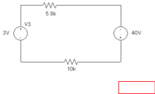
CHAPTER FIVE SOLUTIONS
Engineering Circuit Analysis, 6th Edition Copyright ©2002 McGraw-Hill, Inc. All Rights Reserved.
18. We may ignore the 10-kΩ and 9.7-kΩ resistors, as 3-V will appear across them
regardless of their value. Performing a quick source transformation on the 10-kΩ
resistor/ 4-mA current source combination, we replace them with a 40-V source in
series with a 10-kΩ resistor:
I = 43/ 15.8 mA = 2.722 mA. Therefore, P5.8Ω = I2. 5.8×103 = 42.97 mW.
Ω
Ω
I →
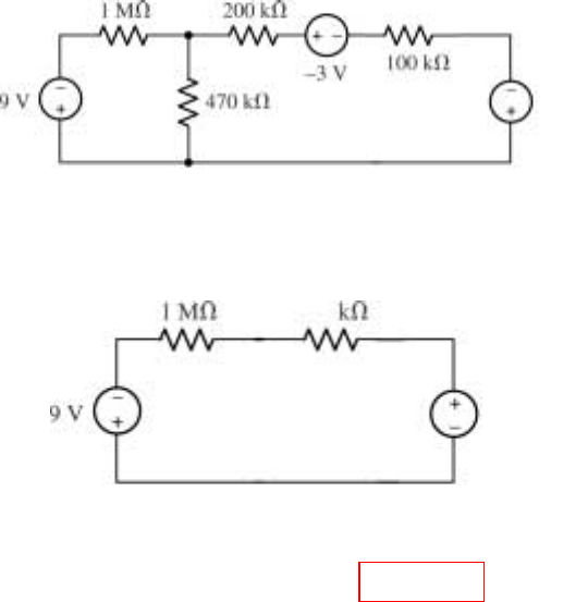
CHAPTER FIVE SOLUTIONS
Engineering Circuit Analysis, 6th Edition Copyright ©2002 McGraw-Hill, Inc. All Rights Reserved.
19. (100 kΩ)(6 mA) = 0.6 V
470 k || 300 k = 183.1 kΩ
(-3 – 0.6)/ 300×103 = -12 µA
(183.1 kΩ)(-12 µA) = -2.197 V
Solving, 9 + 1183.1×103 I – 2.197 = 0, so I = -5.750 µA. Thus,
P1MΩ = I2 . 106 = 33.06 µW.
0.6 V
183.1
-2.197 V
← I
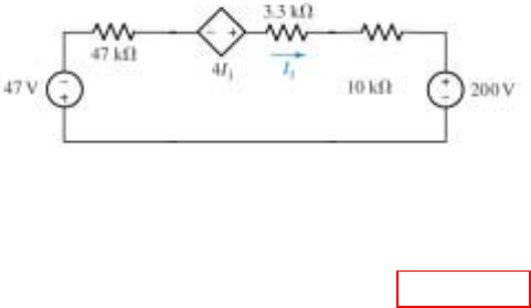
CHAPTER FIVE SOLUTIONS
Engineering Circuit Analysis, 6th Edition Copyright ©2002 McGraw-Hill, Inc. All Rights Reserved.
20. (1)(47) = 47 V. (20)(10) = 200 V. Each voltage source “+” corresponds to its
corresponding current source’s arrow head.
Using KVL on the simplified circuit above,
47 + 47×103 I1 – 4 I1 + 13.3×10³ I1 + 200 = 0
Solving, we find that I1 = -247/ (60.3×10³ – 4) = -4.096 mA.
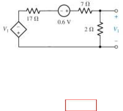
CHAPTER FIVE SOLUTIONS
Engineering Circuit Analysis, 6th Edition Copyright ©2002 McGraw-Hill, Inc. All Rights Reserved.
21. (2 V1)(17) = 34 V1
Analysing the simplified circuit above,
34 V1 – 0.6 + 7 I + 2 I + 17 I = 0 [1] and V1 = 2 I [2]
Substituting, we find that I = 0.6/ (68 + 7 + 2 + 17) = 6.383 mA. Thus,
V1 = 2 I = 12.77 mV
34
← I
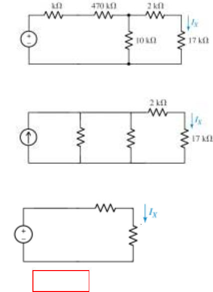
CHAPTER FIVE SOLUTIONS
Engineering Circuit Analysis, 6th Edition Copyright ©2002 McGraw-Hill, Inc. All Rights Reserved.
22. 12/ 9000 = 1.333 mA. 9k || 7k = 3.938 kΩ. → (1.333 mA)(3.938 kΩ) = 5.249 V.
5.249/ 473.938×103 = 11.08 µA
473.9 k || 10 k = 9.793 kΩ. (11.08 mA)(9.793 kΩ) = 0.1085 V
I
x = 0.1085/ 28.793×103 = 3.768 µA.
5.249 V
3.938
473.9 kΩ 10 kΩ
11.08 µA
0.1085 V 17 kΩ
11.793 kΩ
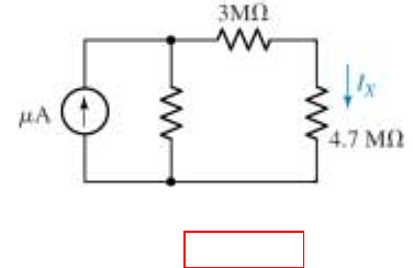
CHAPTER FIVE SOLUTIONS
Engineering Circuit Analysis, 6th Edition Copyright ©2002 McGraw-Hill, Inc. All Rights Reserved.
23. First, (-7 µA)(2 MΩ) = -14 V, “+” reference down. 2 MΩ + 4 MΩ = 6 MΩ.
+14 V/ 6 ΜΩ = 2.333 µA, arrow pointing up; 6 M || 10 M = 3.75 MΩ.
(2.333)(3.75) = 8.749 V. Req = 6.75 MΩ
∴ Ix = 8.749/ (6.75 + 4.7) µA = 764.1 nA.
2.333
3.75 MΩ
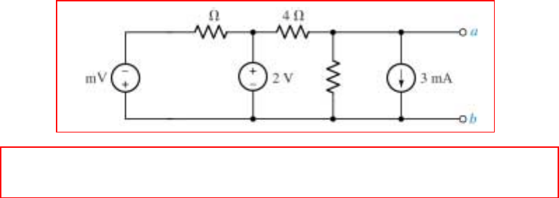
CHAPTER FIVE SOLUTIONS
Engineering Circuit Analysis, 6th Edition Copyright ©2002 McGraw-Hill, Inc. All Rights Reserved.
24. To begin, note that (1 mA)(9 Ω) = 9 mV, and 5 || 4 = 2.222 Ω.
The above circuit may not be further simplified using only source transformation
techniques.
9
15
2.222 Ω
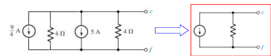
CHAPTER FIVE SOLUTIONS
Engineering Circuit Analysis, 6th Edition Copyright ©2002 McGraw-Hill, Inc. All Rights Reserved.
25. Label the “-” terminal of the 9-V source node x and the other terminal node x'. The
9-V source will force the voltage across these two terminals to be –9 V regardless of
the value of the current source and resistor to its left. These two components may
therefore be neglected from the perspective of terminals a & b. Thus, we may draw:
7.25 A 2 Ω

CHAPTER FIVE SOLUTIONS
Engineering Circuit Analysis, 6th Edition Copyright ©2002 McGraw-Hill, Inc. All Rights Reserved.
26. Beware of the temptation to employ superposition to compute the dissipated power- it
won’t work!
Instead, define a current I flowing into the bottom terminal of the 1-MΩ resistor.
Using superposition to compute this current,
I = 1.8/ 1.840 + 0 + 0 µA = 978.3 nA.
Thus,
P1MΩ = (978.3×10⁻⁹)2 (106) = 957.1 nW.
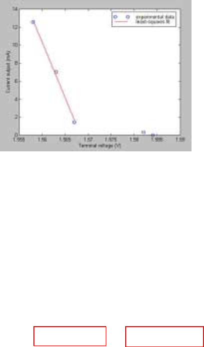
CHAPTER FIVE SOLUTIONS
Engineering Circuit Analysis, 6th Edition Copyright ©2002 McGraw-Hill, Inc. All Rights Reserved.
27. Let’s begin by plotting the experimental results, along with a least-squares fit to part
of the data:
We see from the figure that we cannot draw a very good line through all data points
representing currents from 1 mA to 20 mA. We have therefore chosen to perform a
linear fit for the three lower voltages only, as shown. Our model will not be as
accurate at 1 mA; there is no way to know if our model will be accurate at 20 mA,
since that is beyond the range of the experimental data.
Modeling this system as an ideal voltage source in series with a resistance
(representing the internal resistance of the battery) and a varying load resistance, we
may write the following two equations based on the linear fit to the data:
1.567 = Vsrc – Rs (1.6681×10⁻³)
1.558 = Vsrc – Rs (12.763×10⁻³)
Solving, Vsrc = 1.568 V and Rs = 811.2 mΩ. It should be noted that depending on the
line fit to the experimental data, these values can change somewhat, particularly the
series resistance value.
Least-squares fit results:
Voltage (V) Current (mA)
1.567 1.6681
1.563 6.599
1.558 12.763
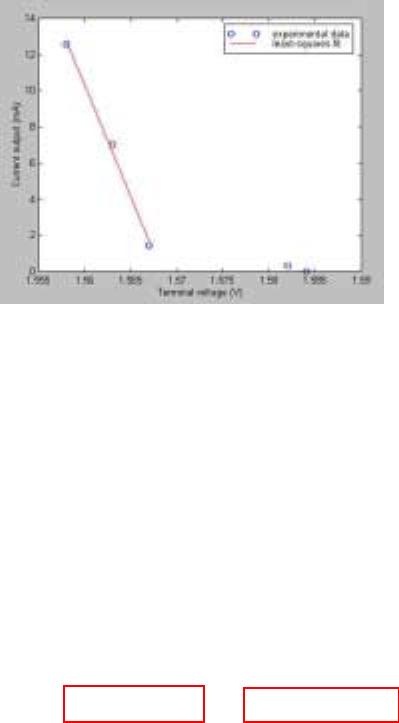
CHAPTER FIVE SOLUTIONS
Engineering Circuit Analysis, 6th Edition Copyright ©2002 McGraw-Hill, Inc. All Rights Reserved.
28. Let’s begin by plotting the experimental results, along with a least-squares fit to part
of the data:
We see from the figure that we cannot draw a very good line through all data points
representing currents from 1 mA to 20 mA. We have therefore chosen to perform a
linear fit for the three lower voltages only, as shown. Our model will not be as
accurate at 1 mA; there is no way to know if our model will be accurate at 20 mA,
since that is beyond the range of the experimental data.
Modeling this system as an ideal current source in parallel with a resistance Rp
(representing the internal resistance of the battery) and a varying load resistance, we
may write the following two equations based on the linear fit to the data:
1.6681×10-3 = Isrc – 1.567/ Rp
12.763×10-3 = Isrc – 1.558/ Rp
Solving, Isrc = 1.933 A and Rs = 811.2 mΩ. It should be noted that depending on the
line fit to the experimental data, these values can change somewhat, particularly the
series resistance value.
Least-squares fit results:
Voltage (V) Current (mA)
1.567 1.6681
1.563 6.599
1.558 12.763
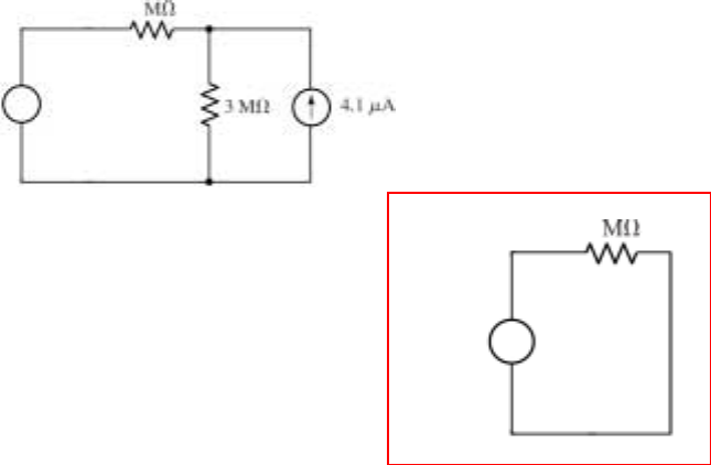
CHAPTER FIVE SOLUTIONS
Engineering Circuit Analysis, 6th Edition Copyright ©2002 McGraw-Hill, Inc. All Rights Reserved.
29. Reference terminals are required to avoid ambiguity: depending on the sources with
which we begin the transformation process, we will obtain entirely different answers.
Working from left to right in this case,
2 µA – 1.8 µA = 200 nA, arrow up.
1.4 MΩ + 2.7 MΩ = 4.1 MΩ
An additional transformation back to a voltage source yields (200 nA)(4.1 MΩ) =
0.82 V in series with 4.1 MΩ + 2 MΩ = 6.1 MΩ, as shown below:
Then, 0.82 V/ 6.1 MΩ = 134.4 nA, arrow up.
6.1 MΩ || 3 MΩ = 2.011 MΩ
4.1 µA + 134.4 nA = 4.234 mA, arrow up.
(4.234 µA) (2.011 MΩ) = 8.515 V.
±
6.1
0.82 V
±
8.515 V
2.011
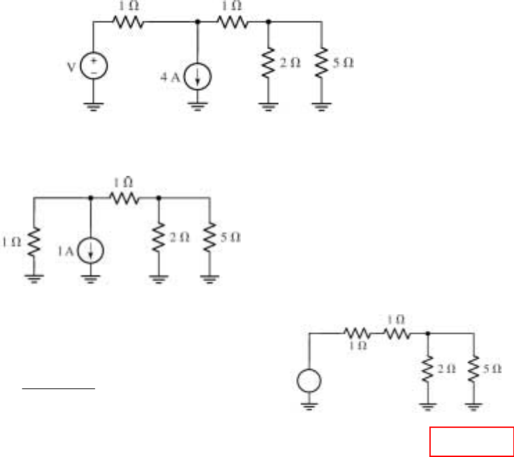
CHAPTER FIVE SOLUTIONS
Engineering Circuit Analysis, 6th Edition Copyright ©2002 McGraw-Hill, Inc. All Rights Reserved.
30. To begin, we note that the 5-V and 2-V sources are in series:
Next, noting that 3 V/ 1 Ω = 3 A, and 4 A – 3 A = +1 A (arrow down), we obtain:
By voltage division, the voltage across the
5-Ω resistor in the circuit to the right is:
(-1) 2 5||2
5||2
+ = -0.4167 V.
Thus, the power dissipated by the 5-Ω resistor is (-0.4167)2 / 5 = 34.73 mW.
3
The left-hand resistor and the current
source are easily transformed into a
1-V source in series with a 1-Ω
resistor:
±
-1 V
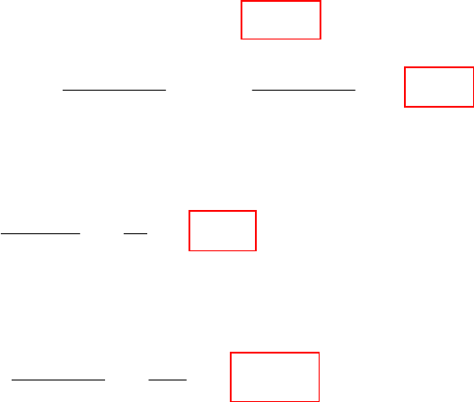
CHAPTER FIVE SOLUTIONS
Engineering Circuit Analysis, 6th Edition Copyright ©2002 McGraw-Hill, Inc. All Rights Reserved.
31. (a) RTH = 25 || (10 + 15) = 25 || 25 = 12.5 Ω.
V
TH = Vab =
++
+
+
++ 251015
1015
100
251510
25
50 = 75 V.
(b) If Rab = 50 Ω,
P
50Ω = W72
50
1
12.550
50
75
2
=
+
(c) If Rab = 12.5 Ω,
P
12.5Ω = W112.5
12.5
1
12.55.21
12.5
75
2
=
+
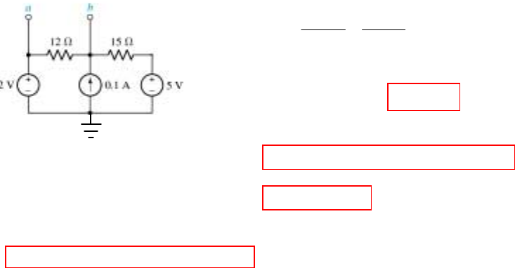
CHAPTER FIVE SOLUTIONS
Engineering Circuit Analysis, 6th Edition Copyright ©2002 McGraw-Hill, Inc. All Rights Reserved.
32. (a) Removing terminal c, we need write only one nodal equation:
0.1 = 15
5V
12
2V bb −
+
−, which may be solved to
yield Vb = 4 V. Therefore, Vab = VTH = 2 – 4
= -2 V.
RTH = 12 || 15 = 6.667 Ω. We may then
calculate IN as IN = VTH/ RTH
= -300 mA (arrow pointing upwards).
(b) Removing terminal a, we again find RTH = 6.667 Ω, and only need write a single
nodal equation; in fact, it is identical to that written for the circuit above, and we once
again find that Vb = 4 V. In this case, VTH = Vbc = 4 – 5 = -1 V, so IN = -1/ 6.667
= -150 mA (arrow pointing upwards).
CHAPTER FIVE SOLUTIONS
Engineering Circuit Analysis, 6th Edition Copyright ©2002 McGraw-Hill, Inc. All Rights Reserved.
33. (a) Shorting out the 88-V source and open-circuiting the 1-A source, we see looking
into the terminals x and x' a 50-Ω resistor in parallel with 10 Ω in parallel with
(20 Ω + 40 Ω), so
RTH = 50 || 10 || (20 + 40) = 7.317 Ω
Using superposition to determine the voltage Vxx' across the 50-Ω resistor, we find
Vxx' = VTH =
++
+
++
+
)10||50(2040
40
10)||(1)(50
)]4020(||50[10
)4020(||50
88
=
++
+
333.82040
40
(1)(8.333)
27.37
27.27
88 = 69.27 V
(b) Shorting out the 88-V source and open-circuiting the 1-A source, we see looking
into the terminals y and y' a 40-Ω resistor in parallel with [20 Ω + (10 Ω || 50 Ω)]:
RTH = 40 || [20 + (10 || 50)] = 16.59 Ω
Using superposition to determine the voltage Vyy' across the 1-A source, we find
Vyy' = VTH = (1)(RTH) +
+
+4020
40
27.2710
27.27
88
= 59.52 V
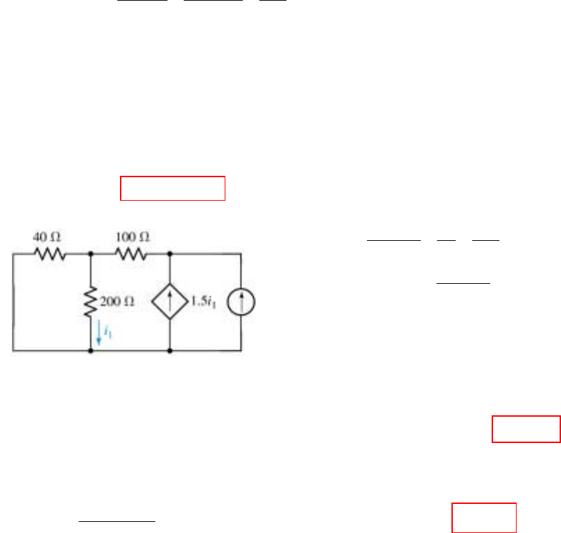
CHAPTER FIVE SOLUTIONS
Engineering Circuit Analysis, 6th Edition Copyright ©2002 McGraw-Hill, Inc. All Rights Reserved.
34. (a) Select terminal b as the reference terminal, and define a nodal voltage V1 at the
top of the 200-Ω resistor. Then,
0 = 200
V
100
VV
40
20V 1TH11 +
−
+
− [1]
1.5 i1 = (VTH – V1)/ 100 [2]
where i1 = V1/ 200, so Eq. [2] becomes 150 V1/ 200 + V1 - VTH = 0 [2]
Simplifying and collecting terms, these equations may be re-written as:
(0.25 + 0.1 + 0.05) V1 – 0.1 VTH = 5 [1]
(1 + 15/ 20) V1 – VTH = 0 [2]
Solving, we find that VTH = 38.89 V. To find RTH, we short the voltage source and
inject 1 A into the port:
0 = 200
V
40
V
100
VV 11in1++
− [1]
1.5 i1 + 1 = 100
VV 1in − [2]
i1 = V1/ 200 [3]
Combining Eqs. [2] and [3] yields 1.75 V1 – Vin = -100 [4]
Solving Eqs. [1] & [4] then results in Vin = 177.8 V, so that RTH = Vin/ 1 A = 177.8 Ω.
(b) Adding a 100-Ω load to the original circuit or our Thévenin equivalent, the
voltage across the load is
V100Ω = V 14.00
177.8100
100
VTH =
+, and so P100Ω = (V100Ω)2 / 100 = 1.96 W.
1 A
+
Vin
-
V1
Ref.

CHAPTER FIVE SOLUTIONS
Engineering Circuit Analysis, 6th Edition Copyright ©2002 McGraw-Hill, Inc. All Rights Reserved.
35. We inject a current of 1 A into the port (arrow pointing up), select the bottom terminal
as our reference terminal, and define the nodal voltage Vx across the 200-Ω resistor.
Then, 1 = V1/ 100 + (V1 – Vx)/ 50 [1]
-0.1 V1 = Vx/ 200 + (Vx – V1)/ 50 [2]
which may be simplified to
3 V1 – 2 Vx = 100 [1]
16 V1 + 5 Vx = 0 [2]
Solving, we find that V1 = 10.64 V, so RTH = V1/ (1 A) = 10.64 Ω.
Since there are no independent sources present in the original network, IN = 0.
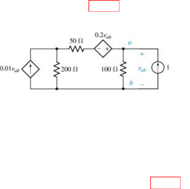
CHAPTER FIVE SOLUTIONS
Engineering Circuit Analysis, 6th Edition Copyright ©2002 McGraw-Hill, Inc. All Rights Reserved.
36. With no independent sources present, VTH = 0.
We decide to inject a 1-A current into the port:
Node ‘x’: 0.01 vab = vx/ 200 + (vx – vf)/ 50 [1]
Supernode: 1 = vab/ 100 + (vf – vx) [2]
and: vab – vf = 0.2 vab [3]
Rearranging and collecting terms,
-2 vab + 5 vx – 4 vf = 0 [1]
vab – 2 vx + 2 vf = 100 [2]
0.8 vab - vf = 0 [3]
Solving, we find that vab = 192.3 V, so RTH = vab/ (1 A) = 192.3 Ω.
Ref.
vx
vf
•
A
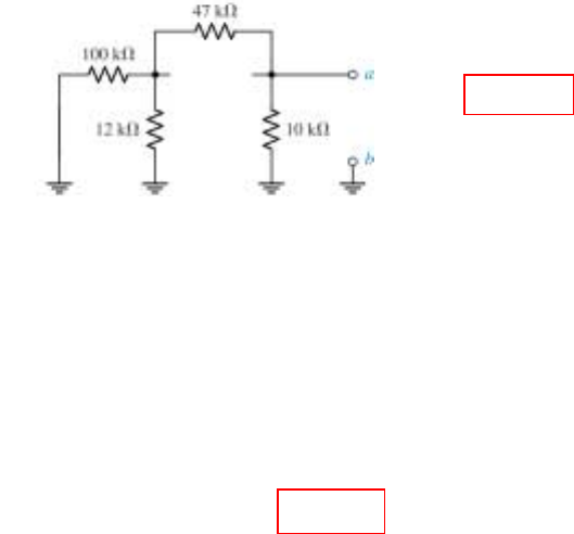
CHAPTER FIVE SOLUTIONS
Engineering Circuit Analysis, 6th Edition Copyright ©2002 McGraw-Hill, Inc. All Rights Reserved.
37. We first find RTH by shorting out the voltage source and open-circuiting the current
source.
Looking into the terminals a & b, we see
RTH = 10 || [47 + (100 || 12)]
= 8.523 Ω.
Returning to the original circuit, we decide to perform nodal analysis to obtain VTH:
-12×103 = (V1 – 12)/ 100×103 + V1/ 12×103 + (V1 – VTH)/ 47×103 [1]
12×103 = VTH/ 10×103 + (VTH – V1)/ 47×103 [2]
Rearranging and collecting terms,
0.1146 V1 - 0.02128 VTH = -11.88 [1]
-0.02128 V1 + 0.02128 VTH = 12 [2]
Solving, we find that VTH = 83.48 V.

CHAPTER FIVE SOLUTIONS
Engineering Circuit Analysis, 6th Edition Copyright ©2002 McGraw-Hill, Inc. All Rights Reserved.
38. (a) RTH = 4 + 2 || 2 + 10 = 15 Ω.
(b) same as above: 15 Ω.

CHAPTER FIVE SOLUTIONS
Engineering Circuit Analysis, 6th Edition Copyright ©2002 McGraw-Hill, Inc. All Rights Reserved.
39. For Fig. 5.78a, IN = 12/ ~0 → ∞ A in parallel with ~ 0 Ω.
For Fig. 5.78b, VTH = (2)(~∞) → ∞ V in series with ~∞ Ω.

CHAPTER FIVE SOLUTIONS
Engineering Circuit Analysis, 6th Edition Copyright ©2002 McGraw-Hill, Inc. All Rights Reserved.
40. With no independent sources present, VTH = 0.
Connecting a 1-V source to the port and measuring the current that flows as a result,
I = 0.5 Vx + 0.25 Vx = 0.5 + 0.25 = 0.75 A.
R
TH = 1/ I = 1.333 Ω.
The Norton equivalent is 0 A in parallel with 1.333 Ω.
+
-
← I
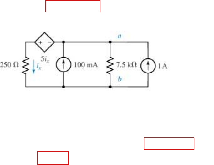
CHAPTER FIVE SOLUTIONS
Engineering Circuit Analysis, 6th Edition Copyright ©2002 McGraw-Hill, Inc. All Rights Reserved.
41. Performing nodal analysis to determine VTH,
100×10-3 = Vx/ 250 + Voc/ 7.5×10³ [1]
and Vx – Voc = 5 ix
where ix = Vx/ 250. Thus, we may write the second equation as
0.98 Vx – Voc = 0 [2]
Solving, we find that Voc = VTH = 23.72 V.
In order to determine RTH, we inject 1 A into the port:
V
ab/ 7.5×10³ + Vx/ 250 = 1 [1]
and Vx – Vab = 5 ix = 5Vx/ 250 or
-V
ab + (1 – 5/ 250) Vx = 0 [2]
Solving, we find that Vab = 237.2 V. Since RTH = Vab/ (1 A), RTH = 237.2 Ω.
Finally, IN = VTH/ RTH = 100 mA.

CHAPTER FIVE SOLUTIONS
Engineering Circuit Analysis, 6th Edition Copyright ©2002 McGraw-Hill, Inc. All Rights Reserved.
42. We first note that VTH = Vx, so performing nodal analysis,
-5 V
x = Vx/ 19 which has the solution Vx = 0 V.
Thus, VTH (and hence IN) = 0. (Assuming RTH ≠ 0)
To find RTH, we inject 1 A into the port, noting that RTH = Vx/ 1 A:
-5 Vx + 1 = Vx/ 19
Solving, we find that Vx = 197.9 mV, so that RTH = RN = 197.9 mV.
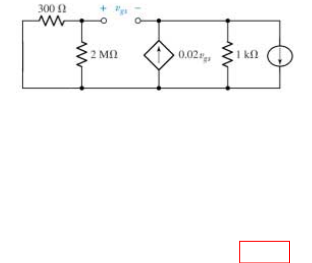
CHAPTER FIVE SOLUTIONS
Engineering Circuit Analysis, 6th Edition Copyright ©2002 McGraw-Hill, Inc. All Rights Reserved.
43. Shorting out the voltage source, we redraw the circuit with a 1-A source in place of
the 2-kΩ resistor:
Noting that 300 Ω || 2 MΩ ≈ 300 Ω,
0 = (vgs – V)/ 300 [1]
1 – 0.02 vgs = V/ 1000 + (V – vgs)/ 300 [2]
Simplifying & collecting terms,
vgs – V = 0 [1]
0.01667 vgs + 0.00433 V = 1 [2]
Solving, we find that vgs = V = 47.62 V. Hence, RTH = V/ 1 A = 47.62 Ω.
1 A
Ref.
V
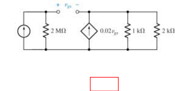
CHAPTER FIVE SOLUTIONS
Engineering Circuit Analysis, 6th Edition Copyright ©2002 McGraw-Hill, Inc. All Rights Reserved.
44. We replace the source vs and the 300-Ω resistor with a 1-A source and seek its
voltage:
By nodal analysis, 1 = V1/ 2×10⁶ so V1 = 2×10⁶ V.
Since V = V1, we have Rin = V/ 1 A = 2 MΩ.
1 A
+
V
-
Ref.
V1 V2
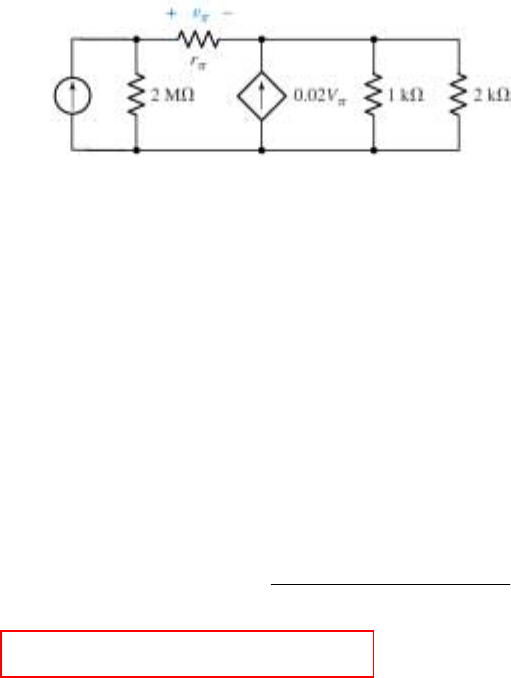
CHAPTER FIVE SOLUTIONS
Engineering Circuit Analysis, 6th Edition Copyright ©2002 McGraw-Hill, Inc. All Rights Reserved.
45. Removing the voltage source and the 300-Ω resistor, we replace them with a 1-A
source and seek the voltage that develops across its terminals:
We select the bottom node as our reference terminal, and define nodal voltages V1
and V2. Then,
1 = V1 / 2×10⁶ + (V1 – V2)/ rπ [1]
0.02 vπ = (V2 – V1)/ rπ + V2/ 1000 + V2/ 2000 [2]
where vπ = V1 – V2
Simplifying & collecting terms,
(2×10⁶ + rπ) V1 – 2×10⁶ V2 = 2×10⁶ rπ [1]
-(2000 + 40 rπ) V1 + (2000 + 43 rπ) V2 = 0 [2]
Solving, we find that V1 = V =
++×
+
×
π
π
r 14.33 666.7 102
r 14.33 666.7
102 6
6.
Thus, RTH = 2×10⁶ || (666.7 + 14.33 rπ) Ω.
1 A
+
V
- Ref.

CHAPTER FIVE SOLUTIONS
Engineering Circuit Analysis, 6th Edition Copyright ©2002 McGraw-Hill, Inc. All Rights Reserved.
46. Such a scheme probably would lead to maximum or at least near-maximum power
transfer to our home. Since we pay the utility company based on the power we use,
however, this might not be such a hot idea…
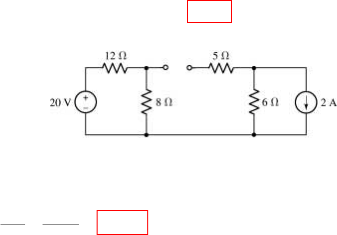
CHAPTER FIVE SOLUTIONS
Engineering Circuit Analysis, 6th Edition Copyright ©2002 McGraw-Hill, Inc. All Rights Reserved.
47. We need to find the Thévenin equivalent resistance of the circuit connected to RL, so
we short the 20-V source and open-circuit the 2-A source; by inspection, then
RTH = 12 || 8 + 5 + 6 = 15.8 Ω
Analyzing the original circuit to obtain V1 and V2 with RL removed:
V
1 = 20 8/ 20 = 8 V; V2 = -2 (6) = -12 V.
We define VTH = V1 – V2 = 8 + 12 = 20 V. Then,
P
RL|max = W6.329
4(15.8)
400
R 4
V
L
2
TH ==
+ VTH -
V1 V2
Ref.
CHAPTER FIVE SOLUTIONS
Engineering Circuit Analysis, 6th Edition Copyright ©2002 McGraw-Hill, Inc. All Rights Reserved.
48. (a) RTH = 25 || (10 + 15) = 12.5 Ω
Using superposition, Vab = VTH = 50
1015
100
251015
25
50 +
+
++ = 75 V.
(b) Connecting a 50-Ω resistor,
P
load = W90
50 12.5
75
R R
V2
loadTH
2
TH =
+
=
+
(c) Connecting a 12.5-Ω resistor,
P
load =
()
W112.5
12.5 4
75
R 4
V2
TH
2
TH ==
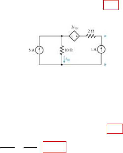
CHAPTER FIVE SOLUTIONS
Engineering Circuit Analysis, 6th Edition Copyright ©2002 McGraw-Hill, Inc. All Rights Reserved.
49. (a) By inspection, we see that i10 = 5 A, so
VTH = Vab = 2(0) + 3 i10 + 10 i10 = 13 i10 = 13(5) = 65 V.
To find RTH, we connect a 1-A source between terminals a & b:
5 = V1/ 10 + (V2 – V)/ 2 [1] → V
1 + 5 V2 – 5 V = 50 [1]
1 = (V – V2)/ 2 [2] → -V2 + V = 2 [2]
and V2 – V1 = 3 i10 [3]
where i10 = V1/ 10 → -13 V1 + 10 V2 = 0 [3]
Solving, we find that V = 80 V, so that RTH = V / 1 A = 80 Ω.
(b) Pmax = W13.20
4(80)
65
R 4
V2
TH
2
TH ==
Ref.
V1 V2 V
•
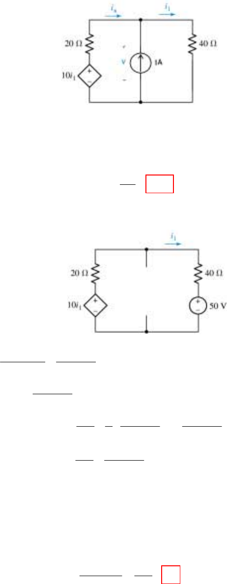
CHAPTER FIVE SOLUTIONS
Engineering Circuit Analysis, 6th Edition Copyright ©2002 McGraw-Hill, Inc. All Rights Reserved.
50.
(a) Replacing the resistor RL with a 1-A source, we seek the voltage that develops across
its terminals with the independent voltage source shorted:
11 1
11
1
1
10 20 40 0 [1] 30 20 0 [1]
and 1 [2] 1 [2]
Solving, 400mA
So 40 16V and 16
1A
−+ + = ⇒ + =
−= ⇒ −=
=
== ==Ω
xx
xx
TH
iii ii
ii ii
i
V
Vi R
(b) Removing the resistor RL from the original circuit, we seek the resulting open-circuit
voltage:
1
1
10 50
0[1]
20 40
50
where 40
150 50
so [1] becomes 0 20 2 40 40
50
020 80
04 50
550
or 10V
−−
=+
−
=
−−
=− +
−
=+
=+−
=
=
TH TH
TH
TH TH TH
TH TH
TH TH
TH
TH
ViV
V
i
VV V
VV
VV
V
V
Thus, if
16 ,
5V
2
==Ω
===
+
L
LTH
LTH
RTH
LTH
RR
RV
VV
RR
+
VTH
-
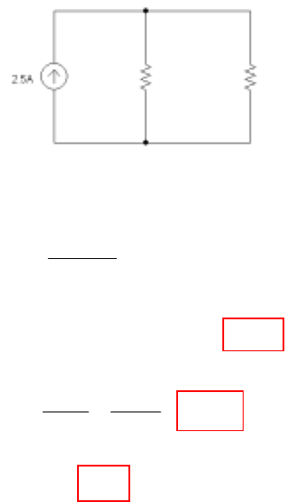
CHAPTER FIVE SOLUTIONS
Engineering Circuit Analysis, 6th Edition Copyright ©2002 McGraw-Hill, Inc. All Rights Reserved.
51.
(a) 2.5A=
N
I
2
20 80
2A
=
=
i
i
By current division,
2 2.5 20
=+
N
N
R
R
Solving, 80==Ω
NTH
RR
Thus, 2.5 80 200V==×=
TH OC
VV
(b)
22
max
200 125W
4480
== =
×
TH
TH
V
PR
(c) 80==Ω
LTH
RR
RN 20 Ω
↓
2 A
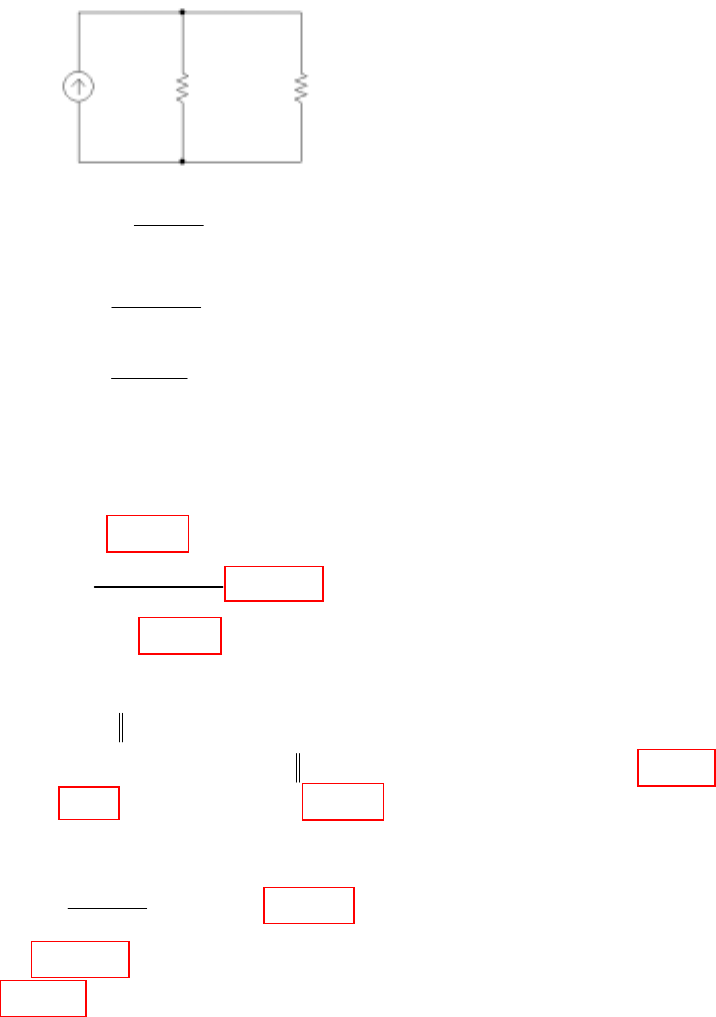
CHAPTER FIVE SOLUTIONS
Engineering Circuit Analysis, 6th Edition Copyright ©2002 McGraw-Hill, Inc. All Rights Reserved.
52.
By Voltage ÷, =+N
RN
N
R
II
RR
So
Solving, 1.7 A=
N
I and 33.33=Ω
N
R
(a) If
(b) If
(c) If
is a maximum,
33.33
33.33
1.7 850mA
33.33 33.33
33.33 28.33V
== Ω
=× =
+
==
LL
LN
L
LL
vi
RR
i
vi
is a maximum
; max when 0
So 1.7A
0V
==Ω
+
=
=
L
N
LN L
NL
L
L
i
R
ii R
RR
i
v
0.2 [1]
250
0.5 [2]
80
=+
=+
N
N
N
N
N
N
R
IR
R
IR
10W to 250 corresp to 200mA.
20W to 80 corresp to 500mA.
Ω
Ω
RN R
IN
is a maximum
()
So is a maximum when is a maximum, which occurs at .
Then 0 and 1.7 56.66V
=
=∞
==×=
L
LNNL
LNL L
LLN
v
VIRR
vRR R
ivR

CHAPTER FIVE SOLUTIONS
Engineering Circuit Analysis, 6th Edition Copyright ©2002 McGraw-Hill, Inc. All Rights Reserved.
53. There is no conflict with our derivation concerning maximum power. While a dead
short across the battery terminals will indeed result in maximum current draw from
the battery, and power is indeed proportional to i2, the power delivered to the load is
i2RLOAD = i2(0) = 0 watts. This is the minimum, not the maximum, power that the
battery can deliver to a load.
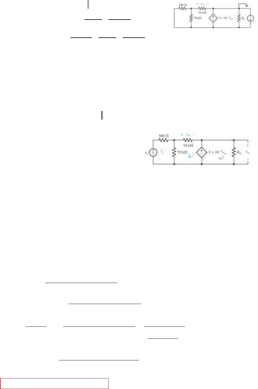
CHAPTER FIVE SOLUTIONS
Engineering Circuit Analysis, 6th Edition Copyright ©2002 McGraw-Hill, Inc. All Rights Reserved.
54. Remove RE: =
TH E in
RRR
bottom node: 3
3
1 3 10 [1]
300 70 10
−ππ
π
−−
−× = + ×
Vv Vv
v
at other node: 33
010 10 300 70 10
ππ π
−−
=++
××
vvVvV
[2]
Simplifying and collecting terms,
210×105 = 70×103 V + 300V + 63000 vπ – 70x103 vπ - 300 vπ
35
33
33
or 70.3 10 7300 210 10 [1]
0 2100 70 10 70 10 300 300
or 69.7 10 72.4 10 0 [2]
solving, 331.9 So 331.9
π
ππ π
π
×− =×
=+×−×+−
−× +× =
==Ω
TH E
Vv
vvVvV
Vv
VVRR
Next, we determine vTH using mesh analysis:
33
12
70.3 10 70 10 0 [1]−+ × − × =
s
vii
33
213
80 10 70 10 0 [2]×−×+=
E
iiRi
and: 3
32
310 [3]
−π
−=×ii v
or 33
32 2
3 10 (10 10 )
−
−=× ×ii i
or 32 2
30−=ii i
or
23
31 0 [3]−+=ii
Solving :
33
1
33
2
3
70.3 10 70 10 0
70 10 80 10 0
03110
×−×
−× × =
−
s
E
iv
Ri
i
We seek i3:
3
363
21.7 10
7.24 10 21.79 10
−×
=×+ ×
s
E
v
iR
So 3
363
21.7 10
7.24 10 21.79 10
−×
== = ×+ ×
E
OC TH E s
E
R
VVRi v
R
22
32
82
63
62
2
632
21.7 10 8
88 7.24 10 21.79 10 331.9
331.9
11.35 10 (331.9 )
(7.24 10 21.79 10 )
Ω
−×
==
+×+×
+
×+
=×+ ×
TH E
TH E E
E
E
E
VRvs
PRR
R
R
Rvs
R
This is maximized by setting .=∞
E
R
V
1 A
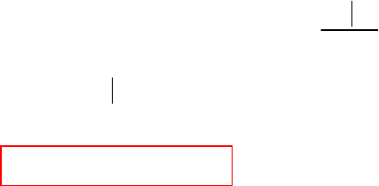
CHAPTER FIVE SOLUTIONS
Engineering Circuit Analysis, 6th Edition Copyright ©2002 McGraw-Hill, Inc. All Rights Reserved.
55. Thévenize the left-hand network, assigning the nodal voltage Vx at the free end of
right-most 1-kΩ resistor.
A single nodal equation: 3
3
40 10 710
−
×=
×
xoc
V
So 280V==
TH x oc
VV
R
TH = 1 k + 7 k = 8 kΩ
Select R1 = RTH = 8 kΩ.
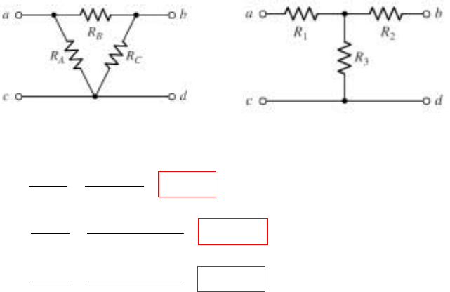
CHAPTER FIVE SOLUTIONS
Engineering Circuit Analysis, 6th Edition Copyright ©2002 McGraw-Hill, Inc. All Rights Reserved.
56.
6
65
1
56
26
66
36
1 850 0.1 851.1 10
10 10 117.5
10 850 10 99.87
851.1 10
850 10 10 998.7
851.1 10
=++=+ += ×
×
== =Ω
××
== = Ω
×
××
== = Ω
×
ABC
AB
BC
CA
DR R R
RR
RDD
RR
Rk
D
RR
Rk
D
1 MΩ
100 kΩ
850 MΩ
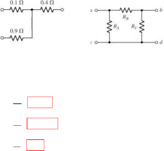
CHAPTER FIVE SOLUTIONS
Engineering Circuit Analysis, 6th Edition Copyright ©2002 McGraw-Hill, Inc. All Rights Reserved.
57.
12 23 31
2
3
1
0.1 0.4 0.4 0.9 0.9 0.1
0.49
1.225
544.4m
4.9
=++
=×+×+×
=Ω
== Ω
== Ω
==Ω
A
B
C
NRR RRRR
N
RR
N
RR
N
RR
R1 R2
R3
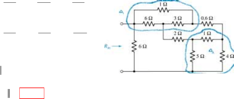
CHAPTER FIVE SOLUTIONS
Engineering Circuit Analysis, 6th Edition Copyright ©2002 McGraw-Hill, Inc. All Rights Reserved.
58.
1
2
:16310
61 63 31
0.6, 1.8 , 0.3
10 10 10
:5 1 4 10
51 14 54
0.5 , 0.4 , 2
10 10 10
1.8 2 0.5 4.3
0.3 0.6 0.4 1.3
1.3 4.3 0.9982
0.9982 0.6 2 3.598
3.598 6 2.249
∆++=Ω
×××
===
∆++=Ω
×× ×
===
++ = Ω
++=Ω
=Ω
++= Ω
=Ω
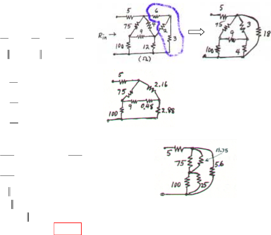
CHAPTER FIVE SOLUTIONS
Engineering Circuit Analysis, 6th Edition Copyright ©2002 McGraw-Hill, Inc. All Rights Reserved.
59.
2
2
622336 36
36 36 36
6 , 18 , 12
62 3
12 4 3 , 6 12 4
4 3 18 25
18
3 2.16
25
18
4 2.88
25
3
4 0.48
25
9.48 2.16 9.48 2.88 2.88 2.16 54
54 54
18.75 5.696
2.88 9.48
54 25
2.16
75 18.75 15
100 25 20
(15 20) 5.696
×+×+×= Ω
=Ω = Ω = Ω
=Ω Ω=Ω
++ = Ω
×= Ω
×= Ω
×= Ω
×+×+×=Ω
=Ω =Ω
=Ω
=Ω
=Ω
+=4.899
5 4.899 9.899
Ω
∴=+ = Ω
in
R
96
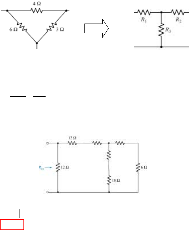
CHAPTER FIVE SOLUTIONS
Engineering Circuit Analysis, 6th Edition Copyright ©2002 McGraw-Hill, Inc. All Rights Reserved.
60. We begin by converting the ∆-connected network consisting of the 4-, 6-, and 3-Ω
resistors to an equivalent Y-connected network:
1
2
3
64313
64 1.846
13
43 923.1m
13
36 1.385
13
=++= Ω
×
===Ω
×
=== Ω
×
===Ω
AB
BC
CA
D
RR
RD
RR
RD
RR
RD
Then network becomes:
Then we may write
12 [13.846 (19.385 6.9231)]
7.347
=+
=Ω
in
R
RA RB
RC
1.846 Ω 0.9231 Ω
1.385 Ω
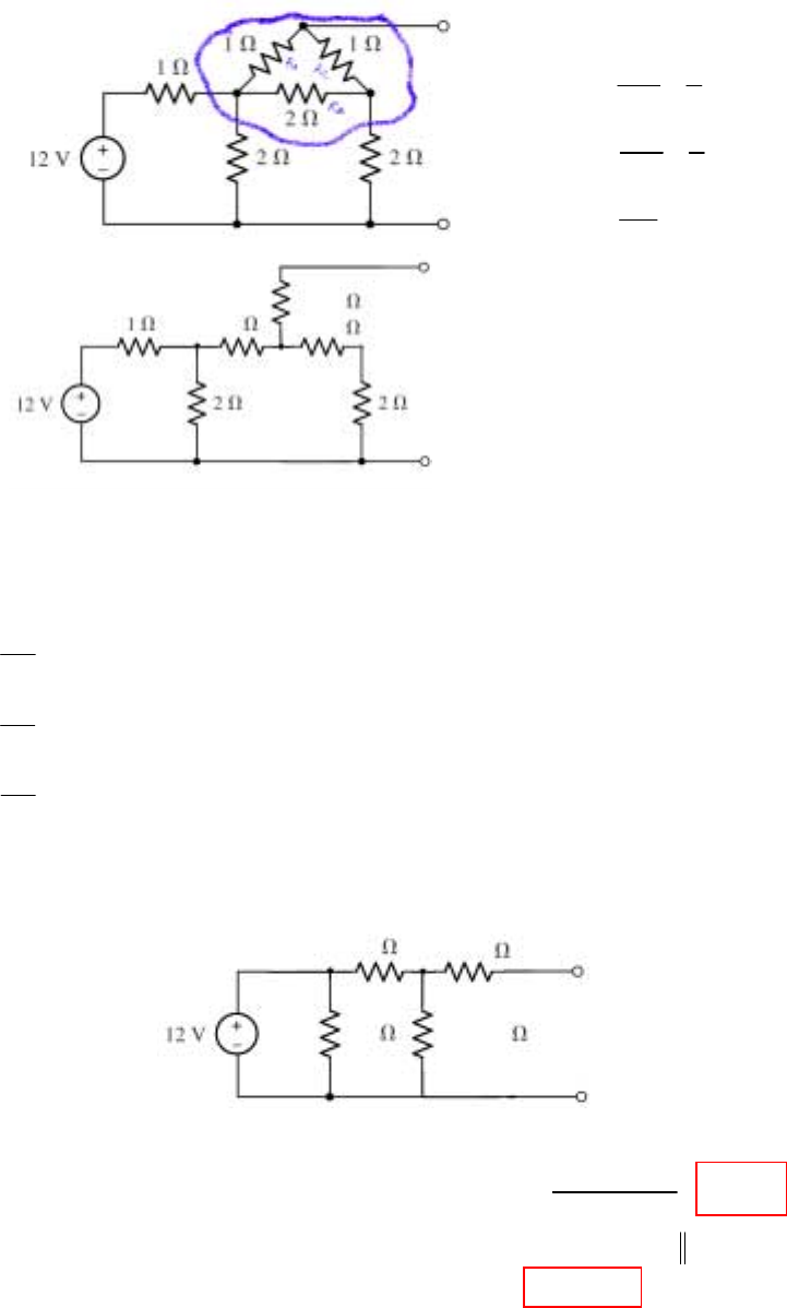
CHAPTER FIVE SOLUTIONS
Engineering Circuit Analysis, 6th Edition Copyright ©2002 McGraw-Hill, Inc. All Rights Reserved.
0.5 0.5
0.25
61.
Next, we convert the Y-connected network on the left to a ∆-connected network:
2
1 0.5 0.5 2 2 1 3.5×+×+×=Ω
3.5 7
0.5
3.5 1.75
2
3.5 3.5
1
==Ω
==Ω
==Ω
A
B
C
R
R
R
After this procedure, we have a 3.5-Ω resistor in parallel with the 2.5-Ω resistor. Replacing
them with a 1.458-Ω resistor, we may redraw the circuit:
This circuit may be easily analysed to find:
1
2
3
112 4
12 1
42
21 1
42
11 0.25
4
++ = Ω
×
==Ω
×
==Ω
×
==Ω
R
R
R
12 1.458 5.454V
1.75 1.458
0.25 1.458 1.75
1.045
×
==
+
=+
=Ω
oc
TH
V
R
7
1.75 0.25
1.458
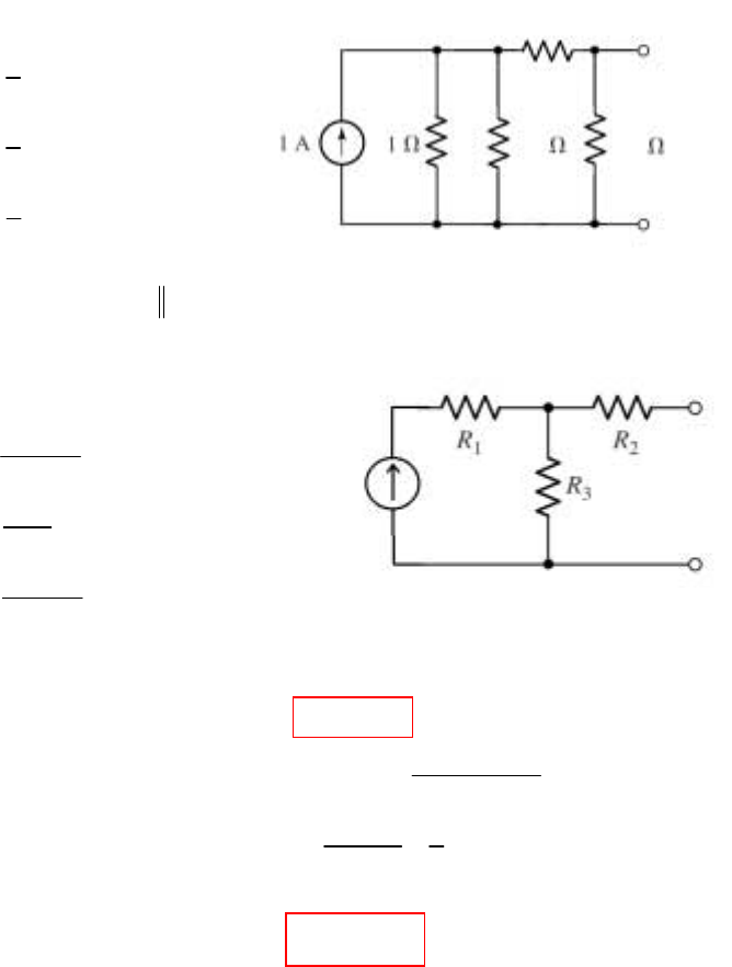
CHAPTER FIVE SOLUTIONS
Engineering Circuit Analysis, 6th Edition Copyright ©2002 McGraw-Hill, Inc. All Rights Reserved.
62. We begin by converting the Y-network to a ∆-connected network:
2
1.1 1.1 1.1 3
33
1
33
1
33
1
=++=Ω
==Ω
==Ω
==Ω
A
B
C
N
R
R
R
Next, we note that 1 3 0.75=Ω, and hence have a simple ∆-network. This is easily
converted to a Y-connected network:
1
2
3
0.75 3 3 6.75
0.75 3 0.3333
6.75
33 1.333
6.75
3 0.75 0.3333
6.75
++= Ω
×
==Ω
×
==Ω
×
==Ω
R
R
R
1.333 0.3333
1.667
1/3
11/3 1 1/3
11
131 5
0.2A
200mA
=+
=Ω
==×++
==
++
=
=
N
NSC
R
II
33
3 Ω
1 A
Analysing this final
circuit,
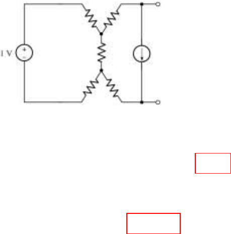
CHAPTER FIVE SOLUTIONS
Engineering Circuit Analysis, 6th Edition Copyright ©2002 McGraw-Hill, Inc. All Rights Reserved.
63. Since 1 V appears across the resistor associated with I1, we know that I1 = 1 V/ 10 Ω
= 100 mA. From the perspective of the open terminals, the 10-Ω resistor in parallel
with the voltage source has no influence if we replace the “dependent” source with a
fixed 0.5-A source:
Then, we may write: -1 + (10 + 10 + 10) ia – 10 (0.5) = 0
so that ia = 200 mA.
We next find that VTH = Vab = 10(-0.5) + 10(ia – 0.5) + 10(-0.5) = -13 V.
To determine RTH, we first recognise that with the 1-V source shorted, I1 = 0 and
hence the dependent current source is dead. Thus, we may write RTH from inspection:
RTH = 10 + 10 + 10 || 20 = 26.67 Ω.
0.5 A
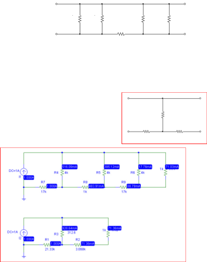
CHAPTER FIVE SOLUTIONS
Engineering Circuit Analysis, 6th Edition Copyright ©2002 McGraw-Hill, Inc. All Rights Reserved.
64. (a) We begin by splitting the 1-kΩ resistor into two 500-Ω resistors in series. We then
have two related Y-connected networks, each with a 500-Ω resistor as a leg.
Converting those networks into ∆-connected networks,
Σ = (17)(10) + (1)(4) + (4)(17) = 89×106 Ω2
89/0.5 = 178 kΩ; 89/ 17 = 5.236 kΩ; 89/4 = 22.25 kΩ
Following this conversion, we find that we have two 5.235 kΩ resistors in parallel,
and a 178-kΩ resistor in parallel with the 4-kΩ resistor. Noting that 5.235 k || 5.235 k
= 2.618 kΩ and 178 k || 4 k = 3.912 kΩ, we may draw the circuit as:
We next attack the Y-connected network in the center:
Σ = (22.25)(22.25) + (22.25)(2.618) + (2.618)(22.25) = 611.6×10⁶ Ω2
611.6/ 22.25 = 27.49 kΩ; 611.6/ 2.618 = 233.6 kΩ
Noting that 178 k || 27.49 k = 23.81 kΩ and 27.49 || 3.912 = 3.425 kΩ, we are left
with a simple ∆-connected network. To convert this to the requested Y-network,
Σ = 23.81 + 233.6 + 3.425 = 260.8 kΩ
(23.81)(233.6)/ 260.8 = 21.33 kΩ
(233.6)(3.425)/ 260.8 = 3.068 kΩ
(3.425)(23.81)/ 260.8 = 312.6 Ω
178 kΩ
233.6 kΩ
27.49 kΩ 27.49 kΩ 3.912 kΩ
312.6 Ω
21.33 kΩ 3.068 kΩ
(b)
CHAPTER FIVE SOLUTIONS
Engineering Circuit Analysis, 6th Edition Copyright ©2002 McGraw-Hill, Inc. All Rights Reserved.
65. (a) Although this network may be simplified, it is not possible to replace it with a
three-resistor equivalent.
(b) See (a).
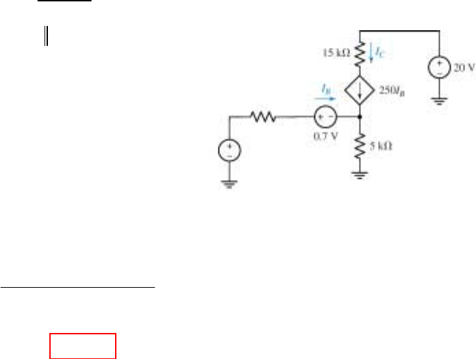
CHAPTER FIVE SOLUTIONS
Engineering Circuit Analysis, 6th Edition Copyright ©2002 McGraw-Hill, Inc. All Rights Reserved.
66. First, replace network to left of the 0.7-V source with its Thévenin equivalent:
15
20 2.609V
100 15
100 15 13.04
=× =
+
==Ω
TH
TH
V
Rkkk
Redraw:
Analysing the new circuit to find IB, we note that IC = 250 IB:
3
3
4
2.609 13.04 10 0.7 5000( 250 ) 0
2.609 0.7 1.505 A
13.04 10 251 5000
250 3.764 10 A
376.4 A
−
−+×++ + =
−
==µ
×+×
==×
=µ
BBB
B
CB
III
I
II
2.609 V
13.04 kΩ
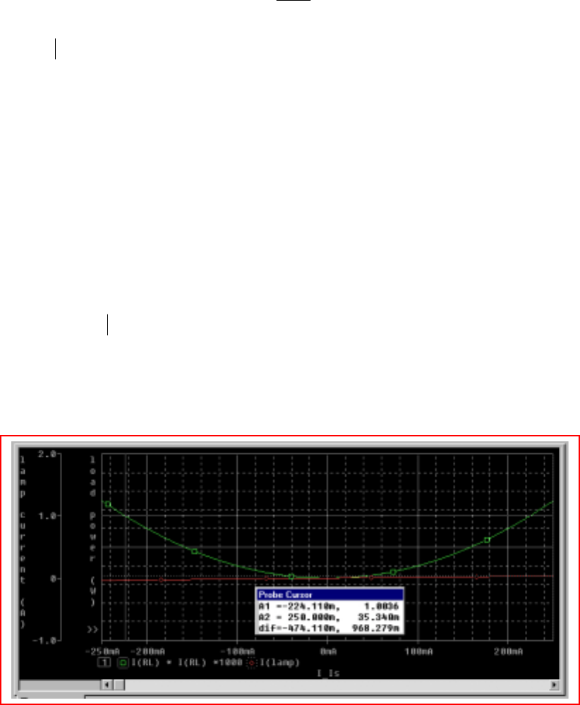
CHAPTER FIVE SOLUTIONS
Engineering Circuit Analysis, 6th Edition Copyright ©2002 McGraw-Hill, Inc. All Rights Reserved.
67. (a) Define a nodal voltage V1 at the top of the current source IS, and a nodal voltage
V2 at the top of the load resistor RL. Since the load resistor can safely dissipate 1 W,
and we know that
PRL = 1000
V2
2
then V 31.62 V max
2=. This corresponds to a load resistor (and hence lamp) current
of 32.62 mA, so we may treat the lamp as a 10.6-Ω resistor.
Proceeding with nodal analysis, we may write:
IS = V1/ 200 + (V1 – 5 Vx)/ 200 [1]
0 = V2/ 1000 + (V2 – 5 Vx)/ 10.6 [2]
Vx = V1 – 5 Vx or Vx = V1/ 6 [3]
Substituting Eq. [3] into Eqs. [1] and [2], we find that
7 V1 = 1200 IS [1]
-5000 V1 + 6063.6 V2 = 0 [2]
Substituting V 31.62 V max
2=into Eq. [2] then yields V1 = 38.35 V, so that
IS| max = (7)(38.35)/ 1200 = 223.7 mA.
(b) PSpice verification.
The lamp current does not exceed 36 mA in the range of operation allowed
(i.e. a load power of < 1 W.) The simulation result shows that the load will dissipate
slightly more than 1 W for a source current magnitude of 224 mA, as predicted by
hand analysis.

CHAPTER FIVE SOLUTIONS
Engineering Circuit Analysis, 6th Edition Copyright ©2002 McGraw-Hill, Inc. All Rights Reserved.
68. Short out all but the source operating at 104 rad/s, and define three clockwise mesh
currents i1, i2, and i3 starting with the left-most mesh. Then
608 i1 – 300 i2 = 3.5 cos 104 t [1]
-300 i1 + 316 i2 – 8 i3 = 0 [2]
-8 i2 + 322 i3 = 0 [3]
Solving, we find that i1(t) = 10.84 cos 104 t mA
i2(t) = 10.29 cos 104 t mA
i3(t) = 255.7 cos 104 t µA
Next, short out all but the 7 sin 200t V source, and and define three clockwise mesh
currents ia, ib, and ic starting with the left-most mesh. Then
608 ia – 300 ib = -7 sin 200t [1]
-300 ia + 316 ib – 8 ic = 7 sin 200t [2]
-8 ib + 322 ic = 0 [3]
Solving, we find that ia(t) = -1.084 sin 200t mA
ib(t) = 21.14 sin 200t mA
ic(t) = 525.1 sin 200t µA
Next, short out all but the source operating at 103 rad/s, and define three clockwise
mesh currents iA, iB, and iC starting with the left-most mesh. Then
608 iA – 300 iB = 0 [1]
-300 iA + 316 iB – 8 iC = 0 [2]
-8 iB + 322 iC = -8 cos 104 t [3]
Solving, we find that iA(t) = -584.5 cos 103 t µA
iB(t) = -1.185 cos 103 t mA
iC(t) = -24.87 cos 103 t mA
We may now compute the power delivered to each of the three 8-Ω speakers:
p1 = 8[i1 + ia + iA]2 = 8[10.84×10⁻³ cos 104 t -1.084×10⁻³ sin 200t -584.5×10⁻⁶ cos 103 t]2
p2 = 8[i2 + ib + iB]2 = 8[10.29×10⁻³ cos 104 t +21.14×10⁻³ sin 200t –1.185×10⁻³ cos 103 t]2
p3 = 8[i3 + ic + iC]2 = 8[255.7×10⁻⁶ cos 104 t +525.1×10⁻⁶ sin 200t –24.87×10⁻³ cos 103 t]2
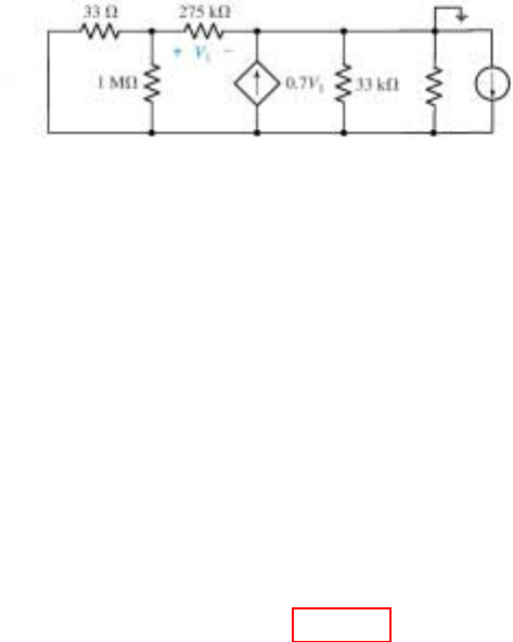
CHAPTER FIVE SOLUTIONS
Engineering Circuit Analysis, 6th Edition Copyright ©2002 McGraw-Hill, Inc. All Rights Reserved.
69. Replacing the DMM with a possible Norton equivalent (a 1-MΩ resistor in parallel
with a 1-A source):
We begin by noting that 33 Ω || 1 MΩ ≈ 33 Ω. Then,
0 = (V1 – Vin)/ 33 + V1/ 275×103 [1]
and
1 - 0.7 V1 = Vin/ 106 + Vin/ 33×103 + (Vin – V1)/ 33 [2]
Simplifying and collecting terms,
(275×103 + 33) V1 - 275×103 Vin = 0 [1]
22.1 V1 + 1.001 Vin = 33 [2]
Solving, we find that Vin = 1.429 V; in other words, the DMM sees 1.429 V across its
terminals in response to the known current of 1 A it’s supplying. It therefore thinks
that it is connected to a resistance of 1.429 Ω.
1 A
Vin

CHAPTER FIVE SOLUTIONS
Engineering Circuit Analysis, 6th Edition Copyright ©2002 McGraw-Hill, Inc. All Rights Reserved.
70. We know that the resistor R is absorbing maximum power. We might be tempted to
say that the resistance of the cylinder is therefore 10 Ω, but this is wrong: The larger
we make the cylinder resistance, the small the power delivery to R:
PR = 10 i2 = 10
2
10
120
+
cylinder
R
Thus, if we are in fact delivering the maximum possible power to the resistor from the
120-V source, the resistance of the cylinder must be zero.
This corresponds to a temperature of absolute zero using the equation given.
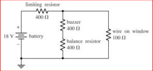
CHAPTER FIVE SOLUTIONS
Engineering Circuit Analysis, 6th Edition Copyright ©2002 McGraw-Hill, Inc. All Rights Reserved.
71. We note that the buzzer draws 15 mA at 6 V, so that it may be modeled as a
400-Ω resistor. One possible solution of many, then, is:
Note: construct the 18-V source from 12 1.5-V batteries in series, and the two 400-Ω
resistors can be fabricated by soldering 400 1-Ω resistors in series, although there’s
probably a much better alternative…
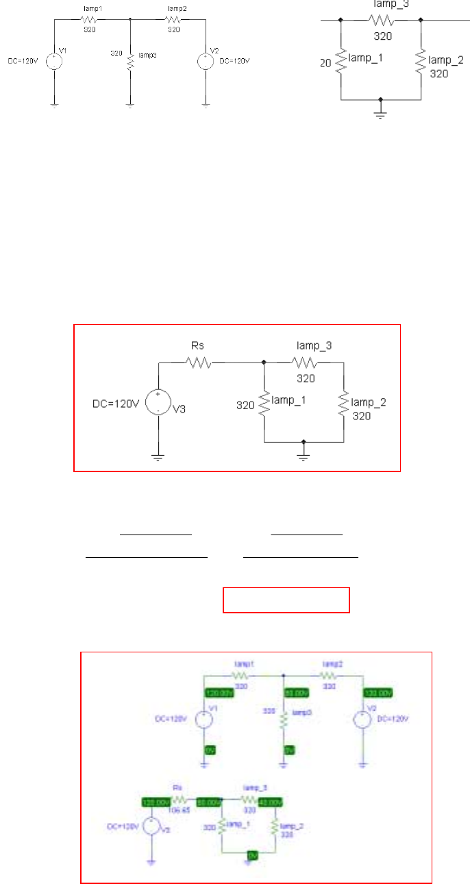
CHAPTER FIVE SOLUTIONS
Engineering Circuit Analysis, 6th Edition Copyright ©2002 McGraw-Hill, Inc. All Rights Reserved.
72. To solve this problem, we need to assume that “45 W” is a designation that
applies
when 120 Vac is applied directly to a particular lamp. This corresponds to a current
draw of 375 mA, or a light bulb resistance of 120/ 0.375 = 320 Ω.
Original wiring scheme New wiring scheme
In the original wiring scheme, Lamps 1 & 2 draw (40)2 / 320 = 5 W of power each,
and Lamp 3 draws (80)2 / 320 = 20 W of power. Therefore, none of the lamps is
running at its maximum rating of 45 W. We require a circuit which will deliver the
same intensity after the lamps are reconnected in a ∆ configuration. Thus, we need a
total of 30 W from the new network of lamps.
There are several ways to accomplish this, but the simplest may be to just use one
120-Vac source connected to the left port in series with a resistor whose value is
chosen to obtain 30 W delivered to the three lamps.
In other words,
30
320
213.3Rs
213.3
06
2
320
213.3Rs
213.3
120
22
=
+
+
+
Solving, we find that we require Rs = 106.65 Ω, as confirmed by the PSpice
simulation below, which shows that both wiring configurations lead to one lamp with
80-V across it, and two lamps with 40 V across each.
3
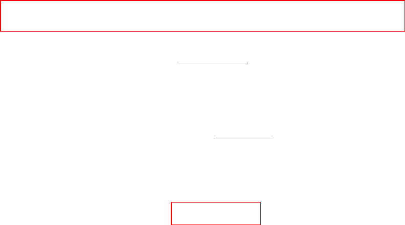
CHAPTER FIVE SOLUTIONS
Engineering Circuit Analysis, 6th Edition Copyright ©2002 McGraw-Hill, Inc. All Rights Reserved.
73.
• Maximum current rating for the LED is 35 mA.
• Its resistance can vary between 47 and 117 Ω.
• A 9-V battery must be used as a power source.
• Only standard resistance values may be used.
One possible current-limiting scheme is to connect a 9-V battery in series with a
resistor Rlimiting and in series with the LED.
From KVL,
ILED =
LEDlimiting R R
9
+
The maximum value of this current will occur at the minimum LED resistance, 47 Ω.
Thus, we solve
35×10-3 = 47 R
9
limiting +
to obtain Rlimiting ≥ 210.1 Ω to ensure an LED current of less than 35 mA. This is not a
standard resistor value, however, so we select
Rlimiting = 220 Ω.
CHAPTER SIX SOLUTIONS
Engineering Circuit Analysis, 6th Edition Copyright ©2002 McGraw-Hill, Inc. All Rights Reserved.
1. The first step is to perform a simple source transformation, so that a 0.15-V source in
series with a 150-Ω resistor is connected to the inverting pin of the ideal op amp.
Then, vout =
()
V 2.2- 15.0
150
2200
=−
CHAPTER SIX SOLUTIONS
Engineering Circuit Analysis, 6th Edition Copyright ©2002 McGraw-Hill, Inc. All Rights Reserved.
2. In order to deliver 150 mW to the 10-kΩ resistor, we need vout =
V. 38.73 )1010)(15.0( 3=× Writing a nodal equation at the inverting input,
we find
1000
5
R
5
0 out
v−
+=
Using vout = 38.73, we find that R = 148.2 Ω.

CHAPTER SIX SOLUTIONS
Engineering Circuit Analysis, 6th Edition Copyright ©2002 McGraw-Hill, Inc. All Rights Reserved.
3. Since the 670-Ω switch requires 100 mA to activate, the voltage delivered to it by our
op amp circuit must be (670)(0.1) = 67 V. The microphone acts as the input to the
circuit, and provides 0.5 V. Thus, an amplifier circuit having a gain = 67/0.5 = 134 is
required.
One possible solution of many: a non-inverting op amp circuit with the microphone
connected to the non-inverting input terminal, the switch connected between the op
amp output pin and ground, a feedback resistor Rf = 133 Ω, and a resistor R1 = 1 Ω.
CHAPTER SIX SOLUTIONS
Engineering Circuit Analysis, 6th Edition Copyright ©2002 McGraw-Hill, Inc. All Rights Reserved.
4. We begin by labeling the nodal voltages v- and v+ at the inverting and non-inverting
input terminals, respectively. Since no current can flow into the non-inverting input,
no current flows through the 40-kΩ resistor; hence, v+ = 0. Therefore, we know that
v- = 0 as well.
Writing a single nodal equation at the non-inverting input then leads to
22000
) - (
100
) - (
0 out-S- vvvv +=
or
22000
-
100
-
0 outSvv +=
Solving,
vout = -220 vS

CHAPTER SIX SOLUTIONS
Engineering Circuit Analysis, 6th Edition Copyright ©2002 McGraw-Hill, Inc. All Rights Reserved.
5. We first label the nodal voltage at the output pin Vo. Then, writing a single nodal
equation at the inverting input terminal of the op amp,
17000
V-4
1000
3-4
0 o
+=
Solving, we find that Vo = 21 V. Since no current can flow through the 300-kΩ
resistor, V1 = 21 as well.
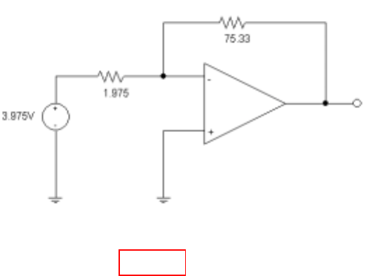
CHAPTER SIX SOLUTIONS
Engineering Circuit Analysis, 6th Edition Copyright ©2002 McGraw-Hill, Inc. All Rights Reserved.
6. A source transformation and some series combinations are well worthwhile prior to
launching into the analysis. With 5 kΩ || 3 kΩ = 1.875 kΩ and (1 mA)(1.875 kΩ) =
1.875 V, we may redraw the circuit as
This is now a simple inverting amplifier with gain – Rf/ R1 = -75.33/ 1.975 = -38.14.
Thus, V2 = -38.14(3.975) = -151.6 V.
Ω
Ω
V2

CHAPTER SIX SOLUTIONS
Engineering Circuit Analysis, 6th Edition Copyright ©2002 McGraw-Hill, Inc. All Rights Reserved.
7. This is a simple inverting amplifier, so we may write
()()
V 3sin 14- 3sin22
1000
2000-
out ttv +=+=
vout(t = 3 s) = -5.648 V.

CHAPTER SIX SOLUTIONS
Engineering Circuit Analysis, 6th Edition Copyright ©2002 McGraw-Hill, Inc. All Rights Reserved.
8. We first combine the 2 MΩ and 700 kΩ resistors into a 518.5 kΩ resistor.
We are left with a simple non-inverting amplifier having a gain of
1 + 518.5/ 250 = 3.074. Thus,
vout = (3.074) vin = 18 so vin = 5.856 V.

CHAPTER SIX SOLUTIONS
Engineering Circuit Analysis, 6th Edition Copyright ©2002 McGraw-Hill, Inc. All Rights Reserved.
9. This is a simple non-inverting amplifier circuit, and so it has a gain of 1 + Rf/ R1.
We want vout = 23.7 cos 500t V when the input is 0.1 cos 500t V, so a gain of 23.7/0.1
= 237 is required.
One possible solution of many: Rf = 236 kΩ and R1 = 1 kΩ.
CHAPTER SIX SOLUTIONS
Engineering Circuit Analysis, 6th Edition Copyright ©2002 McGraw-Hill, Inc. All Rights Reserved.
10. Define a nodal voltage V- at the inverting input, and a nodal voltage V+ at the non-
inverting input. Then,
At the non-inverting input: -3×10-6 = 6
101.5
V
×
+ [1]
Thus, V+ = -4.5 V, and we therefore also know that V- = -4.5 V.
At the inverting input:
7
out-
6
-
R
V - V
R
V
0 += [2]
Solving and making use of the fact that V- = -4.5 V,
vout =
()
V 1
R
R
4.5- 4.5 - 5.4
R
R
6
7
6
7
+=−
CHAPTER SIX SOLUTIONS
Engineering Circuit Analysis, 6th Edition Copyright ©2002 McGraw-Hill, Inc. All Rights Reserved.
11. (a) B must be the non-inverting input: that yields a gain of 1 + 70/10 = 8 and an
output of 8 V for a 1-V input.
(b) R1 = ∞, RA = 0. We need a gain of 20/10 = 2, so choose R2 = RB = 1 Ω.
(c) A is the inverting input since it has the feedback connection to the output pin.
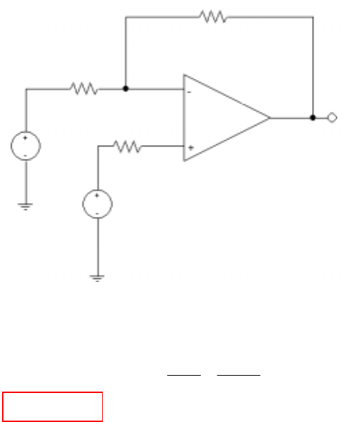
CHAPTER SIX SOLUTIONS
Engineering Circuit Analysis, 6th Edition Copyright ©2002 McGraw-Hill, Inc. All Rights Reserved.
12. It is probably best to first perform a simple source transformation:
(1 mA)(2 kΩ) = 2 V.
Since no current can flow into the non-inverting input pin, we know that V+ = 2 V,
and therefore also that V- = 2 V. A single nodal equation at the inverting input yields:
13000
-2
1000
3-2
0 out
v
+=
which yields vout = -11 V.
2 V
3 V
vout
13 kΩ
1 kΩ
2 kΩ V+
V-
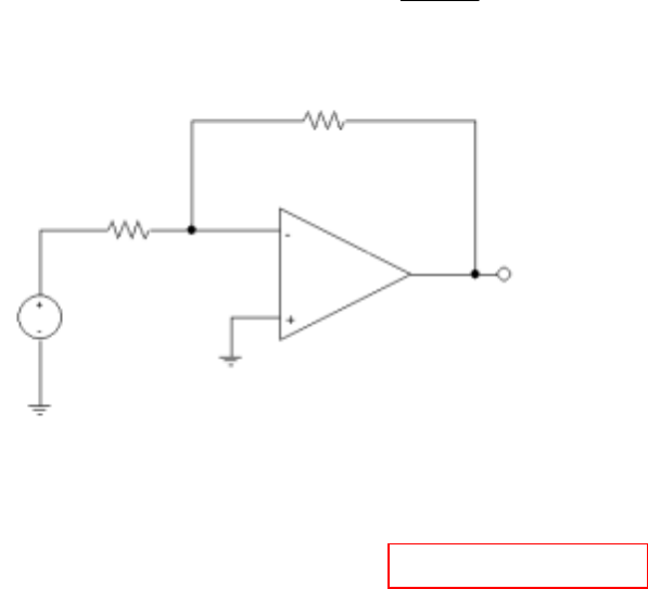
CHAPTER SIX SOLUTIONS
Engineering Circuit Analysis, 6th Edition Copyright ©2002 McGraw-Hill, Inc. All Rights Reserved.
13. We begin by find the Thévenin equivalent to the left of the op amp:
Vth = -3.3(3) v
π
= -9.9 v
π
= 1100
1000
9.9 S
v
− = -9 vS
R
th = 3.3 kΩ, so we can redraw the circuit as:
which is simply a classic inverting op amp circuit with gain of -100/3.3 = -30.3.
Thus, vout = (-30.3)( -9 vS) = 272.7 vS
For vS = 5 sin 3t mV, vout = 1.364 sin 3t V, and vout(0.25 s) = 0.9298 V.
vout
-9 vS
3.3 kΩ
100 kΩ
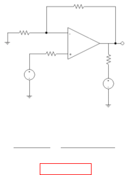
CHAPTER SIX SOLUTIONS
Engineering Circuit Analysis, 6th Edition Copyright ©2002 McGraw-Hill, Inc. All Rights Reserved.
14. We first combine the 4.7 MΩ and 1.3 kΩ resistors: 4.7 MΩ || 1.3 kΩ = 1.30 kΩ.
Next, a source transformation yields (3×10⁻⁶)(1300) = 3.899 mV which appears in
series with the 20 mV source and the 500-Ω resistor. Thus, we may redraw the circuit
as
Since no current flows through the 1.8 kΩ resistor, V+ = 23.899 mV and hence
V- = 23.899 mV as well. A single nodal equation at the inverting input terminal yields
3
out
-3-3
1037.7
- 1023.899
500
1023.899
0 ×
×
+
×
=v
Solving, vout = 1.826 V
23.899 mV
-6 V
370 Ω
37.7 kΩ
1.8 kΩ
vout
500 Ω

CHAPTER SIX SOLUTIONS
Engineering Circuit Analysis, 6th Edition Copyright ©2002 McGraw-Hill, Inc. All Rights Reserved.
15. We first combine the 4.7 MΩ and 1.3 kΩ resistors: 4.7 MΩ || 1.3 kΩ = 1.30 kΩ.
Next, a source transformation yields (27×10-6)(1300) = 35.1 mV which appears in
series with the 20 mV source and the 500-Ω resistor. Thus, we may redraw the circuit
as
Since no current flows through the 1.8 kΩ resistor, V+ = 55.1 mV and hence
V- = 55.1 mV as well. A single nodal equation at the inverting input terminal yields
3
out
-3-3
1037.7
- 101.55
500
101.55
0 ×
×
+
×
=v
Solving, vout = 4.21 V
55.1 mV
-6 V
370 Ω
37.7 kΩ
1.8 kΩ
vout
500 Ω

CHAPTER SIX SOLUTIONS
Engineering Circuit Analysis, 6th Edition Copyright ©2002 McGraw-Hill, Inc. All Rights Reserved.
16. The 3 mA source, 1 kΩ resistor and 20 kΩ resistor may be replaced with a –3 V
source (“+” reference up) in series with a 21 kΩ resistor. No current flows through
either 1 MΩ resistor, so that the voltage at each of the four input terminals is
identically zero. Considering each op amp circuit separately,
V 14.29
21
100
(-3)-
AMLEFTOP
out ==
P
v
V 50-
10
100
(5)-
AMPOP RIGH
out ==v
vx = PP vv AMOP RIGH
out
AMLEFTOP
out - = 14.29 + 50 = 64.29 V.
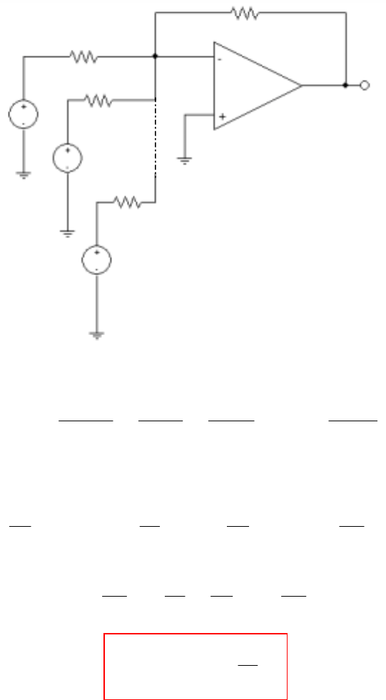
CHAPTER SIX SOLUTIONS
Engineering Circuit Analysis, 6th Edition Copyright ©2002 McGraw-Hill, Inc. All Rights Reserved.
17. A general summing amplifier with N input sources:
1. va = vb = 0
2. A single nodal equation at the inverting input leads to:
N
Na
2
2a
1
1a
f
a
R
...
R
R
R
0 vvvvvvvv out −
++
−
+
−
+
−
=
Simplifying and making use of the fact that va = 0, we may write this as
∏∏∏∏ ====
+++=
−N
1
i
N
N
N
1
i
2
2
N
1
i
1
1
N
1
i
f
R
R
... R
R
R
R
R
R
1
iii
out
i
vvv
v
or simply
N
N
2
2
1
1
fR
...
R
R
R
vvvvout +++=−
Thus,
vout = ∑
=
N
1
fR
R-
ii
i
v
v1
v2
vN
vout
RN
R1
R2
Rf
va
vb
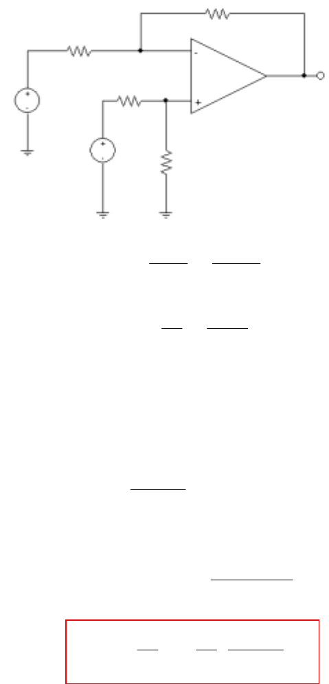
CHAPTER SIX SOLUTIONS
Engineering Circuit Analysis, 6th Edition Copyright ©2002 McGraw-Hill, Inc. All Rights Reserved.
18. A general difference amplifier:
Writing a nodal equation at the inverting input,
f
a
1
1a
R
-
R
-
0 out
vvvv +=
Writing a nodal equation at the non-inverting input,
2
2b
3
b
R
-
R
0 vvv +=
Simplifying and collecting terms, we may write
(R
f + R1) va – R1 vout = Rf v1 [1]
(R
2 + R3) vb = R3 v2 [2]
From Eqn. [2], we have vb = 2
32
3
RR
Rv
+
Since va = vb, we can now rewrite Eqn. [1] as
()
2
32
31f
1f1 RR
RRR
R R vvvout +
+
−=−
and hence
2
32
1f
1
3
1
1
f
RR
RR
R
R
R
R
- vvvout
+
+
+=
v1
v2
R1
R2
R3
R4
vout

CHAPTER SIX SOLUTIONS
Engineering Circuit Analysis, 6th Edition Copyright ©2002 McGraw-Hill, Inc. All Rights Reserved.
19. In total darkness, the CdS cell has a resistance of 100 kΩ, and at a light intensity L of
6 candela it has a resistance of 6 kΩ. Thus, we may compute the light-dependent
resistance (assuming a linear response in the range between 0 and 6 candela) as RCdS =
-15L + 100 Ω.
Our design requirement (using the standard inverting op amp circuit shown) is that the
voltage across the load is 1.5 V at 2 candela, and less than 1.5 V for intensities greater
than 2 candela.
Thus, vout(2 candela) = -RCdS vS/ R1 = -70 VS/ R1 = 1.5 (R1 in kΩ).
Pick R1 = 10 kΩ. Then vS = -0.2143 V.
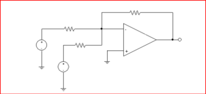
CHAPTER SIX SOLUTIONS
Engineering Circuit Analysis, 6th Edition Copyright ©2002 McGraw-Hill, Inc. All Rights Reserved.
20. We want Rf/ Rinstrument = 2K, and Rf/ Rvocal = 1K, where K is a constant not specified.
Assuming K = 1, one possible solution of many is:
vout
vocals
microphone
instruments
microphone
Rvocal = 1 Ω
Rinstruments = 2 Ω
Rf = 2 Ω
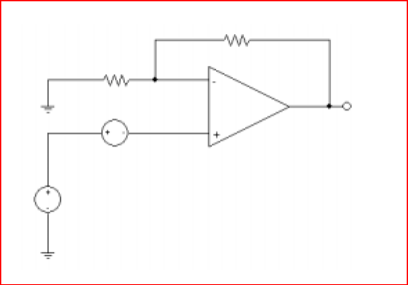
CHAPTER SIX SOLUTIONS
Engineering Circuit Analysis, 6th Edition Copyright ©2002 McGraw-Hill, Inc. All Rights Reserved.
21. One possible solution of many:
vS
vout
2 V
1 kΩ
99 kΩ

CHAPTER SIX SOLUTIONS
Engineering Circuit Analysis, 6th Edition Copyright ©2002 McGraw-Hill, Inc. All Rights Reserved.
22. vout of stage 1 is (1)(-20/ 2) = -10 V.
vout of stage 2 is (-10)(-1000/ 10) = 1000 V
Note: in reality, the output voltage will be limited to a value less than that used to
power the op amps.
CHAPTER SIX SOLUTIONS
Engineering Circuit Analysis, 6th Edition Copyright ©2002 McGraw-Hill, Inc. All Rights Reserved.
23. We have a difference amplifier as the first amplifier stage, and a simple voltage
follower as the second stage. We therefore need only to find the output voltage of the
first stage: vout will track this voltage. Using voltage division, then, we vind that the
voltage at the non-inverting input pin of the first op amp is
+32
3
2RR
R
V
and this is the voltage at the inverting input terminal also. Thus, we may write a
single nodal equation at the inverting input of the first op amp:
+
+
+
=1
out
32
3
2
f
1
32
3
2
1
V -
RR
R
V
R
1
V -
RR
R
V
R
1
0 Stage
which may be solved to obtain:
1
1
f
2
32
3
1
f
1
outout V
R
R
- V
RR
R
1
R
R
V V +
+== Stage
CHAPTER SIX SOLUTIONS
Engineering Circuit Analysis, 6th Edition Copyright ©2002 McGraw-Hill, Inc. All Rights Reserved.
24. The output of the first op amp stage may be found by realising that the voltage at the
non-inverting input (and hence the voltage at the inverting input) is 0, and writing a
ingle nodal equation at the inverting input:
7
3 - 0
1
2 - 0
47
V - 0
0 1 stage
out ++= which leads to 1 steage
out
V = -114.1 V
This voltage appears at the input of the second op amp stage, which has a gain of
–3/ 0.3 = 10. Thus, the output of the second op amp stage is –10(-114.1) = 1141 V.
This voltage appears at the input of the final op amp stage, which has a gain of
–47/ 0.3 = -156.7.
Thus, the output of the circuit is –156.7(1141) = -178.8 kV, which is completely and
utterly ridiculous.
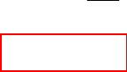
CHAPTER SIX SOLUTIONS
Engineering Circuit Analysis, 6th Edition Copyright ©2002 McGraw-Hill, Inc. All Rights Reserved.
25. The output of the top left stage is –1(10/ 2) = -5 V.
The output of the middle left stage is –2(10/ 2) = -10 V.
The output of the bottom right stage is –3(10/ 2) = -15 V.
These three voltages are the input to a summing amplifier such that
Vout =
()
10 15105
100
R
=−−−−
Solving, we find that R = 33.33 Ω.

CHAPTER SIX SOLUTIONS
Engineering Circuit Analysis, 6th Edition Copyright ©2002 McGraw-Hill, Inc. All Rights Reserved.
26. Stage 1 is configured as a voltage follower: the output voltage will be equal to the
input voltage. Using voltage division, the voltage at the non-inverting input (and
hence at the inverting input, as well), is
V 1.667
50100
50
5=
+
The second stage is wired as a voltage follower also, so vout = 1.667 V.
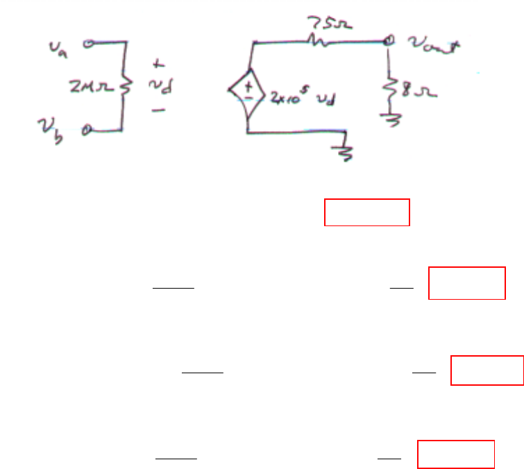
CHAPTER SIX SOLUTIONS
Engineering Circuit Analysis, 6th Edition Copyright ©2002 McGraw-Hill, Inc. All Rights Reserved.
27.
(a) va = vb = 1 nV ∴ vd = 0 and vout = 0. Thus, P8Ω = 0 W.
(b) va = 0, vb = 1 nV ∴ vd = -1 nV
vout = (2×10⁵)(-1×10⁻⁹)875
8
+ = -19.28 µV. Thus, P8Ω = 8
2
out
v = 46.46 pW.
(c) va = 2 pV, vb = 1 fV ∴ vd = 1.999 pV
vout = (2×10⁵)(1.999×10⁻¹²)875
8
+ = 38.53 nV. Thus, P8Ω = 8
2
out
v = 185.6 aW.
(c) va = 50 µV, vb = -4 µV ∴ vd = 54 µV
vout = (2×10⁵)(54×10-6)875
8
+ = 1.041 V. Thus, P8Ω = 8
2
out
v = 135.5 mW.
CHAPTER SIX SOLUTIONS
Engineering Circuit Analysis, 6th Edition Copyright ©2002 McGraw-Hill, Inc. All Rights Reserved.
28.
Writing a nodal equation at the “-vd” node,
f
outd
1
Sd
in
d
R
- -
R
V - -
R
-
0 vvvv ++= [1]
or (R1Rf + RinRf + RinR1) vd + RinR1vout = -RinRfVS [1]
Writing a nodal equation at the “vout” node,
f
dout
o
dout
R
)(- -
R
A - -
0 vvvv += [2]
Eqn. [2] can be rewritten as:
()
out
fo
of
d
AR - R
R R-
vv +
= [2]
so that Eqn. [1] becomes:
vout =
()
ino1o1infin1f1in
Sofin
RR RR RR RR RR RAR
V R - ARR
- +++++
where for this circuit, A = 106, Rin = 10 TΩ, Ro = 15 Ω, Rf = 1000 kΩ, R1 = 270 kΩ.
(a) –3.704 mV; (b) 27.78 mV; (c) –3.704 V.

CHAPTER SIX SOLUTIONS
Engineering Circuit Analysis, 6th Edition Copyright ©2002 McGraw-Hill, Inc. All Rights Reserved.
29. vout = Avd =
()
V 2 sin 1080
R16
R
A15
i
it×
+
(a) A = 105, Ri = 100 MΩ, Ro value irrelevant. vout = 8 sin 2t nV
(b) A = 106, Ri = 1 TΩ, Ro value irrelevant. vout = 80 sin 2t nV
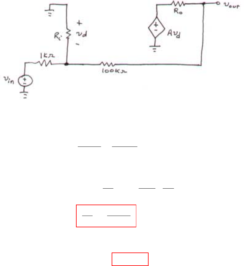
CHAPTER SIX SOLUTIONS
Engineering Circuit Analysis, 6th Edition Copyright ©2002 McGraw-Hill, Inc. All Rights Reserved.
30.
(a) Find vout/ vin if Ri = ∞, Ro = 0, and A is finite.
The nodal equation at the inverting input is
100
- -
1
- -
0 outdindvvvv += [1]
At the output, with Ro = 0 we may write vout = Avd so vd = vout/ A. Thus, Eqn. [1]
becomes
100
100A
A
0 outout
in
out vv
v
v+++=
from which we find
A 101
100A-
in
out
+
=
v
v [2]
(b) We want the value of A such that vout/ vin = -99 (the “ideal” value would be –100
if A were infinite). Substituting into Eqn. [2], we find
A = 9999
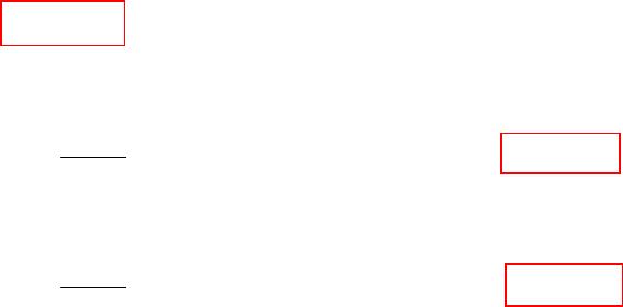
CHAPTER SIX SOLUTIONS
Engineering Circuit Analysis, 6th Edition Copyright ©2002 McGraw-Hill, Inc. All Rights Reserved.
31. (a)
δ
= 0 V ∴ vd = 0, and P8Ω = 0 W.
(b)
δ
= 1 nV, so vd = 5 – (5 + 10-9) = -10-9 V
Thus,
vout = (2×10⁵)vd 758
8
+ = -19.28 µV and P8Ω = (vout)2/ 8 = 46.46 pW.
(c)
δ
= 2.5 µV, so vd = 5 – (5 + 2.5×10⁻⁶) = -2.5×10⁻⁶V
Thus,
vout = (2×10⁵)vd 758
8
+ = -48.19 mV and P8Ω = (vout)2/ 8 = 290.3 µW.
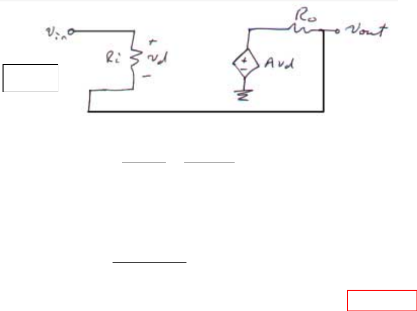
CHAPTER SIX SOLUTIONS
Engineering Circuit Analysis, 6th Edition Copyright ©2002 McGraw-Hill, Inc. All Rights Reserved.
32.
Writing a single nodal equation at the output, we find that
o
dout
i
inout
R
A -
R
-
0 vvvv += [1]
Also, vin – vout = vd, so Eqn. [1] becomes
0 = (vout – vin) Ro + (vout – Avin + Avout) Ri
and
vout =
()
in
v
A
R )1(R
AR R
io
io
++
+
To within 4 significant figures (and more, actually), when vin = -16 mV, vout = -16 mV
(this is, after all, a voltage follower circuit).
AD549
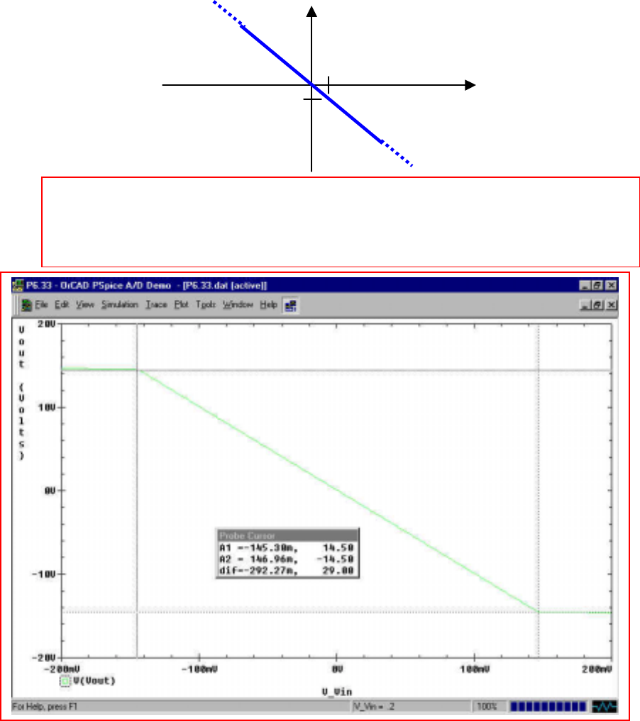
CHAPTER SIX SOLUTIONS
Engineering Circuit Analysis, 6th Edition Copyright ©2002 McGraw-Hill, Inc. All Rights Reserved.
33. The ideal op amp model predicts a gain vout/ vin = -1000/ 10 = -100, regardless of the
value of vin. In other words, it predicts an input-output characteristic such as:
From the PSpice simulation result shown below, we see that the ideal op amp model
is reasonably accurate for |vin| × 100 < 15 V (the supply voltage, assuming both have
the same magnitude), but the onset of saturation is at ±14.5 V, or |vin| ~ 145 mV.
Increasing |vin| past this value does not lead to an increase in |vout|.
vout (V)
vin (V)
-100
1

CHAPTER SIX SOLUTIONS
Engineering Circuit Analysis, 6th Edition Copyright ©2002 McGraw-Hill, Inc. All Rights Reserved.
34. Positive voltage supply, negative voltage supply, inverting input, ground, output pin.
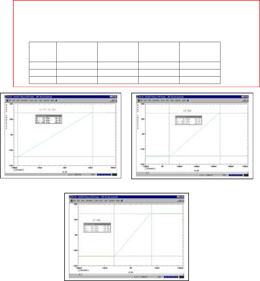
CHAPTER SIX SOLUTIONS
Engineering Circuit Analysis, 6th Edition Copyright ©2002 McGraw-Hill, Inc. All Rights Reserved.
35. This op amp circuit is an open-loop circuit; there is no external feedback path from
the output terminal to either input. Thus, the output should be the open-loop gain
times the differential input voltage, minus any resistive losses.
From the simulation results below, we see that all three op amps saturate at a voltage
magnitude of approximately 14 V, corresponding to a differential input voltage of 50
to 100 µV, except in the interest case of the LM 324, which may be showing some
unexpected input offset behavior.
op amp onset of
negative
saturation
negative
saturation
voltage
onset of
positive
saturation
positive
saturation
voltage
µA 741 -92 µV -14.32 V 54.4 mV 14.34 V
LM 324 41.3 µV -14.71 V 337.2 mV 13.87 V
LF 411 -31.77 µV -13.81 V 39.78 mV 13.86 V
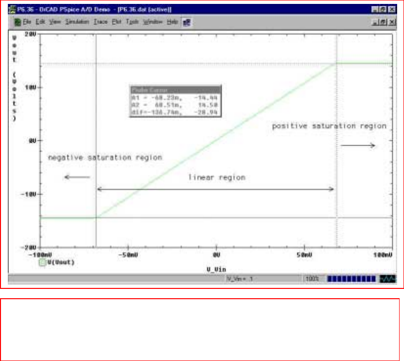
CHAPTER SIX SOLUTIONS
Engineering Circuit Analysis, 6th Edition Copyright ©2002 McGraw-Hill, Inc. All Rights Reserved.
36. This is a non-inverting op amp circuit, so we expect a gain of 1 + 1000/4.7 = 213.8.
With ±15 V DC supplies, we need to sweep the input just above and just below this
value divided by the gain to ensure that we see the saturation regions. Performing the
indicated simulation and a DC sweep from –0.1 V to +0.1 V with 0.001 V steps, we
obtain the following input-output characteristic:
Using the cursor tool, we see that the linear region is in the range of
–68.2 mV < Vin < 68.5 mV.
The simulation predicts a gain of 7.103 V/ 32.87 mV = 216.1, which is reasonably
close to the value predicted using the ideal op amp model.
CHAPTER SIX SOLUTIONS
Engineering Circuit Analysis, 6th Edition Copyright ©2002 McGraw-Hill, Inc. All Rights Reserved.
37. Referring to the detailed model of an op amp, shorting the input terminals together
shorts the dependent source to ground. Therefore, any 1-V source connected to the
output through a 1-Ω resistor should “see” 1 Ω + Ro. For the µA 741, we expect 1 +
75 = 76 Ω. For the LF 411, we expect ~1 + 1 Ω or ~ 2 Ω.
Simulating the µA741 circuit, we find:
Supply voltages Current into output Total resistance Output resistance
±15 V -42.5 mA -23.53 Ω -22.53 Ω
±5 V -40.55 mA -24.66 Ω -24.66 Ω
±2 V -40.55 mA -24.66 Ω -24.66 Ω
0 V 579.2 mA 1.727 Ω 727 mΩ
Conclusion: as we might expect from previous experience in determining Thévenin
equivalent resistances, we must short out the voltage supplies to the op amp when
performing such an experiment (hence the negative resistance values obtained above).
However, we obtained 0.727 Ω instead of the expected 75 Ω, which leads to two
possible conclusions: (1) The PSpice model is not designed to represent the op amp
behavior accurately in such a circuit configuration or (2) such an experimental
connection is not adequate for measuring the output resistance.
Simulating the LF411 circuit, we find:
Supply voltages Current into output Total resistance Output resistance
±15 V 25.46 mA 39.28 Ω 38.28 Ω
±5 V 25.43 mA 39.32 Ω 38.32 Ω
±2 V 25.48 mA 39.24 Ω 28.24 Ω
0 V 1000 mA 1 Ω 0 Ω
Conclusion: as we might expect from previous experience in determining Thévenin
equivalent resistances, we must short out the voltage supplies to the op amp when
performing such an experiment. However, we obtained ~0 Ω instead of the expected 1
Ω, which leads to two possible conclusions: (1) The PSpice model is not designed to
represent the op amp behavior accurately in such a circuit configuration or (2) such an
experimental connection is not adequate for measuring the output resistance.
However, it is interesting that PSpice did predict a much lower output resistance for
the LF 411 than the µA 741, as we would expect.
CHAPTER SIX SOLUTIONS
Engineering Circuit Analysis, 6th Edition Copyright ©2002 McGraw-Hill, Inc. All Rights Reserved.
38. Based on the detailed model of the LF 411 op amp, we can write the following nodal
equation at the inverting input:
o
6
dd
4
dx
in
d
R10
- A
10
-
R
-
0 +
++= vvvvv
Substituting values for the LF 411 and simplifying, we make appropriate
approximations and then solve for vd in terms of vx, finding that
199.9
-
10199.9
10-
x
x
6
6
d
v
vv =
×
=
With a gain of –1000/10 = -100 and supply voltage magnitudes of 15 V, we are
effectively limited to values of |vx| < 150 mV.
For vx = -10 mV, PSpice predicts vd = 6 µV, where the hand calculations based on the
detailed model predict 50 µV, which is about one order of magnitude larger. For the
same input voltage, PSpice predicts an input current of -1 µA, whereas the hand
calculations predict 99.5vx mA = -995 nA (which is reasonably close).

CHAPTER SIX SOLUTIONS
Engineering Circuit Analysis, 6th Edition Copyright ©2002 McGraw-Hill, Inc. All Rights Reserved.
(a) The gain of the inverting amplifier is –1000. At a sensor voltage of –30 mV, the
predicted output voltage (assuming an ideal op amp) is +30 V. At a sensor voltage of +75
mV, the predicted output voltage (again assuming an ideal op amp) is –75 V. Since the op
amp is being powered by dc sources with voltage magnitude equal to 15 V, the output
voltage range will realistically be limited to the range
–15 < Vout < 15 V.
(b) The peak input voltage is 75 mV. Therefore, 15/ 75×10-3 = 200, and we should set
the resistance ratio Rf/ R1 < 199 to ensure the op amp does not saturate.
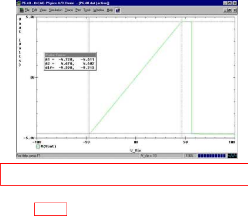
CHAPTER SIX SOLUTIONS
Engineering Circuit Analysis, 6th Edition Copyright ©2002 McGraw-Hill, Inc. All Rights Reserved.
39. (a)
We see from the simulation result that negative saturation begins at Vin = –4.72 V,
and positive saturation begins at Vin = +4.67 V.
(b) Using a 1 pΩ resistor between the output pin and ground, we obtain an output
current of 40.61 mA, slightly larger than the expected 35 mA, but not too far off.
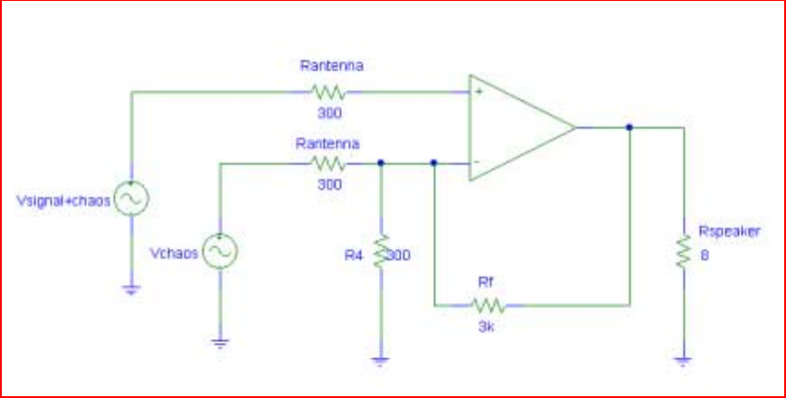
CHAPTER SIX SOLUTIONS
Engineering Circuit Analysis, 6th Edition Copyright ©2002 McGraw-Hill, Inc. All Rights Reserved.
41. We assume that the strength of the separately-broadcast chaotic “noise” signal is
received at the appropriate intensity such that it may precisely cancel out the chaotic
component of the total received signal; otherwise, a variable-gain stage would need to
be added so that this could be adjusted by the user. We also assume that the signal
frequency is separate from the “carrier” or broadcast frequency, and has already been
separated out by an appropriate circuit (in a similar fashion, a radio station
transmitting at 92 MHz is sending an audio signal of between 20 and 20 kHz, which
must be separated from the 92 MHz frequency.)
One possible solution of many (all resistances in ohms):
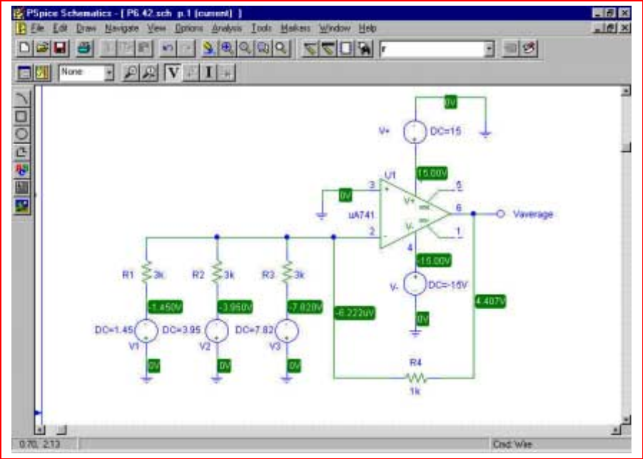
CHAPTER SIX SOLUTIONS
Engineering Circuit Analysis, 6th Edition Copyright ©2002 McGraw-Hill, Inc. All Rights Reserved.
41. One possible solution of many:
This circuit produces an output equal to the average of V1, V2, and V3, as shown in the
simulation result: Vaverage = (1.45 + 3.95 + 7.82)/ 3 = 4.407 V.
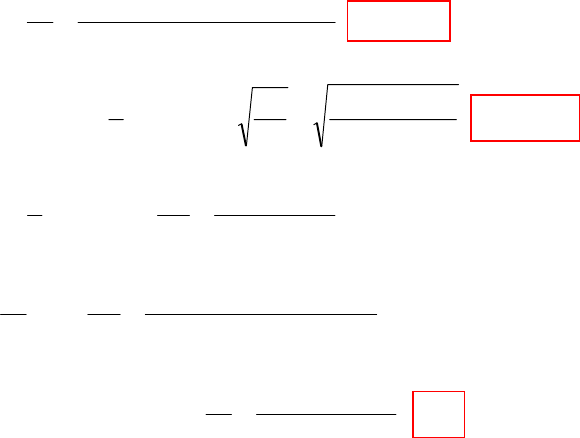
CHAPTER SEVEN SOLUTIONS
Engineering Circuit Analysis, 6th Edition Copyright
2002 McGraw-Hill, Inc. All Rights Reserved
1. (a)
()
pF
d
A
C954.6
10100
1054.7810854.8
6
612 =
×
××
== −
−−
ε
(b)
()
kV
C
E
VCVEEnergy 959.16
10954.6
10122
2
1
,12
3
2=
×
×
==∴= −
−
(c)
()
()
pF
V
E
CCVE 500
100
105.222
2
1
2
6
2
2=
×
==∴= −
()()
()
1
6
612 .62.636
1054.78
1010010500 −
−
−− =
×
××
==∴= mpF
A
Cd
d
A
C
ε
ε
9.71
10854.8
1062.636
,_Re 12
12
0
=
×
×
=∴ −
−
ε
ε
typermittivilative
CHAPTER SEVEN SOLUTIONS
Engineering Circuit Analysis, 6th Edition Copyright
2002 McGraw-Hill, Inc. All Rights Reserved
2. (a) For VA = -1V,
()
()
()
()()
()
157.0
101106.1
10854.88.112
2
2419
12
0+
××
×
=−= −
−
Abi
sVV
qN
K
W
ε
m
9
10281.45 −
×=
(
)
(
)
fFC j307.2
10281.45
10110854.88.11
9
1212 =
×
××
=−
−−
(b) For VA = -5V,
()
()
()
()()
()
557.0
101106.1
10854.88.112
2
2419
12
0+
××
×
=−= −
−
Abi
sVV
qN
K
W
ε
m
9
10289.85 −
×=
(
)
(
)
fFC j225.1
10289.85
10110854.88.11
9
1212 =
×
××
=−
−−
(c) For VA = -10V,
()
()
()
()()
()
1057.0
101106.1
10854.88.112
2
2419
12
0+
××
×
=−= −
−
Abi
sVV
qN
K
W
ε
m
9
10491.117 −
×=
(
)
(
)
aFC j239.889
10491.117
10110854.88.11
9
1212 =
×
××
=−
−−
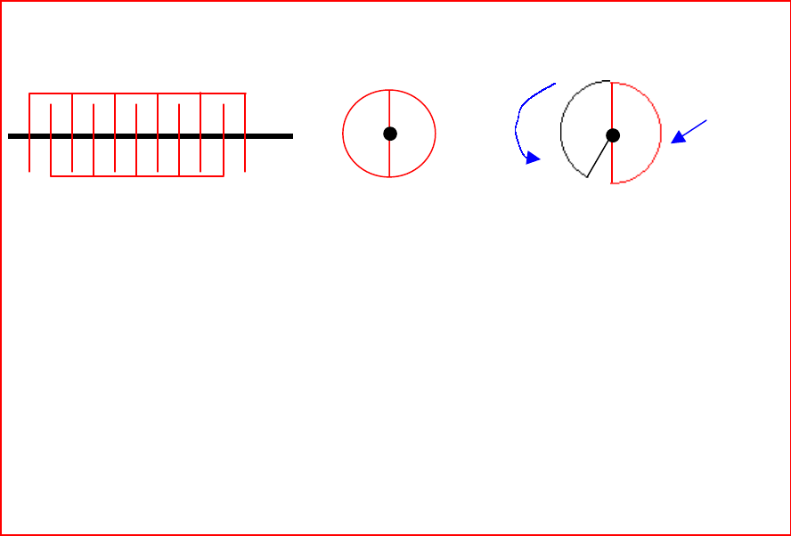
CHAPTER SEVEN SOLUTIONS
Engineering Circuit Analysis, 6th Edition Copyright
2002 McGraw-Hill, Inc. All Rights Reserved
3. We require a capacitor that may be manually varied between 100 and 1000 pF by rotation
of a knob. Let’s choose an air dielectric for simplicity of construction, and a series of 11
half-plates:
Constructed as shown, the half-plates are in parallel, so that each of the 10 pairs must
have a capacitance of 1000/ 10 = 100 pF when rotated such that they overlap completely.
If we arbitrarily select an area of 1 cm2 for each half-plate, then the gap spacing between
each plate is d = εA/C = (8.854×10⁻¹⁴ F/cm)(1 cm2)/ (100×10-12 F) = 0.8854 mm. This is
tight, but not impossible to achieve. The final step is to determine the amount of overlap
which corresponds to 100 pF for the total capacitor structure. A capacitance of 100 pF is
equal to 10% of the capacitance when all of the plate areas are aligned, so we need a pie-
shaped wedge having an area of 0.1 cm2. If the middle figure above corresponds to an
angle of 0o and the case of perfect alignment (maximum capacitance) corresponds to an
angle of 180o, we need to set out minimum angle to be 18o.
Side view with no
overlap between plates
Top view Side view with a small
overlap between plates.
fixed

CHAPTER SEVEN SOLUTIONS
Engineering Circuit Analysis, 6th Edition Copyright
2002 McGraw-Hill, Inc. All Rights Reserved
4. (a) Energy stored JdteeC
dt
dv
Cv
tt
t
t
µ
080.1
5
3
.3. 5
102
05
3
0
−=
−== −
×−
∫∫ −
(b) Vmax = 3V
Max. energy at t=0, JEmJCV
µ
5.499%3735.1
2
1max
2=∴==
V at 37% Emax = 1.825V
()
sstetv
t
2486.23825.1 5⇒≈=∴== −
(c) Ae
dt
dv
Ci
µ
593.141
5
3
10300 5
2.1
6−=
−×== −
−
(d)
(
)
WviP
µ
6.24210658.120011.2 6−=×−== −

CHAPTER SEVEN SOLUTIONS
Engineering Circuit Analysis, 6th Edition Copyright
2002 McGraw-Hill, Inc. All Rights Reserved
5. (a)
()
()
()
mV
C
v421.33101
2
14159.3
.
1047
1
101
2
.
12
3
6
2
3=×
×
=×= −
−
−
π
(b)
()
()
()
mV
C
v421.33101
2
14159.3
.
1047
1
0101
2
.
12
3
6
2
3=×
×
=
+×= −
−
−
π
(c)
()() ()
mV
C
v132.50101
4
3
.
1047
1
101
4
101
2
.
12
3
6
2
3
2
3=
×
×
=
×+×= −
−
−−
πππ
CHAPTER SEVEN SOLUTIONS
Engineering Circuit Analysis, 6th Edition Copyright
2002 McGraw-Hill, Inc. All Rights Reserved
6. C
t
C
idt
C
V
ms
ms 426.0
cos
10711 200
0
3
200
0=
×
−== −
∫
π
π
()
FC
C
CVE
µ
30181
1032
10086.181
2
10086.181
103
2
1
6
99
62 =
×
×
=∴
×
=×== −
−−
−

CHAPTER SEVEN SOLUTIONS
Engineering Circuit Analysis, 6th Edition Copyright
2002 McGraw-Hill, Inc. All Rights Reserved
7.
(a)
(b) 2722 7
max
11
2 10 (5 3cos 200 ) 10 64 6.4 J
22
cc c
wcv tw
µ
−−
==×× + ∴=×=
(c) 6 100 3 3 100 100
0
110 8 10 10 40( 0.01)( 1) 400(1 )V
0.2
−− −
=× × =×− −= −
∫tttt
c
vedt e e
(d) 100
500 400 V
t
c
ve
−
=−
0.12sin 400 mA∴=−
c
it
26
0.2 F, 5 3cos 200 V; 0.2 10 (3)( 2)200sin 200 cos 200
−
==+ ∴=×−
cc
cv ti tt
µ

CHAPTER SEVEN SOLUTIONS
Engineering Circuit Analysis, 6th Edition Copyright
2002 McGraw-Hill, Inc. All Rights Reserved
8.
0.1
0
0.2
0.1
0.9
22
(0) 250V, 2mF ( ) (0.1) 250 500 5
(0.1) 500V; (0.2) 500 10 1000V
(0.6) 1750V, (0.9) 2000V
0.9 1: 2000 500 10 2000 5000( 0.9)
2100 2000 5000( 0.9) 0.92 0.9 0
== =+
∴= = =
∴= =
∴<< = + = + −
∴= = + − ∴= ∴ <<
∫
∫
∫
cc
cc
cc
t
c
c
vcav dt
vv dt
vv
t v dt t
vttt.92s
CHAPTER SEVEN SOLUTIONS
Engineering Circuit Analysis, 6th Edition Copyright
2002 McGraw-Hill, Inc. All Rights Reserved
9.
(a)
(b)
2 6 2 2 1000 500
6 500 500
11
C 10 2 10 200 V
22
C 10 ( 200)( 500) 0.1
200
R2
0.1
−−− −
−−−
==×=× ∴=±
′
== ± − =
−
∴= = = Ω
m
tt
c
tt
wv v ev e
iv e e
vk
i
2 1000 1000
1000 1000
R0
0
P R 0.01 2000 20 W
W 20 0.02 0.02J
−−
∞−−∞
==× =
∴= =− =
∫
tt
R
tt
iee
edt e
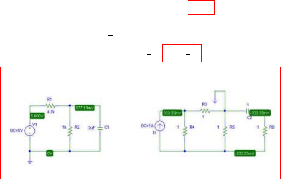
CHAPTER SEVEN SOLUTIONS
Engineering Circuit Analysis, 6th Edition Copyright
2002 McGraw-Hill, Inc. All Rights Reserved
10. (a) Left circuit:
By Voltage division,
()
V
kk
k
VC877.05
17.4
1=
+
=
Right circuit:
()
VV 3
2
2//11
1==
By Voltage Division, VVVV C3
1
3
1
2−=∴=
(b)
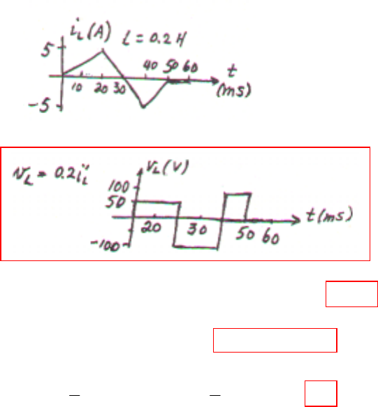
CHAPTER SEVEN SOLUTIONS
Engineering Circuit Analysis, 6th Edition Copyright
2002 McGraw-Hill, Inc. All Rights Reserved
11.
(a)
(b) max
P P ( 100)( 5) 500W at 40 ms
−
=∴ =− −= =
L
LLi L
vt
(c) min
P 100( 5) 500W at 20 and 40 ms
++
=−=− =
Lt
(d) 22
11
W L W (40ms) 0.2( 5) 2.5J
22
=∴ =×−=
L
LL
i
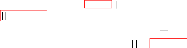
CHAPTER SEVEN SOLUTIONS
Engineering Circuit Analysis, 6th Edition Copyright
2002 McGraw-Hill, Inc. All Rights Reserved
12.
3 100 100
-100t 100 1
max
100
max
100 100
L 50 10 , 0: 0; 0 80 mA 0.08 A
i =0.08e 8 0.08 8 , , 0.01 , 0.08 0.01
0.2943mA; 0.05 (0.004 0.4 )
( 0.4) 100 (0.004 0.4 ) 0.4 0.4 40 ,
−−−
−−
−
−−
=× < = > = =
′
∴−∴===×
′
∴= = = −
′
∴= − − − ∴− = −
tt
t
m
t
tt
t i t i te te
te t t s i e
iviet
ve e t t
2
max
0.8 0.02
40
(0.004 0.008) 0.5413mV this is minimum 0.004Vat t=0
−
==
=−=− ∴=
ts
ve v
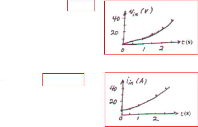
CHAPTER SEVEN SOLUTIONS
Engineering Circuit Analysis, 6th Edition Copyright
2002 McGraw-Hill, Inc. All Rights Reserved
13.
(a) 22
0: 0.4 A 10 5 4 4 V
′
>=∴=+=+
sinss
ti tv iitt
(b) 2
0
1
0.1 40 5 4 4 5A
5
′=+ +=++
∫t
in s
iv tdttt
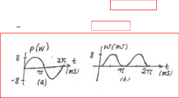
CHAPTER SEVEN SOLUTIONS
Engineering Circuit Analysis, 6th Edition Copyright
2002 McGraw-Hill, Inc. All Rights Reserved
14. 20cos1000 V, L 25mH, (0) 0===
LL
vti
(a) 0
40 20 cos 1000 0.8sin 1000 A 8sin 2000 W==∴=
∫t
L
i tdt t p t
(b) 32 2
125 10 0.64sin 1000 8sin 1000 mJ
2
wtt
−
=× × × =
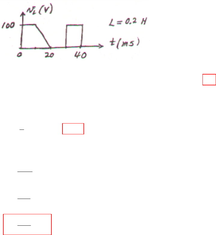
CHAPTER SEVEN SOLUTIONS
Engineering Circuit Analysis, 6th Edition Copyright
2002 McGraw-Hill, Inc. All Rights Reserved
15.
(a) 0
0 10 ms: 2 5 100 2 500 (10ms) 3A, (8ms) 2A<< =−+ =−+ ∴ = =
∫t
LLL
t i dt t i i
(b)
(c) If the circuit has been connected for a long time, L appears like short circuit.
()
VVV 80100
82
8
8=
+
=
Ω
A
V
I10
2
20
2=
Ω
=
Ω
A
V
ix1
80
80 =
Ω
=∴
0.02 4
0.01
40.024
0.01
2
(0) 0 (10ms) 500 0.01 5A (20ms) 5 5 10 (0.02 )
(20ms) 5 5 10 (0.02 0.5 ) 5 5 10 (0.0002 0.00015) 7.5A
10.2 7.5 5.625J
2
LL L
L
L
ii i tdt
itt
w
=∴ = × = ∴ =+ −
∴ =+× − =+× − =
∴=×× =
∫

CHAPTER SEVEN SOLUTIONS
Engineering Circuit Analysis, 6th Edition Copyright
2002 McGraw-Hill, Inc. All Rights Reserved
16. 2
L 5H,V 10( )V, (0) 0.08A
−−
==− =
tt
LL
ee i
(a) 12
(1) 10( ) 2.325 V
L
vee
−− +
=−=
(b)
(c) ( ) 1.08A
L
i∞=
22
0
0
22
0.08 0.2 10( ) 0.08 2( 0.5 )
0.08 2( 0.5 1 0.5) 1.08 2 (1) 0.4796A
−− − −
−− −−
=+ − =+−+
=+−+ +−=+−∴=
∫ttt t tt
L
tt tt
L L
ieedtee
iee eei
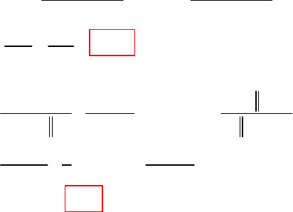
CHAPTER SEVEN SOLUTIONS
Engineering Circuit Analysis, 6th Edition Copyright
2002 McGraw-Hill, Inc. All Rights Reserved
17.
(a)
(b)
40 12
120 40 5
12 20 40 12 20 40
200 100 100V
33
=× +××
++ ++
=+=
x
v
15 12
120 15 40 40 5
12 15 60 15 60 15 12 60
120 1 6.667
40 200
12 12 5 66.667
40 20 60V
=××+×
++ +
=××+
+
=+=
x
v
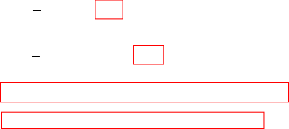
CHAPTER SEVEN SOLUTIONS
Engineering Circuit Analysis, 6th Edition Copyright
2002 McGraw-Hill, Inc. All Rights Reserved
18.
(a) 2
15 1.6 6.4J
2
L
w=×× =
(b) 62
120 10 100 0.1J
2
c
w−
=× × × =
(c) Left to right (magnitudes): 100, 0, 100, 116, 16, 16, 0 (V)
(d) Left to right (magnitudes): 0, 0, 2, 2, 0.4, 1.6, 0 (A)
CHAPTER SEVEN SOLUTIONS
Engineering Circuit Analysis, 6th Edition Copyright
2002 McGraw-Hill, Inc. All Rights Reserved
19.
(a)
(b)
(c) 0.4
24 45
0
4 , P 100 16 1600 320 0.4 3.277J==×∴= =×=
∫
RR R
it tw tdt
2
52
400 V, 0; (0) 0.5A; 0.4
1
400 0.16 64V, 10 64 20.48mJ
2
−
=>==
=× = ××=
sL
cc
vtti ts
vw
0.4 23
0
2
1
0.5 0.1 400 0.5 40 0.4 1.3533A
3
110 1.3533 9.1581J
2
=+ =+×× =
∴=×× =
∫
L
L
itdt
w
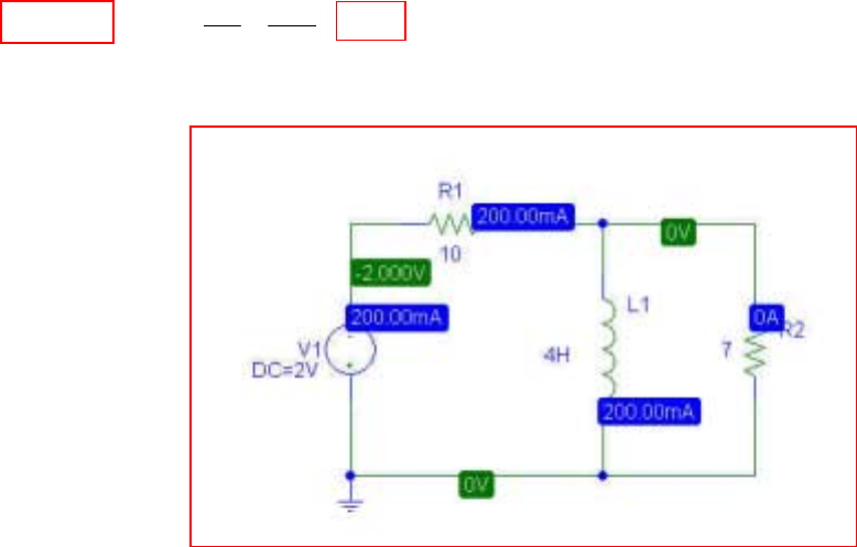
CHAPTER SEVEN SOLUTIONS
Engineering Circuit Analysis, 6th Edition Copyright
2002 McGraw-Hill, Inc. All Rights Reserved
20. (a)
()
W
R
V
PWP 4.0
10
2
;0 2
2
107==== ΩΩ
(b) PSpice verification
We see from the PSpice
simulation that the
voltage across the 10-Ω
resistor is –2 V, so that
it is dissipating 4/10
= 400 mW.
The 7-Ω resistor has
zero volts across its
terminals, and hence
dissipates zero power.
Both results agree with
the hand calculations.
CHAPTER SEVEN SOLUTIONS
Engineering Circuit Analysis, 6th Edition Copyright
2002 McGraw-Hill, Inc. All Rights Reserved
21.
+
+≡
µµ
µ
10
1
10
1
1
10
equiv
Cin series with
µ
10 in series with
+
+
µµ
µ
10
1
10
1
1
10
F
µ
286.4
≡

CHAPTER SEVEN SOLUTIONS
Engineering Circuit Analysis, 6th Edition Copyright
2002 McGraw-Hill, Inc. All Rights Reserved
22.
()()()()
pHpppppppLequiv 6.1797777//77777777//77 &
=++++≡
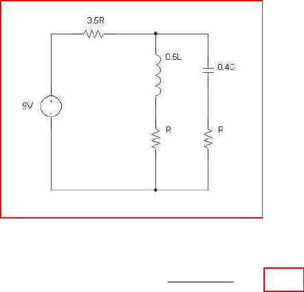
CHAPTER SEVEN SOLUTIONS
Engineering Circuit Analysis, 6th Edition Copyright
2002 McGraw-Hill, Inc. All Rights Reserved
23. (a) Assuming all resistors have value R, all inductors have value L, and all capacitors
have value C,
(b) At dc, 20µF is open circuit; 500µH is short circuit.
Using voltage division,
()
V
kk
k
Vx6.39
1510
10 =
+
=
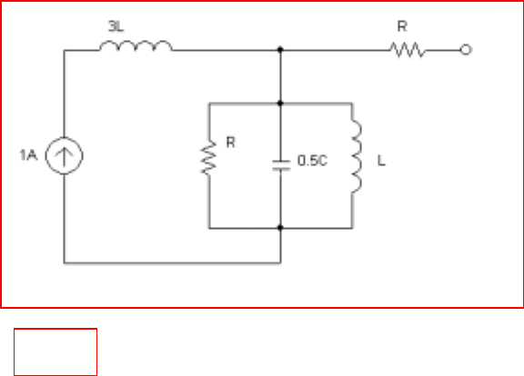
CHAPTER SEVEN SOLUTIONS
Engineering Circuit Analysis, 6th Edition Copyright
2002 McGraw-Hill, Inc. All Rights Reserved
24. (a) Assuming all resistors have value R, all inductors value L, and all capacitors value C,
(b) VVx0= as L is short circuit at dc.
+
Vx
-

CHAPTER SEVEN SOLUTIONS
Engineering Circuit Analysis, 6th Edition Copyright
2002 McGraw-Hill, Inc. All Rights Reserved
25. Cequiv = { [(100 n + 40 n) || 12 n] + 75 n} || {7 µ + (2 µ || 12 µ)}
nFCequiv 211.85≡

CHAPTER SEVEN SOLUTIONS
Engineering Circuit Analysis, 6th Edition Copyright
2002 McGraw-Hill, Inc. All Rights Reserved
26. Lequiv = {[ (17 p || 4 n) + 77 p] || 12 n} + {1 n || (72 p + 14 p)}
pHLequiv 388.172≡
CHAPTER SEVEN SOLUTIONS
Engineering Circuit Analysis, 6th Edition Copyright
2002 McGraw-Hill, Inc. All Rights Reserved
27.
()
FCC xT
µ
171100161477 =++++=−
()()()
JVCCE xTCC xT
µµ
375.5345.2171
2
1
2
12
2==−=
−
()
nJJEEE xTTx CCCC 425375.5348.534 =−=−= −
µ
()
()
nF
n
CVCnE xxCx136
5.2
2425
2
1
425 2
2==⇒==∴
CHAPTER SEVEN SOLUTIONS
Engineering Circuit Analysis, 6th Edition Copyright
2002 McGraw-Hill, Inc. All Rights Reserved
28.
(a) For all L = 1.5H, HLequiv 75.2
5.1
1
5.1
1
5.1
1
1
5.1
1
5.1
1
1
5.1 =
++
+
+
+=
(b) For a general network of this type, having N stages (and all L values equiv),
∑
=−
=n
NN
N
equiv NL
L
L
11
CHAPTER SEVEN SOLUTIONS
Engineering Circuit Analysis, 6th Edition Copyright
2002 McGraw-Hill, Inc. All Rights Reserved
29.
(a) HLequiv 3
3
1
3
1
3
1
1
2
1
2
1
1
1=
++
+
+
+=
(b) For a network of this type having 3 stages,
() ()
()
() ()
()
2
32
22 33
3
22
2
1
3
1
3
33
1
2
22
1
1++=
+
+
+
+
+=
equiv
L
Extending for the general case of N stages,
N
1
N
1
1
3
1
3
1
3
1
1
2
1
2
1
1
1 Κ
Κ+
++
++
+
+
+=
equiv
L
N
N(1/N)
1
)3/1(3
1
)2/1(2
1
1 =++++=Κ

CHAPTER SEVEN SOLUTIONS
Engineering Circuit Analysis, 6th Edition Copyright
2002 McGraw-Hill, Inc. All Rights Reserved
30.
()( )
pF
pp
pp
Cequiv 231.0
25.03
25.03 =
+
=

CHAPTER SEVEN SOLUTIONS
Engineering Circuit Analysis, 6th Edition Copyright
2002 McGraw-Hill, Inc. All Rights Reserved
31.
()()
nH
n
nn
Lequiv 6291.0
6.2
3.03.2 &
&
&& ==

CHAPTER SEVEN SOLUTIONS
Engineering Circuit Analysis, 6th Edition Copyright
2002 McGraw-Hill, Inc. All Rights Reserved
32. (a) Use 2 x 1µH in series with 4 x 1µH in parallel.
(b) Use 2 x 1µH in parallel, in series with 4 x 1µH in parallel.
(c) Use 5 x 1µH in parallel, in series with 4 x 1µH in parallel.
CHAPTER SEVEN SOLUTIONS
Engineering Circuit Analysis, 6th Edition Copyright
2002 McGraw-Hill, Inc. All Rights Reserved
33.
(a)
(b) L 10H L 11.379H=∴=
eq
(c)
10 10 55
R 10 :10 10 10 , 10 10 10
33 3
55
R 30 11.379
3
=Ω = ++ =
∴= = Ω
eq
1
C 10F : 5.4545
1/ 30 1/10 1/ 20
10
C 5.4545 8.788F
3
==
++
∴= +=
eq
CHAPTER SEVEN SOLUTIONS
Engineering Circuit Analysis, 6th Edition Copyright
2002 McGraw-Hill, Inc. All Rights Reserved
34.
(a)
(b)
17 1
:1 , 1.3125F
1/4 1/2 3 3/7 1/2
15 5
: ,C 4 4.833F
1/5 1 6 6
+== =
++
==+=
+
eq
eq
oc c
sc
:L 6 1 3 3.857H
: L (3 2 1) 4 2.2 4 1.4194H
=+=
=+= =
eq
eq
oc
sc
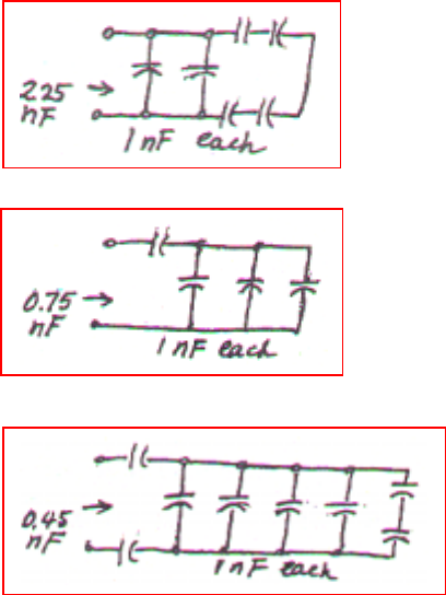
CHAPTER SEVEN SOLUTIONS
Engineering Circuit Analysis, 6th Edition Copyright
2002 McGraw-Hill, Inc. All Rights Reserved
35.
(a)
(b)
(c)
CHAPTER SEVEN SOLUTIONS
Engineering Circuit Analysis, 6th Edition Copyright
2002 McGraw-Hill, Inc. All Rights Reserved
36. 200
1
60 mA, (0) 20mA
t
s
ie i
−
==
(a)
(b)
(c) 200 200 200
21
60 24 4 36 4mA( 0)
tt t
s
iii e e e t
−− −
=−= − += + >
200
200
6 4 2.4H L 2.4 0.06( 200)
or 28.8 V
−
−
′
=∴= =×−
=−
t
eq s
t
vi e
ve
200 200
1
200
14.8
28.8 0.02 ( 1) 0.02
6200
24 4mA( 0)
−−
−
=− + = −+
=−>
∫ttt
o
t
iedt e
et
CHAPTER SEVEN SOLUTIONS
Engineering Circuit Analysis, 6th Edition Copyright
2002 McGraw-Hill, Inc. All Rights Reserved
37. 80
1
100 , (0) 20V
t
s
veVv
−
==
(a) 680 380
C 0.8 10 ( 80)100 6.4 10 A
−− −−
′
==×− =−×
tt
eq s
iv e e
(b)
(c)
6 3 80 80
1
80
1
6400
10 ( 6.4 10 ) 20 ( 1) 20
80
80 60V
−− −
−
=−× += −+
∴= −
∫ttt
o
t
v e dt e
ve
6380 80
2
80
10 1600
( 6.4 10 ) 80 ( 1) 80
480
20 60V
−− −
−
−× += −+
=+
∫ttt
o
t
v e dt e
e
CHAPTER SEVEN SOLUTIONS
Engineering Circuit Analysis, 6th Edition Copyright
2002 McGraw-Hill, Inc. All Rights Reserved
38.
(a)
(b)
6
3
510 0
20 10
120
10 8 10
−
−
−−
′
+× + =
−++=
×∫
cs cL
c
t
Lc L
o
vv vv
v
vv vdt
20 20
6
3
20
6
1
20 ( ) 12
510
1( ) 12 10 8 10 0
510
−
−
−
+−+=
×
′
−−++× =
×
∫
∫
t
Ls
o
t
LLL
o
iiidtv
iidt i i

CHAPTER SEVEN SOLUTIONS
Engineering Circuit Analysis, 6th Edition Copyright
2002 McGraw-Hill, Inc. All Rights Reserved
39.
3
333
( ): 30mA: 0.03 20 0.6V, 0.6V
9V: 9V, 20mA: 0.02 20 0.4V
0.04cos10 : 0
( ) 9.2V
( ): 30mA,20mA,
9V: 0; 0.04cos10 : 0.06 0.04( 1000)sin10 2.4sin10 V
×= =
==−×=
=
∴=
==−×−=
cc
cc
c
c
L
LL
vt v
vv
tv
vt
vt
vtv tt
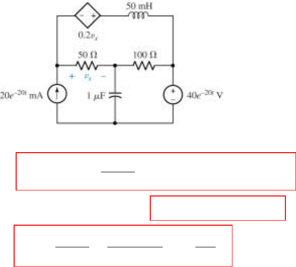
CHAPTER SEVEN SOLUTIONS
Engineering Circuit Analysis, 6th Edition Copyright
2002 McGraw-Hill, Inc. All Rights Reserved
40. We begin by selecting the bottom node as the reference and assigning four nodal
voltages:
1, 4 Supernode: 20×10-3 e-20t =
()
∫′
−×+ −
tttde
0
20
4
3
21 40V100.02
50
V-V [1]
and: V1 – V4 = 0.2 Vx or 0.8V1 + 0.2 V2 – V4 = 0 [2]
Node 2: dt
de t
2
6-
20
212 V
10
100
40 - V
50
V - V
0 ++= − [3]
Ref.
V1
V2 V3
V4
CHAPTER SEVEN SOLUTIONS
Engineering Circuit Analysis, 6th Edition Copyright
2002 McGraw-Hill, Inc. All Rights Reserved
41. (a)
R,R0,A 0 C
also 0 R 0 RC
1
RA 0,
11A
AAR
1111A
AARCA
1A 1A
AorA0
RC RC
′
=∞ = =∞∴ = ∴ =
′
++=∴=−
−+ − = = +
−+
=− ∴ = ∴ =
+
∴= − =− + −
++
′′ ′ ′
∴=−− + +=
∫
∫∫
io i s
oo s
iis i
oiio i
o
soo
so oo os
viv
iv v v
viv v idtv
c
vvvvi v
v
v idt v v dt
c
vv vv vv
(b)
CHAPTER SEVEN SOLUTIONS
Engineering Circuit Analysis, 6th Edition Copyright
2002 McGraw-Hill, Inc. All Rights Reserved
42. Place a current source in parallel with a 1-MΩ resistor on the positive input of a buffer
with output voltage, v. This feeds into an integrator stage with input resistor, R2, of
1-MΩ and feedback capacitor, Cf, of 1 µF.
sec
10602.1 19 ions
dt
dv
Ci f
c
f××== −
sec
10602.1
101101
019
66
ions
VV
dt
dv
C
VV a
c
f
af−
×+
×
−
=+
×
−
=
sec
10602.1
101
019
6
2
ionsV
dt
dv
C
R
Vf
c
f−
×+
×
−
=+
−
=
Integrating current with respect to t,
()
()
0'
1
0
2ff cc
t
fVVCvdt
R−=
∫
f
cf VC
R
ions =
×× −
2
19
10602.1
ions
C
Vions
CR
R
VVVV
f
out
f
outoutacf×××
−
=⇒×××
−
=⇒−= −− 1919
2
110602.1
1
10602.1
R1 = 1 MΩ, Cf = 1µF
CHAPTER SEVEN SOLUTIONS
Engineering Circuit Analysis, 6th Edition Copyright
2002 McGraw-Hill, Inc. All Rights Reserved
43. R 0.5M , C 2 F, R , R 0, cos10 1V=Ω= =∞== −
ioo
vt
µ
(a)
(b) Let A 10sin10 V
s
vt=∞∴ =
11
Eq. (16) is: 1 (0)
ARCA
11 1 11
1 1 ( 10sin10 ) 1 cos10
ARCAA A A
111
1 10sin10 cos10 Let A 2000
AAA
10.005sin10 0.0005 0.0005c
+=− +−
′
∴ + =− + ∴ + − =− + −
∴=+ + − =
∴= + −
∫to
osc
o
o
os s
s
s
v
v v dt v
v
vv tv t
vtt
vt os10t

CHAPTER SEVEN SOLUTIONS
Engineering Circuit Analysis, 6th Edition Copyright
2002 McGraw-Hill, Inc. All Rights Reserved
44. Create a op-amp based differentiator using an ideal op amp with input capacitor C1 and
feedback resistor Rf followed by inverter stage with unity gain.
min/
1
60
1rpm
mV
dt
dvs
CR
R
R
Vfout ×=+=
R
fC1=60 so choose Rf = 6 MΩ and C1 = 10 µF.
CHAPTER SEVEN SOLUTIONS
Engineering Circuit Analysis, 6th Edition Copyright
2002 McGraw-Hill, Inc. All Rights Reserved
45. (a) ∫−
+=
f
outa
R
VV
vdt
L
1
0
'
1
,0 0dtv
L
R
V
R
V
dtv
L
VV t
s
f
out
f
out
La ∫∫ −
=⇒=∴==
(b) In practice, capacitors are usually used as capacitor values are more readily
available than inductor values.
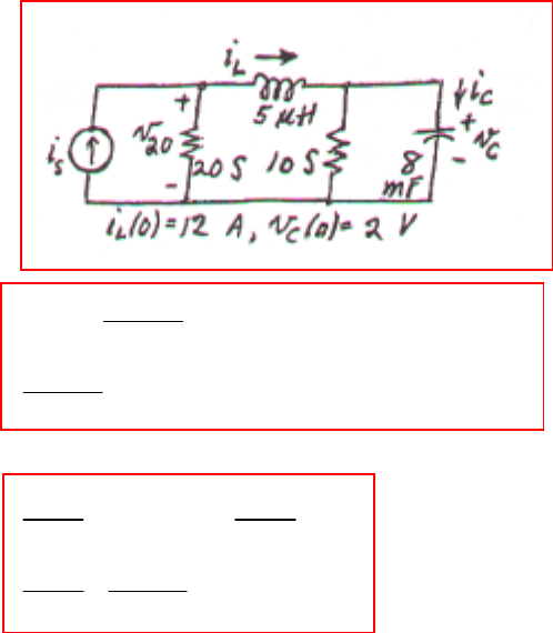
CHAPTER SEVEN SOLUTIONS
Engineering Circuit Analysis, 6th Edition Copyright
2002 McGraw-Hill, Inc. All Rights Reserved
46.
(a)
(b)
(c)
20 20
6
3
20
6
1
20 ( ) 12
510
1( ) 12 10 8 10 0
510
−
−
−
+−+=
×
′
−−++× =
×
∫
∫
t
cs
o
t
ccc
o
vvvdti
vvdt v v
6
3
510 0
20 10
120
10 8 10
−
−
−−
′
+× + =
−++=
×∫
Ls Lc
L
t
cL c
o
ii ii
i
ii idt
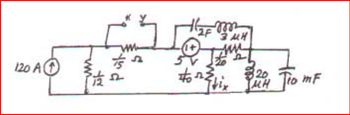
CHAPTER SEVEN SOLUTIONS
Engineering Circuit Analysis, 6th Edition Copyright
2002 McGraw-Hill, Inc. All Rights Reserved
47.
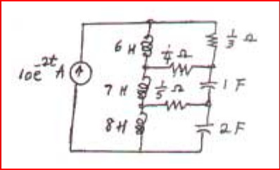
CHAPTER SEVEN SOLUTIONS
Engineering Circuit Analysis, 6th Edition Copyright
2002 McGraw-Hill, Inc. All Rights Reserved
48.
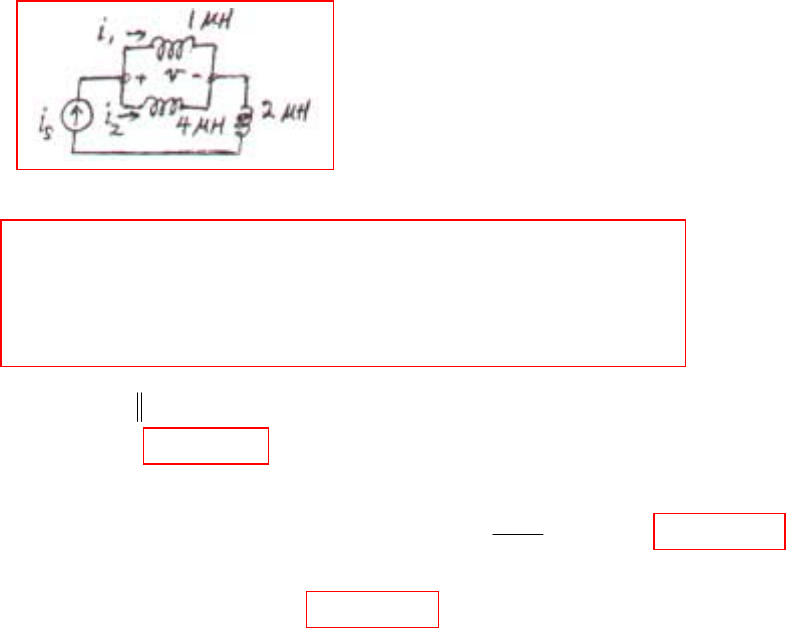
CHAPTER SEVEN SOLUTIONS
Engineering Circuit Analysis, 6th Edition Copyright
2002 McGraw-Hill, Inc. All Rights Reserved
49.
(a)
(b) “Let is = 100e-80t A and i1 (0) = 20 A in the circuit of (new) Fig. 7.62.
(a) Determine v(t) for all t.
(b) Find i1(t) for t ≥ 0.
(c) Find v2(t) for t ≥ 0.”
(c) (a)
(b) 6 3 80 80 80
11
6400
( ) 10 6.4 10 20 ( ) ( 1) 80 60A
80
−− − −
=−× +∴= −= −
∫tttt
o
it e dt it e e
(c) 80
212
() () () 20 60A
t
s
it i it it e
−
=− ∴ = +
680
-80t
L 1 4 0.8 H ( ) L 0.8 10 100( 80) V
v(t) 6.43 mV
−−
′
== ∴= =× × −
∴=−
t
eq eq s
vt i r
µ
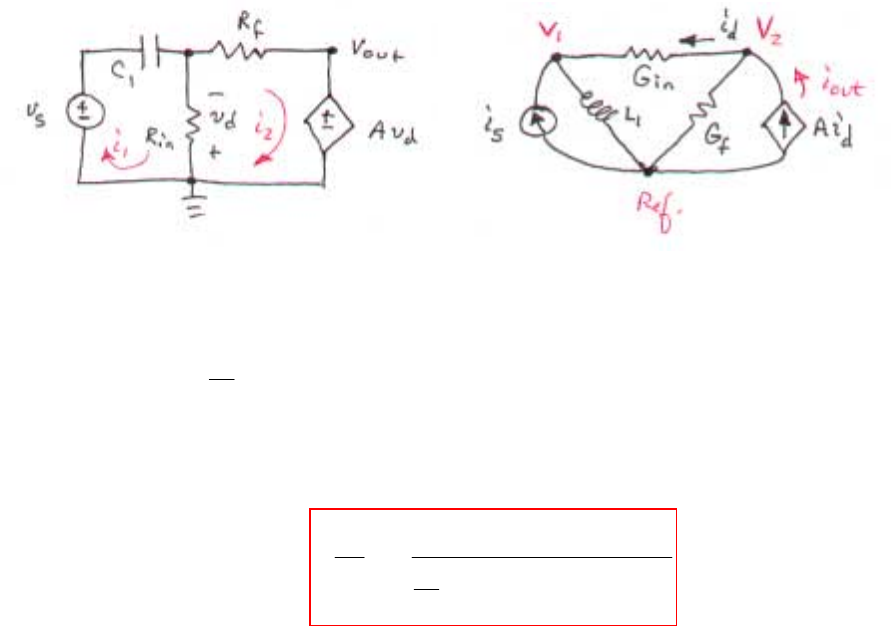
CHAPTER SEVEN SOLUTIONS
Engineering Circuit Analysis, 6th Edition Copyright
2002 McGraw-Hill, Inc. All Rights Reserved
50.
In creating the dual of the original circuit, we have lost both vs and vout. However, we
may write the dual of the original transfer function: iout/ is. Performing nodal analysis,
)V - (V G V
L
1
21in
01
1
S+
′
=∫ttdi [1]
iout = Aid = GfV2 + Gin (V2 – V1) [2]
Dividing, we find that
)V - (V G V
L
1
V G )V - (V G
21in
01
1
2f12in
S
out
+
′
+
=∫ttd
i
i
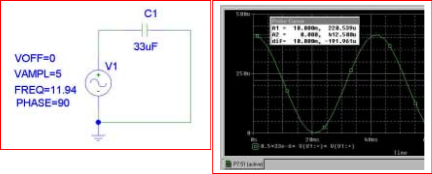
CHAPTER SEVEN SOLUTIONS
Engineering Circuit Analysis, 6th Edition Copyright
2002 McGraw-Hill, Inc. All Rights Reserved
51. PSpice verification
w = ½ Cv2 = 0.5 (33×10-6)[5 cos (75×10-2)]2 = 220.8 µJ. This is in agreement with the
PSpice simulation results shown below.
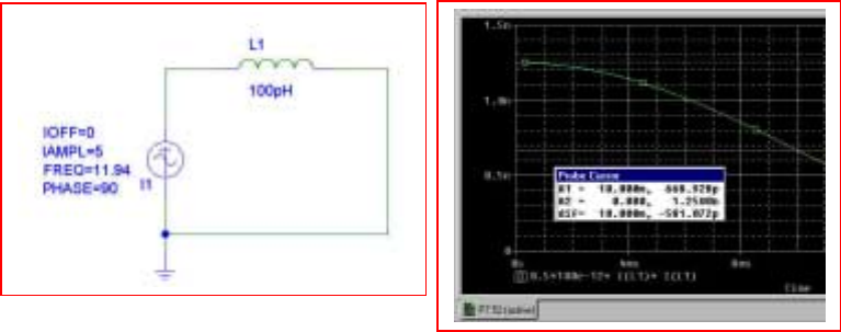
CHAPTER SEVEN SOLUTIONS
Engineering Circuit Analysis, 6th Edition Copyright
2002 McGraw-Hill, Inc. All Rights Reserved
52. PSpice verification
w = ½ Li2 = 0.5 (100×10-12)[5 cos (75×10-2)]2 = 669.2 pJ. This is in agreement with
the PSpice simulation results shown below.
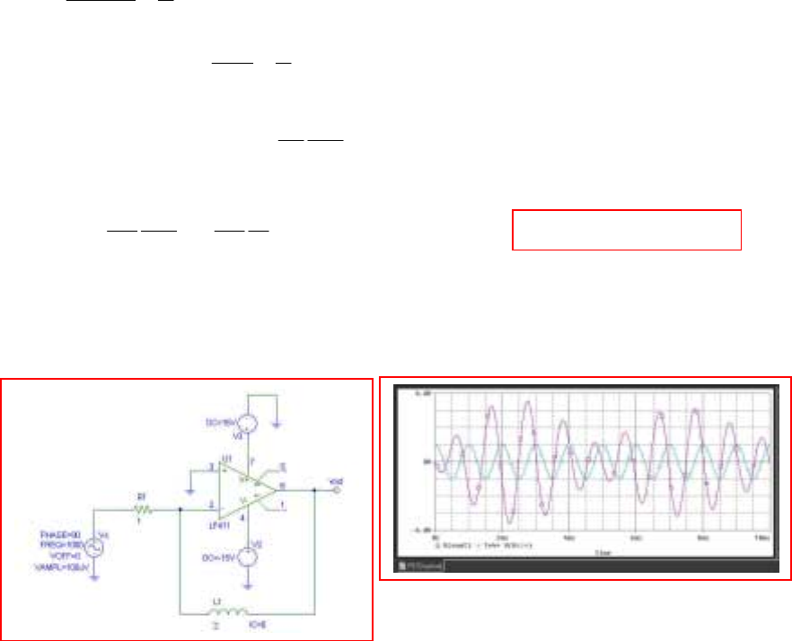
CHAPTER SEVEN SOLUTIONS
Engineering Circuit Analysis, 6th Edition Copyright
2002 McGraw-Hill, Inc. All Rights Reserved
53. ∫
+
−
=dtv
LR
VV
f
L
sa 1
0
1
,0== ba VV ∫
+
−
=dtv
LR
V
f
L
s1
0
1
dt
dVs
R
L
VVVV outoutaLf1
0=−=−=
()
LetRLtA
dt
d
R
L
dt
dVs
R
L
Vf
ff
out
π
_
;2102cos 1
3
11
=⇒−=−= R = 1 Ω and L = 1 H.
PSpice Verification: clearly, something rather odd is occuring in the simulation of this
particular circuit, since the output is not a pure sinusoid, but a combination of several
sinusoids.
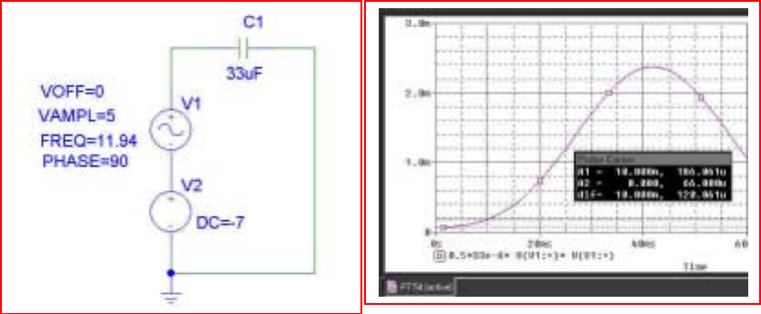
CHAPTER SEVEN SOLUTIONS
Engineering Circuit Analysis, 6th Edition Copyright
2002 McGraw-Hill, Inc. All Rights Reserved
54. PSpice verification
w = ½ Cv2 = 0.5 (33×10-6)[5 cos (75×10-2) - 7]2 = 184.2 µJ. This is in reasonable
agreement with the PSpice simulation results shown below.
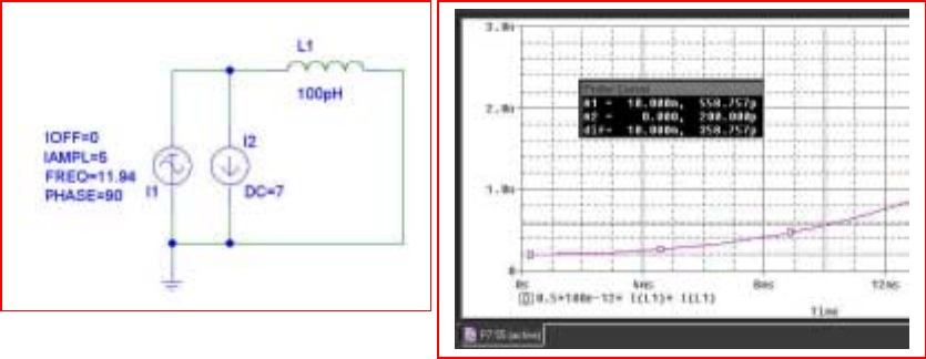
CHAPTER SEVEN SOLUTIONS
Engineering Circuit Analysis, 6th Edition Copyright
2002 McGraw-Hill, Inc. All Rights Reserved
55. PSpice verification
w = ½ Li2 = 0.5 (100×10-12)[5 cos (75×10-2) - 7]2 = 558.3 pJ. This is in agreement with
the PSpice simulation results shown below.
CHAPTER EIGHT SOLUTIONS
Engineering Circuit Analysis, 6th Edition Copyright
2002 McGraw-Hill, Inc. All Rights Reserved
1.
(a)
(b) 4
(0.01) 2 36.63mA
L
ie
−
==
(c) 11
400 400
1
2 1, 2, 1.7329ms
−===
tt
eet
80 /0.2
400
100
(0) 2A ( ) 2
50
2A,0
−
−
==∴=
=>
t
LL
t
iite
et
CHAPTER EIGHT SOLUTIONS
Engineering Circuit Analysis, 6th Edition Copyright
2002 McGraw-Hill, Inc. All Rights Reserved
2.
(a) 12
(0 ) 60 30mA, (0 ) 30 20mA
23
Lx
ii
−−
=× = =× =
(b) (0 ) 30mA, (0 ) 30mA
Lx
ii
++
==−
(c)
250 /0.05 5000
1.5
( ) 30 30 mA, (0.3ms)
30 6.694mA
tt
LL
x
it e e i
ei
−−
−
==
== =−
CHAPTER EIGHT SOLUTIONS
Engineering Circuit Analysis, 6th Edition Copyright
2002 McGraw-Hill, Inc. All Rights Reserved
3.
(a)
= 1.289 mA.
(b) iSW( 5 µs) = 9 – 1.289 = 7.711 mA.
6
36
3
10 /4 1.25
10 10
(0) 4.5mA, R/L 410 4
4.5 mA (5 ) 4.5
−
−−
===
×
∴= ∴ =
L
t
LL
i
ie ise
µ

CHAPTER EIGHT SOLUTIONS
Engineering Circuit Analysis, 6th Edition Copyright
2002 McGraw-Hill, Inc. All Rights Reserved
4.
(a) Since the inductor current can’t change instantaneously, we simply need to find iL while
the switch is closed. The inductor is shorting out both of the resistors, so iL(0+) = 2 A.
(b) The instant after the switch is thrown, we know that 2 A flows through the inductor. By
KCL, the simple circuit must have 2 A flowing through the 20-Ω resistor as well. Thus,
v = 4(20) = 80 V.

CHAPTER EIGHT SOLUTIONS
Engineering Circuit Analysis, 6th Edition Copyright
2002 McGraw-Hill, Inc. All Rights Reserved
5. (a) Prior to the switch being thrown, the 12-Ω resistor is isolated and we have a simple
two-resistor current divider (the inductor is acting like a short circuit in the DC circuit,
since it has been connected in this fashion long enough for any transients to have
decayed). Thus, the current iL through the inductor is simply 5(8)/ (8 + 2) = 4 A.
The voltage v must be 0 V.
(b) The instant just after the switch is thrown, the inductor current must remain the same,
so iL = 4 A. KCL requires that the same current must now be flowing through the 12-Ω
resistor, so v = 12(-4) = -48 V.
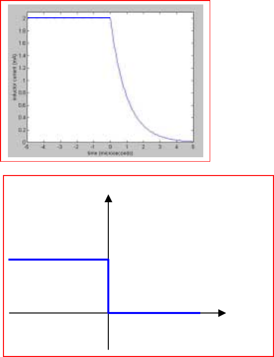
CHAPTER EIGHT SOLUTIONS
Engineering Circuit Analysis, 6th Edition Copyright
2002 McGraw-Hill, Inc. All Rights Reserved
6. For t < 0, we have a current divider with iL(0-) = ix(0-) = 0.5 [ 10 (1/ (1 + 1.5)] mA
= 2 mA. For t > 0, the resistor through which ix flows is shorted, so that ix(t > 0) = 0.
The remaining 1-kΩ resistor and 1-mH inductor network exhibits a decaying current such
that iL(t) = 2e-t/
τ
mA where
τ
= L/R = 1 µS.
(a)
(b)
t (µs)
ix (mA)
2
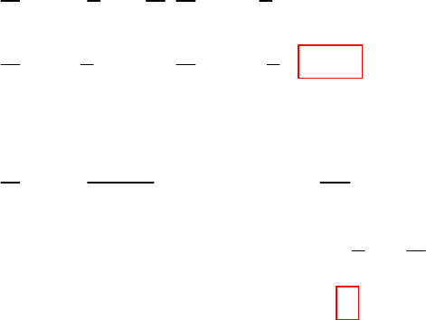
CHAPTER EIGHT SOLUTIONS
Engineering Circuit Analysis, 6th Edition Copyright
2002 McGraw-Hill, Inc. All Rights Reserved
7.
(a)
(b)
/II
, , 10 10 2.303;
I
II
100, 4.605; 1000, 6.908
−
== =∴==
== = =
ll
too
o
oo
it t
en n
ii
tt
ii
τ
ττ
ττ
// 1
11
11
(/I) ()
,; at /1,
I(/) ()
Now, ( 1) ( 1) , I
At 0, ( 1) 2 / 2
−−
−−
−−
==−==−
=−+=− −+ = =
=−=∴=∴=
tt
o
o
o
diid
eete
dt d
ti
ymx b ex e x y
yex ex t
ττ
τ
τ
τ
τ

CHAPTER EIGHT SOLUTIONS
Engineering Circuit Analysis, 6th Edition Copyright
2002 McGraw-Hill, Inc. All Rights Reserved
8. Reading from the graph current is at 0.37 at 2 ms
A 10I
ms 2
0=
=∴
τ
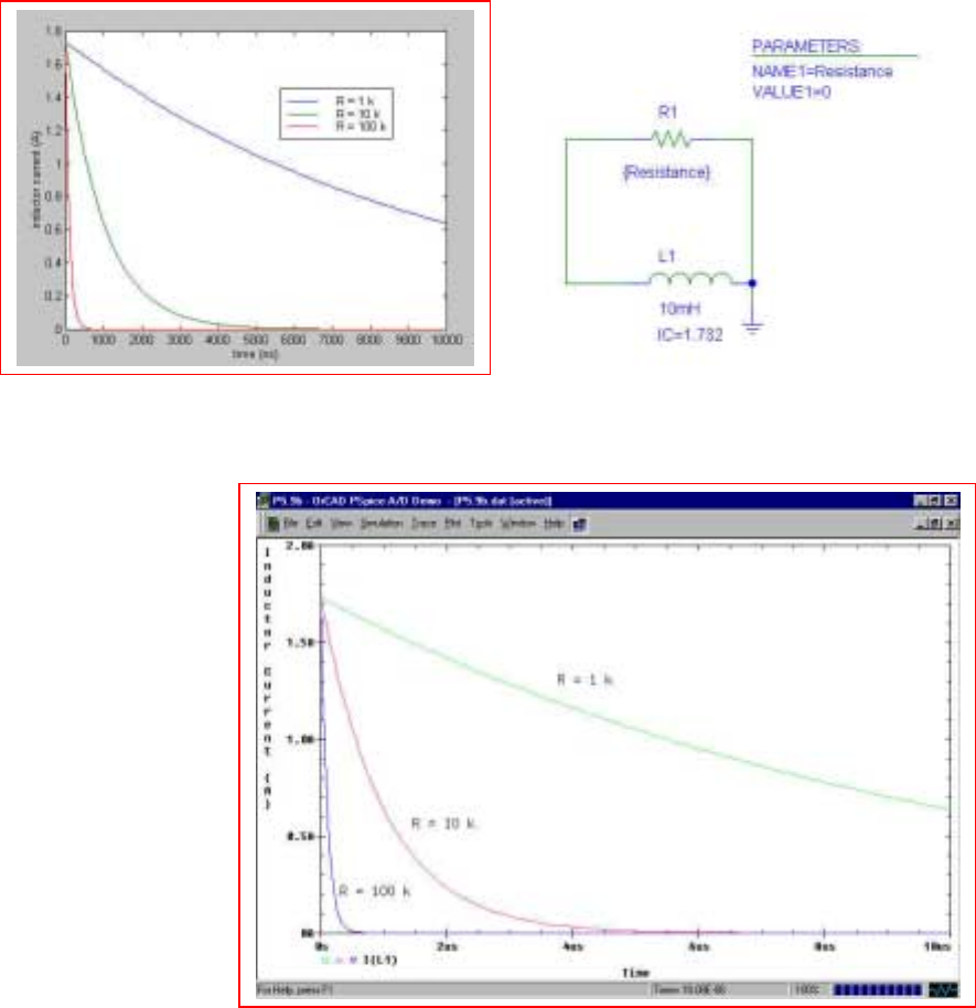
CHAPTER EIGHT SOLUTIONS
Engineering Circuit Analysis, 6th Edition Copyright
2002 McGraw-Hill, Inc. All Rights Reserved
9. w = ½ Li2, so an initial energy of 15 mJ in a 10-mH inductor corresponds to an initial
inductor current of 1.732 A. For R = 1 kΩ,
τ
= L/R = 10 µs, so iL(t) = 1.732 e–0.1t A.
For R = 10 kΩ,
τ
= 1 µs so iL(t) = 1.732 e-t. For R = 100 kΩ,
τ
= 100 ns or 0.1 µs so
iL(t) = 1.732 e-10t A. For each current expression above, it is assumed that time is
expressed in microseconds.
To create a sketch, we first realise that the maximum current for any of the three cases
will be 1.732 A, and after one time constant (10, 1, or 0.1 µs), the current will drop to
36.79% of this value (637.2 mA); after approximately 5 time constants, the current will
be close to zero.
Sketch based on hand analysis Circuit used for PSpice
verification
As can be seen by
comparing the two plots,
which probably should
have the same x-axis scale
labels for easier
comparison, the PSpice
simulation results obtained
using a parametric sweep
do in fact agree with our
hand calculations.
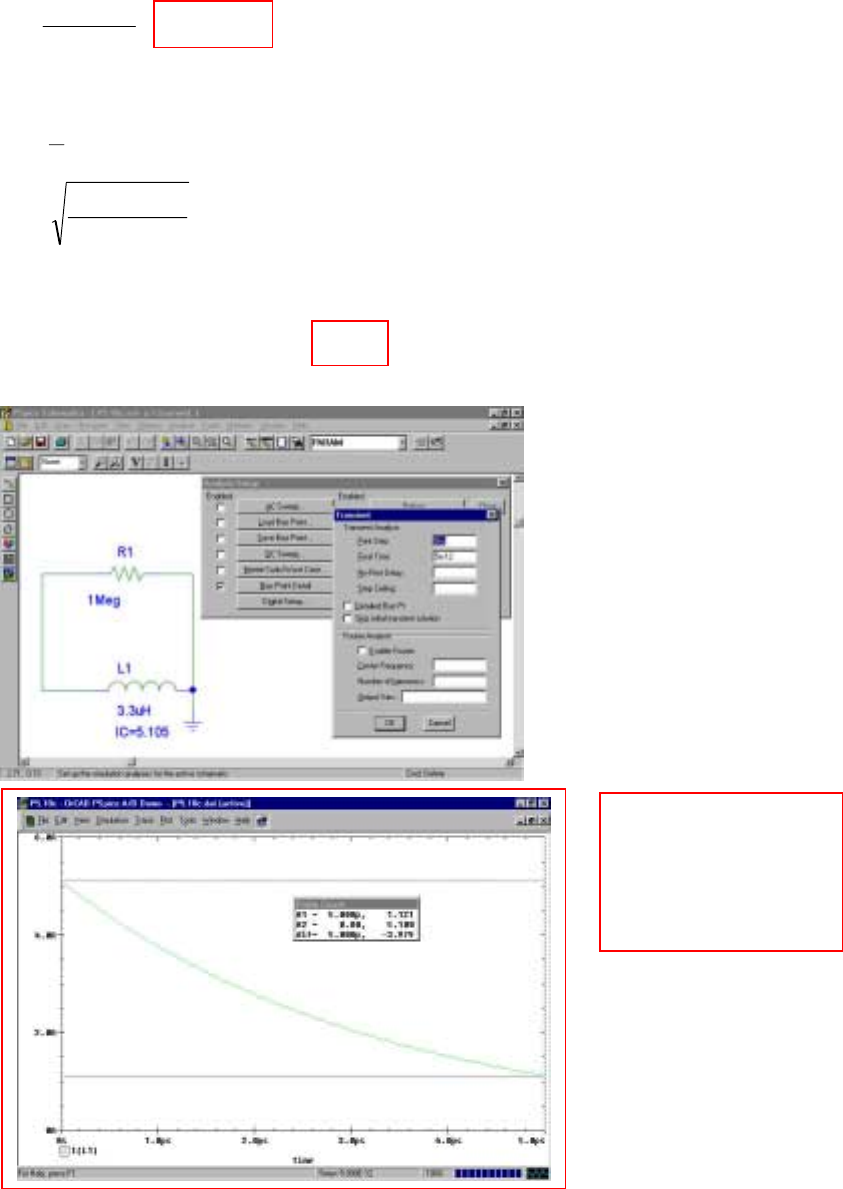
CHAPTER EIGHT SOLUTIONS
Engineering Circuit Analysis, 6th Edition Copyright
2002 McGraw-Hill, Inc. All Rights Reserved
10.
(a) 12
6
6103.3
101
103.3 −
−×=
×
×
=
τ
(b)
()
A 1.121.55
A 1.5
103.3
10432
..
2
1
6126 103.3/105101
6
6
0
2
0
==
=
×
××
=
=
−− ××××−
−
−
epsi
I
IL
ω
(c)
From the PSpice
simulation, we see that
the inductor current is
1.121 A at t = 5 ps, in
agreement with the hand
calculation.
CHAPTER EIGHT SOLUTIONS
Engineering Circuit Analysis, 6th Edition Copyright
2002 McGraw-Hill, Inc. All Rights Reserved
11. Assume the source Thévenin resistance is zero, and assume the transient is measured to
5τ. Then,
9
6
7
L5L
5 100 10 secs
RR
(5)(125.7)10
R10
−
−
−
τ=∴τ==×
∴> so R must be greater than 6.285 kΩ.
(If 1τ assumed then 6.285
R 125.7
5
>=Ω)

CHAPTER EIGHT SOLUTIONS
Engineering Circuit Analysis, 6th Edition Copyright
2002 McGraw-Hill, Inc. All Rights Reserved
The film acts as an intensity integrator. Assuming that we may model the intensity as a simple
decaying exponential,
φ(t) = φo e-t/ τ
where the time constant τ represents the effect of the Thévenin equivalent resistance of
the equipment as it drains the energy stored in the two capacitors, then the intensity of the
image on the film Φ is actually proportional to the integrated exposure:
Φ = dte t
∫−
timeexposure
0
/
o
K
τ
φ
where K is some constant. Solving the integral, we find that
Φ =
[
]
1 - K - time)/ osure(exp
o
τ
τφ
−
e
The maximum value of this intensity function is –Kφo
τ
.
With 150 ms yielding an image intensity of approximately 14% of the maximum
observed and the knowledge that at 2 s no further increase is seen leads us to estimate
that 1 - e-150x10-3/
τ
= 0.14, assuming that we are observing single-exponential decay
behavior and that the response speed of the film is not affecting the measurement. Thus,
we may extract an estimate of the circuit time constant as
τ
= 994.5 ms.
This estimate is consistent with the additional observation that at t = 2 s, the image
appears to be saturated.
With two 50-mF capacitors connected in parallel for a total capacitance of 100 mF, we
may estimate the Thévenin equivalent resistance from
τ
= RC as Rth =
τ
/ C
= 9.945 Ω.
CHAPTER EIGHT SOLUTIONS
Engineering Circuit Analysis, 6th Edition Copyright
2002 McGraw-Hill, Inc. All Rights Reserved
13.
(a)
(b) 125
0.1 18.421ms
t
et
−
=∴=
3000 / 24 125
30
(0) 8(50 200) 192V
50
( ) 192 192 V
c
tt
c
v
vt e e
−−
=×=
==

CHAPTER EIGHT SOLUTIONS
Engineering Circuit Analysis, 6th Edition Copyright
2002 McGraw-Hill, Inc. All Rights Reserved
14.
(a) 64 4
10 /100 10 10
80 80 V, 0; 0.5 69.31
−− −
== >=∴=
tt t
c
ve e t e t s
µ
(b) 2 20,000 2
11
80 80 34.66
24
−
==∴=
t
c
wCe C t s
µ
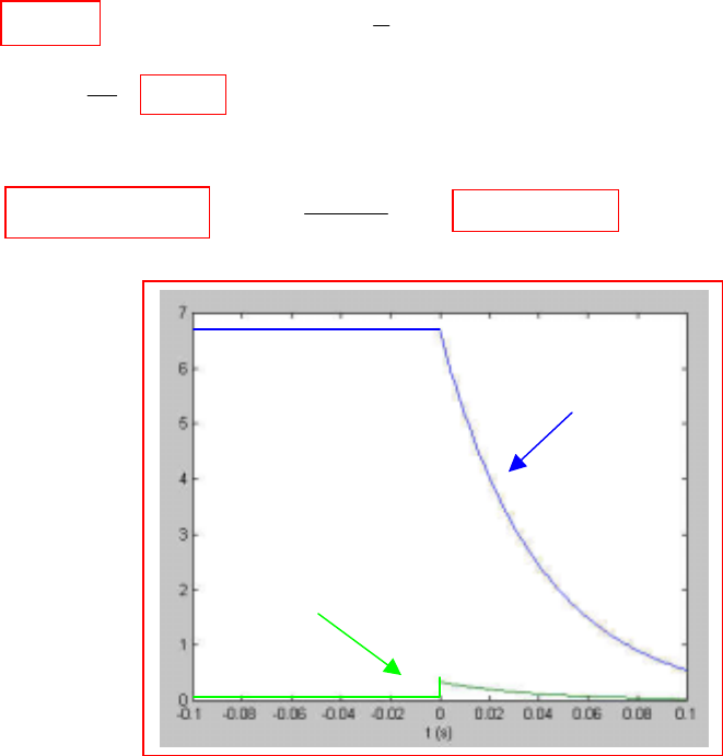
CHAPTER EIGHT SOLUTIONS
Engineering Circuit Analysis, 6th Edition Copyright
2002 McGraw-Hill, Inc. All Rights Reserved
15.
46
4
/ 2 10 2 10
25 25 25
3
2
0: ( ) 0, 10 5000 10 mA
3
20
( ) 6.667V
3
0: 0 ( ) 6.667
6.667
( ) 6.667 V ( ) 0.3333 mA
20 10
−
−×××
−−−
<==+∴=
∴==
>=∴=
−
∴= ∴= =
×
csss
c
t
sc
ttt
cc
tit i ii
vt
ti vt e
vt e it e e
vC(t)
iC(t)

CHAPTER EIGHT SOLUTIONS
Engineering Circuit Analysis, 6th Edition Copyright
2002 McGraw-Hill, Inc. All Rights Reserved
16.
()
()
()
()
()
()
Amsi
Vemsv
Amsi
Vemsv
Ai
Vv
03
1203
05.1
5.4205.1
1.00
200
63
63
102050/103
102050/105.1
=
==
=
==
=
=
−−
−−
×××−
×××−
+
+
CHAPTER EIGHT SOLUTIONS
Engineering Circuit Analysis, 6th Edition Copyright
2002 McGraw-Hill, Inc. All Rights Reserved
17.
(a)
(b)
500
0.4
(0)4A ()4 A(0 1ms)
(0.8ms) 4 2.681A
t
LL
L
iitet
ie
−
−
=∴ = ≤≤
==
0.5
250( 0.001)
0.25
(1ms) 4 2.426A
( ) 2.426
(2ms) 2.426 1.8895 A
L
t
L
L
ie
it e
ie
−
−−
−−
==
∴=
∴= =

CHAPTER EIGHT SOLUTIONS
Engineering Circuit Analysis, 6th Edition Copyright
2002 McGraw-Hill, Inc. All Rights Reserved
18.
(a) 50,000 50,000 1
40 mA 10 40 , 27.73
−−
=∴=∴=
tt
L
ie e t s
µ
(b)
6
0.5
(1000 )50
(1000 )5 10
33
(10 ) 40 24.26mA
24.26 ( 10 )
10 24.26 2.426 0.8863
0.25(1000 R)10 ,1000 R 0.8863 4 10 R 2545
LL
Rt
R
ise i
ets
en
µ
µ
−
−
−+
−+×
−+
== ∴
=>
∴= ∴ =
=+ +=××∴=Ω
l
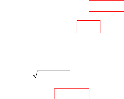
CHAPTER EIGHT SOLUTIONS
Engineering Circuit Analysis, 6th Edition Copyright
2002 McGraw-Hill, Inc. All Rights Reserved
19.
(a)
(b) 0.75 1.5
(15 ) 40 45 28.94Vvs e e
µ
−−
=+=
(c)
12
50000 100000
(0) 20mA, (0) 15mA
( ) 40 45 V (0) 85V
−−
==
∴= + ∴ =
tt
ii
vt e e v
50000 100000 . 50000
2
50000
85 40 45 Let
10
45 40 8.5 0
40 1600 1530 0.17718, 0
90
0.17718, 34.61
ttt
t
ee ex
xx
x
ets
µ
−− −
−
=+ =
∴+−=
−± +
∴= = <
∴= =
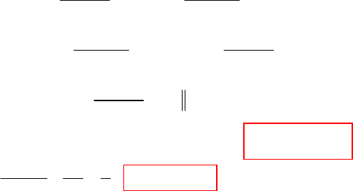
CHAPTER EIGHT SOLUTIONS
Engineering Circuit Analysis, 6th Edition Copyright
2002 McGraw-Hill, Inc. All Rights Reserved
20.
22
2
12 1
12 1 2
50 50
112
12 12
12 12
12
50 /1000
22
1
1
2R R 2R
0: , (0)
R+R R R
2R 2R R
0: ( ) RR R+R
2R R
(0 ) 10 R R 5 . Also, (1ms)
R+R
5 10 0.05R 0.6931 R 13.863
111
R 7.821
13.863 R 5
−−
+
−
<= ↓=
+
>= ∴=
+
∴== ∴=Ω
== ∴ = ∴ = Ω
∴+=∴=Ω
RL
Rt Rt
LR
RR
R
tv i
tit e v e
vv
e
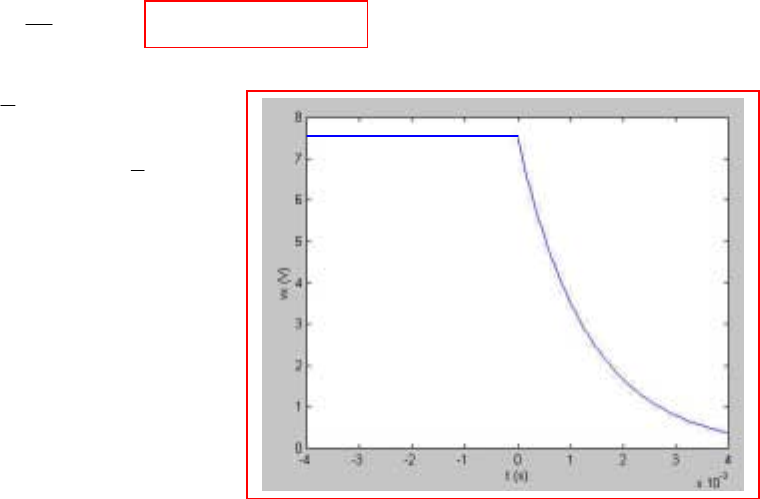
CHAPTER EIGHT SOLUTIONS
Engineering Circuit Analysis, 6th Edition Copyright
2002 McGraw-Hill, Inc. All Rights Reserved
21.
(a) 750
24
(0) 0.4A ( ) 0.4 A, 0
60
−
== ∴ = >
t
LL
iitet
(b)
750
524 20V, 0
6
3
(0 ) 50 0.4 7.5V
8
() 7.5 V, 0
+
−
=× = <
=× ×=
∴= >
x
x
t
x
vt
v
vt e t
CHAPTER EIGHT SOLUTIONS
Engineering Circuit Analysis, 6th Edition Copyright
2002 McGraw-Hill, Inc. All Rights Reserved
22.
25 /0.5 50
320 10 25
4
25 10 10 A, 0
−−
=×+ =
∴=Ω∴= = >
L
in L L
tt
in
in L
L
i
vii
v
vieet
i
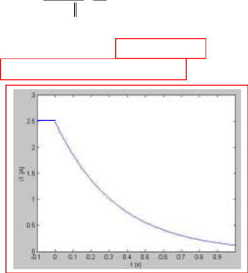
CHAPTER EIGHT SOLUTIONS
Engineering Circuit Analysis, 6th Edition Copyright
2002 McGraw-Hill, Inc. All Rights Reserved
23.
= 2.5 A
24 /8 3
3
11
11
64 40
(0) 5A
440848
55A
( ) 2.5 A, 0; ( 0.1)
(0.03) 2.285 A, (0.1) 1.
8
−−
−
−
=×=
+
∴= =
∴= > −
==
L
tt
L
t
i
ie e
it e t i
ii
52 A

CHAPTER EIGHT SOLUTIONS
Engineering Circuit Analysis, 6th Edition Copyright
2002 McGraw-Hill, Inc. All Rights Reserved
24.
(a)
(b)
100
1.5
(0) 4A 4 A, 0 15ms
(15ms) 4 0.8925 A
−
−+
=∴= <<
∴==
t
LL
L
iiet
ie
20( 0.015)
0.3
15ms: 0.8925 A
(30ms) 0.8925 0.6612A
t
L
L
ti e
ie
+− −
+−
>=
∴= =
CHAPTER EIGHT SOLUTIONS
Engineering Circuit Analysis, 6th Edition Copyright
2002 McGraw-Hill, Inc. All Rights Reserved
25.
(a) 11 2 2
(0 ) (0 ) 10A, (0 ) (0 ) 20A (0 ) 30Aii ii i
+− + − +
== ==∴=
(b) 0.08 5
L / R ms 1.6667ms;
48 3
eq eq
τ
====
(c) 12
(0 ) 10A, (0 ) 20Aii
−−
==; 600
( ) 30 A
t
it e
−
=
(d) 600
48 1440 V
t
vi e
−
=− =−
(e)
(f)
600 600 600
10
0
600
20
600 600
0
10( 440) 10 24 10 24 14A
2.5( 1440) 20
6 20 6 14A
−−−
−
−−
=− += += −
=− +
=+=+
∫
∫
ttttt
tt
tt t
iedtee
iedt
ee
22
22
L
2 1200
R00
11
W (0) 0.1 10 0.4 20 5 80 85J
22
11
W ( ) 0.1 14 0.4 14 9.8 39.2 49J
22
900 48
W 48 900 48 ( 1) 36J
1200
49 36 85 checks
L
t
idt e dt
∞∞
−
=× × +× × =+ =
∞= × × + × × = + =
×
==× =−=
−
∴+=
∫∫
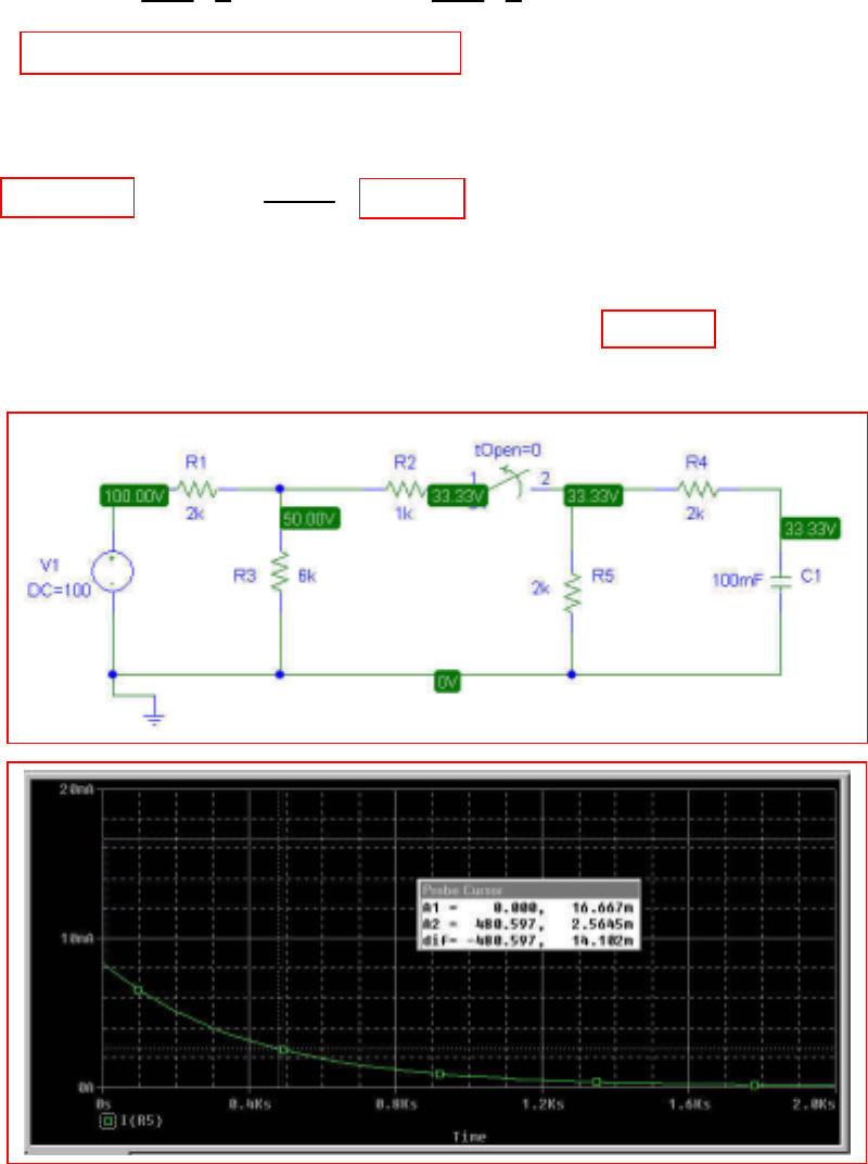
CHAPTER EIGHT SOLUTIONS
Engineering Circuit Analysis, 6th Edition Copyright
2002 McGraw-Hill, Inc. All Rights Reserved
26.
(a)
(b)
(c)
τ
= 400 s, so 1.2
τ
= 480 s. vC(1.2
τ
) = 33.33 e–1.2 = 10.04 V.
Using Ohm’s law, we find that i1(1.2
τ
) = vC(1.2
τ
)/ 4000 = 2.51 mA.
(d) PSpice Verification:
We see from the DC analysis of the circuit that our initial value is correct; the Probe
output confirms our hand calculations, especially for part (c).
1
c1
22 1002
(0) 100 33.33V; (0 ) 16.667mA
223 223
v (9:59) 33.33V, (9:59) 16.667mA
c
vi
i
−
=× ×= = ×=
++
∴= =
/ 400 300/ 400
1
( ) 33.33 , 10:00 (10:05) 33.33
15.745
15.745 V, (10:05) 3.936mA
4000
t
cc
vt e t v e
i
−−
+
=>∴=
===
CHAPTER EIGHT SOLUTIONS
Engineering Circuit Analysis, 6th Edition Copyright
2002 McGraw-Hill, Inc. All Rights Reserved
27.
25
0: 1.25 34 100(1.25 0.8 ) 25 0.2A
20
xxxxxxx
i
ti iiiii>=∴= −++∴=
(a) (0 ) (1.25 0.8 1)0.2 0.290A
s
i−=−+=
(b) (0 ) 0.2A
x
i−=
(c) 5
( ) 25 0.2 5 V (0 ) 0.05A
100
tt
cx
vt e e i
−− +
=× = ∴ = =
(d) 34 20 33.2
0.8 (0 ) 0.04A (0 ) 0.04 0.2767A
120 120 120
xs
ii
++
=∴=−×==
(e) 0.4
1
(0.4) 5 0.03352A
100
x
ie
−
=× =
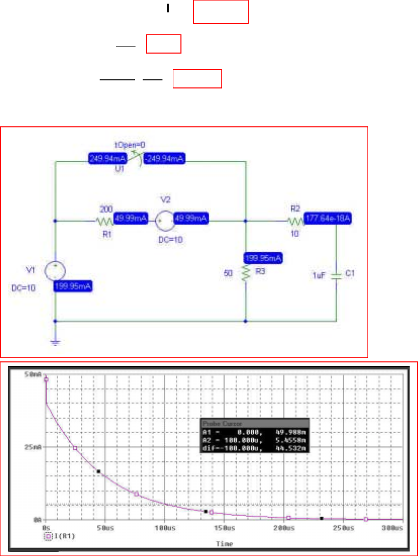
CHAPTER EIGHT SOLUTIONS
Engineering Circuit Analysis, 6th Edition Copyright
2002 McGraw-Hill, Inc. All Rights Reserved
28.
(a) 6
10 /(10 50 200) 20000
(0) 10V ( ) 10 10 V
tt
cc
vvte e
−+ −
=∴ = =
(b)
(c) PSpice Verification.
From the DC simulation, we see that PSpice verifies our hand calculation of iA = 50 mA.
The transient response plotted using Probe indicates that at 100 µs, the current is approximately
5.46 mA, which is within acceptable round-off error compared to the hand calculated value.
2
10
( 100 ) (0 ) 50mA
200
150
(100 ) 10 5.413mA
10 40 250
AA
A
isi
ise
µ
µ
−
−
−===
==
+
CHAPTER EIGHT SOLUTIONS
Engineering Circuit Analysis, 6th Edition Copyright
2002 McGraw-Hill, Inc. All Rights Reserved
29.
(a) 1
12
() 8( 1) 6mA( 0)
12 4
it t=− =− <
+
(b)
63
10 / 5 2 10 100
100
4 12 6 2 , (0) 48V
( ) 48 48 V, 0
() 12 mA, 0
−×× −
−
=Ω =
∴= = >
∴= >
c
tt
c
t
kv
vt e e t
it e t

CHAPTER EIGHT SOLUTIONS
Engineering Circuit Analysis, 6th Edition Copyright
2002 McGraw-Hill, Inc. All Rights Reserved
30.
(a)
(b)
66
10 /8 10 /0.8
1,250,000 125,000
(0) 20V, (0) 80V
20 , 80
80 20 V, 0
−−
−−
==
∴= =
∴=−= − >
CLeft CRIGHT
tt
CL CR
tt
out CR CL
vv
veve
vvv e e t
1.25 0.125
6.25 0.625
(0 ) 60V; (1 ) 80 20 5.270V
(5 ) 80 20 10.551V
+−−
−−
==−=
=− =−
out out
out
vvsee
vse e
µ
µ
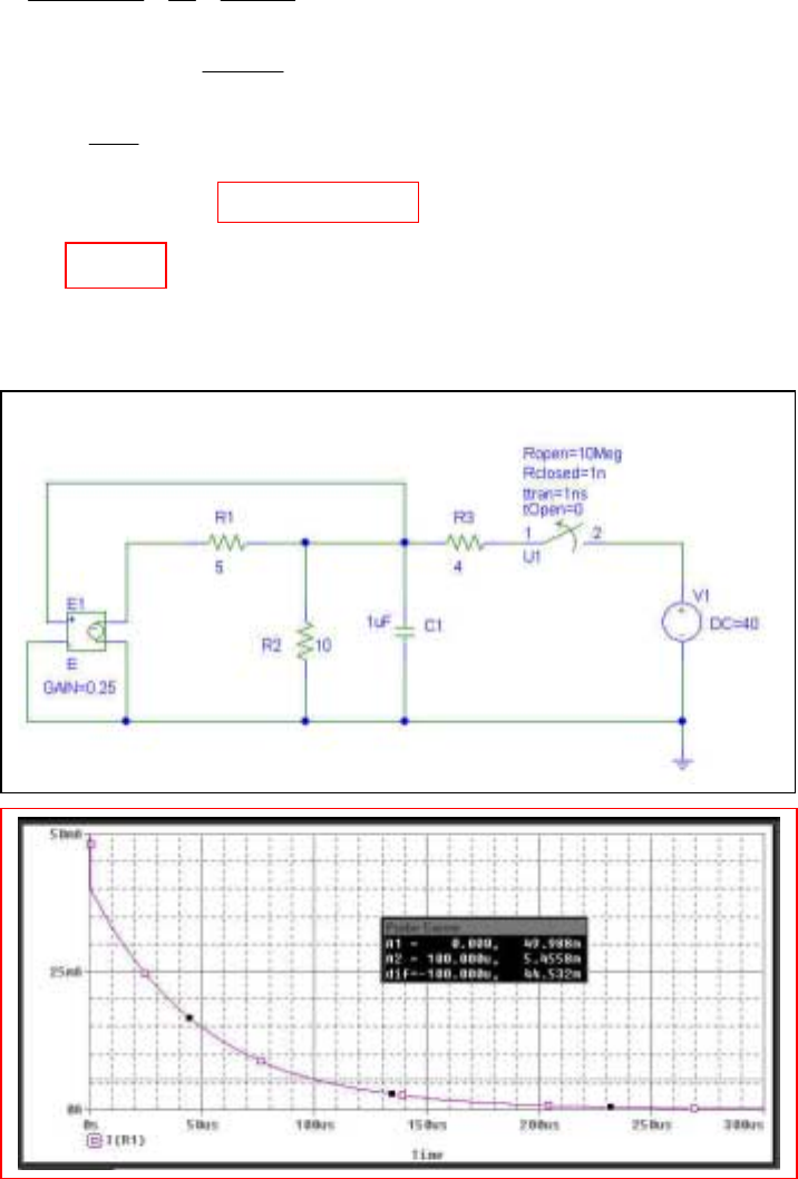
CHAPTER EIGHT SOLUTIONS
Engineering Circuit Analysis, 6th Edition Copyright
2002 McGraw-Hill, Inc. All Rights Reserved
31. (a)
(b) vC(3 µs) = 9.447 V
(c) PSpice verification. Note that the switch parameters had to be changed in order to
perform this simulation.
As can be seen from the simulation results, our hand calculations are accurate.
6
10 /4 250,000
0.25 40
0: 0 20V( 0)
5104
1 0.25
0: Apply 1V 0.1 0.25A
5
1
R4
0.25
( ) 20 20 V( 0)
−−
−−
<++=∴=<
−
>=∴+−=
∴= =Ω
∴= = >
c ccc c
cin
eq
tt
c
v vvv
tvt
tv i
vt e e t
CHAPTER EIGHT SOLUTIONS
Engineering Circuit Analysis, 6th Edition Copyright
2002 McGraw-Hill, Inc. All Rights Reserved
32.
6
63
10 /( 1000) 500/( 1000)
1000/ 2742.4
10 ( 10 )
1
10
0: (0) 60V
50
01ms: 60 60
R500 1.2 0.18232 2 5.4848, 1742.4
R 1000 500
(1ms) 60 41.67V
1ms : 41.67 /(1742.4 R 1000)
25 41.67
oo
c
tR R
c
oo
o
c
t
c
tv
tve e
nR
ve
tv e
e
−
−+ −+
−
−−
−
<=
<< = ∴
∴==∴+==Ω
+
∴= =
>= +
∴=
l
00() 1
1
3
11
1
.1000
0.5108 ,1742.4 R 1000
1742.4 R 1000
11
1957.6, R 1000 215.2 10 R 274.2
R 215.2
−
∴= +
+
==+=∴=Ω

CHAPTER EIGHT SOLUTIONS
Engineering Circuit Analysis, 6th Edition Copyright
2002 McGraw-Hill, Inc. All Rights Reserved
33.
(a) With the switch closed, define a nodal voltage V1 at the top of the 5-kΩ resistor.
Then,
0 = (V1 – 100)/ 2 + (V1 – VC)/ 3 + V1/ 5 [1]
0 = VC/ 10 + (VC – V1)/ 3 + (VC – 100) [2]
Solving, we find that VC = vC(0-) = 99.76 V.
(b) 7
10 /3939 2539
0: R 10 6.5 3.939 87.59 87.59 V ( 0)
−−
>==Ω∴= = >
tt
eq c
tkveet
CHAPTER EIGHT SOLUTIONS
Engineering Circuit Analysis, 6th Edition Copyright
2002 McGraw-Hill, Inc. All Rights Reserved
34. t < 0:
39 6
111 11 1
111 1
/75 10 2 10 10 /150 6667
6667
14
12 4 20 0.5mA (0) 6 20 26
(0) 13V
0: Apply 1mA 1 0.6 2.5mA; 30 75V R 75
( ) 13 13 13
( ) 0.4333 mA ( 0)
310
−
−××× − −
−
=+ ∴= ∴ =+ =
=
>←∴+=∴=±==∴=Ω
∴= = =
∴= = >
×
c
c
in eq
ttt
c
t
o
iii v iii
v
tiiivik
vt e e e
v
it e t
CHAPTER EIGHT SOLUTIONS
Engineering Circuit Analysis, 6th Edition Copyright
2002 McGraw-Hill, Inc. All Rights Reserved
35.
(a) 12
(0 ) 100V. (0 ) 0, (0 ) 0
R
vvv
−−−
===
(b) 12
(0 ) 100V. (0 ) 0, (0 ) 100V
R
vvv
−++
===
(c) 64 2
20 5 10 2 10 8 10
20 5 s
τ
−−
×
=××=×
+
(d) 12.5
( ) 100 V, 0
t
R
vt e t
−
=>
(e) 12.5
4
()
() 5 mA
210
t
R
vt
it e
−
==
×
(f)
(g)
63
3 12.5 12.5 12.5
1
12.5 12.5 12.5
2
10 10
( ) 5 10 100 100 20 80V
20 50
1000
( ) 5 0 80 0 80 80V
5
−− − −
−−−
=−× += +=− +
=+=−+=−+
∫
∫
ttttt
o
o
ttttt
o
o
vt e dt e e
vt e dt e e
62 62
12
62
12
625 4 4 6
11
( ) 20 10 80 64mJ, ( ) 5 10 80 16mJ
22
1
(0) 20 10 100 100mJ, (0) 0
2
25
25 10 2 10 2 10 ( 1)10 20mJ
25
64 16 20 100 checks
−−
−
∞−− −
∞= × × × = ∞ ×× × =
=× × × = =
=× ××=××− =
−
++ =
∫
cc
cc
t
Ro
ww
ww
wedt

CHAPTER EIGHT SOLUTIONS
Engineering Circuit Analysis, 6th Edition Copyright
2002 McGraw-Hill, Inc. All Rights Reserved
36.
(a) 0: 1mA (0) 10V, (0) 1mA (0) 10V, 0
sc L x
ti v i v t<=∴± =↓=−∴= <
(b)
49
/10 20 10 5000
3 3 /0.1 3 10000 10000
L
5000 10000
0: ( ) 10 10 V
i() 10 10 10 A () V, 0
( ) 10 V, 0
tt
c
tt t
L
tt
xcL
tvt e e
te e vtet
vvvt e e t
−
−×× −
−−− −
−−
>= =
=− − =− ∴± = >
∴=− = − >

CHAPTER EIGHT SOLUTIONS
Engineering Circuit Analysis, 6th Edition Copyright
2002 McGraw-Hill, Inc. All Rights Reserved
37.
(a) 0: 20V 20V, 20mA ( ) 20mA, 0<=∴= = ∴= <
scL x
tv v i it t
(b)
84
10000 / 2 10 10 5000
8 5000 5000
10000 5000 10000 5000
0: 0 ( ) 0.02 A; ( ) 20 20 V
( ) 2 10 20( 5000) 2 mA
( ) ( ) ( ) 0.02 0.002 A 20 2 m
A
tt t
sL c
tt
c
tttt
xLc
tv it e vt e e
it e e
it it it e e e e
−
−−×−
−−−
−−−−
>=∴= = =
↓=××− =−
=+= − = −
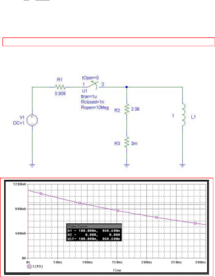
CHAPTER EIGHT SOLUTIONS
Engineering Circuit Analysis, 6th Edition Copyright
2002 McGraw-Hill, Inc. All Rights Reserved
38.
PSpice verification: Note that the switch properties were changed.
We see from the simulation result that the current through the fuse (R3) is 869 mA, in
agreement with our hand calculation.
()
blow.not does fuse thems, 100 prior toA 1 than less todropped hascurrent thesince
A .868501.11.0
A )( :0
A 1.1
909.0
1
R
V
)0(
1.0363.2
363.2
=∴
==
=>
===
×−
−
−
t
esi
etit
i
L
t
L
L
CHAPTER EIGHT SOLUTIONS
Engineering Circuit Analysis, 6th Edition Copyright
2002 McGraw-Hill, Inc. All Rights Reserved
39. (a)
1
1
11
300 ( 1)V, 120 ( 1)V; 3 ( )A
100
1.5: ( 1.5) 3 1A
300
120
0.5: ( 0.5) 1 0.6A;
300
120 300 120
0.5: 0.4A; 1.5: 0.6A
300 300 300
=− =−+=−
=− − = × =
−
=−=+=
= =−=− = =−=
AB c
vutv utiut
ti
ti
ti ti
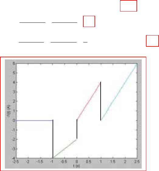
CHAPTER EIGHT SOLUTIONS
Engineering Circuit Analysis, 6th Edition Copyright
2002 McGraw-Hill, Inc. All Rights Reserved
40.
600 ( 1) , 600( 1) ( )V, 6( 1) ( 1)A
AB c
vtutvv tutitut
↑
=+=+ =−−
(a)
(b)
11
1
1
1.5: 0; 0.5: 600( 0.5) /300 1A
600(0.5) 600(1.5)
0.5: 4A
300 300
600(1.5) 600(2.5) 1
1.5: 6 0.5 3 5 1 9A
300 300 3
=− = =− = − =−
== + =
== + +××=++=
titi
ti
ti
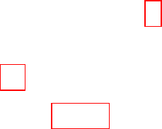
CHAPTER EIGHT SOLUTIONS
Engineering Circuit Analysis, 6th Edition Copyright
2002 McGraw-Hill, Inc. All Rights Reserved
41.
(a) 2 ( 1) 3 (1) 4 (3) 3 4 1uuu−− + =−+=
(b)
(c) (1) 1
4 (1) 4 1.4715
u
eu e
−−+
==
[5 (2)] [2 (1)] [1 ( 1)]
43112
uuu−+−−
=××=
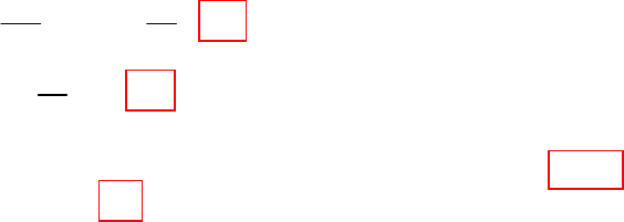
CHAPTER EIGHT SOLUTIONS
Engineering Circuit Analysis, 6th Edition Copyright
2002 McGraw-Hill, Inc. All Rights Reserved
42.
(a)
(b) t < 0: The voltage source is shorting out the 30-Ω resistor, so ix = 0.
t > 0: ix = 60/ 30 = 2 A.
100 20
0: 0 10 6A
50 50
60
0: 0 0 2A
30
x
x
ti
ti
<=++×=
>=++=
CHAPTER EIGHT SOLUTIONS
Engineering Circuit Analysis, 6th Edition Copyright
2002 McGraw-Hill, Inc. All Rights Reserved
43. 0.5:t=− 200 1/50 1
50 25 16.667, 2 3 2.5A
66.67 1/50 1/ 25 1/ 50 2
x
i==− =−=
++
0.5:t= 200 3A
66.67
x
i==
1.5:t= 100 1
3 2.5A
66.67 3
x
i=− ×=
2.5:t= 200 100 2A
50
x
i−
==
3.5:t= 100 2A
50
x
i=− =−
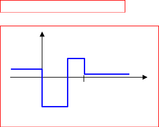
CHAPTER EIGHT SOLUTIONS
Engineering Circuit Analysis, 6th Edition Copyright
2002 McGraw-Hill, Inc. All Rights Reserved
44. () 4 16() 20( 4) 6( 6)Vvt ut ut ut=− + − − −
t (s)
v(t) (V)
4
-12
8
2
0 4 6

CHAPTER EIGHT SOLUTIONS
Engineering Circuit Analysis, 6th Edition Copyright
2002 McGraw-Hill, Inc. All Rights Reserved
45. (a)
(b) Resistor of value 2Ω
7()0.2()8( 2)3
(1) 9.8 volts
−+−+
=
ut ut t
v

CHAPTER EIGHT SOLUTIONS
Engineering Circuit Analysis, 6th Edition Copyright
2002 McGraw-Hill, Inc. All Rights Reserved
46.
(a) 200000
() (2 2 ) ()
m
t
L
it e ut
−
=− mA
(b)
33
200000 200000
() L 15 10 10 ( 2)
( 200000 ) ( ) 6 ( )V
−−
−−
′
==×× −
−=
LL
tt
vt i
euteut

CHAPTER EIGHT SOLUTIONS
Engineering Circuit Analysis, 6th Edition Copyright
2002 McGraw-Hill, Inc. All Rights Reserved
47.
(a) 2.5 1
( ) 2 2(1 ) ( )A ( 0.5) 2A
t
L
it e ut i
−
=+ − ∴− =
(b) 1.25
(0.5) 2 2(1 ) 3.427A
L
ie
−
=+ − =
(c) 3.75
(1.5) 2 2(1 ) 3.953A
L
ie
−
=+ − =
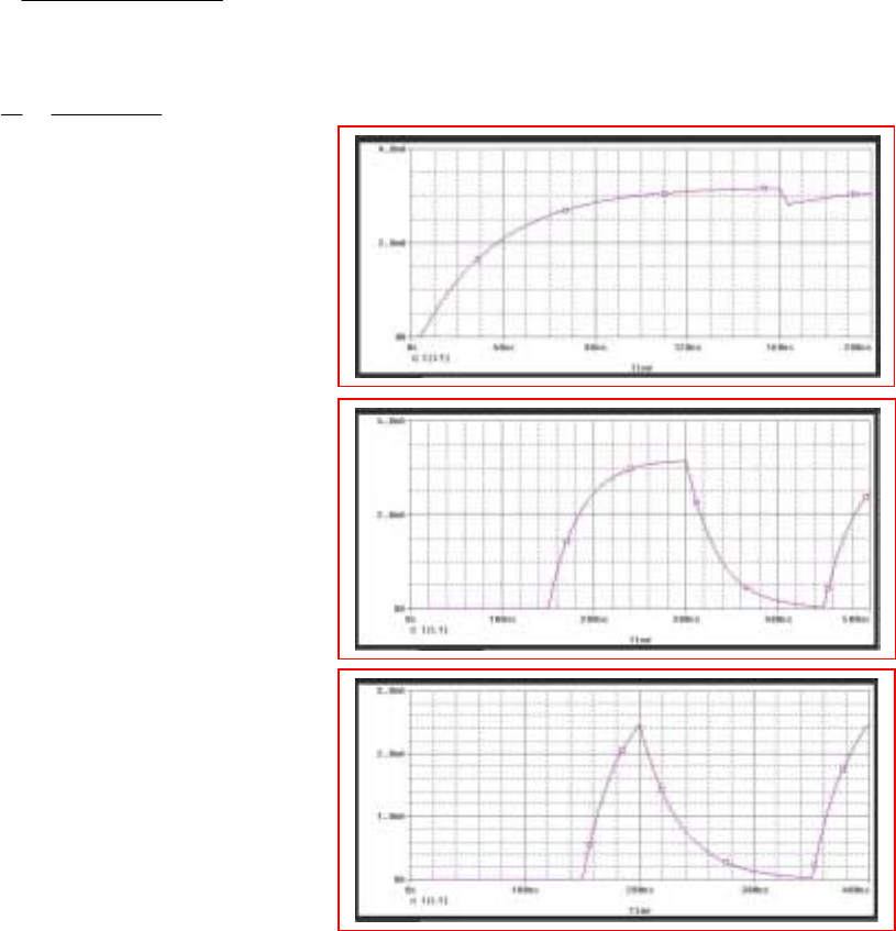
CHAPTER EIGHT SOLUTIONS
Engineering Circuit Analysis, 6th Edition Copyright
2002 McGraw-Hill, Inc. All Rights Reserved
48.
Ai
Aii
ii
ns
R
L
R
L
L
L
th
3
3
1
33
1
3
6
3
33
33
102.3
1010
1010.107.4.
156
102.3
10500
102.3
107.41010
107.41010
−
−
−
×=∴
×=+
×=×
=
×
×
==
Ω×=
×+×
×××
=
τ
(a)
(b)
(c)
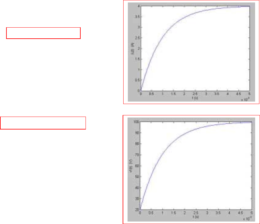
CHAPTER EIGHT SOLUTIONS
Engineering Circuit Analysis, 6th Edition Copyright
2002 McGraw-Hill, Inc. All Rights Reserved
49.
(a)
(b) 1000
1( ) (100 80 ) ( )V
t
vt e ut
−
=−
20 /0.02
1000
() (4 4 ) ()
( ) 4(1 ) ( )A
t
L
t
L
it e ut
it e ut
−
−
=−
∴=−
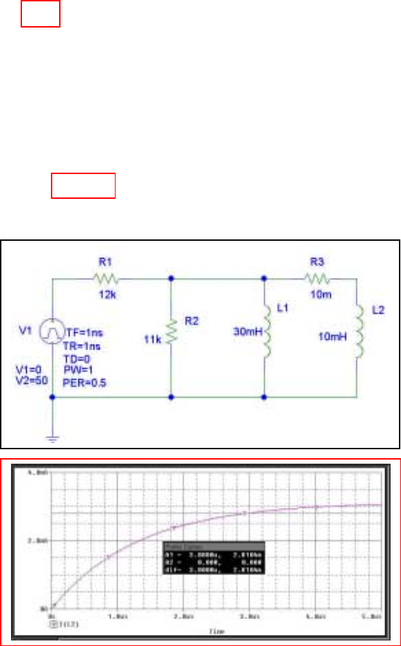
CHAPTER EIGHT SOLUTIONS
Engineering Circuit Analysis, 6th Edition Copyright
2002 McGraw-Hill, Inc. All Rights Reserved
50. (a) 0 W
(b) The total inductance is 30 || 10 = 7.5 mH. The Thévenin equivalent resistance is
12 || 11 = 5.739 kΩ. Thus, the circuit time constant is L/R = 1.307 µs. The final value of
the total current flowing into the parallel inductor combination is 50/12 mA = 4.167 mA.
This will be divided between the two inductors, so that i(∞) = (4.167)(30)/ (30 + 10) =
3.125 mA.
We may therefore write i(t) = 3.125[1 – e-106t/ 1.307] A. Solving at t = 3 µs,
we find 2.810 A.
(c) PSpice verification
We see from the Probe output that our hand calculations are correct by verifying using
the cursor tool at t = 3 µs.

CHAPTER EIGHT SOLUTIONS
Engineering Circuit Analysis, 6th Edition Copyright
2002 McGraw-Hill, Inc. All Rights Reserved
51.
(a) ( ) 10 , 0=<
L
it At
(b)
5/0.5
10
() 8 2
() 8 2 A, 0
t
L
t
L
it e
it e t
−
−
=+
∴=+ >

CHAPTER EIGHT SOLUTIONS
Engineering Circuit Analysis, 6th Edition Copyright
2002 McGraw-Hill, Inc. All Rights Reserved
52.
(a) ( ) 2A, 0
L
it t=>
(b)
4 /0.1
40
() 5
() 5 3 A, 0
t
L
t
L
it e
it e t
−
−
=−
∴=− >
CHAPTER EIGHT SOLUTIONS
Engineering Circuit Analysis, 6th Edition Copyright
2002 McGraw-Hill, Inc. All Rights Reserved
53.
(a)
(b)
(c) 25
10 10 ( )
Q( ) 2 2 ( ) 0.16 0.08 A, 0
5
−
+
==+∴=− >
t
ut
tutiet
(d)
P Q, Q , R 125 , L 5H
L LP LQ LP 5P R 125 P 25
−−
+= = + = Ω=
∴=∴===∴=
∫
Pt Pt Pt
di iieedtAe
dt
di i
dt
25 25 25 25 25 25
25
10 2
Q( ) 2 2 A A
L25
21022
A , (0) A 0 0.08A
25 125 25 25
−−− −
−
==∴= + = × +
∴= + = = ∴ = ∴= =
∫t
tt tt tt t
o
o
t
tieedteeee
iei i
25 25 25 25
25
10 ( ) 2
Q( ) 2 ( ) 2 A A
525
2
(0) 0 A ( ) 0.08(1 )A, 0
25
−−−
−
==∴= +=+
=∴ =− ∴ = − >
∫t
tt t t
o
t
ut
tutieedtee
iitet
25 25 25
25
25 25
22
25
25 25
10 ( )cos50
Q( ) 2 ( )cos50 2cos50
5
2 (25cos50 50sin 50 ) A
50 25
1
2 (25cos50 50sin50 ) 25 A
3125 3125
242
cos50 sin50
125 125 125
−−
−−
− −
==∴= ×+
∴= + +
+
=+−×+
=+−
∫t
ttt
o
t
t
tt
o
t
t t
ut t
tuttietedtAe
e
ie t t e
e
ette
tte
25 25
25
A
22
(0) 0 0 A A 0
125 125
( ) 0.016cos50 0.032sin50 0.016 A, 0
−−
−
+
=∴= − + ∴ =
∴= + − >
tt
t
e
i
it t t e t
CHAPTER EIGHT SOLUTIONS
Engineering Circuit Analysis, 6th Edition Copyright
2002 McGraw-Hill, Inc. All Rights Reserved
54.
(a) 0, 0
(b) 0, 200V
(c) 1A, 100V
(d)
34000
4000
11
50 10 1 ms 1(1 ) ( )A, (0.2ms) 0.5507A
200 4
( ) (100 100 ) ( )V, (0.2ms) 144.93V
t
LL
t
ieuti
vt e ut v
τ
−−
−
×
==∴=− =
=+ =
CHAPTER EIGHT SOLUTIONS
Engineering Circuit Analysis, 6th Edition Copyright
2002 McGraw-Hill, Inc. All Rights Reserved
55.
(a) 100 100
( ) 15A, 0
20 5
L
it t=−=− <
(b) (0 ) (0 ) 15A
LL
ii
+−
==−
(c) 100
() 5A
20
L
i∞= =
(d) 40
() 5 20 A, 0
t
L
it e t
−
=− >

CHAPTER EIGHT SOLUTIONS
Engineering Circuit Analysis, 6th Edition Copyright
2002 McGraw-Hill, Inc. All Rights Reserved
56.
L
9000
9000
9000
18 1
(0 ) 0.1A (0 ) 0.1A
60 30 2
i ( ) 0.1 0.1 0.2A
( ) 0.2 0.1 A, 0
( ) 0.1 ( ) (0.2 0.1 ) ( )A
or, ( ) 0.1 (0.1 0.1 ) ( )A
−+
−
−
−
=×=∴=
+
∞= + =
∴=− >
∴= −+−
=+ −
LL
t
L
t
L
t
L
ii
it e t
it u t e ut
it e ut
CHAPTER EIGHT SOLUTIONS
Engineering Circuit Analysis, 6th Edition Copyright
2002 McGraw-Hill, Inc. All Rights Reserved
57.
(a) 30 3
(0 ) 3A, (0 ) 4A
7.5 4
xL
ii
−−
=×= =
(b) (0 ) (0 ) 4A
xL
ii
++
==
(c)
10 /0.5 20
0.8
() () 3A
() 3 1 3 A (0.04)
3 3.449A
−−
−
∞= ∞=
∴=+ =+ ∴
=+ =
xL
tt
xx
ii
it e e i
e
CHAPTER EIGHT SOLUTIONS
Engineering Circuit Analysis, 6th Edition Copyright
2002 McGraw-Hill, Inc. All Rights Reserved
58.
(a) 30
(0 ) (0 ) 3A
10
xL
ii
−−
===
(b)
(c)
30 30 15
(0 ) 3 2.4A
30 7.5 40 10 15
+=×+×=
++
x
i
6 /0.5
12 0.48
30 30
() 3A () 30.6
7.5 40
3 0.6 (0.04) 3 0.6 2.629A
t
xx
t
x
iite
ei e
−
−−
∞= × = ∴ = −
=− ∴ =− =
CHAPTER EIGHT SOLUTIONS
Engineering Circuit Analysis, 6th Edition Copyright
2002 McGraw-Hill, Inc. All Rights Reserved
59.
52 /0.2 260
260
OC: 0, 4 ( )V
0.2
SC : 0.1 ( ) ,12 ( ) 0.6 2
40 60
12 ( ) 12 ( ) ( )
2.6 60 2.6 60 13
4() ()
413 52 (1 )() (1 )()
52 13
60 4.615 (1 ) ( )V
−−
+−
==
−
=+ =+
∴= ∴= = =
×
∴=×=Ω∴= − = −
∴= = −
xoc
xxx xx
x
xab
tt
th L
t
xL
vvut
vvv
ut ut v v
vut ut ut
vi
ut ut
Rieuteut
vi eut
CHAPTER EIGHT SOLUTIONS
Engineering Circuit Analysis, 6th Edition Copyright
2002 McGraw-Hill, Inc. All Rights Reserved
60.
(a)
(b)
11 1
1
40
OC: 100 30 20 0, 2A
80 ( )V
20 10
SC: 10A, 10 20A
20
R 4 () 20(1 ) ()A
−
−++ = =
∴=
×
=↓=+ =
∴=Ω∴ = −
oc
sc
t
th L
iii
vut
ii
it e ut
40 40
40 40
1
0.12040()80()
100 ( ) 80 ( )
() 10 8 ()A
10
tt
L
tt
veuteut
ut e ut
it e ut
−−
−−
=×× =
−
∴= =−
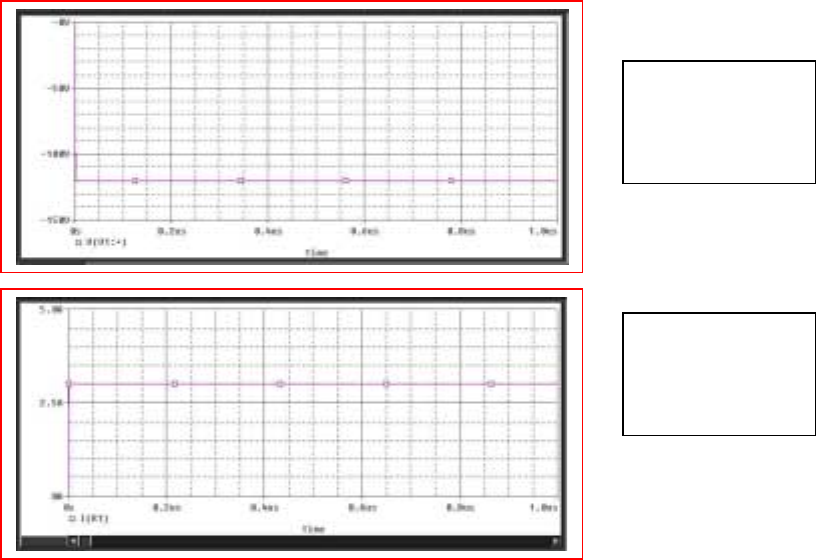
CHAPTER EIGHT SOLUTIONS
Engineering Circuit Analysis, 6th Edition Copyright
2002 McGraw-Hill, Inc. All Rights Reserved
61. Unfortunately, PSpice will not allow us to use negative time values. Thus, we must
perform the simulation starting from t = 0, and manually shift the results if needed to
account for sources that change value prior to t = 0.
Voltage source
vB(t) from
Exercise 39.
Current source
iC(t) from
Exercise 39.
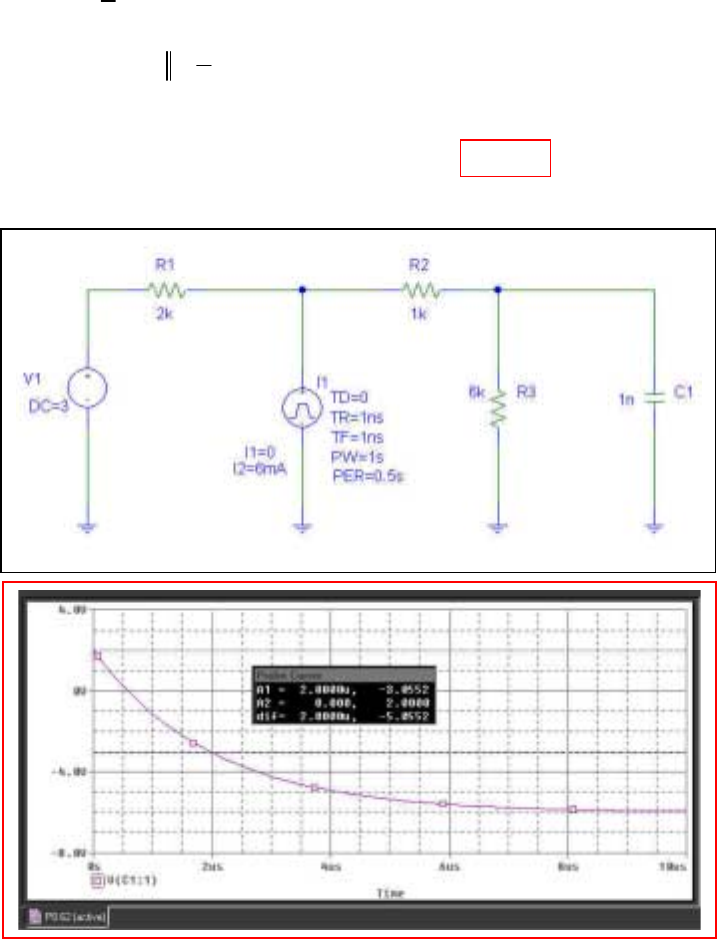
CHAPTER EIGHT SOLUTIONS
Engineering Circuit Analysis, 6th Edition Copyright
2002 McGraw-Hill, Inc. All Rights Reserved
62. (a)
(b) PSpice verification.
As can be seen from the plot above, the PSpice simulation results confirm our hand
calculations of vC(t < 0) = 2 V and vC(t = 2 µs) = -3.06 V
93
10 / 2 10 500000
1
6
(0 ) 3 2V (0 )
9
6
() 26(27) 6V
7
() 68 68 V, 0
( 2 ) (0 ) 2V, (2 ) 6 8 3.057V
−+
−× −
−−
=×= =
∞= − =−
∴=−+ =−+ >
−= = =−+=−
cc
c
tt
c
cc c
vv
v
vt e e t
vsv vs e
µµ

CHAPTER EIGHT SOLUTIONS
Engineering Circuit Analysis, 6th Edition Copyright
2002 McGraw-Hill, Inc. All Rights Reserved
63.
83 5
10 /10 10
10
(0 ) 2.5mA, ( ) 10mA
4
10 7.5
(0) 7.5V (0 ) 17.5mA
11
10 7.5 10 7.5 mA, 0, 2.5mA 0
−
+
−−
== ∞=
=∴ =+=
=+ =+ > = <
AA
cA
tt
AA
ii
vi
ie etit

CHAPTER EIGHT SOLUTIONS
Engineering Circuit Analysis, 6th Edition Copyright
2002 McGraw-Hill, Inc. All Rights Reserved
64.
83
10 /1.75 10 57140
10
(0 ) 10mA, ( ) 2.5mA, (0) 0
1
10 1
(0 ) 1.4286mA 10mA, 0
1.75 4
2.5 (1.4286 2.5) 2.5 1.0714 mA, 0
AAc
AA
tt
A
iiv
iit
ie et
−
+
−× −
== ∞= =
=× ∴= <
=+ − =− >
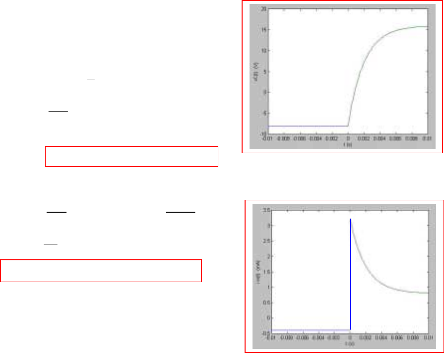
CHAPTER EIGHT SOLUTIONS
Engineering Circuit Analysis, 6th Edition Copyright
2002 McGraw-Hill, Inc. All Rights Reserved
65.
(a)
(b)
37 3
500
500
12 ( ) 24 ( )V
0: (0 ) 8V (0 ) 8V
2
0: ( ) 24 16V
3
200
RC 10 3 10 2 10
30
( ) 16 24 V, 0
( ) 8 ( ) (16 24 ) ( )
s
cc
c
t
c
t
c
vutut
tv v
tv
vt e t
vt u t e ut
−+
−−
−
−
=− − +
<=−∴=−
>∞=×=
=×××=×
∴=− >
∴=−−+−
500
12 24 8
(0 ) 0.4mA, (0 ) 3.2mA
30 10
24
( ) 0.8mA
30
( ) 0.4 ( ) (0.8 2.4 ) ( )mA
in in
in
t
in
ii
i
it ut e ut
−+
−
−+
==− = =
∞= =
=− + +

CHAPTER EIGHT SOLUTIONS
Engineering Circuit Analysis, 6th Edition Copyright
2002 McGraw-Hill, Inc. All Rights Reserved
66.
(a) iin (-1.5) = 0
(b) iin (1.5) = 0
(0 ) 10V (0 ), (0 ) 0
(0 ) 0 ( ) 0 for all
−+−
+
== =
=∴ =
ccin
in in
vvi
iit t
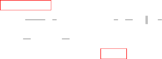
CHAPTER EIGHT SOLUTIONS
Engineering Circuit Analysis, 6th Edition Copyright
2002 McGraw-Hill, Inc. All Rights Reserved
67.
2.5
0.375 20( 0.5) 7.5( 0.5)
7.5(0.3)
0 0.5 : 10(1 )V
(0.4) 6.321V, (0.5) 7.135V
20 10 5 5 50 8
0.5: A ( ) 10 8 V, 4 8
12 6 6 3 3
50 50
( ) 7.135 16.667 9.532 V
33
(0.8) 16.667 9.532 15.
t
c
cc
c
tt
c
c
tsv e
vv
tv
vt e e
ve
−
−×− −−
−
<< = −
==
−
>=∴∞=++==Ω
=+ − = −
∴=− =662V
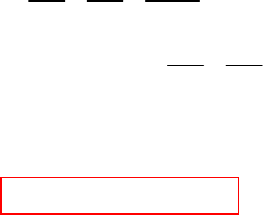
CHAPTER EIGHT SOLUTIONS
Engineering Circuit Analysis, 6th Edition Copyright
2002 McGraw-Hill, Inc. All Rights Reserved
68.
6
/10 /33.33
30,000
3
OC: 0 1, 3 1 2V
100 100 100
SC : 3V 0.06A
100 100
R / 2/ 0.06 33.33
(1 ) 2(1 )
2(1 ) V, 0
th
xx x xoc
xx
xsc
th oc sc
tRC t
coc
t
vv v vv
vv
vi
vi
vv e e
et
−−
−
−−
−+ =∴= =−=
=∴= + =
∴= = = Ω
∴= − = −
=− >
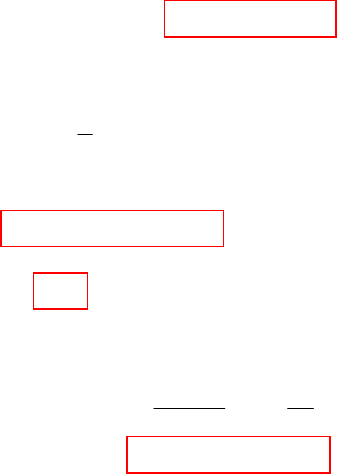
CHAPTER EIGHT SOLUTIONS
Engineering Circuit Analysis, 6th Edition Copyright
2002 McGraw-Hill, Inc. All Rights Reserved
69.
(a) 0: 8(10 20) 240V ( ) 80V, 0
R
tvtt<+===<
(b)
(c) 0: ( ) 80V
R
tvt<=
(d)
6
/10 10 100000
100000
0: ( ) 8 30 240V (0 ) 240V
1
( ) : ( ) 8(10 10) 80V
2
( ) 80 160 80 160 V
( ) 80 160 V, 0
cc
c
tt
c
t
R
tvt v
tv
vt e e
vt e t
−
+
−× −
−
<=×=∴=
=∞ ∞= × + =
∴=+ =+
∴=+ >
6
/50 10 20000
20000
(0 ) 80V, ( ) 240V ( ) 240 160 240 160 V
20 80
(0 ) 80V, (0 ) 8 10 10 32 16 48V
30 20 50
() 80V () 8032 V, 0
tt
cc c
RR
t
RR
vv vte e
vv
vvtet
−
−−×−
−+
−
= ∞= ∴ =− =−
==×+×=+=
+
∞= ∴ = − >
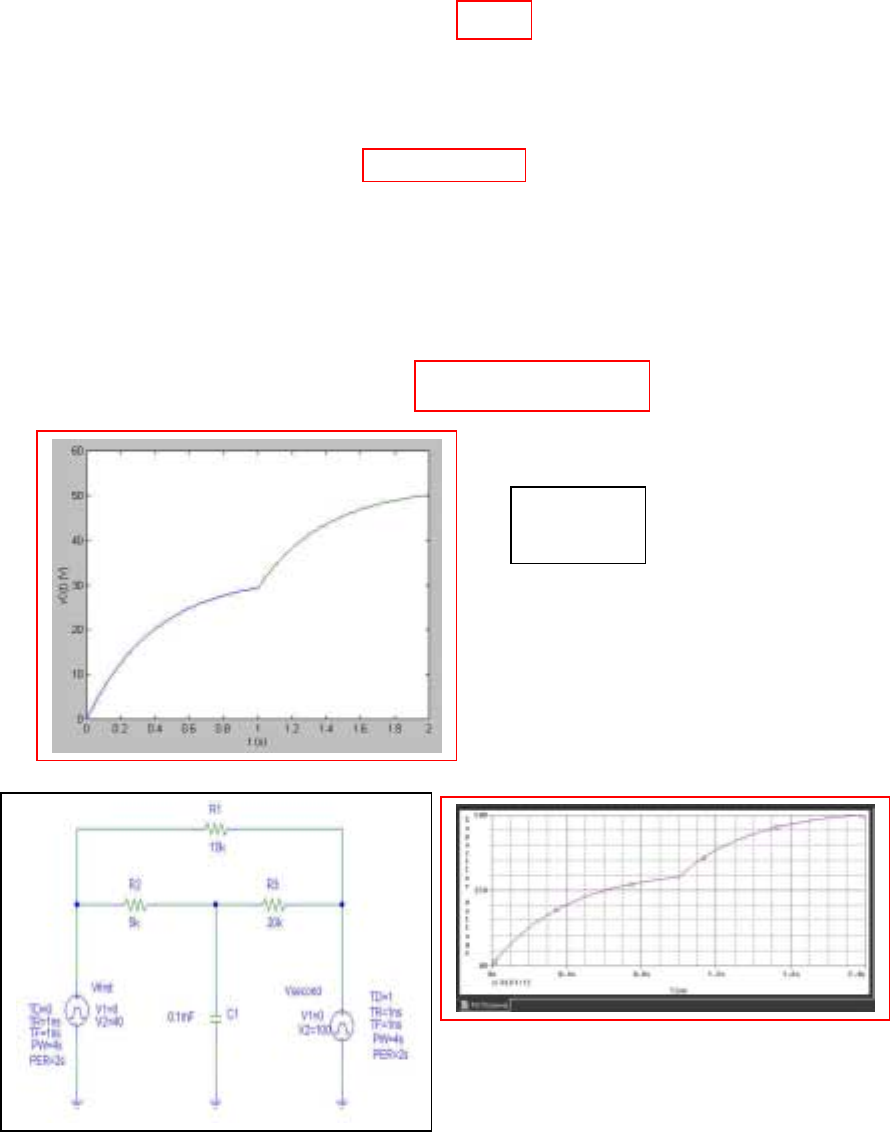
CHAPTER EIGHT SOLUTIONS
Engineering Circuit Analysis, 6th Edition Copyright
2002 McGraw-Hill, Inc. All Rights Reserved
70.
(a) For t < 0, there are no active sources, and so vC = 0.
For 0 < t < 1, only the 40-V source is active. Rth = 5k || 20 k = 4 kΩ and hence
τ
= Rth C = 0.4 s. The “final” value (assuming no other source is ever added) is found
by voltage division to be vC(∞) = 40(20)/(20 + 5) = 32 V. Thus, we may write
vC(t) = 32 + [0 – 32] e–t/ 0.4 V = 32(1 – e-2.5t) V.
For t > 1, we now have two sources operating, although the circuit time constant remains
unchanged. We define a new time axis temporarily: t' = t – 1. Then vC(t' = 0+) =
vC(t = 1) = 29.37 V. This is the voltage across the capacitor when the second source
kicks on. The new final voltage is found to be vC(∞) = 40(20)/ (20 + 5) +
100(5)/ (20 + 5) = 52 V.
Thus, vC(t') = 52 + [29.37 – 52] e-2.5t' = 52 – 22.63 e-2.5(t – 1) V.
(b)
(c)
For t < 0,
vC = 0.
We see from the simulation results that
our hand calculations and sketch are
indeed correct.
CHAPTER EIGHT SOLUTIONS
Engineering Circuit Analysis, 6th Edition Copyright
2002 McGraw-Hill, Inc. All Rights Reserved
71.
2000
,
1000
,
,,
2000 1000
1000 1000 2
1000
1000
200 V
100(1 )V
0
200 100 100
100 200( ) 100 0,
100 10,000 80,000 0.25 0.75
400
0.5, 0.6931ms
−
−
−−
−−
−
−
=
=−
=−=
∴=−
∴+ −=
−± +
==−±
∴==
t
xL
t
xc
xxLxc
tt
tt
t
t
ve
ve
vv v
ee
ee
e
et
CHAPTER EIGHT SOLUTIONS
Engineering Circuit Analysis, 6th Edition Copyright
2002 McGraw-Hill, Inc. All Rights Reserved
72.
61
11
62
10 /( 100)
1000/( 100) 1000/( 100)
1
1
10 /( 100) 3 1000
2
2
2
0: 0
01ms:9(1 )
1
89(1 ),
9
1000 2.197, R 355.1
R 100
1ms : 8 , 10 1 8 (R 100)
1000 2.079, R 480.9 100 380.9
R 100
c
tR
c
RR
tR
c
tv
tve
ee
tve tt e
−+
−+ −+
′
−+ − −
<=
<< = −
∴= − =
∴= =Ω
+
′
>= =−∴− +
∴= =−=Ω
+
CHAPTER EIGHT SOLUTIONS
Engineering Circuit Analysis, 6th Edition Copyright
2002 McGraw-Hill, Inc. All Rights Reserved
73. For t < 0, the voltage across all three capacitors is simply 9 (4.7)/ 5.7 = 7.421 V. The
circuit time constant is
τ
= RC = 4700 (0.5455×10⁻⁶) = 2.564 ms.
When the circuit was first constructed, we assume no energy was stored in any of the
capacitors, and hence the voltage across each was zero. When the switch was closed, the
capacitors began to charge according to ½ Cv2. The capacitors charge with the same
current flowing through each, so that by KCL we may write
dt
dv
C
dt
dv
C
dt
dv
C3
3
2
2
1
1 ==
With no initial energy stored, integration yields the relationship C1v1 = C2v2 = C3v3
throughout the charging (i.e. until the switch is eventually opened). Thus, just prior to
the switch being thrown at what we now call t = 0, the total voltage across the capacitor
string is 7.421 V, and the individual voltages may be found by solving:
v1 + v2 + v3 = 7.421
10
-6 v1 – 2×10⁻⁶ v2 = 0
2×10⁻⁶ v2 – 3×10⁻⁶ v3 = 0
so that v2 = 2.024 V.
With the initial voltage across the 2-uF capacitor now known, we may write
v(t) = 2.024 e-t/ 2.564×10⁻³ V
(a) v(t = 5.45 ms) = 241.6 mV.
(b) The voltage across the entire capacitor string can be written as 7.421 e-t/ 2.564×10⁻³ V.
Thus, the voltage across the 4.7-kΩ resistor at t = 1.7 ms = 3.824 V and the dissipated
power is therefore 3.111 mW.
(c) Energy stored at t = 0 is ½ Cv2 = 0.5(0.5455×10⁻⁶)(7.421)2 = 15.02 µJ.
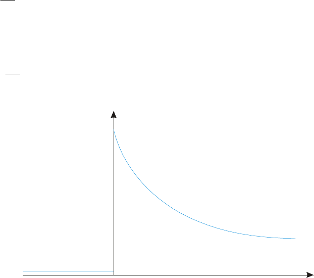
CHAPTER EIGHT SOLUTIONS
Engineering Circuit Analysis, 6th Edition Copyright
2002 McGraw-Hill, Inc. All Rights Reserved
74.
()
W0.02
V 3.31000//900107
W0.08
V 6.3900107.
W0.00110001.00
2
3
2
3
322
==
=ΩΩ××=
==
=××==
=×==<
−
−
R
V
P
V
R
V
P
RIV
RItP
final
final
init
init
8
6
4
2
Power (W)
07
Time (ms)
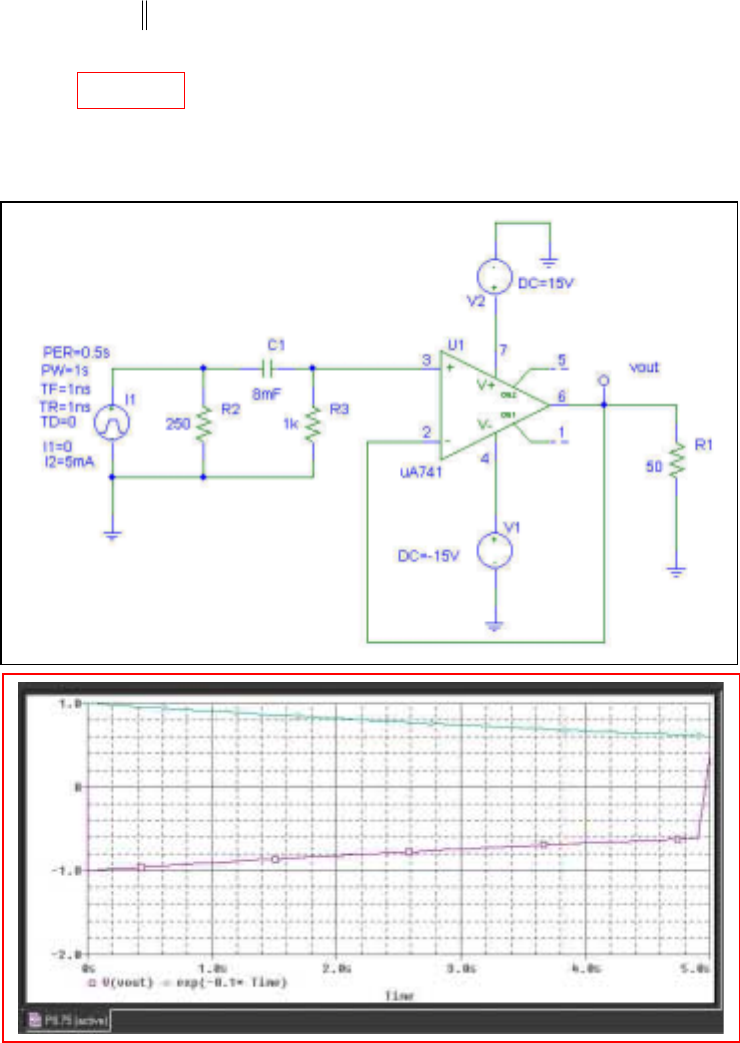
CHAPTER EIGHT SOLUTIONS
Engineering Circuit Analysis, 6th Edition Copyright
2002 McGraw-Hill, Inc. All Rights Reserved
75. voltage follower 2
() ()
o
vt vt∴=
PSpice verification:
From the simulation results, we see that modeling the operation of this circuit using an
ideal op amp model does not provide an accurate accounting for the operation of the
actual circuit.
2
2
0.1
(0 ) 5(0.25 1) 1 ( )V
v ( ) 0, 1.25 8 10
() ()V
+
−
==
∞= = × =
∴=
t
o
vut
s
vt e ut
τ

CHAPTER EIGHT SOLUTIONS
Engineering Circuit Analysis, 6th Edition Copyright
2002 McGraw-Hill, Inc. All Rights Reserved
76. voltage follower 2
() ()
o
vt vt∴=
6
2
10 /0.5 200
10,000
( ) 1.25 ( )V ( )
( ) 1.25 ( )
1.25 ( )V
−×
−
==
=
=
o
x
t
vt ut vt
vt e ut
eut
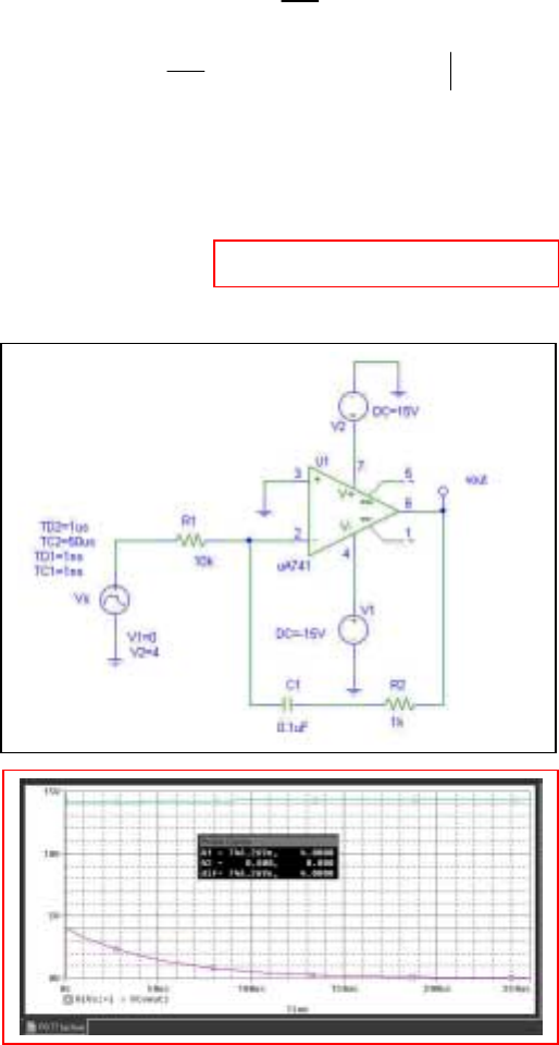
CHAPTER EIGHT SOLUTIONS
Engineering Circuit Analysis, 6th Edition Copyright
2002 McGraw-Hill, Inc. All Rights Reserved
77. (a)
And we may write vo(t) = -0.2[1 + e-20×103t]u(t) V.
(b) PSpice verification:
We can see from the simulation result that our ideal op amp approximation is not
providing a great deal of accuracy in modeling the transient response of an op amp in this
particular circuit; the output was predicted to be negative for t > 0.
20,000
14
7 20,000 20,000
4
20,000
3 20,000
20,000 20,000
4
0 (virtual gnd) ( )A
10
4
10 0.2
10
( ) 0.2(1 ) ( )
() 10 () 0.4 ()V
( ) ( ) ( ) ( 0.2 0.2 0.4 ) ( )
t
tttt
co
o
t
c
t
R
tt
ocR
vieut
vedte
vt e ut
vt it e ut
vt vt vt e e ut
−
−−
−
−
−−
=∴=
∴= =−
∴= −
∴= =
∴=−− =−+ −
∫
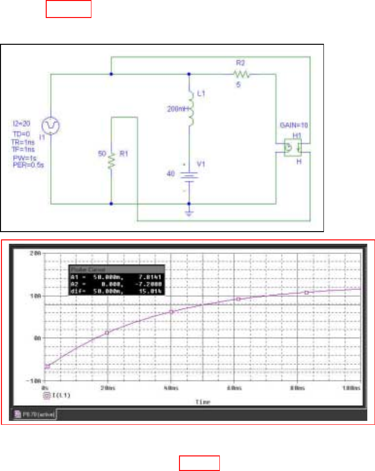
CHAPTER EIGHT SOLUTIONS
Engineering Circuit Analysis, 6th Edition Copyright
2002 McGraw-Hill, Inc. All Rights Reserved
78. For t < 0, the current source is an open circuit and so i1 = 40/ 50 = 0.8 A.
The current through the 5-Ω resistor is [40 – 10(0.8)]/ 5 = 7.2 A, so the inductor current
is equal to – 7.2 A
PSpice Simulation
From the PSpice simulation, we see that our t < 0 calculation is indeed correct, and find
that the inductor current at t = 50 ms is 7.82 A.

CHAPTER EIGHT SOLUTIONS
Engineering Circuit Analysis, 6th Edition Copyright
2002 McGraw-Hill, Inc. All Rights Reserved
79. Assume at least 1 µA required otherwise alarm triggers.
Add capacitor C.
6
1
10 6
(1) 1 volt
1000
(0) .1.5 1.496 volts
1002.37
1
We have 1 1.496 or C 2.48 F
10 (1.496)
−
=
==
∴= = =
µ
l
c
c
C
v
v
en
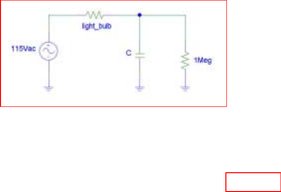
CHAPTER EIGHT SOLUTIONS
Engineering Circuit Analysis, 6th Edition Copyright
2002 McGraw-Hill, Inc. All Rights Reserved
80. One possible solution of many: implement a capacitor to retain charge; assuming the
light is left on long enough to fully charge the capacitor, the stored charge will run the
lightbulb after the wall switch is turned off. Taking a 40-W light bulb connected to 115
V, we estimate the resistance of the light bulb (which changes with its temperature) as
330.6 Ω. We define “on” for the light bulb somewhat arbitrarily as 50% intensity, taking
intensity as proportional to the dissipated power. Thus, we need at least 20 W (246 mA
or 81.33 V) to the light bulb for 5 seconds after the light switch is turned off.
The circuit above contains a 1-MΩ resistor in parallel with the capacitor to allow current
to flow through the light bulb when the light switch is on. In order to determine the
required capacitor size, we first recognise that it will see a Thevenin equivalent resistance
of 1 MΩ || 330.6 Ω = 330.5 Ω. We want vC(t = 5s) = 81.33 = 115e-5/
τ
, so we need a
circuit time constant of t = 14.43 s and a capacitor value of
τ
/ Rth = 43.67 mF.
CHAPTER NINE SOLUTIONS
Engineering Circuit Analysis, 6th Edition Copyright
2002 McGraw-Hill, Inc. All Rights Reserved
1.
11
12
22 22
1
22
L10, 6 , 8
6 , 8 adding,
14 2 7
1
6 7 49 48 , 6.928
LC
rad/s 6.928L 10, L 1.4434H,
11
C 14.434mF, 7 R 4.949
48L 2RC
o
oo
oo o
ssss
s
ω
ααω ααω
αα
ωω ω
−−
−
= Ω =− =−
∴− = + − − =− − −
−=−∴=
∴− =− + − ∴ = =
∴==
== =∴= Ω
CHAPTER NINE SOLUTIONS
Engineering Circuit Analysis, 6th Edition Copyright
2002 McGraw-Hill, Inc. All Rights Reserved
2. 100 200
40 30 mA, C 1mF, (0) 0.25V
−−
=− = =−
tt
c
ie e v
(a)
(b)
(c)
100 200
100 200
100 200
1
( ) 0.25 (40 30 ) 0.25
C
( ) 0.4( 1) 0.15( 1) 0.25
( ) 0.4 0.15 V
tt
tt
c
oo
tt
tt
vt idt e e dt
vt e e
vt e e
−−
−−
−−
=−= − −
∴=− −+ −−
∴=− +
∫∫
22 22
12
3
22
100 200
R
100 , 200
300 2 , 150 1
1 500
150 ,R 3.333 Also,
2R10 150
200 150 22500 20000
1 100
20000 , L 0.5H
LC L
i ( ) 0.12 0.045 A
R
−
−−
=− =−α+ α −ω =− =−α− α −ω
∴− =− α α = −
∴+ = = Ω
−=−− −ω∴ω=
∴== =
∴== +
oo
oo
tt
ss
s
v
tee
100 200
100 200
( ) ( ) ( ) (0.12 0.04) ( 0.045 0.03)
( ) 80 15 mA, 0
tt
Rc
tt
it i t i t e e
it e e t
−−
−−
=− − = − + − +
∴= − >
CHAPTER NINE SOLUTIONS
Engineering Circuit Analysis, 6th Edition Copyright
2002 McGraw-Hill, Inc. All Rights Reserved
3. Parallel RLC with ωo = 70.71 × 10¹² rad/s. L = 2 pH.
(a)
(b)
(c) α is the neper frequency: 5 Gs-1
(d)
(e) 95
12
510 7.071 10
70.71 10
−
α×
ζ= = = ×
ω×
o
2122
12 2 12
1(70.71 10 )
1
So 100.0aF
(70.71 10 ) (2 10 )
−
ω= = ×
==
××
oLC
C
91
10 18
1510
2
1
So 1 M
(10 )(100 10 )
−
−
α= = ×
==Ω
×
s
RC
R
22 9 121
1
22 9 121
2
5 10 70.71 10
5 10 70.71 10
−
−
=−α+ α −ω =− × + ×
=−α− α −ω =− × − ×
o
o
Sjs
Sjs
CHAPTER NINE SOLUTIONS
Engineering Circuit Analysis, 6th Edition Copyright
2002 McGraw-Hill, Inc. All Rights Reserved
4. Given: 21
4, 2
=α=LRC RC
Show that 12
() ( )
−α
=+
t
vt e At A is a solution to
2
2
11
0[1]++=
dv dv
Cv
dt R dt L
112
11 2
2
11 2 1
2
1211
121
() ( )
() [2]
()()
()
(2 ) [3]
−α −α
−α
−α −α
−α
−α
=−α+
=−α−α
=−α−α−α −α
=−α −α + −α
=−α −α −α
tt
t
tt
t
t
dv eA eAtA
dt
AAtAe
dv AAtA e Ae
dt
AAAAte
AAAte
Substituting Eqs. [2] and [3] into Eq. [1], and using the information initially provided,
2
1121
12 12
22
11 1
(2 ) ( ) ( )
22
11
() ()
24
0
−α −α −α
−α −α
−+++
−++ +
=
ttt
tt
Ae At Ae Ae
RC RC RC
At A e At A e
RC R C
Thus, 12
() ( )
−α
=+
t
vt e At A is in fact a solution to the differential equation.
Next, with 2
(0) 16==vA
and 121
0
()(16)4
=
=−α=−α=
t
dv AA A
dt
we find that 1416=+ αA
CHAPTER NINE SOLUTIONS
Engineering Circuit Analysis, 6th Edition Copyright
2002 McGraw-Hill, Inc. All Rights Reserved
5. Parallel RLC with ωo = 800 rad/s, and α = 1000 s-1 when R = 100 Ω.
2
1 so 5 F
2
1 so 312.5 mH
α= = µ
ω= =
o
C
RC
L
LC
Replace the resistor with 5 meters of 18 AWG copper wire. From Table 2.3, 18 AWG soft solid
copper wire has a resistance of 6.39 Ω/1000ft. Thus, the wire has a resistance of
100cm 1in 1ft 6.39
(5m) 1m 2.54cm 12in 1000ft
0.1048 or 104.8m
Ω
=Ω Ω
(a) The resonant frequency is unchanged, so 800 rad/sω=
o
(b) 31
1954.0 10
2
−
α= = × s
RC
(c)
Define the percent change as 100
ζ
−
ζ
×
ζ
new old
old
100
95300%
α−α
=×
α
=
new old
old
α
ζ=
ω
α
ζ=
ω
old
old
o
new
new
o
CHAPTER NINE SOLUTIONS
Engineering Circuit Analysis, 6th Edition Copyright
2002 McGraw-Hill, Inc. All Rights Reserved
6. 5H, R 8 , C 12.5mF, (0 ) 40V
+
==Ω= =Lv
(a)
(b)
2
28
1,2 1 2
12
12 12 2 2 1
1 1000 1
(0 ) 8A: 5, 16,
2RC 2 8 12.5 LC
4 5 25 16 2, 8 ( ) A A
1000 40
40 A A (0 ) (0 ) 80( 8 5) 1040
12.5 8
/ 2A 8A 520 A 4A 3A 480, A 160,A 120
( ) 120
o
tt
o
L
i
svtee
vi
vs
vt
+
−−
++
=α= = =ω==
××
ω= =−± − =− −∴ = +
′
∴=+ = − − = −−=−
=− − ∴− =− − ∴− =− = =−
∴=− 28
160 V, 0
tt
eet
−−
+>
28
34
34
34 34
28
443
(0 ) 40
(0 ) 8A Let ( ) A A ; (0 ) 5A
R8
(0 ) A A (0 ) (0 ) 8 5 13A;
40
(0 ) 2A 8A 8 A / 4 A 4A
5
3A 13 4, A 3, A 16 ( ) 16 3 A, 0
+
+−−+
+++
+
−−
==+ ===
∴=+=− − =−−=−
=− − = = ∴ =− −
∴− =− + = =− ∴ =− + >
tt
cR
Rc
tt
v
iiteei
iii
is
it e e t
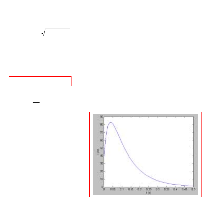
CHAPTER NINE SOLUTIONS
Engineering Circuit Analysis, 6th Edition Copyright
2002 McGraw-Hill, Inc. All Rights Reserved
7. 1
(0) 40A, (0) 40V, L H, R 0.1 , C 0.2F
80
====Ω=iv
(a)
(b) i(t) = – v/ R – C dt
dv = tt-tt eeee 401040 10 -40)(0.2)(60)( 10)0.2(-20)(- 600 200 −−− −−−
= tt ee 40 10 120 160 −− − A
2
1,2
10 40
12 12
12
12 2 2 1
10 40
180
25, 400,
2 0.1 0.2 0.2
20, 25 625 400 10, 40
( ) A A 40 A A ;
1(0)
(0 ) 10A 40A (0 ) (0) 2200
CR
A 4A 220 3A 180 A 60, A 20
( ) 20 60 V,
−−
++
−−
α= = ω = =
××
ω= =− ± − = −
∴= + ∴=+
′′
=− − = − =−
∴−− =−∴− =−∴= =−
∴=− + >
o
o
tt
tt
s
vt e e
v
vvi
vt e e t 0
CHAPTER NINE SOLUTIONS
Engineering Circuit Analysis, 6th Edition Copyright
2002 McGraw-Hill, Inc. All Rights Reserved
8.
663
26
3
1,2
2000 6000
12 1
3
12 12 2
100
(0) 2A, (0) 100V
50
10 3 10
4000, 12 10
2 50 2.5 100 2.5
16 12 10 200, 4000 2000
() A A , 0 A A 2
10 3
(0 ) 100 3000 2000A 6000A 1.5 A 3A 0.5 2A
100
Lc
o
tt
Ls
L
iv
w
s
it e e t
i
+
−−
+
== =
×
α= = = = ×
×× ×
−× = =− ±
∴= + >∴+=
−×
′=×=−=−−∴−=−−∴=−
2000 6000
21
2000 6000
A 0.25, A 2.25 ( ) 2.25 0.25 A, 0
0: ( ) 2A ( ) 2 ( ) (2.25 0.25 ) ( )A
tt
L
tt
LL
it e e t
tit itut e e ut
−−
−−
∴=− = ∴ = − >
>=∴=−+ −
CHAPTER NINE SOLUTIONS
Engineering Circuit Analysis, 6th Edition Copyright
2002 McGraw-Hill, Inc. All Rights Reserved
9.
2
21
1,2
50 450
12 12 12
12 2 2 1
12
(0) 2A, (0) 2V
51
1000 1000 45
= 250, 22500
212 2
250 250 22500 50, 450
A A A A 2; (0 ) 45( 2) 50A 450A
A 9A 1.8 8A 0.2 A 0.025, A 2.025(A)
( ) 2.025
−
−− +
−
== =
+×
== =
××
=− ± − =− −
′
∴= + ∴ + = = −=− −
∴+ =∴− = ∴ =− =
∴=
Lc
o
tt
LL
L
iv
ss
ie e i
it e
αω
50 450
0.025 A, 0
−
−>
tt
et
CHAPTER NINE SOLUTIONS
Engineering Circuit Analysis, 6th Edition Copyright
2002 McGraw-Hill, Inc. All Rights Reserved
10.
(a)
(b)
(c)
Solving using a scientific calculator, we find that ts = 1.181 s.
2
436
1,2 1 2
12
1212 22 1
436
1 1440 1440
20, 144
2RC 72 10
20 400 144 4, 36: A A
118
(0) 18 , (0) 1440 0
236
0 4A 36A A 9A 18 8A , A 2.25, A 20.25
( ) 20.25 2.25 V, 0
o
tt
t
svee
vAAv
vt e e t
αω
+
−−
−−
=== ==
=− ± − =− − = +
′
==+ = − =
∴=− − =− − =∴ =− =− =
∴= − >
436 4 36
436
1
( ) 0.5625 0.0625 0.05625 0.05625
36 1440
( ) 0.50625 0.00625 A, 0
tt t t
tt
v
it v e e e e
it e e t
−− − −
−−
′
=+ = − − +
∴= − >
436
max max
at 0 18V 0.18 20.25 2.25
ss
tt
vt v e e
−−
=∴ = ∴ = −
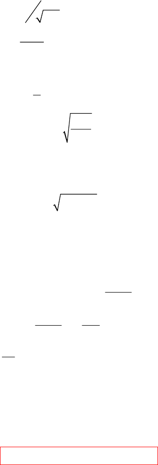
CHAPTER NINE SOLUTIONS
Engineering Circuit Analysis, 6th Edition Copyright
2002 McGraw-Hill, Inc. All Rights Reserved
11. L = 1250 mH
so Since α > ωo, this circuit is over damped.
The capacitor stores 390 J at t = 0−:
2
1
1
2
2
So (0 ) 125 V (0 )
+
=
===
cc
c
cc
WCv
W
vv
C
The inductor initially stores zero energy,
so
Thus, 82
() −−
=+
tt
v t Ae Be
Using the initial conditions, (0) 125 [1]==+vAB
38 2
3
(0 )
(0 ) (0 ) (0 ) 0 (0 ) 0
2
(0 ) 125
So (0 ) 62.5 V
22
50 10 [ 8 2 ]
(0 ) 62.5 50 10 (8 2 ) [2]
+
+++ +
+
+
−− −
+−
++=++=
=− =− =−
==×− −
=− =− × +
LRc c
c
tt
c
c
v
iii i
v
i
dv
iC Ae Be
dt
iAB
Solving Eqs. [1] and [2], A = 150 V
B = −25 V
Thus, 82
( ) 166.7 41.67 , 0
−−
=− >
tt
vt e e t
1
14rad/s
15
2
−
ω= =
α= =
oLC
s
RC
22
1,2
(0 ) (0 ) 0
53 8, 2
−+
==
=−α± α −ω =− ± =− −
LL
o
ii
S
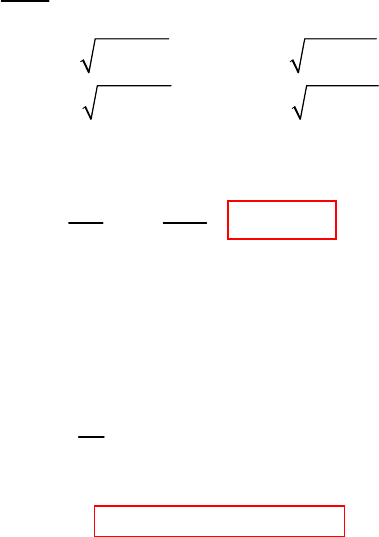
CHAPTER NINE SOLUTIONS
Engineering Circuit Analysis, 6th Edition Copyright
2002 McGraw-Hill, Inc. All Rights Reserved
12. (a) We want a response 46−−
=+
tt
vAe Be
1
22 2
1
22 2
2
15
2
4525
6525
−
α= =
=−α+ α −ω =− =− + −ω
=−α− α −ω =− =− − −ω
oo
oo
s
RC
S
S
Solving either equation, we obtain ωo = 4.899 rad/s
Since
2
2
11
, 833.3 mHω= = =
ω
o
o
L
LC C
(b) If (0 ) 10 A and (0 ) 15 A, find A and B.
++
==
Rc
ii
with
34 6
3
46
(0 ) 10 A, (0 ) (0 ) (0 ) 20 V
(0) 20 [1]
50 10 ( 4 6 )
(0 ) 50 10 ( 4 6 ) 15 [2]
Solving, 210 V, 190 V
Thus, 210 190 , 0
++++
−− −
+−
−−
====
=+=
==×− −
=× −− =
==−
=− >
RR c
tt
c
c
tt
ivvv
vAB
dv
i C Ae Be
dt
iAB
AB
ve et
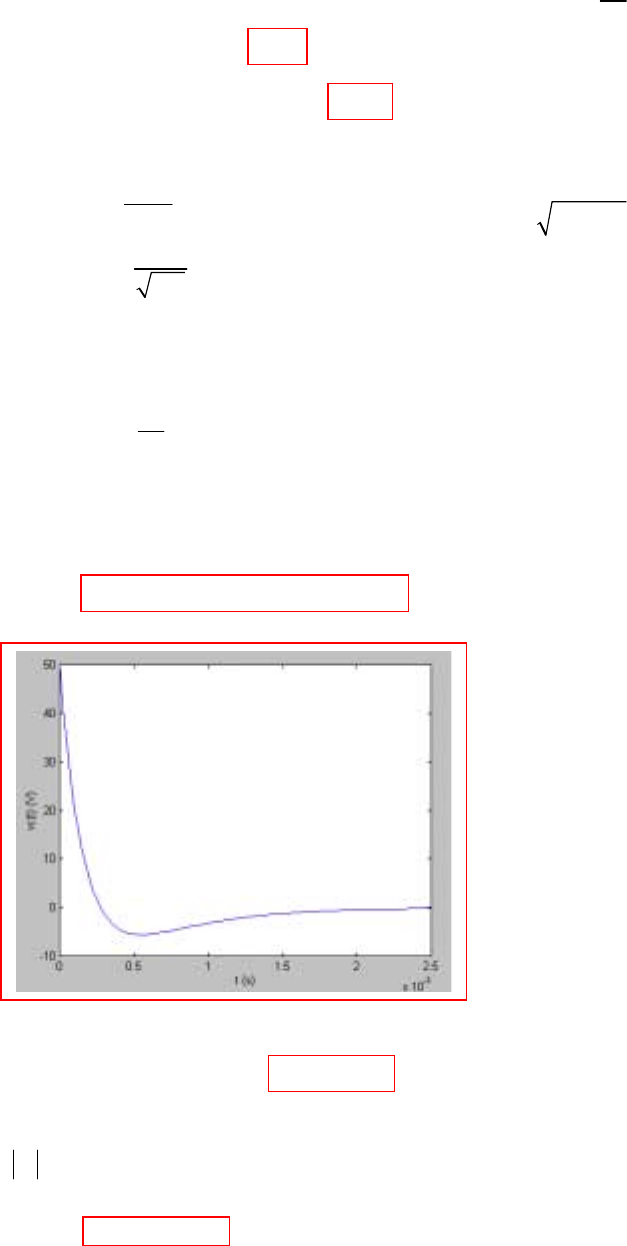
CHAPTER NINE SOLUTIONS
Engineering Circuit Analysis, 6th Edition Copyright
2002 McGraw-Hill, Inc. All Rights Reserved
13. Initial conditions: 50
(0) (0) 0 (0) 2 A
25
−+ +
== ==
LL R
ii i
(a) (0 ) (0 ) 2(25) 50 V
+−
===
cc
vv
(b) (0 ) (0 ) (0 ) 0 2 2 A
+++
=− − = − =−
cLR
iii
(c) t > 0: parallel (source-free) RLC circuit
1
14000
2
13464 rad/s
−
α= =
ω= =
o
s
RC
LC
Since α >
ω
0, this system is overdamped. Thus,
Solving, we find A = −25 and B = 75
so that 2000 6000
( ) 25 75 , 0
−−
=− + >
tt
c
vt e e t
(d)
(e) 2000 6000
25 75 0 274.7
−−
−+ =⇒=
µ
tt
ee t s
using a scientific calculator
(f) max 25 75 50 V=− + =
c
v
So, solving | 2000 6000
25 75
−−
−+
ss
tt
ee| = 0.5 in view of the graph in part (d),
we find ts = 1.955 ms using a scientific calculator’s equation solver routine.
2000 6000
6 2000 6000
()
(5 10 )( 2000 6000 )
(0 ) 0.01 0.03 2 [1]
and (0 ) 50 [2]
−−
−− −
+
+
=+
==× − −
=− − =−
=+=
tt
c
tt
c
c
c
v t Ae Be
dv
i C Ae Be
dt
iAB
vAB
22
2000, 6000
=−α± α −ω
=− −
o
s1,2
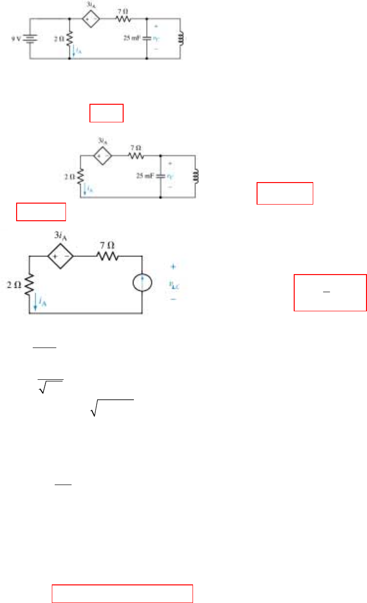
CHAPTER NINE SOLUTIONS
Engineering Circuit Analysis, 6th Edition Copyright
2002 McGraw-Hill, Inc. All Rights Reserved
14. Due to the presence of the inductor, (0 ) 0
−=
c
v. Performing mesh analysis,
12
21 2
12
92 2 0 [1]
22370 [2]
and
−+ − =
−+ + =
−=
A
A
ii
iiii
ii i
Rearranging, we obtain 2i1 – 2i2 = 0 and –4i1 + 6 i2 = 0. Solving, i1 = 13.5 A and i2 = 9 A.
(a) 12 2
(0 ) 4.5 A and (0 ) 9 A
−−
=−= = =
AL
iii ii
(b) t > 0:
(c) (0 ) 0
−=
c
v due to the presence of the inductor.
(d)
(e)
To find the second equation required to determine the coefficients, we write:
=− −
=− −
LcR
cA
iii
dv
Ci
dt
3
(0 ) 9 25 10 [ 1.881(6 ) 4.785(6 )]
+−
==−× − − −−
L
iABAB
or 9 = -0.7178A – 0.2822B [2]
Solving Eqs. [1] and [2], A = −20.66 and B = +20.66
So that 4.785 1.881
( ) 20.66[ ]
−−
=−
tt
A
it e e
1
22
1,2
13.333
2
13 rad/s
1.881, 4.785
−
α= =
ω= =
=−α± α −ω =− −
o
o
s
RC
LC
S
4.444 H
→i2
→i1
(0 ) 7 (0 ) 3 (0 ) 2 (0 ) 0
so, (0 ) 0
++++
+
−+ − + =
=
cAAA
A
viii
i
around left mesh:
4.444 H
1 A
73(1)20
6
6 V 6
1
−+− +=
=∴ ==Ω
LC
LC TH
v
vR
1.881 4.785
()
(0 ) 0 [1]
−−
+
=+
==+
tt
A
A
i t Ae Be
iAB
Thus,
3 1.881 4.785
1.881 4.785
25 10 1.881(6 ) 4.785(6 )
−− −
−−
−× − −
−
tt
tt
Ae Be
Ae Be
=
-
CHAPTER NINE SOLUTIONS
Engineering Circuit Analysis, 6th Edition Copyright
2002 McGraw-Hill, Inc. All Rights Reserved
15. Diameter of a dime: approximately 8 mm. Area = 22
0.5027cmπ=r
Capacitance
4H
=
µ
L
179.89Mrad/sω= =
oLC
For an over damped response, we require α > ωo.
Thus,
or 159.8<ΩR
*Note: The final answer depends quite strongly on the choice of εr.
14 2
(88)(8.854 10 F/cm)(0.5027cm )
0.1cm
39.17pF
−
εε ×
==
=
ro
A
d
6
12 6
179.89 10
2
1
2(39.17 10 )(79.89 10 )
−
>×
<××
RC
R
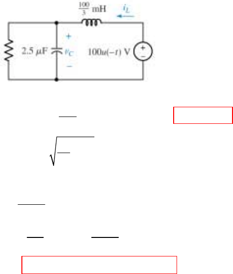
CHAPTER NINE SOLUTIONS
Engineering Circuit Analysis, 6th Edition Copyright
2002 McGraw-Hill, Inc. All Rights Reserved
16.
crit. damp. (a) 2326
100
L 4R C 10 4R 10 R 57.74
3
−−
==×=×∴=Ω
(b)
31
3464
12
2
65
121
3464 5
1
10 / 2.5 3464
30
( ) (A A ) (0) 100V
100
(0) 1.7321A 100 A
57.74
10 100
(0 ) 1.7321 0 A 3464A A 3.464 10
2.5 57.74
( ) (3.464 10 100)V, 0
o
t
cc
L
c
t
c
s
vt e t v
i
v
vt e t t
ωα
−
−
+
−
== × =
∴= + =
== ∴=
′=−==−∴=×
∴= ×+ >
R
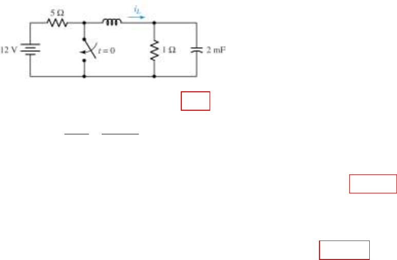
CHAPTER NINE SOLUTIONS
Engineering Circuit Analysis, 6th Edition Copyright
2002 McGraw-Hill, Inc. All Rights Reserved
17.
crit. damp. (a) 23
L4RC41210 8mH
−
==×××=
(b)
(c)
max
250
max
: (250 2) 0, 1 250 2, 0 No!
0, 2A 0.02 (250 2); SOLVE: 23.96ms
s
Lm mm
t
mL s s
it tt
ti e t t
−
+= = + <
∴= = ∴ = + =
250
12
250
1
3 3 1.25
1
1 1000 250 (A A )
2RC 2 1 2
(0) 2A, (0) 2V (A 2)
Then 8 10 (0 ) 2 8 10 (A 500), (1.25 2) 0.9311A
t
oL
t
Lc L
L
ie t
iv iet
ie
αω
−
−
−+ − −
===∴= +
××
==∴=+
′
×=−=×−=+=
L
CHAPTER NINE SOLUTIONS
Engineering Circuit Analysis, 6th Edition Copyright
2002 McGraw-Hill, Inc. All Rights Reserved
18. 8
L 5mH, C 10 F, crit. damp. (0) 400V, (0) 0.1A
−
== =− =vi
(a) 2328
L 4R C 5 10 4R 10 R 353.6
−−
==×= ∴=Ω
(b)
(c) max (0) 0.1Aii∴= =
8141,420
12
141,421 3
21
11
141,421
10 141,420 (A A )
2 353.6
A 0.1 (A 0.1), 5 10
(A 141,420 0.1) 400 A 65,860
( 65,860 0.1). 0
( 65860) 141,420 ( 65,860 0.1) 0
8.590 ( )
t
t
t
tt
m
mm
ie t
et
ie t i
eet
tsit
αα
α
µ
−
−−
−
−−
==∴= +
×
∴=∴= + ×
−×=−∴=−
′
∴= − + =
∴+ + − +=
∴= ∴ = 6
141,420 8.590 10
6
max
( 65,860 8.590 10 0.1) 0.13821A
i ( ) 0.13821A
m
e
it
−
−××
−
−××+=−
∴= =
CHAPTER NINE SOLUTIONS
Engineering Circuit Analysis, 6th Edition Copyright
2002 McGraw-Hill, Inc. All Rights Reserved
19. Diameter of a dime is approximately 8 mm. The area, therefore, is πr2 = 0.5027 cm2.
The capacitance is
14
(88)(8.854 10 )(0.5027)
0.1
39.17 pF
−
εε ×
=
=
ro
A
d
with 1
4 H, 79.89 Mrad/s=µ ω= =
o
LLC
For critical damping, we require 1
2=ω
o
RC
or 1159.8
2
==Ω
ωo
RC
CHAPTER NINE SOLUTIONS
Engineering Circuit Analysis, 6th Edition Copyright
2002 McGraw-Hill, Inc. All Rights Reserved
20. Critically damped parallel RLC with 31
10 , 1M
−−
α= = ΩsR .
We know 3
3
6
110
10 , so 500 F
2210
−
===
µ
×
C
RC
Since α = ωo,
If
29
2
72
9
29 22 9
13
210
50 turns 1 m
(4 10 H/m) . (0.5cm) . .
cm 100 cm
So
210
(4 10 )(50) (0.5) 2 10
So 8.106 10 cm
−
−
µ
==×
π× π
=×
π× = ×
=×
NA
LS
s
s
s
s
3
6
110
1
or 10
so 2 GH (!)
−
−
ω= =
=
=
oLC
LC
L
CHAPTER NINE SOLUTIONS
Engineering Circuit Analysis, 6th Edition Copyright
2002 McGraw-Hill, Inc. All Rights Reserved
21.
663
27
66
4000
12
6
110 110
4000, 2 10
2RC 100 2.5 LC 50
20 10 16 10 2000
(B cos 2000 B sin 2000 )
(0) 2A, (0) 0 (0 ) 2A; (0 ) (0 ) (0 )
11 1 210
(0 ) (0) (0 ) 0 (0 )
L R RC 125
o
d
t
c
Lcc cLR
ccc c
ie t t
ivi iii
ivv i
αω
ω
+
−
++++
+++
== = ===×
×
=×−×=
∴= +
′
′′
==∴=− =−−
×
′′
∴=− − =− =
∴6
122
4000
210
B 2A, 16,000 2000B ( 2)( 4000) B 4
125
( ) ( 2cos2000 4sin 2000 )A, 0
t
c
it e t t t
−
×
=− = = + − − ∴ =
∴= − + >
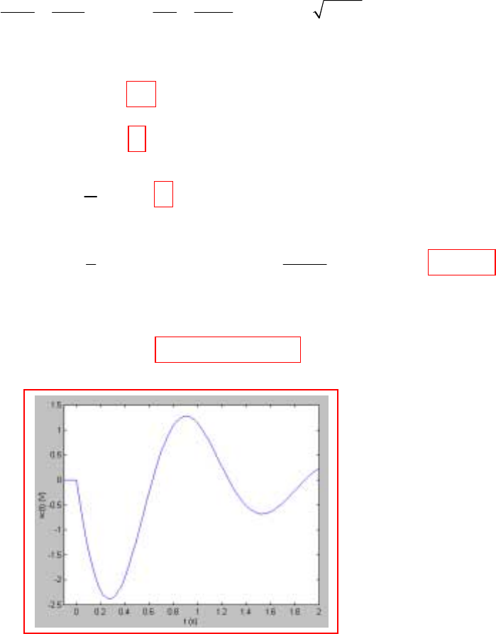
CHAPTER NINE SOLUTIONS
Engineering Circuit Analysis, 6th Edition Copyright
2002 McGraw-Hill, Inc. All Rights Reserved
22.
2
12
14 1413
1, 26, 26 1 5
2RC 2 2 LC 2
() ( cos5 sin5)
od
t
c
vt e B t B t
αω ω
−
×
===== = =−=
×
∴= +
(a) (0 ) (0) 4A
LL
ii
+==
(b) (0 ) (0) 0
cc
vv
+==
(c) 1
(0 ) (0 ) 0
L
Lc
iv
++
′==
(d) (0 )
1
(0 ) [ (0 ) (0 )] 4 4 4( 4 0) 16
2
c
cLR
v
vii
c
+
+++
′=− − =−− =−+=−
V/s
(e)
(f)
11 2 2
2
( )0 1(B ) B 0, ( ) B sin5 , (0 ) B (5) 16
B 3.2, ( ) 3.2 sin5 V, 0
t
cc
t
c
evtetv
vt e t t
−+
−
′
∴=∴= = = =−
∴=− =− >
CHAPTER NINE SOLUTIONS
Engineering Circuit Analysis, 6th Edition Copyright
2002 McGraw-Hill, Inc. All Rights Reserved
23.
(a)
(b)
93 9
28
22 6 6
5000 4 4
12
5000 4 4
2
9
110 110
5000, 1.25 10
2RC 2 20 5 LC 1.6 5
125 10 25 10 10,000
() (Bcos10 B sin10 )
(0) 200V, (0) 10mA ( ) (200cos10 B sin10 )
110
(0 ) (0 ) (0)
5
−
−
−
++
α= = ω== =×
×× ×
ω= ω−α= × − × =
∴= +
==∴= +
′== −
o
do
t
c
t
cL c
c
cc L
vt e t t
vi vte tt
v
vi i
c
924
2
5000 4 4
2
(0)
20,000
10 200
10 0 10 B 200(5000)
5 20,000
B 100V ( ) (200cos10 100sin10 ) V, 0
−
−
=−==−
∴= ∴ = + >
t
c
vt e t t t
2
5000 4
500 6 6 5000 4
5000 9 6 5000 4
5
1
10 , C
R
[10 ( 200sin 100cos] 5000(200cos 100sin)]
[10 ( 2sin 0.5cos)] 2.5 10 sin10 /
1(200cos 100sin) 5 10 2.5 10 sin10
20,000
−
−
−−
−−−
−
′
=− = +
′=−+− +
=−−=−×
∴= + −× × ×
=
sw L L c c
t
c
tt
t t
L
iiivv
ve
eetvs
ie e t
e000 4 4
5000 4 4
(0.01cos10 0.0075sin10 )A
10 (10cos10 7.5sin10 ) mA, 0
−
−
∴=− − >
t
t
sw
tt
ie t tt
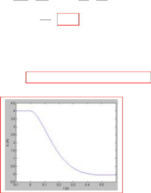
CHAPTER NINE SOLUTIONS
Engineering Circuit Analysis, 6th Edition Copyright
2002 McGraw-Hill, Inc. All Rights Reserved
24.
(a)
(b)
(c)
222
2
1 100 1 100
8, , 36 64
2RC 12.5 LC L
100
100 L 1H
L
odo
o
α= = = ω = = ω = =ω −
∴ω = = ∴ =
812
8
12
22
8
0: ( ) 4A; 0: ( ) (B cos6 B sin 6 )
(0) 4A B 4A, (4cos6 B sin 6 ) (0) 0
(0 ) (0 ) 0 6B 8(4) 0, B 16/ 3
( ) 4 ( ) (4cos6 5.333sin6 ) ( )A
−
−
++
−
<=>= +
=∴= = + =
′==∴−==
∴=−+ +
t
LL
t
LL c
Lc
t
L
tit tite t t
iiettv
itv
it u t e t tut
CHAPTER NINE SOLUTIONS
Engineering Circuit Analysis, 6th Edition Copyright
2002 McGraw-Hill, Inc. All Rights Reserved
25.
63 12 6
44
100 12
100
12
66
1
110 1
100 , 1.01 10
2RC 2 5 LC
60
101 10 10 100; (0) 6mA
10
(0) 0 ( ) (A cos1000 A sin1000 ), 0
A 0, ( ) A sin1000
11
(0) (0) 10[ (0) (0)] 10
C 5000
(610
−−
−
−
++ + +
−
α= = = ω = = ×
×
∴ω = × − = = =
=∴ = + >
∴= =
′==−− =
−×
o
dL
t
cc
t
c
cc c
s
i
vvte t tt
vt e t
vi i v
3
22
100 14
4 100
100
1
) 6000 1000A A 6
1
( ) 6 sin1000 V, 0 ( ) 10
( ) 10 ( 6) sin1000 A
( ) 0.6 sin1000 mA, 0
−
−−
−
=− = ∴ =−
∴=− >∴=−
=− −
∴= >
t
c
t
c
t
vt e t t it
vt e t
it e t t
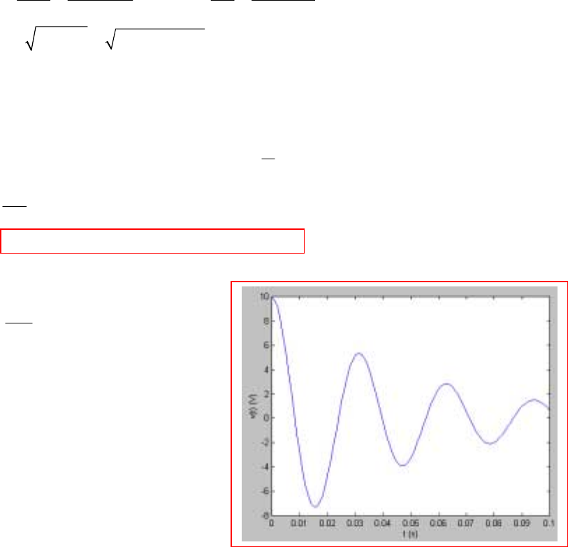
CHAPTER NINE SOLUTIONS
Engineering Circuit Analysis, 6th Edition Copyright
2002 McGraw-Hill, Inc. All Rights Reserved
26.
(a)
(b)
66
2
22
20
12
1
20
2
22
6
1 10 1 1.01 10
20, 40,400
2RC 2000 25 LC 25
40,400 400 200
(A cos200 A sin 200 )
(0) 10V, (0) 9mA A 10V
(10cos 200 A sin 200 ) V, 0
1
(0 ) 200A 20 10 200(A 1) (0 )
C
10
2
o
do
t
L
t
o
ve t t
vi
ve t t t
vi
−
−
++
×
α= = = ω = = =
×
ω= ω−α= − =
∴= +
==∴=
∴= + >
′=−×= −=
=3
2
20
( 10 ) 40 A 1 0.2 0.8
5
( ) (10cos 200 0.8sin 200 ) V, 0
t
vt e t t t
−
−
−=−∴=−=
∴= + >
20
10.032 cos (200 4.574 )V
2
T3.42ms
200
−
=−°
==
t
ve t
π
CHAPTER NINE SOLUTIONS
Engineering Circuit Analysis, 6th Edition Copyright
2002 McGraw-Hill, Inc. All Rights Reserved
27.
11
1
1
21 1
/
112
/
2
1
1
(0) 0; (0) 10A
(Acos Bsin ) A 0,
Bsin
[Bsin Bcos ]0
1
tan , tan
1T;
2
Bsin B
sin ; let
V
mmd
d
t
dd
t
d
t
dd d
dd
dm
d
mm dm
d
tt
mdmm
m
dm
m
vi
ve t t
ve t
ve t t
tt
tt t
ve tv e
v
te
α
−α
−α
−
−α −α −απ ω
−απ ω
==
=ω+ω∴=
=ω
′=−αω+ω ω=
ωω
∴ω= =
αωα
π
=+ =+
ω
=ω=−
ω∴=− 2
1
/
222
0
2
2
1
2
1
100
121
100, 100; ,
2RC R
1 21 100
6 6 441/ R 6R 441
LC R R
21
R 1/6 441 10.3781 To keep
100
0.01, chose R 10.3780 (0 )
21 0
BB6 4R10
10.378 10.
d
m
m
d
d
md
m
v
v
en
n
vv
v
απ ω
+
=
ω
∴ = α= α= =
π
ω= = ∴ω= − ∴ −
π
π
∴= + = Ω
′
<=Ω=ω
=− = +
l
l
2
2.02351
1
1
21
B 1.380363
3780
21 21
2.02351; 6 1.380363
10.378 10.378
304.268 sin 1.380363 0.434 ,
71.2926 Computed values show
2.145sec; 0.7126 0.01
d
t
m
m
sm m
ve tvts
vv
tv v
−
∴=
α= = ω = − =
∴= =
=
==<
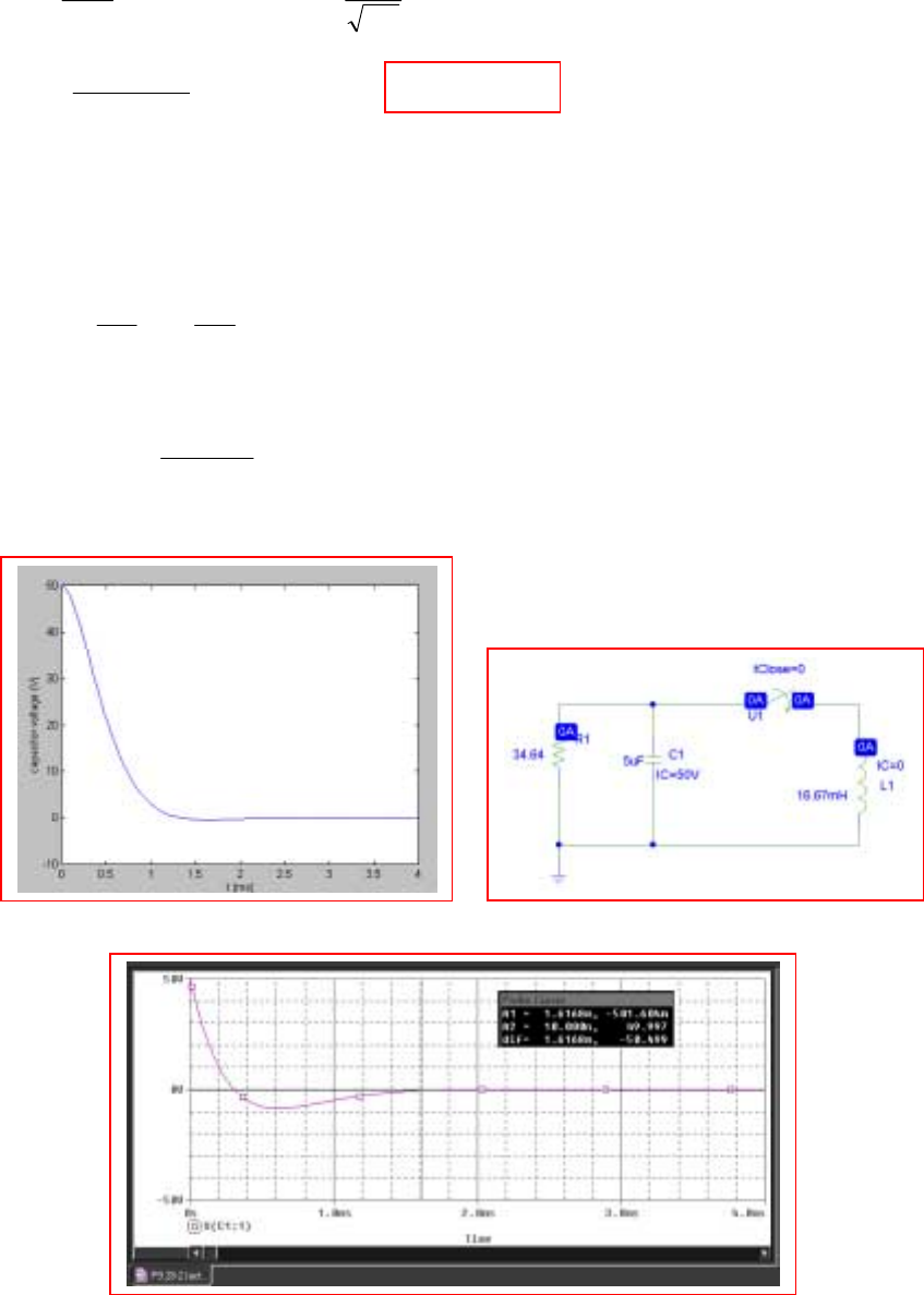
CHAPTER NINE SOLUTIONS
Engineering Circuit Analysis, 6th Edition Copyright
2002 McGraw-Hill, Inc. All Rights Reserved
28. We replace the 25-Ω resistor to obtain an underdamped response:
LC
1
and
2RC
1
0==
ωα
; we require
α
<
ω
0.
Thus, 3464
R 1010
1
6<
×− or R > 34.64 mΩ.
For R = 34.64 Ω (1000× the minimum required value), the response is:
v(t) = e-
α
t (A cos
ω
dt + B sin
ω
dt) where
α
= 2887 s-1 and
ω
d = 1914 rad/s.
iL(0+) = iL(0-) = 0 and vC(0+) = vC(0-) = (2)(25) = 50 V = A.
iL(t) = dt
dv
dt
dv CL L L =
=
()()
[
]
tBtAettBttAe dd
t
dddd
t
ωωαωωωω αα
sin cos - cos sin L ++− −−
iL(0+) = 0 =
[]
A - B
3
1050
d
3
αω
−
×, so that B = 75.42 V.
Thus, v(t) = e-2887t (50 cos 1914t + 75.42 sin 1914t) V.
From PSpice the settling time using R = 34.64 Ω is approximately 1.6 ms.
Sketch of v(t). PSpice schematic for t > 0 circuit.
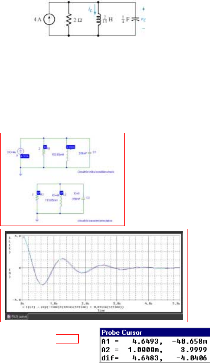
CHAPTER NINE SOLUTIONS
Engineering Circuit Analysis, 6th Edition Copyright
2002 McGraw-Hill, Inc. All Rights Reserved
29. (a,b) For t < 0 s, we see from the circuit below that the capacitor and the resistor are
shorted by the presence of the inductor. Hence, iL(0-) = 4 A and vC(0-) = 0 V.
When the 4-A source turns off at t = 0 s, we are left with a parallel RLC circuit such that
α
= 1/2RC = 1 s-1 and
ω
0 = 5.099 rad/s. Since
α
<
ω
0, the response will be underdamped
with
ω
d = 5 rad/s. Assume the form iL(t) = e-
α
t (C cos
ω
dt + D sin
ω
dt) for the response.
With iL(0+) = iL(0-) = 4 A, we find C = 4 A. To find D, we first note that
vC(t) = vL(t) = L dt
diL
and so vC(t) = (2/13) [e-
α
t (-C
ω
d sin
ω
dt + D
ω
d cos
ω
dt) -
α
e-
α
t (C cos
ω
dt + D sin
ω
dt)]
With vC(0+) = 0 = (2/13) (5D – 4), we obtain D = 0.8 A.
Thus, iL(t) = e-t (4 cos 5t + 0.8 sin 5t) A
(c) Using the cursor tool, the settling
time is approximately 4.65 s.
We see that the simulation
result confirms our hand
analysis; there is only a
slight difference due to
numerical error between
the simulation result and
our exact expression.
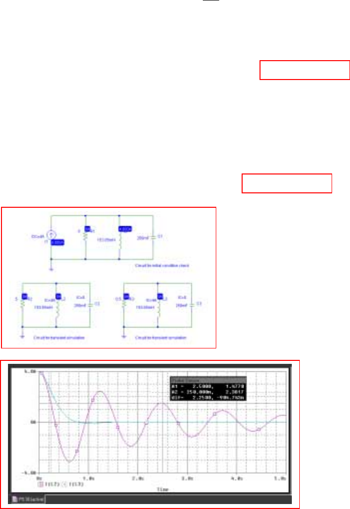
CHAPTER NINE SOLUTIONS
Engineering Circuit Analysis, 6th Edition Copyright
2002 McGraw-Hill, Inc. All Rights Reserved
30. (a) For t < 0 s, we see from the circuit that the capacitor and the resistor are shorted by
the presence of the inductor. Hence, iL(0-) = 4 A and vC(0-) = 0 V.
When the 4-A source turns off at t = 0 s, we are left with a parallel RLC circuit such that
α
= 1/2RC = 0.4 s-1 and
ω
0 = 5.099 rad/s. Since
α
<
ω
0, the response will be
underdamped with
ω
d = 5.083 rad/s. Assume the form iL(t) = e-
α
t (C cos
ω
dt + D sin
ω
dt)
for the response.
With iL(0+) = iL(0-) = 4 A, we find C = 4 A. To find D, we first note that
vC(t) = vL(t) = L dt
diL
and so vC(t) = (2/13) [e-
α
t (-C
ω
d sin
ω
dt + D
ω
d cos
ω
dt) -
α
e-
α
t (C cos
ω
dt + D sin
ω
dt)]
With vC(0+) = 0 = (2/13) (5.083D – 0.4C), we obtain D = 0.3148 A.
Thus, iL(t) = e-0.4t (4 cos 5.083t + 0.3148 sin 5.083t) A and iL(2.5) = 1.473 A.
(b)
α
= 1/2RC = 4 s-1 and
ω
0 = 5.099 rad/s. Since
α
<
ω
0, the new response will still be
underdamped, but with
ω
d = 3.162 rad/s. We still may write
vC(t) = (2/13) [e-
α
t (-C
ω
d sin
ω
dt + D
ω
d cos
ω
dt) -
α
e-
α
t (C cos
ω
dt + D sin
ω
dt)]
and so with vC(0+) = 0 = (2/13) (3.162D – 4C), we obtain D = 5.06 A.
Thus, iL(t) = e-4t (4 cos 3.162t + 5.06 sin 3.162t) A and iL(.25) = 2.358 A.
(c)
We see from the simulation
result below that our hand
calculations are correct; the
slight disagreement is due to
numerical inaccuracy.
Changing the step ceiling
from the 10-ms value
employed to a smaller value
will improve the accuracy.
CHAPTER NINE SOLUTIONS
Engineering Circuit Analysis, 6th Edition Copyright
2002 McGraw-Hill, Inc. All Rights Reserved
31. Series:
2
4
12
1
22
4
214
4, 20, 20 16 2
2L 1/ 2 LC 0.2
(A cos 2 A sin 2 ); (0) 10A, (0) 20V
1
A 10; (0 ) (0 ) 4(20 20) 0
L
(0 ) 2A 4 10 A 20
( ) (10cos 2 20sin 2 )A, 0
od
t
LLc
LL
L
t
L
R
ie t ti v
iv
i
it e t t t
αω ω
−
++
+
−
== = === = −=
∴= + = =
′
∴= = = − =
′
∴=−×∴=
∴= + >
CHAPTER NINE SOLUTIONS
Engineering Circuit Analysis, 6th Edition Copyright
2002 McGraw-Hill, Inc. All Rights Reserved
32.
22
20
12 1
20
2
20
22
R80
(0)50802210V,(0)0, 20
2L 4
100 500: 500 20 10
2
( ) (A cos10 A sin10 ) A 210V
1
( ) (210cos10 A sin10 ); (0 ) (0 ) 0
C
0 10A 20(210), A 420 ( ) (210cos10
cL
od
t
c
t
ccc
t
c
vi
vt e t t
vt e t t v i
vt e t
α
ωω
−
−++
−
=+×= = = = =
== = −=
∴= + ∴=
′
∴= + = =
∴= − = ∴ = +
0.8
20
12
22
20
20
420sin10 )
(40ms) (210cos0.4 420sin 0.4) 160.40V
Also, (B cos10 B sin10 ),
11 1
(0 ) (0 ) [0 (0 )] 210
L2 2
(0 ) 105 10B B 10.5
( ) 10.5 sin10 A, 0
( ) 80 840 sin
c
t
L
LL c
L
t
L
t
RL
t
ve
ie t t
iv v
i
it e t t
vt i e
−
−
++ +
+
−
−
∴= + =
=+
==−=×
′
∴=−=∴=
∴=− >
∴==
0.8
20
20
0.8
10 V
(40ms) 840 sin 0.4 146.98V
() () () ()
(40ms) 160.40 146.98 13.420V
[check: ( 210cos 420sin 840sin)
( 210cos10 420sin10 ) V, 0
(40ms) ( 210cos 420sin 840
R
LccRL
t
L
t
L
t
ve
vt vt vt vt v
ve
ettt
ve
−
−
−
−
∴=− =−
=− − − ∴
=− + =−
=− − +
=− + >
∴=−−+ 20
0.8
sin)
( 210cos10 420sin10 )V, 0
V (40ms)
(420sin 0.4 210cos0.4) 13.420VChecks]
t
L
e
ttt
e
−
−
=
−+ >
∴=
−=−
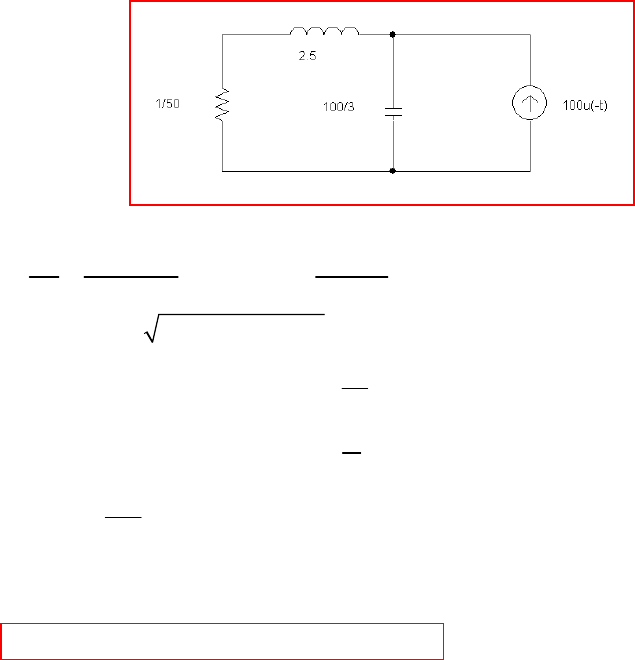
CHAPTER NINE SOLUTIONS
Engineering Circuit Analysis, 6th Edition Copyright
2002 McGraw-Hill, Inc. All Rights Reserved
33. “Obtain an expression for vc(t) in the circuit of Fig. 9.8 (dual) that is valid for all t′′.
66
27
66
1,2
2000 6000
12
12
3
R 0.02 10 10 3
4000, 1.2 10
2L 2 2.5 2.5 10
4000 16 10 12 10 2000, 6000
1
( ) A A ; (0) 100 2V
50
1
(0) 100A 2 A A , (0 ) C
3
( (0)) 10 100 3000 /
100
3000 200A
o
tt
cc
Lc
L
s
vt e e v
iv
ivs
αω
−−
+
××
== = = =×
××
∴=− ± ×−× =− −
∴= + =×=
′
=∴=+ =
−=−××=−
∴− =− 12 12
21
200 6000
600A , 1.5 A 3A
0.5 2A , 0.25, A 2.25
( ) (2.25 0.25 ) ( ) 2 ( )V (checks)
tt
c
vt e e ut u t
−−
−−=−−
∴=− =− =
∴= − +−
A
Ω
µF
mF
CHAPTER NINE SOLUTIONS
Engineering Circuit Analysis, 6th Edition Copyright
2002 McGraw-Hill, Inc. All Rights Reserved
34. (a)
(b)
(c)
,max 0.2489V
c
v=
2
22 2
2
46 4
10000
12
10000
21
6
1
R11
crit. damp; L R C
4L LC 4
1 200
L 4 10 0.01H, 10
4 0.02
( ) (A A ); (0) 10V, (0) 0.15A
1
A10,() (A0);(0)
C
(0) 10 ( 0.15) 150,000
Now, (0 ) A
−
−
−+
+
===∴=
∴=×× = = = =
∴= + =− =−
′
∴=− = − =−
=− − =
′=
o
o
t
ccL
t
cc
L
c
vt e t v i
vt e t v
i
v
αω
αω
5
1
10,000
10 150,000 A 50,000
( ) (50,000 10) V, 0
−
+= ∴=
∴= − >
t
c
vt e t t
10,000
33
max
( ) [50,000 10,000(50,000 10)]
15
5 50,000 10 0.3ms
50,000
( ) (15 10) 5 0.2489V
(0) 10V 10V
t
c
mm
cm
cc
vt e t
tt
vt e e
vv
−
−−
′=− −=∴
=−∴==
∴= −==
=− ∴ =
CHAPTER NINE SOLUTIONS
Engineering Circuit Analysis, 6th Edition Copyright
2002 McGraw-Hill, Inc. All Rights Reserved
35. (a)
(b)
6
2
22
1,2
10 40
12
12
12
111
11
R250 1 10
25, 400
2L 10 LC 2500
25 15 10, 40
A A , (0) 0.5A, (0) 100V
11
0.5 A A , (0 ) (0 )
55
(100 25 100) 5 A / 10A 40A
5 10A 40 (0.5 A ) 10A 40
A20 30A
o
o
tt
LLc
LL
s
ie ei v
iv
s
αω
ααω
−−
++
== = == =
=− ± − =− ± =− −
∴= + = =
′
∴=+ = =
− − =− =− −
∴= + − = −
+∴− 12
10
15, A 0.5, A 0
( ) 0.5 A, 0
t
L
it e t
−
=− = =
∴= >
10 40
34 34
6
34 443
10
A A 100 A A ;
110
(0 ) ( 0.5) 1000
500
10A 40A 1000 3A 0, A 0, A 100
( ) 100 V 0
tt
c
cc
t
c
ve e
vi
c
vt e t
−−
+
−
=+∴=+
′
′=−=−
∴− − =− ∴− = = =
∴= >
CHAPTER NINE SOLUTIONS
Engineering Circuit Analysis, 6th Edition Copyright
2002 McGraw-Hill, Inc. All Rights Reserved
36. (a)
(b)
222
12
12
12
2
R2 1
1, 5, 2
2L 2 LC
(B cos2 B sin2 ), (0) 0, (0) 10V
B0, B sin2
1
(0) (0 ) (0 ) V (0 ) 0 10 2B
1
B5 5sin2A,0
odo
t
LLc
t
L
LR c
t
L
ie t ti v
iet
ivv
iett
αωωωα
−
−
+++
−
=== == = −=
∴= + = =
∴= =
==−=−=
∴=∴=− >
11
22
2max
max
5[ (2cos2 sin2 )] 0
2cos2 sin 2 ,tan 2 2
0.5536 , ( ) 2.571A
2 2 0.5536 , 2.124,
( ) 0.5345 2.571A
and 0.5345A
−
′=− − =
∴= =
∴= =−
=× + =
=∴=
=
t
L
L
LL
L
ie tt
ttt
tsit
tt
it i
i
π
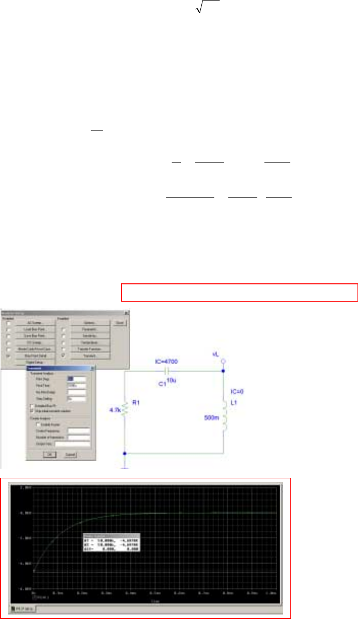
CHAPTER NINE SOLUTIONS
Engineering Circuit Analysis, 6th Edition Copyright
2002 McGraw-Hill, Inc. All Rights Reserved
37. We are presented with a series RLC circuit having
α = R/2L = 4700 s-1 and
ω
o = 1/ LC = 447.2 rad/s; therefore we expect an
overdamped response with s1 = -21.32 s-1 and s2 = -9379 s-1.
From the circuit as it exists for t < 0, it is evident that iL(0-) = 0 and vC(0-) = 4.7 kV
Thus, vL(t) = A e–21.32t + B e-9379t [1]
With iL(0+) = iL(0-) = 0 and iR(0+) = 0 we conclude that vR(0+) = 0; this leads to vL(0+) =
-vC(0-) = -4.7 kV and hence A + B = -4700 [2]
Since vL = L dt
di , we may integrate Eq. [1] to find an expression for the inductor current:
iL(t) =
−− tt ee 937932.21
9379
B
-
21.32
A
-
L
1
At t = 0+, iL = 0 so we have 0
9379
B
-
21.32
A
-
10500
1
3- =
× [3]
Simultaneous solution of Eqs. [2] and [3] yields A = 10.71 and B = -4711. Thus,
vL(t) = 10.71e-21.32t - 4711 e-9379t V, t > 0
and the peak inductor voltage magnitude is 4700 V.
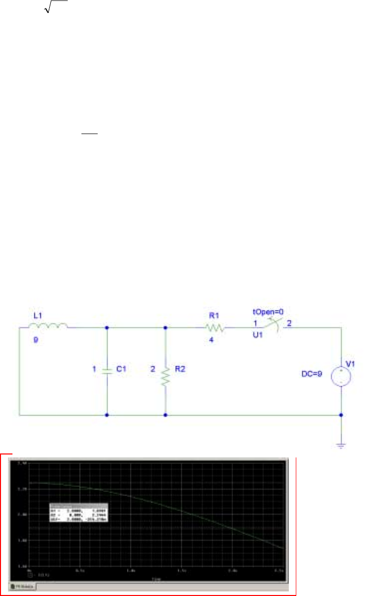
CHAPTER NINE SOLUTIONS
Engineering Circuit Analysis, 6th Edition Copyright
2002 McGraw-Hill, Inc. All Rights Reserved
38. Considering the circuit as it exists for t < 0, we conclude that vC(0-) = 0 and iL(0-) = 9/4 =
2.25 A. For t > 0, we are left with a parallel RLC circuit having α = 1/2RC = 0.25 s-1 and
ω
o = 1/ LC = 0.3333 rad/s. Thus, we expect an underdamped response with
ω
d =
0.2205 rad/s:
iL(t) = e-αt (A cos
ω
dt + B sin
ω
dt)
iL(0+) = iL(0-) = 2.25 = A
so iL(t) = e–0.25t (2.25 cos 0.2205t + B sin 0.2205t)
In order to determine B, we must invoke the remaining boundary condition. Noting that
vC(t) = vL(t) = L dt
diL
= (9)(-0.25)e-0.25t (2.25 cos 0.2205t + B sin 0.2205t)
+ (9) e-0.25t [-2.25(0.2205) sin 0.2205t + 0.2205B cos 0.2205t]
vC(0+) = vC(0-) = 0 = (9)(-0.25)(2.25) + (9)(0.2205B)
so B = 2.551 and
iL(t) = e-0.25t [2.25 cos 0.2205t + 2.551 sin 0.2205t] A
Thus, iL(2) = 1.895 A
This answer is borne out by PSpice simulation:
CHAPTER NINE SOLUTIONS
Engineering Circuit Analysis, 6th Edition Copyright
2002 McGraw-Hill, Inc. All Rights Reserved
39. Considering the circuit at t < 0, we note that iL(0-) = 9/4 = 2.25 A and vC(0-) = 0.
For a critically damped circuit, we require α =
ω
o, or LC
1
RC2
1=, which, with
L = 9 H and C = 1 F, leads to the requirement that R = 1.5 Ω (so α = 0.3333 s-1).
The inductor energy is given by wL = ½ L [iL(t)]2, so we seek an expression for iL(t):
iL(t) = e-αt (At + B)
Noting that iL(0+) = iL(0-) = 2.25, we see that B = 2.25 and hence
iL(t) = e-0.3333t (At + 2.25)
Invoking the remaining initial condition requires consideration of the voltage across the
capacitor, which is equal in this case to the inductor voltage, given by:
vC(t) = vL(t) = dt
diL
L = 9(-0.3333) e-0.3333t (At + 2.25) + 9A e-0.3333t
vC(0+) = vC(0-) = 0 = 9(-0.333)(2.25) + 9A so A = 0.7499 amperes and
iL(t) = e-0.3333t (0.7499t + 2.25) A
Thus, iL(100 ms) = 2.249 A and so wL(100 ms) = 22.76 J

CHAPTER NINE SOLUTIONS
Engineering Circuit Analysis, 6th Edition Copyright
2002 McGraw-Hill, Inc. All Rights Reserved
40. With the 144 mJ originally stored via a 12-V battery, we know that the capacitor has a
value of 2 mF. The initial inductor current is zero, and the initial capacitor voltage is 12
V. We begin by seeking a (painful) current response of the form
ibear = Aes1t + Bes2t
Using our first initial condition, ibear(0+) = iL(0+) = iL(0-) = 0 = A + B
di/dt = As1 es1t + Bs2 es2t
vL = Ldi/dt = ALs1 es1t + BLs2 es2t
vL(0+) = ALs1 + BLs2 = vC(0+) = vC(0-) = 12
What else is known? We know that the bear stops reacting at t = 18 µs, meaning that the
current flowing through its fur coat has dropped just below 100 mA by then (not a long
shock).
Thus, A exp[(18×10-6)s1] + B exp[(18×10-6)s2] = 100×10-3
Iterating, we find that Rbear = 119.9775 Ω.
This corresponds to A = 100 mA, B = -100 mA, s1 = -4.167 s-1 and s2 = -24×106 s-1
CHAPTER NINE SOLUTIONS
Engineering Circuit Analysis, 6th Edition Copyright
2002 McGraw-Hill, Inc. All Rights Reserved
41.
2
4
12,
4
,12
4
11 2
R2 1
(0) 0, (0) 0, 4, 4 5 20
2L 0.5 LC
20 16 2 ( ) (A cos2 A sin 2 )
10A ( ) 10 (A cos2 A sin 2 )
010A,A 10,()10 (Asin2 10cos2)
1
(0) (0) 4 0 0 (0)
L
cL o
t
dL Lf
t
Lf L
t
L
LL L
vi
it e t t i
iitett
it e t t
iv i
αω
ω
−
−
−
++ +
=======×=
∴= −=∴ = + +
=∴=+ +
∴= + =− = + −
==×=∴ 22
02A 40,A 20== + =−
i
L(t) = 10 - e-4t (20 sin 2t + 10 cos 2t) A, t > 0
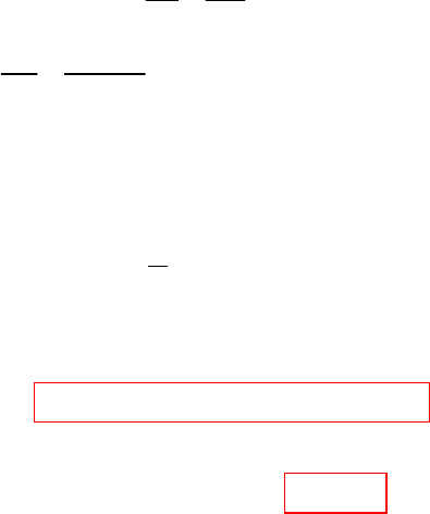
CHAPTER NINE SOLUTIONS
Engineering Circuit Analysis, 6th Edition Copyright
2002 McGraw-Hill, Inc. All Rights Reserved
42. (a)
(b) 500 (3000 6) 3; by SOLVE, 3.357ms
o
t
oo
et t
−+= =
6
2
500
12 22
1
5000 500
1
R 100
Series, driven: 500,
2L 0.2
11010250,000
LC 40
Crit. damp ( ) 3(1 2) 3,
(0) 3, (0) 300V
3(AA)33A,A6A
1
(0 ) A 300 [ (0) (0 )] 0
L
A 3000 ( ) 3
o
L
Lc
t
L
LcR
t
L
if
iv
iet
ivv
eit e
α
ω
−
++
−−
== =
×
== =
∴=−=−
==
∴=−+ + ∴=−+ =
=− = − =
∴= ∴ =−+
500
(3000 6), 0
( ) 3 ( ) [ 3 (3000 6)] ( )A
t
t
L
tt
it u t e t ut
−
+>
∴=−+−+ +
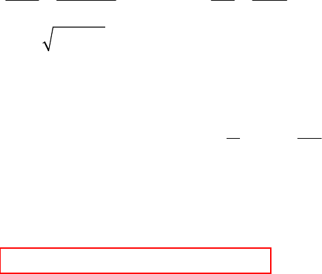
CHAPTER NINE SOLUTIONS
Engineering Circuit Analysis, 6th Edition Copyright
2002 McGraw-Hill, Inc. All Rights Reserved
43.
663
26
22
400
,, 1 2
4000 12 1
4000
2
110 110
4000, 20 10
2RC 100 2.5 LC 50
2000, (0) 2A, (0) 0
0, ( 0) (A cos2000 A sin 2000 )
work with : ( ) (B cos2000 B sin 2000 ) B 0
B sin 2000
o
do L c
t
cf cf c
t
cc
t
c
iv
iv ie t t
vvt e t t
ve t
+
−
−
−
α= = = ω = = = ×
×
∴ω = ω −α = = =
==∴= +
=+∴=
∴= 65
54000
22
6 4000
6 3 3 4000
4000
110
,(0) (0) (21)810
C 2.5
8 10 2000B , B 400, 400 sin 2000
( ) C 2.5 10 400 ( 4000sin 200 2000cos 200 )
10 ( 4sin 2000 2cos2000 )
(2cos2000 4sin 2000
cc
t
c
tt
cc
t
t
vi
ve t
it v e t
ett
ett
++
−
−−
−++ −
−
′==×=×
∴× = = =
′
∴= =×× − +
=−+
=−
)A, 0t>
CHAPTER NINE SOLUTIONS
Engineering Circuit Analysis, 6th Edition Copyright
2002 McGraw-Hill, Inc. All Rights Reserved
44.
6
2
1,2
,
10 40
12
12
R 250 1 10
25, 400
2L 10 LC 2500
25 625 400 10, 40
(0) 0.5A, (0) 100V, 0.5A
( ) 0.5 A A A
0 : (0 ) 100 50 1 200 0.5 50V 50 5 (0 )
(0 ) 10 10 10A 40A , 0.5 0.5
o
LcLf
tt
L
L L
L
s
ivi
it e e
tv i
i
−−
++ +
+
α= = = ω = = =
=− ± − =− −
===−
∴=−+ +
′
==−×−×=−∴−=
′
∴=−∴−=−− =−12
12 2 1 1 1 2
10
AA
A A 1 10 10A 40( 1+A ) 50A 40, A 1,A 0
( ) 0.5 1 A, 0; ( ) 0.5A, 0
t
LL
it e t it t
−
++
∴+ =∴−=− − − =− + = =
∴=−+ > = >
CHAPTER NINE SOLUTIONS
Engineering Circuit Analysis, 6th Edition Copyright
2002 McGraw-Hill, Inc. All Rights Reserved
45.
2
,
1
11
R1 1
1, 1 crit. damp
2L 1 LC
5
(0) 12 10V, (0) 2A, 12V
6
11
( ) 12 (A 2); (0 ) (0 ) (0 ) 1
C2
1A 2;A 1 ()12 ( 2)V, 0
−+++
−
α= = = ω = = ∴
=× = = =
′
∴=+ − = =× =
∴= + =−∴ = − + >
o
cLcf
t
cccL
t
c
viv
vt e t v i i
vt e t t
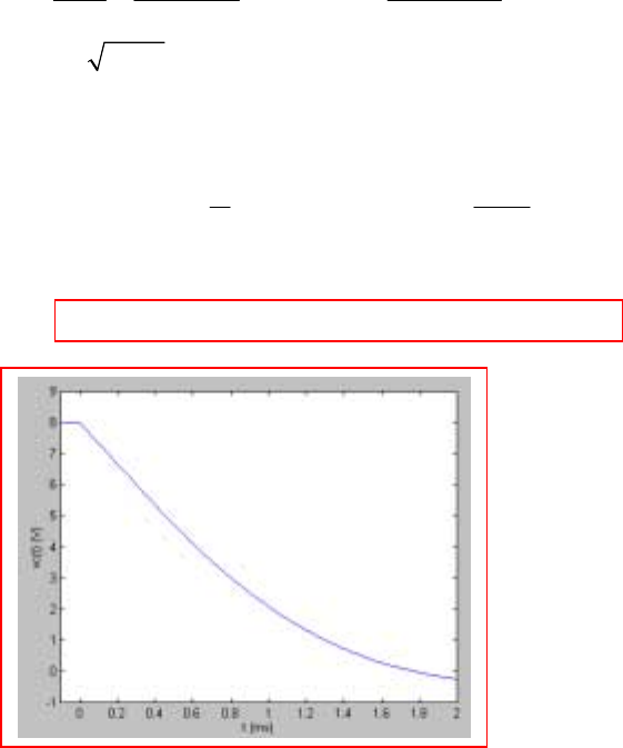
CHAPTER NINE SOLUTIONS
Engineering Circuit Analysis, 6th Edition Copyright
2002 McGraw-Hill, Inc. All Rights Reserved
46. (a)
So vc(t) = e-1000t (8 cos 1000t + 1.6 sin 1000t) V, t > 0
(b)
66
26
3
3
,
1000
12
6
1
22
1 8 10 8 10 13
1000, 26 10
2RC 2 4 10 4
26 1 10 5000, (0) 8V
(0) 8mA, 0
(A cos1000 A sin5000 )
18
A 8; (0 ) (0 ) 8 10 (0.01 0.008) 0
C 4000
5000A 1000 8 0, A 1.6
o
dc
Lcf
t
c
cc
v
iv
ve t t
vi
−
++
×××
α= = = ω = = ×
××
∴ω = − × = =
==
∴= +
′
∴= = =× − − =
∴−×==
CHAPTER NINE SOLUTIONS
Engineering Circuit Analysis, 6th Edition Copyright
2002 McGraw-Hill, Inc. All Rights Reserved
47. (a)
(b)
6
6
266
1,2
500 1500
,12
66 4
12
4
11
110
( ) 10 ( )V: 1000
2RC 1000
1103 3
1000 10 10 500, 1500
LC 4 4
0 A A , (0) 10V, (0) 0
10
10 A A , 10 (0 ) 10 0 2 10
500
2 10 500A 1500A 40 A
s
o
tt
cf c c L
cc
vt u t
s
vveev i
vi
−−
+
=−α= = =
×
ω= = ∴ =− ± − × =− −
=∴ = + = =
′
∴= + = = − =−×
∴− × =− − ∴ = 2221
500 1500
6 500 1500
500 1500
3A 30 2A , A 15, A 5
515V,0 C
10 (2500 22,500 )
2.5 22.5 mA, 0
tt
cscc
tt
s
tt
ve e t iiv
iee
eet
−−
−− −
−−
+∴= = =−
′
∴=− + >∴==
∴= −
=− >
,
500 1500
34 34
66 4
34
34 4 4 3
500 1500
6
() 10 ()V 10V, (0) 0, (0) 0
10 A A A 10
10
(0 ) 10 (0 ) 10 0 2 10 500A 1500A
500
A 3A 40, add: 2A 30, A 15, A 5,
10 5 15 V,
10 (
scfcL
tt
c
cc
tt
csc
vt ut v v i
vAe e
vi
veeii
−−
++
−−
−
=∴= ==
∴= + + ∴ + =−
′==+=×=−−
∴− − = − = =− =
=+ − ==
500 1500 500 1500
2500 22,500 ) 25 22.5 mA, 0
tttt
eeeet
−−−−
−+ =+ >

CHAPTER NINE SOLUTIONS
Engineering Circuit Analysis, 6th Edition Copyright
2002 McGraw-Hill, Inc. All Rights Reserved
48. (a)
(b)
500 1500
,34
6
34
6
34
34 4 4 3
500 1500
10 ( )V, 10, 10 A A ,
(0) 0, (0) 0 A A 10V, (0 ) 2 10
[ (0) (0 )] 2 10 (0 0) 0 500A 1500A
A 3A 0, add: 2A 10, A 5 A 15
( ) 10 15 5 V, 0
()
tt
scfc
cL c
LR
tt
c
R
vutv v e e
vi v
ii
vt e e t
it
−−
+
+
−−
===++
′
==∴+=− =×
−=×−==−−
∴− − = − =− = ∴ = −
∴=− + >
∴500 1500
10 15 5 mA, 0
tt
ee t
−
=− + >
6
6
26
1,2
500 1500
12
66
12
12
110
10 ( ) V : 1000
2RC 2000 0.5
1 2 10 3 0.75 10 500, 1500
LC 8
A A , (0) 10V, (0) 10mA
A 10, (0 ) 2 10 [ (0) (0 )] 2 10
10
0.01 0 500A 1500A 0,
1000
A
s
o
tt
coL
cLR
vut
s
ve ev i
Av ii
−−
++
=− α= = =
×
××
ω= = = × ∴ =− −
∴= + = =
′
∴+ = =× − =×
−=∴−− =
−12 2 2 1
500 1500
500 1500
3A 0; add: 2A 10, A 5, A 15
( ) 15 5 V 0
( ) 15 5 mA, 0
tt
c
tt
R
vt e e t
it e e t
−−
−−
−= − = =− =
∴= − >
∴= − >
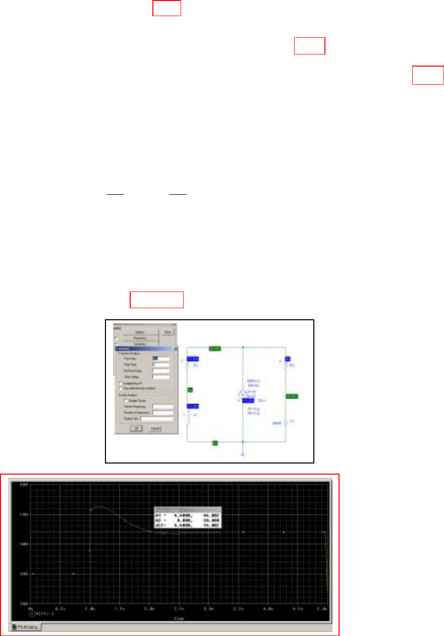
CHAPTER NINE SOLUTIONS
Engineering Circuit Analysis, 6th Edition Copyright
2002 McGraw-Hill, Inc. All Rights Reserved
49. (a) vS(0-) = vC(0-) = 2(15) = 30 V
(b) iL(0+) = iL(0-) = 15 A
Thus, iC(0+) = 22 – 15 = 7 A and vS(0+) = 3(7) + vC(0+) = 51 V
(c) As t → ∞, the current through the inductor approaches 22 A, so vS(t→ ∞,) = 44 A.
(d) We are presented with a series RLC circuit having α = 5/2 = 2.5 s-1 and
ω
o = 3.536
rad/s. The natural response will therefore be underdamped with
ω
d = 2.501 rad/s.
iL(t) = 22 + e-αt (A cos
ω
dt + B sin
ω
dt)
iL(0+) = iL(0-) = 15 = 22 + A so A = -7 amperes
Thus, iL(t) = 22 + e-2.5t (-7 cos 2.501t + B sin 2.501t)
vS(t) = 2 iL(t) + dt
di
i
dt
di L
L
L 2 L += = 44 + 2e-2.5t (-7cos 2.501t + Bsin 2.501t)
– 2.5e-2.5t (-7cos 2.501t + Bsin 2.501t) + e-2.5t [7(2.501) sin 2.501t + 2.501B cos 2.501t)]
vS(t) = 51 = 44 + 2(-7) – 2.5(-7) + 2.501B so B = 1.399 amperes and hence
vS(t) = 44 + 2e-2.5t (-7cos 2.501t + 1.399sin 2.501t)
-2.5e-2.5t (-7cos 2.501t + 1.399sin 2.501t) + e-2.5t [17.51sin 2.501t + 3.499cos 2.501t)]
and vS(t) at t = 3.4 s = 44.002 V. This is borne out by PSpice simulation:
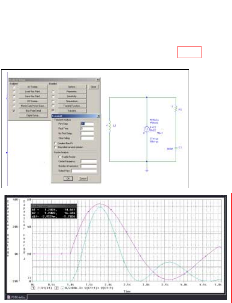
CHAPTER NINE SOLUTIONS
Engineering Circuit Analysis, 6th Edition Copyright
2002 McGraw-Hill, Inc. All Rights Reserved
50. Considering the circuit at t < 0, we see that iL(0-) = 15 A and vC(0-) = 0.
The circuit is a series RLC with α = R/2L = 0.375 s-1 and
ω
0 = 1.768 rad/s. We therefore
expect an underdamped response with
ω
d = 1.728 rad/s. The general form of the
response will be
vC(t) = e-αt (A cos
ω
dt + B sin
ω
dt) + 0 (vC(∞) = 0)
vC(0+) = vC(0-) = 0 = A and we may therefore write vC(t) = Be-0.375t sin (1.728t) V
iC(t) = -iL(t) = C dt
dvC= (80×10-3)(-0.375B e-0.375t sin 1.728t
At t = 0+, iC = 15 + 7 – iL(0+) = 7 = (80×10-3)(1.728B) so that B = 50.64 V.
Thus, vC(t) = 50.64 e–0.375t sin 1.807t V and vC(t = 200 ms) = 16.61 V.
The energy stored in the capacitor at that instant is ½ CvC2 = 11.04 J
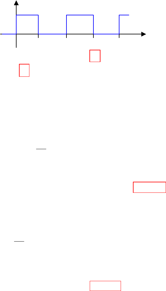
CHAPTER NINE SOLUTIONS
Engineering Circuit Analysis, 6th Edition Copyright
2002 McGraw-Hill, Inc. All Rights Reserved
51. It’s probably easiest to begin by sketching the waveform vx:
(a) The source current ( = iL(t) ) = 0 at t = 0-.
(b) iL(t) = 0 at t = 0+
(c) We are faced with a series RLC circuit having α = R/2L = 2000 rad/s and
ω
0 = 2828
rad/s. Thus, an underdamped response is expected with
ω
d = 1999 rad/s.
The general form of the expected response is iL(t) = e-αt (A cos
ω
dt + B sin
ω
dt)
iL(0+) = iL(0-) = 0 = A so A = 0. This leaves iL(t) = B e-2000t sin 1999t
vL(t) = L dt
diL= B[(5×10⁻³)(-2000 e-2000t sin 1999t + 1999 e-2000t cos 1999t)]
vL(0+) = vx(0+) – vC(0+) – 20 iL(0+) = B (5×10⁻³)(1999) so B = 7.504 A.
Thus, iL(t) = 7.504 e-2000t sin 1999t and iL(1 ms) = 0.9239 A.
(d) Define t' = t – 1 ms for notational convenience. With no source present, we expect a
new response but with the same general form:
iL(t') = e-2000t' (A' cos 1999t' + B' sin 1999t')
vL(t) = L dt
diL, and this enables us to calculate that vL(t = 1 ms) = -13.54 V. Prior to the
pulse returning to zero volts, -75 + vL + vC + 20 iL = 0 so vC(t' = 0) = 69.97 V.
iL(t' = 0) = A' = 0.9239 and –vx + vL + vC + 20 iL = 0 so that B' = -7.925.
Thus, iL(t') = e-2000 t' (0.9239 cos 1999t' – 7.925 sin 1999t') and
hence iL(t = 2 ms) = iL(t' = 1 ms) = -1.028 A.
1 2 3 4 t (s)
vx (V)
75
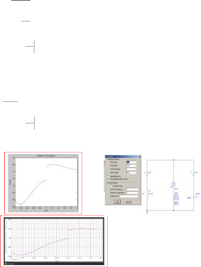
CHAPTER NINE SOLUTIONS
Engineering Circuit Analysis, 6th Edition Copyright
2002 McGraw-Hill, Inc. All Rights Reserved
52. For t < 0, we have 15 A dc flowing, so that iL = 15 A, vC = 30 V, v3Ω = 0 and vS = 30
V. This is a series RLC circuit with α = R/2L = 2.5 s-1 and
ω
0 = 3.536 rad/s. We
therefore expect an underdamped response with
ω
d = 2.501 rad/s.
vC(t) = e-αt (A cos
ω
dt + B sin
ω
dt)
vC(0+) = vC(0-) = 30 = A so we may write vC(t) = e-2.5t (30 cos 2.501t + B sin 2.501t)
C=
dt
dv -2.5e-2.5t(30 cos 2.501t + B sin 2.501t)
+ e-2.5t [-30(2.501)sin 2.501t + 2.501B cos 2.501t]
iC(0+) =
0
C
+
=t
dt
dv
C= 80×10-3[-2.5(30) + 2.501B] = -iL(0+) = -iL(0-) = -15 so B = -44.98 V
Thus, vC(t) = e-2.5t (30 cos 2.501t – 44.98 sin 2.501t) and
iC(t) = e-2.5t (-15 cos 2.501t + 2.994 sin 2.501t).
Hence, vS(t) = 3 iC(t) + vC(t) = e-2.5t (-15 cos 2.501t – 36 sin 2.501t)
Prior to switching, vC(t = 1) = -4.181 V and iL(t = 1) = -iC(t = 1) = -1.134 A.
t > 2: Define t' = t – 1 for notational simplicity. Then, with the fact that vC(∞) = 6 V,
our response will now be vC(t') = e-αt' (A' cos
ω
dt' + B' sin
ω
dt') + 6.
With vC(0+) = A' + 6 = -4.181, we find that A' = -10.18 V.
iC(0+) =
0
C
+
=
′
′t
td
dv
C= (80×10-3)[(-2.5)(-10.18) + 2.501B')] = 3 – iL(0+) so B' = 10.48 V
Thus, vC(t') = e-2.5t (-10.18 cos 2.501t' + 10.48 sin 2.501t') and
iC(t') = e-2.5t (4.133 cos 2.501t' – 0.05919 sin 2.501t').
Hence, vS(t') = 3 iC(t') + vC(t') = e-2.5t (2.219 cos 2.501t' + 10.36 sin 2.501t')
0 < t < 1
We see that our hand
calculations are supported by
the PSpice simulation.
CHAPTER NINE SOLUTIONS
Engineering Circuit Analysis, 6th Edition Copyright
2002 McGraw-Hill, Inc. All Rights Reserved
53. The circuit described is a series RLC circuit, and the fact that oscillations are detected
tells us that it is an underdamped response that we are modeling. Thus,
iL(t) = e-αt (A cos
ω
dt + B sin
ω
dt) where we were given that
ω
d = 1.825×10⁶ rad/s.
ω
0 = LC
1 = 1.914×10⁶ rad/s, and so
ω
d2 =
ω
02 – α2 leads to α2 = 332.8×10⁹
Thus, α = R/2L = 576863 s-1, and hence R = 1003 Ω.
Theoretically, this value must include the “radiation resistance” that accounts for the
power lost from the circuit and received by the radio; there is no way to separate this
effect from the resistance of the rag with the information provided.
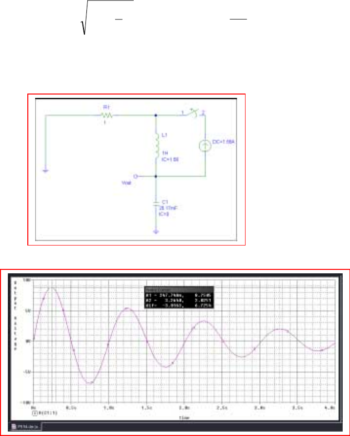
CHAPTER NINE SOLUTIONS
Engineering Circuit Analysis, 6th Edition Copyright
2002 McGraw-Hill, Inc. All Rights Reserved
54. The key will be to coordinate the decay dictated by α, and the oscillation period
determined by
ω
d (and hence partially by α). One possible solution of many:
Arbitrarily set
ω
d = 2π rad/s.
We want a capacitor voltage vC(t) = e-αt (A cos 2πt + B sin 2πt). If we go ahead and
decide to set vC(0-) = 0, then we can force A = 0 and simplify some of our algebra.
Thus, vC(t) = B e-αt sin 2πt. This function has max/min at t = 0.25 s, 0.75 s, 1.25 s, etc.
Designing so that there is no strong damping for several seconds, we pick α = 0.5 s-1.
Choosing a series RLC circuit, this now establishes the following:
R/2L = 0.5 so R = L and
ω
d =
2
2
02
1
-
ω
= 39.73 rad/s = LC
1
Arbitrarily selecting R = 1 Ω, we find that L = 1 H and C = 25.17 mF. We need the first
peak to be at least 5 V. Designing for B = 10 V, we ∴need iL(0+) = 2π(25.17×10⁻³)(10) =
1.58 A. Our final circuit, then is:
And the operation is verified by a simple PSpice simulation:
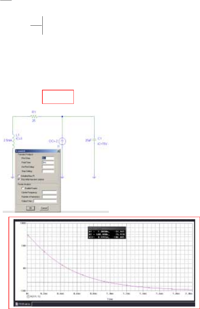
CHAPTER NINE SOLUTIONS
Engineering Circuit Analysis, 6th Edition Copyright
2002 McGraw-Hill, Inc. All Rights Reserved
55. For t < 0, iL(0-) = 3 A and vC(0-) = 25(3) = 75 V. This is a series RLC circuit with α =
R/2L = 5000 s-1 and
ω
0 = 4000 rad/s. We therefore expect an overdamped response with
s1 = -2000 s-1 and s2 = -8000 s-1. The final value of vC = -50 V.
For t > 0, vC(t) = A e-2000t + B e-8000t - 50
vC(0+) = vC(0-) = 75 = A + B – 50
so A + B = 125 [1]
dt
dvC= -2000 Ae-2000t – 8000 Be-8000t
iC(0+) =
+
=0
C
t
dt
dv
C= 3 – 5 – iL(0-) = -5 = -25×10-6 (2000A + 8000B)
Thus, 2000A + 8000B = 5/25×10-6 [2]
Solving Eqs. [1] and [2], we find that A = 133.3 V and B = -8.333 V. Thus,
vC(t) = 133.3 e-2000t – 8.333 e-8000t – 50
and vC(1 ms) = -31.96 V. This is confirmed by the PSpice simulation shown below.
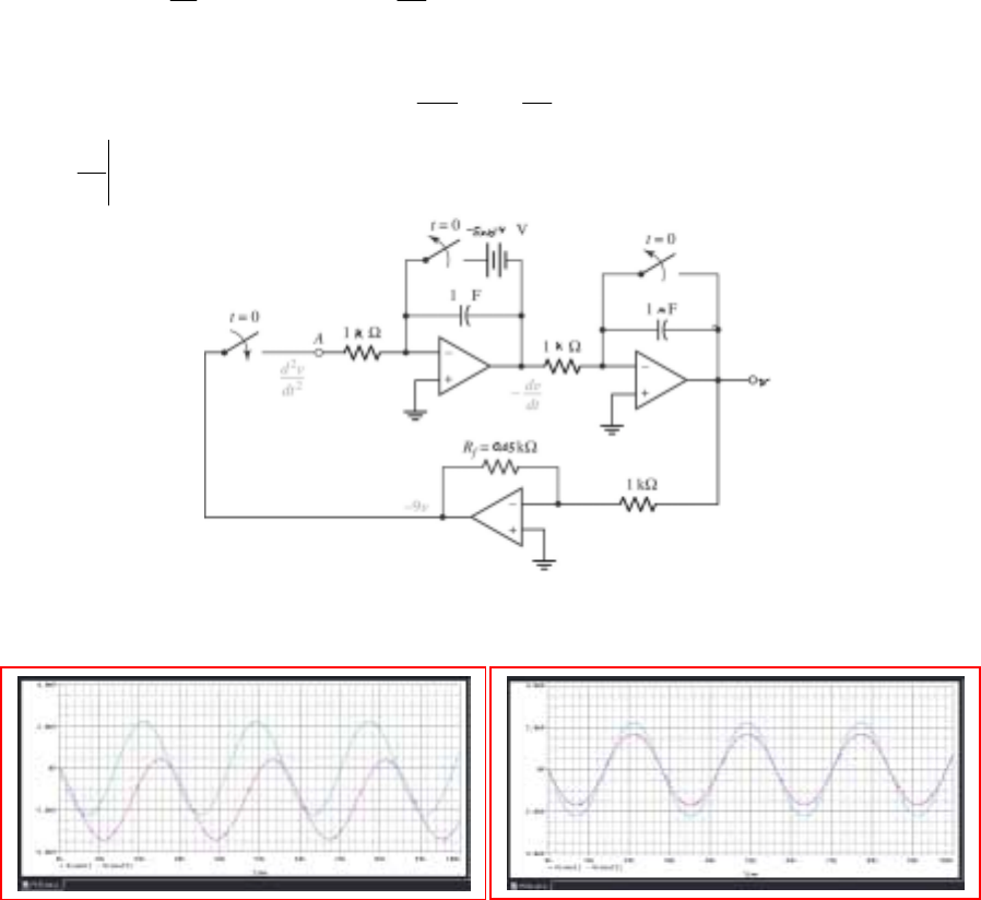
CHAPTER NINE SOLUTIONS
Engineering Circuit Analysis, 6th Edition Copyright
2002 McGraw-Hill, Inc. All Rights Reserved
56. α = 0 (this is a series RLC with R = 0, or a parallel RLC with R = ∞)
ω
o2 = 0.05 therefore
ω
d = 0.223 rad/s. We anticipate a response of the form:
v(t) = A cos 0.2236t + B sin 0.2236t
v(0+) = v(0-) = 0 = A therefore v(t) = B sin 0.2236t
dv/dt = 0.2236B cos 0.2236t; iC(t) = Cdv/dt = 0.4472B cos 0.2236t
iC(0+) = 0.4472B = -iL(0+) = -iL(0-) = -1×10⁻³ so B = -2.236×10⁻³ and thus
v(t) = -2.236 sin 0.2236t mV
In designing the op amp stage, we first write the differential equation:
)0( 0 2 10
10
13-
0=+=++
′
∫LC
tii
dt
dv
tdv
and then take the derivative of both sides:
v
dt
vd
20
1
- 2
2=
With 43
0
105)10236.2)(2236.0( −−
=
×−=×−=
+
t
dt
dv , one possible solution is:
PSpice simulations are very sensitive to parameter values; better results were obtained
using LF411 instead of 741s (both were compared to the simple LC circuit simulation.)
Simulation using 741 op amps Simulation using LF411 op amps
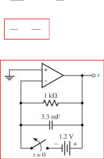
CHAPTER NINE SOLUTIONS
Engineering Circuit Analysis, 6th Edition Copyright
2002 McGraw-Hill, Inc. All Rights Reserved
57.
(a)
v
dt
dv
dt
dvv
3.3
1
-
or
0 103.3
1000
3-
=
=×+
(b) One possible solution:
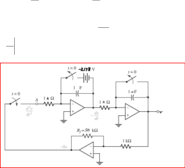
CHAPTER NINE SOLUTIONS
Engineering Circuit Analysis, 6th Edition Copyright
2002 McGraw-Hill, Inc. All Rights Reserved
58. α = 0 (this is a series RLC with R = 0, or a parallel RLC with R = ∞)
ω
o2 = 50 therefore
ω
d = 7.071 rad/s. We anticipate a response of the form:
v(t) = A cos 7.071t + B sin 7.071t, knowing that iL(0-) = 2 A and v(0-) = 0.
v(0+) = v(0-) = 0 = A therefore v(t) = B sin 7.071t
dv/dt = 7.071B cos 7.071t; iC(t) = Cdv/dt = 0.007071B cos 7.071t
iC(0+) = 0.007071B = -iL(0+) = -iL(0-) = -2 so B = -282.8 and thus
v(t) = -282.8 sin 7.071t V
In designing the op amp stage, we first write the differential equation:
)0( 0 10 2
20
13-
0=+=++
′
∫LC
tii
dt
dv
tdv
and then take the derivative of both sides:
v
dt
vd 05- 2
2=
With 2178)8.282)(071.7(
0
−=−=
+
=t
dt
dv , one possible solution is:
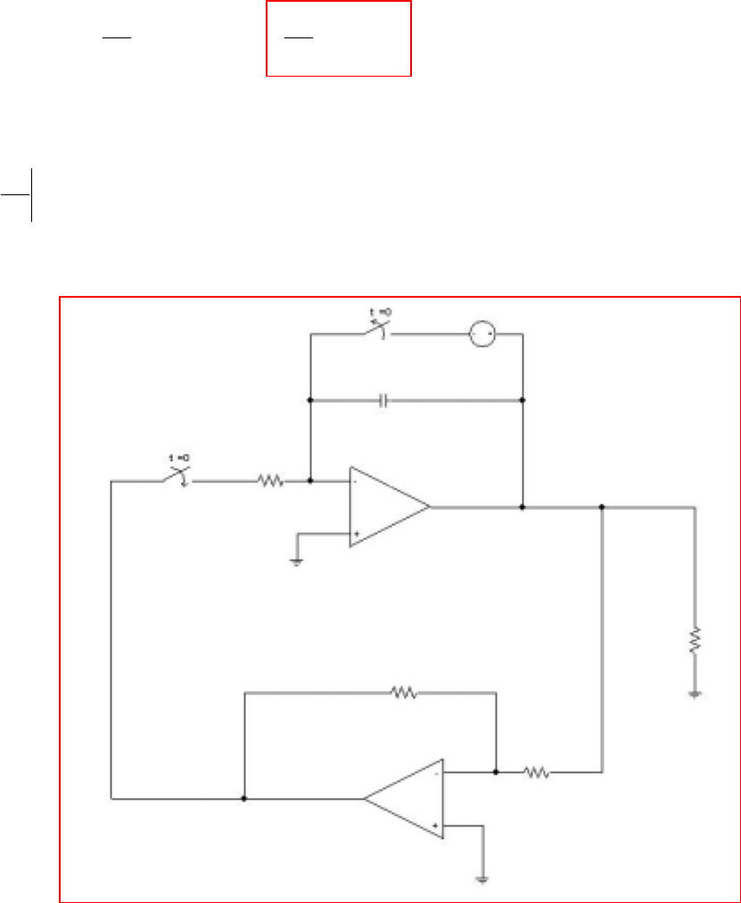
CHAPTER NINE SOLUTIONS
Engineering Circuit Analysis, 6th Edition Copyright
2002 McGraw-Hill, Inc. All Rights Reserved
59. (a) vR = vL
20(-iL) = 5 dt
diL or L
L4- i
dt
di =
(b) We expect a response of the form iL(t) = A e-t/ τ where τ = L/R = 0.25.
We know that iL(0-) = 2 amperes, so A = 2 and iL(t) = 2 e-4t
+
=0
L
t
dt
di = -4(2) = -8 A/s.
One possible solution, then, is
1 MΩ
4 kΩ
1 kΩ
1 Ω
1 µF
8 V
i
↓
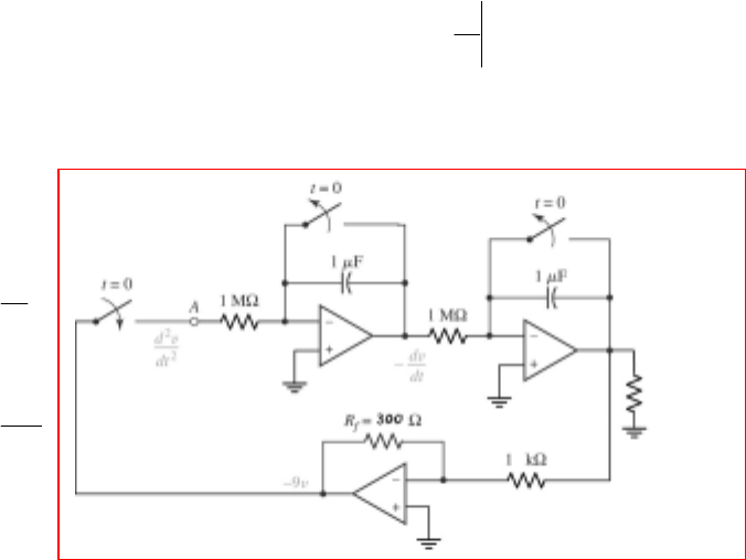
CHAPTER NINE SOLUTIONS
Engineering Circuit Analysis, 6th Edition Copyright
2002 McGraw-Hill, Inc. All Rights Reserved
and
+
=0 t
dt
di = 0
60. We see either a series RLC with R = 0 or a parallel RLC with R = ∞; either way, α = 0.
ω
02 = 0.3 so
ω
d = 0.5477 rad/s (combining the two inductors in parallel for the
calculation). We expect a response of the form i(t) = A cos
ω
dt + B sin
ω
dt.
i(0+) = i(0-) = A = 1×10⁻³
di/dt = -A
ω
d sin
ω
dt + B
ω
d cos
ω
dt
vL = 10di/dt = -10A
ω
d sin
ω
dt + 10B
ω
d cos
ω
dt
vL(0+) = vC(0+) = vC(0-) = 0 = 10B(0.5477) so that B = 0
and hence i(t) = 10-3 cos 0.5477t A
The differential equation for this circuit is
v
dt
vd
dt
dv
tvdtvd
tt
3.0
or
0 2
2
1
10
10
1
2
2
0
3-
0
−=
=+
′
++
′∫∫
One possible solution is:
1 Ω
↓
i
CHAPTER TEN (Phasor Analysis) SOLUTIONS
Engineering Circuit Analysis, 6th Edition Copyright
2002 McGraw-Hill, Inc. All Rights Reserved
1.
(a)
(b)
(c)
3
33
3
rad rad
210
T 4(7.5 2.1)10 21.6 10 , 290.9 rad/s
21.6
( ) 8.5sin (290.9 ) 0 8.5sin (290.9 2.1 10 )
0.6109 2 5.672 or 325.0
( ) 8.5sin (290.9 325.0 )
−−
−
π
=− =×ω= =
∴= +Φ∴= ××+Φ
∴Φ = − + π = °
∴= + °
t
ft t
ft t
8.5sin (290.9 325.0 ) 8.5
cos(290.9 235 ) 8.5cos(290.9 125 )
t
tt
+°=
+°= −°
8.5cos( 125 )cos 8.5sin125
sin 4.875 cos 290.9 6.963sin 290.9
+
−° ω+ °
ω=− +
t
ttt
CHAPTER TEN (Phasor Analysis) SOLUTIONS
Engineering Circuit Analysis, 6th Edition Copyright
2002 McGraw-Hill, Inc. All Rights Reserved
2.
(a)
(b)
(c)
(d)
10cos 4sin ACos( ), A 0, 180 180
A 116 10.770, Acos 10, Asin 4 tan 0.4, 3 quad
21.80 201.8 ,too large 201.8 360 158.20
d
tt wt−ω+ω+ +Φ>−°<Φ≤°
== Φ=− Φ=−∴Φ=
∴Φ = °= ° ∴Φ = °− °=− °
200cos(5 130 ) Fcos5 Gsin5 F 200cos130 128.56
G 200sin130 153.21
+°= + ∴= °=−
=− °=− °
ttt
sin10 5
( ) 5cos10 3sin10 0, 0 1 , 10 1.0304,
cos10 3
0.10304 ; also, 10 1.0304 , 0.4172 ; 2 : 0.7314
=−=≤≤∴==
==+π=π
t
it t t t s t
t
tst ts s
0 10ms, 10cos100 12sin100 ; let 10cos100 t =12sin100 t
10
tan100 t = , 100 0.6947 2.211ms 0 2.211ms
12
<< π≥ π π π
∴π π= ∴= ∴<<
ttt
tt t

CHAPTER TEN (Phasor Analysis) SOLUTIONS
Engineering Circuit Analysis, 6th Edition Copyright
2002 McGraw-Hill, Inc. All Rights Reserved
3.
(a)
(b) ( ) leads ( ) by 149.04 15.255 133.78
°− °= °
ft gt
( ) 50cos 30sin 58.31cos( 149.04 )
( ) 55cos 15sin 57.01cos( 15.255 )
ampl. of ( ) 58.31, ampl. of ( ) 57.01
=− ω − ω = ω + °
=ω−ω= ω+°
∴= =
ft t t t
gt t t t
ft gt
CHAPTER TEN (Phasor Analysis) SOLUTIONS
Engineering Circuit Analysis, 6th Edition Copyright
2002 McGraw-Hill, Inc. All Rights Reserved
4.
222 222
( ) Acos( ), L( / ) R V cos
L[ Asin ( )] RA cos( ) V cos
LA sin cos LA cos sin
RAcos cos RAsin sin
V cos LAcos RAsin and sin RAcos V
LL R
tan LA RA
RL RL
m
m
m m
it t di dt i t
ttt
tt
tt
tLA
R
=ω−θ +=ω
∴ −ω ω −θ + ω −θ = ω
∴−ω ω θ+ω ω θ
+ωθ+ωθ=
ω∴ω θ= θ ω θ+ θ=
ωω
∴θ= ∴ω +
+ω +ω
22 2 222
222
V
VLR
AV R LAV.A RL
m
m
mm
=
ω
∴+ =∴+ω==
+ω
CHAPTER TEN (Phasor Analysis) SOLUTIONS
Engineering Circuit Analysis, 6th Edition Copyright
2002 McGraw-Hill, Inc. All Rights Reserved
5. f = 13.56 MHz so
ω
= 2
π
f = 85.20 Mrad/s.
Delivering 300 W (peak) to a 5-Ω load implies that 300
5
V2
m= so Vm = 38.73 V.
Finally, (85.2×10⁶)(21.15×10⁻³) +
φ
= n
π
, n = 1, 3, 5, …
Since (85.2×10⁶)(21.15×10⁻³) = 1801980, which is 573588+
π
, we find that
F = 573587
π
- (85.2×10⁶)(21.15×10⁻³) = -3.295 rad = -188.8o.
CHAPTER TEN (Phasor Analysis) SOLUTIONS
Engineering Circuit Analysis, 6th Edition Copyright
2002 McGraw-Hill, Inc. All Rights Reserved
6. (a) -33 sin(8t – 9o) → -33∠(-9-90)o = 33∠81o
12 cos (8t – 1o) → 12∠-1o
(b) 15 cos (1000t + 66o) → 15 ∠ 66o
-2 cos (1000t + 450o) → -2 ∠ 450o = -2 ∠90o = 2 ∠ 270o
(c) sin (t – 13o) → 1∠-103o
cos (t – 90o) → 1 ∠ -90o
(d) sin t → 1 ∠ -90o
cos (t – 90o) → 1 ∠ -90o
These two waveforms are in phase. Neither leads the other.
33∠81o
12∠-1o
-33 sin(8t – 9o) leads 12 cos (8t – 1o) by
81 – (-1) = 82o.
15∠66o
2∠270o
15 cos (1000t + 66o) leads -2 cos (1000t + 450o)
by 66 – -90 = 156o.
1∠-103o 1 ∠ -90o
cos (t – 90o) leads sin (t – 13o)
by 66 – -90 = 156o.
CHAPTER TEN (Phasor Analysis) SOLUTIONS
Engineering Circuit Analysis, 6th Edition Copyright
2002 McGraw-Hill, Inc. All Rights Reserved
7. (a) 6 cos (2
π
60t – 9o) → 6∠-9o
-6 cos (2
π
60t + 9o) → 6∠189o
(b) cos (t - 100o) → 1 ∠ -100o
-cos (t - 100o) → -1 ∠ -100o = 1 ∠80o
(c) -sin t → -1∠-90o = 1∠90o
sin t → 1∠ -90o
(d) 7000 cos (t –
π
) → 7000 ∠ -
π
= 7000 ∠ -180o
9 cos (t – 3.14o) → 9 ∠ -3.14o
6∠-9o
6∠189o
-6 cos (2
π
60t + 9o) lags 6 cos (2
π
60t – 9o)
by 360 – 9 – 189 = 162o.
1∠80o
1∠-100o
-cos (t - 100o) lags cos (t - 100o) by 180o.
1∠90o
1 ∠ -90o
-sin t lags sin t by 180o.
7000 ∠ -180o
9 ∠ -3.14o
7000 cos (t –
π
) lags 9 cos (t – 3.14o)
b
y
180 – 3.14 = 176.9o.
CHAPTER TEN (Phasor Analysis) SOLUTIONS
Engineering Circuit Analysis, 6th Edition Copyright
2002 McGraw-Hill, Inc. All Rights Reserved
8. v(t) = V1 cos
ω
t - V2 sin
ω
t [1]
We assume this can be written as a single cosine such that
v(t) = Vm cos (
ω
t +
φ
) = Vm cos
ω
t cos
φ
- Vm sin
ω
t sin
φ
[2]
Equating terms on the right hand sides of Eqs. [1] and [2],
V
1 cos
ω
t – V2 sin
ω
t = (Vm cos
φ
) cos
ω
t – (Vm sin
φ
) sin
ω
t
yields
V1 = Vm cos
φ
and V2 = Vm sin
φ
Dividing, we find that
φ
φ
φ
tan
cos V
sin V
V
V
m
m
1
2== and
φ
= tan-1(V2/ V1)
Next, we see from the above sketch that we may write Vm = V1/ cos
φ
or
2
2
2
11
1
mV VV
V
V +
= = 2
2
2
1V V +
Thus, we can write v(t) = Vm cos (
ω
t +
φ
) = 2
2
2
1V V + cos [
ω
t + tan-1(V2/ V1)].
φ
V2
V1
2
2
2
1V V +
CHAPTER TEN (Phasor Analysis) SOLUTIONS
Engineering Circuit Analysis, 6th Edition Copyright
2002 McGraw-Hill, Inc. All Rights Reserved
9. (a) In the range 0 ≤ t ≤ 0.5, v(t) = t/0.5 V.
Thus, v(0.4) = 0.4/0.5 = 0.8 V.
(b) Remembering to set the calculator to radians, 0.7709 V.
(c) 0.8141 V.
(d) 0.8046 V.
CHAPTER TEN (Phasor Analysis) SOLUTIONS
Engineering Circuit Analysis, 6th Edition Copyright
2002 McGraw-Hill, Inc. All Rights Reserved
10. (a) Vrms = 2
1
T
0
2
2
m cos
T
V
∫dtt
ω
= 2
1
T
0
2
2
m
T
2
cos
T
V
∫dt
t
π
= 2
1
T
0
2
m
T
4
cos 1
2T
V
+
∫dt
t
π
= 2
1
T
0
2
m
T
0
2
m
T
4
cos
2T
V
2T
V
+∫∫ dt
t
dt
π
= 2
1
4
0
2
m
2
m cos
8
V
T
2T
V
+
π
π
u
=
2
Vm
(b) Vm = V 155.6 2 110 =, V 162.6 2 115 =, V 169.7 2 201 =
CHAPTER TEN (Phasor Analysis) SOLUTIONS
Engineering Circuit Analysis, 6th Edition Copyright
2002 McGraw-Hill, Inc. All Rights Reserved
11.
1
22
3
At : 15cos500 V
4
R 5 20 60 20
V 15V,R 20 , L 10
15 10
cos 500 tan 0.6708cos(500 26.57)A
20
20 10
−
−==
=+ = Ω
∴= =Ωω=Ω
∴= − = −
+
oc s
th
m
L
xxv v t
it t
CHAPTER TEN (Phasor Analysis) SOLUTIONS
Engineering Circuit Analysis, 6th Edition Copyright
2002 McGraw-Hill, Inc. All Rights Reserved
12.
(a)
(b)
At : R 80 20 16
80
0.4(15 85) cos500
85
4.8cos500 V
th
oc
oc
xx
vt
vt
−==Ω
=−
∴=
1
22
4.8 10
cos 500 tan 15
16 10
0.2544cos(500 32.01 )A
−
=−
+
=−°
L
it
t
L 0.02 0.02544( 500)
sin (500 32.01 ) 2.544sin (500 32.01 ) V
2.544cos(500 57.99 ) V,
31.80cos(500 57.99 ) mA
LL
Lx
vi
tt
vti
t
′
==× −
−°=− −°
∴= + °
=+°
CHAPTER TEN (Phasor Analysis) SOLUTIONS
Engineering Circuit Analysis, 6th Edition Copyright
2002 McGraw-Hill, Inc. All Rights Reserved
13.
(a)
(b)
(c)
55
22
5
100 800
cos 10 0.10600cos(10 57.99 )A
500
500 800
57.99
0 when 0 10 , 25.83
180 2
R
it t
pit ts
=−=−°
+
°π
==∴−π==µ
355
5
5
55
5
L 8 10 0.10600( 10 ) sin(10 57.99 )
84.80sin (10 57.99 )
8.989sin (10 57.99 )
cos(10 57.99 ) 4.494 sin (2 16 115.989 )
0 when 2 10 115.989 0 , 180 ,
10.121 or 25.83
L
L
LL
L
vi t
vt
pvi t
tt
pt
ts
−
′
±= =× × − − °
∴=− − °
∴==− − °
−°=− ×− °
∴= × − °=° °
∴=
µ
55
5
10.600cos10 cos(10 57.99 )
0 when 10 , 15.708 and also 25.83
2
== − °
π
∴= = =
µ
=
µ
ssL
s
pvi t t
pttsts
CHAPTER TEN (Phasor Analysis) SOLUTIONS
Engineering Circuit Analysis, 6th Edition Copyright
2002 McGraw-Hill, Inc. All Rights Reserved
14.
55
5
5
5
51 5
22
3cos10 V, 0.1cos10 A
in series with 30 0.1cos10 A 30
Add, getting 0.2cos10 A 30
change to 6 cos 10 Vin series with 30 ; 30 20 50
610
cos 10 tan 0.11767cos(10 11.310
50
50 10
−
==
Ω→ Ω
Ω
ΩΩ+Ω=Ω
∴= − = − °
+
ss
s
L
vti t
vt
t
t
it t
5rad
rad
)A
At 10 , 10 1 0.1167cos(1 11.310 ) 81.76mA
0.11767 10cos(1 11.30 90 ) 0.8462V
=µ =∴= − °=
∴= × − °+°=−
L
L
tsti
v
CHAPTER TEN (Phasor Analysis) SOLUTIONS
Engineering Circuit Analysis, 6th Edition Copyright
2002 McGraw-Hill, Inc. All Rights Reserved
15.
1
22
cos500 V
cos500 100(0.8 )
1cos500 A R 80
80
1 150
cos 500 tan 80
80 150
5.882cos(500 61.93 )mA
−
∴=
∴=
∴= ∴ = =Ω
∴= −
+
=−°
oc
sc
oc
sc th
sc
L
L
vt
ti
v
it
i
it
it
CHAPTER TEN (Phasor Analysis) SOLUTIONS
Engineering Circuit Analysis, 6th Edition Copyright
2002 McGraw-Hill, Inc. All Rights Reserved
16.
(a)
(b) ,
10.2383 0.11916J
2
ω=× =
Lav
12
1
22
V 120cos120 V
120 120
2A, 1A, 2 1 3A, 60 120 40
60 12
3 40 120V, L 12 37.70
120 37.70
cos 120 tan 40
40 37.70
2.183cos(120 43.30 ) A
ss
L
vt
it
t
−
== π
==+= =Ω
×= ω=π= Ω
∴= π−
+
=π−°
22
2
10.1 2.183 cos (120 43.30 )
2
0.2383cos (120 43.30 ) J
∴ω = × × π − °
=π−°
Lt
t
CHAPTER TEN (Phasor Analysis) SOLUTIONS
Engineering Circuit Analysis, 6th Edition Copyright
2002 McGraw-Hill, Inc. All Rights Reserved
17.
12
22 22
120cos400 V, 180cos200 V
120 180
2A, 1.5A, 60 120 40
60 120
2 40 80V, 1.5 40 60V
80 60
cos(400 45 ) cos(200 26.57 ) A
40 40 40 20
or 1.4142cos(400 45 ) 1.3416cos(200 26.57 )A
ss
L
L
vtvt
it t
it t
↑= =
== =Ω
×= ×=
=−°+−°
++
=−°+−°
CHAPTER TEN (Phasor Analysis) SOLUTIONS
Engineering Circuit Analysis, 6th Edition Copyright
2002 McGraw-Hill, Inc. All Rights Reserved
18.
11
1
11
1
11
L
R , R 0, A , ideal, R C R
Vcos ,
RR
(Vcos)C
R
L
Vcos RC R
For RL circuit, V cos L R
L
Vcos R
By c
io
m out
upper lower
c upper lower out m out
m out out out out
R
mr
mRR
tv
ii
i
ii i v t v
tv v v v
dv
tv dt
tv v
ω
ω
ω
ω
ω
=∞ = =∞ =
=− =
′
∴= + = − =−
′′
∴=+=+
=+
′
∴=+
omparison, Rout
vv=
CHAPTER TEN (Phasor Analysis) SOLUTIONS
Engineering Circuit Analysis, 6th Edition Copyright
2002 McGraw-Hill, Inc. All Rights Reserved
19.
(a)
(b)
1
V cos R (ignore I.C)
C
1
Vsin R
=+
′
∴− = +
∫
m
m
ti idt
ti i
C
ω
ωω
()
1
Assume Acos( )
A
Vsin R Asin( ) cos( )
C
AA
V sin R Acos sin R Asin cos cos cos sin sin
CC
Equating terms on the left and right side,
A1
[1] R Asin cos tan so tan 1 CR ,
CCR
−
=+Φ
∴− = − +Φ + +Φ
∴− = − Φ Φ + Φ− Φ
Φ= Φ∴ Φ= Φ=
m
m
it
tt t
ttttt
ω
ωωωω ω
ωωω ωω ω ω ω
ωω
ω
222 22 2
222 222
222 22 2
1
222
and
CR A 1
[2] V R A C
1CR 1CR
CVAR C1 A
V1CRA
CC
1CR 1CR
CV 1
cos tan CR
1CR
−
−=− −
++
+
∴= = + ∴=
++
∴= +
+
m
m
m
m
it
ω
ωω
ωω
ωω
ωω
ωω
ωωω
ω
-
CHAPTER TEN (Phasor Analysis) SOLUTIONS
Engineering Circuit Analysis, 6th Edition Copyright
2002 McGraw-Hill, Inc. All Rights Reserved
20. (a) 7 ∠ -90o = -j 7
(b) 3 + j + 7 ∠ -17o = 3 + j + 6.694 – j 2.047 = 9.694 – j 1.047
(c) 14ej15o = 14 ∠ 15o = 14 cos 15o + j 14 sin 15o = 13.52 + j 3.263
(d) 1 ∠ 0o = 1
(e) –2 (1 + j 9) = -2 – j 18 = 18.11 ∠ - 96.34o
(f) 3 = 3 ∠ 0o

CHAPTER TEN (Phasor Analysis) SOLUTIONS
Engineering Circuit Analysis, 6th Edition Copyright
2002 McGraw-Hill, Inc. All Rights Reserved
21. (a) 3 + 15 ∠ -23o = 3 + 13.81 – j 5.861 = 16.81 – j 5.861
(b) (j 12)(17 ∠ 180o) = (12 ∠ 90o)(17 ∠ 180o) = 204 ∠ 270o = -j 204
(c) 5 – 16(9 – j 5)/ (33 ∠ -9o) = 5 – (164 ∠ -29.05o)/ (33 ∠ -9o)
= 5 – 4.992 ∠ -20.05o = 5 – 4.689 – j 1.712 = 0.3109 + j 1.712

CHAPTER TEN (Phasor Analysis) SOLUTIONS
Engineering Circuit Analysis, 6th Edition Copyright
2002 McGraw-Hill, Inc. All Rights Reserved
22. (a) 5 ∠ 9o – 9 ∠ -17o = 4.938 + j 0.7822 – 8.607 + j 2.631 = -3.669 – j 1.849
= 4.108 ∠ -153.3o
(b) (8 – j 15)(4 + j 16) – j = 272 + j 68 – j = 272 + j 67 = 280.1 ∠ 13.84o
(c) (14 – j 9)/ (2 – j 8) + 5 ∠ -30o = (16.64 ∠-32.74o)/ (8.246 ∠ - 75.96o) + 4.330 – j 2.5
= 1.471 + j 1.382 + 4.330 – j 2.5 = 5.801 – j 1.118 = 5.908 ∠ -10.91o
(d) 17 ∠ -33o + 6 ∠-21o + j 3 = 14.26 – j 9.259 + 5.601 – j 2.150 + j 3
= 19.86 – j 8.409 = 21.57 ∠ -22.95o

CHAPTER TEN (Phasor Analysis) SOLUTIONS
Engineering Circuit Analysis, 6th Edition Copyright
2002 McGraw-Hill, Inc. All Rights Reserved
23. (a) ej14o + 9 ∠ 3o – (8 – j 6)/ j2 = 1 ∠ 14o + 9 ∠ 3o – (8 – j 6)/ (-1)
= 0.9703 + j 0.2419 + 8.988 + j 0.4710 + 8 – j 6 = 17.96 – j 5.287 = 18.72 ∠ -16.40o
(b) (5 ∠ 30o)/ (2 ∠ -15o) + 2 e j5o/ (2 – j 2)
= 2.5 ∠ 45o + (2 ∠ 5o)/ (2.828 ∠ -45o) = 1.768 + j 1.768 + 0.7072 ∠ 50o
= 1.768 + j 1.768 + 0.4546 + j 0.5418
= 2.224 + j 2.310 = 3.207 ∠ 46.09o
CHAPTER TEN (Phasor Analysis) SOLUTIONS
Engineering Circuit Analysis, 6th Edition Copyright
2002 McGraw-Hill, Inc. All Rights Reserved
24.
(a) 5 110 1.7101 4.698∠− °=− − j
(b) 160
6 5.638 2.052
°=− +
j
ej
(c) (3 6)(2 50 ) 5.336 12.310
+∠°=−+
jj
(d) 100 40 107.70 158.20−− = ∠− °j
(e) 2 50 3 120 1.0873 101.37∠°+∠− °= ∠− °
CHAPTER TEN (Phasor Analysis) SOLUTIONS
Engineering Circuit Analysis, 6th Edition Copyright
2002 McGraw-Hill, Inc. All Rights Reserved
25.
(a) 40 50 18 25 39.39 76.20∠− °− ∠ °= ∠− °
(b) 22 5
3 4.050 69.78
12
j
jj
−
−
++ = ∠− °
+
(c) 3
(2.1 25 ) 9.261 75 2.397 8.945+
∠°= ∠°= +j
(d) 0.3 rad
0.7 0.7 0.3 0.6687 0.2069=∠ = +
j
ej

CHAPTER TEN (Phasor Analysis) SOLUTIONS
Engineering Circuit Analysis, 6th Edition Copyright
2002 McGraw-Hill, Inc. All Rights Reserved
26.
(40 30 ) (40 30 )
(40 30 ) (40 30 )
(40 30 ) (40 30 )
(40 30 ) (40 30 )
(40 53
20 A 100 20
50 , 10 A
(20 10) , 40 0.08(20 10)
(32 64) V (32 64 50)
34.93
+° +°
+° +°
+° +°
+° +°
−
=∴=
=− =−
∴= − = × −
∴= + ∴= + −
∴=
∫
tjt
cc
jt jt
cR
jt jt
LL
jt jt
Ls
jt
s
ie v e dt
vje ije
ijevj je
vje vjje
ve
.63 ) V
°

CHAPTER TEN (Phasor Analysis) SOLUTIONS
Engineering Circuit Analysis, 6th Edition Copyright
2002 McGraw-Hill, Inc. All Rights Reserved
27.
(10 25 )
(10 25 ) (10 25 )
(10 25 )
(10 25 ) (10 25 )
(10 25 ) (10 25 )
(10 125.62 )
20 A
0.2 [20 ] 40
80
(80 40) , 0.08(80 40) 10
( 32 64) ( 12 64)
65.12 A
jt
L
jt t
L
jt
R
jt jt
sc
jt jt
cs
jt
s
ie
d
veje
dt
ve
vjei jje
ijeije
ie
+°
+° =°
+°
+° +°
+° +°
+°
=
==
=
=+ = +
∴=−+ ∴=−+
∴=
CHAPTER TEN (Phasor Analysis) SOLUTIONS
Engineering Circuit Analysis, 6th Edition Copyright
2002 McGraw-Hill, Inc. All Rights Reserved
28. 80cos(500 20 )V 5cos(500 12 )A−° → +°tt
(a) 40cos(500 10 ) 2.5cos(500 42 )A
s out
vti t=+°∴= +°
(b)
(c)
(d)
40sin (500 10 ) 40cos(500 80 )
2.5cos(500 48 )A
=+°=−°
∴= −°
s
out
vt t
it
(500 10 )
(500 42 )
40 40cos(500 10 )
40sin (500 10 ) 2.5 A
+°
+°
==+°
++°∴=
jt
s
jt
out
ve t
jtie
500 21.80 500
(500 53.80 )
(50 20) 53.85
3.366 A
+°+
+°
=+ =
∴=
jt j jt
s
jt
out
vje e
ie
CHAPTER TEN (Phasor Analysis) SOLUTIONS
Engineering Circuit Analysis, 6th Edition Copyright
2002 McGraw-Hill, Inc. All Rights Reserved
29.
(a) 12sin (400 110 )A 12 20 A+°→∠°t
(b)
(c)
(d)
(e)
7sin800 3cos800 7 3
3 7 7.616 113.20 A
−− →−
=− + = ∠ °
ttj
j
4cos(200 30 ) 5cos(200 20 )
4 30 5 20 3.910 108.40 A
−°− +°
→∠− °−∠ °= ∠− °
tt
3rad
600, 5ms : 70 30 V
70cos(600 5 10 30 ) 64.95 V
−+
ω= = ∠ °
→××+°=−
t
rad
600, 5ms : 60 40 V 72.11 146.3
72.11cos(3 146.31 ) 53.75 V
+
ω= = + = ∠ °
→+°=
tj
CHAPTER TEN (Phasor Analysis) SOLUTIONS
Engineering Circuit Analysis, 6th Edition Copyright
2002 McGraw-Hill, Inc. All Rights Reserved
30. 4000, 1mstω= =
(a)
(b)
(c)
(d)
(e)
rad
I5 80A
4cos(4 80 ) 4.294A
=∠− °
∴= − °=−
x
x
i
rad
I 4 1.5 4.272 159.44 A
4.272cos(4 159.44 ) 3.750 A
−
=− + = ∠ °
∴= + °=
x
x
j
i
( ) 50sin (250 40 )
50cos(250 130 ) V 50 103 V
=−°
=−°→=∠−°
x
x
vt t
t
20cos108 30sin108
20 30 36.06 56.31 V
=−
→+ = ∠ °
x
vtt
j
33cos(80 50 ) 41cos(80 75 )!
33 50 41 75 72.27 63.87 V
=−°+−°
→∠−°+∠−°= ∠− °
x
vt t

CHAPTER TEN (Phasor Analysis) SOLUTIONS
Engineering Circuit Analysis, 6th Edition Copyright
2002 McGraw-Hill, Inc. All Rights Reserved
31.
12
3rad
rad rad
V 10 90mV, 500;V 8 90mV,
1200, M by 5, 0.5ms
( 5) [10cos(500 0.5 10 90 )
8cos(1.2 0.5 90 )]
50sin 0.25 40sin 0.6 34.96mV
out
t
v−
=∠° ω= =∠°
ω= − =
=− × × + °
+×+°
=+=

CHAPTER TEN (Phasor Analysis) SOLUTIONS
Engineering Circuit Analysis, 6th Edition Copyright
2002 McGraw-Hill, Inc. All Rights Reserved
32. Begin with the inductor:
(2.5 ∠40o) (j500) (20×10-3) = 25∠130o V across the inductor and the 25-Ω resistor.
The current through the 25-Ω resistor is then (25∠130o) / 25 = 1∠130o A.
The current through the unknown element is therefore 25∠130o + 1∠130o = 26∠130o;
this is the same current through the 10-Ω resistor as well. Thus, KVL provides that
Vs = 10(26∠130o) + (25 ∠ -30o) + (25∠130o) = 261.6 ∠128.1o
and so vs(t) = 261.6 cos (500t + 128.1o) V.

CHAPTER TEN (Phasor Analysis) SOLUTIONS
Engineering Circuit Analysis, 6th Edition Copyright
2002 McGraw-Hill, Inc. All Rights Reserved
33.
ω
= 5000 rad/s.
(a) The inductor voltage = 48∠ 30o = j
ω
L IL = j(5000)(1.2×10⁻³) IL
So IL = 8∠-60o and the total current flowing through the capacitor is
10 ∠ 0o - IL = 9.165∠49.11o A and the voltage V1 across the capacitor is
V1 = (1/j
ω
C)(9.165∠49.11o) = -j2 (9.165∠49.11o) = 18.33∠-40.89o V.
Thus, v1(t) = 18.33 cos (5000t – 40.89o) V.
(b) V2 = V1 + 5(9.165∠49.11o) + 60∠120o = 75.88∠79.48o V
(c) V3 = V2 – 48∠30o = 75.88 ∠79.48o – 48∠30o = 57.70∠118.7o V
2( ) 75.88cos(5000 79.48 ) V∴= + °vt t
3( ) 57.70cos(5000 118.70 )V∴= + °vt t

CHAPTER TEN (Phasor Analysis) SOLUTIONS
Engineering Circuit Analysis, 6th Edition Copyright
2002 McGraw-Hill, Inc. All Rights Reserved
34. VR = 1∠0o V, Vseries = (1 + j
ω
–j/
ω
)(1∠0o)
V
R = 1 and Vseries =
()
1/ - 1 2
ωω
+
We desire the frequency w at which Vseries = 2VR or Vseries = 2
Thus, we need to solve the equation
()
4 1/ - 1 2=+
ωω
or 0 1 - 3 -
2=
ωω
Solving, we find that
ω
= 2.189 rad/s.

CHAPTER TEN (Phasor Analysis) SOLUTIONS
Engineering Circuit Analysis, 6th Edition Copyright
2002 McGraw-Hill, Inc. All Rights Reserved
35. With an operating frequency of
ω
= 400 rad/s, the impedance of the 10-mH inductor is
j
ω
L = j4 Ω, and the impedance of the 1-mF capacitor is –j/
ω
C = -j2.5 Ω.
V 2 40 ( 2.5) 5 50 A
I 3 2 40 1.9513 41.211 A
V 4 1.9513 90 4.211 7.805 48.79 V
V V V 7.805 48.79 5 50
V 9.892 78.76 V, 9.892cos(400 78.76 ) V
+
+
∴=∠°− =∠−°
∴=−∠°= ∠− °
∴=× ∠°− °= ∠ °
∴=−= ∠ °−∠−°
∴= ∠ ° = + °
c
L
L
xLc
xx
j
vt
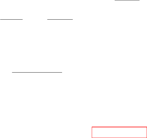
CHAPTER TEN (Phasor Analysis) SOLUTIONS
Engineering Circuit Analysis, 6th Edition Copyright
2002 McGraw-Hill, Inc. All Rights Reserved
36.
2
12
12
out 1 2
If I 2 20 A, I 3 30 A V 80 10 V
II440AV 9030V
Now let I 2.5 60 A and I 2.5 60 A
Let V AI BI 80 10 A(2 20 ) B(3 30 )
90 30
and 90 30 (A B)(4 40 ) A B 12.45 20.21
440
si s out
s s out
ss
ss
j
j
jj
+
=∠ ° =∠− ° → = ∠ °
==∠°→ =−
=∠−° =∠°
=+∴∠°=∠°+∠−°
−
−=+ ∠°∴+= = −
∠°
80 10 3 30
A B A 40 10 B(1.5 50 )
220 220
12.415 20.21 B 40 10 B(1.5 50 )
12.415 20.21 40 10 B(1 1.5 50 )
B(1.1496 88.21 )
30.06 153.82
B 10.800 23.81
1.1496 88.21
26.15 65.61
j
j
j
+
+
∠° ∠− °
∴=+ ∴=∠−°−∠−°
∠° ∠
∴ − − = ∠− °− ∠− °
∴−−∠−°=−∠−°
=∠−°
∠− °
∴= = −
∠− °
=∠−°
∴A 12.415 20.21 10.800 23.81
3.952 65.87
V (3.952 65.87 )(2.5 60 )
(26.15 65.61 ) (2.5 60 ) 75.08 4.106 V
out
jj
+
−
−
=−−+
=∠°
∴= ∠ ° ∠−°
+∠−°∠°=∠−°
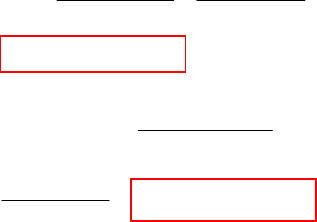
CHAPTER TEN (Phasor Analysis) SOLUTIONS
Engineering Circuit Analysis, 6th Edition Copyright
2002 McGraw-Hill, Inc. All Rights Reserved
37.
(a)
(b)
800: 2 F 625, 0.6H 480
300( 625) 600( 480)
Z300 625 600 480
478.0 175.65
in
jj
jj
jj
j
ω=
µ
→− →
−
∴= +
−+
=+ Ω
300( 312.5)
1600: Z 300 312.5
600( 960) 587.6 119.79
600 960
in
j
j
jj
j
−
ω= = −
+=+Ω
+
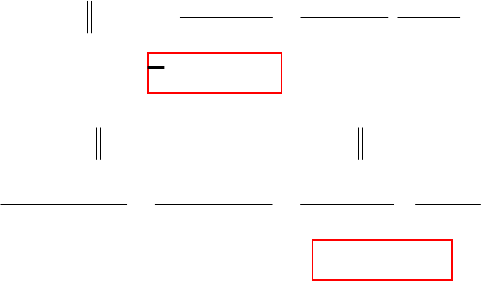
CHAPTER TEN (Phasor Analysis) SOLUTIONS
Engineering Circuit Analysis, 6th Edition Copyright
2002 McGraw-Hill, Inc. All Rights Reserved
38.
(a)
(b)
SC , : 20 10 6.667, (6.667 5) 10
50 66.67 150 200 30 40 4 3
6.667 5 20 15 4 3 4 3
(1.2 1.6)(4 3) 9.6 2.8
in in
ab j j
jjjj
jj jj
ZZ j j j
=−
+++−
===×
++ +−
=∴ + − =+ Ω
50 50 10 10 2 1
(10 10) ( 5) 10 5 2 1 2 1
26 Z226
−−−
+−= =
++−
=− Ω∴ − − Ω
in
jjj
jj jjj
jj
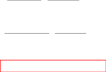
CHAPTER TEN (Phasor Analysis) SOLUTIONS
Engineering Circuit Analysis, 6th Edition Copyright
2002 McGraw-Hill, Inc. All Rights Reserved
39.
120 625
I478.0 175.65 300 625
or I 0.2124 45.82 A
−
∴= ×
+−
=∠−°
j
jj
Thus, i(t) = 212.4 cos (800t – 45.82o) mA.
800: 2 F 625, 0.6H 480
300( 625) 600( 480)
Z300 625 600 480
478.0 175.65
in
jj
jj
jj
j
ω=
µ
→− →
−
∴= +
−+
=+ Ω

CHAPTER TEN (Phasor Analysis) SOLUTIONS
Engineering Circuit Analysis, 6th Edition Copyright
2002 McGraw-Hill, Inc. All Rights Reserved
40.
(a) 3 2mH : V (3 20 ) (3 4) 15,000 33.13 V
Ω=∠−°+=∠°
j
(b) 3 125 F: V (3 20 ) (3 4) 15,000 73.3 VjΩ
µ
=∠− ° − = ∠− °
(c) 3 2mH 125 F: V (3 20 ) 3 9,000 20 V
Ω
µ
=∠−°= ∠−°
(d)
same: 4000 V (3 20 ) (3 8 2)
V (3 20 ) (3 6) 20.12 43.43 V
ω= ∴ = ∠− ° + −
∴=∠−° + = ∠ °
jj
j
CHAPTER TEN (Phasor Analysis) SOLUTIONS
Engineering Circuit Analysis, 6th Edition Copyright
2002 McGraw-Hill, Inc. All Rights Reserved
41.
(a)
(b)
(c)
6
C 20 F, 100
11
Z11 0.005 0.01 0.002
1000 20 10
200 1000
1
Z 196.12 11.310
0.005 0.001
−
=
µ
ω=
==
−+
++××
∴= = ∠− °Ω
+
in
in
jj
j
j
j
222
3
11
100 Z 125
0.005 0.001 1000C 0.008
0.005 (100C 0.001) 0.008 100C 0.001
6.245 10 , C 72.45 F
in jj
−−
ω= ∴ = = ∠=
−+ ∠
∴+− =∴−=
±−× = µ
5
22
25 5 5
55525
55
11
C 20 F Z 100
0.0005 0.1/ 2 10 0.01
0.1 0.1
0.005 2 10 0.0001, 2 10 7.5 10
0.01
2 10 866.0 10 0 2 10 866.0 10 0.1 0
866.0 10 7.5 10 8 10
use sign:
in jj
−
−−−
−−−−
−−−
=µ∴ = = ∠=
−ω+×ω ∠
∴+×ω−= ×−=×
ωω
∴×− × =∴×ω ×ω−=
ω
×± ×+×
−ω=
mm
6
5
556
5
444.3 and 0
410
866.0 10 7.5 10 8 10
use + sign: 11.254 and <0
410
=11.254 and 444.3rad/s
−
−−−
−
=<
×
−×±×+×
ω= =
×
∴ω
CHAPTER TEN (Phasor Analysis) SOLUTIONS
Engineering Circuit Analysis, 6th Edition Copyright
2002 McGraw-Hill, Inc. All Rights Reserved
42.
(a)
(b)
(c)
(d)
2
1111
25 0.0016
11 0.04 900
30
X 45.23 0.002W, 2261rad/s
x
jx
== ∴ +=
+
∴= Ω= ω=
1
11 30
Y25 of tan
30
64.34 0.02 , 3217rad/s
−−
∠=−°=∠ − =
∴= = ωω=
in jxx
x
2
2
22
22
30( 0.02 ) 30 0.092 0.012 18
Z30 0.02 30 0.02 900 0.0004
0.012 25 (900 0.0004 )
0.012 0.01 22,500, 3354rad/s
ω− ω ω+ω
=× =
+ω−ω + ω
∴ω= + ω
∴ω=ω+ ω=
in
jj j
jj
22
26
66
18 10(900 0.0004 ),0.004 18 9000 0,
4500 2.25 10 0
4500 20.25 10 9 10 4500 3354 572.9, 3927rad/s
22
ω= + ω ω − ω+ =
ω− ω+ × =
±×−× ±
ω= = =

CHAPTER TEN (Phasor Analysis) SOLUTIONS
Engineering Circuit Analysis, 6th Edition Copyright
2002 McGraw-Hill, Inc. All Rights Reserved
43. With an operating frequency of
ω
= 400 rad/s, the impedance of the 10-mH inductor is
j
ω
L = j4 Ω, and the impedance of the 1-mF capacitor is –j/
ω
C = -j2.5 Ω.
V240(2.5)5 50A
I 3 2 40 1.9513 41.211 A
∴=∠°− =∠−°
∴=−∠°= ∠− °
c
L
j
2
1
2
1
2
2
22
1
2 40 (R 2.5)
IR4
2 40 (R 2.5)
R4
1.9513 41.21
1.0250 81.21 ( 2.5)
R (1.0250 81.21 ) 2.562 8.789
0.15662R 1.0130R 2.532 0.3915
R 2.532 0.
L
L
j
j
j
j
Rj
jj
∠° −
=+
∠° −
∴+= ∠− °
=∠°−
=∠°+∠−°
=++−
∴= + 22
21
15662R , 4 1.0130R 0.395
R 4.335 , R 3.211
−
+
=−
∴= Ω = Ω
CHAPTER TEN (Phasor Analysis) SOLUTIONS
Engineering Circuit Analysis, 6th Edition Copyright
2002 McGraw-Hill, Inc. All Rights Reserved
44.
ω
= 1200 rad/s.
(a)
(b)
2
2
(200 80) (80 200 )[200 ( 80)]
Z200 (80 ) 40,000 6400 160
X 0 40,000 80 6400 0
1
46,400 80 , 580 C 14.368 F
1200
−× + − + −
==
+− +−+
=∴− + − =
∴==Ω=∴=
µ
in
in
jjxjxjx
jx xx
xx x
xx c
22
2
222
2
80X 200X
Z Z 100
200 (80 X)
6400X 40,000X 10,000
40,000 6400 160X X
0.64X 4X X 160X 46,400
3.64X 160 46,400 0,
160 25,600 675,600 160 837.4
X7.28 7.28
1
X 93.05 ( 0) C 8.956 F
1200C
in in
j
j
X
−
−
==
+−
+
∴=
+−+
∴+=−+
∴+−=
−± + −±
==
∴= > = ∴= µ
CHAPTER TEN (Phasor Analysis) SOLUTIONS
Engineering Circuit Analysis, 6th Edition Copyright
2002 McGraw-Hill, Inc. All Rights Reserved
45. At
ω
= 4 rad/s, the 1/8-F capacitor has an impedance of –j/
ω
C = -j2 Ω, and the 4-H
inductor has an impedance of j
ω
L = j16 Ω.
(a)
(b)
(8 16)(2 2) 16(3 1)
abOC : Z 10 14 10 14
2.378 1.7297
in
jj j
jj
j
+− +
==
++
=− Ω
16 32
abSC: Z (8 2) (2 16) 82216
2.440 1.6362
−
=−+ = +
−+
∴= − Ω
in
in
jj
jj jj
Zj

CHAPTER TEN (Phasor Analysis) SOLUTIONS
Engineering Circuit Analysis, 6th Edition Copyright
2002 McGraw-Hill, Inc. All Rights Reserved
46. f = 1 MHz,
ω
= 2
π
f = 6.283 Mrad/s
2 µF → -j0.07958 Ω = Z1
3.2 µH → j20.11 Ω = Z2
1 µF → -j0.1592 Ω = Z3
1 µH → j6.283 Ω = Z4
20 µH → j125.7 Ω = Z5
200 pF → -j795.8 Ω = Z6
The three impedances at the upper right, Z3, 700 kΩ, and Z3 reduce to –j0.01592 Ω
Then we form Z2 in series with Zeq: Z2 + Zeq = j20.09 Ω.
Next we see 106 || (Z2 + Zeq) = j20.09 Ω.
Finally, Zin = Z1 + Z4 + j20.09 = j26.29 Ω.
CHAPTER TEN (Phasor Analysis) SOLUTIONS
Engineering Circuit Analysis, 6th Edition Copyright
2002 McGraw-Hill, Inc. All Rights Reserved
47.
2H 2,1F 1Let I 1 0 A
V 2V I I 0.5 1 1
V2(11)(1)11
10 1 1 1
V 0.5 0.55
V1111
1
Now 0.5 2 , 0.5S 2H
2
∈
→→− =∠°
∴= ∴=+ =+
∴=++ −=+
∠° −
∴= = =−
+−
→Ω− = →
LcinL
in
in
in
jj
jvj
jjjj
jj
jj
sj
j
CHAPTER TEN (Phasor Analysis) SOLUTIONS
Engineering Circuit Analysis, 6th Edition Copyright
2002 McGraw-Hill, Inc. All Rights Reserved
48.
(a)
(b) ,
106
R 21.2
5
==Ω
in ab
(c)
500,Z 510159
159 9
Y Y 500C
5 9 106 106
9
C 169.81 F
53,000
inRLC
inRLC c
jj j
j
j
ω= = + − = +
−
∴= = ∴==
+
∴= =
µ
,
91
1000 Y 53 5 20 0.5
0.012338 0.12169S or 0.12232 84.21 S
ω= ∴ = + +−
=+ ∠°
in ab jjj
j
CHAPTER TEN (Phasor Analysis) SOLUTIONS
Engineering Circuit Analysis, 6th Edition Copyright
2002 McGraw-Hill, Inc. All Rights Reserved
49.
(a)
(b)
(c)
(d)
62
462
62 6
462
42 6 42
42
0.1
R 550 : Z 500 100 0.001
50,000 0.6 100 0.001
Z100 0.001 100 0.001
5 10 0.0006 (60 50 )
Z10 10
5 10 0.006
R 550 5.5 10
10 10
5.5 10 5 10 10
0.5 10
in in
in
in
in
j
j
jj
jj
j
−
−
−−
−
ω
=Ω =++ω
+ω − ω
∴= ×
+ω−ω
×+ ω+ ω−ω
∴= +ω
×+ ω
∴= =∴×
+ω
+× ω=×× ω
∴× ω= 6 2 10 5
0.5 10 , 10 , 10 rad/s×ω= ω=
642
462
2510
51010
55
10
X 50 0.5 10 0.5 10 10
10 10
0, 2 10 10 0
210 410 410 10 10 rad/s
2
−
−
ω
=Ω= = × + × ω−ω
+ω
=ω−× ω+ =
×±× −×
∴ω= = ∴ω=
in
3
642
82
642
3
82
642 6 62
662
100 0.001 50,000 0.6
G 1.8 10 : Y 50,000 0.6 50,000 0.6
510 610 (50 6)
25 10 0.36
510 610
1.8 10 25 10 0.36
5 10 6 10 4.5 10 648 10
0.5 10 48 10 102.06
−
−
−
−−
−
+ω −ω
=× = ×
+ω −ω
×+× ω+ ω−ω
=×+ ω
×+× ω
∴× = ×+ ω
∴× +× ω= × + × ω
∴× =× ω∴ω=
in in
jj
jj
j
Krad/s
4
82
462
62 4
6
10
B 1.5 10 25 10 0.36
10 37.5 10 54 10
54 10 10 37.5 10 0,
100 81
10 52.23 and 133.95krad/s
108 10
−
−
−
−
−ω
=× =×+ ω
∴ω= × + × ω
∴× ω−ω+ × =
−
ω= ± =
×
in
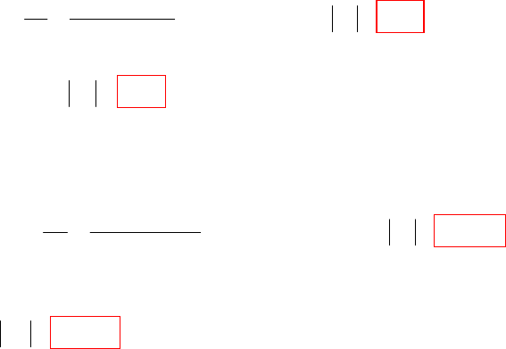
CHAPTER TEN (Phasor Analysis) SOLUTIONS
Engineering Circuit Analysis, 6th Edition Copyright
2002 McGraw-Hill, Inc. All Rights Reserved
50.
(a) 1
11
3
1
I 0.1 30
V 20 23.13 V 20V
Y(34)10
−
∠°
== =∠− °∴=
+j
(b) 21 2
VVV 20V=∴ =
(c)
(d)
3
222
312
3
33
3
3
I Y V (5 2)10 20 23.13 0.10770 1.3286 A
I I I 0.1 30 0.10770 1.3286 0.2 13.740 A
I 0.2 13.740
V 44.72 77.18 V V 44.72V
Y(24)10
j
j
−
−
==+ ×∠−°= ∠−°
∴=+= ∠°+ ∠− °= ∠ °
∠°
∴= = = ∠ °∴ =
−
13
V V V 20 23.13 44.72 77.18 45.60 51.62
V 45.60V
=++∠− °+ ∠ °= ∠ °
∴=
in
in
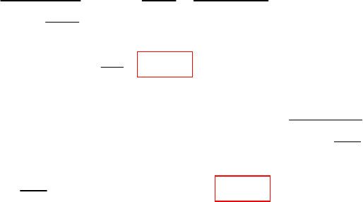
CHAPTER TEN (Phasor Analysis) SOLUTIONS
Engineering Circuit Analysis, 6th Edition Copyright
2002 McGraw-Hill, Inc. All Rights Reserved
51.
(a)
(b)
1
1
11
50 F 20 Y 0.1 0.05
1 1000 1
YR 84
1000 C 0.1 0.05
RC
1
R 8 and C 250 F
4
in
in
jj
jj
j
j
µ
µ
ω
→− Ω∴ = +
=∴−==−
+
−
∴=Ω = =
1
1
111
1
1
2000: 50 F 10 Y 0.1 0.1 500
RC
500
R 5 5 R 5 , C 100 F
C
in
jj
j
jj
ωµ
µ
=→−Ω∴=+=
−
∴− =−∴=Ω =
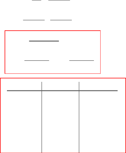
CHAPTER TEN (Phasor Analysis) SOLUTIONS
Engineering Circuit Analysis, 6th Edition Copyright
2002 McGraw-Hill, Inc. All Rights Reserved
52.
(a)
ω Gin Bin
0
1
2
5
10
20
∞
0
0.0099
0.0385
0.2
0.5
0.8
1
0
0.0099
0.1923
0.4
0.5
0.4
0
2
2
2
22
10 10
Z1
10
Y10 10
10
Y100
10
G,B
100 100
in
in
in
in in
j
jj
jj
jj
j
ω
ωω
ωω
ωω
ωω
ω
ωω
ωω
+
=+ =
−
∴×
+−
+
∴= +
==
++
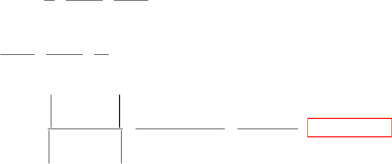
CHAPTER TEN (Phasor Analysis) SOLUTIONS
Engineering Circuit Analysis, 6th Edition Copyright
2002 McGraw-Hill, Inc. All Rights Reserved
53.
11212 11212
12
21 21 2
21212 1 2
2
VV V
5 , 75 5V 3V 3V 5V 5V
353
(5 2)V 2V 75
VVVV10
356
10V 10V 6V 6V 5V 300 4V (5 4)V 300
52 75
4 300 1500 600 300 1200
V52 2 17 30 8
454
vv
jjjjjj
jj
jj j
v
jj
jjjj j j
jj
jj
jj j
jj
−−
−=+ + −=+−−+
−
∴− + =−
−−
++=
−
−++−+=∴+− =
−−
−− −
∴= = =
−−+
−
600 34.36 23.63 V
25 30
j
j=∠°
−
(1)
(2)
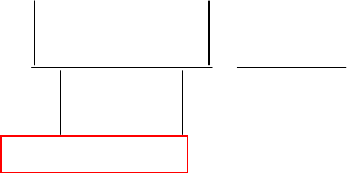
CHAPTER TEN (Phasor Analysis) SOLUTIONS
Engineering Circuit Analysis, 6th Edition Copyright
2002 McGraw-Hill, Inc. All Rights Reserved
54.
3I 5(I I ) 0 2I 5I 0
3(I 5) 5(I I ) 6(I 10) 0
5I (9 5)I 60 15
05
60 15 9 5 75 300
I25 15 18
59 5
13.198 154.23 A
BBD BD
DDBD
BD
B
jj j
jj
jj j
j
jj j
jj j
jj
−−=∴−+=
+− −+ +=
∴+− =−−
−− − −+
==
−−
−
=∠°
CHAPTER TEN (Phasor Analysis) SOLUTIONS
Engineering Circuit Analysis, 6th Edition Copyright
2002 McGraw-Hill, Inc. All Rights Reserved
55.
12
12
20cos1000 V, 20sin1000 V
V200V,V 20V
0.01H 10 , 0.1mF 10
20 20 0, 0.04 2 2 0,
10 25 10
V 25(2 2) 70.71 45 V
( ) 70.71cos(1000 45 )V
ss
ss
xxx x
x
x
vtvt
j
jj
vvvj vj
jj
j
vt t
==
∴=∠° =−
→Ω →−Ω
−+
∴++ = +−=
−
=−=∠−°
∴= −°
CHAPTER TEN (Phasor Analysis) SOLUTIONS
Engineering Circuit Analysis, 6th Edition Copyright
2002 McGraw-Hill, Inc. All Rights Reserved
56.
(a)
(b)
32 2
1
1
3
Assume V 1V V 1 0.5V, I 1 0.5mA
V 1 0.5 (2 0.5)( 0.5) 0.75 1.5V
I 0.75 1.5mA, I 0.75 1.5 2 0.5 2.75 2mA
V 0.75 1.5 1.5 (2.75 2)( 0.5)
100
0.25 2.875V V 34.65 94.
0.25 2.875
in
in
jj
jjj j
jjjj
jj jj
jjj
+
= ∴ =− =−
∴=− +− − = −
∴= − ∴ = − +− = −
∴=−−+ −−
=− − ∴ = = ∠
−− 97 V°
33
22 12
22 2
11
223 233
2
0.5 Assume V 1V I 1A,
V 1 X, I 1 X, I 2 X
V 1 X(2 X)( X)1X 3X,I 1X 3X,I 3X 4
V1X 3X4X X 3X15X (X6X)X6X0
X 6, X 6, Z 2.449K
in
in
c
jjx
jj j
jjj j j jX
jjj j
j
−→− =∴=
=− =− → = −
∴=− +− − =− − =− − =− −
∴=−− − + − =− + − ∴−=
∴= = =− Ω
CHAPTER TEN (Phasor Analysis) SOLUTIONS
Engineering Circuit Analysis, 6th Edition Copyright
2002 McGraw-Hill, Inc. All Rights Reserved
57. Define three clockwise mesh currents i1, i2, i3 with i1 in the left mesh, i2 in the top right
mesh, and i3 in the bottom right mesh.
Mesh 1: 10∠0o + (1 + 1 – j0.25)I1 – (-j0.25)I2 = 0
Mesh 2: – I1 + (1 + 1 + j4)I2 – I3 = 0
Mesh 3: (-j0.25 + 1 + 1)I3 – I2 – (-j0.25I1) = 0
2 0.25 1 10
1240
0.25 1 0
I2 0.25 1 0.25
124 1
0.25 1 2 0.25
10(1 1 0.5)
I0.25(2 0.5) ( 2 0.25 0.25) (2 0.25)(4 1 0.5 8 1)
20 5 I 1.217 75.96 A, ( ) 1.2127cos(100 75.96 )A
815
x
x
xx
j
j
j
jj
j
jj
j
jj jj j jj
jit t
j
−−
−+
−
=−−
−+−
−−
+−
∴= −+−+ + +− +−+−
−
=∴=∠−°= −°
+
CHAPTER TEN (Phasor Analysis) SOLUTIONS
Engineering Circuit Analysis, 6th Edition Copyright
2002 McGraw-Hill, Inc. All Rights Reserved
58.
11 12
12
212 2
12
12
12
V 10 0.25V 0.25V V V 0
(2 0.25) V V 0.25V 10
VVVV 4V0
V(2 4)VV 0
0.25V 0.25V V V V
0.25V V (2 0.25)V 0
2 0.25 1 10
1240
0.25 1 0
V0.25 1 0.25
124 1
0.25 1 2
x
x
x
x
xxx
x
x
jj
jj
j
j
jj
jj
j
j
j
jj
j
jj
−− + +− =
∴− − + =
−+−+ =
−++ − =
−+++−
∴−+− =
−−
−+
−
=−−
−+ −
−−
0.25
10(1 1 0.5)
0.25(2 0.5) ( 2 0.25 0.25) (2 0.25)(4 1 0.5 8 1)
20 5 1.2127 75.96 V
815
1.2127cos(100 75.96 ) V
x
j
jj jj j jj
j
j
vt
+−
=−+−+ + +− +−+−
−
==∠−°
+
∴= − °
CHAPTER TEN (Phasor Analysis) SOLUTIONS
Engineering Circuit Analysis, 6th Edition Copyright
2002 McGraw-Hill, Inc. All Rights Reserved
59.
(a)
(b)
1
11
11
11
1
1
1
R,R0,AV/V0
VAV
IC(VV)
R
V(1 A CR ) CR V
V
VAV (1A CR) CRV
A
CR A
VV
As A , C R
V1A CR V
ooi
isi
f
iffs
o
oi f fs
f
oo
f
sfs
j
jj
jj
jj
j
ω
ωω
ωω
ωω
ω
=∞ = =− >>
+
==−
∴++ =
=− ∴− + + =
∴=− →∞ →−
++
11
11
11
11
1
R
1
RC 11CR
CR
(V AV )
I(1CR)(VV)C,VAV
R
V(1 A)(1 C R ) V CR CR V,
V [(1 A) (1 C R ) C R ] C R V
V[(1 A)(1 C R ) C R ] C R V
A
CR A
V
V(1A)(1
f
ff
ff
f
f
iff s i o i
f
iffsffi
iffffs
off f fs
f
o
s
j
j
jj
jjj
jjj
jjj
j
j
ω
ω
ωω
ωωω
ωωω
ωωω
ω
==
+
+
+
=+=− =−
∴+ + = −
++ + =
∴− + + + =
−
∴=
++
1
1
CR
V
As A ,
CR) CR V 1 CR
f
o
ff f s ff
j
jj
ω
ωω ω
−
→∞ →
++
CHAPTER TEN (Phasor Analysis) SOLUTIONS
Engineering Circuit Analysis, 6th Edition Copyright
2002 McGraw-Hill, Inc. All Rights Reserved
60. Define the nodal voltage v1(t) at the junction between the two dependent sources.
The voltage source may be replaced by a 3∠-3o V source, the 600-µF capacitor by a
–j/ 0.6 Ω impedance, the 500-µF capacitor by a –j2 Ω impedance, and the inductor by a
j2 Ω impedance.
5V2 + 3V2 = 2-
) - (
6.0/100
3-3 - 21
o
1
jj
VVV +
−
∠ [1]
-5V2 =
()
2
2
221
jj
VVV +
−
− [2]
Simplifying and collecting terms,
j2 V1 + (960.1∠ -90.95o) V2 = 6 ∠ 87o [1]
-j2 V1 + 20 V2 = 0 [2]
Solving, we find that V1 = 62.5 ∠ 86.76o mV and V2 = 6.25 ∠ 176.8o mV.
Converting back to the time domain,
v2(t) = 6.25 cos (103t + 176.8o) mV

CHAPTER TEN (Phasor Analysis) SOLUTIONS
Engineering Circuit Analysis, 6th Edition Copyright
2002 McGraw-Hill, Inc. All Rights Reserved
61. Define three clockwise mesh currents: i1(t) in the left-most mesh, i2(t) in the bottom right
mesh, and i3(t) in the top right mesh. The 15-µF capacitor is replaced with a –j/ 0.15 Ω
impedance, the inductor is replaced by a j20 Ω impedance, the 74 µF capacitor is
replaced by a –j1.351 Ω impedance, the current source is replaced by a 2∠0o mA source,
and the voltage source is replaced with a 5∠0o V source.
Around the 1, 2 supermesh: (100 + j20) I1 + (13000 – j1.351) I2 – 5000 I3 = 0
and
-I1 + I2 = 2×10⁻³
Mesh 3: 5∠0o + (5000 – j6.667) I2 – 5000 I3 = 0
Solving, we find that I1 = 1.22∠179.9o mA. Converting to the time domain,
i1(t) = 1.22 cos (104t + 179.9o) mA
Thus, P1000 = [i1(1 ms)]2 • 1000
= (1.025×10⁻⁶)(1000) W = 1.025 W.

CHAPTER TEN (Phasor Analysis) SOLUTIONS
Engineering Circuit Analysis, 6th Edition Copyright
2002 McGraw-Hill, Inc. All Rights Reserved
62. We define an additional clockwise mesh current i4(t) flowing in the upper right-hand
mesh. The inductor is replaced by a j0.004 Ω impedance, the 750 µF capacitor is
replaced by a –j/ 0.0015 Ω impedance, and the 1000 µF capacitor is replaced by a –j/ 2
Ω impedance. We replace the left voltage source with a a 6 ∠ -13o V source, and the
right voltage source with a 6 ∠ 0o V source.
(1 – j/ 0.0015) I1 – I3 = 6 ∠ -13o [1]
(0.005 + j/ 0.0015) I1 + j0.004 I2 - j0.004 I4 = 0 [2]
-I1 + (1 – j/ 2) I3 + j0.5 I4 = -6 ∠ 0o [3]
-j0.004 I2 + j0.5 I3 + (j0.004 – j0.5) I4 = 0 [4]
Solving, we find that
I1 = 0.00144∠ -51.5o A, I2 = 233.6 ∠ 39.65o A, and I3 = 6.64 ∠ 173.5o A.
Converting to the time domain,
i1(t) = 1.44 cos (2t – 51.5o) mA
i2(t) = 233.6 cos (2t + 39.65o) A
i3(t) = 6.64 cos (2t + 173.5o) A
CHAPTER TEN (Phasor Analysis) SOLUTIONS
Engineering Circuit Analysis, 6th Edition Copyright
2002 McGraw-Hill, Inc. All Rights Reserved
63. We replace the voltage source with a 2115 ∠0o V source, the capacitor with a
–j/ 2
π
C1 Ω impedance, and the inductor with a j0.03142 Ω impedance.
Define Z such that Z-1 = 2
π
C1 - j/0.03142 + 1/20
By voltage division, we can write that 6.014 ∠85.76o = 2115 20 +Z
Z
Thus, Z = 0.7411 ∠ 87.88o Ω. This allows us to solve for C1:
2
π
C1 – 1/0.03142 = -1.348 so that C1 = 4.85 F.
CHAPTER TEN (Phasor Analysis) SOLUTIONS
Engineering Circuit Analysis, 6th Edition Copyright
2002 McGraw-Hill, Inc. All Rights Reserved
64. Defining a clockwise mesh current i1(t), we replace the voltage source with a
2115 ∠0o V source, the inductor with a j2
π
L Ω impedance, and the capacitor with a
–j1.592 Ω impedance.
Ohm’s law then yields
()
o
108.132
592.1220
2115
∠=
−+
=Lj
π
I
Thus, 20 =
()
2
2592.12 20 −+ L
π
and we find that L = 253.4 mH.
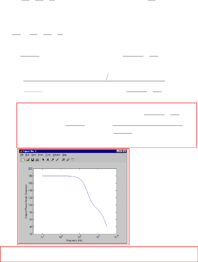
CHAPTER TEN (Phasor Analysis) SOLUTIONS
Engineering Circuit Analysis, 6th Edition Copyright
2002 McGraw-Hill, Inc. All Rights Reserved
65. (a) By nodal analysis:
0 = (V
π
– 1)/ Rs + V
π
/ RB + V
π
/ r
π
+ j
ω
C
π
V
π
+ (V
π
– Vout) j
ω
C
µ
[1]
-gmV
π
= (Vout – V
π
) j
ω
Cµ + Vout / RC + Vout / RL [2]
Simplify and collect terms:
()
S
out
BS R
1
C - CC
r
1
R
1
R
1=
++
++ VV
µπµπ
π
ωω
jj [1]
(-gm + j
ω
C
µ
) V
π
- (j
ω
C
µ
+ 1/RC + 1/RL) Vout = 0 [2]
Define
π
r
1
R
1
R
1
R
1
BS
S
++=
′ and ′
L
R = R
C || RL
Then
()
′
+
′
+
+++
′′
=∆
SL
22
LS R
C
R
CC
C - CC 2C
R R
1-
µπµ
µπµµ ωω
m
gj
And Vout =
()
′
+
′
+
+++
′′
−
SL
22
LS
SSm
R
C
R
CC
C - CC 2C
R R
1-
RCRg
µπµ
µπµµ
µ
ωω
ω
m
gj
j
Therefore, ang(Vout) =
−
−
2
1
tan
SmRg
Cj
µ
ω
-
()
++
′′
′
+
′
+
+−
−
πµµ
µπµ
µ
ω
ω
CC 2C
R R
1-
R
C
R
CC
C
tan
22
LS
SL
1
m
g
(c) The output is ~180o out of phase with the input for f < 105 Hz; only for f = 0 is it
exactly 180o out of phase with the input.
(b)
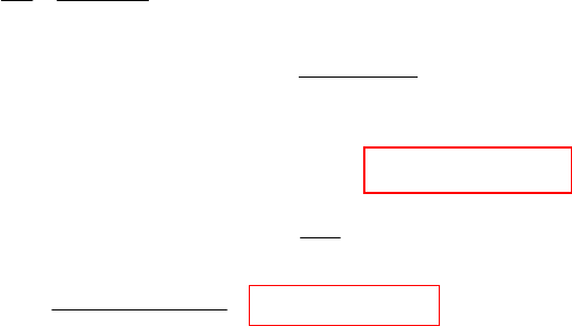
CHAPTER TEN (Phasor Analysis) SOLUTIONS
Engineering Circuit Analysis, 6th Edition Copyright
2002 McGraw-Hill, Inc. All Rights Reserved
66.
,
V 100 V
OC: 0.02V 0
20 10
10
10 (0.05 0.1 0.02) V ,V 0.07 0.1
V 67.11 46.98
V 100 V 32.89 46.98 57.35 55.01 V
100
SC:V 100 I 0.02 100 7A
20
57.35 55.01
Z 4.698 6.711
7
xx
x
xx
x
ab oc x
xSC
th
j
j
jj j
j
j
j
−
−+ − =
−
=++ =
+
∴= +
∴=−= − =∠−°
=∴↓= ×+ =
∠− °
∴= = − Ω
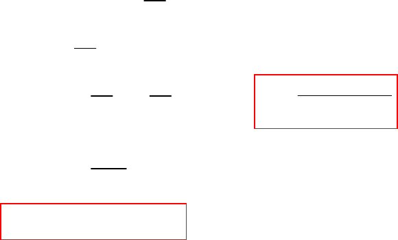
CHAPTER TEN (Phasor Analysis) SOLUTIONS
Engineering Circuit Analysis, 6th Edition Copyright
2002 McGraw-Hill, Inc. All Rights Reserved
67.
V 210 0.5V
1
V(1 ) 2
1
12
V1
Z12
1
At 1, Z 1 1 2 1
1
Y 0.5 0.5
11
LL
in
in
in
in
in
jj
jj
j
j
j
j
j
jj j
j
j
ω
ωω
ω
ω
ω
ω
ω
ω
=∴ =
∴=+ +
=+ +
∴= =+ +
==−+=+
∴= =+
+
R = 500 mΩ, L = 500 mH.
so Yin =
()
12 2−+
ωω
ω
j
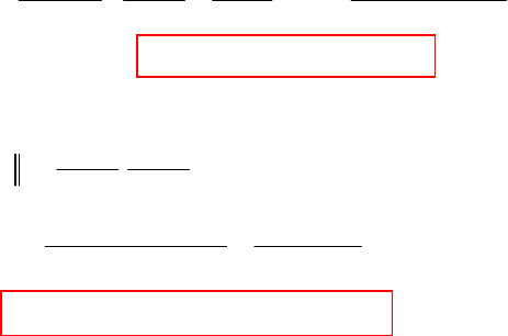
CHAPTER TEN (Phasor Analysis) SOLUTIONS
Engineering Circuit Analysis, 6th Edition Copyright
2002 McGraw-Hill, Inc. All Rights Reserved
68.
(a)
(b) Is:
1
21 2
2 1 0.8 0.4 V
1212
0.8 0.4 10 20
25 11.785 135 V
1 1 0.8 0.4 1.8 0.6
jj
jj
jj
jj
jjj j
+
−
==+∴
+−
+−+
===∠°
−+ + −
so v1(t) = 11.79 cos (1000t + 135o) V.
1
11
(1 1)1 2 1 3 1 15
V: V 0.6 0.2
2121 5 20.60.2
V 5 90 ( ) 5cos(1000 90 )V
s
jjj j
jj j j
vt t
−+− −
×=∴= ×−
−+ +−
∴=∠°∴ = +°
CHAPTER TEN (Phasor Analysis) SOLUTIONS
Engineering Circuit Analysis, 6th Edition Copyright
2002 McGraw-Hill, Inc. All Rights Reserved
69.
,
OC:V 0 V 1 0 V
SC : I V 2I 1 0 1[0.25( 2I ) I ] 2I
1 (0.5 2)I (0.5 1)I
I1
I 0.4 0.8 0.4 0.8
0.5 1 1 0
111 1
R 2.5 , 0.8, L 1.25H
0.4 L L 0.8
I 0.4 0.8 0.8944 63.43 A
Laboc
NL N NN N
NN
N
NN
NN
NN
N
jjjj
jj j
jY j
j
j
jj
j
ω
=∴ =∠°
↓∴ = ∴∠°=− + +
∴= − + = +
∴= =− ∴= =−
+∠°
∴= =Ω = =− = =
=− = ∠− °
CHAPTER TEN (Phasor Analysis) SOLUTIONS
Engineering Circuit Analysis, 6th Edition Copyright
2002 McGraw-Hill, Inc. All Rights Reserved
70.
,200
,100
1211
V 2( 1) ( 2) 2 1 1
11 1111
V 1.4142cos(200 45 ) V
1
100:V , 0.5cos(100 90 )V
2
L
L
LL
jj
jj j j
jjj
t
jv t
ω
−
=+− =+ = =+
++−
∴= +°
== = +°
so vL(t) = 1.414 cos (200t + 45o) + 0.5 cos (100t + 90o) V
CHAPTER TEN (Phasor Analysis) SOLUTIONS
Engineering Circuit Analysis, 6th Edition Copyright
2002 McGraw-Hill, Inc. All Rights Reserved
71.
100
Use superposition. Left: V 100 100 300
300
50 0 V Right: V 100 150V
300 100
V 50 150 158.11 108.43 V
30,000
Z 100 300 150
200
ab
ab
th
th
j
jj
j
jj
jj
j
jj j
j
=−
−
=− ∠ ° = =
−+
∴=−+ = ∠ °
=−= =Ω
−
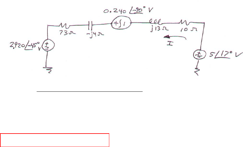
CHAPTER TEN (Phasor Analysis) SOLUTIONS
Engineering Circuit Analysis, 6th Edition Copyright
2002 McGraw-Hill, Inc. All Rights Reserved
72. This problem is easily solved if we first perform two source transformations to yield a
circuit containing only voltage sources and impedances:
Then I = 4131073
45-2.920 90-0.240 175 oo
jj
o
−++
∠+∠+∠
= (6.898∠ -7.019o)/ (83.49 ∠ 6.189o) = 82.62 ∠ -13.21 mA
Converting back to the time domain, we find that
i(t) = 82.62 cos (103t – 13.21o) mA
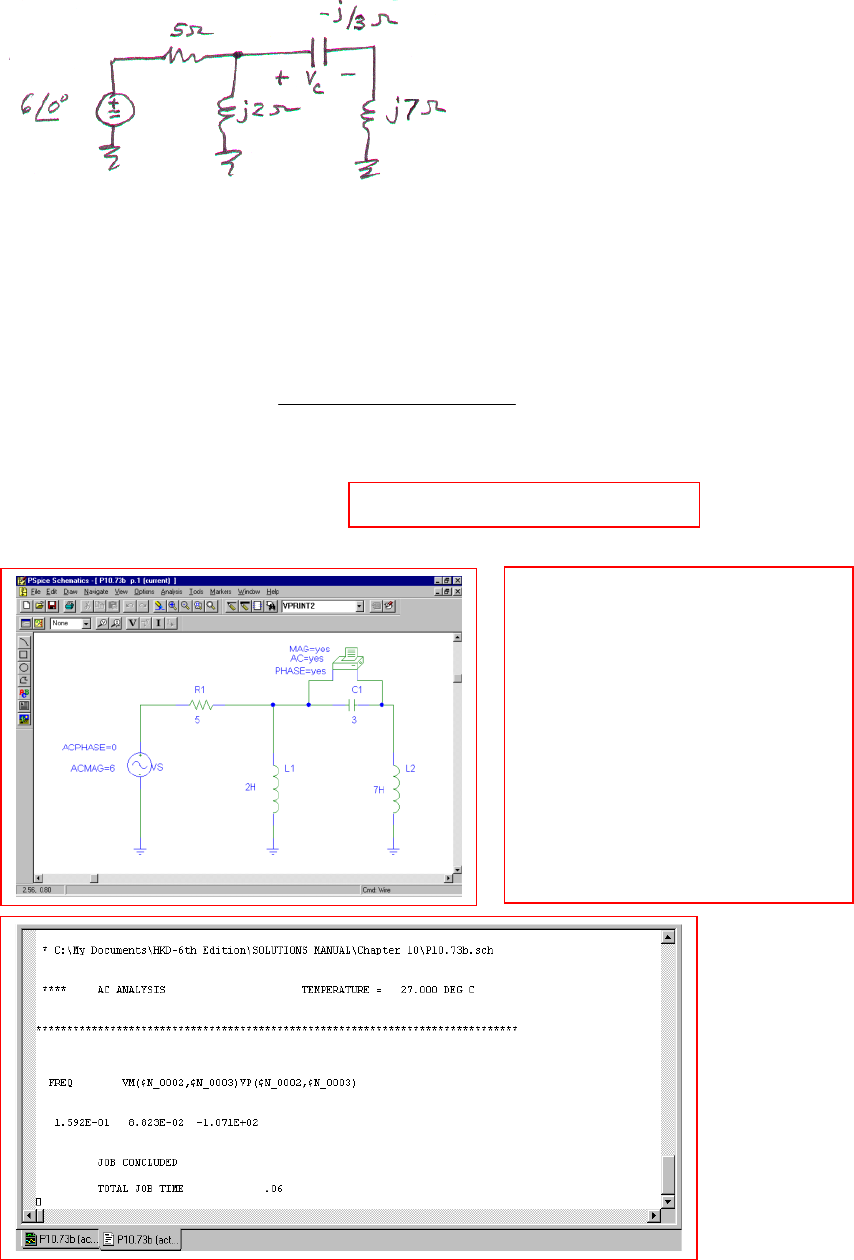
CHAPTER TEN (Phasor Analysis) SOLUTIONS
Engineering Circuit Analysis, 6th Edition Copyright
2002 McGraw-Hill, Inc. All Rights Reserved
73.
(a) There are a number of possible approaches: Thévenizing everything to the left of the
capacitor is one of them.
VTH = 6(j2)/ (5 + j2) = 2.228 ∠ 68.2o V
ZTH = 5 || j2 = j10/ (5 + j2) = 1.857 ∠ 68.2o Ω
Then, by simple voltage division, we find that
V
C = (2.228 ∠ 68.2o) 7 3/ - 2.68857.1
3/
ojj
j
+∠
−
= 88.21 ∠-107.1o mV
Converting back to the time domain, vC(t) = 88.21 cos (t – 107.1o) mV.
(b) PSpice verification.
Running an ac sweep at the
frequency f = 1/2
π
= 0.1592 Hz,
we obtain a phasor magnitude of
88.23 mV, and a phasor angle of
–107.1o, in agreement with our
calculated result (the slight
disagreement is a combination
of round-off error in the hand
calculations and the rounding
due to expressing 1 rad/s in Hz.
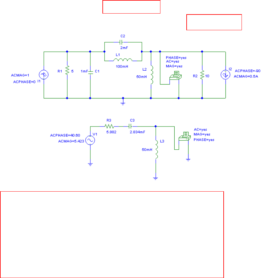
CHAPTER TEN (Phasor Analysis) SOLUTIONS
Engineering Circuit Analysis, 6th Edition Copyright
2002 McGraw-Hill, Inc. All Rights Reserved
74. (a) Performing nodal analysis on the circuit,
Node 1: 1 = V1/ 5 + V1/ (-j10) + (V1 – V2)/ (-j5) + (V1 – V2)/ j10 [1]
Node 2: j0.5 = V2/ 10 + (V2 – V1)/ (-j5) + (V2 – V1)/ j10 [2]
Simplifying and collecting terms,
(0.2 + j0.2) V1 – j0.1 V2 = 1 [1]
-j V1 + (1 + j) V2 = j5 [2]
Solving, we find that V2 = VTH = 5.423 ∠ 40.60o V
ZTH = 10 || [(j10 || -j5) + (5 || -j10)] = 10 || (-j10 + 4 – j2) = 5.882 – j3.529 Ω.
FREQ VM($N_0002,0) VP($N_0002,0)
1.592E+01 4.474E+00 1.165E+02
FREQ VM($N_0005,0) VP($N_0005,0)
1.592E+01 4.473E+00 1.165E+02
(b)
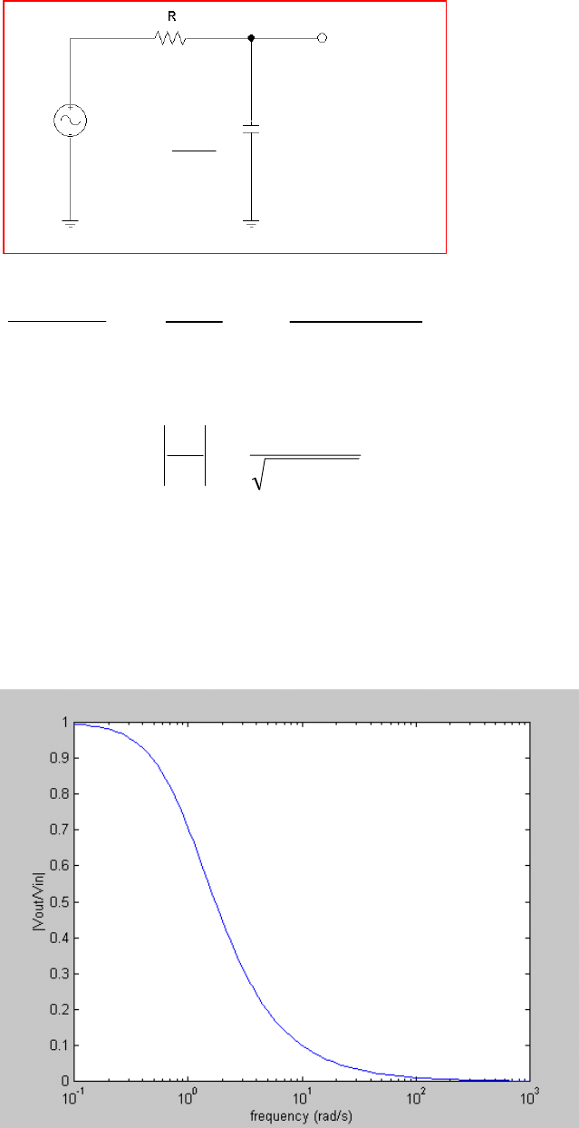
CHAPTER TEN (Phasor Analysis) SOLUTIONS
Engineering Circuit Analysis, 6th Edition Copyright
2002 McGraw-Hill, Inc. All Rights Reserved
75. Consider the circuit below:
Using voltage division, we may write:
Vout = Vin CjR
Cj
ω
ω
/1
/1
+, or RCj
ω
+
=1
1
in
out
V
V
The magnitude of this ratio (consider, for example, an input with unity magnitude and
zero phase) is
()
2
in
out
1
1
RC
ω
+
=
V
V
As
ω
→ 0, this magnitude → 1, its maximum value.
As
ω
→ ∞, this magnitude → 0; the capacitor is acting as a short circuit to the ac signal.
Thus, low frequency signals are transferred from the input to the output relatively
unaffected by this circuit, but high frequency signals are attenuated, or “filtered out.”
This is readily apparent if we plot the magnitude as a function of frequency (assuming R
= 1 Ω and C = 1 F for convenience):
Cj
ω
1
Vin
Vout

CHAPTER TEN (Phasor Analysis) SOLUTIONS
Engineering Circuit Analysis, 6th Edition Copyright
2002 McGraw-Hill, Inc. All Rights Reserved
76. Consider the circuit below:
Using voltage division, we may write:
Vout = Vin CjR
R
ω
/1+, or RCj
RCj
ω
ω
+
=1
in
out
V
V
The magnitude of this ratio (consider, for example, an input with unity magnitude and
zero phase) is
()
2
in
out
1
RC
RC
ω
ω
+
=
V
V
As
ω
→ ∞, this magnitude → 1, its maximum value.
As
ω
→ 0, this magnitude → 0; the capacitor is acting as an open circuit to the ac signal.
Thus, high frequency signals are transferred from the input to the output relatively
unaffected by this circuit, but low frequency signals are attenuated, or “filtered out.”
This is readily apparent if we plot the magnitude as a function of frequency (assuming R
= 1 Ω and C = 1 F for convenience):
Vin
Vout
1/j
ω
C
R
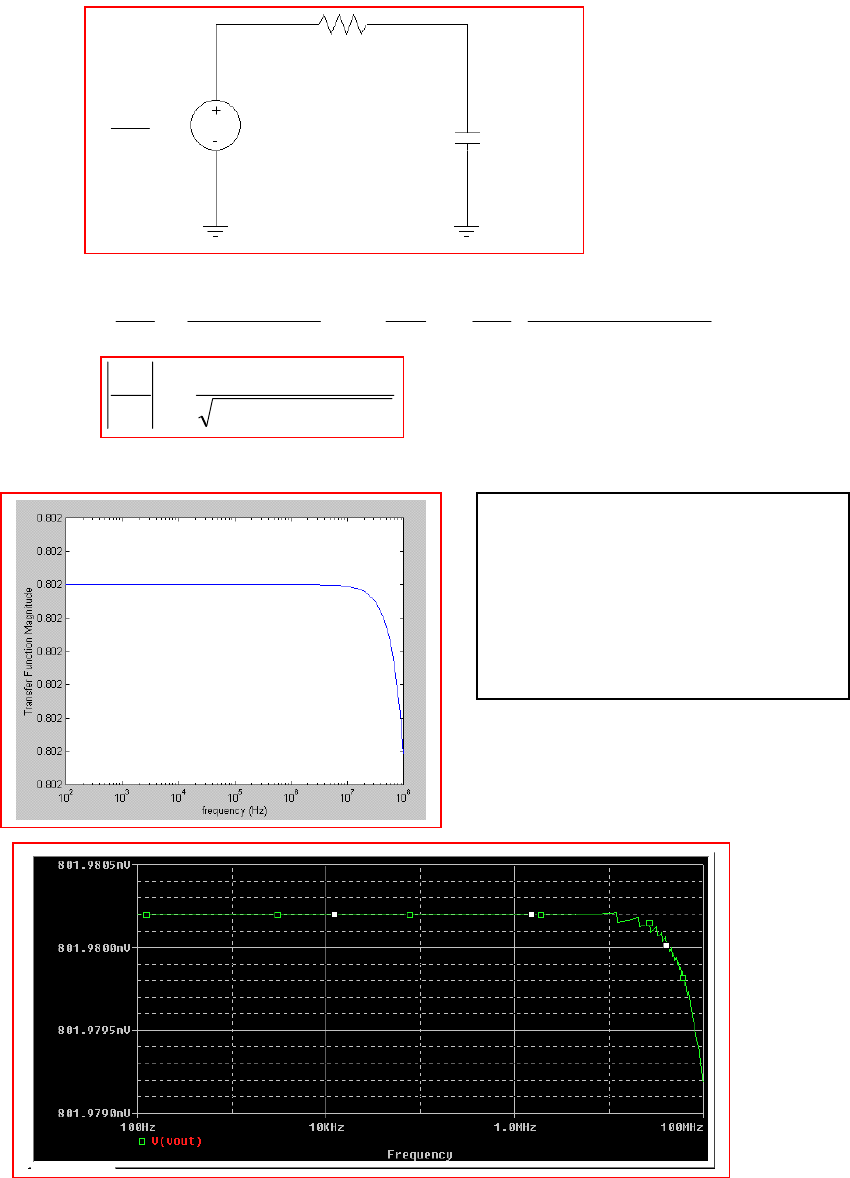
CHAPTER TEN (Phasor Analysis) SOLUTIONS
Engineering Circuit Analysis, 6th Edition Copyright
2002 McGraw-Hill, Inc. All Rights Reserved
77. (a) Removing the capacitor temporarily, we easily find the Thevenin equivalent:
Vth = (405/505) VS and Rth = 100 || (330 + 75) = 80.2 Ω
(b) Cj
Cj
ω
ω
/12.80
1/
505
405
Sout +
=VV so
ω
12
S
out
10532.21
1
505
405
−
×+
=jV
V
and hence 224
S
out
10411.61
0.802
ω
−
×+
=
V
V
(c)
S
505
405 V
80.2 Ω
31.57 fF +
Vout
-
Both the MATLAB plot of the
frequency response and the PSpice
simulation show essentially the
same behavior; at a frequency of
approximately 20 MHz, there is a
sharp roll-off in the transfer
function ma
g
nitude.
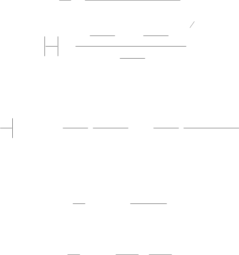
CHAPTER TEN (Phasor Analysis) SOLUTIONS
Engineering Circuit Analysis, 6th Edition Copyright
2002 McGraw-Hill, Inc. All Rights Reserved
78. From the derivation, we see that
µ
µ
ω
ω
)CR||(R1
)CR||(R )R || (Rg-
LC
LCLCm
in
out
j
j
+
+
=
V
V
so that
2
1
2
2
LC
LC
2
2
2
LC
LC
2
2
LC
LC
2
m
in
out
C
RR
RR
1
C
RR
RR
RR
RR
g
+
+
+
+
+
=
µ
µ
ω
ω
V
V
This function has a maximum value of gm (RC || RL) at
ω
= 0. Thus, the capacitors reduce
the gain at high frequencies; this is the frequency regime at which they begin to act as
short circuits. Therefore, the maximum gain is obtained at frequencies at which the
capacitors may be treated as open circuits. If we do this, we may analyze the circuit
of Fig. 10.25b without the capacitors, which leads to
()
BBS
B
LC
LC
m
BS
B
LC
LC
m
frequency low
S
out
Rr)Rr(R
Rr
RR
RR
g-
R|| rR
R|| r
RR
RR
g-
ππ
π
π
π
++
+
=
+
+
=
V
V
The resistor network comprised of rπ, RS, and RB acts as a voltage divider, leading to a
reduction in the gain of the amplifier. In the situation where rπ || RB >> RS, then it has
minimal effect and the gain will equal its “maximum” value of –gm (RC || RL).
(b) If we set RS = 100 Ω, RL = 8 Ω, RC | max = 10 kΩ and rπgm = 300, then we find that
B
B
m
S
t
ou
R || r100
R || r
(7.994) g-
π
π
+
=
V
V
We seek to maximize this term within the stated constraints. This requires a large value
of gm, but also a large value of rπ || RB. This parallel combination will be less than the
smaller of the two terms, so even if we allow RB → ∞, we are left with
ππ
π
r100
2398-
r100
rg
(7.994) - m
S
t
ou
+
=
+
≈
V
V
Considering this simpler expression, it is clear that if we select rπ to be small, (i.e.
r
π << 100), then gm will be large and the gain will have a maximum value of
approximately –23.98.
(c) Referring to our original expression in which the gain Vout/ Vin was computed, we
see that the critical frequency
ω
C = [(RC || RL) Cµ]-1. Our selection of maximum RC,
R
B → ∞, and rπ << 100 has not affected this frequency.

CHAPTER TEN (Phasor Analysis) SOLUTIONS
Engineering Circuit Analysis, 6th Edition Copyright
2002 McGraw-Hill, Inc. All Rights Reserved
79. Considering the
ω
= 2×10⁴ rad/ s source first, we make the following replacements:
100 cos (2×10⁴t + 3o) V → 100 ∠3o V
33 µF → -j1.515 Ω 112 µH → j2.24 Ω 92 µF → -j0.5435 Ω
Then
(V1´ – 100 ∠ 3o)/ 47×103 + V1´/ (-j1.515) + (V1´ – V2´)/ (56×103 + j4.48) = 0 [1]
(V2´ – V1´)/ (56×103 + j4.48) + V2´/ (-j0.5435) = 0 [2]
Solving, we find that
V1´ = 3.223 ∠ -87o mV and V2´ = 31.28 ∠ -177o nV
Thus, v1´(t) = 3.223 cos (2×10⁴t – 87o) mV and v2´(t) = 31.28 cos(2×10⁴t – 177o) nV
Considering the effects of the
ω
= 2×10⁵ rad/ s source next,
100 cos (2×10⁵t - 3o) V → 100 ∠-3o V
33 µF → -j0.1515 Ω 112 µH → j22.4 Ω 92 µF → -j0.05435 Ω
Then
V1"/ -j0.1515 + (V1" – V2")/ (56×103 + j44.8) = 0 [3]
(V2" – V1")/ (56×103 + j44.8) + (V2" – 100 ∠ 3o)/ 47×103 + V2"/ (-j0.05435) = 0 [4]
Solving, we find that
V1" = 312.8 ∠ 177o pV and V2" = 115.7 ∠ -93o µV
Thus,
v1"(t) = 312.8 cos (2×10⁵t + 177o) pV and v2"(t) = 115.7 cos(2×10⁵t – 93o) µV
Adding, we find
v1(t) = 3.223×10⁻³ cos (2×10⁴t – 87o) + 312.8×10⁻¹² cos (2×10⁵t + 177o) V and
v2(t) = 31.28×10⁻⁹ cos(2×10⁴t – 177o) + 115.7×10⁻¹² cos(2×10⁵t – 93o) V

CHAPTER TEN (Phasor Analysis) SOLUTIONS
Engineering Circuit Analysis, 6th Edition Copyright
2002 McGraw-Hill, Inc. All Rights Reserved
80. For the source operating at
ω
= 4 rad/s,
7 cos 4t → 7∠ 0o V, 1 H → j4 Ω, 500 mF → -j0.5 Ω, 3 H → j12 Ω, and 2 F → -j/ 8 Ω.
Then by mesh analysis, (define 4 clockwise mesh currents I1, I2, I3, I4 in the top left, top
right, bottom left and bottom right meshes, respectively):
(9.5 + j4) I1 – j4 I2 – 7 I3 - 4 I4 = 0 [1]
-j4 I1 + (3 + j3.5) I2 – 3 I4 = -7 [2]
-7 I1 + (12 – j/ 8) I3 + j/ 8 I4 = 0 [3]
-3 I2 + j/ 8 I3 + (4 + j11.875) I4 = 0 [4]
Solving, we find that I3 = 365.3 ∠ -166.1o mA and I4 = 330.97 ∠ 72.66o mA.
For the source operating at
ω
= 2 rad/s,
5.5 cos 2t → 5.5∠ 0o V, 1 H → j2 Ω, 500 mF → -j Ω, 3 H → j6 Ω, and 2 F → -j/ 4 Ω.
Then by mesh analysis, (define 4 clockwise mesh currents IA, IB, IC, ID in the top left, top
right, bottom left and bottom right meshes, respectively):
(9.5 + j2) IA – j2 IB – 7 IC – 4 ID = 0 [1]
-j2 IA + (3 + j) IB – 3 ID = -7 [2]
-7 IA + (12 – j/ 4) IC + j/ 4 ID = 0 [3]
-3 I2 + j/ 4 IC + (4 + j5.75) ID = 0 [4]
Solving, we find that IC = 783.8 ∠ -4.427o mA and ID = 134 ∠ -25.93o mA.
V1´ = -j0.25 (I3 – I4) = 0.1517∠131.7o V and V1" = -j0.25(IC – ID) = 0.1652∠-90.17o V
V2´ = (1 + j6) I4 = 2.013∠155.2o V and V2" = (1 + j6) ID = 0.8151∠54.61o V
Converting back to the time domain,
v
1(t) = 0.1517 cos (4t + 131.7o) + 0.1652 cos (2t - 90.17o) V
v
2(t) = 2.013 cos (4t + 155.2o) + 0.8151 cos (2t + 54.61o) V
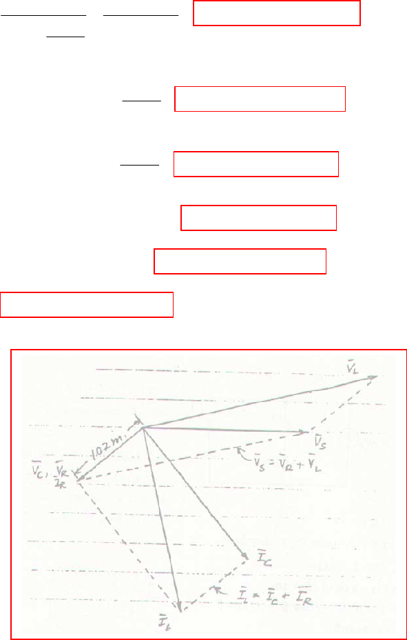
CHAPTER TEN (Phasor Analysis) SOLUTIONS
Engineering Circuit Analysis, 6th Edition Copyright
2002 McGraw-Hill, Inc. All Rights Reserved
81.
(a) 100 100(2 1)
I 57.26 76.76 (2.29 )
22.5 3
2.5 21
L
jin
j
jj
−
===∠−°
−+
+−
1
I (57.26 76.76 ) 25.61 140.19 (1.02 )
21
R
jin
j
−
=∠−° =∠−°
−
2
I (57.26 76.76 ) 51.21 50.19 (2.05 )
21
cin
j
=∠−° =∠−°
−
V 2.5 57.26 90 76.76 143.15 13.24 (2.86 )
Lin=× ∠°− °= ∠ °
V 2 25.61 140.19 51.22 140.19 (1.02 )
Rin= × ∠− °= ∠− °
V 51.21 140.19 (1.02 )
cin=∠− °
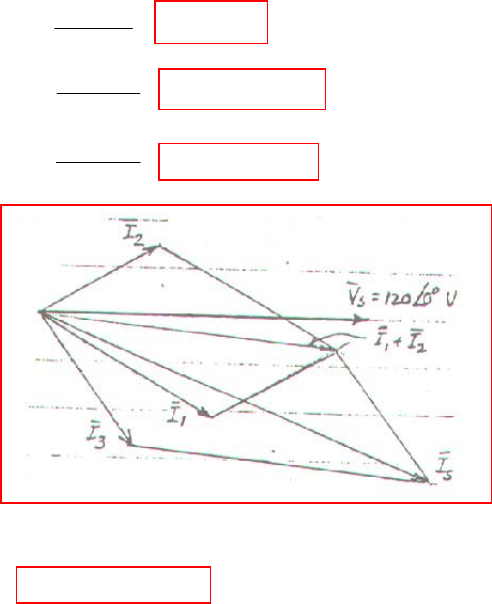
CHAPTER TEN (Phasor Analysis) SOLUTIONS
Engineering Circuit Analysis, 6th Edition Copyright
2002 McGraw-Hill, Inc. All Rights Reserved
82.
(a)
(b)
(c)
1
2
3
120
I 3 30 A
40 30
120
I 2.058 30.96 A
50 30
120
I 2.4 53.13 A
30 40
j
j
==∠−°
∠°
==∠°
−
==∠−°
+
123
IIII
6.265 22.14 A
s=++
=∠−°
CHAPTER TEN (Phasor Analysis) SOLUTIONS
Engineering Circuit Analysis, 6th Edition Copyright
2002 McGraw-Hill, Inc. All Rights Reserved
83.
12
12 1 2
12
22 2
I5A,I7A
I I 10 0 , I lags V,I leads V
I lags I . Use 2.5A /
[Analytically: 5 7 10
5cos 5sin 7cos 7sin
sin 1.4sin
5 1 1.4 sin 7 1 1sin 10
By SOLVE, 40.54 27.66 ]
in
jj
αβ
αα
ββ
αβ
ββ
αβ
==
+=∠°
∠+∠=
=+ ++
∴=−
∴− +− =
=− ° = °

CHAPTER TEN (Phasor Analysis) SOLUTIONS
Engineering Circuit Analysis, 6th Edition Copyright
2002 McGraw-Hill, Inc. All Rights Reserved
84. V1 = 100∠0o V, |V2| = 140 V, |V1 + V2| = 120 V.
Let 50 V = 1 inch. From the sketch, for ∠V2 positive,
V
2 = 140∠122.5o. We may also have V2 = 140∠-122.5o V
[Analytically: |100 + 140∠
α
| = 120
so | 100 + 140 cos
α
+ j140 sin
α
| = 120
Using the “Solve” routine of a scientific calculator,
α
= ±122.88o.]

CHAPTER 11 SOLUTIONS
Engineering Circuit Analysis, 6th Edition Copyright
2002 McGraw-Hill, Inc. All Rights Reserved
1.
6
22
50( 80)
10 80 , 42.40 32.01
500 25 50 80
84.80 32.01 V, 1.696 32.01 A
1.0600 57.99 A
( / 2ms) 84.80cos(45 32.01 )2cos 45 116.85W
50 1.696 cos (45 32.01 ) 136.55W
84.80cos(45 32
c
R
c
s
R
c
j
j
jj
p
p
p
π
−
==−Ω =∠−°Ω
×−
∴ = ∠− ° = ∠− °
=∠°
=°−°°=
=× °− °=
=°−
Z
VI
I
.01 ) 1.060cos(45 57.99 ) 19.69W°= °+ °=−
CHAPTER 11 SOLUTIONS
Engineering Circuit Analysis, 6th Edition Copyright
2002 McGraw-Hill, Inc. All Rights Reserved
2.
(a)
(b)
2242
42 4 2
11
4H: 2 1 4(4 ) 16 , 4(4 4 1)
22
8 8 2 (3) (1) 83 83 2 81812 576 J
L
LLL
it vLi t tw Li t t
wtt w w
′
=−∴== = = =× −+
∴ = − +∴ − = × −× + −×+×− =
233
11
1222
0.2F: (2 1) 25 25 5 1 2
0.2 3 3 3
10 10 61 61
(2) 8 10 5 2 V P (2) 7 142.33W
333 3
t
t
c
cc
vtdttt tt
v
=−+=−+=−−−+
∴=×−−++=∴=×=
∫
CHAPTER 11 SOLUTIONS
Engineering Circuit Analysis, 6th Edition Copyright
2002 McGraw-Hill, Inc. All Rights Reserved
3. 2
1,2
R1
(0) 2V, (0) 4A, 2, 3, 2 1 1, 3
2L LC
co
vi s
αω
=− = =====−±=−−
(a)
(b) 0.2 0.6 0.2 0.6
P (0.2) (3 5 )( 5 ) 0.5542W
ceeee
−− −
=− −+=−
(c) 0.4 1.2 1.2 0.4
P (0.4) (3 5 )(5 ) 0.4220W
ceeee
−−−−
=− −=
3
3
333
3
1
AB AB4;(0) (0)(442)14
1
A38 14B5,A 1, 5 A
3( 5 ) 23( 5 ) 2 35 52
35 P(0)(35)(15)8W
tt
L
tt
ttt ttt t t
co
o
tt
cc
ie e i v
ie e
veedtee ee
ve e
−− + +
−−
−− −− − −
−− +
=+∴+= = =−××+=−
∴− − =− ∴ = =− =− +
∴+ = − + − = − − = − − + −
∴= − ∴ =− −+=−
∫
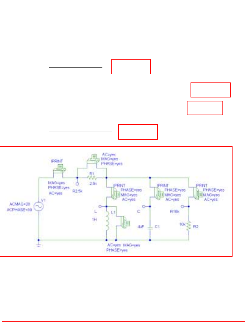
CHAPTER 11 SOLUTIONS
Engineering Circuit Analysis, 6th Edition Copyright
2002 McGraw-Hill, Inc. All Rights Reserved
4. We assume the circuit has already reached sinusoidal steady state by t = 0.
2.5 kΩ → 2.5 kΩ, 1 H → j1000 Ω, 4 µF → -j250 Ω, 10 kΩ → 10 kΩ
Zeq = j1000 || -j250 || 10000 = 11.10 – j333.0 Ω
Veq = V 54.50631.2
0.33310.112500
)0.33310.11)(3020( o
∠=
−+
−∠
j
j
I10k = mA 50.54- 2631.0
10000
o
eq ∠=
V I1 H = mA 140.5- 631.2
1000
o
eq ∠=
j
V
I
4 µF = mA 46.93 52.10
250
o
eq ∠=
−j
V V2.5k = V 55.3774.19
0.33310.112500
)2500)(3020( o
∠=
−+
∠
j
Thus, P2.5k =
[]
mW 97.97
2500
55.37cos74.19 2
o=
P
1 H =
()
[
]
[]
mW 3.395- )5.140cos(102.631 54.50cos631.2 o-3
o=−×−
P
4 µF =
(
)
[
]
[
]
mW 13.58 )cos(39.461010.52 54.50cos631.2 o-3o =×−
P
2.5k =
()
[]
W 279.6
10000
54.50cos631.2 2
o
µ
=
−
FREQ IM(V_PRINT1) IP(V_PRINT1)
1.592E+02 7.896E-03 3.755E+01
FREQ VM(R2_5k,$N_0002)VP(R2_5k,$N_0002)
1.592E+02 1.974E+01 3.755E+01
FREQ IM(V_PRINT2) IP(V_PRINT2)
1.592E+02 2.628E-03 -1.405E+02
FREQ VM(L,0) VP(L,0)
1.592E+02 2.629E+00 -5.054E+01
FREQ IM(V_PRINT11) IP(V_PRINT11)
1.592E+02 1.052E-02 3.946E+01
FREQ IM(V_PRINT12) IP(V_PRINT12)
1.592E+02 2.629E-04 -5.054E+01
CHAPTER 11 SOLUTIONS
Engineering Circuit Analysis, 6th Edition Copyright
2002 McGraw-Hill, Inc. All Rights Reserved
5.
rad rad
,
8
8
40 53.13
50A,C 4, 8(3 4) 11 4
3.417 33.15 17.087 33.15 ,
17.087cos(25 33.15 )V
P (0.1) 17.087cos(2.5 33.147 ) 5cos2.5 23.51 W
17.087 cos(25 33.15 )
8
(0.1) 2.136c
sin
s
s
s abs
ijj
j
vt
it
i
∠− °
→∠° →− Ω = − = −
=∠−°∴= ∠−°
=−°∴
=− − ° × =−
=−°∴
=
Z
V
rad
2
8,
3
rad
3
2
3,
os(2.5 33.15 ) 0.7338 A
P 0.7338 8 4.307 W;
17.087 33.15 3.417 19.98 A
34
(0.1) 3.417cos(2.5 19.98 ) 3.272A
P 3.272 3 32.12 W
4(3.417 19.983 ) 13.67 70.02 ,
(0.1) 13.67
abs
abc
c
c
j
i
j
v
−°=−
∴= ×=
∠− °
==∠°
−
∴= +°=− ∴
=×=
=− ∠ ° = ∠− °
=
I
V
rad
,
0cos(2.5 70.02 ) 3.946V
P 3.946( 3.272) 12.911 W ( 0)
cabc
−°=
∴= − =− Σ=
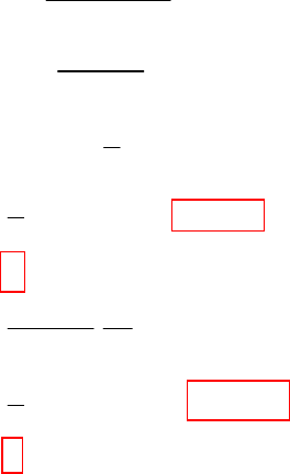
CHAPTER 11 SOLUTIONS
Engineering Circuit Analysis, 6th Edition Copyright
2002 McGraw-Hill, Inc. All Rights Reserved
6.
,
2
4,
10
2
10,
5(10 5)
4 4 2.5 5 6.5 5
10
100 12.194 37.57 A
6.5 5
1
P 100 12.194cos37.57 483.3W
2
1
P (12.194) 4 297.4W,
2
P0
100 5 6.097 52.43 so
6.5 5 10
1
P (6.097) 10 185.87
2
in
s
s abs
abs
cabs
abs
jj jj
j
j
j
−
=+ =+ + = + Ω
∴= = ∠− °
+
∴=−×× °=−
==
=
==∠°
+
=×=
Z
I
I
W
P 0 ( 0)
L=Σ=
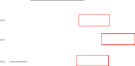
CHAPTER 11 SOLUTIONS
Engineering Circuit Analysis, 6th Edition Copyright
2002 McGraw-Hill, Inc. All Rights Reserved
7.
10,
10,
2
820
40 30
(10 10) 52.44 69.18 V
550 8 20
1
P 10 52.44cos69.18 93.20 W
2
1
P 10 52.44cos(90 69.18 ) 245.08 W
2
1 52.44
P 8cos( 20 ) 161.51 W ( )
28
gen
jgen
abs gen abs
j
∠−
∠°
=+ = ∠ °
∠°+∠− °
=×× °=
=×× °− °=
=−°=Σ=Σ
V
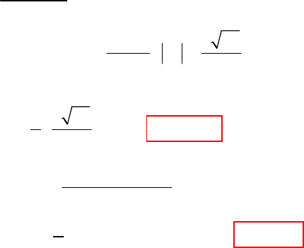
CHAPTER 11 SOLUTIONS
Engineering Circuit Analysis, 6th Edition Copyright
2002 McGraw-Hill, Inc. All Rights Reserved
8.
1
331343
0.1 0.3
25 529
Ignore 30 on , 5 ,
68 10
R
sR R
jj
j
j
j
=+ =++ =+ Ω
−
+
°= =
+
Z
VI I
(a)
2
3
1529
P 3 10.875 W
210
Ω
=×=
(b)
,
(2 5)(4 3)
V 5 0 13.463 51.94 V
68
1
P 13.463 5cos 51.94 20.75 W
2
s
sgen
jj
j
++
=∠° = ∠ °
+
∴=× × °=
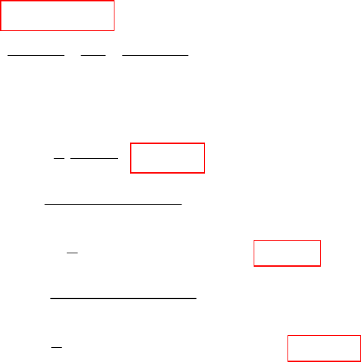
CHAPTER 11 SOLUTIONS
Engineering Circuit Analysis, 6th Edition Copyright
2002 McGraw-Hill, Inc. All Rights Reserved
9.
10 5
10 10 10
10
10
2
10
50
50
50
PP0,
50 50 0
10 10 5
( 0.1 0.1 0.2) 5 10 0
79.06 16.57 V
1 79.06
P 312.5 W;
210
79.06 161.57 50 12.75 78.69 A
10
1
P 50 12.748cos78.69 62.50 W
2
79.06 161.57
jj
V
j
j
jj
jjj
j
−
Ω
==
−−
++ =
−
∴−++ ++=
∴= ∠ °
==
∠°−
==∠°
∴=×× °=
∠°
=
VVV
V
V
I
I
50
50 15.811 7.57 :
5
1
P 50 15.811cos (90 71.57 ) 375.0 W
2
j
j
j
−=∠−°
−
=× × °+ °=−
CHAPTER 11 SOLUTIONS
Engineering Circuit Analysis, 6th Edition Copyright
2002 McGraw-Hill, Inc. All Rights Reserved
10.
20 2,
23
3602212
514 60, 0
32
22 30,2(23) 0
60 14
02 3 120 180 9.233 83.88 V
514
10 15 28
22 3
560
20 5.122 140.9 V
18 15
1
P 9.233 2 5
2
xxc
c
xxcc
cx c
xc
cx c x c
x
c
gen
j
jj
jj
j
j
j
−−
+=
−+ − =
−
∴− = + =
−
∴−+ =−++ =
−
++
== =∠−°
−+−
−+
−
==∠−°∴
−+
=× ××
VVV
V
VVVV
VV V
VV
VV V V V
V
V
.122cos( 83.88 140.19 ) 26.23 W−°+ °=
CHAPTER 11 SOLUTIONS
Engineering Circuit Analysis, 6th Edition Copyright
2002 McGraw-Hill, Inc. All Rights Reserved
11.
(a) X 0 R 0
in L th j=∴ = +Z
(b) R ,X independent R X
LL L th th th
j
∗
∴= = −ZZ
(c)
2
22
V
1
R fixed P R R X
2(R R ) (X X )
th
LL LLLth
th L th L
j∴= × ∴ = −
+++ Z
(d)
(e) 22
X0R RX
L L th th th
=∴ = + =Z
222
22
2
22
222 2
22 2 2
2P RL
X fixed, Let X X (R R )
RR 2R(RR)
0
(R R )
R 2RR R 2RR 2R 0
RR R(XX)
L
LLth
th L
th
th L L th L
Lth L
th th L L th L L
Lth ththL
af a
a
df
dR a
a
a
+=∴= = ++
++− +
==
++
+++−==
∴= += + +
V
CHAPTER 11 SOLUTIONS
Engineering Circuit Analysis, 6th Edition Copyright
2002 McGraw-Hill, Inc. All Rights Reserved
12. 10
120 107.33 116.57 V
10 5
10(10 15) 814
10 5
th
th
j
jj j
j
−
==∠−°
+
−+
==−Ω
+
V
Z
(a) 8 15
Lj∴=+ΩZ
(b)
2
,max
107.33 116.57
16
1 107.33
P 8 180 W
216
L
L
∠− °
=∴
=×=
I
CHAPTER 11 SOLUTIONS
Engineering Circuit Analysis, 6th Edition Copyright
2002 McGraw-Hill, Inc. All Rights Reserved
13.
22
2
22
R R 8 14 16.125
1 107.33
P 16.125 119.38W
2(8 16.125) 14
Lth L
L
=∴=+= Ω
=×=
++
Z

CHAPTER 11 SOLUTIONS
Engineering Circuit Analysis, 6th Edition Copyright
2002 McGraw-Hill, Inc. All Rights Reserved
14.
9.6 4.8I 1.92 I 4.8I
9.6
I5
1.92
V (0.6 5)8 24V
1
P 24 1.6 5 96 W ( )
2
xxx
x
o
jj
gen
−=− − −+
∴= =
∴= × =
∴=×××=
CHAPTER 11 SOLUTIONS
Engineering Circuit Analysis, 6th Edition Copyright
2002 McGraw-Hill, Inc. All Rights Reserved
15.
(a)
(b)
max
480 80 60
80 60 80 60 80 60
28.8 38.4 28.8 38.4
th
L
jj
jjj
jj
−
==
+−
=+ Ω∴ =− Ω
Z
Z
22
,max 2
5(28.8 38.4) 144 192V,
144 192
2 28.8
1 144 192
and P 28.8 250 W
24 28.8
th
L
L
jj
j
=+=+
+
∴= ×
+
=×=
×
V
I

CHAPTER 11 SOLUTIONS
Engineering Circuit Analysis, 6th Edition Copyright
2002 McGraw-Hill, Inc. All Rights Reserved
16. Zeq = (6 – j8) || (12 + j9) = 8.321 ∠ -19.44o W
Veq = (5 ∠-30o) (8.321 ∠ -19.44o) = 41.61 ∠ -49.44o V
P
total = ½ (41.61)(5) cos (-19.44o) = 98.09 W
I6-j8 = Veq / (6 – j8) = 4.161 ∠ 3.69o A
I4+j2 = I8+j7 = Veq/ 12+j9 = 2.774 ∠ -86.31o A
P
6-j8 = ½ (41.61)(4.161) cos (-49.44o – 3.69o) = 51.94 W
P
4+j2 = ½ (2.774)2 (4) = 15.39 W
P
8+j7 = ½ (2.774)2 (8) = 30.78 W
Check: Σ = 98.11 W (okay)
CHAPTER 11 SOLUTIONS
Engineering Circuit Analysis, 6th Edition Copyright
2002 McGraw-Hill, Inc. All Rights Reserved
17.
22
,max 2
10(20)
10
100 20 40, 4 8
20 10 20 10
R R 8.944
12040
P 8.944 38.63W
2(4 8.944) 64
th th
Lth L
L
j
jjj
jj
==+==+Ω
++
∴= ∴= Ω
+
∴= ×=
++
VZ
Z
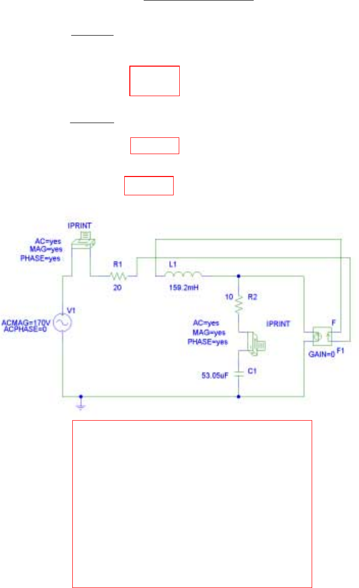
CHAPTER 11 SOLUTIONS
Engineering Circuit Analysis, 6th Edition Copyright
2002 McGraw-Hill, Inc. All Rights Reserved
18. We may write a single mesh equation: 170 ∠0o = (30 + j10) I1 – (10 – j50)(-λI1)
Solving,
I1 =
λλ
50101030
0170 o
jj −++
∠
(a) λ = 0, so I1 = A 18.43-5.376
1030
0170 o
o∠=
+
∠
j and, with the same current flowing
through both resistors in this case,
P
20 = ½ (5.376)2 (20) = 289.0 W
P
10 = ½ (5.376)2 (10) = 144.5 W
(b) λ = 1, so I1 = A 543.005
4040
0170 o
o∠=
−
∠
j
P
20 = ½ (3.005)2 (20) = 90.30 W
The current through the 10-Ω resistor is I1 + λI1 = 2 I1 = 6.01 ∠ 45o so
P
10 = ½ (6.01)2 (10) = 180.6 W
(c)
(a)
FREQ IM(V_PRINT3) IP(V_PRINT3)
6.000E+01 5.375E+00 -1.846E+01
FREQ IM(V_PRINT4) IP(V_PRINT4)
6.000E+01 5.375E+00 -1.846E+01
(b)
FREQ IM(V_PRINT3) IP(V_PRINT3)
6.000E+01 6.011E+00 4.499E+01
FREQ IM(V_PRINT4) IP(V_PRINT4)
6.000E+01 3.006E+00 4.499E+01
CHAPTER 11 SOLUTIONS
Engineering Circuit Analysis, 6th Edition Copyright
2002 McGraw-Hill, Inc. All Rights Reserved
19. (a) Waveform (a): Iavg = A 667.1
3
)1(0)1)(5()1)(10( =
+−+
Waveform (b): Iavg = A 5
2
)1(0)1)(20(
2
1
=
+
Waveform (c):
I
avg =
()
3
310
0
3
3
3
10
0 33
102
cos
2
104
108-
104
2
8sin
101
1
−
−
×
×
×=
×× −
−
−− ∫t
dt
t
π
π
π
=
()
A
16
10
16
ππ
=−−
(b) Waveform (a): 22
avg A 41.67
3
(0)(1)(25)(1)(100)(1)
I =
++
=
Waveform (b): i(t) = -20×103 t + 20
i2(t) = 4×10⁸ t2 – 8×10⁵ t + 400
()
dttt
∫+××
×
=-3
10
0
528
3-
2
avg 400 108 - 104
102
1
I
=
() () ()
2
3-
3
2
3
5
3
3
8
3- A 66.67
102
0.1333
10400 10
2
108
- 10
3
104
102
1=
×
=
+
××
×
−−−
Waveform (c):
()
()
2
3
3
3
10
0
3
3
3
10
0 3
2
3
2
avg
A 32
102
sin
2
10
1064
102
10sin
-
2
1064
104
2
64sin
101
1
I
3
3
=
×
−×=
×
×
×=
××
=
−
−−
−
−
∫
π
π
π
ππ
tt
dt
t
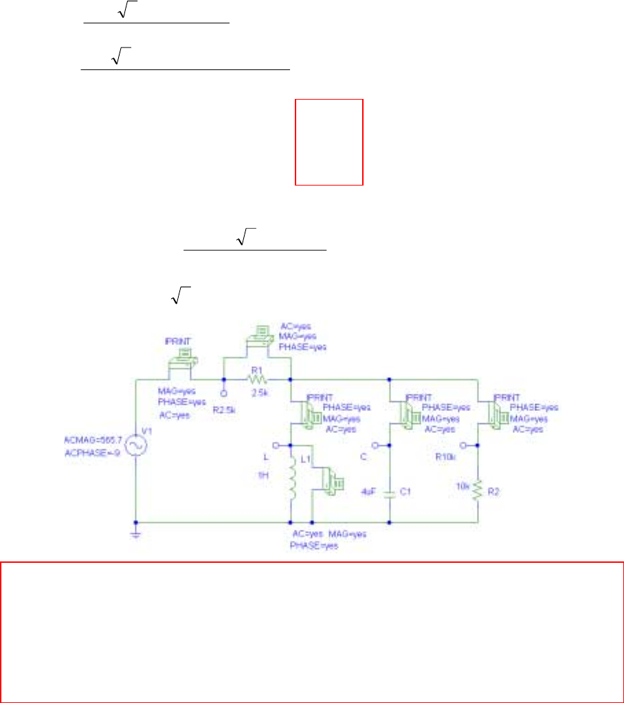
CHAPTER 11 SOLUTIONS
Engineering Circuit Analysis, 6th Edition Copyright
2002 McGraw-Hill, Inc. All Rights Reserved
20. At
ω
= 120π, 1 H → j377 Ω, and 4 µF → -j663.1 Ω
Define Zeff = j377 || -j663.1 || 10 000 = 870.5 ∠ 85.01o Ω
V2.5k =
(
)
V 27.61- 520.4
85.01 870.5 2500
2500 92400 o
o
o∠=
∠+
−∠
V
10k =
(
)
()
V 40.75 181.2
85.01 870.5 2500
85.01 870.5 92400 o
o
oo ∠=
∠+
∠−∠
Thus, P2.5k = ½ (520.4)2 / 2 500 = 54.16 W
P
10k = ½ (181.2)2 / 10 000 = 1.642 W
P
1H = 0
P
4µF = 0 (A total absorbed power of 55.80 W.)
To check, the average power delivered by the source:
Isource = A 27.61- 0.2081
85.01870.52500
92400 o
o
o∠=
∠+
−∠
and Psource = ½ ( 2400 )(0.2081) cos (-9o + 27.61o) = 55.78 W (checks out).
FREQ IM(V_PRINT1) IP(V_PRINT1)
6.000E+01 2.081E-01 -2.760E+01
FREQ VM(R2_5k,$N_0002) VP(R2_5k,$N_0002)
6.000E+01 5.204E+02 -2.760E+01
FREQ IM(V_PRINT2) IP(V_PRINT2)
6.000E+01 4.805E-01 -3.260E+01
FREQ VM(L,0) VP(L,0)
6.000E+01 1.812E+02 5.740E+01
FREQ IM(V_PRINT11) IP(V_PRINT11)
6.000E+01 2.732E-01 1.474E+02
FREQ IM(V_PRINT12) IP(V_PRINT12)
6.000E+01 1.812E-02 5.740E+01
CHAPTER 11 SOLUTIONS
Engineering Circuit Analysis, 6th Edition Copyright
2002 McGraw-Hill, Inc. All Rights Reserved
21.
(a)
(b) 222
1
F (10 20 10 ) 150 12.247
4
eff =++==
(c) Favg = 10
4
40
4
)1)(10()1)(20()1)(10( ==
++
10 9cos100 6sin100
11
V 100 81 36 158.5 12.590V
22
eff
vtt=+ +
∴ = +× +× = =

CHAPTER 11 SOLUTIONS
Engineering Circuit Analysis, 6th Edition Copyright
2002 McGraw-Hill, Inc. All Rights Reserved
22.
(a) g(t) = 2 + 3cos100t + 4cos(100t – 120o)
3 ∠0 + 4∠-120o = 3.606 ∠-73.90o so Geff = 2
606.3
4
2
+ = 3.240
(b)
(c)
22
( ) 2 3cos100 4cos(101 120 )
11
H 2 3 4 16.5 4.062
22
eff
ht t t=+ + − °
∴=++ = =
0.1 62
0
63
1
( ) 100 , 0 0.1 F 10
0.3
10 1
10 10 33.33
33
eff
ft t t tdt
−
=<<∴=
=×××=
∫
CHAPTER 11 SOLUTIONS
Engineering Circuit Analysis, 6th Edition Copyright
2002 McGraw-Hill, Inc. All Rights Reserved
23. 2
( ) (2 3cos100 )ft t=−
(a)
(b) 22 2
11
F 8.5 12 4.5 12.43
22
eff =+×+×=
2
( ) 4 12cos100 9cos 100
( ) 4 12cos100 4.5 4.5cos200 F 4 4.5 8.5
av
ft t t
ft t t
=− +
∴=− ++ ∴=+=
CHAPTER 11 SOLUTIONS
Engineering Circuit Analysis, 6th Edition Copyright
2002 McGraw-Hill, Inc. All Rights Reserved
24. (a) ieff =
()
A 6.455 0)5(10
3
12
1
22 =
+−+
(b) ieff =
[]
A 2.236 5 0 2020
2
12
1
1
0 ==
+
+−
∫dtt
(c) ieff = A 2.257
2
cos
2
8-
4
2
sin8
1
1 1
0
2
1
1
0 =
=
∫t
dtt
π
π
π
CHAPTER 11 SOLUTIONS
Engineering Circuit Analysis, 6th Edition Copyright
2002 McGraw-Hill, Inc. All Rights Reserved
25.
(a)
(b)
(c)
(d)
(e) 2
10
// 10 P 55.18 80.18 W
4
av
dc+∴= +=
o
2
A B 10V, C D 0 10 0 10 45 18.48 22.50
11
P 18.48 42.68 W
24
= = = = ∴ ∠ °+ ∠− °= ∠−
∴=×× =
22
A C 10V, B D 0, 10cos10 10cos40 ,
110 110
P25 W
24 24
s
vtt== == = +
=+=
o
2
10cos10 10sin (10 45 ) 10 10 45 7.654 67.50
1 7.654
P 7.322 W
24
s
vtt=− +°→−∠−°=∠
∴= =
o
22
10cos10 10sin (10 45 ) 10cos40 ;
10 0 10 45 18.48 22.50
1111
P 18.48 10 55.18 W
2424
vt t t=++°+
∠°+ ∠− °= ∠−
∴=× ×+× ×=
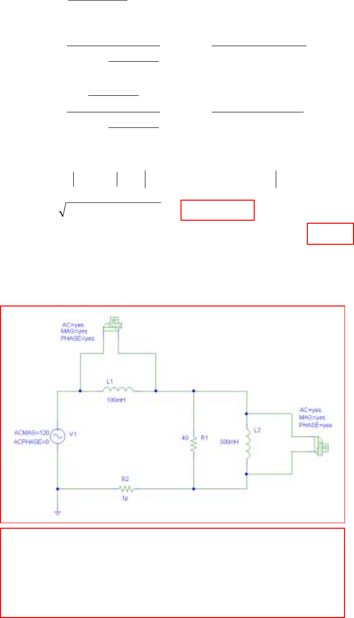
CHAPTER 11 SOLUTIONS
Engineering Circuit Analysis, 6th Edition Copyright
2002 McGraw-Hill, Inc. All Rights Reserved
26. Zeq = R || j0.3
ω
=
ω
ω
RjR
Rj
3.0
3.0
+. By voltage division, then, we write:
V100mH =
ωω
ωω
ω
ω
ω
ω
Rj
Rj
jR
Rj
j
j
4.003.0
1.00.03-
0120
3.0
3.0
1.0
1.0
0120 2
2
+−
+
∠=
+
+
∠
V
300mH = Rω.jω.
Rj
jR
Rj
j
jR
Rj
40030
36
0120
3.0
3.0
1.0
3.0
3.0
0120 2+−
∠=
+
+
+
∠
ω
ω
ω
ω
ω
ω
(a) We’re interested in the value of R that would lead to equal voltage magnitudes, or
()
R0.10.03- (120) 36 2
ωωω
jRj +=
Thus, 36R
ω
= 224 14496.12 R
ωω
+ or R = 0.1061
ω
(b) Substituting into the expression for V100mH, we find that V100mH = 73.47 V,
independent of frequency.
To verify with PSpice, simulate the circuit at 60 Hz, or
ω
= 120π rad/s, so R = 40 Ω.
We also include a miniscule (1 pΩ) resistor to avoid inductor loop warnings. We see
from the simulation results that the two voltage magnitudes are indeed the same.
FREQ VM($N_0002,$N_0003)VP($N_0002,$N_0003)
6.000E+01 7.349E+01 -3.525E+01
FREQ VM($N_0001,$N_0002)VP($N_0001,$N_0002)
6.000E+01 7.347E+01 3.527E+01

CHAPTER 11 SOLUTIONS
Engineering Circuit Analysis, 6th Edition Copyright
2002 McGraw-Hill, Inc. All Rights Reserved
27.
(a) ,1
V30V
av =
,2
1
V (10 30 50) 30V
3
av =++=
(b)
(c) PSpice verification for Sawtooth waveform of Fig. 11.40a:
32
,1 0
222
,2
111
V (20 ) 400 27 1200 34.64V
333
11
V (10 30 50 ) 3500 34.16V
33
eff
eff
tdt
==×××==
=++=×=
∫
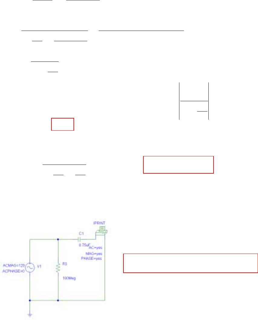
CHAPTER 11 SOLUTIONS
Engineering Circuit Analysis, 6th Edition Copyright
2002 McGraw-Hill, Inc. All Rights Reserved
28. Zeff = R || 6
66
103
10
3
10
jR
jRj
−
−
=
−
ωω
ISRC =
()
()
666
6
6
66 1010310
10-R3120
103
1010
0120
RjjRj
j
jR
R
jj
ωω
ωω
ωω
−−−
=
−
−−
∠
I3µF = ISRC
ω
3
106
jR
R
−
(a) For the two current magnitudes to be equal, we must have 1
3
106=
−
ω
jR
R. This is
only true when R = ∞; otherwise, current is shunted through the resistor and the two
capacitor currents will be unequal.
(b) In this case, the capacitor current is
A )90 cos( 90 or A, 90
3
1010
1
0120 o
66
µωωµω
ωω
+=
−−
∠tj
jj
(c) PSpice verification: set f = 60 Hz, simulate a single 0.75-µF capacitor, and include a
100-MΩ resistor in parallel with the capacitor to prevent a floating node. This should
resit in a rms current amplitude of 33.93 mA, which it does.
FREQ IM(V_PRINT3) IP(V_PRINT3)
6.000E+01 3.393E-02 9.000E+01
CHAPTER 11 SOLUTIONS
Engineering Circuit Analysis, 6th Edition Copyright
2002 McGraw-Hill, Inc. All Rights Reserved
29.
0.5( 3)
22
1, 0
5(3) 3 5
2, 3
3
22
23
( ) 10 [ ( ) ( 2)] 16 [ ( 3) ( 5)] V
Find eff. value separately
120
V 100 8 7.303
53
1 256
V 256 ( ) 6.654
55
V 7.303 6.654 9.879
1
V 100 256
5
t
eff
tt
eff
eff
t
eff
vt tut ut e ut ut
tdt
edt ee
tdt ee
−−
−− −
−
=−−+ −−−
==×=
==−=
∴= + =
=+
∫
∫
25
03
33 5
2
1 100 8 256 ( )
53
1 800 256(1 ) 9.879VOK
53
dt
ee e
e
−−
−
=×+ −
=+−=
∫∫
CHAPTER 11 SOLUTIONS
Engineering Circuit Analysis, 6th Edition Copyright
2002 McGraw-Hill, Inc. All Rights Reserved
30. The peak instantaneous power is 250 mW. The combination of elements yields
Z = 1000 + j1000 Ω = 1414 ∠45o Ω.
Arbitrarily designate V = Vm ∠0 , so that I = 1414
45V
0V o
mm −∠
=
∠
Z A.
We may write p(t) = ½ Vm Im cos φ + ½ Vm Im cos (2
ω
t + φ) where φ = the angle of the
current (-45o). This function has a maximum value of ½ VmIm cos φ + ½ VmIm.
Thus, 0.250 = ½ VmIm (1 + cos φ) = ½ (1414) Im2 (1.707)
and Im = 14.39 mA.
In terms of rms current, the largest rms current permitted is 14.39 / 2 = 10.18 mA rms.
CHAPTER 11 SOLUTIONS
Engineering Circuit Analysis, 6th Edition Copyright
2002 McGraw-Hill, Inc. All Rights Reserved
31. 435Arms=∠ °
I
(a) ,
20 80 35 Vrms, P 80 10cos35 655.3 W
sgen
=+∠° =× °=VI
(b) 2
P R 16 20 320 W
R==×=I
(c) P 655.3 320 335.3 W
Load =−=
(d) ,
AP 80 10 800 VA
sgen =×=
(e) AP P 320VA
RR
==
(f)
(g)
10 0 4 35 7.104 18.84 A rms
AP 80 7.104 568.3 VA
L
L
=∠°−∠°= ∠− °
∴=× =
I
P335.3
PF cos 0.599
AP 568.3
since I lags V, PF is lagging
L
LL
L
LL
θ
====
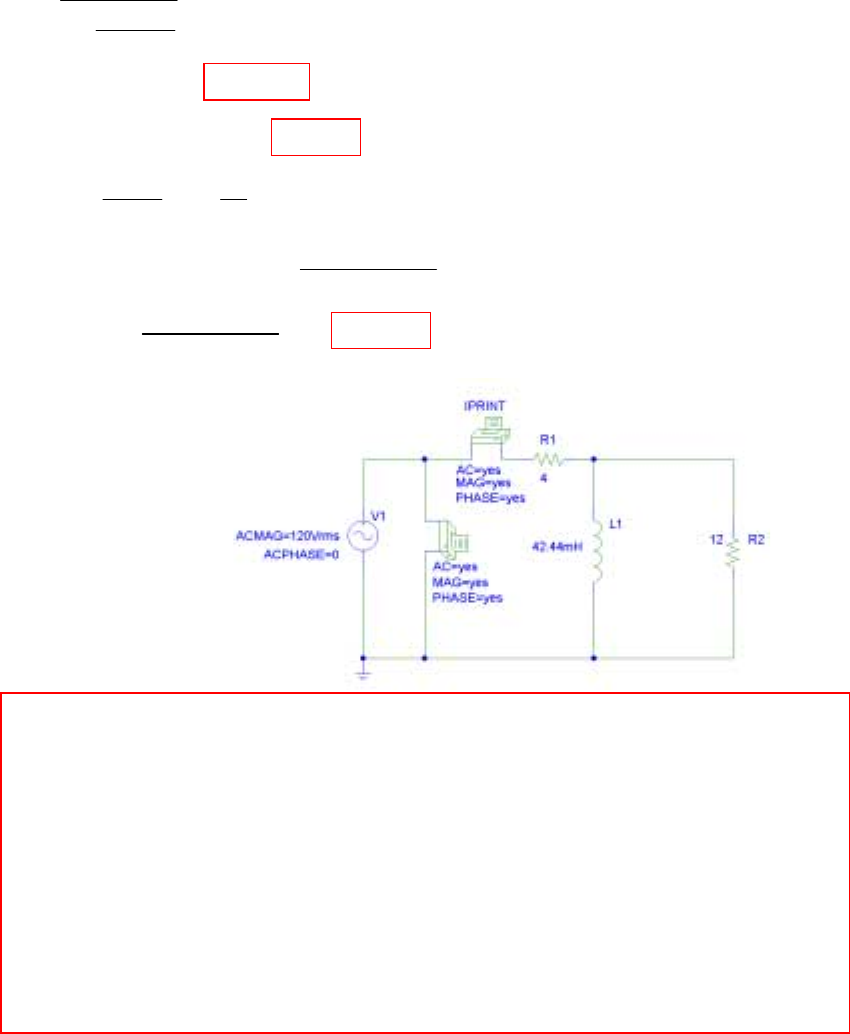
CHAPTER 11 SOLUTIONS
Engineering Circuit Analysis, 6th Edition Copyright
2002 McGraw-Hill, Inc. All Rights Reserved
32.
(a)
(b) P 120 9.214 0.8969 991.7W
s=× × =
(c)
(d) PSpice verification
FREQ VM($N_0003,0) VP($N_0003,0)
6.000E+01 1.200E+02 0.000E+00
FREQ IM(V_PRINT1) IP(V_PRINT1)
6.000E+01 9.215E+00 -2.625E+01 ; (a) and (b) are correct
Next, add a 90.09-
µ
F capacitor in parallel with the source:
FREQ IM(V_PRINT1) IP(V_PRINT1)
6.000E+01 8.264E+00 -9.774E-05 ;(c) is correct (-9.8×10⁻⁵ degrees
is essentially zero, for unity PF).
120
I 9.214 26.25 A rms
192
412 16
PF cos26.25 0.8969lag
s
s
j
j
==∠−°
++
∴= =
22
22
48 1
Z 4 4 (192 144)
34 25
11.68 5.76
Z 11.68 5.76 , Y 11.68 5.76
5.76
120 C , C 90.09 F
11.68 5.76
L
LL
jj
j
j
j
j
j
πµ
=+ =+ +
+
−
∴= + Ω = +
∴= =
+
CHAPTER 11 SOLUTIONS
Engineering Circuit Analysis, 6th Edition Copyright
2002 McGraw-Hill, Inc. All Rights Reserved
33.
1
2
5 2 , 20 10 , 10 30 8.660 5
10 60 5 8.660
200 20 10
0 33.66 13.660 7265 22.09 15.11 3.908 A rms
25 8 20 10 480.9 26.00
20 10 33.66 13.660
25 8 200
20 10 0 200
480.9 26.00
AB c
D
jj j
j
j
j
jj
jj
j
j
=+ Ω = − Ω = ∠°Ω= + Ω
=∠−°=− Ω
−+
−∠°
===∠°
−−+ ∠− °
−+ −
−
−+
==
∠− °
ZZ Z
Z
I
I
22
1
22
12
2
2
22
21
1
(20 10) 9.300 0.5681 A rms
480.9 20.00
AP 15.108 29 1229 VA
AP 5.881 10 5 773.5VA
AP 2 9.3 10 86.49VA
AP 9.3 10 864.9VA
AP 200 200 15.108 3022VA
AA
BB
CC
D
S
j−=∠− °
∠°
== =
=− = × =
==×=
==×=
==×=
IZ
IIZ
IZ
IZ
I

CHAPTER 11 SOLUTIONS
Engineering Circuit Analysis, 6th Edition Copyright
2002 McGraw-Hill, Inc. All Rights Reserved
34. Perhaps the easiest approach is to consider the load and the compensation capacitor
separately. The load draws a complex power Sload = P + jQ. The capacitor draws a
purely reactive complex power SC = -jQC.
θ
load = tan-1(Q/P), or Q = P tan θload
Q
C = SC = Vrms rms
(/C)j
ω
−
V = 2
Crms
ω
V = 2
CVrms
ω
Stotal = Sload + SC = P + j(Q – QC)
θnew = ang(Stotal) = 1C
Q-Q
tan P
−
, so that Q – QC = P tan θnew
Substituting, we find that QC = P tan θload – P tan θnew
or
2
CVrms
ω
= P (tan θload – tan θnew)
Thus, noting that θold = θload,
()
old new
2
rms
P tan - tan
C = V
θθ
ω
CHAPTER 11 SOLUTIONS
Engineering Circuit Analysis, 6th Edition Copyright
2002 McGraw-Hill, Inc. All Rights Reserved
35. 12
30 15 , 40 40= ∠ °Ω = ∠ °ΩZZ
(a)
(b)
30 15 40 40 68.37 29.31
PF cos 29.3 0.8719 lag
tot =∠°+∠°= ∠ °Ω
∴= °=
Z
1
68.37 29.31 59.62 33.48
PF 0.9 lag
cos 0.9 25.84
X
tan 25.84 0.4843 X 28.88
59.62
1
33.48 28.88,
100 C
C 691.8 F
tot
new
new
new
new
j
θ
π
µ
−
=∠°=+
=
∴= = °
°= = ∴ = Ω
∴− =
=
Z
CHAPTER 11 SOLUTIONS
Engineering Circuit Analysis, 6th Edition Copyright
2002 McGraw-Hill, Inc. All Rights Reserved
36. θ1 = cos-1(0.92) = 23.07o, θ 2 = cos-1 (0.8) = 36.87o, θ 3 = 0
S
1 = VA 42.59 100
92.0
23.07 100 o
j+=
∠
S
2 = VA 5.871 250
8.0
78.63 250 o
j+=
∠
S
3 = VA 500
1
0 500 o=
∠
Stotal = S1 + S2 + S3 = 500 + j230.1 VA = 550.4 ∠24.71o VA
(a) Ieff = rmsA 4.786
115
550.4
V
S
eff
total ==
(b) PF of composite load = cos (24.71o) = 0.9084 lagging
CHAPTER 11 SOLUTIONS
Engineering Circuit Analysis, 6th Edition Copyright
2002 McGraw-Hill, Inc. All Rights Reserved
37.
2
1
AP 10,000 VA, PF 0.8lag, 40A rms
Let 40 0 A rms; P 10,000 0.8 8000 W
8000
Let R X R 5
40
cos 0.8lag cos 0.8 36.87
X 5tan 36.87 3.75 , 5 3.75, 5.2 3.75
40(5.2 3.75) 256.4
LLL
LL
LL LL
LL
LLtot
s
j
jj
j
θθ
−
===
=∠° = × =
=+ ∴= =Ω
=∴= =°
∴= °= Ω =+ =+ Ω
∴= + =
I
I
Z
ZZ
V1
35.80 V; 5.2 3.75
0.12651 0.09124S, 0.12651 (120 C 0.09124),
PF 0.9 lag, 25.84 tan 25.84 0.4843
0.09124 120 C
0.12651
C 79.48 F
tot
new
new new
j
jj
π
θ
π
µ
∠° =
+
=− =+ −
==°∴°=
−
=∴
=
Y
Y
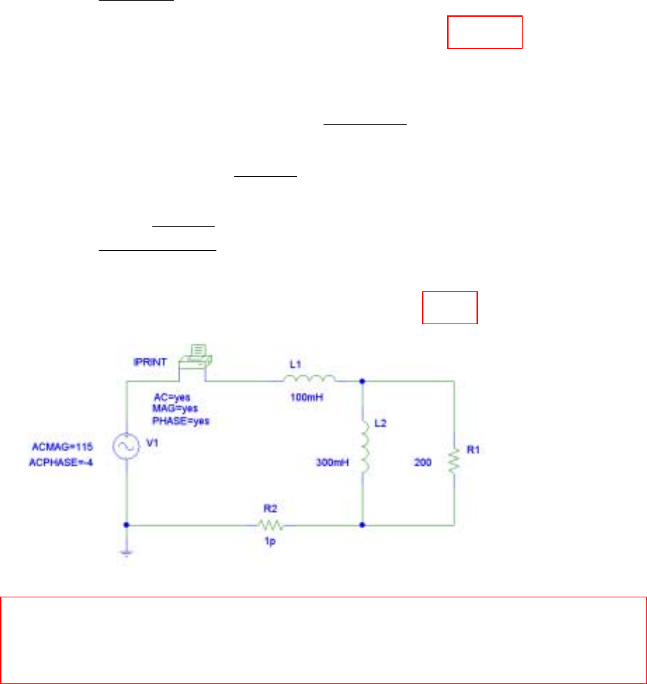
CHAPTER 11 SOLUTIONS
Engineering Circuit Analysis, 6th Edition Copyright
2002 McGraw-Hill, Inc. All Rights Reserved
38. Zeff = j100 + j300 || 200 = 237 ∠54.25o. PF = cos 54.25o = 0.5843 lagging.
(a) Raise PF to 0.92 lagging with series capacitance
Znew = j100 + jXC + j300 || 200 = 138.5 + j(192.3 + XC) Ω
o1-
C
123.07 0.92 cos
138.5
X 192.3
tan ==
+
−
Solving, we find that XC = -133.3 Ω = -1/
ω
C, so that C = 7.501 µF
(b) Raise PF to 0.92 lagging with parallel capacitance
Znew = j100 || jXC + j300 || 200 = )X100(
X 100
C
C
+
−
j+138.5 + j92.31 Ω
= 138.5 +
+
+
C
C
X100
X100
31.92j Ω
o1-
C
C
123.07 0.92 cos
138.5
X100
100X
92.31
tan ==
+
+
−
Solving, we find that XC = -25 Ω = -1/
ω
C, so that C = 40 µF
General circuit for simulations. Results agree with hand calculations
FREQ IM(V_PRINT1) IP(V_PRINT1) θ PF
With no compensation: 1.592E+02 4.853E-01 -5.825E+01 54.25o 0.5843 lag
With series compensation: 1.592E+02 7.641E-01 -2.707E+01 23.07o 0.9200 lag
With parallel compensation: 1.592E+02 7.641E-01 -2.707E+01 23.07o 0.9200 lag
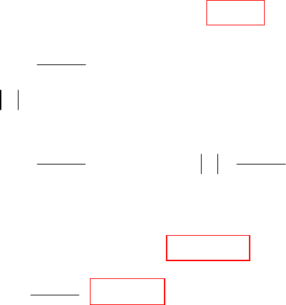
CHAPTER 11 SOLUTIONS
Engineering Circuit Analysis, 6th Edition Copyright
2002 McGraw-Hill, Inc. All Rights Reserved
39.
(a) ,
P 20 25 0.8 30 0.75 70 kW
stot =+×+× =
(b)
(c) 3
70,000
PF 0.8604lag
81,360
==
1
2
1o
22
33
1
33
20,000 80 0 A rms
250
25,000 / 250 100 Arms
cos 0.8 36.87 100 36.87 A rms
30,000 40,000
AP 40,000 VA, 160Arms
0.75 250
cos 0.75 41.41 160 41.41 A rms
80 0 100 36.87 160
s
−
−
==∠°
==
∠=− =− ∴= ∠−
== ==
∠=− =− °∴ = ∠− °
∴=∠°+ ∠− °+ ∠−
I
I
II
I
II
I41.41 325.4 30.64 A rms
AP 250 325.4 81,360 VA
s
°= ∠− °
∴=× =
CHAPTER 11 SOLUTIONS
Engineering Circuit Analysis, 6th Edition Copyright
2002 McGraw-Hill, Inc. All Rights Reserved
40. 200 kW average power and 280 kVAR reactive result in a power factor of
PF = cos (tan-1 (280/200) = 0.5813 lagging, which is pretty low.
(a) 0.65 peak = 0.65(200) = 130 kVAR
Excess = 280 – 130 = 150 kVAR, for a cost of (12)(0.22)(150) = $396 / year.
(b) Target = S = P + j0.65 P
θ = tan-1(0.65P/P) = 33.02o, so target PF = cos θ = 0.8385
(c) A single 100-kVAR increment costs $200 to install. The excess kVAR would then be
280 – 100 – 130 = 50 kVAR, for an annual penalty of $332. This would result in a
first-year savings of $64.
A single 200-kVAR increment costs $395 to install, and would remove the entire excess
kVAR. The savings would be $1 (wow) in the first year, but $396 each year thereafter.
The single 200-kVAR increment is the most economical choice.
CHAPTER 11 SOLUTIONS
Engineering Circuit Analysis, 6th Edition Copyright
2002 McGraw-Hill, Inc. All Rights Reserved
41.
20
2
20
20(1 2)
10 10.769 3.846 11.435 19.65
32
100 8.745 19.65
11.435 19.654
100 8.745 19.65 823.5 294.1VA
10 20
8.745 19.65 5.423 49.40
30 20
20 5.432 588.2 0 VA
in
s
sss
j
jj
j
j
j
j
j
+
∗
+
=− + = − = ∠− °Ω
+
∴= = ∠ °
∠− °
∴=− =− × ∠− °=− +
+
=∠°× =∠°
+
∴=× = +
Z
I
SVI
I
S
10
2
10
2
20
2
10
20 5.423 49.40 4.851 14.04
10 20
10 4.851 235.3 0 VA
20 4.851 470.6 VA,
10 8.745 764.7 VA, 0
j
j
j
j
jj
jj
−
×∠
==∠−°
+
=× = +
=× =
=− × = − Σ=
I
S
S
S
CHAPTER 11 SOLUTIONS
Engineering Circuit Analysis, 6th Edition Copyright
2002 McGraw-Hill, Inc. All Rights Reserved
42.
1
1.
2
6,
4,
100 100 0
6 4 10 5
1 100
0.1 0.2 20
64 64
53.35 42.66 V
100 53.35 42.66 9.806 64.44 A
64
1100 9.806 64.44 211.5 4423VA
2
16 9.806 288.5 0VA
2
1
xxx
x
x
gen
abs
jabs
j
jj
jj
jj
j
j
j
−
−
−−
++ =
+−
∴++=+
++
∴= ∠ °
−∠°
∴= = ∠− °
+
∴=××∠°= +
=×× = +
=
VVV
V
V
I
S
S
S2
2
2
5
2,
10,
( 4)9.806 0 192.3VA
2
100 53.35 42.66 14.99 121.6 ,
5
15 14.99 561.5 0VA
2
1( 100)14.99 121.57 638.4 392.3VA
2
1 53.35 ( 10) 0 142.3VA 142.3 0 VA 0
210
abs
gen
j abs
jj
j
j
jj
jj
−
−
=+
−∠°
==∠°
=×× = +
=∠−°=−
=−=−=∠Σ=
I
S
S
S
CHAPTER 11 SOLUTIONS
Engineering Circuit Analysis, 6th Edition Copyright
2002 McGraw-Hill, Inc. All Rights Reserved
43.
(a)
(b)
(c)
1
500VA, PF 0.75 lead
500 cos 0.75 375 330.7 VAj
−
=∴
=∠− = −S
1
500W, PF 0.75 lead
500
500 sin (cos 0.75) 500 441.0 VA
.075 j
j
−
=∴
=− = −S
1
500 VAR, PF 0.75(lead) cos 0.75 41.41
P500/ tan 41.41 566.9W,
566.9 500 VAj
θ
−
−=∴=−=−°
∴°=
=−S
CHAPTER 11 SOLUTIONS
Engineering Circuit Analysis, 6th Edition Copyright
2002 McGraw-Hill, Inc. All Rights Reserved
44. 1600 500VA(gen)
sj=+S
(a)
(b) 11833.3
PF cos tan 0.6575 lag
1600
L
−+
==
(c) 1600 500 1676 17.35 VA PF cos17.35 0.9545 lag
ss
j=+=∠°∴= °=S
1600 500 4 1.25 4 1.25
400
400 3.333A rms 4 1.25 3.333
120
4 4.583A rms
400(4 4.583) 1600 1833 VA
ss
cLsc
L
L
jjj
jjj
j
j
jj
∗+
==+∴=−
= = ∴=−=− −
−
∴=− ∴
=+ =+
II
IIII
I
S
CHAPTER 11 SOLUTIONS
Engineering Circuit Analysis, 6th Edition Copyright
2002 McGraw-Hill, Inc. All Rights Reserved
45. 11
(cos 0.8 36.87 , cos 0.9 25.84 )
−−
=° =°
(a)
(b) PF cos23.245 0.9188
s=°=
(c) 3300 1417 VAj=+S
1200 36.87 1600 25.84 900
960 720 1440 697.4 900
3300 1417.4 3592 23.25 VA
3591.5 15.62 A rms
230
tot
s
jj
j
=∠°+∠°+
=+ + + +
=+ =∠°
∴= =
S
I
CHAPTER 11 SOLUTIONS
Engineering Circuit Analysis, 6th Edition Copyright
2002 McGraw-Hill, Inc. All Rights Reserved
46. V = 339 ∠-66o V,
ω
= 100π rad/ s, connected to Z = 1000 Ω.
(a) Veff = rms V 239.7
2
339 =
(b) pmax = 3392 / 1000 = 114.9 W
(c) pmin = 0 W
(d) Apparent power = Veff Ieff = VA 57.46
1000
V
1000
2
339
2
339 2
eff ==
(e) Since the load is purely resistive, it draws zero reactive power.
(f) S = 57.46 VA
CHAPTER 11 SOLUTIONS
Engineering Circuit Analysis, 6th Edition Copyright
2002 McGraw-Hill, Inc. All Rights Reserved
47. V = 339 ∠-66o V,
ω
= 100π rad/s to a purely inductive load of 150 mH (j47.12 Ω)
(a) I = A 156- 7.194
12.47
66-339
o
o∠=
∠
=jZ
V
so Ieff = rmsA 5.087
2
194.7 =
(b) p(t) = ½ VmIm cos φ + ½ VmIm cos(2
ω
t + φ)
where φ = angle of current – angle of voltage
pmax = ½ VmIm cos φ + ½ VmIm = (1 + cos(-90o)) (339)(7.194)/ 2 = 1219 W
(c) pmin = ½ VmIm cos φ - ½ VmIm = -1219 W
(d) apparent power = Veff Ieff =
()
VA 1219 087.5
2
339 =
(e) reactive power = Q = Veff Ieff sin (θ – φ) = 1219 VA
(f) complex power = j1219 VA
CHAPTER 11 SOLUTIONS
Engineering Circuit Analysis, 6th Edition Copyright
2002 McGraw-Hill, Inc. All Rights Reserved
48. 1 H → j Ω, 4 µF → -j250 kΩ
Zeff = j || -j250×103 || 103 Ω = 1 ∠89.99o Ω
V10k = V 89.97 0.002
)89.99 (12500
)89.99 (1 )05( o
o
o∠=
∠+
∠∠
(a) pmax = (0.002)2 / 10×103 = 400 pW
(b) 0 W (purely resistive elements draw no reactive power)
(c) apparent power = VeffIeff = ½ VmIm = ½ (0.002)2 / 10000 = 200 pW
(d) Isource = A 0.02292- 0.002
99.8912500
05 o
o∠=
∠+
∠
S = ½ VmIm ∠(89.99o + 0.02292o) = 0.005 ∠90.01o VA
CHAPTER 11 SOLUTIONS
Engineering Circuit Analysis, 6th Edition Copyright
2002 McGraw-Hill, Inc. All Rights Reserved
49. (a) At
ω
= 400 rad/s, 1 µF → -j2500 Ω, 100 mH → j40 Ω
Define Zeff = -j2500 || (250 + j40) = 256 ∠ 3.287o Ω
IS = rmsA 3.049- 43.48
287.325620
012000 o
o∠=
∠+
∠
Ssource = (12000)(43.48) ∠ 3.049o = 521.8 ∠3.049o kVA
S20Ω = (43.48)2 (20) ∠0 = 37.81 ∠0 kVA
Veff = rms V 0.2381 11130
287.325620
)287.3256)(012000( o
∠=
∠+
∠∠
o
o
I1µF = rmsA 90.24 4.452
0250-
o
eff ∠=
j
V
so S1µF = (11130)(4.452) ∠-90o = 49.55 ∠-90o kVA
V100mH = rms V 15.18 1758
40250
)40)(2381.011130( o
∠=
+
∠
j
j
o
I
100mH = rmsA 852.8- 43.96
40
o
100mH ∠=
j
V
so S100µΗ = (1758)(4.43.96) ∠90o = 77.28 ∠90o kVA
V250Ω = rms V 852.8 10990
40250
)250)(2381.011130( o
−∠=
+
∠
j
o
so S250Ω = (10990)2 / 250 = 483.1 ∠0o kVA
(b) 37.81 ∠0 + 49.55 ∠-90o +77.28 ∠90o + 483.1 ∠0o = 521.6 ∠3.014o kVA,
which is within rounding error of the complex power delivered by the source.
(c) The apparent power of the source is 521.8 kVA. The apparent powers of the passive
elements sum to 37.81 + 49.55 + 77.28 + 483.1 = 647.7 kVA, so NO! Phase angle is
important!
(d) P = Veff Ieff cos (ang VS – ang IS) = (12000)(43.48) cos (3.049o) = 521 kW
(e) Q = Veff Ieff sin (ang VS – ang IS) = (12000)(43.48) sin (3.049o) = 27.75 kVAR
CHAPTER 11 SOLUTIONS
Engineering Circuit Analysis, 6th Edition Copyright
2002 McGraw-Hill, Inc. All Rights Reserved
50. (a) Peak current = 28 2 = 39.6 A
(b) θload = cos-1(0.812) = +35.71o (since lagging PF). Assume ang (V) = 0o.
p(t) =
(
)
(
)
)7135120(cos)120(co 239.60 22300 o
.πt - πts
at t = 2.5 ms, then, p(t) = 147.9 kW
(c) P = Veff Ieff cos θ = (2300)(28) cos (35.71o) = 52.29 kW
(d) S = Veff Ieff ∠θ = 64.4 ∠ 35.71o kVA
(e) apparent power = |S| = 64.4 kVA
(f) |Zload| = |V/ I| = 2300/28 = 82.14 Ω. Thus, Zload = 82.14 ∠ 35.71o Ω
(g) Q = Veff Ieff sin θ = 37.59 kVAR
CHAPTER TWELVE SOLUTIONS
Engineering Circuit Analysis, 6th Edition Copyright
2002 McGraw-Hill, Inc. All Rights Reserved
1. Vbc = Vbe + Vec = 0.7 – 10 = -9.3 V
V
eb = - Vbe = -0.7 V
V
cb = Vce + Veb = 10 – 0.7 = 9.3 V

CHAPTER TWELVE SOLUTIONS
Engineering Circuit Analysis, 6th Edition Copyright
2002 McGraw-Hill, Inc. All Rights Reserved
2. (a) Vgd = Vgs + Vsd = -1 – 5 = -6 V
(b) Vsg = Vsd + Vdg = -4 – 2.5 = -6.5 V

CHAPTER TWELVE SOLUTIONS
Engineering Circuit Analysis, 6th Edition Copyright
2002 McGraw-Hill, Inc. All Rights Reserved
3. (a) positive phase sequence
Van = |Vp| ∠ 0o Vdn = |Vp| ∠ -180o
Vbn = |Vp| ∠ -60o Ven = |Vp| ∠ -240o
Vcn = |Vp| ∠ -120o Vfn = |Vp| ∠ -300o
(b) negative phase sequence
Van = |Vp| ∠ 0o Vdn = |Vp| ∠ 180o
Vbn = |Vp| ∠ 60o Ven = |Vp| ∠ 240o
Vcn = |Vp| ∠ 120o Vfn = |Vp| ∠ 300o
CHAPTER TWELVE SOLUTIONS
Engineering Circuit Analysis, 6th Edition Copyright
2002 McGraw-Hill, Inc. All Rights Reserved
4. (a) Vyz = Vyx + Vxz = -110 ∠20o + 160 ∠ -50o
= -103.4 – j37.62 + 102.8 – j122.6 = -0.6 – j160.2
= 160.2 ∠ -90.21o V
(b) Vaz = Vay + Vyz = 80 ∠130o + 160.2 ∠ -90.21o
= -51.42 + j61.28 -0.6 – j160.2 = -52.02 – j98.92
= 111.8 ∠ -117.7o V
(c) o
o
o
o
o
xy
zx 1101.455
20110
301160
20110
50-160-
∠=
∠
∠
=
∠
∠
=
V
V

CHAPTER TWELVE SOLUTIONS
Engineering Circuit Analysis, 6th Edition Copyright
2002 McGraw-Hill, Inc. All Rights Reserved
5. (a) V25 = V24 + V45 = -80 ∠ 120o + 60 ∠ 75o
= 40 – j69.28 + 15.53 + j57.96 = 55.53 – j11.32
= 56.67 ∠ -11.52o V
(b) V13 = V12 + V25 + V53 = 100 + 55.53 – j11.32 + j120
= 155.53 + j108.7
= 189.8 ∠ 34.95o V
CHAPTER TWELVE SOLUTIONS
Engineering Circuit Analysis, 6th Edition Copyright
2002 McGraw-Hill, Inc. All Rights Reserved
6.
230/ 460V rms Z : S 10 40 kVA; Z : 8 10 kVA;
10,000 40
Z : 4 80 kVA Let V 230 0 V S V I ,I 43.48 40 A
230
4000 80
I 43.48 40 A, S V I I 8.696 80 , I 8.696 80 I I I
460
I 43.
∗∗
∗∗
=∠° ∠°
∠°
∠− ° = ∠ ° ∴ = = = ∠ °
∠− °
∴=∠−° = ∴= =∠−°=∠°∴=+
∴=
AN NB
AB AN AN AN AN AN
AN AB AB AB AB AB aA AN AB
aA 48 40 8.696 80 39.85 29.107 I 39.85 A
8000 10
I 34.78 10 , I 34.78 10 A
230
I 34.78 10 8.696 80 35.85 175.96 , I 35.85 A
I 43.48 40 34.78 10 21.93 87.52 , I 21.93A
−−
∗
++
∠°+ ∠°= ∠− °∴ =
∠°
==∠°=∠−°
∴=− ∠−°− ∠°= ∠− °∴=
=− ∠− °+ ∠− °= ∠ ° =
aA
NB NB
bB bB
nN nN
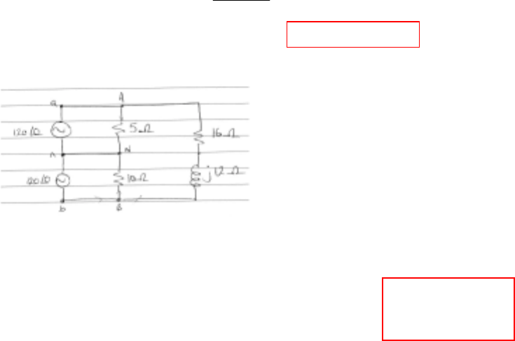
CHAPTER TWELVE SOLUTIONS
Engineering Circuit Analysis, 6th Edition Copyright
2002 McGraw-Hill, Inc. All Rights Reserved
7. (a) InN = 0 since the circuit is balanced.
IAN = 12 ∠0 IAB = o
36.9- 12
1216
0240 ∠=
+
∠
j
IaA = IAN + IAB = 12 + 9.596 – j7.205 = 22.77 ∠ -18.45o A
(b)
The voltage across the 16-Ω resistor and j12-Ω impedance has not changed, so IAB
has not changed from above.
IaA = IAN + IAB = 24 ∠ 0o + 12 ∠ -36.9o = 34.36 ∠ -12.10o A
IbB = IBN - IAB = -12 ∠ 0o - 12 ∠ -36.9o = 7.595 ∠ -108.5o A
InN = IBN – IAN = -12 – 24 = 36 ∠180o A
IAN = 24 ∠ 0o A
IBN = -12 ∠ 0o A
InN = -12 ∠ 0o A
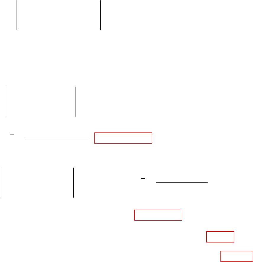
CHAPTER TWELVE SOLUTIONS
Engineering Circuit Analysis, 6th Edition Copyright
2002 McGraw-Hill, Inc. All Rights Reserved
8.
(a)
(b)
(c) 222
,
P 126.06 1 130.65 1 4.730 10 15.891 17.069 0.224 33.18kW
tot
ω
= ×+ ×+×=++=
(d) ,
P 720 126.06 cos 6.479 720 130.65 cos5.968 90.18 93.56 183.74kW
gen tot −
=× °+× °= + =
21 3 10 10 3
10 19 2 8 2 (21 3)(674 167 60 32)
10 3 8 2 36 5
10( 360 50 74 44) (10 3)(80 20 184 77)
5800 1995 6127 18.805
720 10 10 3
720 19 2 8 2 720(614 135 434 94) 7
082365
+−−−
∆= − + − − = + + − −
−− −− +
+− − −− − + + + +
∴∆= + = ∠ °
−−−
+−−= +++=
−− +
jj
jj jj j
jj j
jj jj j
j
j
jj j j
jj
20 1072.7 12.326
720 1072.7 12.326
I 126.06 6.479 A
6127 18.805
×∠°
×∠°
∴= = ∠− °
∠°
aA
21 3 720 10 3 720(1084 247)
10 720 8 2 720(1084 247) I 130.65 5.968 A
6127 18.805
10 3 0 36 5
I 130.65 5.968 126.06 6.479 4.730 7.760 A
−
−
+−− +
−−−=+∴= =∠−°
∠°
−− +
∴= ∠− °− ∠− °= ∠ °
Bb
nN
jj j
jj
jj
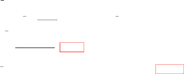
CHAPTER TWELVE SOLUTIONS
Engineering Circuit Analysis, 6th Edition Copyright
2002 McGraw-Hill, Inc. All Rights Reserved
9. V 220Vrms, 60Hz
AN =
(a)
(b) 6
I 377 91.47 10 440 15.172A VA 440 15.172 6.676kVA
AB −
=× ××= ∴=× =
220 0
PF 1 I 40.85 21.80 A; I 377C 440
52
I 40.85cos21.80 (377C440 40.85sin 21.80 )
40.85sin 21.80
C 91.47 F
377 440
+
∠°
=∴ = = ∠− ° = ×
+
∴= °+ − °
°
∴= =
×
AN AB
aA
j
j
j
µ
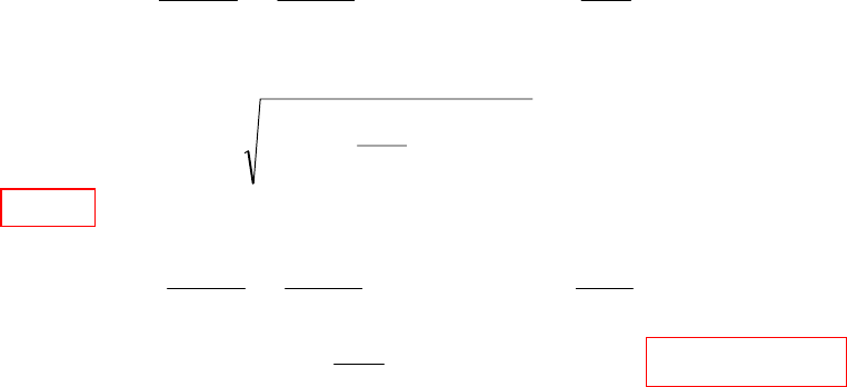
CHAPTER TWELVE SOLUTIONS
Engineering Circuit Analysis, 6th Edition Copyright
2002 McGraw-Hill, Inc. All Rights Reserved
10. (a) IaA = IAN + IAB =
AB
R
0400
312
0200 ∠
+
+
∠
j = 15.69 – j3.922 +
AB
R
400
Since we know that |IaA| = 30 A rms = 42.43 A,
2
2
AB
3.922
R
400
69.1543.42 +
+=
or RAB = 15.06 Ω
(b) IaA = IAN + IAB =
ABAB X
400
922.3- 15.69
X-
0400
312
0200 j
j
jj +=
∠
+
+
∠
In order for the angle of IaA to be zero,
AB
X
400 = 3.922, so that XAB = 102 Ω capacitive.
CHAPTER TWELVE SOLUTIONS
Engineering Circuit Analysis, 6th Edition Copyright
2002 McGraw-Hill, Inc. All Rights Reserved
11. seq. V 120 60 V rms, R 0.6 P 5kVA, 0.6 lag
BC w load
+=∠° =Ω=
(a)
(b)
2
120 5000 5000
V 150 V S 0.8 0.6
33
3
120
S 150 I I 24.06 113.13 A
3
I 24.06 113.13 P 3 24.06 0.6 1041.7W
AN AN
AN aA aA
aA wire
j
∗∗
=∠°∴= ×+
∴=∠°∴= ∠− °
∴= ∠ °∴ =× × =
V 0.6 24.06 113.13 14.434 113.13 V
120
V V V 14.434 113.13 158 81.29 143.88 V
3
aA
an aA AN
=× ∠ °= ∠ °
∴=+= ∠°+∠°=∠°
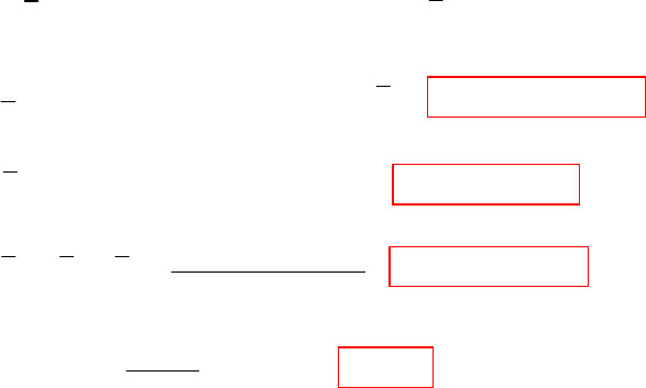
CHAPTER TWELVE SOLUTIONS
Engineering Circuit Analysis, 6th Edition Copyright
2002 McGraw-Hill, Inc. All Rights Reserved
12. rms
V 2300 0 V , R 2 , ., S 100 30kVA
an w tot
seq j↑= ∠° =Ω+ =+
(a) 1(100,000 30,000) 2300I I 15.131 16.699 A
3aA aA
j∗
+=∴=∠−°
(b) V 2300 2 15.131 16.699 2271 0.2194 V
AN =−× ∠− °=∠ °
(c) 2271 0.2194
Z V / I 143.60 43.67
15.131 16.699
pANaA j
∠°
== =+Ω
∠− °
(d) 143.60
trans. eff. 0.9863, or98.63%
145.60
==
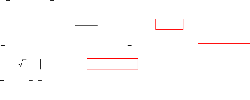
CHAPTER TWELVE SOLUTIONS
Engineering Circuit Analysis, 6th Edition Copyright
2002 McGraw-Hill, Inc. All Rights Reserved
13. Z 12 5 , I 20 0 A rms, +seq., PF 0.935
pbB
j↑=+Ω =∠° =
(a) 15
cos 0.935 20.77 tan 20.77 , R 1.1821
12 R w
w
θ
−
==°∴=°=Ω
+
(b)
(c) V 3 V / V 150 450.3 172.62 V
AB BN BN
=∠+°=∠°
(d)
V I Z 20(12 5) 240 100V V 20(13.1821 5) 281.97 20.77 V==+=+ ∴= += ∠°
BN bB p bn
jj j
S 3 V I 3 281.97 20.77 (20)
15.819 6.000kVA
∗
==×∠−°
=−
source Bn bB
j
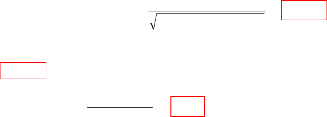
CHAPTER TWELVE SOLUTIONS
Engineering Circuit Analysis, 6th Edition Copyright
2002 McGraw-Hill, Inc. All Rights Reserved
14. 125 mH → j(2π)(60)(0.125) = j47.12 Ω 75 Ω → 75 Ω
55 µF → -j/(2π)(60)(55×10-6) = -j48.23 Ω
The per-phase current magnitude |I| is then I =
)23.4812.47(75
125
22 =
−+ 1.667 A.
The power in each phase = (1.667)2 (75) = 208.4 W, so that the total power taken by the
load is 3(208.4) = 625.2 W.
The power factor of the load is 1.000
75
23.4812.47
cos =
−
This isn’t surprising, as the impedance of the inductor and the impedance of the
capacitor essentially cancel each other out as they have approximately the same
magnitude but opposite sign and are connected in series.
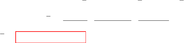
CHAPTER TWELVE SOLUTIONS
Engineering Circuit Analysis, 6th Edition Copyright
2002 McGraw-Hill, Inc. All Rights Reserved
15.
Bal.,+ seq. Z 8 6 , Z 12 16 , Z 5 0, V 120 0 V rms
120 0 120 120 120 120
R 0.5 ( ) I 6.803 83.86 A
8.5 6 12.5 16 5.5
I 6.803 96.14 A rms
AN BN CN AN
wnN
nN
jj j
ajj
↑=+Ω=−Ω=+=∠°
∠° ∠− ° ∠ °
=Ω −= + + = ∠ °
+−
∴= ∠− °
CHAPTER TWELVE SOLUTIONS
Engineering Circuit Analysis, 6th Edition Copyright
2002 McGraw-Hill, Inc. All Rights Reserved
16. Working on a per-phase basis, the line current magnitude is simply
()
2
2
w105R
40
++
=I
(a) RW = 0
Then A 578.3
1025
40
2=
+
=I, and the power delivered to each phase of the load is
(3.578)2(5) = 64.01 W. The total power of the load is therefore 3(64.01) = 192.0 W.
(b) RW = 3 Ω
Then A 123.3
1064
40
2=
+
=I, and the power delivered to each phase of the load is
(3.123)2(5) = 48.77 W. The total power of the load is therefore 3(48.77) = 146.3 W.
CHAPTER TWELVE SOLUTIONS
Engineering Circuit Analysis, 6th Edition Copyright
2002 McGraw-Hill, Inc. All Rights Reserved
17. Z 75 25 25 F, V 240 0 V rms, 60Hz, R 2
pan w
µ
↑=∠°Ω = ∠° =Ω
(a)
(b) 2
P 3(2.968) 2 52.84 W
w=×=
(c) 2
P 3(2.968) 75.34 1990.6W
load ==
(d) PF cos16.989 0.9564 lead
source =°=
6
10 75 25 ( 106.10)
Z 106.10 Z 75.34 23.63
377 25 75 25 106.10
240
Z 77.34 23.63 I 2.968 16.989 A
77.34 23.63
+
∠°−
=− =− Ω∴ = = − Ω
×∠°−
∴= − ∴= = ∠ °
−
cap p
pw aA
j
jj j
j
jj
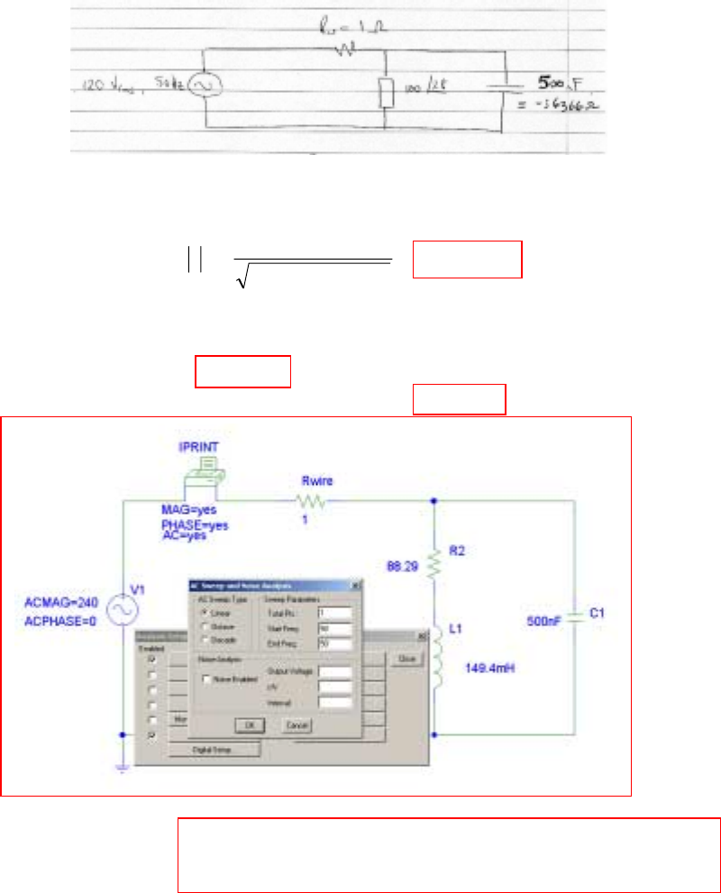
CHAPTER TWELVE SOLUTIONS
Engineering Circuit Analysis, 6th Edition Copyright
2002 McGraw-Hill, Inc. All Rights Reserved
18. Working on a per-phase basis and noting that the capacitor corresponds to a –j6366-Ω
impedance,
-j6366 || 100 ∠ 28o = 89.59 + j46.04 Ω so that the current flowing through the combined
load is
rmsA 362.2
04.4690.59
240
22 =
+
=I
The power in each phase is (2.362)2 (90.59) = 505.4 W, so that the power deliverd to the
total load is 3(505.4) = 1.516 kW.
The power lost in the wiring is (3)(2.362)2 (1) = 16.74 W.
Simulation Result:
FREQ IM(V_PRINT1) IP(V_PRINT1)
5.000E+01 1.181E+00 -2.694E+01
CHAPTER TWELVE SOLUTIONS
Engineering Circuit Analysis, 6th Edition Copyright
2002 McGraw-Hill, Inc. All Rights Reserved
19. Bal., R 0, Z 10 5 , 60 Hz
wp jf↑ = =+Ω =
(a) 10 5 11.180 26.57 PF cos 26.57 0.8944j
+= ∠ °∴= °=
(b)
(c)
1
PF 0.93 lag, 21.57 , Y 0.08 0.04S
11.180 26.57
377C 0.04
Y 0.08 (377C 0.04) tan 21.57 0.3952
0.08
377C 0.04 0.08 0.3952 0.00838 C 22.23 F
pj
pj
θ
µ
==°= =−
∠°
−
′=+ − ∴ =− °=−
∴=−× = ∴=
6
,
10 440 / 3
V 440Vrms, Z 119.30 ,I 2.129A
120 22.23 119.30
440
VAR 2.129 540.9 VAR ( .)
3
−
===−Ω==
∴=×=
L load c c
jj
cap
π
CHAPTER TWELVE SOLUTIONS
Engineering Circuit Analysis, 6th Edition Copyright
2002 McGraw-Hill, Inc. All Rights Reserved
20. Working from the single-phase equivalent,
Van rms =
∠
2
0115
3
1o
= 46.9 ∠0o V rms
1.5 H → j565 Ω, 100 µF → -j26.5 Ω and 1 kΩ → 1 kΩ.
These three impedances appear in parallel, with a combined value of 27.8 ∠ -88.4o Ω.
Thus, |Irms| = 46.9/ 27.8 = 1.69 A rms
Zload = 27.8 ∠88.4o = 0.776 – j 27.8 Ω, so Pload = (3)(1.69)2 (0.776) = 2.22 W.
CHAPTER TWELVE SOLUTIONS
Engineering Circuit Analysis, 6th Edition Copyright
2002 McGraw-Hill, Inc. All Rights Reserved
21.
R 0, V 200 60 V rms. S 2 1 kVA seq.
wan p
j==∠° =− +
(a) V 220 3 30 346.4 30 V
bc = ∠−°= ∠−°
(b)
(c)
S 2000 1000 V I 346.4 30 I
I 6.455 3.435 , I 6.455 3.435
200 3 30
Z 53.67 26.57 48 24
6.455 3.435
BC BC BC BC
BC BC
p
j
j
∗∗
∗− −
−
=− = =∠−°
∴= ∠ ° = ∠− °
∠− °
∴= = ∠− °=− Ω
∠− °
I I I 6.455 120 3.43 6.455 120 3.43 11.180 86.57 A rms
aA AB CA −−
= − = ∠ °− °− ∠− °− °= ∠ °
CHAPTER TWELVE SOLUTIONS
Engineering Circuit Analysis, 6th Edition Copyright
2002 McGraw-Hill, Inc. All Rights Reserved
22. 15kVA, 0.8lag, +seq., V 180 30 V rms, R 0.75
BC w
↑=∠°=Ω
(a)
(b)
1
V 180 30 V 180 150 V, S 5000 cos 0.8 5000 36.87 180 30 I
I 27.78 6.87 and I 27.78 113.13 A I I I
I 27.78(1 6.87 1 113.13 ) 48.11 36.87 A V 0.75(I I )
V 0.75 48.11(1
−∗
=∠°∴ =∠° = ∠ = ∠ °=∠°
∴= ∠− ° = ∠ °∴=−
∴= ∠− °−∠ °= ∠− °∴ = −
∴= × ∠−
BC AB p BC
BC AB bB BC AB
bB bC bB cC
bC 36.87 1 156.87 ) 180 30 233.0 20.74 V°− ∠− ° + ∠ °= ∠ °
2
P 3 48.11 0.75 5208W
S 5208 15,000 36.87 17.208 9.000kVA
wire
gen j
=× × =
=+ ∠°= +
CHAPTER TWELVE SOLUTIONS
Engineering Circuit Analysis, 6th Edition Copyright
2002 McGraw-Hill, Inc. All Rights Reserved
23. Bal., S 3 1.8 kVA, S 3.45 1.8 kVA, R 5
Lgen w
jj↑=+ =+ =Ω
(a) 2
1
P 450 W 450 I 5 I 5.477A rms
3
=∴×=×∴=
waAaA
(b) 1
I 5.477 3.162A rms
3
AB =× =
(c)
1
Assume I 3.162 0 and +seq. (3000 1800) (3.162 0 )
3
V 368.8 30.96 V V V V V V
V 5I 5 5.477 30 27.39 30 ,V 27.39 150
V 27.39 30 27.39 150 368.8 30.96 V (1
∗
=∠° ∴ + = = ∠°
∴= ∠ °∴=+−+
==×∠−°=∠−°=∠−°
∴ = ∠− °− ∠− °+ ∠ °+ ∠−
AB AB AB AB
AB an aA AB bB bn
aA aA bB
an an
jVIV
120 )
27.39 30 27.39 150 368.8 30.96
V 236.8 2.447 236.8V rms
1 1 120
°
∠− °− ∠− °+ ∠ °
∴= = ∠− °∴=
−∠− °
an an
V
CHAPTER TWELVE SOLUTIONS
Engineering Circuit Analysis, 6th Edition Copyright
2002 McGraw-Hill, Inc. All Rights Reserved
24. If a total of 240 W is lost in the three wires marked Rw, then 80 W is lost in each 2.3-Ω
segment. Thus, the line current is rmsA 898.5
3.2
80 =. Since this is a D-connected load,
the phase current is 1/ 3 times the line current, or 3.405 A rms.
In order to determine the phase voltage of the source, we note that
Ptotal =
=⋅⋅ 2
2
(5.898) 3 PF 3 linelineline VIV = 1800
where |Vline| =
()()
V 249.2
(5.898) 3 2
21800 =
This is the voltage at the load, so we need to add the voltage lost across the wire, which
(taking the load voltage as the reference phase) is
()
W
1R
2
1
cos898.5
−∠ −
= 13.57 ∠-45o V. Thus, the line voltage magnitude of the source is
|249.2 ∠ 0o + 13.57 ∠ -45o| = 259.0 V rms.
CHAPTER TWELVE SOLUTIONS
Engineering Circuit Analysis, 6th Edition Copyright
2002 McGraw-Hill, Inc. All Rights Reserved
25. Bal., +seq.
(a)
(b) I 41.57 20.78 30 60.47 170.10 A rms
bB =− − ∠ °= ∠− °
(c) I 20.78 120 41.57 36.00 30 A rms
cC =∠−°+ =∠−°
(d)
120 3 30
V 120 0 V 120 3 30 , ., I 20.78 30 A
10
120 3 90 120 3 150
I 41.57 ; I 20.78 120 A
510
I I I 20.78(1 30 1 120 ) 40.15 45 Arms
∠°
=∠°∴= ∠° = = ∠°
∠− ° ∠ °
==−==∠−°
−
=−= ∠°−∠−°= ∠°
an ab AB
BC CA
aA AB CA
etc
A
jj
S V I V I V I 120 3 30 20.78 30 120 3 90 ( 41.57)
120 3 150 20.78 120 4320 0 0 8640 0 4320 4320 4320VA
tot AB AB BC BC CA CA
jj j j
∗∗∗
=++=∠°×∠−°+∠−°−+
∠°× ∠°= +++ +− = +
CHAPTER TWELVE SOLUTIONS
Engineering Circuit Analysis, 6th Edition Copyright
2002 McGraw-Hill, Inc. All Rights Reserved
26. IAB = A 18.4- 21.1
4.1849.9
0200
30 ||10
0200 o
o∠=
∠
∠
=
∠
j
|IA| = A 36.5 I 3 AB =
The power supplied by the source = (3) |IA|2 (0.2) + (3) (200)2 / 10 = 12.8 kW
Define transmission efficiency as η = 100 × Pload/ Psource. Then η = 93.8%.
IA leads IAB by 30o, so that IA = 36.5 ∠ 11.6o.
V 11.6 7.3 )11.6 (0.2)(36.5 oo
RW∠=∠=V
With VAN = o
30
3
200 ∠, and noting that Van = VAN +
W
R
V= 122 ∠ 28.9o, we may now
compute the power factor of the source as
PF = cos (ang(Van) – ang(IA)) = cos (28.9o – 11.6o) = 0.955.
CHAPTER TWELVE SOLUTIONS
Engineering Circuit Analysis, 6th Edition Copyright
2002 McGraw-Hill, Inc. All Rights Reserved
27. Bal., V 140 0 V , seq., R 0, S 15 9 kVA
an rms w L j↑=∠°+==+
(a) V V 3 140 30 242.5 30 V
−
== ∠°= ∠°
ab AB
(b) V I 5000 3000 242.5 30 I I 24.05 0.9638 A rms
AB AB AB AB
j
∗−∗−
=+=∠°∴=∠−°
(c) I I I 24.05 0.9638 24.05 119.03 41.65 30.96 A rms
aA AB CA −−−
=−= ∠− °− ∠ °= ∠− °
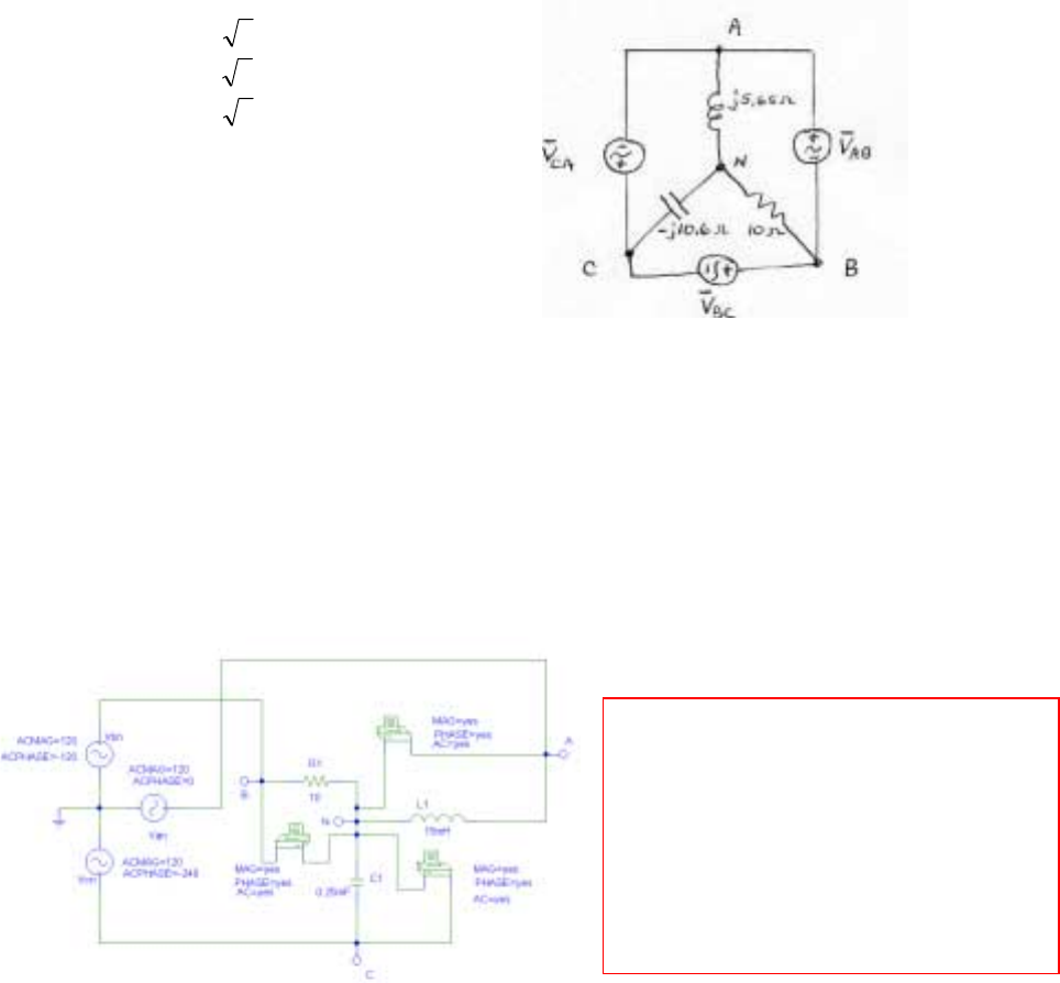
CHAPTER TWELVE SOLUTIONS
Engineering Circuit Analysis, 6th Edition Copyright
2002 McGraw-Hill, Inc. All Rights Reserved
28. 15 mH → j5.65 Ω, 0.25 mF → -j10.6 Ω
VAB = V 30 3120 o
∠
VBC = V 90 3120 o
−∠
VCA = V 012 3120 o
−∠
Defining three clockwise mesh currents I1,
I2 and I3 corresponding to sources VAB,
VBC and VCA, respectively, we may write:
VAB = (10 + j5.65) I1 – 10 I2 + j5.65 I3 [1]
VBC = -10 I1 + (10 – j10.6) I2 + j10.6 I3 [2]
VCA = - j5.65 I1 + j10.6 I2 + (j5.65 – j10.6) I3 [3]
Solving using MATLAB or a scientific calculator, we find that
I
1 = 53.23 ∠ -5.873o A, I2 = 40.55 ∠ 20.31o A, and I3 = 0
(a) VAN = j5.65(I1 – I3) = 300.7 ∠ 84.13o V, so VAN = 300.7 V
(b) VBN = 10(I2 – I1) = 245.7 ∠ 127.4o V, so VBN = 245.7 V
(c) VCN = -j10.6 (-I2) = 429.8 ∠ 110.3o V, so VCN = 429.8 V
PSpice Simulation Results
(agree with hand calculations)
FREQ VM(A,N) VP(A,N)
6.000E+01 3.007E+02 8.410E+01
FREQ VM(B,N) VP(B,N)
6.000E+01 2.456E+02 1.274E+02
FREQ VM(C,N) VP(C,N)
6.000E+01 4.297E+02 1.103E+02
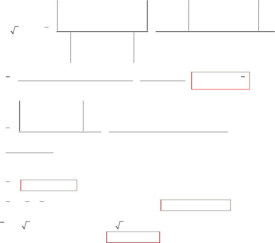
CHAPTER TWELVE SOLUTIONS
Engineering Circuit Analysis, 6th Edition Copyright
2002 McGraw-Hill, Inc. All Rights Reserved
29. 1↑=Ω
line
R
(a)
1
207.8[1 30 (70 40) 1( 10 45)] 21.690 34.86
I 33.87 45.20 I
630 115 630 115 aA
jj j
jj
∠° + + − − ∠ °
∴= = = ∠ °=
−−
2
12 1 30 10
1 1 5 207.8
10 0 10 5 207.8[ 1 30 ( 10 45) 1(20 60)]
I630 115 630 115
16,136 162.01 25.20 172.36 A
630 115
∠° −
−− −
−− −∠ °− − − −
∴= =
−−
∠°
==∠°
−
jj
jjj j
jj
j
(b) I 25.20 7.641 A
cC
∴= ∠− °
(c) I I I 33.87 45.20 25.20 7.641 53.03 157.05 A rms
bB aA CC
∴=−−=−∠°−∠−°=∠− °
(d)
S 120 3 30 (33.87 45.20 ) 120 3 90 (25.20 7.641 )
6793 1846.1 696.3 5190.4 6096 3344VAjjj
=∠°∠−°+∠°∠°
=− − + =+
1
207.8 30 1 10 1 30 1 10
207.8 90 2 5 5 207.8 1 2 5 5
05105 05105
120 3 207.8 I 12 1 10 12(70 40) ( 10 45) 10(20 55)
12 5 5
10 5 10 5
j
jj j jj
jj jj
jjj j
jj
jj
∠° − − ∠° − −
∠− ° + − − + −
−− −−
== =
−− ++−−− +
−+ −
−− −
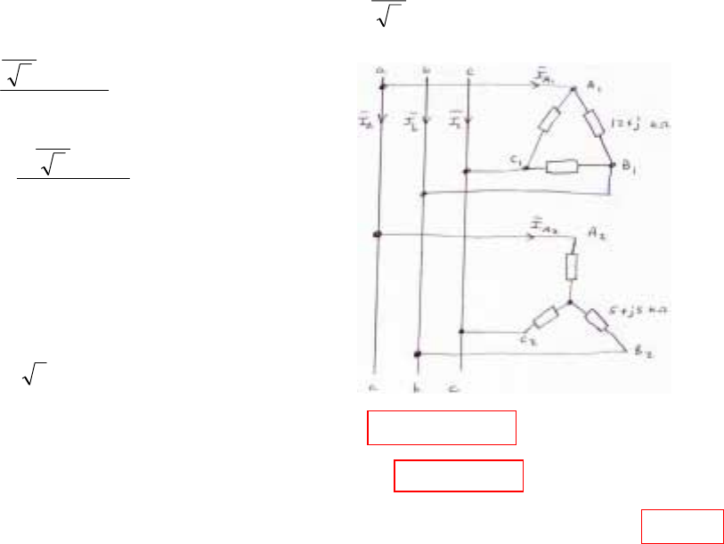
CHAPTER TWELVE SOLUTIONS
Engineering Circuit Analysis, 6th Edition Copyright
2002 McGraw-Hill, Inc. All Rights Reserved
30. |Vline| = 240 V. Set Vab = 240∠0o V. Then Van = o
30
3
240 −∠ .
IA2 = A 1.068.23
35
30
3
240
o
o
−∠=
+
−∠
j
I
A1B1 =
()
mA 76.40.20
1021
0
3
240
o
3
o
−∠=
×+
∠
j
I
phase leads Iline by 30o, so
IA1 = mA 8.3434.6 mA 8.34320 oo −∠=−∠
Ia = IA1 + IA2 = 11.5 – j20.8 + 28.4 – j19.7 mA = 56.9∠-45.4o mA
The power factor at the source = cos (45.4o – 30o) = 0.964 lagging.
The power taken by the load = (3)(20×10-3)2 (12×103) + (3)(23.8×10⁻³)2 (5000) = 22.9 W.

CHAPTER TWELVE SOLUTIONS
Engineering Circuit Analysis, 6th Edition Copyright
2002 McGraw-Hill, Inc. All Rights Reserved
31. Define I flowing from the ‘+’ terminal of the source. Then,
I = o
o74.2941.12
29.7416.12
0200
)20||10(10
0200 −∠=
∠
∠
=
+
∠
j
(a) Vxy = 10 I = 124.1 ∠-29.74o V. Thus, Pxy = (12.41)(124.1) = 1.54 kW
(b) Pxz = (200)(12.41) cos (29.74o) = 2.155 kW
(c) Vyz = 200 ∠0 – 124.1 ∠-29.74o = 110.9 ∠ 33.72o V
Thus, Pyz = (110.9)(12.41) cos (33.72o + 29.74o) = 614.9 W
No reversal of meter leads is required for any of the above measurements.
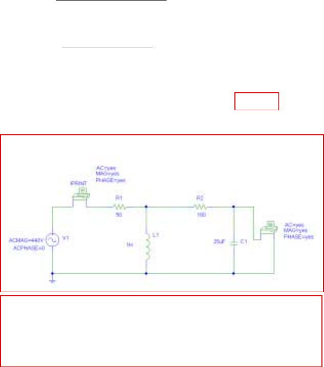
CHAPTER TWELVE SOLUTIONS
Engineering Circuit Analysis, 6th Edition Copyright
2002 McGraw-Hill, Inc. All Rights Reserved
32. 1 H → j377 Ω, 25 µF → -j106 Ω
I1 =
()
[]
A 2186.1
10610037750
0440
o
∠=
+
∠
-j||j
IC = I A 41.32.43
106100377
377 o
∠=
−+ jj
j
V2 = (106∠-90o)(2.43∠-41.3o) = 257∠-48.7o V
P
measured = (257)(1.86) cos (21o + 48.7o) = 166 W.
No reversal of meter leads is needed. PSpice verification:
FREQ VM($N_0002,0) VP($N_0002,0)
6.000E+01 2.581E+02 -4.871E+01
FREQ IM(V_PRINT1) IP(V_PRINT1)
6.000E+01 1.863E+00 2.103E+01

CHAPTER TWELVE SOLUTIONS
Engineering Circuit Analysis, 6th Edition Copyright
2002 McGraw-Hill, Inc. All Rights Reserved
33. 2.5 A peak = 1.77 A rms. 200 V peak = 141 V rms. 100 µF → -j20 Ω.
Define the clockwise mesh current I1 in the bottom mesh, and the clockwise mesh current
I2 in the top mesh. IC = I1 – I2.
Since I2 = -177∠-90o, we need write only one mesh equation:
141∠0o = (20 - j40o) I1 + (-20 + j20) I2
so that I1 = A78.474.023
40-20
)90-20)(1.77 (-20 0141 o
o∠=
∠++∠
j
j
and IC = I1 – I2 = 2.361 ∠ 63.43o A. Imeter = -I1 = 4.023∠-105.2o
Vmeter = 20 IC = 47.23 ∠63.43o V
Thus, Pmeter = (47.23)(4.023)cos(63.43o + 105.2o) = -186.3 W.
Since this would result in pegging the meter, we would need to swap the potential leads.
CHAPTER TWELVE SOLUTIONS
Engineering Circuit Analysis, 6th Edition Copyright
2002 McGraw-Hill, Inc. All Rights Reserved
34. (a) Define three clockwise mesh currents I1, I2 and I3 in the top left, bottom left and right-
hand meshes, respectively. Then we may write:
100 ∠0 = (10 – j10) I1 - (10 – j10) I3
50 ∠90o = (8 + j6) I2 – (8 + j6) I3
0 = -(10 – j10) I1 – (8 + j6) I2 + (48 + j6) I3
Solving, we find that I1 = 10.12∠ 32.91o A, I2 = 7.906 ∠ 34.7o and I3 = 3.536 ∠ 8.13o A.
Thus, PA = (100)(10.12) cos (-32.91o) = 849.6 W
and PB = (5)(7.906) cos (90o – 34.7o) = 225.0 W
(b) Yes, the total power absorbed by the combined load (1.075 kW) is the sum of the
wattmeter readings.
PSpice verification:
FREQ IM(V_PRINT1) IP(V_PRINT1)
6.280E+00 1.014E+01 6.144E-02
FREQ IM(V_PRINT2) IP(V_PRINT2)
6.280E+00 4.268E-01 1.465E+02
FREQ VM($N_0002,$N_0006) VP($N_0002,$N_0006)
6.280E+00 1.000E+02 0.000E+00
FREQ VM($N_0004,$N_0006) VP($N_0004,$N_0006)
6.280E+00 5.000E+01 - 9.000E+01
CHAPTER TWELVE SOLUTIONS
Engineering Circuit Analysis, 6th Edition Copyright
2002 McGraw-Hill, Inc. All Rights Reserved
35. This circuit is equivalent to a Y-connected load in parallel with a ∆-connected load.
For the Y-connected load, Iline = A 6062.4
3025
30
3
200
o
o
o
−∠=
∠
−∠
P
Y =
()
kW 1.386 30cos62.4
3
200
)3( o=
For the ∆-connected load, Iline = A 604
6050
0200
o
o
∠=
−∠
∠
P
∆ = (3)(200)(4 cos 60o) = 1.2 kW
P
total = PY + P∆ = 2.586 kW
P
wattmeter = Ptotal / 3 = 862 W
CHAPTER TWELVE SOLUTIONS
Engineering Circuit Analysis, 6th Edition Copyright
2002 McGraw-Hill, Inc. All Rights Reserved
36. We assume that the wire resistance cannot be separated from the load, so we measure
from the source connection:
(a)
(b)
CHAPTER TWELVE SOLUTIONS
Engineering Circuit Analysis, 6th Edition Copyright
2002 McGraw-Hill, Inc. All Rights Reserved
37. We assume that the wire resistance cannot be separated from the load, so we measure
from the source connection:
(a)
(b)

CHAPTER THIRTEEN SOLUTIONS
Engineering Circuit Analysis, 6th Edition Copyright
2002 McGraw-Hill, Inc. All Rights Reserved
1. 1 and 3, 2 and 4
1 and 4, 2 and 3
3 and 1, 2 and 4

CHAPTER THIRTEEN SOLUTIONS
Engineering Circuit Analysis, 6th Edition Copyright
2002 McGraw-Hill, Inc. All Rights Reserved
2. 12
4 A, 10 A==
SS
iti t
(a) 20 4 4 10 120 V=×+×=
AG
v
(b) 4 6 24 V=− × =−
CG
v
(c) 3 10 4 4 6 4 30 16 24 22 V=× +×−×= + − =
BG
v
CHAPTER THIRTEEN SOLUTIONS
Engineering Circuit Analysis, 6th Edition Copyright
2002 McGraw-Hill, Inc. All Rights Reserved
3.
(a)
(b)
2
22
50 2000
113
P 50 0.4745 5.630 W, P 2000 0.4745 4.769 W
2 2 20 5
−
=× × = =× × × =
+
j
j
(c) 0 each
(d) 0
12 21
21
1
11
,
100 (50 200) I 300I ,(2000 500)I 300I 0
3 900
I , 100 50 200
20 5 20 5
900 4250
100 I I 0.4745 64.01 A
20 5
1
P 100 0.4745cos 64.01 10.399 W
2
=+ + + + =
−
∴= = + +
++
+
∴= ∴= ∠− °
+
∴=−×× °=−
SabS
jj jj
jjI
jj
j
j

CHAPTER THIRTEEN SOLUTIONS
Engineering Circuit Analysis, 6th Edition Copyright
2002 McGraw-Hill, Inc. All Rights Reserved
4.
KVL Loop 1 100 ∠0 = 2(I1 – I2) + j
ω
3 (I1 – I3) + j
ω
2 (I2 – I3)
KVL Loop 2 2(I2 – I1) + 10I2 + j
ω
4 (I2 – I3) + j
ω
2 (I1 – I3) = 0
KVL Loop 3 5I3 + j
ω
3 (I3 – I1) + j
ω
2 (I3 – I2) + j
ω
4 (I3 – I2) + j
ω
2 (I3 – I1) = 0
∴LINEAR EQUATIONS
∠
=
+−
−++−
−+−+
0
0
0100
11525
641222
52232 1
3
2
I
I
I
jjj
jjj
jjj
ωω
ωωω
ωωω
Since
ω
= 2πf = 2π(50) = 314.2 rad/s, the matrix becomes
∠
=
+−
−++−
−+−+
0
0
0100
345654.6281571
18851257124.6282
15714.62826.9422 1
3
2
I
I
I
jjj
jjj
jjj
Solving using a scientific calculator or MATLAB, we find that
I1 = 278.5 ∠ -89.65o mA, I2 = 39.78 ∠ -89.43o mA, I3 = 119.4 ∠ -89.58o mA.
Returning to the time domain, we thus find that
i1(t) = 278.5 cos (100πt – 89.65o) mA, i2(t) = 39.78 cos (100πt – 89.43o) mA, and
i3(t) = 119.4 cos (100πt – 89.58o) mA.
CHAPTER THIRTEEN SOLUTIONS
Engineering Circuit Analysis, 6th Edition Copyright
2002 McGraw-Hill, Inc. All Rights Reserved
5.
(a)
(b)
,
12 2 1
12 22
,2
100
V ( 300) 145.52 165.96 V
50 200
100 (50 200) I 300I , 500I 300I 0
55
I I , 100 (50 200) 300 I I 1.1142 158.199 A
33
145.52 165.96
ZV/I 1.1142 158.
=−=∠−°
+
=+ + + =
∴=− = + − + ∴ = ∠ °
∠− °
∴= = ∠
ab oc
SC SC
SC SC SC
th ab bc SC
j
j
jjj j
jj
130.60 35.84 105.88 76.47
199 =∠°=+ Ω
°j
2
max
145.52
Z 105.88 76.47 I 0.6872 A
2 105.88
1
P 0.6872 105.88 25.00 W
2
=−Ω∴= =
×
∴=× × =
LL
L
j

CHAPTER THIRTEEN SOLUTIONS
Engineering Circuit Analysis, 6th Edition Copyright
2002 McGraw-Hill, Inc. All Rights Reserved
6.
(a) 11 2 11 2 2 2 1
() L M , () L M L M
′′ ′′ ′′
=− =−+ −
AB
vt i ivt i i i i
(b) V1(j
ω
) = j
ω
L1 IA + j
ω
M(IB + IA)
V2(j
ω
) = j
ω
L2 (IB + IA) + j
ω
MIA
CHAPTER THIRTEEN SOLUTIONS
Engineering Circuit Analysis, 6th Edition Copyright
2002 McGraw-Hill, Inc. All Rights Reserved
7.
22
22
22
22
222
64 4
222
10 ( ) 1000
0.01 ( )
0.01 0.01
15 1500
0.015 ( ), 100 ( )
0.01 0.01
15 ( 0.01)2 2
100 10 10 ( ) 15 10 ( )
0.01 ( 0.01)
−− −
′′
==∴=
++
′
== =
++
+−×
′
∴= × = =×
++
sSS
xS x
Cx
tut t
viiut
tt
tt
vi utv ut
tt
dt t ttt
iv ut ut
dt t t
40.02
15 10 (
−
∴=×
C
t
it22 22
30
() A,
0.01) ( 0.01)
∴=
µ
++
C
t
it t
t > 0
CHAPTER THIRTEEN SOLUTIONS
Engineering Circuit Analysis, 6th Edition Copyright
2002 McGraw-Hill, Inc. All Rights Reserved
8.
(a)
Thus, v(t) = 126 cos (100πt + 90o) V
(b) Define V2 across the 2-H inductor with + reference at the dot, and a clockwise
currents I1 and I2, respectively, in each mesh. Then,
V = -V2 and we may also write
V2 = j
ω
L2 I2 + j
ω
MI1 or -V = j
ω
L2 10
V + j
ω
M
Solving for V,
V =
()()
()()
21001
0.4 100
π
π
j
j
+
− = o
o
o
179.1- 2.000
89.0962.84
90-125.7
83.621
907.125 ∠=
∠
∠
=
+
−∠
j
o
Thus,
v(t) = 2 cos (100πt – 179.1o) V.
(c) Define V1 across the left inductor, and V2 across the right inductor, with the “+”
reference at the respective dot; also define two clockwise mesh currents I1 and I2.
Then,
1
12
2
10
Now and
4
and 10
∠−
==−
=
out
out
V
IVV
V
I
1
11
1
2
11
1
2
1
10 EQN 1
410
10 EQN 2
10 4
10
1410 4
10
1
410 4
1 39 12.6 3
31.4 1 62.8
∠−
⇒=ω +ω
∠−
−=ω +ω
ω−ω ω∠
−
=
ωω ω∠
−+
−−
=
−+
out
out
out
out
out
jL jM
jL jM
jL jM jL
jM jL jM
jj
jj
VV
V
VV
V
V
V
V
V
9.3
31.4
j
j
Solving, we find that Vout (= V) = 1.20 ∠ -2.108o V and hence
v(t) = 1.2 cos (100πt – 2.108o) V.
2
2
0.4 1 0
100 0.4 1 0
−=ω ∠
=− π× × ∠
j
j
V
V= 126 ∠ 90o V
111 2
222 1
=ω +ω
=ω +ω
jL jM
jL jM
VII
VII

CHAPTER THIRTEEN SOLUTIONS
Engineering Circuit Analysis, 6th Edition Copyright
2002 McGraw-Hill, Inc. All Rights Reserved
9.
(a) 100 = j5
ω
(I1 – I2) + j3
ω
I2 + 6(I1 – I3) [1]
(4 + j4
ω
)I2 + j3
ω
(I1 – I2) + j2
ω
(I3 – I2) + j6
ω
(I2 – I3) – j2
ω
I2 + j5
ω
(I2 – I1)
– j3
ω
I2 = 0 [2]
6 (I3 – I1) + j6
ω
(I3 – I2) + j2
ω
I2 + 5 I3 = 0 [3]
Collecting terms,
(6 + j5
ω
) I1 – j2
ω
I2 – 6 I3 = 100 [1]
-j2
ω
I1 + (4 + j5
ω
) I2 – j4
ω
I3 = 0 [2]
-6 I1 - j4
ω
I2 + (11 + j6
ω
) I3 = 0 [3]
(b) For
ω
= 2 rad/s, we find
(6 + j10) I1 – j4 I2 – 6 I3 = 100
-j4 I1 + (4 + j10) I2 – j8 I3 = 0
-6 I1 – j8 I2 + (11 + j12) I3 = 0
Solving, I3 = 4.32 ∠ -54.30o A

CHAPTER THIRTEEN SOLUTIONS
Engineering Circuit Analysis, 6th Edition Copyright
2002 McGraw-Hill, Inc. All Rights Reserved
10.
(a)
1 1
2 2
=ω +ω =
=ω +ω =−
aab a
bba b
jL jM
jL jM
VI I II
VII II
111
11 1
11 11 2
=+
=+ω+ω
=+ω−ω
a
ab
R
RjL jM
RjL jM
VI V
III
III
222
22 2
22 22 1
=−
=−ω−ω
=+ω−ω
b
ba
R
RjL jM
RjL jM
VI V
III
III
(b) Assuming that the systems connecting the transformer are fully isolated.
11
22
=ω +ω =−
=ω +ω =−
aab a
bba b
jL jM
jL jM
VII II
VII II
11
11
111 2
=−
=−ω−ω
=+ω+ω
a
ab
R
RjL jM
RjL jM
VI V
III
III
22
22 2
22 22 1
=+
=− +ω +ω
=− − ω − ω
bb
ba
R
RjL jM
RjL jM
VVI
III
III
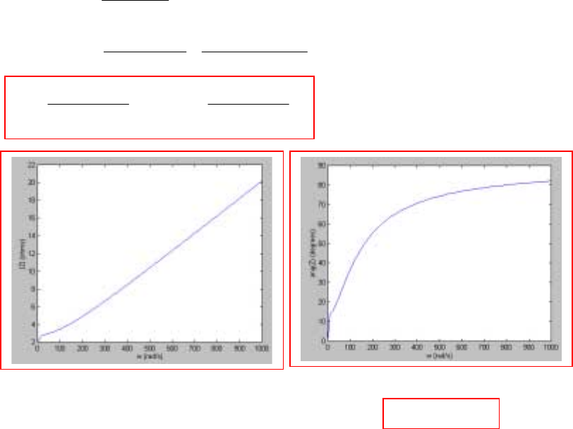
CHAPTER THIRTEEN SOLUTIONS
Engineering Circuit Analysis, 6th Edition Copyright
2002 McGraw-Hill, Inc. All Rights Reserved
11.
(a)
22
22 22
2222
22
22
(0.2)
2 0.1 5 0.5
5 (0.2) 0.5 (0.2)
2 0.1 5 ( 0.5) 5 ( 0.5)
0.2 0.02
2 0.1
25 0.25 25 0.25
ω
=
+ω + +ω
ωωω
=
+ω + −
+ω +ω
ωω
=
++ω−
+ω +ω
jj
j
j
j
(b)
(c) Zin(j
ω
) at
ω
= 50 is equal to 2 + 0.769 + j(50)(0.023) = 2.77 + j1.15 Ω.
Z
CHAPTER THIRTEEN SOLUTIONS
Engineering Circuit Analysis, 6th Edition Copyright
2002 McGraw-Hill, Inc. All Rights Reserved
12.
22
11
22
22
3
3
22 32
3
232232
22 322
3
232 232
50 10 81010
81010
50 10 8 ( 10 10 ) 8 ( 10 10 )
81010
50 10
8 ( 10 10 ) 8 ( 10 10 )
−
−
−
−
−−
−
−
−−
ω
=+
ω
=ω × ++ω ×
ωω×ω
⇒=ω× + −
+ω × +ω ×
ω×ω
=+ω×−
+ω × +ω ×
in
in
M
M
jj
Mj M
j
MM
j
ZZ Z
Z
In this circuit the real power delivered by the source is all consumed at the speaker, so
2
222
232
22 2
232
1
20 8
3.2 8 ( 10 10 )
2
820
8 ( 10 10 ) 2 3.2
−
−
ω
=⇒= ×
ω×
ω
⇒=
+ω × ×
rms
VM
PR
M
= 62.5 W

CHAPTER THIRTEEN SOLUTIONS
Engineering Circuit Analysis, 6th Edition Copyright
2002 McGraw-Hill, Inc. All Rights Reserved
13. 12
2cos10 A, 1.2cos10 A==
SS
iti t
(a)
(b)
(c) 12
11
P 27.34 2cos69.44 9.601 W, P 23.64 1.2cos66.04 5.760 W
22
=× × °= =× × °=
SS
1
1
0.6( 20sin10 ) 0.2( 12sin10 ) 0.5( 32sin10 ) 9.6cos10
9.6cos10 25.6sin10 27.34cos(10 69.44 ) V
=− −− +− +
∴= − = + °
vtttt
vtt t
2
2
0.8( 12sin10 ) 0.2( 20sin10 ) 16sin10 9.6cos10
9.6cos10 21.6sin10 23.64cos(10 66.04 ) V
=− −− − +
∴= − = + °
vtttt
vtt t

CHAPTER THIRTEEN SOLUTIONS
Engineering Circuit Analysis, 6th Edition Copyright
2002 McGraw-Hill, Inc. All Rights Reserved
14.
84
10 4 10 5
65
=ω +ω
=ω +ω =ω +ω
=ω +ω
aab
bbabc
ccb
jj
jjjj
jj
VII
*V I I I I
VII
Also =− =− =
abc
II II
Now examine equation *.
10 4 10 5−ω −ω =−ω + ω c
jj jjII II
∴ the only solution to this circuit is I = and hence
( ) 120cos
∴
=ω
vt tV.
CHAPTER THIRTEEN SOLUTIONS
Engineering Circuit Analysis, 6th Edition Copyright
2002 McGraw-Hill, Inc. All Rights Reserved
15.
12
21
2
2 1
11
100 10I 15I
0 200I 15I 15I
0 (5 10) I 15I
510 12 12
I I I 0 200 15 I 15I
15 3 3
400 200 118.33 66.67
0 15 I 15I I I
33 15
2
100 (66.67 118.33) 5 10 I (39.
3
=−
=−−
=+ −
++ +
∴= = ∴= − −
+
∴= − + − ∴ =
∴= + −− =
L
L
LL L
LL
L
jj
jjj
jj
jj j
jjj
jj j
j
jj j j
jj44 68.89) I
I 1.2597 60.21 A
+
∴= ∠− °
L
L
j
CHAPTER THIRTEEN SOLUTIONS
Engineering Circuit Analysis, 6th Edition Copyright
2002 McGraw-Hill, Inc. All Rights Reserved
16. 2cos10 A, 0==
s
itt
(a) 22
11
O.C. (0) 5 2 4 2 10 8 18 J
22
− ∴ =××+××=+=ab w
(b)
22 2
2
2
1
S.C. 10, I 2 0 A, M 12 3 H
2
20 3
( 30 5) I 10 3 2, I 1.1390 9.462 A 1.1390cos(10 9.462 ) A
530
1
(0) 1.1235 (0) 10 8 3 2 1.1235 3 1.1235 16.001 J
2
−
−ω==∠°==
+− ×∴= = ∠ °∴= + °
+
∴= ∴=+−×× +×× =
S
ab
j
jj i t
j
iw
CHAPTER THIRTEEN SOLUTIONS
Engineering Circuit Analysis, 6th Edition Copyright
2002 McGraw-Hill, Inc. All Rights Reserved
17.
1221
12 2
2
22 2
22
24 2
V 12 0 V rms, 100 rad/s
12 (6 20) I 100(0.4K) I , (24 80) I 40KI 0
310 310
I I 12 (6 20) 40K I
5K 5K
18 200 60 60 200K 60K
12 I I
5K 182 200K 120
60 K 24
P(200K 1
=∠° ω=
=+ + + + =
++
∴= ∴ = + +
−−
−+++ −
∴= ∴=
−−++
∴= −
s
jj jj
jj
jj
jj
jj j
jj
22
22 4 2 4 2
86,400 K 2.16K W
82) 120 40,000K 72,800K 47,524 K 1.82K 1.1881
==
+−+−+
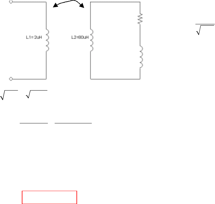
CHAPTER THIRTEEN SOLUTIONS
Engineering Circuit Analysis, 6th Edition Copyright
2002 McGraw-Hill, Inc. All Rights Reserved
18.
12
=M
kLL
250 /ω= k rad s
6
12 28010
12.6 H
−
==××
=µ
MLL
Zin 22 22
22 22
11 22 22
22 22 22 22
ω−ω
=+ +
++
n
MR jM X
RX RX
Z
36
11 22
36
22
250 10 2 10 2
0.5 (250 10 )(80 10 )
20
−
−
=× × ×× =Ω
==××
=
jR
jX
Z
Thus, Zin = j0.5 + 19.8/404 – j198/ 404
= 0.049 + j0.010 Ω.
Zin →
2 Ω
j10 Ω
M
• •
CHAPTER THIRTEEN SOLUTIONS
Engineering Circuit Analysis, 6th Edition Copyright
2002 McGraw-Hill, Inc. All Rights Reserved
19. 100 rad/sω=
(a)
(b) 2
20
P 0.1144 20 0.2617 W=×=
(c) P 100 0.5833cos88.92 1.1039 W=× °=
gen
12
123
21
31
3121 1
11 2
K 50,K 20,1H j100
100 j200 I 50I 20I
0 (10 100) I 50I
0 (20 100) I 20I
25 52
II,II102052I
2 10 1 10 1 10 2 10
25 4
10 20 I I 0.5833 88.92 A, I
110210
→Ω →Ω→ Ω
=−−
=+ −
=+ −
∴= = ∴= − −
++ ++
∴= + + ∴= ∠− ° =
++
jj
jj
jj
jj
jj jj
jj j
jj jj
jjj
2
310
0.2902 83.20 A,
I 0.11440 77.61 A P 0.2902 10 0.8422 W
Ω
∠− °
=∠−°∴=×=
CHAPTER THIRTEEN SOLUTIONS
Engineering Circuit Analysis, 6th Edition Copyright
2002 McGraw-Hill, Inc. All Rights Reserved
20.
(a)
(b)
(c) The total energy stored at t = 0.
12
22
11 22 1212
41
11
22
11
5 16 1.8 1 1.2 4 1
22
40 0.9 4.8
36.1J
==
=++
=×× +× ×− ××
=+ −
=
AA
W total L L M
II
IIII
12 3
231
510
510 410
−−
+=
⇒=−
=× −×
tt
II I
III
12
0.4 5 1.8
1.2H
=
⇒= ×
=
M
kLL
M
CHAPTER THIRTEEN SOLUTIONS
Engineering Circuit Analysis, 6th Edition Copyright
2002 McGraw-Hill, Inc. All Rights Reserved
21.
12 1 1 2 2
11 122
12 1 2 2
2
12
12
62
1212
2
12
12
2
K 1000K L L , L 1000L , L 1000L
V (2 1000L ) I 1000K L L I
0 1000K L L I (40 1000L ) I
40 1000L
1000 rad/s I I
1000K L L
(2 1000L )(40 1000L ) 10 K L L
VI
1000K L L
1000K L L
I8
→→→
∴=+ −
=− + +
+
ω= ∴ =
+++
∴=
∴=
s
s
jjj
jj
jj
j
j
jj
j
j
62
1212
12
2
62
s12 12
0 40,000L 2000L 10 L L (1 K )
40,000K L L
V
V 80 10 L L (1 K ) (40,000L 2000L )
++−−
∴=−−+ +
jj
j
j
(a)
(b)
(c) 2
12
V 40,000 5 200,000
L 1, L 25, K 1 2.222 0.05093
V 80 0 90,000 80 90,000
×
== =∴= = =∠ °
−+ +
s
jj
jj
33
2
12
V405 200
L 10, L 2510, K 1 1.660941.63
V 80 0 (40 50) 80 90
−− ×
==×=∴= = =∠°
−+ + +
s
jj
jj
2
12 62
3
2
V 40,000 0.99 5
L 1, L 25, K 0.99 V 80 25 10 (1 0.99 ) (40,000 50,000)
V 198,000 0.3917 79.74
V 80 497,500 90,000
××
== =∴=
−× − + +
∴= = ∠− °
−+
S
j
j
j
j
CHAPTER THIRTEEN SOLUTIONS
Engineering Circuit Analysis, 6th Edition Copyright
2002 McGraw-Hill, Inc. All Rights Reserved
22.
(a)
(b)
,,
,
12
2
L 10 mH, L 5 mH
L8 mH
L 10 mH, L 5 mH, 8 10 M M (5 M) (mH)
M(5 M)
8 10 M , 5M (10 8)5 5M M M 3.162 mH ( 10)
5
3.162
K K 0.4472
50
==
=
∴= = =−+ −
−
∴= − + ∴ = − + − ∴ = =
∴= ∴=
AB CDOC CD ABOC
AB CDSC
1
33 32 3
22
22
2222 2
2
Dots at A and D, 5 A, 100 mJ
11
100 10 10 10 25 5 10 10 5 10
22
210 40 40
100 125 2.5 5 10 2 10 10 0, 10
2
3.162 A
−− − −
==
∴× =×× ×+×× − ××
±−
=+ − ∴− += = =
∴=
tot
iw
ii
iiii i
i
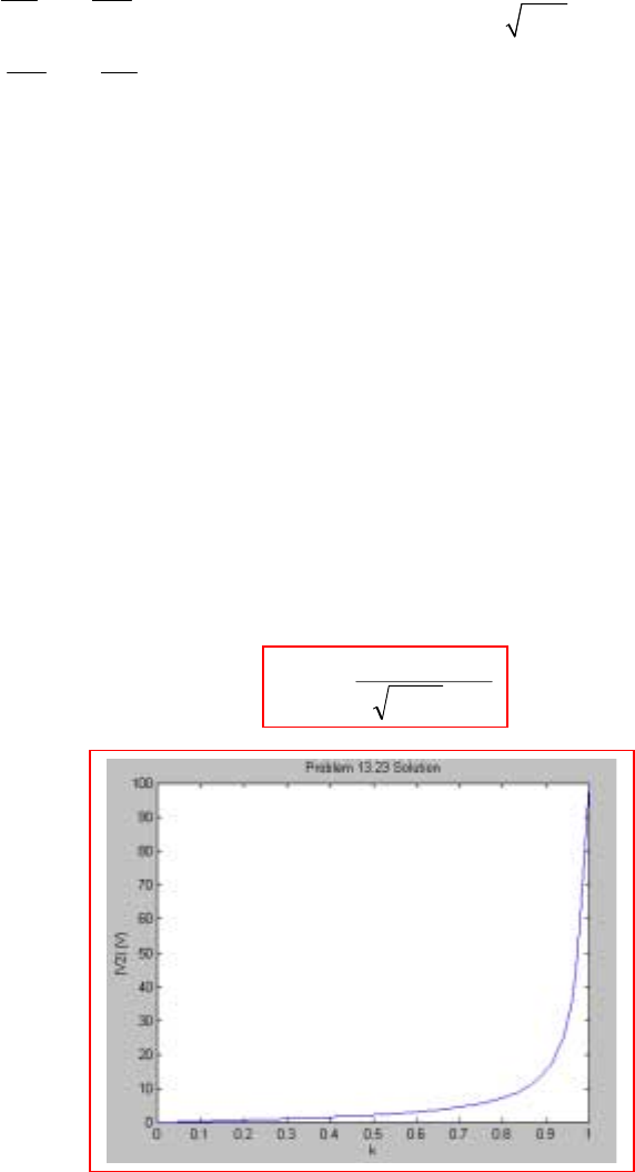
CHAPTER THIRTEEN SOLUTIONS
Engineering Circuit Analysis, 6th Edition Copyright
2002 McGraw-Hill, Inc. All Rights Reserved
23. Define coil voltages v1 and v2 with the “+” reference at the respective dot.
Also define two clockwise mesh currents i1 and i2. We may then write:
12
11
21
22 260 /
=+
=+ ω=π
dd
vL M
dt dt
dd
v L M rad s
dt dt
II
II
or, using phasor notation,
111 2
222 1
=ω +ω
=ω +ω
jL jM
jL jM
VII
VII
111 2
222 1
100 0 50
25
∠= +ω +ω
−=ω+ω
jL jM
jL jM
II I
II I
Rearrange:
or
We can solve for I2 and V2 = −25I2:
V2 = 1 LL
658.1
21 +
−k
j
11 2
122
[50 ] 100 0
[25 ] 0
+ω +ω = ∠
ω−+ω =
jL jM
jM jL
II
II
11
22
50 100 0
25 0
+ω ω ∠
=
ω−+ω
jL jM
jM jL
I
I
12
=
MkLL

CHAPTER THIRTEEN SOLUTIONS
Engineering Circuit Analysis, 6th Edition Copyright
2002 McGraw-Hill, Inc. All Rights Reserved
24.
1max
2222
max
2cos500 A W at 0
111
42 62 52 32
222
8121012 42 J
==
∴=××+××+××+×
=+ + + =
it t
w
CHAPTER THIRTEEN SOLUTIONS
Engineering Circuit Analysis, 6th Edition Copyright
2002 McGraw-Hill, Inc. All Rights Reserved
25.
(a) 12
All DC: L 2 1 1 H
−=−=
(b) 12
AB SC: L 1 2 8 0.6 H
−=− + =
(c) 12
BC SC: L 2 ( 1) 9 2 9 /8 0.875 H
−=+− =− =
(d) 12
AC SC: L (2 1) (1 2) 1 3 0.750 H
−=− += =
CHAPTER THIRTEEN SOLUTIONS
Engineering Circuit Analysis, 6th Edition Copyright
2002 McGraw-Hill, Inc. All Rights Reserved
26.
(a)
+
+
+
++
=
ω
ω
ω
ωω
ω
320
2
320
)20(2
315
1
S
L
j
j
j
jj
j
V
I
=
ωω
ω
14511300
2
2j
j
+−
(b)
2
1,2
2.57 10.61
145 145 13,200
( ) 100 ( ), (0) 0, (0) 0, 2.570, 10.612
22
,0, A B,0AB
100 15 5 2 , 0 20 3 2 At 0 : 100 0 5 (0 ) 2 (0 ) and
003(0)2
−−
+++
+
−± −
==== =−−
=+ =∴= + ∴=+
′′ ′′ ′ ′
=+− = +− = =+ −
′′
=+ −
ssL
tt
LLfLnLf L
ssL LLs s L
L
vt ut i i s
ii ii i e e
ii i iii t i i
ii
2.57 10.612
(0 ) (0 ) 1.5 (0 ) 100 7.5 (0 ) 2 (0 ) 5.5 (0 )
(0 ) 18.182 A/s 18.182 2.57A 10.61B 2.57A 10.61A 8.042A
A 2.261, B 2.261, ( ) 2.261( ) A, 0
++ + ++ +
+
−−
′′ ′′ ′
∴= ∴= − =
′
∴= ∴ =−− =−+ =
∴= =− = − >
ss L LL L
L
tt
L
ii ii i
i
it e e t
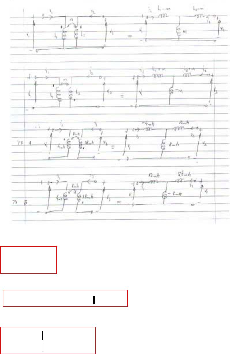
CHAPTER THIRTEEN SOLUTIONS
Engineering Circuit Analysis, 6th Edition Copyright
2002 McGraw-Hill, Inc. All Rights Reserved
27.
(a) Open-Circuit
4
4
×
×
=ω Ω
=ω Ω
TA
oc
TB
oc
jM
jM
Z
Z
(b) Short-Circuit
4810
××
==−ωΩ+ωωΩ
TA TB
SS SS jM j j MZZ
(c) If the secondary is connected in parallel with the primary
4108
26 12 8
×
×
=− ω − ω + ω Ω
=ω ω −ω Ω
TA
in
TB
in
jj jM
jj jM
Z
Z
CHAPTER THIRTEEN SOLUTIONS
Engineering Circuit Analysis, 6th Edition Copyright
2002 McGraw-Hill, Inc. All Rights Reserved
28. Define three clockwise mesh currents I1, I2, and I3 beginning with the left-most mesh.
Vs = j8
ω
I1 – j4
ω
I2
0 = -4j
ω
I1 + (5 + j6
ω
) I2 – j2
ω
I3
0 = -j2
ω
I2 + (3 + j
ω
) I3
Solving, I3 = j
ω
/ (15 + j17
ω
). Since Vo = 3 I3,
ω
ω
1715
3
S
o
j
j
+
=
V
V

CHAPTER THIRTEEN SOLUTIONS
Engineering Circuit Analysis, 6th Edition Copyright
2002 McGraw-Hill, Inc. All Rights Reserved
29. Leq = 2/ 3 + 1 + 2 + 6/5 = 4.867 H
Z(j
ω
) = 10 j
ω
(4.867)/ (10 + j
ω
4.867)
= j4.867
ω
/ (1 + j0.4867
ω
) Ω.
CHAPTER THIRTEEN SOLUTIONS
Engineering Circuit Analysis, 6th Edition Copyright
2002 McGraw-Hill, Inc. All Rights Reserved
30. 100 rad/s
V 100 0 V rms
ω=
=∠°
s
(a)
(b)
,
100( 400)
V 39.99 1.146 V rms
20 1000
400(20 600) 240,000 8,000
Z , V 0 200 200 40.19 85.44
20 1000 20 1,000
==∠°
+
+−+
==− + =− + = ∠ °Ω
++
OC cd
incd S
j
j
jj j
jj
jj
400(10 200) 80,000 4,000
Z 20 600 20 600
10 200 10 200
−−+
=+ + =+ +
++
ina b
jj j
jj
jj
= 210.7∠73.48o V and Voc = 0.
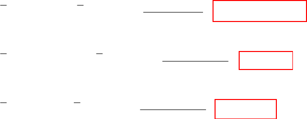
CHAPTER THIRTEEN SOLUTIONS
Engineering Circuit Analysis, 6th Edition Copyright
2002 McGraw-Hill, Inc. All Rights Reserved
31. 12
L 1 H, L 4 H, K 1, 1000 rad/s===ω=
(a) 6
10 1 4
Z 1000 Z 1000 24.98 0.6246
4000 100
××
=Ω∴= + = + Ω
+
Lin
jj
j
(b) 6
410
Z 1000 0.1 Z 1000 24.39
4000 100
×
=×∴=+ = Ω
+
Lin
jj j
jj
(c) 6
L
410
Z 100 Z 1000 25.46
4000 100
×
=− ∴ = + =− Ω
−
in
jj j
jj
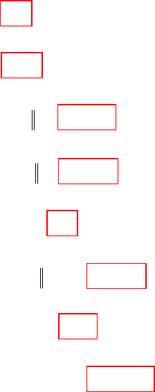
CHAPTER THIRTEEN SOLUTIONS
Engineering Circuit Analysis, 6th Edition Copyright
2002 McGraw-Hill, Inc. All Rights Reserved
32.
12
,
,
,
,
,
,,
,
L 6 H, L 12 H, M 5 H
#1, L 6 H
#2, L 12 H
#3, L 1 7 5 3.917 H
#4, L 7 5 1 7.833 H
#5, L 7 1 8 H
#6, L 7 1 5 5.875 H
#7, L 11 17 28 H
#8, L
== =
=
=
=+ =
=+ =
=+=
=+=
=+=
inAB CDOC
inCD ABOC
inAB CDSC
inCD ABSC
inAC BDSC
inAB ACSC BDSC
inAD BCSC
inA ,5 11/17 1.6786 H=− + =
BADSC
CHAPTER THIRTEEN SOLUTIONS
Engineering Circuit Analysis, 6th Edition Copyright
2002 McGraw-Hill, Inc. All Rights Reserved
33.
22
11
22 22
22
312
22 22
312 12
2222
2
11
31.83 314 /
31.83
ie. a 50Hz system
20 100 10 2 31.83
2 31.83
20 100 10 2 31.83 2 31.83
493 7840
20 31.4 1020 1020
20
−
−
ω
=++
=⇒ω= =
ω×
ω
=+ω× +
−
ωω
=+ω× + −
++
=+ + −
=+
in
in
in
M
RjX
rad s
CC
kLL
jj
kLL j kLL
j
jjk
j
ZZ
Z
Z
2
31.4 [0.483 7.69]
( 0) 20 31.4
( 0.5) 20.2 27.6
( 0.9) 20.4 24.5
( 1.0) 20.5 23.7
+−
==+ Ω
==+ Ω
==+ Ω
== + Ω
in
in
in
in
jk
kj
kj
kj
kj
Z
Z
Z
Z
(a)
(b)
(c)
(d)
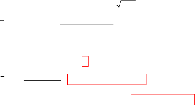
CHAPTER THIRTEEN SOLUTIONS
Engineering Circuit Analysis, 6th Edition Copyright
2002 McGraw-Hill, Inc. All Rights Reserved
34. 12
L 125 H, L 20 H, K 1, M 2500 50 H, M 5000
↑→ → =∴= = ω= Ω
jj
(a)
(b)
6
5000(10 3000)
Z 20 7500 10 2000
15 10 50,000
20 7500 82.499 0.2170
10 2000
82.498 0.3125 V 0
−
−
−
=+ + +
×+
=+ + = ∠ °Ω
+
=+ Ω=
ina b
OC
jj
jj
j
jj
j
,
100( 5000)
V 39.99995 0.09167 V rms
20 12,500
5000(20 7500)
Z , V 0 3000 3.19999 0.00512
20 12,500
==∠°
+
+
==− + = + Ω
+
OC cd
incd S
j
j
jj
jj
j
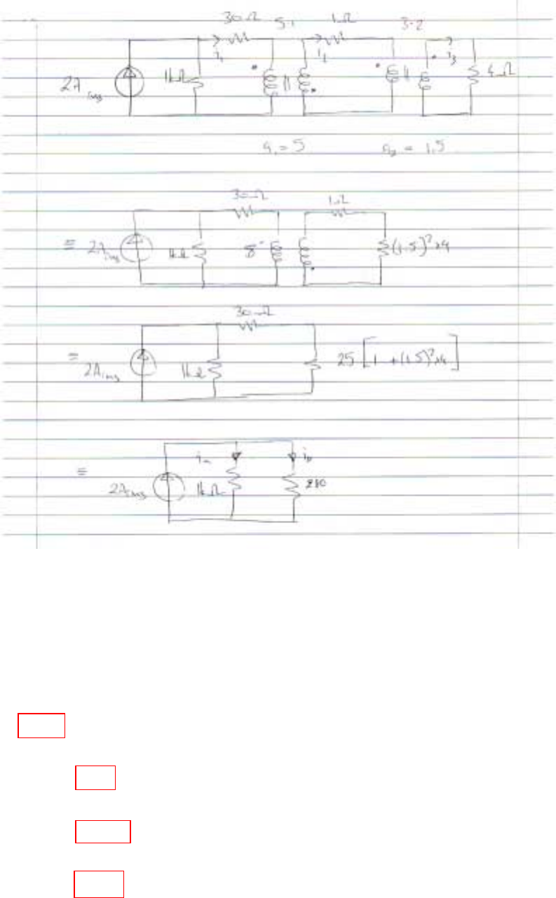
CHAPTER THIRTEEN SOLUTIONS
Engineering Circuit Analysis, 6th Edition Copyright
2002 McGraw-Hill, Inc. All Rights Reserved
35.
280 2 0.438A
1280
1000 2 1.56A
1280
∴=×=
=×=
a
b
I
I
1
2
3
1.56A
5 1.56 7.8A
1.5 7.8 11.7A
∴=
⇒=× =
⇒=× =
A
I
I
I
2
23
22
1
22
2
22
3
(1 )
0.438 1 10
192W
(30 ) (1.56) 30
73W
(1 ) 7.8 1
60.8W
(4 ) 11.7 4
548W
⇒=
=××
=
⇒Ω== ×
=
⇒Ω= = ×
=
⇒Ω= = ×
=
a
Pk IR
PIR
PIR
PIR
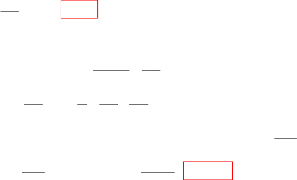
CHAPTER THIRTEEN SOLUTIONS
Engineering Circuit Analysis, 6th Edition Copyright
2002 McGraw-Hill, Inc. All Rights Reserved
36.
(a)
(b)
21 1
21 2 1
1111
11
11 1 11 11
2
21
R 100
VV3V
II/4, V4 VI 40 40
3V I 3V 4V
100 10 I V ,
40 4 40 100
100
I 0.46V 100 10(0.46V 0.075V ) V 4.85 V V 4.85
400 82.47
V 4V 82.47 V P 68.02 W
4.85 100
=Ω
−
==∴==
∴= + = +
∴= ∴ = − + = ∴ =
∴= = = ∴= =
L
X
L
2
2
max
R sees 10 4 160 use R 160
100
P10250 W
20
×= Ω∴ = Ω
=×=
LL
L
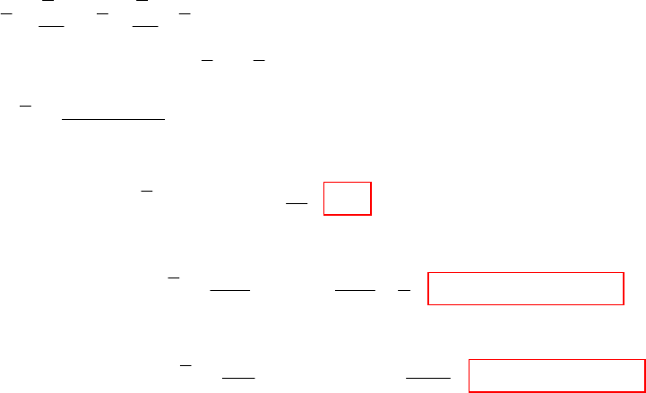
CHAPTER THIRTEEN SOLUTIONS
Engineering Circuit Analysis, 6th Edition Copyright
2002 McGraw-Hill, Inc. All Rights Reserved
37.
22
2112
22
2
VV
II,V5V
840
100 300(C 0.025)V 5V
100
V12.5 300C
=∴= =
∴= + +
∴= +
(a) 2
2
8
C0 V 8V P 8 W
8
=∴ = ∴ = =
L
(b)
2
2
100 100 1
C 0.04 V P 2.082 W (neg. )
24.5 24.5 8
=∴= ∴= =
Lfdbk
(c) 2
2
100 200
C 0.04 V 200 V P 5000 W (pos. )
0.5 8
=− ∴ = = ∴ = =
Lfdbk
CHAPTER THIRTEEN SOLUTIONS
Engineering Circuit Analysis, 6th Edition Copyright
2002 McGraw-Hill, Inc. All Rights Reserved
38.
2
22
1
Apply V 1 V I 0.05 A, V 4 V
41
4 60 I 20 0.05 I 0.05 A
60
I 0.2 A I 0.25 A R 4 , V 0
=∴= =
−
∴= + × ∴ = =
∴= ∴ = ∴ =Ω =
ab x
in th th
CHAPTER THIRTEEN SOLUTIONS
Engineering Circuit Analysis, 6th Edition Copyright
2002 McGraw-Hill, Inc. All Rights Reserved
39.
100
1
2
25
P 1000 W, P 500 W
500
I 5 A, V 100 5 V
100
1000
I 10 A V 100 40 60 V
100
100
Now, P 1000 500 10 4 100W I 2 A; also
25
==
∴= = =
== ∴=−=
=−−×= ∴= =
gen
LL
S
X
130
Around center mesh: 60 2 25 100 5 0.8944
=× + ∴=
aa
05
60 =
Ix = 8944.0
5
2
,25 === bb
CHAPTER THIRTEEN SOLUTIONS
Engineering Circuit Analysis, 6th Edition Copyright
2002 McGraw-Hill, Inc. All Rights Reserved
40.
(a)
(b) 21
I 3I 3.297 0 A== ∠°
(c) 3
4
I 3.297 4.396 180 A
3
=− × = ∠ °
(d) 2
25
P 25 1.0989 30.19 W=× =
(e) 2
2
P 3.297 2 21.74 W=×=
(f) 2
3
P 4.396 3 57.96 W=×=
2
2
1
41616 2222
3,2,(3)66
333 33
100
66 25 91 1.0989 0 A I
91
×=Ω+=Ω =Ω
+=Ω = ∠°=
CHAPTER THIRTEEN SOLUTIONS
Engineering Circuit Analysis, 6th Edition Copyright
2002 McGraw-Hill, Inc. All Rights Reserved
41.
12125022
2
222
22222
222
2
V 2.5 V , I 0.4I , I I 0.1 V
60 2.5 V
60 40(0.4 I ) 2.5V I 16
Also, 60 50(I 0.1 V ) V 50I 6V
60 2.5 V
60 50 6 V 187.5 (7.8125 6) V
16
60 187.5
V 9.231 V
13.8125
===+
+
∴= − ∴=
=+ +=+
+
∴= + = + +
−
∴= =−
CHAPTER THIRTEEN SOLUTIONS
Engineering Circuit Analysis, 6th Edition Copyright
2002 McGraw-Hill, Inc. All Rights Reserved
42.
2
1
2
4
2
48
2
400
400 16 , 16 48 12 , 12 4 16
5
16 10
4 I 2 A P 4 W
241
21 A P 4 W, 10 2 1 8 V
2
8 2 16 V, 16 4 1 12 V, 12 / 48 3 W P , 12 5 60 V
60
P9 W
400
=Ω =Ω +=Ω
=Ω∴ = = ∴ =
+
=∴= −×=
×= −×= = = ×=
==
s
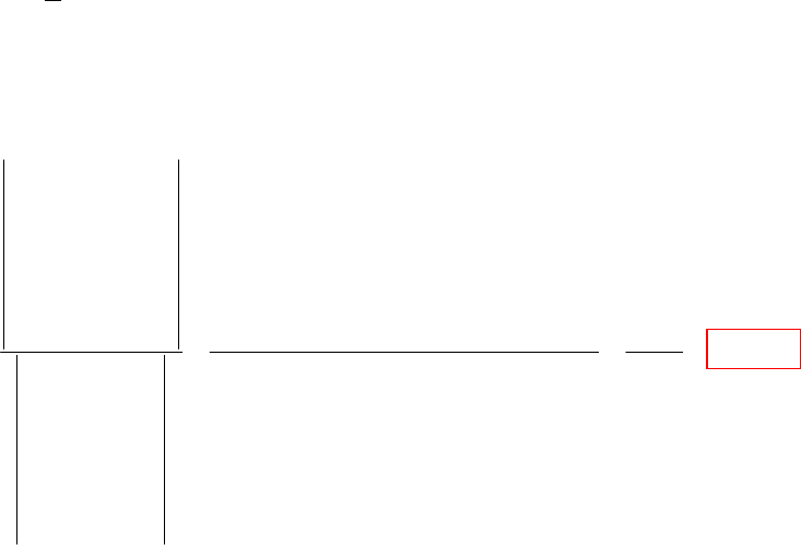
CHAPTER THIRTEEN SOLUTIONS
Engineering Circuit Analysis, 6th Edition Copyright
2002 McGraw-Hill, Inc. All Rights Reserved
43.
122 2
22
2
2
2
I 2I , 2I I I I I 2I 0
1
100 3I (4I 20I 20I )
2
10I 3I 12I 100
100 3 I 5I 20I 20I
25I 3I 20I 100
012
100 3 12
100 3 20 0 100( 26) 100( 18)
I11 2 1(60 36) 10( 20 6) 25( 1
10 3 12
25 3 20
==+∴+−=
=+ + −
∴−−=−
=−+ −
∴−− =−
−
−−−
−−− +−−−
∴= =
−− − −−+ −
−−
−−
sx xs
sx
xs
sx x
xs
X
800 4.819 A
2 6) 166
−
==
−−
CHAPTER THIRTEEN SOLUTIONS
Engineering Circuit Analysis, 6th Edition Copyright
2002 McGraw-Hill, Inc. All Rights Reserved
44.
(a)
(b) Specify 3 A and 4 A in secondaries
2
10 10
II4
25 25
II3 (I4)(I3)
33
2I 7, I 3.5 A
25 25
V V ( 3.5 4) V
36
25 1
P P 1.7361 W
610
AB f
CD b f f
ff
AB CD
AB CD
=+
=− − ∴ + = − −
∴=− =−
∴= =−+=
∴= = =
2
10
2
10
25 25 100
50 10 V 1 4 V
333
100 1 1000
P 111.11 W
3109
25 25
V 1 3 25 V, P 62.5 W
310
AB
AB
CD CD
=Ω∴ =××=
∴= = =
=×× = = =
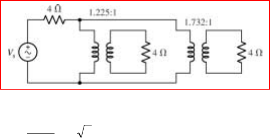
CHAPTER THIRTEEN SOLUTIONS
Engineering Circuit Analysis, 6th Edition Copyright
2002 McGraw-Hill, Inc. All Rights Reserved
45. Corrections required to the problem text: both speakers that comprise the load
are 4-Ω devices. We desire a circuit that will connect the signal generator (whose
Thévenin resistance is 4 Ω) to the individual speakers such that one speaker receives
twice the power delivered to the other. One possible solution of many:
We can see from analysing the above circuit that the voltage across the right-most
speaker will be 2
225.1
732.1 or times that across the left speaker. Since power is
proportional to voltage squared, twice as much power is delivered to the right
speaker.
CHAPTER THIRTEEN SOLUTIONS
Engineering Circuit Analysis, 6th Edition Copyright
2002 McGraw-Hill, Inc. All Rights Reserved
46. (a) We assume Vsecondary = 230∠0o V as a phasor reference. Then,
I
unity PF load = A 034.8 0
230
8000 oo ∠=∠ and
I
0.8 PF load =
()
A 9.3665.2 0.8 cos
230
15000 o1 −∠=−∠ −
Thus, Iprimary =
()
oo 36.9-65.2 08.34
2300
230 ∠+∠
= 0.1 (86.9 – j39.1) = 9.5 ∠-24.3o A
(b) The magnitude of the secondary current is limited to 25×103/230 = 109 A.
If we include a new load operating at 0.95 PF lagging, whose current is
I0.95 PF load = | I0.95 PF load | ∠ (-cos-1 0.95) = | I0.95 PF load | ∠ -18.2o A,
then the new total secondary current is
86.9 – j39.1 + | I0.95 PF load | cos 18.2o – j | I0.95 PF load | sin 18.2o A.
Thus, we may equate this to the maximum rated current of the secondary:
()()
2
o
load PF 0.95
2
o
load PF 0.95 18.2sin || 39.1 18.2 cos || 86.9 109 II +++=
Solving, we find
2
)2800)(4(189189-
||
2
2
load PF 0.95
+±
=I
So, |I0.95 PF load | = 13.8 A (or –203 A, which is nonsense).
This transformer, then, can deliver to the additional load a power of
13.8×0.95×230 = 3 kW.
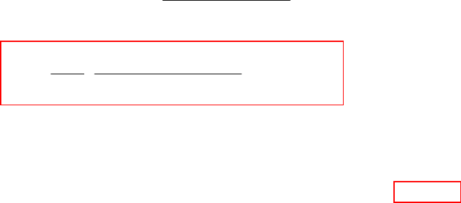
CHAPTER THIRTEEN SOLUTIONS
Engineering Circuit Analysis, 6th Edition Copyright
2002 McGraw-Hill, Inc. All Rights Reserved
47. After careful examination of the circuit diagram, we (fortunately or unfortunately)
determine that the meter determines individual IQ based on age alone. A simplified
version of the circuit then, is simply a 120 V ac source, a 28.8-kΩ resistor and a
(242)RA resistor all connected in series. The IQ result is equal to the power (W)
dissipated in resistor RA divided by 1000.
P = A
2
A
3576R
576R 108.28
120 ×
+×
Thus, IQ = Age576
Age576 108.28
120
1000
12
3××
×+×
(a) Implementation of the above equation with a given age will yield the “measured”
IQ.
(b) The maximum IQ is achieved when maximum power is delivered to resistor RA,
which will occur when 576RA = 28.8×10³, or the person’s age is 50 years.
(c) Well, now, this arguably depends on your answer to part (a), and your own sense
of ethics. Hopefully you’ll do the right thing, and simply write to the Better Business
Bureau. And watch less television.

CHAPTER THIRTEEN SOLUTIONS
Engineering Circuit Analysis, 6th Edition Copyright
2002 McGraw-Hill, Inc. All Rights Reserved
48. We require a transformer that converts 240 V ac to 120 V ac, so that a turns ratio of
2:1 is needed. We attach a male european plug to the primary coil, and a female US
plug to the secondary coil. Unfortunately, we are not given the current requirements
of the CD writer, so that we will have to over-rate the transformer to ensure that it
doesn’t overheat. Checking specifications on the web for an example CD writer, we
find that the power supply provides a dual DC output: 1.2 A at 5 V, and 0.8 A at 12 V.
This corresponds to a total DC power delivery of 15.6 W. Assuming a moderately
efficient ac to DC converter is being used (e.g. 80% efficient), the unit will draw
approximately 15.6/0.8 or 20 W from the wall socket. Thus, the secondary coil
should be rated for at least that (let’s go for 40 W, corresponding to a peak current
draw of about 333 mA). Thus, we include a 300-mA fuse in series with the
secondary coil and the US plug for safety.
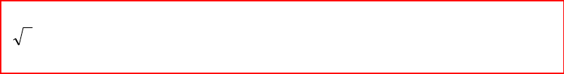
CHAPTER THIRTEEN SOLUTIONS
Engineering Circuit Analysis, 6th Edition Copyright
2002 McGraw-Hill, Inc. All Rights Reserved
49. You need to purchase (and wire in) a three-phase transformer rated at
(
)
()()
kVA. 3.6 102083 = The turns ratio for each phase needs to be 400:208 or
1.923.
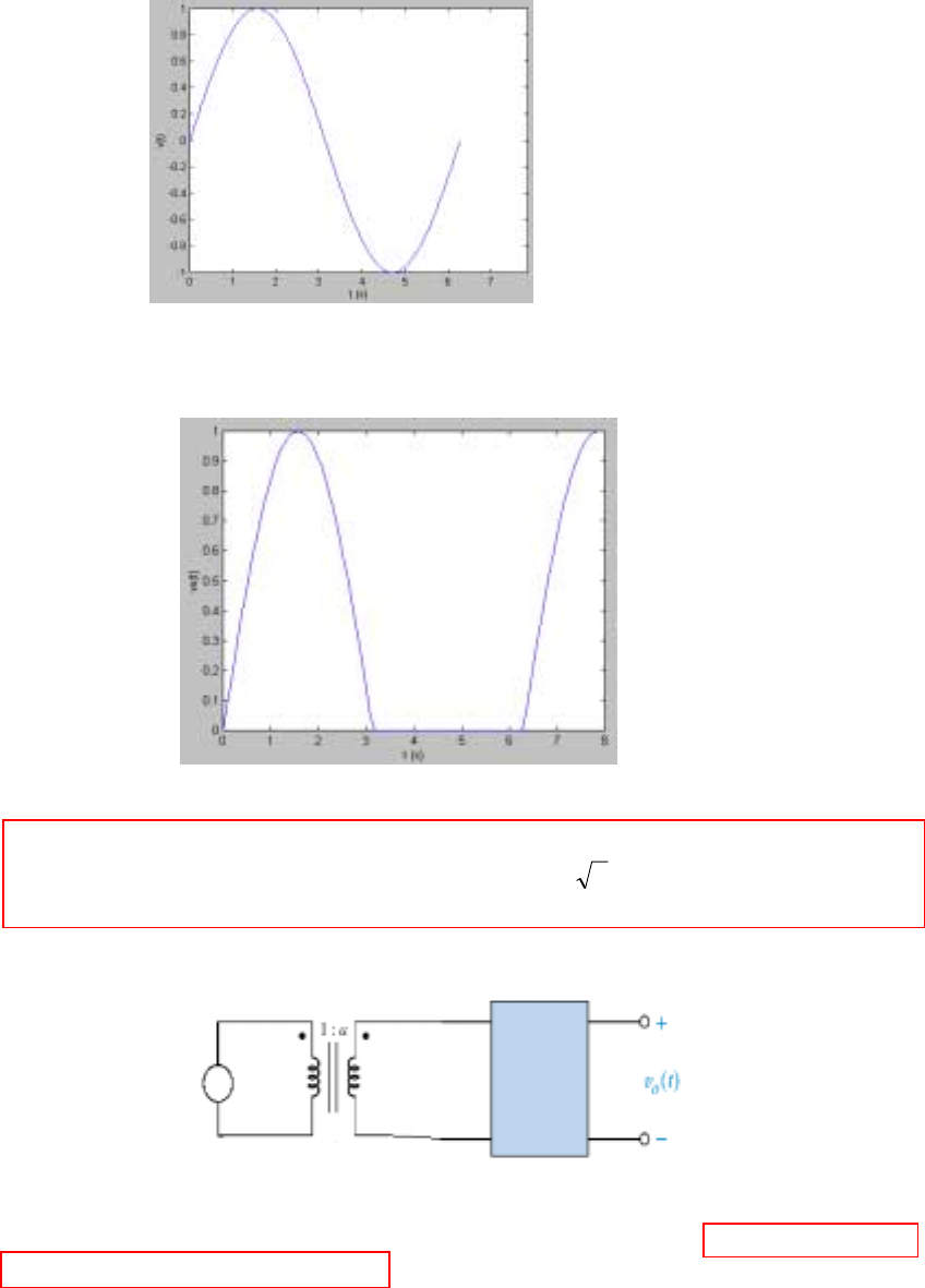
CHAPTER THIRTEEN SOLUTIONS
Engineering Circuit Analysis, 6th Edition Copyright
2002 McGraw-Hill, Inc. All Rights Reserved
50. (a) The input to the left of the unit will have the shape:
and the output voltage will be:
We need to reduce the magnitude from 115-V (rms) to a peak voltage of 5 V. The
corresponding peak voltage at the input will be 2115 = 162.6 V, so we require a
transformer with a turns ratio of 162.6:5 or about 32.5:1, connected as shown:
(b) If we wish to reduce the “ripple” in the output voltage, we can connect a capacitor
in parallel with the output terminals. The necessary size will depend on the maximum
allowable ripple voltage and the minimum anticipated load resistance. When the input
voltage swings negative and the output voltage tries to reduce to follow, current will
flow out of the capacitor to reduce the amount of voltage drop that would otherwise
occur.
±
115 V
rms ac
a = 1/ 32.5
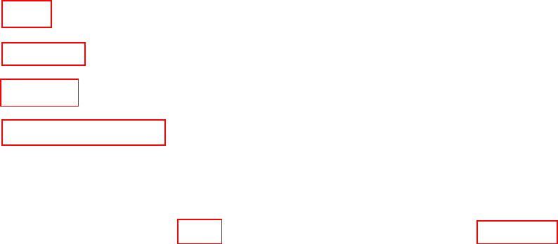
CHAPTER FOURTEEN SOLUTIONS
Engineering Circuit Analysis, 6th Edition Copyright
2002 McGraw-Hill, Inc. All Rights Reserved
1. (a) s = 0;
(b) s = ± j9 s-1;
(c) s = -8 s-1;
(d) s = -1000 ± j1000 s-1;
(e) v(t) = 8 + 2 cos 2t mV cannot be attributed a single complex frequency. In a circuit
analysis problem, superposition will need to be invoked, where the original function v(t)
is expressed as v(t) = v1(t) + v2(t), with v1(t) = 8 mV and v2(t) = 2 cos 2t mV. The
complex frequency of v1(t) is s = 0, and the complex frequency of v2(t) is s = ± j2 s-1.
CHAPTER FOURTEEN SOLUTIONS
Engineering Circuit Analysis, 6th Edition Copyright
2002 McGraw-Hill, Inc. All Rights Reserved
2. (a) (6 – j)* = 6 + j
(b) (9)* = 9
(c) (-j30)* = +j30
(d) (5 e-j6)* = 5 e+j6
(e) (24 ∠ -45o )* = 24 ∠ 45o
(f) o
o
o
94.19 5.303
16.72- 477.3
77.47 18.44
33.3
184
*
33.3
184 ∠=
∠
∠
=
−
+
=
+
−
j
j
j
j
(g)
()
oo
o
oo
60.36 .62020
*
60.36 .62020
*
26.60062.8
1.0 5
*
74
1.0 5 −∠=∠=
−∠
∠
=
−
∠
j
(h) (4 – 22 ∠ 92.5o)* = (4 + 0.9596 – j21.98)* = (4.9596 – j21.98)* = 4.9596 + j21.98
CHAPTER FOURTEEN SOLUTIONS
Engineering Circuit Analysis, 6th Edition Copyright
2002 McGraw-Hill, Inc. All Rights Reserved
3. Re ( ) ( )=it it. No units provided.
(a)
(b)
(c)
(d)
( 3 15) 3 15 3 (15 60.26 )
3
( ) (4 7) (8.062 60.26 ) 8.062
( ) Re ( ) 8.062 cos(15 60.26 )
−+ − − − °
−
=− = ∠− ° =
∴= = − °
jt tjt tjt
x
t
xx
it j e ee ee
it it e t
3 3 15 60.26
3
( ) (4 7) (cos15 sin15 ) 8.062
( ) 8.062 cos(15 60.26 )
−−−+°
−
=+ − =
∴= − °
ttjtj
y
t
y
it j e t j t e e
it e t
( 1.5 12) 57.99 1.5 12 1.5 (125 57.99 )
0.6
( ) (5 8) 9.434 9.434
Re (0.4) 9.434 cos(4.8 57.99 ) 4.134
−+ − °− − − °
−
=− = =
∴= −°=−
tj t j t jt t j
A
rad
A
it je e e e e e
ie
( 1.5 12) 57.99 1.5 12 1.5 (12 57.99 )
( ) (5 8) 9.434 9.434
Re (0.4) 4.134
−+ °− − − − − °
=+ = =
∴=−
jt j t jt t jt
B
B
it je e e e e e
i

CHAPTER FOURTEEN SOLUTIONS
Engineering Circuit Analysis, 6th Edition Copyright
2002 McGraw-Hill, Inc. All Rights Reserved
4. (a)
ω
= 279 Mrad/s, and
ω
= 2
π
f. Thus, f =
ω
/2
π
= 44.4 MHz
(b) If the current i(t) = 2.33 cos (279×106 t) fA flows through a precision 1-TΩ resistor,
the voltage across the resistor will be 1012 i(t) = 2.33 cos (279×106 t) mV. We may write
this as 0.5(2.33) cos (279×106 t) + j (0.5)2.33 sin (279×106 t) + 0.5(2.33) cos (279×106 t)
- j (0.5)2.33 sin (279×106 t) mV
= 1.165 e j279×106 t + 1.165 e -j279×106 t mV
CHAPTER FOURTEEN SOLUTIONS
Engineering Circuit Analysis, 6th Edition Copyright
2002 McGraw-Hill, Inc. All Rights Reserved
5. (a) vs(0.1) = (20 – j30) e(-2 + j50)(0.1) = (36.06 ∠ -56.31o) e(-0.2 + j5)
= 36.06e-0.2 ∠ [-56.31o + j5(180)/
π
] = 29.52 ∠230.2o V (or 29.52 ∠-129.8o V).
(b) Re{ vs } = 36.06 e-2t cos (50t – 56.31o) V.
(c) Re{ vs(0.1) } = 29.52 cos (230.2o) = -18.89 V.
(d) The complex frequency of this waveform is s = -2 + j50 s-1
(e) s* = (-2 + j50)* = -2 – j50 s-1
CHAPTER FOURTEEN SOLUTIONS
Engineering Circuit Analysis, 6th Edition Copyright
2002 McGraw-Hill, Inc. All Rights Reserved
6. (a) s = 0 + j120
π
= + j120
π
(b) We first construct an s-domain voltage V(s) = 179 ∠ 0o with s given above.
The equation for the circuit is
v(t) = 100 i(t) + L dt
di = 100 i(t) + 500×10-6
dt
di
and we assume a response of the form Iest.
Substituting, we write (179 ∠ 0o) est = 100 Iest + sL Iest
Supressing the exponential factor, we may write
6-
o
10500100
0179
×+
∠
=s
I =
()
o
o
6-
o
108.0100
0179
10500120100
0179
∠
∠
=
×+
∠
π
j = 1.79 ∠ -0.108o A
Converting back to the time domain, we find that
i(t) = 1.79 cos (120
π
t – 0.108o) A.
CHAPTER FOURTEEN SOLUTIONS
Engineering Circuit Analysis, 6th Edition Copyright
2002 McGraw-Hill, Inc. All Rights Reserved
7.
(a)
(b) 2
( ) 0.3536 cos(10 105 ) A
t
x
it e t
−
=−°
2
10 cos(10 30 )V 2 10, V 10 30 V
10 5 1 5 5 25 ( 25 125)/ 26
Z,Z5
2 10 1 5 26 26 ( 5 25 130) / 26
25 125 1 5
Z 5 1 Z 5 0.5( 2 10) 1 4 4
125 25 5 1
10 30 ( 5 25)/ 26
I445(
t
ss
cc
cin
x
ve t s j
jj j
jj j
jj
jjjj
jj
j
j
−
=+°∴=−+=∠°
−− −− − −
== = =
−+ −+ −− +
−− −−
∴= = =−∴=+−+−=+Ω
−−
∠° −−
∴= ×
++−
10 30 5 25 5 30 5 25 1 30 1 5
5 25)/ 26 4 4 130 5 25 2 2 125 25 2 2 5 1
130
I ( 1) 0.3536 105 A
2245
x
jjj
jjjjjjj
j
∠° −− ∠°−− ∠°−−
===
−+−−+−+−
∠°
∴= − = ∠− °
∠°
CHAPTER FOURTEEN SOLUTIONS
Engineering Circuit Analysis, 6th Edition Copyright
2002 McGraw-Hill, Inc. All Rights Reserved
8. (a) s = 0 + j100
π
= + j100
π
(b) We first construct an s-domain voltage V(s) = 339 ∠ 0o with s given above.
The equation for the circuit is
v(t) = 2000 i(t) + vC(t) = 2000 dt
dvC
C + vC(t) = dt
dvC
2.0 + vC(t)
and we assume a response of the form VCest.
Substituting, we write (339 ∠ 0o) est = 0.2s VCest + VCest
Supressing the exponential factor, we may write
s
V2.01
0393
o
C+
∠
= =
()
o
oo
09.8984.62
0339
2.01001
0339
∠
∠
=
+
∠
π
j = 5.395 ∠ -89.09o A
Converting back to the time domain, we find that
vC(t) = 5.395 cos (100
π
t – 89.09o) V.
and so the current is i(t) = dt
dvC
C = -0.1695 sin(100
π
t) A = 169.5 sin (100
π
t) mA.
CHAPTER FOURTEEN SOLUTIONS
Engineering Circuit Analysis, 6th Edition Copyright
2002 McGraw-Hill, Inc. All Rights Reserved
9. 33
12
20 cos4 A, 30 sin 4 A
tt
SS
ie tie t
−−
==
(a)
(b) 3
( ) 185.15 cos(4 47.58 ) V
t
x
vt e t
−−
=−°
12
I 20 0 , I 30, 3 4
10 3 4
Z 0.4( 3 4) 1.2 1.6, Z 6 8
3434
5(7.2 6.4) 6 8 ( 6 8)(3.8 1.6)
V20 30
2.2 6.4 7.2 6.4 2.2 6.4
600 800 30( 22.8 12.8 30.4 9.6) 600
2.2 6.4
SS
c L
x
js j
jjj j
jj
jj jj
j
jj j
jj j j
j
=∠° =− =−+
−−
∴= = −− =−− =−+
−+ −−
+−+ −+−
∴= × −
−+ −+ −+
−+ − − + + + −+
==
−+
800 30( 10 40)
2.2 6.4
600 1200 1000 600 1000 185.15 47.58 V
2.2 6.4 2.2 6.4
jj j
j
jj
jj
−
−−+
−+
−+ + +
===∠−°
−+ −+
CHAPTER FOURTEEN SOLUTIONS
Engineering Circuit Analysis, 6th Edition Copyright
2002 McGraw-Hill, Inc. All Rights Reserved
10. (a) If v(t) = 240 2e
-2t cos 120πt V, then V = 240 2∠0o V where s = -2 + j120
π
.
Since R = 3 mΩ, the current is simply I = 3
o
103
0 2240
−
×
∠ = 113.1 ∠0o kA. Thus,
i(t) = 113.1e-2t cos 120πt kA
(b) Working in the time domain, we may directly compute
i(t) = v(t) / 3×10-3 = (240 2e
-2t cos 120πt ) / 3×10-3 = 113.1e-2t cos 120πt kA
(c) A 1000-mF capacitor added to this circuit corresponds to an impedance
Ω
+
=
×+
=
1202-
1
)10)(1000120(-2
1
1
3-
ππ
jjCs in parallel with the 3-mΩ
resistor. However, since the capacitor has been added in parallel (it would have been
more interesting if the connection were in series), the same voltage still appears across its
terminals, and so
i(t) = 113.1e-2t cos 120πt kA as before.
CHAPTER FOURTEEN SOLUTIONS
Engineering Circuit Analysis, 6th Edition Copyright
2002 McGraw-Hill, Inc. All Rights Reserved
11.
{}
∞
−
∞−
∞−
∞−−
==== ∫∫∫ 0
000 )( )( )( --
tttt e
K
dteKdttueKdttuKetuK ssss
s
L
=
+
−−
→
−
∞→
t
t
t
te
K
e
Kss
ss lim lim 0
If the integral is going to converge, then
(
)
finite). bemust (i.e. 0 lim
s
s=
−
∞→
t
teThis leads
to the first term dropping out (l’Hospital’s rule assures us of this), and so
{}
s
K
tuK )( =L
CHAPTER FOURTEEN SOLUTIONS
Engineering Circuit Analysis, 6th Edition Copyright
2002 McGraw-Hill, Inc. All Rights Reserved
12. (a)
{}
∞
−
∞−
∞−
∞−−
==== ∫∫∫ 0
000
3
3 )(3 )(3 )( 3 --
tttt edtedttuedttuetu ssss
s
L
=
+
−−
→
−
∞→
t
t
t
tee ss
ss
3
lim
3
lim 0
If the integral is going to converge, then
(
)
finite). bemust (i.e. 0 lim
s
s=
−
∞→
t
teThis leads
to the first term dropping out (l’Hospital’s rule assures us of this), and so
{}
s
3
)( 3 =tuL
(b)
{}
∞
−
∞−
∞−−
==−=− ∫∫ 3
30
3
3 )3(3 )3( 3 -
ttt edtedttuetu sss
s
L
=
+
−−−
∞→
ss
ss
3
3
3
lim ee t
t
If the integral is going to converge, then
(
)
finite). bemust (i.e. 0 lim
s
s=
−
∞→
t
teThis leads
to the first term dropping out (l’Hospital’s rule assures us of this), and so
{}
s
s
3
3
)3( 3 −
=− etuL
(c)
{}
[]
∞
−
∞
−
∞−
∞−
∞−
−
−−
=
=−−=−− ∫∫∫
03
030
3
-
3
3- 3 3)3(3 3)3( 3 --
tt
ttt
ee
dtedtedtetutu
ss
sss
ss
L
Based on our answers to parts (a) and (b), we may write
{}
3
3
3)3( 3 3
ss
s−=−− −
etuL =
()
1 -
33s
s
−
e
(d)
{}
() ()
1
3
1
3
3
3 )3(3 )3( 3
33
3
0
3
00 -
--
ss
sss
ss
s
−−
−−
∞−
−=−
−
=
−
==−=− ∫∫
ee
edtedttuetu ttt
L
CHAPTER FOURTEEN SOLUTIONS
Engineering Circuit Analysis, 6th Edition Copyright
2002 McGraw-Hill, Inc. All Rights Reserved
13. (a)
{}
[]
∞
−
∞−
∞−−
==+=+ ∫∫ 0
00
5
5 )(32 )( 32 -
ttt edtedttuetu sss
s
L
=
+
−−
→
−
∞→
t
t
t
tee ss
ss
5
lim
5
lim 0
If the integral is going to converge, then
(
)
finite). bemust (i.e. 0 lim
s
s=
−
∞→
t
teThis leads
to the first term dropping out (l’Hospital’s rule assures us of this), and so
{}
s
5
)( 32 =+ tuL
(b)
{}
∞
+−
∞+−
∞−
−
+
−
=== ∫∫
0
)8(
0
)8(
0
8-8-
8
3
3 3 3 --
ttttt edtedteee sss
s
L
=
+
+
+
−+−
→
+−
∞→
t
t
t
tee )8(
0
)8(
8
3
lim
8
3
lim ss
ss = 0 + 8
3
+s = 8
3
+s
(c)
{}
0 )0( )( )( )( -
---
0
0
0
00 ==−=−=− ∫∫∫ −−
∞−dtedttuedttuetu ttt sss
L
(d)
{}
∞
−
∞−
∞−
∞−−
==== ∫∫∫ 0
000 --
tttt e
K
dteKdteKdtKeK ssss
s
L
=
+
−−
→
−
∞→
t
t
t
te
K
e
Kss
ss lim lim 0
If the integral is going to converge, then
(
)
finite). bemust (i.e. 0 lim
s
s=
−
∞→
t
teThis leads
to the first term dropping out (l’Hospital’s rule assures us of this), and so
{}
s
K
K =L
CHAPTER FOURTEEN SOLUTIONS
Engineering Circuit Analysis, 6th Edition Copyright
2002 McGraw-Hill, Inc. All Rights Reserved
14. (a) The frequency-domain representation of the voltage across the resistor is (1)I(s)
where I(s) =
{}
A
1
4
)(4 +
=s
t ue-t
L. Thus, the voltage is V
1
4
+s.
(b)
CHAPTER FOURTEEN SOLUTIONS
Engineering Circuit Analysis, 6th Edition Copyright
2002 McGraw-Hill, Inc. All Rights Reserved
15. (a)
{}
[]
∞
−
∞
−
∞−
∞−
∞−
+
−
==
−−=−−
∫∫
∫
20
20
0
5
5
5 - 5
)2( 5)( 5 )2( 5)( 5 -
tttt
t
eedtedte
dtetutututu
ssss
s
ss
L
=
+
−−
→
−
∞→
t
t
t
tee ss
ss
5
lim
5
lim 0 +
+
−−−
∞→
ss
ss
2
5
5
lim ee t
t
If the integral is going to converge, then
(
)
finite). bemust (i.e. 0 lim
s
s=
−
∞→
t
teThis leads
to the first and third terms dropping out (l’Hospital’s rule assures us of this), and so
{}
()
s
s
2
1
5
)2( 5)( 5 −
+=−− etutuL
(b) The frequency domain current is simply one ohm times the frequency domain voltage,
or
()
s
s
2
1
5
−
+e

CHAPTER FOURTEEN SOLUTIONS
Engineering Circuit Analysis, 6th Edition Copyright
2002 McGraw-Hill, Inc. All Rights Reserved
16.
(a) f(t) ()
0
1F() (1) 0
−
∞−σ+ω
=+∴ = + ∴σ>
∫jt
tstedt
(b) ()
0
() ( 1) () F() ( 1) 0
−
∞−σ+ω
=+ ∴ = + ∴σ>
∫jt
ft t ut s t e dt
(c) 50 50 ( )
0
() () F() 50
−
∞−σ+ω
=∴= ∴σ>
∫
ttjt
ft e ut s e e dt
(d) 50 50 ( )
0
() (5)F() (5) 50
−
∞−σ+ω
=−∴= − ∴σ>
∫
ttjt
ft e ut s e ut e dt
(e) 50 50 ( )
0
() (5)F() (5) 0
−
∞
−−−σ+ω
=−∴= − ∴σ>
∫
ttjt
ft eut s eut e dt
CHAPTER FOURTEEN SOLUTIONS
Engineering Circuit Analysis, 6th Edition Copyright
2002 McGraw-Hill, Inc. All Rights Reserved
17.
(a)
(b)
(c)
3
22
3
03
(2 ) ( 2 ) 6 3 6 3
30
30
2(2 )
(2) 33
(2 ) () 63
(2)
() 8 [ ( 3) ( 3)] F( ) 8
88
F( ) 8 8 [1 ] [1 ]
22
F() 8 8
88
8F[][1
22
−−
−ω
−
−ω −−ω + ω −− ω
−
−− −
−−
−− −+ −
=−−−∴ω=
∴ω= + = − + −
−ω +ω
==
+∴=−+−
−+
∫
∫∫
∫∫
tt
jt
jt jt j j
tst st
st s s
ft e ut ut j e e dt
j e dt e dt e e
jj
s e dt e dt
edt e e
ss
63
3(2 ) 63
0
]
8
F( ) 8 [1 ]
2
−
−
−− −−
==−
+
∫
∫
s
st s
s e dt e
s
3
2(2)
3
3
63 63 (2)
(2) 3
63 63 (2 )
0
63 632
() 8 [ ( 3) ( 3)]F( ) 8
8[]F()8
2
8[],F()8
2
88
[1] [1]
22
−
−ω
−
−ω −+ω −
−
∞
−+ − −
−−
=+−−ω=
=− =
−ω
=−=
−
=−=−
−−
∫
∫
∫
tjt
jj st
ss st
s
ft e ut ut j e dt
ee s edt
j
ee s edt
s
ee
ss
2
3(2 ) 6 3 6 3
3
3(2 ) 6 3 6 3
(2) 3
(2 ) 63
00
() 8 [ ( 3) ( 3)] F( ) ()
8
F( ) 8 [ ]
2
8
F() () 8 [ ]
2
8
F( ) ( ) 8 [1 ]
2
−
∞
−ω
−∞
+ω + ω −− ω
−
∞−−+ +−−
∞−
∞∞
−−+ −−
=+−−∴ω=
∴ω= = −
+ω
===−
+
===−
+
∫
∫
∫∫
∫∫
tjt
jt j j
st s t s s
st s t s
ft e ut ut j fte dt
jedt ee
j
s f t e dt e dt e e
s
sftedtedt e
s
CHAPTER FOURTEEN SOLUTIONS
Engineering Circuit Analysis, 6th Edition Copyright
2002 McGraw-Hill, Inc. All Rights Reserved
18. (a) ss
1
1=
1-
LL
(b)
{}
ssss
3
111
)]([)(1 2=++=++ tutuL
(c)
{}
ss
31
3)( 2−=−tutL
(d)
{}
ss
s
2
1
1
)2()1()( -1 −− −+−=−−−+ eettt
δδδ
L

CHAPTER FOURTEEN SOLUTIONS
Engineering Circuit Analysis, 6th Edition Copyright
2002 McGraw-Hill, Inc. All Rights Reserved
19. (a) f(t) = e-3t u(t)
(b) f(t) =
δ
(t)
(c) f(t) = t u(t)
(d) f(t) = 275 u(t)
(e) f(t) = u(t)

CHAPTER FOURTEEN SOLUTIONS
Engineering Circuit Analysis, 6th Edition Copyright
2002 McGraw-Hill, Inc. All Rights Reserved
20.
{}
[]
{} {}
)( )(
)( )( )( )( )( )(
21
02
01
02121 ---
tftf
dtetfdtetfdtetftftftf ttt
LL
L
+=
+=+=+ ∫∫∫ ∞−
∞−
∞−sss
CHAPTER FOURTEEN SOLUTIONS
Engineering Circuit Analysis, 6th Edition Copyright
2002 McGraw-Hill, Inc. All Rights Reserved
21.
(a)
(b) 224
( ) 2 ( 2) F( ) 2 , F(1 2) 2 0.17692 0.2048
−−−
=δ − ∴ = + = =− +
sj
ft t s e j e e j
(c)
2
22
24
22
( ) 2 ( 2) F( ) 2 ; 1 2
2
F(1 2) 0.04655 0.11174
12
∞
∞−−
−− +
−
=−∴= + = =+
∴+ = = +
+
∫st st s
j
ft ut s e dt e e s j
ss
jee j
j
4
(1) (1) 22
22
22 3
11
() ( 2) F() 11
1
F(1 2) (0.4724 6.458)10
22
∞
−∞
−−+−+−−
−−− −
=−∴= = =
−+ +
∴+ = = +
+
∫
tststs
j
ft e ut s e dt e e
ss
jeee j
j
CHAPTER FOURTEEN SOLUTIONS
Engineering Circuit Analysis, 6th Edition Copyright
2002 McGraw-Hill, Inc. All Rights Reserved
22. (a) 7.671- 15sin 8 )1( 5 sin8 =×=−
∫∞
∞− dttt
δ
(b)
() ( )
9 52 )2(5 2 2 =−=−−
∫∞
∞− dttt
δ
(c) 1.840 5 )10333.3(5 )10333.3(300043000 4==×− −
×−
∞
∞−
−−
∫edtte t
δ
(d) )2( KdttK =−
∫∞
∞−
δ
CHAPTER FOURTEEN SOLUTIONS
Engineering Circuit Analysis, 6th Edition Copyright
2002 McGraw-Hill, Inc. All Rights Reserved
23.
(a)
(b) 2
2
4
() 4 ( 2) F() 4 ∞−−
=−∴= =
∫st s
f t u t s e dt e
s
(c)
(d) 222
02
() 4 ( 2) F() 4 ( 2) 4 ( 2) 4
+
−
∞−− −
=δ − ∴ = δ − = δ − =
∫∫
st s s
f t t s t e dt e t dt e
(e)
0
0
( ) 5 ( )sin (10 0.2 ) F( ) 5 ( ) [sin 0.2 ] X 1 5sin36
F( ) 2.939
+
−
=δ + π∴ = δ π = °
∴=
∫
ft t t s t dt
s
0
5
525
22
() [ (5 )][ ( 2)] (), F() [ (5 )][ ( 2)] ()
11
F( ) ( )
−
∞−
−−−−
=− − ∴ − −
∴= =− = −
∫
∫
st
st st s s
f t u t ut ut s u t ut ut e dt
s e dt e e e
ss
3(3)(3)
22
26
4
() 4 ( 2) F() 4 3
4
F( ) 3
∞
∞
−−+−+
−−
−
=−∴= =
+
∴=
+
∫
tstst
s
ft e ut s e dt e
s
se
s
CHAPTER FOURTEEN SOLUTIONS
Engineering Circuit Analysis, 6th Edition Copyright
2002 McGraw-Hill, Inc. All Rights Reserved
24. (a) 1 0500 cos )( 500 cos =×=
∫∞
∞− dttt
δ
(b)
() ( )
32 2 )2( 5 5 ==−
∫∞
∞− dttt
δ
(c)
()
0.9197 52. )1000(5.2 1000001.0001.0 ==− −
∞
∞−
−
∫edtte t
δ
(d) - )( 22 KdtctK =−−
∫∞
∞−
δ
CHAPTER FOURTEEN SOLUTIONS
Engineering Circuit Analysis, 6th Edition Copyright
2002 McGraw-Hill, Inc. All Rights Reserved
25.
(a) f(t) = 2 u(t – 1) u(3 – t) u(t3)
F(s) =
()
-
2
2
- 3
3
1
3
1
ssss
ss
−−−− ==
∫eeedte tt
(b) 44
4
22
( ) 2 ( 4) F( ) 2 (0 )
∞−−−
−
=−∴= = −=
∫st s s
ft ut s e dt e e
ss
(c) 2(2)48
4
3
() 3 ( 4) F() 3 2
∞
−−+−−
=−∴= =
+
∫
tsts
ft e ut s e dt e
s
(d) 5
0
() 3 ( 5) F() 3 ( 5) 3
−
∞−−
=δ − ∴ = δ − =
∫st s
f t t s t e dt e
(e)
0
() 4 ( 1)[cos sin ]
F( ) 4 ( 1) [cos sin ] F( ) 4
−
∞−−
=δ − π− π
∴=δ− π−π ∴=−
∫st s
ft t t t
st ttedtse
CHAPTER FOURTEEN SOLUTIONS
Engineering Circuit Analysis, 6th Edition Copyright
2002 McGraw-Hill, Inc. All Rights Reserved
26. (a) f(t) = 5 u(t) – 16
δ
(t) + e-4.4t u(t)
(b) f(t) =
δ
(t) + u(t) + t u(t)
(c) F(s) = 1
6
88
7
5
+
+
+
++
+ssss
ba
where a = 3.4-
1
17
6-
=
+=
s
s and b = 3.4
6
17
1-
=
+=
s
s.
Thus, f(t) = 5 e-7t u(t) + 88 u(t) –3.4 e-6t u(t) + 3.4 e-t u(t)
Check with MATLAB:
EDU» T1 = '5/(s+7)';
EDU» T2 = '88/s';
EDU» T3 = '17/(s^2 + 7*s + 6)';
EDU» T = symadd(T1,T2);
EDU» P = symadd(T,T3);
EDU» p = ilaplace(P)
p =
5*exp(-7*t)+88-17/5*exp(-6*t)+17/5*exp(-t)
EDU» pretty(p)
5 exp(-7 t) + 88 - 17/5 exp(-6 t) + 17/5 exp(-t)

CHAPTER FOURTEEN SOLUTIONS
Engineering Circuit Analysis, 6th Edition Copyright
2002 McGraw-Hill, Inc. All Rights Reserved
27. If V(s) = s
5, then v(t) = 5 u(t) V. The voltage at t = 1 ms is then simply 5 V, and the
current through the 2-kΩ resistor at that instant in time is 2.5 mA.
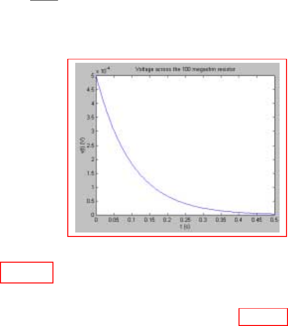
CHAPTER FOURTEEN SOLUTIONS
Engineering Circuit Analysis, 6th Edition Copyright
2002 McGraw-Hill, Inc. All Rights Reserved
28. I(s) = pA,
10
5
+s so i(t) = 5 e-10t u(t) pA. The voltage across the 100-MΩ resistor is
therefore 500 e-10t u(t) µV.
(a) The voltage as specified has zero value for t < 0, and a peak value of 500 µV.
(b) i(0.1 s) = 1.839 pA, so the power absorbed by the resistor at that instant = i2R
= 338.2 aW. (A pretty small number).
(c) 500 e-10t1% = 5
Taking the natural log of both sides, we find t1% = 460.5 ms
CHAPTER FOURTEEN SOLUTIONS
Engineering Circuit Analysis, 6th Edition Copyright
2002 McGraw-Hill, Inc. All Rights Reserved
29.
(a) 12 12
F() 1 () () 2 ()
11
−
+
=+=++↔δ++
++
t
s
stuteut
ss ss
(b) 22
F( ) ( 1) 2 1 ( 2) 2 ( 1) ( )
−−−
=+=++↔δ−+δ−+δ
sss
se e e t t t
(c) (1) 1 2 1
F( ) 2 2 2 ( 1)
−+ − − −
== +δ−
ss
se ee et
(d) F(s) = 2e-3s cosh 2s = e-3s (e2s + e-2s) = e-s + e-5s ↔
δ
(t – 1) +
δ
(t – 5)
CHAPTER FOURTEEN SOLUTIONS
Engineering Circuit Analysis, 6th Edition Copyright
2002 McGraw-Hill, Inc. All Rights Reserved
30. N(s) = 5s.
(a) D(s) = s2 – 9 so
()()()()
3
b
3
a
3- 3
5
9-
5
)(
)(
2−
+
+
=
+
== ssss
s
s
s
sD
sN
where
()
2.5
6-
15-
3
5
a
3-
==
−
=
=s
s
s and
()
2.5
6
15
3
5
b
3
==
+
=
=s
s
s. Thus,
f(t) = [2.5 e-3t + 2.5 e3t] u(t)
(b) D(s) = (s + 3)(s2 + 19s + 90) = (s + 3)(s + 10)(s + 9) so
()()()
9
c
10
b
3
a
)9)(10)(3(
5
)(
)(
+
+
+
+
+
=
+++
=ssssss
s
sD
sN
()()
0.3571,-
(7)(6)
15-
901
5
a
3-
==
++
=
=s
ss
s
()()
7.143-
(-7)(-1)
50-
93
5
b
10-
==
++
=
=s
ss
s
()( )
7.5.
(-6)(1)
45-
103
5
c
9-
==
++
=
=s
ss
s ∴ f(t) = [-0.3571 e-3t - 7.143 e-10t + 7.5 e-9t] u(t)
(c) D(s) = (4s + 12)(8s2 + 6s + 1) = 32(s + 3)(s + 0.5)(s + 0.25) so
()()()
25.0
c
5.0
b
3
a
)25.0)(5.0)(3(32
5
)(
)(
+
+
+
+
+
=
+++
=ssssss
s
sD
sN
()( )
0.06818,
25.05.032
5
a
3-
−=
++
=
=s
ss
s
()( )
0.125
25.0332
5
b
0.5-
=
++
=
=s
ss
s
()( )
0.05682-
5.0332
5
c
-0.25-
=
++
=
=s
ss
s
∴ f(t) = [-0.06818 e-3t + 0.125 e-0.5t – 0.05682e-0.25t] u(t)
(d) Part (a): Part (b): Part (c):
EDU» N = [5 0];
EDU» D = [1 0 -9];
EDU» [r p y] = residue(N,D)
r =
2.5000
2.5000
p =
3
-3
y =
[]
EDU» N = [5 0];
EDU» D = [1 22 147 270];
EDU» [r p y] = residue(N,D)
r =
-7.1429
7.5000
-0.3571
p =
-10.0000
-9.0000
-3.0000
y =
[]
EDU» N = [5 0];
EDU» D = [32 120 76 12];
EDU» [r p y] = residue(N,D)
r =
-0.0682
0.1250
-0.0568
p =
-3.0000
-0.5000
-0.2500
y =
[]
CHAPTER FOURTEEN SOLUTIONS
Engineering Circuit Analysis, 6th Edition Copyright
2002 McGraw-Hill, Inc. All Rights Reserved
31.
(a) 5
F( ) 5 ( )
1
−
=↔
+
t
seut
s
(b) 4
52
F( ) (5 2 ) ( )
14
−−
=− ↔ −
++
tt
seeut
ss
(c) 4
18 6 6
F( ) 6( ) ( )
(1)(4) 1 4
−−
==−↔−
++ + +
tt
seeut
ss s s
(d) 4
18 6 24
F( ) 6(4 ) ( )
(1)(4) 1 4
−−
−
==+↔−
++ + +
tt
s
seeut
ss s s
(e) 24
18 6 96
F( ) 18 18 ( ) 6( 16 ) ( )
(1)(4) 1 4
−−
==+−↔δ+−
++ + +
tt
s
steeut
ss s s
CHAPTER FOURTEEN SOLUTIONS
Engineering Circuit Analysis, 6th Edition Copyright
2002 McGraw-Hill, Inc. All Rights Reserved
32. N(s) = 2s2.
(a) D(s) = s2 – 1 so
()()()()
1
b
1
a
1- 1
2
1-
2
)(
)( 2
2
2
−
+
+
=
+
== ssss
s
s
s
sD
sN + 2
where
()
1-
2-
2
1
2
a
1-
2==
−
=
=s
s
s and
()
1
2
2
1
2
b
1
2==
+
=
=s
s
s. Thus,
f(t) = [2
δ
(t) + e-t + et] u(t)
(b) D(s) = (s + 3)(s2 + 19s + 90) = (s + 3)(s + 10)(s + 9) so
()()()
9
c
10
b
3
a
)9)(10)(3(
2
)(
)( 2
+
+
+
+
+
=
+++
=ssssss
s
sD
sN
()()
0.4286,
(7)(6)
18
901
2
a
3-
2==
++
=
=s
ss
s
()()
28.57
(-7)(-1)
200
93
2
b
10-
2==
++
=
=s
ss
s
()( )
27.-
(-6)(1)
162
103
2
c
9-
2==
++
=
=s
ss
s ∴ f(t) = [0.4286 e-3t + 28.57 e-10t - 27 e-9t] u(t)
(c) D(s) = (8s + 12)(16s2 + 12s + 2) = 128(s + 1.5)(s + 0.5)(s + 0.25) so
()()()
25.0
c
5.0
b
5.1
a
)25.0)(5.0)(5.1(128
2
)(
)( 2
+
+
+
+
+
=
+++
=ssssss
s
sD
sN
()( )
.02813,0
25.05.0128
2
a
1.5-
2
=
++
=
=s
ss
s
()( )
0.01563-
25.05.1128
2
b
0.5-
2
=
++
=
=s
ss
s
()()
0.003125
5.05.1128
2
c
0.25-
2=
++
=
=s
ss
s
∴ f(t) = 0.02813 e-1.5t – 0.01563 e-0.5t + 0.003125e-0.25t] u(t)
(d) Part (a): Part (b): Part (c):
EDU» N = [2 0 0];
EDU» D = [1 0 -1];
EDU» [r p y] = residue(N,D)
r =
-1.0000
1.0000
p =
-1.0000
1.0000
y =
2
EDU» N = [2 0 0];
EDU» D = [1 22 147 270];
EDU» [r p y] = residue(N,D)
r =
28.5714
-27.0000
0.4286
p =
-10.0000
-9.0000
-3.0000
y =
[]
EDU» N = [2 0 0];
EDU» D = [128 288 160 24];
EDU» [r p y] = residue(N,D)
r =
0.0281
-0.0156
0.0031
p =
-1.5000
-0.5000
-0.2500
y =
[]
CHAPTER FOURTEEN SOLUTIONS
Engineering Circuit Analysis, 6th Edition Copyright
2002 McGraw-Hill, Inc. All Rights Reserved
33.
(a) 23
F( ) 1
=−
+
sss so f(t) = 2 u(t) – 3 e-t u(t)
(b) 3
210 4
F( ) 2 2 ( ) 4 ( )
33
−
+
==+↔δ+
++
t
s
steut
ss
(c) 0.8
F( ) 3 3 ( 0.8)
−
=↔δ−
s
se t
(d) 26
12 3 3
F( ) 3( ) ( )
(2)(6) 2 6
−−
==−↔−
++ + +
tt
seeut
ss s s
(e)
22
226
2
12 3 A 0.75
F( ) (2)(6)(2) 2 6
12 3 A 0.75
Let 0 A 0.75
46 4 2 6
3 0.75 0.75
F( ) (3 0.75 0.75 ) ( )
(2) 2 6
−−−
==++
++ + ++
=∴ =+ + ∴ =−
×
∴= − + ↔ − +
+++
ttt
sss s ss
s
steeeut
sss
CHAPTER FOURTEEN SOLUTIONS
Engineering Circuit Analysis, 6th Edition Copyright
2002 McGraw-Hill, Inc. All Rights Reserved
34. F(s) = 2 5 4
1
- 2 23 +++
+ssss
π
=
)954.71)(954.71)(2(
1
- 2 jj ++−++
+ssss
π
= )954.71(
*
)954.71(
)2(
1
- 2 j
b
j
ba
++
+
−+
+
+
+ssss
where 0.04888
)954.71)(954.71(
2-
=
++−+
=
=
s
ss jj
a
π
003073.0 0.02444-
)954.71)(2(
954.71-
j
j
b
j
+=
+++
=
+=s
ss
π
and hence b* = -0.02444 – j0.003073
Thus, we may write
f(t) = 2
δ
(t) – u(t) + 0.04888 e-2t u(t) + [(-0.02444 + j0.003073) e(-1 + j7.954)t
+ (-0.02444 + j0.003073) e(-1 + j7.954)t ] u(t)
This may be further simplified by expressing (-0.02444 + j0.003073) e(-1 + j7.954)t
as 0.02463 e j172.83o e(-1 + j7.954)t . This term, plus its complex conjugate above, add to the
purely real expression 0.02463 e-t cos (7.954t + 172.8o).
Thus, f(t) = 2
δ
(t) – u(t) + 0.04888 e-2t u(t) + 0.02463 e-t cos (7.954t + 172.8o).
CHAPTER FOURTEEN SOLUTIONS
Engineering Circuit Analysis, 6th Edition Copyright
2002 McGraw-Hill, Inc. All Rights Reserved
35. (a) F(s) = )3(
)3(
)2)(1(
+
+=
+
++
ssss
ss ba
3
2
)3(
)2)(1(
0
=
+
++
=
=
s
s
ss
a and 3
2
-
3-
(-2)(-1)
)2)(1(
3-
==
++
=
=s
s
ss
b
so
f(t) =
()
)( 1
3
2
)(
3
2
- )(
3
233 tuetuetu tt −− −=
(b) F(s) = )2(
*
)2(
)4(
)2(
2 2 2 j
c
j
cba
−
+
+
++=
+
+
ssssss
s
0.5
4
2
)4(
)2(
0
2 ==
+
+
=
=s
s
s
a
25.0
4
4
)4(
)2(2)4(
)4(
)2(
2
0
2 2
2
0
2 ==
+
+−+
=
+
+
=
=
=s
ss
sss
s
s
sd
d
b
51200.125
)4(4
22
)2(
)2(
j2
2 .j
j
j
j
c+=
−
−
=
−
+
=
−=s
ss
s = 0.1768∠45o (c* = 0.1768∠-45o)
so
f(t) = 0.5 t u(t) + 0.25 u(t) + 0.1768 ej45o e-j2t u(t) + 0.1768 e-j45o ej2t u(t)
The last two terms may be combined so that
f(t) = 0.5 t u(t) + 0.25 u(t) + 0.3536 cos (2t - 45o)

CHAPTER FOURTEEN SOLUTIONS
Engineering Circuit Analysis, 6th Edition Copyright
2002 McGraw-Hill, Inc. All Rights Reserved
36.
(a) 5[sI(s) – i(0-)] – 7[sI(s) – si(0-) – i'(0-)] + 9I(s) = s
4
(b) m[sP(s) – sp(0-) – p'(0-)] + µf [sP(s) – p(0-)] + kP(s) = 0
(c) [s ∆
∆∆
∆Np(s) – ∆np(0-)] =
()
s
sN L
G
p+
∆
−
τ
CHAPTER FOURTEEN SOLUTIONS
Engineering Circuit Analysis, 6th Edition Copyright
2002 McGraw-Hill, Inc. All Rights Reserved
37.
4/3
15 () 4 () 8 () 6 (), (0) 3
15 15 4 15 4
48F()6F()18 F()(6 8)18
22 15 15/8
F( ) ( ) (1.875 5.542 ) ( )
6 ( 4/30) 4/3
−
′
−δ = + =−
−−
∴−= + += ∴ +=+
−+
∴= = ∴= −
++
t
ut t f t f t f
ss
sss ss
sss
s
sfteut
ss s
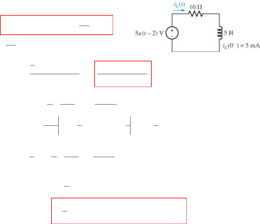
CHAPTER FOURTEEN SOLUTIONS
Engineering Circuit Analysis, 6th Edition Copyright
2002 McGraw-Hill, Inc. All Rights Reserved
38.
(a) -5 u(t – 2) + 10 iL(t) + 5 dt
diL = 0
(b) 0 )](0 - )([ 5 )( 10
5-
LLL
2=++
−−ie ssIsI
s
s
IL(s) = 105
)(0 5
5-
L
2
+
+
−
s
s
sie =
()
2
105
-32
+
×+
−
ss
s
s
e
(c) IL(s) = 2
105
2
-3
2
+
×
+
+
+
−
sss
sba
e
where a = 2
1
2
1
0
=
+=s
s, and b = 2
1
-
1
2-
=
=s
s, so that we may write
IL(s) = 2
105
2
1
1
2
1
-3
2
+
×
+
+
−
−
sss
s
e
Thus, iL(t) =
()
[]
)(105 )2( )2(
2
12-3-22 t uetuetu tt ×+−−− −−
=
()
[]
)(105 )2( 1
2
12-3-2 2 t uetue tt ×+−− −−
CHAPTER FOURTEEN SOLUTIONS
Engineering Circuit Analysis, 6th Edition Copyright
2002 McGraw-Hill, Inc. All Rights Reserved
39.
(a) (0 ) 50V, (0 ) 50 V
cc
vv
−+
==
(b)
3
0.1 0.2 0.1( 20) 0
2
0.1 0.3 2, 0.1 V 5 0.3V
25 2
V (0.1 0.3) 5
5 2 20/3 130/ 3 20 130
V( ) () () V
(0.1 0.3) 3 3 3
−
′++ −=
′
∴+ = −+ =
+
∴+=+=
+
∴= =+ ∴=+
++
cc c
cc c c
c
t
cc
vv v
vv s s
s
sss
s
svteut
ss s s
(c)
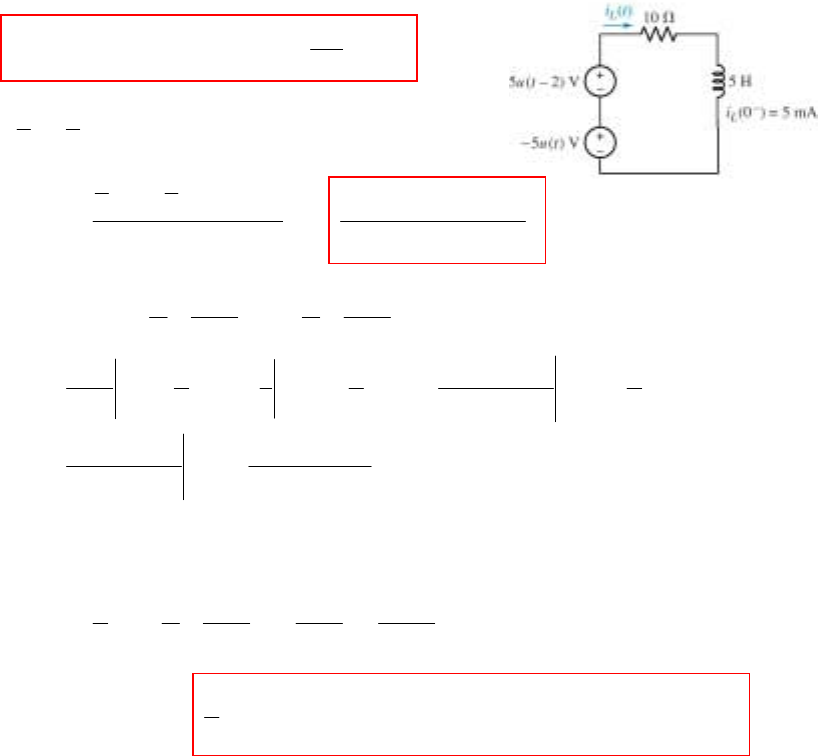
CHAPTER FOURTEEN SOLUTIONS
Engineering Circuit Analysis, 6th Edition Copyright
2002 McGraw-Hill, Inc. All Rights Reserved
40.
(a) 5 u(t) -5 u(t – 2) + 10 iL(t) + 5 dt
diL = 0
(b) 0 )](0 - )([ 5 )( 10
5
5-
LLL
2=++− −ie ssIsI
ss
s
IL(s) = 105
)(0 5
5
-
5-
L
2
+
+
−
s
ss
sie =
()
2
105 5
-32
+
×+−
−
ss
s
s
e
(c) IL(s) = 2
2
2
+
++
+
+
−
ssss
sdcba
e where
a = 2
1
2
1
0
=
+=s
s, b = 2
1
-
1
2-
=
=s
s, c = 5.2
2
5
-
2
5105
0
3−==
+
−×
=
−
s
s
s, and
d = 505.2
2-
5-1010-
5105 3
2-
3=
×
=
−× −
=
−
s
s
s,
so that we may write
IL(s) = ssss
s2.505
2
5.2
2
1
1
2
1
2+
+
−
+
−
−
e
Thus, iL(t) =
()
[]
)( 2.505)(2.5 )2( )2(
2
12-22 tut uetuetu tt +−−−− −−
CHAPTER FOURTEEN SOLUTIONS
Engineering Circuit Analysis, 6th Edition Copyright
2002 McGraw-Hill, Inc. All Rights Reserved
41.
22 2 2
22
0.15
2
12
12 ( ) 20 ( ) 3 (0 ) 2 20 F 20(2) 3F
12 12 40 2 0.6
40 (20 3) F F ( ) ( 0.15)
42
F( ) (4 2 ) ()
0.15
−
−
′
=+=∴=−+
++
∴+= + = ∴ = +
∴=− ↔−
+
t
ut f t f s
s
ss
ss
ssss
seut
ss
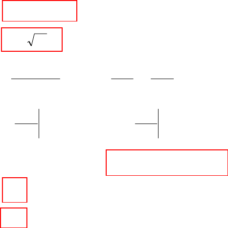
CHAPTER FOURTEEN SOLUTIONS
Engineering Circuit Analysis, 6th Edition Copyright
2002 McGraw-Hill, Inc. All Rights Reserved
42. (a) f(t) = 2 u(t) - 4
δ
(t)
(b) f(t) =
(
)
t 99 cos
(c) F(s) = 5 -
2
3
5 -
65
1
2−
+
−
=
++ ssss
ba
where 1
2
1
3
=
−
=
=s
s
a and 1-
3
1
2
=
−
=
=s
s
b
Thus,
f(t) = e-3t u(t) – e-2t u(t) – 5
δ
(t)
(d) f(t) =
δ
'(t) (a “doublet”)
(e) f(t) =
δ
'"(t)
CHAPTER FOURTEEN SOLUTIONS
Engineering Circuit Analysis, 6th Edition Copyright
2002 McGraw-Hill, Inc. All Rights Reserved
43.
2
22
222
2
2 ( ), 2 3 8 ( ), (0 ) 5, (0 ) 8
281225Y
X5Y ,Y82X3Y X 5Y
4102Y 8 2 418
Y3Y 8 Y 3 8
32 4188 8 1842 6
Y,Y()
( 1)( 2) 1
−−
′′
+= − + = = =
−+ = −− + = ∴ = +− = + −
∴+−−+ =+∴ ++=++
++ ++ ++
=+=++
++ +
xy uty x y utx y
ss
sssssss
ss
sss s sss
ss ss s s
s
ss sssss
0
2
11
() (2 6 ) (); () [ 3 8 ()] 1.5 4 ()
22
1
() [ 6 ()] 1.5[2 6 ] () 4 ()
2
() 6 () () (6 1) ()
−
−−
−−
+
′′
∴=+ = +− =+ −
∴=− + + −
∴= −= −
t
tt
tt
s
yt e ut xt y y ut y y ut
xt e ut e ut ut
xt e ut ut e ut
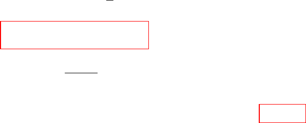
CHAPTER FOURTEEN SOLUTIONS
Engineering Circuit Analysis, 6th Edition Copyright
2002 McGraw-Hill, Inc. All Rights Reserved
44. (a) F(s) = s
s8
88 ++ , with f(0-) = 0. Thus, we may write:
f(t) = 8
δ
(t) + 8 u(t) + 8
δ
' (t)
(b) F(s) = 2 -
)2(
2+
+s
s
s.
f(t) =
δ
' (t) - 2
δ
(t) + 4e-2t u(t) -
δ
' (t) + 2
δ
(t) = 4e-2t u(t)
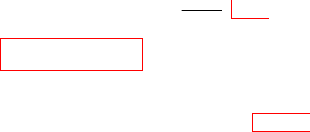
CHAPTER FOURTEEN SOLUTIONS
Engineering Circuit Analysis, 6th Edition Copyright
2002 McGraw-Hill, Inc. All Rights Reserved
45.
(a) 40 100
(0 ) 0, (0) 100 V, (0 ) 0.6 A
100
−+
−
==∴= =−
cc c
iv i
(b) 0
40 100 50 100
−
∞
=+ +
∫
cc
iidt
(c)
0.5
60 50
100 I ( ) I ( )
6 10 5 6 0.6
I , I ( ) ( ) 0.6 ( )
10 5 0.5
−
−= +
+−
∴= = = ↔ =
++
cc
t
cc c
ss
ss
ssiteut
ss ss
CHAPTER FOURTEEN SOLUTIONS
Engineering Circuit Analysis, 6th Edition Copyright
2002 McGraw-Hill, Inc. All Rights Reserved
46. (a) 4 cos 100t ↔ 22 100
4
+s
s
(b) 2 sin 103t – 3 cos 100t ↔ 62
3
10
102
+
×
s - 22 100
3
+s
(c) 14 cos 8t - 2 sin 8o ↔ 64
14
2+s
s - s
o
8sin2
(d)
δ
(t) + [sin 6t ]u(t) ↔ 1 + 36
6
2+s
(e) cos 5t sin 3t = ½ sin 8t + ½ sin (-2t) = ½ (sin 8t – sin 2t) ↔ 64
4
2+s - 4
1
2+s
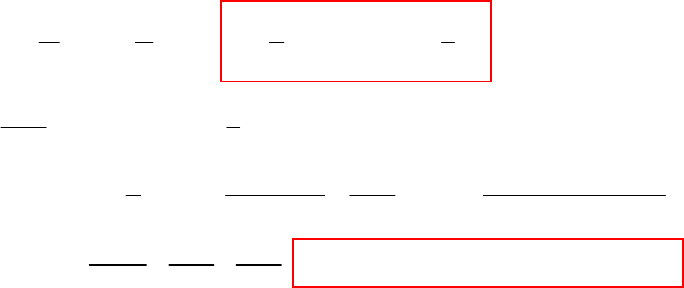
CHAPTER FOURTEEN SOLUTIONS
Engineering Circuit Analysis, 6th Edition Copyright
2002 McGraw-Hill, Inc. All Rights Reserved
47. 5
0
100 ( ) A; 4 3 −
−′
==++
∫t
t
ss
ieutivvvdt
(a) 0
11 1
C;R,C1F,L H
RL 4 3
−
′
=+ + =Ω = =
∫t
s
v
ivvdt
(b)
2
35
100 3
V( ) 4V( ) V( )
5
3 4 3 100 100
V( ) 4 V( ) , V( )
45(1)(3)(5)
12.5 75 62.5
V( ) , ( ) (75 12.5 62.5 ) ( ) V
135
−−−
=++
+
++
++ = = =
++++
−
∴=+− =−−
+++
tt t
ss s s
ss
ss s
ss s s
ss sss
svteeeut
sss
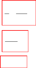
CHAPTER FOURTEEN SOLUTIONS
Engineering Circuit Analysis, 6th Edition Copyright
2002 McGraw-Hill, Inc. All Rights Reserved
48.
(a) V(s) = ss
s2
7−
+eV
(b) V(s) = V
1
2
+
−
s
s
e
(c) V(s) = 48e-s V
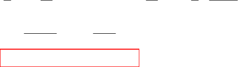
CHAPTER FOURTEEN SOLUTIONS
Engineering Circuit Analysis, 6th Edition Copyright
2002 McGraw-Hill, Inc. All Rights Reserved
49.
0
2
4 ( ) 10 4 [ 0.5 ( )] 0
410 10 424
II4I2, I5 2
2 4 1.6
I 0.4
510 2
( ) 0.4 ( ) 1.6 ( ) A
−
∞
−
++ + − δ =
−
∴+ + + = + =−+
−
∴= = −
++
∴+δ−
∫
ccc
cccc
c
t
c
ut i idt i t
s
ss s ss
s
ss
it t e ut
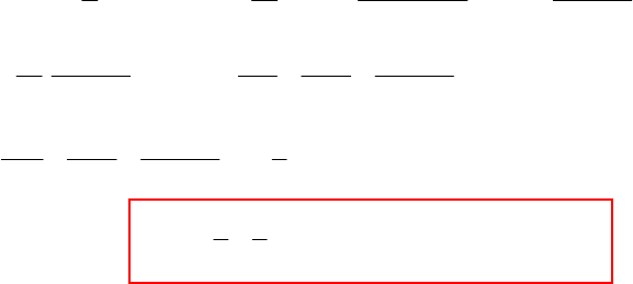
CHAPTER FOURTEEN SOLUTIONS
Engineering Circuit Analysis, 6th Edition Copyright
2002 McGraw-Hill, Inc. All Rights Reserved
50.
0
22
2
2
22
22 2
23(
2
6 9 ( ) 24( 2) ( 2), (0) 0
9169(3)
V( ) 0 6 V( ) V( ) 24 V( ) V( )
1 1/9 1/9 1/3
V( ) 24 24
(3) 3(3)
8/3 8 8 8
V( ) [ ( 2)
3( 3) 3
−
−
−−
−−
′′
++ = − − =
++ +
∴−+ + = = =
∴= = −−
+++
∴= −− ↔ −−
++
∫t
s
ss
s
vv vzdz t ut v
ss s
ss s s e s s
sss s
s
se e
ss s s s
se ut e
ss s
2)
3( 2) 3( 2) 3( 2)
(2)]
88
8(2) (2) () 8(2) (2)
33
−
−− −− −−
−
−− −∴ =− −− −
t
ttt
ut
te ut vt e te ut
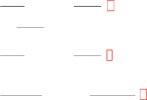
CHAPTER FOURTEEN SOLUTIONS
Engineering Circuit Analysis, 6th Edition Copyright
2002 McGraw-Hill, Inc. All Rights Reserved
51.
(a)
(b)
(c)
22
33
2
3
0
5 ( 1) 5 ( 1)
F( ) (0 ) 5
(1) 1
5( 1)
( ) , but 1 pole in RHP indeterminate
1
+
→∞
→
++
=∴= =
++
+
∞= ∴
+
l
l
im
s
im
s
sss
sf
ss
ss
fs
22
34
5( 1) 5 ( 1)
F( ) (0 ) 0
16 16
( ) is indeterminate since poles on axis
+
→∞
++
=∴= =
++
∞ω
lim
s
sss
sf
ss
fj
44
22
(1)(1 ) (1)(1 )
F( ) (0 ) 1
22
( ) is indeterminate since poles on axis
−−
+
→∞
++ ++
=∴= =
++
∞ω
l
ss
im
s
se sse
sf
ss
fj
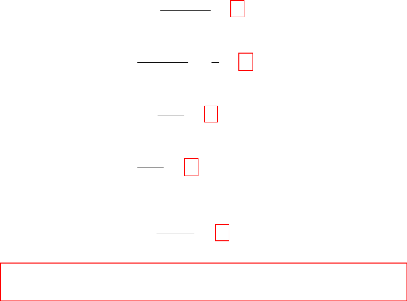
CHAPTER FOURTEEN SOLUTIONS
Engineering Circuit Analysis, 6th Edition Copyright
2002 McGraw-Hill, Inc. All Rights Reserved
52. (a) f(0+) =
[]
2
2 5
6 2
lim )( lim 2
2
=
++
+
=∞→∞→ ss
s
sFs ss
f(∞) =
[]
3
2
6
2 5
6 2
lim )( lim 2
2
0 0 ==
++
+
=→→ ss
s
sFs ss
(b) f(0+) =
[]
0
3
2
lim )( lim =
+
=−
∞→∞→ s
s
sFs s
ss
e
f(∞) =
[]
0
3
2
lim )( lim 0 0 =
+
=−
→→ s
s
sFs s
ss
e
(c) f(0+) =
[]
()
∞=
+
+
=∞→∞→
5
1
lim )( lim 2
2
s
ss
sFs ss
f(∞) : This function has poles on the j
ω
axis, so we may not apply the final value
theorem to determine f(∞).
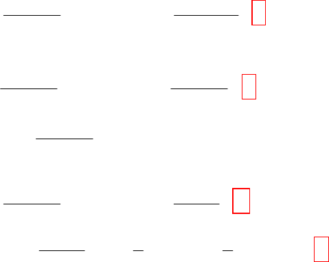
CHAPTER FOURTEEN SOLUTIONS
Engineering Circuit Analysis, 6th Edition Copyright
2002 McGraw-Hill, Inc. All Rights Reserved
53.
(a) 22
33
5( 1) 5 ( 1)
F( ) (0 ) 5
(1) (1)
+
→∞
++
=∴= =
++
lim
s
sss
sf
ss
(b)
(c)
22
33
2
3
0
5( 1) 5( 1)
F( ) (0 ) 0
(1) (1)
5( 1)
( ) 5 (pole OK)
(1)
+
→∞
→
++
=∴= =
++
+
∞= =
+
l
l
im
s
im
s
ss
sf
ss s
s
fs
33
2
32
00
(1 ) 1
F( ) (0 ) 0
111
( ) 1 1 3 9 ... 3 (no poles)
22
−−
+
−
→∞
→→
−−
=∴= =
−
∞= = −+ − × + =
l
ll
ss
s
im
s
im im
ss
ee
sf
ss
e
fss
s
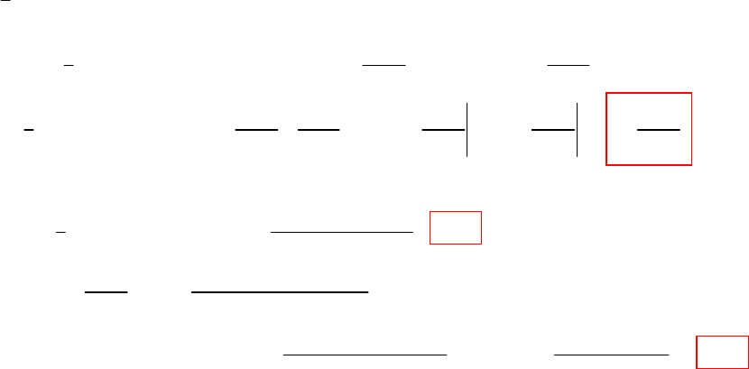
CHAPTER FOURTEEN SOLUTIONS
Engineering Circuit Analysis, 6th Edition Copyright
2002 McGraw-Hill, Inc. All Rights Reserved
54.
1
() ( ) ()
at bt
ft e e ut
t
−
=−
(a)
(b)
2
2
00
1 1 ... 1
()()
()()
1/
1/( ) 1/( ) ( )
Use Hopital. F( ) 1/ ( )( )
−−
++
→→
→∞ →∞
→∞ →∞
−+−+
−= =−
++−+
=
+
+− + −
′∴= =− =−
−++
ll
ll
ll
ll
l
l
at bt
im im
tt
im im
ss
im im
ss
at bt
eeut ba
tt
sb nsb nsa
sn
sa s
sb sa ab
ss s ba
ssbsa
111
Now, () F() () , ()
111
(()
∞−−
∞∞
∞
−−
↔∴↔−↔−
++
+++
∴− ↔ − = = =
++ + + +
∫
∫lll
at bt
s
at bt
sss
ft sds e ut e ut
tsasb
sa sa sb
e e u t ds n n n
tsasbsbsbsa
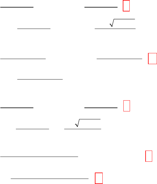
CHAPTER FOURTEEN SOLUTIONS
Engineering Circuit Analysis, 6th Edition Copyright
2002 McGraw-Hill, Inc. All Rights Reserved
55.
(a)
(b)
(c)
(d)
2
22
2
22
0
82
F( ) (0 ) F( ) 0
( 2) ( 1)( 6 10)
(8 2) 10 (pole OK)
( 2) ( 1)( 6 10)
+
→∞
→
−
=∴==
++++
−
∞= =
++++
l
l
im
s
im
s
s
sfs
ssss
ss
fssss
22
2
0
82 (82)
F( ) (0 ) 8
610 610
(8 2) 6 36 40
( ) 0 poles: , LHP, OK
610 2
+
→∞
→
−−
=∴= =
++ ++
−−±−
∞= = = ∴
++
l
l
im
s
im
s
sss
sf
ss ss
ss
fs
ss
32 32
32 2
32
2
0
235 235
F( ) (0 )
610 610
235
( ) 0.5 (poles OK)
610
+
→∞
→
−−− −−−
=∴= =∞
++ ++
−−−
∞= =−
++
l
l
im
s
im
s
ss s ss s
sf
ss s ss
ss s
fss
22
2
0
82 (82)
F( ) (0 ) 8
610 610
(8 2) 6 36 40
( ) , RHP indeterminate
610 2
+
→∞
→
−−
=∴= =
−+ −+
−±−
∞= = ∴
−+
l
l
im
s
im
s
sss
sf
ss ss
ss
fs
ss
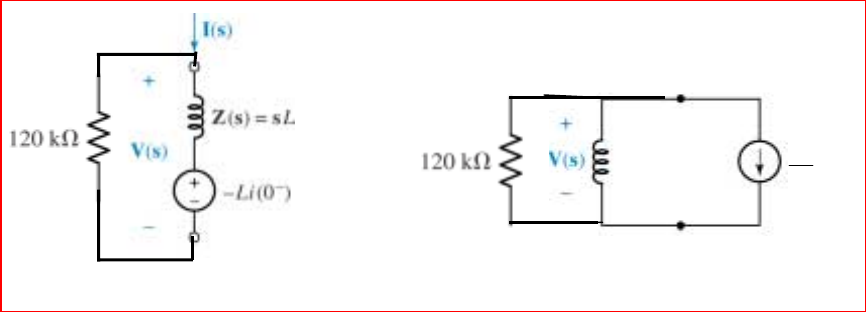
CHAPTER FIFTEEN SOLUTIONS
Engineering Circuit Analysis, 6th Edition Copyright
2002 McGraw-Hill, Inc. All Rights Reserved
1. Note that iL(0+) = 12 mA. We have two choices for inductor model:
= 0.032s Ω
= 384 µV
0.032s Ω 12
smA
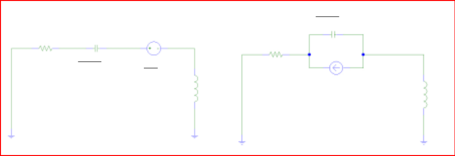
CHAPTER FIFTEEN SOLUTIONS
Engineering Circuit Analysis, 6th Edition Copyright
2002 McGraw-Hill, Inc. All Rights Reserved
2. iL(0-) = 0, vC(0+) = 7.2 V (‘+’ reference on left). There are two possible circuits, since
the inductor is modeled simply as an impedance:
73 Ω 1
0.002s Ω
0.03s Ω
7.2 V
s+
V(s)
-
73 Ω
1
0.002s Ω
0.03s Ω
14.4 mA +
V(s)
-
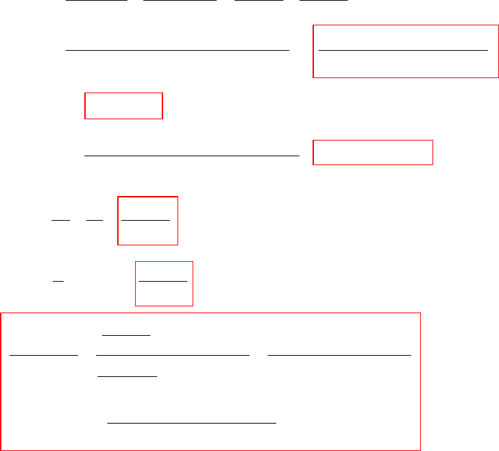
CHAPTER FIFTEEN SOLUTIONS
Engineering Circuit Analysis, 6th Edition Copyright
2002 McGraw-Hill, Inc. All Rights Reserved
3.
(a)
(b) Zin(-80) = - 10.95 Ω
(c) 128,000 880,000 200,000
( 80) 8.095 54.43
6400 56,000 100,000
in
j
jj
−+ +
==∠°Ω
−+ +
Z
(d) 1 10 200
20 20
RL
+
=+=
s
Yss
(e) 1 500
0.001
2 1000
RC
+
=+ =
s
Ys
(f)
22
22
2 2000 / 20 1000
() 20 0.1 2 1000 / 200 500
20 10,000 1000 200,000 20 11, 000 200,000
700 100,000 700 100,000
m=+ =+
++ ++
+++ ++
==
++ ++
sss
Zs ssss
sss ss
ss ss
2
2
2
2
200 0.5 0.001 200 10 0.02
20
(200) 0.001 0.7 100
(0.001 0.5)
20
20 11,000 200,000
( )
700 100,000
RL RC
RL RC
s
+++
++++
==
+++
+
++
==
++
ss
YY sss
s
YY ss
s
s
ss Zs
ss
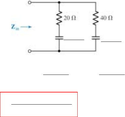
CHAPTER FIFTEEN SOLUTIONS
Engineering Circuit Analysis, 6th Edition Copyright
2002 McGraw-Hill, Inc. All Rights Reserved
4.
Zin = 33
11
20 || 40
210 210
−−
++
××
ss
= (20 + 500s-1) || (40 + 500s-1)
=
80 3000 +25000
6 100
+
+
2
2
ss
ss
3
1
210
−
×s3
1
210
−
×s
CHAPTER FIFTEEN SOLUTIONS
Engineering Circuit Analysis, 6th Edition Copyright
2002 McGraw-Hill, Inc. All Rights Reserved
5. (a)
2
2
50 16(0.2 ) 50 16 16 50 4000
16 0.2 80 80
in
++
=+ =+ =
++
+
ssss
Zssss ss
(b) 1024 4000 400
( 8) 0.15842 4.666
64 640
in
j
jj
j
−+ +
==−Ω
−+
Z
(c) 16(4 36 24) 100 300 4000
( 2 6) 6.850 114.3
32 24 160 480
in
jj
jjj
−− − + +
−+ = = ∠− °Ω
−− − +
Z
(d)
(e)
R1
=Ω
2
2
0.2 R
50 0.2R 10 50R ,
R 0.2 0.2 R
5R 50 50
( 5) 55R 50, R 0.9091
55R
in
in
R
++
=+ =
++
−+
−= ∴ = = Ω
−
sss
Zssss
Z
CHAPTER FIFTEEN SOLUTIONS
Engineering Circuit Analysis, 6th Edition Copyright
2002 McGraw-Hill, Inc. All Rights Reserved
6. 2 mF → 3
1
210
−
×sΩ, 1 mH → 0.001s Ω,
Zin = (55 + 500/ s) || (100 + s/ 1000) =
267
25 5
500
55 100 + 55 + 5.5005 10 5 10
1000 =
500 + 5 10 + 1.55 10
155 1000
+
×+×
××
++
s
ss
ssss
s
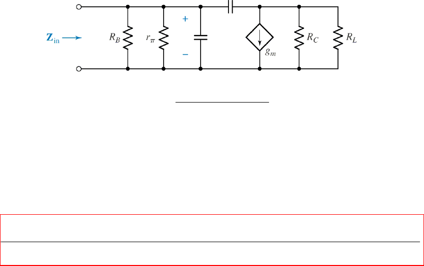
CHAPTER FIFTEEN SOLUTIONS
Engineering Circuit Analysis, 6th Edition Copyright
2002 McGraw-Hill, Inc. All Rights Reserved
7. We convert the circuit to the s-domain:
Defining Zπ = RB || rπ || (1/sCπ) = B
BB
rR
r + R + r R C
π
πππ
s and
ZL = RC || RL = RCRL/ (RC + RL), we next connect a 1-A source to the input and write two
nodal equations:
1 = Vπ/ Zπ + (Vπ – VL)Cµ s [1]
-g
mVπ = VL/ ZL + (VL – Vπ)Cµ s [2]
Solving,
Vπ =
()
BL
2
LB mLB B B L LB B
r R 1 + C
r R C C + (g r R C + r R C + r R C + r C + R C ) + r + R
πµ
ππµ πµπππµ πµ µ π
Zs
ZsZ ZZs
Since we used a 1-A ‘test’ source, this is the input impedance. Setting both capacitors to
zero results in rπ || RB as expected.
Vπ
1/sCπ Ω
1/sCµ Ω
Vπ
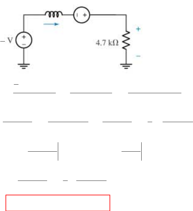
CHAPTER FIFTEEN SOLUTIONS
Engineering Circuit Analysis, 6th Edition Copyright
2002 McGraw-Hill, Inc. All Rights Reserved
8.
V(s) =
6
2460 10
4700 4700 0.115
−
+×
+
ss = 2.162 9400
+
0.115 4700 (0.115 + 4700)+
sss
=
18.8 81740
+
40870 ( + 40870)+sss
= 18.8 a b
+ +
40870 + 40870+sss
where a =
= 0
81740 = 2
40870+s
s and b =
= -40870
81740 = -2
s
s
Thus, V(s) = 18.8 2 2
+ -
40870 + 40870+sss
. Taking the inverse transform of each term,
v(t) = [16.8 e-40870t + 2] u(t) V
V
I
2
s
460 µV
0.115s Ω
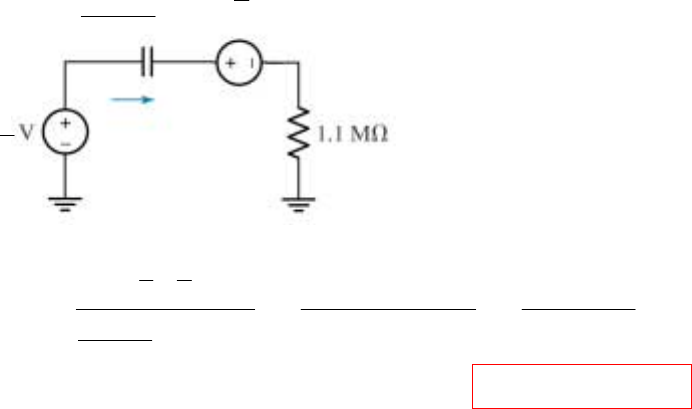
CHAPTER FIFTEEN SOLUTIONS
Engineering Circuit Analysis, 6th Edition Copyright
2002 McGraw-Hill, Inc. All Rights Reserved
9. v(0-) = 4 V
I(s) =
-6
6
6
94
5 4.545 10
= =
303030 +0.2755
1.1 10 303030
1.1 10
−×
×+
+×
ss s
s
Taking the inverse transform, we find that i(t) = 4.545 e-0.2755t u(t) µA
9
s
303030
s Ω
4 V
s
I(s)
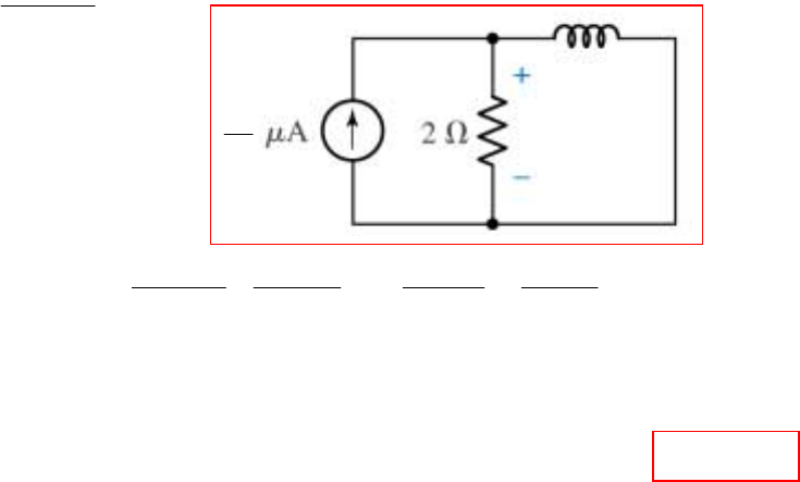
CHAPTER FIFTEEN SOLUTIONS
Engineering Circuit Analysis, 6th Edition Copyright
2002 McGraw-Hill, Inc. All Rights Reserved
10. From the information provided, we assume no initial energy stored in the inductor.
(a) Replace the 100 mH inductor with a 0.1s-Ω impedance, and the current source with a
6
25 10 A
−
×
ssource.
(b) V(s) =
6-6-5
25 10 2 (0.1 ) 5 10 5 10
= = V
2 + 0.1 0.1 2 20
−
×××
++
s
ssss
Taking the inverse transform,
v(t) = 50 e-20t mV
The power absorbed in the resistor R is then p(t) = 0.5 v2(t) = 1.25 e-40t nW
V
25
s
0.1s Ω
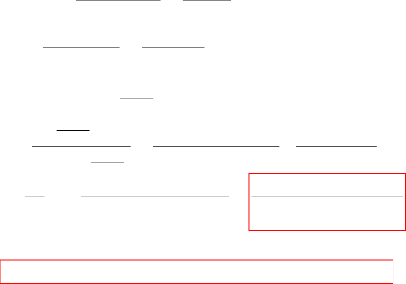
CHAPTER FIFTEEN SOLUTIONS
Engineering Circuit Analysis, 6th Edition Copyright
2002 McGraw-Hill, Inc. All Rights Reserved
11. v(t) = 10e-2t cos (10t + 30o) V
cos (10t + 30o) ⇔
oo
22
cos30 -10sin30 0.866 - 5
=
+100 + 100
ss
ss
Λ {f(t)e-at} ⇔ F(s + a), so
V(s) =
()
()
2
0.866 2 - 5 8.66 - 16.34
10 = + 100
2 + 100
+
+
ss
s
s
The voltage across the 5-Ω resistor may be found by simple voltage division. We first
note that Zeff = (10/s) || 5 = 50
510+sΩ. Thus,
V5Ω =
()()
s
ss
2
50 50 50
510 = =
50 0.5 + 5 5 + 10 + 50 2.5 30 100
0.5 + 5 + 510
+
++
+
VVV
s
sss
ss
s
(a) Ix = eff
5
V =
() () ()
222
2
0.866 - 3.268 34.64 - 130.7
40 =
2 100 12 + 40 2 100 6 + 100
++ + ++ +
ss
ssss s
(b) Taking the inverse transform using MATLAB, we find that
ix(t) = e-6t [0.0915cos 2t - 1.5245 sin 2t] - e-2t [0.0915 cos10t - 0.3415 sin 10t] A
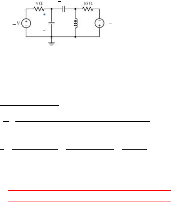
CHAPTER FIFTEEN SOLUTIONS
Engineering Circuit Analysis, 6th Edition Copyright
2002 McGraw-Hill, Inc. All Rights Reserved
12.
Node 1: 0 = 0.2 (V1 – 3/ s) + 0.2 V1 s + 0.5 (V1 – V2) s
Node 2: 0 = 0.5 (V2 – V1) s + 0.125 V2 s + 0.1 (V2 + 5/ s)
Rewriting, (3.5 s 2 + s) V1 + 2.5 s 2 V2 = 3 [1]
-4 s 2 V1 + (4 s 2 + 0.8 s + 1) V2 = -4 [2]
Solving using MATLAB or substitution, we find that
()( )()
2
1432
2
20 + 16 + 20
( ) =
40 + 68 + 43 + 10
1 20 + 16 + 20
=
40 + 0.5457 - 0.3361 + 0.5457 + 0.3361 + 0.6086jj
−
−
ss
Vs ssss
ss
ss s s
which can be expanded:
*
1( ) = + + +
+ 0.5457 - 0.3361 + 0.5457 + 0.3361 + 0.6086
ab b c
jj
Vs ss s s
Using the method of residues, we find that
a = 2, b = 2.511 ∠101.5o, b* = 2.511∠-101.5o and c = -1.003.
Thus,taking the inverse transform,
v1(t) = [2 – 1.003 e-0.6086t + 5.022 e-0.5457t cos (0.3361t – 101.5o)] u(t) V
VC1
V1 V2
3
s 5 V
s
5 Ω
s
2 Ω
s
8s Ω
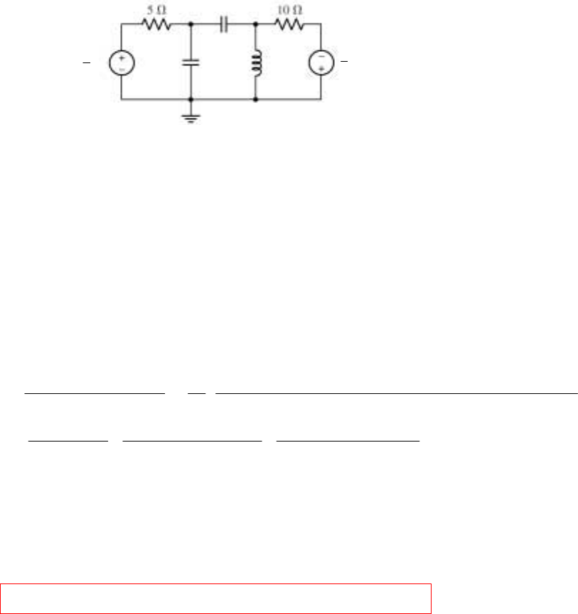
CHAPTER FIFTEEN SOLUTIONS
Engineering Circuit Analysis, 6th Edition Copyright
2002 McGraw-Hill, Inc. All Rights Reserved
13. With zero initial energy, we may draw the following circuit:
Define three clockwise mesh currents I1, I2, and I3 in the left, centre and right meshes,
respectively.
Mesh 1: -3/s + 5I1 + (5/s)I1 – (5/s)I2 = 0
Mesh 2: -(5/s)I1 + (8s + 7/s)I2 – 8s I3 = 0
Mesh 3: -8sI2 + (8s + 10)I3 – 5/s = 0
Rewriting,
(5s + 5) I1 – 5 I2 = 3 [1]
-5 I1 + (8s2 +7) I2 – 8s2 I3 = 0 [2]
- 8s2 I2 + (8s2 + 10s) I3 = 5 [3]
Solving, we find that
I2(s) =
2
32
20 + 32 + 15
40 + 68 + 43 + 10
ss
sss=
()( )( )
2
1 20 + 32 + 15
40 + 0.6086 + 0.5457 - 0.3361 + 0.5457 + 0.3361
jj
ss
ss s
=
()()()
*
+ 0.6086 + 0.5457 - 0.3361 + 0.5457 + 0.3361
ab b
jj
++
ss s
where a = 0.6269, b = 0.3953∠-99.25o, and b* = 0.3955∠+99.25o
Taking the inverse tranform, we find that
i2(t) = [0.6271e-0.6086t + 0.3953e-j99.25o e(-0.5457 + j0.3361)t + 0.3953ej99.25o e(-0.5457 - j0.3361)t ]u(t)
= [0.6271e-0.6086t + 0.7906 e-0.5457t cos(0.3361t + 99.25o)] u(t)
8 s Ω
5 s-1 Ω
2 s-1 Ω
3 V
s
5 V
s
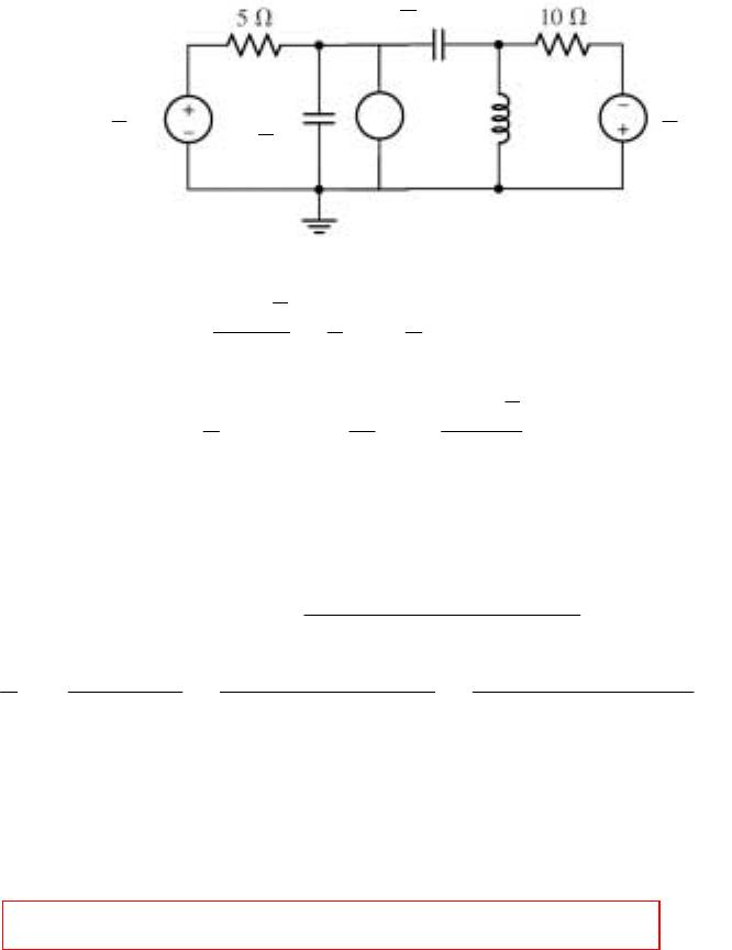
CHAPTER FIFTEEN SOLUTIONS
Engineering Circuit Analysis, 6th Edition Copyright
2002 McGraw-Hill, Inc. All Rights Reserved
14. We choose to represent the initial energy stored in the capacitor with a current source:
Node 1:
1
112
3
-
1.8 = + + ( - )
552
Vss
sVVV
Node 2:
2
21 2
5
+
1
0 = ( - ) + +
2810
V
ss
VV V
s
Rewriting, (5s2 + 4s) V1 – 5s2 V2 = 18s + 6 [1]
-4s2 V1 + (4s2 + 0.8s + 1)V2 = -4 [2]
Solving, we find that V1(s) =
32
32
360 + 92 + 114 + 30
(40 + 68 + 43 + 10)
ss s
ss s s
=
*
+ + +
+ 0.6086 + 0.5457 - 0.3361 + 0.5457 + 0.3361
ab c c
jjss s s
where a = 3, b = 30.37, c = 16.84 ∠136.3o and c* = 16.84 ∠-136.3o
Taking the inverse transform, we find that
v
1(t) = [3 + 30.37e-0.6086t + 16.84 ej136.3o e-0.5457t ej0.3361t
+ 16.84 e-j136.3o e-0.5457t e-j0.3361t ]u(t) V
= [3 + 30.37e-0.6086t + 33.68e-0.5457t cos (0.3361t + 136.3o]u(t) V
1.8 A
↑
5Ω
s
2Ω
s
8s Ω
3 V
s
5 V
s
V1 V2
•
•
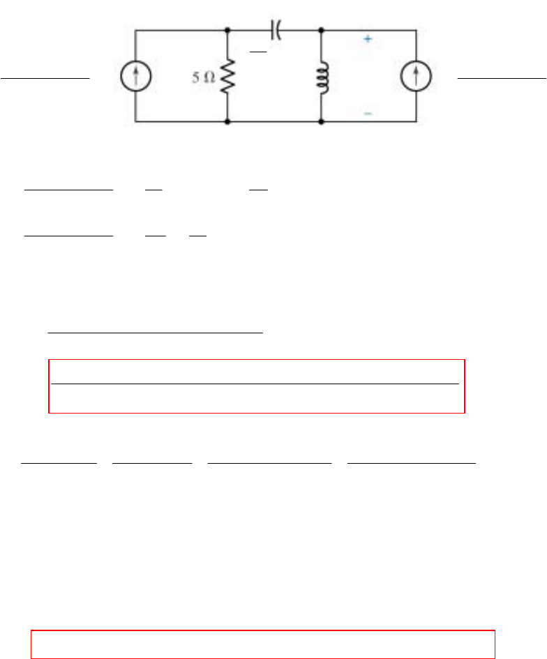
CHAPTER FIFTEEN SOLUTIONS
Engineering Circuit Analysis, 6th Edition Copyright
2002 McGraw-Hill, Inc. All Rights Reserved
15. We begin by assuming no initial energy in the circuit and transforming to the s-domain:
(a) via nodal analysis, we write:
()
1
1x
2
20 + 60 = - +
( + 3) + 16 10 5
Vss
VV
s [1] and
()
x
x1
2
120 = +
( + 3) + 16 2 10 −
Vs
VV
ss [2]
Collecting terms and solving for Vx(s), we find that
Vx(s)
(b) Using the method of residues, this function may be rewritten as
with a = 92.57 ∠ -47.58o, a* = 92.57 ∠ 47.58o, b = 43.14 ∠106.8o, b* = 43.14 ∠-106.8o
Taking the inverse transform, then, yields
vx(t) = [92.57 e-j47.58o e-3t ej4t + 92.57 ej47.58o e-3t e-j4t
+ 43.14ej106.8o e-1.25t ej1.854t + 43.14e-j106.8o e-1.25t e-j1.854t] u(t)
= [185.1 e-3t cos (4t - 47.58o) + 86.28 e-1.25t cos (1.854t + 106.8o)] u(t)
2
+ 3
20 A
( + 3) + 16
s
s 2s Ω Vx
10 Ω
s
V1
2
4
30 A
( + 3) + 16s
()( )( )( )
2
432
2
200 ( + 9 + 12)
2 + 17 + 90 + 185 + 250
200 ( + 9 + 12)
= + 3 - 4 + 3 + 4 + 1.25 - 1.854 + 1.25 + 1.854jj j j
=ss s
sss s
ss s
ss s s
()()()()
**
+ 3 - 4 + 3 + 4 + 1.25 - 1.854 + 1.25 + 1.854
aa b b
jj j j
++ +
ss s s
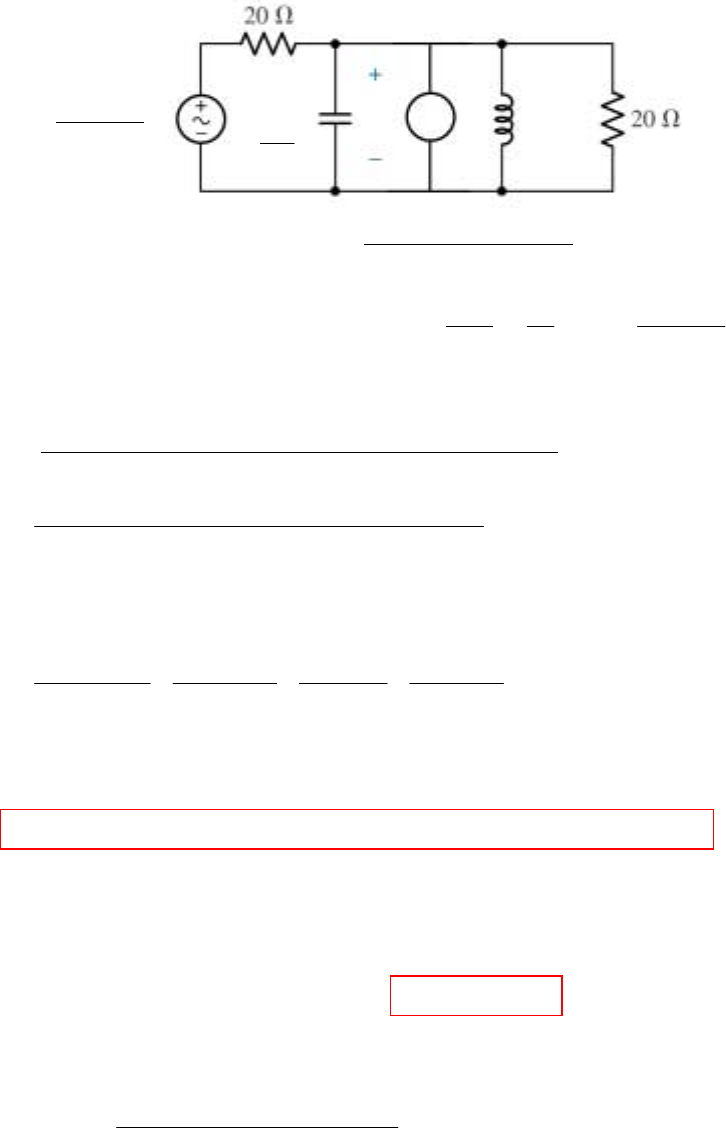
CHAPTER FIFTEEN SOLUTIONS
Engineering Circuit Analysis, 6th Edition Copyright
2002 McGraw-Hill, Inc. All Rights Reserved
16. We model the initial energy in the capacitor as a 75-µA independent current source:
First, define Zeff = 106/s || 0.005s || 20 = -6 2
10 + 0.005 + 200 Ω
s
ss
Then, writing a single KCL equation, -6
22
eff
(s) 1 162.6
75 10 = + ( ) -
20 + 4
π
×
Vs
Vs
Zs
which may be solved for V(s):
V(s) =
()
25
44382 6 9
75 + 1.084 10 + 39.48
+ 5.5 10 + 2 10 + 2.171 10 + 7.896 10
×
×× × ×
ss s
sss s
=
()
()()()()
25
75 + 1.084 10 + 12.57
+ 51085 + 3915 - 6.283 + 6.283jj
×ss s
ssss
(NOTE: factored with higher-precision denominator coefficients using MATLAB to
obtain accurate complex poles: otherwise, numerical error led to an exponentially
growing pole i.e. real part of the pole was positive)
=
()()()()
*
+ 51085 + 3915 - 2 + 2
abcc
jj
ππ
+++
ssss
where a = -91.13, b = 166.1, c = 0.1277∠89.91o and c* = 0.1277∠-89.91o.
Thus, consolidating the complex exponential terms (the imaginary components cancel),
v(t) = [-91.13e-51085t + 166.1e-3915t + 0.2554 cos (2πt + 89.91o)] u(t) V
(b) The steady-state voltage across the capacitor is V = [255.4 cos(2πt + 89.91o)] mV
This can be written in phasor notation as 0.2554 ∠89.91o V. The impedance across
which this appears is Zeff = [j
ω
C + 1/j
ω
L + 1/20]-1 = 0.03142 ∠89.91o Ω, so
Isource = V/ Zeff = 8.129∠-89.91o A.
Thus, isource = 8.129 cos 2πt A.
(c) By phasor analysis, we can use simple voltage division to find the voltage division to
find the capacitor voltage:
VC(j
ω
) =
()
()
o
o
o
162.6 0 0.03142 89.91 = 0.2554 89.92 V
20 + 0.03142 89.91
∠∠ ∠
∠ which agrees with
our answer to (a), assuming steady state. Dividing by 0.03142 ∠89.91o Ω, we find
isource = 8.129 cos 2πt A.
↑
22
162.6 V
+ 4
π
s
s V
75 µA
0.005s Ω
6
10 Ω
s
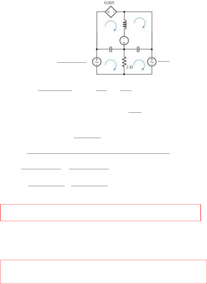
CHAPTER FIFTEEN SOLUTIONS
Engineering Circuit Analysis, 6th Edition Copyright
2002 McGraw-Hill, Inc. All Rights Reserved
17. Only the inductor appears to have initial energy, so we model that with a voltage source:
Mesh 1: 123
2
5.846 + 2.699 1333 1333
= 2 + - - 2
+ 4
sIII
sss
Mesh 2: 0 = 0.005I1 – 0.001 + (0.001s + 1333/s) I2 – (1333/s)I1 – 0.001sI4
Mesh 3: 0 = (2 + 1000/s)I3 – 2I1 – (1000/s)I4 + 2
6
4+
s
s
Mesh 4: 0 = (0.001s + 1000/s) I4 - 0.001sI2 – (1000/s)I3 + 0.001
Solving, we find that I1 = 2
154 2699
0.2 4
−
−+
s
s and
I2 =
47310213 14
453929
154 - 7.378 10 - 1.912 10 - 4.07 10 + 7.196 10
0.001 2333 + 6.665 10 + 1.333 10 + 5.332 10
××××
×××
ss ss
sss
oo
oo
-5
0.4328 166.6 0.4328 166.6
+
+ 142.8 + 742 + 142.8 - 742
135.9 96.51 135.9 96.51
+ + + 6.6 10
- 2 + 2
jj
jj
∠− ∠+
=
∠− ∠+ ×
ss
ss
Taking the inverse transform of each,
i1(t) = 271.7 cos (2t – 96.51o) A and
i2(t) = 0.8656 e-142.8t cos (742.3t + 166.6o) + 271.8 cos (2t – 96.51o) + 6.6×10⁻⁵
δ
(t) A
Verifying via phasor analysis, we again write four mesh equations:
6∠-13o = (2 – j666.7)I1 + j667I2 – 2I3
0 = (0.005 + j666.7)I1 + (j2x10-3 – j666.7)I2 – j2×10-3I4
-6∠0 = -2I1 + (2 – j500)I3 + j500I4
0 = -j2×10-3I2 + j500I3 + (j2×10-3 – j500)I4
Solving, we find I1 = 271.7∠-96.5o A and I2 = 272∠-96.5o A. From the Laplace analysis,
we see that this agrees with our expression for i1(t), and as t → ∞, our expression for i2(t)
→ 272 cos (2t – 96.5o) in agreement with the phasor analysis.
I1
I1
I2
I3
I4
0.001s Ω
1 mV
2
5.846 + 2.699 V
+ 4
s
s
1333/s Ω 1000/s Ω
2
6V
+ 4
s
s
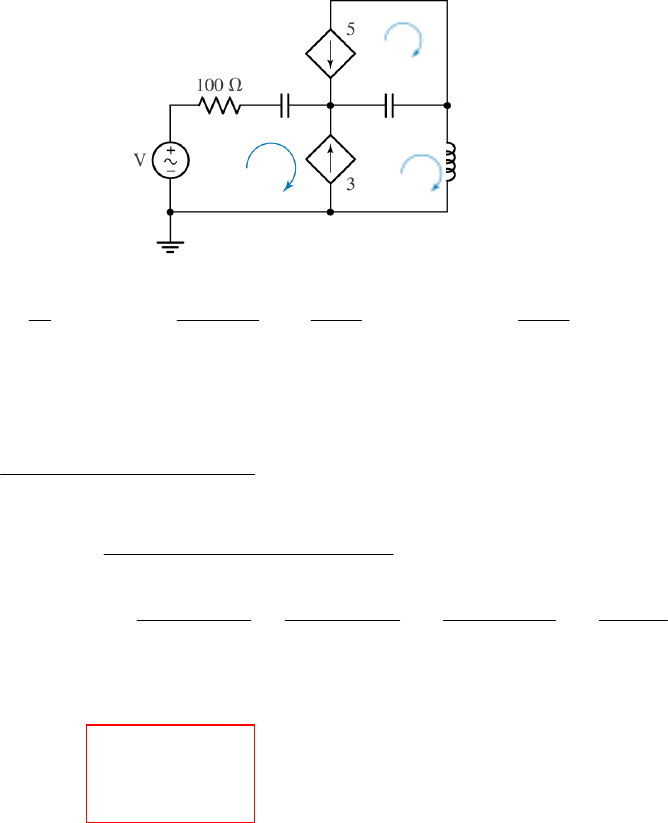
CHAPTER FIFTEEN SOLUTIONS
Engineering Circuit Analysis, 6th Edition Copyright
2002 McGraw-Hill, Inc. All Rights Reserved
18. With no initial energy storage, we simply convert the circuit to the s-domain:
Writing a supermesh equation,
11332
24
1 1 2000 2000
= 100 + + + 0.002 -
610
−
×
IIIsII
ssss
we next note that I2 = -5V2 = -5(0.002s)I3 = -0.01sI3
and I3 – I1 = 3V2 = 0.006sI3, or I1 = (1 – 0.006s)I3, we may write
332
1
=
0.598 + 110 + 3666−
Iss s
V2(s) = I3/ 0.002s = 43 2
1
0.0012 + 0.22 + 7.332−ss s
= 53 3
2
7.645 10 4.167 10 4.091 10 0.1364
+
212.8 28.82
−− −
×× ×
−−+
−+ss ss
Taking the inverse transform,
v2(t) = -7.645×10⁻⁵ e212.8t + 4.167×10⁻³ e-28.82t – 4.091×10⁻³ + 0.1364 t] u(t) V
(a) v2(1 ms) = -5.58×10⁻⁷ V
(b) v2(100 ms) = -1.334×10⁵ V
(c) v2(10 s) = -1.154×10920 V. This is pretty big- best to start running.
0.002s Ω
2000/s Ω
1667/s Ω
s-2
V2
V2
V2
I1
I2
I3

CHAPTER FIFTEEN SOLUTIONS
Engineering Circuit Analysis, 6th Edition Copyright
2002 McGraw-Hill, Inc. All Rights Reserved
19. We need to write three mesh equations:
Mesh 1: 13
2
5.846 + 2.699 1333
= 2 + - 2
+ 4
sII
ss
Mesh 3: 0 = (2 + 1000/s)I3 – 2I1 – (1000/s)I4 + 2
6
4+
s
s
Mesh 4: 0 = (0.001s + 1000/s) I4 – (1000/s)I3 + 10-6
Solving,
I1 =
()
362 8 9
453 26 9
154 - 2.925 10 + 1.527 10 - 2.699 10
0.001 2333 + 6.665 10 + 1.333 109 + 2.666 10 + 5.332 10
×××
−×× ××
ss s
sssss
oo
oo
-5
0.6507 12.54 0.6507 12.54
+
+ 142.8 742.3 + 142.8 + 742.3
0.00101 6.538 0.00101 6.538
+ + 6.601 10
2 2
jj
jj
∠∠−
=−
∠− ∠ −×
−+
ss
ss
which corresponds to
i1(t) = 1.301 e-142.8t cos (742.3t + 12.54o) + 0.00202 cos (2t – 6.538o) – 6.601×10⁻⁵ δ(t) A
and
I
3 =
()
()( )
4638212 6
22 5 9
154 + 3.997 10 + 1.547 10 + 3.996 10 - 2.667 10
0.001 + 4 2333 + 6.665 10 + 1.333 10
××××
−××
sss s
ss s
oo
oo
0.7821 33.56 0.7821 33.56
+
+ 142.8 742.3 + 142.8 + 742.3
1.499 179.9 1.499 179.9
+ +
2 2
jj
jj
∠− ∠
=−
∠∠−
−+
ss
ss
which corresponds to
i3(t) = 1.564 e-142.8t cos (742.3t – 33.56o) + 2.998 cos (2t + 179.9o) A
The power absorbed by the 2-Ω resistor, then, is 2
13
2() ()it it
−
or
p(t) = 2[1.301 e-142.8t cos (742.3t + 12.54o) + 0.00202 cos (2t – 6.538o) – 6.601×10⁻⁵ δ(t)
- 1.564 e-142.8t cos (742.3t – 33.56o) - 2.998 cos (2t + 179.9o)]2 W
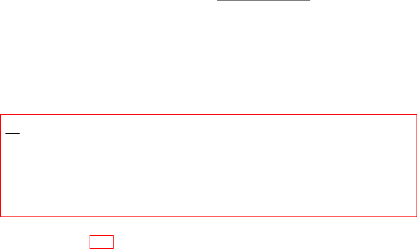
CHAPTER FIFTEEN SOLUTIONS
Engineering Circuit Analysis, 6th Edition Copyright
2002 McGraw-Hill, Inc. All Rights Reserved
20. (a) We first define Zeff = RB || rπ || (1/sCπ) = B
BB
rR
r + R rRC
π
πππ
+s. Writing two nodal
equations, then, we obtain:
0 = (Vπ – VS)/ RS + Vπ (rπ + RB + rπ RBCπs)/rπRB + (Vπ – Vo)Cµ s
and
-gmVπ = Vo(RC + RL)/RCRL + (Vo – Vp) Cµ s
Solving using MATLAB, we find that
2
o
BCLm sBCL sBC sBC
s
sBL sBL BCL sCL
sBCL ms BCL
= rRRR(-g + C ) [RrRRRCC (RrRRC RrRRC
+ R r R R C R r R R C r R R R C R r R R C
R R R R C g R r R R R C )
πµππµπππµ
πππµπ µπµ
µπ µ
++
+++
++
Vss
V
s
1
BCsCsBC BLsLsBL
+ r R R R r R R R R r R R R r R R R R ]
ππ ππ
−
++ +++
(b) Since we have only two energy storage elements in the circuit, the maximum number
of poles would be two. The capacitors cannot be combined (either series or in parallel),
so we expect a second-order denominator polynomial, which is what we found in part (a).
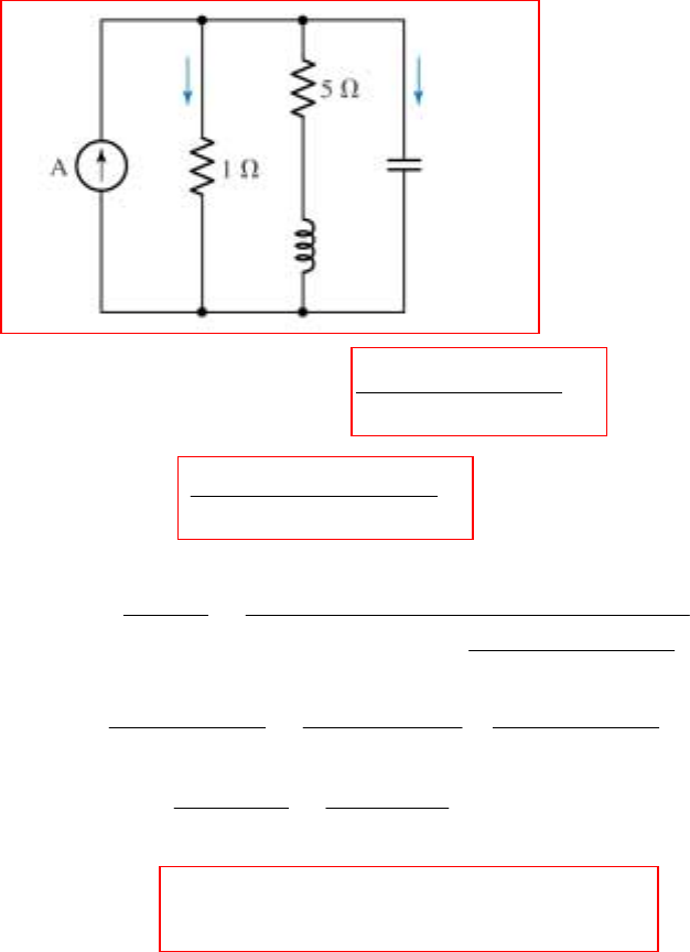
CHAPTER FIFTEEN SOLUTIONS
Engineering Circuit Analysis, 6th Edition Copyright
2002 McGraw-Hill, Inc. All Rights Reserved
21.
(a)
(b) ZTH = (5 + 0.001s) || (500/ s) = 2
2500 + 0.5
0.001 + 5 + 500 Ω
s
ss
VTH = (3/ s)ZTH =
()
6
25
7.5 10 + 1500 V
+ 5000 + 5 10
×
×
s
ss s
(c) V1Ω =
()
6
TH
2
TH
2
1 7.5 10 + 1500
= 2500 + 0.5
1 + + 505000 1 + 0.001 + 5 + 500
×
s
Vs
Zss ss
oo
6
-3
2.988 10.53 -89.92 10.53 +89.92
+ +
+ 2.505 10 + 710.6 710.6
2.956 2.967 10
+ +
+ 0.1998
jj
∠∠
=− ×−
×
sss
ss
Thus, i1Ω = v1Ω(t) = [-2.988 e-2.505×10⁶t + 2.956 e-0.1998t + 2.967×10⁻³
+ 21.06 cos(710.6t + 89.92o)] u(t)
3/s
0.001s Ω
500/s Ω
I IC
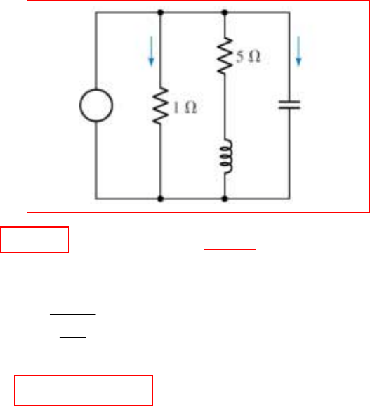
CHAPTER FIFTEEN SOLUTIONS
Engineering Circuit Analysis, 6th Edition Copyright
2002 McGraw-Hill, Inc. All Rights Reserved
22.
(a)
(b) ZTH = 0, VTH = 20/ s V so IN = ∞
(c) IC =
20
0.04 A
500
=
s
s
. Taking the inverse transform, we obtain a delta function:
iC(t) = 40δ(t) mA.
This “unphysical” solution arises from the circuit above
attempting to force the voltage across the capacitor to change in zero time.
20/s
0.001s Ω
500/s Ω
I IC
±

CHAPTER FIFTEEN SOLUTIONS
Engineering Circuit Analysis, 6th Edition Copyright
2002 McGraw-Hill, Inc. All Rights Reserved
23. Beginning with the source on the left (10/s V) we write two nodal equations:
12
11
-6
10 1
- + + = 0
47000 30303 56 + 336 10
′′
−
′′
×
VVs
VV
ss
221
2-6
+ + = 0
47000 10870 56 + 336 10
′′′
−
′×
VVVsVs
Solving,
13 11 2
110 3 15 2 18 18
303030(0.3197 10 + 0.1645 10 + 98700 )
= (0.4639 10 + 0.7732 10 + 0.5691 10 + 0.1936 10 )
××
′××××
ss
Vss s s
18
210 3 15 2 18 18
0.9676 10
= (0.4639 10 + 0.7732 10 + 0.5691 10 + 0.1936 10 )
×
′××××
Vss s s
Shorting out the left source and activating the right-hand source (5 – 3/s) V:
12
11 -6
1 + + = 0
47000 30303 56 + 336 10
′′ ′′
−
′′ ′′ ×
VVs
VV s
221
2-6
3
- 5 +
+ + = 0
47000 10870 56 + 336 10
′′ ′′ ′′
−
′′ ×
VVVs
sVs
Solving,
17
110 3 15 2 18 18
0.9676 10 (5 3)
= (0.4639 10 + 0.7732 10 + 0.5691 10 + 0.1936 10 )
×−
′′ ××××
s
Vss s s
312214 14
210 3 15 2 18 18
7609(705000 + 0.1175 10 + 0.6359 10 - 0.3819 10 )
= (0.4639 10 + 0.7732 10 + 0.5691 10 + 0.1936 10 )
×××
′′ ××××
sss
Vss s s
Adding, we find that
13 13 2
110 3 15 2 18 18
30303(0.2239 10 + 0.1613 10 + 98700 )
= (0.4639 10 + 0.7732 10 + 0.5691 10 + 0.1936 10 )
××
××××
ss
Vss s s
3 12 2 14 14
210 3 15 2 18 18
7609(705000 + 0.1175 10 + 0.6359 10 + 0.8897 10 )
= (0.4639 10 + 0.7732 10 + 0.5691 10 + 0.1936 10 )
×××
××××
sss
Vss s s
(b) Using the ilaplace() routine in MATLAB, we take the inverse transform of each:
v1(t) = [3.504 + 0.3805×10⁻² e-165928t – 0.8618 e-739t – 2.646 e-0.3404t] u(t) V
v2(t) = [3.496 – 0.1365×10⁻² e-165928t + 0.309 e-739t – 2.647 e-0.3404t] u(t) V

CHAPTER FIFTEEN SOLUTIONS
Engineering Circuit Analysis, 6th Edition Copyright
2002 McGraw-Hill, Inc. All Rights Reserved
24. (10/ s)(1/47000) = 2.128×10⁻⁴/ s A
(5 – 3/s)/ 47000 = (1.064 – 0.6383/ s)×10-4 A
ZL = 47000 || (30303/ s) =
9
1.424 10
47000 + 30303
×Ω
s
ZR = 47000 || (10870/ s) =
8
5.109 10
47000 + 10870
×Ω
s
Convert these back to voltage sources, one on the left (VL) and one on the right (VR):
VL = (2.128×10⁻⁴/ s )
9
1.424 10
47000 + 30303
×
s =
()
5
3.0303 10 V
47000 + 30303
×
ss
VR = (1.064 – 0.6383/ s)×10-4
8
5.109 10
47000 + 10870
×
s
=
()
54360 32611
-
47000 + 10870 47000 + 10870sss
Then, I56Ω = LR
-6
LR
+ + 336 10 +56
−
×
VV
ZZ s
=
()
9 2 10 9
9 3 14 2 17 17
2.555 10 - 1.413 10 - 4.282 10
6250 4.639 10 + 7.732 10 + 5.691 10 + 1.936 10
×××
−××××
ss
ss s s
18
5
-5 18 4
0.208 0.0210 1.533 10
+ 1.659 10 + 739 + 0.6447
2.658 10 2.755 10 1.382 10
+ + 0.3404 + 0.2313
−
−−
×
=−−
×
×× ×
++
sss
ss s
Thus,
i56Ω(t) = [0.208 exp(-1.659×10⁵t) – 0.0210 exp(-739t) – 1.533×10⁻¹⁸ exp(-.06447t)
+ 2.658×10⁻⁵ exp(-0.3404t) + 2.755×10⁻¹⁸ exp(-0.2313t) + 1.382×10⁻⁴] u(t) A.
The power absorbed in the 56-Ω resistor is simply 56 [i56Ω(t)]2 or
56 [0.208 exp(-1.659×10⁵t) – 0.0210 exp(-739t) – 1.533×10⁻¹⁸ exp(-.06447t)
+ 2.658×10⁻⁵ exp(-0.3404t) + 2.755×10⁻¹⁸ exp(-0.2313t) + 1.382×10⁻⁴]2 W
CHAPTER FIFTEEN SOLUTIONS
Engineering Circuit Analysis, 6th Edition Copyright
2002 McGraw-Hill, Inc. All Rights Reserved
25. (a) Begin by finding ZTH = ZN:
ZTH = 47000 + (30303/ s) || [336×10-6 s + 56 + (10870/ s) || 47000]
=
3 14 2 17 17
3 10 2 13 12
4.639 109 + 7.732 10 + 5.691 10 + 1.936 10
98700 + 1.645 10 + 1.21 10 + 2.059 10
××××
×××
sss
sss Ω
To find the Norton source value, define three clockwise mesh currents I1, I2 and I3 in the
left, centre and right hand meshes, such that IN(s) = -I1(s) and the 10/s source is replaced
by a short circuit.
(47000 + 30303/ s) I1 - (30303/ s) I2 = 0
(10870/ s + 56 + 336×10-6 s + 30303/ s) I2 - (30303/ s) I1 – (10870/ s)I3 = 0
(47000 + 10870/ s) I3 - (10870/ s)I2 = -5 + 3/ s
Solving,
IN = -I1 =
12
9 3 14 2 17 17
2.059 10 (5 - 3)
(4.639 10 + 7.732 10 + 5.691 10 + 1.936 10 )
×
×× ××
s
ss s s
(b) Isource = (10/ s) (1/ ZTH) - IN(s)
13 6 19 5 24 4 27 3
29 2 29 28 3 9 2
12
0.001(0.4579 10 + 0.1526 10 + 0.1283 10 + 0.1792 10
+ 0.6306 10 + 0.3667 10 + 0.5183 10 )[ (4639 + 0.7732 10
+ 0.5691 1012 + 0.1936 10 )(0.4639 10
=× × × ×
××× ×
×××
ssss
ss sss
s10 3 15 2 18
18 -1
+0.7732 10 + 0.5691 10
+ 0.1936 10 )]
××
×
ss s
Taking the inverse transform using the MATLAB ilaplace() routine, we find that
isource(t) = 0.1382×10⁻³ + 0.8607×10⁻⁸ exp(-165930t) + 0.8723×10⁻⁷exp(-739t)
+ 0.1063×10⁻³ exp(-0.3403t) – 0.8096×10⁻⁷ exp(-165930t)
+ 0.1820×10⁻⁴ exp(-739t) – 0.5×10⁻⁴ exp(-0.3404t)
isource(1.5 ms) = 2.0055×10⁻⁴ A = 200.6 µA

CHAPTER FIFTEEN SOLUTIONS
Engineering Circuit Analysis, 6th Edition Copyright
2002 McGraw-Hill, Inc. All Rights Reserved
26. We begin by shorting the 7 cos 4t source, and replacing the 5 cos 2t source with 2
5
4+
s
s.
(a) Define four clockwise mesh currents I1, I2, I3 and Ix in the top left, top right, bottom
left and bottom right meshes, respectively. Then,
2
5
4+
s
s = (12 + 1/2s) I3 – 7 I1 – (1/ 2s) Ix [1]
0 = -4 Ix + (9.5 + s) I1 – s I2 – 7 I3 [2]
0 = (3 + s + 2/ s) I2 – s I1 – 3 Ix [3]
0 = (4 + 3s + 1/2s) Ix – 3 I2 – (1/2s) I3 [4]
1
′
V = (I3 – Ix) (2s) [5]
Solving all five equations simultaneously using MATLAB, we find that
1
′
V=
33 2
654 3 2
20 (75 + 199 + 187 + 152)
1212 + 3311 + 7875 + 15780 + 12408 + 10148 + 1200
ss s s
ssssss
Next we short the 5 cos 2t source, and replace the 7 cos 4t source with 2
7
16+
s
s.
Define four clockwise mesh currents I1, I2, I3 and Ix in the bottom left, top left, top right
and bottom right meshes, respectively (note order changed from above). Then,
0 = (12 + 1/2s) I1 – 7 I2 – (1/ 2s) Ix [1]
0 = -4 Ix + (9.5 + s) I2 – s I3 – 7 I1 [2]
2
7
16
−+
s
s = (3 + s + 2/ s) I3 – s I2 – 3 Ix [3]
0 = (4 + 3s + 1/2s) Ix – 3 I3 – (1/2s) I1 [4]
1′′
V = (I1 – Ix) (2s) [5]
Solving all five equations simultaneously using MATLAB, we find that
1′′
V=
()
42
65 4 3 2
-56 (21 - 8 - 111)
1212 + 3311 + 22420 + 55513 + 48730 + 40590 + 4800
sss
ss s s s s
The next step is to form the sum V1(s) = 1
′
V + 1′′
V, which is accomplished in MATLAB
using the function symadd(): V1 = symadd(V1prime, V1doubleprime);
V1(s) =
()( )
3543 2
265432
4 (81 + 1107 + 7313 + 17130 + 21180 + 12160)
+ 4 1212 + 3311 + 22420 + 55513 + 48730 + 40590 + 4800
ss s s s s
sssssss
(b) Using the ilaplace() routine from MATLAB, we find that
v1(t) = [0.2673 δ(t) + 6.903×10⁻³ cos 2t – 2.403 sin 2t – 0.1167 e-1.971t
– 0.1948 e-0.3315t cos 0.903t + 0.1611 e-0.3115t sin 0.903t – 0.823×10⁻³ e-0.1376t
+ 3.229 cos 4t + 3.626 sin 4t] u(t) V
CHAPTER FIFTEEN SOLUTIONS
Engineering Circuit Analysis, 6th Edition Copyright
2002 McGraw-Hill, Inc. All Rights Reserved
27. (a) We can combine the two sinusoidal sources in the time domain as they have the same
frequency. Thus, there is really no need to invoke source transformation as such to find
the current.
65 cos 103t ⇔ 26
65
+ 10
s
s, and 13 mH → 0.013s Ω
We may therefore write
I(s) =
()
()
26 26
65 1 5000
=
+ 10 83 + 0.013 + 10 + 6385
ss
ss
ss
=
()
() ()
oo
33
0.7643 0.3869 8.907 0.3869 8.907
+ 6385 - 10 + 10jj
∠− ∠
−+ +
sss
(b) Taking the inverse transform,
i(t) = [-0.7643 e-6385t + 0.7738 cos (103t – 8.907o)] u(t) A
(c) The steady-state value of i(t) is simply 0.7738 cos (103t – 8.907o) A.
CHAPTER FIFTEEN SOLUTIONS
Engineering Circuit Analysis, 6th Edition Copyright
2002 McGraw-Hill, Inc. All Rights Reserved
28.
(a)
(b)
(c) -1
Poles: same; = -0.1615, -1.239 ss
(d) 1
Zeros: same; 0.7 0.7141 sj−
=− ±s
2 1
2 1
1.4 1.96 0.8
Poles: 1.4 0.2 0, 0.1615, 1.239s
2
1.4 1.96 4
Zeros: 1.4 1 0, 0.7 0.7141s
2j
−
−
−± −
++== =− −
−± −
++== =−±
ss s
ss s
2
22
2
2
5
5(25)
(5 5)(2 5 ) 25 35 10
575/ 575 575
575
() 25 35 10
in
in
++
++ ++
===
++ ++ ++
++
∴=
++
sssss
s
Zss
ss ss
ss
Ys ss
CHAPTER FIFTEEN SOLUTIONS
Engineering Circuit Analysis, 6th Edition Copyright
2002 McGraw-Hill, Inc. All Rights Reserved
29. (a) Regarding the circuit of Fig. 15.45, we replace each 2-mF capacitor with a 500/ s Ω
impedance. Then,
Zin(s) =
500 500
20 + 40 + ( + 25)( + 12.5)
= 13.33
100 ( + 1.667)
60 +
ss
ss
ss
s
Reading from the transfer function, we have
zeros at s = -25 and -12.5 s-1, and
poles at s = 0 and s = -1.667 s-1.
(b) Regarding the circuit of Fig. 15.47, we replace the 2-mF capacitor with a 500/ s Ω
impedance and the 1-mH inductor with a 0.001s-Ω impedance. Then,
Zin(s) =
()
()
5
5
500 500
55 + 100 + 0.001 ( + )( + 10 )
55
= 55
500 + 1.55 10 ( + 3.226)
155 + + 0.001
×
sss
s
ss
s
s
Reading from the transfer function, we have
zeros at s = -9.091 and -105 s-1, and
poles at s = -1.55×10⁵ and s = -3.226 s-1.
CHAPTER FIFTEEN SOLUTIONS
Engineering Circuit Analysis, 6th Edition Copyright
2002 McGraw-Hill, Inc. All Rights Reserved
30. 1
( ) : zeros at 0; 10; at 5, 20 s ; ( ) 12 S as poles −
=− =−− → →∞Ys s s Ys s
(a)
(b) ( 10) 6.788 45 Sj
−= ∠−°Y
(c) 12( 15)( 5)
( 15) 18 S
( 10)5
−−
−= =−
−
Y
(d)
2
2
K ( 10)
() ,K 12
( 5)( 20)
12 ( 10) 12 120
() ( 5)( 20) 25 100
1200 1200
( 10) 4.800 4.800 6.788 45 S
100 250 100
j
jj
j
+
==∴
++
++
==
++ ++
−+
∴= =+=∠°
−+ +
ss
Ys ss
ss s s
Ys ss ss
Y
2
22
2
-1 -1
245 245 68(500)
12 120 17 245 500
5()5 ,
( 5)( 20) 34
25 100
Zeros: 2.461 and 11.951 s ; Poles: 5, 20 s
−± −
+++
+=+ = =
++
++
=− − =− −
ssss
Ys s
ss
ss
ss
CHAPTER FIFTEEN SOLUTIONS
Engineering Circuit Analysis, 6th Edition Copyright
2002 McGraw-Hill, Inc. All Rights Reserved
31.
(a) 1 1 0.2(6 9) 5( 1)( 4)
4 5 5 (4 )(1 ) 6( 1.5)
in in
+++
=+ = ∴=
++ ++ +
sss
YZ
ssss s
(b) -1
Poles: 1.5, ; Zeros: -1, -4 s=− ∞ =ss
CHAPTER FIFTEEN SOLUTIONS
Engineering Circuit Analysis, 6th Edition Copyright
2002 McGraw-Hill, Inc. All Rights Reserved
32. 2
+ 2
( ) = ( + 5)( + 6 + 25)
s
Hs sss
(a) d(t) ⇔ 1, so the output is 2
+ 2
( + 5)( + 6 + 25)
s
sss
(b) e-4t u(t) ⇔ 1 / (s + 4), so the output is 2
+ 2
( + 4)( + 5)( + 6 + 25)
s
ssss
(c) 2 cos 15t u(t) ⇔ 2
2
+ 225
s
s, so the output is
()
22
2 + 2
( + 225)( + 5)( + 6 + 25)
ss
ssss
(d) t e-t u(t) ⇔ 1/ (s + 1), so the output is 2
+ 2
( + 1)( + 5)( + 6 + 25)
s
ssss
(e) poles and zeros of each:
(a): zero at s = -2, poles at s = -5, -3 ± j4
(b): zero at s = -2, poles at s = -4, -5, -3 ± j4
(c): zeros at s = 0, -2, poles at s = ± j15, -5, -3 ± j4
(d): zero at s = -2, poles at s = -1, -5, -3 ± j4
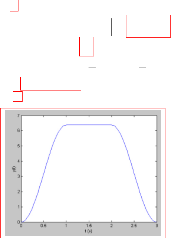
CHAPTER FIFTEEN SOLUTIONS
Engineering Circuit Analysis, 6th Edition Copyright
2002 McGraw-Hill, Inc. All Rights Reserved
33. h(t) = 5 [u(t) – u(t – 1)] sin πt x(t) = 2[u(t) – u(t – 2)]
y(t) =
()
0() hxt d
λλλ
−
∞−
∫
t < 0: y(t) = 0
0 < t < 1: y(t) =
()
00
10 10
10sin = - cos = 1 cos
t
tdt
πλ λ πλ π
λπ
−
∫
1 < t < 2: y(t) = 1
0
20
10sin = d
πλ λ π
∫
2 < t < 3: y(t) =
[]
1
1
22
10 10
10sin = - cos = - 1 cos( 2 )
tt
dt
πλ λ πλ π π
ππ
−−
−− −
∫
= (10/
π
) (1 + cos
π
t)
t > 3: y(t) = 0
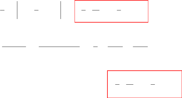
CHAPTER FIFTEEN SOLUTIONS
Engineering Circuit Analysis, 6th Edition Copyright
2002 McGraw-Hill, Inc. All Rights Reserved
34. f1(t) = e-5t u(t), f2(t) = (1 – e-2t) u(t)
(a) f1 * f2 =
() ( )
-12
0 fftd
λλλ
∞−
∫
t < 0: f1 * f2 = 0
t > 0: f1 * f2 =
()( )
--
522 523
00
1 =
tt
tt
eed eeed
λλ λ λ
λλ
−− −−−
−−
∫∫
=
523 52
00
11 121
+ = ( )
53 5153
tt
ttt
eee eeut
λλ
−−− −−
−+−
(b) F1(s) = 1/ (s + 5), F2(s) = 1/s – 1/ (s + 2)
F1(s) F2(s) =
()()()
11abc
= + +
+ 5 + 5 + 2 + 2 + 5
−
ss s s s s s
Where a = 0.2, b = -1/3, and c = -1/5 + 1/3 = 2/15.
Taking the inverse transform, we find that f1 * f2 = 52
12 1
()
515 3
tt
eeut
−−
+−
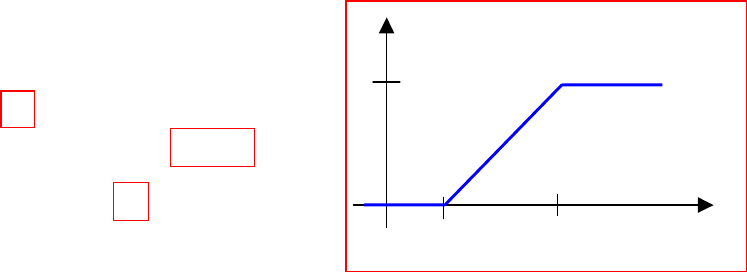
CHAPTER FIFTEEN SOLUTIONS
Engineering Circuit Analysis, 6th Edition Copyright
2002 McGraw-Hill, Inc. All Rights Reserved
35. The impulse response is vo(t) = 4u(t) – 4u(t – 2) V,
so we know that h(t) = 4u(t) – 4u(t – 2). vi(t) = 2u(t - 1), and vo(t) = h(t) * vi(t).
Thus, vo(t) =
()
0()
i
hvt d
λλλ
−
∞−
∫
t < 0: vo = 0
1 < t < 3: vo =
1
08 = 8 8
tdt
λ
−
−−
∫
t > 3: vo =
2
08 = 16d
λ
∫
t (s)
vo (V)
16
1 3
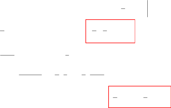
CHAPTER FIFTEEN SOLUTIONS
Engineering Circuit Analysis, 6th Edition Copyright
2002 McGraw-Hill, Inc. All Rights Reserved
36. h(t) = 2e-3t u(t), x(t) = u(t) – δ(t)
(a) y(t) =
(b)
Taking the inverse transform, we find that y(t) = 3
28
() ()
33
t
ut e ut
−
−
[]
0
333
00
33 3
()( )
0: ( ) 0
1
0 : ( ) 2 1 ( ) = 2 - ( ) - ( )
3
228
(1 ) ( ) 2 ( ) = ( )
333
t
tt
tt t
hxt d
tyt
tyt e td eut eut
eut eut e ut
λλ
λλλ
δλλ
−
−
∞
−−−
−− −
−
<=
>= −−
=− − −
∫
∫
()
()
21
( ) = ( ) = - 1
+ 3
21 - 21 8 1
, ( ) = = -
+ 3 3 3 + 3
thus
Hs Xs
ss
s
Ys ss s s
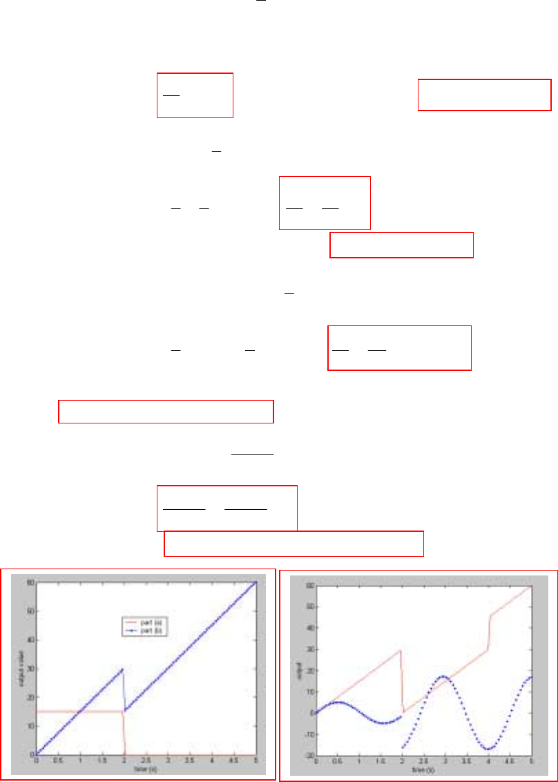
CHAPTER FIFTEEN SOLUTIONS
Engineering Circuit Analysis, 6th Edition Copyright
2002 McGraw-Hill, Inc. All Rights Reserved
37. h(t) = 5 u(t) - 5 u(t – 2), so H(s) = -2
5 - 5e s
s
(a) vin(t) = 3δ(t), so Vin(s) = 3
Vout(s) = Vin(s) H(s) = -2
15 - 15e s
s. vout(t) = Λ-1{Vout(s)} = 15 u(t) – 15 u(t - 2)
(b) vin(t) = 3u(t), so Vin(s) = 3
s
Vout(s) = Vin(s) H(s) = -2 -2
2
3 5 15 15
- 5e = - e
ss
ss s
s.
vout(t) = Λ-1{Vout(s)} = 15 t u(t) – 15 u2(t - 2) = 15 t u(t) – 15 u (t - 2)
(c) vin(t) = 3u(t) – 3u(t – 2), so Vin(s) = -2
3 - 3e s
s
Vout(s) = Vin(s) H(s) = -2 -2 -2 4
2
3 5 15 30
- 3e - 5e = - e 15e−
+
ss ss
ss s
s.
vout(t) = Λ-1{Vout(s)} = 15 t u(t) – 30 u2(t - 2) + 15 u2 (t – 4)
= 15 t u(t) – 30 u (t - 2) + 15 u(t)
(d) vin(t) = 3 cos 3t, so Vin(s) = 2
3
+ 9
s
s
Vout(s) = Vin(s) H(s) = -2
22
15 15
- e
+ 9 + 9
s
s
ss .
vout(t) = Λ-1{Vout(s)} = 5 sin 3t u(t) – 15 cos [3(t – 2)] u(t - 2)
CHAPTER FIFTEEN SOLUTIONS
Engineering Circuit Analysis, 6th Edition Copyright
2002 McGraw-Hill, Inc. All Rights Reserved
38.
2
22
2
2
2
2
22
10 20(20 10 / )
10 10
20 20 20 40 10 /
40
10 40 20 40 60 10 40 60 10
41 4
20 2 2 ;
10 41 40 60 10
40
10 4 1 4
20 4614
in in
in
in in in
top in in in
out in top in
s
s
==
+
+
++
+
+
== =
+++ ++
+++
∴= = =
+++
+
+
=+= +
++ +
VV
Is
ss
ss
VV ss
V
sss ss
ss ss
ss
II I V
sss
ss
VIIV
ss s
22 2
22
61
4 4 1 0.25 ( 0.5)
() ( 0.19098)( 1.3090)
4 6 1 1.5 0.25
zeros: 0.5, 0.5; poles: 1.3090, 0.19098
out
in
s
∴
+
++ ++ +
== = = ∴
++
++ + +
=− =− =− −
s
Vss ss s
Hs Vss
ss s s
ss
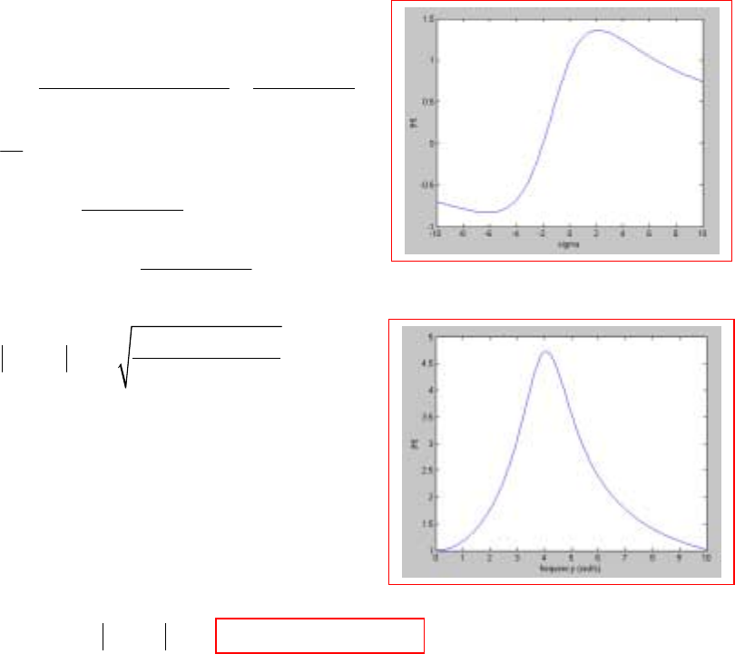
CHAPTER FIFTEEN SOLUTIONS
Engineering Circuit Analysis, 6th Edition Copyright
2002 McGraw-Hill, Inc. All Rights Reserved
39.
(a)
(b)
2
22 2
4
( ) 8.5 (17 ) 4
Hj ω+
ω= −ω + ω
(c)
21
2
2
2
() ()/ (), (0) 1
K( 2) K( 2)
() (1 4)(1 4) 217
K
1 2 , so K=8.5
17
8.5( 2)
, ( ) 217
8.5( 2)
Let 0 ( ) 217
jj
Thus
==
++
∴= =
++ +− ++
=
+
=++σ+
ω= ∴ σ =σ+σ+
Hs V s V s H
ss
Hs ss ss
s
Hs ss
H
max
By trial & error: ( ) 4.729 at 4.07 rad/sjω= ω=
H
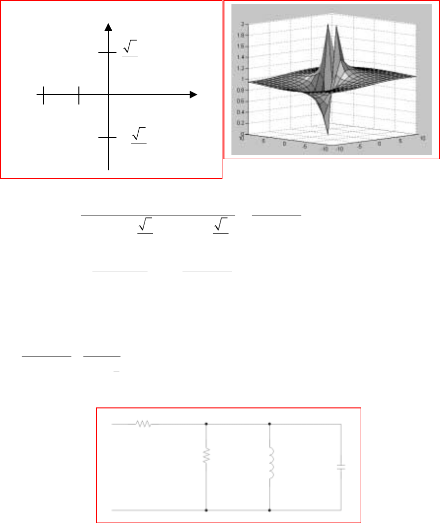
CHAPTER FIFTEEN SOLUTIONS
Engineering Circuit Analysis, 6th Edition Copyright
2002 McGraw-Hill, Inc. All Rights Reserved
40. (a) pole-zero constellation (b) elastic-sheet model
(c) H(s) =
() ()
22
2
2
22
+ 1 + 1
= + + 1
33
+ 0.5 + + 0.5 -
22
+ 2 + 1
= = 1 +
+ + 1 + + 1
jj
ss
ss
ss
ss s
ss ss
We can implement this with a 1-Ω resistor in series with a network having the impedance
given by the second term. There are two energy storage elements in that network (the
denominator is order 2). That network impedance can be rewritten as
2
1
1
+ + 1 1
=++
s
ss ss
, which can be seen to be equal to the parallel combination of a 1-Ω
resistor, a 1-H inductor, and a 1-F capacitor.
1 Ω
1 Ω 1 H 1 F
O
-1
(2 zeros)
X
X
3
2
3
2
−
σ
j
ω
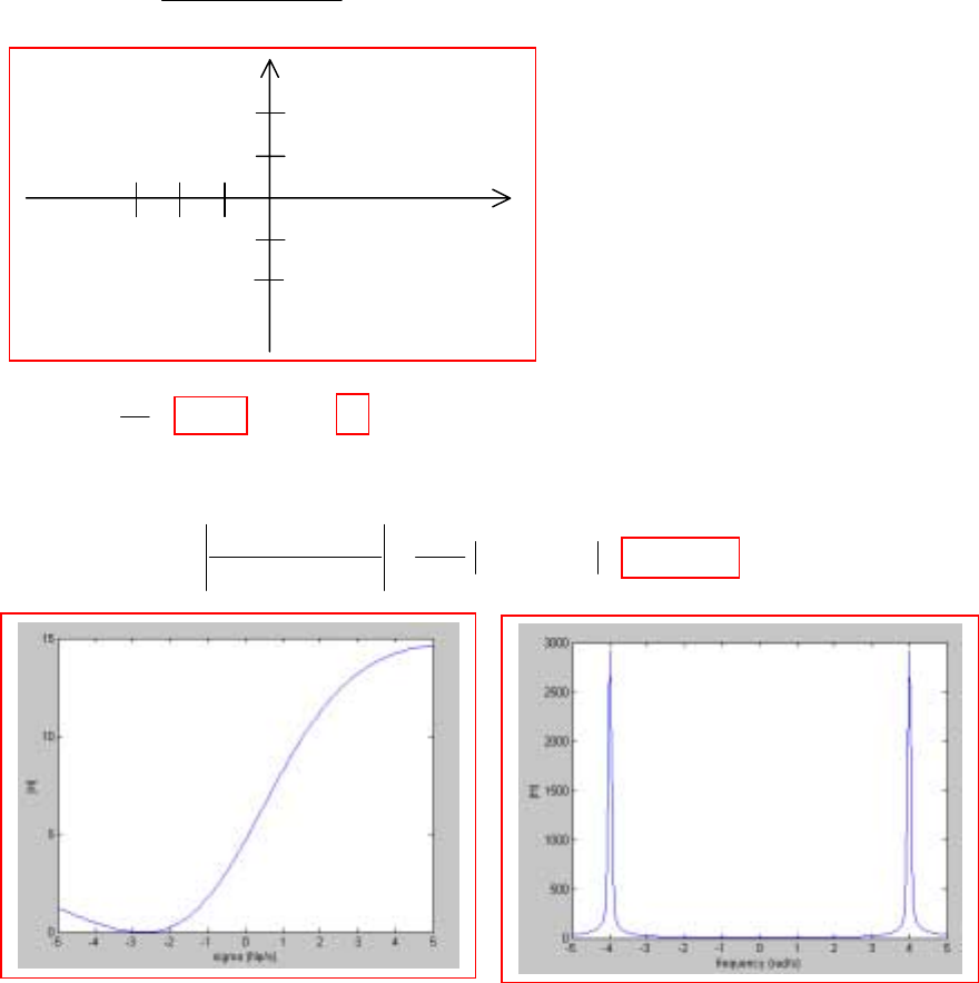
CHAPTER FIFTEEN SOLUTIONS
Engineering Circuit Analysis, 6th Edition Copyright
2002 McGraw-Hill, Inc. All Rights Reserved
41. 22
( ) (10 55 75) /( 16)=++ +Hs s s s
(a)
()( )
( + 3)( + 2.5)
( ) = 10 + 4 4jj−
ss
Hs ss. Critical frequencies: zeros at –3, -2.5; poles at ± j4.
(b) 75
(0) 4.688, ( ) 10
16
== ∞=HH
(c)
(d)
(0) 4.679 K 3, so K 0.64
90 75 165 0.64
( 3) 0.64 15 165 15.15
77
j
jjcm
===
−+ +
∴= =−+=
H
H
X 4
-4
O O
3 2 1
X
σ
j
ω
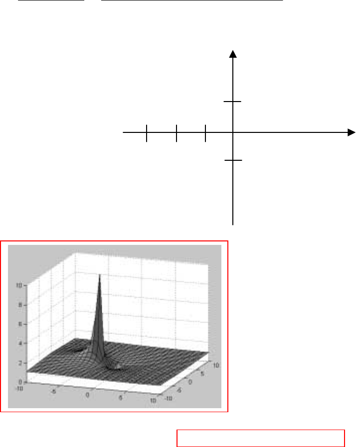
CHAPTER FIFTEEN SOLUTIONS
Engineering Circuit Analysis, 6th Edition Copyright
2002 McGraw-Hill, Inc. All Rights Reserved
42. (a)
()()
()( )
2
2
+ 0.5 + 0.3873 + 0.5 - 0.3873
5 + 5 + 2
( ) = =
5 + 15 + 2 + 2.86 + 0.1399
jjss
ss
Ys ss s s
Zeros: s = -0.5 ± j0.3873
Poles: s = -2.86, s = -0.1399
(b) elastic sheet model
(c) lattitude 5o5’2”, longitude 5o15’2” puts it a little off the coast of Timbuktu.
σ
j
ω
+1
-1
-3 -2 -1
X X
O
O
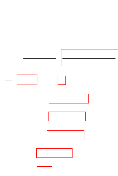
CHAPTER FIFTEEN SOLUTIONS
Engineering Circuit Analysis, 6th Edition Copyright
2002 McGraw-Hill, Inc. All Rights Reserved
43. 0
( ) ; ( 2) 6
M
=−=
I
Hs H
I
(a)
(b) 30
(0) 2.308, ( )
13
=− =− ∞ =∞HH
(c)
232
22
(1)(1)(3)
() K
(3 2)(3 2)
(3)(1)K 3K
(2) 6 K 10,
(1 2)(1 2) 5
( 1)( 3) 10 30 10 30
, ( ) 10 613 613
jj
jj
Thus
−++
=++ +−
−−
−== = ∴=
+−
−+ + −−
==
++ ++
sss
Hs ss
H
ss sss
Hs ss ss
1: ( 1) ( 2 1) 2.236 116.57
1:( 1)(21)2.23663.43
3 : ( 3) 2 3 3.606 33.69
3 2 : 2 3 2 5.000 53.13
32:23230
sj
sj
sj
jj j
jj j
−= −= ∠ °
−+=+= ∠ °
−+=+= ∠°
−− + + = ∠ °
−+ + − =∠°
CHAPTER FIFTEEN SOLUTIONS
Engineering Circuit Analysis, 6th Edition Copyright
2002 McGraw-Hill, Inc. All Rights Reserved
44.
: zero at 10 0; 20 : zero at 3.6 0
R/ C R 1/ C 5 5 / RC 1/ C
555
R1/SC CR1 1/RC 1/RC
5( 1/ RC 1/5C)
1/ RC
11
Thus, using the fact that = 0 at = -10, we may write 10
RC 5C
Also,
AA
A
A
A
jj
=− + + =− +
++
∴=+ =+ =+ =
++++
++
∴= +
+=
Zs Z s
ss
Zss s
s
Zs
Zs
Z
11
25 1 25
25
1/C RC 25C
RC C
25 1
1/ RC 1/ RC
RC
11 4
3.6 or 6.4,
RC 25C 25C
1
C25 mF,
40
40 40 40
10, 2, so R 20
R5 R
B
++
++
=+ = =
++ +
∴+ = =
==
+= = =Ω
s
s
ss s
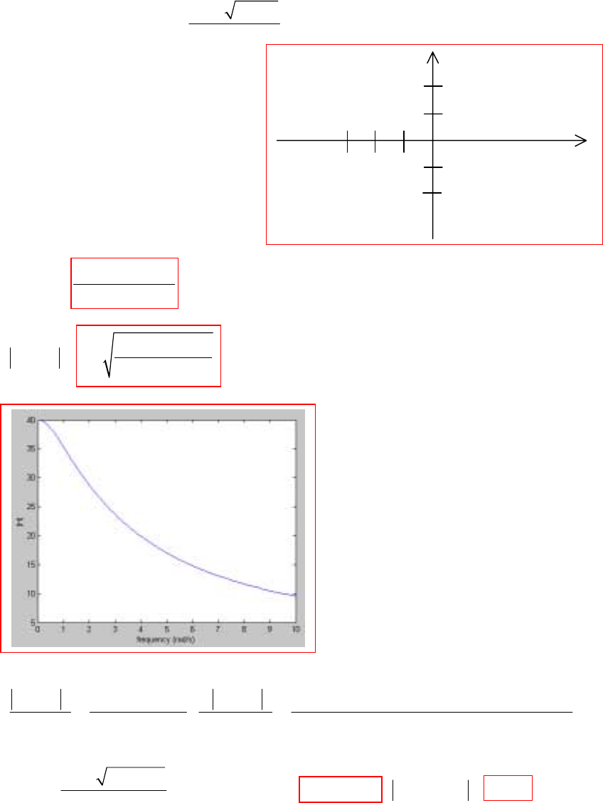
CHAPTER FIFTEEN SOLUTIONS
Engineering Circuit Analysis, 6th Edition Copyright
2002 McGraw-Hill, Inc. All Rights Reserved
45. 2
( ) 100( 2) /( 2 5)=+ ++Hs s s s
(a) zero at s = -2, poles at 2420 12
2j
−± −
==−±s
(b) 2
100(2 )
()(5 ) 2
j
jj
+ω
ω= −ω + ω
H
(c)
2
42
4
( ) 100 625
jω+
ω= ω−ω+
H
(d)
(e)
22
24223
42
42 2 2 42 42 42
2
() ()
4 ( 6 25)2 ( 4)(4 12 )
,
10 000 625
6 25 ( 4)(2 6), 6 25 2 2 24, 8 49 0
8 64 196 4.062 2.016 rad/s, H( 2.016) 68.61
2mar
jdj
detc
j
ωω
ω+ ω−ω+ ω−ω+ ω− ω
==
ω
ω−ω+
∴ω−ω+ =ω+ ω− ω−ω+ =ω+ω− ω+ω− =
−± +
∴ω = = ∴ω = =
HH
X j2
-j2
O
3 2 1
X
CHAPTER FIFTEEN SOLUTIONS
Engineering Circuit Analysis, 6th Edition Copyright
2002 McGraw-Hill, Inc. All Rights Reserved
46. 520
()
2
in
+
=Ω
+
s
Zs s
(a)
(b)
2
5( 4)
(0) 25V; ( ) ,
2
5( 4)
( ) , single pole at 2 ( ) 25 V, 0
2
ab in ab in in
t
ab
v
vt e t
−
+
== =
+
+
∴= =−∴ = >
+
s
Zs V ZI
s
s
Hs s
s
4
12
(0) 3A ( ) single poleat 4
5( 4)
() 3 A, 0
sab
ab ab
in in in
t
ab
i
it e t
−
+
=∴= ∴ === =−
+
∴= >
VI s
IHs s
ZVZs
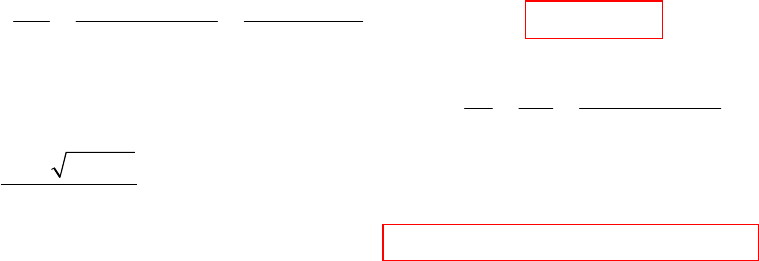
CHAPTER FIFTEEN SOLUTIONS
Engineering Circuit Analysis, 6th Edition Copyright
2002 McGraw-Hill, Inc. All Rights Reserved
47. 2
( ) 5( 4 20) /( 1)
in =++ +Zs s s s
(a)
(b)
6
6
2
160 V 160 V, 6
160( 1) 32( 5) 5A ( ) 5 A (all )
32420
5( 4 20)
t
ab ab
t
ab
a a
in
ve
it e t
b
−
−
=∴==−
+−
== = =−∴=−
−+
++
Vs
Vs
IZss
6
2
62
62
11
160 ( ), (0) 0, (0) 32 A/s ( ) 5( 4 20)
41680 2 4 ( ) 5 (A cos 4 Bsin 4 ) 0 5 A, A 5
2
(0) 32 30 10 4B B 3 ( ) [ 5 (5cos 4 3sin 4 )] ( ) A
ta
ab a a
sin
tt
a
tt
aa
veuti i
jit ee t t
iiteettut
−
−−
−−
+
′
===∴===
++
−± −
==−±∴=−++∴=−+=
′==−+ ∴=∴ =− + +
Is
Hs VZ ss
s
CHAPTER FIFTEEN SOLUTIONS
Engineering Circuit Analysis, 6th Edition Copyright
2002 McGraw-Hill, Inc. All Rights Reserved
48.
(a) 2
0.5 250
() / 0.5 0.002 500 / 250 25 000
cs
== =
++ ++
s
Hs I I ss
ss
(b) 61
1( 250 62 500 10 ) 125 484.1s
2j−
=− ± − =− ±s
(c) -1 6 -1 4 -1
od
R 0.5
= = 125 s , ω= 10 /4= 500 s , ω= 25×10 -15,625 = 484.1 s
2L 0.004
α
=
(d) 1, 0 I 0 0
sccf
i==∴=∴=Is
(e) 125
,( cos 484 Bsin 484 )
t
cn
ieA t t
−
=+
(f) 3
1
(0) 0 (0 ) 0, (0) 0 1 2 10 (0 ) 0 (0 ) 250 A/s
2
Lcc
iiv ii
+−++
=∴ = =∴×=× +∴ =
(g) 125
A 0, 484B 250, B 0.5164 ( ) (0.5164 sin 484.1 ) ( ) A
t
c
it e tut
−
∴= = = ∴ =
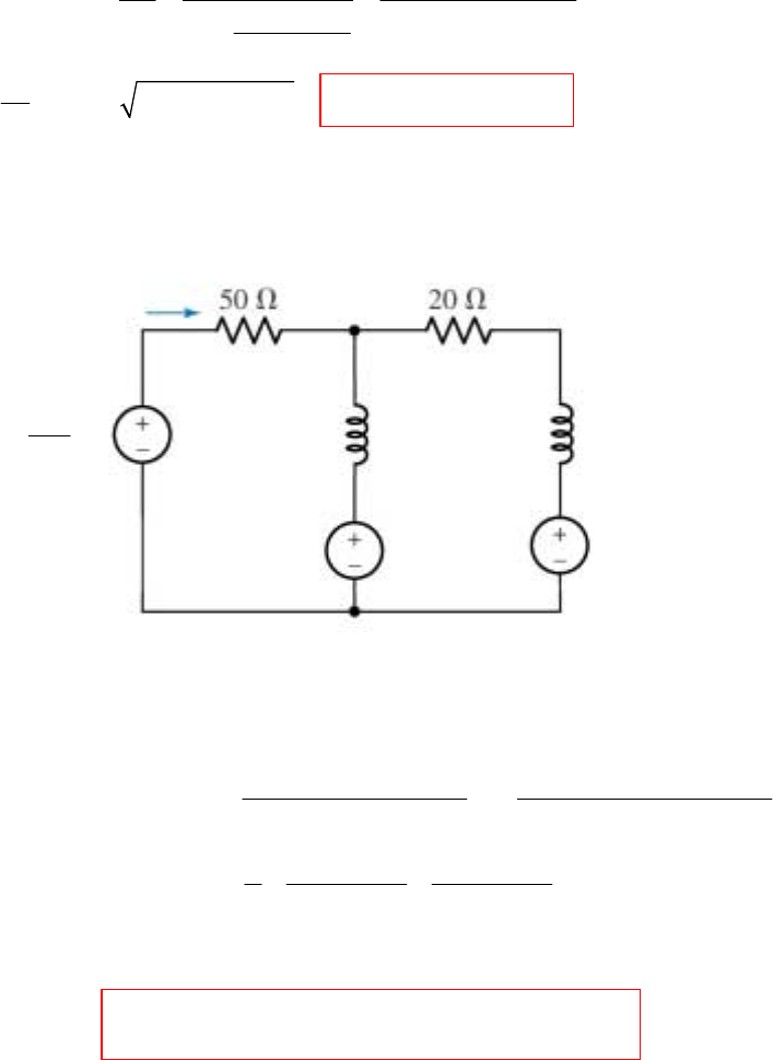
CHAPTER FIFTEEN SOLUTIONS
Engineering Circuit Analysis, 6th Edition Copyright
2002 McGraw-Hill, Inc. All Rights Reserved
49.
(a)
(b) Note that the element labeled 6 H should be an inductor, as is suggested by the context of
the text (i.e. initial condition provided). Convert to s-domain and define a clockwise mesh
current I2 in the right-hand mesh.
Mesh 1: 0 = -500/ s + (50 + 6s) Iin – 30 - 6s I2 [1]
Mesh 2: 0 = 30 + (20 + 10s) I2 – 6s Iin – 8 [2]
Solving, we find that
where a = 10, b = -2.115 and c = -0.8855. Thus, we may write
iin(t) = [10 – 2.115 e-24.10t – 0.885 e-1.729t] u(t) A
2
2-1
1 1 10 20
() / 6 (4 20) 24 620 1000
50 10 20
1( 620 620 96,000) 1.729 and 24.10 s
48
in in
in
+
=== =
+++
++
∴= − ± − =− −
s
Hs I V ss
Zss
s
s
6s Ω 4s Ω
-30 V -8 V
500 V
s
Iin
()
()()
()()
22
in 2
42 + 1400 + 2500 7 + 233.3 + 416.7
= = + 24.10 + 1.729
6 + 155 + 250
+ 24.10 + 1.729
ab c
=+ +
ss s s
Iss s
ss s
ss s
CHAPTER FIFTEEN SOLUTIONS
Engineering Circuit Analysis, 6th Edition Copyright
2002 McGraw-Hill, Inc. All Rights Reserved
50.
(a) 50(1000 / ) 1000
() 50 (1000 / ) 20
s
== =
++
Vs
Hs Iss
(b)
() ()
() ()
020
-20
2 2 1000 2000 b
= so ( ) = = +
20 20 20
2000 2000
100; b = 100
20
100 100
, ( ) = - and ( ) = 100 1 - e ( ) V
20
s
t
a
s
aa
Thus v t u t
s
==−
=
+++
== ==−
+
+
ss
IVs
ssssss
ss
Vs s
(c) This function as written is technically valid for all time (although that can’t be possible
physically). Therefore, we can’t use the one-sided Laplace technique we’ve been
studying. We can, however, use simple s-domain/ complex frequency analysis:
(d) 4e-10t u(t) ⇔ 4
+ 10s, so V(s) = 4 1000 a b
= +
+ 10 + 20 + 10 + 20
ss s s
a = 400 and b = -400, so v(t) = 400 [e-10t – e-20t] u(t) V
10
10
1000
4 A 4 A, 10 4 ( 10) 4 400 V
10
() 400 V (all )
t
ss
t
ie
vt e t
−
−
=∴==∴=−=×=∴
=
IsVH
CHAPTER FIFTEEN SOLUTIONS
Engineering Circuit Analysis, 6th Edition Copyright
2002 McGraw-Hill, Inc. All Rights Reserved
51.
(a)
(b) No initial energy stored in either capacitor. With vs = u(t), Vs(s) = 1
s, so
VC2 =
()( )
2.5
+ 6.357 + 0.3933ss s = + +
+ 6.357 + 0.3933
ab c
ss s
Where a = 1, b = 0.06594 and c = -1.066. Thus,
vC2(t) = [1 + 0.06594 e-6.357t – 1.066 e-0.3933t ] u(t) V
2
2
2
100 25
100 20 (20 100)25
() / 50
100 125 (20 125)
20 20
2500 (20 125)
() (20 125) 1000 6250 500 2500
2.5
() 6.75 2.5
c
s
+
+
== × +
+
++
+
∴= ++++
∴=
++
Vs
ss
s
Hs Vss
ss
ss
Hs ss s s s
Hs ss
CHAPTER FIFTEEN SOLUTIONS
Engineering Circuit Analysis, 6th Edition Copyright
2002 McGraw-Hill, Inc. All Rights Reserved
52.
22
11
() 1 0.05
0.1 0.025 0.1 0.025
20 (80 / ) 4
4 40( 4) 40( 4)
(2)(8)
0.025 0.25 0.4 10 16
in ==
++ ++
++
+++
===Ω
++
++ ++
Zs s
ss
ss
sss
ss
ss ss
20u(t) 20
⇔s, so Vin(s) = 20 40( 4)
(2)(8)
+
++
s
ss s = a + +
28
bc
++ss s
a = 200, b = -133.3 and c = -66.67, so vin(t) = [200 – 133.3 e-2t – 66.67 e-8t] u(t) V
CHAPTER FIFTEEN SOLUTIONS
Engineering Circuit Analysis, 6th Edition Copyright
2002 McGraw-Hill, Inc. All Rights Reserved
53.
1
() f
=−Z
Hs Z
(a)
(b)
38 8 5
38
1
10 10 / 1000 10 R 10
5000, 10 10 / ( ) 5000 5000 5
f
+++
= = + ∴ =− =− =−
ss
ZZ sHs ss
(c)
8
3
188
5
10 5000 5000
10 , 5000 ( ) 1000 (10 / ) 1000 10
5
() 10
f
s
=+ = ∴ =− =−
++
−
∴=
+
s
ZZHs
sss
s
Hs
48 4 8 5
38 48
1885
10 10 / 10 10 10 10
10 10 / , 10 10 / ( ) 1000 10 / 1000 10 10
f
+++
=+ =+ ∴ =− =− =−
+++
ss s
ZsZ sHs ss s
CHAPTER FIFTEEN SOLUTIONS
Engineering Circuit Analysis, 6th Edition Copyright
2002 McGraw-Hill, Inc. All Rights Reserved
54.
1
11
4
1
11
1
R20 k,() RC RC
1
() 2 10C RC
out
ff
in
=Ω ==− +
∴=−× +
V
Hs s
V
Hs s
(a)
4
11
1
210
( ) 50 C 0, 50, R 400
R
×
=− ∴ = = = ΩHs
(b)
(c)
34 4 4 3
11
11
4
11
9
1
1
() 10( 10) 210C 210C 10
RC
1
C 50nF; 10 , so R 2 k
50 10 R
− −
−
=− + =− × + ∴ × =
∴= = = Ω
×
Hs s s
44 44
111
11
28
25
2
1
( ) 10 ( 1000) 2 10 C 2 10 C =10 , C 5 nF
RC
( ) 200 A B , (0) 0 0 200 A B
(0 ) 20 0.025 (0 ) 0.025( 2A 8B) A 4B 400 3B 200
200 400 400 200
B , A ( ) 200
33 33
tt
in in
in
t
in
vt e e v
iv
vt e e
− −
−−
++
−
=−+=−× + ∴× =
∴=+ + =∴=++
== = −− ∴−−= ∴−=
′
=− ∴ =− ∴ = − −
Hs s s
8()V
tut
−
CHAPTER FIFTEEN SOLUTIONS
Engineering Circuit Analysis, 6th Edition Copyright
2002 McGraw-Hill, Inc. All Rights Reserved
55.
(a)
(b)
(c)
(d)
1
3
1
1
( ) 50,
1/ R C
( ) , R 20 k
1/ R C
R20 10
set C 0 50 R 400
R50
out
in
f
f
ff
f
f
==−
−
==Ω
+
×
=∴−=− ∴ = = Ω
V
Hs V
Hs s
1
11
8 9
1
1/R C
1000 1
( ) 10 000
10 000 1/ 20 000C 20 000 C
11
C 5 nF We may then find R : 1000 R 200 kΩ
2 10 5 10 R
f
ff
f−
=− = ∴ =
++
== = ∴=
××
Hs ss
1
1
9
1
1/ R C
10 000 1
( ) 1000 C 50 nF
1000 1/ 20 000 C 20 000
11000, R 200 kΩ
510R
f
f
ff
C
−
=− = ∴ = =
++
==
×
Hs ss
5
1A fA 1B fB 1A fA fB
1B
fA fA fB fB fA fA
fB
1B 1A fA
5
fA fA
100
()
+ 10
11 1
RC RC RC R
= - - = - -
11 1
R
s + s + s +
RC RC RC
R
We may therefore set 100
RRC
1
and 10 . Arbitraril
RC
out
in
==
=
=
V
Hs Vs
fA fA
fB
1B 1A
y choosing R = 1 k , we find that C 10 nF.
Arbitrarily selecting R = 100 , we may complete the design by choosing
R = R = 10 k
Ω=
Ω
Ω
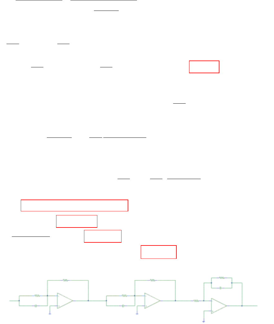
CHAPTER FIFTEEN SOLUTIONS
Engineering Circuit Analysis, 6th Edition Copyright
2002 McGraw-Hill, Inc. All Rights Reserved
56.
()
()
4
C
o
i
1A
1A f a
11
11
[ K ][ K ( 100)]
10 ( 100)
() K
1000
1000
Let ( ) K . Choose inverting op amp with parallel RC network at inverting input.
V
-V
0 = 1+ C -
RR
RR
() 1 R C =
AB
AA
fA fA
AAA
AA
RR
−−−+
−+
==
+
−
+
=−
∴=−+ −
ss
ss
Hs s
s
Hs s
s
Hs s
()
11A
4
11
11
1
R C K . Set R = . Then
R C 10 C
R
Same configuration for ( ) ( ) K ( 100) = 1 R C
For the last stage, choose an inverting op amp circuit with a parallel RC circui
fA A A
fA A A
fB
BB B BB
B
R
−=− ∞
−=−
∴=−+ −+
ss
ss
Hs Hs s s
()
1
t in the feedback loop.
R
11
Let ( ) K
1000 1 R C
fC
CC
CFCFC
R
=− = −
++
Hs ss
Cascading these three tranfer functions, we find that
HA HB HC = fC
fB
1fB1B
1B 1 fc fc
R
R1
RC RC + RRRC + 1
fA A
C
−− −
ss s
Choosing all remaining resistors to be 10 kΩ, we compare this to our desired transfer function.
(Rfc Cfc)-1 = 1000 so Cfc = 100 nF
Next, fB
1B fB 1B
R = 100
R R C so C1B = 1 µF.
Finally, RfAC1ARfBC1BRfC (R1CRfCCfC) = 10-4, so C1A = 1 nF
Cfc
C1a
R1a
Rfa
C1b
R1b
Rfb
R1c
Rfc
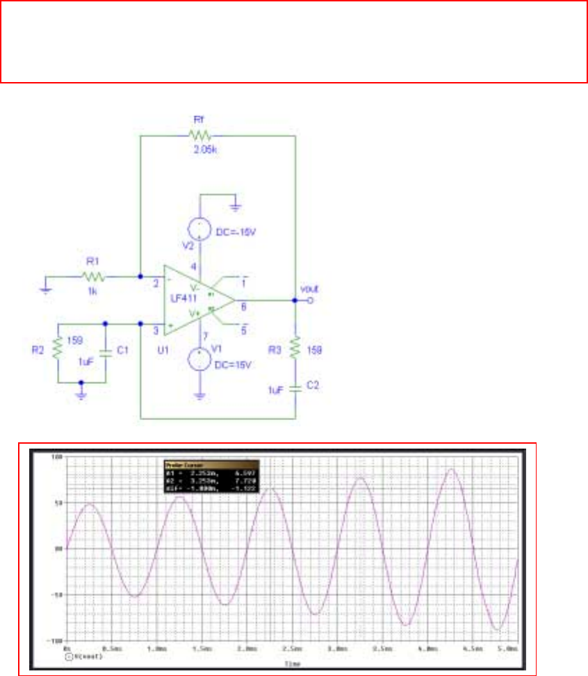
CHAPTER FIFTEEN SOLUTIONS
Engineering Circuit Analysis, 6th Edition Copyright
2002 McGraw-Hill, Inc. All Rights Reserved
57. Design a Wien-bridge oscillator for operation at 1 kHz, using only standard resistor
values. One possible solution:
ω
= 2πf = 1/RC, so set (2πRC)-1 = 1000
If we use a 1-µF capacitor, then R = 159 Ω. To construct this using standard resistor
values, connect a 100-Ω, 56-Ω and 3-Ω in series.
To complete the design, select Rf = 2 kΩ and R1 = 1 kΩ.
PSpice verification:
The feedback resistor was set to
2.05 kΩ to initiate oscillations
in the simulation. The output
waveform shown below exhibits
a frequency of 1 kHz as desired.

CHAPTER FIFTEEN SOLUTIONS
Engineering Circuit Analysis, 6th Edition Copyright
2002 McGraw-Hill, Inc. All Rights Reserved
58. Design a Wien-bridge oscillator for operation at 60 Hz. One possible solution:
ω
= 2πf = 1/RC, so set (2πRC)-1 = 60
If we use 10-nF capacitors, then R = 265.3 kΩ.
To complete the design, select Rf = 200 kΩ and R1 = 100 kΩ.
PSpice verification:
The simulated output of the circuit
shows a sinusoidal waveform
having period 54.3 ms – 37.67 ms =
0.01663 ms, which corresponds to a
frequency of 60.13 Hz, as desired.
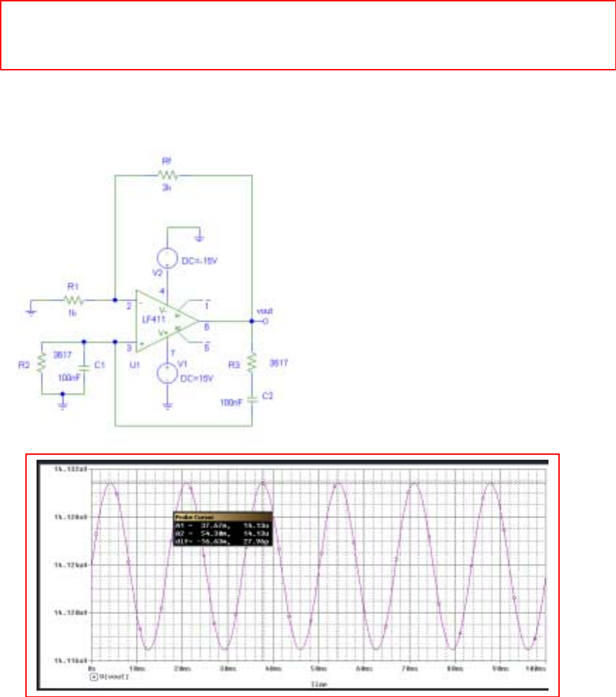
CHAPTER FIFTEEN SOLUTIONS
Engineering Circuit Analysis, 6th Edition Copyright
2002 McGraw-Hill, Inc. All Rights Reserved
59. Design a Wien-bridge oscillator for operation at 440 Hz, using only standard resistor
values. One possible solution:
ω
= 2πf = 1/RC, so set (2πRC)-1 = 440
If we use 100-nF capacitors, then R = 3.167 kΩ. To construct this using standard resistor
values, connect a 3.6-kΩ, 16-Ω and 1-Ω in series. (May not need the 1-Ω, as we’re using
5% tolerance resistors!). This circuit will produce the musical note, ‘A.’
To complete the design, select Rf = 2 kΩ and R1 = 1 kΩ.
PSpice verification:
Simulation results show a sinusoidal
output having a period of approximately
5.128 – 2.864 = 2.264 ms, or a frequency
of approximately 442 Hz. The error is
likely to uncertainty in cursor placement;
a higher-resolution time simulation
would enable greater precision.
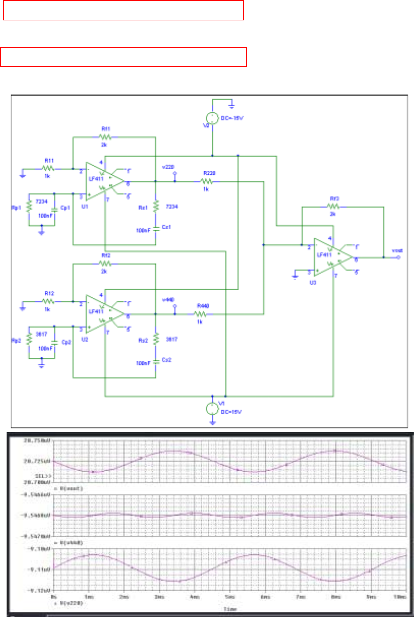
CHAPTER FIFTEEN SOLUTIONS
Engineering Circuit Analysis, 6th Edition Copyright
2002 McGraw-Hill, Inc. All Rights Reserved
60. Design a Wien-bridge oscillator for 440 Hz:
ω
= 2πf = 1/RC, so set (2πRC)-1 = 440
If we use 100-nF capacitors, then R = 3.167 kΩ.
Design a Wien-bridge oscillator for 220 Hz:
ω
= 2πf = 1/RC, so set (2πRC)-1 = 220
If we use 100-nF capacitors, then R = 7.234 kΩ.
Using a summing stage to add the two waveforms together:
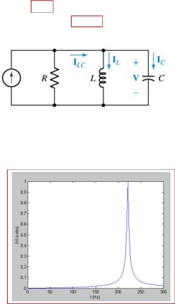
CHAPTER SIXTEEN SOLUTIONS
Engineering Circuit Analysis, 6th Edition Copyright
2002 McGraw-Hill, Inc. All Rights Reserved
1. We have a parallel RLC with R = 1 kΩ, C = 47 µF and L = 11 mH.
(a) Qo = R(C/L)½ = 65.37
(b) fo =
ω
o/ 2
π
= (LC)-½ / 2
π
= 221.3 Hz
(c) The circuit is excited by a steady-state 1-mA sinusoidal source:
The admittance Y(s) facing the source is Y(s) = 1/R + 1/sL + sC
= C(s2 + s/RC + 1/LC)/ s so Z(s) = (s/C) / (s2 + s/RC + 1/LC) and
Z(j
ω
) = (1/C) (j
ω
) / (1/LC –
ω
2 + j
ω
/RC).
Since V = 10-3 Z, we note that |V| > 0 as
ω
→ 0 and also as
ω
→ ∞.
10-3∠
∠∠
∠0o A j
ω
ωω
ω
L -j/
ω
ωω
ω
C

CHAPTER SIXTEEN SOLUTIONS
Engineering Circuit Analysis, 6th Edition Copyright
2002 McGraw-Hill, Inc. All Rights Reserved
2. (a) R = 1000 Ω and C = 1 µF.
Q
o = R(C/L)½ = 200 so L = C(R/ Qo)2 = 25 µH
(b) L = 12 fH and C = 2.4 nF
R = Qo (L/ C)½ = 447.2 mΩ
(c) R = 121.7 kΩ and L = 100 pH
C = (Qo / R)2 L = 270 aF
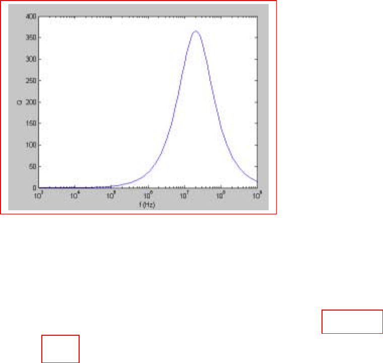
CHAPTER SIXTEEN SOLUTIONS
Engineering Circuit Analysis, 6th Edition Copyright
2002 McGraw-Hill, Inc. All Rights Reserved
3. We take the approximate expression for Q of a varactor to be
Q ≈
ω
CjRp/ (1 +
ω
2 Cj2 Rp Rs)
(a) Cj = 3.77 pF, Rp = 1.5 MΩ, Rs = 2.8 Ω
(b) dQ/d
ω
= [(1 +
ω
2 Cj2 Rp Rs)(Cj Rp) -
ω
CjRp(2
ω
Cj2 Rp Rs)]/ (1 +
ω
2 Cj2 RpRs)
Setting this equal to zero, we may subsequently write
CjRp (1 +
ω
2 Cj2 Rp Rs) -
ω
CjRp(2
ω
Cj2 Rp Rs) = 0
Or 1 –
ω
2 Cj2 Rp Rs = 0. Thus,
ω
o = (Cj2 RpRs)–½ = 129.4 Mrad/s = 21.00 MHz
Q
o = Q(
ω
=
ω
o) = 366.0
CHAPTER SIXTEEN SOLUTIONS
Engineering Circuit Analysis, 6th Edition Copyright
2002 McGraw-Hill, Inc. All Rights Reserved
4. Determine Q for (dropping onto a smooth concrete floor):
(a) A ping pong ball: Dropped twice from 121.1 cm (arbitrarily chosen).
Both times, it bounced to a height of 61.65 cm.
Q = 2
π
h1/ (h1 – h2) = 12.82
(b) A quarter (25 ¢). Dropped three times from 121.1 cm.
Trial 1: bounced to 13.18 cm
Trial 2: bounced to 32.70 cm
Trial 3: bounced to 16.03 cm. Quite a bit of variation, depending on how it struck.
Average bounce height = 20.64 cm, so
Qavg = 2
π
h1/ (h1 – h2) = 7.574
(c) Textbook. Dropped once from 121.1 cm. Didn’t bounce much at all- only 2.223 cm.
Since the book bounced differently depending on angle of incidence, only one trial was
performed.
Q = 2
π
h1/ (h1 – h2) = 6.4
All three items were dropped from the same height for comparison purposes. An
interesting experiment would be to repeat the above, but from several different heights,
preferrably ranging several orders of magnitude (e.g. 1 cm, 10 cm, 100 cm, 1000 cm).
CHAPTER SIXTEEN SOLUTIONS
Engineering Circuit Analysis, 6th Edition Copyright
2002 McGraw-Hill, Inc. All Rights Reserved
5.
22
80Np/s, 1200 rad/s, Z( 2 ) 400
1200 80 1202.66 rad/s Q 7.517
2
()() ()(2)
Now, Y( ) C Y( 2 ) C 2
80( 80 2400)
Y( 160 1200) C Y( 160 1200)
160 1200
dd
o
oo
dd d
d
d
j
sjsj j
sj
sj
j
jj
j
αω αω
ω
ωα
αω αω αα ω
αω αω
== −+=Ω
=+= ∴==
+− ++ − −+
=∴−+=
−+
−−+
∴− + = ∴ − + =
−+
2
1130
80C
400 2 15
1 229 1 1
C 15.775 F; L 43.88mH; R 396.7
32,000 901 C 2
o
j
j
C
µωα
−
−+
=−+
∴= = = = = = Ω
CHAPTER SIXTEEN SOLUTIONS
Engineering Circuit Analysis, 6th Edition Copyright
2002 McGraw-Hill, Inc. All Rights Reserved
6.
2
2
262 226
35 3 2
1 1 2 0.1
Y 0.2 0.2
2 0.1 1 1000/ 4 0.01 1000 10
2 0.1 1000 0.1 1000
0.2 0
4 0.1 10 4 0.01 10
0.1 10 4000 10 9.9 96,000 98.47 rad/s
−
=++ = ++
+++ +
−+−
=++ ∴ +=
++++
∴+= +∴ = ∴=
in
jj
jj j
jj
ωω
ωωω
ωω ω ω ω
ωωωω
ωω ωω ω ω
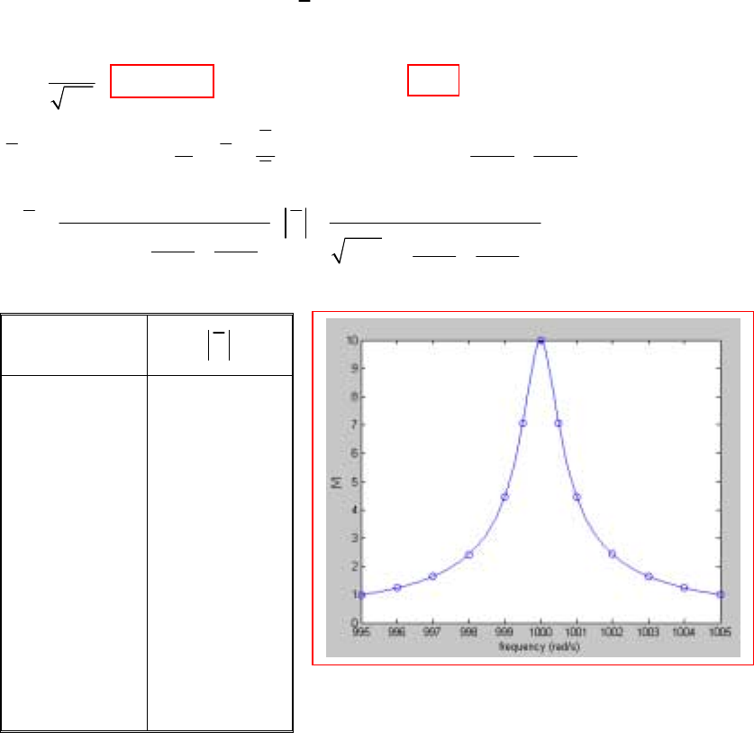
CHAPTER SIXTEEN SOLUTIONS
Engineering Circuit Analysis, 6th Edition Copyright
2002 McGraw-Hill, Inc. All Rights Reserved
7. 66
Parallel: R 10 , L 1, C 10 , I 10 0 A
s
µ
−
=== =∠°
(a) 366
11000 rad/s; Q RC 10 1000
LC
ooo
ωω
+−
== = = =
(b)
ω V
995
996
997
998
999
1000
1001
1002
1003
1004
1005
999.5
1000.5
0.993
1.238
1.642
2.423
4.47
10.0
4.47
2.428
1.646
1.243
0.997
7.070
7.072
66 533
22
2
6
1 I 1000
Y 10 10 , V 10 /10 10
Y 1000
10 10
V,V
1000 1000
0.001 10
1000 1000
jj
j
ω
ωω
ωω
ωω
−− −−−
−−
−
=+ − == + −
∴= =
+− +−
CHAPTER SIXTEEN SOLUTIONS
Engineering Circuit Analysis, 6th Edition Copyright
2002 McGraw-Hill, Inc. All Rights Reserved
8.
(a)
(b) 2
226
102000
Z ( ) 2 2.294
400 10
o
in o
oo
ω
ωωω
=++=Ω
++
226
426 2 2
226
5(100/ ) 0.1
Z2
5 (100 / ) 10 0.01
500 10 100 10 100(20 ) 10 (1000 )
22 2
100 5 1000 20 1000 400 10
100 10 0 10 100 40,000, 99 960,000
400 10
960,000/99 9
=++
++
−−
=++=++= ++
+++++ +
−
∴+=∴+=+ =
++
∴= =
in
o
jj
jj
jjjjj
jjjj
ωω
ωω
ωωωω
ωωωωω ω
ωω ωω ω
ωω
ω
8.47 rad/s

CHAPTER SIXTEEN SOLUTIONS
Engineering Circuit Analysis, 6th Edition Copyright
2002 McGraw-Hill, Inc. All Rights Reserved
9.
(a)
(b) 46
11
Y 10 10 , 1000 Z 9997 1.4321
0.9975 Y
j
ωω
ω
−−
=+ − = ∴== ∠ °Ω
11222
66
2
50 , 1000 1,002,500 1001.249
110 110
L0.9975H;R10
C 1,002,500 2 C 100
dod o
o
ss
k
αω ωαω ω
ωα
−−
+
==∴=+= ∴=
== = ===Ω
CHAPTER SIXTEEN SOLUTIONS
Engineering Circuit Analysis, 6th Edition Copyright
2002 McGraw-Hill, Inc. All Rights Reserved
10.
min max
o
33
max min
2
14
max min max 3
33
535kHz, 1605kHz, Q 45 at one end and
Q 45 for 535 1605 kHz
11
1/ 2 LC 535 10 ,1605 10
2LC 2LC
1
L / L 3; L C 8.8498 10
2 535 10
RC 45,535 10 1605 10 . Use
2
o
o
o
o
f
ff
f
πππ
π
ω
ωπ
−
===
≤≤≤
=∴×= ×=
∴== =×
××
≤×≤≤× max
33
14 max
max min
12
2 1605 10 20 10 C 45 C 223.1pF
L
8.8498 10
L 397.6 H, L 44.08 H
223.1 10 9
o
ω
π
µµ
−
−
∴× × ×× = ∴=
×
∴= = = =
×
CHAPTER SIXTEEN SOLUTIONS
Engineering Circuit Analysis, 6th Edition Copyright
2002 McGraw-Hill, Inc. All Rights Reserved
11.
(a)
(b)
4
4548
3
82 4
48
82 4
Apply 1V. I 10 A
1
Y I 10 (1 [10 ( 10 )])10
4.4 10
1000 48.4 10 4.4 10 1000
Y101110
4.4 4.4
1000 48.4 10 4.4 10
Y( ) 4.4
−
−−−
−
−−
−−
−−
±∴=−
∴== + +− −
×
×+×+
∴= + +× =
−× +×
∴=
R
in in
in
in
s
s
ss
s
ss
j
jj
ωω
ωω
82
1
4
At , 1000 48.4 10 , 45.45 krad/s
4.4 10
Z( ) 10
4.4
−−
−
−
==× =
×
==Ω
ooo
o
in o
o
j
jk
j
ωω ωω
ω
ωω
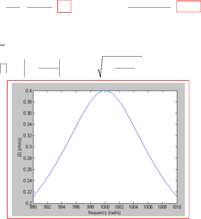
CHAPTER SIXTEEN SOLUTIONS
Engineering Circuit Analysis, 6th Edition Copyright
2002 McGraw-Hill, Inc. All Rights Reserved
12. 1000 rad/s, Q 80, C 0.2 F
oo
ω
µ
===
(a) 6
26 36
110 80
L 5H, Q RC R 400
C 0.2 10 10 0.2 10
oo
o
k
ω
ω
−
== = = ∴= =Ω
×××
(b)
2
3
B / Q 1000 /80 12.5
1B 6.25 rad/s
2
Z R / 1 400 10 / 1
B/ 2 6.25
oo
oo
j
ω
ωω ωω
== =
∴=
−−
∴= + = × +
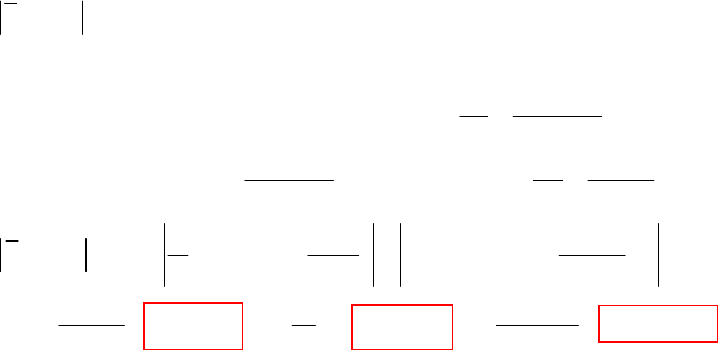
CHAPTER SIXTEEN SOLUTIONS
Engineering Circuit Analysis, 6th Edition Copyright
2002 McGraw-Hill, Inc. All Rights Reserved
13.
12
212
o
3
2
1
103rad/s, 118,
Z( 105) 10
103 118
110.245
110.245 , B 118 103 15 rad/s, Q 7.350
B15
7.350 1 1
7.350 RC RC 66.67 10 ,LC
110.245 12,154
11
Y( 105) 0.1 105C 15C 105C
R 105L
o
o
o
o
o
j
jj j
ωω
ωωω
ω
ω
ωω
+
+
−
+
==
=Ω
==×
∴= = − = = = =
∴= ∴= =× ==
==+ − = +
12,154 C 18.456C
105
0.1 1 1
C 5.418mF, R C 12.304 , L 15.185 mH
18.456 15 12,154C
−
−=
∴= = = = Ω = =
CHAPTER SIXTEEN SOLUTIONS
Engineering Circuit Analysis, 6th Edition Copyright
2002 McGraw-Hill, Inc. All Rights Reserved
14. 30 krad/s, Q 10, R 600 ,===Ω
oo
ω
(a) B 3 krad/s
Q
o
o
ω
==
(b) 28 30
N 1.3333
B/ 2 1.5
o
ωω
−−
== =−
(c) Zin(j28 000) = 600 / (1 – j1.333) = 360 ∠ 53.13o Ω
(d)
(e)
1
1
Q11 10
Z ( 28,000) 28,000C ,C
600 28,000L R 30,000 600
R 600 1 30,000 10 1 28 10 30 10
L,Z
Q 30,000 10 L 600 600 30 600 28 600
600
Z 351.906 54.0903
28 30
110
30 28
−
−
=+ − ==
×
×
== = ∴=+×−
×
==∠°Ω
+−
o
in
o
in
oo
in
jjj
j
j
ω
ω
approx-true 360 351.906
magnitude: 100% 100% 2.300%
true 351.906
53.1301 54.0903
angle: 100% 1.7752%
54.0903
−
==
°− °=−
°
CHAPTER SIXTEEN SOLUTIONS
Engineering Circuit Analysis, 6th Edition Copyright
2002 McGraw-Hill, Inc. All Rights Reserved
15. 3
400Hz, Q 8, R 500 , I 2 10 A B 50Hz
oo S
f−
===Ω=×∴=
(a)
(b)
32 2 400
V 2 10 500 / 1 N 0.5 1 N 4, N 3 50/ 2
400 25 3 443.3 and 356.7Hz
f
f
−−
=× × + = ∴+ = =± =
∴= ± =
322
2
11
I 0.5 10 1 N 4, N 15, N 15
R 500
1N
400 25 15 496.8 and 303.2 Hz
R
v
f
−
== × = × ∴+ = = =±
+
∴= ± =
CHAPTER SIXTEEN SOLUTIONS
Engineering Circuit Analysis, 6th Edition Copyright
2002 McGraw-Hill, Inc. All Rights Reserved
16. 63
10 , Q 10, R 5 10 , . .===×
oo pr
ω
(a) 3
6
R510
Q L 0.5mH
L1010
o
o
ω
×
=∴= =
×
(b)
(c)
6
2
6
2
222 2
22
422
10
Approx: 2 5/ 1 N N 2.291 1.1146 Mrad/S
10 / 20
11
Exact: Y 1 Q 0.5 0.2 1 100 ( in Mrad/S)
R
11
6.25 1 100( 2 1/ ), 2 0.0525, 2.0525
1
2.0525 1 0, 2
2
−
=+∴= = ∴=
=+ − ∴= + −
∴ =+ −+ −+= +=
−+==
o
o
o
j
ωω
ωω ωω
ωω ω
ωωω ω
ωω
ωωω
()
2
.0525 2.0525 4 1.2569, 1.1211 Mrad/s+−==
ω
1
2
2
1
Approx: Y 30 tan N 30 , N 0.5774 , 1.0289 Mrad/s
1/20
11 1
Exact: Y 1 10 (in Mrad/s) tan30 0.5774 10
5000
1 0.05774 0.05774 4
0.05774, 0.05774 1 0, 1.0293 Mrad/s
2
−−
∠= °∴ = ° = = =
=+− ∴°==−
++
∴− = − −= = =
j
ωω
ωω
ωω
ωωωω
ω
CHAPTER SIXTEEN SOLUTIONS
Engineering Circuit Analysis, 6th Edition Copyright
2002 McGraw-Hill, Inc. All Rights Reserved
17.
(a) 6
48
1
C 3 7 10nF 10 rad/s
10 10
o
ω
−−
=+= ∴ = =
(b)
(c) 3
3
1
3
15 10 15 90
15 10 N 1.5 V 8.321 33.69 V
10 10 1 1.5
oj
ωω
×∠°
−=× ∴= = ∴= = ∠ °
×+
68 3
969
3
33
1,0
QCR1010551050
B/Q20 krad/s
10
Parallel current source is 3 10 At , I 10 3
Z
V3105101590V
oo
oo
os
jj
j
ω
ω
ωω
−
−−
−
== ×=
==
∠°
=× = ×
∴=×××=∠°
CHAPTER SIXTEEN SOLUTIONS
Engineering Circuit Analysis, 6th Edition Copyright
2002 McGraw-Hill, Inc. All Rights Reserved
18.
(a)
(b) 25 10,000
Z ( ) (5 100) (5 100) 1002.5
10
in o
jjj
ω
+
=+ − = = Ω
66
626
246
26
62
62
626
(5 0.01 )(5 10 / ) (5 0.01 )(5 10 )
Z() 10 0.01 10 / 0.01 10 10
0.05 25 10 5 10
Z() 0.01 10 10
5 10 0.05 10,025
Z( ) 10 0.01 10
10,025 10
At , 5 10 0.05 10 0.01
++ + +
==
++ ++
++ +×
=++
×− +
∴=−+
==
×− −
in
in
in
oo
o
o
ss ss
sss ss
sss
sss
j
jj
ωω
ωωω
ωω
ωω ω
9272
2
29
, 10.025 10 100.25 5 10 0.5
99.75 9.975 10 , 10,000 rad/s
×− =×−
∴=×=
oo
o
oo
ωω
ω
ωω
CHAPTER SIXTEEN SOLUTIONS
Engineering Circuit Analysis, 6th Edition Copyright
2002 McGraw-Hill, Inc. All Rights Reserved
19.
,
1000Hz, Q 40, Z ( ) 2 B 25Hz
ooino
fjk
ω
===Ω∴=
(a) Zin(j
ω
) =
Z
in = 2000 / (1 + j0.8) = 1562 ∠ -38.66o Ω
(b) 0.9 1.1 900 1100 Hz
oo
ff f f<< ∴ <<
2000 1000
, N , 1010, N 0.8
1 N 12.5
−
==∴=
+
ff
j

CHAPTER SIXTEEN SOLUTIONS
Engineering Circuit Analysis, 6th Edition Copyright
2002 McGraw-Hill, Inc. All Rights Reserved
20. Taking 2–½ = 0.7, we read from
Fig. 16.48a: 1.7 kHz – 0.6 kHz = 1.1 kHz
Fig. 16.48b: 2×10⁷ Hz – 900 Hz = 20 MHz
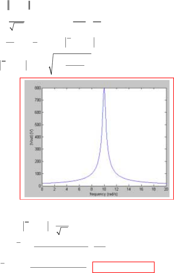
CHAPTER SIXTEEN SOLUTIONS
Engineering Circuit Analysis, 6th Edition Copyright
2002 McGraw-Hill, Inc. All Rights Reserved
21.
(a)
(b)
2
20A 6 , 3 6 2, 40V in series with 2 1 3
L160
10 rad/s, Q 20
R3
LC
10 1
B 0.5, B 0.25, V ( ) 40Q 800V
20 2
10
V ( ) 800 / 1 0.25
o
oo
out o o
out
j
j
ω
ω
ω
ω
ω
Ω= +=Ω
== ===Ω
== = = =
−
∴=+
9 rad/s
800
(Approx: V ( 9) 194.03V
17
40 600
Exact: V 3 (6 600 / )
24,000
V ( 9) 204.86 13.325 V
9[3 (54 66.67)]
out
out
out
j
jj
jj
ω
ωωω
−
=
==
=×
+−
∴= =∠−
+−
CHAPTER SIXTEEN SOLUTIONS
Engineering Circuit Analysis, 6th Edition Copyright
2002 McGraw-Hill, Inc. All Rights Reserved
22. 7
Series: R 50 , L 4mH, C 10−
=Ω= =
(a) 37
1/ 4 10 50 krad/s
o
ω
−−
=× =
(b) 3
50 10 / 2 7.958kHz
o
f
π
=× =
(c) 33
L5010410
Q4
R50
o
o
ω
−
×××
== =
(d) 3
B / Q 50 10 / 4 12.5 krad/s
oo
ω
==×=
(e) 2
11 (1/ 2 ) 1/ 2 50 1 1/ 64 1/8 44.14 krad/s
ooo
QQ
ωω
=+ − =+−=
(f) 250 65/ 64 1/8 56.64 krad/s
ω
=+=
(g) 73
Z ( 45,000) 50 (180 10 / 45) 50 42.22 65.44 40.18
in jj j
−
=+ − =− = ∠− °Ω
(h) 7
45,000
Z / Z 10 / 45,000 50 4.444
cR j=×=
CHAPTER SIXTEEN SOLUTIONS
Engineering Circuit Analysis, 6th Edition Copyright
2002 McGraw-Hill, Inc. All Rights Reserved
23. Apply 1 A, in at top. V 10V
R
∴=
(a)
(b) 33
L 346.4 10
Q 34.64
R10
o
o
ω
−
×
== =
88
33
383 8
211
10 1.2 10
V Z 10 10 (0.5 10 1) 10 10
5
Z ( ) 10 (10 1.2 10 / ) 10 1.2 10 /
1.2 10 , 346.4 krad/s
in in
in o o
oo
ss
ss
jj
ωωωωω
ωω
−−
−−
×
== ++ ×+= ++
=+ −× ∴ = ×
∴=× =
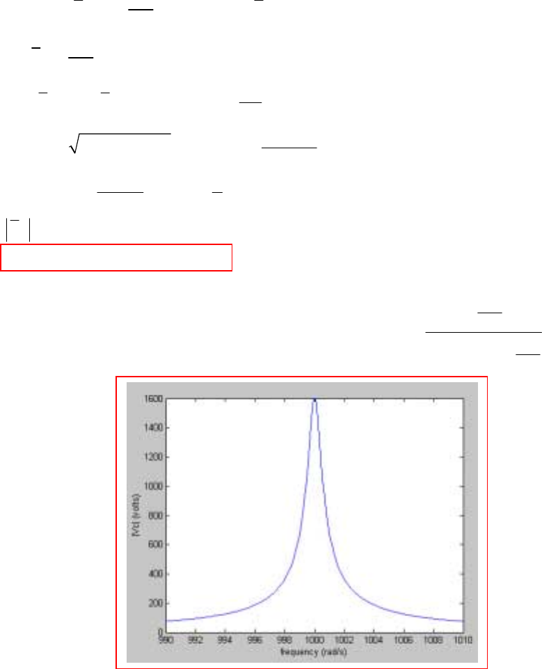
CHAPTER SIXTEEN SOLUTIONS
Engineering Circuit Analysis, 6th Edition Copyright
2002 McGraw-Hill, Inc. All Rights Reserved
24. Find the Thévenin equivalent seen by the inductor-capacitor combination:
1
111
1
6
max
V
SC : 1.5 V 10 0.105V V 50 V
125
50
I 0.4A
125
1.5
OC:V 0 V 1.5V R 3.75
0.4
1000 4
1/ 4 0.25 10 1000,Q 1066.7
3.75
1000 1
B / Q 0.9375, B 0.4688 rad/s
1066.7 2
V Q V 1066.7 1.5 1600V
−
=+ − ∴=
∴↓ = =
=∴ = ∴ = = Ω
×
∴= × × = = =
=== =
== ×=
SC
OC th
oo
oo
Coth
ω
ω
Therefore, keep your hands off!
To generate a plot of |VC| vs. frequency, note that VC(j
ω
) =
C
j
Lj
C
j
ω
ω
ω
−+
−
75.3
5.1
CHAPTER SIXTEEN SOLUTIONS
Engineering Circuit Analysis, 6th Edition Copyright
2002 McGraw-Hill, Inc. All Rights Reserved
25. ,0
Series, 500Hz, Q 10, X 500
ooL
f===Ω
(a)
(b)
22
,0
12
500 L 2 (500)L L 0.15915 H, C 0.6366 F
L (2 500)
X500
Q10 R50
RR
+
== ∴= = = =
×
== = ∴=Ω
o
o
L
o
π
ωπ
µ
ωπ
6
6
1 10 0.5 250,000
1 I 50 2 I 50
22
10 0.5
I 1/ 50 ( 250,000 / ), V I
2
250,000/
V V (2 450) 4.757V
50 ( 250,000/ )
V (2 500) 10,000V V (2 550) 4.218V
×
=+×− =+−
×
∴= + − =
−
=∴×=
+−
×= ×=
c
Cc
cc
jf j jfj
ff
jf f jf
jf
jf f
π
πππ
π
π
π
ππ
CHAPTER SIXTEEN SOLUTIONS
Engineering Circuit Analysis, 6th Edition Copyright
2002 McGraw-Hill, Inc. All Rights Reserved
26.
14
828
8
1
X : 0, ,0: 20,000 80,000 , Z ( 10 ) 20 0 SERIES
1
20,000, 80,000 (64 4)10 82,462 rad/s, 68 10
LC
R R 1 L 68 10 1
20,000 40,000, 170,000; Z( ) R L
2L L LC R 40,000 C
1
20 R 10,000L 10,00
−
= ∞ =− ± − =− + Ω ∴
==∴=+= ==×
×
== ∴ = ×= = =+ +
∴− = − −
in
do o
ss js j
αω ω ω
ασσ
σ
1 170,000
R R R R 1.2308
0C 4 10,000
1.2308 1
L 30.77 H, C 4.779 F
40,000 170,000 1.2308
=− − ∴= Ω
∴= = = =
×
µµ
CHAPTER SIXTEEN SOLUTIONS
Engineering Circuit Analysis, 6th Edition Copyright
2002 McGraw-Hill, Inc. All Rights Reserved
27.
= 4.287 ∠ 59.04o kΩ
53
37 5
2
57
57
3
10
1/ 10 10 rad/s, Q 100, R 10,000
1
1
Q 500, R 500 0.2 50,000
10 0.2
50 10 8.333 Q CR 10 8333 83.33
100,000
B 1200 rad/s, Z ( ) 8333
83.33
(99 100)10
99,000 N 1.6667,Z
600
−
−−
−
−
ω====Ω
===×=Ω
×
=Ω∴=ω=×=
== ω=Ω
−
ω= ∴ = =−
B
oLPL
cPC
oo
in o
i
k
j
8.333
( 99,000) 1 1.667
=−
njj

CHAPTER SIXTEEN SOLUTIONS
Engineering Circuit Analysis, 6th Edition Copyright
2002 McGraw-Hill, Inc. All Rights Reserved
28. Req = Qo/
ω
o C = 50 / 105-7 = 5000 Ω.
Thus, we may write 1/5000 = 1/8333 + 1/Rx so that
R
x = 12.5 kΩ.
CHAPTER SIXTEEN SOLUTIONS
Engineering Circuit Analysis, 6th Edition Copyright
2002 McGraw-Hill, Inc. All Rights Reserved
29.
35
34 2
34
43
2
6
4
1
3mH 1.5mH 1mH, 2 F 8 F 10 F, 10 krad/s
10
310 10
Q 100, R 100 0.3 3
0.3
1.5 10 10
Q 60, R 60 0.25 900
0.25
692.3
900 3000 692.3 Q 69.23
10
692.3
R 0.14444
69.23
10
Q 125, R
10 0.1 8
−−
−
−
−
=µ+µ=µ∴ω= =
××
===×=Ω
××
===×=Ω
=Ω∴= =
∴= = Ω
==
××
o
p
p
L
LS
pc
k
2
45
2
,min
125 0.1 1562.5 10 F
1562.5
Q 10 10 15625 156.25 R 0.064
(156.25)
R 0.14444 0.064 0.2084 Z , 10 krad/s
−
=×= Ωµ
∴= × × = ∴ = = Ω
∴= + = Ω= ω=
cSC
S tot in o
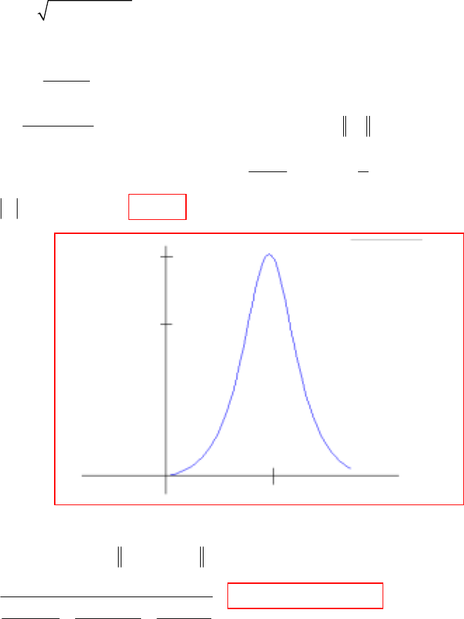
CHAPTER SIXTEEN SOLUTIONS
Engineering Circuit Analysis, 6th Edition Copyright
2002 McGraw-Hill, Inc. All Rights Reserved
30.
(a)
(b)
3
2
2
2
3
1/ 2 0.2 10 50 rad/s
Q 50 2.5/ 2 62.5, 2 62.5 7812.5
50 10
Q 50, 10 50 25
10
1000
Q 100, 100 1 10 , R 7.8125 25 10 3731
50 0.2 1
50 1
Q 50 3731 0.2 10 37.31; B 1.3400, B 0.6700
37.31 2
V10
−
−
ω××=
=× = × = Ω
×
==×=Ω
==×=Ω= =Ω
××
=× × × = = = =
∴=
B
o
leftL
rightL
cp
o
o
k
k
33731 3.731V
−×=
3
3
V 10 [(2 125) (10 500) (1 100)]
10 3.7321 0.3950 V
111
2 125 10 500 1 100
−
−+
=+ + −
==∠−°
++
++−
jjj
jjj
3.731 V
2.638 V
50
↔
↔↔
↔
1.34 rad/s
|V| (volts)
ω
(rad/s)
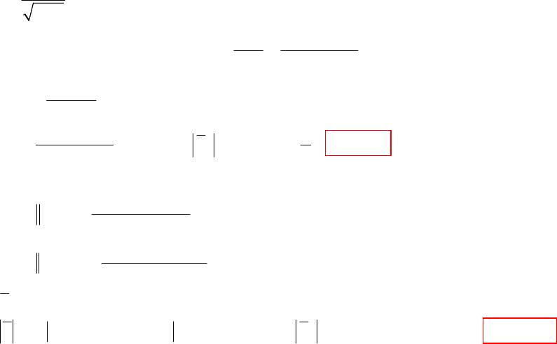
CHAPTER SIXTEEN SOLUTIONS
Engineering Circuit Analysis, 6th Edition Copyright
2002 McGraw-Hill, Inc. All Rights Reserved
31.
(a)
(b)
63
4
2
,
,
1000 2000 rad/s, Q 2000 2 10 25 10 100
0.25
R2010
R 25,000/100 2.5 ; Q 40
L 2000 0.25
20,000
R 12.5 R 12.5 2.5 15
1600
2000 0.25 1
Q 33.33 V 1 33.33 16.667V
15 2
−
ω= =××××=
×
∴= =Ω== =
ω×
∴= =Ω∴=+=Ω
×
∴= = ∴ =× ×=
B
oc
CS L
o
LS tot
ox
20,000 500
20,000 500 12,4922 499.688
20,000 500
25,000( 250)
25,000 250 2.4998 249.975
25,000 250
Z 12.4922 2.4998 499.688 250 249.975 14.9920 0.2870
I 1/ 14.9920 0.2870 66.6902mA V 250
×
==+Ω
+
−
−= = −
−
∴= + + − − = − Ω
∴= − = ∴ = ×
in
x
j
jj
j
j
jj
j
jjj j
j3
66.6902 10 16.6726V
−
×=
CHAPTER SIXTEEN SOLUTIONS
Engineering Circuit Analysis, 6th Edition Copyright
2002 McGraw-Hill, Inc. All Rights Reserved
32.
(a)
(b) same ordinate; divide numbers on abscissa by 50
3
6
50 20 10
K 0.5 K 0.02
100 10
1 0.5
9.82 H 0.5 9.82 24.55 H, 31.8 H 31.8 795 H
0.02 0.02
2.57
2.57nF 257nF
0.5 0.02
×
== = =
∴
µ
→× × =
µµ
→×=
µ
→=
×
mf
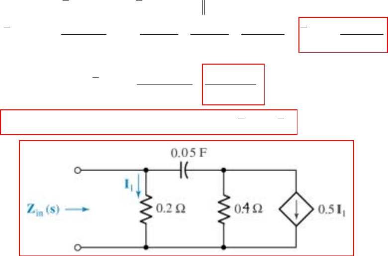
CHAPTER SIXTEEN SOLUTIONS
Engineering Circuit Analysis, 6th Edition Copyright
2002 McGraw-Hill, Inc. All Rights Reserved
33.
(a)
(b) 2( /5 10) 0.1( 50)
K2,K5Z()20( / 5 5) 25
++
==∴→ =
++
mf in
ss
sss
(c) 11
0.1 0.2 , 0.2 0.4 , 0.5F 0.05F, 0.5I 0.5IΩ→ Ω Ω→ Ω → →
11
Apply 1 V I 10A 0.5 I 5A ; 5A 0.2 can be replaced by 1 V in series with 0.2
1 ( 1) 2 4 20 20( 5) 10
I10 10 Z()
0.2 2 / 0.2 2 0.2 2 10 20( 5)
∴= ∴ = ↓ Ω Ω
−− + + +
∴→=+ =+ = = ∴ =
++++ +
in in
ss s s
s
ssss s
CHAPTER SIXTEEN SOLUTIONS
Engineering Circuit Analysis, 6th Edition Copyright
2002 McGraw-Hill, Inc. All Rights Reserved
34.
(a)
(b)
(c) 6
610
10 rad/s, Q stays the same, B 21.40 krad/s
46.73
ω= ∴ = =
oo
36 4
4
434
,8 , 2
43
2 2
, ,
46
46
1/ (2 8)10 10 10 rad/s
10
Q 10 /8 10 10 125 R 0.64
125
10 10 10
2 8 10mH Q 156.25
0.64
1
R 0.64 156.25 15.625 ; Q 100, R 100 1 10
10 10
R 20 15.625 10 4.673 Q 10 10 4
−−
−
−
−
−
ω+ =
=× =∴==Ω
××
+= ∴ = =
∴=× = Ω= = =×=Ω
×
∴= = Ω∴=× ×
B
o
LLS
L
LP C CP
Po
kk
k3
.673 10 46.73×=
64
K 10 /10 100, K 1 R s stay the same; 2 mH 20 H, 8mH 80 H,1 F 10nF
′
===∴ →µ→µµ→
fm
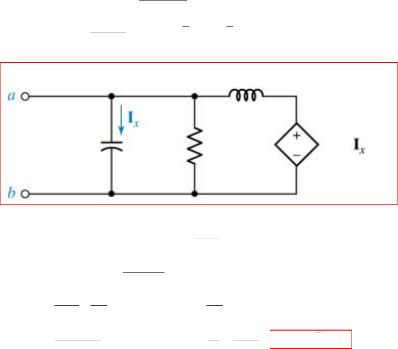
CHAPTER SIXTEEN SOLUTIONS
Engineering Circuit Analysis, 6th Edition Copyright
2002 McGraw-Hill, Inc. All Rights Reserved
35.
(a)
(b)
3
0.1
K 250, K 400 0.1F 1 F
250 400
2 250
5 1250 , 2H 1.25H, 4I 10 I
400
==∴→ =µ
×
×
Ω→ Ω → = →
mf
xx
36
1250
3
3
6363
3
33
1
10 . Apply 1 V I 10 , I 1250
110
1000 I 10 I 1.25
1 0.8 0.8
I 10 (1 10 ) 10 ; 10
1250
0.8 10 1 1000
I 10 0.2 10 Z 5 V 0
I 0.2
−
−
−
−−−
−
−−
ω= ∴ = ↓ =
−
∴=∴→=
∴= + + − = + =
×
∴= + = × ∴ = = =− Ω =
x
xL
in
in th oc
in
s
s
ss
ssssj
ss
jj jk
jj
1 µF
1.25 H
1250 Ω 103
CHAPTER SIXTEEN SOLUTIONS
Engineering Circuit Analysis, 6th Edition Copyright
2002 McGraw-Hill, Inc. All Rights Reserved
36.
(a) I 2 0 A, 50 V 60 25 V=∠° ω= ∴ = ∠ °
s out
(b) I 2 40 A, 50 V 60 65 V=∠ ° ω= ∴ = ∠ °
sout
(c) I 2 40 A, 200, OTSK=∠ ° ω= ∴
s
(d) K 30, I 2 40 A, 50 V 1800 65 V==∠°ω=∴=∠°
m S out
(e) K 30, K 4, I 2 40 A, 200 V 1800 65 V
===∠°ω=∴=∠°
m f s out
CHAPTER SIXTEEN SOLUTIONS
Engineering Circuit Analysis, 6th Edition Copyright
2002 McGraw-Hill, Inc. All Rights Reserved
37.
(a) H /( ) 0.2 H 20 log 0.2 13.979dB=∴= =−
dB
s
(b) H( ) 50 H 20 log 50 33.98dB=∴= =
dB
s
(c)
(d) 37.6 / 20
H 37.6dB H( ) 10 75.86=∴==
dB s
(e) 8/20
H 8dB H( ) 10 0.3981
−
=− ∴ = =
dB s
(f) 0.01/ 20
H 0.01dB H( ) 10 1.0012=∴==
dB s
12 26 6 13 292 380
H( 10) H 20 log 20 log 6.451dB
2 10 20 10 1 5 10 5 60 220
+
=+ ∴= += =
++ ++ −+
dB
j
jjj jj j
CHAPTER SIXTEEN SOLUTIONS
Engineering Circuit Analysis, 6th Edition Copyright
2002 McGraw-Hill, Inc. All Rights Reserved
38. (d) MATLAB verification- shown adjacent to Bode plots below.
(a) 20( 1) 0.2(1 )
H( ) , 0.2 14dB
100 1 /100
++
== →−
++
ss
sss
(b) 22
2000( 1) 0.2 (1 )
H( ) , 0.2 14dB
( 100) (1 /100)
++
== →−
++
ss ss
sss
(c)
2
200 45 200 ( 5)( 40) 200(1 / 5)(1 / 40)
H( ) 45 , 200 46dB
++ ++ + +
=+ + = = = →
ss ss s s
ss ss s s
1 10
100
CHAPTER SIXTEEN SOLUTIONS
Engineering Circuit Analysis, 6th Edition Copyright
2002 McGraw-Hill, Inc. All Rights Reserved
39.
2
V (20 2 )(182 200/ ) 200/
H( ) 202 2 200/ 182 200/
400( 10) 200(10 )
2( 101 100) (1 )(100 )
20(1 /10)
H( ) , 20 26dB
(1 )(1 /100)
++
== ×
++ +
++
==
++ + +
+
=→
++
C
R
sss
sIss s
ss
ss s s
s
sss
CHAPTER SIXTEEN SOLUTIONS
Engineering Circuit Analysis, 6th Edition Copyright
2002 McGraw-Hill, Inc. All Rights Reserved
40.
(a) 8
33
5 10 ( 100) 2.5 (1 /100)
H( ) , 2.5 8dB
( 20)( 1000) (1 / 20)(1 /1000)
×+ +
== →
++ + +
ss s s
sss s s
(b)
(c)
29
33
Corners: 20, 34dB;
100, 34dB;
1000, 54dB
Intercepts: 0dB, 2.5 1, 0.4
2.5 ( /100) 2.5 (20)10
1, 8dB; 0dB, 1 22,360 rad/s
( / 20)( /1000) 100
ω=
ω=
ω=
ω= ω=
ωω ω
ω= = = ∴ω=
ωω ωω
2
223
Corners: 20, 31.13dB
1 ( /100)
100, 36.69dB H 20 log 2.5 [1 ( / 20) ][1 ( /1000) ]
1000, 44.99dB
ω=
+ω
ω= = ω +ω +ω
ω=
dB
CHAPTER SIXTEEN SOLUTIONS
Engineering Circuit Analysis, 6th Edition Copyright
2002 McGraw-Hill, Inc. All Rights Reserved
41.
(a)
8
33
5 10 ( 100) 2.5 (1 /100)
H( ) ,
( 20)( 1000) (1 / 20)(1 /1000)
×+ +
==
++ + +
ss s s
sss s s
(b)
(c)
2: 90
10
10 : 90 45 45 log 58.5
20
100 100
100 : 90 45 45 log 45 45 log 58.5
20 100
200 200
200 : 90 90 45 45 log 3 45 45 log 17.9
100 100
1000 : 90 9
ω
ω
ω
ω
ω
=∠=°
=∠=°−°+° = °
= ∠=°− °+° + °+° = °
=∠=°−°+°+° −°+° =°
=∠=°− 1000
0 90 3 45 45 log 45
1000
10,000 : 90 90 90 3 90 180
ω
°+ °− °+ ° =− °
=∠=°−°+°−×°=−°
111
11 1
11 1
11 1
1
2 : 90 tan 0.02 tan 0.1 3tan 0.002 85.09
10 : 90 tan 0.1 tan 0.5 3tan 0.01 67.43
100 : 90 tan 1 tan 5 3tan 0.1 39.18
200 : 90 tan 2 tan 10 3tan 0.2 35.22
1000 : 90 tan 10 t
ω
ω
ω
ω
ω
−−−
−− −
−− −
−− −
−
=∠=°+ − − = °
=∠=°+ − − = °
=∠=°+ − − =°
=∠=°+ − − =°
=∠=°+ −
11
11 1
an 50 3tan 1 49.56
10,000 : 90 tan 100 tan 500 3tan 10 163.33
ω
−−
−− −
−=−°
=∠=°+− − =−°
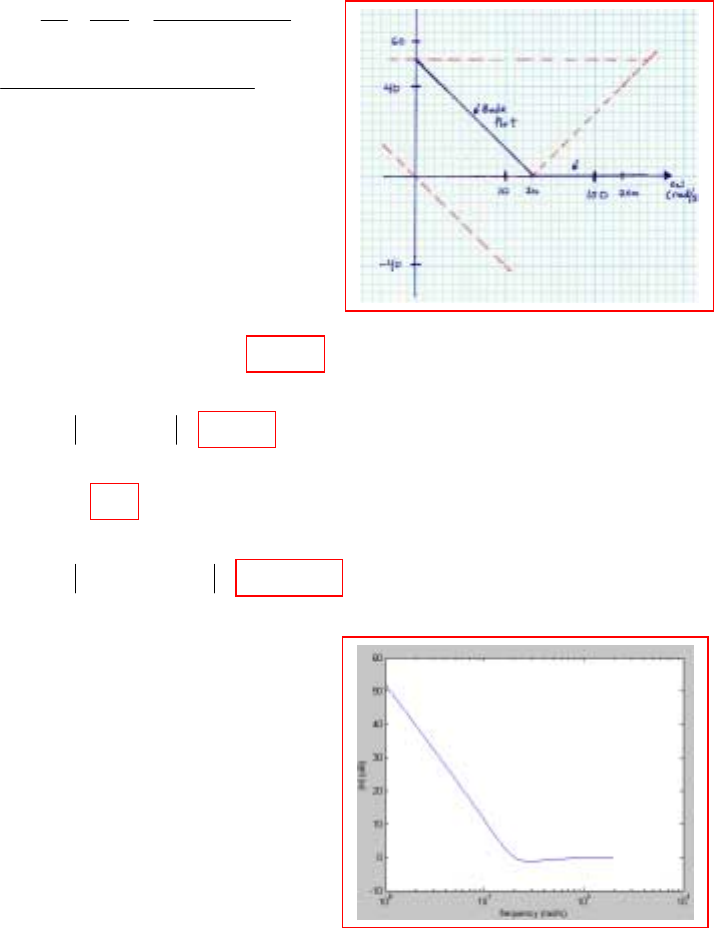
CHAPTER SIXTEEN SOLUTIONS
Engineering Circuit Analysis, 6th Edition Copyright
2002 McGraw-Hill, Inc. All Rights Reserved
42.
(a)
(b)
(c)
2
22
2
2
20 400 20 400
H( ) 1
1 2 0.5( / 20) ( / 20)
400
20, 0.5
20 log 400 52dB
Correction at is 20 log 2 0 dB
o
o
ss
sss s
ss
s
ωζ
ωζ
++
=+ + =
+× +
=
∴= =
=
=
5: H 52 2 20 log 5 24.0dB(plot)
H 20 log 1 16 4 23.8dB (exact)
100: H 0dB (plot)
H 20 log 1 0.04 0.2 0.170 dB (exact)
dB
dB
dB
dB
j
j
ω
ω
==−× =
=−+=
==
=−+=−
Hdb
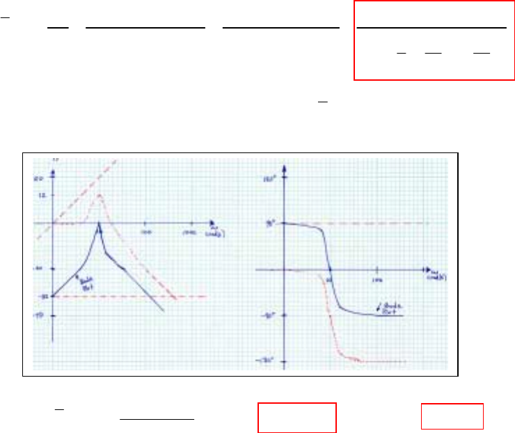
CHAPTER SIXTEEN SOLUTIONS
Engineering Circuit Analysis, 6th Edition Copyright
2002 McGraw-Hill, Inc. All Rights Reserved
43.
(a)
(c) 0.5
20, H( 20) H 15.68 dB H( 20) 80.54
1 4 0.5 dB
j
jj
j
ω
== ∴=−∠=−°
−+
2
2
5
V 25 25 0.025
H( ) V 10 25 1000/ 10 25 1000 1
12
810 10
1
10, 1/8 correction 20 log 2 12 dB
8
0.025 32 dB
== = =
++ + +
++
∴= = ∴ =− ×=
→−
R
o
ss
sssss ss
ωζ
(b)
HdB ang(H)
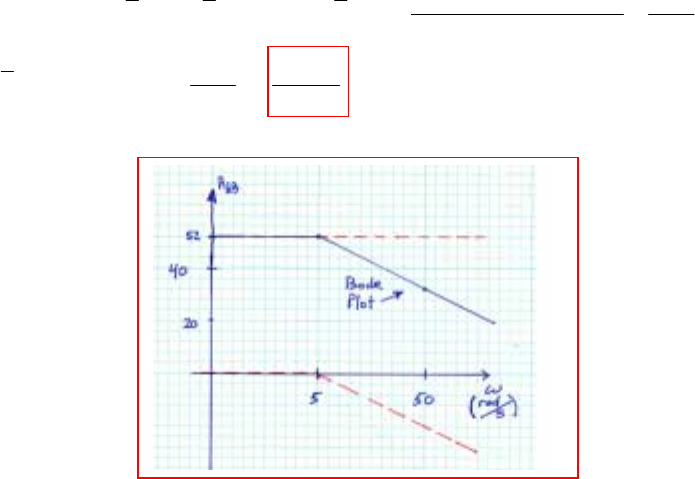
CHAPTER SIXTEEN SOLUTIONS
Engineering Circuit Analysis, 6th Edition Copyright
2002 McGraw-Hill, Inc. All Rights Reserved
44.
36
12 3 36
1/(50 10 10 ) 20
1st two stages, H ( ) H ( ) 10; H ( ) 1/(200 10 10 ) 5
20 400
H( ) ( 10)( 10) 51/5
400 52 dB
ss s
ss
sss
−
−
−×× −
==− = =
+×× +
−−
∴=−− =
++
−→
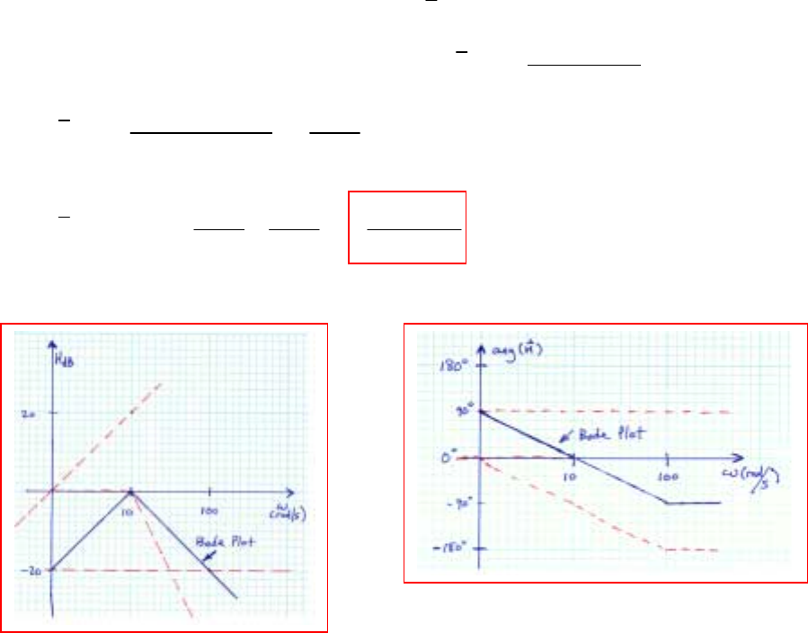
CHAPTER SIXTEEN SOLUTIONS
Engineering Circuit Analysis, 6th Edition Copyright
2002 McGraw-Hill, Inc. All Rights Reserved
45.
(a)
20log10(0.1) = -20 dB
(b) (c)
5
11 1
1
55
1
56
56
1st stage: C 1 F, R , R 10 H (S) R C 0.1
1/R C
2nd stage: R 10 , R 10 , C 1 F H ( ) 1/R C
1/(10 10 ) 10
H() 1/(10 10 ) 10
3rd stage: same as 2nd
1
H( ) ( 0.1 )
AAfA AfAA
BfB
BfBfB B
fB fB
B
ss
ss
sss
ss
µ
µ
−
−
==∞=∴=−=−
−
===∴=
+
×
∴= =−
+× +
−
∴=− 2
0 10 0.1
10 10 (1 /10)
s
ss s
−
=−
++ +
CHAPTER SIXTEEN SOLUTIONS
Engineering Circuit Analysis, 6th Edition Copyright
2002 McGraw-Hill, Inc. All Rights Reserved
46. An amplifier that rejects high-frequency signals is required. There is some ambiguity in
the requirements, as social conversations may include frequencies up to 50 kHz, and
echolocation sounds, which we are asked to filter out, may begin below this value.
Without further information, we decide to set the filter cutoff frequency at 50 kHz to
ensure we do not lose information. However, we note that this decision is not necessarily
the only correct one.
Our input source is a microphone modeled as a sinusoidal voltage source having a peak
amplitude of 15 mV in series with a 1-Ω resistor. Our output device is an earphone
modeled as a 1-kΩ resistor. A voltage of 15 mV from the microphone should correspond
to about 1 V at the earphone according to the specifications, requiring a gain of 1000/15
= 66.7.
If we select a non-inverting op amp topology, we then need 65.7 1- 66.7
1
==
R
Rf
Arbitrarily choosing R1 = 1 kΩ, we then need Rf = 65.7 kΩ. This completes the
amplification part. Next, we need to filter out frequencies greater than 50 kHz.
Placing a capacitor across the microphone terminals will “short out” high frequencies.
We design for
ω
c = 2πfc = 2π(50×103) =
filtermicCR
1. Since Rmic = 1 Ω, we require
Cfilter = 3.183 µF.
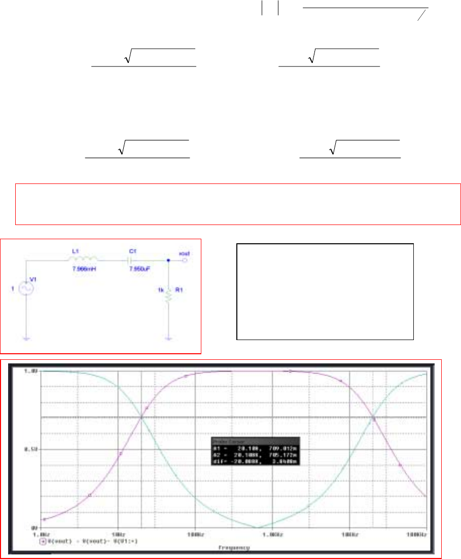
CHAPTER SIXTEEN SOLUTIONS
Engineering Circuit Analysis, 6th Edition Copyright
2002 McGraw-Hill, Inc. All Rights Reserved
47. We choose a simple series RLC circuit. It was shown in the text that the “gain” of the
circuit with the output taken across the resistor is
()
[]
2
1
222
2
2 -1
RC
CRLC
AV
ωω
ω
+
=.
This results in a bandpass filter with corner frequencies at
LC
LCCR-RC
L
c2
4
22 ++
=
ω
and LC
LCCRRC
H
c2
4
22 ++
=
ω
If we take our output across the inductor-capacitor combination instead, we obtain the
opposite curve- i.e. a bandstop filter with the same cutoff frequencies. Thus, we want
2π(20) = LC
LCCR-RC
2
4
22 ++ and 2π(20×103) = LC
LCCRRC
2
4
22 ++
Noting that
H
c
ω
–
L
c
ω
= R/L = 125.5 krad/s, we arbitrarily select R = 1 kΩ, so that L =
7.966 mH. Returning to either cutoff frequency expression, we then find C = 7.950 µF
PSpice verification. The circuit
performs as required, with a
lower corner frequency of about
20 Hz and an upper corner
frequency of about 20 kHz.
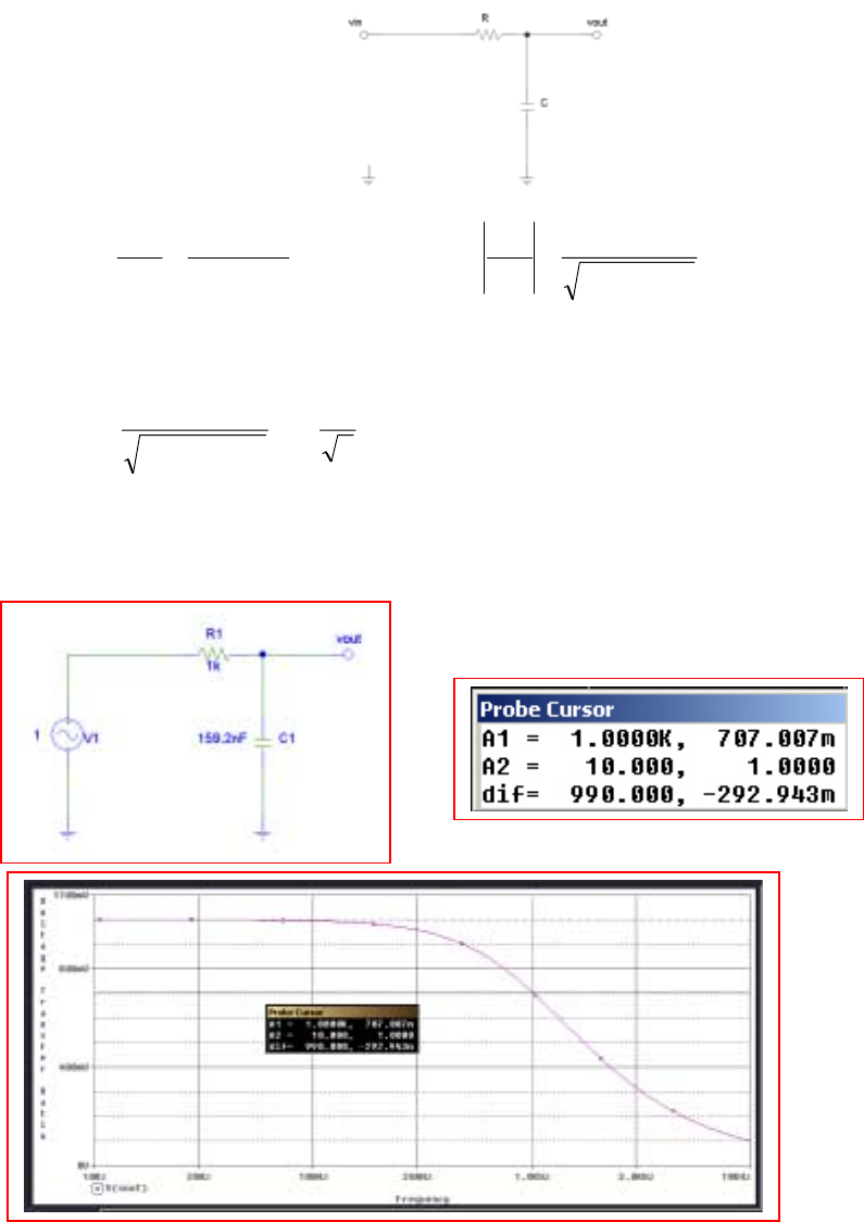
CHAPTER SIXTEEN SOLUTIONS
Engineering Circuit Analysis, 6th Edition Copyright
2002 McGraw-Hill, Inc. All Rights Reserved
48. We choose a simple RC filter topology:
Where RC1
1
V
V
in
out
ω
j+
= and hence
()
2
in
out
RC1
1
V
V
ω
+
=. We desire a cutoff
frequency of 1 kHz, and note that this circuit does indeed act as a low-pass filter (higher
frequency signals lead to the capacitor appearing more and more as a short circuit).
Thus,
()
2
1
RC1
1
2
c
=
+
=
ω
where
ω
c = 2πfc = 2000π rad/s.
A small amount of algebra yields 1 + [2π(1000)RC]2 = 2 or 2000πRC = 1. Arbitrarily
setting R = 1 kΩ, we then find that C = 159.2 nF. The operation of the filter is verified in
the PSpice simulation below:
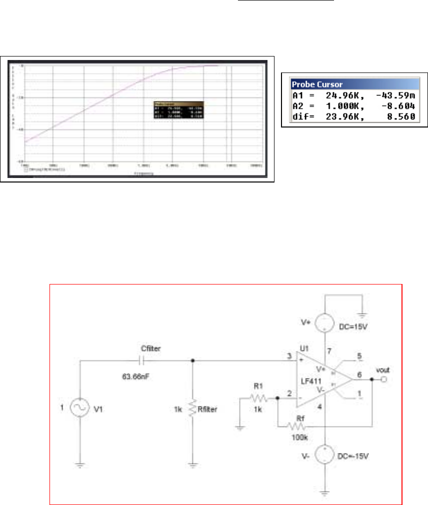
CHAPTER SIXTEEN SOLUTIONS
Engineering Circuit Analysis, 6th Edition Copyright
2002 McGraw-Hill, Inc. All Rights Reserved
49. We are not provided with the actual spectral shape of the noise signal, although the
reduction to 1% of its peak value (a drop of 40 dB) by 1 kHz is useful to know. If we
place a simple high-pass RC filter at the input of an op amp stage, designing for a pole at
2.5 kHz should ensure an essentially flat response above 25 kHz, and a 3 dB reduction at
2.5 kHz. If greater tolerance is required, the 40 dB reduction at 1 kHz allows the pole to
be moved to a frequency even closer to 1 kHz. The PSpice simulation below shows a
filter with R = 1 kΩ (arbitrarily chosen) and C = nF 63.66
)1000)(105.2(2
1
3=
×
π
.
At a frequency of 25 kHz, the filter shows minimal gain reduction, but at 1 kHz any
signal is reduced by more than 8 dB.
We therefore design a simple non-inverting op amp circuit such as the one below, which
with Rf = 100 kΩ and R1 = 1 kΩ, has a gain of 100 V/V. In simulating the circuit, a gain
of approximately 40 dB at 25 kHz was noted, although the gain dropped at higher
frequencies, reaching 37 dB around 80 kHz. Thus, to completely assess the suitability of
design, more information regarding the frequency spectrum of the “failure” signals would
be required.
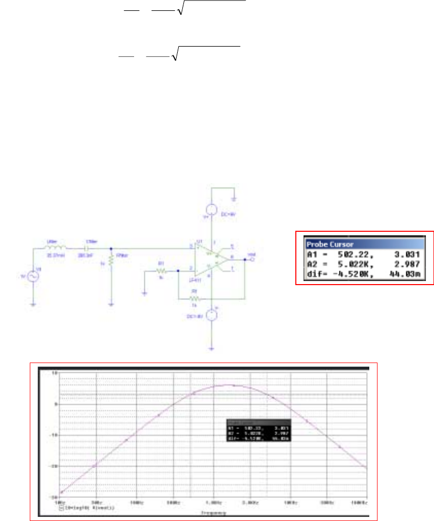
CHAPTER SIXTEEN SOLUTIONS
Engineering Circuit Analysis, 6th Edition Copyright
2002 McGraw-Hill, Inc. All Rights Reserved
50. We select a simple series RLC circuit with the output taken across the resistor to serve as
a bandpass filter with 500 Hz and 5000 Hz cutoff frequencies. From Example 16.12, we
know that
(500)2 4LC CR
2LC
1
2L
R
- 22
πω
=++=
L
c
and
(5000)2 4LC CR
2LC
1
2L
R
22
H
πω
=++=
c
With - LH cc
ωω
= 2p(5000 – 500) = R/L, we (arbitrarily) select R = 1 kΩ, so that L
= 35.37 mH. Substituting these two values into the equation for the high-frequency
cutoff, we find that C = 286.3 nF. We complete the design by selecting R1 = 1 kΩ and Rf
= 1 kΩ for a gain of 2 (no value of gain was specified). As seen in the PSpice simulation
results shown below, the circuit performs as specified at maximum gain (6 dB or 2 V/V),
with cutoff frequencies of approximately 500 and 5000 KHz and a peak gain of 6 dB.
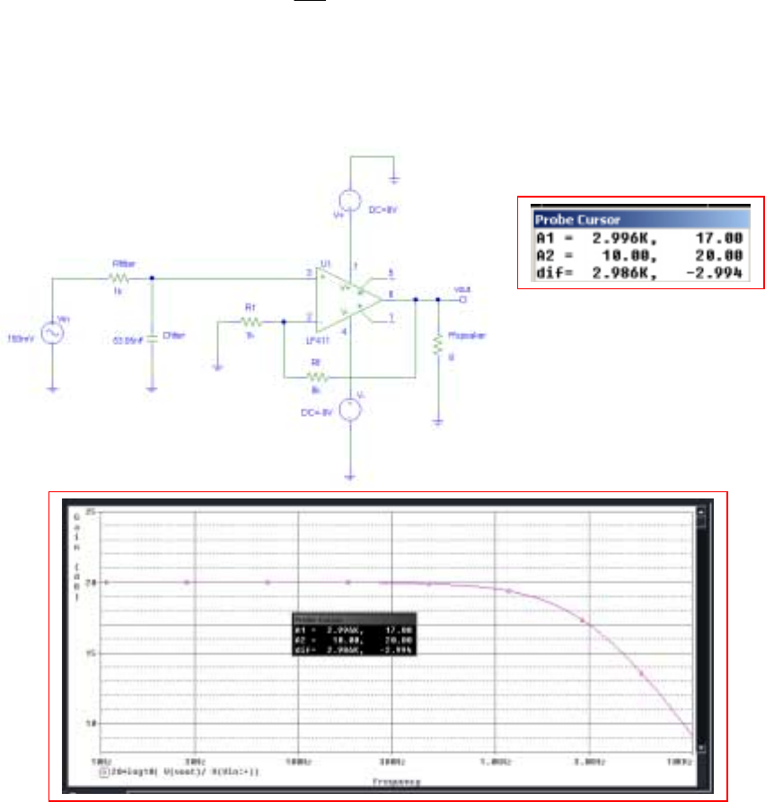
CHAPTER SIXTEEN SOLUTIONS
Engineering Circuit Analysis, 6th Edition Copyright
2002 McGraw-Hill, Inc. All Rights Reserved
51. For this circuit, we simply need to connect a low-pass filter to the input of a non-
inverting op amp having Rf/R1 = 9 (for a gain of 10). If we use a simple RC filter, the
cutoff frequency is
(3000)2
RC
1
πω
==
c
Selecting (arbitrarily) R = 1 kΩ, we find C = 53.05 nF. The PSpice simulation below
shows that our design does indeed have a bandwidth of 3 kHz and a peak gain of 10 V/V
(20 dB).
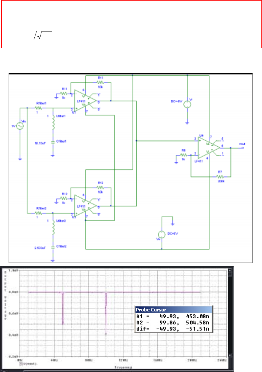
CHAPTER SIXTEEN SOLUTIONS
Engineering Circuit Analysis, 6th Edition Copyright
2002 McGraw-Hill, Inc. All Rights Reserved
52. We require four filter stages, and choose to implement the circuit using op amps to isolate each filter sub-
circuit. Selecting a bandwidth of 1 rad/s (no specification was given) and a simple RLC filter as suggested
in the problem statement, a resistance value of 1 Ω leads to an inductor value of 1 H (bandwidth for this
type of filter =
ω
H –
ω
L = R/L). The capacitance is found by designing each filter’s respective resonant
frequency ( LC1) at the desired “notch” frequency. Thus, we require CF1 = 10.13 µF, CF2 = 2.533 µF,
CF3 = 1.126 µF and CF4 = 633.3 nF.
The Student Version of PSpice® will not permit more than 64 nodes, so that the total solution must be
simulated in two parts. The half with the filters for notching out 50 and 100 Hz components is shown
below; an additional two op amp stages are required to complete the design.
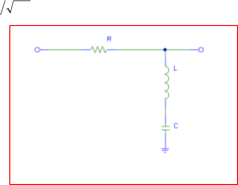
CHAPTER SIXTEEN SOLUTIONS
Engineering Circuit Analysis, 6th Edition Copyright
2002 McGraw-Hill, Inc. All Rights Reserved
53. Using the series RLC circuit suggested, we decide to design for a bandwidth of 1 rad/ s
(as no specification was provided). With
ω
H –
ω
L = R/ L, we arbitrarily select R = 1 Ω so
that L = 1 H. The capacitance required is obtained by setting the resonant frequency of
the circuit ( LC1) equal to 60 Hz (120π rad/s). This yields C = 7.04 µF.
1 H
1 Ω
7.04 µF
vin vout
CHAPTER SEVENTEEN (TWO-PORT) SOLUTIONS
Engineering Circuit Analysis, 6th Edition Copyright
2002 McGraw-Hill, Inc. All Rights Reserved
1.
3
17 8 3
8 17 4 17(273) 8( 148) 3(83) 3208
3417
−−
∆=− −= + − − = Ω
−−
Z
(a) 2
11
11
3208 100
Z 11.751 P 851.0 W
273 11.751
∆
== = Ω∴= =
∆Z
in
(b) 2
22
22
3208 100
Z 11.457 P 872.8 W
280 11.457
∆
== = Ω∴= =
∆Z
in
(c) 2
33
33
3208 100
Z 14.258 P 701.4
225 14.258
∆
== = Ω∴= = Ω
∆Z
in
CHAPTER SEVENTEEN (TWO-PORT) SOLUTIONS
Engineering Circuit Analysis, 6th Edition Copyright
2002 McGraw-Hill, Inc. All Rights Reserved
2.
3
0.35 0.1 0.2
0.1 0.5 0.15 0.35(0.3525) 0.1( 0.105) 0.2(0.115) 0.089875 S
0.2 0.15 0.75
−−
∆=− − = + − − =
−−
Y
(a) 2
11
11
0.089875 10
Y 0.254965 P 392.2 W
0.3525 0.254965
Y
in
∆
== = ∴= =
∆
(b) 2
22
22
0.089875 10
Y 0.403933 P 247.6 W
0.2225 0.403933
Y
in
∆
== = ∴= =
∆
(c) 33
0.089875 100
Y 0.544697 S P 183.59 W
0.165 0.544697
in == ∴==
CHAPTER SEVENTEEN (TWO-PORT) SOLUTIONS
Engineering Circuit Analysis, 6th Edition Copyright
2002 McGraw-Hill, Inc. All Rights Reserved
3.
4
11
3120 413 120 120
14 13
[R] ()325212522413
22 52 326 326 326
0326
3[4(34) 2(12) 3( 13)] [ 1(34) 2( 12) 3( 4)] 2[ 1(12) 4( 12) 3( 6)]
161
3(73) ( 22) 2(18) 161 R 2.205
73
R
in +
−−
−− −−
−
=Ω=+−
−−− −− −−
−−
= − −− +− −− −− =− −− −−
∆
=+−−=Ω∴=== Ω
∆
CHAPTER SEVENTEEN (TWO-PORT) SOLUTIONS
Engineering Circuit Analysis, 6th Edition Copyright
2002 McGraw-Hill, Inc. All Rights Reserved
4. Define a counter-clockwise current I2 in the left-most mesh, and a counter-clockwise
current I1 flowing in the right-most mesh. Then,
12 1 2
11 22 12
2122
12
2
11
2
V 4I 0.2V 0.8I
V I 5( I 0.8 I I ) ( 5) I I
Also, I (2 4) 5(I 0.8I I ) 0
or 0 5I (5 2 )I
( 5)(5 2 ) 5 2 15 20, 5 2
21520
Z25
in
Z
th
ss
s
s
ssss s
ss
s
=∴ =
=+ + −=+ −
+− + − =
=− + +
∴∆ = + + − = + + ∆ = +
++
∴= +
CHAPTER SEVENTEEN (TWO-PORT) SOLUTIONS
Engineering Circuit Analysis, 6th Edition Copyright
2002 McGraw-Hill, Inc. All Rights Reserved
5. Define a clockwise mesh current I1 flowing in the bottom left mesh, a clockwise mesh
current I2 flowing in the top mesh, and a clockwise mesh current I3 flowing in the
bottom right mesh. Then,
(a)
(b)
12 2 1 2
213 1 23
232 23
V 10(I I ) 0.6 8I 10I 14.8I
0 50I 10I 12I 10I 50I 12I
0 4.8I 17I 12I 7.2I 17I
10 14.8 0 5120
10 50 12 10(763.6) 10( 251.6) 5120 Z 6.705
763.6
0 7.2 17
in
Zin +
=−−×=−
=−−=−+−
=+−=−+
−
∴∆ = − − = + − = ∴ = = Ω
−
112 12
221 2 12
21 12
V 0.6VVV
I 0.13571 V 0.03571V 0.06V
28 10
V 0.6VVV V
0 0.03571V 0.31905V 0.05V
28 12 5
V VVV
0 0.05V 0.05V 0.175V
820
0.13571 0.03571 0.06
0.03571 0.31905 0.05
0.05 0.05 0.1
x
in x
xx
xx x
y−
−−
=+ = − −
−−
=+ +=− + −
−−
=− + =− + −
−−
∴∆ = − −
−−
11
11
0.13571( 0.05583 0.0025) 0.03571(0.00625 0.003)
75
0.05(0.00179 0.01914) 0.00724
0.007954
0.007954, 0.05333 Y 0.14926 S
0.05333
1
Z 6.705
0.14926
y
ym
in +
=−++ +
−+=−
∆−
∴∆ = ∆ =− ∴ = = =
∆−
∴= = Ω
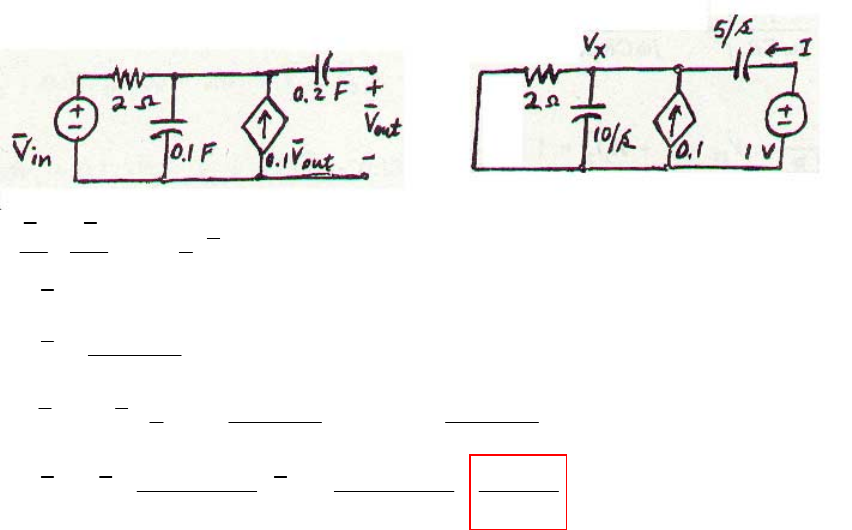
CHAPTER SEVENTEEN (TWO-PORT) SOLUTIONS
Engineering Circuit Analysis, 6th Edition Copyright
2002 McGraw-Hill, Inc. All Rights Reserved
6.
VV
0.1 (V 1) 0
210 5
V (0.5 0.3 ) 0.1 0.2
0.2 0.1
V0.3 0.5
0.2 0.1 0.1 0.4
I (1 V ) 1 0.2 0.2
5 0.3 0.5 0.3 0.5
(0.1 0.4) 1.5 2.5 15 25
YI ,Z
1.5 2.5 (0.1 0.4) ( 4)
xx x
x
x
x
out out
ss
ss
s
s
ss s
ss
ss
ss s s
sssss
+−+ −=
∴+=+
+
∴= +
++
∴= − = − =
++
+++
∴== = =
+++
CHAPTER SEVENTEEN (TWO-PORT) SOLUTIONS
Engineering Circuit Analysis, 6th Edition Copyright
2002 McGraw-Hill, Inc. All Rights Reserved
7.
44
V 1 V, V 0 V V 0, V 1 V
V1
I ;210I 210I 0
RR
1
II R V/I
R
in i x in x
x
xinx
xx
inx inininx
x
R
==∴+==−
==− × +× =
∴=−= ∴ =− =−
CHAPTER SEVENTEEN (TWO-PORT) SOLUTIONS
Engineering Circuit Analysis, 6th Edition Copyright
2002 McGraw-Hill, Inc. All Rights Reserved
8.
(a) Assume 1 V at input. Since Vi = 0 at each op-amp input, 1 V is present between R2 and
R3, and also C and R4.
44
44
3
3434
2
23 12 22
34 34
13412 2
1
1134 2
11 1
VR 1
RCCR
11 1
I11
RCRCRR
1R
II V1RI1
CR R CR R
RRR1V R 1
IIZC
RCRRR I R
∴= + =+
∴= −− =−
∴==− ∴ =+ =−
−
== =∴==
in in
in
jj
jj
jj
j
j
ωω
ωω
ωω
ω
ω
(b)
333310
1234
10 6 3
R410, R1010, R1010, R10, C210
4101
Z 2 10 10 0.8 10 (L 0.8 mH)
10
−
−
=× = × = × = =×
××
∴= × × = ×Ω =
in in
jj
ωω
CHAPTER SEVENTEEN (TWO-PORT) SOLUTIONS
Engineering Circuit Analysis, 6th Edition Copyright
2002 McGraw-Hill, Inc. All Rights Reserved
9. Define a clockwise mesh current I1 in the left-most mesh, a clockwise mesh current Ix in
the center mesh, and a counter-clockwise mesh current I2 in the right-most mesh. Then,
112
1
2
121
22
12
112
11 12
V 13I 10I
V100
03520
V2022
0 10I 35I 20I I 13 10 0
10 35 20
02022
V 20I 22I
V (370) V ( 200) 37 20
I V V
13(370) 10( 220) 261 261
37 20
141.76 mS, 76.63 mS
261 261
=−
−
=− + + ∴ = −
−
=+
+−
∴= = −
+−
−
∴= = = =−
x
x
yy
CHAPTER SEVENTEEN (TWO-PORT) SOLUTIONS
Engineering Circuit Analysis, 6th Edition Copyright
2002 McGraw-Hill, Inc. All Rights Reserved
10.
11 2
212 112 2
12112
2212 2121
11
10 5
[ ] (mS) I 0.01V 0.005V ,
50 20
I 0.05V 0.02V , 100 25I V , V 100I
100 0.25V 0.125V V 1.25V 0.125V
5
I 0.01V 0.05V 0.02V 0.03V 0.05V V V
3
0.625 4.375
100 1.25V V V
32
y−
=∴=−
=+ =+=−
∴= − += −
=− = + ∴− = ∴ =−
∴= + = 11 2 1
300 5
V 68.57 V, V V 114.29 V
4.375 3
∴= = =− =−
CHAPTER SEVENTEEN (TWO-PORT) SOLUTIONS
Engineering Circuit Analysis, 6th Edition Copyright
2002 McGraw-Hill, Inc. All Rights Reserved
11.
12
112
2
21 11 2 1 2
11 12 21 22
VV
I 0.04V 0.04V
25
V
I 2I I I 0.01V 0.04V 0.03V
100
0.04S, 0.04S, 0.04S, 0.03 Syy y y
−
==−
= + −=+ = −
∴= =− = =−
CHAPTER SEVENTEEN (TWO-PORT) SOLUTIONS
Engineering Circuit Analysis, 6th Edition Copyright
2002 McGraw-Hill, Inc. All Rights Reserved
12.
111 1 1
22 21 12
21 22 1 2
V 100(I 0.5I ) 50I I 0.02 V
V 300I 200(I 0.5I ) 100I 500I
V 2V 500I , I 0.004V 0.002V
0.02 0
[] (S)
0.004 0.002
y
∴= − = ∴=
=+ +=+
∴= + =− +
∴=
−
CHAPTER SEVENTEEN (TWO-PORT) SOLUTIONS
Engineering Circuit Analysis, 6th Edition Copyright
2002 McGraw-Hill, Inc. All Rights Reserved
13.
0.1 0.0025
[] (S)
8 0.05
y−
=
−
(a)
(b)
11 221 2
122
2212 2121
21 111 12 11 1
21 11
I 0.1V 0.0025V , I 8V 0.05V
1 2I V, V 5I
I 0.2V 8V 0.05V 0.25V 8V , V / V 32
I 8V 0.05 32V , I 0.1V 0.0025 32V I 6.4V , I 0.02V
6.4
I / I 320, V / I 50
0.02
=− =−+
=+ =−
∴=− =− + ∴ = =
=− + × = − × ∴ =− =
−
∴==− =Ω
111 1 22 1 2
111 21 2
12 2 2 2 2
2
2
V 2I , I 0.1V 0.0025V , I 8V 0.05V
I 0.5V 0.1V 0.0025V 0.6V 0.0025V
11
V V / 240, I 8 V / 240 V V
20 60
V60
I
=− = − =− +
∴=− = − ∴ =
∴= =−× + =
∴=Ω
CHAPTER SEVENTEEN (TWO-PORT) SOLUTIONS
Engineering Circuit Analysis, 6th Edition Copyright
2002 McGraw-Hill, Inc. All Rights Reserved
14. 10 5
[] (mS)
20 2
y−
=
−
(a)
(b)
11 22 1 2
111
111 121 2
212 22 2
I 0.01V 0.005V , I 0.02V 0.002V
V100IV
V V1 100I I 0.01V1 I 0.005V I 0.005V1 0.0025V
I 0.02V1 2I 0.002V 0.02V1 0.01V1 0.005V 0.002V 0.01V1 0.003V
0.005 0.0025
[] 0.01 0.0
new
y
=− =−+
′=+
∴= − ∴= −− ∴= −
=− + + =− + − + =− −
−
∴=
−− (S)
03
22 2 2
21 2
21 21
11 2 1 1
11 2
V2 100I V , V V2 100I
I 0.02V 0.002V2 0.2I
11
1.2I 0.02V 0.002V2 I V V2
60 600
11
I 0.01V 0.005(V2 100I ) 0.01V 0.005V2 0.5 V V2
60 600
11 1 1
I V V
100 120 200 1200
=+∴=−
∴=− + −
∴=− + ∴=− +
=− −=− +−+
∴= − − −
12
11
V V
600 240
=−
1/ 600 1/ 240
[] (S)
1/ 60 1/ 600
new
y−
∴=
−
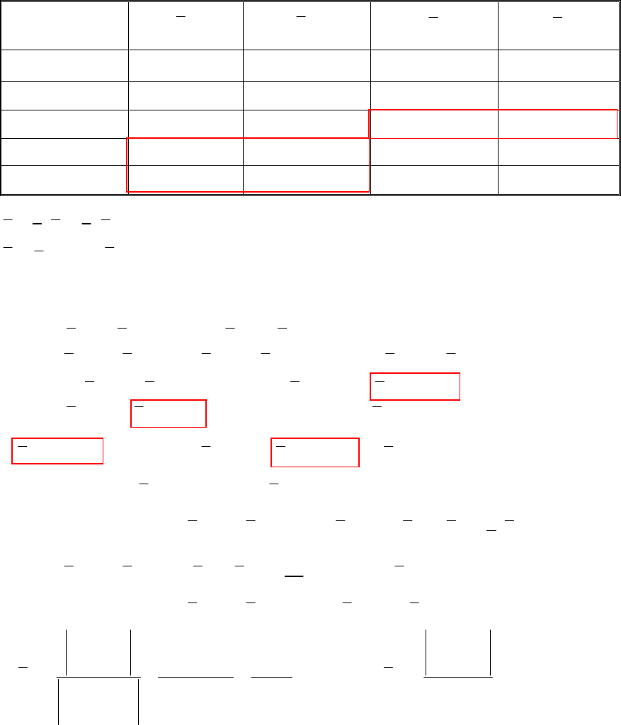
CHAPTER SEVENTEEN (TWO-PORT) SOLUTIONS
Engineering Circuit Analysis, 6th Edition Copyright
2002 McGraw-Hill, Inc. All Rights Reserved
15.
1
VS 2
VS 1
I 2
I
Exp #1 100 V 50 V 5 A -32.5 A
Exp #2 50 110 -20 -5
Exp #3 20 0 4 -8
Exp #4 -8.333 -22.22 5 0
Exp #5 -58.33 -55.56 5 15
1 11 1 12 2
2 21 1 22 2
11 12 21 22
11 12, 21 22 21 22
11 12 12 12
IVV
IVV
Use 1st 2 rows to find y's
5 100 50 , 32.5 100 50
20 50 100 5 50 100 10 100 200
40 100 200 Substracting, 150 45 0.3 S
5 100
=+
=+
∴= + − = +
−= + −= + →∴−= +
∴− = + =− ∴ =−
∴=
yy
yy
yy yy
yy yy y y
yy y y
y11 11 22
22 21 21
12
12
15 0.2 S Subtracting 22.5 150
0.2 0.3
0.15 S 32.5 100 7.5 0.4 S [ ] (S)
0.4 0.15
Completing row 3: I 0.2 20 4 A, I 0.4 20 8 A
Completing row 4: 5 0.2V 0.3V , 0 0
−∴ = =
−
∴= ∴− = +∴=− ∴=
−
=×= =−×=−
=− =−
SS
yy
yyyy
1221
11 11 2
12 1 2
1
8
.4V 0.15V V V
3
50
5 0.2V 0.8V 0.6V V 8.333 V, V 22.22 V
6
Completing row 5: 5 0.2V 0.3V , 15 0.4V 0.15V
5 0.3
15 0.15 0.75 4.5 5.25
V 58.33
0.2 0.3 0.03 0.12 0.09
0.4 0.15
+∴=
∴ = − =− ∴ =− =− =−
=− =−+
−
+
∴= = = =−
−−−
−
SSSS
SS SS S
SS S S
S2
0.2 5
0.4 15
V, V 55.56 V
0.09
−
==−
−
S
CHAPTER SEVENTEEN (TWO-PORT) SOLUTIONS
Engineering Circuit Analysis, 6th Edition Copyright
2002 McGraw-Hill, Inc. All Rights Reserved
16.
1
2
61 63 31
:1 6 3 10 0.6, 1.8, 0.3
10 10 10
51 14 54
: 5 1 4 10 0.5, 0.4, 2
10 10 10
1.8 2 0.5 4.3 , 0.3 0.6 0.4 1.3
1.3 4.3 0.99821 , 0.9982 0.6 2 3.598
3.598 6 2.249
×××
∆++=Ω→ = = =
×× ×
∆++=Ω→ = = =
++ = Ω + + = Ω
=Ω++=Ω
=Ω
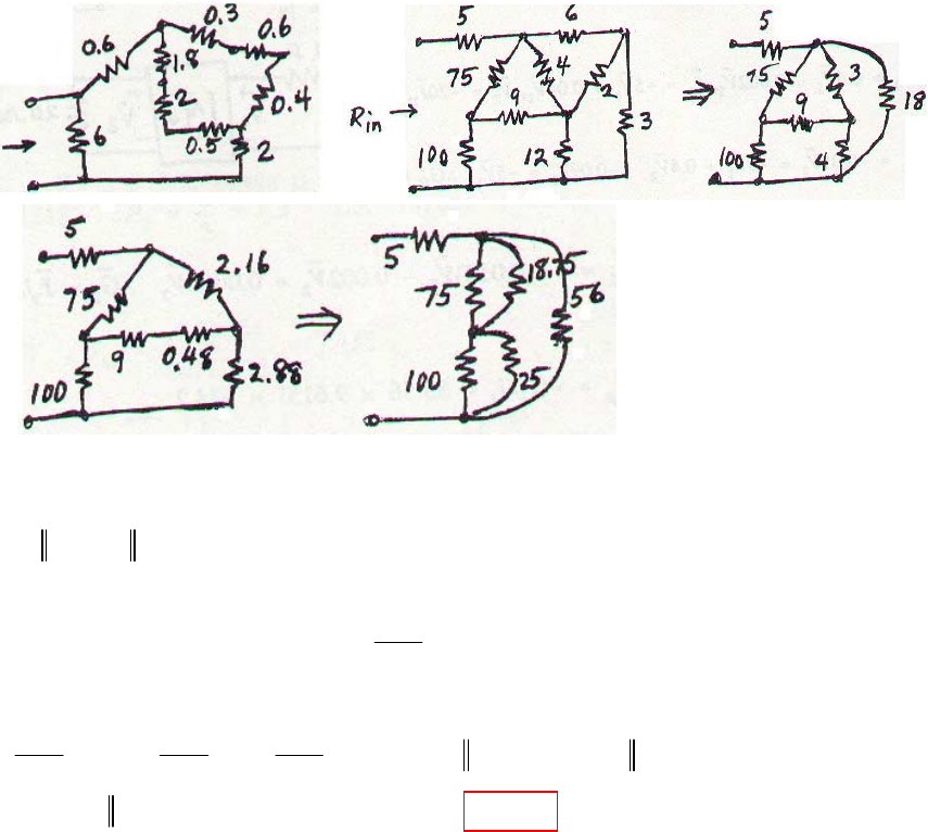
CHAPTER SEVENTEEN (TWO-PORT) SOLUTIONS
Engineering Circuit Analysis, 6th Edition Copyright
2002 McGraw-Hill, Inc. All Rights Reserved
17.
2
2
622336 36
36/ 6 6, 36/ 2 18, 36 / 3 12
12 4 3, 6 12 4
4 3 18 25
43
3 18/ 25 2.16, 4 18/ 25 2.88, 0.48
25
9.48 2.16 9.48 2.88 2.88 2.16 54
54 54 54
18.75, 25, 5.6962, 75 18.75 15, 100 25 20
2.88 2.16 9.48
(15 20) 5.696 4.
×+×+×= Ω
== =
==
++ = Ω
×
×= ×= =
×+×+×=Ω
=== ==
+=899 R 5 4.899 9.899
in
∴=+ = Ω
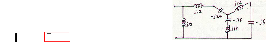
CHAPTER SEVENTEEN (TWO-PORT) SOLUTIONS
Engineering Circuit Analysis, 6th Edition Copyright
2002 McGraw-Hill, Inc. All Rights Reserved
18.
:6 431
24 12 18
24, 12, 18, 18 18 0(S.C)
111
ignore 12, 6
24 12 12
12 12 Z
∆−++=
−
=− = =− − =
∴−
−+=−
−=∞∴=∞
in
jjjj
jjjjj
jjj
jj
jj j
jj
CHAPTER SEVENTEEN (TWO-PORT) SOLUTIONS
Engineering Circuit Analysis, 6th Edition Copyright
2002 McGraw-Hill, Inc. All Rights Reserved
19. 0.4 0.002
[] (S)
5 0.04
y−
=
−
(a)
(b) 2
122221
2
0.05V
I 0.4(0.018)V 0.002V 0.0052V G I / I 9.615
0.0052V
I+
−
=−=∴===−
(c) G G G 55.56 9.615 534.2
pVI +
=− = × =
(d) 12 111
1
I 0.0052V 0.0052 55.56V Z V / I 3.462
0.0052 55.56
in
==×∴== =Ω
×
(e)
11 221 22 2 11
2212 21 21
I 0.4V 0.002V , I 5V 0.04V ,V 20I , V V 2I
500
I 0.05V 5V 0.4V 0.09V 5V G V / V 55.56
9
S
V
=− =−+ =− =+
=− =− + ∴− =− ∴ = = =
11 1 1 1 21 2
222222
0.002
V 2I , V 0 I 0.5V 0.4V 0.002V V V
0.9
0.002
I 5 V 0.04V 0.02889V Z V / I 34.62
0.9
S
out
=− = ∴ =− = − ∴ =
=− + = ∴ = = Ω
CHAPTER SEVENTEEN (TWO-PORT) SOLUTIONS
Engineering Circuit Analysis, 6th Edition Copyright
2002 McGraw-Hill, Inc. All Rights Reserved
20. 0.1 0.05
[] (S)
0.5 0.2
y−
=
−
(a)
(b) 1
21
1
( 0.5 0.2 1.25)V
G I / I 6.667
(0.1 0.005 1.25)V
I
−+×
== =−
−×
(c) G 1.25 6.667 8.333
P=× =
(d) 1111
I (0.1 0.05 1.25)V Z V / I 26.67
in
=−× ∴= = Ω
(e)
(f) ,12
G V / V 0.25
Vrev==
(g)
11 2
2121122
212 21
I 0.1V 0.05V
I 0.5V 0.2V , 1 10I V , I 0.2V
0.2V 0.5V 0.2V G V / V 1.25
V
=−
=− + = + =−
∴− =− + ∴ = =
111 11 2
122 22 2 22
V 0, V 10I I 0.1V 0.1V 0.05V
V 0.25V , I 0.05(0.25V ) 0.2V 0.075V Z V / I 13.333
==−∴=−=−
∴= ∴=− + = ∴ = + Ω
S
out
11
22
11 2 2
2
With 2 port: 1 10I 26.67I
6.667 1
1 36.67 I , I 1/ 36.67 I 0.15182 P I 5 2.5(0.15182) 0.08264 W
36.67 2
1 1 0.08264
Without 2 port: P 5 0.011111 W G 7.438
2 15 0.011111
L
Lins
=+
−
∴= = ∴ = =− ∴ = × = =
=×= ∴= =
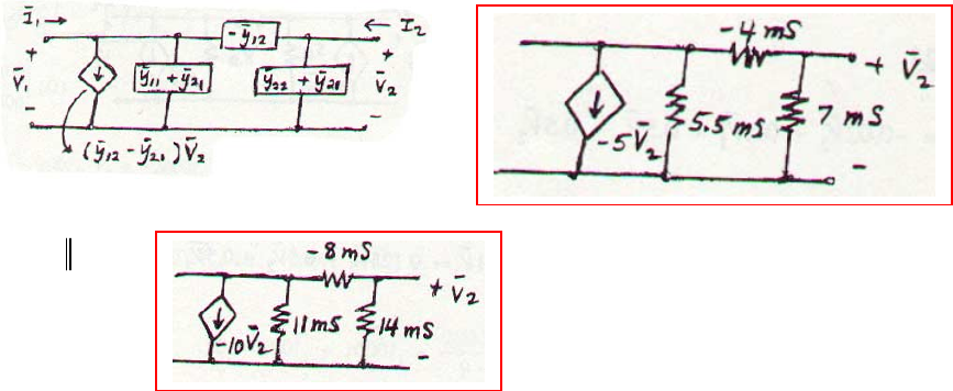
CHAPTER SEVENTEEN (TWO-PORT) SOLUTIONS
Engineering Circuit Analysis, 6th Edition Copyright
2002 McGraw-Hill, Inc. All Rights Reserved
21.
(a)
(b) 2 in :
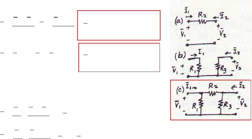
CHAPTER SEVENTEEN (TWO-PORT) SOLUTIONS
Engineering Circuit Analysis, 6th Edition Copyright
2002 McGraw-Hill, Inc. All Rights Reserved
22.
(a) 22
12 21
12
22
22
1/R 1/R
VV VV
I, I []
1/R 1/R
RR
a
y−
−−
== =
−
(b) 1
1112 23
3
1/R 0
I V /R , I V /R [ ] 01/R
B
y
==∴=
(c)
12 2
112
1
232
12
12 2
221
2
232
32
1/R 1/R 1/R
VVV
I[]
1/R 1/R 1/R
RR
1/R 1/R 1/R
VVV
I,[][]
1/R 1/R 1/R
RR ab
y
yy
+−
−
=+ ∴=
−+
+−
−
=+ + =
−+
CHAPTER SEVENTEEN (TWO-PORT) SOLUTIONS
Engineering Circuit Analysis, 6th Edition Copyright
2002 McGraw-Hill, Inc. All Rights Reserved
23.
11 2 2 1 1
22 12 1 1 1
21111
112122121
212
V 8I 0.1V V 10V 80I
1
I V /12 0.05V I (10V 80I ) 0.05V
12
5 1 20 53 20
I V I V I
6 20 3 60 3
60 20 400 60 4000 600
V III IV I I80I
53 3 53 53 53 53
7
240 600
V I I[]
53 53 z
=+ ∴= −
=+ ∴= −+
∴= + − = −
∴= + = + ∴= + −
∴=− + ∴=.547 1.1321 ()
4.528 11.321
Ω
−

CHAPTER SEVENTEEN (TWO-PORT) SOLUTIONS
Engineering Circuit Analysis, 6th Edition Copyright
2002 McGraw-Hill, Inc. All Rights Reserved
24.
(a)
(b) 2
12
1
V 1.7429 3.050
I I 1 A 0.9607
V 2.723 2.266
+
== ∴ = =
+
12112
11 221 221
21 2
1 1
2 2
12
1122
12
2
I 0.02V 0.2V 0.5V 0.5V
I 0.7V 0.52V I 0.1V 0.125V 0.5V 0.5V
I 0.4V 0.625V
I 0.52 0.7 I
I 0.625 0.4 I
0.625I 0.52I
V 2.723I 2.266I , V
0.7 0.52 0.2295 0.2295
0.4 0.625
0.4I 0.7 I
V0.
=− + + −
∴= − = + + −
∴=− +
−
−
+
∴= = = + =
−
−
+
∴= 12
2.723 2.266
1.7429I 3.050I [ ] ( )
1.7429 3.050
2295 z
=+∴= Ω
CHAPTER SEVENTEEN (TWO-PORT) SOLUTIONS
Engineering Circuit Analysis, 6th Edition Copyright
2002 McGraw-Hill, Inc. All Rights Reserved
25. 4 1.5
[ ] ( ), R 5 , R 2
10 3 SL
z
=Ω=Ω=Ω
(a) 11 22 122 2 2 121
V 4I 1.5I , V 10I 3I , V 2I 10I 3I G I / I 2= + = + =− = + ∴ = =−
(b) 11
21
1
10I 6I
GV/V 4
4I 3I
v
−
== =
−
(c) GGG8=− =
pVI
(d) 1
1111
1
V
V4I3II Z 1
I
in
=−=∴==Ω
(e) 11121 22 22 2
1108
V 5I 4I 1.5I I I V I 3I I Z 1.3333
666
out
=− = + ∴ =− ∴ =− + = ∴ = Ω
CHAPTER SEVENTEEN (TWO-PORT) SOLUTIONS
Engineering Circuit Analysis, 6th Edition Copyright
2002 McGraw-Hill, Inc. All Rights Reserved
26. 1000 100
[] ( )
2000 400
z
=Ω
−
(a)
(b) 26
500
P 15.625 500 10 122.07 mW
−
=××=
(c)
1122 12 112 2
21221 111
26
1 2 1 200
V 1000I 100I , V 2000I 400I , 10 200I V ,V 500I
20 2000
500I 2000I 400I , I I ; 10 200I 1000I I
99
20
I 7.031 mA, I I 15.625 mA P 7.031 200 10 9.888 mW
9
−
=+ =−+ =+=−
∴− =− + = ∴ = + +
∴= ∴= = ∴ = × × =
1 2 200 500
P 10I 70.31 mW(gen) P P P P 70.31 9.89 122.07
S port S
== ∴ =−−= −− ∴
2
P61.65 mW
port −
∴
=−
CHAPTER SEVENTEEN (TWO-PORT) SOLUTIONS
Engineering Circuit Analysis, 6th Edition Copyright
2002 McGraw-Hill, Inc. All Rights Reserved
27.
85 4 4
11 1 12
54 4
112
44
221 21
444
212
4
1
44 4
2
1544
24 44
10 , I 10 V 5 10 V 10 (V V )
I (10 6 10 ) V 10 V
I 10 V 0.01V 10 (V V )
I (0.01 10 ) V (10 10 )V
I10
I10 10 (10
V10 6 10 10
10 10 10 10
−−−
−− −
−−
−−−
−
−− −
−−−
−− −−
==+×+ −
∴= + × −
=++ −
∴= − + +
−
++
∴= =
+× −
−+
jj
jj
j
jj
j
j
jj
j
ω
44
11
12
6
12
54
1
24 21
2
2622
133.15 47.64
10 )I 10 I
1.0621 10 92.640 94.15 2.642
10 6 10 I
9416 86.78
10 10 I
V565.0 3.60
1.0621 10 92.64
−
−−
−+
−−
−−
−
∴= ∠− °Ω
+
×∠ =∠−°Ω
+×
∴= ∠ °Ω
−
==∠−°Ω
×∠ °
z
jj
z
j
z
j
z
CHAPTER SEVENTEEN (TWO-PORT) SOLUTIONS
Engineering Circuit Analysis, 6th Edition Copyright
2002 McGraw-Hill, Inc. All Rights Reserved
28.
111 1 2 1 2
2121 22 2 22
222 2 2
20 2
[ ] ( ), V 100 0 V, R 5 , R 25
40 10
100 5I V , V 20I 2I 100 25I 2I
1 1 25 25
V 40I 10I I V I 100 V I 2I
40 4 40 4
517 817
100 V I V 160 I 160 6.8I
84 54
V 160 V, R 6.8
SSL
th th
z
=Ω=∠°=Ω=Ω
=+ = + ∴ = +
=+ ∴= − ∴= − +
∴= − ∴=+× =+
∴= =Ω
CHAPTER SEVENTEEN (TWO-PORT) SOLUTIONS
Engineering Circuit Analysis, 6th Edition Copyright
2002 McGraw-Hill, Inc. All Rights Reserved
29. 92
[] 20 0.2 S
hΩ−
=
(a)
(b)
11 22 1 2111 1
111 11 1 21 2
V 9I 2V , I 20I 0.2V , V 1I V Eliminate V
10 2
VV I V I9I2V, V10I2V [] 20 0.2 S
new
h
′
=− = + =+
Ω−
′′ ′
∴= −∴−= − = − ∴ =
11 22 1 22 22
2222
11 222 1 2 2 2 1 2
21 2112 1 2
11 2
V 9I 2V, I 20I 0.2V, V 1I V
Eliminate V V V I
V 9I 2V 2I , I 20I 0.2V 0.2I 1.2I 20I 0.2V
I 16.667I 0.16667V V 9I 2V 2(16.667 I 0.1667 V )
V 42.38 I 1.6667V [ ]new
h
′
=− = + =+
′
∴= −
′′
=− + = + − ∴ = +
′′ ′
∴= + = − + +
′
∴= − ∴ 42.33 1.6667
16.667 0.16667 S
Ω−
=
CHAPTER SEVENTEEN (TWO-PORT) SOLUTIONS
Engineering Circuit Analysis, 6th Edition Copyright
2002 McGraw-Hill, Inc. All Rights Reserved
30.
11 221 212 21
11 1 1
11121 2
2
100 0.01
R 100 , R 500 [ ] 20 1 mS
Z : V 100I 0.01V , I 20I 0.001V 20I 0.5I 1.5I 20I
20
V 100I 0.01( 500) I 33.33I Z 33.33
1.5
0.01
Z : V 100I 100I 0.01V I V
200
0.01
I202
Ω
=Ω =Ω =
= + =+ =− ∴=
∴= + − = ∴ = Ω
=− = + ∴ =−
=−
SL
in
in
out
h
22
V 0.001 I 0 Z
00
+=∴=∞
out
CHAPTER SEVENTEEN (TWO-PORT) SOLUTIONS
Engineering Circuit Analysis, 6th Edition Copyright
2002 McGraw-Hill, Inc. All Rights Reserved
31.
(a)
(b)
1
1
12 12
20
V 1.2
From above, 9.6
I 0.125
I
zz
=
===Ω
(c)
1
12 1 2 0 2
10 1 4 2
22 22
112
V / V | Let V 1 V
I 0.1 A, I 0 I 0.2I
0.1 I 0.2 I 0.8I , I 0.125 A
V 0.3 4(0.2)(0.125) 1 1.2 V 1.2
I
h
h
=
Ω
==
∴↓= =∴ ←=
∴=− = =
∴= − += ∴=
1
12 1 2 2
0
21
112
I / V SC input Let V 1 V
1.3 1.3
I 0.1 0.425 A, I 0.2(0.425)
44
I 0.24 A 0.24 S
V
y
y
=
==
=+= = −
∴=− ∴ =
CHAPTER SEVENTEEN (TWO-PORT) SOLUTIONS
Engineering Circuit Analysis, 6th Edition Copyright
2002 McGraw-Hill, Inc. All Rights Reserved
32. 1000 1
[] 4 500 S
h
µ
Ω−
=
(a)
(b) 2
3
21
4000 68.97
V 25.86 10 68.97 V P 4.756 W
1.5 1000
K
−
=××= ∴= =
(c)
112 12
43 3
21 2 2 1 2
21 111
26
200
100 200 I 1000I V 1200I V
I 4I 5 10 V 10 V 4I 1.5 10 V
4000 4000
V I 100 1200I I I 25.86 mA
1.5 1.5
P 25.86 10 200 133.77 mW
−− −
−
=+−=−
=+× =− ∴=−×
∴=− ∴ = + ∴=
∴= ××=
3
2
P 100 25.86 10 2.586 W (gen)
P 2.586 0.1338 4.756 2.304W
−
=× × =
∴= − − −−
S
port
CHAPTER SEVENTEEN (TWO-PORT) SOLUTIONS
Engineering Circuit Analysis, 6th Edition Copyright
2002 McGraw-Hill, Inc. All Rights Reserved
33.
(a)
(b)
()
5
11212
44
22 12 12
24
2122
4
21 2 4
V 1000 I 10 V 1000I 0.01V
V 10 I 100V I 10 (100V V )
I 10 (1000I 0.01V ) 10 V
1000 0.01
I10I210V [] 10 2 10 S
h
−
−
−−
−
−
=+=+
=− ∴= +
∴= + +
Ω
∴= +× ∴ =
×
1 112
46
1221222 2
6
22
V 200I 1000I 0.01V
111
I V I 10I 2 10 V V V 116.67 10 V
12,000 12,000 5000
Z V / I 10 /116.67 8.571
out k
−−
=− = +
−−
∴= ∴= +× = + + ×
∴= = = Ω
CHAPTER SEVENTEEN (TWO-PORT) SOLUTIONS
Engineering Circuit Analysis, 6th Edition Copyright
2002 McGraw-Hill, Inc. All Rights Reserved
34.
(a)
(b)
12
1
11 2
12 12
2
11 2
21
VV
I1/R 1/R
VIRV RR
[] 1/R 1/R
II VV
IRR
[ ] parameters are all
R1
VIRV [] 10
II
y
z
h
∴= − −
=+
=
−
=−
=− +
∞
=+
∴=
−
=−
121 1 2
1
12212
12
2
21
[ ] parameters are
RR
VVVRIRI [] RR
V
IIVRIRI
R
VV
01
V
II []11/R
R
y
z
h
∞
==+∴=
=− = +
=
=− + ∴ =
−
CHAPTER SEVENTEEN (TWO-PORT) SOLUTIONS
Engineering Circuit Analysis, 6th Edition Copyright
2002 McGraw-Hill, Inc. All Rights Reserved
35.
12 1
12 46 3241 305
[] ,[] ,[] ,[]
34 15 2350 2 31
442
ybc d
−
−−
=== =
−− −−
−
(a) 1246 64
[][] 34 15 838
yb −−
==
−
(b) 4 6 1 2 22 16
[][] 1 5 3 4 14 22
by −
==
−
(c) 46 324 1 0 2646 4
[][] 15 235 0 131321 1
bc −−
==
−− −
(d)
12 1
3241305 3 29
[][] 2 3 5 0 2 3 1 3 19 22
442
cd
−
−−−
==
−−−−−
−
(e) 6 4 3 2 9 6 64 34
[][][][] 8 38 3 19 22 138 738 908
ybcd −−− − −
==
−− −−−
CHAPTER SEVENTEEN (TWO-PORT) SOLUTIONS
Engineering Circuit Analysis, 6th Edition Copyright
2002 McGraw-Hill, Inc. All Rights Reserved
36.
(a)
(b)
1 11 2 12 2 1 21 2 22 2
22 12 11
112 12
2211 22
122
11 2 1 2 2 2
1
VVI, IV I
V V 1.5V V 1.5V V
V 10I V 1.5V , I 20 25 10
0.19 1
I 0.19V 0.31V , V V I
0.31 0.31
V 0.6129V 3.226 I
Then, 10I V (V 1.5V ) 2.5(0.6129V 3.226I ) V
I 0.05
tt tt=− =−
−−−
=+− =+ +
∴= − = −
∴= −
=− − = − −
∴= 22
0.6129 3.226
323V 0.8065 I [ ] 0.05323S 0.8065
t
−
−
Ω
−∴=
12212211
12222
22 22
Let R 15
V 0.06129V 3.226I , I 0.05323V 0.8065I , V 15I
15I 15(0.05323V 0.8065 I ) 0.6129V 3.226I
1.4114V 15.324I Z V / I 10.857
S
out
−
=Ω
∴= − = − =−
∴− =− − = −
∴= ∴==Ω
CHAPTER SEVENTEEN (TWO-PORT) SOLUTIONS
Engineering Circuit Analysis, 6th Edition Copyright
2002 McGraw-Hill, Inc. All Rights Reserved
37.
11 12 112
12221 22
122222
122
V 5I 0.3V V 1.3V 5I V
I 0.1V V / 4 I I 0.35V I
1.3V 5(0.35V I ) V 2.75 V 5I
2.115 3.846
V 2.115 V 3.846I [ ] 0.35 S 1
t
+
+
=− + ∴ =+
=+−∴= −
∴= −+= −
Ω
∴= − ∴ =
CHAPTER SEVENTEEN (TWO-PORT) SOLUTIONS
Engineering Circuit Analysis, 6th Edition Copyright
2002 McGraw-Hill, Inc. All Rights Reserved
38.
(a)
(b)
1121 22
221122
112 1 22
2211 22
1121 22
211
V 2I V I 0.2V I
I 0.2V I V 1.4V 2I
1.4 2
1
V3IV I VI [] 0.2 S 1
6
1.5 3
1
I V I V 1.5V 3I [ ] 1
6 S1
6
11/ 7 4
1
V4IV I VI[] 1/7 S 1
7
111
I VIV
77
A
B
C
R
t
t
t
=+ ∴= −
=−∴=−
Ω
=+ ∴= −∴ =
Ω
=−∴=−∴=
Ω
=+ ∴= − =
=− =
22
V4I−
1.4 2 1.5 3 11/ 7 4 2.433 6.2 11/ 7 4
[] [][][] 0.2 1 1/ 6 1 1/ 7 1 0.4667 1.6 1/ 7 1
4.710 15.933
[] 0.9619 S 3.467
ABC
tttt
t
== =
Ω
∴=
CHAPTER SEVENTEEN (TWO-PORT) SOLUTIONS
Engineering Circuit Analysis, 6th Edition Copyright
2002 McGraw-Hill, Inc. All Rights Reserved
39.
(a)
(b)
112 2222
12
12
V2IV 2IVV2I [] 01
II
A
t
=+=−+=− ∴ =
=−
5
1212 14 1414 18
,
0101 01 0101 01
1812 110 12 110
Also, 10
0101 0 1 01 0 1
==
Ω
== →
CHAPTER SEVENTEEN (TWO-PORT) SOLUTIONS
Engineering Circuit Analysis, 6th Edition Copyright
2002 McGraw-Hill, Inc. All Rights Reserved
40.
(a)
(b)
12
12 2
10
VV [] 1/R 1
IV/RI
a
t
=∴=
=−
12 2
12
1R
VVRI [] 01
II
b
t
=− ∴ =
=−
1 2 1 0 0.25 0 1 20 1 0
[] 0 1 0.1 1 0 4 0 1 0.02 1
1.2 2 0.25 5 1 0 0.3 14 1 0 0.58 14
[] 0.1 1 0 4 0.02 1 0.025 4.5 0.02 1 0.115 S 4.5
t
t
=
Ω
∴= = =
12
12
1/ 0
VV/ [] 0
II
c
a
at a
a
=∴=
=−

CHAPTER SEVENTEEN (TWO-PORT) SOLUTIONS
Engineering Circuit Analysis, 6th Edition Copyright
2002 McGraw-Hill, Inc. All Rights Reserved
41.
(a)
(b) 1 0 10/3 400/ 3 1 0 10 133.33
[]
0.05 1 1/ 6 55/6 0.05 1 0.625 S 9.167
new
tΩ
∴= =
1112
221
12 12
1122 1221
21212
I 0.1V , 0.1V 0.02(V V ) 0.2(V V V ) 0
I 0.08V 0.2(V V V )
11 5
0.32V 0.22V 0.2 V V V V
16 8
11 1 11 5
I V V Also, I 0.28 V V 0.2V 0.2 V
160 16 16 8
31 10
I V VV V
400 40 3
xx x x
xx
xx
=−+ −+−−=
=+−+
∴=−∴=−
∴= − = − + −
∴=− + ∴ = − 2
122222
3.333 133.33
400 I[] 0.16667S 9.17
3
3.333 133.33
11 10 400 1 1 55
I V I V VI[]
0.16667S 9.167
160 3 3 16 6 6
t
t
Ω
=
Ω
∴= − − = − ∴ =
CHAPTER EIGHTEEN (Fourier Analysis) SOLUTIONS
Engineering Circuit Analysis, 6th Edition Copyright
2002 McGraw-Hill, Inc. All Rights Reserved
1.
( ) 3 3cos(100 40 ) 4sin(200 10 ) 2.5cos300 Vvt t t t
ππ π
=− − °+ − °+
(a) V 3 0 0 0 3.000 V
av =−++=
(b) 2222
1
V 3 (3 4 2.5 ) 4.962 V
2
eff =+ ++ =
(c) 22
T 0.02
100
o
s
ππ
ωπ
== =
(d) (18 ) 3 3cos( 33.52 ) 4sin(2.960 ) 2.5cos(19.440 ) 2.459 Vvms=− − °+ °+ °=−
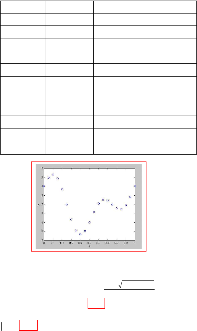
CHAPTER EIGHTEEN (Fourier Analysis) SOLUTIONS
Engineering Circuit Analysis, 6th Edition Copyright
2002 McGraw-Hill, Inc. All Rights Reserved
2. (a)
t v t v
0 2 0.55 -0.844
0.05 2.96 0.6 0.094
0.1 3.33 0.65 0.536
0.15 2.89 0.7 0.440
0.2 1.676 0.75 0
0.25 0 0.8 -0.440
0.3 -1.676 0.85 -0.536
0.35 -2.89 0.9 -0.094
0.4 -3.33 0.95 0.844
0.45 -2.96 1 2
0.5 -2
(b)
(c) min 3.330v=
22
2
max
4 sin 2 7.2 cos4 0
4sin 2 7.2(cos 2 sin 2 )
4 16 414.72
4sin 2 7.2(1 2sin 2 ) 0.5817, 0.8595 sin 2
28.8
0.09881,0.83539 3.330(0.5593 for smaller max)
vtt
ttt
ttx t
tv
ππ ππ
πππ
ππ π
′=− + =
∴= −
−± +
∴=− ∴= =−=
∴= ∴ =
CHAPTER EIGHTEEN (Fourier Analysis) SOLUTIONS
Engineering Circuit Analysis, 6th Edition Copyright
2002 McGraw-Hill, Inc. All Rights Reserved
3.
(a) T 10 , F 0.1(2 4 2 2) 1.200
av o
sa===×+×=
(b)
(c)
22
22
00
2
2
223
00
0
1
F (4 ) 0.2 (16 8 )
5
18
0.2 16 4 0.2 32 16 1.9322
33
=−= −+
=−+=−+=
∫∫
eff tdt ttdt
tt t
222
3
000
22
20
0
2
22
2 (4 )cos3 0.4 4cos0.6 0.4 cos0.6
10 10
11
1.6 sin 0.6 0.4 cos 0.6 sin 0.6
0.6 0.36 0.6
810 4
sin1.2 (cos1.2 1) sin 1.2 0.04581
39 3
=×−×= −
=− +
=− −− =−
∫∫∫
t
atdt tdtttdt
t
ttt
πππ
πππ
πππ
ππ π
ππ π
CHAPTER EIGHTEEN (Fourier Analysis) SOLUTIONS
Engineering Circuit Analysis, 6th Edition Copyright
2002 McGraw-Hill, Inc. All Rights Reserved
4.
(a) T = 8 − 2 = 6 s
(b) 1Hz
6
o
f=
(c) 2 rad/s
3
oo
f
π
ωπ
==
(d) 1(10 1 5 1) 2.5
6
o
a=×+×=
(e)
34
2
23
4
3
23
2
22 2
10sin 5sin
63 3
1 30 2 15 2
cos cos
32 3 2 3
1 15 4 7.5 8 1 15 7.5
cos2 cos cos cos2 (1.5) ( 1.5) 1.1937
3333
=+
=− −
∴= − − − − = − − − =−
∫∫
tt
bdtdt
tt
b
ππ
ππ
ππ
ππ
ππ
ππ ππ
CHAPTER EIGHTEEN (Fourier Analysis) SOLUTIONS
Engineering Circuit Analysis, 6th Edition Copyright
2002 McGraw-Hill, Inc. All Rights Reserved
5.
4
3
34
3
3
2
23
4
3
34
3
23
23
2 6 6 1 10 5
10cos 5cos sin sin
66 63
10 1 1
sin3 sin 2 sin 4 sin 3 0
322
1 1 10 5
10sin 5sin cos cos
33
10 1
cos3 cos2 cos
32
=+=−
=−+−=
=+=−−
=− − +
∫∫
∫∫
tt
adtdttt
b tdt t dt t t
ππ ππ
ππ
ππ π π
π
ππ ππ
ππ
ππ
π
22
33
110
4 cos3 ( 1) 1.0610
23
1.0610
−=−−=
+=ab
ππ
π
CHAPTER EIGHTEEN (Fourier Analysis) SOLUTIONS
Engineering Circuit Analysis, 6th Edition Copyright
2002 McGraw-Hill, Inc. All Rights Reserved
6.
(a) 22
3.8cos 80 1.9 1.9cos160 , T 12.5 ms, ave value 1.9
160
π
π= + π = = =
π
tt
(b)
(c) 2
3.8cos70 3.8sin80 ; , , T 2 ; ave value 0
π
π− π ω =π ω=π = = =
π
oo
tttt s
3
3.8cos 80 (3.8cos80 )(0.5 0.5cos 160 )
1.9cos80 0.95cos240 0.95cos80 2.85cos80 0.95cos 240
2
T 25ms, ave value 0
80
π= π + π
=π+ π+ π= π+ π
π
== =
π
tt t
ttttt
CHAPTER EIGHTEEN (Fourier Analysis) SOLUTIONS
Engineering Circuit Analysis, 6th Edition Copyright
2002 McGraw-Hill, Inc. All Rights Reserved
7. T = 2 s
(a)
(b) 4
1
4
=π
b
()
1
1
4
0
0
41
11
242 1
sin cos4
22 4
11 cos4
4
max when 4 , 0.125
2
×π
==−π
π
∴= − π
ππ
π= =
∫t
tt
bdtt
bt
tt s

CHAPTER EIGHTEEN (Fourier Analysis) SOLUTIONS
Engineering Circuit Analysis, 6th Edition Copyright
2002 McGraw-Hill, Inc. All Rights Reserved
8.
( ) 5 8cos10 5cos15 3cos20 8sin10 4sin15 2sin 20
=+ − + − − +
gt t t t t t t
(a) 2
5 T 1.2566
5
π
ω= ∴ = =
os
(b) 510
4 3.183 Hz
2
=β= ==
ππ
oo
ff
(c) G 5=−
av
(d) 2 222222
1
G ( 5) (8 5 3 8 4 2 ) 116 10.770
2
=−+ +++++ = =
eff
(e)
CHAPTER EIGHTEEN (Fourier Analysis) SOLUTIONS
Engineering Circuit Analysis, 6th Edition Copyright
2002 McGraw-Hill, Inc. All Rights Reserved
9.
[]
0.1 0.1
0.1 0.1
0.1
0.1
T 0.2, ( ) V cos5 , 0.1 0.1
2V cos5 cos10 5V cos(5 10 ) cos(10 5 )
0.2
11
5V sin(10 5 ) sin(10 5 )
10 5 10 5
V2 2
sin(10 5 )0.1 sin(10
21 21
−−
−
==π−<<
=ππ=π+π+π−π
=π+π+π−π
π+ π π− π
=π+π+
π+ −
∫∫
m
nm m
m
m
ft t t
a t n t dt n t n t dt
nt nt
nn
n
nn
22
5 )0.1
V2 2
sin( 0.5 ) sin( 0.5 )
21 21
V2V22 11
cos ( cos ) cos
21 21 2121
2V 4V
2121 cos
cos 41 41
11
V cos5 5V sin sin
0.2 5 2 2
π− π
=π+π+π−π
π+ −
=π+−π=π−
π+ − π + −
−− − π
=π =−
π−π−
ππ
=π=−−
π
m
mm
mm
om m
n
nn
nn
nnn
nn nn
nn n
nnn
atdt
0.1
0.1
2V
2V 4V 4V 4V 4V
( ) cos10 cos20 cos30 cos 40 ...
3153563
−
=
π
∴= + π− π+ π− π+
ππ π π π
∫m
mm m m m
vt tttt
CHAPTER EIGHTEEN (Fourier Analysis) SOLUTIONS
Engineering Circuit Analysis, 6th Edition Copyright
2002 McGraw-Hill, Inc. All Rights Reserved
10.
(a) 1
even, wave
2−
(b) 0 for all ; 0; 0===
neveno
bnaa
(c)
123 2
2
2
1
1
13
0, 0
810620
5cos sin sin sin
12 6 3 6 3 6
20 20 20
sin sin 2.330, sin sin 2.122
36 3 23
=== =
ππππ
===−
ππ
ππ π
∴= −= = π−=−=−
πππ
∫
n
bbb a
nt nt n n
adt
nn
aa
CHAPTER EIGHTEEN (Fourier Analysis) SOLUTIONS
Engineering Circuit Analysis, 6th Edition Copyright
2002 McGraw-Hill, Inc. All Rights Reserved
11.
(a)
(b) 222
Y 0.5(0.2 0.6 0.4 ) 0.5(0.56) 0.5292=++= =
eff
(c) (2ms) 0.2sin 0.2 0.6sin 0.4 0.4sin 0.6 1.0686= π+π+π=y
0
( ) 0.2sin1000 0.6sin 2000 0.4sin 3000
==
∴ = π+ π+ π
on
aa
yt t t t
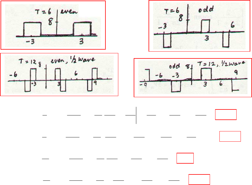
CHAPTER EIGHTEEN (Fourier Analysis) SOLUTIONS
Engineering Circuit Analysis, 6th Edition Copyright
2002 McGraw-Hill, Inc. All Rights Reserved
12.
(a) (b)
(c) (d)
(e)
3
3
55
2
2
3
55
2
55
4 2 5 32 6 5 3.2 15 10
[ ] 0, 8cos sin sin sin 0.8821
666103 33
4 2 5 32 6 15 10 3.2
[ ] 0, 8sin cos cos ( 0.5) 0.5093
6661033
825641215
[ ] 0, 8cos sin
12 12 12 10
ππππ
== = = − =
ππ
π−ππ
== = − =−−=
ππ
π
== = π
∫
∫
tt
ab a dt
t
ba b dt
t
cb a dt
3
2
3
55
2
10
sin 3.801
66
81064121510
[ ] 0, 8sin cos cos 1.0186
12 12 12 10 6 6
ππ
−=
πππ
== =− − =
π
∫
∫t
da b dt
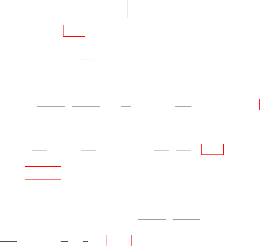
CHAPTER EIGHTEEN (Fourier Analysis) SOLUTIONS
Engineering Circuit Analysis, 6th Edition Copyright
2002 McGraw-Hill, Inc. All Rights Reserved
13.
T = 4 ms
(a)
(b)
(c) 4 0 : 8sin125
−<< π
tt
(d)
0.004
0.004
0
0
1000 250 8
8sin125 cos125
4 125
16 16
cos 1 5.093
2
×
=π=π
−π
π
=− − = =
ππ
∫
o
a t dt t
0.004
1
0
0.004 0.004
1
00
0.004
0
1
2
4000 sin125 cos 0.004
4000 sin125 cos500 2000 (sin 625 sin 375 )
cos625 cos375 3.2 5.333
2000 (1 cos 2.5 ) (1 cos1.5 ) 0.6791
625 375
4000 sin125
π
=π
∴= π π = π− π
ππ
=− + =−π− −π=−
πππ π
=π
∫
∫∫
t
atdt
attdt ttdt
tt
b
0.004 0.004
00
sin500 2000 (cos375 cos625 )
11 11
2000 (sin1.5 ) (sin 2.5 ) 2000 2.716
375 625 375 625
π= π− π
−
=π−π=−=−
ππ ππ
∫∫
t t dt t t dt
[]
()
0.004
11
0
0.004
0.004
1
0
0
4000
0, 8sin125 cos250
8
cos375 cos125
2000 sin375 sin125 2000 375 125
5.333 16
1 cos1.5 cos 1 3.395
2
+
== π π
ππ
∴= π− π = − +
ππ
π
=−π+ −=−
ππ
∫
∫
ba t tdt
tt
attdt
CHAPTER EIGHTEEN (Fourier Analysis) SOLUTIONS
Engineering Circuit Analysis, 6th Edition Copyright
2002 McGraw-Hill, Inc. All Rights Reserved
14.
0.001
0.001
00
13579
1
odd and wave 0, 0, 0
2
T 10 0.01
81
10sin 200 8000 cos 200
0.01 200
40 40
(cos0.2 1) (1 cos0.2 )
2.432, 5.556, 5.093, 2.381, 0.27
−∴== =
==
−
=π= π
π
∴=− π−= − π
ππ
∴=====
∫
o n even
odd
odd
aab
ms s
bntdt nt
n
bn n
nn
bbbbb02
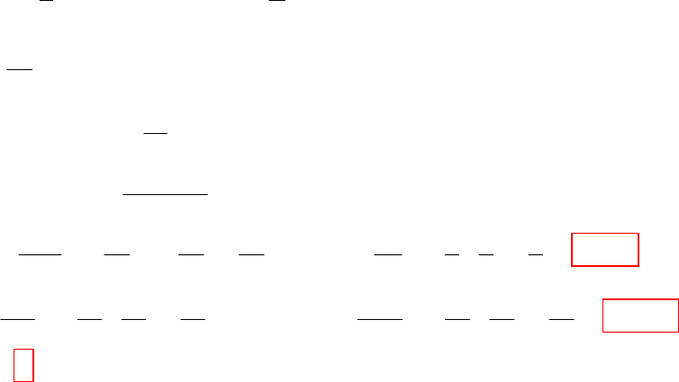
CHAPTER EIGHTEEN (Fourier Analysis) SOLUTIONS
Engineering Circuit Analysis, 6th Edition Copyright
2002 McGraw-Hill, Inc. All Rights Reserved
15.
()
()
/4
0
0.001
0
2
60.001
3
222 0
22
18
odd and wave, T 8 ( )sin
2T
2250 1000 1000 sin 250
T
1
Now, sin sin cos , 250
10
( ) 10 sin 250 250 cos 250
250
16 sin 0
4
−=∴= ω
π
ω= = π∴ = π
=− =π
=∴= π−π π
π
π
∴= −
π
∫
∫
∫
T
no
on
x
n
n
ms b f t n t dt
b t nt dt
x ax dx a ax ax a n
a
ft t b nt nt nt
n
n
bn12
35
22
16
cos 0 sin cos 0.2460
44 444
16 3 3 3 16 5 5 5
sin cos 0.4275 ; sin cos 0.13421
9 4 4 4 25 4 4 4
0
−
ππ πππ
−+∴=−=
π
ππ π ππ π
=−== −=
ππ
=
even
nn b
bb
b
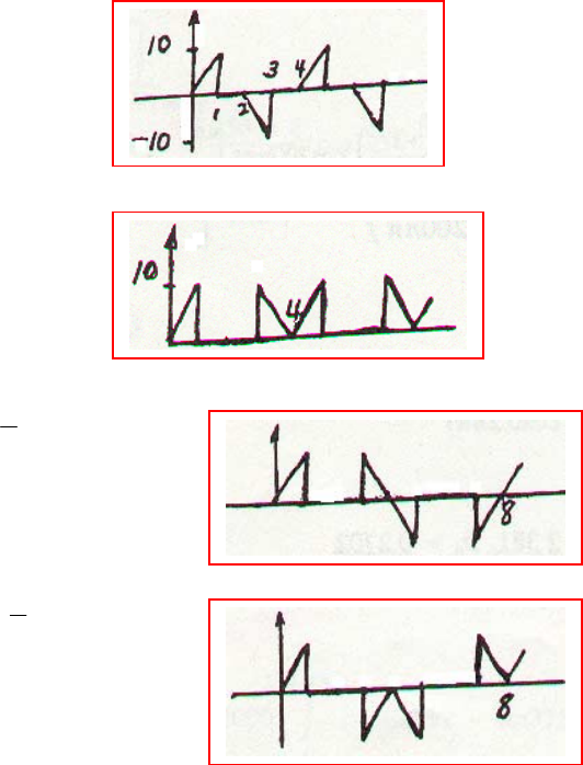
CHAPTER EIGHTEEN (Fourier Analysis) SOLUTIONS
Engineering Circuit Analysis, 6th Edition Copyright
2002 McGraw-Hill, Inc. All Rights Reserved
16.
(a) odd, T = 4
(b) even, T = 4:
(c) 1
odd, wave: T 8
2−=
(d) 1
even, wave, T 8:
2−=
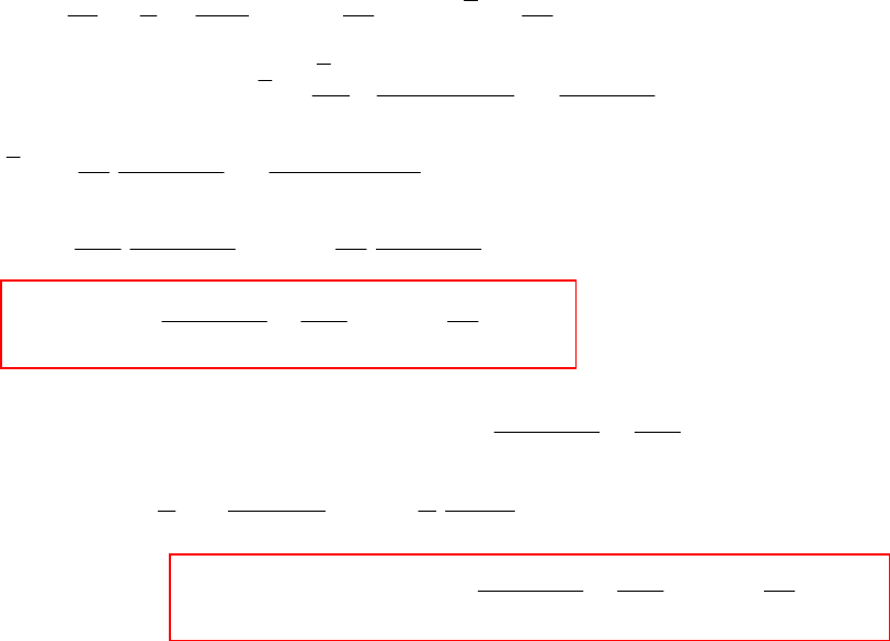
CHAPTER EIGHTEEN (Fourier Analysis) SOLUTIONS
Engineering Circuit Analysis, 6th Edition Copyright
2002 McGraw-Hill, Inc. All Rights Reserved
17.
(a)
(b)
2
2
1,
2
1,
2
2
1,
1 12.5
Ae , , (0) 0, (0) 1.25 1 6.25
21 2
(0) 1.25 1.25 tanh 0.2 0.55388
0.16 4 0.4
1 12.5 5
A 0.55388, 0.55388 1.25 cos5 sin5
1 6.25
∞
−
∞
∞
−
==+==+ −
+π
π
∴=− =− π=
π+ π×
∴=− =− + + − +
+ππ
∑
∑
∑
t
nfnf
odd
f
odd
t
odd
iiiiii n
in
i e nt nt
nn
1,
22
22
20 1 2 20 20
5sin sin5,V(1)
0.4
V20 5
Z452410,I Z (4 10 ) 1 2.5
5 1 2.5 12.5 5
I1 6.25 (1 6.25 )
12.5 1 5 1
cos5 sin5
1 6.25 1 6.25
∞π
=+ ∴ = = −
πππ π
−
=+ =+ = = =−
π+ +
−+
∴=− =−
π+ π+
∴=− +
π+ π+
∑
ssnsn
odd
sn
nfn
n
fn
fn
nt
v v nt j
nnn
jj
jn j n njn jn
jjn j
nnnn
intnt
nnn
2
1,
1 12.5 5
1.25 cos5 sin5
1 6.25
∞
∴= + − +
+ππ
∑
f
odd
intnt
nn

CHAPTER EIGHTEEN (Fourier Analysis) SOLUTIONS
Engineering Circuit Analysis, 6th Edition Copyright
2002 McGraw-Hill, Inc. All Rights Reserved
18.
(a) 20.4
0 0.2 : 2.5(1 ) (0.2 ) 2.5(1 ) 1.78848 A
−−π
<< π = − ∴ π= − =
t
ti ei e
(b) 2( 0.2 )
0.2 0.4 : 1.78848 (0.4 ) 0.50902 A
−−π
π< < π = ∴ π =
t
ti e i
(c) 2( 0.4 )
0.4 0.6 : 2.5 (2.5 0.50902) , (0.6 ) 1.9335
−−π −
π< < π = − − π =
t
ti ei
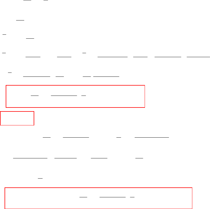
CHAPTER EIGHTEEN (Fourier Analysis) SOLUTIONS
Engineering Circuit Analysis, 6th Edition Copyright
2002 McGraw-Hill, Inc. All Rights Reserved
19.
(a)
(b) /4
Ae−
=t
n
v
(c)
()
1,
22
2
20 1
5sin5
20 sin5
20
V
1 1 20 / 1 20/ 1 20
Z2 2 V
5 2 10 2 1/ 10 10 1 20 1 20
20 1 20 20 1
V, 20cos5sin5
1 400 1 400
20 1 1
5sin5
1400
∞
=+
π
=π
=− π−π −π−
=+ =+ ∴ = × = ×
++−
−−
∴= × = − +
+ππ+
∴=+
π+
∑
s
odd
sn
sn
ncn
cn cn
cf
vnt
n
vnt
n
jn
jn jn jn
jn jn jn jn jn jn
nj v n nt nt
nn n n
vnn
1,
20cos5
∞
−
∑
odd
nt nt
222
1, 1,
22
1,
/4
2
1,
20 20 1 1
(0) A 5 A 5
1 400 (1/ 20)
1tanh 5 tanh 1.23117
(1/ 20) 4(1/ 20) 20 2 40
1
A 0 5 1.23117 4.60811
20 1 1
( ) 4.60811 5 sin5 20cos5
1400
∞∞
∞
∞
−
−
=++ =+−
π+ π +
ππ π
==π=
+×
∴=−+× =−
π
∴=− ++ −
π+
∑∑
∑
∑
c
odd odd
odd
t
c
odd
vnn
n
vt e nt nt
nn
CHAPTER EIGHTEEN (Fourier Analysis) SOLUTIONS
Engineering Circuit Analysis, 6th Edition Copyright
2002 McGraw-Hill, Inc. All Rights Reserved
20.
()
3
0.001 0.005
33 2 / 6 10 100
3
0 0.003
0.001 0.005
51000 1000
0 0.003
53
33
3
10 100 100
6
10 1 1
6 1000 1000
100 100
1 (1 1 1 1) 10.610
66
10.610; 10.610
2
−
−×π × − π
−π −π
−π − π − π
−
=−
−
=+
ππ
=++−=+−+=−
ππ
∴= =
=
∫∫
jt jt
jt jt
jjj
ce e
ee
jj
eee j
jj
cj c
a
()
0.001 0.005
3
00.003
5
22
333 33 33
10 100cos100 100cos1000
6
210 1 sin 0 sin 5 sin3 0
6 1000
11
( ) 21.22 and 21.22
22
×π− π
×
=π−−π+π=
π
=−=− ∴= +=
∫∫
tdt tdt
cajbjbb ab
CHAPTER EIGHTEEN (Fourier Analysis) SOLUTIONS
Engineering Circuit Analysis, 6th Edition Copyright
2002 McGraw-Hill, Inc. All Rights Reserved
21.
0.001 0.002
5 400 400
0 0.001
0.001 0.002
400 400
0 0.001
0.00
400 0.001 400
0
22
0.001
1
T 5 10 100
0.005
20,000 1000
1
20,000 ( 400 1)
160 400
jnt jnt
m
jnt jnt
n
jnt jnt
n
msc te dt e dt
ctedtedt
e
c j nt e
njn
−π −π
−π −π
−π −π
== +
∴= +
∴= π+ +
π−π
∫∫
∫∫
()
2
33
0.4 0.8 0.4
122
2
1
(50 10 100 10 ) 0.15 200 30
0.005
111
20,000 (1 0.4 )
160 160 400
125 (1 72 )(1.60597 51.488 ) 12.66515 15.91548 90 (1 144 1 72 )
12.665(1 72
oo
jjj
ca
cej ee
j
−−
−π −π −π
∴= = × + × = × =
=+π−−−
πππ
= ∠− ° ∠ ° − + ∠ ° ∠− °− ∠− °
π
=∠−
2
)(1 1.2566) 12.665 15.915(1 144 1 72 )
20.339 20.513 12.665 18.709 108 24.93 88.61
3.16625 144 (1 2.5133) 3.16625 7.9575(1 288 1 144 )
8.5645 75.697 3.16625 15.1361 144 13.309 1
jj
cjj
° + − + ∠− °− ∠− °
= ∠− °− + ∠− °= ∠− °
=∠−°+ −+ ∠−°−∠−°
=∠−°− + ∠°=∠77.43°
(a)
(b)
CHAPTER EIGHTEEN (Fourier Analysis) SOLUTIONS
Engineering Circuit Analysis, 6th Edition Copyright
2002 McGraw-Hill, Inc. All Rights Reserved
22.
Fig. 17-8a: V 8 V, 0.2 , 6000
oo
s f pps
τ
µ
== =
(a) 11
T , 6000, 0.2 5 MHz
6000 o
fsf
τµ τ
===∴==
(b) 6000 Hz
o
f=
(c)
(d) 66 6
333
3 6
2 10 8 0.2 10 sin(1/ 2 333 12,000 0.2 10
333.3 7.270 mV
6 10 1/ 6000 1/ 2 333 12,000 0.2 10
c
π
π
−−
−
×××××××
=∴= =
×××××
(e) 1/ 5 MHz
β
τ
==
(f)
(g)
66
3
3
8 0.2 10 sin(1/ 2 3 12,000 0.2 10
6000 3 18,000 (closest) 1/ 6000 0.0036
9.5998 mV
c
c
π
π
−−
×× ×× ××
×= ∴ =
∴=
2000 2200
2 2.2 Mrad/s kHz or 318.3 350.1 kHz
22
6 kHz 6 53 318; 324,330,336,342,348kHz 5
o
ff
ff n
ωππ
<< ∴ << <<
=∴=×= ∴=
66
227
8 0.2 10 sin(1/ 2 227 12,000 0.2 10 8.470 mV
1/ 6000 ( )
227 6 1362 kHz
c
f
π
−−
×× × × ××
==
′′
=×=
CHAPTER EIGHTEEN (Fourier Analysis) SOLUTIONS
Engineering Circuit Analysis, 6th Edition Copyright
2002 McGraw-Hill, Inc. All Rights Reserved
23.
12 3
T 5 ; 1, 0.2 0.2, 0.5 0.25, 1 2, 0, 4===−=+ =−−=≥
o n
ms c c j c j c j c n
(a)
(b)
11 1 2 2 3 3
2 1, 0.4 0.4 0.4, 1 0.5, 2
( ) 1 0.4cos400 cos800 2cos1200 0.4sin 400 0.5sin800 4sin1200
nnnoo
ajbcacajbjbjajbjajb
vt t t t t t t
ππ π π π π
=−= ∴== −=−=− −=+ −=−
∴=+ + − + − +
(1 ) 1 0.4cos72 cos144 2cos 216 0.4sin 72 0.5sin144 4sin 216vms= + °+ °− °+ °− °+ °
(1 ) 0.332Vvms∴=−
CHAPTER EIGHTEEN (Fourier Analysis) SOLUTIONS
Engineering Circuit Analysis, 6th Edition Copyright
2002 McGraw-Hill, Inc. All Rights Reserved
24.
(a)
(b) 4
1(sin172.8 sin115.2 ) 0.06203
4
c
π
=°−°=−
(c) 66
6
0.2 10 0.2 10 0.08
510
oo
ca −−
−
×+×
== =
×
(d) max
a little testing shows is max 0.08
o
cc
∴=
(e)
(f) 6
740 10
740 148 MHz
5
×
== =
o
f
β
()
()
6
6
0.6 10
6
6
0.4 10
6
5
10
T5 2 1cos2
5510
510
4 10 sin 43.2 sin 28.8
2
1sin 43.2 sin 28.8
n
n
n
t
sc n dt
cnn
n
cnn
n
µπ
π
π
−
−
×
−
×
−
=∴=× ×
×
∴=× °− °
∴= °− °
∫
()
()
33
1
0.01 0.08 0.8 10 sin 43.2 sin 28.8 0.8 10
125 sin 43.2 sin 28.8 1
ok for 740
−−
×=×∴ °− °≤×
∴°−°≤
>
nn
n
nn
n
n
π
π
CHAPTER EIGHTEEN (Fourier Analysis) SOLUTIONS
Engineering Circuit Analysis, 6th Edition Copyright
2002 McGraw-Hill, Inc. All Rights Reserved
25.
T1/16, 32
o
ωπ
==
(a)
(b)
1/96
1/96
96 96
3
00
3
16 40
16 40 96
20 40
( 1) 4.244 V
33
jt j
j
c e dt e
j
cj e j j
ππ
π
π
ππ
−−
−
×
=−
−
∴= −=− =−
∫
33 3 3 3
2
33
64
2
Near harmonics are 2 32 Hz, 3 48 Hz
Only 32 and 48 Hz pass filter 2
2 8.488 0, 8.488 V
8.488 1
I 1.4536 31.10 A; P 1.4536 5 5.283 W
5 0.01 96 2
1 640
40
1/16 6
oo
nn n
jt
ff
ajb c
ajb c j a b
j
cedt
j
π
π
−
==
−=
−==− ∴= =
==∠−°=××=
+×
==
−
1/96
64 /96
0
22 2
2
2
2
( 1) 2.7566 4.7746 V
4
2 5.5132 9.5492 11.026 60
11.026 60
I 2.046 65.39 A
5 0.01 64
1
P 2.046 5 10.465 W P 15.748 W
2
j
tot
ej
ab c j
j
π
π
π
−−= −
−= = − = ∠−°
∠− °
∴= = ∠− °
+×
∴=× ×= ∴ =
∫
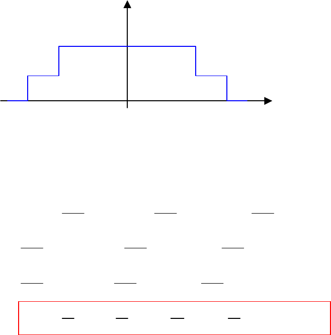
CHAPTER EIGHTEEN (Fourier Analysis) SOLUTIONS
Engineering Circuit Analysis, 6th Edition Copyright
2002 McGraw-Hill, Inc. All Rights Reserved
26. ( ) 5[ ( 3) ( 2) ( 2) ( 3)]f t ut ut ut ut= +++−−−−
(a)
(b)
22 3
32 2
23 22 3 2
33 22 22
F( ) ( )
F( ) 5 10 5
510 5
F()( )( )( )
5510
()()()
55
(2)sin3 (
∞−ω
−∞
−−ω −ω −ω
−−
ωω −ωω −ω−ω
ω−ω ω−ω ω−ω
ω=
∴ω= + +
∴ω= − + − + −
−ω −ω −ω
=−++ −+−+
−ω −ω −ω
=− ω+
−ω −ω
∫
∫∫ ∫
jt
jt jt jt
jj jj j j
jj jj jj
jftedt
j e dt e dt e dt
jee ee ee
jj j
ee ee ee
jjj
j
jj
10
2)sin 2 ( 2)sin 2
10 10 20 10
F( ) sin 3 sin 2 sin 2 (sin3 sin 2 )
ω+ − ω
−ω
∴ω= ω− ω+ ω= ω+ ω
ωωω ω
jj
j
j
-3 -2 -1 0 1 2 3
f(t)
t
CHAPTER EIGHTEEN (Fourier Analysis) SOLUTIONS
Engineering Circuit Analysis, 6th Edition Copyright
2002 McGraw-Hill, Inc. All Rights Reserved
27.
(a)
(b)
(c)
0
()
0
() (), 0 F( ) ()
11
F( )
∞∞
−−−−
−∞
∞
−+
=>∴= =
−
∴= =
++
∫∫
at j t at j t
aj t
f t e u t a j f t e dt e e dt
je
aj aj
ωω
ω
ω
ωωω
6()
()
()
() ( ), 0 F( )
111
F( )
∞
−−+
∞
−+ −
−+
=−>∴=
−−
∴= = − =
+++
∫
o
o
oooo
o
at at
at a j t
o
t
at at a j t j t
aj t
t
ft e e ut t a j e e dt
je e e e e
aj aj aj
ω
ωω
ω
ω
ωωωω
[]
()
0
()
222
0
() (), 0 F( )
11
F( ) ( ) 1 0 [ 1]
() () ()
∞
−−+
−+ ∞
=>∴=
∴= −+−=− −=
+++
∫
at a j t
aj t
ft te ut a j te dt
e
jajt
aj aj aj
ω
ω
ω
ωω
ωωω
CHAPTER EIGHTEEN (Fourier Analysis) SOLUTIONS
Engineering Circuit Analysis, 6th Edition Copyright
2002 McGraw-Hill, Inc. All Rights Reserved
28.
04
40
0
1
4
44
1
00
4 0: ( ) 2.5( 4); 0 4: ( ) 2.5(4 )
F( ) 2.5( 4) 2.5(4 5)
ln 1 , let I 2.5(4 ) ( )
I 2.5(4 ) F( ) 2.5 (4 )( )
F( ) 5 (4 )cos 20
−ω −ω
−
ωτ
ωτ ω − ω
−<< = + << = −
∴ω= + + −
=τ ∴ = −τ − τ
∴= −τ τ∴ ω= − +
∴ω=−ω=×
∫∫
∫
∫∫
jt jt
st j
jjtjt
tft t tft t
jtedt edt
ted
ed j te e dt
jttdt
4
44
00
0
4
0
2
222
2
2
2
1sin 5 cos
20 5
F( ) sin 4 (cos sin )
20 5 5 5
sin 4 (cos4 1) 4 sin 4 (1 cos4 )
25 sin2
or, F( ) sin 2 10
ω− ω
ω
∴ω= ω− ω+ω ω
ωω
=ω− ω−−ωω=−ω
ωω ω ω
×ω
ω= ω=
ωω
∫∫
ttdt
jttt
j
CHAPTER EIGHTEEN (Fourier Analysis) SOLUTIONS
Engineering Circuit Analysis, 6th Edition Copyright
2002 McGraw-Hill, Inc. All Rights Reserved
29.
(1 ) (1 )
(1 ) (1 ) (1 ) (1 )
() 5sin F( ) 5sin
5
F( ) ( )
2
5[]
2
51 1
F( ) ( ) ( )
2(1 ) (1 )
2.5 2.5
()(
11
π−ω
−π
π−−ω
−π
π−ω − +ω
−π
π−ω −π−ω −π+ω π+ω
−πω πω
=−π<<π∴ω=
∴ω= −
=−
ω= − − −
−ω − +ω
−
=−+−
−ω +ω
∫
∫
∫
jt
jt jt j t
jt jt
jj jj
jj
ft t t j te dt
jeeedt
j
eedt
j
jee ee
jj j
ee
222
)
2.5 2.5 1 1
(2sin) (2sin)5sin
11 11
11 10sin 10sin
5sin ( 1) 11 1
−πω πω
−+
−
=πω−πω=πω−−
−ω +ω −ω +ω
+ω+ −ω πω πω
=πω− =− =
−ω −ω ω −
jj
ee
jjj
jj
j
,
CHAPTER EIGHTEEN (Fourier Analysis) SOLUTIONS
Engineering Circuit Analysis, 6th Edition Copyright
2002 McGraw-Hill, Inc. All Rights Reserved
30.
/2
/2
/2 /2
/2 /2
/2
(1 ) (1 )
/2
/2
/2
/2
( ) 8cos [ ( 0.5 ) ( 0.5 )]
F( ) 8cos 4 ( )
4
11
4(1 ) (1 )
1
4()
(1 )
π
−π
ππ
−ω − −ω
−π −π
π−ω − +ω
−π
π
−ω −−ω
−π
−πω
=+π−−π
∴ω= = +
=+
=−
−ω +ω
=−−
−ω
∫∫
∫
jt jt jt jt
jt jt
jt
jt jt j t
j
ft tut ut
jtedteeedt
eedt
ee ee
jj
je j e
j
/2 /2 /2
22
1
(1 )
11 11
4 2cos 2cos 8cos
1212211
2cos/2
8cos 16
21 1
πω − πω πω
−−−
+ω
πω πω πω
=× +× = +
−ω +ω −ω +ω
πω πω
==
−ω −ω
jjj
je je
j
(a) 0 F( 0) 16ω= ∴ =j
(b) 16cos72
0.8, F( 0.8) 13.734
0.36
°
ω= = =j
(c) 16cos(3.1 90 )
3.1, F( 3.1) 0.2907
1 3.12
×°
ω= = =−
−
j
CHAPTER EIGHTEEN (Fourier Analysis) SOLUTIONS
Engineering Circuit Analysis, 6th Edition Copyright
2002 McGraw-Hill, Inc. All Rights Reserved
31.
(a)
(b)
(c)
[]
()
2
2
22
22
1
F( ) 4 ( 2) ( 2) ( ) F( )
2
4212
() 2
24 5
( ) 2sin 2 sin 2 (0.8) sin1.6 1.5909
2
∞ω
−∞
ωω −
−−
ω = ω+ −ω ω− ∴ = ω ω
π
∴= ω= = −
ππ π
∴= = ∴ = =
ππ π
∫
∫
jt
jt jt jt jt
rad
ju ft ejd
ft e d e e e
jt j t
ft j t t f
tt
22
0
(2 ) ( 2 )
0
2
2
4
F( ) 4 ( ) 2
22
()
21 1 21 1 24
(1 0) (0 1)
22 224
88
( ) (0.8) 0.5488
(4 ) 4.64
∞
−ω −ω+ω
−∞
∞
+ω −+ω
−∞
ω= ∴ = ω
π
∴= ω+ ω
ππ
=−+−=+=
π+ −+ π+ − π+
∴= ∴ = =
π+ π×
∫
∫∫
jt
jt j t
je ft e d
ft e d e d
jt jt jt jt t
ft f
t
[]
()
()
0.5 0.5
0.5 0.5
0.5
() (0.50.5)
0.5
0.5 0.5 0.5 0.5 0.5 0.5 0.5 0.5
F( ) 4cos ( 0.5) ( 0.5)
421
() cos
22
1
11 1
() ( )
ωπω−πωω
−−
π+ ω − π− ω
−
π+ − π− − π+ π−
ω= πω ω+ − ω−
∴= πω× ω= + ω
ππ
=+ ω
π
=−+−
ππ+ −π+
∫∫
∫
jt j j jt
jjt j jt
jjt jjt jjtjj
juu
ft ed e e ed
ee d
ee e e
jt j t
()
()()
0.5 0.5 0.5 0.5
22 22
11 1
() ( )
1 1 1 2cos0.5 1 1
2cos0.5 2cos0.5
24
2cos0.5 cos0.5 (0.8) 0.3992
−−
=++−−
ππ+ −π+
=−=−
π π+ −π+ π π+ −π+
−
==∴=
−π π −
t
jt jt jt jt
je je je je
jt j t
t
tt
tt tt
ttf
tt
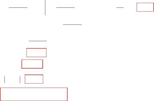
CHAPTER EIGHTEEN (Fourier Analysis) SOLUTIONS
Engineering Circuit Analysis, 6th Edition Copyright
2002 McGraw-Hill, Inc. All Rights Reserved
32. 1.5
( ) 20 ( 2) V=−−
t
vt e u t
(a)
(b)
(c) B (2) 0.3891=−
v
(d) F ( 2) 0.3983=
vj
(e)
φ
v(j2) = 282.3o or -77.69o
2
1.5 1.5
2
(1.5 ) 3 2 3
F( ) 20 ( 2) 20
20 20 20
F ( 0) 0.6638
1.5 1.5 1.5
∞−
−ω −ω
−∞ −∞
−
−ω −+ ω −
−∞
ω= −− =
==∴==
−ω −ω
∫∫
tjt tjt
v
jt j v
jeutedtedt
eeje
jj
32
34
20
F( ) A ( ) B( ) 1.5
20
F ( 2) 0.39830 282.31 0.08494 0.38913
1.5 2
A (2) 0.08494
−ω
−
ω= ω+ ω= −ω
∴= = ∠°= −
−
∴=
j
vvv
j
v
v
jee
j
jee j
j
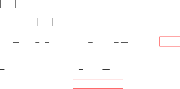
CHAPTER EIGHTEEN (Fourier Analysis) SOLUTIONS
Engineering Circuit Analysis, 6th Edition Copyright
2002 McGraw-Hill, Inc. All Rights Reserved
33.
[]
I( ) 3cos10 ( 0.05 ) ( 0.05 )ω= ωω+π−ω−πjuu
(a)
(b)
0.05
22
0.05
/20
/20
/20
/20
12
W4 I() 9cos10
2
18 1 1 9 9 1
cos20 0.1 sin 20 0.9 J
22 20
∞π
−∞ − π
π
π
−π
−π
=× ω ω= ωω
ππ
=+ωω=×π+ ω=
πππ
∫∫
∫
jd d
d
991
(1 cos20 ) 0.45 2 2sin 20
20
0.05 2 0.1sin 20 , 0.04159 rad/s
ω
−ω
+ωω==ω+× ω
ππ
∴π=ω+ ωω=
∫x
x
xx
xxx
d
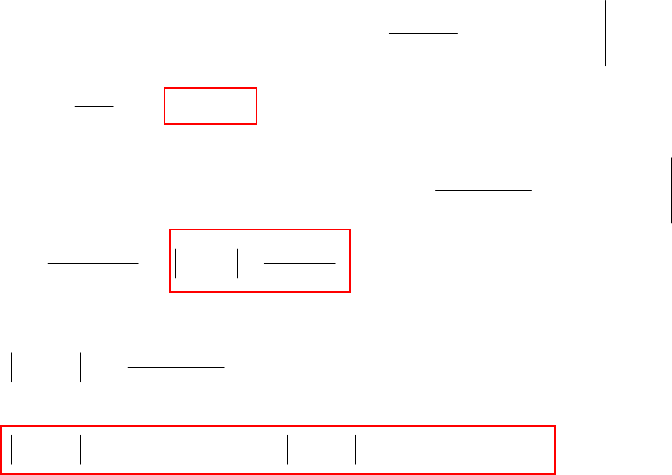
CHAPTER EIGHTEEN (Fourier Analysis) SOLUTIONS
Engineering Circuit Analysis, 6th Edition Copyright
2002 McGraw-Hill, Inc. All Rights Reserved
34. 4
() 10 ()
−
=t
ft te ut
(a)
(b)
(c)
()
2
2
2
16
100
)( +
=
ω
ω
jF
mJ/Hz 90.63 )( 2
0=
=
ω
ω
jF , mJ/Hz 7.669 )( 2
4=
=
ω
ω
jF
8
228 2
1
00 0
W ( ) 100 100 (64 16 2)
(512)
100 2 0.3906 J
512
∞
∞∞ −
−
Ω== =× ++
−
=×=
∫∫ t
te
f t dt t e dt t t
(4 )
4(4)
2
00
22
10
F( ) {10 ( )} 10 [ (4 ) 1
(4 )
10 10
F( )
(4 ) 16
∞
∞−+ω
−−+ω
ω= = = − +ω −
+ω
=∴ω=
+ω ω+
∫jt
tjt
e
jteuttedt jt
j
j
j
F
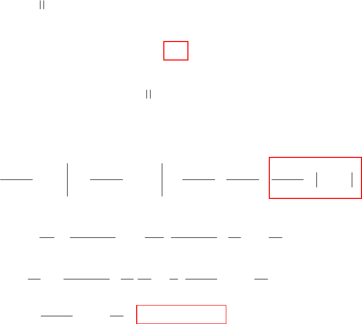
CHAPTER EIGHTEEN (Fourier Analysis) SOLUTIONS
Engineering Circuit Analysis, 6th Edition Copyright
2002 McGraw-Hill, Inc. All Rights Reserved
35. 2
() 8 V
−
=t
vt e
(a) 24
1
0
W ( ) 2 64 32 J
∞∞
−
Ω
−∞
==× =
∫∫
t
v t dt e dt
(b)
(c)
2
0
(2 ) (2 )
0
0
(2 ) (2 )
2
0
F( ) () 8
F( ) 8 8
88 8832
F( )
22 224
∞∞
−
−ω −ω
−∞ −∞
∞
−ω − +ω
−∞
∞
−ω − +ω
−∞
ω= =
∴ω= +
= − =+==ω
−ω +ω −ω +ω +ω
∫∫
∫∫
t
jt jt
v
jt jt
v
jt jt v
j e v t dt e e dt
j e dt e dt
ee j
jj jj
1
1
22 11
22 2
1
1
11 11
22
11
1
11
1
2
1
132 32 1
0.9 32 tan
2(4) 28(4)16 2
16 1 2 2
0.9 2 tan
8( 4) 16 2 4 2
2
0.45 tan 2.7174 rad/s (by SOLVE)
42
ω
−
−ω
−
−
ωω
×= ω= +
πω+ πω+
ωω ωω
∴=× + = +
πω+ πω+
ωω
∴π= + ∴ω=
ω+
∫d
CHAPTER EIGHTEEN (Fourier Analysis) SOLUTIONS
Engineering Circuit Analysis, 6th Edition Copyright
2002 McGraw-Hill, Inc. All Rights Reserved
CHAPTER EIGHTEEN (Fourier Analysis) SOLUTIONS
Engineering Circuit Analysis, 6th Edition Copyright
2002 McGraw-Hill, Inc. All Rights Reserved
36.
(a)
(b)
(c)
(d) Prove: { ( )} F( ) Let 1 in (c) above−=−ω =ft j k
F
(e)
Prove: { ( )} { ( )} ( ) Let
{( )} () {()}
∞
−ω −ω
−∞
∞−ω −ω
−ωτ
−∞
−= = − −=τ
∴−=τ =
∫
∫
o
oo
jt jt
ooo
jt jt
j
o
ft t e ft ft t e dt t t
f t t f e e dt e f t
FF
FF
Prove: { ( )} { ( )} Let , ,
,{()}() ()
We assume ( ) 0 { ()} { ()}
∞−ω −ω −ω
−∞
∞
∞
−ω −ω
−∞ −∞
=ω = = =−ω
==∴ = +ω
±∞ = ∴ = ω
∫
∫
jt jt jt
jt jt
df
f t j f t e dt u e du j e
dt
dv df v f f t f t e j f t e dt
fftjft
FF
F
FF
/
1
Prove: { ( )} F ( ) Let , 0
11
{( )} () F
1
If 0, limits are interchanged and we get: F
1
{( )} F
∞−ω
−∞
∞−ωτ
−∞
ω
== τ=>
ω
∴=τ τ=
ω
<−
ω
∴=
∫
∫
jt
jk
j
fkt fkte dt ktk
kk
j
fkt f e d
kkk
j
kkk
j
fkt kk
F
F
F
Prove: { ( )} F( ) Now, F( ) ( )
dF( ) ( )( ) { ( )} { ( )} ( )}
∞−ω
−∞
∞−ω
−∞
=ω ω=
ω
ω
∴=− =− ∴ =ω
ω
∫
∫
jt
jt
d
tf t j j j f t e dt
d
jft jte dt j tft tf f j ft
d
F
FF F

CHAPTER EIGHTEEN (Fourier Analysis) SOLUTIONS
Engineering Circuit Analysis, 6th Edition Copyright
2002 McGraw-Hill, Inc. All Rights Reserved
37.
(a)
(b) ( ) 4[sgn( 1) ( )] {4sgn( 1) ( )} { 4 ( )} 4=−δ∴ −δ=−δ=−ft t t t t
FF
(c)
(10 30 ) (10 30 )
30 10 30 10 / 6 / 6
/6 /6
4
( ) 4sin(10 30 ) {4sin(10 30 ) 2
{ 2 2 } 2 2 ( 10) 2 2 ( 10)
4 [ ( 10) ( 10)]
−° − −°
−° °− −π π
−π π
=−°∴ −°= − =
−+ =−πδω−+πδω+
=− π δω− − δω+
jt jt
jjt j jt j j
jj
ft t t e e
j
je e je e je je
je e
FF
F
( ) 4[sgn( ) ( 1)] {4[sgn( ) ( 1)] {4sgn(1) ( 1)} {4 ( 1)} 4 −ω
= δ− ∴ δ− = δ− = δ− = j
ft tt tt t t e
FF F
CHAPTER EIGHTEEN (Fourier Analysis) SOLUTIONS
Engineering Circuit Analysis, 6th Edition Copyright
2002 McGraw-Hill, Inc. All Rights Reserved
38.
(a)
(b)
(c)
( ) A cos( ) F( ) {A cos cos Asin sin }
Acos { [ ( ) ( )]} Asin [ ( ) ( )]
A{cos [ ( ) ( )] sin [ ( ) ( )]}
F( ) A[ ( ) ( )]
φ−φ
=ω+
φ
∴ω=
φ
ω−
φ
ω=
π
φ
πδω+ω +δω−ω −
φ
δ ω−ω −δ ω+ω =
π φ δ ω+ω +δ ω−ω + φ δ ω−ω −δ ω+ω
∴ω=π δω−ω+ δω+ω
ooo
oo oo
oo oo
jj
oo
ft t j t t
j
j
je e
F
2
2
21
( ) 3sgn( 2) 2 ( ) ( 1) F( ) 3 2 ( )
61
F( ) 2 ( )
−ω −ω
−ω −ω
=−−δ−−∴ω=××−−πδω+
ωω
∴ω=− −− πδω−
ωω
jj
jj
ft t t ut j e e
jj
jje e j
22 22
1
() sinh () F( ) [ ] ()
2
11 11
F( ) 2 2 2( )
−
=∴ω=−
+ω+ −ω −
∴ω= − = =
−+ω +ω − −ω ω+
kt kt
ft ktut j e e ut
kj kj k
jkj kj k k
F
CHAPTER EIGHTEEN (Fourier Analysis) SOLUTIONS
Engineering Circuit Analysis, 6th Edition Copyright
2002 McGraw-Hill, Inc. All Rights Reserved
39.
(a)
(b)
so f(5) = 0.1039∠73.52o
(c)
1
1
3
33
1
F( ) 3( 3) 3( 1) () [3( 3) 3( 1)]
2
3313
() ( )
22 2
3
(5) (1 5 1 15 ) 0.10390 106.48
10
∞ω
−∞
ωω+−
−−
ω = ω+ − ω− ∴ = ω+ − ω− ω
π
∴= = = −
ππ π
∴=− ∠−∠− = ∠− °
π
∫
∫
jt
jt jt jt jt
rad rad
ju u ft u u ed
ft e dt e e e
jt j t
fj
3
F( ) 3 ( 3 ) 3 ( 1)
F( ) 3 F ( )
3
( ) 3 ( ) ( ) (5) 0 0.10390 106.48
2
−
ω= −−ω+ ω− →
∴ω=− ω
=δ − − ∴ = − ∠− °
π
a
jt j t
ju u
jj
ft t e e f
jt
3
21
F( ) 2( ) 3(3 ) 3( 1) Now, {2( )} 2
13 1
( ) ( ) (5) 0.10390 106.48 0.3618 15.985
2
− +
ω= δω+ −−ω+ ω− δω = =
ππ
∴=+− − ∴=− ∠− °= ∠ °
ππ π
jt j t
juu
ft e e f
jt
F
CHAPTER EIGHTEEN (Fourier Analysis) SOLUTIONS
Engineering Circuit Analysis, 6th Edition Copyright
2002 McGraw-Hill, Inc. All Rights Reserved
40.
(a)
(b)
(c) 3
222
6(3 ) 6(3 )
F( ) ( ) 3 cos2 ( )
(3 ) 4 (3 ) 2
−
+ω +ω
ω= = ∴ =
+ω + +ω +
t
jj
jfttut
jj
33
F( ) 3 3 ( 1)
1
1.5
( ) 3 ( ) 1.5sgn( ) 3 ( )
−
ω= + + +δω−
+ω ω
∴= + +δ+
π
tjt
jjj
ft eut t t e
1sin8/2
F( ) 5sin 4 8 2.5
8/2
() 2.5[ ( 4) ( 4)]
ω
ω= ω= ×
ωω
∴= +−−
j
f t ut ut
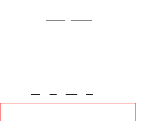
CHAPTER EIGHTEEN (Fourier Analysis) SOLUTIONS
Engineering Circuit Analysis, 6th Edition Copyright
2002 McGraw-Hill, Inc. All Rights Reserved
41.
1
/2
1
1
/2
22
1
/2 /2
22 22
/2 /2
22
T 4, periodic; find exp l form
110
4
1
2.5 /2 /4
11 11
2.5 2/4 /2/4
14
2.5 ( ) (
/2
−π
−
−π
−
−π π
−π π
′
=
∴=
∴= −
−π −π
∴= + − +
−π π π π
=−−+
ππ
∫jn t
n
jn t
n
jn jn
n
jn jn
ctedt
t
ce jn n
ce e
jn n jn n
ee
jn n
/2 /2
22
/2
22
22
)
510
2cos 2sin
22
10 20
() cos sin
22
10 20
F( ) cos sin 2
222
−π π
∞π
−∞
∞
−∞
−
ππ
=× + −
ππ
ππ
∴= −
ππ
πππ
∴ω= − πδω−
ππ
∑
∑
jn jn
jn t
ee
jn n
j
nn
jn n
ft j e
nn
jn n n
jj
nn
CHAPTER EIGHTEEN (Fourier Analysis) SOLUTIONS
Engineering Circuit Analysis, 6th Edition Copyright
2002 McGraw-Hill, Inc. All Rights Reserved
42.
1
/2 3
/2
0.002
500
0.002
0.001 0.001 0.002
500 500 500
0.002 0 0.001
T 4 , ( ) 10 ( ) 6 ( 0.001) 4 ( 0.003)
1210
( ) , 500
T4
250 ( )
250 4 10 4
250
5
−ω
−
−π
−
−−π −π −π
−
==−−−−
π
=ω==π
=
=++
=
∫
∫
∫∫∫
o
Tjn t
no
T
jnt
jnt jnt jnt
ms f t ut ut ut
cftedt
fte dt
edt edt edt
j0.001 0.001 0.002
500 500 500
0.002 0 0.001
/2 /2 /2
/2 /2 /2
4104
00
4( ) 10( 1) 4( )
2
4( ) 4( ) 10( 1)
2
42sin 42sin
22
−π −π −π
−
π−π −π −π−π
π−π π−π −π
++
π
=−+−+−
π
=−−−+−
π
π
=−
π
jnt jnt jnt
jn jn jn jn jn
jn jn jn jn jn
eee
n
jee e ee
n
jee ee e
n
jn
jj
n
/2
/2 /4 /4 /4
/4 /4
/4
10( 1)
11
4sin 5( 1) 5 ( ) 4sin
22
11
5 2sin 4sin 10 sin 4sin
42 42
1
F( ) 2 10 sin 4
−π
−π −π −π π
−π −π
−π
π+ −
ππ
=− + −= − −
ππ
ππ ππ
=−−= −
ππ
π
∴ω=π −
π
jn
jn jn jn jn
jn jn
jn
ne
nn
je je e e
nn
nn nn
je j e
nn
n
je
n4sin ( 500 )
2
∞
−∞
π
δω− π
∑nn
CHAPTER EIGHTEEN (Fourier Analysis) SOLUTIONS
Engineering Circuit Analysis, 6th Edition Copyright
2002 McGraw-Hill, Inc. All Rights Reserved
43.
1
F( ) 20 ( 20 )
!1
11 1 1 1
20 ( ) ( 20) ( 20) ( 40) ( 40)
11 11 11 21 3
11
( 60) ( 60) ...
77
20 20
10 ( ) [ ( 20) ( 20)] [ ( 40) ( 40)]
23
20 20
[ ( 60) ( 60) [ (
725
∞
−∞
ω= δω−
+
= δω+ δω+ + δω− + δω+ + δω−
++ + +
+δω+ +δω− +
= δ ω + πδ ω+ + πδ ω− + πδ ω+ + πδ ω − +
ππ
πδ ω+ + πδ ω− + πδ
ππ
∑
jn
n
80) ( 80)] ...
10 20 20 20 20
( ) cos 20 cos 40 cos60 cos80 ...
22 3 7 25
20111 1
0.25 cos 20 cos40 cos60 cos80 ...
23725
20 1 1 1 1
(0.05) 0.25 cos1 cos2 cos3 cos4 ... 1.3858
23725
ω+ +πδ ω− +
∴=+ + + + +
ππ π π π
=++++ +
π
∴= + ++++=
π
rad
ft ttt t
ttt t
f
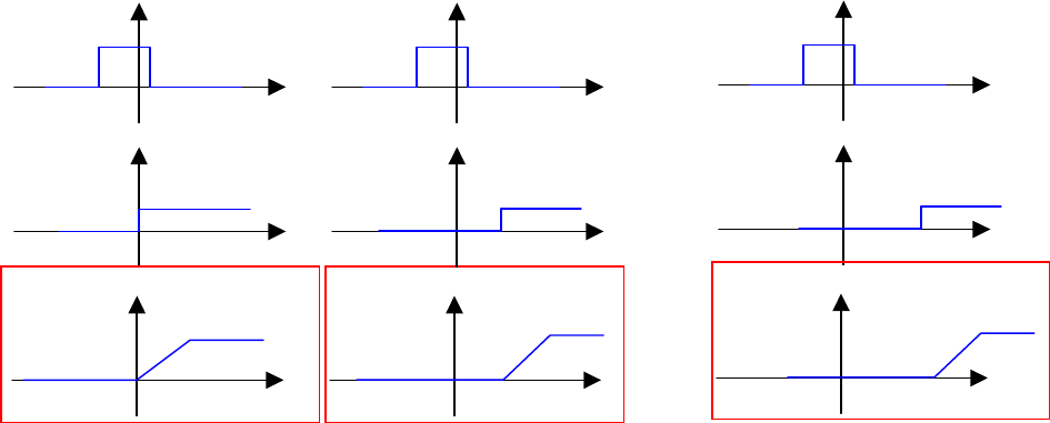
CHAPTER EIGHTEEN (Fourier Analysis) SOLUTIONS
Engineering Circuit Analysis, 6th Edition Copyright
2002 McGraw-Hill, Inc. All Rights Reserved
44. Input ( ) 5[ ( ) ( 1)] ( ) ( ) ( )
t
xt ut ut yt xz ht z dz
−∞
== −− = −
∫
(a) () 2 ()ht ut
= (b) () 2 ( 1)ht ut
=− (c)
() 2 ( 2)ht ut
=−
t < 0:
y(t) = 0 1: ( ) 0tyt
<= 2: ( ) 0tyt
<=
01:t<< 12:t<< 23:t<<
0
( ) 10 10==
∫
t
y t dz t ∫== t
tdzty
1
1) - 10( 10 )(
∫== t
tdzty
2
2) - 10( 10 )(
t > 1: t > 2: t > 3:
∫== t
t
dzty
1-
10 10 )( ∫== t
t
dzty
1-
10 10 )( ∫== t
t
dzty
1-
10 10 )(
5
h( z)
z
2
y(t)
t
10
1
x(t – z)
z
t-1 t
x(t – z)
z
t-1 t
h( z)
z
2
y(t)
t
10
3
2
x(t – z)
z
t-1 t
h( z)
z
2
y(t)
t
10
1 2
1 2

CHAPTER EIGHTEEN (Fourier Analysis) SOLUTIONS
Engineering Circuit Analysis, 6th Edition Copyright
2002 McGraw-Hill, Inc. All Rights Reserved
45. () 5[ () ( 2)]; () 2[ ( 1) ( 2)]xt ut ut ht ut ut=−− =−−−
or….
same answers as above
1
0
2
2
() ( ) ( )
1: ( ) 0
1 2: ( ) 10 10( 1)
23:()10
3 4: ( ) 10 10(2 2) 10(4 )
4: ( ) 0
( 0.4) 0; (0.4) 0; (1.4) 4
(2.4) 10; (3.4) 6; (4.4) 0
−∞
−
−
=−
<=
<< = = −
<< =
<< = = −+ = −
>=
∴− = = =
===
∫
∫
∫
t
t
t
yt xz ht z dz
tyt
tyt dzt
tyt
tyt dz t t
tyt
yyy
yyy
0
1
2
2
() ( ) ( )
1: ( ) 0
1 2 : ( ) 10 10( 1)
23:()10
3 4: ( ) 10 10(2 2) 10(4 )
4: ( ) 0
∞
−
=−
<=
<< = = −
<< =
<< = = −+ = −
>=
∫
∫
∫
t
t
yt xt zhzdz
tyt
tyt dzt
tyt
tyt dz t t
tyt

CHAPTER EIGHTEEN (Fourier Analysis) SOLUTIONS
Engineering Circuit Analysis, 6th Edition Copyright
2002 McGraw-Hill, Inc. All Rights Reserved
46.
2
() 2()
0
22
0
0
22
22
() 3[ ], () ()
() ( ) ( )
3[ ]
1
3[] 3 2
3 ( 1) 1.5 ( 1)
( ) 3(1 ) 1.5(1 ) 1.5 3 1.5 , 0
−−
−∞
−− − −
−−
−−
−− −−
=− =
=−
=−
=−
=−− −
∴=−− − =−+ >
∫
∫
tt
t
t
tz tz
t
tzt t Z
tt t t
tttt
ht e e xt ut
yt xzht zdz
eedz
ee e e
ee e e
yt e e e e t
CHAPTER EIGHTEEN (Fourier Analysis) SOLUTIONS
Engineering Circuit Analysis, 6th Edition Copyright
2002 McGraw-Hill, Inc. All Rights Reserved
47.
0
() ( 2) ( )
2
( ) (5 ), 2 5
3
∞
=−
=−<<
∫
yt xt hzdz
ht t t
(a)
(b)
55
22
220
() 10 (5 ) (5 )
33
Note: ( )is in window for 4 6
=×− = −
<<
∫∫
yt z dz z dz
hz t
5
2
2
20 1
() (5 )
32
10 (0 9) 30 at 5
3
yt z
t
=− −
=− − = =
CHAPTER EIGHTEEN (Fourier Analysis) SOLUTIONS
Engineering Circuit Analysis, 6th Edition Copyright
2002 McGraw-Hill, Inc. All Rights Reserved
48. (2)
0
( ) 5 ( 2), ( ) (4 16) [ ( 4) ( 7)], ( ) ( ) ( )
∞
−−
=−=−−−−=−
∫
t
xt e ut ht t ut ut yt xt z hz dz
(a) 6: ( ) 0 (5) 0tyt y
<=∴=
(b)
(c)
6(8 2)
4
66
66
44
6
6664
4
66 4 2 2 2
2
8: (8) 5 (4 16)
(8) 20 80
20 ( 1) 80 ( )
1
20 (5 3 ) 80 80 20 80 60
20(1 ) 22.71
−−−
−−
−−
−−−−
−
== −
∴= −
=−−−
=−−+=+−
=+=
∫
∫∫
z
zz
z
ty e zdz
y e z e dz e e dz
e
ez eee
ee e e e e
e
7(10 2)
4
78
4
77
8887874
4
44
87 4 1 4 1 4
10: (10) 5 (4 16)
(10) 20 ( 4)
(10) 20 80 20 [ ( 1)] 80 ( )
20 (6 3 ) 80( ) 40 20 15.081
−−−
−
−−− −
−−−−−
== −
∴= −
∴= − = −− −
=−−−=+=
∫
∫
∫∫
z
z
zzz
ty e zdz
yeezdz
y e ze dz e e dz e e z e e e
ee e ee e e
CHAPTER EIGHTEEN (Fourier Analysis) SOLUTIONS
Engineering Circuit Analysis, 6th Edition Copyright
2002 McGraw-Hill, Inc. All Rights Reserved
49.
0
00
0
( ) sin , 0 ; 0 elsewhere, Let ( ) ( )
() ( ) ( )
0: ( ) 0
0:()sin sin
1
() (sin cos )
2
1[ (sin cos ) 1]
2
1(sin cos )
2
−
∞
−+ −
−
−
−
=<<π =
=−
<=
<<π = × =
∴= −
=−+
=−+
∫
∫∫
t
tt
tz t z
t
tz
tt
t
ht t t xt e ut
yt xt z hzdz
tyt
tyt zedzeezdz
yt e e z z
ee t t
tte
(a) (1) 0.3345y+
=
(b) (2.5) 0.7409y=
(c)
0
0
:() sin
11
: ( ) (sin cos ) ( 1) 12.070
22
(4) 0.2211
π
−
π
−−π−
>π =
>π = − = + =
∴=
∫
tz
tz t t
yyteezdz
yyteezz ee e
y
CHAPTER EIGHTEEN (Fourier Analysis) SOLUTIONS
Engineering Circuit Analysis, 6th Edition Copyright
2002 McGraw-Hill, Inc. All Rights Reserved
50.
0
1
2
12
2
23
()0.8(1)[(1) (3)],
( ) 0.2 ( 2)[ ( 2) ( 3)]
() ( ) ( ) ,
3: ( ) 0
3 4: ( ) 0.8( 1)0.2( 2)
( ) 0.16 ( 2 2 2)
11
0.16 [ ( 1) 2 2 ] 0.16 ( 1)
32
∞
−
−
=− −−−
=− −−−
=−
<=
<< = −− −
∴= −−+−+
=−+++−=−++
∫
∫
∫
t
t
xt t ut ut
ht t ut ut
yt xt z hzdz
tyt
tyt tz zdz
yt tz t z z z dz
ztz tdz z t
1
12
2
2
32
32 2 2
32
(2 2 )
181 1
0.16 ( 1) ( 1)( 1) ( 1)4 (2 2 )( 1 2)
332 2
1181
( ) 0.16 ( 1)( 1) 2 2 2 6 2 6
3332
11 11
0.16 1 2 1 6 3 8
62 22
−
−
+−
=−−+++−−++−−−
∴= −+−+++ −−−−+−−+
= + −− +−−+ ++−
∫t
t
ztz
tttttt
yt t t t t t t t t t
tt t 32
1399
0.16 6222
=−+−
ttt
3
(4.8) 90.67 10y−
∴=×
3
3
332
2
2
(3.8) 13.653 10
11
4 5: ( ) 0.16( 1)( 2) 0.16 ( 1) (2 2 )
32
11
( ) 0.16 (27 8) ( 1)5 (2 2 )1
32
19 11
0.16 2.5 2.5 2 2 0.16 0.5
36
−
∴=×
<< = −− − = − + + + −
∴= − −+++−
=−+++−= −
∫
y
t y t t z z dz z t z t z
yt t t
ttt
(b)
(a)

CHAPTER EIGHTEEN (Fourier Analysis) SOLUTIONS
Engineering Circuit Analysis, 6th Edition Copyright
2002 McGraw-Hill, Inc. All Rights Reserved
51.
22
0
2( ) 2
0
22
0
2
() 10 (), () 10 ()
() ( ) ( )
() 10 10
100 100
() 100 ()
−−
∞
−− −
−−
−
==
=−
∴=
==×
∴=
∫
∫
∫
tt
t
tz z
t
tt
t
xt e ut ht e ut
yt xt zhzdz
yt e e dz
edz et
yt te ut
CHAPTER EIGHTEEN (Fourier Analysis) SOLUTIONS
Engineering Circuit Analysis, 6th Edition Copyright
2002 McGraw-Hill, Inc. All Rights Reserved
52. 4
() 5 ()
t
ht e ut
−
=
(a)
(b)
0.8
80.86.4
1
0.1
25
W 25 ( ) 1.3990 J
8
25
% 1.3990/ 100% 44.77%
8
−−−
Ω==−=
∴= × =
∫t
edt e e
2
21
120
0
1
1
5 1 25 25 1
H( ) W tan
41644
25 1 0.9224
W tan 0.9224 J % 100% 29.52%
42 25/8
−
Ω
−
Ω
ω
ω= ∴ = ω=
ω+ π ω + π
∴= = ∴= × =
π
∫
jd
j
CHAPTER EIGHTEEN (Fourier Analysis) SOLUTIONS
Engineering Circuit Analysis, 6th Edition Copyright
2002 McGraw-Hill, Inc. All Rights Reserved
53.
2
222
F( ) ( ) (2 2 ) ( )
(1 )(2 ) 1 2
−−
ω= = − ∴ = −
+ω +ω +ω +ω
tt
jfteeut
jj j j
(a) 234
1
0
4841
W(484) J
2343
∞−−−
Ω=−+ =−+=
∫tt t
eeedt
(b)
2
0.69315 2 0.69315
max
( ) 2 4 0, 2 4 0, 2, 0.69315
2( ) 0.5
tt t t
ft e e e e t
fe e
−− −
−−×
=− + = − + = = =
∴= − =
CHAPTER EIGHTEEN (Fourier Analysis) SOLUTIONS
Engineering Circuit Analysis, 6th Edition Copyright
2002 McGraw-Hill, Inc. All Rights Reserved
54.
(a)
(b)
(c)
(d)
23
1 1/6 1/2 1/3
F( ) (2 )(3 ) 2 3
11 1
( ) sgn( ) ( ) ( )
12 2 3
−−
ω= = − +
ω +ω +ω ω +ω +ω
∴= − +
tt
jjj jj j j
ft t e ut e ut
23
11/61/22/3
F( ) (2 )(3 ) 2 3
11 2
( ) sgn( ) ( ) ( )
12 2 3
−−
+ω
ω= = + −
ω +ω +ω ω +ω +ω
∴= + −
tt
j
jjj jj j j
ft t e ut e ut
2
23
(1 ) 1/ 6 1/ 2 4 / 3
F( ) (2 )(3 ) 2 3
11 4
( ) sgn( ) ( ) ( )
12 2 3
−−
+ω
ω= = − +
ω +ω +ω ω +ω +ω
∴= − +
tt
j
jjj jj j j
ft t e ut e ut
3
23
(1 ) 1/ 6 1 / 2 8 / 3
F( ) 1
(2 )(3 ) 2 3
11 8
() () sgn() () ()
12 2 3
−−
+ω
ω= = + + −
ω+ω +ω ω +ω +ω
∴=δ+ + −
tt
j
jjj j j j j
ft t t e ut e ut
CHAPTER EIGHTEEN (Fourier Analysis) SOLUTIONS
Engineering Circuit Analysis, 6th Edition Copyright
2002 McGraw-Hill, Inc. All Rights Reserved
55. ( ) 2 ( )
t
ht e ut
−
=
(a) 12
H( ) 2 11
ω= × =
+ω +ω
jjj
(b) V1111/
H( )
212V11/
ω
ω= = =
+ω + ω
o
i
j
jjj
(c) Gain = 2
CHAPTER EIGHTEEN (Fourier Analysis) SOLUTIONS
Engineering Circuit Analysis, 6th Edition Copyright
2002 McGraw-Hill, Inc. All Rights Reserved
56.
2
2
2
22
11
() 2
2
V( ) 11
() 2()2
12
( ) 2( ) 2 2( ) 2( )
V( ) 1
() 2()2 () 2()2
2248
Let V ( ) 1 ; 1 1
22 2
AB AB
V( ) 1 Let 0 0
11 11 1111
Let
ω+ ω+
ω
ω= = ω+ ω+
+ω+
ω
ω+ ω+− ω − ω
∴ω= =+
ω+ ω+ ω+ ω+
−± −
ω= ∴ = − = =− ±
++
∴=+ + = =∴+=
++ +− + −
o
o
o
o
jj
j
jjj
jj
jj j j
jjj jj
x
jx x x j
xx
xx
xjxj j j
(1 1) (1 1)
AB B2 B
12AB2, AB2 0
11 1111
B B 22B B0 B 1 1 A 1 1
11 11 11 11
V( ) 1 , V( ) 1
11 11 ()11()11
() () (1 1) () (1 1) (
−− −+
+
=−∴ + =∴−= =+ ∴ + =
−+−
∴ − + + + + = ∴ =− − ∴ =− +
−+ −− − +
∴=+ + ω=− −
++ +− ω++ ω+−
∴=δ−− −+
oo
jt jt
o
j
xjj
jj j j
jj j j j
jj j j
xj
xjxj jjjj
vtt jeut jeu
45 45
)
() 2 () 2 ()
( ) 2 2 cos( 45 ) ( )
−°−− °+−
−
=δ − −
=δ − + °
j jtt j jtt
t
t
te uteut
tetut
CHAPTER EIGHTEEN (Fourier Analysis) SOLUTIONS
Engineering Circuit Analysis, 6th Edition Copyright
2002 McGraw-Hill, Inc. All Rights Reserved
57.
22
/6
5/ 10 /
V( ) 105/ 35 30( ) 1/ 7 6( )
10 10 / 6
V( ) 71
6( ) 7( ) 1 () ()
66
49 24 1 10 / 6 2 2
7/6 /2 , 1 V( )
36 36 6 ( 1/6)( 1) 1/6 1
( ) 2( ) ( )
−−
ωω
ω= =
ω+ + ω ω+ + ω
∴ω= =
ω+ ω+ ω+ ω+
∴ω=− ± − =− − ∴ ω= = −
ω+ ω+ ω+ ω+
∴= −
c
c
c
tt
c
jj
jjjjj
jjj jj
jj
jjj j
vt e e ut
CHAPTER EIGHTEEN (Fourier Analysis) SOLUTIONS
Engineering Circuit Analysis, 6th Edition Copyright
2002 McGraw-Hill, Inc. All Rights Reserved
58. 23
() 5 (), () 4 ()
tt
ft e ut gt e ut
−−
==
(a)
(b)
0
22 3 2
00
2
23
()()
54 20
20 ( 1) V
()()
∞
−− −−
−
−−
∗= −
==
=− −
∴∗= −
∫
∫∫
tt
tz z t z
tt
tt
fg ftzgzdz
ee edz e edz
ee
fg e e ut
23
54 20
F( ) , G( ) F( )G( )
23 (2)(3)
20 20
F( )G( ) 20( 2 ) ( )
23
−−
ω= ω= ∴ ω ω=
ω+ ω+ ω+ ω+
∴ω ω= − ∴∗= −
ω+ ω+
tt
jj jj
jj jj
jj fge ut
jj
CHAPTER NINETEEN (WEB CHAPTER) SOLUTIONS
Engineering Circuit Analysis, 6th Edition Copyright
2002 McGraw-Hill, Inc. All Rights Reserved
1.
123 1 3 1 2
2123
213 13
0
13 12
1232
12 3 1
Order , , : 2 6 5 2cos10 3 2 (1)
4 0.05 0.15 0.25 (2)
2 5 0.4 ( ) 8 (3)
(1) 2 6 3 2 5 2cos10 A
(2) 0.05 0.15 0.25 4 B
(3) 2 5 0.4 0
′′
−−=+ −+
′′
=−+
=− − + − +
′′
→− − =− + + + =
′′′
→−+==
′′ ′
→++= −
∫
t
iii i i t i i
iiii
iii iidt
ii ii t
iiii
ii i i 3
112 2 1 3
1
2
.4 C
30 20 50 20cos10 240 3.6 3.6
A0 6
B 0.15 0.25
C1 5 A( 1) B(6) C( 0.9) A 6B 0.9C 10A 60B 9C
20 6 2( 1) 6(0.35) 0.1
0.05 0.15 0.25
215
2A 6
0.05 B 0.25
2C5 10[ A( 0.25) B(2) C(
0.1
=
′
∴= + + + + + −
−
−
−− + − −− −
′
∴= = = = + +
−−
−−− −
−
−−
′==−−−+−−
−
i
iii t i ii
i
i
212 213
2123
3
312 21
0.2)] 2.5A 20B 2C
7.5 5 12.5 5cos10 80 0.8 0.8
6.7 85 0.8 12.5 5cos10
20A
0.05 0.15 B
21C
10[A(0.35) B( 2) C(0.3)] 3.5A 20B 3C
0.1
10.5 7 17.5 7cos10 80 1.2 1.
=− − −
′=−−− −−+
′
∴= − + − −
−
−
′==−−−+=−−−
−
′=−−− −−+
iii tiii
iiii t
i
iii tii
3
3123
2
9.3 87 1.2 17.5 7cos10
′
∴= − + − − ←
i
iiii t
CHAPTER NINETEEN (WEB CHAPTER) SOLUTIONS
Engineering Circuit Analysis, 6th Edition Copyright
2002 McGraw-Hill, Inc. All Rights Reserved
2. 1, 2 2 1xyxy x y xy
′′ ′ ′
+=++ − = −−
(a)
(b)
(c)
Order , M by 2: 2 2 2 2 2; add: 3 4 1
411 122
and
333 333
xy x y x y x x y
xxy y xy
′′ ′
+=++ =++
′′
∴= + + =− + +
4112241224
3333339993
12 2
(3 4 1)
99 9
2 , or 2 0
′′ ′ ′ ′
= +−+ += −+ +=
′
−+ −−+
′′ ′ ′′ ′
∴= − − +=
xx xy xxy x
xxx
xxxxxx
4 1 1851 4
Let (0) 2 and (0) 5 (0) (2) ( 5)
33 33333
1 2 2 2 10 2 10
Also, (0) (2) ( 5)
33 33333
82
(0) 2 (0) (0) 2
33
24
(0) 2 (0) (0) 2 0
33
xyx
y
xxx
xxx
′
= =−∴ = + −+=−+=
′=− + − + =− − + =−
′′ ′
∴= −=−=
′′′ ′′ ′
=−=−=

CHAPTER NINETEEN (WEB CHAPTER) SOLUTIONS
Engineering Circuit Analysis, 6th Edition Copyright
2002 McGraw-Hill, Inc. All Rights Reserved
3.
1
11
11
2 3 ( ), 2 5 3, 2 0 Order , ,
2.5 1.5 (1)
25 1
2.5 1.5 2 3 0.5 (3)
36 3
2511 11 511
2(2)
3623 231246
xyzftxz zyx xyz
xz
zyzfzyz f
yzx y z fxy x y z f
′′ ′ ′′
−−= += − −=
′
∴=− +
′′
−+−−=∴=−−+−
′′ ′
∴=−=−−+− −∴=−−− +−
CHAPTER NINETEEN (WEB CHAPTER) SOLUTIONS
Engineering Circuit Analysis, 6th Edition Copyright
2002 McGraw-Hill, Inc. All Rights Reserved
4. 1
234, 567,(0)2,(0)
3
xxyyxyx y
′′
=− − + = − + = =
(a)
(b) 56 (0)5(1)6(15)95yxyy
′′ ′ ′ ′′
=− ∴ =−− =−
(c) 5 6 (0) 5( 43) 6( 95) 215 570 355yxyy
′′′ ′′ ′′ ′′′
=− ∴ =−−−=−+=
11
2 3 , (0) 2(2) 3 4 1, (0) 5(2) 6 7 15
33
(0) 2( 1) 3(15) 2 45 43
xxyx y
x
′′ ′ ′ ′ ′
=− − =− − + =− = − + =
′′
∴=−−−=−=−
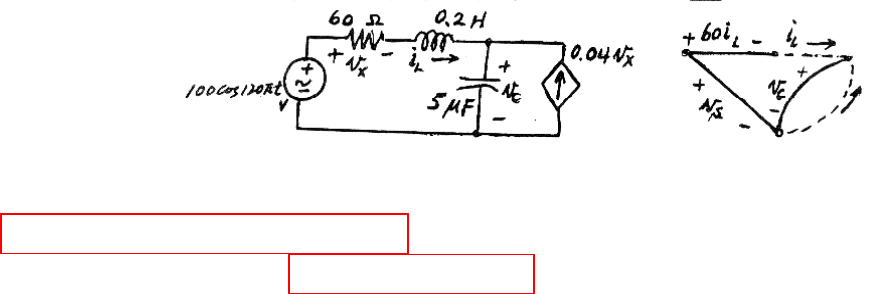
CHAPTER NINETEEN (WEB CHAPTER) SOLUTIONS
Engineering Circuit Analysis, 6th Edition Copyright
2002 McGraw-Hill, Inc. All Rights Reserved
5.
65
0.2 60
300 5 500cos 120 (1)
5 10 2.4 3.4 6.8 10 (2)
Ls LC
LLC
CL L L C L
iv iv
iiv t
vi i i v i
π
−
′
∴=−−
∴=− − +
′′
×=+=∴=×
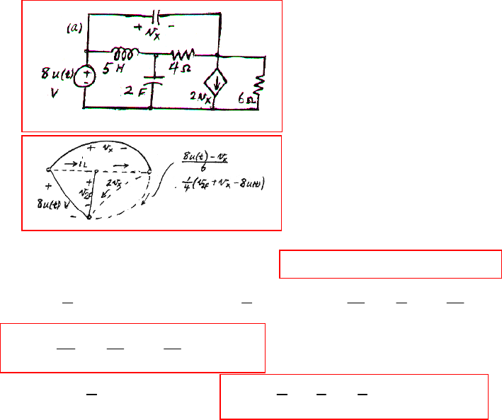
CHAPTER NINETEEN (WEB CHAPTER) SOLUTIONS
Engineering Circuit Analysis, 6th Edition Copyright
2002 McGraw-Hill, Inc. All Rights Reserved
6.
(a)
(b)
(c)
()()
()
22 2
2 2
2
22 2 2
Order: , , 5 8 ( ) 0.2 1.6 ( ) (1)
1 1 19 1 10
3 8 () 2 8 () ()
461243
19 1 10 () (2)
36 12 9
1111
2 8 () () (3)
4288
Lx F L F L F
xFx x xxF
xx F
FL F x F L x F
ivv i v ut i v ut
vvvutvutvvvut
vvv ut
v i v v ut v i v v ut
′′
∴=−+ ∴=− +
′=− + − + + − = − +
′
∴= − +
′′
=− +− ∴ = − − +
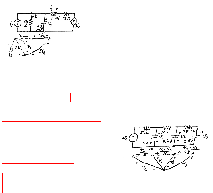
CHAPTER NINETEEN (WEB CHAPTER) SOLUTIONS
Engineering Circuit Analysis, 6th Edition Copyright
2002 McGraw-Hill, Inc. All Rights Reserved
7.
(a)
(b)
4
Order: ,
0.002 3 15 , 0.02
0.002 15 0.94 , 7500 470 (1)
2 10 0.02
5000 100 5000 (2)
LC
LC A LA C
LL CL LC
CLAsL Cs
CLCs
iv
iv i ii v
iivi iv
viiii vi
vivi
−
′=− − =
′′
∴=−+ =−+
′
× =−− +=−− +
∴=− − +
123
11 12
112
212 2
212
323323
Order: , ,
0.1 0.2 0.2 0.1 0.1
32(1)
0.2 0.1 0.1 0.04 0.04
0.5 0.7 0.2 (2)
0.5 0.04 0.04 , 0.08 0.08 (3)
s
s
s
s
vvv
vvvvv
vvvv
vvv v v
vvvv
vvvvvv
′=− + − +
′
∴=− ++
′=−− +
′
∴= − +
′′
=− =−
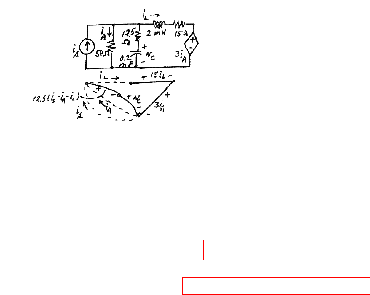
CHAPTER NINETEEN (WEB CHAPTER) SOLUTIONS
Engineering Circuit Analysis, 6th Edition Copyright
2002 McGraw-Hill, Inc. All Rights Reserved
8.
2
0.02(12.5 12.5 12.5 )
1.25 0.25 0.02 0.25
0.2 0.016 0.2
0.002 15 3 12.5 12.5 12.5
0.002 27.5 15.5( 0.2 0.016 0.2 ) 12.5
0.002 24.4 0
AsAC
ALCs
AL Cs
LLACsAL
LLC LCss
LL
iiiiv
iivi
ii vv
iiiviii
iiv ivii
ii
=−−+
∴=−+ +
∴=− + +
′=− − + + − −
′
∴=−+−−+ ++
′
∴=−+.752 9.4
12,200 376 4700 (1)
Order: , Also, 0.0002 0.2 0.016 0.2
0.0002 0.8 0.016 0.8 4000 80 4000 (2)
Cs
LLCs
LC C s A L s L C s L
CL CsC LC s
vi
iivi
iv v i i i i i v i i
vi viv ivi
+
′
∴=− + +
′=−−=+ − − −
′′
∴=−−+∴=−−+
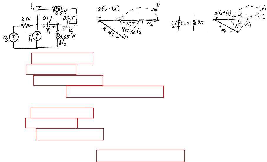
CHAPTER NINETEEN (WEB CHAPTER) SOLUTIONS
Engineering Circuit Analysis, 6th Edition Copyright
2002 McGraw-Hill, Inc. All Rights Reserved
9.
112 1 1 2
21 2 1
112 1 12
21 2 2 1 2
1212
112 1 1 2
21 2 1
0.1 10 10 (1)
0.2 5 (2)
0.5 , 2 2 (3)
0.05 2 2 20 40 40 20 (4)
Order: , , ,
0.1 10 10 (1)
0.2 5 (2)
0.
ss ss
vii v i i
viv i
ivv i vv
iv i iv i v i i v
vvii
vii v i i
viv i
′′
=− ∴ = −
′′
=− ∴ =−
′′
=− + ∴ =− +
′′
=+ − + ∴= − + +
′′
=− ∴ = −
′′
=− ∴ =−
1121 12
21 2 2 2
21 2 2 2 1 2
522(3)
0.05 2 2 , 3 2 2 0.4 0.2
0.05 0.8 0.4 2 20 24 12 (4)
sR R R s R s
ss s
ivvi vv
ivv i ii i iv i i v
ivv i v i i v i v
′′
=− + ∴ =− +
′=+− − =− − + ∴=− +
′′
∴=++−−∴=−+
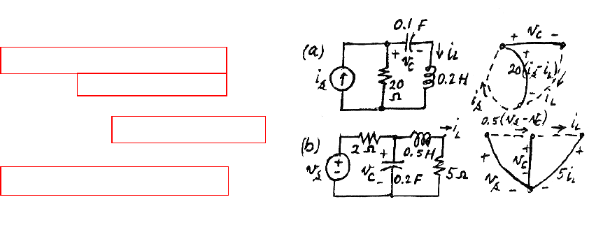
CHAPTER NINETEEN (WEB CHAPTER) SOLUTIONS
Engineering Circuit Analysis, 6th Edition Copyright
2002 McGraw-Hill, Inc. All Rights Reserved
10.
(a)
(b)
Order: , 0.2 20 20
100 5 100 (1)
0.1 10 (2)
LC L C L s
LLCs
CL C L
iv i v i i
iivi
vi v i
′
∴=−−+
′
∴=− − +
′′
=∴=
0.5 5 10 2 (1)
0.2 0.5 0.5
5 2.5 2.5 (2)
LC L L L C
CsCL
CL C s
iv i i i v
vvvi
vivv
′′
=− ∴=− +
′=−−
′
∴=−− +
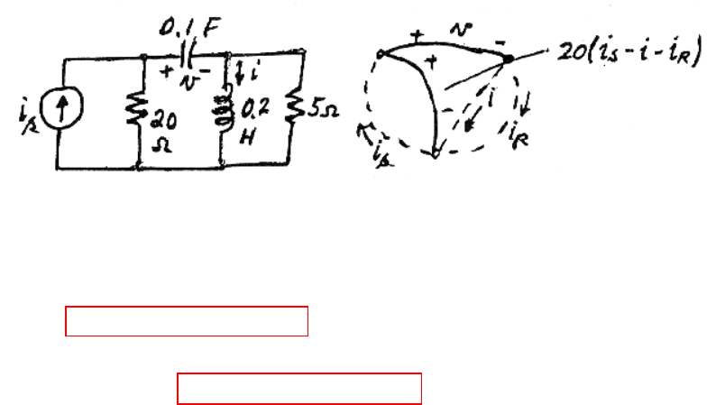
CHAPTER NINETEEN (WEB CHAPTER) SOLUTIONS
Engineering Circuit Analysis, 6th Edition Copyright
2002 McGraw-Hill, Inc. All Rights Reserved
11.
5202020
0.04 0.8 0.8
0.1 0.04 0.2 0.8
Order: , 0.4 2 8 (1)
0.2 20 20 20( 0.04 0.2 0.8 )
0.2 0.2 4 4 20 20 (2)
Rs R
Rs
Rs
s
ss
ss
ivi ii
ivii
vii v i i
vi v v i i
ivi i v i i
iviiivii
∴=−+ −−
∴=− − +
′
∴=+=− ++
′
∴=− + +
′=− + + − − + +
′′
∴=−−+∴=−−+
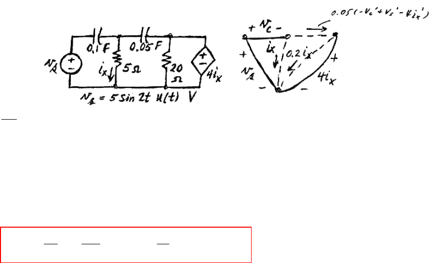
CHAPTER NINETEEN (WEB CHAPTER) SOLUTIONS
Engineering Circuit Analysis, 6th Edition Copyright
2002 McGraw-Hill, Inc. All Rights Reserved
12.
40.2
20
0.1 0.05 0.05 0.2
0.15 0.2 0.05
5 , 0.2 0.2 , 0.2 0.2
0.15 0.2 0.2 0.04 0.04 0.05
0.11 0.2 0.2 0.01 0.11 0.
xx
Cx C s x
Cx x s
xcsx c sx C s
CCsC ss
CCs s C
ii
vi v v i
vi i v
ivvi v vi v v
vvvvvv
vvvv v
=
′′′′
=− + −
′′′
∴=−+
′′′
=− + =− + =− +
′′′′
∴=−++−+
′′′
∴=−++ ∴=−2 sin 2 ( ) 0.1cos2 ( )
20 100 10
sin2 () cos2 () (1)
11 11 11
C
CC
vtut tut
vv tut tut
++
′
∴=− + +
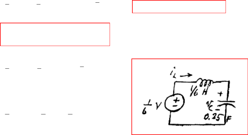
CHAPTER NINETEEN (WEB CHAPTER) SOLUTIONS
Engineering Circuit Analysis, 6th Edition Copyright
2002 McGraw-Hill, Inc. All Rights Reserved
13.
(a)
(b)
1
2
2112
2
212
12
123 2
,456,3 232(1)
789 1
4563 (2)
7891 (3)
L
LLLLC
C
LLL C
CLL C
it
qi a f t i i i v t
vt
iiivt
viiv t
−−−
′
==− =∴=−−−+
−− +
′=−++
′=−−++
06 1
,,
40 0
61, 4
0.25 C 0.25 F
111
L H
666
L
C
LCCL
CL
LC
i
qa f
v
ivvi
vi
iv
−
== =
′′
∴=− + =
′
∴=∴=
′=− + ∴ =
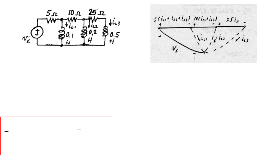
CHAPTER NINETEEN (WEB CHAPTER) SOLUTIONS
Engineering Circuit Analysis, 6th Edition Copyright
2002 McGraw-Hill, Inc. All Rights Reserved
14.
123
1123
2123
2 123 3123
3123
0.1 5 5 5
50 50 50 10 (1)
0.2 5 15 15
25 75 75 5 (2) 0.5 5 15 40
10 30 80 2 (3)
50 50 50
25 75 75
10 3
LLLLs
LLLLs
LLLLs
LLLLs LLLLs
LLLLs
iiiiv
iiiiv
iiiiv
iiiiv iiiiv
iiiiv
a
′=− − − +
′
∴=− − − +
′=− − − +
′′
∴=− − − + =−− − +
′
∴=− − − +
−−−
=− − −
−−
10
5
080 2
s
s
s
v
fv
v
=
−
CHAPTER NINETEEN (WEB CHAPTER) SOLUTIONS
Engineering Circuit Analysis, 6th Edition Copyright
2002 McGraw-Hill, Inc. All Rights Reserved
15.
01
1
02
2
1
2
12 0 0
33 0 10 00 1 2
,210, 0; , ,
012 2
14 2 0 13 0 0
,,
12 0
00 1
012
13 0
C
C
R
L
R
v
vv
qv a f w b d
i
ii
w bq d q aq f w bq d w bq baq bf
ba
−
−
==− === =
−−
−
′′′
=+∴=+ =+ = = +
−
=−
12
1
1
2
110 120 10
33 0 10
142 00 1 0
210 , 0
09 4 012 0
14 2 0
300 130 10
10
110 10
142 0
09 4 0
300 10
CC
C
C
C
L
bf
vv
vv
wv
i
−
−− −
−= = =
−−
−
++
−
−−
′
∴= + =
−
2
2
1
01 1 2 02 1 2 1 02 2 1
42
94
310
10, 4 2 , 9 4 , 3 10
CL
CL
C
CC C C LR LR C
vi
vi
v
vvv v v v ii v ii v
−+
−
+
′′ ′′
∴=++ =−− + = − = +
CHAPTER NINETEEN (WEB CHAPTER) SOLUTIONS
Engineering Circuit Analysis, 6th Edition Copyright
2002 McGraw-Hill, Inc. All Rights Reserved
16.
1
1
2
2
3
3
4
3 1 2 cos2 1 2 0 3
,221,sin2, ,0111
130 0 2 1 13
10
210
1, / , , (0) 5
35
12 03
0111
2113
−
==−− = ==−
−−−
−
==+=+=
−
∴= −
−−
y
qt
y
qqa f ty b
y
qy
dqaqfqbydy
q
π
π
1
124
2
234
3
123 4
4
2 232 7
11(0)11
32 33 53
3 1 2 7 1 21 11 106 1
(0) 2 2 1 11 0 14 22 53
13053 0 733
+++
+=−+++ ∴ =
−−+ +
−−+++
′=− − + = − − +
−−+
yyyy
yyyy q
yyyy y
y
q
97
17
26
=
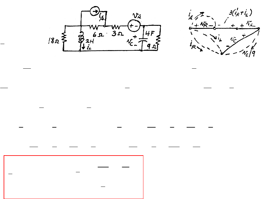
CHAPTER NINETEEN (WEB CHAPTER) SOLUTIONS
Engineering Circuit Analysis, 6th Edition Copyright
2002 McGraw-Hill, Inc. All Rights Reserved
17.
1
4 , 2 3 3 , 18 2
99
21
666 66,4
6399
21
Also, 2 6 6 3 3 9 6
33
1
3
C
L
C
CLRLRRLsCRLRL
CR RLs R R L s L L s C L L
L LLs LLCs LCLss
L
v
qi
v
v iiiv i ivv i i i i
vv iii v i i i i i i v i i
iiiiiivvivivi
iv
=
′′ ′′
=− − − = − − + + = ∴ =
′′′
=− − − ∴ =− − − =− − − ∴ =− − −
′′ ′ ′
=− − − − − + + ∴ = − + −
′
∴= 111112
32(2)4
39273279
4212 111 1
4(1)
27 3 27 9 27 6 108 18
11
1/27 1/6 108 18
[] []
1/3 3 1 2
3
CL ss C CL C L s s
CCLssCCLss
ss
ss
ivi v vi vi vi
vvivivvivi
vi
af
vi
′
−+ − =− −− + − +
′′
∴=− −− +∴=− −− +
−+
−−
∴= =
−
−
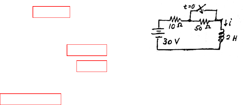
CHAPTER NINETEEN (WEB CHAPTER) SOLUTIONS
Engineering Circuit Analysis, 6th Edition Copyright
2002 McGraw-Hill, Inc. All Rights Reserved
18.
(a) 30 10 2 5 15ii i i
′′
=+ ∴=−+
(b)
(c) 55
3(1 ) A, 0.5 A
tt
zero state zero input
ieie
−−
=− =
(d)
555
0
555 5
(0) 0.5 A, 5 0.5 15
0.5 3( 1) 3 2.5 A, 0
−−
−− −
==−∴=+
∴= + − = − >
∫
t
ttZ
ttt t
iaieeedz
ieee e t
55 5
5
3, A 3 A , (0) 0.5 3 2.5 A
2.5 A, 3 A
tt t
fn
t
nf
iie i ei i e
iei
−− −
−
= = ∴= + = ∴= −
∴=− =
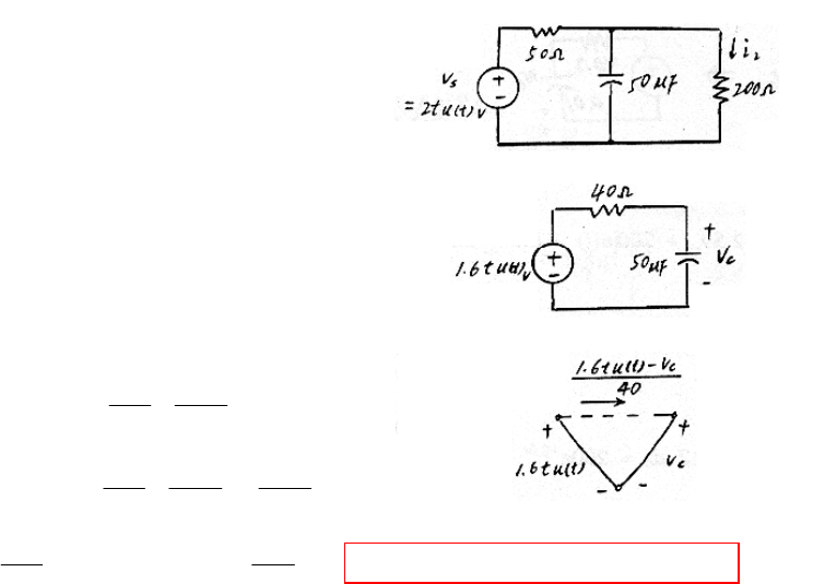
CHAPTER NINETEEN (WEB CHAPTER) SOLUTIONS
Engineering Circuit Analysis, 6th Edition Copyright
2002 McGraw-Hill, Inc. All Rights Reserved
19.
5
500 500
0
500 500
0
500 500
2
0
500 500
22
5 10 0.04 ( ) 0.025
500 800 ( ) 500
800Z
800 Z
Z1
800 500 500
11
800 500 500 500
1.
1.6
−
−
−
−
−
′
∴× = −
′
∴=− + ∴=−
∴=
=
∴= −
∴= − +
∴= +
∫
∫
CC
CC
t
tZ
C
t
tZ
t
tZ
C
tt
C
C
vtut v
vvtuta
ve e dz
eedz
vee
t
vee
vt 500 3 6 500
2
61
( 1 ) 8 10 16 10 (1 ) A, 0
500 200
−−−−
−+ ∴ = = × − × − >
tt
C
eiv t et
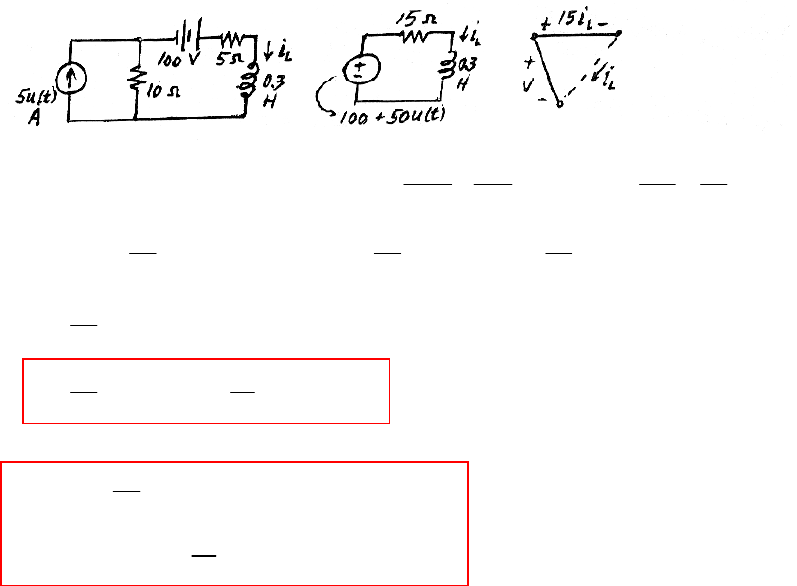
CHAPTER NINETEEN (WEB CHAPTER) SOLUTIONS
Engineering Circuit Analysis, 6th Edition Copyright
2002 McGraw-Hill, Inc. All Rights Reserved
20.
(a)
(b)
50 50 50 50 50 50
0
50 50
50
1000 500 100 20
0.3 15 100 50 ( ), 50 ( ), (0) A
3 3 15 3
20 20 1
500dZ 500 ( 1)
3350
20 10(1 ) 0
3
20 10
( ) 10 ( ) A
33
−− −−
−−
−
′′
=− + + =− + + = =
∴= × + = + −
∴= + − >
∴= −+ −
∫
LL LL L
t
ttZ ttt
L
tt
L
t
L
ii utii uti
ie e e e e e
ie et
iut eut
50 50
,,
50
20 A, 10(1 ) A
3
10
10 A, A
3
tt
L zero input L zero state
t
Lf Ln
iei e
iie
−−
−
==−
==−
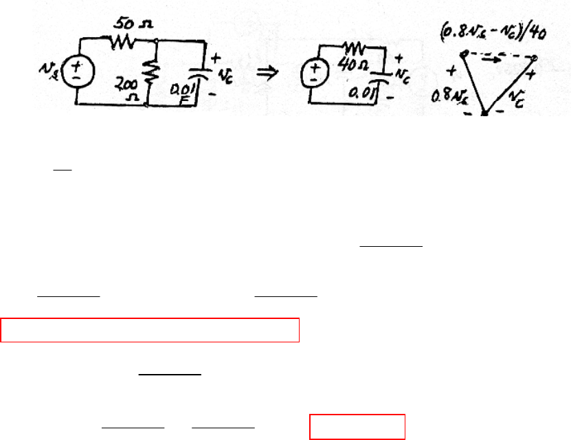
CHAPTER NINETEEN (WEB CHAPTER) SOLUTIONS
Engineering Circuit Analysis, 6th Edition Copyright
2002 McGraw-Hill, Inc. All Rights Reserved
21.
2.5
2.5 2.5 2.5
2
00
2
100[ ( ) ( 0.5)]cos V
1
0.01 (0.8 ) 2.5 200[ ( ) ( 0.5)]cos
40
00
0 0.5 200 cos Z 200 (2.5cos Z sin Z)
6.25
200 (2.5cos si
6.25
−−
=−−
′′
=−∴=−+−−
<=
≤≤ = × = +
+
∴= +
+
∫
s
CsCCC
C
t
tZ
tZ t
C
C
vutut t
vvvvvutut t
tv
e
t v e e dz e
vt
π
π
ππππ
π
ππ
π
2.5
2
2.5
0.5
2.5
2.5
2
0
1.25
2.5 2.5
22
200
n ) 2.5
6.25
31.02cos 38.98sin 31.02
0.5 200 (2.5cos Z sin Z)
6.25
1
200 2.5 105.03 V
6.25 6.25
−
−
−
−−
−+
∴= + −
>= +
+
∴= − × =
++
t
t
C
Z
t
C
tt
C
te
vtte
e
tv e
e
ve e
ππ
ππ
πππ
π
π
ππ
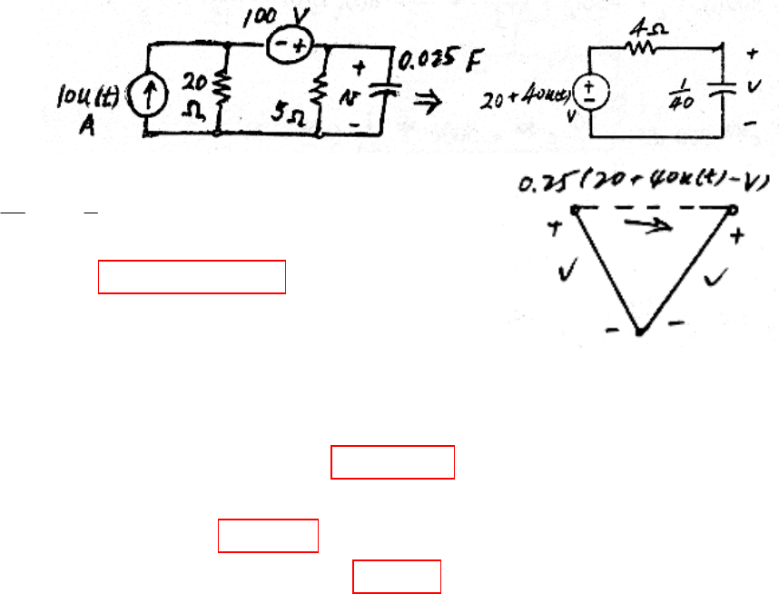
CHAPTER NINETEEN (WEB CHAPTER) SOLUTIONS
Engineering Circuit Analysis, 6th Edition Copyright
2002 McGraw-Hill, Inc. All Rights Reserved
22.
11
510()
40 4
vv ut
′
∴=−++
(a) 10 200 400 ( )vv ut
′
∴=− + +
(b)
(c)
10 10 10 10 10 10
0
10 10 10
020 V
0 20 600 20 60 ( 1)
20 60 60 60 40 V
−− −−
−− −
<∴=
>= + = + −
∴= + − ∴= −
∫
Z
ttZ ttt
tt t
tv
tve eedze ee
ve e v e
10
10 10
60V 40 V
60(1 ) V 20 V
t
forced nat
tt
zero state zero input
vve
veve
−
−−
==−
=− =
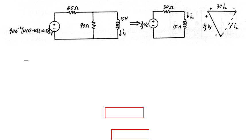
CHAPTER NINETEEN (WEB CHAPTER) SOLUTIONS
Engineering Circuit Analysis, 6th Edition Copyright
2002 McGraw-Hill, Inc. All Rights Reserved
23.
22
0
22 2
0
0.5
220.52
0
2
15 30 3
2 4 [ ( ) ( 0.5)]
4 [ (Z) (Z 0.5)]
0 0.5 4 dZ 4 ( 1) 4 4 A
0.5 4 dZ 0 4 ( 1) 2.595 A
−
−−
−−−−
−−−−
′=− +
′
∴=− + − −
∴= − −
≤≤ = = − = −
≥= += −=
∫
∫
∫
LLs
t
LL
t
tZZ
L
t
tZ tt t t
L
tZ t t
L
iv
iieutut
ieeeu u dz
tiee ee ee
tiee ee e

CHAPTER NINETEEN (WEB CHAPTER) SOLUTIONS
Engineering Circuit Analysis, 6th Edition Copyright
2002 McGraw-Hill, Inc. All Rights Reserved
24.
85
[ ] , 0.01
10 10
at
−
==
−
(a)
(b)
(c) 1.0860 0.0547 0.9254 0.0457 1.0000 0
0.1095 1.1079 0.0915 0.9071 0 1.0000
ta ta
ee
−−
==
−
0.08 0.05 0.08 0.05 0.08 0.05
1
I ...
0.1 0.1 0.1 0.1 0.1 0.1
2
1 0 0.08 0.05 0.0114 0.0090 0.0114 0.009 0.08 0.05
11
0 1 0.1 0.1 0.0180 0.0150 0.018 0.015 0.1 0.1
26
ta
e−−−−
=− + −
−−−
−−−−
=− + −
−− − −
...
1.08 0.05 0.0057 0.0045 0.00181 0.00147 1.0860 0.0547
1
0.1 1.1 0.009 0.0075 0.00294 0.00240 0.1095 1.1079
6
+
−−− −
=+ − =
−− −−
1 0 0.08 0.05 0.0057 0.0045 0.0003 0.0002 0.9254 0.0457
0 1 0.1 0.1 0.009 0.0075 0.0005 0.0004 0.0915 0.9071
ta
e−−−
=+ + + =
−− −
CHAPTER NINETEEN (WEB CHAPTER) SOLUTIONS
Engineering Circuit Analysis, 6th Edition Copyright
2002 McGraw-Hill, Inc. All Rights Reserved
25.
(a)
(b)
(c)
() 1 2 1
,cos,013
() 2 3 1
2 ( ), 3 cos , 2 3 ( )
xut
qyf ta
zut
x x y z ut y y z t z x y z ut
−
== =−
−−−−
′′′
∴=+ −+ =−+ + =− − −−
2121214
(0) 3 , /(0) 0 1 3 3 1 7 0.1
1231113
2 0.4 1.6
(0.1) (0) 0.1 (0) 3 0.7 2.3
1 0.3 1.3
qq t
qq q
−−
=− ∴ = − − + = ∆=
−−− −
−
′
=+ =−+ =−
2 4 1.8
0.05 (0.5) 3 0.05 7 2.65
1 3 1.15
1 2 1 1.8 1 3.65
(0.05) 0 1 3 2.65 cos0.05 7.0988
2 3 1 1.15 1 2.2
(0.1) (0.05) 0.05 (0.05)
tq
q
qq q
−
∆= ∴ =− + =−
−−
′=− −+ =
−−− −
′
=+ =
1.8 3.65 1.6175
2.65 0.05 7.0988 2.2951
1.15 2.2 1.26
−
−+ =−

CHAPTER NINETEEN (WEB CHAPTER) SOLUTIONS
Engineering Circuit Analysis, 6th Edition Copyright
2002 McGraw-Hill, Inc. All Rights Reserved
26.
232
12 3 1 2 3
0 1 2 Now, I 0 1 2
31 1 3 1 1
det[ ] ( 1 )( 2 1 2) 3(4 3 3 ) 3 8 22 0
s
aass
s
ss s s s s s
−−−
=− −= −−
−−−
=−− ++−+++=−−++=
By trial and error, Solve, or high school algebra (Hormer’s method) we find s = -3.48361. Now
divide polynomial by s + 3.48361. Get quadratic, s2 – 0.48361s – 6.31592 = 0.
The remaining two roots are: s = -2.28282 and s = + 2.76641.
CHAPTER NINETEEN (WEB CHAPTER) SOLUTIONS
Engineering Circuit Analysis, 6th Edition Copyright
2002 McGraw-Hill, Inc. All Rights Reserved
27.
12
2
12 11 12
25 25 25
11 11
225 2
32 3 2
det( I) det 7 12 2 0
14 1 4
Roots are 2, 5 Now, ,
11
2, 5 3, 33
22 5
, or
33 3
−− −− −−
−−− −
−−−
=−= =++−=
−−−
=− =− = + = +
∴=− =−∴−= = −
∴= + − =
st st
oo
tt tt tt
oo
ttt
oo
s
aas ss
s
s s e u us e u us
euueuuee uue e
ue e e u e 5
25
25
1
25
2525 25
25 252 5
2
2
3
52 032
11
33
I52 14
33
033
52 22
33 33
11 5244
33 3333
21
33
−
−−
−−
−−
−−−− −−
−− −−− −
−−
−
−
−
=+= + −
−
−
−−+ −
=
− −−+
+
∴=
tt
tt
ta tt
o
tt
tttt tt
ta
tt tttt
t
ta
e
ee
eu ua e e
ee
eeee ee
e
ee eeee
ee
e
525
25 25
22
33
1112
3333
−−
−− −−
−
−+
ttt
tt t t
ee
eeee
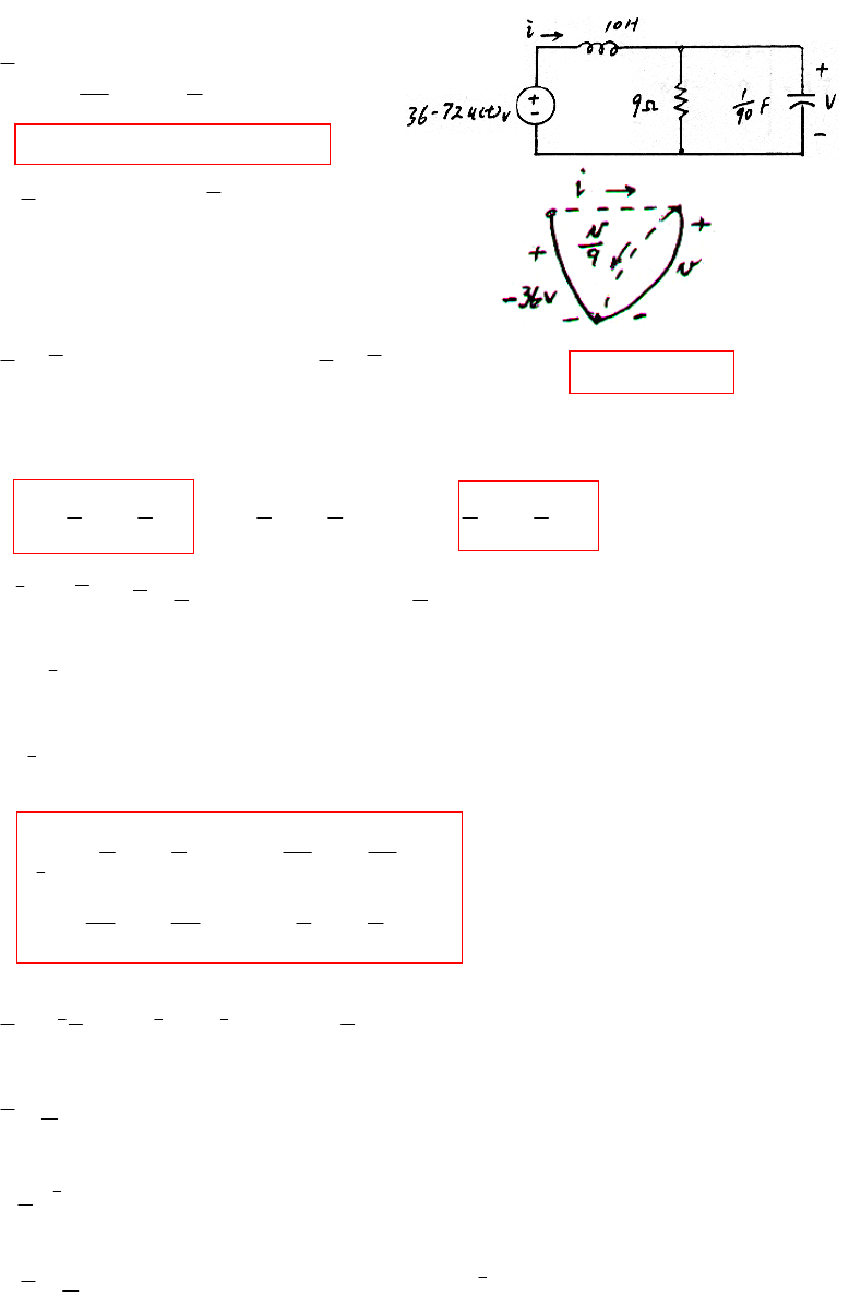
CHAPTER NINETEEN (WEB CHAPTER) SOLUTIONS
Engineering Circuit Analysis, 6th Edition Copyright
2002 McGraw-Hill, Inc. All Rights Reserved
28.
(a)
(b) 2
12
0 0.1
I , det( I) 10 9 1, 9
90 10
s
as as s s s s
s
−−
−= − =+ +∴=− =−
−−
(c)
(d)
(e)
10 36
11
90 9
0.1 3.6, 90 10
0 0.1 3.6
,
90 10 0
iv
i
qvvi v
ivviv
af
′=− −
= ′=−
′′
∴=− − = −
−−
∴= =
−
99
11 1
99 9
1
,9 8
11 11 91
,
88 88 88
−− −−
−− −−− −−
=− =− ∴− =
∴= − = − + = −
tt tt
oo
tt ttttt
o
euue uuee u
ue eue ee e e
99
1
9 9
999
99
99
1 0 0 0.1
11
I(9) ()
0 1 90 10
88
9 0 0 0.1 0.1
80 9 90 90 10 10
9 0.1 0.1
890 90 9
ta tt tt
o
tt t t
ta
tt t t t t
tt t t
ta
tt tt
eu ua ee ee
ee e e
eee e e e e
ee e e
eee ee
−− −−
−− − −
−− − − − −
−− − −
−− −−
−
=+= − + −
−
−−+
∴= +
−−−+
−−+
=−−+
99
99
91 1 1
8 8 80 80
90 90 1 9
88 88
tt t t
ta
tt tt
ee e e
e
ee ee
−− − −
−− −−
−−+
∴=
−−+
0
99
99
99
99
0
9
(0) 4
(0) (Z) (0) (0) 36
1
9 0.1 0.1
1
9
290 90 9
3.6
9 0.1 0.1
1
0
890 90 9
9
1
2
−
−− − −
−− −−
−−
=+ ==
−−+
=
−−+
−
−−+
+
−−+
−−
∴=
∫
∫
t
ta ta Za
tt t t
tt tt
tZZ Z Z
ta
ZZ ZZ
tt
i
q e q e e f dz q v
ee e e
qee ee
ee e e
edz
ee ee
ee
q
99
99 9
0
0.9 0.9 9
0.45 dZ
90 90 9 81 90 90
−−
−−−−
+−
−
−−+ −
∫
t
tt ZZ
ta
tttt ZZ
ee ee
e
eeee ee
CHAPTER NINETEEN (WEB CHAPTER) SOLUTIONS
Engineering Circuit Analysis, 6th Edition Copyright
2002 McGraw-Hill, Inc. All Rights Reserved
9
9
99
9
999
999
11
99
4.05 0.05 0.45 99
40.5 4.5 90 10 90 10
180
9
4.05 0.05 9 0.1 0.1
0.45 99
8
40.5 4.5 90 90 9 90 1
tt
tt ta
tt tt
tt
tt tttt
tt tttt
t
ee
ee e
ee ee
ee
ee ee ee
qee ee ee e
−
−−
−− −− −−
−− −− −−
−−+
−
=−
−
−−+
−−
−−+
=−
−−−+
−9
9
9
889889
889889
080
4.05 0.05
4.05 4.5
180
81 80 9 9 8 9 1 8
0.45 99
8810 10 800 810 10 800 90 10 80 810 90 720
4.05
t
tt
tt
ttt t ttt t
tt t t tt t t
e
ee
ee
eee e eee e
eee e eee e
e
−−
−−
−− − −− −
−− − −− −
−
−
=
−
−− − ++ −++ + −−
−
−− − ++ −+++ −−
=9
9
99
99
99
9
9
18
71 72
0.05 0.45 99
7
40.5 4.5 640 720 80
4.05 0.05 4 4.05 0.05
40.5 4.5 36 40.5 4.5
4 8.1 0.1
36 81 9
tt
tt
tt tt
tt tt
tt tt
tt
tt
ee
e
ee ee
ee ee
ee ee
ee
qee
−−
−−
−− −−
−− −−
−− −−
−−
−−
+− +
−
−
−
−+
−−+
=−
−−+
−+ −
∴=−+ − (0)t
>
