Focal Mechanisms Managing, Classification And Plot Program. The FMC Manual
User Manual:
Open the PDF directly: View PDF ![]() .
.
Page Count: 34

Contents
I The manual 4
1 Introduction 4
2 Versions 4
3 Installation 5
4 Usage 5
4.1 Input ................................ 6
4.2 output ............................... 7
4.3 Plot ................................. 10
4.4 Clustering ............................. 15
5 License 19
II The background 20
6 Introduction 20
7 The focal mechanism 21
8 Diagram 23
9 Focal Mechanism Classification 26
9.1 Comparison between rake-based and SMT axes-based clas-
sifications .............................. 28
References 31
2
Acknowledgments
I have been using different versions of this program during the last decade.
Initially I reworked some of the Gasperini and Vannucci (2003) FORTRAN
subroutines on Matlab in order to obtain all the focal mechanism parame-
ters from the Harvard CMT formatted catalog. During my research
on seismotectonics I started to use the Frohlich and Apperson (1992) dia-
gram, but after Kagan (2005) I decided to try the Kaverina et al. (1996) one.
From the original Matlab program I jumped to the Free Software world
adapting it to Octave. The program only produced the x and y positions of
the events and all the plotting was done by means of GMT (Wessel et al.,
2013).
Some colleagues wanted to use the diagram for their work, but they were
not familiar with GMT, so I decided to make a big improvement in the
program to make it easy to use, distributable and with plotting support. I
choose to program it in Python with the following basic ideas:
1. It should be called from the terminal or the command line in order to
be incorporated into shell scripts
2. It should behave like any other shell unix tool, compatible with redi-
rection, piping and ASCII format
3. it should be compatible with the GMT formats to allow the
mapping of the focal mechanisms
4. It should has the option to produce a Kaverina et al. (1996) type clas-
sification diagram
Part of the programming was done during my happy days as Ph.D. can-
didate at the UCM; so I have to acknowledge the UCM scholarship that
allowed me to start my scientific career.
I would like to thank the beta testers Jorge L. Giner-Robles and Alberto
Jiménez-Díaz for their comments and suggestions. Dr. Andrei Bala (Na-
tional Institute for Earth Physics, Romania) has tested different versions
and suggested several improvements.
If you use , and consider it appropriate, you can acknowledge it by
citing the following reference:
• Álvarez-Gómez, J.A. (2014) FMC: a one-liner Python program to man-
age, classify and plot focal mechanisms. Geophysical Research Ab-
stracts, Vol. 16, EGU2014-10887.
3
Part I
The manual
1 Introduction
This is the user manual for the program (from Focal Mechanisms Clas-
sification). This program was originally developed on Python 2.7.3 and
adapts some of the Gasperini and Vannucci (2003) FORTRAN routines to
obtain the different parameters of the earthquake focal mechanisms de-
pending on the input format. Since version 1.3 it is compatible with Python
3. Several output formats are eligible, clustering analysis of the data can be
performed and a classification diagram for the focal mechanisms is pro-
duced. The default input and output formats are the same used by the
GMT program in order to make the program integration easiest
and facilitate the mapping of the data.
The program basically takes the focal mechanisms data, computes the dif-
ferent parameters that can be obtained, classifies each focal mechanism in
one of seven possible types, perform a clustering analysis of the data if it
is required by the user and optionally outputs the parameters in different
formats and generates a classification diagram from the input data.
2 Versions
1.3 New features:
• Added support for Pyhton 3
• Added new base diagram labels and tick marks.
• Added symbol labeling.
1.2 New features:
• Added slip sense and plunge parameters for each focal mechanism
nodal plane.
1.1 New features:
• New custom output parsing. The user can choose between the stan-
dard predefined output or any parameters in any order.
4
• Added a header with the parameter name in the output.
• Added symbol coloring.
• Added hierarchical clustering with several methods and options.
1.01 New features:
• Column number is now included in the header of the output file with
all the parameters.
Bug fixes:
• Error in the nd2ar function to obtain the tensor components from the
nodal planes.
1.0 Initial release of with basic plotting function and focal mechanims
management.
3 Installation
has been programmed in Python 2.7.3 and uses several common python
libraries: , , , and . Depending on your
operative system and Python installation you could need to install some of
the libraries manually.
Since version 1.3 works also on Python 3. In order to work properly
needs version 1.14 or higher.
For Windows and Mac users a good starting point is the installation of pre-
defined packages. From www.SciPy.org you can download program pack-
ages that includes , and , as well as other modules
and IDEs. With one of these packages installed should work properly.
For Linux users all the required software can be easily installed through
your favorite distribution repository (the python modules ,
and are usually installed with the default python installation).
4 Usage
The user interface is as simple as a “command line”, or a “terminal”. I de-
cided to keep the program as simple as possible so it can be integrated into
5
scripts with other programs such as GMT, or any other tool
running from a shell or script (in *nix) or a command window or batch file
(in Windows/DOS). In the following the commands are written assuming
that your python installation recognizes automatically the python format.
In some systems, depending on your personal configuration, you will need
to call first Python (like “ ” or ” ”) or
in a *nix system with the “./” needed to execute a script (like
).
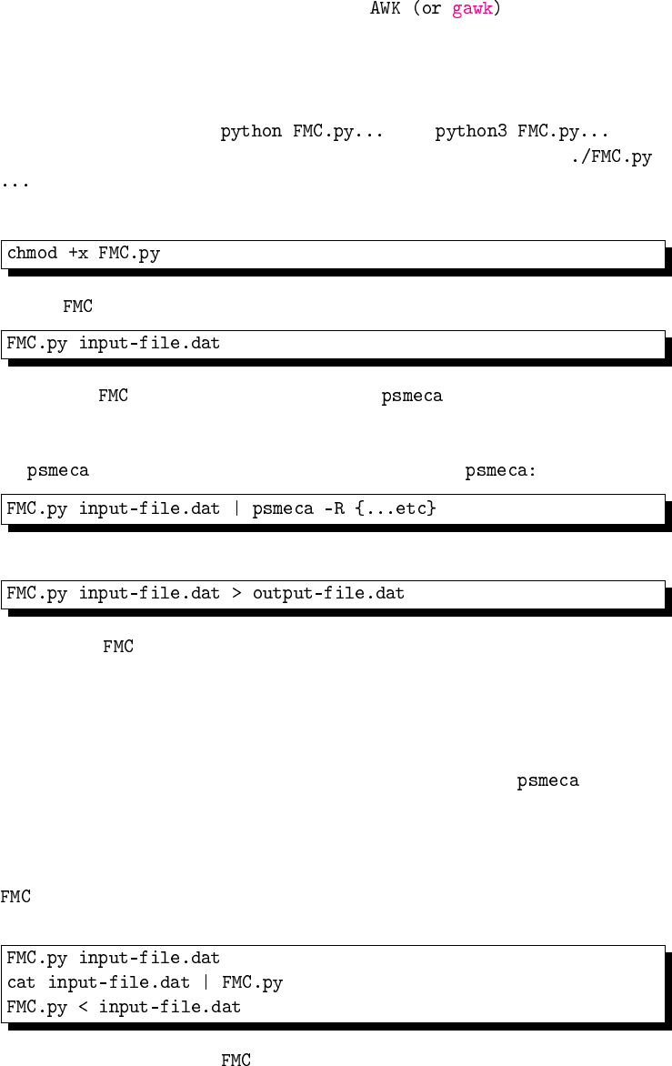
In *nix you will need to give execution permission to the program:
To run on a file simply type in the terminal:
By default will read the input file as a Centroid Moment Ten-
sor (CMT) format (in Harvard convention). This kind of file can be down-
loaded directly from Global CMT. The output will be shown on the screen
in CMT format so it can be directly pipe into
Or stored as an ASCII file:
In this case will add a new column at the end of each register with the
focal mechanism type.
Alternatively the input file can be a single plane in Aki and Richards (1980)
convention (Right Hand Rule for the plane orientation, and rakes from 0
to 180 in reverse faults and 0 to -180 in normal faults, 0 for left-lateral and
±180 for right-lateral). This format is also compatible with .
4.1 Input
input can be given as an ASCII file or as standard input, from a pipe
(“|”) or a redirection (“<”). The following codes are then equivalent:
If no input is given, then will show the on-screen help.
6
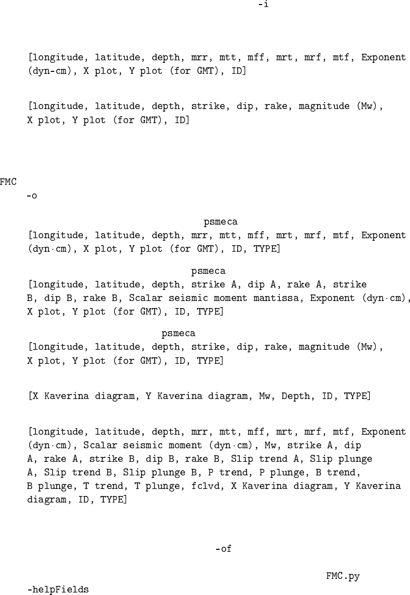
The input format is specified with the optional flag “ ”, and the possible
values are:
CMT Harvard Centroid Moment Tensor (by default):
AR Aki and Richards one plane convention:
4.2 output
output format can be selected among the following options with the
flag “ ”:
CMT Harvard Centroid Moment Tensor ( compatible):
PFocal mechanism both nodal planes ( compatible):
AR Focal mechanism one plane ( compatible):
KKaverina diagram position for plotting outside FMC:
ALL All the parameters obtained:
CUSTOM In case you need any focal mechanism parameters in any or-
der you can use the CUSTOM option and give the requested pa-
rameters in any order using the flag “ ”. The output parameters
need to be listed separated by commas. The accepted parameters
names are listed below, and can be seen on the terminal using
7
lon longitude
lat latitude
dep depth
mrr mrr centroid moment tensor component
mtt mtt centroid moment tensor component
mff mff centroid moment tensor component
mrt mrt centroid moment tensor component
mrf mrf centroid moment tensor component
mtf mtf centroid moment tensor component
mant mantissa of the seismic moment tensor
expo exponent of the seismic moment tensor
Mo Scalar seismic moment
Mw Moment (or Kanamori) magnitude
strA Strike of nodal plane A
dipA Dip of nodal plane A
rakeA Rake of nodal plane A
strB Strike of nodal plane B
dipB Dip of nodal plane B
rakeB Rake of nodal plane B
slipA Slip sense of plane A
plungA Plunge of slip vector of plane A
slipB Slip sense of plane B
plungB Plunge of slip vector of plane B
trendp Trend of P axis
plungp Plunge of P axis
trendb Trend of B axis
plungb Plunge of B axis
trendt Trend of T axis
plungt Plunge of T axis
fclvd Compensated linear vector dipole ratio
x_kav x position on the Kaverina diagram
y_kav y position on the Kaverina diagram
ID ID of the event
clas Focal mechanism rupture type
posX X plotting position for GMT psmeca
posY Y plotting position for GMT psmeca
8
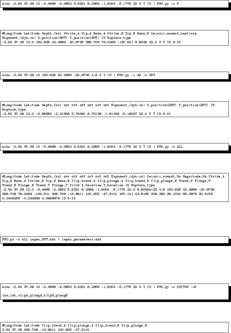
Examples of use
Obtaining nodal planes from moment tensor
Command:
Result:
Obtaining moment tensor from one nodal plane
Command:
Result:
Obtaining all the parameters from the moment tensor
Command:
Result:
Obtaining all the parameters from CMT input file and storing to an ASCII
file
Command:
Using CUSTOM output to obtain event location and slip vector of both
nodal planes
Command:
Result:
9

4.3 Plot
Optionally will produce a classification diagram. uses
libraries and can generate figures in different formats (emf, eps, jpeg, jpg,
pdf, png, ps, raw, rgba, svg, svgz, tif, tiff). The format is determined auto-
matically from the plot file name extension.
The diagram uses the Kaverina et al. (1996) projection technique, used also
by Kagan (2005); but incorporating a classification similar to the geologi-
cal conceptual classification of faults. The earthquakes are classified into
seven types according to the values of the P, T and B Centroid Moment
Tensor axes following a simple algorithm (Figure 4.1), and are represented
conveniently on the Kaverina diagram (Figure 4.2). This classification is
very similar to the used by Johnston et al. (1994).
10
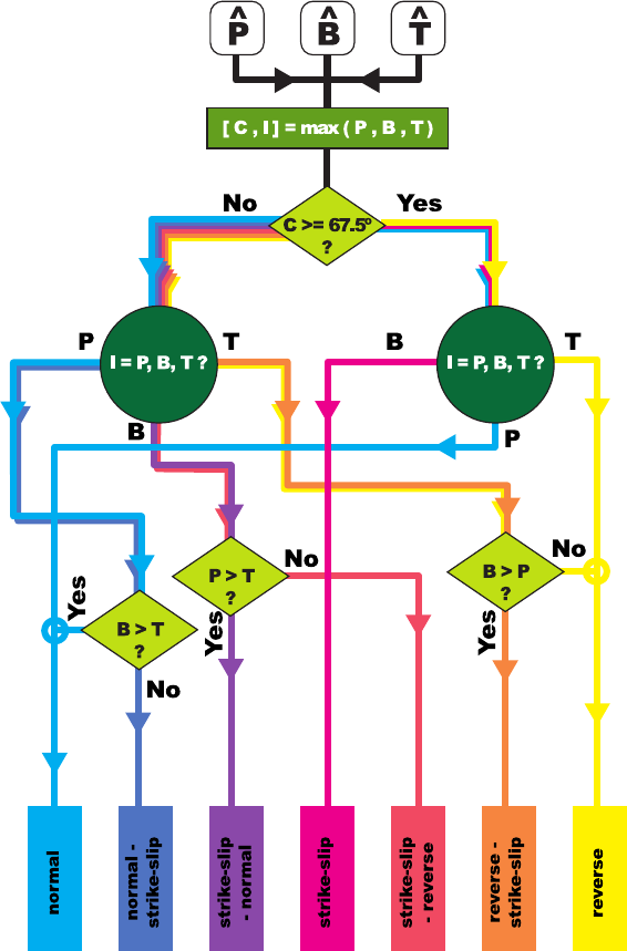
Figure 4.1: Focal mechanism classification algorithm flow chart.
11
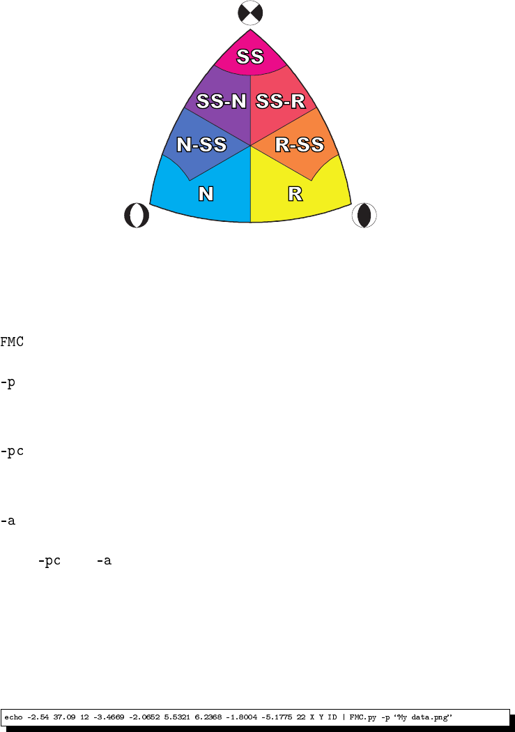
Figure 4.2: Classification diagram. N: Normal; N-SS: Normal - Strike-slip;
SS-N: Strike-slip - Normal; SS: Strike-slip; SS-R: Strike-slip - Reverse; R-SS:
Reverse - Strike-slip; R: Reverse.
uses several flags in order to customize the plot.
This flag activates the plotting. It must be followed by the name of the
figure file that will be produced. The name used for the file (without
the extension) is used as title for the plot.
With this flag the user specifies the parameter that is used to fill the
symbols. A color palette is produced with the range of the selected
parameter values.
This flag is used to annotate the symbols with a certain parameter.
With and the parameters must be given with its corresponding in-
ternal name as listed in section 4.2 on page 7.
Examples of use
Plotting data from standard input
Command:
12
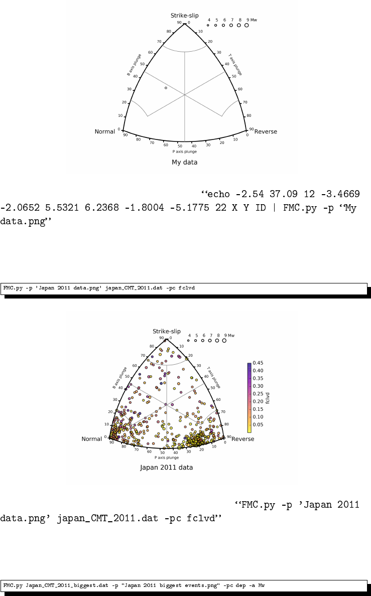
Figure 4.3: Plot result from the command
Plotting data from input file and shading the symbols with a parameter
Command:
Figure 4.4: Plot result from the command
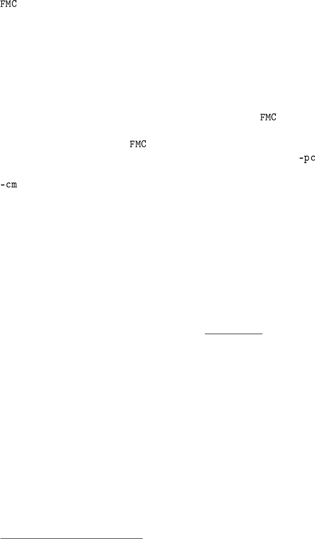
Plotting data from input file shading and annotating the symbols
Command:
13
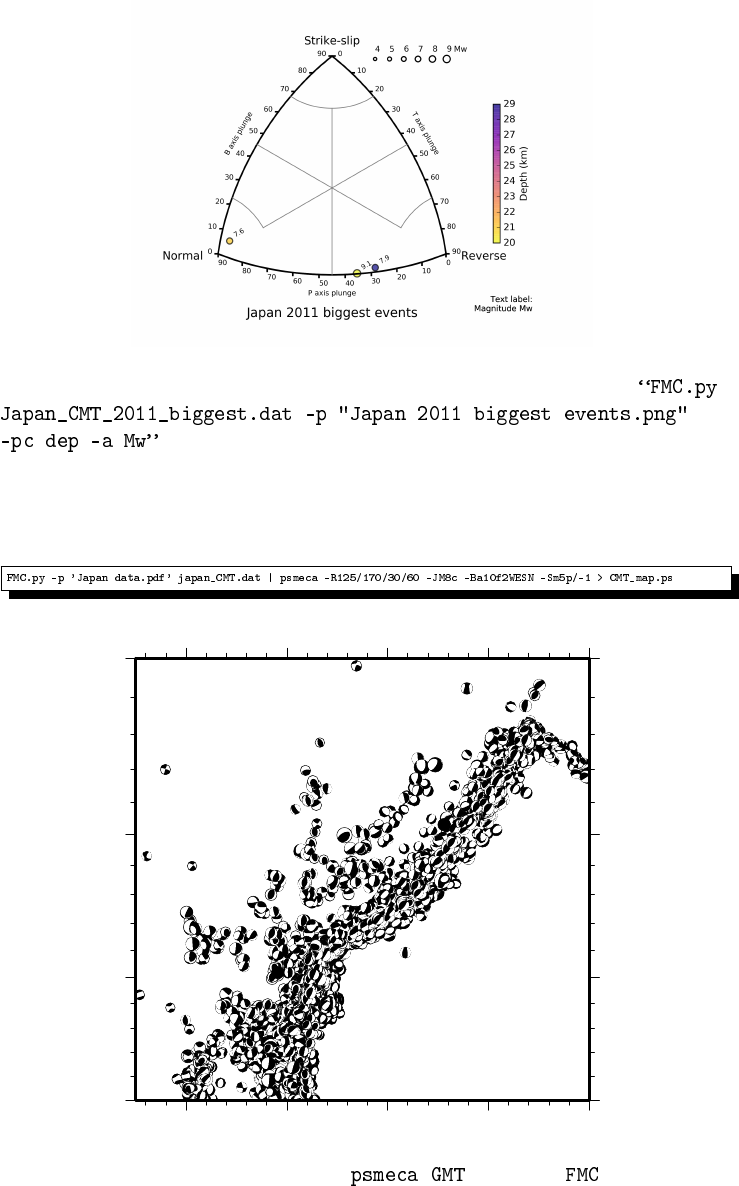
Figure 4.5: Plot result from the command
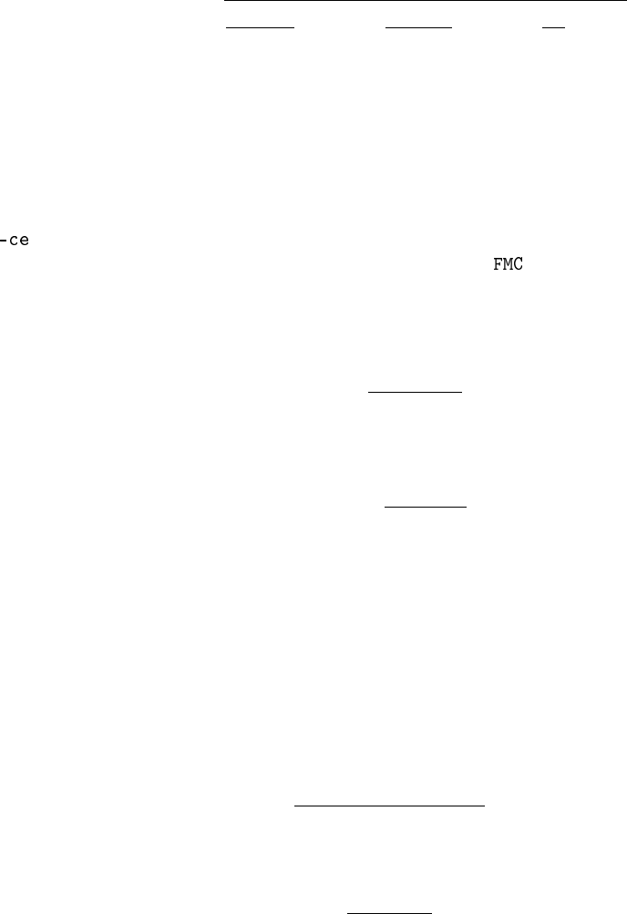
Plotting data from input file and piping to psmeca
Command:
130˚
130˚
140˚
140˚
150˚
150˚
160˚
160˚
170˚
170˚
30˚ 30˚
40˚ 40˚
50˚ 50˚
60˚ 60˚
Figure 4.6: Map generated with ( ) from the output.
14
4.4 Clustering
implements the hierarchical agglomerative clustering algorithms from
SciPy (scipy.cluster.hierarchy) in order to group the data1. The advantages
of this algorithms are its versatility, as the user can choose between a num-
ber of metrics and grouping methods, its capacity to automatically select a
minimum number of clusters without an a priori estimation, and its poten-
tial to work with different parameters with different scales and with strong
different populations in clusters.
The parameters for the clustering are passed by several optional flags. If
any of the following flags is given in the command line will perform the
clustering analysis using some default options if needed. When a clustering
analysis is done, by default will shade the symbols in the diagram using
the cluster number, unless a different parameter is stated with flag.
Method to be used in the clustering analysis. The options are:
single single/min/nearest
d(u,v) = min(dist(u[i],v[j]))
complete complete/max/farthest point
d(u,v) = max(dist(u[i],v[j]))
average average/UPGMA
d(u,v) = ∑
ij
d(u[i],v[j])
(|u|∗|v|)
weighted weighted/WPGMA
d(u,v) = (dist(s,v) + dist(t,v))/2
centroid centroid/UPGMC [default]
dist(s,t) = kcs−ctk2
where csand ctare the centroids of clusters sand t, respectively.
When two clusters sand tare combined into a new cluster u, the
new centroid is computed over all the original objects in clusters
sand t. The distance then becomes the Euclidean distance be-
tween the centroid of uand the centroid of a remaining cluster v
in the forest.
1The details on the clustering algorithms shown in this section are taken from the SciPy
documentation.
15
median median/WPGMC, assigns d(s,t)like the centroid method.
When two clusters sand tare combined into a new cluster u, the
average of centroids sand tgive the new centroid.
ward Ward variance minimization algorithm.
d(u,v) = r|v|+|s|
Td(v,s)2+|v|+|t|
Td(v,t)2−|v|
Td(s,t)2
where uis the newly joined cluster consisting of clusters sand t,
vis an unused cluster in the forest,T=|v|+|s|+|t|, and |∗|is
the cardinality of its argument.
Methods ”centroid”, ”median” and ”ward” are correctly defined only
if Euclidean pairwise metric is used.
Metric used to measure distances between events parameters. These
metrics work with non-Boolean vectors. By default uses euclidean
distance.
braycurtis The Bray-Curtis distance between two points uand vis
d(u,v) = ∑i|ui−vi|
∑i|ui+vi|
canberra The Canberra distance between two points uand vis
d(u,v) = ∑
i
|ui−vi|
|ui|+|vi|
chebyshev The Chebyshev distance between two n-vectors uand v
is the maximum norm-1 distance between their respective ele-
ments. More precisely, the distance is given by
d(u,v) = max
i|ui−vi|
cityblock City block or Manhattan distance between the points.
correlation Correlation distance between vectors uand v. This is
1−(u−¯
u)·(v−¯
v)
k(u−¯
u)k2k(v−¯
v)k2
cosine Cosine distance between vectors uand v,
1−u·v
kuk2kvk2
16

euclidean Distance between m points using Euclidean distance (2-
norm). [Default]
hamming Normalized Hamming distance, or the proportion of those
vector elements between two n-vectors uand vwhich disagree.
jaccard Jaccard distance between the points. Given two vectors, u
and v, the Jaccard distance is the proportion of those elements
u[i]and v[i]that disagree.
mahalanobis The Mahalanobis distance between two points uand v
is q(u−v)(1/V)(u−v)T
where 1/Vis the inverse covariance matrix.
minkowski Distances using the Minkowski distance ku−vkp(p-norm)
where p≥1.
seuclidean Standardized Euclidean distance. The standardized Eu-
clidean distance between two n-vectors uand vis
q∑(ui−vi)2÷V[xi]
Vis the variance vector; V[i]is the variance computed over all
the i’th components of the points. It is automatically computed.
sqeuclidean Squared Euclidean distance ku−vk2
2between the vec-
tors.
A priori number of clusters to obtain. If zero or non-present the num-
ber of clusters is automatically computed using the Elbow method.
This method uses the percentage of variance explained as a function
of the number of clusters; when the increment of number of clusters
does not improves the percentage of variance explained the number
of clusters is set.
Parameters used to perform the cluster analysis. By default uses
the position on the Kaverina diagram, which is a proxy for the prin-
cipal moment tensor axes plunges. If the parameters given are not
in the same physical magnitude and unit the euclidean distance is
not appropriate and a different metric should be used. In these cases
the Mahalanobis distance is a good choice, as is equivalent to the Eu-
clidean distance in the transformed space, using the covariance ma-
trix of each parameter.
The parameters must be given with its corresponding internal name
as listed in section 4.2 on page 7.
17
Examples of use
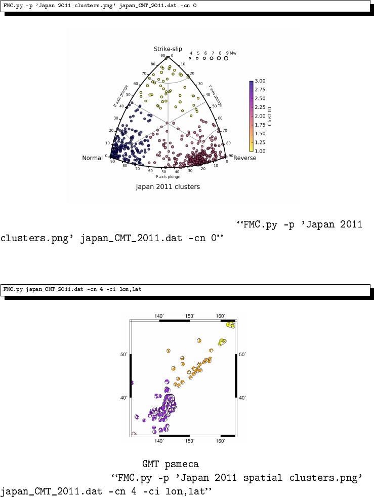
Automatic clustering using the position in the Kaverina diagram (de-
fault)
Figure 4.7: Plot result from the command
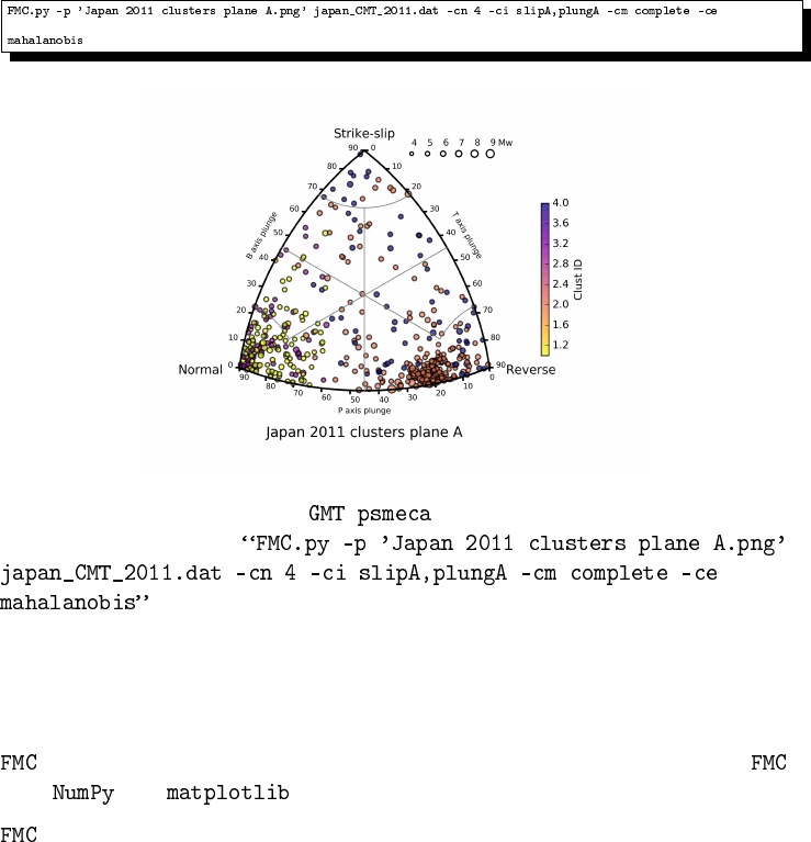
Clustering using the epicentral location
Figure 4.8: Plotting with of the clusters obtained with
the command
Clustering using Mahalanobis metric and complete grouping with the
slip and plunge of the slip vector of nodal plane A
18
Part II
The background
6 Introduction
Seismicity is frequently used to deduce the tectonics of a region. The study
of earthquakes as a tectonic component, the seismotectonics (Scholz,2002),
has grown as one of the key research areas on active tectonics, specially
from the analysis of earthquake focal mechanisms.
The first focal mechanism determination methods, based on P wave’s first
motion polarities, were developed on the first half of the 20th century, spe-
cially in Japan where a dense seismic network were available (Byerly,1928,
1938;Koning,1941;Honda and Masatuke,1952;Scheidegger,1957). Since
1960 the development of the digital computer allow the numerical determi-
nation of fault-plane solutions with different methods (e.g. Knopoff,1961;
Langston and Helmberger,1975;Dziewonski et al.,1981).
In parallel with the development of the modern seismology, the theory of
Plate Tectonics changed the way geologists understand the Earth. Since
the end of the 16th century naturalists made observations on the potential
continental drifting; but it was in the early 20th century when the theory
started to be formally proposed (Taylor,1910;Wegener,1912;Schwinner,
1919;Holmes,1931). The relevant information acquired on the magnetic
stripes on the ocean floor in the 60’s (e.g. Hess,1962;Vine,1966;Le Pichon,
1968;Morgan,1968), in addition to an increasing number of geological and
geophysical observations, established the Plate Tectonics as the global geo-
dynamical paradigm on Earth Sciences. The study of earthquakes related
to Plate Tectonics was developed at the same time establishing the basic
concepts of seismotectonics and the lithospheric deformation (e.g. Benioff,
1954;Sykes,1967;Isacks et al.,1968;Isacks and Molnar,1969).
Since the 70’s focal mechanisms are computed in a systematic way and
global catalogs of focal mechanisms are available since then. As the amount
of data increases, our knowledge on the active tectonics improves. As a
consequence of the continuous increase of data available we need new tools
to analyze it systematically.
In order to represent focal mechanism populations Frohlich and Apperson
(1992) proposed a diagram to visualize focal mechanism data as a function
of the rupture type. This kind of representation is popular and widely used
on seismotectonics to represent the focal mechanism types of the study
areas (e.g. Frohlich et al.,1997;Borges et al.,2001;Igarashi et al.,2001;
Ratchkovski and Hansen,2002;Kita et al.,2006;Serpelloni et al.,2007). This
20

representation is not accurate, presenting distortion problems (Frohlich,
2001), and Kagan (2005) used the Kaverina et al. (1996) projection to avoid
them. The latter projection is used in by default.
7 The focal mechanism
The term “focal mechanism” is used to refer to the parameters that char-
acterize an earthquake rupture. A focal mechanism usually presents the
characteristics of the two orthogonal possible rupture planes: strike, dip
and rake of the slip vector over the plane. The energy released by the event,
its hypocentral location and the exact time of occurrence are also given.
The focal mechanism can, instead of describe the geometry of the possi-
ble rupture planes (6 variables), describe the characteristics of the rupture
by means of the seismic moment tensor (SMT) or centroid moment tensor
(CMT) (6 variables).
The SMT is based in the representation of the equivalent forces on a point
seismic source. In this tensor the sum of angular moments should be null,
in other words, the SMT is a symmetric tensor on a three dimensional space
(9 components) with 6 independent components:
M
M
M=
MXX MXY MXZ
MYX MYY MYZ
MZX MZY MZZ
(7.1)
where
MXY =MYX
MXZ =MZX (7.2)
MYZ =MZY
Similarly to the strain tensor where we can define the orientation of the
principal axes (eigenvectors) and its magnitudes (eigenvalues), the SMT
can be defined by the orientation of its principal axes P, B and T (eigenvec-
tors) and its magnitudes (eigenvalues). The T axis describes the greatest of
the eigenvalues, the P describes the lowest and the B the intermediate.
If the seismic event is generated by the slip in a fault rupture, its character-
istics should be well described as a double couple moment tensor (Figure
7.1):
M
M
M=
M00 0
0−M00
0 0 0
(7.3)
21
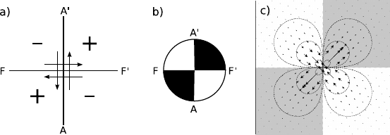
Figure 7.1: Double couple deformation mechanism. a) Plan view of hori-
zontal displacement on an idealized point vertical fault A-A’ or F-F’ and re-
sulting distribution of compressions (+) and dilatations (-). b) Focal mecha-
nism representation on a stereographic projection. Compression quadrants
are filled. c) Horizontal displacement produced by a point size vertical dis-
location computed with the Okada (1992) equations; compressional quad-
rants are filled while dilatational are kept empty following the focal mech-
anism representation. a) and b) modified from Bullen and Bolt (1985).
where M0is the scalar seismic moment.
The most used representation of the double couple is based on the stereo-
graphic projection. In this projection both nodal planes of the focal mecha-
nism are plotted, and the quadrants containing the T axis, the compression
quadrants, are filled (Figure 7.1). This kind of representation - commonly
called “beach-ball” - located on a map on the earthquake epicenter is use-
ful to interpret the seismic data from a tectonic point of view, allowing the
study of the earthquake and its rupture fault plane on its tectonic context,
being one of the basis of the seismotectonics. The compressional and dilata-
tional quadrants are separated by two orthogonal planes, the nodal planes,
being one of them the plane of rupture that generated the earthquake (Fig-
ure 7.2).
As we increase the number of focal mechanisms to study, we increase the
difficulty to interpret the data, obscuring frequently the details of a tectonic
environment if we just project them over a map. In order to facilitate the
study of groups of focal mechanisms several plots can be proposed, great
part of them based on classical structural geology plots.
The plots inherited from the structural geology are based in the geometrical
characteristics of the nodal planes of the SMT, equivalent to the character-
istics of the fault planes: strike (ϕ), dip (δ) and rake (λ) (Figure 7.2). The
main problem of these representations is the duplication of data. Each fo-
cal mechanism presents two equivalent and orthogonal nodal planes. The
selection of one of them as the fault plane is not straightforward and al-
though from a mechanical point of view they can be discriminated (McKen-
zie,1969;Michael,1987;Gephart,1990), when both nodal planes are me-
22
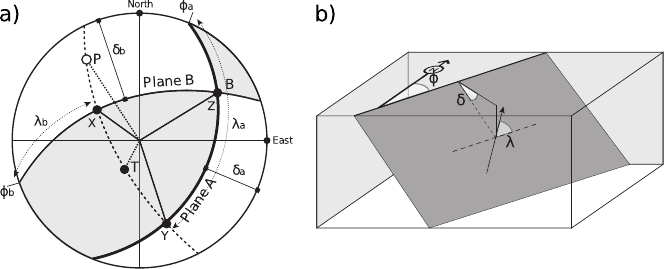
Figure 7.2: a) Focal sphere diagram on stereographic projection on the
lower hemisphere. Nodal planes A and B, A representing the fault plane
and B the auxiliary plane, with its orientation characteristics: ϕ, strike; δ,
dip and λ, rake. The orientation of the SMT principal axes are also shown:
T, B and P. Modified from Udías (1989). b) Block diagram showing the pa-
rameters that define the orientation of a fault plane in the space: ϕ, strike;
δ, dip and λ, rake.
chanically compatible or reactivated structures can be present, additional
geological and/or geophysical information is required. There are as many
representations of this kind as possible combinations between these pa-
rameters and its derivatives (usually trigonometrical functions). These re-
lations can be represented in biaxial plots or stereographic projections (e.g.
Davis and Reynolds,1996;Ramsay and Huber,1997;Pollard and Fletcher,
2005).
The focal mechanisms can also be plotted as function of the principal axes
T, B and P. These axes form an orthogonal system. The orientation of each
axis can be defined in the space as any line, by its direction and plunge. The
main advantages of these representations are: the univocality, each focal
mechanism is represented by one point; its simplicity of interpretation, the
kind of deformation (normal, reverse, strike-slip) is function of the plunge
of the axes; and the reduction of errors compared with the planes, as they
are derived from the principal axes of the SMT (Vannucci and Gasperini,
2003).
8 Diagram
Frohlich and Apperson (1992) developed a ternary diagram to represent
focal mechanisms based in the trigonometrical relation:
sin2ιT+sin2ιB+sin2ιP=1, (8.1)
23

where ιT,ιBand ιPare the plunges of the axis T, B and P of the SMT. This
relation is true for three orthogonal axes.
As the equation of a sphere with radius unity is
x2+y2+z2=1 (8.2)
and all the plunge angles are positive between 0°and 90°, then the repre-
sentation of a focal mechanism defined by these axes is equivalent to the
projection of a point in an spherical octant over a planar surface. As a
sphere is not a developable surface can not be projected onto a plane with-
out distortion.
The projection used by Frohlich and Apperson (1992) represents this spher-
ical octant as a triangle, which is equivalent to the gnomonic geographical
projection. In this projection we define the angles
ψ=arctan sin ιT
sin ιP−45◦, (8.3)
and
ιs=arcsin 1
√3=arctan 1
√2≈35.26◦, (8.4)
which is the angle of the ternary symmetry axis with the orthogonal axes
of the octant.
From these angles the xand ycoordinates over the plane are given by:
x=cos ιB·sin ψ
sin ιs·sin ιB+cos ιs·sin ιB·cos ψ(8.5)
y=cos ιs·sin ιB−sin ιs·cos ιB·cos ψ
sin ιs·sin ιB+cos ιs·sin ιB·cos ψ(8.6)
The angle ιsin the projection is the angle of the plunges of the axes T, B
and P for the focal mechanism that occupies the barycentre of the ternary
diagram where x=y=0.
As can be seen in Figure 8.1a this projection introduces remarkable distor-
tions towards the extremes of the diagram. This distortions could difficult
the study of some groups of focal mechanisms as the author pointed out
(Frohlich,2001). In order to avoid these distortions Kaverina et al. (1996)
proposed the use of a projection capable of maintain the proportion of
the areas equal, equivalent to the Lambert azimuthal equal-area projection
(Figure 8.1b), which is the used in structural geology to generate the stereo-
graphic equal-area Schmidt stereonet. In this case the limits of the diagram
are formed by great circles instead of straight lines forming a triangle (Fig-
ure 8.1).
24
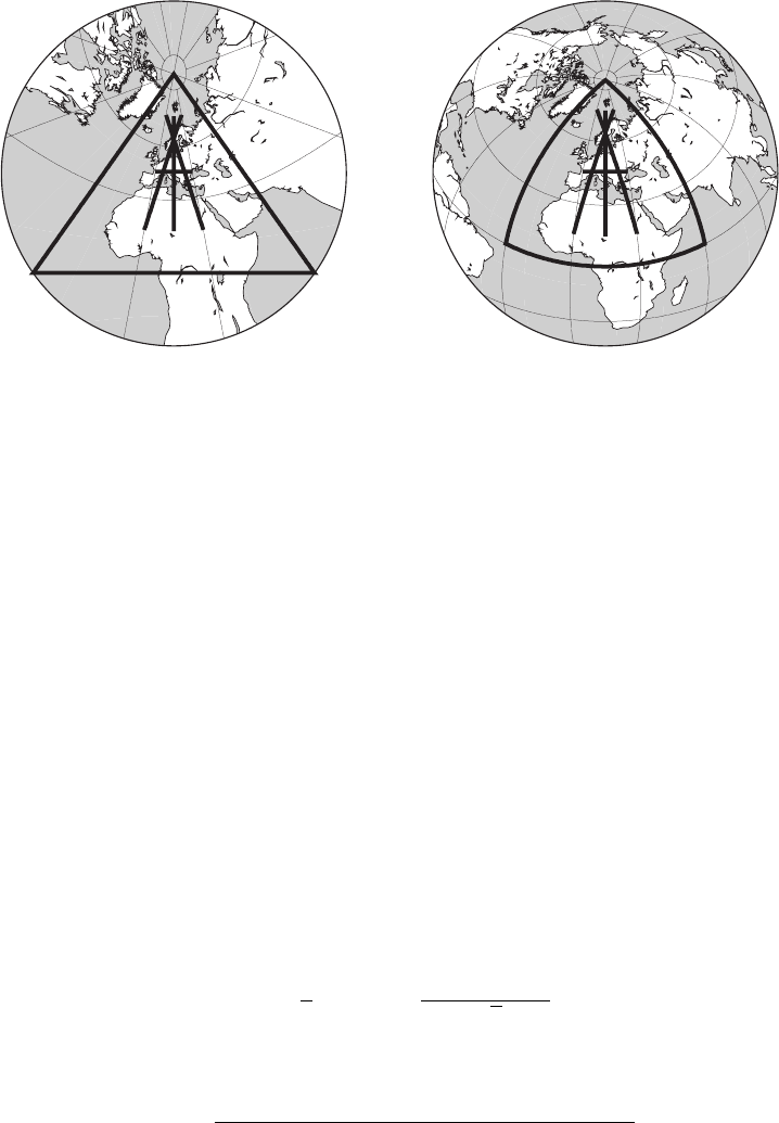
Gnomonic Lambert Azimuthal
Equal-Area
a) b)
Figure 8.1: Representation of an hemisphere of the globe centred on Eu-
rope (45°N, 15°E) in the two different projections referenced in the text: a)
Gnomonic projection; b) Lambert azimuthal equal-area. In thick lines are
marked the spheric octant and some reference lines in order to compare
both projections.
If we take the sines of the plunges of the main axes ιT,ιBand ιP:
zT=sin ιT
zP=sin ιP(8.7)
zB=sin ιB
the length of the vector that connects the center of the diagram with the
projected point is defined by
L=2 sin 1
2·arccos zT+zP+zB
√3 (8.8)
and the normalization factor is:
N=q2·[(zB−zP)2+ (zB−zT)2+ (zT−zP)2](8.9)
The coordinates of the projected focal mechanisms in the plane are defined
as follows (these equations corrects the wrong equations showed in Kagan
(2005)):
25
x=√3·L
N·(zP−zT)
y=L
N·(2zB−zP−zT)(8.10)
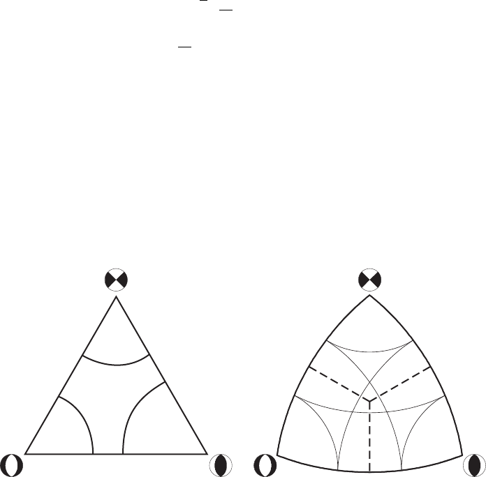
9 Focal Mechanism Classification
In order to classify the focal mechanisms Kagan (2005) divided the octant
in three areas (Figure 9.1b) corresponding to the three basic Andersonian
regimes: normal, reverse and strike-slip. The dividing lines start at the di-
agram center and run through the middle of each great circle (dashed lines
in Figure 9.1b). This classification, although simple and straightforward, is
too basic sometimes for a detailed seismotectonic study.
Strike‐slip
Reverse
Normal
Strike‐slip
Reverse
Normal
Odd
Frohlich & Apperson, 1992 Kaverina et al., 1996
Kagan, 2005
a) b)
Figure 9.1: Focal mechanisms classification diagrams based on SMT axes
plunges proposed by a) Frohlich and Apperson (1992) and b) Kagan (2005).
From the seismotectonic point of view an earthquake reflects the brittle
lithospheric strain produced by tectonic processes. The vast majority of
earthquakes are produced by displacements on faults (some other pro-
cesses as deep volume changes or cave collapses can produce seismic sig-
nals too), and they are interpreted usually as fault ruptures. Following
this reasoning the most appropriate classification for the focal mechanism
should be done by means of the slip vector on the fault, given by the rake
angle. This classification can be done following one of the proposed con-
ventions (Rickard,1972;Aki and Richards,1980;Angelier,1994). As has
been mentioned before, the problem is the duplicity of data due to the two
nodal planes solution of the focal mechanism.
26
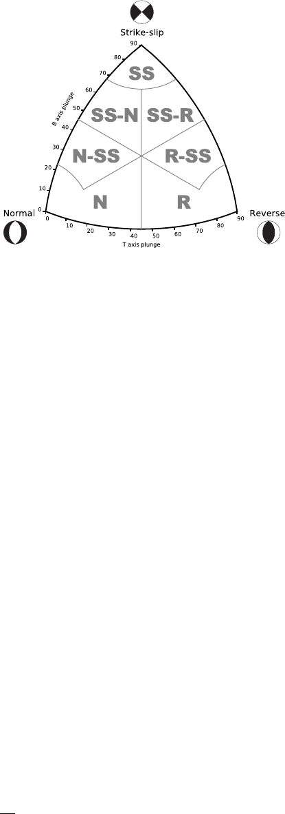
Figure 9.2: Focal mechanism classification diagram. N) Normal; N-SS) Nor-
mal - Strike-slip; SS-N) Strike-slip - Normal; SS) Strike-slip; SS-R) Strike-slip
- Reverse; R-SS) Reverse - strike-slip and R) Reverse.
An extended discussion on the relation among the different focal mech-
anism parameters can be found on Célérier (2010); the author also points
out the difficulty on interpreting the stress state from the focal mechanisms,
specially where oblique faulting takes place and reactivation of inherited
structures is possible (Wyss et al.,1992).
However the SMT can be interpreted as a seismic strain tensor (Kostrov,
1974) where the main axes are equivalent to the SMT main axes (Wyss et al.,
1992). With this relation in mind we can interpret the populations of fo-
cal mechanisms as representations of strains in different tectonic settings.
Oblique slip focal mechanisms with normal component can be interpreted
as transtensional strain, while oblique slip focal mechanisms with reverse
component can be interpreted as transpressional.
In order to count with a classification more detailed than the one of Kagan
(2005) I decided to classify the focal mechanism in a series of fields that
include the oblique slip regimes (Álvarez-Gómez,2009). This approxima-
tion is similar to the Johnston et al. (1994) classification; with 7 classes of
earthquakes: 1) Normal; 2) Normal - Strike-slip; 3) Strike-slip - Normal; 4)
Strike-slip; 5) Strike-slip - Reverse; 6) Reverse - Strike-slip and 7) Reverse.
The resulting diagram incorporating this 7 fields classification to the Kave-
rina projection is shown in Figure 9.2.
The algorithm to classify the focal mechanisms based on the SMT main axes
plunges is the shown in Figure 4.1.
When one of the three main SMT axes is greater or equal than 67.5◦(re-
sulted from 3 ∗π/2
4) we obtain a "pure" Andersonian tectonic regime. From
27
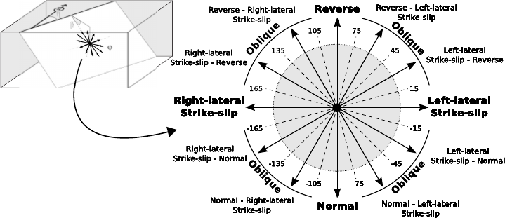
Figure 9.3: Diagram showing the convention used in this work for the rake
classification of faults or focal mechanism nodal planes. Inside the grey
circle the equivalent SMT axes-based classification is shown (Figure 8.1).
the pure normal or reverse faulting to the strike-slip faulting there is a range
of oblique faulting types with more or less relevance of the horizontal com-
ponent. On the other hand between the pure normal and pure reverse fault-
ing there is a permutation of the T and P axes in the vertical position, while
the B axis remains horizontal. The transition takes place when the P and T
axes plunge equally and a vertical nodal plane is present.
In the following section I compare the results of both classifications, the one
based in the main axes plunges of the moment tensor and the one based on
the fault rakes.
9.1 Comparison between rake-based and SMT axes-based classi-
fications
In order to classify the nodal planes according to its rakes I adopted a con-
vention hybrid between the Rickard (1972) and Aki and Richards (1980)
conventions. The focal mechanism rakes are usually given with the Aki
and Richards (1980) convention, while from a geological point of view the
Rickard (1972) convention is more used. I define 7 equivalent classes to
those used in the SMT axes-based classifications (Figure 9.3).
Each one of the nodal planes of the focal mechanisms from the Global CMT
catalog (Ekström et al.,2012) is classified according to the rake classification
shown in Figure 9.3. From the analysis of the focal mechanism alone we
cannot choose unequivocally the fault plane responsible of the earthquake.
To analyze the degree of uncertainty I show in Figure 9.4a the relative fre-
quency of relations between nodal planes rupture types. For example, it
28
can be seen that when one nodal plane is classified as normal, the other can
be normal as well, or can present some strike-slip component, but it can
not present reverse component; the same can be said for the reverse nodal
planes. When one nodal plane is pure strike-slip, the other can present dip-
slip component too, ranging from normal with strike-slip component (N-
SS) to reverse with strike-slip component (R-SS), but being more frequent
the relations between nodal planes of mainly strike-slip type.
Comparing the focal mechanism classified with the SMT axes and the nodal
planes classified with the rakes (Figure 9.4b) a similar picture as the de-
scribed above can be seen. The percentages of relations change sensibly,
but the common picture is the same. When the focal mechanism is clas-
sified as normal type we can expect that both nodal planes are of normal
type or normal with some strike-slip component. Similarly when the focal
mechanism is classified as reverse, both nodal planes are mainly of the re-
verse type too. For the case of the strike-slip focal mechanism almost all
the nodal planes are of strike-slip type too.
We can conclude that there is not much difference between the results ob-
tained from the rake classification of the nodal planes and the classifica-
tion of the focal mechanism attending to the SMT axes plunges. The focal
mechanism classification based on the SMT axes has the advantage of the
univocallity of its classification, in contrast with the duplicity of data and
uncertainty related to the nodal planes rake classification.
29
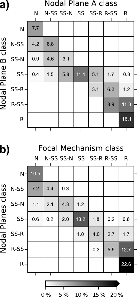
Figure 9.4: Heatmaps of the proportion of relations between a) both nodal
planes rupture type based on the rake classification, and b) between the fo-
cal mechanism classification and the nodal planes rupture types rake clas-
sification. The data used is the entire Global CMT catalog (Ekström et al.,
2012). Numbers show percentages over the entire catalogue.
30
References
Aki, K., Richards, P., 1980. Quantitative Seismology, Theory and Methods,
Vol. I and II. W.H. Freeman, San Francisco.
Álvarez-Gómez, J. A., 2009. Tectónica Activa y Geodinámica en el Norte
de Centroamérica. Ph.D. thesis, Universidad Complutense de Madrid,
Madrid.
Angelier, J., 1994. Palaeostress analysis of small-scale brittle structures. In:
Hancock, P. (Ed.), Continental Deformation. Pergamon Press Ltd, p. 421.
Benioff, H., 1954. Orogenesis and Deep Crustal Structure-Additional Ev-
idence from Seismology. Geological Society of America Bulletin 65 (5),
385–400.
Borges, J. F., Fitas, A. J., Bezzeghoud, M., Teves-Costa, P., 2001. Seismotec-
tonics of Portugal and its adjacent Atlantic area. Tectonophysics 331 (4),
373–387.
Bullen, K. E., Bolt, B. A., 1985. An introduction to the theory of seismology,
4 Edition. Cambridge University Press, Cambridge.
Byerly, P., 1928. The nature of the first motion in the Chilean earthquake
of November 11, 1922. American Journal of Science Series 5 Vol. 16 (93),
232–236.
Byerly, P., 1938. The earthquake of July 6, 1934: Amplitudes and First Mo-
tion. Bulletin of the Seismological Society of America 28 (1), 1–13.
Célérier, B., 2010. Remarks on the relationship between the tectonic regime,
the rake of the slip vectors, the dip of the nodal planes, and the plunges
of the P, B, and T axes of earthquake focal mechanisms. Tectonophysics
482 (1–4), 42–49.
Davis, G. H., Reynolds, S. J., 1996. Structural geology of rocks and regions,
2 Edition. Willey, New York.
Dziewonski, A. M., Chou, T.-A., Woodhouse, J. H., 1981. Determination of
earthquake source parameters from waveform data for studies of global
and regional seismicity. Journal of Geophysical Research: Solid Earth
86 (B4), 2825–2852.
Ekström, G., Nettles, M., Dziewo´nski, A., 2012. The global CMT project
2004-2010: Centroid-moment tensors for 13,017 earthquakes. Physics of
the Earth and Planetary Interiors 200-201 (0), 1–9.
31
Frohlich, C., 2001. Display and quantitative assessment of distributions of
earthquake focal mechanisms. Geophysical Journal International 144 (2),
300–308.
Frohlich, C., Apperson, K. D., 1992. Earthquake focal mechanisms, moment
tensors, and the consistency of seismic activity near plate boundaries.
Tectonics 11 (2), 279–296.
Frohlich, C., Coffin, M. F., Massell, C., Mann, P., Schuur, C. L., Davis, S. D.,
Jones, T., Karner, G., 1997. Constraints on Macquarie Ridge tectonics pro-
vided by Harvard focal mechanisms and teleseismic earthquake loca-
tions. Journal of Geophysical Research: Solid Earth (1978–2012) 102 (B3),
5029–5041.
Gasperini, P., Vannucci, G., 2003. FPSPACK: a package of FORTRAN sub-
routines to manage earthquake focal mechanism data. Computers &
Geosciences 29 (7), 893–901.
Gephart, J. W., 1990. Stress and the direction of slip on fault planes. Tecton-
ics 9 (4), 845–858.
Hess, H. H., 1962. History of ocean basins. Petrologic studies 4, 599–620.
Holmes, A., 1931. Radioactivity and earth movements. Nature 128, 496.
Honda, H., Masatuke, A., 1952. On the Mechanism of the Earthquakes and
the Stresses Producing Them in Japan and Its Vicinity. Science Reports
Tohoku University 4 (1).
Igarashi, T., Matsuzawa, T., Umino, N., Hasegawa, A., 2001. Spatial distri-
bution of focal mechanisms for interplate and intraplate earthquakes as-
sociated with the subducting Pacific plate beneath the northeastern Japan
arc: A triple-planed deep seismic zone. Journal of Geophysical Research:
Solid Earth (1978–2012) 106 (B2), 2177–2191.
Isacks, B., Molnar, P., 1969. Mantle earthquake mechanisms and the sinking
of the lithosphere. Nature 223 (5211), 1121–1124.
Isacks, B., Oliver, J., Sykes, L. R., 1968. Seismology and the new global tec-
tonics. Journal of Geophysical Research 73 (18), 5855–5899.
Johnston, A. C., Coppersmith, K. J., Kanter, L. R., Cornell, C. A., 1994. The
earthquakes of stable continental regions. Volume 1: Assessment of large
earthquake potential. Tech. rep.
Kagan, Y. Y., 2005. Double-couple earthquake focal mechanism: random
rotation and display. Geophysical Journal International 163, 1065–1072.
32
Kaverina, A. N., Lander, A. V., Prozorov, A. G., 1996. Global creepex distri-
bution and its relation to earthquake-source geometry and tectonic ori-
gin. Geophysical Journal International 125 (1), 249–265.
Kita, S., Okada, T., Nakajima, J., Matsuzawa, T., Hasegawa, A., 2006. Ex-
istence of a seismic belt in the upper plane of the double seismic zone
extending in the along-arc direction at depths of 70–100 km beneath NE
Japan. Geophysical Research Letters 33 (24).
Knopoff, L., 1961. Analytical calculation of the fault-plane problem. Publi-
cations of the Dominion Observatory (Ottawa) 24, 309–315.
Koning, L. P. G., 1941. On the Mechanism of Deep Focus Earthquakes. Ger-
lands Beitrage z. Geophysik 58, 159–197.
Kostrov, V., 1974. Seismic moment and energy of earthquakes, and seis-
mic flow of rock. Izv. Earth Phys. 1, 23–40 (translation UDC 550.341,
pp13–21).
Langston, C. A., Helmberger, D. V., 1975. A procedure for modelling shal-
low dislocation sources*. Geophysical Journal of the Royal Astronomical
Society 42 (1), 117–130.
Le Pichon, X., 1968. Sea-floor spreading and continental drift. Journal of
Geophysical Research 73 (12), 3661–3697.
McKenzie, D. P., 1969. The relation between fault plane solutions for earth-
quakes and the directions of the principal stresses. Bulletin of the Seis-
mological Society of America 59 (2), 591–601.
Michael, A. J., 1987. Use of focal mechanisms to determine stress: a control
study. Journal of Geophysical Research 92 (B1), 357–368.
Morgan, W. J., 1968. Rises, trenches, great faults, and crustal blocks. Journal
of Geophysical Research 73 (6), 1959–1982.
Okada, Y., 1992. Internal deformation due to shear and tensile faults in
a half-space. Bulletin of the Seismological Society of America 82 (2),
1018–1040.
Pollard, D. D., Fletcher, R. C., 2005. Fundamentals of Structural Geology, 1
Edition. Cambridge University Press, Cambridge.
Ramsay, J. G., Huber, M. I., 1997. The Techniques of Modern Structural Ge-
ology, Vol 2: Folds and Fractures, 5 Edition. Academic Press, London.
Ratchkovski, N. A., Hansen, R. A., 2002. New evidence for segmentation
of the Alaska subduction zone. Bulletin of the Seismological Society of
America 92 (5), 1754–1765.
33
Rickard, M. J., 1972. Fault Classification: Discussion. Geological Society of
America Bulletin 83 (8), 2545–2546.
Scheidegger, A. E., 1957. The geometrical representation of fault-plane so-
lutions of earthquakes. Bulletin of the Seismological Society of America
47 (2), 89–110.
Scholz, C. H., 2002. The mechanics of earthquakes and faulting, 2nd Edi-
tion. Cambridge University Press, Cambridge.
Schwinner, R., 1919. Vulkanismus und Gebirgsbildung: ein Versuch.
Reimer.
Serpelloni, E., Vannucci, G., Pondrelli, S., Argnani, A., Casula, G., Anzidei,
M., Baldi, P., Gasperini, P., 2007. Kinematics of the Western Africa-
Eurasia plate boundary from focal mechanisms and GPS data. Geophys-
ical Journal International 169, 1180–1200.
Sykes, L. R., 1967. Mechanism of earthquakes and nature of faulting on the
Mid-Oceanic Ridges. Journal of Geophysical Research 72 (8), 2131–2153.
Taylor, F. B., 1910. Bearing of the tertiary mountain belt on the origin of the
earth’s plan. Geological Society of America bulletin 21, 179–226.
Udías, A., 1989. Parámetros del foco de los terremotos. Física de la Tierra 1,
87–104.
Vannucci, G., Gasperini, P., 2003. A database of revised fault plane solu-
tions for Italy and surrounding regions. Computers & Geosciences 29 (7),
903–909.
Vine, F. J., 1966. Spreading of the ocean floor: New evidence. Science
154 (3755), 1405–1415.
Wegener, A., 1912. Die Entstehung der Kontinente. Geologische Rundschau
3 (4), 276–292.
Wessel, P., Smith, W. H. F., Scharroo, R., Luis, J. F., Wobbe, F., 2013. Generic
Mapping Tools: Improved version released. EOS Transactions of the
American Geophysical Union 94, 409–410.
Wyss, M., Liang, B., Tanigawa, W. R., Wu, X., 1992. Comparison of orienta-
tions of stress and strain tensors based on fault plane solutions in Kaoiki,
Hawaii. Journal of Geophysical Research 97 (B4), 4769–4790.
34
