Flask Guide
User Manual:
Open the PDF directly: View PDF ![]() .
.
Page Count: 10

Base applications
All work is available either at GitHub hosted in .git format or at BitBucket hosted in .hg
(Mercurial) format. Although .hg was used initially so links in README.md’s link to Bitbucket,
additionally there are some .hg related files lingering in the directory.
. Git links are available here for both:
- The Flask application: https://github.com/podit/flawsk
- The web frontend: https://github.com/podit/flawsk-web
. Or through Mercurial:
- Flask application: https://bitbucket.org/tomody/flawsk/src/default/
- Frontend: https://bitbucket.org/tomody/flawsk-web/src/default/
Project initialization
. Create a virtual environment (venv) for python version 3.6 (2.7 or 3.3+)
. Add flask to the venv with pip install flask once the venv is activated
. Create ‘.gitignore’ (and if using mercurial ‘.hgignore’) containing the venv directory
- AWS uses the .gitignore so see what from the directory should be uploaded (it will
ignore a .hgignore)
. Create ‘application.py’ as the main script
Flask core (application.py)
. Import flask with from flask import Flask
. Implement functions to perform desired actions
. Set flask name with application = Flask(__name__)
- I believe that app (or anything) could potentially work in place of application
although this may not work for an AWS deployment.
. Create url rule with application.add_url_rule('<url>', '<name>', (lambda:
<function>))
- e.g application.add_url_rule('/hi', 'hi', (lambda: hi()))
- This will call the function hi() when the server is called with /hi appended
to the server address e.g. http://127.0.0.1:5000 or
http://localhost:5000 for the default Flask application
. Finally initialize the server checking that the name has been initialized properly
if __name__ == "__main__":
application.run()
. To add debugging and allow the server to update itself when changes are detected add
debug=True to application.run() in the brackets
Functions in flask
. Can be in ‘application.py’ as long as they are earlier in the script than the url calls
. No additional python rules to follow in the flask framework, try to keep it light, make sure
not to overuse resources. A slow response holds up the entire API.
. The only thing to be wary of is the output, which is handled using return () just like any
other python function. This when used in flask will return the value as a string in the
response to the http request that called it.
. Using the example from the section above the function called would look something like
this:
def hi():
return 'Hello there...'
- This would respond with the string ‘Hello there…’
. Another example to raise one number to the power of another would be:
def power(num, exp):
pwr = num ** exp
return str(pwr)
. Called by the url rule:
application.add_url_rule('/pwr/<int:num>/<int:exp>', 'power', (lambda
num, exp: power(num, exp)))
- In the example of http://127.0.0.1:5000/pwr/4/4 being requested the response
would be the string ‘256’
- Note that attempting to return an integer without converting it will result in an internal
server error, code 500. As an integer has been returned instead of a string
. See ‘example.py’ for a simple example of how to structure a flask application. I would
recommend ‘httpie’ as an application with which to test the url rules before advancing to
using CORS for use within a browser.
Additional Flask functionality
. CORS allows for the http responses from the server to be processed in a browser. Allowing
for processing by frontend web applications.
- Installed using: pip install flask-cors
- Then it is imported using from flask_cors import CORS. And added using the
function CORS(application) with ‘application’ being the application name. This
should be done just below where the application name is set
. Another flask feature is the ability to create a json response, this is achieved by importing
‘Flask’ and ‘jsonify’ from flask as so: from flask import Flask, jsonify
Data handling in flask
. Data handling in flask can be achieved in many ways, for example data can be inputted into
the server and serialised into file allowing for real time, automatic data management. Flask
can work with multiple types of data storage methods as well, however due to the web
frontend based nature of the task I chose to use JSON. Although a .csv or any other type
would be just as applicable.
. The dataset I used to build the flask backend was a collection of various pieces if
information pertaining to stock analysis. In particular this dataset contained various points
pertaining to oil, every 4 hours from 2008 to 2018. This dataset has around 16 thousand
data-points.

. In this first example, the JSON dataset is being opened and each data point for ‘<TIME>’
and ‘<CLOSE>’ is being returned as a JSON output:
def jdata():
time = []
close = []
fname = os.path.join(application.static_folder, 'jdat.json')
with open(fname) as jdatr:
data = json.load(jdatr)
for item in data:
time.append(item['<TIME>'])
close.append(item['<CLOSE>'])
return jsonify(time, close)
- The os.path.join module links the files in the ‘static’ directory in the application home
directory. This allows for multiple files to be opened in the static directory and read
sequentially using the with open(fname) as jdatr: . Additionally this means that
the file will always be read from the beginning instead of reaching the end and failing
to read again until the server is restarted.
- Once the values have been read into the list they are returned using the flask ‘jsonify’
function to combine the lists into a json object. Allowing it to be used directly in
javascript applications (this will be demonstrated in the third example in this section).
. In the next example, to allow a faster render time on the web frontend, the data taken from
the dataset is averaged by week to reduce the 16 thousand data points down to around 500:
def jdatwcavg():
fname = os.path.join(application.static_folder, 'jdat.json')
x = 0
time = []
close = []
close_avg = []
with open(fname) as jdatr:
data = json.load(jdatr)
for item in data:
if x < 30:
x += 1
close.append(float(item['<CLOSE>']))
if x == 30:
close.append(float(item['<CLOSE>']))
closeav = stat.mean(close)
time.append(item['<TIME>'])
close_avg.append(closeav)
x = 0
close = []
return jsonify(time, close_avg)
- This function works very similarly to the previous function, however another list is
used to store the averaged data and an iterator is added to count the samples,

allowing for a rudimentary sense of time to be recorded. However this is probably not
the most nuanced solution to achieve this.
- The file is sampled in a similar fashion to the previous example, however the iterator
which is set to 0 in the beginning is incremented by one each time up until 29
samples from the data have been taken. At which point the 30th sample is taken
(30/5 = 6 for 6 samples a day 24/4 = 6 for 5 business days), the list of recorded
values is then averaged to get the weekly average and an approximate time value
recorded for the end of the week into a separate list. The iterator is then reset and
the sample list cleared and the process is restarted.
- These lists are then returned as a json object.
- This method of data sampling is much faster than it would be on the frontend and so
doing it in the backend is imperative to building a good experience.
. Finally to allow for specific values to be requested from the dataset to allow for a more
concise representation of the data:
def dates(sd, ed):
fname = os.path.join(application.static_folder, 'jdat.json')
t = 0
time = []
close = []
with open(fname) as jdatr:
data = json.load(jdatr)
for item in data:
if sd in item['<TIME>']:
t = 1
if ed in item['<TIME>']:
t = 2
if t == 1:
time.append(item['<TIME>'])
close.append(float(item['<CLOSE>']))
return jsonify(time, close)
- This function works in a similar way to the first example, setting the directory and
iterating through each element in the file(s), however a variable named ‘t’ is set as 0
to allow for the state of the sampling to be toggled.
- The data-points are iterated through until the start date (‘sd’) provided is met, at
which point the toggle is set to 1. The dates continue to be checked against the
provided dates, although additionally since the toggle has been set both the time and
close values are sampled into a list. This continues until the end date (ed) provided is
encountered at which point the data stops being sampled as the toggle is set to 2
from 1.
- This is a very rudimentary approach, and once again I am certain there is a more
nuanced approach. Although in spite of this the process is still very quick. Although if
the two dates are very far apart, it can lead to very slow render times on the frontend.
- However the second example could be implemented quite easily into the toggled if
statement to allow for weekly (or daily) averaged results to streamline larger
requests.
- Additionally if a date on the weekend is requested (when the stock market is closed)
then the toggle will either never be activated or closed. But this seems quite difficult
to tackle.
. This function is called using this url rule:
application.add_url_rule('/dates/<sd>/<ed>', 'dates', (lambda sd, ed:
dates(sd, ed)))
- This takes the start and end date from the http request as a string, for example:
/dates/2014-01-02/2016-01-02
- This would parse the string ‘2014-01-02’ as the start date or ‘sd’ and the second the
end date, ‘ed’.
. There are more examples as well as commented examples dealing with more information
in the application.py python script.
AWS deployment
. Install elastic beanstalk command line interface (EBCLI) using pip install aws-eb-cli
. Create ‘requirements.txt’ file containing modules and versions. Easiest way is to use pip
freeze > requirements.txt from within the venv
- Note that this is a likely cause of issues with AWS deployment when packages are
installed and the requirements.txt not updated. Additionally the package
pkgresources==0.0.0 may be erroneously added.
- Check this file before any other debugging on error code 404 after an AWS
deployment
. Configure AWS credentials using eb config
. Navigate to flask application directory and run eb init
- Select region (server location) (16 being London)
- Select application to use (or create new application)
- Answer the python prompt and select the python version (3.6)
- Source control can be set up
- Create ssh link
- Select load balancer (classic)
. Wait for AWS EB environment to be built
- Configure WSGI with eb config and change ‘WSGIPath’ to application script
filename if you have not used ‘application.py’
. Test using url <application name>.<region>.elasticbeanstalk.com/<url rule>
- e.g flawsk.eu-west-2.elasticbeanstalk.com/hi
. To update AWS EB server use eb deploy
Notes on production deployment
A production WSGI server should be used such as ‘Waitress’, the development server used
by flask (Werkzeug) has many security flaws and serious scalability issues

Frontend development
. To utilise the flask backend through a web application a http request must be made. The
simplest way to do this being:
<div id="box" style="text-align: centre; font-size: 20px;
display: inline-block; border-radius: 5px;">
<b>API DataViz</b>
<input id="clickMe" type="button" value="clickme"
onclick="request()" />
</div>
<div id="div">
</div>
<script>
var xhr = new XMLHttpRequest();
function request() {
xhr.onreadystatechange = function() {
if (this.readyState == 4 && this.status == 200) {
var msg = this.responseText;
document.getElementById("div").innerHTML = msg
}
}
xhr.open('get',
'http://flawsk-dev.eu-west-2.elasticbeanstalk.com/', true);
xhr.send(null);
}
</script>
- This displays a title and a button, once the button is clicked (in this case requesting
from the AWS deployment of the flask api) a http requests is sent using a javascript
function. It does this by waiting for the http request to be made and received and then
inputted into the empty division labeled “div” using the ‘XMLHttpRequest()’ function.
This makes the response “This is a Flask application for Python 3.6” appear below
the title and button. Variables can be inputted into the http request using a javascript
stringbuilder like so:
var num = document.getElementById("num").value;
var exp = document.getElementById("exp").value;
...
var url = `http://127.0.0.1:5000/pwr/${num}/${exp}`
xhr.open('get', url, true);
...
- Where ‘num’ and ‘exp’ are inputs in the html file

Frontend graphing from backend api
. Another way for the backend data to be used on the frontend is in graphing using a
javascript plotting library such as ‘D3’ or ‘Chart.js’
. Due to my very limited javascript experience I chose to use C3, a library that uses D3 to
produce it’s plots but has a much easier syntax, making development much faster. I tried
many of these libraries, and whilst not being the best documented, or powerful, or most
widely used, it is definitely the easiest to get a quick grasp of. However with javascript
knowledge I would use D3 as it is much more versatile and presents almost every feature C3
does, just without the improved syntax. C3 documentation is also severely lacking in places.
. C3 uses SVG elements to create the plots, it can insert these SVG canvases into almost
any identifiable element, meaning the plot is very versatile within the frontend application.
. Another benefit is that it offloads the job of rendering these charts onto the machine making
the request, instead of putting a large onus on the server to manage the data and render the
plots, which would be very inefficient. However if the data is not efficiently delivered, the
render times can be very long.
. To import C3 into a web application you will need both the C3, D3 and C3 stylesheet. I
would recommend importing them in the head:
<head>
<link
href="https://cdnjs.cloudflare.com/ajax/libs/c3/0.6.7/c3.min.css"
rel="stylesheet" />
<script
src="https://cdnjs.cloudflare.com/ajax/libs/d3/5.5.0/d3.min.js"></script
>
<script
src="https://cdnjs.cloudflare.com/ajax/libs/c3/0.6.7/c3.min.js"></script
>
</head>
- The ‘.min’ libraries are just reduced plotting libraries, leaving out the much more
advanced D3 features such as geoplotting on a map
- Apologies for the html syntax highlighting in this document, from what I can tell the
plugin I’m using has no html mode.
. Here is an example from the chart.js script using C3 to plot the results from the ‘dates’
function from the flask application:
<div id="dates">
<form id="inp">
Start date:
<input id="startdate" name="sd" type="date"
value="2014-01-02" min="2008-01-02" max="2018-01-17">
End date:
<input id="enddate" name="ed" type="date"
value="2016-01-02" min="2008-01-02" max="2018-01-17">
<input id="submit" type="button" onclick="dgraph()" />

</form>
</div>
<div id="out">
</div>
- In this section the inputs are gathered from two date input objects, however care
must be taken when inputting dates that are not part of the dataset, such as
weekends. When the button is clicked, the ‘dgraph’ function is called from the
‘chart.js’ javascript file.
function dgraph() {
var sd = document.getElementById("startdate").value;
var ed = document.getElementById("enddate").value;
var url =
`http://flawsk-dev.eu-west-2.elasticbeanstalk.com/dates/${sd}/${ed}`
// var url = `http://127.0.0.2:5000/dates/${sd}/${ed}`
document.getElementById("out").innerHTML = url;
var splot = c3.generate({
bindto: '#out',
data: {
type: 'line',
x: '0',
xFormat: '%Y-%m-%d %H:%M:%S',
url: url,
mimeType: 'json'
},
axis: {
x: {
label: 'Date & Time',
type: 'timeseries',
tick: {
format: '%Y-%m-%d %H:%M:%S'
}
}
},
point: {
show: false
}
});
}
- When the function is called, the start and end dates are collected from the date input
elements and imported as variables into the javascript. A stringbuilder is then used to
create the url to be used (switch out for commented url to work from a local flask
application. The url is then displayed for bug fixing in the ‘out’ division.
- The plot is then generated using ‘c3.generate()’ and bound to the ‘out’ division. Once
the plot is generated it will overwrite the url in this division.
- Data needs to be imported and properly used within the plot to create the desired
graph.
- The ‘type’ variable should automatically detected although I declared it. However
there are other types that can be used such as pie charts or curved (sigmoid?
) line
graphs.
- The ‘X’ data also needs to be declared, otherwise the dates will be used as part of
the plot leading to some strange results, additionally the format must be set so that it
can be used as a label, using a standard date and time format.
- The data is then called using the url generated earlier from the flask backend. This
returns a JSON response which can be directly used as the data for the plot.
Although it must be declared that a JSON response is being called. Although other
response types such as ‘.csv’ can be used here.
- Now the x axis must be configured by setting a label, and declaring that the data is a
‘timeseries’ so it can be correctly plotted using a mirror format to the one used earlier.
- Lastly the points are disabled, this is to make the graph look cleaner as there can
potentially be a lot of data points used making the actual values being represented
very unclear.
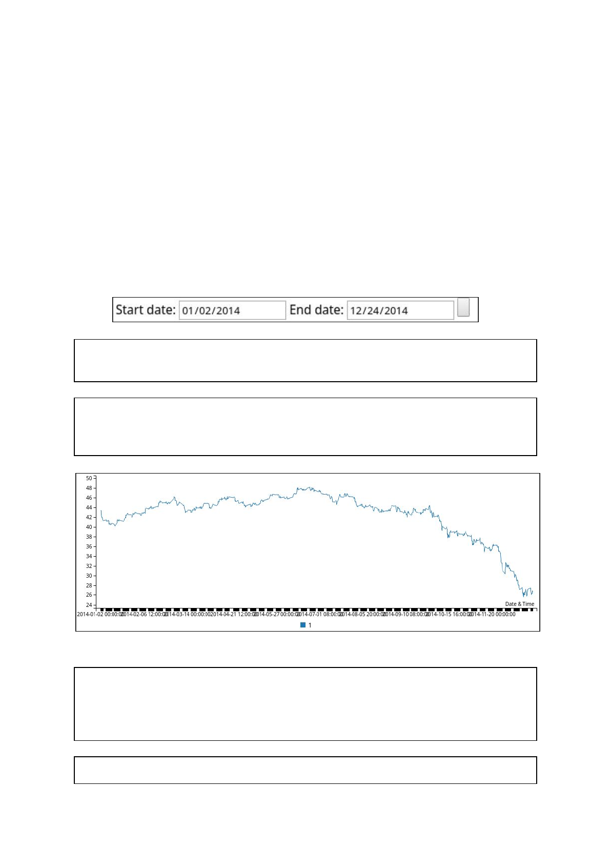
. As an example, the dates 01-02-2014 and 12-24-2014 in the input fields. To make a plot of
the ‘<CLOSE>’ data between the specified dates:
- The flask api actually uses the standard date format (Y-M-D instead of M-D-Y), but
this is handled automatically by the application
- Once the submit button is clicked the generated url becomes:
http://flawsk-dev.eu-west-2.elasticbeanstalk.com/dates/2014-01-02/2014-1
2-24
- The generated url provides the json output:
[["2014-01-02 00:00:00","2014-01-02 04:00:00","2014-01-02 08:00:00", ...
"2014-12-23 12:00:00","2014-12-23 16:00:00","2014-12-23 20:00:00"],
[43.3201,43.4299,43.1006, ... 26.2954,26.5495,26.9589,26.7095]]
- Leading to the plot:
. There are additional features available in C3 such as a zoom function. This can be done by
adding the following to the c3.generate arguments:
zoom: {
enabled: true,
rescale: true
}
. Additionally the size of the plot can be altered using the ‘size’ argument like so:
size: {
height: 600
}
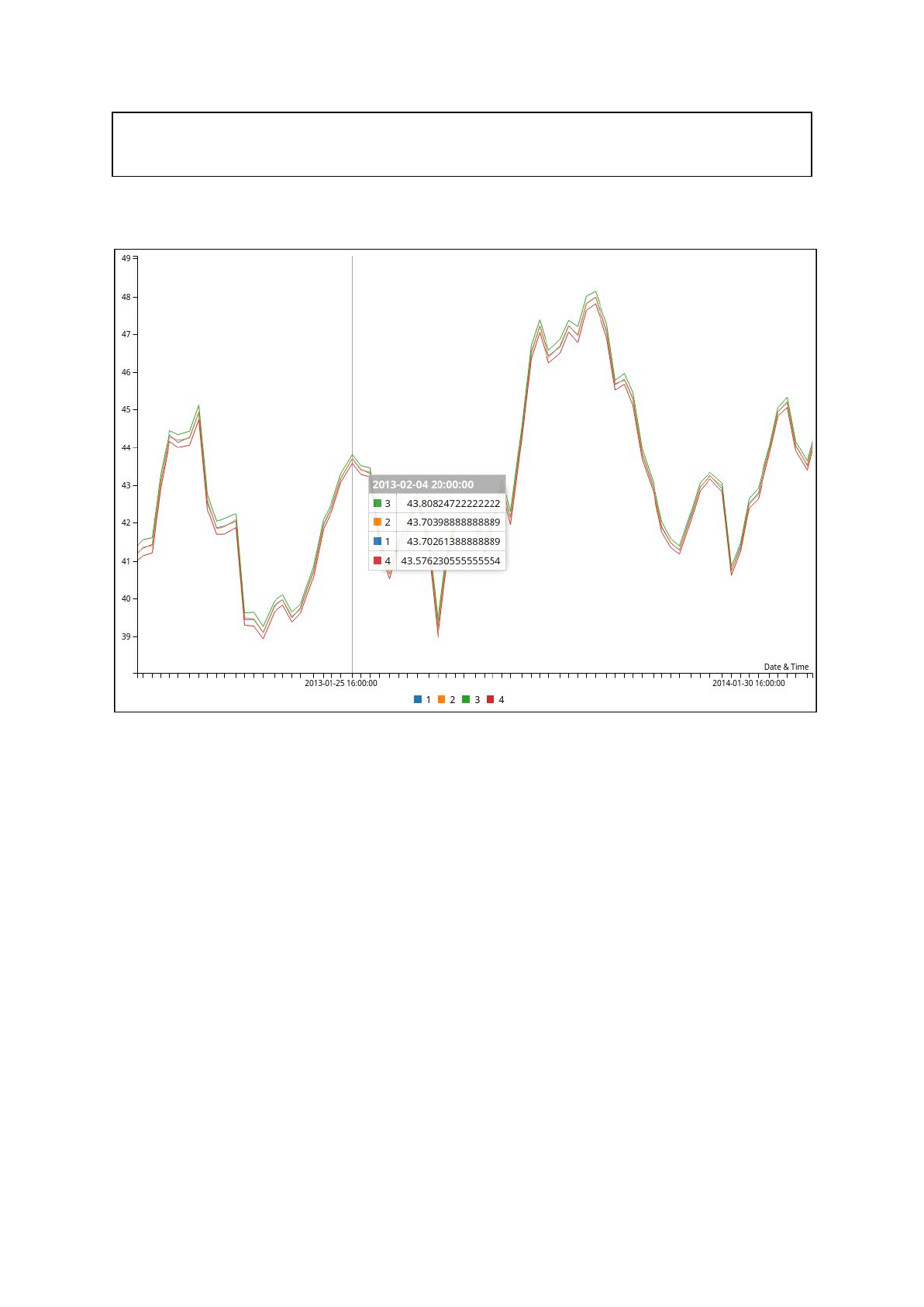
. Also if multiple data fields are used in the json output, multiple lines can be plotted to
represent each data field. The following plot is 4 similar data fields plotted with the zoom
feature enabled and the height set to 600:
- This shows the weekly averages for ‘<CLOSE>’ (1), ‘<OPEN>’ (2), ‘<HIGH>’ (3) and
‘<LOW>’ (4).
- The plot has been zoomed in to increase the resolution of the represented data.
Zoom works by scaling the x and y axis, although this can be configured just like
everything else in C3.
- The augmented hover is a default C3 feature, although it can be disabled. It allows
for specific values at an x location to be displayed. This can be styled through css.
. In fact every element in a C3 (or D3) plot can be customized using CSS
. Once again there are more examples of C3 plots in the chart.js file
