FoxNet User Guide V1.0.0 Fox Net

User Manual:

Open the PDF directly: View PDF .
Page Count: 45

About FoxNet
Getting started
Building a simple scenario from scratch
An example customisation
- Glenelg - a built-in scenario
- Building the Glenelg scenario from scratch
Building a new customised scenario
Running batch scripts
- Within NetLogo
- From R using the RNetLogo package
Implementation verification
Submodels
- Submodels used during model processing
- Submodels specific to model set-up
Appendices
- Customisable model parameters
- Week Conversion Table
References

FoxNet User Guide V1.0.0

Bronwyn Hradsky, Quantitative and Applied Ecology, University of Melbourne

Contents

1 About FoxNet 3

1.1 Overview ............................................... 3

1.2 Components.............................................. 3

1.3 Temporalandspatialscales ..................................... 5

1.4 Process overview and scheduling . . . . . . . . . . . . . . . . . . . . . . . . . . . . . . . . . . 5

1.5 Designconcepts............................................ 7

1.6 Initialisation ............................................. 8

2 Getting started 10

2.1 Installing NetLogo and opening FoxNet . . . . . . . . . . . . . . . . . . . . . . . . . . . . . . 10

2.2 Theuserinterface .......................................... 10

2.3 Thecode ............................................... 11

2.4 Modeldemonstration......................................... 11

3 Building a simple scenario from scratch 12

3.1 A fox population in a homogenous landscape . . . . . . . . . . . . . . . . . . . . . . . . . . . 12

3.2 Monitoring your model outputs . . . . . . . . . . . . . . . . . . . . . . . . . . . . . . . . . . . 14

3.3 Experiment .............................................. 14

3.4 Addingabaitingprogram...................................... 15

4 An example customisation 18

4.1 Glenelg-abuilt-inscenario..................................... 18

4.2 Building the Glenelg scenario from scratch . . . . . . . . . . . . . . . . . . . . . . . . . . . . . 19

5 Building a new customised scenario 25

5.1 Acustomisedlandscapelayer .................................... 25

5.2 Customised region(s) of interest . . . . . . . . . . . . . . . . . . . . . . . . . . . . . . . . . . . 26

5.3 Customisedbaitlayout........................................ 26

5.4 Customisedsurveytransect ..................................... 26

6 Running batch scripts 27

6.1 WithinNetLogo ........................................... 27

6.2 From R using the RNetLogo package . . . . . . . . . . . . . . . . . . . . . . . . . . . . . . . . 27

7 Implementation veriﬁcation 31

7.1 Eﬀect of productivity on fox-family territories . . . . . . . . . . . . . . . . . . . . . . . . . . . 31

7.2 Eﬀect of productivity on fox density . . . . . . . . . . . . . . . . . . . . . . . . . . . . . . . . 32

7.3 Eﬀect of baiting on fox mortality . . . . . . . . . . . . . . . . . . . . . . . . . . . . . . . . . . 33

8 Submodels 34

8.1 Submodels used during model processing . . . . . . . . . . . . . . . . . . . . . . . . . . . . . . 34

8.2 Submodels speciﬁc to model set-up . . . . . . . . . . . . . . . . . . . . . . . . . . . . . . . . . 37

9 Appendices 40

9.1 Customisable model parameters . . . . . . . . . . . . . . . . . . . . . . . . . . . . . . . . . . . 40

9.2 WeekConversionTable ....................................... 44

10 References 45

Notation

The names of agent-sets are italicised. An agent-set is a group of the same entities within FoxNet.

Submodel names are in bold.

Parameter names are shown in code font.

“Input values” for a

parameter

are shown in “quotes”. “Input values” can be varied to customise the FoxNet

modelling framework to a scenario and explore key sensitivities.

This project is licensed under the GNU General Public License v3.0 - see the LICENSE.md ﬁle for details.

To cite this User Guide

Hradsky B, Kelly L, Robley A, Wintle B (2019) FoxNet: an individual-based modelling framework to support

red fox management Journal of Applied Ecology.

Software source

Data available via Zenodo http://doi.org/10.5281/zenodo.2572045 (Hradsky et al. 2019b). A current version

of FoxNet and the User Guide is also maintained at this location.

For further information or help with customising model code

Email hradskyb@unimelb.edu.au or bhradsky@gmail.com

The development of FoxNet was funded by the

•

Australian Government’s National Environmental Science Program through the Threatened Species

Recovery Hub

•Victorian Government (Department of Environment, Land, Water and Planning)

•Parks Victoria

1 About FoxNet

1.1 Overview

FoxNet is a customisable, individual-based modelling framework for running spatially-explicit red fox

population models at a landscape-scale. It can be used to predict red fox population density, age structure,

composition and responses to management across an entire landscape or within customised region(s) of

interest.

1.2 Components

FoxNet has four main types of agent: habitat-cells,foxes,fox-families and bait-stations. Another type of

short-lived agent (vacancy) is used to execute territory-checking processes eﬃciently.

Habitat-cells are the squares of habitat that deﬁne the spatial resolution, conﬁguration and productivity of a

model landscape in FoxNet. Within a habitat-cell, productivity and fox access to bait-stations is homogenous.

The area represented by each habitat-cell can be speciﬁed using

cell-dimension

, and is usually in the order

of 0.01 km

to provide a compromise between computational eﬃciency and intra-home-range variation (fox

home-range size varies between <0.5 and >9 km

; Trewhella et al. 1988). Each habitat-cell keeps track of

the following parameters:

•habitat-type

: an integer that denotes the type of habitat (e.g. “0” = ocean, “1” = forest, “2” =

farmland). If the model landscape is generated within FoxNet, there will only be one

habitat-type

However, if the model landscape is imported as an ascii raster layer, the

uninhabitable-raster-value

second-habitat-raster-value

and

hab2:hab1

inputs can be used to specify, respectively, a raster

integer value that denotes habitat-cells that are not available to foxes (such as ocean or lakes), a raster

integer value that denotes a secondary type of habitat (e.g. farmland if the primary habitat type is

forest), and the productivity of the second

habitat-type

relative to the primary

habitat-type

. The

productivity of the habitat-cells determines how many habitat-cells afox-family needs to acquire to

establish a territory (see below).

•available-to-foxes

: “true” or “false”. This parameter defaults to “true” unless the habitat-cell’s

habitat-type

is the same as the

uninhabitable-raster-value

for an imported landscape. In this case,

the habitat-cell becomes unavailable to foxes and is not included in the

available-landscape-size

This allows to you to specify areas that foxes cannot access, such as oceans, lakes, predator-proof fenced

areas etc.

•part-of-region-of-interest

: “true” or “false”. This parameter defaults to “false”. When “true”, the

habitat-cell becomes part of the

region-of-interest

where the fox population is monitored (e.g. a

central square or a nature reserve). The region-of-interest can be the entire landscape if desired.

•part-of-region-of-interest2

: “true” or “false”. This parameter defaults to “false”. When “true”,

the habitat-cell becomes part of a second region of interest (

region-of-interest2

) where the fox

population is also monitored (e.g. a second nature reserve).

•true-color

: the intrinsic colour of the habitat-cell when unoccupied by a fox-family. This defaults to

black for the primary habitat type, but will be a diﬀerent colour if the habitat-cell is the secondary

habitat type, is not available to foxes, or is part of the region(s)-of-interest.

•true-productivity

: the intrinsic amount of food available to a fox in the habitat-cell during each

time-step (in grams time-step

-1

). The

true-productivity

of habitat-cells in the primary habitat

type is calculated from the size of an average fox home-range (input by the user) and the daily food

requirements of an adult fox (378 g/day; Lockie 1959); an approach similar to Carter et al. (2015)

but which facilitates scenario customisation.

True-productivity

in the secondary habitat-type (if

applicable) depends on the

hab2:hab1

ratio. See the

set-landscape-productivity

submodel for more

information.

•current-productivity: the current amount of food available to a fox in the habitat-cell during each

time-step (in grams time-step

-1

). The

current-productivity

of each habitat-cell determines how many

habitat-cells foxes need to acquire to establish a territory - see the

fox-families-check-territories

and

foxes-disperse

submodels. By default, a habitat-cell’s

current-productivity

is the same as

its

true-productivity

, but it can be varied spatially or temporally through manual coding. Future

extensions will use this feature to incorporate disturbance events such as ﬁre that have short-term

eﬀects on red fox habitat selection.

•fox-family-owner

: the identity of the fox-family that currently owns the habitat-cell (set to “nobody”

when the cell is unowned).

•cell-relative-productivity

: set to 0 by default. However, if the habitat-cell is owned by a fox-family,

it is calculated as the

current-productivity

of the habitat-cell weighted by the inverse of its distance

from the centre of the fox-family’s territory. This value is updated by the fox-family.

•cell-relative-use

: set to 0 by default. However, if the habitat-cell is owned by a fox-family,

it is calculated as the intensity with which the habitat-cell is used by the fox-family, i.e., the

current-productivity

of the habitat-cell divided by the total productivity of the fox-family’s terri-

tory. For example, in a homogeneous landscape with a territory-size of 100 ha and 1-ha habitat-cells,

cell-relative use

would be 0.01. However, if the territory-size was 500 ha,

cell-relative-use

would be 0.002.

cell-relative-use

is used to scale the exposure of foxes to bait-stations with

territory-size and habitat-cell productivity, and to derive the density of foxes (a monitoring output).

•cell-relative-use-foxes

: set to 0 by default. However, if the habitat-cell is owned by a fox-family, it

is calculated as

cell-relative-use

multiplied by the number of foxes in the fox-family. This is used to

calculate the density of foxes. For example, if 4 foxes share the 500-ha territory and

cell-relative-use

is 0.002, cell-relative-use-foxes is 0.222 x 4 = 0.008.

•checked-already

: “no” (default) or “yes”: indicates whether the fox-family owner has already consid-

ered discarding this habitat-cell. Used to speed up the update-territory submodel.

Foxes are mobile individuals whose behaviour is determined by their

age

and

status

, and the time of year

(Larivière & Pasitschniak-Arts 1996). Each “alpha” fox is a member of a fox-family .Foxes have the following

characteristics:

•age: in weeks. Foxes are born at age “0”.

•sex: “female” or “male”.

•status

: “cub”, “subordinate”, “disperser” or “alpha”, depending on the fox’s

age

and territory-holding

status.

•natal-id: the fox-family that the fox was born into.

•natal-cell: the habitat-cell where the fox was born.

•family-id: the fox-family that the fox currently belongs to.

•my-dispersal-distance

: the distance (km) that the fox intends to move from its

natal-cell

(drawn

from a random-exponential distribution which is inﬂuenced by the fox’s sex and size of its natal territory)

- see the foxes-disperse submodel.

•distance-from-natal: the current distance of the fox from its natal-cell (in kilometres).

•my-dispersal-duration

: the length of time the fox has been attempting to join or establish a new

territory (in weeks).

•failed-territory-id: a list of this fox’s territories which have failed.

Fox-families are used to establish and update the territories of their family-members (foxes within a family

share a semi-exclusive territory; Sargeant 1972). A fox-family must contain at least one “alpha” fox, and may

also include the alpha’s mate, cubs and subordinate oﬀspring. Fox-families have the following characteristics:

•family-members

- an agent-set comprising the “alpha female” and/or “alpha male” fox, and any of

their “cub” or “subordinate” oﬀspring that have not yet dispersed.

•my-territory - an agent-set comprising the habitat-cells held as territory by the fox-family.

•territory-productivity: the total productivity of the fox-family’s territory.

•vacancy-score

: the sum of the

relative-productivity

values of the vacancy agents surrounding

the territory at the end of the last time-step. Fox-families only try to improve their territory if the

vacancy-score

this time-step is diﬀerent - this helps the model run more eﬃciently. The

vacancy-score

will change if the

current-productivity

of the habitat-cells has changed, if new habitat-cells have

become available through the death of a fox-family, or if location of the fox-family has changed. See

the fox-families-check-territories submodel.

Bait-stations are static agents that mark the locations of baiting sites (this is more eﬃcient than using the

habitat-cells to record this). Bait-stations track:

•bait-present - whether a bait is currently available (“true” or “false”).

•Pr-death-bait-scaled - the likelihood of the bait aﬀecting a fox whose territory overlaps it.

Vacancies are temporary static agents. They are brieﬂy created and used by fox-families to (a) identify any

habitat-cells that are adjacent to their territory and not owned by another fox-family, and (b) determine

the

relative-productivity

of each of these available habitat-cells (i.e. the

current-productivity

of the

habitat-cell weighted by the inverse of its distance from the centre of the fox-family’s territory). The sum of

these values becomes the fox-family’s

vacancy-score

for that time-step. Vacancies are removed at the end

of each fox-family’s territory-checking procedure and are simply used to help the model run eﬃciently.

1.3 Temporal and spatial scales

FoxNet progresses in time-steps (or ticks) of 1, 2 or 4 weeks, depending on the

weeks-per-timestep

setting.

There are 52 weeks per year (and therefore 13 ‘months’, each of 4-weeks duration). A series of processes occur

consecutively each time step, and key seasonal events are linked to

week-of-year

, making the framework

customisable to northern- and southern-hemisphere scenarios.

The landscape can either be generated within FoxNet (as a square with the area speciﬁed by the

landscape-size

input parameter), or uploaded as raster layer, with each cell of the raster corresponding to

ahabitat-cell in the model. By default, the landscape doesn’t wrap (i.e. boundaries are non-permeable).

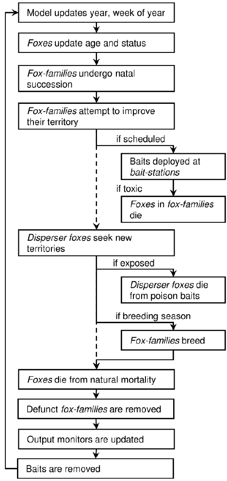
1.4 Process overview and scheduling

Each timestep, FoxNet works through a series of processes in order. Because key seasonal events are linked

to week-of-year, the framework is customisable to northern- and southern-hemisphere scenarios. There is no

hierarchy among agents of the same type (i.e. the order in which agents conduct each process is random and

varies each time-step).

The key processes are as follows:

(1)

Year and week counters are updated (by 1, 2 or 4 weeks, as required). Key seasonal events are linked

to week-of-year, making FoxNet customisable to northern- and southern-hemisphere scenarios.

(2)

The

age

of each fox is updated by the appropriate number of weeks. “Cub” foxes become “subordinates”

if they have reached the

age-of-independence

. If it is the dispersal season, “subordinate male”

and “subordinate female” foxes have user-speciﬁed probabilities of becoming “dispersers”. See the

update-fox-age-and-status submodel.

(3)

Natal succession occurs within fox-families. That is, if a fox-family is missing an “alpha” fox, one of

the family’s “subordinates” that is the right sex and at least 24 weeks old becomes the “alpha” (as

described by Baker et al. 1998).

(4)

Fox-families check their territories. Fox-families seek to maximise their

territory-productivity

within a compact area by acquiring or replacing habitat-cells. This enables the fox-family to take over

unoccupied productive habitat-cells (Sargeant 1972), and respond to changes in resource availability

(Bino et al. 2010; Hradsky et al. 2017b). If the

territory-productivity

of fox-family’s territory

is less than an adult fox’s minimum food requirements (<295 g/day; Winstanley et al. 2003), the

fox-family fails, causing all adult foxes in the family to become “dispersers” and any “cubs” to die. See

the fox-families-check-territories submodel.

(5)

If applicable, baits are laid at bait-stations and the cost of the baiting session is calculated. Foxes

belonging to a fox-family with a territory that overlaps an active bait-station are at risk of dying. Risk

scales directly with the number of bait-stations and bait eﬃcacy, and inversely with territory size and

the number of foxes in the familiy. Each bait-station only aﬀects one fox each time-step. See the

bait-if-applicable submodel.

(6)

Foxes who have just become “dispersers” leave their natal fox-family and move a random distance

generated from a sex-speciﬁc exponential distribution, scaled by their territory-size (Trewhella et al.

1988). “Disperser” foxes then explore the area within their

territory-perception-radius

(set to

an area three times the radius of an average home-range; Soulsbury et al. 2011) where they (1) are

exposed to any active bait-stations; (2) attempt to join a fox-family that lacks an “alpha” fox of the

appropriate sex; (3) try to establish a new fox-family. If unsuccessful, they remain a “disperser” until

the next time-step. See the foxes-disperse submodel.

(7)

If it is the breeding season, fox-families that contain an “alpha” male and an “alpha” female fox breed,

producing a Poisson-distributed number of “cub” foxes. If an “alpha” fox is absent, all family-members

become dispersers and attempt to join other nearby fox-families, promoting the persistence of the

population at low densities. See the fox-families-breed submodel.

(8)

Provided that

include-fox-mortality

is “on”, stochastic background mortality of foxes occurs, based

on their age. See the foxes-die submodel.

(9)

“Cub” foxes belonging to fox-families without any adults die, reﬂecting their dependence on food-

provision (Baker et al. 1998). This allows baiting to aﬀect reproductive success. Defunct fox-families

(those that have no family members) are removed from the model.

(10)

Model outputs are updated (and plotted if speciﬁed). Outputs can include age structure, population struc-

ture, dispersal distances, density or number of neighbours of foxes within the

region-of-interest

(s),

the number of foxes with territories overlapping a monitoring transect, and/or bait-take rates. See the

update-monitors submodel.

(11)

If baits were deployed at bait-stations at step 5, any baits that were not eaten by foxes are removed to

mimic the removal of baits by managers or the degradation of the poison to non-toxic levels (Saunders

et al. 2000).

(12) The time-step (tick) counter increases by 1.

(13) The model checks if any foxes are alive. If all foxes are dead, the model stops.

Detailed descriptions of the submodels underlying these processes can be found in Chapter 8

1.5 Design concepts

1.5.1 Basic principles

The size of a fox-family’s territory depends on the productivity of the habitat-cells, and can be updated in

response to changes in the productivity or availability of these habitat-cell.

Foxes with established territories are only exposed to bait-stations within their territory. “Disperser” foxes

are exposed to bait-stations within their territory-perception-radius.

1.5.2 Emergence

The density of foxes, the distribution of ages and dispersal-distances within the population, and the conﬁgu-

ration of fox-family territories emerge over time from demographic processes, territory dynamics and the

spatial conﬁguration of diﬀerent habitat-types.

Bait-take rates result from the conﬁguration of active bait-stations relative to fox-family territories and the

relative-use of habitat-cells,fox density, and the likelihood of a fox consuming a bait.

1.5.3 Adaptation

Fox-families adapt the size and position of their territory to the productivity of the habitat-cells and the

presence of surrounding fox-families.

1.5.4 Objectives

Each fox-family aims to maximise the productivity of its territory (up to 110% of an adult fox’s daily food

requirements) within as compact an area as possible.

“Disperser” foxes seek to join an existing fox-family as an “alpha”, or establish their own fox-family.

Foxes seek to breed, and so will disband their fox-family if it lacks an “alpha” of the opposite sex during the

breeding period.

1.5.5 Sensing

When they are dispersing, foxes can sense the location of fox-family territories and unoccupied habitat-cells

within their territory-perception-radius.

Fox-families can sense the productivity of the habitat-cells within their territory. They can also sense the

productivity and availability of the habitat-cells surrounding their territory, via the vacancy agents.

1.5.6 Interaction

Fox-families indirectly compete for habitat-cells, as each habitat-cell can only be used by one fox-family. The

fox-families use vacancy agents to determine which habitat-cells surrounding their territory are currently

available. This eﬀectively limits the carrying-capacity of the landscape, as only foxes within fox-families can

breed. See Eﬀect of productivity on fox density.

1.5.7 Stochasticity

Stochasticity occurs throughout the model to represent natural variation, including the dispersal locations of

foxes,fox sex and survival rates, and fox-family territory-acquisition and litter size.

1.5.8 Collectives

The

region-of-interest

(s) is nominated by the user, and deﬁnes the area(s) in which foxes are monitored.

Foxes form family-groups (represented by a fox-family agent) which share a territory. The status of each fox

is inﬂuenced by the sex and status of its other family-members.

The survival of a “cub” fox depends on the presence of at least one adult member in its fox-family until it

reaches the age-of-independence.

1.5.9 Observation

At the end of each time-step, data can be collected on the foxes,fox-families and bait-stations. The user

speciﬁes which data to collect and plot. See the update-monitors submodel.

1.6 Initialisation

FoxNet initialises by setting the input parameters as per the model interface, and then running through the

following processes in order:

1. A random-seed is set and recorded, so that the model run can be reproduced exactly if required.

2. set-current-directory.

The current directory is set to the

working-directory

so that any spatial

layers can be easily imported and model outputs will be saved in the appropriate folder.

3. check-for-errors.

This checks for inconsistencies in the input parameters. If an error is found, the

model returns a detailed error message and stops. See the check-for-errors submodel.

4. calculate-conversion-factors.

This calculates the factors for converting between input units and the

model (e.g. km2to habitat-cells).

5. set-fox-parameters.

This sets a variety of parameters which are not available on the interface and

derives others, such as the duration of the dispersal season. See the set-fox-parameters submodel.

6. create-world.

This generates a landscape of an appropriate size, either by generating it within the

model or importing a raster layer. See the create-world submodel.

7. identify-region-of-interest.

This identiﬁes the part of the landscape in which fox populations

will be monitored. This may be the entire landscape or a subset group of habitat-cells. See the

identify-region-of-interest submodel.

8. set-landscape-productivity.

This calculates the distribution of productivity values across the habitat-

cells using the

home-range-area

and

kernel-percent

inputs. See the

set-landscape-productivity

submodel.

9. set-up-bait-stations.

This sets up the bait-stations across the landscape (if applicable). See the

set-up-bait-stations submodel.

10. set-up-survey-transect.

This sets up a survey transect for monitoring the number of foxes, if

applicable.

11. set-up-foxes.

This creates an initial number of foxes at the speciﬁed density. Each fox immediately

disperses and tries to join an existing fox-family or establish a new fox-family. See the

set-up-foxes

submodel.

12. update-monitors.

This calculates the model ouputs and plots them if applicable. See the

update-

monitors submodel.

13. Finally, the model resets the time-step counter.

2 Getting started

2.1 Installing NetLogo and opening FoxNet

FoxNet was built in NetLogo (Wilensky 1999) version 6.0.2 - an open-source modelling environment, download-

able from https://ccl.northwestern.edu/netlogo/. FoxNet is saved in within the FoxNet folder:

FoxNet_model

/ FoxNet.nlogo. You can open it from within NetLogo or by double-clicking the ﬁle name.

For an introduction to using NetLogo see https://ccl.northwestern.edu/netlogo/docs/, particularly the three

tutorials listed in the LH menu.

2.2 The user interface

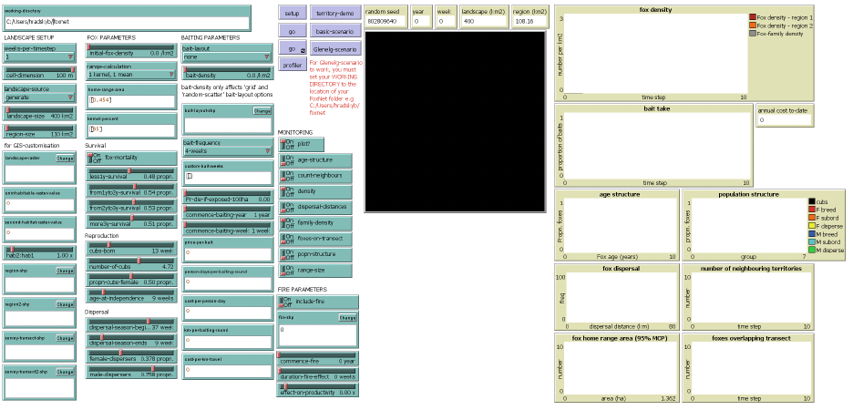
When you ﬁrst open FoxNet, you should see the graphic user interface. The interface has four key sections:

Inputs (green) - these boxes and sliders allow you to set model parameters and customise FoxNet to

your scenario.

2. Buttons (mauve) - these are used to control FoxNet:

•setup will parameterise FoxNet with whatever settings you have chosen in the inputs.

•go will run FoxNet for one timestep.

•go (continuous)

will run FoxNet forever (or at least until you click the button again) - this is shown

by the circling arrows.

•territory-demo will provide a demonstration of key model processes - see Model demonstration.

•basic-scenario

will setup FoxNet with a simple example scenario - see Building a simple scenario from

scratch.

•glenelg-scenario

will setup FoxNet with a complex scenario to demonstrate all the bells and whistles

(see An example customisation). You must set the

working-directory

to the location of the FoxNet

folder to use this option.

World-view (large black square) - this depicts some aspects of the model so that you can watch what is

happening as you run FoxNet.

4. Outputs (beige boxes and plots) - these enable you to track key model outputs.

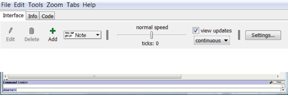
At the top of the screen, there are additional controls that aﬀect how FoxNet displays, including a slider that

controls the model speed, a tick-box that speciﬁes whether you want to watch updates in the world-view or

not, and a drop-down option for whether updates should be shown continuously or just at the end of each

time-step.

Under the Settings button, you can adjust the number of pixels per cell in the world-view and the frame rate.

TIP: To make the world-view larger/smaller you can increase/decrease the number of pixels per

cell. If the world-view is too large, you may encounter memory constraints.

At the bottom of the screen is the command center where you can issue direct instructions to the model.

Information on what is happening during the territory-demo is also shown here.

2.3 The code

The underlying model code can be viewed by clicking across to the Code tab. Submodels are provided in

separate ﬁles, which can be viewed by clicking on the Included Files dropdown box, within the Code tab.

Ignore this for now - you don’t need to view or edit the code to build or run a model in FoxNet.

2.4 Model demonstration

FoxNet comes with a build-in demonstration of several key processes, including territory formation, fox

responses to changes in habitat productivity, mate-seeking and reproduction.

Click on

territory-demo

(mauve button). A description of what is happening will appear in the Command

Center bar at the bottom of the screen. You can expand this bar if you want to see more than one line of

writing at once.

TIP: To stop the demonstration (or any FoxNet model) part-way through, click Tools > Halt.

3 Building a simple scenario from scratch

3.1 A fox population in a homogenous landscape

Let’s start by building a simple landscape. Using the Interface tab, either:

•

Set the following inputs manually by moving the sliders and entering the values, and then click

setup

, OR

•

Click the mauve

basic-scenario

button (which will automatically set up the model with the same

input parameters)

Parameter Value

Landscape setup

‘weeks-per-timestep‘ 1

‘cell-dimension (m)‘ 100

‘landscape-source‘ generate

‘landscape-size (km^2^)‘ 400

‘region-size (km^2^)‘ 110

Fox parameters

‘initial-fox-density (foxes km^-2^) ‘ 0

‘range-calculation‘ 1 kernel, 1 mean

‘home-range-area (km^2^)‘ [0.454] **make sure to include the brackets

‘kernel-percent (%)‘ [95] **make sure to include the brackets

‘fox-mortality‘ on

‘less1y-survival (propn.)‘ 0.48

‘from1yto2y-survival (propn.)‘ 0.54

‘from2yto3y-survival (propn.)‘ 0.53

‘more3y-survival (propn.)‘ 0.51

‘breeding-season (week)‘ 13

‘number-of-cubs‘ 4.72

‘propn-cubs-female (propn.)‘ 0.5

‘age-at-independence (weeks)‘ 12

‘dispersal-season-begins (week)‘ 37

‘dispersal-season-ends (week)‘ 9

‘female-dispersers (propn.)‘ 0.378

‘male-dispersers (propn.)‘ 0.758

Baiting parameters

‘bait-layout‘ none

Monitoring parameters

‘plot? ‘ "on"

‘density‘ "on"

These parameters are based on a fox population in Bristol, United Kingdom, with survival data from

Devenish-Nelson et al. (2013), and breeding and dispersal data from Trewhella and Harris (1988). See

Hradsky et al. (2019a) Table S1 for a full list of citations.

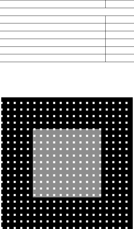
Whichever approach you chose, you should now see a black landscape with a central grey square in the

world-view. The entire landscape is 400 km

. The central grey square is your ‘region-of-interest’ where the

fox population is monitored, and is 110.25 km2 1. These values are shown in the beige output boxes.

Because FoxNet is generating a square lnadscape with 1 ha pixels (as speciﬁed by

cell-dimension

), it has had to adjust the

size of the region-of-interest slightly

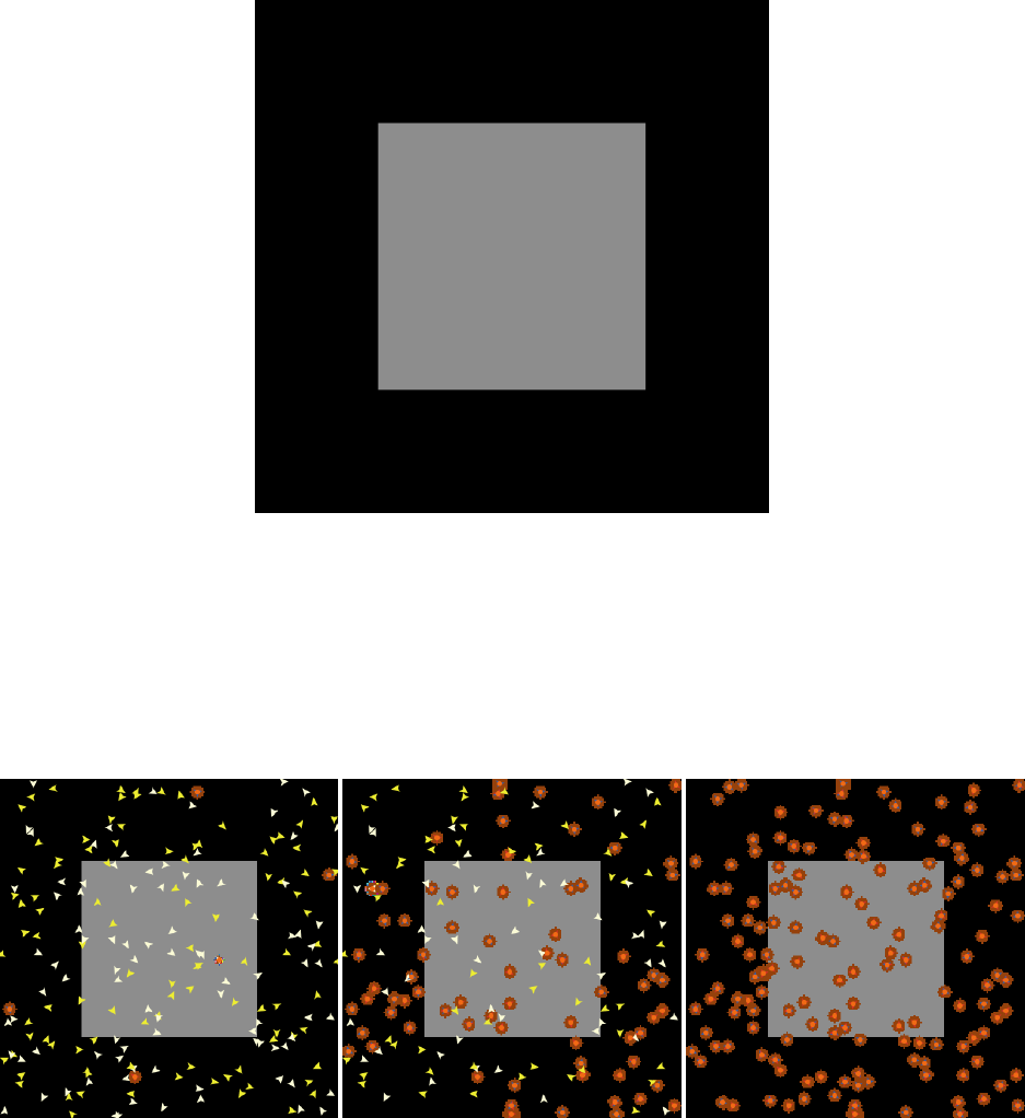
Now change initial-fox-density to “0.5” foxes km-2 by sliding or clicking the slider to the right.

TIP: You can also alter the value of a slider by right-clicking the slider, selecting “edit” and then

typing in a new value in the appropriate box.

Click

setup

again. A scattering of white and yellow triangles should appear - these are “female” and “male”

foxes without territories (i.e. their

status

is “disperser”). Each fox should attempt to establish or join a

circular brown territory. A fox with a territory acquires “alpha”

status

, becomes red (“female”) or blue

(“male”), and sits beneath an orange-coloured fox-family in the centre of its territory. A “female” and “male”

fox can share a territory.

TIP: If you would like to slow this process down so that you can see what is happening, try sliding

the speed toggle in the grey header bar to about 25% speed and click setup again.

If you’d like to see the foxes more clearly, right-click the world-view > Edit, and change the

patch-size

to 2

pixels.

Now click

. You might see a fox or two move, but not much else will change. However, the beige year and

week of year output boxes at the top of the screen will now show year 1, week 1.

Click go (continuous). As time progresses, foxes breed, disperse, establish new territories and die.

You can observe the density of foxes and fox-families within your 110 km

2region-of-interest

by looking

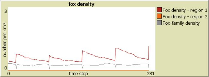
at the plot to the right of the world-view. For example, by Year 5, week 13, the density of foxes has just

spiked with the ﬁfth breeding season, because the

cub-birth-season

is currently set to week 13 of the year

(late March - see the Week Conversion Table). The density of fox-families remains relatively stable:

TIP: To export the fox density data, right-click the plot and select “export”. End the ﬁlename

with “.csv”.

Click

setup

and

go (continuous)

again. Each time you run the model with the same settings, you will get

slightly diﬀerent results due to stochastic variation.

3.2 Monitoring your model outputs

The

basic-scenario

defaults to plotting the density of foxes and fox-families within the

region-of-interest

However, you can monitor other aspects of the fox population within the

region-of-interest

using the

switches under MONITORING on the FoxNet interface. Options include:

•“age-structure” - the proportion of foxes in each age class from 0 to 8+ years.

•“bait-consumption” - the proportion of baits that have been removed by foxes per time-step.

•

“count-neighbours” - the mean (min, max) number of territories directly abutting each fox-family’s

territory.

•“density” - the density of foxes and fox-families.

•“dispersal distances” - the distance moved by foxes that have attempted to disperse.

•“family-density” - the density of fox-families.

•“popn-structure” - the proportion of foxes in each demographic group.

•

“foxes-on-transect - the number of foxes who have territories that overlap the

survey-transect

. This

only works for landscapes that have been imported as a raster and where a survey transect shapeﬁle

has been uploaded.

•“home range size” - not provided in this version of FoxNet.

You can choose whether or not to plot summary values using the

plot?

button. Plotting makes the model

run more slowly.

3.3 Experiment

Have a play with the input parameters. For example, try making

landscape-size

larger,

initial-fox-density

higher, home-range-area bigger or switch fox-mortality to “oﬀ”.

TIP: Huge landscapes with high densities of foxes may take a very long time to setup and run.

To cancel a model at any point, select Tools > halt.

Note that all week-related inputs must be consistent with

weeks-per-timestep

. FoxNet checks this during

model set-up and will return an error if, for example,

weeks-per-timestep

is “4” but

cub-birth-season

set to week “6”.

3.4 Adding a baiting program

Return to the original settings by clicking basic-scenario.

Then alter the baiting parameters as follows to apply a uniform grid of bait-stations across your model

landscape:

Parameter Value

Baiting parameters

‘bait-layout‘ grid

‘bait-density (km^-2^)‘ 1

‘bait-frequency‘ 4-weeks

‘Pr-die-if-exposed-100ha (propn.)‘ 0.3

‘commence-baiting-year‘ 3

‘commence-baiting-week‘ 13

Click setup to see the layout of bait-stations.

The current setting will have established a 1 km-2 grid of 400 bait-stations across your landscape.

initial-fox-density

is > “0” and you click “go”, baits will be deployed at bait-stations every 4 weeks.

Baits are deployed at bait-stations from the start of the model, but under the current settings only become

poisonous from Year 3 week 13 - this allows the population to begin to establish without baiting, and enables

you to quantify uptake of non-toxic baits (i.e. free-feeding).

TIP: Baits are only deployed at bait-stations if the initial-fox-density is greater than 0.

Setting

Pr-die-if-exposed-100ha

to “0.3” means that one fox with a 100-ha territory has a 30% chance of

consuming a bait if one bait is deployed on its territory (and dying if the bait is toxic). The risk to a fox

scales with the number of baits and inversely with the territory size and number of foxes in its fox-family.

See Eﬀect of baiting on fox mortality

Try altering bait-density to “4.0” baits km-2 or changing bait-layout to “random-scatter”, and clicking

setup again.

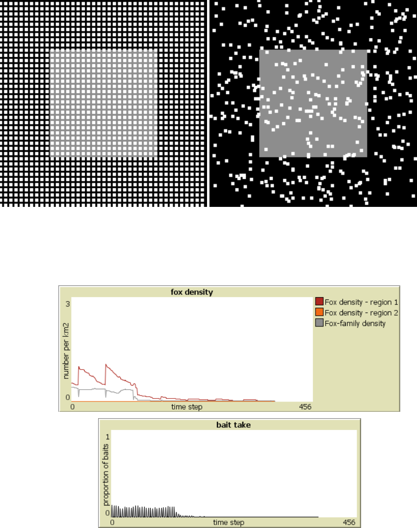
Look at the eﬀects of baiting on the population by changing the settings to a “grid” of baits with “2” baits

-2

, setting

initial-fox-density

to “0.5” km

-2

, turning “on” the

bait-consumption

monitor, and then

clicking setup and go (continuous).

Fox density declines rapidly in Year 3 after the baits become toxic, in this case, going extinct by Year 8 week

21. The model stops when all foxes are dead. Bait-take rates ﬂuctuate with fox density.

TIP: By default, baits only remain at bait-stations for one time-step. You can change the duration

of a time-step to “1”, “2” or “4” weeks. Other durations require a customised code. See foxnet /

foxnet_model / foxnet_carnarvon_custombait.nlogo for an example.

Baits can be deployed at bait-stations at custom intervals (e.g. quarterly, only in winter or once per year), by

changing bait-frequency to “custom*" and adding the relevant week numbers to custom-bait-weeks.

TIP: Make sure that the week inputs are surrounded by square-brackets, are consistent with the

weeks-per-timestep parameter and do not include commas between values.

For example, the following will deploy baits in weeks 6, 19, 31 and 45 each year (i.e. the start of February,

May, August and November):

Parameter Value

Baiting parameters

‘bait-frequency‘ custom*

‘custom-bait-weeks‘ [6 19 31 45]

To calculate the cumulative annual cost of a baiting regime (displayed in a beige box to the right of the

world-view), you can specify the price per bait deployed, the number of person-days it takes to deploy all

baits in a single bait deployment, the number of kilometres travelled per bait deployment, and the cost of

travel per kilometre. For example, if the parameters as set as follows. . .

Parameter Value

Baiting parameters

‘price-per-bait ($)‘ 2.00

‘person-days-per-baiting-round (days)‘ 3.00

‘cost-per-person-day ($)‘ 250.00

‘km-per-baiting-round (km)‘ 420.00

‘cost-per-km-travel ($)‘ 0.67

. . . a single bait deployment costs $2599, and the cost of deploying baits every 4 weeks for a year is $33,792.

TIP: The FoxNet interface constrains you to a baiting schedule that remains constant across years.

To vary the location of bait sites or baiting frequency between years, you will need to write a

customised baiting schedule. For an examplecode, open

foxnet_carnarvon_custombait.nlogo

click across to the

Code

tab, then

Included Files

and select

bait_routines_carnarvon.nls

Please get in contact with model developers if you need help with writing a customised schedule.

4 An example customisation

FoxNet models can be customised to real-world management landscapes using GIS layers that describe the land-

scape size and conﬁguration of diﬀerent habitat types, the area and location of the

region(s)-of-interest

survey-transect(s), and/or the layout of bait-stations.

Example spatial layers are provided so that you can explore the suite of customisation features in FoxNet

before developing your own.

4.1 Glenelg - a built-in scenario

To explore the built-in customised scenario:

Set the

working-directory

to wherever you have saved the FoxNet folder, for example:

C:/Users/hradsky/foxnet.

Take careful note of the direction of the slashes if you are using Windows.

2) Click Glenelg-scenario

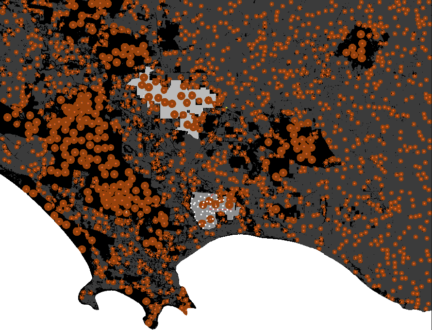
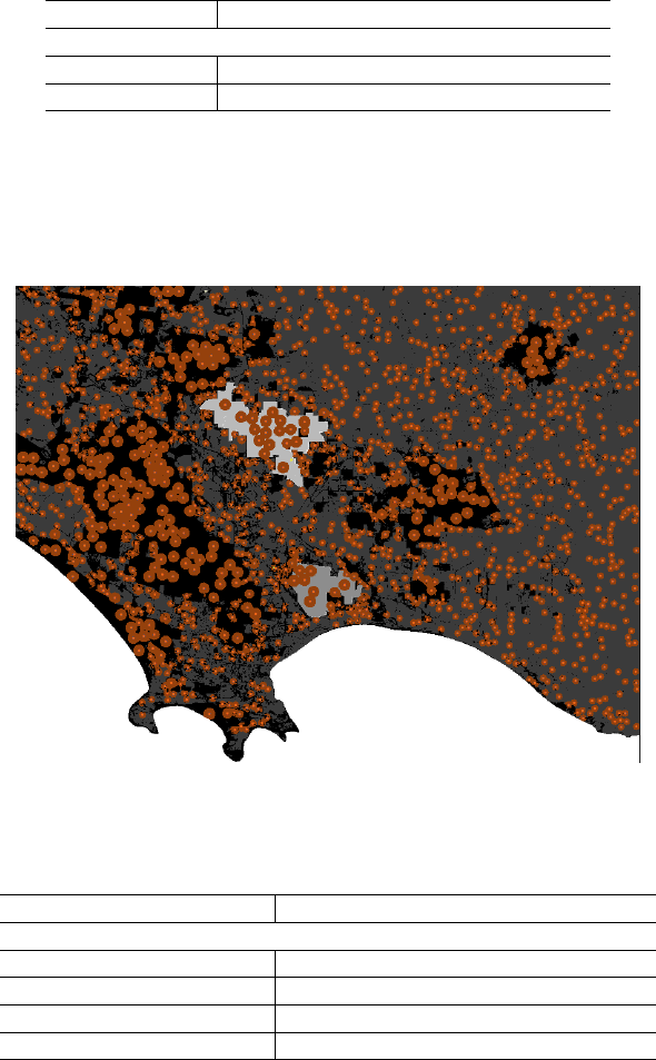
The world-view should now be much larger, and show an imported landscape layer with three diﬀerent types

of habitat-cells: forest (black), farmland (dark grey) and ocean (white, unavailable to foxes). Fox home

ranges are three times smaller in the farmland than the forest because of diﬀerences in the productivity of

the habitat-cells.

Within the landscape, there are two

regions-of-interest

for monitoring the fox population. The ﬁrst

is mid-grey (to the south), and includes bait-stations (white squares) and a survey-transect (red line) for

monitoring the number of foxes. The second region-of-interest is lighter grey (to the north).

If you’d like to see the landscape more clearly, set initial-fox-density to 0 and click setup again.

Set

initial-fox-density

back to 0.5, and explore the eﬀects of some of the other parameters . After

you change the parameters, you must click

set-up

again. For example, make the productivity of the

farmland the same as the productivity of the forest by changing the hab2:hab1 slider to “1.00”.

TIP: Don’t forget that you can make the model run more quickly by sliding the toggle at the top

of the screen to the right.

4.2 Building the Glenelg scenario from scratch

Now let’s work through each customisation process to build the Glenelg scenario from scratch

Once you are comfortable with how the Glenelg customisation scenario works, you can follow the same

processes to customise FoxNet to your own management scenario. Additional information on how to do this

is provided in the next chapter.

4.2.1 A customised landscape layer

Let’s start by importing an ascii raster layer to create a customised landscape of south-western Victoria,

Australia. This landscape is rectangular and contains three types of habitat-cell: forest, farmland and ocean.

Begin by clicking “basic-scenario” to reset all your parameters.

Alter the number of pixels per cell but clicking on the worldview > Edit. . . > Patch size > 0.5.

Then adjust the following parameters and click “setup”:

Parameter Value

‘working-directory‘ Location of FoxNet folder, e.g. C:/Users/hradsky/foxnet

Landscape setup

‘cell-dimension (m)‘ 100

‘landscape-source‘ import raster

‘landscape-raster (.asc)‘ gis_layers/glenelg/mtclay_landscape.asc

‘uninhabitable-raster-value ‘ 2

‘second-habitat-raster-value‘ 0

‘hab2:hab1‘ 1.00 x

Fox parameters

‘initial-fox-density (km^-2^)‘ 0

Baiting parameters

‘bait-layout‘ none

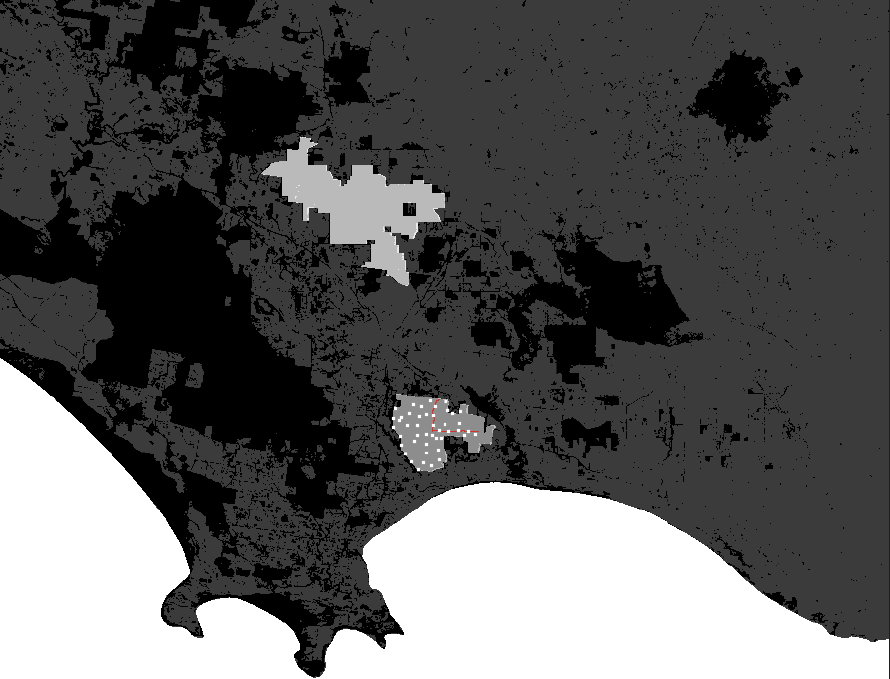
The worldview should now look like this:

Forest (the primary habitat type, which has a value of “1” in the raster) is shown in black, farmland (the

second habitat type, with raster value ‘0’) is shown in dark grey, and the ocean (speciﬁed by raster value ‘2’)

appears white.

TIP. You can check these values by right-clicking a habitat-cell, selecting inspect patch x y and

then seeing the integer shown next to habitat-type.

The

region-of-interest

has still been generated within the model and so forms a 200 km

lighter-shaded

block in the centre of the landscape.

At the top of the interface, the output box

actual landscape size

shows the area habitable by foxes

(4970.79 km2).

The total size of the landscape including the ocean is 6260.46 km

. To ﬁnd this out, type

count patches *

cells-to-km2 into the command center at the bottom of the screen.

4.2.2 Add some foxes

Provided the

intial-fox-density

is large enough that the population doesn’t go extinct through stochastic

processes, the fox density will eventually stabilise at the landscape’s carrying capacity (see Eﬀect of productivity

on fox density ).

The productivity of the landscape is set by specifying an average home-range-area for foxes in this landscape

(in km2), and the percentage of the home range kernel that this comprises.

For example, foxes in the forested regions of south-western Victoria have an average 95% kernel of 2.14 km

Specify the following parameters, then click setup again.

Parameter Value

Fox parameters

‘initial-fox-density (km^-2^)‘ 0.5

‘home-range-area (km^2^)‘ [2.14]

‘kernel-percent (%)‘ [95]

‘less1y-survival‘ 0.39

‘from1yto2y-survival‘ 0.65

‘from2yto3y-survival‘ 0.92

‘more3y-survival‘ 0.18

‘breeding-season‘ 37

‘number-of-cubs‘ 3.2

‘propn-cubs-female‘ 0.5

‘age-at-independence‘ 12

‘dispersal-season-begins‘ 9

‘dispersal-season-ends‘ 21

‘female-dispersers‘ 0.7

‘male-dispersers‘ 0.999

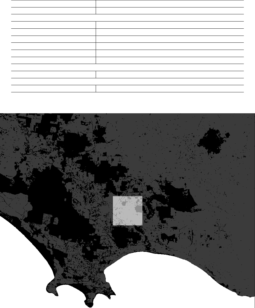
If forest and farmland habitats have equal productivity, a landscape with an initial-fox-density of 0.5 km

-2

looks like this after setup:

If diﬀerent habitat types support diﬀerent densities of foxes (Sálek, Drahnikova & Tkadlec 2015), you can

specify this using the

hab2:hab1

input slider. For example, farmland (the second habitat type) might be

three times more productive than forest (the primary habitat type), and so the slider would be set to “3.00”.

This causes foxes to select for farmland over forest. Territories entirely within the farmland are a third of the

size of those entirely within the forest (0.75 km

vs. 2.26 km

, 100% kernel), and the landscape’s carrying

capacity increases.

TIP To ﬁnd out the size of the smallest and largest fox-family territories, type

min [count

my-territory] of fox-families * cells-to-km2

max [count my-territory] of

fox-families * cells-to-km2 into the command center at the bottom of the screen

4.2.3 Add two monitoring regions

Rather than monitoring foxes in a central, square region-of-interest, we can monitor fox density in one or two

customised regions, in this case: Mt Clay Nature Reserve (where fox baiting occurs) and Annya State Forest

(where baiting does not occur). These regions are speciﬁed as separate polygon shapeﬁles:

Parameter Value

Landscape setup

‘region-shp‘ gis_layers/glenelg/mtclay_region.shp

‘region2-shp‘ gis_layers/glenelg/annya_region.shp

The ﬁrst region-of-interest is Mt Clay Nature Reserve (48.29 km2, as shown in the output box).

The second region of interest (

region-of-interest2

) is Annya State Forest. The size of this region is not

automatically displayed but can be shown by typing “region-of-interest2-size” into the observer input pane at

the bottom of the screen. The value is in km2.

4.2.4 Add customised bait sites

To import a customised layout of bait-stations, use a shapeﬁle with a point for each bait-station location.

Parameter Value

Baiting parameters

‘bait-layout‘ custom

‘bait-layout-shp‘ gis_layers/glenelg/mtclay_baits.shp

‘bait-frequency‘ 4-weeks

‘Pr-die-if-exposed-100-ha‘ 0.3

In this case the bait-stations are entirely within the ﬁrst

region-of-interest

, however, this isn’t required -

bait-stations can cover the entire landscape if preferred.

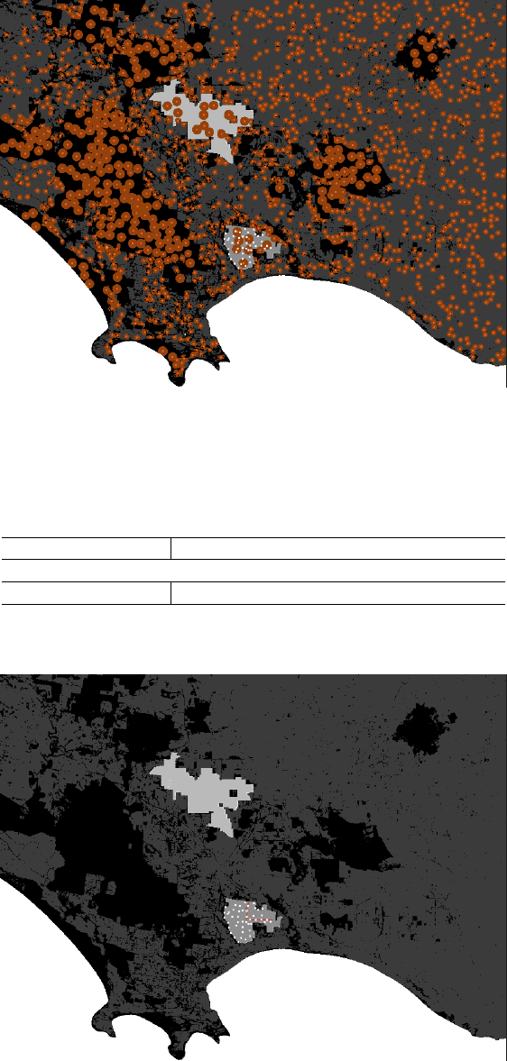
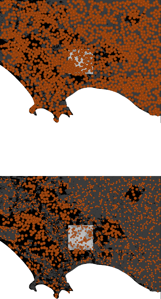
4.2.5 Add a survey transect

We can also calculate the number of foxes that have territories which overlap a linear transect, if for example,

we intend to collect fox scats and identify individuals using DNA analysis. The transect can be imported as a

line shapeﬁle.

Parameter Value

Landscape setup

‘survey-transect‘ gis_layers/glenelg/mtclay_transect.shp

initial-fox-density has been set to 0 to make the transect easier to see.

5 Building a new customised scenario

5.1 A customised landscape layer

5.1.1 Preparing your ascii ﬁle

The underlying landscape in FoxNet can be customised using a raster in ascii format (.asc). This allows you

to depict, for example, a rectangular landscape, diﬀerent habitat types that support diﬀerent densities of

foxes, and/or areas that are inaccessible to foxes such as oceans, lakes or fenced reserves.

You can prepare your ascii ﬁle in any spatial software you like (e.g. ArcGIS, QGIS or R).

The usual procedure involves drawing a rectangle for your landscape, dividing it into polygons that represent

each habitat type, and editing the attribute table so that each habitat type has a diﬀerent number (e.g. 1 =

ocean, 2 = forest, 3 = farmland). You then convert the polygon to a raster, and the raster to an ascii.

The size of your landscape should reﬂect the likely dispersal distance of foxes into your management zone.

A simple calculator can be found in

foxnet/user_guide/Calculator_dispersaldistance.xlsx

. You can

use this to estimate the proportion of potential dispersers that would be captured by a given buﬀer size,

based on the relationship between home range size and dispersal distance derived by Trewhella et al. (1988).

Take care with your projection ﬁle!

The .asc ﬁle must be accompanied by a projection ﬁle (.prj), which has the same ﬁlename and is saved in the

same folder. Your spatial software will automatically generate this. However,for NetLogo to accept it, the

.prj ﬁle must show the projection in one continuous line, like this:

PROJCS["WGS_1984_UTM_Zone_54S",GEOGCS["GCS_WGS_1984",DATUM["D_WGS_1984",SPHEROID["WGS_1984",6378137.0,298.257223563]],PRIMEM["Greenwich",0.0],UNIT["Degree",0.0174532925199433]],PROJECTION["Transverse_Mercator"],PARAMETER["False_Easting",500000.0],PARAMETER["False_Northing",10000000.0],PARAMETER["Central_Meridian",141.0],PARAMETER["Scale_Factor",0.9996],PARAMETER["Latitude_Of_Origin",0.0],UNIT["Meter",1.0]]

You can open the .prj ﬁle in Notepad (or similar) to check.

If you have generated your ascii layer in ArcGIS, the projection layer might be in the wrong format, and

instead look like this:

Projection UTM

Zone 54

Datum WGS84

Spheroid WGS84

Units METERS

Zunits NO

Yshift 10000000.0

Parameters

This will not work! The easiest way to ﬁx this problem is to open the .prj ﬁle for a shapeﬁle that uses the

same projection as your raster, and copy and paste the contents over the .prj information for your ascii.

A list of acceptable projection coordinate systems can be found at

<https://ccl.northwestern.edu/netlogo/docs/gis.html>

TIP: It is easiest to save all your GIS layers for customising FoxNet within

FoxNet/GIS_Layers/YourNewSubfolder

5.1.2 Importing your ascii ﬁle into FoxNet

On the FoxNet interface:

1) Change the landscape-source to “import raster”.

Click on ‘change’ on the

landscape-raster

input box, and type the ﬁle path to your .asc ﬁle. If the ﬁle

is saved within your FoxNet folder, you only need to enter the location within your

working-directory

(e.g. GIS_Layers/YourNewSubfolder/Yourascii.asc). Click OK.

Your raster should use diﬀerent integers for each habitat type as well as uninhabitable ar-

eas (such as ocean). Enter the relevant integers into the

second-habitat-raster-value

and

unihabitable-raster-value boxes, respectively.

If the second habitat type is more or less productive for foxes than the primary habitat type, you can

specify this using the

hab2:hab1

slider (a ratio of the productivity of habitat type 2 to habitat type 1).

5.2 Customised region(s) of interest

To monitor foxes within a customised area of your raster-based landscape (for example, a nature reserve)

rather than a generic central square, you can import a polygon shapeﬁle of the

region-of-interest

. Make

sure that it is in the same spatial projection as your raster layer.

Click ‘change’ on the

region-shp

input box, and type the ﬁle path to your .shp ﬁle. If the ﬁle is

saved within your FoxNet folder, you only need to enter the location within your

working-directory

(e.g. GIS_Layers/YourNewSubfolder/RegionShapeﬁle.shp)

2) If you have a second region-of-interest, you can enter the ﬁle path in the region2-shp input box.

5.3 Customised bait layout

Customised bait-stations can be imported as a point shapeﬁle, in the same projection as your raster layer.

Click ‘change’ on the

bait-layout-shp

input box, and type the ﬁle path to your .shp ﬁle. If the ﬁle is

saved within your FoxNet folder, you only need to enter the location within your

working-directory

(e.g. GIS_Layers/YourNewSubfolder/BaitsShapeﬁle.shp)

5.4 Customised survey transect

A customised survey transect can be imported as a line shapeﬁle, in the same projection as your raster layer.

Click ‘change’ on the

survey-transect-shp

input box, and type the ﬁle path to your .shp ﬁle. If the ﬁle

is saved within your FoxNet folder, you only need to enter the location within your

working-directory

(e.g. GIS_Layers/YourNewSubfolder/TransectShapeﬁle.shp)

6 Running batch scripts

Specifying inputs from the interface and running scenarios becomes tedious when you want to run many

experiments with varying parameters.

There are two ways to run batch scripts: (1) within NetLogo and (2) from R, using the RNetLogo package.

6.1 Within NetLogo

On the NetLogo interface, go to Tools > BehaviourSpace.

You can then setup a new experiment or run an existing script.

Information on how to use BehaviourSpace can be found at

<https://ccl.northwestern.edu/netlogo/docs/behaviorspace.html>

Example BehaviourSpace scripts for each of the FoxNet models described in Hradsky et al. (2019a) J. Applied

Ecology are saved within FoxNet. Note that you must set the

working-directory

within the BehaviourSpace

experiment to the correct ﬁle path (the location of your FoxNet folder e.g.

C:/Users/hradskyb/foxnet

) for

any script that involves importing a raster layer.

6.2 From R using the RNetLogo package

NetLogo can be called from R via the RNetLogo package. However, this package is no longer maintained.

See:

•

Thiele J (2014). R Marries NetLogo: Introduction to the RNetLogo Package. Journal of Statistical

Software, 58(2), 1-41. http://www.jstatsoft.org/v58/i02/

•

Thiele J, Kurth W, Grimm V (2012). RNetLogo: An R Package for Running and Exploring Individual-

Based Models Implemented in NetLogo. Methods in Ecology and Evolution 3 (3), 480-483. http:

//onlinelibrary.wiley.com/doi/10.1111/j.2041-210X.2011.00180.x/abstract/

Example R scripts for running each of the FoxNet models described in Hradsky et al. (2019a) J. Applied

Ecology in parallel are provided within the FoxNet folder - see

foxnet/r_scripts/run_model

. Note again

that you must set the

working-directory

within the script to the correct ﬁle path (the location of your

FoxNet folder e.g. C:/Users/hradskyb/foxnet) for any model that involves importing a raster layer.

An example for running a single version of FoxNet from R is provided here:

# LOAD PACKAGES

require(rJava)

.jinit(options(java.parameters=c("-server","-Xmx6000m")), force.init = TRUE)

#this may be required to override memory constraints for some computers

require(RNetLogo) #version 1.0-4

# SPECIFY PATHS FOR NETLOGO SOFTWARE AND FOXNET FOLDER

computersetup <- "laptop"

if (computersetup == "laptop") {

netlogo.path <- "C:/Program Files/NetLogo 6.0.2/app"

foxnet.path <- "C:/Users/hradskyb/FoxControlPatrol/Dropbox/personal/bron/ibm/foxnet"

}

corename <- "testrun"

# LOAD NETLOGO

NLStart(netlogo.path, gui = TRUE,nl.jarname = "netlogo-6.0.2.jar",

nl.obj = corename)

# make sure version number is correct

# ignore the Warning about error code 5 and "Unable to locate empty model: /system/empty.nlogo"

# it only occurs when gui (the visual interface) = TRUE and doesn't affect anything

# LOAD FOXNET MODELLING PLATFORM

NLLoadModel(paste0(foxnet.path, "/foxnet_model/foxnet.nlogo"),

nl.obj = corename)

# SET MODEL PARAMETERS

NLCommand(

# LANDSCAPE CONFIGURATION

"set working-directory",paste0("\"", foxnet.path, "\""),

"set weeks-per-timestep 2",

"set cell-dimension 100",

"set landscape-source \"import raster\"",

"set landscape-size 0",

"set region-size 0",

"set landscape-raster \"gis_layers/glenelg/mtclay_landscape.asc\"",

"set uninhabitable-raster-value 2",

"set second-habitat-raster-value 0",

"set hab2:hab1 1",

"set region-shp \"gis_layers/glenelg/mtclay_region.shp\"",

"set region2-shp \"\"",

"set survey-transect-shp \"\"",

"set survey-transect2-shp \"\"",

# FOX PARAMETERS

"set initial-fox-density 0.5",

# ranging behaviour

"set range-calculation \"1 kernel, 1 mean\"",

"set home-range-area \"[2.14]\"",

"set kernel-percent \"[95]\"",

# survival

"set fox-mortality true",

"set less1y-survival 0.39",

"set from1yto2y-survival 0.65",

"set from2yto3y-survival 0.92",

"set more3y-survival 0.18",

# reproduction

"set cub-birth-season 37",

"set number-of-cubs 3.74",

"set propn-cubs-female 0.5",

"set age-at-independence 12",

# dispersal

"set dispersal-season-begins 9",

"set dispersal-season-ends 21",

"set female-dispersers 0.7",

"set male-dispersers 0.999",

# BAITING PARAMETERS

"set bait-layout \"custom\"",

"set bait-density 0",

"set bait-layout-shp \"gis_layers/glenelg/mtclay_baits.shp\"",

"set bait-frequency \"fortnightly*\"",

"set custom-bait-weeks \"[]\"",

"set Pr-die-if-exposed-100ha 0.3",

"set commence-baiting-year 16",

"set commence-baiting-week 1",

"set price-per-bait 0",

"set person-days-per-baiting-round 0",

"set cost-per-person-day 0",

"set km-per-baiting-round 0",

"set cost-per-km-travel 0",

# MONITORING

"set plot? false",

"set age-structure false",

"set bait-consumption false",

"set count-neighbours false",

"set density true",

"set dispersal-distances false",

"set family-density false",

"set foxes-on-transect false",

"set popn-structure false",

"set range-size false",# this won't work from R as it requires calling R

nl.obj = corename)

# SETUP MODEL

NLCommand("setup",nl.obj = corename)

# NLCommand("go", nl.obj = corename)

# RUN MODEL

timesteps <- 702 # number of ticks

output.parameters <- c("year",

"week-of-year",

"total-fox-density",

"all-fox-but-cub-density",

"bait-take",

"bait-cost"

)

output <- NLDoReport(timesteps, "go", output.parameters,

as.data.frame = TRUE,

df.col.names=output.parameters,

nl.obj = corename)

# EXPORT OUTPUT AS A .csv

write.csv(output, paste0(foxnet.path, "/outputs/mtclay/mtclay_example_test.csv"))

# CLOSE NETLOGO (restart R if you want to run another model)

NLQuit(nl.obj = corename)

7 Implementation veriﬁcation

These FoxNet outputs illustrate key model behaviours at an individual-level, and are intended to supplement

the population-level output veriﬁcations provided in Hradsky et al (2019a). Netlogo code for these testing

procedures can be found in the demo_routines.nls ﬁle within FoxNet.

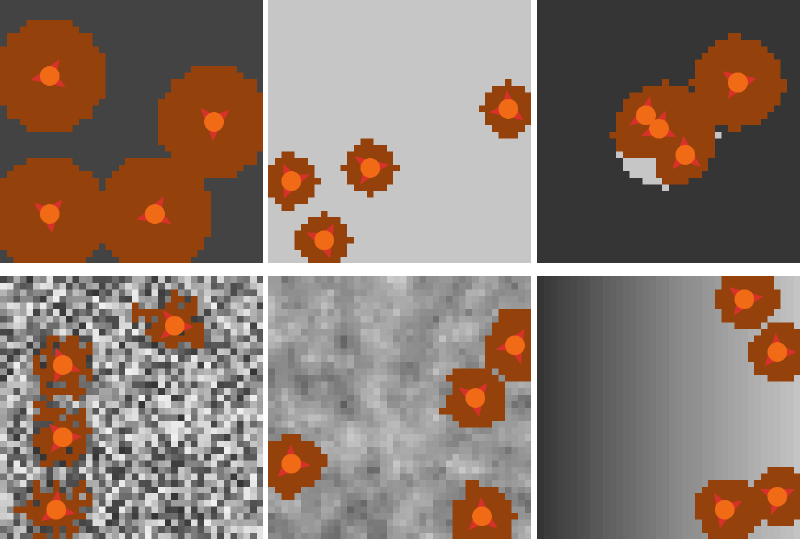
7.1 Eﬀect of productivity on fox-family territories

The size and location of fox-family territories in FoxNet is determined by the productivity of available

habitat-cells.

Following the example of Carter et al. (2015), we modelled a 16 km

landscape with ﬁve diﬀerent habitat-cell

productivity patterns to demonstrate this behaviour. The patterns were:

homogenenous, low productivity. The

home-range-area

was set to 2 km

and

kernel-percent

to 100

%. This resulted in each habitat-cell having a current-productivity of 13.23 g ha-1 week-1.

ii.

homogenous, high productivity. The

current-productivity

of each habitat-cell was quadrupled to

52.92 g ha-1 week-1.

iii.

two habitat types. A low productivity landscape (13.23 g ha

-1

week

-1

) with a central circle of high

productivity (52.92 g ha-1 week-1).

iv.

scattered random. The

current-productivity

of each habitat-cell was chosen at at random between

13.23 and 52.92 g ha-1 week-1.

smoothed random. As for heterogeneous random, but the

current-productivity

of each habitat-cell

was then averaged by that of its eight neighbours.

vi. a left-right gradient from 13.23 to 52.92 g ha-1 week-1.

We then visualised the conﬁguration of territories established by four foxes of the same sex after a 12 month

period (with no mortality or reproduction), and output the size of each territory.

The territory sizes of the four fox-families (in km2) for each of these six scenarios were:

i. 2, 2, 2, 2.

ii. 0.5, 0.5, 0.5, 0.5

iii. 0.52, 0.53, 0.54, 1.65.

iv. 0.54, 0.55, 0.56, 0.58.

v. 0.64, 0.65, 0.68, 0.73.

vi. 0.59, 0.59, 0.65, 0.70.

These outputs show that territory size scales inversely with habitat-cell productivity, and that territory

location is determined by the productivity of the habitat-cells.Fox-families select for the most productive

habitat-cells, while trying to keep their territory as compact as possible. They also adjust the size of their

territory so that it supplies no more than 110%2of an adult fox’s food requirements (2646 g week-1).

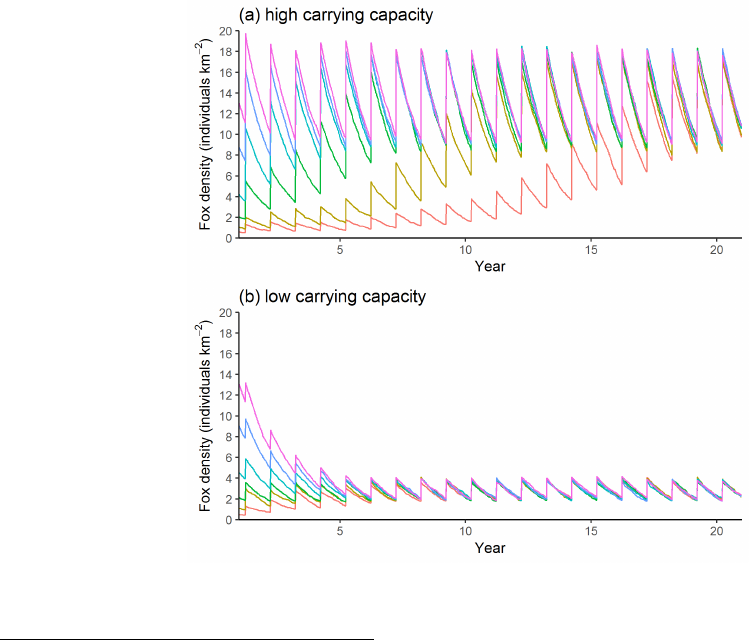
7.2 Eﬀect of productivity on fox density

Fox density in FoxNet models stabilises at a carrying capacity determined by the productivity of the

habitat-cells.

To demonstrate this, we simulated a landscape as per the Bristol, UK model described in Hradsky et al

(2019a). We populated the model with

initial-fox-density

inputs ranging from 0.5 to 12 foxes km

-2

and

home-range-area

inputs of (a) 0.454 km

(small home range, i.e. high productivity and high carrying

capacity) and (b) 2.14 km

(large home range, i.e. low productivity and low carrying capacity). We tracked

the density of foxes for 20 years.

Fox densities reached a dynamic equilibrium in both landscapes, regardless of the

initial-fox-density

Densities were substantially higher in the more productive landscape (where home ranges were smaller).

a value slightly greater than 100% is necessary to prevent rounding problems when the productivity of each habitat-cel l does

not divide neatly into the adult fox’s total food requirements.

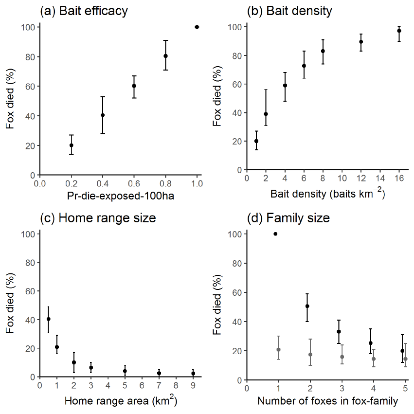
7.3 Eﬀect of baiting on fox mortality

The probability of a fox dying from a poison-bait in FoxNet scales with bait eﬃcacy, the number of baits on

the territory, territory size, and the number of foxes in the fox-family.

To demonstrate this behaviour, we modelled a homogenous 16 km

landscape with one fox-family with

a central territory and no natural mortality. The baseline settings were

Pr-die-if-exposed-100ha

0.2,

bait-density 0.5 baits km-2,home-range-area 1 km2and one fox.

Holding the other parameters constant, we varied (a)

Pr-die-if-exposed-100ha

from 0.2 to 1.0, (b)

bait-density

from 0.5 to 16 baits km

-2

, (c)

home-range-area

from 0.5 to 9 km

and (d) the number of

foxes in the fox-family from 1 to 5 with a bait-efficacy of 0.2 (grey) or 1.0 (black).

For each set of model parameters, we ran 100 iterations of the model for 1 time-step to determine the number

of foxes that were killed. We repeated this process 30 times. Results are presented as the mean (min, max)

percentage of iterations where the fox was killed.

As expected, foxes were more likely to die as

bait-efficacy

and

bait-density

increased, and were less

likely to die as

home-range-area

and the number of foxes within the fox-family increased. The eﬀect of the

number of foxes within the fox-family was greater when bait-efficacy was high.

8 Submodels

8.1 Submodels used during model processing

8.1.1 update-fox-age-and-status

Each time-step:

•

The

age

of all foxes is increased by the appropriate number of weeks (1, 2 or 4, depending on the

weeks-per-timestep setting).

•The status of any “cub” fox that has reached the age-of-independence is changed to “subordinate”.

•

If it is the dispersal season, a proportion of “subordinate” foxes become “dispersers”. The duration

of the dispersal season is determined by the

dispersal-season-begins

(week of year; inclusive)

and

dispersal-season-ends

(week of year; exclusive) inputs. It can either occur within one year

or overlap two years, and so accommodates both southern hemisphere (March - May; Pech et al.

1992) and northern hemisphere (September - March; Trewhella & Harris 1988) scenarios. The annual

probability of a “subordinate female” or “subordinate male” becoming a “disperser” is set via the

female-dispersers

and

male-dispersers

input, respectively. The probability that a “subordinate”

fox becomes a “disperser” during any time-step of the dispersal season is:

1−(1 −dispersal.probability)1/dispersal.season.duration

where the dispersal.season.duration is measured in time-step units.

8.1.2 fox-families-check-territories

Each fox-family checks its territory each time-step by:

Moving to the centre of its territory (along with all its family-members) and updating the

cell-relative-productivity

of the habitat-cells within its territory. See the

move-to-centroid

submodel.

Discarding any excess habitat-cells from its territory. If the total productivity of the habitat-cells within

the fox-family’s territory is greater than 110% of an adult fox’s food requirements (378 g day

-1

; Lockie

1959), the habitat-cell with the lowest

cell-relative-productivity

is removed. Steps (1) and (2)

are repeated until the total productivity of the territory is no more than 110 % of an adult fox’s food

requirements.

Creating a temporary agent (a vacancy) on each un-owned habitat-cell immediately adjacent to its

territory, and calculating the relative-productivity of these habitat-cells.

If there has been a change to the total productivity of the unoccupied habitat-cells surrounding

the territory (i.e. if the sum of the

relative-productivity

of the vacancy agents is diﬀerent to

the value from the previous time-step), the fox-family will attempt to updating its territory by

acquiring or swapping habitat-cells to maximise their

relative-productivity

(see the

update-

territory

submodel). However, if the available habitat-cells haven’t changed, the territory won’t be

updated (this speeds up the model). The territory is updated one cell at a time and is repeated until

the maximum-territory-update-area has been reached.

Removing any habitat-cells from its territory that have become isolated (i.e. habitat-cells that don’t have

any neighbours which are owned by the same fox-family). It then recalculates the total productivity of

its territory.

Checking whether the total productivity of its territory is less than the minimum productivity required

to sustain an adult fox’s metabolic rate (295 g day

-1

; Winstanley et al. 2003) . If so, the territory fails

(see the

territory-fail

submodel). If not, the fox-family ﬁnalises its updates by repeating step (1),

removing all temporary vacancy agents, and updating the

cell-relative-use

of the habitat-cells in

its territory.

8.1.3 bait-if-applicable

Baits are laid at bait-stations during time-steps identiﬁed by the

bait-frequency

input, either: “weekly”

(52

per year), “fortnightly” (26

per year), “4-weeks” (13

per year) or “custom” (where the week-numbers

are speciﬁed using the

custom-bait-weeks

input). Regardless of

bait-frequency

, no baits will be laid

bait-layout

is set to “none”. As part of the

check-for-errors

submodel during model setup, FoxNet

will return an error if the

bait-frequency

is incompatible with the

weeks-per-timestep

.Bait-stations are

white when no bait is present, and red when a bait is present. Note that this happens very quickly - if the

model is running fast, you won’t see it.

Baits are only toxic if the

commence-baiting-year

and

commence-baiting-week

values have been reached.

This allows you to run-in the model before baiting commences and determine the rate of bait-take during

free-feeding.

Baits that are is within the territory of a fox-family are at

Pr-death-bait-scaled

risk of being eaten by each

family member that not a cub. This is calculated as

Pr-die-if-exposed-100ha ×

100

×cell-relative-use

of the habitat-cell where the bait-station is located. Each bait can only be eaten once eat time step. If the

bait is toxic, the fox dies.

8.1.4 foxes-disperse

Each fox whose status is “disperser”:

(1) Updates how long it has been attempting to ﬁnd a new territory.

(2)

If it is its ﬁrst dispersal attempt, leaves its natal fox-family and moves a random distance and bearing

from the exponential distribution appropriate to its sex and home range size, as per Trewhella et al.

(1988):

F emale : 3.853 + 2.659 ×hr.100perc

Male : 2.778 + 4.038 ×hr.100perc

(1)

If that location is not possible (e.g. because it is in the ocean or beyond the edge of the landscape), the

fox chooses another random distance and bearing from the appropriate distribution and tries again

until it succeeds in moving.

(2)

Checks for baits within its

territory-perception-radius

. The likelihood of the disperser eating a

bait scales inversely with the radius. If the bait is toxic, the disperser dies.

(3)

Looks for a fox-family that lacks an “alpha” fox of the appropriate sex within its

territory-perception-radius

If any candidate fox-families exist, the “disperser” fox will join the nearest one and become an “alpha”

fox.

(4) If this fails, the “disperser” fox will try-to-establish-new-territory. It will:

Move to a random cell within its

territory-perception-radius

that hasn’t already been occupied

by another fox-family.

ii.

Create a fox-family which has the “disperser” fox as its sole family-member. The fox-

family’s territory is the single cell where it is located, its

territory-productivity

is the

current-productivity of that cell, and its vacancy-score is 0.

iii.

The new fox-family then creates vacancy agents on any of the 4 neighbouring habitat-cells that

aren’t already owned by other fox-families. It moves to the centre of this area and calculates the

cell and vacancy relative-productivities of its territory - see the

move-to-centroid

submodel. It

then:

iv. Repeats the update-territory submodel up to 10 ×the maximum-territory-update-area.

Removes any habitat-cells from its territory that have become isolated, recalculates the total

productivity of its territory and checks whether the total productivity of its territory is less than

the minimum productivity required to sustain an adult fox’s metabolic rate. If so, the territory

fails. See the fox-families-check-territories submodel for more details.

(5)

If the fox is still a “disperser” (i.e. if the new territory failed), it returns to its original dispersal location.

8.1.5 fox-families-breed

Fox-families that contain both an “alpha male” and an “alpha female” fox breed. The number of “cub” foxes

born to each fox-family is drawn from a Poisson distribution with mean

number-of-cubs

. The

sex

of the

cubs is randomly allocated, with the likelihood of a “cub” fox being “female” given by

propn-cubs-female

Cub

age

is 0, their

natal-cell

is their current location, their

natal-id

and

family-id

is that of their

fox-family, and they update the family-members of their fox-family to include themselves.

If instead the fox-family lacks an “alpha” fox of either sex, it is removed and all its family-members become

“dispersers”. These individuals then look for another a fox-family that lacks an “alpha” fox of the appropriate

sex within their

territory-perception-radius

. If any candidate fox-families exist, the “disperser” fox will

join the nearest one as a new “alpha”. This helps the population persist at low densities.

8.1.6 foxes-die

The probability of a fox surviving for each time-step depends on its age (<52 weeks, 52 - 103 weeks, 104 -

155 weeks, or >156 weeks), and is given by:

age.specific.annual.probability.of.survivalweeks.per.tick/52

8.1.7 update-monitors

The parameters that are calculated depend on the monitoring options selected on the interface - see Monitoring

your model outputs and Customisable model parameters for descriptions of each parameter. Outputs are

plotted if plot? is set to “on”.

8.1.8 move-to-centroid

To move to the centre of its territory, the fox-family creates a list of the x and y coordinates of each of the

habitat-cells in its territory, and moves to the habitat-cell with the mean x and y coordinates. It then asks

its family-members to move to this location. Finally, it updates the

cell-relative-productivity

of the

habitat-cells in its territory and the relative-productivity of any vacancies to:

distance.from.fox.family ×current.productivity ×100

8.1.9 update-territory

With each repeat, the fox-family checks whether the productivity of its territory is below the average

requirements of an adult fox. If so, it will try to add new habitat-cells to its territory. This involves

acquiring-the-best-available-vacancy by:

(1)

Identifying the vacancy that has the highest

relative-productivity

and adding the habitat-cell that

the vacancy is sitting on to the fox-family’s territory.

(2)

Asking the neighbours of this habitat-cell that aren’t currently owned by a fox-family or don’t already

have a vacancy on them, to create a vacancy agent.

(3) Updating the productivity score for the fox-family’s territory.

(4)

Moving to the centre of the fox-family’s territory and updating the

relative-productivity

of the

habitat-cells and vacancies (see move-to-centroid).

If the productivity of its territory is already adequate, the fox-family won’t expand its territory. Rather, it

will try to

swap-poor-territory-for-better

. This involves identifying which habitat-cell in its territory has

the lowest

cell-relative-productivity

. If the habitat-cell has already been checked, the routine aborts

(this speeds up the model). If not:

(5) The habitat-cell’s checked-already parameter is updated to “true”.

(6)

The vacancy agent on the unoccupied habitat-cell neighbouring the fox-family’s territory with the

highest relative-productivity is identiﬁed.

(7)

If the best vacancy has a higher

relative-productivity

than the worst territory cell (and isn’t a

neighbour of that cell), the fox-family will:

•Remove the worst habitat-cell from its territory.

•Update its territory-productivity score.

•

Add the best vacancy cell to its territory, following the

acquiring-the-best-available-vacancy

routine described above.

8.1.10 territory-fail

Afox-family will fail if the total productivity of its territory is less than the minimum required to sustain

an adult fox’s metabolism. In this case, the

fox-family-owner

of the habitat-cells in its territory is set

to “nobody”, any “cub” foxes die and the

status

of all other family-members is reset to “disperser”. The

fox-family and all associated vacancies are removed from the model.

8.2 Submodels speciﬁc to model set-up

8.2.1 check-for-errors

This checks for inconsistencies in the input parameters. The model will return a detailed error message and

stops if:

•bait-frequency is set to “weekly” but the weeks-per-timestep input is greater than “1”.

•bait-frequency is set to “fortnightly but the weeks-per-timestep input is greater than”2“.

•bait-frequency

is set to “custom” but the

custom-bait-weeks

values are incompatible with the

weeks-per-timestep input (i.e. if (value - 1) MOD weeks-per-timestep != 0).

•

the

dispersal-season-begins

dispersal-season-ends

values are incompatible the

weeks-per-timestep

input.

•dispersal-season-begins and dispersal-season-ends are the same value.

•the cub-birth-season value is incompatible with the weeks-per-timestep input.

•you have asked the model to monitor the number of foxes on a transect without uploading a transect

•you have imported a shapeﬁle for region2-shp without importing a shapeﬁle for region-shp

•

you are trying to use a customised bait layout in a model-generated (rather than imported) landscape.

8.2.2 set-fox-parameters

This sets a variety of parameters which are not available on the interface, including the minimum amount of

food required for short-term sustenance of an adult fox’s metabolic rate - 295 g day

-1

(Winstanley et al. 2003)

and a fox’s average daily food requirements - 378 g day

-1

(Lockie 1959), see also (Sargeant 1978; Winstanley

et al. 2003).

It also calculates several derived parameters:

•maximum-territory-update-area

: The maximum area of territory that can be updated each time-step

- half the area of a home range: hr.100perc ×0.5

•territory-perception-radius

: the distance that a fox can perceive adjacent fox-families. Three

times the radius of a home range: 3×phr.100perc)/π

•dispersal-duration: The duration of the dispersal season:

If dispersal.season.ends > dispersal.season.begins (i.e.southern hemisphere scenarios):

dispersal.duration =dispersal.season.ends−dispersal.season.begins

weeks.per.tick

Else (i.e. northern hemisphere scenarios):

dispersal.duration

dispersal.season.ends+(52−dispersal.season.begins)

weeks.per.tick

8.2.3 create-world

This generates a landscape of an appropriate size.

landscape-source

= “generate”, the landscape is generated by the model as a square with an area as

close to world-size as possible.

landscape-source

= “input raster”, the landscape is imported at a raster layer (ascii ﬁle), and will

automatically re-size to the appropriate dimensions. In the latter case, the

habitat-type

of each habitat-cell

will be determined by the raster value.

Habitat-types

that are unavailable to all agents (e.g. ocean) can be speciﬁed using the

uninhabitable-raster-value

These areas are not included in the landscape size output.

For both options, the spatial resolution is set by

cell-dimension

; this must correspond to the size of the

raster cells if applicable.

8.2.4 identify-region-of-interest

This identiﬁes the part of the landscape in which fox populations will be monitored. This may be the entire

landscape, or a smaller area to reduce any potential edge eﬀects. The

region-of-interest

can be speciﬁed

using the

region-size

input (which creates a central square of appropriate size), or imported as a shapeﬁle.

This changes the part-of-region-of-interest value of habitat-cells to “true”.

8.2.5 set-landscape-productivity

This determines the

true-productivity

values for the habitat-cells across the landscape using the input

data on fox

home-range-area

. The productivity of each habitat-cell in the primary habitat-type is calculated

from the

home-range-area

and

kernel-percent

of an average fox for that location (input by the user) and

the daily food requirements of an adult fox (378 g/day; Lockie 1959); an approach similar to Carter et al.

(2015). The calculations are based on the assumption that the intensity of use of an area by a fox corresponds

to the amount of food it obtains from the area. For example, if an average adult red fox requires ~370 g of

fresh food a day (Lockie 1959; Winstanley et al. 2003) and 100 % of its range covers 100 ha, 1-ha habitat-cell

would be supplying 3.7 g food day-1 on average.

range-calculation

is set to “1 kernel, 1 mean”, a single estimate of

home-range-area

and

kernel-percent

(e.g. mean 95% MCP) is used to create a homogeneous landscape, with the productivity of

each cell during each time-step being:

adult.f ox.timestep.food ×proportion.of.range

home.range.area ×area.of.habitat.cell

range-calculation

is set to “1 kernel, min and max”, minimum and maximum estimates of

home-range-area

(and one

kernel-percent

, e.g. mean 95% MCP) are used to create a heterogeneous

landscape, with the productivity of each cell during each time-step being a random value drawn between the

minimum and maximum productivity values, each calculated as above.

Whichever approach is used, the productivity of the second habitat type is speciﬁed relative to this primary

habitat type, according to the hab2:hab1 ratio.

8.2.6 set-up-bait-stations

The locations of bait-stations can be speciﬁed by choosing a

bait-layout

: “none”, “regular grid”, “random

scatter” or “custom”.

If “regular grid” or “random scatter” is chosen, bait-stations are generated by the model at the speciﬁed

density. If “custom”, the locations for the bait-stations are imported as a shapeﬁle. The

bait-present

attribute of all bait-stations is set to “false” (i.e. no bait is present).

8.2.7 set-up-foxes

An initial number of foxes are created at the speciﬁed density, with

ages

ranging between 36 and 166 weeks,

and a sex ratio in accordance with the propn-cubs-female input. Each fox is moved to a random location

and its status is set to “disperser”. All foxes then disperse (see the foxes-disperse submodel).

9 Appendices

9.1 Customisable model parameters

Parameter Unit Explanation

‘working-directory‘ — Location of FoxNet folder, e.g.

‘C:/Users/hradsky/FoxNet‘

Landscape setup

‘weeks-per-timestep‘ weeks Number of weeks for each model

timestep ("1", "2" or "4")

‘cell-dimension‘ m Distance along one edge of a

*habitat-cell*

‘landscape-source‘ “generate” or “import raster” Whether the landscape is

generated within the model or

imported as a raster

‘landscape-size‘ km^2^ The size of the landscape, if it is

generated within the model

‘region-size‘ km^2^ The size of the region-of-interest

(where the *fox* population is

monitored), if it is generated

within the model

‘landscape-raster‘ .asc ﬁle The raster (ascii) ﬁle describing

the landscape layout (e.g.

‘GIS_layers/Glenelg/

mtclay_landscape.asc‘), if the

landscape is imported

‘uninhabitable-raster-value‘ integer

The value used in the raster layer

to specify *habitat-cells* that

can’t be inhabited by *foxes*

(e.g. ocean)

‘second-habitat-raster-value‘ integer

The value used in the raster layer

to specify *habitat-cells* that are

a secondary type of habitat (e.g.

farmland rather than forest)

‘hab2:hab1‘ ratio The productivity of the

secondary habitat type relative

to the primary habitat type

‘region-shp‘ .shp ﬁle A shapeﬁle (polygon) describing

a region-of-interest (where *fox*

populations are monitored) if the

landscape is imported

‘region2-shp‘ .shp ﬁle A shapeﬁle (polygon) describing

a second region-of-interest (where

*fox* populations are monitored)

if the landscape is imported –

optional.

‘survey-transect-shp‘ .shp ﬁle A shapeﬁle (line) describing a

transect for surveying *fox*

populations

‘survey-transect2-shp‘ .shp ﬁle A shapeﬁle (line) describing a

second transect for surveying

*fox* populations

Fox parameters

‘initial-fox-density‘ individuals km^-2^ The number of *foxes* per

square kilometre when the model

is initiated

(continued)

Parameter Unit Explanation

‘range-calculation‘ ‘ “1 kernel, 1 mean” ‘ or “1

kernel, min and max”

The method used for calculating

the productivity of the landscape

from the fox home range data

‘home-range-area‘ km^2^ The area of an average fox home

range in this landscape

‘kernel-percent‘ % The proportion of the home

range kernel included in the %

area (e.g. 90 for a 90% MCP)

‘fox-mortality‘ "true"/"false" Whether natural mortality of

*foxes* occurs. Usually set to

"on".

‘less1-survival‘ propn. Annual survival rate for *foxes*

< 1 year old

‘from1yto2y-survival‘ propn.

Annual survival rate for *foxes* 1

- 2 years old

‘from2yto3y-survival‘ propn.

Annual survival rate for *foxes* 2

- 3 years old

‘more3y-survival‘ propn. Annual survival rate for *foxes*

> 3 years old

‘cub-birth-season‘ week of year

Time of year when *fox* cubs are

born

‘number-of-cubs‘ cubs fox-family^-1^ Average number of cubs born to

a *fox-family*

‘propn-cubs-female‘ propn Proportion of cubs that are

female when born

‘age-at-independence‘ weeks Age of cubs when they can

survive the death of all adults in

their *fox-family*

‘dispersal-season-begins‘ week of year Start of dispersal season

‘dispersal-season-ends‘ week of year End of dispersal season

‘female-dispersers‘ propn. Female dispersal rate

‘male-dispersers‘ propn. Male dispersal rate

Baiting parameters

‘bait-layout‘ “none”, “grid”, “random-scatter”,

“custom”

The layout of *bait-stations*. A

shapeﬁle must be imported for

the "custom" option.

‘bait-density‘ baits-stations km^-2^ The density of *bait-stations*.

This only aﬀects the “grid” and

“random-scatter” ‘bait-layout‘

options

‘bait-layout-shp‘ .shp ﬁle A shapeﬁle (points) describing

the locations of the

*bait-stations*, if ‘bait-layout‘ is

“custom”

‘bait-frequency‘ “weekly*”, “fortnightly*,

“4-weeks” or “custom*”

The frequency with which baits

are laid at baitstations. Check

that * options are compatible

with ‘weeks-per-timestep‘.

‘custom-bait-weeks‘ week(s) of year Weeks-of-year when baits will be

deployed at *bait-stations* if a

“custom*” bait-frequency is

chosen

(continued)

Parameter Unit Explanation

‘Pr-die-if-exposed-100ha‘ index The eﬃcacy of the poison baits

when they are deployed at

*bait-stations*

‘commence-baiting-year‘ year The ﬁrst year when baits at

*bait-stations* will be poisonous

(until then, baits are deployed

and eaten but don’t kill *foxes*)

‘commence-baiting-week‘ week of year The ﬁrst week of the ﬁrst year

when baits at *bait-stations* will

be poisonous

‘price-per-bait‘ $ The cost of a single bait

‘person-days-per-baiting-round‘

days The number of person-days it

takes to deploy a bait at each

*bait-station*

‘cost-per-person-day‘ $ The cost per person-day while

deploying baits

‘km-per-baiting-round‘ km

Total distance travelled to deploy

a bait at each *bait-station*

‘cost-per-km-travel‘ $ The per-kilometre cost of travel

while deploying baits

Monitoring Parameters

‘plot‘ "true"/"false" Whether you want monitored

variables to be shown in the

beige plot(s)

‘age-structure‘ "true"/"false" The number of *foxes* in each

age class within the

‘region-of-interest‘

‘count-neighbours‘ "true"/"false" The number of neighbouring

territories for each *fox-family*

within the ‘region-of-interest‘

‘density‘ "true"/"false" The density of *foxes*, various

classes of *foxes*, and

*fox-families* within the

‘region-of-interest‘ (and

‘region-of-interest2‘ if applicable)

‘dispersal-distances‘ "true"/"false" The distance that *foxes* within

the ‘region-of-interest‘ have

dispersed (excludes cubs &

individuals that have not

attempted to disperse)

‘family-density‘ "true"/"false" The density of *fox-families*

within the ‘region-of-interest‘

‘foxes-on-transect‘ "true"/"false"

The number of *foxes* (excluding

cubs) who have a territory that

overlaps ‘survey-transect‘ (and

‘survey-transect2‘, if applicable)

‘popn-structure‘ "true"/"false"

The number of *foxes* in various

status/sex classes within the

‘region-of-interest‘

‘range-size‘ "true"/"false" Not currently activated

9.2 Week Conversion Table

week start end

Week 1 1-Jan 7-Jan

Week 2 8-Jan 14-Jan

Week 3 15-Jan 21-Jan

Week 4 22-Jan 28-Jan

Week 5 29-Jan 4-Feb

Week 6 5-Feb 11-Feb

Week 7 12-Feb 18-Feb

Week 8 19-Feb 25-Feb

Week 9 26-Feb 4-Mar

Week 10 5-Mar 11-Mar

Week 11 12-Mar 18-Mar

Week 12 19-Mar 25-Mar

Week 13 26-Mar 1-Apr

Week 14 2-Apr 8-Apr

Week 15 9-Apr 15-Apr

Week 16 16-Apr 22-Apr

Week 17 23-Apr 29-Apr

Week 18 30-Apr 6-May

Week 19 7-May 13-May

Week 20 14-May 20-May

Week 21 21-May 27-May

Week 22 28-May 3-Jun

Week 23 4-Jun 10-Jun

Week 24 11-Jun 17-Jun

Week 25 18-Jun 24-Jun

Week 26 25-Jun 1-Jul

Week 27 2-Jul 8-Jul

Week 28 9-Jul 15-Jul

Week 29 16-Jul 22-Jul

Week 30 23-Jul 29-Jul

Week 31 30-Jul 5-Aug

Week 32 6-Aug 12-Aug

Week 33 13-Aug 19-Aug

Week 34 20-Aug 26-Aug

Week 35 27-Aug 2-Sep

Week 36 3-Sep 9-Sep

Week 37 10-Sep 16-Sep

Week 38 17-Sep 23-Sep

Week 39 24-Sep 30-Sep

Week 40 1-Oct 7-Oct

Week 41 8-Oct 14-Oct

Week 42 15-Oct 21-Oct

Week 43 22-Oct 28-Oct

Week 44 29-Oct 4-Nov

Week 45 5-Nov 11-Nov

Week 46 12-Nov 18-Nov

Week 47 19-Nov 25-Nov

Week 48 26-Nov 2-Dec

Week 49 3-Dec 9-Dec

Week 50 10-Dec 16-Dec

Week 51 17-Dec 23-Dec

Week 52 24-Dec 30-Dec

10 References

Baker, P.J., Robertson, C.P.J., Funk, S.M. & Harris, S. (1998) Potential ﬁtness beneﬁts of group living in the

red fox, Vulpes vulpes.Animal Behaviour, 56, 1411-1424.

Bino, G., Dolev, A., Yosha, D., Guter, A., King, R., Saltz, D. & Kark, S. (2010) Abrupt spatial and numerical

responses of overabundant foxes to a reduction in anthropogenic resources. Journal of Applied Ecology, 47,

1262-1271.

Carter, N., Levin, S. et al. (2015) Modeling tiger population and territory dynamics using an agent-based

approach. Ecological Modelling, 312, 347-362.

Devenish-Nelson, E.S., Harris, S., Soulsbury, C.D., Richards, S.A. & Stephens, P.A. (2013) Demography of a

carnivore, the red fox, Vulpes vulpes: what have we learnt from 70 years of published studies? Oikos, 122,

705-716.

Hradsky, B.A., Kelly, L.T., Robley, A. & Wintle, B.A. (2019a) FoxNet: an individual-based model framework

to support management of an invasive predator, the red fox. Journal of Applied Ecology.

Hradsky, B.A., Kelly, L.T., Robley, A. & Wintle, B.A. (2019b) Data from: FoxNet: an individual-based

model framework to support management of an invasive predator, the red fox. Zenodo. http://doi.org/10.

5281/zenodo.2572045.

Hradsky, B.A., Mildwaters, C.A., Ritchie, E.G., Christie, F. & Di Stefano, J. (2017a) Responses of invasive

predators and native prey to a prescribed forest ﬁre. Journal of Mammalogy, 98, 835-847.

Hradsky, B.A., Robley, A., Alexander, R., Ritchie, E.G., York, A. & Di Stefano, J. (2017b) Human-modiﬁed

habitats facilitate forest-dwelling populations of an invasive predator, Vulpes vulpes.Scientiﬁc Reports, 7,

12291.

Larivière, S. & Pasitschniak-Arts, M. (1996) Vulpes vulpes.Mammalian Species, 537, 1-11.

Lockie, J.D. (1959) The estimation of the food of foxes. The Journal of Wildlife Management, 23, 224-227.

Pech, R.P., Sinclair, A., Newsome, A. & Catling, P. (1992) Limits to predator regulation of rabbits in

Australia: evidence from predator-removal experiments. Oecologia, 89, 102-112.

Šálek, M., Drahnikova, L. & Tkadlec, E. (2015) Changes in home range sizes and population densities of

carnivore species along the natural to urban habitat gradient.* Mammal Review*, 45, 1-14.

Sargeant, A.B. (1972) Red fox spatial characteristics in relation to waterfowl predation. Journal of Wildlife

Management, 36, 225-&.

Saunders, G., McLeod, S. & Kay, B. (2000) Degradation of sodium monoﬂuoroacetate (1080) in buried fox

baits. Wildlife Research, 27, 129-135.

Soulsbury, C.D., Iossa, G., Baker, P.J., White, P.C. & Harris, S. (2011) Behavioral and spatial analysis of

extraterritorial movements in red foxes (Vulpes vulpes). Journal of Mammalogy, 92, 190-199.

Thiele, J.C. (2014) R Marries NetLogo: Introduction to the RNetLogo Package. Journal of Statistical

Software, 58, 1-41.

Trewhella, W. & Harris, S. (1988) A simulation model of the pattern of dispersal in urban fox (Vulpes vulpes)

populations and its application for rabies control. Journal of Applied Ecology, 435-450.

Trewhella, W.J., Harris, S. & McAllister, F.E. (1988) Dispersal distance, home-range size and population

density in the red fox (Vulpes vulpes) - a quantitative analysis. Journal of Applied Ecology, 25, 423-434.

Wilensky, U. (1999) Netlogo. Center for Connected Learning and Computer-Based Modeling, Northwestern

University, Evanston, IL.

Winstanley, R.K., Buttemer, W.A. & Saunders, G. (2003) Field metabolic rate and body water turnover of

the red fox Vulpes vulpes in Australia. Mammal Review, 33, 295-301.

FoxNet User Guide V1.0.0 Fox Net

Navigation menu

Versions of this User Manual:

Views

Navigation