Fusion 9 Tool Reference
User Manual:
Open the PDF directly: View PDF ![]() .
.
Page Count: 791 [warning: Documents this large are best viewed by clicking the View PDF Link!]
- Contents
- 3D Tools
- 3D Light Tools
- 3D Material Tools
- 3D Texture Tools
- Blur Tools
- Color Tools
- Composite Tools
- Creator Tools
- DeepPixel Tools
- Effect Tools
- Film Tools
- Filter Tools
- Flow Tools
- FlowOrg Tools
- Fuses
- I/O Tools
- LUT Tools
- Mask Tools
- Matte Tools
- Metadata Tools
- Miscellaneous Tools
- Optical Flow
- Paint Tool
- Particle Tools
- Position Tools
- Stereo Tools
- Tracker Tools
- Transform Tools
- Warp Tools
- Modifiers
- VR Tools
- 3D Tools
- Alembic Mesh 3D [ABc]
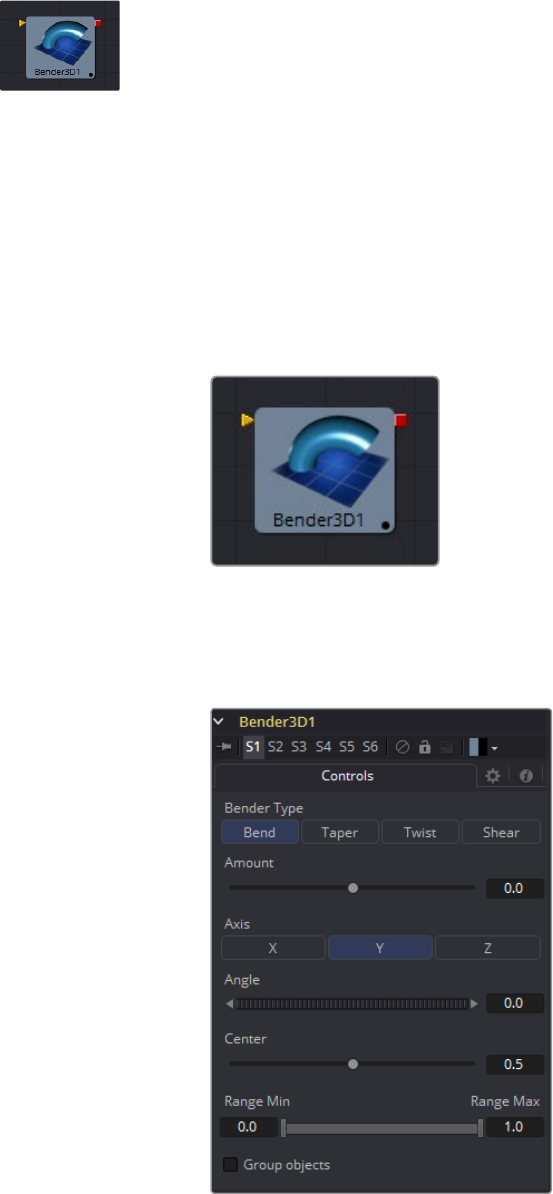
- Bender 3D [3Bn]
- Camera 3D [3Cm]
- Cube 3D [3Cb]
- Custom Vertex 3D [3Cv]
- Displace 3D [3Di]
- Duplicate 3D [3Dp]
- FBX Exporter 3D [FBX]
- FBX Mesh 3D [FBX]
- Fog 3D [3Fo]
- Image Plane 3D [3Im]
- Locator 3D [3Lo]
- Merge 3D [3Mg]
- Override 3D [3Ov]
- Point Cloud 3D [3PC]
- Projector 3D [3Pj]
- Renderer 3D [3Rn]
- Replace Material 3D [3Rpl]
- Replace Normals 3D [3Rn]
- Replicate 3D [3Rep]
- Ribbon 3D [3Ri]
- Shape 3D [3Sh]
- Softclip [3Sc]
- Text 3D [3Txt]
- Transform 3D [3Xf]
- Triangulate 3D [3Tri]
- UV Map 3D [3UV]
- Weld 3D [3We]
- Modifier
- 3D Light Tools
- 3D Material Tools
- 3D Texture Tools
- Blur Tools
- Color Tools
- Composite Tools
- Creator Tools
- DeepPixel Tools
- Effect Tools
- Film Tools
- Filter Tools
- Flow Tools
- FlowOrg Tools
- Fuses
- I/O Tools
- LUT Tools
- Mask Tools
- Matte Tools
- Metadata Tools
- Miscellaneous Tools
- Optical Flow
- Paint Tool
- Particle Tools
- Position Tools
- Stereo Tools
- Tracker Tools
- Transform Tools
- Warp Tools
- Modifiers
- VR Tools
1
Contents
Tool Reference Manual
July 2017
Fusion 9
2
Contents
Fusion 9
1 3D Tools 5
2 3D Light Tools 106
3 3D Material Tools 119
4 3D Texture Tools 148
5 Blur Tools 172
6 Color Tools 194
7 Composite Tools 245
8 Creator Tools 261
9 DeepPixel Tools 304
10 Effect Tools 317
11 Film Tools 338
12 Filter Tools 354
13 Flow Tools 366
14 FlowOrg Tools 371
15 Fuses 377
16 I/O Tools 380
17 LUT Tools 399
18 Mask Tools 407
19 Matte Tools 433
20 Metadata Tools 484
5
3D Tools Chapter – 1
3D Tools
Alembic Mesh 3D [ABC] 7
Bender 3D [3BN] 10
Camera 3D [3CM] 12
Cube 3D [3CB] 21
Custom Vertex 3D [3CV] 25
Displace 3D [3DI] 27
Duplicate 3D [3DP] 29
FBX Exporter 3D [FBX] 33
FBX Mesh 3D [FBX] 35
Fog 3D [3FO] 39
Image Plane 3D [3IM] 41
Locator 3D [3LO] 45
Merge 3D [3MG] 48
Override 3D [3OV] 50
Point Cloud 3D [3PC] 52
Projector 3D [3PJ] 56
Renderer 3D [3RN] 62
Replace Material 3D [3RPL] 72
Replace Normals 3D [3RN] 74
Replicate 3D [3REP] 76
Ribbon 3D [3RI] 82
Shape 3D [3SH] 84
Softclip [3SC] 89
Text 3D [3TXT] 91
Transform 3D [3XF] 95
Triangulate 3D [3TRI] 98
UV Map 3D [3UV] 99
Weld 3D [3WE] 102
Modifier 104
Coordinate Transform 3D 104
6
3D Tools Chapter – 1
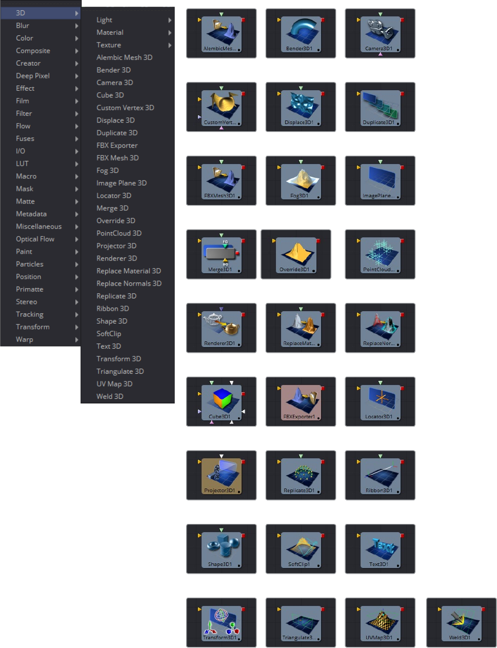
3D Tools
Softclip Text 3DShape 3D
FBX Exporter 3DCube 3D Locator 3D
Replace Normals 3DReplace Material 3DRenderer 3D
Merge 3D Override 3D Point Cloud 3D
FBX Mesh 3D Fog 3D Image Plane 3D
Bender 3D Camera 3DAlembic Mesh 3D
Transform 3D UV Map 3D Weld 3DTriangulate 3D
Replicate 3DProjector 3D Ribbon 3D
Duplicate 3DDisplace 3DCustom Vertex 3D
7
3D Tools Chapter – 1
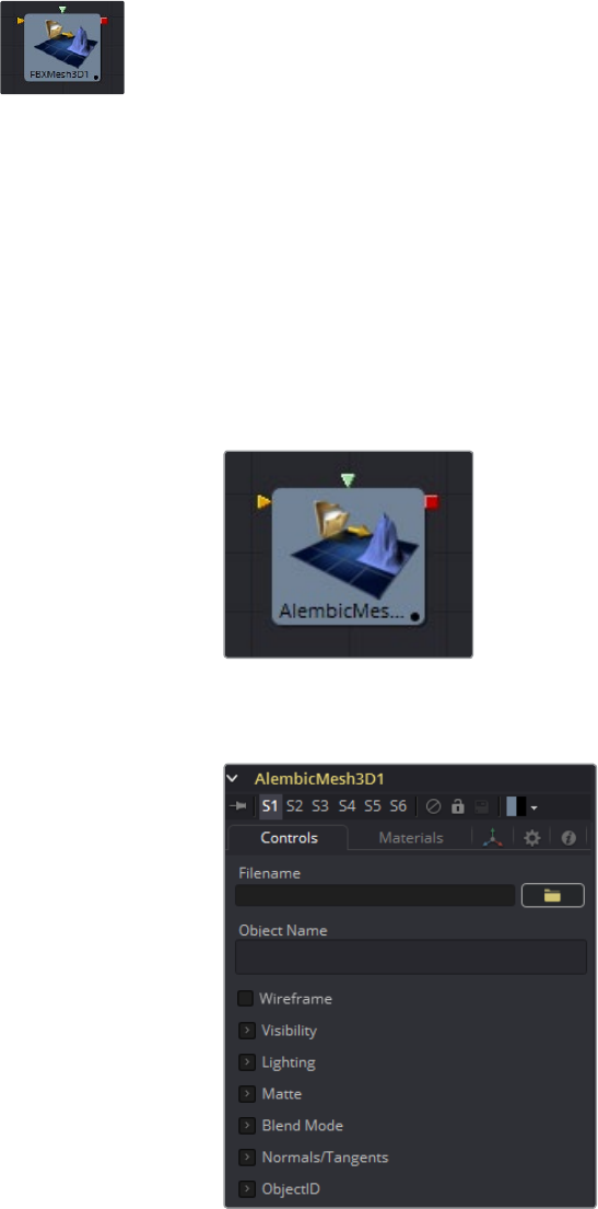
Alembic Mesh 3D [ABC]
There are two way to import Alembic files:
Using the File > Import > Alembic menu option
Manually adding an AlembicMesh3D tool to the flow
The first method is strongly recommended.
The Alembic format allows for arbitrary user data to be stored within the file. Fusion ignores
most of this metadata for various reasons. No conventions have been defined yet for how this
metadata is named and metadata might change between different ABC exporters. When the
Alembic file is imported through the menu option, the transforms are read into splines and into
the inputs on the tools, which get saved with the comp.
This means that when re-loading the comp, the transforms are loaded from the comp and notthe
Alembic file. The meshes are handled differently; they are always reloaded from the Alembic file.
Controls
Filename
The name of the imported Alembic file.
Object Name
This input shows the name of the mesh from the Alembic file that is being imported.
Ifthis field is blank, then the entire contents of the FBX geometry will be imported as
asingle mesh. This input is not editable by the user; it is set by Fusion when importing
Alembic files via the File > Import > Alembic utility.
8
3D Tools Chapter – 1
Sampling Rate
The framerate is set when importing the file. It can be altered using this slider to create
effects like slow motion.
Dump File
Opens the resulting ASCII in the preferred text editor.
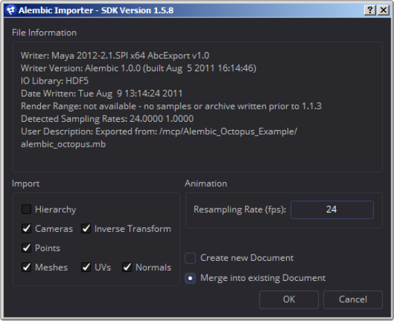
Alembic import dialog
Writer: The name of the plug-in/application that created/wrote out the Alembic file
Writer Version: The version of the Alembic sdk that was used to write out the
Alembic file
RenderRange: This gives you an idea of the duration of the animation in the Alembic
file in seconds
DetectedSamplingRates: Fusion examines the framerates in the file and reports
them here. This is useful to determine the value at which to set the Resampling Rate.
Hierarchy
If disabled, the transforms in the Alembic file are flattened down into the cameras and
meshes. This results in a number of meshes/cameras connected to a single merge
node in Fusion. When enabled, you get the full parenting hierarchy.
Orphaned transforms
Transforms that do not parent a mesh or camera will not be imported if this option is
unchecked. For example, if you have a skeleton and associated mesh model, the model
will be imported as an Alembic mesh and the skeleton will be imported as a tree of
merge3Ds. Disabling this option causes the merge3Ds not to be imported.
Cameras
Near/Far/Apertures/Angles of View/Plane of Focus are imported. The resolution Gate
Fit may be imported; it depends if the Writer correctly tagged the resolution Gate Fit
metadata. If your camera does not import correctly, you should check to see if
Camera3D.ResolutionGateFit is set correctly. Stereo information is not imported.
9
3D Tools Chapter – 1
InverseTransform
Imports the Inverse Transform (World to Model) for cameras.
Points
Alembic supports a Points type. This is a collection of 3D points without orientation.
Some 3D apps export particles as points, but keep in mind the direction and orientation
of the particles are lost; you just get positions. It very well may be possible that the
exocortex Alembic plug-ins write out extra user data that contains orientation.
Meshes
Optionally import UVs and normals.
ResamplingRate
When an Alembic animation is exported, it is stored on disk in seconds, not in frames.
When the Alembic data is brought into Fusion, you need to supply a framerate with
which to resample the animation. Ideally, you should choose the same framerate that it
was exported with so your samples match up with the original samples. Detected
Sampling Rates can give an idea of what to pick if unsure.
Lights
Import currently not supported. There is no universal convention on Alembic
light schemas.
Materials
Import currently not supported. There is no universal convention on Alembic
material schemas.
Curves
Import currently not supported.
Multiple UVs
Import currently not supported. There is no universal convention yet.
Velocities
Import currently not supported.
Cyclic/Acyclic sampling
Currently not implemented. Uniform sampling, which is the most common mode, works
fine. We recommend the use of FBX for lights/cameras/materials and Alembic for
meshes only. If cameras and Alembic work for you, then go for it. The reason is that our
Alembic plug-in doesn’t support lights/materials, but FBX has good support. Alembic
import of cameras has problems with Resolution Gate Fit and doesn’t import
stereo options.
10
3D Tools Chapter – 1
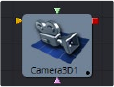
Bender 3D [3BN]
The Bender 3D tool is used to bend, taper, twist or shear the geometry in a 3D scene based
upon its bounding box. It takes a 3D scene as input and outputs a modified 3D scene. Only
thegeometry in the scene is modified. Any lights, cameras or materials are passed
throughunaffected.
The Bender tool does not produce new vertices in the geometry; only existing vertices in the
geometry are altered. As a result, when applying the Bender 3D tool to primitives created in
Fusion, it is a good idea to increase the value of the Subdivision controls in the original
primitives to give a higher quality result.
External Inputs
The following inputs appear on the tools tile in the Flow Editor.
Bender3D.SceneInput
[gold, required] This input expects a 3D scene.
Controls Tab

11
3D Tools Chapter – 1
Bender Type
Use the Bender Type to select the type of deformation to apply to the geometry. There
are four modes available: Bend, Taper, Twist and Shear.
Amount
Adjust the Amount slider to change the strength of the deformation.
Axis
The Axis control determines the axis along which the deformation is applied and has a
different meaning depending on the type of deformation. When bending, this
determines the axis that is bent, in conjunction with the Angle control. In other cases,
the deform is applied around the specified axis.
Angle
The Angle thumbwheel control determines what direction about the axis that a bend or
shear is applied. It is not visible for taper or twist deformations.
Range
The Range control can be used to limit the effect of a deformation to a small portion of
the geometry. The Range control is not visible when the Bender Type is set to Shear.
Group Objects
When this is checked, all the objects in the input scene are grouped together into a
single object and that object is deformed around the common center, instead of
deforming each component object individually.
12
3D Tools Chapter – 1
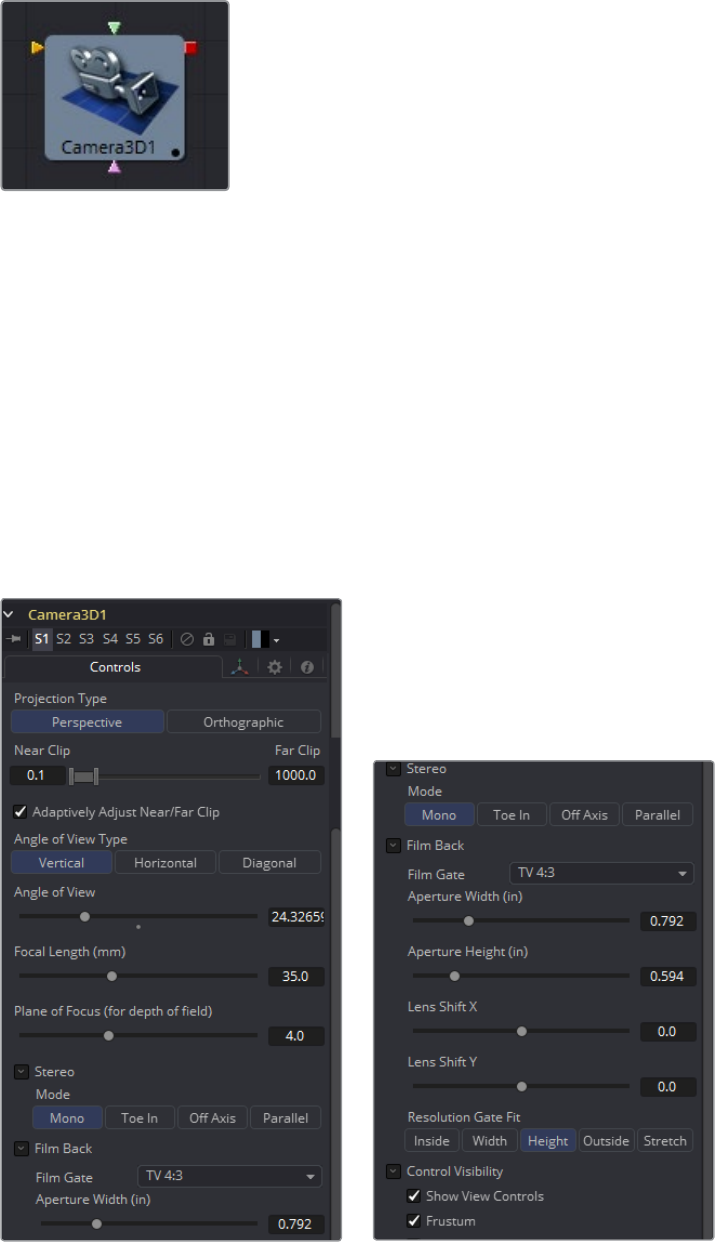
Camera 3D [3CM]
The Camera 3D tool generates a virtual camera through which the 3D environment can be
viewed. It closely emulates the settings used in both real and virtual cameras in an effort to
make matching the cameras used in other scene elements as seamless as possible.
The camera should be added to the scene using a Merge 3D tool. Displaying a camera tool
directly in the Viewer shows only an empty scene; there is nothing for the camera to see.
Toview the scene through the camera, view the scene from the Merge 3D tool that introduces
the camera, or any tool downstream of that Merge 3D. Then right click in the view and select
Camera > Cameraname from the contextual menu. Right clicking on the axis label found in the
bottom corner will display the Camera sub-menu directly.
The aspect of the Viewer may be different from the aspect of the camera, so that the view
through the camera interactively may not match the true boundaries of the image which will
actually be rendered by the Renderer 3D tool. To assist you in framing the shot, guides can be
enabled that represent the portion of the view the camera actually sees. Right click in the
Viewer and select an option from the Guides > Frame Format sub-menu. The default option will
use the format enabled in the Composition > Frame Format preferences. To toggle the guides
on or off select Guides > Show Guides from the Viewers contextual menu, or use the
Command-G (Mac OS X) or Ctrl-G (Windows) keyboard shortcut when the view is active.
The Camera 3D tool can also be used to perform Camera Projection, where a 2D image is
projected through the camera into 3D space. This can be done as a simple Image Plane aligned
with the camera, or as an actual projection, similar to the behavior of the Projector 3D tool, with
the added advantage of being aligned exactly with the camera. The Image Plane, Projection
and Materials tabs will not appear until a 2D image is connected to the Camera 3D tool in the
Flow Editor.
The Camera tool has built in stereoscopic features. They offer control over eye separation and
convergence distance. The camera for the right eye can be replaced using a separate camera
tool connected to the green input. Additionally the plane of focus control for depth of field
rendering is also available here.
If you add a camera by means of dragging the 3Cm icon from the toolbar onto the 3D view,
itwill automatically merge it with the scene you are viewing. In addition, it will be automatically
set to the current viewpoint, and the view will be set to look through the new camera.
Alternatively, it is possible to copy the current viewpoint to a camera (or Spotlight or any other
object) by means of the Copy PoV To option in the Viewer’s contextual menu, under the
Camera submenu.
13
3D Tools Chapter – 1
External Inputs
The following inputs appear on the tools tile in the Flow Editor.
Camera3D.SceneInput
[gold, required] This input expects a 3D scene.
Camera3D.RightStereoCamera
[green, optional] This input should be connected to another Camera 3D tool. It is used to
override the internal camera used for the right eye in stereoscopic renders and Viewers.
Camera3D.ImageInput
[magenta, optional] This input expects a 2D image. The image is used as a texture
when camera projection is enabled, as well as when the camera’s image plane controls
are used to produce parented planar geometry linked to the camera’s field of view.
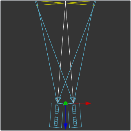
Controls
The options in this tab are used to set the camera’s clipping, field of view, focal length and
stereoscopic properties.

14
3D Tools Chapter – 1
Projection Type
Use the Projection Type button to choose between Perspective and Orthographic
cameras. Generally, real world cameras are perspective cameras. An orthographic
camera uses parallel orthographic projection, a technique where the view plane is
perpendicular to the viewing direction. This produces a parallel camera output that is
undistorted by perspective.
Orthographic cameras only present controls for the near and far clipping planes, and a
control to set the viewing volume.
Near/Far Clip
The clipping plane is used to limit what geometry in a scene is rendered based on the
object’s distance from the camera’s focal point. This is useful for ensuring that objects
which are extremely close to the camera are not rendered and for optimizing a render
to exclude objects that are too far away to be useful in the final rendering.
The default perspective camera ignores this setting unless the the Adaptively Adjust
Near/Far Clip checkbox control below is disabled.
The values are expressed in units, so a far clipping plane of 20 means that any object
more than 20 units distant from the camera will be invisible to the camera. A near
clipping plane of 0.1 means that any object closer than 0.1 units will also be invisible.
Adaptively Adjust Near/Far Clip
When selected, the Renderer will automatically adjust the camera’s near/far clipping
plane to match the extents of the scene. This setting overrides the values of the Near
and Far clip range control described above. This option is not available for
orthographic cameras.
Viewing Volume Size
The Viewing Volume Size control only appears when the Projection Type is set to
Orthographic. It determines the size of the box that makes up the camera’s field of view.
The Z distance of an orthographic camera from the objects it sees does not affect the
scale of those objects, only the viewing size does.
Angle of View Type
Use the Angle of View Type button array to choose how the camera’s angle of view is
measured. Some applications use vertical measurements, some use horizontal and
others use diagonal measurements. Changing the Angle of View type will cause the
Angle of View control below to recalculate.
NOTE: A smaller range between the near and far clipping planes allows
greater accuracy in all depth calculations. If a scene begins to render strange
artifacts on distant objects, try increasing the distance for the Near Clip plane.
15
3D Tools Chapter – 1
Angle of View
Angle of View defines the area of the scene that can be viewed through the camera.
Generally, the human eye can see much more of a scene than a camera, and various
lenses record different degrees of the total image. A large value produces a
widerangle of view and a smaller value produces a narrower, or more tightly focused,
angle of view.
The angle of view and focal length controls are directly related. Smaller focal lengths
produce a wider angle of view, so changing one control automatically changes the
other to match.
Focal Length
In the real world, a lens’ Focal Length is the distance from the center of the lens to the
film plane. The shorter the focal length, the closer the focal plane is to the back of the
lens. The focal length is measured in millimeters. The angle of view and focal length
controls are directly related. Smaller focal lengths produce a wider angle of view, so
changing one control automatically changes the other to match.
The relationship between focal length and angle of view is angle = 2 * arctan[aperture /
2 / focal_length].
Use the vertical aperture size to get the vertical angle of view and the horizontal
aperture size to get the horizontal angle of view.
Plane of Focus (for Depth of Field)
This value is used by the OpenGL renderer to calculate depth of field. It defines the
distance to a virtual target in front of the camera.
Stereo Method
Allows you to adjust your stereoscopic method to your preferred working model.
Toe in
Both cameras point at a single focal point. Though the result is stereoscopic, the
vertical parallax introduced by this method can cause discomfort by the audience.
16
3D Tools Chapter – 1
Off Axis
Often regarded as the correct way to create stereo pairs, this is the default method in
Fusion. Off Axis introduces no vertical parallax, thus creating less stressful
stereo images.
Parallel
The cameras are shifted Parallel to each other. Since this is a purely parallel shift, there
is no Convergence Distance control. Parallel introduces no vertical parallax, thus
creating less stressful stereo images.
Eye Separation
Defines the distance between both stereo cameras. If the Eye Separation is set to a
value larger than 0, controls for each camera will be shown in the Viewer when this tool
is selected. There is no Convergence Distance control in Parallel mode.
17
3D Tools Chapter – 1
Convergence Distance
This control sets the stereoscopic convergence distance, defined as a point located
along the Z-axis of the camera that determines where both left and right eye
cameras converge.
Film Back
Film Gate
The Film Gate menu shows a list of preset camera types. Selecting one of the options
will automatically set the aperture width and aperture height to match the selected
camera type.
Aperture Width/Height
The Aperture Width and Height sliders control the dimensions of the camera’s aperture,
or the portion of the camera that lets light in on a real world camera. In video and film
cameras, the aperture is the mask opening that defines the area of each frame exposed.
Aperture is generally measured in inches, which are the units used for this control.
Resolution Gate Fit
Determines how the film gate is fit within the resolution gate. This only has an effect
when the aspect of the film gate is not the same aspect as the output image. This
setting corresponds to the Maya Fit Resolution Gate. The modes Overscan, Horizontal,
Vertical and Fill correspond to Inside, Width, Height and Outside.
Inside: The image source will be scaled uniformly until one of its dimensions (X or
Y) fits the inside dimensions of the Mask. Depending on the relative dimensions of
image source and Mask Background, either the image source’s width or height may
be cropped to fit the respective dimension of the Mask.
Width: The image source will be scaled uniformly until its width (X) fits the width
of the Mask. Depending on the relative dimensions of image source and Mask, the
image source’s Y-dimension might not fit the Mask’s Y-dimension, resulting in either
cropping of the image source in Y or the image source not covering the Mask’s
height entirely.
Height: The image source will be scaled uniformly until its height (Y) fits the height
of the Mask. Depending on the relative dimensions of image source and Mask, the
image source’s X-dimension might not fit the Mask’s X-dimension, resulting in either
cropping of the image source in X or the image source not covering the Mask’s
width entirely.
Outside: The image source will be scaled uniformly until one of its dimensions (X or
Y) fits the outside dimensions of the Mask. Depending on the relative dimensions of
image source and Mask, either the image source’s width or height may be cropped or
not fit the respective dimension of the Mask.
Stretch: The image source will be stretched in X and Y to accommodate the full
dimensions of the generated Mask. This might lead to visible distortions of the
image source.
18
3D Tools Chapter – 1
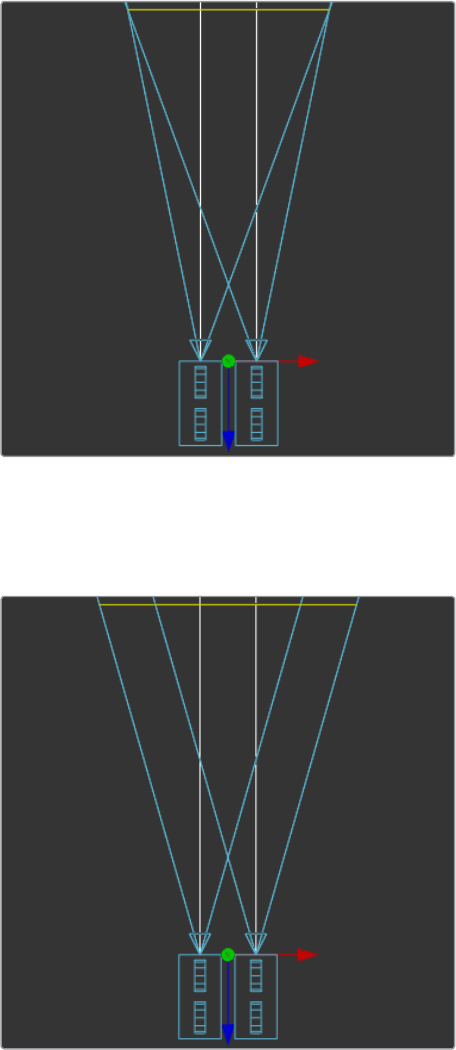
Control Visibility
Allows you to selectively activate the on screen controls that are displayed along with
the camera.
Frustrum: Displays the actual viewing cone of the camera.
View Vector: Displays a white line inside the viewing cone, which can be used to
determine the shift when in Parallel mode.
Near Clip: The Near clipping plane. This plane can be subdivided for better visibility.
Far Clip: The Far clipping plane. This plane can be subdivided for better visibility.
Plane of Focus: The Plane of Focus according to the respective slider explained
above. This plane can be subdivided for better visibility.
Convergence Distance: The point of convergence when using Stereo mode. This
plane can be subdivided for better visibility.
Import Camera
The Import Camera button displays a dialog to import a camera from
anotherapplication.
It supports the following file types:
*LightWave Scene .lws
*Max Scene .ase
*Maya Ascii Scene .ma
*dotXSI .xsi
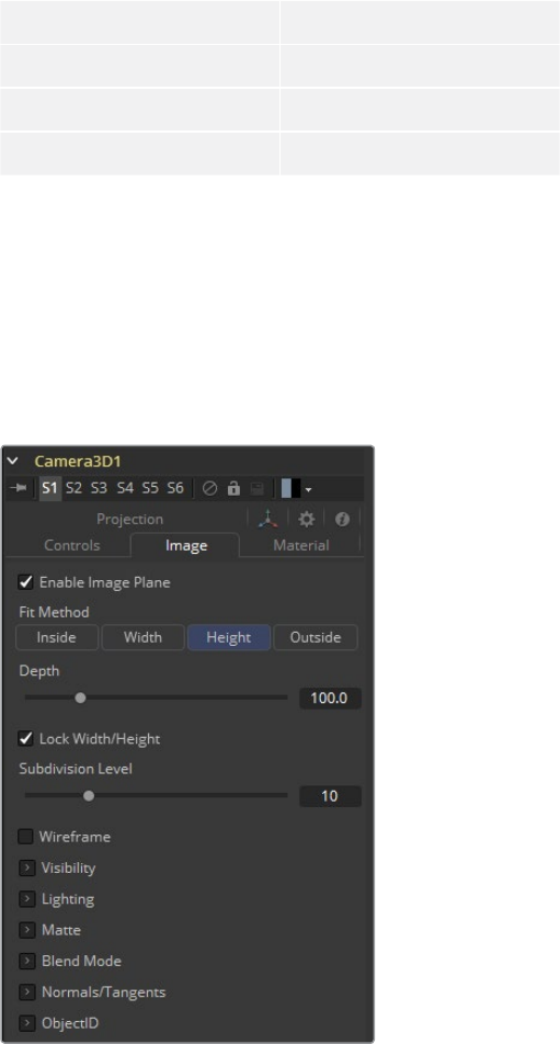
Image
When a 2D image is connected to the camera, an Image Plane is created that is always oriented
so that the image fills the camera’s field of view. The Image Plane tab is hidden until a 2D image
is connected to the Camera 3D’s input on the flow.
With the exception of the controls listed below, the options presented in this tab are identical to
those presented in the Image Plane tools control tab. Consult that tools documentation for a
detailed description.
19
3D Tools Chapter – 1
Enable Image Plane
Use this checkbox to enable or disable the creation of the Image Plane.
Fill Method
Describes how to deal with the input image if the camera has a different aspect ratio.
Inside: The image source will be scaled uniformly until one of its dimensions (X or
Y) fits the inside dimensions of the Mask. Depending on the relative dimensions of
image source and Mask Background, either the image source’s width or height may
be cropped to fit the respective dimension of the Mask.
Width: The image source will be scaled uniformly until its width (X) fits the width
of the Mask. Depending on the relative dimensions of image source and Mask, the
image source’s Y-dimension might not fit the Mask’s Y-dimension, resulting in either
cropping of the image source in Y or the image source not covering the Mask’s
height entirely.
Height: The image source will be scaled uniformly until its height (Y) fits the height
of the Mask. Depending on the relative dimensions of image source and Mask, the
image source’s X-dimension might not fit the Mask’s X-dimension, resulting in either
cropping of the image source in X or the image source not covering the Mask’s
width entirely.
Outside: The image source will be scaled uniformly until one of its dimensions (X or
Y) fits the outside dimensions of the Mask. Depending on the relative dimensions of
image source and Mask, either the image source’s width or height may be cropped or
not fit the respective dimension of the Mask.
Depth: The Depth slider controls the image plane’s distance from the camera.
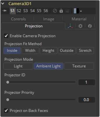
Projection
If a 2D image is connected to the camera it becomes possible to project the image into the
scene. A projection is different from an image plane in that the projection will fall onto the
geometry in the scene exactly as if there was a physical projector present in the scene. The
image is projected as light, which means the Renderer must be set to enable lighting for the
projection to be visible.
See the Projector 3D tool for additional information.
20
3D Tools Chapter – 1
Enable Camera Projection
Select this checkbox to enable projection of the 2D image connected to the
Camera tool.
Projection Fit Method
This button array can be used to select the method used to match the aspect of
projected image to the camera’s Field of View.
Projection Mode
Light: Defines the projection as a spotlight.
Ambient Light: Defines the projection as an ambient light.
Texture: Allows a projection which can be relighted using other lights. Needs a
Catcher tool connected to the appropriate input ports of the specific material.
Tips for Camera 3D
When importing a camera from a 3D application that will also be used as a projector, make sure
that the Fit Resolution Gate options on the main Controls tab as well as the Projection tab are in
sync. Only the first one will automatically be set to what the 3D app was using. The latter might
have to be adjusted manually.
The camera‘s image plane isn‘t just a virtual guide for you in the Viewers. It‘s actual geometry
that you can also project onto. You need to use a Replace Material tool after your Camera node.
To achieve real Parallel Stereo mode you can:
Connect an additional external (right) camera to “Right Stereo Camera“ input of
your camera.
Create separate left and right cameras
Set the ConvergenceDistance slider to a very large value of 999999999.
Rendering with Overscan from Fusion’s 3D Space
If you want to render an image with overscan you also have to modify your scene‘s Camera3D.
Since overscan settings aren‘t exported along with camera data from 3D applications, this is
also necessary for cameras you‘ve imported via .fbx or .ma files. The solution is to increase the
film back‘s width and height by the factor necessary to account for extra pixels on each side.
21
3D Tools Chapter – 1
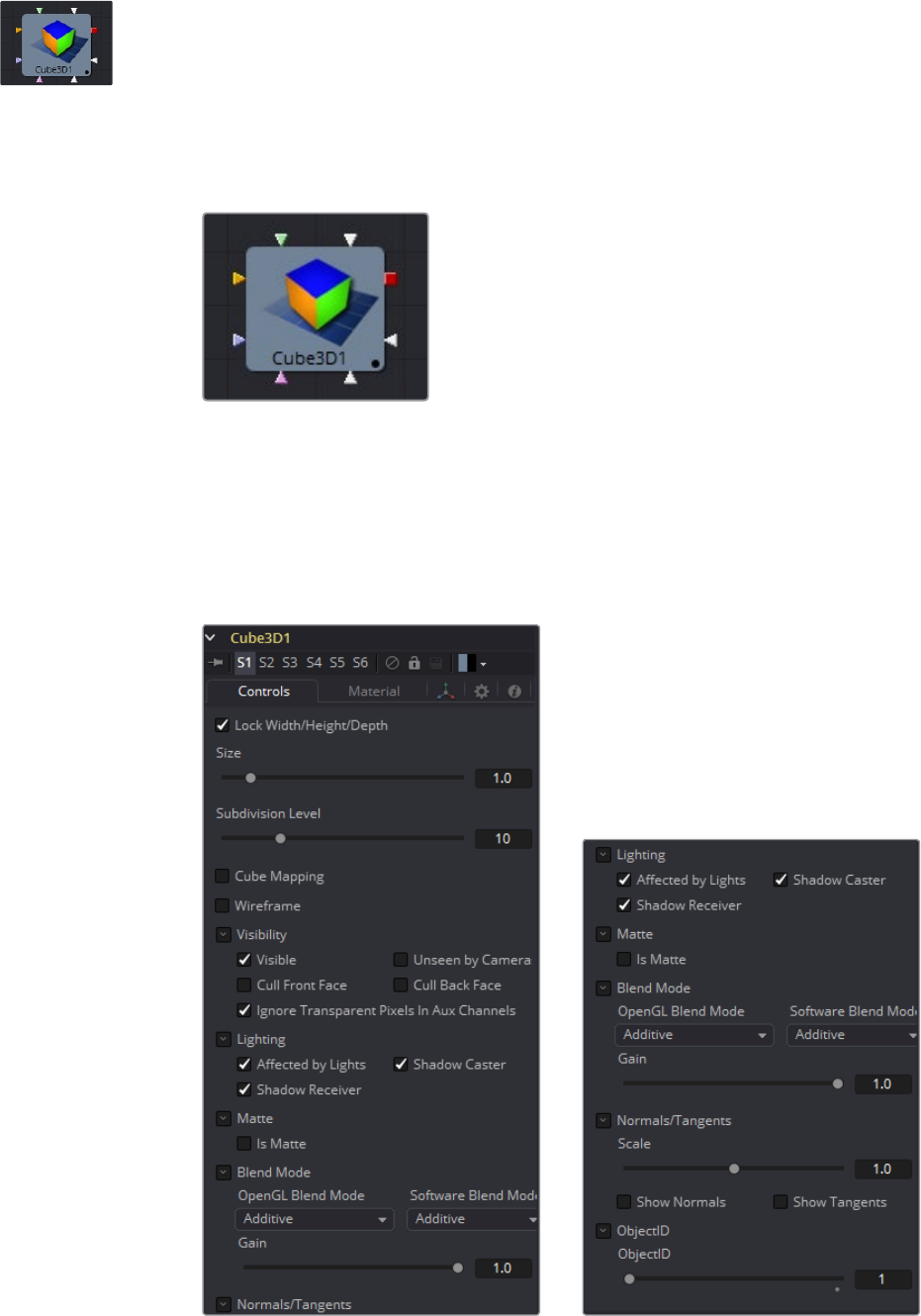
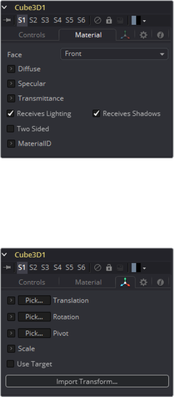
Cube 3D [3CB]
The Cube 3D tool is a basic primitive geometry type capable of generating a simple cube.
Thetool also provides six additional image inputs that can be used to map a texture onto the
six faces of the cube. Cubes are often used as shadow casting objects and for environment
maps. For other basic primitives, see the Shape 3D tool.
External Inputs
Cube3D.SceneInput
[orange, optional] This input expects a scene from a 3D tool output.
Cube3D.NameMaterialInput
These 6 inputs are used to define the materials applied to the six faces of the cube.
They will accept either a 2D image or a 3D material as valid.
Controls
22
3D Tools Chapter – 1
Lock Width/Height/Depth
This checkbox locks the Width, Height and Depth dimensions of the cube together, so
that they are always the same size. When selected, only a Size control is displayed,
otherwise separate Width, Height and Depth sliders are shown.
Size or Width/Height/Depth
If the Lock checkbox is selected then only the Size is shown, otherwise separate sliders
are displayed for Width, Height and Depth. The Size and Width sliders are the same
control renamed, so any animation applied to Size will also be applied to Width when
the controls are unlocked.
Subdivision Level
Use the Subdivision Level slider to set the number of subdivisions used when creating
the image plane.
If the Open GL viewer and renderer are set to Vertex lighting, the more subdivisions in
the mesh, the more vertices will be available to represent the lighting. For this reason,
high subdivisions can be useful when working interactively with lights.
Cube Mapping
Enabling the Cube Mapping checkbox causes the cube to wrap its first texture across
all six faces using a standard cubic mapping technique. This approach expects a
texture laid out in the shape of a cross.
Wireframe
Enabling this checkbox will cause the Mesh to render only the Wireframe for the object
when rendering with the OpenGL renderer.
Visibility
Visible: If the Visibility checkbox is not selected, the object will not be visible in the
Viewers, nor will it be rendered into the output image by the Renderer 3D tool. A
non-visible object does not cast shadows.
Unseen by Cameras: If the unseen by cameras checkbox is selected, the object will
be visible in the Viewers (unless the Visible checkbox is turned off), except when
viewed through a camera. The object will not be rendered into the output image by
the Renderer 3D tool. Shadows cast by an unseen object will still be visible when
rendered by the Software renderer, though not by the OpenGL renderer.
Cull Front Face/Back Face: Use these options to cull (eliminate) rendering and
display of certain polygons in the geometry. If Cull Back Face is selected, all polygons
facing away from the camera not be rendered, and will not cast shadows. If Cull Front
Face is selected, all polygons facing toward the camera will likewise be dropped.
Selecting both checkboxes has the same effect as deselecting the Visible checkbox.
Ignore Transparent Pixels in Aux Channels: In previous versions of Fusion,
transparent pixels were rejected by the Software/GL renderers. To be more specific,
the Software renderer rejected pixels with R=G=B=A=0 and the GL renderer rejected
pixels with A=0. This is now optional. The reason you might want to do this is to get
aux channels (e.g., Normals, Z, UVs) for the transparent areas. For example, suppose
in post you want to replace the texture on a 3D element that is transparent in certain
areas with a texture that is transparent in different areas, then it would be useful to
have transparent areas set aux channels (in particular UVs). As another example,
suppose you are doing post DoF. You will probably not want the Z channel to be set
on transparent areas, as this will give you a false depth. Also, keep in mind that this
rejection is based on the final pixel color including lighting, if it is on. So if you have a
specular highlight on a clear glass material, this checkbox will not affect it.
23
3D Tools Chapter – 1
Lighting
Affected by Lights: If this checkbox is not selected, lights in the scene will not
affect the object, it will not receive nor cast shadows, and it will be shown at the full
brightness of its color, texture or material.
Shadow Caster: If this checkbox is not enabled, the object will not cast shadows on
other objects in the scene.
Shadow Receiver: If this checkbox is not enabled, the object will not receive
shadows cast by other objects in the scene.
Matte
Enabling the Is Matte option will apply a special texture to this object, causing this
object to not only become invisible to the camera, but also making everything that
appears directly behind the camera invisible as well. This option will override all
textures. See the Matte Objects section of the 3D chapter for more information.
Is Matte: When activated, objects whose pixels fall behind the matte object’s pixels
in Z do not get rendered.
Opaque Alpha: Sets the alpha value of the matte object to 1. This checkbox is only
visible when the Is Matte option is enabled.
Infinite Z: Sets the value in the Z channel to infinite. This checkbox is only visible
when the Is Matte option is enabled.
Blend Mode
A Blend mode specifies which method will be used by the Renderer when combining
this object with the rest of the scene. The Blend modes are essentially identical to
those listed in the section for the 2D Merge tool. For a detailed explanation of each
mode, see the section for that tool.
The blending modes were originally designed for use with 2D images. Using them in a
lit 3D environment can produce undesirable results. For best results, use the Apply
modes in unlit 3D scenes rendered in software.
OpenGL Blend Mode: Use this menu to select the blending mode that will be used
when the geometry is processed by the OpenGL renderer. This is also the mode
used when viewing the object in the Viewers. Currently the OpenGL renderer
supports three blending modes.
Software Blend Mode: Use this menu to select the blending mode that will be used
when the geometry is processed by the Software renderer. Currently, the Software
renderer supports all of the modes described in the Merge tool documentation,
except for the Dissolve mode.
24
3D Tools Chapter – 1
Material Tab
The options which appear in this tab determine the appearance of the geometry created by this
tool. Since these controls are identical on all tools that generate geometry, these controls are
fully described in the Common 3D Controls section of this documentation.
If an external 3D material is connected to the tool tile’s material input, then the controls in this
tab will be replaced with the “Using External Material“ label.
Transform Tab
The options which appear in this tab determine the position of the geometry created by this
tool. Since these controls are identical on all tools that generate geometry, these controls are
fully described in the Common 3D Controls section of this documentation.
25
3D Tools Chapter – 1
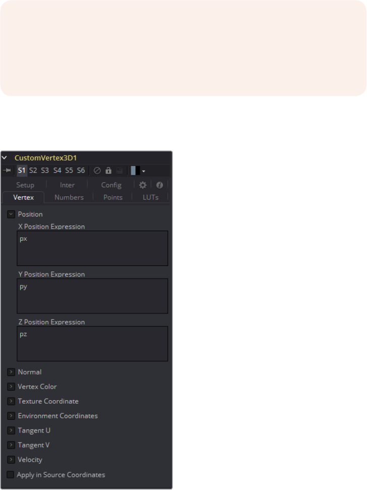
Custom Vertex 3D [3CV]
This is a custom tool for 3D geometry that can be used to do per vertex manipulations, for
example on an image plane like: (px, py, sin(10*(px^2 + py^2 ) + n1)). Other vertex attributes like
normals, vertex color, texture coordinates, tangents, and velocity can be modified as well.
No geometry has envcoord currently. Only particles have velocities. If a stream is not present
on the input geometry it is assumed to have a default value.
These default values are:
Tangentu (tux, tuy, tuz) (1,0,0)
Tangentv (tvx, tvy, tvz) (0,1,0)
Normals (nx, ny, nz) (0,0,1)
Vertexcolor (vcr, vcg, vcb, vca) (1,1,1,1)
Velocity (vx, vy, vz) (0,0,0)
Envcoord (eu, ev, ew) (0,0,0)
Texcoord (tu, tv, tw) (0,0,0)
NOTE: Modifying the X, Y and Z positions of a 3D object does not modify
thenormals/tangents. You can use a ReplaceNormals tool afterwards to
recompute thenormals/tangents.
TIP: Not all geometry has all vertex attributes. For example, most Fusion
geometry does not have vertex colors, with the exception of particles and
some imported FBX/Alembic meshes.
26
3D Tools Chapter – 1
Controls
NOTE: Missing streams on the input geometry are created if the expression
for a stream is non-trivial. The values for the streams will be as given in the
above point. Forexample, if the input geometry does not have normals, then
the values of (nx, ny, nz) will always be (0,0,1). To change this, you could use a
ReplaceNormals tool beforehand to generate them.
27
3D Tools Chapter – 1
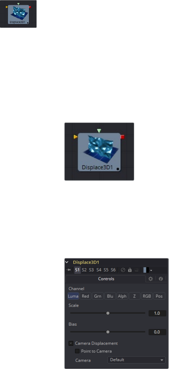
Displace 3D [3DI]
The Displace 3D tool is used to displace the vertices of an object along their normals based
upon a reference image. The texture coordinates on the geometry are used to determine where
to sample the image.
When using Displace 3D, keep in mind that it will only displace existing vertices and will not
tessellate objects. To obtain a more detailed displacement, increase the subdivision amount for
the geometry that is being displaced. Note that the pixels in the displacement image may
contain negative values.
Passing a particle system through a Displace 3D tool will disable the Always Face Camera
option set in the pEmitter. Particles are not treated as point-like objects; each of the four particle
vertices are individually displaced, which may or may not be the preferred outcome.
External Inputs
Displace3D.SceneInput
[orange, required] This input expects to receive a 3D scene.
Displace3D.Input
[green, optional] This input expects a 2D image to be used as the displacement map.
Ifno image is provided this tool will effectively pass the scene straight through to
its output.
Controls
28
3D Tools Chapter – 1
Channel
Determines which channel of the image is connected to Displace3D. Input is used to
displace the geometry.
Scale and Bias
Use these sliders to scale (magnify) and bias (offset) the displacement. The bias is
applied first and the scale afterwards.
Camera Displacement
Point to Camera
When the Point to Camera checkbox is enabled, each vertex is displaced towards the
camera rather than along its normal. One possible use of this option is for displacing a
camera’s image plane. The displaced camera image plane would appear unchanged
when viewed through the camera, but is deformed in 3D space allowing one to comp in
other 3D layers that correctly interact in Z.
Camera
This drop down box is used to select which camera Viewer in the scene is used to
determine the camera displacement when the Point to Camera option is selected.
29
3D Tools Chapter – 1
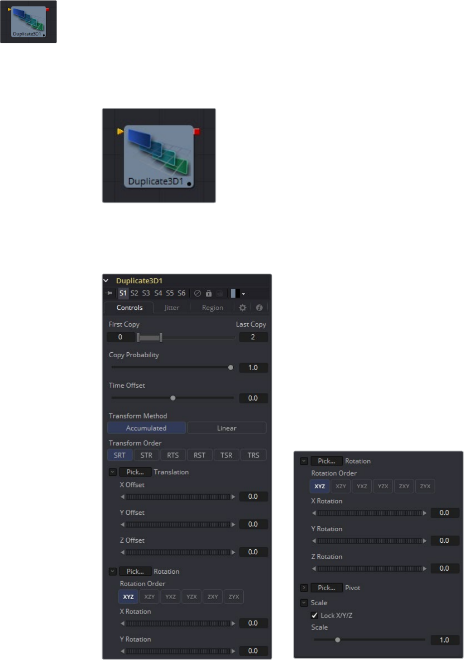
Duplicate 3D [3DP]
The Duplicate 3D tool can be used to quickly duplicate any geometry in a scene, applying a
successive transformation to each, and creating repeating patterns and complex arrays of
objects. The options in the Jitter tab allow for non-uniform transformations, such as random
positioning or sizes.
External Inputs
Duplicate3D.SceneInput
[orange, required] This input expects a 3D scene.
Controls
30
3D Tools Chapter – 1
First/Last Copy
Use this range control to set how many copies of the geometry to make. Each copy is a
copy of the last copy so, if this control is set to [0,3], the parent is copied, then the copy
is copied, then the copy of the copy is copied, and so on. This allows for some
interesting effects when transformations are applied to each copy using the
controls below.
Using a value for both the First Copy and the Last Copy will show only the original
input. Setting the First Copy to a value greater than 0 will exclude the original input and
show only the copies.
Time Offset
Use the Time Offset slider to offset any animations that are applied to the source
geometry by a set amount per copy. For example, set the value to -1.0 and use a cube
set to rotate on the Y-axis as the source. The first copy will show the animation from a
frame earlier. The second copy will show animation from a frame before that, and so
forth. This can be used with great effect on textured planes, for example, where
successive frames of a clip can be shown.
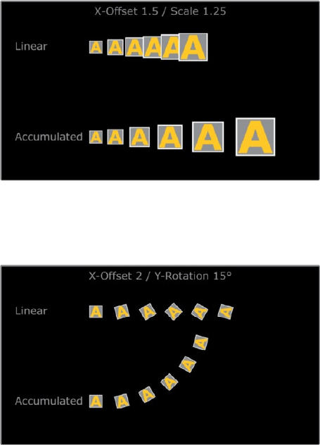
Transform Method
Accumulated
When set to Accumulated, each object copy starts at the position of the previous object
and is transformed from there. The result is transformed again for the next copy.
Linear
When set to Linear, transforms are multiplied by the number of the copy, and the total
scale, rotation and translation are applied in turn, independent of the other copies.
Transform Order
With these buttons, the order in which the transforms are calculated can be set. It
defaults to Scale-Rotation-Transform (SRT).
Using different orders will result in different positions of your final objects.
31
3D Tools Chapter – 1
XYZ Offset
These three sliders tell the tool how much offset to apply to each copy. An X offset of 1
would offset each copy 1 unit along the X-axis from the last copy.
Rotation Order
These buttons can be used to set the order in which rotations are applied to the
geometry. Setting the rotation order to XYZ would apply the rotation on the X-axis first,
followed by the y-axis rotation, then the Z-axis rotation.
XYZ Rotation
These three Rotation sliders tell the tool how much rotation to apply to each copy.
XYZ Pivot
The pivot controls determine the position of the pivot point used when rotating
each copy.
Lock XYZ
When the Lock XYZ checkbox is selected any adjustment to the duplicate scale will be
applied to all three axes simultaneously. If this checkbox is disabled the scale slider will
be replaced with individual sliders for the X, Y and Z scale.
Scale
The scale controls tell Duplicate how much scaling to apply to each copy.
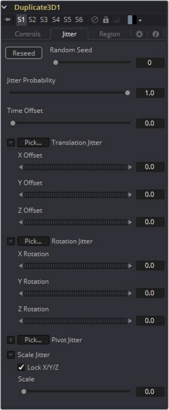
Jitter
32
3D Tools Chapter – 1
Random Seed/Randomize
The Random Seed is used to ‘seed’ the amount of jitter applied to the duplicated
objects. Two Duplicate tools with identical settings but different random seeds will
produce two completely different results. Click on the Randomize button to assign a
random seed value.
Time Offset
Use the Time Offset slider to offset any animations that are applied to the source
geometry by a set amount per copy. For example, set the value to -1.0 and use a cube
set to rotate on the Y-axis as the source. The first copy will show the animation from a
frame earlier. The second copy will show animation from a frame before that, and so
forth. This can be used with great effect on textured planes, for example, where
successive frames of a clip can be shown.
Translation XYZ Jitter
Use these three controls to adjust the amount of variation in the Translation of the
duplicated objects.
Rotation XYZ Jitter
Use these three controls to adjust the amount of variation in the Rotation of the
duplicated objects.
Pivot XYZ Jitter
Use these three controls to adjust the amount of variation in the Rotational Pivot Center
of the duplicated objects. This affects only the additional jitter rotation, not the rotation
produced by the Rotation settings in the Controls tab.
Scale XYZ Jitter
Use this control to adjust the amount of variation in the scale of the duplicated objects.
Uncheck the Lock XYZ checkbox to adjust the scale variation independently on all
three axes.
33
3D Tools Chapter – 1
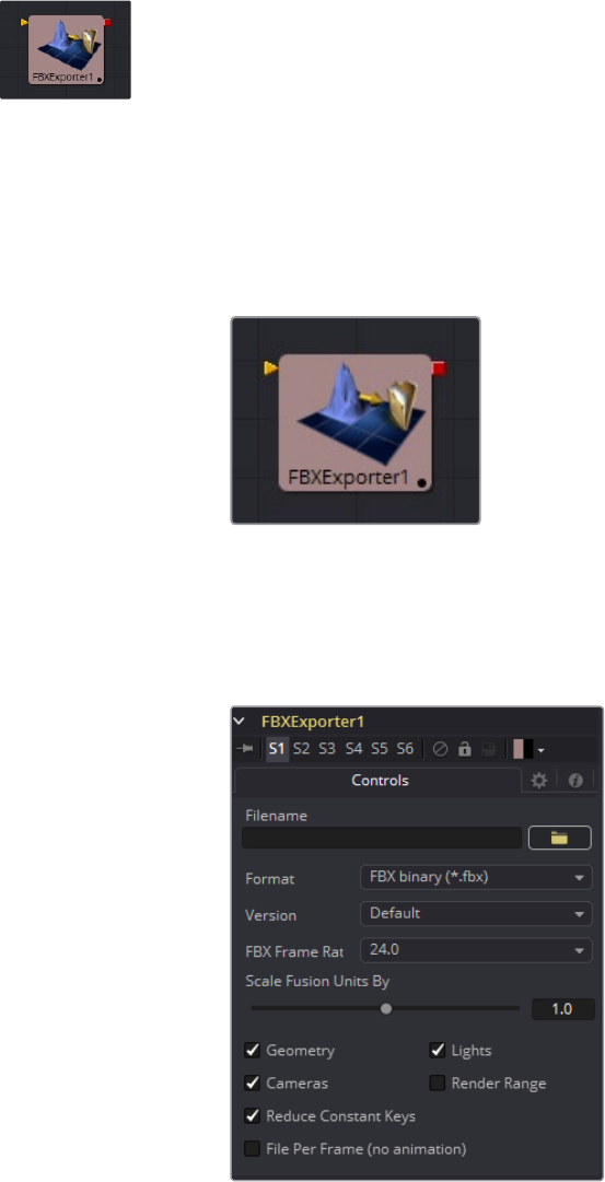
FBX Exporter 3D [FBX]
The FBX Exporter provides a method of exporting a Fusion 3D scene to the FBX scene
interchange format. Each node in Fusion is a single object in the exported file. Objects, lights
and cameras will use the name of the node that created them. The tool can be set to export a
single file for the entire scene, or to output one frame per file.
In addition to the FBX format, this tool can also export to the 3D Studio’s .3ds, Collada’s .dae,
Autocad’s .dxf and the Alias .obj formats.
External Inputs
FBXExporter.Input
[orange, required] This input expects a 3D scene.
Controls
Filename
This file browser control can be used to set the file which will be output by the tool.
Click on the yellow folder icon to open a file browser dialog.

34
3D Tools Chapter – 1
Format
This control is used to set the Format of the output file. It is possible to export the
following file formats:
FBX ascii (*.fbx)
FBX 5.0 binary (*.fbx)
Autocad DXF (*.dxf )
3D Studio 3Ds (*.3ds)
Alias OBJ (*.obj)
Collada DAE (*.dae)
Not all of the formats support all of the features of this tool. For example,
the obj formatdoes not handle animation.
Version
The Version drop down menu shows the available versions for the Format selected by
the control above. The menu’s contents will change dynamically to reflect the available
versions for that format. If the selected format only provides a single option, this menu
will be hidden.
Choosing Default for the FBX formats uses FBX200611.
Geometry/Lights/Cameras
These three checkbox controls determine whether the tool will attempt to export the
named scene element. For example, deselecting Geometry and Lights but leaving
Cameras selected would output only the cameras currently in the scene.
Reduce Constant Keys
Enabling this option will automatically remove keyframes if the adjacent keyframes
have the same value.
File Per Frame (No Animation)
Enabling this option will force the tool to export one file per frame, resulting in a
sequence of numbered files. This will disable the export of animation.
Set Sequence Start
Normally, Fusion will use the render range of a composition to determine the numeric
sequence used when rendering a file sequence to disk. Enable this checkbox to reveal
the Sequence Start Frame control to set the number of the first frame in the sequence
to a custom value.
Sequence Start Frame
This thumbwheel control can be used to set an explicit start frame for the number
sequence applied to the rendered filenames. For example, if Global Start is set to 1 and
frames 1 - 30 are rendered, files will normally be numbered 0001 - 0030. If the
Sequence Start Frame is set to 100, the rendered output would be numbered
from 100-131.
35
3D Tools Chapter – 1
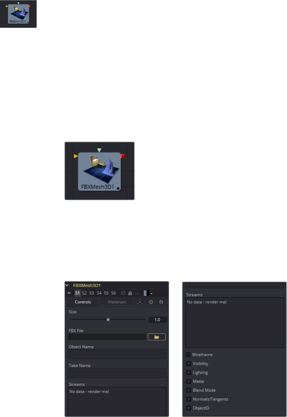
FBX Mesh 3D [FBX]
The FBXMesh3D tool is used to import polygonal geometry from scene files that are saved
using the FilmBox (FBX) format. It is also able to import geometry from OBJ, 3DS, DAE and
DXFscene files. This provides a method for working with more complex geometry than is
available using Fusion‘s built-in primitives.
When importing geometry with this tool, all of the geometry contained in the FBX file will be
combined into one mesh with a single pivot and transformation. The FBXMesh tool will ignore
any animation applied to the geometry.
The File > Import > FBX utility can be used to import an FBX and create individual tools for each
camera, light and mesh contained in the file. This utility can also be used to preserve the
animation of the objects.
If the Global > General > Auto Clip Browse option is enabled (default) then adding this tool to a
composition from the toolbars or menus will automatically display a file browser.
External Inputs
FBXMesh3D.SceneInput
[orange, required] This input expects a 3D scene as its input.
FBXMesh.MaterialInput
[green, optional] This input will accept either a 2D image or a 3D material. If a 2D image
is provided, it will be used as a diffuse texture map for the basic material built into the
tool. Ifa 3D material is connected, then the basic material will be disabled.
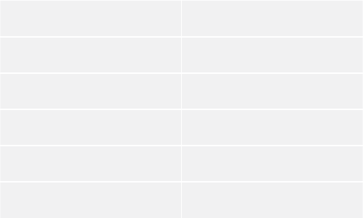
Controls
36
3D Tools Chapter – 1
Size
The size slider controls the size of the FBX geometry that is imported. FBX meshes
have a tendency to be much larger than Fusion’s default unit scale, so this control is
useful for scaling the imported geometry to match the Fusion environment.
FBX File
This control shows the filename of the currently loaded FBX. Click on the icon of the
yellow folder to open a file browser that can be used to locate an FBX file. Despite the
tool’s name, this tool is also able to load a variety of other formats.
FBX ascii (*.fbx)
FBX 5.0 binary (*.fbx)
Autocad DXF (*.dxf )
3D Studio 3Ds (*.3ds)
Alias OBJ (*.obj)
Collada DAE (*.dae)
Object Name
This input shows the name of the mesh from the FBX file that is being imported. If this
field is blank, then the entire contents of the FBX geometry will be imported as a single
mesh. This input is not editable by the user; it is set by Fusion when importing FBX files
via the File > Import > FBX utility.
Take Name
This input shows the name of the animation take to use from the FBX file. If this field is
blank, then no animations will be imported. This input is not editable by the user; it is
set by fusion when importing FBX files via the File > Import > FBX utility.
Wireframe
Enabling this checkbox will cause the mesh to render only the Wireframe for the object.
Currently, only the OpenGL renderer supports wireframe rendering.
Visibility
Visible: If the visibility checkbox is not selected, the object will not be visible in the
Viewers, nor will it be rendered into the output image by the Renderer 3D tool. A
non-visible object does not cast shadows.
Unseen by Cameras: If the Unseen by Cameras checkbox is selected, the object
will be visible in the Viewers (unless the Visible checkbox is turned off), except when
viewed through a camera. The object will not be rendered into the output image by
the Renderer 3D tool. Shadows cast by an Unseen object will still be visible when
rendered by the Software renderer, though not by the OpenGL renderer.
Cull Front Face/Back Face: Use these options to cull (eliminate) rendering and
display of certain polygons in the geometry. If Cull Back Face is selected, all polygons
facing away from the camera not be rendered, and will not cast shadows. If Cull Front
Face is selected, all polygons facing toward the camera will likewise be dropped.
Selecting both checkboxes has the same effect as deselecting the Visible checkbox.
37
3D Tools Chapter – 1
Ignore Transparent Pixels in Aux Channels: In previous versions of Fusion,
transparent pixels were rejected by the Software/GL renderers. To be more specific
the Software renderer rejected pixels with R=G=B=A=0 and the GL renderer rejected
pixels with A=0. This is now optional. The reason you might want to do this is to get
aux channels (e.g., Normals, Z, UVs) for the transparent areas. For example, suppose
in post you want to replace the texture on a 3D element that is transparent in certain
areas with a texture that is transparent in different areas, then it would be useful to
have transparent areas set aux channels (in particular UVs). As another example,
suppose you are doing post DoF. You will probably not want the Z channel to be set
on transparent areas, as this will give you a false depth. Also keep in mind that this
rejection is based on the final pixel color including lighting, if it is on. So if you have a
specular highlight on a clear glass material, this checkbox will not affect it.
Lighting
Affected by Lights: If this checkbox is not selected, lights in the scene will not
affect the object, it will not receive nor cast shadows, and it will be shown at the full
brightness of its color, texture or material.
Shadow Caster: If this checkbox is not enabled, the object will not cast shadows on
other objects in the scene.
Shadow Receiver: If this checkbox is not enabled, the object will not receive
shadows cast by other objects in the scene.
Matte
Enabling the Is Matte option will apply a special texture to this object, causing this object to not
only become invisible to the camera, but also making everything that appears directly behind
the camera invisible as well. This option will override all textures. See the Matte Objects section
of the 3D chapter for more information.
Is Matte: When activated, objects whose pixels fall behind the matte object’s pixels
in Z do not get rendered.
Opaque Alpha: Sets the alpha value of the matte object to 1. This checkbox is only
visible when the Is Matte option is enabled.
Infinite Z: Sets the value in the Z channel to infinite. This checkbox is only visible
when the Is Matte option is enabled.
Blend Mode
A Blend mode specifies which method will be used by the Renderer when combining this
object with the rest of the scene. The blend modes are essentially identical to those listed in
the section for the 2D Merge tool. For a detailed explanation of each mode see the section for
that tool.
The blending modes were originally designed for use with 2D images. Using them in a lit 3D
environment can produce undesirable results. For best results use the Apply modes in unlit 3D
scenes rendered in software.
OpenGL Blend Mode: Use this menu to select the blending mode that will be
used when the geometry is processed by the OpenGL renderer. This is also the
mode used when viewing the object in the Viewer. Currently the OpenGL renderer
supports three blending modes.
Software Blend Mode: Use this menu to select the blending mode that will be used
when the geometry is processed by the Software renderer. Currently the Software
renderer supports all of the modes described in the Merge tool documentation,
except for the Dissolve mode.
38
3D Tools Chapter – 1
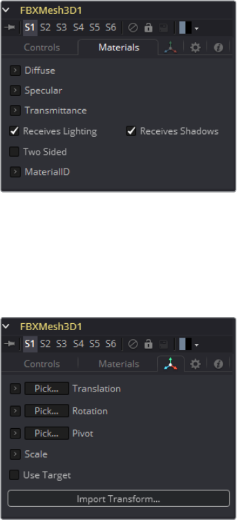
Material Tab
The options that appear in this tab determine the appearance of the geometry created by this
tool. Since these controls are identical on all tools that generate geometry, these controls are
fully described in the Common 3D Controls section of this documentation.
If an external 3D material is connected to the tool tile’s material input, then the controls in this
tab would be replaced with the Using External Material label.
Transform Tab
The options that appear in this tab determine the position of the geometry created by this tool.
Since these controls are identical on all tools that generate geometry, these controls are fully
described in the Common 3D Controls section of this documentation.
39
3D Tools Chapter – 1
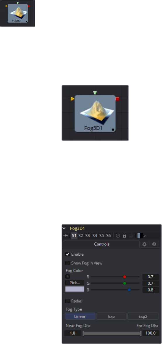
Fog 3D [3FO]
The Fog 3D tool applies depth cue based Fog to the scene. It is the 3D version of the Fog tool
in the Deep Pixel category. It is designed to work completely in 3D space and takes full
advantage of antialiasing and depth of field effects during rendering.
The Fog 3D tool essentially re-textures the geometry in the scene by applying a color
correction based on the object’s distance from the camera. An optional density texture image
can be used to apply variation to the correction.
External Inputs
Fog3D.SceneInput
[orange, required] This input expects a 3D scene.
Fog3D.DensityTexture
[green, optional] This input expects a 2D image. The color of the fog created by this
tool is multiplied by the pixels in the image. When creating the image for the density
texture, keep in mind that the texture is effectively projected onto the scene from
the camera.
Controls
40
3D Tools Chapter – 1
Enable
Use this checkbox to enable or disable the tool.
Show Fog in View
By default, the fog created by this tool is only visible when the scene is viewed using a
Camera tool. When this checkbox is enabled, the fog becomes visible in the scene
from all points of view.
Color
This control can be used to set the color of the fog. The color is also multiplied by the
densitytexture image, if one has been provided.
Radial
By default, the fog is done based upon the perpendicular distance to a plane (parallel
with the near plane) passing through the eye point. When the Radial option is checked,
the radial distance to the eye point is used instead of the perpendicular distance. The
problem with perpendicular distance fog is that when you move the camera about, as
objects on the left or right side of the frustum move into the center, they become less
fogged even though they remain the same distance from the eye. Radial fog fixes this.
Sometimes Radial fog is not desirable. For example, if you are fogging an object that is
close to the camera, like an image plane, the center of the image plane could be
unfogged while the edges could be fully fogged.
Fog type
This control is used to determine the type of falloff applied to the fog.
Linear: Defines a linear falloff for the fog.
Exp: Creates an exponential nonlinear falloff.
Exp2: Creates an stronger exponential falloff.
Near/Far Fog Distance
This control expresses the Range of the fog in the scene as units of distance from the
camera. The Near Distance determines where the fog starts, while the Far Distance
sets the point where the fog has its maximum effect. Fog is cumulative, so the further
an object is from the camera, the thicker the fog should appear.
41
3D Tools Chapter – 1
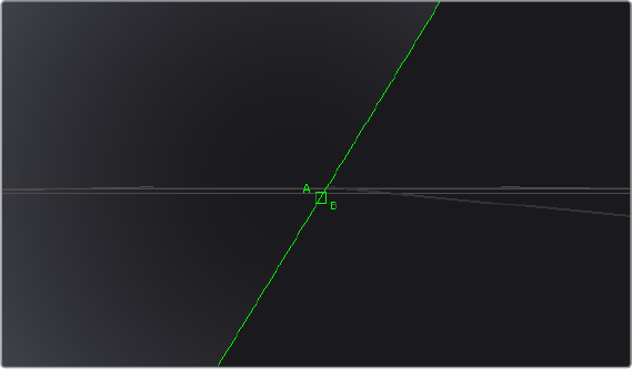
Image Plane 3D [3IM]
The Image Plane tool produces 2D planar geometry in 3D space. The most common use of the
tool is to represent 2Dimages in the 3D space. An image input on the tool’s tile provides the
texture for the rectangle from another source in the composition. The aspect of the Image Plane
is determined by the aspect of the image used for its diffuse texture. If planar geometry whose
dimensions are not relative to the texture image is required, then use a Shape 3D tool instead.
External Inputs
Imageplane3D.SceneInput
[orange, optional] This input expects a 3D scene. As this tool creates geometry, it is
not required.
Imageplane3D.MaterialInput
[green, optional] This input will accept either a 2D image or a 3D material. If a 2D image
is provided, it will be used as a diffuse texture map for the basic material built into the
tool. If a 3D material is connected, then the basic material will be disabled.
42
3D Tools Chapter – 1
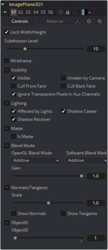
Controls
Lock Width/Height
When checked, the subdivision of the plane will be applied evenly in X and Y. When
unchecked, there are two sliders for individual control of the subdivisions in X and Y.
Defaults to on.
Subdivision Level
Use the Subdivision Level slider to set the number of subdivisions used when creating
the image plane. If the Open GL viewer and renderer are set to Vertex lighting, the
more subdivisions in the mesh, the more vertices will be available to represent the
lighting. For this reason, high subdivisions can be useful when working interactively
with lights.
Wireframe
Enabling this checkbox will cause the Mesh to render only the wireframe for the object
when using the OpenGL renderer.
43
3D Tools Chapter – 1
Visibility
Visible: If the Visibility checkbox is not selected, the object will not be visible in the
Viewer, nor will it be rendered into the output image by the Renderer 3D tool. A non-
visible object does not cast shadows.
Unseen by Cameras: If the Unseen by Cameras checkbox is selected, the object
will be visible in the Viewers (unless the Visible checkbox is turned off), except when
viewed through a camera. The object will not be rendered into the output image by
the Renderer 3D tool. Shadows cast by an Unseen object will still be visible when
rendered by the Software renderer, though not by the OpenGL renderer.
Cull Front Face/Back Face: Use these options to cull (eliminate) rendering and
display of certain polygons in the geometry. If Cull Back Face is selected, all polygons
facing away from the camera not be rendered, and will not cast shadows. If Cull Front
Face is selected, all polygons facing toward the camera will likewise be dropped.
Selecting both checkboxes has the same effect as deselecting the Visible checkbox.
Ignore Transparent Pixels in Aux Channels: In previous versions of Fusion,
transparent pixels were rejected by the Software/GL renderers. To be more specific,
the Software renderer rejected pixels with R=G=B=A=0 and the GL renderer rejected
pixels with A=0. This is now optional. The reason you might want to do this is to get
aux channels (e.g., Normals, Z, UVs) for the transparent areas. For example, suppose
in post you want to replace the texture on a 3D element that is transparent in certain
areas with a texture that is transparent in different areas. then it would be useful to
have transparent areas set aux channels (in particular UVs). As another example
suppose you are doing post DoF. You will probably not want the Z channel to be set
on transparent areas, as this will give you a false depth. Also keep in mind that this
rejection is based on the final pixel color including lighting, if it is on. So if you have a
specular highlight on a clear glass material, this checkbox will not affect it.
Lighting
Affected by Lights: If this checkbox is not selected, lights in the scene will not
affect the object, it will not receive nor cast shadows, and it will be shown at the full
brightness of its color, texture or material.
Shadow Caster: If this checkbox is not enabled, the object will not cast shadows on
other objects in the scene.
Shadow Receiver: If this checkbox is not enabled, the object will not receive
shadows cast by other objects in the scene.
Matte
Enabling the Is Matte option will apply a special texture to this object, causing this object to not
only become invisible to the camera, but also making everything that appears directly behind
the camera invisible as well. This option will override all textures. See the Matte Objects section
of the 3D chapter for more information.
Is Matte: When activated, objects whose pixels fall behind the matte objects pixels in
Z do not get rendered.
Opaque Alpha: Sets the alpha value of the matte object to 1. This checkbox is only
visible when the Is Matte option is enabled.
Infinite Z: Sets the value in the Z channel to infinite. This checkbox is only visible
when the Is Matte option is enabled.
44
3D Tools Chapter – 1
Blend Mode
A Blend mode specifies which method will be used by the Renderer when combining this
object with the rest of the scene. The Blend modes are essentially identical to those listed in
the section for the 2D Merge tool. For a detailed explanation of each mode, see the section for
that tool.
The blending modes were originally designed for use with 2D images. Using them in a lit 3D
environment can produce undesirable results. For best results use the apply modes in unlit 3D
scenes rendered in software.
OpenGL Blend Mode: Use this menu to select the blending mode that will be used
when the geometry is processed by the OpenGL renderer. This is also the mode
used when displaying the object in the Viewers. Currently the OpenGL renderer
supports three blending modes.
Software Blend Mode: Use this menu to select the blending mode that will be used
when the geometry is processed by the Software renderer. Currently the Software
renderer supports all of the modes described in the Merge tool documentation
except for the Dissolve mode.
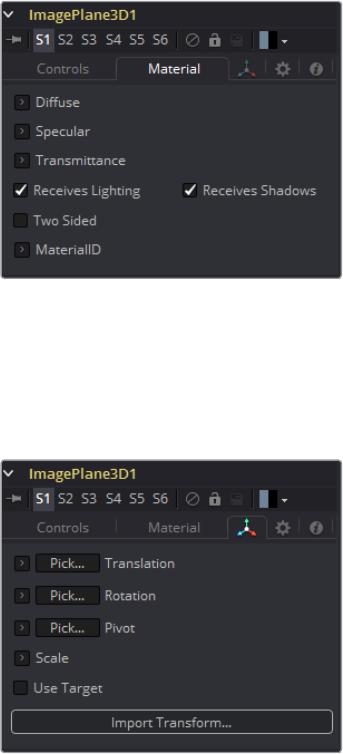
Material Tab
The options that appear in this tab determine the appearance of the geometry created by this
tool. Since these controls are identical on all tools that generate geometry, these controls are
fully described in the Common 3D Controls section of this documentation.
If an external 3D material is connected to the tool tile’s material input, then the controls in this
tab would be replaced with the Using External Material label.
Transform Tab
The options that appear in this tab determine the position of the geometry created by this tool.
Since these controls are identical on all tools that generate geometry, these controls are fully
described in the Common 3D Controls section of this documentation.
45
3D Tools Chapter – 1
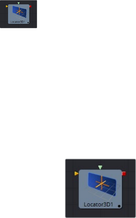
Locator 3D [3LO]
The Locator 3D tool’s purpose is to transform a point in 3D space to 2D coordinates that other
tools can use as part of expressions or modifiers.
When the Locator is provided with a camera and the dimensions of the output image, it will
transform the coordinates of a 3D control into 2D screen space. The 2D position is exposed as
a numeric output which can be connected to/from other tools. For example, to connect the
center of an ellipse to the 2D position of the Locator, right-click on the Mask center control and
select Connect To > Locator 3D > Position.
The scene provided to the Locator’s input must contain the camera through which the
coordinates are projected. As a result, the best practice is to place the Locator after the merge
that introduces the camera to the scene.
If an object is connected to the Locator tool’s second input, the Locator will be positioned at the
object’s center, and the Transformation tab’s Offset XYZ sliders will function in the object’s local
coordinate space rather than global scene space. This is useful for tracking an object’s position
regardless of any additional transformations applied further downstream.
External Inputs
Locator3D.SceneInput
[orange, required] This input expects a 3D scene.
Locator3D.Target
[green, optional] This input expects a 3D scene. When provided, the transform center of
the scene is used to set the position of the Locator. The transformation controls for the
Locator become offsets from this position.
46
3D Tools Chapter – 1
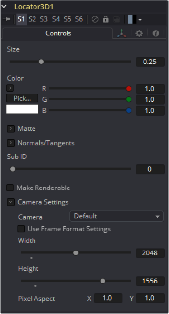
Controls
Size
The size slider is used to set the size of the Locator’s onscreen crosshair.
Color
A basic Color control is used to set the color of the Locator’s onscreen crosshair.
Matte
Enabling the Is Matte option will apply a special texture to this object, causing this object to not
only become invisible to the camera, but also making everything that appears directly behind
the camera invisible as well. This option will override all textures. See the Matte Objects section
of the 3D chapter for more information.
Is Matte: When activated, objects whose pixels fall behind the matte object’s pixels
in Z do not get rendered.
Opaque Alpha: Sets the alpha value of the matte object to 1. This checkbox is only
visible when the Is Matte option is enabled.
Infinite Z: Sets the value in the Z channel to infinite. This checkbox is only visible
when the Is Matte option is enabled.
Sub id: The Sub ID slider can be used to select an individual sub-element of certain
geometry, such as an individual character produced by a Text 3D tool, or a specific
copy created by a Duplicate 3D tool.
47
3D Tools Chapter – 1
Make Renderable: Defines if the Locator is rendered as a visible object by the
OpenGL renderer. The Software renderer is not currently capable of rendering lines,
and hence will ignore this option.
Unseen by Camera: This checkbox control appears when the Make Renderable
option is selected. If the Unseen by Camera checkbox is selected, the Locator
will be visible in the Viewers, but not rendered into the output image by the
Renderer 3D tool.
Controls
Camera
This drop down control is used to select the Camera in the scene that defines the
screen space used for 3D to 2D coordinate transformation.
Use Frame Format Settings
Select this checkbox to override the width, height and pixel aspect controls, and force
them to use the values defined in the composition’s Frame Format preferences instead.
Width, Height and Pixel Aspect
In order for the Locator to generate a correct 2D transformation, it must know the
dimensions and aspect of the image. These controls should be set to the same
dimensions as the image produced by a renderer associated with the camera specified
above. Right-clicking on these controls will display a contextual menu containing the
frame formats configured in the composition’s preferences.
48
3D Tools Chapter – 1
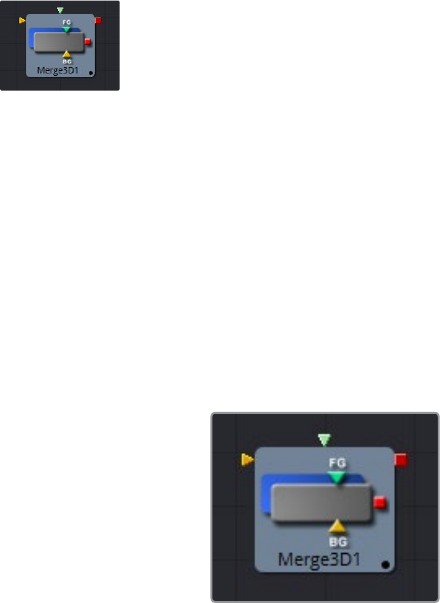
Merge 3D [3MG]
The Merge 3D tool is used to combine separate 3D elements into the same 3D environment.
For example, with a scene that is created with an image plane, a camera and a light, the camera
would not be able to see the image plane and the light would not affect the image plane until all
three objects are introduced into the same environment using the Merge 3D tool.
The tool tile displays only two inputs at first, but as each input is connected a new input will
appear on the tool, assuring there is always one free to add a new element into the scene.
The Merge provides the standard transformation controls found on most tools in Fusion’s
3Dsuite. Unlike those tools, changes made to the translation, rotation or scale of the merge
affect all of the objects connected to the merge. This behavior forms the basis for all parenting
in Fusion’s 3D environment.
External Inputs
Merge3D.SceneInput[#]
[any, see description] These inputs expect a 3D scene. When the tool is constructed it
will display two inputs. There is no limit to the number of inputs this tool can accept.
The tool dynamically adds more inputs as needed, ensuring that there is always at least
one input available for connection.
49
3D Tools Chapter – 1
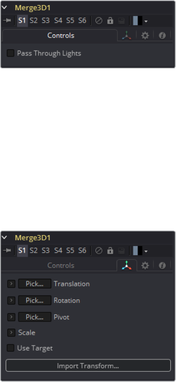
Controls
Pass Through Lights
When the Pass Through Lights checkbox is selected, lights will be passed through the
merge into its output so they can affect downstream elements. Normally, the lights are
not passed downstream to affect the rest of the scene. This is frequently used to
ensure projections are not applied to geometry introduced later in the scene.
Transform Tab
The options that appear in this tab determine the position of the geometry created by this tool.
Since these controls are identical on all tools that generate geometry, these controls are fully
described in the Common 3D Controls section of this documentation.
50
3D Tools Chapter – 1
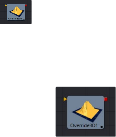
Override 3D [3OV]
The Override tool lets you change object-specific options for every object in a 3D scene
simultaneously. This is useful, for example, when you wish to set every object in the input scene
to render as a wireframe. Additionally, this tool is the only way to set the wireframe, visibility,
lighting, matte and ID options for 3D particle systems and the Text 3D tool.
It is frequently used in conjunction with the Replace Material tool to produce isolated passes.
For example, a scene can be branched out to an Override tool which turns off the Affected by
Lights property of each tool, then connected to a Replace Material tool that applies a Falloff
shader to produce a falloff pass of the scene.
External Inputs
Override3D.SceneInput
[orange, required] This input expects a 3D scene.
51
3D Tools Chapter – 1
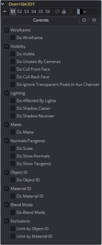
Controls
The philosophy of the controls found in the Override tool is fairly straightforward. First, you
select the option to override using the Do [Option] checkbox. That will reveal a control that can
be used to set the value of the option itself. The individual options are not documented here; a
full description of each can be found in any geometry creation tool, such as the Image Plane,
Cube or Shape tools.
Do [option]
Enables the override for this option.
[Option]
If the Do [option] checkbox is enabled, then the control for the property itself becomes
visible. The control values of the properties for all upstream objects are overridden by
the new value.
52
3D Tools Chapter – 1
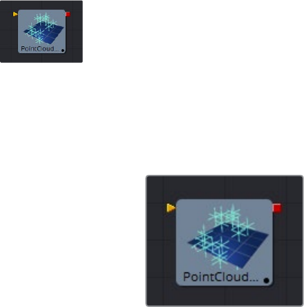
Point Cloud 3D [3PC]
A Point Cloud is generally a large number of nulls created by 3D tracking or modeling software.
When produced by 3D tracking software the points typically represent each of the patterns
tracked to create the 3D camera path. These point clouds can be used to identify a ground
plane and to orient other 3D elements with the tracked image. The Point Cloud 3D tool creates
a point cloud by importing a 3D scene
External Inputs
Pointcloud3DSceneInput
[orange, required] This input expects a 3D scene.
53
3D Tools Chapter – 1
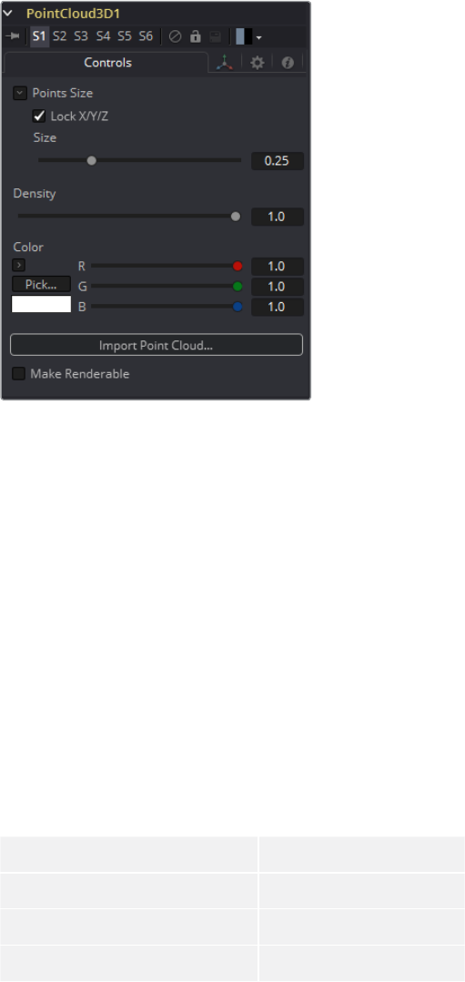
Controls
Lock x/y/Z
Deselect this checkbox to provide individual control over the size of the X, Y and Z
arms of the points in the cloud.
Size x/y/Z
These sliders can be used to increase the size of the onscreen crosshairs used to
represent each point.
Density
This slider defines the probability of displaying a specific point. If the value is 1, then all
points are displayed. A value of 0.2 shows only every fifth point.
Color
Use the standard Color control to set the color of onscreen crosshair controls.
Import Point Cloud
The Import Point Cloud button displays a dialog to import a point cloud from another
application. Supported filetypes are:
* Alias's Maya .ma
* 3DS Max ASCII Scene Export .ase
* NewTek's LightWave .lws
* Softimage XSI's .xsi.
Make Renderable
Determines if the point cloud is visible in the OpenGL viewport, and in final renderings
made by the OpenGL renderer. The Software renderer does not currently support
rendering of visible crosshairs for this tool.
Unseen by Camera
This checkbox control appears when the Make Renderable option is selected. If the
Unseen by Cameras checkbox is selected, the point cloud will be visible in the
Viewers, but not rendered into the output image by the Renderer 3D tool.
54
3D Tools Chapter – 1
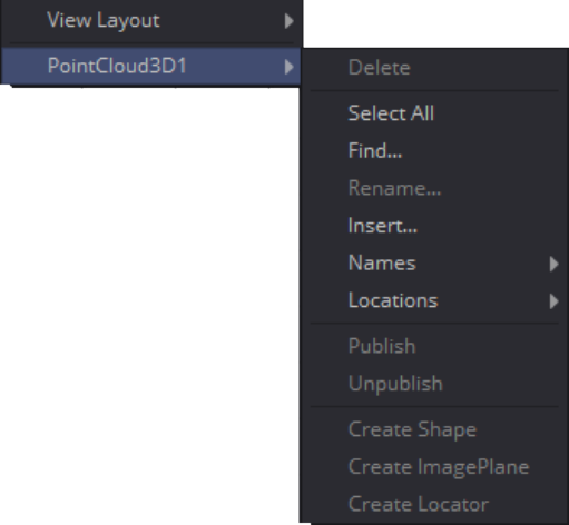
Onscreen Contextual Menu
Frequently, one or more of the points in an imported point cloud will have been
manually assigned in order to track the position of a specific feature. These points
usually have names that distinguish them from the rest of the points in the cloud. To see
the current name for a point, hover the mouse pointer directly over a point, and after a
moment a small popup will appear with the name of the point.
When the Point Cloud 3D tool is selected, a submenu will be added to the display
Viewer’s contextual menu with several options that make it simple to locate, rename
and separate these points from the rest of the point cloud. The contextual menu
contains the following options:
Find
Selecting this option from the display Viewer contextual menu will open a dialog that
can be used to search for and select a point by name. Each point that matches the
pattern will be selected.
Rename
Rename one or more points by selecting Rename from the contextual menu. Type the
new name into the dialog that appears and hit enter. The point will now have that name,
with a four-digit number added to the end. For example, the name window will be
window0000 and multiple points would be window0000, window0001, etc. Names
must be valid Fusion identifiers (i.e., no spaces allowed, and the name cannot start with
a number).
Delete
Selecting this option will delete the currently selected points.
Publish
Normally, the exact position of a point in the cloud is not exposed. To expose the
position, select one or more points then select the publish option from this contextual
menu. This will add a coordinate control to the control panel for each published point
that displays the point’s current location.
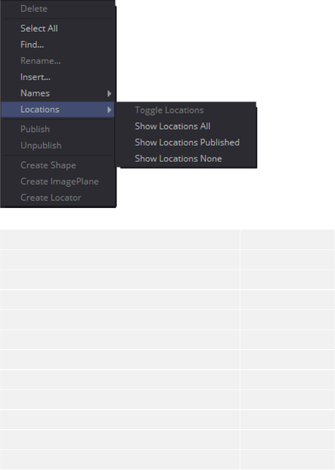
55
3D Tools Chapter – 1
Additional toolbar and shortcuts
Delete Selected Points Del
Select All Shift+A
Find Points Shift+F
Rename Selected Points F2
Create New Point Shift+C
Toggle Names on None/Selected/Published/All Points Shift+N
Toggle Locations on None/Selected/Published/All Points Shift+L
Publish Selected Points Shift+P
Unpublish Selected Points Shift+U
Create a Shape at Selected Points Shift+S
Create and Fit an ImagePlane to Selected Points Shift+I
Create a Locator at Selected Points Shift+O
56
3D Tools Chapter – 1
Projector 3D [3PJ]
The Projector 3D tool is used to project an image upon 3D geometry. This can be useful in
many ways: texturing objects with multiple layers, applying a texture across multiple separate
objects, projecting background shots from the camera’s viewpoint, image-based rendering
techniques and much more. The Projector tool is just one of several tools capable of projecting
images and textures. Each method has advantages and disadvantages. See the Projection
section of the 3D chapter for more information about each approach.
Projected textures can be allowed to “slide“ across the object if the object moves relative to the
Projector 3D, or alternatively, by grouping the two together with a Merge 3D they can be moved
as one and the texture will remain locked to the object.
The Projector 3D tool’s capabilities and restrictions are best understood if the Projector is
considered to be a variant on the Spotlight tool. The fact that the Projector 3D tool is actually a
light has several important consequences when used in Light or Ambient Light projection mode:
Lighting must be turned on for the results of the projection to be visible.
The light emitted from the projector is treated as diffuse/specular light. This means that
it will be affected by the surface normals and can cause specular highlights. If this is
undesirable, set Projector 3D to project into the Ambient Light channel.
Enabling Shadows will cause Projector 3D to cast shadows.
Just as with other lights, the light emitted by a Projector 3D will only affect objects that
feed into the first Merge 3D that is downstream of the Projector 3D tool on the flow.
Enabling Merge 3D’s Pass Through Lights checkbox will allow the projection to light
objects further downstream.
The light emitted by a Projector 3D is controlled by the Lighting options settings on
objects and the Receives Lighting options on materials.
Alpha values in the projected image will not clip geometry in Light or Ambient Light
mode. Use Texture mode instead.
If two projections overlap, their light contributions will be added together.
To project re-lightable textures or textures for non-diffuse color channels (like Specular Intensity
or Bump), use the Texture projection mode instead:
Projections in Texture mode will only strike objects that use the output of the Catcher
tool for all or part of the material applied to that object.
Texture mode projections will clip the geometry according to the alpha channel of the
projected image.
See the section for the Catcher tool for additional details.
The Camera 3D tool also provides a projection feature, and should be used when the
projection is meant to match a camera, as this tool has more control over aperture, film back,
and clip planes. Projector 3D was designed to be used as a custom light in 3D scenes for
layering and texturing. The projector provides better control over light intensity, color, decay
and shadows.
When using projectors in an OpenGL view or in the OpenGL renderer, the lighting must be set
to Per-pixel (the default) in order to see the results of the projection in the main view. The
Per-pixel lighting mode requires a certain level of shader support from your graphics card. Even
if the graphics card does not support pixel shading, the projection will still be visible when using
the Software renderer.
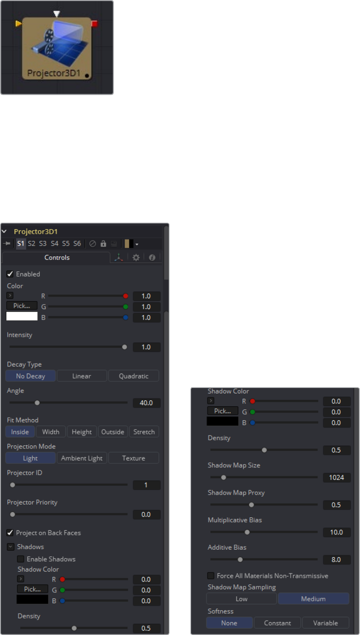
57
3D Tools Chapter – 1
External Inputs
Projector3D.SceneInput
[orange, optional] This input expects a 3D scene. If a scene is connected to this input,
then transformations applied to the spotlight will also affect the rest of the scene.
Projector3D.ProjectiveImage
[white, optional] This input expects a 2D image to be used for the projection.
Controls
58
3D Tools Chapter – 1
Enabled
When this checkbox is selected the projector affects the scene. Clear the checkbox to
turn it off.
Color
The input image is multiplied by this color before projected into the scene.
Intensity
Use this slider to set the Intensity of the projection when the Light and Ambient Light
projection modes are used. In Texture mode this option scales the Color values of the
texture after multiplication by the color.
Decay Type
A projector defaults to No Falloff, meaning that its light has equal intensity on geometry
regardless of the distance from the projector to the geometry. To cause the intensity to
fall off with distance, set the Decay type to either Linear or Quadratic modes.
Angle
The Cone Angle of the tool refers to the width of the cone where the projector emits its
full intensity. The larger the angle, the wider the cone angle, up to a limit of 90 degrees.
Fit Method
The Fit Method determines how the projection is fit within the projection cone.
The first thing to know is that although this documentation may call it a ‘cone,’ the
Projector3D tool and the Camera3D tools do not project actual cones; its more of a
pyramid of light with its apex at the camera/projector. The Projector3D tool always
projects a square pyramid of light, i.e., its X and Y angles of view are the same. The
pyramid of light projected by the Camera3D tool can be non-square depending on
what the Film Back is set to in the camera. The aspect of the image connected into the
Projector3D/Camera3D does not affect the X/Y angles of the pyramid, but rather the
image is scaled to fit into the pyramid based upon the fit options.
When both the aspect of the pyramid (AovY/AovX) and the aspect of the image (height *
pixelAspectY)/(width * pixelAspectX) are the same, there is no need for the fit options,
and in this case, the fit options all do the same thing. However, when the aspect of the
image and the pyramid (as determined by the Film Back settings in Camera3D) are
different, the fit options become important.
For example, ‘Fit by Width’ will fit the width of the image across the width of the
Camera3D pyramid. In this case, if the image has a greater aspect ratio than the aspect
of the pyramid, some of the projection will extend vertically outside of the pyramid.
59
3D Tools Chapter – 1
There are five options:
Inside: The image is uniformly scaled so that its largest dimension fits inside the
cone. Another way to think about this is that it scales the image as big as possible
subject to the restriction that the image is fully contained within the pyramid of the
light. This means, for example, that nothing outside the pyramid of light will ever
receive any projected light.
Width: The image is uniformly scaled so that its width fits inside the cone. Note that
the image could still extend outside the cone in its height direction.
Height: The image is uniformly scaled so that its height fits inside the cone. Note that
the image could still extend outside the cone in its width direction.
Outside: The image is uniformly scaled so that its smallest dimension fits inside the
cone. Another way to think about this is that it scales the image as small as possible
subject to the restriction that the image covers the entire pyramid (i.e., the pyramid is
fully contained within the image). This means that any pixel of any object inside the
pyramid of light will always get illuminated.
Stretch: The image is non-uniformly scaled, so it exactly covers the cone of the
projector.
Projection Mode
Light: Projects the texture as a diffuse/specular light.
Ambient Light: Uses an ambient light for the projection.
Texture
When used in conjunction with the Catcher tool, this mode allows re-lightable texture
projections. The projection will only strike objects that use the catcher material as part
of their material shaders.
One useful trick is to connect a Catcher tool to the Specular Texture input on a 3D
Material tool (such as a Blinn). This will cause any object using the Blinn material to
receive the projection as part of the specular highlight. This technique can be used in
any material input that uses texture maps, such as the Specular and Reflection maps.
Shadows
Since the projector is based on a spotlight, it is also capable of casting shadows using shadow
maps. The controls under this reveal are used to define the size and behavior of the
shadow map.
Enable Shadows
The Enable Shadows checkbox should be selected if the light is to produce shadows.
This defaults to selected.
Shadow Color
Use this standard Color control to set the color of the shadow. This defaults to black
(0, 0, 0).
Density
The Shadow Density determines how opaque the shadow will be. A density of 1.0 will
produce a completely transparent shadow, whereas lower values make the shadow
transparent.
Shadow Map Size
The Shadow Map Size control determines the size of the bitmap used to create the
shadow map. Larger values will produce more detailed shadow maps at the expense of
memory and performance.
60
3D Tools Chapter – 1
Shadow Map Proxy
Shadow Map Proxy determines the size of the shadow map used for proxy and auto
proxy calculations. A value of 0.5 would use a 50% shadow map.
Multiplicative/Additive Bias
Shadows are essentially textures applied to objects in the scene, so there will
occasionally be Z-fighting, where the portions of the object that should be receiving the
shadows render over top of the shadow instead.
Biasing works by adding a small depth offset to move the shadow away from the
surface it is shadowing, eliminating the Z-fighting. Too little bias and the objects can
self-shadow themselves. Too much bias and the shadow can become separated from
the surface.
Make adjustments to the multiplicative bias first, then fine tune the result using the
additive bias control.
Force All Materials Non-Transmissive
Normally, a RGBAZ shadowmap is used when rendering shadows. By enabling this
option you are forcing the renderer to use a Z-only shadowmap. This can result in
significantly faster shadow rendering while using a fifth as much memory. The
disadvantage is that you can no longer cast ‘stained-glass’ like shadows.
Shadow Map Sampling
Sets the quality for sampling of the shadow map.
Softness
Soft edges in shadows are produced by filtering the shadowmap when it is sampled.
Fusion has three separate filtering methods available when rendering shadows which
produce different effects.
None: Shadows will have a hard edge. No filtering of the shadowmap is done at
all. The advantage of this method is that you only have to sample one pixel in the
shadowmap, so it is fast.
Constant: Shadows edges will have a constant softness. A filter with a constant
width is used when sampling the shadowmap. Adjusting the Constant Softness slider
controls the size of the filter. Note that the larger you make the filter, the longer it will
take to render the shadows.
Variable: The softness of shadow edges will grow the further away the shadow
receiver is from the shadow caster. The variable softness is achieved by changing
the size of the filter based on the distance between the receiver and caster.
When this option is selected, the Softness Falloff, Min Softness and Max Softness
sliders appear.
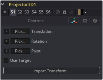
61
3D Tools Chapter – 1
Constant Softness
If the Softness is set to constant, then this slider will appear. It can be used to set the
overall softness of the shadow.
Softness Falloff
The Softness Falloff slider appears when the Softness is set to variable. This slider
controls how fast the softness of shadow edges grows with distance. To be more
precise, it controls how fast the shadowmap filter size grows based upon the distance
between shadow caster and receiver. Its affect is mediated by the values of the Min
and Max Softness sliders.
Min Softness
The Min Softness slider appears when the Softness is set to variable. This slider
controls the Minimum Softness of the shadow. The closer the shadow is to the object
casting the shadow, the sharper it will be up to the limit set by this slider.
Max Softness
The Max Softness slider appears when the Softness is set to variable. This slider
controls the Maximum Softness of the shadow. The further the shadow is from the
object casting the shadow, the softer it will be up to the limit set by this slider
Transform Tab
The options that appear in this tab determine the position of the geometry created by this tool.
Since these controls are identical on all tools that generate geometry, these controls are fully
described in the Common 3D Controls section of this documentation.
62
3D Tools Chapter – 1
Renderer 3D [3RN]
The Renderer 3D tool converts the 3D environment into a 2D image using either a default
perspective camera, or one of the cameras found in the scene. Every 3D scene in a
composition should terminate with at least one Render 3D tool. The Renderer tool can use
either of the Software or OpenGL render engines to produce the resulting image. Additional
render engines may also be available via third party plug-ins.
The Software render engine uses the system’s CPU only to produce the rendered images. It is
usually much slower than the OpenGL render engine, but produces consistent results on all
machines making it essential for renders that involve network rendering. The Software mode is
required to produce soft shadows, and generally supports all available illumination, texture, and
material features.
The OpenGL render engine employs the GPU processor on the graphics card to accelerate the
rendering of the 2D images. The output may vary slightly from system to system, depending on
the exact graphics card installed. The graphics card driver can also affect the results from the
OpenGL renderer. The OpenGL render engines speed makes it possible to provide customized
supersampling and realistic 3D depth of field options. The OpenGL renderer cannot generate
soft shadows. For soft shadows, the Software renderer is recommended.
Like most tools, the Renderer’s motion blur settings can be found under the Common Control
tab. Be aware that scenes containing one or more particle systems will require that the Motion
Blur settings on the pRender tools exactly match the settings on the Renderer 3D tool.
Otherwise, the subframe renders will conflict producing unexpected (and incorrect) results.
External Inputs
Renderer3D.SceneInput
[orange, required] This input expects a 3D scene.
Renderer3D.EffectMask
[violet, optional] This input uses a single or four channel 2D image to mask the output of
the tool.
NOTE: The GL renderer respects the Color Depth option in the Image tab of the
Renderer3D tool. This can cause slowdowns on certain graphics cards when
rendering to int16 or float32.
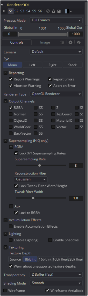
64
3D Tools Chapter – 1
Eye
The Eye control tells the tool how to render the image in stereoscopic projects. The
Mono option will ignore the stereoscopic settings in the camera. The Left and Right
options will translate the camera using the stereo Separation and Convergence options
defined in the camera to produce either left or right eye outputs.
Reporting
The first two checkboxes in this reveal can be used to determine whether the tool will
print warnings and errors produced while rendering to the console. The second row of
checkboxes tells the tool whether it should abort rendering when a warning or error is
encountered. The default for this tool enables all four checkboxes.
Renderer Type
This drop down menu lists the available render engines. Fusion provides two: the
Software and OpenGL render engines (described above), and additional renderers can
be added via third party plug-ins.
All of the controls found below this drop down menu are added by the render engine.
They may change depending on the options available to each renderer. As a result,
each renderer is described in its own section below.
Software Controls
Output Channels
In addition to the usual Red, Green, Blue and Alpha channels, the Software renderer
can also embed the following channels into the image. Enabling additional channels will
consume additional memory and processing time, so these should be used only
when required.
RGBA: This option tells the renderer to produce the Red, Green, Blue and Alpha color
channels of the image. These channels are required and they cannot be disabled .
Z: This option enables rendering of the Z-channel. The pixels in the Z-channel
contain a value that represents the distance of each pixel from the camera. Note that
the Z-channel values cannot include anti-aliasing. In pixels where multiple depths
overlap, the frontmost depth value is used for this pixel.
Coverage: This option enables rendering of the Coverage channel. The Coverage
channel contains information about which pixels in the Z-buffer provide coverage
(are overlapping with other objects). This helps tools that use the Z-buffer to provide
a small degree of antialiasing. The value of the pixels in this channel indicates, as a
percentage, how much of the pixel is composed of the foreground object.
BgColor: This option enables rendering of the BgColor channel. This channel
contains the color values from objects behind the pixels described in the
Coverage channel.
Normal: This option enables rendering of the X, Y and Z Normals channels. These
three channels contain pixel values that indicate the orientation (direction) of
each pixel in the 3D space. A color channel containing values in a range from [-1,1]
represents each axis.
TexCoord: This option enables rendering of the U and V mapping coordinate
channels. The pixels in these channels contain the texture coordinates of the pixel.
Although texture coordinates are processed internally within the 3D system as
3-component UVW, Fusion images only store UV components. These components
are mapped into the Red and Green color channel.
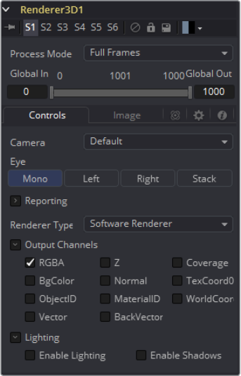
65
3D Tools Chapter – 1
ObjectID: This option enables rendering of the ObjectID channel. Each object in the
3D environment can be assigned a numeric identifier when it is created. The pixels
in this floating-point image channel contain the values assigned to the objects that
produced the pixel. Empty pixels have an ID of 0, and the channel supports values as
high as 65534. Multiple objects can share a single Object ID. This buffer is useful for
extracting mattes based on the shapes of objects in the scene.
MaterialID: This option enables rendering of the MaterialID channel. Each material
in the 3D environment can be assigned a numeric identifier when it is created.
The pixels in this floating-point image channel contain the values assigned to the
materials that produced the pixel. Empty pixels have an ID of 0, and the channel
supports values as high as 65534. Multiple materials can share a single Material ID.
This buffer is useful for extracting mattes based on a texture; for example, a mask
containing all of the pixels that comprise a brick texture.
Lighting
Enable lighting
When the Enable Lighting checkbox is selected, objects will be lit by any lights in the
scene. If no lights are present, all objects will be black.
Enable Shadows
When the Enable Shadows checkbox is selected, the renderer will produce shadows,
at the cost of some speed.
OpenGL Controls
Output channels
In addition to the usual Red, Green, Blue and Alpha channels, the OpenGL render
engine can also embed the following channels into the image. Enabling additional
channels will consume additional memory and processing time, so these should be
used only when required.
66
3D Tools Chapter – 1
RGBA: This option tells the renderer to produce the Red, Green, Blue and Alpha color
channels of the image. These channels are required and they cannot be disabled.
Z: This option enables rendering of the Z-channel. The pixels in the Z-channel
contain a value that represents the distance of each pixel from the camera. Note that
the Z-channel values cannot include anti-aliasing. In pixels where multiple depths
overlap, the frontmost depth value is used for this pixel.
Normal: This option enables rendering of the X, Y and Z Normals channels. These
three channels contain pixel values that indicate the orientation (direction) of each
pixel in the 3D space. A color channel containing values in a range from [-1,1] is
represented by each axis.
TexCoord: This option enables rendering of the U and V mapping coordinate
channels. The pixels in these channels contain the texture coordinates of the pixel.
Although texture coordinates are processed internally within the 3D system as
3-component UVW, Fusion images only store UV components. These components
are mapped into the Red and Green color channel.
ObjectID: This option enables rendering of the ObjectID channel. Each object in the
3D environment can be assigned a numeric identifier when it is created. The pixels
in this floating-point image channel contain the values assigned to the objects that
produced the pixel. Empty pixels have an ID of 0, and the channel supports values as
high as 65534. Multiple objects can share a single Object ID. This buffer is useful for
extracting mattes based on the shapes of objects in the scene.
MaterialID: This option enables rendering of the MaterialID channel. Each material
in the 3D environment can be assigned a numeric identifier when it is created.
The pixels in this floating-point image channel contain the values assigned to the
materials that produced the pixel. Empty pixels have an ID of 0, and the channel
supports values as high as 65534. Multiple materials can share a single Material ID.
This buffer is useful for extracting mattes based on a texture; for example, a mask
containing all of the pixels that comprise a brick texture.
Supersampling
Supersampling can be enabled for each channel by means of the SS tickbox. It produces an
output image with higher quality anti-aliasing by brute force rendering a much larger image,
then rescaling it down to the target resolution. Rendering a larger image in the first place, then
using a Resize tool to bring the image to the desired resolution can achieve the exact same
results. Using the supersampling built into the renderer offers two distinct advantages over
this method.
The rendering is not restricted by memory or image size limitations. For example, consider the
steps to create a float16 1920 x 1080 image with 16x supersampling. Using the traditional Resize
tool would require first rendering the image with a resolution of 30720 x 17280, then using a
resize to scale this image back down to 1920 x 1080. Simply producing the image would require
nearly 4GB of memory. When supersampling is performed on the GPU, the OpenGL renderer
can use tile rendering to significantly reduce memory usage.
The GL renderer can perform the rescaling of the image directly on the GPU much more quickly
than the CPU can manage it. In general, the more GPU memory the graphics card has the faster
the operation will be.
Interactively, Fusion will skip the supersampling stage unless the HiQ button is selected in the
Time Ruler. Final quality renders will always include supersampling, if it is enabled.
Due to hardware limitations, point geometry (particles) and lines (locators) are always rendered
at their original size, independent from supersampling. This means that these elements will be
scaled down from their original sizes, and will likely appear much thinner than expected.
67
3D Tools Chapter – 1
Supersampling of Aux Channels in the OpenGL Renderer
The reason we supply separate SS options for color and aux channels is that supersampling of
color channels is a quite a bit slower than aux channels. You may find that 4 x 4 SS is sufficient
for color, but for worldposition or Z, you may require 64 x 64 to get adequate results. The
reasons color SS is slower are that the shaders for RGBA can be 10x to even 100x or 1000x
more complex, and color is rendered with sorting enabled, while aux channels get rendered
using the much faster Z buffer method.
Enable (HiQ Only)
This checkbox can be used to enable supersampling of the rendered image. The
remaining controls in this reveal will only appear if this is selected.
Lock X/Y Supersampling Rates
When this checkbox is disabled separate sliders are presented to control the amount of
supersampling on the X- and y-axis.
Supersampling Rate X
The Supersampling Rate tells the OpenGL render how large to scale the image. For
example, if the supersampling rate is set to 4 and the OpenGL renderer is set to output
a 1920 x 1080 image, internally a 7680 x 4320 image will be rendered and then scaled
back to produce the target image. Set the multiplier higher to get better edge
antialiasing at the expense of render time. Typically 8x8 supersampling (64 samples per
pixel) is sufficient to reduce most aliasing artifacts.
The supersampling rate doesn’t exactly define the number of samples done per
destination pixel; the width of the reconstruction filter used may also have an impact.
NOTE: RGBA supersampling is no longer enabled in the Supersampling nest,
but rather in the OutputChannels nest. For some things, sometimes using an
SS Z buffer will improve quality, but for other things like using the merge’s
PerformDepthMerge option, it may make things worse.
Do not mistake SS with improved quality. SSing an aux channel does not mean
it’s better quality. In fact, SSing an aux channel in many cases can make the
results much worse. The only channels we recommend you enable SS on are
WorldCoord and Z.
TIP: We strongly recommend disabling SSing on MaterialID and ObjectID
channels. We recommend disabling SSing on TexCoord, Normal, BackVector,
and Vector channels. The issue arises when you have multiple 3D surfaces
with radically different TexCoord values in one pixel. The SSing does not
restrict itself to sampling the main surface, but will sample both surfaces. For
example, if one surface has TexCoords that are approx (u,v)=(0, 0) within that
pixel and the other surface has (0.5, 0.5) you will get a blending of these two.
The blended area of the texture could have colors like (0, 0) or (0.5, 0.5),
resulting in an oddly colored pixel artifact being output from the 2D Texture
tool. The same problem can happen for normals.
68
3D Tools Chapter – 1
Reconstruction Filter
When downsampling the supersized image, the surrounding pixels around a given pixel
are often used to give a more realistic result. There are various filters available for
combining these pixels. More complex filters can give better results, but are usually
slower to calculate. The best filter for the job will often depend on the amount of scaling
and on the contents of the image itself.
The functions of these filters are shown in the image above.
From left to right these are:
Box This is a simple interpolation scale of the image.
Bi-Linear (triangle) This uses a simplistic filter, which produces relatively clean and
fast results.
Bi-Cubic (quadratic) This filter produces a nominal result. It offers a good compromise
between speed and quality.
Bi-Spline (cubic)
This produces better results with continuous tone images but is
slower than Quadratic. If the images have fine detail in them, the
results may be blurrier than desired.
Catmul-Rom
This produces good results with continuous tone images which
are scaled down, producing sharp results with finely
detailed images.
Gaussian This is very similar in speed and quality to Quadratic.
Mitchell This is similar to Catmull-Rom but produces better results with
finely detailed images. It is slower than Catmull-Rom.
Lanczos This is very similar to Mitchell and Catmull-Rom but is a little
cleaner and also slower.
Sinc
This is an advanced filter that produces very sharp, detailed
results, however, it may produce visible `ringing' in some
situations.
Bessel This is similar to the Sinc filter but may be slightly faster.
Window Method
The Window Method menu appears only when the reconstruction filter is set to Sinc
or Bessel.
Hanning This is a simple tapered window.
Hamming Hamming is a slightly tweaked version of Hanning.
Blackman A window with a more sharply tapered falloff.

69
3D Tools Chapter – 1
Lock Tweak Filter Width/Height
When this checkbox is disabled it is possible to set different values for the X and y-axis
when setting the filter width.
Tweak Filter Width
This slider can be used to adjust the size of the filter kernel. The kernel describes how
many of the pixels surrounding the current pixel are sampled to produce the scaled
result. Decreasing the width of the filter causes the anti-aliasing in the resulting image
to appear sharper, while increasing it makes it seem blurrier.
Each type of filter has a default width setting. For example, a Box filter by default uses a
1x1 kernel, a Triangle filter is 2x2, a Bi-cubic filter is 3x3, B-spline and Catmull-Rom use
4x4, while a Gaussian filter is 3.34x3.34. The kernel width of the filter is essentially
multiplied by the value set in this control.
This can be used as a mechanism to blur the resulting image but is not recommended
as it becomes increasingly inefficient for larger tweak multipliers and consumes
significantly more resources. Larger values will often cause a graphics card to fail
entirely. For values higher than 4, using a blur tool on the output image will almost
certainly be more efficient.
Accumulation Eects
Rendering multiple subframes to produce the final image creates accumulation effects.
Thistechnique allows depth of field rendering on the graphic hardware.
Enable Accumulation Effects
This checkbox enables calculation of the accumulation effects.
Depth of Field
This checkbox enables depth of field rendering. Rendering subframes then combining
them into a single frame creates depth of field. In each subframe the camera is rotated
around a virtual target point. The distance to the target point is set by the plane of focus
control in the Camera 3D tool. Pixels at the plane of focus will appear to be in focus.
If supersampling is enabled, then each subframe will be produced using the
supersampled size.
For reasons of efficiency, the subframes created for the DoF effect are also used to
produce motion blur when this option is enabled in the Common Controls tab.
Effectively, both features share subframes.
Depth of Field Quality
This control sets the number of subframes used to create the DoF calculation. As with
motion blur, the value of the control is doubled internally, so setting this control to 2
actually produces 5 subframes (4 + 1 original). If both motion blur and DoF are enabled,
the number of sub-frames produced is determined by the higher quality value. This
prevents the number of subframes produced from growing exponentially.
The following image shows the effect of DoF quality on a small circle:
The value of the controls are from left to right: 0, 1, 2, 8, 32, 128, 1024, 4096.
Amount of DoF Blur
Defines how much the camera is moved per subframe from its original position.
Ahigher value will result in a blurrier image or stronger DoF effect.
70
3D Tools Chapter – 1
Lighting
Enable Lighting
When the Enable Lighting checkbox is selected, any lights in the scene will light
objects. If no lights are present, all objects will be black.
Enable Shadows
When the Enable Shadows checkbox is selected, the renderer will produce shadows,
at the cost of some speed.
Lighting Mode
The Per-vertex lighting model calculates lighting at each vertex of the scene’s
geometry. This produces a fast approximation of the scene’s lighting, but tends to
produce blocky lighting on poorly tessellated objects. The Per-pixel method uses a
different approach that does not rely on the amount of detail in the scene’s geometry
for lighting, so generally produces superior results.
While using Per-pixel lighting in the OpenGL renderer produces results closer to that
produced by the more accurate Software renderer, it still has some disadvantages.
Even with Per-pixel lighting, the OpenGL renderer is less capable of dealing correctly
with semi transparency, soft shadows and colored shadows. The color depth of the
rendering will be limited by the capabilities of the graphics card in the system.
Transparency
The OpenGL renderer reveals this control for selecting which ordering method to use
when calculating transparency.
Z Buffer (fast): This mode is extremely fast, and is adequate for scenes containing
only opaque objects. The speed of this mode comes at the cost of accurate sorting;
only the objects closest to the camera are certain to be in the correct sort order. As
a result, semi-transparent objects may not be shown correctly, depending on their
ordering within the scene.
Sorted (accurate): This mode will sort all objects in the scene (at the expense of
speed) before rendering, giving correct transparency.
Quick Mode: This experimental mode is best suited to scenes that almost exclusively
contain particles.
Shading Model
Use this menu to select a Shading model to use for materials in the scene. Smooth is
the shading model employed in the views and Flat produces a simpler and faster
shading model.
Wireframe
Renders the whole scene as Wireframe. This will show the edges and polygons of the
objects. The edges are still shaded by the material of the objects.
Wireframe Antialiasing
Enables anti-aliasing for the Wireframe render.
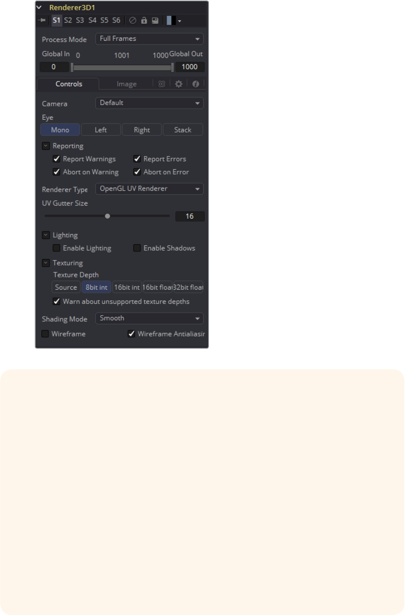
71
3D Tools Chapter – 1
OpenGL UV Unwrap Renderer
Takes a model with existing textures and renders it out via the Renderergluv3D to
produce an unwound flattened 2D version of the model. Optionally lighting can be
baked in. You can then paint on the texture and reapply it.
Caution
After you have baked lighting into a models texture, you need to be careful to turn
lighting off on the object in the future when you render it with the burnt-in-
lighting texture.
Issue Beware of cases where a single area of the texture map is used on multiple
areas of the model. This is often done to save texture memory and decrease
modeling time. An example of this is the texture for a person where the artist
mirrored the left side mesh/uvs/texture to produce the right side. Trying to burn in
lighting in this case won’t work.
Unwrapping more than one mesh at once can cause problems. The reason is that
most models are authored so they make maximal usage of (u,v) in [0,1]x[0,1], so that
in general models will overlap each other in UV space.
Seams When the UV gutter size is left at 0 this produces seams when the model is
retextured with the unwrapped texture.
UV Gutter Size Increase this value to hide seams between faces.
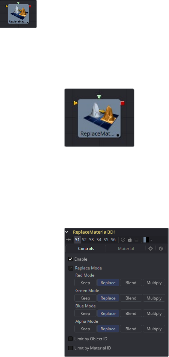
72
3D Tools Chapter – 1
Replace Material 3D [3RPL]
The Replace Material 3D tool replaces the material applied to all of the geometry in the input
scene with its own material input. Any lights or cameras in the input scene are passed through
unaffected.
The scope of the replacement can be limited using Object and Material identifiers. The scope
can also be limited to individual channels, making it possible to use a completely different
material on the Red channel, for example.
External Inputs
Replacematerial3D.SceneInput
[orange, required] This input expects a 3D scene.
Replacematerial3D.MaterialInput
[green, optional] This input will accept either a 2D image or a 3D material. If a 2D image
is provided, it will be used as a diffuse texture map for the basic material built into the
tool. If a 3D material is connected, then the basic material will be disabled.
Controls
Enable
Enables the material replacement.
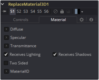
73
3D Tools Chapter – 1
Replace Mode
Red, Green, Blue, and Alpha Mode
Offers several replacing modes for each rgba channel:
Keep: Prevents the channel from being replaced by the input material.
Replace: Replaces the material for the according color channel.
Blend: Blends the materials together.
Multiply: Multiplies the according channels of both inputs.
Limit by Object id/Material id
When enabled, a slider appears where the desired IDs can be set. All other objects will
keep their materials. If both options are enabled an object must satisfy both conditions.
Material Tab
The options that appear in this tab determine the appearance the geometry created by this tool.
Since these controls are identical on all tools that generate geometry, these controls are fully
described in the Common 3D Controls section of this documentation.
If an external 3D material is connected to the tool tile’s material input, then the controls in this
tab will be replaced with the “Using External Material” label.
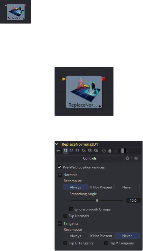
74
3D Tools Chapter – 1
Replace Normals 3D [3RN]
ReplaceNormals is used to replace the Normals/Tangents on incoming geometry. All geometry
in the input scene is affected. Lights/Cameras/PointClouds/Locators/Materials and other
non-mesh tools are passed through unaffected. The normals/tangents affected by this tool are
Per-vertex normals/tangents, not Per-face normals/tangents. The input geometry must have
texture coordinates in order for tangents to be computed. Sometimes geometry does not have
texture coordinates or the texture coordinates were set to All by FBX import because they were
not present on the FBX.
Controls
Pre-Weld Position Vertices
Pre-welds the position vertices. Sometimes position vertices are duplicated in a
geometry, even though they have the same position, causing normals/tangents to be
miscomputed. The results of pre-welding are thrown away; they do not affect the
output geometry’s position vertices.
Recompute
Controls when normals/tangents are recomputed.
Always: The normals on the mesh will always be recomputed.
If Not Present: The normals on the mesh are recomputed only if they are not present.
Never: The normals will never be computed. This option is useful when animating.

75
3D Tools Chapter – 1
Smoothing Angle
Adjacent faces with angles in degrees smaller than this will have their adjoining edges
smoothed across. A typical value one might choose for the Smoothing Angle is
between 20 and 60 degrees. There is special case code for 0.0f and 360.0f. When set
to 0.0f, faceted normals are produced; this is useful for artistic effect.
Ignore Smooth Groups
If set to False, two faces that have different Smooth Groups will not be smoothed across
(e.g., the faces of a cube or the top surfaces of a cylinder have different Smooth
Groups). If you check this On and set the smoothing angle large enough, the faces of a
cube will be smoothed across. There is currently no way to visualize Smooth Groups
within Fusion.
Flip Normals
Flipping of tangents can sometime be confusing. Flip will have an effect if the mesh has
tangent vectors. Most meshes in Fusion don’t have tangent vectors until they reach a
Renderer3D, though. Also, when viewing tangent vectors in the Viewers, the tangent
vectors will be created if they don’t exist. The confusing thing is if you view a Cube3D
that has no tangent vectors and press the FlipU/FlipV button, nothing happens. This is
because there were no tangent vectors to create, but later the GL renderer created
some (unflipped) tangent vectors.
Known issues: The FBX importer will recompute the normals if they don’t
exist, but you can get a higher quality result from this tool.
Bumpmaps can sometimes depend on the model’s normals. In particular,
when you simplify a complex high poly model to a low poly model + bumpmap,
the normals and bumpmap can become ‘linked.’ Recomputing the normals in
this case can make the model look funny. The bumpmap was intended to be
used with those normals.
Most primitives in Fusion are not generated with tangents; when needed they
are generated on the fly by a Renderer3D and cached.
Tangents currently are only needed for bumpmapping. If a material needs
bumpmapping, then tangents are created. These tangents are created with
some default settings (e.g., smoothingAngle, etc), and if you don’t want Fusion
automatically creating tangents you should manually create them using
ReplaceNormals.
All the computations are done in the local coordinates of the geometries
rather than in the coordinate system of the ReplaceNormals3D tool. This can
cause problems when there is a non-uniform scale applied to the geometry
before ReplaceNormals3D is applied.
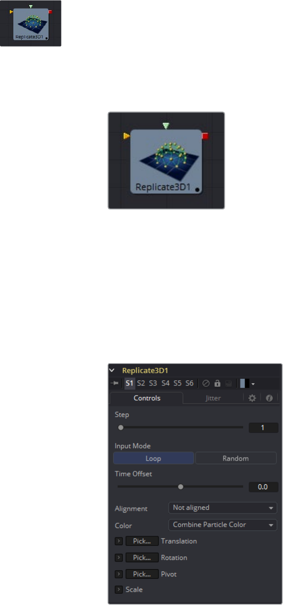
76
3D Tools Chapter – 1
Replicate 3D [3REP]
The Replicate 3D tool replicates input geometry at positions of destination vertices. This
includes mesh vertices as well as particle positions. For each copy of the replicated input
geometry, various transformations can be applied. The options in the Jitter tab allow for
non-uniform transformations, such as random positioning or sizes.
External Inputs
Replicate3d.Destination
[orange, required] This input expects a 3D scene with vertex positions, either from
meshes or 3D particle animations.
Replicate3d.Input[#]
[any, required] This input expects a 3D scene that will be replicated. Once connected, a
new input for alternating 3D scenes will be created.
At least one connected input is required.
Controls
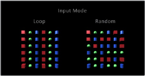
77
3D Tools Chapter – 1
Step
Defines how many positions are skipped. For example, a step of 3 means that only
every 3rd position of the destination mesh will be used, while a step of 1 means that all
positions will be used.
The Step helps to keep reasonable performance for big destination meshes. On
parametric geometry like a torus, it can be used to isolate certain parts of the mesh.
Pointclouds are internally represented by 6 points once the Make Renderable option
has been set. In order to get a single point, use a step of 6 and set a X offset of -0.5 in
the Replicate3D to get to the center of the pointcloud. Use -0.125 for Locator3Ds. Once
these have been scaled the offset may differ.
Input Mode
This parameter defines in which order multiple input scenes are replicated at the
destination. Both parameters won’t have a visible effect if only one input scene
is supplied.
With Loop, the inputs are used successively. The first input will be at the first position,
the second at the second and so on. If there are more positions in the destination
present than inputs, the sequence will be looped.
Random will use a definite but random input for each position based on the seed in the
Jitter tab. This input mode can be used to simulate variety with few input scenes.
Death of Particles causes their IDs to change, therefore their copy order may change.
Time Offset
Use the Time Offset slider to offset any animations that are applied to the source
geometry by a set amount per copy. For example, set the value to -1.0 and use a cube
set to rotate on the Y-axis as the source. The first copy will show the animation from a
frame earlier. The second copy will show animation from a frame before that, and
so forth.
This can be used with great effect on textured planes, for example, where successive
frames of a clip can be shown.
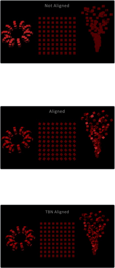
78
3D Tools Chapter – 1
Alignment
Alignment specifies how to align the copies in respect of the destination mesh normal
or particle rotation.
Not Aligned: Does not align the copy. It stays rotated in the same direction as its
input mesh.
Aligned: This mode uses the point’s normal and tries to reconstruct an upvector.
It works best with organic meshes that have unwelded vertices, like imported FBX
meshes, since it has the same rotations for vertices at the same positions. On plane
geometric meshes a gradual shift in rotation will be noticeable. For best results, it is
recommended to use this method at the origin before any transformations.
Aligned TBN: Results in a more accurate and stable alignment based on the tangent,
binormal and normal of the destination point. Works best for particles and geometric
shapes. On unwelded meshes, two copies of multiple unwelded points at the same
position may result in different alignments due to their individual normals.
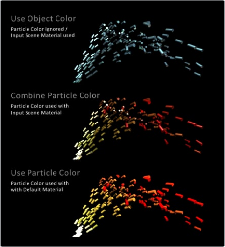
79
3D Tools Chapter – 1
Color
Affects the diffuse color or shader of each copy based on the input’s particle color.
Use Object Color: Does not use the color of the destination particle.
Combine Particle Color: Uses the shader of any input mesh and modifies the diffuse
color to match the color from the destination particle.
Use Particle Color: Replaces the complete shader of any input mesh with a default
shader. Its diffuse color is taken from the destination particle.
Translation
These three sliders tell the tool how much offset to apply to each copy. An X Offset of 1
would offset each copy 1 unit; 1 unit along the X-axis from the last copy.
Rotation Order
These buttons can be used to set the order in which rotations are applied to the
geometry. Setting the rotation order to XYZ would apply the rotation on the X-axis first,
followed by the Y-axis rotation, then the Z-axis rotation.
XYZ Rotation
These three rotation sliders tell the tool how much rotation to apply to each copy.
XYZ Pivot
The pivot controls determine the position of the pivot point used when rotating
each copy.
Lock XYZ
When the Lock XYZ checkbox is selected, any adjustment to the scale will be applied
to all three axes simultaneously.
If this checkbox is disabled, the scale slider will be replaced with individual sliders for
the X, Y and Z scale.
Scale
The Scale control sets how much scaling to apply to each copy.
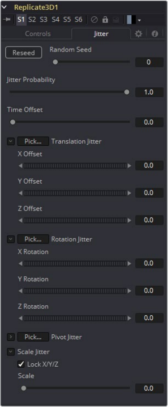
80
3D Tools Chapter – 1
Jitter
Random Seed/Randomize
The Random Seed is used to ‘seed’ the amount of jitter applied to the replicated
objects. Two replicate tools with identical settings but different random seeds will
produce two completely different results. Click on the Randomize button to assign a
Random Seed value.
Time Offset
Use the Time Offset slider to offset any animations that are applied to the source
geometry by a set amount per copy. For example, set the value to -1.0 and use a cube
set to rotate on the Y-axis as the source. The first copy will show the animation from a
frame earlier. The second copy will show animation from a frame before that, and so
forth. This can be used with great effect on textured planes, for example, where
successive frames of a clip can be shown.
81
3D Tools Chapter – 1
Translation XYZ Jitter
Use these three controls to adjust the amount of variation in the translation of the
replicated objects.
Rotation XYZ Jitter
Use these three controls to adjust the amount of variation in the rotation of the
replicated objects.
Pivot XYZ Jitter
Use these three controls to adjust the amount of variation in the rotational pivot center
of the replicated objects. This affects only the additional jitter rotation, not the rotation
produced by the rotation settings in the Controls tab.
Scale XYZ Jitter
Use this control to adjust the amount of variation in the scale of the replicated objects.
Uncheck the Lock XYZ checkbox to adjust the scale variation independently on all
three axes.
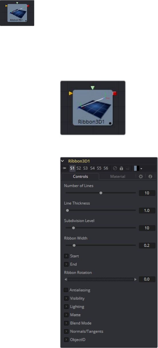
82
3D Tools Chapter – 1
Ribbon 3D [3RI]
Ribbon 3D generates an array of subdivided line segments or a single line between two points.
It is quite useful for motion graphics, especially in connection with Replicate 3D to attach other
geometry to the lines, and with Displace3D for creating lightning-bolt like structures. The array
of lines is, by default, assigned with texture coordinates, so they can be used with a 2D texture.
As usual, UVMap3D can be used to alter the texture coordinates. This tool heavily relies on
certain OpenGL features and will not produce any visible result in the Software renderer.
Furthermore, the way lines are drawn is completely up to the graphic card vendor, so any
artifacts may vary from card to card.
Controls
83
3D Tools Chapter – 1
Number of Lines
The number of parallel lines drawn between the start point and endpoint.
Line Thickness
Line thickness is allowed in the user interface to take on a floating point value, but
some graphics cards will only allow integer values. Some cards may only allow lines
equal to or thicker than 1, or max out at a certain value.
Subdivision Level
The number of vertices on each line between start point and endpoint. The higher the
number, the more precise any 3D displacement can be applied.
Ribbon Width
Determines how far the lines are apart from each other.
Start
XYZ control to set the start point of the ribbon.
End
XYZ control to set the endpoint of the ribbon.
Ribbon Rotation
Allows rotation of the ribbon around the virtual axis defined by start point and endpoint.
Antialiasing
Allows you to apply antialiasing to the rendered lines. Using antialiasing isn’t
necessarily advised. When activated, there will be gaps between the line segments.
This is especially noticeable with high values of line thickness. Again, the way lines are
drawn is completely up to the graphic card vendor which means that these artifacts can
vary from card to card.
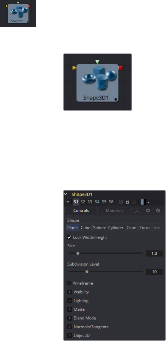
84
3D Tools Chapter – 1
Shape 3D [3SH]
The Shape 3D tool is used to produce several basic primitive 3D shapes, including planes,
cubes, spheres and cylinders.
External Inputs
Shape3d.SceneInput
[orange, required] This input expects to receive a 3D scene.
Shape3d.MaterialInput
[green, optional] This input will accept either a 2D image or a 3D material. If a 2D image
is provided it will be used as a diffuse texture map for the basic material built into the
tool. If a 3D material is connected, then the basic material will be disabled.
Controls
85
3D Tools Chapter – 1
Shape
Select one of these options to determine which geometry primitive will be produced by
the Shape 3D tool. The controls below will change to match the selected shape.
Lock Width/Height/Depth: [plane, cube] If this checkbox is selected, the width,
height and depth controls are locked together as a single size slider. Otherwise,
individual control over the size of the shape along each axis is provided.
Size Width/Height/Depth: [plane, cube] Used to control the size of the shape.
Cube Mapping
[Cube] Uses cube mapping to apply the Shape tool’s texture (a 2D image connected to
the Texture input).
Radius
[Sphere, Cylinder, Cone, Torus] Sets the radius of the selected shape.
Top Radius
[Cone] This control is used to define a radius for the top of a cone, making it possible to
create truncated cones.
Start/End Angle
[Sphere, Cylinder, Cone, Torus] This range control determines how much of the sweep
of the shape is drawn. A start angle of 180 and end angle of 360 would only draw half
of the shape.
Start/End Latitude
[Sphere, Torus] This range control is used to slice the object by defining a latitudinal
sub-section of the object.
Bottom/Top Cap
[Cylinder, Cone] Used for cylinder and cone shapes only, the Bottom Cap and Top Cap
checkboxes are used to determine if the end caps of these shapes are created or if the
shape is left open.
Section
[Torus] Used for torus only, section controls the thickness of the tube making up
the torus.
Subdivision Level/Base/Height
[All shapes] Used for all shapes, the Subdivision controls are used to determine the
tessellation of the mesh composing the object. The higher the subdivision, the more
vertices each shape will have.
Wireframe
Enabling this checkbox will cause the mesh to render only the wireframe for the object.
86
3D Tools Chapter – 1
Visibility
Visible
If the Visibility checkbox is not selected, the object will not be visible in the Viewers,
nor will it be rendered into the output image by the Renderer 3D tool. A non-visible
object does not cast shadows.
Unseen by Cameras
If the Unseen by Cameras checkbox is selected, the object will be visible in the
Viewers (unless the Visible checkbox is turned off), except when viewed through a
camera. The object will not be rendered into the output image by the Renderer 3D tool.
Shadows cast by an unseen object will still be visible when rendered by the Software
renderer, though not by the OpenGL renderer.
Cull Front Face/Back Face
Use these options to cull (eliminate) rendering and display of certain polygons in the
geometry. If Cull Back Face is selected, all polygons facing away from the camera not
be rendered, and will not cast shadows. If Cull Front Face is selected, all polygons
facing toward the camera will likewise be dropped. Selecting both checkboxes has the
same effect as deselecting the Visible checkbox.
Ignore Transparent Pixels in Aux Channels
In previous versions of Fusion, the Software/OpenGL renderers rejected transparent
pixels. To be more specific, the Software renderer rejected pixels with R=G=B=A=0 and
the GL renderer rejected pixels with A=0. This is now optional. The reason you might
want to do this is to get aux channels (e.g., Normals, Z, UVs) for the transparent areas.
For example, suppose in post you want to replace the texture on a 3D element that is
transparent in certain areas with a texture that is transparent in different areas, then it
would be useful to have transparent areas set aux channels (in particular UVs).
Asanother example, suppose you are doing post DoF. You will probably not want the
Zchannel to be set on transparent areas, as this will give you a false depth. Also keep in
mind that this rejection is based on the final pixel color including lighting, if it is on. Soif
you have a specular highlight on a clear glass material, this checkbox will not affect it.
Lighting
Affected by Lights
If this checkbox is not selected, lights in the scene will not affect the object, it will not
receive nor cast shadows, and it will be shown at the full brightness of its color, texture
or material.
Shadow Caster
If this checkbox is not enabled, the object will not cast shadows on other objects in
the scene.
Shadow Receiver
If this checkbox is not enabled, the object will not receive shadows cast by other
objects in the scene.
Matte
Enabling the Is Matte option will apply a special texture to this object, causing this
object to not only become invisible to the camera, but also making everything that
appears directly behind the camera invisible as well. This option will override all
textures. See the matte objects section of the 3D chapter for more information.
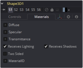
87
3D Tools Chapter – 1
Is Matte
When activated, objects whose pixels fall behind the matte objects pixels in Z do not
get rendered.
Opaque Alpha
Sets the alpha value of the matte object to 1. This checkbox is only visible when the Is
Matte option is enabled.
Infinite Z
Sets the value in the Z channel to infinite. This checkbox is only visible when the Is
Matte option is enabled.
Blend Mode
A Blend mode specifies which method the renderer will use when combining this
object with the rest of the scene. The blend modes are essentially identical to those
listed in the documentation for the 2D Merge tool. For a detailed explanation of each
mode, see the documentation for that tool.
The blending modes were originally designed for use with 2D images. Using them in a
lit 3D environment can produce undesirable results. For best results, use the Apply
modes in unlit 3D scenes rendered in software.
OpenGL Blend Mode
Use this menu to select the blending mode that will be used when the geometry is
processed by the OpenGL renderer. This is also the mode used when viewing the
object in the Viewers. Currently the OpenGL renderer supports three blending modes.
Software Blend Mode
Use this menu to select the blending mode that will be used when the geometry is
processed by the Software renderer. Currently, the Software renderer supports all of
the modes described in the Merge tool documentation, except for the Dissolve mode.
Material Tab
The options that appear in this tab determine the appearance the geometry created by this tool.
Since these controls are identical on all tools that generate geometry, these controls are fully
described in the Common 3D Controls section of this documentation.
If an external 3D material is connected to the tool tile’s material input then the controls in this
tab will be replaced with the “Using External Material” label.
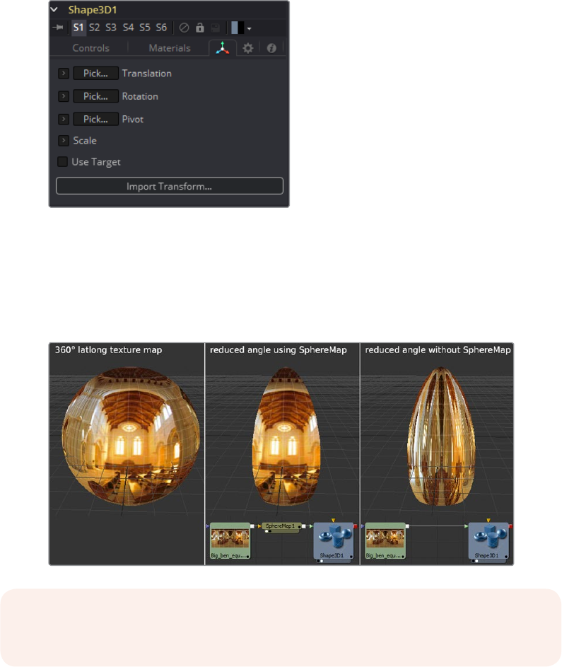
88
3D Tools Chapter – 1
Transform Tab
The options that appear in this tab determine the position of the geometry created by this tool.
Since these controls are identical on all tools that generate geometry, these controls are fully
described in the Common 3D Controls section of this documentation.
Sphere Map vs. Connecting the Texture to a Sphere Directly
You can connect a latlong (equirectangular) texture map directly to a sphere instead of piping it
through the Sphere Map tool first. This results in a different rendering if you set the start/end
angle and latitude to less than 360°/180°. In the first case, the texture will be squashed. When
using the Sphere Map tool, the texture will be cropped. Compare:
NOTE: If you pipe the texture directly into the sphere, it will also be mirrored
horizontally. You can “fix” this by using a Transform tool first.
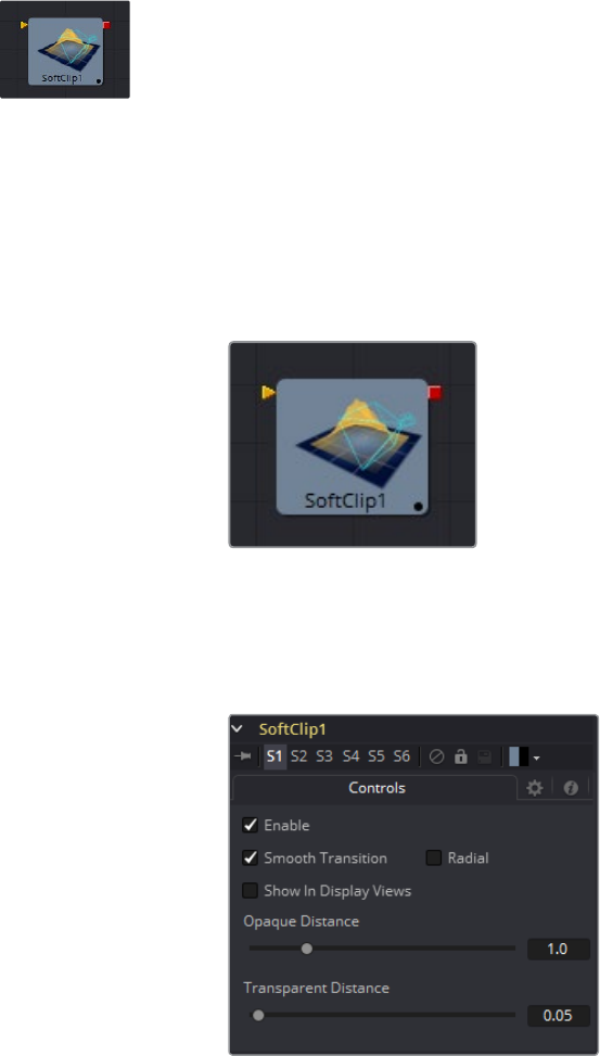
89
3D Tools Chapter – 1
Softclip [3SC]
The Softclip tool is used to fade out geometry and particles that get close to the camera. This
helps avoid the visible ‘popping off’ that affects many particle systems and 3D flythroughs.
Thistool is very similar to the Fog 3D tool, in that it is dependent on the geometry’s distance
from the camera.
The Softclip tool is usually placed just before the renderer to ensure that downstream
adjustments to lighting and textures do not affect the result. It can be placed in any part of the
3D portion of the flow if the soft clipping effect is only required for a portion of the scene.
External Inputs
Softclip.SceneInput
[orange, required] This input expects a 3D scene.
Controls
Enable
This checkbox can be used to enable or disable the tool.
Smooth Transition
Changes the linear gradient to a curve shaped one.
90
3D Tools Chapter – 1
Radial
By default, the softclipping is done based upon the perpendicular distance to a plane
(parallel with the near plane) passing through the eye point. When the radial option is
checked, the Radial distance to the eye point is used instead of the Perpendicular
distance. The problem with Perpendicular distance softclipping is that when you move
the camera about, as objects on the left or right side of the frustum move into the
center, they become less clipped, even though they remain the same distance from the
eye. Radial softclip fixes this. Sometimes Radial softclipping is not desirable.
For example, if you apply softclip to an object that is close to the camera, like an image
plane, the center of the image plane could be unclipped while the edges could be fully
clipped because they are further from the eye point.
Show In Display Views
Normally, the effect is only visible when the scene is viewed using a Camera tool. When
enabled, the softclip becomes visible in the scene from all points of view.
Transparent/Opaque Distance
Defines the range of the softclip. The objects will begin to fade in from an opacity of 0
at the Transparent distance and are fully visible at the Opaque distance. All units are
expressed as distance from the camera along the Z-axis.
91
3D Tools Chapter – 1
Text 3D [3TXT]
The Text3D tool is a 3D version of the 2D Text tool. The controls for this tool are mostly identical
to the controls for the 2D version in almost all respects, except that it only supports one shading
element. See Text Plus for more details on the controls found in this tool.
The Text 3D tool was based on a tool that pre-dates the Fusion 3D environment. As a result,
some of the controls found in the basic primitive shapes and geometry loaders, such as many of
the material, lighting, and matte options, are not found in this tool’s controls. The Text 3D tool
has a built in material, but unlike the other 3D tools it does not have a Material input. The
Shading tab contains controls to adjust the diffuse and specular components. To replace this
default material with a more advanced material, follow the Text Plus tool with a Replace Material
3D tool. The Override 3D tool can be used to control the lighting, visibility and matte options for
this tool.
One thing to be aware of when network-rendering a comp that contains a Text3D tool is that
each machine that does not have the font installed will fail. Fusion cannot share or copy fonts to
Render Slaves due to legal issues.
External Inputs
Text3d.SceneInput
[orange, required] This input expects a 3D scene.
Text3d.ColorImage
[orange, required] This input expects a 2D image. It is only visible when the Image
mode is enabled in the Material section of the Shading tab.
Text3d.BevelTexture
[orange, required] This input expects a 2D image. It is only visible when the Image
mode is enabled in the Bevel Material section of the Shading tab.
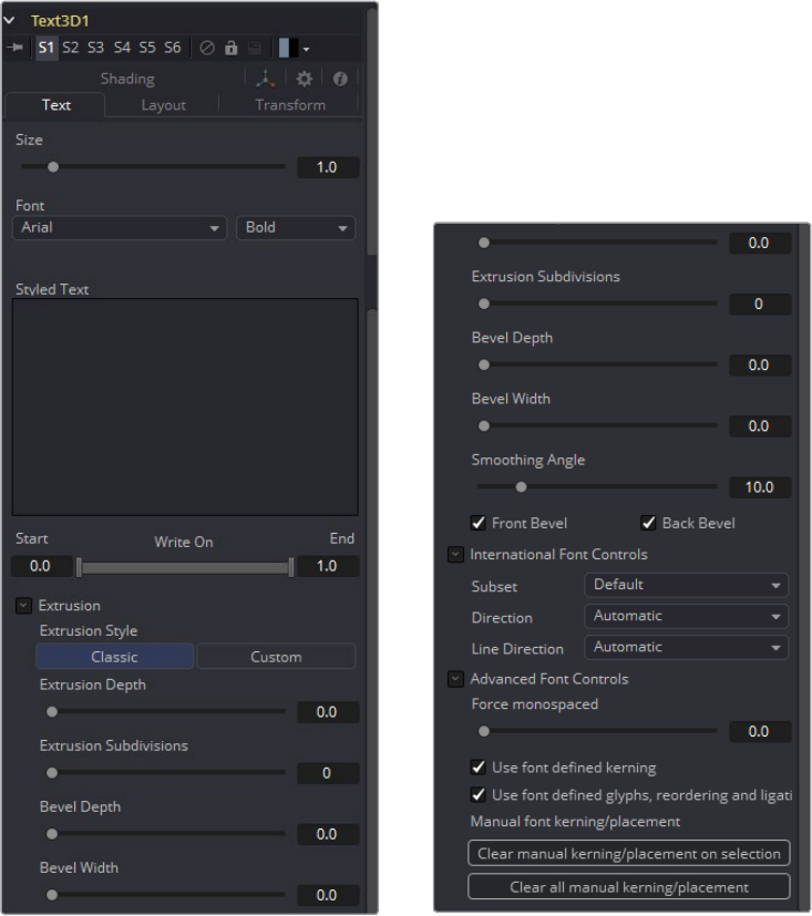
92
3D Tools Chapter – 1
Text Extrusion
Extrusion Depth
An extrusion of 0 produces completely 2D text. Any value greater than 0 will extrude
the text to generate text with depth.
Bevel Depth
Increase the value of the Bevel Depth slider to bevel the text. The text must have
extrusion before this control has any effect.
Bevel Width
Use the Bevel Width control to increase the width of the bevel.
Smoothing Angle
Use this control to adjust the smoothing angle applied to the edges of the bevel.
Front/Back Bevel
Use these checkboxes to enable beveling for the front and back faces of the text
separately
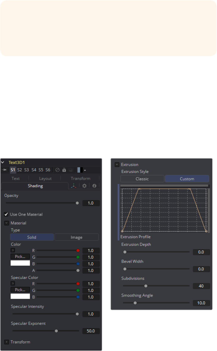
93
3D Tools Chapter – 1
Custom Extrusion
In Custom mode, the Smoothing Angle controls the smoothing of normals around the
edges of a text character. The spline itself controls the smoothing along the extrusion
profile. If a spline segment is smoothed, for example by using the shortcut Shift-S, the
Normals will be smoothed as well. If the keypoint is linear, there will be a sharp shading
edge. The first and last keypoint on the spline defines the extent of the text.
Custom Extrusion Subdivisions: Controls the number of subdivisions within the
smoothed portions of the extrusion profile.
Shading
Opacity
Reducing the material’s opacity will decrease the color and alpha values of the specular
and diffuse colors equally, making the material transparent and allowing hidden objects
to be seen through the material.
Use One Material
Deselecting this option will reveal a second set of Material controls for the beveled
edge of the text.
Material
TIP: Remember that the spline can also be edited from within the SplineEditor
tab and you do not have to work with the limited abilities and size of
thetext3D. Extrusionprofile spline control. Do not try to go to zero size at the
Front/Back face. This will result in Z-fighting due to self-intersecting faces. To
avoid this problem, make sure the first and last point have their profile set to 0.
94
3D Tools Chapter – 1
Type
To use a solid color texture, select the Solid mode. Selecting the Image mode will
reveal a new external input on the tools tile that can be connected to another
2D image.
Specular Color
Specular Color determines the color of light that reflects from a shiny surface. The more
specular a material is, the glossier it appears. Surfaces like plastics and glass tend to
have white specular highlights, whereas metallic surfaces like gold have specular
highlights that tend to inherit their color from the material color. The basic shader
material does not provide an input for textures to control the specularity of the object.
Use tools from the 3D Material category when more precise control is required over the
specular appearance.
Specular Intensity
Specular Intensity controls the strength of the specular highlight. If the specular
intensity texture port has a valid input, then this value is multiplied by the alpha value of
the input.
Specular Exponent
Specular Exponent controls the falloff of the specular highlight. The greater the value,
the sharper the falloff, and the smoother and glossier the material appears. The basic
shader material does not provide an input for textures to control the specular exponent
of the object. Use tools from the 3D Material category when more precise control is
required over the specular exponent.
Image Source
This control determines the source of the texture applied to the material. If the option is
set to Tool, then an input will appear on the tool tile that can be used to apply the
output of a 2D tool as the texture. Selecting Clip will expose a file browser that can be
used to select an image or image sequence from disk. The Brush option will provide a
list of clips found in the Fusion\brushes folder.
Bevel Material
This reveal only appears when the Use One Material checkbox control is selected. The controls
under this reveal are an exact copy of the Material controls above, but are applied only to the
beveled edge of the text.
Transform
These controls can be used to transform the material applied to the text. See the Text Plus tool
for a complete description of these tools.
Tips for Text3D
Character Level Styling
The Text 3D tool doesn’t support Character Level Styling directly. You have to create a
Text+ tool first and modify its text field with a Character Level Styling modifier. Then
either connect the Text 3D’s text field to the modifier that is now available or copy the
Text+ tool and paste its settings to the Text 3D tool (right-click > Paste Settings).
Uncapped 3D Text
To hide the front face of extruded text, uncheck Use One Material on the Shading tab
and reduce the first material’s color to black including its alpha value.
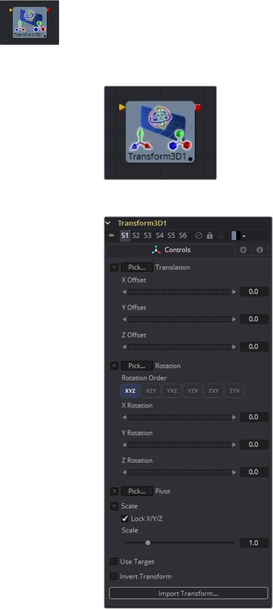
95
3D Tools Chapter – 1
Transform 3D [3XF]
The Transform 3D tool can be used to translate, rotate or scale all the elements within a scene
without requiring a Merge 3D tool. This can be useful for hierarchical transformations, or for
offsetting objects that are merged into a scene multiple times. Its controls are identical to those
found in other 3D tools’ Transformation tabs.
3D Transform Tab
96
3D Tools Chapter – 1
Translation
X, Y, Z Offset
These controls can be used to position the 3D element.
Rotation
Rotation Order
Use these buttons to select the order used to apply the Rotation along each axis of the
object. For example, XYZ would apply the rotation to the X-axis first, followed by the
Y-axis and then followed by the Z-axis.
X, Y, Z Rotation
Use these controls to rotate the object around its pivot point. If the Use Target
checkbox is selected, then the rotation is relative to the position of the target,
otherwise the global axis is used.
Pivot Controls
X, Y, Z Pivot
A pivot point is the point around which an object rotates. Normally, an object will rotate
around its own center, which is considered to be a pivot of 0,0,0. These controls can be
used to offset the pivot from the center.
Scale
X, Y, Z Scale
If the lock X/Y/Z checkbox is checked, a single scale slider will be shown. This adjusts
the overall size of the object. If the Lock checkbox is unchecked, individual X, Y and Z
sliders will be displayed to allow scaling in any dimension.
Use Target
Selecting the Use Target checkbox enables a set of controls for positioning an XYZ
target. When Target is enabled, the object will always rotate to face the target. The
rotation of the object becomes relative to the target.
Import Transform
Opens a file browser where you can select a scene file saved or exported by your
3Dapplication. It supports the following file types:
LightWave Scene .lws
Max Scene .ase
Maya Ascii Scene .ma
dotXSI .xsi
NOTE: If the Lock checkbox is checked, scaling of individual dimensions is not
possible, even when dragging specific axes of the Transformation widget in
Scale mode.
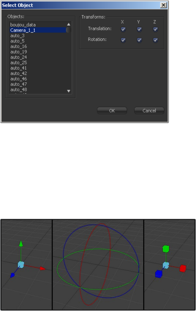
97
3D Tools Chapter – 1
The Import Transform button will only import transformation data. For 3D geometry,
lights and cameras, consider using the File > FBX Import option from the menus.
On Screen Transformation Widget
A Transformation Widget represents most of the controls in this tab in the Viewer, with
modes for transformation, rotation and scaling. To change the mode of the widget,
select one of the three buttons in the toolbar along the side of the Viewer. The modes
can also be toggled using the keyboard shortcut q for translation, w for rotation and e
for scaling. In all three modes, an individual axis of the control may be dragged to affect
just that axis, or the center of the control may be dragged to affect all three axes.
The scale sliders for most 3D tools defaults to locked, which causes uniform scaling of
all three axes. Unlock the Lock X/Y/Z Scale checkbox to scale an object on a single
axis only.
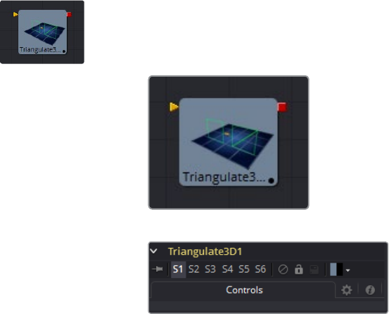
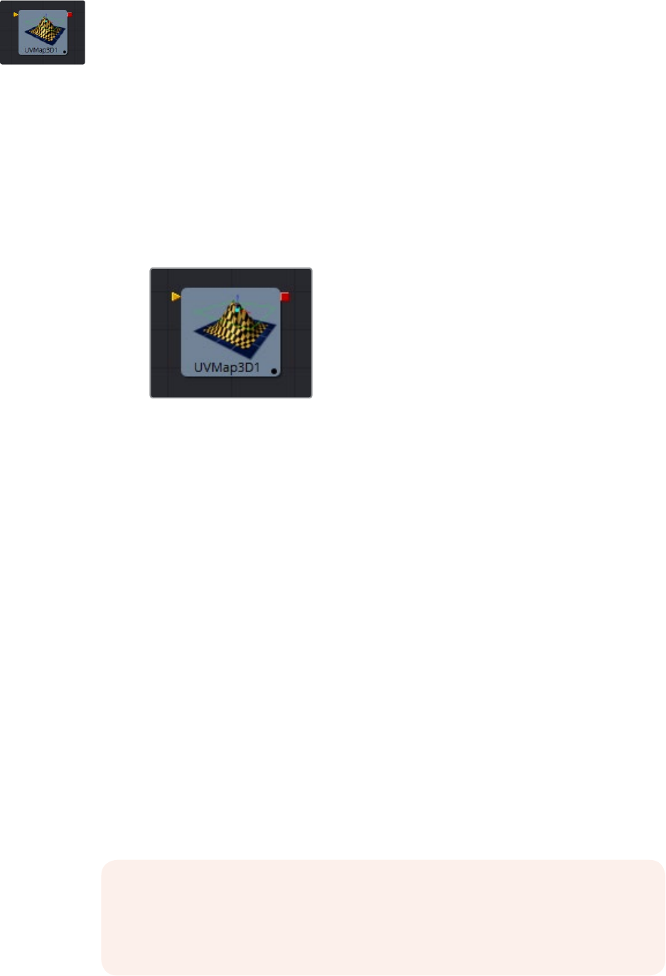
99
3D Tools Chapter – 1
UV Map 3D [3UV]
The UV map 3D tool replaces the UV texture coordinates on the geometry in the scene. These
coordinates tell Fusion how to apply a texture to an object. The tool provides Planar, Cylindrical,
Spherical, XYZ and Cubic Mapping modes, which can be applied to basic Fusion primitives as
well as imported geometry. The position, rotation and scale of the texture coordinates can be
adjusted to allow for fine control over the texture’s appearance. An option is also provided to
lock the UV produced by this tool to animated geometry according to a reference frame. This
can be used to ensure that textures applied to animated geometry do not slide.
While it is possible to adjust the global properties of the selected mapping mode, it is not
possible to manipulate the UV coordinates of individual vertices directly from within Fusion.
Theonscreen controls drawn in the Viewers are for reference only and cannot be manipulated.
External Inputs
UVMap3d.SceneInput
[orange, required] This input expects to receive a 3D scene.
UVMap3d.CameraInput
[green, optional] This input expects the output of the Camera 3D tool. It is only visible
when the Camera Map mode is used.
Camera Projections with UV Map 3D
The Camera Mapping mode makes it possible to project texture coordinates onto geometry
through a camera. Enable the Camera Mapping mode on the UV Map 3D tool. Directly connect
the camera that will be used to create the UV coordinates to the new ‘Camera’ input that
appears on the UV Map 3D tool’s tile in the flow.
Note that this does not directly project an image through the camera. The image to be
projected should be connected to the diffuse texture input of whatever material is assigned to
the objects. When the texture is applied it will use the UV coordinates created by the camera.
Because this is a texture projection and not light, the alpha channel of the texture will correctly
set the opacity of the geometry.
See the Camera 3D and Projector 3D tool for alternate approaches to projection.
The projection can optionally be locked to the vertices as it appears on a selected frame.
Thiswill fail if the number of vertices in the mesh changes over time, as Fusion must be able to
match up the mesh at the reference time and the current time. To be more specific, vertices
may not be created or destroyed or reordered. For this reason, projection locking does not
work for many particle systems, for primitives with animated subdivisions, and with duplicate
tools using non-zero time offsets.
NOTE: The UV Map 3D tool does not put a texture or material on the mesh, it only
modifies the texture coordinates that the materials will use. This may be confusing
because the material usually sits upstream. For example, a composition containing the
tools: Loader > Blinn > Shape 3D (cube) > UV Map 3D > Renderer 3D.
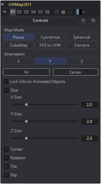
100
3D Tools Chapter – 1
Controls
Map Mode
Defines how the texture coordinates are created. Think of it as a virtual geometry which
projects the UV space on the object.
Planar: Creates the UV coordinates using a plane.
Cylindrical: Creates the UV coordinates using a cylindrical shaped object.
Spherical: The UVs are created using a sphere.
XYZ to UVW: The position coordinates of the vertices are converted to uvw
coordinates directly. This is used for working with procedural textures.
CubeMap: The UVs are created using a cube.
Camera: Enables the Camera Input port of the tool. After connecting a camera to it,
the texture coordinates are created based on camera projection.
Orientation X/Y/Z
Defines the reference axis for aligning the Map mode.
Fit
Clicking this button will fit the Map mode to the bounding box of the input scene.
Center
Clicking this button will move the center of the Map mode to the bounding box center
of the input scene.

101
3D Tools Chapter – 1
Lock UVs on Animated Objects
If the object is animated, the UVs can be locked to it. Enabling this option will do so and
also reveal the Ref Time slider, where it is possible to choose a reference frame for the
UV mapping. Using this feature, it is not required to animate the uvmap parameters. It is
enough to set up the UV map at the reference time.
Size X/Y/Z
Defines the size of the projection object.
Center X/Y/Z
Defines the position of the projection object.
Rotation/Rotation Order
Use these buttons to select which order is used to apply the rotation along each axis of
the object. For example, XYZ would apply the rotation to the X-axis first, followed by
the y-axis and then followed by the Z-axis.
Rotation X/Y/Z
Sets the orientation of the projection object for each axis, dependent from the
rotation order.
Tile u/v/w
Defines how often a texture fits into the projected UV space on the according axis.
Note that the UVW coordinates are transformed, not a texture. Works best when used
in conjunction with the Create Texture tool.
Flip u/v/w
Mirrors the texture coordinates around the according axis.
Flip Faces (CubeMap mode only)
Mirrors the texture coordinates on the individual faces of the cube.
NOTE: To utilize the full capabilities of the UV Map 3D tool it helps to have a basic
understanding of how 2D images are mapped onto 3D geometry. When a 2D image is
applied to a 3D surface, it is converted into a texture map that uses UV coordinates to
determine how the image translates to the object. Each vertex on a mesh has a (U, V)
texture coordinate pair that describes the appearance the object will take when it is
unwrapped and flattened. Different mapping modes use different methods for working
out how the vertices transform into a flat 2D texture. When using the UV Map 3D tool
to modify the texture coordinates on a mesh, it is best to do so using the default
coordinate system of the mesh or primitive. So the typical workflow would look like
Shape 3D > UV Map 3D > Transform 3D. The Transformation tab on the shape tool
would be left to its default values, and the Transform 3D tool following the UV Map
3Ddoes any adjustments needed to place the tool in the scene. Modifying/animating
the transform of the Shape tool will cause the texture to slide across the shape, which
is generally undesirable. The UV Map 3D tool modifies texture coordinates per vertex
and not per pixel. If the geometry the UV map is applied to is poorly tessellated, then
undesirable artifacts may appear.
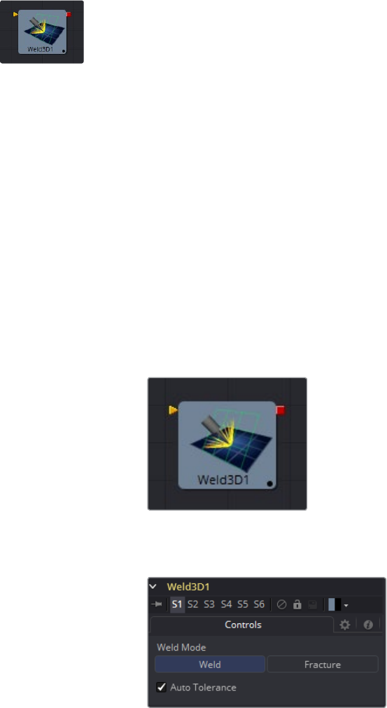
102
3D Tools Chapter – 1
Weld 3D [3WE]
Sometimes 3D geometry has vertices that should have been joined but haven’t. This can cause
artifacts, especially when the two vertices have different normals.
For example:
The different normals will produce a hard shading/lighting edge where
nonewas intended;
If you try to Displace3D the vertices along their normals, a crack will appear;
Missing pixels or doubled up pixels in the rendered image;
Particles to pass through the tiny invisible cracks.
Rather than roundtripping back to your 3D modeling application to fix the ‘duplicated’ vertices,
the Weld3D tool allows you to do this in Fusion. Weld3D welds together vertices with the same
or nearly the same positions. This can be used to fix cracking issues when vertices are
displaced by welding the geometry before the Displace. There are no user controls to pick
vertices. Currently, this tool welds together just Position vertices; it does not weld normals,
texcoords, or any other vertex stream. So even though the positions of two vertices have been
made the same, their normals will still have their old values. This can lead to hard edges in
certain situations.
Controls
Fracture
Fracturing is the opposite of welding, so all vertices are unwelded. This means that all
polygon adjacency information is lost. For example, an Imageplane3D normally consists
of connected quads that share vertices. Fracturing the image plane causes it to
become a bunch of unconnected quads.
Tolerance
In auto-mode the Tolerance value is automatically detected. This should work in most
cases. It can also be adjusted manually if needed.

103
3D Tools Chapter – 1
Usage
Use Weld3D when issues occur with the geometry. Don’t use it everywhere just
because it’s there, as it will influence render time.
Weld3D is intended to be used as a mesh robustness tool and not as a mesh editing
tool to merge together vertices. If you can see the gap between the vertices you want
to weld in the 3D view, you are probably misusing Weld3D. Unexpected things may
happen when you do this; do so at your own peril.
Current Issues
Setting the tolerance too large can cause edges/faces to collapse to points.
If your model has detail distributed over several orders of scale, picking a tolerance
value can be hard or impossible.
For example, suppose you have a model of the iss and there are lots of big polygons
and lots of really tiny polgyons. If you set the tolerance too large, small polygons will
be merged that shouldn’t; if you set the tolerance too small, some large polgyons
won’t be merged.
Vertices that are far from the origin can fail to be merged correctly. This is because
bignumber + epsilon can exactly equal bignumber in float math. This is one reason it
may be best to merge in local coords and not in world coords.
Sometimes Weld3-ing a mesh can make things worse. Take Fusion’s cone as an
example. The top vertex of the cone is currently duplicated for each adjoining face and
they all have different normals. If you weld the cone, the top vertices will merge
together and will only have one normal, making the lighting look weird.
Weld3D is not multithreaded.
Warning
Do not misuse Weld3D to simplify (reduce the polgyon count of) meshes. It is
designed to efficiently weld vertices that differ by only very small values, like a 0.001
distance.
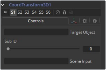
104
3D Tools Chapter – 1
Modifier
Coordinate Transform 3D
Because of the hierarchical nature of the Fusion 3D flow, the original position of an object in the
3D scene often fails to indicate the current position of the object. For example, an image plane
might initially have a position at 1, 2, 1, but then be scaled, offset, and rotated by other tools
further downstream in the 3D scene, ending up with an absolute location of 10, 20, 5.
This can complicate connecting an object further downstream in the composition directly to the
position of an upstream object. The Coordinate Transform modifier can be added to any set of
XYZ coordinate controls, and will calculate the current position of a given object at any point in
the scene hierarchy.
To add a Coordinate Transform modifier, simply right-click on the a numeric input on any tool,
and select Modify With/CoordTransform Position from the Controls contextual menu.
Controls Tab
Target Object
This control should be connected to the 3D tool that produces the original coordinates
to be transformed. To connect a tool, drag and drop a tool tile from the flow into the
Text Edit control, or right-click on the control and select the tool from the contextual
menu. It is also possible to type the tools name directly into the control.
Sub-ID
The SubID slider can be used to target an individual sub-element of certain types of
geometry, such as an individual character produced by a Text 3D tool or a specific copy
created by a Duplicate 3D tool.
Scene Input
This control should be connected to the 3D tool that outputs the scene containing the
object at the new location. To connect a tool, drag and drop a tool tile from the flow into
the Text Edit control, or right-click on the control and select an object from the Connect
To pop-up menu.
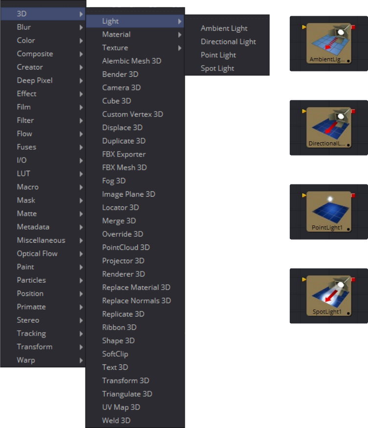
108
3D Light Tools Chapter – 2
Ambient Light [3AM]
An Ambient Light is a directionless light that globally illuminates a scene. It has no real position
or rotation, although an onscreen widget will appear in the views to indicate that a light is
present in the scene. Position controls for the widget are provided to make it possible to move
the widget out of the way of other geometry, if necessary.
External Inputs
AmbientLight.SceneInput
[orange, optional] This input expects a 3D scene. If a scene is provided, the Transform
controls in this tool will apply to the entire scene provided.
Controls Tab
Enabled
When the Enabled checkbox is selected, the ambient light affects the scene. Clear the
checkbox to turn off the light.
Color
Use this standard Color control to set the color of the light.
Intensity
Use this slider to set the Intensity of the ambient light. A value of .2 indicates 20%
percent light. Aperfectly white texture lit only with a .2 ambient light would render at
20% gray (.2, .2, .2).
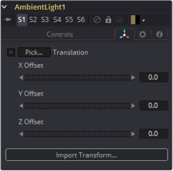
109
3D Light Tools Chapter – 2
Transform Tab
The options that appear in this tab determine the position of the geometry created by this tool.
Since these controls are identical on all tools that generate geometry, these controls are fully
described in the Common 3D Controls section of this documentation.
110
3D Light Tools Chapter – 2
Directional Light [3DL]
A Directional Light is a light with a clear direction but without a clear source. This light shows an
onscreen widget, but the position of the widget has no meaning. The rotation of the widget is
used to determine from where in the scene the light appears to be coming.
External Inputs
DirectionalLight.SceneInput
[orange, optional] This input expects a 3D scene. If a scene is provided, the Transform
controls in this tool will apply to the entire scene provided.
Control Tab
This tab contains all parameters for the tool.
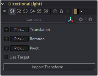
111
3D Light Tools Chapter – 2
Enabled
When the Enabled checkbox is selected, the directional light affects the scene. Clear
the checkbox to turn off the light.
Color
Use this standard Color control to set the color of the light.
Intensity
Use this slider to set the Intensity of the ambient light. A value of .2 indicates 20%
percent light.
Transform Tab
The options that appear in this tab determine the position of the geometry created by this tool.
Since these controls are identical on all tools that generate geometry, these controls are fully
described in the Common 3D Controls section of this documentation.
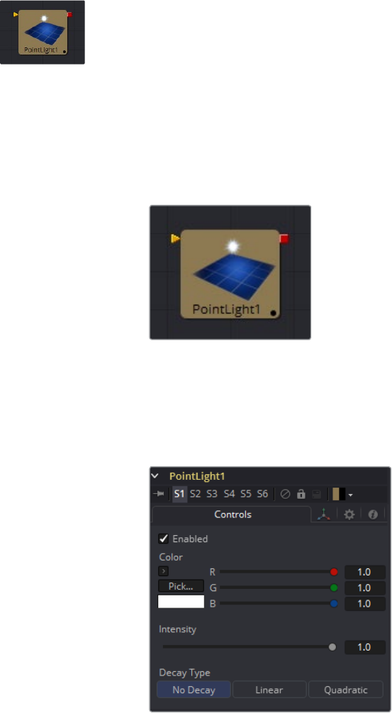
112
3D Light Tools Chapter – 2
Point Light [3PL]
A Point Light is a light source with a clear position in space that emits light in all directions.
Alight bulb is a point light, as is the sun, although light from the sun can appear to be ambient
due to scattering from the atmosphere.
This light shows an onscreen widget, although only the position of the widget affects the light.
Since the light is a 360-degree source, the rotation of the widget has no meaning. Unlike both
ambient and directional lights, a point light may fall off with distance.
External Inputs
PointLight.SceneInput
[orange, optional] This input expects a 3D scene. If a scene is provided, the Transform
controls in this tool will apply to the entire scene provided.
Controls Tab
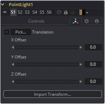
113
3D Light Tools Chapter – 2
Enabled
When the Enabled checkbox is selected, the point light affects the scene. Clear the
checkbox to turn off the light.
Color
Use this standard Color control to set the color of the light.
Intensity
Use this slider to set the Intensity of the ambient light. A value of .2 indicates 20%
percent light.
Decay Type
A point light defaults to No Decay, meaning that its light has equal intensity at all points
in the scene. To cause the intensity to fall off with distance, set the Decay Type either to
Linear or Quadratic modes.
Transform Tab
The options that appear in this tab determine the position of the geometry created by this tool.
Since these controls are identical on all tools that generate geometry, these controls are fully
described in the Common 3D Controls section of this documentation.
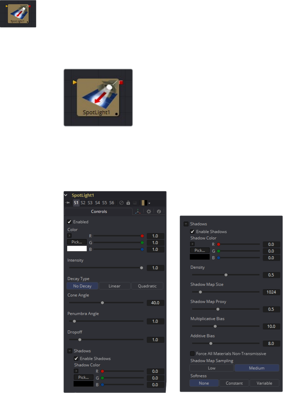
114
3D Light Tools Chapter – 2
Spot Light [3SL]
A Spotlight is a light that comes from a specific point and that has a clearly defined cone, with
falloff of the light to the edges. Experienced stage and theatre lighting technicians will
recognize the spotlight as being very similar to standard luminaries that are used in live
productions. This is the only type of light capable of casting shadows.
External Inputs
SpotLight.SceneInput
[orange, optional] This input expects a 3D scene. If a scene is provided, the
Transformcontrols in this tool will apply to the entire scene provided.
Controls
This tab contains all parameters for the tool.
115
3D Light Tools Chapter – 2
Enabled
When this checkbox is selected, the spotlight light affects the scene. Clear the checkbox to turn
off the light.
Color
Use this standard color control to set the color of the light.
Intensity
Use this slider to set the intensity of the spotlight.
Decay Type
A spotlight defaults to No Falloff, meaning that its light has equal intensity on geometry
regardless of the distance from the light to the geometry. To cause the intensity to fall
off with distance, set the Decay type either to Linear or Quadratic modes.
Cone Angle
The Cone Angle of the light refers to the width of the cone where the light emits its full
intensity. The larger the angle, the wider the cone angle, up to a limit of 90 degrees.
Penumbra Angle
The Penumbra Angle determines the area beyond the cone angle where the light’s intensity
falls off toward 0. A larger penumbra angle defines a larger falloff, while a value of 0 generates
a hard-edged light.
Dropoff
The Dropoff controls how quickly the penumbra angle falls off from full intensity to 0.
Shadows
This section provides several controls used to define the shadow map used when this spotlight
creates shadows. See the Lights and Shadows chapter for details.
Enable Shadows
The Enable Shadows checkbox should be selected if the light is to produce shadows.
This defaults to selected.
Shadow Color
Use this standard Color control to set the color of the shadow. This defaults to black
(0, 0, 0).
Density
The shadow Density determines how opaque the shadow will be. A density of 1.0 will
produce a completely transparent shadow, whereas lower values make the shadow
transparent.
Shadow Map Size
The Shadow Map Size control determines the size of the bitmap used to create the
shadow map. Larger values will produce more detailed shadow maps at the expense of
memory and performance.
Shadow Map Proxy
Shadow Map Proxy determines the size of the shadow map used when the Proxy or
Auto Proxy modes are enabled. A value of 0.5 would produce a shadow map at half the
resolution defined in the Shadow Map Size.

116
3D Light Tools Chapter – 2
Multiplicative/Additive Bias
Shadows are essentially textures applied to objects in the scene so there will
occasionally be Z-fighting, where the portions of the object that should be receiving the
shadows render over top of the shadow instead. Biasing works by adding a small depth
offset to move the shadow away from the surface it is shadowing, eliminating the
Z-fighting. Too little bias and the objects can self-shadow themselves. Too much bias
and the shadow can become separated from the surface. Make adjustments to the
Multiplicative Bias first, then fine tune the result using the Additive Bias control.
See the Multiplicative and Additive Bias section of the 3D chapter for examples and
more information.
Force All Materials Non-Transmissive
Normally, a RGBAZ shadow map is used when rendering shadows. By enabling this
option you are forcing the renderer to use a Z-only shadow map. This can result in
significantly faster shadow rendering while using a fifth as much memory. The
disadvantage is that you can no longer cast ‘stained-glass’ like shadows.
Shadow Map Sampling
Sets the quality for sampling of the shadow map.
Softness
Soft edges in shadows are produced by filtering the shadow map when it is sampled.
Fusion has three separate filtering methods available when rendering shadows which
produce different effects.
Constant: Shadows edges will have a constant softness. A filter with a constant
width is used when sampling the shadow map. Adjusting the Constant Softness slider
controls the size of the filter. Note that the larger you make the filter, the longer it will
take to render the shadows.
Variable: The softness of shadow edges will grow the further away the shadow
receiver is from the shadow caster. The variable softness is achieved by changing
the size of the filter based on the distance between the receiver and caster.
When this option is selected, the Softness Falloff, Min Softness and Max Softness
sliders appear.
NONE: Shadows will have a hard edge. No filtering of the shadow map is
done at all. The advantage of this method is that you only have to sample one
pixel in the shadow map, so it is fast.
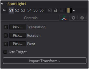
117
3D Light Tools Chapter – 2
Constant Softness
If the Softness is set to constant, then this slider will appear. It can be used to set the
overall softness of the shadow.
Softness Falloff
The Softness Falloff slider appears when the Softness is set to variable. This slider
controls how fast the softness of shadow edges grows with distance. To be more
precise, it controls how fast the shadow map filter size grows based upon the distance
between shadow caster and receiver. Its effect is mediated by the values of the Min
and Max Softness sliders.
Min Softness
The Min Softness slider appears when the Softness is set to variable. This slider
controls the Minimum Softness of the shadow. The closer the shadow is to the object
casting the shadow, the sharper it will be up to the limit set by this slider.
Max Softness
The Max Softness slider appears when the Softness is set to variable. This slider
controls the Maximum Softness of the shadow. The further the shadow is from the
object casting the shadow, the softer it will be up to the limit set by this slider.
Transform Tab
The options that appear in this tab determine the position of the geometry created by this tool.
Since these controls are identical on all tools that generate geometry, these controls are fully
described in the Common 3D Controls section of this documentation.
121
3D Material Tools Chapter – 3
Blinn [3BI]
The Blinn tool is a basic illumination material that can be applied to geometry in the 3D scene. It
describes how the object will respond to light, and provides a large number of texture map
inputs to allow fine control over the diffuse, specular and bumpmap components of the material.
The standard basic material provided in the Material tab of most geometry tools is a simplified
version of the Blinn tool. The primary difference is that the Blinn tool provides additional texture
map inputs beyond just diffuse.
The Blinn tool outputs a 3D Material that can be connected to the material inputs on any 3D
geometry tool.
The Blinn model implemented by Fusion calculates the highlight as the dot product of the
surface normal and the half angle vector between lightsource and viewer (dot(N, H)). This may
not always match the Blinn model illumination model used by other 3D applications.
External Inputs
Blinn.DiffuseTex
[orange, optional] This input will accept a 2D image or a 3D material to be used as a
diffuse texture map.
Blinn.SpecularColorTex
[green, optional] This input will accept a 2D image or a 3D material to be used as a
specular color texture map.
Blinn.SpecularIntensityTex
[magenta, optional] This input will accept a 2D image or a 3D material to be used as an
intensity map for the materials specular highlights. When the input is a 2D image, the
alpha channel is used to create the map while the color channels are discarded.
Blinn.SpecularExponentTex
[light blue, optional] This input will accept a 2D image or a 3D material to be used as a
falloff map for the materials specular highlights. When the input is a 2D image, the alpha
channel is used to create the map while the color channels are discarded.
Blinn.BumpmapTex
[white, optional] This input will accept a 2D image or a 3D material, then uses the RGB
information as texture-space normals.
Each of these inputs multiplies the pixels in the texture map by the equivalently named
parameters in the tool itself. This provides an effective method for scaling parts of the material.

122
3D Material Tools Chapter – 3
When tools have as many inputs as this one does, it is often difficult to make connections with
any precision. Hold the Option (Mac OS X) or Alt (Windows) key down while dragging the output
from another tool over the tool tile, and keep holding Option or Alt when releasing the left
mouse button. A small menu listing all of the inputs provided by the tool will appear. Click on
the desired input to complete the connection.
Alternatively, you can drag the output from a tool with the right mouse button to activate the
same menu.
Controls
123
3D Material Tools Chapter – 3
Diuse
Diffuse describes the base surface characteristics without any additional effects like reflections
or specular highlights. In addition to defining the base color of an object, the diffuse color also
defines the transparency of the object. The alpha in a diffuse texture map can be used to make
portions of the surface of any object the material is applied to transparent.
Diffuse Color
A material’s Diffuse Color describes the base color presented by the material when it is
lit indirectly or by ambient light. If a diffuse texture map is provided, then the color value
provided here is multiplied by the color values in the texture.
Alpha
This slider sets the material’s Alpha channel value. This affects diffuse and specular
colors equally, and affects the alpha value of the material in the rendered output. If a
diffuse texture map is provided, then the alpha value set here is multiplied by the alpha
values in the texture map.
Opacity
Reducing the material’s Opacity will decrease the color and alpha values of the
specular and diffuse colors equally, making the material transparent.
Specular
The parameters in the Specular section describe the look of the specular highlight of the
surface. These values are evaluated in a different way for each illumination model.
Specular Color
Specular Color determines the color of light that reflects from a shiny surface. The more
specular a material is, the glossier it appears. Surfaces like plastics and glass tend to
have white specular highlights, whereas metallic surfaces like gold have specular
highlights that inherit their color from the material color. If a specular texture map is
provided, then the value provided here is multiplied by the color values from
the texture.
Specular Intensity
Specular Intensity controls how strong the specular highlight is. If the specular intensity
texture is provided, then this value is multiplied by the alpha value of the texture.
Specular Exponent
Specular Exponent controls the falloff of the specular highlight. The greater the value,
the sharper the falloff, and the smoother and glossier the material appears. If the
specular exponent texture is provided, then this value is multiplied by the alpha value
of the texture map.
124
3D Material Tools Chapter – 3
Transmittance
Transmittance controls the way light passes through a material. For example, a solid blue
sphere will cast a black shadow, but one made of translucent blue plastic would cast a much
lower density blue shadow.
There is a separate Opacity option. Opacity determines how transparent the actual surface is
when it is rendered. Fusion allows for adjusting both opacity and transmittance separately. This
might be a bit counter-intuitive to those who are unfamiliar with 3D software at first. It is possible
to have a surface that is fully opaque but transmits 100% of the light arriving upon it, effectively
making it a luminous/emissive surface.
Attenuation
Attenuation determines how much color is passed through the object. For an object to
have transmissive shadows, set the attenuation to (1, 1, 1), which means 100% of green,
blue, red light pass through the object. Setting this color to RGB (1, 0, 0) means that the
material will transmit 100% of the red arriving at the surface but none of the green or
blue light. This allows for ‘stained glass’ shadows.
Alpha Detail
When the Alpha Detail slider is set to 0, the alpha channel of the object is ignored and
the entire object casts a shadow. If it is set to 1, the alpha channel determines what
portions of the object cast a shadow.
Color Detail
The Color Detail slider modulates light passing through the surface by the diffuse
color+ texture colors. Use this to throw a shadow that contains color details of the
texture applied to the object. Increasing the slider from 0 to 1 brings in more of diffuse
color + texture color into the shadow. Note that the alpha and opacity of the object is
ignored when transmitting color, allowing an object with a solid alpha to still transmit its
color to the shadow.
Saturation
The Saturation slider controls the saturation of the color component transmitted to the
shadow. Setting this to 0.0 will result in monochrome shadows.
Receives Lighting/Shadows
These checkboxes control whether the material is affected by lighting and shadows in
the scene. If turned off, the object will always be fully lit and/or unshadowed.
Two Sided Lighting
This makes the surface effectively two sided by adding a second set of normals facing
the opposite direction on the backside of the surface. This is normally off, to increase
rendering speed, but can be turned on for 2D surfaces or for objects that are not fully
enclosed, to allow the reverse or interior surfaces to be visible as well.
Normally, in a 3D application only the front face of a surface is visible and the back face
is culled, so that if a camera were to revolve around a plane in a 3D application, when it
reached the backside, the plane would become invisible. Making a plane two sided in
a3D application is equivalent to adding another plane on top of the first but rotated by
180 degrees so the normals are facing the opposite direction on the backside. Thus,
when you revolve around the back, you see the second image plane, which has its
normals facing the opposite way.

125
3D Material Tools Chapter – 3
Fusion does exactly the same thing as 3D applications when you make a surface two
sided. The confusion about what two sided does arises because Fusion does not cull
backfacing polygons by default. If you revolve around a one-sided plane in Fusion you
will still see it from the backside (but you are seeing the frontside duplicated through to
the backside as if it were transparent). Making the plane two sided effectively adds a
second set of normals to the backside of the plane.
Material ID
This slider sets the numeric identifier assigned to this material. This value will be
rendered into the MatID auxiliary channel if the according option is enabled in
the renderer.
NOTE: This can become rather confusing once you make the surface
transparent, as the same rules still apply and produce a result, which is
counter-intuitive. If you view from the frontside a transparent two-sided
surface illuminated from the backside, it will look unlit.
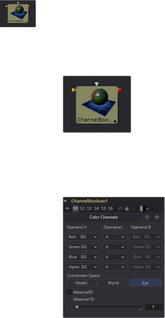
126
3D Material Tools Chapter – 3
Channel Boolean Material [3BOL]
The Channel Boolean Material can be used to remap and modify channels of 3D materials using
mathematical operations. For example, if you want to use the red channel of a material to
control an scalar input of an illumination model which uses the alpha channel (e.g., Blinn.
SpecularExponent), you can remap the channels here. Furthermore, it allows the use of
geometry-specific information like texture space coordinates and normals.
External Inputs
ChannelBooleanMaterial.BackgroundMaterial
[orange, optional] This input will accept a 2D image or a 3D material.
ChannelBooleanMaterial.ForegroundMaterial
[green, optional] This input will accept a 2D image or a 3D material.
Controls
Operand A/B
The Operand menus, one for each output RGBA channel, allow the user to set the
desired input information for the according channel.
Red/Green/Blue/Alpha FG
Reads the color information of the foreground material.
Red/Green/Blue/Alpha BG
Reads the color information of the background material.
127
3D Material Tools Chapter – 3
Black/White/Mid Gray
Sets the value of the channel to 0, 1 or 0.5.
Hue/Lightness/Saturation FG
Reads the color information of the foreground material, converts it into the HLS color
space and puts the selected information into the according channel.
Hue/Lightness/Saturation BG
Reads the color information of the background material, converts it into the HLS color
space and puts the selected information into the according channel.
Luminance FG
Reads the color information of the foreground material and calculates the luminance
value for the channel.
Luminance BG
Reads the color information of the background material and calculates the luminance
value for the channel.
X/Y/Z Position FG
Sets the value of the channel to the position of the pixel in 3D space. The vector
information is returned in eye space.
U/V/W Texture FG
Applies the texture space coordinates of the foreground material to the channels.
U/V/W EnvCoords FG
Applies the environment texture space coordinates to the channels. Use it upstream
of tools modifying the environment texture coordinates like the Reflect 3D tool.
X/Y/Z Normal
Set the value of the channel to the selected axis of the normal vector. The vector is
returned in eye space.
Operation
Determines the Operation of how the operands are combined.
A: Uses Operand A only for the output channel.
B: Uses Operand B only for the output channel.
1-A: Subtracts the value of Operand A from 1.
1-B: Subtracts the value of Operand B from 1.
A+B: Adds the value of Operand A and B.
A-B: Subtracts the value of Operand B from A.
A*B: Multiplies the value of both Operands.
A/B: Divides the value of Operand B from A.
min(A,B): Compares the values of Operands A and B and returns the smaller one.
max(A,B): Compares the values of Operands A and B and returns the bigger one.
avg(A,B): Returns the average value of both Operands.
Material ID
This slider sets the numeric identifier assigned to this material. This value will be
rendered into the MatID auxiliary channel if the according option is enabled in
the renderer.
128
3D Material Tools Chapter – 3
Cook Torrance [3CT]
The Cook Torrance tool is a basic illumination material that can be applied to geometry in the
3D scene. The diffuse calculation for this tool is similar to that used in the basic material and the
Blinn tool, but the specular highlights are evaluated using an optimized Fresnel/Beckmann
equation. This illumination model is primarily used for shading metal or other shiny and highly
reflective surfaces.
The Cook Torrance tool outputs a 3D Material that can be connected to the material inputs on
any 3D geometry tool.
External Inputs
CookTorrance.DiffuseTex
[orange, optional] This input will accept a 2D image or a 3D material to be used as a
diffuse texture map.
CookTorrance.SpecularColorTex
[green, optional] This input will accept a 2D image or a 3D material to be used as a
specular color texture map.
CookTorrance.SpecularIntensityTex
[magenta, optional] This input will accept a 2D image or a 3D material to be used as an
intensity map for the materials specular highlights. When the input is a 2D image, the
alpha channel is used to create the map while the color channels are discarded.
CookTorrance.SpecularRoughnessTex
[light blue, optional] This input will accept a 2D image or a 3D material to be used as a
map for modifying the roughness of the specular highlight. The alpha of the texture
map is multiplied by the value of the roughness control.
CookTorrance.SpecularRefractiveIndexTex
[white, optional] This input will accept a 2D image or a 3D material to be used as a map
for modifying the roughness of the specular refractive index. The alpha of the texture
map is multiplied by the value of the refractive index.
CookTorrance.BumpmapTex
[white, optional] This input will accept a 2D image or a 3D material, then uses the RGB
information as texture-space normals.
Each of these inputs multiplies the pixels in the texture map by the equivalently named
parameters in the tool itself. This provides an effective method for scaling parts of the material.
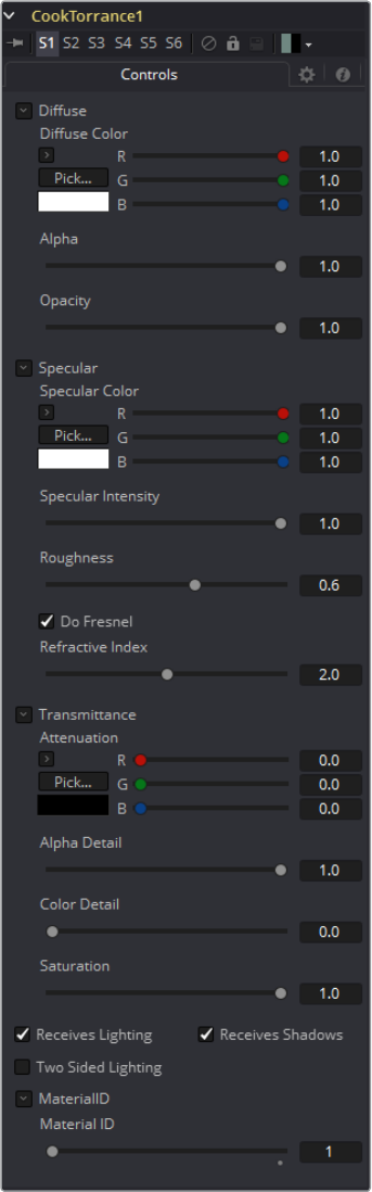
129
3D Material Tools Chapter – 3
When tools have as many inputs as this one does, it is often difficult to make connections with
any precision. Hold the Option (Mac OS X) or Alt (Windows) key down while dragging the output
from another tool over the tool tile, and keep holding Option or Alt when releasing the left
mouse button. A small menu listing all of the inputs provided by the tool will appear. Click on
the desired input to complete the connection.
Controls
130
3D Material Tools Chapter – 3
Diuse
Diffuse describes the base surface characteristics without any additional effects like reflections
or specular highlights. In addition to defining the base color of an object, the diffuse color also
defines the transparency of the object. The alpha in a diffuse texture map can be used to make
portions of the surface of any object the material is applied to transparent.
Diffuse Color
A material’s Diffuse Color describes the base color presented by the material when it is
lit indirectly or by ambient light. If a diffuse texture map is provided, then the color value
provided here is multiplied by the color values in the texture.
Alpha
This slider sets the material’s Alpha channel value. This affects diffuse and specular
colors equally, and affects the alpha value of the material in the rendered output. If a
diffuse texture map is provided, then the alpha value set here is multiplied by the alpha
values in the texture map.
Opacity
Reducing the material’s Opacity will decrease the color and alpha values of the
specular and diffuse colors equally, making the material transparent.
Specular
The parameters in the Specular section describe the look of the specular highlight of the
surface. These values are evaluated in a different way for each illumination model.
Specular Color
Specular Color determines the color of light that reflects from a shiny surface. The more
specular a material is, the glossier it appears. Surfaces like plastics and glass tend to
have white specular highlights, whereas metallic surfaces like gold have specular
highlights that inherit their color from the material color. If a specular texture map is
provided, then the value provided here is multiplied by the color values from
the texture.
Specular Intensity
Specular Intensity controls how strong the specular highlight is. If the specular intensity
texture is provided, then this value is multiplied by the alpha value of the texture.
Roughness
The Roughness of the specular highlight describes diffusion of the specular highlight
over the surface. The greater the value, the wider the falloff, and the more brushed and
metallic the surface appears. If the roughness texture map is provided, then this value
is multiplied by the alpha value from the texture.
Do Fresnel
Selecting this checkbox will add Fresnel calculations to the materials illumination
model. This will provide more realistic looking metal surfaces by taking into account the
refractiveness of the material.
Refractive Index
This slider appears when the Do Fresnel checkbox is selected. The Refractive Index
applies only to the calculations for the highlight; it does not perform actual refraction of
light through transparent surfaces. If the refractive index texture map is provided, then
this value is multiplied by the alpha value of the input.
131
3D Material Tools Chapter – 3
Transmittance
Transmittance controls the way light passes through a material. For example, a solid blue
sphere will cast a black shadow, but one made of translucent blue plastic would cast a much
lower density blue shadow.
There is a separate Opacity option. Opacity determines how transparent the actual surface is
when it is rendered. Fusion allows for adjusting both opacity and transmittance separately. This
might be a bit counter-intuitive to those who are unfamiliar with 3D software at first. It is possible
to have a surface that is fully opaque but transmits 100% of the light arriving upon it, effectively
making it a luminous/emissive surface.
Attenuation
Attenuation determines how much color is passed through the object. For an object to
have transmissive shadows, set the attenuation to (1, 1, 1), which means 100% of green,
blue, red light pass through the object. Setting this color to RGB (1, 0, 0) means that the
material will transmit 100% of the red arriving at the surface but none of the green or
blue light. This allows for ‘stained glass’ shadows.
Alpha Detail
When the Alpha Detail slider is set to 0, the alpha channel of the object is ignored and
the entire object casts a shadow. If it is set to 1, the alpha channel determines what
portions of the object cast a shadow.
Color Detail
The Color Detail slider modulates light passing through the surface by the diffuse color
+ texture colors. Use this to throw a shadow that contains color details of the texture
applied to the object. Increasing the slider from 0 to 1 brings in more of diffuse color +
texture color into the shadow. Note that the alpha and opacity of the object is ignored
when transmitting color, allowing an object with a solid alpha to still transmit its color to
the shadow.
Saturation
The Saturation slider controls the saturation of the color component transmitted to the
shadow. Setting this to 0.0 will result in monochrome shadows.
Receives Lighting/Shadows
These checkboxes control whether the material is affected by lighting and shadows in
the scene. Ifturned off, the object will always be fully lit and/or unshadowed.

132
3D Material Tools Chapter – 3
Two Sided Lighting
This makes the surface effectively two sided by adding a second set of normals facing
the opposite direction on the backside of the surface. This is normally off, to increase
rendering speed, but can be turned on for 2D surfaces or for objects that are not fully
enclosed, to allow the reverse or interior surfaces to be visible as well.
Normally, in a 3D application only the front face of a surface is visible and the back face
is culled, so that if a camera were to revolve around a plane in a 3D application, when
itreached the backside, the plane would become invisible. Making a plane two sided in
a 3D application is equivalent to adding another plane on top of the first but rotated by
180 degrees so the normals are facing the opposite direction on the backside. Thus,
when you revolve around the back, you see the second image plane, which has its
normals facing the opposite way.
Material ID
This slider sets the numeric identifier assigned to this material. This value will be
rendered into the MatID auxiliary channel if the according option is enabled in
the renderer.
NOTE: This can become rather confusing once you make the surface
transparent, as the same rules still apply and produce a result that is counter-
intuitive. If you view from the frontside a transparent two-sided surface
illuminated from the backside, it will look unlit.
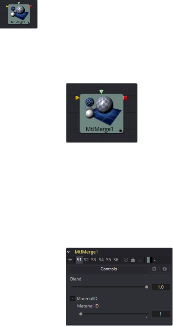
133
3D Material Tools Chapter – 3
Material Merge 3D [3MM]
The Material Merge tool can be used to combine two separate materials together. This tool can
be used to composite Material tools, combining multiple Illumination materials (Blinn, Cook
Torrance) with Texture tools (Bumpmap, Reflection) to create complex shader networks.
The tool also provides a mechanism for assigning a new material identifier to the
combined material.
External Inputs
MtlMerge3D.BackgroundMaterial
[orange, required] This input will accept a 2D image or a 3D material to be used as the
background material. A 2D image will be treated as a diffuse texture map in the basic
shading model.
MtlMerge3D.ForegroundMaterial
[green, optional] This input will accept a 2D image or a 3D material to be used as the
foreground material.
A 2D image will be treated as a diffuse texture map in the basic shading model.
Controls
Blend
The Blend behavior of the Material Merge is similar to the Dissolve (DX) tool for images.
The two materials/textures are mixed together using the value of the slider to
determine the percentage each input contributes. While the background and
foreground inputs can be a 2D image rather than a material, the output of this tool will
always be a material.
Unlike the 2D Dissolve tool, both foreground and background inputs are required.
MaterialID
This slider sets the numeric identifier assigned to the resulting material. This value will
be rendered into the MatID auxiliary channel if the according option is enabled in
the renderer.
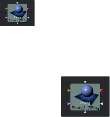
134
3D Material Tools Chapter – 3
Phong [3PH]
The Phong tool is a basic illumination material that can be applied to geometry in the 3D scene.
It describes how the object will respond to light, and provides a large number of texture map
inputs to allow fine control over the diffuse, specular and bumpmap components of the material.
While producing a highlight similar to that produced by the Blinn model, it is more commonly
used for shiny/polished plastic surfaces.
External Inputs
Phong.DiffuseTex
[orange, optional] This input will accept a 2D image or a 3D material to be used as a
diffuse texture map.
Phong.SpecularColorTex
[green, optional] This input will accept a 2D image or a 3D material to be used as a
specular color texture map.
Phong.SpecularIntensityTex
[magenta, optional] This input will accept a 2D image or a 3D material to be used as an
intensity map for the material’s specular highlights. When the input is a 2D image, the
alpha channel is used to create the map while the color channels are discarded.
Phong.SpecularExponentTex
[light blue, optional] This input will accept a 2D image or a 3D material to be used as a
falloff map for the material’s specular highlights. When the input is a 2D image, the
alpha channel is used to create the map while the color channels are discarded.
Phong.BumpmapTex
[white, optional] This input will accept a 2D image or a 3D material, then uses the RGB
information as texture-space normals.
Each of these inputs multiplies the pixels in the texture map by the equivalently named
parameters in the tool itself. This provides an effective method for scaling parts of the material.
When tools have as many inputs as this one does it is often difficult to make connections with
any precision. Hold the Option or Alt key down while dragging the output from another tool
over the tool tile, and keep holding Option or Alt when releasing the left mouse button. A small
menu listing all of the inputs provided by the tool will appear. Click on the desired input to
complete the connection.
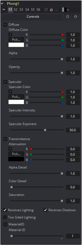
136
3D Material Tools Chapter – 3
The alpha in a diffuse texture map can be used to make portions of the surface of any object
the material is applied to transparent.
Diffuse Color
A material’s Diffuse Color describes the base color presented by the material when it is
lit indirectly or by ambient light. If a diffuse texture map is provided, then the color value
provided here is multiplied by the color values in the texture.
Alpha
This slider sets the material’s Alpha channel value. This affects diffuse and specular
colors equally, and affects the alpha value of the material in the rendered output. If a
diffuse texture map is provided, then the alpha value set here is multiplied by the alpha
values in the texture map.
Opacity
Reducing the material’s Opacity will decrease the color and alpha values of the
specular and diffuse colors equally, making the material transparent.
Specular
The parameters in the Specular section describe the look of the specular highlight of the
surface. These values are evaluated in a different way for each illumination model.
Specular Color
Specular Color determines the color of light that reflects from a shiny surface. The more
specular a material is, the glossier it appears. Surfaces like plastics and glass tend to
have white specular highlights, whereas metallic surfaces like gold have specular
highlights that inherit their color from the material color. If a specular texture map is
provided, then the value provided here is multiplied by the color values from
the texture.
Specular Intensity
Specular Intensity controls how strong the specular highlight is. If the specular intensity
texture is provided, then this value is multiplied by the alpha value of the texture.
Specular Exponent
Specular Exponent controls the falloff of the specular highlight. The greater the value,
the sharper the falloff, and the smoother and glossier the material appears. If the
specular exponent texture is provided, then this value is multiplied by the alpha value
of the texture map.
Transmittance
Transmittance controls the way light passes through a material. For example, a solid blue
sphere will cast a black shadow, but one made of translucent blue plastic would cast a much
lower density blue shadow.
There is a separate Opacity option. Opacity determines how transparent the actual surface is
when it is rendered. Fusion allows for adjusting both opacity and transmittance separately. This
might be a bit counter-intuitive to those who are unfamiliar with 3D software at first. It is possible
to have a surface that is fully opaque but transmits 100% of the light arriving upon it, effectively
making it a luminous/emissive surface.
Attenuation
Attenuation determines how much color is passed through the object. For an object to
have transmissive shadows, set the attenuation to (1, 1, 1), which means 100% of green,
blue, red light pass through the object. Setting this color to RGB (1, 0, 0) means that the
material will transmit 100% of the red arriving at the surface but none of the green or
blue light. This allows for ‘stained glass’ shadows.

137
3D Material Tools Chapter – 3
Alpha Detail
When the Alpha Detail slider is set to 0, the alpha channel of the object is ignored and
the entire object casts a shadow. If it is set to 1, the alpha channel determines what
portions of the object cast a shadow.
Color Detail
The Color Detail slider modulates light passing through the surface by the diffuse color
+ texture colors. Use this to throw a shadow that contains color details of the texture
applied to the object. Increasing the slider from 0 to 1 brings in more of diffuse color +
texture color into the shadow. Note that the alpha and opacity of the object is ignored
when transmitting color, allowing an object with a solid alpha to still transmit its color to
the shadow.
Saturation
The Saturation slider controls the saturation of the color component transmitted to the
shadow. Setting this to 0.0 will result in monochrome shadows.
Receives Lighting/Shadows
These checkboxes control whether the material is affected by lighting and shadows in
the scene. If turned off, the object will always be fully lit and/or unshadowed.
Two Sided Lighting
This makes the surface effectively two sided by adding a second set of normals facing
the opposite direction on the backside of the surface. This is normally off, to increase
rendering speed, but can be turned on for 2D surfaces or for objects that are not fully
enclosed, to allow the reverse or interior surfaces to be visible as well.
Normally, in a 3D application only the front face of a surface is visible and the back face
is culled, so that if a camera were to revolve around a plane in a 3D application, when it
reached the backside, the plane would become invisible. Making a plane two sided in a
3D application is equivalent to adding another plane on top of the first but rotated by
180 degrees so the normals are facing the opposite direction on the backside. Thus,
when you revolve around the back, you see the second image plane, which has its
normals facing the opposite way.
Fusion does exactly the same thing as 3D applications when you make a surface two
sided. The confusion about what two sided does arises because Fusion does not cull
backfacing polygons by default. If you revolve around a one-sided plane in Fusion, you
will still see it from the backside (but you are seeing the frontside duplicated through to
the backside as if it were transparent). Making the plane two sided effectively adds a
second set of normals to the backside of the plane.
Material ID
This slider sets the numeric identifier assigned to this material. This value will be
rendered into the MatID auxiliary channel if the according option is enabled in
the renderer.
NOTE: This can become rather confusing once you make the surface
transparent, as the same rules still apply and produce a result, which is
counter-intuitive. If you view from the frontside a transparent two-sided
surface illuminated from the backside, it will look unlit.
138
3D Material Tools Chapter – 3
Reflect [3RR]
The Reflection tool is used to add environment map reflections and refractions to materials.
Control is offered over the face on and glancing strength, falloff, per channel refraction indexes
and tinting. Several texture map inputs can modify the behavior of each parameter.
The Reflection tool is usually combined with a standard lighting material such as Blinn, Cook
Torrance, Phong or Ward by connecting the output of that tool to the Reflection tool’s
background material input. Then a reflection texture is connected to the reflection texture input.
This can be a 2D image, but is more frequently an environmental map created by the Sphere
Map or Cube Map tools.
Environment mapping is an approximation that assumes an object’s environment is infinitely
distant from the object. It’s best to picture this as a cube or sphere with the object at the center.
In particular, this infinite distance assumption means that objects cannot interact with
themselves (e.g., the reflections on the handle of a teapot will not show the body of the teapot
but rather the infinite environment map). It also means that if you use the same cubemap on
multiple objects in the scene, those objects will not inter-reflect each other (e.g., two
neighboring object would not reflect each other). If you want objects to reflect each other you
need to render a cubemap for each.
For more information see Reflections and Refractions in this manual.
External Inputs
Reflect.BackgroundMaterial
[orange, optional] This input expects a 2D image or a 3D material. If a 2D image is
provided, the tool will treat it as a diffuse texture map applied to a basic material.
Reflect.Reflection.ReflectionTex
[green, optional] This input expects a 2D image or a 3D material. The RGB channels are
used as the reflection texture, and the alpha is ignored.
Reflect.Reflection.ReflectionIntensityTex
[magenta, optional] This input expects a 2D image or a 3D material. The alpha channel
of the texture is multiplied by the intensity of the reflection.
Reflect.Refraction.RefractionTex
[light blue, optional] This input expects a 2D image or a 3D material. The RGB channels
are used as the refraction texture.
Reflect.BumpmapTex
[white, optional] This input will accept a 2D image or a 3D material, then uses the RGB
information as texture-space normals.
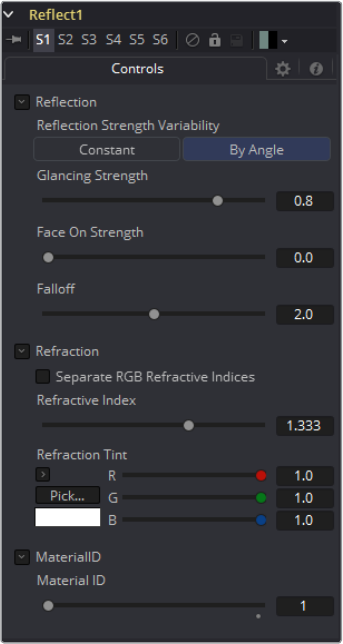
139
3D Material Tools Chapter – 3
Controls
Reflection
Reflection Strength Variability
This multi-button control can be set to Constant or By Angle for varying the reflection
intensity, according to the relative surface orientation to the viewer. The following three
controls are only visible when this control is set to By Angle.
Glancing Strength
[By Angle] Glancing Strength controls the intensity of the reflection for those areas of
the geometry where the reflection faces away from the camera.
Face On Strength
[By Angle] Face On Strength controls the intensity of the reflection for those parts of
the geometry that reflect directly back to the camera.
Falloff
[By Angle] Falloff controls the sharpness of the transition between the Glancing and
Face On Strength regions. It can be considered to be analogous to applying gamma
correction to a gradient between the Face On and Glancing values.
Constant Strength
[Constant Angle] This control is only visible when the reflection strength variability is set
to Constant. In this case, the intensity of the reflection is constant regardless of the
incidence angle of the reflection.
140
3D Material Tools Chapter – 3
Refraction
If the incoming background material has a lower opacity than 1, then it is possible to use an
environment map as refraction texture, and it is possible to simulate refraction effects in
transparent objects.
Separate RGB Refraction Indices
When this checkbox is enabled, the Refraction Index slider will be hidden and three
sliders for adjusting the refraction index of the Red, Green and Blue channels will
appear in its place. This allows for simulation of the spectral refraction effects
commonly seen in thick imperfect glass, for example.
Refraction Index
This slider controls how strongly the environment map will be deformed when viewed
through a surface. The overall deformation is based on the incidence angle. Since this
is an approximation and not a simulation, the results are not intended to model real
refractions accurately.
Refraction Tint
The refraction texture is multiplied by the tint color for simulating color-filtered
refractions. It can be used to simulate the type of coloring found in tinted glass, as seen
in many brands of beer bottles, for example.
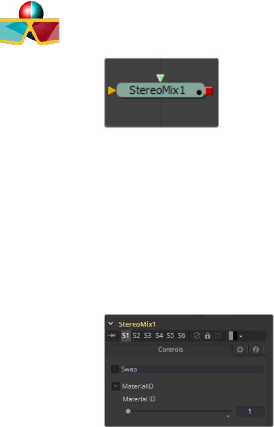
141
3D Material Tools Chapter – 3
Stereo Mix [3SMM]
External Inputs
StereoMix.LeftMaterial
[orange, required] This input will accept a 2D image or a 3D material to be used as the
material for the left eye rendering. If a 2D image is used, it will be converted to a diffuse
texture map using the basic material type.
StereoMix.RightMaterial
[green, required] This input will accept a 2D image or a 3D material to be used as the
material for the right eye rendering. If a 2D image is used, it will be converted to a
diffuse texture map using the basic material type.
While the inputs can be either 2D images or 3D materials, the output will always be
a material.
Controls
Swap
This option will swap both inputs of the tool.
Material ID
This slider sets the numeric identifier assigned to this material. This value will be
rendered into the MatID auxiliary channel if the according option is enabled in
the renderer.
142
3D Material Tools Chapter – 3
Ward [3WD]
The Ward tool is a basic illumination material that can be applied to geometry in the 3D scene. It
describes how the object will respond to light, and provides a large number of texture map
inputs to allow fine control over the diffuse, specular and bumpmap components of the material.
In particular, the Ward tool is ideal for simulating brushed metal surfaces, as the highlight can be
elongated in along the U or V directions of the mapping co-ordinates. This is known as an
Anisotrophic highlight.
The Ward tool outputs a 3D Material that can be connected to the material inputs on any
3Dgeometry tool.
External Inputs
Ward.DiffuseTexture
[orange, optional] This input will accept a 2D image or a 3D material to be used as a
specular color texture map.
Ward.SpecularColorTexture
[green, optional] This input will accept a 2D image or a 3D material to be used as a
specular color texture map.
Ward.SpecularIntensityTexture
[magenta, optional] This input will accept a 2D image or a 3D material to be used as an
intensity map for the material’s specular highlights. When the input is a 2D image, the
alpha channel is used to create the map while the color channels are discarded.
Ward.SpreadUTexture
[light blue, optional] This input will accept a 2D image or a 3D material. The value of the
Spread U option in the tool’s controls will be multiplied against the pixel values in the
material’s alpha channel.
Ward.SpreadVTexture
[white, optional] This input will accept a 2D image or a 3D material. The value of the
Spread V option in the tool’s controls will be multiplied against the pixel values in the
material’s alpha channel.
Ward.BumpmapTexture
[white, optional]This input will accept a 2D image or a 3D material, then uses the RGB
information as texture-space normals.
Each of these inputs multiplies the pixels in the texture map by the equivalently named
parameters in the tool itself. This provides an effective method for scaling parts of the material.
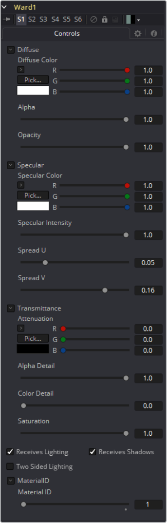
143
3D Material Tools Chapter – 3
When tools have as many inputs as this one does it is often difficult to make connections with
any precision. Hold the Option or Alt key down while dragging the output from another tool
over the tool tile, and keep holding Option or Alt when releasing the left mouse button. A small
menu listing all of the inputs provided by the tool will appear. Click on the desired input to
complete the connection.
Controls
144
3D Material Tools Chapter – 3
Diuse
Diffuse describes the base surface characteristics without any additional effects like reflections
or specular highlights. In addition to defining the base color of an object, the diffuse color also
defines the transparency of the object. The alpha in a diffuse texture map can be used to make
portions of the surface of any object the material is applied to transparent.
Diffuse Color
A material’s Diffuse Color describes the base color presented by the material when it is
lit indirectly or by ambient light. If a diffuse texture map is provided, then the color value
provided here is multiplied by the color values in the texture.
Alpha
This slider sets the material’s Alpha channel value. This affects diffuse and specular
colors equally, and affects the alpha value of the material in the rendered output. If a
diffuse texture map is provided, then the alpha value set here is multiplied by the alpha
values in the texture map.
Opacity
Reducing the material’s Opacity will decrease the color and alpha values of the
specular and diffuse colors equally, making the material transparent.
Specular
The parameters in the Specular section describe the look of the specular highlight of the
surface. These values are evaluated in a different way for each illumination model.
Specular Color
Specular Color determines the color of light that reflects from a shiny surface. The more
specular a material is, the glossier it appears. Surfaces like plastics and glass tend to
have white specular highlights, whereas metallic surfaces like gold have specular
highlights that inherit their color from the material color. If a specular texture map is
provided, then the value provided here is multiplied by the color values from
the texture.
Specular Intensity
Specular Intensity controls how strong the specular highlight is. If the specular intensity
texture is provided, then this value is multiplied by the alpha value of the texture.
Spread U
Spread U controls the falloff of the specular highlight along the U-axis in the UV-Map of
the object. The smaller the value, the sharper the falloff, and the smoother and glossier
the material appears in this direction. If the Spread U texture is provided, then this value
is multiplied by the alpha value of the texture.
Spread V
Spread V controls the falloff of the specular highlight along the V-axis in the UV-Map of
the object. The smaller the value, the sharper the falloff, and the smoother and glossier
the material appears in this direction. If the Spread V texture is provided, then this value
is multiplied by the alpha value of the texture.
145
3D Material Tools Chapter – 3
Transmittance
Transmittance controls the way light passes through a material. For example, a solid blue
sphere will cast a black shadow, but one made of translucent blue plastic would cast a much
lower density blue shadow.
There is a separate Opacity option. Opacity determines how transparent the actual surface is
when it is rendered. Fusion allows for adjusting both opacity and transmittance separately. This
might be a bit counter-intuitive to those who are unfamiliar with 3D software at first. It is possible
to have a surface that is fully opaque but transmits 100% of the light arriving upon it, effectively
making it a luminous/emissive surface.
Attenuation
Attenuation determines how much color is passed through the object. For an object to
have transmissive shadows, set the attenuation to (1, 1, 1), which means 100% of green,
blue, red light pass through the object. Setting this color to RGB (1, 0, 0) means that the
material will transmit 100% of the red arriving at the surface but none of the green or
blue light. This allows for ‘stained glass’ shadows.
Alpha Detail
When the Alpha Detail slider is set to 0, the alpha channel of the object is ignored and
the entire object casts a shadow. If it is set to 1, the alpha channel determines what
portions of the object cast a shadow.
Color Detail
The Color Detail slider modulates light passing through the surface by the diffuse color
+ texture colors. Use this to throw a shadow that contains color details of the texture
applied to the object. Increasing the slider from 0 to 1 brings in more of diffuse color
+texture color into the shadow. Note that the alpha and opacity of the object is ignored
when transmitting color, allowing an object with a solid alpha to still transmit its color to
the shadow.
Saturation
The Saturation slider controls the saturation of the color component transmitted to the
shadow. Setting this to 0.0 will result in monochrome shadows.
Receives Lighting/Shadows
These checkboxes control whether the material is affected by lighting and shadows in
the scene. If turned off, the object will always be fully lit and/or unshadowed.

146
3D Material Tools Chapter – 3
Two Sided Lighting
This makes the surface effectively two sided by adding a second set of normals facing
the opposite direction on the backside of the surface. This is normally off, to increase
rendering speed, but can be turned on for 2D surfaces or for objects that are not fully
enclosed, to allow the reverse or interior surfaces to be visible as well.
Normally, in a 3D application only the front face of a surface is visible and the back face
is culled, so that if a camera were to revolve around a plane in a 3D application, when it
reached the backside, the plane would become invisible. Making a plane two sided in a
3D application is equivalent to adding another plane on top of the first but rotated by
180 degrees so the normals are facing the opposite direction on the backside. Thus,
when you revolve around the back, you see the second image plane, which has its
normals facing the opposite way.
Fusion does exactly the same thing as 3D applications when you make a surface two
sided. The confusion about what two sided does arises because Fusion does not cull
backfacing polygons by default. If you revolve around a one-sided plane in Fusion you
will still see it from the backside (but you are seeing the frontside duplicated through to
the backside as if it were transparent). Making the plane two sided effectively adds a
second set of normals to the backside of the plane.
Material ID
This slider sets the numeric identifier assigned to this material. This value will be
rendered into the MatID auxiliary channel if the according option is enabled in
the renderer.
NOTE: This can become rather confusing once you make the surface
transparent, as the same rules still apply and produce a result that is
counter-intuitive. If you view from the frontside a transparent two-sided
surface illuminated from the backside, it will look unlit.
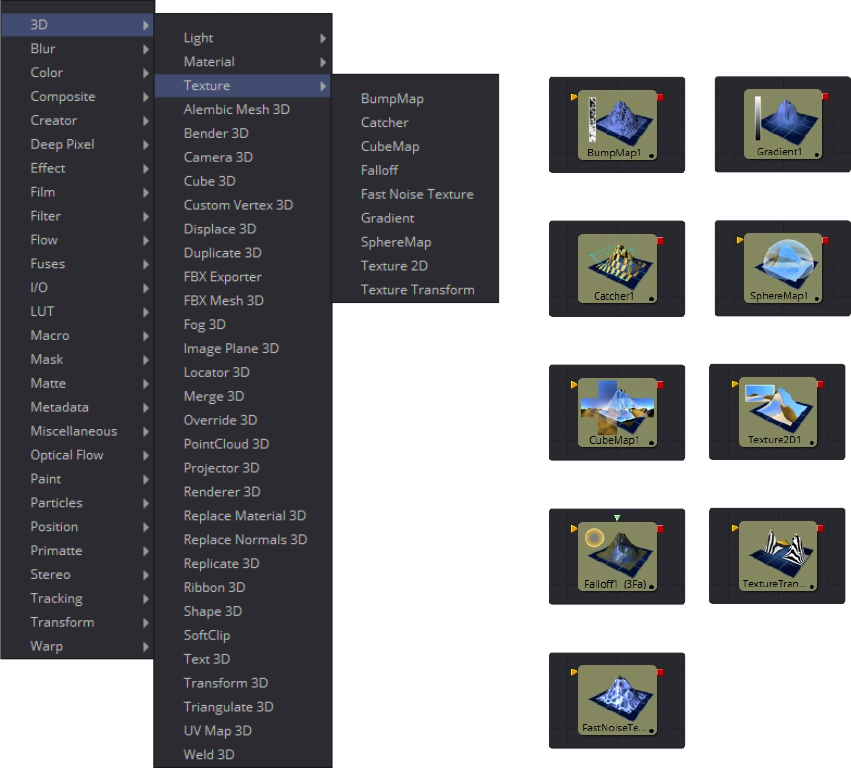
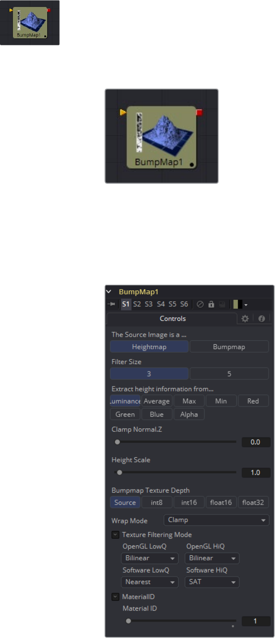
150
3D Texture Tools Chapter – 4
BumpMap [3BU]
The Bumpmap tool either converts a grayscale (heightmap) image into a bump map or takes a
bumpmap created by the Create Bumpmap tool directly. The tool outputs a material.
External Inputs
Bumpmap.ImageInput (white)
Receives the RGBA channels from an image for the
bump calculation or an existing Bumpmap.
Controls
This tab contains all parameters for the tool.
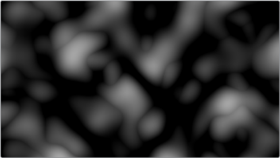
151
3D Texture Tools Chapter – 4
The Source Image is a...
Toggle between Heightmap, which will create a bumpmap similar to the
CreateBumpmap tool, and BumpMap, which expects a bumpmap created by the
CreateBumpmap tool.
Filter Size
The process of generating the bump information is basically a Custom Filter. This
multi-button control sets the filter size.
Extract height information from...
Set the channel from where to extract the grayscale information.
Clamp Normal.Z
Clips the lower values of the Blue channel in the resulting bump texture.
Filter Wrap Mode
Basically “wraps” the image at the borders, so the filter produces correct result when
using seamless tileable textures.
Height Scale
Changes the contrast of the resulting values in the bump map. Increasing this value
yields in a more visible bump map.
Bumpmap Texture Depth
Optionally converts the resulting bump texture into the desired bit depth.
Notes on Bumpmaps
There is some confusion of terminology with bumpmapping, depending on which papers/
books/people you are reading/talking to. Here are Fusion conventions:
Heightmap
A grayscale image containing a height value per pixel
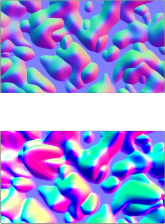
152
3D Texture Tools Chapter – 4
Bumpmap
An image containing normals stored in the RGB channels used for
modifying the existing normals (usually given in tangent space)
Normalmap
An image containing normals stored in the RGB channels used for
replacing the existing normals (usually given in tangent or object space)
153
3D Texture Tools Chapter – 4
Catcher [3CA]
The Catcher material is used to “catch” texture-mode projections cast from Projector 3D and
Camera 3D tools. The intercepted projections are converted into a texture map and applied by
the Catcher material to the geometry to which it is connected.
To understand the purpose of the Catcher tool it helps to understand the difference between
light-based projections and texture-based projections. A light-based projection simply adds the
values of the RGB channels in the projected image to the diffuse texture of any geometry that
lies within the projection cone. This makes it impossible to clip away geometry based on the
alpha channel of an image when using light mode projections.
Imagine a scenario where you want to project an image of a building onto an image plane as part
of a set extension shot. You first rotoscope the image to matte out the windows. This will make it
possible to see the geometry of the rooms behind the wall in the final composite. When this
image is projected as light, the alpha channel is ignored, so the matted windows remain opaque.
By connecting the Catcher to the diffuse texture map of the material applied to the image plane,
and then switching the projection from Light or Ambient Light mode to Texture mode, Fusion
knows to apply the projected image as a texture map. When using this technique, the windows
would become transparent, and it would be possible to see the geometry behind the window.
The main advantages of this approach over light projection are that the Catcher can be used to
project alpha onto an object, and it doesn‘t require lighting to be enabled. Another advantage
is that the Catcher is not restricted to the diffuse input of a material, making it possible to project
specular intensity maps, or even reflection and refraction maps.
Note: The Catcher material requires a Projector 3D or Camera 3D tool in the scene, set to
project an image in Texture mode on the object to which the Catcher is connected. Without a
projection, or if the projection is not set to Texture mode, the Catcher will simply make the
object transparent and invisible.
External Inputs
This material tool does not have any external inputs.
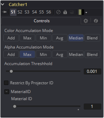
154
3D Texture Tools Chapter – 4
Controls
Enable
Use this checkbox to enable or disable the tool.
Color Accumulation Mode
The Color Accumulation mode is used to control how the Catcher will combine the light
from multiple projectors. It will have no affect on the results when only one projector is
in the scene. This control is designed to work with the Software renderer, and will have
no affect when using the OpenGL renderer.
Alpha Accumulation Mode
The Alpha Accumulation mode is used to control how the Catcher will combine the
Alpha channels from multiple projectors. It will have no affect on the results when only
one projector is in the scene. This control is designed to work with the Software
renderer, and will have no affect when using the OpenGL renderer.
Accumulation Threshold
The Accumulation Threshold can be used to exclude certain low values from the
accumulation calculation. For example, when using the Median Accumulation mode, a
threshold of 0.01 would exclude any pixel with a value of less than 0.01 from the median
calculation.
Restrict by Projector ID
When active, the Catcher will only receive light from Projectors with a matching ID.
Projectors with a different ID will be ignored.
Material ID
This slider sets the numeric identifier assigned to this material. This value will be
rendered into the MatID auxiliary channel if the according option is enabled in
the renderer.
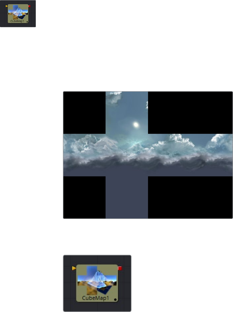
155
3D Texture Tools Chapter – 4
CubeMap [3CU]
The CubeMap tool creates texture maps using separate images for each face of the cube. It can
also extract the individual faces of the cube from a single image containing an unfolded cube in
the Vertical or Horizontal Cross layouts.
A cube map is produced by mounting 6 cameras at 90 degrees angle of views to point up,
down, left, right, front, and back.
The tool provides options to set the reference coordinate system and rotation for the resulting
texture map. The CubeMap tool is typically used to produce environment maps for distant areas
(such as skies or horizons) or reflection and refraction maps.
External Inputs
CubeMap.CrossImage
[white, required] This input is only visible when the tool is set to the Vertical Cross or
Horizontal Cross orientation. It expects a 2D image.
CubeMap.[DIRECTION]
[white, required] These six inputs are only visible when the tool is set to the Separate
Images orientation mode. Each input expects an image aligned to match the left, right,
up, down, front and back faces.
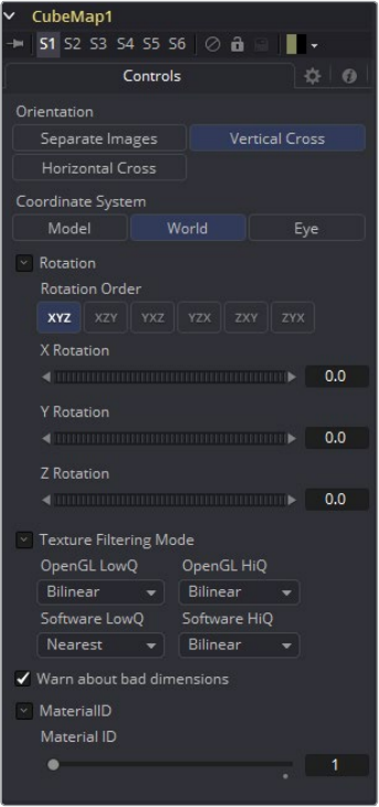
156
3D Texture Tools Chapter – 4
Controls
Orientation
This multi-button control tells the tool which type of input to expect for the cubemap
texture. Valid options are:
Separate Images: This option exposes six inputs on the tool tile, one for each face of
the cube. If the separate images are not square or not of the same size, they will be
rescaled into the largest 1:1 image that can contain all of them.
Vertical Cross: This option exposes a single input on the tool tile. The image should
be an unwrapped texture of a cube containing all the faces organized into a Vertical
Cross formation, where the height is larger than the width. If the image aspect of
the cross image is not 3:4, the Cubemap tool will crop it down so that matches the
appropriate aspect ratio.
Horizontal Cross: This option exposes a single input on the tool tile. The image
should be an unwrapped texture of a cube containing all the faces organized into
a Horizontal Cross formation, where the width is larger than the height. If the image
aspect of the cross image is not 4:3, the Cubemap tool will crop it down so that
matches the appropriate aspect ratio.
157
3D Texture Tools Chapter – 4
Coordinate System
This multi-button control sets the coordinate system used when converting the image
into a texture.
Model: This option orients the texture along the object local coordinate system.
World: This option orients the resulting texture using the global or world
coordinate system.
Eye: This option aligns the texture map to the coordinate system of the camera
or viewer.
Warn about bad dimensions
Selecting this checkbox will print a warning message into the console if the dimensions
of the image provided do not meet the requirements of the selected orientation mode.
Material ID
This slider sets the numeric identifier assigned to this material. This value will be
rendered into the MatID auxiliary channel if the according option is enabled in
the renderer.
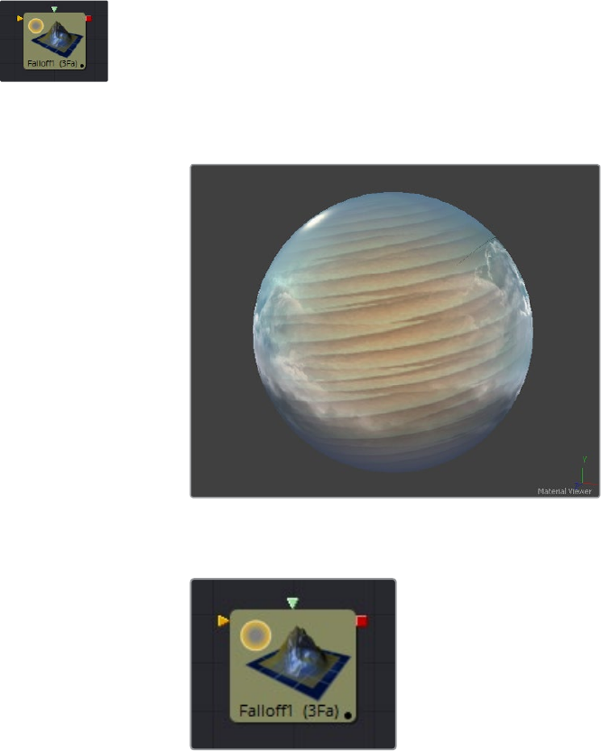
158
3D Texture Tools Chapter – 4
Falloff [3FA]
The Falloff tool blends two materials together based on the incidence angle between the
object the material is applied to and the camera. This is useful when you wish to use one
material for portions of the geometry that would reflect light directly back to the camera and a
different material for parts that reflect light back into the scene.
External Inputs
Falloff.FaceOnMaterial
[orange, optional] This input expects a 2D image or a 3D material. If a 2D image is
provided, it will be turned into a diffuse texture map using the basic material shader.
Falloff.GlancingMaterial
[green, optional] This input expects a 2D image or a 3D material. If a 2D image is
provided, it will be turned into a diffuse texture map using the basic material shader.
While the inputs for this tool can be images, the output will always be a material.
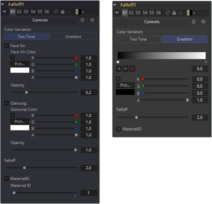
159
3D Texture Tools Chapter – 4
Controls
Color Variation
Two Tone
Two regular Color controls define the colors for Glancing and Face On.
Gradient
A Gradient control defines the colors for Glancing and Face On. This can be used for a
multitude of effects, like creating Toon Shaders, for example.
Face On Color
Face On Color
The Face On Color defines the color of surface parts facing the camera. If the Face On
texture map is provided, then the color value provided here is multiplied by the color
values in the texture.
Face On Opacity
Reducing the material’s Opacity will decrease the color and alpha values of the Face
On material, making the material transparent.
160
3D Texture Tools Chapter – 4
Glancing Color
Glancing Color
The Glancing Color defines the color of surface parts more perpendicular to the
camera. If the Glancing material port has a valid input, then this input is multiplied by
this color.
Glancing Opacity
Reducing the material’s Opacity will decrease the color and alpha values of the
Glancing material, making the material transparent.
Falloff
This value controls the transition between Glancing and Face On strength. It is very
similar to a gamma operation applied to a gradient blending one value into another.
Material ID
This slider sets the numeric identifier assigned to this material. This value will be
rendered into the MatID auxiliary channel if the according option is enabled in
the renderer.
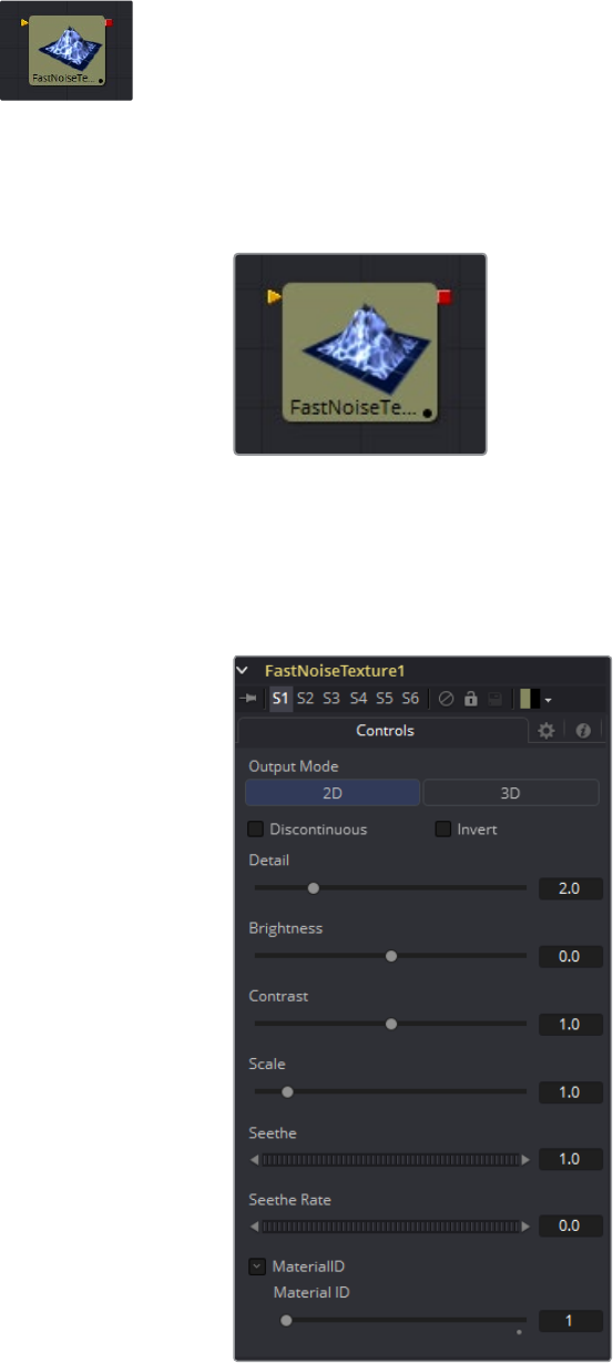
161
3D Texture Tools Chapter – 4
Fast Noise Texture [3FN]
The Fast Noise Texture tool is the procedural resolution-independent version of the 2D Fast
Noise tool. It creates a noise texture directly as a material for usage with 3D tools. It offers a 3D
volumetric mode for creating seamless textures in conjunction with tools providing UVW texture
coordinates (like the UV Map tool set to XYZtoUVW or Camera).
External Inputs
FastNoiseTexture.SourceMaterial
[orange, required] This input will accept a 2D image or a
3D material. This is modulated by the noise pattern.
Controls
162
3D Texture Tools Chapter – 4
Output Mode
2D: Calculates the noise texture based on 2D texture coordinates (UV). This mode
allows smoothly varying the noise pattern.
3D: Calculates the noise texture based on 3D texture coordinates (UVW). Tools like
Shape 3D automatically provide a third texture coordinate, otherwise a 3D texture
space can be created using the UV Map tool. Does not support animation of the
noise pattern.
Discontinuous
Normally, the noise function interpolates between values to create a smooth
continuous gradient of results. Enable this checkbox to create hard discontinuity lines
along some of the noise contours. The result will be a dramatically different effect.
Invert
Select this checkbox to Invert the noise, creating a negative image of the original
pattern. This is most effective when Discontinuous is also enabled.
Detail
Increase the value of this slider to produce a greater level of detail in the noise result.
Larger values add more layers of increasingly detailed noise without affecting the
overall pattern. High values take longer to render but can produce a more natural result
(not all graphics cards support higher detail levels in hardware).
Brightness
This control adjusts the overall Brightness of the noise map.
Contrast
This control increases or decreases the overall Contrast of the noise map. It can
exaggerate the effect of the noise.
Scale
The feature scale of the noise map can be adjusted using the Scale slider, changing it
from gentle variations over the whole image to a tighter overall texture effect. This
value represents the scale along the UV axis.
Scale Z
(3D only) The Scale Z value scales the noise texture along the W-axis in texture space.
Seethe
(2D only) The Seethe control smoothly varies the 2D noise pattern.
Seethe Rate
(2D only) As with the Seethe control above, the Seethe Rate also causes the noise map
to evolve and change. The Seethe Rate defines the rate at which the noise changes
each frame, causing an animated drift in the noise automatically, without the need for
spline animation.
Material ID
This slider sets the numeric identifier assigned to this material. This value will be
rendered into the MatID auxiliary channel if the according option is enabled in
the renderer.
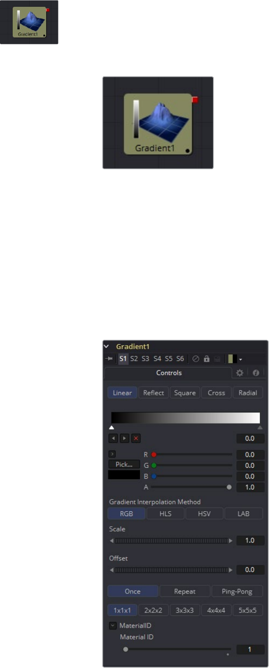
163
3D Texture Tools Chapter – 4
Gradient 3D [3GD]
With the Gradient 3D tool it is possible to texture objects with a variety of gradient types. It
offers many of the controls of the Background tool. While it is not possible to transform the
gradient directly in 3D space, it is orientable using the following tools:
Texture Transform tool
The Texture Transform tool can be used to adjust the mapping per pixel.
UVMap tool
The UV Map tool can be used to adjust the mapping per vertex (use the XYZtoUVW
mode). This has onscreen controls, so you can see what the gradient is doing. Using
this tool is recommended because it is faster to evaluate.
Working with the Gradient tool may be a bit confusing at first. The gradient defaults to a linear
gradient that goes from -1 to +1 along the Z-axis. All primitives in Fusion (Shape 3D) can output a
third texture coordinate for UVW mapping.
Controls
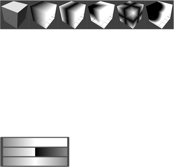
164
3D Texture Tools Chapter – 4
Gradient Type
Determines the type of or pattern used for the gradient.
Linear: A simple linear gradient.
Reflect: Based on the Linear mode, this gradient will be mirrored at the middle of the
textured range.
Square: The gradient is applied using a square pattern.
Cross: Similar to the Reflect mode, but it will use two axes to apply the gradient.
Radial: The Radial mode uses a circular pattern to apply the gradient.
Gradient
The Gradient control consists of a bar where it is possible to add, modify and remove
points of the gradient. Each point has its own color. It is possible to animate the color as
well as the position of the point. Furthermore, a From Image modifier can be applied to
the gradient to evaluate it from an image.
Gradient Interpolation Method
The gradient is linear interpolated from point to point in RGB color space by default.
This can result in unwanted colors sometimes. Choosing another color space may
provide a better result.
Offset
Allows panning through the gradient.
Repeat
Defines how the left and right border of the gradient is treated.
Gradients set to Once, Repeat and Ping Pong from top to
bottom respectively and shifting the gradient to the left.
Once: When using the Gradient Offset control to shift the gradient, the border colors
will keep their values. Shifting the default gradient to the left will result in a white
border on the left, shifting it to the right will result in a black border on the right.
Repeat: When using the Gradient Offset control to shift the gradient, the border
colors will be wrapped around. Shifting the default gradient to the left will result in a
sharp jump from white to black, shifting it to the right will result in a sharp jump from
black to white.
Ping Pong: When using the Gradient Offset control to shift the gradient, the border
colors ping pong back and forth. Shifting the default gradient to the left will result in
the edge fading from white back to black, shifting it to the right will result in the edge
fading from black back to white.
Sub Pixel
Determines the accuracy with which the gradient is created.
Material ID
This slider sets the numeric identifier assigned to this material. This value will be
rendered into the MatID auxiliary channel if the according option is enabled in
the renderer.
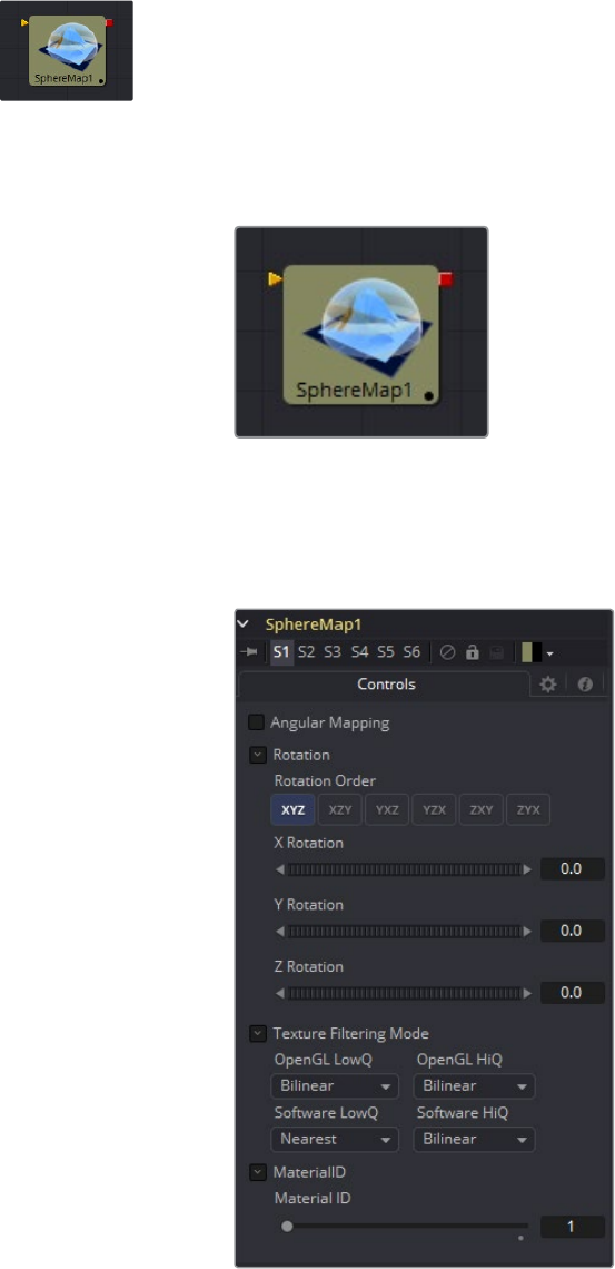
165
3D Texture Tools Chapter – 4
Sphere Map [3SPM]
The Sphere Map tool allows the creation of a spherical texture map from an image. The input
image should represent the texture information in a longitude/latitude format, where the X-axis
represents 0-360 degrees longitude and the Y-axis represents -90 to +90 degrees latitude.
External Inputs
SphereMap.ImageImage
[white, required] Receives the RGBA channels from an image output
Controls
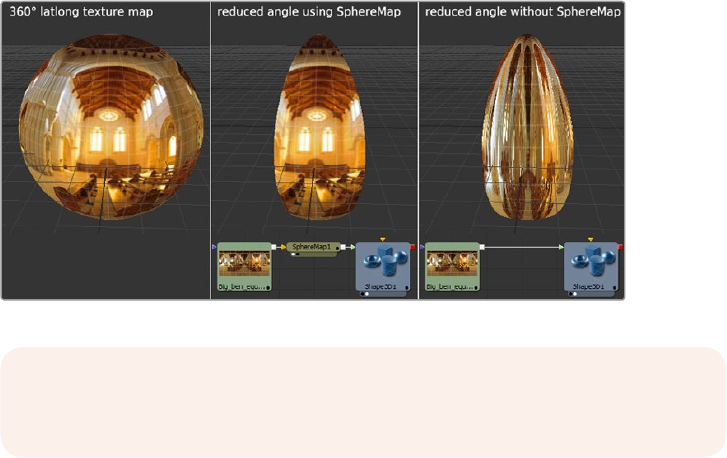
166
3D Texture Tools Chapter – 4
Angular Mapping
Adjusts the texture coordinate mapping so the poles are less squashed and areas in
the texture get mapped to equal areas on the sphere. In other words, it turns the
mapping of the latitude lines from a hemispherical fisheye to an angular fisheye. This
mapping attempts to preserve area and makes it easier to paint on or modify a sphere
map since the image is not as compressed at the poles.
Rotation
Offers controls to rotate the texture map.
Material ID
This slider sets the numeric identifier assigned to this material. This value will be
rendered into the MatID auxiliary channel if the according option is enabled in
the renderer.
The tool expects an image with an aspect ratio of 2:1. Otherwise, the image is clamped
according to the following rules:
2 * width > height
The width is fit onto the sphere and the poles will display clamped edges.
2 * width < height
The height is fit onto the sphere and there will be clamping about the 0 degree
longitude line.
Sphere Map vs. Connecting the Texture to a Sphere Directly
You can connect a latlong (equirectangular) texture map directly to a sphere instead of piping it
through the Sphere Map tool first. This results in a different rendering if you set the start/end
angle and latitude to less than 360°/180°. In the first case, the texture will be squashed. When
using the Sphere Map tool, the texture will be cropped. Compare:
NOTE: If you pipe the texture directly into the sphere, it will also be mirrored
horizontally. You can “fix” this by using a Transform tool first.
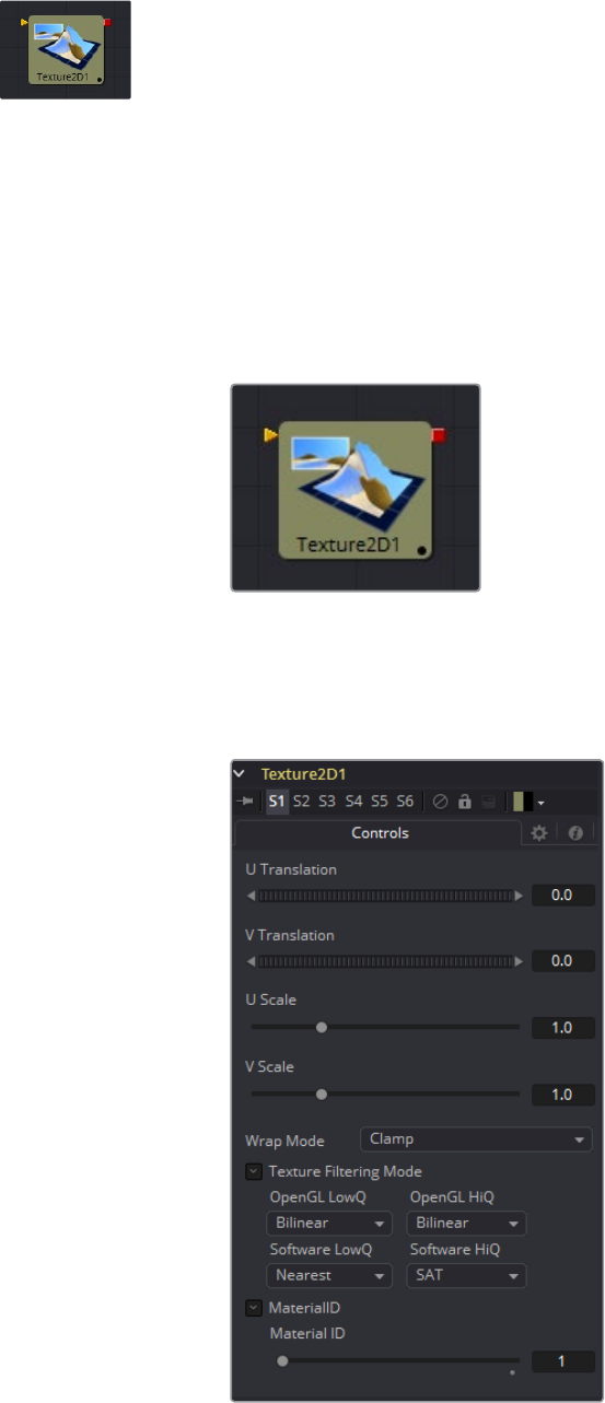
167
3D Texture Tools Chapter – 4
Texture [TXR]
The Texture tool can control the texture mapping of elements in a rendered image. The
Texture-map image (connected to the green input) can be wrapped around objects to replace
the current texture. The Texture tool relies on the presence of U and V Map channels in 3D
rendered images. If these channels are not present, this tool has no effect.
Note: Background pixels may have U and V values of 0.0, which will set those pixels to the color
of the texture’s corner pixel. To restrict texturing to specific objects, use an effect mask based
on the alpha of the object, or its Object or Material ID channel.
For more information, see the Auxiliary Channels chapter.
External Inputs
CreateTexture.ImageInput
[orange, required] This input expects a 2D image.
Controls
168
3D Texture Tools Chapter – 4
Wrap Mode
If a texture is transformed in the texture space (using the controls below or the UV Map
tool), then it´s possible that areas beyond the image borders are mapped on the object.
The Wrap Mode determines how the image is applied in these areas.
Wrap: This wraps the edges of the image around the borders of the image.
Clamp: The color at the edges of the images is used for texturing. This mode is
similar to the Duplicate mode in the Transform tool.
Black: The image is clipped along its edges. A black color with alpha=0 is
used instead.
Mirror: The image is mirrored in both X and Y.
U/V Offset
These sliders can be used to offset the texture along the U and V coordinates.
U/V Scale
These sliders can be used to scale the texture along the U and V coordinates.
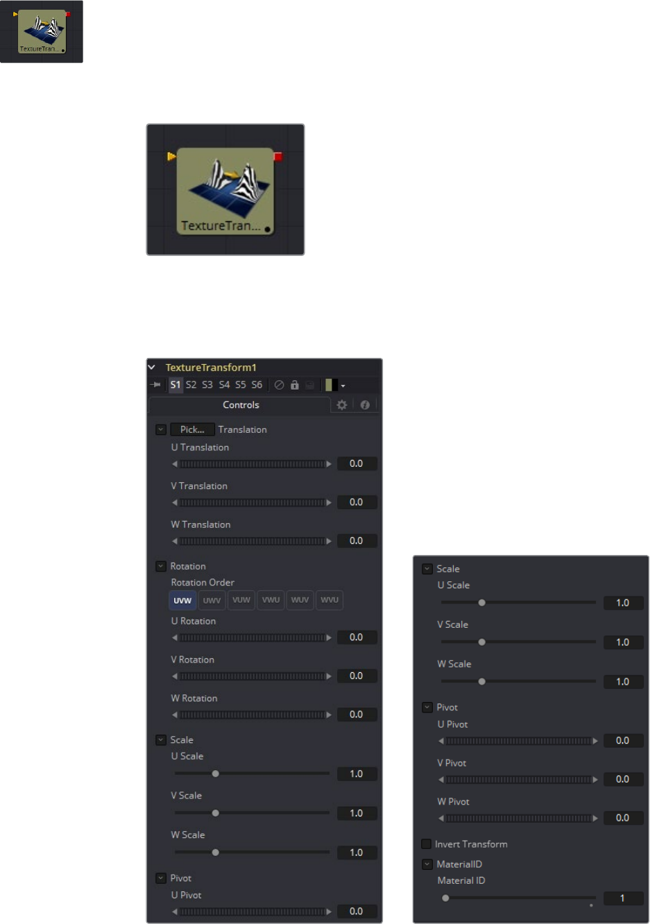
169
3D Texture Tools Chapter – 4
Texture Transform [3TX]
The TextureTransform tool can be used to translate, rotate and scale image textures on the
input material. While the input can also be an image, the output will always be a material.
External Inputs
TextureTransform.MaterialInput
[orange, optional] This input expects a 2D image or 3D material.
Controls

170
3D Texture Tools Chapter – 4
Translation
U, V, W Translation
These sliders will shift the texture along U, V, and W axes.
Rotation
Rotation Order
Use these buttons to set the order in which the rotation is applied.
U, V, W Rotation
In conjunction with the Rotation Order, these settings define the rotation around
the UVW axis.
Scale
U, V, W Scale
Scales the texture along the according UVW axis.
Pivot
U, V, W Pivot
Sets the reference point for rotation and scaling.
Material ID
This slider sets the numeric identifier assigned to this material. This value will be
rendered into the MatID auxiliary channel if the according option is enabled in
the renderer.
NOTE: Not all Wrap modes will be supported by all graphics cards.

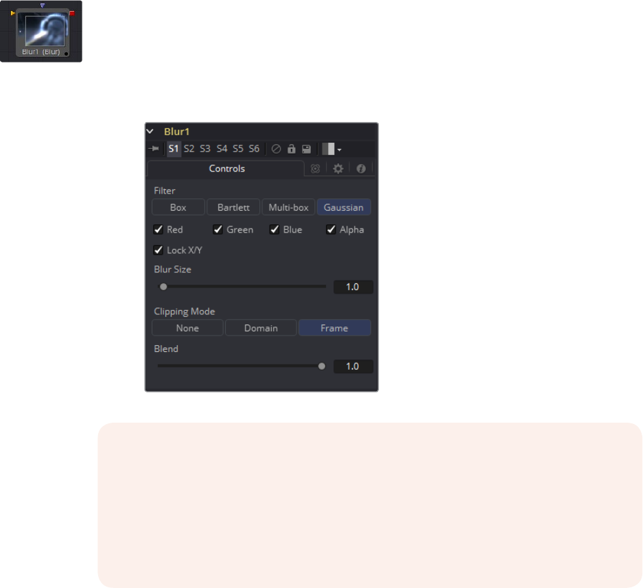
174
Blur Tools Chapter – 5
Blur [Blur]
The Blur tool does exactly what its name implies - it blurs the input image. This is one of the
most commonly used image processing operations.
Controls
NOTE: Since a perfect Gaussian filter would require examining an infinite number of
pixels, all practical Gaussians are, of necessity, approximations. Thealgorithm Fusion
uses is a highly-optimized approach that has many strengths, but can give rise to
visible ringing around the edges in certain extreme cases. This ringing only appears
when blurring float-depth images and is normally far below the limits of visibility,
especially in final renders or HiQ mode, but may appear in subsequent processing.
Ifyou experience this, selecting the Multi-Box filter may be a viable alternative.

175
Blur Tools Chapter – 5
Filter Type
The Filter Type button array allows for the selection of the filter to be applied to
the image.
Box Blur: This option applies a Box Blur effect to the whole image. This method is
faster than the Gaussian blur but produces a lower quality result.
Soften: Soften applies a general softening filter effect. This filter method is slower
than the Gaussian filter and produces a lower quality result. It is included for
compatibility with older flows only.
Bartlett: Bartlett applies a more subtle, anti-aliased blur filter.
Multi-Box: Multi-Box uses a box filter layered in multiple passes to approximate a
Gaussian shape. With a moderate number of passes (e.g., 4), a high quality blur can
be obtained, often faster than the Gaussian filter and without any ringing.
Gaussian: Gaussian applies a smooth, symmetrical blur filter, using a sophisticated
constant-time Gaussian approximation algorithm. This mode is the default
filter method.
Color Channels (RGBA)
The filter defaults to operating on R, G, B and A channels. Selective channel filtering is
possible by clicking the checkboxes beside each channel to make them active
or inactive
In contrast, the channel controls under the Common Controls tab are applied after the
tool has processed.
Lock X/Y
Locks the X and Y Blur sliders together for symmetrical blurring. This is checked
by default.
Blur Size
Sets the amount of blur applied to the image. When the Lock X and Y control is
deselected, independent control over each axis is provided.
Clipping Mode
This option sets the mode used to handle the edges of the image when performing
domain of definition rendering. This is profoundly important for tools like Blur, which
may require samples from portions of the image outside the current domain.
Frame
The default option is Frame, which automatically sets the tool’s domain of definition to
use the full frame of the image, effectively ignoring the current domain of definition. If
the upstream DoD is smaller than the frame, the remaining area in the frame will be
treated as black/transparent.
Domain
Setting this option to Domain will respect the upstream domain of definition when
applying the tool’s effect. This can have adverse clipping effects in situations where the
tool employs a large filter.
NOTE: This is not the same as the RGBA checkboxes found under the
common controls. The Blur tool takes these selections into account before it
processes the image, so deselecting a channel will cause the tool to skip that
channel when processing, speeding up the rendering of the effect.
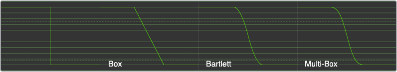
176
Blur Tools Chapter – 5
None
Setting this option to None will not perform any source image clipping at all. This means
that any data required to process the tool’s effect that would normally be outside the
upstream DoD will be treated as black/transparent.
Blend
This is a cloned instance of the Blend slider in the Common Controls tab. Changes
made to this control are simultaneously made to the one in the common controls.
The Blend slider mixes the result of the tool with its input, blending back the effect at
any value less than 1.0.
Examples
This is a comparison of Blur filters visualized as “cross-sections” of a filtered edge. As you can
see, Box will create a linear ramp, while Bartlett creates a somewhat smoother ramp. Multibox
and Gaussian result in even smoother ramps that are virtually indistinguishable unless you
zoom in really close on the slopes. As mentioned above, Gaussian will overshoot slightly and
may result in negative values if used on floating-point images.
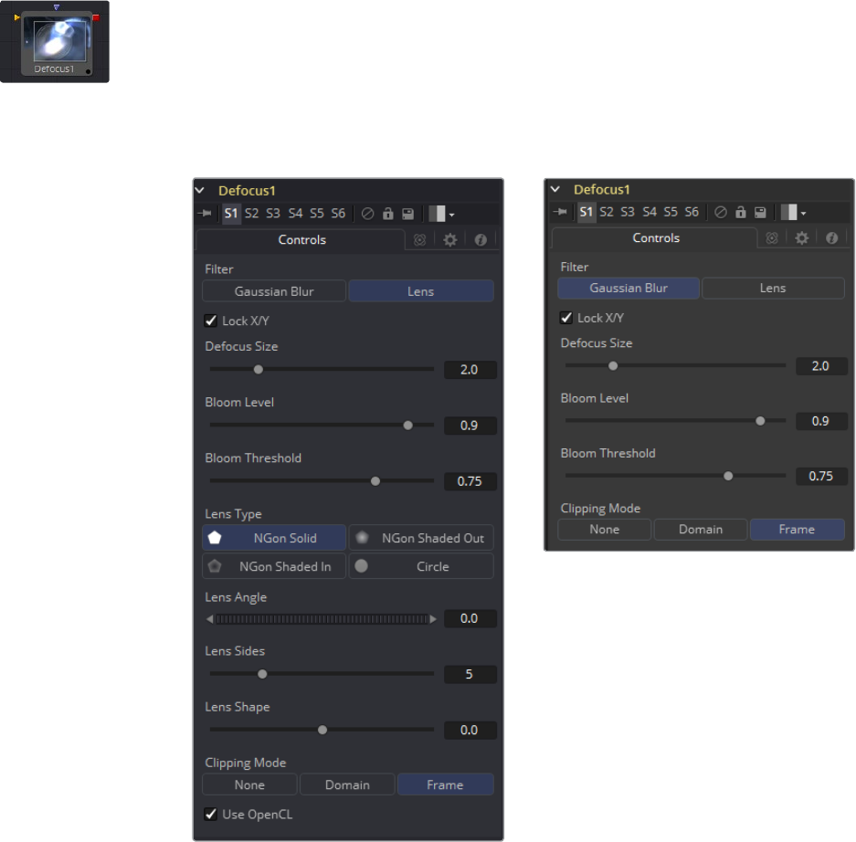
177
Blur Tools Chapter – 5
Defocus [DFO]
The Defocus Tool simulates the effects of an out-of focus camera lens, including blooming and
image flaring. It provides a fast but relatively inaccurate Gaussian mode, as well as a more
realistic but much slower Lens mode.
Controls
Filter
Use this menu to select the exact method applied to create the defocus. Gaussian
applies a fairly simplistic effect, while Lens mode will create a much more realistic
defocus. Lens mode will take significantly longer than Gaussian.
Lock X/Y
When Lock X/Y is selected, this performs the same amount of defocusing to both the
X- and Y-axis of the image. Deselect to obtain individual control.
Defocus Size
The Defocus Size control sets the size of the defocus effect. Higher values blur the
image by greater amounts and produce larger blooms.
178
Blur Tools Chapter – 5
Bloom Level
The Bloom Level control determines the intensity and size of the blooming applied to
pixels that are above the bloom threshold.
Bloom Threshold
Pixels with values above the set Bloom Threshold are defocused and have a glow
applied (blooming). Pixels below that value are only defocused.
Lens Type
The basic shape that is used to create the “bad bokeh” effect. This can be refined
further with the Angle, Sides and Shape sliders.
Lens Angle
Defines the rotation of the shape. Best visible with NGon Lens Types. Due to the round
nature of a circle, this slider will have no visible effect when the Lens Type is set
to Circle.
Lens Sides
Defines how many sides the NGon shapes will have. Best visible with NGon Lens
Types. Due to the round nature of a circle, this slider will have no visible effect when the
Lens Type is set to Circle.
Lens Shape
Defines how pointed the NGons are. Higher values will create a more pointed, starry
look. Lower values create smoother NGons. Best visible with NGon Lens Types and
Lens Sides between 5 and 10. Due to the round nature of a circle, this slider will have
no visible effect when the Lens Type is set to Circle.
Use OpenCL
Introduced with Fusion’s OpenCL Supercomputing, this option renders the effect on
the GPU rather than on the CPU. Depending on the graphics card used in the
computer, this can boost the speed of the tool by a factor of 30 and more.
Clipping Mode
This option sets the mode used to handle the edges of the image when performing
domain of definition rendering. This is profoundly important for tools like Blur, which
may require samples from portions of the image outside the current domain.
Frame
The default option is Frame, which automatically sets the tool’s domain of definition to
use the full frame of the image, effectively ignoring the current domain of definition. If
the upstream DoD is smaller than the frame, the remaining area in the frame will be
treated as black/transparent.
Domain
Setting this option to Domain will respect the upstream domain of definition when
applying the tool’s effect. This can have adverse clipping effects in situations where the
tool employs a large filter.
None
Setting this option to None will not perform any source image clipping at all. This means
that any data required to process the tool’s effect that would normally be outside the
upstream DoD will be treated as black/transparent.
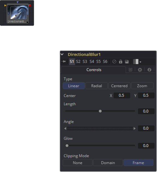
179
Blur Tools Chapter – 5
Directional Blur [DRBL]
This tool is used to create Directional and Radial blurs. It is useful for creating simulated motion
blur and light ray type effects. Directional Blur affects all channels (RGBA).
Controls
Type
This button array is used to select the Type of directional blur to be supplied to
the image.
Linear
Linear distorts the image in a straight line, resembling the scenery that appears in the
window of a speeding train.
Radial
Radial will create a distortion that originates at some arbitrary center, radiating outward
the way that a view would appear if one were at the head of the train looking forward.
Centered
The Centered button produces a similar result to linear, but the blur effect is equally
distributed on both sides of the original.
Zoom
Zoom creates a distortion in the scale of the image smear to simulate the zoom
streaking of a camera filming with a slow shutter speed.
Center X and Y
This coordinate control and crosshair affects the Radial and Zoom Motion blur types
only. It is used to calculate the position from where the blurring effect starts.
Length
Length adjusts the strength and heading of the effect. Values lower than zero cause
blurs to oppose the angle control. Values greater than the slider maximum may be
typed into the slider’s edit box.
180
Blur Tools Chapter – 5
Angle
In both Linear modes, this control will modify the direction of the directional blur. In the
Radial and Zoom modes, the effect will be similar to that of the camera spinning while
looking at the same spot. If the setting of the length slider is other than 0, the effect will
create a whirlpool effect.
Glow
This will add a Glow to the directional blur, which can be used to duplicate the effect of
increased camera exposure to light caused by longer shutter speeds.
Clipping Mode
This option sets the mode used to handle the edges of the image when performing
domain of definition rendering. This is profoundly important for tools like Blur, which
may require samples from portions of the image outside the current domain.
Frame
The default option is Frame, which automatically sets the tool’s domain of definition to
use the full frame of the image, effectively ignoring the current domain of definition. If
the upstream DoD is smaller than the frame, the remaining area in the frame will be
treated as black/transparent.
Domain
Setting this option to Domain will respect the upstream domain of definition when
applying the tool’s effect. This can have adverse clipping effects in situations where the
tool employs a large filter.
None
Setting this option to None will not perform any source image clipping at all. This means
that any data required to process the tool’s effect that would normally be outside the
upstream DoD will be treated as black/transparent.
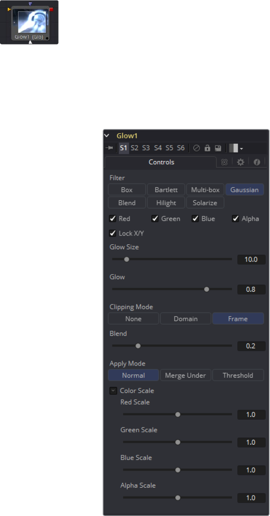
181
Blur Tools Chapter – 5
Glow [GLO]
A Glow is basically created by blurring an image, then brightening the blurred result and mixing
it back with the original.
The Glow tool provides a more convenient way to accomplish this effect, as well as a variety of
variations on the theme. For example, a Bartlett glow is a high quality glow with smoother drop
off, however, it is more processor-intensive at larger sizes.
Controls
Filter
Use these buttons to select the method of Blur used in the filter. The selections are
described below.
Box
A simple but very fast Box filter.
Bartlett
Bartlett adds a softer, subtler glow with a smoother drop off, but may take longer to
render than Box.
182
Blur Tools Chapter – 5
Multi-box
Multi-box uses a Box filter layered in multiple passes to approximate a Gaussian shape.
With a moderate number of passes (e.g., 4), a high quality blur can be obtained, often
faster than the Gaussian filter, and without any ringing.
Gaussian
Gaussian adds a soft glow, blurred by the Gaussian algorithm. This is the
default method.
Blend
Blend adds a non-linear glow that is evenly visible in the whites and blacks.
Hilight
Hilight adds a glow without creating a halo in the surrounding pixels.
Solarize
Solarize adds a glow and solarizes the image.
Color Channels (RGBA)
The filter defaults to operating on R, G, B and A channels. Selective channel filtering is
possible by clicking the checkboxes beside each channel to make them active
or inactive.
This is not the same as the RGBA checkboxes found under the common controls. The
tool takes these controls into account before it processes. Deselecting a channel will
cause the tool to skip that channel when processing, speeding up the rendering of
the effect.
In contrast, the channel controls under the Common Controls tab are applied after the
tool has processed.
Lock X/Y
When Lock X/Y is checked, both the horizontal and vertical glow amounts will be
locked. Otherwise, separate amounts of blur may be applied to each axis.
Glow Size
Glow Size determines the size of the glow effect. Larger values expand the size of the
glowing highlights of the image.
Num Passes
Only available in Multi-box mode. Larger values result in a smoother distribution of the
effect but also increase render times. It’s good to find that thin line between desired
quality and acceptable render times.
Glow
The Glow slider determines the intensity of the glow effect. Larger values tend to
completely blow the image out to white.
Clipping Mode
This option sets the mode used to handle the edges of the image when performing
domain of definition rendering. This is profoundly important for tools like Blur, which
may require samples from portions of the image outside the current domain.
183
Blur Tools Chapter – 5
Frame
The default option is Frame, which automatically sets the tool’s domain of definition to
use the full frame of the image, effectively ignoring the current domain of definition. If
the upstream DoD is smaller than the frame, the remaining area in the frame will be
treated as black/transparent.
Domain
Setting this option to Domain will respect the upstream domain of definition when
applying the tool’s effect. This can have adverse clipping effects in situations where the
tool employs a large filter.
None
Setting this option to None will not perform any source image clipping at all. This means
that any data required to process the tool’s effect that would normally be outside the
upstream DoD will be treated as black/transparent.
Blend
This is a cloned instance of the Blend slider in the Common Controls tab. Changes
made to this control are simultaneously made to the one in the common controls.
The Blend slider mixes the result of the tool with its input, blending back the effect at
any value less than 1.0.
Apply Mode
Three Apply Modes are available when it comes to applying the glow to the image.
Normal: Default. This mode simply adds the glow directly over top of the
original image.
Merge Under: Merge Under places the glow beneath the image, based on the alpha
channel. Threshold mode permits clipping of the threshold values.
Threshold: This control clips the effect of the glow. A new range slider will appear.
Pixels in the glowed areas with values below the low value will be pushed to black.
Pixels with values greater than high will be pushed to white.
High-Low Range Control: Only available in Threshold mode. Pixels in the glowed
areas with values below the low value will be pushed to black. Pixels with values
greater than high will be pushed to white.
Color Scale (RGBA)
These Scale sliders are normally a reveal control labeled Color Scale. They can be
used to adjust the amount of glow applied to each color channel individually, thereby
tinting the glow.
Glow Pre Mask
The Glow tool supports pre-masking using the glow mask. A Glow Pre Mask filters the
image before applying the glow. The glow is then merged back over the original image.
This is different from a regular effect mask that clips the rendered result.
The glow mask allows the glow to extend beyond the borders of the mask, while
restricting the source of the glow to only those pixels within the mask.
To apply a glow mask, select Glow Mask instead of Effect Mask from the contextual
menu when a glow tool is active. Glow masks are identical to effects masks in every
other respect.
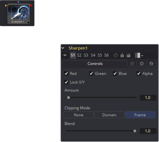
184
Blur Tools Chapter – 5
Sharpen [SHRP]
The Sharpen tool uses a convolution filter to enhance detail in an image.
Controls
Color Channels (RGBA)
The filter defaults to operating on R, G, B and A channels. Selective channel filtering is
possible by clicking the checkboxes beside each channel to make them active
or inactive.
This is not the same as the RGBA checkboxes found under the common controls. The
tool takes these controls into account before it processes, so deselecting a channel will
cause the tool to skip that channel when processing, speeding up the rendering of
the effect.
In contrast, the channel controls under the Common Controls tab are applied after the
tool has processed.
Lock X/Y
This Locks the X and Y Sharpen sliders together for symmetrical sharpening. This is
checked by default.
Amount
This slider sets the Amount of sharpening applied to the image. When the Lock X/Y
control is deselected, independent control over each axis is provided.
185
Blur Tools Chapter – 5
Clipping Mode
This option sets the mode used to handle the edges of the image when performing
domain of definition rendering. This is profoundly important for tools like Blur, which
may require samples from portions of the image outside the current domain.
Frame
The default option is Frame, which automatically sets the tool’s domain of definition to
use the full frame of the image, effectively ignoring the current domain of definition. If
the upstream DoD is smaller than the frame, the remaining area in the frame will be
treated as black/transparent.
Domain
Setting this option to Domain will respect the upstream domain of definition when
applying the tool’s effect. This can have adverse clipping effects in situations where the
tool employs a large filter.
None
Setting this option to None will not perform any source image clipping at all. This means
that any data required to process the tool’s effect that would normally be outside the
upstream DoD will be treated as black/transparent.
Blend
This is a cloned instance of the Blend slider in the Common Controls tab. Changes
made to this control are simultaneously made to the one in the common controls.
The Blend slider mixes the result of the tool with its input, blending back the effect at
any value less than 1.0.
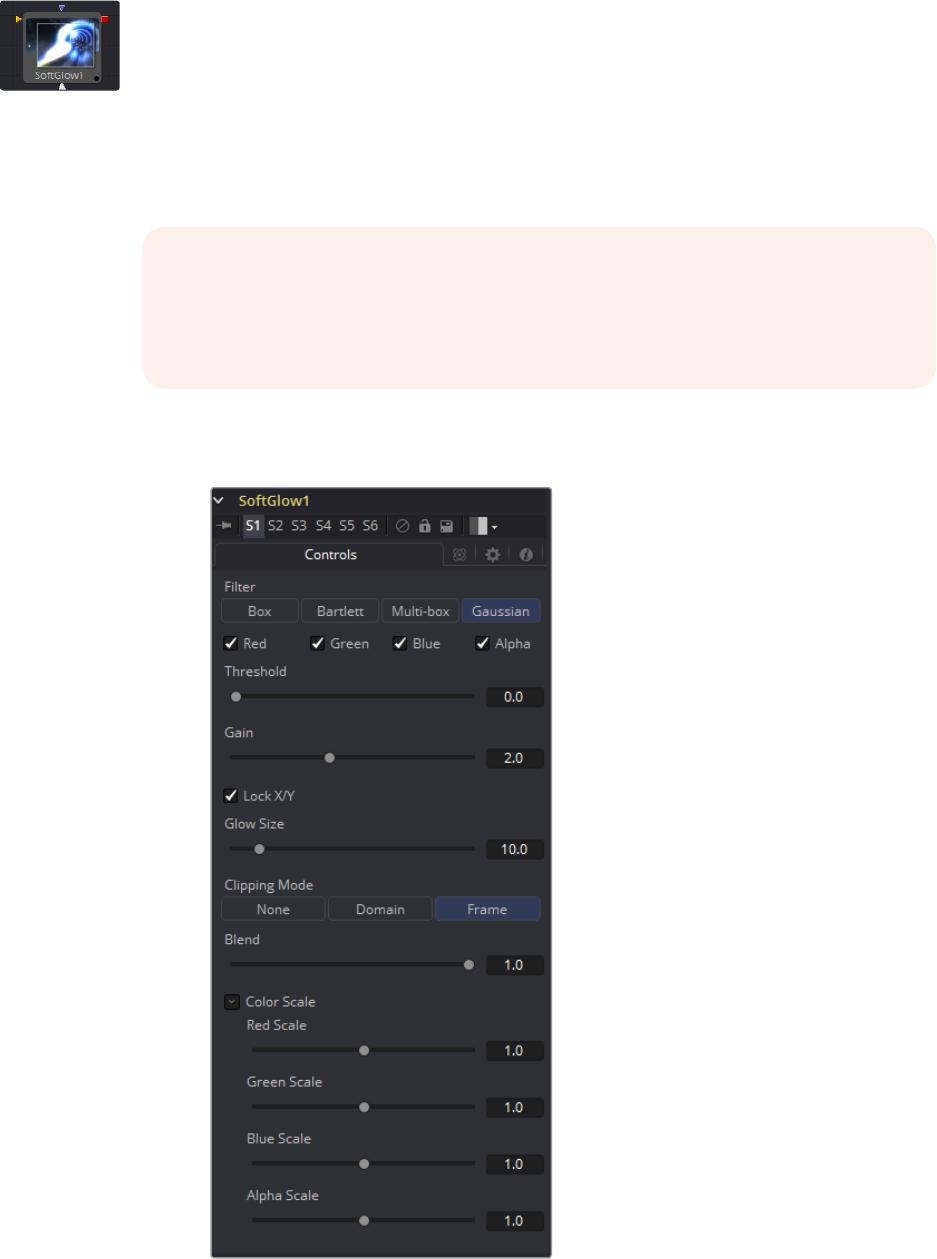
186
Blur Tools Chapter – 5
Soft Glow [SGL]
The Soft Glow tool is similar to the Glow tool but performs additional processing of the image to
create a much softer, more natural glow.
This tool is perfect for atmospheric haze around planets, skin tones, and simulating dream-like
environments.
Controls
The glow mask allows the glow to extend beyond the borders of the mask, while restricting the
source of the glow to only those pixels within the mask.
NOTE: The Glow tool supports pre-masking using the Glow Pre Mask input on the tool
tile. A pre-mask limits the image before applying the glow. The glow is then is
combined with the original image. This is different from a regular effect mask that limits
the rendered result.
187
Blur Tools Chapter – 5
Filter
Use these buttons to select the method of Blur used in the filter. The selections are
described below.
Box: A simple but very fast Box filter.
Bartlett: Bartlett adds a softer, subtler glow with a smoother drop off, but may take
longer to render than Box.
Multi-Box: Multi-Box uses a box filter layered in multiple passes to approximate a
Gaussian shape. With a moderate number of passes (e.g., 4), a high quality blur can
be obtained, often faster than the Gaussian filter and without any ringing.
Gaussian: Gaussian adds a soft glow, blurred by the Gaussian algorithm. This is the
default method.
Color Channels (RGBA)
The filter defaults to operating on R, G, B and A channels. Selective channel filtering is
possible by clicking the checkboxes beside each channel to make them active
or inactive.
This is not the same as the RGBA checkboxes found under the common controls. The
tool takes these controls into account before it processes, so deselecting a channel will
cause the tool to skip that channel when processing, speeding up the rendering of
the effect.
In contrast, the channel controls under the Common Controls tab are applied after the
tool has processed.
Threshold
This control is used to limit the affect of the soft glow. The higher the threshold, the
brighter the pixel must be before it is affected by the glow.
Gain
The Gain control defines the brightness of the glow.
Lock X/Y
When Lock X/Y is checked, both the horizontal and vertical glow amounts will be
locked. Otherwise, separate amounts of glow may be applied to each axis of the image.
Glow Size
Amount determines the size of the glow effect. Larger values expand the size of the
glowing highlights of the image.
Num Passes
Only available in Multi-box mode. Larger values result in a smoother distribution of the
effect but also increase render times. It’s good to find that thin line between desired
quality and acceptable render times.
Clipping Mode
This option sets the mode used to handle the edges of the image when performing
domain of definition rendering. This is profoundly important for tools like Blur, which
may require samples from portions of the image outside the current domain.
188
Blur Tools Chapter – 5
Frame
The default option is Frame, which automatically sets the tool’s domain of definition to
use the full frame of the image, effectively ignoring the current domain of definition. If
the upstream DoD is smaller than the frame, the remaining area in the frame will be
treated as black/transparent.
Domain
Setting this option to Domain will respect the upstream domain of definition when
applying the tool’s effect. This can have adverse clipping effects in situations where the
tool employs a large filter.
None
Setting this option to None will not perform any source image clipping at all. This means
that any data required to process the tool’s effect that would normally be outside the
upstream DoD will be treated as black/transparent.
Blend
This is a cloned instance of the Blend slider in the Common Controls tab. Changes
made to this control are simultaneously made to the one in the common controls. The
Blend slider mixes the result of the tool with its input, blending back the effect at any
value less than 1.0.
Color Scale (RGBA)
These Scale sliders are normally a reveal control labeled Color Scale. They can be
used to adjust the amount of glow applied to each color channel individually, thereby
tinting the glow.
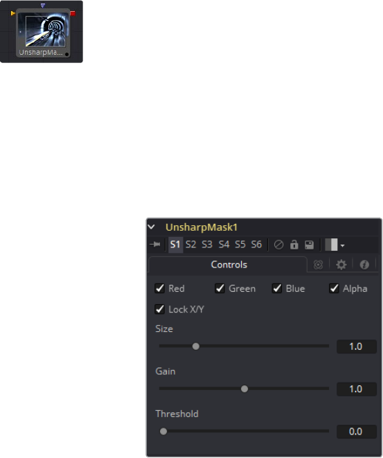
189
Blur Tools Chapter – 5
Unsharp Mask [US]
Unsharp masking is a technique used to sharpen only the edges within an image. This tool is
most often used to correct for blurring and loss of detail in low contrast images, for example, to
extract useful detail from long exposure shots of far-away galaxies.
This filter extracts a range of frequencies from the image and blurs them to reduce detail. The
blurred result is then compared to the original images. Pixels with a significant difference
between the original and the blurred image are likely to be an edge detail. The pixel is then
brightened to enhance it.
Controls
Color Channels (RGBA)
The filter defaults to operating on R, G, B and A channels. Selective channel filtering is
possible by clicking the checkboxes beside each channel to make them active
or inactive.
This is not the same as the RGBA checkboxes found under the common controls.
Thetool takes these controls into account before it processes, so deselecting a
channel will cause the tool to skip that channel when processing, speeding up the
rendering of the effect.
In contrast, the channel controls under the Common Controls tab are applied after the
tool has processed.
Lock X/Y
When Lock X/Y is checked, both the horizontal and vertical sharpen amounts will be
locked. Otherwise, separate amounts of glow may be applied to each axis of the image.
Size
This control adjusts the size of blur filter applied to the extracted image. The higher this
value, the more likely it is that pixels will be identified as detail.
Gain
The Gain control adjusts how much gain is applied to pixels identified as detail by the
mask. Higher values will create a sharper image.
Threshold Low and High
This range control determines the frequencies from the source image to be extracted.
Raising low values will eliminate dark pixels from the comparison. Pixels above the high
value will have the full effect of the gain applied.
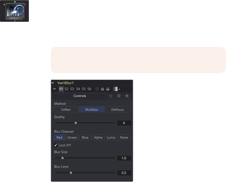
190
Blur Tools Chapter – 5
VariBlur [VBL]
The VariBlur tool gives a true Per-pixel Variable blur, using a second image to control the
amount of blur for each pixel. It is somewhat similar in effect to the Depth Blur tool but uses a
different approach for cleaner results in many cases.
Controls
Method
Soften
This method varies from a simple Box shape to a Bartlett triangle to a decent-looking
Smooth blur as Quality is increased. It is a little better at preserving detail in less-
blurred areas than Multibox.
Multibox
Similar to Soften, this gives a better Gaussian approximation at higher Quality settings.
Defocus
Not really a true defocus, this gives a flat, circular shape to blurred pixels that can
approximate the look of a defocus.
NOTE: The Blur Image input must be connected, or no blurring will be
performed.
191
Blur Tools Chapter – 5
Quality
Increasing Quality gives smoother blurs, at the expense of speed. Quality set to 1 uses
a very fast but simple Box blur for all Method settings. A Quality of 2 is usually sufficient
for low Blur Size values. 4 is generally good enough for most jobs unless Blur Size is
particularly high.
Blur Channel
This selects which channel of the Blur Image controls the amount of blurring applied to
each pixel.
Lock X/Y
When selected, only a Blur Size control is shown and changes to the amount of blur are
applied to both axes equally. If the checkbox is cleared, individual controls appear for
both X and Y Blur Size.
Blur Size
Increasing this control will increase the overall amount of blur applied to each pixel.
Those pixels where the Blur Image is black or non-existent will never be blurred,
regardless of Blur Size.
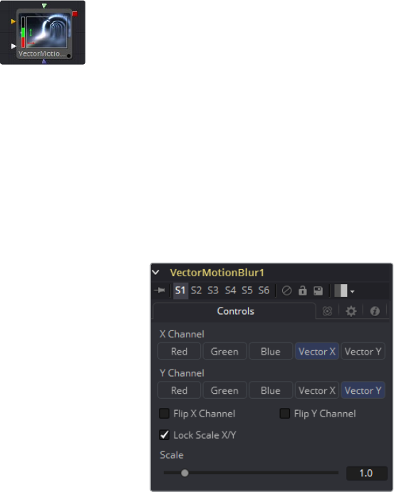
192
Blur Tools Chapter – 5
Vector Motion Blur [VBL]
This tool is used to create Directional blurs based on a Vector Channel.
This tool will perform a 2D blur on the image, using a vector map produced by a 3D application.
The vector map is typically two floating-point images, one channel specifies how far the pixel is
moving in X, and the other specifies how far the pixel is moving in Y. These channels may be
embedded in the image in the case of OpenEXR or RLA/RPF images, or may be provided as
separate images using the tool’s Vectors input.
The vector channels should use a float16 or float32 color depth, to provide + and - values.
Avalue of 1 in the X channel would indicate that pixel has moved one pixel to the right, while a
value of -10 indicates ten pixels of movement to the left.
Controls
X Channel
Use this multi-button array to choose which channel of the image will provide the
vectors for the movement of the pixels along the X-axis.
Y Channel
Use this multi-button array to choose which channel of the image will provide the
vectors for the movement of the pixels along the Y-axis.
Flip X Channel
This checkbox can be used to flip, or invert, the X-vectors. A value of 5 for a pixel in the
X-vector channel would become -5 when this checkbox is selected.
Flip Y Channel
This checkbox can be used to flip, or invert, the Y vectors. A value of 5 for a pixel in the
Y-vector channel would become -5 when this checkbox is selected.
Lock Scale X/Y
Selecting this checkbox will provide access to separate sliders for X and Y Scale. By
default only a single Scale slider is provided.
Scale/Scale X
This slider will be labeled Scale if the Lock Scale X/Y checkbox is not selected, otherwise
it will be labeled Scale X. The vector channel value for a pixel is multiplied by the value of
this slider. For example, given a scale of 2 and a vector value of 10, the result would be 20.
Scale Y
This slider will only appear if the Lock Scale X/Y checkbox is selected. Otherwise, it will
be hidden, and use the same value set in the Scale slider above.
194
Color Tools Chapter – 6
Color Tools
Auto Gain [AG] 196
Brightness Contrast [BC] 197
Channel Boolean [BOL] 199
Color Corrector [CC] 202
Color Curves [CCV] 213
Color Gain [CLR] 216
Color Matrix [CMX] 221
Color Space [CS] 225
Copy Aux [CPA] 227
Gamut [GMT] 230
Hue Curves [HCV] 232
OCIO CDL Transform [OCD] 234
OCIO ColorSpace [OCC] 236
OCIO FileTransform [OCF] 237
Set Canvas Color [SCV] 239
White Balance [WB] 240
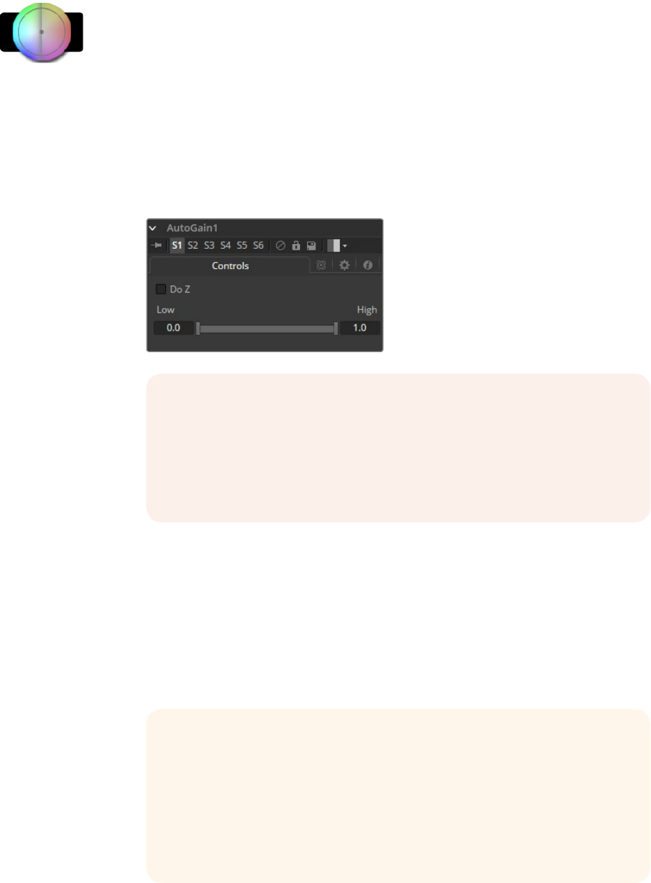
196
Color Tools Chapter – 6
Auto Gain [AG]
The Auto Gain tool is used to automatically adjust the color range of an image so that the
darkest and brightest pixels are set to user-selected values. By default, the darkest pixels in the
image are pushed down to black, the brightest pixels are pushed to white and all of the pixels in
between are stretched to cover the color range evenly.
This can be useful when compensating for variations in lighting, dealing with low contrast
images, or visualizing the full color range of float images (though the Viewer’s View Normalized
Image button is generally more suitable for this).
Controls
Do Z
Select the Do Z checkbox to apply the Auto Gain effect to the Z-channels. This can be
useful for matching the ranges of one Z-channel to another, or to view a float Z-channel
in the RGB values.
Range
This Range control is used to set the lowest and highest possible pixel value in the
image. All color values in the image are rescaled to fit within this range.
NOTE: Variations over time in the input image can cause corresponding
variations in the levels of the result. For example, if a bright object moves out
of an otherwise dark shot, the remaining scene will get suddenly brighter, as
the remaining darker values are stretched to white. This also applies to
sudden depth changes when Do Z is applied; existing objects may be pushed
forward or backward when a near or far object enters or leaves the scene.
Example
Create a horizontal gradient with the Background tool. Set one color to dark
gray (RGBValues 0.2). Set the other color to light gray (RGB Values 0.8).
Add an Auto Gain tool and set the Low value to 0.0 and the High to 0.5. This
will cause the brightest pixels to be pushed down to 0.5 and the darkest
pixels will get pushed to black. The remainder of the pixel values will be
scaled between those limits.
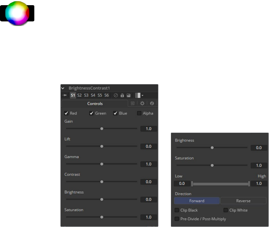
197
Color Tools Chapter – 6
Brightness Contrast [BC]
The Brightness Contrast tool is used to adjust the gain, brightness, contrast, gamma and
saturation of an image. The order of the controls represents the order in which each operation
is applied (for example, gamma is applied before contrast but after gain). The Brightness
Contrast is also reversible using the Forward and Reverse buttons. So color corrections, once
applied, can be reversed further downstream.
For this to work best, make sure that your image is processed in 32bit floating point.
Controls
Color Channels (RGBA)
The filter defaults to operating on R, G, B and A channels. Selective channel filtering is
possible by clicking the checkboxes beside each channel to make them active
or inactive.
This is not the same as the RGBA checkboxes found under the common controls.
Thetool takes these controls into account before it processes, so deselecting a
channel will cause the tool to skip that channel when processing, speeding up the
rendering of the effect.
In contrast, the channel controls under the Common Controls tab are applied after the
tool has processed.
Gain
The pixel values are multiplied by the value of this control. A Gain of 1.2 will make a
pixel that is R0.5 G0.5 B0.4 into R0.6 G0.6, B0.48 (i.e., 0.4 * 1.2 = 0.48). Gain affects
higher values more than it affects lower values, so the effect will be strongest in the
midrange and top range of the image.
198
Color Tools Chapter – 6
Lift
While Gain basically scales the color values around Black, Lift scales the color values
around White. The pixel values are multiplied by the value of this control. A Lift of 0.5
will make a pixel that is R0.0 G0.0 B0.0 into R0.5 G0.5, B0.5, while leaving white pixels
totally unaffected. Lift affects lower values more than it affects higher values, so the
effect will be strongest in the midrange and low range of the image.
Gamma
Values higher than 1.0 will raise the Gamma (mid gray), whereas lower values will
decrease it. The effect of this tool is not linear and existing black or white levels will not
be affected at all. Pure gray colors will be affected the most.
Contrast
Contrast is the range of difference between the light to dark areas. Increasing the value
of this slider will increase the contrast, pushing color from the midrange toward black
and white. Reducing the contrast will cause the colors in the image to move toward
midrange, reducing the difference between the darkest and brightest pixels in
the image.
Brightness
The value of the Brightness slider is added to the value of each pixel in the image. This
control’s affect on an image is linear so the effect will be applied identically to all pixels
regardless of value.
Saturation
This control is used to increase or decrease the amount of Saturation in the image. A
saturation of 0 has no color. All colors are grayscale.
Low and High
This range control is similar to the Gain control in some respects. If Low is anchored at
0.0 and the High value is reduced from 1.0, the effect is identical to increasing the gain.
High values are multiplied by the inverse of the high value. (i.e., if high is 0.75, each
pixel will be multiplied by 1/0.75 or 1.3333).
Leaving the high anchored at 1.0 and increasing the low is exactly the same as inverting
the image colors and increasing the gain and inverting it back again. This pushes more
of the image toward black without affecting the whites at all.
Direction
Forward applies all values normally. Reverse effectively inverts all values.
Clip Black/White
The Clip Black and Clip White checkboxes are used to clip out of range color values
that can appear in an image when processing in floating-point color depth. Out of
range colors are below black (0.0) or above white (1.0). These checkboxes will have no
affect on images processed at 8-bit or 16-bit per channel, as such images cannot have
out of range values.
Pre-Divide/Post-Multiply
Selecting the Pre-Divide/Post-Multiply checkbox will cause the image pixel values to
be divided by the alpha values prior to the color correction, and then re-multiplied by
the alpha value after the correction.
This helps to prevent the creation of illegally additive images, particularly around the
edges of a blue/green key or when working with 3D rendered objects.
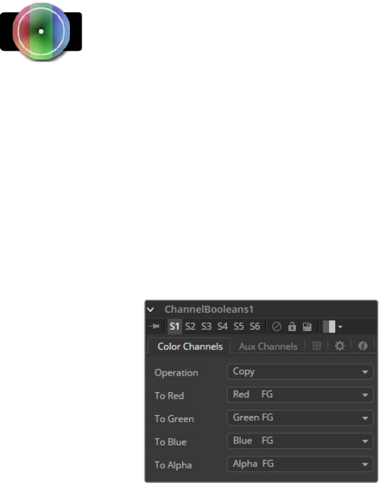
199
Color Tools Chapter – 6
Channel Boolean [BOL]
The Channel Booleans tool can be used to apply a variety of mathematical and logical
operations on the channels in an image. This tool works by using one image’s channels to
modify another image’s channels. If a foreground input is not available, selecting options that
use color channels from the foreground will end up using the background input’s color
channels instead.
On the Color Channels Tab the Tool Controls are Divided as Follows:
On the left side are target channels for the image piped into the Channel Booleans (background
input). The drop down to the right lets you choose whether you want to modify the BG image
with its own channels (suffix BG after list name) or with the channels from another image, which
must be piped into the foreground input on the Channel Booleans node (suffix FG in the
drop-down list).
Controls
Operation Type
This drop-down box is used to select the mathematical method applied to the selected
channels. Its settings are as follows:
Copy
Copy the value from one color channel to another. For example, copy the foreground
red channel into the alpha channel to create a matte.
Add
Add the color values from color channel to channel.
Subtract
Subtract the color values of one color channel from another color channel.
And
Perform a logical AND on the color values from color channel to color channel. The
foreground image will generally remove bits from the color channel of the
background image.
Or
Perform a logical OR on the color values from color channel to color channel. The
foreground image will generally add bits from the color channel of the
background image.
200
Color Tools Chapter – 6
0Exclusive Or
Perform a logical XOR on the color values from color channel to color channel. The
foreground image will generally flip bits from the color channel of the
background image.
Multiply
Multiply the values of a color channel. This will give the appearance of darkening the
image as the values are scaled from 0 to 1. White has a value of 1 so the result would be
the same. Gray has a value of 0.5 so the result would be a darker image or, in other
words, an image half as bright.
Divide
Divide the values of a color channel. This will give the appearance of lightening the
image as the values are scaled from 0 to 1.
Maximum
Compare the two images and take the Maximum, or brightest, values from each image.
Minimum
Compare the two images and take the Minimum, or darkest, values from each image.
Negative
Invert the FG input to make a Negative version of the image.
Solid
Solid sets a channel to a full value of 255. This is useful for setting the alpha to
full value.
Clear
Clear sets a channel to a value of zero. This is useful for clearing the alpha.
Difference
Difference subtracts the greater color values of one color channel from the lesser
values of another color channel.
Signed Add
Signed Add subtracts areas that are lower than mid-gray and add areas that are higher
than mid-gray, which is useful for creating effects with embossed gray images.
To Red, Green, Blue, Alpha
These menus represent the four color channels of the output image. Use the drop-
down menu to select which channel from the source images will be used to produce
the output channel.
The default setting simply copies the channels from the foreground channel. Select any
one of the four color channels, as well as several auxiliary channels like Z-buffer,
saturation, luminance and hue.
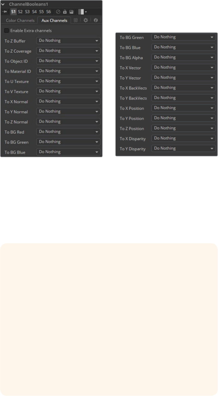
201
Color Tools Chapter – 6
Auxiliary Channels
There are several Auxiliary Channels. Use these menus to select a source for the
auxiliary channels of the output image. See the chapter on 3D Tools for further details
on auxiliary channels.
Enable Extra Channels
When the Enable Extra Channels checkbox is selected, the Channel Boolean tool will
be able to output images with channels beyond the usual RGBA. The remaining
controls in this tab will become active and can be used to copy data into the
auxiliary channels.
Examples: To copy the Alpha channel of one image to its own color channels,
set the Red, Green and Blue channels to Alpha BG. Set the Operation to Copy.
To copy the Alpha channel from another image, set operation type
to Alpha FG.
To replace the existing Alpha channel of an image with the Alpha of another
image choose ‘Do Nothing’ for To Red, To Green, and To Blue and ‘Alpha FG’
for To Alpha. Pipe the image containing the Alpha into the Foreground input
on the Channel Booleans node. Set Operation: ‘Copy.’ The same operation
can also be performed using the Matte Control tool.
To combine any type of mask into an Alpha for an image choose ‘Do Nothing’
for To Red, To Green, and To Blue and ‘Matte’ for To Alpha. Pipe the mask into
the Foreground input on the Channel Booleans node. Set Operation: ‘Copy.’
To subtract the Red channel’s pixels of another image from the Blue channel
choose ‘Do Nothing’ for To Red and To Green and ‘Red FG’ for To Blue. Pipe
the image containing the Red channel to subtract into the Foreground input on
the Channel Booleans node. Set Operation: ‘Subtract.’
202
Color Tools Chapter – 6
Color Corrector [CC]
The Color Corrector tool is a comprehensive color tool with histograms, matching and
equalization, hue shifting, tinting and color suppression. The Color Corrector has two image
inputs. Connect the image to be corrected to the primary input. The secondary input can be
used as a reference for histogram matching.
Overview
Controls in the Color Correction tool are separated into four separate categories: colors, levels,
histogram and suppress. Selecting one of the category buttons from the array at the top of the
Correction tab will cause that category’s controls to appear. Each category is described in
detail below.
Colors Mode
Master/Shadows/Midtones/Highlights
This array of buttons determines the range of colors affected by the controls in this tab.
For example, when the Shadows range is selected, any color adjustments made will
affect only the darker pixels of the image.
The selected state of this button is maintained throughout the Colors, Levels and
Suppress sections of the Color Corrector tool.
Adjustments made to the image in the Master channel are applied to the image after
any changes made to the Highlight, Midtone and Shadow ranges.

203
Color Tools Chapter – 6
Color Wheel
The Color Wheel display provides a visual representation of adjustments made to Hue
and Saturation, as well as any tinting applied to the image. Adjustments can be made
directly on the display, or by entering values in the text boxes to the right of the
Color Wheel.
Hue
The Hue control provides a method of shifting the Hue of the image (or selected color
range) through the color spectrum. The control value has an effective range between
0.0 and 1.0, which represents the angle of rotation in a clockwise direction. A value of
0.25 would be 90 degrees (90/360) and would have the effect of shifting red toward
blue, green to red and so on.
The degree of hue shifting can be entered directly into the text control, or by placing
the mouse above the outer ring of the color control and dragging the mouse up or
down. The outer ring will always show the shifted colors compared to the original colors
shown in the center of the control.
Saturation
The Saturation control is used to adjust the intensity of the color values. A Saturation of
0 produces gray pixels without any chroma or color component, whereas a value of
1.0produces no change in the chroma component of the input image. Higher values will
generate over-saturated values with a high color component.
Saturation values can be entered directly into the text control, or by dragging the
mouse to the left and right on the outer ring of the color wheel control.
Tint/Strength
The Tint control is used to tint an image or selected color range. The values in this
control go from 0 to 1.0, which indicate the angle of the tint color on the color wheel.
Avalue of.25 would indicate 90 degrees, which would be midway between green and
yellow on the color wheel.
The Strength control determines how much tint is applied to the selected range
of colors.
The tinting is represented in the Color Wheel control by small circles that show the
color and strength of the tint. The Highlight Ranges marker is a black outline of a circle.
The Midtones and Shadows are represented by gray circles. The Master Tint Marker is
also black, but it has a white M in the center to distinguish it from the others.
The mouse can position the marker for each range only when the appropriate range is
selected. For example, the Highlight Marker cannot be moved when the Master range
is selected.
Holding down the Command or Ctrl key while dragging this control will allow you to
make finer adjustments by reducing the control’s sensitivity to mouse movements.
Holding the Shift key down will limit the movement of the marker to a single axis,
allowing you to restrict the effect to either tint or strength.
NOTE: The controls are independent for each color range. For example,
adjusting the Gamma control while in Shadows mode will not change or affect
the value of the Gamma control for the Highlights mode. Each control is
independent and applied separately.
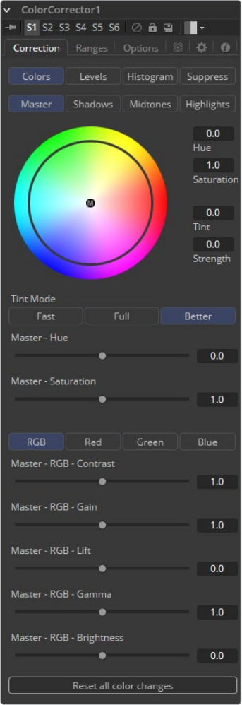
204
Color Tools Chapter – 6
Tint Mode
Fast/Full/Better
These three buttons are used to select the speed and quality of the algorithm used to
apply the tint, hue and saturation adjustments. The default is Better, but for working
with larger images, it may be desirable to use a faster method.
Hue
This slider is a clone of the Hue control shown in the Color Wheel above. The slider
makes it easier to make small adjustments to the value with the mouse
205
Color Tools Chapter – 6
Saturation
This slider is a clone of the Saturation control shown in the Color Wheel above. The
slider makes it easier to make small adjustments to the value with the mouse.
RGB/Red/Green/Blue
These buttons are the same buttons seen in the Histogram, Color and Levels sections
of the Color Corrector tool. When the Red channel is selected, the controls in this tab
will affect the Red channel only, and so on.
The controls are independent, so switching to Blue will not remove or eliminate any
changes made to Red, Green or Master. The animation and adjustments made to each
channel are separate. These buttons simply determine what controls to display.
Master RGB Contrast
Contrast is the range of difference between the light to dark areas. Increasing the value
of this slider will increase the contrast, pushing color from the midrange toward black
and white. Reducing the contrast will cause the colors in the image to move toward
midrange, reducing the difference between the darkest and brightest pixels in
the image.
Master RGB Gain
The pixel values are multiplied by the value of this control. A Gain of 1.2 will make a
pixel that is R0.5 G0.5 B0.4 into R0.6 G0.6, B0.48 (i.e., 0.4 * 1.2 = 0.48). Gain affects
higher values more than it affects lower values, so the effect will be strongest in the
midrange and top range of your image.
Master RGB Lift
While Gain basically scales the color values around Black, Lift scales the color values
around White. The pixel values are multiplied by the value of this control. A Lift of 0.5
will make a pixel that is R0.0 G0.0 B0.0 into R0.5 G0.5, B0.5, while leaving white pixels
totally unaffected. Lift affects lower values more than it affects higher values, so the
effect will be strongest in the midrange and lowrange of the image.
Master RGB Gamma
Values higher than 1.0 will raise the Gamma (mid gray) while lower values will decrease
it. The effect of this tool is not linear, and existing black or white levels will not be
affected at all. Pure grays will be affected the most.
Master RGB Brightness
The value of the Brightness slider is added to the value of each pixel in your image.
This control’s affect on an image is linear, so the effect will be applied identically to all
pixels regardless of value.
Reset All Color Changes
Selecting this button will return all color controls in this section to their default values.
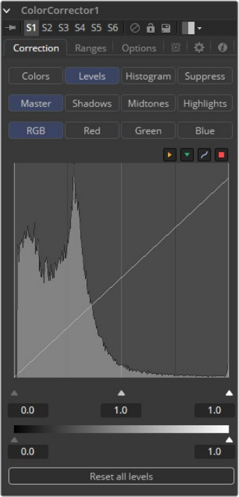
206
Color Tools Chapter – 6
Levels Mode
Master/Shadows/Midtones/Highlights
This array is described in the Colors mode above.
Histogram Control
A Histogram is a chart that represents the distribution of color values in the scene. The
chart reads from left to right, with the leftmost values representing the darkest colors in
the scene and the rightmost values representing the brightest. The more pixels in an
image with the same or similar value, the higher that portion of the chart will be.
Luminance is calculated per channel, therefore, the Red, Green and Blue channels all
have their own histogram and the combined result of these comprise the Master
Histogram.
To scale the histogram vertically, place the mouse pointer inside the control and drag
the pointer up to zoom in or down to zoom out.
RGB/Red/Green/Blue
These buttons are used to select and display the histogram for each color channel or
for the master channel.
Display Selector Toolbar
The Display Selector Toolbar provides a method of enabling and disabling components
of the histogram display. Hold the mouse pointer over the button to display a tooltip
that describes the button’s function.
207
Color Tools Chapter – 6
Input Histogram
This enables or disables the display of the Input image’s histogram.
Reference Histogram
This enables or disables the display of the Reference image’s histogram.
Output Histogram
This enables or disables the display of the histogram from the post color
corrected image.
Corrective Curve
This toggles the display of a spline used to visualize exactly how auto color corrections
applied using a reference image are affecting the image. This can be useful when
equalizing luminance between the input and reference images.
Low/Mid/High
These controls are used to adjust the input image’s histogram, compressing or shifting
the ranges of the selected color channel.
The controls can be adjusted by dragging the triangles beneath the histogram display
to the left and right.
Shifting the high value toward the left (decreasing the value) will cause the histogram to
slant toward white, shifting the image distribution toward white. The low value will have
a similar effect in the opposite direction, pushing the image distribution toward black.
Threshold Output Low/High
The Threshold control can apply clipping to the image, compressing the histogram.
Decreasing the level of the High control will reduce the value of pixels in the image,
sliding white pixels down toward gray and gray pixels toward black.
Adjusting the Low control toward High will do the opposite, sliding the darkest pixels
toward white.
If the low value was set to 0.1, pixels with a value of 0.0 would be set to 0.1 instead, and
all other values would increase to accommodate the change. The best way to visualize
the effect is to observe the change to the output histogram displayed above.
Reset All Levels
Clicking on this button will reset all of the controls in the Levels section to their defaults.
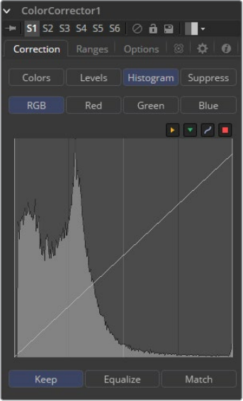
208
Color Tools Chapter – 6
Histogram Mode
This Color Corrector mode produces a Histogram display of the input image. If a reference
image is also provided, the histogram for the reference image is also displayed. The controls in
this tab are primarily used to match one image to another, using either the Equalize or Match
modes of the Color Corrector.
Float Images and Histogram Equalization or Matching
Use the histogram Matching or Equalization methods on a float image and the color
depth of the output image will be converted to 16-bit integer. Two-dimensional
histograms are not well suited to working with the extreme dynamic range of float
images, so these operations will always revert to 16-bit integer processing.
Histogram Control
The Histogram Control is described in detail earlier in this tool documentation, under
the heading of the Levels Mode.
Keep/Equalize/Match Buttons
Each of these buttons enables a different type of color correction operation.
Keep
Keep produces no change to the image and the reference histogram is ignored.
Equalize
Selecting Equalize adjusts the source image so that all of the color values in the image
are equally represented, in essence, flattening the histogram so that the distribution of
colors in the image becomes more even.
Match
The Match mode modifies the source image based on the histogram from the reference
image. It is used to match two shots with different lighting conditions and exposures so
that they will appear similar.
When selected, the Equalize and Match modes reveal the following controls.
209
Color Tools Chapter – 6
Match/Equalize Luminance
This slider affects the degree to which the Color Corrector tool will attempt to affect the
image basedon its luminance distribution. When this control is zero (the default),
matching and equalization are applied to each color channel independently and the
Luminance, or combined value of the three color channels, is not affected.
If this control has a positive value when Equalizing the image, the input image’s
luminance distribution will be flattened before any color equalization is applied.
If this control has a positive value when the correction mode is set to Match, the
luminance values of the input are matched to the reference before any correction is
applied to the R, G and B channels.
The L uminance and RGB controls can have a cumulative effect, and generally they are
not both set to full (1.0) at the same time.
Lock Red/Green/Blue
When this checkbox is selected, color matching will be applied to all color channels
equally. When the checkbox is not selected, individual controls for each channel
will appear.
Equalize/Match Red, Green, Blue
The name of this control changes depending on whether the Equalize or Match modes
have been selected. The slider can be used to reduce the amount of correction applied
to the image to equalize or match it. A value of 1.0 causes the full effect of the equalize
or match to be applied, whereas lower values moderate the result.
8-Bit, 10-Bit, 16-Bit Buttons
This array of buttons determines the level of color fidelity used when sampling the
image to produce the histogram. 10-bit produces higher fidelity than 8-bit, and 16-bit
produces higher fidelity than 10-bit.
Smooth Out Correction Curves
Often, color equalization and matching operations will introduce Posterization in an
image, which occurs because gradients in the image have been expanded or
compressed so that the dynamic range between colors is not sufficient to display a
smooth transition. This control can be used to smooth the correction curve, blending
some of the original histogram back into the result for a more even transition.
Snapshot Match
Click this button to take a freeze the current reference histogram, storing its current state
as a Snapshot in memory. If the reference histogram is not snapshot, the reference
histogram is updated from frame to frame. This can cause flickering and phasing of the
correction as the tool tries to match a changing source to a changing reference.
Release Match
Click on this button to Release the current snapshot of the histogram and return to
using the live reference input.
Reset All Histogram Changes
Selecting this button will remove all changes made to the histogram, returning the
controls to default and setting the mode back to keep.
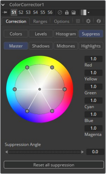
210
Color Tools Chapter – 6
Suppress Mode
Color Suppression provides a mechanism for removing an unwanted color component from the
image. The Color Wheel control is similar to that shown in the Colors section of the tool, but this
one is surrounded by six controls, each representing a specific color along the wheel.
To suppress a color in the selected range, drag the control that represents that color toward the
center of the Color Wheel. The closer the control is to the center, the more that color will be
suppressed from the image.
Suppression Angle
Use the Suppression Angle control to rotate the controls on the suppression wheel and
zero in on a specific color.
Reset All Suppression
Clicking on this control resets the suppression colors to 1.0, the default value.
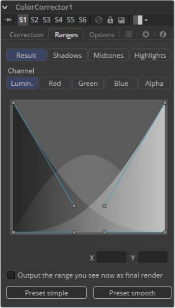
211
Color Tools Chapter – 6
Ranges Tab
The Ranges tab contains the controls used to specify which pixels in an image are considered
to be shadows and which are considered to be highlights. The midrange is always calculated as
any pixels not already included in either the shadows or the highlights.
Result/Shadows/Midtones/Highlights
These buttons are used to select the color range displayed in the Viewers. They help
to visualize the actual pixels that will be included in the range. When the Result button
is selected, the image displayed by the color corrector in the views will be that of the
color corrected image. This is the default.
Selecting one of the other buttons will switch the display to a grayscale image showing
which pixels are part of the selected range. White pixels represent pixels that are
considered to be part of the range and black pixels are not included in the range. For
example, choosing Shadows would show pixels considered to be shadows as white
and pixels that are not shadows as black. Mid gray pixels are only partly in the range
and will not receive the full effect of any color adjustments to that range.
Spline Display
The extent of the ranges is selected by manipulating the spline handles. There are four
spline points, each with one Bezier handle. The two handles at the top represent the
start of the shadow and highlight ranges, whereas the two at the bottom represent the
end of the range. The Bezier handles are used to control the falloff.
The midtones range has no specific controls since its range is understood to be the
space between the shadow and the highlight ranges.
The X and Y text controls below the Spline Display can be used to enter precise
positions for the selected Bezier point or handle.
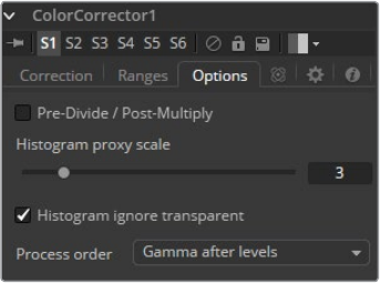
212
Color Tools Chapter – 6
Channel
The Channel selection buttons shown in this tab can be used to examine the range of a
specific color channel. By default, Fusion displays the luminance channel when the
color ranges are examined.
Output the Range You See Now as Final Render
Selecting this checkbox will cause the monochrome display of the range shown in the
Viewers to be output as the final render. Normally, the color tool will output the full
RGBA image, even if the tool was left to display one of the color ranges in the view
instead. This control makes it possible to use the Color Corrector tool to generate a
range’s matte for use as an effect mask in other tools.
Preset Simple/Smooth Ranges
These two buttons can be used to return the spline ranges to either Smooth (default) or
Simple (linear) settings.
Options Mode
Pre-Divide/Post-Multiply
Selecting this option will divide the color channels by the value of the alpha before
applying the color correction. After the color correction, the color values are re-
multiplied by the alpha to produce a properly additive image. This is crucial when
performing an additive merge or when working with CG images generated
against black.
Histogram Proxy Scale
The Histogram Proxy Scale determines the level of precision used when creating and
calculating histograms. Lower values represent higher precision and higher values
produce a rougher, generalized histogram.
Process Order
This menu is used to select whether adjustments to the image’s gamma are applied
before or after any changes made to the images levels.
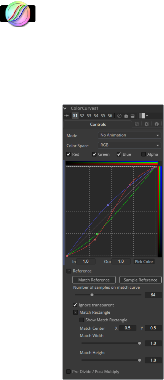
213
Color Tools Chapter – 6
Color Curves [CCV]
The Color Curves tool is a spline-based tool for performing Look Up Table (LUT) color
manipulations. A separate spline is provided for each color channel. The effect can be animated
or dissolved and can be applied to the image using RGB, YUV, YIQ, CMY or HLS color spaces.
The LUT view in the color corrector can be scaled using the + and - keys on the numeric
keypad. The color curves LUT has full support for out of range values, pixels with color values
above 1.0 or below 0.0.
The splines shown in this LUT view are also available from the Spline Editor, should a greater
precision be required when adjusting the controls.
Controls
214
Color Tools Chapter – 6
Mode
The Mode options change between Animated and Dissolve modes. The default mode
is static, where adjustments to the curves are static. Setting the mode provides a
change spline for each channel, allowing the color curve to be animated over time.
Dissolve mode is essentially obsolete and is included for compatibility reasons only.
Color Space
The splines in the LUT view can represent color channels from a variety of Color
Spaces. The default is Red, Green and Blue. The options in this menu allow an alternate
color space to be selected. A detailed description of the color spaces available here
can be found in the online reference documentation for the Color Space tool.
Color Channels (RGBA)
Use the Color Channel controls to select which channel’s spline is currently active for
editing. The labels of these controls will change to reflect the names of the channels for
the current color space. Normally, they will read as Red, Green and Blue. If the Color
Curves tool is operating in YUV color space, they will read as Y, U and V instead.
These controls do not restrict the effect of the tool to a specific channel. They only
select whether the spline for that channel is editable. These controls are most often
used to ensure that adding or moving points on one channel’s spline does not
unintentionally affect a different channel’s spline.
Spline Window
The Spline Window displays splines for each RGBA channel. These can be edited
individually or as a group depending on the color channels selected above.
The Spline default to a linear range, from 0 in, 0 out at the bottom left to the 1 in, 1 out
Top right. In the default a color will process to the same value to the output. If a point is
added in the middle at 0.5 in 0.5 out, and the point is moved up, this will raise the mid
color of the image brighter.
The Spline curves allow for precise control over color ranges, so specific adjustments
can be made without affecting other color values.
In and Out
Use the In and Out controls to manipulate the precise values of a selected point. To
change a value, select a point and enter the in/out values desired.
215
Color Tools Chapter – 6
Pick
Click on the Pick button and select a color from an image in the display to automatically
set keypoints on the spline for the selected color. The new points will be drawn with a
triangular shape and can only be moved vertically (if point is locked, only the Out value
can change).
Points are only added to enabled splines. To add points only on a specific channel,
disable the other channels before making the selection.
One use for this technique is white balancing an image. Use the Pick control to select a
pixel from the image that should be pure gray. Adjust the points that appear so that the
Out value is 0.5 to change the pixel colors to gray.
Use the contextual menu’s Locked Pick Points option to unlock points created using the
Pick option, converting them into normal points.
Match Reference
Clicking on the Match Reference button will automatically set points on the curve to
match an image provided in the second (reference) input of the Color Curves tool.
Sample Reference
Clicking the Sample Reference button will sample the center scanline of the
background image and create a LUT of its color values
Number of Samples on Match Curve
This slider determines how many points are used to match the curve to the range in the
reference image.
Pre-Divide/Post-Multiply
Selecting this checkbox will cause the image’s pixel values to be divided by the alpha
values prior to the color correction, and then re-multiplied by the alpha value after the
correction. This helps to avoid the creation of illegally additive images, particularly
around the edges of a blue/green key or when working with 3D rendered objects.
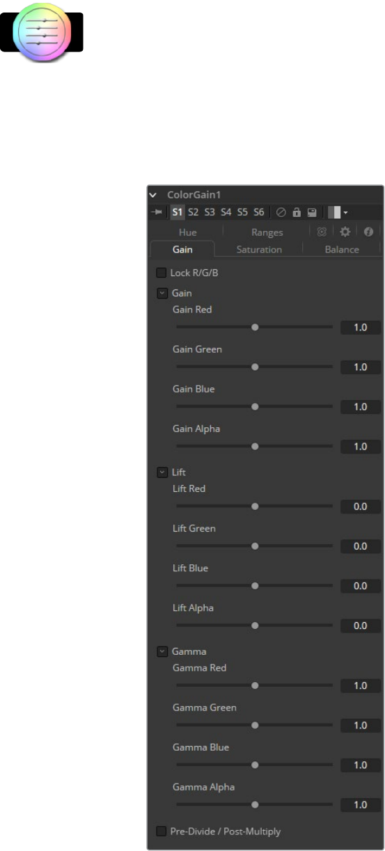
216
Color Tools Chapter – 6
Color Gain [CLR]
The Color Gain tool contains options for adjusting the gain, gamma, saturation and hue of the
image. Many of the controls provided by the Color Gain tool are also found in the Color
Corrector tool, but this simpler tool may render more quickly. One feature that distinguishes the
Color Gain tool from the color corrector is its balance controls. These can be used to adjust the
tinting of the colors in the high, mids and lows.
Gain Tab
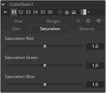
217
Color Tools Chapter – 6
Lock R/G/B
When selected, the Red, Green and Blue channel controls for each effect are combined
into one slider. Alpha channel effects remain separate.
Gain RGBA
The Gain RGBA controls multiply the values of the image channel in a linear fashion.
Allpixels are multiplied by the same factor, but the effect will be larger on bright pixels
and smaller on dark. Black pixels will not be changed (x * 0=0).
Lift RGBA
While Gain basically scales the color values around Black, Lift scales the color values
around White. The pixel values are multiplied by the value of this control. A Lift of 0.5
will make a pixel that is R0.0 G0.0 B0.0 into R0.5 G0.5, B0.5, while leaving white pixels
totally unaffected. Lift affects lower values more than it affects higher values, so the
effect will be strongest in the midrange and lowrange of the image.
Gamma RGBA
The Gamma RGBA controls affect the brightness of the mid-range in the image. The
effect of this tool is non-linear. White and black pixels in the image are not affected
when gamma is modified, whereas pure grays are affected most by changes to this
parameter. Large value changes to this control will tend to push mid-range pixels into
black or white, depending on the value used.
Pre-Divide/Post-Multiply
Selecting this checkbox will cause the image pixel values to be divided by the alpha
values prior to the color correction, and then re-multiplied by the alpha value after the
correction. This helps to avoid the creation of illegally additive images, particularly
around the edges of a blue/green key or when working with 3D rendered objects.
Saturation Tab
RGB Saturation
This setting controls the intensity of the colors in the image channels. A value of 0.0 will
strip all of the color out of an image channel. Values greater than one will intensify the
colors in the scene, pushing them toward primary colors.
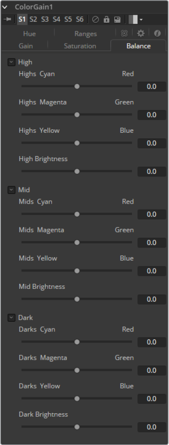
218
Color Tools Chapter – 6
Balance Tab
CMY Brightness Highs/Mids/Darks
This section of the Color Gain tool offers controls for adjusting the overall balance of a
color channel. Independent color and brightness controls are offered for the High,
Midand Dark ranges of the image.
Colors are grouped into opposing pairs from the two dominant color spaces. Red
values can be pushed toward Cyan, Green values to Magenta and Blue to Yellow.
Brightness can be raised or lowered for each of the channels.
By default, the Balance sliders can be adjusted by -1 to +1, but values outside of this
range can be entered manually to increase the effect. A value of 0.0 for any slider
indicates no change to the image channel. Positive and negative values indicate that
the balance of the image channel has been pushed toward one color or the other
in the pair.
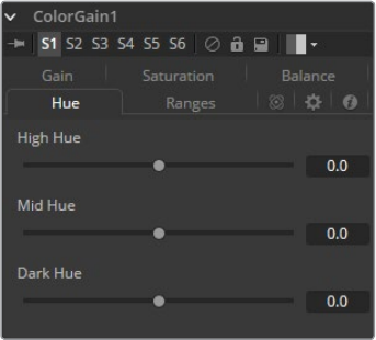
219
Color Tools Chapter – 6
Hue Tab
High/Mid/Dark Hue
Use the Hue section of the Color Gain tool to shift the overall hue of the image, without
affecting the brightness or saturation. Independent control of the High, Mid and Dark
ranges is offered by three sliders.
The following is the order of the hues in the RGB color space Red, Yellow, Green, Cyan,
Blue, Magenta and Red. Values above 0 push the hue of the image toward the right
(red turns to yellow). Values below 0 push the hue toward the left (red turns to
magenta). At -1.0 or 1.0, the hue completes the cycle and returns to its original value.
The default range of the hue sliders is -1.0 to +1.0. Values outside of this range can be
entered manually.
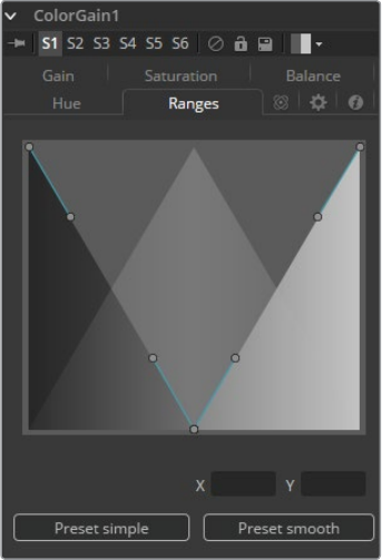
220
Color Tools Chapter – 6
Ranges Tab
The Ranges tab contains the controls used to specify which pixels in an image are considered
to be shadows and which are considered to be highlights. The midrange is always calculated as
any pixels not already included in either the shadows or the highlights.
Spline Display
The extent of the ranges is selected by manipulating the spline handles. There are four
spline points, each with one Bezier handle. The two handles at the top represent the
start of the shadow and highlight ranges, whereas the two at the bottom represent the
end of the range. The Bezier handles are used to control the falloff.
The midtones range has no specific controls since its range is understood to be the
space between the shadow and the highlight ranges. The X and Y text controls below
the Spline Display can be used to enter precise positions for the selected Bezier point
or handle.
Preset Simple/Smooth Ranges
These two buttons can be used to return the spline ranges to either Smooth (default) or
Simple (linear) settings.
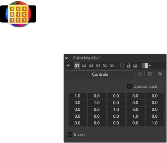
221
Color Tools Chapter – 6
Color Matrix [CMX]
The ColorMatrix allows for a vast number of operations to modify values individually in the
different color channels.
Controls
Update Lock
When this control is selected, Fusion will not render the tool. This is useful for setting up
each value of the tool, then turning Update Lock off in order to render it.
Matrix
This defines what type of operation actually takes place. The horizontal rows define the
output values of the tool, the vertical columns the input values. The “add” column
allows for simple adding of values to the individual color channels. By default the output
values are identical to the input values.
100% of the Red channel input is copied to the Red channel output.
100% of the Green channel input is copied to the Green channel output.
100% of the Blue channel input is copied to the Blue channel output.
100% of the Alpha channel input is copied to the Alpha channel output.
We can also write the default settings as mathematical equations
[R out] = 1 * [R in] + 0 * [G in] + 0 * [B in] + 0 * [A in] + 0
[G out] = 0 * [R in] + 1 * [G in] + 0 * [B in] + 0 * [A in] + 0
[B out] = 0 * [R in] + 0 * [G in] + 1 * [B in] + 0 * [A in] + 0
[A out] = 0 * [R in] + 0 * [G in] + 0 * [B in] + 1 * [A in] + 0
Invert
Enabling this option will invert the Matrix. Think of swapping channels around, doing
other operations with different tools, and then copying and pasting the original
ColorMatrix and setting it to Invert to get your channels back to the original.
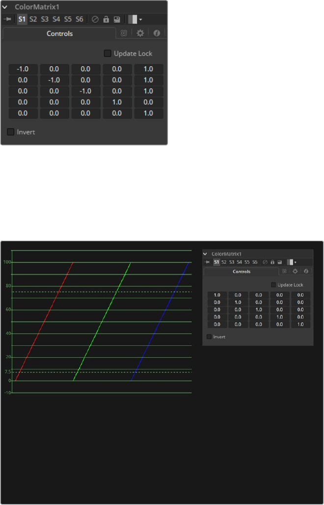
222
Color Tools Chapter – 6
Example 1 – Invert
If we want to do a simple invert or negative of the color values, but keep our Alpha channel as it
is, the matrix would look like this.
Observe the fact that we have to Add 1 to each channel to push the inverted values back into
the positive numbers.
Let’s follow this example step by step by viewing the waveform of a 32-bit grayscale gradient.
01: The original grayscale
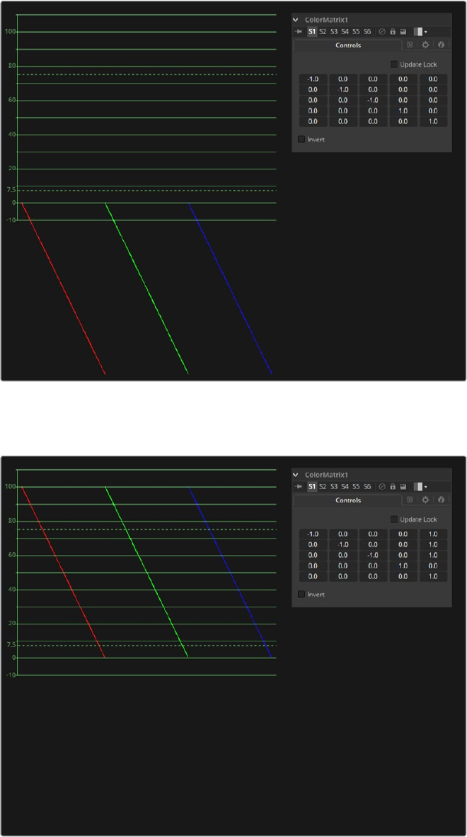
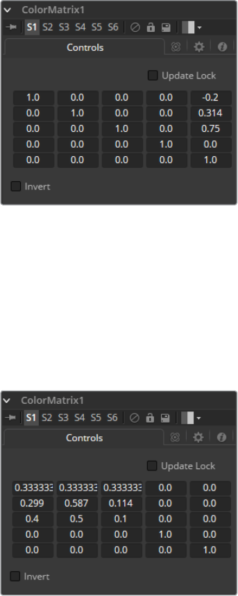
224
Color Tools Chapter – 6
Example 2 – Brightness per Channel
Let’s influence the brightness of each channel individually. This subtracts 0.2 from the Red
channel, adds 0.314 to the Green channel and adds 0.75 to the Blue channel while keeping
Alpha as it is.
Example 3 – Copying Values
Of course we can also copy color values back and forth between individual channels. Let’s
make the Red channel contain the luminance values of the image based on thirds and the
Green channel contain the luminance values based on the proper black-and-white conversion
method, whereas in the Blue channel we use a third method based on getting more information
from Red and less from Blue. We also lower the Blue channel’s brightness by 0.1 and replace
the Alpha Channel with the original Blue channel.
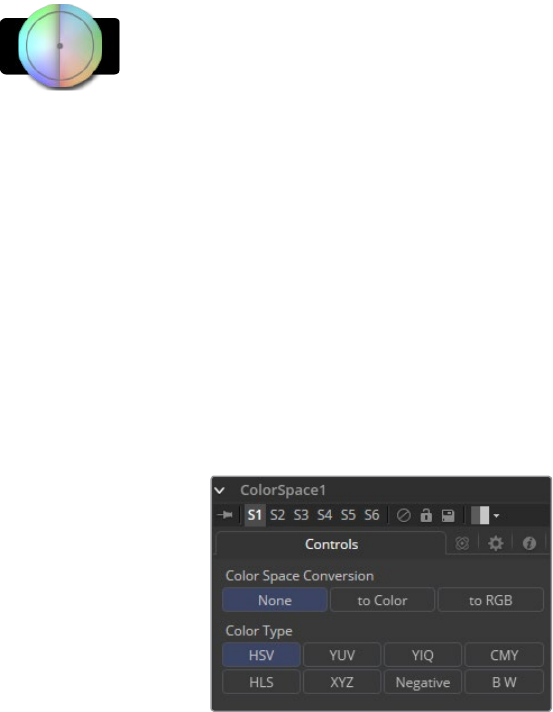
225
Color Tools Chapter – 6
Color Space [CS]
The Color Space tool provides the ability to work on an image in a variety of alternate color
space formats. By default, Fusion uses the RGB color space, and most tools and displays
interpret the primary channels of an image as Red, Green and Blue.
Changing the color space from RGB will cause most images to look odd, as Fusion’s Viewers
will still interpret the primary channels as Red, Green and Blue. For example, viewing an image
converted to YUV in one of the Viewers will show the Y channel as Red, the U channel as
Green and the V channel as Blue.
Several elements of the Fusion interface refer to the RGB channels directly. The four
checkboxes used to restrict the effect of the tool to a single color channel are one example.
When a conversion is applied to an image, the labels of these elements remain R, G and B, but
the values they represent are from the current color space. (Red is Hue, Green is Luminance,
Blue is Saturation for a RGB to HLS conversion. The Alpha value is never changed by the color
space conversion.)
Controls
Color Space Conversion
This button array has three options.
None
The Color Space tool has no effect on the image.
To Color
The input image will be converted to the color space selected in the Color Type control
found below.
To RGB
The input image will be converted back to the RGB color space from the type selected
in the Color Type control below (for example, YUV to RGB).
Color Type
These buttons are used to select the color space conversion applied when the To
Color conversion is selected.
226
Color Tools Chapter – 6
HSV (Hue, Saturation and Value)
Each pixel in the HSV color space is described in terms of its Hue, Saturation and Value
components. Value is defined as the quality by which we distinguish a light color from a
dark one or brightness. Decreasing saturation roughly corresponds to adding white to a
paint chip on a palette. Increasing value is roughly similar to adding black.
YUV (Luma, Blue Chroma and Red Chroma)
The YUV color space is used in the analog broadcast of PAL video. This format is often
used to color correct images, due to its familiarity to a large percentage of video
engineers. Each pixel is described in terms of its Luminance, Blue Chroma and Red
Chroma components.
YIQ (Luma, In Phase and Quadrature)
The YIQ color space is used in the analog broadcast of NTSC video. This format is
much more rare than YUV and almost never seen in production. Each pixel is described
in terms of its Luminance, Chroma (in-phase or red-cyan channel) and Quadrature
(magenta-green) components.
CMY (Cyan, Magenta and Yellow)
Although more common in print, the CMY format is often found in computer graphics
from other software packages. Each pixel is described in terms of its Cyan, Magenta
and Yellow components. CMY is non-linear.
HLS (Hue, Luminance and Saturation)
Each pixel in the HLS color space is described in terms of its Hue, Luminance and
Saturation components. The differences between HLS and HSV color spaces are minor.
XYZ (CIE Format)
This mode is used to convert a CIE XYZ image to and from RGB color spaces. CIE XYZ
is a weighted space, rather than a non-linear one, unlike the other available color
spaces. Non-linear in this context means that equal changes in value at different
positions in the color space may not necessarily produce the same magnitude of
change visually to the eye.
Expressed simply, the CIE color space is a perceptual color system, with weighted
values obtained from experiments where subjects were asked to match an existing
light source using three primary light sources.
This color space is most often used to perform gamut conversion and color space
matching between image display formats because it contains the entire gamut of
perceivable colors.
Negative
The color channels are inverted.The color space remains RGBA.
BW
The image is converted to black and white. The contribution of each channel to the
luminance of the image is adjustable via slider controls that appear when this option is
selected. The default values of these sliders represent the usual perceptual
contribution of each channel to an image’s luminance. The color space of the image
remains RGBA
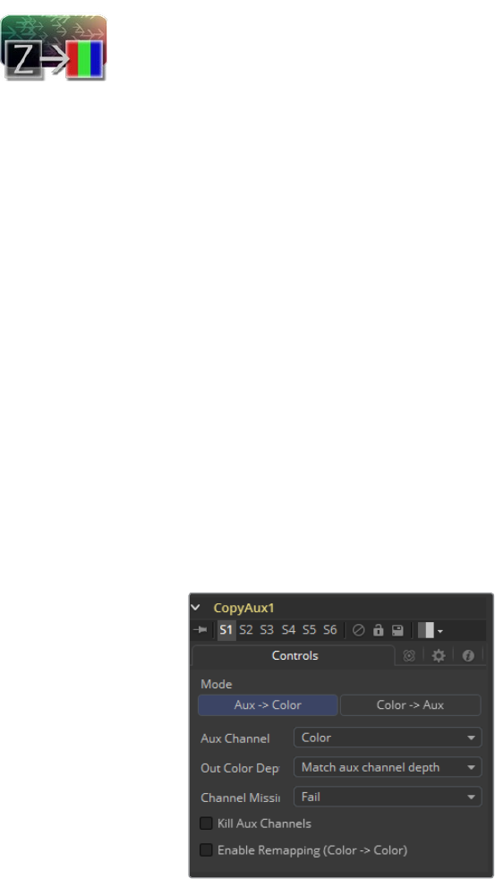
227
Color Tools Chapter – 6
Copy Aux [CPA]
CopyAux copies aux channel groups into RGBA channels. CopyAux is only available in
Fusion Studio.
It is mostly a convenience tool as the copying can also be accomplished with more effort using
a ChannelBoolean tool. Although CopyAux has quite a few options, most of the time you will
only adjust the channel to copy and ignore the rest.
Before Fusion 6.31, to access aux channels you used a ChannelBoolean to copy them into the
RGBA channels. Often this would also involve a ChangeDepth tool to make sure that the RGBA
channels that were receiving the aux channel were float32. Now in Dimension, CopyAux
accomplishes the same result in fewer mouse clicks, allowing you to work faster. Where
ChannelBooleans deals with individual channels, CopyAux deals with channel groups. By
default, the CopyAux tool will automatically promote the depth of its output to match the depth
of the aux channel.
CopyAux also supports static normalization ranges. The advantage of static normalization
versus the dynamic normalization that Fusion’s Viewers do is that colors remain constant over
time. For example, if you are viewing Z or WorldPos values for a ball, you will see a smooth
gradient from white to black. Now imagine that some other 3D object is introduced into the
background at a certain time. Dynamic normalization will turn the ball almost completely white
while the background object is now the new black. Dynamic normalization also causes flicker
problems while viewing vector/disparity channels, which can make it difficult to compare the
aux channels of two frames at different times visually.
Controls
Mode
Mode determines whether the aux channel is copied into the RGBA color channel or
vice versa. Using this option, you can use one CopyAux to bring an aux channel into
color, do some compositing operations on it, and then use another CopyAux to write
the color back in the aux channel. When the Mode is set to “Color>Aux,” all the inputs
except AuxChannel are hidden.
Aux Channel
The Aux Channel is to be copied from or written to depending on the current Mode.
When the aux channel abcd has one valid component, it will be copied as aaa1, two
valid components as ab01, three valid components as abc1, and four components as
abcd. For example, the Z channel will be copied as zzz1, texture coordinates as uv01,
and normals as nxnynz1.
228
Color Tools Chapter – 6
Out Color Depth
Out Color Depth controls the color depth of the output image. Most aux channels
contain float values or, if they are integer valued, they can contain values beyond 255.
When you copy float values into an int8 or int16 image, this can be a problem since
negative values and values over 1.0 can get clipped. In addition, precision can be lost.
This option determines what happens if the depth of RGBA channels of the input image
is insufficient to contain the copied aux channel.
Be careful about copying float channels into integer image formats, as they can get
clipped if you do not set up CopyAux correctly. For the purpose of this tool, all aux
channels are considered to be float32 except ObjectID/MaterialID, which are
considered to be int16.
Match Aux Channel Depth
The bit depth of the RGBA channels of the output image will be increased to match the
depth of the aux channel. In particular, this means that the RGBA channels of the output
image will be either int16 or float32. It is wise to be careful when using this option as, for
example, if you normally have int8 color channels, you will now be using 2x or 4x more
memory for the color channels. In particular, the Z, Coverage, TextureCoordinate,
Normal, Vector, BackVector, WorldPosition, and Disparity channels will always be
output as float and the Material/ObjectID channels will be output as int16.
Match Source Color Depth
The bit depth of the RGBA channels of the output image will be the same as the input
image. This can have some unexpected consequences. For example, if your input
image is int8, the XYZ components of normals which are floating-point numbers in the
[-1, 1] range will be clipped to a non-negative numbers [0, 1] range. As a more extreme
example, consider what will happen to Z values. Z values are floating point numbers
stored in the [-1e30, 0] range and they will all get truncated to the [0, 1] range, which
means your Z channel will be full of zeroes.
Force Float32
The bit depth of the RGBA channels of the output image will always be float32.
Channel Missing
Channel Missing determines what happens if a channel is not present. For example, this
determines what happens if you chose to copy Disparity to Color and your input image
does not have a Disparity aux channel.
Fail
The tool fails and prints an error message to the console.
Use Default Value
This fills the RGBA channels with the default value of zero for everything except Z for
which it is-1e30.
Kill Aux Channels
When this is checked, CopyAux will copy the requested channel to RGBA and then
output a resulting image that is purely RGBA with all other channels being killed. This is
useful if you want to increase the number of frames of CopyAux that can be cached for
playback, for example to play back a long sequence of disparity. A handy tip is that you
can use the “Kill Aux” feature also with just Copy Color > Color for a longer
color playback.
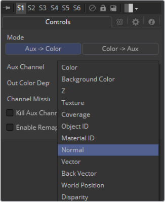
229
Color Tools Chapter – 6
Enable Remapping
When remapping is enabled, the currently selected aux channel will be rescaled,
linearly mapping the range according to the From and To slider selections as explained
below. The Remapping options are applied before the conversion operation. This
means you could set the From. Min/From. Max values to -1, 1 to rescale your normals
into the [0, 1] range, or set them to [-1000, 0] to rescale your Z values from [-1000, 0] into
the [0, 1] range before the clipping occurs.
Note that the Remapping options are per channel options. That means the default scale
for Normals can be set to [-1, +1] > [0, 1] and for Z it can be set [-1000, 0] > [0, 1]. When
you flip between normals and Z, both options will be remembered. One way this could
be useful is that you can set up all of your remapping ranges and save this as a setting
that you can reuse. The remapping can be useful to squash the aux channels into a
static [0, 1] range for viewing or, for example, if you wish to compress normals into the
[0, 1] range in order to store them in an int8 image.
From. Min
This is the value of the aux channel that will correspond to To. Min.
From. Max
This is the value of the aux channel that will correspond to To. Max. It is possible to set
the max value less than the min value to achieve a flip/inversion of the values.
Detect Range
This scans the current image to detect the min/max values and then sets the From. Min/
From. Max Value controls to these values.
Update Range
This scans the current image to detect the min/max values and then enlarges the current
[From. Min, From. Max] region so that it contains the min/max values from the scan.
To. Min
This is the minimum output value, whichdefaults to 0.
To. Max
This is the maximum output value, which defaults to 1.
Invert
After the values have been rescaled into the [To. Min, To. Max] range, this inverts/flips
the range.
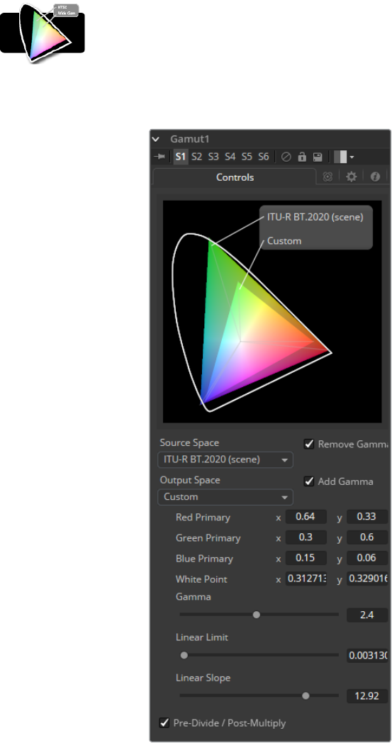

231
Color Tools Chapter – 6
Source Space
Source Space determines the input color space of the image. Leave this at “No
Change” if you want to just add Gamma using the Output Space control.
DCI-P3
The DCI-P3 color space is most commonly used in association with DLP projectors, and
is frequently provided as a color space available with 2K DLP projectors, and as an
emulation mode for 10-bit LCD monitors such as the HP Dreamcolor. This color space is
defined in the SMPTE-431-2 standard.
Custom
The custom gamut allows you to describe the color space according to CIE 1931
primaries and white point, which are expressed as XY coordinates, as well as by
gamma, limit and slope. For example, the DCI-P3 gamut mentioned above would have
the following values if described as a Custom color space.
Red Primary 0.68 0.32
Green Primary 0.265 0.69
Blue Primary 0.15 0.06
White Point 0.314 0.351
Gamma 2.6 –
Linear Limit 0.0313 –
To understand how these controls work you could view the tool attached to a gradient
background in Waveform mode and observe how different adjustments modify
the output.
Output Space
Output Space is the converted gamut to the desired color space. Leave this at No
Change if you want to just remove Gamma using the Source Space control.
Remove/Add Gamma
Select these checkboxes to do the gamut conversion in a linear or non-linear gamma,
or simply remove or add the appropriate gamma values without changing the
color space.
Pre-Divide/Post-Multiply
Selecting this checkbox will cause the image’s pixel values to be divided by the alpha
values prior to the color correction, and then re-multiplied by the alpha value after the
correction. This helps to avoid the creation of illegally additive images, particularly
around the edges of a blue/green key or when working with 3D rendered objects.
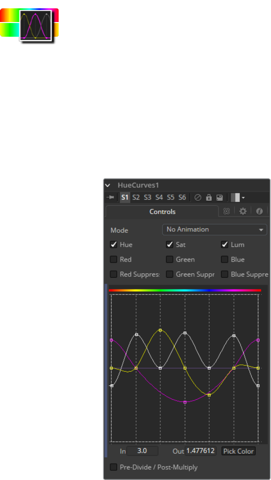
232
Color Tools Chapter – 6
Hue Curves [HCV]
The Hue Curves tool allows you to adjust the color in an image using a series of spline curves.
Splines are provided to control the images Hue, Saturation and Luminance as well as each
individual color channel. An additional set of curves allows you to apply suppression to
individual color channels.
The advantage of the Hue Curves tool over other color correction tools in Fusion is that the
splines can be manipulated to restrict the tools effect to a very narrow portion of the image, or
expanded to include a wide-ranging portion of the image. Additionally, these curves can be
animated to follow changes in the image over time. Since the primary axis of the spline is defined
by the image’s Hue, it is much easier to isolate a specific color from the image for adjustment.
Controls
Mode
The Mode options changes between Animate and Dissolve modes. The default mode
is Static, where adjustments to the curves are applied consistently over time. Setting
the Mode to Animate or Dissolve allows for the color curve to be animated over time.
Dissolve mode is essentially obsolete and is included for compatibility reasons only.
233
Color Tools Chapter – 6
Color Channel Checkboxes
These checkboxes define which Splines are editable and are included in the Pick
Color process.
Any number of activated splines can be edited simultaneously, however in most cases
it’s more convenient to have only the currently modified spline active to avoid
unwanted changes to other splines.
When using the Pick Color button a point will be created on all active splines,
representing the selected color.
Spline Window
This Look Up Table (LUT) control is the main interface element of the Hue Curves tool,
which hosts the various splines. In appearance the tool is very similar to the Color
Curves tool, but in this case the horizontal axis represents the image’s Hue, while the
vertical axis represents the degree of adjustment. The Spline Window shows the
curves for the individual channels. It is basically a miniature Spline Editor. In fact, the
curves shown in this window can also be found and edited in the Spline Editor.
The spline curves for all components are initially flat, with key points placed horizontally
at each of the primary colors. From left to right these are: Red, Yellow, Green, Cyan,
Blue, and Magenta. Due to the cyclical nature of the Hue gradient, the leftmost key
point in each curve is connected to the rightmost key point of the curve.
Right clicking in the LUT Control will display a contextual menu containing options for
resetting the curves, importing external curves, adjusting the smoothness of the
selected key points and more. For detailed information of how a Spline Control works in
general, please consult the Tool Controls chapter of the manual.
In and Out
Use the In and Out controls to manipulate the precise values of a selected point. To
change a value, select a point and enter the in/out values desired.
Pick
Left clicking and dragging from the Pick Color button will change the current mouse
cursor to an eyedropper. While still holding down the left mouse button, drag the cursor
to a Viewer to pick a pixel from a displayed image. This will cause key points, which are
locked on the horizontal axis, to appear on the currently active curves. The key points
will represent the position of the selected color on the curve. Use the contextual
menu’s ‘Lock Selected Points’ toggle to unlock points and restore the option of
horizontal movement.
Points are only added to enabled splines. To add points only on a specific channel,
disable the other channels before making the selection.
Pre-Divide/Post-Multiply
Selecting this checkbox will cause the image’s pixel values to be divided by the alpha
values prior to the color correction, and then re-multiplied by the alpha value after the
correction. This helps to avoid the creation of illegally additive images, particularly
around the edges of a blue/green key or when working with 3D rendered objects.
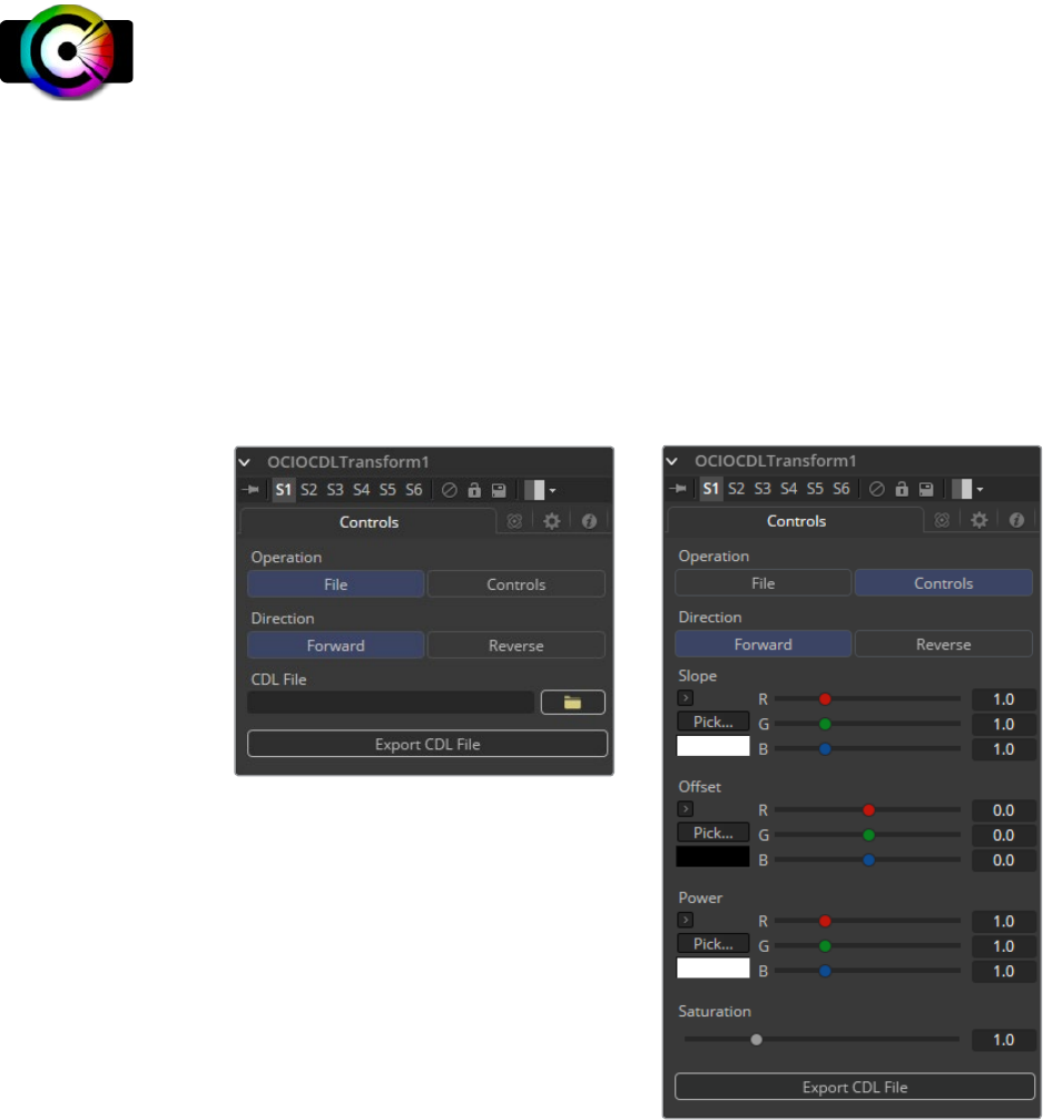
234
Color Tools Chapter – 6
OCIO CDL Transform [OCD]
Fusion supports the Open Color IO workflow specified by Sony Imageworks. In general, the
color pipeline is made up from a set of color transformations defined by OCIO-specific config
files, commonly named with a “.ocio” extension, which allows users to easily share color
settings within or between facilities. The path to the config file to be used is normally specified
by a user-created environment variable called “OCIO,” though some tools allow overriding this.
If no other *.ocio config files are located, the DefaultConfig.ocio file in Fusion’s LUTs directory
will be used.
For in-depth documentation of the format’s internals, please refer to the official pages on
opencolorio.org.
The OCIO CDLTransform allows users to create, save, load, and apply CDL files.
Controls
Operation
Toggles between File and Controls. In File mode, standard ASC-CDL files can be
loaded. In Controls mode, manual adjustments can be made to Slope, Offset, Power
and Saturation, and the CDL file can be saved.
Direction
Toggles between Forward and Reverse. Forward applies the corrections specified in
the tool, while reverse tries to remove those corrections. Keep in mind that not every
color correction can be undone.
Imagine all slope-values have been set to 0.0, resulting in a fully black image. Reversing
that operation is not possible, neither mathematically nor visually.
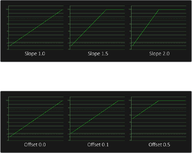
235
Color Tools Chapter – 6
Slope
Multiplies the color values. This is the same as Gain in the BrightnessContrast tool.
Offset
Adds to the color values. This is the same as Brightness in the BrightnessContrast tool.
Power
Applies a Gamma Curve. This is an inverse of the Gamma function of the
BrightnessContrast tool.
Saturation
Enhances or decreases the color saturation. This works the same as Saturation in the
BrightnessContrast tool.
Export File
Allows the user to export the settings as a CDL file.
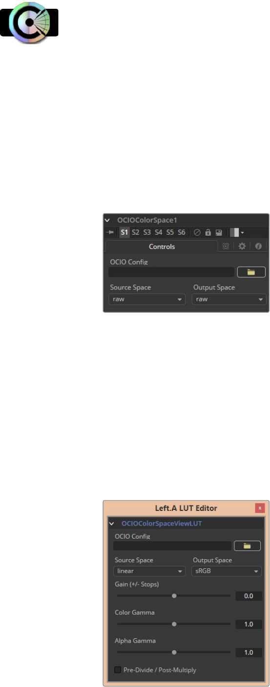
236
Color Tools Chapter – 6
OCIO ColorSpace [OCC]
Fusion supports the Open Color IO workflow specified by Sony Imageworks.
In general, the color pipeline is made up from a set of color transformations defined by OCIO-
specific config files, commonly named with a “.ocio” extension, which allows users to easily share
color settings within or between facilities. The path to the config file to be used is normally specified
by a user-created environment variable called “OCIO,” though some tools allow overriding this.
If no other *.ocio config files are located, the DefaultConfig.ocio file in Fusion’s LUTs directory will
be used. For in-depth documentation of the format’s internals, please refer to the official pages on
opencolorio.org. The OCIOColorSpace allows for sophisticated color space conversions, based
on an OCIO Config File. Sample configs can be obtained from opencolorio.org/downloads.html
The functionality of the OCIOColorSpace tool is also available as a ViewLUT tool from the
ViewLUT Menu.
Controls
OCIO Config
Displays a File > Open dialog to load the desired Config File.
Source Space
Based on the Config file, the available source color spaces will be listed here.
The content of this list is solely based on the loaded profile and hence can vary
immensely.
Output Space
Based on the Config file, the available output color spaces will be listed here.
The content of this list is solely based on the loaded profile and hence can vary
immensely.
The ViewLUT Version of the Tool
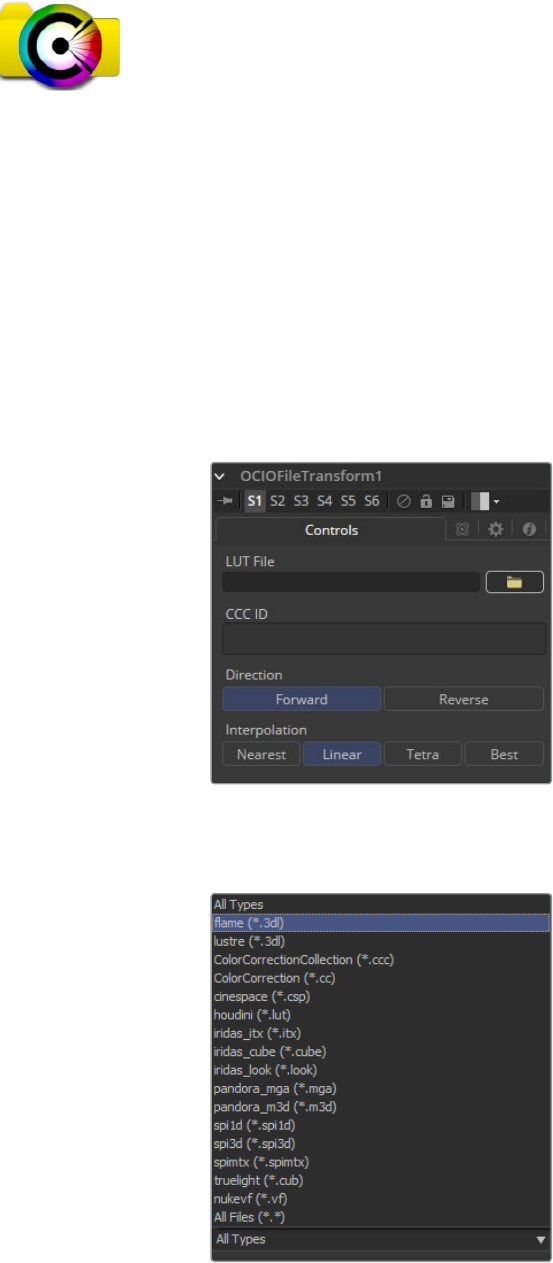
237
Color Tools Chapter – 6
OCIO FileTransform [OCF]
Fusion supports the Open Color IO workflow specified by Sony Imageworks.
In general, the color pipeline is made up from a set of color transformations defined by OCIO-
specific config files, commonly named with a “.ocio” extension, which allows users to easily
share color settings within or between facilities. The path to the config file to be used is
normally specified by a user-created environment variable called “OCIO,” though some tools
allow overriding this.
If no other *.ocio config files are located, the DefaultConfig.ocio file in Fusion’s LUT directory
will be used. For in-depth documentation of the format’s internals, please refer to the official
pages on opencolorio.org. The OCIOFileTransform allows the user to load and apply a variety
of Look Up Tables.
The functionality of the OCIOFileTransform tool is also available as a ViewLUT tool from the
ViewLUT Menu.
Controls
LUT File
Displays a File > Open dialog to load the desired LUT.
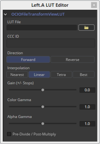
238
Color Tools Chapter – 6
CCC ID
Direction
Toggles between Forward and Reverse. Forward applies the corrections specified in
the tool, while reverse tries to remove those corrections. Keep in mind that not every
color correction can be undone. Imagine all slope values have been set to 0.0, resulting
in a fully black image. Reversing that operation is not possible, neither mathematically
nor visually.
Interpolation
Allows user to select the color interpolation to achieve the best quality/render
time ratio.
The ViewLUT Version of the Tool
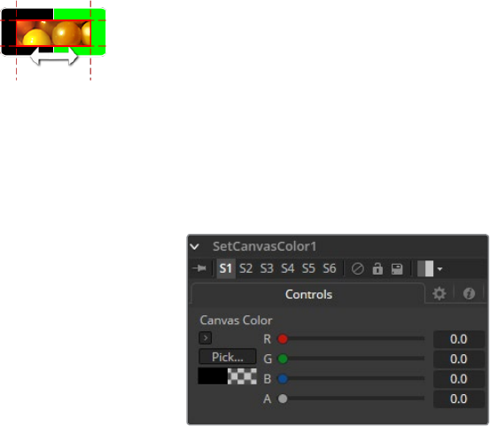
239
Color Tools Chapter – 6
Set Canvas Color [SCV]
Set Canvas Color is used to set the color of the workspace - all the area beyond the defined
pixels within an image (the DoD). This area usually extends to infinity. By default, the canvas
color used is Black/no Alpha (transparent).
Some tools may change an image’s canvas color, for example, inverting a mask will change the
mask’s canvas from black to white. Set Canvas Color allows you to control and override this.
Controls Tab
Color Picker
Use these controls to adjust the Color and the Alpha value for the image’s canvas. It
defaults to Black with zero Alpha.
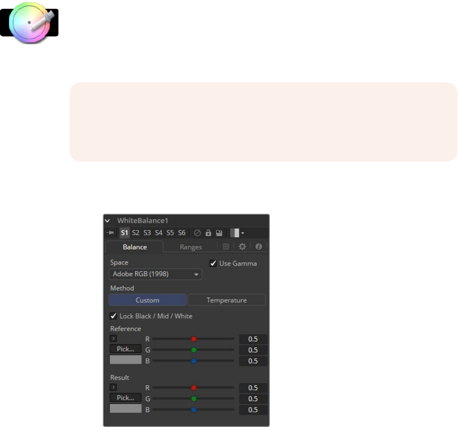
240
Color Tools Chapter – 6
White Balance [WB]
The White Balance tool can be used to automatically remove color casts in the image caused
by the incorrect setup of a camera, problems in a camera’s CCD, or bad lighting conditions.
Correction can be done by selecting a color temperature, or by choosing a neutral color from
the original image that exhibits the color cast to be corrected.
Balance Tab
Color Space
Use this menu to select the Color Space of the source image, if it is known. This can
make the correction more accurate since the tool will be able to take the natural
gamma of the color space into account as part of the correction. If the color space that
the image uses is unknown, leave this menu at its default value.
Method
The white balance tool can operate using one of two methods, a Custom method and a
color Temperature method.
IMPORTANT When picking neutral colors using the Custom method, make sure you
are picking from the source image, not the results of the White Balance tool. This
ensures that the image doesn‘t change while you are still picking, and that the White
Balance tool gets an accurate idea of the original colors it needs to correct.
241
Color Tools Chapter – 6
Custom
The Custom method requires the selection of a pixel from the scene that should have
been pure gray.
The tool uses this information to calculate the color correction required to convert the
pixel so that it actually is gray. When that correction is applied to the entire image, it
generally white balances the entire shot.
Temperature
The color Temperature method requires that the actual color temperature of the shot
be specified.
Lock Black/Mid/White
This checkbox locks the Black, Mid and White points together so that the entire image
is affected equally. Unchecking the control will provide individual controls for white
balancing each range separately. This control affects both methods equally.
Black/Mid/White Reference
These controls only appear if the Custom method is selected. They are used to select a
color from a pixel in the source image. The White Balance tool will color correct the
image so that the selected color is transformed to the color set in the Result color
picker below. Generally, this is gray. A color that is supposed to be pure gray but is not
truly gray for one reason or another should be selected.
If the Lock Black/Mid/White checkbox is deselected, different references can be
selected for each color range.
For example, try to select a pixel for the black and white references that is not clipped
in any of the color channels. In the high end, an example would be a pixel that is light
pink with values of 255, 240, 240. The pixel is saturated/clipped in the Red, even
though the color is not white. Similarly, a really dark blue-gray pixel might be 0, 2, 10. It
is clipped in Red as well, even though it is not black.
Neither example would be a good choice as a reference pixel because there would not
be enough headroom left for the White Balance tool.
Black/Mid/White Result
These controls only appear if the Custom method is selected. They are used to select
the color to which the tool will balance the reference color. This generally defaults to
pure, midrange gray.
If the Lock Black/Mid/White checkbox is deselected, different results can be selected
for each color range.
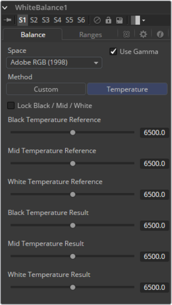
242
Color Tools Chapter – 6
Temperature Control
Temperature Reference
Use this control to set the color Temperature of the source image. If the Lock Black/
Mid/White checkbox is deselected, different references can be selected for each
color range.
Temperature Result
Use this control to set the target color temperature for the image. If the Lock Black/Mid/
White checkbox is deselected, different results can be selected for each color range.
Use Gamma
This checkbox selects whether the tool will take the gamma of the image into account
when applying the correction, using the default gamma of the color space selected in
the menu at the top of the tab.
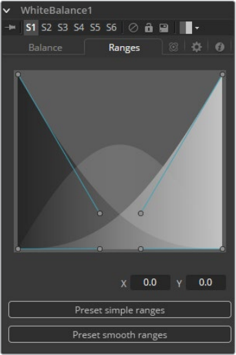
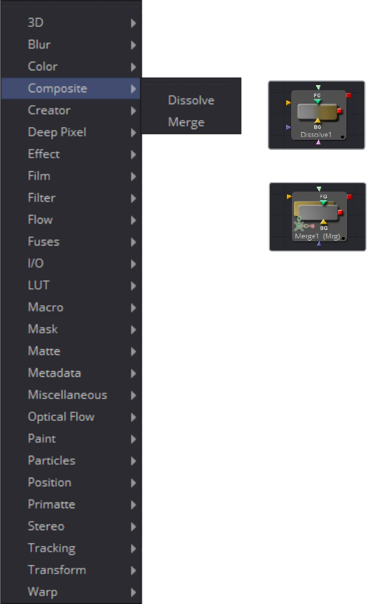
247
Composite Tools Chapter – 7
Dissolve [DX]
The Dissolve tool is used to mix two images together, providing a gradual transition between
two clips. A slider controls the amount of mix between the foreground and background layers.
Dissolves are commonly used to transition between one clip and another and are a very
common effect in editing. The Gradient Wipe setting allows arbitrary animated dissolve patterns
based on the luminance of a third input. Use this with geometric shapes, fire, water ripples, rain,
Perlin noise, particle systems or a video clip of your choice to get a variety of unique and
creative transitions. Soft-edged effect masks may also be used to add to the possible effects.
One useful attribute of the Dissolve tool is that, unlike all other tools in Fusion, it does not
require a valid background at all times, but will output either background or foreground as
appropriate. This allows you to use it as an easy automatic switcher tool. You may connect clips
to both background and foreground. Use the Background/Foreground control to determine
priority of which is output, and if one clip terminates early, the other is automatically output
instead. Animating the Background/Foreground control allows manual switching.
The tool tile provides three image inputs: Foreground, Background and Gradient Map. The
Gradient Map input is required only when Gradient Wipe is selected. The Dissolve tool works
best when both foreground and background inputs are images with the same resolution. If input
images of different sizes are mixed together, the output size will be large enough to cover both
images. If full Foreground or Background is selected, that image is output untouched, at its
native size. Animating the Foreground/Background slider in this case may cause undesirable
resolution changes.
For example, attempt to dissolve between an NTSC image (background) and a PAL image
(foreground) and the output of the Dissolve tool will be NTSC when the slider is set to full
Background. It will suddenly jump to PAL when set to full Foreground. Mix between FG and BG
and the resolution of the output image will be the largest dimension from each image; in this
case the output will be 720 x 576 (PAL sized).
It is recommended to ensure all inputs of the Dissolve tool are the same resolution and
pixel aspect.
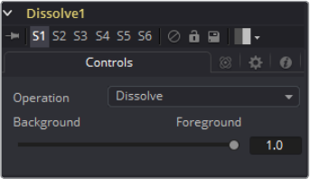
248
Composite Tools Chapter – 7
Controls
Operation
The Operation drop-down menu contains one of seven different methods for mixing
the Foreground and Background inputs. The two images are mixed together using the
value of the Background/Foreground slider to determine the percentage each image
contributes.
Dissolve
The standard Dissolve mode is the equivalent of a cross dissolve, one clip fades out as
another clip fades in.
Additive Dissolve
Similar in look to a standard film dissolve, an Additive Dissolve adds the second clip
and then fades out the first one.
Erode
The Erode method transitions between the two images by growing the darkest areas of
the background image to reveal the foreground image. The effect appears similar to a
filmstrip burning out.
Random Dissolve
A randomly generated dot pattern is used to perform the mix of the images.
Random Noise Dissolve
A moving random dot pattern is used to perform the mix of the images.
Gradient Wipe
The dissolve is controlled by the luminance values of the image in the Gradient Map
input. The edges of this dissolve can be softened. The density and the color of the
border can be adjusted independently.
SMPTE Wipe
The SMPTE Wipe is similar to the basic effect wipes found on many video effects
switchers. There is a horizontal wipe and a vertical wipe provided. The wipes can have
soft edges and borders added. The density and the color of the border can be
adjusted independently.
Background/Foreground
This control determines whether the output is the background image, the foreground
image, or a mix between the two. The type of mix is determined by the Operation
control. If one of the input images is not currently available, the other one will be output
regardless of the setting of this slider.
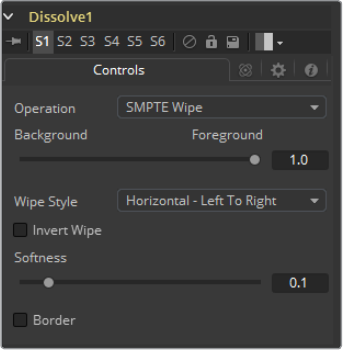
249
Composite Tools Chapter – 7
Gradient/SMPTE wipe controls
The following controls appear only when Gradient Wipe or SMPTE Wipe are selected.
Wipe Style
(SMPTE Wipe only) The drop-down list allows the selection of two wipe styles:
Horizontal - Left to Right and Vertical - Top to Bottom. The direction of the wipes can be
reversed by using the Invert Wipe checkbox.
Invert Wipe
(SMPTE Wipe only) When checked, the direction of the wipe will be reversed.
Softness
Use this control to soften the edge of the transition.
Border
Select the Border to enable coloring of the transition’s edge and to reveal the
associated controls. The effect is to create a border around the transition edge.
Border Softness
The Border Softness slider controls the width and density of the border. Higher values
will create a denser border and lower values will create a thinner one.
Border Color
Use Border Color to select the color used in the border.
250
Composite Tools Chapter – 7
Merge [MRG]
The Merge tool combines two images based on the alpha (opacity) channel associated with the
one in front. This tool takes two inputs - a background and a foreground image. The Operation
mode of the merge determines what method is used to combine the images.
Instead of providing you with a dozen tools for each different method used to combine images,
Fusion uses a single Merge tool that supports the standard over, in, held out, atop and xor
methods for compositing images, as well as many common blending modes like screen,
dissolve, multiply and overlay.
The Merge tool can handle both additive (premultiplied) and subtractive (non-premultiplied)
compositing. Use Merge to blend between the additive and subtractive results, providing
solutions for some otherwise tricky problems.
This tool can also be used to composite images based on information from the Z-buffer channel
of the images, if available. Rather than relying on the foreground and background order to
determine layer order, Z-merging compares the depth value of each pixel to determine which is
the foreground pixel and which is the background pixel.
Merge Tab
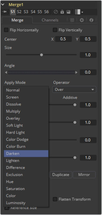
251
Composite Tools Chapter – 7
Center X and Y
This control determines the position of the foreground image in the composite.
Thedefault is 0.5, 0.5, which centers the foreground image in the exact center of the
background image. The value shown is always the actual position in normalized
coordinates, multiplied by the reference size.
See below for a description of the reference size controls.
Size
Use this control to increase or decrease the Size of the foreground image before it is
composited over the background. The range of values for this slider is 0.0 to 5.0, but
any value greater than 0 can be entered manually. A size of 1.0 gives a pixel-for-pixel
composition, where a single pixel in the foreground is the same size as a single pixel in
the background.
Angle
Use this control to rotate the foreground image before it is combined with the
background.
Apply Modes
The Apply Mode setting determines the math used when blending or combining the foreground
and background pixels.
252
Composite Tools Chapter – 7
Normal
The Default merge mode uses the foreground’s alpha channel as a mask to determine
which pixels are transparent and which are not. When this is active, another menu
shows possible operations, including: over, in, held out, atop and xor.
Screen
Screen merges the images based on a multiplication of their color values. The alpha
channel is ignored and layer order becomes irrelevant. The resulting color is always
lighter. Screening with black leaves the color unchanged, whereas screening with white
will always produce white. This effect creates a similar look to projecting several film
frames onto the same surface.
Dissolve
Dissolve mixes two image sequences together. It uses a calculated average of the two
images to perform the mixture.
Multiply
Multiply the values of a color channel. This will give the appearance of darkening the
image as the values are scaled from 0 to 1. White has a value of 1, so the result would
be the same. Gray has a value of 0.5, so the result would be a darker image or, in other
words, an image half as bright.
Overlay
Overlay multiplies or screens the color values of the foreground image, depending on
the color values of the background image. Patterns or colors overlay the existing pixels
while preserving the highlights and shadows of the color values of the background
image. The background image is not replaced but is mixed with the foreground image
to reflect the original lightness or darkness of the background image.
Soft Light
Soft Light darkens or lightens the foreground image, depending on the color values of
the background image. The effect is similar to shining a diffused spotlight on the image.
Hard Light
Hard Light multiplies or screens the color values of the foreground image, depending
on the color values of the background image. The effect is similar to shining a harsh
spotlight on the image.
Color Dodge
Color Dodge uses the foreground’s color values to brighten the background image.
This is similar to the photographical practice of dodging by reducing the exposure of an
area of a print.
Color Burn
Color Burn uses the foreground’s color values to darken the background image. This is
similar to the photographical practice of burning by increasing the exposure of an area
of a print.
253
Composite Tools Chapter – 7
Darken
Darken looks at the color information in each channel and selects the background or
foreground image’s color value, whichever is darker, as the result color. Pixels lighter
than the merged colors are replaced, and pixels darker than the merged color do
not change.
Lighten
Lighten looks at the color information in each channel and selects the background or
foreground image’s color values, whichever is lighter, as the result color value. Pixels
darker than the merged color are replaced, and pixels lighter than the merged color do
not change.
Difference
Difference looks at the color information in each channel and subtracts the foreground
color values from the background color values or the background from the foreground,
depending on which has the greater brightness value. Merging with white inverts the
color. Merging with black produces no change.
Exclusion
Exclusion creates an effect similar to, but lower in contrast than, the Difference mode.
Merging with white inverts the base color values. Merging with black produces
no change.
Hue
Hue creates a result color with the luminance and saturation of the background color
values and the hue of the foreground color values.
Saturation
Saturation creates a result color with the luminance and hue of the base color and the
saturation of the blend color.
Color
Color creates a result color with the luminance of the background color value and the
hue and saturation of the foreground. This preserves the gray levels in the image and is
useful for coloring monochrome images.
Luminosity
Luminosity creates a result color with the hue and saturation of the background color
values and the luminance of the foreground color values. This mode creates an inverse
effect from that of the Color mode.
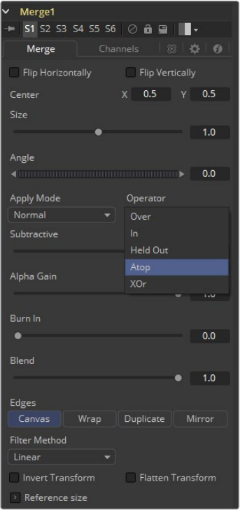
254
Composite Tools Chapter – 7
Operator Modes
This menu is used to select the Operation mode of the merge. Changing the Operation mode
changes how the foreground and background are combined to produce a result. The menu will
only be visible when the Merge tool’s Apply mode is set to Normal.
For an excellent description of the math underlying the Operation modes, read Compositing
Digital Images, Porter, T., and T. Duff, SIGGRAPH 84 proceedings, pages 253-259. Essentially,
the math is as described below. Note that some modes not listed in the Operator drop-down
(Under, In, Held In, Below) are easily obtained by swapping the foreground and background
inputs (with Command-T or Ctrl-T) and choosing a corresponding mode.
The formula used to combine pixels in the merge is always fg * x + bg * y. The different
operations determine exactly what x and y are, as shown in the description for each mode.
Over
The Over mode adds the FG layer to the BG layer by replacing the pixels in the BG with
the pixels from the Z wherever the FG’s alpha channel is greater than 1.
x = 1, y = 1-[foreground alpha]
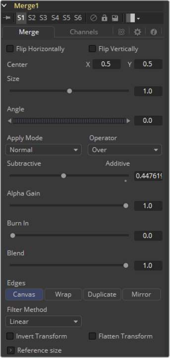
255
Composite Tools Chapter – 7
In
The In mode multiplies the alpha channel of the BG input against the pixels in the FG.
The color channels of the FG input are ignored. Only pixels from the FG are seen in the
final output. This essentially clips the FG using the mask from the BG.
x = [background alpha], y = 0
Held Out
Held Out is essentially the opposite of the In operation. The pixels in the FG image are
multiplied against the inverted alpha channel of the BG image. Accomplish exactly the
same result using the In operation and a Matte Control tool to invert the matte channel
of the BG image.
x = 1-[background alpha], y = 0
ATop
ATop places the FG over the BG only where the BG has a matte.
x = [background alpha], y = 1-[foreground alpha]
XOr
XOr combines the FG with the BG wherever either the FG or the BG have a matte, but
never where both have a matte.
x = 1-[background alpha], y = 1-[foreground alpha]
Subtractive and Additive
256
Composite Tools Chapter – 7
This slider controls whether Fusion performs an Additive or a Subtractive merge. An Additive
merge assumes that the foreground image is pre-multiplied, meaning that the pixels in the color
channels have been multiplied by the pixels in the alpha channel. The result is that transparent
pixels are always black, since any number multiplied by 0 is always going to be 0.
When the Merge tool can assume the image is pre-multiplied, it can perform an Additive merge.
This obscures the background (by multiplying with the inverse of the foreground alpha), then
simply adds the pixels from the foreground.
If the images are not pre-multiplied then usually all that is required is a Subtractive merge. This
method is similar to additive, but the foreground image is first multiplied by its own alpha, to
eliminate any background pixels outside the alpha area.
Fusion defaults to Additive merging for most operations, assuming that the images are pre-
multiplied. Using Subtractive merging on a pre-multiplied image may result in darker edges,
whereas using Additive merging with a non-premultiplied image will cause any non-black area
outside the foreground’s alpha to be added to the result.
Although the Additive/Subtractive option could easily have been a checkbox to select one
mode or another, Fusion allows for blending between the Additive and Subtractive modes, an
operation that can occasionally be useful for dealing with problem images.
Alpha Gain
Alpha Gain linearly scales the values of the foreground’s alpha channel. In Subtractive
merges, this controls the density of the composite, similarly to Blend. In Additive
merges, this effectively reduces the amount that the background is obscured by, thus
brightening the overall result. In an Additive merge with Alpha Gain set to 0.0, the
foreground pixels are simply added to the background.
Burn In
The Burn In control adjusts the amount of alpha used to darken the background,
without affecting the amount of foreground added in. At 0.0, the merge behaves like a
straight alpha blend, whereas at 1.0, the foreground is effectively added onto the
background (after alpha multiplication if in Subtractive mode).
This gives the effect of the foreground image brightening the background image, as
with Alpha Gain. In fact, for Additive merges, increasing the Burn In gives an identical
result to decreasing Alpha Gain.
Filter Modes
Nearest Neighbor
This skips or duplicates pixels as needed. This produces the fastest but crudest results.
Box
This is a simple interpolation resize of the image.
Linear
This uses a simplistic filter, which produces relatively clean and fast results.
Quadratic
This filter produces a nominal result. It offers a good compromise between speed
and quality.
Cubic
This produces better results with continuous tone images but is slower than Bi-Cubic.
Ifthe images have fine detail in them, the results may be blurrier than desired.
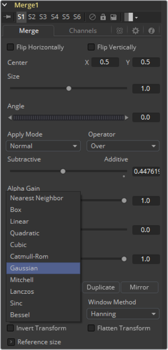
257
Composite Tools Chapter – 7
Catmull-Rom
This produces good results with continuous tone images that are resized down.
Produces sharp results with finely detailed images.
Gaussian
This is very similar in speed and quality to Bi-Cubic.
Mitchell
This is similar to Catmull-Rom but produces better results with finely detailed images. It
is slower than Catmull-Rom.
Lanczos
This is very similar to Mitchell and Catmull-Rom but is a little cleaner and also slower.
Sinc
This is an advanced filter that produces very sharp, detailed results, however it may
produce visible ‘ringing’ in some situations.
Bessel
This is similar to the Sinc filter but may be slightly faster.

258
Composite Tools Chapter – 7
Window Method
Some filters, such as Sinc and Bessel, require an infinite number of pixels to calculate
exactly. To speed up this operation, a windowing function is used to approximate the
filter and limit the number of pixels required. This control appears when a filter that
requires windowing is selected.
Hanning
This is a simple tapered window.
Hamming
Hamming is a slightly tweaked version of Hanning.
Blackman
A window with a more sharply tapered falloff.
Kaiser
A more complex window, with results between Hamming and Blackman.
Most of these filters are useful only when making an image larger. When shrinking
images, it is common to use the Bi-Linear filter, however the Catmull-Rom filter will
apply some sharpening to the results and may be useful for preserving detail when
scaling down an image.
Different Resize Filters. From left to right: Nearest Neighbor, Box, Linear,
Quadratic, Cubic, Catmull-Rom, Gaussian, Mitchell, Lanczos, Sinc, Bessel
Blend
This is a cloned instance of the Blend slider in the Common Controls tab. Changes
made to this control are simultaneously made to the one in the common controls.
The Blend slider mixes the result of the tool with its input, blending back the effect at
any value less than 1.0. In this case it will blend the background with the merged result.
Invert Transform
Select the Invert Transform control to invert any position, rotation or scaling
transformation. This option is useful when connecting the merge to the position of a
tracker for the purpose of match moving.
Flatten Transform
The Flatten Transform option prevents this tool from concatenating its transformation
with subsequent tools. The tool may still concatenate transforms from its input, but it will
not concatenate its transformation with the tool at its output. See the Transformations
chapter earlier in this manual for details on concatenated transformation.
Reference Size
The controls under the Reference Size reveal do not directly affect the image. Instead
they allow you to control how Fusion represents the position of the Merge tool’s center.
Normally, coordinates are represented as values between 0 and 1, where 1 is a distance
equal to the full width or height of the image. This allows for resolution independence,
because the size of the image can be changed without having to change the value of
the center.
259
Composite Tools Chapter – 7
One disadvantage to this approach is that it complicates making pixel accurate
adjustments to an image. To demonstrate, imagine an image that is 100 x 100 pixels in
size. To move the center of the foreground element to the right by 5 pixels, we would
change the X value of the merge center from 0.5, 0.5 to 0.55, 0.5. We know the change
must be 0.05 because 5/100 = 0.05.
If you specify the dimensions of the background image in the Reference Size controls,
this changes the way the Center control values are displayed so that it shows the actual
pixel positions in its X and Y fields.
Extending the example, set the width and height to 100 each and the center will now be
shown as 50, 50, and we would move it 5 pixels toward the right by entering 55, 50.
Internally, the Merge tool still stores this value as a number between 0 to 1 and, if the
center control’s value were to be queried via scripting or the center control were to be
published for use by other tools, the original normalized value would be retrieved. The
change is only visible in the value shown for merge center in the tool control.
Use Frame Format Settings
Select this to force the merge to use the composition’s current frame format settings to
set the reference width and reference height values.
Width and Height
Set these sliders to the width and height of the image to change the way that Fusion
displays the values of the Merge tool’s center control.
Channels Tab
Perform Depth Merge
When checked, the Z-buffer channel of both images will be used to determine the
composite order. Alpha channels are still used for transparency, but the values of the
Z-buffer channel will determine the ordering of image elements. If a Z-buffer channel is
not available for either image, the setting of this checkbox will be ignored, and no
depth compositing will take place.
Depth merging is off by default. If an image has an associated Z-buffer channel, and
that channel is not to be used to perform a depth merge, turn this checkbox off.
Foreground Z-Offset
This slider sets an offset applied to the foreground image’s Z value. Click the Pick
button to pick a value from a displayed image’s Z-channel, or enter a value using the
slider or input boxes. Raising the value causes the foreground image’s Z-buffer to be
offset further away along the Z-axis, whereas lowering the value causes the foreground
to move closer.
Subtractive and Additive
When Z-compositing, it is possible for image pixels from the background to be
composited in the foreground of the output because the Z-buffer for that pixel is closer
than the Z of the foreground pixel. This slider controls whether these pixels are merged
in an Additive or a Subtractive mode, in exactly the same way as the comparable slider
in the Merge tab.
When merged over a background of a different color, the original background will still
be visible in the semi-transparent areas. An Additive merge will maintain the
transparencies of the image but will add their values to the background.
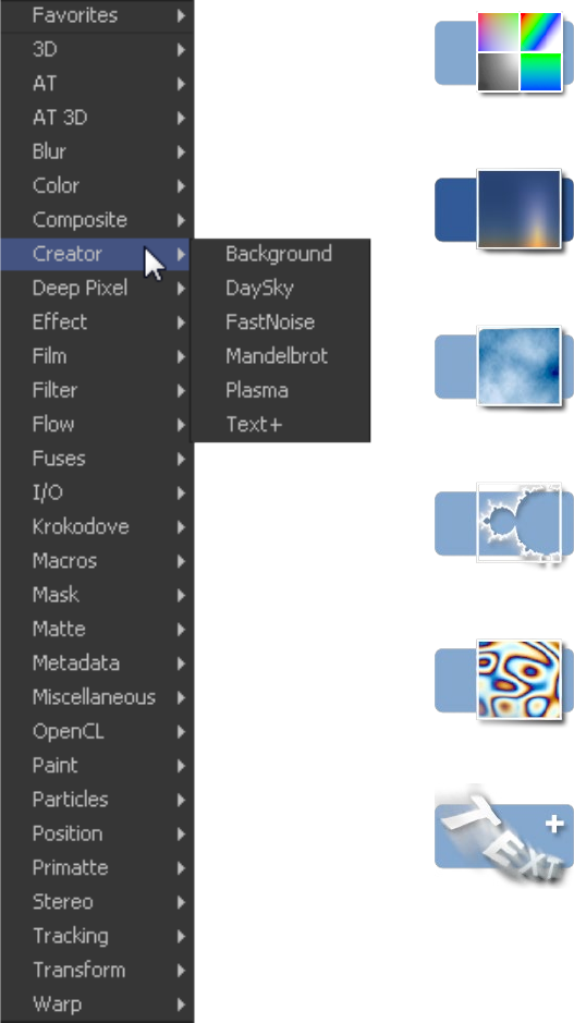
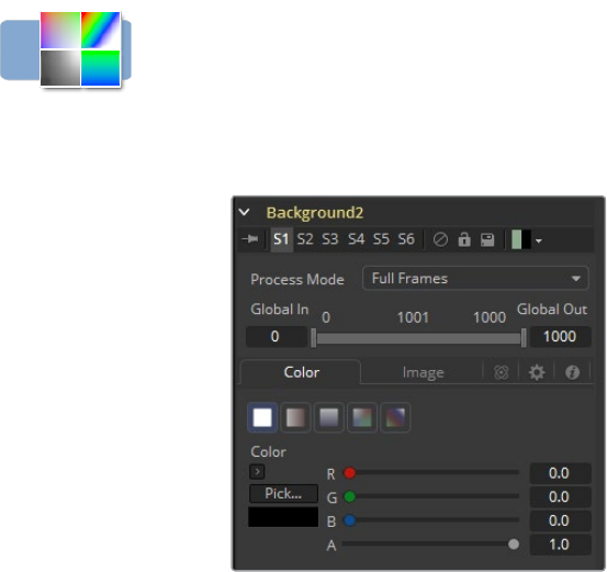
263
Creator Tools Chapter – 8
Background [BG]
The Background tool can be used to produce anything from simple color backgrounds to
complex loopable gradients.
Color Tab
Mode
This control is used to select the mode used by the background tool when the image is
generated. Four selections are available.
Solid Color: This default creates a single color image.
Horizontal: This creates a two color horizontal gradation.
Vertical: This creates a two color vertical gradation.
Four Corner: This creates a four color corner gradation.
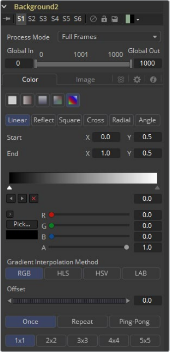
264
Creator Tools Chapter – 8
Gradient
This creates a background from a custom gradient.
Color
These controls are used to select the color of the Background tool. Depending on the
mode selected, one to four color controls will be displayed to create linear color ramp
backdrops. Select one and pick a color from the preset menu or create them. Alternatively,
enter values in RGB via the keyboard by clicking in the values box and typing in the
value. Each color has its own alpha value slider to adjust the transparency of each color.
Custom Gradient Controls
The Custom Gradient controls that appear are described in depth in the Tool Controls
chapter of this manual. Consult this chapter for details on setting up a custom gradient
for use in the Background tool.
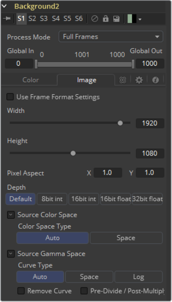
265
Creator Tools Chapter – 8
Image Tab
The controls in this tab are used to set the resolution, color depth and pixel aspect of the image
produced by the tool.
Process Mode
Use this menu control to select the Fields Processing mode used by Fusion to render
changes to the image. The default option is determined by the Has Fields checkbox
control in the Frame Format preferences. For more information on fields processing,
consult the Frame Formats chapter.
Global In and Out
Use this control to specify the position of this tool within the project. Use Global In to
specify on which frame that the clip starts and Global Out to specify on which frame
this clip ends (inclusive) within the project’s Global Range.
The tool will not produce an image on frames outside of this range.
Use Frame Format Settings
When this checkbox is selected, the width, height and pixel aspect of the image
created by the tool will be locked to values defined in the composition’s Frame Format
preferences. If the Frame Format preferences change, the resolution of the image
produced by the tool will change to match. Disabling this option can be useful to build a
composition at a different resolution than the eventual target resolution for the
final render.
266
Creator Tools Chapter – 8
Width/Height
This pair of controls is used to set the Width and Height dimensions of the image to be
created by the tool.
Pixel Aspect
This control is used to specify the Pixel Aspect ratio of the created images. An aspect
ratio of 1:1 would generate a square pixel with the same dimensions on either side (like
a computer display monitor) and an aspect of 0.9:1 would create a slightly rectangular
pixel (like an NTSC monitor).
Depth
The Depth button array is used to set the pixel color depth of the image created by the
Creator tool. 32-bit pixels require 4 times the memory of 8-bit pixels, but have far
greater color accuracy. Float pixels allow high dynamic range values outside the normal
0..1 range, for representing colors that are brighter than white or darker than black. See
the Frame Formats chapter for more details.
Right-click on the Width, Height or Pixel Aspect controls to display a menu listing the
file formats defined in the preferences Frame Format tab. Selecting any of the listed
options will set the width, height and pixel aspect to the values for that
formataccordingly.
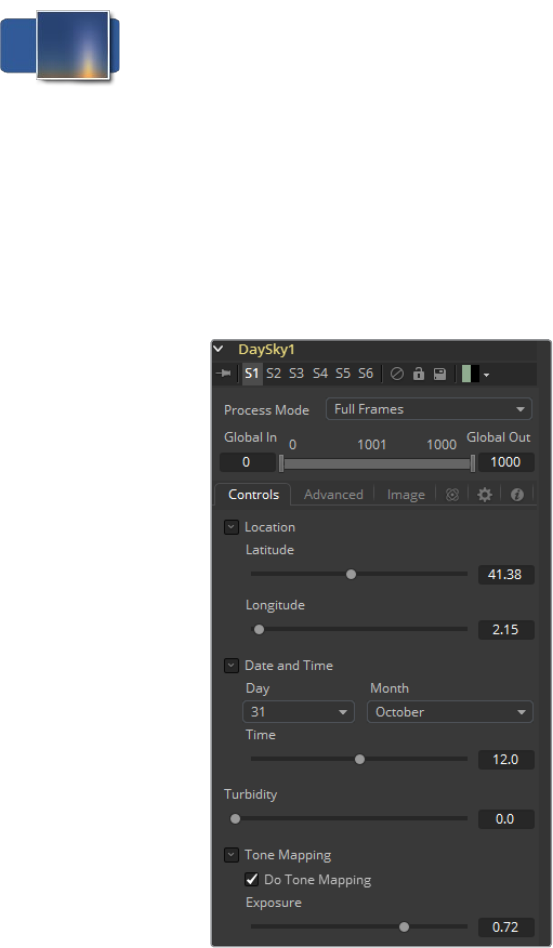
267
Creator Tools Chapter – 8
Day Sky [DS]
The DaySky generator is a practical implementation of the research paper, A Practical
Analytical Model for Daylight, by Preetham, Shirley, and Smits. A copy of the original paper can
be found at the website for the Visual Simulation Group at the University of Utah [http://www.
cs.utah.edu/~shirley/papers/sunsky/].
This tool aims to produce a simulation of the daylight produced at a specific time and location
on the earth, and generates a high dynamic range image that represents a map of that light. It is
not a sky generator, although it could be combined with a cloud generator or noise tool to
produce one.
Controls Tab
Latitude, Longitude
Use these sliders to specify the Latitude and Longitude used to create the Day Sky
simulation.
Day, Month, Time
Use these controls to specify the Day, Month and Time for the DaySky simulation.
Turbidity
Turbidity causes light to be scattered and absorbed rather than transmitted in straight
lines through the simulation. Increasing the turbidity will give the sky simulation a murky
feeling, as if smoke or atmospheric haze were present.
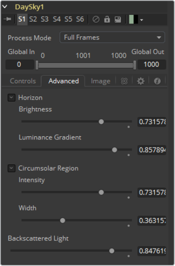
268
Creator Tools Chapter – 8
Do Tone Mapping
Deselect this checkbox to disable any tone mapping applied to the simulation. Since
the simulation is calculated in 32-bit floating-point color space, it generates color values
well above 1.0 and well below 0.0. Tone Mapping is a process that takes the full
dynamic range of the resulting simulation and compresses the data into the desired
exposure range while attempting to preserve as much detail from the highlights and
shadows as possible.
Generally, this option should only be deselected if the resulting image will later be color
corrected as part of a floating-point color pipeline.
Exposure
Use this control to select the exposure used for Tone Mapping.
Advanced Tab
Horizon Brightness
Use this control to adjust the brightness of the horizon relative to the sky.
Luminance Gradient
Use this control to adjust the width of the gradient separating the horizon from the sky.
Circumsolar Region Intensity
Use this control to adjust the intensity or brightness of the sky nearest to the sun.
Circumsolar Region Width
Use this control to adjust the width or size of the area in the sky affected by the sun.
Backscattered Light
Use this control to increase or decrease the amount of backscatter light in the
simulation.
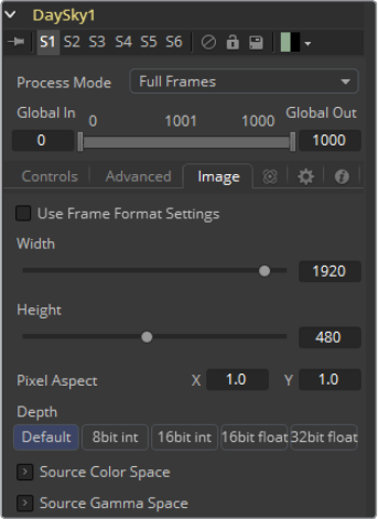
269
Creator Tools Chapter – 8
Image Tab
The controls in this tab are used to set the resolution, color depth and pixel aspect of the image
produced by the tool.
Process Mode
Use this menu control to select the Fields Processing mode used by Fusion to render
changes to the image. The default option is determined by the Has Fields checkbox
control in the Frame Format preferences. For more information on fields processing,
consult the Frame Formats chapter.
Global In and Out
Use this control to specify the position of this tool within the project. Use Global In to
specify on which frame that the clip starts and Global Out to specify on which frame
this clip ends (inclusive) within the project’s Global Range.
The tool will not produce an image on frames outside of this range.
Use Frame Format Settings
When this checkbox is selected, the width, height and pixel aspect of the image
created by the tool will be locked to values defined in the composition’s Frame Format
preferences. If the Frame Format preferences change, the resolution of the image
produced by the tool will change to match. Disabling this option can be useful to build a
composition at a different resolution than the eventual target resolution for the
final render.
Width/Height
This pair of controls is used to set the Width and Height dimensions of the image to be
created by the tool.
Pixel Aspect
This control is used to specify the Pixel Aspect ratio of the created images. An aspect
ratio of 1:1 would generate a square pixel with the same dimensions on either side (like
a computer display monitor) and an aspect of 0.9:1 would create a slightly rectangular
pixel (like an NTSC monitor).
270
Creator Tools Chapter – 8
Depth
The Depth button array is used to set the pixel color depth of the image created by the
creator tool. 32-bit pixels require 4 times the memory of 8-bit pixels, but have far
greater color accuracy. Float pixels allow high dynamic range values outside the normal
0..1 range, for representing colors that are brighter than white or darker than black. See
the Frame Formats chapter for more details.
Right-click on the Width, Height or Pixel Aspect controls to display a menu listing the
file formats defined in the preferences Frame Format tab. Selecting any of the listed
options will set the width, height and pixel aspect to the values for that format
accordingly.
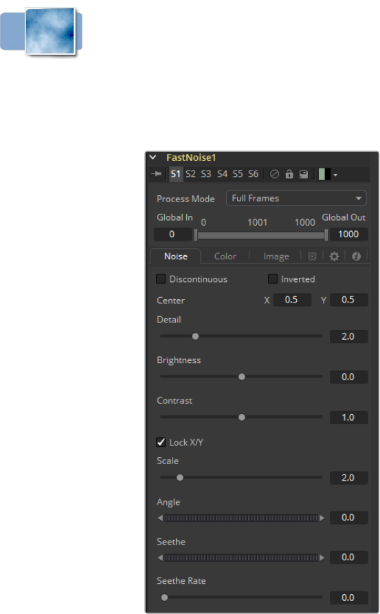
271
Creator Tools Chapter – 8
Fast Noise [FN]
The Fast Noise tool is a very fast and flexible Perlin Noise generator. It can be useful for a wide
range of effects, from clouds and swirling fog to waves, water caustics, stylized fire and smoke
and other organic textures. It is also invaluable as a noise source for other effects, such as heat
shimmer, particle systems and dirtiness maps.
Noise Tab
Discontinuous
Normally, the noise function interpolates between values to create a smooth
continuous gradient of results. Enable this checkbox to create hard discontinuity lines
along some of the noise contours. The result will be a dramatically different effect.
Inverted
Select this checkbox to invert the noise, creating a negative image of the original
pattern. This is most effective when Discontinuous is also enabled.
Center
Use the Center coordinate control to pan and move the noise pattern.
Detail
Increase the value of this slider to produce a greater level of detail in the noise result.
Larger values add more layers of increasingly detailed noise without affecting the
overall pattern. High values take longer to render but can produce a more
natural result.

272
Creator Tools Chapter – 8
Brightness
This control adjusts the overall brightness of the noise map, before any gradient color
mapping is applied. In Gradient mode, this has a similar effect to the Offset control.
Contrast
This control increases or decreases the overall Contrast of the noise map, prior to any
gradient color mapping. It can exaggerate the effect of the noise, and widen the range
of colors applied in Gradient mode.
Lock and Scale X/Y
The size of the noise map can be adjusted using the Scale slider, changing it from
gentle variations over the whole image to a tighter overall texture effect. The Scale
slider can be separated into independent X- and Y-axis scale sliders by clicking on the
Lock X/Y checkbox immediately above, which can be useful for a brushed-metal effect.
Angle
Use the Angle control to rotate the noise pattern.
Seethe
Adjust this thumbwheel control to interpolate the noise map against a different noise
map. This will cause a crawling shift in the noise, like it was drifting or flowing. This
control must be animated to affect the gradient over time, or you can use the Seethe
Rate control below.
Seethe Rate
As with the Seethe control above, the Seethe Rate also causes the noise map to evolve
and change. The Seethe Rate defines the rate at which the noise changes each frame,
causing an animated drift in the noise automatically, without the need for spline
animation.
Color Tab
Two Color
A simple two color gradient is used to color the noise map. The noise function will
smoothly transition from the first color into the second.
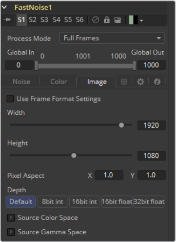
273
Creator Tools Chapter – 8
Gradient
The Advanced Gradient control in Fusion is used to provide much more control over
the color gradient used with the noise map. The controls that appear are when this
mode is selected are described in depth in the Tool Controls chapter of this manual.
Consult this chapter for details on setting up a custom gradient for use in the Fast
Noise tool.
Image Tab
The controls in this tab are used to set the resolution, color depth and pixel aspect of the image
produced by the tool.
Process Mode
Use this menu control to select the fields processing mode used by Fusion to render
changes to the image. The default option is determined by the Has Fields checkbox
control in the Frame Format preferences. For more information on fields processing,
consult the Frame Formats chapter.
Global In and Out
Use this control to specify the position of this tool within the project. Use Global In to
specify on which frame that the clip starts and Global Out to specify on which frame
this clip ends (inclusive) within the project’s Global Range.
The tool will not produce an image on frames outside of this range.
Use Frame Format Settings
When this checkbox is selected, the width, height and pixel aspect of the image
created by the tool will be locked to values defined in the composition’s Frame Format
preferences. If the Frame Format preferences change, the resolution of the image
produced by the tool will change to match. Disabling this option can be useful to build a
composition at a different resolution than the eventual target resolution for the
final render.
274
Creator Tools Chapter – 8
Width/Height
This pair of controls is used to set the Width and Height dimensions of the image to be
created by the tool.
Pixel Aspect
This control is used to specify the Pixel Aspect ratio of the created images. An aspect
ratio of 1:1 would generate a square pixel with the same dimensions on either side (like
a computer display monitor) and an aspect of 0.9:1 would create a slightly rectangular
pixel (like an NTSC monitor).
Depth
The Depth button array is used to set the pixel color depth of the image created by the
creator tool. 32-bit pixels require 4 times the memory of 8-bit pixels, but have far
greater color accuracy. Float pixels allow high dynamic range values outside the normal
0..1 range, for representing colors that are brighter than white or darker than black. See
the Frame Formats chapter for more details.
Right-click on the Width, Height or Pixel Aspect controls to display a menu listing the
file formats defined in the preferences Frame Format tab. Selecting any of the listed
options will set the width, height and pixel aspect to the values for that format
accordingly.
Mask Map Inputs
These external connections allow you to use masks to control the value of the Noise
Detail and Brightness controls individually for each pixel. This can allow some
interesting and creative effects.
Noise Detail Map
A soft-edged mask connected to the Noise Detail Map will give a flat noise map (zero
detail) where the mask is black, and full detail where it is white, with intermediate values
smoothly reducing in detail. It is applied before any gradient color mapping. This can be
very helpful for applying maximum noise detail in a specific area, while smoothly falling
off elsewhere.
Noise Brightness Map
A mask connected to this input can be used to control the noise map completely, such
as boosting it in certain areas, combining it with other textures, or if Detail is set to 0,
replacing the Perlin Noise map altogether.
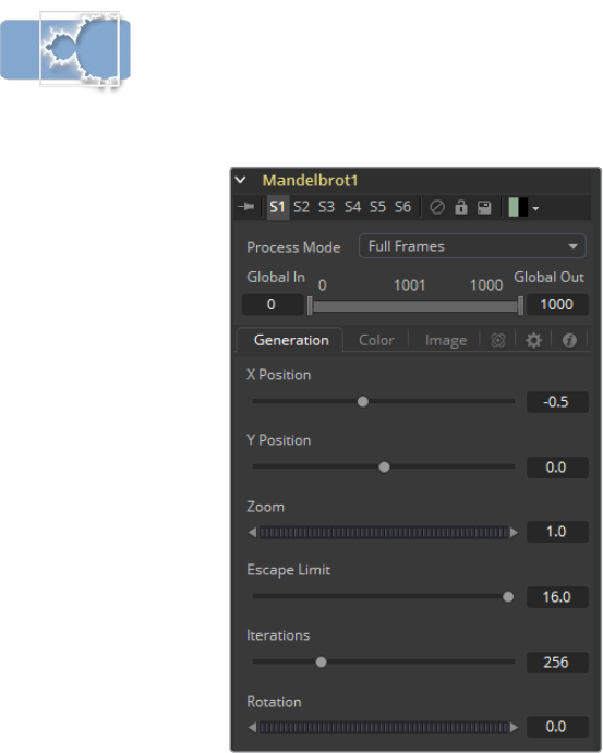
275
Creator Tools Chapter – 8
Mandelbrot [MAN]
This tool creates an image pattern based on the Mandelbrot fractal theory set.
Generation Tab
Position X and Y
This designates the image’s horizontal and vertical position or seed point.
Zoom
Zoom magnifies the pattern in or out. Every magnification is recalculated so that there
is no practical limit to the zoom.
Escape Limit
Defines a point where the calculation of the iteration is aborted. Low values lead to
blurry halos.
Iterations
This determines the repetitiveness of the set. When animated, it simulates a growing
of the set.
Rotation
This rotates the pattern. Every new angle requires recalculation of the image.
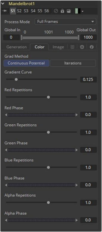
276
Creator Tools Chapter – 8
Color Tab
Grad Method
Use this control to determine the type of gradation applied at the borders of
the pattern.
Continuous Potential
This causes the edges of the pattern to blend to the background color.
Iterations
This causes the edges of the pattern to be solid.
Gradient Curve
This affects the width of the gradation from the pattern to the background color.
R/G/B/A Phase/Repetitions
Set the color values of the pattern generators.
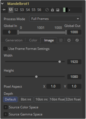
277
Creator Tools Chapter – 8
Image Tab
The controls in this tab are used to set the resolution, color depth and pixel aspect of the image
produced by the tool.
Process Mode
Use this menu control to select the Fields Processing mode used by Fusion to render
changes to the image. The default option is determined by the Has Fields checkbox
control in the Frame Format preferences. For more information on fields processing,
consult the Frame Formats chapter.
Global In and Out
Use this control to specify the position of this tool within the project. Use Global In to
specify on which frame that the clip starts and Global Out to specify on which frame
this clip ends (inclusive) within the project’s Global Range.
The tool will not produce an image on frames outside of this range.
Use Frame Format Settings
When this checkbox is selected, the width, height and pixel aspect of the image
created by the tool will be locked to values defined in the composition’s Frame Format
preferences. If the Frame Format preferences change, the resolution of the image
produced by the tool will change to match. Disabling this option can be useful to build a
composition at a different resolution than the eventual target resolution for the
final render.
Width/Height
This pair of controls is used to set the Width and Height dimensions of the image to be
created by the tool.
278
Creator Tools Chapter – 8
Pixel Aspect
This control is used to specify the Pixel Aspect ratio of the created images. An aspect
ratio of 1:1 would generate a square pixel with the same dimensions on either side (like
a computer display monitor) and an aspect of 0.9:1 would create a slightly rectangular
pixel (like an NTSC monitor).
Depth
The Depth button array is used to set the pixel color depth of the image created by the
creator tool. 32-bit pixels require 4 times the memory of 8-bit pixels, but have far
greater color accuracy. Float pixels allow high dynamic range values outside the normal
0..1 range, for representing colors that are brighter than white or darker than black. See
the Frame Formats chapter for more details.
Right-click on the Width, Height or Pixel Aspect controls to display a menu listing the
file formats defined in the preferences Frame Format tab. Selecting any of the listed
options will set the width, height and pixel aspect to the values for that format
accordingly.
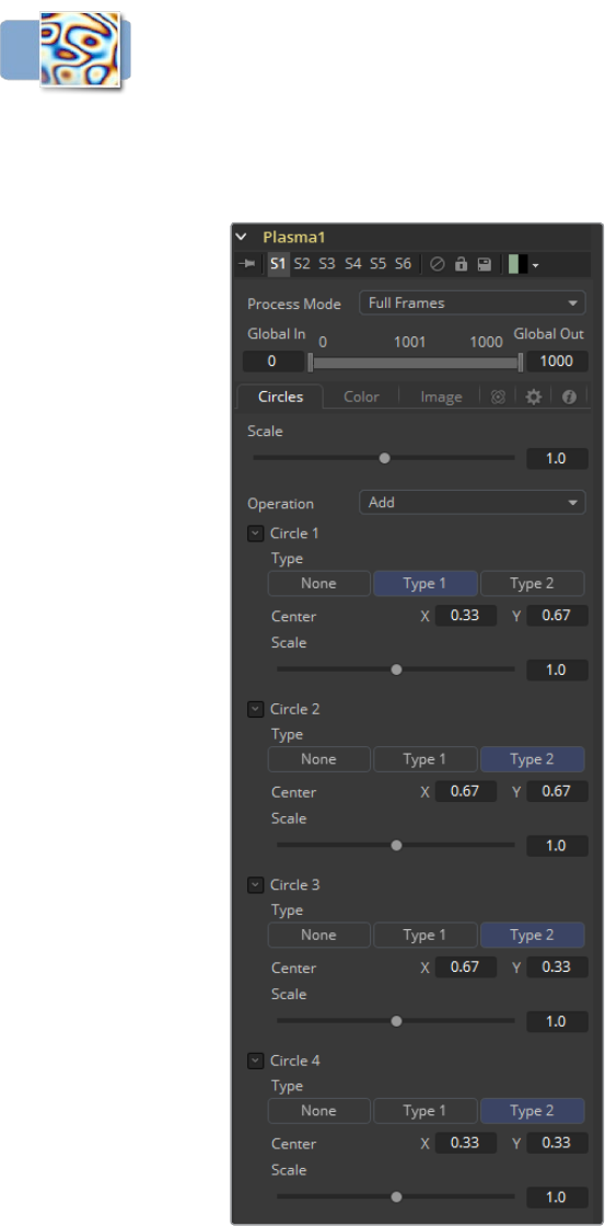
279
Creator Tools Chapter – 8
Plasma [PLAS]
This background generation tool uses four circular patterns to generate images similar to
Plasma. It is useful as a deforming pattern for the Shadow and Deform tools and to create a
variety of other useful shapes and patterns. See also the Fast Noise tool.
Circles Tab
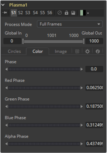
280
Creator Tools Chapter – 8
Scale
The Scale control is used to adjust the size of the pattern created.
Operation
The options in this menu determine the mathematical relationship between the four
circles whenever they intersect.
Circle Type
Select the type of circle to be used.
Circle Center
Report and change the position of the circle center.
Circle Scale
Determine the size of the circle to be used for the pattern.
Color Tab
Phase
Phase changes the color phase of the entire image. When animated, this creates
psychedelic color cycles.
R/G/B/A Phases
Changes the phase of the individual color channels and the alpha. When animated, this
creates color cycling effects.
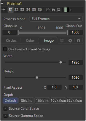
281
Creator Tools Chapter – 8
Image Tab
The controls in this tab are used to set the resolution, color depth and pixel aspect of the image
produced by the tool.
Process Mode
Use this menu control to select the Fields Processing mode used by Fusion to render
changes to the image. The default option is determined by the Has Fields checkbox
control in the Frame Format preferences. For more information on fields processing,
consult the Frame Formats chapter.
Global In and Out
Use this control to specify the position of this tool within the project. Use Global In to
specify on which frame that the clip starts and Global Out to specify on which frame
this clip ends (inclusive) within the project’s Global Range.
The tool will not produce an image on frames outside of this range.
Use Frame Format Settings
When this checkbox is selected, the width, height and pixel aspect of the image
created by the tool will be locked to values defined in the composition’s Frame Format
preferences. If the Frame Format preferences change, the resolution of the image
produced by the tool will change to match. Disabling this option can be useful to build a
composition at a different resolution than the eventual target resolution for the
final render.
Width/Height
This pair of controls is used to set the Width and Height dimensions of the image to be
created by the tool.
Pixel Aspect
This control is used to specify the Pixel Aspect ratio of the created images. An aspect
ratio of 1:1 would generate a square pixel with the same dimensions on either side (like
a computer display monitor) and an aspect of 0.9:1 would create a slightly rectangular
pixel (like an NTSC monitor).
282
Creator Tools Chapter – 8
Depth
The Depth button array is used to set the pixel color depth of the image created by the
creator tool. 32-bit pixels require 4 times the memory of 8-bit pixels, but have far
greater color accuracy. Float pixels allow high dynamic range values outside the normal
0..1 range, for representing colors that are brighter than white or darker than black. See
the Frame Formats chapter for more details.
Right-click on the Width, Height or Pixel Aspect controls to display a menu listing the
file formats defined in the preferences Frame Format tab. Selecting any of the listed
options will set the width, height and pixel aspect to the values for that format
accordingly.

283
Creator Tools Chapter – 8
Text Plus [TXT+]
Fusion’s Text tool is an advanced character generator capable of 3D transformations, multiple
styles and several layers of shading. Text can be laid out to a user-defined frame, circle or
along a path.
Any True Type or Postscript 1 font installed on the computer can be used to create text. Support
for multibyte and Unicode characters allows text generation in any language, including right to
left and vertically oriented text.
This tool generates a 2D image. To produce extruded 3D text with optional beveling, see the
Text 3D tool.
Text Tab
284
Creator Tools Chapter – 8
Size
This control is used to increase or decrease the size of the text. This is not like selecting
a point size in a word processor. The size is relative to the width of the image.
Font
The Font controls are used to select the font used by Fusion to create the text. Fusion
has limited support for third-party font managers. Fonts managed by a third-party font
manager may need to move the Mac OS X or Windows Fonts folder.
Underline and Strikeout
These checkboxes enable the addition of emphasis styles to the font used.
Styled Text
The edit box in this tab is where the text to be created is entered. Any common
character can be typed into this box. The common OS clipboard shortcuts (Command-C
or Ctrl-C to copy, Command-X or Ctrl-X to Cut, Command-V or Ctrl-V to paste) will also
work, however right-clicking on the edit box displays a custom contextual menu.
The Styled Text contextual menu has the following options.
Animate
Use this command to set to a keyframe on the entered text and animate the content
over time.
Character Level Styling
This command enables Character Level Styling, which will place a set of controls in the
Modifiers tab. Use these controls to affect changes in the font, color, size and
transformations applied to individual characters.
Comp Name
Comp Name puts the name of the composition in the edit box and is generally used to
create slates.
Follower
Follower is a text modifier that can be used to ripple animation applied to the text
across each character in the text. See Text Modifiers at the end of this section.
Publish
Publish the text for connection to other text tools.
Text Scramble
A text modifier ID is used to randomize the characters in the text. See Text Modifiers at
the end of this section.
Text Timer
A text modifier is used to count down from a specified time or to output the current
date and time. See Text Modifiers at the end of this section.
285
Creator Tools Chapter – 8
Time Code
A text modifier is used to output Time Code for the current frame. See Text Modifiers at
the end of this section.
Connect To
Use this option to connect the text generated by this Text tool to the published output
of another tool.
Write On
This range control is used to quickly apply simple Write On and Write Off effects to the
text. To create a Write On effect, animate the End portion of the control from 1 to 0 over
the length of time required. To create a Write Off effect, animate the Start portion of the
range control from 0 to 1.
International Font Controls
This drop-down menu can be used to select a language specific to a subset of a font.
Direction
This menu provides options for determining the Direction in which the text is to
be written.
Line Direction
These menu options are used to determine the text flow from top-bottom, bottom-top,
left-right or right-left.
Force Monospaced
This slider control can be used to override the kerning (spacing between characters)
that is defined in the font. Setting this slider to zero (the default value) will cause Fusion
to rely entirely on the kerning defined with each character. A value of one will cause the
spacing between characters to be completely even, or Monospaced.
Do Font Defined Kerning
This enables kerning as specified in the true type font and is on by default.
Advanced Font Controls
Leave the Font Defined Glyphs, Reordering and Ligation checkbox selected unless
instructed to do otherwise by support.
Manual Font Kerning/Placement
Right-clicking on this label will display a contextual menu that can be used to animate
the kerning of the text. See the Toolbar section of this tool’s documentation later in this
chapter for details on manual kerning.
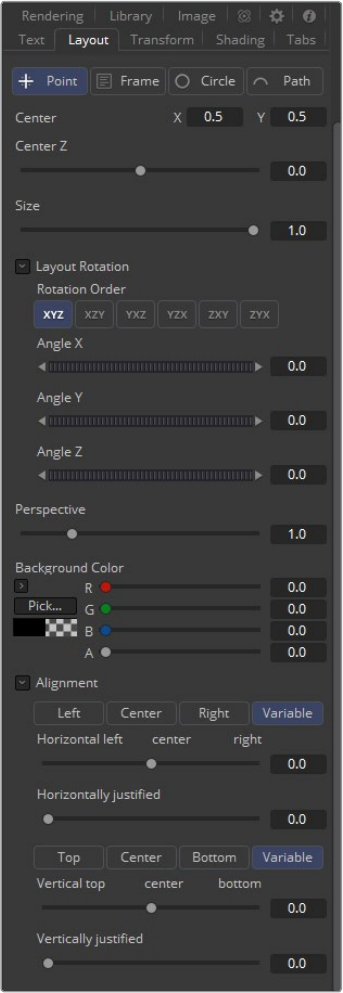
286
Creator Tools Chapter – 8
Layout Tab
The controls used to position the text are located in the Layout Tab. One of four layout types
can be selected using the button array.
Point
Point layout is the simplest of the layout modes. Text is arranged around an adjustable
center point.
Frame
Frame layout allows you to define a rectangular frame used to align the text. The
alignment controls are used to justifying the text vertically and horizontally within the
boundaries of the frame.
287
Creator Tools Chapter – 8
Circle
Circle Layout places the text around the curve of a circle or oval. Control is offered over
the diameter and width of the circular shape. When the layout is set to this mode, the
Alignment controls determine whether the text is positioned along the inside or outside
of the circle’s edge, and how multiple lines of text are justified.
Path
Path layout allows you to shape your text along the edges of a path. The path can be
used simply to add style to the text, or it can be animated using the Position on Path
control that appears when this mode is selected.
Center X, Y and Z
These controls are used to position the center of the layout element in space. X and Y
are onscreen controls and Center Z is a slider in the tool controls.
Size
This slider is used to control the scale of the layout element.
Layout Rotation
Select this checkbox and another set of options appears to set the Rotation options
of the text.
Rotation Order
This button array allows you to select the order in which 3D rotations are applied to
the text.
Angle X, Y and Z
These Angle controls can be used to adjust the angle of the Layout element
along any axis.
Width and Height
The Width control is visible when the Layout mode is set to Circle or Frame. The Height
control is only visible when the Layout mode is set to Frame. They are used to adjust
the dimensions and aspect of the Layout element.
Perspective
This slider control is used to add or remove Perspective from the rotations applied by
the Angle X, Y and Z controls.
Fit Characters
This menu control is only visible when the Layout type is set to Circle. This menu is
used to select how the characters are spaced to fit along the circumference.
Position On Path
The Position On Path control is used to control the position of the text along the path.
Values less than zero or greater than one will cause the text to move beyond the path
in the same direction as the vector of the path between the last two keyframes.
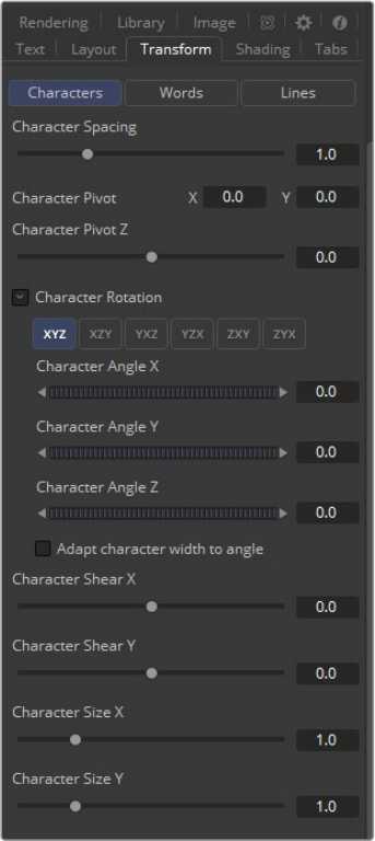
288
Creator Tools Chapter – 8
Background Color
This label only appears when the Layout type is set to Path. It is used to provide access
to a contextual menu that provides options for connecting the path to other paths in the
flow, and animating the shape of the path over time.
The text generated by this tool is normally rendered against black. This color picker
control can be used to set a new background color.
Right-Click Here for Shape Animation
Consult the Motion Paths chapter of this manual for details.
Horizontal and Vertical Alignment
Two identical sets of controls are used to control Vertical and Horizontal Alignment of
the text. Use the first array of buttons to choose the alignment of the text. The slider
beneath controls the justification.
Transform Tab
Select Transform
There are three buttons to determine the portion of the text affected by the
transformations applied in this tab. Transformations can be applied to line, word and
character levels simultaneously. This menu is only used to keep the number of visible
controls to a reasonable number.
289
Creator Tools Chapter – 8
Characters
Each character of text is transformed along its own center axis.
Words
Each word is transformed separately on the word’s center axis.
Lines
Each line of the text is transformed separately on that line’s center axis.
Spacing
The Spacing slider is used to adjust the amount of space between each line, word or
character. Values less than one will usually cause the characters to begin overlapping.
Pivot X, Y and Z
This provides control over the exact position of the axis. By default, the axis is
positioned at the calculated center of the line, word or character. The Axis control
works as an offset, such that a value of 0.1, 0.1 in this control would cause the axis to be
shifted downward and to the right for each of the text elements. Positive values in the
Z-axis slider will move the axis further along the axis (away from the viewer). Negative
values will bring the axis of rotation closer.
Rotation Order
These buttons are used to determine the order in which transforms are applied. X, Y
and Z would mean that the rotation is applied to X, then Y, and then Z.
Angle X, Y and Z
These controls can be used to adjust the angle of the text elements in any of the three
dimensions.
Shear X and Y
Adjust these sliders to modify the slanting of the text elements along the X- and Y-axis.
Size X and Y
Adjust these sliders to modify the size of the text elements along the X- and Y-axis.
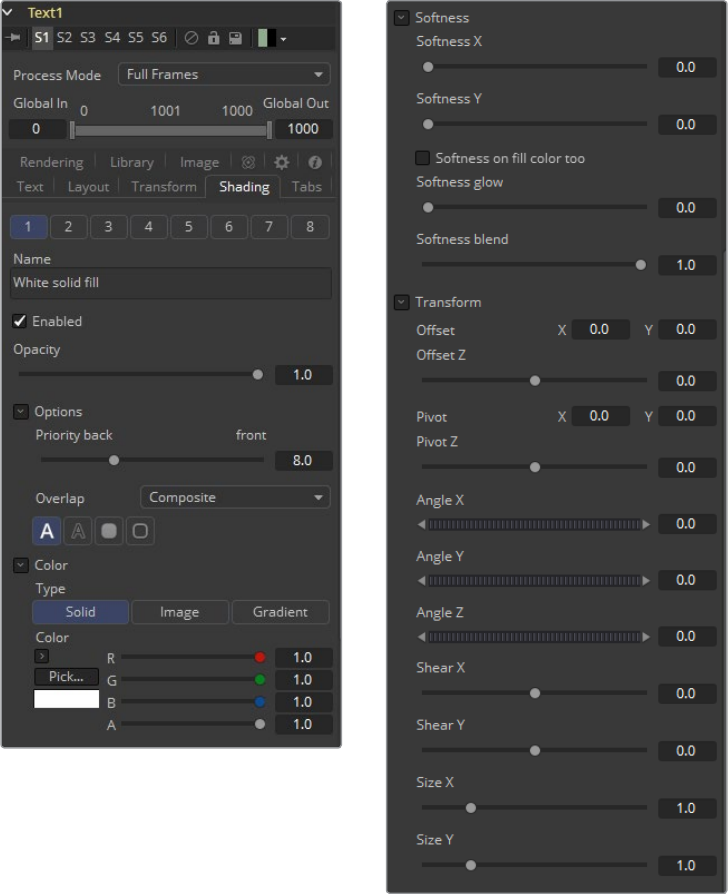
290
Creator Tools Chapter – 8
Shading Tab
The Shading tab provides controls to adjust the shading, texture and softness of the text.
Transformations can be controlled from this tab as well, applying additional transformations to
as many as eight separate text shading elements independently. The Number menu is used to
select the element affected by adjustments to the controls in this tab.
Name
This text label can be used to assign a more descriptive name to each shading element.
Enabled
Select this checkbox to enable or disable each layer of shading elements. Element 1 is
enabled by default. The controls for a shading element will not be displayed unless this
checkbox is selected.
291
Creator Tools Chapter – 8
Opacity
The Opacity slider controls the overall transparency of the shading element. It is usually
better to assign opacity to a shading element than to adjust the alpha of the color
applied to that element.
Priority Back/Front
This slider determines the layer’s order for the shading elements, also known as the
Z-order. Slide the control to the right to bring an element closer to the front. Move it to
the left to tuck one shading element behind another.
Overlap
This menu is used to select how the renderer deals with an Overlap between two
characters in the text.
Composite
This Overlap option will merge the shading over top of itself.
Solid
This option sets the pixels in the overlap region to pure opaque.
Transparent
This option sets the pixels in the overlap region to pure transparent.
Element Type (Buttons)
There are four options available from this menu, providing control over how the shading
element is applied to the text. Different controls will appear below depending on the
element type selected.
Text Fill
The shading element is applied to the entire text. This is the default mode.
Text Outline
The shading element is drawn as an outline around the edges of the text.
Border Fill
The shading element fills a border surrounding the text. Five additional controls are
provided with this shading mode.
Border Outline
The Border Outline mode draws an outline around the border that surrounds the text. It
offers several additional controls.
Overlap
(All Types) Overlap is used to determine how the shading is handled when portions of
the same shading element overlap. Setting this menu to transparent will cause the
pixels’ color and alpha channels to be set to 0 (transparent).
Thickness
(Outline only) Use this slider control to adjust the thickness of the outline. Higher values
equal thicker outlines.
Adapt Thickness To Perspective
(Outline only) Selecting this checkbox will cause your outline to become thinner where
the text is farther away from the camera, and thicker where it is closer. This will create a
much more realistic outline for text transformed in 3D but takes significantly longer
to render.
292
Creator Tools Chapter – 8
Outside Only
(Outline only) Selecting this checkbox will cause the outline to be drawn only on the
outside edge of the text. By default the outline is centered on the edge and partially
overlaps the text.
Join Style
(Outline only) This menu provides options for how the corners of the outline are drawn.
Options include Sharp, Rounded and Beveled.
Line Style
(Outline only) This menu offers additional control over the style of the line. In addition to
the default solid line, a variety of dash and dot patterns are available.
Shape
(Border Fill only) Shape creates a solid rectangular image around the character.
Shape
(Border Outline only) Creates a rectangular outline around each character.
Level
(Border Fill only) This is used to control the portion of the text border filled.
Text
This draws a border around the entire text.
Line
This draws a border around each line of text.
Word
This draws a border around each word.
Character
This draws a border around each character.
Extend Horizontal and Extend Vertical
(Border only) Use this slider to change the dimensions of each border.
Round
(Border only) This slider is used to round off the edges of the border.
Color Types
In addition to solid shading, it is also possible to map an external image onto the text.
This menu is used to determine if the color of the shading element is derived from a
user-selected color or if it comes from an external image source. Different controls will
be displayed below depending on the Color Type selected.
Solid Mode
When the Type menu is set to Solid mode, color selector controls are provided to
select the color of the text.
Image Mode
The output of a tool in the flow will be used to texture the text. The tool used is chosen
using the Color Image control revealed when this option is selected.
293
Creator Tools Chapter – 8
Color Image
(Image Mode only) This Color Image text box is used to enter the name of the tool in
the flow that will provide the image. You can type the name in with the keyboard, drag
the tool from the flow into the text box or right-click and select Connect To from the
contextual menu to select the image to be used.
Image Size
(Image Mode only) The Image Size menu is used to select how the image is mapped
to the text.
Full Image
This option applies the entire image to the text.
Text
This option applies the image to fit the entire set of text.
Line
This option applies the image per line of text.
Word
This option applies the image per each word of text.
Character
This option applies the image per individual character.
Softness X and Y
These sliders control the softness of the text outline used to create the shading
element. Control is provided for the X- and Y-axis independently.
Softness On Fill Color Too
Selecting this checkbox will cause blur (softness) to be applied to the shading element
as well. The effect is best seen when applied to a shading element colored by an
external image.
Softness Glow
This slider will apply a glow to the softened portion of the shading element.
Softness Blend
This slider controls the amount that the result of the softness control is blended back
with the original. It can be used to tone down the result of the soften operation.
Transform Controls
Selecting the Transform button in the Shading tab will display controls for performing
transformations to the shading elements. These controls work in exactly the same way
as their equivalents in the Alignment and Layout Tabs, with the addition of a Center
Offset control.
Offset X, Y and Z
These controls are used to apply offset from the text’s global center (as set in the Layout
tab) for the shading elements. A value of X0.0, Y0.1 in the coordinate controls would
place the shading element center 10 percent of the image further down the screen along
the Y-axis. Positive values in the Z-Offset slider control will push the center farther away
from the camera, while positive values will bring it closer to the camera.
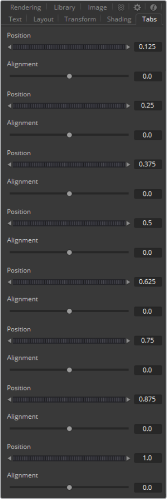
294
Creator Tools Chapter – 8
Tabs Tab
The controls in the Tabs area are used to configure the horizontal screen positions of 8
separate tab stops. Any tab characters in the text will conform to these positions.
Because the Tab key is used by Fusion to advance to the next control, it is not possible to enter
a tab directly into the Styled Text input. Enter a tab using one of the following methods.
Copy and Paste
Copy a tab from another document, such as Notes on Mac OS X or Notepad on
Windows, and paste it into the text box.
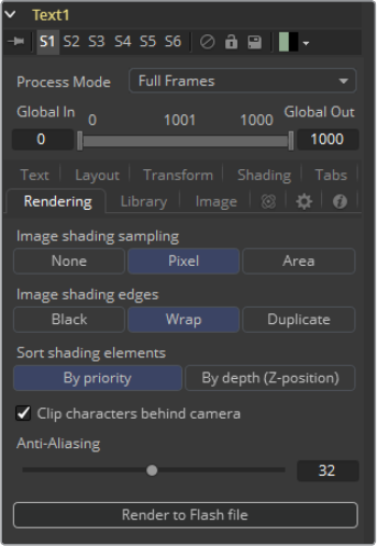
295
Creator Tools Chapter – 8
Position
This control is used to set the horizontal position of the tab in the frame. The values
range from 0.0 to 1.0, where 0 is the far left side and 1 is the far right side of the frame.
The position of the tab will be indicated in the Viewer by a thin vertical white line when
the Text tool is selected and the Tabs tab is open.
Alignment
Each tab can be set to either left aligned, right aligned or centered. This slider ranges
from -1.0 to 1.0, where -1.0 is a left aligned tab, 0.0 is a centered tab and 1.0 is a right
aligned tab. Small white boxes at the top of the tab lines indicate that there are tabs
present in the flow. Clicking within these boxes will toggle the alignment of the tab
between the three states.
Rendering Tab
Image Shading Sampling
Use this button array to select the sampling type for shading rendering and
transformations. The default of Pixel shading is sufficient for 90% of tasks. To reduce
detectable aliasing in the text, set the sampling type to Area. This is slower but may
produce better quality results. A setting of None will render faster, but with no
additional sampling applied, so the quality will be lower.
Image Shading Edges
Use this button array to choose how transformations applied to image shading
elements are handled when they wrap off the text’s edges.
Sort Shading Elements
This button selection determines the ordering of the shading elements. The default is
By Priority, which organizes the shading elements back to front, according to the
priority back/front slider in each shading element’s controls.
Selecting the By Depth (Z-Position) option will re-organize these according to each
element’s Z-position, as set by the element’s transformations.
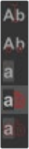
296
Creator Tools Chapter – 8
Clip Characters Behind Camera
This checkbox determines whether characters that go beyond the plane of the camera
will be clipped, or if they will reflect back toward the center of the image. This should
normally be enabled for clipping, but some interesting effects can be produced when
clipping is disabled.
Anti-Aliasing
This slider is used to increase or decrease the amount of anti-aliasing applied to the
text. Higher values mean exponentially longer render times, while lower values reduce
render times at the expense of quality.
Render to Flash File
Click this button to render the output of the Text tool to an Adobe Flash file.
Library Tab
The Shading Library is used to store and retrieve the settings of a Text tool for
easy re-use.
Put
To add a new text element to the library, click on the Put button. All of the current
settings for the tool will be saved according to the name assigned. A thumbnail will
appear in the Shading Library showing how that style looks on the letter A.
Get
Click on a shading element in the library, then click on the Get button to apply those
settings to the current tool. Get will replace all of the text as well as the style.
Shading
Clicking on Shading will replace the shading elements only, without affecting the text
entered. Right-click in the Shading Library window for a list of display options.
Text+ Toolbar
When the Text tool is selected, a toolbar will appear in the Viewer.
Allow Typing In Preview Window
Enable this button to type and edit text directly in the Viewer, click on the text to
produce a cursor that can be positioned within the text. The cursor can be moved using
the arrow keys. Type normally.
297
Creator Tools Chapter – 8
Allow Manual Kerning
This button enables Manual Kerning, which overrides the automatic kerning normally
applied to text. A small red dot will appear beneath each character of text in the Viewer.
Drag on the dot to reposition a character. Also select multiple characters and move
them together. Hold the Option or Alt key down while dragging to constrain motion to a
single axis.
Use the arrow keys on the keyboard to make manual adjustments to the position of
theselected characters. Hold the Command or Ctrl key down while pressing arrow
keys to move the character in smaller increments. Shift will move the characters in
largerincrements.
To animate the position of each character, right-click on the control label Manual Font
Kerning/Placement beneath the Text tab’s Advanced Font controls and select Animate
from the contextual menu. A new key will be set on the animation spline each time a
character is moved. All characters are animated with the same spline, as with polyline
mask animation.
No Text Outline
This button disables the drawing of any outline around the edges of the text. The
outline is not a part of the text. It is an onscreen control used to help identify the
position of the text.
Text Outline Outside Frame Only
This button draws an outline around the edges of text, which is outside the visible
frame. This is useful for locating text that has moved off screen and is no longer
rendering a visible result.
Show Always Text Outline
This button draws an outline around the edges of text at all times, whether the text is
visible within the frame or not.
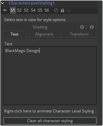
298
Creator Tools Chapter – 8
Modifiers
Character Level Styling
The Character Level Styling modifier only works on Text+ tools. You can then select individual
characters directly in your view and apply different text attributes to them. Think of larger
capitals at the beginning of each line, different fonts in one word, colored highlighting and more.
It can be applied by right-clicking into the Styled Text field of a Text+ tool and selecting
Character Level Styling.
Character Level Styling can only be directly applied to Text+ tools, not to Text 3D tools.
However, styled text from a Text+ tool can be applied to a Text 3D tool by means of copying the
Text+, right-clicking on the Text 3D and choosing Paste Settings.
Text Tab
Text Controls, Alignment, Transform and Shading Tab
For details see the Text+ tool documentation.
Clear Character Styling on Selection
All changes made to the currently selected Characters will be reset.
Clear all Character Styling
All character attributes will be reset to their original values.
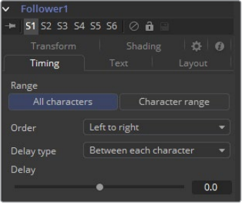
299
Creator Tools Chapter – 8
Comp Name
The Comp Name only works on Text+ tools. It sets the Styled text to become the current
Composition Name. This is quite useful to automate burn-ins for daily renderings. See also the
TimeCode modifier. It can be applied by right-clicking into the Styled text field of a Text+ tool
and selecting Comp Name.
Controls
This Modifier Has No Controls
For further details see the Text+ Tool documentation.
Follower
The Follower only works on Text and Text3D tools. This tool allows for a plethora of cool motion
graphics effects. The basic idea is that you animate the parameters of a single character and
the other characters will follow that animation with a delay. It can be applied by right-clicking
into the Styled Text field of a Text tool and selecting Follower.
Timing Tab
Range
Allows the user to select if all characters should be influenced or only a selected range.
You can drag-select a range of characters directly on the screen.
Order
Determines in which order the Characters are influenced. Notice that empty spaces are
counted as characters as well. Available options are:
Left to right: The animation ripples from left to right through all characters.
Right to left: The animation ripples from right to left through all characters.
Inside out: The animation ripples symmetrically from the center point of the
characters toward the margin.
Outside in: The animation ripples symmetrically from the margin toward the center
point of the characters.
Random but one by one: The animation is applied to randomly selected characters
but only influences one character at a time.
Completely random: The animation is applied to randomly selected characters,
influencing multiple characters at a time.
Manual curve: The affected characters can be specified by sliders.
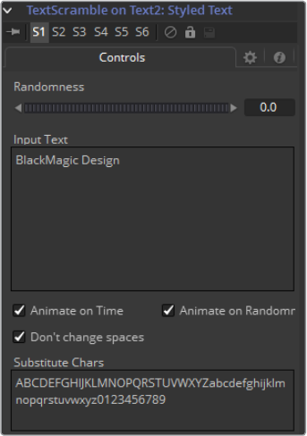
300
Creator Tools Chapter – 8
Delay Type
Determines what sort of delay is applied to the animation. Available options are:
Between Each Character: The more characters there are in your text, the longer the
animation will take to the end.
Between First and Last Character: No matter how many characters are in your text,
the animation will always be completed in the selected amount of time.
Clear all Character Styling
All character attributes will be reset to their original values.
Text Controls, Alignement, Transform and Shading Tab
In these tabs, the actual animation for the characters is done. Observe that simply
changing a value in these tabs will have no influence at all. The value needs to be
animated for the effect to show.
For a detailed description on the various parameters, see the Text+ tool documentation.
Text Scramble
The Text Scramble only works on Text+ tools. It scrambles the Text around, randomly replacing
the characters with others from a user definable set. It can be applied by right-clicking into the
Styled text field of a Text+ tool and selecting TextScramble.
Controls
Randomness
Defines how many characters are exchanged randomly. A value of 0 will change no
characters at all. A value of 1 will change all characters in the text. Animating this
thumbwheel to go from 0 to 1 will gradually exchange all characters.
Input Text
This reflects the original Text in the Text+ Styled Text. Text can be entered either here
on in the Text+.
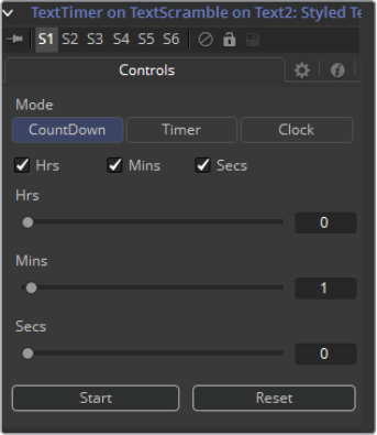
301
Creator Tools Chapter – 8
Animate On Time
When set, the characters will get scrambled randomly on every new frame. This switch
has no effect when Randomness is set to 0.
Animate On Randomness
When set, the characters will get scrambled randomly on every new frame, when the
Randomness thumbwheel is animated.
This switch has no effect when Randomness is set to 0.
Don’t Change Spaces
When set, the length of the single words will stay the same, though their characters get
scrambled around.
Substitute Chars
Defines which characters are used to scramble the text.
Text Timer
The Text Timer only works on Text+ tools. It makes the Text+ tool either a Countdown, a Timer
or a Clock. This is quite useful for on screen real-time displays or to burn in the creation time of
a frame into the picture.
It can be applied by right-clicking into the Styled text field of a Text+ tool and selecting
TextScramble.
Controls
Mode
Sets the mode the timer is working in. In Clock mode the current system time will
bedisplayed.
Hrs, Mins, Secs (Switches)
Defines which parts of the clock should be shown on screen.
Hrs, Mins, Secs (Sliders)
Set the start time for the Countdown and Timer mode.
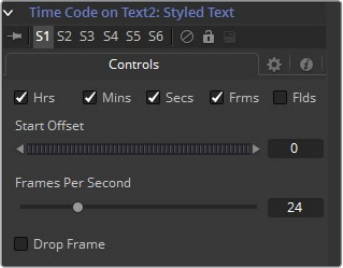
302
Creator Tools Chapter – 8
Start
Starts the Counter or Timer. Toggles to Stop once the timer is running.
Reset
Resets the Counter and Timer to the values set by the sliders.
Time Code
The Time Code only works on Text+ tools. It sets the Styled text to become a counter based on
the current frame. This is quite useful to automate burn-ins for daily renderings.
It can be applied by right-clicking into the Styled text field of a Text+ tool and selecting
Time Code.
Controls
Hrs, Mins, Secs, Frms, Flds
Activate or de-activate these options to customize the time code display to show hours,
minutes, seconds, frames and fields respectively. Activating Frames only will give you
aplain frame counter
Start Offset
Introduce a positive or negative offset to Fusion’s current time to match up with
existingtime codes.
Frames per Second
This should match with your Composition’s FPS setting to provide accurate time
measurement.
Drop Frame
Activate this checkbox to match the time code with footage that has drop frames,
forexample, certain NTSC formats.
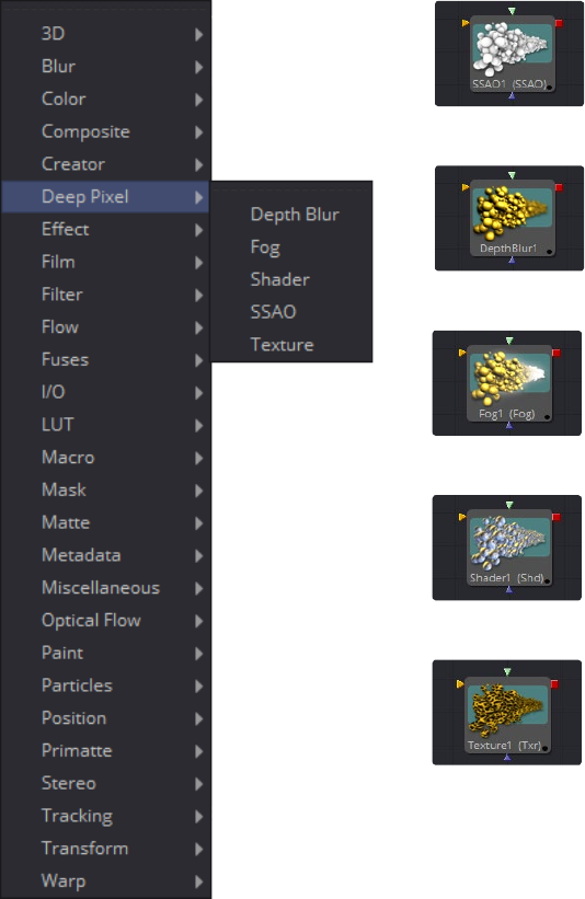
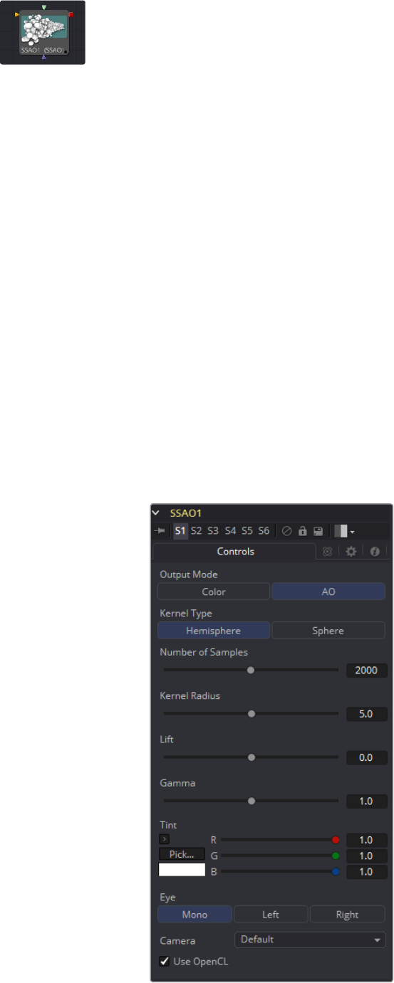
306
DeepPixel Tools Chapter – 9
Ambient Occlusion
Ambient Occlusion (AO) is the lighting caused when a scene is surrounded by a uniform diffuse
spherical light source. Think of the scene as being surrounded by a humongous sphere that
uniformly emits light from its surface. AO captures the low frequency lighting. It does not
capture sharp shadows or Diffuse or Specular lighting. For this reason, AO is usually combined
with Diffuse and Specular lighting to create a full lighting solution.
The Ambient Occlusion tool generates global lighting effects in 3D-rendered scenes as a post
effect. It approximates expensive raytraced global illumination quickly. Being a post effect, it
exposes similar aliasing issues like the Shader, Texture, and VolumeFog tool. Hence, artifacts
may appear in certain situations.
Usage
The AO tool rarely works out of the box, but requires some tweaking. The setup process
involves adjusting the KernelRadius and NumberOfSamples to get the desired affect.
The KernelRadius depends on the natural ‘scale’ of the scene. Initially there might appear to be
no AO at all. At this point either the KernelRadius is too small or too big and working values
have to be found.
Inputs
Image (required): Requires RGBA, Z-Depth and Normals.
Scene (required): The Scene or 3D Camera the image was rendered with.
If any of these are not supplied, the tool will fail with a descriptive error.
Controls
307
DeepPixel Tools Chapter – 9
Output Mode
Color: The incoming image with Ambient Occlusion applied
AO: Outputs the pure Ambient Occlusion as a grayscale image.
White corresponds to regions in the beauty pass that should be bright, while black
correspond to regions that should be darker. This allows you to create a lighting
equation by combining separate ambient/diffuse/specular passes. Having the AO as a
separate buffer allows for creative freedom to combine the passes in various ways.
Kernel Type
To determine the AO, rays are cast outward from a point on the surface being shaded
outwards to a large enclosed sphere.
The number of unoccluded rays, that is those rays that reach the sphere, determines
the AO factor.
Hemisphere
Rays are cast toward a hemisphere oriented to the surfaces normal. This option is more
realistic than “Sphere” and should be used unless there is a good reason otherwise.
Flat surfaces will receive 100% ambient intensity, while other parts will be darkened.
Sphere
Rays are cast toward a sphere centered about the point being shaded. This option is
provided to produce a stylistic effect. Flat surfaces will receive 50% ambient intensity,
while other parts will be made darker or brighter.
Number of Samples
Increase the number of samples until artifacts in the AO pass disappear. Higher values
can generate better results but also increase render time.
Kernel Radius
The Kernel Radius controls the size of the filter kernel in 3D space. For each pixel, it
controls how far one searches in 3D space for occluders. Most likely, the Filter Kernel is
finicky and may need to be adjusted manually for each individual scene.
If made too small, nearby occluders can be missed. If made too large, the quality of the
AO will decrease and the number of samples needs to be increased dramatically to get
the quality back.
This value is dependent on the scene Z-depth. That means with huge Z values in the
scene, the kernel size needs to be large as well. With tiny Z values, a small kernel size
like 0.1 should be sufficient.
Lift/Gamma/Tint
Used to adjust the AO for artistic effects.
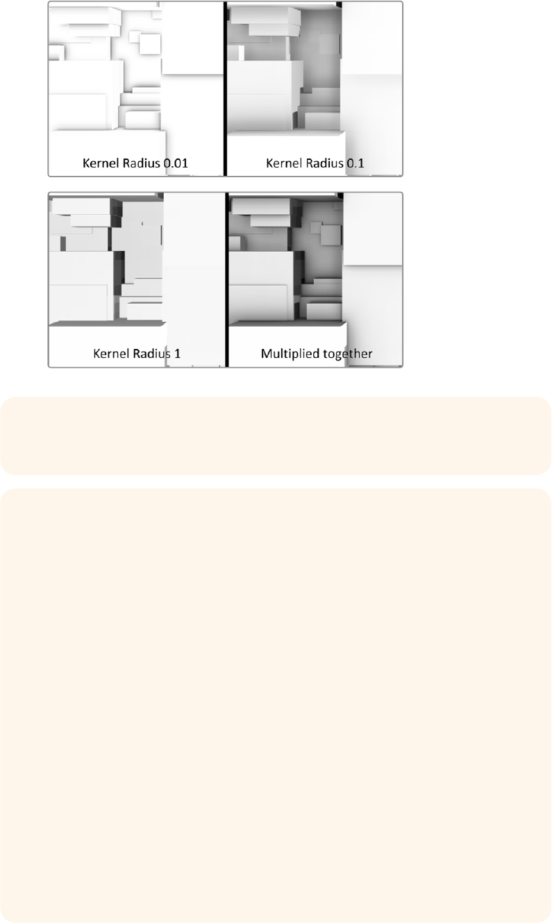
308
DeepPixel Tools Chapter – 9
Use OpenCL
Ambient Occlusion is very slow on the CPU, but performs much better on the GPU.
Activate this switch to utilize the OpenCL power of your Graphics Card
TIP Combining multiple AO passes with different kernel radii can produce
better effects.
Known Issues
Transparency/Translucency: AO is designed to work with opaque objects. There will
be two kinds of problems: those with transparent receivers and those with transparent
occluders. You can work around some of these problems by splitting out the
transparent/translucent objects into separate scenes and only computing AO on the
opaque objects.
Particles: Do not use AO on particles, unless the particles are solid opaque geometry.
This is just the transparency problem again. Antialiased edges (another form of
transparency) will also cause problems with AO. There’s not much you can do
about this.
Supersampling: See Antialiased edges. In order for this to work, the AO needs to be
computed in the big image before it is downsampled to the final image.
View Dependence: AO methods work in view space and the results are view
dependent. This is a limitation of the technique itself. This means the amount of
darkening can vary depending on the view location when in reality it should be
constant. If at a point on an object the AO is 0.5, moving the camera could change
it to 0.4.
Baking of AO: The UV renderer can be used to bake AO into the textures on models.
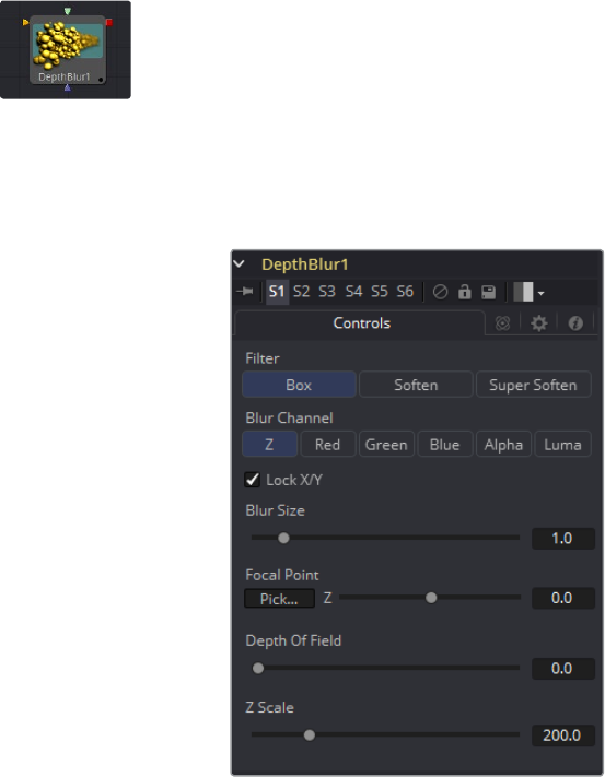
309
DeepPixel Tools Chapter – 9
Depth Blur
The Depth Blur tool is primarily used to create focal length or depth-of-field effects. It blurs 3D
rendered images based on included Z-channel values, and can also be used for general
per-pixel blurring effects by means of the Blur Channel controls. If the Blur Image input is
connected, channels from that image will be used to control the blur.
Controls
Filter
These buttons are used to select the filter used for applying the blur.
Box
This applies a depth-based box blur effect to the image.
Soften
This applies a depth-based general softening filter effect.
Super Soften
This applies a depth-based high quality softening filter effect.
Blur Channels
Select one of these options to determine the channel used to control the level of blur
applied to each pixel. The channel from the main image input is used, unless a tool is
connected to the tool’s Blur Image input on the flow.
310
DeepPixel Tools Chapter – 9
Lock X/Y
When toggled on, this control locks the X and Y Blur sliders together for
symmetrical blurring.
Blur Size
This slider is used to set the strength of the horizontal and vertical blurring applied to
the image.
Focal Point
This control is only visible when the Blur channel is set to use the Z buffer.
Use this control to select the distance of the simulated point of focus. Lowering the
value causes the Focal Point to be closer to the camera, raising the value causes the
Focal Point to be farther away.
Drag the Pick button (the pointer changes to a dropper) over the displayed image and
select a Z-buffer value. If the image does not contain a valid Z-buffer, no change will
occur in the value.
Depth of Field
This control is used to determine the depth of the area in focus. The focal point is
positioned in the middle of the region and all pixels with a Z-value within the region stay
in focus. For example, if the focal point was selected from the image and set to a value
of 300, and the depth of field is set to 200, any pixel with a Z-value between 200 and
400 would remain in focus.
Z Scale
Scales the Z-buffer value by the selected amount. Raising the value causes the
distances in the Z channel to expand. Lowering the value causes it to contract. This is
useful for exaggerating the depth effect. It can also be used to soften the boundaries of
the blur. Some images with small depth values may require the Z scale to be set quite
low, below 1.0.
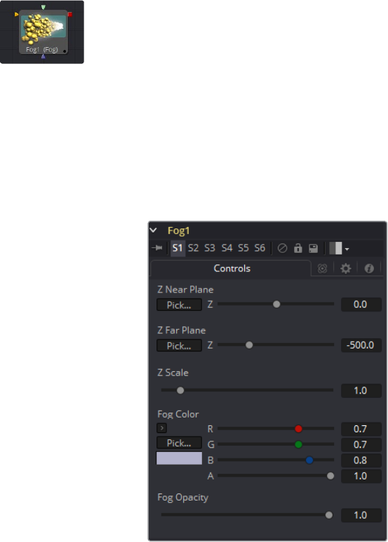
311
DeepPixel Tools Chapter – 9
Fog
The Fog tool is used to create simulated fog effects on 3D rendered images that contain a valid
Z-buffer channel. The fog can be placed in front of or behind various elements of a rendered
image based on the selected Z-channel planes. For more information, see the Auxiliary
Channels chapter.
The second image input on the Fog tool can be used to provide an image that is used as the
source of the fog. If no image is provided, the fog consists of a single color. Generally, a noise
map of some sort is provided here.
Controls
Z-Buffer Near Plane and Far Plane
These controls are used to select the extents of the fog within the scene. To pick a
value, drag the Pick button to an area on the image being viewed where the plane is to
be located.
The Near Plane is used to select the depth where the fog thins out to nothing. The Far
Plane is used to select the depth at which the fog becomes opaque.
Z Depth Scale
This option scales the Z-buffer values by the selected amount. Raising the value causes
the distances in the Z channel to expand, whereas lowering the value causes it to
contract. This is useful for exaggerating the fog effect.
Fog Color
This option displays and controls the current fog color. Alpha adjusts the fog’s
transparency value.
Fog Opacity
Use this control to adjust the opacity of the fog.
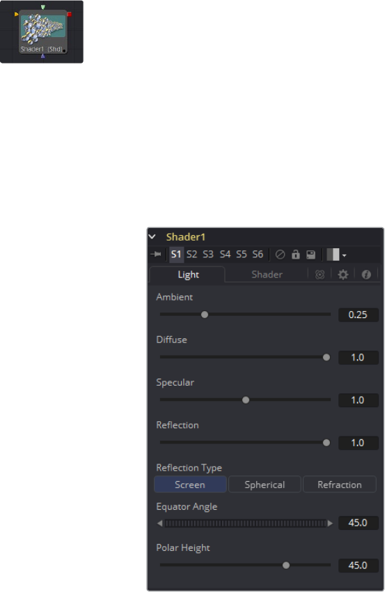
312
DeepPixel Tools Chapter – 9
Shader
The Shader tool can control the lighting, reflection mapping and 3D shading of elements in a
rendered image. The reflection map image (connected to the green input) can be projected
onto all elements in the scene, or to elements selected by the Object and Material ID channels
in the common controls. Effect masking can also be used to limit the effect of this tool.
The Shader tool relies on the presence of the X, Y and Z normal map channels in 3D rendered
images. If these channels are not present, this tool has no effect.
For more information, see the Auxiliary Channels chapter in the User Manual.
Light Tab
313
DeepPixel Tools Chapter – 9
Ambient
Ambient controls the amount of Ambient color present in the scene or for the selected
object. This is a base level of light, added to all pixels, even in completely
shadowed areas.
Diffuse
This option controls the amount of Diffuse color present in the scene or for the selected
object. This is the normal color of the object, reflected equally in all directions.
Specular
This option controls the amount of Specular color present in the scene or for the
selected object. This is the color of the glossy highlights reflected toward the eye from
a light source.
Reflection
This option controls the amount of Reflection contribution in the scene or for the
selected object. High levels make objects appear mirrored, low levels overlay subtle
reflections giving a polished effect. It has no effect if no reflection map is connected.
Reflection Type
Select from these three buttons to determine the type of reflection mapping used to
project the image in the second input.
Screen
Screen causes the reflection map to appear as if it were projected on to a screen
behind the point of view.
Spherical
Spherical causes the reflection map to appear as if it were projected on to a huge
sphere around the whole scene.
Refraction
Refraction causes the reflection map to appear as if it were refracting or distorting
according to the geometry in the scene.
Equator Angle
Equator Angle controls the left to right angle of the light generated and mapped by the
Shader tool for the scene or the selected object.
Polar Height
Polar Height controls the top to bottom angle of the light generated and mapped by the
Shader tool for the scene or the selected object.
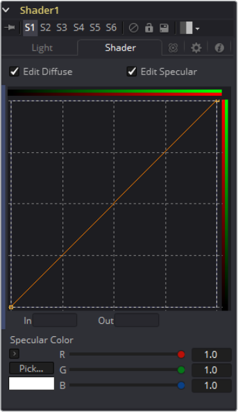
314
DeepPixel Tools Chapter – 9
Shader Tab
Edit Diffuse and Specular
Toggle these controls on to enable editing of the Shader curves for the individual
channels in the Shader spline window.
In and Out
These options are used to display and edit point values on the spline.
Specular Color
Use the Diffuse curve to manipulate the diffuse shading and the Specular curve to
affect the specular shading. Drag a box over a number of points to group select them.
Right-clicking displays a menu with options for adjusting the spline curves. For a
complete description of the options and controls for the spline windows, see the
documentation for the LUT Editor in the Controls chapter of the manual.
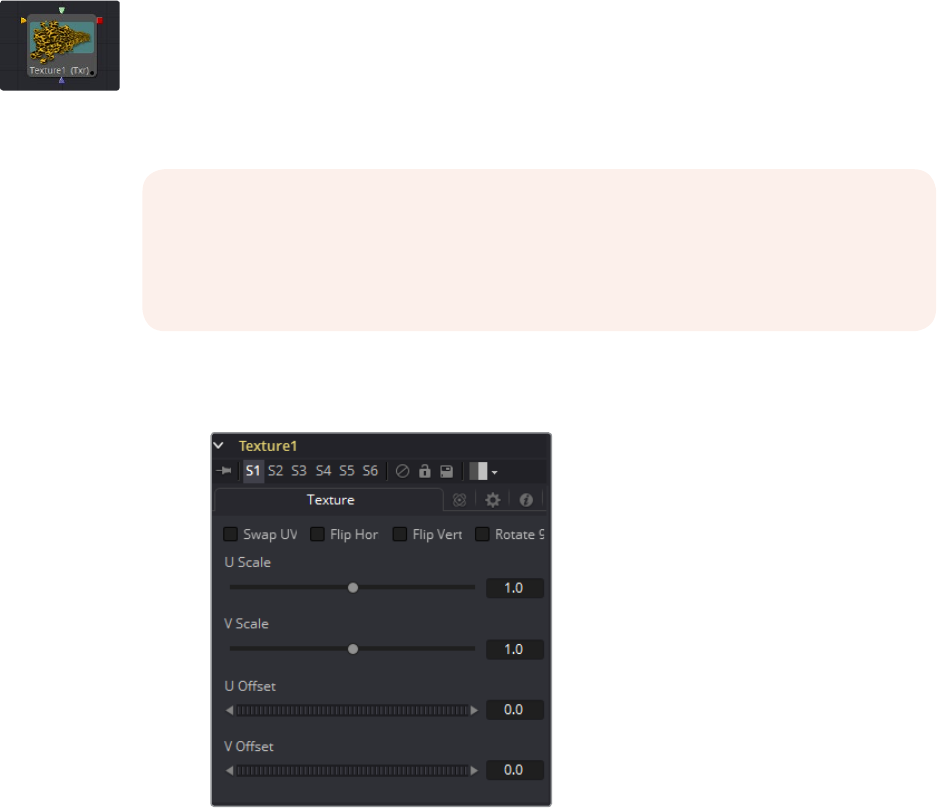
315
DeepPixel Tools Chapter – 9
Texture
The Texture tool can control the texture mapping of elements in a rendered image. The
texture-map image (connected to the green input) can be wrapped around objects to replace
the current texture. The Texture tool relies on the presence of U and V Map channels in
3Drendered images. If these channels are not present, this tool has no effect.
Texture Tab
Swap UV
When this checkbox is selected the U and V channels of the source image
are swapped.
Flip Horizontal and Vertical
The texture-map image is flipped horizontally and/or vertically when this control is
toggled on.
Rotate 90
The texture-map image is rotated 90 degrees when this checkbox is enabled.
U and V Scale
These controls change the scaling of the U and V coordinates used to map the texture.
Changing these values effectively enlarges and shrinks the texture map as it is applied.
U and V Offset
Adjust these controls to offset the U and V coordinates. Changing the values causes
the texture to appear to move along the geometry of the object.
NOTE: Background pixels may have U and V values of 0.0, which will set those pixels
to the color of the texture’s corner pixel. To restrict texturing to specific objects, use
aneffect mask based on the alpha of the object, or its Object or Material ID channel.
Formore information, see the Auxiliary Channels chapter.
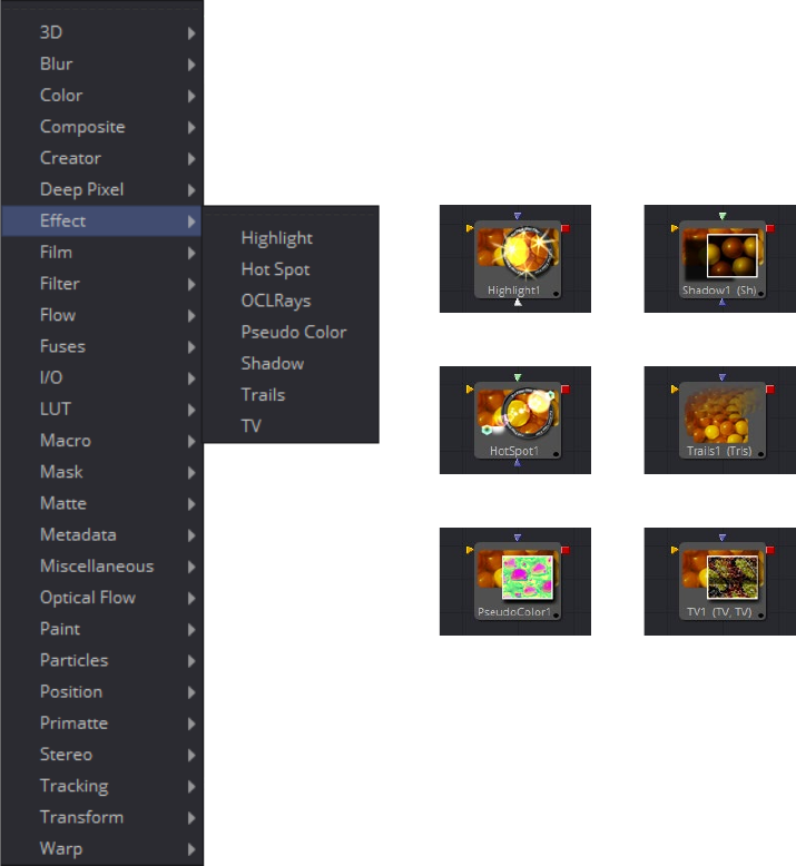
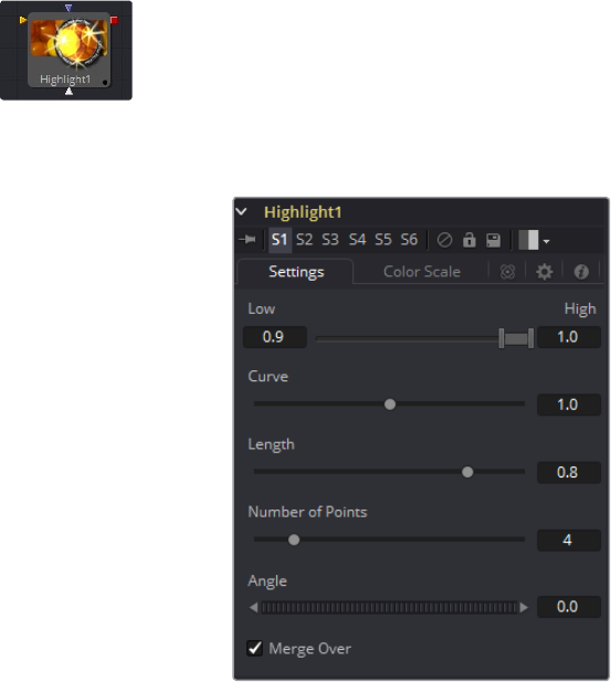
319
Effect Tools Chapter – 10
Highlight [HIL]
The Highlight filter creates star-shaped highlights in bright regions of the image, similar to a lens
star filter effect.
Settings Tab
Low and High
This range control designates the range of Luminance values in the image that will
generate highlights. Values less than the Low value will not receive highlights. Values
above the High value will receive the full highlight effect.
Curve
The Curve value changes the drop off over the length of the highlight. Higher values
will cause the brightness of the flares to drop off closer to the center of the highlight,
whereas lower values will drop off further from the center.
Length
This designates the Length of the flares from the highlight.
Number of Points
This determines the Number of flares emanating from the highlight.
Angle
Use this control to rotate the highlights.
Merge Over
When this checkbox is on, it will overlay the effect on the original image. With the
checkbox off, the output will be the highlights only. This is useful for downstream color
correction of the highlights.
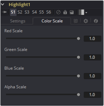
320
Effect Tools Chapter – 10
Color Scale Tab
Red, Green and Blue Scale
Moving the sliders of one or all of these channels down will change the falloff color of
the highlight.
Alpha Scale
Moving the Alpha slider down will make highlight falloff more transparent.
Highlight Masks
The Highlight tool offers an additional mask input called the Highlight Mask. This is a
pre-mask that determines what pixels can be affected by the highlight before the
highlight is applied. Unlike regular masks, it will not crop off highlights from source
pixels when the highlight extends past the masks edges.
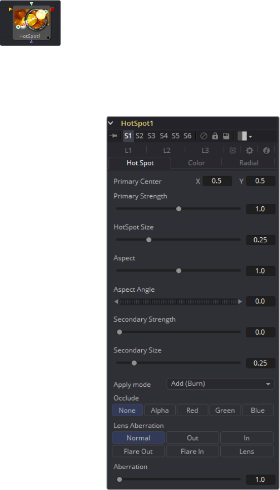
321
Effect Tools Chapter – 10
Hot Spot [HOT]
The Hot Spot tool is used to create lens flare, spotlight and burn/dodge effects of various types.
In the real world, lens flares occur when extremely bright light sources present in the scene by the
reflections are reflected off elements inside the lens of the camera. One might see lens flares in a
shot when viewing a strong light source through a camera lens, like the sun or a bright star.
Hot Spot Tab
Primary Center X and Y
This is the position of the Primary Hot Spot within the scene. Secondary lens elements
and reflections are positioned relative to the position of the primary.
Primary Strength
This control determines the brightness of the primary hotspot.
Hotspot Size
This control determines the diameter of the primary hotspot. A value of 1.0 represents a
circle the full width of the image.
Aspect
This controls the Aspect of the spot. A value of 1.0 produces a perfectly circular
hotspot. Values above 1.0 will elongate the circle horizontally and values below 1.0 will
elongate the circle vertically.
322
Effect Tools Chapter – 10
Aspect Angle
This control can be used to rotate the primary hotspot.
Secondary Strength
This control determines the strength, which is to say the brightness, of the secondary
hotspot. The secondary hotspot is a reflection of the primary hotspot. It will always be
positioned on the opposite side of the image from the primary hotspot.
Secondary Size
This determines the size of the secondary hotspot.
Apply Mode
This control determines how the hotspot affects the underlying image.
Add (Burn)
This causes the spots created to brighten the image.
Subtract (Dodge)
This causes the spots created to dim the image.
Multiply (Spotlight)
This causes the spots created to isolate a portion of the image with light and to darken
the remainder of the image.
Occlude
Use this button array to select which channel of the image connected to the Hotspot
tool’s Occlusion input is used to provide the occlusion matte.
Occlusion happens when the source of the hotspot is blocked by something between it
and the camera. When the source of a hotspot is occluded, the hotspot simply
winks out.
Occlusion can be controlled from Alpha or R, G or B channels of any image connected
to the Occlusion input on the tool’s tile. The white pixels in the image will occlude the
hotspot. Gray pixels will partially suppress the hotspot.
Lens Aberration
Aberration changes the shape and behavior of the primary and secondary hotspots.
In and Out Modes
Elongates the shape of the hotspot into a flare. The hotspot stretches toward the center
of the image when in In mode, stretching toward the corners when in Out mode.
Flare In and Flare Out Modes
This option is a lens distortion effect that is controlled by the movement of the lens
effect. Flare In will cause the effect to become more severe the closer the hotspot gets
to the center. Flare Out causes the effect to increase, as the hotspot gets closer to the
edges of the image.
Lens
This mode emulates a round, ringed lens effect.
Aberration
The Aberration slider controls the overall strength of the lens aberration effect.
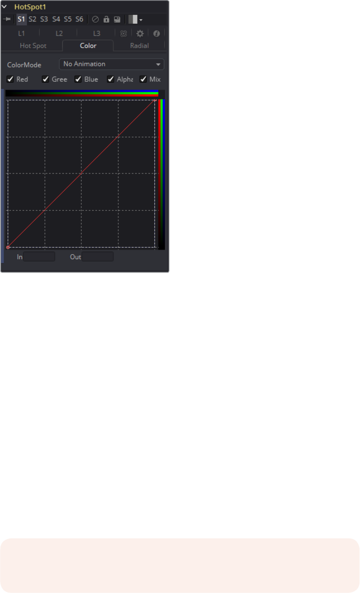
323
Effect Tools Chapter – 10
Color Tab
Color Channel and Mix
When selected, these checkbox controls enable the editing of the chosen splines in
the LUT below.
Red, Green, Blue and Alpha Splines
The Red, Green, Blue and Alpha splines are used to adjust the color of the spotlight
along the radius of the hotspot.
The vertical axis represents the intensity or strength of the color channel, from a value
of 0 at the bottom to 1 at the top. The horizontal axis represents the position along the
radius of the hotspot, from the outside edge on the left to the inside on the right.
So the default curve of the tool indicates that the red, green, blue and alpha channels
all have a linear falloff from the outside edge of the curve to the inside edge.
Mix Spline
The Mix spline is used to determine the influence of the controls that the Radial tab will
have along the radius of the hotspot. The horizontal axis represents the position along
the circle’s circumference, with 0 being 0 degrees and 1.0 being 360 degrees. The
vertical axis represents the amount of the radial hotspot to blend with the color hotspot.
A value of 0 is all radial hotspot, while a value of 1.0 is all color hotspot.
A complete description of LUT editor controls and options can be found in the Tool
Controls chapter of this manual.
NOTE: Right-clicking in the LUT will display a contextual menu with options
related to modifying spline curves.
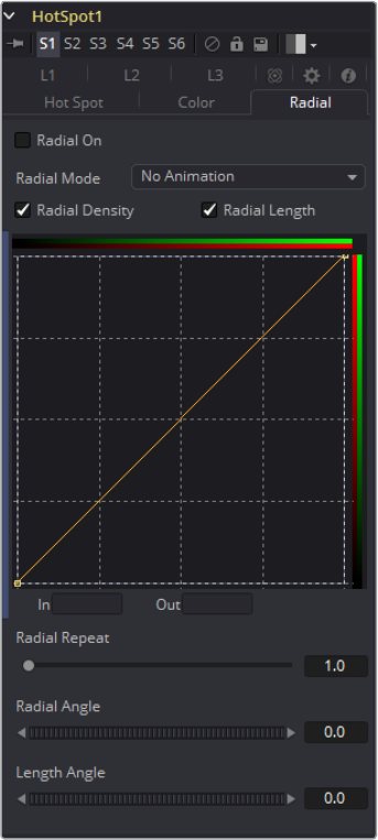
324
Effect Tools Chapter – 10
Radial Tab
Radial On
When selected, this control enables the Radial splines. Otherwise the radial matte
created by the splines is not applied to the hotspot, and the Mix spline in the color
controls will have no affect on the hotspot.
Radial Length and Radial Density Splines
The key to these splines is realizing that the LUT Editor’s horizontal axis represents a
position around the circumference of the hotspot. A value of 0.0 is 0 degrees and 1.0 is
360 degrees. With that in mind, the length determines the radius of the light making up
the hotspot along the circumference, and the density represents how bright the light is
along the circumference.
Radial Repeat
This control will repeat the effect of the radial splines by X number of times. For
example, a repeat of 2.0 causes the spline to take effect between 0 and 180 degrees
instead of 0 and 360, repeating the spline again between 180 and 360.
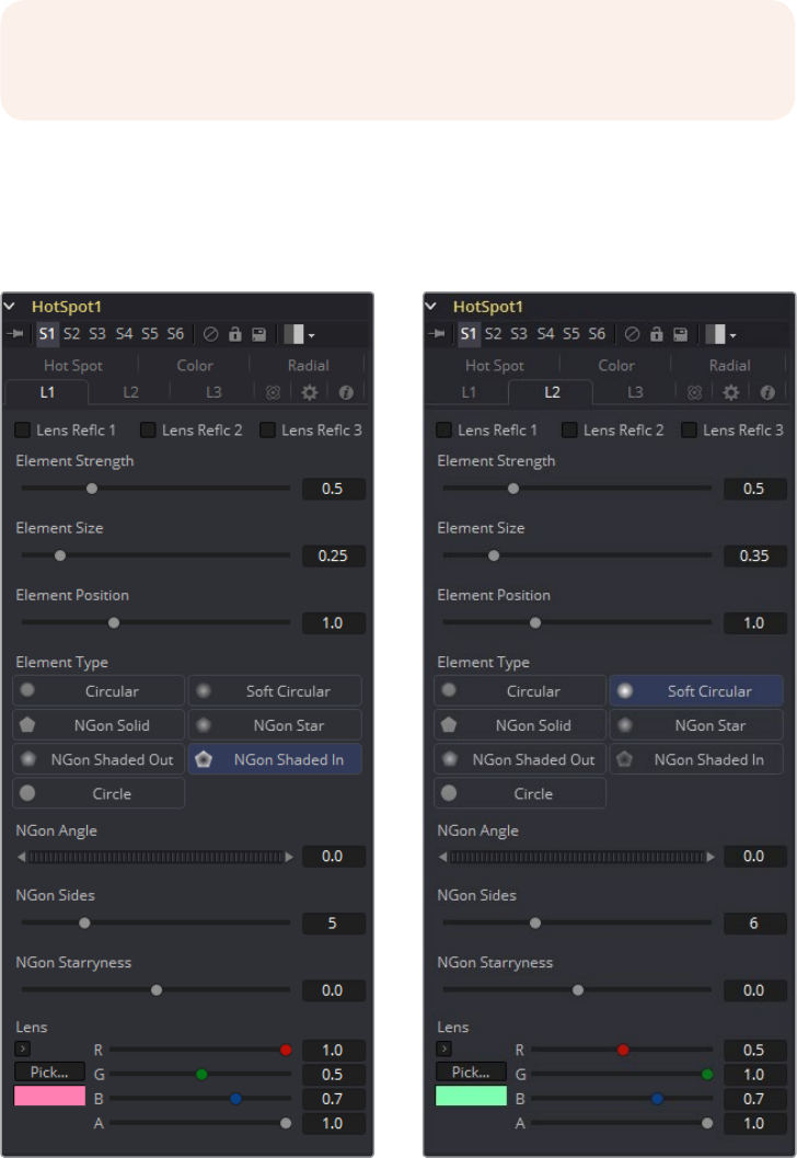
325
Effect Tools Chapter – 10
Length Angle
This control will rotate the effect of the Radial Length spline around the circumference
of the hotspot.
Density Angle
This control will rotate the effect of the Radial Density spline around the circumference
of the hotspot.
A complete description of LUT Editor controls and options can be found in the Tool
Controls chapter of this manual.
L1, L2 and L3 Tab
L1 Tab L2 Tab
NOTE: Right-clicking in the spline area will display a contextual menu
containing options related to modifying spline curves.
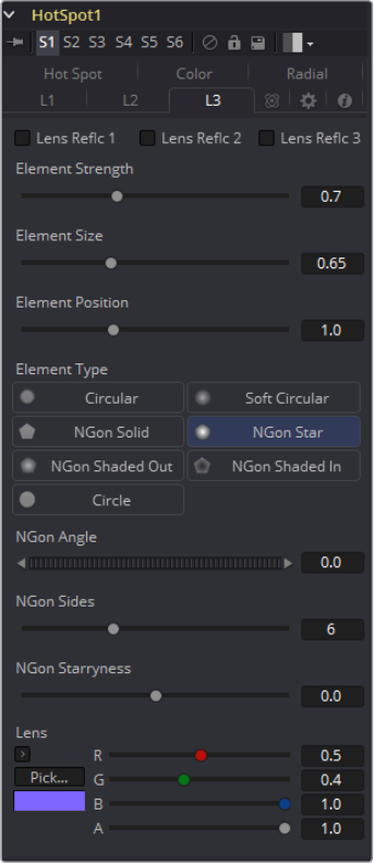
326
Effect Tools Chapter – 10
L3Tab
Lens Reflect 1-3
When selected, the reflection caused by the element is enabled.
Element Strength
This determines the brightness of element reflections.
Element Size
This determines the size of element reflections.
Element Position
This determines the distance of element reflections from the axis. The axis is calculated
as a line between the hotspot position and the center of the image.
Element Type
Use this array of buttons to choose the shape and density of the element reflections.
The presets available are described below.
Circular
This creates slightly soft-edged circular shaped reflections.
327
Effect Tools Chapter – 10
Soft Circular
This creates very soft-edged circular shaped reflections.
Circle
This creates a hard-edged circle shape.
NGon Solid
This creates a filled polygon with a variable number of sides.
NGon Star
This creates a very soft-edged star shape with a variable number of sides.
NGon Shaded Out
This creates soft-edged circular shapes.
NGon Shaded In
This creates a polygon with a variable number of sides, which has a very soft reversed
(dark center, bright radius) circle.
NGon Angle
This control is used to determine the angle of the NGon shapes.
NGon Sides
This control is used to determine the amount of sides used when the Element Type is
set to Ngon Star, Ngon Shaded Out, and Ngon Shaded In.
NGon Starriness
This control is used to bend polygons into star shapes. The higher the value the more
star-like the shape.
Lens Color Controls
These controls determine the color of the lens that affects the colors of the reflections.
To choose a lens color, pick one from a displayed image, or enter RGBA values using
the sliders or input boxes.
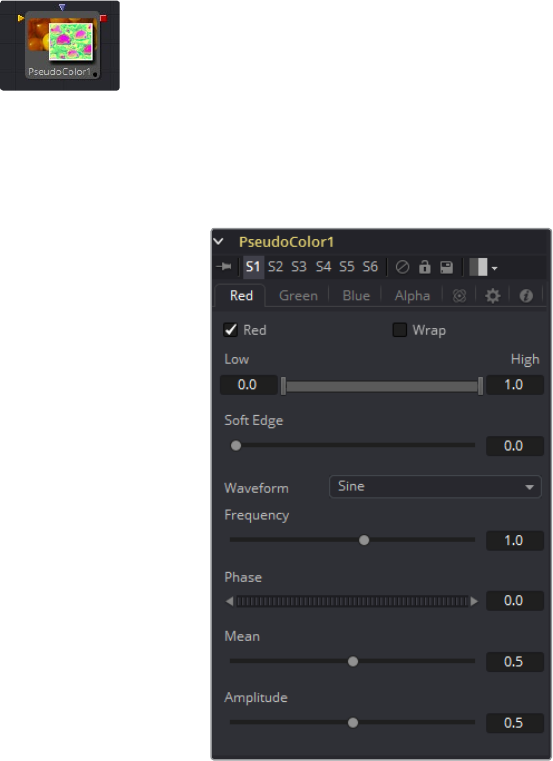
328
Effect Tools Chapter – 10
Pseudo Color [PSCL]
The Pseudo Color tool provides the ability to produce variations of color based on waveforms
generated by the tool’s controls. Static or animated variances of the original image can be
produced. The tool’s controls are separated into four identical tabs, one for each of the
color channels.
R/G/B/A Tabs
Color Check Box
When selected, the Pseudo Color tool will affect this color channel.
Wrap
When selected, waveform values that exceed allowable parameter values will be
wrapped to the opposite extreme.
High and Low
High and Low determine the range to be affected by the tool in a specific
color channel.
Soft Edge
This slider determines the soft edge of color transition.
329
Effect Tools Chapter – 10
Waveform
This selects the type of Waveform to be created by the generator. Four waveforms are
available: Sine, Triangle, Sawtooth and Square.
Frequency
This controls the Frequency of the waveform selected. Higher values will increase the
number of occurrences of the variances.
Phase
This modifies the Phase of the waveform. Animating this control will produce color
cycling effects.
Mean
This determines the level or Mean value of the waveform selected. Higher values will
increase the overall brightness of the channel until the allowed maximum is reached.
Amplitude
Amplitude increases or decreases the overall power of the waveform.
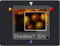
330
Effect Tools Chapter – 10
Shadow [SH]
Shadow is a versatile tool used in the creation of shadows that are based on the alpha channel
information from an image. It is also possible to use an additional image to control the shadow’s
apparent depth.
The Shadow tool is designed to cast simple 2D shadows. Use a Spotlight tool and an Image
Plane tool for full 3D shadow casting.
Controls
Shadow Offset
This control sets the apparent distance of the shadowed object from the background.
Adjusting the position of the Shadow Offset crosshair in the views is the quickest way
to create simple drop shadows.
Softness
Softness controls how blurry the shadow’s edges appear. The further the background
is from the object, the fuzzier it becomes.
Shadow Color
Use this control to select the color of the shadow. The most realistic shadows are
usually the ones that are not totally black and razor sharp.
Light Position
This control sets the position of the light relative to the shadow-casting object. The
Light Position is only taken into consideration when the Light Distance slider is NOT set
to infinity (1.0).
Light Distance
This slider will vary the apparent distance of the light between infinity (1.0) and being at
zero distance from the shadow-casting object. The advantage of setting the Light
Distance is that the resulting shadow is more realistic-looking with the further parts of
the shadow being longer than those that are closer.
Minimum Depth Map Light Distance
This control is active when an image is connected to the shadow’s Depth Map input.
The slider is used to control the amount that the depth map contributes to the Light
Distance. Dark areas of a depth map make the shadow deeper. White areas bring it
closer to the camera.
Z Map Channel
This menu is used to select which color channel of the image connected to the tool’s Z
Map input will be used to create the shadows depth map. Selections exist for the RGB
and A, Luminance, and Z-buffer channels.
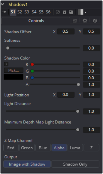
331
Effect Tools Chapter – 10
Output
The Output image can either contain the image with shadow applied or the
shadow only.
Changing the setting in the output drop-down list controls which mode will be used.
This method is useful when color correction, perspective or other effects need to be
applied to the resulting shadow before it is merged back with the object.
For example, Shadow Alpha controls the shadow’s degree of transparency.
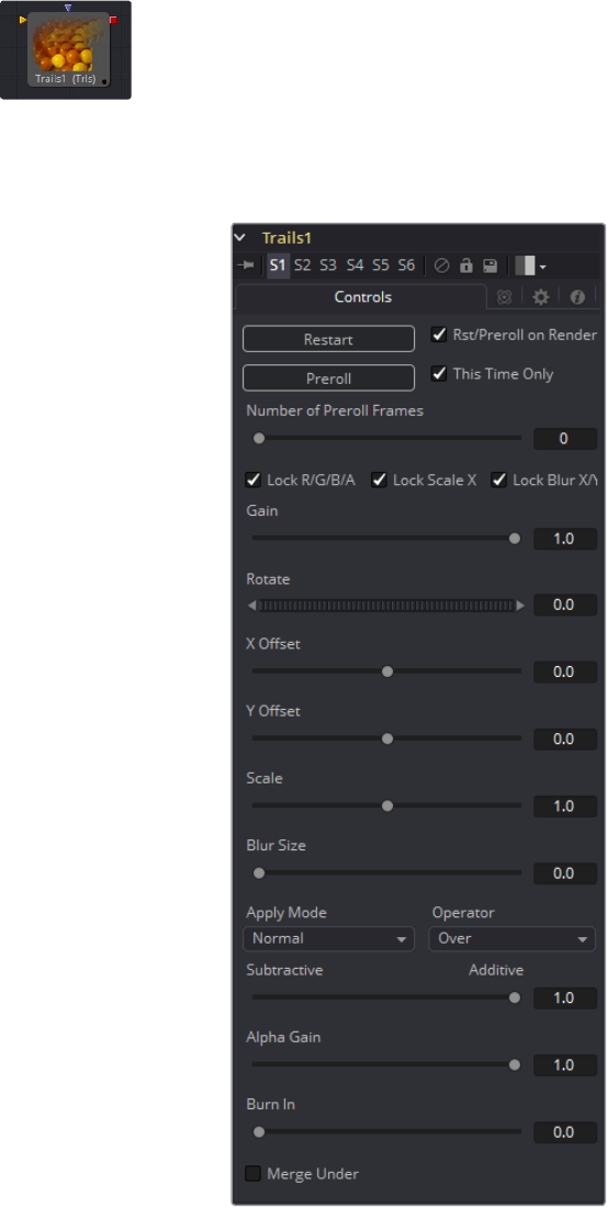
332
Effect Tools Chapter – 10
Trails [TRLS]
The Trails tool is used to create a ghost-like after-trail of the image. This creates an interesting
effect when applied to moving images with an alpha channel. Unlike a directional blur, only the
preceding motion of an image is displayed as part of the effect.
Controls
Restart
This control clears the image buffer and displays a clean frame, without any of the
ghosting effect.
Preroll
This will make the Trails tool pre-render the effect by the number of frames on the
slider. This will make the Trails tool pre-render the effect by the number of frames on
the slider.
333
Effect Tools Chapter – 10
Reset/Pre-Roll on Render
When this checkbox is enabled, the Trails tool will reset itself when a preview or final
render is initiated. It will Pre-roll the designated number of frames.
This Time Only
Selecting this checkbox will make the pre-roll use this current frame only and not the
previous frames.
Number of Pre-roll Frames
This determines the number of frames to pre-roll.
Lock RGBA
When selected, this checkbox allow the Gain of the color channels to be controlled
independently. This allows for tinting of the Trails effect.
Lock Scale X/Y
When selected, this checkbox allows the X- and Y-axis scaling of the image buffer to be
manipulated separately for each axis.
Lock Blur X/Y
When selected, this checkbox allows the blurring of the image buffer to be controlled
separately for each axis.
Gain
The Gain control affects the overall intensity and brightness of the image in the buffer.
Lower values in this parameter will create a much shorter, fainter trail, whereas higher
values will create a longer, more solid trail.
Rotate
The Rotate control rotates the image in the buffer before the current frame is merged
into the effect.
Offset X/Y
These controls offset the image in the buffer before the current frame is merged into
the effect. Control is given over each axis independently.
Scale
The Scale control resizes the image in the buffer before the current frame is merged
into the effect.
Blur Size
The Blur Size control applies a blur to the image in the buffer before the current frame
is merged into the effect.
Apply Mode
This menu is used to determine the method used by the Trails tool when merging one
sample over another. The methods in this menu are documented more completely in
the Merge tool’s documentation in the Composite Tools chapter of this manual.
334
Effect Tools Chapter – 10
Operator Mode
This menu is used to select to determine how the foreground and background are
combined to produce a result. The menu will only be visible when the tool’s Apply
mode is set to Normal.
For an excellent description of the math underlying the operation modes, read
Compositing Digital Images, Porter, T., and T. Duff, SIGGRAPH 84 proceedings, pages
253-259. Essentially, the math is as described below. Note that some modes not listed
in the Operator dropdown (Under, In, Held In, Below) are easily obtained by swapping
the foreground and background inputs (with Command-T or Ctrl-T and choosing a
corresponding mode.
The formula used to combine pixels in the merge is always fg * x + bg * y. The different
operations determine exactly what x and y are, as shown in the description for
each mode.
Over
The Over mode adds the FG layer to the BG layer by replacing the pixels in the BG with
the pixels from the Z wherever the FG’s alpha channel is greater than 1.
x = 1, y = 1-[foreground alpha]
In
The In mode multiplies the alpha channel of the BG input against the pixels in the FG.
The color channels of the FG input are ignored. Only pixels from the FG are seen in the
final output. This essentially clips the FG using the mask from the BG.
x = [background alpha], y = 0
Held Out
Held Out is essentially the opposite of the In operation. The pixels in the FG image are
multiplied against the inverted alpha channel of the BG image. Accomplish exactly the
same result using the In operation and a Matte Control tool to invert the matte channel
of the BG image.
x = 1-[background alpha], y = 0
ATop
ATop places the FG over the BG only where the BG has a matte.
x = [background alpha], y = 1-[foreground alpha]
XOr
XOr combines the FG with the BG wherever either the FG or the BG have a matte, but
never where both have a matte.
x = 1-[background alpha], y = 1-[foreground alpha]
Subtractive/Additive, Alpha Gain, Burn In
For details on these controls and their effect, consult the documentation for the Merge
tool in the Composite Tools chapter.
Merge Under
This merges the current image under the generated trail, rather than the usual, over top
operation.
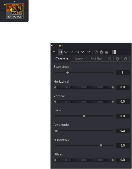
335
Effect Tools Chapter – 10
TV [TV]
The TV tool is a simple tool designed to mimic some of the typical flaws seen in analog
television broadcasts and screens.
Controls
Scan Lines
This slider is used to emulate the interlaced look by dropping lines out of the image.
Setting it to black, with a transparent alpha, drops a line. A value of 1 (default) will drop
every second line. A value of 2 shows one line, then drops the second and third and
repeats. A value of zero turns off the effect.
Horizontal
Use this slider to apply a simple Horizontal offset to the image.
Vertical
Use this slider to apply a simple Vertical offset to the image.
Skew
This slider is used to apply a diagonal offset to the image. Positive values skew the
image to the top left. Negative values skew the image to the top right. Pixels pushed off
frame wrap around and reappear on the other side of the image.
Amplitude
The Amplitude slider can be used to introduce smooth sine wave-type deformation to
the edges of the image. Higher values will increase the intensity of the deformation.
Use frequency to determine how often the distortion is repeated.
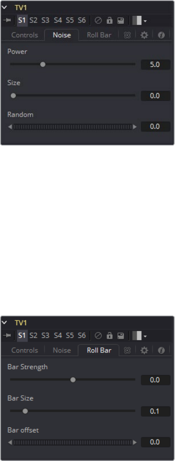
336
Effect Tools Chapter – 10
Frequency
The Frequency slider sets the frequency of the sine wave used to produce distortion
along the edges of the image when the amplitude control is greater than 1.
Offset
Use Offset to adjust the position of the sine wave, causing the deformation applied to
the image via the Amplitude and Frequency controls to see across the image.
Noise Tab
Power
Increase the value of this slider above 0 to introduce noise into the image. The higher
the value, the stronger the noise.
Size
Use this slider to scale the noise map larger.
Random
If this thumbwheel control is set to 0, the noise map will be static. Change the value
over time to cause the static to change from frame to frame.
Roll Bar Tab
Bar Strength
At the default value of 0 no bar is drawn. The higher the value, the darker the area
covered by the bar will become.
Bar Size
Increase the value of this slider to make the bar taller.
Bar Offset
Animate this control to scroll the bar across the screen.
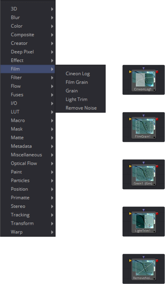
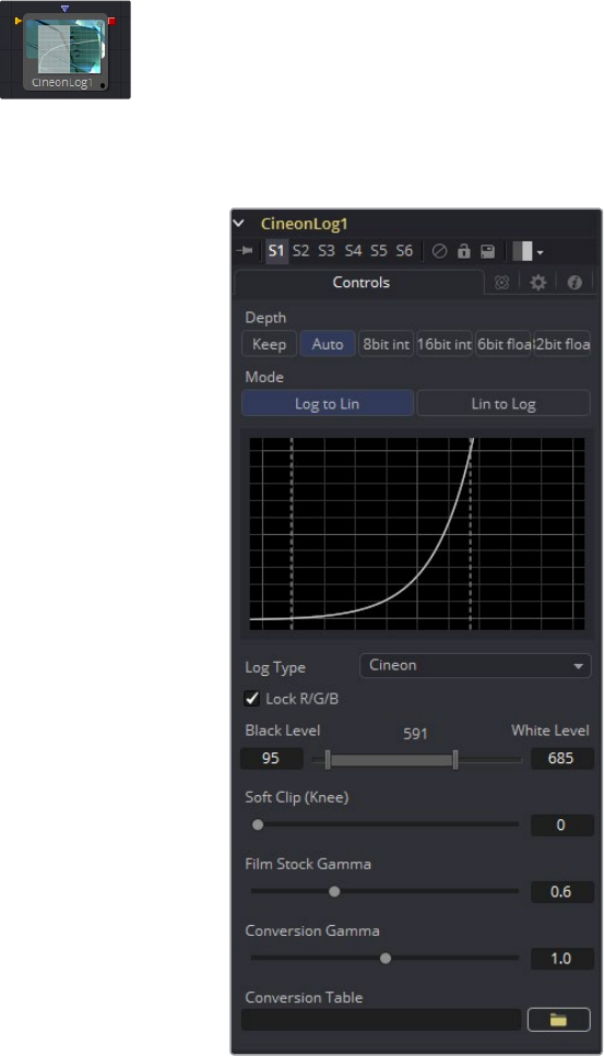
340
Film Tools Chapter – 11
Cineon Log [LOG]
The Cineon Log Tool is used to convert image data from logarithmic to linear. Use this tool if the
log-lin conversion was bypassed in a Cineon Loader to return processing to Linear.
Controls
Mode
These buttons offer two options, one for converting log images to linear and one for
converting linear images to logarithmic.
Lock RGB
When selected, the settings in this tab will affect all of the color channels equally.
De-select this control to convert the Red, Green and Blue channels of the image using
separate settings for each channel.
341
Film Tools Chapter – 11
Black Level and White Level
Use this control to set the black point and white point in the log image before
converting. Pixels with values in log space below the Black Level will become out of
range values below 0.0. Pixels with values above the White Level will become out of
range values above 1.0 after conversion.
When processing in floating point color space, the out of range values stored in the
Cineon format are preserved through the conversion. In 16-bit or 8-bit mode, the out of
range values are clipped.
Soft Clip (Knee)
The Soft Clip control is used to draw values that are out of range back into the image.
This is done by smoothing the conversion curve at the top and bottom of the curve,
allowing more values to be represented.
Applying a soft clip of any value other than 1 will immediately cause the tool to process
at 16-bit integer, eliminating all out of range values that do not fit within the soft clip.
Film Stock Gamma, Conversion Gamma and Conversion Table
These controls are used to set the response curves of the logarithmic data during
conversion. In addition to the settings above, a custom ASCII file Look Up Table can be
created with specific conversion values. The ASCII LUT file can be loaded using the
File Folder Icon button.
Black Rolloff
Since a mathematical log() operation on a value of zero or lower will result in invalid
values, Fusion will clip values below 1e-38 (0 followed by 38 zeros) to 0 to ensure
correct results. This is almost never an issue, since values that small have no visual
impact on an image. To see such tiny values you would have to add three Brightness
Contrast tools, each with a gain set to 1,000,000. Even then the values would hover
very close to zero.
We have seen processes where instead of cropping these very small values, they are
instead scaled. So values between 0.0 and 1e-16 are scaled be between 1e-18 and
1e-16. The idea is to crush the majority of the visual range in a float image into values
very near to zero, then expand them again, forcing a gentle ramp to produce a small
ramp in the extreme black values. Should you find yourself facing a color pipeline using
the process, here is how you can mimic it with the help of a custom tool.
The process involves converting the log image to linear with a very small gamma and a
wider than normal black level to white level. (e.g., conversion gamma of 0.6, black of 10,
white of 1010) This will crush most of the images range into very very small values. This
is followed by a custom tool (described below), then by a linear to log conversion that
reverses the process, but uses a slightly higher black level. The difference between the
black levels defines the falloff range.
Since this will lift the blacks, the image is usually then converted back to linear one
more time, using more traditional values (i.e., 95-685) to reset the black point.
The custom tool should use the following equation in the Red, Green and Blue
expressions:
if (c1< 1e-16, 1e-18 + (c1/1e-16)*(1e-16 - 1e-18), c1)
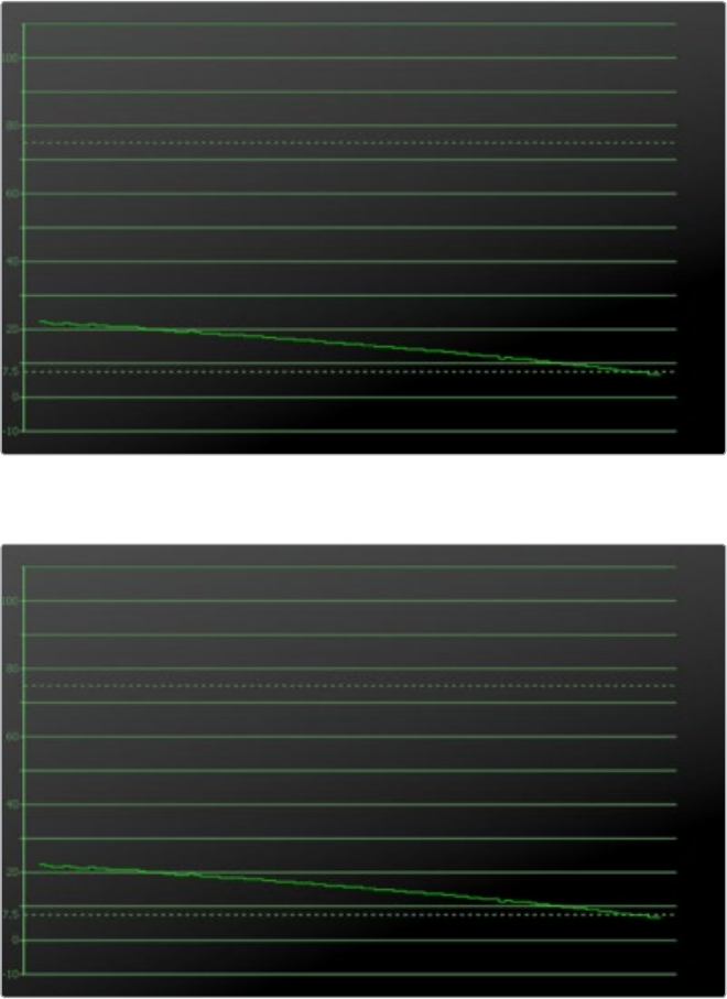
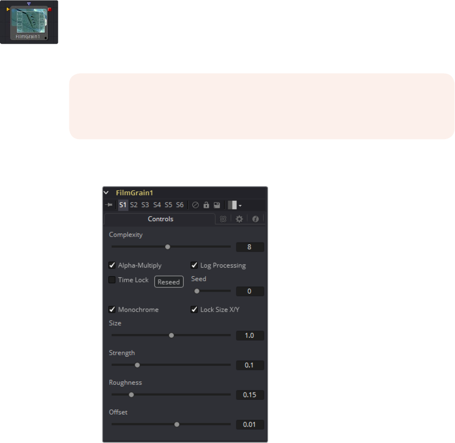
343
Film Tools Chapter – 11
Film Grain [FGR]
The Film Grain tool takes a new approach to grain, which should be more closely aligned with
the grain profiles of modern film stocks. This provides you with more control over the final
appearance of the grain.
Controls Tab
Complexity
The complexity of the Grain indicates the number of ‘layers’ of grain applied to the
image. With a complexity of 1, only one grain layer is calculated and applied to the
image. When complexity is set to 4, the tool calculates four separate grain layers and
applies the mean combined result of each pass to the final image. Higher complexities
produce visually more complex results, without the apparent regularity often
perceivable in digitally-produced grain.
NOTE: The Film Grain tool does not replace the original Grain tool, which is still
provided to allow older compositions to load and render, but in almost every case, use
of the new Film Grain tool is now encouraged.

344
Film Tools Chapter – 11
Alpha Multiply
When the Alpha Multiply checkbox is enabled, the Film Grain tool will multiply its results
by the source images alpha channel. This is necessary when working with post
multiplied images to ensure that the grain does not affect areas of the image where the
alpha is 0.0 (transparent).
Log Processing
When this checkbox is enabled (default), the grain applied to the image will have its
intensity applied non-linearly to match the grain profile of most film. Roughly speaking,
the intensity of the grain will increase exponentially from black to white. When this
checkbox is disabled the grain will be applied uniformly, regardless of the brightness of
the affected pixel.
One of the primary features of grain in film is that the appearance of the grain varies
radically with the exposure, so that there appears to be very little grain present in the
blacks, with the amount and deviation of the grain increasing as the pixels exposure
increases. In a film negative the darkest portions of the developed image will appear
completely opaque, and this obscures the grain. As the negative becomes
progressively clearer, more of the grain becomes evident in the result. Chemical
differences in the response to light of the Red, Green and Blue layers of the film also
cause each color component of the film to present a different grain profile, typically
with the Blue channel presenting the largest amount of grain.
As a result, the most important control in the new Film Grain tool is the Log Processing
checkbox, which should be enabled when matching film, and disabled when working
with images that require a more linear grain response. Having this checkbox enabled
will closely mimic the results of preceding the old grain tool with a Linear > Log
conversion and following with a Log > Linear conversion immediately after.
Seed
The Seed slider and Randomize button are presented whenever a Fusion tool relies on
a random result. Two tools with the same seed values will produce the same random
results. Click on the Randomize button to randomly select a new seed value, or adjust
the slider to manually select a new seed value.
Monochrome
When the Monochrome checkbox is enabled (default) the grain will be applied to the
Red, Green and Blue color channels of the image equally. When deselected, individual
control over the Size, Strength and Roughness of the grain in each channel
becomes possible.
Lock Size X/Y
Deselect the Lock Size X/Y checkbox to control the size of the Grain along the X- and
Y-axis individually.
Size
The Grain Size is calculated relative to the size of a pixel, so that changing the
resolution of the image does not impact the relative appearance of the grain. The
default Grain Size of 1.0 will produce grain kernels that cover roughly 2 pixels.
NOTE: Since it is impossible to say what the final value of semi-transparent
pixels in the image are until after they are composited with their background,
you should avoid applying log-processed grain to the elements until after they
have been composited. This will ensure that the strength of the grain
is accurate.

345
Film Tools Chapter – 11
Strength
Grain is expressed as a variation from the original color of a pixel. The stronger the
grain’s strength, the wider the possible variation from the original pixel value. For
example, given a pixel with an original value of p, and a grain tool with complexity=1
size=1; roughness=0; log processing=off; the grain will produce an output value of p +/-
strength. In other words, a pixel with a value of 0.5 with a grain strength of 0.02 could
end up with a final value between 0.48 and 0.52.
Once again, that’s a slight over simplification, especially when the complexity exceeds
1. Enabling the Log Processing checkbox will also cause that variation to be affected
such that there will be less variation in the blacks and more variation in the whites of
the image.
Roughness
The Roughness slider applies low frequency variation to give the impression of
clumping in the grain. Try setting the Roughness to 0, and you will observe that the
grain produced has a very even luminance variation across the whole image. Increase
the roughness to 1.0 and you will observe the presence of ‘cellular’ differences in the
luminance variation.
Offset
The Offset control helps to match the intensity of the grain in the deep blacks by
offsetting the values before the intensity (strength) of the grain is calculated. So an
offset of 0.1 would cause a pixel with a value of 0.1 to receive grain as if its value was
actually 0.2.
NOTE: When visualizing the effect of the grain on the image, the more
mathematically inclined may find it helps to picture a sine wave, where each
lobe of the sine wave covers 1 pixel when the Grain Size is 1.0. The Grain Size
controls the frequency of the sine wave, while the Grain Strength controls its
amplitude. Again, this is something of an oversimplification.
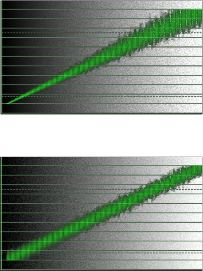
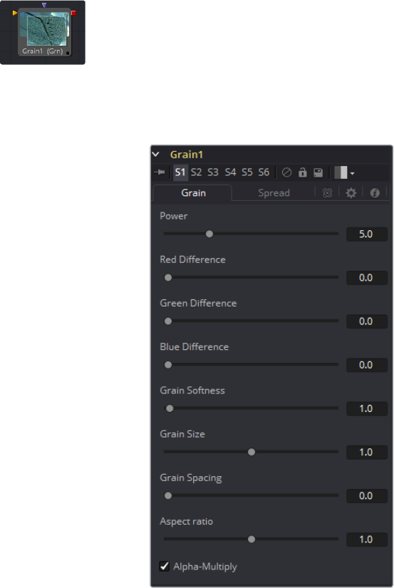
347
Film Tools Chapter – 11
Grain [GRN]
The Grain tool offers comprehensive film grain emulation. This is useful for introducing
simulated grain into a video or computer-generated image and matching existing grain in a
given scene.
Grain Tab
Power
This slider determines the strength of the grain. A higher value increases visibility,
making the grain more prevalent.
RGB Difference
Separate Red, Green and Blue sliders are used to modify the strength of the effect on a
per channel basis.
Grain Softness
This slider controls the blurriness or fuzziness of the grain. Smaller values cause the
grain to be more sharp or coarse.
Grain Size
This slider determines the size of the grain particles. Higher values increase the
grain size.
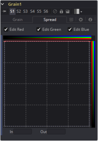
348
Film Tools Chapter – 11
Grain Spacing
This slider determines the density or amount of grain per area. Higher values cause the
grain to appear more spaced out.
Aspect Ratio
This slider adjusts the aspect of the grain so that it can be matched with
anamorphic images.
Alpha-Multiply
When enabled, this checkbox will multiply the image by the alpha, clearing the black
areas of any grain effect.
Spread Tab
Edit RGB Checkboxes
Separate Red, Green and Blue to enable the custom curves for each channel. More
grain would appear in the Blue channel than the Red, and the Green channel would
receive the least. This curve mimics usual film responses. Right-clicking in the spline
area will display a contextual menu containing options related to modifying spline
curves. A complete description of the LUT Editor control and its options can be found in
the Tool Controls chapter of this manual.
In and Out
This control gives direct editing of points on the curve by setting In/Out point values.
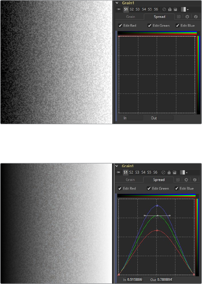
349
Film Tools Chapter – 11
Spread Examples
Default Spread
In the default setting, the Grain is applied evenly to the entire image as shown here.
However, film often shows a different amount of grain in the blacks, mids and whites.
Bell-Shaped Spread
Setting a bell shape is often a good starting point to create more realistic looking grain.
Here we have a non-uniform distribution with different amounts of grain in the Red,
Green and Blue channel as well.
In both examples, the Grain’s power has been over-exaggerated to show the effect a
bit better.
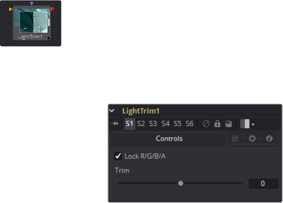
350
Film Tools Chapter – 11
Light Trim [LT]
This tool emulates film scanner light trims. By design, this tool works best with logarithmic data,
such as the images stored by the Cineon file system. When logarithmic data is provided, the
Light Trim tool can be used to increase or decrease the apparent exposure level of the image.
Controls
Lock RGBA
When selected, the Lock RGBA control collapses control of all image channels into one
slider. This selection is on by default. To manipulate the various color channels
independently, de-select this checkbox.
Trim
This slider shifts the color in film, optical printing and lab printing points. 8 points equal
one stop of exposure.
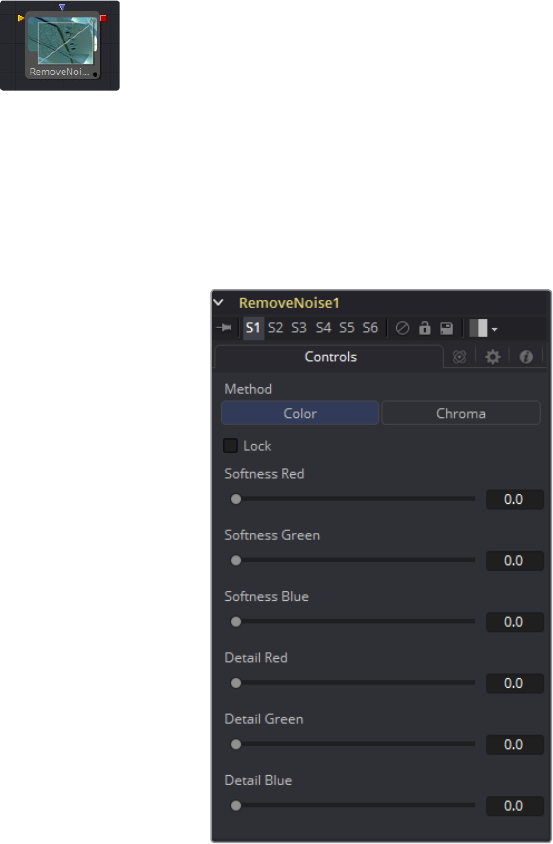
351
Film Tools Chapter – 11
Remove Noise [RN]
The Remove Noise tool provides simple noise management. The basic principle of its operation
is the tool blurs the image channels, then compares the blurred image to the original to extract
the noise. A sharpness is then applied to the image, except where noise was detected.
To use this tool, view the image and look at the Red channel. Then increase the Red Softness
until the grain appears to be gone. Next, increase the sharpness until the detail reappears, but
stop before the grain reappears. Repeat for the Green and Blue channels.
Controls / Color
Method
Use these buttons to choose whether the tool processes color using Color or Chroma
methods. This will also give you a different set of control sliders.
Lock
This checkbox will link the Softness and Detail sliders of each channel together.
Softness Red, Green and Blue
The Softness sliders determine the amount of blur applied to each channel of the
image. In Chroma mode you have sliders for the softness in the Luminance and
Chrominance channels respectively.
Detail Red, Green and Blue
The Sharpness sliders determine how much detail is reintroduced into each channel
after each channel is softened. In Chroma mode you have sliders for Luminance and
Chrominance channels respectively.
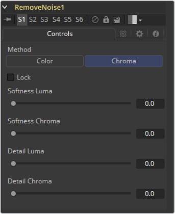
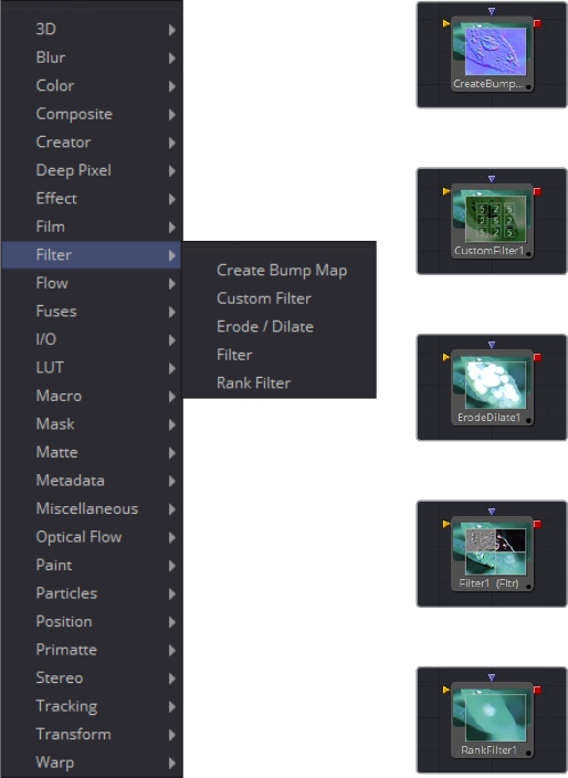
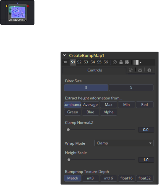
356
Filter Tools Chapter – 12
CreateBumpmap
The Create Bumpmap tool converts a grayscale (heightmap) image into a bump map. Check the
notes for the naming conventions used in Fusion. Since the resulting bump vector information is
represented as RGB, it´s possible to modify them using all the image processing tools in Fusion.
Use the Create Bumpmap tool for applying to a material.
Input Port
CreateBumpmap.Input (white): Receives the RGBA channels from an image output for the bump
calculation
357
Filter Tools Chapter – 12
Controls
This tab contains all parameters for the tool.
Filter Size
The process of generating the bump information is basically a Custom Filter. This
multi-button control sets the filter size.
Extract height information from…
Set the channel from where to extract the grayscale information from.
Clamp Normal.Z
Clips the lower values of the Blue channel in the resulting bump texture.
Filter Wrap Mode
Basically wraps the image at the borders, so the filter produces correct result when
using seamless tileable textures.
Height Scale
Changes the contrast of the resulting values in the bump map. Increasing this value
yields in a more visible bump map.
Bumpmap Texture Depth
Optionally converts the resulting bump texture into the desired bit depth.
Notes on Bumpmaps
This tab contains all parameters for the tool.
Heightmap
A grayscale image containing a height value per pixel.
Bumpmap
An image containing normals stored in the RGB channels used for modifying the
existing normals (usually given in tangent space)
Normalmap
An image containing normals stored in the RGB channels used for replacing the
existing normals (usually given in tangent or object space)
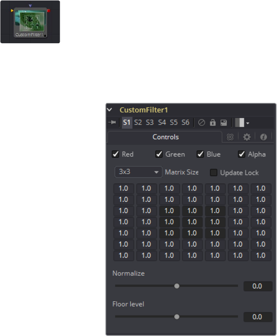
358
Filter Tools Chapter – 12
Custom Filter Tool
The Custom Tool is used to apply custom convolution filters to images. A custom convolution
filter can give a wide variety of image effects. For example, emboss, relief, sharpen, blurring
and edge detection are all convolution filters. There are many supplied custom filters in the
Filters directory that can be loaded by right-clicking on the control header and selecting
Settings > Load from the context menu.
A Kernel filter is an array (or grid) of either 3 x 3, 5 x 5 or 7 x 7 values. The center of the array
represents the current pixel, and entries nearby represent adjacent pixels. A value of 1 applies
the full value of the pixel to the filter. A value of 0 ignores the pixel’s value. A value greater than
one multiplies the pixel’s effect on the result. Negative values can also be entered, where the
value of the pixel will be subtracted from the average. Only integer values can be entered; 0.5
is not valid.
For example, a filter with the values...
0 0 0
0 1 0
0 0 0
...will have zero effect from its neighboring pixels and the resulting image would be
unchanged. A blurring effect would be...
1 1 1
1 1 1
1 1 1
...where the neighboring pixels are averaged with the center, resulting in a
softening effect.
-5 0 0
0 1 0
0 0 5
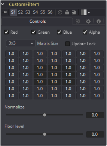
359
Filter Tools Chapter – 12
This example will subtract five times the value from the top left and add five times the value
from the lower right. If parts of the image that is processed are very smooth in color, the
neighboring values will be very similar. In parts of the image where the pixels are different (i.e.,
an edge), the results will be different and tend to highlight or emboss edges in the image.
Using the values...
1 1 1
1 1 1
1 1 1
...in a filter and sliding Normalize to Positive will make the image go brighter or glow,
simulating film over-exposure.
Using the values...
-1 0 0
0 0 0
0 0 1
...in a filter and sliding Floor Level to Positive will look like a Relief filter.
Custom Filter Controls Tab
Color Channels (RGBA)
The color corrector defaults to operating on R, G, B and A channels. Selective channel
editing is possible by clicking the checkboxes beside each channel, making selected
channels active or inactive.
This is not the same as the RGBA checkboxes found under the common controls. The
tool takes these controls into account before it processes. Deselecting a channel will
cause the tool to skip that channel when processing, speeding up the rendering of the
effect. In contrast, these controls under the Common Controls tab are applied after the
tool has processed.
360
Filter Tools Chapter – 12
Matrix Size
Use this drop-down to set the size of the filter at 3 x 3 pixels, 5 x 5 pixels or 7 x 7 pixels,
thus setting the radius of the pixels sampled. The larger the size, the more time it takes
to render.
Update Lock
When this control is selected, Fusion will not render the filter. This is useful for setting
up each value of the filter, then turning Update Lock off and rendering the filter.
Filter Matrix
The Filter Matrix control is a 7 x 7 grid of text boxes where a number is entered to
represent how much influence each pixel has on the overall convolution filter. The text
box in the center represents the pixel that is processed by the filter. The text box to the
left of the center represents the pixel to the immediate left, and so forth.
The default Matrix size is 3 x 3. Only the pixels immediately adjacent to the current pixel
will be analyzed. If a larger Matrix size is set, more of the text boxes in the grid will be
enabled for input.
Normalize
This controls the amount of filter normalization that is applied to the result. Zero will
give a normalized image. Positive values will brighten or raise the level of the filter
result. Negative values will darken or lower the level.
Floor Level
This will add or subtract a minimum, or Floor Level, to the result of the filtered image.
Zero will not add anything to the image. Positive values will add to the filtered image
and Negative values will subtract from the image.
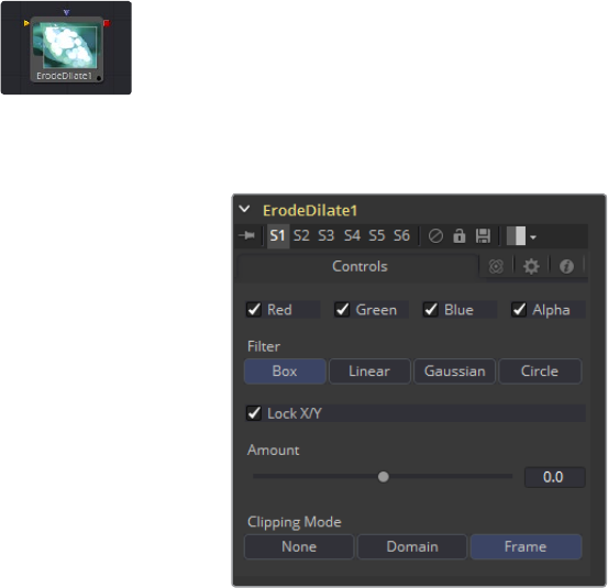
361
Filter Tools Chapter – 12
ErodeDilate Tool
This simple tool erodes or dilates the image, depending on whether the Amount slider is set to
a negative or positive value.
ErodeDilate Controls Tab
Color Channels (RGBA)
The filter defaults to operating on R, G, B and A channels. Selective channel filtering is possible
by clicking the checkboxes beside each channel to make them active or inactive. This is not the
same as the RGBA checkboxes found under the common controls. The tool takes these
controls into account before it processes. Deselecting a channel will cause the tool to skip that
channel when processing, speeding up the rendering of the effect. In contrast, the channel
controls under the Common Controls tab are applied after the tool has processed.
Lock X/Y
The Lock X/Y checkbox is used to separate the Amount slider into amount X and
amount Y, allowing a different value for the effect on each axis.
Amount
A negative value for Amount causes the image to erode. Eroding simulates the effect of
an underexposed frame, shrinking the image by growing darker areas of the image so
that they eat away at brighter regions.
A positive value for Amount causes the image to dilate, similar to the effect of
overexposing a camera. Regions of high luminance and brightness grow, eating away
at the darker regions of the image. Both techniques will eradicate fine detail in the
image and tend to posterize fine gradients.
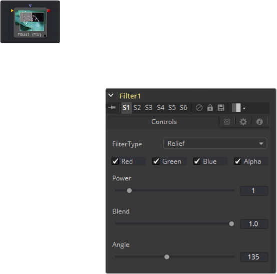
362
Filter Tools Chapter – 12
Filter Tool
The Filter Tool contains several pre-set filters, enabling a variety of effects, from radically
changing the look of an image to adding subtle randomly-generated film grain.
Filter Controls Tab
Filter Type
This drop-down control provides a selection of filter types. The options are
displayed below.
Relief
This appears to press the image into metal, such as an image on a coin. The image will
appear to be bumped and overlaid on gray.
Emboss Over
Embosses the image over top of itself, with adjustable highlight and shadow height and
direction.
Noise
Uniformly adds noise to images. This is often useful for 3D computer-generated images
that need to be composited with live action as it reduces the squeaky clean look that is
inherent in rendered images. The frame number acts as the random generator seed.
Therefore, the effect is different on each frame and is repeatable.
Defocus
This filter type blurs the image.
Sobel
Sobel is an advanced edge detection filter. Used in conjunction with a Glow filter,
itcreates amazing neon light effects from live action or 3D rendered images.
Laplacian
Laplacian is a very sensitive edge detection filter that produces a finer edge than the
Sobel filter.
363
Filter Tools Chapter – 12
Grain
Adds noise to images similar to the grain of film (mostly in the mid-range). This is useful
for 3D computer-generated images that need to be composited with live action as it
reduces the squeaky clean look that is inherent in rendered images. The frame number
acts as the random generator seed. Therefore, the effect is different on each frame and
is repeatable.
Color Channels (RGBA)
The filter defaults to operating on R, G, B and A channels. Selective channel filtering is
possible by clicking the checkboxes beside each channel to make them active or
inactive.
Power
Values range from 1 to 10. It proportionately increases the amount by which the
selected filter affects the image. This does not apply to Laplacian filter type.
Angle
This control has a range from 0 to 315 degrees and changes the effect in increments of
45 degrees. This only applies to the Relief and Emboss filters.
Median
Depending on which Filter Type is selected, the control may appear. It varies the
Median filter’s effect. A value of 0.5 will produce the true median result, as it will find
the middle values. A value of 0.0 will find the minimums and 1.0 will find the maximums.
Applies to the Median filter only.
Seed
This control is only visible when applying the Grain or Noise filter types. The Seed
slider can be used to ensure that the random elements of the effect are seeded with a
consistent value. The randomizer will always produce the same result given the same
seed value.
Animated
This control is only visible when applying the Grain or Noise filter types. Select the
checkbox to cause the noise or grain to change from frame to frame. To produce static
noise, remove the selection from this checkbox.
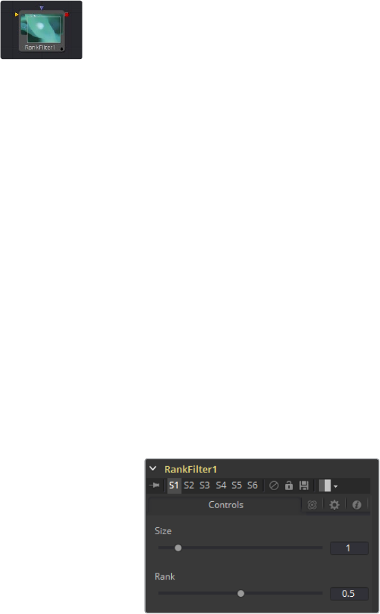
364
Filter Tools Chapter – 12
Rank Filter Tool
The Rank Filter is a very simple tool. This filter examines nearby pixels, sorts the pixels by value,
and then replaces the color of all the pixels examined by the color of the pixel with the
specified rank.
For example, a Rank filter with a size of 1 will sample 9 adjacent pixels for their values.
Thefollowing shows some example values, sorted by value.
0.0
0.4
0.4
0.5
0.5
0.7
0.7
0.7
A Blur filter with the same size would average these values together to produce a value of 3.9.
A Rank filter lets you choose a value from the list to select. For example, a rank of four would
select the fourth item in the list, producing a value of.5
A Median filter is simply a linear Rank filter that selects the median, or middle value from the list
of sorted values.
Rank Filter Controls Tab
Size
This control determines the Size in pixels of the area sampled by the filter. A value of 1
will sample only the pixels immediately adjacent to the center pixel, while larger values
sample from a larger area.
Small values are excellent for removing salt and pepper style noise, while larger values
produce an effect similar to water color paintings.
Rank
The Rank determines which value from the sampled values will be chosen, where 0 is
the lowest value and 1 is the brightest.

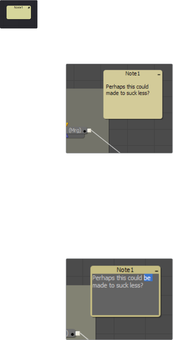
368
Flow Tools Chapter – 13
Sticky Note [NTE]
Sticky Notes are a useful way of providing notes, comments and history for a specific area of
acomp. By changing their size and color, they can provide unobtrusive comments or crucial
notices, as required. Sticky Notes make a good complement to the Comments tab.
Usage
As with conventional tools, a Sticky Note can be added to a comp by selecting it from the Tools
menu, in the Flow category, or from the Flow Editor’s Add Tool contextual menu. The new Sticky
Note will be created with its title bar centered on the last click position.
Like Groups, Sticky Notes are created in a smaller, collapsed form. They can be expanded by
double-clicking anywhere on them, or by clicking the icon in the top right corner. Once
expanded, they can be resized by dragging on any side or corner. To collapse them again, click
the icon in the top right corner once more.
Sticky Notes can be renamed, deleted, copied and pasted and have their tile color and text
color changed, using the Flow Editor’s contextual menu like any other tool. It is also possible to
lock them to prevent editing.
To edit the text in a Sticky Note, first expand it by double-clicking anywhere on the note,
thenclick below its title bar. If the note is not locked, the text will become editable.
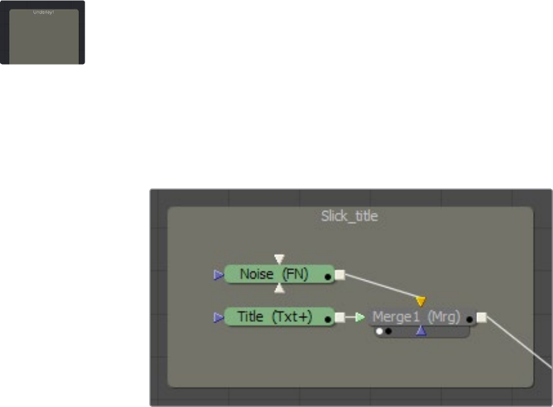
369
Flow Tools Chapter – 13
Underlay [UND]
Underlays are a convenient method of visually organizing areas of a composition. As with
Groups, Underlays can improve the readability of a comp by separating it into labeled functional
blocks. While Groups are designed to streamline the look of a comp by collapsing complex
layers down to single tools, Underlays highlight, rather than hide, and do not restrict outside
connections.
Usage
As with conventional tools, an Underlay can be added to a comp by selecting it from the
Toolsmenu, in the Flow category, or from the Flow Editor’s Add Tool contextual menu. The new
Underlay will be created with its title bar centered on the last click position.
Underlays can be resized by dragging on any side or corner. This will not affect any tools.
Underlays can also be used as simple selection groups. Activating an Underlay, by clicking on
its title, will select all the tools contained wholly within it as well, allowing the entire set to be
moved, duplicated, passed-through, etc.

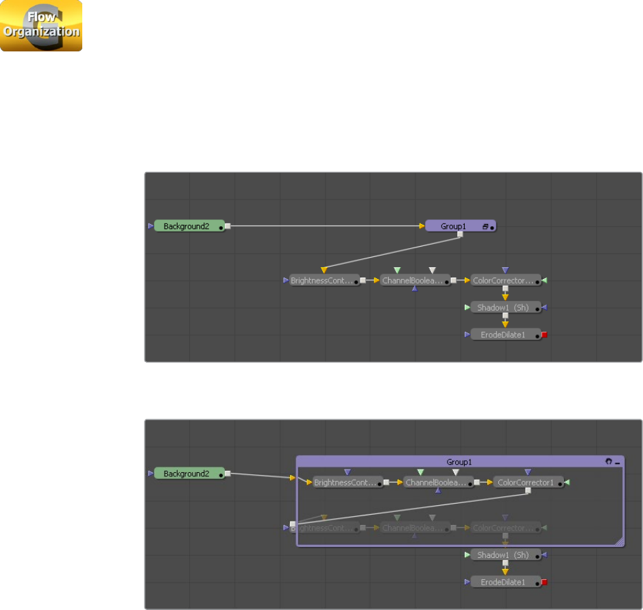
372
FlowOrg Tools Chapter – 14
Groups [NTE]
Groups can be used to neatly organize your comps, especially by putting together
multiple tools.
Usage
To group tools, select them and either press Command-G or Ctrl-G or right-click and
select Group from the contextual menu. Press Command-E or Ctrl-E to either Expand or
Collapse a selected Group.
Right-click and select Ungroup from the contextual menu to ungroup all tools.
When opened, Groups will hover over existing elements, allowing editing of the
enclosed tools.
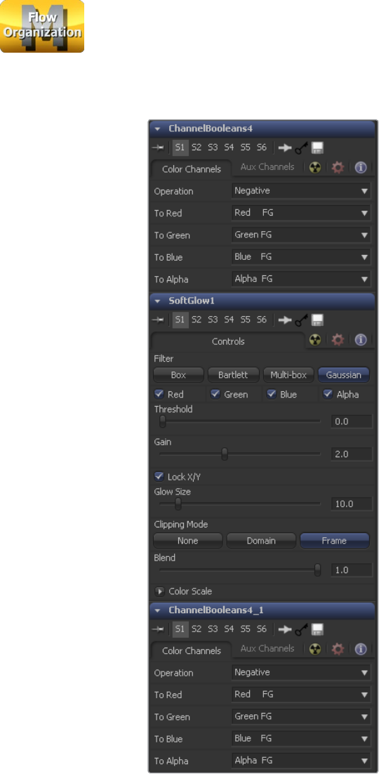
373
FlowOrg Tools Chapter – 14
Macro [-/-]
Macros can be used to combine multiple tools and expose a user-definable set of controls.
They are meant as a fast and convenient way for building your own customized tools.
Usage
Creating a Macro
To create a Macro, select the tools intended for the macro, right-click on any of them
and select Macro > Create Macro from the contextual menu.
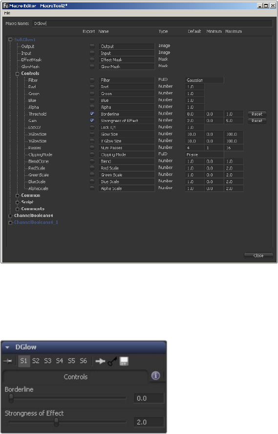
374
FlowOrg Tools Chapter – 14
Macro Editor
The Macro Editor then allows you to specify and rename the controls that shall be
exposed in the final macro.
In this example we only expose the Threshold and Gain sliders of a Softglow tool,
which is sandwiched between two ChannelBooleans.
After setting up the Macro to your liking, type in a name in the Macro Name field and
select File > Save.
To add the Macro to your flow, right-click anywhere on the flow and select Macro >
[NameOfYourMacro] from the contextual menu.
The Final Macro
The final Macro looks and behaves just like any other tool in Fusion.
As another example, you could take a single ChannelBoolean, set it to Add mode, and
make it into a macro exposing no controls at all, thus creating the equivalent of a Add
Node like the one that can be found in programs like Shake.
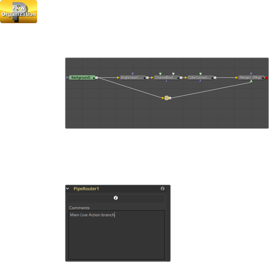
375
FlowOrg Tools Chapter – 14
Pipe Router [-/-]
Pipe Routers can be used to neatly organize your comps by creating diversions in your pipes to
make them better visible and help you understand the flow more easily. Pipe Routers do not
have any influence on render times.
Usage
Pipe Router
To insert a Router in your pipe, Option or Alt left-click on the pipe and place the Router
anywhere on the flow.
Though Routers have no actual controls, they still can be used to add comments to your comp.
378
Fuses Chapter – 15
Fuses [FUS]
Fuses are scriptable plug-ins. They can be edited within Fusion by pressing the Edit button, and
will compile on-the-fly when clicking on Reload.
Fuses are a great way to prototype plug-ins or to deal with experimental code.
Please refer to the SDK for further information.
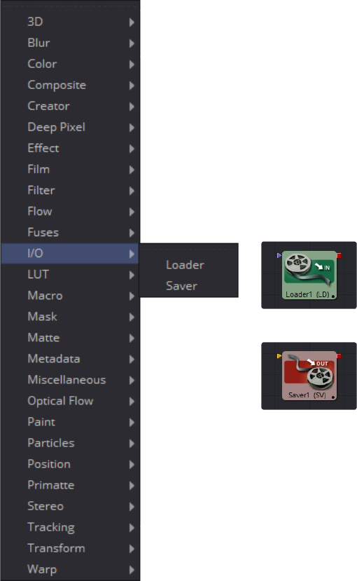
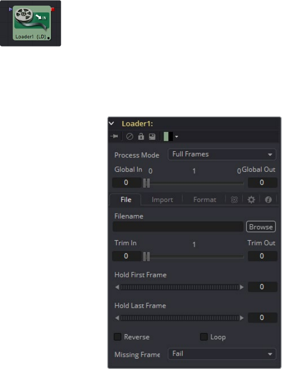
382
I/O Tools Chapter – 16
Loader [LD]
The Loader tool is used to select and load footage from the hard drive or network storage.
TheLoader is responsible for trimming, looping, and extending the footage, as well as
settingthe field order, pixel aspect and color depth. Loader is arguably the most important tool
in Fusion.
File Tab
Filename
Clicking on the yellow Folder button will display a standard Fusion file browser.
Thepath to the footage can also be typed directly using the text box provided.
The text box supports filename completion. As the name of a directory or file is typed
in the text box, Fusion will display a popup that lists possible matches. Use the arrow
keys to select the correct match and complete the path.
When a Loader is added to the flow, a file dialog will appear automatically to allow
selection of a clip from the hard drives. To select footage later, select Cancel. The
Loader will still be added to the flow. Disable the automatic display of the file browser
by disabling Auto Clip Browse in the Global > General Preferences.
File Sequences
It is common practice to use file sequences to identify an image that is part of a series.
If the last part of a file’s name is a number (not counting file extension), Fusion will
automatically scan the directory looking for files that match the sequence.
383
I/O Tools Chapter – 16
For example, the following filenames would be valid sequences.
image.0001.tga
image.0002.tga
image.0003.tga
i m ag e151.e x r
image152.exr
i m ag e153.e x r
i m ag e1.ti f
i m ag e2.ti f
image3.tif
The following would not be considered a sequence,
since the last characters are notnumeric.
sh o t.1.fg.tga
sh o t.2.fg.tga
sh o t.3.fg.tga
It is not necessary to select the first file in the sequence; Fusion will search the entire
folder for files matching the sequence in the selected filename. Also, Fusion will
determine the length of the sequence based on the first and last numeric value in the
filenames. Missing frames are ignored.
For example, if the folder contains two files with the following names:
image.0001.tga
i m ag e.0100.tga
Fusion will see this as a file sequence with 100 frames, not a file sequence containing
two frames. The Missing Frames drop-down menu is used to choose how Fusion
handles missing frames. The Trim In/Trim Out control’s contextual menu can also be
used to force a specific clip length, or to rescan the folder. Both controls are described
in greater detail below.
Occasionally, you only want to load a single frame out of a sequence, like, for example,
a photograph out of a folder containing many other files as well. By default, Fusion will
detect those as a sequence, but if you hold Shift while dragging the file from Explorer
to the Flow Editor, Fusion will only take that specific file and disregard any sequencing.
Also, if you use the Preview controls on the bottom right of the screen, you can
Command-click or Ctrl-click on the slider once you reached the frame you want to use
as a still, and Fusion will set up the loader accordingly.
Proxy Filename
The Proxy Filename control only appears once the filename control points to a valid
clip. This can specify a clip that will be loaded when the Proxy mode is enabled. This
allows smaller versions of the image to be loaded to speed up file I/O from disk and
processing.
For example, create a 1/4 scale version of a Cineon film sequence to use as a file proxy.
Whenever the proxy mode of the flow is enabled, the smaller resolution proxy clip will
be loaded from disk and all processing will be performed at the lower resolution,
significantly improving render times.
This is particularly useful when working with large film plates stored on a remote
fileserver. Lower resolution versions of the plates can be stored locally, reducing
network bandwidth, interactive render times and memory usage.
384
I/O Tools Chapter – 16
The proxy clip must have the same number of frames as the source clip, and the
sequence numbers for the clip must start and end on the same frame numbers.
It is strongly suggested that the proxies are exactly the same format as the main files. In
the case of formats with options, such as Cineon, DPX and OpenEXR, the proxies will
use the same format options as the primary.
Trim In and Out
The Trim range control is used to trim frames from the start or end of a clip. Adjust the
Trim In to remove frames from the start and Trim Out to specify the last frame of the clip.
The values used here are offsets. A value of 5 in Trim In would use the 5th frame in the
sequence as the start, ignoring the first four frames. A value of 95 would stop loading
frames after the 95th.
Right-click on the range control to see three options appear in a submenu
Autodetect Clip Length
This rescans the clip to see if frames have been added or removed since the last time
the clip was scanned (when it was loaded).
Set Clip Start Frame
Selecting this will display a dialog box to set the number of the actual start frame of the
clip on disk. Use this when the first frames of the file sequence are not yet available to
set the clip’s properties manually.
Set Clip Length
This sets the actual clip length, overriding the scanned length. This is useful if the entire
clip has not yet been rendered or captured. Used in combination with Set Clip Start
Frame, it can be used to define a clip before the clip is available.
For example, imagine there is only a single animatic frame available for a scene that is
being precomped. The animation department has yet to render the entire layer. Use the
Set Clip Start and Set Clip Length to define the clip anyway, and the composition will
load the correct frames when they become available. If the Missing Frames control is
set to Wait, then rendering will pause until the frame is available, instead of failing.
Hold First and Last Frame
The Hold First Frame and Hold Last Frame controls will hold the first or last frame of the
clip for the specified amount of frames. Held frames are included in a loop if the
footage is looped.
Reverse
Select this checkbox to reverse the footage so that the last frame is played first and the
first frame played last.
Loop
Select this checkbox to loop the footage until the end of the project. Any lengthening
of the clip using Hold First/Last Frame or shortening using Trim In/Out is included in the
looped clip.
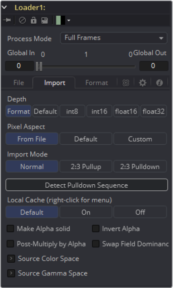
385
I/O Tools Chapter – 16
Missing Frames
The Missing Frames drop-down menu provides options for selecting how the Loader
will behave when an expected frame is missing from the footage, or is unable to load
for any reason.
Fail: The Loader will not output any image unless a frame becomes available.
Rendering will abort.
Hold Previous: Output the last valid frame until a frame becomes available again.
This fails if no valid frame has been seen, for example if the first frame is missing.
Output Black: Output a black frame until a valid frame becomes available again.
Wait: Fusion will wait for the frame to become available, checking every few seconds.
Useful for rendering a flow simultaneously with a 3D render. All rendering will cease
until the frame appears.
Import Tab
Depth
The buttons in this array are used to select the Color Depth used by Fusion to process
footage from this loader. The default option is Format.
Format
The color depth is determined by the color depth supported in the file format loaded.
For example, TGA files will automatically process at 8-bit because the TGA file format
does not store color depths greater than 8. Cineon files will load at Float, etc. If the
color depth of the format is undetermined, the default depth defined in the flow’s
Frame Format preferences is used.
386
I/O Tools Chapter – 16
Formats that support multiple color depths will be set to the appropriate color depth
automatically.
Default: The color depth is determined by the settings in the composition’s Frame
Format Preferences panel.
Int 8-bit/Int 16-bit/Float 16/Float 32: These options set the color depth in which the
image will be processed. For a more complete discussion of color depth and how it
affects composites, consult the Frame Formats chapter of this manual.
Pixel Aspect
This button array is used to determine the image’s pixel aspect ratio.
From File
The loader will conform to the image aspect detected in the saved file. There are a few
formats that can store aspect information. TIFF, JPEG and OpenEXR are examples of
image formats that may have the pixel aspect embedded in the file’s header. When no
aspect ratio information is stored in the file, the default frame format method is used.
Default: Any pixel aspect ratio information stored in the header of the image file will
be ignored. The pixel aspect set in the composition’s Frame Format preferences will
be used instead.
Custom: Select this option to override the preferences and set a pixel aspect for the
clip manually. Selecting this button will cause the X/Y Pixel Aspect control to appear.
For a more complete discussion of pixel aspect and how it affects composites,
consult the Frame Formats chapter of this manual.
Custom Pixel Aspect
This control is only visible when the Custom Pixel Aspect method is used. Enter the
desired aspect, or right-click on the control to display a menu of common frame formats
and their aspects.
Import Mode
This menu provides options for removing pull-up from an image sequence. Pull-up is a
reversible method of combining frames used to convert 24fps footage into 30fps. It is
commonly used to broadcast NTSC versions of films.
Normal: This passes the image without applying pull-up or pull-down.
2:3 Pull Up: This will remove existing 3:2 pull-down applied to the image sequence,
converting from 30fps to 24fps.
2:3 Pull Down: The footage will have pull-down applied, converting 24fps footage to
30fps by creating 5 frames out of every four. The Process mode of a loader set to Pull
Down should always be Full Frames.
First Frame
This control is used to determine which frame of the 3:2 sequence is used as the first
frame of the loaded clip. It only appears if the Pull-up or Pull-down options are selected
from the Import Mode menu.
Detect Pulldown Sequence
Pressing this button will cause Fusion to attempt to automatically detect and set the
Pull-up sequence of the footage. It only appears if Pull-up or Pull-down is selected from
the Import Mode menu. If it succeeds in detecting the order, the First Frame control will
automatically be set to the correct value.
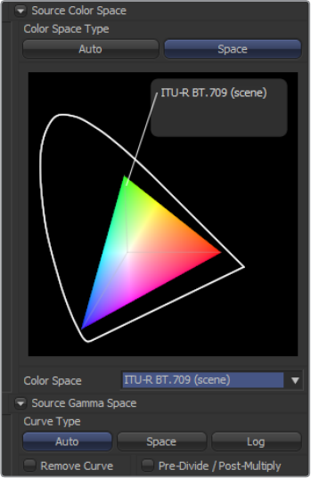
387
I/O Tools Chapter – 16
Make Alpha Solid
When checked, the original alpha channel of the clip will be cleared and set to solid
white (completely opaque).
Invert Alpha
When checked, the original alpha channel of the clip will be inverted. This may also be
used in conjunction with Make Alpha Solid to set the alpha to pure black (completely
transparent).
Post-multiply by Alpha
Selecting this option will cause the color value of each pixel to be multiplied by the
alpha channel for that pixel. This option can be used to convert subtractive (non-
premultiplied) images to additive (premultiplied) images.
Swap Field Dominance
When this control is selected, the field order (dominance) of the image will be swapped,
so that the order in time that the fields appear in is reversed. Unlike the Process Mode
control, this is done without spatially swapping the scanlines in the image.
Source Color Space
Sets the Color Space of the footage to help achieve a linear workflow.
Unlike the Gamut tool, this doesn‘t perform any actual color space conversion, but
rather adds the source space data into the metadata, if that metadata doesn‘t already
exist. The metadata can then be used downstream by a Gamut tool with the From
Image option, or in a Saver, if explicit output spaces are defined there.
Auto: Passes along any metadata that might be in the incoming image.
Space: Allows the user to set the Color Space from a variety of options.
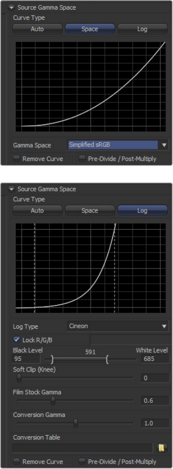
388
I/O Tools Chapter – 16
Source Gamma Space
Determines the Gamma Space of the footage and gives the option to remove the
Gamma Curve to help achieve a linear workflow.
Auto: Passes along any metadata that might be in the incoming image.
Space: Allows the user to set the Gamma Space from a variety of options.
Log: Brings up the Log/Lin settings, similar to the Cineon Tool.
Remove Curve
Depending on the selected Gamma Space or on the Gamma Space found in
Automode, the associated Gamma Curve is removed from, or a log-lin conversion is
performed on, the material, effectively converting it to a linear output space.
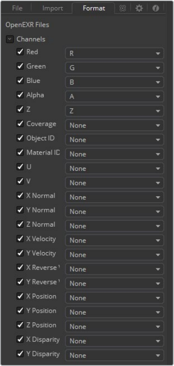
389
I/O Tools Chapter – 16
Format Tab
The Format tab contains information, options and settings relative to loading the image format.
Not all file formats have options. Notably, the Cineon, DPX, PSD, OMF, OpenEXR and
QuickTime formats all provide additional options when loaded. See Appendix A, File Formats,
for a description of all supported formats.
Options for JPG and DPX are shown for reference on the right.
OMF Format
An OMF file is not just a media format; it can contain information about edits, multiple
sequences, and even multiple versions of the same shot. If multiple clips exist within
the OMF file, the format options may be used to select the desired clip. To import all
clips from an OMF file, complete with edit and combine information, use the Import
OMF option from Fusion’s File menu to create a entire composition from the contents
of the OMF.
Photoshop PSD Format
Fusion can load any one of the individual layers stored in the PSD file, or the completed
image with all layers. Transformation and adjustment layers are not supported. To load
all layers individually from a PSD file, with appropriate blend modes to combine them,
use the Import PSD option from Fusion’s File menu to create a entire composition from
the contents of the PSD file.
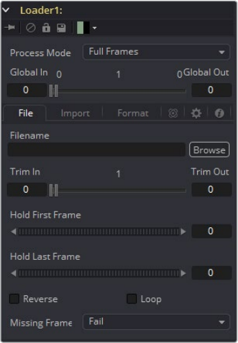
390
I/O Tools Chapter – 16
Cineon and DPX Format
See the chapter Film in Fusion and the chapter for the Cineon Log tool for a detailed
discussion of the options found in the Cineon and DPX file formats.
OpenEXR Format
Industrial Light and Magic developed the OpenEXR format. Its initial design was to
provide a compact and flexible format to support storage of high dynamic range
images (float). The format has been expanded to support a variety of extra channels
and metadata.
The format options for OpenEXR files provide a mechanism for mapping any
non-RGBAchannels to the channels supported natively in Fusion. Enter the name of a
channel in the OpenEXR file into any of the edit boxes next to the Fusion channel
name. Acommand line utility for dumping the names of the channels can be found at
http://www.openexr.com/.
QuickTime
QuickTime files can potentially contain multiple tracks. Use the format options to select
one of the tracks.
Image File Lists
One of the more interesting formats supported by Fusion is the Image File List format.
An IFL is actually a text file containing a list of files that should be loaded. Use IFL files
to specify a sequence of arbitrarily named files, or files from different directories.
Common Controls
Process Mode
Use this menu to select the Fields Processing mode used by Fusion when loading the
image. The default option is determined by the Has Fields checkbox control in the
Frame Format preferences, and the default height as well. Available options are Full
frames, NTSC fields, PAL/HD fields, PAL/HD fields (reversed) and NTSC fields
(reversed). The two Reversed options load fields in the opposite order, and will thus
result in the fields being swapped both in time order and in vertical order as well. Use
the Reverse Dominance checkbox (described in the Import tab below) to swap fields in
time only.

391
I/O Tools Chapter – 16
For more information on Fields Processing, consult the Frame Formats chapter.
Global In and Out
Use this control to specify the position of this tool within the project. Use Global In to
specify the frame on which that the clip starts and Global Out to specify the frame on
which this clip ends within the project’s Global Range. The tool will not produce an
image on frames outside of this range.
If the Global In and Out values are decreased to the point where the range between
the In and Out values is smaller than the amount of available frames in the clip, Fusion
will automatically trim the clip by adjusting the Clip Time range control. If the global in/
out values are increased to the point where the range between the In and Out values is
larger than the amount of available frames in the clip, Fusion will automatically lengthen
the clip by adjusting the Hold First/Last Frame controls.
Extended frames are visually represented in the range control by changing the color of
the held frames to purple in the control.
To slip the clip in time or move it through the project without changing its length, place
the mouse pointer in the middle of the range control and drag it to the new location, or
enter the value manually in the Global In value control.
The Magic Comp Variable
The pathnames in this example start with C o m p :\.
The Comp-variable in Fusion works for Loaders and Savers and helps you to keep
your work organized. C o m p:\ stands for the folder your actual composition is stored in.
So as long as all your source footage is stored in subfolders of your Comp folder,
Fusion will find that footage regardless of the actual hard drive or network share name.
You could, for example, copy an entire shot from the network to your local drive, set up
your Loaders and Savers to use the Comp-variable, work all your magic locally (i.e., set
up your composition) and then copy just the composition back to the server and issue
a net-render.
All Render Slaves will automatically find the source footage.
Some examples:
Your Composition is stored in
X:\Project\Shot0815\Fusion\Shot0815.comp
Your source footage sits in
X:\Project\Shot0815\Fusion\Greenscreen\0815Green_0000.dpx
The relative path in the loader would then be:
Comp:\Greenscreen\0815Green_0000.dpx
If your source footage is stored in
X:\Project\Shot0815\Footage\Greenscreen\0815Green_0000.dpx, the relative
path in the loader would then be: Comp:\..\Footage\
Greenscreen\0815Green_0000.dpx
Observe how the two dots .. set the directory to go up one folder; pretty much the
same as CD .. in a command shell window.
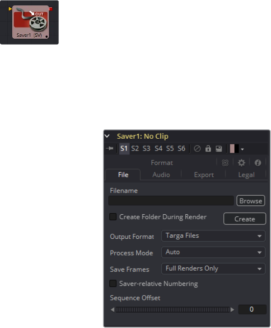
392
I/O Tools Chapter – 16
Saver [SV]
The Saver is responsible for writing the results of a composition to disk. It can be inserted into a
composition at any point. The Saver tool can also be used to add scratch track audio to your
flow, which can be heard during interactive playback.
A composition can contain any number of Saver tools, and Savers can be placed at any point
in the flow.
File Tab
Filename
Use the Filename dialog to select the name and path of the rendered image output.
Click on the yellow folder icon to display a file browser to select a folder and filename
to be used for output.
Sequence numbering is automatically added to the filename when rendered. For
example, if c\renders\image.tga is entered as the filename and 30 frames of output is
rendered, the files will automatically be numbered as image0000.tga, image0001.tga,
image0003.tga...and so on. Four digit padding is automatically used for numbers lower
than 10000.
Specify the number of digits to use for padding the sequence number by explicitly
entering the digits into the filename.
For example, image000000.tga would apply 6 digit padding to the numeric sequence,
image.001.tga would use 3 digit padding and image1.tga would use none.
Saving to an Image File List
It is possible to save to an IFL file if more control is required over the filenames written
to disk than specified here. To create an IFL, create a text file with the extension .ifl.
Each line of the text file specifies the name for one frame of the output.
393
I/O Tools Chapter – 16
For example, to render using roman numerals instead of decimals for the file sequence
numbering would create the following files:
i m ag e.i.t ga
i m ag e.i i.t ga
image.iii.tga
i m a g e.iv.t ga
i m a g e.v.t g a
The render will fail if there are not enough lines to match the number of frames
rendered. In the above example, the render would fail after the fifth frame.
Format options cannot be specified when using image file lists to save to disk. The
defaults will be used instead.
Output Format
Use this control to select the image format to be saved. Selecting a new format from
this menu does not change the extension used in the filename to match. Modify the
filename manually to match the expected extension for that format to avoid a mismatch
between name and image format.
For a list of file formats supported for saving by Fusion, see Appendix A.
Process Mode
The Process Mode menu is used to set the method of field processing used by Fusion
when the flow is rendered.
The default option is Auto. This will render the flow using the field ordering set in the
Process mode of the most background Loader or Creator tool in the flow.
To force a flow to render individual fields or full frames regardless of the settings of
other tools in the flow, change this menu’s setting to one of the other listed options.
For example, if the Saver’s process mode is set to NTSC fields, a Loader set to process
full frames will still load a full frame from disk, but animation applied to that layer will be
applied with field level accuracy. In all cases, footage will be re-interlaced, if necessary,
and saved as frames on disk.
See the Frame Formats chapter for additional details on frame and fields processing
in Fusion.
Save Frames
This control selects between two modes.
Full Renders Only
Images are only saved to disk when a final render is started using the Start Render
button in the Time Ruler.
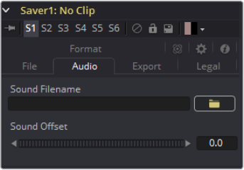
394
I/O Tools Chapter – 16
High Quality Interactive
This render mode is designed for real-time rendering when painting and rotoscoping.
Fusion will save each frame to disk as it is processed interactively.
When used correctly, this feature can completely eliminate the need to perform a final
render after rotoscoping. It can cause tremendous confusion when used in conjunction
with a flow that contains spline-animated parameters.
If these splines are modified in such a way that frames already saved interactively are
changed, the frames already on the disk will not automatically be re-rendered. Either
step through each frame again or perform a final render to make certain that the result
is correct.
Set Sequence Start
Normally, Fusion will use the render range of a composition to determine the numeric
sequence used when rendering a file sequence to disk. Enable this checkbox to reveal
the Sequence Start Frame control to adjust the starting number in the sequence to a
custom value.
Sequence Start Frame
This thumbwheel control can be used to set an explicit start frame for the number
sequence applied to the rendered filenames. For example, if Global Start is set to 1 and
frames 1-30 are rendered, files will normally be numbered 0001-0030. If the Sequence
Start Frame is set to 100, the rendered output would be numbered from 100-131.
Audio Tab
The Audio functionality is included in Fusion for scratch track (aligning effects to audio and clip
timing) purposes only. Final renders should almost always be performed without audio. The
smallest possible audio files should be used, as Fusion will load the entire audio file into
memory for efficient display of the waveform in the Timeline.
The audio track will be included in the saved image if a QuickTime or AVI file format is selected.
Fusion currently supports playback of WAV audio.
Audio Browse
Select the optional audio scratch track to be used. Select the *.WAV file of choice, then
expand the Saver segment in the Timeline layout to view the audio waveform. Drag the
pointer over the audio wave in the Timeline layout to hear the track.
Sound Offset
Drag the control left or right to create an offset in time between the audio and images
of the flow.
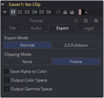
395
I/O Tools Chapter – 16
Export Tab
Export Mode
This menu is used to apply a SMPTE standard 3:2 pulldown to the footage as it is saved
to disk, converting the footage from 24fps to 30 fps.
First Frame
First Frame determines the cadence of the 3:2 pulldown by choosing what frames are
combined from the 24fps source to create the first frame in the 30fps pulldown result.
Normally, this should be left to AA. When saving a clip that originally had pulldown that
was removed to apply effects and it needs to be reinserted into an existing edit, the
cadence of the original clip may need to be matched.
Clipping Mode
These radio buttons define how the edges of image should be treated. This can also
be called source image clipping.
They default to Frame, which will provide the same behavior as previous versions of
Fusion. Since this option will clip to the parts of the image visible within its visible
dimensions, it will break any infinite-workspace behavior.
If the upstream DoD is smaller than the frame, the remaining area in the frame will be
treated as black/transparent. None does not perform any source image clipping at all.
This means that any data that would normally be needed outside the upstream DoD will
be treated as black/transparent. Be aware that this might create humongous images
which can consume a huge amount of diskspace. So you should use this option only if
really needed.
For more information about ROI, DoD and Infinite Workspace, please see the
dedicated chapter.
Save Alpha to Color
When selected, this control will cause the alpha channel to be saved into the color
channels as a grayscale image. This will completely overwrite any existing color
information.
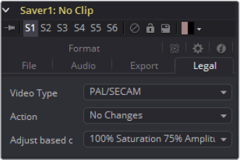
396
I/O Tools Chapter – 16
Legal Tab
Video Type
Select the standard to be used for broadcast legal color correction. NTSC, NHK or PAL/
SECAM can be chosen.
Action
Use this menu to choose how Fusion will treat illegal colors in the image.
Adjust to Legal
This will cause the images to be saved with legal colors relevant to the Video
Type selected.
Indicate as Black
This causes the illegal colors to be displayed as black in the views.
Indicate as White
This causes the illegal colors to be displayed as white in the views.
No Changes
This causes the images to be saved unaffected.
Adjust Based On
This menu is used to choose whether Fusion will legalize the image to 75% or 100%
amplitude. Very few broadcast markets permit 100% amplitude, but for the most part
this should be left to 75%.
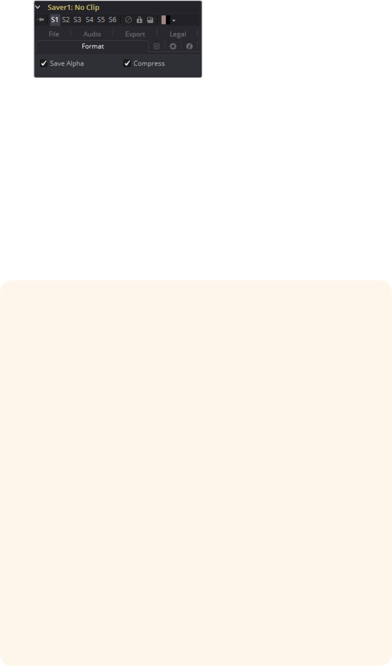
397
I/O Tools Chapter – 16
Format Tab
The Format tab contains information, options and settings specific to the image format
being saved. The controls for a TGA sequence will be entirely different from the ones
displayed when a DPX file is saved.
TGA and DPX are displayed on the right for reference.
When the Saver is set to DPX, it’s important to understand the reason for the “Data is
Linear” option. When saving log data into a DPX, and not using the Saver’s own lin-log
conversion (that is, Bypass Conversion is checked), the “Data is Linear” option should
be off. This indicates whether the reason for checking Bypass Conversion is because
the data is linear, or whether it’s already log.
If “Data is Linear” is enabled, then the DPX is marked in its Header as containing linear
data. In turn, that means that when the DPX is loaded back into Fusion, or into other
apps that evaluate the Header, those apps will think the data is linear, and will not
perform any log-lin conversion.
The Magic Comp Variable
As you can see in the screenshots, the pathnames in this example start with C o m p:\.
The Comp-variable in Fusion works for Loaders and Savers and helps you to keep
your work organized. C o m p:\ stands for the folder your actual composition is stored in.
So as long as all your source footage is stored in subfolders of your comp-folder,
Fusion will find that footage regardless of the actual hard-drive or network
share name.
You could, for example, copy an entire shot from the network to your local drive, set up
your Loaders and Savers to use the Comp:-variable, work all your magic locally (i.e.,
set up your composition) and then copy just the composition back to the server and
issue a net-render. All render slaves will automatically find the source footage.
Some examples:
Your Composition is stored in
X:\Project\Shot0815\Fusion\Shot0815.comp
Your source footage sits in
X:\Project\Shot0815\Fusion\Greenscreen\0815Green_0000.dpx The relative
path in the Loader would then be: Comp:\Greenscreen\0815Green_0000.dpx
If your source footage is stored in
X:\Project\Shot0815\Footage\Greenscreen\0815Green_0000.dpx The relative
path in the Loader would then be: Comp:\..\Footage\
Greenscreen\0815Green_0000.dpx
Observe how the two dots .. set the directory to go up one folder. Pretty much the
same like CD .. in a command shell window.
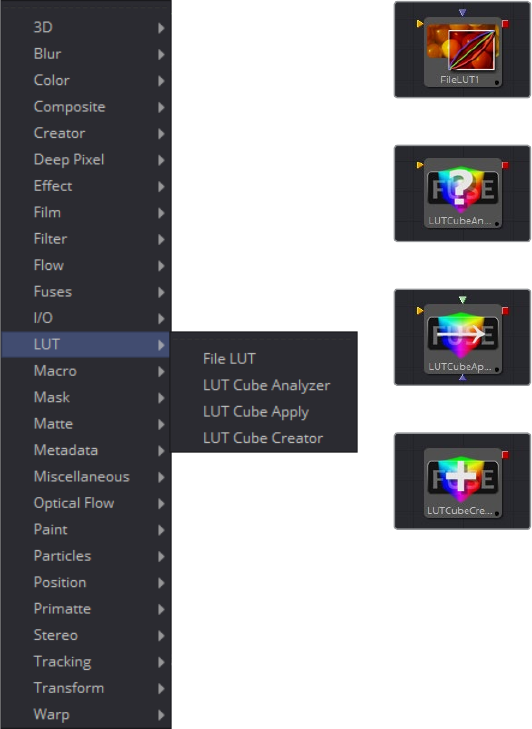
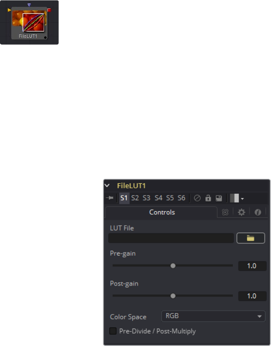
401
LUT Tools Chapter – 17
File LUT [FLU]
The File LUT tool applies a Look up Table (LUT) to the image, either a simple 1D LUT or a
supported 3D LUT. Unlike the Color Curves tool, it does not use a spline-based LUT. Instead, it
loads the LUT from a file stored on the system or network.
This approach has two advantages. The first is that the only part of the LUT stored in the
composition is the path to the file. Since LUT files can be very large, this can dramatically
reduce the file size of a composition when several LUTs are present. The second advantage is
that it becomes possible to adjust all File LUT tools using the same file at the same time, simply
by changing the contents of the LUT. This can be useful when the same LUT-based color
correction is applied in many different compositions.
Controls
LUT File
Use this control to select the path to the file describing the LUT. Currently, this tool
supports LUTs exported from Fusion in .LUT and .ALUT formats, Shake’s LUT format,
and a number of 3D LUT formats as well. The tool will fail with an error message on the
Console if it is unable to find or load the specified file.
Color Space
Use this control to change the color space the LUT is applied in. The default is to apply
the curves described in the LUT to the RGB color space, but options for YUV, HLS, HSV
and others are also available.
Pre-Divide/Post-Multiply
Selecting the Pre-Divide/Post-Multiply checkbox will cause the image pixel values to
be divided by the alpha values prior to applying the LUT, and then re-multiplied by the
alpha value after the correction.
This helps to prevent the creation of illegally additive images, particularly around the
edges of a blue/green key or when working with 3D rendered objects.
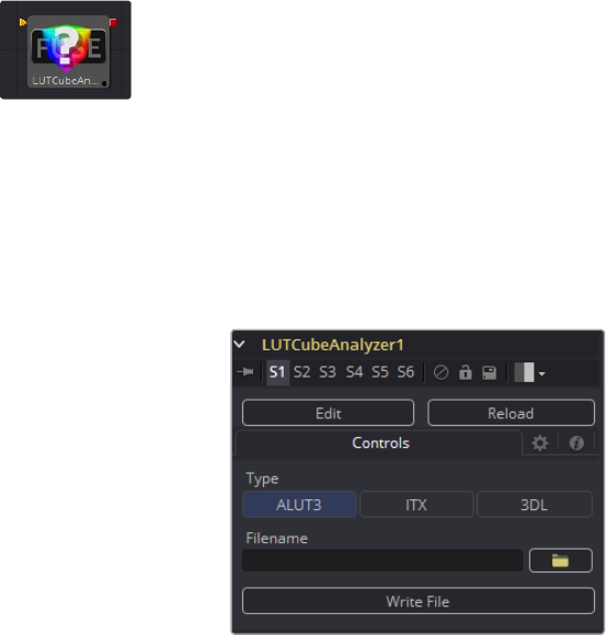
402
LUT Tools Chapter – 17
LUT Cube Analyzer [LCA]
The LUT Cube Analyzer takes an image created by the LUT Cube Creator as an input and
allows the user to create a 3D LUT file in ALUT3, ITX or 3DL format.
Feeding the original image into the tool would result in an unaltered or 1:1 LUT file.
You can, however, modify, grade and color correct the original cube image with as many tools
as you like and feed the result into the LUT Cube Analyzer. This will create a LUT that exactly
resembles your color pipeline.
Usage
Connect the output of any tool modifying an image that was created with the LUT Cube Creator
to the input of the Analyzer, view the Analyzer, select the desired output format, specify a
filename and press Write File to create the 3D LUT.
Controls
Type
Select the desired output format of the 3D LUT.
Filename
Specify a path and name the LUT file is written to.
Write File
Press this button to generate the 3D LUT file based on the settings above.
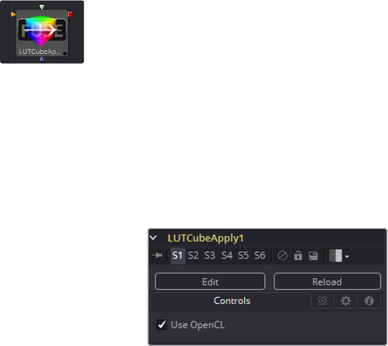
403
LUT Tools Chapter – 17
LUT Cube Apply [LCP]
The LUT Cube Apply takes an image created by the LUT Cube Creator as the Foreground input
and applies that LUT to the image connected to the Background input.
Feeding the original image into the tool would result in an unaltered or 1:1 output.
You can, however, modify, grade and color correct the original cube image with as many tools
as you like and feed the result into the LUT Cube Apply. Or, take a LUT image that has been
graded beforehand to apply the LUT without having to write an actual 3D LUT using the LUT
Cube Analyzer.
Usage
Connect any image that is meant to be modified according to the LUT to the Background input
of the tool. Connect a LUT Cube image to the Foreground input of the tool.
Use OpenCL
If your graphics card supports OpenCL, enabling this option will tremendously speed
up the processing on this tool.
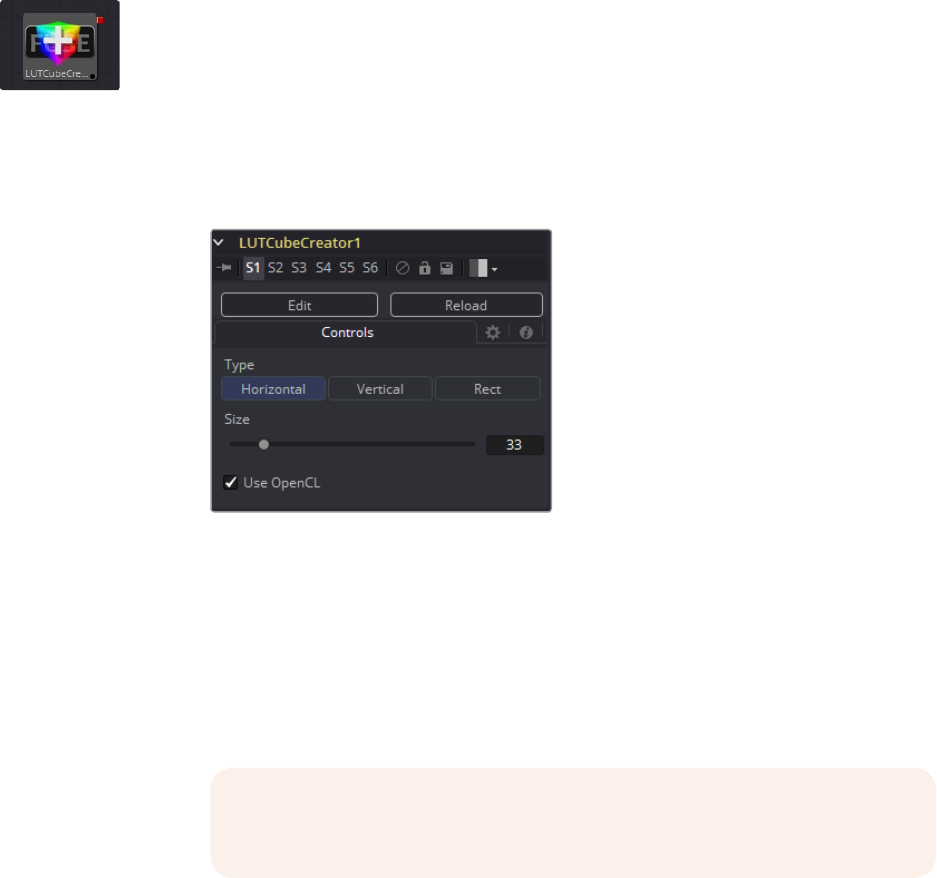
404
LUT Tools Chapter – 17
LUT Cube Creator [LCC]
The LUT Cube Creator creates an image for further use with the LUT Cube Analyzer or LUT
Cube Apply. The output can be graded, color corrected or modified with any tool inside and
outside of Fusion. If working outside Fusion, make sure to keep the image in 32-bit floating
point to preserve color accuracy.
Controls
Type
Horizontal: Creates a long, horizontal strip representing a color cube.
Vertical: Creates a long, vertical strip representing a color cube.
Rect: Creates a rectangular image, as depicted below, representing a color cube.
Size
Determines the resolution of the color cube.
Common values for color cubes are 17x17x17 or 33x33x33, or in a mathematical
fashion n^2+1.
NOTE: Higher resolutions yield more accurate results but are also more
memory and computational extensive.
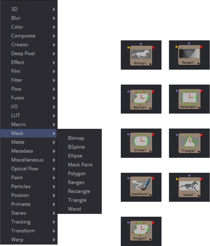
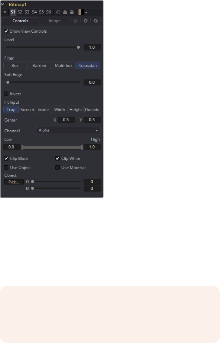
409
Mask Tools Chapter – 18
Common Mask Controls [CMC]
Common Controls can be found in every Mask tool. This chapter is therefore valid for all
Mask tools.
Common Mask Controls
Although each mask has its own set of controls unique to that mask type, several of the controls
shown are common for all types of masks. The controls listed here are generally found on
all masks.
Show View Controls
Use the Show View Controls checkbox to disable the display of the Mask controls in
the Viewer. Polylines, centers, angles and other controls will not be displayed, even
when the tool is selected.
Level
The Level control designates the transparency level of the pixels in the Mask channel.
When the value is 1.0, the effect mask is completely opaque (unless it has a soft edge).
Lower values will cause the mask to be partially transparent. The result is identical to
lowering the blend control of an effect.
NOTE: Lowering the level of a mask will lower the values of all pixels covered
by the mask in the Mask channel. For example, if a Circle mask is placed over
a Rectangle mask, lowering the level of the circle mask will lower the values of
all of the pixels in the Mask channel, regardless of the fact that the rectangle
mask beneath it is still opaque.
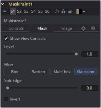
410
Mask Tools Chapter – 18
Filter
This control selects the filtering algorithm to be used when applying Soft Edge
to the mask.
Box
This is the fastest method, but at reduced quality. This is best suited for very small
amounts of blur.
Bartlett
Otherwise known as a Pyramid filter, Bartlett makes a good compromise between
speed and quality.
Multi-box
When selecting this filter, the Num Passes slider appears to let you control the quality.
At 1 and 2 passes, results are identical to Box and Bartlett, respectively. At 4 and above,
results are usually as good as Gaussian, in less time and with no edge ‘ringing.’
Gaussian
The default filter, this uses a true Gaussian approximation and gives excellent results,
but it is a little slower than the other filters. In some cases, it can produce extremely
slight edge ‘ringing’ on floating-point pixels.
Soft Edge
Use the Soft Edge slider to blur (feather) the edges of the mask, using the selected
Filter. Higher values will cause the edge to fade off well beyond the boundaries of the
mask. A value of 0.0 will create a crisp, well-defined edge.
Border Width
The Border Width control adjusts the thickness of the mask’s edge. When the Solid
checkbox is toggled on, the border thickens or narrows the mask. When the mask is not
solid, an outline of the mask shape is drawn and the thickness of the outline is handled
with this control.
Paint Mode
Although each mask has its own set of controls unique to that mask type, several of the controls
shown are common for all types of masks. The controls listed here are generally found on
all masks.
Merge
Merge is the default for all masks. The new mask is merged together with the
input mask.
411
Mask Tools Chapter – 18
Add
The mask’s values are added to the input mask’s values.
Subtract
In the intersecting areas, the new mask values are subtracted from the input
mask’s values.
Minimum
The input mask’s values are compared to the new mask, and the lowest (minimum)
value is taken.
Maximum
The input mask’s values are compared to the new mask, and the highest (maximum)
value is taken.
Average
This calculates the average (half the sum) of the new mask and the input mask.
Multiply
This multiplies the values of the input mask by the new mask’s values.
Replace
The new mask completely replaces the input mask wherever they intersect. Areas that
are zero (completely black) in the new mask do not affect the input mask.
Invert
Areas of the input mask that are covered by the new mask are inverted; white becomes
black and vice versa. Gray areas in the new mask are partially inverted.
Copy
This mode completely discards the input mask and uses the new mask for all values.
Ignore
This mode completely discards the new mask and uses the input mask for all values.
Invert
Selecting this checkbox inverts the entire mask. This differs from the Invert Paint mode
in that it affects all pixels, regardless of whether they are covered by the new
mask or not.
Solid
When the Solid checkbox is enabled, all areas completely enclosed by the mask will be
filled solid white. Turning off the checkbox will treat the mask as an outline, with the
width of the outline determined by the Border Width control. This checkbox is enabled
by default.
Center
All masks have a Center, with the exception of the common controls found on Creator
tools, such as Background and Fast Noise.
Process Mode
Use this menu control to select the Fields Processing mode used by Fusion to render
changes to the mask. The default option is determined by the Has Fields checkbox
control in the Frame Format preferences. For more information on fields processing,
consult the Frame Formats section.
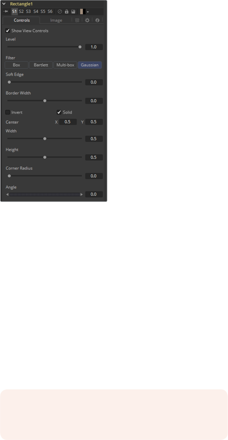
412
Mask Tools Chapter – 18
Use Frame Format Settings
When this checkbox is selected, the width, height and pixel aspect of the mask created
will be locked to values defined in the composition’s Frame Format preferences. If the
Frame Format preferences change, the resolution of the mask produced will change to
match. Disabling this option can be useful to build a composition at a different
resolution than the eventual target resolution for the final render.
Width and Height
This pair of controls is used to set the Width and Height dimensions of the mask to
be created.
Pixel Aspect
This control is used to specify the Pixel Aspect ratio of the created mask. An aspect
ratio of 1:1 would generate a square pixel with the same dimensions on either side (like
a computer display monitor) and an aspect of 0.91 would create a slightly rectangular
pixel (like an NTSC monitor).
Depth
The Depth button array is used to set the pixel color depth of the image created by the
mask. 32-bit pixels require four times the memory of 8-bit pixels, but have far greater
accuracy. Float pixels allow high dynamic range values outside the normal 0..1 range,
for representing colors that are brighter than white or darker than black. See the Frame
Format chapter for more details.
NOTE: Right-click on the Width, Height or Pixel Aspect controls to display a
menu listing the file formats defined in the preferences Frame Format tab.
Selecting any of the listed options will set the width, height and pixel aspect to
the values for that format.
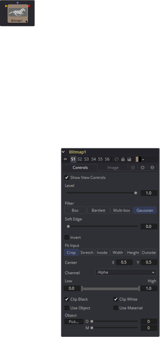
413
Mask Tools Chapter – 18
Bitmap Mask [BMP]
The Bitmap Mask allows images from the flow to act as masks for tools and effects. Bitmap masks
can be based on values from any of the color, alpha, hue, saturation, luminance and auxiliary
coverage channels of the image. Tools can also be masked based on the Object or Material ID of
a 3D rendered image (provided those channels were included when the file was rendered).
The output of any tool can be connected directly to another tool’s Effect Mask input. The
Bitmap Mask tool is not required for many common tasks. If the output is connected directly, the
Common Controls tab for the masked tool will display a control to select which channel of the
mask image is used to create the mask.
However, Bitmap Mask tools may still be required to connect to other mask inputs on some
tools, such as Garbage Mattes and Pre-Masks. Also, using a Bitmap Mask tool between the
mask source and the target tool provides additional options that would not be available when
connecting directly, such as combining masks, blurring the mask or clipping its threshold.
Many of the controls found in this mask tool are common to all mask tools. These controls are
documented at Common Mask Controls.
Controls Tab
Level, Filter, Soft Edge and Border Width
Please refer to the Common Mask controls.
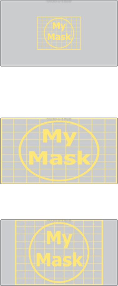
414
Mask Tools Chapter – 18
Fit Input
This control defines how the image source is treated if it does not fit the dimensions of
the generated mask.
Imagine a 720*576 image source being used to generate a 1920x1080 mask.
In the following section we refer to image source as being the 720x576 image (yellow)
and mask as being the mask that is actually generated (gray).
Crop
If the image source is smaller than the generated mask it will be placed according to
the X/Y controls, masking off only a portion of the mask. If the image source is bigger
than the generated mask it will be placed according to the X/Y controls and cropped
off at the borders of the mask.
Stretch
The image source will be stretched in X and Y to accommodate the full dimensions of
the generated mask. This might lead to visible distortions of the image source.
Inside
The image source will be scaled uniformly until one of its dimensions (X or Y) fits the
inside dimensions of the mask. Depending on the relative dimensions of the image
source and mask background, either the image source’s width or height may be
cropped to fit the respective dimension of the mask.
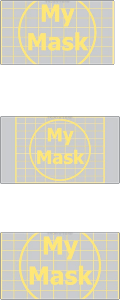
415
Mask Tools Chapter – 18
Width
The image source will be scaled uniformly until its width (X) fits the width of the mask.
Depending on the relative dimensions of the image source and mask, the image
source’s Y-dimension might not fit the mask’s Y-dimension, resulting in either cropping
of the image source in Y or the image source not covering the mask’s height entirely.
Height
The image source will be scaled uniformly until its height (Y) fits the height of the mask.
Depending on the relative dimensions of the image source and mask, the image
source’s X-dimension might not fit the mask’s X-dimension, resulting in either cropping
of the image source in X or the image source not covering the mask’s width entirely.
Outside
The image source will be scaled uniformly until one of its dimensions (X or Y) fits the
outside dimensions of the mask. Depending on the relative dimensions of the image
source and mask, either the image source’s width or height may be cropped or not fit
the respective dimension of the mask.
416
Mask Tools Chapter – 18
Other Controls
Channel
Use this control to select the Channel of the input image used to create the mask.
Choices include the red, green, blue and alpha channels, the hue, luminance or
saturation values, or the auxiliary coverage channel of the input image (if one is
provided).
Threshold Low/High
The Threshold range control can be used to clip the bitmap image. Increasing the value
of the low control will clip pixels below the specified value to black (0.0). Decreasing
the high value will force pixels higher than the specified value to white (1.0).
Use Object/Use Material
This control has no affect unless the input image contains a Material or Object
IDchannel. When toggled on, the selected Object ID and/or Material ID is used to
create a mask based on the selected object or material. When toggled off, the regular
color channels will generate the mask.
Image Tab
Please refer to the Common Mask Controls.
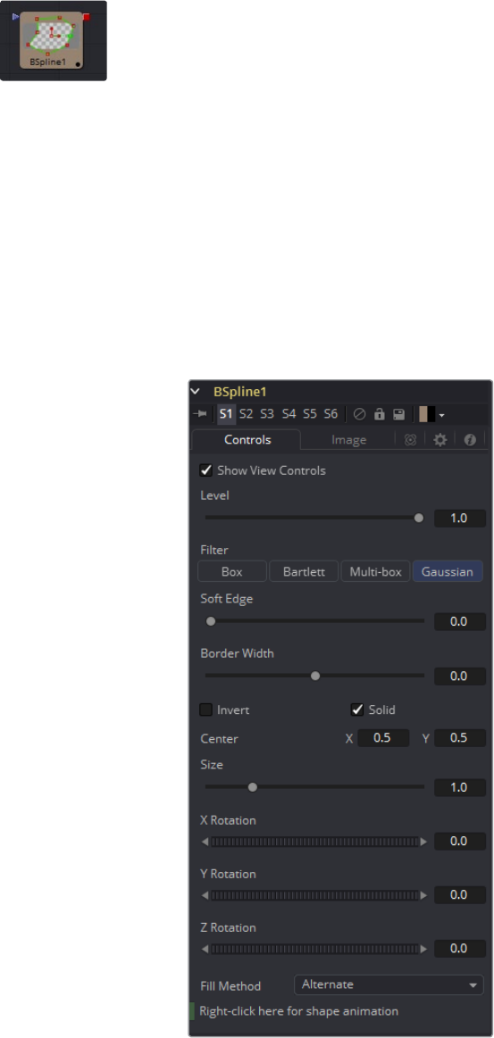
417
Mask Tools Chapter – 18
B-Spline Mask [BSP]
A B-spline Mask is identical to a Polygon Mask in all respects except one. Where Polygon
masks use Bezier splines, this Mask tool uses B-splines. Where Bezier splines employ a main
point and two handles to manage the smoothing of the spline segment, a B-spline requires only
a single point. This means that a B-spline shape requires far fewer control points to create a
nicely smoothed shape.
The smoothness of a B-spline is determined by the tension of the control points. To adjust the
tension of a B-spline’s control points, select the point, hold down the W key and drag the
mouse pointer to the left and right to increase or decrease the tension of the curve through
that point.
Many of the controls found in this Mask tool are common to all Mask tools. These controls are
documented at Common Mask Controls.
Controls Tab
Level, Filter, Soft Edge and Border Width
Please refer to the Common Mask Controls.
Size
Use the Size control to adjust the scale of the B-spline effect mask, without affecting
the relative behavior of the points that compose the mask or setting a keyframe in the
mask animation.

418
Mask Tools Chapter – 18
X, Y and Z Rotation
Use these three controls to adjust the rotation angle of the effect mask along any axis.
Fill Method
The Fill Method drop-down menu offers two different techniques for dealing with
overlapping regions of a polyline. If overlapping segments in a mask are causing
undesirable holes to appear, try switching the setting of this control from Alternate to
Non Zero Winding.
Right Click Here for Shape Animation
By default, all B-spline masks are animated when they are created. The initial keyframe
is set to the current time and any changes to the shape at different times will
create new keys.
Right-clicking on this label will display a contextual menu that offers options for
removing or re-adding animation to the mask, or publishing and connecting the
masks together.
Adding Points
Adding Points to a B-spline effect mask is relatively simple. Immediately after creating the mask
there are no points, but the mask will be in Click Append mode. Simply click once in the Viewer
wherever a point is required for the mask. Continue clicking to draw the shape of the mask.
When the shape is complete, click on the initial point again to close the mask.
When the shape is closed, the mode of the polyline will change to Insert and Modify. This
allows for the adjusting and adding of additional points to the mask by clicking on segments of
the polyline. To lock down the mask’s shape and prevent accidental changes, switch the
Polyline mode to Done using the Polyline toolbar or contextual menu.
When a B-spline mask is added to a tool, a toolbar will appear in the view with buttons that offer
easy access to the modes and tools. Hold the mouse pointer over any button in the toolbar to
display a tooltip that describes that button’s function.
Change the way the toolbar is displayed by right-clicking on the toolbar and selecting from the
options displayed in the toolbar’s contextual menu.
The functions of the buttons in this toolbar are explained in depth in the Polylines chapter.
Image Tab
Please refer to the Common Mask Controls.
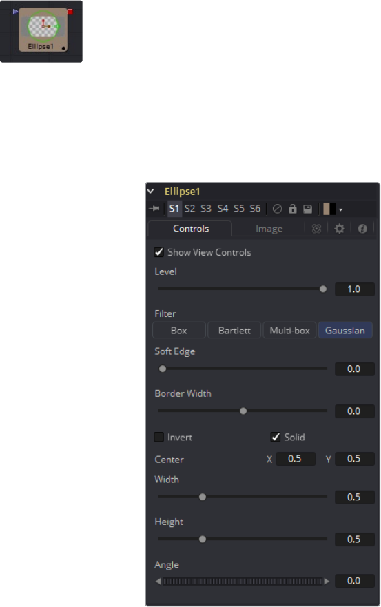
419
Mask Tools Chapter – 18
Ellipse Mask [ELP]
The Ellipse Mask is most useful for masking round objects. It is a circle by default, but
independent control is offered over the width, height and angle, providing for a wide variety of
ellipsoidal shapes.
Many of the controls found in this Mask tool are common to all Mask tools. These controls are
documented at Common Mask Controls.
Controls Tab
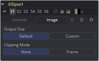
420
Mask Tools Chapter – 18
Level, Filter, Soft Edge and Border Width
Please refer to the Common Mask Controls.
Width
This control allows independent control of the ellipse mask’s Width. In addition to the
slider in the mask’s controls, interactively drag the width (left or right edge) of the mask
on the view using the pointer. Any changes will be reflected on this control.
Height
Height allows independent control of the ellipse mask’s Height. In addition to the slider
in the mask’s controls, interactively drag the height (top or bottom edge) of the mask on
the view using the pointer. Any changes will be reflected on this control.
To change the mask’s size without affecting the aspect ratio, drag the on screen
controlbetween the edges (diagonal). This will modify both the width and
heightproportionately.
Angle
Change the rotational angle of the mask by moving the Angle control left or right.
Values can be entered in the input boxes provided. Alternately, use the onscreen
controls by dragging the little circle at the end of the dashed angle line to interactively
adjust the rotation of the ellipse.
Image Tab
Please refer to the Common Mask Controls.
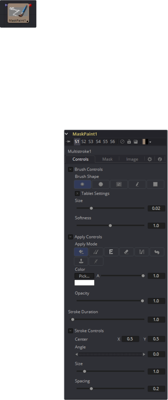
421
Mask Tools Chapter – 18
Mask Paint [PNM]
The Mask Paint tool allows direct painting on mask images, using the mouse pointer as if it was
a paintbrush. In addition to regular paint strokes, it is possible to apply basic primitive shapes
and polyline style strokes.
Each stroke can have a duration that lasts for the entire project, a single frame or field, or an
arbitrary number of fields. The strokes can have independent durations in the Timeline for easy
manipulation of time. Alternatively, Multistrokes is a faster but non-editable way for doing many
mask cleanup paint tasks.
Controls Tab
As the Paint Mask tool is fundamentally identical to the Paint tool, see the Paint tool and the
Paint and Rotoscoping chapter for more details on the many options and capabilities available.
The only difference is that, as Paint Mask operates on single-channel mask images, there is no
Channel Selector control and all color controls have only a single Alpha value.
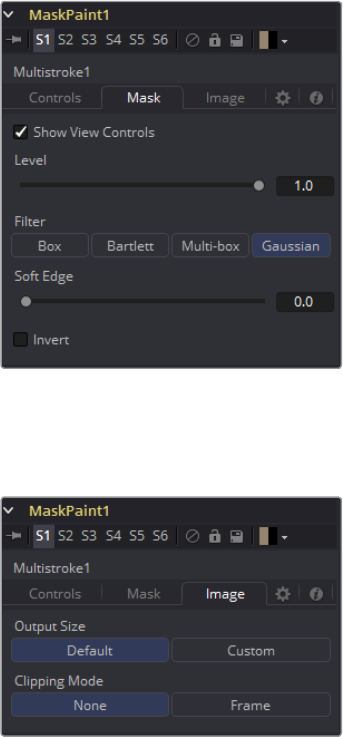
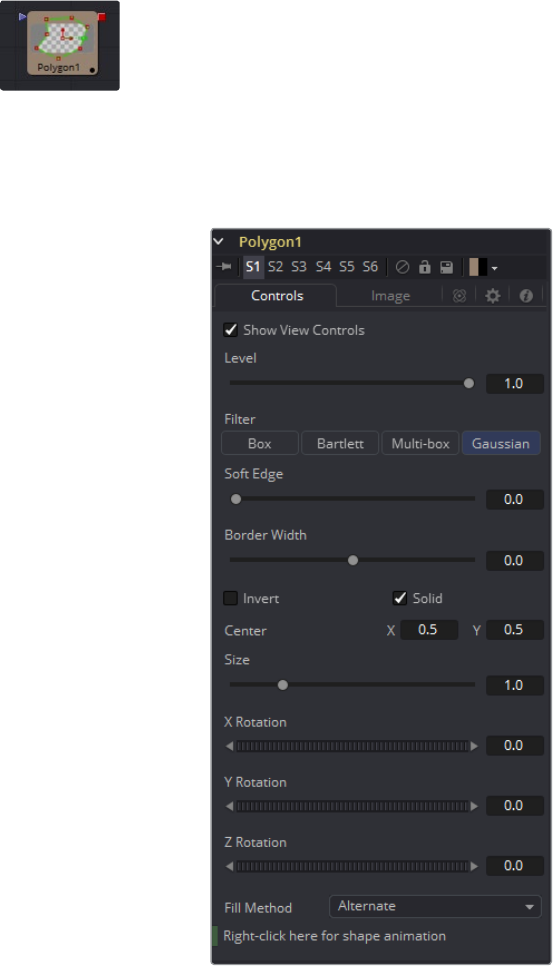
423
Mask Tools Chapter – 18
Polygon Mask [PLY]
The Polygon Mask is most useful for masking objects that do not have a regular shape. When
first added to a tool, the Polygon mask consists of only Center and Angle controls, which are
visible onscreen. Points are added to the polyline by clicking in the Viewer. Each new point is
connected to the last one created.
Controls Tab
Level, Filter, Soft Edge and Border Width
Please refer to the Common Mask Controls.
Size
Use the Size control to adjust the scale of the Polygon effect mask, without affecting
the relative behavior of the points that compose the mask or setting a keyframe in the
mask animation.
X, Y and Z Rotation
Use these three controls to adjust the rotation angle of the effect mask along any axis.
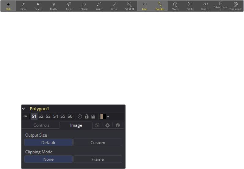
424
Mask Tools Chapter – 18
Fill Method
The Fill Method drop-down menu offers two different techniques for dealing with
overlapping regions of a polyline. If overlapping polyline segments in a mask are
causing undesirable holes in the mask, try switching the setting of this control from
Alternate to Non Zero Winding.
Right Click Here for Shape Animation
By default, all polyline masks are animated when they are created. The initial keyframe
is set to the current time and any changes to the shape at different times will
create new keys.
Right-clicking on this label will display a contextual menu that offers options for
removing or re-adding animation to the mask, or publishing and connecting
masks together.
Adding Points
Adding Points to a polygonal effect mask is relatively simple. Immediately after creating the
mask there are no points, but the mask will be in Click Append mode. Simply click once in the
Viewer wherever a point is required for the mask. Continue clicking to draw the shape of the
mask. When the shape is complete, click on the initial point again to close the mask.
When the shape is closed, the mode of the polyline will change to Insert and Modify. This
allows for the adjusting and adding of additional points to the mask by clicking on segments of
the polyline. To lock down the mask’s shape and prevent accidental changes, switch the
Polyline mode to Done using the Polyline toolbar or contextual menu.
When a Polygon mask is added to a tool, a toolbar will appear in the view with buttons that offer
easy access to modes and tools. Hold the mouse pointer over any button in the toolbar to
display a tooltip that describes that button’s function.
Change the way the toolbar is displayed by right-clicking on the toolbar and selecting from the
options displayed in the toolbar’s contextual menu. The functions of the buttons in this toolbar
are explained in depth in the Polylines chapter.
Image Tab
Please refer to the Common Mask Controls.
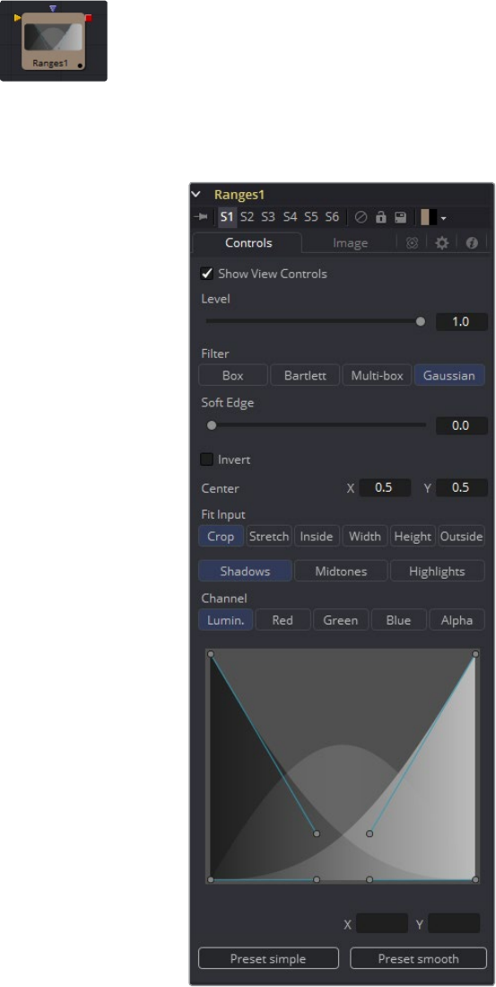
425
Mask Tools Chapter – 18
Ranges Mask [RNG]
Similar to Bitmap Mask, the Range Mask allows images from the flow to act as masks for tools
and effects. Instead of creating a simple luminance-based mask from a given channel, Range
allows spline-based selection of low, mid and high ranges, akin to Color Corrector.
Controls Tab
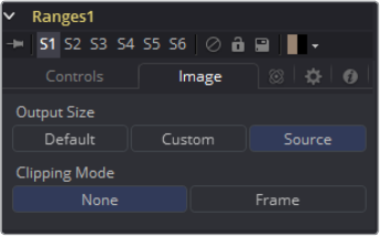
426
Mask Tools Chapter – 18
Level, Filter, Soft Edge and Border Width
Please refer to the Common Mask Controls.
Shadows/Midtones/Highlights
These buttons are used to select which range will be output by the tool as a mask.
White pixels represent pixels that are considered to be part of the range and black
pixels are not included in the range. For example, choosing Shadows would show
pixels considered to be shadows as white and pixels that are not shadows as black.
Mid gray pixels are only partly in the range and will not receive the full effect of any
color adjustments to that range.
Channel
The Channel selection buttons shown in this tab can be used to extract a mask from
the range of a specific color channel. By default, Fusion uses the luminance channel
when the color ranges are examined.
Spline Display
The extent of the ranges is selected by manipulating the spline handles. There are four
spline points, each with one Bezier handle. The two handles at the top represent the
start of the shadow and highlight ranges, whereas the two at the bottom represent the
end of the range. The Bezier handles are used to control the falloff.
The midtones range has no specific controls since its range is understood to be the
space between the shadow and the highlight ranges. In other words, after low and high
masks have been applied, midtones is everything else.
The X and Y text controls below the Spline Display can be used to enter precise
positions for the selected Bezier point or handle.
Presets
This sets the splines to two commonly-used configurations. Simple gives a
straightforward linear-weighted selection, while Smooth uses a more natural falloff.
Image Tab
Please refer to the Common Mask Controls.

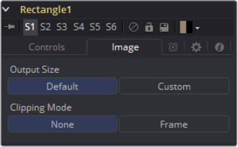
428
Mask Tools Chapter – 18
Level, Filter, Soft Edge and Border Width
Please refer to the Common Mask Controls.
Width and Height
Use these controls to change the X or Y scale of the rectangular effect mask
independently of each other. Alternatively, drag the edges of the rectangle in the
Viewer to interactively adjust its size.
Corner Radius
Corner Radius allows the corners of the rectangle mask to be rounded. A value of 0.0 is
not rounding at all, which means that the rectangle has sharp corners. A value of 1.0 will
apply the maximum amount of rounding to the corners.
Angle
Change the rotation angle of an effect mask by moving the Angle control left or right.
Values can be entered in the provided input boxes. Alternately, use the onscreen
controls by dragging the little circle at the end of the dashed angle line to interactively
adjust the rotation of the ellipse.
Image Tab
Please refer to the Common Mask Controls.
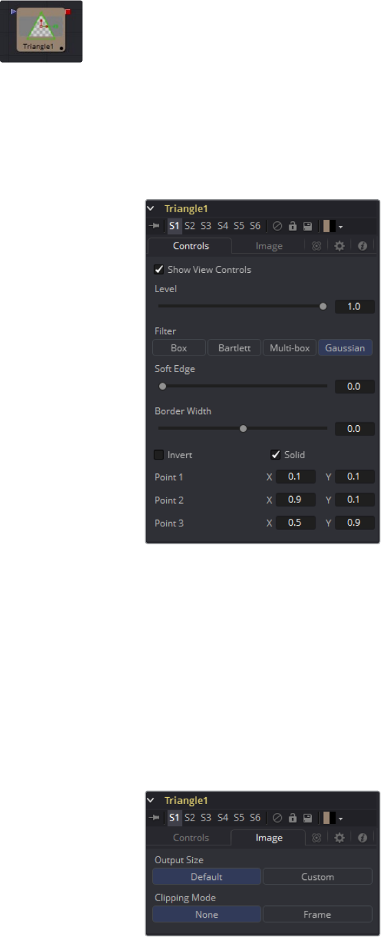
429
Mask Tools Chapter – 18
Triangle Mask [TRI]
The Triangle Mask is unique in that it has no Center, Size or Angle control. Unlike most other
types of masks, all three points of the triangle may be attached to a tracker or motion path.
Complex effect masking is possible using trackers and other tools’ paths to manipulate the
triangle shape.
Many of the controls found in this mask tool are common to all mask tools. These controls are
documented at Common Mask Controls.
Controls Tab
Level, Filter, Soft Edge and Border Width
Please refer to the Common Mask Controls.
Point 1, Point 2, Point 3
These controls indicate the position of the three corners of the triangle. Each point can
be published, connected to other controls, animated with a path, or attached to
trackers. To perform any of these tasks, right-click on the Position control in the mask
controls, or directly on the point in the Viewer, and select the appropriate option from
the contextual menu.
Image Tab
Please refer to the Common Mask Controls.
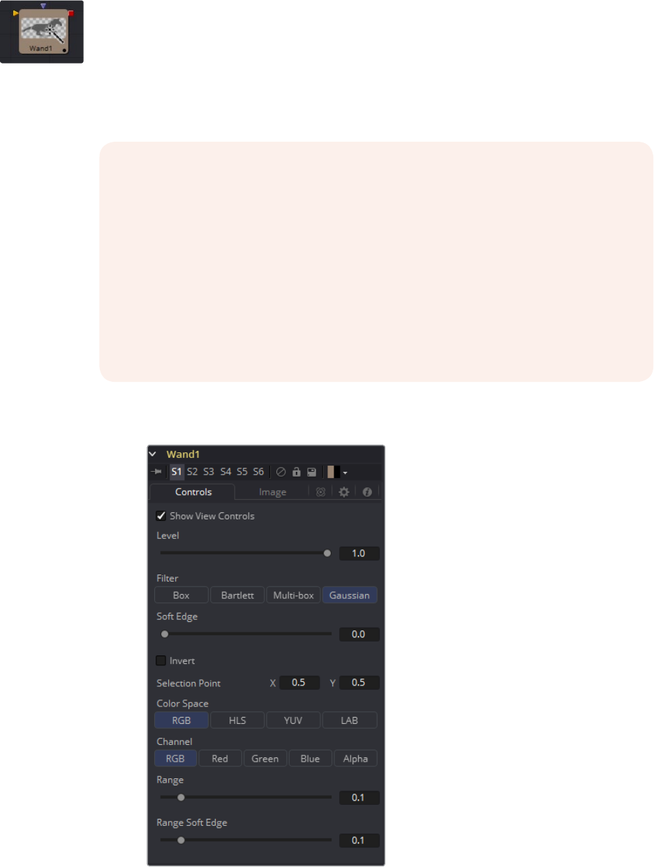
430
Mask Tools Chapter – 18
Wand Mask [WND]
The Wand Mask provides the ability to mask an image based on a magic wand-style selection,
similar to the magic wand tools found in traditional 2D paint applications. As with a Bitmap
mask, any image in the composition can be used as a source for the mask. Generally, the
default is most useful, where the source image is the input of the tool to which the mask
is applied.
Controls Tab
NOTE: When adding a Wand mask to a tool, a crosshair will appear in the Viewers.
This crosshair should be positioned in the image to select the color used to create the
Wand mask. The mask itself is created by examining the color of the pixel beneath the
selection point and adding that color to the mask. The mask then expands to examine
the pixels surrounding the selection point. If the surrounding pixels are the same color,
they are also added to the mask. The mask stops expanding when no connecting
pixels fall within the color range of the mask. The tool to be used as the image source
for the mask should be connected to the Source (orange) input on the flow. As with
other masks, the Effect Mask (blue) input is used to combine the wand’s result with
other Mask tools. Many of the controls found in this Mask tool are common to all Mask
tools. These controls are documented at Common Mask Controls.
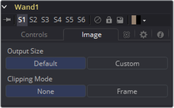
431
Mask Tools Chapter – 18
Level, Filter, Soft Edge and Border Width
Please refer to the Common Mask Controls.
Selection Point
The Selection Point is a pair of X and Y coordinates that determine from where in the
source image the Wand mask derives its initial color sample. This control is also seen
as a crosshair in the Viewers. The selection point can be positioned manually,
connected to a tracker, path or other expressions.
Color Space
The Color Space button group determines the color space used when selecting the
source color for the mask. The Wand mask can operate in RGB, YUV, HLS or LAB
color spaces.
Channel
The Channel button group is used to select whether the color that is masked comes
from all three color channels of the image, the alpha channel, or from an individual
channel only.
The exact labels of the buttons will depend on the color space selected for the Wand
Mask operation. If the color space is RGB, the options will be R, G or B. If YUV is the
color space, the options will be Y, U or V.
Range
The Range slider controls the range of colors around the source color that will be
included in the mask. If the value is left at 0.0, only pixels of exactly the same color as
the source will be considered part of the mask. The higher the value, the more that
similar colors in the source will be considered to be wholly part of the mask.
Range Soft Edge
The Range Soft Edge determines the falloff range of the colors selected. Any pixel
within the range defined above will be treated as 100% within the mask. If the soft
range is set to 0.0, no other pixels will be considered for the mask. Increasing the soft
range will increase the number of colors close to, but not quite within, the range that
will be included in the mask. These pixels will be semi-transparent in the mask.
Image Tab
Please refer to the Common Mask Controls.
433
Matte Tools Chapter – 19
Matte Tools
Alpha Divide [ADV] 435
Alpha Multiply [AML] 436
Chroma Keyer [CKY] 437
Clean Plate 441
Delta Keyer 443
Difference Keyer [DKY] 450
Luma Keyer [LKY] 452
Matte Control [MAT] 454
Primatte 5 459
Basic Operation Tutorial 467
Removing Spill Setup 470
Repeatable Sampling Tools 473
Spill Replacement Options 475
Ultra Keyer [UKY] 478
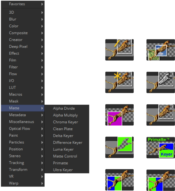
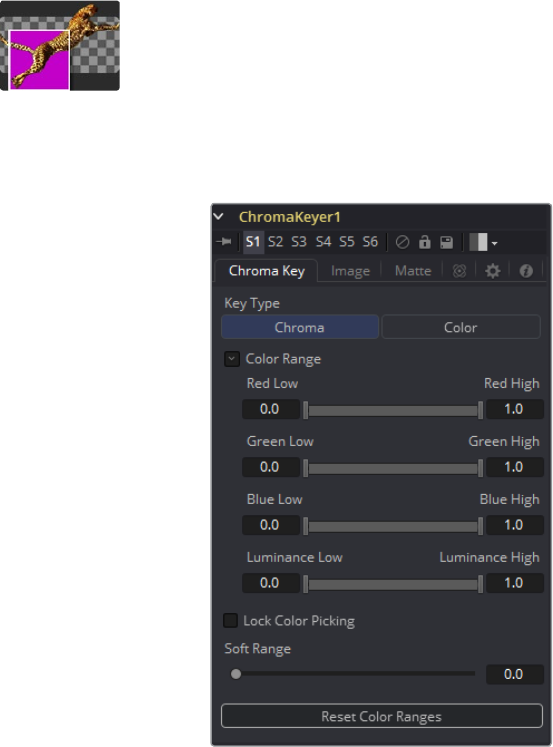
437
Matte Tools Chapter – 19
Chroma Keyer [CKY]
The Chroma Keyer Tool creates an alpha channel (matte) for an image by removing selected
colors from the scene. Unlike the Ultrakeyer, which has specific optimizations for keying from
blue and green colors, the chroma keyer works equally well with any color.
Chroma Key Tab
Key Type
This determines the type of selection to be used for the matte creation.
Chroma
Chroma causes a matte to be created based on the RGB values of the selected
color range.
Color
This causes a matte to be created based on the hue of the selected color range.
Color Range
These range controls update automatically to represent the current color selection.
Colors are selected by selecting the Chroma Keyer tool’s tile in the flow, then dragging
in the Viewer to select the colors to be used to create the matte. These range controls
can be used to tweak the selection slightly, although generally selecting colors in the
displays is all that is required.
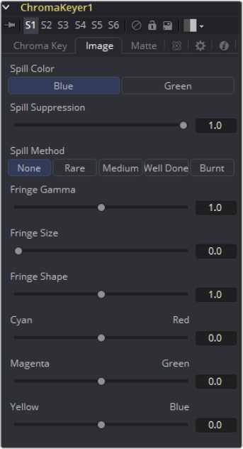
438
Matte Tools Chapter – 19
Lock Color Picking
When this checkbox is selected, Fusion will prevent accidental growing of the selected
range by selecting more colors from the view. It is a good idea to select this checkbox
once the color selection has been made for the matte. All other controls in the tool
remain editable.
Soft Range
This control softens the selected color range to include additional colors into the matte.
Reset Color Ranges
Clicking on this button resets the Chroma Keyer’s range controls, discarding all color
selections. All other sliders and controls maintain their values.
Image Tab
Spill Color
Use these buttons to select the color used as the base for all spill suppression
techniques.
Spill Suppression
Spill is generally caused by the transmission of the color of the background through the
semitransparent areas of the alpha channel. In the case of blue or green screen keying,
this usually causes the color of the background to become apparent in the fringe of the
foreground element.
Spill suppression attempts to remove color from the fringe. The process used is
optimized for either blue or green screens; you select which color is used as the base
from the control above.
When this slider is set to 0 no spill suppression is applied to the image.
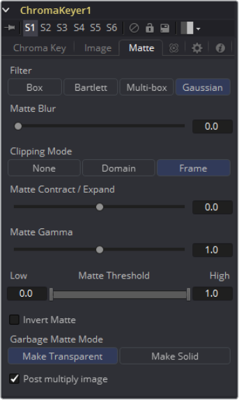
439
Matte Tools Chapter – 19
Spill Method
This selects the strength of the algorithm used to apply spill suppression to the image.
None
None is selected when no spill suppression is required.
Rare
This removes very little of the spill color, the lightest of all methods.
Medium
This works best for green screens.
Well Done
This works best for blue screens.
Burnt
This works best for blue. Use this mode only for very troublesome shots. Most likely
you will have to add strong color correction after the key to get, for example, your
skin tones back.
Fringe Gamma
This control can be used to adjust the brightness of the fringe or halo that surrounds
the keyed image.
Fringe Size
This expands and contracts the size of the fringe or halo surrounding the keyed image.
Fringe Shape
Fringe Shape forces the fringe to be pressed toward the external edge of the image or
pulled toward the inner edge of the fringe. Its effect is most noticeable while the Fringe
Size sliders value is large.
Cyan/Red, Magenta/Green and Yellow/Blue
Use these three controls to color correct the fringe of the image. This is useful for
correcting semi-transparent pixels that still contain color from the original background
to match the new background.
Chroma Keyer Matte Tab
440
Matte Tools Chapter – 19
Matte Blur
Matte Blur blurs the edge of the matte using a standard constant speed Gaussian blur.
A value of zero results in a sharp, cutout-like hard edge. The higher the value, the more
blur applied to the matte.
Matte Contract/Expand
This slider shrinks or grows the semi-transparent areas of the matte. Values above 0.0
expand the matte while values below 0.0 contract it.
This control is usually used in conjunction with the Matte Blur to take the hard edge of a
matte and reduce fringing. Since this control only affects semi-transparent areas, it will
have no effect on a hard edge’s matte.
Matte Gamma
Matte Gamma raises or lowers the values of the matte in the semi-transparent areas.
Higher values cause the gray areas to become more opaque and lower values cause
the gray areas to become more transparent. Completely black or white regions of the
matte remain unaffected.
Since this control only affects semi-transparent areas, it will have no effect on a hard
edge’s matte.
Matte Threshold
Any value below the lower threshold becomes black or transparent in the matte.
Anyvalue above the upper threshold becomes white or opaque in the matte. All values
within the range maintain their relative transparency values.
This control is often used to reject salt and pepper noise in the matte.
Invert Matte
When this checkbox is selected, the alpha channel created by the keyer is inverted,
causing all transparent areas to be opaque and all opaque areas to be transparent.
Garbage Matte Mode
Garbage Mattes are Mask tools or images connected to the Garbage Matte input on
the tool’s tile. The Garbage matte is applied directly to the alpha channel of the image.
Generally, Garbage mattes are used to remove unwanted elements that cannot be
keyed, such as microphones and booms. They are also used to fill in areas that contain
the color being keyed but that you wish to maintain.
Garbage mattes of different modes cannot be mixed within a single tool. A Matte
Control tool is often used after a Keyer tool to add a Garbage matte with the opposite
effect of the matte applied to the keyer.
Make Transparent
Select this button to make the Garbage matte transparent.
Make Solid
Select this button to make the Garbage matte solid.
Post Multiply Image
Select this option to cause the keyer to multiply the color channels of the image against
the alpha channel it creates for the image. This option is usually enabled and is on
by default.
Deselect this checkbox and the image can no longer be considered pre-multiplied for
purposes of merging it with other images. Use the Subtractive option of the Merge tool
instead of the Additive option.
For more information, see the Merge tools documentation.
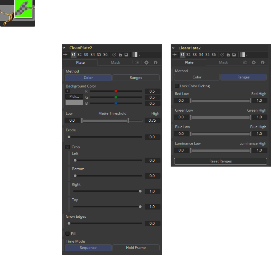
441
Matte Tools Chapter – 19
Clean Plate
The Clean plate tool is a pre keying tool used to generate an image of the Green or Blue color
screen to smooth out the lighting differences so that later keying can key fine detail without
choking or clipping the matte.
Method
Color Uses a difference method to replace the color, choose by Click Drag clicking to
the image.
Ranges uses a chroma range method to separate the background color
Matte Threshold
Any value below the lower threshold becomes black or transparent in the matte.
Anyvalue above the upper threshold becomes white or opaque in the matte. All values
within the range maintain their relative transparency values. This control is often used
to reject salt and pepper noise in the matte.
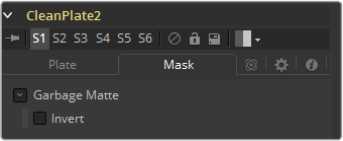
442
Matte Tools Chapter – 19
Erode
Will decrease the size of the screen area.
Crop
Will trim in from the edges of the image.
Grow Edges
Will expand the color of the edges of the subject
Fill
Will fill in remaining holes with color from the surrounding screen color.
Time Mode
Sequence will generate a new clean plate every frame
Hold Frame will hold the clean plate at a single frame.
Mask Tab
Garbage Mask
Garbage mask can apply applied to clear areas before growing edges or filling
remaining holes.
Invert
will use the transparent parts of the mask to clear the image
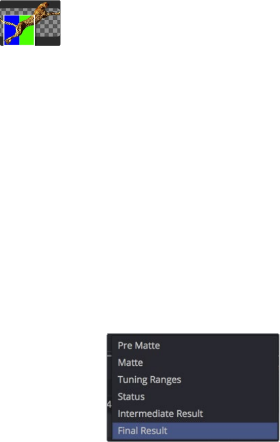
443
Matte Tools Chapter – 19
Delta Keyer
The Delta Keyer is a classic color difference keyer, with many features and controls for tuning
the matte and separating the subject from blue or green screen.
It contains several keying systems, the Key tab is the master difference keyer, Pre Matte is a pre
clean plate to smooth out screen color. Tuning, Fringe and Matte finish the key process.
How to Key
Use the Pick Button on the Background Color to select the the blue or green screen color from
the image. Hold Option (Alt) while click dragging the pick and it will pick the color from the up
stream image, making the key not flicker.
The Pre Matte is clean plate generator that smooths out the color of the screen and is instigated
by box selecting areas of the screen color, and tweaking the Erode will expand the pre matte so
it does not clip into the subject of the image.
Inputs
Delta keyer has the image input,
Garbage Matte
Clean Plate
Effect mask
Solid Matte
View Mode
At the top of the controls is View Mode, the default is to show the final result. This can be
changed to see the output of the various intermediate stages of the Key process.
Pre Matte will display the output of the Pre Matte key.
Matte will display the alpha of the key before being combined with solid and
garbage masks.
Tuning Ranges will display the Shadow Midtone and Highlight range of the image.
Shadows are in the red channel, Midtones in the green channel and Highlights in the
blue channel.
Status displays information to indicate areas that are solid, transparent or in-between. It
also displays areas that have been affected by matte adjustments such as thresholding
or erode/dilate, and areas affected by the solid mask.
Intermediate Result the original source image colour channels combined with the final
matte. This can be combined with further DeltaKeyer tools.
Final Result is the final keyed image with spill suppression, ready to merge
onto a scene.
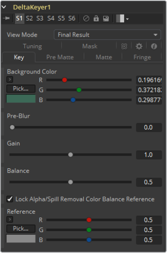
444
Matte Tools Chapter – 19
Key Tab
Background Color
This is the color of the blue or green screen, the keying color, this will be turned black
with no alpha. Use the Pick Button on the Background Color to select the the blue or
green screen color from the image. Hold Option (Alt) while click dragging the pick and it
will pick the color from the upstream image, making the key not flicker.
Pre-Blur
Applies a blur before generating the alpha. This can help with certain types of noise
and edge enhancements and artifacts in the source image.
Gain
Increases the influence of the background color. This will cause areas of background
color to become more transparent.
Balance
The key is performed by comparing the differences between the dominant channel
determined by the background color and the other two channels, with balance
determining the proportions of the other two channels. A value of 0 will use the
minimum of the other two channels, where a value of 1 will use the maximum. A value of
0.5 will use half of each.
Lock Alpha/Spill Removal Color Balance Reference
Unlocking this allows a different color references to be used when generating the
alpha, and when determining how much of the background color to subtract from
the image.
Color Balance Reference
Can be used to adjust for lighting or white balance that might be reducing background
color purity and saturation. A correction can be applied based on the reference of a
neutral colored object when generating the key alpha and determining the amount of
background color subtraction, without altering the background color that is subtracted.
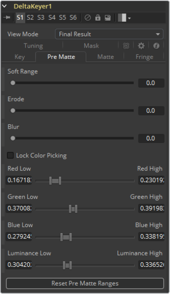
445
Matte Tools Chapter – 19
Pre Matte
Soft Range
The soft range will extend the range of selected color and roll off the screen color.
Erode
Will contract the edge of the pre matte, so the edge detail will not be clipped
Blur
This will soften the edges of the pre matte.
PreMatte Range
These range controls update automatically to represent the current color selection.
Generally, the Reveal control does not have to be opened to display these controls.
Colors are selected by selecting the Ultra Keyer tool’s tile in the flow and dragging in
the Viewer to select the colors to be used to create the matte. These range controls
can be used to tweak the selection slightly, although generally selecting colors in the
displays is all that is required.
Lock Color Picking
When this checkbox is selected, Fusion will prevent accidental growing of the selected
range by selecting more colors from the view. It is a good idea to select this checkbox
once the color selection is made for the matte. All other controls in the tool
remain editable.
Reset Pre Matte Ranges
This discards all color selection by resetting the ranges but maintains all other slider
and control values.
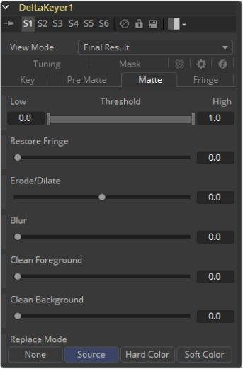
446
Matte Tools Chapter – 19
Matte Tab
Threshold
Any value below the lower threshold becomes black or transparent in the matte.
Anyvalue above the upper threshold becomes white or opaque in the matte. All values
within the range maintain their relative transparency values.
Restore Fringe
This restores the edge of the matte around the keyed subject. Often to get a key, the
edge of the subject where you have hair will get clipped out, Restore Fringe will bring
back that edge while keeping the matte solid.
Erode/Dilate
Will expand or contract the matte
Blur
Soften the matte
Clean Foreground
Will fill slightly transparent areas of the matte
Clean Background
Will clip the bottom dark range of the matte
Replace Mode
Determines how matte adjustments will cause color to be restored to the image.
None is no color replacement. Matte processing will not affect the color.
Source is the original color from the unkeyed image.
Hard Color is solid color.
Soft Color is solid color weighted by how much background color was
originally removed.
Replace Color
The color used with the Hard Color and Soft Color replace modes.
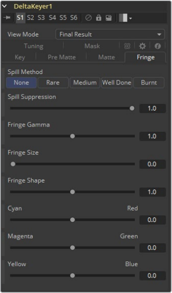
447
Matte Tools Chapter – 19
Fringe Tab
Spill Suppression
Spill is generally caused by the transmission of the color of the background through the
semi transparent areas of the alpha channel. In the case of blue or green screen keying,
this usually causes the color of the background to become apparent in the fringe of the
foreground element.
Spill suppression attempts to remove color from the fringe. The process used is
optimized for either blue or green screens; you select which color is used as the base
from the control above.
When this slider is set to 0, no spill suppression is applied to the image.
Spill Method
This selects the strength of the algorithm used to apply spill suppression to the image.
None None is selected when no spill suppression is required.
Rare This removes very little of the spill color, the lightest of all methods.
Medium This works best for green screens.
Well Done This works best for blue screens.
Burnt This works best for blue. Use this mode only for very troublesome shots.
Fringe Gamma
This control can be used to adjust the brightness of the fringe or halo that surrounds
the keyed image.
Fringe Size
This expands and contracts the size of the fringe or halo surrounding the keyed image.
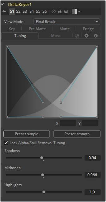
448
Matte Tools Chapter – 19
Fringe Shape
Fringe Shape forces the fringe to be pressed toward the external edge of the image or
pulled toward the inner edge of the fringe. Its effect is most noticeable while the Fringe
Size value is large.
Cyan/Red, Magenta/Green and Yellow/Blue
Use these three controls to color correct the fringe of the image.
This is useful for correcting semi-transparent pixels that still contain color from the
original background to match the new background.
Tuning Tab
Range controls
This defines how much color range is in the Dark Shadows, Midtones, and Highlight
bright areas of the image. This spline controls allow for easy adjusting of the tonal
ranges of each Shadow and Highlight tonal map.
Preset Simple will set the range to be linear. Preset Smooth sets a smooth tonal
gradient for the ranges.
Lock Alpha/Spill Removal Tuning
Unlocking this allows a different tuning to be used when generating the alpha, and
when determining how much of the background color to subtract from the image.
Shadows
Adjusts the strength of the key in darker areas of the background.
Midtones
Adjusts the strength of the key in midtone areas of the background.
Highlights
Adjusts the strength of the key in brighter areas of the background.
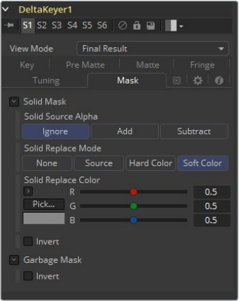
449
Matte Tools Chapter – 19
Mask Tab
Solid Mask
Solid Source Alpha
Used to combine the existing alpha from the source image into the solid mask.
Ignore does not combine the alpha from the source image.
Add solid areas of the source image alpha will be made solid in the solid mask.
Subtract transparent areas of the source image alpha will be made transparent in the
solid mask.
Solid Replace Mode
This determines how the solid mask will cause color to be restored to the image.
None is no color replacement. The solid mask will not affect the color.
Source is the original color from the unkeyed image.
Hard Color is solid color.
Soft Color is solid color weighted by how much background color was
originally removed.
Solid Replace Color
The color used with the Hard Color and Soft Color replace modes.
Invert
will invert the solid mask, before it is combined with the source alpha.
Garbage Mask
Invert
Normally solid areas of the garbage mask will clear the image. When inverted it’s the
transparent areas of the mask that will clear the image.
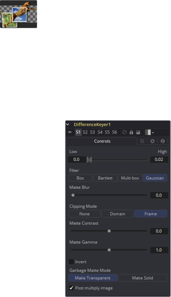
450
Matte Tools Chapter – 19
Difference Keyer [DKY]
Difference keying is a process that produces a matte based on the differences between two
images. A Difference key uses two input images, one containing the subject with the
background and another containing the background without the subject.
The Difference Keyer tool is very sensitive and, although the process sounds reasonable at first
glance, subtle variations in the position of the camera from shot to shot usually make it difficult
to pull a highly-detailed alpha channel using this method. Think of the futile attempt of trying to
key smoke in front of a brick wall and using a clean plate of the brick wall as your difference
input. Part of the wall’s structure will always be visible in this keying method. Instead, a
Difference keyer is often used to produce a rough matte that is combined with other tools to
produce a more detailed matte.
Controls Tab
Threshold High and Low
This slider works by defining a range of difference values between the images to
create a matte. A difference below the lower threshold becomes black in the matte.
Any difference above the upper threshold becomes white (solid) in the matte. The
difference values in the range in between create a gray scale matte.
Matte Blur
This blurs the edge of the matte using a standard constant speed Gaussian blur.
Avalue of zero results in a sharp, cutout-like hard edge. The higher the value, the
more blur.
451
Matte Tools Chapter – 19
Matte Contrast
The Matte Contrast slider changes the Look up Table curve of the matte’s luminance
values. This creates a soft cropping of the matte at the low end of the slider and a hard
edge expansion of the matte at higher slider values.
Matte Gamma
Matte Gamma raises or lowers the values of the matte in the semi-transparent areas.
Higher values cause the gray areas to be more opaque and lower values cause the
gray areas to be more transparent. Completely black or white regions of the matte
remain unaffected.
Invert
Selecting this checkbox inverts the matte, causing all transparent areas to be opaque
and all opaque areas to be transparent.
Garbage Matte Mode
Garbage Mattes are Mask tools or images connected to the Garbage Matte input on
the tool’s tile. The Garbage matte is applied directly to the alpha channel of the image.
Generally, Garbage mattes are used to remove unwanted elements that cannot be
keyed, such as microphones and booms. They are also used to fill in areas that contain
the color being keyed but that you wish to maintain.
Garbage mattes of different modes cannot be mixed within a single tool. A Matte
Control tool is often used after a Keyer tool to add a Garbage matte with the opposite
effect of the matte applied to the keyer.
Make Transparent
Select this button to make the Garbage matte transparent.
Make Solid
Select this button to make the Garbage matte solid.
Post Multiply Image
Select this option to cause the keyer to multiply the color channels of the image against
the alpha channel it creates for the image. This option is usually enabled and is on
by default.
Deselect this checkbox and the image can no longer be considered pre-multiplied for
purposes of merging it with other images. Use the Subtractive option of the Merge tool
instead of the Additive option.
For more information, see the Merge Tools documentation.
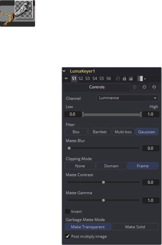
452
Matte Tools Chapter – 19
Luma Keyer [LKY]
The Luma Keyer tool uses the overall luminance of an image to create an alpha channel. When
this tool was first created it was used exclusively on the luminance channel of the image, but it
has since grown to allow pulling mattes from virtually any channel Fusion understands. In some
respects, it would now be more accurate to call this tool a Channel Keyer.
Controls Tab
Channel
Use this drop-down list to select the color channel used for creating the matte. Select
from the Red, Green, Blue, Alpha, Hue, Luminance, Saturation and Depth
(Z-buffer) channels.
Threshold High and Low
This slider works by defining a range of luminance values in the image to create a
matte. Any value below the lower threshold becomes black in the matte. Any value
above the upper threshold becomes white (solid) in the matte. All values within the
range create the gray scale matte.
Matte Blur
Matte Blur blurs the edge of the matte using a standard constant speed Gaussian blur.
A value of zero results in a sharp, cutout-like hard edge. The higher the value, the more
blur applied to the matte.
453
Matte Tools Chapter – 19
Matte Contrast
The Contrast slider changes the Look up Table curve of the matte’s luminance values.
This creates a soft cropping of the matte at the low end of the slider and a hard edge
expansion of the matte at higher slider values.
Matte Gamma
Matte Gamma raises or lowers the values of the matte in the semi-transparent areas.
Higher values cause the gray areas to be more opaque and lower values cause the
gray areas to be more transparent. Completely black or white regions of the matte
remain unaffected.
Invert
When toggled on, the matte is inverted, causing all transparent areas to be opaque and
all opaque areas to be transparent.
Garbage Matte Mode
Garbage Mattes are Mask tools or images connected to the Garbage Matte input on
the tool’s tile. The Garbage matte is applied directly to the alpha channel of the image.
Generally, Garbage mattes are used to remove unwanted elements that cannot be
keyed, such as microphones and booms. They are also used to fill in areas that contain
the color being keyed but that you wish to maintain.
Garbage mattes of different modes cannot be mixed within a single tool. A Matte
Control tool is often used after a Keyer tool to add a Garbage matte with the opposite
effect of the matte applied to the keyer.
Make Transparent
Select this button to make the Garbage matte transparent.
Make Solid
Select this button to make the Garbage matte solid.
Post Multiply Image
Select this option to cause the keyer to multiply the color channels of the image against
the alpha channel it creates for the image. This option is usually enabled and is on
by default.
Deselect this checkbox and the image can no longer be considered pre-multiplied for
purposes of merging it with other images. Use the Subtractive option of the Merge tool
instead of the Additive option.
For more information, see the Merge Tools documentation.
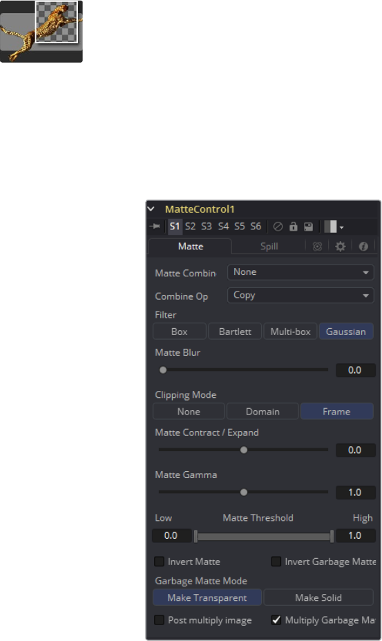
454
Matte Tools Chapter – 19
Matte Control [MAT]
Keyer tools are generally used to create an alpha channel on an image that does not already
have one. The Matte Control tool is used to manipulate an existing alpha channel or to create
one by hand via rotoscoping.
The Matte Control tool also has a Foreground Image input. Use this tool to copy a color channel
or alpha channel from the foreground to the background, or to combine alpha channels from the
two images.
Controls Tab
Matte Combine
The Matte Control tool can combine alpha or color channels from an image in the
foreground input with the background image. Use this menu to select which operation
is applied. The default is set to None for no operation.
None
This causes the foreground image to be ignored.
Combine Red
This combines the FG red channel to the BG alpha channel.
Combine Green
This combines the FG green channel to the BG alpha channel.
Combine Blue
This combines the FG blue channel with the BG alpha channel.
455
Matte Tools Chapter – 19
Combine Alpha
This combines the FG alpha channel with the BG alpha channel.
Solid
This causes the BG alpha channel to become completely opaque.
Clear
This causes the BG alpha channel to become completely transparent.
Combine Operation
Use this menu to select the method used to combine the foreground channel with the
background.
Copy
This copies the foreground source over the background alpha, overwriting any
existing alpha in the background.
Add
This adds the foreground source to the background alpha.
Subtract
This subtracts foreground source from the background alpha.
Inverse Subtract
This subtracts the background alpha from the foreground source.
Maximum
This compares the foreground source and the background alpha and takes the value
from the pixel with the highest value.
Minimum
This compares the foreground source and the background alpha and takes the value
from the pixel with the lowest value.
And
This performs a logical AND on the two values.
Or
This performs a logical OR on the values.
Merge Over
This merges the foreground source channel over the background alpha channel.
Merge Under
This merges the foreground source channel under the background alpha channel.
Filter
Selection of the Filter that is used when blurring the matte.
Box Blur: This option applies a Box Blur effect to the whole image. This method is
faster than the Gaussian blur but produces a lower quality result.
Bartlett: Bartlett applies a more subtle, anti-aliased blur filter.
Multi-box: Multi-Box uses a box filter layered in multiple passes to approximate a
Gaussian shape. With a moderate number of passes (e.g., 4), a high quality blur can
be obtained, often faster than the Gaussian filter and without any ringing.
Gaussian: Gaussian applies a smooth, symmetrical blur filter, using a sophisticated
constant-time Gaussian approximation algorithm. In extreme cases, this algorithm
may exhibit ringing; see below for a discussion of this. This mode is the default
filter method.
456
Matte Tools Chapter – 19
Matte Blur
This blurs the edge of the matte using a standard constant speed Gaussian blur. A
value of zero results in a sharp, cutout-like hard edge. The higher the value, the more
blur applied to the matte.
Matte Contract/Expand
This shrinks or grows the matte to exclude some of the keyed image or include some of
its surrounding area. Values above 0.0 expand the matte and values below 0.0
contract it.
Matte Gamma
This raises or lowers the values of the matte in the semi-transparent areas. Higher
values cause the gray areas to become more opaque and lower values cause the gray
areas to become more transparent. Completely black or white regions of the matte
remain unaffected.
Matte Threshold
Any value below the lower threshold becomes black or transparent in the matte. Any
value above the upper threshold becomes white or opaque in the matte. All values
within the range maintain their relative transparency values.
Invert Matte
When this checkbox is selected, the alpha channel of the image is inverted, causing all
transparent areas to be opaque and all opaque areas to be transparent.
Garbage Matte
Garbage Mattes are Mask tools or images connected to the Garbage Matte input on
the tools tile. The Garbage matte is applied directly to the alpha channel of the image.
Generally, Garbage mattes are used to remove unwanted elements that cannot be
keyed, such as microphones and booms. They are also used to fill in areas that contain
the color being keyed but that you wish to maintain.
Garbage mattes of different modes cannot be mixed within a single tool. A Matte
Control tool is often used after a Keyer tool to add a Garbage matte with the opposite
effect of the matte applied to the keyer.
Make Transparent
Select this button to make the Garbage matte transparent.
Make Solid
Select this button to make the Garbage matte solid.
Post Multiply Image
Select this option to cause the keyer to multiply the color channels of the image
against the alpha channel it creates for the image. This option is usually enabled and
is on by default.
Deselect this checkbox and the image can no longer be considered pre-multiplied
for purposes of merging it with other images. Use the Subtractive option of the Merge
tool instead of the Additive option.
Multiply Garbage Matte
When selected, the values of the image’s Red, Green and Blue channels will be
multiplied against the Garbage Matte input.
For more information, see the Merge Tools documentation.
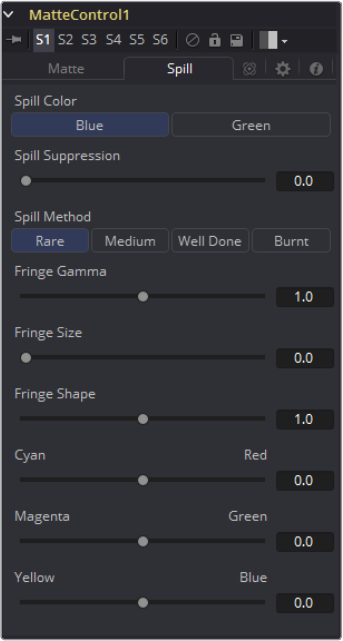
457
Matte Tools Chapter – 19
Spill Tab
Spill Color
Use these buttons to select the color used as the base for all spill suppression
techniques.
Spill Suppression
Spill is generally caused by the transmission of the color of the background through the
semitransparent areas of the alpha channel. In the case of blue or green screen keying,
this usually causes the color of the background to become apparent in the fringe of the
foreground element.
Spill suppression attempts to remove color from the fringe. The process used is
optimized for either blue or green screens; you select which color is used as the base
from the control above.
When this slider is set to 0, no spill suppression is applied to the image.
458
Matte Tools Chapter – 19
Spill Method
This selects the strength of the algorithm used to apply spill suppression to the image.
None
None is selected when no spill suppression is required.
Rare
This removes very little of the spill color, the lightest of all methods.
Medium
This works best for green screens.
Well Done
This works best for blue screens.
Burnt
This works best for blue. Use this mode only for very troublesome shots.
Fringe Gamma
This control can be used to adjust the brightness of the fringe or halo that surrounds
the keyed image.
Cyan/Red, Magenta/Green and Yellow/Blue
Use these three controls to color correct the fringe of the image. This is useful for
correcting semi-transparent pixels that still contain color from the original background
to match the new background.
Fringe Size
This expands and contracts the size of the fringe or halo surrounding the keyed image.
Fringe Shape
Fringe Shape forces the fringe to be pressed toward the external edge of the image or
pulled toward the inner edge of the fringe. Its effect is most noticeable while the Fringe
Size sliders value is large.
459
Matte Tools Chapter – 19
Primatte 5
Primatte is an advanced keying system for Fusion. It’s distributed and licensed by IMAGICA
Corp. of America, Los Angeles, CA, USA. Primatte was developed by and is a trademark of
IMAGICA Corp., Tokyo, Japan
External Inputs
Orange (required): The primary input. As opposed to other tools in Fusion, this is
actually the “Foreground” input, since it holds the image to be keyed, or in other words,
the image that is to be layered in the foreground of the composite. Connect the image
to be keyed to this input.
Green (optional): In Primatte this is the Background input. It holds the background layer
of the composite. If no image is connected, Primatte will just output the keyed element.
Connect an image here to utilize Primatte’s advanced edge blending options.
Pink (optional): The replacement image input.
White (optional): Garbage matte.
Blue (optional): Post Mask input.
NOTE: If the background input is connected, but the replacement image input is not,
then the Image Replacement mode will use the background image, and the keyed
foreground will be placed over that background. If the replacement image input is
connected, then it’ll be used for image replacement, and the keyed foreground will still
be placed over the image from the background input.
460
Matte Tools Chapter – 19
Primatte Tab
Lock Color Picking
Activate this button once you finished adjusting your key. This prevents accidentally
changing the settings by clicking into the view.
Auto Compute
This is most likely the first button you want to press when starting to key your footage.
Primatte then automagically analyzes the original foreground image and determines the
backing color and sets it as the central backing color. Then, using that information,
analyzes the original foreground image and determines the foreground areas using the
new Primatte V5 foreground detection routine. Then, internally, using the newly
determined foreground areas performs the Clean FG Noise operation and determines a
more desirable shape for the middle and outer polyhedrons. It then renders the
composite using the generated polyhedrons. This does not automatically use the
Adjust Lighting functionality, as it must be selected in a separate operation.
461
Matte Tools Chapter – 19
Select Background Color
Allows the user to select the background color, which is meant to be keyed in the view
by means of a color picker. It uses the traditional Primatte method of taking the sampled
backing screen color, projecting a line in the opposite direction on the hue wheel and
generating artificial pixels that MAY represent the FG object. Then, using the artificially
generated foreground pixels internally does the Clean FG Noise operation and creates
the shape of the middle and outer polyhedrons. It then renders the composite using the
generated polyhedrons. This does not automatically use the Adjust Lighting
functionality, as it must be selected in a separate operation.
Clean Background Noise
Helps to remove any white regions in the dark screen area (“noise”), or shades of blue
that did not get picked up on the first sample. Move the cursor through these areas
while holding the left mouse button down to sample these whitish noise regions.
Clean Foreground Noise
If there are dark regions in the middle of the mostly white foreground object, that is, if
the key is not 100% in some portion of the targeted foreground, use Clean Foreground
with the same techniques as for Clean Background Noise, but this time sample the dark
pixels in the foreground area until that area is as white as possible.
Spill Sponge
The quickest method for removing color spill on your object is the Spill Sponge to
sample the spill areas away. By positioning the cursor over a bluish pixel and selecting
it, the blue will disappear from the selected color region and be replaced by a more
natural color. Additional spill removal should be done using the tools under the Fine
Tuning tab or by using the Spill (-) feature. Both are explained further on in this manual.
Matte Sponge
Sometimes in the Primatte operation, a 100% foreground area (all white) will become
slightly transparent (gray). You can clean those transparent areas up by using the Matte
Sponge. Click on the transparent pixels and they will become 100% foreground. All of
the spill-suppression information will remain intact.
Restore Detail
With this mode selected, the completely transparent background region sampled in the
image window becomes translucent. This operation is useful for restoring lost hair
details, thin wisps of smoke and the like. It shrinks the small polyhedron slightly.
Make Foreground Transparent
When this mode is selected, the opaque foreground color region sampled in the image
window becomes slightly translucent. This operation is useful for the subtle tuning of
foreground objects that are otherwise 100 percent covered with smoke or clouds. It can
only be used one time on a particular color. For a more flexible way to thin out a color
region and be able to make multiple samples, you should use the Matte (-) tool. It
expands the medium polyhedron slightly.
Spill(+)
Color spill will be returned to the sampled pixel color (and all colors like it) in the amount
of one Primatte increment. This tool can be used to move the sampled color more in
the direction of the color in the original foreground image. It can be used to nullify a
Spill (-) step. This tool dents the Primatte large polyhedron in the color region sampled.
Spill(-)
Color spill will be removed from the sampled pixel color (and all colors like it) in the
amount of one Primatte increment. If spill color remains, another click using this
operational mode tool will remove more of the color spill. Continue using this tool until
all color spill has been removed from the sampled color region. This tool expands the
Primatte large polyhedron in the color region sampled.
462
Matte Tools Chapter – 19
Matte(+)
The matte will be made more opaque for the sampled pixel color (and all colors like it)
in the amount of one Primatte increment. If the matte is still too translucent or thin,
another click using this operational mode tool will make the sampled color region even
more opaque. This can be used to thicken smoke or make a shadow darker to match
shadows in the background imagery. It can only make these adjustments to the density
of the color region on the original foreground image. It can be used to nullify a Matte (-)
step. This tool dents the Primatte medium polyhedron in the color region sampled.
Matte(-)
The matte will be made more translucent for the sampled pixel color (and all colors like
it) in the amount of one Primatte increment. If the matte is still too opaque, another click
using this operational mode tool will make the sampled color region even more
translucent. This can be used to thin out smoke or make a shadow thinner to match
shadows in the background imagery. This tool expands the Primatte medium
polyhedron in the color region sampled.
Detail(+)
The foreground detail will become less visible for the sampled pixel color (and all colors
like it) in the amount of one Primatte increment. If there is still too much detail, another
click using this operational mode tool will make more of it disappear. This can be used
to remove smoke or wisps of hair from the composite. Sample where is visible and it will
disappear. This is for moving color regions into the 100% background region. It can be
used to nullify a Detail (-) step. This tool expands the Primatte small polyhedron in the
color region sampled.
Detail(-)
When this operational mode is selected, foreground detail will become more visible for
the sampled pixel color (and all colors like it) in the amount of one Primatte increment. If
detail is still missing, another click using this operational mode tool will make detail
more visible. This can be used to restore lost smoke or wisps of hair. Sample where the
smoke or hair just disappears and it will return to visibility. This is for restoring color
regions that were moved into the 100% background region. It may start to bring in
background noise if shooting conditions were not ideal on the foreground image. This
tool dents the Primatte small polyhedron in the color region sampled.
Algorithms
Primatte: The Primatte algorithm mode delivers the best results and supports
both the Solid Color and the Complement Color spill suppression methods. It is the
algorithm that uses three multi-faceted polyhedrons (as described later in the this
document) to separate the 3D RGB colorspace. It is also the default algorithm mode
and, because it is computationally intensive, it may take the longest to render.
Primatte RT: Primatte RT is the simplest algorithm and therefore, the fastest. It uses
only a single planar surface to separate the 3D RGB colorspace (as described later
in the this document) and, as a result, does not have the ability to separate out the
foreground from the backing screen as carefully as the above Primatte algorithm.
Other disadvantages of the Primatte RT algorithm are that it does not work well with
less saturated backing screen colors and it does not support the Complement Color
spill suppression method.
Primatte RT+: Primatte RT+ is in between the above two options. It uses a six planar
surface color separation algorithm (as described later in the this document) and will
deliver results in between the other two in both quality and performance. Other
disadvantages of the Primatte RT+ algorithm are that it does not work well with less
saturated backing screen colors and it does not support the Complement Color spill
suppression method.
463
Matte Tools Chapter – 19
Hybrid Rendering
After sampling the backing screen color and finding that the edges of the foreground
object look very good, you sometimes find that an area of the foreground object is
transparent. This is due to the foreground containing a color that is close to the backing
screen color. When this transparency is removed using the Clean FG Noise operational
mode, the edge of the foreground object picks up a fringe that is close to the backing
screen color and it is very hard to remove without sacrificing quality somewhere else
on the image. The Hybrid Render mode internally creates two keying operations: Body
and Edge. The Edge operation is optimized around getting the best edge around the
foreground object without any fringe effect. The Body operation is used to deal with
the transparency within the foreground object. The resultant matte is created by
combining these two mattes, Body and Edge, by blurring and then eroding the
foreground object in the Body operation and then combining it with the matte created
in the Edge operation.
The user first keys the main foreground area using the smart Select BG Color mode (or
any of the other Primatte backing screen detection methods), until a good result is
obtained with good edges around the foreground object. Then the user selects the
Hybrid Render button and chooses the Clean FG Noise operational mode. When the
transparent area is then sampled, the Primatte V5 Hybrid Render mode will internally
perform the ‘Body/Edge’ operation. This results in a final composite with good edges
around the foreground object while still preserving the area within the foreground
object that was transparent.
Hybrid Blur
Blurs the Body matte that has been automatically generated.
Hybrid Erode
This slider allows the user to adjust the amount of Erosion applied to the Hybrid
Matte. The results can be viewed if the Hybrid Matte button has been activated.
Adjust Lighting
Prior to applying the Adjust Lighting operation, it is necessary to determine the backing
screen color using one of the methods described above.
Upon performing one of those operations, the user then clicks on the Adjust Lighting
button. Primatte will internally generate an artificial backing screen without the
foreground object and use it to generate the pre-processed image that has an evenly lit
backing screen behind the foreground object.
The default setting should detect all the areas of the Adjust Lighting grid that contain
foreground pixels and deliver a smooth ‘artificially created’ optimized backing screen
for the keying. Should it fail to do this, the user can adjust the settings of the algorithm
by selecting the Adjust Lighting mode and then moving the Lighting S-Poly slider. The
user can then see the result of the lighting adjustment by selecting Cntl 2 tab and
clicking on the Auto Backing Screen button. This displays the optimized artificial
backing screen that the Adjust Lighting mode creates. By again using one of the
operations that sample the backing screen color (listed above), the new results will be
visible. This operation can be repeated until a smooth, evenly lit optimized artificial
backing screen is created.
Crop
This button reveals the Crop sliders to create a rectangular Garbage matte with the
Primatte node. As opposed to Fusion’s Crop tool, this will not change the actual
image size.
Reset
Resets all of the Primatte key control data back to a blue or green screen.
Soft Reset
Resets just the Primatte features used since the Select Background Color operation
was last completed.
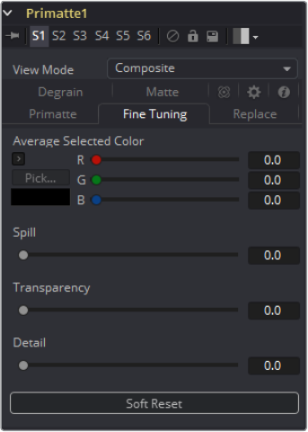
464
Matte Tools Chapter – 19
Fine Tuning Tab
Pick
This shows the color selected (or registered) by the Fine Tuning operational mode.
Fine Tuning Sliders
When this operational mode is selected, the color of the sampled pixel within the image
window is registered as a reference color for fine tuning. It is displayed in the Color
Chip below the Detail slider. To perform the tuning operation, sample a color region on
the image, select a Fine Tuning slider and move the slider to achieve the desired effect.
See the Fine Tuning Sliders tool descriptions further on in this chapter for more details
on slider selection.
Spill
This Spill slider can be used to remove spill from the registered color region. The more
to the right the slider moves, the more spill will be removed. The more to the left the
slider moves, the closer the color component of the selected region will be to the color
in the original foreground image. If moving the slider all the way to the right does not
remove all the spill, re-sample the color region and again move the slider to the right.
These slider operations are additive. This result achieved by moving the slider to the
right can also be achieved by clicking on the color region using the Spill (-) operational
mode. This slider bulges the Primatte large polyhedron near the registered
color region.
Transparency
The Transparency slider can be used to make the matte more translucent in the
registered color region. Moving this slider to the right makes the registered color region
more transparent. Moving the slider to the left makes the matte more opaque. If moving
the slider all the way to the right does not make the color region translucent enough,
re-sample the color region and again move the slider to the right. These slider
operations are additive. This result achieved by moving the slider to the right can also
be achieved by clicking on the color region using the Matte (-) operational mode. This
slider bulges the Primatte medium polyhedron near the registered color region.
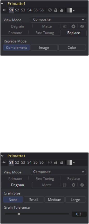
465
Matte Tools Chapter – 19
Detail
The Detail slider can be used to restore lost detail. After choosing the Fine Tuning
operational mode and selecting a color region, moving this slider to the left makes the
registered color region more visible. Moving the slider to the left makes the color
region less visible. If moving the slider all the way to the left does not make the color
region visible enough, re-sample the color region and again move the slider to the left.
These slider operations are additive. This result achieved by moving the slider to the
left can also be achieved by clicking on the color region using the Detail(-) operational
mode. This shrinks the small polyhedron, which contains all the blue or green
background colors, and releases pixels that were close to the background color. The
Small Polyhedron Slider in the Fine Tuning mode is useful for restoring pixels that were
lost because they were so similar to the background color. This slider dents the
Primatte small polyhedron near the registered color region.
Replace Tab
Allows the user to choose between the three methods of color spill replacement as covered in
detail in Spill Replacement Options above.
Complemental
Replaces the spill color with the complement of the backing screen color.
Image
Replaces the spill color with colors from a defocused version of the background image.
Color
Replaces the spill color with a ‘user selected’ solid color.
Degrain Tab
The Grain Tools are used when a foreground image is highly compromised by film grain. As a
result of the grain, when backing screen noise is completely removed, the edges of the
foreground object often become harsh and jagged, leading to a poor key.
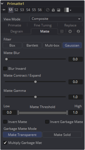
466
Matte Tools Chapter – 19
Grain Size
The Grain Size selector provides a range of grain removal from Small to Large. If the
foreground image has a large amount of film grain-induced pixel noise, you may lose a
good edge to the foreground object when trying to clean all the grain noise with the
Clean Background Noise Operation Mode. These tools allow the user to clean up the
grain noise without affecting the quality of the key.
None
No degraining will be performed.
Small
The average color of a small region of the area around the sampled pixel. This should
be used when the grain is very dense.
Medium
The average color of a medium-sized region of the area around the sampled pixel. This
should be used when the grain is less dense.
Large
The average color of a larger region of the area around the sampled pixel. This should
be used when the grain is very loose.
Grain Tolerance
Adjusting this slider increases the effect of the Clean Background Noise tool without
changing the edge of the foreground object.
Matte Tab
These controls behave the same as in the other Fusion Keyer tools. Please have a look at the
Matte Control.
467
Matte Tools Chapter – 19
Basic Operation Tutorial
Auto Compute Tools
Select Background Color
There are four main steps to using the Primatte; Select Background Color is the first
step. Ensure that the Select Background Color button is selected (it should be at this
time as it is the default Operational Mode when you start Primatte).
Position the cursor in the blue screen area (or whatever background color you
are using), usually somewhere near the foreground object. Sample the targeted
background color. Release the mouse button and Primatte will start the compositing
process. If the foreground shot was done under ideal shooting conditions, Primatte
will have done 90-95% of the keying in this one step.
Primatte will work equally well with any color backing screen. It does not have to be a
specific shade of green or blue.
If you dragged the cursor in the blue area, Primatte averages the multi-pixel sample
to get a single color to which to adjust. Sometimes Primatte works best when only a
single pixel is sampled instead of a range of pixels. The color selected at this point in
the Primatte operation is critical to the operation of the spark from this point forward.
Should you have difficulties further along in the tutorial after selecting a range of blue
shades, try the Select Background Color operation again with a single dark blue pixel
or single light blue pixel. You can also switch to the Alpha Channel view and click
around in the blue screen area to see the different results you get when the initial
sample is made in different areas. Make sure the View Mode buttons at the top of the
Primatte interface has the Black Mode selected.
If you would rather make a ‘rectangular or box selection’ and not use the ‘snail trail or
line’ sampling method, you can switch between the two methods by clicking on either
the Line or Box buttons in the top left-hand corner of the image window. The third
method, Median, is the same as Line selection, except that each point sampled is the
result of taking a 3x3 region around the point the user clicked and then applying a
median filter. This can potentially reduce any noisy pixels.
NOTE: This version of Primatte has a new feature that may eliminate the first three
steps of using Primatte. It is called the Auto Compute button and may make your
keying operation much easier. Click on this button as a first step and it may
automatically sense the backing screen color, eliminate it, and even get rid of some of
the foreground and background noise that would normally be cleaned up in Steps 2
(Clean Background Noise) and 3 (Clean Foreground Noise) of the Primatte operation. If
you get good results, then jump ahead to the Spill Removal tools.
If you don’t get the results you wanted from Auto Compute, continue from this point on
to get the basic Primatte operation procedures. The basic functionality for the Primatte
interface is centered on the Operational Mode Selector buttons and the
image window
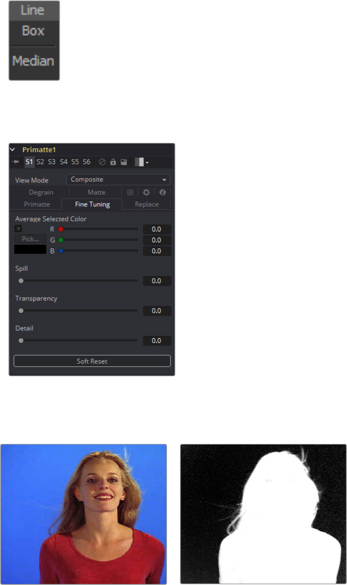
468
Matte Tools Chapter – 19
If the foreground image has a shadow in it that you want to keep in the composite, do
not select any of the dark blue pixels in the shadow and the shadow will come along
with the rest of the foreground image.
The second and third steps in using Primatte require viewing the Matte View in
the monitor window. Make sure the View Mode buttons at the top of the Primatte
interface has the Black Mode selected.
Click on the Alpha Channel/RGB button located below the Viewer. The image
displayed will change to a black and white ‘matte’ view of the image that looks
like this:
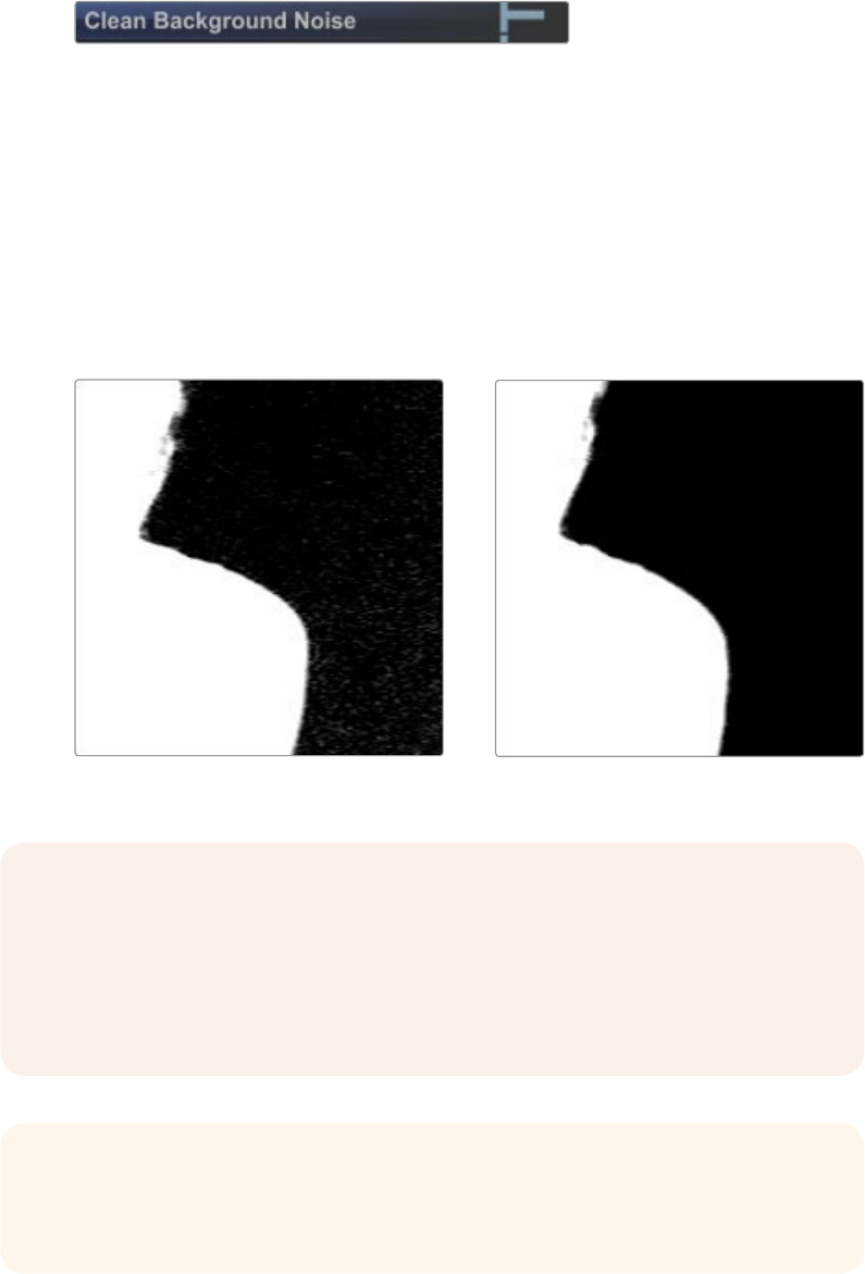
469
Matte Tools Chapter – 19
Clean Background Noise
Change the Operational Mode Selector from Select Background Color to Clean
Background Noise. If there are any white regions in the dark, `blue screen area,’ this is
referred to as ‘noise.‘ Technically, it is some shades of blue that did not get picked up
on the first sample and should be removed. Move the cursor through these areas if
using the Line Sampling method (or make a box around them if using the Box Sampling
method), and sample these whitish noise regions. When you let up on the mouse
button, Primatte will process the data and eliminate the noise. Repeat this procedure as
often as necessary to clear the noise from the background areas. Sometimes
increasing the brightness of your monitor or the screen gamma allows you to see noise
that would otherwise be invisible.
Before Background noise removal After Background noise removal
NOTE: You do not need to remove every single white pixel to get good results. Most
pixels displayed as a dark color close to black in a key image will become transparent
and virtually allow the background to be the final output in that area. Consequently,
there is no need to eliminate all noise in the blue screen portions of the image. In
particular, if an attempt is made to meticulously remove noise around the foreground
object, a smooth composite image is often difficult to generate.
TIP When clearing noise from around loose, flying hair or any background/foreground
transitional area, be careful not to select any of areas near the edge of the hair. Leave
a little noise around the hair as this can be cleaned up later using the Fine Tuning tool.
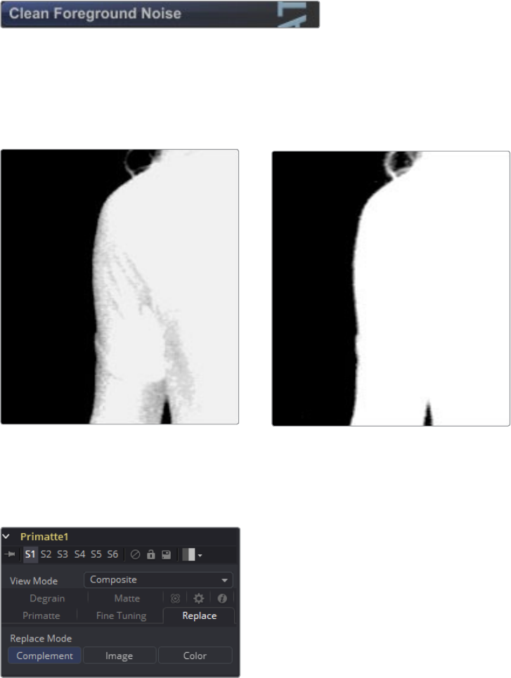
470
Matte Tools Chapter – 19
Clean Foreground Noise
If there are dark regions in the middle of the mostly white foreground object, that is, if
the key is not 100% in some portion of the targeted foreground, choose Clean
Foreground Noise from the Operational Mode Selector pop-up menus. Use the same
techniques as for Clean Background Noise, but this time sample the dark pixels in the
foreground area until that area is as white as possible.
Before Foreground noise removal After Foreground noise removal
Removing Spill Setup
These were the steps necessary to create a clean ‘matte’ or ‘key’ view of the image.
With this key, the foreground can be composited onto any background image.
However, if there is `spill’ on the foreground object from light that was reflected off the
background, a final operation is necessary to remove that background spill to get a
more natural looking composite.
For the fourth step in the Primatte operation, return the Composite view to the monitor
window by clicking again on the Alpha/RGB toggle button. Now change the View mode
to Composite. This will turn off the Alpha Channel viewing mode and the monitor
window will again display the Composite view with the background image. The sample
image below has gone through the first three steps and has examples of spill. Notice
the blue fringe to her hair and a blue tint on her right cheek, arm and chest.
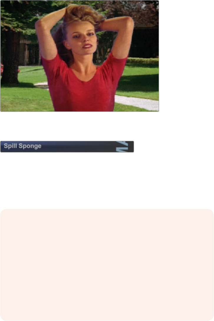
471
Matte Tools Chapter – 19
Spill Removal – Method #1
There are three ways in Primatte to remove the spill color. The quickest method is to
select the Spill Sponge button from the Operational Mode area and then sample the
spill areas away. By just positioning the cursor over a bluish pixel and selecting it, the
blue will disappear from the selected color region and be replaced by a more natural
color. Additional spill removal should be done using the tools under the Fine Tuning tab
or by using the Spill (-) feature. Both are explained further on in this manual.
If the spilled color was not been totally removed using the Spill Sponge, or if the result
of the Spill Sponge resulted in artifacts or false coloring, a fine-tuning operation Spill (-)
tool should be used instead for a more subtle and sophisticated removal of the spilled
background color.
NOTE: All spill removal/replacement operations in Primatte can be modified
using the Background Spill Replacement tools under the Replace tab. Spill can
be replaced with either the complement of the background color, a solid color
selected by the user or by colors brought from a defocused copy of the
background. Depending on the spill conditions, one of these options should
provide the results you are looking for. See the information in Section 5, Spill
Replacement Options for more details.
Primatte’s Spill Removal tools work on ‘color regions.’ In the image above,
samples should be made on the light flesh tones, the dark flesh tones, the
light blonde hair, the dark blonde hair and the red blouse color regions. One
sample in each color region will remove spill from all similar colors in the
foreground image.
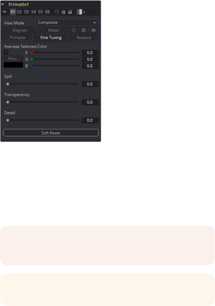
472
Matte Tools Chapter – 19
Spill Removal – Method #2
Select the Fine Tuning tab in the Primatte interface.
Using the zoom and pan capabilities of the Fusion application, zoom into an area that
has some blue edges or spill.
Using the cursor, sample a color has spill in it. When you let up on the mouse button,
Primatte will register the color selected (or an average of multiple pixels) in the Pick...
Color Chip. For most images, the Spill slider is all that is required to remove any
remaining bluespill. The more to the right the slider moves, the more background
screen color will be removed from the sampled pixels. The more to the left the slider
moves, the more the selected pixels will move toward the color in the original
foreground image.
NOTE: When using the slider in the Fine Tuning tab to remove spill, spill color
replacement will be replaced based on the setting of the Spill
Replacement options.
TIP: It is better to make several small adjustments to the bluespill areas than a
single major one.
473
Matte Tools Chapter – 19
You can use the other two sliders in the same way for different key adjustments. The
Detail slider controls the matte softness for the color that is closest to the background
color. For example, you can recover lost rarefied smoke in the foreground by selecting
the Fine Tuning mode, clicking on the area of the image where the smoke just starts to
disappear and moving the Detail slider to the left. The Transparency slider controls the
matte softness for the color that is closest to the foreground color. For example, if you
have thick and opaque smoke in the foreground, you can make it semi-transparent by
moving the Transparency slider to the right after selecting the pixels in the Fine
Tuning mode.
Spill Removal – Method #3
This method uses a fairly recent Primatte tool that is covered in detail in the next
section: Repeatable Sampling Tools.
Repeatable Sampling Tools
Most of the Primatte operations are done using a ‘mouse sampling’ operation. The only
exceptions are the Fine Tuning operational mode and its sliders. The Fine Tuning operation
gives a continuous valuator for fine-tuning, but some of the sliders are not often used because
results are often unpredictable or not subtle enough. Note: Another weak point in previous
versions of Primatte is the lack of functionality to attenuate and thicken the existing matte
density. This version of Primatte offers a more intuitive, easy-to-use and powerful user interface
called Repeatable Sampling.
TIP: If the foreground image changed color dramatically during the fine-tuning
process, you can recover the original color by selecting an area of the off-color
foreground image and moving the Spill slider slightly to the left. This may introduce
blue spill back into that color region. Again, use the Fine Tuning option to suppress the
blue, but make smaller adjustments this time.
NOTE: If these final ‘spill suppression’ operations have changed the final compositing
results, you may have to return to earlier operations to clean up the matte. If the
Composite view looks good, it is a good idea to go back and take a final look at the
Alpha Channel view. Sometimes in the Primatte operation, a 100% foreground area (all
white) will become slightly transparent (gray). You can clean those transparent areas up
by using the Matte Sponge tool. After selecting the Matte Sponge tool, just click on the
transparent pixels and they will become 100% foreground. All of the spill-suppression
information will remain intact. Alternatively, you can go to the Alpha Channel view and
then using the Fine Tuning option, select those transparent areas and move the
Transparency slider slightly to the left. This will move that color region from 0-99%
foreground with spill suppression to 100% foreground with spill suppression and should
solve the problem. The Matte (+) tool will also work to solve this problem.
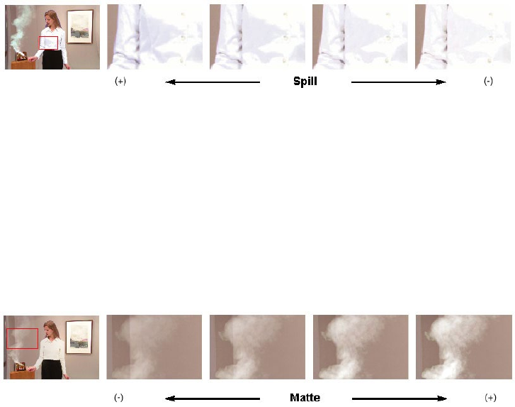
474
Matte Tools Chapter – 19
In addition to the conventional Primatte operation modes previously mentioned, six other tools
are added:
Spill (+)
Spill (-)
Matte (+)
Matte (-)
Detail(+)
Detail(-)
The Spill Sampling Tools
Using the Spill (+) and Spill (-) modes, you can gradually remove or recover the spill
intensity on the foreground object by sampling the referenced color region repeatedly.
The conventional Spill Sponge tool removed the spill component in a single action at
one level and did not allow sampling the same pixel a second time. Even though just a
small amount of spill needed to be removed, the Spill Sponge removed a preset
amount without allowing any finer adjustment.
Effect of Spill (+/-) Repeatable Sampling
Using the zoom and pan capabilities of the Fusion application, zoom into an area that
has some blue edges and click on a pixel with some spill on it. Repeated clicking will
incrementally remove the spill. Continue this operation until the desired result
is achieved.
The Matte Sampling Tools
The Matte (+) and Matte (-) modes are used to thicken or attenuate the matte
information. If you want a thinner shadow on a foreground object, you can use the
Matte (-) mode as many times as you like to make it more transparent. On the other
hand, you can use the Matte (+) mode to make the matte thicker in that color region.
Effect of Matte (+/-) Repeatable Sampling
The Detail Sampling Tools
The Detail (+) and Detail (-) modes are a refined version of Clean Background Noise and
Restore Detail. For example, when you see some dilute noise in the backing area but
don’t want to remove it completely because it affects some fine detail in a different
area, try using Detail (-). It will attenuate the noise gradually as multiple samples are
made on the pixel. You should stop the sampling when important fine details start to
disappear.
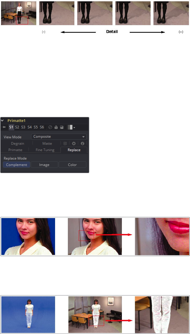
475
Matte Tools Chapter – 19
Effect of Detail (+/-) Repeatable Sampling
Spill Replacement Options
The proper processing of spill on foreground objects is one of the many useful features of
Primatte. You can move between these three modes to see how they affect the image clip you
are working with. The three methods are as follows:
Complemental Spill Replacement (Complement)
Defocus Spill Replacement (Image)
Solid Color Spill Replacement (Color)
Complemental Replacement Mode
This is the default Spill Replacement mode. This mode will maintain fine foreground
detail and deliver the best quality results. If foreground spill is not a major problem, this
mode is the one that should be used.
Complemental Replacement Mode maintains fine detail.
The Complemental Replacement mode is sensitive to foreground spill. If the spill
intensity on the foreground image is rather significant, this mode may often introduce
serious noise in the resultant composite.
Solid Color Replacement Mode
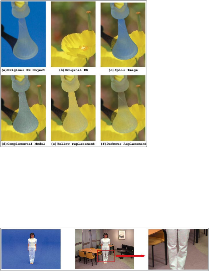
476
Matte Tools Chapter – 19
Defocus Replacement Mode
The Defocus Replacement mode uses a defocused copy of the background image to
determine the spill replacement colors instead of a solid palette color or just the
complement color. This mode can result in good color tone on the foreground object
even with a high contrast background. As in the example below, spill can even be
removed from frosted glass using this feature and still retain the translucency. On the
negative side, the Defocus Replacement mode sometimes results in the fine edge
detail of the foreground objects getting lost. Another problem could occur if the user
wanted to later change the size of the foreground image against the background.
Sincethe background/foreground alignment would change, the applied color tone from
the defocused image might not match the new alignment.
Blue Suppression of a Frosted Glass Object
Solid Color Replacement Mode
In the Solid Color Replacement mode, the spill component will be replaced by a ‘user
defined’ palette color. While the Complemental Replacement mode uses only the
backing color complement to remove small amounts of spill in the original foreground,
the Solid Color Replacement mode tries to assuage the noise using the ‘user defined’
palette color. Changing the palette color for the solid replacement, the user can apply
good spill replacement that matches the composite background. Its strength is that it
works fine with even serious blue spill conditions.
Smooth Spill Processing with Solid Color Replacement
On the negative side, when using the Solid Color Replacement mode, fine detail on the
foreground edge tends to be lost. The single palette color sometimes cannot make a
good color tone if the background image has some high contrast color areas.
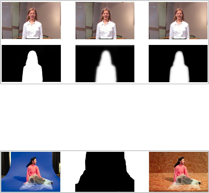
477
Matte Tools Chapter – 19
Matte Blur Inward Feature
A new method of defocusing or blurring the matte has been added. This new feature
can be set to only blur inward toward the center of the foreground subject. The
conventional Primatte defocus feature affected the matte edges in both directions
(inward and outward) and sometimes introduced a halo artifact around the object edge
in the composite view. This was most evident when using the Complemental
Replacement mode. With the Blur Inward switch On, the matte defocus functions only in
the inward direction of the foreground subject (toward the center of the white area). The
final result is that it removes small and dark noise in the backing area without picking
them up again in the Clean Background Noise mode and sometimes results in softer,
cleaner edges on the foreground objects. Background Noise mode and sometimes
results in softer, cleaner edges on the foreground objects.
Normal Conventional Defocus Inward Defocus
External Garbage Matte Input
Primatte accepts a hand-drawn matte as the external matte to hide the unnecessary
garbage like light arms, microphones and other undesirable foreground object. Areas
that are white in the Garbage Matte clip will take the pixels from the background and
areas that are black will be from the composite image. This External Garbage Matte can
also be inverted.

478
Matte Tools Chapter – 19
Ultra Keyer [UKY]
The Ultra Keyer tool has 2 keyers built in to it, a Prematte keyer acts as garbage matte creator
and the color difference keyer that will extract fine detail and transparency.This optimized to
extract mattes from images using blue screen or green screen backgrounds.
How to Key
Use the Pick Button on the Background Color to select the the blue or green screen color from
the image. Hold Option (Alt) while click dragging the pick and it will pick the color from the up
stream image, making the key not flicker.
The Pre Matte garbage keyer is instigated by box selecting areas of the screen color, and
tweaking the Pre Matte Size will expand the garbage matte so it does not clip into the subject of
the image.
Pre Matte Tab
Background Color
This is used to select the color of the blue or green screen of the images. It is good
practice to select the screen color close to the subject to be separated from the screen
background.
Red Level, Green Level, Blue Level
These tune the level of the difference channels, to help separate the color. When the
background color is green, Red and Blue level options are provided. When the
background color is blue, Red and Green level options are provided.
Background Correction
Depending on the background color selected above, the keyer will iteratively merge
the pre-keyed image over either a blue or green background before processing
it further.
In certain cases this leads to better, more subtle edges.
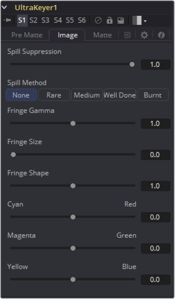
479
Matte Tools Chapter – 19
Matte Separation
Matte Separation performs a pre-process on the image to help separate the foreground
from the background before color selection. Generally, increase this control while
viewing the alpha to eliminate the bulk of the background, but stop just before it starts
cutting holes in the subject or eroding fine detail on the edges of the matte.
PreMatte Range
These range controls update automatically to represent the current color selection.
Generally, the Reveal control does not have to be opened to display these controls.
Colors are selected by selecting the Ultra Keyer tool’s tile in the flow and dragging in
the Viewer to select the colors to be used to create the matte. These range controls
can be used to tweak the selection slightly, although generally selecting colors in the
displays is all that is required.
Lock Color Picking
When this checkbox is selected, Fusion will prevent accidental growing of the
selected range by selecting more colors from the view. It is a good idea to select this
checkbox once the color selection is made for the matte. All other controls in the tool
remain editable.
Pre Matte Size
The Pre Matte Size control can be used to soften the general area around the keyed
image. This is used to close holes in the matte often caused by spill in semi-transparent
areas of the subject. This generally will also cause a small halo around the subject,
which can be removed using the Matte Contract tools found later in the tool.
Reset Pre Matte Ranges
This discards all color selection by resetting the ranges but maintains all other slider
and control values.
Image Tab
480
Matte Tools Chapter – 19
Spill Suppression
Spill is generally caused by the transmission of the color of the background through the
semitransparent areas of the alpha channel. In the case of blue or green screen keying,
this usually causes the color of the background to become apparent in the fringe of the
foreground element.
Spill suppression attempts to remove color from the fringe. The process used is
optimized for either blue or green screens; you select which color is used as the base
from the control above.
When this slider is set to 0, no spill suppression is applied to the image.
Spill Method
This selects the strength of the algorithm used to apply spill suppression to the image.
None
None is selected when no spill suppression is required.
Rare
This removes very little of the spill color, the lightest of all methods.
Medium
This works best for green screens.
Well Done
This works best for blue screens.
Burnt
This works best for blue. Use this mode only for very troublesome shots.
Fringe Gamma
This control can be used to adjust the brightness of the fringe or halo that surrounds
the keyed image.
Fringe Size
This expands and contracts the size of the fringe or halo surrounding the keyed image.
Fringe Shape
Fringe Shape forces the fringe to be pressed toward the external edge of the image or
pulled toward the inner edge of the fringe. Its effect is most noticeable while the Fringe
Size sliders value is large.
Cyan/Red, Magenta/Green and Yellow/Blue
Use these three controls to color correct the fringe of the image. This is useful for
correcting semi-transparent pixels that still contain color from the original background
to match the new background.
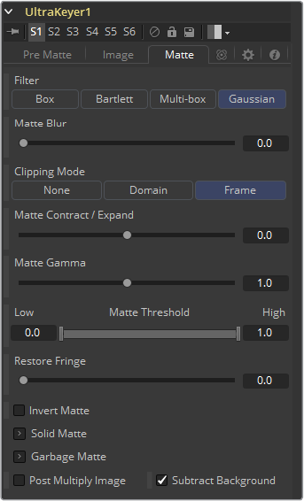
481
Matte Tools Chapter – 19
Matte Tab
Matte Blur
Matte Blur blurs the edge of the matte using a standard constant speed Gaussian blur.
A value of zero results in a sharp, cutout-like hard edge. The higher the value, the more
blur applied to the matte.
Matte Contract/Expand
This slider shrinks or grows the semi-transparent areas of the matte. Values above 0.0
expand the matte while values below 0.0 contract it.
This control is usually used in conjunction with the Matte Blur to take the hard edge of a
matte and reduce fringing. Since this control only affects semi-transparent areas, it will
have no effect on a hard edge’s matte.
Matte Gamma
Matte Gamma raises or lowers the values of the matte in the semi-transparent areas.
Higher values cause the gray areas to become more opaque and lower values cause
the gray areas to become more transparent. Completely black or white regions of the
matte remain unaffected.
Since this control only affects semi-transparent areas, it will have no effect on a hard
edge’s matte.
Matte Threshold
Any value below the lower threshold becomes black or transparent in the matte. Any
value above the upper threshold becomes white or opaque in the matte. All values
within the range maintain their relative transparency values.
This control is often used to reject salt and pepper noise in the matte.
482
Matte Tools Chapter – 19
Restore Fringe
This restores the edge of the matte around the keyed subject. Often to get a key, the
edge of the subject where you have hair will get clipped out, Restore Fringe will bring
back that edge while keeping the matte solid.
Invert Matte
When this checkbox is selected, the alpha channel created by the keyer is inverted,
causing all transparent areas to be opaque and all opaque areas to be transparent.
Make Solid
Select this button to make the Garbage matte solid.
Make Transparent
Select this button to make the Garbage matte transparent.
Garbage Matte
Garbage Mattes are Mask tools or images connected to the Garbage Matte input on
the tool’s tile. The Garbage matte is applied directly to the alpha channel of the image.
Generally, Garbage mattes are used to remove unwanted elements that cannot be
keyed, such as microphones and booms. They are also used to fill in areas that contain
the color being keyed but that you wish to maintain.
Garbage mattes of different modes cannot be mixed within a single tool. A Matte
Control tool is often used after a Keyer tool to add a Garbage matte with the opposite
effect of the matte applied to the keyer.
Post Multiply Image
Select this option to cause the keyer to multiply the color channels of the image against
the alpha channel it creates for the image. This option is usually enabled and is on
by default.
Deselect this checkbox and the image can no longer be considered pre-multiplied for
purposes of merging it with other images. Use the Subtractive option of the Merge tool
instead of the Additive option.
For more information, see the Merge Tools documentation.
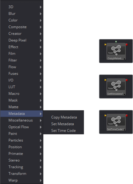
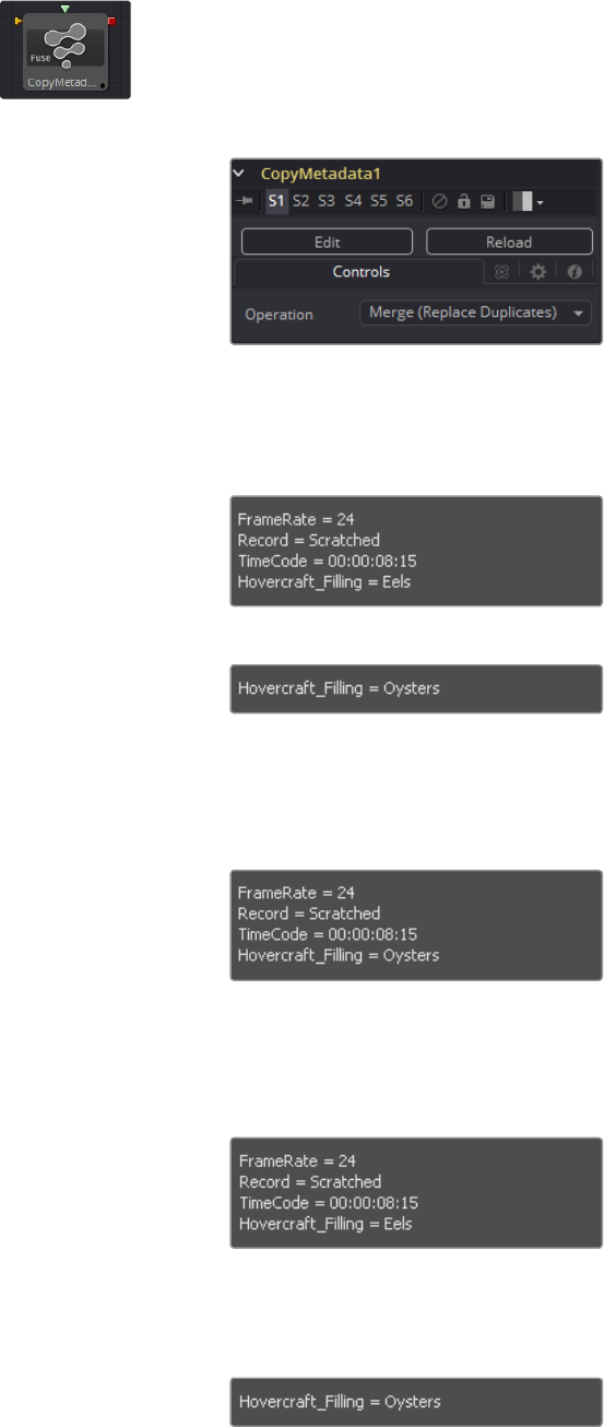
486
Metadata Tools Chapter – 20
Copy Metadata [META]
Copy Metadata combines, replaces or clears the metadata in your image.
Controls Tab
Operation
The dropdown defines how the metadata of foreground and background input
are treated.
Imagine having metadata in the background image looking like this:
and the foreground’s metadata looking like this:
Merge (Replace Duplicates)
All values will be merged, but values with duplicate names will be taken from the
foreground input.
The output looks like this:
Merge (Preserve Duplicates)
All values will be merged, but values with duplicate names will be taken from the
background input.
The output looks like this:
Replace
The entire metadata in the background will be replaced by the ones in the foreground.
The output looks like this:
Clear
All metadata will be discarded.

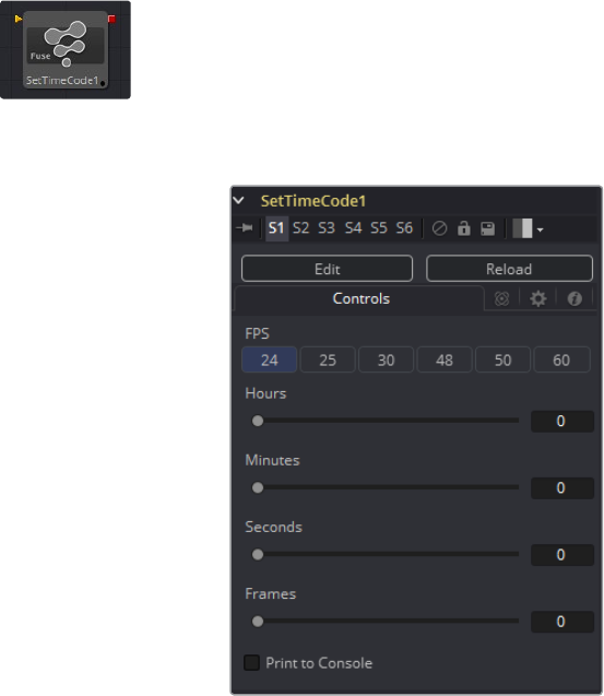
488
Metadata Tools Chapter – 20
Set Timecode [TCMETA]
Set Timecode inserts dynamic timecode values into the metadata table based on the
FPS settings.
Controls Tab
FPS
You can choose from a variety of Frame Per Second settings here. Since this is a
Fuseyou can easily adapt the settings to your needs by editing the appropriate piece
of code for the buttons:
MBTNC_StretchToFit = true,
{ MBTNC_AddButton = “24“ },
{ MBTNC_AddButton = “25“ },
{ MBTNC_AddButton = “30“ },
{ MBTNC_AddButton = “48“ },
{ MBTNC_AddButton = “50“ },
{ MBTNC_AddButton = “60“ },
})
as well as for the actual values:
local rates = { 24, 25, 30, 48, 50, 60 }
Hours/Minutes/Seconds/Frames sliders
Define an offset from the starting frame of the current comp.
Print to Console
Verbose output of the Timecode/Frame value in the Console.
The Timecode/Frames conversion is done according to the FPS settings.
The result can look like this:
Ti m eCode: 00:00:08:15
Fra m es: 207
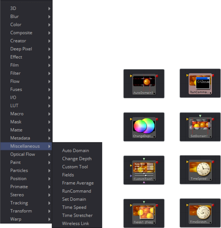
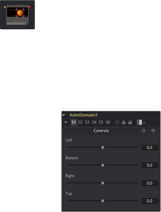
492
Miscellaneous Tools Chapter – 21
Auto Domain [ADOD]
The Auto Domain tool automatically sets the image’s domain of definition based on bounds of
the input image’s background Canvas color. It does not change the image’s physical
dimensions. This tool can be used to speed up compositions by optimizing the DoD of images
based on their content rather than their dimensions.
For example, a CG character rarely takes up the entire frame of an image. The Auto Domain tool
would set the DoD to a rectangular region encompassing the portion of the scene actually
containing the character. The DoD is updated on each frame to accommodate changes, such as
a character walking closer to the camera.
See the Set Canvas Color tool for more information about the Canvas color.
Controls Tab
Left
Defines the left border of the search area of the ADoD. Higher values on this slider
move the left border toward the right, excluding more data from the left margin.
1 represents the right border of the image, 0 represents the left border. The slider
defaults to 0 (Left Border).
Bottom
Defines the bottom border of the search area of the ADoD. Higher values on this slider
move the bottom border toward the top, excluding more data from the bottom margin.
1 represents the Top border of the image, 0 represents the bottom border. The slider
defaults to 0 (Bottom Border).
Right
Defines the right border of the search area of the ADoD. Higher values on this slider
move the right border toward the left, excluding more data from the right margin.
1 represents the right border of the image, 0 represents the left border. The slider
defaults to 1 (Right Border).
Top
Defines the top border of the search area of the ADoD. Higher values on this slider
move the top border toward the bottom, excluding more data from the top margin.
1 represents the top border of the image, 0 represents the bottom border. The slider
defaults to 1 (Top Border).
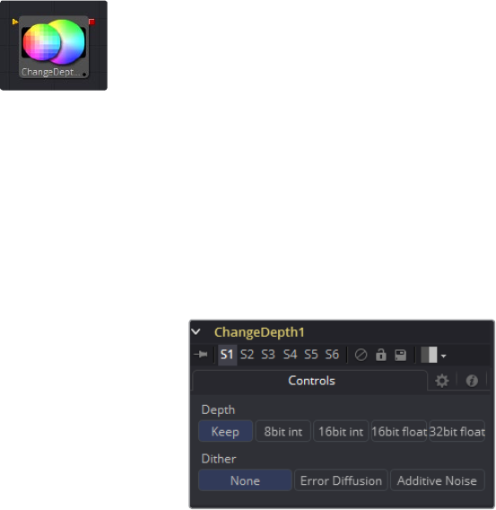
493
Miscellaneous Tools Chapter – 21
Change Depth [CD]
The Change Depth tool has one simple use, to change the bits per color channel used to
process a tool. The single control for this tool is Depth, which contains five buttons. Select Keep
to leave the color depth as is, or either 8-bit, 16-bit or Float to change to the selected
color depth.
This tool is often used after color correcting Cineon files, converting from Float processing to
16-bit per channel to preserve memory and performance.
It can also be useful if, from a certain point in your flow, you feel the need to process your
images in a higher bit depth than their original one or to reduce the bit depth to save memory.
Controls Tab
Depth
Keep doesn‘t do anything to the image but rather keeps the input depth. The other
options change the bit depth of the image to the respective value.
Dither
When down converting from higher bit depth it might be useful to add Error Diffusion or
Additive Noise to camouflage artifacts that result from problematic (high contrast) areas.
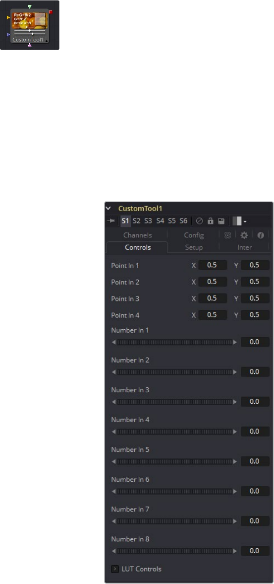
494
Miscellaneous Tools Chapter – 21
Custom [CU]
The Custom tool is quite likely the most complex, and the most powerful, tool in Fusion. Any
user moderately experienced with scripting, or C++ programming, should find the structure and
terminology used by the Custom tool to be familiar.
The Custom tool is used to create custom expressions and filters to modify an image. In
addition to providing three image inputs, the Custom tool will allow for the connection of up to
eight numeric inputs and as many as four XY position values from other controls and
parameters in the flow.
Per-pixel calculations can be performed on the Red, Green, Blue, Alpha, Z, Z Coverage, UV
texture coords, XYZ Normals, RGBA background color and XY motion vector channels of
the images.
Custom Controls Tab
Point in 1-4, X and Y
These four controls are 2D X and Y center controls that are available to expressions
entered in the Setup, Intermediate and Channels tabs as variables p1x, p1y, ...., p4x, p4y.
They are normal positional controls and can be animated or connected to modifiers as
any other tool might.
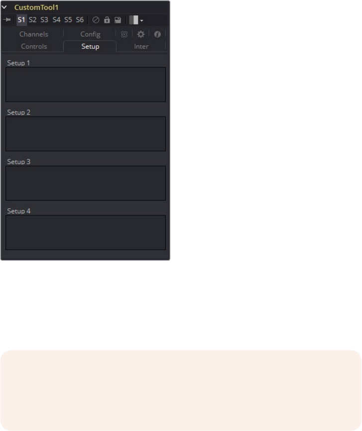
495
Miscellaneous Tools Chapter – 21
Number in 1-8
The values of these controls are available to expressions entered in the Setup,
Intermediate and Channels tabs as variables n1, n2, n3, ..., n8. They are normal slider
controls, and can be animated or connected to modifiers exactly as any other
tool might.
LUT in 1-4
The Custom tool provides 4 LUT splines. The values of these controls are available to
expressions entered in the Setup, Intermediate and Channels tabs using the getlut#
function. For example, setting the R, G, B and A expressions to getlut1(r1), getlut2(g1),
getlut3(b1), and getlut4(a1) respectively would cause the Custom tool to mimic the Color
Curves tool.
These controls can be renamed using the options in the Config tab to make their
meanings more apparent, but expressions will still see the values as n1, n2, ..., n8.
Custom Setup Tab
Setup 1-4
Up to four separate expressions can be calculated in the Setup tab of the Custom tool.
The Setup expressions are evaluated once per frame, before any other calculations are
performed. The results are then made available to the other expressions in the Custom
tool as variables s1, s2, s3 and s4.
NOTE: Because these expressions are evaluated once per frame only and not
for each pixel, it makes no sense to use per-pixel variables like X and Y or
channel variables like r1,g1,b1, etc. Allowable values include constants,
variables like n1..n8, time, W and H, etc., and functions like sin() or getr1d().
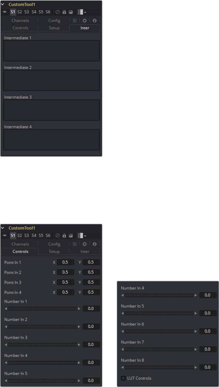
496
Miscellaneous Tools Chapter – 21
Custom Inter Tab
Intermediate 1-4
An additional four expressions can be calculated in the Inter tab. The Inter expressions
are evaluated once per pixel, after the Setup expressions are evaluated but before the
Channel expressions are evaluated. Per-pixel channel variables like r1,g1,b1 and a1 are
allowable. Results are available as variables i1, i2, i3 and i4.
Custom Config Tab
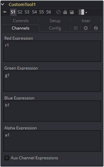
497
Miscellaneous Tools Chapter – 21
Random Seed
Use this to set the seed for the rand() and rands() functions. Click the Randomize button
to set the seed to a random value. This control may be needed if multiple Custom tools
are required with different random results for each.
Number Controls
There are eight sets of Number controls, corresponding to the eight Number In sliders
in the Controls tab. Untick the Show Number checkbox to hide the corresponding
Number In slider, or edit the Name for Number text field to change its name.
Point Controls
There are four sets of Point controls, corresponding to the four Point In controls in the
Controls tab. Untick the Show Point checkbox to hide the corresponding Point In
control and its crosshair in the Viewer. Similarly, edit the Name for Point text field to
change the control’s name.
Channels Tab
RGBA, Z, UV Expressions and XYZ Normal Expressions
The Channel tab is used to set up one expression per each available channel of the
image. Each expression is evaluated once per pixel, and the result is used to create the
value for that pixel in the output of the image.
Color Channel expressions (RGBA) should generally return floating-point values
between 0.0 and 1.0. Values beyond this will be clipped if the destination image is an
integer. Other expression fields should produce values appropriate to their channel
(e.g., between -1.0 and 1.0 for Vector and Normal fields, 0.0 to 1.0 for Coverage, or any
value for Depth). The Channel expressions may use the results from both the Setup
expressions (as variables s1-s4) and Inter expressions (as variables i1-i4).
498
Miscellaneous Tools Chapter – 21
Custom Tool Syntax
Value Variables
n1..n8 Numeric Inputs
p1x..p4x Position Values (X-axis)
p1y..p4y Position Values (Y-axis)
s1..s4 Setup Expression Results
i1..i4 Inter Expression Results
time Current Frame
x Horizontal co-ordinate of the current pixel, between 0.0 and 1.0
y Vertical co-ordinate of the current pixel, between 0.0 and 1.0
w (or w1..w3) Width of Image (for image1..image3)
h (or h1..h3) Height of Image (for image1..image3)
ax (or ax1..ax3) Image Aspect X (for image1..image3)
ay (or ay1..ay3) Image Aspect Y (for image1..image3)
Channel (Pixel) Variables
c1..c3 Current Channel (for image1..image3)
r1..r3 Red (for image1..image3)
g1..g3 Green (for image1..image3)
b1..b3 Blue (for image1..image3)
a1..a3 Alpha (for image1..image3)
z1..z3 Z-Buffer (for image1..image3)
cv1..cv3 Z Coverage (for image1..image3)
u1..u3 U Coordinate (for image1..image3)
v1..v3 V Coordinate (for image1..image3)
nx1..nx3 X Normal (for image1..image3)
ny1..ny3 Y Normal (for image1..image3)
NOTE: Use w and h and ax and ay without a following number to get the
dimensions and aspect of the primary image.
499
Miscellaneous Tools Chapter – 21
nz1..nz3 Z Normal (for image1..image3)
bgr1..bgr3 Background Red (for image1..image3)
bgg1..bgg3 Background Green (for image1..image3)
bgb1..bgb3 Background Blue (for image1..image3)
bga1..bga3 Background Alpha (for image1..image3)
vx1..vx3 X Vector (for image1..image3)
vy1..vy3 Y Vector (for image1..image3)
To refer to the red value of the current pixel in input 1, type r1. For the image in input 2, it
would be r2.
get[ch][#]b(x, y) Read pixel at x,y, or 0 if out of bounds, e.g., getr1b(0,0)
get[ch][#]d(x, y) Read pixel at x,y or edge pixel if out of bounds, e.g., getr1d(0,0)
get[ch][#]w(x, y) Read pixel at x,y or wrap if out of bounds, e.g., getr1w(0,0)
In the above description, [ch] is a letter representing the channel to access, and [#] is a
number representing the input image. So to get the red component of the current pixel
(equivalent to ‘r‘), you would use getr1b(x,y). To get the alpha component of the pixel at
the center of image 2 you would use geta2b(0.5, 0.5).
getr1b(x,y) Output the red value of the pixel at position x, y, if there were a valid pixel
present. It would output 0.0, if the position were beyond the boundaries of the image
(all channels).
getr1d(x,y) Output the red value of the pixel at position x, y. If the position specified
were outside of the boundaries of the image, the result would be from the outer edge
of the image (RGBA only).
getr1w(x,y) Output the red value of the pixel at position x, y. If the position specified
were outside of the boundaries of the image, the x and y coordinates would wrap
around to the other side of the image and continue from there (RGBA only).
To access other channel values with these functions, substitute the r in the above
examples with the correct channel variable (r, g, b, a and, for the getr1b() functions
only, z, etc...), as shown above. Substitute the 1 with either 2 or 3 in the above
examples to access the images from the other image inputs.
NOTE: Use c1, c2, c3 to refer to the value of a pixel in the current channel. This
makes copy/pasting expressions easier. For example, if c1/2 is typed as the
red expression, the result would be half the value of the red pixel from image
1, but if the expression is copied to the blue channel, now it would have the
value of the pixel from the blue channel.
NOTE: There are a variety of methods used to refer to pixels from other
locations than the current one in an image.
500
Miscellaneous Tools Chapter – 21
Mathematical Expressions
pi The value of pi
e The value of e
log(x) The base-10 log of x
ln(x) The natural (base-e) log of x
sin(x) The sine of x (x is degrees)
cos(x) The cosine of x (x is degrees)
tan(x) The tangent of x (x is degrees)
asin(x) The arcsine of x, in degrees
acos(x) The arccosine of x, in degrees
atan(x) The arctangent of x, in degrees
atan2(x,y) The arctangent of x,y, in degrees
abs(x) The absolute (positive) value of x
int(x) The integer (whole) value of x
frac(x) The fractional value of x
sqrt(x) The Square Root of x
rand(x,y) A random value between x and y
rands(x,y,s) A random value between x and y, based on seed s
min(x,y) The minimum (lowest) of x and y
max(x,y) The maximum (highest) of x and y
dist(x1,y1,x2,y2) The distance between point x1,y2 and x2,y2
dist3d(x1,y1,z1,x2,y2,z2) The distance between 3D points x1,y2,z1 and x2,y2,z2
noise(x) A smoothly varying Perlin noise value based on x
noise2(x, y) A smoothly varying Perlin noise value based on x and y
noise3(x, y, z) A smoothly varying Perlin noise value based on x, y and z
if(c, x, y) returns x if c not 0, otherwise y
501
Miscellaneous Tools Chapter – 21
Mathematical Operators
!x 1.0 if x = 0, otherwise 0.0
-x (0.0 - x)
+x (0.0 + x) i.e. effectively does nothing
x ^ y x raised to the power of y
x * y x multiplied by y
x / y x divided by y
x % y x modulo y, i.e. remainder of (x divided by y)
x + y x plus y
x - y x minus y
x < y 1.0 if x is less than y, otherwise 0.0
x > y 1.0 if x is greater than y, otherwise 0.0
x <= y 1.0 if x is less than or equal to y, otherwise 0.0
x >= y 1.0 if x is greater than or equal to y, otherwise 0.0
x = y 1.0 if x is exactly equal to y, otherwise 0.0
x == y 1.0 if x is exactly equal to y, otherwise 0.0, identical to above
x <> y 1.0 if x is not equal to y, otherwise 0.0
x != y 1.0 if x is not equal to y, otherwise 0.0, i.e. identical to above
x & y 1.0 if both x and y are not 0.0, otherwise 0.0
x && y 1.0 if both x and y are not 0.0, otherwise 0.0, i.e. identical to above
x|y 1.0 if either x or y (or both) are not 0.0, otherwise 0.0
x||y 1.0 if either x or y (or both) are not 0.0, otherwise 0.0
Example
The following examples are intended to help you understand the various components of the
Custom tool.
Rotation
To rotate an image, we need the standard equations for 2D rotation:
x’ = x * cos(theta) - y * sin(theta)
y’ = x * sin(theta) + y * cos(theta)
Using the n1 slider for the angle theta, and a sample function, we get (for the
red channel):
getr1b(x * cos(n1) - y * sin(n1), x * sin(n1) + y * cos(n1))
502
Miscellaneous Tools Chapter – 21
This will calculate the current pixel’s (x,y) position rotated around the origin at (0,0) (the
bottom-left corner), and then fetch the red component from the source pixel at this
rotated position. For centered rotation, we need to subtract 0.5 from our x and y
coordinates before we rotate them, and add 0.5 back to them afterwards:
getr1b((x-.5) * cos(n1) - (y-.5) * sin(n1) + .5, (x-.5) * sin(n1) + (y-.5) *
cos(n1) + .5)
Which brings us to the next lesson: Setup and Intermediate Expressions. These are
useful for speeding things up by minimizing the work that gets done in the channel
expressions. The Setup expressions are executed only once, and their results don‘t
change for any pixel, so you can use these for s1 and s2 respectively
c o s(n 1)
si n(n1)
Intermediate expressions are executed once for each pixel, so you can use these for
i1 and i2:
(x-.5) * s1 - (y-.5) * s2 + .5
(x-.5) * s2 + (y-.5) * s1 + .5
These are the x and y parameters for the getr1b() function, from above, but with the
Setup results, s1 and s2, substituted so that the trig functions are executed only once
per frame, not every pixel. Now you can use these intermediate results in your channel
expressions:
get r1b(i1, i 2)
getg1b(i1, i 2)
getb1b(i1, i2)
geta1 b(i1, i2)
With the Intermediate expressions substituted in, we only have to do all the adds,
subtracts and multiplies once per pixel, instead of four times per pixel. As a rule of
thumb, if it doesn‘t change, do it only once.
This is a simple rotation that doesn‘t take into account image aspect at all. It is left as an
exercise to the reader to include this (sorry). Another improvement could be to allow
rotation around different points than the center.
Filtering
Our second example duplicates the functionality of a 3x3 Custom Filter tool set to
averages the current pixel together with the eight pixels surrounding it. To duplicate it
with a Custom tool, add a Custom tool to the flow, and enter the following expressions
into the Setup tab.
(Leave the tool disconnected to prevent it from updating until we are ready.)
S1
1.0/w1
S2
1.0/h1
These two expressions will be evaluated at the beginning of each frame. S1 divides 1.0
by the current width of the frame, and S2 divides 1.0 by the height. This provides a
floating-point value between 0.0 and 1.0 that represents the distance from the current
pixel to the next pixel along each axis.
503
Miscellaneous Tools Chapter – 21
Now enter the following expression into the first text control of the Channel tab (r).
(getr1w(x-s1, y-s2) + getr1w(x, y-s2) + getr1w(x+s1, y-s2) +
getr1w(x+s1, y) + getr1w(x-s1, y) + r1 +
getr1w(x-s1, y+s2) + getr1w(x, y+s2) + getr1w(x+s1, y+s2)) / 9
This expression adds the nine pixels above the current pixel together by calling the
getr1w() function nine times and providing it with values relative to the current position.
Note that we referred to the pixels by using x+s1, y+s2, rather than using x+1, y+1.
Fusion refers to pixels as floating-point values between 0.0 and 1.0, which is why we
created the expressions we used in the Setup tab. If we had used x+1, y+1 instead, the
expression would have sampled the exact same pixel over and over again. (The
function we used wraps the pixel position around the image if the offset values are out
of range.)
That took care of the red channel; now use the following expressions for the green,
blue and alpha channels.
(getg1w(x-s1, y-s2) + getg1w(x, y-s2) + getg1w(x+s1, y-s2) +
getg1w(x+s1, y) + getg1w(x-s1, y) + g1 +
getg1w(x-s1, y+s2) + getg1w(x, y+s2) + getg1w(x+s1, y+s2)) / 9
(getb1w(x-s1, y-s2) + getb1w(x, y-s2) + getb1w(x+s1, y-s2) +
getb1w(x+s1, y) + getb1w(x-s1, y) + b1 +
getb1w(x-s1, y+s2) + getb1w(x, y+s2) + getb1w(x+s1, y+s2)) / 9
(geta1w(x-s1, y-s2) + geta1w(x, y-s2) + geta1w(x+s1, y-s2) +
geta1w(x+s1, y) + geta1w(x-s1, y) + a1 + geta1w(x-s1, y+s2) +
geta1w(x, y+s2) + geta1w(x+s1, y+s2)) / 9
It is time to view the results. Add a Background tool set to solid color and change the
color to a pure red. Add a hard-edged Rectangular Effects mask and connect it to the
expression just created.
For comparison, add a Custom Filter tool and duplicate the settings from the image
above. Connect a pipe to this tool from the background to the tool and view the results.
Alternate between viewing the Custom tool and the Custom Filter while zoomed in
close to the top corners of the Effects mask.
Of course, the Custom Filter tool renders a lot faster than the Custom tool we created,
but the flexibility of the Custom tool is its primary advantage. For example, you could
use an image connected to input 2 to control the median applied to input one by
changing all instances of getr1w, getg1w, and getb1w in the expression to getr2w,
getg2w, and getb2w, but leaving the r1, g1, and b1s as they are.
This is just one example; the possibilities of the Custom tool are limitless.
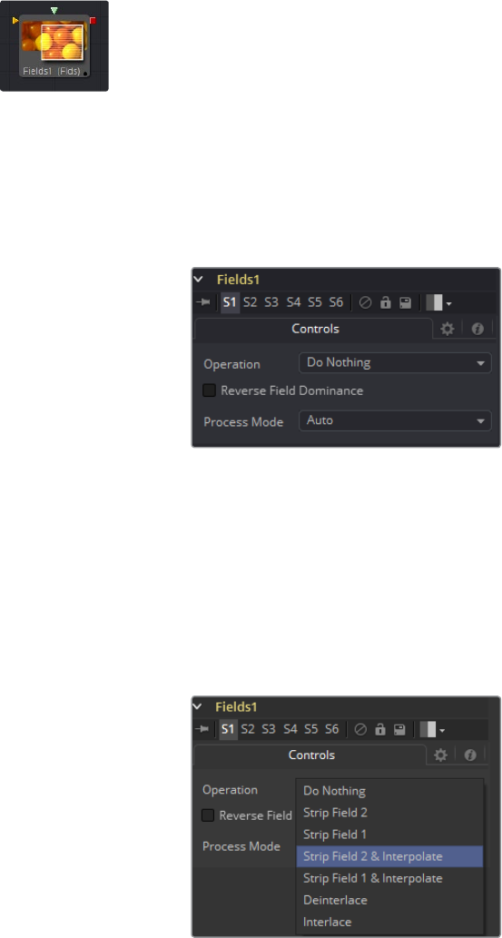
504
Miscellaneous Tools Chapter – 21
Fields [FLD]
The Fields tool is a robust multi-purpose utility offering several functions related to interlaced
video frames. It interpolates separate video fields into video frames, or separates video frames
into individual fields. It can be used to assist in the standards conversion of PAL to NTSC and
provides the ability to process fields and frames for specific portions of a flow.
For more information about how Fusion handles fields processing, consult the Frame Formats
chapter in this manual.
Controls Tab
Operation
This control is used to select the type of operation the tool will perform. See below for
a detailed explanation.
Process Mode
This control is used to select the field’s format used for the output image. See below for
a detailed explanation.
Operation
Do Nothing
This causes the images to be affected by the Process Mode selection exclusively.
Strip Field 2
This removes field 2 from the input image stream, which shortens the image to half of
the original height.
Strip Field 1
This removes field 1 from the input image stream, which shortens the image to half of
the original height.
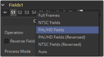
505
Miscellaneous Tools Chapter – 21
Strip Field 2 and Interpolate
This removes field 2 from the input image stream and inserts a field interpolated from
field 1 so that image height is maintained. Should be supplied with frames, not fields.
Strip Field 1 and Interpolate
This removes field 1 from the input image stream and inserts a field interpolated from
field 2 so that image height is maintained. Should be supplied with frames, not fields.
Interlace
This combines fields from the input image stream(s). If supplied with one image stream,
each pair of frames will be combined to form half of the amount of double height
frames. If supplied with two image streams, single frames from each stream will be
combined to form double height images.
De-Interlace
This separates fields from one input image stream. This will produce double the amount
of half height frames.
Reverse Field Dominance
When selected, the Field Order or Dominance of the image will be swapped.
Process
Full Frames
This forces Frame Processing. Useful for processing frames in a part of a flow that is
otherwise field processing.
NTSC Fields
This forces NTSC Field Processing. Useful for processing fields in a part of a flow that is
otherwise frame processing.
PAL Fields
This forces PAL Field Processing. Useful for processing fields in a part of a flow that is
otherwise frame processing.
PAL Fields (Reversed)
This forces PAL swapped Field Processing.
NTSC Fields (Reversed)
This forces NTSC swapped Field Processing.
Auto
This attempts to match the mode of its input images. Fields is used if the input types
are mixed.
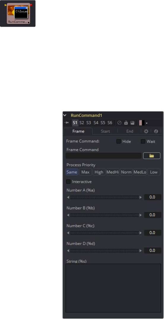
506
Miscellaneous Tools Chapter – 21
Run Command [RUN]
The RunCommand tool is used to execute an external command or batch file at certain points
during a render. Choose to run a command once at the start, or at the end of a render, or have
the command execute once for each frame.
An image input is not required for this tool to operate. However, if RunCommand is connected
to a tool‘s output, the command will only be launched after that tool has finished rendering. This
is often useful when connected to a Saver, to ensure that the output frame has been fully saved
to disk first. If the application launched returns a non-0 result, the tool will also fail.
RunCommand can be used to net render other command line applications using the Fusion
render manager, as well as a host of other useful functions.
Controls Tab
507
Miscellaneous Tools Chapter – 21
Frame Command
The first file browser in the tool is used to specify the path and parameters for the
command to be run after each frame is rendered. Select the Hide checkbox to prevent
the application or script from displaying a window when it is executed.
Hide
Select this checkbox to suppress the display of any window or dialog started by
the command.
Wait
Enable this checkbox to cause the tool to Wait for the remote application or tool to exit
before continuing. If this checkbox is cleared, the system will continue rendering
without waiting for the external application.
Number A (%B) And Number B (%B)
Various wildcards can be used with the frame commands; these wildcards will be
substituted at render time with the correct values.
%a: Outputs the number from the Number A thumbwheel control
%b: Outputs the number from the Number B thumbwheel control
%t: Outputs the current frame number (without zero padding)
%s: Substituted with the text from the large text entry field
If you want to add zero padding to the numbers generated by %t, refer to the wildcard
with %0x where x is the number of characters with which to pad the value. This also
works for %a and %b.
For example, test%04t.tga would return the following values at render time:
test0000.tga
test0001.tga
test0009.tga
tes t0010.tga
You may also pad a value with spaces by calling the wildcard as %x, where x is the
number of spaces with which you would like to pad the value.
Process Priority
The Process Priority buttons provide options for selecting the priority at which the
launched process runs. This determines how much processor time the launched
process receives compared to other applications.
Interactive
This checkbox determines whether the launched application should run interactively,
allowing user input.
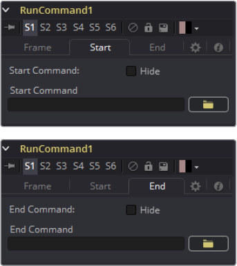
508
Miscellaneous Tools Chapter – 21
RunCommand Start and End Tabs
The Start and End tabs contain a file browser for a command to be run when the composition
starts to render and when the composition is done rendering.
Example
To copy the saved files from a render to another directory as each frame is rendered, save the
following text in a file called copyfile.bat to your C\ directory (the root folder).
@echo off
set parm=%1 %2
copy %1 %2
set parm=
Create or load any flow that contains a Saver. The following example assumes a Saver is set to
output D\ test0000.tga, test0001.tga, etc. You may have to modify the example to match.
Add a RunCommand tool after the Saver, to ensure the Saver has finished saving first. Now
enter the following text into the RunCommand tool’s Frame Command text box:
C\copytest.bat D\test%04f.tga C\
Select the Hide Frame command checkbox to prevent the command prompt window from
appearing briefly after every frame.
When this flow is rendered, each file will be immediately copied to the C\ directory as it
is rendered.
The RunCommand tool could be used to FTP the files to a remote drive or Abekas device on
the network, to print out each frame as it is rendered, or to execute a custom image-
processing tool.
The RunCommand tool is not restricted to executing simple batch files. FusionScript, VBScript,
Jscript, CGI, and Perl files could also be used, as just a few examples.
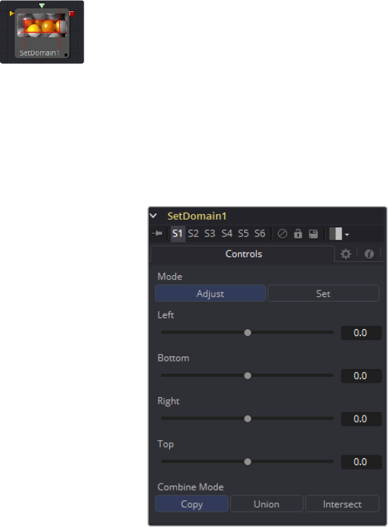
509
Miscellaneous Tools Chapter – 21
Set Domain [DOD]
Set Domain is used to adjust or set the active area of an image, or in other words the area of the
image considered to have valid data.
It does not change the image‘s physical dimensions. Anything outside the DoD will not be
processed by downstream tools, thus speeding up rendering of computational intensive tools.
This tool provides an absolute mode, for setting the Domain of Definition manually, and a
relative mode for adjusting the existing Domain of Definition.
Controls Tab/Set Mode
Left
Defines the left border of the DoD. Higher values on this slider move the left border
toward the right, excluding more data from the left margin.
1 represents the right border of the image, 0 represents the left border. The slider
defaults to 0 (Left Border).
Bottom
Defines the bottom border of the DoD. Higher values on this slider move the bottom
border toward the top, excluding more data from the bottom margin.
1 represents the Top border of the image, 0 represents the bottom border. The slider
defaults to 0 (Bottom Border).
Right
Defines the right border of the DoD. Higher values on this slider move the right border
toward the left, excluding more data from the right margin.
1 represents the right border of the image, 0 represents the left border. The slider
defaults to 1 (Right Border).
Top
Defines the top border of the DoD. Higher values on this slider move the top border
toward the bottom, excluding more data from the top margin.
1 represents the top border of the image, 0 represents the bottom border. The slider
defaults to 1 (Top Border).
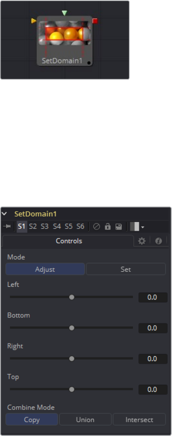
510
Miscellaneous Tools Chapter – 21
External Inputs
SetDomain.Input: [orange, required] This input must be connected to the output of a
tool that produces a 2D image.
SetDomain.Foreground: [green, optional] This input expects a 2D image as its
input. When the foreground input is connected, the Set Domain tool will replace the
Background input’s Domain of Definition with the foreground’s DoD.
Set Mode defaults to the full extent of the visible image.
Controls Tab/Adjust Mode
In Adjust mode, basically the same operations can be carried out like in Set Mode. All Sliders
default to 0, though, marking their respective full extent of the image. Positive values shrink the
DoD while negative values expand the DoD to include more data.
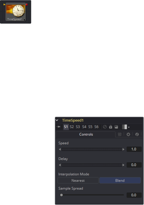
511
Miscellaneous Tools Chapter – 21
Time Speed [TSP]
Time Speed allows image sequences to be sped up, slowed down, reversed or delayed. Image
Interpolation offers smooth, high quality results. Time Speed should be used for static speed
changes or to introduce delays in the footage. To apply animated changes in time, such as
accelerating or decelerating time, use a Time Stretcher instead.
When operating in Flow mode, Optical Flow data is required.
This tool does not generate optical flow directly. You have to create it manually upstream using
an OpticalFlow tool or by loading the forward/reverse vector channels from disk.
TimeSpeed does not interpolate the aux channels, but rather destroys them. In particular, the
Vector/BackVector channels are consumed and destroyed after computation.
Add an OpticalFlow after the FlowSpeed if you want to generate flow vectors for the
retimed footage.
Controls
Speed
This control is used to adjust the Speed, in percentage values, of the outgoing image
sequence. Negative values reverse the image sequence. 200% Speed is represented
by a value of 2.0, 100% is 1.0, 50% is 0.5 and 10% is 0.1.
The Speed control cannot be animated.
Delay
Use this control to Delay the outgoing image sequence by the specified number of
frames. Negative numbers will offset time back and positive numbers will advance.
Interpolate Between Frames
When checked, frames before and after the current frame will be interpolated to create
new frames. This usually offers smoother and cleaner results. When cleared, no
interpolation will take place.
Sample Spread
This slider controls the strength of the interpolated frames on the current frame. A value
of 0.5 causes 50% of the frame before and 50% of the frame ahead of the current frame
to be blended with 0% of the current frame.
512
Miscellaneous Tools Chapter – 21
Depth Ordering
The Depth Ordering is used to determine which parts of the image should be rendered
on top. This is best explained by example.
In a locked off camera shot where a car is moving through the frame, the background
does not move, so it will produce small or slow vectors. The car will produce larger or
faster vectors.
The Depth Ordering in this case is Fastest Ontop, since the car will draw over the
background.
In a shot where the camera pans to follow the car, the background will have faster
vectors, and the car will have slower vectors, so the Depth ordering method would be
Slowest Ontop.
Clamp Edges
Under certain circumstances, this option can remove the transparent gaps that may
appear on the edges of interpolated frames. Clamp Edges will cause a stretching
artifact near the edges of the frame that is especially visible with objects moving
through it or when the camera is moving.
Because of these artifacts, it is a good idea to only use clamp edges to correct small
gaps around the edges of an interpolated frame.
Softness
Helps to reduce the stretchy artifacts that might be introduced by Clamp Edges.
If you have more than one of the Source Frame and Warp Direction checkboxes turned
on, this can lead to doubling up of the stretching effect near the edges. In this case,
you‘ll want to keep the softness rather small at around 0.01. If you only have one
checkbox enabled, you can use a larger softness at around 0.03)
Source Frame and Warp Direction
This control set allows for the choosing of which frames and which vectors are used to
create the inbetween frames. Each method ticked on will be blended into the result.
Prev Forward: Will take the previous frame and use the Forward vector to interpolate
the new frame.
Next Forward: Will take the next frame in the sequence and use the Forward vector
to interpolate the new frame.
Prev Backward: Will take the previous frame and use the Back Forward vector to
interpolate the new frame.
Next Backward: Will take the next frame in the sequence and use the Back vector to
interpolate the new frame.
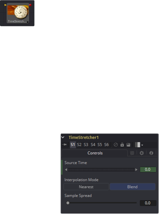
513
Miscellaneous Tools Chapter – 21
Time Stretcher [TST]
The Time Stretcher tool is similar to the Time Speed tool, but it permits the speed of the clip to
be animated over the course of the effect. Full spline control of the effect is provided, including
smoothing. As a result, the Time Stretcher can be used to animate a single clip to 200, back to
normal speed, pause for a second, and then play backward (like a VCR rewinding).
Image interpolation offers smooth, high quality results, all using a spline curve to adjust time
non-linearly. To apply steady time changes such as frame rate changes, use a TimeSpeed
instead. When operating in Flow mode, Optical Flow data is required.
This tool does not generate optical flow directly, you have to create it manually upstream using
an OpticalFlow tool or by loading the forward/reverse vector channels from disk.
FlowStretcher does not interpolate the aux channels but rather destroys them. In particular,
theVector/BackVector channels are consumed/destroyed. Add an OpticalFlow after the
FlowStretcher if you want to generate flow vectors for the retimed footage.
Controls Tab
Source Time
This control designates from which frame in the original sequence to begin sampling.
When a Time Stretcher tool is added to the flow, the Source Time control already
contains a Bezier spline with a single keyframe set to 0.0. The position of the keyframe
is determined by the current time when the tool is added to the flow.
(The Source Time spline may not be immediately visible until Edit is selected from the
Source Time’s contextual menu, or Display all Splines from the Spline Window’s
contextual menu.)
Interpolate Between Frames
This toggles whether the Time Stretcher will interpolate between the next and
previous frames.
Sample Spread
This determines the strength of the interpolated frames on the current frame. A value of
0.5 causes 50% of the frame before and 50% of the frame ahead of the current frame to
be blended with 0% of the current frame. A value of 0.25 would blend 25% of the
previous and next frames with 50% of the current frame. Set this control over 0.25 only
in extreme cases.
514
Miscellaneous Tools Chapter – 21
Clamp Edges
Under certain circumstances this option can remove the transparent gaps that may
appear on the edges of interpolated frames. Clamp Edges will cause a stretching
artifact near the edges of the frame that is especially visible with objects moving
through it or when the camera is moving.
Because of these artifacts, it is a good idea to only use clamp edges to correct small
gaps around the edges of an interpolated frame.
Softness
Helps to reduce the stretchy artifacts that might be introduced by Clamp Edges.
If you have more than one of the Source Frame and Warp Direction checkboxes turned
on, this can lead to doubling up of the stretching effect near the edges. In this case,
you‘ll want to keep the softness rather small at around 0.01. If you only have one
checkbox enabled, you can use a larger softness at around 0.03.
Source Frame and Warp Direction
This control set allows for the choosing of which frames and which vectors are used to
create the in between frames. Each method ticked on will be blended into the result.
Prev Forward: Will take the previous frame and use the Forward vector to interpolate
the new frame.
Next Forward: Will take the next frame in sequence and use the Forward vector to
interpolate the new frame.
Prev Backward: Will take the previous frame and use the Back Forward vector to
interpolate the new frame.
Next Backward: Will take the next frame in sequence and use the Back vector to
interpolate the new frame.
Depth Ordering
The Depth ordering is used to determine which parts of the image should be rendered
on top. This is best explained by example.
In a locked off camera shot where a car is moving through the frame, the background
does not move, so it will produce small or slow vectors. The car will produce larger or
faster vectors. The Depth ordering in this case is Fastest Ontop, since the car will draw
over the background.
In a shot where the camera pans to follow the car, the background will have faster
vectors, and the car will have slower vectors, so the Depth ordering method would be
Slowest Ontop.
515
Miscellaneous Tools Chapter – 21
Example
Make certain that the current time is either the first or last frame of the clip to be affected in the
project. Add the Time Stretcher tool to the flow. This will create a single point on the Source
Time spline at the current frame. The value of the Source Time will be set to zero for the entire
Global Range.
Set the value of the Source Time to the frame number to be displayed from the original source,
at the frame in time it is to be displayed in during the project.
To shrink a 100-frame sequence to 25 frames, follow these steps:
Change the Current Time to frame 0.
Change the Source Time control to 0.0.
Advance to frame 24.
Change the Source Time to 99.
Check that the spline result is linear.
Fusion will render 25 frames by interpolating down the 100 frames to a length of 25.
Hold the last frame for 30 frames, then play the clip backward at regular speed.
Continue the example from above and follow the steps below.
Advance to frame 129.
Right-click on the Source Time control and select Set Key from the menu.
Advance to frame 229 (129 + 100).
Set the Source time to 0.0.
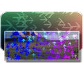
519
Optical Flow Chapter – 22
Optical Flow [OF]
This tool computes the Optical Flow between the frames of the input sequence. The optical
flow can be thought of as a per pixel displacement vector which matches up features between
two frames.
The computed optical flow is stored within the Vector and BackVector aux channels of the
output image. At its highest quality settings, the Optical Flow tool can be slow to process. If you
find optical flow is too slow, you should consider tweaking the quality settings, using a disk
cache, or pre-rendering it out into OpenEXR files.
There are quite a few quality settings to tweak, many with small or diminishing returns;
depending on the settings, there is easily a variation of 10x in rendering time. As a hint to those
interested in reducing process time, try experimenting with the Proxy, Number of Iterations, and
Number of Warps sliders and changing the filtering to Bilinear.
OpticalFlow can only work with the frames you allow. If you trim an upstream Loader to a sub
frame range, OpticalFlow cannot see beyond the subframe range, even if there are additional
frames on disk that it could use.
If the footage input flickers on a frame-by-frame basis, it is a good idea to deflicker the footage
beforehand.
Currently, OpticalFlow will have to render twice for a downstream Time Stretcher or Time Speed
to evaluate. This is because Time Speed needs A. FwdVec and B. BackVec to work but
OpicalFlow generates A. BackVec and A. FwdVec when it processes.
When pre-generating Optical Flow vectors, consider adding a SmoothMotion tool afterward
with smoothing for forward/ backward vectors enabled.
Inputs/Outputs
Input
This is the sequence of images for which you want to compute optical flow.
Output
This is the sequence of images with the optical flow stored in its Vector and
BackVector channels.

520
Optical Flow Chapter – 22
Controls
Proxy (for tracking)
The input images are re-sized down by the proxy scale, and tracked to produce the
optical flow. This option is purely to speed up calculation of the optical flow. The
computational time is roughly proportional to the number of pixels in the image. This
means a proxy scale of 2 will give a 4x speedup and a proxy scale of 3 will give a
9x speedup.
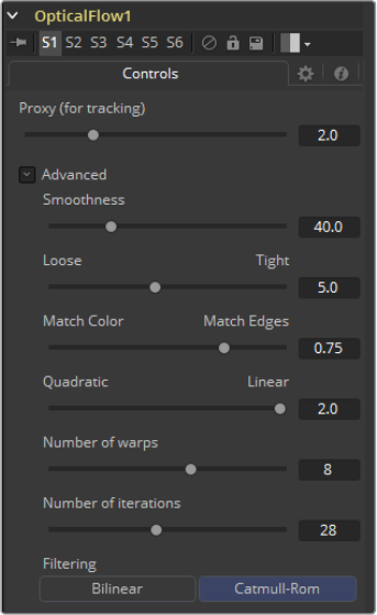
521
Optical Flow Chapter – 22
Advanced
The Advanced Control section has parameter controls to tune the OpticalFlow vector
calculations. The default settings have been chosen to be the best default values from
experimentation with many different shots and should serve as a good standard. In most cases,
tweaking of the advanced settings will not be needed.
Smoothness
This controls the Smoothness of the optical flow. Higher smoothness helps deal with
noise, while lower smoothness brings out more detail.
Edges
This slider is another control for smoothness but applies smoothing based upon the
color channel. It tends to have the effect of determining how edges in the flow follow
edges in the color images. When it is set to Loose, the optical flow becomes smoother
and tends to overshoot edges. When it is set Tight, details from the color images start
to slip into the optical flow, which is not desirable, and edges in the flow more tightly
align with the edges in the color images. As a rough guideline, if you are using the
disparity to produce a Z-channel for post effects like DoF, then prefer it tight, and if you
are using the disparity to do interpolation, you might want to be looser.
In general, if it is too tight, there can be problems with streaked out edges when the
optical flow is used for interpolation.
522
Optical Flow Chapter – 22
Match Weight
This controls how the matching of neighborhoods in the subsequent image is done.
When set to Match Color, large structural color features are matched. When set to
Match Edges, small sharp variations in the color are matched. Typically, a good value for
this slider is in the [0.7, 0.9] range although on some shots, values closer to 0.0 work
well. Setting this option higher tends to improve the matching results in the presence of
differences due to smoothly varying shadows or local lighting variations between the
left and right images. The user should still do a color match or deflickering on the initial
images, if necessary, so they are as similar as possible. This option also helps with local
variations like lighting differences due to light passing through a mirror rig.
Mismatch Penalty
This option controls how the penalty for mismatched regions grows as they become
more dissimilar. The slider gives the choice between a balance of Quadratic and Linear
penalties. Quadratic strongly penalizes large dissimilarities while Linear is more robust
to dissimilar matches. Moving this slider toward Quadratic tends to give a disparity with
more small random variations in it, while Linear produces smoother more visually
pleasing results.
Number of Warps
Turning this option down makes the optical flow computations faster. In particular, the
computational time depends linearly upon this option. To understand what this option
does, you need to understand that the optical flow algorithm progressively warps one
image until it matches with the other image. After some point, convergence is reached
and additional warps are just a waste of computational time. The default value in Fusion
is set high enough that convergence should always be reached. You can tweak this
value to speed up the computations, but it is good to watch what the optical flow is
doing at the same time.
Number of Iterations
Turning this option down makes the computations faster. In particular, the
computational time depends linearly upon this option. Just like adjusting Number of
Warps, at some point adjusting this option higher will give diminishing returns and not
produce significantly better results. By default, this value is set to something that should
converge for all possible shots and can be tweaked lower fairly often without reducing
the disparity’s quality.
Filtering
This controls filtering operations used during flow generation. Catmull-Rom filtering will
produce better results, but at the same time, turning on Catmull-Rom will increase the
computation time steeply.
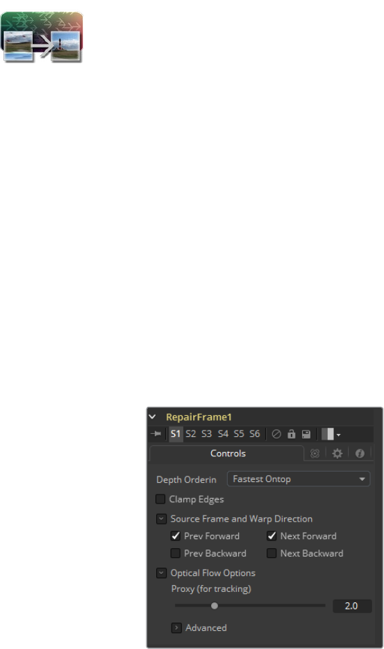
523
Optical Flow Chapter – 22
Repair Frame [REP]
RepairFrame is used for replacing damaged or missing frames or portions of frames with
scratches or other temporally transient artifacts.
You can use the Mask input to limit the repairs to certain areas. If your footage varies in color
from frame to frame, sometimes the repair can be noticeable because, to fill in the hole,
RepairFrame needs to pull color values from adjacent frames. Consider some kind of
deflickering, color correction, and/or using a soft edged mask to help reduce these kinds of
artifacts.
RepairFrame replaces parts of a frame by examining its two neighboring frames and thus
requires three sequential frames as opposed to TimeStretcher/TimeSpeed, which work
between two sequential frames to create a new inbetween frame.
Unlike TimeStretcher and TimeSpeed, RepairFrame does not require, nor need, input Vector/
BackVectors in order to work. An upstream OpticalFlow is not required.
RepairFrame internally will compute the optical flow it needs. This can make it slow to process.
RepairFrame will not pass through, but rather destroy, any aux channels after the
computation is done.
See the Optical Flow Tool for control and setting information:
Controls
Depth Ordering
The Depth Ordering is used to determine which parts of the image should be rendered
on top. This is best explained by an example.
In a locked off camera shot where a car is moving through the frame, the background
does not move, so it will produce small or slow vectors, while the car will produce larger
or faster vectors.
The depth ordering in this case is Fastest Ontop since the car will draw over the
background.
In a shot where the camera pans to follow the car, the background will have faster
vectors and the car will have slower vectors, so the Depth ordering method would be
Slowest Ontop.
524
Optical Flow Chapter – 22
Clamp Edges
Under certain circumstances, this option can remove the transparent gaps that may
appear on the edges of interpolated frames. Clamp Edges will cause a stretching
artifact near the edges of the frame that is especially visible with objects moving
through it or when the camera is moving.
Because of these artifacts, it is a good idea to only use clamp edges to correct small
gaps around the edges of an interpolated frame.
Softness
Helps to reduce the stretchy artifacts that might be introduced by Clamp Edges.
If you have more than one of the Source Frame and Warp Direction checkboxes turned
on, this can lead to doubling up of the stretching effect near the edges. In this case
you‘ll want to keep the softness rather small at around 0.01. If you only have one
checkbox enabled you can use a larger softness at around 0.03).
Source Frame and Warp Direction
This control set allows for the choosing of which frames and which vectors are used to
create the inbetween frames. Each method ticked on will be blended into the result.
Prev Forward: Will take the previous frame and use the Forward vector to interpolate
the new frame.
Next Forward: Will take the next frame in the sequence and use the Forward vector
to interpolate the new frame.
Prev Backward: Will take the previous frame and use the Back Forward vector to
interpolate the new frame.
Next Backward: Will take the next frame in the sequence and use the Back vector to
interpolate the new frame.
Advanced: Please see the Advanced Controls chapter of Optical flow.
525
Optical Flow Chapter – 22
Smooth Motion [SM]
This tool takes an image sequence and smooths it using optical flow to look at
neighboring frames.
It is important that the input sequence has pre-computed Vector and BackVector channels
contained in it, otherwise this tool will print error messages.
Check on the channels you want to temporally smooth. If a channel selected for smoothing is
not present, SmoothMotion will not fail nor will it print any error messages.
SmoothMotion was initially designed for smoothing of the Disparity channel, where it helps
reduce temporal edge/fringing artifacts.
It can also be used to smooth the Vector and BackVector channels, however do be aware that
in various situations this can make the interpolated results worse, especially if there are
conflicting motions or objects in the shot that move around erratically, jitter or bounce rapidly.
One thing you can try is using two or more SmoothMotion tools in sequence to get additional
smoothing. With one SmoothMotion tool, the previous, current and next frames are examined
for a total of 3; with 2 SmoothMotion tools, 5 frames are examined, and with 3 SmoothMotion
tools, 7 frames are examined.
Another thing you can try is using 2 SmoothMotion tools, but in the first tool enable the
smoothing of the Vector and BackVector channels, and in the second SmoothMotion enable
the channels you want to smooth (e.g., Disparity). This way you use the smoothed vector
channels to smooth Disparity.
You can also try using the smoothed motion channels to smooth the motion channels.
Controls
Channel
SmoothMotion can be applied to more than just the RGBA channels. It can also do all of
the other aux channel groups in Fusion.

526
Optical Flow Chapter – 22
Tween [TW]
Tween constructs an in between frame by interpolating between two frames using the optical
flow. Tween is nearly identical in functionality to TimeSpeed and TimeStretcher. The major
difference is that it works on two images that are not serial members of a sequence. As a
consequence, it cannot use the Vector or BackVector aux channels stored in the images and it
must manually generate the optical flow. There is no need to add an upstream OpticalFlow tool.
The generated optical flow is thrown away and not stored back into the output frames.
Since optical flow is based upon color matching, it is a good idea to color correct your images
to match ahead of time. Also, if you are having trouble with noisy images, it may also help to
remove some of the noise ahead of time.
Tween will destroy any input aux channels. See the Optical Flow Tool for control and setting
information.
Inputs/Outputs
InputA
This is an image to interpolate from.
InputB
This is an image to interpolate to.
Output
This is the interpolated image.
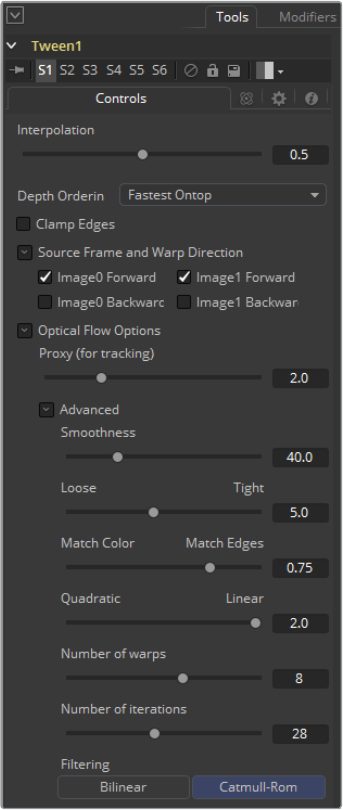
527
Optical Flow Chapter – 22
Controls
Interpolation Parameter
This option determines where the frame we are interpolating is, relative to the two
source frames A and B. An Interpolation Parameter of 0.0 will give frame A back, a
parameter of 1.0 will give frame B back, and a parameter of 0.5 will give a result that is
halfway between A and B.
Depth Ordering
The Depth ordering is used to determine which parts of the image should be rendered
on top. This is best explained by an example.
In a locked off camera shot where a car is moving through the frame, the background
does not move, so will produce small or slow vectors. The car will produce larger or
faster vectors.
The Depth Ordering in this case is Fastest Ontop since the car will draw over the
background.
In a shot where the camera pans to follow the car, the background will have faster
vectors and the car will have slower vectors, so the Depth Ordering method would be
Slowest Ontop.
528
Optical Flow Chapter – 22
Clamp Edges
Under certain circumstances, this option can remove the transparent gaps that may
appear on the edges of interpolated frames. Clamp Edges will cause a stretching
artifact near the edges of the frame that is especially visible with objects moving
through it or when the camera is moving.
Because of these artifacts, it is a good idea to only use clamp edges to correct small
gaps around the edges of an interpolated frame.
Softness
Helps to reduce the stretchy artifacts that might be introduced by Clamp Edges.
If you have more than one of the Source Frame and Warp Direction checkboxes turned
on, this can lead to doubling up of the stretching effect near the edges. In this case
you‘ll want to keep the softness rather small at around 0.01. If you only have one
checkbox enabled you can use a larger softness at around 0.03).
Source Frame and Warp Direction
This control set allows for the choosing of which frames and which vectors are used to
create the in between frames. Each method ticked on will be blended into the result.
Prev Forward: Will take the previous frame and use the Forward vector to interpolate
the new frame.
Next Forward: Will take the next frame in the sequence and use the Forward vector
to interpolate the new frame.
Prev Backward: Will take the previous frame and use the Back Forward vector to
interpolate the new frame.
Next Backward: Will take the next frame in the sequence and use the Back vector to
interpolate the new frame.
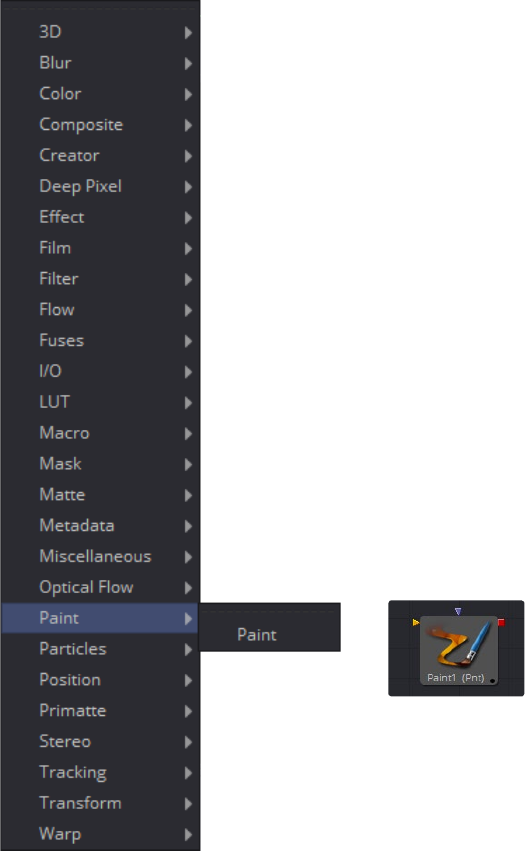
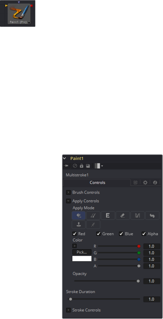
532
Paint Tool Chapter – 23
Paint
Paint is an extremely flexible, stroke-based system for making changes directly to a series of
images. Use the Paint tool for wire and rig removal, image cloning, or to rapidly create custom
masks and mattes.
Fusion’s paint can even be used to create new images and artistic elements from scratch.
Each Paint tool is made up of a series of brush strokes. These strokes are vector shapes
created directly on a view. The type of brush used, the size of the stroke and the effect of the
stroke on the image are all user-controllable. A wide range of apply modes and brush types
areavailable.
Brush strokes can be made into editable polylines for fine control. They can be animated to
change shape, length and size over time. The opacity and size of a stroke can be affected by
velocity and pressure (when used with a supported tablet).
Unlimited undo and redo of paint provides the ability to experiment before committing changes
to an image sequence. Paint strokes can be re-ordered, deleted and modified with virtually
infinite flexibility.
Controls Tab
Not all of the controls described here appear in all modes. Certain controls are only useful in a
specific Paint mode and are hidden when they are not applicable. Additionally, several of the
controls are considered to be self-explanatory; the purpose of a Center control, Angle or Size
control should be relatively straightforward to determine.
To reduce complexity, these controls are not all described. For further details on the
functionality of the Controls tab, please see the Working with Paint Strokes – Animating Strokes
section in this chapter.
533
Paint Tool Chapter – 23
Color Space
The Color Space array of buttons is only visible when the current mode is set to Fill.
These are used to select the color space when sampling colors around the fill center
for inclusion in the fill range.
R, G, B and Alpha
When selected, these checkboxes reflect which color channel is being painted. For
example, with R, G and B off and Alpha on, painting will occur on the Alpha channel.
Brush Controls
Brush Shape
Soft Brush: The Soft Brush type is a circular brush with soft edges. Modify the size
of the brush in the Viewer by holding the Command or Ctrl key down while dragging
the mouse.
Circular Brush: A Circular Brush is a brush shape with hard edges. Resize this brush
interactively.
Image Brush: The Image Brush allows images from any tool in the flow, or from a file
system, to be used as a brush. See Creating Custom Brushes later in this chapter.
Single Pixel Brush: The Single Pixel Brush is perfect for fine detail work, creating a
brush exactly one pixel in size. No anti-aliasing is applied to the single pixel brush.
Square Brush: A Square Brush is a brush shape with hard edges.
Vary Size
Constant: The brush will be a constant size over the stroke.
With Pressure: The stroke size will vary with the actual applied pressure.
With Velocity: The stroke size will vary with the speed of painting.
The faster the stroke, the thinner it is.
Vary Opacity
Constant: The Constant brush will be a constant transparency over the entire stroke.
With Pressure: The stroke transparency will vary with the applied pressure.
With Velocity: The stroke transparency will vary with the speed of painting.
The faster the stroke, the more transparent it is.
Softness
Use this control to increase or decrease the Softness of a soft brush.
Image Source
When using the Image Source brush type, select between three possible sources
brush images.
Tool
The image source is derived from the output of a tool on the flow. Drag the tool into the
Source Tool input to set the source.
Clip
The image source is derived from an image or sequence on disk. Any file supported by
Fusion’s Loader can be used. Locate the file using the filename Clip browser that
appears to set the clip used as a source.
Brush
Images stored in the Fusion > Brushes directory are used as a brush for the Paint tool.
Select the brush from the menu that appears.
534
Paint Tool Chapter – 23
Apply Controls
Apply Mode
Color: The Color Apply Mode paints simple colored strokes on the screen. When
used in conjunction with an image brush, it can also be used to tint the brush.
Clone: The Clone Apply Mode copies portions of one image into another image, or to
clones from the same image using adjustable positions and time offsets. Any image
from the flow can be used as the source image.
Emboss: The Emboss Apply Mode embosses the portions of the image covered by
the brush stroke.
Erase: Erase reveals the underlying image through all other strokes, effectively
erasing portions of the strokes beneath it with out actually destroying the strokes.
Merge: This Apply Mode effectively Merges the brush onto the image. This mode
behaves in much the same way as the Color Apply Mode but has no color controls. It
is best suited for use with the image brush type.
Smear: Smear the image using the direction and strength of the brush stroke
as a guide.
Stamp: Stamp the brush onto the image, completely ignoring any alpha channel
or transparency information. This mode is best suited for applying decals to the
target image.
Wire: This Wire Removal Mode is used to remove wires, rigging and other small
elements in the frame by sampling adjacent pixels and drawing them in toward
the stroke.
Stroke Controls
Size: This control adjusts the Size of the brush when the brush type is set to either
soft brush or circle. The diameter of the brush is drawn in the Viewer as a small circle
surrounding the mouse pointer. The size can also be adjusted interactively in the
Viewer by holding the Command or Ctrl key while dragging the mouse pointer.
Spacing: The Spacing slider determines the distance between dabs (samples used
to draw a straight line along the underlying vector shape that composes a stroke or
polyline stroke). Increasing the value of this slider increases the density of the stroke,
whereas decreasing the value is likely to cause the stroke to assume the appearance
of a dotted line.
Stroke Animation: The Stroke Animation menu control provides several pre-built
animation effects that can be applied to a paint stroke. This menu only appears for
Vector strokes.
All Frames: This default displays the stroke for All Frames of the project where a valid
target image is available to the Paint tool.
Limited Duration: This exists on the number of frames specified by the
Duration slider.
Write On: When Write On is selected, an animation spline will be added to the paint
stroke that precisely duplicates the timing of the paint stroke’s creation. The stroke
will be written on the image exactly as it was drawn. To adjust the timing of the Write
On effect, switch to the Spline Editor and use the Time Stretcher mode to adjust the
overall length of the animation spline. To smooth or manually adjust the motion, try
reducing the points in the animation spline.
Write Off: Write Off will perform the reverse of write on, drawing the stroke starting
from the end and working backward to the start of the stroke.
Write On Then Off: This mode will apply a Write On and then a Write Off animation
mode to the stroke.
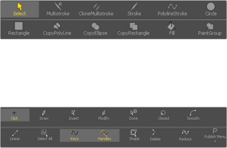
535
Paint Tool Chapter – 23
Trail: Selecting the Trail mode will cause both the start and end points of the stroke
to be animated simultaneously, offset from each other by the amount specified in the
duration control. This has the effect of creating a segment of the stroke that follows
the stroke as if it were a path. As with the Write On and Off effects, this will start at
the frame that is current when the animation mode is selected. The timing of the
animation can be adjusted manually using the Spline or Timeline Editors.
Duration: Duration sets the duration of each stroke in frames. This control is only
present for Multistrokes or when the stroke animation mode is set to Limited Duration.
It is most commonly employed for frame-by-frame rotoscoping through a scene.
Each Vector stroke applied to a scene will have a duration in the Timeline that can be
trimmed independently from one stroke to the next. The duration can be set to 0.5,
which will allow each stroke to last for a single field only when the flow is processing
in Fields mode.
Write On and Write Off: This range slider appears when the Stroke Animation
is set to one of the Write On and Write Off methods. The range represents the
beginning and end points of the stroke. Drag the low value upward to give the
impression that the stroke is being erased, or drag the high value from 0.0 to 1.0 to
give the impression that the stroke is being drawn on the screen. This control can
be animated to good effect. It works most effectively when automatically animated
through the use of the Write On, Write Off modes of the Stroke Animation menu.
Make Editable: This button only appears for Vector strokes. Clicking on
‘MakeEditable’ turns the current stroke into a polyline spline so that the shape can
be adjusted or animated.
Working with Paint Strokes
Strokes Menu
To create a new paint stroke, you can select the type of stroke you want from the menu
that is displayed in the view. Please refer to Paint Stroke Modifiers in the Modifiers
chapter for further explanation. When a paint stroke is selected or edited, a menu is
displayed in the view to select different editing options.
Please refer to Working with Polylines for further explanation.
Types of Paint Strokes
536
Paint Tool Chapter – 23
Circle
Creates a circular shape with animatable control over radius and center.
Clone Multistroke
Like the Multistroke described further below, but specifically meant to clone elements
from one image to the other.
Copy Polyline
A Polyline area with animatable offset to clone elements from one image to the other.
Copy Rectangle
A rectangular shape area with animatable offset to clone elements from one image to
the other.
Fill
Fills an area of the image based on adjustable color values.
Multistroke
Perfect for those 100-strokes-per-frame retouching paint jobs like removing tracking-
markers. Much faster than the Stroke, but not editable later on.
Paint Group
Allows easy grouping of multiple strokes with full control over center and size.
Polyline Stroke
A fully editable stroke based on animatable Polylines. Can be connected to existing
polylines like Masks or Animation Paths.
Rectangle
Creates a rectangular area.
Stroke
The ‘standard’ Stroke. Fully animatable and editable. Might become slow if hundreds of
strokes are used in an image; for huge amounts of strokes it is better to use MultiStroke.
537
Paint Tool Chapter – 23
Hot Keys
Hot key control over paint makes it interactive to adjust painting styles and color without having
to navigate menus.
While painting:
Hold Ctrl while left-dragging to change brush size
Hold Alt while clicking to pick colour
While cloning:
Alt+click to set the clone source position. Strokes start cloning from here.
Hold O to temporarily enable a 50% transparent overlay of the clone source
(% can be changed with pref Tweaks.CloneOverlayBlend)
Press P to toggle an opaque overlay of the clone source
While overlay is showing:
Painting will “rub through” pixels onto the destination.
Arrow keys will change the clone source position you can also drag
crosshair and angle control, or Size slider
Alt+left or right will change the clone source angle
Alt+up or down will change the clone source size
Shift + Ctrl can be used with the above for greater or lesser adjustments
[ & ] (Left and right square brackets) will change the clone source Time Offset
(this requires a specific clone source tool to be set in the Source Tool field).
Copy Rect/Ellipse:
Hold Shift while dragging out the source to constrain the shape
With single stroke selected (not multi or polyline strokes):
Press X or Y to flip the stroke
Paint Groups:
Ctrl+drag to change the position of a group’s crosshair,
without changing the position of the group
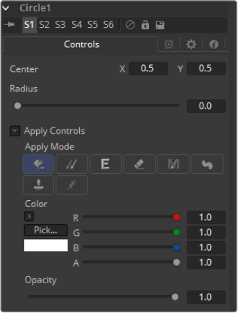
538
Paint Tool Chapter – 23
Modifiers
Circle
The Circle only works on Paint tools. Creates a circular shape with animatable control over
radius and center. It can be applied by clicking on Circle in the Paint tool’s Stroke menu.
Controls
Center
The Center of the circle.
Radius
The Radius of the circle.
Apply Mode
For details see the Apply Controls of the Paint tool.
Color
The Color of the circle.
Opacity
The Opacity of the circle.
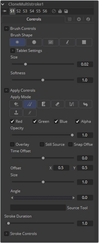
539
Paint Tool Chapter – 23
CloneMultistroke
The CloneMultistroke is pretty much like the normal Multistroke, but specifically meant to clone
areas from one image to the other. In addition to the Multistroke, it has a Source Tool input,
described later in this manual.
Perfect for those 100-strokes-per-frame retouching paint jobs like removing
tracking markers.
Much faster than the Stroke, but not editable later on.
It can be applied by clicking on the CloneMultistroke button in the Paint tool’s
Stroke menu.
Controls Tab
Not all of the controls described here appear in all modes. Certain controls are only useful in a
specific paint mode and are hidden when they are not applicable. Additionally, several of the
controls are considered to be self-explanatory; the purpose of a Center control, Angle or Size
control should be relatively straightforward to determine.
To reduce complexity, these controls are not all described. For further details on the
functionality of the Controls Tab, see the Working with Paint Strokes – Animating Strokes
section in this chapter.
540
Paint Tool Chapter – 23
Brush Shape
Soft Brush: The Soft Brush type is a circular brush with soft edges. Modify the size
of the brush in the Viewer by holding the Command or Ctrl key down while dragging
the mouse.
Circular Brush: A Circular Brush is a brush shape with hard edges. Resize this brush
interactively.
Image Brush: The Image Brush allows images from any tool in the flow, or from a file
system, to be used as a brush. See Creating Custom Brushes later in this chapter.
Single Pixel Brush: The Single Pixel Brush is perfect for fine detail work, creating a
brush exactly one pixel in size. No anti-aliasing is applied to the single pixel brush.
Square Brush: A Square Brush is a brush shape with hard edges.
Vary Size
Constant: The brush will be a constant size over the stroke.
With Pressure: The stroke size will vary with the actual applied pressure.
With Velocity: The stroke size will vary with the speed of painting.
The faster the stroke, the thinner it is.
Vary Opacity
Constant: The Constant brush will be a constant transparency over the entire stroke.
With Pressure: The stroke transparency will vary with the applied Pressure.
With Velocity: The stroke transparency will vary with the speed of painting.
The faster the stroke, the more transparent it is.
Softness
Use this control to increase or decrease the Softness of a soft brush.
Image Source
When using the Image Source brush type, select between three possible sources
brush images.
Tool: The image source is derived from the output of a tool on the flow. Drag the tool
into the Source Tool input to set the source.
Clip: The image source is derived from an image or sequence on disk. Any file
supported by Fusion’s Loader can be used. Locate the file using the filename Clip
browser that appears to set the clip used as a source.
Brush: Images stored in the Fusion > Brushes directory are used as a brush for the
Paint tool. Select the brush from the the menu that appears.
Apply Controls
Apply Mode
Color: The Color apply mode paints simple colored strokes on the screen. When
used in conjunction with an image brush, it can also be used to tint the brush.
Clone: The Clone apply mode copies portions of one image into another image, or
clones from the same image using adjustable positions and time offsets. Any image
from the flow can be used as the source image.
Emboss: The Emboss apply mode embosses the portions of the image covered by
the brush stroke.
Erase: Erase reveals the underlying image through all other strokes, effectively
erasing portions of the strokes beneath it without actually destroying the strokes.
541
Paint Tool Chapter – 23
Merge: This apply mode effectively Merges the brush onto the image. This mode
behaves in much the same way as the Color apply mode but has no color controls. It
is best suited for use with the image brush type.
Smear: Smear the image using the direction and strength of the brush stroke
as a guide.
Stamp: Stamp the brush onto the image, completely ignoring any alpha channel
or transparency information. This mode is best suited for applying decals to the
target image.
Wire: This Wire Removal mode is used to remove wires, rigging and other small
elements in the frame by sampling adjacent pixels and drawing them in toward
the stroke.
Source Tool: Shows which tool’s image output is used to clone from.
Stroke Controls
Size
This control adjusts the Size of the brush when the brush type is set to either Soft Brush
or Circle. The diameter of the brush is drawn in the Viewer as a small circle surrounding
the mouse pointer. The size can also be adjusted interactively in the Viewer by holding
the Command or Ctrl key while click-dragging the mouse pointer.
Spacing
The Spacing slider determines the distance between dabs (samples used to draw a
straight line along the underlying vector shape that composes a stroke or polyline
stroke). Increasing the value of this slider increases the density of the stroke, whereas
decreasing the value is likely to cause the stroke to assume the appearance of a
dotted line.
Stroke Animation
The Stroke Animation menu control provides several pre-built animation effects that
can be applied to a paint stroke. This menu only appears for Vector strokes.
All Frames: This default displays the stroke for All Frames of the project where a valid
target image is available to the paint tool.
Limited Duration: This exists on the number of frames specified by the
Duration slider.
Write On: When Write On is selected, an animation spline will be added to the paint
stroke that precisely duplicates the timing of the paint stroke’s creation. The stroke
will be written on the image exactly as it was drawn. To adjust the timing of the Write
On effect, switch to the Spline Editor and use the Time Stretcher mode to adjust the
overall length of the animation spline. To smooth or manually adjust the motion, try
reducing the points in the animation spline.
Write Off: Write Off will perform the reverse of Write On, drawing the stroke starting
from the end and working backward to the start of the stroke.
Write On Then Off: This mode will apply a Write On and then a Write Off animation
mode to the stroke.
Trail: Selecting the Trail mode will cause both the start and end points of the stroke
to be animated simultaneously, offset from each other by the amount specified in the
duration control. This has the effect of creating a segment of the stroke that follows
the stroke as if it were a path. As with the Write On and Off effects, this will start at
the frame that is current when the animation mode is selected. The timing of the
animation can be adjusted manually using the Spline or Timeline Editors.

542
Paint Tool Chapter – 23
Duration
Duration sets the duration of each stroke in frames. This control is only present for
Multistrokes or when the stroke animation mode is set to Limited Duration. It is most
commonly employed for frame-by-frame rotoscoping through a scene.
Write On and Write Off
This range slider appears when the Stroke Animation is set to one of the Write On and
Write Off methods. The range represents the beginning and end points of the stroke.
Drag the low value upward to give the impression that the stroke is being erased, or
drag the high value from 0.0 to 1.0 to give the impression that the stroke is being drawn
on the screen. This control can be animated to good effect. It works most effectively
when automatically animated through the use of the Write On, Write Off modes of the
stroke animation menu.
Make Editable
This button only appears for Vector strokes. Clicking on ‘Make Editable’ turns the
current stroke into a polyline spline so that the shape can be adjusted or animated.
NOTE: Each Vector stroke applied to a scene will have a duration in the
Timeline that can be trimmed independently from one stroke to the next. The
duration can be set to 0.5, which will allow each stroke to last for a single field
only when the flow is processing in Fields mode.
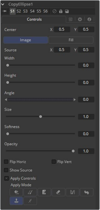
543
Paint Tool Chapter – 23
Copy Ellipse
The Copy Ellipse only works on Paint tools. It creates an elliptical shape to clone elements from
one area of the image to the other. It can be applied by clicking on the Copy Ellipse button in
the Paint tool’s Stroke menu.
Controls
Center X Y
The Center of the Ellipse. Move this control to determine where the content will be
copied to.
Image
The Source will be used to copy content to the destination.
Fill
The Fill color will be used to create a plain fill on the destination.
Source Center X Y
The Center of the Source Ellipse. Move this control to determine where the content will
be copied from. Activate Show Source to see the on screen controls.
544
Paint Tool Chapter – 23
Width/Height Sliders
The Width and Height of the ellipse. This can also be modified with the on
screen controls.
Angle
The Rotation of the ellipse. This can also be modified with the on screen controls.
Size
The overall Size of the ellipse. This is a multiplier to the Width and Height settings.
Softness
The Softness of the edge of the ellipse.
Opacity
The overall opacity of the output.
Flip Horiz/Flip Vert
The area inside the ellipse will be flipped horizontally and/or vertically.
Show Source
Show the on screen controls to adjust the position of the Source Ellipse.
Apply Mode
For more details see the Apply Controls of the Paint tool section.
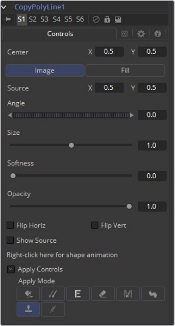
545
Paint Tool Chapter – 23
Copy Polyline
The Copy Polyline only works on Paint tools. It creates a user-definable Polyline to clone
elements from one area of the image to the other. See the Polylines and Rotoscoping chapter of
this manual. It can be applied by clicking on the Copy Polyline button in the Paint tool’s
Stroke menu.
Controls
Center X Y
The Center of the Polyline. Move this control to determine where the content will be
copied to.
Image
The Source will be used to copy content to the Destination.
Fill
The Fill color will be used to create a plain fill on the Destination.
Source Center X Y
The Center of the Source Polyline. Move this control to determine where the content
will be copied from. Activate Show Source to see the on screen controls.
Width/Height Sliders
The Width and Height of the Polyline. This can also be modified with the on
screen controls.
546
Paint Tool Chapter – 23
Angle
The Rotation of the Polyline. This can also be modified with the on screen controls.
Size
The overall Size of the Polyline. This is a multiplier to the Width and Height settings.
Softness
The Softness of the edge of the Polyline.
Opacity
The overall Opacity of the output.
Flip Horiz/Flip Vert
The area inside the Polyline will be flipped horizontally and/or vertically.
Show Source
Show the on screen controls to adjust the position of the source Polyline.
Apply Mode
For more details see the Apply Controls of the Paint tool section.
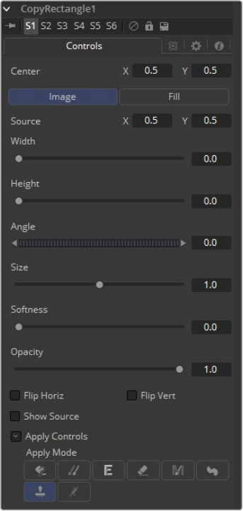
547
Paint Tool Chapter – 23
Copy Rectangle
The Copy Rectangle only works on Paint tools. It creates a user-definable Rectangle to clone
elements from one area of the image to the other. It can be applied by clicking on the Copy
Rectangle button in the Paint tool’s Stroke menu.
Controls
Center X Y
The Center of the Rectangle. Move this control to determine where the content will be
copied to.
Image
The Source will be used to copy content to the Destination.
Fill
The Fill color will be used to create a plain fill on the Destination.
Source Center X Y
The Center of the Source Rectangle. Move this control to determine where the content
will be copied from. Activate Show Source to see the on screen controls.
548
Paint Tool Chapter – 23
Width/Height Sliders
The Width and Height of the Rectangle. This can also be modified with the on
screen controls.
Angle
The Rotation of the Rectangle. This can also be modified with the on screen controls.
Size
The overall Size of the Rectangle. This is a multiplier to the Width and Height settings.
Softness
The Softness of the edge of the Rectangle.
Opacity
The overall Opacity of the output.
Flip Horiz/Flip Vert
The area inside the Rectangle will be flipped horizontally and/or vertically.
Show Source
Show the on screen controls to adjust the position of the source Rectangle.
Apply Mode
For more details see the Apply Controls of the Paint tool section.
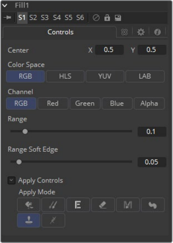
549
Paint Tool Chapter – 23
Fill
The Fill only works on Paint tools. It fills an area of the image with a user-definable color. From
the way it works, it can be compared with the Wand mask. It can be applied by clicking on the
Fill button in the Paint tool’s Stroke menu.
Controls
Selection Point
The Selection Point is a pair of X and Y coordinates that determine from where in the
source image the fill derives its initial color sample. This control is also seen as a
crosshair in the Viewers. The selection point can be positioned manually, connected to
a Tracker, Path or other expressions.
Color Space
The Color Space button group determines the color space used when selecting the
source color for the mask. The fill can operate in RGB, YUV, HLS or LAB color spaces.
Channel
The Channel button group is used to select whether the color that is masked comes
from all three color channels of the image, the alpha channel, or from an individual
channel only.
The exact labels of the buttons will depend on the Color Space selected for the fill
operation. If the color space is RGB, the options will be R, G or B. If YUV is the color
space, the options will be Y, U or V.
Range
The Range slider controls the range of colors around the source color that will be
included in the fill. If the value is left at 0.0, only pixels of exactly the same color as the
source will be considered part of the file. The higher the value, the more similar colors
in the source will be considered to be wholly part of the fill.
550
Paint Tool Chapter – 23
Range Soft Edge
The Range Soft Edge determines the falloff range of the colors selected. Any pixel
within the range defined above will be treated as 100% for the fill. If the soft range is set
to 0.0, no other pixels will be considered for the fill. Increasing the soft range will
increase the number of colors close to, but not quite within, the range that will be
included in the fill. These pixels will be semi-transparent in the fill.
Apply Mode
For more details see the Apply Controls of the Paint tool section.
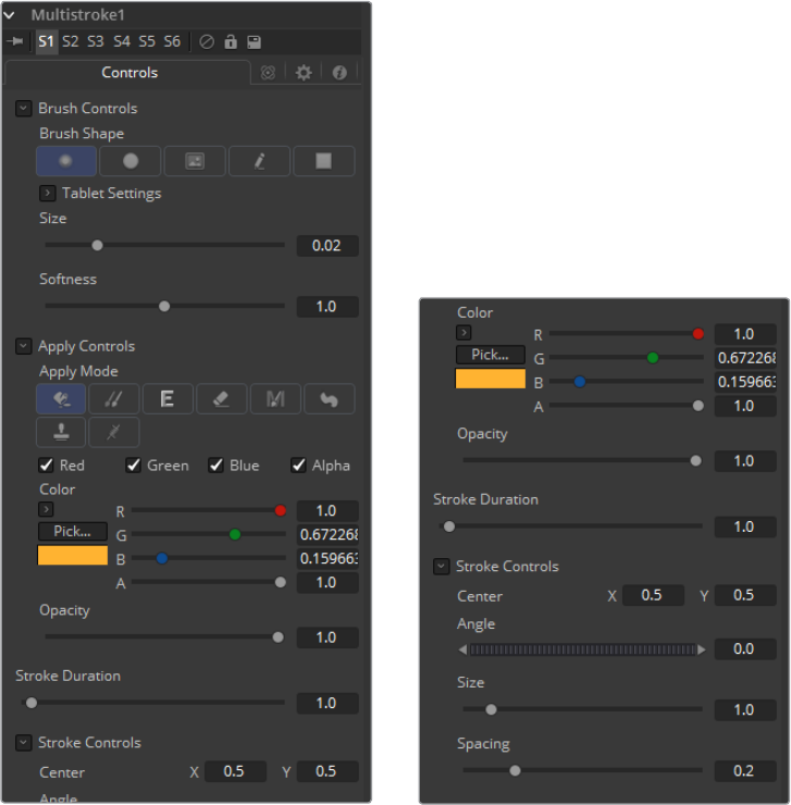
551
Paint Tool Chapter – 23
Multistroke
The Multistroke is the standard stroke in the Paint tool. Perfect for those 100-strokes-per-frame
retouching paint jobs like removing tracking-markers. Much faster than the Stroke, but not
editable later on.
While Multistrokes aren‘t directly editable, they can be grouped with the PaintGroup modifier,
then tracked, moved and rotated by animating the PaintGroup instead. Alternatively, the Edit
Multistrokes and Combine Strokes tool scripts can be used to convert multistrokes into ordinary,
editable strokes, and vice versa.
It can be applied by clicking on the Multi Stroke button in the Paint tool’s Stroke menu.
Controls Tab
Not all of the controls described here appear in all modes. Certain controls are only useful in a
specific paint mode and are hidden when they are not applicable. Additionally, several of the
controls are considered to be self-explanatory the purpose of a Center control, Angle or Size
control should be relatively straightforward to determine.
To reduce complexity, these controls are not all described. For further details on the
functionality of the Controls Tab, see the Working With Paint Strokes – Animating Strokes
section in this chapter.
552
Paint Tool Chapter – 23
Brush Controls
Brush Shape
Soft Brush: The Soft Brush type is a circular brush with soft edges. Modify the size of
the brush in the Viewer by holding Command or Ctrl down while dragging the mouse.
Circular Brush: A Circular Brush is a brush shape with hard edges. Resize this brush
interactively.
Image Brush: The Image Brush allows images from any tool in the flow, or from a file
system, to be used as a brush. See Creating Custom Brushes later in this chapter.
Single Pixel Brush: The Single Pixel Brush is perfect for fine detail work, creating a
brush exactly one pixel in size. No anti-aliasing is applied to the single pixel brush.
Square Brush: A Square Brush is a brush shape with hard edges.
Vary Size
Constant: The brush will be a constant size over the stroke.
With Pressure: The stroke size will vary with the actual applied pressure.
With Velocity: The stroke size will vary with the speed of painting. The faster the
stroke, the thinner it is.
Vary Opacity
Constant: The Constant brush will be a constant transparency over the entire stroke.
With Pressure: The stroke transparency will vary with the applied pressure.
With Velocity: The stroke transparency will vary with the speed of painting. The
faster the stroke, the more transparent it is.
Softness
Use this control to increase or decrease the Softness of a soft brush.
Image Source
When using the Image Source brush type, select between three possible sources
brush images.
Tool: The image source is derived from the output of a tool on the flow. Drag the tool
into the Source Tool input to set the source.
Clip: The image source is derived from an image or sequence on disk. Any file
supported by Fusion’s Loader can be used. Locate the file using the filename Clip
browser that appears to set the clip used as a source.
Brush: Images stored in the Fusion > Brushes directory are used as a brush for the
paint tool. Select the brush from the menu that appears.
Apply Controls
Apply Mode
Color: The Color apply mode paints simple colored strokes on the screen. When
used in conjunction with an Image brush, it can also be used to tint the brush.
Clone: The Clone apply mode copies portions of one image into another image, or to
clones from the same image using adjustable positions and time offsets. Any image
from the flow can be used as the source image.
Emboss: The Emboss apply mode embosses the portions of the image covered by
the brush stroke.
Erase: Erase reveals the underlying image through all other strokes, effectively
erasing portions of the strokes beneath it with out actually destroying the strokes.
Merge: This apply mode effectively Merges the brush onto the image. This mode
553
Paint Tool Chapter – 23
behaves in much the same way as the Color apply mode but has no color controls. It
is best suited for use with the image brush type.
Smear: Smear the image using the direction and strength of the brush stroke
as a guide.
Stamp: Stamp the brush onto the image, completely ignoring any alpha channel
or transparency information. This mode is best suited for applying decals to the
target image.
Wire: This Wire Removal mode is used to remove wires, rigging and other small
elements in the frame by sampling adjacent pixels and drawing them in toward
the stroke.
Stroke Controls
Size
This control adjusts the Size of the brush when the brush type is set to either soft brush
or circle. The diameter of the brush is drawn in the Viewer as a small circle surrounding
the mouse pointer. The size can also be adjusted interactively in the Viewer by holding
the Command or Ctrl key while click-dragging the mouse pointer.
Spacing
The Spacing slider determines the distance between dabs (samples used to draw a
straight line along the underlying vector shape that composes a stroke or polyline
stroke). Increasing the value of this slider increases the density of the stroke, whereas
decreasing the value is likely to cause the stroke to assume the appearance of a
dotted line.
Stroke Animation
The Stroke Animation menu control provides several pre-built animation effects that
can be applied to a paint stroke. This menu only appears for Vector strokes.
All Frames
This default displays the stroke for All Frames of the project where a valid target image
is available to the paint tool.
Limited Duration
This exists on the number of frames specified by the Duration slider.
Write On
When Write On is selected, an animation spline will be added to the paint stroke that
precisely duplicates the timing of the paint stroke’s creation. The stroke will be written
on the image exactly as it was drawn. To adjust the timing of the Write On effect, switch
to the Spline Editor and use the Time Stretcher mode to adjust the overall length of the
animation spline. To smooth or manually adjust the motion, try reducing the points in
the animation spline.
Write Off
Write Off will perform the reverse of Write On, drawing the stroke starting from the end
and working backward to the start of the stroke.
Write On Then Off
This mode will apply a Write On and then a Write Off animation mode to the stroke.

554
Paint Tool Chapter – 23
Trail
Selecting the Trail mode will cause both the start and end points of the stroke to be
animated simultaneously, offset from each other by the amount specified in the
duration control. This has the effect of creating a segment of the stroke that follows the
stroke as if it were a path. As with the Write On and Off effects, this will start at the
frame that is current when the Animation mode is selected. The timing of the animation
can be adjusted manually using the Spline or Timeline Editors.
Duration
Duration sets the duration of each stroke in frames. This control is only present for
Multistrokes or when the Stroke Animation mode is set to Limited Duration. It is most
commonly employed for frame-by-frame rotoscoping through a scene.
Write On and Write Off
This range slider appears when the Stroke Animation is set to one of the Write On and
Write Off methods. The range represents the beginning and end points of the stroke.
Drag the low value upward to give the impression that the stroke is being erased, or
drag the high value from 0.0 to 1.0 to give the impression that the stroke is being drawn
on the screen. This control can be animated to good effect. It works most effectively
when automatically animated through the use of the Write On/Write Off modes of the
Stroke animation menu.
Make Editable
This button only appears for Vector strokes. Clicking on ‘Make Editable’ turns the
current stroke into a polyline spline so that the shape can be adjusted or animated.
Each Vector stroke applied to a scene will have a duration in the Timeline that
can be trimmed independently from one stroke to the next. The duration can
be set to 0.5, which will allow each stroke to last for a single field only when
the flow is processing in Fields mode.
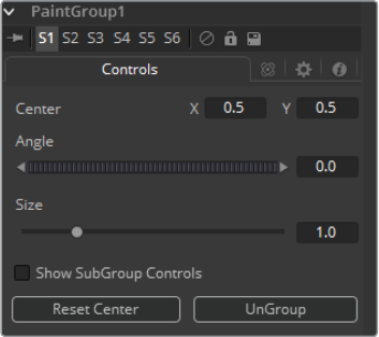
555
Paint Tool Chapter – 23
Paint Group
The Paint Group only works on Paint strokes and objects. It groups all currently selected paint
strokes together, making it easier to handle them all together.
Multistroke modifiers can be grouped as well, which includes all the multistrokes contained
within that modifier. By animating the Paint Group, it is thus possible to move, track and rotate a
collection of multistrokes.
It can be applied by clicking on the Paint Group button in the Paint tool’s Stroke menu.
Controls
Center X Y
The Center of the Group. Modify this control to move the group around.
Angle
The entire group can be rotated using this control.
Size
Scales the entire group.
Show Subgroup Controls
Displays the controls of the individual strokes in the group and allows the user to
modify them.
Reset Center
Puts the Center back to the position where it was when the group was created.
Ungroup
Disassembles the group back into individual strokes and deletes the Group modifier.
For temporary opening of the group, use the Show Subgroup controls switch instead.
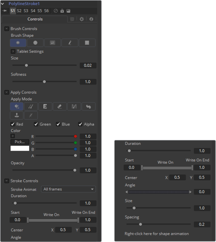
556
Paint Tool Chapter – 23
Polyline Stroke
Fusion offers a Polyline Stroke mode. This provides the ability to create and manipulate a stroke
in the same way that a path or mask might be created. To add a polyline stroke to the flow,
select the Polyline button from the Paint tool’s Stroke toolbar and click in the view to add the
first point. Continue clicking to add additional points to the polyline.
Notice that the usual Polyline toolbar buttons will appear in the Viewer toolbar. Polyline strokes
are created in Click Append mode by default, but they can also be created in Draw
Append mode.
Controls Tab
Not all of the controls described here appear in all modes. Certain controls are only useful in a
specific paint mode and are hidden when they are not applicable. Additionally, several of the
controls are considered to be self-explanatory; the purpose of a center control, angle or size
control should be relatively straightforward to determine.
To reduce complexity, these controls are not all described. For further details on the
functionality of the Controls Tab, see the Working With Paint Strokes – Animating Strokes
section in this chapter.
557
Paint Tool Chapter – 23
Brush Controls
Brush Shape
Soft Brush: The Soft Brush type is a circular brush with soft edges. Modify the size of
the brush in the Viewer by holding Command or Ctrl down while dragging the mouse.
Circular Brush: A Circular Brush is a brush shape with hard edges. Resize this brush
interactively.
Image Brush: The Image Brush allows images from any tool in the flow, or from a file
system, to be used as a brush. See Creating Custom Brushes later in this chapter.
Single Pixel Brush: The Single Pixel Brush is perfect for fine detail work, creating a
brush exactly one pixel in size. No anti-aliasing is applied to the single pixel brush.
Square Brush: A Square Brush is a brush shape with hard edges.
Vary Size
Constant: The brush will be a constant size over the stroke.
With Pressure: The stroke size will vary with the actual applied pressure.
With Velocity: The stroke size will vary with the speed of painting. The faster the
stroke, the thinner it is.
Vary Opacity
Constant: The Constant brush will be a constant transparency over the entire stroke.
With Pressure: The stroke transparency will vary with the applied Pressure.
With Velocity: The stroke transparency will vary with the speed of painting. The
faster the stroke, the more transparent it is.
Softness
Use this control to increase or decrease the Softness of a soft brush.
Image Source
When using the Image Source brush type, select between three possible sources
brush images.
Tool: The image source is derived from the output of a tool on the flow. Drag the tool
into the Source Tool input to set the source.
Clip: The image source is derived from an image or sequence on disk. Any file
supported by Fusion’s Loader can be used. Locate the file using the filename Clip
browser that appears to set the clip used as a source.
Brush: Images stored in the Fusion > Brushes directory are used as a brush for the
paint tool. Select the brush from a the menu that appears.
Apply Controls
Apply Mode
Color: The Color apply mode paints simple colored strokes on the screen. When
used in conjunction with an image brush, it can also be used to tint the brush.
Clone: The Clone apply mode copies portions of one image into another image, or to
clones from the same image using adjustable positions and time offsets. Any image
from the flow can be used as the source image.
Emboss: The Emboss apply mode embosses the portions of the image covered by
the brush stroke.
Erase: Erase reveals the underlying image through all other strokes, effectively
erasing portions of the strokes beneath it with out actually destroying the strokes.

558
Paint Tool Chapter – 23
Merge: This apply mode effectively Merges the brush onto the image. This mode
behaves in much the same way as the color apply mode but has no color controls. It
is best suited for use with the image brush type.
Smear: Smear the image using the direction and strength of the brush stroke
as a guide.
Stamp: Stamp the brush onto the image, completely ignoring any alpha channel
or transparency information. This mode is best suited for applying decals to the
target image.
Wire: This Wire Removal mode is used to remove wires, rigging and other small
elements in the frame by sampling adjacent pixels and drawing them in toward
the stroke.
Source Tool: Shows which tool’s image output is used to clone from.
Stroke Controls
Size
This control adjusts the Size of the brush when the brush type is set to either soft brush
or circle. The diameter of the brush is drawn in the Viewer as a small circle surrounding
the mouse pointer. The size can also be adjusted interactively in the Viewer by holding
the Command or Ctrl key while click-dragging the mouse pointer.
Spacing
The Spacing slider determines the distance between dabs (samples used to draw a
straight line along the underlying vector shape that composes a stroke or polyline
stroke). Increasing the value of this slider increases the density of the stroke, whereas
decreasing the value is likely to cause the stroke to assume the appearance of a
dotted line.
Stroke Animation
The Stroke Animation menu control provides several pre-built animation effects that
can be applied to a paint stroke. This menu only appears for Vector strokes.
All Frames: This default displays the stroke for All Frames of the project where a valid
target image is available to the Paint tool.
Limited Duration: This exists on the number of frames specified by the
Duration slider.
Write On: When Write On is selected, an Animation spline will be added to the paint
stroke that precisely duplicates the timing of the paint stroke’s creation. The stroke
will be written on the image exactly as it was drawn. To adjust the timing of the Write
On effect, switch to the Spline Editor and use the Time Stretcher mode to adjust the
overall length of the Animation spline. To smooth or manually adjust the motion, try
reducing the points in the Animation spline.
Write Off: Write Off will perform the reverse of Write On, drawing the stroke starting
from the end and working backward to the start of the stroke.

559
Paint Tool Chapter – 23
Write On Then Off: This mode will apply a Write On and then a Write Off animation
mode to the stroke.
Trail: Selecting the Trail mode will cause both the start and end points of the stroke
to be animated simultaneously, offset from each other by the amount specified in the
duration control. This has the effect of creating a segment of the stroke that follows
the stroke as if it were a path. As with the Write On and Off effects, this will start at
the frame that is current when the Animation mode is selected. The timing of the
animation can be adjusted manually using the Spline or Timeline Editors.
Duration
Duration sets the duration of each stroke in frames. This control is only present for
Multistrokes or when the stroke animation mode is set to Limited Duration. It is most
commonly employed for frame-by-frame rotoscoping through a scene.
Write On and Write Off
This range slider appears when the Stroke Animation is set to one of the Write On and
Write Off methods. The range represents the beginning and end points of the stroke.
Drag the low value upward to give the impression that the stroke is being erased, or
drag the high value from 0.0 to 1.0 to give the impression that the stroke is being drawn
on the screen. This control can be animated to good effect. It works most effectively
when automatically animated through the use of the Write On/Write Off modes of the
stroke animation menu.
Right Click Here for Shape Animation
To animate the Polyline shape like Polyline Masks, right click on this control and
choose animate.
NOTE: Each Vector stroke applied to a scene will have a duration in the
Timeline that can be trimmed independently from one stroke to the next.
Theduration can be set to 0.5, which will allow each stroke to last for a single
field only when the flow is processing in Fields mode.
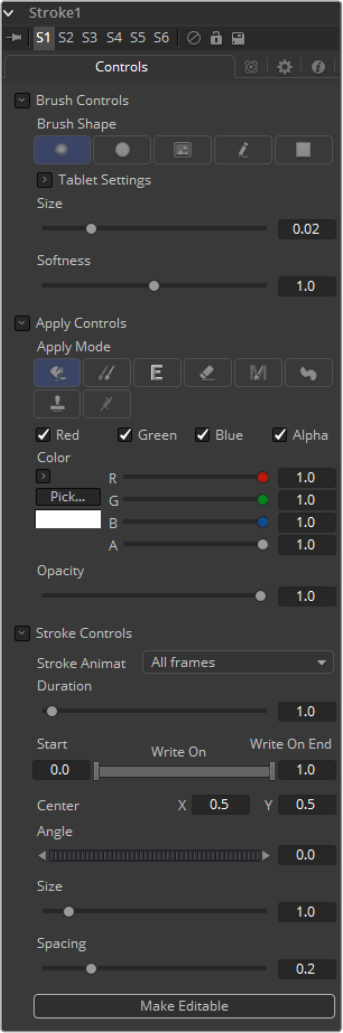
560
Paint Tool Chapter – 23
Stroke
When the Paint tool is first added to the flow, the brush type is set to a medium sized soft,
circular brush with a white Color apply mode.
Release the mouse button to end the creation of the stroke. To draw another stroke, simply
click again and continue. A new stroke will be added to the image with the same settings as the
last applied stroke. When the painting is complete, choose the Select button in the Paint toolbar
to avoid accidentally adding new strokes.
While in Brush or Polyline modes, the controls displayed in the Tool tab affect the next stroke
created, not the strokes that are already created. To adjust the settings of an existing stroke,
switch to Select mode using the Paint toolbar and select the stroke.
To add a stroke to the flow, select the Polyline Button from the Paint tool’s Stroke toolbar, place
the mouse or pen over the image, click-hold the left mouse button and start drawing.
Controls Tab
561
Paint Tool Chapter – 23
Not all of the controls described here appear in all modes. Certain controls are only useful in a
specific paint mode and are hidden when they are not applicable. Additionally, several of the
controls are considered to be self-explanatory; the purpose of a center control, angle or size
control should be relatively straightforward to determine. To reduce complexity, these controls
are not all described. For further details on the functionality of the Controls Tab, see the
Working With Paint Strokes – Animating Strokes section in this chapter.
Brush Controls
Brush Shape
Soft Brush: The Soft Brush type is a circular brush with soft edges. Modify the size of
the brush in the Viewer by holding Command or Ctrl down while dragging the mouse.
Circular Brush: A Circular Brush is a brush shape with hard edges. Resize this brush
interactively.
Image Brush: The Image Brush allows images from any tool in the flow, or from a file
system, to be used as a brush. See Creating Custom Brushes later in this chapter.
Single Pixel Brush: The Single Pixel Brush is perfect for fine detail work, creating a
brush exactly one pixel in size. No anti-aliasing is applied to the single pixel brush.
Square Brush: A Square Brush is a brush shape with hard edges.
Vary Size
Constant: The brush will be a constant size over the stroke.
With Pressure: The stroke size will vary with the actual applied pressure.
With Velocity: The stroke size will vary with the speed of painting. The faster the
stroke, the thinner it is.
Vary Opacity
Constant: The Constant brush will be a constant transparency over the entire stroke.
With Pressure: The stroke transparency will vary with the applied Pressure.
With Velocity: The stroke transparency will vary with the speed of painting. The
faster the stroke, the more transparent it is.
Softness
Use this control to increase or decrease the Softness of a soft brush.
Image Source
When using the Image Source brush type, select between three possible sources
brush images.
Tool: The image source is derived from the output of a tool on the flow. Drag the tool
into the source Tool input to set the source.
Clip: The image source is derived from an image or sequence on disk. Any file
supported by Fusion’s Loader can be used. Locate the file using the filename Clip
browser that appears to set the clip used as a source.
Brush: Images stored in the Fusion > Brushes directory are used as a brush for the
Paint tool. Select the brush from the menu that appears.
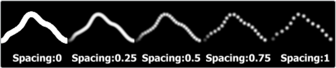
562
Paint Tool Chapter – 23
Apply Controls
Apply Mode
Color: The Color apply mode paints simple colored strokes on the screen. When
used in conjunction with an image brush, it can also be used to tint the brush.
Clone: The Clone apply mode copies portions of one image into another image, or to
clones from the same image using adjustable positions and time offsets. Any image
from the flow can be used as the source image.
Emboss: The Emboss apply mode embosses the portions of the image covered by
the brush stroke.
Erase: Erase reveals the underlying image through all other strokes, effectively
erasing portions of the strokes beneath it with out actually destroying the strokes.
Merge: This apply mode effectively Merges the brush onto the image. This mode
behaves in much the same way as the color apply mode but has no color controls. It
is best suited for use with the image brush type.
Smear: Smear the image using the direction and strength of the brush stroke
as a guide.
Stamp: Stamp the brush onto the image, completely ignoring any alpha channel
or transparency information. This mode is best suited for applying decals to the
target image.
Wire: This Wire removal mode is used to remove wires, rigging and other small
elements in the frame by sampling adjacent pixels and drawing them in toward
the stroke.
Source Tool: Shows which tool’s image output is used to clone from.
Stroke Controls
Size
This control adjusts the Size of the brush when the brush type is set to either soft brush
or circle. The diameter of the brush is drawn in the Viewer as a small circle surrounding
the mouse pointer. The size can also be adjusted interactively in the Viewer by holding
the Command or Ctrl key while click-dragging the mouse pointer.
Spacing
The Spacing slider determines the distance between dabs (samples used to draw a
straight line along the underlying vector shape that composes a stroke or polyline
stroke). Increasing the value of this slider increases the density of the stroke, whereas
decreasing the value is likely to cause the stroke to assume the appearance of a
dotted line.
Stroke Animation
The Stroke Animation menu control provides several pre-built animation effects that
can be applied to a paint stroke. This menu only appears for Vector strokes.
All Frames: This default displays the stroke for All Frames of the project where a valid
target image is available to the paint tool.

563
Paint Tool Chapter – 23
Limited Duration: This exists on the number of frames specified by the
Duration slider.
Write On: When Write On is selected, an Animation spline will be added to the paint
stroke that precisely duplicates the timing of the paint stroke’s creation. The stroke
will be written on the image exactly as it was drawn. To adjust the timing of the Write
On effect, switch to the Spline Editor and use the Time Stretcher mode to adjust the
overall length of the Animation spline. To smooth or manually adjust the motion, try
reducing the points in the Animation spline.
Write Off: Write Off will perform the reverse of Write On, drawing the stroke starting
from the end and working backward to the start of the stroke.
Write On Then Off: This mode will apply a Write On and then a Write Off animation
mode to the stroke.
Trail: Selecting the Trail mode will cause both the start and end points of the stroke
to be animated simultaneously, offset from each other by the amount specified in the
duration control. This has the effect of creating a segment of the stroke that follows
the stroke as if it were a path. As with the Write On and Off effects, this will start at
the frame that is current when the Animation mode is selected. The timing of the
animation can be adjusted manually using the Spline or Timeline Editors.
Duration
Duration sets the duration of each stroke in frames. This control is only present for
Multistrokes or when the stroke Animation mode is set to Limited Duration. It is most
commonly employed for frame-by-frame rotoscoping through a scene.
Write On and Write Off
This range slider appears when the Stroke Animation is set to one of the Write On and
Write Off methods. The range represents the beginning and end points of the stroke.
Drag the low value upward to give the impression that the stroke is being erased, or
drag the high value from 0.0 to 1.0 to give the impression that the stroke is being drawn
on the screen. This control can be animated to good effect. It works most effectively
when automatically animated through the use of the Write On, Write Off modes of the
stroke animation menu.
Right Click Here for Shape Animation
To animate the shape, like Polyline Masks, right-click on this control and
choose animate.
NOTE: Each Vector stroke applied to a scene will have a duration in the
Timeline that can be trimmed independently from one stroke to the next. The
duration can be set to 0.5, which will allow each stroke to last for a single field
only when the flow is processing in Fields mode.
565
Particle Tools Chapter – 24
Particle Tools
pAvoid [PAV] 567
pBounce [PBN] 569
pChangeStyle 572
pCustom 574
pCustomForce 576
pDirectionalForce 579
pEmitter 581
pFlock 585
pFriction 587
pGradientForce 589
pImageEmitter 591
pKill 594
pMerge 595
pPointForce 596
pRender [PRN] 598
pSpawn [PSP] 604
pTangentForce [PTF] 606
pTurbulence [PTR] 608
pVortex [PVT] 610
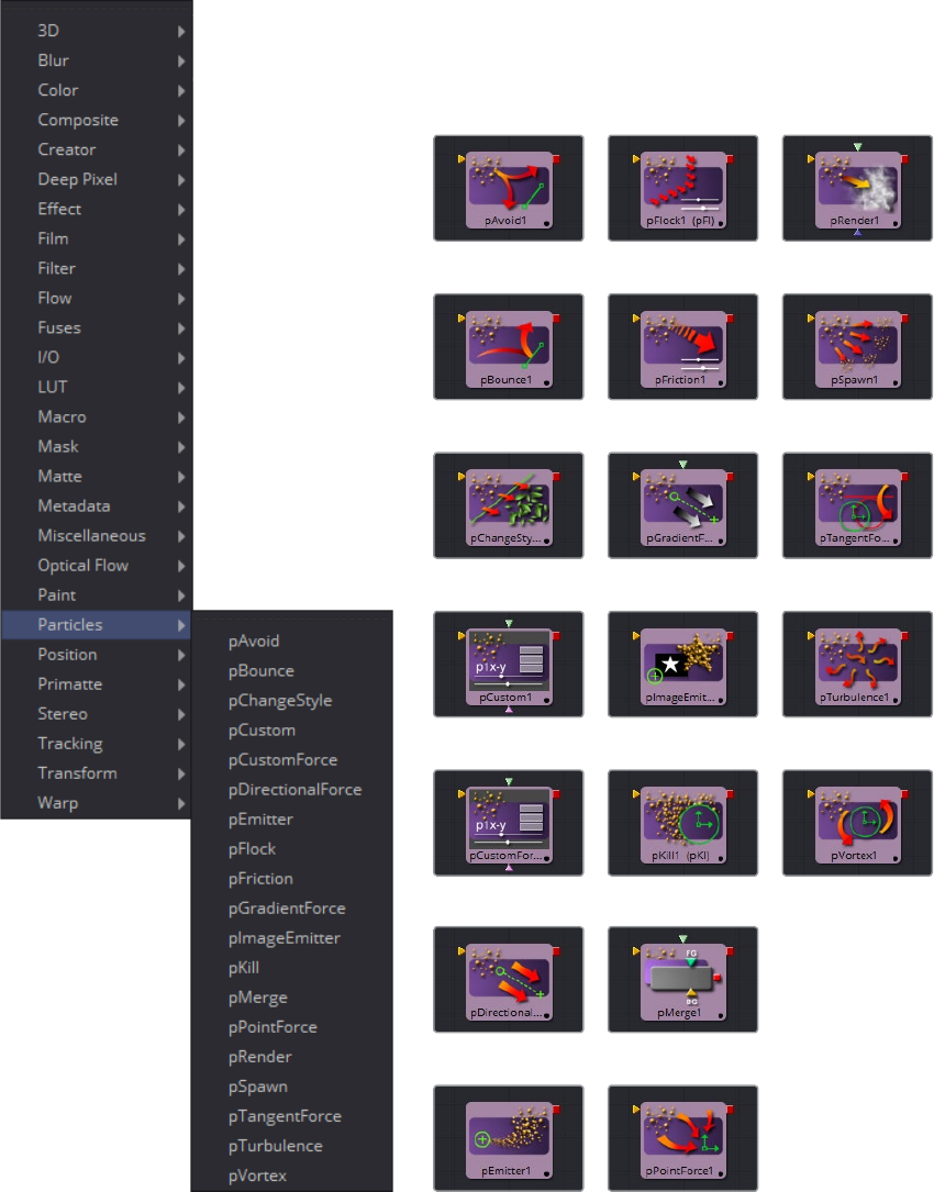
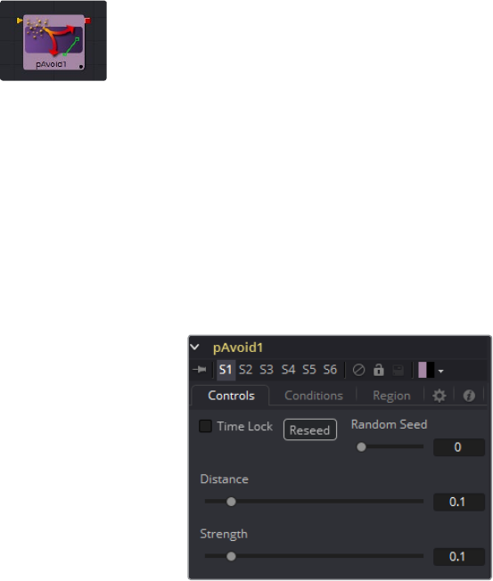
567
Particle Tools Chapter – 24
pAvoid [PAV]
The pAvoid tool is used to create a region or area within the image that affected particles will
attempt to avoid entering and/or crossing.
It has two primary controls, one that determines the distance from the region a particle should
be before it begins to move away from the region, and another to determine how strongly the
particle moves away from the region.
A pAvoid tool creates a ‘desire’ in a particle to move away from a specific region. If the velocity
of the particle is stronger than the combined distance and strength of the pAvoid region, the
particle’s desire to Avoid the region will not overcome its momentum and the particle will cross
that region anyway.
Controls Tab
Randomize
The Seed slider and Randomize button are presented whenever a Fusion tool relies on
a random result. Two tools with the same seed values will produce the same random
results. Click on the Randomize button to randomly select a new seed value, or adjust
the slider to manually select a new seed value.
Distance
Determines the distance from the region a particle should be before it begins to move
away from the region.
Strength
Determines how strongly the particle moves away from the region. Negative values will
make the particles move toward the region instead.
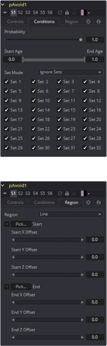

569
Particle Tools Chapter – 24
pBounce [PBN]
The pBounce tool is used to create a region from which affected particles will bounce away
when they come into contact with the region. The pBounce tool has three main controls, as
described below.
Controls Tab
Randomize
The Seed slider and Randomize button are presented whenever a Fusion tool relies on
a random result.
Two tools with the same seed values will produce the same random results. Click on
the Randomize button to randomly select a new seed value, or adjust the slider to
manually select a new seed value.
Elasticity
Elasticity affects the strength of a bounce, or how much velocity the particle will have
remaining after impacting upon the Bounce region. A value of 1.0 will cause the particle
to possess the same velocity after the bounce as it had entering the bounce. A value of
0.1 will cause the particle to lose 90% of its velocity upon bouncing off of the region.
The range of this control is 0.0 to 1.0 by default, but greater values can be entered
manually. This will cause the particles to gain momentum after an impact, rather than
lose it. Negative values will be accepted, but do not produce a useful result.
Variance
By default, particles that strike the Bounce region will reflect evenly off the edge of the
Bounce region, according to the vector or angle of the region. Increasing the Variance
above 0.0 will introduce a degree of variation to that angle of reflection. This can be
used to simulate the effect of a rougher surface.
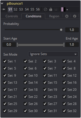
570
Particle Tools Chapter – 24
Spin
By default, particles that strike the region will not have their angle or orientation
affected in any way. Increasing or decreasing the Spin value will cause the Bounce
region to impart a spin to the particle based on the angle of collision, or to modify any
existing spin on the particle. Positive values will impart a forward spin and negative
values impart a backward spin. The larger the value, the faster the spin applied to the
particle will be.
Roughness
This slider varies the bounce off the surface to slightly randomize particle direction.
Surface Motion
This slider makes the bounce surface behave as if it had motion, thus affecting the
particles.
Surface Motion Direction
This thumbwheel control sets the angle relative to the bounce surface.
Conditions Tabs
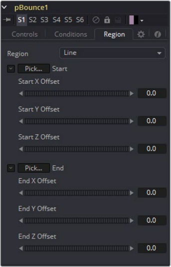
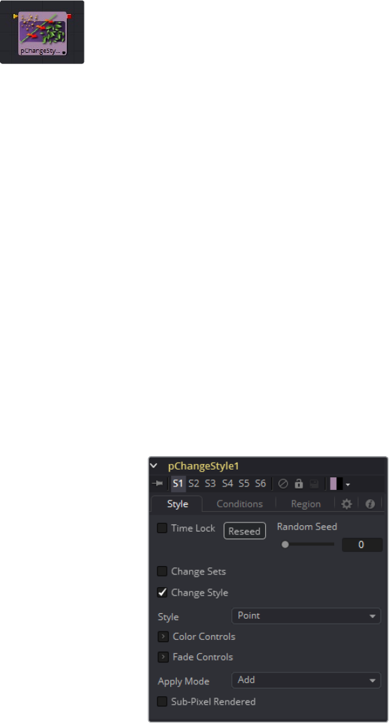
572
Particle Tools Chapter – 24
pChangeStyle
The pChangeStyle tool provides a mechanism for changing the appearance or style of particles
that interact with a defined region. The primary controls in this tool perfectly mirror those found
in the Style tab of the pEmitter tool. Particles that intersect or enter the region defined for this
tool will change as described by this tool.
With the possible exception of the pCustom tool, this is the only tool that modifies the
appearance of a particle, rather than its motion. It is often used to cause the appearance of
particles changing in response to some event, like striking a barrier.
When using the pChangeStyle tool in this fashion, it would be natural to assume that the tool
should be placed after the tool causing the event. As an example, consider the creation of a
particle system that appears to change its style after bouncing off a pBounce using a line
region. In this case, the pChangeStyle tool also uses a line region, positioned identically to the
one in the pBounce tool. Placing the pBounce before the pChangeStyle in the flow causes the
particles to bounce off the region before the pChangeStyle gets an opportunity to calculate its
effect on the particle.
The result is that the particle is no longer intersecting with the pChangeStyle tool’s region, and
so the style never changes.
As a rule, to create a change in style that appears to be caused by a physical event created by
another modifier tool in the flow, the pChangeStyle tool must be placed before that tool for the
effect to work properly.
Style Tab
Randomize
The Seed slider and Randomize button are presented whenever a Fusion tool relies on
a random result. Two tools with the same seed values will produce the same random
results. Click on the Randomize button to randomly select a new seed value, or adjust
the slider to manually select a new seed value.
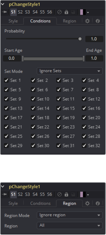
573
Particle Tools Chapter – 24
Change Sets
This option allows the user to change the particle’s Set to become influenced by other
forces than the original particle. See Particle Common Controls in the Particles chapter
to learn more about Sets.
Style
This option allows the user to change the particle’s Style and thus the look. See Particle
Styles in the Particles chapter to learn more about Styles.
Conditions Tab
Regions Tab
See Particle Common Controls in the Particles chapter.
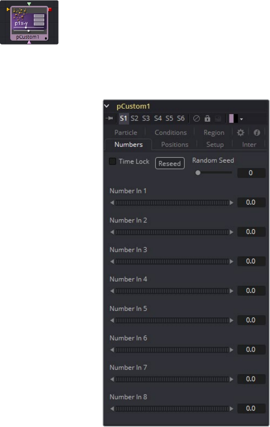

575
Particle Tools Chapter – 24
Conditions and Regions Tab
See Particle Common Controls in the Particles chapter.
The following particle properties are exposed to the pCustom control:
px, py, pz particle position on the x, y, and z axis
vx, vy, vz particle velocity on the x, y and z axis
rx, ry, rz particle rotation on the x, y, and z axis
sx, sy, sz particle spin on the x, y, and z axis
pxi1, pyi1 the 2d position of a particle, corrected for image 1’s aspect
pxi2, pyi2 the 2d position of a particle, corrected for image 2’s aspect
mass not currently used by anything
size the current size of a particle
id the particle’s identifier
r, g, b, a the particles red, green, blue and alpha color values
rgnhit this value is 1 if the particle hit the pcustom tools defined region
rgndist this variable contains the particles distance from the region
condscale the strength of the region at the particle’s position
rgnix, rgniy, rgniz values representing where on the region the particle hit
rgnnx, rgnny, rgnnz region surface normal of the particle when it hit the region
w1, h1 image 1 width and height
w2 h2 image 2 width and height
i1, i2, i3, i4 the result of the intermediate calculations 1 through 4
s1, s2, s3, s4 the result of the setup calculations 1 through 4
n1..n8 the values of numeric inputs 1 through 8
p1x, p1y, p1z .. p4x,
p4y, p4z the values of position inputs 1 through 4
time the current time or frame of the compositions
age the current age of the particle
lifespan the lifespan of the current particle
Additional information on the custom class of tools can be found in documentation for
the Custom tool.
All of the operators, functions and conditional statements described for that tool apply
to pCustom as well, including Pixel-read functions for the two image inputs (e.g.,
getr1w(x,y), getz2b(x,y), etc.).
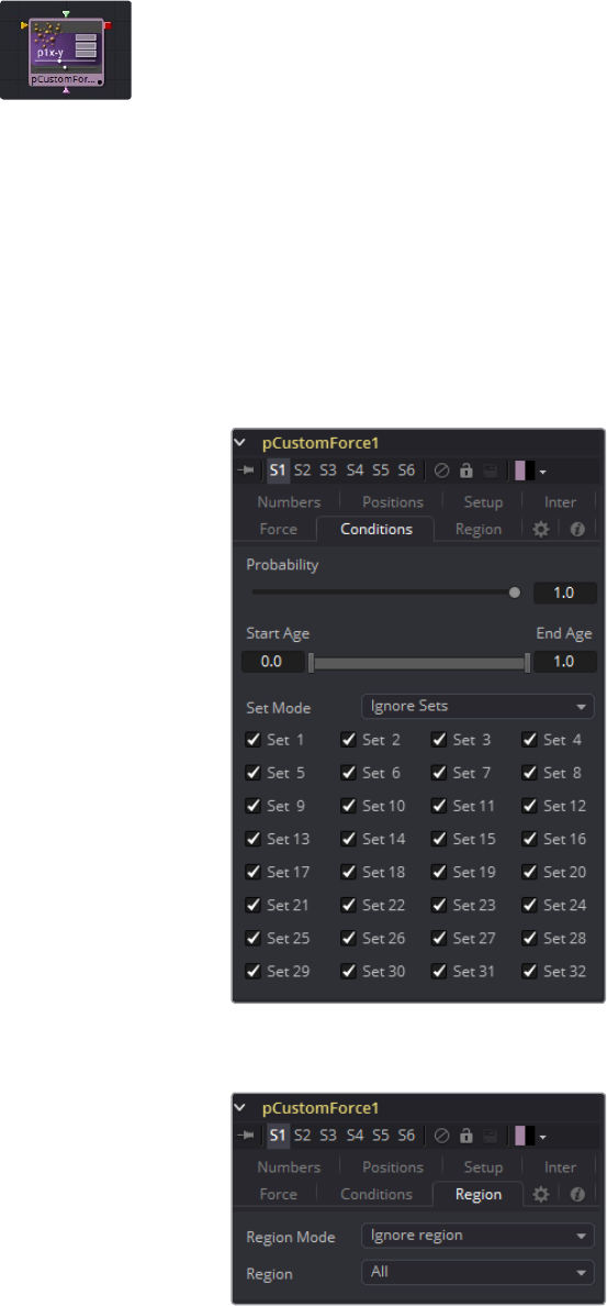
576
Particle Tools Chapter – 24
pCustomForce
The Particle Custom Force tool allows you to change the forces applied to a particle system or
subset. This tool is quite likely the most complex and the most powerful tool in Fusion. Any user
moderately experienced with scripting or C++ programming, should find the structure and
terminology used by the Custom Force tool to be familiar.
The forces on a particle within a system can have their positions and rotations affected by
forces. The position in XYZ and the Torque, which is the spin of the particle, are controlled by
independent custom equations. The Custom Force tool is used to create custom expressions
and filters to modify the behavior. In addition to providing three image inputs, this tool will allow
for the connection of up to eight numeric inputs and as many as four XY position values from
other controls and parameters in the flow.
Conditions Tab
Regions Tab
See Particle Common Controls in the Particles chapter.
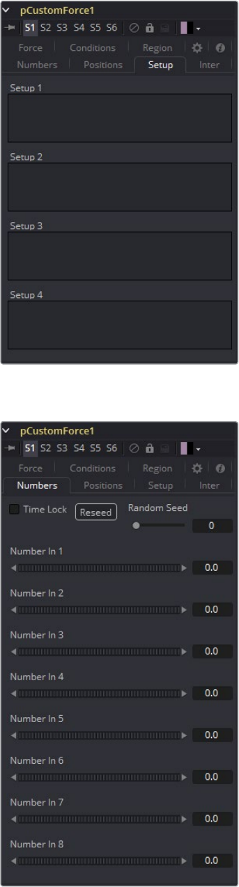
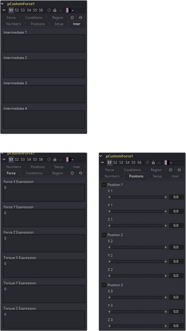
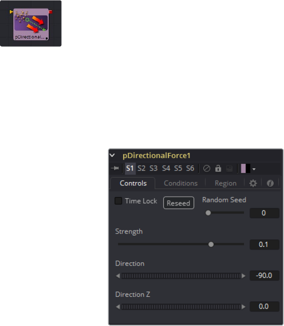
579
Particle Tools Chapter – 24
pDirectionalForce
This tool applies a uni-directional force that pulls the affected particles in a specified direction.
Its primary controls affect the strength of the force, and the angle of the forces pull along the X,
Y and Z axis.
As the most common use of this tool is to simulate gravity, the default direction of the pull is
down along the Y axis (-90 degrees) and the default behavior is to ignore regions and affect all
particles.
Controls Tab
Randomize
The Seed slider and Randomize button are presented whenever a Fusion tool relies on
a random result. Two tools with the same seed values will produce the same random
results. Click on the Randomize button to select a new seed value randomly, or adjust
the slider to select a new seed value manually.
Strength
Determines the power of the force. Positive values will move the Particles in the
direction set by the controls, negative values will move the Particles in the opposite
direction.
Direction
Determines the direction in X/Y Space.
Direction Z
Determines the direction in Z Space.
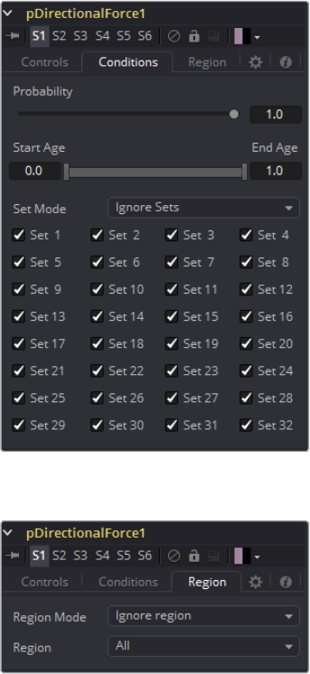
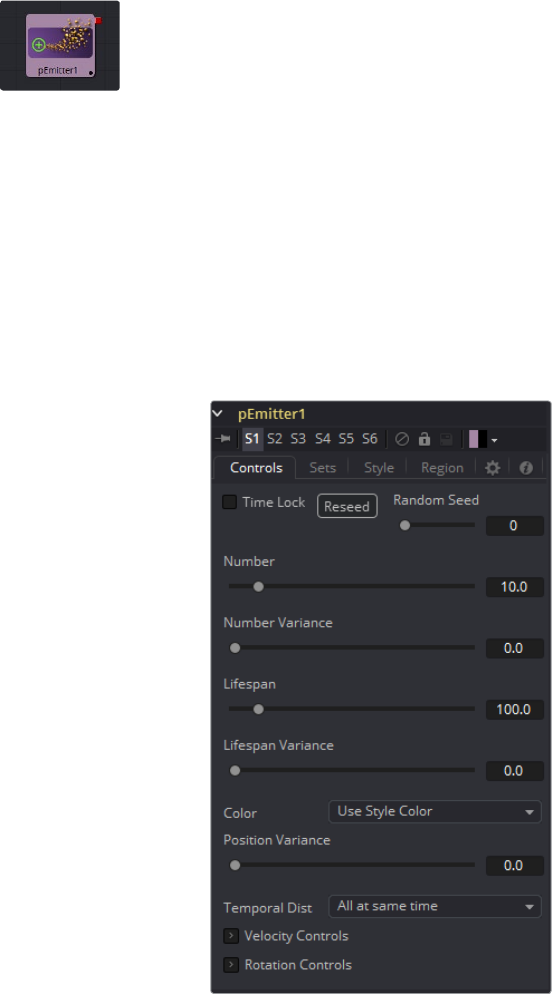
581
Particle Tools Chapter – 24
pEmitter
The pEmitter tool is the main source of Particles (pImageEmitter is another) and will usually be
the first tool used in any new particle system. This tool contains controls for setting the initial
position, orientation and motion of the particles, as well as controls for the visual style of
each particle.
Like all other Particle tools (with the exception of the pRender tool), the pEmitter produces a
particle set, not a visible image, and therefore cannot be displayed directly on a Viewer. To view
the output of a particle system, add a pRender tool after the pEmitter.
Controls Tab
This tab contains settings that affect the physics of the particles emitted by the tool. These
settings do not directly affect the appearance of the particles. They modify behavior like
velocity, spin, quantity and lifespan instead.
Randomize and Random Seed
The Random Seed slider is used to seed all of the variance and random number
generators used by the tool when creating the particle system. Two pEmitter tools with
exactly the same settings for all controls and the same random seed will generate
exactly the same particle system. Changing the random seed will cause variation
between the tools. Click on the Randomize button to automatically set a randomly
chosen value for the Random Seed.
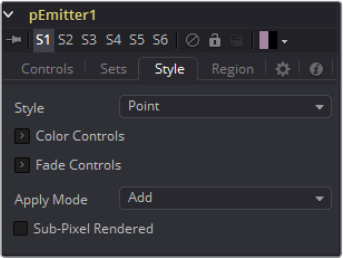
582
Particle Tools Chapter – 24
Style Tab
Number
This control is used to set the amount of new particles generated on each frame. A
value of 1 would cause one new particle to be generated each frame. By frame 10, there
would be a total of 10 particles in existence (unless Particle Lifespan was set to fewer
than 10 frames).
Animate this parameter to specify the number of particles generated in total. For
example, if only 25 particles in total are desired, animate the control to produce five
particles on frame 0-4, then set a key on frame five to generate zero particles for the
remainder of the project.
Number Variance
This modifies the amount of particles generated for each frame, as specified by the
Number control. For example, if Number is set to 10.0 and Number Variance is set to
2.0, the emitter will produce anywhere from 9-11 particles per frame. If the value of
Number Variance is more than twice as large as the value of Number, it is possible that
no particles will be generated for a given frame.
Lifespan
This control determines how long a particle will exist before it disappears or ‘dies.’ The
default value of this control is 100 frames, although this can be set to any value. The
timing of many other particle controls is relative to the Lifespan of the particle. For
example, the size of a particle can be set to increase over the last 80% of its life, using
the Size Over Life graph in the Style tab of the pEmitter.
Lifespan Variance
Like Number Variance, the Lifespan Variance control allows the Lifespan of particles
produced to be modified. If Particle Lifespan was set to 100 frames and the Lifespan
Variance to 20 frames, particles generated by the emitter would have a lifespan of
90-110 frames.
Color Source
This provides the ability to specify from where the color of each particle is derived. The
default setting is Use Style Color, which will provide the color from each particle
according to the settings in the Style tab of the pEmitter tool.
The alternate setting is Use Color From Region, which overrides the color settings from
the Style tab and uses the color of the underlying bitmap region.
The Use Color From Region option only makes sense when the pEmitter region is set to
use a bitmap produced by another tool in the composition. Particles generated in a
region other than a bitmap region will be rendered as white when the Use Color From
Region option is selected.
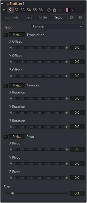
583
Particle Tools Chapter – 24
Position Variance
This control determines whether or not particles can be ‘born’ outside the boundaries
of the pEmitter region. By default, the value is set to zero, which will restrict the creation
area for new particles to the exact boundaries of the defined region. Increasing this
control’s value above 0.0 will allow the particle to be born slightly outside the
boundaries of that region. The higher the value, the ‘softer’ the region’s edge
will become.
Regions Tab
Velocity and Velocity Variance
These determine the initial speed or velocity of new particles. By default, the particle
has no velocity and will not move from its point of origin unless acted upon by outside
forces. A velocity setting of 10.0 would cause the particle to cross the entire width of
the image in one step so a velocity of 1.0 would cause the particle to cross the width of
the image over 10 frames.
Velocity Variance modifies the velocity of each particle at birth, in the same manner
described in Lifespan Variance and Number Variance above.
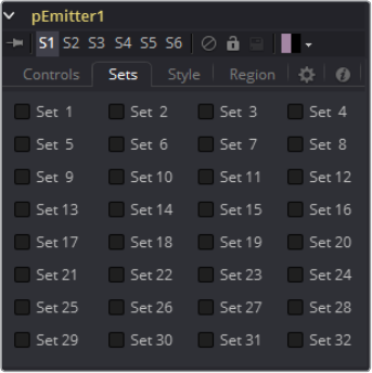
584
Particle Tools Chapter – 24
Angle and Angle Variance
This determines the angle at which particles with velocity applied will be heading at
their birth.
Angle Z and Angle Z Variance
This is as above, except this control determines the angle of the particles along the Z
space axis (toward or away from the camera).
Rotation Mode
This menu control provides two options to help determine the orientation of the
particles emitted. When the particles are spherical, the effect of this control will be
unnoticeable.
Absolute Rotation
The particles will be oriented as specified by the Rotation controls, regardless of
velocity and heading.
Rotation Relative To Motion
The particles will be oriented in the same direction as the particle is moving. The
Rotation controls can now be used to rotate the particle‘s orientation away from
its heading.
Rotation XYZ and Rotation XYZ Variance
These controls allow for Rotation of the individual particles. This can be particularly
useful when dealing with a bitmap particle type, as the incoming bitmap may not be
oriented in the desired direction.
Rotation XYZ Variance can be used to randomly vary the rotation by a specified
amount around the center of the Rotation XYZ value to avoid having every particle
oriented in the exact same direction.
Spin XYZ and Spin Variance
These provide a spin to be applied to each particle at birth. The particles will rotate ‚x‘
degrees each frame, as determined by the value of Spin XYZ.
The Spin XYZ variances will vary the amount of rotation applied to each frame in the
manner described by Number Variance and Lifespan Variance documented above.
Sets Tab
This tab contains settings that affect the physics of the particles emitted by the tool. These
settings do not directly affect the appearance of the particles. They modify behavior like
velocity, spin, quantity and lifespan instead.
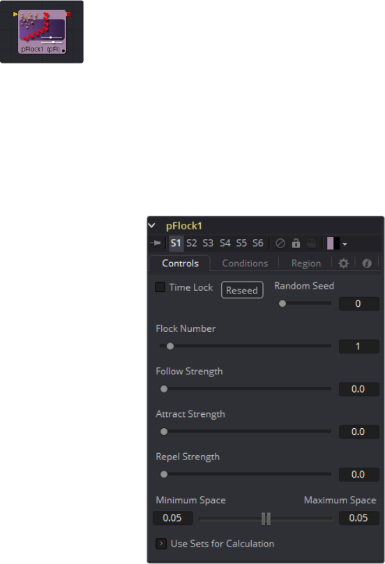
585
Particle Tools Chapter – 24
pFlock
Flocking is a mechanism that can be used to simulate the behavior of organic systems, such as
a flock of birds or a colony of ants. Its use can make an otherwise mindless particle system
appear to be motivated, or acting under the direction of intelligence.
The pFlock tool works through two basic principles. Each particle attempts to stay close to
other particles and each particle attempts to maintain a minimum distance from other particles.
The strength of these desires produces the seemingly motivated behavior perceived by
the viewer.
Controls Tab
Randomize
The Seed slider and Randomize button are presented whenever a Fusion tool relies on
a random result. Two tools with the same seed values will produce the same random
results. Click on the Randomize button to randomly select a new seed value, or adjust
the slider to manually select a new seed value.
Flock Number
The value of this control represents the number of other particles that the affected
particle will attempt to follow. The higher the value, the more visible `clumping’ will
appear to be in the particle system and the larger the groups of particles will
appear to be.
Follow Strength
This value represents the strength of each particle’s desire to follow other particles.
Higher values will cause the particle to appear to expend more energy and effort to
follow other particles. Lower values increase the likelihood that a given particle will
break away from the pack.
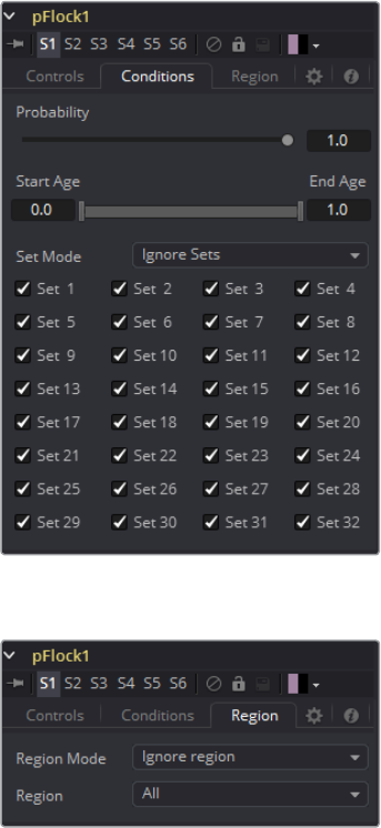
586
Particle Tools Chapter – 24
Attract Strength
This value represents the strength of attraction between particles. When a particle
moves farther from other particles than the Maximum Space defined in the pFlock tool,
it will attempt to move closer to other particles. Higher values cause the particle to
maintain its spacing energetically, resolving conflicts in spacing more rapidly.
Repel Strength
This value represents the force applied to particles that get closer together than the
distance defined by the Minimum Space control of the pFlock tool. Higher values will
cause particles to move away from neighboring particles more rapidly, shooting away
from the pack.
Minimum/Maximum Space
This range control represents the distance each particle attempts to maintain between
it and other particles. Particles will attempt to get no closer or farther than the space
defined by the Minimum/Maximum values of this range control. Smaller ranges will give
the appearance of more organized motion. Larger ranges will be perceived as
disorganized and chaotic.
Conditions Tab
Regions Tab
See Particle Common Controls in the Particles chapter.
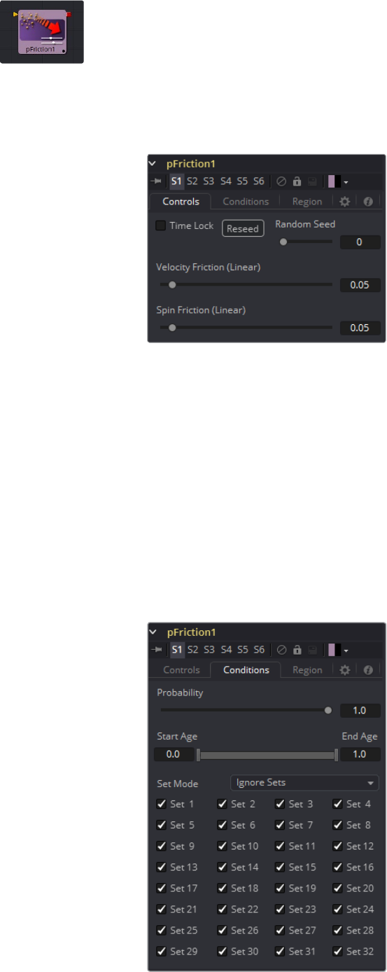
587
Particle Tools Chapter – 24
pFriction
The pFriction tool applies resistance to the motion of a particle, slowing the particle’s motion
through a defined region. This tool produces two types of Friction. One type reduces the
Velocity of any particle intersecting/crossing the defined region, and one reduces or eliminates
spin and rotation.
Controls Tab
Randomize
The Seed slider and Randomize button are presented whenever a Fusion tool relies on
a random result. Two tools with the same seed values will produce the same random
results. Click on the Randomize button to randomly select a new seed value, or adjust
the slider to manually select a new seed value.
Velocity Friction
This value represents the Friction force applied to the particle’s Velocity. The larger the
value, the greater the Friction, thus slowing down the particle.
Spin Friction
This value represents the Friction force applied to the particle’s Rotation or Spin. The
larger the value, the greater the friction, thus slowing down the rotation of the particle.
Conditions Tab
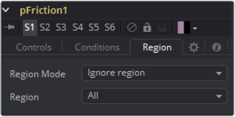
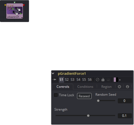
589
Particle Tools Chapter – 24
pGradientForce
The Gradient Force control accepts two inputs, one from a particle system and one from a
bitmap image. The particles are affected by a force generated by the gradients in the alpha
values of the input image. Particles will accelerate along the gradient, moving from white to
black (high values to low).
This tool can be used to give particles the appearance of moving downhill, or of following the
contour of a provided shape.
Controls Tab
Randomize
The Seed slider and Randomize button are presented whenever a Fusion tool relies on
a random result.
Two tools with the same seed values will produce the same random results. Click on
the Randomize button to randomly select a new seed value, or adjust the slider to
manually select a new seed value.
Strength
Gradient Force has only one specific control, it affects the strength of the force and
acceleration applied to the particles. Negative values on this control will cause the
Gradient Force to be applied from black to white (low values to high values).
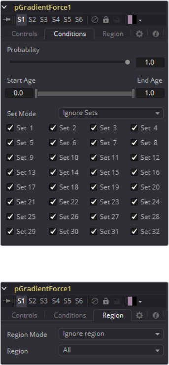
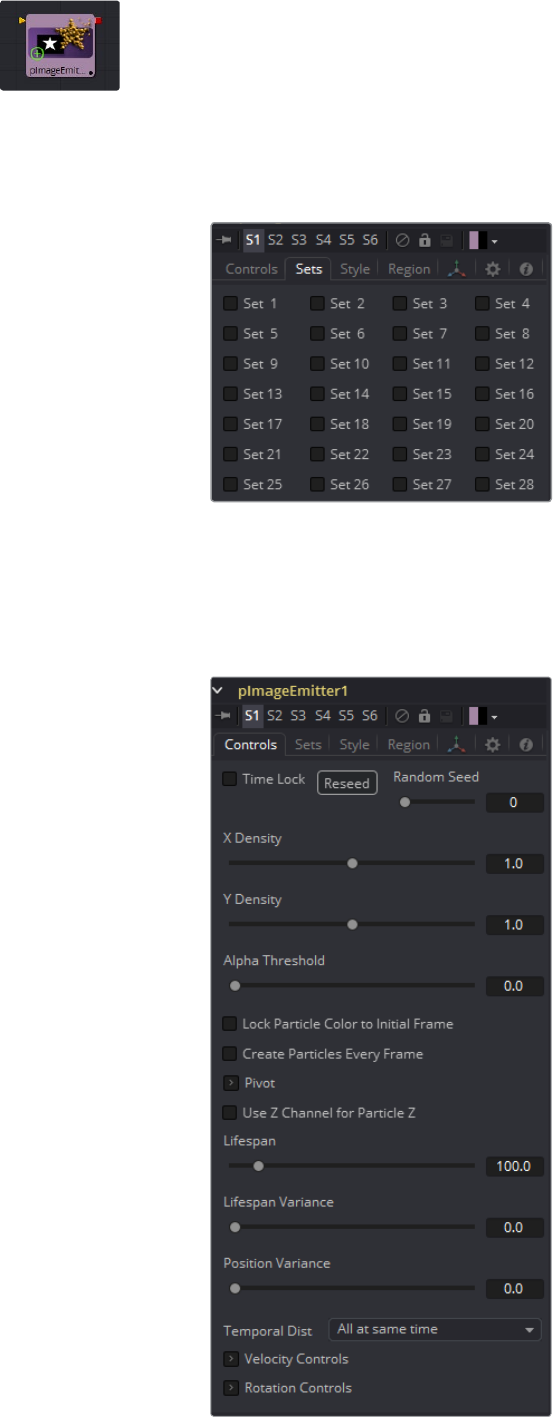
591
Particle Tools Chapter – 24
pImageEmitter
The pImageEmitter tool takes an input image and treats each pixel of the image as if it were a
particle. The main differences between the pImageEmitter and the normal pEmitter is that
instead of emitting particles randomly within a given region, this tool emits pixels in a regular 2D
grid with colors based on the input image.
Sets Tab
Controls Tab
The great majority of controls in this tool are identical to those found in the pEmitter, and those
controls are documented there. Below are the descriptions of the controls unique to the
pImageEmitter tool.
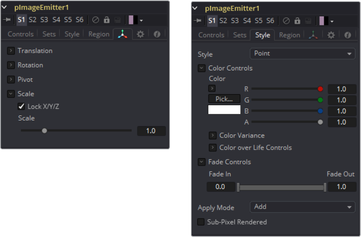
592
Particle Tools Chapter – 24
X and Y Density
The X and Y Density sliders are used to set the mapping of particles to pixels for each
axis. They control the density of the sampling grid. A value of 1.0 for either slider
indicates 1 sample per pixel. Smaller values will produce a looser, more pointillistic
distribution of particles, while values above 1.0 will create multiple particles per pixel in
the image.
Alpha Threshold
The Alpha Threshold is used for limiting particle generation so that pixels with semi-
transparent alpha values will not produce particles. This can be used to harden the
edges of an otherwise soft alpha channel. The higher the threshold value, the more
opaque a pixel has to be before it will generate a particle. Note that the default
threshold of 0.0 will create particles for every pixel, regardless of alpha, though many
may be transparent and invisible.
Lock Particle Color to Initial Frame
Select this checkbox to force the particles to keep the color with which they were born
throughout the life of the particle. If this is off, and the input image changes on
successive frames, the particles will also change color to match the image. This allows
video playback on a grid of particles.
Create Particles Every Frame
Enabling this creates a whole new set of particles every frame, instead of just one set
on the frame. This can lead to very large particle systems, but allows some interesting
effects, for example, if the particles are given some initial velocity or if emitting from an
animated source. Try a small velocity, Angle Z of -90 and a seething Fast Noise as a
source, to get smoothly-varying clouds of particles that you could fly through. Note that
if this checkbox is left off, only one set of particles is ever created, and thus animating
any of the emitter’s other controls will have no effect.
X/Y/Z Pivot
These controls allow you to position the grid of emitted particles.
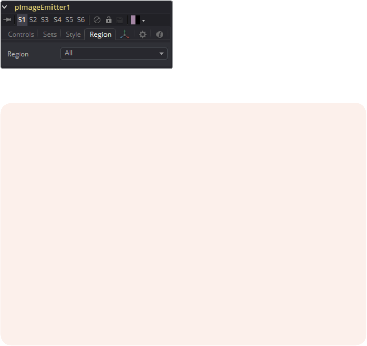
593
Particle Tools Chapter – 24
Use Z Channel for Particle Z
If the input image used to generate the particles has a Z depth channel, that channel
can be used to determine the initial position of the particle in Z space. This can have an
interesting hollow shell effect when used in conjunction with camera rotation in the
pRender tool.
Regions Tab
See Particle Common Controls in the Particles chapter.
NOTES: Pixels with a black (transparent) alpha channel will still generate
invisible particles, unless you raise the Alpha Threshold above 0.0. This can
slow down rendering significantly.
An Alpha Threshold value of 1/255 = 0,004 is good for eliminating all fully-
transparent pixels.
The pixels are emitted in a fixed-size 2D grid on the XY plane, centered on the
Pivot position. Changing the Region from the default of All allows you to
restrict particle creation to more limited areas. If you need to change the size
of this grid, use a Transform 3D tool after the pRender.
Remember that the various emitter controls apply only to particles when they
are emitted. That is, they set the initial state of the particle, and do not affect it
for the rest of its lifespan. Since pImageEmitter (by default) emits particles only
on the first frame, animating these controls will have no effect. However, if the
Create Particles Every Frame checkbox is turned on, new particles will be
emitted each frame, and will use the specified initial settings for that frame.
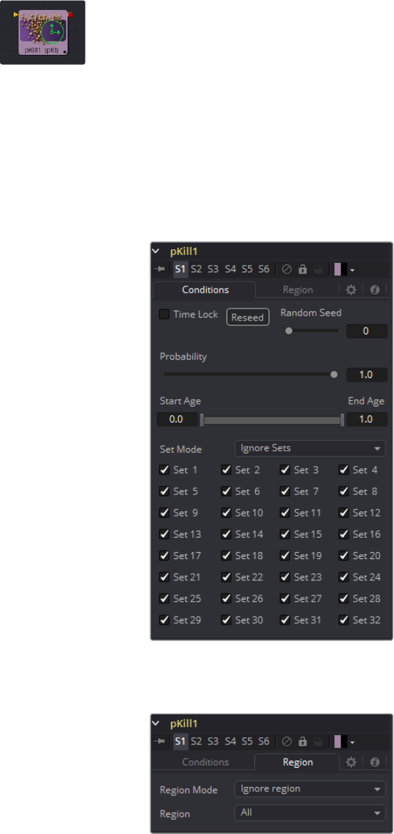
594
Particle Tools Chapter – 24
pKill
The great majority of controls in this tool are identical to those found in the pEmitter, and those
controls are documented there. Below are the descriptions of the controls unique to the
pImageEmitter tool.
The Kill tool is used to destroy (kill) any particle that crosses or intersects its region. It has no
specific controls, as it has only one possible affect on a particle. The controls found in the
Region tab are normally used to limit this tool, by restricting the effect to particles which fall
within a certain region, age, set, or by reducing the probability of the tool applying to a
given particle.
Conditions Tab
Regions Tab
See Particle Common Controls in the Particles chapter.
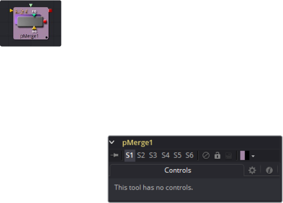
595
Particle Tools Chapter – 24
pMerge
This tool has no controls whatsoever. It serves to combine particles from two streams. Any tools
downstream of the Particle Merge tool will treat the two streams as one.
The combined particles will preserve any sets assigned to them when they were created,
making it possible for tools downstream of the pMerge to isolate specific particles when
necessary.
Control Tab
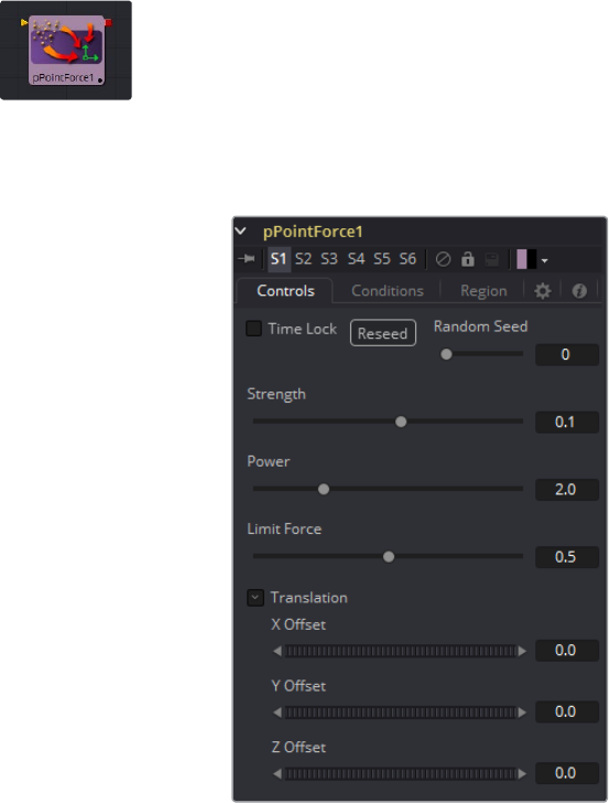
596
Particle Tools Chapter – 24
pPointForce
This tool applies a force to the particles that emanates from a single point in 3D space. The
pPointForce can either attract or repel particles within its sphere of influence. There are four
controls specific to the pPointForce tool.
Control Tab
Randomize
The Seed slider and Randomize button are presented whenever a Fusion tool relies on
a random result. Two tools with the same seed values will produce the same random
results. Click on the Randomize button to randomly select a new seed value, or adjust
the slider to manually select a new seed value.
Strength
This parameter sets the Strength of the force emitted by the tool. Positive values
represent attractive forces. Negative values represent repellent forces.
Power
This determines the degree to which the Strength of the force falls off over distance.
Avalue of zero causes there to be no falloff of strength. Higher values will impose an
ever-sharper falloff in strength of the force with distance.
Limit Force
The Limit Force control is used to counter-balance potential problems with temporal
sub-sampling. Because the position of a particle is only sampled once a frame (unless
sub-sampling is increased in the pRender tool), it is possible that a particle can
overshoot the Point Force’s position and end up getting thrown off in the opposite
direction. Increasing the value of this control reduces the likelihood that this will happen.
X, Y, Z Center Position
These controls are used to represent the X, Y, and Z coordinates of the point force
in 3D space.
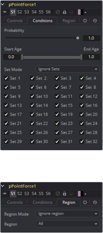
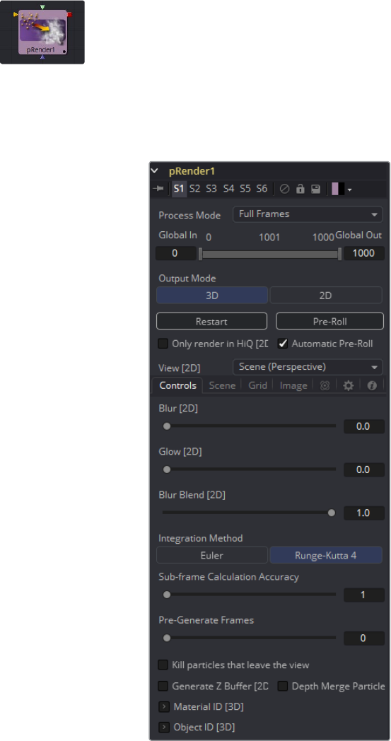
598
Particle Tools Chapter – 24
pRender [PRN]
The pRender tool converts the particle system to either an image or geometry. The default is a
3D particle system, which must be connected to a Renderer 3D to produce an image. This
allows the particles to be integrated with other elements in a 3D scene before they are
rendered.
Control Tab
Output Mode (2D/3D)
While the pRender defaults to 3D output, it can be made to directly render a 2D image
instead, as with DF4. This is done with the 3D and 2D buttons on the Output Mode
control. If the pRender is not connected to a 3D-only or 2D-only tool, you can also
switch it by selecting View > 2D Viewer from the display view’s context menu.
In 3D mode, the only controls in the pRender tool that have any affect at all are Restart,
Pre-roll and Automatic Pre-Roll, Sub-Frame Calculation Accuracy and Pre-Generate
frames. The remaining controls affect 2D particle renders only. The pRender tool also
has a Camera input on the flow that allows connection of a 3D}} /Camera 3D |Camera
3D tool. This can be used in both 2D and 3D modes to allow control of the viewpoint
used to render an output image.
599
Particle Tools Chapter – 24
Render and the Display Views
When the pRender tool is selected in a flow, all of the onscreen controls from particle
tools connected to it are presented in the display views. This provides a fast,
easy-to-modify overview of the forces applied to the particle system as a whole.
Pre-Roll Options
Particle tools generally need to know the position of each particle on the last frame
before they can calculate the affect of the forces applied to them on the current frame.
This makes changing current time manually by anything but single frame intervals likely
to produce an inaccurate image.
The controls here are used to help accommodate this by providing methods of
calculating the intervening frames.
Restart
This control also works in 3D. Clicking on the Restart button will restart the particle
system at the current frame, removing any particles created up to that point and starting
the particle system from scratch at the current frame.
Pre-Roll
This control also works in 3D. Clicking on this button will cause the particle system to
recalculate, starting from the beginning of the render range up to the current frame. It
will not render the image produced. It will only calculate the position of each particle.
This provides a relatively quick mechanism to ensure that the particles displayed in the
views are correctly positioned.
If the pRender tool is displayed when the Pre-Roll button is selected, the progress of
the pre-roll is shown in the display view, with each particle shown as point style only.
Automatic Pre-Roll
Selecting the Automatic Pre-Roll checkbox causes the particle system to automatically
pre-roll the particles to the current frame whenever the current frame changes. This
prevents the need to manually select the Pre-Roll button whenever advancing through
time in jumps larger than a single frame. The progress of the particle system during an
Automatic Pre-Roll is not displayed to the views, to prevent distracting visual
disruptions.
About Pre-Roll
Pre-Roll is necessary because the state of a particle system is completely dependent on the
last known position of the particles. If the current time were changed to a frame where the last
frame particle state is unknown, the display of the particle is calculated on the last known
position, producing inaccurate results.
To demonstrate, add a pEmitter and pRender tool to the composition. View the pEmitter in one
of the display views. Right-click in the display view and select Views > 2D Viewer from the
context menu.
Set the Velocity of the particles to 0.1. Place the pEmitter on the left edge of the screen and set
the Current Frame to 0. Set a Render Range from 0-100 and press the Play button. Observe
how the particle system behaves.
Stop the playback and return the current time to frame 0. Make sure that the Automatic Pre-Roll
option is off in the pRender tool. Now try jumping from frame 0 to 10, then to frame 60 and 90.
Do not pass through the frames in between. Use the current time edit control or click in the
ruler directly to jump straight to the frame.
600
Particle Tools Chapter – 24
See how the particle system only adds to the particles it has already created and does not try
to create the particles that would have been emitted in the intervening frames. Try selecting the
Pre-Roll button in the Pre-Render tool. Now the particle system state is represented correctly.
For simple, fast rendering particle systems, it is recommended to leave the Automatic Pre-Roll
option on. For slower particle systems with long time ranges, it may be desirable to only
Pre-Roll manually, as required.
Only Render in Hi-Q
Selecting this checkbox causes the style of the particles to be over-ridden when the
Hi-Q checkbox is de-selected, producing only fast rendering Point style particles. This
is useful when working with a large quantity of slow Image-based or Blob-style
particles. To see the particles as they would appear in a final render, simply enable the
Hi-Q checkbox.
View
This drop-down list provides options to determine the position of the camera view in a
3D particle system. The default option of Scene (Perspective) will render the particle
system from the perspective of a virtual camera, the position of which can be modified
using the controls in the Scene tab. The other options provide orthographic views of
the front, top and side of the particle system.
It is important to realize that the position of the onscreen controls for particle tools is
unaffected by this control. In 2D mode the onscreen controls are always drawn as if the
display view were showing the front orthographic view. (3D mode gets the position of
controls right at all times.)
The View setting is ignored if a Camera 3D tool is connected to the pRender tool’s
Camera input on the Flow, or if the pRender is in 3D mode.
Output Mode
Blur, Glow and Blur Blend
These sliders apply a Gaussian blur, glows and blur blending to the image as it is
rendered, which can be used to soften the particles and blend them together. The end
result is no different than adding a Blur after the pRender tool in the flow. For 2D
particles only.
Sub Frame Calculation Accuracy
This determines the number of sub-samples taken between frames when calculating
the particle system. Higher values will increase the accuracy of the calculation but also
increase the amount of time taken to render the particle system.
Pre-Generate Frames
This control is used to cause the particle system to pre-generate a set number of
frames before its first valid frame. This is used to give a particle system an initial state
from which to start.
A good example of when this might be useful is in a shot where particles are used to
create the smoke rising from a chimney. Pre-Generate Frames would be set to a
number high enough to ensure that the smoke is already present in the scene before
the render begins, rather than having it just starting to emerge from the emitter for the
first few frames.
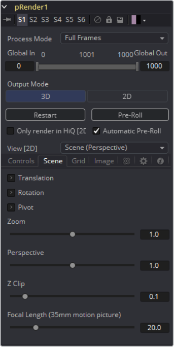
601
Particle Tools Chapter – 24
Kill Particles that Leave the View
Selecting this checkbox control will automatically destroy any particles that leave the
visible boundaries of the image. This can help to speed render times. Particles
destroyed in this fashion will never return, regardless of any external forces acting
upon them.
Generate Z Buffer
Selecting this checkbox will cause the pRender tool to produce a Z Buffer channel in
the image. The depth of each particle is represented in the Z Buffer. This channel can
then be used for additional depth operations like Depth Blur, Depth Fog, and
Downstream Z Merging.
Enabling this option is likely to increase the render times for the particle system
dramatically.
Depth Merge Particles
Enabling this option will cause the particles to be merged together using Depth Merge
techniques, rather than layer-based techniques.
Scene Tab
Z Clip
The Z Clip control is used to set a clipping plane in front of the camera. Particles that
cross this plane are clipped, preventing them from impacting on the virtual lens of the
camera and dominating the scene.
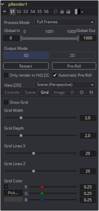
602
Particle Tools Chapter – 24
Grid Tab
None of the controls in this tab have any effect on 3D particles.
The Grid is a helpful, non-rendering display guide used to orient the 2D particles in 3D space.
The grid is never seen in renders, just like a center crosshair is never seen in a render. The
width, depth, number of lines and grid color can be set using the controls found in this tab.
These controls cannot be animated.
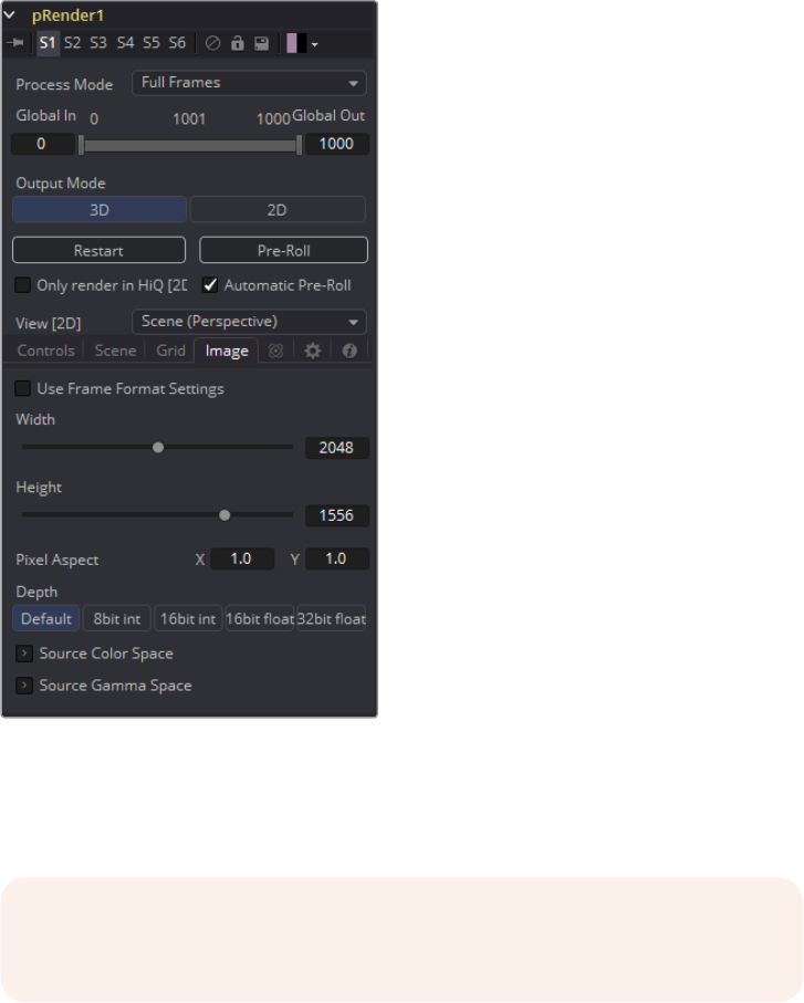
603
Particle Tools Chapter – 24
Image Tab
The controls in the Image tab of this tool determine the width, height and aspect of the image.
Refer to the Creator Common Controls page for details on the use of these controls.
Motion Blur
As with other 2D tools in Fusion, Motion Blur is enabled from within the Fusion tab. You
may set Quality, Shutter Angle, Sample Center and Bias, and Blur will be applied to all
moving particles.
NOTE: Motion Blur on 3D mode particles (rendered with a Renderer 3D) also
requires that identical motion blur settings are applied to the Renderer 3D tool.
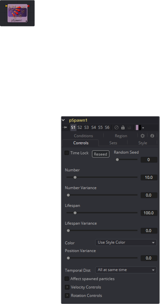
604
Particle Tools Chapter – 24
pSpawn [PSP]
The pSpawn tool makes each affected particle act as an emitter that can produce one or more
particles of its own. The original particle continues until the end of its own lifespan, and each of
the particles it emits becomes wholly independent with a lifespan and properties of its own.
As long as a particle falls under the effect of the pSpawn tool, it will continue to generate
particles. It is important to restrict the effect of the tool with limiters like Start and End Age,
Probability, Sets and Regions, and by animating the parameters of the emitter so that the tool is
operative only when required.
Control Tab
The pSpawn tool has a large number of controls, most of which exactly duplicate those found
within the pEmitter tool. There are a few controls that are unique to the pSpawn tool, and their
effects are described below.
Affect Spawned Particles
Selecting this checkbox causes particles created by spawning to also become affected
by the Spawn tool on subsequent frames. This can exponentially increase the number
of particles in the system, driving render times up to an unreasonable degree. Use this
checkbox cautiously.
Velocity Transfer
This control determines how much velocity of the source particle is transferred to the
particles it spawns. The default value of 1.0 causes each new particle to adopt 100
percent of the velocity and direction from its source particle. Lower values will transfer
less of the original motion to the new particle.
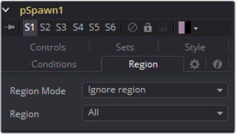
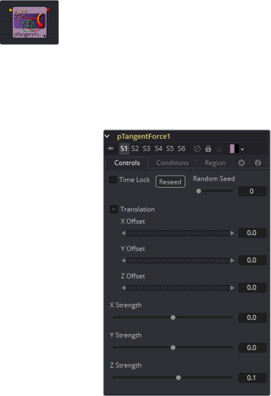
606
Particle Tools Chapter – 24
pTangentForce [PTF]
This tool is used to apply a tangential force to the particles, a force that is applied
perpendicularly to the vector between the pTangentForce’s region and the particle it is
affecting.
The controls for this tool are used to position the offset in 3D space and to determine the
strength of the tangential force along each axis independently.
Control Tab
Randomize
The Seed slider and Randomize button are presented whenever a Fusion tool relies on
a random result.
Two tools with the same seed values will produce the same random results. Click on
the Randomize button to randomly select a new seed value, or adjust the slider to
manually select a new seed value.
X, Y, Z Center Position
These controls are used to represent the X, Y, and Z coordinates of the Tangent force
in 3D space.
X, Y, Z Center Strength
These controls are used to determine the Strength of the Tangent force in 3D space.
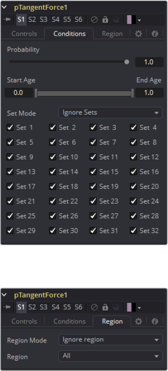
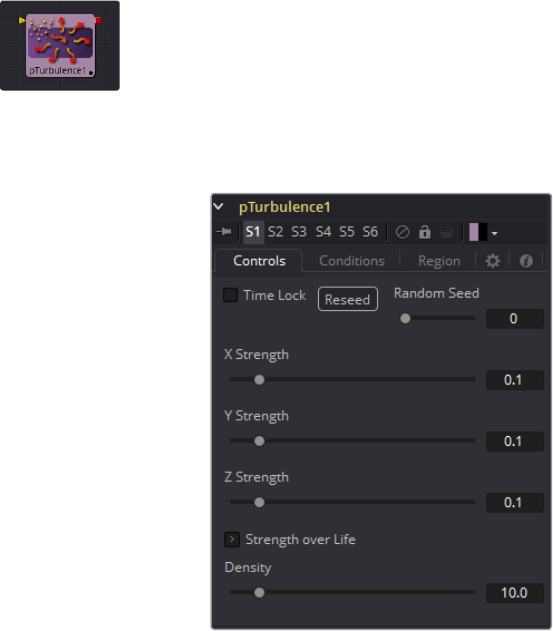
608
Particle Tools Chapter – 24
pTurbulence [PTR]
The pTurbulence tool imposes a frequency-based chaos on the position of each particle,
causing the motion to become unpredictable and uneven. The controls for this tool affect the
strength and density of the Turbulence along each axis.
Control Tab
Randomize
The Seed slider and Randomize button are presented whenever a Fusion tool relies on
a random result. Two tools with the same seed values will produce the same random
results. Click on the Randomize button to randomly select a new seed value, or adjust
the slider to manually select a new seed value.
X, Y and Z Strength
The Strength control affects the amount of chaotic motion imparted to particles.
Strength Over Life
This LUT control can be used to control the amount of turbulence applied to a particle
according to its age. For example, a fire particle may originally have very little
turbulence applied at the start of its life, and as it ages, the turbulence increases.
Density
Use this control to adjust the density of the turbulence. Higher values will produce finer
variations in the turbulence produced.
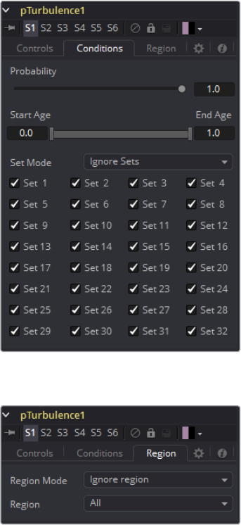
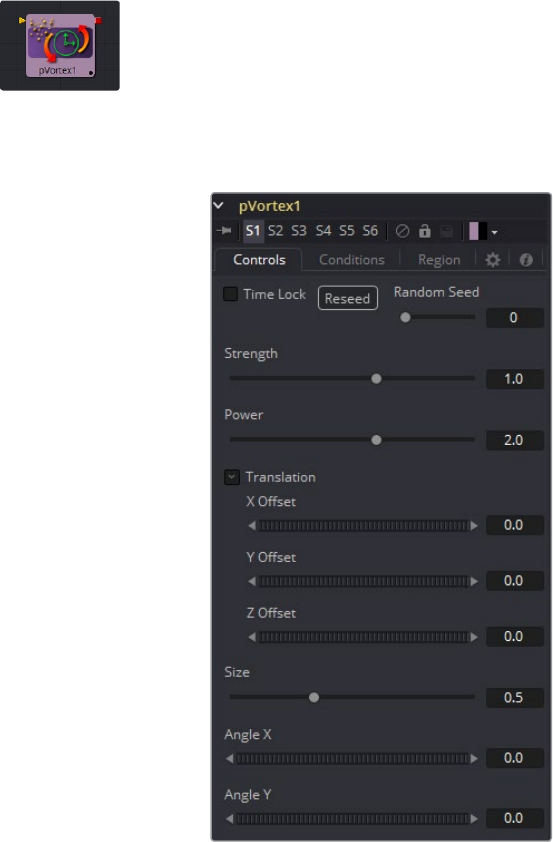
610
Particle Tools Chapter – 24
pVortex [PVT]
The pVortex tool applies a rotational force to each particle, causing them to be drawn toward
the source of the Vortex. In addition to the Common Particle Controls, the pVortex tool also has
the following controls.
Control Tab
Randomize
The Seed slider and Randomize button are presented whenever a Fusion tool relies on
a random result. Two tools with the same seed values will produce the same random
results. Click on the Randomize button to randomly select a new seed value, or adjust
the slider to manually select a new seed value.
Strength
This control determines the Strength of the Vortex Force applied to each particle.
Power
This control determines the degree to which the Strength of the Vortex Force falls off
with distance.
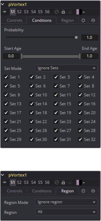
611
Particle Tools Chapter – 24
X, Y, and Z Offset
Use these sliders to set the amount by which the vortex Offsets the affected particles.
Size
Used to set the Size of the vortex force.
Angle X and Y
These sliders control the amount of rotational force applied by the Vortex along the X
and Y axis.
Conditions Tab
Regions Tab
See Particle Common Controls in the Particles chapter.
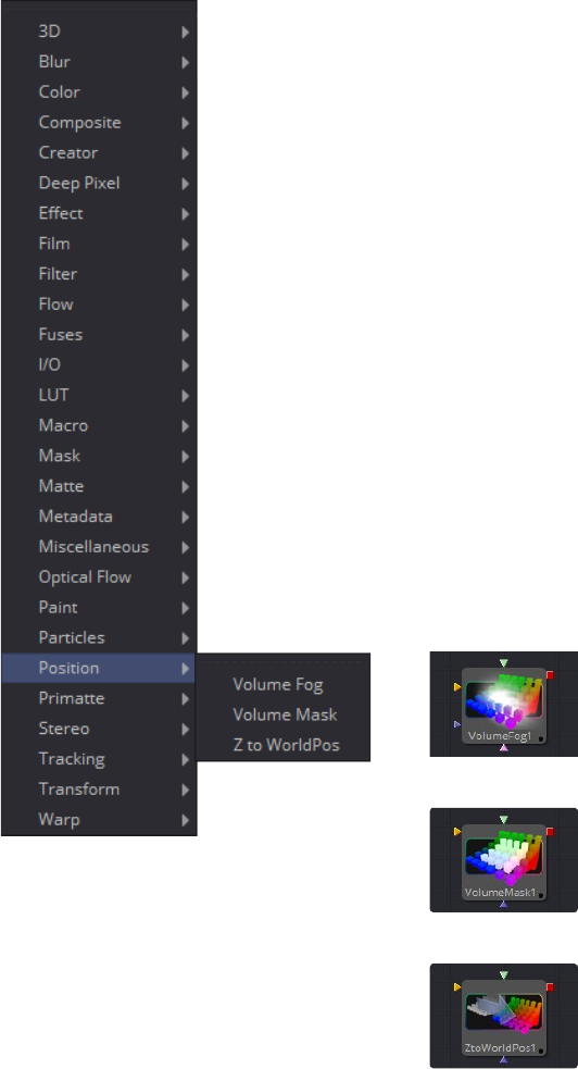
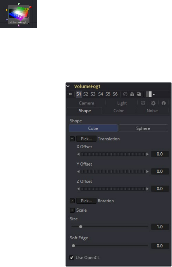
615
Position Tools Chapter – 25
Volume Fog [VLF]
The Volume Fog tool is used to create sophisticated volumetric fog on images containing XYZ
Position channels.
As opposed to 3D-rendered volumetric Fog, it works on 2D images and delivers much faster
results and interactive feedback when setting up the fog. See the WPP Concepts section for
further explanation on how this technology works and to learn about the required imagery.
Shape Tab
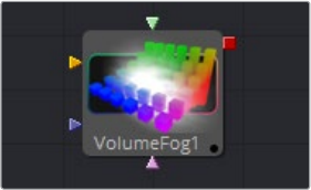
616
Position Tools Chapter – 25
External Inputs
The following inputs appear on the tool’s tile in the Flow Editor.
VolumeFog.Image: [orange, required] This input expects an image containing a World
Position Pass in the XYZ Position channels.
VolumeFog.FogImage: [green, optional] For creating volumetric fog with varying depth
and extent; an image sequence can be connected here.
VolumeFog.EffectMask: [blue, optional] The standard Effect Mask input as found on
other Fusion tools.
VolumeFog.SceneInput: [pink, optional] This input expects a 3D scene containing a
3D Camera.
Shape
Toggle between a basic spherical or rectangular volume to be placed in your image.
These Volumes can then be further refined by means of the MaskImage or
MaskImage sequence.
Translation Pick
Left-click and hold this button to pick XYZ coordinates from any 3D scene or 2D image
containing XYZ values, such as a rendered World Pass, to position the center of the
Volume object. When picking from a 2D image, make sure it’s rendered in 32-bit float to
get full precision.
X, Y, Z Offset
These controls can be used to position the center of the fog volume manually or can be
animated or connected to other controls in Fusion.
Rotation Pick
Left-click and hold this button to pick rotational values from any 3D Scene or 2D image
containing those values, like an XYZ-Normal-Pass, to re-orient the volume.
When picking from a 2D image, like an XYZ-Normal-pass, make sure it’s rendered in
32-bit float to get full precision and accurate rotational values.
X, Y, Z Rotation
Use these controls to rotate the Volume around its center.
X, Y, Z Scale
Scale the Volume in any direction from its center to further refine the overall Size value
specified below.
Size
The overall Size of the volume created.
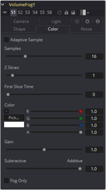
617
Position Tools Chapter – 25
Soft Edge
Controls how much the Volume is faded toward the center from its perimeter to achieve
a softer look.
Use OpenCL
Introduced with Fusion’s OpenCL Supercomputing, this option renders the effect on
the GPU rather than on the CPU. Depending on the graphics card used in the
computer, this can boost the speed of the tool by a factor of 30 or more.
Color Tab
Samples
Determines how many times a “ray” shot into the volume will be evaluated before the
final image is created. Not unlike raytracing, higher values lead to more detail inside the
volume but also increase render times.
Z Slices
The higher this value, the more images from the connected MaskImage sequence will
be used to form the Depth of the Volume.
You can, for example, use a FastNoise with a high Seethe Rate to create such a
sequence of images. Be careful with the resolution of the images though. Higher
resolutions can require a large amount of memory. As a rule of thumb, a resolution of
256 x 256 pixels with 256 Z Slices (i.e., forming a 256 x 256 x 256 cubic volume, which
will use up to 256MB for full color 32-bit float data) should give you a good
starting point.
First Slice Time
Determines which frame of the Global Range is used to deliver the first slice from the
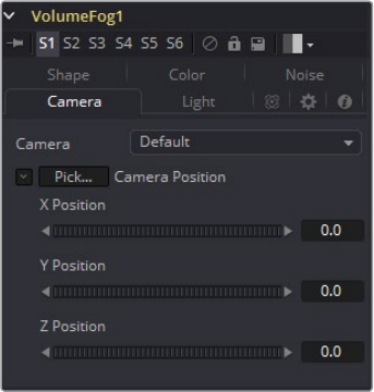
618
Position Tools Chapter – 25
connected MaskImage sequence.
Make sure that both GlobalIn and GlobalOut as well as the valid range of your source
tool fall within the range of FirstSliceTime + Z Slices.
Color
Allows you to modify the color of the Fog generated. This will multiply over any color
provided by the connected MaskImage.
Gain
Increases or decreases intensity of the fog created. More Gain will lead to a stronger
glow and less transparency in the fog. Lower values let the fog appear less dense.
Subtractive/Additive Slider
Similar to the Merge tool, this value controls if the fog is composed onto the image in
additive or subtractive mode, leading to brighter or dimmer appearance of the fog.
Fog Only
Outputs the generated fog on a black background which then can be composited
manually, or used as a mask on a Color Corrector for further refinement.
Camera Tab
For a perfect evaluation of a Volume, a Camera or 3D scene can be connected to the Scene
input of the tool.
Camera
If multiple Cameras are available in the connected Scene input, this drop-down allows
the user to choose the correct Camera needed to evaluate the Volume. Instead of
connecting a Camera, position values can be provided manually or by connecting the
XYZ values to other controls.
Translation Pick
Left-click and hold this button to pick XYZ coordinates from any 3D scene or 2D image
containing XYZ values, like a rendered World Pass, to define the center of the Camera.
When picking from a 2D image, make sure it’s rendered in 32-bit float to get full
precision.
X, Y, Z Offset
These controls can be used to define the center of the Camera manually or can be
animated or connected to other controls in Fusion.
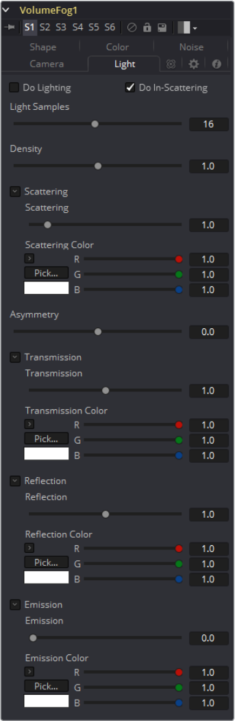
620
Position Tools Chapter – 25
Do Lighting
Enables or disables lighting calculations. Keep in mind that when not using OpenCL
(i.e., rendering on the CPU), these calculations may become a bit slow.
Do In-Scattering
Enables or disables light scattering calculations. The volume will still be lit according to
the state of the Do Lighting checkbox, but scattering will not be performed.
Light Samples
Determines how accurate the lighting is calculated. Higher values mean more accurate
calculation at the expense of higher render times.
Density
This is similar to Scattering in that it makes the fog appear thicker. With a high amount
of scattering, though, the light will be scattered out of the volume before it has had
much chance to travel through the fog, meaning it won’t pick up a lot of the
transmission color. With a high density instead, the fog still appears thicker, but the light
gets a chance to be transmitted, thus picking up the transmission color before it gets
scattered out. Scattering is affected by the light direction when Asymmetry is not 0.0.
Density is not affected by light direction at all.
Scattering
Determines how much of the light bouncing around in the volume ends up scattering
the light out of the fog. If the light scatters more, or more accurately, then there’s a
higher probability of the light being scattered out of the volume, hence less light is left
to continue on through the fog. This option can make the fog seem denser.
Asymmetry
Determines in what direction the light is scattered. A value of 0 produces uniform, or
isotropic, scattering, meaning all directions have equal probability. A value greater than
0 causes “forward scattering,” meaning the light is scattered more into the direction of
the light rays. This is similar to what happens with water droplets in clouds. A value
smaller than 0 produces “back scattering,” where the light is more scattered back
toward the original light source.
Transmission
Defines the color that is transmitted through the fog. Light that doesn’t get scattered
out will tend toward this color. It is a multiplier, though, so if you have red light, but blue
transmission, you won’t see any blue.
Reflection
Changes the intensity of the light that is scattered out. It can be used to modify the
overall color before Emission is added. This will be combined with the color channels of
the volume texture and then used to scale the values. The color options and the color
channels of the volume texture are multiplied together, so if the volume texture was
red, setting the Reflection color options to blue would not make the result blue. In such
a case they will multiply together to produce black.
Emission
This adds a bit of “glowing” to the fog, or adding energy/light back into the calculation.
In fact, if there are no lights in the scene, and the fog emission is set to be 1.0, the
results are similar to no lighting, like turning off the Do Lighting option. Glowing can also
be done while producing a different kind of look, by having a Transmission greater than
1. This, however, would never actually happen in the real world.
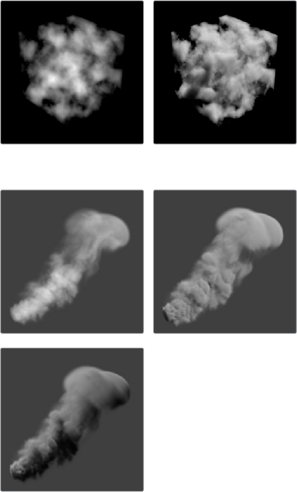
621
Position Tools Chapter – 25
Examples
In these examples we are looking at a volume from the outside. On the right you see
how the VolumeFog looks with straight accumulation. That means the “Do Lighting”
option is turned off.
On the right, you see the same volume with lighting/scattering turned on and a single
point light. Here we have a slightly more complex Volume.
On the left with straight accumulation, in the middle with lighting, scattering and a
single point light. On the right the actual light in the scene has been moved, which also
influences the look of the volume.
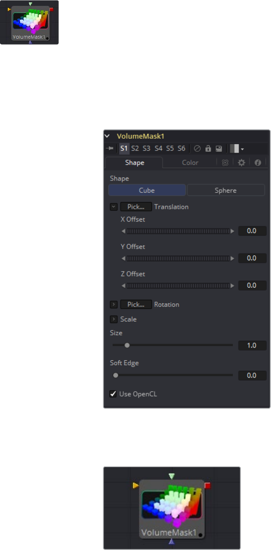
622
Position Tools Chapter – 25
Volume Mask [VLM]
The Volume Mask tool is used to create volumetric masks from images containing
XYZPosition channels.
This can, for example, be used to isolate objects for color correction without the need to track
or roto the scene. See the WPP Concepts section for further explanation on how this
technology works and to learn about the required imagery.
Shape Tab
External Inputs
The following inputs appear on the tools tile in the Flow Editor.
VolumeFog.Image: [orange, required] This input expects an image containing a World
Position Pass in the XYZ Position channels.
VolumeFog.MaskImage: [green, optional] For refining the mask, an image can be
connected here.
623
Position Tools Chapter – 25
VolumeFog.EffectMask: [blue, optional] The standard Effect Mask input as found on
other Fusion tools.
VolumeFog.SceneInput: [pink, optional] This input expects a 3D scene input
containing a 3D Camera.
Shape
Toggle between a basic spherical or rectangular Mask to be placed in your image. The
Mask can be further refined by means of the MaskImage.
Translation Pick
Left-click and hold this button to pick XYZ coordinates from any 3D scene or 2D image
containing XYZ values, like a rendered World Pass, to position the center of the
volumetric Mask. When picking from a 2D image make sure it’s rendered in 32-bit float
to get full precision.
X, Y, Z Offset
These controls can be used to position the center of the Mask manually or can be
animated or connected to other controls in Fusion.
Rotation Pick
Left-click and hold this button to pick rotational values from any 3D scene or 2D image
containing those values, like an XYZ-Normal-Pass, to re-orient the Mask.
When picking from a 2D image, like an XYZ-Normal-pass, make sure it’s rendered in
32-bit float and WorldSpace coordinates to get full precision and the correct
rotational values.
X, Y, Z Rotation
Use these controls to rotate the Mask around its center.
X, Y, Z Scale
Scale the Mask in any direction from its center to further refine the overall Size value
specified below.
Size
The overall Size, in X, Y and Z, of the Mask created.
Soft Edge
Controls how much the Volume is faded toward the center from its perimeter to achieve
a softer look.
Use OpenCL
Introduced with Fusion’s OpenCL Supercomputing, this option renders the effect on
the GPU rather than on the CPU. Depending on the graphics card used in the
computer, this can boost the speed of the tool by a factor of 30 or more.
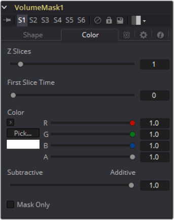
624
Position Tools Chapter – 25
Color Tab
Color
Allows user to modify the color of the Mask generated. This will add to any color
provided by the connected MaskImage.
Subtractive/Additive Slider
Similar to the Merge tool, this value controls if the Mask is composed onto the image in
Additive or Subtractive mode, leading to brighter or dimmer appearance of the Mask.
Mask Only
Outputs the generated Mask on a black background, which then can be used as a
mask on a Color Corrector for further refinement.
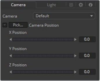
625
Position Tools Chapter – 25
Camera Tab
For a perfect evaluation of a Volume, a Camera or 3D scene can be connected to the Scene
input of the tool.
Camera
If multiple Cameras are available in the connected Scene input, this drop-down allows
the user to choose the correct Camera needed to evaluate the Volume.
Instead of connecting a Camera, position values can also be provided manually or by
connecting the XYZ values to other controls.
Translation Pick
Left-click and hold this button to pick XYZ coordinates from any 3D scene or 2D image
containing XYZ values, like a rendered World Pass, to define the center of the Camera.
When picking from a 2D image, make sure it’s rendered in 32bit float to get full
precision.
X, Y, Z Offset
These controls can be used to define the center of the Camera manually or can be
animated or connected to other controls in Fusion.
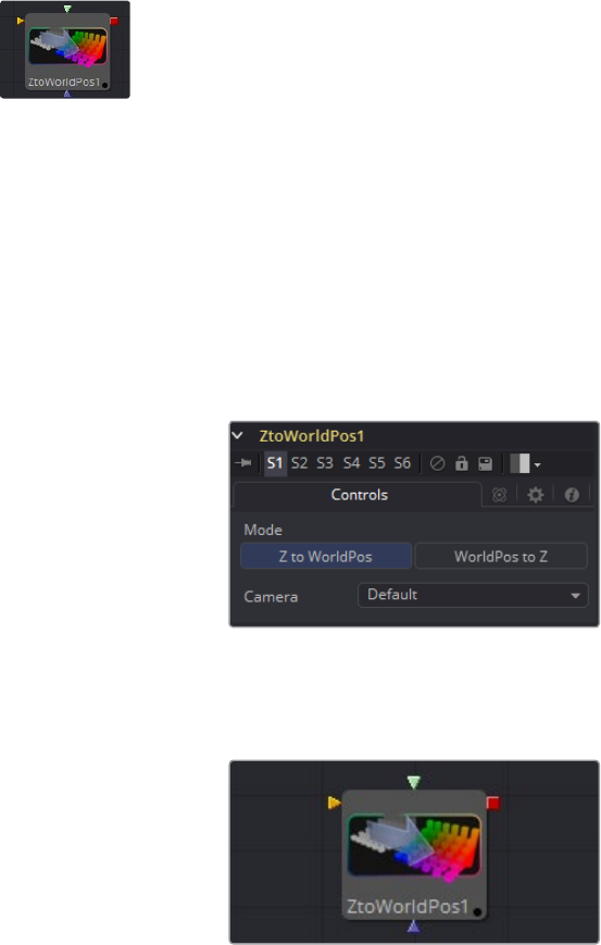
626
Position Tools Chapter – 25
Z to World [ZTW]
The Z to World tool is used to either generate a World Position Pass from a Z channel and a 3D
Camera or a Z channel from a World Position Pass and a 3D Camera.
Creating a World Position Pass from Z depth can be useful when your 3D application is not
capable of creating a WPP.
It can also be used when a 3D tracking software outputs a per-pixel Z depth together with the
3D Camera. Thus, the VolumeMask and Volumne Fog could be applied to real-world scenes.
The quality of the resulting WPP depends largely on the quality of the incoming Z channel.
See the WPP Concepts section for further explanation on how this technology works and to
learn about the required imagery.
Controls Tab
External Inputs
The following inputs appear on the tools tile in the Flow Editor.
ZtoWorld.Image: [orange, required] This input expects an image containing a World
Position Pass or a Z depth pass, depending on the desired operation.
ZtoWorld.EffectMask: [blue, optional] The standard Effect Mask input as found on
other Fusion tools.
ZtoWorld.SceneInput: [pink, required] This input expects a 3D scene input containing
a 3D Camera.
Mode
Toggle between creating a Z channel from a World Position Pass or vice versa.
Camera
If multiple Cameras are available in the connected Scene input, this drop-down allows
the user to choose the correct Camera needed to evaluate the image.
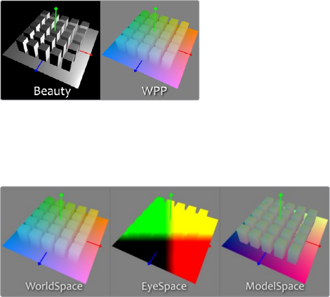
627
Position Tools Chapter – 25
WPP Concept
The Position tools in Fusion offer a completely new way of working with Masks and Volumetrics
for footage containing XYZ Position channels. ZtoWorld offers the option to create those
channels out of a Z channel and 3D Camera information. Just for the sake of this overview we
will refer to the World Position Pass as WPP.
What is a WPP?
The WPP reflects each pixel’s XYZ position in the original scene as RGB color values.
So if the face the pixel was derived from in the original scene sits at 0/0/0, the resulting pixel
will have an RGB value of 0/0/0 and thus will be black. If said face sits at 1/0/0 in the original
scene, the resulting pixel will be fully red. Of course if the coordinates of our face are something
like -60/75/123, the pixel will hold those values as well.
As you can see here, due to the huge extent 3D scenes can have, the WPP channel should
always be rendered in 32-bit floating point to provide the accuracy needed. This image shows a
3D Rendering of a scene with its center sitting at 0/0/0 in 3D Space and the according WPP. For
better visibility the WPP has been normalized.
.
Dierent Coordinate Spaces
WPPs can be rendered in different Coordinate Spaces. These include World Space, Eye Space
and Object Space. The image below depicts how those different spaces look, though the tools
in Fusion require the WPP to be rendered in World Space.
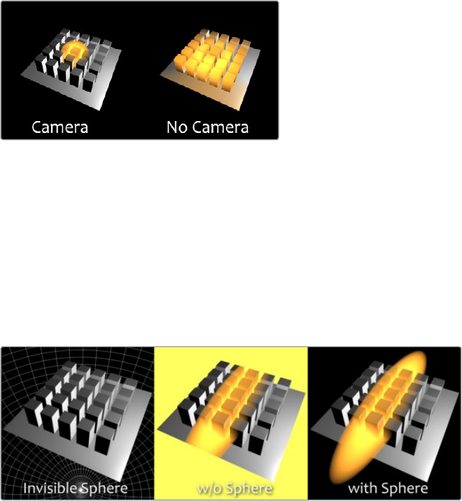
628
Position Tools Chapter – 25
The Scene Input
The tools offer a Scene Input, which can either be a 3D Camera or a 3D scene containing a
camera. While the camera is vital for the ZtoWorld tool, Volume Mask and Volume Fog will still
generate their output without any camera attached or with the camera position set to 0/0/0.
However, connecting a camera that lines up with the original camera the WPP has been
rendered from, or setting the camera’s position manually, greatly improves accuracy and look of
the resulting Fog or Mask.
The “Invisible Sphere”
The example scene shown so far has an empty background, meaning there is nothing in the
scene apart from the ground plane and the cubes.
If applying fog to a scene like that which is larger than said ground plane, the result will look
similar to the “w/o Sphere” example shown below because with no WPP information outside the
ground plane, the resulting value will be 0/0/0; the fog fills that area as well.
To get around that you can add an invisible bounding sphere to your scene to create “dummy”
WPP values to help the Fog tool to create the correct volume as shown in “with Sphere” below.

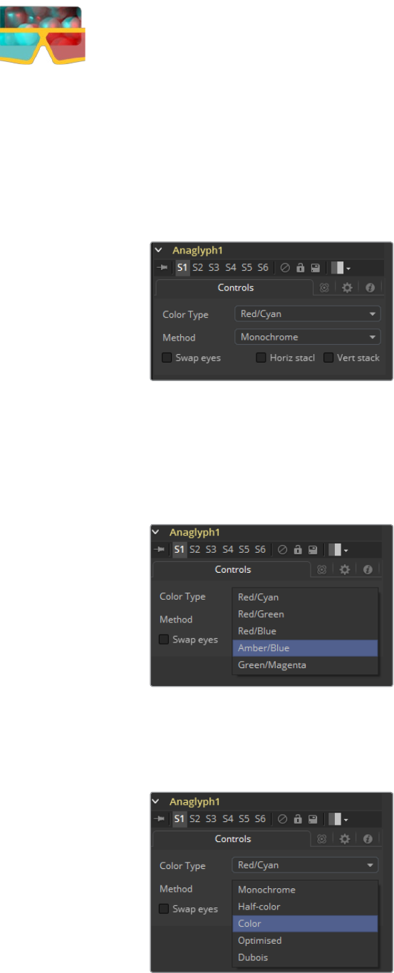
632
Stereo Tools Chapter – 26
Anaglyph [ANA]
The Anaglyph tool is used to create stereoscopic images by combining separate left eye and
right eye images. It is most commonly used at the end of a stereoscopic workflow to display or
deliver the final result. Stereoscopic tools are only available in Fusion Studio.
Controls Tab
When using separate images for the left and right eye, the left eye image is connected to the
orange input and the right eye image is connected to the green input of the tool. When using
either horizontally or vertically stacked images containing both left eye and right eye
information, these only connect to the orange input. Based on one of the methods described
below, the separate images are then combined to create a stereoscopic output
.
Color Type Menu
The ColorType menu allows you to choose between different color encodings to fit your
preferred display device. To match your stereo glasses you can choose between Red/Cyan,
Red/Green, Red/Blue, Amber/Blue and Green/Magenta encoding; Red/Cyan turns out to be the
most commonly used.
Method Menu
In addition to the color used for encoding the image, you can also choose five different
methods: Monochrome, Half-color, Color, Optimized and Dubois.
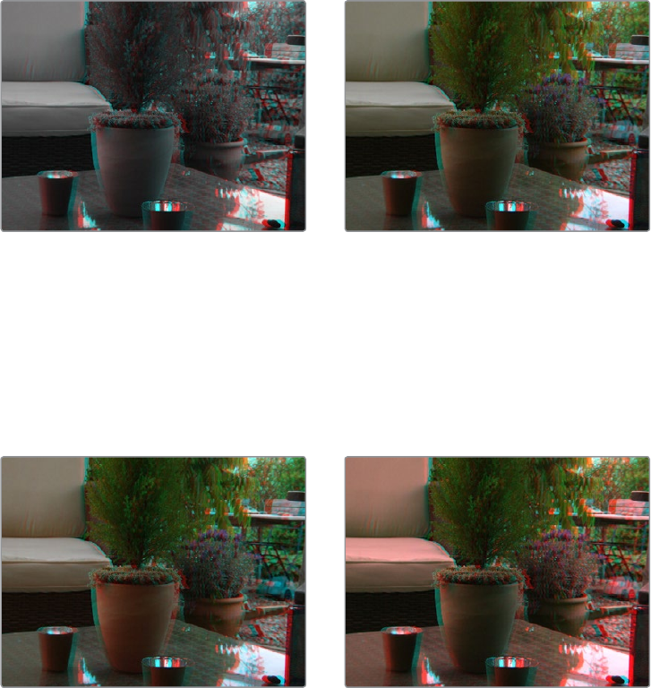
633
Stereo Tools Chapter – 26
Monochrome
The left eye contains the luminance of the left image, and the right eye contains the
luminance of the right image (e.g., the luminance of the left image is placed in the
output red channel, and the luminance of the right image is placed in the output green
and blue channels).
Half-Color
The left eye contains the luminance of the left image, and the right eye contains the
color channels from the right image that match the glasses color for that eye (e.g., the
luminance of the left image is placed in the output red channel, and the green and blue
channels of the right image are placed in the output green and blue channels).
Monochrome Half-Color
Color
The left eye contains the color channels from the left image that match the glasses
color for that eye, and the right eye contains the color channels from the right image
that match the glasses color for that eye (e.g., the red channel of the left image is
placed in the output red channel, and the green and blue channels of the right image
are placed in the output green and blue channels).
Color Optimized
Optimized
Used with red/cyan glasses, for example, the resulting brightness of what shows
through the left eye will be substantially less than the brightness of the right eye. Using
typical ITU-R 601 ratios for luminance as a guide, the red eye would give 0.299
brightness, while the cyan eye would give 0.587+0.114=0.701 brightness - over twice as
bright. The difference in brightness between the eyes can produce what’s referred to
as retinal rivalry or binocular rivalry, which can destroy the stereo effect. The Optimized
method generates the right eye in the same fashion as the Color method. The left eye
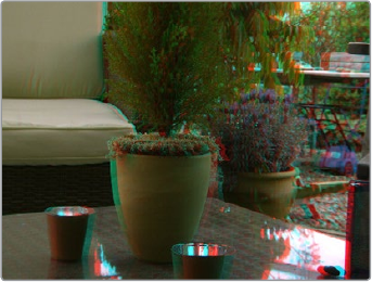
634
Stereo Tools Chapter – 26
also uses the green and blue channels, but in a combination with increased brightness
that reduces retinal rivalry. Since it uses the same two channels from each of the source
images, it doesn’t reproduce the remaining one (e.g., 1.05× the green and 0.45× the
blue channels of the left image is placed in the output red channel, and the green and
blue channels of the right image are placed in the output green and blue channels. Red
from both the left and right images is not used.).
Dubois
Images with fairly saturated colors can produce retinal rivalry with Half-color, Color and
Optimized methods because the color is only visible in one eye. For example, with red/
cyan glasses, a saturated green object looks black in the red eye, and green in the
cyan eye. The Dubois method uses the spectral characteristics of (specifically) red/cyan
glasses and CRT (Trinitron) phosphors to produce a better anaglyph and in the end
tends to reduce retinal rivalry caused by such color differences in each eye, and also
tends to reduce ghosting produced when one eye ‘leaks’ into the other eye. The
particular calculated matrix we use is designed for red/cyan glasses and isn’t available
for other glasses types. Since it is also derived from CRT color primaries, it may not give
the best results with a common LCD (though it’ll still likely produce less retinal rivalry
and ghosting than the other methods).
Dubois
Swap Eyes
Allows the user to easily swap the left and right eye input.
Horiz Stack
Takes an image that contains both left and right eye information stacked horizontally.
These images are often referred to as ‘crosseyed’ or ‘straight stereo’ images. You only
need to connect that one image to the orange input of the tool. It then creates an image
half the width of the original input, using the left half of the original image for the left
eye and the right half of the original image for the right eye. Color encoding takes place
using the specified color type and method.
Vert Stack
Takes an image that contains both left and right eye information stacked vertically. You
only need to connect that one image to the orange input of the tool. It then creates an
image half the height of the original input, using the bottom half of the original image for
the left eye and the top half of the original image for the right eye. Color encoding takes
place using the specified color type and method.
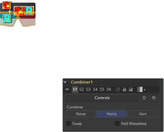
635
Stereo Tools Chapter – 26
Combiner [COM]
The Combiner tool takes two stereoscopic inputs and creates so called stacked images with
the left and right eye, either side by side or on top of each other. Stereoscopic tools are only
available in Fusion Studio
Controls Tab
To stack the images, the left eye image is connected to the orange input and the right eye
image is connected to the green input of the tool.
None
No operation will take place. The output image is identical to the left eye input.
Horiz
Both images will be stacked horizontally, or side-by-side, with the image connected to
the left eye input on the left. This will result in an output image double the width of the
input image.
Vert
Both images will be stacked vertically, or on top of each other, with the image
connected to the left eye input on the bottom. This will result in an output image double
the height of the input image.
Swap Eyes
Allows the user to easily swap the left and right eye input.
636
Stereo Tools Chapter – 26
Disparity [DIS]
Stereoscopic tools are only available in Fusion Studio.
Disparity generates the left/right shift between the frames in a stereo pair. It also generates the
vertical disparity between the left/right images, which is usually a lot smaller than the horizontal
disparity and ideally should be 0 to minimize viewing discomfort. When viewing the output of
the Disparity tool in the views, the human eye can distinguish quality/detail in the Disparity map
better by looking at either the grayscale X disparity or Y disparity, rather than looking at the
combined XY disparity as a Red/Green color image.
The generated disparity is stored in the output image’s Disparity aux channel, where the left
image contains the left > right disparity and the right image contains the right > left disparity.
Because disparity works based upon matching regions in the left eye to regions in the right eye
by comparing colors and gradients of colors, it is important that colors in the two eyes are as
similar as possible. Thus, it is a good idea to color correct ahead of time. It is also a good idea to
crop away any black borders around the frames, as this will confuse the disparity tracking
(andalso cause problems if you are using ColorCorrector’s histogram match ability to do the
colormatching).
In Stack mode, left and right outputs will output the same image. If the left and right images
have a global vertical offset bigger than a few pixels from each other, it can help the disparity
tracking algorithm if you approximately vertically align features in the left/right eyes ahead of
time using a Transform tool. Small details tend to get lost in the tracking process when you have
a large vertical offset between left/right eyes.
Consider using a SmoothMotion tool to smooth your Disparity channel. This can help reduce
time-dependent flickering when warping an eye. Also think about whether you want to remove
lens distortion before computing disparity. If you do not, your Disparity map will become a
combined Disparity and Lens Distortion map. This can have advantages and disadvantages.
One disadvantage is if you then do a vertical alignment you are also removing lens distortion
effects. When trying to reduce the computation time, start first with adjusting the Proxy and
Number of Iterations sliders.
The Disparity tool does not support RoI or DoD.
Inputs/outputs
Left Input
Connect either the left eye image or the stacked image.
Right Input
Connect the right eye image. This input is invisible unless Stack Mode is set
to Separate.
Left Output
This holds the left eye image with a new Disparity channel, or a Stacked Mode image
with a new disparity channel.
Right Output
This holds the right eye image with a new Disparity channel. This output is only visible if
Stack Mode is set to Separate.
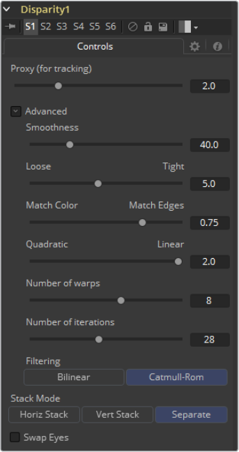
637
Stereo Tools Chapter – 26
Controls
Proxy (for tracking)
The input images are re-sized down by the proxy scale, tracked to produce the
disparity, and then the resulting disparities are scaled back up. This option is purely to
speed up calculation of the disparity, which can be slow. The computational time is
roughly proportional to the number of pixels in the image. This means a proxy scale of
2 will give a 4x speed up and a proxy scale of 3 will give a 9x speed up. In general, 1:1
proxy will give the most detailed flow, but keep in mind that this is highly dependent on
the amount of noise and film grain, which if present in large quantities can completely
obliterate any gains moving from 2:1 to 1:1 proxy and in some situations even make
things worse (in some sense you can think of the Proxy setting as acting as a simplistic
low-pass filter for removing noise/grain).
Stack Mode
Determines how the input images are stacked.
When set to Separate, the Right Input and Output will appear and separate left and
right images need to be connected.
Swap Eyes
With Stacked Mode, image stereo pairs, left and right images can be swapped.

638
Stereo Tools Chapter – 26
Advanced
The Advanced Control section has parameter controls to tune the Disparity map calculations.
The default settings have been chosen to be the best default values from experimentation with
many different shots and should serve as a good standard. In most cases, tweaking of the
advanced settings will not be needed.
Smoothness
This controls the Smoothness of the disparity. Higher smoothness helps deal with
noise, while lower smoothness brings out more detail.
Edges
This slider is another control for smoothness but applies smoothing based upon the
color channel. It tends to have the effect of determining how edges in the disparity
follow edges in the color images. When it is set to Loose, the disparity becomes
smoother and tends to overshoot edges. When it is set to Tight, edges in the disparity
align more tightly with the edges in the color images and details from the color
channels start to slip into the disparity, which is not usually desirable.
As a rough guideline, if you are using the disparity to produce a Z-channel for post
effects like depth of field, then you can experiment with making it tighter, but if you are
using the disparity to do interpolation, you might want to keep it looser.
In general, if it is too tight, there can be problems with streaked out edges when the
disparity is used for interpolation.
639
Stereo Tools Chapter – 26
Match Weight
This controls how the matching of neighborhoods in the left to neighborhoods in the
right image is done. When set to Match Color, large structural color features are
matched. When set to Match Edges, small sharp variations in the color are matched.
Typically, a good value for this slider is in the [0.7, 0.9] range, although on some shots
values closer to 0.0 work well. Setting this option higher tends to improve the matching
results in the presence of differences due to smoothly varying shadows or local lighting
variations between the left and right images. The user should still do a color match on
the initial images so they are as similar as possible; this option tends to help with local
variations (e.g., lighting differences due to light passing through a mirror rig).
Mismatch Penalty
This controls how the penalty for mismatched regions grows as they become more
dissimilar. The slider gives the choice between a balance of Quadratic and Linear
penalties. Quadratic strongly penalizes large dissimilarities while Linear is more robust
to dissimilar matches. Moving this slider toward Quadratic tends to give a disparity with
more small random variations in it, while Linear produces smoother, more visually
pleasing results.
Number of Warps
Turning this option down makes the disparity computations faster. In particular, the
computational time depends linearly upon this option. To understand what this option
does, you need to understand that the Disparity algorithm progressively warps the left
image until it matches with the right image. After some point, convergence is reached
and additional warps are just a waste of computational time. The default value in Fusion
is set high enough that convergence should always be reached. You can tweak this
value to speed up the computations, but it is good to watch how the disparity is
degrading in quality at the same time.
Number of Iterations
Turning this option down makes the disparity computations faster. In particular, the
computational time depends linearly upon on this option. Just like adjusting Number of
Warps, at some point adjusting this option higher will give diminishing returns and not
produce significantly better results. By default, this value is set to something that should
converge for all possible shots and can be tweaked lower fairly often without reducing
the disparity’s quality.
Filtering
This controls Filtering operations used during flow generation. Catmull-Rom filtering will
produce better results, but at the same time, turning on Catmull-Rom will increase the
computation time steeply.
640
Stereo Tools Chapter – 26
Disparity To Z [D2Z]
Description
DisparityToZ takes a 3D camera and an image containing a Disparity channel as inputs and
outputs the same image but with a newly computed Z channel. Stereoscopic tools are only
available in Fusion Studio
Optionally, this tool can output Z into the RGB channels. Ideally, either a stereo Camera3D or a
tracked stereo camera is connected into DisparityToZ, however, if no camera is connected, the
tool provides artistic controls for determining a Z channel. The depth created by this tool can be
used for post effects like fogging or depth of field.
The Z values produced become more incorrect the larger (negative) they get. The reason is that
disparity approaches a constant value as Z approaches -infinity. So Z = -1000 and Z = -10000
and Z = -100000 may map to D=142. 4563 and D=142. 4712 and D=142. 4713. As you can see,
there is only 0.0001 in D to distinguish between 10,000 and 100,000 in Z. The maps produced
by Disparity are not accurate enough to make distinctions like this.
Inputs/outputs
Left Input
Connect either the left eye image or the stack image.
Right Input
Connect the right eye image. This input is invisible unless Stack Mode is set
to Separate.
Stereocamera
An external stereo camera tool.
Left Output
Holds the left eye image with a new Z channel or a stacked mode image with a new
Z channel.
Right Output
Holds the right eye image with a new Z channel. This output is only visible if Stack
Mode is Separate.
Controls
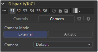
641
Stereo Tools Chapter – 26
In addition to outputting Z values in the Z channel, this option promotes the color channels to
float32 and outputs the Z values into the color channels as {z, z, z, 1}. This option is useful to get
a quick look to see what the Z channel looks like. Note that Dimension’s Z values are negative,
getting more negative the further you are from the camera, so you will need view Normalization
On to see them correctly.
Output Z to RGB
Rather than keeping the Z values within the associated aux-channel only, they will be
copied into the RGB channels for further modification with any of Fusion’s tools.
Refine Z
This option refines the depth map based upon the RGB channels. The refinement
causes edges in the flow to align more closely to edges in the color channels. The
downside is that unwanted details in the color channels start to show up in the flow.
You may want to experiment with using this option to soften out harsh edges for
Z-channel post effects like depth of field or fogging.
HiQ Only
This option only processes in HiQ.
Strength
Increasing this slider does two things. It smooths out the depth in constant color
regions and moves edges in the Z channel to correlate with edges in the
RGB channels.
Increasing the refinement has the undesirable effect of causing texture in the color
channel to show up in the Zchannel. You will want to find a balance between the two.
Radius
This is the radius of the smoothing algorithm.
Camera Tab
If you need correct real-world Z values because you are trying to match some effect to an
existing scene, you should use the External Camera options to get precise Z values back. If you
just want any Z-buffer and are not that particular about the exact details on how it is offset and
scaled, or if there is no camera available, the Artistic option might be helpful.
External Mode
An input will appear on the flow to connect an existing stereo Camera3D. This can
either be a single stereo Camera3D (i.e., its eye separation is set to non-zero), or a pair
of (tracked) Camera3Ds connected together via the Camera3D > Stereo >
RightCamera input.
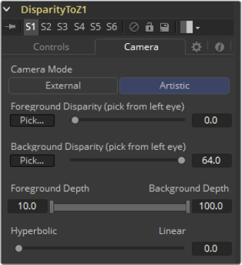
642
Stereo Tools Chapter – 26
Artistic Mode
If you do not have a camera, you can adjust these controls to produce an “artistic” Z
channel whose values will not be physically correct but still useful. To reconstruct the
Disparity > Z Curve, pick (D, Z) values for a point in the foreground and a point in the
background
If artistic mode is a little too “artistic” for you and you want more physically-based
parameters to adjust (e.g., convergence and eye separation), you can always create a
bogus Camera3D, connect it into the DisparityToZ > Camera input, and then fiddle with
the Camera3D’s controls.
Foreground Disparity (pick from left eye)
This is the disparity for the closest foreground object. It will get mapped to depth value
specified by the Foreground Depth control. Any objects with disparity outside of the
range [ForegroundDisparity, BackgroundDisparity] will have their disparity values
clipped to this range leading to flat areas in the Z channel, so make sure that you pick
values that enclose the actual disparity range.
Background Disparity (pick from left eye)
This is the disparity for the furthest background object. It will get mapped to the depth
value specified by the Background Depth control. One way to think of this input is as
the upper limit to disparity values for objects at -infinity. This value should be for the left
eye. The corresponding value in the right eye will be the same in magnitude
but negative.
Foreground Depth
This is the depth to which Foreground Disparity will be mapped. Think of this as the
depth of the nearest object. Note that values here are positive depth.
Background Depth
This is the depth to which Background Disparity will be mapped. Think of this as the
depth of the most distant object.
Falloff
Falloff controls the shape of the depth curve between the requested foreground and
background depths. When set to Hyperbolic, the disparity-depth curve behaves
roughly like depth = constant/disparity. When set to Linear, the curve behaves like
depth = constant*disparity. Hyperbolic tends to emphasize Z features in the foreground,
while linear gives foreground/background features in the Z channel equal weighting.
Unless there’s a specific reason not to, prefer Hyperbolic, as it is more physically
accurate, while Linear does not correspond to nature and is purely for artistic effect.
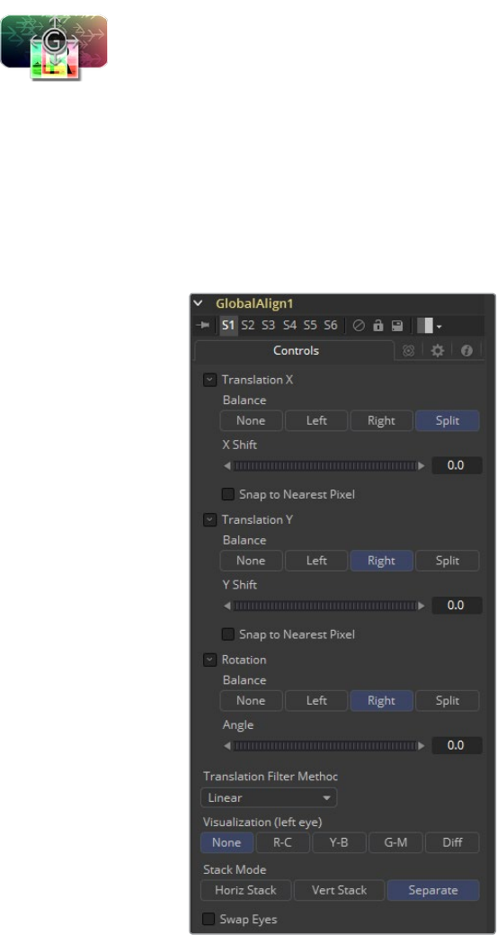
643
Stereo Tools Chapter – 26
Global Align [GA]
As opposed to Stereo Align, this tool does not utilize optical flow at all. It’s meant as a fast and
convenient way to do simple stereo alignment for both X and Y as well as rotation. Stereoscopic
tools are only available in Fusion Studio.
Global Align comes in handy at the beginning of the tool chain to visually correct major
differences between left and right eye before calculating Disparity.
Manual correction of large discrepancies between left and right, as well as applying an initial
color matching, helps Disparity to generate more accurate results.
Controls
Translation X and Y
Balance: Determines how the global offset is applied to the stereo footage.
None: No translation is applied.
Left Only: The left eye is shifted, while the right eye remains unaltered.
Right Only: The right eye is shifted, while the left eye remains unaltered.
Split Both: Left and right eyes are shifted in opposite directions.
644
Stereo Tools Chapter – 26
Snap to Nearest Pixel
While adjusting the translation slider, this option ensures that the image is shifted in full
pixel amounts only to maintain optimum quality. This avoids sub-pixel rendering of the
image, which could result in subtle blurring.
Rotation
Balance: Determines how the global rotation is applied to the stereo footage.
None: No rotation is applied.
Left Only: The left eye is rotated, while the right eye remains unaltered.
Right Only: The right eye is rotated, while the left eye remains unaltered.
Split Both: Left and right eyes are rotated in opposite directions.
Angle
The angle of the rotation. Keep in mind that the result depends on the Balance settings.
If only rotating one eye by, for example, 10 degrees, a full 10 degree rotation will be
applied to that eye.
When applying rotation in Split mode, one eye will receive a -5 degree and the other
eye a +5 degree rotation.
Translation Filter Method
A dropdown to choose a filter method that delivers the best results depending on the
content of your footage.
Visualization
This control allows for different color-encodings of the left and right eye to conveniently
examine the results of the above controls without needing to add an extra Anaglyph or
Combiner tool.
Set this to None for final output.
Stack Mode
Determines how the input images are stacked.
When set to Separate, the right input and output will appear and separate left and right
images need to be connected.
Swap Eyes
With Stacked Mode, image stereo pairs, left and right images can be swapped.
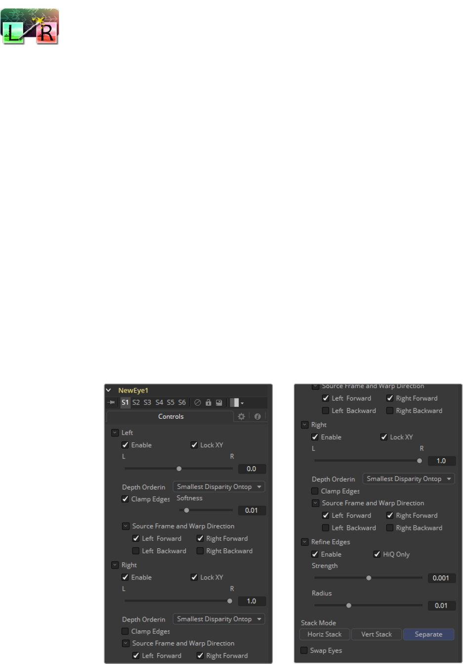
645
Stereo Tools Chapter – 26
New Eye [NE]
This option constructs a New Eye by interpolating between two existing eyes using the
embedded Disparity channels. This tool can also be used to replace one view with a warped
version of the other. In Stack Mode, L and R outputs will output the same image. Stereoscopic
tools are only available in Fusion Studio.
You can map the left eye onto the right eye and replace it. This can be helpful when removing
errors from certain areas of the frame.
NewEye does not interpolate the aux channels, but rather destroys them. In particular, the
Disparity channels are consumed/destroyed. Add another Disparity tool after the NewEye if you
want to generate Disparity for the realigned footage.
Inputs/outputs
Left Input
Connect either the left eye image or the stacked image.
Right Input
Connect the right eye image. This input is invisible unless Stack Mode is set
to Separate.
Left Output
This holds the left eye image with a new Disparity channel, or a Stacked Mode image
with a new disparity channel.
Right Output
This holds the right eye image with a new Disparity channel. This output is only visible if
Stack Mode is set to Separate.
Controls
646
Stereo Tools Chapter – 26
Enable
When an eye is enabled, NewEye will replace it with an interpolated eye. For example,
if the left eye is your “master” eye and you are recreating the right eye, you would
disable the left eye and enable the right eye.
Lock XY
Locks the X and Y interpolation parameters. When they are unlocked you can provide
separate interpolation factors for using the X and Y disparity. For example, if you are
working with the right eye and you have the X Interpolation slider set to 1.0 and the Y
Interpolation slider set to -1.0, you will be effectively interpolating the left eye onto the
right eye but vertically aligned to the left eye.
Interpolation
Interpolation determines where the frame we are interpolating is relative to the two
source frames: Left and Right. An interpolation parameter of -1.0 will give frame Left
back and a parameter of 1.0 will give frame Right back. A parameter of 0.0 will give a
result that is halfway between Left and Right.
Depth Ordering
The Depth Ordering is used to determine which parts of the image should be rendered
on top. When warping images there is often overlap. When the image overlaps itself,
there are two options for which should be drawn on top.
Largest Disparity Ontop: The larger disparity values will be drawn on top in the
overlapping image sections.
Smallest Disparity Ontop: The smaller disparity values will be drawn on top in the
overlapping image sections.
Clamp Edges
Under certain circumstances, this option can remove the transparent gaps that may
appear on the edges of interpolated frames. Clamp Edges will cause a stretching
artifact near the edges of the frame that is especially visible with objects moving
through it or when the camera is moving.
Because of these artifacts, it is a good idea to only use clamp edges to correct small
gaps around the edges of an interpolated frame.
Softness
Helps to reduce the stretchy artifacts that might be introduced by Clamp Edges.
If you have more than one of the Source Frame and Warp Direction checkboxes turned
on, this can lead to doubling up of the stretching effect near the edges. In this case
you‘ll want to keep the softness rather small at around 0.01. If you only have one
checkbox enabled you can use a larger softness at around 0.03.
Source Frame and Warp Direction
The output of this tool is generated by combining up to four different warps. You can
choose to use either the color values from the left or right frame in combination with the
Forward (left > right) Disparity or the Backward (right > left) Disparity. Sometimes you
will want to replace an existing eye. For example, if you want to regenerate the right
eye, you would only use left eye warps.
647
Stereo Tools Chapter – 26
It is good to experiment with various options to see which gives the best effect. Using
both the left and right eyes can help fill in gaps on the left/right side of images. Using
both the Forward/Backward Disparity can give a doubling up effect in places where the
disparities disagree with each other.
Left Forward: This will take the Left frame and use the Forward Disparity to
interpolate the new frame.
Right Forward: This will take the Right frame and use the Forward Disparity to
interpolate the new frame.
Left Backward: This will take the Left frame and use the Back Disparity to interpolate
the new frame.
Right Backward: This will take the Right frame and use the Back Disparity to
interpolate the new frame.
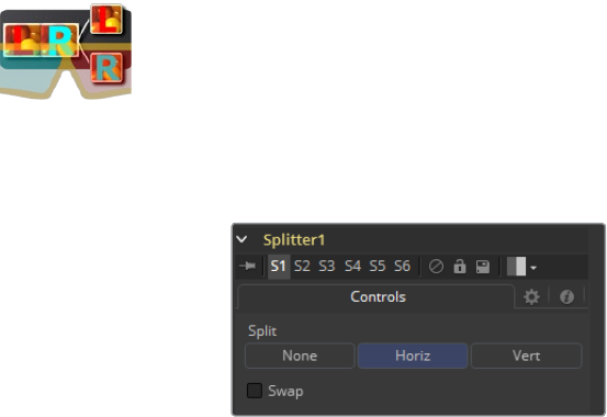
648
Stereo Tools Chapter – 26
Splitter [SPL]
The Splitter takes a stacked input image, for example created with the Combiner, and provides
two output images: a left eye and a right eye. Stereoscopic tools are only available in
Fusion Studio.
Controls Tab
None
No operation will take place. The output image on both outputs is identical to the
input image.
Horiz
The tool expects a horizontally stacked image. This will result in two output images,
each being half the width of the input image.
Vert
The tool expects a vertically stacked image. This will result in two output images, each
being half the height of the input image.
Swap Eyes
Allows the user to easily swap the left and right eye output.
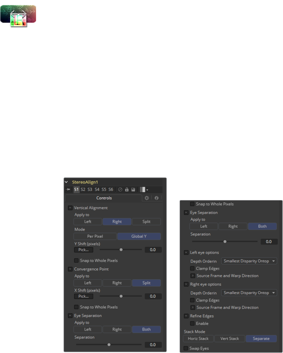
649
Stereo Tools Chapter – 26
Stereo Align [SA]
This extremely versatile tool for fixing Stereo issues can be used for doing any of the following
or combinations of:
Vertical Alignment of one eye to the other
Changing the convergence
Changing the eye separation
By combining these operations in one tool, you can execute them using only a single image
resampling. In essence, this tool can be thought of as applying scales and translation to the
disparities, and then using the modified disparities to interpolate between the views.
Changing the eye separation can cause a lot of holes to appear and it may not be possible to fill
them since the information needed may not be in either image. Even if the information is there,
the disparity may have mismatched the holes. You may have to fill the holes in manually. For
now, this tool will modify just the RGBA channels.
StereoAlign does not interpolate the aux channels, but rather destroys them. In particular, the
Disparity channels are consumed/destroyed. Add another Disparity tool after the StereoAlign if
you want to generate Disparity for the realigned footage. Stereoscopic tools are only available
in Fusion Studio.
Controls
Vertical Alignment
This option determines how the Vertical Alignment is split between two eyes. Usually
the left eye is declared inviolate and the right eye is aligned to it to avoid resampling
artifacts.
When doing per pixel vertical alignment, it may be helpful to roughly pre-align the images
by a global Y-shift before disparity computation because the disparity generation
algorithm can have problems resolving small objects that move large distances.
650
Stereo Tools Chapter – 26
Also note that you have to be careful about lens distortion because, even if two
cameras are perfectly vertically aligned, they will still have vertical disparities due to
lens distortion. It is probably a good idea to remove the lens distortion before
computing the Disparity since, by doing a vertical alignment of the right eye, you are in
effect removing the Y-component of the lens distortion in the right eye and it will look
wrong later when you try to redistort it.
Right: Only the right eye is adjusted.
Left: Only the left eye is adjusted.
Both: The vertical alignment is split evenly between the left and right eyes.
Mode
Global: The eyes are simply translated up or down by the Y-shift to match up.
Per Pixel: The eyes are warped pixel-by-pixel using the Disparity to vertically align.
Keep in mind that this can introduce sampling artifacts and edge artifacts.
Y-shift
Y-shift is only available in Global Mode. You can either adjust the Y-shift manually to get
a match or drag the pick button, which picks from the Disparity channel of the left eye.
Also remember that, if you use this tool to modify disparity, you can’t pick from the
tool’s output.
Snap
You can snap the global shift to whole pixels using this option. In this mode there is no
resampling of the image, but rather a simple shift is done so there will be no softening
or image degradation.
Convergence
Convergence is just a global X-translation of L/R images.
Eyes
This determines which eyes are affected by convergence. In most cases, this will be set
to both. If you set the eyes to Both/Split, then the convergence will be shared 50-50
between both eyes. Sharing the convergence between both eyes means you get half
the shift in each eye, which in turn means smaller holes and artifacts that need to be
fixed later. The tradeoff is that you’ve resampled both eyes now rather than keeping
one eye as a pure reference master.
X-shift
X-shift can be picked from the Disparity channels for easy point to feature alignment.
Snap
You can snap the global shift to whole pixels using this option. In this mode there is no
resampling of the image, but rather a simple shift is done so there will be no softening
or image degradation.
Eye Separation
Eye separation changes the distance between the left/right eyes, causing objects in
the left/right eyes to converge/diverge further apart depending on their distance from
the camera.
This has the same effect as Eye Separation option in Camera3D.
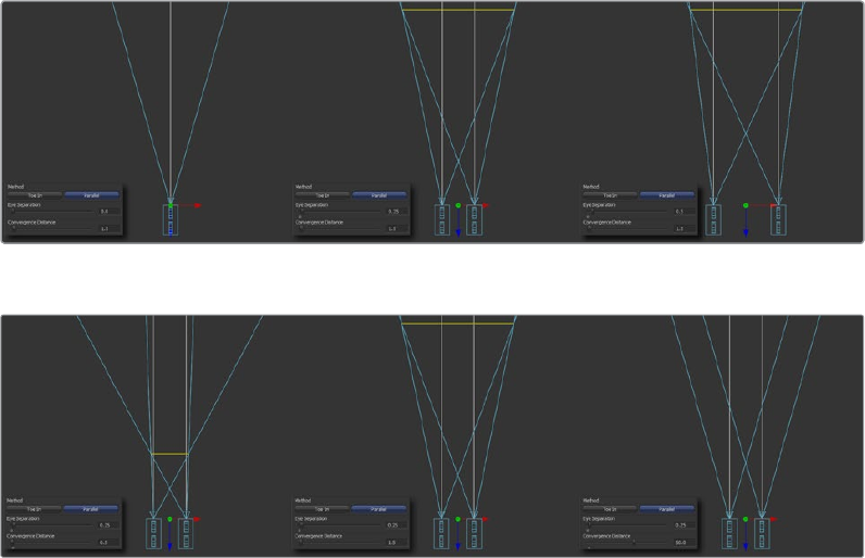
651
Stereo Tools Chapter – 26
Separation
This is a scale factor for eye separation.
When set to 0.0, this leaves the eyes unchanged.
Setting it to 0.1 increases the shifts of all objects in the scene by a factor of 10% in
each eye.
Setting it to 0.1 will scale the shifts of all objects 10% smaller.
Unlike the Split option for vertical alignment, which splits the alignment effect 50-50
between both eyes, the Both option will apply 100-100 eye separation to both eyes. If
you are changing eye separation, it can be a good idea to enable per-pixel vertical
alignment or the results of interpolating from both frames can double up.
Stack Mode
In Stack Mode, L and R outputs will output the same image.
If HiQ is off, the interpolations are done using nearest neighbor sampling leading to a
more “noisy” result.
Clamp Edges
Under certain circumstances, this option can remove the transparent gaps that may
appear on the edges of interpolated frames. Clamp Edges will cause a stretching
artifact near the edges of the frame that is especially visible with objects moving
through it or when the camera is moving.
Because of these artifacts, it is a good idea to only use clamp edges to correct small
gaps around the edges of an interpolated frame.
Softness
Helps to reduce the stretchy artifacts that might be introduced by Clamp Edges.
If you have more than one of the Source Frame and Warp Direction checkboxes turned
on, this can lead to doubling up of the stretching effect near the edges. In this case
you‘ll want to keep the softness rather small at around 0.01. If you only have one
checkbox enabled you can use a larger softness at around 0.03.
Example
Different settings for Eye Separation:
and Convergence:
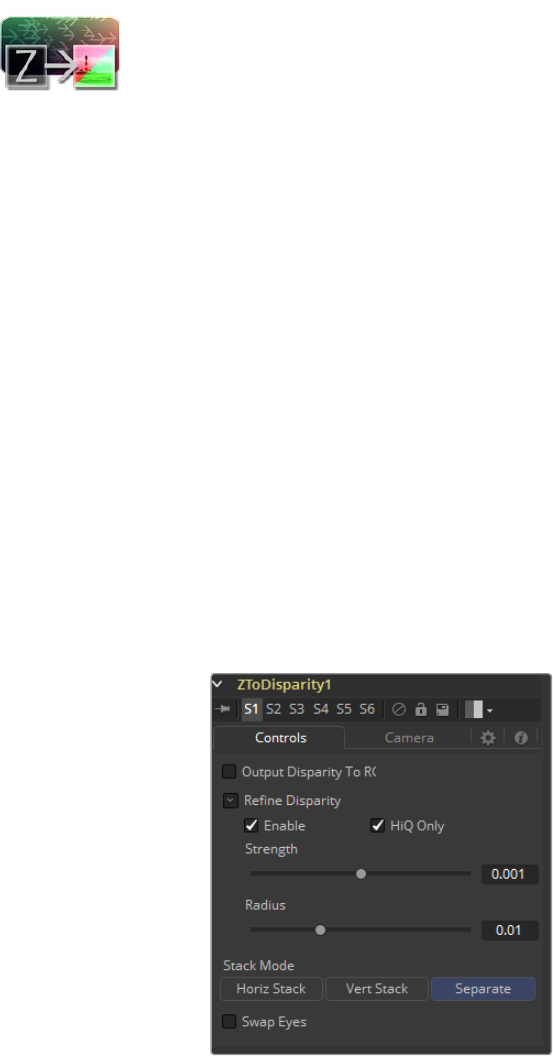
652
Stereo Tools Chapter – 26
Z To Disparity [Z2D]
ZToDisparity takes a stereo camera and an image containing a Z channel and outputs the same
image but with Disparity channels in it. This is useful for constructing a Disparity map from CG
renders, which will be more accurate than the Disparity map created from the Disparity
generator tool. Stereoscopic tools are only available in Fusion Studio
Inputs/outputs
Left
This is the left image or stack input.
Right
This is the right image.
Stereocamera
A stereo perspective camera may be either a Camera3D with eye separation or a
tracked L/R Camera3D.
Left Output
This is the left image or stack output containing new Disparity channel.
Right Output
This is the right image that contains a new Disparity channel. This output will be hidden
in Stack Mode.
Controls
Output Disparity To Rgb
In addition to outputting disparity values into the Disparity channel, this option causes
ZToDisparity to also output the disparity values into the color channels as {x, y, 0, 1}.
When enabled, this option will automatically promote the RGBA color channels to
float32. This option is useful for a quick look to see what the Disparity channel
looks like.
Refine Disparity
This refines the Disparity map based upon the RGB channels.
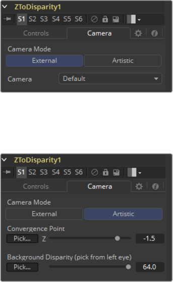
653
Stereo Tools Chapter – 26
Strength
Increasing this slider does two things. It smooths out the depth in constant color
regions and moves edges in the Zchannel to correlate with edges in the RGB channels.
Increasing the refinement has the undesirable effect of causing texture in the color
channel to show up in the Z channel. You will want to find a balance between the two.
Radius
This is the pixel-radius of the smoothing algorithm.
Camera Tab
If you need correct real-world disparity values because you are trying to match some effect to
an existing scene, you should use the External Camera options to get precise disparity values
back. If you just want any disparity and do not particular care about the exact details on how it is
offset and scaled, or if there is no camera available, then the Artistic option might be helpful.
External
An input will appear on the flow to connect an existing stereo Camera3D, and use the
Camera settings to determine the Disparity settings.
Artistic
If you do not have a camera, you can adjust these controls to produce an “artistic”
Disparity channel whose values will not be physically correct but good enough for
compositing hacks. There are two controls to adjust:
Convergence Point
This is the Z value of the convergence plane. This corresponds to the negative of the
Convergence Distance control that appears in Camera3D. At this distance, objects in
the left and right eyes are at exactly the same position (i.e., have zero disparity).
Objects closer appear to pop out of the screen, and objects further appear behind
the screen.
Background Disparity (pick from left eye)
This is the Disparity of objects in the distant background. You can think of this as the
upper limit to disparity values for objects at infinity. This value should be for the left eye.
The corresponding value in the right eye will be the same in magnitude but negative.
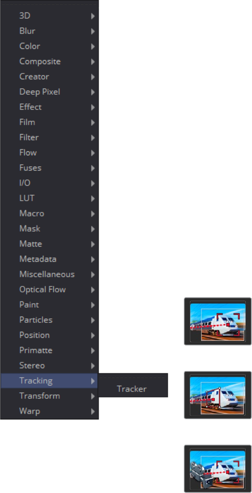
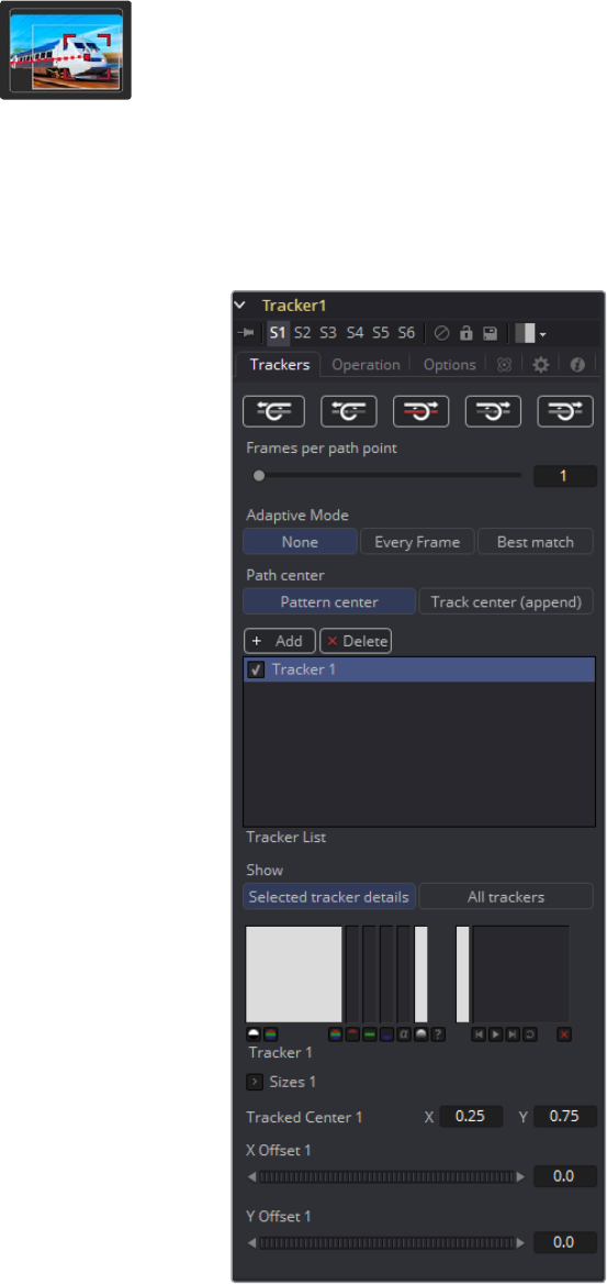
657
Tracker Tools Chapter – 27
Tracker [TRA]
The Tracker is used to detect and follow one or more pixel patterns across frames in moving
video. The tracking data can then be used to control the position or values of other tools in the
composition (for example, the center of a Drip). Additionally, trackers can be used to stabilize an
image, or to apply de-stabilization to one image based on the motion of another.
Please also refer to the Tracking Explained section in the User Manual.
Trackers Tab
Track Buttons
There are four buttons used to initiate tracking and one in the middle used to stop a
track in progress. These buttons can track the current pattern forward or backward in
time. Hold the mouse pointer over each button for a moment, and a tooltip with the
name of the button will appear.
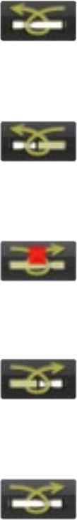
658
Tracker Tools Chapter – 27
The buttons operate as follows:
Track Reverse: Clicking on this button will cause all Active trackers to begin tracking
their patterns, starting at the end of the render range and moving backward through
time until the beginning of the render range.
Track Reverse From Current Time: Clicking on this button will cause all Active
trackers to begin tracking their patterns, starting at the current frame and moving
backward through time until the beginning of the render range.
Stop Tracking: Clicking on this button will Stop the tracking process immediately.
This can also be achieved by pressing ESC. This button will only be active when
tracking is in process.
Track Forward From Current Time: Clicking on this button will cause all Active
trackers to begin tracking their patterns, starting at the current frame and moving
forward through time until the end of the render range.
Track Forward: Clicking on this button will cause all Active trackers to begin tracking
their patterns, starting at the first frame in the render range and moving forward
through time until the end of the render range.
Frames Per Path Point
The value of this slider determines how often the Tracker sets a Keyframe on the Path.
The normal default is 1, which sets a Keyframe on the tracked path at every frame.
Increasing the value of this slider will cause the tracked path to be less accurate. This
may be desirable if the track is returning fluctuating results, but under normal
circumstances this control should be left at its default value.
If the project is field rendered, a value of 1 sets a Keyframe on every field. Since the
tracker is extremely accurate, this will result in a slight up-and-down jittering due to the
position of the tracked pattern fields. For fielded footage tracked in Field mode, you
will get better results setting this slider to a value of 2, which will result in one keyframe
per frame of your footage.
Adaptive Mode
Fusion is capable of re-acquiring the tracked pattern, as needed, to help with complex
tracks. This button array determines what mode of Adaptive tracking is employed.
659
Tracker Tools Chapter – 27
None
If selected, Fusion searches only for the pattern originally selected in each single frame.
Every Frame
If selected, Fusion re-acquires the pattern every frame. This helps the tracker
compensate for gradual changes in profile and lighting over time.
Best Match
If selected, the Tracker will compare the pattern acquired at each frame and compare it
to the original selected pattern. If the variation between the two patterns exceeds the
threshold amount defined by the Match Tolerance control, Fusion will not re-acquire the
pattern on that frame. This helps to avoid tracker drift caused by transient artifacts that
cross the pattern’s path (such as a shadow).
Path Center
The two buttons in this button array determine how the Tracker behaves when re-
positioning a pattern. These controls are used when switching a path from one pattern
to another, which happens when a pattern leaves the frame, or changes so significantly
it can no longer be tracked.
Pattern Center
When Pattern Center is the Active mode, the tracked path continues from the center of
the new path. This is appropriate when replacing an existing path entirely, but when
trying to append to a path using a new pattern, this will cause a discontinuity.
Track Center (append)
When Track Center (append) is selected, the path tracked by a new pattern will be
appended to the existing path. The Path created is automatically offset by the required
amount. This technique will work best if the new pattern is located close to the position
of the old pattern to avoid any problems with parallax or lens distortion.
This mode can also be used to virtually continue the tracking of patterns that move out
of the frame or get obstructed by other objects.
Add/Delete Tracker
Use these to add or delete Trackers from your Tracker List.
Add
Add a new Tracker.
Delete
Delete the tracker that is currently selected in the Tracker List.
Tracker List
The Tracker List shows the names of all of the patterns created on this Tracker. It is also
used to add new Trackers.
The Tracker tool is capable of hosting a virtually unlimited number of Tracker patterns.
Click on the Add button immediately above the list to add a new Tracker pattern.
Each pattern appears in the list by name, next to a small checkbox. Clicking on the
name of the pattern will select that pattern.
The controls below the list will change to affect that pattern only. Click once on a
selected pattern to rename the pattern to something more descriptive.
Clicking on the checkbox changes the state of the Tracker.
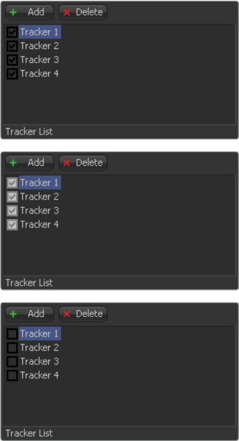
660
Tracker Tools Chapter – 27
Tracker States
Enabled (Black Checkbox): An Enabled pattern will re-track each time the Track is
initiated. Its path data is available for use by other tools, and the data is available for
Stabilization and Corner Positioning.
Suspended (Gray Checkbox): A Suspended pattern does not re-track when the
Track is initiated. The data is locked to prevent additional changes. The data from the
Path is still available for other tools, and the data is available for advanced Tracking
modes like Stabilization and Corner Positioning.
Disabled (Clear): A Disabled pattern does not create a path when tracking is
initialized, and its data is not available to other tools, or for advanced Tracking
operations like Stabilization and Corner Positioning.
Show
These two buttons determine what controls are displayed in the tool controls. They
have no effect on the operation of the Tracker; they only affect the interface.
Selected Tracker Details
When Selected Tracker Details is selected, the controls displayed pertain only to the
currently selected Tracker. You will have access to the Pattern Window and the
Offset sliders.
All Trackers
When All Trackers is selected, the pattern window for each of the Trackers is displayed
simultaneously below the Tracker List.
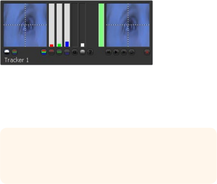
661
Tracker Tools Chapter – 27
Left Pattern Display
The Pattern Display has two image windows next to each other, and a series of status
bars. The window on the left shows the pattern initially selected, while the one on the
right shows a real-time display of the current pattern as tracking progresses.
As the onscreen controls are moved for a pattern, the display in the leftmost window
will update to show the pattern. As the pattern is moved, the vertical bars immediately
to the right of the image display indicate the clarity and contrast of the image channels.
The channel, or channels, with the best clarity are automatically selected for tracking.
These channels have a white background in the vertical bar representing that channel.
The automatic tracking can be allowed to stand, or you can override the automatic
selection and choose the channel used for tracking by disabling the button labeled
with a question mark, and selecting the button beneath the channel to track.
Under normal circumstances, the channel selected is indicated in the Pattern Display.
Ifthe selected channel is blue, then a grayscale representation of the blue channel for
the pattern appears. The image is only represented in full color if all three channels are
selected for tracking.
Override this behavior by selecting the Show Full Color button beneath the Pattern
Display, instead of the Show Selected Channel button.
Right Pattern Display
The Pattern Display on the right indicates the actual pattern acquired for tracking. This
display is clear until the first time the selected pattern is actually tracked. The Pattern
Display becomes active during tracking, displaying the pattern that Fusion acquires
from frame to frame.
As the tracking occurs, the pattern from each frame is accumulated into a Flipbook,
which can be played back in the Pattern window after tracking by using the transport
controls at the bottom of the window.
As Fusion looks for the channel with the highest contrast automatically, you
might end up tracking the blue channel, especially on scanned film material.
Unfortunately the blue channel on most film stock contains the most grain as
well, which naturally leads to unclean tracks. Before tracking it’s always a good
idea to zoom into your footage and check the RGB channels individually.
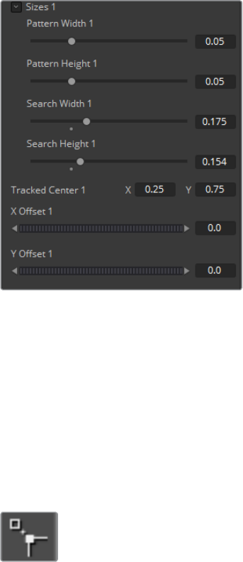
662
Tracker Tools Chapter – 27
While the track is progressing, the vertical bar immediately to the right of the pattern
shows how confident Fusion is that the current pattern matches the originally selected
pattern. A green bar indicates a high degree of confidence that the current pattern
matches the original. A yellow bar indicates less certainty, and a red bar indicates that
Fusion has detected extreme variations in the current pattern, and is no longer certain
of its accuracy.
After tracking, the pattern display will show a small Flipbook of the track for that pattern,
overlaid with a frame number to help identify problem frames for the Track.
Pattern Width and Height
Use these controls to adjust the width and height of the selected Tracker pattern
manually. The size of the Tracker pattern can also be adjusted in the Viewer, which is
the normal method, but small adjustments are often easier to accomplish with the
precision of manual controls.
Search Width and Height
The search area defines how far Fusion will look in the image from frame to frame to
re-acquire the pattern during tracking. As with the Pattern Width and Height, the Search
Area can be adjusted in the Viewer, but you may want to make small adjustments
manually using these controls.
Tracked Center
This positional control indicates the position of the Tracker’s center. To remove a path
from a Tracker pattern, right-click on this control and select Remove Path from the
contextual menu.
X and Y Offset
You will often need to track the position of an object in the scene, but that object does
not provide for a very reliable pattern. The Offsets permit the tracking of something
close to the intended object instead. Use these Offsets to adjust the reported position
of the Tracker so that the data is reported for the intended pattern instead of the
actual one.
The Offset can also be adjusted directly in the view by activating the positioner’s
Offsets icon next to your view.
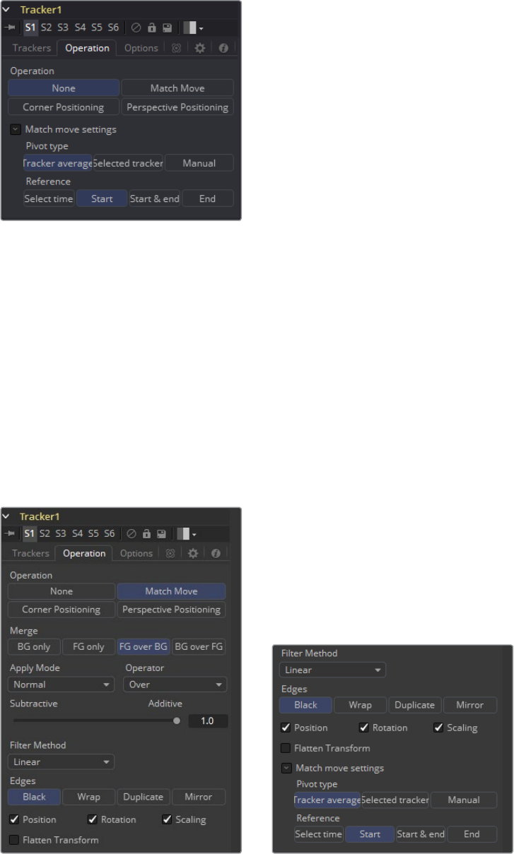
663
Tracker Tools Chapter – 27
Operation Tab
The Tracker tool is capable of performing a wide variety of functions, from match moving an
object into a moving scene, smoothing out in a shaky camera movement, or replacing the content
of a sign. Use the options and buttons in the Operation tab to select the function performed by
the Tracker tool. Please also refer to the Tracking Explained section in the Appendices.
Operation Buttons
These four buttons select the exact function performed by the Tracker. The remaining
controls in this tab fine-tune the result of the Operation.
None
The Tracker performs no additional operation on the image beyond simply locating and
tracking the chosen pattern. This is the default mode, used to create a path that will
then drive another control in Fusion.
Match Move
This mode is used when stabilizing an image, or when matching the position, rotation
and scaling of the layer for match moving another element into the scene. Stabilizing
requires a minimum of one Tracker to determine position, and two or more to determine
scaling and rotation in the sequence.
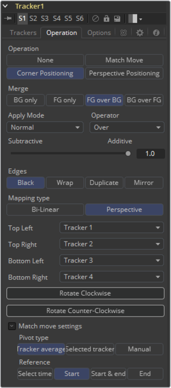
664
Tracker Tools Chapter – 27
Corner Positioning
The Corner Positioning mode is used to track the four corners of a rectangular object
and replace the contents with a new image. A minimum of four Trackers is required for
this mode, and if there are not enough Trackers, new ones will be created until the total
equals four.
Perspective Positioning
This mode is similar to the Corner Positioner, but rather than replacing the contents of
the rectangle, the four tracked corners are mapped to the four corners of the image.
This is generally used to remove Perspective from an image. Like the Corner Positioner,
this mode requires four Trackers, which will be created if there are not already
that many.
Merge
The Merge control determines what is done (if anything) with the image provided to the
Foreground input of the Tracker. This array of buttons appears when the operation is
set to anything other than None.
BG Only
The Foreground input is ignored, only the Background is affected. This is used primarily
when Stabilizing an image sequence.
665
Tracker Tools Chapter – 27
FG Only
The Foreground input is transformed to match the movement in the background, and
this transformed image is passed through the Tracker’s output. This Merge technique is
used when match moving one layer’s motion to another layer’s motion.
FG Over BG
The Foreground image is merged over the Background image, using the Merge
method described by the Apply Mode control that appears.
BG Over FG
The Background is merged over the Foreground. This technique is often used when
tracking a layer with an Alpha channel so that a more static background can be applied
behind it.
Apply Mode
This drop-down menu provides a variety of options to determine how the two layers
should be combined. The options in this menu are explained in more detail in the
reference chapter for the Merge tool.
Subtractive - Additive
This determines whether the Foreground layer is placed over the Background in using
Additive or Subtractive merging techniques. This control is explained in more detail in
the documentation for the Merge tool.
Edges Match Move
This button array only appears if the Operation mode is set to Match Move. The various
options select how the revealed edges are handled when the image is moved to match
position and scaling.
Black Edges
Out of frame edges revealed by Stabilization are left black.
Wrap
Portions of the image moved off frame to one side are used to fill edges that are
revealed on the opposite side.
Duplicate
The last valid pixel on an edge is repeated to the edge of the frame.
Position, Rotation and Scaling Checkboxes
The Position, Rotation and Scaling checkboxes only appear when the mode is set to
Match Move. They determine what components of motion that Stabilization will attempt
to correct in the image. For example, if only the Position checkbox is selected, no
attempt will be made to correct for Rotation and Scaling in the image.
Flatten Transformation
This checkbox only appears when the mode is set to Match Move. Like most
transformations in Fusion, Stabilization is concatenated with other sequential
transformations by default. Selecting this checkbox will flatten the transform, breaking
any concatenation taking place and applying the transform immediately.
Mapping Type
The Mapping Type control only appears in the Corner Positioning mode. There are two
options in the button array.
666
Tracker Tools Chapter – 27
Bi-Linear
The first method is Bi-Linear where the Foreground image is mapped into the
Background without any attempt to correct for perspective distortion. This is identical to
how previous versions of Fusion operated, and the Classic mode is included pretty
much for compatibility reasons only.
Perspective
The preferred setting for this control is True Perspective.
Corner Selector
When the operation of the Tracker is set to either Corner or Perspective Positioner
modes, these four drop-down menus appear. They are used to select which trackers
map to each of the four corners of the rectangle used by these modes. This is useful
when a Tracker has more than four patterns selected, and you must choose which the
positioners use.
Rotate Buttons
These controls only appear when the operation of the Tracker is set to either Corner or
Perspective Positioner modes. They are used to rotate the Foreground image by 90
degrees before it is applied to the Background.
Stabilize Settings
The Tracker tool automatically outputs several steady and unsteady position outputs to
which other controls in the flow can be connected. The Stable Position output provides
X and Y coordinates to match or reverse motion in a sequence. These controls are
available even when the operation is not set to Match Move, since the Stable Position
output is always available for connection to other tools.
Axis Type (Stabilize Setting)
Under virtually all circumstances, the Axis for any stabilization should be the average
position of all Trackers on that frame, however, the rare occasion arises when the
Tracker’s axis must be elsewhere.
This array of buttons allows for the selection of an axis for the Stabilization based on
the position of a single Tracker, or a manual position.
Reference (Stabilize Setting)
The Reference controls are used to set the `snapshot frame’ for Stabilization. When you
stabilize an image, there must be a position that is considered correct, to which all
subsequent movement is detected and corrected.
Select Time
The Select Time Reference mode determines the `snapshot frame’ based on the frame
where the pattern is first selected. All Stabilization is intended to return the image back
to that reference.
Start
The Snapshot Frame is determined to be the first frame in the tracked path. All
Stabilization is intended to return the image back to that reference.
Start and End
The Start and End Reference mode is somewhat different from all other Reference
modes. Where the others are intended to take a snapshot frame to which all
stabilization returns, immobilizing the image, the Start and End mode is intended to
smooth existing motion, without removing it. This mode averages the motion between
the Start and End of the path, drawing a straight line between those points.
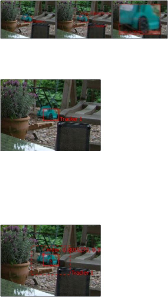
667
Tracker Tools Chapter – 27
When this mode is Active, it reveals the Reference Intermediate Points control.
Increasing the value of this control increases the number of points in the path used by
the Reference, smoothing the motion from a straight line between Start and End
without making it wholly linear.
End
The Snapshot Frame is determined to be the last frame in the tracked path. All
Stabilization is intended to return the image back to that reference.
Onscreen Controls
Each pattern in the Tracker has its own set of onscreen controls, used to select the pixels in the
image to be tracked.
These controls are visible in the Viewers whenever a tracker is selected in a flow.
The onscreen control is indicated by a red rectangle with a handle in the top left corner.
This rectangle indicates the position of the pattern in the image. Every pixel within the
rectangle is considered to be part of the pattern used for tracking. Resize the pattern
by clicking and dragging on the rectangle’s borders.
Whenever the mouse moves over the pattern rectangle, a second rectangle with a
dashed outline appears. This represents the search area, which determines how far
away from the current pattern the Tracker looks on the next frame. This should always
be larger than the pattern, and it should be large enough to encompass the largest
frame-to-frame movement in the scene. Faster moving objects require larger search
areas and slower moving objects can get away with smaller search areas. The larger
the search area, the longer it will take to track, so try not to make the search area larger
than necessary.
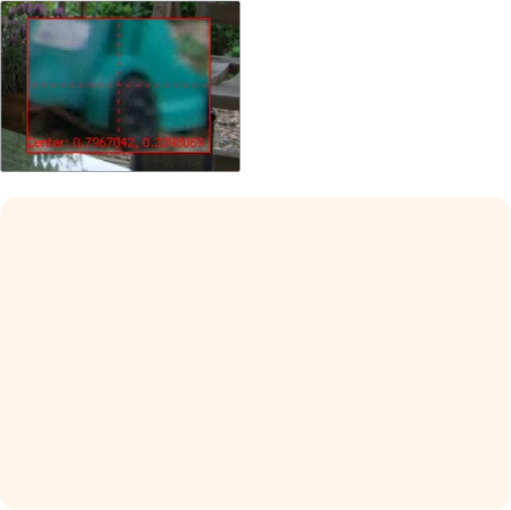
668
Tracker Tools Chapter – 27
Dragging on the handle repositions the pattern. While repositioning the pattern, a
thumbnail window with an enlarged view of the pattern is displayed in the views, to
assist with precise positioning of the pattern. This thumbnail disappears when the
mouse button is released. The magnification ratio can be adjusted in the Options tab. If
the selected Tracker has a custom name, the name of that Tracker will be displayed as
a label at the bottom right of the search area rectangle.
X/Y Paths
By default the Tracker applies a Displacement Path to the tracked points. To apply an
XY Path to the tracked points go to Preferences > Globals > Splines.
There is no limit to the number of trackers that can be used in one flow, or in
the number of connections that can be made to a tracker. This chapter serves
as a reference for the various controls in the Tracker, but we strongly suggest
you read the more general information about using the Tracker in the
Tracking chapter.
The Tracker can be employed in two forms: as a tool in the Flow, or as a
modifier attached to a control. When the Tracker is used as a tool in the Flow,
the image tracked comes from the input to the Tracker tool. There is no limit to
the number of patterns that can be tracked by a single Tracker tool.
When the Tracker is used as a modifier, its controls appear in the Modifier tab
for any tool with a control connected to that modifier. Only one pattern can be
tracked by a Tracker Modifier, but the image source can come from anywhere
in the composition. This technique is generally used when tracking a quick
position for a control.
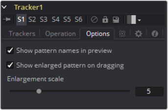
669
Tracker Tools Chapter – 27
Options Tab
Show Pattern Names in Preview
This option defines if the Tracker’s name will be displayed in the view. Switch it off to
see just the Pattern Rectangle instead.
Show Enlarged Pattern on Dragging
This option defines if there is an enlarged view on positioning the Pattern
Rectangle or not.
Enlargement Scale
The Zoom factor that is used on positioning the Pattern Rectangle when the above
option is on. The outputs of a Tracker (seen in the Connect to… menu) can also be used
by scripts. They are:
They are:
SteadyPosition: Steady Position
UnsteadyPosition: Unsteady Position
SteadyAxis: Steady Axis
SteadySize: Steady Size
UnsteadySize: Unsteady Size
SteadyAngle: Steady Angle
UnsteadyAngle: Unsteady Angle
Position1: Tracker 1 Offset position
PerspectivePosition1: Tracker 1 Perspective Offset position
PositionX1: Tracker 1 Offset X position (3D Space)
PositionY1: Tracker 1 Offset Y position (3D Space)
PerspectivePositionX1: Tracker 1 Perspective Offset X position (3D Space)
PerspectivePositionY1: Tracker 1 Perspective Offset Y position (3D Space)
SteadyPosition1: Tracker 1 Steady Position
UnsteadyPosition1: Tracker 1 Unsteady Position (similarly for the 2nd, 3rd and so on)
670
Tracker Tools Chapter – 27
Planar Tracker Tool
The Planar Tracker tool is designed to solve a matchmoving problem that commonly comes up
during post-production. Live action footage containing a planar surface such as a license plate,
a road sign, or a brick wall and need to replace the numbers in the license plate, a city’s name
in the road sign, or place a billboard poster on the blank brick wall. The problem is that the
camera is moving in the shot so the license plate, road sign, or brick wall undergo continuous
changes in perspective. The artist cannot simply merge a new license plate over the existing
background without accounting for the perspective distortions. A time intensive way to solve
this problem would be to use Fusion’s Corner Pin tool and manually keyframe the four corners
to match the perspective distortions. Planar Tracker automates this keyframing process, to track
the perspective distortions of a planar surface in a background plate over time and then
re-apply those same perspective distortions to a different foreground.
Part of using Planar Tracker is also knowing when to give up and fall back to using Fusion’s
Tracker tool or to manual keyframing. Some shots are simply not trackable or the resulting track
suffers from too much jitter or drift. Planar Tracker is a useful time saving tool in the artist’s
toolbox and, while it may track most shots, it is not a 100% solution.
Planar Tracker has four operation modes:
Track: use to select a planar surface and track it over time.
Steady: removes all motion and distortions from the planar surface.
Corner Pin: computes and applies a matching perspective distortion to a foreground
image and merges it on top of the tracked footage.
Stabilize: allows smoothing of translation, rotation, and scale over time.
The last three modes (Steady, Corner Pin, Stabilize) use the tracking data produced in Track
mode. Note that none of the operations can be combined together. For example, both corner
pin and stabilize cannot be done at the same time, nor can a track be done while in corner
pinning mode.
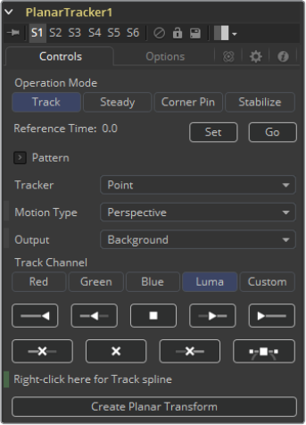
671
Tracker Tools Chapter – 27
While Planar Tracker does save the final resulting track in the composition on disk, it does not
save temporary tracking information such as the individual point trackers (compare with Camera
Tracker which does save the individual point trackers). Some consequences of this are:
The point trackers no longer appear in the view when a comp containing a Planar
Tracker tool is saved and reloaded.
Tracking may not be resumed after a comp containing a Planar Tracker tool has been
saved and reloaded. In particular, this also applies to auto saves. For this reason, it is
good to complete all tracking within one Fusion session.
The size of composition files is kept reasonable (in some situations Planar Tracker can
produce 100s of megabytes of temporary tracking data).
Saving and loading of compositions is faster and more interactive.
Main Inputs
Background: Contains the planar surface to be tracked.
Corner Pin 1: An image to be pinned on top of the background. There may be
multipleCorner Pin inputs named Corner Pin 1, Corner Pin 2, … etc.
Occlusion Mask: Used to mask out regions that do not need to be tracked. Regions
where this mask is white will not be tracked. For example, a person moving in front of
and occluding bits of the pattern may be confusing the tracker, and a quickly-created
rough rotomask around the person can be used to tell the tracker to ignore the
masked out bits.
Effect Mask: Used to mask the output from tool.
Track Mode
672
Tracker Tools Chapter – 27
The standard tracking workflow with Planar Tracker is:
1 Remove lens distortion: The more lens distortion in the footage, the more the resulting
track will slide and wobble.
2 Connect in footage: Connect a Loader whose footage has a planar surface that can be
tracked over time and view the Planar Tracker tool in a view.
3 Select a reference frame: Move to a frame where the planar surface to be tracked is
unoccluded and set this as the reference frame.
4 Choose the pattern: In the view, draw a polygon around the planar surface to track.
This is called the “pattern”. In most cases, this will probably be a rectangle but an
arbitrary closed polygon can be used. The pixels enclosed by this region will serve as
the pattern that will be searched for on other frames. Note that it is important that the
pattern is drawn on the reference frame. Do not confuse the pattern with the region
to corner pin (which always has four corners and is separately specified in Corner
Pin mode).
5 Adjust render range: In the timeline, adjust the render range to match the range of
frames where the planar surface is visible.
6 Adjust track options: Frequently changed options are Tracker, Motion Type, and
Track Channel.
7 Mask out occluders: If moving objects partially cover up the planar surface, you may
wish to connect in an occlusion mask to Planar Tracker. When using the Hybrid tracker,
providing a mask to deal with occluding objects is pretty much mandatory, while with
the Point tracker it is recommended to try tracking without a mask.
8 Track: Go back to the reference frame. Press the Track To End button and wait for the
track to complete. Go back to the reference frame. Press the Track To Start button and
wait for the track to complete. Note that the tracks in the view are not selectable or
deletable like in Camera Tracker.
9 Check track quality: Visually inspect the track to see how accurate it is. Does it stick to
the surface? Switching to Steady mode can help here.
10 Use the track: The Steady, Corner Pin, and Stabilize operation modes use the
tracking data produced in Track mode. At this point, you may also choose to export
a Planar Transform tool that can be used to mirror the tracked perspective distortion
onto masks.
Reference Time
The reference time determines the frame where the pattern is taken from. It is also the
time from which tracking begins. The reference time cannot be changed once it has
been set without destroying all pre-existing tracking information so scrub through the
footage to be tracked and choose carefully. The reference frame needs to be carefully
chosen to give the best possible quality pattern to track from.
Pattern Polygon
The region to track is specified by drawing a polygon on the reference frame. Make
sure the region selected belongs to a physically planar surface in the shot. Sometimes
a region that is only approximately planar can be used. In general, the less planar the
surface, the poorer the quality of the resulting track.
673
Tracker Tools Chapter – 27
As a rule of thumb, the more pixels in the pattern, the better the quality of the track. In
particular, this means on the reference frame. the pattern to be tracked should:
be as large as possible.
be as much in frame as possible,
be as unoccluded as possible eg. by any moving foreground objects.
be at its maximal size eg. when tracking an approaching road sign, it is good to pick
a later frame where it is 400x200 pixels big rather than 80x40 pixels.
be relatively undistorted eg. when the camera orbits around a flat stop sign, it is
better to pick a frame where the sign is face on parallel to the camera rather than a
frame where it is at a highly oblique angle.
If the pattern contains too few pixels or not enough trackable features, this can cause
problems with the resulting track such as jitter, wobble, and slippage. Sometimes
dropping down to a simpler motion type can help in this situation.
Tracker
There are two available trackers to pick from:
Point: Tracks points from frame to frame. Internally, this tracker does not actually
track points-per-se but small patterns like Fusion’s trusty Tracker tool. The point
tracker possesses the ability to automatically create its own internal occlusion mask
to detect and reject outlier tracks that do not belong to the dominant motion. Tracks
are colored green or red in the view, depending on whether the point tracker thinks
they belong to the dominant motion or they have been rejected. The user can
optionally supply an external occlusion mask to further guide the Point tracker.
Hybrid Point/Area: Uses an area tracker to track all the pixels in the pattern. Unlike
the point tracker, the area tracker does not possess the ability to automatically reject
parts of the pattern that do not belong to the dominant motion so you must manually
provide it with an occlusion mask. Note that for performance reasons, the Hybrid
tracker internally first runs the point tracker which is why the point tracks can still be
seen in the view.
There is no best tracker. They each have their own advantages and disadvantages:
Artist Effort (occlusion masks): the Point tracker will automatically create its own
internal occlusion mask while, with the Hybrid tracker, more time needs to be spent
manually creating occlusion masks.
Accuracy: the Hybrid tracker is more accurate and less prone to wobble, jitter,
and drift since it tracks all of the pixels in the pattern rather than a few salient
feature points.
Speed: the Hybrid tracker is slower than the Point tracker.
In general, it is recommended to first quickly track the shot with the Point tracker and
examine the results. If the results are not good enough, then try the Hybrid tracker.
Motion Type
Determines how Planar Tracker internally models the distortion of the planar surface
being tracked. The five distortion models are:
Translation
Translation, Rotation (rigid motions).
Translation, Rotation, Scale (takes squares to squares, scale is uniform in x & y).
Affine - includes translation, rotation, scale, skew (maps squares to parallelograms).
Perspective (maps squares to generic quadrilaterals).
674
Tracker Tools Chapter – 27
Each successive model is more general and includes all previous models as a
special case.
When in doubt, choose Perspective for the initial track attempt. If the footage being
tracked has perspective distortions in it and Planar Tracker is forced to work with a
simpler motion type, this can end up causing the track to slide and wobble.
Sometimes with troublesome shots, it can help to drop down to simpler motion model.
This can happen (for example) when a lot of track points are clustered in one side of the
region to be tracked or when tracking a small region where Planar Tracker does not
have a lot of pixels to work with.
Output
Controls what is output from the Planar Tracker tool while in the Track operation mode.
Background: Outputs the input image unchanged.
Background - Preprocessed: Planar Tracker does various types of preprocessing on
the input image (eg. converting it to luma) before tracking. It can be useful to see this
when deciding which Track Channel to choose.
Mask: Outputs the pattern as a black and white mask.
Mask over Background: Outputs the pattern mask merged over the background.
Track Channel
Determines which image channel in the background image is tracked. It is good to pick
a channel with high contrast, lots of trackable features, and low noise. Allowed values
are red, green, blue, and luminance.
Tracking Controls
These controls are used to control the tracker. Note that while tracking, only track to a
new frame if the current frame is already tracked or it is the reference frame.
Track to start: Tracks from the current frame backward in time to the start
(asdetermined by the current render range).
Step tracker to previous frame: Tracks from current frame to the previous frame.
Stop Tracking: Stops any ongoing tracking operations.
Step tracker to next frame: Tracks from current frame to the next frame.
Track to end: Tracks from the current frame forward in time to the end
(asdeterminedby the current render range).
Trim to start: Removes all tracking data before the current frame.
Delete: Deletes all tracking data at all times. Use this to destroy all current results and
start tracking from scratch.
Trim to end: Removes all tracking data after the current frame. This can be useful,
forexample, to trim the end of a track which has become inaccurate when the pattern
starts to move off frame.
Show Splines
Opens the spline editor and shows the splines associated with the Planar Tracker tool.
This can be useful for manually deleting points from the Track and Stable Track splines.
Right-click here for Track spline
While tracking, a spline containing 4x4 matrices at each keypoint is created. This is
known as the “Track spline” or just “Track” for short. These matrices completely
describe the distortions of the tracked pattern.
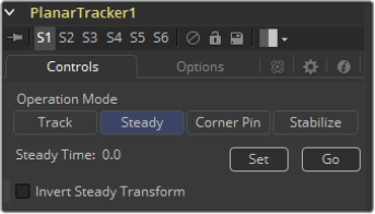
675
Tracker Tools Chapter – 27
Create Planar Transform
After tracking footage, this button can be pressed to create a Planar Transform tool on
the flow. The information currently encoded in the Track spline is shared with the
Planar Transform tool so that it can replicate the planar distortions tracked by the Planar
Tracker tool.
Steady Mode
In Steady Mode, the Planar Tracker transforms the background plate to keep the pattern as
motionless as possible. Any leftover motion is because the tracker failed to follow the pattern
accurately or because the pattern did not belong to a physically planar surface. Steady mode is
not very useful to do actual stabilization but is useful for checking the quality of a track. If the
track is good, during playback the pattern should not move at all while the rest of the
background plate distorts around it. It can be helpful to zoom in on parts of the pattern and
place the mouse cursor over a feature and see how far that feature drifts away from the mouse
cursor over time.
Steady Time
This is the time where the pattern’s position is snapshotted and frozen in place. It is
most common to set this to the reference time.
Invert Steady Transform
Causes the Planar Tracker tool to reverse the effects of the steady transform. This
means two Planar Tracker tools connected back-to-back with the 2nd set to invert the
first should give back the original image. If you place an effects tool in between the
two, then the effect will be locked in place. This should only be used to accomplish
effects that cannot be done through corner pinning, since it involves two resamplings
causing degradation (softening) of the background image.
Clipping Mode
Determines what happens to the parts of the background image that get moved off
frame by the steady transform:
Domain: The off frame parts are kept.
Frame: The off frames parts are thrown away.
Domain mode is useful when Steady Mode is being used to “lock” an effect to the
pattern. As an example, consider painting on the license plate of a moving car. One way
to do this is to use a Planar Tracker tool to steady the license plate, then a Paint tool to
paint on the license plate, and then a second Planar Tracker to undo the steady
transform. If the Clipping Mode is set to Domain, the off frame parts generated by the
first Planar Tracker are preserved so that the second Planar Tracker can in turn map
them back into frame.
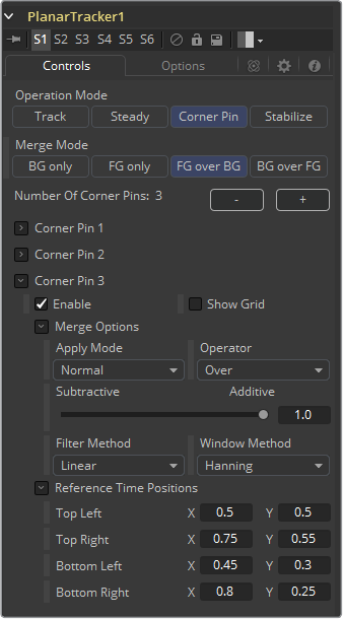
676
Tracker Tools Chapter – 27
Corner Pin Mode
In Corner Pin mode, one or more textures can be attached to a previously tracked planar
surface and undergo the same perspective distortions as the surface.
The corner pin workflow with Planar Tracker is:
1 Track: select a planar surface in the shot that you wish to attach a texture to or replace
the texture on. Track the shot (see the tracking workflow in the Track section).
2 Switch the Operation Mode to Corner Pin: When Corner Pin mode is entered
from Track mode, the pattern polygon is hidden and a corner pin control is shown
in the view.
3 Connect in the texture: In the flow view, connect the output of the Loader containing
the texture to the Corner Pin 1 input on the Planar Tracker tool.
4 Adjust corner pin: Drag the corners of the corner pin in the view until the texture is
positioned correctly. Sometimes the Show Grid option is useful when positioning the
texture. Additionally, if it helps to position it more accurately, scrub to other times and
make adjustments to the corner pin.
5 Review: Play back the footage and make sure the texture “sticks” to the planar surface.
Merge Mode
Controls how the foreground (the corner pinned texture) is merged over the
background (the tracked footage). If there are multiple corner pins, this option is shared
by all of them. There are four options to pick from:
BG only
FG only
FG over BG
BG over FG
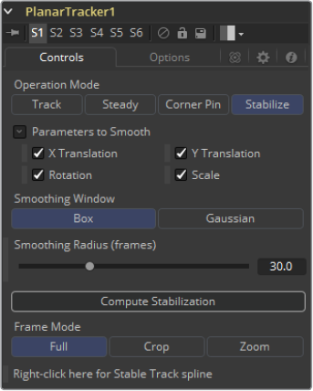
677
Tracker Tools Chapter – 27
Number of Corner Pins
Use the + and - buttons to increase and decrease the number of corner pins. Each time an
additional corner pin is created, a corresponding input appears on the tool in the flow view.
Corner Pin 1 Input Group
Each corner pin has a group of related inputs:
Enable: controls the visibility of the corner pin in the view.
Show Grid: shows a grid over the corner pin. This can be useful when positioning
the corners.
Merge Options: control merging of corner pin texture over the background - see the
documentation for the Merge tool.
Reference Time Positions: The positions of the four corners at the reference time.
Ifthe track was not perfect, these positions can be animated to make adjustments on
top of the track.
Stabilize Mode
Stabilize mode is used to smooth out shakiness in the camera by applying a transform that
partially counteracts the camera shake. This stabilizing transform (contained in the Stable Track
spline) is computed by smoothing out the tracked transforms over neighboring frames. Note
that Stabilize Mode only smooths out motions, while Steady Mode tries to completely “lock off”
all motion.
One thing to be aware of is that Planar Tracker stabilizes based upon the motion of the pattern
so it is important to choose the pattern carefully. If the motion of the pattern does not represent
the motion of the camera then there may be unexpected results. For example, if a shot has a
truck moving down the road and the camera is on a vehicle also moving alongside the truck,
and the tracking pattern is picked to be the side of the truck, Planar Tracker will end up
smoothing the combined motion of both the truck and the vehicle the camera is mounted on. In
some cases, this may not be desired and it may be better to choose the pattern to be on some
fixed object like the road or the side of a building, which would result in only the motion of the
camera being smoothed.

678
Tracker Tools Chapter – 27
One unavoidable side effect of the stabilization process is that transparent edges are
introduced along the edges of the image. These edges come about because the stabilizer
does not have any information about what lies off frame so it cannot fill in the missing bits. The
Planar Tracker tool offers the option to either crop or zoom away these edges. When filming, if
the need for post-production stabilization is anticipated, it can be sometimes useful to film at a
higher resolution (or lower zoom).
The stabilization workflow with Planar Tracker is:
1 Track: For the pattern, select a roughly planar region in the shot that represents the
motion that you want to stabilize. Track the shot (see the tracking workflow in the Track
section).
2 Switch the Operation Mode to Stabilize: Until a stabilization is computed, Planar
Tracker will just output the input footage.
3 Adjust stabilization options: Frequently changed options are Parameters to Smooth
and Smoothing Radius.
4 Compute stabilization: Press the Compute Stabilization button and wait for the
stabilization computations to finish. Play back the output of the Planar Tracker tool to
see the effects of the stabilization. Notice that transparent edges have been introduced
around the edges of the image by the stabilization transform.
5 Refine: Adjust the stabilization options and recompute the stabilization as many times
as desired.
6 Handle transparent edges (optional): Set the Frame Mode to either Zoom or Crop
as desired and then click the Auto Zoom or Auto Crop button. Playback the footage
to observe the effects. If there is too much zoom or the image has been cropped too
small, try reducing the amount of smoothing.
Parameters to Smooth
Specify which of the following parameters to smooth:
X Translation
Y Translation
Rotation
Scale
Smoothing Window
When stabilizing a particular frame, this determines how the contributions of
neighboring frames are weighted. Available choices are Box and Gaussian.
Smoothing Radius (frames)
Determines the number of frames whose transforms are averaged together to compute
the stabilization. A larger Smoothing Radius results in more smoothing but introduces
more transparent edges.
Compute Stabilization
Clicking this button runs the stabilizer, overwriting the results of any previous
stabilization. As soon as the stabilization is finished, the output of the Planar Tracker
tool will be immediately updated with the stabilization applied.
NOTE: The stabilizer uses the Track spline (created by the tracker) to produce
the Stable Track spline. Both of these splines keyframes contain 4x4 matrices
and the keyframes are editable in the spline editor.
679
Tracker Tools Chapter – 27
Clipping Mode
Determines what happens to the parts of the background image that get moved off
frame by the stabilization:
Domain: The off frame parts are kept.
Frame: The off frames parts are thrown away.
Frame Mode
This controls how transparent edges are handled. The available options are:
Full: Do nothing, leaves the transparent edges as is.
Crop: Crops away the transparent edges. When this option is selected, the
size of Planar Tracker’s output image is smaller than the input image. No image
resamplings occur.
Zoom: Scales the image bigger until the transparent edges are off frame. Choosing
this option causes an image resampling to occur. The downside of this approach is
that it reduces the quality (slightly softens) of the output image.
Crop
In crop mode, use the Auto Crop button or manually adjust the crop window by
changing the sliders:
X Offset
Y Offset
Scale
Auto Crop
When this button is clicked, Planar Tracker will examine all of the frames and pick the
largest possible crop window that removes all the transparent edges. The computed
crop window will always be centered in frame and pixel aligned. When clicked, Auto
Crop updates the X/Y Offset and Scale sliders.
Zoom
In zoom mode, use the Auto Zoom button or manually adjust the zoom window by
changing the sliders:
X Offset
Y Offset
Scale
Auto Zoom
When
this button is clicked, Planar Tracker will examine all of the frames and pick the smallest
possible zoom factor that removes all of the transparent edges. The computed zoom
window will always be centered in frame. When clicked, Auto Zoom updates the X/Y
Offset and Scale sliders.
Right-click here for Stable Track spline
Provides access to a spline whose keyframes contain 4x4 matrices which in turn
represent the stabilization transforms. This is mostly here for completeness and for
advanced users.
680
Tracker Tools Chapter – 27
Options Page
Darken Image
Darkens the image while in Track mode in order to better see the in view controls and
tracks. The Shift+D keyboard shortcut toggles this.
Show Track Markers
Toggles the display of the dots marking the location of trackers at the current time.
Show Trails
Toggles the display of the trails following the location of trackers.
Trail Length
Allows the changing of the length of tracker trails. If the pattern is moving very slowly,
increasing the length can sometimes make the trails easier to follow in the view. If the
pattern is moving very fast, the tracks can look like spaghetti in the view. Decreasing
the length can help.
Inlier/Outlier Colors
When tracking, the tracker analyzes the frame and detects which of the multitudinous
tracks belong to the dominant motion and which ones represent anomalous,
unexplainable motion. By default, tracks belonging to the dominant motion are colored
green (and are called inliers) and those that do not belong are colored red (and are
called outliers). Only the inlier tracks are used when computing the final resulting track.
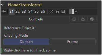
681
Tracker Tools Chapter – 27
Planar Transform Tool
The Planar Transform tool applies perspective distortions computed by a Planar Tracker tool to
any input mask The Planar Transform tool can be used to reduce the amount of artist time
spent rotoscoping objects. The workflow here centers around the notion that the Planar Tracker
tool can be used to track objects that are only roughly planar. After an object has been tracked,
a Planar Transform tool can then to be used to warp a rotospline, making it approximately follow
the object over time. Fine level cleanup work on the rotospline then needs to be done.
Depending on how well the Planar Tracker followed the object, this can result in a substantial
time savings in the amount of tedious rotowork that needs to be done. The key to using this
technique is recognizing situations where the Planar Tracker will do passably well tracking an
object that needs to be rotoscoped.
A rough outline of the workflow involved is:
1 Track: Using a Planar Tracker tool, select a pattern that represents the object to be
rotoscoped. Track the shot (see the tracking workflow in the the Track section for the
Planar Tracker tool).
2 Evaluate: Check the quality of the resulting track. If it does not follow the object
passably well then give up and do the rotowork the old fashioned way.
3 Create a Planar Transform tool: Press the Create Planar Transform button on the Planar
Tracker tool to do this. The newly created Planar Transform tool can be freely cut and
paste into another composition as desired.
4 Rotoscope the object: Move to any frame that was tracked by the Planar Tracker.
When unsure if a frame was tracked, look in the Spline Editor for a tracking keyframe on
the Planar Transform tool. Connect a Polygon tool into the Planar Transform tool. While
viewing the Planar Transform tool rotoscope the object.
5 Refine: Scrub the timeline to see how well the polygon follows the object. Make tweaks
to the polyline on frames where it is off. It is possible to add new points to further refine
the polygon.
Reference Time
The reference time that the pattern was taken from in the Planar Tracker tool used to
produce the Planar Transform.
Right-click here for Track spline
The Track spline contains information about the perspective distortions stored in 4x4
matrices. When a Planar Transform tool is exported from a Planar Tracker tool, the track
spline produced by the Planar Tracker is shared by connecting it with the Planar
Transform tool. A consequence of this sharing of the track spline is that, if the track is
changed in the Planar Tracker tool, the Planar Transform will be automatically updated.
Note that this spline can be examined in the Spline Editor which is useful for seeing the
extent of tracked frames.
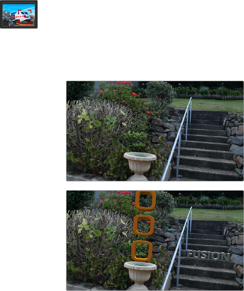
682
Tracker Tools Chapter – 27
Camera Tracker
Camera tracking is matchmoving and a vital link between 2D and 3D, allowing compositors to
integrate 3D renders into live action scenes. The Camera Tracker tool is used to calculate the
path of a live-action camera and generate a virtual camera in 3D space. This virtual camera’s
motion is intended to be identical to the motion of the actual camera that shot the scene. Using
the calculated position and movement of the virtual camera provides the flexibility to add 3D
elements to a live action scene. The Camera Tracker will also create a point cloud in 3D space
which can be used to align objects and other 3D models to the live action scene.
How It Works
The Camera Tracker is a complete workflow in one tool. By tracking the frames from a camera
that is moving in a scene, the 3D environment of the location and the camera’s motion can be
reconstructed. To do this, the track needs to be of a scene that has tracking features that are in
a fixed frame of reference. Moving objects or people need to be masked out from the tracker to
get a good solve, as these false tracks will cause inaccuracies when solving for the virtual
camera. When solving for the virtual camera, it is helpful to provide certain additional pieces of
information, such as the camera sensor size, the focal length of the lens, and measured
distances of known tracking marks. This will help guide the solver toward generating a more
accurate 3D camera and point cloud.
The Camera Tracker’s task is to create a 3D animated camera and point cloud of the scene.
Togenerate a camera, the basic approach to camera tracking has two steps. Tracking, which is
the analysis of a scene, and Solving, which calculates the virtual camera and point cloud. Once
these steps are taken, an animated camera can be exported from the tool.
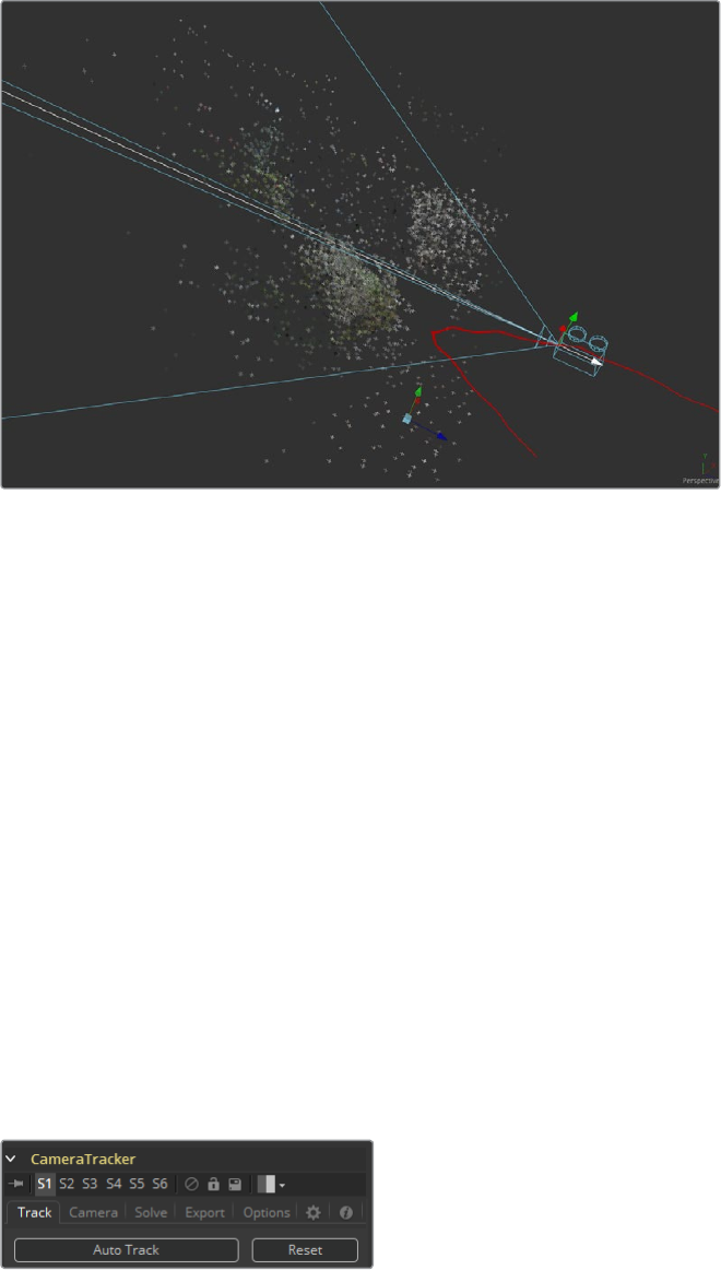
683
Tracker Tools Chapter – 27
There are five tabs in the Camera Tracker tool: Track, Camera, Solve, Export, and Options. To
define the workflow where an image sequence is tracked, set basic Camera parameters, Solve,
then Export the 3D virtual camera and point cloud. The top buttons of each tab section are the
operational process that will trigger the actions for each process.
Tracking
Tracking is the term used to describe the task of observing or analyzing the shot. The
Camera Tracker tool needs to take into account the movement of the source footage
before it can determine the location and movement of the virtual camera. To do this, the
tool searches for features, which are high contrast patterns within the shot, and assigns
trackers automatically to those features. A widespread of tracking points across the
scene will result in the best possible track, and adjusting controls such as the Minimum
Feature Separation will help populate the scene with more points. It is recommended
when tracking a scene to avoid features on moving objects or features that are caused
by parallax differences at different depths.
One way of avoiding these problem areas is masking. Applying a mask to the Camera
Tracker will isolate areas of a scene the Camera Tracker can analyze. For example,
suppose some footage shot with a moving camera of a subject standing in front of a
green screen needs camera tracking. Apply a mask to the subject, invert that mask (so
the subject is black and the environment is white) and attach it to the Camera Tracker
Track Mask input. By doing this, the tool will look for features within the mask area and
not on the subject. Alternatively, tracks can be selected and deleted from the viewer.
Camera
This section is where the basic settings of the camera are set, like film gate size, focal
length, and lens distortion parameters. If the actual values are not known, try a best
guess. The solver will attempt to find a camera near these parameters and it helps the
solver by giving parameters as close to the live action as possible.
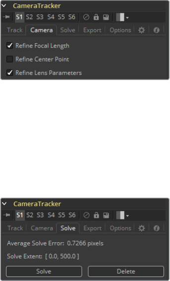
684
Tracker Tools Chapter – 27
Solving
Solving is the process in which the tool takes the currently existing tracks and
calculates from them the movement of the live action camera. From a user’s point of
view, solving should be thought of as an iterative process where the user repeatedly:
1 Runs the solver.
2 Deletes poor tracks and/or adjusts the initial guess provided in the Camera tab.
Until the solved camera motion path is good enough. Sometimes the first solve will be
good enough. Other times it may take many hours of cleaning up tracks to get a good
solve, and other times it is impossible. With experience, one gets a feel for which
tracks should be deleted and which should be kept, and which shots will be easy,
difficult, or impossible to solve. Be aware that deleting too many tracks can cause solve
quality to decrease as the solver has too little information to work with. In particular, if
there are less than eight tracks on any frame, mathematically there is not enough
information to solve the shot, however, it is strongly recommended to use a lot more
than 8 tracks to get a robust and accurate solve.
It may be tempting for users unfamiliar with working with camera trackers to try to
directly edit the 3D splines of the resulting camera in order to improve a solved
camera’s motion path. This option should be used as an absolute last resort, preferring
instead to modify the 2D tracks being fed into the solver.
Cleaning up false tracks is facilitated by showing the tracks overlaid on the live action
footage. Under the Options tab, the length of these tracks can be lengthened to show
more of the paths. Tracks can be individually selected or boxed selected, and the
Delete button will remove them. Understanding what false tracks look like and cleaning
the track data to a precise set of clear tracks will result in a more accurate solve.
In general, when cleaning up tracks, keep 2D tracks whose motion is completely
determined by the motion of the live action camera. Tracks on moving objects or
people and tracks that have parallax issues will need to be deleted. Tracks that are
reflected in windows or water or tracks of highlights that move over a surface will also
need to be cleared away. Tracks that do not do a good job of following a feature should
be deleted along with tracks that follow false illusionary corners created by the
superposition of foreground and background layers. Also consider deleting tracks that
correspond to locators which the solver has reconstructed at an incorrect z-depth.
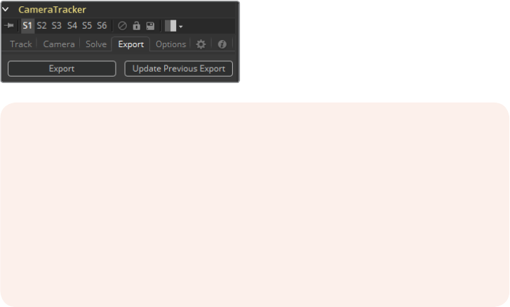
685
Tracker Tools Chapter – 27
When deleting tracks, it is good practice to note the current “Average Solve Error”, then
rerun the solver, and note whether the changes increased or decreased the average
solve error. In addition to looking at the average solve error to judge the quality of a
camera solve, it is useful to also:
Look at the camera path in 3D views to see if it contains any unexpected jumps,
breaks, or jitter.
Look through the camera in a 3D view at the locators in the 3D point cloud to see
how well they stick to features in the live action footage.
The Solve tab has filters that can be used to delete tracks based on track length, track
error, and solve error. These can be used to quickly remove poorly performing tracks
that may be misleading to the resulting camera, leaving a concise list of accurate tracks.
For the solver to accurately triangulate and reconstruct the camera and point cloud, it is
important to have:
A good balance of tracks across objects at different depths with not too many tracks
in the distant background or sky (these do not provide any additional perspective
information to the solver).
Tracks distributed evenly over the image and not highly clustered on a few objects or
on one side of the image.
Track starts and ends staggered in time with not too many tracks ending on the
same frame.
Some shots, if they do not have enough camera motion to triangulate feature locations,
can not be reconstructed with any useful accuracy. Ensuring that a shot is camera-
trackable begins on the set with proper usage of track markers and ensuring camera
moves have enough perspective for the solver to “latch” onto.
It is important to providing accurate live action camera information such as focal length
and film gate size, which can greatly improve the accuracy of the camera solve. For
example, if the provided focal length is too far away from the correct physical value, the
solver can fail to converge, resulting in a useless solution.
Export
Before exporting, it is a good idea to line up the virtual ground plane in Fusion’s 3D
environment with the physical ground plane in the live action footage. Camera Tracker
provides various translation, rotation, and scale controls to accomplish this. By selecting
tracking points on screen, the ground plane can be aligned to these points, as well as
rotation. By using two points of known distance, the scale of the scene can be set.
The Export will maintain a link to the exported tools so adjustments and new solves will
auto update these tools.
NOTE: Camera Tracker saves all its 2D tracks into the composition,
sometimes resulting in a rather large file on disk. If there are too many 2D
tracks over a long shot, the saved composition can reach over a gigabyte in
size. In some cases, this can make compositions containing Camera Tracker
tools cumbersome to load and work with. While it is possible to work directly
with the Camera Tracker tool via the camera coming out of the 3D output,
once the quality of the solve is satisfactory, consider instead using the Export
functionality to take a “low memory” snapshot which can be cut and paste into
another composition.
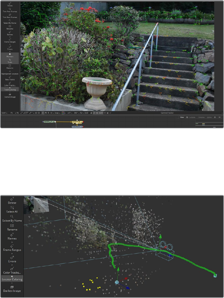
686
Tracker Tools Chapter – 27
Viewing 2D, 3D and Onscreen Controls
The Camera Tracker tool has two outputs: the primary output is 2D and there is also a
3D output for viewing the camera path and point cloud in 3D space. When refining
tracks to increase the accuracy of the solve, it can be helpful to simultaneously view the
2D and 3D outputs in side by side views. Note that selection of tracks in the 2D view
and their corresponding locators (in the point cloud) in the 3D view are synchronized.
There are also on Viewer menus docked on the side in the 2D and 3D views to give
quick control of functionality of this tool.
2D View
The 2D view is the primary display for the tool, by dragging and dropping the tool to the
view, it will display the image being tracked as well as overlay tracker markers and
plotted paths of the tracker motion.
A dedicated tool bar will be docked on the side of the view, giving access to the
common features used to track and solve a shot.
3D View
The second output of the Camera Tracker tool displays a 3D scene. To view this,
connect this 3D output to a 3D transform node and view that tool. The 3D output will
display the point cloud and the camera along with the image connected to it.
Selecting points will invoke the onscreen menu that will give control of various
functions such as, displaying Frame Ranges, Solve Error, and Name, as well as
Renaming, Deleting, and changing the colors.
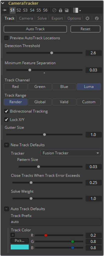
687
Tracker Tools Chapter – 27
Track Tab
Auto Track
Automatically detects trackable features and tracks them through the source footage.
Tracks will be automatically terminated when the track error becomes too high and new
tracks are created as needed. The values of the Detection Threshold and Minimum
Feature Separation sliders can be used to control the number and distribution of
auto tracks.
Reset
Deletes all the data internal to the Camera Tracker tool - this includes the tracking data
and the solve data (camera motion path and point cloud). To only delete the solve data,
use the “Delete” button on the Solve tab.
Preview AutoTrack Locations
Turning this checkbox on will show where the auto tracks will be distributed within the
shot. This is helpful for determining if the Detection Threshold and Minimum Feature
Separation need to be adjusted to get an even spread of trackers.
688
Tracker Tools Chapter – 27
Detection Threshold
Determines the sensitivity to detect features. Automatically generated tracks will be
assigned to the shot and the detection threshold will force them to be either in
locations of high contrast or low contrast.
Minimum Feature Separation
Determines the spacing between the automatically generated tracking points.
Decreasing this slider causes more auto tracks to be generated. Keep in mind that a
large number of tracking points will also result in a lengthier solve.
Track Channel
Used to nominate a colour channel to track: red, green, blue, or luminance. When
nominating a channel, choose one that has a high level of contrast and detail.
Track Range
Used to determine which frames are tracked:
Global: The global range which is the full duration of the timeline.
Render: The render duration set on the timeline.
Valid: The valid range is the duration of the source media.
Custom: A user determined range. When this is selected, a separate range slider
appears to set the start and end of the track range.
Bidirectional Tracking
Enabling this will force the tracker to track backward after the initial forward tracking.
When tracking backward, new tracks are not started but rather existing tracks are
extended backward in time. It is recommended to leave this option on, as long tracks
help give better solved cameras and point clouds.
Gutter Size
Trackers can become unstable when they get close to the edge of the image and
either drift or jitter or completely lose their pattern. Camera Tracker will automatically
terminate any tracks that enter the gutter region. Gutter size is given as a percentage of
pattern size. By default, it’s 100% of pattern size, so a 0.04 pattern means a 0.04 gutter.
New Track Defaults:
There are three methods in which the Camera Tracker Tool can analyze the scene and
each has its own strengths when dealing with certain types of camera movement.
Tracker: Internally, all the Trackers use the Optical Flow Tracker to follow features
over time and then further refine the tracks with the trusted Fusion Tracker or Planar
Tracker. The Planar Tracker method allows the pattern to warp over time by various
types of transforms to find the best fit. These transforms are:
Translation
Translation and Rotation
Translation, Rotation, and Scale
Affine
Perspective
It is recommended to use the default TRS setting when using the Planar Tracker.
Theaffine and perspective settings need large patterns in order to track accurately.
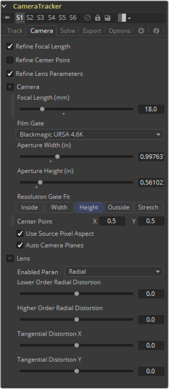
689
Tracker Tools Chapter – 27
Close Tracks when Track Error Exceeds: Tracks will be automatically terminated
when the tracking error gets too high. When tracking a feature, a snapshot of the
pixels around a feature are taken at the reference time of the track - this is called
a “pattern” - and that same pattern of pixels is searched for at future times. The
difference between the current time pattern and the reference time pattern is called
the “track error”. Setting this option higher produces longer but increasingly less
accurate tracks.
Solve Weight: By default, each track is weighted evenly in the solve process.
Increasing a track’s weight means it has a stronger effect on the solved camera path.
This is an advanced option that should be rarely changed.
Auto Track Defaults
Set a custom prefix name and/or colour for the automatically generated tracks. This
custom color will be visible when Track Colors in the Options tab is set to “User
Assigned”.
Camera Tab
Use this section to specify the physical aspects of the live action camera, which will be used as
a starting point when searching for solve parameters that match the real world camera. The
more accurate the information provided in this section, the more accurate the camera solve.
690
Tracker Tools Chapter – 27
The three top tick boxes define which parameters the solver can adjust to make the solve work.
Refine Focal Length
This will allow the solver to adjust the focal length of the lens to match the
tracking points.
Refine Centre Point
Normally ticked off, Camera lenses are normally centered in the middle of the film gate
but this may differ on some cameras For example, a cine camera may be set up for
Academy 1.85, which has a sound stripe on the left, and shooting super35, the lens is
offset to the right.
Refine Lens Parameters
This will refine the lens distortion or curvature of the lens. There tends to be larger
distortion on wide angle cameras
Focal length
Specify the known constant focal length used to shoot the scene or a guess if the
Refine Focal Length option is ticked.
Film Gate
Choose a film gate preset from the dropdown menu or manually enter the film back size
in the Aperture Width and Aperture Height inputs. Note, these values are in inches.
Aperture Width
In the event that the camera used to shoot the scene is not in the preset pulldown,
manually enter the aperture width (inches).
Aperture Height
In the event that the camera used to shoot the scene is not in the preset pulldown,
manually enter the aperture height (inches).
Resolution Gate Fit
This defines how the image fits the sensor size. Often film sensors are of a size to cover
a number of formats, and only a portion of the sensor area is recorded into an image.
For example, a 16:9 image is saved out of a full aperture sized sensor.
Typically fit to Width or Height is the best setting. The other fit modes are Inside
Outside or Stretched.
Center Point
This is where the camera lens is aligned to the camera. The default is (0.5, 0.5) which is
middle of the sensor.
Use Source Pixel Aspect
This will use the squeeze Aspect of the pixels that is loaded in the image. HD is square
pixels but NTSC has a pixel aspect ratio of 0.9:1, or Anamorphic cinema scope is
2:1 aspect.
Auto Camera Planes
When this is enabled, the camera’s image plane and far plane are automatically moved
to enclose the point cloud whenever a solve completes. Sometimes though, the solver
can anomalously fling points off really deep into the scene and consequently the image
plane ends up being pushed really far out, making the resulting scene unwieldy to work
with in the 3D views. In these cases, use this option to override this default behaviour
(or delete the offending tracks).
691
Tracker Tools Chapter – 27
Lens
When solving for the camera’s motion path, Camera Tracker internally creates and then
uses a simulated lens to model lens distortion in the source footage. This simulated
lens model is much simpler than real world lenses but captures the lens distortion
characteristics important for getting an accurate camera solve. Two types of distortion
are modelled by Camera Tracker:
1 Radial Distortion: The strength of this type of distortion varies depending on the
distance from the center of the lens. Examples of this include pincushion, barrel, and
mustache distortion. Larger values correspond to larger lens curvatures. Modelling
radial distortion is especially important for wide angle lenses and fisheye lenses (which
will have a lot of distortion because they capture 180 degrees of an environment and
then optically squeeze it onto a flat rectangular sensor).
2 Tangential Distortion: This kind of distortion is produced when the camera’s imaging
sensor and physical lens are not parallel to each other. It tends to produce skew
distortions in the footage similar to distortions that can be produced by dragging the
corners of a corner pin within Fusion. This kind of distortion occurs in very cheap
consumer cameras and is practically non-existent in film cameras, DSLRs, and pretty
much any kind of camera used in film or broadcast. It is recommended that it be
left disabled.
Enable Parameters
Determines which lens parameters will be modelled and solved for. Parameters that are
not enabled will be left at their default values. The following options are available:
None: do not do any lens curvature simulations. This should be picked if there is a
very low distortion lens or the lens distortion has already been removed from the
source footage in a preprocessing step.
Radial: model only radial lens curvature. This causes the low and high order
distortion values to be solved for.
Radial & Tangential: model and solve for both radial and tangential distortion.
Lower Order Radial Distortion
Determines the quadratic lens curvature.
Higher Order Radial Distortion
Determines the quartic lens curvature.
Tangential Distortion X/Y
Determines skew distortion.
Solve
The Solve section is where the tracking data is used to reconstruct the camera’s motion path
along with the point cloud. It is also where cleanup of bad or false tracks is done, and other
operations on the tracks can be performed, such as defining which marks are exported in the
Point Cloud 3D. The markers can also have their weight set to affect the solve calculations.
Forexample, a good camera solve may have already been generated but there are not enough
locators in the point cloud in an area where an object needs to be placed so adding more
tracks and setting their Solve Weight to zero will not affect the solved camera but will give more
points in the point cloud.
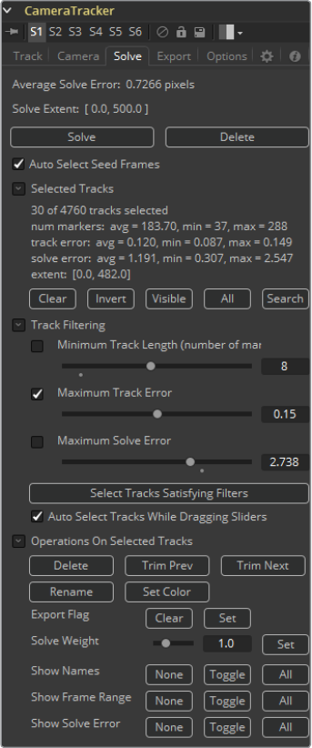
692
Tracker Tools Chapter – 27
Average Solve Error
Once the camera has been solved, the Average Solve Error will display here. This
number is a good indicator whether the camera solve was successful or not. It can be
thought of as the difference (measured in pixels) between tracks in the 2D image and
the reconstructed 3D locators reprojected back onto the image through the
reconstructed camera. Ultimately, in trying to achieve a low solve error - any value less
than 1.0 pixels will generally result in a good track. A value between 0.6 and 0.8 pixels
is considered excellent.
Solve Extent
Displays the frame range for which the camera’s motion will be reconstructed.
Thesolver will reconstruct any frames that have tracks on them.
Solve
Pressing Solve will launch the solver, which uses the tracking information and the
camera specifications to generate a virtual camera path and point cloud, approximating
the motion of the physical camera in the live action footage. The console will
automatically open, displaying the progress of the solver.

693
Tracker Tools Chapter – 27
Delete
Delete will remove any solved information, such as the camera and the point cloud, but
will keep all of the tracking data.
Auto Select Seed Frames
Seed frames are the reference images that are used to initialize the solve process.
These two frames are initially solved for and a camera is reconstructed and then
gradually more frames are added in and the solution is ‘grown’ outward from the seed
frames. The choice of seed frames strongly affects the entire solve and can easily
cause the solve to fail. Seed frames can be found automatically or defined manually.
Manual choice of seed frames is an option for advanced users. When choosing seed
frames, it is important to satisfy two conflicting desires: the seed frames should have
lots of tracks in common yet be far apart in perspective (the baseline distance between
the two associated cameras is long).
Selected Tracks
This area displays the properties of a track point or group of points. It has options to:
Clear: deselects all tracks and clears this area.
Invert: deselects the current selected tracks and selects the other tracks.
Visible: selects all the trackers at the current frame.
All: selects all trackers on all frames.
Search: selects tracks whose names contain a substring.
Track Filtering
Camera Tracker can produce a large number of automatically generated tracks. Rather
than spending a lot of time individually examining the quality of each track, it is useful to
have some less time intensive ways to filter out large swaths of potentially bad tracks.
The following input sliders are useful for selecting large amounts of tracks based on
certain quality metrics and then a number of different possible operations can be made
on them. For example, weaker tracks can selected and deleted, giving a stronger set of
tracks to solve from. Each filter can be individually ticked on or off.
Minimum Track Length (number of markers)
Selects tracks that have a duration shorter than the slider’s value. Short tracks usually
don’t get a chance to move very far and thus provide less perspective information to
the solver than a longer track, yet both short and long tracks are weighted evenly in the
solve process, making long tracks more valuable to the solver. Locators corresponding
to shorter tracks are also less accurately positioned in 3D space than those
corresponding to longer tracks. If the shot has a lot of long tracks, it can be helpful to
delete the short tracks. For typical shots, using a value in the range of 5 to 10 is
suggested. If there are not e a lot of long tracks (eg. the camera is quickly rotating,
causing tracks to start and move off frame quickly), using a value closer to 3 is
recommended.
NOTE: also select tracks directly in the 2D view using the mouse or in the 3D
view by selecting their corresponding locators in the point cloud.

694
Tracker Tools Chapter – 27
Maximum Track Error
Selects tracks that have an average track error greater than the slider’s value. When
tracking, tracks are automatically terminated when their track error exceeds some
threshold. This auto termination controls the maximum track error, while this slider
controls the average track error. For example, tracks following the foliage in a tree tend
to be inaccurate and sometimes may be detected by their high average error.
Maximum Solve Error
Selects tracks that have a solve error greater than the slider’s value. One of the easiest
ways to increase the accuracy of a camera solve is to select the 20% of the tracks with
the highest solve error and simply delete them (although this can sometimes make
things worse).
Auto Select Tracks While Dragging Sliders
When this is ticked on, dragging the above sliders (minimum track length, maximum
track error, maximum solve error) will cause the corresponding tracks to be interactively
selected in the view.
Select Tracks Satisfying Filters
Selects the tracks within the scene that meet the above Track Filtering values. Note
that when this button is pressed, the tracks that satisfy the filter values are displayed in
the Selected Tracks area of the Solve Tab and are coloured in the viewer. This button is
useful when “Auto Select Tracks While Dragging Sliders” is turned off or if the selection,
for example, was accidentally lost by misclicking in the view.
Operations On Selected Tracks
Tracks selected directly in the view with the mouse or selected via track filtering can
have the following operations applied:
Delete will remove the tracks from the set. When there are bad tracks, the simplest and
easiest option is to simply delete them.
Trim Previous will cut the tracked frames from the current frame to the start of the track.
Sometimes it can be more useful to trim a track than deleting it. For example, high quality
long tracks that become inaccurate when the feature they are tracking starts to become
occluded or when the tracked feature moves too close to the edge of the image.
Trim Next will cut the tracked frames from the current frame to the end of the track.
Rename will replace the current auto generated name with a new name.
Set Color will allow for user assigned color of the tracking points.
Export Flag This controls whether the locators corresponding to the selected tracks will
be exported in the point cloud. By default all locators flagged as exportable.
Solve Weight By default, all the tracks are used and equally weighted when solving for
the camera’s motion path. The most common use of this option is to set a track’s weight
to zero so it does not influence the camera’s motion path but is still has a reconstructed
3D locator. Setting a tracks’ weight to values other than 1.0 or 0.0 should only be done
by advanced users.
Onscreen display of track names and values are controlled by these functions:
None will clear/hide the selected tracks.
Toggle will swap the selected tracks and unselect sets.
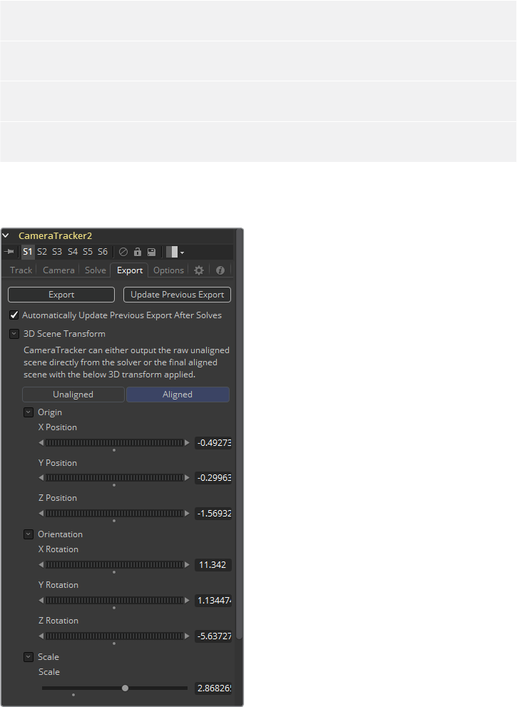
695
Tracker Tools Chapter – 27
All will select all tracks.
Show Names will display the track name, by default these are a number.
Show Frame Range will display the start and end frame of a track.
Show Solve Error will display the amount of solve error each selected track has.
Export
Export
Export button will create a basic setup that can be used for 3D match moving:
A Camera 3D with animated translation and rotation that matches the motion of the
live action camera and an attached image plane.
A Point Cloud 3D containing the reconstructed 3D positions of the tracks.
A Shape 3D set to generate a ground plane.
A Merge 3D merging together the camera, point cloud, and ground plane. When the
Merge 3D is viewed through the camera in a 3D view, the 3D locators should follow
the tracked footage.
A Renderer 3D set to match the input footage.
The export of individual tools can be enabled/disabled in the Export Options tab.
696
Tracker Tools Chapter – 27
Update Previous Export
When this button is clicked, the previously exported tools are updated with any new
data generated. These previously exported tools are remembered in the Previous
Export section at the bottom of this section. An example of where this is handy:
1 Solve the camera and export.
2 Construct a complex flow based around the exported tools for use in set extension.
3 The camera is not as accurate as preferred or perhaps the solver is rerun to add
additional tracks to generate a denser point cloud. Rather than re-exporting the
Camera 3D and Point Cloud 3D tools and connecting them back in, just press this
button to “overwrite” the existing tools in place.
Automatically Update Previous Export After Solves
Will cause the already exported tools (Camera 3D, Point Cloud 3D, Lens Distort,
Renderer 3D, and the ground plane) to auto update on each solve.
3D Scene Transform
This defines the origin and alignment of the virtual camera, point cloud, and ground
plane. By default, the solver will always place the camera in Fusion’s 3D virtual
environment so that on the first frame it is located at the origin (0, 0, 0) and it is looking
down the -Z axis. In this default orientation, the physical ground plane in the footage
will often not match up with the virtual ground plane in the 3D view and the 3D Scene
Transform provides a mechanism to correct that. Note that adjusting the 3D Scene
Transform does not modify the camera solve but simply repositions the 3D scene to
best represent the position of the live action camera. Also note that if these options
need changing, it is important to manually hit “Update Previous Export” to see the
results in the exported tools.
Unaligned, Aligned
The Unaligned button allows the origin and ground plane settings to be adjusted, either
manually or by using a selected set of locators from the point cloud. When in unaligned
mode, a 3D transform control will be shown in the 3D view which can be manually
manipulated to adjust the origin.
Once alignment has been complete, the section is locked by switching to the Aligned
button. From the Coordinate System, either output the Raw Unaligned scene where
the3D grid runs directly through the solved camera, or an Aligned scene where the
3Dgrid can be adjusted to the plane of the user’s choice.
Set From Selection
Takes selected 3D points from the point cloud and aligns the ground plane to fit those
points. This can be adjusted individually for position, rotation, and scale. To set a
ground plane, select a number of Point Cloud points that are on the ground - to get the
best result, try to select as many points as possible belonging to the ground and having
a wide separation. Under the Origin pull down, press Set from Selection. This will
reposition the Ground Plane. Under the Orientation pull down, press Set from Selection.
This will alter the orientation of the Ground plane to the selected points. Finally, press
the Aligned button, which repositions the 3D system so the 3D grid is aligned to the
Ground Plane.
When selecting points for the ground plane, it is helpful to have the Camera Tracker
tool viewed in side by side 2D and 3D views. It may be easier to select tracks
belonging to the ground by selecting tracks from multiple frames in the 2D view rather
than trying to box select locators in the 3D view.
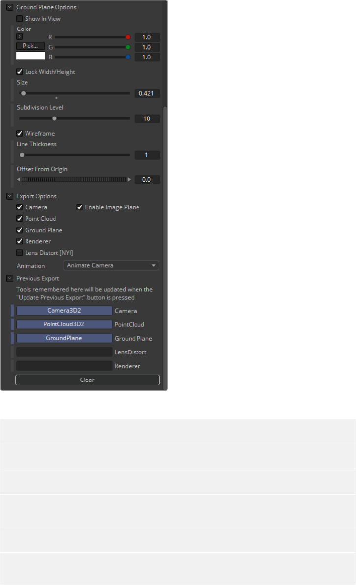
697
Tracker Tools Chapter – 27
Ground Plane Options
Color will set the color of the ground plane.
Size controls how big the ground plane can be set.
Subdivision Level set ,show many polygons are in the ground plane.
Wireframe sets whether the ground plane is set as wireframe or solid surface when
displayed in 3D.
Line Thickness adjusts how wide the lines will draw in the view.
Offset By default, the center of the ground plane is placed at the origin (0, 0, 0). This can
be used to shift the ground plane up and down along the y-axis.
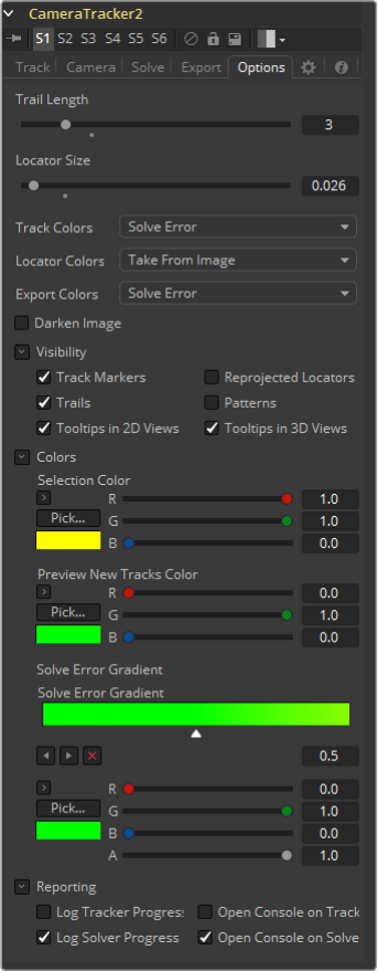
698
Tracker Tools Chapter – 27
Export Options
Provides a checkbox list of what will be exported as tools when the Export button is
pressed. These options are Camera, Point Cloud, Ground Plane, Renderer, Lens
Distortion, and Enable Image Plane in the camera.
Previous Export
When the Update Previous Export button is clicked, the previously exported tools listed
here are updated with any new data generated (this included the camera path and
attributes, the point cloud, and the renderer).
Options
Trail Length
Will display trail lines of the tracks overlaid on the view. The amount of frames forward
and back from the current frame is set by length.

699
Tracker Tools Chapter – 27
Locator Size
In the 3D View, the point cloud locators can be sized by this control.
Track Colors, Locator Colors, and Export Colors each have options for setting their
color to one of the following: User Assigned, Solve Error, Take From Image, and White.
Track Colors are the onscreen tracks in the 2D view.
Locator Colors are the Point Cloud locators in the 3D view.
Export Colors are colors of the locators that get exported within the Point Cloud tool.
Darken Image
Dim the brightness of the image in views to better view the overlaid tracks. This affects
both the 2D and 3D view.
Visibility
Toggles which overlays will be displayed in the 2D and 3D views. The options are
Tracker Markers, Trails, Tooltips in the 2D View, Tooltips in the 3D View, Reprojected
Locators, and Tracker Patterns.
Colors
Sets the color of the overlays
Selection Color: controls the color of selected tracks/locators.
Preview New Tracks Color: controls the color of the points displayed in the view
when the “Preview AutoTrack Locations” option is enabled.
Solve Error Gradient: By default, tracks and locators are colored by a green-yellow-
red gradient to indicate their solve error. This gradient is completely user adjustable.
Reporting
Outputs various parameters and information to the console.
Understanding Camera Tracking
On large feature films, Camera Matchmoving is often farmed out to experts who have a
lot of experience with the process of tracking and solving these types of shots. There is
rarely a shot where automatic, press a couple of buttons and the process is complete,
can be done. It does take understanding of the whole process and what is important to
get a good solved track.
The Camera Tracker has to solve for hundreds of thousands of unknown variables,
which is a complex task. To create an accurate solve, it is important to get to a precise
set of good tracks that exists for a long time. False or bad tracks will skew the result.
This section explains how to clean up false tracks and other theory to get a good solve.
Workflow
Track -> Solve -> Refine Filters -> Solve -> Cleanup tracks -> Solve -> Cleanup from
point cloud -> Solve -> Repeat.
The Solve is a repeated process to get a good result. Initially, there will be a lot of
tracks, and not all are good, so a process of filtering and cleaning up unwanted tracks
to get to the best set is a process. At the end of each clean up stage, pressing Solve
will give you a result for Solve Error. This needs to be below 1 for it to be good for use,
the lower the better. Refining the tracks will result in a better solve.
700
Tracker Tools Chapter – 27
False Tracks
False tracks are tracks that move or are incorrect and are caused by a number of
conditions, such as moving people or objects in a shot, or reflections and highlights
from a car. There are other types of false tracks like parallax errors where two objects
are at different depths and the intersection gets tracked. These Moire effects can
cause the track to creep. Reflections in glass on buildings are warped, trees in the
wind, recognizing these False tracks and eliminating them is the most important step in
the Solve process.
Track lengths
Getting a good set of long tracks is important, longer makes the solve fitting better.
Bi-directional tracking is used to extend the beginning of tracks in time. The longer in
time a track exists and the more tracks that overlap in time of a shot, the more
consistent and accurate the solve.
Seed frames
There are two seed frames that are used in the solve process, the algorithm chooses
two frames that are as far apart in time yet share the same tracks, hence longer tracks
makes the greater difference in the selection of seed frames.
The two Seed frames are used as the reference frames, which should be from different
angles of the same scene. The Solve process will use these as a master starting point
to fit the rest of the tracks of the sequence.
There is an option that auto detects Seed frames, which can take some time. In the
workflow of solving, auto detect is a good idea. When refining the trackers and
resolving, it should be set to manual mode and use the previous solve’s seed frames,
which are displayed in the solve dialog window.
Refine Filters
After the first solve, all of the trackers will have extra data generated. These are solve
errors and tracking errors.
Use the refine filters to reduce unwanted tracks, like setting minimum tracker length to
eight frames. As the value for each filter is adjusted, the Solve dialog window will
indicate how many tracks are affected by the filter. Solve again.
Onscreen Culling
Under the Options Tab, set the track to 20, this will display each track on footage with
+-20 frame trail. When scrubbing/playing through the footage, false tracks can be seen
and selected on screen, and deleted by pressing the delete key. This process takes an
experienced eye to spot tracks that go bad. Solve again.
View the 3D scene in perspective, the point cloud will be visible. Move and pan around
the point cloud, select and delete points that seem to have no inline with the image and
the scene space. Solve again
Repeat process until the Solve error is below 1.0 before exporting.
Selecting Points for Ground plane
Selecting tracks or points in the point cloud will allow for alignment and fitting of the
ground plane.
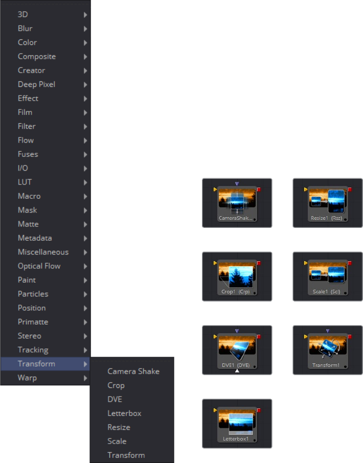
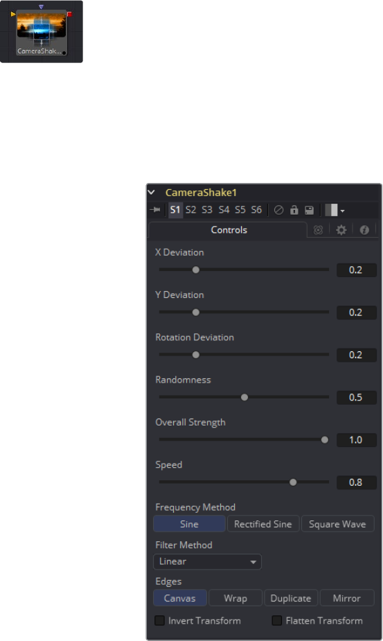
704
Transform Tools Chapter – 28
Camera Shake [CSH]
This tool can simulate a variety of Camera Shake style motions from organic to mechanical. It is
not the same as the Shake Modifier, which generates random number values for tool controls.
See the Connections and Modifiers chapter for more information about the Shake Modifier.
The Camera Shake tool concatenates its result with adjacent transformation tools. For more
information on concatenation, consult the Transformations chapter.
Controls Tab
Deviation X and Y
These controls determine the amount of shake that is applied to the image along the
horizontal (X) and vertical (Y) axis. Values between 0.0 and 1.0 are permitted. A value of
1.0 generates shake positions anywhere within the boundaries of the image.
Rotation Deviation
This determines the amount of shake that is applied to the rotational axis. Values
between 0.0 and 1.0 are permitted.
Randomness
Higher values in this control cause the movement of the shake to be more irregular or
random. Smaller values cause the movement to be more predictable.
Overall Strength
This adjusts the general amplitude of all the parameters and blends that affect in and
out. A value of 1.0 applies the effect as described by the remainder of the controls.
705
Transform Tools Chapter – 28
Speed
Speed controls the frequency, or rate, of the shake.
Frequency Method
This selects the overall shape of the shake. Available frequencies are Sine, Rectified
Sine and Square Wave. A Square Wave will generate a much more mechanical looking
motion than a Sine.
Edges
This determines how the Edges of the image are treated.
Black
This causes the edges that are revealed by the shake to be black.
Wrap
This causes the edges to wrap around (the top is wrapped to the bottom, the left is
wrapped to the right, etc.).
Duplicate
This causes the Edges to be duplicated, causing a slight smearing effect at the edges.
Invert Transform
Select this control to Invert any position, rotation or scaling transformation. This option
might be useful to exactly removing the motion produced in an upstream
Camera Shake.
Flatten Transform
The Flatten Transform option prevents this tool from concatenating its transformation
with adjacent tools. The tool may still concatenate transforms from its input, but it will
not concatenate its transformation with the tool at its output.
Filter Modes
Nearest Neighbor
This skips or duplicates pixels as needed. This produces the fastest but crudest results.
Box
This is a simple interpolation resize of the image.
Linear
This uses a simplistic filter, which produces relatively clean and fast results.
Quadratic
This filter produces a nominal result. It offers a good compromise between speed
and quality.
Cubic
This produces better results with continuous tone images but is slower than Bi-Cubic.
Ifthe images have fine detail in them, the results may be blurrier than desired.
Catmull-Rom
This produces good results with continuous tone images that are resized down.
Produces sharp results with finely detailed images.
Gaussian
This is very similar in speed and quality to Bi-Cubic.

706
Transform Tools Chapter – 28
Mitchell
This is similar to Catmull-Rom but produces better results with finely detailed images. It
is slower than Catmull-Rom.
Lanczos
This is very similar to Mitchell and Catmull-Rom but is a little cleaner and also slower.
Sinc
This is an advanced filter that produces very sharp, detailed results, however, it may
produce visible ‘ringing’ in some situations.
Bessel
This is similar to the Sinc filter but may be slightly faster.
Window Method
Some filters, such as Sinc and Bessel, require an infinite number of pixels to calculate
exactly. To speed up this operation, a windowing function is used to approximate the
filter and limit the number of pixels required. This control appears when a filter that
requires windowing is selected.
Hanning
This is a simple tapered window.
Hamming
Hamming is a slightly tweaked version of Hanning.
Blackman
A window with a more sharply tapered falloff.
Kaiser
A more complex window, with results between Hamming and Blackman.
Most of these filters are useful only when making an image larger. When shrinking
images, it is common to use the Bi-Linear filter, however, the Catmull-Rom filter will
apply some sharpening to the results and may be useful for preserving detail when
scaling down an image.
Example
Different Resize Filters. From left to right: Nearest Neighbor, Box, Linear, Quadratic, Cubic,
Catmull-Rom, Gaussian, Mitchell, Lanczos, Sinc, Bessel
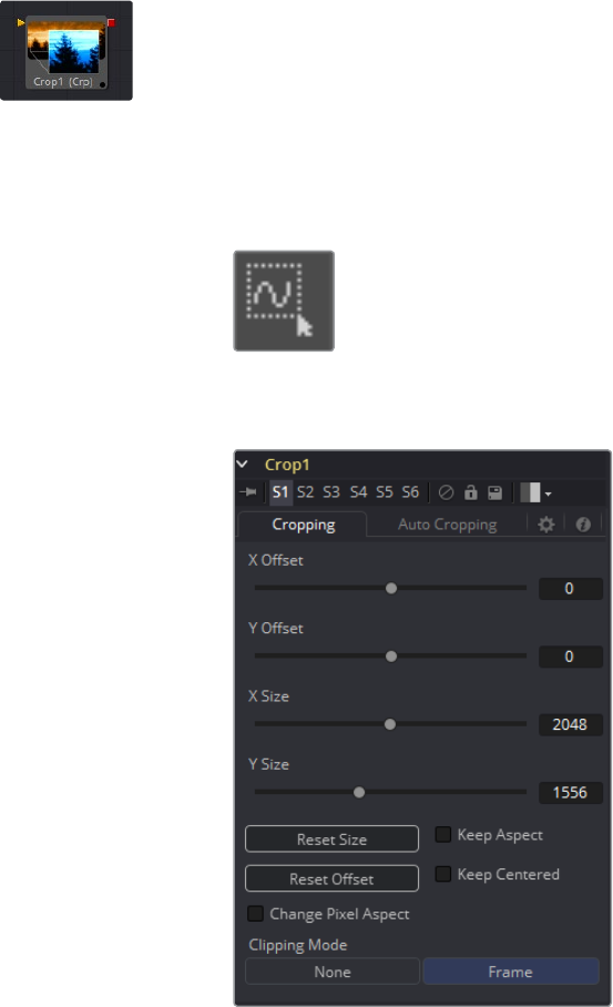
707
Transform Tools Chapter – 28
Crop [CRP]
The Crop tool can be used to cut out a portion of an image or to offset the image into a larger
image area. This tool actually changes the resolution of the image and should not be animated
under normal circumstances.
It is possible to crop an image in the view by viewing the upstream tool and selecting a region
with the mouse. To do so, first activate Allow Box Selection by clicking on the icon next to your
view, then dragging a rectangle to perform the operation.
Crop Tab
Offset X and Y
These controls position the top left corner of the Cropping window. Values larger than
the actual resolution of the cropped image cause it to disappear off the edges of the
output image. Values below 0 will push the input image toward the bottom right of the
result. The values of these controls are measured in pixels.
Size X and Y
Use this control to set the vertical and horizontal resolution of the image output by the
Crop tool. The values of these controls are measured in pixels.
Keep Aspect
When toggled on, the Crop tool maintains the aspect of the input image.
Keep Centered
When toggled on, the Crop tool automatically adjusts the X and Y Offset controls to
keep the image centered.
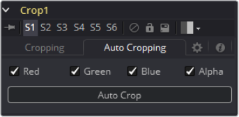
708
Transform Tools Chapter – 28
Reset Size
This resets the image dimensions to the Size of the input image.
Reset Offset
This resets the X and Y Offsets to their defaults.
Change Pixel Aspect
Enable this checkbox to reveal a Pixel Aspect control that can be used to change the
pixel aspect that the image is considered to have. See the Frame Formats section for
details on how Pixel Aspect operates in Fusion.
Clipping Mode
This option sets the mode used to handle the edges of the image when performing
Domain of Definition rendering. This is profoundly important for tools like Blur, which
may require samples from portions of the image outside the current domain.
Frame
The default option is Frame, which automatically sets the tool’s Domain of Definition to
use the full frame of the image, effectively ignoring the current Domain of Definition. If
the upstream DoD is smaller than the frame, the remaining area in the frame will be
treated as black/transparent.
Domain
Setting this option to Domain will respect the upstream Domain of Definition when
applying the tool’s effect. This can have adverse clipping effects in situations where the
tool employs a large filter.
None
Setting this option to None will not perform any source image clipping at all. This means
that any data required to process the tool’s effect which would normally be outside the
upstream DoD will be treated as black/transparent.
Auto Crop Tab
RGBA Color Channels
Select which channels are examined for an Auto Crop. This is useful for auto cropping
images with non-solid backgrounds in a specific color channel, like a blue color
gradient. Toggling the channel off causes Auto Crop to ignore it when evaluating
the image.
Auto Crop
This evaluates the image and attempts to determine the background color. It then crops
each side of the image to the first pixel that is not this color.
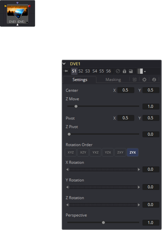
709
Transform Tools Chapter – 28
DVE [DVE]
The DVE tool is a 3D-image transformation similar to tools found in an online edit suite. The tool
encompasses image rotations, perspective changes and Z moves. The axis can be defined for
all transformations.
Settings Tab
Pivot X, Y and Z
Position the axis of rotation and scaling. The default is 0.5, 0.5 for X and Y, which is in
the center of the image, and 0 for Z, which is at the center of Z space.
Rotation Order
Use these buttons to determine in what order Rotations are applied to the image.
XYZ Rotation
These controls are used to rotate the image around the pivot along the X-, Y-
and Z-axis.
Center X and Y
This positions the Center of the DVE image on screen. The default is 0.5, 0.5, which
positions the DVE in the center of the image.
Z Move
This zooms the image in and out along the Z-axis. Visually, when this control is
animated, the effect is similar to watching an object approach from a distance.
Perspective
This adds additional Perspective to an image rotated along the X- or Y-axis, similar to
changing the Field of View and zoom of a camera.
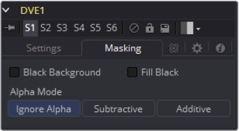
710
Transform Tools Chapter – 28
Masking Tab
The DVE tool allows pre-masking of its input image. This offers the ability to create
transformations from the masked area of the image while leaving the remainder of the image
unaffected.
Unlike regular effect masking, the masking process occurs before the transformation. To use
this feature, connect a mask to the DVE tool’s DVE Mask input. Alternatively, select the DVE
tool, right-click on the view and select DVE Mask from the contextual menu. All of the usual
mask types can be applied to the DVE mask.
Black Background
Toggle this on to erase the area outside the mask from the transformed image.
Fill Black
Toggle this on to erase the area within the mask (before transformation) from the DVE’s
input, effectively cutting the masked area out of the image. Enabling both Black
Background and Fill Black will show only the masked, transformed area.
Alpha Mode
This determines how the DVE will handle the alpha channel of the image, when
merging the transformed image areas over the untransformed image.
Ignore Alpha
This causes the input image’s alpha channel to be ignored, so all masked areas will
be opaque.
Subtractive/Additive
These cause the internal merge of the pre-masked image over the input image to be
either Subtractive or Additive. For more information on Subtractive and Additive
merges, see the Merge tool.
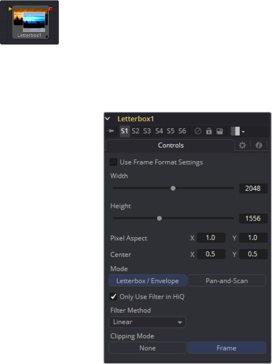
711
Transform Tools Chapter – 28
Letterbox [LBX]
Use the Letterbox Tool to adapt existing images to the frame size and aspect ratios of any other
format. The most common use of this tool is to adapt film resolution images to NTSC or PAL
sized frames for viewing on an external television monitor. Horizontal or vertical black edges
are automatically added where necessary to compensate for aspect ratio differences.
Controls Tab
Formats Contextual Menu
Place the pointer on the Aspect X or Y control and press the right mouse button to
display a menu with available frame formats. Select any one of the choices from the
menu to set the Height, Width and Aspect controls automatically, or enter the required
information manually.
Width and Height
The values of these controls determine the size of the output image as measured
in pixels.
Pixel Aspect X and Y
The controls determine the Pixel Aspect Ratio of the output image.
Center X and Y
This Center control repositions the image window when used in conjunction with
Pan-And-Scan mode. It has no effect on the image when the tool is set to
Letterbox mode.
Mode
This control is used to determine the Letterbox tool’s mode of operation.
712
Transform Tools Chapter – 28
Letterbox/Envelope
This corrects the aspect of the input image and resizes it to match the specified width.
Pan-And-Scan
This corrects the aspect of the input image and resizes it to match the specified height.
If the resized input image is wider than the specified width, the center control can be
used to animate the visible portion of the resized input.
Filter Modes
Nearest Neighbor
This skips or duplicates pixels as needed. This produces the fastest but crudest results.
Box
This is a simple interpolation resize of the image.
Linear
This uses a simplistic filter, which produces relatively clean and fast results.
Quadratic
This filter produces a nominal result. It offers a good compromise between speed
and quality.
Cubic
This produces better results with continuous tone images but is slower than Bi-Cubic. If
the images have fine detail in them, the results may be blurrier than desired.
Catmull-Rom
This produces good results with continuous tone images that are resized down.
Produces sharp results with finely detailed images.
Gaussian
This is very similar in speed and quality to Bi-Cubic.
Mitchell
This is similar to Catmull-Rom but produces better results with finely detailed images. It
is slower than Catmull-Rom.
Lanczos
This is very similar to Mitchell and Catmull-Rom but is a little cleaner and also slower.
Sinc
This is an advanced filter that produces very sharp, detailed results, however, it may
produce visible ‘ringing’ in some situations.
Bessel
This is similar to the Sinc filter but may be slightly faster.
Window Method
Some filters, such as Sinc and Bessel, require an infinite number of pixels to calculate
exactly. To speed up this operation, a Windowing function is used to approximate the
filter and limit the number of pixels required. This control appears when a filter that
requires windowing is selected.
Hanning
This is a simple tapered window.

713
Transform Tools Chapter – 28
Hamming
Hamming is a slightly tweaked version of Hanning.
Blackman
A window with a more sharply tapered falloff.
Kaiser
A more complex window, with results between Hamming and Blackman. Most of these
filters are useful only when making an image larger. When shrinking images, it is
common to use the Bi-Linear filter, however, the Catmull-Rom filter will apply some
sharpening to the results and may be useful for preserving detail when scaling
down an image.
Example
Different Resize Filters. From left to right: Nearest Neighbor, Box, Linear, Quadratic,
Cubic, Catmull-Rom, Gaussian, Mitchell, Lanczos, Sinc, Bessel
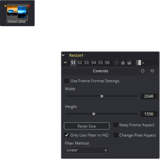
714
Transform Tools Chapter – 28
Resize [Rsz]
Use the Resize tool to increase or decrease the resolution of an input image. This is useful for
converting images from one format to another (for example, from film to video resolution).
Controls Tab
Width
This controls the new resolution for the image along the X-axis.
Height
This controls the new resolution for the image along the Y-axis.
Keep Frame Aspect
When toggled on, the Resize tool maintains the aspect of the original image, preserving
the original ratio between width and height.
Reset Size
Reset the image dimensions to the original size of the image.
Only Use Filter in HiQ
The Resize tool will normally use the fast Nearest Neighbor filter for any non-HiQ
renders, where speed is more important than full accuracy. Disable this checkbox to
force Resize to always use the selected filter for all renders.
Change Pixel Aspect
Enable this checkbox to reveal a Pixel Aspect control that can be used to change the
pixel aspect that the image is considered to have. See the Frame Formats chapter for
details on how pixel aspect operates in Fusion.
Filter Method
When rescaling a pixel, surrounding pixels are often used to give a more realistic result.
There are various algorithms for combining these pixels, called filters. More complex
filters can give better results but are usually slower to calculate. The best filter for the
job will often depend on the amount of scaling and on the contents of the image itself.
Nearest Neighbor
This skips or duplicates pixels as needed. This produces the fastest but crudest results.
Box
This is a simple interpolation resize of the image.
Linear
This uses a simplistic filter, which produces relatively clean and fast results.
715
Transform Tools Chapter – 28
Quadratic
This filter produces a nominal result. It offers a good compromise between speed
and quality.
Cubic
This produces better results with continuous tone images but is slower than Bi-Cubic.
Ifthe images have fine detail in them, the results may be blurrier than desired.
Catmull-Rom
This produces good results with continuous tone images that are resized down.
Produces sharp results with finely detailed images.
Gaussian
This is very similar in speed and quality to Bi-Cubic.
Mitchell
This is similar to Catmull-Rom but produces better results with finely detailed images. It
is slower than Catmull-Rom.
Lanczos
This is very similar to Mitchell and Catmull-Rom but is a little cleaner and also slower.
Sinc
This is an advanced filter that produces very sharp, detailed results, however, it may
produce visible ‘ringing’ in some situations.
Bessel
This is similar to the Sinc filter but may be slightly faster.
Window Method
Some filters, such as Sinc and Bessel, require an infinite number of pixels to calculate
exactly. To speed up this operation, a Windowing function is used to approximate the
filter and limit the number of pixels required. This control appears when a filter that
requires windowing is selected.
Hanning
This is a simple tapered window.
Hamming
Hamming is a slightly tweaked version of Hanning.
Blackman
A window with a more sharply tapered falloff.
Kaiser
A more complex window, with results between Hamming and Blackman. Most of these
filters are useful only when making an image larger. When shrinking images, it is
common to use the Bi-Linear filter, however, the Catmull-Rom filter will apply some
sharpening to the results and may be useful for preserving detail when scaling
down an image.
Example
Different Resize Filters. From left to right: Nearest Neighbor, Box, Linear,
Quadratic, Cubic, Catmull-Rom, Gaussian, Mitchell, Lanczos, Sinc, Bessel
NOTE: Because this tool changes the physical resolution of the image, we do
not normally advise animating the controls.
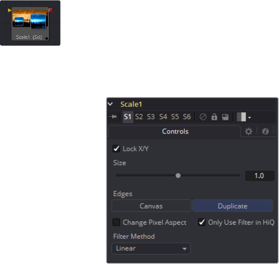
716
Transform Tools Chapter – 28
Scale [SCL]
The Scale tool is almost identical to the Resize tool, except that Resize uses exact dimensions
where the Scale tool uses relative dimensions to describe the change to the source image’s
resolution.
Controls Tab
Lock X/Y
When selected, only a Size control is shown and changes to the image’s scale are
applied to both axes equally. If the checkbox is cleared, individual size controls appear
for both X and Y Size.
Size X/Y
The Size control is used to set the scale used to adjust the resolution of the source
image. A value of 1.0 would have no affect on the image, while 2.0 would scale the
image to twice its current resolution. A value of 0.5 would halve the image’s resolution.
Change Pixel Aspect
Enable this checkbox to reveal a Pixel Aspect control that can be used to change the
Pixel Aspect that the image is considered to have. See the Frame Formats chapter for
details on how Pixel Aspect operates in Fusion.
Only Use Filter in HiQ
The Scale tool will normally use the fast Nearest Neighbor filter for any non-HiQ
renders, where speed is more important than full accuracy. Disable this checkbox to
force Scale to always use the selected filter for all renders.
Filter Method
When rescaling a pixel, surrounding pixels are often used to give a more realistic result.
There are various algorithms for combining these pixels, called Filters. More complex
filters can give better results, but are usually slower to calculate. The best filter for the
job will often depend on the amount of scaling and on the contents of the image itself.
Nearest Neighbor
This skips or duplicates pixels as needed. This produces the fastest but crudest results.
Box
This is a simple interpolation resize of the image.
Linear
This uses a simplistic filter, which produces relatively clean and fast results.
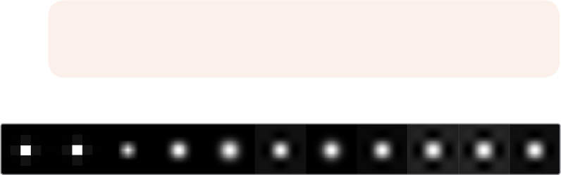
717
Transform Tools Chapter – 28
Quadratic
This filter produces a nominal result. It offers a good compromise between speed
and quality.
Cubic
This produces better results with continuous tone images but is slower than Bi-Cubic. If
the images have fine detail in them, the results may be blurrier than desired.
Catmull-Rom
This produces good results with continuous tone images that are resized down.
Produces sharp results with finely detailed images.
Gaussian
This is very similar in speed and quality to Bi-Cubic.
Mitchell
This is similar to Catmull-Rom but produces better results with finely detailed images. It
is slower than Catmull-Rom.
Lanczos
This is very similar to Mitchell and Catmull-Rom but is a little cleaner and also slower.
Sinc
This is an advanced filter that produces very sharp, detailed results, however, it may
produce visible ‘ringing’ in some situations.
Bessel
This is similar to the Sinc filter but may be slightly faster.
Window Method
Some filters, such as Sinc and Bessel, require an infinite number of pixels to calculate
exactly. To speed up this operation, a Windowing function is used to approximate the
filter and limit the number of pixels required. This control appears when a filter that
requires windowing is selected.
Hanning
This is a simple tapered window.
Hamming
Hamming is a slightly tweaked version of Hanning.
Blackman
A window with a more sharply tapered falloff.
Kaiser
A more complex window, with results between Hamming and Blackman.
Most of these filters are useful only when making an image larger. When shrinking
images, it is common to use the Bi-Linear filter, however, the Catmull-Rom filter will
apply some sharpening to the results and may be useful for preserving detail when
scaling down an image.
Example
Different Resize Filters. From left to right: Nearest Neighbor, Box, Linear,
Quadratic, Cubic, Catmull-Rom, Gaussian, Mitchell, Lanczos, Sinc, Besse
NOTE: Because this tool changes the physical resolution of the image, we do
not normally advise animating the controls.
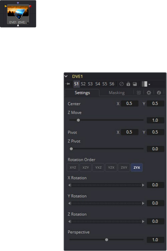
718
Transform Tools Chapter – 28
Transform [XF]
The Transform tool can be used for simple 2D Transformations of the image, such as moving,
rotating and scaling. The image’s aspect can also be modified using the Transform tool.
The Transform tool concatenates its result with adjacent Transformation tools. For more
information on concatenation, consult the Transformations chapter.
Controls Tab
Flip Horizontally and Vertically
Toggle this control on to flip the image along the X- or Y-axis.
Edges
Edges determines how the edges of the image will be treated.
Canvas
This causes the edges of the image that are revealed to show the current Canvas Color.
This defaults to black with no Alpha and can be set using the Set Canvas Color tool.
Wrap
This wraps the edges of the image around the borders of the image. This is useful for
seamless images to be panned, creating an endless moving background image.
Duplicate
This causes the edges of the image to be duplicated as best as possible, continuing
the image beyond its original size.
719
Transform Tools Chapter – 28
Center X and Y
This sets the position of the image on the screen. The default is 0.5, 0.5, which places
the image in the center of the screen. The value shown is always the actual position
multiplied by the reference size. See below for a description of the reference size.
Pivot X and Y
This positions the axis of rotation and scaling. The default is 0.5, 0.5, which is the center
of the image.
Use Size and Aspect
This checkbox determines whether the Transform tool provides independent Size
controls for the X and Y scale, or if Size and Aspect controls are used instead.
Size
This modifies the Size, or scale, of the image. Values range from 0 to 5, but any value
greater than zero can be entered into the edit box. If the Use Size and Aspect
checkbox is selected, this control will scale the image equally along both axes. If the
Use Size and Aspect option is off, independent control is provided for X and Y.
Aspect
This control changes the Aspect Ratio of an image. Setting the value above 1.0
stretches the image along the X-axis. Values between 0.0 and 1.0 stretch the image
along the Y-axis. This control is available only when the Use Size And Aspect checkbox
is enabled.
Angle
This control rotates the image around the axis. Increasing the Angle rotates the image
in a counter-clockwise direction. Decreasing the Angle rotates the image in a clockwise
direction.
Invert Transform
Select this control to Invert any position, rotation or scaling transformation. This option
is useful when connecting the Transform to the position of a tracker for the purpose of
re-introducing motion back into a stabilized image.
Flatten Transform
The Flatten Transform option prevents this tool from concatenating its transformation
with adjacent tools. The tool may still concatenate transforms from its input but it will not
concatenate its transformation with the tool at its output. See the Transformations
chapter earlier in this manual for details on concatenated transformation.
Reference Size
The controls under the Reference Size reveal do not directly affect the image. Instead
they allow you to control how Fusion represents the position of the Transform
tool’s center.
Normally, coordinates are represented as values between 0 and 1, where 1 is a distance
equal to the full width or height of the image. This allows for resolution independence,
because you can change the size of the image without having to change the value of
the center.
One disadvantage to this approach is that it complicates making pixel accurate
adjustments to an image. To demonstrate, imagine an image that is 100 by 100 pixels in
size. To move the center of the image to the right by 5 pixels, we would change the X
value of the transform center from 0.5, 0.5 to 0.55, 0.5. We know the change must be
0.05 because 5/100 = 0.05.
720
Transform Tools Chapter – 28
The Reference Size controls allow you to specify the dimensions of the image. This
changes the way the control values are displayed, so that the Center shows the actual
pixel positions in the X and Y fields of the Center control. Extending our example, if you
set the Width and Height to 100 each, the Center would now be shown as 50, 50, and
we would move it 5 pixels toward the right by entering 55, 50.
Internally, the Transform tool still stores this value as a number between 0 to 1, and if
you were to query the Center controls value via scripting, or publish the Center control
for use by other tools, then you would retrieve the original normalized value. The
change is only visible in the value shown for Transform Center in the tool control.
Use Frame Format Settings
Select this to force the Merge to use the composition’s current frame format settings to
set the Reference Width and Reference Height values.
Reference Width and Height Sliders
Set these to the width and height of the image to change the way that Fusion displays
the values of the Transform tool’s Center control.
Filter Method
Nearest Neighbor
This skips or duplicates pixels as needed. This produces the fastest but crudest results.
Box
This is a simple interpolation resize of the image.
Linear
This uses a simplistic filter, which produces relatively clean and fast results.
Quadratic
This filter produces a nominal result. It offers a good compromise between speed
and quality.
Cubic
This produces better results with continuous tone images but is slower than Bi-Cubic. If
the images have fine detail in them, the results may be blurrier than desired.
Catmull-Rom
This produces good results with continuous tone images that are resized down.
Produces sharp results with finely detailed images.
Gaussian
This is very similar in speed and quality to Bi-Cubic.
Mitchell
This is similar to Catmull-Rom but produces better results with finely detailed images. It
is slower than Catmull-Rom.
Lanczos
This is very similar to Mitchell and Catmull-Rom but is a little cleaner and also slower.
Sinc
This is an advanced filter that produces very sharp, detailed results, however, it may
produce visible ‘ringing’ in some situations.

721
Transform Tools Chapter – 28
Bessel
This is similar to the Sinc filter but may be slightly faster.
Window Method
Some filters, such as Sinc and Bessel, require an infinite number of pixels to calculate
exactly. To speed up this operation, a Windowing function is used to approximate the
filter and limit the number of pixels required. This control appears when a filter that
requires windowing is selected.
Hanning
This is a simple tapered window.
Hamming
Hamming is a slightly tweaked version of Hanning.
Blackman
A window with a more sharply tapered falloff.
Kaiser
A more complex window, with results between Hamming and Blackman. Most of these
filters are useful only when making an image larger. When shrinking images, it is
common to use the Bi-Linear filter, however, the Catmull-Rom filter will apply some
sharpening to the results and may be useful for preserving detail when scaling
down an image.
Example
Different Resize Filters. From left to right: Nearest Neighbor, Box, Linear,
Quadratic, Cubic, Catmull-Rom, Gaussian, Mitchell, Lanczos, Sinc, Bessel
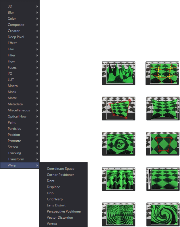
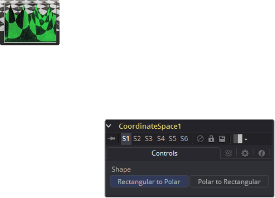
725
Warp Tools Chapter – 29
Coordinate Space [CDS]
The Coordinate Space tool changes the coordinate space of the image at its input from
Rectangular to Polar or from Polar to Rectangular.
Controls Tab
Select between Rectangular to Polar and Polar to Rectangular. Consider the following example
to demonstrate the two coordinate spaces.
Example
To demonstrate a basic tunnel effect that can be achieved with this tool:
Create some text and animate it to move along a path from the top of the frame to
the bottom.
Connect the output of the Text+ tool to a Coordinate Space tool.
Select Polar to Rectangular from the Shape menu.
As the text moves from top to bottom along the original path, it will appear to move
from an infinite distance in the Coordinate Space tool. It may be necessary to flip the
text using the Transform (Xf) tool to make it appear the correct way in the Coordinate
Space tool. Another common use for the Coordinate Space tool is to use it in pairs; two
of them set to different Shape settings with a Drip or Transform tool in between. When
used in this way, the effect gets modified while the image remains the same.
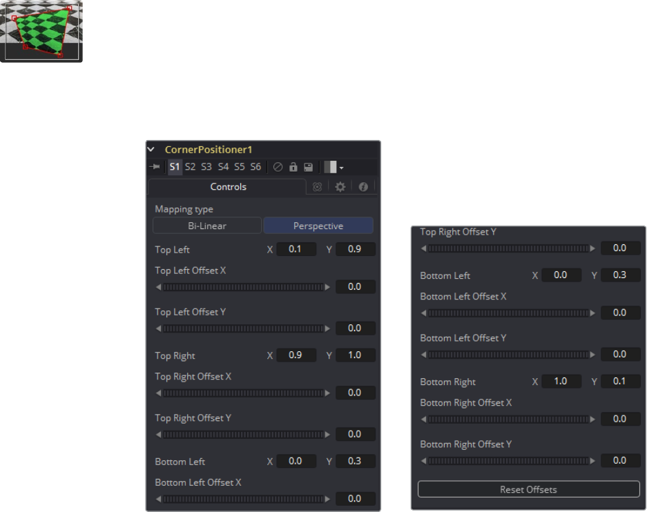
726
Warp Tools Chapter – 29
Corner Positioner [CPN]
The Corner Positioner can be used to interactively position the four corners of an image. This
would typically be used to replace a sign or other rectangular portion of a scene. Connect all
corners to Paths or Trackers for animation purposes.
Controls Tab
Mapping Type
This determines the method used to project the image caused by the Corner
Positioner. In Bi-Linear mode, a straight 2D warping takes place. In Perspective mode,
the image is calculated with the offsets in 2D space and then mapped into a 3D
perspective.
Corners X and Y
There are four points in the Corner Positioner. Drag these around to position each corner
of the image interactively. Attach these control points to any of the usual modifiers.
The image input will be deformed and perspective corrected to match the position of
the four corners.
Offset X and Y
These controls can be used to offset the position of the corners slightly. Useful when
the corners are attached to Trackers with patterns that may not be positioned exactly
where they are needed.
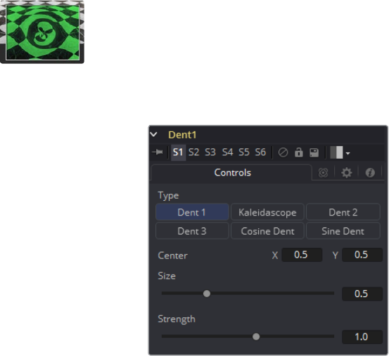
727
Warp Tools Chapter – 29
Dent [DNT]
The Dent function creates a circular deformation of an image similar to a Fish Eye Lens effect,
with the choice of six different Dent filters.
Controls Tab
Type
Select the type of Dent filter to use from this menu. All parameters for Dent are
animatable.
Dent 1
This creates a bulge dent.
Kaleidoscope
This creates a dent, mirrors, and inverts it.
Dent 2
This creates a displacement dent.
Dent 3
This creates a deform dent.
Cosine Dent
This creates a fracture to a center point.
Sine Dent
This creates a smooth rounded dent.
Center X and Y
This positions the Center of the Dent effect on the image. The default values are 0.5,
0.5, which center the effect in the image.
Size
This changes the Size of the area affected by the dent. Animate this slider to make the
Dent grow.
Strength
This changes the overall Strength of the Dent.
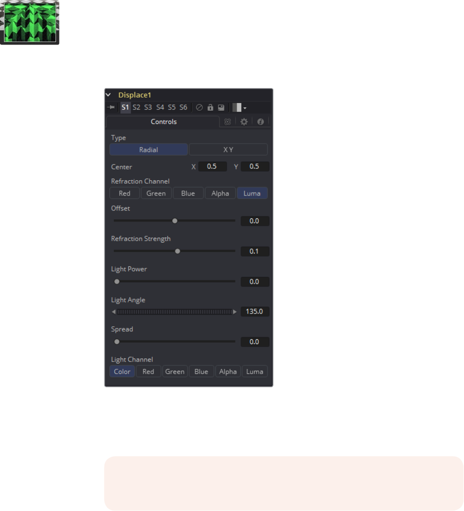
728
Warp Tools Chapter – 29
Displace [DSP]
This tool uses a map image to displace or refract another image. This is useful for creating a
vast range of effects from bevels and heat distortion to glass and water effects.
Controls Tab
Type
The Type buttons can choose in what mode the Displace tool operates. The Radial
mode uses the map image that refracts each pixel out from the center, while X/Y mode
provides control over the amount of displacement along each axis individually.
NOTE: There is one set of Refraction controls while in Radial mode, and two
sets in XY mode, one for each of the X and Y channels.

729
Warp Tools Chapter – 29
Center (Radial Only)
The Center control defines the point from which pixels are displaced toward or
away from.
Refraction Channel
This array of buttons controls which Channel from the foreground image is used to
displace the image. Select from Red, Green, Blue, Alpha or Luminance channels. In XY
mode, this control appears twice, once for the X displacement and once for the Y
displacement.
Refraction Strength (Radial)
Controls the strength of the refraction. Higher values cause stronger or more
pronounced refraction.
X and Y Refraction (X/Y)
Two separate sliders appear to control the Refraction strength along the X- and Y-axis
separately. Otherwise, this is exactly like Refraction Strength.
Light Power
This controls the intensity or strength of the simulated light, causing bright and dim
areas to form according to the contour of the refraction image. Higher values cause the
bright and dim areas to be more pronounced.
Light Angle
This sets the angle of the simulated light source.
Spread
This widens the Displacement effect and takes the edge off the Refraction map. Higher
values cause the ridges or edges spread out.
Light Channel
Select the channel from the refraction image that will be used as the simulated light
source. Select from Color, Red, Green, Blue, Alpha or Luminance channels.
NOTE: The Radial mode pushes pixels inwards or outwards from a center
point, based on pixel values from the Displacement map. The XY mode uses
two different channels from the map to displace pixels horizontally and
vertically, allowing more precise results. Using the XY mode, the Displace tool
can even accomplish simple morphing effects. The Light controls allow
directional highlighting of refracted pixels for simulating a beveled look.
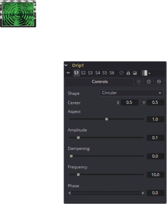
730
Warp Tools Chapter – 29
Drip [DRP]
The Drip function creates a ripple effect over the entire image, which has the potential to
animate outward from a central source. There are a variety of different Drip effects from which
to choose.
Controls Tab
Shape
Use this control to select the shape of the Drip.
Circular
This creates circular ripples. This is the default Drip mode.
Square
This creates even-sided quadrilateral drips.
Random
This creates randomly dispersed noise that distorts your image. Similar to a
particle effect.
Horizontal
This creates horizontal waves that move in one direction.
Vertical
This creates vertical waves that move in one direction.
731
Warp Tools Chapter – 29
Exponential
This creates a Drip effect that looks like a diamond shape with inverted, curved sides
(an exponential curve flipped and mirrored).
Star
This creates an eight-way symmetrical star-shaped ripple that acts like a kaleidoscope
when the phase is animated.
Radial
This creates a star-shaped ripple that emits from a fixed pattern.
Center X and Y
Use this control to position the Center of the Drip effect in the image. The default is 0.5,
0.5, which centers the effect in the image.
Aspect
Control the Aspect Ratio of the various drip shapes. A value of 1.0 causes the shapes to
be symmetrical. Smaller values cause the shape to be taller and narrower, while larger
values cause shorter and wider shapes.
Amplitude
The Amplitude of the Drip effect refers to the peak height of each ripple. Use the slider
to change the amount of distortion the Drip applies to the image. A value of 0.0 gives
all ripples no height and, therefore, makes the effect transparent. A maximum amplitude
of 10 makes each ripple extremely visible and completely distorts the image. Higher
numbers can be entered via the text entry boxes.
Dampening
Controls the Dampening, or falloff, of the Amplitude as it moves away from the center of
the effect. It can be used to limit the size or area affected by Drip.
Frequency
This changes the number of ripples emanating from the center of the Drip effect. A
value of 0.0 indicates that there will be no ripples. Move the slider up to a value of 100,
to correspond with the density of desired ripples.
Phase
This controls the offset of the frequencies from the center. Animate the Phase value to
make the ripple emanate from the center of the effect.
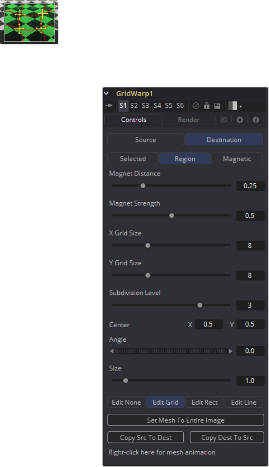
732
Warp Tools Chapter – 29
Grid Warp [GRD]
The Grid Warp tool is a simple 2D deformation grid with flexible vertices. The image will be
deformed so that the Source grid matches the Destination grid.
Controls Tab
Source and Destination
The Source and Destination buttons determine whether the Source grid or Destination
grid is currently active. Only one grid can be displayed or manipulated at a time. The
selected button will be highlighted to indicate that is the active grid at the moment.
All of the other controls in this tab affect the grid selected by this control.
Selection Type
These three buttons determine the selection types used for manipulating the points.
There are three options available.
Selected
When in Selected mode, adjustments to the grid will be applied only to the currently
selected points. This mode is identical to normal polyline operation.
733
Warp Tools Chapter – 29
Region
In Region mode, all points within the area around the mouse pointer, when the left
mouse button is clicked, will move. New points that enter the region during the move
will be ignored. Choosing this option will expose Magnet Distance and Magnet Strength
controls to determine the size and falloff of the area.
Magnetic
In Magnetic mode, all points within the area around the mouse pointer when the left
mouse button is clicked will move. New points that enter the region during the move
will be affected as well. Choosing this option will expose Magnet Distance and Magnet
Strength controls to determine the size and falloff of the area.
Magnet Distance
The default tool for selecting and manipulating the grid is a Magnet tool. The magnet is
represented in the Viewer by a circle around the mouse pointer. The Magnet Distance
slider controls how large the region of affect for the magnet is, as in the size of the
circle. Drag on the grid and any vertex within the range of the slider will move.
To increase the size of the magnet, increase the value of this slider. Alternately, adjust
the size of the magnet by holding down the D key while dragging the mouse.
Magnet Strength
The Magnet Strength slider will increase or decrease the falloff of the magnet cursor’s
effect. At a setting of 0.0, the magnetic cursor has no effect, and vertices will not move
at all. As the values increase, the magnet causes a greater range of motion in the
selected vertices. Use smaller values for a more sensitive adjustment and larger values
for broad-sweeping changes to the grid.
X and Y Grid Size
The X and Y Grid Size sliders control the number of divisions in the grid. Where the X
and Y divisions intersect, a control vertex is created.
Be aware that changing either of these controls after applying changes in the grid will
reset the entire grid. Set the X and Y grid sizes to the appropriate resolution before
making serious detailed adjustments to the grid.
Subdivision Level
The Subdivision Level determines how many subdivisions there are between each set
of divisions. Subdivisions do not generate vertices at intersections. The more
subdivisions there are, the smoother the deformation is likely to be (and the slower it
will be to render the deformation).
Center
The Center coordinates determine the exact center of the grid. The onscreen Center
control is invisible while editing the grid. Select the Edit Rect mode and the grid center
becomes visible and available for editing.
Use the Center control to move the grid through a scene without affecting the
animation applied to the individual vertices. For example, while deforming lips on a
face, track the motion of the face with a Tracker and connect the grid center to the
Tracker. This matches the grid with slight movements of the head while focusing on the
deformation of the lips.
Angle
This Angle control rotates the entire grid.
734
Warp Tools Chapter – 29
Size
The Size control increases or decreases the scale of the grid.
Edit Buttons
There are four edit modes available, each of which can be selected by clicking on the
appropriate button.
Edit None
Set the grid to Edit None mode to disable the display of all onscreen controls.
Edit Grid
The Edit Grid mode is the default mode. While this mode is enabled, the grid is drawn
in the Viewer and the control vertices of the grid can be manipulated directly.
Edit Rectangle
When the grid is in Edit Rectangle mode, the onscreen controls display a rectangle that
determines the dimensions of the grid. The sides of the rectangle can be adjusted to
increase or decrease the grid’s dimension. This mode also reveals the onscreen Center
control for the grid.
Edit Line
The Edit Line mode is extremely useful for creating grids around organic shapes. When
this mode is enabled, all onscreen controls will disappear and a spline can be drawn
around the shape or object to be deformed. While drawing the spline, a grid is
automatically created that best represents that object. Additional controls for Tolerance,
Over Size and Snap Distance appear when this mode is enabled. These controls are
documented below.
Set Mesh to Entire Image
The Set Mesh to Entire Image button automatically resets the size of the grid to the
exact dimensions of the image. Any adjustments to vertices within the grid will be reset.
Copy Buttons
These two buttons provide a technique for copying the exact shape and dimensions of
the Source grid to the Destination, or the Destination grid to the Source. This is
particularly useful after setting the Source grid to ensure that the Destination grid’s
initial state matches the Source grid before beginning a deformation.
Point Tolerance
This control is only visible when the Edit Line mode is enabled. The Point Tolerance
slider determines how much tessellation the grid will apply to closely match the density
of points in the spline. The lower this value, the fewer vertices there will be in the
resulting grid and the more uniform the grid will appear. Higher values will start applying
denser grids with variations to account for regions in the spline that require more detail.
Oversize Amount
This control is only visible when the Edit Line mode is enabled. The Oversize Amount
slider is used to set how large an area around the spline should be included in the grid.
Higher values create a larger border, which can be useful when blending a deformation
back into the source image.
Snap Distance
This control is only visible when the Edit Line mode is enabled. The Snap Distance
slider dictates how strongly the drawn spline will attract surrounding vertices. If a vertex
is close enough to a spline’s edge, the vertex will move to line up with the spline. The
higher the value, the further the reach of the spline.
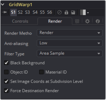
735
Warp Tools Chapter – 29
Right-Click Here for Mesh Animation
The grids are static by default. Right-clicking on the Right-Click Here for Mesh
Animation label will provide a contextual menu with options for animating the grid or
connecting it to another grid in the composition.
The grid uses a Polychange spline. Any adjustment to any of the control points will add
or modify the keyframe for all points to the Polychange spline.
Right-Click Here for Shape Animation
This label only appears in the Edit Line mode. Right-clicking on the Right-Click Here for
Shape Animation label will reveal a contextual menu that can be used to animate the
shaping polyline or to connect it to other polylines in the composition.
Render Tab
Render Method
The Render Method drop-down menu is used to select the rendering technique and
quality applied to the mesh. The three settings are arranged in order of quality, with the
first (Wireframe) as the fastest and lowest of quality. The default mode is Render, which
produces final resolution, full quality results.
Anti-Aliasing
The Anti-aliasing control is a checkbox in Wireframe Render mode.
It is otherwise a drop-down menu with three levels of quality. Higher degrees of
anti-aliasing improve image quality dramatically but vastly increase render times. The
Low setting may be an appropriate option while setting up a large dense grid, or
previewing a flow, but almost never for a final render.
Filter Type
The Area Sample control is only visible when the Render Method is not set to
Wireframe. Checked by default, disabling this checkbox prevents the grid from
calculating area samples for each vertex in the grid. Area sampling vastly improves
render quality at the cost of speed.
Wireframe Width
This control only appears when the Render Method is set to Wireframe. It determines
the width of the lines that make up the wireframe.
Anti-Aliased
This control only appears when the Render Method is set to Wireframe. Use this
checkbox to enable/disable antialiasing for the lines that make up the wireframe.
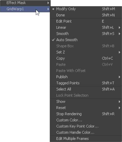
736
Warp Tools Chapter – 29
Black Background
The Black Background checkbox determines whether pixels outside of the grid in the
source image will be set to black or if they will be preserved.
Object ID and Material ID
Enable the Object ID or Material ID checkboxes to have the grid output the proper ID
channel in the final render.
Set Image Coordinates at Subdivision Level
Checkbox that defaults to On.
Force Destination Render
Checkbox that defaults to On.
Right Click Menu
The Grid Warp tool places a submenu for both Source and Destination grids in the Viewer’s
contextual menu. Both menus have the exact same name, where only the menu for the active
grid is populated with options. The other menu is empty. The contextual menu options are all
available from the toolbar that appears in the Viewer.
Modify Only/Done
These two options set the mesh to modify only and done modes, respectively. Select
Modify Only to edit the mesh or Modify Done to prevent any further changes to a mesh.
Smooth/Linear
Use Smooth and Linear to apply or remove smoothing from selected vertices.

737
Warp Tools Chapter – 29
Auto Smooth Points
When Auto Smooth Points is enabled, the vertices in the grid will automatically be
smoothed whenever they are moved. This is generally on by default.
Z Under/Z Same/Z Over
When two vertices in a grid overlap, one ends up getting clipped by the other. Z Under,
Z Same and Z Over are used to select which vertices are rendered on top and which
are rendered behind.
Select All
This option will Select All points in the mesh.
Show Key Points, Handles, Grid and Subdivisions
Use these four options to enable or disable the display of the grid, key points (vertices),
Bezier handles and subdivisions in the Viewers.
Reset Selected Points
Reset Selected Points (vertices) to their default positions.
Reset All Points
This will Reset All Points (vertices) in the mesh to their default positions.
Stop Rendering
This option will enable Stop Rendering, which disables all rendering of the Grid Warp
tool until the mode is turned off. This is frequently useful when making a series of fine
adjustments to a complex grid.
Screen Controls
Whenever the Grid Warp tool is selected and is in Edit Grid mode, the Grid Warp toolbar is
displayed in the views. This toolbar provides a variety of options for manipulating and adjusting
the grid. The toolbar buttons in this toolbar are described above in the contextual menu.
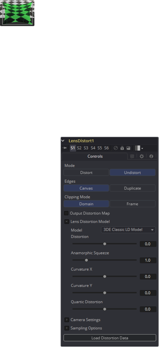
738
Warp Tools Chapter – 29
Lens Distort [LENS]
This tool can be used to remove or add lens distortion in an image. The amount and type of
lens distortion in an image depends on a variety of factors such as the actual lens that has been
used, the quality and amount of lensgroups in that lens, adjustments like shift lenses and
much more.
One reason to remove lens distortion is to comp an undistorted layer as, for example, a 3D
rendering, on top of a distorted layer as, for example, a real world camera shoot. When
combining the layers without removing the lens distortion, unwanted effects like straight lines
not matching up on foreground and background will occur. The resulting composite will not look
believable.
In a typical workflow one would apply the LensDistort in Undistort mode to the original layer,
add the 3D elements, do all other compositing work and finally apply LensDistort again with
exactly the same settings, but this time in Distort mode to get the original look and distortion
back into the image.
Controls Tab
739
Warp Tools Chapter – 29
Mode
Undistort removes the lens distortion to create a flattened image. Distort brings the
original lens distortion back into the image.
Edges
Determines how samples that fall outside the frame are treated.
Canvas: Pixels outside the frame are set to the default canvas color. In most cases
this is black with no alpha.
Duplicate: Pixels outside the frame are duplicated. This results in “smeared” edges
but is useful when, for example, applying a blur, because black pixels would in that
case result in unwanted blurring between the actual image and the black canvas.
Clipping Mode
Domain: Retains all pixels that might be moved out of the frame for later re-distorting.
Frame: Pixels moved outside the frame will be discarded.
Output Distortion Map
Outputs the location of pixels as a warped screen-coordinate map.
Camera Settings
The options known from the Camera3D are duplicated here. They can either be set
manually or connected to an already existing Camera3D.
Lens Distortion Model
Select the appropriate 3D Equalizer Lens Distortion model here: 3DE Classic Model,
3DE4 Anamorphic, 3DE4 Radial Fisheye or 3DE4 Radial. Please consult the 3D
Equalizer manual for further explanation. The sliders in the 3DE Classic LD Model are
most likely best suited for manually applying (un)distortion, without having imported
lens data.
Supersampling [HiQ]
Sets the number of samples used to determine each destination pixel. As always,
higher supersampling leads to higher render times. 1×1 bilinear is usually of sufficient
quality, but with high lens distortion near the edges of the lens there will be noticeable
differences to higher settings.
Supersampling Mode [HiQ]
The type of sample done for each supersample. Nearest will lead to a crisper but more
aliased image. Bilinear will give a blurrier result.
Load Distortion Data
Allows the user to load a Lens Distortion profile created, for example, by the 3D
Equalizer.
How to Manually Determine Lens Distortion
In the ideal world, one would have exact lens-parameters from each lens that was used
during the shoot, and one could use those values to undistort the image. However, in
the real world, those parameters have not been taken on set or don’t match. Another
approach is to use a software like 3DEqualizer which analyzes the footage and delivers
a dataset that can be imported into the LensDistort tool right away.
And finally, one could try to manually eyeball the amount of lens distortion using the
control sliders. To do that, one could either look out for horizontal or vertical lines in the
footage that are supposed to be straight and straighten them out using the controls, or
shoot a full frame checkerboard pattern on set as a reference.
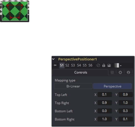
740
Warp Tools Chapter – 29
Perspective Positioner [PPN]
The Perspective Positioner is the complementary tool to the Corner Positioner tool. By
positioning corner points on an image and moving them, it is possible to remove the
perspective from an image. This function can also be used to wobble and warp the image by
animating the points over time.
Controls Tab
Corners X and Y
There are the four control points of the Perspective Positioner. Interactively drag these
in the views to position each corner of the image.
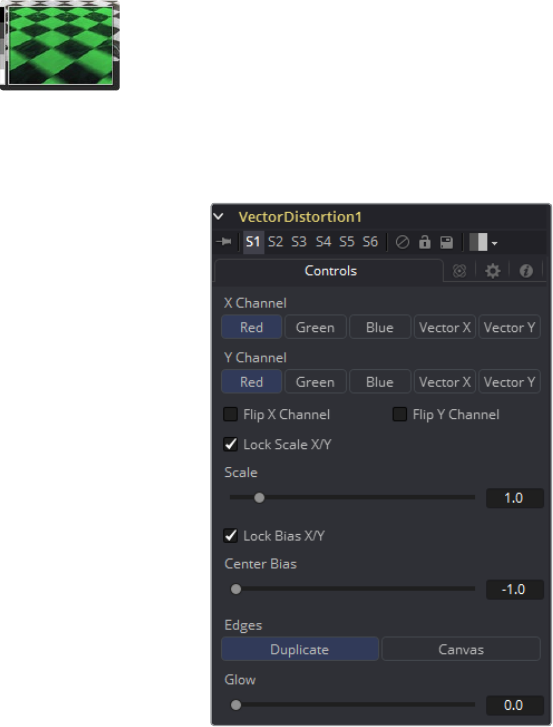
741
Warp Tools Chapter – 29
Vector Distortion [DST]
The Vector Distortion tool distorts the main source image along the X- and Y-axis separately,
based on the vector channel data in the source image, or a channel from a second image or
reference image.
Controls Tab
X Channel and Y Channel
Use these buttons to select which channel of the reference image will be used to
distort the X and Y channels. If no Distort reference image is connected to the second
(green) input of the tool, then channels from the main input are used instead.
Flip X and Flip Y Channel
Use these checkboxes to flip the direction of the distortion along the specified axis.
Lock Scale X/Y
Select this checkbox to separate the Scale slider into separate Scale X and Scale
Y sliders.
Scale
Use the Scale slider to apply a multiplication to the values of the distortion reference image.
Lock Bias X/Y
Select this checkbox to separate the Bias slider into separate Bias X and Bias Y sliders.
Center Bias
Use the Center Bias slider to shift or nudge the distortion along a given axis.
Edges
The Edges buttons are used to set how the tool deals with pixels that reach the edge of
the screen.
Glow
Use this slider to add a glow to the result of the vector distortion.
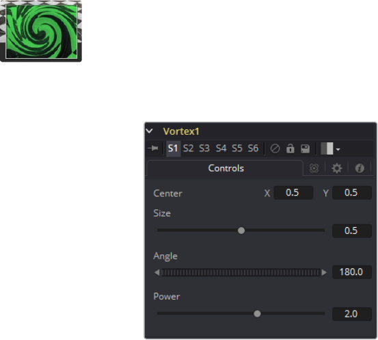
742
Warp Tools Chapter – 29
Vortex [VTX]
The Vortex effect appears as a swirling whirlpool in specified regions of the image. The Vortex
can be made to move and grow by animating the various controls.
Controls Tab
Center X and Y
This control is used to position the Center of the Vortex effect on the image. The
default is 0.5, 0.5, which positions the effect in the center of the image.
Size
Change the area affected by the Vortex in the display window by dragging the
circumference of the effect or by using the Size slider.
Angle
Drag the rotation handle in the Viewer or use the thumbwheel control to change the
amount of rotation in the Vortex. The higher the angle value, the greater the
swirling effect.
Power
Increasing the Power slider makes the Vortex smaller but tighter. It effectively
concentrates it inside the given image area.
744
Modifiers Chapter – 30
Modifiers
Bezier Spline 745
B-Spline 746
Calculation 747
Cubic Spline 750
Expression 751
Expression Syntax Formulas 754
Expression Syntax Operators 755
From Image 757
GradientColorModifier 759
MIDI Extractor 761
Natural Cubic Spline 765
Offset 766
Path 769
Perturb 771
Probe 773
Publish 775
Shake 776
Track 778
Vector 779
XY Path 780
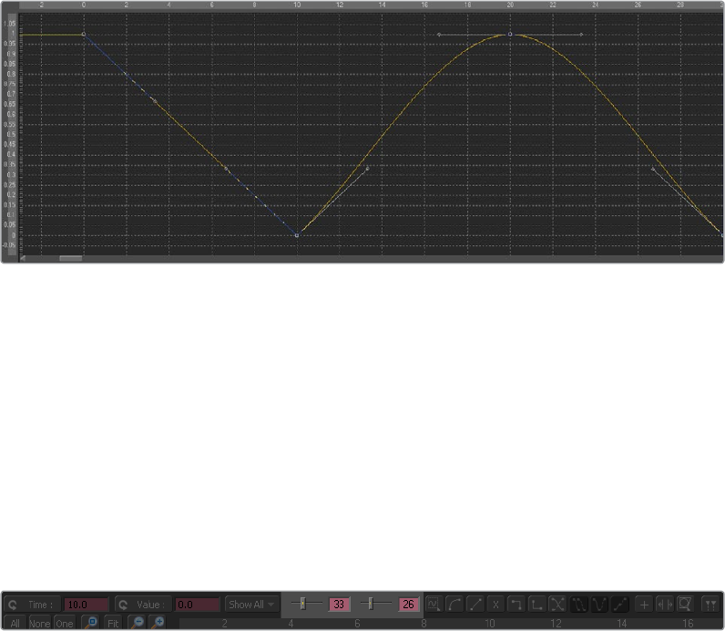
745
Modifiers Chapter – 30
Bezier Spline
The BezierSpline is one of the animation modifiers in Fusion and normally is applied to
numerical values rather than point values. It is applied by default each time you right-click on a
numerical control and select Animate.
It can also be applied by right-clicking on a numerical control and selecting Modify with >
BezierSpline.
Usage
Being an animation spline, this modifier has no actual Controls tab. However, its effect can be
seen and influenced in the Spline Editor. The Bezier Spline offers individual control over each
point’s smoothness by means of handles. The smoothness can be applied by multiple ways.
To make the keys smooth, select them and press Shift-S. The handles can then be used
to further modify the behavior of in and out.
To make the keys linear, select them and press Shift-L. These operations can also be
performed using the contextual menu.
Select the keyframe(s), right click and select Smooth or Linear. The menu also allows
the user to apply smoothing using a Savitzky-Golay filter. Select the keyframe(s), right-
click and select Smooth Points -Y Dialog.
Ease In/Out Can Also Be Modified by Using the Control Slider
Select the keyframe you want to modify, right-click and select Ease In/Out... fromthecontextual
menu. Then use the sliders to individually control the Ease In/Out numerically.
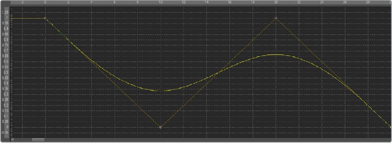
746
Modifiers Chapter – 30
B-Spline
The B-spline is one of the animation modifiers in Fusion and normally is applied to numerical
values rather than point values.
It can be applied by right-clicking on a numerical control and selecting Modify with > B-Spline.
Usage
Being an animation spline, this modifier has no actual Controls tab. However its effect can be
seen and influenced in the Spline Editor. Notice that, though the actual value of the second
keyframe is 0, the value of the resulting spline is 0.33 due to the unique smoothing and
weighing algorithms of a B-spline.
The weight can be modified by left-clicking on the keyframe to select it, holding down W as
well as the left mouse button, and moving the mouse to the left to lower the tension and to the
right to increase the tension. This also can be done with multiple selected keyframes
simultaneously.
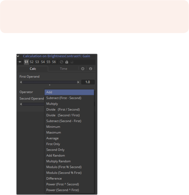
747
Modifiers Chapter – 30
Calculation
Calculations are used to create indirect connections between value controls. A calculation can
perform a mathematical expression based on two operands, where each operand can be
connected to another control or set manually by the user.
Additionally, the Calculation control can access the values of a connected control at times other
than the current time, using Time offsets and Time Scale controls built into the
Calculation Modifier.
The most common use for a calculation is when two controls need to be connected to each
other, but the range or scope of the value’s output by one control is inappropriate for the
other control.
Calc Tab
First and Second Operand
These sliders are either connected to published or animated controls from other tools
in the composition or manually set to the desired values for the calculation.
Operator
Select from the mathematical operations listed in this menu to determine how the two
operands are combined. Clicking on the down arrow opens the menu with the
following options:
NOTE: The Expression modifier is essentially a more flexible version of the Calculation
modifier, with a single exception. It is far easier to manipulate the timing of the
operands provided to a Calculation than it is to do so with an Expression.
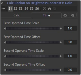
748
Modifiers Chapter – 30
Time Tab
First and Second Operand Time Scale
These sliders cause the frame used to read the values of the Operands specified in the
Calc tab to be scaled. A value of 1 returns the value of the operand at frame x when the
composition is set to frame x. For example, if the first operand is animated with a value
of 1 to 10 from frame 0 to 10, then a scale of 0.5 would cause the calculation to return a
value of 5 at frame 10 (effectively slowing the animation by half for the purposes of the
calculation).
First Operand and Second Operand Time Offset
These sliders return the value of the Operand at the Time Offset specified. A value of
10 would return the value of the operand 10 frames forward in time and -10 would return
the value of the operand 10 frames back in time. See the example below for a
practical example.
749
Modifiers Chapter – 30
Example
The following example uses a calculation to apply blur to a text in inverse proportion to the size
of the text.
Create a new composition, and set the Global Start and Render Start to 1. Set the
Global End and Render End to 100.
Add a Text Plus tool to the composition.
Enter a small amount of text in the StyledText input.
Make sure the current frame is 0
Set the Size parameter of the Text tool to a value of 0.06 at frame 0.
Right-click on the Size slider and animate the slider by setting a key.
Advance to frame 100 and set the value of the Size control to 0.50.
Add a Blur tool immediately after the Text tool. Connect the Blur input to the Text
tool’s output.
View the Blur tool in one of the Viewers.
We want the blur to decrease in strength as the text gets bigger. The controls cannot
be directly connected together because the values of the Text Size control are getting
bigger instead of smaller.
Right-click on the Blur size and select Modify With Calculation from the contextual
menu. Anew set of controls will appear in the Modifiers tab while the Blur tool
is selected.
Switch to the Modifier tab (F11)
Right-click on the First Operand slider. Select Connect To > Text 1 > Size from the
contextual menu. This connection isn‘t very useful, though; the maximum value of the
Blur Size control is 0.5, which is hardly noticeable as a blur.
Set the Operator drop-down menu to Multiply.
Set the Second Operand slider to 100.
Switch to the Time tab of the modifier and set the First Operand Time Scale to -1.0.
Normally, the First Operand will get the value of the control it is connected to from the
same frame as the current time. So at frame 10, the first operand will be set to the same
value as the Text size at frame 10. By setting this value to -1, the value is read from one
frame back in time whenever the current time of the composition advances by 1 frame.
However, this means that the Calculation would be reading the value of the Text size at
frame -10 when we are at frame 10 in the composition. To correct for this, set the First
Operand Time Offset slider to 100.
Return to the Tools tab of the Tool Control Area (F9). Press play (spacebar) and watch
how the value of the Blur Size relates to the value of the Text Size.
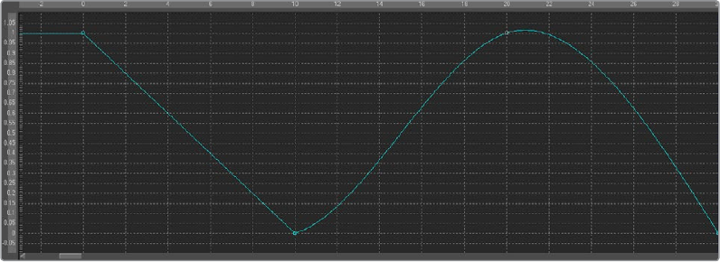
750
Modifiers Chapter – 30
Cubic Spline
The Cubic Spline is one of the animation modifiers in Fusion and normally is applied to
numerical values rather than point values. It can be applied by right-clicking on a numerical
control and selecting Modify with > Natural Cubic Spline.
Usage
Being an animation spline, this modifier has no actual Controls tab. However its effect can be
seen and influenced in the Spline Editor.
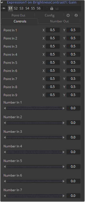
751
Modifiers Chapter – 30
Expression
Adding an Expression modifier to a control will add the ability to control and manipulate either
position or value controls based on any number of controls, either positional or value-based.
This modifier offers exceptional flexibility compared to the more limited Calculation or Offset
modifiers, but it is unable to access values from frames other than the current time.
An Expression will accept up to nine value inputs and nine position inputs that are used as part
of a user-defined mathematical expression to output a value.
To add an Expression to a control, right-click on the control and choose Modify With >
Expression from the contextual menu. The type of value that will be returned by the Expression
entirely depends on the type of control it is modifying.
When used with a value control (like a slider), the Expression in the Number Out tab will be
evaluated to create the result. When used to modify a positional control (like a tool’s center), the
Point Out tab will control the result.
The Modifiers view contains the controls for the Expression modifier. Its controls are
described below.
Controls Tab
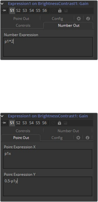
752
Modifiers Chapter – 30
This tab provides nine number controls and nine point controls. The values of the number
controls can be referred to in an expression as n1 through n9. The X-coordinate of each point
control can be referred to as p1x through p9x, while the Y-coordinate is p1y through p9y.
These values can be set manually by the user, connected to other parameters, animated and
even connected to other Expressions or Calculations.
Number Out Tab
This enables a mathematical formula to be entered, which can access the values from both the
Number In and the Point In tabs and output a value used to modify the control to which the
expression was applied. See below for the syntax to use in this field.
Point Out Tab
Each one of the text boxes in this tab can contain a mathematical formula that can access the
values from both the Number In and the Point In tabs and output a value used to modify the
control to which the Expression was applied. The Expression in the top text box control is used
to calculate the X-axis value and the bottom text box is used to calculate the Y-axis control. See
below for the syntax to use in this field.
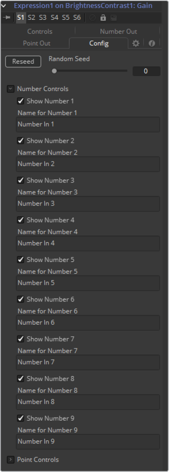
753
Modifiers Chapter – 30
Config Tab
A good expression can be re-used over and over again. As a result, it can be useful to
provide more descriptive names for each input and to hide the ones that are unused.
The Config Tab of the Expressions modifier is used to customize visibility and name for
each of the nine point and number inputs.
Random Seed
The Random Seed control is used to seed the Rand() function. The rand(x, y) function
produces a random value between X and Y, producing a new value for every frame.
Aslong as the setting of this Random Seed slider remains the same, the values
produced at frame x will always be the same. Adjust the seed slider to a new value to
get a different value for that frame.

754
Modifiers Chapter – 30
Show Number or Point X
There are eighteen of these checkbox controls, one for each of the nine Number and
Point inputs. Enable this checkbox to display the control for Number x or Point x in the
Controls tab.
Name for Number or Point X
There are eighteen of these edit controls, one for each of the nine Number and Point
inputs. Type a new name for the input into this edit control to assign a new name for the
Input’s label in the Controls tab.
Expression Syntax Formulas
Formulas are entered into the Number Out or Point Out tabs as part of an expression.
They can be made up of the following functions:
n1..n9 The value of Number Input 1..9.
p1x..p9x The X of Positional Control 1..9.
p1y..p9y The Y of Positional Control 1..9.
time The current time (frame number).
pi The value of pi.
e The value of e.
log(x) The base-10 log of x.
ln(x) The natural (base-e) log of x.
sin(x) The sine of x (x is degrees).
cos(x) The cosine of x (x is degrees).
tan(x) The tangent of x (x is degrees).
asin(x) The arcsine of x, in degrees.
acos(x) The arccosine of x, in degrees.
atan(x) The arctangent of x, in degrees.
atan2(x, y) The arctangent of x,y, in degrees.
abs(x) The absolute (positive) value of x.
int(x) The integer (whole) value of x.
frac(x) The fractional value of x.
sqrt(x) The Square Root of x.
rand(x, y) A random value between x and y.
rands(x, y, s) A random value between x and y, based on seed s.
min(x, y) The minimum (lowest) of x and y.
max(x, y) The maximum (highest) of x and y.

755
Modifiers Chapter – 30
dist(x1, y1, x2, y2) The distance between point x1,y2 and x2,y2.
dist3d(x1,y1,z1,x2,y2,z2) The distance between 3D points x1,y2,z1 and x2,y2,z2
noise(x) A smoothly varying Perlin noise value based on x
noise2(x, y) A smoothly varying Perlin noise value based on x and y
noise3(x, y, z) A smoothly varying Perlin noise value based on x, y and z
if(c, x, y) Returns x if c not 0, otherwise y.
Expression Syntax Operators
Operators are used to evaluate statements. They are combined with functions to perform
logical and mathematical calculations in the Number Out and Point Out tabs.
x + y x plus y.
x - y x minus y.
x > = y 1.0 if x is less than y, otherwise 0.0.
x > y 1.0 if x is greater than y, otherwise 0.0.
!x 1.0 if x = 0, otherwise 0.0.
-x (0.0 - x).
+x (0.0 + x) (effectively does nothing).
x ^ y x raised to the power of y.
x y x multiplied by y.
x y x divided by y.
x % y x modulo y, (remainder of (x divided by y)).
x > = y 1.0 if x is less than or equal to y, otherwise 0.0.
x > = y 1.0 if x is greater than or equal to y, otherwise 0.0.
x = y 1.0 if x is exactly equal to y, otherwise 0.0.
x == y 1.0 if x is exactly equal to y, otherwise 0.0 (identical to above).
x < > y 1.0 if x is not equal to y, otherwise 0.0.
x != y 1.0 if x is not equal to y, otherwise 0.0 (identical to above).
x & y 1.0 if both x and y are not 0.0, otherwise 0.0.
x && y 1.0 if both x and y are not 0.0, otherwise 0.0 (identical to above).
x | y 1.0 if either x or y (or both) are not 0.0, otherwise 0.0.
x || y 1.0 if either x or y (or both) are not 0.0, otherwise 0.0 (identical
to above).
756
Modifiers Chapter – 30
Examples
Example 1
To make a numeric control equal to the Y value of a motion path, add an expression to
the desired target control and connect the Path to Point In 1. Enter the formula:
p1y
into the Number Out field.
Example 2
To make the result of the Expression’s Number Out be the largest of Number In 1 and
Number In 2, multiplied by the cosine of Number In 3, plus the X coordinate of Point In 1,
enter the formula:
max(n1, n2) * cos(n3) + p1x
into the Number Out field.
Example 3
Add a Background tool set to solid black and a Hotspot tool. Set the Hotspot size to
0.08 and set the Strength to maximum. Modify the Hotspot center with an expression.
Change the current frame to 0.
Set n1 to 0.0 and add a Bezier spline. At frame 29, set the value of n1 to 1.0. Select both
points and loop the spline using the Spline Editor. Now enter the following equations
into the Point Out tab of the expression.
X-Axis Expression
n1
Y-Axis Expression
0.5 + sin(time*50) 4
Render out a preview and have a look at the results. (Try this one with motion blur.)
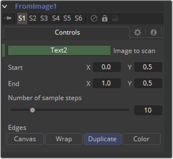
757
Modifiers Chapter – 30
From Image
The From Image only works on gradients, like the gradient on a Background tool. It takes
samples of an image along a user-definable line and creates a gradient from those samples.
It can be applied by right-clicking on a Gradient control and selecting From Image.
Controls
Image to Scan
Drop the tool you want to be examined into this box.
Start X/Y, End X/Y
These two point controls define the Start and End points of the line along which the
samples are taken from the image defined in the Image to scan box.
The points can also be moved directly in the view.
Number of Sample Steps
Defines how many individual color samples are taken along the line. You can also see
the result of this setting when you look at the actual tool’s Gradient control. The more
sample steps you define here, the more individual points you will see on the Gradient
control. It is also possible to first create a gradient using the From Image modifier and
then remove that modifier from the Gradient control again. The created gradient will
stay intact and can then be fine tuned by hand.
Edges
Edges determines how the edges of the image will be treated when the sample line
extends over the actual frame of the image to be sampled.
Black
This outputs black for every point on the sample line outside of the image bounds.
Wrap
This wraps the edges of the line around the borders of the image.
Duplicate
This causes the edges of the image to be duplicated as best as possible, continuing
the image beyond its original size.
Color
Outputs a user-definable color instead of black for every point on the sample line
outside of the image bounds.
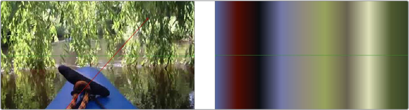
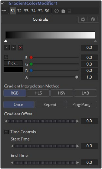
759
Modifiers Chapter – 30
GradientColorModifier
The Gradient Color modifier allows the user to control the value of a parameter. A gradient with
customized values is mapped into a specific time range to control the value. If both time values
are set to 0, then the modifier returns the value at the starting point of the gradient. You can use
the Offset control to animate the gradient manually.
It can be applied by right-clicking onto a control and selecting Modify with >
GradientColorModifier.
Controls Tab
Gradient
The Gradient control consists of a bar where it is possible to add, modify and remove
points of the gradient. Each point has its own color. It is possible to animate the color as
well as the position of the point. Furthermore, a From Image modifier can be applied to
the gradient to evaluate it from an image.
Gradient Interpolation Method
The gradient is linearly interpolated from point to point in RGB color space by default.
This can sometimes result in unwanted colors. Choosing another color space may
provide a better result.
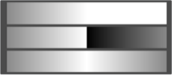
760
Modifiers Chapter – 30
Repeat
Defines how the left and right borders of the gradient are treated.
Gradients set to Once, Repeat and Ping Pong from top to
bottom respectively and shifting the gradient to the left.
Once: When using the Gradient Offset control to shift the gradient, the border colors
will keep their values. Shifting the default gradient to the left will result in a white
border on the left, shifting it to the right will result in a black border on the right.
Repeat: When using the Gradient Offset control to shift the gradient, the border
colors will be wrapped around. Shifting the default gradient to the left will result in a
sharp jump from white to black, shifting it to the right will result in a sharp jump from
black to white.
Ping Pong: When using the Gradient Offset control to shift the gradient, the border
colors ping-pong back and forth. Shifting the default gradient to the left will result in
the edge fading from white back to black, shifting it to the right will result in the edge
fading from black back to white.
Gradient Offset
Allows you to pan through the gradient.
Time Controls
The Start Time and End Time thumbwheels determine the time range the gradient is
mapped into. This is set in frames. The same effect can be achieved by setting the
Gradient to Once and animating the offset thumbwheel.
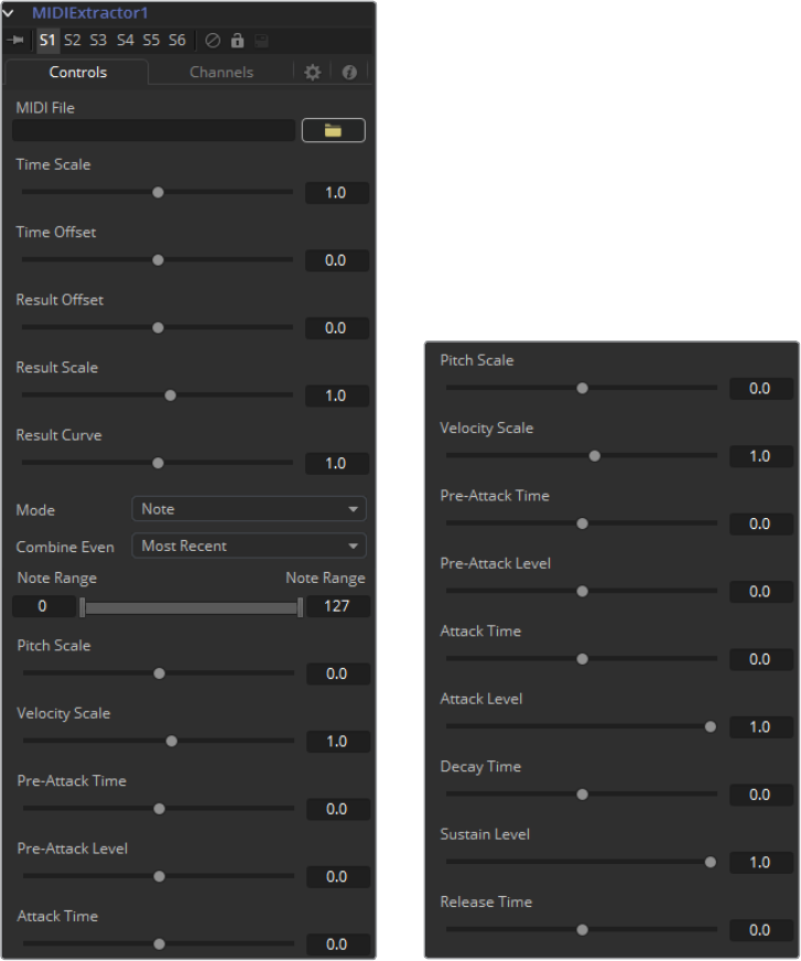
761
Modifiers Chapter – 30
MIDI Extractor
The MIDI Extractor Modifier provides the ability to modify the value of a control using the values
stored in a MIDI file. Using the modifier relies on some knowledge of MIDI, which is outside of
the scope of this manual to describe in detail.
The value produced by the modifier is extracted from the MIDI event selected in the Mode
menu. Each mode can be trimmed so only specific messages for that event are processed. For
example, only some notes are processed, while others are ignored. The value of the event can
be further scaled or modified by additional factors, such as Scale, Velocity, Attack and Decay.
It can be applied by right-clicking on a control and selecting Modify with > Midi Extractor.
Controls Tab
762
Modifiers Chapter – 30
MIDI File
This browser control is used to specify the MIDI file that will be used as the input for
the modifier.
Time Scale
Time Scale is used to specify the relationship between time as the MIDI file defines it
and time as Fusion defines it. A value of 1.0 will play back the MIDI events at normal
speed, 2.0 at double speed, etc.
Time Offset
Time Offset adjusts the sync between the MIDI file’s timing and Fusion’s timing. If there
is an unexpected delay or if the MIDI file should start part way into or before some
animation in Fusion, this control can be used to offset the MIDI data as required.
Result Offset, Result Scale
These sliders adjust the range of values produced by the modifier. By default, values
between 0 and 1 (or -1 and 1 for PitchBend mode) are generated. This will not always suit
the tool/parameter and scale can be used to make this range larger (such as * 0.0 - 2.0).
Offset is used to provide some constant value as a base.
Result Curve
The Result Curve can also be used to adjust the output, however, this adjusts the curve
of the result. By default, for any input MIDI data, the result will fall linearly between 0.1
and 1.0 (for example, a velocity 127 note will generate 1.0, where 63 will generate
approximately 0.5).
Result curve applies a gamma-like curve so that middle values can produce higher or
lower results while still maintaining the full scale.
Mode
This menu provides Beat, Note, Control Change, Poly AfterTouch, Channel AfterTouch
or Pitch Bend, indicating from which MIDI event the values are being read. Beat mode is
slightly different in that it produces regular pulses based on the tempo of the MIDI file
(including any tempo maps).
The Beat mode does not actually use any specific messages. It bases its event timing
on the tempo map contained in the MIDI file.
Combine Events
This menu selects what will happen when multiple events occur at the same time. In
Notes mode, this can happen easily. For other events, this can happen if Multiple
Channels are selected.
Use this to take the result from the most recent event to occur, the oldest event still
happening, the highest or lowest valued event, the average, sum or the median of all
events currently occurring.
Beat (Quarters) Beat Mode Only
This defines how often a beat will occur when in Beat mode. This is in Quarter notes so
a value of 1.0 will give a beat every quarter.
Note Range Note and Poly Aftertouch Modes Only
This defines what range of notes will cause a value to be generated. For example, use
this to pick out the kick drum from a GM drum track by setting the note range
between 35-36.
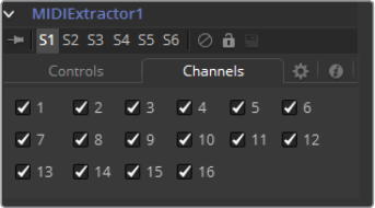
763
Modifiers Chapter – 30
Pitch Scale Note Mode Only
Pitch Scale defines how much the result changes with pitch. A value of 1.0 will cause
the result to vary from 0.0 to 1.0 over the entire range.
Velocity Scale Note Mode Only
This defines how much the result changes with velocity. A value of 1.0 will cause the
result to vary from 0.0 to 1.0 over the entire range. This is added to the result from pitch
scale for the final result.
Control Number Control Change Mode Only
This specifies the MIDI controller number from which to extract events.
Envelope Controls Note and Beat Modes Only
These define an Envelope to follow for values before, during and after the note or beat.
Pre-Attack Time defines how long before the event it will start ramping up to the
pre-attack level. Attack is the Time/Level to ramp to once the event has occurred,
followed by the Decay ramp and Sustain, until the event stops. This stage is for Notes
only. Beats have an instantaneous duration, so it goes straight to Release. Release is
the ramp down time after the event finishes. When trying to do a Beat, set Release to
some value, or there likely will not be much on the beats.
These values can be used to follow actual sounds in the MIDI sequence, or just to
create interesting effects. All time values used in the MIDI Extractor are in seconds.
Channels Tab
Channels
Channels checkboxes select which of the 16 channels in the MIDI file are actually
considered for events. This is a good way to single out a specific instrument from
anarrangement.
More About MIDI
A single MIDI interface allows 16 channels. Typically, these will be assigned to different
instruments within a device or different devices.
Usually, MIDI data is 7-bits, ranging from 0..127. This is represented as a value between 0..1 to be
more consistent with the way data is handled throughout the rest of Fusion.
764
Modifiers Chapter – 30
There are quite a number of different MIDI messages and events but the ones that are
particularly useful with this modifier are detailed below.
MIDI Messages
Note On: This indicates that a note (on a specific channel) is being turned on, has a
pitch (0..127, with middle C being 60) and a Velocity (0..127, how fast the key was or
whatever was hit).
Note Off: This indicates that a note (on a specific channel) is being turned off, has a
pitch (0..127, with middle C being 60) and a Velocity (0..127, how fast the key was or
whatever was released).
Control Change: This message indicates that some controller has changed. There
are 128 controllers (0..127), each of which has data from 0..127. Controllers are used to
set things such as Volume, Pan, amount of Reverb or Chorus, and generic things like
foot controllers or breath controllers.
Midi Events
Channel Aftertouch: This event defines that pressure is being applied to the keys
(or whatever) during a note. It is general, overall pressure for this channel so it simply
uses a pressure value (0..127).
Poly Aftertouch: This event defines that pressure is being applied to the keys (or
strings, or whatever) during a note. It is specific to each particular note and, therefore,
contains a note number as well as a pressure value (0..127).
General
Pitch Bend
The Pitch Bend controller generally specifies the degree of pitch bending or variation
applied to the note. Because pitch bend values are transmitted as a 14-bit value, this
control has a range between -1 and 1, and a correspondingly finer degree of resolution.
For a resource on how MIDI works, have a look at http://www.harmony-central.com/
MIDI/Doc/doc.html.
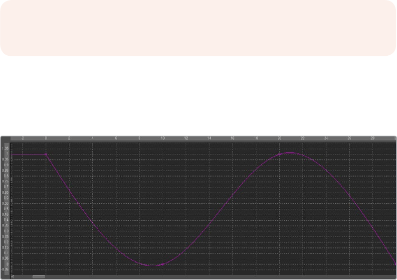
765
Modifiers Chapter – 30
Natural Cubic Spline
The Natural Cubic Spline is one of the animation modifiers in Fusion and normally is applied to
numerical values rather than point values. It can be applied by right-clicking on a numerical
control and selecting Modify with > Natural Cubic Spline.
Usage
Being an animation spline, this modifier has no actual Controls tab, however, its effect can be
seen and influenced in the Spline Editor.
NOTE: Unlike other spline types, Cubic splines have no control handles and attempt to
automatically provide a smooth curve through the keypoints.
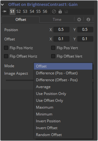
766
Modifiers Chapter – 30
Offset
Offsets are useful for creating constant or animated variances between values, relating to
various controls, paths and points. There are three types of offsets available in Fusion:
Offset Distance
Offset Angle
Offset Position
Offset Angle
The Offset Angle Modifier outputs a value between 0 and 360 that is based on the angle
between two positional controls. The Position and Offset parameters may be static, connected
to other positional parameters or connected to paths of their own. All of the offsets use the
same set of controls, which behave differently depending on the offset type used. These
controls are described below.
Offset Distance
The Offset Distance modifier outputs a value that is based on the distance between
two positional controls. This modifier is the first one discussed that is capable of
outputting a value based on a mathematical expression applied to a position.
Offset Position
The Offset Position modifier outputs a position (X and Y coordinate) that is based on
the relationship between positional controls. This modifier is the equivalent of a
calculation control except that it outputs X and Y coordinates instead of a value.
It can be applied by right-clicking on a control and selecting Modify with > Offset.
Oset Tab
767
Modifiers Chapter – 30
Position X and Y
The first position value is used by the Position to generate the calculation.
Offset X and Y
The first position value is used by the Offset to generate the calculation.
Flip Position Horizontal and Vertical
When these controls are selected, the Position will be mirrored along the vertical or
horizontal axis of the image.
Flip Offset Horizontal and Vertical
When these controls are selected, the Offset position will be mirrored along the vertical
or horizontal axis of the image.
Mode
Select an option from the Mode menu to choose the mathematical operation
performed by the offset control.
Available options are:
Offset
Difference (Position - Offset)
Difference (Offset - Position)
Average
Use Position Only
Use Offset Only
Maximum
Minimum
Invert Position
Invert Offset
Invert Sugar
Random Offset
Image Aspect
Adjust the modifier’s output to compensate for the Image Aspect (not pixel aspect) of
the project. A square image of 500 x 500 would use an Image Aspect value of 1 and a
rectangular image of 500 x 1000 would use an Aspect value of 2. The default value is
always based on the current frame format selected in the preferences. To calculate
Image Aspect, divide the width by the height. This control can also be used to create
the illusion of aspect.
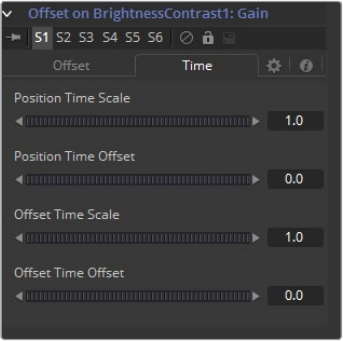
768
Modifiers Chapter – 30
Time Tab
Position Time Scale
This returns the value of the Position at the Time Scale specified (for example, 0.5 is the
value at half the current frame time).
Position Time Offset
This returns the value of Position at the Time Offset specified (for example, 10 is 10
frames back).
Offset Time Scale
This returns the value of the Offset at the Time Scale specified.
Offset Time Offset
This returns the value of Offset at the Time Offset specified.
Example
Let’s continue the Text banking example at the beginning of this chapter to illustrate
one potential use of offsets.
Select and view the Merge tool in this flow. Right-click on the Merge Size control and
select Modify With > Offset Distance from the contextual menu. This will add two new
crosshairs and Offset controls in the Modifier tab.
The size of the text will now be determined by the distance or offset between the two
new cross hairs. These points are animatable and can be connected to other controls.
Connect the position value of the offset to the existing path by right-clicking on the
Position control and selecting Connect To > Path on Merge 1 Center Value. Manually
place the Offset crosshair at the bottom of the screen between the two path points.
Now, the text should shrink near the ends of the path (when the distance between the
offset and the path is at its minimum) and grow at its ends (where the distance between
the offset and the path is at its maximum).
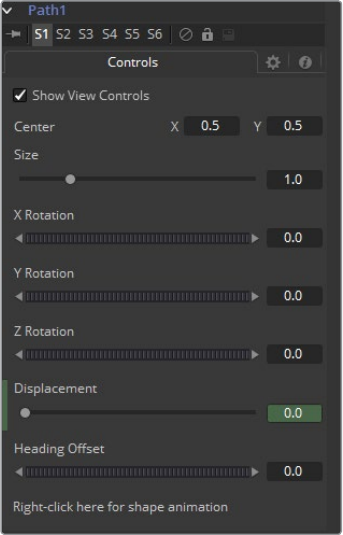
769
Modifiers Chapter – 30
Path
The Path uses two splines to control the animation of Points. An onscreen motion path (spacial)
and a Time spline visible in the Spline Editor (temporal). To animate a Coordinate control using a
Path, right-click on the control and select Path from the contextual menu.
Controls Tab
For an in-depth explanation, see the chapter Working with Motion Paths in this documentation.
Center
The actual Center of the path. This can be modified and animated as well to move the
entire path around.
Size
The Size of the path. Again this allows for later modification of the animation.
X Y Z Rotation
The Path can be rotated in all three dimensions to allow for sophisticated controls.
Displacement
Every motion path has an associated Displacement spline in the Spline Editor. The
Displacement spline represents the position of the animated control along its path,
represented as a value between 0.0 and 1.0. Displacement splines are used to control
the speed of a control’s movement along its path.
To slow down, speed up, stop or even reverse the motion of the control along the path,
adjust the values of the points for the path’s displacement in the Spline Editor.
A Displacement value of 0.0 in the Spline Editor indicates that the control is at the
very beginning of a path.
A value of 1.0 indicates that the control is positioned at the end of the path.
Each locked point on the motion path will have an associated point on the
Displacement spline.
770
Modifiers Chapter – 30
Unlocked points will not have a corresponding point on the Displacement spline.
For an in-depth explanation, see the chapter Working with Motion Paths in this
documentation.
Heading Offset
If another control, for example a mask’s Angle, is connected to the path’s heading, this
control allows for adding or subtracting from the calculated angle.
Right Click Here for Shape Animation
It is possible to animate the shape of the path as well, or to connect it to other path
controls like Polyline Masks or Paint Strokes.
Switching Default Paths
Change the Default Path type used when animating a Coordinate control to Path (if this
is the preferred type of animation). Open the Global preferences and look under the
Default tab for the drop-down list in the default animate section labeled Point With.
Change this from the current value to Path. The next time Animate is selected from a
Coordinate control’s contextual menu, a Path will be used.
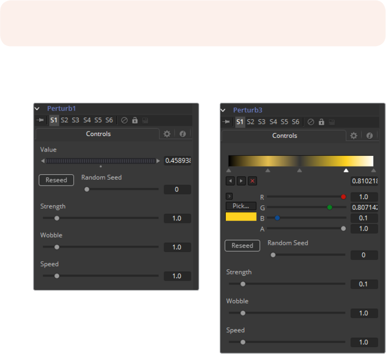
771
Modifiers Chapter – 30
Perturb
The Perturb modifier generates smoothly varying random values for several input types, based
on Perlin noise. It can be used to add jitter, shake or wobble to any animatable control, even if
the control is already animated. Its results are similar to those of the Shake modifier, though it
uses a different set of controls that may be more suitable to your needs. Unlike other random
modifiers, the Perturb modifier can also be applied to polylines, shapes, grid meshes and even
color gradients.
For example, to add camera shake to an existing path, right-click on the crosshair and choose
Insert > Perturb, then adjust the Strength down to suit. Alternatively, right-click on the path’s
Shape Animation control, and apply the wobble to the path’s polyline itself (this works best if
the polyline has many points, for example, if it has been tracked, or hand-drawn with the Draw
Append pencil tool). A third option is to insert the modifier onto the Displacement control, which
will cause the motion along the path to jitter back and forth without actually leaving the line
of the path.
Controls Tab
NOTE: Perturb can only add jitter it cannot smooth out existing animation curves.
772
Modifiers Chapter – 30
Value
The actual contents of this control will depend on what type of control the modifier was
applied to. If the Perturb modifier was added to a basic Slider control, the Value will be
a slider. If it was added to a Gradient control, then a Gradient control will be displayed
here. Use the control to set the default, or center value, for the Perturb modifier
to work on.
Jaggedness
(Polylines, Meshes only) This allows you to increase the amount of variation along the
length of the polyline or mesh, rather than over time. Increasing this will give a
squigglier polyline or more tangled mesh, independent of its movement.
Phase
(Polylines, Meshes only) Animating this can be used to move the ripple of a polyline or
mesh along itself, from end to end. The effect can be most clearly seen when Speed is
set to 0.0.
Random Seed Randomize
The Random Seed is used to ‘seed’ the amount of jitter applied by the modifier. Two
Perturb modifiers with identical settings, but different random seeds, will produce two
completely different results. Click on the Randomize button to assign a random
seed value.
Strength
Use this control to adjust the Strength of the Perturb modifier’s output, or its maximum
variation from the primary value specified above.
Wobble
Use the Wobble control to determine how smooth the resulting values are. Less wobble
implies a smoother transition between values, while more wobble produces less
predictable results.
Speed
Increasing the Speed slider value will speed up the rate at which the value changes.
This can increase the apparent wobbliness in a more predictable fashion than the
Wobble control and make the jitter more frantic or languorous in nature.
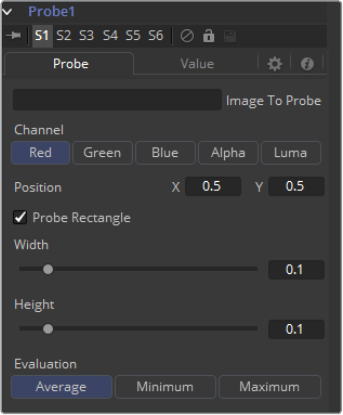
773
Modifiers Chapter – 30
Probe
The Probe Modifier is one of the most versatile modifiers in Fusion. It allows you to control any
numeric parameter by the pixel color or luminosity at a certain position or rectangular region of
an image. Think of driving values by the presence or absence of an image or by color values of
an image, using colors to create X Y positions on other controls, or measuring graded LUTs to
compare values.
It can be applied by right-clicking on a control and selecting Modify with > Probe.
Probe Tab
Image to Probe
Drop the tool of the image you want to probe into this field.
Channel
Select the Channel you want to probe. The usual options are:
Red
Green
Blue
Alpha
Luma
Once a Probe modifier is present somewhere in your comp you can connect other
tool’s values to its outputs as well. The Probe allows to connect to its values
individually:
Result
Red
Green
Blue
Alpha
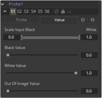
774
Modifiers Chapter – 30
Position X Y
The position in the image from where the probe samples the values.
Probe Rectangle
By default the Probe only samples the value of a single pixel at its position. By using the
Probe Rectangle mode you can sample from a larger area of pixels based on the
Evaluation method.
Width Height Controls
These determine the size of the area to be probed.
Evaluation
Sets how the pixels inside the rectangle are computed to generate the output value.
Options are:
Average (all pixel values inside the rectangle are averaged).
Minimum (The smallest value of all pixels inside the rectangle is used).
Maximum (The highest value of all pixels inside the rectangle is used).
Value Tab
Scale Input Black White
By default, the Probe generates the Black Value when the probed area results in a
value of 0 (i.e., Black) and it generates its White Value when the probed area results in a
value of 1 (i.e., White). By using this range control you can modify the sensitivity of
the Probe.
Black Value
The value that is generated by the Probe if the probed area delivers the result set in
Scale Input Black.
White Value
The value that is generated by the Probe if the probed area delivers the result set in
Scale Input White.
Out of Image Value
The value that is generated by the Probe if the probed area is outside the frame
boundaries of the probed image. If probing a rectangle, this value will not be generated
before the entire rectangle is outside the frame boundaries of the image to be probed.
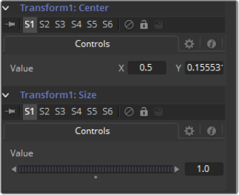
775
Modifiers Chapter – 30
Publish
Only controls that are animated can be available from the Connect To menu option. Anon-
animated control (static) must be published before it can be connected. Animated controls are
automatically published, whereas static controls have to be manually published.
To publish a control, right-click on the control and select Publish from the contextual menu.
Published Value
This is obviously dependent on which value is published from which tool.
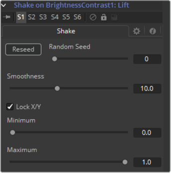
776
Modifiers Chapter – 30
Shake
The Shake modifier is used to randomize a position or value control to create semi-random
numeric inputs. The resulting shake can be entirely random. The motion can also be smoothed
for a more gentle, organic feel.
To add the Shake modifier to a control, select Modify With > Shake from the Control’s
contextual menu. The Shake modifier uses the following controls to achieve its effect. It can be
applied by right-clicking on a control and selecting Modify with > Shake.
Shake Tab
Random Seed
The Random Seed control contains the value used to seed the random number
generator. Given the same seed, a random number generator will always produce the
same results. Change the seed if the results from the randomizer are not satisfying.
Smoothness
This control is used to smooth the overall randomness of the shake. The higher the
value is set, the smoother the motion will appear. A value of zero will generate
completely random results, with no smoothing applied.
Lock X and Y
This checkbox is used to Unlock the X- and Y-axis, revealing independent slider
controls for each axis.
Min and Max
This control is used to determine the overall strength of the shake. The low values
represent the lowest value that can be generated by the randomizer and the high
values represent the highest values. To create a shake that moves a center crosshair
anywhere within the image, set the low to 0.0 and the high to 1.0. To restrict the motion
to a smaller shake in the bottom right corner of the image, set the Min to 0.70 and the
Max to 0.90.
777
Modifiers Chapter – 30
Example
Create a new comp and add a Text tool.
Type something in the Text tool and view it in the large display.
Add a shake modifier by selecting Modify With > Shake Position from the contextual
menu for the Text Center control.
Switch to the Modifier tab and set the smoothing to 5.0.
Set the Low to 0.1 and the High to 0.9.
Go to frame 0 and add a Bezier spline to both the Low and the High controls.
Advance to frame 90 and set the Low to 0.45 and the High to 0.55.
Render out a preview and view the results.
The text should start out by flying all over the screen and then tighten in toward the
center of the screen.
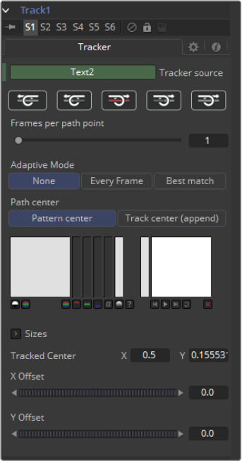
778
Modifiers Chapter – 30
Track
Another technique for adding a tracker directly to a control is to apply the Tracker as a modifier.
Right-click on the center of the mask and select Ellipse x Center > Modify With > Tracker
Position > Steady Position or Unsteady Position. This would add a modifier with a set of controls
almost identical to those found in the Tracker tool itself.
Tracker Tab
For an in-depth explanation of this tool, refer to the Tracker documentation in this manual.
The differences between a Tracker Modifier and a Tracker Tool are as follows:
The Tracker modifier can only track a single pattern.
A source image must be set for the Tracker modifier.
The Tracker modifier can only output a single value and cannot be used for complex
stabilization procedures.
The default source image for the modifier is the tool immediately upstream of the
tool that contains the modifier (i.e., when adding a Tracker modifier to a Glow tool
with a Loader as its input, the Tracker Source input will default to the output of the
Loader). Set a different source image for the Tracker modifier by typing in the name
of the tool. Alternately, drag and drop the Source tool from the flow into the Text
Box control.
Example
Imagine that you needed to track an actor’s eyes so that an unearthly, alien glow could be
applied to the eyes. Add a Glow tool and then create an Ellipse mask in the shape of the eye.
Right-click on the center of that mask and select modify with > Track. Track the actor’s eye.
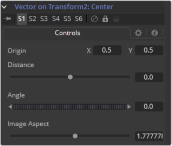
779
Modifiers Chapter – 30
Vector
The Vector Modifier is used to offset positional controls, such as crosshairs, by distance and
angle. These can be static or animated values.
It can be applied by right-clicking on a control and selecting Modify with > Vector.
Controls Tab
Origin
This control is used to represent the position from which the vector’s distance and
angle values originate.
Distance Slider Control
This control is used to determine the Distance of the vector from the origin.
Angle Thumbwheel Control
This control is used to determine the Angle of the vector relative to the origin.
Image Aspect Slider Control
This control is used primarily to compensate for image aspect differences. A square
image of 500 x 500 would use an Image Aspect value of 1, while a rectangular image
of 500 x 1000 would use an Aspect value of 2. The default for this value is taken from
the current Frame Format preferences using width/height. It may be required to modify
this control to match the current image.
Example
To illustrate, create a simple flow consisting of a black background, a Text tool
and a Merge.
Right-click on the center of the merge and select Modify With > Vector. This will add a
Vector Control header under the small view. Expand it by clicking on the gold triangle.
Drag the Distance control to distance the text from the vector origin.
Drag the Angle thumbwheel to rotate the text around the vector origin.
Add a path to the vector origin by right-clicking on the Origin control and selecting the
Path option from the contextual menu. Verify that the current frame is set to frame 0
(zero) and drag the Vector Origin crosshair to the bottom left corner of the screen.
Right-click on the Vector Angle thumbwheel and select Bezier Spline to animate
this control.
Set the Angle thumbwheel to a value of 10.
Advance to frame 100 and click at the top left corner of the screen to move the vector
origin crosshair.
Set the Vector Angle thumbwheel to a value of 1000. This will cause the text to orbit
around the path just created.
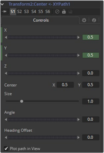
780
Modifiers Chapter – 30
XY Path
The XY Path type uses a separate spline for the position along the X-axis, as it does for the
position along the Y-axis.
To animate a coordinate control using an XY path, right-click on the control and select Modify
With > XY Path from the contextual menu.
At first glance, XY paths work like Displacement paths. To describe the path, change frames
and position the control where it should be on that frame, then change frames again and move
the control to its new position. Fusion automatically interpolates between the points. The
difference is that no keyframes are created on the onscreen path.
Look in the Spline Editor to find the X and Y channel splines. Changes to the controls position
will be keyframed on these splines. The advantage to the XY path is that it becomes very easy
to work with motion along an individual axis.
Controls Tab
X Y Z Values
These reflect the position of the animated control.
Center
The actual Center of the path. This can be modified and animated as well to move the
entire path around.
Size
The Size of the path. Again this allows for later modification of the animation.
Angle
The Angle of the path. Again this allows for later modification of the animation.
781
Modifiers Chapter – 30
Heading Offset
If another control, for example a mask’s Angle, is connected to the path’s heading, this
control allows for adding or subtracting from the calculated angle.
Plot Path In View
Toggles if or if not the actual path is displayed in the views.
Switching Default Paths
Change the Default Path type used when animating a coordinate control to XY path
(ifthis is the preferred type of animation). Open the Global preferences and look under
the default’s tab for the drop-down list in the default animate section labeled Point With.
Change this from the current value to XY Path. The next time Animate is selected from
a Coordinate Control’s contextual menu, an XY path will be used instead of a
Displacement path.
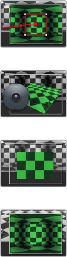
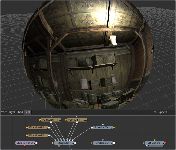
784
VR Tools Chapter – 31
VR Tools
360° (spherical) video, often described as Virtual Reality or VR, has been created and fixed in
Fusion for over a decade. Dome productions, planetariums and other special-venue
productions utilize the flexibility of Fusion and its 3D system to produce and deliver
special content.
360° video is often represented with an equirectangular (lat-long) format, similar to how the
globe is represented by a world map, with the poles at the top and bottom edges of the image
and the forward view point at the center. Stereo VR can be created from two stacked lat-long
images, one for each eye. VR video can also be created from 3D CGI scenes.
Fusion supports a number of common spherical image formats, and can easily convert
between them.
VCross and HCross are the six square faces of a cube laid out in a cross, vertically or
horizontally, with the forward view in the center of the cross, in a 3:4 or 4:3 image.
VStrip and HStrip are the six square faces of a cube laid vertically or horizontally in
a line, ordered as Left, Right, Up, Down, Back, Front (+X, -X, +Y, -Y, +Z, -Z), in a 1:6 or
6:1 image.
LatLong is a single 2:1 image in an equirectangular mapping.
Fusion 9 has built-in support for VR headsets like the Oculus Rift and HTC Vive. Fusion will
display both spherical video and live 3D scenes from the comp directly to the headset.
Fusion’s “Fix it in Post” tools for VR make it easy to do several important tasks that are common
in these types of productions.
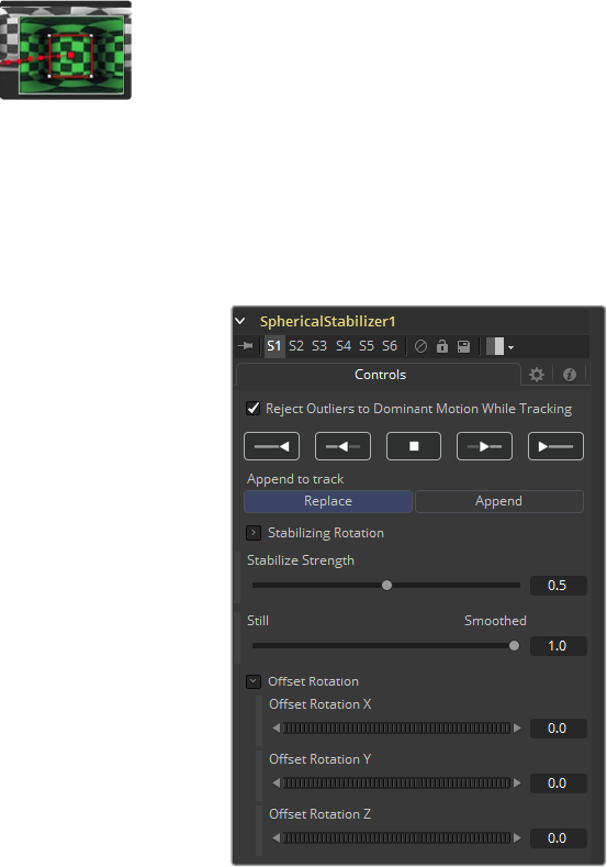
785
VR Tools Chapter – 31
Spherical Stabilizer
VR live action is often shot with a handheld camera, so the footage can be shaky. The Spherical
Stabilizer tool will automatically identify and track visible features in the footage, then analyse
their movement to identify pan, tilt, and roll rotations. After tracking, it is then possible to smooth
out or stabilize the rotation of the footage. The tool requires images in a spherical layout, which
can be any of LatLong (2:1 equirectangular), Horizontal/Vertical Cross, or Horizontal/
Vertical Strip.
Controls Tab
Reject Outliers to Dominant Motion While Tracking
With this control ticked (the default setting), features that move contrary to the majority
of other features will be ignored. This helps ignore the movement of subjects in the
shot, preferring stable and consistent markers from the surrounding environment.
Track Controls
These initiate tracking and analysis of the shot. Note that the reference frame used for
stabilization is set to the first frame tracked.
Track Backwards from end frame starts tracking backwards from the end of the
current render range.
Track Backwards from current time starts tracking backwards from the
current frame.
Stop ceases tracking, preserving all results so far.
Track Forward from current time starts tracking forwards from the start of the
current render range.
Track Forward from start frame starts tracking forwards from the current time.
786
VR Tools Chapter – 31
Append to Track
Replace will cause the Track Controls to discard any previous tracking results, and
replace them with the newly-created track.
Append will add the new tracking results to any earlier tracks.
Stabilization Strength
This control varies the amount of smoothing or stabilization applied, from 0.0 (no
change) to 1.0 (maximum).
Still – Smooth
The Spherical Stabilizer tool can eliminate all rotation from a shot, fixing the forward
viewpoint (Still mode, 0.0) or gently smooth out any panning, rolling or tilting in order to
increase viewer comfort (Smooth mode, 1.0). This control allows either option, or
anything in between.
Offset Rotation
Often a shot is not completely level and needs the horizon to be realigned, or perhaps
a desired pan should be reintroduced after fully stabilizing the shot. The Offset Rotation
controls allow additional manual control of the Stabilizer’s rotation of the footage, for
pitch/tilt (X), pan/yaw (Y), and roll (Z), respectively. Rotation is always performed in that
order, i.e. XYZ.
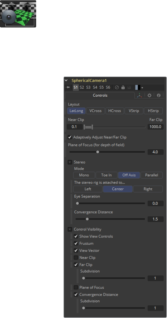
787
VR Tools Chapter – 31
Spherical Camera
The Spherical Camera allows the 3D Renderer to output an image covering all viewing angles,
laid out in several different formats. This image may be used e.g. as a skybox texture or
reflection map, or viewed in a VR headset, The Image Width setting in the 3D Renderer is used
as the size of each square cube face, so the resulting image may be a multiple of this size
horizontally and vertically.
Controls Tab
Layout
VCross and HCross are the six square faces of a cube laid out in a cross, vertical or
horizontal, with the forward view in the center of the cross, in a 3:4 or 4:3 image.
VStrip and HStrip are the six square faces of a cube laid vertically or horizontally in
a line, ordered as Left, Right, Up, Down, Back, Front (+X, -X, +Y, -Y, +Z, -Z), in a 1:6 or
6:1 image.
LatLong is a single 2:1 image in equirectangular mapping.

788
VR Tools Chapter – 31
Near/Far Clip
The clipping plane is used to limit what geometry in a scene is rendered based on the
object’s distance from the camera’s focal point. This is useful for ensuring that objects
which are extremely close to the camera are not rendered and for optimizing a render
to exclude objects that are too far away to be useful in the final rendering.
The default perspective camera ignores this setting unless the the Adaptively Adjust
Near/Far Clip checkbox control below is disabled.
The values are expressed in units, so a far clipping plane of 20 means that any object
more than 20 units distant from the camera will be invisible to the camera. A near
clipping plane of 0.1 means that any object closer than 0.1 units will also be invisible.
Adaptively Adjust Near/Far Clip
When selected, the Renderer will automatically adjust the camera’s near/far clipping
plane to match the extents of the scene. This setting overrides the values of the Near
and Far clip range control described above. This option is not available for
orthographic cameras.
Viewing Volume Size
The Viewing Volume Size control only appears when the Projection Type is set to
Orthographic. It determines the size of the box that makes up the camera’s field of
view. The Z distance of an orthographic camera from the objects it sees does not affect
the scale of those objects, only the viewing size does.
Plane of Focus (for Depth of Field)
This value is used by the OpenGL renderer to calculate depth of field. It defines the
distance to a virtual target in front of the camera.
Stereo Method
Allows you to adjust your stereoscopic method to your preferred working model.
Toe in
Both cameras point at a single focal point. Though the result is stereoscopic,
thevertical parallax introduced by this method can cause discomfort by the audience.
Off Axis
Often regarded as the correct way to create stereo pairs, this is the default method in
Fusion. Off Axis introduces no vertical parallax, thus creating less stressful
stereo images.
Parallel
The cameras are shifted Parallel to each other. Since this is a purely parallel shift, there
is no Convergence Distance control. Parallel introduces no vertical parallax, thus
creating less stressful stereo images.
NOTE: A smaller range between the near and far clipping planes allows
greater accuracy in all depth calculations. If a scene begins to render strange
artifacts on distant objects, try increasing the distance for the Near Clip plane.
Use the vertical aperture size to get the vertical angle of view and the
horizontal aperture size to get the horizontal angle of view.
789
VR Tools Chapter – 31
Eye Separation
Defines the distance between both stereo cameras. If the Eye Separation is set to a
value larger than 0, controls for each camera will be shown in the Viewer when this tool
is selected. There is no Convergence Distance control in Parallel mode.
Convergence Distance
This control sets the stereoscopic convergence distance, defined as a point located
along the Z-axis of the camera that determines where both left and right eye
cameras converge
Control Visibility
Allows you to selectively activate the on screen controls that are displayed along with
the camera.
Frustum: Displays the actual viewing cone of the camera.
View Vector: Displays a white line inside the viewing cone, which can be used to
determine the shift when in Parallel mode.
Near Clip: The Near clipping plane. This plane can be subdivided for better visibility.
Far Clip: The Far clipping plane. This plane can be subdivided for better visibility.
Plane of Focus: The Plane of Focus according to the respective slider explained
above. This plane can be subdivided for better visibility.
Convergence Distance: The point of convergence when using Stereo mode. This
plane can be subdivided for better visibility.
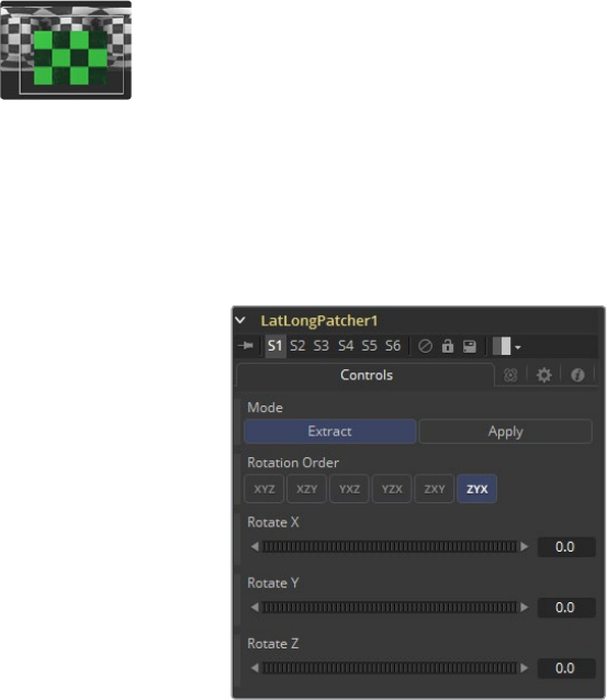
790
VR Tools Chapter – 31
LatLong Patcher
Equirectangular stitched images often need patches, paint work, or other VFX applied. The
LatLong Patcher extracts and de-warps a section of a lat-long (equirectangular) image to be
treated, and can warp and merge fixes back over the original. This gives the ability to quickly
pick a section of the spherical image to patch or paint, then apply it back to the original image.
Note that matching rotations will be used in both Extract and Apply modes, allowing a tool’s
operation to be easily reversed by a copy or instance with the same rotation settings.
Control Tab
Mode
Extract will pull a de-warped 90 degree square image from the
equirectangular image.
Apply will warp and merge a 90 degree square image over the equirectangular
image. Because the square image’s alpha is used, this allows e.g. paint strokes
or text drawn over a transparent black background to be applied to the original
equirectangular image, avoiding any double-filtering from de-warping and re-warping
the original.
Rotation
These will rotate the spherical image around each of the X, Y, and Z axes, offering
independent control over pitch/tilt, pan/yaw, and roll, respectively.
Rotation Order
This chooses the ordering of the rotations around each axis. For example, XYZ will
rotate first around the X axis (pitch/tilt), then around the Y axis (pan/yaw), then around
the Z axis (roll). Any of the six possible orderings can be chosen.
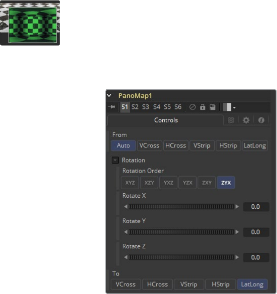
791
VR Tools Chapter – 31
PanoMap
Converts images from one spherical layout to another, such as cubemap to equirectangular
formats. The tool can also do rotations of the spherical images when converting.
Control Tab
From and To
Auto will detect the incoming image layout from the metadata and image
frame aspect.
VCross and HCross are the six square faces of a cube laid out in a cross, vertical or
horizontal, with the forward view in the center of the cross, in a 3:4 or 4:3 image.
VStrip and HStrip are the six square faces of a cube laid vertically or horizontally in
a line, ordered as Left, Right, Up, Down, Back, Front (+X, -X, +Y, -Y, +Z, -Z), in a 1:6 or
6:1 image.
LatLong is a single 2:1 image in equirectangular mapping.
Rotation
These will rotate the spherical image around each of the X, Y, and Z axes, offering
independent control over pitch/tilt, pan/yaw, and roll, respectively.
Rotation Order
This chooses the ordering of the rotations around each axis. For example, XYZ will
rotate first around the X axis (pitch/tilt), then around the Y axis (pan/yaw), then around
the Z axis (roll). Any of the six possible orderings can be chosen.
