GAMP Users Manual
User Manual:
Open the PDF directly: View PDF ![]() .
.
Page Count: 21
GAMP Users Guide
Feng Zhou
Email: zhouforme@163.com
Last modified: Dec 20, 2017
1 Introduction ........................................................................................................................................... 1
2 Supported Platforms .......................................................................................................................... 1
3 Installation .............................................................................................................................................. 2
3.1 Windows .......................................................................................................................................... 2
3.2 Unix/Linux/Macintosh ............................................................................................................... 2
4 GNSS data downloads ....................................................................................................................... 3
5 Run
GAMP
............................................................................................................................................... 4
5.1 Preparation of GNSS data files .............................................................................................. 4
5.2 Configure file ................................................................................................................................. 5
5.3 Data processing ............................................................................................................................ 8
5.3.1 Single-session processing ............................................................................................... 8
5.3.2 Multi-session processing ................................................................................................. 8
5.4 Results analysis and plotting ................................................................................................ 10
5.5 A new receiver data interchange format – RCVEX ...................................................... 17
6 Support .................................................................................................................................................. 18
7 References ............................................................................................................................................. 19
1
1 Introduction
As the number of GNSS satellites and stations increases, GNSS data
processing software should be developed that is easy to operate, efficient to
run, and have a robust performance. To meet these requirements, we
developed a new GNSS analysis software called GAMP (GNSS Analysis
software for Multi-constellation and multi-frequency Precise positioning), which
can perform multi-GNSS precise point positioning (PPP) based on
undifferenced and uncombined observations. GAMP is a secondary
development based on RTKLIB but with many improvements, such as cycle
slip detection, receiver clock jump repair, and handling of GLONASS
pseudorange inter-frequency biases. A simple, but unified format of output files,
including positioning results, number of satellites, satellite elevation angles,
pseudorange and carrier phase residuals, and slant Total Electron Content
(sTEC), is defined for results analysis and plotting. Moreover, a new
receiver-independent data interchange format called RCVEX (ReCeiVer
independent EXchange) is designed to improve computation efficiency for
post-processing.
The main features of GAMP are:
► standard and ionosphere-constrained single- and dual-frequency
undifferenced and uncombined GNSS PPP processing
► multi-constellation support – GPS, GLONASS, BDS, Galileo, and QZSS
► handling of GLONASS pseudorange inter-frequency biases (IFBs)
► efficient batch processing using C shell scripts
► powerful in results output, analysis, and plotting
► works in Windows, UNIX/Linux, and Macintosh
2 Supported Platforms
The GAMP software was written in the platform-independent ANSI C language.
It can compile and run on the popular operating systems, such as Windows,
UNIX/Linux, and Macintosh. It is recommended that one debug GAMP under
Microsoft Visual Studio (VS), and then compile and run it in UNIX/Linux or
Macintosh for batch processing.
GAMP is an open-source software, which includes source code files,
documents, and examples. It is governed by the GNU General Public License
(GPL). The source code can be accessed via the website of GPS Toolbox
(https://www.ngs.noaa.gov/gps-toolbox/GAMP).
NOTE: GAMP is a command-line program. To view GAMP document,
PDF reader software (e.g., Adobe Acrobat or Foxit Reader) is required.
2
3 Installation
3.1 Windows
You can either use the existing project under the folder of “GAMP_Windows”,
or follow steps 1) – 5):
1) To create an empty Microsoft Visual Studio project and import the source
code files
Add GAMP source code files to project
Click Project -> Add Existing Item, in the “Add Existing Item” dialog box, locate
and select the GAMP source code files.
2) To change project properties
Click Project -> Properties
A: Configuration Properties -> C/C++ -> Preprocessor -> Preprocessor
Definitions
WIN32;_DEBUG;_CONSOLE;%(PreprocessorDefinitions);_CRT_SECURE_N
O_WARNINGS;ENAGLO;ENACMP;ENAGAL;ENAQZS;NFREQ=3
B: Configuration Properties -> Linker -> Debugging -> Generate Debug Info:
Y(/DEBUG)
C: Configuration Properties -> C/C++ -> General -> Debug Information Format:
C7
4) To set up pthread
Put pthreads-w32-2-9-1-release directory in the C: drive.
Click Project -> Properties
A: Configuration Properties -> C/C++ -> General -> Additional Include
Directories
Add the path: C:\pthreads-w32-2-9-1-release\Pre-built.2\include
B: Configuration Properties -> Linker -> General -> Additional Library
Directories
Add the path: C:\pthreads-w32-2-9-1-release\Pre-built.2\lib\x86
C: Configuration Properties -> Linker -> Input -> Additional Dependencies
Add item: pthreadVSE2.lib
5) To add Linux compatible header files
Put unistd.h and dirent.h into the VS install directory, such as C:\Program Files
(x86)\Microsoft Visual Studio 10.0\VC\include.
NOTE: The GAMP project compiled under VS 2010 is also provided in the
installation directory (e.g., GAMP_src\Windows\gamp_c).
3.2 Unix/Linux/Macintosh
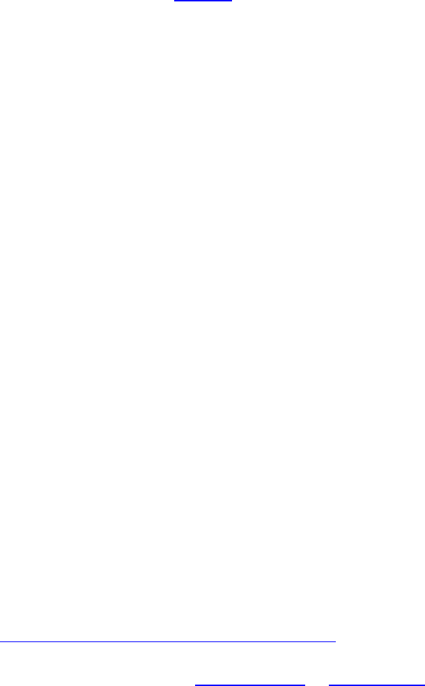
Put the directory of GAMP_Linux in Unix/Linux or GAMP_Mac in Macintosh,
then enter into the directory and type “make” at the terminal as shown in Fig. 1.
3
Fig. 1 The compilation of GAMP in Linux
4 GNSS data downloads
GAMP also includes some useful GNSS download tools written in C shell. By
convention, we have the following definitions firstly:
WWWW: GPS week
WWWWD: GPS week and day of week
YY: 2-digit year
YYYY: 4-digit year
DDD: day of year
MM: month
sh_code_dcb: to download GPS and GLONASS differential code bias (DCB)
files provided by CODE from ftp://ftp.unibe.ch/aiub/CODE/YYYY
sh_mgex_dcb: to download Multi-GNSS DCB files provided by CAS and DLR
from ftp://igs.ign.fr/pub/igs/products/mgex/dcb/YYYY
sh_igs_prod: to download GPS and/or GLONASS precise orbit and clock
products of IGS from ftp://igs.ign.fr/pub/igs/products/WWWW or
ftp://cddis.gsfc.nasa.gov/pub/gps/products/WWWW
sh_igs_snx: to download solution independent exchange (SINEX) format
weekly files from ftp://igs.ign.fr/pub/igs/products/WWWW or
ftp://cddis.gsfc.nasa.gov/pub/gps/products/WWWW
sh_mgex_prod: to download multi-GNSS precise orbit and clock products of
MGEX from ftp://igs.ign.fr/pub/igs/products/mgex/WWWW or
ftp://cddis.gsfc.nasa.gov/pub/gps/products/mgex/WWWW
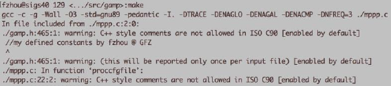
sh_cddis_nav: to download GPS, GLONASS, and multi-GNSS broadcast
ephemeris files from ftp://cddis.gsfc.nasa.gov/pub/gps/data/daily/YYYY/brdc,
ftp://cddis.gsfc.nasa.gov/pub/gps/data/campaign/mgex/daily/rinex3/YYYY/brdm
sh_code_ion: to download CODE global ionosphere map (GIM) files
(CODGDDD0.YYI.Z) from ftp://ftp.unibe.ch/aiub/CODE/YYYY
sh_igs_obs: to download GPS and GLONASS observation files from
ftp://cddis.gsfc.nasa.gov/pub/gps/data/daily/YYYY/DDD/YYo
sh_mgex_obs: to download multi-GNSS observation files from
ftp://igs.ign.fr/pub/igs/data/campaign/mgex/daily/rinex3/YYYY/DDD *.crx.gz
ftp://igs.ign.fr/pub/igs/data/campaign/mgex/daily/rinex3/YYYY/DDD *d.Z
ftp://cddis.gsfc.nasa.gov/pub/gps/data/daily/YYYY/DDD/YYd *.crx.gz
4
ftp://cddis.gsfc.nasa.gov/pub/gps/data/campaign/mgex/daily/rinex3/YYYY/DD
D/YYo *.Z
Note: Each script can be run independently. Type the corresponding script,
and you will get the help information like:
Fig. 2 The help information of “sh_cddis_nav”
In addition, the main script “sh_main_gnss_download” is provided, which can
call the aforementioned scripts.
Fig. 3 The help information of “sh_main_gnss_download”
5 Run GAMP
5.1 Preparation of GNSS data files
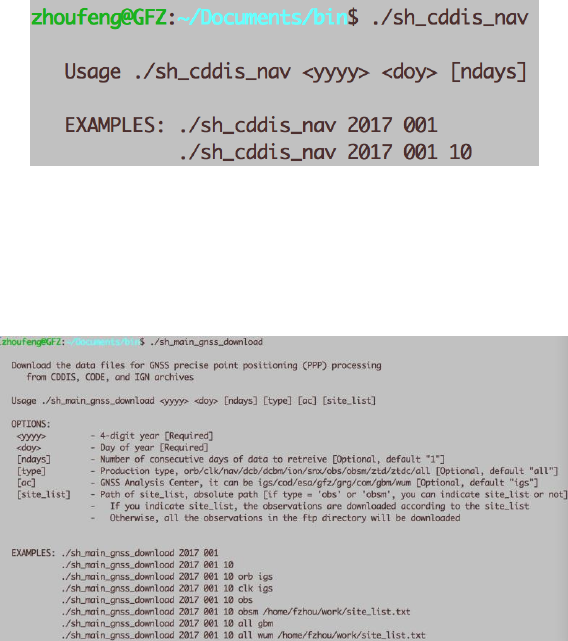
With the data for GNSS PPP processing downloaded, put the observation,
navigation, precise orbit and clock, IGS ANTEX (igs14.atx), IGS SINEX,
configure file (gamp.cfg), ocean tide loading coefficients, DCBs, site
coordinate file (site.crd) into the same directory like
C:\mannual_GAMP\Examples\2017244 as presented in Fig. 4:
5
Fig. 4 The list of data in test example directory
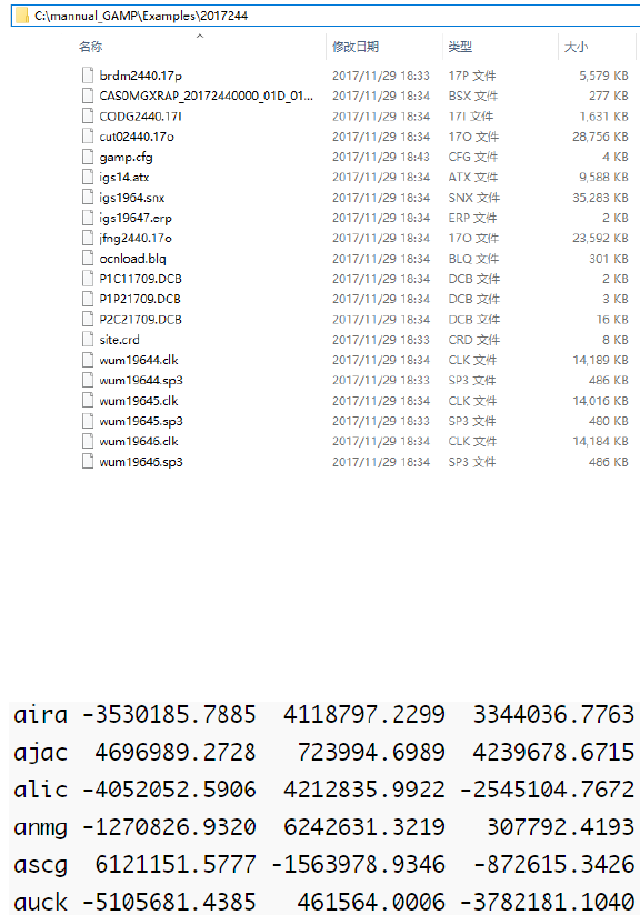
If the precise coordinates for some specific stations are not found in the
SINEX file, then the program will read them from “site.crd” file, of which the
format is shown in Fig. 5 (the element is separated by blank space):
Fig. 5 The list of site coordinates
5.2 Configure file
obs file/folder: The path of observation files. If you choose 0, the absolute file
path of the observation file should be provided. If you choose 1, it means all
the sites/files in one folder are in the waiting line of processing. Thus the
absolute directory path of the experiment should be given.
start_time: The start time of processing. 0 indicates that the start time will be
set at the first epoch of the specific observation file; 1 represents that the start
time is set in the configure file. The option of “end_time” is similar to
“start_time”. If both of them are set to 1, one can modified the time set freely.
Note that “end_time” should be later than “start_time”.
posmode: The position processing mode. In the current version of GAMP,
three modes (i.e. single point positioning (SPP), static PPP and kinematic PPP)
are provided.
6
soltype: Filter processing mode. You can choose forward, backward, or
combined Kalman filter processing mode. 0 = forward, 1 = backward, 2 =
backwards+forwards, 3 = forwards+backwards.
navsys: The selected navigation system. It is a binary setup mode that 1 for
GPS, 4 for GLONASS, 8 for Galileo, 16 for QZSS, and 32 for BDS. It is easy to
set the system combinations, such as 5 for GPS + GLONASS and 33 for GPS
+ BDS.
gnsisb: Different handling schemes of inter-system biases (ISBs) in
multi-GNSS processing. They are modeling ISBs as time constant (option: 1),
as piece-wise constant (option: 2), as random walk process (option: 3), and
white noise process (option: 4).
gloicb: Different handling schemes of GLONASS pseudorange inter-frequency
biases (IFBs). They are neglecting IFBs (option: 0), modeling IFBs as a linear
(option: 1) or quadratic polynomial (option: 2) function of frequency numbers,
estimating IFBs for each GLONASS satellite (option: 3), and estimating IFBs
for each GLONASS frequency number (option: 4).
minelev: Satellite cutoff elevation angles in degrees, the default is 10°.
maxout: To reset phase-bias if expire observation outage counter (epoch
number). The default is 3.
sampleprc: To intercept observations. The default is 0.
inpfrq: The number of selected frequencies. 1 for single-frequency PPP or
dual-frequency ionosphere-free PPP, and 2 for dual-frequency undifferenced
and uncombined PPP.
ionoopt: The option of dealing with ionospheric delays. Correction, elimination,
or estimation as parameters. 0=off, 1-brdc, 2=IF12, 3=UC1, 4=UC12,
5=ion-tec.
ionopnoise: The option of estimation process (white noise or random walk) for
slant ionospheric delay parameters. 0=static, 1=random walk, 2=random walk
(new), 3= white noise.
ionoconstraint: 1 indicates that adds virtual observations for ionospheric
parameters and their corresponding constraints to the observation equations,
while 0 represents not. 0=off, 1=on.
troopt: The option for tropospheric delay estimation. 0=off, 1=saas, 2=sbas,
3=ztd-est, 4=ztdgrad-est.
tropmf: Tropospheric mapping function. The map function of “nmf” (option: 0)
denotes Niell mapping function (NMF), and “gmf” (option: 1) represents global
mapping function (GMF).
tidecorr: The 3D displacement corrections of tidal loading. It is a binary setup
mode that 1 is for solid earth tide, 2 for ocean tide loading, and 4 pole tide.
Furthermore, 7 means the combination of solid earth tide, ocean tide loading,
and pole tide.
cycleslip_GF: This option is for geometry-free (GF) cycle-slip detection. The
first parameter is one switch (0:off, 1:on). The second parameter on this line is
the threshold value in meters for GF cycle-slip detection.
7
cycleslip_MW: This option is for Melbourne-Wübbena (MW) cycle-slip
detection. The first parameter is one switch (0:off, 1:on). The second
parameter on this line is the threshold value in cycles for MW cycle-slip
detection.
errratio(P/L GPS): The measurement error ratio between pseudorange and
carrier phase observations for GPS, default is 100.
errratio(P/L GLO): The measurement error ratio between pseudorange and
carrier phase observations for GLONASS, default is 100.
errratio(P/L BDS): The measurement error ratio between pseudorange and
carrier phase observations for BDS, default is 100.
errratio(P/L GAL): The measurement error ratio between pseudorange and
carrier phase observations for Galileo, default is 100.
errratio(P/L QZS): The measurement error ratio between pseudorange and
carrier phase observations for QZSS, default is 100.
errmeas(L): The precision of carrier phase observations in meters, default is
0.003 m.
prcNoise(AMB): The process noise for ambiguity parameters (unit:
/ms
).
prcNoise(ZTD): The process noise for tropospheric zenith total delay (ZTD)
parameters (unit:
/ms
).
prcNoise(ION): The process noise (the corresponding ionoopt “1”) for slant
ionospheric delay parameters (unit:
/ms
).
prcNoise(ION_GF): The process noise (the corresponding ionoopt “2”) for
slant ionospheric delay parameters (unit:
/ms
).
outdir: The sub-directory for output results is in the current working directory
(e.g., C:\mannual_GAMP\Examples\2017244).
output: The number of output types. The following lines are the output types
(0:off, 1:on):
pos: position results
debug: some processing information, such as cycle-slip, eclipse satellites
etc
pdop: position dilution of precision (PDOP)
elev: satellite elevation angles in degrees
dtrp: tropospheric ZTDs
ifamb: ionospheric-free combined ambiguities
wlamb_no: non-smoothed MW combined ambiguities
wlamb_yes: smoothed MW combined ambiguities
gf: GF combined ambiguities
amb_cs: cycle slip information
resc1: carrier phase residuals at the frequency f1
resp1: pseudorange residuals at the frequency f1
8
resc2: carrier phase residuals at the frequency f2
resp2: pseudorange residuals at the frequency f2
resc3: carrier phase residuals at the frequency f3
resp3: pseudorange residuals at the frequency f3
stec: slant ionospheric delays at the frequency f1
isb: epoch-wise inter-system biases (ISBs) in ns for multi-GNSS
processing
ibm: ISBs in ns every 30 min for multi-GNSS processing
ifb: GLONASS pseudorange inter-frequency biases (IFBs)
ippp: initialized files for PPP post-processing
The details of configure file can refer to the file of “gamp.cfg”.
5.3 Data processing
To run GAMP, the user only needs to specify one input parameter in the
command line: the name of the text file containing the configuration information
of data processing. We will take the processing in Linux for a typical example.
After the compilation of GAMP, one should firstly set the PATH (where the
executable program of GAMP is).
5.3.1 Single-session processing
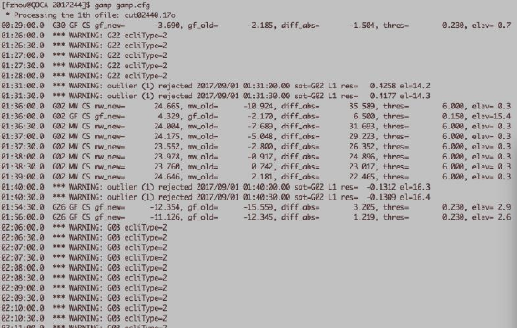
First, enter into the experiment directory, then type the command line “gamp
gamp.cfg”. It works site-by-site in the current directory. For example, the
following plot (Fig. 6) shows it works in the folder 2017244:
e.g., /data1/PROJECT/projects/gamp_exam/2017244
Fig. 6 The screen output of GAMP processing
5.3.2 Multi-session processing
9
The multi-session (or batch) processing is realized by the C shell script
“sh_ppp_1site”, which can copy GNSS files to experiment directory, modify the
configure file, and make a batch processing site-by-site and day-by-day. The
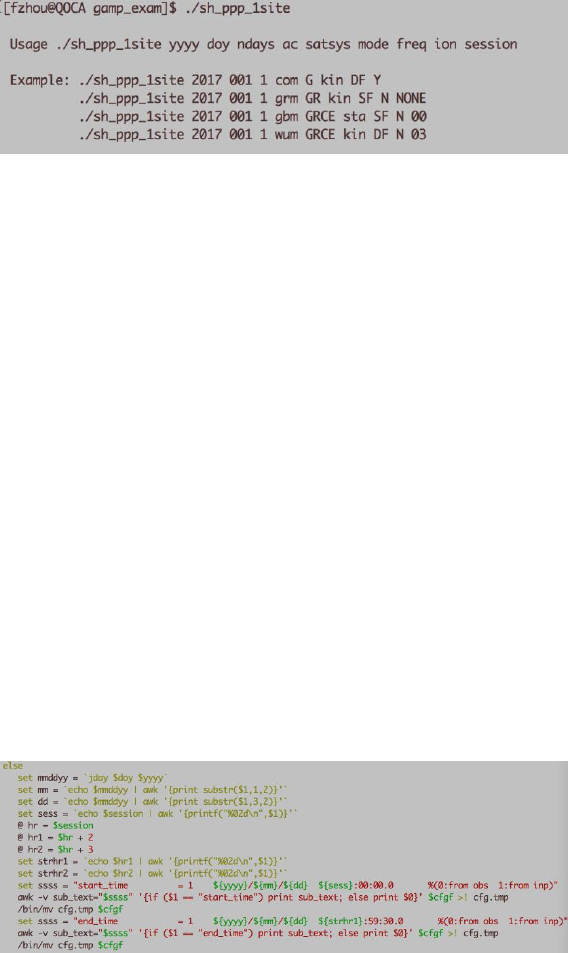
users are suggested to use this convenient and powerful tool. One can type
“sh_ppp_1site” at the terminal to get the help information as shown in Fig. 7.
Fig. 7 The help information of “sh_ppp_1site”
In this script, at least 7 parameters are required, specifically,
yyyy: 4-digit year
doy: day of year (e.g., 001 or 1, 010 or 10)
ndays: number of days to process
ac: the type of products from the corresponding analysis center, i.e., the orbit
and clock products of “gbm” from GFZ.
satsys: the selected satellite system combination
mode: PPP processing mode (sta: static mode, kin: kinematic mode)
freq: the selected frequencies (SF: single-frequency, DF: dual-frequency)
ion: whether to add constraints to ionospheric parameters (Y: yes, N: no). If
yes, the CODE GIM file (i.e. CODG2440.17I) should be used.
session: the processing session length (blank or NONE denotes the whole
session of the specific observation; “00” represents from 00:00:00 to 02:59:30
(default setting is 3-hour interval) and “03” denotes from 03:00:00 to 05:59:30).
You can revise the “sh_ppp_1site” to get the suitable session length for your
data processing as displayed in Fig. 8:
Fig. 8 The session length setting in “sh_ppp_1site”
Note that “sh_ppp_1site” must be run in “csh” environment. Besides this script,
the GAMP package also provides a Python script called “gamp_batch.py”,
which can be run like “sh_ppp_1site”. You can use “gamp_batch.py” for batch
processing under Windows platform (Python 2.7 must be installed on your
computer in advance). To get help information, please type “python
10
gamp_batch.py” or “python gamp_batch.py -h”.
5.4 Results analysis and plotting
A simple but unified format of output files, including positioning results, number
of satellites, satellite elevation angles, pseudorange and carrier phase
residuals, slant Total Electron Content (sTEC), etc. is designed for analysis
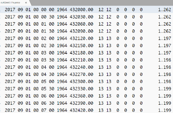
and plotting. Each line of the output files (Fig. 9) starts with 4-digit year, month,
day, hour, minute, second, GPS week, and GPS seconds of week. The other
columns are the corresponding results. Each element is separated by a space,
which is convenient for analysis and plotting with MATLAB or Python.
Fig. 9 The output results of satellite number and PDOP
This is the output file of PDOP for CUT0 station. The 9th, 10th, 11th, 12th, 13th,
14th, and 15th columns are total number of satellites, the number of GPS
satellites, the number of GLONASS satellites, the number of BDS satellite, the
number of Galileo satellites, the number of QZSS satellites, and the PDOP
values, respectively.
A graphical user interface (GUI) of MATLAB called MatPlot (Fig. 10) is
provided for results analysis and plotting. It works in Windows, UNIX/Linux,
and Macintosh. Here, it has been tested under the version of MATLAB R2012a,
R2014a, and R2016b.

11
Fig. 10 The GUI of “MatPlot”
The source code of MatPlot is listed in Fig. 11. The main program is
“GUIPlot.m”. In addition, the executable version of MatPlot called “MatPlot.exe”
is also provided. Before running it, please refer to “MatPlot_Readme.txt” first.
Fig. 11 The list of source code of “MatPlot”
MatPlot selects files by their suffix name. For example, when you pick the
12
“Plot PPP” button, the files with “.pos” as suffix name will be selected. Once
you choose the file(s), the figure(s) will be generated automatically in the
chosen directory. The descriptions of each button and labels are as follows:
Plot PPP: The files of PPP positioning results with “.pos” as suffix name will be
selected. The figures display the PPP positioning errors of east, north, and up
components. The label of “ylim(ppp)” can be used to set Y-axis range. Note
that “ylim(ppp)” sets the maximum value along the axis and the negative of this
value is the minimum along the axis. A value of 10, for example, plots the
Y-axis as -10 to 10. Setting 0 uses a MATLAB default along the Y-axis. It is
recommended to set this value greater than or equal to 0.
Plot SPP: The files of code-based single point positioning (SPP) positioning
results with “.spp” as suffix name will be selected. The label of “ylim(spp)” can
be used to set Y-axis range. The figures display the SPP positioning errors of
east, north, and up components.
Plot PDOP: The files of PDOP values with “.pdop” as suffix name will be
selected. The figures display the number of used satellites and PDOP values.
Plot ZTD: The files of tropospheric zenith total delays (ZTDs) with “.dtrp” as
suffix name will be selected. The label of “ylim(ztd)” can be used to set Y-axis
range. The figures display the tropospheric ZTDs of the selected stations.
Plot sTEC: The files of slant ionospheric delays with “.stec” as suffix name will
be selected. The figures display the satellite slant ionospheric delays.
Plot resx: The files of pseudorange and carrier phase residuals with “.resc*”
and “.resp*” (* is wildcard character) as suffix name will be selected. The
figures display the satellite pseudorange and carrier phase observation
residuals for each frequency, respectively.
Plot wlamb: The files of non-smoothed and smoothed MW ambiguities with
“.wlamb_no” and “. wlamb_yes” as suffix name will be selected.
Analysis: The files of PPP positioning results with “.pos” as suffix name will be
selected. A file “analysis.ana” will be created. It includes the convergence time
for the east, north, and up components and the positioning accuracy after
convergence. The description of this file can refer to "MatPlot_Readme.txt" in
“MatPlot” directory.
Plot Any: By using the ctrl or shift key you can select multiple files and the
program will make the plots of all of the selected files.
To check and view the results quickly, a Perl script named “gnup”, which is
from the GNSS-Inferred Positioning System (GIPSY) software, is provided. It
calls the executable program of gnuplot. For this application to work, Perl
(http://www.perl.org) and gnuplot (http://www.gnuplot.info) are required to be
installed in advance. To get the help information of “gnup”, please type “gnup –
help” at the terminal.
Taking CUT0 on DOY 244, 2017 for a typical example, we can plot the
positioning error (Fig. 12) in east (the 12th column), north (the 13th column),
and up (the 14th column) components derived from the standard GPS-only
single-frequency kinematic PPP. The 8th column is GPS seconds. The Y-axis
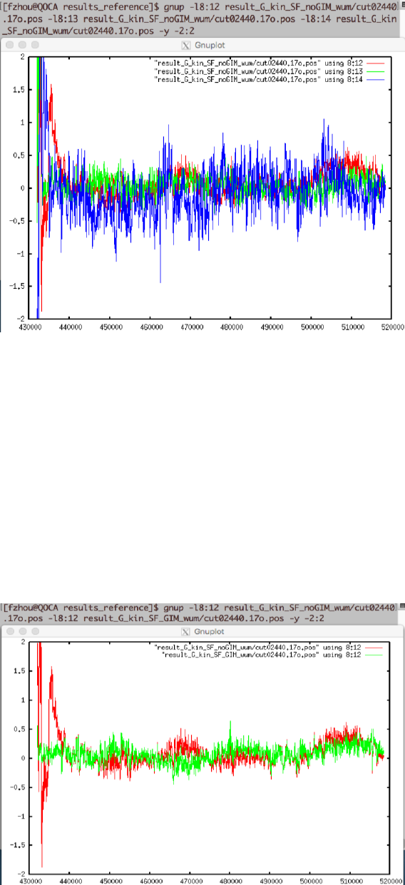
13
range can be limited by setting the parameter “-y” (e.g., -y -2:2). We can also
output the figure by adding “-o” parameter (e.g., -o cut0_2017244.ps).
Fig. 12 The positioning error of GPS-only single-frequency kinematic PPP in east (in red),
north (in green), and up (in blue) components. The X-axis denotes GPS seconds of week,
and the Y-axis denotes positioning errors in meters
Furthermore, the results derived from different methods can also be
plotted in the same figure for comparison. The positioning error in east
component derived from the standard and ionosphere-constrained GPS-only
single-frequency kinematic PPP is plotted in Fig. 13. It is clear that adding
external ionospheric delays as constraint can accelerate the positioning
convergence at CUT0 station, comparing with the standard single-frequency
PPP.
Fig. 13 The positioning error of standard (in red) and ionosphere-constrained (in green)
14
GPS-only single-frequency kinematic PPP in east component. The X-axis denotes GPS
seconds of week, and the Y-axis denotes positioning errors in meters
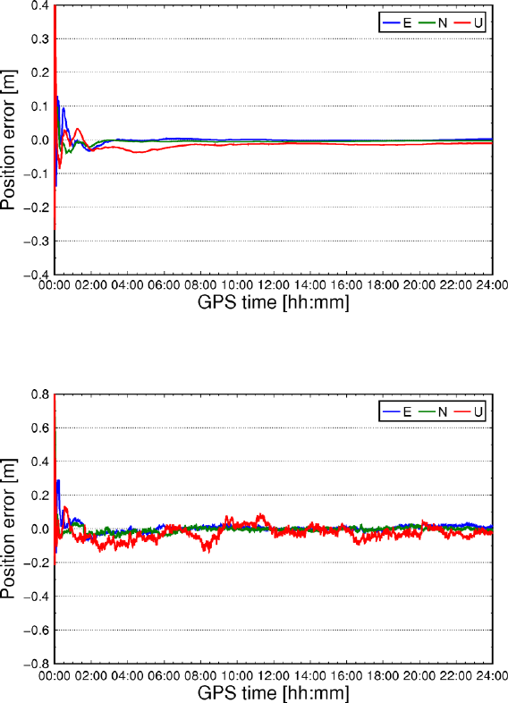
sh_plot_pos: Plot the positioning error (Figs. 14 and 15) in east, north, and up
components.
Fig. 14 The positioning error of GPS-only static PPP in east, north, and up component
Fig. 15 The positioning error of GPS-only kinematic PPP in east, north,
and up component
sh_plot_pdop: Plot number of satellites and PDOP (double y-axis display) in
the processing (Fig. 16).
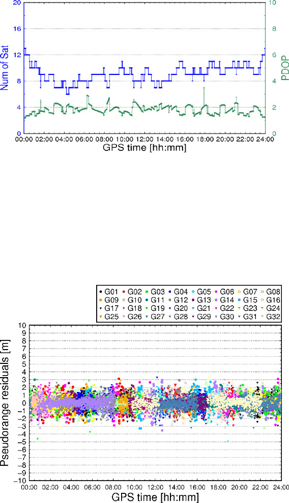
15
Fig. 16 Time series of visible GPS satellite number and PDOP
Since observation residuals contain measurement noises and other
unmodeled errors, they can be used as an important indicator to evaluate the
positioning model.
sh_plot_resp: Plot satellite pseudorange residuals (Figs. 17 and 18). In the
figure, different colors represent different satellites.
Fig. 17 Pseudorange residuals of P1
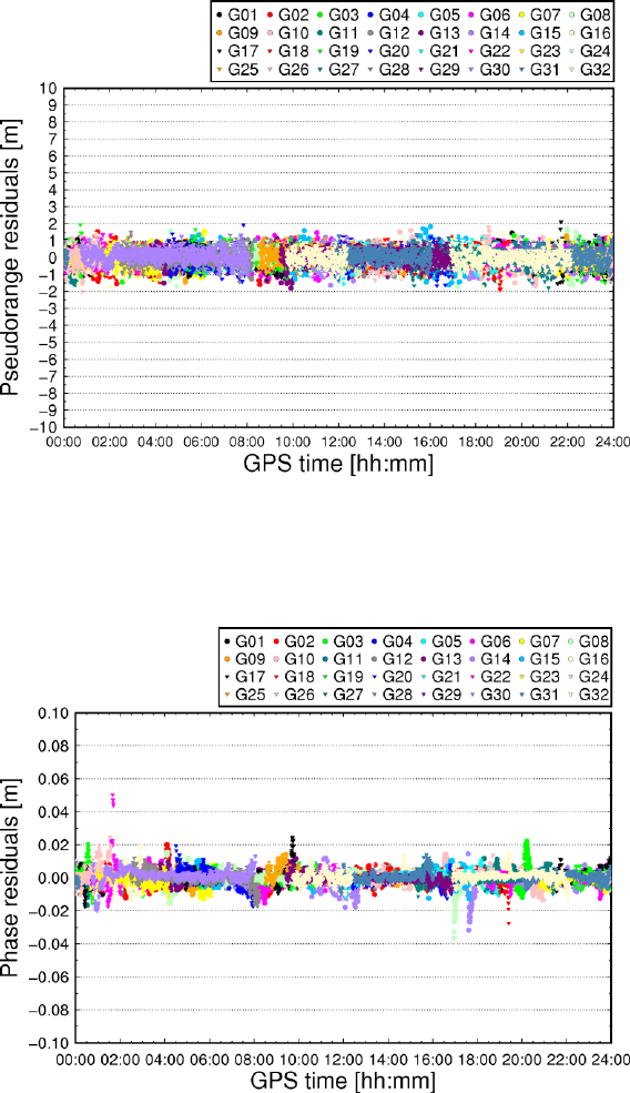
16
Fig. 18 Pseudorange residuals of P2
sh_plot_resc: Plot satellite carrier phase residuals (Figs. 19 and 20).
Fig. 19 Carrier phase residuals of L1
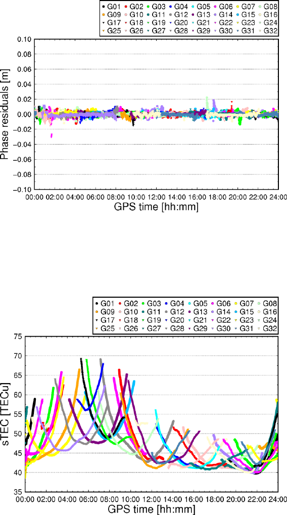
17
Fig. 20 Carrier phase residuals of L2
sh_plot_stec: Plot satellite slant ionospheric delays (“pure” ionospheric delays
+ satellite DCBs + receiver DCBs) as shown in Fig. 21.
Fig. 21 Slant ionospheric delays (“pure” ionospheric delays + satellite DCBs
+ receiver DCBs)
5.5 A new receiver data interchange format – RCVEX
In order to improve processing efficiency, a new GNSS receiver data storage
format has been designed. Following the convention of Receiver Independent
Exchange (RINEX), this exchange format can be referred to as “RCVEX”. The
RCVEX format consists of a header section and a data section. The RCVEX
data format should at least allow for exchanging the following information, to
18
ensure interoperability:
the marker name, the receiver type, and the antenna type
the precise station coordinates (xyz)
the observation sampling interval
the selected observation type for GPS, GLONASS, BDS, Galileo, and QZSS
the tropospheric correction models and mapping functions
the type of satellite orbit and clock products
the satellite elevation cutoff angles
the GLONASS channel numbers
the start and end time of the data
For each satellite, the data section provides:
the PRNs, the indicator of cycle slip and eclipse satellite
the satellite position (xyz) and clock offsets in meters
the azimuth and elevation angles of satellite in degrees
the original pseudorange and carrier phase observations
the tropospheric zenith total delays and the wet mapping function
the Sagnac effect
the tidal deformations, including solid earth tides, pole tides, and ocean tides,
which are mapped into LOS directions
the PCO and PCV corrections at each frequency
the phase windup in cycles
A MATLAB program is provided to read RCVEX files and show how the
parameters and information included could be used by users. An example of
RCVEX file “cut02440.17o.ippp” for CUT0 station on DOY 244, 2017 is
provided.
6 Support
Any suggestions, corrections, and comments about GAMP are sincerely
welcomed and could be sent to:
Feng Zhou
Email: zhouforme@163.com
WeChat: zhouforme0318
Address: Room 411, School of Information Science Technology, East China
Normal University, No. 500 Dongchuan Road, 200241 Shanghai, China
It is recommended to acknowledge GAMP when you find it useful!
19
7 References
Blewitt G (1990) An automatic editing algorithm for GPS data. Geophys Res
Lett 17(3):199–202
Guo F, Zhang X (2014) Real-time clock jump compensation for precise point
positioning. GPS Solut 18(1):41–50
Kouba J (2015) A guide to using international GNSS service (IGS) products,
September 2015 update.
http://kb.igs.org/hc/en-us/articles/201271873-A-Guide-to-Using-the-IGS-Pro
ducts
Takasu T, Yasuda A (2009) Development of the low-cost RTK-GPS receiver
with an open source program package RTKLIB. International symposium on
GPS/GNSS, Seogwipo-si Jungmun-dong, Korea, 4–6 November
Wessel P, Smith WHF, Scharroo R, Luis J, Wobbe F (2013) Generic mapping
tools: improved version released. EOS Trans AGU 94(45):409–410
Zhou F, Gu S, Chen W, Dong D (2017) Comprehensive assessment of
positioning and zenith delay retrieval using GPS + GLONASS precise point
positioning. Acta Geodyn Geomater 14(3):317–326
Zhou F, Dong D, Ge M, Li P, Wickert J, Schuh H (2018) Simultaneous
estimation of GLONASS pseudorange inter-frequency biases in precise
point positioning using undifferenced and uncombined observations. GPS
Solut 22. https://doi.org/10.1007/s10291-017-0685-7
