GCDkit Manual
User Manual:
Open the PDF directly: View PDF ![]() .
.
Page Count: 314 [warning: Documents this large are best viewed by clicking the View PDF Link!]
- .claslist
- about
- accessVar
- Add contours
- addResults
- addResultsIso
- AFM
- ageEps
- Agrawal
- Ague
- appendSingle
- apSaturation
- ArcMapSetup
- assign1col
- assign1symb
- assignColLab
- assignColVar
- assignSymbGroup
- assignSymbLab
- assignSymbLett
- atacazo
- Batchelor
- binary
- binaryBoxplot
- blatna
- Boolean conditions
- bpplot2
- Cabanis
- calc
- calcAnomaly
- calcCore
- Catanorm
- CIPW
- classify
- clr.transform
- cluster
- contourGroups
- coplotByGroup
- coplotTri
- correlationCoefPlot
- Cox
- crosstab
- customScript
- cutMy
- Debon
- deleteSingle
- EarthChem
- Edit labels
- Edit numeric data
- editLabFactor
- elemIso
- epsEps
- Export to Access
- Export to DBF
- Export to Excel
- Export to HTML tables
- F-M-W diagram
- FeMiddlemost
- figAdd
- figaro.identify
- figCol
- figEdit
- figGbo
- figLoad
- figMulti
- figOverplot
- figOverplotDiagram
- figRedraw
- figSave
- figScale
- figUser
- figZoom
- filledContourFig
- Frost
- gcdOptions
- graphicsOff
- groupsByCluster
- groupsByDiagram
- groupsByLabel
- Harris
- Hastie
- Hollocher
- ID
- info
- isochron
- isocon
- Jensen
- joinGroups
- Jung
- Laroche
- LaRocheCalc
- loadData
- Maniar
- mergeData
- Meschede
- Mesonorm
- Middlemost
- millications
- mins2deg
- Misc
- Miyashiro
- Mode
- Molecular weights
- Mullen
- MullerK
- Multiple plots
- mzSaturation
- NaAlK
- Niggli
- OConnor
- overplotDataset
- oxide2oxide
- oxide2ppm
- pairsCorr
- pdfAll
- Pearce and Cann
- Pearce and Norry
- Pearce Nb-Th-Yb
- Pearce Nb-Ti-Yb
- Pearce1982
- Pearce1996
- PearceEtAl
- PearceGranite
- PeceTaylor
- peekDataset
- peterplot
- Plate
- Plate editing
- plateAddReservoirs
- plateLabelSlots
- plotPlate
- plotWithCircles
- pokeDataset
- ppm2oxide
- prComp
- printSamples
- printSingle
- profiler
- psAll
- purgeDatasets
- QAPF
- quitGCDkit
- r2clipboard
- recast
- reciprocalIso
- Regular expressions
- Ross
- rtSaturation
- saveData
- saveResults
- saveResultsIso
- sazava
- Schandl
- selectAll
- selectByDiagram
- selectByLabel
- selectColumnLabel
- selectColumnsLabels
- selectNorm
- selectPalette
- selectSubset
- setCex
- setShutUp
- setTransparency
- Shand
- Shervais
- showColours
- showLegend
- showSymbols
- spider
- spider2norm
- spiderBoxplot
- spiderByGroupFields
- spiderByGroupPatterns
- srnd
- statsByGroup
- statsByGroupPlot
- statsIso
- strip
- stripBoxplot
- Subset by range
- summaryAll
- summaryByGroup
- summarySingle
- summarySingleByGroup
- Sylvester
- TAS
- TASMiddlemost
- ternary
- tetrad
- threeD
- tkSelectVariable
- tk_winDialog
- tk_winDialogString
- trendTicks
- Verma
- Villaseca
- Wedge
- Whalen
- WinFloyd1
- WinFloyd2
- Wood
- YbN vs. LaN/YbN
- zrSaturation
- Index
Package ‘GCDkit’
March 28, 2018
Version 5.0
Date 2018-03-19
Title Geochemical Data Toolkit for Windows
Author Vojtech Janousek <vojtech.janousek@geology.cz>
Colin Farrow <colinfarrow537@gmail.com>
Vojtech Erban <vojtech.erban@geology.cz>
Jean-Francois Moyen <jfmoyen@gmail.com>
Maintainer Vojtech Janousek <vojtech.janousek@geology.cz>
Depends R (>= 3.4.3), stats, methods, utils, graphics, MASS, grid, compiler, lattice, for-
eign, tcltk, RODBC, R2HTML
Suggests XML, rgdal, tkrplot, curl, sp
Description A program for recalculation of geochemical data from igneous
and metamorphic rocks. Runs under Windows Vista/7/8/10, complete functionality/stability un-
der 2000/XP cannot be guaranteed.
License GPL (>= 2)
URL http://www.gcdkit.org
Rtopics documented:
.claslist ........................................... 5
about ............................................ 6
accessVar .......................................... 6
Addcontours ........................................ 7
addResults.......................................... 8
addResultsIso........................................ 9
AFM............................................. 10
ageEps............................................ 11
Agrawal........................................... 13
Ague............................................. 15
appendSingle ........................................ 18
apSaturation......................................... 18
ArcMapSetup........................................ 20
assign1col.......................................... 21
assign1symb......................................... 22
assignColLab ........................................ 23
assignColVar ........................................ 24
1
2Rtopics documented:
assignSymbGroup...................................... 25
assignSymbLab....................................... 26
assignSymbLett....................................... 27
atacazo ........................................... 28
Batchelor .......................................... 29
binary ............................................ 31
binaryBoxplot........................................ 33
blatna ............................................ 34
Booleanconditions ..................................... 35
bpplot2 ........................................... 36
Cabanis ........................................... 37
calc ............................................. 39
calcAnomaly ........................................ 40
calcCore........................................... 42
Catanorm .......................................... 43
CIPW ............................................ 44
classify ........................................... 46
clr.transform......................................... 48
cluster............................................ 50
contourGroups ....................................... 51
coplotByGroup ....................................... 53
coplotTri........................................... 55
correlationCoefPlot..................................... 57
Cox ............................................. 58
crosstab ........................................... 61
customScript ........................................ 62
cutMy............................................ 63
Debon............................................ 64
deleteSingle......................................... 66
EarthChem ......................................... 67
Editlabels.......................................... 69
Editnumericdata...................................... 70
editLabFactor........................................ 70
elemIso ........................................... 71
epsEps............................................ 73
ExporttoAccess ...................................... 74
ExporttoDBF........................................ 75
ExporttoExcel ....................................... 76
ExporttoHTMLtables................................... 77
F-M-Wdiagram....................................... 79
FeMiddlemost........................................ 81
figAdd............................................ 82
figaro.identify........................................ 86
figCol ............................................ 87
figEdit............................................ 88
figGbo............................................ 89
figLoad ........................................... 90
figMulti ........................................... 90
figOverplot ......................................... 93
figOverplotDiagram..................................... 95
figRedraw.......................................... 97
figSave ........................................... 98
Rtopics documented: 3
figScale ........................................... 99
figUser............................................100
figZoom...........................................101
filledContourFig.......................................102
Frost.............................................103
gcdOptions .........................................106
graphicsOff .........................................109
groupsByCluster ......................................109
groupsByDiagram......................................110
groupsByLabel .......................................111
Harris ............................................112
Hastie ............................................113
Hollocher ..........................................115
ID ..............................................118
info .............................................119
isochron...........................................119
isocon............................................121
Jensen............................................124
joinGroups .........................................125
Jung.............................................126
Laroche ...........................................128
LaRocheCalc ........................................131
loadData...........................................132
Maniar............................................136
mergeData..........................................138
Meschede ..........................................139
Mesonorm..........................................140
Middlemost.........................................142
millications .........................................144
mins2deg ..........................................145
Misc.............................................145
Miyashiro..........................................146
Mode ............................................148
Molecularweights .....................................150
Mullen............................................151
MullerK...........................................152
Multipleplots........................................155
mzSaturation ........................................157
NaAlK............................................158
Niggli ............................................160
OConnor ..........................................161
overplotDataset .......................................163
oxide2oxide.........................................165
oxide2ppm .........................................166
pairsCorr ..........................................167
pdfAll............................................169
PearceandCann ......................................170
PearceandNorry ......................................171
PearceNb-Th-Yb......................................173
PearceNb-Ti-Yb ......................................175
Pearce1982 .........................................177
Pearce1996 .........................................178
4Rtopics documented:
PearceEtAl .........................................180
PearceGranite........................................182
PeceTaylor .........................................184
peekDataset.........................................186
peterplot...........................................187
Plate.............................................189
Plateediting.........................................191
plateAddReservoirs.....................................193
plateLabelSlots .......................................195
plotPlate...........................................196
plotWithCircles.......................................197
pokeDataset.........................................199
ppm2oxide .........................................200
prComp ...........................................201
printSamples ........................................202
printSingle..........................................203
profiler............................................204
psAll.............................................207
purgeDatasets........................................207
QAPF ............................................208
quitGCDkit .........................................211
r2clipboard .........................................211
recast ............................................212
reciprocalIso ........................................213
Regularexpressions.....................................214
Ross.............................................216
rtSaturation .........................................218
saveData...........................................220
saveResults .........................................220
saveResultsIso........................................221
sazava............................................222
Schandl ...........................................223
selectAll...........................................225
selectByDiagram ......................................226
selectByLabel........................................227
selectColumnLabel .....................................228
selectColumnsLabels ....................................229
selectNorm .........................................231
selectPalette.........................................233
selectSubset.........................................235
setCex............................................237
setShutUp..........................................238
setTransparency.......................................239
Shand ............................................240
Shervais...........................................242
showColours ........................................243
showLegend.........................................244
showSymbols........................................245
spider ............................................246
spider2norm.........................................251
spiderBoxplot........................................254
spiderByGroupFields....................................256

.claslist 5
spiderByGroupPatterns...................................257
srnd .............................................258
statsByGroup ........................................260
statsByGroupPlot......................................261
statsIso ...........................................261
strip .............................................264
stripBoxplot.........................................265
Subsetbyrange.......................................267
summaryAll.........................................267
summaryByGroup......................................269
summarySingle .......................................270
summarySingleByGroup ..................................272
Sylvester ..........................................273
TAS .............................................274
TASMiddlemost.......................................277
ternary............................................279
tetrad ............................................282
threeD............................................283
tkSelectVariable.......................................285
tk_winDialog ........................................286
tk_winDialogString.....................................286
trendTicks..........................................287
Verma............................................289
Villaseca...........................................291
Wedge............................................293
Whalen ...........................................297
WinFloyd1 .........................................298
WinFloyd2 .........................................300
Wood ............................................302
YbNvs.LaN/YbN .....................................304
zrSaturation.........................................305
Index 307
.claslist List of available classification schemes
Description
The function returns a list of classification diagrams available in the system.
Usage
.claslist()
Value
A matrix with two columns:
menu menu items
function the attached functions

6accessVar
Author(s)
Vojtech Erban, <vojtech.erban@geology.cz>
about About GCDkit
Description
Prints short information about the current version of GCDkit and contact addresses of its authors.
Usage
about()
Arguments
None.
Author(s)
Vojtech Janousek, <vojtech.janousek@geology.cz>
accessVar Accessing data in memory of R
Description
Loads data already present in memory of R into GCDkit.
Usage
accessVar(var=NULL,GUI=FALSE)
Arguments
var a text string specifying the variable to be accessed
GUI logical; is the function called from GUI (or from the command line)?
Details
This function makes possible to access a variable, already present in R, most importantly the sample
data sets. Firstly these need to be made available using the command data.
Value
WR numeric matrix: all numeric data
labels data frame: all at least partly character fields; labels$Symbol contains plotting
symbols and labels$Colour the plotting colours
The function prints a short summary about the attached data. It also loads and executes the Plugins,
i.e. all the R code that is currently stored in the subdirectory ’\Plugin’.

Add contours 7
Author(s)
Vojtech Janousek, <vojtech.janousek@geology.cz>
Examples
data(swiss)
accessVar("swiss")
binary("Catholic","Education")
data(sazava)
accessVar("sazava")
binary("SiO2","Ba")
Add contours Add contours
Description
Superposes contour lines to a Figaro-compatible plot.
Usage
addContours(GUI = FALSE, bandwidth = "auto",...)
Arguments
GUI logical; is the function called from GUI (or in a direct mode)?
bandwidth vector of bandwidths for x and y directions provided to the function kde2d. See
Details.
... additional parameters passed to the underlying function contour. Typically
plotting parameters.
Details
This is, in principle, a front end to the standard R function contour. It will work on both the
stand-alone Figaro-compatible plot or a plate thereof.
The bandwidth should be a positive number or ’auto’, whereby the higher value corresponds to a
smoother result. The necessary calculations are done by the function kde2d.
Value
None.
Author(s)
Vojtech Erban, <vojtech.erban@geology.cz> Vojtech Janousek, <vojtech.janousek@geology.cz>
See Also
’filled.contour’ ’kde2d’ ’par’ ’figaro’

8addResults
Examples
data(sazava)
accessVar("sazava")
plotDiagram("CoxPlut",FALSE,TRUE)
addContours(col="darkblue",lty="dashed",bandwidth=10)
addContours(col="darkgreen",lty="dotted",bandwidth=5)
multiple("SiO2","Al2O3,MgO,CaO,K2O")
plateCex(2)
plateCexLab(1.5)
addContours(col="darkgreen",lty="dashed")
addResults Appending results to data
Description
Appends the most recently calculated results to the data stored in memory.
Usage
addResults(what="results", save=TRUE, overwrite=TRUE, GUI=FALSE)
Arguments
what character; the name of variable to be appended.
save logical; Append to the data matrix ’WR’?
overwrite logical; overwrite any matching items in the matrix ’WR’?
GUI logical; Is the function called within the GUI environment?
Details
This function appends the variable ’results’ (a matrix or vector) returned by most of the calcula-
tion algorithms to a the numeric data stored in the matrix ’WR’.
In case that any items of the same name are already present in the matrix ’WR’, the user is asked
whether they should be overwritten (GUI). In batch mode, they can be ovewritten silently if ’overwrite=TRUE’.
Value
Modifies the matrix ’WR’.
Author(s)
Vojtech Janousek, <vojtech.janousek@geology.cz>

addResultsIso 9
addResultsIso Append Sr-Nd isotopic data
Description
Appends the calculated isotopic parameters stored in the matrix ’init’ to the numeric data already
in the system.
Usage
addResultsIso()
Value
Modifies the numeric data matrix(’WR’) to which it appends the following columns:
Age (Ma) Age in Ma
87Sr/86Sri Initial 87Sr/86Sr ratios
143Nd/144Ndi Initial 143Nd/144N d ratios
EpsNdi Initial (Nd)values
TDM Single-stage depleted-mantle Nd model ages (Liew & Hofmann, 1988)
TDM.Gold Single-stage depleted-mantle Nd model ages (Goldstein et al., 1988)
TDM.2stg Two-stage depleted-mantle Nd model ages (Liew & Hofmann, 1988)
Plugin
SrNd.r
Author(s)
Vojtech Janousek, <vojtech.janousek@geology.cz>
References
Goldstein S L, O’Nions R K & Hamilton P J (1984) A Sm-Nd isotopic study of atmospheric dusts
and particulates from major river systems. Earth Planet Sci Lett 70: 221-236 doi: 10.1016/0012-
821X(84)90007-4
Liew T C & Hofmann A W (1988) Precambrian crustal components, plutonic associations, plate
environment of the Hercynian Fold Belt of Central Europe: indications from a Nd and Sr isotopic
study. Contrib Mineral Petrol 98: 129-138 doi: 10.1007/BF00402106
See Also
’addResults’
10 AFM
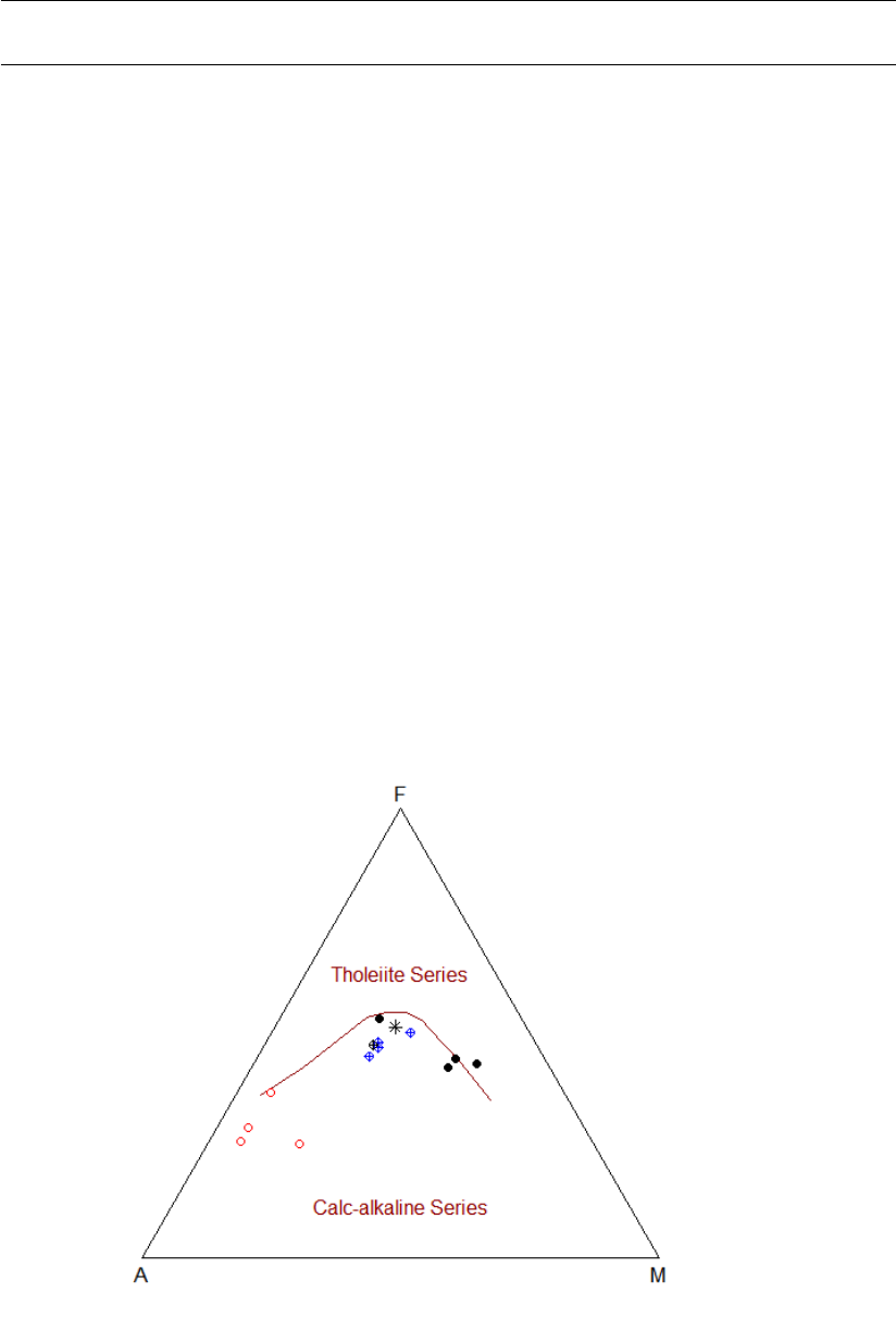
AFM AFM diagram (Irvine + Baragar 1971)
Description
Assigns data for AFM ternary diagram into Figaro template (list ’sheet’) and appropriate values
into ’x.data’ and ’y.data’.
Usage
AFM(equ=FALSE)
Arguments
equ Logical: Should the template use boundary defined by equation?
Details
The AFM diagram is a triangular plot with apices A, F and M defined as follows:
A=(K2O+Na2O) wt. %
F = FeOtot wt. %
M = MgO wt. %
A+F+M=100%
The classification diagram divides data into ’tholeiite series’ and ’calc-alkaline series’ as proposed
by Irvine & Baragar (1971). For extreme values linear extrapolation of boundary curve is employed.

ageEps 11
Value
sheet list with Figaro Style Sheet data
x.data, y.data A, F, M values (see details) transformed into 2D
Author(s)
Vojtech Erban, <vojtech.erban@geology.cz>
& Vojtech Janousek, <vojtech.janousek@geology.cz>
References
Irvine T M & Baragar W R (1971) A guide to the chemical classification of common volcanic rocks.
Canad J Earth Sci 8: 523-548 doi: 10.1139/e71-055
See Also
classify figaro plotDiagram
Examples
#Within GCDkit, AFM is called using following auxiliary functions:
#To Classify data stored in WR (Groups by diagram)
classify("AFM")
#To plot data stored in WR or its subset (menu Classification)
plotDiagram("AFM", FALSE)
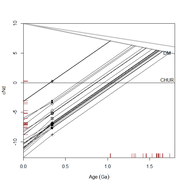
ageEps Plot Sr or Nd growth lines
Description
Plots Nd or Sr growth curves in the binary diagram age-(N d)or age-Sr isotopic ratio.
12 ageEps
Usage
ageEps(GUI=FALSE,...)
ageEps2(GUI=FALSE,...)
ageSr(GUI=FALSE,...)
Arguments
GUI logical; is the function called from the GUI?
... optional parameters to the underlying function {plotWithLimits}
Details
The Nd growth curves in individual samples can be plotted using either a single- or two-stage (Liew
& Hofmann 1988) models.

Agrawal 13
In case of Nd are shown growth curves for the two main mantle reservoirs, CHUR and Depleted
Mantle (DM) (the latter in two modifications, after Goldstein et al. (1988) and Liew & Hofmann
(1988).
For Sr only uniform reservoir (UR) development is calculated using parameters of Faure (1986 and
references therein).
The small ticks, or rugs, on x axis correspond to Nd model ages, on y axis to initial (Nd)values.
This function is Figaro compatible.
Value
None.
Plugin
SrNd.r
Author(s)
Vojtech Janousek, <vojtech.janousek@geology.cz>
References
Faure G (1986) Principles of Isotope Geology. J.Wiley & Sons, Chichester, 589 pp
Goldstein S L, O’Nions R K & Hamilton P J (1984) A Sm-Nd isotopic study of atmospheric dusts
and particulates from major river systems. Earth Planet Sci Lett 70: 221-236 doi: 10.1016/0012-
821X(84)90007-4
Liew T C & Hofmann A W (1988) Precambrian crustal components, plutonic associations, plate
environment of the Hercynian Fold Belt of Central Europe: indications from a Nd and Sr isotopic
study. Contrib Mineral Petrol 98: 129-138 doi: 10.1007/BF00402106
See Also
The actual plotting is done by the function plotWithLimits.
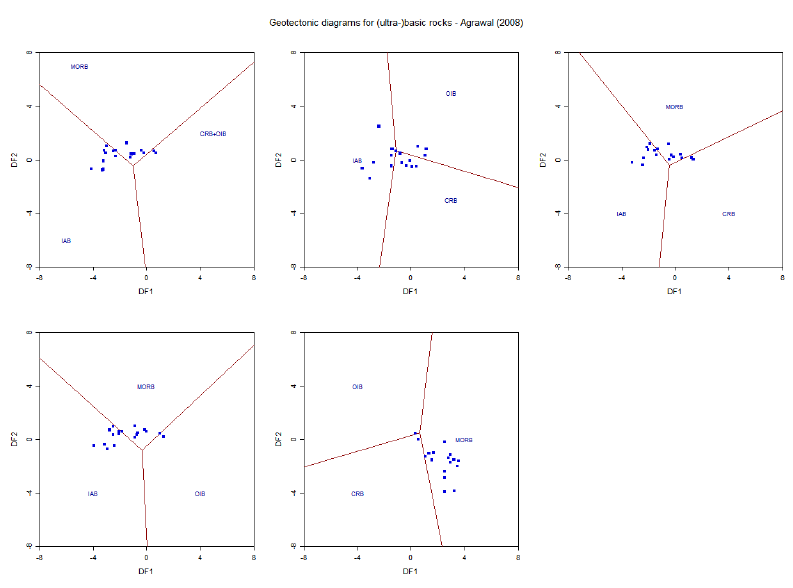
Agrawal Trace-element based discrimination plots for (ultra-)basic rocks
(Agrawal et al. 2008)
Description
Plots data stored in ’WR’ into discrimination plots proposed by Agrawal et al. (2008) for (ultra-)
basic rocks (SiO2< 52 wt. %).
Usage
Agrawal(plot.txt = getOption("gcd.plot.text"),GUI=FALSE)
Arguments
plot.txt logical, annotate fields by their names?
GUI logical, is the function called from a GUI?
14 Agrawal
Details
Suite of five diagrams for discrimination of geotectonic environment of ultrabasic and basic rocks,
proposed by Agrawal et al. (2008). It is based on linear discriminant analysis applied to log-
transformed concentration ratios of five trace elements (La, Sm, Yb, Nb, and Th), i.e., using four
ratios ln(La/T h),ln(Sm/T h),ln(Y b/T h), and ln(N b/T h). The two discriminant functions,
DF1 and DF2, are mathematically designed to maximize the separation between the groups and
account for 100 percent of the variance in the data.
Note that only samples with SiO2< 52 wt. % are plotted.
Also note that each diagram applies only to environments explicitly mentioned. Samples from the
environment not taken into account will be misinterpreted (the CRB + OIB + MORB diagram is not
designed for IAB etc.) See the Agrawal et al (2008) for further details.
Following geotectonic settings may be deduced:
Abbreviation used Environment
IAB island arc basic rocks
CRB continental rift basic rocks
OIB ocean-island basic rocks
MORB mid-ocean ridge basic rocks
Value
None.

Ague 15
Note
This function uses the plates concept. The individual plots can be selected and their proper-
ties/appearance changed as if they were stand alone Figaro-compatible plots.
See Plate,Plate editing and figaro for details.
Author(s)
Vojtech Janousek, <vojtech.janousek@geology.cz>
References
Agrawal S, Guevara M, Verma S (2008) Tectonic discrimination of basic and ultrabasic volcanic
rocks through log-transformed ratios of immobile trace elements. Int Geol Review 50: 1057-1079
doi: 10.2747/0020-6814.50.12.1057
See Also
Verma,Plate,Plate editing,plotPlate,figaro
Examples
#plot the diagrams
plotPlate("Agrawal")
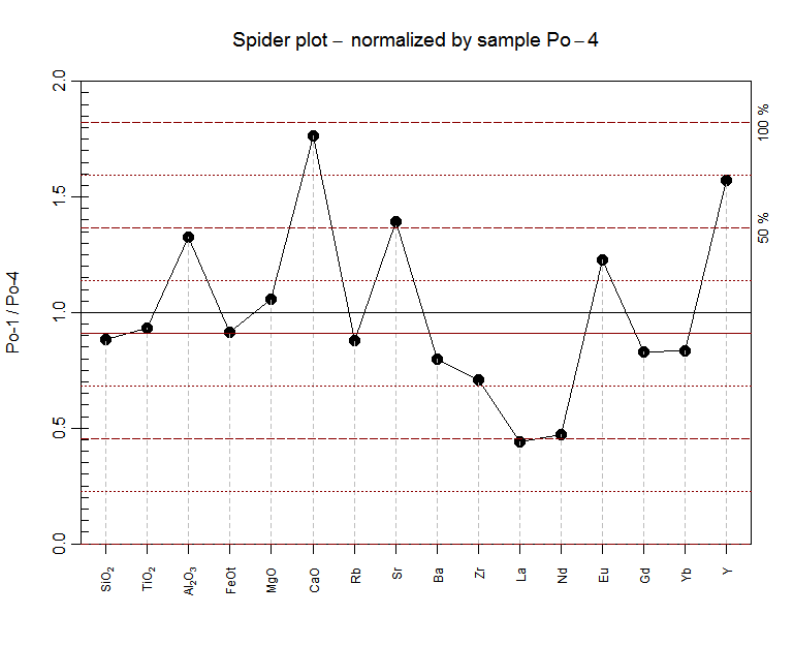
Ague Concentration ratio diagram (Ague 1994)
Description
Implementation of Concentration ratio diagrams after Ague (1994) used for judging the mobility of
elements or oxides in course of various geochemically open-system processes such as alteration or
partial melting.
Usage
Ague(x = NULL,
whichelems = "SiO2,TiO2,Al2O3,FeOt,MnO,MgO,CaO,Na2O,K2O,P2O5",
immobile = NULL, bars = NULL, plot = TRUE)
Arguments
xtwo sample names for analyses of the protolith and altered rock compositions,
respectively.
whichelems list of elements to be plotted.
immobile list of (one or more) elements considered as immobile.
bars optional name of the variable containing 1σerrors for plotting error bars.
plot logical, should be the diagram plotted or just the results calculated?

16 Ague
Details
The Concentration ratio diagram shows concentration ratio of each geochemical species of interest
(element or oxide) in the ’altered rock’ to that in its presumed ’protolith’. These ratios are plotted
on the y-axis, and the elements are arranged in any convenient order along x.
Following an open-system geological process, any of the perfectly immobile constituents ishould
ideally have exactly the same concentration ratio rinv defined as (Ague 2003):
rinv =cA
i
c0
i
where ciis the concentration of the species i,0refers to the ’protolith’ and Ato the ’altered rock’.
This ratio, however, would only exceptionally equate unity, when the mass of the whole system
is conserved. Using the presumably immobile species ias the geochemical reference frame, the
change in the rock mass can be defined as Ague (1994):
∆Mass =c0
i
cA
i−1
Thus rinv >1indicates overall rock mass loss due to removal of mobile constituents; this has the
effect of increasing the concentrations of the immobile species ("residual enrichment"). Conversely,
rinv <1shows an overall rock mass gain ("residual dilution").
The mass change of any mobile constituent jcan be expressed as (Ague 1994):
∆j=1
rinv
cA
j
c0
j−1
Mobile species jthat have cA
j
c0
j
ratios greater than rinv have been added to the system, and those
with ratios lower than rinv have been lost.
In the GCDkit’s implementation of the Concentration ratio diagrams, firstly the parental and altered
rock samples can be chosen interactively from a binary plot M gO −SiO2, if not specified at the
function call. Then the user is prompted for the elements/oxides to be plotted.
If not provided as a comma delimited list among the arguments, the presumably immobile elements
are to be specified. To facilitate this choice, printed and plotted as barplots are ordered ratios of the
elemental concentrations in the ’altered rock’ to that in the ’protolith’ (cA
j
c0
j
)).
Finally the concentration ratio diagram is plotted. If the parameter bars is given, error bars are also
shown corresponding to +/−1σ.
Ague 17
Value
Returns a matrix ’results’ with the following columns:
Altered/Protolith
concentration ratios of the given geochemical species in the ’altered rock’ to that
in the ’protolith’ - primary y axis of the plot
Gain/loss in % relative gains (positive) or losses (negative) corrected for the rock mass change
- secondary y axis of the plot
Plugin
Isocon.r
Author(s)
Vojtech Janousek, <vojtech.janousek@geology.cz>
References
Ague J J (1994) Mass transfer during Barrovian metamorphism of pelites, south-central Con-
necticut; I, Evidence for changes in composition and volume. Amer J Sci 294: 989-1057 doi:
10.2475/ajs.294.8.989
Ague J J (2003) Fluid infiltration and transport of major, minor, and trace elements during regional
metamorphism of carbonate rocks, Wepawaug Schist, Connecticut, USA. Amer J Sci 303: 753-816
doi: 10.2475/ajs.303.9.753

18 apSaturation
Grant J A (1986) The isocon diagram - a simple solution to Gresens equation for metasomatic
alteration. Econ Geol 81: 1976-1982 doi: 10.2113/gsecongeo.81.8.1976
Grant J A (2005) Isocon analysis: a brief review of the method and applications. Phys Chem Earth
(A) 30: 997-1004 doi: 10.1016/j.pce.2004.11.003
Gresens R L (1967) Composition-volume relationships of metasomatism. Chem Geol 2: 47-55 doi:
10.1016/0009-2541(67)90004-6
See Also
Wedge,isocon
Examples
data<-loadData("sazava.data",sep="\t")
Ague(c("Po-4","Po-1"),
"SiO2,TiO2,Al2O3,FeOt,MgO,CaO,Rb,Sr,Ba,Zr,La,Nd,Eu,Gd,Yb,Y",
"TiO2,SiO2,FeOt")
appendSingle Append empty label or variable
Description
Appends an empty numeric data column or a new label to the current data set.
Usage
appendSingle()
Value
Returns the corrected version of the data frame ’labels’ or numeric matrix ’WR’.
Author(s)
Vojtech Janousek, <vojtech.janousek@geology.cz>
apSaturation Apatite saturation
Description
Calculates apatite saturation temperatures for observed whole-rock major-element compositions.
Prints also phosphorus saturation levels for the given major- element compositions and assumed
magma temperature.
Usage
apSaturation(Si = WR[, "SiO2"], ACNK = WR[, "A/CNK"],
P2O5 = WR[, "P2O5"], T = 0)

apSaturation 19
Arguments
Si SiO2contents in the melt (wt. %)
ACNK vector with A/CNK (mol %) values
P2O5 vector with P2O5concentrations
Tassumed magma temperature in °C
Details
* Calculates phosphorus saturation levels following Harrison & Watson (1984):
ln(DP) = 8400 + 26400(SiO2−0.5)
T−3.1−12.4(SiO2−0.5)
P2O5.HW =42
DP
where ’T’ = absolute temperature (K), ’DP’ = distribution coefficient for phosphorus between
apatite and melt and ’SiO2’ is the weight fraction of silica in the melt, SiO2wt. %/100.
These formulae were shown to be valid only for metaluminous rocks, i.e. A/CNK < 1, and were
modified for peraluminous rocks (A/CNK > 1) by Bea et al. (1992):
P2O5.Bea =P2O5.HW e 6429(A/CN K−1)
(T−273.15)
and Pichavant et al. (1992):
P2O5.P V =P2O5.HW + (A/CNK −1)e
−5900
T−3.22SiO2+9.31
Note that the phosphorus saturation concentrations are not returned by the function but printed only.
* Calculates saturation temperatures in °C using the observed P2O5concentrations (Harrison &
Watson, 1984):
T.HW =8400 + 26400(SiO2−0.5)
ln(42
P2O5)+3.1 + 12.4(SiO2−0.5) −273.15
for peraluminous rocks (A/CNK > 1) the equation of Bea et al. (1992) needs to be solved for ’T’
(in K) by iterations:
P2O5.Bea =42
e8400+26400(SiO2−0.5)
T−3.1−12.4(SiO2−0.5) e6429(A/CNK−1)
(T−273.15)
as is that of Pichavant et al. (1992):
P2O5.P V =42
e8400+26400(SiO2−0.5)
T−3.1−12.4(SiO2−0.5) + (A/CNK −1)e
−5900
T−3.22SiO2+9.31
Value
Returns a matrix ’results’ with the following columns:
A/CNK A/CNK values
Tap.sat.C.H+W saturation T of Harrison & Watson (1984) in °C
Tap.sat.C.Bea saturation T of Bea et al. (1992) in °C, peraluminous rocks only
Tap.sat.C.Pich saturation T of Pichavant et al. (1992) in °C, peraluminous rocks only

20 ArcMapSetup
Plugin
Saturation.r
Author(s)
Vojtˇ
ech Janoušek, <vojtech.janousek@geology.cz>
References
Bea F, Fershtater GB & Corretge LG (1992) The geochemistry of phosphorus in granite rocks and
the effects of aluminium. Lithos 29: 43-56 doi: 10.1016/0024-4937(92)90033-U
Harrison TM & Watson EB (1984) The behavior of apatite during crustal anatexis: equilibrium and
kinetic considerations. Geochim Cosmochim Acta 48: 1467-1477 doi: 10.1016/0016-7037(84)90403-
4
Pichavant M, Montel JM & Richard LR (1992) Apatite solubility in peraluminous liquids: exper-
imental data and extension of the Harrison-Watson model. Geochim Cosmochim Acta 56: 3855-
3861 doi: 10.1016/0016-7037(92)90178-L
ArcMapSetup Drawing Arc GIS shapefiles
Description
This function provides a rudimentary support for drawing Arc GIS-compatible shape files (.shp).
Usage
ArcMapSetup(object, layers = NULL, map.col = NULL, map.palette = "heat.colours", labels.txt = FALSE,
col.txt = "black", cex.txt = 0.5, axes = TRUE, longlat = TRUE, xlab = "Longitude", ylab = "Latitude")
Arguments
object name of the object to be drawn, normally GCDmap.
layers names of layers to be drawn.
map.col a vector with colors specified for each of the polygons.
map.palette name of a palette to fill the individual polygons by a random colour.
labels.txt logical; label the individual polygons?
col.txt colour of these textual labels.
cex.txt relative size of these textual labels.
axes logical; should be the axes drawn?
longlat logical; should be long-lat grid added?
xlab label for the x axis.
ylab label for the y axis.
Details
By default, the loadData function of the GCDkit system loads a shape (*.shp) file into a list object
called GCDmap. Each layer represents one item.
If required, the longitude-latitude grid is also drawn using the function llgridlines.

assign1col 21
Value
None. It just modifies properties of a Figaro object (a map).
Author(s)
Vojtech Janousek, <vojtech.janousek@geology.cz>
This code relies heavily on rgdal and sp packages that were written by Roger Bivand, Edzer
Pebesma and their co-workers.
References
None.
See Also
sp readOGR llgridlines loadData assignColVar figaro http://proj.maptools.org.
Examples
# Example of a public-domain World map
shp.file<-"world_country_admin_boundary_shapefile_with_fips_codes.shp"
setwd(earthchem.dir)
loadData(shp.file)
figRedraw()
ArcMapSetup(GCDmap,map.palette="heat.colors",labels.txt=TRUE,col.txt="darkblue",cex.txt=0.8,axes=TRUE,longlat=FALSE)
figRedraw()
#Scaling (not precise clipping, as it needs to preserve the aspect ratio)
figXlim(c(-77,-50))
figYlim(c(0,30))
# Other Figaro functions should be finally working, too
figMain("Caribbean and adjacent South America")
figColMain("darkred")
assign1col Uniform colours
Description
Assigns the same plotting colour to all samples.
Usage
assign1col(col=-1)
Arguments
col numeric; code of the colour.

22 assign1symb
Details
This function sets the same colour to all of the plotting symbols. If ’col’ = -1 (the default), the user
is prompted to specify its code.
Value
Sets ’labels$Colour’ to code of the selected plotting colour.
Author(s)
Vojtech Janousek, <vojtech.janousek@geology.cz>
See Also
To display the current legend use showLegend. Symbols and colours by a single label can be
assigned by assignSymbLab and assignColLab respectively, symbols and colours by groups si-
multaneously by assignSymbGroup. Uniform symbols are obtained by assign1symb. Table of
available plotting symbols is displayed by showSymbols and colours by showColours.
assign1symb Uniform symbols
Description
Assigns the same plotting symbol to all samples.
Usage
assign1symb(pch=-1)
Arguments
pch numeric; code of the plotting symbol.
Details
This function sets the same plotting symbol to all the data points. If ’pch’ = -1 (the default), the
user is prompted to specify its code.
Value
Sets ’labels$Symbol’ to code of the selected plotting symbol.
Author(s)
Vojtech Janousek, <vojtech.janousek@geology.cz>
See Also
To display the current legend use showLegend. Symbols and colours by a single label can be as-
signed by assignSymbLab and assignColLab respectively, symbols and colours by groups simul-
taneously by assignSymbGroup. Uniform colours are obtained by assign1col. Table of available
plotting symbols is displayed by showSymbols and colours by showColours.

assignColLab 23
assignColLab Colours by label
Description
Assigns plotting colours according to the levels of the chosen label or, alternatively, sample names.
Usage
assignColLab(lab = NULL, pal = NULL, colours = NULL, display.legend = FALSE)
Arguments
lab specification of the variable to be used for colours assignment. See Details.
pal character; name of the palette to be used when no colours are specified directly.
Batch mode only.
colours a vector with codes of colours to be assigned. Batch mode only.
display.legend logical; should be the legend displayed? Batch mode only.
Details
If called from in interactive mode (from GUI), the variable (sample names or label) can be selected
using the function ’selectColumnLabel’.
In batch mode, ’lab’ can be an integer (1 for sample names, or a sequence number of the column
in the ’labels’ plus 1). Alternatively, it can contain the full name of a column in ’labels’. See
examples.
If in batch mode, either ’colours’ or ’palette’ have to be specified for the correct colour assign-
ment.
Value
Sets ’leg.col’ to a sequence number of column in ’labels’ that is to be used to build the legend
or -1 if sample numbers are to be used; ’labels$Colour’ contains the codes of the desired plotting
colours.
Author(s)
Vojtech Janousek, <vojtech.janousek@geology.cz>
See Also
To display the current legend use showLegend. Symbols by a single label can be assigned by
assignSymbLab, symbols and colours by groups simultaneously by assignSymbGroup. Uniform
colours and symbols are obtained by assign1symb and assign1col. Table of available plotting
symbols is displayed by showSymbols and colours by showColours.
Selecting a label: selectColumnLabel.
Selecting a palette: selectPalette.

24 assignColVar
Examples
data(sazava)
accessVar("sazava")
assignColLab() # Interactive mode
# Sample names, standard GCDkit colours palette
assignColLab(1,colours=palette.gcdkit,display.legend=TRUE)
# Standard palettes
assignColLab(3,pal="jet.colours",display.legend=TRUE) # Second column in labels
assignColLab("Locality",pal="jet.colours",display.legend=TRUE) # Ditto (here Locality)
# User defined palette
my.palette<-colorRampPalette(c("black", "darkgreen", "red"),space = "rgb")
assignColLab("Locality",pal="my.palette",display.legend=TRUE)
assignColVar Colours by a variable
Description
Assigns plotting colours according to the values of the variable.
Usage
assignColVar(what=NULL,pal="heat.colours",save=TRUE,n=15,quant=0,eq.classes=FALSE,alt.leg=FALSE)
Arguments
what variable name or a formula; if NULL a dialogue is displayed
pal character; name of a palette
save logical;should the newly picked colours be assigned to ’labels’?
ndesired approximate number of colours to be assigned.
quant numeric, 0-50; quantile to be potentially used to get rid of outliers. See details.
eq.classes logical; should classes contain equal number of values?
alt.leg logical; should be the alternative (continuous) legend shown? See Examples.
Details
For selection of the variable is employed the function ’selectColumnLabel’. The user can spec-
ify either existing data column in the ’WR’ or a formula. The colours can be optionally (default
behaviour) assigned globally, so that all the plots will use these from this point on. If not spec-
ified upon function call, the palette is picked using selectPalette. The possible values are:
'grays','reds','blues','greens','cyans','violets','yellows','cm.colors',
'heat.colors','terrain.colors','topo.colors','rainbow'and 'jet.colors'.
Also, user-defined palette functions are supported now. See Examples.
The analyses with no data available for the colours assignment will remain black.

assignSymbGroup 25
If quant differs from the default value of zero, the data are trimmed to an interval (quant, 100-quant)-
th quantile of the dataset and all values out of it plotted in gray.
Setting eq.classes=TRUE allows to have classes with equal number of values (as opposed to equal
intervals). This option is best suited for very skewed datasets (lots of points with similar values,
some outliers).
Value
A list of two components, col and leg. The former are the plotting colours, the latter contains
information needed to build a legend. If save = TRUE, ’labels$Colour’ will acquire the codes of
desired plotting colours.
Author(s)
Vojtech Janousek, <vojtech.janousek@geology.cz>
Jean-Francois Moyen, <jfmoyen@gmail.com>
See Also
quantile Colours by a single variable can be assigned by assignColLab, symbols and colours by
groups simultaneously by assignSymbGroup. Uniform colours are obtained by assign1col. Table
of available plotting colours is obtained by showColours.
Examples
assignColVar("Na2O/K2O","greens")
plotDiagram("PeceTaylor",FALSE,FALSE)
my.palette<-colorRampPalette(c("black", "darkgreen", "red"),space = "rgb")
assignColVar("SiO2","my.palette")
plotDiagram("PeceTaylor",FALSE,FALSE)
assignColVar("SiO2","my.palette",n=7,quant=5)
plotDiagram("PeceTaylor",FALSE,FALSE)
showLegend()
showLegend(alt.leg=TRUE)
assignSymbGroup Symbols/colours by groups
Description
Lets the user to assign plotting symbols and colours according to the levels of the defined groups.
Usage
assignSymbGroup()
Arguments
None.

26 assignSymbLab
Value
Sets ’leg.col’ and ’leg.pch’ to zero, ’labels$Symbol’ contains the codes of desired plotting
symbols, ’labels$Colour’ of plotting colours.
Author(s)
Vojtech Janousek, <vojtech.janousek@geology.cz>
See Also
To display the current legend use showLegend. Symbols by a single label can be assigned by
assignSymbLab, colours using assignColLab. Uniform colours and symbols are obtained by
assign1symb and assign1col. Table of available plotting symbols is displayed by showSymbols
and colours by showColours.
assignSymbLab Symbols by label
Description
Assigns plotting symbols according to the levels of the chosen label or, alternatively, sample names.
Usage
assignSymbLab(lab = NULL, symbols = NULL, display.legend = FALSE)
Arguments
lab specification of the variable to be used for symbols assignment. See Details.
symbols a vector with codes of plotting symbols to be assigned. Batch mode only.
display.legend logical; should be the legend displayed? Batch mode only.
Details
If called from in interactive mode (from GUI), the variable (sample names or label) can be selected
using the function ’selectColumnLabel’.
In batch mode, ’lab’ can be an integer (1 for sample names, or a sequence number of the column
in the ’labels’ plus 1). Alternatively, it can contain the full name of a column in ’labels’. See
examples.
If in batch mode, ’symbols’ have to be specified for the correct plotting symbols assignment.
Value
Sets ’leg.pch’ to a sequence number of column in ’labels’ that is to be used to build the legend
or -1 if sample numbers are to be used; ’labels$Symbol’ contains the codes for desired plotting
symbols.
Author(s)
Vojtech Janousek, <vojtech.janousek@geology.cz>

assignSymbLett 27
See Also
To display the current legend use showLegend.
Using the function assignSymbLett, initial letters of the respective levels of the chosen label can
be assigned to the plotting symbols.
Colours by a single label can be assigned by assignColLab, symbols and colours by groups si-
multaneously by assignSymbGroup. Uniform colours and symbols are obtained by assign1symb
and assign1col. Table of available plotting symbols is displayed by showSymbols and colours by
showColours.
Selecting a label: selectColumnLabel.
Examples
data(sazava)
accessVar("sazava")
assignSymbLab() # Interactive mode
# Sample names, standard GCDkit colours palette
assignSymbLab(1,symbols=1:nrow(WR),display.legend=TRUE)
assignSymbLab(2,symbols=c("+","*","@"),display.legend=TRUE) # First column in labels
assignSymbLab("Intrusion",symbols=c(12,15,17),display.legend=TRUE) # Ditto (here Intrusion)
assignSymbLett Symbols by label - initial letters
Description
Assigns plotting symbols to initial letters of the respective levels of the chosen label.
Usage
assignSymbLett(lab = NULL, display.legend = FALSE)
Arguments
lab specification of the variable to be used for symbols assignment. See Details.
display.legend logical; should be the legend displayed? Batch mode only.
Details
If called from in interactive mode (from GUI), the variable (sample names or label) can be selected
using the function ’selectColumnLabel’.
In batch mode, ’lab’ can be an integer (a sequence number of the column in the ’labels’). Alter-
natively, it can contain the full name of a column in ’labels’. See examples.
Value
Sets ’leg.pch’ to a sequence number of column in ’labels’ that is to be used to build the legend;
’labels$Symbol’ contains the plotting symbols, which correspond to initial letters for the levels of
the specified label.

28 atacazo
Author(s)
Vojtech Janousek, <vojtech.janousek@geology.cz>
See Also
To display the current legend use showLegend. Symbols by a single label can be assigned by
assignSymbLab, colours by assignColLab, symbols and colours by groups simultaneously by
assignSymbGroup. Uniform colours or symbols are achieved by assign1symb and assign1col.
Table of available plotting symbols is displayed by showSymbols and colours by showColours.
Examples
data(sazava)
accessVar("sazava")
assignSymbLett() # Interactive mode
assignSymbLett(2,display.legend=TRUE) # Second column in labels
assignSymbLett("Locality",display.legend=TRUE) # The same (here Locality)
atacazo Whole-rock composition of lavas from the Atacazo and Ninahuilca vol-
canoes, Ecuador
Description
This data set gives the whole-rock major- and trace-element contents, together with Sr and Nd
isotopic compositions of lavas from two volcanic complexes in Ecuador: the Atacazo and the Ni-
nahuilca (Hidalgo, 2006; Hidalgo et al., 2008). This dataset is used in a worked example (chapter
25) of Janousek et al.’s book (2016).
Note that this data set contains information on symbols and colours to be used in GCDkit, as well
as labels (Volcano) that can be used for grouping or similar purposes. It also includes 87Sr/86Sr
and 143Nd/144Nd. Therefore, if the SrNd plugin for GCDkit is installed, these columns will au-
tomatically be recognized as Sr and Nd initial isotopic ratios when loading it into GCDkit (via
accessVar("atacazo"), allowing variables such as TDM to be calculated and isotope-based dia-
grams to be plotted. As no Age column is supplied, the user will be prompted for the emplacement
age; the volcanoes being Quaternary in age (220-71 ka for Atacazo and 71-2 ka for Ninahuilca), the
age correction is insignificant and a small value (of 0.1 for instance) is adequate.
Usage
data(atacazo)
Format
A data frame containing 110 observations of 38 variables.
Source
data by Silvana Hidalgo, <shidalgo@igepn.edu.ec>,
formatted by Jean-François Moyen, <jfmoyen@gmail.com>

Batchelor 29
References
Hidalgo S (2006) Les interactions entre magmas calco-alcalins "classiques" et adakitiques: exem-
ple du complexe volcanique Atacazo- Ninahuilca (Equateur). Unpublished PhD thesis, Université
Blaise-Pascal, Clermont-Ferrand, France
Hidalgo S, Monzier M, Almeida E, Chazot G, Eissen JP, van der Plicht J, Hall M (2008) Late
Pleistocene and Holocene activity of the Atacazo-Ninahuilca Volcanic Complex (Ecuador). J Volc
Geoth Res 176: 16-26 doi: 10.1016/j.jvolgeores.2008.05.017
Janousek V, Moyen JF, Martin H, Erban V, Farrow CM (2016) Geochemical Modelling of Igneous
Processes - Principles and Recipes in the R Language. Springer Verlag, Berlin isbn: 978-3-662-
46792-3
Examples
data(atacazo)
accessVar("atacazo")
binary("SiO2","Ba")
ageEps()
Batchelor Batchelor and Bowden (1985)
Description
Plots data stored in ’WR’ (or its subset) into Batchelor and Bowden’s R1−R2diagram.
Usage
Batchelor(ideal=TRUE)
Arguments
ideal logical, plot ideal minerals composition?
Details
Diagram in R1−R2space, proposed by De la Roche et al. (1980), with fields defined by Batchelor
& Bowden (1985) as characteristic for following geotectonic environments:
Mantle Fractionates
Pre-plate Collision
Post-collision Uplift
Late-orogenic
Anorogenic
Syn-collision
Post-orogenic
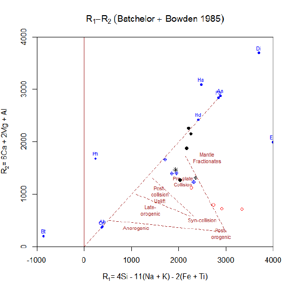
30 Batchelor
Value
sheet list with Figaro Style Sheet data
x.data R1 = 4 * Si - 11 * (Na + K) - 2 * (Fe[total as bivalent] + Ti), all in millications;
as calculated by the function ’LaRoche’
y.data R2 = 6 * Ca + 2 * Mg + Al, all in millications; as calculated by the function
’LaRoche’
Author(s)
Vojtech Janousek, <vojtech.janousek@geology.cz>
References
Batchelor R A & Bowden P (1985) Petrogenetic interpretation of granitoid rock series using multi-
cationic parameters. Chem Geol 48: 43-55. doi: 10.1016/0009-2541(85)90034-8
De La Roche H, Leterrier J, Grandclaude P, & Marchal M (1980) A classification of volcanic and
plutonic rocks using R1R2- diagram and major element analyses - its relationships with current
nomenclature. Chem Geol 29: 183-210. doi: 10.1016/0009-2541(80)90020-0
See Also
LaRoche figaro plotDiagram
Examples
#plot the diagram
plotDiagram("Batchelor", FALSE)

binary 31
binary Binary plot
Description
These functions display data as a binary plot.
Usage
binary(x=NULL,y=NULL,log="",samples=rownames(WR),
new=TRUE, ...)
plotWithLimits(x.data, y.data,
digits.x=NULL, digits.y=NULL,log = "",new = TRUE,
xmin=.round.min.down(x.data,dec.places=digits.x,expand=TRUE),
xmax=.round.max.up(x.data,dec.places=digits.x,expand=TRUE),
ymin=.round.min.down(y.data,dec.places=digits.y,expand=TRUE),
ymax=.round.max.up(y.data,dec.places=digits.y,expand=TRUE),
xlab = "", ylab = "", fousy = "",
IDlabels=getOption("gcd.ident"), fit = FALSE, main = "",
pch = labels[names(x.data), "Symbol"],
col = labels[names(x.data), "Colour"],
cex=labels[names(x.data),"Size"],title=NULL,xaxs="i",yaxs="i",interactive=FALSE)
Arguments
x,y character; specification of the plotting variables (formulae OK).
log a vector '','x','y'or 'xy'specifying which of the axes are to be logarith-
mic
samples character or numeric vector; specification of the samples to be plotted.
new logical; should be opened a new plotting window?
... Further parameters to the function ’plotWithLimits’.
x.data a numerical vector with the x data.
y.data a numerical vector with the y data.
digits.x Precision to which should be rounded the x axis labels.
digits.y Precision to which should be rounded the y axis labels.
xmin, xmax limits of the x axis.
ymin, ymax limits of the y axis.
xlab, ylab labels for the x and y axes, respectively.
fousy numeric vector: if specified, vertical error bars are plotted at each data point.
IDlabels labels that are to be used to identify the individual data points
fit logical, should be the data fitted by a least squares line?
main main title for the plot.
pch plotting symbols.
col plotting colours.
32 binary
cex relative size of the plotting symbols.
title title for the plotting window.
xaxs, yaxs type of the x and y axes.
interactive logical; for internal use by our French colleagues.
Details
The function ’plots.with.limits’ sets up the axes, labels them, plots the data and, if desired,
enables the user to identify the data points interactively.
’binary’ is the user interface to ’plotWithLimits’.
The variables to be plotted are selected using the function ’selectColumnLabel’. In the specifica-
tion of the variables can be used also arithmetic expressions, see calcCore for the correct syntax.
The samples can be selected based on combination of three searching mechanisms (by sample
name/label, range or a Boolean condition) - see selectSubset for details.
The functions are Figaro-compatible.
Value
None.
Author(s)
Vojtech Janousek, <vojtech.janousek@geology.cz>
See Also
plot
Examples
binary("K2O/Na2O","Rb")
binary("Rb/Sr","Ba/Rb",log="xy",samples=1:10,col="red",pch="+",main="My plot")
plotWithLimits(WR[,"SiO2"]/10,WR[,"Na2O"]+WR[,"K2O"],xlab="SiO2/10",
ylab="alkalis")
plotWithLimits(WR[,"Rb"],WR[,"Sr"],xlab="Rb",ylab="Sr",log="xy")
plotWithLimits(WR[,"SiO2"],WR[,"Rb"],fousy=WR[,"Rb"]*0.05,xlab="SiO2",
ylab="Rb",fit=TRUE)
binaryBoxplot 33
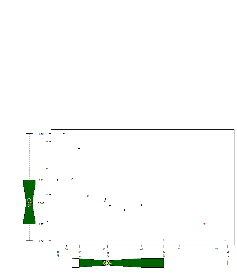
binaryBoxplot Binary boxplot
Description
A binary plot combined with boxplots for both variables.
Usage
binaryBoxplot(xaxis="",yaxis="")
Arguments
xaxis, yaxis specification of the variables. Formulae are OK.
Details
Unless specified in the call, the variables to be plotted are selected using the function ’selectColumnLabel.
In the specification of the variables can be used also arithmetic expressions, see calcCore for the
correct syntax.
The samples can be selected based on combination of three searching mechanisms (by sample
name/label, range or a Boolean condition) - see selectSubset for details.
Value
None.

34 blatna
Warning
This function IS NOT Figaro-compatible.
Author(s)
Vojtech Janousek, <vojtech.janousek@geology.cz>
See Also
plot boxplot
Examples
binaryBoxplot("SiO2/10","Na2O+K2O")
blatna Whole-rock composition of the Blatná suite, Central Bohemian Plu-
tonic Complex
Description
This data set gives the whole-rock major- and trace-element contents in selected samples (monzo-
gabbros, quartz monzonites and granodiorites) of the c. 345 My old high-K calc-alkaline Blatná
suite of the Variscan Central Bohemian Plutonic Complex (Bohemian Massif, Czech Republic).
Usage
data(blatna)
Format
A data frame containing 11 observations.
Source
Vojtech Janousek, <vojtech.janousek@geology.cz>
References
Janousek V, Rogers G, Bowes DR (1995) Sr-Nd isotopic constraints on the petrogenesis of the
Central Bohemian Pluton, Czech Republic. Geol Rundsch 84: 520-534 doi: 10.1007/BF00284518
Janousek V, Bowes DR, Rogers G, Farrow CM, Jelinek E (2000) Modelling diverse processes in the
petrogenesis of a composite batholith: the Central Bohemian Pluton, Central European Hercynides.
J Petrol 41: 511-543 doi: 10.1093/petrology/41.4.511
Janousek V, Wiegand B, Zak J., 2010. Dating the onset of Variscan crustal exhumation in the core
of the Bohemian Massif: new U-Pb single zircon ages from the high-K calc-alkaline granodiorites
of the Blatná suite, Central Bohemian Plutonic Complex. J Geol Soc (London) 167: 347-360 doi:
10.1144/0016-76492009-008

Boolean conditions 35
Examples
data(blatna)
accessVar("blatna")
binary("SiO2","Ba")
Boolean conditions Select subset by Boolean condition
Description
Selecting subsets of the current dataset using Boolean conditions that can query both numeric fields
and labels. Regular expressions can be employed to search the labels.
Details
The menu item ’Select subset by Boolean’, connected to the function selectSubset, enables
the user to query by any combination of the numeric columns and labels in the whole dataset. The
current data will be replaced by its newly chosen subset.
First, the user is prompted to enter a search pattern which can contain conditions that may employ
most of the comparison operators common in R, i.e. < (lower than), > (greater than), <= (lower or
equal to), >= (greater or equal to), = or == (equal to), != (not equal to). The character strings should
be quoted. The conditions can be combined together by logical and, or and brackets.
Logical and can be expressed as .and. .AND. &
Logical or can be expressed as .or. .OR. |
Please note that at the moment no extra spaces can be handled (apart from in quoted character
strings).
Value
Overwrites the data frame ’labels’ and numeric matrix ’WR’ by subset that fulfills the search crite-
ria.
Author(s)
Vojtech Janousek, <vojtech.janousek@geology.cz>
See Also
regular.expressions regex
Examples
## Not run:
# Valid search patterns
Intrusion="Rum"
# Finds all analyses from Rum
Intrusion="Rum".and.SiO2>65
Intrusion="Rum".AND.SiO2>65
Intrusion="Rum"&SiO2>65

36 bpplot2
# All analyses from Rum with silica greater than 65
# (all three expressions are equivalent)
MgO>10&(Locality="Skye"|Locality="Islay")
# All analyses from Skye or Islay with MgO greater than 10
MgO>=10&(Locality!="Skye"&Locality!="Islay")
# All analyses from any locality except Skye and Islay with MgO greater
# or equal to 10
Locality="^S"
# All analyses from any locality whose name starts with capital S
## End(Not run)
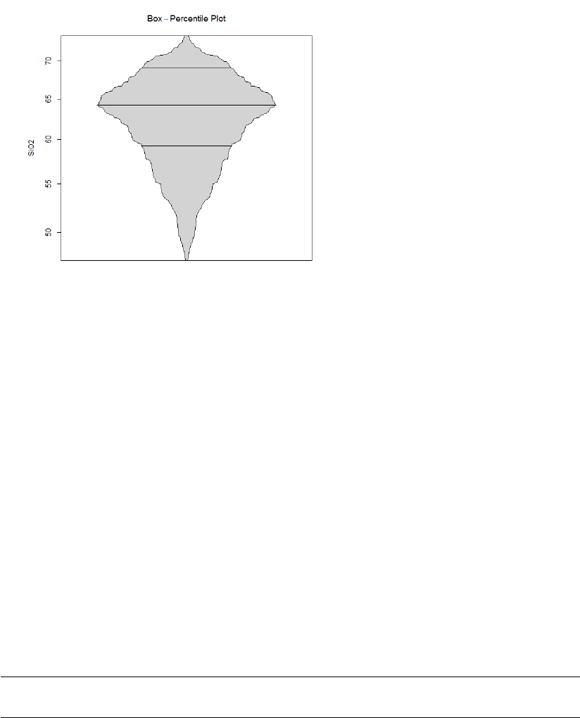
bpplot2 Box-Percentile Plot
Description
Displays statistical distribution each of the variables in a data frame using a box-percentile plot
(Esty & Banfield 2003).
Usage
bpplot2(x,main="Box-Percentile Plot",sub="",xlab = "",
ylab="",log="y",col="lightgray",horizontal=FALSE,ylim = NULL,axes=TRUE,...)
Arguments
xdata frame with the data to be plotted
main main title for the plot
sub sub title for the plot
xlab label for x axis
ylab label for y axis
log which of the axes is to be logarithmic?
col colour to fill the boxes
horizontal logical, should be the orientation horizontal?
ylim optional; limits for the y axis
axes logical; should be the axis drawn?
... additional plotting parameters
Cabanis 37
Details
The box-percentile plot is analogous to a boxplot but the width of the box is variable, mimicking
the distribution of the given variable. As in boxplots, the median and two quartiles are marked by
horizontal lines.
Value
None.
Warning
This function IS NOT Figaro-compatible. It means that the set of diagrams cannot be further edited
in GCDkit (e.g. tools in "Plot editing" menu are inactive).
Author(s)
The code represents a modified function 'bpplot'from the package 'Hmisc'by Frank E Har-
rell Jr. (originally designed by Jeffrey Banfield). Adopted for GCDkit by Vojtech Janousek,
<vojtech.janousek@geology.cz>.
References
Esty, W. W. & Banfield, J. D. (2003). The Box-Percentile Plot. Journal of Statistical Software 8
(17)
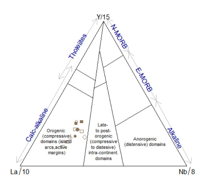
Cabanis Cabanis + Lecolle (1989) La/10-Y/15-Nb/8
Description
Assigns data for a La/10-Y/15-Nb/8 ternary diagram into Figaro template (list ’sheet’) and appro-
priate values into ’x.data’ and ’y.data’.
38 Cabanis
Usage
Cabanis()
Arguments
None.
Details
The ternary plot La/10-Y/15-Nb/8 designed by Cabanis and Lecolle (1989) serves for distinguish-
ing magmas that have originated (1) at orogenic, compressive, destructive plate boundaries (calc-
alkaline, closer to the La apex and tholeiitic, closer to the Y apex); (2) in anorogenic, distensive
inter-plate domains (including NMORB/EMORB and alkaline rocks); and, in between, (3) in either
compressive or distensive, intra-continental, late- to post- orogenic zones. See the original paper
for details.
The diagram can also serve for recognition of magmas contaminated by continental crust or result-
ing from magma mixing.
Value
sheet list with Figaro Style Sheet data
x.data x coordinates
y.data y coordinates
Author(s)
Vojtech Janousek, <vojtech.janousek@geology.cz>

calc 39
References
Cabanis B, Lecolle M (1989) Le diagramme La/10-Y/15-Nb/8: un outil pour la discrimination des
séries volcaniques et la mise en évidence des processus de mélange et/ou de contamination crustale.
CR Acad Sci IIA 309: 2023-2029
Coordinates and graph layout are taken from website of Kurt Hollocher.
See Also
figaro plotDiagram
Examples
plotDiagram("Cabanis",FALSE,TRUE)
calc Calculate a new variable
Description
Calculates a single numeric variable and appends it to the data.
Usage
calc()
Details
The formula can invoke any combination of names of existing numerical columns, with the con-
stants, brackets, arithmetic operators +-*/^ and R functions. See calcCore for a correct syntax.
If the result is a vector of the length corresponding to the number of the samples in the system, the
user is prompted for the name of the new data column. Unless a column with the specified name
already exists or the given name is empty, the newly calculated column is appended to the data in
memory (’WR’).
Value
results numerical vector with the results
Modifies, if appropriate, the numeric matrix ’WR’.
Author(s)
Vojtech Janousek, <vojtech.janousek@geology.cz>
See Also
selectColumnLabel.

40 calcAnomaly
Examples
## Not run:
# examples of valid formulae....
(Na2O+K2O)/CaO
Rb^2
log10(Sr)
mean(SiO2)/10
# ... but this command is in fact a simple R shell -
# meaning lots of fun for power users!
summary(Rb,na.rm=T)
cbind(SiO2/2,TiO2,Na2O+K2O)
cbind(major)
hist(SiO2,col="red")
boxplot(Rb~factor(groups))
# possibilities are endless
plot(Rb,Sr,col="blue",pch="+",xlab="Rb (ppm)",ylab="Sr (ppm)",log="xy")
## End(Not run)
calcAnomaly Anomaly on a spiderplot
Description
Calculates a magnitude of an anomaly on a spiderplot, based on concentrations of selected neigh-
boring elements.
Usage
calcAnomaly(which.elem="Eu",dataset=WR,ref="^REE Boynton",left="Sm",
right="Gd")
Arguments
which.elem character; which element is being examined?
dataset character; name of variable holding the whole-rock data.
ref character; a specification of the normalization scheme.
left character; a name of element to the left, used for extrapolation.
right character; a name of element to the right, used for extrapolation.
Details
This is a general function that calculates a magnitude of an anomaly on a spiderplot. For the given
element it is a ratio of its normalized contents divided by an extrapolated value (denoted by a star).
The extrapolation is performed is from two neighboring elements, one to the left and one to the right,
of the examined one. But these two elements used for extrapolation do not need to be immediately
adjacent.
The best known and the most commonly used is the Eu anomaly on chondrite-normalized REE
plots expressed as:
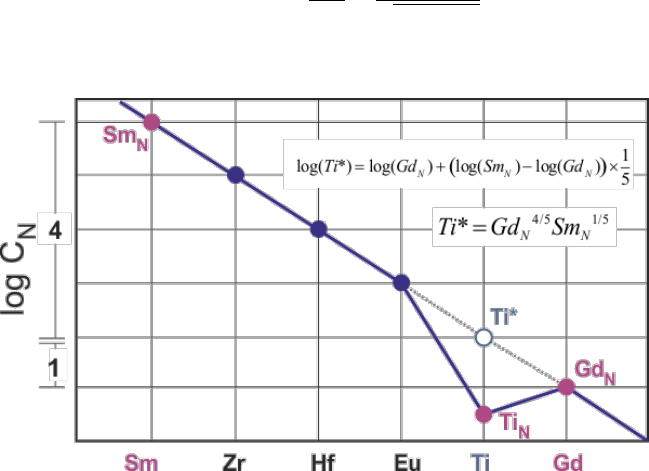
calcAnomaly 41
Eu
Eu∗=EuN
√SmNGdN
But this principle can be generalized even for elements that are not immediately adjacent to the
anomaly, like on its figure:
The spiderplot is selected using the parameter ’ref’ which can contain a substring (or a regular
expression) specifying the name of the normalizing scheme stored in the file ’spider.data’ of the
main GCDkit directory. For details and examples, see selectNorm.
Value
A numeric matrix with a single row, containing the calculated values.
Author(s)
Vojtech Janousek, <vojtech.janousek@geology.cz>
References
Boynton WV (1984) Cosmochemistry of the rare earth elements: meteorite studies. In: Henderson
P (eds) Rare Earth Element Geochemistry. Elsevier, Amsterdam, pp 63-114
Pearce JA (2014) Immobile element fingerprinting of ophiolites. Elements 10: 101-108 doi: 10.2113/gse-
lements.10.2.101
See Also
selectNorm spider
Examples
calcAnomaly() # Eu anomaly on chondrite-normalized REE plot after Boynton (1984).
# Nb anomaly, Nb/Nb*, based on immobile NMORB spiderplot after Pearce (1984)
NbNb<-calcAnomaly(which.elem="Nb",dataset=WR,
ref="^NMORB immobile",left="Th",right="La")
WR<-addOn("Nb/Nb*",as.vector(NbNb),where=WR) # Append to the current data set

42 calcCore
calcCore Calculation of user-defined parameters
Description
Calculates a user-defined parameter specified by the equation.
Usage
calcCore(equation, where = "WR", redo = TRUE)
Arguments
equation a text string to be evaluated.
where which matrix should be used?
redo logical; should be the routine called again and again?
Details
This is a core calculation function.
The expression specified by ’equation’ can involve any combination of names of existing numer-
ical columns in the matrix ’where’, numbers (i.e. constants), arithmetic operators +-*/^ and R
functions.
The most useful of the latter are ’sqrt’ (square root), ’log’ (natural logarithm), ’log10’ (common
logarithm), ’exp’ (exponential function), ’sin’, ’cos’ and ’tan’ (trigonometric functions).
Potentially useful can be also min (minimum), max (maximum), length (number of elements/cases),
’sum’ (sum of the elements), ’mean’ (mean of the elements), and ’prod’ (product of the elements).
However, any user-defined function can be also invoked here.
For most statistical functions, an useful parameter ’na.rm=T’ can be specified. This makes the
function to calculate the result from the available data only, ignoring the not determined value (see
Examples).
The quotation marks in ’equation’ need to preceded by a backslash. Option ’redo’ specifies
whether the routine should be called repeatedly until some meaningful result is obtained. Otherwise
’NA’ is returned.
Value
A list of three items:
equation equation as entered by the user
results numeric vector with the results or NA if none can be calculated
formula the unevaluated expression corresponding to the ’equation’
Author(s)
Vojtech Janousek, <vojtech.janousek@geology.cz>

Catanorm 43
Examples
calcCore("SiO2/10")
calcCore("Na2O+K2O")
calcCore("log10(Na2O+K2O)")
calcCore("SiO2/MW[\"SiO2\"]")
# dividing by the built-in molecularWeight, NB the backslashes
calcCore("length(MgO)")
calcCore("mean(MgO,na.rm=TRUE)")
# na.rm is a safety measure in case some missing values are present
# otherwise the result would be 'NA'
Catanorm Niggli’s Molecular Norm (Catanorm)
Description
Calculates the Niggli’s Molecular Norm (Catanorm) using the algorithm given by Hutchison (1974).
Usage
Catanorm(WR,precision=getOption("gcd.digits"))
Arguments
WR a numerical matrix; the whole-rock data to be normalized.
precision precision of the result.
Details
Normative minerals of the Catanorm
Parameter Full name Formula
Q Quartz SiO2
C Corundum AlO1.5
Or Orthoclase KO0.5.AlO1.5.3SiO2
Plag Plagioclase Abx.An100−x
Ab (Albite) NaO1.5.AlO1.5.3SiO2
An (Anorthite) CaO.2AlO1.5.2SiO2
Lc Leucite KO0.5.AlO1.5.2SiO2
Ne Nepheline NaO0.5.AlO1.5.SiO2
Kp Kaliophilite KO0.5.AlO1.5.SiO2
Ac Acmite NaO0.5.F eO1.5.2SiO2
Ns Sodium metasilicate 2NaO0.5.SiO2
Ks Potassium metasilicate 2KO0.5.SiO2
Hy Hypersthene Enx.F s100−x
Di Diopside W o50.Enx.F s50−x
Wo (Wollastonite) CaO.SiO2

44 CIPW
En (Enstatite) MgO.SiO2
Fs (Ferrosillite) F eO.SiO2
Ol Olivine F ox.F a100−x
Fo (Forsterite) 2MgO.SiO2
Fa (Fayalite) 2F eO.SiO2
Cs Calcium orthosilicate 2CaO.SiO2
Mt Magnetite F eO.2F eO1.5
Hm Hematite F eO1.5
Il Ilmenite F eO.T iO2
Tn Sphene CaO.T iO2.SiO2
Pf Perovskite CaO.T iO2
Ru Rutile T iO2
Ap Apatite 9CaO.6P O2.5.CaF2
or with no F 5CaO.3P O2.5
Fr Fluorite CaF2
Py Pyrite F eS2
Cf Calcite CaO.CO2
Value
A numeric matrix ’results’.
Author(s)
Vojtech Janousek, <vojtech.janousek@geology.cz>
References
Hutchison C S (1974) Laboratory Handbook of Petrographic Techniques. John Wiley & Sons, New
York, p. 1-527
CIPW CIPW norm
Description
Calculates various modifications of the CIPW norm.
Usage
CIPW(wrdata, precision = getOption("gcd.digits"), normsum =
FALSE, cancrinite = FALSE, spinel = FALSE, complete.results = FALSE)
CIPWhb(wrdata, precision = getOption("gcd.digits"), normsum = FALSE,
cancrinite = FALSE, spinel = FALSE, complete.results = FALSE)
CIPW 45
Arguments
wrdata a numerical matrix; the whole-rock data to be normalized.
precision precision of the result.
normsum logical; shall be the normative minerals recast to 100 %?
cancrinite logical; is cancrinite present/to be calculated?
spinel logical; is spinel to be calculated (for ultrabasic rocks, i.e. for samples with
SiO2< 45 % only)?
complete.results
logical; should be returned more extensive list of minerals, including the end
members making up Di, Hy, Ol, Bi and Hbl?
Details
The method adopted for ’classic’ CIPW norm calculation is that of Hutchison (1974, 1975). The
function ’CIPWHB’ is its modification with biotite and hornblende (Hutchison 1975).
Normative minerals of the standard CIPW norm
Parameter Full name Formula Molecular weight
Q Quartz SiO260.08
C Corundum Al2O3101.96
Or Orthoclase K2O.Al2O3.6SiO2556.64
Ab Albite Na2O.Al2O3.6SiO2524.42
An Anorthite CaO.Al2O3.2SiO2278.20
Lc Leucite K2O.Al2O3.4SiO2436.48
Ne Nepheline Na2O.Al2O3.2SiO2284.10
Kp Kaliophilite K2O.Al2O3.2SiO2316.32
Nc Sodium carbonate Na2O.CO2105.99
Ac Acmite Na2O.F e2O3.4SiO2461.99
Ns Sodium metasilicate Na2O.SiO2122.06
Ks Potassium metasilicate K2O.SiO2154.28
Di Diopside
__(MgDi) __(Mg-diopside) CaO.MgO.2SiO2216.55
__(FeDi) __(Fe-diopside) CaO.F eO.2SiO2248.09
Wo Wollastonite CaO.SiO2116.16
Hy Hypersthene
__(En) __(Enstatite) MgO.SiO2100.39
__(Fs) __(Ferrosillite) F eO.SiO2131.93
Ol Olivine
__(Fo) __(Forsterite) 2MgO.SiO2140.70
__(Fa) __(Fayalite) 2F eO.2SiO2203.78
Dcs Dicalcium silicate 2CaO.SiO2172.24
Mt Magnetite F eO.F e2O3231.54
Il Ilmenite F eO.T iO2151.75
Hm Hematite F e2O3159.69
Tn Sphene CaO.T iO2.SiO2196.06
Pf Perovskite CaO.T iO2135.98
Ru Rutile T iO2.SiO279.90
Ap Apatite 3CaO.P2O5.1/3CaF2336.21
Fr Fluorite CaF278.08
Py Pyrite F eS2119.98
Sp Spinel

46 classify
__(MgSp) __(Mg-spinel; spinel s. s.) CaO.MgO.2SiO2142.27
__(FeSp) __(Fe-spinel; hercynite) CaO.F eO.2SiO2173.81
Cc Calcite CaO.CO2100.09
Additional minerals of the modification with hornblende and biotite
Parameter Full name Formula Molecular weight
Bi Biotite
__(MgBi) __(Phlogopite) KO0.5.3MgO.AlO1.5.3SiO2798.50
__(FeBi) __(Annite) KO0.5.3F eO.AlO1.5.3SiO2987.74
Hbl Hornblende
Act Actinolite
__(MgAct) __(Tremolite) 2CaO.5MgO.8SiO2794.35
__(FeAct) __(Ferroactinolite) 2CaO.5F eO.8SiO2952.05
Ed Edenite
__(MgEd) __(Edenite) NaO0.5.2CaO.5MgO.AlO1.5.7SiO21632.48
__(FeEd) __(Ferroedenite) NaO0.5.2CaO.5F eO.AlO1.5.7SiO21947.88
Ri Riebeckite 2NaO0.5.2F eO1.5.3F eO.8SiO2917.87
Value
A numeric matrix ’results’.
Author(s)
Vojtech Janousek, <vojtech.janousek@geology.cz>
References
Hutchison C S (1974) Laboratory Handbook of Petrographic Techniques. John Wiley & Sons, New
York, p. 1-527
Hutchison C S (1975) The norm, its variations, their calculation and relationships. Schweiz Mineral
Petrogr Mitt 55: 243-256
classify Generic Classification Algorithm
Description
Classifies rocks using specified diagram.
Usage
classify(diagram = NULL, grp = TRUE, labs = FALSE,
source.sheet = TRUE, overlap = FALSE, X = x.data,
Y = y.data, silent = FALSE, clas=sheet$d$t, ...)
classify 47
Arguments
diagram name of diagram to be used, see details for more info
grp logical: if TRUE, results are assigned to the variable ’groups’
labs logical: if TRUE, yes/no dialogue for results assignment into the matrix ’labels’
appears
source.sheet logical: if TRUE, the sheet for diagram is newly assigned
overlap logical: if TRUE, possible overlap between polygons of diagram is expected,
and duplicate positive result for one sample is treated as polygon intersection
Xvector of values for abscissa
Yvector of values for ordinate
silent logical: if TRUE, informative outputs are reduced to minimum
clas classification template to be used
... any additional graphical parameters
Details
Function looks for the name of the polygon within the classification diagram, into which falls the
rock analysis represented by the coordinates [x.data,y.data].
In some cases (TAS diagram, Winchester & Floyd’s diagram) additional computations are per-
formed. The argument ’diagram’ may acquire one of following values:
'AFM','PeceTaylor','Shand','TAS','CoxPlut','CoxVolc',
'Jensen','LarochePlut','LarocheVolc','WinFloyd1',
'WinFloyd2','TASMiddlemostPlut','TASMiddlemostVolc',
'DebonPQ','DebonBA','MiddlemostPlut','QAPFPlut',
'QAPFVolc','OConnorPlut','QAPFVolc','OConnorVolc',
'Miyashiro','Hastie','Pearce1996','Villaseca','NaAlK'.
The function is based on the sp package.
Value
Vector of resulting rock names is stored in a variable ’results’. If ’grp = TRUE’ results are also
assigned to the ’groups’ and ’grouping’ is set to -1 (as if called from the menu 'Data handling').
If rock projection falls on the boundary between two or more fields, rock names in question are
merged together with comment ’boundary between ...’.
Author(s)
The sp package was written by Edzer Pebesma, Roger Bivand and others.
Vojtech Erban, <vojtech.erban@geology.cz>

48 clr.transform
See Also
plotDiagram
.claslist
figaro
AFM,PeceTaylor,Shand,NaAlK,TAS,Cox,TASMiddlemost,Jensen,Laroche,WinFloyd1,WinFloyd2,
DebonPQ,DebonBA,Middlemost,QAPF,OConnor Miyashiro Hastie Pearce1996 Villaseca
clr.transform Centered-log-ratio transformation
Description
Implementation of centred-log-ratio (clr) transformation for compositional data.
Usage
clr.trans(comp.data=NULL,GUI=FALSE)
pr.comp.clr(comp.data="SiO2,TiO2,Al2O3,FeOt,MnO,MgO,CaO,Na2O,K2O",cor=TRUE,GUI=FALSE)
Arguments
comp.data a numerical matrix; the data to be normalized. Or just names of variables in the
data matrix ’WR’.
cor logical; should be the correlation matrix used instead of covariance matrix?
GUI logical; is the function called from a menu (GUI)?
Details
Compositional data - i.e., multivariate data in which all the components sum up to some constant
(e.g. 1 or 100, for percentages) - are widespread in the geosciences. A typical example represent
major-element analyses from whole-rock samples.
Numerous workers have argued that much of correlation in such closed datasets is spurious, due to
the so-called constant sum or closure effect (e.g., Chayes 1960; Rock 1988; Rollinson 1992, 1993).
This effect arises from the fact that such components in the compositional datasets cannot vary
independently. If one oxide, for instance SiO2that dominates the whole-rock analyses of many
igneous rocks, increases in abundance, all other oxides must decrease. Therefore, everything must
be anti-correlated with silica.
For their correct statistical treatment, compositional data have to be transformed, or ’opened’. A
classic remedy to the closure effect are log-ratio transformations (Aitchison 1986; Buccianti et al.
eds 2006).
The functions ’clr.trans’ and ’pr.comp.clr’ implement the so-called centred-log-ratio (clr)
transformation. Data opening in this case is done by dividing each value of a variable by the geo-
metric mean of all the variables for that sample and then taking logarithms. It is critical of course
that all the variables are expressed in the same measurement unit.
For instance, for MgO, the centred-log-ratio transformed version is given as:

clr.transform 49
MgO_clr = ln
CMgO
n
sn
Q
i=1
Ci
where ’ln’ is natural logarithm, ’C’ concentration in wt. % of the selected variable (oxide) and
the denominator a geometric mean of all variables being transformed (e.g., Pawlowsky-Glahn &
Egozcue 2006)).
Value
A numeric matrix ’results’. The names of components are preserved, and supplemented by a
suffix ’_clr’.
Plugin
disclosure.r
Author(s)
Vojtˇ
ech Janoušek, <vojtech.janousek@geology.cz>
Vladimír Kusbach, <kusbach@gmail.com>
References
Aitchison J (1986) The Statistical Analysis of Compositional Data. Methuen, New York, pp 1-416
Buccianti A, Mateu-Figueras G, Pawlowsky-Glahn V (eds) (2006) Compositional Data Analysis in
the Geosciences. Geological Society London Special Publications 264: pp 1-212
Chayes F (1960) On correlation between variables of constant sum. J Geophys Res 65: 4185-4193
doi:10.1029/JZ065i012p04185
Pawlowsky-Glahn V, Egozcue JJ (2006) Compositional data and their analysis: an introduction.
In: Buccianti A, Mateu-Figueras G, Pawlowsky-Glahn V (eds) Compositional Data Analysis in the
Geosciences. Geological Society London Special Publications 264: pp 1-10
Reimann C, Filzmoser P, Garrett R, Dutter R (2008) Statistical Data Analysis Explained: Applied
Environmental Statistics with R. John Wiley & Sons, Chichester, pp 1-362
Rock NMS (1988) Numerical geology. A Source Guide, Glossary and Selective Bibliography to
Geological Uses of Computers and Statistics. Lecture Notes in Earth Sciences 18, Springer, Berlin,
pp 1-427
Rollinson HR (1992) Another look at the constant sum problem in geochemistry. Mineral Mag 56:
469-475 doi:10.1180/minmag.1992.056.385.03
Rollinson HR (1993) Using Geochemical Data: Evaluation, Presentation, Interpretation. Longman,
London, pp 1-352
van den Boogaart KG, Tolosana-Delgado R (2008) "compositions": a unified R package to analyze
compositional data. Comput Geosci 34: 320-338 doi:10.1016/j.cageo.2006.11.017
van den Boogaart KG, Tolosana-Delgado R (2013) Analyzing Compositional Data with R. Springer,
Berlin, pp 1-258

50 cluster
See Also
prComp
See Reimann et al. (2008) with van den Boogaart and Tolosana-Delgado (2013) for further details
and van den Boogaart and Tolosana-Delgado (2008) for implementation of a comprehensive R
library dealing with compositional data.
Examples
data(sazava)
accessVar("sazava")
ox<-c("SiO2","Al2O3","FeOt","MgO","CaO")
clr.trans(ox)
addResults() # Needed to append the clr-transformed data to the matrix 'WR'
multiple(x = "SiO2_clr", y = "Al2O3_clr,FeOt_clr,MgO_clr,CaO_clr")
plateCex(2)
plateCexLab(1.3)
pr.comp.clr(ox)
cluster Statistics: Hierarchical clustering
Description
Hierarchical cluster analysis on a set of dissimilarities.
Usage
cluster(elems = "SiO2,TiO2,Al2O3,FeOt,MnO,MgO,CaO,Na2O,K2O",
method = "average")
Arguments
elems numerical columns to be used for cluster analysis, typically major elements
method the agglomeration method to be employed. This should be one of (or an unam-
biguous abbreviation thereof): 'ward','single','complete',
'average','mcquitty','median','centroid'.
Details
The samples can be selected based on combination of three searching mechanisms (by sample
name/label, range or a Boolean condition) - see selectSamples for details.
Even though a list of major elements is assumed as a default, different variables can be specified by
the function ’selectColumnsLabels’.
The user is also asked to specify a label for the individual samples, default are their names.
After the dendrogram is drawn, the individual clusters can be identified. For each sample falling
into the given group, specified information (e.g. Locality, Rock Type and/or Author) can be printed.
For further details on the clustering algorithm, see the R manual entry of ’hclust’.

contourGroups 51
Value
None.
Warning
Names of existing numeric data columns and not formulae involving these can be handled at this
stage. Only complete cases are used for the cluster analysis.
Author(s)
Vojtech Janousek, <vojtech.janousek@geology.cz>
See Also
’hclust’
contourGroups Outline individual groups in a binary plot
Description
The functions outline the individual clusters of data (groups by default) on a binary plot. Imple-
mented methods are the convex hull or contours. This can be useful for a quick appreciation of the
data distribution, e.g. in classification diagrams.
Usage
contourGroups(clusters=groups,border=NULL,fill=FALSE,precision=50, ...)
chullGroups(clusters=groups,border=NULL,fill=FALSE,...)
Arguments
clusters grouping information for each of the samples.
border outline colours.
fill logical; should be the polygons filled by the border colour?
precision a number indicating how tight the contours should be.
... additional parameters to the functions contour and polygon, respectively.
Details
If not specified, the colours are selected as the most frequently occurring one defined among samples
within each group.
For the function contourGroups, the shape of the contours drawn can be controlled using the pa-
rameter (precision). The higher it is, the smoother contours result.
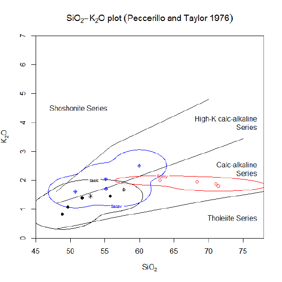
52 contourGroups
Value
None.
Author(s)
Vojtech Janousek, <vojtech.janousek@geology.cz>
See Also
chull,contour,polygon
Examples
data<-loadData("sazava.data",sep="\t")
groupsByLabel("Intrusion")
plotDiagram("PeceTaylor",FALSE,FALSE)
chullGroups()
chullGroups(fill=TRUE)
plotDiagram("PeceTaylor",FALSE,FALSE)
contourGroups()

coplotByGroup 53
coplotByGroup Coplot by groups
Description
Plots a series of binary plots, for each of the groups separately.
Usage
coplotByGroup(xaxis = "",yaxis = "",show.leg = "")
Arguments
xaxis Name of the data column to be used as x axis.
yaxis Name of the data column to be used as y axis.
show.leg Logical: are the levels of the conditioning variable (’groups’) to be shown?
Details
For examination of large datasets split into user-defined subsets serves in R function coplot. It
produces a set of binary diagrams with the data filtered out according to the values of the third
(conditioning) variable. In case of the function ’coplotByGroup’ it is done by groups.
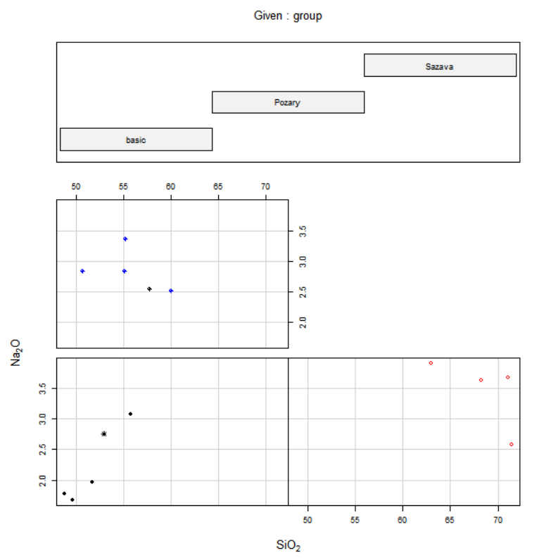
54 coplotByGroup
If no parameters 'xlab','ylab'and ’show.leg’ are given, the user is prompted to specify them.
The variables to be plotted are selected using the function ’selectColumnLabel.
See manual entry for ’coplot’ for further details.
Value
None.
Warning
Please note that no formulae can be handled at this stage.
This function IS NOT Figaro-compatible.
Author(s)
Vojtech Janousek, <vojtech.janousek@geology.cz> & Vojtech Erban, <vojtech.erban@geology.cz>

coplotTri 55
See Also
’coplot’
Examples
coplotByGroup("SiO2","Na2O",show.leg=TRUE)
coplotTri Coplot for three variables
Description
Plots a series of binary plots split into several groups according to the values of the third, so called
conditioning, variable.
Usage
coplotTri(xaxis = "", yaxis = "", zaxis = "", int = "")
Arguments
xaxis Name of the data column to be used as x axis.
yaxis Name of the data column to be used as y axis.
zaxis Name of the data column with the conditioning variable.
int The specification of the intervals: either ’auto’ or a list of break points separated
by commas.
Details
For examination of large datasets split into user-defined subsets serves in R the function ’coplot’.
It displays a series of binary diagrams with the data filtered out according to the values of the third
(conditioning) variable.
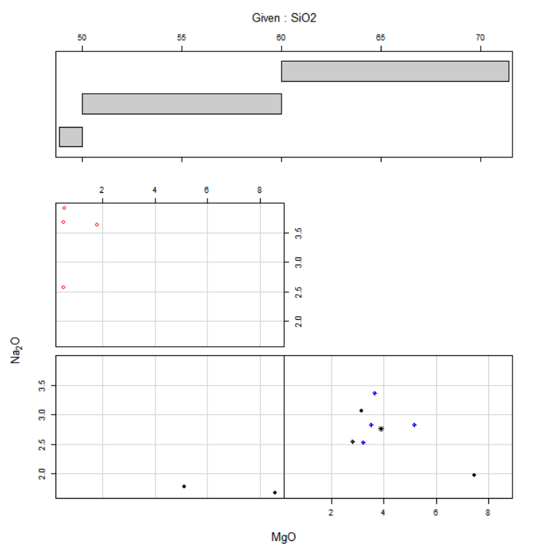
56 coplotTri
If no parameters 'xlab','ylab'and 'zlab'are given, the user is prompted to specify them.
The variables to be plotted are selected using the function ’selectColumnLabel.
After this is done, the user is prompted to enter a comma-delimited list of at least one break point
defining the intervals. The default includes the mean, that will be automatically supplemented by
minimum and maximum (i.e. two intervals).
See manual entry for ’coplot’ for further details.
Value
None.
Warning
Please note that no formulae can be handled at this stage.
This function IS NOT Figaro-compatible.
Author(s)
Vojtech Janousek, <vojtech.janousek@geology.cz> & Vojtech Erban, <vojtech.erban@geology.cz>

correlationCoefPlot 57
See Also
’coplot’
Examples
coplotTri("SiO2","Na2O","MgO","auto")
coplotTri("MgO","Na2O","SiO2","50,60")
# the intervals of the conditioning variable, SiO2,
# will be (min(SiO2) - 50),(50 - 60) and (60 - max(SiO2))
correlationCoefPlot Statistics: Correlation coefficient patterns
Description
Produces, for each group a separate, set of plots of correlation coefficient patterns.
Usage
correlationCoefPlot(elems = NULL)
Arguments
elems list of desired elements
Details
The utility of correlation coefficient patterns was discussed by Rollinson (1993 and references
therein). Basically similarity in correlation patterns between two or more elements means their
analogous geochemical behaviour, potentially controlled by the same geochemical process (frac-
tional crystallization, partial melting, weathering, hydrothermal alteration...)
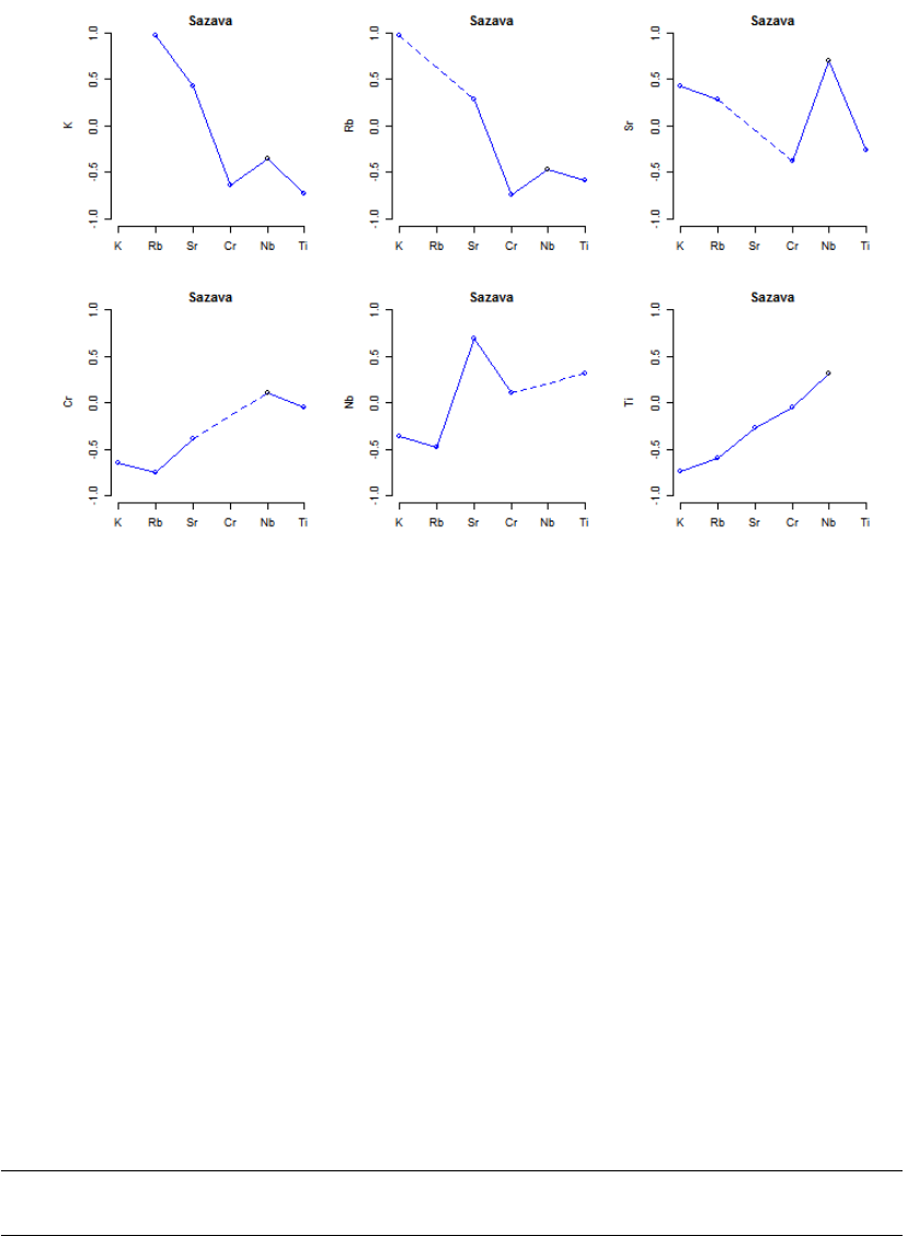
58 Cox
The variables are selected using the function ’selectColumnsLabels’.
Value
None.
Author(s)
Vojtech Janousek, <vojtech.janousek@geology.cz>
References
Rollinson H R (1993) Using Geochemical Data: Evaluation, Presentation, Interpretation. Longman,
London, p. 1-352
Examples
correlationCoefPlot(elems="K,Rb,Sr,Cr,Nb,Ti")
Cox TAS diagram (Cox et al. 1979)
Description
Assigns data for Cox’s diagram into Figaro template (list ’sheet’) and appropriate values into
’x.data’ and ’y.data’.
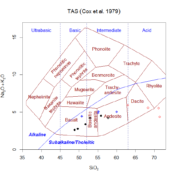
Cox 59
Usage
CoxVolc(alkline=TRUE)
CoxPlut(alkline=TRUE)
Arguments
alkline Logical: Should the boundary between alkaline and subalkaline rocks (Irvine &
Baragar 1971) be drawn?
Details
TAS diagram, as proposed by Cox et al. (1979) for volcanic rocks and adapted by Wilson (1989)
for plutonic rocks.
For volcanic rocks, the following diagram is plotted:
And the version for plutonic rocks contains the following fields:
volcanic rocks plutonic rocks
basalt gabbro
basaltic andesite undefined
andesite diorite
dacite quartz diorite (granodiorite)
rhyolite alkali granite/granite
hawaiite gabbro
trachyandesite undefined
basanite/tephrite undefined
mugearite syeno-diorite
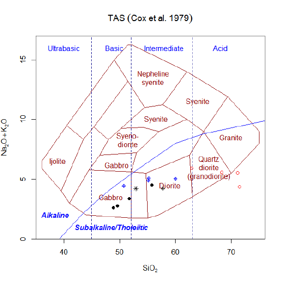
60 Cox
benmorite syenite
trachyte syenite
nephelinite ijolite
phonology nephelinite undefined
phonolitic tephrite undefined
phonolite nepheline syenite
Value
sheet list with Figaro Style Sheet data
x.data SiO2 weight percent
y.data Na2O+K2O weight percent
Author(s)
Vojtech Erban, <vojtech.erban@geology.cz>
& Vojtech Janousek, <vojtech.janousek@geology.cz>
References
Cox K G, Bell J D & Pankhurst (1979) The Interpretation of Igneous Rocks. Allen & Unwin,
London
Wilson M (1989) Igneous Petrogenesis. Chapman & Hall, London
Irvine T M & Baragar W R (1971) A guide to the chemical classification of common volcanic rocks.
Canad J Earth Sci 8: 523-548 doi: 10.1139/e71-055

crosstab 61
See Also
classify figaro plotDiagram
Examples
#TAS diagram is called using following auxiliary functions:
#Classifies data stored in WR (Groups by diagram)
classify("CoxVolc")
#or
classify("CoxPlut")
#Plots data stored in WR or its subset (menu Classification)
plotDiagram("CoxVolc", FALSE)
#or
plotDiagram("CoxPlut", FALSE)
crosstab Cross table of labels
Description
Prints a cross table (contingency table) for 1-3 labels.
Usage
crosstab(plot = TRUE)
Arguments
plot logical; should be also a barplot plotted?
Details
This command prints a frequency distribution (for a single label) or a contingency table (for 2-3
labels) useful for inspection of the data structure. Optionally a barplot is plotted (for 1-2 labels).
Just press Enter (enter an empty field), when the desired number of variables is reached.
Value
results the frequency/contingency table
Author(s)
Vojtech Janousek, <vojtech.janousek@geology.cz>

62 customScript
customScript Add a new variable to a script
Description
Adds a formula to calculate a single numeric variable to the specified *.r file (a R script).
Usage
customScript()
Details
A formula can be entered that can involve any combination of names of existing numerical columns,
with the constants, brackets, arithmetic operators +-*/^ and R functions. See calcCore for a correct
syntax.
Then the user is prompted for the name of the variable an any comments that should appear in the
file.
The filename is chosen interactively, the default suffix for the R programs is .r. If the file exists
already, the script is appended to its end.
If desired, the calculated variable can be, after the script is executed, added automatically to the
numeric data, i.e. the numeric matrix WR. If not, the contents of the calculated variable can be
viewed by simply typing its name in the R Console window.
The script can be run at a later time using the R command File|Source. Alternatively, it can be
placed among the so-called plugins into the subdirectory Plugin. All files placed here with a suffix
*.r are executed each time when the new data file is being loaded into the GCDkit.
Value
None.
Author(s)
Vojtech Janousek, <vojtech.janousek@geology.cz>
Examples
## Not run:
# examples of valid formulae....
(Na2O+K2O)/CaO
Rb^2
log10(Sr)
mean(SiO2)/10
# ... but this command is in fact a simple R shell -
# meaning lots of fun for power users!
summary(Rb,na.rm=T)
cbind(SiO2/2,TiO2,Na2O+K2O)
cbind(major)
hist(SiO2,col="red")
boxplot(Rb~factor(groups))

cutMy 63
# possibilities are endless
plot(Rb,Sr,col="blue",pch="+",xlab="Rb (ppm)",ylab="Sr (ppm)",log="xy")
## End(Not run)
cutMy Groups by numerical variable
Description
Grouping the data according to the interval of a single numerical variable it falls into.
Usage
cutMy(where=NULL,int=NULL,int.lab=NULL,na.lab="Unclassified")
Arguments
where Numeric data column in ’WR’ - the basis of the classification.
int Boundaries of intervals.
int.lab Labels for the intervals
na.lab Labels for samples that cannot be classified
Details
The numeric data column is selected using the function ’selectColumnLabel’.
After this is done, the user is prompted to enter a comma-delimited list or at least one break point
defining the intervals. The default includes the mean, that will be automatically supplemented by
minimum and maximum (i.e. two intervals).
Then the names of the individual groups are to be specified; values out of range are automatically
labeled as 'Unclassified'. The vector containing the information on the current groups can be
appended to the data frame ’labels’.
Value
groups character vector: the grouping information
grouping If the new column was appended the data frame labels, sequence number of
this column; if not appended, though, this variable is set to -100.
Author(s)
Vojtech Janousek, <vojtech.janousek@geology.cz>
See Also
cut
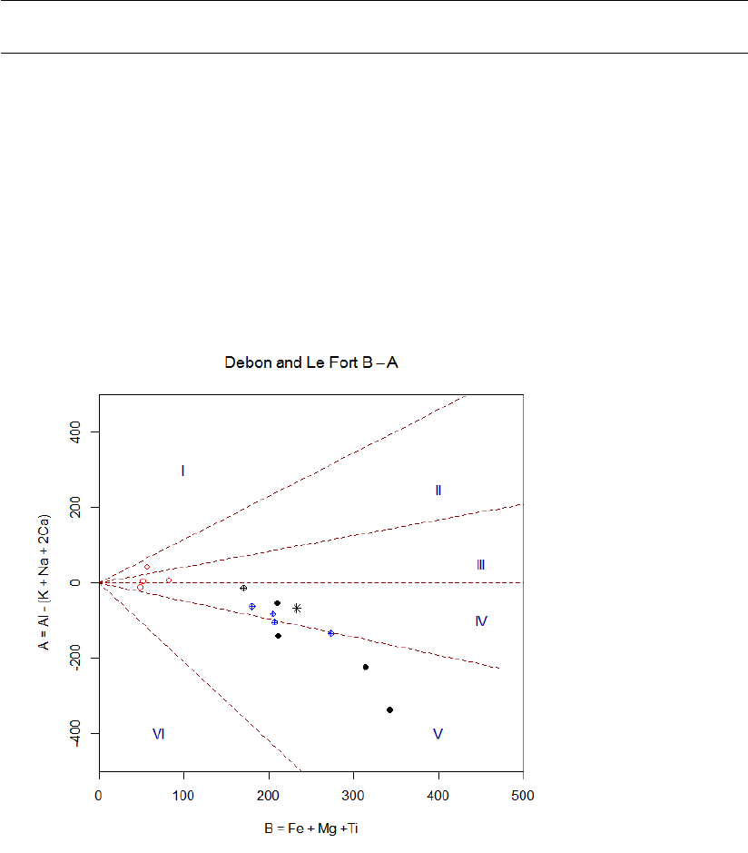
64 Debon
Debon BA and PQ diagrams (Debon + Le Fort 1983)
Description
Assigns data for Debon & Le Fort’s B-A and P-Q diagrams into Figaro template (list ’sheet’) and
appropriate values into ’x.data’ and ’y.data’.
Usage
DebonBA()
DebonPQ()
Details
The B-A diagram as proposed by Debon and Le Fort (1983) defines six sectors (I - VI), reflecting
alumina balance of samples. Following minerals are characteristic for individual sectors:
I Peraluminous domain muscovite > biotite
II biotite > muscovite
III biotite (+- minor amphibole)
IV Metaluminous domain biotite, amphibole, +- pyroxene
Vclinopyroxene, +- amphibole, +-biotite
VI unusual mineral associations (carbonatites ...)
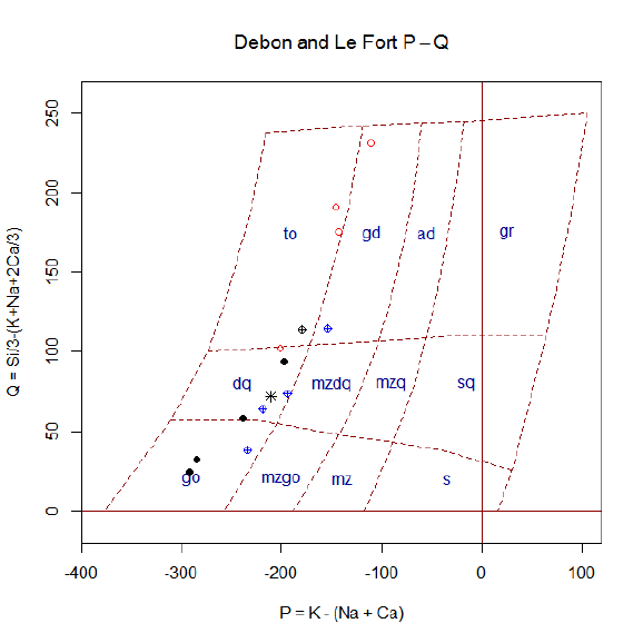
Debon 65
Layout of the P-Q diagram of the same authors corresponds to cationic proportions of quartz, K-
feldspar and plagioclase. Abbreviations used as classification output represent following rocks
groups:
label plutonic rocks volcanic rocks
go gabbro, diorite, anorthosite basalt, andesite, kenningite
mzgo monzogabbro, monzodiorite latibasalt, latiandesite
mz monzonite latite
ssyenite trachyte
dq qtz diorite,qtz gabbro,qtz anorthosite qtz andesite,qtz basalt
mzdq qtz monzodiorite,qtz monzogabbro qtz latiandesite,qtz latibasalt
mzq quartz monzonite quartz latite
sq quartz syenite quartz trachyte
to tonalite, trondhjemite dacite
gd granodiorite, granogabbro rhyodacite
ad adamellite dellenite
gr granite rhyolite
Parameters for the diagram are calculated by the function ’DebonCalc’. All of them are based on
millications (1000 gram-atoms per 100 grams).
P=K-(Na+Ca)
Q=Si/3-(K+Na+2*Ca/3)
A=Al-(K+Na+2Ca)
B=Fe+Mg+Ti
Note that the diagrams B-A and P-Q are recommended as complementary, i.e. resulting names
should be used in conjunction (granite II etc.). For details, see Debon & Le Fort (1983) or (1988).

66 deleteSingle
Value
sheet list with Figaro Style Sheet data
x.data P or B value. See details.
y.data Q or A value. See details.
Author(s)
Vojtech Erban, <vojtech.erban@geology.cz>
& Vojtech Janousek, <vojtech.janousek@geology.cz>
References
Debon F & Le Fort P (1983) A chemical-mineralogical classification of common plutonic rocks
and associations. Trans Roy Soc Edinb; Earth Sci 73: 135-149
Debon F & Le Fort P (1988) A cationic classification of common plutonic rocks and their magmatic
associations: principles, method, applications. Bull. Mineral 111: 493-511
See Also
classify figaro plotDiagram DebonCalc
deleteSingle Delete label or variable
Description
Deletes a single numeric variable or a label.
Usage
deleteSingle()
Details
The variables to be deleted is selected using the function ’selectColumnLabel’. In any case, a
confirmation is required before a variable is deleted from the system. Note that some variables are
required by the system and cannot be deleted.
Value
Returns the corrected version of the data frame ’labels’ or numeric matrix ’WR’.
Author(s)
Vojtech Janousek, <vojtech.janousek@geology.cz>

EarthChem 67
EarthChem Import from EarthChem.org
Description
This function serves for importing the whole-rock geochemical data from EarthChem.org online
database. Since 2010, EarthChem has been part of IEDA (Integrated Earth Data Applications), the
National Science Foundation (NSF)-funded data facility for solid earth geoscience data. The data
are gathered from several publicly available databases such as PetDB, SedDB, NAVDAT, or are
contributed, and can be accessed through the EarthChem’s REST Search Service utilized by our
function.
Usage
EarthChem(x)
Arguments
xa list of parameters, given below, detailed account of which is to be found at the
web page with the EarthChem REST Server Documentation. See also Exam-
ples.
Details
The function EarthChem imports the specified data taking advantage of the EarthChem REST
Search Service, which accepts GET string variables that determine search criteria. The results
are returned using html or xml protocols, and can be then imported to the GCDkit using the library
'XML'.
Possible parameters are (in square brackets are GCDkit default values)
Data source specification (reference(s))
author author
title title of the article
journal journal
doi Digital Object Identifier (not always available)
minpubyear minimum publication year of the citation article
maxpubyear maximum publicationyear (reqd with the former option)
exactpubyear exact year of publication
keyword free-text generic descriptor field
Sample ID, location or age
sampleid sample number/identifier from the original database
polygon geographic region, specified by geographic coordinates
north, east, south, west coordinates of a geographic envelope, all to be provided together
minage minimum age of the sample (Ma)
maxage maximum age of the sample (Ma)
exactage age of the sample (Ma)
geologicalage geological age
material either ’bulk’, ’whole rock’, ’glass’ or ’inclusion’
Output format
searchtype type of search, only ’rowdata’ (table of items matching the criteria)
is implemented so far [rowdata].
68 EarthChem
outputtype either ’html’ or ’xml’ [html]
outputlevel either ’sample’ or ’method’ [sample]
startrow sequence number of the first output row minus 1 [0]
endrow sequence number of the last output row minus 1 [number_of_hits-1]
standarditems logical; output just the standard items? [yes]
outputitems comma-separated list of output items
showcolumnnames logical; import the names of variables? [yes]
Value
(Invisibly) the query string. If no hits were found, the function returns (again invisibly) the value
-1.
Imports the data into the GCDkit system. Stores the imported dataset into memory (i.e., the variable
WRCube) together with the fields source that contains the string "EarthChem" and date with tome
of the search, EarthChem.query.var with the query variable (a list) and EarthChem.query.url
with URL sent to the web service.
Then, the previously active dataset becomes the current one.
Warning
XML library is required.
Author(s)
Function by Vojtech Janousek, <vojtech.janousek@geology.cz> (with helpful assistance from
Jason Ash, <jasonash@ku.edu>).
Tcl/Tk GUI by Oscar Laurent, <oscar.laurent@erdw.ethz.ch>
The XML package was written by Duncan Temple Lang.
See Also
For further details, see the EarthChem REST Server Documentation.
Examples
# Some of these examples are based on original examples
# from http://ecp.iedadata.org/rest_search_documentation
EarthChem(list(author="smith",outputtype="html",showcolumnnames="yes",startrow=0,endrow=100,
outputitems="sample_id,source,longitude,latitude"))
EarthChem(list(author="janousek",outputtype="xml",showcolumnnames="yes",outputitems="sample_id,
source,longitude,latitude",standarditems="yes"))
EarthChem(list(author="moyen",outputtype="html",showcolumnnames="yes",outputitems=
"sample_id,source,longitude,latitude",standarditems="yes"))
EarthChem(list(geologicalage="cambrian",outputtype="html",startrow=0,endrow=100,
outputitems="sample_id,source,longitude,latitude"))
EarthChem(list(polygon="-101.953125 39.9375,-99.95625 39.9375,-100.603125 38.53125, -99.815625
36.95625,-101.98125 36.984375,-101.953125 39.9375",searchtype="rowdata",outputtype="html",
outputitems="sampleid",showcolumnnames="yes",standarditems="yes"))

Edit labels 69
# Read a map directly into R
query<-"http://ecp.iedadata.org/restsearchservice?
north=49&east=-100&south=23&west=-24&outputtype=staticmap"
#shell.exec(query) # easy solution, gets to browser
filename<-paste(gcdx.dir,"map.jpg",sep="/")
download.file(query,filename,method="internal",mode="wb")
shell.exec(filename)
Edit labels Edit labels
Description
Simultaneous editing of all labels using a spreadsheet-like interface.
Usage
editLabels()
Arguments
none.
Details
The function invokes a spreadsheet-like interface that enables the user to edit the labels for individ-
ual samples. When all the desired changes have been performed, close button is to be clicked.
Value
Returns the corrected version of the data frame ’labels’.
Author(s)
Vojtech Janousek, <vojtech.janousek@geology.cz>
See Also
’data.entry’

70 editLabFactor
Edit numeric data Edit numeric data
Description
Simultaneous editing of all numeric data using a spreadsheet-like interface.
Usage
editData(x=WR)
Arguments
xdata frame/numeric matrix to be edited; default is ’WR’, i.e. numeric data
Details
The function invokes a spreadsheet-like interface that enables the user to edit the numeric data
for individual samples. When all the desired changes have been performed, close button is to be
clicked.
The system then performs some recalculations as if the data set was loaded from the disc afresh
(calling ’Gcdkit.r’).
Value
Returns the corrected version of the numeric matrix ’WR’.
Author(s)
Vojtech Janousek, <vojtech.janousek@geology.cz>
See Also
’data.entry’
editLabFactor Edit label as factor
Description
Global replacement each of the discrete values (levels) for a selected label.
Usage
editLabFactor()
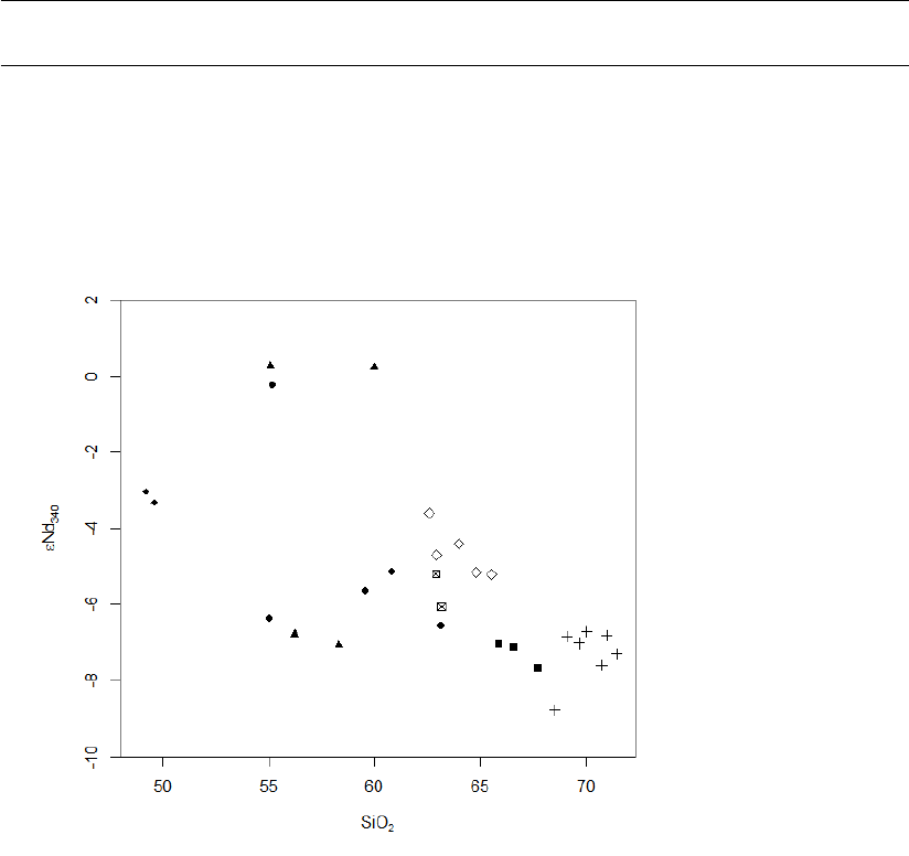
elemIso 71
Details
The label to be edited is selected using the function ’selectColumnLabel’.
Then the function invokes a spreadsheet-like interface that enables the user to overwrite directly
any of the discrete values for the a given label, in the R jargon called levels. When all the desired
changes have been performed, close button is to be clicked.
Value
Returns the corrected version of the data frame labels.
Author(s)
Vojtech Janousek, <vojtech.janousek@geology.cz>
See Also
’data.entry’
elemIso Binary plot of a WR geochemical parameter vs isotopic ratio
Description
Plots a diagram of a selected whole-rock geochemical parameter vs initial Sr isotopic ratios or initial
(Nd)for selected samples.
72 elemIso
Usage
elemIso(xlab=NULL,what=NULL,GUI=FALSE,...)
Arguments
xlab variable name or a formula for the x axis; if NULL a dialogue is displayed
what name of the desired isotopic parameter
GUI logical; is the function called from the GUI?
... optional parameters to the underlying function {plotWithLimits}
Details
The variable to be plotted as x axis is based on whole-rock geochemical data. If not specified upon
the function call, it is selected using the function ’selectColumnLabel’. In the specification of the
variable can be used also an arithmetic expression, see calcCore for the correct syntax.
The plotted isotopic parameters (y axis) can be one of:
Menu item Explanation
87Sr/86Sri Initial Sr isotopic ratios
143Nd/144Ndi Initial Nd isotopic ratios
EpsNdi Initial (Nd)values
1 stg DM model ages (Goldstein et al. 1988) Single-stage DM Nd model ages
1 stg DM model ages (Liew & Hofmann 1988) Single-stage DM Nd model ages
2 stg DM model ages (Liew & Hofmann 1988) Two-stage DM Nd model ages
If called from GUI, the samples can be selected based on combination of three searching mecha-
nisms (by sample name/label, range or a Boolean condition) - see selectSamples for details.
Value
None.
Plugin
SrNd.r
Author(s)
Vojtech Janousek, <vojtech.janousek@geology.cz>
References
Goldstein S L, O’Nions R K & Hamilton P J (1984) A Sm-Nd isotopic study of atmospheric dusts
and particulates from major river systems. Earth Planet Sci Lett 70: 221-236 doi: 10.1016/0012-
821X(84)90007-4
Liew T C & Hofmann A W (1988) Precambrian crustal components, plutonic associations, plate
environment of the Hercynian Fold Belt of Central Europe: indications from a Nd and Sr isotopic
study. Contrib Mineral Petrol 98: 129-138 doi: 10.1007/BF00402106
See Also
The actual plotting is done by the function plotWithLimits.
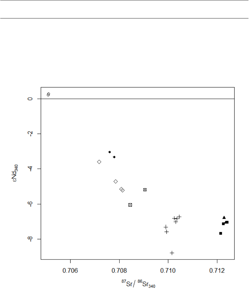
epsEps 73
epsEps Binary plot of initial Sr isotopic ratios vs. initial epsilon Nd values
Description
Plots a diagram of initial 87Sr/86Sr ratios vs. initial (Nd)values for selected samples.
Usage
epsEps(GUI=FALSE,...)
Arguments
GUI logical; is the function called from the GUI?
... optional parameters to the underlying function {plotWithLimits}

74 Export to Access
Details
If in GUI, the samples can be selected based on combination of three searching mechanisms (by
sample name/label, range or a Boolean condition) - see selectSamples for details.
Value
None.
Plugin
SrNd.r
Author(s)
Vojtech Janousek, <vojtech.janousek@geology.cz>
See Also
The actual plotting is done by the function plotWithLimits.
Export to Access Export to Access
Description
This function serves for exporting the specified data into MDB (MS Access) format (via the ODBC
interface).
Usage
accessExport(what=cbind(labels, WR), tablename=NULL,
transpose=FALSE,dec.places=NULL)
Arguments
what a matrix, data frame or a list
tablename name of the data table
transpose logical; transpose the data?
dec.places numeric; number of decimal places
Details
The function accessExport outputs the specified data via Microsoft’s ODBC interface, taking an
advantage of the library 'RODBC'. Unlike for the function ’excelExport’, ODBC makes possible
opening a new file.
If the argument 'what'is a matrix or data frame, the name of the table can be specified using the
optional parameter 'tablename'.
For a list, several tables are created, their number and names corresponding to the items present.

Export to DBF 75
Value
None.
Warning
This function is not available on 64-bit systems!
Author(s)
The RODBC package was written by Brian Ripley.
Vojtech Janousek, <vojtech.janousek@geology.cz>
See Also
’excelExport’ ’dbfExport’
Examples
accessExport(results) # Saves the last calculated results
Export to DBF Export to DBF
Description
This function serves for exporting the specified data into DBF (dBase III) format (using the function
’write.dbf’ of the package ’foreign’).
Usage
dbfExport(what=cbind(labels,WR), transpose=FALSE)
Arguments
what a matrix or data frame
transpose logical; transpose the data frame?
Details
The function dbfExport outputs the specified data. Note that it cannot handle lists.
Value
None.
Author(s)
Vojtech Janousek, <vojtech.janousek@geology.cz>
See Also
’write.dbf’ ’excelExport’ ’accessExport’

76 Export to Excel
Examples
dbfExport(results) # Saves the last calculated results
Export to Excel Export to Excel
Description
This function serves for exporting the specified data into XLS or XLSX (MS Excel) formats (via
the ODBC interface).
Usage
excelExport(what=cbind(labels, WR), tablename =NULL,
transpose=FALSE, dec.places=NULL)
excel2007Export(what=cbind(labels, WR), tablename =NULL,
transpose=FALSE, dec.places=NULL)
Arguments
what a matrix, data frame or a list
tablename name of the data sheet
transpose logical; transpose the data?
dec.places numeric; number of decimal places
Details
The functions excelExport and excel2007Export output the specified data via Microsoft’s ODBC
interface, taking an advantage of the library 'RODBC'.
If the argument 'what'is a matrix or data frame, the name of the sheet can be specified using the
optional parameter 'tablename'.
For a list, several sheets are attached, their number and names corresponding to the items present.
Value
None.
Warning
These functions are not available on 64-bit systems!
Unfortunately the way the ODBC is programmed by Microsoft does not make opening a new Excel
file possible. Thus only adding new sheet(s) to a pre-existing spreadsheet file is feasible.
Author(s)
The RODBC package was written by Brian Ripley.
Vojtech Janousek, <vojtech.janousek@geology.cz>

Export to HTML tables 77
See Also
’accessExport’ ’dbfExport’
Examples
excelExport(results) # Saves the last calculated results in XLS format
excel2007Export(results) # Saves the last calculated results in XLSX (or XLS) format
Export to HTML tables Export to HTML tables
Description
Outputs the specified data with (optional) labels into HTML. This format is useful for importing
into spreadsheets, word processors or publishing on the WWW.
Usage
HTMLTableMain(what,digits=2,desc=NULL,title=" ",sum.up=FALSE,open=TRUE,
close=TRUE,browse=TRUE,filename=paste(data.dir,"R2HTML/htmltable",sep="/"),
rotate=FALSE)
HTMLtableOrdered(what,which=rownames(what),labs=labels,digits=2,desc=NULL,
title=" ",sum.up=FALSE,key1=NULL,key2=NULL,
filename=paste(data.dir,"R2HTML/htmltable",sep="/"),split.by=25,rotate=TRUE)
HTMLTableWR(filename="htmltable")
HTMLTableResults(filename="htmltable")
Arguments
what numeric matrix; data to be exported
digits required precision
desc name of the columns within ’labels’ to be attached to the table
title main title
sum.up logical; should be a sum calculated?
open logical; should be opened a new HTML file?
close logical; should be the HTML file closed when finished?
browse logical; should be the HTML file finally opened in the default browser?
filename optional name for the file produced
rotate logical, should be the table transposed, with samples in columns and variables
in rows?
which (optional) sample names in numeric matrix ’what’ for the output
labs name of variable with textual labels
key1 is a variable in numeric matrix ’what’
key2 is a grouping information (name of a column in ’labs’)
split.by maximal number of data columns per page
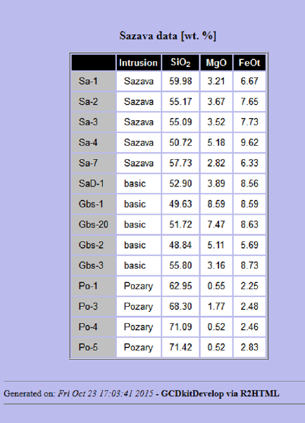
78 Export to HTML tables
Details
HTMLTableWR and HTMLTableResults are GUI front ends to HTMLTableMain, the former enabling
the user to choose samples (rows) and columns for the output using the searching mechanisms
common in the GCDkit.
HTMLTableWR outputs the numeric data (with optional labels and sum) stored in the data matrix
'WR'.
HTMLtableOrdered also outputs the numeric data stored in the numeric matrix specified by param-
eter 'what'. Optional argument 'which'gives the list of sample names (rows) in the matrix to
be saved. The data are first sorted based on 'key2', which typically gives a grouping information
(name of a column in 'labs'). Within each of the groups, the data are further sorted based on the
numeric variable 'key1'. See example.
HTMLTableResults outputs the results of the most recent calculation (with optional labels and sum)
as stored in the variable 'results'.
The plugin attempts to format sub- and superscripts in the names of variables.
The created file 'filename'is placed in the subdirectory 'R2HTM'of the current working directory;
when finished, it is previewed in a browser. The style for the table is determined by the cascade
style file R2HTML.css in the subdirectory 'Plugin'.
Value
None.

F-M-W diagram 79
Warning
The plugin uses R2HTML library, which must be downloaded from CRAN and properly installed.
Its presence is checked before the code is executed.
Author(s)
The R2HTML package was written by Eric Lecoutre.
Vojtech Janousek, <vojtech.janousek@geology.cz>
Examples
# Works on the 'sazava'test data set
setwd(paste(gcdx.dir,"Test_data",sep="/"))
loadData("sazava.data")
HTMLTableMain(WR[,c("SiO2","MgO","FeOt")],digits=2,desc="Intrusion",title="Sazava [wt.%]")
HTMLtableOrdered(WR[,LILE],digits=1,key1="SiO2",key2="Intrusion",title="Large Ion Lithophile
Elements (ppm)",split.by=3)
F-M-W diagram Ohta + Arai (2007) FMW weathering index
Description
Assigns data for the F-M-W diagram by Ohta & Arai (2007) into Figaro template (list ’sheet’) and
appropriate values into ’x.data’ and ’y.data’.
This function is meant to be used with plotDiagram.
Usage
OhtaArai(fixTi=F)
Arguments
fixTi logical, if TRUE, the T iO2value of samples where this is not determined (or 0)
will be replaced by FeOt/7.
Details
This (ternary) diagram has been proposed by Ohta & Arai (2007) to identify chemically weathered
igneous rocks. It turns out to be also very useful to separate para- from orthogneisses (Moyen et al.
2017).
The values of the apices are complex combination of oxides defining three end-members: M (mafic
igneous rocks), F (felsic igneous rocks) and W (chemical weathering):
M= exp (−0.395 ×ln(SiO2)+0.206 ×ln(T iO2)−0.316 ×ln(Al2O3)
+0.160 ×ln(F e2O3t)+0.246 ×ln(MgO)+0.368 ×ln(CaO)
+0.073 ×ln(N a2O)−0.342 ×ln(K2O)+2.266)
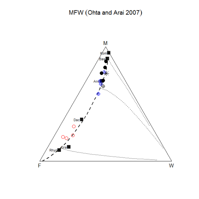
80 F-M-W diagram
F= exp (0.191 ×ln(SiO2)−0.397 ×ln(T iO2)+0.020 ×ln(Al2O3)
−0.375 ×ln(F e2O3t)−0.243 ×ln(MgO)+0.079 ×ln(CaO)
+0.392 ×ln(N a2O)+0.333 ×ln(K2O)−0.892)
W= exp (0.203 ×ln(SiO2)+0.191 ×ln(T iO2)+0.296 ×ln(Al2O3)
+0.215 ×ln(F e2O3t)−0.002 ×ln(MgO)−0.448 ×ln(CaO)
−0.464 ×ln(N a2O)+0.008 ×ln(K2O)−1.374)
Value
A list containing the Figaro template. In addition the following global variables are modified:
sheet list with Figaro Style Sheet data
x.data x coordinates in ternary projection
y.data y coordinates in ternary projection
Author(s)
Jean-Francois Moyen, <jfmoyen@gmail.com>

FeMiddlemost 81
References
Ohta T, Arai H (2007) Statistical empirical index of chemical weathering in igneous rocks: a new
tool for evaluating the degree of weathering. Chem Geol 240: 280-297 doi:10.1016/j.chemgeo.2007.02.017
Moyen JF, Laurent O, Chelle-Michou C, Couzinie S, Vanderhaeghe O, Zeh A, Villaros A, Gardien
V (2017) Collision vs. subduction-related magmatism: two contrasting ways of granite formation
and implications for crustal growth. Lithos 277: 154-177. doi:10.1016/j.lithos.2016.09.018
See Also
figaro plotDiagram
Examples
# plot the diagram
# assuming a dataset is loaded, of course!
## Not run:
plotDiagram("OhtaArai",FALSE)
## End(Not run)
FeMiddlemost Adjustment of Fe oxidation ratio (Middlemost 1989))
Description
Auxiliary function performing adjustment of the iron-oxidation ratio as proposed by Middlemost
(1989).
Usage
FeMiddlemost(anhydrous = TRUE)
Arguments
anhydrous logical; should be returned major-element analyses recast to anhydrous basis?
Details
This function performs an adjustment of the iron-oxidation ratio for individual volcanic rock types
as proposed by Middlemost (1989).
The classification is based on TAS classification (Le Bas et al. 1986,Le Maitre et al. 1989).
The F e2O3/F eO ratios for individual rock types, based on Verma et al. (2002) (Fig. 1), are as
follows:
foidite, Na2O+K2O<= 3 0.15
foidite, 3 < Na2O+K2O<= 7 0.2
foidite, 7 < Na2O+K2O<= 10 0.3
foidite, Na2O+K2O> 10 0.4
picrobasalt 0.15
basalt 0.2
basaltic andesite 0.3

82 figAdd
andesite 0.35
dacite 0.4
rhyolite 0.5
trachybasalt 0.3
basaltic trachyandesite 0.35
trachyandesite 0.4
trachyte/trachydacite 0.5
tephrite/basanite, Na2O+K2O<= 6 0.2
tephrite/basanite, Na2O+K2O> 6 0.3
phonotephrite 0.35
tephriphonolite 0.4
phonolite 0.5
If the parameter ’anhydrous’ is set, returned are the major-element data recast to 100 % anhydrous
basis.
Value
A matrix with adjusted whole-rock chemical data.
No permanent changes to either ’WR’ or ’WRanh’ are made.
Author(s)
Vojtech Janousek, <vojtech.janousek@geology.cz>
References
Le Bas M J, Le Maitre R W, Streckeisen A & Zanettin B (1986) A chemical classification of vol-
canic rocks based on the total alkali-silica diagram. J Petrology 27: 745-750 doi: 10.1093/petrol-
ogy/27.3.745
Le Maitre R W et al (1989) Igneous Rocks: A Classification and Glossary of Terms, 1st edition.
Cambridge University Press
Middlemost E A K (1989) Iron oxidation ratios, norms and the classification of volcanic rocks.
Chem Geol 77: 19-26 doi: 10.1016/0009-2541(89)90011-9
Verma S P, Torres-Alvarado I S, Sotelo-Rodriguez Z T (2002) SINCLAS: standard igneous norm
and volcanic rock classification system. Comput and Geosci 28: 711-715 doi: 10.1016/S0098-
3004(01)00087-5
See Also
TAS Verma
figAdd Plot editing: Add
Description
These functions enable adding new components to Figaro-compatible plots.
figAdd 83
Usage
figTicks(major=-0.5, minor=0.25, xmjr=NULL, xmin=NULL, ymjr=NULL, ymin=NULL)
figGrid(x.int=NULL, y.int=NULL, lty="dotted", col="gray30",GUI=FALSE)
figLegend()
figAddReservoirs(autoscale=FALSE, var.name=NULL, sample.names=NULL,
reserv.condition=NULL, labs=NULL, pch="*", col="darkred", cex=1, type="p",...)
figAddText()
figAddArrow()
figAddBox()
figAddFit()
figAddCurve(equation=NULL)
Arguments
major length of the major tick marks.
minor length of the minor tick marks.
xmjr, ymjr intervals for the major tick marks.
xmin, ymin intervals for the minor tick marks.
x.int intervals for the grid, x axis component.
y.int intervals for the grid, y axis component.
GUI logical; is the function called from GUI?
lty grid line type.
col plotting colour.
autoscale logical; should be the scaling changed so that all the plotted data fit in?
var.name text; either ’reservoirs.data’, ’idealmins.data’or a name of a global vari-
able. See Details.
sample.names character vector; names of reservoirs, ideal minerals or samples to be plotted.
reserv.condition
text; regular expression specifying reservoirs compositions of which are to be
plotted.
labs text; optional abbreviated labels for the individual reservoirs
pch plotting symbol.
cex numeric; relative size of the plotting symbol.
type character; plot type; see plot.default.
... additional parameters to the plotting function. See figOverplot.
equation text; equation expressed as a function of x; see curve.
84 figAdd
Details
’figTicks’ adds major and minor tick marks for the x and y axes. Their length is specified as a
fraction of the height of a line of text. Negative numbers imply outward and positive inward pointing
ticks. The user is prompted for four numbers separated by commas, xmjr, xmin, ymjr, ymin. These
specify the intervals of major and minor ticks for x and y axes, respectively. Not implemented to
logarithmic plots and spiderplots yet.
’figGrid’ adds grid lines for x and/or y axes.
’figLegend’ adds legend(s) on specified location.
’figAddReservoirs’ overplots compositions of selected geochemical reservoirs (taken from the
file ’reservoirs.data’, see selectNorm for the file structure as well as relevant references) or
ideal minerals (from the file ’idealmins.data’). Alternatively, if the name of a numeric matrix
or dataframe in the global environment is provided via the argument ’var.name’, the selection of
data from this object is used (see Examples). The selection is specified by either ’sample.names’
or by ’reserv.condition’ parameters. Optional argument ’labs’ can specify alternative, perhaps
abbreviated textual labels to the points plotted.
Please note that the function ’figAddReservoirs’ is available so far for simple spiderplots, binary
and ternary plots only. Technically, the function invokes ’figOverplot’ setting just.draw=FALSE,
and thus the overplotted dataset is added permanently. If just.draw=FALSE, the points for the ref-
erence dataset do not become a part of the template, and thus will vanish upon redrawing, zooming
. . . . See Examples.
’figAddText’ adds text on specified location. The parameters are the text style (’n’ = normal, ’b’ =
bold, ’i’ = italic and ’bi’ = bold italic), colour and relative size.
’figAddArrow’ adds arrow on specified location. The parameters are colour and line style (’solid’,
’dashed’, ’dotted’ and ’dotdash’).
’figAddBox’ adds box on specified location (click bottom left and then top right corner).
’figAddFit’ adds either a single least-squares fit to all data, or several fit lines, for each of the
groups separately. The parameters are colour and line style (’solid’, ’dashed’, ’dotted’ and
’dotdash’). The equation of each fit line is plotted at the user-defined location.
’figAddCurve’ adds a curve, specified as a function of variable ’x’. The parameters are colour and
line style (’solid’, ’dashed’, ’dotted’ and ’dotdash’).
The colours can be specified both by their code (see table under menu ’Data handling|Show
available colours’) or R name (see Examples).
The additional two menu items, available for binary and ternary plots, allow adding contours or
convex hulls outlining individual groups of data. See contourGroups and chullGroups.
Value
For ’figAddReservoirs’, a numeric matrix with the overplotted analyses from the reference dataset.
Warning
Most of these functions serve to adding some extra components/annotations immediately before the
graph is printed/exported. Note that, except for ’figAddReservoirs’, all user-defined components
added via ’Plot editing: Add’ will be lost upon redrawing, zooming . . . .
Author(s)
Colin M. Farrow, <colinfarrow537@gmail.com>
Vojtech Janousek, <vojtech.janousek@geology.cz>
figAdd 85
See Also
par showColours colours figaro selectNorm
contourGroups chullGroups
figOverplot figOverplotDiagram overplotDataset curve
Examples
## figTicks and figGrid
data(blatna)
accessVar("blatna")
setCex(1.5)
binary("Zr/Nb","Ba/La")
figTicks(major=-0.5, minor=0.25,10,1,10,1)
figGrid(,5,col="darkblue") # just y axis (second parameter)
figRedraw()
figGrid(2,5,col="darkblue")
## figAddReservoirs
data(blatna)
accessVar("blatna")
setCex(1.5)
# binary
binary("Zr/Nb","Ba/La")
# Sun & McDonough mantle reservoirs, Taylor & McLennan 1995 Upper and Lower Crust
reserv<-c("(MORB|OIB) McDonough","Upper Crust Taylor 1995","Lower Crust Taylor 1995")
reserv.names<-c("NMORB","EMORB","OIB","UCC","LCC")
figAddReservoirs(TRUE,"reservoirs.data",reserv.condition=reserv,labs=reserv.names)
# ternary
ternary("SiO2/10","MgO","FeOt")
figAddReservoirs(var.name="idealmins.data",sample.names=c("Or","Bt","Ph"))
# spider
spider(WR,"NMORB..Sun",field=TRUE,colour="gray",field.colour=TRUE,ymin=0.1,ymax=100)
figAddReservoirs(var.name="reservoirs.data",reserv.condition="Continental Crust",
autoscale=TRUE,col=c("red","black","darkblue"),pch=1:3)
# Calculate Rayleigh-type fractionation trend
ff<-seq(1,0.1,-0.1) # F, amount of melt left
x<-80*ff^(1.2-1) # cL for three elements, arbitrary D of 1.2, 2.0 and 1.3
y<-550*ff^(2.0-1)
z<-1000*ff^(1.3-1)
my.trend<-cbind(x,y,z)
colnames(my.trend)<-c("Rb","Sr","Ba")
rownames(my.trend)<-ff
# By default, the overplotted information is added permanently
binary("Rb","Sr",log="xy")
figAddReservoirs(var.name="my.trend",pch="+",col="blue",autoscale=TRUE,type="o",
labs=rownames(my.trend))
figXlim(c(10,500))

86 figaro.identify
# But this is controlled by the argument just.draw
binary("Rb","Sr",log="xy")
figAddReservoirs(var.name="my.trend",pch="+",col="red",autoscale=TRUE,type="o",
labs=rownames(my.trend),just.draw=TRUE)
figRedraw()
figaro.identify Plot editing: Identification of plotted symbols
Description
These functions allow the user to identify points in Figaro-compatible plots.
Usage
figIdentify()
highlightSelection()
Details
’figIdentify’ identifies points closest to a mouse pointer, if a mouse button is pressed. For binary
and ternary plots, sample names are plotted; for spider plots the function prints the sample name,
concentration of the given element (in ppm) and highlights the whole pattern. The identification is
terminated by pressing the right button and selecting 'Stop'from the menu.
’highlightSelection’ allows the selected analyses to be highlighted. The samples can be selected
based on combination of three searching mechanisms (by sample name/label, range or a Boolean
condition) - see selectSubset for details.
If the search results are empty or embrace all samples, the user is given a chance to select the
samples from the list of their names. Press Ctrl+click to select multiple ones.
For binary and ternary plots, Press Esc in the Console window to stop the points blinking. In spider
plots are shown overall ranges of normalized concentrations (by a gray field) with superimposed
patterns for selected samples.
Author(s)
Colin M. Farrow, <colinfarrow537@gmail.com>
and Vojtech Janousek, <vojtech.janousek@geology.cz>
See Also
identify selectSubset ’figaro’

figCol 87
figCol Plot editing: Colours
Description
These functions enable altering colours for titles or all plotting symbols in Figaro-compatible plots.
Usage
figCol(col=NULL)
figColMain(col=NULL)
figColSub(col=NULL)
figBw()
Arguments
col colour specification
Details
The colours can be specified both by their code (see table under Data handling|Show available
colours) or R name (see Examples).
figBw sets the whole plot (main title and subtitle, axes and plotting symbols) in black and white,
making them ready for printing/exporting.
Author(s)
Colin M. Farrow, <colinfarrow537@gmail.com>
& Vojtech Janousek, <vojtech.janousek@geology.cz>
See Also
’showColours’ ’colours’ ’figaro’
Examples
colours() # prints the list of available colour names
plotDiagram("TAS",FALSE) # example of a classification plot
figSub(txt="My TAS diagram")
figCol(col="green")
figColMain(col="red")
figColSub(col="blue")
figBw()
spider(WR,selectNorm("Boynton"),0.1,1000,pch=labels$Symbol,col=labels$Colour)
figMain(txt="My REE plot")
figSub(txt="Normalized by Boynton (1989)")

88 figEdit
figCol(col="green")
figColMain(col="red")
figColSub(col="blue")
figEdit Plot editing: Changing titles and axis labels
Description
These functions enable altering titles and axis labels of binary (figXlab, figYlab) and ternary
(figAlab, figBlab, figClab), Figaro-compatible plots.
Usage
figMain(txt=NULL)
figSub(txt=NULL)
figXlab(txt=NULL)
figYlab(txt=NULL)
figAlab(txt=NULL)
figBlab(txt=NULL)
figClab(txt=NULL)
Arguments
txt text
Details
If specified, the parameter txt will be passed to the function 'annotate'to guess the correct
reformatting to sub- and superscripts for production of "publication quality" plots. Otherwise, the
current value (titles or labels for axes/apices) are edited.
Author(s)
Colin M. Farrow, <colinfarrow537@gmail.com>
and Vojtech Janousek, <vojtech.janousek@geology.cz>
See Also
’annotate’
’figaro’

figGbo 89
Examples
plotDiagram("TAS",FALSE) # example of a classification plot
figMain(txt="My TAS diagram")
figSub(txt="test")
figXlab(txt="Silica")
figYlab(txt="Total alkalis")
figGbo Defining groups on Figaro-compatible plots
Description
Interactive definition of groups on any Figaro-compatible plot.
Usage
figGbo(x.tol = 0, y.tol = 0, max.points = 100, max.polygons = 25)
Arguments
x.tol, y.tol tolerance for the automatic closing of polygons.
max.points maximum number of vertices for a single polygon.
max.polygons maximum number of polygons.
Details
Each of the groups is defined by clicking vertices of a polygon with the corresponding data points.
The polygons are closed automatically. To finish, right click anywhere on the plot and select ’Stop’.
The groups are numbered consecutively, points falling into two or more fields form extra groups, as
do unclassified samples.
Author(s)
Vojtech Erban, <vojtech.erban@geology.cz> & Vojtech Janousek, <vojtech.janousek@geology.cz>
See Also
’figaro’

90 figMulti
figLoad Loading a Figaro plot
Description
Loads a Figaro-compatible plot (both the template and the data) stored in a file.
Usage
figLoad()
Arguments
None.
Details
The default suffix for the saved diagrams is ’fgr’. Note that only the data needed for the plotting
(’x.data’, ’y.data’) are stored in the ’fgr’ files. Thus the data set currently in memory (e.g.,
variables ’WR’, ’labels’, . . . ) is unaffected by the function ’figLoad’.
Author(s)
Colin Farrow, <colinfarrow537@gmail.com>
and Vojtech Janousek, <vojtech.janousek@geology.cz>
See Also
figSave figaro
figMulti Figaro: Multiple plot by groups
Description
Displays multiple plots, for each of the groups one, based on a most recently plotted Figaro-
compatible template. For spiderplots, the colour field denotes the total variation with the whole
dataset.
Usage
figMulti(x=x.data,y=y.data,nrow=NULL,ncol=NULL,xlab=sheet$demo$call$xlab,
ylab=sheet$demo$call$ylab,pch=NULL,col=NULL,
cex = NULL,plot.symb=NULL,shaded.col="gray",rotate.xlab=TRUE,
offset=TRUE,centered=FALSE,title=NULL,...)
figMulti 91
Arguments
x, y data to be plotted
nrow, ncol dimensions of the plots’ matrix
xlab, ylab labels for the axes
pch plotting symbols
col plotting colours
cex relative size of the plotting symbols
plot.symb logical, spiders. Shall be shown also plotting symbols or just lines?
shaded.col (spiders) Colour for the field portraying the overall variability in the dataset.
rotate.xlab logical, spiders. Shall be the element names on x axis rotated?
offset logical, spiders. Shall be the names for odd and even elements shifted relative
to each other?
centered logical, spiders. Shall be the element names on x axis plotted in between tick
marks?
title optional title for the whole plate. If not provided, it is taken from the title of the
Figaro template.
... any additional graphical parameters
Note
This function uses the plates concept. The individual plots can be selected and their proper-
ties/appearance changed as if they were stand alone Figaro-compatible plots. See Plate,Plate editing
and figaro for details.
Details
The function can handle any Figaro-compatible plots, including binary, ternary or spiderplots.
For classification plots, it may be advantageous to switch off the field names using the function
'plateAnnotationsRemove', (see the figure below as well as the Examples).
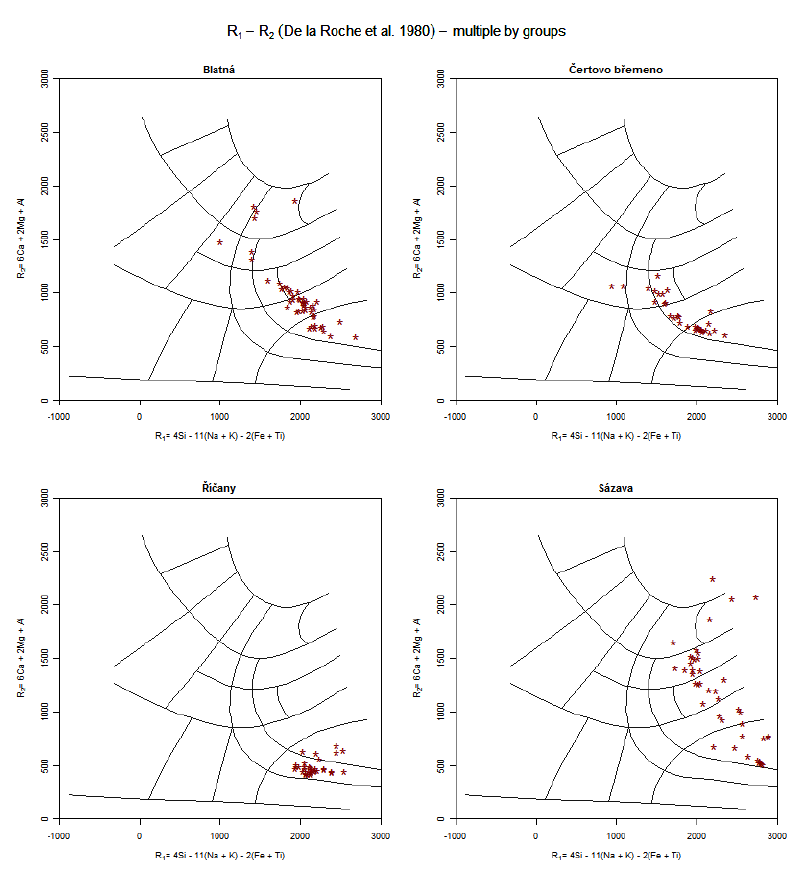
92 figMulti
Author(s)
Vojtech Janousek, <vojtech.janousek@geology.cz>
and Colin M. Farrow, <colinfarrow537@gmail.com>
See Also
figaro,Plate,Plate editing binary,ternary,spider
Examples
# Note that groups should have been defined before running these.
# switch on the field names (default, valid globally for the whole system)
options("gcd.plot.text"=TRUE)

figOverplot 93
plotDiagram("TAS",FALSE)
figMulti()
# switch off the field names
options("gcd.plot.text"=FALSE)
plotDiagram("LarochePlut",FALSE)
figMulti(col="black",pch="*",cex=2)
options("gcd.plot.text"=TRUE)
spider(WR,selectNorm("Boynton"),0.1,1000,pch=labels$Symbol,
col=labels$Colour,cex=labels$cex)
figMulti(plot.symb=TRUE,cex=2)
figMulti(col="red",plot.symb=FALSE,rotate.xlab=FALSE,offset=TRUE)
figMulti(col="red",plot.symb=FALSE,rotate.xlab=FALSE,offset=FALSE,shaded.col="khaki")
figOverplot Overplotting data onto pre-existing binary, ternary or spider plots
Description
This function allows overplotting new data points onto Figaro-compatible binary or ternary plots,
or patterns onto spiderplots. It is most useful in adding selected data from typical geochemical
reservoirs (e.g., Upper Continental Crust, MORB . . . ), ideal mineral compositions, results of pet-
rogenetic modelling or just another dataset used for comparison (any of these will be henceforth
referred to as a reference dataset).
Usage
figOverplot(var.name, mat=NULL, sample.names=NULL, condition=NULL,
labs=NULL, autoscale=FALSE, pch="*", col="darkred", cex=1,
type="p", just.draw = FALSE,overplotDataset = FALSE,...)
Arguments
var.name either ’reservoirs.data’, ’idealmins.data’ or a quoted name of a global
variable.
mat matrix with data for all reservoirs available for overplotting. Meant mainly for
internal use of the GCDkit system.
sample.names character vector; list of names of desired reservoirs, ideal minerals or samples
in the reference dataset to be overplotted.
condition text; regular expression specifying names of desired reservoirs, ideal minerals
or samples in the reference dataset.
labs text; optional (typically abbreviated) labels for the overplotted data from the
reference dataset.
autoscale logical; should be the scaling changed so that all the plotted analyses fit in?
pch plotting symbol(s) for the reference dataset.
col plotting colour(s) for the reference dataset.
cex numeric; relative size of the plotting symbol(s) for the reference dataset.
94 figOverplot
type character; plot type; see plot.default. For obvious reasons, not implemented for
spiderplots.
just.draw logical; if FALSE, the overplotted bit is added permanently, i.e. the Figaro tem-
plate is also affected.
overplotDataset
logical; for internal use by the system only.
... additional parameters to the underlying plotting function(s). See Details.
Details
If called directly, the function is employed to overplot data from a reference dataset, either real-
world data or a numeric matrix spanning, for instance, from petrogenetic modelling. The data
originate from a two-dimensional variable in the global environment, whose name is provided via
the obligatory argument ’var.name’.
Argument ’mat’ is meant for internal use by the system and does not need to be specified by the
user as the data frame/matrix mat is generated automatically by the function ’figOverplot’.
In both cases, the selection from the numeric matrix or dataframe ’mat’ is based on a list of desired
’sample.names’ or on a regular expression yielding their subset (’condition’). Of course, from
this selection, only analyses with data sufficient to be plotted on the current diagram are used.
If neither ’sample.names’ nor ’condition’ is provided, all samples are shown.
For plotting are used functions ’points’, ’triplotadd’ and ’spider’ for binary plots, ternary plots
and spiderplots, respectively. Argument ’...’ can supply additional parameters to these low-level
plotting functions.
Optional parameter ’labs’ can specify alternative, typically abbreviated textual labels to the points
plotted.
Logical argument ’autoscale’ determines whether the plot should be rescaled to accommodate
both the original data points and the reference dataset. Clearly, it does not make sense for a ternary
plot.
By default, the overplotted information is added permanently but this behaviour is controlled by the
argument just.draw.
Value
A numeric matrix with the overplotted analyses from the reference dataset.
Note
Within the GCDkit system, this function is invoked by ’figAddReservoirs’ to overplot selected
compositions from typical geochemical reservoirs (system file ’reservoirs.data’) or chemistries
of ideal minerals (system file ’idealmins.data’).
Warning
If just.draw=FALSE, the points for the reference dataset do not become a part of the template, and
thus will vanish upon redrawing, zooming . . . . See Examples.
Author(s)
Vojtech Janousek, <vojtech.janousek@geology.cz>

figOverplotDiagram 95
See Also
figAddReservoirs plateAddReservoirs
figOverplotDiagram overplotDataset
points triplotadd spider
figaro selectNorm par
Examples
data(sazava)
accessVar("sazava")
setCex(1.5)
pokeDataset("sazava", overwrite.warn=FALSE)
# Calculate Rayleigh-type fractionation trend
ff<-seq(1,0.1,-0.1) # F, amount of melt left
x<-80*ff^(1.2-1) # cL for three elements, arbitrary D of 1.2, 2.0 and 1.3
y<-550*ff^(2.0-1)
z<-1000*ff^(1.3-1)
my.trend<-cbind(x,y,z)
colnames(my.trend)<-c("Rb","Sr","Ba")
rownames(my.trend)<-ff
# By default, the overplotted information is added permanently
binary("Rb","Sr",log="xy")
figOverplot(var.name="my.trend",pch="+",col="blue",autoscale=TRUE,type="o",
labs=rownames(my.trend))
figXlim(c(30,100))
# But this is controlled by the argument just.draw
binary("Rb","Sr",log="xy")
figOverplot(var.name="my.trend",pch="+",col="darkred",autoscale=TRUE,type="o",
labs=rownames(my.trend),just.draw=TRUE)
# Any function redrawing the plotting window will wipe the added trend out
figXlim(c(30,100))
ternary("10*Rb","2*Sr","Ba/2")
figOverplot(var.name="my.trend",pch="+",col="blue",type="o",
labs=rownames(my.trend))
figOverplotDiagram Overplotting data onto classification or geotectonic plots
Description
This function allows overplotting new data points onto single Figaro-compatible templates defined
for classification or geotectonic plots (binary or ternary, designed as stand alone or extracted from
plates).
Usage
figOverplotDiagram(overplot.dataset, bg.dataset=NULL, diagram=NULL,
which=NULL, xlim=NULL, ylim=NULL, pch="*", col="darkred",
cex=1, labs=NULL, type="p", lwd=1, lty="solid",
transp=0, just.draw=TRUE,...)
96 figOverplotDiagram
Arguments
overplot.dataset
(obligatory) name of the main (foreground) dataset stored in memory, or global
variable name.
bg.dataset (optional) name of the background dataset stored in memory.
diagram character; existing diagram name.
which which plot is to be extracted (if belonging to a plate)?
xlim new limits of the x axis.
ylim new limits of the y axis.
pch plotting symbol(s) for the foreground dataset.
col plotting colour(s) for the foreground dataset.
cex numeric; relative size of the plotting symbol(s) for the foreground dataset.
labs text; optional labels for the overplotted data.
type character; see ’points’.
lwd, lty parameters for connecting line, if drawn; see ’par’.
transp numeric; transparency for the background set, 0-1.
just.draw logical; NOT FUNCTIONAL, kept just for compatibility sake.
... additional parameters to the underlying plotting function(s). See Details.
Details
The function ’figOverplotDiagram’ can be employed in two ways.
If quoted names of two datasets in memory are provided (’bg.dataset’ and ’overplot.dataset’),
a new plot is created, whereby the background dataset is plotted using either the function ’plotDiagram’
(for stand-alone plots) or ’plateExtract’ (for one of diagrams extracted from a plate).
If only a single name of dataset is given, then the data are overplotted onto the current (preexisting)
diagram.
Optional plotting parameters ’pch’, ’col’, ’cex’, ’type’, ’lwd’ and ’lty’ can be defined for the
overplotted (foreground) dataset.
Argument ’...’ can supply additional parameters to the original plotting functions (e.g., ’TAS’)
invoked by ’plotDiagram’ or ’plateExtract’.
Value
None.
Warning
This function serves to add extra components/annotations immediately before the graph (a spider-
plot, simple binary or ternary plot) is printed or exported. Note that the points for the overplotted
dataset are not part of the template, and thus will vanish upon redrawing, zooming . . . .
Author(s)
Vojtech Janousek, <vojtech.janousek@geology.cz>

figRedraw 97
See Also
figOverplot figAddReservoirs overplotDataset
underplotDataset plotDiagram plateExtract
figaro par
Examples
data(sazava)
accessVar("sazava")
data(blatna)
accessVar("blatna")
setCex(2)
pokeDataset("blatna", overwrite.warn=FALSE)
## Two datasets
# stand alone plot
figOverplotDiagram("sazava","blatna","DebonBA",pch=15,col="darkred",
cex=2,transp=0.5)
# plateExtract
figOverplotDiagram("sazava","blatna","PearceGranite",col="darkred",
cex=2,transp=0.5,which=2)
## Overplotting on existing plot - plotDiagram
peekDataset("blatna")
plotDiagram("DebonPQ",FALSE,TRUE)
figCex(2)
figRemove()
figOverplotDiagram("sazava",pch=15,col="darkred",cex=2,transp=0.6)
# Overplotting of existing plot - plateExtract
peekDataset("blatna")
plateExtract("PearceGranite",which=2)
figXlim(c(1,100))
figYlim(c(1,300))
figCex(2)
figOverplotDiagram("sazava",pch=15,col="darkred",cex=2,transp=0.6)
figRedraw Redrawing/refreshing a Figaro plot
Description
This function redraws/refreshes a Figaro-compatible plot.
Usage
figRedraw(x=x.data, y=y.data, zoom=NULL, bw=FALSE, title=NULL)
refreshFig()

98 figSave
Arguments
xvector of x coordinates
yvector of y coordinates
zoom logical; redraw while zooming?
bw logical; should be the output black and white?
title character; optional title for the plotting window.
Warning
Note that all user-defined components added via ’Plot editing: Add’ (legend, lines, text, boxes,
. . . ) - will be lost.
Author(s)
Colin M. Farrow, <colinfarrow537@gmail.com>
and Vojtech Janousek, <vojtech.janousek@geology.cz>
See Also
figaro
figSave Saving a Figaro plot
Description
Saves the current Figaro-compatible plot, both the template and the data needed for the plotting
(’x.data’, ’y.data’).
Usage
figSave()
Arguments
None.
Details
The default suffix for the saved diagrams is ’fgr’.
Author(s)
Colin M. Farrow, <colinfarrow537@gmail.com>
and Vojtech Janousek, <vojtech.janousek@geology.cz>
See Also
figLoad figaro

figScale 99
figScale Plot editing: Scaling text or plotting symbols
Description
These functions enable changing a size of titles, axis labels or plotting symbols of Figaro-compatible
plots. The size is relative to 1 (the original).
Usage
figCex(x=NULL)
figCexLab(x=NULL)
figCexMain(x=NULL)
figCexSub(x=NULL)
Arguments
xnumeric: scaling factor.
Author(s)
Colin M. Farrow, <colinfarrow537@gmail.com>
and Vojtech Janousek, <vojtech.janousek@geology.cz>
See Also
’figaro’
Examples
plotDiagram("TAS",FALSE) # example of a classification plot
figSub(txt="My TAS diagram")
figCex(2)
figCexMain(1.5)
figCexSub(0.5)
spider(WR,selectNorm("Boynton"),0.1,1000,pch=labels$Symbol,col=labels$Colour)
figMain(txt="My REE plot")
figSub(txt="Normalized by Boynton (1989)")
figCex(2)
figCexMain(1.5)
figCexSub(0.5)

100 figUser
figUser Plot editing: User defined parameter
Description
Enables the power users to modify the plot parameters directly.
Usage
figUser(expression=NULL,redraw=TRUE)
Arguments
expression character; expression to be evaluated
redraw logical; should be modified Figaro template redrawn?
Details
The parameters can be specified at the function call. If not, they are chosen by a dialogue. Several
of the, can entered simultaneously, as a semicolon delimited list. The most useful might be:
main Main title
sub Sub title
xlab Label of x axis
ylab Label of y axis
xlim Limits for the x axis
ylim Limits for the y axis
bg Colour of background
pch Plotting symbols
col Colour of plotting symbols
cex Relative size of plotting symbols
log Which of the axes is logarithmic? ("","x","y" or "xy")
If no parameters are entered, they can be chosen from a list (still experimental!)
Menu
Plot editing: User defined parameter
Warning
If requesting a logarithmic plot, make sure that the axis ranges are positive. See Examples or invoke
menu items ’Plot editing: Scale x axis’ and ’Plot editing: Scale y axis’.
Author(s)
Colin M. Farrow, <colinfarrow537@gmail.com>
and Vojtech Janousek, <vojtech.janousek@geology.cz>

figZoom 101
See Also
par figaro
Examples
plotDiagram("TAS")
figUser()
figUser("pch=1; col=2")
figUser("pch=\"+\"")
figUser("col=\"darkblue\"")
figUser("bg=\"khaki\",cex=1.5") # for camouflage purposes
figUser("main=\"My plot\"; las=2; font.main=4; cex.main=2; col.main=\"blue\"")
figZoom Plot editing: Zooming
Description
These functions zoom in and out Figaro-compatible plots.
Usage
figZoom()
figUnzoom()
figXlim(range=NULL)
figYlim(range=NULL)
figFixLim(no.action.warn=TRUE)
Arguments
range numeric: two limits, minimum and maximum, for the given axis.
no.action.warn logical: should be a warning shown if there is no action needed?
Details
’figZoom’ zooms the specified rectangular area (click bottom left and then top right corner) in a
new window. The zoomed area is highlighted in the old window.
’figUnzoom’ closes the new window with blown up portion of the plotting window and returns to
the original window.
’figXlim’ and ’figYlim’ allow to change the plotting limits (as a list of two components, separated
by commas).
’figFixLim’ extends the scales of both axes of a binary plot automatically if necessary to accom-
modate all the data points.

102 filledContourFig
Warning
If requesting a logarithmic plot, make sure that the axis ranges are positive.
Author(s)
Colin M. Farrow, <colinfarrow537@gmail.com>
and Vojtech Janousek, <vojtech.janousek@geology.cz>
See Also
’figaro’
Examples
## Not run:
# requires a preexisting Figaro-compatible plot
plot.diagram("Shand",select.samples=FALSE)
figXlim(c(0.6,1.2))
figYlim(c(0.8,3))
## End(Not run)
filledContourFig Filled contours plot
Description
Generates a frequency plot on the basis of the most recently plotted Figaro template.
Usage
filledContourFig(xlab=sheet$demo$call$xlab,ylab=sheet$demo$call$ylab,
xlim=sheet$demo$call$xlim,ylim=sheet$demo$call$ylim,
annotate.fields=FALSE,...)
Arguments
xlab character vector; label for the x axis
ylab character vector; label for the y axis
xlim limits for the x axis
ylim limits for the y axis
annotate.fields
logical; should be the plotted fields labeled by their names?
... additional plotting parameters
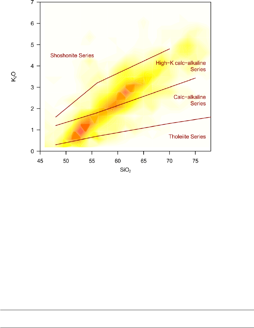
Frost 103
Details
This is a somewhat modified version of the R function ’filled.contour’ that produces a frequency
plot on the basis of a Figaro template and superimposes, if desired, selected data points.
First the user is prompted, how many intervals should be each of the axes split into. This corre-
sponds to a density of grid, in which are the individual points classified into. Then a colour scheme
(palette) can be chosen. Lastly, after the frequency plot is generated, selected analyses can be
plotted (’overplot’). In the latter case, standard GCDkit routine is used to selectSamples.
Value
None.
Author(s)
Vojtech Janousek, <vojtech.janousek@geology.cz>
See Also
’addContours’ ’selectSubset’ ’figaro’
Frost Frost et al. (2001)
Description
Classification of granitic rocks proposed by Frost et al (2001).
104 Frost
Usage
Frost(plot.txt = getOption("gcd.plot.text"),
clssf = FALSE, GUI = FALSE)
Arguments
plot.txt logical, annotate fields by their names?
clssf logical, should the samples be classified?
GUI logical, is the function called from a GUI?
Details
Classification scheme proposed by Frost et al. (2001). It consists of three diagrams:
•F e number vs. SiO2. Note, that the Fe-number is calculated as weight proportion of
F eO/(F eO +MgO)(or F eOtot/(F eOtot +MgO)), see below). The approach used here
should not be confused with the more common usage of the term "Fe-number" (as well as
"Mg-number") as molecular proportions.
•Na2O+K2O−CaO vs. SiO2(in wt. %).
•A/NK vs. ASI, where A/NK stands for molecular Al2O3/(N a2O+K2O), and ASI for
molecular Al2O3/(Na2O+K2O+CaO −3.33P2O5). In fact, it is the A/CNK parameter
of Shand (1943), corrected for the Ca content in apatite. As approved by one of the authors
(C. Barnes, pers. comm., 2008), the equation for ASI in the original work (Frost et al. 2001)
was stated erroneously in molecular proportions of elements, instead of oxides. In fact, this
diagram was not plotted in the paper, but it replaces the conditions mentioned in the text and
is in our view more instructive.
The classification is designed to work both with analyses distinguishing between ferrous and ferric
iron (preferred) and those with total iron only. The dialogue box lets the user decide, whether to use
the ferrous iron value or the total iron.
Similarly, if some P2O5concentration are missing in the dataset, the user is prompted whether
the missing values should be replaced with zero. If not, the problematic analyses are not plot-
ted/classified.
Value
The function returns table of calculated coefficients (Fe-Number, MALI, ASI). There are two values
for the ASI: one labeled 'ASI'is calculated from molecular proportions of oxides, and is used for
plotting and classification. The other one is labeled 'ASI_orig', and is calculated exactly as stated
in the original paper (i.e. Al/(Ca −1.67P+Na +K).
The following associations are distinguished:
ferroan
magnesian
As well as:
alkalic
alkali-calcic
calc-alkalic
calcic
Or:
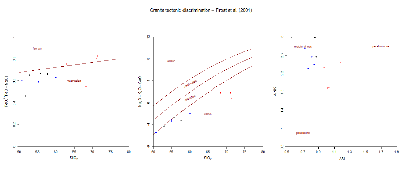
Frost 105
peralkaline
metaluminous
peraluminous
The geologically reasonable combinations, together with examples, are listed in the ../doc/FrostTable.
html, modified from the original article.
Note
Due to the specific design of this classification (combination of multiple diagrams), the classifi-
cation option is not available via the pull-down menus. Currently, the only way to apply Frost’s
classification in GCDkit on individual samples is to call the function manually from the Console
(Frost(clssf = TRUE)).
Note
This function uses the plates concept. The individual plots can be selected and their proper-
ties/appearance changed as if they were stand alone Figaro-compatible plots. See Plate,
Plate editing and figaro for details.
Author(s)
Vojtech Erban, <vojtech.erban@geology.cz>
& Vojtech Janousek <vojtech.janousek@geology.cz>
References
Frost B R, Barnes C G, Collins W J, Arculus R J, Ellis D J, Frost C D (2001) A geochemical
classification for granitic rocks. J Petrol 42: 2033-2048. doi: 10.1093/petrology/42.11.2033
Shand, S J (1943) Eruptive rocks, 2nd ed. John Wiley, New York, pp 1-444
See Also
classify Shand Plate Plate editing plotPlate figaro

106 gcdOptions
Examples
#plot the diagrams
plotPlate("Frost")
#classify the samples, suppress the graphical output
Frost(clssf = TRUE)
gcdOptions GCDkit options
Description
A graphical user interface (GUI, programmed in Tcl/Tk) for setting the main options controlling
the behaviour of the GCDkit.
Usage
gcdOptions(permanent.only=FALSE)
Arguments
permanent.only logical; should be shown exclusively the option that can be set permanently?
Details
The settings are stored permanently in the file ’gcdkit.xxx’ residing in the main GCDkit directory.
They are loaded upon start up. If is missing or damaged, this file is created anew based on the
default values.
The panel connected to the function ’gcdOptions’ serves to change several parameters. Most of
them are passed to a list accessible in a way similar to the standard R options. See the corre-
sponding manual page for details and Examples for their implementation. Only a few are stored in
dedicated variables (see below).
First, the default working directory can be set (and stored in the global variable data.dir).
The parameter ’Minimize output on screen?’ is linked to the option gcd.shut.up. It controls
excessive output to the Console window. Its default value is FALSE, meaning that detailed informa-
tion is to be printed. This, however, may become not viable on slower systems and/or for extensive
data sets.
The preferred precision of the numeric values that need to be rounded off are controlled by the
parameter ’Precision of results’ (option gcd.digits).
Using the parameter ’Plotting symbols magnification’, linked to the option gcd.cex, one
can define a factor, by which are multiplied the plotting sizes defined for individual analyses upon
startup and stored in the variable ’labels[,"Size"]’. Please note that this is effective for the next
plot if the GUI frontend is used to set this parameter, otherwise it will work for data files loaded
from now on.
In this way, the magnification is maintained proportional to the original sizes. If uniform plotting
symbols sizes are desired, one should use the function setCex invoked from the menu
Plot settings|Set uniform symbol size.
The parameter ’Annotate fields in discrimination plots?’ toggles the labeling of the fields
on and off, typically for classification or geotectonic diagrams. It is stored in a logical variable
gcdOptions 107
gcd.plot.text, whose default is TRUE. The language for the field annotations can be selected
using the list box connected to the option gcd.language.
The next possibility is to alter the colours used, e.g, for texts or field boundaries on diagrams. There
are in total three colours stored in the list plt.col. Alternatively, all the plots can be set to black
and white (check box ’Set to BW?’ linked to the option ’gcd.plot.bw’), excluding the data points.
The default is FALSE (i.e. colour plotting).
The parameter ’Identify points?’ toggles on and off the identification/labelling of individual
data points on plots. In general, the identification can be either interactive (option
gcd.ident.each = TRUE) or all the points can be labeled automatically as soon as the plotting is
finished (option
gcd.ident.each = FALSE). In the former case, the user may click the left mouse button near the
points to be identified, pressing the right mouse button when finished.
The option gcd.ident determines whether identification should take place at all (the default value
is zero, which means no identification). If the identification is on, the option gcd.ident attains
either 1 (identification by sample name), or the sequential number of the column in the data frame
’labels’ increased by one (identification by a label).
The identification by sample name for a current plot can be invoked also from the menu
’Plot editing|Identify points’. There can be also chosen alternative means of points identi-
fication (’Plot editing|Highlight multiple points’).
Value
Sets the following options:
gcd.plot.text logical; should be fields on classification diagrams labeled by their names?
gcd.language language for these labels.
gcd.plot.bw logical; if TRUE, plots are produced as black and white.
gcd.shut.up logical; determines whether extensive textual output is to be printed.
gcd.ident numeric; if zero, no identification takes place after plotting each diagram. If
greater than zero, indicates the variable used to identify individual data points.
See Details.
gcd.ident.each logical; are the data points to be identified individually?
gcd.digits preferred number of digits for rounding off the numeric values.
gcd.cex a factor by which are multiplied all symbol sizes previously defined.
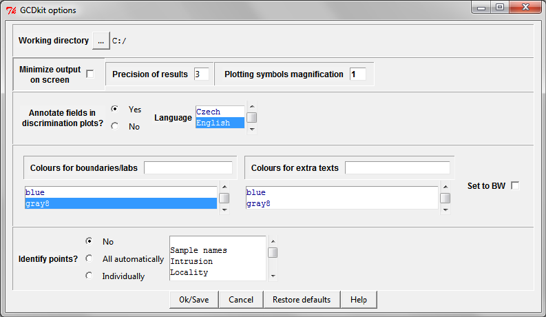
108 gcdOptions
Remaining options changed by GCDkit which cannot be altered via the GUI, though:
prompt "GCDkit-> "
windowsBuffered
FALSE
locatorBell FALSE
scipen 20
max.print 99999999
If necessary they can be set directly in the file ’gcdkit.xxx’.
Apart from that the GUI panel sets the variables data.dir (default data directory) and plt.col
(colours for Figaro-compatible plots).
Author(s)
Vojtech Janousek, <vojtech.janousek@geology.cz>
See Also
options identify ID figaro setCex
Examples
bak <- options() # backup the current options
options("gcd.ident"=1) # identify by sample names
options("gcd.ident.each"=FALSE) # to label by sample names automatically,
# i.e. without the user interference
plotDiagram("TAS",FALSE,FALSE)
options("gcd.ident"=0) # to turn off the identification completely
options("gcd.plot.bw"=TRUE) # to set the diagram to black and white
plotDiagram("TAS",FALSE,FALSE)

graphicsOff 109
options("gcd.cex"=2) # make the plotting symbols double as big
# (effective for the data files loaded from now on;
# for immediate result use the GUI front end)
getOption("gcd.plot.bw") # printing the current value of the given option
options(bak) # restore the previous options
graphicsOff Close all graphic windows
Description
Closes all graphic windows.
Usage
graphicsOff()
Arguments
None.
Details
Under Windows 95/98/ME, the R system may become install, failing to redraw graphical windows
if too many of them are being open. It is always a good idea to close the unnecessary ones, for
instance using this function.
See Also
’dev.off’
groupsByCluster Groups by cluster analysis
Description
Grouping the data using the cluster analysis.
Usage
groupsByCluster(elems=
"SiO2,TiO2,Al2O3,FeOt,MnO,MgO,CaO,Na2O,K2O",
method="ave")
Arguments
elems numerical columns to be used for cluster analysis, typically major elements
method the agglomeration method to be employed. This should be one of (or an unam-
biguous abbreviation thereof): 'ward','single','complete',
'average','mcquitty','median','centroid'.

110 groupsByDiagram
Details
After the dendrogram is drawn, the user is asked how many clusters is the dataset to be broken into.
The vector containing the information on the current groups can be appended to the data frame
’labels’.
The groups are initially numbered but this can be changed readily using the function editLabFactor.
For further details on the clustering algorithm, see the R manual entry of ’hclust’.
Value
groups character vector: the grouping information
grouping set to zero.
Author(s)
Vojtech Janousek, <vojtech.janousek@geology.cz>
See Also
classify groupsByLabel groupsByDiagram
groupsByDiagram Groups by diagram
Description
Grouping the data on a basis of selected classification diagram.
Usage
groupsByDiagram(fun = NULL, silent = TRUE)
Arguments
fun character; name of the classification function available in the system.
silent logical; should be echoed the information about classification each of the sam-
ples?
Value
groups character vector: the grouping information
grouping set to -1.
Author(s)
Vojtech Erban, <vojtech.erban@geology.cz>
Vojtech Janousek, <vojtech.janousek@geology.cz>

groupsByLabel 111
See Also
classify groupsByLabel groupsByCluster
AFM,PeceTaylor,Shand,NaAlK,TAS,Cox,TASMiddlemost,Jensen,Laroche,WinFloyd1,WinFloyd2,
DebonPQ,DebonBA,Middlemost,QAPF,OConnor Miyashiro Hastie Pearce1996 Villaseca
Examples
data(sazava)
accessVar("sazava")
groupsByDiagram("TASMiddlemostPlut") # Function called "TASMiddlemostPlut"
groupsByDiagram("^TAS$") # Function called "TAS"
groupsByLabel Groups by label
Description
Grouping the data according to the levels of a single label.
Usage
groupsByLabel(lab=NULL)
Arguments
lab name or sequence number of the label
Details
Sets the groups on the selected column within the data frame ’labels’. If not specified at the
function call, the appropriate label is selected by the function ’selectColumnLabel’.
Value
groups character vector: the grouping information
grouping the sequence number of the column in the data frame ’labels’ used for grouping
Author(s)
Vojtech Janousek, <vojtech.janousek@geology.cz>
See Also
classify groupsByCluster groupsByDiagram
Examples
data(sazava)
accessVar("sazava")
groupsByLabel("Intrusion")
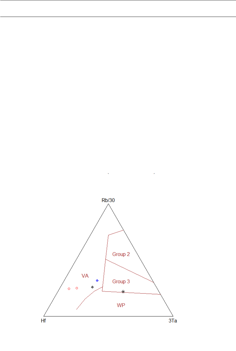
112 Harris
Harris Harris et al. (1986) Hf-Rb/30-Ta*3
Description
Assigns data for the Hf-Rb/30-Ta*3 ternary diagram of Harris et al. (1986) into Figaro template
(list ’sheet’) and appropriate values into ’x.data’ and ’y.data’.
Usage
Harris()
Details
Triangular diagram with apices Hf, Rb/30 and Ta*3, proposed by Harris et al. (1986) for classifi-
cation of collisional granites.
Following fields are defined:
VA Volcanic-Arc granites (Group 1, VA)
WP Within-Plate granites (Group 4, WP)
Group 2
Group 3

Hastie 113
Quoting from their abstract:
(i) Group 1 - Pre-collision calc-alkaline (volcanic-arc) intrusions which are mostly derived from
mantle modified by a subduction component and which are characterized by selective enrichments
in LIL elements.
(ii) Group 2 - Syn-collision peraluminous intrusions (leucogranies) which may be derived from the
hydrated bases of continental thrust sheets and which are characterized by high Rb/Zr and Ta/Nb
and low K/Rb ratios.
(iii) Group 3 - Late or post-collision calc-alkaline intrusions which may be derived from a mantle
source but undergo extensive crustal contamination and can only be distinguished from volcanic-arc
intrusions by their higher ratios of Ta/Hf and Ta/Zr.
(iv) Group 4 - Post-collision alkaline intrusions which may be derived from mantle lithosphere
beneath the collision zones and which carry high concentrations of both LIL and HFS elements.
Value
sheet list with Figaro Style Sheet data
x.data, y.data Th, Hf/3 and Ta in ppm recalculated into two dimensions
Author(s)
Vojtech Janousek, <vojtech.janousek@geology.cz>
References
Harris N B W, Pearce J A, Tindle A G (1986) Geochemical characteristics of collision-zone mag-
matism. In: Coward M P, Ries A C (eds) Collision Tectonics. Geological Society London Special
Publication 19, pp 67-81
See Also
figaro plotDiagram
Examples
#plot the diagram
plotDiagram("Harris", FALSE)
Hastie Co-Th diagram (Hastie et al. 2007)
Description
Assigns data for Co vs. Th (ppm) diagram into Figaro template (list ’sheet’) and appropriate values
into ’x.data’ and ’y.data’
Usage
Hastie()
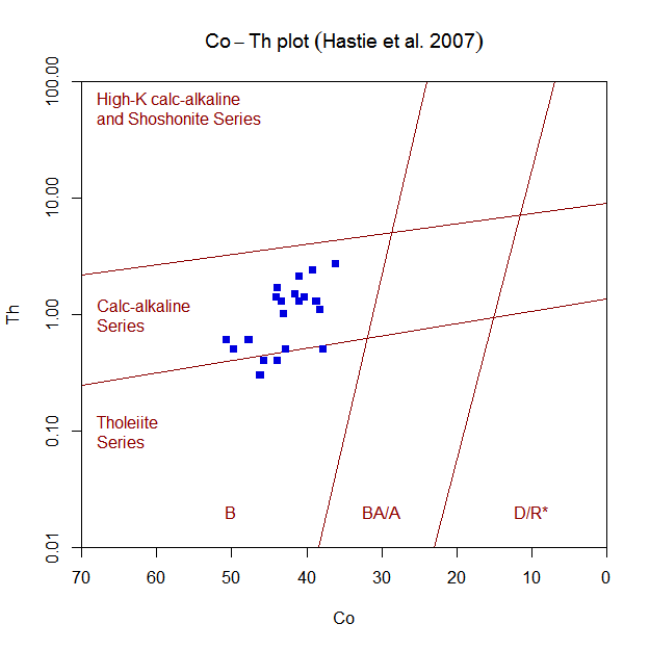
114 Hastie
Details
Diagram in Co vs. Th space, proposed by Hastie et al. (2007) for subdivision of volcanic arc
rocks. This is thought to be a more robust replacement for SiO2vs. K2Oplot of Peccerillo &
Taylor (1976) for altered/weathered volcanic rocks. The decreasing Co concentrations are used as
an index of fractionation (as a proxy for SiO2), the Th contents mimic those of K2O.
The following fields are defined:
Tholeiite Series
Calc-alkaline Series
High-K Calc-alkaline and Shoshonite Series
Rocks with composition falling beyond defined boundaries are labeled ’undefined’ by the ’classify’
function.
In addition, the diagram discriminates between the following rock types:
Abbreviation Full name
B basalt
BA/A basaltic andesite and andesite
D/R* dacite and rhyolite*
* latites and trachytes also fall in the D/R fields
Value
sheet list with Figaro Style Sheet data

Hollocher 115
x.data Co ppm
y.data Th ppm
Author(s)
Vojtech Janousek, <vojtech.janousek@geology.cz>
References
Hastie AR, Kerr AC, Pearce JA & Mitchell SF (2007) Classification of altered volcanic island arc
rocks using immobile trace elements: development of the Th-Co discrimination diagram. J Pet 48:
2341-2357 doi: 10.1093/petrology/egm062
Peccerillo A & Taylor S R (1976) Geochemistry of Eocene calc-alkaline volcanic rocks from the
Kastamonu area, Northern Turkey. Contrib Mineral Petrol 58: 63-81 doi: 10.1007/BF00384745
See Also
classify figaro plotDiagram
Examples
#Within GCDkit, the plot is called using following auxiliary functions:
#To Classify data stored in WR (Groups by diagram)
classify("Hastie")
#To plot data stored in WR or its subset (menu Classification)
plotDiagram("Hastie", FALSE)
Hollocher Hollocher et al. (2012) La/Yb vs. Nb/La or Th/Nb
Description
Assigns data for La/Yb vs. Nb/La or La/Yb vs. Th/Nb binary diagrams into Figaro template (list
’sheet’) and appropriate values into ’x.data’ and ’y.data’.
Usage
Hollocher1()
Hollocher2()
Arguments
None.
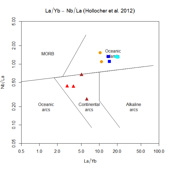
116 Hollocher
Details
The two binary plots, La/Yb vs. Nb/La and La/Yb vs. Th/Nb, of Hollocher et al. (2012) serve for
geotectonic discrimination of basalts or basaltic amphibolite units. These diagrams can distinguish
between the MORB, enriched ocean island basalts, and the near continuum defined by oceanic,
continental, and alkaline arcs.
However, the authors have noted that basalts from back-arc basins have a wide range of composi-
tions caused by basalt source region variation between depleted N-MORB, ocean-sland (hot spot),
and subduction component-enriched (sub-volcanic arc) mantle end members. See also their Fig.
16.
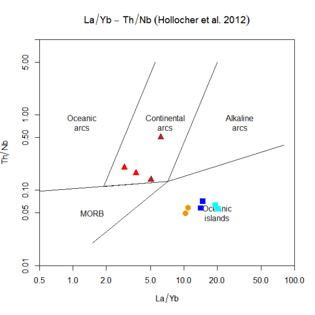
Hollocher 117
Value
sheet list with Figaro Style Sheet data
x.data x coordinates
y.data y coordinates
Author(s)
Vojtech Janousek, <vojtech.janousek@geology.cz>
References
Hollocher K, Robinson P, Walsh E, Roberts D (2012) Geochemistry of amphibolite-facies volcanics
and gabbros of the Storen Nappe in extensions west and southwest of Trondheim, western gneiss
region, Norway: a key to correlations and paleotectonic settings. Amer J Sci 312: 357-416 doi:
10.2475/04.2012.01
Coordinates and graph layout are taken from website of Kurt Hollocher.
See Also
figaro plotDiagram

118 ID
Examples
plotDiagram("Hollocher1",FALSE,TRUE)
plotDiagram("Hollocher2",FALSE,TRUE)
ID Sample identification
Description
Identification/labelling of individual data points on plots.
Usage
ID(x, y, labs = getOption("gcd.ident"), offset = 0.4,
col = "gray30", cex = 1)
Arguments
x, y vector with x-y coordinates of the data points
labs text to label individual data points, see details
offset distance (in char widths) between label and identified points.
col colour of the text
cex its size
Details
In GCDkit, the option ’ident’ determines whether the user wishes to identify data points on binary
and ternary plots. The default is zero, which means no identification.
If ’ident’ differs from zero, internal function ’ID’ can be invoked. Its parameter labs is either a
single number, or character vector.
In the former case, the variable ’labs’ contains either 1 (identification by sample name), or the
sequential number of the column in the data frame ’labels’ increased by one (identification by a
user- defined label).
Alternatively, a character vector labs can be used to specify the text directly.
Value
None.
Author(s)
Vojtech Janousek, <vojtech.janousek@geology.cz>
See Also
identify gcdOptions options
Examples
getOption("ident") # yields the current value of the given option

info 119
info Info on datafile
Description
Prints information about the current dataset (and its selected subset, if applicable).
Usage
info()
Details
This function prints comprehensive information about the current dataset. For each of the labels,
individual levels and their frequencies are given. The number of numeric columns is printed, and
for each of the variables number of available values. Moreover, the information concerning the
total number of samples, the names of the samples in the selected subset (or all samples if none is
defined) and the current grouping are shown.
Value
None
Author(s)
Vojtech Janousek, <vojtech.janousek@geology.cz>
isochron Rb-Sr and Sm-Nd isochrons
Description
Plots a Rb-Sr or Sm-Nd isochron diagram and calculates a simple linear fit to the selected data.
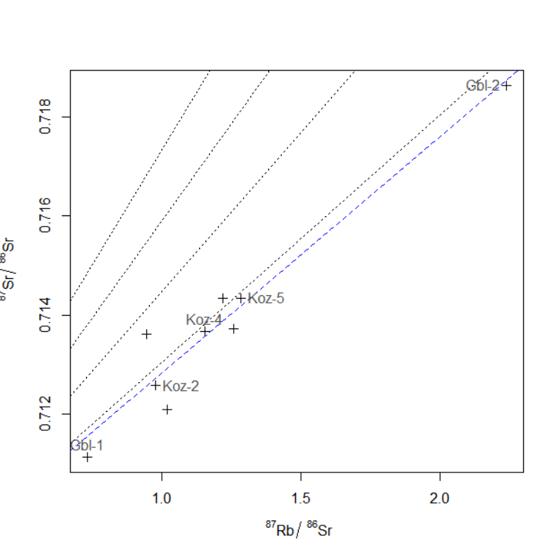
120 isochron
Usage
isochron()
Arguments
None.
Details
The samples can be selected based on combination of three searching mechanisms (by sample
name/label, range or a Boolean condition) - see selectSamples for details.
If empty list is given, all the samples for which the required isotopic data are available are plotted
and the user can choose their subset interactively. Then the isochron diagram is redrawn only with
those samples.
The data are fitted by simple least-squares linear fit, from which the age and initial ratio are calcu-
lated.

isocon 121
Value
Returns a numeric vector with the calculated age and initial ratio.
Plugin
SrNd.r
Author(s)
Vojtech Janousek, <vojtech.janousek@geology.cz>
isocon Isocon plots (Grant 1986)
Description
Implementation of isocon plot after Grant (1986, 2005) widely used for quantitative estimates of
changes in mass/volume/concentration of elements or oxides in course of various open-system geo-
chemical processes such as alteration or partial melting.
Usage
isocon(x = NULL, whichelems = NULL, immobile = NULL, atomic = FALSE, plot = TRUE)
isoconAtoms()
isoconOxides()
Arguments
xnumeric matrix with the chemical data
whichelems list of elements for plotting, separated by commas
immobile list of presumed immobile elements, separated by commas
atomic logical; should be atomic wt. % used for oxides?
plot logical; is the graphical output desirable?
Details
Isocon plot (Grant 1986, 2005) spans from the theoretical quantitative treatment of losses or gains
of geochemical species (elements or oxides). It is applicable to balancing mass, volume and/or con-
centration changes in course of open-system processes such as weathering, hydrothermal alteration,
metasomatic addition/leaching or migmatitization.
According to Grant (2005 and references therein) the equation for composition/volume changes in
open-system process can be written as:
cA
i=M0
MA(c0
i+ ∆ci)
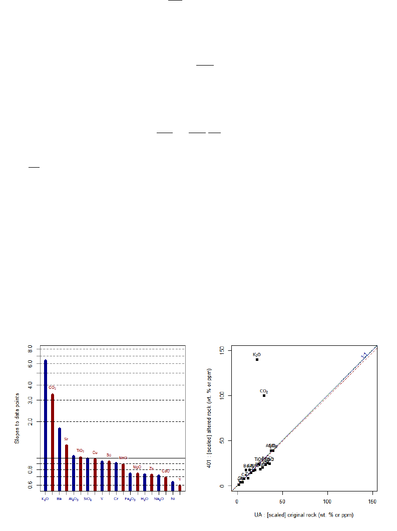
122 isocon
where ciis the concentration of the species i,0refers to the original rock and Ato the altered rock,
M0is the equivalent mass before and MAafter alteration.
For immobile element (∆ci= 0) the ratio M0
MAreflecting the overall change in mass can be obtained.
This can be done graphically in the plot of the analytical data for presumed protolith (c0
i) and altered
rock (cA
i). Such a straight line passing through the origin is termed isocon, the equation of which
is:
cA= ( M0
MA)c0
Species plotting above the isocon were gained, whereas those plotting below were lost, and the gain
or loss is according to Grant (2005):
∆ci
c0
i
=MA
M0
cA
i
c0
i−1
where cA
i
c0
i
is the slope of the tie line from the origin to the data point.
In the GCDkit’s implementation of the function 'isocon', firstly the parental and altered rock
samples are to be chosen interactively from a binary plot MgO −SiO2. Then the user is prompted
for the elements/oxides to be used in the isocon analysis. Printed and plotted in the form of barplots
are ordered slopes for each data point in the isocon diagram.
The user can choose the presumably immobile elements. These can be either provided as a comma
delimited list, or, if empty, chosen interactively from the isocon plot. Finally are plotted two isocons,
as well as a blue equiline (a straight line with the slope 1).
Implemented are two methods for assessing the change in mass of the system. Traditionally used
has been the slope of the isocon line, obtained by linear regression of the presumably immobile data
(dark green). However, this depends on the scaling of the isocon plot, which is arbitrary. In partic-
ular, the data plotted close to the origin may appear erroneously to lie on an isocon (Baumgartner
& Olsen, 1995).
More objectively, the change in the mass can be estimated by clustering slopes to data points, de-
ciphering the elements/oxides with a similar behaviour and averaging the slopes for the selected
presumably immobile species.
Functions ’isoconAtoms’ and ’isoconOxides’ are frontends to the function 'isocon', providing
different default values. See Arguments above.
isocon 123
Value
Returns a list ’results’ with the following components:
slope.avg slope of the isocon obtained as an average of the slopes for the individual pre-
sumably ’immobile’ species
slope.regression
slope obtained by linear regression
balance numeric matrix; balance of individual species. This matrix contains the follow-
ing columns:
XXX=orig. composition of the parental (unaltered) rock
XXX=alt. composition of the altered rock
Slope data point
slope of the line connecting the data point with origin
G/L rel.(LQ) relative mass gain/loss, isocon slope by least-squares fit
G/L rel.(avg) relative mass gain/loss, averaged slopes for immobile elements
G/L wt%/ppm(LQ)
absolute mass gain/loss, isocon slope by least-squares fit
G/L wt%/ppm(avg)
absolute mass gain/loss, averaged slopes for immobile elements
Plugin
Isocon.r
Author(s)
Vojtech Janousek, <vojtech.janousek@geology.cz>
References
Baumgartner L P & Olsen S N (1995). A least-squares approach to mass transport calculations
using the isocon method. Econ Geol 90: 1261-1270 doi: 10.2113/gsecongeo.90.5.1261
Grant J A (1986) The isocon diagram - a simple solution to Gresens equation for metasomatic
alteration. Econ Geol 81: 1976-1982 doi: 10.2113/gsecongeo.81.8.1976
Grant J A (2005) Isocon analysis: A brief review of the method and applications. Phys Chem Earth
(A) 30: 997-1004 doi: 10.1016/j.pce.2004.11.003
Gresens R L (1967) Composition-volume relationships of metasomatism. Chem Geol 2: 47-55
Examples
# Grant (2005) - see Tab. 1, Fig. 1
x<-matrix(c(46.45,1.29,14.30,11.05,0.17,5.28,12.14,2.93,0.49,3.00,3.29,42,327,
313,67,77,100,170,29,80,45.62,1.30,14.74,8.20,0.15,3.89,8.29,2.09,3.12,2.18,
10.96,39,305,282,42,75,72,214,17,140), byrow=TRUE,nrow=2)
y<-"SiO2,TiO2,Al2O3,Fe2O3,MnO,MgO,CaO,Na2O,K2O,H2O,CO2,Sc,V,Cr,Ni,Cu,Zn,Sr,Y,Ba"
colnames(x)<-unlist(strsplit(y,","))
rownames(x)<-c("UA","401")
isocon(x,y,atomic=FALSE,plot=TRUE,immobile="Al2O3,SiO2,TiO2,Cu,Sc")
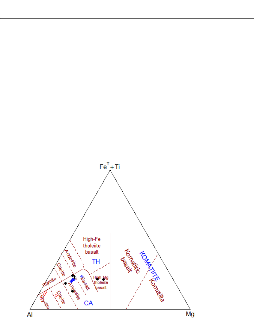
124 Jensen
isocon(x,y,atomic=TRUE,plot=FALSE)
Jensen Jensen cation plot (1976)
Description
Assigns data for Jensen’s cation plot into Figaro template (list ’sheet’) and appropriate values into
’x.data’ and ’y.data’.
Usage
Jensen()
Details
Jensen’s cation plot, proposed by Jensen (1976) and modified by Jensen & Pyke (1982). The trian-
gular diagram is defined on the basis of millications as follows:
left apex: Al
upper apex: F eT+T i
right apex: Mg
The diagram defines following rock series and names:
Komatiite series (KOMATIITE) Komatiite

joinGroups 125
Komatiitic basalt
Tholeiite series (TH) Rhyolite
Dacite
Andesite
High-Fe tholeiite basalt
High-Mg tholeiite basalt
Calc-alkaline series (CA) Rhyolite
Dacite
Andesite
Basalt
Value
x.data, y.data Values for the three apices transformed into 2D space
sheet list with Figaro Style Sheet data
Author(s)
Vojtech Erban, <vojtech.erban@geology.cz>
& Vojtech Janousek, <vojtech.janousek@geology.cz>
References
Grunsky E C (1981) An algorithm for the classification of subalkalic volcanic rocks using the Jensen
cation plot. In: Wood J, White O L, Barlow R B, Colvine A C (eds). Ontario Geological Survey,
Misc Pap 100, pp 61-65
Jensen L S (1976) A new cation plot for classifying subalkalic volcanic rocks. Ont Div Mines, Misc
Pap 66, 1-21
Jensen L S & Pyke D R (1982) Komatiites in the Ontario portion of the Abitibi belt. In: Arndt N T
& Nisbet E G (eds) Komatiites. Allen & Unwin, London
See Also
classify figaro plotDiagram
Examples
#plot the diagram
plotDiagram("Jensen", FALSE)
joinGroups Merge groups
Description
Enables merging several groups into a single one.
Usage
joinGroups()

126 Jung
Arguments
None.
Details
This function is the most useful to merge several groups, defined e.g. on the basis of a classification
plot. A simple spreadsheet is invoked with two columns, the first ('Old') containing the old levels
of groups and the second, 'New', which can be edited. Finally, groups with identical names will be
merged into a single one.
Optionally, the vector containing the information on the current groups can be appended to the data
frame ’labels’.
Value
groups character vector: the grouping information
grouping Sequential number of the column with grouping information in labels (if ap-
pended) or simply set to -100.
Author(s)
Vojtech Janousek, <vojtech.janousek@geology.cz>
Jung Al/Ti thermometer for granitic rocks (Jung + Pfänder 2007)
Description
This function estimates the temperature of a granitic magma based on measured Al2O3/T iO2ratio
and experimental constraints. The regression formulae were defined by Jung & Pfänder (2007).
Usage
Jung(model = NULL, plot = TRUE)
Arguments
model specification of the model
plot logical; should be shown a Al2O3/T iO2vs. CaO/Na2Oplot?
Details
As shown by Sylvester (1998), the Al2O3/T iO2ratio in the granitic magmas is temperature sen-
sitive, decreasing with the increasing temperature of the crustal anatexis. This probably reflects an
increasing instability of Ti-bearing phases with progressive crustal fusion.
Jung & Pfänder (2007) compiled the available experimental data and defined a set of regression
formulae (linear, power law and exponential) for several types of protoliths.
Any of the following models can be chosen: pelite melting, psammite melting, igneous rock melt-
ing, A-type granite melting, amphibolite melting after Rapp & Watson (1995) and amphibolite
melting after Patino Douce & Beard (1995).

Jung 127
Optionally, also Al2O3/T iO2vs. CaO/N a2Oplot could be displayed with three secondary axes
annotated by the calculated temperatures.
Value
Returns a matrix ’results’ with the following columns:
Al2O3/TiO2 wt. % ratio of Al2O3/T iO2
T_Al/Ti.power.C
temperature in C, power law calibration
T_Al/Ti.exp.C temperature in C, exponential calibration
T_Al/Ti.linear.C
temperature in C, linear calibration
T_Al/Ti.mean.C mean temperature in C, based on the above three models
Plugin
Jung.r

128 Laroche
Erratum
As pointed out by S. Jung (pers. com. 2009), in Table 1 of their original paper were printed wrongly
several of the regression coefficients. These are:
Rock Model Jung and Pfander (2007) Corrected
A-type power law B = 0.992 B = 9.921
amphibolite (Rapp and Watson 1995) power law A = 2.82x10^3 A = 2.82x10^30
The function implements these corrected values.
Author(s)
Vojtech Janousek, <vojtech.janousek@geology.cz>
References
Jung S, Pfänder J A (2007) Source composition and melting temperatures of orogenic granitoids:
constraints from CaO/Na2O,Al2O3/T iO2and accessory mineral saturation thermometry. Eur J
Mineral 19: 859-870 doi: 10.1127/0935-1221/2007/0019-1774
Patino Douce A E, Beard J S (1995) Dehydration-melting of biotite gneiss and quartz amphibolite
from 3 to 15 kbar. J Petrol 36: 707-738 doi: 10.1093/petrology/36.3.707
Rapp R P, Watson E B (1995) Dehydration melting of metabasalt at 8-32 kbar: implications for con-
tinental growth and crust-mantle recycling. J Petrol 36: 891-931 doi: 10.1093/petrology/36.4.891
Sylvester P J (1998) Post-collisional strongly peraluminous granites. Lithos 45: 29-44
doi: 10.1016/S0024-4937(98)00024-3
Examples
Jung()
Jung("A-type")
Jung("psammite",plot=FALSE)
Laroche R1-R2 diagram (De la Roche et al. 1980)
Description
Assigns data for the R1−R2diagram into Figaro template (list ’sheet’) and appropriate values
into ’x.data’ and ’y.data’.
Usage
LarocheVolc()
LarochePlut()
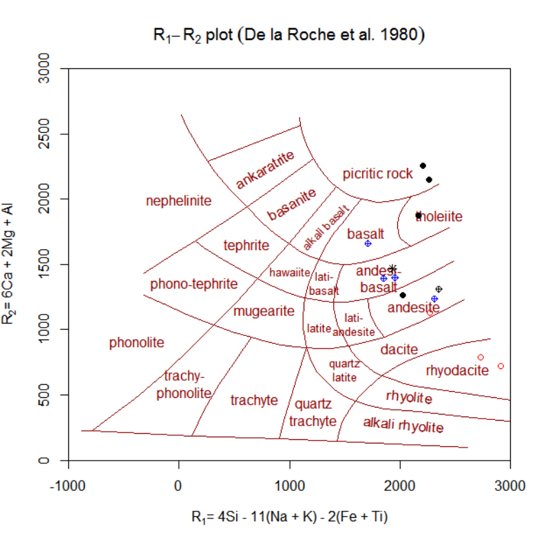
Laroche 129
Details
R1−R2plot, as proposed by De La Roche et al. (1980) for volcanic, as well as plutonic rocks.
volcanic rocks plutonic rocks
trachyphonolite nepheline syenite
phonolite nepheline syenite
phono-tephrite essexite
tephrite essexite
alkali rhyolite alkali granite
qtz.trachyte qtz.syenite
trachyte syenite
rhyolite granite
qtz.latite qtz.monzonite
rhyodacite granodiorite
dacite tonalite
andesite diorite
lati-andesite monzodiorite
latite monzonite
mugearite syenodiorite
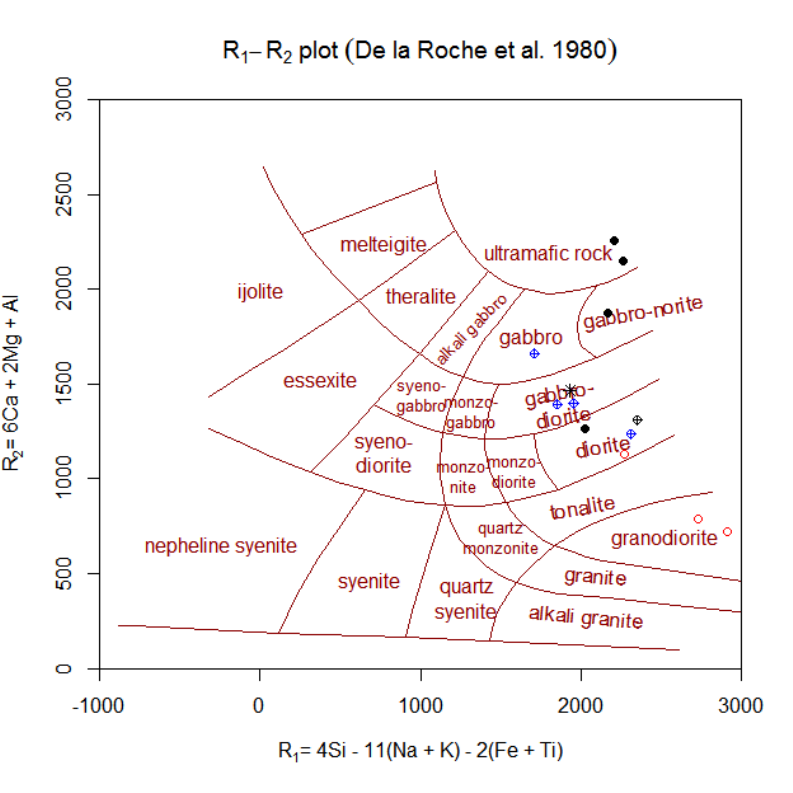
130 Laroche
nephelinite ijolite
andesi-basalt gabbro-diorite
lati-basalt monzogabbro
hawaiite syenogabbro
tholeiite gabbronorite
basalt gabbro
alkali basalt alkaligabbro
basanite theralite
ankaratrite melteigite
picritic rock ultramafic rock
Value
sheet list with Figaro Style Sheet data
x.data R1 = 4 * Si - 11 * (Na + K) - 2 * (Fe[total as bivalent] + Ti), all in millications;
as calculated by the function ’LaRocheCalc()’
y.data R2 = 6 * Ca + 2 * Mg + Al, all in millications; as calculated by the function
’LaRocheCalc()’

LaRocheCalc 131
Author(s)
Vojtech Erban, <vojtech.erban@geology.cz>
& Vojtech Janousek, <vojtech.janousek@geology.cz>
References
De La Roche H, Leterrier J, Grandclaude P, & Marchal M (1980) A classification of volcanic and
plutonic rocks using R1R2- diagram and major element analyses - its relationships with current
nomenclature. Chem Geol 29: 183-210 doi: 10.1016/0009-2541(80)90020-0
See Also
classify figaro LaRocheCalc millications plotDiagram
Examples
#Within GCDkit, the plot is called using following auxiliary functions:
#To classify data stored in WR (Groups by diagram)
classify("LarocheVolc")
#or
classify("LarochePlut")
#To plot data stored in WR or its subset (menu Classification)
plotDiagram("LarocheVolc", FALSE)
#or
plotDiagram("LarochePlut", FALSE)
LaRocheCalc Calculation: De la Roche
Description
Recalculates whole-rock data into R1−R2values of De La Roche et al. (1980).
Usage
LaRocheCalc(rock=WR)
Arguments
rock a numeric matrix with whole-rock data to be recalculated.
Details
R1−R2parameters, as proposed by De La Roche et al. (1980):
R1 = 4 * Si - 11 * (Na + K) - 2 * (Fe[total as bivalent] + Ti), all in millications R2 = 6 * Ca + 2 *
Mg + Al, all in millications
Value
results numeric matrix with the two above specified parameters

132 loadData
Author(s)
Vojtech Janousek, <vojtech.janousek@geology.cz>
References
De La Roche H, Leterrier J, Grandclaude P, & Marchal M (1980) A classification of volcanic and
plutonic rocks using R1R2- diagram and major element analyses - its relationships with current
nomenclature. Chem Geol 29: 183-210 doi: 10.1016/0009-2541(80)90020-0
See Also
LaRoche
loadData Loading data into GCDkit
Description
Loads data from a file (or, alternatively, a clipboard) into GCDkit. The files may contain plain text,
or, if library RODBC (has been installed, can be in the dBase III/IV (*.dbf), Excel (*.xls), Access
(*.mdb), PetroGraph (*.peg), IgPet or NewPet (*.roc) formats.
Usage
loadData(filename=NULL,separators = c("\t", ",", ";"," "),
na.strings = c("NA","-","bd", "b.d.", "bdl", "b.d.l.", "N.A.","n.d."),
clipboard = FALSE, merging = FALSE);
loadDataOdbc(filename=NULL,na.strings=c("NA","-", "bd",
"b.d.", "bdl", "b.d.l.", "N.A.","n.d."),merging=FALSE,
ODBC.choose=TRUE)
Arguments
filename fully qualified name of the file to be loaded, including suffix.
separators strings that should be tested as prospective delimiters separating individual items
in the data file.
na.strings strings that will be interpreted, together with empty items, zeros and negative
numbers, as missing values (NA).
clipboard logical; is clipboard to be read instead of a file?
merging logical; is the function invoked during merging of two data files?
ODBC.choose logical; if TRUE, ODBC channel can be chosen interactively.
loadData 133
Details
If library RODBC is available, the functions attempt to establish an ODBC connection to the se-
lected file, and open it as dBase III/IV (*.dbf), Excel (*.xls) or Access (*.mdb) format. The DBF
files are used to store data by other popular geochemical packages, such as IgPet (Carr, 1995) or
MinPet (Richard, 1995).
Another format that can be imported is *.csv. It is employed by geochemical database systems
such as GEOROC (http://georoc.mpch-mainz.gwdg.de/georoc/) and PETDB (http://www.
petdb.org/).
The import filter for the *.csv files has been tailored to keep the structure of these databases in mind.
The package PetroGraph (Petrelli et al. 2005) saves data into *.peg files that are also, in principle,
*.csv files compatible with the GCDkit.
Data files *.roc are yet another variant of *.csv files, used by NewPet (Clarke et al. 1994). This is
not to be confused with the *.roc format designed for IgPet (Carr, 1995). This is a text file with a
quite complex structure, whose import is still largely experimental. DBF files are to be preferred
for this purpose.
If not successful, the function ’loadData’ assumes that it is dealing with a simple text file.
On the other hand ’loadDataOdbc’ allows an ODBC channel to be specified interactively if
’ODBC.choose=TRUE’.
Plain text files can be delimited by tabs, commas or semicolons (the delimiter is recognized au-
tomatically). Alternative separators list can be specified by the optional ’separators’ parameter.
The Windows clipboard is just taken as a special kind of a tab-delimited text file.
In the text file, the first line contains names for the data columns (except for the first one that is
automatically assumed to contain the sample names); hence the first line may (or may not) have one
item less than the following ones. The data rows start with sample name and do not have to be all
of the same length (the rest of the row is filled by ’NA’ automatically).
Missing values (’NA’) are allowed anywhere in the data file (naturally apart from sample and column
names); any of 'NA','N.A.','-','b.d.','bd','b.d.l.','bdl'or 'n.d.'are also treated
as such, as specified by the parameter na.strings.
While loading, the values ’#WHATEVER!’ (Excel error messages) are also replaced by ’NA’ automat-
ically.
Please note that the function ’loadDataOdbc’, due to the current limitations of the RODBC package,
cannot handle correctly columns of mixed numeric and textual data. In such a column all textual
information is converted to 'NA'and this unfortunately concerns the sample names as well. If
encountering any problems, please use import from text file or via clipboard, which are much more
robust.
The negative numbers and values ’< x’ (used by some authors to indicate items below detection
limit) can be either replaced by their half (i.e. half of the detection limit) or ’NA’. User is prompted
which of these options he prefers.
Alternatively, the negative values can be viewed either as missing (’NA’) or can be imported, as may
be desirable for instance for stable isotope data in the delta notation.
Decimal commas, if present in text file, are converted to decimal points.
The data files can be practically freeform, i.e. no specified oxides/elements are required and no exact
order of these is to be adhered to. Analyses can contain as many numeric columns as necessary, the
names of oxides and trace elements are self-explanatory (e.g. "SiO2", "Fe2O3", "Rb", "Nd".
In the text files (or if pasting from clipboard), any line starting with the hash symbol ('#') is ignored
and can be used to introduce comments or to prevent the given analysis from loading temporarily.
134 loadData
Note that names of variables are case sensitive in R. However, any of the fully upper case names of
the oxides/elements that appear in the following list are translated automatically to the appropriate
capitalization:
SiO2, TiO2, Al2O3, Fe2O3, FeO, MnO, MgO, CaO, Na2O, FeOt, Fe2O3t,
Li2O, mg#, Ac, Ag, Al, As, At, Au, Ba, Be, Bi,
Br, Ca, Cd, Ce, Cl, Co, Cr, Cs, Cu, Dy, Er, Eu,
Fe, Ga, Gd, Ge, Hf, Hg, Ho, In, Ir, La, Li, Lu,
Mg, Mn, Mo, Na, Nb, Nd, Ne, Ni, Np, Os, Pa, Pb,
Pd, Pm, Pr, Pt, Pu, Rb, Re, Rh, Ru, S, Sb, Sc,
Se, Si, Sm, Sn, Sr, Ta, Tb, Te, Th, Ti, Tl, Tm,
Yb, Zn, Zr.
Total iron, if given, should be expressed either as ferrous oxide (’FeOt’, ’FeOT’, ’FeOtot’, ’FeOTOT’
or ’FeO*’) or ferric oxide (’Fe2O3t’, ’Fe2O3T’, ’Fe2O3tot’, ’Fe2O3TOT’ or ’Fe2O3*’).
Structurally bound water can be named 'H2O.PLUS','H2O+','H2OPLUS','H2OP'or ’H2O_PLUS’.
Upon loading, all the completely empty columns are removed first. Any non-numeric items found
in a data column with one of the names listed in the above dictionary are assumed to be typos and
replaced by ’NA’, after a warning appears. At the next stage all fully numeric data columns are
stored in a numeric data matrix ’WR’.
For any missing major- and minor-element data (SiO2, TiO2, Al2O3, Fe2O3, FeO, MnO, MgO,
CaO, Na2O, K2O, H2O.PLUS, CO2, P2O5, F, S), an empty (NA) column is created automatically.
The remaining, that is all at least partly textual data columns are transferred to the data frame
’labels’. To this are also attached a column whose name starts with ’Symbol’ (if any) that is
taken as containing plotting symbols and a column whose name is ’Colour’ or ’Color’(if any,
capitalization does not matter) that may contain plotting colours specification. The relative size of
the individual plotting symbols may be specified in a column named ’Size’ or ’cex’ that is also to
be attached to the ’labels’.
The plotting symbols can be given either by their code (see showSymbols) or directly as strings of
single characters.
The colours can be specified as codes (1-49) or English names (see showColours or type 'colours()'
into the Console window).
If specifications of the plotting symbols and colours are missing completely, and at least one non-
numeric variable is present, the user is prompted whether he does not want to have the symbols and
colours assigned automatically, from 1 to n, according to the levels of the selected label. Otherwise
default symbols (empty black circles) are used.
The default grouping is set on the basis of plotting symbols ’(labels$Symbol)’ or the data column
used to autoassign the plotting symbols and colours.
Lastly, a backup copy of the data is stored in the list ’WRCube’ using the function ’pokeDataset’.
It is stored either under the name of the file, or, if it already exists, under the file name with a time
stamp attached.
loadData 135
Value
WR numeric matrix: all numeric data
labels data frame: all at least partly character fields; labels$Symbol contains plotting
symbols and labels$Colour the plotting colours
The function prints a short summary about the loaded file. It also loads and executes the Plugins,
i.e. all the R code (*.r) that is currently stored in the subdirectory ’\Plugin’. Finally, the system
performs some recalculations (calling ’Gcdkit.r’).
Note
In order to ensure the database functionality, duplicated column (variable) names are not allowed.
This concerns, to a large extent, also the sample names. The only exception are CSV files - if
duplicated samples are found, sequence numbers are assigned instead.
All completely empty rows and columns in both labels and numeric data are ignored.
Author(s)
The RODBC package was written by Brian Ripley.
Vojtech Janousek, <vojtech.janousek@geology.cz>
References
Carr M (1995) Program IgPet. Terra Softa, Somerset, New Jersey, U.S.A.
Clarke D, Mengel F, Coish RA, Kosinowski MHF(1994) NewPet for DOS, version 94.01.07. De-
partment of Earth Sciences, Memorial University of Newfoundland, Canada.
Petrelli M, Poli G, Perugini D, Peccerillo A (2005) PetroGraph: A new software to visualize, model,
and present geochemical data in igneous petrology. Geochemistry Geophysics Geosystems 6: 1-15
Richard LR (1995) MinPet: Mineralogical and Petrological Data Processing System, Version 2.02.
MinPet Geological Software, Quebec, Canada.
See Also
’saveData’ ’mergeData’ ’pokeDataset’ ’showColours’ ’showSymbols’ ’read.table’ ’getwd’
’setwd’
Examples
# Sets the working path and loads the 'sazava'test data set
setwd(paste(gcdx.dir,"Test_data",sep="/"))
loadData("sazava.data")

136 Maniar
Maniar Maniar and Piccoli (1989)
Description
Plots data stored in ’WR’ (or its subset) into Maniar and Piccoli’s series of diagrams.
Usage
Maniar(plot.txt = getOption("gcd.plot.text"))
Arguments
plot.txt logical, annotate fields by their names?
Details
Collection of six binary diagrams, based on major elements chemistry, developed by Maniar &
Piccoli (1989) for tectonic discrimination of granitic rocks. Shand’s (1943) diagram is also used.
Diagrams are defined as follows:
x axis y axis
SiO2K2O
SiO2Al2O3
SiO2F eO(T)
(F eO(T)+M gO)
100∗MgO
(Al2O3+Na2O+K2O+F eO(T)+MgO)
100∗F eO(T)
(Al2O3+Na2O+K2O+F eO(T)+MgO)
M and F proportion in the AFM system
100∗CaO
(Al2O3+Na2O+K2O+F eO(T)+MgO+CaO)
100∗(F eO(T)+M gO)
(Al2O3+Na2O+K2O+F eO(T)+MgO+CaO)
C and F proportion in the ACF system
A/CNK (molar) A/NK (molar)
Abbreviations used in diagrams represent granitoids from following geotectonic environments:
IAG Island Arc Granitoids
CAG Continental Arc Granitoids
CCG Continental Collision Granitoids
POG Post-orogenic Granitoids
RRG Rift-related Granitoids
CEUG Continental Epeirogenic Uplift Granitoids
OP Oceanic Plagiogranites
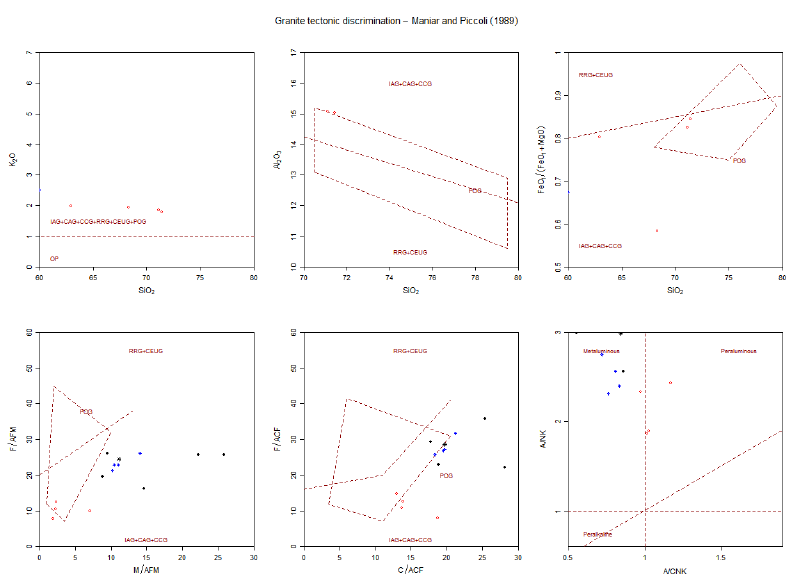
Maniar 137
Peralkaline, Metaluminous and Peraluminous rocks are defined in the last (Shand’s) diagram.
Note
This function uses the plates concept. The individual plots can be selected and their proper-
ties/appearance changed as if they were stand alone Figaro-compatible plots.
See Plate,Plate editing and figaro for details.
Author(s)
Vojtech Janousek, <vojtech.janousek@geology.cz>
References
Maniar P D & Piccoli P M (1989) Tectonic discriminations of granitoids. Geol Soc Amer Bull 101:
635-643. doi: 10.1130/0016-7606(1989)101<0635:TDOG>2.3.CO;2
Shand (1943) Eruptive Rocks. John Wiley & Sons.
See Also
Plate,Plate editing,figaro,plotPlate,
Examples
#plot the diagrams
plotPlate("Maniar")

138 mergeData
mergeData Appending data to a current data set
Description
These functions append new data to the analyses currently stored in the memory of the GCDkit.
Usage
mergeDataRows()
mergeDataCols(all.rows=NULL)
Arguments
all.rows logical; should be all samples preserved, even those missing in one of the datasets
?
Details
The function ’mergeDataRows’ appends new samples (i.e. new rows). The structures of both
datafiles are, as much as possible, matched against each other, and, if necessary, new empty columns
are introduced to the original data file, if they are missing. If any duplicated sample names are found,
they are replaced by sequence numbers and a new column ’old.ID’ is appended to the labels. Also
appended is a column named ’file’ containing the name of the file the particular sample originated
from.
’mergeDataCols’ adds new data (i.e. new data columns) to the samples stored in the memory. If
desired (’all.rows’ is ’TRUE’), included are also samples that occur solely in one of the files.
For the guidelines on correct formatting of the data files see loadData.
Value
WR numeric matrix: all numeric data
labels data frame: all at least partly character fields; labels$Symbol contains plotting
symbols and labels$Colour the plotting colours
The function prints a short summary about the loaded file.
Author(s)
Vojtech Janousek, <vojtech.janousek@geology.cz>
See Also
’loadData’ ’saveData’ ’merge’
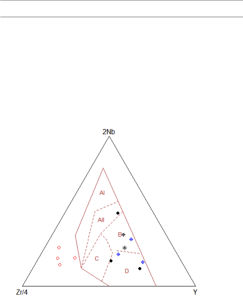
Meschede 139
Meschede Meschede (1986) Zr/4-2Nb-Y
Description
Assigns data for a Meschede’s (1986) triangular diagram into Figaro template (list ’sheet’) and
appropriate values into ’x.data’ and ’y.data’.
Usage
Meschede()
Details
Triangular diagram with apices Zr/4, 2Nb and Y, proposed by Meschede (1986). The plot serves
primarily for tectonic discrimination of tholeiitic basalts.
Abbreviations used in diagram represent following geotectonic settings:
AI-AII Within-Plate Alkaline Basalts
AII-C Within-Plate Tholeiites
BP-type Mid-Ocean Ridge Basalts
DN-type Mid-Ocean Ridge Basalts
C-D Volcanic Arc Basalts

140 Mesonorm
Value
sheet list with Figaro Style Sheet data
x.data, y.data Zr/4, 2Nb and Y values recalculated into two dimensions
Author(s)
Vojtech Janousek, <vojtech.janousek@geology.cz>
References
Meschede M (1986) A method of discriminating between different types of mid-ocean ridge basalts
and continental tholeiites with the Nb-Zr-Y diagram. Chem Geol 56: 207-218 doi: 10.1016/0009-
2541(86)90004-5
See Also
figaro plotDiagram
Examples
#plot the diagram
plotDiagram("Meschede",FALSE)
Mesonorm Improved Mesonorm for granitoid rocks
Description
Calculates eine bessere Mesonorm for granitoids of Mielke & Winkler (1979).
Usage
Mesonorm(WR, GUI = FALSE, precision = getOption("gcd.digits"))
Streckeisen(x, new = TRUE)
Arguments
WR a numerical matrix; the whole-rock data to be normalized.
GUI logical, is the function called from the GUI?
precision precision of the result.
xNormative minerals calculated by the function Mesonorm.
new logical, is a new plotting window to be opened?
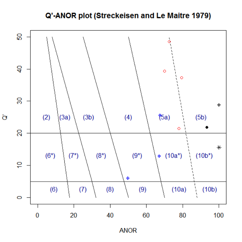
Mesonorm 141
Details
This method of norm calculation should yield mineral proportions close to the actual mode of
granitoid rocks. The calculated components are:
Orthoclase, Albite, Anorthite, Quartz, Apatite, Magnetite,
Hematite, Ilmenite, Biotite, Amphibole, Calcite, Corundum,
Rest
If desired, the function plots Q’-ANOR diagram of Streckeisen & Le Maitre (1979) using the func-
tion Streckeisen. The fields in this diagram are labeled as follows:
2 alkali feldspar granite
3 granite
4 granodiorite
5 tonalite
6* quartz alkali feldspar syenite
7* quartz syenite
8* quartz monzonite
9* quartz monzodiorite/quartz monzogabbro

142 Middlemost
10* quartz diorite/quartz gabbro
6 alkali feldspar syenite
7 syenite
8 monzonite
9 monzodiorite/monzogabbro
10 diorite/gabbro
Value
A numeric matrix ’results’.
Author(s)
Vojtech Janousek, <vojtech.janousek@geology.cz>
& Vojtech Erban, <vojtech.erban@geology.cz>
References
Mielke P & Winkler H G F (1979) Eine bessere Berechnung der Mesonorm fuer granitische Gesteine.
Neu Jb Mineral, Mh 471-480
Streckeisen, A. & Le Maitre, R. W. (1979) A chemical approximation to the modal QAPF classifi-
cation of the igneous rocks. Neu Jb Mineral, Abh 136, 169-206.
Middlemost Middlemost’s diagram (1985)
Description
Assigns data for Middlemost’s diagram into Figaro template (list ’sheet’) and appropriate values
into ’x.data’ and ’y.data’.
Usage
MiddlemostPlut()
Details
Classification diagram, as proposed by Middlemost (1985) for plutonic rocks.
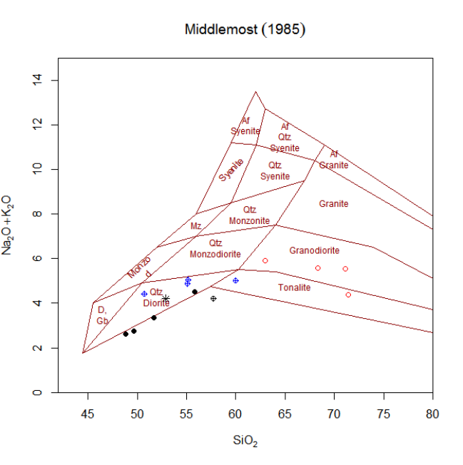
Middlemost 143
Value
sheet list with Figaro Style Sheet data
x.data SiO2 weight percent
y.data Na2O+K2O weight percent
results matrix with classification results
groups vector with classification results
grouping set to -1
Author(s)
Vojtech Erban, <vojtech.erban@geology.cz>
& Vojtech Janousek, <vojtech.janousek@geology.cz>
References
Middlemost E A K (1985) Magmas and Magmatic Rocks. Longman, London
See Also
classify figaro plotDiagram

144 millications
Examples
#Within GCDkit, the plot is called using following auxiliary functions:
#To classify data stored in WR (Groups by diagram)
classify("MiddlemostPlut")
#To plot data stored in WR or its subset (menu Classification)
plotDiagram("MiddlemostPlut", FALSE)
millications Millications
Description
Returns millications.
Usage
millications(x,print=FALSE,save=FALSE)
Arguments
xmatrix or vector with major-element data
print logical: print the result?
save logical: should be the results assigned globally?
Details
The millications are used for many plots of the French school, e.g. De la Roche et al. (1980) or
Debon & Le Fort (1983, 1988).
The calculated values are Si, Ti, Al, Fe3, Fe2, Fe, Mn, Mg, Ca, Na, K, P.
Elementi= 1000 Oxidei(wt.%)
MW (Oxidei)) ∗x(Elementi)
Where: MW = molecularWeight of the Oxide[i], x = number of atoms of Element[i] in its formula
Value
Numeric matrix (or vector) with the millications. If ’save=TRUE’, ’results’ and ’milli’ are as-
signed globally.
Author(s)
Vojtech Janousek, <vojtech.janousek@geology.cz>
References
De La Roche H, Leterrier J, Grandclaude P, & Marchal M (1980) A classification of volcanic and
plutonic rocks using R1R2- diagram and major element analyses - its relationships with current
nomenclature. Chem Geol 29: 183-210
Debon F & Le Fort P (1988) A cationic classification of common plutonic rocks and their magmatic
associations: principles, method, applications. Bull Mineral 111: 493-510
Debon F & Le Fort P (1983) A chemical-mineralogical classification of common plutonic rocks
and associations. Trans Roy Soc Edinb, Earth Sci 73: 135-149

mins2deg 145
mins2deg Recasts degrees and minutes to degrees (with decimal places).
Description
The functions serves to recast strings in the form 48°53.6814’ to decimal values in degrees. As
separators are used the ’degree’ sign (unicode + 00B0) and apostrophe, respectively. There are no
spaces.
Usage
mins2deg(x="Easting",varname="XX")
Arguments
xa text string, to be interpreted directly, or a colname of variable in ’labels’
varname a name of a numeric variable in ’WR’ to store the recalculated output
Value
Returns, invisibly, the converted numbers. Appends the recalculated coordinate to the data matrix
’WR’.
Author(s)
Vojtech Janousek, <vojtech.janousek@geology.cz>
Examples
data(sazava)
accessVar("sazava")
WR<-WR[1:5,]
x<-c("48°53.6814'","48°53.6814'","48°53.6814'","48°53.6814'","48°53.6814'")
mins2deg(x,"E")
Misc Miscellaneous geochemical indexes
Description
Calculates a series of useful geochemical indexes.
Usage
Misc(WR)
Arguments
WR a numerical matrix; the whole-rock data to be recalculated.

146 Miyashiro
Details
Various petrochemical indexes are calculated, such as:
• total iron as F e2O3
•F e2O3/FeO, Na2O/K2Oand K2O/N a2Oratios
• Larsen’s DI - Differentiation index (Larsen 1938)
• Kuno’s SI - Solidification index (Kuno 1959)
• Agpaitic index (Ussing 1912)
Value
A numeric matrix ’results’.
Author(s)
Vojtech Janousek, <vojtech.janousek@geology.cz>
References
Kuno H (1959) Origin of Cenozoic petrographic provinces of Japan and surrounding
provinces. Bull Volcanol 20: 37-76
Larsen E S (1938) Some new variation diagrams for groups of igneous rocks. J Geol 46: 505-520
Sorensen H (1997) The agpaitic rocks; an overview. Min Mag 61: 485-498
Ussing N V (1912) Geology of the country around Sulianehaab, Greenland. Meddr Grolnland, 38:
1-426
Miyashiro SiO2-FeOt/MgO diagram (Miyashiro 1974)
Description
Assigns data for SiO2vs. F eOt/MgO diagram into Figaro template (list ’sheet’) and appropriate
values into ’x.data’ and ’y.data’
Usage
Miyashiro()
Details
Diagram in SiO2vs. F eOt/MgO space, proposed by Miyashiro (1974), defines the following
fields:
Tholeiite Series
Calc-alkaline Series
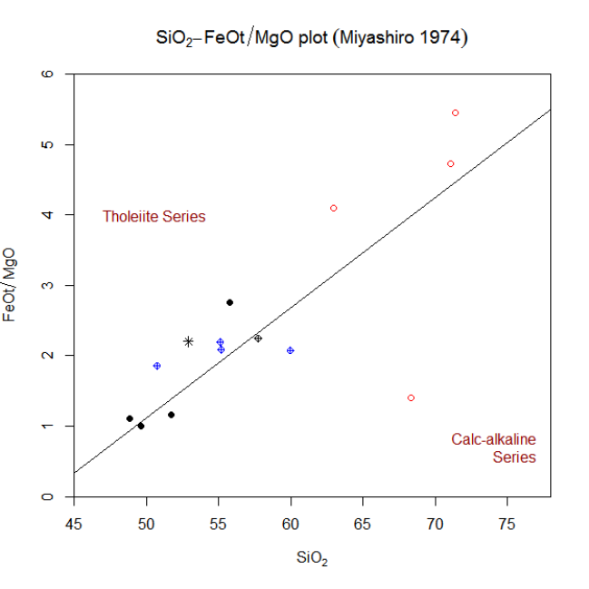
Miyashiro 147
As the boundary was defined by Akiho Miyashiro as straight line passing through two specific
points, no limits of diagram validity for ultrabasic and high-silica rocks were given. Thus, the
boundary implemented in GCDkit script spreads from F eOt/MgO = 0 to SiO2= 100%.
Value
sheet list with Figaro Style Sheet data
x.data SiO2 weight percent
y.data FeOt/MgO weight percent
Author(s)
Vojtech Erban, <vojtech.erban@geology.cz>
& Vojtech Janousek, <vojtech.janousek@geology.cz>
References
Miyashiro A (1974) Volcanic rock series in island arcs and active continental margins. Am J Sci
274, 321-355. doi: 10.2475/ajs.274.4.321
See Also
classify figaro plotDiagram

148 Mode
Examples
#Within GCDkit, the plot is called using following auxiliary functions:
#To Classify data stored in WR (Groups by diagram)
classify("Miyashiro")
#To plot data stored in WR or its subset (menu Classification)
plotDiagram("Miyashiro", FALSE)
Mode Approximating the mode by least-squares method
Description
The functions ’Mode’ and ’ModeC’ calculate the best approximations of the mode given major-
element compositions of the rock and its main mineral constituents. Function ’WRComp’ does the
opposite, i.e. yields the whole-rock composition given the chemistry of individual minerals and
their modal proportions.
Usage
ModeMain(WR,sample.id="",select.oxides=TRUE,select.minerals=TRUE)
Mode(rock, mins,sample.id="")
ModeC(rock, mins,sample.id="")
ModeAll(WR)
WRComp(mins, f)
Arguments
WR a numerical matrix; the whole-rock data to be normalized.
rock whole-rock composition of the given sample.
sample.id (optional) sample name.
select.oxides (logical) should be selected oxides used for calculation?
select.minerals
(logical) should be selected minerals used for calculation?
mins composition of its main rock-forming minerals.
ftheir modal proportions.
Details
’Mode’ uses unconstrained least-squares method taking advantage of the standard R function
’lsfit(mins,rock,intercept=F)’. It produces results that generally do not sum up to 100 % due
to the presence of elements not used in calculation (such as water), and, or, analytical noise.
’ModeC’ is the constrained variation whose output ought to sum up to 100 % by definition (Albarede
1995). As such it seems to be more appropriate in most applications.
In both cases, the printed output involves the input data, calculated modal proportions of the indi-
vidual minerals, the calculated composition of the rock (using the auxiliary function ’WRComp’) and
differences between the approximated and the real data (residuals).
The sum of squared residuals is a measure of fit (as a rough guide it should be less than ca. 1).
Mode 149
The mineral compositions are provided by a tab-delimited ASCII file, whose first row contains the
names of the determined oxides, the following ones start with the mineral abbreviation and the
numeric data (hence the first row has one item less than the following ones).
’ModeMain’ is entry point to both ’Mode’ and ’ModeC’ that enables the user to read the mineral data
file, select the oxides and minerals to be used in the calculation.
The options ’select.oxides=FALSE’ and ’select.minerals=FALSE’ read the mineral file in its
entirety, using all minerals and oxides present.
’ModeAll’ is a front end that performs the constrained least squares calculation for samples specified
by the function selectSamples.
Value
’ModeMain’, ’Mode’ and ’ModeC’ return a list with two items. The first of them (’table’) is a matrix
with the real composition of the rock and its minerals, the calculated whole-rock composition and
the residuals. The second (’(un)constrained’) returns calculated mineral proportions and sum of
squared residuals.
’ModeAll’ returns a simple matrix listing, for each rock sample, calculated proportions of rock-
forming minerals and the sum of squared residuals.
’WRComp’ yields a vector with the calculated whole-rock composition.
Author(s)
Vojtech Janousek, <vojtech.janousek@geology.cz>
References
Albarede F (1995) Introduction to Geochemical Modeling. Cambridge University Press, Cam-
bridge, p. 1-543
See Also
For example of the mineral data, see file ’Test_data\sazava mins.data’.
Examples
# Albarede (1995) - page 7
# Calculate WRComposition of olivine gabbro containing 40 % olivine,
# 30 % diopside and 30 % plagioclase.
mins<-matrix(c(40.01,0.00,14.35,45.64,0.00,0.00,54.69,0.00,3.27,16.51,
25.52,0.00,48.07,33.37,0.00,0.00,16.31,2.25),3,6,byrow=TRUE)
rownames(mins)<-c("ol","di","plg")
colnames(mins)<-c("SiO2","Al2O3","FeO","MgO","CaO","Na2O")
print(mins)
f<-c(0.4,0.3,0.3)
names(f)<-c("ol","di","plg")
print(f)
rock<-WRComp(mins,f)
print(rock)
# Reverse
mode1<-Mode(rock,mins)

150 Molecular weights
mode2<-ModeC(rock,mins)
Molecular weights Calculating molecularWeights of oxides
Description
These functions plot multiple binary plots with a common x axis, such as Harker plots.
Usage
molecularWeight(formula)
Arguments
formula a character vector of length 1, a formula of the oxide.
Details
So far only simple oxide formulae in form of AxOy(where x, y are optional indexes) can be
handled. The atomic weights are stored in a file MW.data. The atomic weights come from official
CIAAW web site http://www.ciaaw.org.
Value
A list with items:
MW molecularWeight
x.atoms number of atoms in the formula
x.oxygen number of oxygens
Author(s)
Vojtech Janousek, <vojtech.janousek@geology.cz> Vojtech Erban, <vojtech.erban@geology.cz>
References
Commission on Isotopic Abundances and Atomic Weights (CIAAW) of the International Union of
Pure and Applied Chemistry. Accessed on January 8, 2016, at http://www.ciaaw.org
Examples
molecularWeight("SiO2")
molecularWeight("SiO2")[[1]]
oxides<-c("SiO2","TiO2","Al2O3","Fe2O3","FeO")
sapply(oxides,molecularWeight)
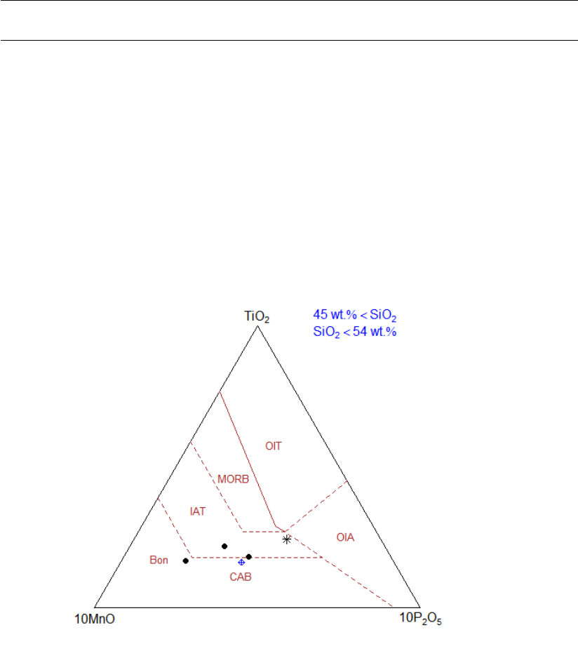
Mullen 151
Mullen Mullen (1983) 10MnO-TiO2-10P2O5
Description
Assigns data for the diagram of Mullen (1983) into Figaro template (list ’sheet’) and appropriate
values into ’x.data’ and ’y.data’.
Usage
Mullen()
Details
Triangular diagram with apices 10MnO, T iO2and 10P2O5, proposed by Mullen (1983).
Abbreviations used in diagram represent following geotectonic settings:
CAB Calc-Alkaline Basalts
IAT Island Arc Tholeiites
MORB Mid-Ocean Ridge Basalts
OIA Ocean Island Andesites
OIT Ocean Island Tholeiites

152 MullerK
Value
sheet list with Figaro Style Sheet data
x.data, y.data 10MnO, T iO2and 10P2O5in wt. % recalculated to 2D
Author(s)
Vojtech Janousek, <vojtech.janousek@geology.cz>
References
Mullen E D (1983) MnO/T iO2/P2O5: a minor element discriminant for basaltic rocks of oceanic
environments and its implications for petrogenesis. Earth Planet Sci Lett 62: 53-62 doi: 10.1016/0012-
821X(83)90070-5
See Also
figaro plotDiagram
Examples
#plot the diagram
plotDiagram("Mullen",FALSE)
MullerK Muller et al. (1992) potassic igneous rocks discrimination
Description
Assigns Figaro templates to geotectonic diagrams for potassic igneous rocks of Müller et al. (1992)
into the list ’plate’) and appropriate values into the list ’plate.data’ for subsequent plotting.
Usage
MullerKbinary(plot.txt=getOption("gcd.plot.text"))
MullerKternary(plot.txt=getOption("gcd.plot.text"))
Arguments
plot.txt logical, annotate fields by their names?
Details
Suite of binary and ternary diagrams for discrimination of geotectonic environment of potassic ig-
neous rocks, proposed by Müller et al. (1992) and Müller & Groves (1995). Following geotectonic
settings may be deduced:
Abbreviation used Environment
CAP Continental Arc
PAP Postcollisonal Arc
IOP Initial Oceanic Arc
LOP Late Oceanic Arc
WIP Within Plate
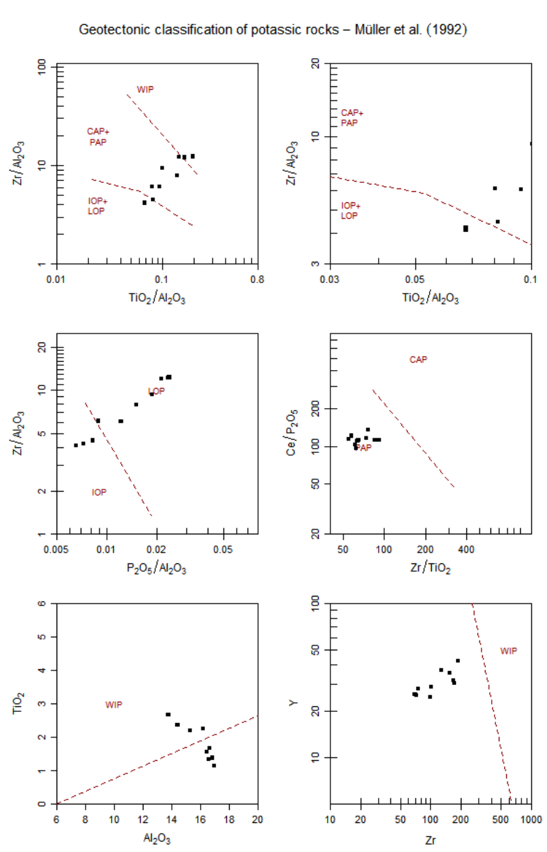
MullerK 153
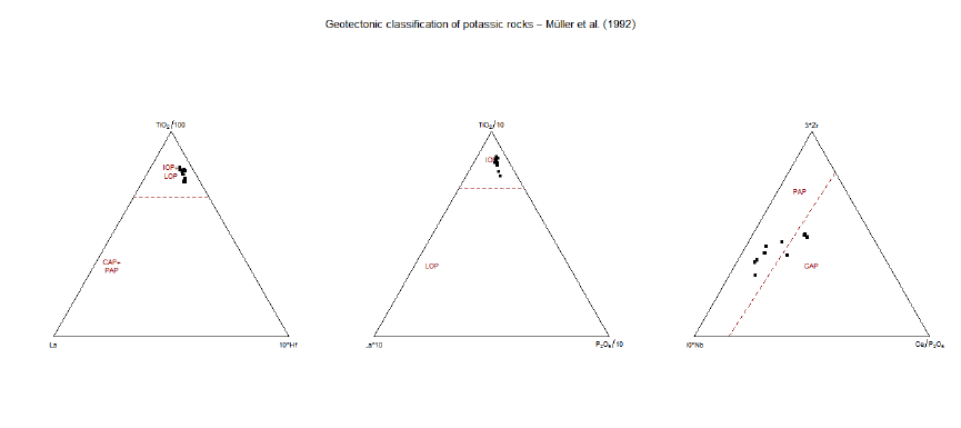
154 MullerK
Note
This function uses the plates concept. The individual plots can be selected and their proper-
ties/appearance changed as if they were stand alone Figaro-compatible plots. See Plate,Plate editing
and figaro for details.
Author(s)
Vojtˇ
ech Janoušek, <vojtech.janousek@geology.cz>
References
Müller D, Rock NMS, Groves DI (1992) Geochemical discrimination between shoshonitic and
potassic volcanic rocks in different tectonic settings: a pilot study. Mineral Petrol 46: 259-289
doi:10.1007/BF01173568
Müller D, Groves DI (1995) Potassic Igneous Rocks and Associated Gold-Copper Mineralization.
Springer, Berlin, pp 1-210
See Also
Plate,Plate editing,plotPlate,figaro
Examples
plotPlate("MullerKbinary")
plotPlate("MullerKternary")

Multiple plots 155
Multiple plots Multiple binary plots
Description
These functions plot multiple binary plots with a common x axis, such as Harker plots.
Usage
multiple(x,y=paste(colnames(WR),sep=","),
samples=rownames(WR),pch=labels$Symbol,
col=labels$Colour,xmin=NULL,xmax=NULL,GUI=FALSE,nrow=NULL,ncol=NULL,...)
multipleMjr(x = "",
y = "SiO2,TiO2,Al2O3,FeOt,MgO,CaO,Na2O,K2O,P2O5",
pch = labels$Symbol, col = labels$Colour, ...)
multipleTrc(x = "",
y = "Rb,Sr,Ba,Cr,Ni,La,Ce,Y,Zr,mg#,A/CNK,K2O/Na2O",
pch = labels$Symbol, col = labels$Colour, ...)
Arguments
xa character vector, name of the common x axis. Formulae are OK.
ya character vector, names of oxides/elements to be plotted as y axes separated
by commas. Formulae are OK.
nrow, ncol dimensions of the plots’ matrix
samples character or numeric vector; specification of the samples to be plotted.
pch plotting symbols.
col plotting colours.
xmin, xmax minimum and maximum for the x axis.
GUI logical; is the call being made from within GCDkit GUI or not?
... further graphical parameters: see ’help(par) for details.
Details
If x axis occurs among the arguments to be plotted as y axes, it is skipped.
Functions ’multipleMjr’ and ’multipleTrc’ are entry points supplying the default lists for major-
and trace elements.
Even though as a default is assumed a list of major (SiO2, TiO2, Al2O3, FeOt, MnO, MgO, CaO,
Na2O, K2O) or trace (Rb, Sr, Ba, Cr, Ni, La, Ce, Y,Zr and mg#) elements, the variable(s)
to be displayed can be specified.
The easiest way is to type directly the names of the columns, separated by commas. Alternatively
can be used their sequence numbers or ranges. Also built-in lists can be employed, such as ’LILE’,
’REE’, ’major’ and ’HFSE’ or their combinations with the column names.
These lists are simple character vectors, and additional ones can be built by the user (see Exam-
ples). Note that currently only a single, stand-alone, user-defined list can be employed as a search
criterion.
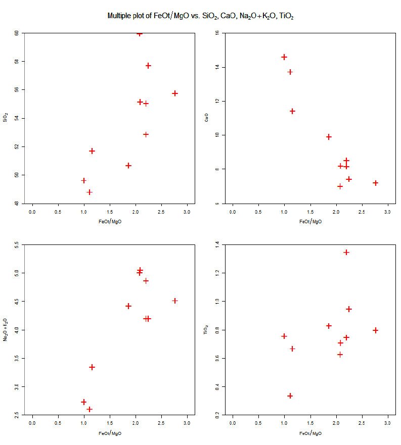
156 Multiple plots
In the specification of the x axis or any of the y axes can be used also arithmetic expressions, see
calcCore for the correct syntax.
Lastly, the user is asked to enter the limits for the x axis, two numbers separated by a comma.
Note that the scaling takes into account the size of the plotting symbols, i.e. the axes are extended
somewhat.
Value
None.
Note
This function uses the plates concept. The individual plots can be selected and their proper-
ties/appearance changed as if they were stand alone Figaro-compatible plots. See Plate,Plate editing
and figaro for details.

mzSaturation 157
Author(s)
Vojtech Janousek, <vojtech.janousek@geology.cz>
See Also
figaro,Plate,Plate editing
Examples
multipleMjr("SiO2")
multiple("Na2O+K2O",LILE,xmin=0)
# Plots the LILE against the sum of alkalis
multiple("FeOt/MgO","SiO2,CaO,Na2O+K2O,TiO2",pch="+",col="red",samples=1:10,cex=2.5)
multipleTrc("Zr")
# Plots the default trace-element set against the Zr
mzSaturation Monazite saturation (Montel 1993)
Description
Calculates monazite saturation temperatures for given major-element compositions and LREE con-
tents of the magma.
Usage
mzSaturation(cats = milli,
REE = filterOut(WR, c("La", "Ce", "Pr","Nd","Sm", "Gd"), 1),
H2O = 3, Xmz = 0)
Arguments
cats numeric matrix; whole-rock data recast to millications
REE numeric matrix with LREE concentrations - only complete set of La-Gd
H2O assumed water contents of the magma
Xmz mole fractions of the REE-phosphates in monazite
Details
This function uses saturation model of Montel (1993). The formulae are as follows:
LREE =P(REEi
at.weight(REEi))
Xmz
where REEi: La, Ce, Pr, Nd, Sm, Gd.
Dmz = 100N a +K+ 2Ca
Al .1
Al +Si
T mz.sat.C =13318
9.5+2.34Dmz + 0.3879√H2O−ln(LREE)−273.15

158 NaAlK
Value
Returns a matrix ’results’ with the following components:
Dmz distribution coefficient
Tmz.sat.C monazite saturation temperature in °C
Plugin
Saturation.r
Author(s)
Vojtˇ
ech Janoušek, <vojtech.janousek@geology.cz>
References
Montel JM (1993) A model for monazite/melt equilibrium and application to the generation of
granitic magmas. Chem Geol 110: 127-146 doi: 10.1016/0009-2541(93)90250-M
NaAlK Na2O - Al2O3 - K2O (mol. %) diagram
Description
Assigns data for ternary diagram Na2O-Al2O3-K2O(mol. %) into Figaro template (list ’sheet’)
and appropriate values into ’x.data’ and ’y.data’. Calculates molar concentrations of alkalis and
alumina, as well as several molar ratios involving these three oxides.
Usage
NaAlK()
Details
Ternary plot Na2O-Al2O3-K2O(mol. %). Dashed lines define the following compositional
fields (all oxides are expressed in mol. %):
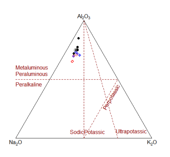
NaAlK 159
peraluminous + metaluminous (Shand 1943) (N a2O+K2O)/Al2O3<1
peralkaline (Shand 1943) (Na2O+K2O)/Al2O3>1
perpotassic K2O/Al2O3>1andK2O/Na2O > 1
potassic 1< K2O/Na2O < 3
ultrapotassic K2O/Na2O >= 3
The molar ratio of K2O/Na2O>= 3, is equivalent to K2O/Na2O>= 2 in wt. %, i.e. to the
definition of ultrapotassic igneous rocks by Foley et al. (1987).
Value
sheet list with Figaro Style Sheet data
x.data, y.data Na2O, Al2O3andK2Ocontentsinmol.%transf ormedinto2D
Na2O Na2Oinmol.%
Al2O3 Al2O3inmol.%
K2O K2Oinmol.%
(Na2O+K2O)/Al2O3
molecular ratio (Na2O+K2O)/Al2O3
K2O/Al2O3 molecular ratio K2O/Al2O3
K2O/Na2O molecular ratio K2O/Na2O
Author(s)
Vojtech Janousek, <vojtech.janousek@geology.cz>

160 Niggli
References
Foley S F, Venturelli G, Green D H, Toscani L (1987) Ultrapotassic rocks: characteristics, clas-
sification and constraints for petrogenetic models. Earth Sci Rev 24: 81-134 doi: 10.1016/0012-
8252(87)90001-8
Shand (1943) Eruptive Rocks. John Wiley & Sons
See Also
classify figaro plotDiagram Shand
Examples
#Within GCDkit, the plot is called using following auxiliary functions:
#To Classify data stored in WR (Groups by diagram)
classify("NaAlK")
#To plot data stored in WR or its subset (menu Classification)
plotDiagram("NaAlK", FALSE)
Niggli Niggli’s values
Description
Calculates cationic parameters of Niggli (1948).
Usage
Niggli(WR, precision = getOption("gcd.digits"))
Arguments
WR a numerical matrix; the whole-rock data to be normalized.
precision precision of the result.
Details
The calculated parameters are:
si, al, fm, c, alk, k, mg, ti, p, c/fm, qz
Value
A numeric matrix ’results’.
Author(s)
Vojtech Janousek, <vojtech.janousek@geology.cz>
References
Niggli P (1948) Gesteine und Minerallagerstatten. Birkhauser, Basel, p. 1-540
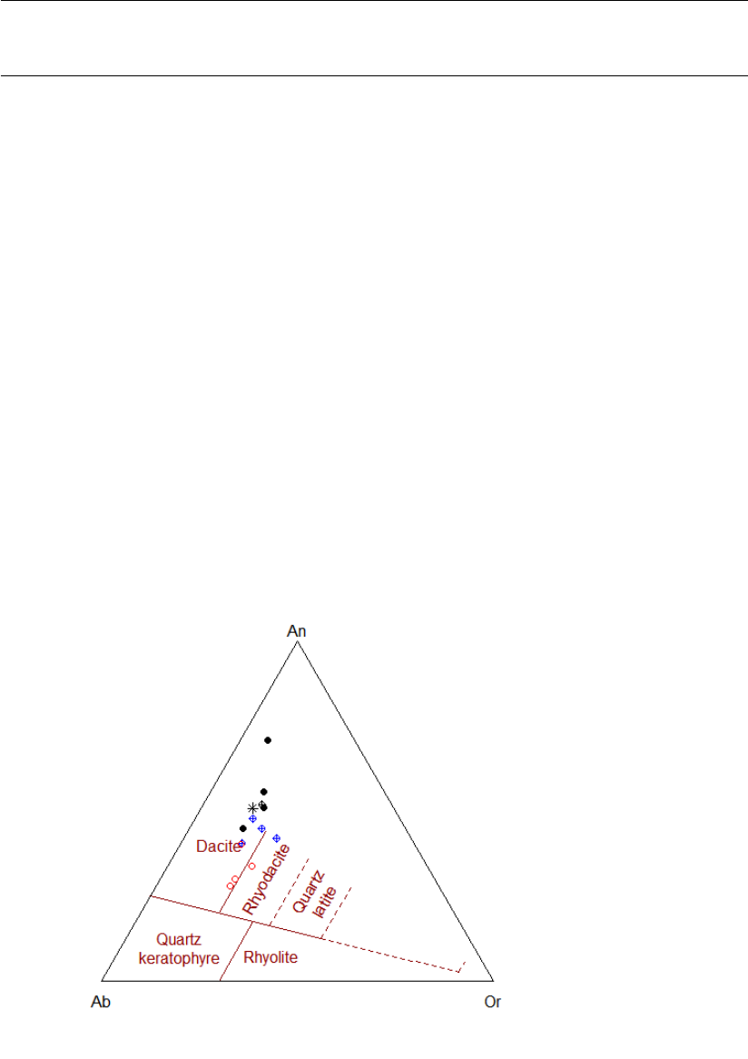
OConnor 161
OConnor Classification diagram for siliceous igneous rocks, based on Fsp com-
position (O’Connor 1965)
Description
Assigns data for O’Connor’s triangular diagram into Figaro template (list ’sheet’) and appropriate
values into ’x.data’ and ’y.data’.
Usage
OConnorVolc()
OConnorPlut(ab=NULL,an=NULL,or=NULL)
Arguments
ab,an,or character; specification of the plotting variables.
Details
The O’Connor’s triangular diagram is based on combination of Albite, Anorthite and K-feldspar
modal or normative data. While the function ’OConnorPlut’ can plot either modal or normative
diagrams for plutonic rocks, ’OConnorVolc’ is to be used exclusively with normative data computed
from chemical compositions of volcanic rocks.
In fact, the triangle represents projection of the Quartz - K-feldspar - Albite - Anorthite tetrahedron.
All three diagrams are designed for quartz-rich rocks, i.e. those with quartz contents higher than
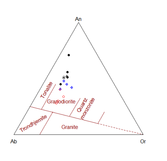
162 OConnor
10 such silica-rich samples, the rock type can be determined purely on the basis of the feldspars’
proportions.
As the specific version of the normative calculation is not mentioned in the original paper by
’O’Connor (1965)’, the function ’CIPW’, designed after ’Hutchison (1974, 1975)’ was implemented
as a default calculation scheme.
Alternatively, the plotting variables can be present already in the dataset (variable WR). The variables
to be plotted can be then specified upon call or can be selected using the function ’selectColumnLabel’.
The samples can be selected based on combination of three searching mechanisms (by sample
name/label, range or a Boolean condition) - see selectSubset for details.
Value
sheet list with Figaro Style Sheet data
x.data, y.data An, Ab and Or data (see details) transformed to orthogonal coordinates
Author(s)
Vojtech Erban, <vojtech.erban@geology.cz>
Vojtech Janousek, <vojtech.janousek@geology.cz>
Jean-Francois Moyen, <jfmoyen@gmail.com>
References
O’Connor J T (1965) A classification for Quartz-rich igneous rocks based on feldspar ratios. U.S.
Geol. Survey Prof Paper 525-B: B79-B84
Hutchison C S (1974) Laboratory Handbook of Petrographic Techniques. John Wiley & Sons, New
York, p. 1-527

overplotDataset 163
Hutchison C S (1975) The norm, its variations, their calculation and relationships. Schweiz Mineral
Petrogr Mitt 55: 243-256
See Also
classify figaro CIPW plotDiagram
Examples
plotDiagram("OConnorVolc",FALSE)
classify("OConnorVolc")
results<-Mesonorm(WR)
addResults()
plotDiagram("OConnorPlut",FALSE,ab="Albite",an="Anorthite",or="Orthoclase")
overplotDataset Adding another dataset to the current plot
Description
This function allows overplotting new data points stored in the memory onto any type of single
Figaro-compatible plots (or their plates). This can be done either into foreground or into back-
ground.
Usage
overplotDataset(reference.dataset=NULL, underplotting=FALSE, transp=0,
pch=NULL, col=NULL, cex=NULL, ...)
underplotDataset(reference.dataset=NULL, transp=0,...)
Arguments
reference.dataset
object name (given as a character string or unquoted); the dataset to be added to
the current diagram. See Details.
underplotting logical; should be the reference dataset added at the background?
transp numeric, 0-1; transparency of the background dataset (in underplotting).
pch plotting symbol(s) for the foreground dataset.
col plotting colour(s) for the foreground dataset.
cex numeric; relative size of the plotting symbol(s) for the foreground dataset.
... additional parameters to the underlying plotting function(s). See Details.
164 overplotDataset
Details
These are front-ends to the functions ’figOverplot’ and ’figOverplotDiagram’, invoked as ap-
propriate. However, the functions ’overplotDataset’ and ’underplotDataset’ work correctly
also on plates.
Also underplotDataset is just a convenience function, calling overplotDataset with the param-
eter underplotting=TRUE.
Most typically, reference.dataset is a (quoted) name of a dataset stored in memory. Alterna-
tively, a (unquoted) name of a global variable can be specified.
Plotting parameters ’pch’, ’col’ and ’cex’ are available only for overplotting.
On the other hand, transparency can be set only in underplotting. See ’setTransparency’ for further
info.
Argument ’...’ can supply additional parameters to the original plotting functions (e.g., ’TAS’)
invoked by ’plotDiagram’ or ’plateExtract’.
Value
(Invisibly) name of the reference dataset.
Note
This function is a front-end, truly a ’mother of all’ specialized and less versatile overplotting func-
tions such as ’figOverplot’, ’figOverplotDiagram’ or ’figAddReservoirs(just.draw=TRUE)’.
Please use ’overplotDataset’ instead, unless permanent addition to the plot is required. For
such cases, ’figAddReservoirs’ ’plateAddReservoirs’ in their default form, i.e. with argument
just.draw=FALSE, are the functions of choice.
Warning
NB that the points for the overplotted dataset do not from a part of the template, and thus will vanish
upon redrawing, zooming . . . .
Author(s)
Vojtech Janousek, <vojtech.janousek@geology.cz>
See Also
’figOverplot’ ’figOverplotDiagram’ ’figAddReservoirs’ ’plateAddReservoirs’
’peekDataset’ ’pokeDataset’ ’purgeDatasets’
’setTransparency’ ’plotDiagram’ ’plateExtract’
Examples
# Loading two testing datasets
data(sazava)
accessVar("sazava")
data(blatna)
accessVar("blatna")
setCex(1.5)
pokeDataset("blatna",overwrite.warn=FALSE) # Store a version with larger symbols

oxide2oxide 165
# Single plots
peekDataset("blatna")
plotDiagram("DebonPQ",FALSE,TRUE)
figRemove()
overplotDataset("sazava",cex=2,col="darkred",pch=15)
plotDiagram("DebonPQ",FALSE,TRUE)
figRemove()
underplotDataset("sazava",transp=0.5)
plateExtract("PearceGranite",2,main=" ")
overplotDataset("sazava")
# Spiderplots
peekDataset("blatna")
spider(WR,"Boynton",1,1000,cex=0,join=TRUE,offset=TRUE,
centered=FALSE,xrotate=FALSE,xaxs="r")
overplotDataset("sazava")
spider(WR,"Boynton",0.1,1000,field=TRUE,fill.col=TRUE,shaded.col="gray")
# Blatna as gray field
overplotDataset("sazava")
# A simple plate
peekDataset("blatna")
multiple("SiO2",y="TiO2,Al2O3,FeOt,MgO,CaO,Na2O,K2O,P2O5",nrow=3,ncol=3,main="")
plateCex(1.8)
plateCexLab(1.3)
overplotDataset("sazava")
# A plate of classification diagrams
peekDataset("blatna")
multiplePerPage(4,nrow=2,ncol=2,title="A classification plate")
plotDiagram("DebonPQ",FALSE,FALSE,main=" ")
plotDiagram("DebonBA",FALSE,FALSE,main=" ")
plotDiagram("LarocheVolc",FALSE,FALSE,main=" ")
plotDiagram("Meschede",FALSE,FALSE,main=" ")
plateLabelSlots(text=letters,cex=1.5,pos="topleft")
plateCexLab(1.2)
plateCol("black")
plateRedraw()
overplotDataset("sazava")
plateRedraw()
overplotDataset("sazava",cex=2,col=2,pch=15)
plateRedraw()
underplotDataset("sazava",transp=0.5)
oxide2oxide Recalculation of one oxide to a different one

166 oxide2ppm
Description
Returns a factor needed to multiply concentrations of an element given as an oxide (in wt %) to a
different target oxide (of the same element).
Usage
oxide2oxide(formula1, formula2)
Arguments
formula1 character: the oxide which is to be recalculated
formula2 character: the target oxide
Value
A factor for recalculation.
Author(s)
Vojtech Janousek, <vojtech.janousek@geology.cz>
See Also
oxide2ppm,ppm2oxide,molecularWeight
Examples
oxide2oxide("FeO","Fe2O3")
oxide2oxide("Mn2O3","MnO")
oxide2ppm Calculation of ppm of atom from wt% of an oxide
Description
Recasts concentrations of an oxide (in wt. %) to that of appropriate cation (in ppm).
Usage
oxide2ppm(formula,where="WR")
Arguments
formula character: the oxide which is to be recalculated
where character: a name of matrix or dataframe with the data to be recalculated
Value
A numeric matrix with one column containing the recalculated concentrations of the given cation
(ppm) for individual samples.

pairsCorr 167
Author(s)
Vojtech Janousek, <vojtech.janousek@geology.cz>
See Also
ppm2oxide,oxide2oxide,molecularWeight
Examples
data(sazava)
accessVar("sazava")
oxide2ppm("K2O")
pairsCorr Statistics: Correlation
Description
Plots a matrix of scatterplots in the lower panel and one of other pre-defined panel functions in the
upper.
Usage
pairsCorr(elems = major)
pairsMjr()
pairsTrc()
Arguments
elems list of desired elements
Details
The samples can be selected based on combination of three searching mechanisms (by sample
name/label, range or a Boolean condition) - see selectSamples for details.
Even though a list of major elements is assumed as a default, different variables can be specified by
the function ’selectColumnsLabels’.
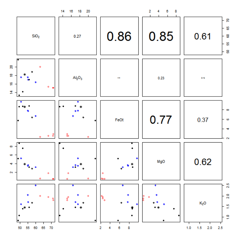
168 pairsCorr
The upper panels to choose from are:
’panel.corr’ Prints correlations, with size proportional to the correlations;
’panel.cov’ Prints covariances;
’panel.smooth’ Fits smooth trendlines;
’panel.hist’ Plots frequency histograms.
Value
None.
Warning
Names of existing numeric data columns and not formulae involving these can be handled at this
stage.
Author(s)
Vojtech Janousek, <vojtech.janousek@geology.cz>

pdfAll 169
Examples
pairsCorr(LILE)
pairsMjr()
pairsTrc()
# user-defined list
my.elems<-c("Rb","Sr","Ba")
pairsCorr(my.elems)
pdfAll Save all graphics to PDF
Description
Saves all graphical windows to a single PDF file.
Usage
pdfAll(filename=NULL)
Arguments
filename a name of file for saving the output.
Details
The function prompts for filename under which it saves all graphical windows, each on a separate
page. PDF is the most portable format, that should preserve practically the same layout on all
platforms.
Individual diagram can be saved from a menu that appears after clicking on the appropriate graphical
window (’File|Save as|PDF’).
Value
None.
Author(s)
Vojtech Janousek, <vojtech.janousek@geology.cz>
See Also
’psAll’ ’pdf’
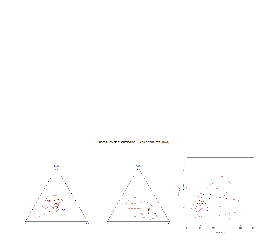
170 Pearce and Cann
Pearce and Cann Pearce and Cann (1973)
Description
Plots data stored in ’WR’ (or its subset) into Pearce and Cann’s diagrams.
Usage
Cann(plot.txt = getOption("gcd.plot.text"))
Arguments
plot.txt logical, annotate fields by their names?
Details
Set of two triangular and one binary diagram, proposed by Pearce & Cann (1973).
Following abbreviations are used:
IAT Low-K Tholeiites
MORB Ocean Floor Basalts
CAB Island Arc Basalts
WPB Within Plate Basalts
Note
This function uses the plates concept. The individual plots can be selected and their proper-
ties/appearance changed as if they were stand alone Figaro-compatible plots. See Plate,Plate editing
and figaro for details.
Author(s)
Vojtech Janousek, <vojtech.janousek@geology.cz>

Pearce and Norry 171
References
Pearce J A & Cann J R (1973) Tectonic setting of basic volcanic rocks determined using trace
element analyses. Earth Planet Sci Lett 19: 290-300. doi: 10.1016/0012-821X(73)90129-5
See Also
Plate,Plate editing,plotPlate,figaro
Examples
#plot the diagrams
plotPlate("Cann")
Pearce and Norry Pearce and Norry (1979)
Description
Assigns data for the diagram of Pearce & Norry (1979) into Figaro template (list ’sheet’) and
appropriate values into ’x.data’ and ’y.data’.
Usage
Norry()
Details
Diagram proposed by Pearce & Norry (1979) for geotectonic discrimination between basaltic rocks
from distinct geotectonic positions:
Within-plate Basalts
Island-arc basalts
Mid-ocean Ridge Basalts
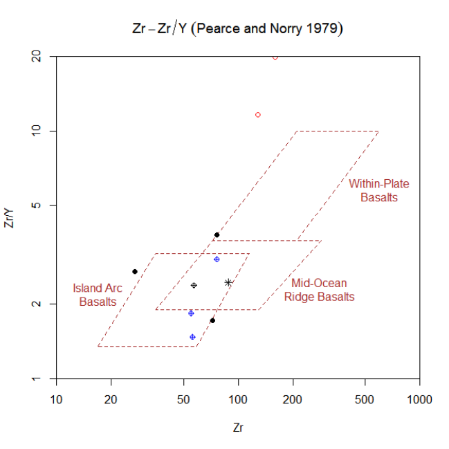
172 Pearce and Norry
Value
sheet list with Figaro Style Sheet data
x.data Zr ppm
y.data Zr/Y by weight
Author(s)
Vojtech Janousek, <vojtech.janousek@geology.cz>
References
Pearce J A & Norry M J (1979) Petrogenetic implications of Ti, Zr, Y, and Nb variations in volcanic
rocks. Contrib Mineral Petrol 69: 33-47. doi: 10.1007/BF00375192
See Also
figaro plotDiagram
Examples
#plot the diagram
plotDiagram("Norry",FALSE)

Pearce Nb-Th-Yb 173
Pearce Nb-Th-Yb Pearce (2008) Nb/Yb-Th/Yb diagram
Description
Assigns data for a Th/Yb vs. Nb/Yb diagram into Figaro template (list ’sheet’) and appropriate
values into ’x.data’ and ’y.data’.
Usage
PearceNbThYb(reservoirs=TRUE,xmin=0.1,xmax=1000,ymin=0.01,ymax=100)
Arguments
reservoirs logical, should be plotted average NMORB, EMORB and OIB?
xmin,xmax numeric, limits for the x axis.
ymin,ymax numeric, limits for the y axis.
Details
This diagram (Th/Yb vs. Nb/Yb) has been developed by J. Pearce in the 2000s to characterize (and
discriminate) arc magmatism. The current version is based on paper by Pearce (2008) dealing with
oceanic basalts, though. According to this author, Th-Nb serves as a ’crustal input proxy’ and hence
for demonstrating an oceanic, non-subduction setting.
The ’MORB-OIB array’ at the bottom extends from N-MORB to OIB (plotted for reference are
average compositions of NMORB, EMORB and OIB taken from Sun and McDonough (1989).
Melting of the metasomatized mantle yields trends parallel to the mantle array.
Arc lavas, formed by fluxed melting of the mantle, are shifted above the mantle array; the same
effects have mantle-derived magma-crust interactions. The top dashed line is the outer limit of
typical arc lavas, but there is a great deal of variation.
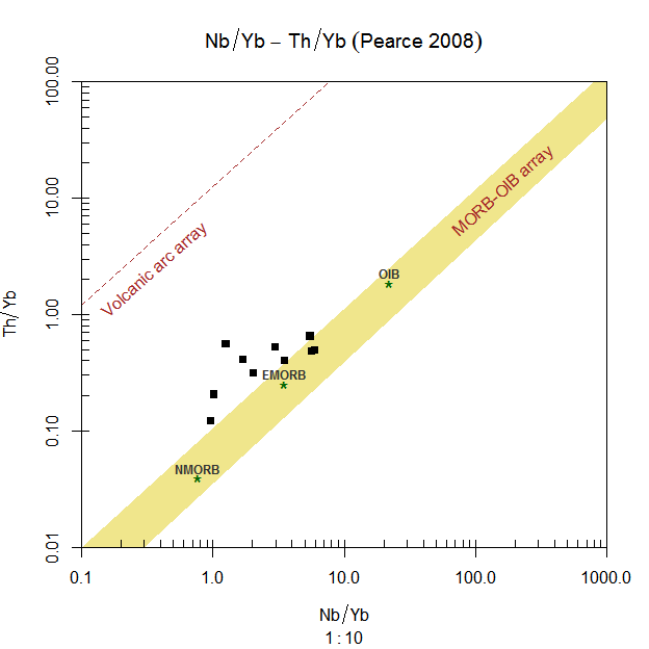
174 Pearce Nb-Th-Yb
Value
sheet list with Figaro Style Sheet data
x.data Nb/Yb
y.data Th/Yb
Author(s)
Vojtech Janousek, <vojtech.janousek@geology.cz> and Jean-Francois Moyen, <jfmoyen@gmail.com>
References
Pearce JA (2008) Geochemical fingerprinting of oceanic basalts with applications to ophiolite clas-
sification and the search for Archean oceanic crust. Lithos 100: 14-48 doi:10.1016/j.lithos.2007.06.016
Sun SS, McDonough WF (1989) Chemical and isotopic systematics of oceanic basalts: implications
for mantle composition and processes. In: Saunders AD, Norry M (eds) Magmatism in Ocean
Basins. Geological Society of London Special Publications 42, pp 313-345
See Also
figaro plotDiagram PearceNbTiYb

Pearce Nb-Ti-Yb 175
Examples
# Plot the diagram
plotDiagram("PearceNbThYb",FALSE,FALSE,reservoirs=TRUE)
plotDiagram("PearceNbThYb",FALSE,FALSE,reservoirs=FALSE)
Pearce Nb-Ti-Yb Pearce (2008) Nb/Yb-TiO2/Yb diagram
Description
Assigns data for a T iO2/Yb vs. Nb/Yb diagram into Figaro template (list ’sheet’) and appropriate
values into ’x.data’ and ’y.data’.
Usage
PearceNbTiYb(reservoirs=TRUE,xmin=0.1,xmax=100,ymin=0.1,ymax=10)
Arguments
reservoirs logical, should be plotted average NMORB, EMORB and OIB?
xmin,xmax numeric, limits for the x axis.
ymin,ymax numeric, limits for the y axis.
Details
The diagram T iO2/Yb vs. Nb/Yb serves as ’melting depth proxy’ and hence for indicating mantle
temperature and thickness of the conductive lithosphere (Pearce 2008). It distinguishes basalts,
which have originated by shallow melting, out of garnet stability field (’MORB array’) from those
spanning from deep melting with garnet in the residue (’OIB array’). Plotted for reference are
average compositions of NMORB, EMORB and OIB taken from Sun and McDonough (1989).
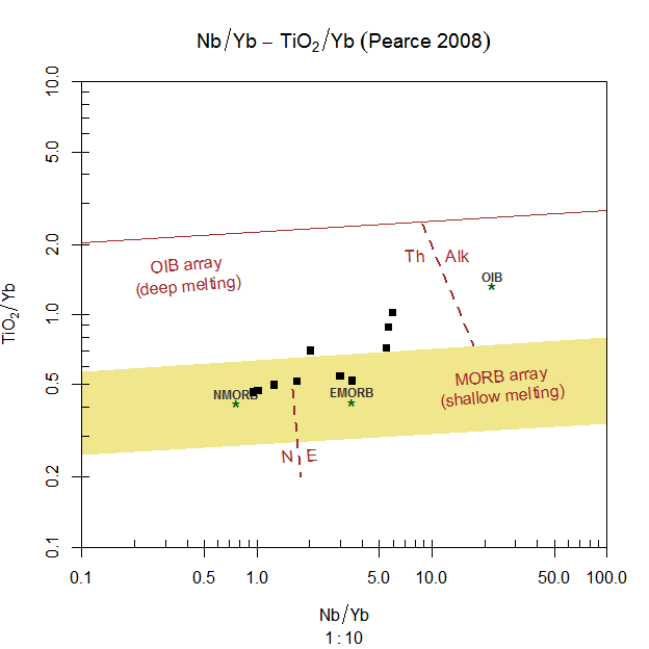
176 Pearce Nb-Ti-Yb
Value
sheet list with Figaro Style Sheet data
x.data Nb/Yb
y.data TiO2/Yb
Author(s)
Vojtech Janousek, <vojtech.janousek@geology.cz>
References
Pearce JA (2008) Geochemical fingerprinting of oceanic basalts with applications to ophiolite clas-
sification and the search for Archean oceanic crust. Lithos 100: 14-48 doi:10.1016/j.lithos.2007.06.016
Sun SS, McDonough WF (1989) Chemical and isotopic systematics of oceanic basalts: implications
for mantle composition and processes. In: Saunders AD, Norry M (eds) Magmatism in Ocean
Basins. Geological Society of London Special Publications 42, pp 313-345
See Also
figaro plotDiagram PearceNbThYb
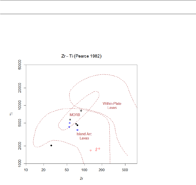
Pearce1982 177
Examples
# Plot the diagram
plotDiagram("PearceNbTiYb",FALSE,FALSE,reservoirs=TRUE)
plotDiagram("PearceNbTiYb",FALSE,FALSE,reservoirs=FALSE)
Pearce1982 Pearce (1982)
Description
Assigns data for the diagram of Pearce (1982) into Figaro template (list ’sheet’) and appropriate
values into ’x.data’ and ’y.data’.
Usage
Pearce1982()
Details
Diagram proposed by Pearce (1982) for geotectonic discrimination between lavas from distinct
geotectonic positions:
Within-plate lavas
Island-arc lavas
Mid-ocean Ridge Basalts

178 Pearce1996
Value
sheet list with Figaro Style Sheet data
x.data Zr ppm
y.data Ti ppm
Author(s)
Jean-Francois Moyen, <jfmoyen@gmail.com>
References
Pearce, J A (1982) Trace element characteristics of lavas from destructive plate boundaries. In: R
S Thorpe (ed) Andesites: Orogenic Andesites and Related Rocks. John Wiley & Sons, Chichester,
pp 525-548, ISBN 0 471 28034 8
See Also
figaro plotDiagram
Examples
#plot the diagram
plotDiagram("Pearce1982",FALSE)
Pearce1996 Nb/Y - Zr/Ti diagram (Winchester + Floyd 1977, modified by Pearce
1996)
Description
Assigns data for Nb/Y vs. Zr/Ti diagram into Figaro template (list ’sheet’) and appropriate values
into ’x.data’ and ’y.data’.
Usage
Pearce1996()
Details
Classification diagram proposed by Winchester & Floyd (1977) using incompatible element ratios
(Nb/Y vs. Zr/Ti). As the original plot has been designed prior to the publication of the TAS diagram
Le Bas et al. 1986, the field definition has been subsequently modified by Pearce (1996).
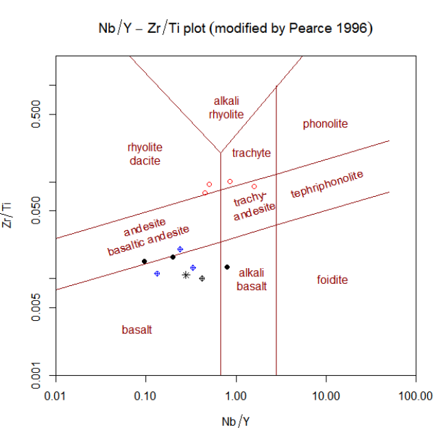
Pearce1996 179
The following fields are defined:
(Subalkaline) Basalt
Alkali basalt
Foidite
Andesite/Basaltic andesite
Trachyandesite
Tephriphonolite
Rhyolite/Dacite
Trachyte
Phonolite
Alkali Rhyolite
Value
sheet list with Figaro Style Sheet data
x.data Nb/Y wt. % ratio
y.data Zr/Ti wt. % ratio
Author(s)
Vojtech Janousek, <vojtech.janousek@geology.cz>

180 PearceEtAl
References
Le Bas M J, Le Maitre R W, Streckeisen A & Zanettin B (1986) A chemical classification of vol-
canic rocks based on the total alkali-silica diagram. J Petrology 27: 745-750 doi: 10.1093/petrol-
ogy/27.3.745
Pearce J A (1996) A User’s Guide to Basalt Discrimination Diagrams. In Wyman D A (ed) Trace
Element Geochemistry of Volcanic Rocks: Applications for Massive Sulphide Exploration. Geo-
logical Association of Canada, Short Course Notes 12, pp 79-113
Winchester J A & Floyd P A (1977) Geochemical discrimination of different magma series and their
differentiation products using immobile elements. Chem Geol 20: 325-343 doi: 10.1016/0009-
2541(77)90057-2
See Also
WinFloyd1 classify figaro plotDiagram
Examples
#Within GCDkit, the plot is called using following auxiliary functions:
#To Classify data stored in WR (Groups by diagram)
classify("Pearce1996")
#To plot data stored in WR or its subset (menu Classification)
plotDiagram("Pearce1996", FALSE)
PearceEtAl Pearce et al. (1977) MgO-FeOt-Al2O3
Description
Assigns data for the MgO-FeOt-Al2O3triangle proposed by Pearce et al.(1977) into Figaro tem-
plate (list ’sheet’) and appropriate values into ’x.data’ and ’y.data’.
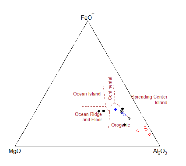
PearceEtAl 181
Usage
PearceEtAl()
Details
Triangular diagram with apices MgO, FeOt and Al2O3, proposed by Pearce et al.(1977). The
boundaries were defined solely for subalkaline volcanic rocks with SiO2between 51-56 wt %.
Following geotectonic positions may be identified using the diagram:
Spreading Center Island (or inter-plate island) - oceanic islands adjacent to ocean-ridge spreading,
such as Iceland or Galapagos; the authors ’do not consider this field well established’.
Orogenic
Ocean Ridge and Floor
Ocean Island
Continental
Value
sheet list with Figaro Style Sheet data
x.data, y.data MgO, FeOt and Al2O3in wt. % recalculated to two dimensions
Author(s)
Vojtech Janousek, <vojtech.janousek@geology.cz>

182 PearceGranite
References
Pearce T H, Gorman B E & Birkett T C (1977) The relationship between major element geochem-
istry and tectonic environment of basic and intermediate volcanic rocks. Earth Planet Sci Lett 36:
121-132. doi: 10.1016/0012-821X(77)90193-5
See Also
figaro plotDiagram
Examples
# Plot the diagram
plotDiagram("PearceEtAl",FALSE)
PearceGranite Pearce et al. (1984)
Description
Assigns Figaro templates to Pearce’s geotectonic diagrams for granitoids into the list ’plate’) and
appropriate values into the list ’plate.data’ for subsequent plotting.
Usage
PearceGranite(plot.txt = getOption("gcd.plot.text"))
Arguments
plot.txt logical, annotate fields by their names?
Details
Suite of four diagrams for discrimination of geotectonic environment of granitoid rocks, proposed
by Pearce et al. (1984). It is based on combination of five trace elements (namely Y, Nb, Rb, Yb
and Ta).
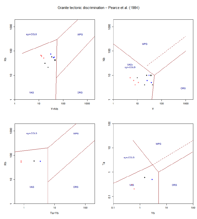
PearceGranite 183
Following geotectonic settings may be deduced:
Abbreviation used Environment
ORG Ocean Ridge Granites
VAG Volcanic Arc Granites
WPG Within Plate Granites
COLG Collision Granites
Note
This function uses the plates concept. The individual plots can be selected and their proper-
ties/appearance changed as if they were stand alone Figaro-compatible plots. See Plate,Plate editing
and figaro for details.

184 PeceTaylor
Author(s)
Vojtech Janousek, <vojtech.janousek@geology.cz>
References
Pearce J A, Harris N W & Tindle A G (1984) Trace element discrimination diagrams for the tectonic
interpretation of granitic rocks. J Petrology 25: 956-983. doi:10.1093/petrology/25.4.956
See Also
Plate,Plate editing,plotPlate,figaro
Examples
plotPlate("PearceGranite")
PeceTaylor SiO2-K2O diagram (Peccerillo + Taylor 1976)
Description
Assigns data for SiO2vs. K2Odiagram into Figaro template (list ’sheet’) and appropriate values
into ’x.data’ and ’y.data’
Usage
PeceTaylor()
Details
Diagram in SiO2vs. K2Ospace, proposed by Peccerillo & Taylor (1976), defines the following
fields:
Tholeiite Series
Calc-alkaline Series
High-K Calc-alkaline Series
Shoshonite Series
Field boundaries were linearly extrapolated up to 75% of SiO2between ’Calc-alkaline Series’ and
’High-K Calc-alkaline Series’, and up to 70% of SiO2between ’High-K Calc-alkaline Series’ and
’Shoshonite Series’.
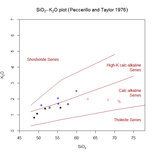
PeceTaylor 185
To employ boundaries as originally defined by Peccerillo & Taylor (1976), change the value of
variable ’extrapolated’ to ’FALSE’ in the file ’[R-root] \ library \ GCDkit \ Diagrams \ Classification
\ PeceTaylor.r’. Also note that the second value for the middle boundary (i.e. [52,1.5]) is in the
original paper obviously misquoted as 1.3 .
Rocks with composition falling beyond defined boundaries are labeled ’undefined’ by the ’classify’
function.
For comparison with similar diagrams used by other authors see Rickwood (1989).
Value
sheet list with Figaro Style Sheet data
x.data SiO2 weight percent
y.data K2O weight percent
Author(s)
Vojtech Erban, <vojtech.erban@geology.cz>
& Vojtech Janousek, <vojtech.janousek@geology.cz>
References
Peccerillo A & Taylor SR (1976) Geochemistry of Eocene calc-alkaline volcanic rocks from the
Kastamonu area, Northern Turkey. Contrib Mineral Petrol 58: 63-81 doi: 10.1007/BF00384745
Rickwood PC (1989) Boundary lines within petrologic diagrams which use oxides of major and
minor elements. Lithos 22: 247-263 doi: 10.1016/0024-4937(89)90028-5

186 peekDataset
See Also
classify figaro plotDiagram
Examples
#Within GCDkit, the plot is called using following auxiliary functions:
#To Classify data stored in WR (Groups by diagram)
classify("PeceTaylor")
#To plot data stored in WR or its subset (menu Classification)
plotDiagram("PeceTaylor", FALSE)
peekDataset Retrieving previous dataset stored in memory
Description
Both functions restore the previously stored dataset and make it current.
Usage
peekDataset(which.dataset=NULL)
selectDataset()
Arguments
which.dataset numeric or character; a sequence number or name of the stored dataset.
Details
The function ’peekDataset’ restores a dataset saved previously into memory by the function
’pokeDataset’. This means that it assigns all global variables specified by individual items of
the list ’WRCube’.
These typically are: ’WR’, ’WRanh’, ’milli’, ’labels’, ’filename’, ’groups’ and ’grouping’.
The function ’selectDataset’ provides a graphical interface to ’peekDataset’, i.e. shows a list
box filled by the names of datasets currently stored in the memory.
Value
None. But several global variables, among others ’WR’, ’WRanh’, ’milli’ and ’labels’, are affected.
The name of the current dataset is stored in ’dataset.name’.
Author(s)
Vojtech Janousek, <vojtech.janousek@geology.cz>
See Also
’pokeDataset’ ’purgeDatasets’

peterplot 187
Examples
data(sazava)
accessVar("sazava")
# stored as sazava in WRCube
assignColVar("MgO","blues")
assign1symb(15)
# store a new copy in the WRCube
pokeDataset("coloured sazava")
data(swiss)
accessVar("swiss")
# stored as swiss in WRCube
peekDataset("sazava")
binary("SiO2","Ba")
peekDataset("coloured sazava")
binary("SiO2","Ba")
peekDataset("swiss")
binary("Catholic","Education",pch=15,col="darkgreen")
peekDataset(2)
binary("SiO2","Sr")
peterplot Anomaly plot
Description
This function plots a conventional binary diagram but the type and size of the plotting symbols is
assigned according to the distribution of a third, conditioning variable.
Usage
peterplot(xaxis = "", yaxis = "", zaxis = "", ident = FALSE,
scaling.small = labels[1,"Size"], scaling.big = 2 * scaling.small,
assign.symbols = FALSE)
Arguments
xaxis, yaxis character; specification of the axes
zaxis character; conditioning variable
ident logical; identify the individual points?
scaling.small scaling factor for the smaller plotting symbols
scaling.big scaling factor for the larger plotting symbols
assign.symbols logical; should be the plotting symbols and their sizes assigned permanently?
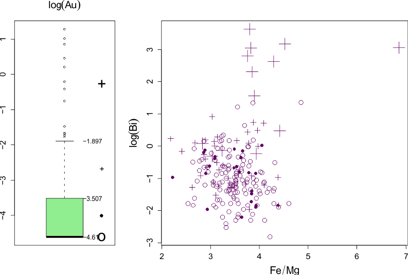
188 peterplot
Details
If no parameters xaxis, yaxis and zaxis are specified, the user is prompted to do so interactively.
The plotting symbols are assigned as follows: the values within 25 quartiles) obtain a dot, the
higher ones are denoted by ’+’and lower ones by ’-’. If the given value is an outlier, its plotting size
is doubled.
Optionally, the user can assign the plotting symbols and their sizes permanently, for use in other
diagrams throughout the system.
Value
May modify the variable cex, as well as the codes of plotting symbols stored in the data frame
labels.
Author(s)
Vojtech Janousek, <vojtech.janousek@geology.cz>
References
Reimann C, Filzmoser P, Garrett R G (2002) Factor analysis applied to regional geochemical data:
problems and possibilities. Applied Geochemistry 17: 185-206
Examples
peterplot("SiO2","MgO","K2O")
peterplot("SiO2","MgO","K2O",assign.symbols=TRUE)
plotDiagram("TAS",FALSE)

Plate 189
Plate Plotting plates of several diagrams
Description
Functions to set up, save or load a so-called ’plate’, i.e. a regular grid of slots to accommodate
(any mixture of) binary or ternary plots, spiderplots or such alike. For instance, Harker plots are
implemented using the plate concept.
Usage
multiplePerPage(which=NULL,nrow=NULL,ncol=NULL,title="Plate",
dummy=FALSE)
Plate(scr=NULL)
plateRedraw(device="windows",filename=NULL,colormodel="rgb")
platePS(colormodel="rgb")
plateSave()
plateLoad()
Arguments
which total number of slots to be occupied by individual diagrams.
nrow number of rows in the plots’ matrix.
ncol number of columns in the plots’ matrix.
title title for the whole plate.
dummy logical; if TRUE, dummy plots are shown. See Details.
scr (optional) number of screen to be selected.
device output device; either 'windows'or 'postscript'.
filename name of file if output redirected to Postscript.
colormodel color mode for Postscript; 'rgb'or 'gray'.
Details
The function 'multiplePerPage'serves to setting up a matrix of slots, each of which could be
taken by a single Figaro-compatible diagram (a binary plot, a ternary plot, a spiderplot,. . . ). If
'which'is NULL, the function asks for their number, and then suggests number of rows ('nrow')
and columns ('ncol') for the matrix arrangement.
If desired, the slots can be filled by the so-called ’dummy plots’, i.e. gray boxes showing the exact
position and the size of each of them.
If 'which'is an integer, specified number of slots is allocated. Alternatively, this argument may
represent a vector containing any mixture of names of diagrams that can be plotted by the function
plotDiagram or even plotting commands themselves used to fill the individual slots directly. See
Examples.
190 Plate
Once set up, a single slot can be selected for further work using the function 'Plate'. The function
can be called directly, with the number of the screen desired. If none is specified, a red box-
like cursor appears in the graphical window, which can be moved around using the cursor keys,
Spacebar or by mouse. The appropriate slot can be chosen by left mouse button or by pressing
Enter. Right-click anywhere on the plate invokes a context menu which enables several actions:
Menu item Function
Introduce plot Select a new Figaro-compatible diagram for this slot.
Plot editing Modify the existing diagram (like the menu Plot editing for stand alone plots).
Plate editing Functions to modify the overall plate properties or all its diagrams simultaneously.
The function 'plateRedraw'serves for replotting a ’clean! version of the whole plate, eg. for
saving/printing, For this purpose, its output can be redirected to Postscript, either in colour or as
black and white. As a wrapper for the Postscript output serves the function 'platePS'
The functions 'plateSave'and 'plateLoad'are designed to save and retrieve definitions of plates
(Figaro sheets and the relevant data) for later use. The default suffix for the saved plates is ’mgr’.
Note that only the data needed for the plotting (’x.data’, ’y.data’) are stored in the ’mgr’ files.
Thus the data set currently in memory (e.g., variables ’WR’, ’labels’, . . . ) is unaffected by the
function ’plateLoad’.
Starting with GCDkit version 3, the plates concept is used by some built-in functions, such as
’Multiple plots’ (function multiple) or ’Multiple plots by groups’ (function figMulti).
Value
plate list of Figaro definitions for individual diagrams
plate.data list containing 'x.data'and 'y.data'for each of them
Author(s)
Vojtech Janousek, <vojtech.janousek@geology.cz>
See Also
Plate editing,plotPlate,multiple,figMulti,plot,binary,ternary,spider,figaro,figLoad,figSave
Examples
data<-loadData("sazava.data",sep="\t")
multiplePerPage(which=c("binary(\"K2O/Na2O\",
\"Rb\",new=FALSE)","DebonPQ","AFM",
"PeceTaylor","Shand"))
Plate()
Plate(3)
plotDiagram("LarochePlut",FALSE,FALSE)

Plate editing 191
Plate editing Editing the plate properties/all its plots simultaneously
Description
A collection of functions to modify the properties of a plate (or all its diagrams) simultaneously.
Usage
plateXLim(xlim=NULL)
plateYLim(ylim=NULL)
plate0YLim()
plateCex(n=NULL)
plateCexLab(n=NULL)
plateCexMain(n=NULL)
plateAnnotationsRemove()
platePch(pch=NULL)
plateCol(col=NULL)
plateBW()
plateExpand(scr=NULL)
plateExtract(diagram,which=NULL,main=NULL,calc.only=FALSE,...)
Arguments
xlim scaling for the x axis
ylim scaling for the y axis
nrelative size (use n = 1 for normal one).
pch plotting symbol specification, either as string or a numeric code (showSymbols).
col colour specification, either by its English name, or by a numeric code (show-
Colours).
scr number of screen to be expanded.
diagram name of the function plotting a plate.
which sequential number of plot in its definition.
main optional alternative main title to the diagram.
calc.only logical; should be performed only calculations, without plotting?
... additional parameters to the diagram (plate) plotting function.
192 Plate editing
Details
The functions serve to change properties of all particular diagrams forming the given plate. They can
be used to set up the uniform size of plotting symbols ('plateCex'), main title ('plateCexMain')
or of the axes’ labels ('plateCexLab'), remove the annotation of classification fields ('plateAnnotationsRemove'),
uniform plotting symbol ('platePch') and/or colour
('plateCol') to all plots, or set them into black and white ('plateBW'). If the same variable is
plotted as x or y axis in all diagrams forming the plate (e.g., on Harker plots), it can be scaled by
means of the functions 'plateXLim'and 'plateYLim'. Using the command 'plate0YLim'it is
possible to set the origin of all non-logarithmic y axes to zero.
The function 'plateExpand'displays a zoomed up version of the selected diagram in a separate
window.
The function 'plateExtract'extracts a Figaro definition of a single plot from a plate plotted by
the function 'diagram'. If 'calc.only'is 'FALSE', the diagram is plotted, either into a separate
window or into current slot, if the active plot is a plate.
Value
None.
Author(s)
Vojtech Janousek, <vojtech.janousek@geology.cz>
References
Pearce J A, Harris N W & Tindle A G (1984) Trace element discrimination diagrams for the tectonic
interpretation of granitic rocks. J Petrology 25: 956-983. doi:10.1093/petrology/25.4.956
See Also
Plate,plotPlate,figaro,figScale,figCol,showSymbols,showColours
Examples
data<-loadData("sazava.data",sep="\t")
showSymbols()
showColours()
multiplePerPage(which=c("binary(\"K2O/Na2O\",
\"Rb\",new=FALSE)","DebonPQ","AFM","PeceTaylor","Shand"))
plateCex(0.5)
plateCex(2)
platePch(11)
platePch("+")
plateCol(11)
plateCol("red")
plateBW()

plateAddReservoirs 193
multiple("SiO2",major)
plateXLim(c(50,70))
groupsByLabel("Intrusion")
spider(WR,selectNorm("Boynton"),0.1,1000,pch=labels$Symbol,col=labels$Colour)
figMulti(plot.symb=TRUE)
plateYLim(c(1,100))
graphicsOff()
plotDiagram("DebonBA",FALSE,FALSE)
figMulti()
plate0YLim()
plateExpand(2)
plateExtract("PearceGranite",2) # Second plot of Pearce et al. (1984), i.e. Y-Nb
plateAddReservoirs Plate editing: plateAddReservoirs
Description
This function enables adding selected data from typical geochemical reservoirs (e.g., Upper Con-
tinental Crust, MORB . . . ), ideal mineral compositions, results of petrogenetic modelling or just
another dataset used for comparison to a plate of Figaro-compatible plots.
Usage
plateAddReservoirs(autoscale=FALSE, var.name="reservoirs.data", sample.names=NULL,
reserv.condition=NULL, labs=NULL, pch="*", col="darkblue", cex=1, type="p",
just.draw=FALSE,...)
Arguments
autoscale logical; should be the scaling changed so that all the plotted data fit in?
var.name text; either ’reservoirs.data’, ’idealmins.data’ or a name of a global vari-
able. See Details.
sample.names character vector; names of reservoirs, ideal minerals or samples to be plotted.
reserv.condition
text; regular expression specifying names of reservoirs, ideal minerals or sam-
ples to be plotted.
labs text; optional labels for the individual reservoirs.
pch plotting symbols.
col plotting colours.
cex numeric; relative size of the plotting symbols.
type character; plot type; see plot.default.
just.draw logical; if FALSE, the overplotted bit is added permanently, i.e. the Figaro tem-
plate is also affected.
... additional parameters to the plotting function. See figOverplot.
194 plateAddReservoirs
Details
The function ’plateAddReservoirs’ overplots compositions of selected geochemical reservoirs
(from the file ’reservoirs.data’, see selectNorm for the file structure as well as relevant refer-
ences) or ideal minerals (from the file ’idealmins.data’) onto a current plate.
Alternatively, if the name of a numeric matrix or dataframe in the global environment is provided via
the argument ’var.name’, data from this object are used (see Examples). The selection of samples
is governed either by ’sample.names’ or by ’reserv.condition’ parameters.
Optional argument ’labs’ can provide alternative, perhaps abbreviated textual labels to the points
plotted.
Please note that this function is so far available for spiderplots, binary and ternary plots only and no
special indexes, e.g. for Debon and Le Fort’s plots, are calculated.
By default, the overplotted information is added permanently but this behaviour is controlled by the
argument just.draw.
Value
A list of numeric matrices with the overplotted analyses from the reference dataset.
Warning
If just.draw=FALSE, the points for the reference dataset do not become a part of the template, and
thus will vanish upon redrawing, zooming . . . . See Examples.
Author(s)
Vojtech Janousek, <vojtech.janousek@geology.cz>
See Also
figAddReservoirs selectNorm overplotDataset figOverplot figOverplotDiagram
Examples
data(blatna)
accessVar("blatna")
# Simple binary plots
multiplePerPage(2,ncol=2,nrow=1,title="Testing plateAddReservoirs",dummy=FALSE)
screen(1)
binary("Ba","Sr",new=FALSE,log="xy")
screen(2)
binary("Ba","Rb/Sr",new=FALSE)
plateCex(2)
plateCexLab(1.5)
# Temporary overplotting with the selected reservoirs
# Sun & McDonough 1989 mantle reservoirs, Taylor & McLennan 1995 Upper/Lower Crust
reserv<-c("(MORB|EMORB|OIB) McDonough","Upper Crust Taylor 1995","Lower Crust Taylor 1995")
reserv.names<-c("NMORB","EMORB","OIB","UCC","LCC")
plateAddReservoirs(TRUE,"reservoirs.data",reserv.condition=reserv,
labs=reserv.names,cex=1.2,col="darkblue",just.draw=TRUE)
plateRedraw()

plateLabelSlots 195
# Permanent overplotting with a modelled trend
# Calculate Rayleigh-type fractionation trend and store in a global variable
ff<-seq(1,0.1,-0.1) # F, amount of melt left
x<-80*ff^(1.2-1) # cL for three elements, arbitrary D of 1.2, 2.0 and 1.3
y<-550*ff^(2.0-1)
z<-1000*ff^(1.3-1)
my.trend<-cbind(x,y,z)
colnames(my.trend)<-c("Rb","Sr","Ba")
rownames(my.trend)<-ff
plateAddReservoirs(TRUE,var.name="my.trend",type="o",col="darkgreen",just.draw=FALSE)
plateRedraw()
# Spider plots
ee<-spider(WR,"NMORB immobile",0.1,1000,pch=1:14,col=1:14,legend=TRUE)
groupsByLabel("Suite")
figMulti(nrow=1,ncol=3,plot.symb=TRUE)
reserv<-c("OIB .* McDonough","Lower Crust Taylor 1995")
reserv.names<-c("OIB","LCC")
plateAddReservoirs(FALSE,"reservoirs.data",reserv.condition=reserv,
labs=reserv.names,cex=1.2,col="darkgreen")
plateLabelSlots Annotate individual slots by letters or Roman numerals
Description
Annotates individual slots in a plate by letters or Roman numerals. For instance (a), (b), (c)... or (i),
(ii), (iii), (iv), (v)...
Usage
plateLabelSlots(text=letters,style="()",cex=1.5,pos="topright")
Arguments
text desired type of labels; see Details.
style optional character strings before and after label, typically brackets.
cex relative size of the text compared to the current codepar("cex").
pos character; position of the label relative to the plot.
Details
The argument ’what’ may acquire one of following values:
'letters' 'LETTERS' 'numbers' 'roman' 'ROMAN'
or can be user-defined character string of longer or of the same length as is the number of slots to
be annotated (see the last example).
Possible positions (parameter pos) are:

196 plotPlate
'bottomright' 'bottom' 'bottomleft' 'left'
'topleft' 'top' 'topright' 'right' 'center'
.
Value
none
Note
This function uses the plates concept. The individual plots can be selected and their proper-
ties/appearance changed as if they were stand alone Figaro-compatible plots. See Plate,Plate editing
and figaro for details.
Author(s)
Vojtech Janousek, <vojtech.janousek@geology.cz>
See Also
Plate,Plate editing,figaro
Examples
multipleMjr("SiO2")
plateLabelSlots("letters","",pos="bottomleft")
plateLabelSlots("ROMAN","{}")
my_labs<-c("1st","2nd","3rd","4th","5th","6th","7th","8th","9th")
plateLabelSlots(my_labs)
plotPlate Plot Plate of Diagrams
Description
Plots a plate of diagrams, based on the Figaro style sheets.
Usage
plotPlate(diagram,where="WR",...)
Arguments
diagram a valid name of the function that uses the plate concept to plot the given diagram.
See Details.
where name of the data matrix/data frame, columns of which are to be used for plotting.
... optional parameters for the diagram function call.

plotWithCircles 197
Details
The argument ’diagram’ may acquire one of following values:
'Maniar' 'Frost' 'PearceGranite' 'Schandl'
'Verma' 'Agrawal' 'Cann' 'Wood'
Value
none
Note
This function uses the plates concept. The individual plots can be selected and their proper-
ties/appearance changed as if they were stand alone Figaro-compatible plots. See Plate,Plate editing
and figaro for details.
Author(s)
Vojtech Janousek, <vojtech.janousek@geology.cz>
See Also
Plate,Plate editing,figaro
Examples
plotPlate("PearceGranite")
plotWithCircles xyz plotWithCircles
Description
Plots a binary diagram of two specified variables and the whole dataset or its selection. The size
and colours of the plotted circles correspond to the third.
Usage
plotWithCircles(xaxis = "", yaxis = "", zaxis = "",
colour = "heat.colors", scaling.factor = NULL,
bins = NULL, ident = getOption("gcd.ident"))
Arguments
xaxis Name of the data column to be used as x axis.
yaxis Name of the data column to be used as y axis.
zaxis Name of the data column to determine the size/colour of the circles.
colour colour scheme for the circles.
scaling.factor a factor determine the size of the circles.
bins number of intervals for the legend.
ident Logical: should be the individual samples identified?
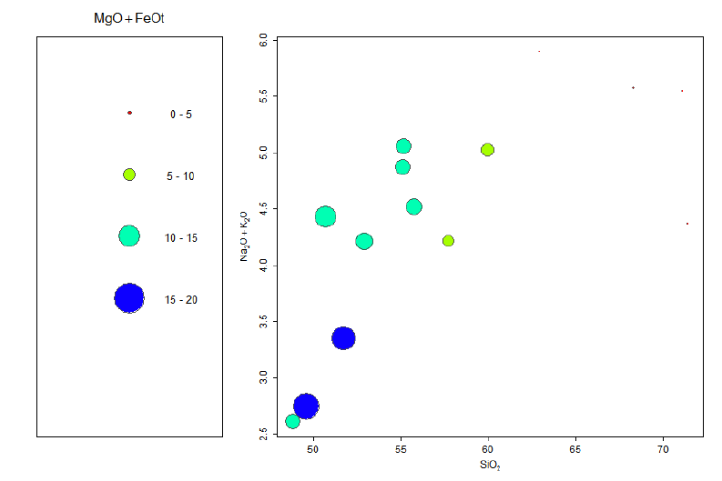
198 plotWithCircles
Details
If no parameters 'xlab','ylab'and 'zlab'are given, the user is prompted to specify them.
The variables are selected using the function ’selectColumnLabel.
In the specification of the apices can be used also arithmetic expressions, see calcCore for the
correct syntax.
The samples to be plotted can be selected based on combination of three searching mechanisms (by
sample name/label, range or a Boolean condition) - see selectSubset for details.
The legal colour schemes are: ’"grays","reds","blues","greens","cyans","violets","yellows"
’"cm.colors","heat.colors","terrain.colors","topo.colors","rainbow", "jet.colors"’.
Value
None.
Warning
This function IS NOT Figaro-compatible.
Author(s)
Vojtech Janousek, <vojtech.janousek@geology.cz>
& Vojtech Erban, <vojtech.erban@geology.cz>
Examples
plotWithCircles("SiO2","Na2O+K2O","MgO+FeOt",colour="rainbow")
plotWithCircles("SiO2","MgO","K2O",colour="grays",scaling.factor=0.5,ident=TRUE)

pokeDataset 199
pokeDataset Storing a dataset into memory for later use
Description
Saves the current dataset into memory so that it can be later re-stored.
Usage
pokeDataset(which.dataset=NULL,
par.list="WR,WRanh,milli,labels,filename,groups,grouping,init,age",
overwrite.warn=TRUE)
Arguments
which.dataset character; a name of the stored dataset.
par.list list of global variables to be stored.
overwrite.warn logical, warn if a dataset is going to be rewritten in ’WRCube’. See Details.
Details
This function stores the global variables specified by par.list, typically ’WR’, ’WRanh’, ’milli’
’labels’, ’filename’, ’groups’ and ’grouping’ into the list ’WRCube’.
If no which.dataset is provided upon the call, it can be typed in or selected from the list of existing
datasets.
Please note that ’pokeDataset’ is also invoked when a new dataset is loaded into memory using
the functions ’loadData’ or ’accessVar’. In the former case it is stored under the name of the file,
in the latter under the variable name. If such a name already exists in ’WRCube’, a time stamp is
attached.
For restoring the stored variables serve functions ’peekDataset’ and ’selectDataset’. The func-
tion ’purgeDatasets’ removes all older datasets, apart from the most recent copy of the current
one.
Value
None.
Warning
If not called from a GUI, no warning is issued upon rewriting the existing dataset.
Author(s)
Vojtech Janousek, <vojtech.janousek@geology.cz>
See Also
’peekDataset’ ’selectDataset’ ’purgeDatasets’ ’loadData’ ’accessVar’

200 ppm2oxide
Examples
data(sazava)
accessVar("sazava")
# stored as sazava in WRCube
assignColVar("MgO","blues")
assign1symb(15)
# store a new copy in the WRCube
pokeDataset("coloured sazava")
data(swiss)
accessVar("swiss")
# stored as swiss in WRCube
peekDataset("sazava")
binary("SiO2","Ba")
peekDataset("coloured sazava")
binary("SiO2","Ba")
peekDataset("swiss")
binary("Catholic","Education",pch=15,col="darkgreen")
ppm2oxide Calculation of wt% of the given oxide from ppm of atom
Description
Recasts concentrations of a cation (in ppm) to those of the selected oxide (in wt %).
Usage
ppm2oxide(formula,where="WR")
Arguments
formula character: the oxide which is to be recalculated
where character: a name of matrix or dataframe with Te data to be recalculated
Value
A numeric matrix with one column containing the recalculated concentrations of the given oxide
(in wt %) for individual samples.
Author(s)
Vojtech Janousek, <vojtech.janousek@geology.cz>
See Also
oxide2ppm,oxide2oxide,molecularWeight

prComp 201
Examples
data(sazava)
accessVar("sazava")
ppm2oxide("K2O")
oxide2ppm("FeOt")
oxide2ppm("FeO")+oxide2ppm("Fe2O3")
prComp Statistics: Principal components
Description
Performs principal components analysis (scaled variables, covariance or correlation matrix) and
plots a biplot (Gabriel, 1971).
Usage
prComp(comp.data=NULL,use.cov=FALSE,scale=TRUE,GUI=FALSE)
Arguments
comp.data a numerical matrix; the data to be normalized. Or just names of variables in the
data matrix ’WR’.
use.cov logical; should be the covariance matrix used instead of correlation matrix?
scale logical; the scalings applied to each variable.
GUI logical; is the function called from a menu (GUI)?
Details
Biplot aims to represent both the observations and variables of a data matrix on a single bivariate
plot (Gabriel, 1971; Buccianti & Peccerillo, 1999).
In the biplots, the length of the individual arrows is proportional to the relative variation of each
variable. A comparable direction of two arrows implies that both variables are positively corre-
lated; the opposite one indicates a strong negative correlation. When two links are perpendicular it
indicates independence of the two variables (Buccianti & Peccerillo, 1999).
If called from menu (GUI version), a list of major elements (SiO2,TiO2,Al2O3,FeOt,MnO,MgO,CaO,Na2O,K2O)
is assumed as a default, but different variables can be specified by the function ’selectColumnsLabels’.
The samples can be selected based on combination of three searching mechanisms (by sample
name/label, range or a Boolean condition) - see selectSamples for details.
Value
Vector of the scores of the supplied data on the principal components is stored in a variable ’results’.
Returns invisibly the complete output from the underlying function ’princomp’.
Warning
Names of existing numeric data columns and not formulae involving these can be handled at this
stage. Only complete cases are used for the principal components analysis.

202 printSamples
Author(s)
Vojtech Janousek, <vojtech.janousek@geology.cz>
References
Buccianti A & Peccerillo A (1999) The complex nature of potassic and ultrapotassic magmatism
in Central-Southern Italy: a multivariate analysis of major element data. In: Lippard S J, Naess A,
Sinding-Larsen R (eds) Proceedings of the 5th Annual Conference of the International Association
for Mathematical Geology. Tapir, Trondheim, p. 145-150
Gabriel K R (1971) The biplot graphical display of matrices with application to principal component
analysis. Biometrika 58: 453-467
See Also
For further details on the used principal components algorithm and biplots, see the R manual entries
of ’princomp’ and ’biplot.princomp’.
printSamples Display samples
Description
Displays specified combination of numeric variable(s) and/or labels for selected range of samples.
Usage
printSamples(elems=NULL,which=NULL,select.samples=FALSE,print=TRUE)
Arguments
elems list of variables to be printed
which list of samples, useful only for select.samples=FALSE
select.samples logical: if TRUE, samples can be chosen using the appropriate dialogue
print logical: should be the result indeed printed or just returned for further evalua-
tion?
Details
This function prints the desired numerical columns, textual labels, or their combinations, for se-
lected samples.
The samples can be selected based on combination of three searching mechanisms (by sample
name/label, range or a Boolean condition) - see selectSamples for details.
The variables to be printed are chosen by the function ’selectColumnsLabels’. In the specification
of the variable can be used also arithmetic expressions, see calcCore for the correct syntax.
Value
results data matrix with the desired data for the specified samples

printSingle 203
Author(s)
Vojtech Janousek, <vojtech.janousek@geology.cz>
Examples
## Not run:
# Querying names of numeric data columns
Search pattern = SiO2, MgO, CaO
Search pattern = major
SiO2, TiO2, Al2O3, Fe2O3, FeO, MnO, MgO, CaO, Na2O, K2O, P2O5
Search pattern = LILE
Rb, Sr, Ba, K, Cs, Li
Search pattern = HFSE
Nb, Zr, Hf, Ti, Ta, La, Ce, Y, Ga, Sc, Th, U
Search pattern = REE
La, Ce, Pr, Nd, Sm, Eu, Gd, Tb, Dy, Ho, Er, Tm, Yb, Lu
Search pattern = Locality,SiO2,LILE,HFSE
Locality, SiO2, Rb, Sr, Ba, K, Cs, Li, Nb, Zr, Hf, Ti,
Ta, La, Ce, Y, Ga, Sc, Th, U
Search pattern = 1:5, 7
Numeric data columns number 1, 2, ...5, 7
# User-defined list
my.elems<-c("Rb","Sr","Ba")
Search pattern = my.elems
Rb, Sr, Ba
## End(Not run)
printSingle Display a variable
Description
Displays a single numeric variable or a result of a calculation.
Usage
printSingle(default="")
Arguments
default character: list of default column names, separated by commas.

204 profiler
Details
The variable to be printed is selected using the function ’selectColumnLabel’. In the specification
of the variable can be used also arithmetic expressions, see calcCore for the correct syntax.
In the specification of the variable can be used also arithmetic expressions, see calcCore for the
correct syntax.
Value
results numerical vector/matrix with the results
Author(s)
Vojtech Janousek, <vojtech.janousek@geology.cz>
Examples
## Not run:
# examples of valid formulae....
(Na2O+K2O)/CaO
Rb^2
log10(Sr)
mean(SiO2)/10
# ... but this command is in fact a simple R shell -
# meaning lots of fun for power users!
summary(Rb,na.rm=TRUE)
cbind(SiO2/2,TiO2,Na2O+K2O)
cbind(major)
hist(SiO2,col="red")
boxplot(Rb~factor(groups))
# possibilities are endless
plot(Rb,Sr,col="blue",pch="+",xlab="Rb (ppm)",ylab="Sr (ppm)",log="xy")
## End(Not run)
profiler Profile plotting
Description
Plotting geochemical profiles. As a x axis can be specified an arbitrary variable or an numerical
interval (for equidistant measurements).
Usage
profiler(x = NULL, y = NULL, method = "Variable", legend = FALSE,
pch = 1, col = "black", cex = 1, xaxs = "r", yaxs = "i",
main = "",xmin = NULL, xmax = NULL)
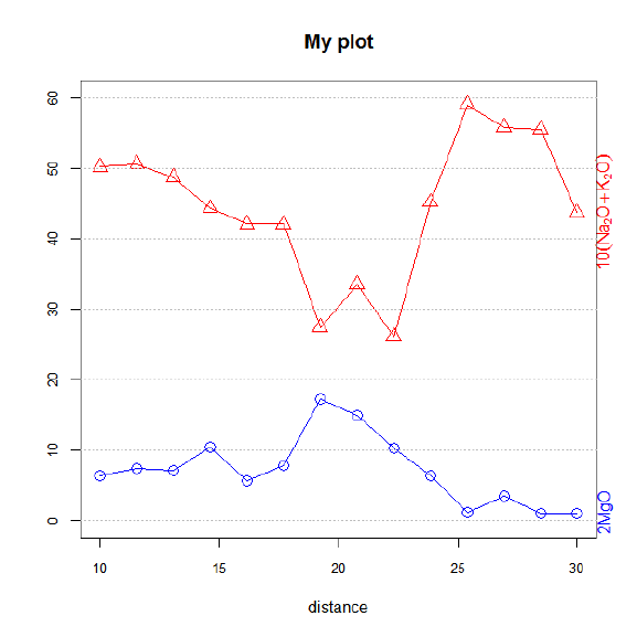
profiler 205
Arguments
xcharacter; optional name of variable to be plotted as x axis.
ycharacter; name(s) of variable(s) for individual profiles.
method character; which of the methods is to be used? Valid are "Variable","Equidistant"
or "From-To".
legend logical; should be plotted also legend (in a separate window)?
pch plotting symbols specification.
col plotting colour(s).
cex numeric; relative size of the plotting symbols.
xaxs, yaxs character; type of the axes. See par for details.
main character; main title for the plot
xmin, xmax range of the x axis (for methods ’Variable’ and ’From/To’))
Details
The function ’profiler’ serves for plotting three different types of profiles involving a single or
several geochemical parameters.
The first one, ’Variable’ uses any numeric variable as the x axis (e.g., SiO2 contents, depth...). It
is in fact a special type of a binary plot, in which the data points are, for each of the y-axis variables,
joined by a line.
The remaining two methods are very similar to each other. The x axis is in both cases equidistant,
and the order of the individual samples follows from their sequence in the data set.
The method ’Equidistant’ uses simply the sequence number of the individual samples in the data
set. It does not label the x-axis, just prints the number of samples used for plotting.
206 profiler
The method ’From/To’ serves for drawing equidistant profiles, where the x axis can be specified by
an interval.
In the specification of the x axis (for the method ’Variable’) or any of the y variables (all methods)
can be used also arithmetic expressions, see calcCore for the correct syntax.
If not called from the command prompt, the samples can be selected based on combination of three
searching mechanisms (by sample name/label, range or a Boolean condition) - see selectSubset
for details.
The easiest way to specify the variable(s) to be plotted on individual profile(s) is to type directly
the names of the columns, separated by commas. Alternatively can be used their sequence numbers
or ranges. Also built-in lists can be employed, such as ’LILE’, ’REE’, ’major’ and ’HFSE’ or their
combinations with the column names.
These lists are simple character vectors, and additional ones can be built by the user (see Exam-
ples). Note that currently only a single, stand-alone, user-defined list can be employed as a search
criterion.
If the function is not called from the command prompt, and it desired so, the symbols and colours
for each of the profiles can be specified separately in a simple spreadsheet-like interface.
If x axis occurs among the arguments to be plotted as y axes, it is skipped.
Likewise the relative scaling of the plotting symbols and the scale of the y axis can be specified.
Lastly, the user is asked to enter the limits for the axes, which are always two numbers separated by
a comma.
Value
results numeric matrix with the values for individual profiles.
Author(s)
Vojtech Janousek, <vojtech.janousek@geology.cz>
Examples
# Profiles of SiO2 versus (scaled) TiO2, MgO and K2O
# if x is specified, method="Variable" assumed automatically
profiler("Na2O+K2O",c("TiO2","6*MgO","SiO2"),pch=c("+","o","@"),col=c("red","blue","darkgreen"),
xmin=2,xmax=10)
# Equidistant profiles of (scaled) MgO, CaO, and Al2O3 (in sample sequence)
# with default symbols and scaling
profiler(y=c("MgO","3*CaO","2*Al2O3"),method="Equidistant",col=c("red","blue","darkgreen"))
# Equidistant profiles of two calculated variables in custom colour
# and user-defined plotting symbols; range of the x axis will be specified
# interactively
profiler(y=c("2*MgO","10*(Na2O+K2O)"),method="From-To",pch=1:10,
col=c("blue","red"),cex=1.5,main="My plot",xmin=10,xmax=30)

psAll 207
psAll Save all graphics to PS
Description
Saves all graphical windows to Postscript files.
Usage
psAll(filename=NULL)
Arguments
filename a name of file for saving the output.
Details
The function prompts for a common root of the filenames and then saves all graphical windows,
each in a separate file, numbering them sequentially. Postscript is the best export format from R,
preserving the necessary quality as well as the possibility to be imported by most graphical editors
(such as Corel Draw!) for retouching.
Otherwise individual diagram can be saved from a menu that appears after clicking on the appro-
priate graphical window (’File|Save as|Postscript’).
Value
None.
Author(s)
Vojtech Janousek, <vojtech.janousek@geology.cz>
See Also
’pdfAll’ ’postscript’
purgeDatasets Removing stored datasets from the memory
Description
Removes all the stored datasets (apart from the current one) in order to save memory.
Usage
purgeDatasets(GUI=FALSE)
Arguments
GUI logical; is the function called from GUI?

208 QAPF
Details
This function removes all older datasets, regardless whether stored automatically by the functions
’loadData’ or ’accessVar’, as well as on demand by ’pokeDataset’.
Only the most recent copy of the current dataset is preserved (i.e. the last item within the list
’WRCube’).
Value
None.
Warning
If not called from a GUI, no warning is issued and all but the current dataset are deleted immediately.
Author(s)
Vojtech Janousek, <vojtech.janousek@geology.cz>
See Also
’pokeDataset’ ’peekDataset’ ’selectDataset’
QAPF QAPF diagram (Streckeisen 1974, 1978)
Description
Assigns data for Streckeisen’s diagram into Figaro template (list ’sheet’) and appropriate values
into ’x.data’ and ’y.data’. The Q, A, P and F coordinates are assigned into matrix ’results’.
Usage
QAPFVolc()
QAPFPlut()
Details
Following the IUGS recommendation (Le Maitre et al 2002), the QAPF diagram should be the
prime classification scheme for holocrystalline plutonic and volcanic rocks containing at least 10%
of felsic minerals.
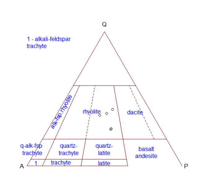
QAPF 209
The apices are defined as follows:
Q = Quartz modal %
A = Alkali feldspar modal %
P = Plagioclase modal %
F = feldspathoid modal %
Q+A+P+F=100%
As the whole QAPF diagram is rather complicated, GCDkit plots just the appropriate triangle if
the dataset contains only Si-oversaturated or only Si-undersaturated rock samples. If both kinds
of rock samples are present, the whole double triangle is shown. This behaviour may be changed
in the source code of the diagram (in file ’QAPFPlut.r’ or ’QAPFVolc.r’, stored in the subdi-
rectory GCDkit\Diagrams\Classification, change the ’triangle<-"auto"’ to ’triangle<-"both"’
and complete double triangle will be always plotted).
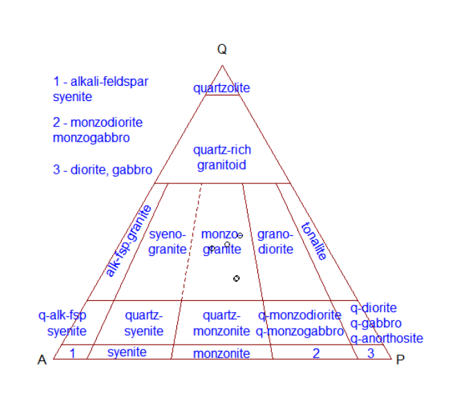
210 QAPF
Value
sheet list with Figaro Style Sheet data
x.data, y.data Q, A, P and F data (see details) transformed to orthogonal coordinates
Author(s)
Vojtech Erban, <vojtech.erban@geology.cz>
References
Streckeisen A (1974) Classification and nomenclature of plutonic rocks. Geol Rundsch 63: 773-786
doi: 10.1007/BF01820841
Streckeisen A (1978) IUGS Subcommission on the Systematics of Igneous Rocks: Classification
and nomenclature of volcanic rocks, lamprophyres, carbonatites and melilitic rocks; recommenda-
tion and suggestions. Neu Jb Min, Abh 134: 1-14.
Le Maitre R. W. et al. (2002) Igneous Rocks. A Classification and Glossary of Terms. 2nd edition.
Cambridge University Press.
See Also
classify figaro plotDiagram
Examples
#plots the QAPF diagram for current dataset

quitGCDkit 211
plotDiagram("QAPFVolc", FALSE)
plotDiagram("QAPFPlut", FALSE)
#classifies the current dataset using the QAPF diagram
classify("QAPFVolc")
classify("QAPFPlut")
quitGCDkit Exit GCDkit
Description
Exits GCDkit (nicely).
Usage
quitGCDkit()
Arguments
None.
Details
By invoking this command the user is not prompted whether he wants to save his unfinished work
in the ’Workspace image’, i.e. file ’.RData’ in the main GCDkit directory.
Menu
GCDkit: Exit GCDkit
See Also
’quit’
r2clipboard Copy results to clipboard
Description
Copies the most recently calculated results to a clipboard.
Usage
r2clipboard(what=results)

212 recast
Arguments
what a variable to be copied, can be either a vector, a matrix, a list or a table.
Details
Copies the variable ’results’ returned by most of the calculation algorithms to the Windows clip-
board.
Value
None.
Author(s)
Vojtech Janousek, <vojtech.janousek@geology.cz>
recast Recast to given sum
Description
Recasts the selected data to a fixed sum.
Usage
recast(total = 100)
normalize2total(what = NULL, total = 100)
Arguments
what numeric matrix or character vector with a list of column names to be normalized,
separated by commas.
total a sum the data should be normalized to.
Details
Both functions return the selected elements/oxides (columns in the data matrix ’WR’) normalized
to the required sum. The function ’recast’ is front-end to ’normalize2total’. If ’what’ is
a comma delimited list, the corresponding columns from the data matrix ’WR’ are selected. If
’what’ is empty, the user is prompted to supply the list of required column names via the func-
tion ’selectColumnsLabels’.
Value
results numerical vector/matrix with the results
Author(s)
Vojtech Janousek, <vojtech.janousek@geology.cz>
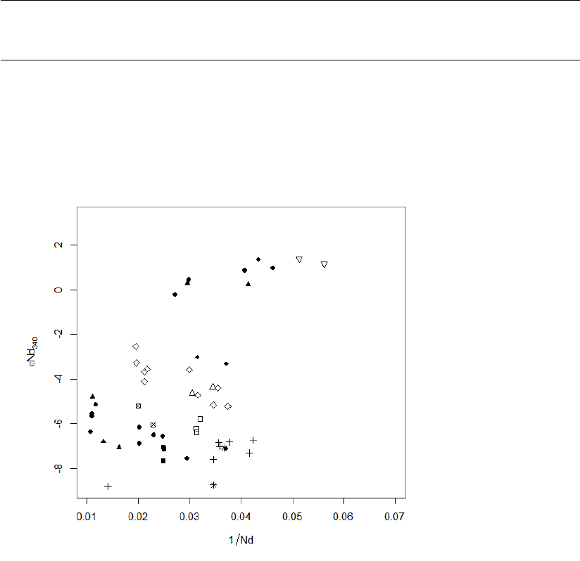
reciprocalIso 213
Examples
normalize2total(major,1)
recast() # to select the sum and elements interactively
reciprocalIso Binary plots of reciprocal element concentration vs initial isotopic
composition
Description
Plots a diagram 1/Sr vs initial Sr isotopic ratios or 1/Nd vs initial (Nd)for selected samples.
Usage
reciprocalIso(what=NULL,GUI=FALSE,...)
Arguments
what name of the desired isotopic parameter
GUI logical; is the function called from the GUI?
... optional parameters to the underlying function {plotWithLimits}

214 Regular expressions
Details
The recognized types of diagrams (specified by ’what’) are: ’Rb-Sr’ and ’Sm-Nd’ for the 1/Sr vs.
87Sr/86Sr[i]or 1/Nd vs. (Nd)plots, respectively.
If called from GUI, the samples can be selected based on combination of three searching mecha-
nisms (by sample name/label, range or a Boolean condition) - see selectSamples for details.
Value
None.
Plugin
SrNd.r
Author(s)
Vojtech Janousek, <vojtech.janousek@geology.cz>
See Also
The actual plotting is done by the function plotWithLimits.
Regular expressions Implementation of regular expressions in GCDkit
Description
Implementation of regular expressions in the searching patterns.
Details
Many enquiries in the GCDkit employ regular expressions. This is a quite powerful searching mech-
anism more familiar to people working in Unix. Put in simple terms, most characters, including all
letters and digits, are regular expressions that match themselves. However, metacharacters with a
special meaning (’?’ ’+’ ’{’ ’}’ ’|’ ’(’ ’)’) must be preceded by a backslash.
Regular expression Matches
. Any character
^Beginning of the expression
\$ End of the expression
[ ] Any of the characters given in square brackets
[m-n] Any character in the range given by mand n
A subexpression is a regular expression enclosed in ’\(’ and ’\)’. Two such subexpressions may
be joined by the infix operator ’|’ (logical or); the resulting regular expression matches any string
matching either of them. For instance:
\(South\)|\(North\)Uist
yields both
South Uist and North Uist.
Regular expressions 215
A regular expression may be followed by one of several repetition operators:
Repetition operator The preceding item will be matched
? At most once (i.e. is optional)
*Zero or more times
+ One or more times
{n} Exactly ntimes
{n,} At least n times
{n,m} At least ntimes, but not more than mtimes
Author(s)
Vojtech Janousek, <vojtech.janousek@geology.cz>
See Also
regex
Examples
## Not run:
# Subset by label
The searched field corresponds to localities with the following levels:
Mull, Rum, Skye, Coll, Colonsay, Hoy, Westray, Sanday,
Stronsay, Tiree, Islay
Search pattern = ol
Coll, Colonsay
Search pattern = n.a
Colonsay, Sanday, Stronsay
Search pattern = ^S
Skye, Sanday, Stronsay
Search pattern = e$
Skye, Tiree
Search pattern = [ds]ay
Colonsay, Sanday, Stronsay
Search pattern = [p-s]ay
Colonsay, Westray, Stronsay
Search pattern = ol|oy
Coll, Colonsay, Hoy
Search pattern = l{2}
Mull, Coll
# Subset by sample name
The sample names are: Bl-1, Bl-3, Koz-1, Koz-2, Koz-5, Koz-11,
KozD-1, Ri-1.

216 Ross
Search pattern = oz-[1-3]
Koz-1, Koz-2, Koz-11
Search pattern = oz-|Bl-
Bl-1, Bl-2, Bl-3, Koz-1, Koz-2, Koz-5, Koz-11
## End(Not run)
Ross Ross + Bedard (2009) Zr/Y-Th/Yb
Description
Assigns data for a Zr/Y vs. Th/Yb binary diagram into Figaro template (list ’sheet’) and appropri-
ate values into ’x.data’ and ’y.data’.
Usage
Ross()
Arguments
None.
Details
The binary plot Zr/Y vs. Th/Yb designed by Ross and Bédard (2009) for classification of ancient
subalkaline volcanic rocks into tholeiitic or calc-alkaline series. In these cases, the conventional
AFM diagram tends to be of limited use due to the potential mobility of alkalis.
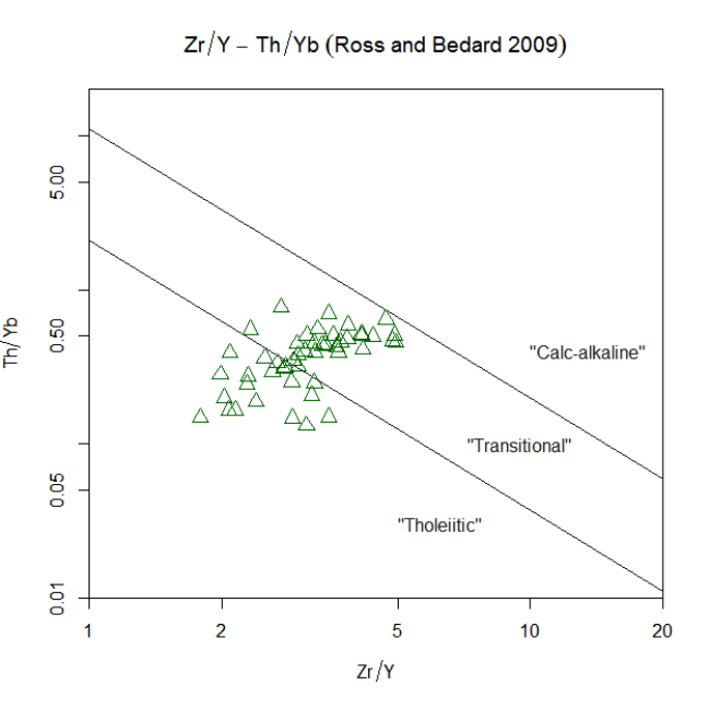
Ross 217
Value
sheet list with Figaro Style Sheet data
x.data x coordinates
y.data y coordinates
Author(s)
Vojtech Janousek, <vojtech.janousek@geology.cz>
References
Ross PS, Bédard LP (2009) Magmatic affinity of modern and ancient subalkaline volcanic rocks de-
termined from trace-element discriminant diagrams. Can J Earth Sci 46: 823-839 doi: 10.1139/E09-
054
Coordinates and graph layout are taken from website of Kurt Hollocher.
See Also
figaro plotDiagram AFM
Examples
plotDiagram("Ross",FALSE,TRUE)

218 rtSaturation
rtSaturation Rutile saturation (Hayden + Watson 2007)
Description
Calculates rutile saturation temperatures for the observed major-element data and Ti concentrations.
Also returns Ti saturation levels for the given major-element compositions and assumed magma
temperature.
Usage
rtSaturation(cats=milli,T=0,P=0,Ti=filterOut(WR,"Ti",1))
Arguments
cats numeric matrix; whole-rock data recast to millications
Tassumed temperature of the magma in °C
Passumed pressure in kbar, Ryerson & Watson (1987) model only
Ti numeric vector with Ti concentrations in ppm
Details
Ryerson & Watson (1987) have first formulated rutile saturation model for melts ranging in com-
position from basalt to rhyodacite. The distribution of T iO2between rutile and liquid was given
as:
DT iO2=e(−3.16+ 9373
T+0.026P−0.152F M)
where ’T’ is the absolute temperature (K) of the magma, ’P’ pressure (kbar) and ’FM’ is a melt
composition parameter:
F M =1
Si
Na +K+ 2(Ca +Mg +F e)
Al
.
The Ti saturation level then would be:
T i.sat.RW =599342.9
DT iO2
(ppm)
In turn, when the rutile saturation was reached, the magma temperature (in °C) can be calculated
as:
T Rt.sat.C.RW =9373
(3.16 + ln(100/T iO2) −0.026P+ 0.152F M )−273.15
The Ti solubility in rutile-saturated hydrous siliceous melts was revisited by Hayden & Watson
(2007). According to these authors, it can be expressed as:
T i.sat.HW = 10(7.95−5305
T+0.124F M)(ppm)

rtSaturation 219
where ’T’ is the absolute temperature (K) of the magma, and ’FM’ is the melt composition parameter
defined above.
The temperature (in °C) for rutile-saturated magma can be calculated as:
T Rt.sat.C.HW =5305
7.95 −log(T i)+0.124F M −273.15
Using these formulae, the function ’rtSaturation’ calculates the rutile saturation levels, Ti activ-
ities and rutile saturation temperatures following both models.
The formulation of Ryerson & Watson (1987) may be more suitable for basic rocks, whereas the
more recent model of Hayden & Watson (2007) seems to be appropriate for siliceous magmas.
Please note also that the latter does not take into account effects of pressure (having been calibrated
at 1 GPa; Hayden & Watson 2007).
Value
Returns a matrix ’results’ with the following columns:
FM melt composition parameter
Ti observed Ti concentrations
Ti.sat.RW saturation levels of Ti for assumed temperature, Ryerson & Watson (1987)
aTi.RW activity of Ti (ratio of Ti/Ti.sat), Ryerson & Watson (1987)
TRt.sat.C.RW rutile saturation temperatures in °C, Ryerson & Watson (1987)
Ti.sat.HW saturation levels of Ti for assumed temperature, Hayden & Watson (2007)
aTi.HW activity of Ti (ratio of Ti/Ti.sat), Hayden & Watson (2007)
TRt.sat.C.HW rutile saturation temperatures in °C, Hayden & Watson (2007)
Plugin
Saturation.r
Author(s)
Vojtˇ
ech Janoušek, <vojtech.janousek@geology.cz>
References
Ryerson FJ, Watson EB (1987) Rutile saturation in magmas; implications for Ti-Nb-Ta depletion in
island-arc basalts. Earth Planet Sci Lett 86: 225-239 doi: 10.1016/0012-821X(87)90223-8
Hayden LA, Watson EB (2007) Rutile saturation in hydrous siliceous melts and its bearing on Ti-
thermometry of quartz and zircon. Earth Planet Sci Lett 258: 561-568 doi: doi:10.1016/j.epsl.2007.04.020

220 saveResults
saveData Save data file
Description
Saves modified data set into a specified datafile.
Usage
saveData(sep="\t")
Arguments
sep delimiter separating individual items in the data file.
Details
Labels (stored in data frame ’labels’) and numeric data (in numeric matrix ’WR’) for the currently
selected subset are glued together and saved under the specified filename. The format is such that the
data can be retrieved again into GCDkit using the loadData command. Note that no mg numbers
are currently saved.
Value
None.
Author(s)
Vojtech Janousek, <vojtech.janousek@geology.cz>
See Also
’loadData’ ’mergeData’ ’showColours’ ’colours’ ’showSymbols’ ’read.table’
saveResults Save results
Description
Saves the most recently calculated results to a text file.
Usage
saveResults(what = results, sep = "\t", digits = 2)
Arguments
what a variable to be saved, can be either a vector, a matrix or a list.
sep separator; default is a tab-delimited file.
digits precision of the results to be saved.

saveResultsIso 221
Details
Saves the variable ’results’ returned by most of the calculation algorithms to a tab-delimited
ASCII file.
Value
None.
Author(s)
Vojtech Janousek, <vojtech.janousek@geology.cz>
saveResultsIso Save Sr-Nd isotopic data
Description
Saves the calculated isotopic parameters stored in the matrix ’init’ to a text file.
Usage
saveResultsIso(digits = 6)
Arguments
digits precision of the results to be saved.
Details
Saves the data matrix init with the following columns:
Age (Ma) Age in Ma
87Sr/86Sri Initial Sr isotopic ratios
143Nd/144Ndi Initial Nd isotopic ratios
EpsNdi Initial (Nd)values
TDM Single-stage depleted-mantle Nd model ages (Liew & Hofmann, 1988)
TDM.Gold Single-stage depleted-mantle Nd model ages (Goldstein et al., 1988)
TDM.2stg Two-stage depleted-mantle Nd model ages (Liew & Hofmann, 1988)
Value
None.
Plugin
SrNd.r
Author(s)
Vojtech Janousek, <vojtech.janousek@geology.cz>

222 sazava
References
Liew T C & Hofmann A W (1988) Precambrian crustal components, plutonic associations, plate
environment of the Hercynian Fold Belt of Central Europe: indications from a Nd and Sr isotopic
study. Contrib Mineral Petrol 98: 129-138
Goldstein S L, O’Nions R K & Hamilton P J (1984) A Sm-Nd isotopic study of atmospheric dusts
and particulates from major river systems. Earth Planet Sci Lett 70: 221-236
See Also
’saveResults’
sazava Whole-rock composition of the Sazava suite, Central Bohemian Plu-
tonic Complex
Description
This data set gives the whole-rock major- and trace-element contents in selected samples (gabbros,
quartz diorites, tonalites and trondhjemites) of the c. 355 My old calc-alkaline Sazava suite of the
Variscan Central Bohemian Plutonic Complex (Bohemian Massif, Czech Republic).
Usage
data(sazava)
Format
A data frame containing 14 observations.
Source
Vojtech Janousek, <vojtech.janousek@geology.cz>
References
Janousek V, Rogers G, Bowes DR (1995) Sr-Nd isotopic constraints on the petrogenesis of the
Central Bohemian Pluton, Czech Republic. Geol Rundsch 84: 520-534 doi: 10.1007/BF00284518
Janousek V, Bowes DR, Rogers G, Farrow CM, Jelinek E (2000) Modelling diverse processes in the
petrogenesis of a composite batholith: the Central Bohemian Pluton, Central European Hercynides.
J Petrol 41: 511-543 doi: 10.1093/petrology/41.4.511
Janousek V, Braithwaite CJR, Bowes DR, Gerdes A (2004) Magma-mixing in the genesis of Hercy-
nian calc-alkaline granitoids: an integrated petrographic and geochemical study of the Sazava intru-
sion, Central Bohemian Pluton, Czech Republic. Lithos 78: 67-99 doi: 10.1016/j.lithos.2004.04.046
Examples
data(sazava)
accessVar("sazava")
binary("SiO2","Ba")

Schandl 223
Schandl Schandl and Gorton (2002)
Description
Plots data stored in ’WR’ (or its subset) into the classification diagrams after Schandl and Gorton
(2002).
Usage
Schandl(plot.txt = getOption("gcd.plot.text"))
Arguments
plot.txt logical, annotate fields by their names?
Details
Suite of four diagrams for geotectonic environment discrimination of felsic volcanic rocks (rhyo-
lites), proposed by Schandl and Gorton (2002). It is based on combination of four presumably little
immobile trace elements (namely Ta, Yb, Th, and Hf). Diagrams were designed to decipher the geo-
tectonic setting of felsic volcanic suites, specifically those associated with the volcanogenic mas-
sive sulphide (VMS) deposits. a) Ta/Yb versus Th/Yb diagram from Gorton and Schandl (2000) is
divided into three fields: Oceanic Arcs, Active Continental Margins (ACM) and Within-Plate Vol-
canic Zones (WPVZ). The Within-Plate Basalts (WPB) and Mid-Ocean Ridge Basalts (MORB)
represent compositions previously determined by Pearce (1982, 1983). b) Ta vs. Th diagram
demonstrates the Th enrichment of felsic volcanic rocks at post-Archaean VMS deposits (and of
some unmineralized Archaean rhyolites) with respect to Ta. c) Graph of Ta/Hf vs Th/Hf ratios
shows the similar incompatibility between Th and Ta in two different tectonic environments: Ac-
tive Continental Margins and Within-Plate Volcanic Zones. d) Yb vs. Th/Ta diagram with fields
for associations of Oceanic Arcs, Active Continental Margins, Within Plate Volcanic Zones and
MORB.
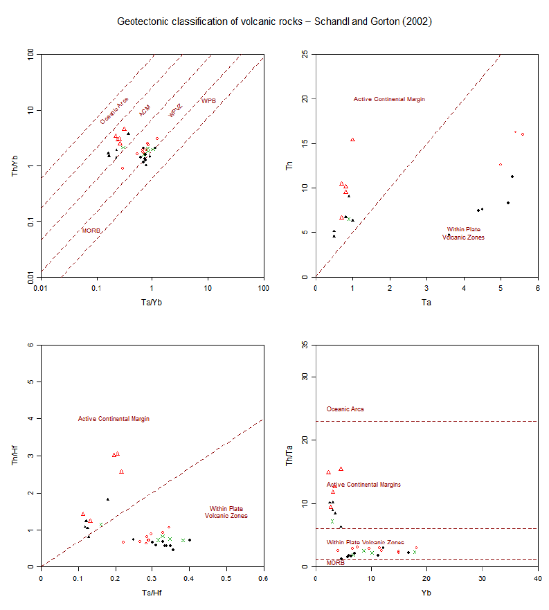
224 Schandl
Taken together, the following geotectonic settings may be deduced:
Rock Association Abbreviation
Oceanic Arcs
Active Continental Margins ACM
Within-Plate Volcanic Zones WPVZ
Further abbreviations used on the plots:
Rock Association Abbreviation
Mid-Oceanic Ridge Basalts MORB
Within-Plate Basalts WPB

selectAll 225
Note
This function uses the plates concept. The individual plots can be selected and their proper-
ties/appearance changed as if they were stand alone Figaro-compatible plots. See Plate,Plate editing
and figaro for details.
Author(s)
Vojtech Janousek, <vojtech.janousek@geology.cz>
References
Gorton M P & Schandl E S (2000) From continents to island arcs: A geochemical index of tectonic
setting for arc-related and within-plate felsic to intermediate volcanic rocks. Can Min 38: 1065-
1073. doi: 10.2113/gscanmin.38.5.1065
Pearce J A (1982) Trace element characteristics of lavas from destructive plate boundaries. In
Thorpe R S (ed) Andesites: Orogenic Andesites and Related Rocks. John Wiley, Chichester, pp
525-548.
Pearce J A (1983) Role of the sub-continental lithosphere in magma genesis at active continental
margins. In Hawkesworth C J & Norry M J (eds) Continental Basalts and Mantle Xenoliths. Shiva,
Nantwich. pp 230-249
Schandl E S & Gorton M P (2002) Application of high field strength elements to discriminate
tectonic settings in VMS environments. Economic Geology 97: 629-642. doi: 10.2113/97.3.629
See Also
Plate,Plate editing,plotPlate,figaro
Examples
#plot the diagrams
plotPlate("Schandl")
selectAll Select whole dataset
Description
Restores data for all samples as they were loaded from a data file.
Usage
selectAll(GUI=FALSE)
Arguments
GUI logical; was the function called from the GUI?.

226 selectByDiagram
Details
When a datafile is loaded into GCDkit using the loadData function, the data and their backup copy
are stored in the memory.
The subsets of the current dataset can be chosen using the functions selectByLabel and selectSubset
(menus 'Select subset by sample name or label','Select subset by range'
,'Select subset by Boolean') and the current data will be replaced by their newly chosen
subset.
The backup copy is kept intact ever since the loadData function has been invoked and can be
uploaded any time in place of the current data set using the function ’selectAll’. Note that all
changes made e.g. to plotting symbols, grouping, newly calculated variables etc. will be lost.
Value
None.
Author(s)
Vojtech Janousek, <vojtech.janousek@geology.cz>
selectByDiagram Selecting subset by diagram
Description
This function enables selecting samples that plot into certain field(s) of the given classification
diagram.
Usage
selectByDiagram(diagram = select.list(claslist[, "menu"]))
Arguments
diagram one of the valid diagram names that appear in ’.claslist()’
Details
The diagram can be chosen from a list (the default) or specified directly as an argument. Clicking
onto a field toggles its inclusion/exclusion - the currently selected fields are cyan.
Value
None.
Author(s)
Vojtech Janousek, <vojtech.janousek@geology.cz> & Vojtech Erban, <vojtech.erban@geology.cz>
See Also
’selectByLabel’, ’selectSubset’, ’selectAll’ and ’classify’.

selectByLabel 227
Examples
.claslist() # names of existing diagrams
selectByDiagram("TAS")
selectByLabel Select subset by sample name or label
Description
Selecting subsets of the data stored in memory by searching sample names or a single label.
Usage
selectByLabel()
Details
This function enables the user to query a single textual column, a label, chosen using the func-
tion ’selectColumnLabel’. The current data will be replaced by its newly chosen subset. These
enquiries employ regular expressions.
Value
Overwrites the data frame ’labels’ and numeric matrix ’WR’ by subset that fulfills the search crite-
ria.
Author(s)
Vojtech Janousek, <vojtech.janousek@geology.cz>
Examples
## Not run:
# Subset by label
The searched field corresponds to localities with the following levels:
Mull, Rum, Skye, Coll, Colonsay, Hoy, Westray,
Sanday, Stronsay, Tiree, Islay
Search pattern = ol
Coll, Colonsay
Search pattern = n.a
Colonsay, Sanday, Stronsay
Search pattern = ^S
Skye, Sanday, Stronsay
Search pattern = e$
Skye, Tiree
Search pattern = [ds]ay
Colonsay, Sanday, Stronsay

228 selectColumnLabel
Search pattern = [p-s]ay
Colonsay, Westray, Stronsay
Search pattern = ol|oy
Coll, Colonsay, Hoy
Search pattern = l{2}
Mull, Coll
# Subset by sample name
The sample names are: Bl-1, Bl-3, Koz-1, Koz-2,
Koz-5, Koz-11, KozD-1, Ri-1.
Search pattern = oz-[1-3]
Koz-1, Koz-2, Koz-11
Search pattern = oz-|Bl-
Bl-1, Bl-2, Bl-3, Koz-1, Koz-2, Koz-5, Koz-11
## End(Not run)
selectColumnLabel Selecting a single variable in GCDkit
Description
This is an auxiliary function invoked by many others to select a single variable.
Usage
selectColumnLabel(where = colnames(labels),
message = "Select the variable\nor press ENTER to pick from a list",
default = "", sample.names = FALSE, silent = FALSE, print = TRUE,
empty.ok = TRUE)
Arguments
where names of data columns to choose from
message prompt
default comma delimited list of default names
sample.names logical; should be the sample names listed
silent logical, echo on/off
print logical, echo on/off
empty.ok is empty selection ok?

selectColumnsLabels 229
Details
The easiest way for specification of the variable is to type directly the name of the numerical column
in the data matrix ’WR’ (e.g., ’SiO2’) or its sequence number (2 for the second column). However,
it is not necessary to enter the name in its entirety. Only a substring that appears somewhere in the
column name or other forms of regular.expressions can be specified.
If the result is ambiguous, the correct variable has to be selected by mouse from the list of the
multiple matches. Ultimately, empty response invokes list of all variables available in the memory.
Value
A numeric index of the selected column.
Author(s)
Vojtech Janousek, <vojtech.janousek@geology.cz>
See Also
selectColumnsLabels
selectColumnsLabels Selecting several data columns
Description
An auxiliary function invoked by many others to select several variables simultaneously.
Usage
selectColumnsLabels(where = colnames(WR),
message = "Select variable(s), e.g. 'SiO2,TiO2,MgO'
or press ENTER to pick from a list", default = "", print = TRUE,
exact.only = TRUE)
Arguments
where vector of names for data columns to choose from
message prompt
default comma delimited list of default names
print logical, echo on/off
exact.only logical, should be the input checked for correctness?
230 selectColumnsLabels
Details
The variable(s) can be specified in several ways. The easiest is to type directly the name(s) of the
column(s), separated by commas. Alternatively can be used their sequence numbers or ranges. Also
built-in lists can be employed, such as 'LILE','REE','major'and 'HFSE'or their combinations
with the column names.
These lists are simple character vectors, and additional ones can be built by the user (see Exam-
ples). Note that currently only a single, stand-alone, user-defined list can be employed as a search
criterion.
Empty response invokes list of all variables available. The correct variables have to be selected by
mouse + SHIFT from this list.
If exact.only=TRUE, the individual items in the input line are checked against the list of existing
column/variable names (i.e. components in the vector 'where').
Value
Vector with the selected column names.
Author(s)
Vojtech Janousek, <vojtech.janousek@geology.cz>
Examples
## Not run:
# Querying names of numeric data columns
Search pattern = SiO2, MgO, CaO
Search pattern = major
SiO2, TiO2, Al2O3, Fe2O3, FeO, MnO, MgO, CaO, Na2O, K2O, P2O5
Search pattern = LILE
Rb, Sr, Ba, K, Cs, Li
Search pattern = HFSE
Nb, Zr, Hf, Ti, Ta, La, Ce, Y, Ga, Sc, Th, U
Search pattern = REE
La, Ce, Pr, Nd, Sm, Eu, Gd, Tb, Dy, Ho, Er, Tm, Yb, Lu
Search pattern = Locality,SiO2,LILE,HFSE
Locality, SiO2, Rb, Sr, Ba, K, Cs, Li, Nb,
Zr, Hf, Ti, Ta, La, Ce, Y, Ga, Sc, Th, U
Search pattern = 1:5, 7
Numeric data columns number 1, 2, ...5, 7
# User-defined list
my.elems<-c("Rb","Sr","Ba")
Search pattern = my.elems
Rb, Sr, Ba
## End(Not run)

selectNorm 231
selectNorm Selecting the normalization data for spiderplots
Description
Displays available normalization schemes and lets the user to choose one interactively.
Usage
selectNorm(ref=NULL,elems = "Rb,Sr,Ba,Cr,Ni,La,Ce,Y,Zr",REE.only=FALSE,
multiple=FALSE)
Arguments
ref character: a specification of the normalization scheme.
elems character: a default list of elements.
REE.only logical: should be only listed normalization schemes for REE?
multiple logical: is a result with several normalizing schemes allowed?
Details
A search pattern can be specified directly (in batch mode) in order to query the available normalizing
model names. The corresponding parameter ’ref ’ can contain a substring appearing in the name of
the normalizing scheme (or even a regular expression).
Alternatively, the parameter ’ref ’ can refer to a name of a sample to be used for normalization, or
even a regular expression if average of several of them is desired.
The function fails if no matches are found or the search in names of normalizing schemes is am-
biguous (returns more than a single match), unless ’multiple = TRUE’.
The second possibility is to pick an option from the list of available normalizing schemes via GUI.
The first option therein offers normalization by a single sample. Its name can be typed in or, after
pressing the Enter key, picked from a list.
The second option is similar but it allows to normalize by average concentrations in a group of
samples specified by one of the three searching mechanisms as above (see selectSubset).
Then the user is prompted to specify the list and order of elements/oxides that should appear on
the plot. The easiest way is to type directly the names of the columns, separated by commas.
Alternatively can be used their sequence numbers or ranges. Also built-in lists can be employed,
such as ’LILE’, ’REE’, ’major’ and ’HFSE’ or their combinations with the column names. These
lists are simple character vectors, and additional ones can be built by the user (see Examples). Note
that currently only a single, stand-alone, user-defined list can be employed as a search criterion.
The samples to be plotted can be selected based on combination of three searching mechanisms (by
sample name/label, range or a Boolean condition) - see selectSubset for details.
The composition of various standards available for normalization and subsequent plotting of spider
diagrams is stored in the file ’spider.data’ in the main GCDkit directory. It is a comma delimited
file such as:
232 selectNorm
Normalization data used for spiderplots
MORB (Pearce 1983)
Sr,K,Rb,Ba,Th,Ta,Nb,Ce,P,Zr,Hf,Sm,Ti,Y,Yb
120,1245,2,20,.2,.18,3.5,10,534,90,2.4,3.3,8992,30,3.4
REE chondrite (Boynton 1984)
La,Ce,Pr,Nd,Pm,Sm,Eu,Gd,Tb,Dy,Ho,Er,Tm,Yb,Lu
.31,.808,.122,.6,1,.195,.0735,.2590,.0474,
.322,.0718,.21,0.0324,.209,.0322
ORG (PearceEtAl.1984)
K2O,Rb,Ba,Th,Ta,Nb,Ce,Hf,Zr,Sm,Y,Yb
0.4,4,50,0.8,0.7,10,35,9,340,9,70,8.0
The first row is always skipped and can contain any comments. The following ones have a fixed
structure. For each normalization scheme, the first row contains the title and reference. If title
starts with ’REE’, the normalization is supposed to be for REE only and special parameters, such as
’Eu/Eu*’, are calculated. The second line gives a comma delimited list of elements in the order they
should appear on the plot. The last line is a comma delimited list of normalization values. There
are empty lines left between the normalization schemes.
As the file ’spider.data’ is read every time ’selectNorm is called, the user can add or delete
normalization schemes on his will using a text editor.
Value
A numeric matrix with one row, containing the normalizing values. The row name contains the
name of the model and reference.
Author(s)
Vojtech Janousek, <vojtech.janousek@geology.cz>
References
Implemented spiderplots:
Anders E, Grevesse N (1989) Abundances of the elements: meteoritic and solar. Geochim Cos-
mochim Acta 53:197-214 doi: 10.1016/0016-7037(89)90286-X4
Becker H, Horan M F, Walker R J, Gao S, Lorand J-P, Rudnick R L (2006) Highly siderophile
element composition of the Earth’s primitive upper mantle: constraints from new data on peridotite
massifs and xenoliths. Geochim Cosmochim Acta 70: 4528-4550 doi: 10.1016/j.gca.2006.06.004
Boynton W V (1984) Cosmochemistry of the rare earth elements: meteorite studies. In: Henderson
P (eds) Rare Earth Element Geochemistry. Elsevier, Amsterdam, pp 63-114
Jochum K P (1996) Rhodium and other platinum-group elements in carbonaceous chondrites.
Geochim Cosmochim Acta 60: 3353-3357 doi: 10.1016/0016-7037(96)00186-X
McDonough W, Sun S S (1995) The composition of the Earth. Chem Geol 120: 223-253 doi:
10.1016/0009-2541(94)00140-4
Nakamura N (1974) Determination of REE, Ba, Fe, Mg, Na and K in carbonaceous and ordinary
chondrites. Geochim Cosmochim Acta 38: 757-775 doi: 10.1016/0016-7037(74)90149-5
Pearce J A (1983) Role of sub-continental lithosphere in magma genesis at active continental mar-
gins. Continental Basalts and Mantle Xenoliths. Shiva, Nantwich, pp 230-249

selectPalette 233
Pearce J A (1996) A user’s guide to basalt discrimination diagrams. In: Wyman D A (eds) Trace
Element Geochemistry of Volcanic Rocks: Applications for Massive Sulphide Exploration. Geo-
logical Association of Canada, Short Course Notes 12, pp 79-113
Pearce J A (2014) Immobile element fingerprinting of ophiolites. Elements 10: 101-108 doi:
10.2113/gselements.10.2.101
Pearce J A, Harris N W, Tindle A G (1984) Trace element discrimination diagrams for the tectonic
interpretation of granitic rocks. J Petrology 25: 956-983 doi:10.1093/petrology/25.4.956
Sun S S, McDonough W F (1989) Chemical and isotopic systematics of oceanic basalts: implica-
tions for mantle composition and processes. In: Saunders A D, Norry M (eds) Magmatism in Ocean
Basins. Geological Society of London Special Publications 42, pp 313-345
Sun S S, Bailey D K, Tarney J, Dunham K (1980) Lead isotopic study of young volcanic rocks from
mid-ocean ridges, ocean islands and island arcs. Philos Trans R Soc London A297: 409-445 doi:
10.1098/rsta.1980.022410.1029/95RG00262
Taylor S R, McLennan S M (1985) The Continental Crust: Its Composition and Evolution. Black-
well, Oxford, pp 1-312
Taylor S R, McLennan S M (1995) The geochemical evolution of the continental crust. Reviews in
Geophysics 33: 241-265 doi: 10.1029/95RG00262
Thompson R N (1982) British Tertiary province. Scott J Geol 18: 49-107
Weaver B L, Tarney J (1984) Empirical approach to estimating the composition of the continental
crust. Nature 310: 575-577 doi: 10.1038/310575a0
Wood D A, Joron J L, Treuil M, Norry M, Tarney J (1979) Elemental and Sr isotope variations
in basic lavas from Iceland and the surrounding ocean floor; the nature of mantle source inhomo-
geneities. Contrib Mineral Petrol 70: 319-339 doi: 10.1007/BF00375360
Examples
selectNorm()
selectNorm("Boynton")
# Regular expressions in action, we take the string from beginning
# and then replace space and left bracket by dots
selectNorm("^Primitive Mantle..McDonough 1995")
# Selecting several samples by regular expression
data(sazava)
accessVar("sazava")
selectNorm("Po-4",elems="Cs,Rb,Ba,Nb,La,Yb")
selectNorm("^Po",elems="Cs,Rb,Ba,Nb,La,Yb")
selectPalette selectPalette
Description
Picks given number of colours from one of the available palettes.
Usage
selectPalette(n,colour.palette=NULL,GUI=TRUE)
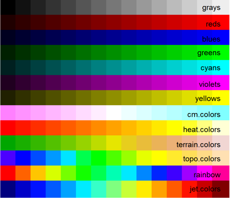
234 selectPalette
Arguments
ndesired number of colours
colour.palette one of the colour palette names, see Details
GUI logical; is the function called from GUI?
Details
The desired number of colours has to be given in any case.
The possible palettes are: 'grays','reds','blues','greens','cyans','violets','yellows',
'cm.colors','heat.colors','terrain.colors','topo.colors','rainbow'and 'jet.colors'.
Also, user-defined palette functions are supported now. See Examples.
If not specified upon function call, the colour palette can be picked from list of available ones.
Optionally (if GUI = TRUE) it plots a chart with their preview.
Value
Returns a matrix with a single row of hexadecimal codes. Its rownames represent the name of the
palette selected.
Note
Note that UK spelling of "colours" in names of palettes is fixed automatically to the US "colors".

selectSubset 235
Author(s)
Vojtech Janousek, <vojtech.janousek@geology.cz>
See Also
Colours by label can be assigned by assignColLab, colours by variable using assignColVar.
Uniform colours are obtained by assign1col. Table of available plotting colours is obtained by
showColours.
Examples
ee<-selectPalette(5,"heat.colours")
ee<-selectPalette(5)
ee<-selectPalette(5,GUI=FALSE)
my.palette<-colorRampPalette(c("black", "darkgreen", "red"),space = "rgb")
ee<-selectPalette(5,"my.palette")
selectSubset Select subset
Description
Selects samples corresponding to given criteria.
Usage
selectSubset(what=NULL,where=cbind(labels,WR),save=TRUE,multiple=TRUE,
text="Press ENTER for all samples, or specify search pattern \n by sample name, range or Boolean condition",
range=FALSE,GUI=FALSE, all.nomatch=TRUE)
selectSamples(what=NULL, print=TRUE, multiple=TRUE, text=NULL)
Arguments
what search pattern
where data to be searched
save should the newly selected subset replace the data in memory, i.e. ’labels’ and
’WR’
multiple logical, can be multiple items selected?
text text prompt
range logical: is the search pattern to be interpreted as a range of samples?
GUI logical: is the function called from within GUI?
all.nomatch logical: return all samples when there is no match?
print logical: should be the chosen samples ID printed?
236 selectSubset
Details
The function ’selectSubset’ has two purposes.
1. If ’save=TRUE’, it is a core function used in selecting subsets of the current data set by ranges
(see subsetRange) or Boolean conditions (see subsetBoolean).
2. If save=FALSE, no permanent subsetting takes place. This is useful for temporary selections of
the data, e.g. in determining which samples are to be plotted on a diagram.
In this case, the samples can be selected based on combination of three searching mechanisms. The
search pattern is first tested whether it obeys a syntax of a valid regular expression that could
be interpreted as a query directed to the sample name(s).
If not, the syntax of the search pattern is assumed to correspond to a selection of sample sequence
numbers.
At the last resort, the search pattern is interpreted as a Boolean condition that may employ most of
the comparison operators common in R, i.e. < (lower than), > (greater than), <= (lower or equal
to), >= (greater or equal to), = or == (equal to), != (not equal to). The character strings should be
quoted. Regular expressions can be employed to search the textual labels.
The conditions can be combined together by logical and, or and brackets.
Logical and can be expressed as .and. .AND. &
Logical or can be expressed as .or. .OR. |
The function ’selectSamples’ is a front-end to ’selectSubset’.
Value
If ’save=TRUE’, the function overwrites the data frame ’labels’ and numeric matrix ’WR’ by subset
that fulfills the search criteria. Otherwise names of samples fulfilling the given criteria are returned.
Warning
So far only names of existing numeric data columns and not formulae involving these can be han-
dled.
Author(s)
Vojtech Janousek, <vojtech.janousek@geology.cz>
See Also
regex,selectByLabel and selectAll
Examples
# permanent selection, the variables 'WR'and 'labels'affected
selectSubset("SiO2>70")
# back to the complete, originally loaded dataset
selectAll()
# both expressions below return only sample names of analyses fulfilling
# the given criteria, variables 'WR'and 'labels'NOT affected
selectSamples("SiO2<70&MgO>5")
selectSubset("SiO2<70&MgO>5",save=FALSE)

setCex 237
## Not run:
#EXAMPLES OF SEARCHING PATTERNS
# Searching by sample name
The sample names are: Bl-1, Bl-3, Koz-1, Koz-2,
Koz-5, Koz-11, KozD-1, Ri-1.
oz-[1-3]
# Samples Koz-1, Koz-2, Koz-11
oz-|Bl-
# Samples Bl-1, Bl-2, Bl-3, Koz-1, Koz-2, Koz-5, Koz-11
# Searching by range
1:5
# First to fifth samples in the data set
1,10
# First and tenth samples
1:5, 10:11, 25
# Samples number 1, 2, ...5, 10, 11, 25
# Searching by Boolean
######################
Intrusion="Rum"
# Finds all analyses from Rum
Intrusion="Rum".and.SiO2>65
Intrusion="Rum".AND.SiO2>65
Intrusion="Rum"&SiO2>65
# All analyses from Rum with silica greater than 65
# (all three expressions are equivalent)
MgO>10&(Locality="Skye"|Locality="Islay")
# All analyses from Skye or Islay with MgO greater than 10
Locality="^S"
# All analyses from any locality whose name starts with capital S
## End(Not run)
setCex Set uniform symbols size
Description
Defines the default relative size of plotting symbols.
Usage
setCex(x)

238 setShutUp
Arguments
xnumeric; scaling for the plotting symbols.
Details
The coefficient determining the plotting symbols expansion is stored in a variable ’labels[,"Size"]’,
the default is 1.
Author(s)
Vojtech Janousek, <vojtech.janousek@geology.cz>
See Also
gcdOptions
Examples
setCex(2) # double size
plotDiagram("TAS",FALSE)
setCex(0.5) # half the size
plotDiagram("TAS",FALSE)
setShutUp Quiet mode?
Description
Determines whether extensive textual output is to be printed.
Usage
setShutUp()
Arguments
None.
Details
The control option is shut.up, whose default is FALSE, meaning that detailed information is to be
printed. This, however, may become not viable on slower systems and/or for extensive data sets.
This can be set from the menu 'GCDkit|Options'by setting the checkbox 'Minimize output on screen?'
or directly, from the command line (see Examples).
Author(s)
Vojtech Janousek, <vojtech.janousek@geology.cz>
See Also
'gcdOptions' 'options'

setTransparency 239
Examples
getOption("shut.up") # query the current value of the given option
options("shut.up"=TRUE) # reduce the printed output to a minimum
setTransparency Setting transparency of plotting colours
Description
Sets transparency of plotting colours for selected samples. Alternatively, it just returns the hexadec-
imal code(s) of specified colour(s) with the desired degree of transparency.
Usage
setTransparency(which.samples=NULL,transp=NULL,alpha=NULL,
col.in="black",save=TRUE,GUI=FALSE)
Arguments
which.samples list of samples; if NULL a dialogue is displayed
transp numeric; transparency to be set
alpha character; alpha value to be set (opacity)
col.in numeric or character vector; colour specification(s)
save logical; should be the result saved into labels$Colour?
GUI logical; is the function called form within GUI?
Details
The transparency value has to fall between 1 (completely transparent) to 0 (opaque).
Alternatively, the so-called alpha channel can be specified, which can attain any hexadecimal num-
ber between 0 (completely transparent) to ff (opaque).
if GUI = TRUE, the samples can be selected based on combination of three searching mechanisms
(by sample name/label, range or a Boolean condition) - see selectSamples for details.
Value
Returns (invisibly) hexadecimal codes of the colours with desired degree of transparency If ’save=TRUE’
it also assigns ’labels$Colour’ producing the new, partly transparent colour.
Warning
As a side product, plotting colours are converted to hexadecimal values, which are not easy to
translate back to symbolic names.
Author(s)
Vojtech Janousek, <vojtech.janousek@geology.cz>

240 Shand
See Also
Colours by a single variable can be assigned by assignColLab, symbols and colours by groups
simultaneously by assignSymbGroup. Uniform colours are obtained by assign1col. Table of
available plotting colours is obtained by showColours.
Examples
# Affects the colour of plotting symbols in the system (save=TRUE by default)
setTransparency(transp=0)
setTransparency(transp=0.5)
setTransparency(which.samples=c("Sa-1","Sa-2","Sa-3"),transp=0.5)
setTransparency(which.samples=c("Sa-1","Sa-2","Sa-3"),alpha="6a")
# No labels assigned
setTransparency(col=2,transp=0.5,save=FALSE)
setTransparency(col=c("blue","red"),transp=0.5,save=FALSE)
Shand A/CNK-A/NK diagram (Shand 1943)
Description
Assigns data for Shand’s diagram into Figaro template (list ’sheet’) and appropriate values into
’x.data’ and ’y.data’
Usage
Shand()
Details
Classic Shand’s diagram (1943). Three rock types are defined in the A/CNK vs A/NK plot:
Peralkaline
Metaluminous
Peraluminous
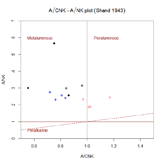
Shand 241
Value
sheet list with Figaro Style Sheet data
x.data molecular ratio A/CNK=Al2O3/(CaO +Na2O+K2O)
y.data molecular ratio A/NK=Al2O3/(Na2O+K2O)
Author(s)
Vojtech Erban, <vojtech.erban@geology.cz>
& Vojtech Janousek, <vojtech.janousek@geology.cz>
References
Shand (1943) Eruptive Rocks. John Wiley & Sons
See Also
classify figaro plotDiagram NaAlK
Examples
#Within GCDkit, the plot is called using following auxiliary functions:
#To Classify data stored in WR (Groups by diagram)
classify("Shand")
#To plot data stored in WR or its subset (menu Classification)
plotDiagram("Shand", FALSE)
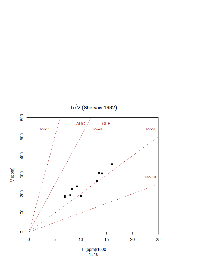
242 Shervais
Shervais Shervais (1982)
Description
Assigns data for the diagram of Shervais (1982) into Figaro template (list ’sheet’) and appropriate
values into ’x.data’ and ’y.data’.
Usage
Shervais()
Details
Discrimination diagram for basalts, as proposed by Shervais (1982) is based on variability of the
Ti/V ratio under different oxygen fugacity.
Following environments may be distinguished:
ARC Arc Tholeiites
OFB Ocean Floor Basalts

showColours 243
Author(s)
Vojtech Erban, <vojtech.erban@geology.cz>
& Vojtech Janousek, <vojtech.janousek@geology.cz>
References
Shervais J W (1982) Ti-V plots and the petrogenesis of modern and ophiolitic lavas. Earth Planet
Sci Lett 59: 101-118. doi: 10.1016/0012-821X(82)90120-0
See Also
figaro plotDiagram
Examples
#plot the diagram
plotDiagram("Shervais",FALSE)
showColours Show available colours
Description
Display colours available for plotting.
Usage
showColours(n=49)
showColours2(n=64)
Arguments
nnumeric: number of colours to display
Details
The function ’showColours’ displays a palette of plotting colours which can be specified by their
numeric codes (1-49). On the other hand, ’showColours2’ demonstrates the colours which can be
given by their English names (there are some 657 of them).
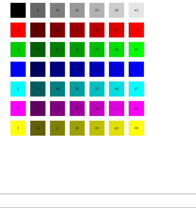
244 showLegend
Author(s)
Vojtech Janousek, <vojtech.janousek@geology.cz>
See Also
’colours’
showLegend Display legend
Description
Displays a graphical legend(s) with assignment of plotting symbols and colours used by majority
of the diagrams.
Usage
showLegend(pch=labels$Symbol,col=labels$Colour,new.plot=TRUE,alt.leg=FALSE,
just.colours=FALSE,GUI=FALSE)
Arguments
pch numeric or character: plotting symbols.
col numeric: code for their colour.
new.plot logical: shall be opened a new plotting window for the legend?

showSymbols 245
alt.leg logical; should be the alternative (continuous) legend shown? See details.
just.colours logical; in cases when two legends would be created, should be only that for
plotting colours shown?
GUI logical; Is teh function called from GUI (and not batch mode)?
Details
The internal variables ’leg.col’ and ’leg.pch’ are set to zero, if the current assignment is on the
basis of ’groups’. Otherwise they contain the sequential number(s) of column(s) in the data frame
’labels’ whose levels are to be used to build the legend(s).
If both variables differ, two legends are created, for plotting symbols and colours separately. This
is done unless ’just.colours’ is set, when only legend for colours is displayed.
If both variables equal zero, the current grouping information is used.
If a complete colour scale is used for plotting symbols, for instance that created by the assignColVar
function, an alternative (continuous) legend can be drawn.
Value
None.
Author(s)
Vojtech Janousek, <vojtech.janousek@geology.cz>
See Also
Symbols and colours by a single label can be assigned by functions assignSymbLab and assignColLab
respectively, symbols and colours by groups simultaneously by assignSymbGroup. Symbols can
be colour-coded according to a variable using the function assignColVar. Uniform symbols are
obtained by assign1symb, uniform colours by assign1col. Table of available plotting symbols is
displayed by showSymbols and colours by showColours.
Examples
showLegend()
showSymbols Show available symbols
Description
Shows numeric codes of symbols available for plotting:
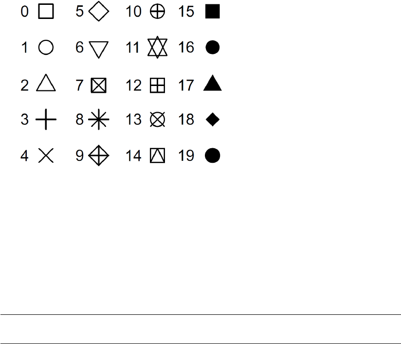
246 spider
Usage
showSymbols()
Author(s)
Vojtech Janousek, <vojtech.janousek@geology.cz>
spider Spider plot(s): Selected samples
Description
Normalization of trace-element data by the given standard and spiderplot plotting.
Usage
spider.individual(new=TRUE)
spider.contour(chondrit = selectNorm(),what=NULL,
colour.palette = "heat.colors", ymin = 0, ymax = 0,
cex = 1,join = TRUE,pch = 15,
main = "",sub = "",offset = TRUE,centered = FALSE,
xrotate = FALSE, xaxs = "r", new = TRUE, legend = TRUE)
spider(rock, chondrit = selectNorm(), ymin = 0,
ymax = 0, cex = NULL, plot = TRUE, join = TRUE,
field = FALSE, legend = FALSE, add = FALSE,
pch = NULL, col = NULL, shaded.col = "gray",
density = 0.02, angle = 0, main = "", sub = "",
offset = FALSE, centered = FALSE, xrotate = FALSE,
xaxs = "r", fill.col = TRUE, log = "y", new = TRUE, ...)
spider 247
Arguments
new logical; if true, new plotting window is opened.
chondrit a numeric matrix with one row; the normalizing values.
what variable name or formula.
colour.palette variable name or formula.
rock a numeric matrix; the whole-rock data from which will be filtered out those to
be normalized.
ymin, ymax y range of the diagram.
cex magnification of the plotting symbols.
plot logical; if set to FALSE, individual patterns are not plotted.
join logical; if TRUE, the NAs are extrapolated so that the patterns are unbroken.
field logical; if TRUE, a shaded field denoting the overall data span is plotted
legend logical; if TRUE, room for legend is reserved.
add logical; if FALSE, a new plot is started (otherwise overplot).
pch a vector specifying the plotting symbols.
col a numeric vector; colour of the plotting symbols and connecting lines.
fill.col logical; should be the field of overall variability filled by solid colour?
shaded.col numeric: colour for the cross-hatched or solid fill.
density numeric: density of the fill pattern (fraction of the whole plotting range).
angle numeric: angle of the fill pattern (in degrees).
main character: the main title for the plot.
sub character: the subtitle for the plot.
xrotate logical; shall be the element names on x axis rotated?
offset logical; shall be the names for odd and even elements shifted relative to each
other?
centered logical; shall be the element names on x axis plotted in between tick marks?
xaxs style of the xaxis: see ’help(par) for details.
log which of the axes should be logarithmic?
... further graphical parameters: see ’help(par) for details.
Details
This is a quite flexible function, a true Mother of All Spiderplots, that can be used in a number of
ways. It is employed by functions of the GCDkit system for normalization and plotting individual
patterns for selected samples (’spiderplot.r’) or each of the groups
(’spider by group individual.r’). In ’spiderplot.r’ is stored a user interface to ’spider’ for
plotting individual patterns.
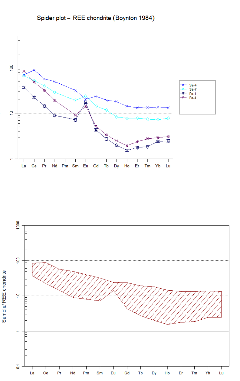
248 spider
Function ’spider’ can also serve for plotting the overall compositional ranges (shown as cross-
hatched fields or, optionally, semitransparent filled polygons) in a manner similar to function ’spider by group.r’.
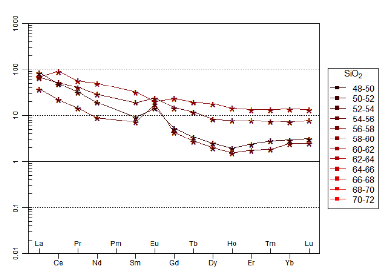
spider 249
In ’spiderplot_contour.r’ is stored a user interface to ’spider’ for plotting individual patterns,
in which the plotting symbols is uniform and colour reflects distribution of an independent variable,
such as silica contents. The variable (or formula) can be specified using the parameter ’what’, the
colour scheme by ’colour.palette’. The legal colour schemes are: ’"grays","reds","blues",
"greens","cyans","violets","yellows","cm.colors","heat.colors","terrain.colors",
"topo.colors","rainbow", "jet.colors"’.
The samples to be plotted can be selected based on combination of three searching mechanisms
(by sample name/label, range or a Boolean condition) - see selectSamples for details. For choos-
ing the correct normalization values serves the auxiliary function selectNorm. Then the user is
prompted whether to use the currently assigned plotting symbols. If desired so, the symbols and
colours can be specified in a simple spreadsheet- like interface. Likewise the scale of the y axis can
be specified. The exact appearance of the labels to the x axis can be fine tuned by the arguments
’rotate.xlab’, ’offset’ and ’centered’. See examples.
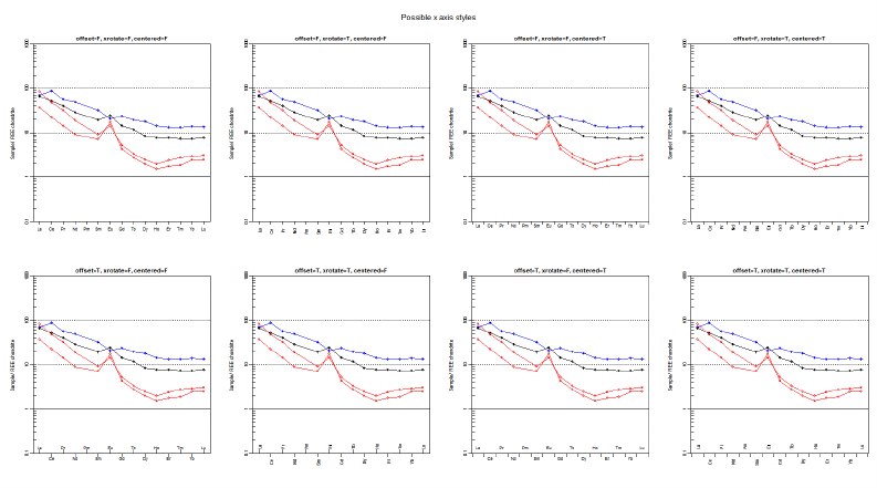
250 spider
If ’plot=FALSE’, not plotting is done, and only the normalized values are returned.
Value
results numeric matrix with normalized concentrations.
Note
If not specified, the parameters pch,col and cex are set up by default to 0 (circle), black and 1
numeric matrix, respectively. The only exception occurs when the plotting object is WR, when the
missing plotting parameters are sought in the dataframe labels, i.e. among the standard plotting
properties.
Author(s)
Vojtech Janousek, <vojtech.janousek@geology.cz>;
Vojtech Erban, <vojtech.erban@geology.cz>, contributed the algorithm hatching closed poly-
gons
See Also
For the syntax of the setup file with normalizing values and adding new normalization schemes
see selectNorm; for further applications of ’spider’ see spider2norm,spiderByGroupPatterns
and spiderByGroupFields.
Examples
ee<-spider.contour("Boynton","SiO2","reds",pch="*",cex=2,ymin=0.01,ymax=1000)
ee<-spider(WR,"Boynton",0.1,1000,pch="*",col="red",cex=2)
# the ee<- construction redirects the textual output
ee<-spider(WR[1:14,],"Boynton",1,500,pch=1:14,col=1:14,legend=TRUE)
ee<-spider(WR,"Boynton",field=T,density=0.02,angle=60,col="darkred",fill.col=F,0.1,1000)

spider2norm 251
ee<-spider(WR,"Boynton",field=TRUE,fill.col=TRUE,shaded.col="khaki",0.1,1000)
# Shade the background field portraying the overall variation
# Shade the background field portraying the overall variation
ee<-spider(WR,"Boynton",0.1,1000,pch=labels$Symbol,col=labels$Colour,cex=labels$Size)
ee<-spider(WR,"Boynton",field=TRUE,fill.col=TRUE,shaded.col="gray",add=TRUE)
ee<-spider(WR,"Boynton",0.1,1000,pch=labels$Symbol,col=labels$Colour,cex=labels$Size)
ee<-spider(WR,"Boynton",field=TRUE,density=0.02,angle=45,col="gray",fill.col=FALSE,add=TRUE)
# Custom normalization scheme
chon<-c(0.4,4,50,0.8,0.7,10,35,9,340,9,70,8.0)
chon<-matrix(chon,nrow=1)
colnames(chon)<-c("K2O","Rb","Ba","Th","Ta","Nb","Ce","Hf","Zr","Sm","Y","Yb")
rownames(chon)<-"ORG (Pearce et al. 1984)"
spider(WR,chon,ymin=0.01,col="navy",ymax=1000)
# Possible styles for x axis
multiplePerPage(8,nrow=2,ncol=4,"Possible x axis styles", dummy=FALSE)
ee<-spider(WR, "Boynton", 0.1, 1000, pch=labels$Symbol,
col=labels$Colour, cex=labels$Size, offset=F, xrotate=F, centered=F,
main="offset=F, xrotate=F, centered=F",new=F)
ee<-spider(WR, "Boynton", 0.1, 1000, pch=labels$Symbol,
col=labels$Colour, cex=labels$Size, offset=F, xrotate=T, centered=F,
main="offset=F, xrotate=T, centered=F",new=F)
ee<-spider(WR, "Boynton", 0.1, 1000, pch=labels$Symbol,
col=labels$Colour, cex=labels$Size, offset=F, xrotate=F, centered=T,
main="offset=F, xrotate=F, centered=T",new=F)
ee<-spider(WR, "Boynton", 0.1, 1000, pch=labels$Symbol,
col=labels$Colour, cex=labels$Size, offset=F, xrotate=T, centered=T,
main="offset=F, xrotate=T, centered=T",new=F)
ee<-spider(WR, "Boynton", 0.1, 1000, pch=labels$Symbol,
col=labels$Colour, cex=labels$Size, offset=T, xrotate=F, centered=F,
main="offset=T, xrotate=F, centered=F",new=F)
ee<-spider(WR, "Boynton", 0.1, 1000, pch=labels$Symbol,
col=labels$Colour, cex=labels$Size, offset=T, xrotate=T, centered=F,
main="offset=T, xrotate=T, centered=F",new=F)
ee<-spider(WR, "Boynton", 0.1, 1000, pch=labels$Symbol,
col=labels$Colour, cex=labels$Size, offset=T, xrotate=F, centered=T,
main="offset=T, xrotate=F, centered=T",new=F)
ee<-spider(WR, "Boynton", 0.1, 1000, pch=labels$Symbol,
col=labels$Colour, cex=labels$Size, offset=T, xrotate=T, centered=T,
main="offset=T, xrotate=T, centered=T",new=F)
spider(WR,"Boynton",plot=FALSE) # Calculation only
spider2norm Spider plot(s): Selected samples, double normalized
Description
Plots a double normalized spiderplot. Trace-element data are first normalized by the given standard,
as usual (see spider). Then the normalized concentrations are multiplied by a factor needed to
252 spider2norm
adjust the normalized content of the selected element in each analysis to a desired value (such as
unity). The goal is to eliminate effects of fractional crystallization (Thompson et al. 1983, Pearce
et al. 2005, Pearce and Stern 2006).
Usage
spider2norm(rock=WR,norm=NULL,norm2=NULL,ymin=0,ymax=0,which=rep(TRUE,nrow(rock)),
legend=FALSE,pch=labels$Symbol,col=labels$Colour,plot=TRUE,join=TRUE,
shaded.col="gray",density=-1,angle=0,xaxs="r",fill.col=FALSE,field=FALSE,
add=FALSE,...)
Arguments
rock a numeric matrix; the whole-rock data from which will be filtered out those to
be normalized.
norm a character string specifying the model.
norm2 name of the variable for the second normalization.
ymin, ymax y range of the diagram.
which specification of the samples to be plotted.
legend logical; if TRUE, room for legend is reserved.
pch a vector specifying the plotting symbols.
col a numeric vector; colour of the plotting symbols and connecting lines.
plot logical; if set to FALSE, individual patterns are not plotted.
join logical; if TRUE, the NAs are extrapolated so that the patterns are unbroken.
shaded.col numeric: colour for the cross-hatched fill.
density numeric: density of the fill pattern (fraction of the whole plotting range).
angle numeric: angle of the fill pattern (in degrees).
xaxs style of the xaxis: see ’help(par) for details.
fill.col colour for solid fill
field logical; if TRUE, a shaded field denoting the overall data span is plotted
add logical; if TRUE, a new plot is started (otherwise overplot).
... further graphical parameters: see ’help(par) for details.
Details
The parameter ’norm’ is an optional search pattern to query the available normalizing model names.
It can contain a substring or even a regular expression. For choosing the correct normalization
values serves the auxiliary function selectNorm.The function fails if no matches are found or the
search is ambiguous. See selectNorm for details.
The samples to be plotted can be selected based on combination of three searching mechanisms (by
sample name/label, range or a Boolean condition) - see selectSamples for details.
Then the user is prompted whether to use the currently assigned plotting symbols. If desired so, the
symbols and colours can be specified in a simple spreadsheet- like interface.
Likewise the scale of the y axis can be specified interactively.
spider2norm 253
Value
results numeric matrix with normalized concentrations
.
Author(s)
Vojtech Janousek, <vojtech.janousek@geology.cz>
References
Pearce J A, Stern R J (2006) Origin of back-arc basin magmas: Trace element and isotope perspec-
tives. Back-Arc Spreading Systems: Geological, Biological, Chemical, and Physical Interactions.
Geophysical Monograph Series 166. American Geophysical Union, pp 63-86
Pearce J A, Stern R J, Bloomer S H, Fryer P (2005) Geochemical mapping of the Mariana arc-basin
system: implications for the nature and distribution of subduction components. Geochem Geophys
Geosyst 6: doi: 10.1029/2004GC000895 doi: 10.1029/2004GC000895
Thompson R N, Morrison M A, Dickin A P, Hendry G L (1983) Continental flood basalts... Arach-
nids rule OK? In: Hawkesworth C J, Norry M J (eds) Continental Basalts and Mantle Xenoliths.
Shiva, Nantwich, pp 158-185
See Also
For the syntax of the setup file with normalizing values and adding new normalization schemes
see selectNorm; for further variants of spiderplots, see spider,spiderByGroupPatterns and
spiderByGroupFields.
Examples
ee<-spider2norm(WR,"Boynton","Yb",0.1,1000,pch="*",col="red",cex=2)
# the ee<- construction redirects the textual output
ee<-spider2norm(WR,"Boynton","Yb",field=TRUE,density=0.05,angle=60,col="red",0.1,1000)
ee<-spider2norm(WR,"Boynton","Yb",field=TRUE,fill.col=TRUE,shaded.col="khaki",0.1,1000)
# Shade the background field portraying the overall variation
ee<-spider2norm(WR,"Boynton","Lu",0.1,1000,pch=labels$Symbol,col=labels$Colour,cex=labels$Size)
ee<-spider2norm(WR,"Boynton","Lu",field=TRUE,density=0.02,angle=45,col="gray",add=TRUE)
# Shade the background field portraying the overall variation
ee<-spider2norm(WR,"Boynton","Lu",0.1,1000,pch=labels$Symbol,col=labels$Colour,cex=labels$Size)
ee<-spider2norm(WR,"Boynton","Lu",field=TRUE,fill.col=TRUE,shaded.col="gray",add=TRUE)
# Possible styles for x axis
multiplePerPage(8,nrow=2,ncol=4,"Possible x axis styles", dummy=FALSE)
ee<-spider2norm(WR, "Boynton","Yb", 0.1, 1000, pch=labels$Symbol,
col=labels$Colour, cex=labels$Size, offset=F, xrotate=F, centered=F,new=F)
ee<-spider2norm(WR, "Boynton","Yb", 0.1, 1000, pch=labels$Symbol,
col=labels$Colour, cex=labels$Size, offset=F, xrotate=T, centered=F,new=F)
ee<-spider2norm(WR, "Boynton","Yb", 0.1, 1000, pch=labels$Symbol,
col=labels$Colour, cex=labels$Size, offset=F, xrotate=F, centered=T,new=F)
ee<-spider2norm(WR, "Boynton","Yb", 0.1, 1000, pch=labels$Symbol,
col=labels$Colour, cex=labels$Size, offset=F, xrotate=T, centered=T,new=F)
ee<-spider2norm(WR, "Boynton","Yb", 0.1, 1000, pch=labels$Symbol,

254 spiderBoxplot
col=labels$Colour, cex=labels$Size, offset=T, xrotate=F, centered=F,new=F)
ee<-spider2norm(WR, "Boynton","Yb", 0.1, 1000, pch=labels$Symbol,
col=labels$Colour, cex=labels$Size, offset=T, xrotate=T, centered=F,new=F)
ee<-spider2norm(WR, "Boynton","Yb", 0.1, 1000, pch=labels$Symbol,
col=labels$Colour, cex=labels$Size, offset=T, xrotate=F, centered=T,new=F)
ee<-spider2norm(WR, "Boynton","Yb", 0.1, 1000, pch=labels$Symbol,
col=labels$Colour, cex=labels$Size, offset=T, xrotate=T, centered=T,new=F)
spider2norm(WR,"Boynton","Yb",plot=FALSE) # Calculation only
spiderBoxplot Spider plot(s): Selected samples - summary boxplot
Description
Normalization of geochemical data by the given standard (optionally also one of the samples) and
spiderplot plotting. No individual patterns are drawn; instead, the statistical distribution of each
element is portrayed by a boxplot.
Usage
spiderBoxplot(norm = NULL, which = rep(TRUE,nrow(WR)),
doublenorm = FALSE, norm2 = "",
ymin = NULL, ymax = NULL, bpplot = TRUE,
col = "lightgray", log = TRUE)
Arguments
norm a character string specifying the model.
which specification of the samples to be plotted.
doublenorm logical; should be the normalization employed? See details.
norm2 name of the variable for the second normalization.
ymin, ymax y range of the diagram.
bpplot logical; if FALSE, boxplot box (instead of box and percentile plot) is shown.
col fill colour.
log logical; should be the y axis scaled logarithmically?
Details
The parameter ’norm’ is an optional search pattern to query the available normalizing model names.
It can contain a substring or even a regular expression. The function fails if no matches are found
or the search is ambiguous. See selectNorm for details.
The samples to be plotted can be selected based on combination of three searching mechanisms (by
sample name/label, range or a Boolean condition) - see selectSamples for details.
For choosing the correct normalization values serves the auxiliary function selectNorm, which is
the same as in ordinary spiderplots. If the user desires so, the data can be normalized by a sample
present in the dataset. Then the elements to be plotted and their order is to be specified, as well.
Optionally, double normalization can be used. Trace-element data are first normalized by the given
standard, then by the normalized content of the selected element in each analysis to eliminate effects
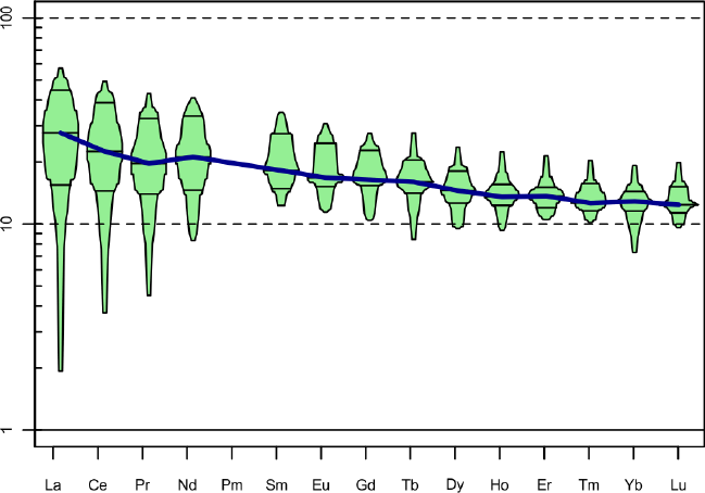
spiderBoxplot 255
of fractional crystallization (Thompson et al. 2003, Pearce et al. 2005, Pearce and Stern 2006). See
spider2norm for details.
Distributions of individual normalized elements are plotted in the form of boxplot or box and per-
centile plot (Esty and Banfield 2003).
In both cases the box denotes 50% of the population (both quartiles), the horizontal line in the
middle is a median and the whiskers denote the overall range. For boxplot this is without outliers.
See manual entry for ’boxplot’ and ’bpplot.my’ for further details.
Printed are number of observations, missing values, mean, standard deviation, minimum, 25% quar-
tile, median (=50% quartile), 75% quartile and maximum.
Value
results numeric matrix with statistical data for individual elements.
Warning
This function IS NOT Figaro-compatible. It means that the set of diagrams cannot be further edited
in GCDkit (e.g. tools in "Plot editing" menu are inactive).
Author(s)
Vojtech Janousek, <vojtech.janousek@geology.cz>
References
Esty, W. W. & Banfield, J. D. (2003). The Box-Percentile Plot. Journal of Statistical Software 8
(17)
Pearce J A, Stern R J (2006) Origin of back-arc basin magmas: Trace element and isotope perspec-
tives. Back-Arc Spreading Systems: Geological, Biological, Chemical, and Physical Interactions.
Geophysical Monograph Series 166. American Geophysical Union, pp 63-86
Pearce J A, Stern R J, Bloomer S H, Fryer P (2005) Geochemical mapping of the Mariana arc-basin
system: implications for the nature and distribution of subduction components. Geochem Geophys
Geosyst 6: doi: 10.1029/2004GC000895

256 spiderByGroupFields
Thompson R N, Morrison M A, Dickin A P, Hendry G L (1983) Continental flood basalts... Arach-
nids rule OK? In: Hawkesworth C J, Norry M J (eds) Continental Basalts and Mantle Xenoliths.
Shiva, Nantwich, pp 158-185
See Also
For the syntax of the setup file with normalizing values and adding new normalization schemes
see selectNorm; for further applications of ’spider’ see spiderByGroupPatterns,
spider2norm and spiderByGroupFields.
Examples
spiderBoxplot("Boynton",col="yellow",bpplot=FALSE)
spiderBoxplot("Primordial Wood",doublenorm=TRUE,norm2="Y",
col="khaki",ymin=0.05,ymax=1000,bpplot=TRUE)
spiderByGroupFields Spider plot(s) - by group fields
Description
Plots a series of spiderplots, for each group one, outlining the overall distribution as a field.
Usage
spiderByGroupFields(rock = WR, norm = NULL,
bw = FALSE, fill = FALSE, ymin = 0, ymax = 0,
xrotate = FALSE, offset = TRUE, centered = FALSE)
Arguments
rock a numeric matrix; the whole-rock data from which will be filtered out those to
be normalized.
norm a character string specifying the model.
bw logical; should be the plot black and white?
fill logical; should be the fields filled by solid colour (and not hatched)?
ymin, ymax y range of the diagram.
xrotate logical; shall be the element names on x axis rotated?
offset logical; shall be the names for odd and even elements shifted relative to each
other?
centered logical; shall be the element names on x axis plotted in between tick marks?
Details
The parameter ’norm’ is an optional search pattern to query the available normalizing model names.
It can contain a substring or even a regular expression. For choosing the correct normalization
values serves the auxiliary function selectNorm.The function fails if no matches are found or the
search is ambiguous. See selectNorm for details.
A series of spiderplots is plotted, for each group one, in which the whole variation range is outlined
as filled/cross-hatched fields.

spiderByGroupPatterns 257
Value
None.
Author(s)
Vojtech Janousek, <vojtech.janousek@geology.cz>;
Vojtech Erban, <vojtech.erban@geology.cz>, contributed the algorithm hatching closed poly-
gons
See Also
For the syntax of the setup file with normalizing values and adding new normalization schemes see
selectNorm. This function is based on spider.
Examples
## Not run:
data<-loadData("sazava.data",sep="\t")
groupsByLabel("Intrusion")
spiderByGroupFields(norm="Boynton",ymin=1,ymax=1000)
spiderByGroupFields(norm="Boynton",bw=TRUE,ymin=1,ymax=1000,xrotate=TRUE,offset=FALSE)
spiderByGroupFields(norm="Boynton",fill=TRUE,ymin=1,ymax=1000)
## End(Not run)
spiderByGroupPatterns Spider plot(s) - by group patterns
Description
Plots a series of spiderplots, for each group one, in which individual patterns are shown.
Usage
spiderByGroupPatterns(rock = WR, norm = NULL, bw = FALSE,
ymin = 0, ymax = 0, xrotate = FALSE, offset = TRUE, centered = FALSE)
Arguments
rock a numeric matrix; the whole-rock data from which will be filtered out those to
be normalized.
norm a character string specifying the model.
bw logical; should be the plot black and white?
ymin, ymax y range of the diagram.
xrotate logical; shall be the element names on x axis rotated?
offset logical; shall be the names for odd and even elements shifted relative to each
other?
centered logical; shall be the element names on x axis plotted in between tick marks?

258 srnd
Details
Firstly, the normalization scheme is chosen and scaling for all the plots specified. Then, a series of
spiderplots is plotted, for each group one, in which patterns for individual samples are shown.
Value
Returns a list ’results’ with the normalized values, and, in case of REE, some extra parameters.
Author(s)
Vojtech Janousek, <vojtech.janousek@geology.cz>
See Also
For the syntax of the setup file with normalizing values and adding new normalization schemes see
selectNorm. This function is based on spider.
Examples
# Get the data ready
data(sazava)
accessVar("sazava")
groupsByLabel("Intrusion")
#Plot
spiderByGroupPatterns(norm="Boynton",ymin=1,ymax=1000)
spiderByGroupPatterns(norm="Boynton",bw=TRUE,ymin=1,ymax=1000,xrotate=TRUE,offset=FALSE)
srnd Recalculations of the Sr-Nd isotopic data
Description
Age-corrects the Sr-Nd isotopic data to a given age; calculates initial (N d)values and Nd model
ages.
Usage
srnd(age="")
initial(x,age,system="Nd")
epsilon(WR,age)
DMage(WR)
DMGage(WR)
DMLHage(WR,age,RCC=0.12)
srnd 259
Arguments
age age in Ma: if empty, the user is prompted to enter a value
x, WR isotopic data to be recalculated
system character; which isotopic system Sr or Nd?
RCC numeric; the 147Sm/144Nd ratio of the intermediate crustal reservoir for calcu-
lation of the two-stage Nd model ages
Details
Recalculates the Sr-Nd isotopic data and returns them in the numeric matrix init with the following
columns (DM = Depleted Mantle):
Age (Ma) Age in Ma
87Sr/86Sri Initial 87Sr/86Sr ratios
143Nd/144Ndi Initial 143Nd/144N d ratios
EpsNdi Initial (Nd)values
TDM Single-stage DM Nd model ages (Liew & Hofmann, 1988), function DMage
TDM.Gold Single-stage DM Nd model ages (Goldstein et al., 1988), function DMGage
TDM.2stg Two-stage DM Nd model ages (Liew & Hofmann, 1988), function DMLHage
Value
init numeric matrix with the results
Plugin
SrNd.r
Author(s)
Vojtech Janousek, <vojtech.janousek@geology.cz>
References
Goldstein S L, O’Nions R K & Hamilton P J (1984) A Sm-Nd isotopic study of atmospheric dusts
and particulates from major river systems. Earth Planet Sci Lett 70: 221-236 doi: 10.1016/0012-
821X(84)90007-4
Liew T C & Hofmann A W (1988) Precambrian crustal components, plutonic associations, plate
environment of the Hercynian Fold Belt of Central Europe: indications from a Nd and Sr isotopic
study. Contrib Mineral Petrol 98: 129-138 doi: 10.1007/BF00402106
Examples
# recalculation to 500 Ma
srnd(500)
# print the isotopic parameters currently in the memory
init

260 statsByGroup
statsByGroup Statistics by groups
Description
Calculates simple descriptive statistics for individual columns of the given data matrix; optionally
this can be done for each of the groups separately.
Usage
statsByGroup(data = WR, groups = groups)
Arguments
data numeric data matrix.
groups a vector, in which is specified, for each sample, a group it belongs to.
Details
The function returns a list containing the calculated statistical parameters respecting the desired
grouping. The statistical summary involves number of observations, missing values, mean, standard
deviation, minimum, 25% quartile, median (= 50% quartile), 75% quartile and maximum. This is a
core function invoked both by summarySingle and summarySingleByGroup.
Value
results a list with the results for individual groups
Author(s)
Vojtech Janousek, <vojtech.janousek@geology.cz>
See Also
summarySingle
statistics
summaryAll
summaryByGroup
Examples
statsByGroup(WR)
statsByGroup(WR[,LILE])

statsByGroupPlot 261
statsByGroupPlot Statistics: Plot summary by element and group
Description
Plots crosses in a binary diagram denoting means and standard deviations for individual groups.
Usage
statsByGroupPlot()
Details
Displays a binary diagram of two elements/oxides in which are plotted averages for the individual
groups with whiskers corresponding to their standard deviations.
The variables are entered via the function ’selectColumnLabel’. In the specification of the vari-
ables can be used also arithmetic expressions, see calcCore for the correct syntax.
Value
results a matrix with the results for individual groups and selected two elements/oxides
Author(s)
Vojtech Janousek, <vojtech.janousek@geology.cz>
statsIso Statistical plots of isotopic ratios/model ages
Description
Plots a boxplot or stripplot for a given isotopic parameter, respecting groups.
Usage
boxplotIso(what=NULL)
stripplotIso(what=NULL)
Arguments
what the variable name; see Details.
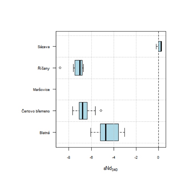
262 statsIso
Details
The boxplot portrays realistically a statistical distribution of the data. The box represents, for each
of the groups, the two quartiles, the line inside is a median, the whiskers show the whole range
without outliers.
Stripplot shows 1D scatter plots for each of the groups, with some artificial noise (jitter) added to
make the individual points better visible. Stripplots are a good alternative to boxplots when sample
sizes are small.
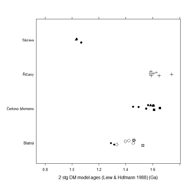
statsIso 263
The variables to choose from are:
Menu item Explanation
87Sr/86Sri Initial Sr isotopic ratios
143Nd/144Ndi Initial Nd isotopic ratios
EpsNdi Initial (Nd)values
1 stg DM model ages (Goldstein et al. 1988) Single-stage DM Nd model ages
1 stg DM model ages (Liew & Hofmann 1988) Single-stage DM Nd model ages
2 stg DM model ages (Liew & Hofmann 1988) Two-stage DM Nd model ages
In addition, any variable names starting with the text "delta" will appear in this list.
The variable names can be specified also upon the function call, as the parameter "what". The
possibilities are "87Sr/86Sri","143Nd/144Ndi","EpsNdi","TDM.Gold","TDM" or "TDM.2stg".
Value
a list object with data produced by the function ’boxplot’.
Plugin
SrNd.r
Author(s)
Vojtech Janousek, <vojtech.janousek@geology.cz>

264 strip
References
Goldstein S L, O’Nions R K & Hamilton P J (1984) A Sm-Nd isotopic study of atmospheric dusts
and particulates from major river systems. Earth Planet Sci Lett 70: 221-236 doi: 10.1016/0012-
821X(84)90007-4
Liew T C & Hofmann A W (1988) Precambrian crustal components, plutonic associations, plate
environment of the Hercynian Fold Belt of Central Europe: indications from a Nd and Sr isotopic
study. Contrib Mineral Petrol 98: 129-138 doi: 10.1007/BF00402106
See Also
’boxplot’
strip Statistics: Stripplot by groups
Description
Stripplot for selected samples and variable, respecting the grouping.
Usage
strip(xlab = "", ...)
Arguments
xlab variable name
... additional parameters to stripplot
Details
Stripplot shows 1D scatter plots for each of the groups, with some artificial noise (jitter) added to
make the individual points better visible. Stripplots are a good alternative to boxplots when sample
sizes are small.
If no variable is specified as an argument ’xlab’, the user can enter it using the function ’selectColumnLabel’.
In the specification of the variable can be used also arithmetic expressions, see calcCore for the
correct syntax.
Value
None.
Author(s)
Vojtech Janousek, <vojtech.janousek@geology.cz>
See Also
stripplot,stripBoxplot
Examples
strip("(Na2O+K2O)/Al2O3")

stripBoxplot 265
stripBoxplot Statistics: Stripplot by groups - with boxplots
Description
Stripplot for selected variable, respecting the grouping. Each of the stripplots for the individual
groups are underlain by a boxplot, so that the median, quartiles and range are immediately appar-
ent. Optionally, the data points can be replaced by variously sized/coloured circles, depicting a
distribution of a second variable.
Usage
stripBoxplot(yaxis="",zaxis="0",ymin=NULL,ymax=NULL,pal="heat.colors",ident=FALSE,
scaling.factor=NULL,boxplot.data=NULL,
pch=NULL,col=NULL,cex=NULL,silent=TRUE,add=FALSE)
Arguments
yaxis specification of the variable used for stripplots/boxplots.
zaxis (optional) specification of the variable depicted by the circles.
ymin, ymax minimum and maximum of the y axis.
pal name of predefined palette.
ident logical; should be the samples identified interactively after plotting?
scaling.factor numeric; relative size of the plotted symbols.
boxplot.data a list; data for the underlying boxplots (if different from those used for the strip-
plots). See Details.
pch plotting symbols.
col plotting colours.
cex relative size of the plotting symbols.
silent logical, should be some of the above parameters chosen by the appropriate dia-
logues?
add logical; should be the diagram added to a preexisting plot (rather than a new
plotting window opened)?
Details
Stripplot shows 1D scatter plots for each of the groups, with some artificial noise (jitter) added to
make the individual points better visible. Stripplots are a good alternative to boxplots when sample
sizes are small.
If no variable is specified as an argument ’yaxis’, and the function is invoked in interactive regime
(silent = FALSE), the user can enter it using the function ’selectColumnLabel’.
If ’zaxis’ is zero, assigned plotting symbols, colours and symbol sizes are used.
If ’zaxis’ refers to a valid variable name, the data points are shown as circles, the size and colours
of which correspond to this second variable. In the batch mode, the relative size of the circles
plotted can be specified using the parameter scaling.factor.
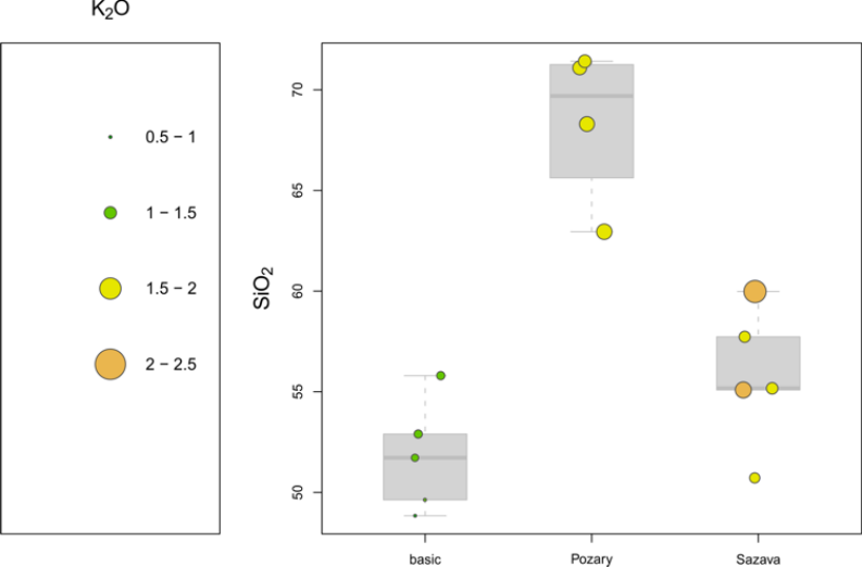
266 stripBoxplot
In the specification of the variable(s) can be used also arithmetic expressions, see calcCore for the
correct syntax.
The colour scheme can be specified by ’pal’. The legal colour schemes are: "grays","reds","blues",
"greens","cyans","violets","yellows","cm.colors","heat.colors","terrain.colors",
"topo.colors","rainbow" and "jet.colors".
Normally, the stripplots are underlain by boxplots portraying the statistical distribution of the same
data, as used for construction of stripplots for each of the groups. However, with caution, one can
specify via boxplot.data a list containing the alternative data to be shown on background. Clearly,
the number of components in the list, as well as their order, needs to exactly match the individual
groups (the levels).
Value
None.
Author(s)
Vojtech Janousek, <vojtech.janousek@geology.cz>
See Also
stripplot,boxplot,strip,plotWithCircles
Examples
stripBoxplot("(Na2O+K2O)/Al2O3")

Subset by range 267
Subset by range Select subset by range
Description
Selecting subsets of the data stored in memory by their range.
Details
The menu item ’Select subset by range’ is connected to the function selectSubset. The
search pattern is treated as a selection of sample sequence numbers (effectively a list separated by
commas that may also contain ranges expressed by colons). The current data will be replaced by its
newly chosen subset.
Value
Overwrites the data frame ’labels’ and numeric matrix ’WR’ by subset that fulfills the search crite-
ria.
Author(s)
Vojtech Janousek, <vojtech.janousek@geology.cz>
Examples
## Not run:
Search pattern = 1:5
# First to fifth samples in the data set
Search pattern = 1,10
# First and tenth samples
Search pattern = 1:5, 10:11, 25
# Samples number 1, 2, ...5, 10, 11, 25
## End(Not run)
summaryAll Statistics: Statistical summaries for the whole data set or its subset
Description
The function ’summaryAll’ prints statistical summary for selected list of elements (majors as a
default) and the current dataset (or its part). Functions ’summaryMajor’ and ’summaryTrace’ are
entry points supplying the default lists for major- and trace elements.
Usage
summaryAll(elems = major, where = NULL, show.boxplot = FALSE,
show.hist = FALSE, silent=TRUE)
summaryMajor()
summaryTrace()
268 summaryAll
Arguments
elems list of desired elements
where list of desired samples to be processed
show.boxplot logical, should be plotted the boxplots?
show.hist logical, should be plotted the histograms?
silent logical, should be the above chosen by the appropriate dialogues?
Details
The statistical summary involves number of observations, missing values, mean, standard deviation,
minimum, 25% quartile, median (= 50% quartile), 75% quartile and maximum. The function also
plots summary boxplots and histograms, if desired so.
The samples can be selected based on combination of three searching mechanisms (by sample
name/label, range or a Boolean condition) - see selectSamples for details.
Even though as a default are assumed majors (SiO2, TiO2, Al2O3,FeOt, MnO, MgO, CaO, Na2O, K2O
for ’summaryMajor’) or selected trace (Rb, Sr, Ba, Cr, Ni, La, Eu, Y, Zr for ’summaryTrace’)
elements, the variable(s) to be displayed can be modified/specified in all cases. To this purpose
serves the function ’selectColumnsLabels’.
In the specification of the variable can be used also arithmetic expressions, see calcCore for the
correct syntax.
Value
results numeric matrix with the results
Author(s)
Vojtech Janousek, <vojtech.janousek@geology.cz>
See Also
statistics summarySingle summarySingleByGroup summaryByGroup
Examples
summaryAll(LILE)
summaryAll(LILE,show.hist=TRUE)
summaryAll(LILE,show.boxplot=TRUE)
# user-defined list
my.elems<-c("Rb","Sr","Ba")
summaryAll(my.elems)
## Not run:
summaryMajor()
summaryTrace()
## End(Not run)

summaryByGroup 269
summaryByGroup Statistics: Statistical summaries by groups
Description
The function ’summaryByGroup’ prints a statistical summary for selected list of elements (majors
as a default) and the whole dataset or its selection, respecting the current grouping. Functions
’summaryByGroupMjr’ and ’summaryByGroupTrc’ are entry points supplying the default lists for
major- and trace elements. The function ’summaryByGroupTrc’ returns only ranges of the given
parameter(s).
Usage
summaryByGroup(elems = major, where = NULL, show.boxplot = FALSE,
show.hist = FALSE, silent = TRUE)
summaryByGroupMjr()
summaryByGroupTrc()
summaryRangesByGroup(elems=major, where=NULL, silent=TRUE)
Arguments
elems list of desired elements
where list of desired samples to be processed
show.boxplot logical, should be plotted the boxplots?
show.hist logical, should be plotted the histograms?
silent logical, should be the above chosen by the appropriate dialogues?
Details
The statistical summary involves number of observations, missing values, mean, standard deviation,
minimum, 25% quartile, median (= 50% quartile), 75% quartile and maximum. The function also
plots a summary boxplots and histograms, if desired so.
The samples can be selected based on combination of three searching mechanisms (by sample
name/label, range or a Boolean condition) - see selectSamples for details.
The defaults are lists of major (SiO2, TiO2, Al2O3, FeOt, MnO, MgO,CaO, Na2O,
K2O) or trace (Rb, Sr, Ba, Cr, Ni, La, Eu, Y, Zr) elements, respectively.
The desired variables are selected using the function ’selectColumnsLabels’.
In the specification of the variable can be used also arithmetic expressions, see calcCore for the
correct syntax.
Value
results a list with the results for individual groups
Author(s)
Vojtech Janousek, <vojtech.janousek@geology.cz>

270 summarySingle
Examples
summaryByGroup(LILE)
summaryByGroup(LILE,show.hist=TRUE)
summaryByGroup(LILE,show.boxplot=TRUE)
# user-defined list
my.elems<-c("Rb","Sr","Ba/Sr")
summaryByGroup(my.elems)
## Not run:
summaryByGroupTrc()
summaryByGroupMjr()
summaryRangesByGroup(elems="Rb/Sr,Na2O+K2O")
## End(Not run)
summarySingle Statistics: Single variable all/selection
Description
Prints statistical summary for a single variable and the current dataset (or its part).
Usage
summarySingle(xlab="")
Arguments
xlab variable name
Details
The statistical summary involves number of observations, missing values, mean, standard deviation,
minimum, 25% quartile, median (=50% quartile), 75% quartile and maximum. The function also
plots a summary boxplot and histogram.
In addition the statistical distribution of the given variable is shown as a boxplot, a box-percentile
plot and two variants of histograms.
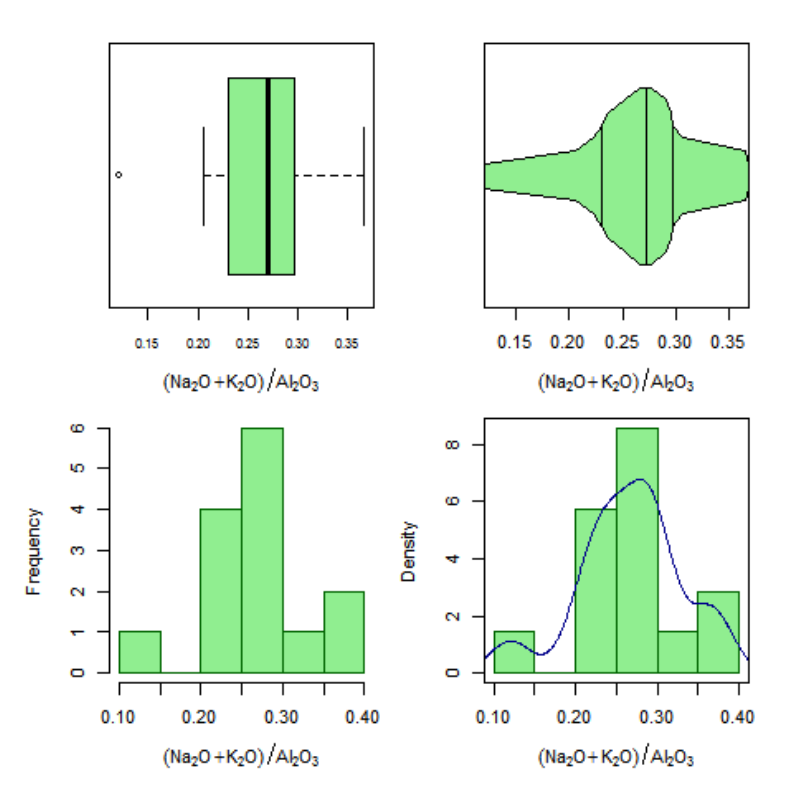
summarySingle 271
If no variable is specified as an argument ’xlab’, the user can enter it using the function ’selectColumnLabel’.
In the specification of the variable can be used also arithmetic expressions, see calcCore for the
correct syntax.
The samples can be selected based on combination of three searching mechanisms (by sample
name/label, range or a Boolean condition) - see selectSamples for details.
Value
results numeric matrix/vector with the results
Author(s)
Vojtech Janousek, <vojtech.janousek@geology.cz>
See Also
boxplot
bpplot2
statistics

272 summarySingleByGroup
summarySingleByGroup summaryAll summaryByGroup
Examples
summarySingle("(Na2O+K2O)/Al2O3")
summarySingleByGroup Statistics: Single variable by groups
Description
Prints statistical summary for a single variable and the whole dataset, divided by groups.
Usage
summarySingleByGroup(xlab="")
Arguments
xlab variable name
Details
The statistical summary involves number of observations, missing values, mean, standard deviation,
minimum, 25% quartile, median (= 50% quartile), 75% quartile and maximum. The function also
plots a summary boxplot and histogram.
If no variable is specified as an argument ’xlab’, the user can enter it using the function
’selectColumnLabel’. In the specification of the variable can be used also arithmetic expressions,
see calcCore for the correct syntax.
Value
results numeric matrix with the results
Author(s)
Vojtech Janousek, <vojtech.janousek@geology.cz>
See Also
boxplot summarySingle statistics summaryAll summaryByGroup
Examples
summarySingleByGroup("(Na2O+K2O)/Al2O3")
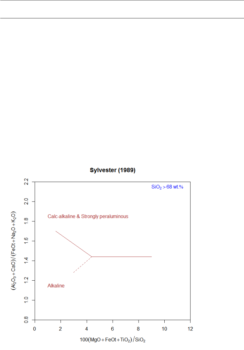
Sylvester 273
Sylvester Sylvester (1989)
Description
Assigns data for a binary plot (Al2O3+CaO)/(F eOt+N a2O+K2O)vs. 100∗(MgO+F eOt+
T iO2)/SiO2, proposed by Sylvester (1989) to distinguish the alkaline collision-related alkaline
granites into Figaro template (list ’sheet’) and appropriate values into ’x.data’ and ’y.data’.
Usage
Sylvester()
Details
In the plot (Al2O3+CaO)/(F eOt +Na2O+K2O)vs. 100 ∗(M gO +F eOt +T iO2)/SiO2
of Sylvester (1989) can be distinguished ’Alkaline’collision-related granites, from ’Calc-alkaline
& Strongly peraluminous’ types (solid line). The strongly fractionated calc-alkaline varieties are
separated by the dashed line.
Note that only samples with SiO2> 68 wt. % are plotted.

274 TAS
Value
sheet list with Figaro Style Sheet data
x.data (Al2O3+CaO)/(FeOt+Na2O+K2O) [wt. %]
y.data 100*(MgO+FeOt+TiO2)/SiO2 [wt. %]
Author(s)
Vojtech Janousek, <vojtech.janousek@geology.cz>
References
Sylvester P J (1989) Post-collisional alkaline granites. J Geol 97: 261-280. doi: 10.1086/629302
See Also
figaro plotDiagram
Examples
#plot the diagram
plotDiagram("Sylvester", FALSE)
TAS IUGS recommended TAS (Le Bas et al. 1986)
Description
Assigns data for IUGS recommended TAS diagram into Figaro template (list ’sheet’) and appro-
priate values into ’x.data’ and ’y.data’
Usage
TAS(cutoff=95)
Arguments
cutoff numeric; the minimal sum of the analysis to be considered for classification
Details
TAS diagram, as proposed by Le Bas et al. (1986), codified by Le Maitre et al. (1989) and slightly
modified by Le Bas (2000).
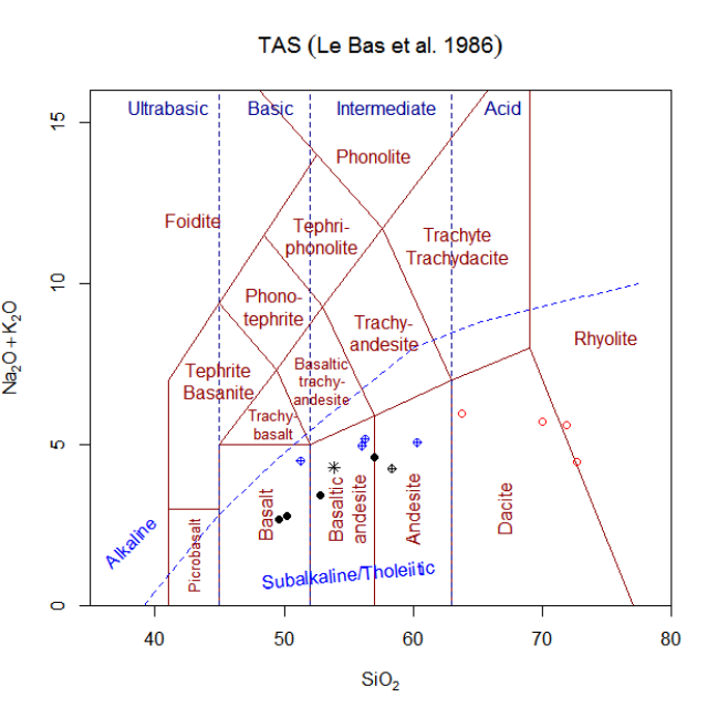
TAS 275
The diagram (in its basic form) defines following fields:
foidite
picrobasalt
basalt
basaltic andesite
andesite
dacite
rhyolite
trachybasalt
basaltic trachyandesite
trachyandesite
trachyte/trachydacite
tephrite/basanite
phonotephrite
tephriphonolite
phonolite
This primary division is further enhanced by the ’TASadd’ routine (called automatically by ’classify’).
Following actions are carried out:
• Analyses with H2O> 2 and CO2> 0.5 (weight percent) are filtered out
•Trachybasalt is subdivided into hawaiite and potassic trachybasalt
•Basaltic trachyandesite is subdivided into mugearite and shoshonite
•Trachyandesite is subdivided into benmoreite and latite
276 TAS
• High-Mg rocks are split into picrite, komatiite, meimechite and boninite
Note that systematics of high-Mg rocks follows revised IUGS Recommendations (Le Bas et al.,
2000; Le Maitre et al. 2002) which differ from their 1st edition (Le Maitre et al, 1989). Further
subdivisions recommended by Le Maitre et al. (1989) are not implemented in GCDkit, mainly for
poorly defined CIPW version used by the Subcommission.
Value
x.data SiO2 data recast to anhydrous sum (matrix ’WRanh’)
y.data Na2O+K2O data recast to anhydrous sum (matrix ’WRanh’)
sheet list with Figaro Style Sheet data
results matrix with classification results
groups vector with classification results
grouping set to -1
Author(s)
Vojtech Erban, <vojtech.erban@geology.cz>
& Vojtech Janousek, <vojtech.janousek@geology.cz>
References
Le Bas M J, Le Maitre R W, Streckeisen A & Zanettin B (1986) A chemical classification of vol-
canic rocks based on the total alkali-silica diagram. J Petrology 27: 745-750 doi: 10.1093/petrol-
ogy/27.3.745
Le Bas M J (2000) IUGS Reclassification of the High-Mg and Picritic Volcanic Rocks. J Petrology
41: 1467-1470 doi: 10.1093/petrology/41.10.1467
Le Maitre R W et al (1989) Igneous Rocks: A Classification and Glossary of Terms, 1st edition.
Cambridge University Press
Le Maitre R W et al (2002) A Classification and Glossary of Terms, 1st edition. Cambridge Uni-
versity Press
See Also
classify figaro plotDiagram
Examples
#Within GCDkit, the plot is called using following auxiliary functions:
#To Classify data stored in WR (Groups by diagram)
classify("TAS")
#To plot data stored in WR or its subset (menu Classification)
plotDiagram("TAS", FALSE)
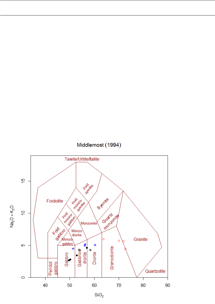
TASMiddlemost 277
TASMiddlemost Middlemost’s modification of TAS diagram
Description
Assigns data for Middlemost’s modification of the TAS diagram into Figaro template (list ’sheet’)
and appropriate values into ’x.data’ and ’y.data’.
Usage
TASMiddlemostVolc()
TASMiddlemostPlut()
Details
Middlemost’s variation of classic IUGS-recommended TAS diagram, originally proposed by Le Bas
et al. (1986). Boundaries of foidite, phonolite, trachyte, trachydacite and rhyolite fields are defined,
as inferred from the phase relations in the TAS system. Moreover, the trachyte + trachydacite field
is split into trachyte and trachydacite fields, silexite and sodalitite + nephelinolith + leucitolith fields
are defined.
The same diagram layout is applied also to plutonic rocks as follows:
plutonic rocks volcanic rocks
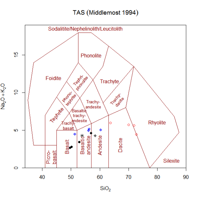
278 TASMiddlemost
Peridotgabbro Picrobasalt
Gabbro Basalt
Gabbroic Diorite Basaltic Andesite
Diorite Andesite
Granodiorite Dacite
Granite Rhyolite
Quartzolite Silexite
Monzogabbro Trachybasalt
Monzodiorite basaltic Trachyandesite
Monzonite Trachyandesite
Quartzmonzonite Trachydacite
Syenite Trachyte
Foid Gabbro Tephrite
Foid Monzodiorite Phonotephrite
Foid Monzosyenite Tephriphonolite
Foid Syenite Phonolite
Foidolite Foidite
Tawite/Urtite/Italite sodalitite/nephelinolith/leucitolith
Value
sheet list with Figaro Style Sheet data
x.data SiO2 weight percent
y.data Na2O+K2O weight percent

ternary 279
Author(s)
Vojtech Erban, <vojtech.erban@geology.cz>
References
Le Bas M J, Le Maitre R W, Streckeisen A & Zanettin B (1986) A chemical classification of volcanic
rocks based on the total alkali-silica diagram. J Petrology 27: 745-750
Middlemost E A K (1994) Naming materials in the magma/igneous rock system. Earth Sci Rev 37:
215-224 doi: 10.1016/0012-8252(94)90029-9
See Also
classify TAS Cox figaro plotDiagram
Examples
#Within GCDkit, the plot is called using following auxiliary functions:
#To Classify data stored in WR (Groups by diagram)
classify("TASMiddlemostVolc")
# or
classify("TASMiddlemostPlut")
#To plot data stored in WR or its subset (menu Classification)
plotDiagram("TASMiddlemostVolc", FALSE)
# or
plotDiagram("TASMiddlemostPlut", FALSE)
ternary Ternary plot
Description
These functions plot/add data to a ternary plot.
Usage
ternary(x = NULL, y = NULL, z = NULL, samples = rownames(WR),
new = TRUE, grid = FALSE, ticks = TRUE, ...)
triplot(aa, bb, cc, alab, blab, clab, title = "", grid.int = 0,
tick.int = 0, label.axes = FALSE, line = FALSE,
pch = labels[names(aa), "Symbol"],
col = labels[names(aa), "Colour"],
cex = labels[names(aa),"Size"],
identify = getOption("gcd.ident"),
new = TRUE,...)
triplotadd(aa, bb, cc,
pch=labels[names(aa),"Symbol"],
col=labels[names(aa),"Colour"],
cex = labels[names(aa),"Size"],
labs=NULL, identify = FALSE, lines = FALSE, lty = "solid", type="p")
280 ternary
Arguments
xcharacter; specification of the plotting variable for the bottom left apex (formu-
lae OK).
ycharacter; specification of the plotting variable for the top apex (formulae OK).
zcharacter; specification of the plotting variables for the bottom right apex (for-
mulae OK).
grid logical; should be grid plotted?
ticks logical; should be ticks plotted?
samples character or numeric vector; specification of the samples to be plotted.
new logical; should be opened a new plotting window?
... Further parameters to the functions ’ternary’ and ’triplot’.
aa a numerical vector, bottom left apex.
bb a numerical vector, top apex.
cc a numerical vector, bottom right apex.
alab,blab,clab labels for the apices.
title title for the whole diagram.
grid.int interval of grid lines (0-1); if set to zero (default value), no grid is drawn.
tick.int interval of ticks on axes (0-1); if set to zero (default value), no ticks are drawn.
label.axes logical; if set to TRUE, axes are labeled by percentages of the components.
line, lines logical; if set to TRUE, lines are drawn instead of plotting points.
lty line type.
pch plotting symbols.
col plotting colours.
cex relative size of plotting symbols.
identify logical; should be samples identified?
labs character; optional text to label the points.
type character; plot type; see plot.default.
Details
The function ’ternary’ is the user interface to ’triplot’. The latter sets up the axes, labels the
apices, plots the data and, if desired, enables the user to identify the data points interactively.
If ’new=TRUE’, new plot window is opened.
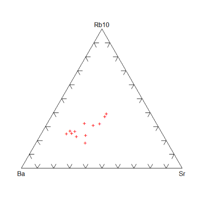
ternary 281
The values for ’label.axes’ are chosen according to ’tick.int’ or ’grid.int’; if these are not
available, labels are drawn by 10%.
’triplotadd ’adds data points/lines to pre-existing ternary plot.
The variables to be plotted are selected using the function ’selectColumnLabel.
In the specification of the apices can be used also arithmetic expressions, see calcCore for the
correct syntax.
The functions are Figaro-compatible.
Value
A numeric matrix with coordinates of the data points recast to a sum of 1.
Author(s)
Jakub Smid <smid@prfdec.natur.cuni.cz> & Vojtech Janousek, <vojtech.janousek@geology.cz>
See Also
plot
Examples
ternary("Ba","Rb*10","Sr",col="red",pch="+")
282 tetrad
ternary("SiO2/10","2*FeOt","K2O*5",samples=1:10,grid=TRUE)
triplot(WR[,"SiO2"]/10,WR[,"Na2O"]+WR[,"K2O"],WR[,"MgO"],"SiO2","A","MgO",
tick.int=0.1)
triplot(WR[,"Rb"]*10,WR[,"Sr"],WR[,"Ba"],"Rb","Sr","Ba",tick.int=0.05,
grid.int=0.1,pch="+",col="darkblue",label.axes=TRUE)
tetrad Lanthanide tetrad effect
Description
Calculates lanthanide tetrad effect following the method of Irber (1999).
Usage
tetrad(method=NULL)
Arguments
method Normalization scheme.
Details
The method indicates which normalization scheme is to be used. It can be either ’Boynton’ or
’Nakamura’. If not specified, the user is prompted to choose it interactively by the function spider.
The anomalies of individual elements are calculated as follows for the first tetrad:
Ce/Cet =CeN
La2
3
N∗Nd 1
3
N
P r/P rt =P rN
La1
3
N∗Nd 2
3
N
t1 = pCe/Cet ∗P r/P rt
By analogy, one can define for the third tetrad:
T b/T bt =T bN
Gd2
3
N∗Ho 1
3
N
Dy/Dyt =DyN
Gd1
3
N∗Ho 2
3
N
t3 = pT b/T bt ∗Dy/Dyt
The magnitude of the tetrad effect is then calculated as a geometric mean:
t3 = √t1∗t3

threeD 283
Value
Returns a matrix ’results’ with the following columns:
Ce/Cet Ce anomaly
Pr/Prt Pr anomaly
t1 first tetrad
Tb/Tbt Tb anomaly
Dy/Dyt Dy anomaly
t3 third tetrad
TE1-3 degree of lanthanide tetrad effect, geometric mean of t1 and t3
Plugin
tetrad.r
Author(s)
Vojtech Janousek, <vojtech.janousek@geology.cz>
References
Irber W (1999) The lanthanide tetrad effect and its correlation with K/Rb, Eu/Eu*, Sr/Eu, Y/Ho,
and Zr/Hf of evolving peraluminous granite suites. Geochim Cosmochim Acta 63: 489-508
See Also
spider
Examples
tetrad("Boynton")
threeD 3D plot
Description
Plots a 3-D plot of three specified variables.
Usage
threeD(xlab="",ylab="",zlab="")
Arguments
xlab Name of the data column to be used as x axis.
ylab Name of the data column to be used as y axis.
zlab Name of the data column to be used as z axis.
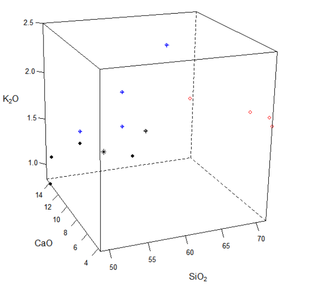
284 threeD
Details
This function displays three variables in a form of 3D plot. The plot can be rotated interactively, if
required so.
The samples to be plotted can be selected based on combination of three searching mechanisms (by
sample name/label, range or a Boolean condition) - see selectSubset for details.
If no parameters 'xlab','ylab'and 'zlab'are given, the user is prompted to specify them.
The variables are selected using the function ’selectColumnLabel.
In the specification of the apices can be used also arithmetic expressions, see calcCore for the
correct syntax.
See manual entry for ’cloud’ for further details.
Value
None.
Warning
This function IS NOT Figaro-compatible.
Author(s)
Vojtech Janousek, <vojtech.janousek@geology.cz> & Vojtech Erban, <vojtech.erban@geology.cz>
Examples
threeD("SiO2","Na2O+K2O","MgO+FeOt")

tkSelectVariable 285
tkSelectVariable TclTk GUI: Select a single variable
Description
Function to select a single variable using the Tcl/Tk-based Graphical User Interface (GUI).
Usage
tkSelectVariable(top.frame = NULL, where = colnames(WR), preselect = 2,
pack = FALSE, message = "Select a variable", background = "wheat",
variable = "x", on.leave = function() {}, row = 0, column = 0, height = 15,
width = 50, buttons = FALSE, state = "normal")
Arguments
top.frame name of the parental frame
where character; names of variables to be chosen from
preselect numeric; which item is to be preselected
pack logical; pack the frame?
message character; textual prompt
background colour for the frame background
variable character; variable name with the output
on.leave function to be invoked upon leave
row, column coordinates within the parental frame
height, width size of the frame
buttons logical; should the frame have also buttons?
state ???
Details
The buttons are: Reset, SortUp, SortDown, OK, Cancel.
Author(s)
Vojtech Janousek, <vojtech.janousek@geology.cz>
See Also
tcltk-package

286 tk_winDialogString
tk_winDialog tk_winDialog
Description
Tcl/Tk replacement for the MS Windows-specific function ’winDialog’.
Usage
tk_winDialog(type="ok",message="")
Arguments
type Character; the type of the dialogue box.
message Character. The information field of the dialogue box.
Details
This is a platform-independent implementation of the MS Windows-specific function ’winDialog’,
written using the Tcl/Tk. Possible types of the dialogue box are: ok,okcancel,yesno and yesnocancel.
Value
A character string giving the name of the button pressed (in capitals).
Author(s)
Vojtech Janousek, <vojtech.janousek@geology.cz>
See Also
winDialog tkmessageBox tk_winDialogString tcltk-package
Examples
tk_winDialog(type="yesnocancel",message="Are you sure?")
tk_winDialogString tk_winDialogString
Description
Tcl/Tk replacement for the MS Windows-specific function ’winDialogString’.
Usage
tk_winDialogString(message="Enter variable",default="",returnValOnCancel=NULL)

trendTicks 287
Arguments
message Character. The information field of the dialog box.
default Character; the default string.
returnValOnCancel
Character; a value to be returned when the dialogue is canceled.
Details
This is a platform-independent implementation of the MS Windows-specific function ’winDialogString’,
written using the Tcl/Tk.
Value
A character string giving the contents of the text box when Ok was pressed, or value specified by
’returnValOnCancel’ if Cancel was pressed.
Author(s)
Vojtech Janousek, <vojtech.janousek@geology.cz>
See Also
winDialogString tkentry tk_winDialog tcltk-package
Examples
tk_winDialogString(message="Enter x value",default="15.7")
trendTicks Petrogenetic trends
Description
Adding a trend with arrow and tick marks to a pre-existing GCDkit plot.
Usage
trendTicks(equation, x, xmin = par("usr")[1], xmax = par("usr")[2],
tick = abs(par("tcl")), text = FALSE, col = "blue", lty = "solid",
lwd = 1, arrow = FALSE, autoscale = TRUE)
Arguments
equation character or expression; a valid formula expressed as a function of x.
xnumeric; x values where the ticks are to be drawn.
xmin numeric; beginning of the trend.
xmax numeric; end of the trend.
tick numeric; length of a tick as a fraction of the height of a line of text.
text logical; should be the tick marks annotated by text?
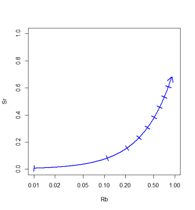
288 trendTicks
col text or numeric; plotting colour specification.
lty text or numeric; the line type.
lwd numeric; the line width, a positive number, defaulting to 1.
arrow logical; should be also an arrow head shown?
autoscale logical; should the plot be autosized in order to accommodate the whole trend
as well as all data points?
Details
Using the function curve, the function trendTicks adds to an existing GCDkit plot a linear or
curved trend with tick marks and (optionally) arrow head. It is required that the trend is defined as
a function of x. The slope of the individual tick marks is then determined using a derivation of the
main function at the respective points.
Value
a list with two components, xand y, with coordinates of the tick marks.
Warning
Autoscaling will work only with Figaro compatible plots!

Verma 289
Author(s)
Vojtech Janousek, <vojtech.janousek@geology.cz>
See Also
par
Examples
binary("Ba","Sr",xmin=200,xmax=2000,ymin=10,ymax=400)
equation<-"x/8+200"
x<-seq(2000,500,by=-100)
trendTicks(equation,x,min(x),max(x),col="darkred",lty="solid",lwd=2,arrow=TRUE,text=FALSE)
plot(1,1,type="n",xlim=c(0.01,1),ylim=c(0,1),xlab="Rb",ylab="Sr",log="x")
equation<-"6*x/8"
x<-seq(0.01,1,by=0.1)
trendTicks(equation,x,min(x),max(x),col=2,lwd=2,arrow=FALSE,text=FALSE,autoscale=FALSE)
Verma Major-element based discrimination plots for (ultra-)basic rocks
(Verma et al. 2006)
Description
Plots data stored in ’WR’ (or its subset) into discrimination plots proposed by Verma et al. (2006) for
(ultra-) basic rocks (SiO2< 52 wt. %).
Usage
Verma(FeMiddlemost=FALSE,GUI=FALSE)
Arguments
FeMiddlemost logical, should be iron adjusted according to Middlemost (1989)?
GUI logical, is the function called from a GUI?
Details
Suite of five diagrams for discrimination of geotectonic environment of ultrabasic and basic rocks
(SiO2< 52 wt. %), proposed by Verma et al. (2006). It is based on log-transformed concentration
ratios of major-element oxides. Note that prior to the transformation, the analyses are recast to 100%
anhydrous basis. Each diagram is a plot of two discriminant functions, DF1 and DF2, respectively in
x- and y-axes. Only samples with SiO2< 52 wt. % are plotted. To work properly, the major element
analysis should be complete (SiO2, T iO2, Al2O3, F e2O3, F eO, MnO, MgO, CaO, N a2O, K2O, P2O5).
Following the recommendation by Verma et al. (2006), prior to the plotting can be performed an
adjustment of the iron-oxidation ratio as proposed by Middlemost (1989) (see ’FeMiddlemost’).
For the F e2O3/F eO ratios implemented for individual rock types (based on TAS classification),
see Verma et al. (2002) (Fig. 1).
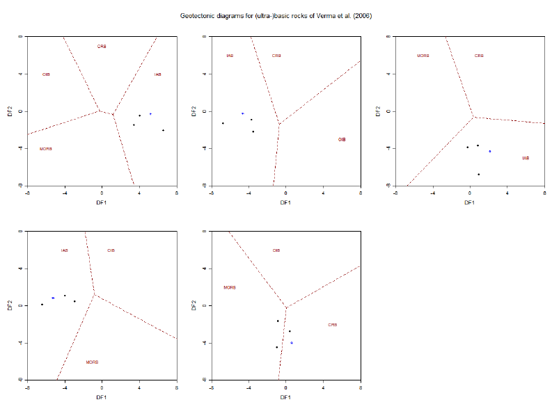
290 Verma
Following geotectonic settings may be deduced:
Abbreviation used Environment
IAB island arc basic rocks
CRB continental rift basic rocks
OIB ocean-island basic rocks
MORB mid-ocean ridge basic rocks
Value
None.
Note
This function uses the plates concept. The individual plots can be selected and their proper-
ties/appearance changed as if they were stand alone Figaro-compatible plots. See Plate,Plate editing
and figaro for details.
Author(s)
Vojtech Janousek, <vojtech.janousek@geology.cz>
References
Middlemost E A K (1989) Iron oxidation ratios, norms and the classification of volcanic rocks.
Chem Geol 77: 19-26. doi: 10.1016/0009-2541(89)90011-9

Villaseca 291
Verma S P, Torres-Alvarado I S, Sotelo-Rodriguez Z T (2002) SINCLAS: standard igneous norm
and volcanic rock classification system. Comput and Geosci 28: 711-715. doi: 10.1016/S0098-
3004(01)00087-5
Verma S P, Guevara M, Agrawal S (2006) Discriminating four tectonic settings: Five new geo-
chemical diagrams for basic and ultrabasic volcanic rocks based on log-ratio transformation of
major-element data. Journal of Earth System Science 115: 485-528. doi: 10.1007/BF02702907
See Also
FeMiddlemost Agrawal Plate Plate editing plotPlate figaro
Examples
#plot the diagrams
plotPlate("Verma")
Villaseca B-A plot (modified by Villaseca et al. 1998)
Description
The B-A diagram as proposed by Debon and Le Fort (1983) with classification fields for various
types of peraluminous rocks designed by Villaseca et al. (1998).
Usage
Villaseca()
Details
Plots modified B-A diagram (designed originally by Debon and Le Fort 1983) with fields for various
peraluminous rock types after Villaseca et al. (1998). Assigns data for the B-A diagram into Figaro
template (list ’sheet’) and appropriate values into ’x.data’ and ’y.data’.
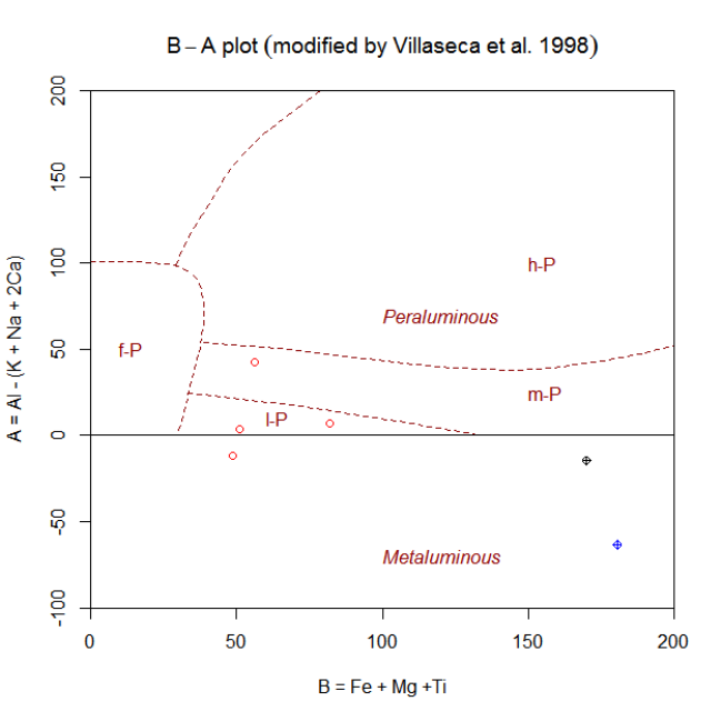
292 Villaseca
The following fields are defined:
l-P low peraluminous
m-P moderately peraluminous
h-P highly peraluminous
f-P felsic peraluminous
metaluminous
Rocks with composition falling beyond defined boundaries are labeled ’undefined’ by the ’classify’
function.
Parameters for the diagram are calculated by the function ’DebonCalc’. All of them are based on
millications (1000 gram-atoms per 100 grams).
A=Al-(K+Na+2Ca)
B=Fe+Mg+Ti
For details, see Debon & Le Fort (1983) or (1988).
Value
sheet list with Figaro Style Sheet data
x.data B value. See details.
y.data A value. See details.

Wedge 293
Author(s)
Vojtech Janousek, <vojtech.janousek@geology.cz>
References
Debon F & Le Fort P (1983) A chemical-mineralogical classification of common plutonic rocks
and associations. Trans Roy Soc Edinb; Earth Sci 73: 135-149
Debon F & Le Fort P (1988) A cationic classification of common plutonic rocks and their magmatic
associations: principles, method, applications. Bull. Mineral 111: 493-511
Villaseca C, Barbero L, Herreros V (1998) A re-examination of the typology of peraluminous gran-
ite types in intracontinental orogenic belts. Trans Roy Soc Edinb, Earth Sci 89: 113-119
See Also
classify figaro plotDiagram DebonCalc Debon
Examples
#plot the diagram
plotDiagram("Villaseca",FALSE)
Wedge Wedge diagrams (Ague 1994)
Description
Implementation of Wedge diagrams after Ague (1994) and Bucholz and Ague (2010) used for judg-
ing the mobility of elements or oxides in course of various geochemically open-system processes
such as alteration or partial melting.
Usage
Wedge(x = "Ti", y = NULL, protolith = NULL,
outline = "chull", precision = 10, plotAltered = TRUE,
xmin = 0, ymin = 0, xmax = NULL, ymax = NULL, fun = NULL)
Arguments
xa single geochemical species presumably immobile during the given rock trans-
formation.
ylist of elements/oxides for plotting, separated by commas.
protolith Boolean search pattern to specify the protolith samples in the data file.
outline method for contouring the clusters of protolith and product compositions, see
Details.
precision precision of contours drawn, if 'outline'="contour", see Details.
plotAltered logical; should be the altered analyses plotted or just contoured?
xmin, xmax (optional) limits for shared x axes of the individual plots.
ymin (optional) minimum for all of the y axes of the plots.
ymax (optional) upper limits for each of the y axes of the plots.
fun panel function to be applied to each of the individual plots.
294 Wedge
Details
Wedge diagrams (Ague 1994) enable qualitative treatment of losses/gains of geochemical species
(elements or oxides) during open-system geological processes, such as alteration, metamorphism or
partial melting. As such they represent a viable alternative to the isocon plots (Grant 1986, 2005)
or concentration ratio diagrams (Ague 1994). However, the Wedge diagrams have an advantage in
that they take into account the overall variability of the whole dataset (both of the putative protolith
and the altered product) and not just a selected whole-rock pair.
Wedge diagrams are simple binary plots of a potentially mobile element jversus a reference (im-
mobile) element i. The compositionally heterogeneous protolith samples yield a cloud of points.
The outer edges of this cloud define a wedge-shaped region that converges towards the origin.
As shown by Bucholz and Ague (2010), the altered samples that plot above and to the left of this
wedge are thought to have gained the mobile species j, whereas those falling below and to the right
suffered its loss. The samples that remain in the wedge but moved upwards are thought to record
residual enrichment, and those shifted downwards to have underwent a residual dilution.
The samples defining the protolith variation can be selected based on combination of three searching
mechanisms (by sample name/label, range or a Boolean condition) - see selectSamples for details.
Implemented are two methods for outlining the clusters of the protolith and altered compositions
(as specified by the argument 'outline'), convex hull (chull) and contour (contour). For the latter,
the shape of the contours drawn can be controlled using the parameter (precision). The higher it is,
the smoother contours result. See contourGroups and chullGroups for further details.
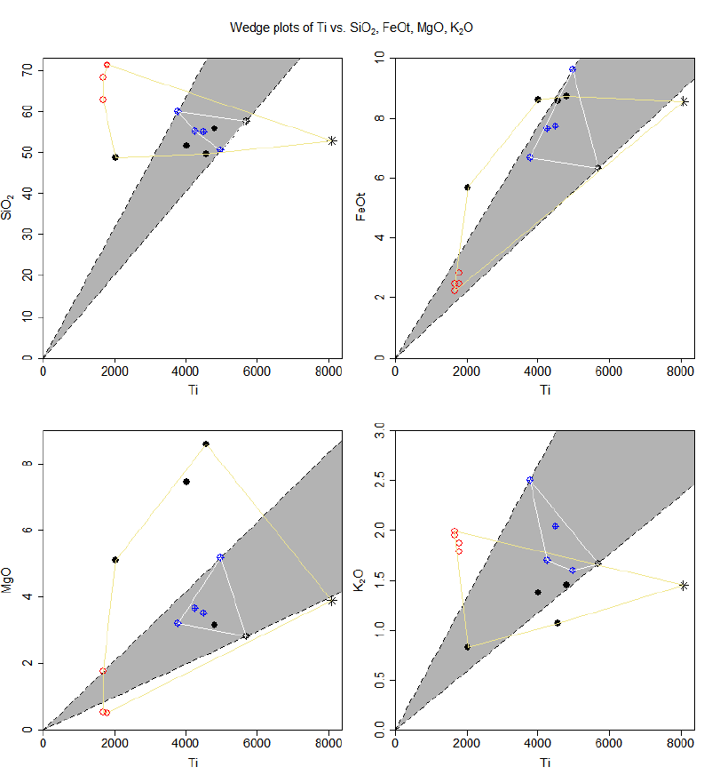
Wedge 295
Optionally, the individual data points for the altered samples may be replaced by contours portray-
ing their density, if plotAltered = FALSE.
Parameters xmin, xmax, ymin and ymax are passed to the function plotWithLimits used for the
actual data plotting.
Optionally, panel function specified by fun with two arguments, xlab and ylab, is applied to each of
the plots.
Value
Returns a matrix ’results’ of slopes of tie-lines from individual protolith samples to the origin
(with a component for each diagram, i.e. for each species evaluated). Lines of maximum and
minimum slopes are those which are plotted as dashed lines, thus defining the wedge of the protolith
variation (see Details).
296 Wedge
Plugin
Isocon.r
Note
This function uses the plates concept. The individual plots can be selected and their proper-
ties/appearance changed as if they were stand alone Figaro-compatible plots. See Plate,Plate editing
and figaro for details.
Author(s)
Vojtech Janousek, <vojtech.janousek@geology.cz>
References
Ague J J (1994) Mass transfer during Barrovian metamorphism of pelites, south-central Con-
necticut; I, Evidence for changes in composition and volume. Amer J Sci 294: 989-1057 doi:
10.2475/ajs.294.8.989
Bucholz C E, Ague J J (2010) Fluid flow and Al transport during quartz-kyanite vein formation,
Unst, Shetland Islands, Scotland. J Metamorph Geol 28: 19-39 doi: 10.1016/0009-2541(67)90004-
6
Grant J A (1986) The isocon diagram - a simple solution to Gresens equation for metasomatic
alteration. Econ Geol 81: 1976-1982 doi: doi:10.2113/gsecongeo.81.8.1976
Grant J A (2005) Isocon analysis: a brief review of the method and applications. Phys Chem Earth
(A) 30: 997-1004 doi: 10.1016/j.pce.2004.11.003
Gresens R L (1967) Composition-volume relationships of metasomatism. Chem Geol 2: 47-55 doi:
10.1016/0009-2541(67)90004-6
See Also
Ague,isocon,Plate,Plate editing,chull,contour contourGroups chullGroups,plotWithLimits
Examples
data<-loadData("sazava.data",sep="\t")
Wedge("Ti","SiO2,FeOt,MgO,CaO,Na2O,K2O",
protolith="Intrusion=\"Sazava\"","chull")
# Using the default precision of 10
Wedge("Ti","Zr,Nb,Sr,Rb,Ba",protolith="Intrusion=\"Sazava\"","contour")
Wedge("Ti","Zr,Nb,Sr,Rb,Ba",protolith="Intrusion=\"Sazava\"","contour",precision=100)
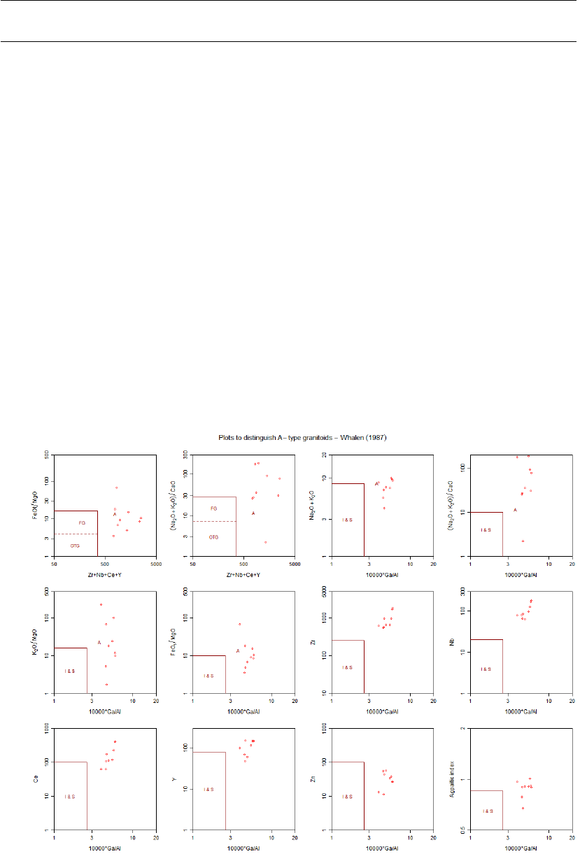
Whalen 297
Whalen A type granitoids (Whalen et al. 1987)
Description
Set of discrimination plots to distinguish A-type granitoids as defined by Whalen et al.(1987).
Usage
Whalen(plot.txt = getOption("gcd.plot.text"))
Arguments
plot.txt logical, annotate fields by their names?
Details
Set of binary plots proposed by Whalen et al.(1987) to distinguish A-type granitoids on the one
hand from ordinary/fractionated I- and S-types on the other.
In total 12 diagrams are plotted split into two pages. Apart from fields for I and S type granites
(’I & S’), sometimes split into ordinary (’OGT’) and fractionated (’'FG'’)domains, average com-
position of the A type granites (labeled ’A’) are shown. See Figs 1, 2 and 5 in the original paper
(Whalen et al.1987) for comparison.

298 WinFloyd1
The following diagrams are plotted: Zr+Nb+Ce+Yvs. F eOt/MgO and (K2O+Na2O)/CaO;
10000Ga/Al vs. K2O+Na2O,(K2O+Na2O)/CaO,K2O/MgO and F eOt/MgO;10000Ga/Al
vs. Zr, Nb, Ce, Y, Zn and Agpaitic Index.
Value
To the matrix ’WR’ are appended two columns, with Ga/Al ratios and values of the Agpaitic Index
(labeled ’A.I.’).
Note
This function uses the plates concept. The individual plots can be selected and their proper-
ties/appearance changed as if they were stand alone Figaro-compatible plots. See Plate,Plate editing
and figaro for details.
Author(s)
Vojtech Janousek, <vojtech.janousek@geology.cz>
References
Whalen J B, Currie K L, Chappell B W (1987) A-type granites: geochemical characteristics,discrimination
and petrogenesis. Contrib Mineral Petrol 95: 407-419. doi: 10.1007/BF00402202
See Also
Plate Plate editing plotPlate figaro
Examples
#plot the diagrams
plotPlate("Whalen")
WinFloyd1 Nb/Y - Zr/TiO2 diagram (Winchester + Floyd 1977)
Description
Assigns data for Nb/Y vs. Zr/T iO2diagram into Figaro template (list ’sheet’) and appropriate
values into ’x.data’ and ’y.data’.
Usage
WinFloyd1()
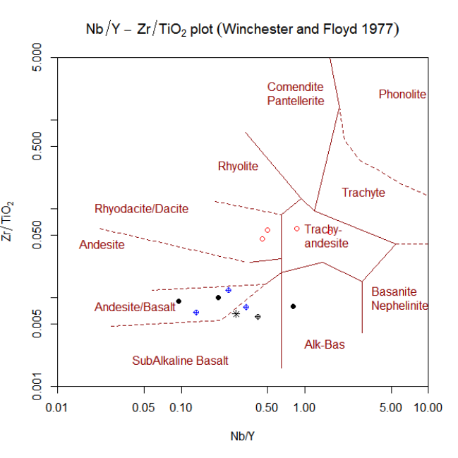
WinFloyd1 299
Details
Classification diagram proposed by Winchester & Floyd (1977).
Using incompatible element ratios (Nb/Y vs. Zr/T iO2), following fields are defined:
Trachyandesite
Alkali basalt
Basanite/Nephelinite
Trachyte
Phonolite
Comendite/Pantellerite
Rhyolite
Rhyodacite/Dacite
Andesite
Andesite/Basalt
Subalkaline basalt
Value
sheet list with Figaro Style Sheet data
x.data Nb/Y wt. % ratio
y.data (Zr/TiO2)*0.0001 wt. % ratio

300 WinFloyd2
Author(s)
Vojtech Erban, <vojtech.erban@geology.cz>
& Vojtech Janousek, <vojtech.janousek@geology.cz>
References
Winchester J A & Floyd P A (1977) Geochemical discrimination of different magma series and their
differentiation products using immobile elements. Chem Geol 20: 325-343 doi: 10.1016/0009-
2541(77)90057-2
See Also
classify figaro plotDiagram
Examples
#Within GCDkit, the plot is called using following auxiliary functions:
#To Classify data stored in WR (Groups by diagram)
classify("WinFloyd1")
#To plot data stored in WR or its subset (menu Classification)
plotDiagram("WinFloyd1", FALSE)
WinFloyd2 Zr/TiO2 - SiO2 (Winchester + Floyd 1977)
Description
Assigns data for Zr/T iO2vs. SiO2diagram into Figaro template (list ’sheet’) and appropriate
values into ’x.data’ and ’y.data’
Usage
WinFloyd2()
Details
Classification diagram proposed by Winchester & Floyd (1977).
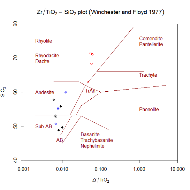
WinFloyd2 301
Using incompatible element ratio and silica (Zr/T iO2vs. SiO2), following fields are defined:
Trachyandesite
Basanite/Trachyte/Nephelinite
Phonolite
Trachyte
Comendite/Pantellerite
Rhyolite/Dacite
Rhyodacite/Dacite
Andesite
Subalkaline basalt
Alkaline basalt
Value
sheet list with Figaro Style Sheet data
y.data SiO2 wt. %
x.data (Zr/TiO2)*0.001 wt. % ratio
Author(s)
Vojtech Erban, <vojtech.erban@geology.cz>
& Vojtech Janousek, <vojtech.janousek@geology.cz>

302 Wood
References
Winchester J A & Floyd P A (1977) Geochemical discrimination of different magma series and their
differentiation products using immobile elements. Chem Geol 20: 325-343 doi: 10.1016/0009-
2541(77)90057-2
See Also
classify figaro plotDiagram
Examples
#Within GCDkit, the plot is called using following auxiliary functions:
#To Classify data stored in WR (Groups by diagram)
classify("WinFloyd2")
#To plot data stored in WR or its subset (menu Classification)
plotDiagram("WinFloyd2", FALSE)
Wood Wood (1980)
Description
Assigns Figaro templates to Wood’s geotectonic diagrams for basaltoids into the list ’plate’ and
appropriate values into the list ’plate.data’ for subsequent plotting.
Usage
Wood(ident = getOption("gcd.ident"),
plot.txt = getOption("gcd.plot.text"))
Arguments
ident logical, identify?
plot.txt logical, annotate fields by their names?
Details
A series of triangular diagrams with apices Th-Hf/3-Ta, Th-Hf/3-Ta and Th-Zr/117-Nb/16, pro-
posed by Wood (1980).
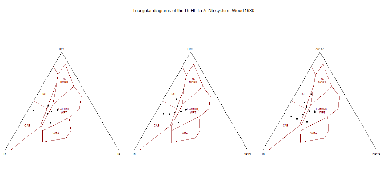
Wood 303
Following fields are defined:
IAT Island-arc Tholeiites
CAB Calc-alkaline Basalts
N-MORB N-type Mid-ocean Ridge Basalts
E-MORB E-type Mid-ocean Ridge Basalts
WPT Within-plate Tholeiites
WPA Alkaline Within-plate Basalts
Value
sheet list with Figaro Style Sheet data
x.data, y.data Th, Hf/3 and Ta in ppm recalculated into two dimensions
Note
This function uses the plates concept. The individual plots can be selected and their proper-
ties/appearance changed as if they were stand alone Figaro-compatible plots. See Plate,Plate editing
and figaro for details.
Author(s)
Vojtech Janousek, <vojtech.janousek@geology.cz>
References
Pearce J A (1996) A User’s Guide to Basalt Discrimination Diagrams. In Wyman D A (ed) Trace
Element Geochemistry of Volcanic Rocks: Applications for Massive Sulphide Exploration. Geo-
logical Association of Canada, Short Course Notes 12, pp 79-113
Wood D A (1980) The application of a Th-Hf-Ta diagram to problems of tectonomagmatic classifi-
cation and to establishing the nature of crustal contamination of basaltic lavas of the British Tertiary
volcanic province. Earth Planet Sci Lett 50: 11-30 doi:10.1016/0012-821X(80)90116-8
See Also
Plate,Plate editing,plotPlate,figaro

304 YbN vs. LaN/YbN
Examples
#plot the diagrams
plotPlate("Wood")
YbN vs. LaN/YbN YbN vs LaN/YbN (Martin 1986) TTG/adakite
Description
Assigns data for the Y bNvs. LaN/Y bNdiagram for adakite/TTG discrimination into Figaro
template (list ’sheet’) and appropriate values into ’x.data’ and ’y.data’.
Usage
LaYb(ybrep=FALSE)
Arguments
ybrep logical, should be missing Yb values replaced by Y/2.4?
Details
Diagram proposed by several authors for discriminating between adakitic (or TTG) and "ordinary"
calc-alkaline rocks. The version used here is from Martin (1986).
Martin (1999) suggested that Yb (ppm) could be replaced by Y (ppm)/2.4. Notionally this could
help with old data with missing values. However if Yb is missing La is also likely to be absent (or
unreliable), so by default this replacement is not done; the user can access it by calling the function
with ybrep=TRUE (not available from GUI).
Normalization values are La = 0.33 ppm, Yb = 0.22 ppm (Nakamura 1974).
Value
sheet list with Figaro Style Sheet data
x.data LaN/Y bNor La/(Y /2.4)
y.data Y bN
Author(s)
Jean-Francois Moyen, <jfmoyen@gmail.com>
References
Martin H (1986) Effect of steeper Archean geothermal gradient on geochemistry of subduction-zone
magmas. Geology 14: 753-756 doi: 10.1130/0091-7613(1986)14<753:EOSAGG>2.0.CO;2
Martin H (1999) Adakitic magmas: modern analogues of Archaean granitoids. Lithos 46: 411-429
doi: 10.1016/S0024-4937(98)00076-0
Nakamura N (1974) Determination of REE, Ba, Fe, Mg, Na and K in carbonaceous and ordinary
chondrites. Geochim Cosmochim Acta 38: 757-775 doi: 10.1016/0016-7037(74)90149-5

zrSaturation 305
See Also
figaro plotDiagram
Examples
# plot the diagram
plotDiagram("LaYb",FALSE)
zrSaturation Zircon saturation (Watson + Harrison 1983, Boehnke et al. 2013)
Description
Calculates zircon saturation temperatures for the observed major-element data and Zr concentra-
tions. Returns also Zr saturation levels for the given major-element compositions and assumed
magma temperature.
Usage
zrSaturation(cats = milli, T = 0, Zr = filterOut(WR, "Zr", 1))
Arguments
cats numeric matrix; whole-rock data recast to millications
Tassumed temperature of the magma in °C
Zr numeric vector with Zr concentrations
Details
Calculates Zr saturation concentration at a given temperature. Given ’T’ is the estimated absolute
temperature (K) of the magma and ’M’ is a cationic ratio:
M= 100Na +K+ 2Ca
Al.Si
it can be written (Watson & Harrison 1983):
DZr =e(−3.8−0.85(M−1)+ 12900
T)
The Zr saturation level is then given by:
Zr.sat =497644
DZr
On the other hand, the saturation temperature can be obtained from the observed Zr concentration
and magma composition (assuming no zircon inheritance)
DZr =497644
Zr

306 zrSaturation
T Zr.sat.C =12900
ln(DZr)+3.8+0.85(M−1) −273.15
An improved calibration of Boehnke et al. (2013) has given:
DZr =e(10108
T−1.16(M−1)−1.48)
and
T Zr.sat.C =10108
ln(DZr)+1.16(M−1) + 1.48 −273.15
Value
Returns a matrix ’results’ with the following columns:
Mcationic ratios
Zr observed Zr concentrations
Zr.sat saturation levels of Zr after Watson & Harrison (1983) for assumed temperature
TZr.sat.C zircon saturation temperatures after Watson & Harrison (1983) in °C
Zr.sat (Boehnke)
saturation levels of Zr after Boehnke et al. (2013) for assumed temperature
TZr.sat.C (Boehnke)
zircon saturation temperatures after Boehnke et al. (2013) in °C
Plugin
Saturation.r
Author(s)
Vojtˇ
ech Janoušek, <vojtech.janousek@geology.cz>
References
Boehnke P, Watson EB, Trail D, Harrison TM, Schmitt AK (2013) Zircon saturation re-revisited.
Chem Geol 351: 324-334 doi: 10.1016/j.chemgeo.2013.05.028
Watson EB & Harrison M (1983) Zircon saturation revisited: temperature and composition ef-
fects in a variety of crustal magma types. Earth Planet Sci Lett 64: 295-304 doi: 10.1016/0012-
821X(83)90211-X
Index
∗Topic aplot
Add contours,7
assign1symb,22
assignSymbGroup,25
assignSymbLab,26
assignSymbLett,27
contourGroups,51
figAdd,82
figCol,87
figEdit,88
figOverplot,93
figOverplotDiagram,95
figScale,99
figUser,100
figZoom,101
overplotDataset,163
peterplot,187
plateAddReservoirs,193
showColours,243
showSymbols,245
∗Topic cluster
cluster,50
groupsByCluster,109
∗Topic color
assign1col,21
assignColLab,23
assignColVar,24
figAdd,82
figCol,87
figOverplot,93
figOverplotDiagram,95
figUser,100
plateAddReservoirs,193
selectPalette,233
setTransparency,239
showColours,243
∗Topic database
Boolean conditions,35
Regular expressions,214
selectColumnLabel,228
selectColumnsLabels,229
selectSubset,235
Subset by range,267
∗Topic datasets
atacazo,28
blatna,34
sazava,222
∗Topic device
figRedraw,97
pdfAll,169
psAll,207
∗Topic dplot
calcAnomaly,40
selectNorm,231
setCex,237
∗Topic file
customScript,62
EarthChem,67
Export to Access,74
Export to DBF,75
Export to Excel,76
Export to HTML tables,77
figLoad,90
figSave,98
loadData,132
mergeData,138
pdfAll,169
peekDataset,186
pokeDataset,199
psAll,207
purgeDatasets,207
r2clipboard,211
saveData,220
saveResults,220
saveResultsIso,221
∗Topic hplot
AFM,10
ageEps,11
Agrawal,13
ArcMapSetup,20
Batchelor,29
binary,31
binaryBoxplot,33
bpplot2,36
Cabanis,37
cluster,50
307
308 INDEX
coplotByGroup,53
coplotTri,55
correlationCoefPlot,57
Cox,58
Debon,64
elemIso,71
epsEps,73
F-M-W diagram,79
figLoad,90
figMulti,90
figSave,98
filledContourFig,102
Frost,103
graphicsOff,109
groupsByDiagram,110
Harris,112
Hastie,113
Hollocher,115
isochron,119
Jensen,124
Laroche,128
Maniar,136
Meschede,139
Middlemost,142
mins2deg,145
Miyashiro,146
Molecular weights,150
Mullen,151
MullerK,152
Multiple plots,155
NaAlK,158
OConnor,161
pairsCorr,167
Pearce and Cann,170
Pearce and Norry,171
Pearce Nb-Th-Yb,173
Pearce Nb-Ti-Yb,175
Pearce1982,177
Pearce1996,178
PearceEtAl,180
PearceGranite,182
PeceTaylor,184
Plate,189
Plate editing,191
plateLabelSlots,195
plotPlate,196
plotWithCircles,197
profiler,204
QAPF,208
reciprocalIso,213
Ross,216
Schandl,223
Shand,240
Shervais,242
spider,246
spider2norm,251
spiderBoxplot,254
spiderByGroupFields,256
spiderByGroupPatterns,257
statsByGroupPlot,261
strip,264
stripBoxplot,265
summaryAll,267
summaryByGroup,269
summarySingle,270
summarySingleByGroup,272
Sylvester,273
TAS,274
TASMiddlemost,277
ternary,279
threeD,283
Verma,289
Villaseca,291
Whalen,297
WinFloyd1,298
WinFloyd2,300
Wood,302
YbN vs. LaN/YbN,304
∗Topic iplot
contourGroups,51
figAdd,82
figaro.identify,86
figCol,87
figEdit,88
figGbo,89
figOverplot,93
figOverplotDiagram,95
figUser,100
gcdOptions,106
ID,118
overplotDataset,163
plateAddReservoirs,193
selectByDiagram,226
showLegend,244
∗Topic manip
.claslist,5
accessVar,6
addResults,8
addResultsIso,9
Ague,15
appendSingle,18
apSaturation,18
Boolean conditions,35
calc,39
INDEX 309
calcCore,42
Catanorm,43
CIPW,44
classify,46
clr.transform,48
customScript,62
cutMy,63
deleteSingle,66
Edit labels,69
Edit numeric data,70
editLabFactor,70
FeMiddlemost,81
groupsByCluster,109
groupsByDiagram,110
groupsByLabel,111
isocon,121
joinGroups,125
Jung,126
LaRocheCalc,131
Mesonorm,140
millications,144
Misc,145
Mode,148
mzSaturation,157
Niggli,160
oxide2oxide,165
oxide2ppm,166
ppm2oxide,200
recast,212
rtSaturation,218
selectAll,225
selectByDiagram,226
selectByLabel,227
selectColumnLabel,228
selectColumnsLabels,229
selectSubset,235
srnd,258
Subset by range,267
tetrad,282
tk_winDialog,286
tk_winDialogString,286
tkSelectVariable,285
trendTicks,287
Wedge,293
zrSaturation,305
∗Topic misc
about,6
crosstab,61
info,119
quitGCDkit,211
∗Topic multivariate
cluster,50
groupsByCluster,109
pairsCorr,167
prComp,201
∗Topic print
printSamples,202
printSingle,203
setShutUp,238
∗Topic univar
statsByGroup,260
statsByGroupPlot,261
statsIso,261
strip,264
stripBoxplot,265
summaryAll,267
summaryByGroup,269
summarySingle,270
summarySingleByGroup,272
.claslist,5,48
87Sr/86Sr vs EpsNdi (epsEps),73
about,6
accessExport,75,77
accessExport (Export to Access),74
accessVar,6,199,208
Add contours,7
addContours,103
addContours (Add contours),7
addResults,8,9
addResultsIso,9
AFM,10,48,111,216,217
ageEps,11
ageEps2 (ageEps),11
ageSr (ageEps),11
Agrawal,13,291
Ague,15,296
annotate,88
appendSingle,18
apSaturation,18
ArcMapSetup,20
assign1col,21,22,23,25–28,235,240,245
assign1symb,22,22,23,26–28,245
assignColLab,22,23,25–28,235,240,245
assignColVar,21,24,235,245
assignSymbGroup,22,23,25,25,27,28,240,
245
assignSymbLab,22,23,26,26,28,245
assignSymbLett,27,27
atacazo,28
Batchelor,29
binary,31,92,190
binaryBoxplot,33
biplot.princomp,202
310 INDEX
blatna,34
Boolean conditions,35
boxplot,34,37,255,263,264,266,271,272
Boxplot isotopic ratios/model ages
(statsIso),261
boxplotIso (statsIso),261
bpplot2,36,271
Cabanis,37
calc,39
calcAnomaly,40
calcCore,32,33,39,42,62,72,156,198,
202,204,206,261,264,266,268,
269,271,272,281,284
Cann (Pearce and Cann),170
Catanorm,43
chull,52,296
chullGroups,84,85,294,296
chullGroups (contourGroups),51
CIPW,44,163
CIPWhb (CIPW),44
classify,11,46,61,66,105,110,111,115,
125,131,143,147,160,163,180,
186,210,226,241,276,279,293,
300,302
cloud,284
clr.trans (clr.transform),48
clr.transform,48
cluster,50
colours,85,87,220,244
Colours: Plotting symbols (figCol),87
Colours: set to B&W (figCol),87
Colours: subtitle (figCol),87
Colours: title (figCol),87
contour,7,51,52,296
contourGroups,51,84,85,294,296
coplot,53–57
coplotByGroup,53
coplotTri,55
Correlation coefficient patterns
(correlationCoefPlot),57
correlationCoefPlot,57
Cox,48,58,111,279
CoxPlut (Cox),58
CoxVolc (Cox),58
crosstab,61
curve,83,85,288
customScript,62
cut,63
cutMy,63
data.entry,69–71
dbfExport,75,77
dbfExport (Export to DBF),75
Debon,64,293
DebonBA,48,111
DebonBA (Debon),64
DebonCalc,66,293
DebonPQ,48,111
DebonPQ (Debon),64
deleteSingle,66
dev.off,109
DMage (srnd),258
DMGage (srnd),258
DMLHage (srnd),258
EarthChem,67
Edit labels,69
Edit numeric data,70
Edit: subtitle (figEdit),88
Edit: title (figEdit),88
Edit: x label (figEdit),88
Edit: y label (figEdit),88
editData (Edit numeric data),70
editLabels (Edit labels),69
editLabFactor,70,110
elemIso,71
epsEps,73
epsilon (srnd),258
excel2007Export (Export to Excel),76
excelExport,74,75
excelExport (Export to Excel),76
Export to Access,74
Export to DBF,75
Export to Excel,76
Export to HTML tables,77
F-M-W diagram,79
FeMiddlemost,81,289,291
figAdd,82
figAddArrow (figAdd),82
figAddBox (figAdd),82
figAddCurve (figAdd),82
figAddFit (figAdd),82
figAddReservoirs,94,95,97,164,194
figAddReservoirs (figAdd),82
figAddText (figAdd),82
figAlab (figEdit),88
figaro,7,11,15,21,30,39,48,61,66,81,
85–92,95,97–99,101–103,105,
108,113,115,117,125,131,137,
140,143,147,152,154,156,157,
160,163,170–172,174,176,178,
180,182–184,186,190,192,196,
197,210,217,225,241,243,274,
INDEX 311
276,279,290,291,293,296,298,
300,302,303,305
figaro.identify,86
figBlab (figEdit),88
figBw (figCol),87
figCex (figScale),99
figCexLab (figScale),99
figCexMain (figScale),99
figCexSub (figScale),99
figClab (figEdit),88
figCol,87,192
figColMain (figCol),87
figColours (figCol),87
figColSub (figCol),87
figEdit,88
figFixLim (figZoom),101
figGbo,89
figGrid (figAdd),82
figIdentify (figaro.identify),86
figLegend (figAdd),82
figLoad,90,98,190
figMain (figEdit),88
figMulti,90,190
figOverplot,83–85,93,97,164,193,194
figOverplotDiagram,85,95,95,164,194
figRedraw,97
figSave,90,98,190
figScale,99,192
figSub (figEdit),88
figTicks (figAdd),82
figUnzoom (figZoom),101
figUser,100
figXlab (figEdit),88
figXlim (figZoom),101
figYlab (figEdit),88
figYlim (figZoom),101
figZoom,101
figZooming (figZoom),101
filled.contour,7,103
filledContourFig,102
Frost,103
gcdOptions,106,118,238
getwd,135
graphicsOff,109
groupsByCluster,109,111
groupsByDiagram,110,110,111
groupsByLabel,110,111,111
Harris,112
Hastie,48,111,113
hclust,51
Highlight multiple points
(figaro.identify),86
highlightSelection (figaro.identify),86
Hollocher,115
Hollocher1 (Hollocher),115
Hollocher2 (Hollocher),115
HTMLTableMain (Export to HTML tables),
77
HTMLtableOrdered (Export to HTML
tables),77
HTMLTableResults (Export to HTML
tables),77
HTMLTableWR (Export to HTML tables),77
ID,108,118
identify,86,108,118
Identify points (figaro.identify),86
info,119
initial (srnd),258
isochron,119
isocon,18,121,296
isoconAtoms (isocon),121
isoconOxides (isocon),121
Jensen,48,111,124
joinGroups,125
Jung,126
kde2d,7
LaRoche,30,132
LaRoche (Laroche),128
Laroche,48,111,128
LaRocheCalc,131,131
LarochePlut (Laroche),128
LarocheVolc (Laroche),128
LaYb (YbN vs. LaN/YbN),304
llgridlines,20,21
loadData,20,21,132,138,199,208,220,226
loadDataOdbc (loadData),132
Maniar,136
merge,138
mergeData,135,138,220
mergeDataCols (mergeData),138
mergeDataRows (mergeData),138
Meschede,139
Mesonorm,140
Middlemost,48,111,142
MiddlemostPlut (Middlemost),142
millications,131,144
mins2deg,145
Misc,145
312 INDEX
Miyashiro,48,111,146
Mode,148
ModeAll (Mode),148
ModeC (Mode),148
ModeMain (Mode),148
Molecular weights,150
molecularWeight,166,167,200
molecularWeight (Molecular weights),150
Mullen,151
MullerK,152
MullerKbinary (MullerK),152
MullerKternary (MullerK),152
multiple,190
multiple (Multiple plots),155
Multiple plots,155
multipleMjr (Multiple plots),155
multiplePerPage (Plate),189
multipleTrc (Multiple plots),155
mzSaturation,157
NaAlK,48,111,158,241
Niggli,160
normalize2total (recast),212
Norry (Pearce and Norry),171
OConnor,48,111,161
OConnorPlut (OConnor),161
OConnorVolc (OConnor),161
OhtaArai (F-M-W diagram),79
options,106,108,118,238
overplotDataset,85,95,97,163,194
oxide2oxide,165,167,200
oxide2ppm,166,166,200
pairsCorr,167
pairsMjr (pairsCorr),167
pairsTrc (pairsCorr),167
panel.cor (pairsCorr),167
panel.cov (pairsCorr),167
panel.hist (pairsCorr),167
panel.smooth (pairsCorr),167
par,7,85,95–97,101,205,289
pdf,169
pdfAll,169,207
Pearce and Cann,170
Pearce and Norry,171
Pearce Nb-Th-Yb,173
Pearce Nb-Ti-Yb,175
Pearce1982,177
Pearce1996,48,111,178
PearceEtAl,180
PearceGranite,182
PearceNbThYb,176
PearceNbThYb (Pearce Nb-Th-Yb),173
PearceNbTiYb,174
PearceNbTiYb (Pearce Nb-Ti-Yb),175
PeceTaylor,48,111,184
peekDataset,164,186,186,199,208
peterplot,187
Plate,15,91,92,105,137,154,156,157,
170,171,183,184,189,192,196,
197,225,290,291,296,298,303
Plate editing,15,92,105,137,154,157,
171,184,190,191,196,197,225,
291,296,298,303
plate0YLim (Plate editing),191
plateAddReservoirs,95,164,193
plateAnnotationsRemove (Plate editing),
191
plateBW (Plate editing),191
plateCex (Plate editing),191
plateCexLab (Plate editing),191
plateCexMain (Plate editing),191
plateCol (Plate editing),191
plateExpand (Plate editing),191
plateExtract,96,97,164
plateExtract (Plate editing),191
plateLabelSlots,195
plateLoad (Plate),189
platePch (Plate editing),191
platePS (Plate),189
plateRedraw (Plate),189
plateSave (Plate),189
plateXLim (Plate editing),191
plateYLim (Plate editing),191
plot,32,34,190,281
plot.default,83,94,193,280
plotDiagram,11,30,39,48,61,66,79,81,
96,97,113,115,117,125,131,140,
143,147,152,160,163,164,172,
174,176,178,180,182,186,189,
210,217,241,243,274,276,279,
293,300,302,305
plotPlate,15,105,137,154,171,184,190,
192,196,225,291,298,303
plotWithCircles,197,266
plotWithLimits,13,72,74,214,295,296
plotWithLimits (binary),31
points,94–96
pokeDataset,134,135,164,186,199,199,
208
polygon,51,52
postscript,207
ppm2oxide,166,167,200
pr.comp.clr (clr.transform),48
INDEX 313
prComp,50,201
princomp,202
printSamples,202
printSingle,203
profiler,204
psAll,169,207
purgeDatasets,164,186,199,207
QAPF,48,111,208
QAPFPlut (QAPF),208
QAPFVolc (QAPF),208
quantile,25
quit,211
quitGCDkit,211
r2clipboard,211
read.table,135,220
readOGR,21
recast,212
reciprocalIso,213
refreshFig (figRedraw),97
regex,35,215,236
regular expression (Regular
expressions),214
Regular expressions,214
regular expressions (Regular
expressions),214
regular.expression (Regular
expressions),214
regular.expressions,35,229
regular.expressions (Regular
expressions),214
Ross,216
rtSaturation,218
saveData,135,138,220
saveResults,220,222
saveResultsIso,221
sazava,222
Scale: axis labels (figScale),99
Scale: subtitle (figScale),99
Scale: symbols (figScale),99
Scale: title (figScale),99
Schandl,223
selectAll,225,226,236
selectByDiagram,226
selectByLabel,226,227,236
selectColumnLabel,23,24,26,27,32,33,
39,54,56,63,66,71,72,111,162,
198,204,227,228,261,264,265,
271,272,281,284
selectColumnsLabels,50,58,167,201,202,
212,229,229,268,269
selectDataset,199,208
selectDataset (peekDataset),186
selectNorm,41,84,85,95,194,231,249,
250,252–254,256–258
selectPalette,23,24,233
selectSamples,50,72,74,120,149,167,
201,202,214,239,249,252,254,
268,269,271,294
selectSamples (selectSubset),235
selectSubset,32,33,35,86,103,162,198,
206,226,231,235,267,284
setCex,106,108,237
setShutUp,238
setTransparency,164,239
setwd,135
Shand,48,105,111,160,240
Shervais,242
showColours,22,23,25–28,85,87,134,135,
191,192,220,235,240,243,245
showColours2 (showColours),243
showLegend,22,23,26–28,244
showSymbols,22,23,26–28,134,135,191,
192,220,245,245
sp,21
spider,41,92,94,95,190,231,246,251,
253,257,258,282,283
spider2norm,250,251,255,256
spider_double_norm.r (spider2norm),251
spiderBoxplot,254
spiderByGroupFields,250,253,256,256
spiderByGroupPatterns,250,253,256,257
spiderplot.r (spider),246
srnd,258
statistics,260,268,271,272
Statistics: Correlation: majors
(pairsCorr),167
Statistics: Correlation: traces
(pairsCorr),167
Statistics: Majors
summaryAll/selection
(summaryAll),267
Statistics: Majors summaryByGroups
(summaryByGroup),269
Statistics: Trace
summaryAll/selection
(summaryAll),267
Statistics: Trace summaryByGroups
(summaryByGroup),269
statsByGroup,260
statsByGroupPlot,261
statsIso,261
Streckeisen (Mesonorm),140
314 INDEX
strip,264,266
stripBoxplot,264,265
stripplot,264,266
Stripplot isotopic ratios/model ages
(statsIso),261
stripplotIso (statsIso),261
Subset by range,267
subsetBoolean,236
subsetBoolean (Boolean conditions),35
subsetRange,236
subsetRange (Subset by range),267
summaryAll,260,267,272
summaryByGroup,260,268,269,272
summaryByGroupMjr (summaryByGroup),269
summaryByGroupTrc (summaryByGroup),269
summaryMajor (summaryAll),267
summaryRangesByGroup (summaryByGroup),
269
summarySingle,260,268,270,272
summarySingleByGroup,260,268,272,272
summaryTrace (summaryAll),267
Sylvester,273
TAS,48,82,96,111,164,274,279
TASadd (TAS),274
TASMiddlemost,48,111,277
TASMiddlemostPlut (TASMiddlemost),277
TASMiddlemostVolc (TASMiddlemost),277
ternary,92,190,279
tetrad,282
threeD,283
tk_winDialog,286,287
tk_winDialogString,286,286
tkentry,287
tkmessageBox,286
tkSelectVariable,285
trendTicks,287
triplot (ternary),279
triplotadd,94,95
triplotadd (ternary),279
underplotDataset,97
underplotDataset (overplotDataset),163
Verma,15,82,289
Villaseca,48,111,291
Wedge,18,293
Whalen,297
winDialog,286
winDialogString,287
WinFloyd1,48,111,180,298
WinFloyd2,48,111,300
Wood,302
WRComp (Mode),148
write.dbf,75
YbN vs. LaN/YbN,304
Zooming: Scale x axis (figZoom),101
Zooming: Scale y axis (figZoom),101
Zooming: Zoom in (figZoom),101
Zooming: Zoom out to original size
(figZoom),101
zrSaturation,305
