GFSSP V1.4 USERS GUIDE

User Manual:

Open the PDF directly: View PDF .
Page Count: 193 [warning: Documents this large are best viewed by clicking the View PDF Link!]

PART1.pdf
- 1 INTRODUCTION
PART2.pdf
- 2.0 MATHEMATICAL FORMULATION
  - 2.1 PROBLEM DEFINITION
  - 2.2 GOVERNING EQUATIONS
- 3.0 COMPUTER PROGRAM
PART3.pdf
- 4.0 USER’S GUIDE

George C. Marshall Space Flight Center

Science and Engineering

Contract NAS 8-40836

A GENERALIZED FLUID SYSTEM

SIMULATION PROGRAM TO MODEL

FLOW DISTRIBUTION IN FLUID

NETWORKS

Report No.: 331-201-96-003

Prepared by:

Alok Majumdar

October 1996

Sverdrup Technology, Inc

Hughes STX

MEVATEC

Micro Craft

MSFC Group

620 Discovery Drive

Huntsville, AL 35806

FOREWARD

The motivation to develop a general purpose computer program to compute pressure and flow

distribution in a complex fluid network came from the need to calculate the axial load on the

impeller shaft bearings in a turbopump. During the past several years, several specific purpose

codes were developed to model the Space Shuttle Main Engine (SSME) turbopumps. However, it

was difficult to use those codes for a new design without making extensive changes in the original

code. Such efforts often turn out to be time consuming and inefficient. To satisfy the need to model

these turbopumps in an efficient and timely manner, a subtask plan, entitled “Generalized Fluid

System Simulation Program (GFSSP)” was prepared in March of 1994, under Task Directive 331-

201 for Contract NAS8-37814, with Mr. Henry Stinson of Marshall Space Flight Center (MSFC) as

Task Initiator. The objective of this subtask was to develop a general fluid flow system solver

capable of handling phase change, compressibility and mixture thermodynamics. Emphasis was

given to construct an “user friendly” program using a modular structured code. The intent of this

effort was that an engineer with an undergraduate background in fluid mechanics and

thermodynamics should be able to rapidly develop a reliable model. The interest in modular code

development was intended to facilitate future modifications to the program.

This document details the GFSSP mathematical formulation, solution procedure and computer

program and it provides instructions for using the code through the inclusion of a number of

example problems. Chapter 1 provides background information and discusses past and present

work. The mathematical formulation used to develop GFSSP is described in detail in Chapter 2.

All of the governing equations used in the code are described in this chapter. The solution

procedure implemented in GFSSP is also described in this chapter. The program structure is

discussed in Chapter 3. Chapter 4 describes how to use the code. Several example problems are

given in Chapter 5. The new user, who is only interested is applying GFSSP to solve flow network

problems, can skip the first three chapters of this document and go directly to Chapter 4 and Chapter

5. With some experience in applying GFSSP, the user will benefit from the first three chapters (in

particular, Chapter 2).

ACKNOWLEDGMENTS

The author would like to acknowledge several individuals for their contributions to this effort. The

author would like to acknowledge Mr. Tom Beasley of Sverdrup Technology for his continuous

encouragement and support throughout the period of code development. Mr. Beasley has provided

a great deal of useful information on flow resistance that has been incorporated into the code. Ms.

Katherine Van Hooser of MSFC has been contributory in testing many versions of the code and has

made numerous useful suggestions to make it more user friendly. The author would also like to

acknowledge Mr. Bruce Tiller of MSFC for testing early versions of the code and for providing

benchmark data for the verification of the code. Mr. John Bailey of Sverdrup Technology has

conducted a very systematic investigation to check the accuracy of various resistance options by

comparing the code’s predictions with existing commercial codes. Mr. Bailey’s models have been

included in this report as an example. Mr. Bailey also has made a significant contribution in the

preparation of this document. Mr. Paul Schallhorn of Sverdrup Technology contributed in the area

of code verification. He developed a rotating disk model which has also been included as an

example for demonstration purposes. Dr. Bob Hendricks and Ms. Angela Haferd of Lewis Research

Center provided all the help necessary to integrate the thermodynamic property programs in the

code. The author would also like to acknowledge Mr. Doug Richards of McDonnell Douglas

Aerospace for many useful discussions and constructive suggestions. The author would also like to

acknowledge the workshop attendees for their participation and many useful suggestions on code

development and documentation.

ABSTRACT

This report describes a general purpose computer program for analyzing flow and pressure

distribution in a complex network. The program is capable of modeling phase changes,

compressibility, mixture thermodynamics and external body forces such as gravity and centrifugal.

The program’s preprocessor allows the user to interactively develop a fluid network simulation

consisting of nodes and branches. Mass, energy and specie conservation equations are solved at the

nodes; the momentum conservation equations are solved in the branches.

The program contains subroutines for computing “real fluid” thermodynamic and thermophysical

properties for 11 fluids. The fluids are: helium, methane, neon, nitrogen, carbon monoxide, oxygen,

argon, carbon dioxide, fluorine, hydrogen, water and kerosine (RP-1). The program also has the

option of using any incompressible fluid with constant density and viscosity.

Fifteen different resistance/source options are provided for modeling momentum sources or sinks in

the branches. The options are: pipe flow, flow through a restriction, pipe flow with entrance and/or

exit losses, thin sharp orifice, thick orifice, square edge reduction, square edge expansion, rotating

annular duct, rotating radial duct, labyrinth seal, face seal, common fittings and valves, pump

characteristics, pump power and valve with a given loss coefficient.

The system of equations describing the fluid network are solved by a hybrid numerical method that

is a combination of the Newton-Raphson and successive substitution methods. This report also

illustrates the application of the code through seven demonstrated example problems. The examples

are: 1) Series flow circuit with common pipe fittings and a valve, 2) Series flow circuit with

common pipe fittings, a valve and a pump, 3) Flow distribution in a parallel flow manifold, 4) Flow

distribution in a parallel flow manifold with heat sources and phase changes, 5) Mixing of cryogenic

fluids in an inter-propellant seal flow circuit of a turbopump, 6) Quasi-steady calculation of

Example 5, and 7) Flow in a rotating disk cavity.

Keywords: Flow, Network, Numerical, Simulation, Turbopump, Cryogenic, Thermodynamics,

Mixture.

iii

TABLE OF CONTENTS

Section Description Page

Number Number

Foreward i

Acknowledgment ii

Abstract iii

Table of Contents iv

List of Figures vii

List of Tables viii

Nomenclature ix

1.0 Introduction 1

1.1 Background 1

1.2 Review of Past work 1

1.3 Present Contribution 2

2.0 Mathematical Formulation 3

2.1 Problem Definition 3

2.2 Governing Equations 4

2.2.1 Mass Conservation Equation 4

2.2.2 Momentum Conservation Equation 5

2.2.3 Energy Conservation Equation 5

2.2.4 Fluid Specie Conservation Equation 6

2.2.5 Thermodynamic and Thermophysical Properties 7

2.2.6 Mixture Property Calculations 7

2.2.7 Friction Factor Calculation 8

2.2.7.1 Branch Option 1 ( Pipe Flow) 10

2.2.7.2 Branch Option 2 ( Flow in Restriction) 10

2.2.7.3 Branch Option 3 ( Non Circular Duct) 11

2.2.7.4 Branch Option 4 ( Pipe with Entrance and Exit Loss) 11

2.2.7.5 Branch Option 5 ( Thin, Sharp Orifice) 12

2.2.7.6 Branch Option 6 ( Thick Orifice) 13

2.2.7.7 Branch Option 7 ( Square Edge Reduction) 14

2.2.7.8 Branch Option 8 ( Square Edge Expansion) 14

2.2.7.9 Branch Option 9 ( Rotating Annular Duct) 15

2.2.7.10 Branch Option 10 ( Rotating Radial Duct) 17

2.2.7.11 Branch Option 11 ( Labyrinth Seal) 18

2.2.7.12 Branch Option 12 ( Face Seal) 19

2.2.7.13 Branch Option 13 ( Common Fittings and Valves) 20

2.2.7.14 Branch Option 14 ( Pump Characteristics) 21

2.2.7.15 Branch Option 15 ( Pump Power) 22

2.2.7.16 Branch Option 16 ( Valve with Given Cv)

TABLE OF CONTENTS (CONTINUED)

Section Description Page

Number Number

2.3 Solution Procedure 22

3.0 Computer Program 24

3.1 Preprocessor 24

3.2 Solver 24

3.3 Thermodynamic Property Package 25

4.0 User’s Guide 26

4.1 Selection of Model Options 26

4.2 Node Information 30

4.3 Branch Information 30

4.4 Boundary Conditions 30

4.5 Miscellaneous Information 30

4.6 Description of Input Data File 32

5.0 Examples 35

5.1 Example 1 - Series Flow Circuit With Common Pipe Fittings

and a Valve

5.2 Example 2 - Series Flow Circuit With Common Pipe Fittings,

Valve and a Pump

5.3 Example 3 - Flow Distribution in a Parallel Flow Manifold 43

5.4 Example 4 - Flow Distribution in a Parallel Flow Manifold with

Heat Sources and Phase Changes

5.5 Example 5 - Mixing of Cryogenic Fluids in an Inter-Propellant

Seal Flow Circuit of a Turbopump

5.6 Example 6 - Quasi-steady Calculation of Example 5 46

5.7 Example 7 - Flow in a Rotating Disk Cavity 46

6.0 References

Appendix A - Derivation of Kf for Pipe Flow

Appendix B - Newton-Raphson Method of Solving Coupled Nonlinear Systems of

Algebraic Equations

Appendix C -Successive Substitution Method of Solving Coupled Nonlinear Systems

of Algebraic Equations

Appendix D - Input and Output Data Files from Example 1

TABLE OF CONTENTS (CONTINUED)

Section Description

Number

Appendix E - Input and Output Data Files from Example 2

Appendix F - Input and Output Data Files from Example 3

Appendix G - Input and Output Data Files from Example 4

Appendix H - Input and Output Data Files from Example 5

Appendix I - Input and Output Data Files from Example 6

Appendix J - Input and Output Data Files from Example 7

Appendix K - Interactive Session with GFSSP Preprocessor

LIST OF FIGURES

Figure Description Page

Number Number

2.1 Inter-propellant Seal Flow Circuit in a Turbopump 3

2.2 Schematic of GFSSP Nodes and Branches and Indexing Practice 4

2.3 Schematic of a Branch Showing the Gravity and Rotation 6

2.4 GFSSP Pipe Resistance Option Parameters 10

2.5 GFSSP Pipe With Entrance and/or Exit Loss Resistance Option

Parameters

2.6 GFSSP Thin Sharp Orifice Resistance Option Parameters 12

2.7 GFSSP Thick Orifice Resistance Option Parameters 13

2.8 GFSSP Square Edge Reduction Resistance Option Parameters 14

2.9 GFSSP Square Edge Expansion Resistance Option Parameters 15

2.10 GFSSP Rotating Annular Duct Resistance Option Parameters 16

2.11 GFSSP Rotating Radial Duct Resistance Option Parameters 17

2.12 GFSSP Labyrinth Seal Resistance Option Parameters 18

2.13 GFSSP Face Seal Resistance Option Parameters 19

3.1 The GFSSP Flowchart 25

4.1 Examples of Flow Circuit Arrangement to Demonstrate the Effect of

Fluid Inertia

5.1 Example 1 Flow Circuit 36

5.2 Example 1 Predicted System Characteristics 36

5.3 Example 2 Flow Circuit 37

5.4 Pump Characteristics Curve for Example 2 38

5.5 Combined Pump And System Characteristics 38

5.6 Example 3 Parallel Flow Manifold 39

5.7 GFSSP Model for Example 3 40

5.8 Inter Propellant Flow Circuit of Example 5 41

vii

LIST OF TABLES

Table Description Page

Number Number

2.1 Resistance Options in GFSSP 9

2.2 Constants for Two K Method of Hooper (Reference 3) for

Fittings/Valves (GFSSP Resistance Option 13)

4.1 GFSSP Logical Variables 32

4.2 Fluids Available in GFSSP 33

5.1 System Characteristic Data of Example 1 35

viii

NOMENCLATURE

Symbol Description

A Area (in2)

A0Pump Characteristic Curve Coefficient

B0Pump Characteristic Curve Coefficient

CLFlow Coefficient

c Clearance (in)

ci,k Mass concentration of kth specie at ith node

cpSpecific heat (Btu/lb o F)

CvFlow Coefficient for a Valve

D Diameter (in)

f Darcy Friction Factor

g Gravitational Acceleration (ft/ sec2)

gcConversion Constant (= 32.174 lb-ft/lbf-sec2)

h Enthalpy (Btu/lb)

KfFlow Resistance Coefficient (/lbf-sec2/(lb-ft)2 )

Krot Non-dimensional Rotating Flow Resistance Coefficient

K1Non-Dimensional Head Loss Factor

KiInlet Loss Coefficient

KeExit Loss Coefficient

L Length (in)

M Molecular weight

m pitch (in)

Mass Flow Rate (lb/sec)

N Revolutions Per Minute (rpm)

n Number of Teeth

p Pressure (lbf/ in2)

P Pump Power (hp)

Q Heat source (Btu/sec)

Re Reynolds Number (Re = ruD/m)

R Gas constant (lbf-ft/lb-R)

r Radius (in)

S Momentum Source (lbf)

T Temperature (o F)

u Velocity (ft/sec)

V Volume (in3)

xkMole fraction of kth specie

z Compressibility factor

Symbol Description

Greek

rDensity (lb/ft3)

qAngle Between Branch Flow Velocity Vector And Gravity Vector (deg)

wAngular Velocity (rad/sec)

eAbsolute Roughness (in)

e/D Relative Roughness

aMultiplier for Labyrinth Seal Resistance

hEfficiency

DhHead Loss (ft)

mViscosity ( lb/ft-sec)



Kinematic viscosity (ft2/sec)





Molar density (lb-mol/ft3)

Specific heat ratio

1 INTRODUCTION

1.1 BACKGROUND

A fluid flow network consists of a group of flow branches such as pipes and ducts that are

joined together at a number of nodes. They can range from simple systems consisting of

a few nodes and branches to very complex networks containing flow branches with

valves, orifices, bends, pumps and turbines. In the analysis of existing or proposed

networks, some node pressures and temperatures are specified or known. The problem is

to determine all unknown nodal pressures, temperatures and branch flow rates.

An accurate prediction of axial thrust in a liquid rocket engine turbopump requires the

modeling of fluid flow in a very complex network. Such a network involves the flow of

cryogenic fluid through extremely narrow passages, flow between rotating and stationary

surfaces, phase changes, mixing of fluids and heat transfer. A Generalized Fluid System

Simulation Program (GFSSP) has been developed to accurately predict the axial thrust

from the predicted pressure distributions in a turbopump assembly. The flow network

was resolved into nodes and branches. In each branch the momentum equation was

solved and in each node the conservation of mass, energy and species were solved. The

solution of these equations provide the pressures at the nodes and flow rates in the

branches.

In the past, specific purpose codes were developed to model the SSME turbopump.

However, it was difficult to use those codes for a new design without making extensive

changes in the original code. Such efforts often turn out to be time consuming and

inefficient. Therefore, GFSSP was developed as a general fluid flow system solver

capable of handling phase change, compressibility and mixture thermodynamics and it

included the capability to model external body forces such as gravity and centrifugal

effects. The program’s preprocessor allows the user to interactively develop a fluid

network simulation consisting of nodes and branches.

Since GFSSP’s initial release in August, 1994, and subsequent releases in December,

1994, February, 1995, and October, 1995, GFSSP has been utilized to model a variety of

fluid flow problems. This report documents the mathematical formulation, solution

procedure and computer program and it provides instructions for using the code through

the inclusion of a number of example problems. These examples include: 1) Series flow

circuit with common pipe fittings and a valve, 2) Series flow circuit with common pipe

fittings, a valve and a pump, 3) Flow distribution in a parallel flow manifold, 4) Flow

distribution in a parallel flow manifold with heat sources and phase changes, 5) Mixing of

cryogenic fluids in an inter-propellant seal flow circuit of a turbopump, 6) Quasi-steady

calculation of Example 5, and 7) Flow in a rotating disk cavity.

1.2 PAST WORK

The oldest method for systematically solving a problem consisting of steady flow in a

pipe network is the Hardy Cross method [1]. Not only is this method suited for solutions

generated by hand, but it has also been widely employed for use in computer generated

solutions. But as computers allowed much larger networks to be analyzed, it become

apparent that the convergence of the Hardy Cross method might be very slow or even fail

to provide a solution in some cases. The main reason for this numerical difficulty is that

the Hardy Cross method does not solve the system of equations simultaneously. It

considers a portion of the flow network to determine the continuity and momentum

errors. The head loss and the flow rates are corrected and then it proceeds to an adjacent

portion of the circuit. This process is continued until the whole circuit is completed.

This sequence of operations is repeated until the continuity and momentum errors are

minimized. It is evident that the Hardy Cross method belongs in the category of

successive substitution methods and it is likely that it may encounter convergence

difficulties for large circuits. In later years, the Newton-Raphson method has been

utilized [2] to solve large networks, and with improvements in algorithms based on the

Newton-Raphson method, computer storage requirements are not much larger than those

needed by the Hardy Cross method.

The flow of fluid in a rocket engine turbopump can be classified into two main

categories. The flow through the impeller and turbine blade passages is designated as

primary flow. Controlled leakage flow through bearings and seals for the purpose of

axial thrust balance, bearing cooling and rotodynamic stability is referred to as secondary

flow. Flows in the blade passages are modeled by solving Navier-Stokes equations of

mass, momentum and energy conservation in three dimensions. Navier-Stokes methods,

however, are not particularly suitable for modeling flow distribution in complex network.

Most of the available commercial software for solving flow networks [3,4] are based on

either the successive substitution method or on the Newton-Raphson method and they are

only applicable for single phase incompressible fluid. They are not suitable for modeling

rocket engine turbopumps where mixing, phase change and rotational effects are present.

Two public domain computer programs [5,6] have been developed in aerospace

industries to analyze the secondary flow in the SSME turbopumps. These programs use

real gas properties to compute variable density in the flow passage. Mixing of fluids,

phase changes and rotational effects, however, are not considered by these programs.

1.3 PRESENT WORK

The objective of the present effort is to develop: a) a robust and efficient numerical

algorithm to solve a system of equations describing a flow network containing phase

changes, mixing and rotation and b) to implement the algorithm in a structured, easy to

use computer program.

The earlier programs on SSME turbopump used a very simplified form of momentum

equation. The momentum equations used in Reference 5 and Reference 6 only

considered pressure and friction forces. A more generalized form of momentum equation

is necessary to account for rotational effects. The momentum equation used in the current

program includes inertia, pressure, friction, gravity, centrifugal and any external

momentum sources. The frictional effects are proportional to the square of mass flow

rate in the branch. The proportionality constant was derived from empirical information

available in the literature [7-12].

The thermodynamic and thermophysical properties required in the conservation equations

are obtained from two thermodynamic property programs, GASP and WASP [13,14]. The

thermodynamic property programs, GASP and WASP, provide thermodynamic and

thermophysical properties for helium, methane, neon, nitrogen, carbon monoxide,

oxygen, argon, carbon dioxide, fluorine, hydrogen, water. The properties of RP-1 fuel

[15] have been provided as a look up table. A real gas formulation has been used to

compute mixture properties. The code also has an option of modeling any incompressible

fluid of constant density and viscosity.

The task of the computational model is to obtain a simultaneous solution of the governing

equations. This system of equations is solved by a novel numerical procedure which is a

combination of Newton-Raphson and successive substitution methods. This algorithm

has been incorporated into GFSSP. GFSSP also includes a preprocessor. With the help

of the preprocessor, a user without a substantial background in computational methods or

the FORTRAN programming language can use the code to model complex flow circuits.

The code development was carried out in several stages. At the end of each stage, a

workshop was held where the latest version of the code was released to MSFC engineers

for testing, verification and feedback. In the first workshop, held in August of 1994,

GFSSP Version 1.0 was released. This version of GFSSP contained the basic

mathematical framework of the solver and the integration of the thermodynamic property

program, GASP.

The second workshop was held in December of 1994 to release GFSSP Version 1.1. This

version included a preprocessor which allowed the user to create an input data file for

GFSSP through an interactive process. The preprocessor eliminated the need for the user

to modify and compile the source code. Additional features of GFSSP Version 1.1

included: a) the inclusion of the water property program, WASP and b) the introduction

of a hybrid numerical technique for use in the solver.

GFSSP Version 1.2 was released in February of 1995. This version included the

capability to model the thermodynamics of real gas mixtures and to calculate the axial

thrust exerted on a rotating component in a flow circuit. The inter-propellant seal flow

circuit was modeled and the predictions were compared with the predictions from Pratt &

Whitney’s model. Excellent agreement [16] was obtained between these two models.

The third workshop was held in October of 1995 to release GFSSP Version 1.3. This

version of GFSSP included four additional capabilities: a) a quasi-steady state option

used for modeling dynamic environments, b) a thermodynamic property routine for RP-1

fuel that was needed for modeling new generation engines, c) provisions for heat sources

or sinks to be used for modeling flows in low clearance rotating passages, and d) a

generalized momentum equation that accounts for fluid inertial forces. This version was

used to model the natural convection process in a cryogenic propellant conditioning

system. A good agreement was obtained [17] between test data and GFSSP predictions.

The capability to include external body forces, such as a pump, as a momentum source

was added into the current version of GFSSP (Version 1.4) of the program. This version

also provides the user with the capability to model rotational flow in turbo-machine.

Another major feature of GFSSP Version 1.4 is its enhanced capability to model

different types of resistance in a flow network. Fifteen different resistance/source options

are provided for modeling momentum sources or sinks in the branches. These include:

pipe flow, flow through a restriction, pipe flow with entrance and/or exit losses, thin

sharp orifice, thick orifice, square edge reduction, square edge expansion, rotating annular

duct, rotating radial duct, labyrinth seal, face seal, common fittings and valves, pump

characteristics, pump power and valve with a given loss coefficient. The additional

features of the code was verified by comparing GFSSP predictions with two other

commercial codes[3,4]. The GFSSP predictions compared [18] favorably with the other

two codes. This report documents Version 1.4 of the code.

2.0 MATHEMATICAL FORMULATION

2.1 PROBLEM DEFINITION

GFSSP assumes a newtonian, steady, non-reacting and one dimensional flow in the flow circuit.

The flow could be either laminar or turbulent, incompressible or compressible, with or without

heat transfer, phase change and mixing.

The analysis of the flow and pressure distribution in a complex fluid flow network requires

resolution of the system into nodes and branches. At each node, scalar properties such as

pressures, temperatures, enthalpies, and mixture concentrations are computed. The flow rates

(vector properties) are computed at the branches. Nodes are either boundary nodes or internal

nodes. Pressures, temperatures, and concentrations of fluid species are specified at the boundary

nodes. The purpose of the mathematical model is to predict the conditions at the internal nodes

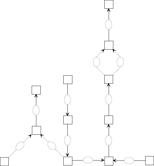
and the flow rates in the branches. A sample flow circuit consisting of 12 nodes and 12 branches

is shown in Figure 2.1. Figure 2.1 is a portion of the propellant flow circuit, where a helium

buffer is used to prevent the mixing of hydrogen and oxygen leakage flow, in Pratt & Whitney's

High Pressure Oxygen Turbopump Secondary Flow Circuit.

129

23 23 22

138

137

142

Notes:

1) Number of Internal Nodes = 7

2) Number of Branches = 12

3) Total Number of Equations = 7 x 4 + 12 = 40

4) Number of Equations Solved by Newton

Raphson Method = 7 + 12 = 19

5) Number of Equations Solved by Successive

Substitution Method = 3 x 7 = 21

Boundary Node

Atmosphere

14.7 psia

Boundary Node

Atmosphere

14.7 psia

Boundary Node

Helium

151 psia

Boundary Node

Oxygen

550 psia

-60

Boundary Node

Hydrogen

172 psia

-174

Figure 2.1 - onter-propellant Ssal Ffow cCicuit in a tTubopump.

In Figure 2.1 the nodes are represented by square boxes and branches are represented by elliptical

boxes. The nodes and branches are numbered arbitrarily. There are five boundary nodes (48, 50, 66,

16, and 22) in the flow circuit. Oxygen, hydrogen, and helium enter into the circuit through nodes

48, 66, and 22 respectively. The pressures and temperatures are specified at these nodes and are

shown in the figure. Nodes 50 and 16 are outflow boundaries where only pressures are specified.

The mixtures of helium-oxygen and helium-hydrogen exit through these nodes. The computer code

calculates pressures, temperatures, and fluid specie concentrations at all internal nodes and flow rates

in all branches.

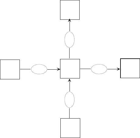
2.2 GOVERNING EQUATIONS

In order to solve for the unknown variables, mass, energy and fluid specie conservation equations

are written for each internal node and flow rate equations are written for each branch. The

schematic of the nodes and branches and the indexing system used by GFSSP is shown in Figure

2.2.

Fluid (k=1)

Fluid (k=2)

mji

mij

mji

mij

.mji

j=1

j=4

j=2

j=3

Mixture

Figure 2.2 - Schematic of GFSSP Nodes and Branches and Indexing Practice

2.2.1 Mass Conservation Equation

mij

j n .





(Equation 2.1)

Equation 2.1 requires that the net mass flow from a given node must equate to zero. In other

words, the total mass flow rate into a node is equal to the total mass flow rate out of the node.

2.2.2 Momentum Conservation Equation

The flow rate in a branch is calculated from the momentum conservation equation (Equation 2.2)

which represents the balance of fluid forces acting on a given branch. Inertia, pressure, gravity,

friction and centrifugal forces are considered in the conservation equation. In addition to these

five forces, a source term S has been provided in the equation to input pump characteristics or to

input power to a pump in a given branch. If a pump is located in a given branch, all other forces

except pressure are set to zero. The source term S is set to zero in all branches without a pump.

 

mij

uiuupipjAgV

Kmij mij AKA

gcj

cos . .

  









    

   

rot

2 2

(Eq.2.2)

Inertia Pressure Gravity Friction Centrifugal Source

The term in the left hand side of the momentum equation represents the inertia of the fluid. This

term is significant when there is a large change in area or density from branch to branch. The

first term in the right hand side of the momentum equation represents the pressure gradient in the

branch. The pressures are located at the upstream and downstream face of a branch. The second

term represents the effect of gravity. The gravity vector makes an angle (



) with the flow

direction vector. The third term represents the frictional effect. Friction was modeled as a

product of Kf and the square of the flow rate and area. Kf is a function of the fluid density in the

branch and the nature of flow passage being modeled by the branch. The calculation of Kf for

different types of flow passages has been described in detail later within this report. The fourth

term in the momentum equation represents the effect of the centrifugal force. This term will be

present only when the branch is rotating as shown in Figure 2.3. Krot is the factor representing

the fluid rotation. Krot is unity when the fluid and the surrounding solid surface rotates with the

same speed. This term also requires a knowledge of the distances between the upstream and

downstream faces of the branch from the axis of rotation. A detailed description of source term,

S, appears in Sections 2.2.7.14 and 2.2.7.15 of this report.

2.2.3 Energy Conservation Equation

MAX mij hjMAX mij hii

j n



















































,0 0

0 +

(Equation 2.3)

The energy conservation equation, Equation 2.3, states that the net energy flow from a given node

must equate to zero. In other words, the total energy leaving a node is equal to the total energy

coming into the node from neighboring nodes and from any external heat sources (Qi) coming

into the node. The MAX operator used in Equation 2.3 is known as an upwind differencing

scheme which has been extensively employed in the numerical solution of Navier-Stokes

equations in convective heat transfer and fluid flow [19] applications. When the flow direction is

not known, this operator allows the transport of energy only from its upstream neighbor. In other

words, the upstream neighbor influences its downstream neighbor but not vice-versa.





Figure 2.3 - Schematic of a Branch Showing the Gravity and Rotation

2.2.4 Fluid

Specie Conservation Equation

The flow network shown in Figure 2.1 has a fluid mixture flowing in most of the branches. In

order to calculate the density of the mixture, the concentration of the individual fluid species

within the branch must be determined. Suppose there are n number of fluids in the mixture. The

concentration for the kth specie can be written as

MAX mij cj k MAX mij ci k

j n



















































0 0

(Equation 2.4)

Equation 2.4 requires that the net mass flow of the kth specie from a given node must equate to

zero. In other words, the total mass flow rate of the given specie into a node is equal to the total

mass flow rate of the same specie out of that node.

2.2.5 Thermodynamic and Thermophysical Properties

The momentum conservation equation, Equation 2.2, requires the knowledge of the density and

viscosity of the fluid within the branch. These properties are functions of the temperatures,

pressures and concentrations of fluid species for a mixture. Two thermodynamic property

routines have been integrated with the program to provide the required property data. GASP [6]

provides the thermodynamic and transport properties for ten fluids. These fluids are Hydrogen,

Oxygen, Helium, Nitrogen, Methane, Carbon Dioxide, Carbon Monoxide, Argon, Neon and

Fluorine. WASP [7] provides the thermodynamic and transport properties for water and steam.

For RP-1 fuel, a look up table of properties has been generated by a modified version of GASP.

An interpolation routine has been developed to determine the required properties from the table.

2.2.6 Mixture Property Calculations

In this section, the procedure of estimating the density and temperature of mixtures of real fluids

is described. The density of individual components of the mixture is calculated from GASP,

WASP or the RP-1 property table using the pressures and the enthalpies of the fluid. Let us

assume that n number of fluids are mixing in the ith node. At node i, pressure, pi, and enthalpy,

hi, are known. The problem is to calculate the density,



, and temperature, Ti , specific heat, cp,

specific heat ratio,  and viscosity, , of the mixture at the ith node.

GFSSP calculates the mixture property using the following steps:

1. Calculate Tk and



from pi and hi using the thermodynamic property routines of the program.

2. Calculate the compressibility of each component of the mixture, zj, from the equation of state

for a real gas.





(Equation 2.5)

Where

is the gas constant for kth fluid.

3. Calculate Ti by taking a molar average of component temperatures, Tj, obtained in Step 1.

Tcp k xkTk

k n

cp k xk

k n









,/,

1 1

(Equation 2.6)

Where cpj is the molar specific heat and xj is the mole-fraction of jth specie.

4. Calculate compressibility of mixture, Zi by taking molar average of component

compressibility obtained in Step 2.

zixkzk

k n





(Equation 2.7)

Equation 2.7 is derived from Amagat's law of partial volume [10].

5. Calculate the molar density of the mixture,



, from the equation of state.



zRT



(Equation 2.8)

Where

is the Universal Gas Constant.

6. Calculate the mixture molecular weight, Mi, by taking the molar average of the component

molecular weights, Mk

k n





(Equation 2.9)

7. Calculate the mass density, ri, from the the molar density and the molecular weight that was

obtained from Step 5 and Step 6 respectively.

i i i

 



(Equation 2.10)

8. Calculate the viscosity and the specific heat ratio of the mixture by taking the molar average of

the component properties, k and k.

k n

 





(Equation 2.11)

k n

 





(Equation 2.12)

2.2.7 Friction Calculation

It was mentioned earlier in this document that the friction term in the momentum equation is

expressed as a product of Kf , the square of the flow rate and the flow area. Empirical

information is necessary to estimate Kf . Several options for flow passage resistance are listed in

Table 1.

Option Type of Resistance Input Parameters Option Type of Resistance Input

Parameters

1 Pipe flow L (in), D (in),

e/D

9 Rotating annular duct L (in), ro (in),

ri (in), N (rpm)

2 Fflow though

restriction

CL, A (in2) 10 Rotating radial duct L (in), D (in),

N (rpm)

3 Non-circular duct INACTIVE 11 Labyrinth seal ri (in), c (in), m

(in), n, a

4 Pipe with entrance

and exit loss

L (in), D (in),

e/D, Ki, Ke

12 Face seal ri (in), c (in),

L (in)

5 Thin, sharp orifice D1 (in), D2 (in) 13 Common fittings and

valves (two K method)

D (in), K1, K2

6 Thick orifice L (in), D1 (in),

D2 (in)

14 Pump characteristics1A0, B0, A (in2)

7 Square Reduction D1 (in), D2 (in) 15 Pump power P (hp), h, A

(in2)

8 Square Expansion D1 (in), D2 (in) 16 Valve with given CvCv , A

Table 2.1 - Resistance Options in GFSSP

1 Pump characteristics are expressed as



p m = A + B

0 0



- Pressure rise, lbf/ft2

- Flow rate, lbm/sec

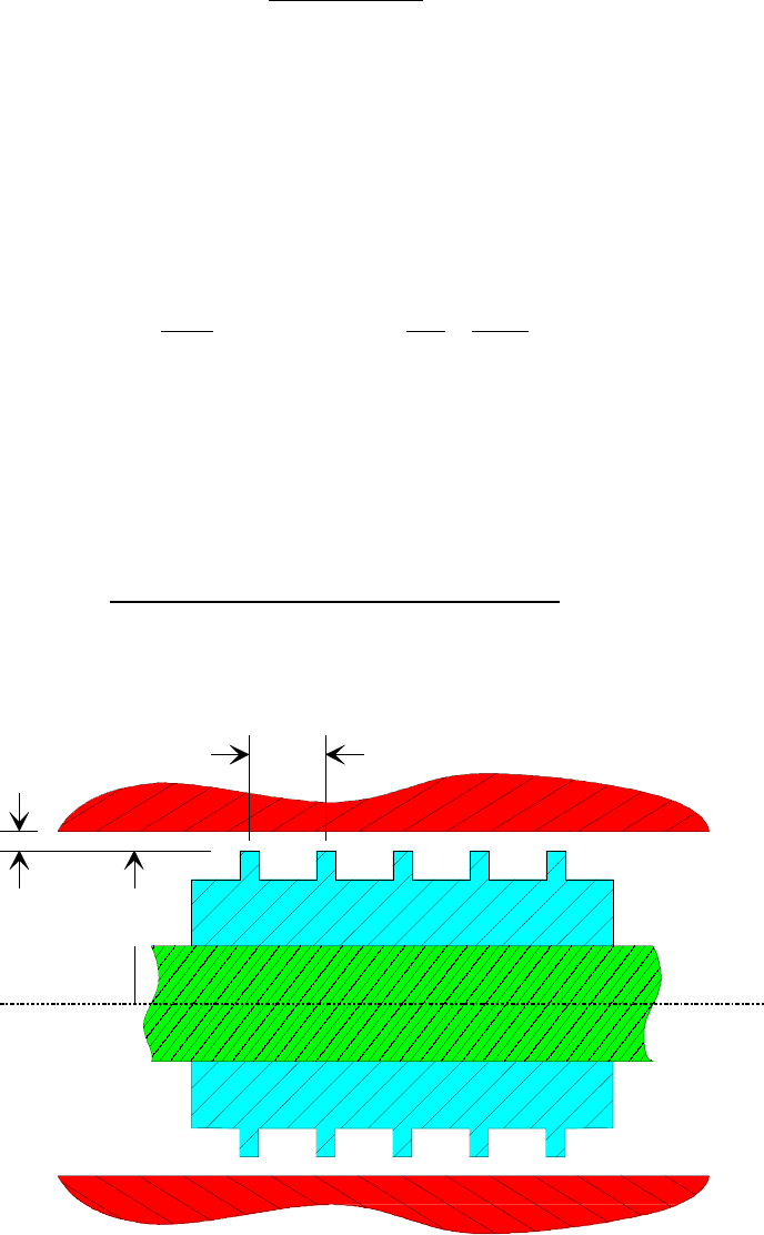
2.2.7.1 Branch

Option 1 (Pipe Flow)

DETAIL A DETAIL A



Where:

D = Pipe Diameter

L = Pipe Length



Absolute Roughness

Pipe Resistance Option Parameters

Figure 2.4 - Pipe Resistance Option Parameters

Figure 2.4 shows the pipe resistance option parameters that are required by GFSSP. This option

considers that the branch is a pipe with length L, diameter D and surface roughness



. For this

option, Kf, can be expressed (Appendix - A) as:

KfL

uDc





(Equation 2.13)

Where



u is the density of the fluid at the upstream node of a given branch.

The Darcy friction factor f is determined from Colebrook Equation [10] which is expressed as:

1237

2 51

fDf

  













log .



(Equation 2.14)

Where e/D and Re are the surface roughness factor and Reynolds number respectively. It should

be noted that

2.2.7.2 Branch

Option 2 (Flow Through Restriction)

This option regards the branch as a flow restriction with a given flow coefficient, CL, and area, A.

For this option, Kf can be expressed as:

guC A



2 2



(Equation 2.15)

In classical fluid mechanics, head loss is expressed in terms of a nondimensional “K factor”.



h K u



(Equation 2.16)

K and CL are related as:



(Equation 2.17)

2.2.7.3 Branch

Option 3 (Non-circular Duct)

This option is currently inactive. Under this option frictional effects in non-circular ducts will be

modeled.

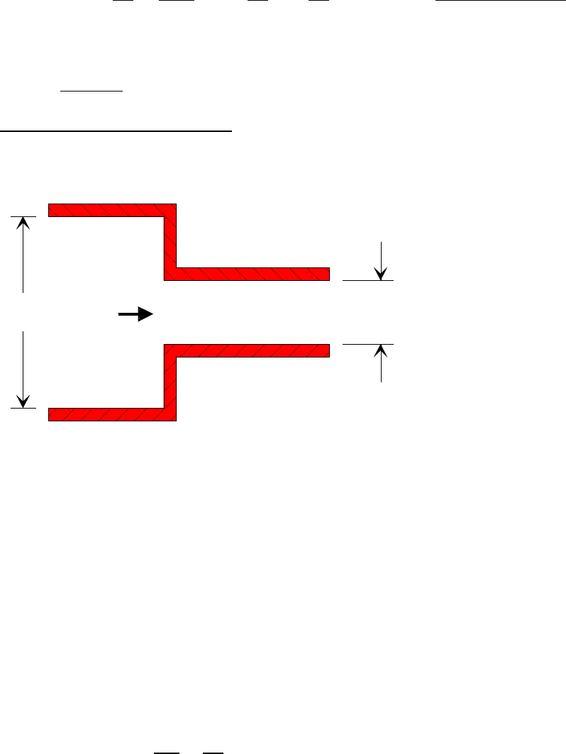
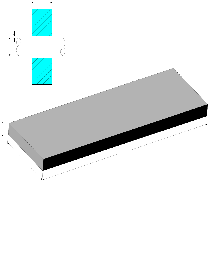
2.2.7.4 Branch Option 4 (Pipe with Entrance and Exit Lloss)

Where:

D = Pipe Diameter

L = Pipe Length



Absolute Roughness

= Entrance Loss Coefficient

= Exit Loss Coefficient

Pipe With Entrance and/or Exit Loss

Entrance Exit

DETAIL A



Figure 2.5 - Pipe With Entrance and/or Exit Loss Resistance Option Parameters

Figure 2.5 shows the pipe with entrance and/or exit loss resistance option parameters that are

required by GFSSP. This option is an extension of Option 1. In addition to friction loss in a

pipe, entrance and exit losses are also calculated. For this option, Kf can be expressed as:

uDc

  



(Equation 2.18)

Where Ki and Ke are entrance and exit loss coefficients respectively.

2.2.7.5 Branch Option 5 (Thin Sharp Orifice)

Where:

= Pipe Diameter

= Orifice Throat Diameter

Thin Sharp Orifice

Figure 2.6 - Thin Sharp Orifice Resistance Option Parameters

Figure 2.6 shows the thin sharp orifice resistance option parameters that are required by GFSSP.

This option considers the branch as a thin sharp orifice with pipe diameter as D1 and orifice

diameter as D2. For this option, Kf can be expressed [11] as:

guA





(Equation 2.19)

Where, for upstream Re



2500:

2 72 120 1 1 1

  











































































.Re

(Equation 2.20)

For upstream Re > 2500:

2 72 4000 1 1

  









































































.Re

(Equation 2.21)

2.2.7.6 Branch Option 6 (Thick Oorifice)

Where:

= Pipe Diameter

= Orifice Throat Diameter

= Orifice Length

Thick Orifice

Figure 2.7 - Thick Orifice Resistance Option Parameters

Figure 2.7 shows the thick orifice resistance option parameters that are required by GFSSP. This

option models the branch as a thick orifice with the pipe diameter as D1 orifice diameter as D2

and length of the orifice as Lor. For this option, Kf can be expressed as in Equation 2.19.

However, the K1 in Equation 2.19 is calculated [11] from the following expressions.

For upstream Re



2500:

 

DL D

1 5

2 72 120 1 1 1 0 584 0 0936

0 225

  

























































































.Re ..

/ .

(Eq. 2.22)

For upstream Re > 2500:

 

DL D

1 5

2 72 4000 1 1 0 584 0 0936

0 225

  























































































.Re ..

/ .

(Eq. 2.23)

2.2.7.7 Branch

Option 7 (Square Reduction)

Where:

= Upstream Pipe Diameter

= Downstream Pipe Diameter

Square Reduction

Flow

Figure 2.8 - GFSSP Square Reduction Resistance Option Parameters

Figure 2.8 shows the square reduction resistance option parameters that are required by GFSSP.

This option considers the branch as a square reduction. The diameters of upstream and

downstream pipes are D1 and D2 respectively. For this option, Kf can be expressed as in

Equation 2.19. However, the K1 in Equation 2.19 is calculated from the following expressions

[11]. The Reynolds number and friction factor that are utilized within these expressions are

based on the upstream conditions. The user must specify the correct flow direction through this

branch. If the model determines that the flow direction is in the reverse direction, the user will

have to replace the reduction with an expansion and rerun the model.

For upstream Re



2500:

12 160 1

 































.Re

(Equation 2.24)

For upstream Re > 2500:

 

K f D

0 6 0 48 1

  





























. .

(Equation 2.25)

2.2.7.8 Branch

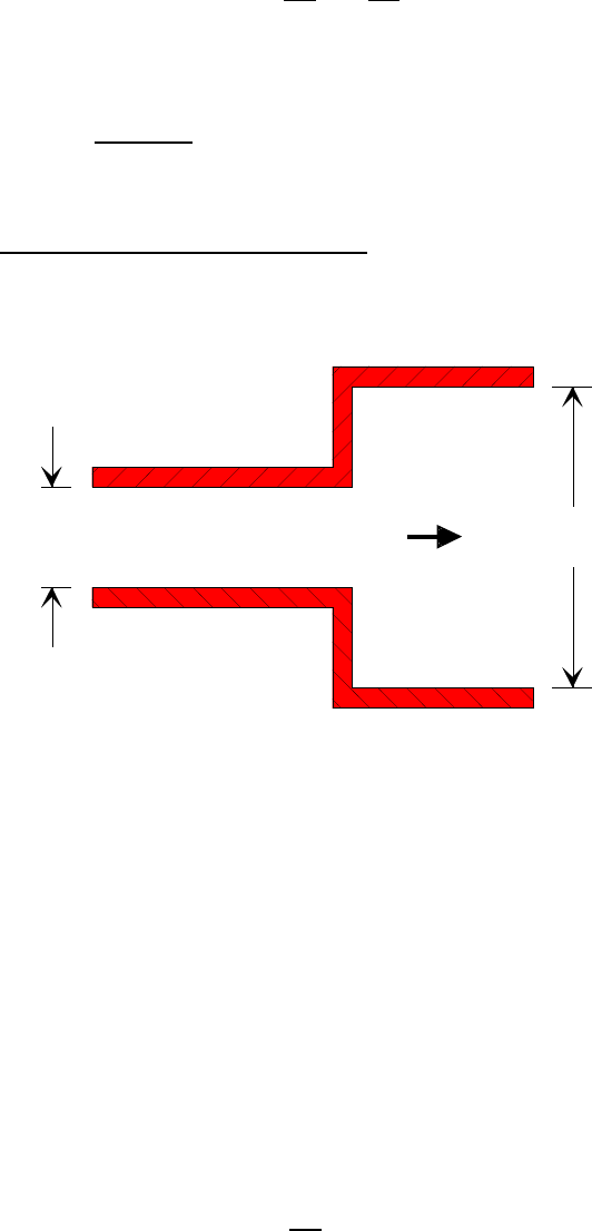
Option 8 (Square Expansion)

Where:

= Upstream Pipe Diameter

= Downstream Pipe Diameter

Square Expansion

Flow

Figure 2.9 - Square Expansion Resistance Option Parameters

Figure 2.9 shows the square expansion resistance option parameters that are required by GFSSP.

This option considers the branch as a square expansion. The diameters of upstream and

downstream pipes are D1 and D2 respectively. For this option, Kf can be expressed as in

Equation 2.19. However, the K1 in Equation 2.19 is calculated from the following expressions

[11]. The Reynolds number and friction factor that are utilized within these expressions are based

on the upstream conditions. The user must specify the correct flow direction through this

branch. If the model determines that the flow direction is in the reverse direction, the user will

have to replace the expansion with a reduction and rerun the model.

For upstream Re



4000:

2 1

  





















(Equation 2.26)

For upstream Re > 4000:

 

K f D

1 0 8 1

   





















(Equation 2.27)

2.2.7.9 Branch

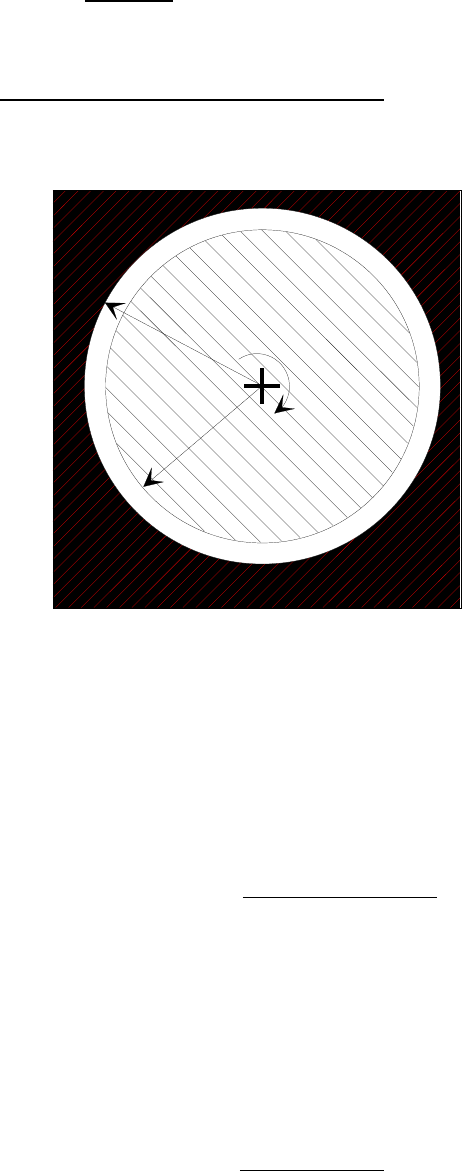
Option 9 (Rotating Annular Duct)

Rotating Annular Duct



Where:

L = Duct Length (Perpendicular to Page)

b = Duct Wall Thickness (b = r

- r

)

 Duct Rotational Velocity

= Duct Inner Radius

= Duct Outer Radius

Figure 2.10 - Rotating Annular Duct Resistance Option Parameters

Figure 2.10 shows the rotating annular duct resistance option parameters that are required by

GFSSP. This option considers the branch as a rotating annular duct. The length, outer and inner

radius of the annular passage are L, r0, and ri respectively. The inner surface is rotating at N rpm

(N=30w/p). For this option, Kf can be expressed as:

 

KfL

uAc

gr r





(Equation 2.28)

The friction factor, f, in equation 2.28 was calculated from the following expressions [12]:

 

0.24

0 077

fRu



(Equation 2.29)

Where:

 

Ru uuri







2 0

(Equation 2.30)

And u is the tean axial velocity, therefore:

1 0 7656 2

20 38

  























(Equation 2.31)

2.2.7.10 Branch

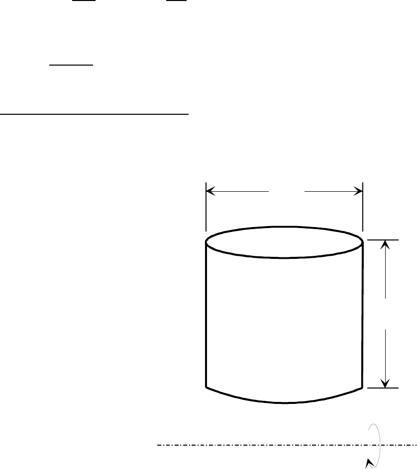
Option 10 (Rotating Radial Duct)

Where:

L = Duct Length

 Duct Rotational Velocity

D = Duct Diameter

Rotating Radial Duct



Center

Line

Figure 2.11 - Rotating Radial Duct Resistance Option Parameters

Figure 2.11 shows the rotating radial duct resistance option parameters that are required by

GFSSP. This option considers the branch as a rotating radial duct. The length and diameter of

the duct are L and D respectively. The rotational speed is



radian/sec. For this option, Kf can be

expressed as:

KfL

uDc





(Equation 2.32)

The friction factor, f, in equation 2.28 was calculated from the following expressions [13]:

 

0.25

0 0791

fRu





(Equation 2.33)

0 942 0 058

20 282

  































. .

 



(Equation 2.34)

2.2.7.11 Branch Option 11 (Labyrinth Sseal)

Labyrinth Seal

Where:

C = Clearance

M = Gap Length (Pitch)

= Radius (Tooth Tip)

N = Number of Teeth

Figure 2.12 - Labyrinth Seal Resistance Option Parameters

Figure 2.13 shows the labyrinth seal resistance option parameters that are required by GFSSP.

This option considers the branch as a labyrinth seal. The number of teeth, clearance, pitch are n,

c and m respectively. For this option, Kf can be expressed [14] as:

 

guA

 

1 05 15

/ . .





(Equation 2.35)

where the carry over factor,

, is expressed as:

 









0 02

n c m

/ .

(Equation 2.36)

For a straight labyrinth seal A should be set to unity. For a stepped labyrinth seal A should be

less than unity.

2.2.7.12 Branch Option 12 (Face Sseal)

Where:

c = Seal Thickness (Clearance)

B = Seal Width

L = Seal Length (L =



Face Seal

Figure 2.13 - Face Seal Resistance Option Parameters

Figure 2.13 shows the face seal resistance option parameters that are required by GFSSP. This

option considers the branch as a face seal. The length, inner diameter and clearance of the seal

are L, D and c respectively. For this option, Kf can be expressed [15] as:

g Dc m



 



(Equation 2.37)

2.2.7.13 Branch

Option 13 (Common Fittings & Valves)

This option considers the branch as a common fittings or valves. The resistance in common

fittings and valves can be computed by two-K method [16]. For this option, Kf can be expressed

as:

 

KKKD

guA

 



1 1

/ Re /



(Equation 2.38)

Where:

K1= K for the fitting at Re =1;



= K for the fitting at Re =



;

D = Internal diameter of attached pipe, in.

The constants K1 and K



for common fittings and valves are listed in Table 2.

f can be expressed as: qua)

Where:

D = Internal diameter of attachfor comm

2.2.7.14 Branch Option 14 (Pump Ccharacterisics)

This option considers the branch as a pump with a given characteristics. The pump

characteristics must be expressed as:



p m = A + B

0 0

(Equation 2.39)

Where:



- Pressure rise, lbf/ft2

- Flow rate, lbm/sec

The momentum source, S in Equation 2.2 is then expressed as:

S p

 

(Equation 2.40)

Fitting Type K1K

Standard (R/D = 1), Screwed 800 0.40

Standard (R/D = 1), Flanged or Welded 800 0.25

Long Radius (R/D = 1.5), All Types 800 0.20

90° Elbows 1 Weld (90° Angle) 1000 1.15

2 Welds (45° Angle) 800 0.35

Mitered (R/D = 1.5) 3 Welds (30° Angle) 800 0.30

4 Welds (22.5° Angle) 800 0.27

5 Welds (18° Angle) 800 0.25

Standard (R/D = 1), All Types 500 0.20

45° Elbows Long Radius (R/D = 1.5), All Types 500 0.15

Mitered, 1 Weld, 45° Angle 500 0.25

Mitered, 2 Weld, 22.5° Angle 500 0.15

Standard (R/D = 1), Screwed 1000 0.60

180° Elbows Standard (R/D = 1), Flanged or Welded 1000 0.35

Long Radius (R/D = 1.5), All Types 1000 0.30

Standard, Screwed 500 0.70

Tee, Flow Through Long Radius, Screwed 800 0.40

Branch Standard, Flanged or Welded 800 0.80

Stub-in-type Branch 1000 1.00

Screwed 200 0.10

Tee, Flow Through Flanged or Welded 150 0.50

Stub-in-type Branch 100 0.0

Gate, Ball, Plug Full Line Size, b = 1.0 300 0.10

(b = dorifice/dpipe) Reduced Trim, b = 0.9 500 0.15

Reduced Trim, b = 0.8 1000 0.25

Globe, Standard 1500 4.0

Valves Globe, Angle or Y-Type 1000 2.0

Diaphragm, Dam Type 1000 2.0

Butterfly 800 0.25

Lift 2000 10.0

Check Swing 1500 1.5

Tilting Disk 1000 0.5

Table 2.2 - Constants for Two K Method of Hooper (Reference 3) for Fittings/Valves

(GFSSP Resistance Option 13)

2.2.7.15 Branch Option 15 (Pump Hhorsepower)

This option considers the branch as a pump with a given horsepower, P, and efficiency,



. The

momentum source, S, in Equation 2.2 is then expressed as:

SuP A



550



(Equation 2.41)

2.2.7.16 Branch Resistance Option 16 (Valve with a Given Loss Coefficient)

This option considers the branch as a valve with a given Cv. For this option, Kf, can be expressed

as:



4 68 5



(Equation 2.42)

2.3 SOLUTION PROCEDURE

In the sample circuit shown in Figure 2.1, pressures, temperatures, and concentrations of

hydrogen and oxygen are to be calculated for the 7 internal nodes; flow rates are to be calculated

in the 12 branches. Therefore, the total number of equations to be solved is 40 (= 7 X 4 +12).

There is no explicit equation for pressure. The pressures are implicitly computed from the mass

conservation equation (Equation 2.1). The flow rates are calculated from Equation 2.2. The

inertia and friction terms are nonlinear in Equation 2.2. The pressures and mass flow rates

appear in the flow rate equations. The enthalpy and concentrations are solved using Equations

2.3 and 2.4 respectively. The flow rates also appear in the enthalpy and the concentration

equations. The governing equations to be solved are strongly coupled and nonlinear and

therefore they must be solved by an iterative method.

Stoecker [20] described two types of numerical methods available to solve a set of non-linear

coupled algebraic equations: (1) the successive substitution method and (2) the Newton-Raphson

method. In the successive substitution method, each equation is expressed explicitly to calculate

one variable. The previously calculated variable is then substituted into the other equations to

calculate another variable. In one iterative cycle each equation is visited. The iterative cycle is

continued until the difference in values of the variables in successive iterations becomes

negligible. The advantages of a successive substitution method are its simplicity to program and

its low code overhead. The main limitation, however, is finding an optimum order for visiting

each equation in the model. This visiting order, which is called the information flow diagram, is

crucial for convergence. Under relaxation (partial substitution) of variables is often required to

obtain numerical stability.

In the Newton-Raphson method, simultaneous solution of a set of non-linear equations is

achieved through an iterative guess and correction procedure. Instead of solving for the variables

directly, correction equations are constructed for all variables. The intent of the correction

equations is to eliminate the error in each equation. The correction equations are constructed in

two steps: (1) the residual errors in all of the equations are estimated and (2) the partial

derivatives of all of the equations, with respect to each variable, are calculated. The correction

equations are then solved by the Gaussian elimination method. These corrections are then

applied to each variable which completes one iterative. These iterative cycles of calculations are

repeated until the residual error in all of the equations is reduced to a specified limit. The

Newton-Raphson method does not require an information flow diagram. Therefore, it has

improved convergence characteristics. The main limitation to the Newton-Raphson method is its

requirement of a large amount of computer memory. Details of the Newton-Raphson method

appear in Appendix A.

In GFSSP, a combination of the successive substitution method and the Newton-Raphson

method is used to solve the set of equations. The mass and momentum conservation equations

are solved by the Newton-Raphson method. The energy and specie conservation equations are

solved by the successive substitution method. The underlying principle for making such a

division was that the equations which are more strongly coupled are solved by Newton-Raphson

method. The equations which are not strongly coupled with the other set of equations are solved

by the successive substitution method. Thus, the computer memory requirement can be

significantly reduced while maintaining superior numerical convergence characteristics.

It may be further mentioned that the solution of compressible flow problems requires two

iterative cycles. In compressible flows, the density is a function of pressure and temperature and

the resistance coefficient (

) in Equation 2.1 is a function of density. Therefore, the flow

resistance parameters are recalculated after attaining a converged solution for the problem with

the initial flow resistance parameters. The iterative cycle for the flow resistance calculations is

continued until the differences in flow resistance, densities and enthalpies in successive iteration

cycles are less than the specified convergence criterion for the problem.

3.0 COMPUTER PROGRAM

GFSSP was developed on an IBM compatible PC using the LAHEY EM32 FORTRAN

compiler. The same source code also runs on Macintosh and Silicon Graphics. The code was

developed with a modular structure to facilitate adding new capabilities in the future. The flow

chart of the program is shown in Figure 3.1. The main routine controls all program operations

and makes the decisions whether to continue or stop the current iterative cycle of calculations.

The computer program has three major parts. The first part consists of the subroutines for the

preprocessor. The preprocessor allows the user to interactively create the flow network model

consisting of nodes and branches. All of the input specifications, including the boundary

conditions are specified through the preprocessor. The second major part of the program consists

of the subroutines that provide the initial conditions and then develop and solve all of the

conservation equations in the flow network. The third part of the program consists of the

thermodynamic property programs, GASP and WASP, that provide the necessary thermodynamic

and thermophysical property data required to solve the resulting system of equations.

3.1 PREPROCESSOR

The preprocessor consists of three subroutines. PREPROP is an interactive routine that allows

the user to select necessary options for flow model. The options include compressibility, mixture

thermodynamics and axial thrust calculations. All network information including numbering and

classification of nodes, the connecting branches, information to calculate branch resistance, the

initial and boundary conditions are provided through interactive dialogue with the user. At the

end of the interactive session, the input data are written (WRITEIN) in a text file. The code reads

the data file through subroutine READIN.

3.2 SOLVER

The main and the set of subroutines under this group perform five major functions. 1) Generation

of trial solution based on initial guess 2) Newton-Raphson solution of conservation equations. 3)

Successive substitution method of solving concentration equation. 4) Calculation of resistance in

branches. 5) Prints input/output variables of the problem. INIT generates trial solution by

interacting with thermodynamic property code GASP and WASP. Subroutine NEWTON

conducts the Newton-Raphson solution of mass conservation, flow rates and energy conservation

equations with the help of EQNS, COEF, SOLVE and UPDATE. The subroutine EQNS generate

the equations. The coefficients of the correction equations are calculated in COEF. The

correction equations are solved by the Gaussian Elimination method in SOLVE. After applying

for the corrections the variables are updated in subroutine UPDATE. The resistancesfor each

branch are calculated in RESIST after calculating densities at each node in the subroutine

DENSITY.

3.3 THERMODYNAMIC PROPERTY PACKAGE

The thermodynamic property package consists of two separate programs GASP and WASP

programs and RP-1 tables. GASP and WASP programs consist of a number of subroutines.

GASP provides thermodynamic properties of ten fluids: helium, methane, neon, nitrogen, carbon

monoxide, oxygen, argon, carbon dioxide, fluorine and hydrogen. WASP provides

thermodynamic properties of water. RP-1 properties are provided in the form of tables.

Subroutine RP1 searches the required property values from these tables. These property

subroutines are called from two subroutines, INIT and DENSITY. In subroutine INIT, enthalpies

and densities are computed from given pressures and temperatures at boundary and internal

nodes. In subroutine DENSITY, density, temperatures, specific heats and specific heat ratios are

calculated from given pressures and enthalpies at each node.

WRITEIN

Writes data

to a file.

PREPROP

Interactively generate network

circuit, supply boundary and

initial conditions.

READIN

Reads input

from data

file.

Main

Inputs

Subroutines

Start

Input

file exists

Obtain

trial

solution.

problem

input

data.

Obtain

solution of

pressure &

flowrate

INIT

Generate trial solution

based on initial guess.

Print headers, boundary and

initial conditions to file.

NEWTON

Controls Newton-Raphson

solution scheme.

GASP & WASP

Obtain enthalpies for given

pressures and temperatures.

EQNS

Calculates residuals

of each equation.

COEF

Calculates coeficients for

correction equations.

SOLVE

Solve correction equation by

Gaussian elimination method

UPDATE

After applying corrections,

update each variable.

Obtain

solution of

enthalpy

ENTHALPY

Solution by successive

substitution.

Obtain

solution of

concentrations

MASSC

Solution by successive

substitution.

Obtain

branch

resistances

RESIST

Calculates resistances

for all branches.

DENSITY

Calculates density at each node

from law of partial pressure.

GASP, WASP & RP1

Obtain density of each specie

from pressure and enthalpy.

KFACT1 - KFACT16

Calculate branch resistances.

Converged

problem

solution.

Print all variables at nodes

and branches to file.

STOP

Yes

Figure 3.1 The GFSSP Flowchart

4.0 USER’S GUIDE

The purpose of this chapter is to explain how to create a data file, for any given flow

circuit, with the help of the GFSSP interactive preprocessor. In order to run the code on a

PC, the user must type at the DOS prompt:

C:\ GFSSP1P4

The first question the code will ask:

“ DO YOU WANT TO READ A DATA FILE? “

If the user answers ‘yes’ to this question, the code will prompt the user to supply the

existing input data file. After a successful reading of the input data file, the code will ask

the user to supply the name of the solution output file that the code will create and

GFSSP will proceed to calculate a solution to the specified data file. If the user answers

‘no’ to the first question, a call to preprocessor subroutine will be invoked and the

interactive session will begin.

The preprocessor prompts the user for all of the necessary information to create the input

data file. At the end of the interactive session, the code writes this input data into a file

who’s name was specified by the user at the end of the interactive session. Before

building the desired model, the preprocessor will prompt the user to input a problem title

of less than or equal to 80 characters. After this information has been input the

preprocessor will proceed to construct the model.

The sequence of inputs to the preprocessor are as follows:

1. Selection of model options

2. Node information

3. Branch information

4. Boundary conditions

5. Miscellaneous information

4.1 SELECTION OF MODEL OPTIONS

During this session, the preprocessor will ask the user to select between various modeling

options available in the code. The user can select the option by typing either upper or

lower case ‘y’ to activate the current option or ‘n’ to leave the option deselected. The

code sets the logical variables either to TRUE or FALSE depending upon the user’s

answer. The logical variables and their meaning appear in Table 4.1. The interactive

session is sequential. This implies that the preprocessor will prompt the user to supply

information based on the choices made previously during this session. The following

questions will be asked in sequence:

“IS FLOW TRANSIENT?”

GFSSP has the capability of modeling quasi-steady state flow circuit. In quasi-steady

state mode, the boundary conditions are allowed to be a function of time.

If the user answers ‘no’ to this question, a steady state flow will be assumed. If the

answer was ‘yes’, the code will ask the user to supply the time step, the start time and the

stop time in seconds. The numbers can either be separated by a comma or by a space.

The ‘enter’ key must be pressed after the requested data has been input. If the user

presses the enter key before supplying all the data requested by the preprocessor, the

program will not proceed until it receives the correct number of values.

The next preprocessor question is:

“IS DENSITY CONSTANT IN THE CIRCUIT?”

If the user answers ‘yes’ to this question, the program will assume a constant density

within the fluid circuit and the user must supply the density and viscosity of the fluid. If

user answers ‘no’ to this question, the program will assume that the density can vary and

the user must select the fluid from the GFSSP library of fluids. In the case of a mixture,

the user will be required to select from a list of fluids. These related questions will be

asked at the end of the “model options” session.

The next preprocessor question is:

“DO YOU WANT TO ACTIVATE GRAVITY?”

If the user answers ‘yes’ to this question, the program will account for gravity effects in

determining a solution for the current model. The user will be asked to supply the

orientation of the branches with respect to the gravitational force vector during the

‘branch information’ session.

The next prompt the user must respond to is:

“DO YOU WANT TO ACTIVATE BUOYANCY?”

For a problem involving natural convection, the user must activate this option by

responding with a ‘y’ at the prompt. In a situation were natural convection occurs, the

fluid experiences a buoyancy force because of density differences in the presence of

gravitational field. Under the action of this force, the lighter fluid tends to move up.

Therefore, the buoyancy force always acts in a direction opposite to the gravitational

force. If this option is activated, the user must supply a reference point for calculating the

density in the ‘miscellaneous information’ session.

The next question the preprocessor will ask is:

“DO YOU WANT TO ACTIVATE INERTIA?”

If the inertia force of the fluid is important to consider in the flow circuit to be analyzed,

user must activate this option by responding with a ‘y’ to the prompt. Also, if there is a

significant change in the density and the area in a flow passage within the model, the

inertia option should be activated. If this option is selected the user will also be required

later in this session to provide the angle between the upstream and downstream branches.

2 3

Node

Branch

1122334

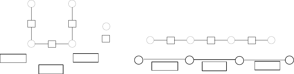
(a) (b)

Figure 4.1 - Examples of Flow Circuit Arrangement to Demonstrate the Effect of

Fluid Inertia.

In Figure 4.1(a), the fluid flowing in Branch 2 experiences no inertial effects from the

fluid flowing in Branch 1, assuming the flow is from Branch 1 to Branch 2 and the angle

between Branch 1 and Branch 2 is 90 degrees. In Figure 4.1(b), the fluid flowing in

Branch 2 experiences the total effect of the inertial force from Branch 1, assuming the

flow is from Branch 1 to Branch 2 and the angle between these branches is zero. In the

data file, the angles between branches are set by default to zero. The user must update the

data file, using a text editor, to supply the correct angles between the branches if this

option is activated.

The next preprocessor question is:

Branch 1

Branch 2

Branch 3

Branch 1 Branch 2 Branch 3

“DO YOU WANT TO ACTIVATE ROTATION?”

GFSSP allows the user to model rotating flows in branches to account for the centrifugal

forces on the fluid that occur in these branches. When the axis of rotation is not parallel

to the main flow direction, the fluid experiences a centrifugal force. The magnitude of

the centrifugal force depends on the radii of the axis of rotation and on the angular speed

of the fluid. If this option is activated, the associated questions are asked in the

‘miscellaneous information’ session.

The next preprocessor question is:

“IS AXIAL THRUST CALCULATION REQUIRED IN THE CIRCUIT?”

GFSSP provides an option to calculate the axial thrust created in a flow circuit. This

axial thrust is created when there exists a pressure differential between opposing faces of

a mechanism that is being modeled, such as a turbine disk. If this option is activated, the

user must supply surface areas normal to the thrust vector. If a normal vector to the input

surface area aligns with the thrust vector, the magnitude of area in square inches (in2) is

entered with a positive sign. The surface area must be entered with a negative sign if a

normal vector to the given surface area is opposite to the direction of the thrust vector.

The user may chose to update the data file, using a text editor, to supply the areas once

the data file is created. The user must answer ‘n’ to this option to avoid answering

questions on areas during the interactive session.

The next preprocessor question is:

“ARE THERE ANY HEAT SOURCES?”

If the presence of heat sources or sinks in the flow circuit can affect the flow distribution,

the user must activate this option by answering ‘y’. During the ‘miscellaneous

information’ session, the user will be required to identify the nodes where heat loads are

applied and the magnitude of heat loads in each of the identified nodes.

The next preprocessor question is:

“DO YOU WANT TO ACTVATE HEAT CONDUCTION?”

The user can activate the heat conduction option between nodes by answering ‘y’ to this

question. If this option is activated, the user must supply the distances between nodes

and the cross sectional flow area normal to the heat conduction path during the branch

information session.

The next preprocessor question is:

“IS THE FLUID A MIXTURE?”

Once the user answers this question, either ‘y’ or ‘n’, the code will print a list of fluids.

GFSSP can calculate the properties of the listed fluids. If the mixture option is not

chosen, the user needs to identify only one fluid from the list. If the user answers ‘y’ to

the previousdingstion, the code will ask:

“HOW MANY OF THESE FLUIDS ARE PRESENT IN THE CIRCUIT?”

The user must provide the total number of fluids as well as identify the index number of

each fluid from the given list. GFSSP requires a reference point for enthalpies for

mixture calculation. It is recommended that the triple point of water should be used for

reference point. NHREF must be kept at its default value of 2 to maintain the

recommended reference point.

4.2

4.2 NODE INFORMATION

In this session, the user will first be required to supply the total number of nodes. The

code will then ask to designate a number for each of the nodes. The numbering scheme is

completely arbitrary. The user can devise any numbering scheme, using a maximum of

four digits. The user is then required to identify the type of each of the nodes. GFSSP

allows two types of nodes. A node could be either an internal node or a boundary node.

The code calculates pressures, temperatures and mixture concentrations at the internal

nodes. The pressures, temperatures and concentrations must be supplied in the boundary

nodes. GFSSP does not use the temperatures and concentrations at the outflow boundary

nodes. However, user must supply those values because GFSSP does not distinguish

between inflow and outflow boundary during problem setup. A boundary node can have

either an inflow or outflow depending upon the specified boundary condition.

4.3

4.3 BRANCH INFORMATION

In this section, the user is required to provide all of the necessary information concerning

each of the branches. Every node in the circuit is connected to the circuit through at least

one branch. The code will visit every internal node, identified by the user in the previous

session, and ask user to supply the number of branches connected with each internal

node.

For each branch, the user must supply:

a) A branch number within four digits.

b) The assumed upstream and downstream nodes of the given branch.

c) A branch type (resistance option) and the appropriate information necessary

for selected type.

If the gravity option is activated, the user must supply the angle that the branch makes

with the gravity vector. If the heat conduction option is activated, the user must also

supply the distances between the nodes and the cross sectional flow area normal to the

heat conduction flux.

4.4 BOUNDARY CONDITIONS

4.4

In this session, the user is required to supply pressures, temperatures and concentrations

at all of the boundary nodes. For transient calculations, user is required to supply the

filename containing the history data.

4.5 MISCELLANEOUS INFORMATION

4.5

The user will be prompted to supply any additional information necessary for the model

closure starting with:

“HOW MANY INTERNAL NODES HAVE SPECIFIED FLOWRATES?”

GFSSP requires the specification of pressure at all of the boundary nodes. The code

calculates flow rates in all of the branches. The code however has been provided with the

capability of accepting a mass source or sink in the internal nodes. The user will enter a

‘0’ if there is no such mass source in the circuit. Otherwise, the actual number of internal

nodes with mass sources must be typed. The code then will ask user to provide the

following information for the supplied number of internal nodes:

a) The internal node number.

b) The mass source (a positive number) or mass sink (a negative number) in

lb/sec.

he next question the preprocessor will ask is:If ththe user will be prompted with the

question:

“HOW MANY INTERNAL NODES HAVE SPECIFIED HEAT SOURCES?”

The user is prompted to supply the number of internal nodes with specified heat sources

if there are any heat sources or sinks in any of the internal nodes in the circuit. The user

must enter a ‘0’ if there is no such source in the circuit. Otherwise, the actual number

must be typed. The heat source can be specified in either BTU/lbm or in BTU/sec. The

user must select the option. The code then will ask the user to provide the following

information for the input number of internal nodes:

a) The internal node number.

b) The heat source flux (a positive number) or sink flux (a negative number) in

appropriate units.

If buoyancy is activated, the code will ask the user to supply the reference node to use for

determining the density. The buoyancy force will be calculated with respect to the

density of the reference point.

If the rotational option is activated in the code, the user will be prompted with the

question:

“HOW MANY BRANCHES HAVE THE ROTATING FLOWS?”

Once the user answers this question, the code will ask the user to provide the following

information for the supplied number of branches:

a) The branch number.

b) The upstream and downstream radius of the branch.

c) The rotational speed and the factor representing the extent of the rotation of

fluid with respect to the solid boundary.

Finally the user will be asked to provide a filename for the data file to be created. An

example of the complete interactive session of creating a data file is provided in

Appendix B.

4.6 DESCRIPTION OF INPUT DATA FILE

The previous sections describe how to create a GFSSP model of a fluid flow network

using the GFSSP preprocessor. This section describes the structure of the GFSSP input

data file that is created by the preprocessor. Example input data files can be found in

Appendix C.

The data in the GFSSP input data file can be classified into the following 11 sections:

1. Title:

The user can specify a model title of 80 characters or less.

2. Logical Variables:

Table 3 contains a listing of the GFSSP logical variables and their options.

3. Node, Branch and Fluid Information:

NNODES - Number of nodes.

NINT - Number of internal nodes.

NBR - Number of branches.

NF - Number of fluids.

NHREF - Reference index for fluid (this must be 2).

4. Relaxation Parameters:

RELAXK - Under relaxation parameter for resistance ( Recommended value = 1.0).

RELAXD - Under relaxation parameter for density ( Recommended value = 0.5).

RELAXH - Under relaxation parameter for enthalpy ( Recommended value = 1.0).

5. Index Number for Fluids:

NFLUID(I), I = 1, NF : Index number for each fluid is printed in this line. Table 4.2

shows the fluids that are available in GFSSP.

Variable Meaning

DENCON = T; Uses constant density and viscosity supplied by the user.

= F; All thermodynamic and thermophysical properties are computed.

GRAVITY = T; Gravitational force will be calculated for branches utilizing Resistance

Option 1 or 4.

= F; Gravitational force is not calculated.

ENERGY = T; Energy equation is solved (for DENCON = F and/or with heat sources).

= F; Energy equation is not solved.

MIXTURE = T; For more than one fluid in the circuit.

= F; For a single fluid in the circuit.

THRUST = T; Thrust is calculated from node pressures and areas.

= F; Thrust is not calculated.

STEADY = T; Performs one steady state calculation.

= F; Performs quasi-steady calculation with given time history of boundary

conditions.

TRANSV = F; This must always be set to FALSE.

INERTIA = T; Inertial effect of fluid is considered.

= F; Inertial effect is neglected.

CONDX = F; This option must be set to FALSE.

TWOD = F; This must be set to FALSE.

PRINTI = T; This option prints out the initial flow field.

= F; This option suppresses the print out of the initial flow field.

ROTATION = T; This option allows the user to input branches with rotation.

= F; Rotation is not activated.

BUOYANCY = T; This option activates buoyancy when GRAVITY = .TRUE.

HRATE = T; Heat source is in Btu/sec

= F; Heat source is in Btu/lbm

Table 4.1 - GFSSP Logical Variables

6. Nodes and Indices:

In this section, the node numbers, NODE(I), and their indices, INDEX(I), are printed.

INDEX(I) = 1 implies an internal node and INDEX(I) = 2 indicates a boundary node.

7. Node Information:

In this section, pressure, temperature, mass source, heat source and areas are printed

sequentially. Node areas are required only when the axial thrust calculation option is

activated.

Index Fluid

1 Helium

2 Methane

3 Neon

4 Nitrogen

5 Carbon monoxide

6 Oxygen

7 Argon

8 Carbon dioxide

9 Fluorine

10 Hydrogen

11 Water

12 RP-1

Table 4.2 - Fluids Available in GFSSP

8. Branch Connection:

The number of branches for every internal node is defined. Every branch connected with

the internal node is also defined.

INODE(I) - Internal node number.

NUMBR(I) - Number of branches connected with the Ith internal node.

NAMEBR(I,J), J = 1, NUMBR(I) - Name of the branches connected with the Ith internal node.

9. Branch Information:

Branch information is provided in this section. In the first part of this section, the branch number,

upstream node, downstream node and selected resistance option are printed. In the second part

the required input parameters of every branch are printed in the same order as in the first part. A

header is printed for every branch describing the required input parameters.

10. Inertia Information:

In order to account for inertial effects in the fluid flow model, the velocity in the upstream branch

is required along with the angle between the branches. During the course of the calculation, if the

flow rate becomes negative, the designated downstream branch becomes the upstream branch.

Therefore, in this section, all of the upstream and downstream branches, for every branch in the

flow circuit, are defined. In the first part of this section, the number of upstream branches and

their designated numbers are listed. In the second part, the number of downstream branches and

their designated numbers are listed. Finally the information about the angle the branch makes

with its upstream and downstream neighbors are printed. The default values of the angle are set to

zero. If the user wants to modify these angles, the user must use a text editor to alter the data file.

11. Rotation Information:

When the option ROTATION is set to TRUE, this section provides related information. First, the

number of rotating branches is printed. This is followed by a table of following data:

BRANCH : Designated branch number.

RADU: Radial distance to the upstream node from the axis of rotation, in units of inches.

RADD: Radial distance to the downstream node from the axis of rotation, in units

of inches.

RPM: Rotational speed of the branch in units of rpm.

AKROT: Empirical factor representing the ratio of the fluid and the solid surface speeds.

5.0 EXAMPLES

The purpose of this chapter is to demonstrate the major features of the code through

seven example problems. These demonstration problems are:

1. Series flow circuit with common pipe fittings and a valve.

2. Series flow circuit with common pipe fittings, a valve and a pump.

3. Flow distribution in a parallel flow manifold

4. Flow distribution in a parallel flow manifold with heat sources and phase changes.

5. Mixing of cryogenic fluids in an inter-propellant seal flow circuit of a turbopump.

6. Quasi-steady calculation of Example 5.

7. Flow in a rotating disk.

5.1 EXAMPLE 1 - SERIES FLOW CIRCUIT WITH COMMON PIPE

FITTINGS AND A VALVE

This example illustrates a model of a flow circuit where several pipes are joined in series

with the help of common pipe fittings such as a gate valve, reducer, expander and elbow.

Two orifices are also placed in the line. The purpose of this example is to demonstrate

the use of various resistance options in the code. Figure 5.1 shows the flow circuit

consisting of 16 nodes and 15 branches. Node 1 and Node 16 are boundary nodes where

pressures and temperatures are specified. Nodes 2 through Node 15 are internal nodes

where pressures and temperatures are calculated by the code. The code also calculates the

flow rates in each branch. The resistance option and geometrical parameters of every

branch are shown in the figure. Branch 45 is a dummy branch with no resistance. In the

following example, this branch will be used to locate a pump. The input and output data

files from Example 1 are provided in Appendix D.

Several runs were made with this model to generate a system characteristics curve. The

system characteristics can be described by plotting the system inlet to outlet pressure

differential with the corresponding flow rate. The model was run with 6 different inlet

pressures (50, 100, 150, 250, 300 and 350 psia) at Node 1. The pressure at the outlet

(Node 16) was kept at 14.7 psia. The assigned pressure differentials and calculated flow

rates are shown in Table 5.1. The predicted system characteristics are shown graphically

in Figure 5.2.

Pressure differential (psi) Flow rate (lbm/sec)

35.3 798

85.3 1350

135.3 1750

235.3 2340

285.3 2590

335.3 2820

Table 5.1 - System Characteristic Data of Example 1

112 223

Entrance

Water @ 14.7

psia & 60 F

Pipe 1, w/

Entrance Loss

L=360 in, D=30.624 in,



D=5.88E-05, K

inlet

=0.5

exit

=0.5

Gate Valve

910

Pipe 5

445 5

Flow Restriction

Pipe 3

Reducer

=30.624 in.,

=22.62 in.

Pipe 4

Thin Orifice

Pipe 2

1011

11 1112

Expander

Pipe 6

12 1213 13 1314 14 1415 15

1516

Thick Orifice Pipe 7 90 Deg. Elbow

Pipe 8, w/

Exit Loss

D=30.624 in, K

=300

=0.10

L=480 in, D=30.624 in,



D=5.88E-05

L=3600 in, D=30.624 in,



D=5.88E-05

L=2400 in, D=22.62 in,



D=7.96E-05

Pipe

=22.62 in.,

Throat

=8.0 in.

L=2400 in, D=22.62 in,



D=7.96E-05

=22.62 in.,

=30.624 in.

L=3600 in, D=30.624 in,



D=5.88E-05

Pipe

=30.624 in.,

Throat

=12.0 in.,

Throat

=9.0

L=1200 in, D=30.624 in,



D=5.88E-05

D=30.624 in, K

=800

=0.20

L=286.0 in, D=30.624 in,



D=5.88E-05, K

inlet

=0.0

exit

=1.0, Vert. Elev.

Change=286.0 in.

Exit,

Water @ 14.7,

psia & 60 F

xxxx

Branch Number

Node Number

= 0.0, A=736.57 in

Figure 5.1 - Example 1 Flow Circuit

System Characteristics

100

150

200

250

300

350

0 500 1000 1500 2000 2500 3000

Flowrate (lbm/sec)

Pre s s ure Diffe rentia l (ps i)

Figure 5.2 - Example 1 Predicted System Characteristics

5.2 EXAMPLE 2 - SERIES FLOW CIRCUIT WITH COMMON PIPE

FITTINGS, A VALVE AND A PUMP

This example is an extension of Example 1. The purpose of this example problem is to

demonstrate how to incorporate a pump into a flow circuit. The dummy branch in

Example 1, branch 45, was used to locate the pump. The flow circuit is shown in Figure

5.3 and the pump characteristics curve is shown in Figure 5.4. The combined pump and

system characteristics is shown in Figure 5.5. The input and output data files from

Example 2 are provided in Appendix E.

112 223

Entrance

Water @ 14.7

psia & 60 F

Pipe 1, w/

Entrance Loss

L=360 in, D=30.624 in,



D=5.88E-05, K

inlet

=0.5

exit

=0.5

Gate Valve

910

Pipe 5

445 5

Pump

Coef.

=30888,

Coef.

=-8.1E-04,

Flow

=736.57 in

Pipe 3

Reducer

=30.624 in.,

=22.62 in.

Pipe 4

Thin Orifice

Pipe 2

1011

11 1112

Expander

Pipe 6

12 1213 13 1314 14 1415 15

1516

Thick Orifice Pipe 7 90 Deg. Elbow

Pipe 8, w/

Exit Loss

D=30.624 in, K

=300

=0.10

L=480 in, D=30.624 in,



D=5.88E-05

L=3600 in, D=30.624 in,



D=5.88E-05

L=2400 in, D=22.62 in,



D=7.96E-05

Pipe

=22.62 in.,

Throat

=8.0 in.

L=2400 in, D=22.62 in,



D=7.96E-05

=22.62 in.,

=30.624 in.

L=3600 in, D=30.624 in,



D=5.88E-05

Pipe

=30.624 in.,

Throat

=12.0 in.,

Throat

=9.0

L=1200 in, D=30.624 in,



D=5.88E-05

D=30.624 in, K

=800

=0.20

L=286.0 in, D=30.624 in,



D=5.88E-05, K

inlet

=0.0

exit

=1.0, Vert. Elev.

Change=286.0 in.

Exit,

Water @ 14.7

psia & 60 F

xxxx

Branch Number

Node Number

Figure 5.3 - Example 2 Flow Circuit

Pump Characteristics

100

150

200

250

0 500 1000 1500 2000 2500 3000

Flow rate (lbm /s )

Pressure differential(psia)

Figure 5.4 - Pump Characteristics Curve for Example 2

System and Pump Characteristics

100

150

200

250

300

350

0 500 1000 1500 2000 2500 3000

Flow rate (lbm /s )

Pressure(psia)

System Curve

Pump Curve

Figure 5.5 - Combined Pump And System Characteristics

5.3 EXAMPLE 3 - FLOW DISTRIBUTION IN A PARALLEL FLOW

MANIFOLD

This example illustrates the use of the code for analyzing a parallel flow circuit. A

parallel flow manifold is shown in Figure 5.6. The flow enters the dividing header at the

bottom-left corner of the flow circuit shown in the figure. The flow is divided into six

lateral branches and enters into a combining header. Finally, the flow leaves the

combining header. The flow has to overcome the frictional losses in the pipe and the

gravitational head. Figure 5.7 shows the GFSSP model of the parallel flow manifold.

The working fluid is water. Node 1 and Node 20 are boundary nodes where the pressures

and temperatures are specified. The dividing and combining headers are made of 1 inch

inner diameter pipe. The lateral pipes are made of 0.4 inch inner diameter pipe. The

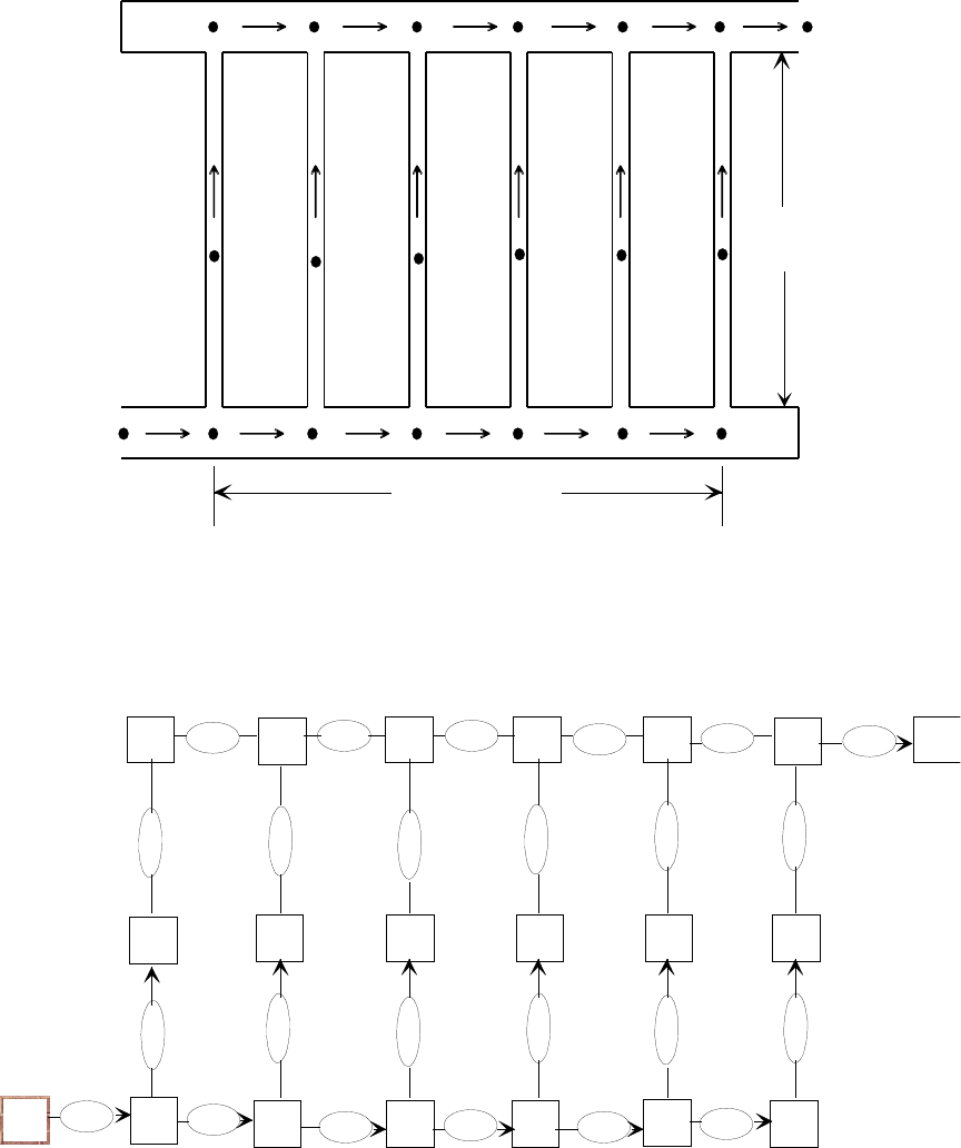
height of the lateral pipes is 12 feet. The purpose of the GFSSP model is to predict the

flow rate in the system and flow distribution in the lateral branches.

L = 36 in.

D = 1 in.

H = 144 in.

d = 0.4 in.

Figure 5.6 Example 3 Parallel Flow Manifold

1234567

8910 11 12 13

14 15 16 17 18 19 20

12 23 34 45 56 67

28 39 410 511 612 713

814 915 1016 1117 1218 1319

1415 1516 1617 1718 1819 1920

Figure 5.7 GFSSP Model for Example 3

The input and output data files for Example 3 are provided in Appendix F. For a pressure

differential of 8 psi, the calculated flow rate in the manifold is 1.44 lb/sec. The extent of

the non-uniformity in the lateral branches ((

713

) is about 16 percent.

5.4 EXAMPLE 4 - FLOW DISTRIBUTION IN A PARALLEL FLOW

MANIFOLD WITH HEAT SOURCES AND PHASE CHANGES

The purpose of this example is to demonstrate the use of heat sources and phase changes

related to the supplied heat. The physical system from Example 3 was modified for this

example. Heat was added at the midpoint of the lateral branches which were represented

by Node 8 through Node 13. It can be observed in the output file that a liquid and vapor

mixture exists in Node 8 through Node 19. The pressure differential is maintained at the

same value as in Example 3 (8 psi). The total heat load of the system was 207.4 Btu/sec.

It may be noted that in this example the “Btu/lb” heat rate option was used. The above

mentioned number was determined from the calculated flow rate. The predicted flow rate

was 0.319 lb/sec. The calculated flow non-uniformity was only 2.1 percent. The input

and output data files from Example 4 are provided in Appendix G.

5.5 EXAMPLE 5 - MIXING OF CRYOGENIC FLUIDS IN AN

INTER-PROPELLANT SEAL FLOW CIRCUIT OF A TURBO-

PUMP

The purpose of this example is to demonstrate an example of fluid mixing in a circuit. A

sample flow circuit, consisting of 12 nodes and 12 branches, is shown in Figure 5.8.

Figure 5.8 represents a portion of an inter propellant flow circuit where a helium buffer is

used to prevent the mixing of hydrogen and oxygen leakage flow in a typical turbopump

flow circuit.

In Figure 5.8 the nodes are represented by the square boxes and the branches are

represented by the elliptical boxes. The nodes and branches are numbered arbitrarily.

There are five boundary nodes (48, 50, 66, 16, and 22) in the flow circuit. Oxygen,

hydrogen, and helium enter into the circuit through Nodes 48, 66, and 22. The pressures

and temperatures that are specified at these nodes are shown in the figure. Nodes 50 and

16 are outflow boundaries where pressures are specified. The mixtures of helium-oxygen

and helium-hydrogen exit through these nodes. The GFSSP model calculates pressures,

temperatures, and concentrations at all internal nodes and flow rates in all branches. The

input and output files of this example are provided in Appendix H.

142

138

137

60 23

129

87 86

23 22

S A M P L E FL OW CIRC UIT

BOUNDARY

OXGE N

550 PSIA

-60 F

HYDROGEN

172 PSIA

-174 F

HEL IUM

151 PSIA

70 F

ATMOSPHERE

14 PSIA

ATMOSPHERE

14 PSIA

Figure 5.8 - Inter Propellant Flow Circuit of Example 5

are provided in Appendix H.

5.6 EXAMPLE 6 - QUASI-STEADY CALCULATION OF EXAMPLE 5

This example is an extension of Example 5. A quasi-steady model of the inter-propellant

seal flow circuit has been developed. In a quasi-steady mode (STEADY = FALSE), all

values at the boundary nodes must be specified in data files. The name of these data files

must appear in GFSSP input file. In this example, the pressures, temperatures and

concentrations history were provided in boundary nodes through HIST48.DAT,

HIST50.DAT, HIST66.DAT, HIST16.DAT and HIST22.DAT. The calculations were

performed for 15 seconds at an interval of 1 second. The input and output files of this

example are provided in Appendix I.

5.7 EXAMPLE 7 - FLOW IN A ROTATING DISC CAVITY

This example illustrates the rotational effect (centrifugal force contribution) of GFSSP by

a model of water flowing through a closed impeller [21]. The impeller is schematically

shown in figure 5.9a, and the GFSSP model circuit is shown in Figure 5.9b below. In the

model, branches 23, 34, 45, 56, 67, 89, 910, 1011, and 1112 are rotating at 5000 rpm.

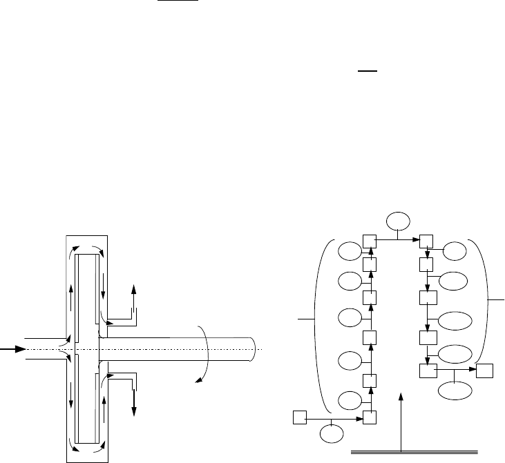
The inlet and outlet radii are defined in the preprocessor for each of the rotating branches.

The area of each of the radial branches are calculated as the average cross sectional area

for each branch

Ar r rdr

branch ab

b a r

















. The ”slip” of the fluid is described by the

rotational K-factor (Krotation). Krotation is defined as the ratio of the mean circumferential

fluid speed divided by the impeller speed:

rotation 















. (Higher Krotation-factors

translates to higher pressure rise for radially outward flow.) For this example the effects

of friction have been neglected for the rotating branches. The input and output files of

this example are provided in Appendix J.



1 2

6 9

7 8

12 13

910

1011

1112

1213

Rotating

Branches

r=1.25”

r=2.25”

r=2.65”

r=3.625”

r=4.6875”

r=5.375”

r=5.5”

Rotating

Branches

Figure 5.9a Physical Situation for Example 7 Figure 5.9b GFSSP Model for Example 7

6.0 REFERENCES

1. Hardy Cross, “Analysis of Flow in Networks of Conduits or Conductors”, Univ. Ill.

Bull. 286, November 1936

2. Jeppson, Ronald W. Analysis of Flow in Pipe Networks , Ann Arbor Science

3. Crane Company, “Flow of Fluids through Valves, Fittings and Pipe.”, Technical

Paper No. 410, 1969.

4. Kelix Software System, “Protopipe for Windows, Version 1.0”, 1993-95

5. Anderson, P. G. et al, “Fluid Flow Analysis of the SSME High Pressure Oxidizer

Turbopump Operating at Full Power Level”, Lockheed Missiles & Space

Company, Inc., Report No. LMSC-HREC TR D698083, Contract No. NAS8-

32703, August 1980.

6. Cheng, A. K., “SSME Alternate Turbopumps Axial Thrust Balance and Secondary

Flow Models”, Sverdrup Technology MSFC Group, Report No. 322-002-91-153-

R01, Contract No. NAS8-37814, October, 1992.

7. Colebrook, C. F.,”Turbulent Flow in Pipes, with Particular Reference to the

Transition Between the Smooth and Rough Pipe Laws”, J. Inst. Civil Engineering,

London, vol. 11, pp. 133-156, 1938-1939.

8. Hooper, W. B., “Calculate Head Loss Caused by Change in Pipe Size”, Chem. Engr.,

Nov. 7, pp. 89-92, 1988.

9. Hooper, W. B., “ The Two-K Method Predicts Head Losses in Pipe Fittings.”, Chem.

Engr., Aug. 24, pp. 97-100, 1981.

10. Howell, G. W. and Weather, T. M., Aerospace Fluid Component Designers

Handbook , Volume 1, Revision D, TRW Systems Group, RPL-TDR-64-25,

February, 1970

11. Ito, H. and Nanbu, K., “Flow in Rotating Straight Pipes of Circular Cross Section”,

Transactions of ASME, Vol. 93, Series D, No. 3, pp. 383-394, 1971.

12. Yamada, Y., “ Resistance to a Flow through an Annulus with an Inner Rotating

Cylinder”, Bulletin of the Japan Society of Mechanical Engineers, Vol. 5, pp. 302-

310, 1962.

13. Hendricks, R. C., Baron, A. K., and Peller, I. C., " GASP - A Computer Code for

Calculating the Thermodynamic and Transport Properties for Ten Fluids:

Parahydrogen, Helium, Neon, Methane, Nitrogen, Carbon Monoxide, Oxygen,

Fluorine, Argon, and Carbon Dioxide", NASA TN D-7808, February, 1975.

14. Hendricks, R. C., Peller, I. C., and Baron, A. K., " WASP - A Flexible Fortran IV

Computer Code for Calculating Water and Steam Properties", NASA TN D-7391,

November, 1973.

15. Hendricks, R. C., “ Personal Communication”, 1995

16. Majumdar, A. K. and VanHooser, K. P., “A General Fluid System Simulation

Program to Model Secondary Flows in Turbomachinery”, Paper No. AIAA 95-

2969, 31st AIAA/ASME/SAE/ASEE Joint Propulsion Conference, July 10-12,

1995, San Diego, California.

17. Majumdar, A. K., Bailey, J. W., Holt, K. A. and Turner, S. G., “Mathematical

Modeling of Free Convective Flows for Evaluating Propellant Conditioning

Concepts”, Paper No. AIAA 96-3117, 32nd AIAA/ASME/SAE/ASEE Joint

Propulsion Conference, July 1-3, 1996, Lake Buena Vista, Florida.

18. Bailey, J. W. and Majumdar, A. K., “GFSSP Resistance Coefficient Option

Evaluation”, Sverdrup Technology MSFC Group, Report No. 331-201-96-001,

Contract No. NAS8-40836, August, 1996.

19. Patankar, S. V. " Numerical Heat Transfer and Fluid Flow", Hemisphere Publishing

Corp., Washington, D. C., 1980.

20. Stoecker, W. F. , " Design of Thermal Systems ", 3rd Edition, McGraw Hill, 1989.

21. Young W. E. and Due H. E., “ Investigation of Pressure Prediction Methods for Low

Flow Radial Impellers”, Pratt & Whitney Aircraft, Report No. PWA FR-1716,

Contract No. NAS8-5442, February, 1966.

APPENDIX A

DERIVATION OF KF FOR PIPE FLOW

A-1

Derivation of Kf for Pipe Flow

It is assumed that there is a dynamic equilibrium that exists between the friction and the

pressure forces. Therefore, the momentum conservation equation can be expressed as:

P K m

 

(A-1)

Where Kf is a function of f, L, D and r.

For a fully developed pipe flow, the momentum conservation equation can be written as:

 

  

DL u

 

(A-2)

The Darcy friction factor, f, can be expressed as:



8 c





(A-3)

From the continuity equation:



 

(A-4)

Substituting Equations A-3 and A-4 into Equation A-2:

PfL

 



(A-6)

Therefore,

KfL





(A-7)

APPENDIX B

NEWTON-RAPHSON METHOD OF SOLVING COUPLED

NONLINEAR SYSTEMS OF ALGEBRAIC EQUATIONS

B-1

Newton-Raphson Method of Solving Coupled Nonlinear System of

Algebraic Equations

The application of the Newton-Raphson Method involves the following 7 steps:

1. Develop the governing equations.

The equations are expressed in the following form:

12 3 0

22 3 0

12 3 0

fxx x n

f x x x n

fxx x n

(, , ,....... )

........................................

(, , ,....... )



(B-1)

If there are n number of unknown variables, there are n number of equations.

2. Guess a solution for the equations.

Guess

1 2 3

*,*,*,....... *

x x x n

as an initial solution for the governing equations

3. Calculate the residuals of each equation.

When the guessed solutions are substituted into Equation B-1, the right hand side of the

equation is not zero. The non-zero value is the residual.

12 3 1

22 3 2

12 3

(,*,*,....... *)

........................................

(,*,*,....... *)

fxx x n

x R

fxx x n

x R

fxx x n



(B-2)

The intent of the solution scheme is to correct

1 2 3

*,*,*,....... *

x x x n

with a set of

corrections

1 2 3

',',',....... '

x x x n

such that

1 2 3

R R R n

, , ,........,

are zero.

B-2

4. Develop a set of correction equations for all variables.

First construct the matrix of influence coefficients:



1 2 3

........

......................................

........

Then construct the set of simultaneous equations for corrections:



1 2 3

........

......................................

........







































5. Solve for

1 2 3

',',',....... '

x x x n

by solving the simultaneous equations.

6. Apply correction to each variable.

7. Iterate until the corrections become very small.

B-3

APPENDIX C

SUCCESSIVE SUBSTITUTION METHOD OF SOLVING COUPLED

NONLINEAR SYSTEMS OF ALGEBRAIC EQUATIONS

C-1

Successive Substitution Method of Solving Coupled Nonlinear System

of Algebraic Equations

The application of the successive substitution method involves the following steps:

1. Develop the governing equations:

12 3

22 3

12 3

xfxx x n

xf x x x n

fxx x n



(, , ,....... )

........................................

(, , ,....... )

C-1

If there are n number of unknown variables, there are n number of equations.

2. Guess a solution for the equations:

Guess

1 2 3

*,*,*,....... *

x x x n

as an initial solution for the governing equations.

3. Compute new values of

1 2 3

x x x n

, , ,.......

by substituting

1 2 3

*,*,*,....... *

x x x n

in the

right hand side of Equation C-1.

4. Under-relax the computed new value:

 

xxx

  

 

where



is the under-relaxation parameter.

5. Replace

1 2 3

*,*,*,....... *

x x x n

with the computed value of

1 2 3

x x x n

, , ,.......

from

Step 4.

6. Repeat Steps 3 to 5 until convergence.

C-2

APPENDIX D

INPUT AND OUTPUT DATA FILES

FROM EXAMPLE 1

Contents Page

Example 1 Input File D-2

Example 1 Output File D-8

D-1

TITLE

FLOW COEFICIENTS

DENCON GRAVITY ENERGY MIXTURE THRUST STEADY TRANSV

F T T F F T F

INERTIA CONDX TWOD PRINTI ROTATION BUOYANCY HRATE

T F F T F F F

NNODES NINT NBR NF NHREF

16 14 15 1 2

RELAXK RELAXD RELAXH

1.000000 0.500000 1.000000

NFLUID(I), I= 1,NF

NODE INDEX

1 2

2 1

3 1

4 1

5 1

6 1

7 1

8 1

9 1

10 1

11 1

12 1

13 1

14 1

15 1

16 2

PRESSURE TEMPERATURE

1 0.5000E+02 0.6000E+02 0.0000E+00 0.0000E+00 0.0000E+00

2 0.1469E+02 0.6000E+02 0.0000E+00 0.0000E+00 0.0000E+00

3 0.1468E+02 0.6000E+02 0.0000E+00 0.0000E+00 0.0000E+00

4 0.1467E+02 0.6000E+02 0.0000E+00 0.0000E+00 0.0000E+00

5 0.1466E+02 0.6000E+02 0.0000E+00 0.0000E+00 0.0000E+00

6 0.1465E+02 0.6000E+02 0.0000E+00 0.0000E+00 0.0000E+00

7 0.1464E+02 0.6000E+02 0.0000E+00 0.0000E+00 0.0000E+00

8 0.1463E+02 0.6000E+02 0.0000E+00 0.0000E+00 0.0000E+00

9 0.1462E+02 0.6000E+02 0.0000E+00 0.0000E+00 0.0000E+00

10 0.1461E+02 0.6000E+02 0.0000E+00 0.0000E+00 0.0000E+00

11 0.1460E+02 0.6000E+02 0.0000E+00 0.0000E+00 0.0000E+00

12 0.1459E+02 0.6000E+02 0.0000E+00 0.0000E+00 0.0000E+00

13 0.1458E+02 0.6000E+02 0.0000E+00 0.0000E+00 0.0000E+00

14 0.1457E+02 0.6000E+02 0.0000E+00 0.0000E+00 0.0000E+00

D-2

15 0.1456E+02 0.6000E+02 0.0000E+00 0.0000E+00 0.0000E+00

16 0.1470E+02 0.6000E+02 0.0000E+00 0.0000E+00 0.0000E+00

INODE NUMBR NAMEBR

2 2 12 23

3 2 23 34

4 2 34 45

5 2 45 56

6 2 56 67

7 2 67 78

8 2 78 89

9 2 89 910

10 2 910 1011

11 2 1011 1112

12 2 1112 1213

13 2 1213 1314

14 2 1314 1415

15 2 1415 1516

BRANCH UPNODE DNNODE OPTION

12 1 2 4

23 2 3 13

34 3 4 1

45 4 5 2

56 5 6 1

67 6 7 7

78 7 8 1

89 8 9 5

910 9 10 1

1011 10 11 8

1112 11 12 1

1213 12 13 6

1314 13 14 1

1415 14 15 13

1516 15 16 4

BRANCH OPTION -4 LENGTH DIA EPSD ANGLE AREA

12 360.00000 30.62400 0.00006 0.50000 0.00000 90.00000 736.56891

BRANCH OPTION -13 DIA K1 K2 AREA

23 30.62400 300.00000 0.10000 736.56891

BRANCH OPTION -1 LENGTH DIA EPSD ANGLE AREA

34 480.00000 30.62400 0.00006 90.00000 736.56891

BRANCH OPTION -2 FLOW COEF AREA

45 0.00 736.57001

BRANCH OPTION -1 LENGTH DIA EPSD ANGLE AREA

56 3600.00000 30.62400 0.00006 90.00000 736.56891

BRANCH OPTION -7 PIPE DIA RED. DIA AREA

D-3

67 30.62400 22.62000 401.85999

BRANCH OPTION -1 LENGTH DIA EPSD ANGLE AREA

78 2400.00000 22.62000 0.00008 90.00000 401.85999

BRANCH OPTION - 5 PIPE DIA ORIFICE DIA AREA

89 22.62000 8.00000 401.85999

BRANCH OPTION -1 LENGTH DIA EPSD ANGLE AREA

910 2400.00000 22.62000 0.00008 90.00000 401.85999

BRANCH OPTION -8 PIPE DIA EXP DIA AREA

1011 22.62000 30.62400 736.56891

BRANCH OPTION -1 LENGTH DIA EPSD ANGLE AREA

1112 3600.00000 30.62400 0.00006 90.00000 736.56891

BRANCH OPTION -6 LENGTH PIPE DIA ORIFICE DIA AR EA

1213 9.00000 30.62400 12.00000 736.56891

BRANCH OPTION -1 LENGTH DIA EPSD ANGLE AREA

1314 1200.00000 30.62400 0.00006 90.00000 736.56891

BRANCH OPTION -13 DIA K1 K2 AREA

1415 30.62400 800.00000 0.20000 736.56891

BRANCH OPTION -4 LENGTH DIA EPSD ANGLE AREA

1516 286.00000 30.62400 0.00006 0.00000 1.00000 180.00000 736.56891

BRANCH NOUBR NMUBR

12 0

23 1 12

34 1 23

45 1 34

56 1 45

67 1 56

78 1 67

89 1 78

910 1 89

1011 1 910

1112 1 1011

1213 1 1112

1314 1 1213

1415 1 1314

1516 1 1415

BRANCH NODBR NMDBR

12 1 23

23 1 34

34 1 45

45 1 56

56 1 67

67 1 78

78 1 89

89 1 910

D-4

910 1 1011

1011 1 1112

1112 1 1213

1213 1 1314

1314 1 1415

1415 1 1516

1516 0

BRANCH

UPSTREAM ANGLE

DOWNSTREAM ANGLE

23 0.0000

BRANCH

UPSTREAM ANGLE

12 0.0000

DOWNSTREAM ANGLE

34 0.0000

BRANCH

UPSTREAM ANGLE

23 0.0000

DOWNSTREAM ANGLE

45 0.0000

BRANCH

UPSTREAM ANGLE

34 0.0000

DOWNSTREAM ANGLE

56 0.0000

BRANCH

UPSTREAM ANGLE

45 0.0000

DOWNSTREAM ANGLE

67 0.0000

BRANCH

UPSTREAM ANGLE

56 0.0000

DOWNSTREAM ANGLE

78 0.0000

BRANCH

D-5

UPSTREAM ANGLE

67 0.0000

DOWNSTREAM ANGLE

89 0.0000

BRANCH

UPSTREAM ANGLE

78 0.0000

DOWNSTREAM ANGLE

910 0.0000

BRANCH

910

UPSTREAM ANGLE

89 0.0000

DOWNSTREAM ANGLE

1011 0.0000

BRANCH

1011

UPSTREAM ANGLE

910 0.0000

DOWNSTREAM ANGLE

1112 0.0000

BRANCH

1112

UPSTREAM ANGLE

1011 0.0000

DOWNSTREAM ANGLE

1213 0.0000

BRANCH

1213

UPSTREAM ANGLE

1112 0.0000

DOWNSTREAM ANGLE

1314 0.0000

BRANCH

1314

UPSTREAM ANGLE

1213 0.0000

DOWNSTREAM ANGLE

1415 0.0000

BRANCH

1415

UPSTREAM ANGLE

1314 0.0000

D-6

DOWNSTREAM ANGLE

1516 90.0000

BRANCH

1516

UPSTREAM ANGLE

1415 90.0000

DOWNSTREAM ANGLE

D-7

**** GENERAL FLUID SYSTEM SIMULATION PROGRAM ****

****************** VERSION 1.4.1 ****************

TITLE :FLOW COEFICIENTS

DATE :9/11/97

ANALYST :jwb

FILEIN :example1.dat

FILEOUT :example1.out

LOGICAL VARIABLES

DENCON = F

GRAVITY = T

ENERGY = T

MIXTURE = F

THRUST = F

STEADY = T

TRANSV = F

INERTIA = T

CONDX = F

TWOD = F

PRINTI = T

ROTATION = F

BUOYANCY = F

HRATE = F

NNODES = 16

NINT = 14

NBR = 15

NF = 1

NVAR = 29

NHREF = 2

FLUIDS: H2O

BOUNDARY NODES

NODE P T RHO AREA

(PSI) (F) (LBM/FT^3) (IN^2)

1 50.0000 60.0000 62.3766 0.0000

16 14.7000 60.0000 62.3694 0.0000

INPUT SPECIFICATIONS FOR INTERNAL NODES

NODE AREA MASS HEAT

NODE (IN^2) (LBM/S) (BTU/LBM)

D-8

2 0.0000 0.0000 0.0000

3 0.0000 0.0000 0.0000

4 0.0000 0.0000 0.0000

5 0.0000 0.0000 0.0000

6 0.0000 0.0000 0.0000

7 0.0000 0.0000 0.0000

8 0.0000 0.0000 0.0000

9 0.0000 0.0000 0.0000

10 0.0000 0.0000 0.0000

11 0.0000 0.0000 0.0000

12 0.0000 0.0000 0.0000

13 0.0000 0.0000 0.0000

14 0.0000 0.0000 0.0000

15 0.0000 0.0000 0.0000

BRANCH UPNODE DNNODE OPTION

12 1 2 4

23 2 3 13

34 3 4 1

45 4 5 2

56 5 6 1

67 6 7 7

78 7 8 1

89 8 9 5

910 9 10 1

1011 10 11 8

1112 11 12 1

1213 12 13 6

1314 13 14 1

1415 14 15 13

1516 15 16 4

BRANCH OPTION -4: LENGTH, DIA, EPSD, ANGLE, AREA

12 360.00000 30.62400 0.00006 0.50000 0.00000 90.00000 736.56891

BRANCH OPTION -13: DIA, K1, K2, AREA

23 30.62400 300.00000 0.10000 736.56891

BRANCH OPTION -1: LENGTH, DIA, EPSD, ANGLE, AREA

34 480.00000 30.62400 0.00006 90.00000 736.56891

BRANCH OPTION -2: FLOW COEF, AREA

45 0.00000 736.57001

BRANCH OPTION -1: LENGTH, DIA, EPSD, ANGLE, AREA

56 3600.00000 30.62400 0.00006 90.00000 736.56891

BRANCH OPTION -7: PIPE DIA, REDUCED DIA, AREA

67 30.62400 22.62000 401.85999

BRANCH OPTION -1: LENGTH, DIA, EPSD, ANGLE, AREA

D-9

78 2400.00000 22.62000 0.00008 90.00000 401.85999

BRANCH OPTION - 5: PIPE DIA, ORIFICE DIA, AREA

89 22.62000 8.00000 401.85999

BRANCH OPTION -1: LENGTH, DIA, EPSD, ANGLE, AREA

910 2400.00000 22.62000 0.00008 90.00000 401.85999

BRANCH OPTION -8: PIPE DIA, EXP DIA, AREA

1011 22.62000 30.62400 736.56891

BRANCH OPTION -1: LENGTH, DIA, EPSD, ANGLE, AREA

1112 3600.00000 30.62400 0.00006 90.00000 736.56891

BRANCH OPTION -6: LENGTH, PIPE DIA, ORIFICE DIA, AREA

1213 9.00000 30.62400 12.00000 736.56891

BRANCH OPTION -1: LENGTH, DIA, EPSD, ANGLE, AREA

1314 1200.00000 30.62400 0.00006 90.00000 736.56891

BRANCH OPTION -13: DIA, K1, K2, AREA

1415 30.62400 800.00000 0.20000 736.56891

BRANCH OPTION -4: LENGTH, DIA, EPSD, ANGLE, AREA

1516 286.00000 30.62400 0.00006 0.00000 1.00000 180.00000 736.56891

INITIAL GUESS FOR INTERNAL NODES

NODE P(PSI) T(F) Z(COMP) RHO QUALITY

(LBM/FT^3)

2 14.6900 60.0000 0.0008 62.3694 0.0000

3 14.6800 60.0000 0.0008 62.3694 0.0000

4 14.6700 60.0000 0.0008 62.3694 0.0000

5 14.6600 60.0000 0.0008 62.3694 0.0000

6 14.6500 60.0000 0.0008 62.3694 0.0000

7 14.6400 60.0000 0.0008 62.3694 0.0000

8 14.6300 60.0000 0.0008 62.3694 0.0000

9 14.6200 60.0000 0.0008 62.3694 0.0000

10 14.6100 60.0000 0.0008 62.3693 0.0000

11 14.6000 60.0000 0.0008 62.3694 0.0000

12 14.5900 60.0000 0.0008 62.3694 0.0000

13 14.5800 60.0000 0.0008 62.3694 0.0000

14 14.5700 60.0000 0.0008 62.3694 0.0000

15 14.5600 60.0000 0.0008 62.3694 0.0000

TRIAL SOLUTION

BRANCH DELP(PSI) FLOWRATE(LBM/SEC)

12 35.3100 0.0100

23 0.0100 0.0100

34 0.0100 0.0100

45 0.0100 0.0100

56 0.0100 0.0100

D-10

67 0.0100 0.0100

78 0.0100 0.0100

89 0.0100 0.0100

910 0.0100 0.0100

1011 0.0100 0.0100

1112 0.0100 0.0100

1213 0.0100 0.0100

1314 0.0100 0.0100

1415 0.0100 0.0100

1516 -0.1400 0.0100

SOLUTION

INTERNAL NODES

NODE P(PSI) T(F) Z RHO QUALITY

(LBM/FT^3)

2 49.9759 59.9997 0.0026 62.3748 0.0000

3 49.9715 60.0005 0.0026 62.3748 0.0000

4 49.9652 59.9997 0.0026 62.3748 0.0000

5 49.9652 59.9997 0.0026 62.3748 0.0000

6 49.9177 59.9997 0.0026 62.3747 0.0000

7 49.6428 60.0008 0.0026 62.3747 0.0000

8 49.4195 60.0006 0.0026 62.3747 0.0000

9 28.2181 60.0620 0.0015 62.3712 0.0000

10 27.9949 60.0621 0.0015 62.3712 0.0000

11 28.0037 60.0611 0.0015 62.3712 0.0000

12 27.9562 60.0616 0.0014 62.3712 0.0000

13 25.1793 60.0705 0.0013 62.3707 0.0000

14 25.1635 60.0699 0.0013 62.3707 0.0000

15 25.1547 60.0699 0.0013 62.3707 0.0000

BRANCHES

BRANCH KFACTOR DELP FLOW RATE VELOCITY REYN. NO. MACH NO.

(LBF-S^2/(LBM-FT)^2) (PSI) (LBM/SEC) (FT/SEC)

12 0.631E-05 0.241E-01 0.798E+03 0.250E+01 0.528E+06 0.209E-02

23 0.989E-06 0.438E-02 0.798E+03 0.250E+01 0.528E+06 0.209E-02

34 0.259E-05 0.633E-02 0.798E+03 0.250E+01 0.528E+06 0.209E-02

45 0.000E+00 0.000E+00 0.798E+03 0.250E+01 0.528E+06 0.209E-02

56 0.194E-04 0.475E-01 0.798E+03 0.250E+01 0.528E+06 0.209E-02

67 0.881E-05 0.275E+00 0.798E+03 0.459E+01 0.714E+06 0.382E-02

78 0.563E-04 0.223E+00 0.798E+03 0.459E+01 0.714E+06 0.382E-02

89 0.479E-02 0.212E+02 0.798E+03 0.459E+01 0.714E+06 0.382E-02

910 0.563E-04 0.223E+00 0.798E+03 0.459E+01 0.715E+06 0.382E-02

D-11

1011 0.667E-05 -0.878E-02 0.798E+03 0.250E+01 0.528E+06 0.209E-02

1112 0.194E-04 0.475E-01 0.798E+03 0.250E+01 0.528E+06 0.209E-02

1213 0.627E-03 0.278E+01 0.798E+03 0.250E+01 0.528E+06 0.209E-02

1314 0.648E-05 0.158E-01 0.798E+03 0.250E+01 0.528E+06 0.209E-02

1415 0.198E-05 0.877E-02 0.798E+03 0.250E+01 0.528E+06 0.209E-02

1516 0.108E-04 0.105E+02 0.798E+03 0.251E+01 0.528E+06 0.209E-02

SOLUTION SATISFIED CONVERGENCE CRITERION OF 0.00100 IN 14 ITERATIONS

D-12

APPENDIX E

INPUT AND OUTPUT DATA FILES FROM EXAMPLE 2

Contents Page

Example 2 Input File E-2

Example 2 Output File E-9

E-1

TITLE

FLOW COEFICIENTS

DENCON GRAVITY ENERGY MIXTURE THRUST STEADY TRANSV

F T T F F T F

INERTIA CONDX TWOD PRINTI ROTATION BUOYANCY HRATE

T F F T F F F

NNODES NINT NBR NF NHREF

16 14 15 1 2

RELAXK RELAXD RELAXH

1.000000 0.500000 1.000000

NFLUID(I), I= 1,NF

NODE INDEX

1 2

2 1

3 1

4 1

5 1

6 1

7 1

8 1

9 1

10 1

11 1

12 1

13 1

14 1

15 1

16 2

PRESSURE TEMPERATURE

1 0.1470E+02 0.6000E+02 0.0000E+00 0.0000E+00 0.0000E+00

2 0.1469E+02 0.6000E+02 0.0000E+00 0.0000E+00 0.0000E+00

3 0.1468E+02 0.6000E+02 0.0000E+00 0.0000E+00 0.0000E+00

4 0.1467E+02 0.6000E+02 0.0000E+00 0.0000E+00 0.0000E+00

5 0.1466E+02 0.6000E+02 0.0000E+00 0.0000E+00 0.0000E+00

6 0.1465E+02 0.6000E+02 0.0000E+00 0.0000E+00 0.0000E+00

7 0.1464E+02 0.6000E+02 0.0000E+00 0.0000E+00 0.0000E+00

8 0.1463E+02 0.6000E+02 0.0000E+00 0.0000E+00 0.0000E+00

9 0.1462E+02 0.6000E+02 0.0000E+00 0.0000E+00 0.0000E+00

10 0.1461E+02 0.6000E+02 0.0000E+00 0.0000E+00 0.0000E+00

E-2

11 0.1460E+02 0.6000E+02 0.0000E+00 0.0000E+00 0.0000E+00

12 0.1459E+02 0.6000E+02 0.0000E+00 0.0000E+00 0.0000E+00

13 0.1458E+02 0.6000E+02 0.0000E+00 0.0000E+00 0.0000E+00

14 0.1457E+02 0.6000E+02 0.0000E+00 0.0000E+00 0.0000E+00

15 0.1456E+02 0.6000E+02 0.0000E+00 0.0000E+00 0.0000E+00

16 0.1470E+02 0.6000E+02 0.0000E+00 0.0000E+00 0.0000E+00

INODE NUMBR NAMEBR

2 2 12 23

3 2 23 34

4 2 34 45

5 2 45 56

6 2 56 67

7 2 67 78

8 2 78 89

9 2 89 910

10 2 910 1011

11 2 1011 1112

12 2 1112 1213

13 2 1213 1314

14 2 1314 1415

15 2 1415 1516

BRANCH UPNODE DNNODE OPTION

12 1 2 4

23 2 3 13

34 3 4 1

45 4 5 14

56 5 6 1

67 6 7 7

78 7 8 1

89 8 9 5

910 9 10 1

1011 10 11 8

1112 11 12 1

1213 12 13 6

1314 13 14 1

1415 14 15 13

1516 15 16 4

BRANCH OPTION -4 LENGTH DIA EPSD ANGLE AREA

12 360.00000 30.62400 0.00006 0.50000 0.00000 90.00000 736.56891

BRANCH OPTION -13 DIA K1 K2 AREA

E-3

23 30.62400 300.00000 0.10000 736.56891

BRANCH OPTION -1 LENGTH DIA EPSD ANGLE AREA

34 480.00000 30.62400 0.00006 90.00000 736.56891

BRANCH OPTION -14 PUMP CONST1 PUMP CONST2 AREA

45 30888.00000 -0.00081 736.57001

BRANCH OPTION -1 LENGTH DIA EPSD ANGLE AREA

56 3600.00000 30.62400 0.00006 90.00000 736.56891

BRANCH OPTION -7 PIPE DIA RED. DIA AREA

67 30.62400 22.62000 401.85999

BRANCH OPTION -1 LENGTH DIA EPSD ANGLE AREA

78 2400.00000 22.62000 0.00008 90.00000 401.85999

BRANCH OPTION - 5 PIPE DIA ORIFICE DIA AREA

89 22.62000 8.00000 401.85999

BRANCH OPTION -1 LENGTH DIA EPSD ANGLE AREA

910 2400.00000 22.62000 0.00008 90.00000 401.85999

BRANCH OPTION -8 PIPE DIA EXP DIA AREA

1011 22.62000 30.62400 736.56891

BRANCH OPTION -1 LENGTH DIA EPSD ANGLE AREA

1112 3600.00000 30.62400 0.00006 90.00000 736.56891

BRANCH OPTION -6 LENGTH PIPE DIA ORIFICE DIA AR EA

1213 9.00000 30.62400 12.00000 736.56891

BRANCH OPTION -1 LENGTH DIA EPSD ANGLE AREA

1314 1200.00000 30.62400 0.00006 90.00000 736.56891

BRANCH OPTION -13 DIA K1 K2 AREA

1415 30.62400 800.00000 0.20000 736.56891

BRANCH OPTION -4 LENGTH DIA EPSD ANGLE AREA

1516 286.00000 30.62400 0.00006 0.00000 1.00000 180.00000 736.56891

BRANCH NOUBR NMUBR

12 0

23 1 12

34 1 23

45 1 34

56 1 45

67 1 56

78 1 67

89 1 78

910 1 89

1011 1 910

1112 1 1011

1213 1 1112

E-4

1314 1 1213

1415 1 1314

1516 1 1415

BRANCH NODBR NMDBR

12 1 23

23 1 34

34 1 45

45 1 56

56 1 67

67 1 78

78 1 89

89 1 910

910 1 1011

1011 1 1112

1112 1 1213

1213 1 1314

1314 1 1415

1415 1 1516

1516 0

BRANCH

UPSTREAM ANGLE

DOWNSTREAM ANGLE

23 0.0000

BRANCH

UPSTREAM ANGLE

12 0.0000

DOWNSTREAM ANGLE

34 0.0000

BRANCH

UPSTREAM ANGLE

23 0.0000

DOWNSTREAM ANGLE

45 0.0000

BRANCH

UPSTREAM ANGLE

34 0.0000

E-5

DOWNSTREAM ANGLE

56 0.0000

BRANCH

UPSTREAM ANGLE

45 0.0000

DOWNSTREAM ANGLE

67 0.0000

BRANCH

UPSTREAM ANGLE

56 0.0000

DOWNSTREAM ANGLE

78 0.0000

BRANCH

UPSTREAM ANGLE

67 0.0000

DOWNSTREAM ANGLE

89 0.0000

BRANCH

UPSTREAM ANGLE

78 0.0000

DOWNSTREAM ANGLE

910 0.0000

BRANCH

910

UPSTREAM ANGLE

89 0.0000

DOWNSTREAM ANGLE

1011 0.0000

BRANCH

1011

UPSTREAM ANGLE

910 0.0000

DOWNSTREAM ANGLE

1112 0.0000

BRANCH

1112

E-6

UPSTREAM ANGLE

1011 0.0000

DOWNSTREAM ANGLE

1213 0.0000

BRANCH

1213

UPSTREAM ANGLE

1112 0.0000

DOWNSTREAM ANGLE

1314 0.0000

BRANCH

1314

UPSTREAM ANGLE

1213 0.0000

DOWNSTREAM ANGLE

1415 0.0000

BRANCH

1415

UPSTREAM ANGLE

1314 0.0000

DOWNSTREAM ANGLE

1516 90.0000

BRANCH

1516

UPSTREAM ANGLE

1415 90.0000

DOWNSTREAM ANGLE

E-7

**** GENERAL FLUID SYSTEM SIMULATION PROGRAM ****

****************** VERSION 1.4.1 ****************

TITLE :FLOW COEFICIENTS

DATE :9/11/97

ANALYST :jwb

FILEIN :example2.dat

FILEOUT :example2.out

LOGICAL VARIABLES

DENCON = F

GRAVITY = T

ENERGY = T

MIXTURE = F

THRUST = F

STEADY = T

TRANSV = F

INERTIA = T

CONDX = F

TWOD = F

PRINTI = T

ROTATION = F

BUOYANCY = F

HRATE = F

NNODES = 16

NINT = 14

NBR = 15

NF = 1

NVAR = 29

NHREF = 2

FLUIDS: H2O

BOUNDARY NODES

NODE P T RHO AREA

(PSI) (F) (LBM/FT^3) (IN^2)

1 14.7000 60.0000 62.3694 0.0000

16 14.7000 60.0000 62.3694 0.0000

E-8

INPUT SPECIFICATIONS FOR INTERNAL NODES

NODE AREA MASS HEAT

NODE (IN^2) (LBM/S) (BTU/LBM)

2 0.0000 0.0000 0.0000

3 0.0000 0.0000 0.0000

4 0.0000 0.0000 0.0000

5 0.0000 0.0000 0.0000

6 0.0000 0.0000 0.0000

7 0.0000 0.0000 0.0000

8 0.0000 0.0000 0.0000

9 0.0000 0.0000 0.0000

10 0.0000 0.0000 0.0000

11 0.0000 0.0000 0.0000

12 0.0000 0.0000 0.0000

13 0.0000 0.0000 0.0000

14 0.0000 0.0000 0.0000

15 0.0000 0.0000 0.0000

BRANCH UPNODE DNNODE OPTION

12 1 2 4

23 2 3 13

34 3 4 1

45 4 5 14

56 5 6 1

67 6 7 7

78 7 8 1

89 8 9 5

910 9 10 1

1011 10 11 8

1112 11 12 1

1213 12 13 6

1314 13 14 1

1415 14 15 13

1516 15 16 4

BRANCH OPTION -4: LENGTH, DIA, EPSD, ANGLE, AREA

12 360.00000 30.62400 0.00006 0.50000 0.00000 90.00000 736.56891

BRANCH OPTION -13: DIA, K1, K2, AREA

23 30.62400 300.00000 0.10000 736.56891

BRANCH OPTION -1: LENGTH, DIA, EPSD, ANGLE, AREA

E-9

34 480.00000 30.62400 0.00006 90.00000 736.56891

BRANCH OPTION -14: PUMP CONST1, PUMP CONST2, AREA

45 30888.00000 -0.00081 736.57001

BRANCH OPTION -1: LENGTH, DIA, EPSD, ANGLE, AREA

56 3600.00000 30.62400 0.00006 90.00000 736.56891

BRANCH OPTION -7: PIPE DIA, REDUCED DIA, AREA

67 30.62400 22.62000 401.85999

BRANCH OPTION -1: LENGTH, DIA, EPSD, ANGLE, AREA

78 2400.00000 22.62000 0.00008 90.00000 401.85999

BRANCH OPTION - 5: PIPE DIA, ORIFICE DIA, AREA

89 22.62000 8.00000 401.85999

BRANCH OPTION -1: LENGTH, DIA, EPSD, ANGLE, AREA

910 2400.00000 22.62000 0.00008 90.00000 401.85999

BRANCH OPTION -8: PIPE DIA, EXP DIA, AREA

1011 22.62000 30.62400 736.56891

BRANCH OPTION -1: LENGTH, DIA, EPSD, ANGLE, AREA

1112 3600.00000 30.62400 0.00006 90.00000 736.56891

BRANCH OPTION -6: LENGTH, PIPE DIA, ORIFICE DIA, AREA

1213 9.00000 30.62400 12.00000 736.56891

BRANCH OPTION -1: LENGTH, DIA, EPSD, ANGLE, AREA

1314 1200.00000 30.62400 0.00006 90.00000 736.56891

BRANCH OPTION -13: DIA, K1, K2, AREA

1415 30.62400 800.00000 0.20000 736.56891

BRANCH OPTION -4: LENGTH, DIA, EPSD, ANGLE, AREA

1516 286.00000 30.62400 0.00006 0.00000 1.00000 180.00000 736.56891

INITIAL GUESS FOR INTERNAL NODES

NODE P(PSI) T(F) Z(COMP) RHO QUALITY

(LBM/FT^3)

2 14.6900 60.0000 0.0008 62.3694 0.0000

3 14.6800 60.0000 0.0008 62.3694 0.0000

4 14.6700 60.0000 0.0008 62.3694 0.0000

5 14.6600 60.0000 0.0008 62.3694 0.0000

6 14.6500 60.0000 0.0008 62.3694 0.0000

7 14.6400 60.0000 0.0008 62.3694 0.0000

8 14.6300 60.0000 0.0008 62.3694 0.0000

9 14.6200 60.0000 0.0008 62.3694 0.0000

10 14.6100 60.0000 0.0008 62.3693 0.0000

11 14.6000 60.0000 0.0008 62.3694 0.0000

E-10

12 14.5900 60.0000 0.0008 62.3694 0.0000

13 14.5800 60.0000 0.0008 62.3694 0.0000

14 14.5700 60.0000 0.0008 62.3694 0.0000

15 14.5600 60.0000 0.0008 62.3694 0.0000

TRIAL SOLUTION

BRANCH DELP(PSI) FLOWRATE(LBM/SEC)

12 0.0100 0.0100

23 0.0100 0.0100

34 0.0100 0.0100

45 0.0100 0.0100

56 0.0100 0.0100

67 0.0100 0.0100

78 0.0100 0.0100

89 0.0100 0.0100

910 0.0100 0.0100

1011 0.0100 0.0100

1112 0.0100 0.0100

1213 0.0100 0.0100

1314 0.0100 0.0100

1415 0.0100 0.0100

1516 -0.1400 0.0100

SOLUTION

INTERNAL NODES

NODE P(PSI) T(F) Z RHO QUALITY

(LBM/FT^3)

2 14.5094 59.9999 0.0008 62.3693 0.0000

3 14.4783 60.0006 0.0008 62.3694 0.0000

4 14.4141 60.0005 0.0007 62.3693 0.0000

5 203.3027 59.4653 0.0105 62.4001 0.0000

6 202.8212 59.4660 0.0105 62.4000 0.0000

7 200.8584 59.4737 0.0104 62.3997 0.0000

8 199.3500 59.4758 0.0103 62.3995 0.0000

9 47.9473 59.9057 0.0025 62.3748 0.0000

10 46.4391 59.9099 0.0024 62.3745 0.0000

11 46.5021 59.9098 0.0024 62.3746 0.0000

12 46.0207 59.9112 0.0024 62.3745 0.0000

E-11

13 26.1837 59.9678 0.0014 62.3713 0.0000

14 26.0232 59.9685 0.0013 62.3712 0.0000

15 25.9608 59.9688 0.0013 62.3712 0.0000

BRANCHES

BRANCH KFACTOR DELP FLOW RATE VELOCITY REYN. NO. MACH NO.

(LBF-S^2/(LBM-FT)^2) (PSI) (LBM/SEC) (FT/SEC)

12 0.615E-05 0.191E+00 0.213E+04 0.669E+01 0.141E+07 0.558E-02

23 0.985E-06 0.312E-01 0.213E+04 0.669E+01 0.141E+07 0.558E-02

34 0.219E-05 0.642E-01 0.213E+04 0.669E+01 0.141E+07 0.558E-02

45 0.000E+00 -0.189E+03 0.213E+04 0.669E+01 0.141E+07 0.558E-02

56 0.165E-04 0.482E+00 0.213E+04 0.669E+01 0.140E+07 0.558E-02

67 0.880E-05 0.196E+01 0.213E+04 0.123E+02 0.190E+07 0.102E-01

78 0.485E-04 0.151E+01 0.213E+04 0.123E+02 0.190E+07 0.102E-01

89 0.479E-02 0.151E+03 0.213E+04 0.123E+02 0.190E+07 0.102E-01

910 0.485E-04 0.151E+01 0.213E+04 0.123E+02 0.191E+07 0.102E-01

1011 0.666E-05 -0.630E-01 0.213E+04 0.669E+01 0.141E+07 0.558E-02

1112 0.164E-04 0.482E+00 0.213E+04 0.669E+01 0.141E+07 0.558E-02

1213 0.627E-03 0.198E+02 0.213E+04 0.669E+01 0.141E+07 0.558E-02

1314 0.548E-05 0.161E+00 0.213E+04 0.669E+01 0.141E+07 0.558E-02

1415 0.197E-05 0.624E-01 0.213E+04 0.669E+01 0.141E+07 0.558E-02

1516 0.106E-04 0.113E+02 0.213E+04 0.670E+01 0.141E+07 0.558E-02

SOLUTION SATISFIED CONVERGENCE CRITERION OF 0.00100 IN 15 ITERATIONS

E-12

APPENDIX F

F-1

INPUT AND OUTPUT DATA FILES FROM EXAMPLE 3

Contents Page

Example 3 Input File F-2

Example 3 Output File F-12

TITLE

Parallel Flow Manifold with heat transfer and phase change

DENCON GRAVITY ENERGY MIXTURE THRUST STEADY TRANSV

F T T F F T F

INERTIA CONDX TWOD PRINTI ROTATION BUOYANCY HRATE

f F F F F F F

NNODES NINT NBR NF NHREF

20 18 24 1 2

RELAXK RELAXD RELAXH

1.000000 0.500000 1.000000

NFLUID(I), I= 1,NF

NODE INDEX

1 2

2 1

3 1

4 1

5 1

6 1

7 1

8 1

9 1

10 1

11 1

12 1

13 1

14 1

15 1

16 1

17 1

18 1

19 1

20 2

PRESSURE TEMPERATURE

1 0.1020E+04 0.4000E+03 0.0000E+00 0.0000E+00 0.0000E+00

2 0.1020E+04 0.4000E+03 0.0000E+00 0.0000E+00 0.0000E+00

3 0.1019E+04 0.4000E+03 0.0000E+00 0.0000E+00 0.0000E+00

4 0.1019E+04 0.4000E+03 0.0000E+00 0.0000E+00 0.0000E+00

5 0.1019E+04 0.4000E+03 0.0000E+00 0.0000E+00 0.0000E+00

6 0.1018E+04 0.4000E+03 0.0000E+00 0.0000E+00 0.0000E+00

7 0.1018E+04 0.4000E+03 0.0000E+00 0.0000E+00 0.0000E+00

8 0.1019E+04 0.4000E+03 0.0000E+00 0.0000E+00 0.0000E+00

9 0.1019E+04 0.4000E+03 0.0000E+00 0.0000E+00 0.0000E+00

10 0.1019E+04 0.4000E+03 0.0000E+00 0.0000E+00 0.0000E+00

F-2

11 0.1018E+04 0.4000E+03 0.0000E+00 0.0000E+00 0.0000E+00

12 0.1018E+04 0.4000E+03 0.0000E+00 0.0000E+00 0.0000E+00

13 0.1018E+04 0.4000E+03 0.0000E+00 0.0000E+00 0.0000E+00

14 0.1019E+04 0.4000E+03 0.0000E+00 0.0000E+00 0.0000E+00

15 0.1019E+04 0.4000E+03 0.0000E+00 0.0000E+00 0.0000E+00

16 0.1018E+04 0.4000E+03 0.0000E+00 0.0000E+00 0.0000E+00

17 0.1018E+04 0.4000E+03 0.0000E+00 0.0000E+00 0.0000E+00

18 0.1018E+04 0.4000E+03 0.0000E+00 0.0000E+00 0.0000E+00

19 0.1012E+04 0.4000E+03 0.0000E+00 0.0000E+00 0.0000E+00

20 0.1012E+04 0.4000E+03 0.0000E+00 0.0000E+00 0.0000E+00

INODE NUMBR NAMEBR

2 3 12 28 23

3 3 23 39 34

4 3 34 410 45

5 3 45 511 56

6 3 56 612 67

7 2 67 713

8 2 28 814

9 2 39 915

10 2 410 1016

11 2 511 1117

12 2 612 1218

13 2 713 1319

14 2 814 1415

15 3 1415 915 1516

16 3 1516 1016 1617

17 3 1617 1117 1718

18 3 1718 1218 1819

19 3 1819 1319 1920

BRANCH UPNODE DNNODE OPTION

12 1 2 1

28 2 8 5

23 2 3 1

39 3 9 5

34 3 4 1

410 4 10 5

45 4 5 1

511 5 11 5

56 5 6 1

612 6 12 5

67 6 7 1

713 7 13 5

814 8 14 1

915 9 15 1

F-3

1016 10 16 1

1117 11 17 1

1218 12 18 1

1319 13 19 1

1415 14 15 1

1516 15 16 1

1617 16 17 1

1718 17 18 1

1819 18 19 1

1920 19 20 1

BRANCH OPTION -1 LENGTH DIA EPSD ANGLE AREA

12 6.00000 1.00000 0.00000 90.00000 0.78540

BRANCH OPTION -5 pipe dia orifice dia area

28 1.00000 0.40000 0.12566

BRANCH OPTION -1 LENGTH DIA EPSD ANGLE AREA

23 6.00000 1.00000 0.00000 90.00000 0.78540

BRANCH OPTION - 5 PIPE DIA ORIFICE DIA AREA

39 1.00000 0.40000 0.12566

BRANCH OPTION -1 LENGTH DIA EPSD ANGLE AREA

34 6.00000 1.00000 0.00000 90.00000 0.78540

BRANCH OPTION - 5 PIPE DIA ORIFICE DIA AREA

410 1.00000 0.40000 0.12566

BRANCH OPTION -1 LENGTH DIA EPSD ANGLE AREA

45 6.00000 1.00000 0.00000 90.00000 0.78540

BRANCH OPTION - 5 PIPE DIA ORIFICE DIA AREA

511 1.00000 0.40000 0.12566

BRANCH OPTION -1 LENGTH DIA EPSD ANGLE AREA

56 6.00000 1.00000 0.00000 90.00000 0.78540

BRANCH OPTION - 5 PIPE DIA ORIFICE DIA AREA

612 1.00000 0.40000 0.12566

BRANCH OPTION -1 LENGTH DIA EPSD ANGLE AREA

67 6.00000 1.00000 0.00000 90.00000 0.78540

BRANCH OPTION - 5 PIPE DIA ORIFICE DIA AREA

713 1.00000 0.40000 0.12566

BRANCH OPTION -1 LENGTH DIA EPSD ANGLE AREA

814 144.00000 0.40000 0.00000 180.00000 0.12566

BRANCH OPTION -1 LENGTH DIA EPSD ANGLE AREA

915 144.00000 0.40000 0.00000 180.00000 0.12566

BRANCH OPTION -1 LENGTH DIA EPSD ANGLE AREA

1016 144.00000 0.40000 0.00000 180.00000 0.12566

BRANCH OPTION -1 LENGTH DIA EPSD ANGLE AREA

1117 144.00000 0.40000 0.00000 180.00000 0.12566

BRANCH OPTION -1 LENGTH DIA EPSD ANGLE AREA

1218 144.00000 0.40000 0.00000 180.00000 0.12566

F-4

BRANCH OPTION -1 LENGTH DIA EPSD ANGLE AREA

1319 144.00000 0.40000 0.00000 180.00000 0.12566

BRANCH OPTION -1 LENGTH DIA EPSD ANGLE AREA

1415 6.00000 1.00000 0.00000 90.00000 0.78540

BRANCH OPTION -1 LENGTH DIA EPSD ANGLE AREA

1516 6.00000 1.00000 0.00000 90.00000 0.78540

BRANCH OPTION -1 LENGTH DIA EPSD ANGLE AREA

1617 6.00000 1.00000 0.00000 90.00000 0.78540

BRANCH OPTION -1 LENGTH DIA EPSD ANGLE AREA

1718 6.00000 1.00000 0.00000 90.00000 0.78540

BRANCH OPTION -1 LENGTH DIA EPSD ANGLE AREA

1819 6.00000 1.00000 0.00000 90.00000 0.78540

BRANCH OPTION -1 LENGTH DIA EPSD ANGLE AREA

1920 6.00000 1.00000 0.00000 90.00000 0.78540

BRANCH NOUBR NMUBR

12 0

28 2 12 23

23 2 12 28

39 2 23 34

34 2 23 39

410 2 34 45

45 2 34 410

511 2 45 56

56 2 45 511

612 2 56 67

67 2 56 612

713 1 67

814 1 28

915 1 39

1016 1 410

1117 1 511

1218 1 612

1319 1 713

1415 1 814

1516 2 1415 915

1617 2 1516 1016

1718 2 1617 1117

1819 2 1718 1218

1920 2 1819 1319

BRANCH NODBR NMDBR

12 2 28 23

28 1 814

23 2 39 34

39 1 915

F-5

34 2 410 45

410 1 1016

45 2 511 56

511 1 1117

56 2 612 67

612 1 1218

67 1 713

713 1 1319

814 1 1415

915 2 1415 1516

1016 2 1516 1617

1117 2 1617 1718

1218 2 1718 1819

1319 2 1819 1920

1415 2 915 1516

1516 2 1016 1617

1617 2 1117 1718

1718 2 1218 1819

1819 2 1319 1920

1920 0

BRANCH

UPSTREAM ANGLE

DOWNSTREAM ANGLE

28 90.0000

23 0.0000

BRANCH

UPSTREAM ANGLE

12 90.0000

23 90.0000

DOWNSTREAM ANGLE

814 0.0000

BRANCH

UPSTREAM ANGLE

12 0.0000

28 90.0000

DOWNSTREAM ANGLE

39 90.0000

34 0.0000

BRANCH

UPSTREAM ANGLE

F-6

23 90.0000

34 90.0000

DOWNSTREAM ANGLE

915 0.0000

BRANCH

UPSTREAM ANGLE

23 0.0000

39 90.0000

DOWNSTREAM ANGLE

410 90.0000

45 0.0000

BRANCH

410

UPSTREAM ANGLE

34 90.0000

45 90.0000

DOWNSTREAM ANGLE

1016 0.0000

BRANCH

UPSTREAM ANGLE

34 0.0000

410 90.0000

DOWNSTREAM ANGLE

511 90.0000

56 0.0000

BRANCH

511

UPSTREAM ANGLE

45 90.0000

56 90.0000

DOWNSTREAM ANGLE

1117 0.0000

BRANCH

UPSTREAM ANGLE

45 0.0000

511 90.0000

DOWNSTREAM ANGLE

612 90.0000

67 0.0000

BRANCH

612

F-7

UPSTREAM ANGLE

56 90.0000

67 90.0000

DOWNSTREAM ANGLE

1218 0.0000

BRANCH

UPSTREAM ANGLE

56 0.0000

612 90.0000

DOWNSTREAM ANGLE

713 90.0000

BRANCH

713

UPSTREAM ANGLE

67 90.0000

DOWNSTREAM ANGLE

1319 0.0000

BRANCH

814

UPSTREAM ANGLE

28 0.0000

DOWNSTREAM ANGLE

1415 90.0000

BRANCH

915

UPSTREAM ANGLE

39 0.0000

DOWNSTREAM ANGLE

1415 90.0000

1516 90.0000

BRANCH

1016

UPSTREAM ANGLE

410 0.0000

DOWNSTREAM ANGLE

1516 90.0000

1617 90.0000

BRANCH

1117

UPSTREAM ANGLE

511 0.0000

DOWNSTREAM ANGLE

1617 90.0000

F-8

1718 90.0000

BRANCH

1218

UPSTREAM ANGLE

612 0.0000

DOWNSTREAM ANGLE

1718 90.0000

1819 90.0000

BRANCH

1319

UPSTREAM ANGLE

713 0.0000

DOWNSTREAM ANGLE

1819 90.0000

1920 90.0000

BRANCH

1415

UPSTREAM ANGLE

814 90.0000

DOWNSTREAM ANGLE

915 90.0000

1516 0.0000

BRANCH

1516

UPSTREAM ANGLE

1415 0.0000

915 90.0000

DOWNSTREAM ANGLE

1016 90.0000

1617 0.0000

BRANCH

1617

UPSTREAM ANGLE

1516 0.0000

1016 90.0000

DOWNSTREAM ANGLE

1117 90.0000

1718 0.0000

BRANCH

1718

UPSTREAM ANGLE

1617 0.0000

1117 90.0000

DOWNSTREAM ANGLE

F-9

1218 90.0000

1819 0.0000

BRANCH

1819

UPSTREAM ANGLE

1718 0.0000

1218 90.0000

DOWNSTREAM ANGLE

1319 90.0000

1920 0.0000

BRANCH

1920

UPSTREAM ANGLE

1819 0.0000

1319 90.0000

DOWNSTREAM ANGLE

F-10

**** GENERAL FLUID SYSTEM SIMULATION PROGRAM ****

****************** VERSION 1.4.1 ****************

TITLE :Parallel Flow Manifold with heat transfer and phase change

DATE :9/11/97

ANALYST :jwb

FILEIN :example3.dat

FILEOUT :example3.out

LOGICAL VARIABLES

DENCON = F

GRAVITY = T

ENERGY = T

MIXTURE = F

THRUST = F

STEADY = T

TRANSV = F

INERTIA = F

CONDX = F

TWOD = F

PRINTI = F

ROTATION = F

BUOYANCY = F

HRATE = F

NNODES = 20

NINT = 18

NBR = 24

NF = 1

NVAR = 42

NHREF = 2

FLUIDS: H2O

BOUNDARY NODES

NODE P T RHO AREA

(PSI) (F) (LBM/FT^3) (IN^2)

1 1020.0000 400.0000 53.9197 0.0000

20 1012.0000 400.0000 53.9170 0.0000

INPUT SPECIFICATIONS FOR INTERNAL NODES

NODE AREA MASS HEAT

NODE (IN^2) (LBM/S) (BTU/LBM)

F-11

2 0.0000 0.0000 0.0000

3 0.0000 0.0000 0.0000

4 0.0000 0.0000 0.0000

5 0.0000 0.0000 0.0000

6 0.0000 0.0000 0.0000

7 0.0000 0.0000 0.0000

8 0.0000 0.0000 0.0000

9 0.0000 0.0000 0.0000

10 0.0000 0.0000 0.0000

11 0.0000 0.0000 0.0000

12 0.0000 0.0000 0.0000

13 0.0000 0.0000 0.0000

14 0.0000 0.0000 0.0000

15 0.0000 0.0000 0.0000

16 0.0000 0.0000 0.0000

17 0.0000 0.0000 0.0000

18 0.0000 0.0000 0.0000

19 0.0000 0.0000 0.0000

BRANCH UPNODE DNNODE OPTION

12 1 2 1

28 2 8 5

23 2 3 1

39 3 9 5

34 3 4 1

410 4 10 5

45 4 5 1

511 5 11 5

56 5 6 1

612 6 12 5

67 6 7 1

713 7 13 5

814 8 14 1

915 9 15 1

1016 10 16 1

1117 11 17 1

1218 12 18 1

1319 13 19 1

1415 14 15 1

1516 15 16 1

1617 16 17 1

1718 17 18 1

1819 18 19 1

1920 19 20 1

F-12

BRANCH OPTION -1: LENGTH, DIA, EPSD, ANGLE, AREA

12 6.00000 1.00000 0.00000 90.00000 0.78540

BRANCH OPTION - 5: PIPE DIA, ORIFICE DIA, AREA

28 1.00000 0.40000 0.12566

BRANCH OPTION -1: LENGTH, DIA, EPSD, ANGLE, AREA

23 6.00000 1.00000 0.00000 90.00000 0.78540

BRANCH OPTION - 5: PIPE DIA, ORIFICE DIA, AREA

39 1.00000 0.40000 0.12566

BRANCH OPTION -1: LENGTH, DIA, EPSD, ANGLE, AREA

34 6.00000 1.00000 0.00000 90.00000 0.78540

BRANCH OPTION - 5: PIPE DIA, ORIFICE DIA, AREA

410 1.00000 0.40000 0.12566

BRANCH OPTION -1: LENGTH, DIA, EPSD, ANGLE, AREA

45 6.00000 1.00000 0.00000 90.00000 0.78540

BRANCH OPTION - 5: PIPE DIA, ORIFICE DIA, AREA

511 1.00000 0.40000 0.12566

BRANCH OPTION -1: LENGTH, DIA, EPSD, ANGLE, AREA

56 6.00000 1.00000 0.00000 90.00000 0.78540

BRANCH OPTION - 5: PIPE DIA, ORIFICE DIA, AREA

612 1.00000 0.40000 0.12566

BRANCH OPTION -1: LENGTH, DIA, EPSD, ANGLE, AREA

67 6.00000 1.00000 0.00000 90.00000 0.78540

BRANCH OPTION - 5: PIPE DIA, ORIFICE DIA, AREA

713 1.00000 0.40000 0.12566

BRANCH OPTION -1: LENGTH, DIA, EPSD, ANGLE, AREA

814 144.00000 0.40000 0.00000 180.00000 0.12566

BRANCH OPTION -1: LENGTH, DIA, EPSD, ANGLE, AREA

915 144.00000 0.40000 0.00000 180.00000 0.12566

BRANCH OPTION -1: LENGTH, DIA, EPSD, ANGLE, AREA

1016 144.00000 0.40000 0.00000 180.00000 0.12566

BRANCH OPTION -1: LENGTH, DIA, EPSD, ANGLE, AREA

1117 144.00000 0.40000 0.00000 180.00000 0.12566

BRANCH OPTION -1: LENGTH, DIA, EPSD, ANGLE, AREA

1218 144.00000 0.40000 0.00000 180.00000 0.12566

BRANCH OPTION -1: LENGTH, DIA, EPSD, ANGLE, AREA

1319 144.00000 0.40000 0.00000 180.00000 0.12566

BRANCH OPTION -1: LENGTH, DIA, EPSD, ANGLE, AREA

1415 6.00000 1.00000 0.00000 90.00000 0.78540

BRANCH OPTION -1: LENGTH, DIA, EPSD, ANGLE, AREA

1516 6.00000 1.00000 0.00000 90.00000 0.78540

BRANCH OPTION -1: LENGTH, DIA, EPSD, ANGLE, AREA

1617 6.00000 1.00000 0.00000 90.00000 0.78540

BRANCH OPTION -1: LENGTH, DIA, EPSD, ANGLE, AREA

1718 6.00000 1.00000 0.00000 90.00000 0.78540

F-13

BRANCH OPTION -1: LENGTH, DIA, EPSD, ANGLE, AREA

1819 6.00000 1.00000 0.00000 90.00000 0.78540

BRANCH OPTION -1: LENGTH, DIA, EPSD, ANGLE, AREA

1920 6.00000 1.00000 0.00000 90.00000 0.78540

SOLUTION

INTERNAL NODES

NODE P(PSI) T(F) Z RHO QUALITY

(LBM/FT^3)

2 1019.9667 399.9988 0.0370 53.9198 0.0000

3 1019.9426 399.9980 0.0369 53.9198 0.0000

4 1019.9265 399.9985 0.0369 53.9197 0.0000

5 1019.9169 399.9990 0.0369 53.9197 0.0000

6 1019.9122 399.9985 0.0369 53.9197 0.0000

7 1019.9108 399.9979 0.0369 53.9197 0.0000

8 1019.2312 399.9991 0.0369 53.9195 0.0000

9 1019.2126 399.9993 0.0369 53.9195 0.0000

10 1019.1995 399.9990 0.0369 53.9195 0.0000

11 1019.1899 399.9991 0.0369 53.9195 0.0000

12 1019.1822 399.9993 0.0369 53.9194 0.0000

13 1019.1754 399.9992 0.0369 53.9194 0.0000

14 1012.0892 400.0070 0.0367 53.9170 0.0000

15 1012.0878 400.0072 0.0367 53.9170 0.0000

16 1012.0831 400.0069 0.0367 53.9169 0.0000

17 1012.0735 400.0068 0.0367 53.9169 0.0000

18 1012.0574 400.0072 0.0367 53.9169 0.0000

19 1012.0333 400.0068 0.0367 53.9168 0.0000

BRANCHES

BRANCH KFACTOR DELP FLOW RATE VELOCITY REYN. NO. MACH NO.

(LBF-S^2/(LBM-FT)^2) (PSI) (LBM/SEC) (FT/SEC)

12 0.107E+01 0.333E-01 0.212E+01 0.722E+01 0.366E+06 0.404E-02

28 0.839E+03 0.735E+00 0.355E+00 0.755E+01 0.153E+06 0.422E-02

23 0.111E+01 0.241E-01 0.177E+01 0.602E+01 0.305E+06 0.336E-02

39 0.839E+03 0.730E+00 0.354E+00 0.752E+01 0.152E+06 0.420E-02

34 0.116E+01 0.161E-01 0.142E+01 0.481E+01 0.244E+06 0.269E-02

410 0.839E+03 0.727E+00 0.353E+00 0.751E+01 0.152E+06 0.419E-02

45 0.124E+01 0.966E-02 0.106E+01 0.361E+01 0.183E+06 0.202E-02

511 0.839E+03 0.727E+00 0.353E+00 0.751E+01 0.152E+06 0.419E-02

56 0.136E+01 0.467E-02 0.709E+00 0.241E+01 0.122E+06 0.135E-02

612 0.839E+03 0.730E+00 0.354E+00 0.752E+01 0.152E+06 0.420E-02

67 0.161E+01 0.141E-02 0.355E+00 0.121E+01 0.612E+05 0.675E-03

F-14

713 0.839E+03 0.735E+00 0.355E+00 0.755E+01 0.153E+06 0.422E-02

814 0.302E+04 0.714E+01 0.355E+00 0.755E+01 0.153E+06 0.422E-02

915 0.303E+04 0.712E+01 0.354E+00 0.752E+01 0.152E+06 0.420E-02

1016 0.303E+04 0.712E+01 0.353E+00 0.751E+01 0.152E+06 0.419E-02

1117 0.303E+04 0.712E+01 0.353E+00 0.751E+01 0.152E+06 0.419E-02

1218 0.303E+04 0.712E+01 0.354E+00 0.752E+01 0.152E+06 0.420E-02

1319 0.302E+04 0.714E+01 0.355E+00 0.755E+01 0.153E+06 0.422E-02

1415 0.161E+01 0.141E-02 0.355E+00 0.121E+01 0.612E+05 0.675E-03

1516 0.136E+01 0.467E-02 0.709E+00 0.241E+01 0.122E+06 0.135E-02

1617 0.124E+01 0.966E-02 0.106E+01 0.361E+01 0.183E+06 0.202E-02

1718 0.116E+01 0.161E-01 0.142E+01 0.481E+01 0.244E+06 0.269E-02

1819 0.111E+01 0.241E-01 0.177E+01 0.602E+01 0.305E+06 0.336E-02

1920 0.107E+01 0.333E-01 0.212E+01 0.723E+01 0.366E+06 0.404E-02

SOLUTION SATISFIED CONVERGENCE CRITERION OF 0.00100 IN 32 ITERATIONS

F-15

APPENDIX G

INPUT AND OUTPUT DATA FILES FROM EXAMPLE 4

G-1

Contents Page

Example 4 Input File G-2

Example 4 Output File G-13

G-2

TITLE

Parallel Flow Manifold with heat transfer and phase change

DENCON GRAVITY ENERGY MIXTURE THRUST STEADY TRANSV

F T T F F T F

INERTIA CONDX TWOD PRINTI ROTATION BUOYANCY HRATE

F F F F F F f

NNODES NINT NBR NF NHREF

20 18 24 1 2

RELAXK RELAXD RELAXH

1.000000 0.500000 1.000000

NFLUID(I), I= 1,NF

NODE INDEX

1 2

2 1

3 1

4 1

5 1

6 1

7 1

8 1

9 1

10 1

11 1

12 1

13 1

14 1

15 1

16 1

17 1

18 1

19 1

20 2

PRESSURE TEMPERATURE

1 0.1020E+04 0.4000E+03 0.0000E+00 0.0000E+00 0.0000E+00

2 0.1020E+04 0.4000E+03 0.0000E+00 0.0000E+00 0.0000E+00

3 0.1019E+04 0.4000E+03 0.0000E+00 0.0000E+00 0.0000E+00

4 0.1019E+04 0.4000E+03 0.0000E+00 0.0000E+00 0.0000E+00

5 0.1019E+04 0.4000E+03 0.0000E+00 0.0000E+00 0.0000E+00

6 0.1018E+04 0.4000E+03 0.0000E+00 0.0000E+00 0.0000E+00

7 0.1018E+04 0.4000E+03 0.0000E+00 0.0000E+00 0.0000E+00

8 0.1019E+04 0.4000E+03 0.0000E+00 6.5000E+02 0.0000E+00

9 0.1019E+04 0.4000E+03 0.0000E+00 6.5000E+02 0.0000E+00

10 0.1019E+04 0.4000E+03 0.0000E+00 6.5000E+02 0.0000E+00

11 0.1018E+04 0.4000E+03 0.0000E+00 6.5000E+02 0.0000E+00

12 0.1018E+04 0.4000E+03 0.0000E+00 6.5000E+02 0.0000E+00

13 0.1018E+04 0.4000E+03 0.0000E+00 6.5000E+02 0.0000E+00

14 0.1019E+04 0.4000E+03 0.0000E+00 0.0000E+00 0.0000E+00

15 0.1019E+04 0.4000E+03 0.0000E+00 0.0000E+00 0.0000E+00

16 0.1018E+04 0.4000E+03 0.0000E+00 0.0000E+00 0.0000E+00

17 0.1018E+04 0.4000E+03 0.0000E+00 0.0000E+00 0.0000E+00

18 0.1018E+04 0.4000E+03 0.0000E+00 0.0000E+00 0.0000E+00

19 0.1012E+04 0.4000E+03 0.0000E+00 0.0000E+00 0.0000E+00

20 0.1012E+04 0.4000E+03 0.0000E+00 0.0000E+00 0.0000E+00

INODE NUMBR NAMEBR

2 3 12 28 23

3 3 23 39 34

4 3 34 410 45

5 3 45 511 56

6 3 56 612 67

7 2 67 713

8 2 28 814

9 2 39 915

10 2 410 1016

11 2 511 1117

12 2 612 1218

13 2 713 1319

14 2 814 1415

15 3 1415 915 1516

16 3 1516 1016 1617

17 3 1617 1117 1718

18 3 1718 1218 1819

19 3 1819 1319 1920

BRANCH UPNODE DNNODE OPTION

12 1 2 1

28 2 8 5

23 2 3 1

39 3 9 5

34 3 4 1

410 4 10 5

45 4 5 1

511 5 11 5

56 5 6 1

612 6 12 5

67 6 7 1

713 7 13 5

814 8 14 1

915 9 15 1

1016 10 16 1

1117 11 17 1

1218 12 18 1

1319 13 19 1

1415 14 15 1

1516 15 16 1

1617 16 17 1

1718 17 18 1

1819 18 19 1

1920 19 20 1

BRANCH OPTION -1 LENGTH DIA EPSD ANGLE AREA

12 6.00000 1.00000 0.00000 90.00000 0.78540

BRANCH OPTION -5 pipe dia orifice dia area

28 1.00000 0.40000 0.12566

BRANCH OPTION -1 LENGTH DIA EPSD ANGLE AREA

23 6.00000 1.00000 0.00000 90.00000 0.78540

BRANCH OPTION - 5 PIPE DIA ORIFICE DIA AREA

39 1.00000 0.40000 0.12566

BRANCH OPTION -1 LENGTH DIA EPSD ANGLE AREA

34 6.00000 1.00000 0.00000 90.00000 0.78540

BRANCH OPTION - 5 PIPE DIA ORIFICE DIA AREA

410 1.00000 0.40000 0.12566

BRANCH OPTION -1 LENGTH DIA EPSD ANGLE AREA

45 6.00000 1.00000 0.00000 90.00000 0.78540

BRANCH OPTION - 5 PIPE DIA ORIFICE DIA AREA

511 1.00000 0.40000 0.12566

BRANCH OPTION -1 LENGTH DIA EPSD ANGLE AREA

56 6.00000 1.00000 0.00000 90.00000 0.78540

BRANCH OPTION - 5 PIPE DIA ORIFICE DIA AREA

612 1.00000 0.40000 0.12566

BRANCH OPTION -1 LENGTH DIA EPSD ANGLE AREA

67 6.00000 1.00000 0.00000 90.00000 0.78540

BRANCH OPTION - 5 PIPE DIA ORIFICE DIA AREA

713 1.00000 0.40000 0.12566

BRANCH OPTION -1 LENGTH DIA EPSD ANGLE AREA

814 144.00000 0.40000 0.00000 180.00000 0.12566

BRANCH OPTION -1 LENGTH DIA EPSD ANGLE AREA

915 144.00000 0.40000 0.00000 180.00000 0.12566

BRANCH OPTION -1 LENGTH DIA EPSD ANGLE AREA

1016 144.00000 0.40000 0.00000 180.00000 0.12566

BRANCH OPTION -1 LENGTH DIA EPSD ANGLE AREA

1117 144.00000 0.40000 0.00000 180.00000 0.12566

BRANCH OPTION -1 LENGTH DIA EPSD ANGLE AREA

1218 144.00000 0.40000 0.00000 180.00000 0.12566

BRANCH OPTION -1 LENGTH DIA EPSD ANGLE AREA

1319 144.00000 0.40000 0.00000 180.00000 0.12566

BRANCH OPTION -1 LENGTH DIA EPSD ANGLE AREA

1415 6.00000 1.00000 0.00000 90.00000 0.78540

BRANCH OPTION -1 LENGTH DIA EPSD ANGLE AREA

1516 6.00000 1.00000 0.00000 90.00000 0.78540

BRANCH OPTION -1 LENGTH DIA EPSD ANGLE AREA

1617 6.00000 1.00000 0.00000 90.00000 0.78540

BRANCH OPTION -1 LENGTH DIA EPSD ANGLE AREA

1718 6.00000 1.00000 0.00000 90.00000 0.78540

BRANCH OPTION -1 LENGTH DIA EPSD ANGLE AREA

1819 6.00000 1.00000 0.00000 90.00000 0.78540

BRANCH OPTION -1 LENGTH DIA EPSD ANGLE AREA

1920 6.00000 1.00000 0.00000 90.00000 0.78540

BRANCH NOUBR NMUBR

12 0

28 2 12 23

23 2 12 28

39 2 23 34

34 2 23 39

410 2 34 45

45 2 34 410

511 2 45 56

56 2 45 511

612 2 56 67

67 2 56 612

713 1 67

814 1 28

915 1 39

1016 1 410

1117 1 511

1218 1 612

1319 1 713

1415 1 814

1516 2 1415 915

1617 2 1516 1016

1718 2 1617 1117

1819 2 1718 1218

1920 2 1819 1319

BRANCH NODBR NMDBR

12 2 28 23

28 1 814

23 2 39 34

39 1 915

34 2 410 45

410 1 1016

45 2 511 56

511 1 1117

56 2 612 67

612 1 1218

67 1 713

713 1 1319

814 1 1415

915 2 1415 1516

1016 2 1516 1617

1117 2 1617 1718

1218 2 1718 1819

1319 2 1819 1920

1415 2 915 1516

1516 2 1016 1617

1617 2 1117 1718

1718 2 1218 1819

1819 2 1319 1920

1920 0

BRANCH

UPSTREAM ANGLE

DOWNSTREAM ANGLE

28 90.0000

23 0.0000

BRANCH

UPSTREAM ANGLE

12 90.0000

23 90.0000

DOWNSTREAM ANGLE

814 0.0000

BRANCH

UPSTREAM ANGLE

12 0.0000

28 90.0000

DOWNSTREAM ANGLE

39 90.0000

34 0.0000

BRANCH

UPSTREAM ANGLE

23 90.0000

34 90.0000

DOWNSTREAM ANGLE

915 0.0000

BRANCH

UPSTREAM ANGLE

23 0.0000

39 90.0000

DOWNSTREAM ANGLE

410 90.0000

45 0.0000

BRANCH

410

UPSTREAM ANGLE

34 90.0000

45 90.0000

DOWNSTREAM ANGLE

1016 0.0000

BRANCH

UPSTREAM ANGLE

34 0.0000

410 90.0000

DOWNSTREAM ANGLE

511 90.0000

56 0.0000

BRANCH

511

UPSTREAM ANGLE

45 90.0000

56 90.0000

DOWNSTREAM ANGLE

1117 0.0000

BRANCH

UPSTREAM ANGLE

45 0.0000

511 90.0000

DOWNSTREAM ANGLE

612 90.0000

67 0.0000

BRANCH

612

UPSTREAM ANGLE

56 90.0000

67 90.0000

DOWNSTREAM ANGLE

1218 0.0000

BRANCH

UPSTREAM ANGLE

56 0.0000

612 90.0000

DOWNSTREAM ANGLE

713 90.0000

BRANCH

713

UPSTREAM ANGLE

67 90.0000

DOWNSTREAM ANGLE

1319 0.0000

BRANCH

814

UPSTREAM ANGLE

28 0.0000

DOWNSTREAM ANGLE

1415 90.0000

BRANCH

915

UPSTREAM ANGLE

39 0.0000

DOWNSTREAM ANGLE

1415 90.0000

1516 90.0000

BRANCH

1016

UPSTREAM ANGLE

410 0.0000

DOWNSTREAM ANGLE

1516 90.0000

1617 90.0000

BRANCH

1117

UPSTREAM ANGLE

511 0.0000

DOWNSTREAM ANGLE

1617 90.0000

1718 90.0000

BRANCH

1218

UPSTREAM ANGLE

612 0.0000

DOWNSTREAM ANGLE

1718 90.0000

1819 90.0000

BRANCH

1319

UPSTREAM ANGLE

713 0.0000

DOWNSTREAM ANGLE

1819 90.0000

1920 90.0000

BRANCH

1415

UPSTREAM ANGLE

814 90.0000

DOWNSTREAM ANGLE

915 90.0000

1516 0.0000

BRANCH

1516

UPSTREAM ANGLE

1415 0.0000

915 90.0000

DOWNSTREAM ANGLE

1016 90.0000

1617 0.0000

BRANCH

1617

UPSTREAM ANGLE

1516 0.0000

1016 90.0000

DOWNSTREAM ANGLE

1117 90.0000

1718 0.0000

BRANCH

1718

UPSTREAM ANGLE

1617 0.0000

1117 90.0000

DOWNSTREAM ANGLE

1218 90.0000

1819 0.0000

BRANCH

1819

UPSTREAM ANGLE

1718 0.0000

1218 90.0000

DOWNSTREAM ANGLE

1319 90.0000

1920 0.0000

BRANCH

1920

UPSTREAM ANGLE

1819 0.0000

1319 90.0000

DOWNSTREAM ANGLE

**** GENERAL FLUID SYSTEM SIMULATION PROGRAM ****

****************** VERSION 1.4.1 ****************

TITLE :Parallel Flow Manifold with heat transfer and phase change

DATE :9/11/97

ANALYST :jwb

FILEIN :example4.dat

FILEOUT :example4.out

LOGICAL VARIABLES

DENCON = F

GRAVITY = T

ENERGY = T

MIXTURE = F

THRUST = F

STEADY = T

TRANSV = F

INERTIA = F

CONDX = F

TWOD = F

PRINTI = F

ROTATION = F

BUOYANCY = F

HRATE = F

NNODES = 20

NINT = 18

NBR = 24

NF = 1

NVAR = 42

NHREF = 2

FLUIDS: H2O

BOUNDARY NODES

NODE P T RHO AREA

(PSI) (F) (LBM/FT^3) (IN^2)

1 1020.0000 400.0000 53.9197 0.0000

20 1012.0000 400.0000 53.9170 0.0000

INPUT SPECIFICATIONS FOR INTERNAL NODES

NODE AREA MASS HEAT

NODE (IN^2) (LBM/S) (BTU/LBM)

2 0.0000 0.0000 0.0000

3 0.0000 0.0000 0.0000

4 0.0000 0.0000 0.0000

5 0.0000 0.0000 0.0000

6 0.0000 0.0000 0.0000

7 0.0000 0.0000 0.0000

8 0.0000 0.0000 650.0000

9 0.0000 0.0000 650.0000

10 0.0000 0.0000 650.0000

11 0.0000 0.0000 650.0000

12 0.0000 0.0000 650.0000

13 0.0000 0.0000 650.0000

14 0.0000 0.0000 0.0000

15 0.0000 0.0000 0.0000

16 0.0000 0.0000 0.0000

17 0.0000 0.0000 0.0000

18 0.0000 0.0000 0.0000

19 0.0000 0.0000 0.0000

BRANCH UPNODE DNNODE OPTION

12 1 2 1

28 2 8 5

23 2 3 1

39 3 9 5

34 3 4 1

410 4 10 5

45 4 5 1

511 5 11 5

56 5 6 1

612 6 12 5

67 6 7 1

713 7 13 5

814 8 14 1

915 9 15 1

1016 10 16 1

1117 11 17 1

1218 12 18 1

1319 13 19 1

1415 14 15 1

1516 15 16 1

1617 16 17 1

1718 17 18 1

1819 18 19 1

1920 19 20 1

BRANCH OPTION -1: LENGTH, DIA, EPSD, ANGLE, AREA

12 6.00000 1.00000 0.00000 90.00000 0.78540

BRANCH OPTION - 5: PIPE DIA, ORIFICE DIA, AREA

28 1.00000 0.40000 0.12566

BRANCH OPTION -1: LENGTH, DIA, EPSD, ANGLE, AREA

23 6.00000 1.00000 0.00000 90.00000 0.78540

BRANCH OPTION - 5: PIPE DIA, ORIFICE DIA, AREA

39 1.00000 0.40000 0.12566

BRANCH OPTION -1: LENGTH, DIA, EPSD, ANGLE, AREA

34 6.00000 1.00000 0.00000 90.00000 0.78540

BRANCH OPTION - 5: PIPE DIA, ORIFICE DIA, AREA

410 1.00000 0.40000 0.12566

BRANCH OPTION -1: LENGTH, DIA, EPSD, ANGLE, AREA

45 6.00000 1.00000 0.00000 90.00000 0.78540

BRANCH OPTION - 5: PIPE DIA, ORIFICE DIA, AREA

511 1.00000 0.40000 0.12566

BRANCH OPTION -1: LENGTH, DIA, EPSD, ANGLE, AREA

56 6.00000 1.00000 0.00000 90.00000 0.78540

BRANCH OPTION - 5: PIPE DIA, ORIFICE DIA, AREA

612 1.00000 0.40000 0.12566

BRANCH OPTION -1: LENGTH, DIA, EPSD, ANGLE, AREA

67 6.00000 1.00000 0.00000 90.00000 0.78540

BRANCH OPTION - 5: PIPE DIA, ORIFICE DIA, AREA

713 1.00000 0.40000 0.12566

BRANCH OPTION -1: LENGTH, DIA, EPSD, ANGLE, AREA

814 144.00000 0.40000 0.00000 180.00000 0.12566

BRANCH OPTION -1: LENGTH, DIA, EPSD, ANGLE, AREA

915 144.00000 0.40000 0.00000 180.00000 0.12566

BRANCH OPTION -1: LENGTH, DIA, EPSD, ANGLE, AREA

1016 144.00000 0.40000 0.00000 180.00000 0.12566

BRANCH OPTION -1: LENGTH, DIA, EPSD, ANGLE, AREA

1117 144.00000 0.40000 0.00000 180.00000 0.12566

BRANCH OPTION -1: LENGTH, DIA, EPSD, ANGLE, AREA

1218 144.00000 0.40000 0.00000 180.00000 0.12566

BRANCH OPTION -1: LENGTH, DIA, EPSD, ANGLE, AREA

1319 144.00000 0.40000 0.00000 180.00000 0.12566

BRANCH OPTION -1: LENGTH, DIA, EPSD, ANGLE, AREA

1415 6.00000 1.00000 0.00000 90.00000 0.78540

BRANCH OPTION -1: LENGTH, DIA, EPSD, ANGLE, AREA

1516 6.00000 1.00000 0.00000 90.00000 0.78540

BRANCH OPTION -1: LENGTH, DIA, EPSD, ANGLE, AREA

1617 6.00000 1.00000 0.00000 90.00000 0.78540

BRANCH OPTION -1: LENGTH, DIA, EPSD, ANGLE, AREA

1718 6.00000 1.00000 0.00000 90.00000 0.78540

BRANCH OPTION -1: LENGTH, DIA, EPSD, ANGLE, AREA

1819 6.00000 1.00000 0.00000 90.00000 0.78540

BRANCH OPTION -1: LENGTH, DIA, EPSD, ANGLE, AREA

1920 6.00000 1.00000 0.00000 90.00000 0.78540

SOLUTION

INTERNAL NODES

NODE P(PSI) T(F) Z RHO QUALITY

(LBM/FT^3)

2 1019.9930 399.9988 0.0370 53.9198 0.0000

3 1019.9880 399.9974 0.0370 53.9198 0.0000

4 1019.9847 399.9990 0.0370 53.9198 0.0000

5 1019.9827 399.9982 0.0370 53.9198 0.0000

6 1019.9818 399.9983 0.0370 53.9198 0.0000

7 1019.9814 399.9983 0.0370 53.9198 0.0000

8 1019.8688 547.2317 0.5612 3.0317 0.7440

9 1019.8638 547.2311 0.5612 3.0317 0.7440

10 1019.8602 547.2307 0.5612 3.0317 0.7440

11 1019.8577 547.2303 0.5612 3.0317 0.7440

12 1019.8560 547.2302 0.5612 3.0316 0.7440

13 1019.8545 547.2300 0.5612 3.0316 0.7440

14 1012.2543 546.3177 0.5622 3.0064 0.7441

15 1012.2504 546.3173 0.5622 3.0064 0.7441

16 1012.2371 546.3158 0.5622 3.0064 0.7441

17 1012.2097 546.3124 0.5622 3.0063 0.7441

18 1012.1638 546.3069 0.5622 3.0061 0.7441

19 1012.0953 546.2987 0.5622 3.0059 0.7441

BRANCHES

BRANCH KFACTOR DELP FLOW RATE VELOCITY REYN. NO. MACH NO.

(LBF-S^2/(LBM-FT)^2) (PSI) (LBM/SEC) (FT/SEC)

12 0.129E+01 0.694E-02 0.881E+00 0.300E+01 0.152E+06 0.167E-02

28 0.835E+03 0.124E+00 0.146E+00 0.311E+01 0.631E+05 0.174E-02

23 0.135E+01 0.499E-02 0.735E+00 0.250E+01 0.127E+06 0.140E-02

39 0.835E+03 0.124E+00 0.146E+00 0.311E+01 0.631E+05 0.174E-02

34 0.142E+01 0.336E-02 0.589E+00 0.200E+01 0.101E+06 0.112E-02

410 0.835E+03 0.124E+00 0.147E+00 0.311E+01 0.631E+05 0.174E-02

45 0.152E+01 0.195E-02 0.442E+00 0.150E+01 0.762E+05 0.840E-03

511 0.835E+03 0.125E+00 0.147E+00 0.312E+01 0.632E+05 0.174E-02

56 0.169E+01 0.977E-03 0.295E+00 0.100E+01 0.509E+05 0.561E-03

612 0.835E+03 0.126E+00 0.147E+00 0.313E+01 0.635E+05 0.175E-02

67 0.203E+01 0.326E-03 0.148E+00 0.503E+00 0.255E+05 0.281E-03

713 0.835E+03 0.127E+00 0.148E+00 0.315E+01 0.638E+05 0.176E-02

814 0.495E+05 0.761E+01 0.146E+00 0.553E+02 0.222E+06 0.243E-01

915 0.495E+05 0.761E+01 0.146E+00 0.553E+02 0.222E+06 0.243E-01

1016 0.495E+05 0.762E+01 0.147E+00 0.554E+02 0.222E+06 0.243E-01

1117 0.494E+05 0.765E+01 0.147E+00 0.555E+02 0.222E+06 0.243E-01

1218 0.494E+05 0.769E+01 0.147E+00 0.557E+02 0.223E+06 0.244E-01

1319 0.494E+05 0.776E+01 0.148E+00 0.559E+02 0.224E+06 0.245E-01

1415 0.263E+02 0.391E-02 0.146E+00 0.893E+01 0.887E+05 0.392E-02

1516 0.224E+02 0.133E-01 0.293E+00 0.179E+02 0.177E+06 0.784E-02

1617 0.205E+02 0.273E-01 0.439E+00 0.268E+02 0.266E+06 0.118E-01

1718 0.192E+02 0.459E-01 0.586E+00 0.357E+02 0.355E+06 0.157E-01

1819 0.184E+02 0.686E-01 0.733E+00 0.447E+02 0.444E+06 0.196E-01

1920 0.177E+02 0.953E-01 0.881E+00 0.538E+02 0.534E+06 0.236E-01

SOLUTION SATISFIED CONVERGENCE CRITERION OF 0.00100 IN 69 ITERATIONS

APPENDIX H

INPUT AND OUTPUT DATA FILES FROM EXAMPLE 5

Contents Page

Example 5 Input File H-2

Example 5 Output File H-7

H-1

TITLE

Sample Flow Circuit of a turbopump

DENCON GRAVITY ENERGY MIXTURE THRUST STEADY TRANSV

F F T T F T F

INERTIA CONDX TWOD PRINTI ROTATION BUOYANCY HRATE

T F F F F F F

NNODES NINT NBR NF NHREF

12 7 12 3 2

RELAXK RELAXD RELAXH

1.000000 0.500000 1.000000

NFLUID(I), I= 1,NF

6 10 1

NODE INDEX

48 2

49 1

50 2

68 1

67 1

66 2

23 1

63 1

46 1

47 1

16 2

22 2

NODE PRESSURE TEMPERATURE MASS SOURCE HEAT SOURCE NODE AREA CONCENTRATIONS

48 0.5500E+03 -0.6000E+02 0.0000E+00 0.0000E+00 0.0000E+00 1.0000 0.0000 0.0000

49 0.5054E+03 -0.6000E+02 0.0000E+00 0.0000E+00 0.0000E+00 1.0000 0.0000 0.0000

50 0.1470E+02 0.8000E+02 0.0000E+00 0.0000E+00 0.0000E+00 0.5000 0.0000 0.5000

68 0.5500E+03 0.7000E+02 0.0000E+00 0.0000E+00 0.0000E+00 0.0000 0.0000 1.0000

67 0.1064E+03 0.7000E+02 0.0000E+00 0.0000E+00 0.0000E+00 0.0000 0.0000 1.0000

66 0.1510E+03 0.7000E+02 0.0000E+00 0.0000E+00 0.0000E+00 0.0000 0.0000 1.0000

23 0.1274E+03 -0.1740E+03 0.0000E+00 0.0000E+00 0.0000E+00 0.0000 0.0000 1.0000

63 0.8278E+02 -0.1740E+03 0.0000E+00 0.0000E+00 0.0000E+00 0.0000 0.0000 1.0000

46 0.3817E+02 -0.1740E+03 0.0000E+00 0.0000E+00 0.0000E+00 0.0000 0.0000 1.0000

47 0.5931E+02 -0.1740E+03 0.0000E+00 0.0000E+00 0.0000E+00 0.0000 0.0000 1.0000

16 0.1470E+02 0.8000E+02 0.0000E+00 0.0000E+00 0.0000E+00 0.0000 0.5000 0.5000

22 0.1720E+03 -0.1740E+03 0.0000E+00 0.0000E+00 0.0000E+00 0.0000 1.0000 0.0000

INODE NUMBR NAMEBR

49 3 58 142 59

68 3 59 138 60

67 2 138 137

23 3 60 129 23

63 2 129 88

H-2

46 3 88 87 86

47 3 87 86 25

BRANCH UPNODE DNNODE OPTION

58 48 49 2

142 49 50 2

59 68 49 2

138 67 68 2

60 68 23 2

137 66 67 2

129 23 63 2

23 22 23 2

88 63 46 2

87 46 47 2

86 46 47 2

25 47 16 2

BRANCH OPTION -2 FLOW COEF AREA

58 0.22000 0.04000

BRANCH OPTION -2 FLOW COEF AREA

142 0.74000 0.78500

BRANCH OPTION -2 FLOW COEF AREA

59 0.34000 0.03000

BRANCH OPTION -2 FLOW COEF AREA

138 0.66000 0.09000

BRANCH OPTION -2 FLOW COEF AREA

60 0.35440 0.03000

BRANCH OPTION -2 FLOW COEF AREA

137 0.88000 0.09000

BRANCH OPTION -2 FLOW COEF AREA

129 0.79000 0.78540

BRANCH OPTION -2 FLOW COEF AREA

23 0.24000 0.04000

BRANCH OPTION -2 FLOW COEF AREA

88 0.71000 0.79000

BRANCH OPTION -2 FLOW COEF AREA

87 0.79000 0.37000

BRANCH OPTION -2 FLOW COEF AREA

86 0.37000 0.46000

BRANCH OPTION -2 FLOW COEF AREA

25 0.51000 1.09000

BRANCH NOUBR NMUBR

58 0

142 2 58 59

59 2 138 60

138 1 137

H-3

60 2 59 138

137 0

129 2 60 23

23 0

88 1 129

87 2 88 86

86 2 88 87

25 2 87 86

BRANCH NODBR NMDBR

58 2 142 59

142 0

59 2 58 142

138 2 59 60

60 2 129 23

137 1 138

129 1 88

23 2 60 129

88 2 87 86

87 2 86 25

86 2 87 25

25 0

BRANCH

UPSTREAM ANGLE

DOWNSTREAM ANGLE

142 0.0000

59 0.0000

BRANCH

142

UPSTREAM ANGLE

58 0.0000

59 0.0000

DOWNSTREAM ANGLE

BRANCH

UPSTREAM ANGLE

138 0.0000

60 0.0000

DOWNSTREAM ANGLE

58 0.0000

142 0.0000

BRANCH

138

UPSTREAM ANGLE

H-4

137 0.0000

DOWNSTREAM ANGLE

59 0.0000

60 0.0000

BRANCH

UPSTREAM ANGLE

59 0.0000

138 0.0000

DOWNSTREAM ANGLE

129 0.0000

23 0.0000

BRANCH

137

UPSTREAM ANGLE

DOWNSTREAM ANGLE

138 0.0000

BRANCH

129

UPSTREAM ANGLE

60 0.0000

23 0.0000

DOWNSTREAM ANGLE

88 0.0000

BRANCH

UPSTREAM ANGLE

DOWNSTREAM ANGLE

60 0.0000

129 0.0000

BRANCH

UPSTREAM ANGLE

129 0.0000

DOWNSTREAM ANGLE

87 0.0000

86 0.0000

BRANCH

UPSTREAM ANGLE

88 0.0000

86 0.0000

DOWNSTREAM ANGLE

86 0.0000

H-5

25 0.0000

BRANCH

UPSTREAM ANGLE

88 0.0000

87 0.0000

DOWNSTREAM ANGLE

87 0.0000

25 0.0000

BRANCH

UPSTREAM ANGLE

87 0.0000

86 0.0000

DOWNSTREAM ANGLE

H-6

**** GENERAL FLUID SYSTEM SIMULATION PROGRAM ****

****************** VERSION 1.4.1 ****************

TITLE :Sample Flow Circuit of a turbopump

DATE :9/11/97

ANALYST :jwb

FILEIN :example5.dat

FILEOUT :example5.out

LOGICAL VARIABLES

DENCON = F

GRAVITY = F

ENERGY = T

MIXTURE = T

THRUST = F

STEADY = T

TRANSV = F

INERTIA = T

CONDX = F

TWOD = F

PRINTI = F

ROTATION = F

BUOYANCY = F

HRATE = F

NNODES = 12

NINT = 7

NBR = 12

NF = 3

NVAR = 19

NHREF = 2

FLUIDS: O2 H2 HE

BOUNDARY NODES

NODE P T RHO AREA CONCENTRATIONS

(PSI) (F) (LBM/FT^3) (IN^2)

O2 H2 HE

48 550.0000 -60.0000 4.4582 0.0000 1.0000 0.0000 0.0000

50 14.7000 80.0000 0.0090 0.0000 0.5000 0.0000 0.5000

66 151.0000 70.0000 0.1057 0.0000 0.0000 0.0000 1.0000

16 14.7000 80.0000 0.0034 0.0000 0.0000 0.5000 0.5000

22 172.0000 -174.0000 0.1123 0.0000 0.0000 1.0000 0.0000

H-7

INPUT SPECIFICATIONS FOR INTERNAL NODES

NODE AREA MASS HEAT

NODE (IN^2) (LBM/S) (BTU/LBM)

49 0.0000 0.0000 0.0000

68 0.0000 0.0000 0.0000

67 0.0000 0.0000 0.0000

23 0.0000 0.0000 0.0000

63 0.0000 0.0000 0.0000

46 0.0000 0.0000 0.0000

47 0.0000 0.0000 0.0000

BRANCH UPNODE DNNODE OPTION

58 48 49 2

142 49 50 2

59 68 49 2

138 67 68 2

60 68 23 2

137 66 67 2

129 23 63 2

23 22 23 2

88 63 46 2

87 46 47 2

86 46 47 2

25 47 16 2

BRANCH OPTION -2: FLOW COEF, AREA

58 0.22000 0.04000

BRANCH OPTION -2: FLOW COEF, AREA

142 0.74000 0.78500

BRANCH OPTION -2: FLOW COEF, AREA

59 0.34000 0.03000

BRANCH OPTION -2: FLOW COEF, AREA

138 0.66000 0.09000

BRANCH OPTION -2: FLOW COEF, AREA

60 0.35440 0.03000

BRANCH OPTION -2: FLOW COEF, AREA

137 0.88000 0.09000

BRANCH OPTION -2: FLOW COEF, AREA

129 0.79000 0.78540

BRANCH OPTION -2: FLOW COEF, AREA

23 0.24000 0.04000

BRANCH OPTION -2: FLOW COEF, AREA

88 0.71000 0.79000

BRANCH OPTION -2: FLOW COEF, AREA

H-8

87 0.79000 0.37000

BRANCH OPTION -2: FLOW COEF, AREA

86 0.37000 0.46000

BRANCH OPTION -2: FLOW COEF, AREA

25 0.51000 1.09000

SOLUTION

INTERNAL NODES

NODE P(PSI) T(F) Z RHO CONCENTRATIONS

(LBM/FT^3)

O2 H2 HE

49 51.7079 -49.2406 1.0171 0.2594 0.9393 0.0000 0.0607

68 136.7143 70.1127 1.0059 0.0957 0.0000 0.0000 1.0000

67 146.0602 70.0390 1.0063 0.1022 0.0000 0.0000 1.0000

23 23.5624 -118.6942 0.9293 0.0178 0.0000 0.5630 0.4370

63 19.3548 -118.6914 0.9291 0.0147 0.0000 0.5630 0.4370

46 18.0815 -118.6906 0.9290 0.0137 0.0000 0.5630 0.4370

47 15.9282 -118.6892 0.9289 0.0121 0.0000 0.5630 0.4370

BRANCHES

BRANCH KFACTOR DELP FLOW RATE VELOCITY REYN. NO. MACH NO.

(LBF-S^2/(LBM-FT)^2) (PSI) (LBM/SEC) (FT/SEC)

58 0.933E+06 0.498E+03 0.277E+00 0.224E+03 0.161E+07 0.227E+00

142 0.368E+04 0.370E+02 0.295E+00 0.209E+03 0.393E+06 0.116E+00

59 0.324E+08 0.850E+02 0.179E-01 0.898E+03 0.103E+06 0.271E+00

138 0.893E+06 0.935E+01 0.383E-01 0.599E+03 0.127E+06 0.181E+00

60 0.298E+08 0.113E+03 0.203E-01 0.102E+04 0.117E+06 0.308E+00

137 0.486E+06 0.494E+01 0.383E-01 0.579E+03 0.127E+06 0.175E+00

129 0.469E+05 0.421E+01 0.465E-01 0.478E+03 0.142E+06 0.148E+00

23 0.311E+08 0.148E+03 0.262E-01 0.840E+03 0.460E+06 0.272E+00

88 0.698E+05 0.127E+01 0.465E-01 0.578E+03 0.141E+06 0.179E+00

87 0.275E+06 0.215E+01 0.248E-01 0.704E+03 0.110E+06 0.218E+00

86 0.812E+06 0.215E+01 0.218E-01 0.497E+03 0.866E+05 0.154E+00

25 0.864E+05 0.123E+01 0.465E-01 0.510E+03 0.120E+06 0.158E+00

SOLUTION SATISFIED CONVERGENCE CRITERION OF 0.00100 IN 45 ITERATIONS

H-9

APPENDIX I

INPUT AND OUTPUT DATA FILES FROM EXAMPLE 6

Contents Page

Example 6 Input File I-2

Example 6 Output File I-7

I-1

TITLE

SAMPLE FLOW CIRCUIT FOR QUASI-STEADY FLOW

DENCON GRAVITY ENERGY MIXTURE THRUST STEADY TRANSV

F F T T F F F

INERTIA CONDX TWOD PRINTI ROTATION BUOYANCY HRATE

F F F F F F F

NNODES NINT NBR NF NHREF

12 7 12 3 2

RELAXK RELAXD RELAXH

1.000 0.500 1.000

DTAU TIMEF TIMEL

1.000 0.000 15.000

NFLUID(I), I= 1,NF

6 10 1

NODE INDEX

48 2

49 1

50 2

68 1

67 1

66 2

23 1

63 1

46 1

47 1

16 2

22 2

NODE PRES (PSI) TEMP(DEGF) MASS SOURC HEAT SOURC THRST AREA CONCENTRATION

49 0.1000E+02 0.0000E+00 0.0000E+00 0.0000E+00 0.0000E+00 0.0000 0.0000 1.0000

68 0.1833E+02 0.0000E+00 0.0000E+00 0.0000E+00 0.0000E+00 0.0000 0.0000 1.0000

67 0.1000E+02 0.0000E+00 0.0000E+00 0.0000E+00 0.0000E+00 0.0000 0.0000 1.0000

23 0.1000E+02 0.0000E+00 0.0000E+00 0.0000E+00 0.0000E+00 0.0000 0.0000 1.0000

63 0.1000E+03 0.0000E+00 0.0000E+00 0.0000E+00 0.0000E+00 0.0000 0.0000 1.0000

46 0.1000E+03 0.0000E+00 0.0000E+00 0.0000E+00 0.0000E+00 0.0000 0.0000 1.0000

47 0.8333E+01 0.0000E+00 0.0000E+00 0.0000E+00 0.0000E+00 0.0000 0.0000 1.0000

1 HIST48.DAT

2 HIST50.DAT

3 HIST66.DAT

4 HIST16.DAT

5 HIST22.DAT

INODE NUMBR BRANCH 1 BRANCH 2 BRANCH 3 BRANCH 4 BRANCH 5 BRANCH 6

49 3 58 142 59

68 3 59 138 60

67 2 138 137

I-2

23 3 60 129 23

63 2 129 88

46 3 88 87 86

47 3 87 86 25

BRANCH UPNODE DNNODE OPTION

58 48 49 2

142 49 50 2

59 68 49 2

138 67 68 2

60 68 23 2

137 66 67 2

129 23 63 2

23 22 23 2

88 63 46 2

87 46 47 2

86 46 47 2

25 47 16 2

BRANCH OPTION -2: FLOW COEF, AREA

58 0.21760 0.04290

BRANCH OPTION -2: FLOW COEF, AREA

142 0.74000 0.78500

BRANCH OPTION -2: FLOW COEF, AREA

59 0.34390 0.03250

BRANCH OPTION -2: FLOW COEF, AREA

138 0.65780 0.09420

BRANCH OPTION -2: FLOW COEF, AREA

60 0.35440 0.03250

BRANCH OPTION -2: FLOW COEF, AREA

137 0.88800 0.09420

BRANCH OPTION -2: FLOW COEF, AREA

129 0.79300 0.78540

BRANCH OPTION -2: FLOW COEF, AREA

23 0.23630 0.04220

BRANCH OPTION -2: FLOW COEF, AREA

88 0.70900 0.78540

BRANCH OPTION -2: FLOW COEF, AREA

87 0.78800 0.37120

BRANCH OPTION -2: FLOW COEF, AREA

86 0.46300 0.37120

BRANCH OPTION -2: FLOW COEF, AREA

25 0.51200 1.09360

BRANCH NOUBR NMUBR

58 0

142 2 58 59

I-3

59 2 138 60

138 1 137

60 2 59 138

137 0

129 2 60 23

23 0

88 1 129

87 2 88 86

86 2 88 87

25 2 87 86

BRANCH NODBR NMDBR

58 2 142 59

142 0

59 2 58 142

138 2 59 60

60 2 129 23

137 1 138

129 1 88

23 2 60 129

88 2 87 86

87 2 86 25

86 2 87 25

25 0

BRANCH

UPSTRM BR. ANGLE

DNSTRM BR. ANGLE

142 0.00

59 0.00

BRANCH

142

UPSTRM BR. ANGLE

58 0.00

59 0.00

DNSTRM BR. ANGLE

BRANCH

UPSTRM BR. ANGLE

138 0.00

60 0.00

DNSTRM BR. ANGLE

58 0.00

142 0.00

BRANCH

I-4

138

UPSTRM BR. ANGLE

137 0.00

DNSTRM BR. ANGLE

59 0.00

60 0.00

BRANCH

UPSTRM BR. ANGLE

59 0.00

138 0.00

DNSTRM BR. ANGLE

129 0.00

23 0.00

BRANCH

137

UPSTRM BR. ANGLE

DNSTRM BR. ANGLE

138 0.00

BRANCH

129

UPSTRM BR. ANGLE

60 0.00

23 0.00

DNSTRM BR. ANGLE

88 0.00

BRANCH

UPSTRM BR. ANGLE

DNSTRM BR. ANGLE

60 0.00

129 0.00

BRANCH

UPSTRM BR. ANGLE

129 0.00

DNSTRM BR. ANGLE

87 0.00

86 0.00

BRANCH

UPSTRM BR. ANGLE

88 0.00

86 0.00

I-5

DNSTRM BR. ANGLE

86 0.00

25 0.00

BRANCH

UPSTRM BR. ANGLE

88 0.00

87 0.00

DNSTRM BR. ANGLE

87 0.00

25 0.00

BRANCH

UPSTRM BR. ANGLE

87 0.00

86 0.00

DNSTRM BR. ANGLE

I-6

**** GENERAL FLUID SYSTEM SIMULATION PROGRAM ****

****************** VERSION 1.4.1 ****************

TITLE :SAMPLE FLOW CIRCUIT FOR QUASI-STEADY FLOW

DATE :9/11/97

ANALYST :jwb

FILEIN :example6.dat

FILEOUT :example6.out

LOGICAL VARIABLES

DENCON = F

GRAVITY = F

ENERGY = T

MIXTURE = T

THRUST = F

STEADY = F

TRANSV = F

INERTIA = F

CONDX = F

TWOD = F

PRINTI = F

ROTATION = F

BUOYANCY = F

HRATE = F

NNODES = 12

NINT = 7

NBR = 12

NF = 3

NVAR = 19

NHREF = 2

FLUIDS: O2 H2 HE

BOUNDARY NODES

NODE P T RHO AREA CONCENTRATIONS

(PSI) (F) (LBM/FT^3) (IN^2)

O2 H2 HE

48 550.0000 -60.0000 4.4582 0.0000 1.0000 0.0000 0.0000

50 14.7000 70.0000 0.0092 0.0000 0.5000 0.0000 0.5000

66 151.0000 70.0000 0.1057 0.0000 0.0000 0.0000 1.0000

16 14.7000 70.0000 0.0035 0.0000 0.0000 0.5000 0.5000

22 172.0000 -174.0000 0.1123 0.0000 0.0000 1.0000 0.0000

I-7

INPUT SPECIFICATIONS FOR INTERNAL NODES

NODE AREA MASS HEAT

NODE (IN^2) (LBM/S) (BTU/LBM)

49 0.0000 0.0000 0.0000

68 0.0000 0.0000 0.0000

67 0.0000 0.0000 0.0000

23 0.0000 0.0000 0.0000

63 0.0000 0.0000 0.0000

46 0.0000 0.0000 0.0000

47 0.0000 0.0000 0.0000

BRANCH UPNODE DNNODE OPTION

58 48 49 2

142 49 50 2

59 68 49 2

138 67 68 2

60 68 23 2

137 66 67 2

129 23 63 2

23 22 23 2

88 63 46 2

87 46 47 2

86 46 47 2

25 47 16 2

BRANCH OPTION -2: FLOW COEF, AREA

58 0.21760 0.04290

BRANCH OPTION -2: FLOW COEF, AREA

142 0.74000 0.78500

BRANCH OPTION -2: FLOW COEF, AREA

59 0.34390 0.03250

BRANCH OPTION -2: FLOW COEF, AREA

138 0.65780 0.09420

BRANCH OPTION -2: FLOW COEF, AREA

60 0.35440 0.03250

BRANCH OPTION -2: FLOW COEF, AREA

137 0.88800 0.09420

BRANCH OPTION -2: FLOW COEF, AREA

129 0.79300 0.78540

BRANCH OPTION -2: FLOW COEF, AREA

23 0.23630 0.04220

BRANCH OPTION -2: FLOW COEF, AREA

88 0.70900 0.78540

BRANCH OPTION -2: FLOW COEF, AREA

I-8

87 0.78800 0.37120

BRANCH OPTION -2: FLOW COEF, AREA

86 0.46300 0.37120

BRANCH OPTION -2: FLOW COEF, AREA

25 0.51200 1.09360

ISTEP = 1 TAU = 0.10000E+01

BOUNDARY NODES

NODE P(PSI) T(F) Z(COMP) RHO CONCENTRATIONS

(LBM/FT^3)

O2 H2 HE

48 550.0000 -60.0000 0.0000 4.4582 1.0000 0.0000 0.0000

50 14.7000 70.0000 0.0000 0.0092 0.5000 0.0000 0.5000

66 151.0000 70.0000 0.0000 0.1057 0.0000 0.0000 1.0000

16 14.7000 70.0000 0.0000 0.0035 0.0000 0.5000 0.5000

22 172.0000 -174.0000 0.0000 0.1123 0.0000 1.0000 0.0000

SOLUTION

INTERNAL NODES

NODE P(PSI) T(F) Z RHO CONCENTRATIONS

(LBM/FT^3)

O2 H2 HE

49 21.6744 -44.4310 1.0207 0.1013 0.9277 0.0000 0.0723

68 130.6775 70.1604 1.0056 0.0915 0.0000 0.0000 1.0000

67 144.0175 70.0551 1.0062 0.1008 0.0000 0.0000 1.0000

23 20.5725 -113.1038 0.9306 0.0156 0.0000 0.5293 0.4707

63 19.5772 -113.1028 0.9305 0.0149 0.0000 0.5293 0.4707

46 18.2701 -113.1015 0.9305 0.0139 0.0000 0.5293 0.4707

47 16.2569 -113.0994 0.9304 0.0124 0.0000 0.5293 0.4707

BRANCHES

BRANCH KFACTOR DELP FLOW RATE VELOCITY REYN. NO. MACH NO.

(LBF-S^2/(LBM-FT)^2) (PSI) (LBM/SEC) (FT/SEC)

58 0.829E+06 0.528E+03 0.303E+00 0.228E+03 0.170E+07 0.231E+00

142 0.942E+04 0.697E+01 0.326E+00 0.591E+03 0.432E+06 0.312E+00

59 0.282E+08 0.109E+03 0.236E-01 0.114E+04 0.131E+06 0.345E+00

138 0.832E+06 0.133E+02 0.480E-01 0.728E+03 0.156E+06 0.220E+00

60 0.265E+08 0.110E+03 0.244E-01 0.118E+04 0.135E+06 0.357E+00

137 0.436E+06 0.698E+01 0.480E-01 0.695E+03 0.156E+06 0.210E+00

129 0.531E+05 0.995E+00 0.519E-01 0.609E+03 0.151E+06 0.188E+00

23 0.289E+08 0.151E+03 0.275E-01 0.835E+03 0.470E+06 0.271E+00

I-9

88 0.698E+05 0.131E+01 0.519E-01 0.640E+03 0.151E+06 0.197E+00

87 0.271E+06 0.201E+01 0.327E-01 0.913E+03 0.138E+06 0.282E+00

86 0.785E+06 0.201E+01 0.192E-01 0.536E+03 0.812E+05 0.166E+00

25 0.831E+05 0.156E+01 0.519E-01 0.554E+03 0.128E+06 0.171E+00

ISTEP = 2 TAU = 0.20000E+01

BOUNDARY NODES

NODE P(PSI) T(F) Z(COMP) RHO CONCENTRATIONS

(LBM/FT^3)

O2 H2 HE

48 550.0000 -60.0000 0.0000 4.4582 1.0000 0.0000 0.0000

50 14.7000 70.0000 0.0000 0.0092 0.5000 0.0000 0.5000

66 96.4800 70.0000 0.0000 0.0677 0.0000 0.0000 1.0000

16 14.7000 70.0000 0.0000 0.0035 0.0000 0.5000 0.5000

22 172.0000 -174.0000 0.0000 0.1123 0.0000 1.0000 0.0000

SOLUTION

INTERNAL NODES

NODE P(PSI) T(F) Z RHO CONCENTRATIONS

(LBM/FT^3)

O2 H2 HE

49 20.5724 -59.2076 1.0183 0.1140 0.9543 0.0000 0.0457

68 84.3891 70.0955 1.0037 0.0592 0.0000 0.0000 1.0000

67 92.3146 70.0329 1.0040 0.0648 0.0000 0.0000 1.0000

23 18.9882 -131.4034 0.9295 0.0142 0.0000 0.6457 0.3543

63 18.2443 -131.4036 0.9294 0.0136 0.0000 0.6457 0.3543

46 17.2759 -131.4039 0.9294 0.0129 0.0000 0.6457 0.3543

47 15.8054 -131.4044 0.9293 0.0118 0.0000 0.6457 0.3543

BRANCHES

BRANCH KFACTOR DELP FLOW RATE VELOCITY REYN. NO. MACH NO.

(LBF-S^2/(LBM-FT)^2) (PSI) (LBM/SEC) (FT/SEC)

58 0.829E+06 0.529E+03 0.303E+00 0.228E+03 0.170E+07 0.231E+00

142 0.838E+04 0.587E+01 0.318E+00 0.511E+03 0.432E+06 0.311E+00

59 0.435E+08 0.638E+02 0.145E-01 0.109E+04 0.806E+05 0.328E+00

138 0.130E+07 0.793E+01 0.297E-01 0.700E+03 0.967E+05 0.211E+00

60 0.410E+08 0.654E+02 0.152E-01 0.113E+04 0.840E+05 0.342E+00

137 0.680E+06 0.417E+01 0.297E-01 0.671E+03 0.967E+05 0.203E+00

129 0.585E+05 0.744E+00 0.428E-01 0.552E+03 0.145E+06 0.173E+00

23 0.289E+08 0.153E+03 0.276E-01 0.840E+03 0.473E+06 0.272E+00

88 0.762E+05 0.968E+00 0.428E-01 0.575E+03 0.145E+06 0.180E+00

87 0.292E+06 0.147E+01 0.270E-01 0.809E+03 0.133E+06 0.253E+00

I-10

86 0.845E+06 0.147E+01 0.158E-01 0.475E+03 0.782E+05 0.149E+00

25 0.870E+05 0.111E+01 0.428E-01 0.477E+03 0.123E+06 0.149E+00

ISTEP = 3 TAU = 0.30000E+01

BOUNDARY NODES

NODE P(PSI) T(F) Z(COMP) RHO CONCENTRATIONS

(LBM/FT^3)

O2 H2 HE

48 550.0000 -60.0000 0.0000 4.4582 1.0000 0.0000 0.0000

50 14.7000 70.0000 0.0000 0.0092 0.5000 0.0000 0.5000

66 123.7400 70.0000 0.0000 0.0867 0.0000 0.0000 1.0000

16 14.7000 70.0000 0.0000 0.0035 0.0000 0.5000 0.5000

22 172.0000 -174.0000 0.0000 0.1123 0.0000 1.0000 0.0000

SOLUTION

INTERNAL NODES

NODE P(PSI) T(F) Z RHO CONCENTRATIONS

(LBM/FT^3)

O2 H2 HE

49 21.1259 -51.4221 1.0201 0.1070 0.9408 0.0000 0.0592

68 107.5339 70.1279 1.0047 0.0754 0.0000 0.0000 1.0000

67 118.1691 70.0439 1.0051 0.0828 0.0000 0.0000 1.0000

23 19.7593 -121.7611 0.9287 0.0149 0.0000 0.5819 0.4181

63 18.8923 -121.7607 0.9287 0.0143 0.0000 0.5819 0.4181

46 17.7579 -121.7602 0.9286 0.0134 0.0000 0.5819 0.4181

47 16.0227 -121.7594 0.9285 0.0121 0.0000 0.5819 0.4181

BRANCHES

BRANCH KFACTOR DELP FLOW RATE VELOCITY REYN. NO. MACH NO.

(LBF-S^2/(LBM-FT)^2) (PSI) (LBM/SEC) (FT/SEC)

58 0.829E+06 0.529E+03 0.303E+00 0.228E+03 0.170E+07 0.231E+00

142 0.892E+04 0.643E+01 0.322E+00 0.552E+03 0.431E+06 0.310E+00

59 0.342E+08 0.864E+02 0.191E-01 0.112E+04 0.106E+06 0.339E+00

138 0.101E+07 0.106E+02 0.389E-01 0.718E+03 0.127E+06 0.217E+00

60 0.322E+08 0.878E+02 0.198E-01 0.116E+04 0.110E+06 0.352E+00

137 0.531E+06 0.557E+01 0.389E-01 0.685E+03 0.127E+06 0.207E+00

129 0.556E+05 0.867E+00 0.474E-01 0.582E+03 0.148E+06 0.181E+00

23 0.289E+08 0.152E+03 0.276E-01 0.838E+03 0.472E+06 0.272E+00

88 0.728E+05 0.113E+01 0.474E-01 0.608E+03 0.148E+06 0.189E+00

87 0.281E+06 0.174E+01 0.298E-01 0.863E+03 0.136E+06 0.268E+00

86 0.813E+06 0.174E+01 0.175E-01 0.507E+03 0.797E+05 0.157E+00

25 0.849E+05 0.132E+01 0.474E-01 0.516E+03 0.126E+06 0.160E+00

I-11

ISTEP = 4 TAU = 0.40000E+01

BOUNDARY NODES

NODE P(PSI) T(F) Z(COMP) RHO CONCENTRATIONS

(LBM/FT^3)

O2 H2 HE

48 550.0000 -60.0000 0.0000 4.4582 1.0000 0.0000 0.0000

50 14.7000 70.0000 0.0000 0.0092 0.5000 0.0000 0.5000

66 151.0000 70.0000 0.0000 0.1057 0.0000 0.0000 1.0000

16 14.7000 70.0000 0.0000 0.0035 0.0000 0.5000 0.5000

22 172.0000 -174.0000 0.0000 0.1123 0.0000 1.0000 0.0000

SOLUTION

INTERNAL NODES

NODE P(PSI) T(F) Z RHO CONCENTRATIONS

(LBM/FT^3)

O2 H2 HE

49 21.6734 -44.4365 1.0208 0.1013 0.9277 0.0000 0.0723

68 130.6795 70.1604 1.0056 0.0915 0.0000 0.0000 1.0000

67 144.0198 70.0551 1.0062 0.1008 0.0000 0.0000 1.0000

23 20.5735 -113.1108 0.9306 0.0156 0.0000 0.5294 0.4706

63 19.5789 -113.1099 0.9306 0.0149 0.0000 0.5294 0.4706

46 18.2715 -113.1085 0.9305 0.0139 0.0000 0.5294 0.4706

47 16.2571 -113.1065 0.9304 0.0124 0.0000 0.5294 0.4706

BRANCHES

BRANCH KFACTOR DELP FLOW RATE VELOCITY REYN. NO. MACH NO.

(LBF-S^2/(LBM-FT)^2) (PSI) (LBM/SEC) (FT/SEC)

58 0.829E+06 0.528E+03 0.303E+00 0.228E+03 0.170E+07 0.231E+00

142 0.942E+04 0.697E+01 0.326E+00 0.591E+03 0.432E+06 0.312E+00

59 0.282E+08 0.109E+03 0.236E-01 0.114E+04 0.131E+06 0.345E+00

138 0.833E+06 0.133E+02 0.480E-01 0.729E+03 0.156E+06 0.220E+00

60 0.265E+08 0.110E+03 0.244E-01 0.118E+04 0.135E+06 0.357E+00

137 0.436E+06 0.698E+01 0.480E-01 0.695E+03 0.156E+06 0.210E+00

129 0.531E+05 0.995E+00 0.519E-01 0.609E+03 0.151E+06 0.188E+00

23 0.289E+08 0.151E+03 0.275E-01 0.835E+03 0.470E+06 0.271E+00

88 0.698E+05 0.131E+01 0.519E-01 0.640E+03 0.151E+06 0.198E+00

87 0.271E+06 0.201E+01 0.327E-01 0.914E+03 0.138E+06 0.282E+00

86 0.785E+06 0.201E+01 0.192E-01 0.537E+03 0.812E+05 0.166E+00

25 0.832E+05 0.156E+01 0.519E-01 0.554E+03 0.128E+06 0.171E+00

I-12

ISTEP = 5 TAU = 0.50000E+01

BOUNDARY NODES

NODE P(PSI) T(F) Z(COMP) RHO CONCENTRATIONS

(LBM/FT^3)

O2 H2 HE

48 550.0000 -60.0000 0.0000 4.4582 1.0000 0.0000 0.0000

50 14.7000 70.0000 0.0000 0.0092 0.5000 0.0000 0.5000

66 14.7000 70.0000 0.0000 0.0103 0.0000 0.0000 1.0000

16 14.7000 70.0000 0.0000 0.0035 0.0000 0.5000 0.5000

22 172.0000 -174.0000 0.0000 0.1123 0.0000 1.0000 0.0000

SOLUTION

INTERNAL NODES

NODE P(PSI) T(F) Z RHO CONCENTRATIONS

(LBM/FT^3)

O2 H2 HE

49 18.6091 -91.5336 0.9968 0.1513 1.0000 0.0000 0.0000

68 15.5103 -97.7043 0.9553 0.0410 0.8479 0.1521 0.0000

67 14.9934 -97.9212 0.9560 0.0397 0.8479 0.1521 0.0000

23 16.7947 -174.4283 1.0014 0.0111 0.0000 1.0000 0.0000

63 16.4167 -174.4295 1.0014 0.0108 0.0000 1.0000 0.0000

46 15.9329 -174.4309 1.0014 0.0105 0.0000 1.0000 0.0000

47 15.2162 -174.4330 1.0014 0.0100 0.0000 1.0000 0.0000

BRANCHES

BRANCH KFACTOR DELP FLOW RATE VELOCITY REYN. NO. MACH NO.

(LBF-S^2/(LBM-FT)^2) (PSI) (LBM/SEC) (FT/SEC)

58 0.829E+06 0.531E+03 0.304E+00 0.229E+03 0.170E+07 0.232E+00

142 0.631E+04 0.391E+01 0.299E+00 0.362E+03 0.439E+06 0.404E+00

59 0.171E+08 -0.310E+01 -0.512E-02 -0.150E+03 0.369E+05 0.167E+00

138 0.205E+07 -0.517E+00 -0.603E-02 -0.225E+03 0.876E+04 0.719E-01

60 0.220E+09 -0.128E+01 -0.917E-03 -0.368E+03 0.181E+05 0.120E+00

137 0.116E+07 -0.293E+00 -0.603E-02 -0.232E+03 0.871E+04 0.744E-01

129 0.752E+05 0.378E+00 0.269E-01 0.446E+03 0.108E+06 0.145E+00

23 0.289E+08 0.155E+03 0.278E-01 0.846E+03 0.476E+06 0.274E+00

88 0.962E+05 0.484E+00 0.269E-01 0.457E+03 0.108E+06 0.149E+00

87 0.359E+06 0.717E+00 0.170E-01 0.627E+03 0.987E+05 0.204E+00

86 0.104E+07 0.717E+00 0.996E-02 0.368E+03 0.580E+05 0.120E+00

25 0.103E+06 0.516E+00 0.269E-01 0.354E+03 0.913E+05 0.115E+00

ISTEP = 6 TAU = 0.60000E+01

I-13

BOUNDARY NODES

NODE P(PSI) T(F) Z(COMP) RHO CONCENTRATIONS

(LBM/FT^3)

O2 H2 HE

48 550.0000 -60.0000 0.0000 4.4582 1.0000 0.0000 0.0000

50 14.7000 70.0000 0.0000 0.0092 0.5000 0.0000 0.5000

66 14.7000 70.0000 0.0000 0.0103 0.0000 0.0000 1.0000

16 14.7000 70.0000 0.0000 0.0035 0.0000 0.5000 0.5000

22 172.0000 -174.0000 0.0000 0.1123 0.0000 1.0000 0.0000

SOLUTION

INTERNAL NODES

NODE P(PSI) T(F) Z RHO CONCENTRATIONS

(LBM/FT^3)

O2 H2 HE

49 18.6091 -91.5336 0.9968 0.1513 1.0000 0.0000 0.0000

68 15.5104 -97.7010 0.9553 0.0410 0.8479 0.1521 0.0000

67 14.9934 -97.9123 0.9560 0.0397 0.8479 0.1521 0.0000

23 16.7949 -174.4283 1.0014 0.0111 0.0000 1.0000 0.0000

63 16.4168 -174.4295 1.0014 0.0108 0.0000 1.0000 0.0000

46 15.9330 -174.4309 1.0014 0.0105 0.0000 1.0000 0.0000

47 15.2162 -174.4330 1.0014 0.0100 0.0000 1.0000 0.0000

BRANCHES

BRANCH KFACTOR DELP FLOW RATE VELOCITY REYN. NO. MACH NO.

(LBF-S^2/(LBM-FT)^2) (PSI) (LBM/SEC) (FT/SEC)

58 0.829E+06 0.531E+03 0.304E+00 0.229E+03 0.170E+07 0.232E+00

142 0.631E+04 0.391E+01 0.299E+00 0.362E+03 0.439E+06 0.404E+00

59 0.171E+08 -0.310E+01 -0.512E-02 -0.150E+03 0.369E+05 0.167E+00

138 0.205E+07 -0.517E+00 -0.603E-02 -0.225E+03 0.876E+04 0.719E-01

60 0.220E+09 -0.128E+01 -0.917E-03 -0.368E+03 0.181E+05 0.120E+00

137 0.116E+07 -0.293E+00 -0.603E-02 -0.233E+03 0.871E+04 0.744E-01

129 0.752E+05 0.378E+00 0.269E-01 0.446E+03 0.108E+06 0.145E+00

23 0.289E+08 0.155E+03 0.278E-01 0.846E+03 0.476E+06 0.274E+00

88 0.962E+05 0.484E+00 0.269E-01 0.457E+03 0.108E+06 0.149E+00

87 0.359E+06 0.717E+00 0.170E-01 0.627E+03 0.987E+05 0.204E+00

86 0.104E+07 0.717E+00 0.996E-02 0.369E+03 0.580E+05 0.120E+00

25 0.103E+06 0.516E+00 0.269E-01 0.354E+03 0.913E+05 0.115E+00

ISTEP = 7 TAU = 0.70000E+01

BOUNDARY NODES

NODE P(PSI) T(F) Z(COMP) RHO CONCENTRATIONS

I-14

(LBM/FT^3)

O2 H2 HE

48 550.0000 -60.0000 0.0000 4.4582 1.0000 0.0000 0.0000

50 14.7000 70.0000 0.0000 0.0092 0.5000 0.0000 0.5000

66 14.7000 70.0000 0.0000 0.0103 0.0000 0.0000 1.0000

16 14.7000 70.0000 0.0000 0.0035 0.0000 0.5000 0.5000

22 172.0000 -174.0000 0.0000 0.1123 0.0000 1.0000 0.0000

SOLUTION

INTERNAL NODES

NODE P(PSI) T(F) Z RHO CONCENTRATIONS

(LBM/FT^3)

O2 H2 HE

49 18.6091 -91.5337 0.9968 0.1513 1.0000 0.0000 0.0000

68 15.5105 -97.6996 0.9553 0.0410 0.8479 0.1521 0.0000

67 14.9935 -97.9159 0.9560 0.0397 0.8479 0.1521 0.0000

23 16.7949 -174.4283 1.0014 0.0111 0.0000 1.0000 0.0000

63 16.4169 -174.4295 1.0014 0.0108 0.0000 1.0000 0.0000