Random Walk.tex GNU Scientific Library Reference Manual
User Manual:
Open the PDF directly: View PDF ![]() .
.
Page Count: 513 [warning: Documents this large are best viewed by clicking the View PDF Link!]

GNU Scientific Library
Reference Manual
Edition 1.13, for GSL Version 1.13
25 August 2009
Mark Galassi
Los Alamos National Laboratory
Jim Davies
Department of Computer Science, Georgia Institute of Technology
James Theiler
Astrophysics and Radiation Measurements Group, Los Alamos National Laboratory
Brian Gough
Network Theory Limited
Gerard Jungman
Theoretical Astrophysics Group, Los Alamos National Laboratory
Patrick Alken
Department of Physics, University of Colorado at Boulder
Michael Booth
Department of Physics and Astronomy, The Johns Hopkins University
Fabrice Rossi
University of Paris-Dauphine
Copyright c
1996, 1997, 1998, 1999, 2000, 2001, 2002, 2003, 2004, 2005, 2006, 2007, 2008,
2009 The GSL Team.
Permission is granted to copy, distribute and/or modify this document under the terms of
the GNU Free Documentation License, Version 1.3 or any later version published by the Free
Software Foundation; with the Invariant Sections being “GNU General Public License” and
“Free Software Needs Free Documentation”, the Front-Cover text being “A GNU Manual”,
and with the Back-Cover Text being (a) (see below). A copy of the license is included in
the section entitled “GNU Free Documentation License”.
(a) The Back-Cover Text is: “You have the freedom to copy and modify this GNU
Manual.” Printed copies of this manual can be purchased from Network Theory Ltd at
http://www.network-theory.co.uk/gsl/manual/.
The money raised from sales of the manual helps support the development of GSL.
i
Table of Contents
1 Introduction ...... .... ..... ..... .... ..... .. 1
1.1 Routines available in GSL.................................... 1
1.2 GSL is Free Software ........................................ 1
1.3 Obtaining GSL .............................................. 2
1.4 No Warranty ................................................ 2
1.5 Reporting Bugs ............................................. 3
1.6 Further Information ......................................... 3
1.7 Conventions used in this manual.............................. 3
2 Using the library .... ..... .... ..... ..... ... 4
2.1 An Example Program ....................................... 4
2.2 Compiling and Linking ...................................... 4
2.2.1 Linking programs with the library ........................ 4
2.2.2 Linking with an alternative BLAS library ................. 5
2.3 Shared Libraries............................................. 5
2.4 ANSI C Compliance ......................................... 6
2.5 Inline functions ............................................. 6
2.6 Long double ................................................ 6
2.7 Portability functions ......................................... 7
2.8 Alternative optimized functions............................... 7
2.9 Support for different numeric types ........................... 8
2.10 Compatibility with C++ ..................................... 9
2.11 Aliasing of arrays .......................................... 9
2.12 Thread-safety .............................................. 9
2.13 Deprecated Functions...................................... 10
2.14 Code Reuse ............................................... 10
3 Error Handling ...... .... ..... ..... .... ... 11
3.1 Error Reporting ............................................ 11
3.2 Error Codes ............................................... 11
3.3 Error Handlers ............................................. 12
3.4 Using GSL error reporting in your own functions ............. 13
3.5 Examples .................................................. 14
4 Mathematical Functions ......... ..... ..... 16
4.1 Mathematical Constants .................................... 16
4.2 Infinities and Not-a-number ................................. 16
4.3 Elementary Functions ...................................... 17
4.4 Small integer powers........................................ 18
4.5 Testing the Sign of Numbers ................................ 18
4.6 Testing for Odd and Even Numbers.......................... 18
4.7 Maximum and Minimum functions........................... 19
4.8 Approximate Comparison of Floating Point Numbers . . . . . . . . . 19

ii
5 Complex Numbers . . . . . . . . . . . . . . . . . . . . . . . . 21
5.1 Representation of complex numbers .......................... 21
5.2 Properties of complex numbers .............................. 22
5.3 Complex arithmetic operators ............................... 22
5.4 Elementary Complex Functions.............................. 23
5.5 Complex Trigonometric Functions ........................... 24
5.6 Inverse Complex Trigonometric Functions .................... 24
5.7 Complex Hyperbolic Functions .............................. 25
5.8 Inverse Complex Hyperbolic Functions ....................... 26
5.9 References and Further Reading ............................. 26
6 Polynomials .... .... ............ .... ..... . 28
6.1 Polynomial Evaluation ...................................... 28
6.2 Divided Difference Representation of Polynomials ............. 28
6.3 Quadratic Equations ....................................... 29
6.4 Cubic Equations ........................................... 29
6.5 General Polynomial Equations .............................. 30
6.6 Examples .................................................. 31
6.7 References and Further Reading ............................. 31
7 Special Functions ........ ..... ..... .... ... 33
7.1 Usage ..................................................... 33
7.2 The gsl sf result struct ..................................... 33
7.3 Modes ..................................................... 34
7.4 Airy Functions and Derivatives .............................. 34
7.4.1 Airy Functions ........................................ 34
7.4.2 Derivatives of Airy Functions ........................... 35
7.4.3 Zeros of Airy Functions ................................ 35
7.4.4 Zeros of Derivatives of Airy Functions ................... 36
7.5 Bessel Functions ........................................... 36
7.5.1 Regular Cylindrical Bessel Functions .................... 36
7.5.2 Irregular Cylindrical Bessel Functions ................... 36
7.5.3 Regular Modified Cylindrical Bessel Functions ........... 37
7.5.4 Irregular Modified Cylindrical Bessel Functions . . . . . . . . . . 38
7.5.5 Regular Spherical Bessel Functions ...................... 39
7.5.6 Irregular Spherical Bessel Functions ..................... 40
7.5.7 Regular Modified Spherical Bessel Functions ............. 40
7.5.8 Irregular Modified Spherical Bessel Functions . . . . . . . . . . . . 41
7.5.9 Regular Bessel Function—Fractional Order .............. 41
7.5.10 Irregular Bessel Functions—Fractional Order. . . . . . . . . . . . 42
7.5.11 Regular Modified Bessel Functions—Fractional Order. . . . 42
7.5.12 Irregular Modified Bessel Functions—Fractional Order . . . 42
7.5.13 Zeros of Regular Bessel Functions ...................... 43
7.6 Clausen Functions .......................................... 43
7.7 Coulomb Functions ......................................... 43
7.7.1 Normalized Hydrogenic Bound States ................... 43
7.7.2 Coulomb Wave Functions............................... 44

iii
7.7.3 Coulomb Wave Function Normalization Constant . . . . . . . . 45
7.8 Coupling Coefficients ....................................... 45
7.8.1 3-j Symbols ........................................... 45
7.8.2 6-j Symbols ........................................... 46
7.8.3 9-j Symbols ........................................... 46
7.9 Dawson Function ........................................... 46
7.10 Debye Functions .......................................... 46
7.11 Dilogarithm............................................... 47
7.11.1 Real Argument ....................................... 47
7.11.2 Complex Argument ................................... 47
7.12 Elementary Operations .................................... 48
7.13 Elliptic Integrals .......................................... 48
7.13.1 Definition of Legendre Forms .......................... 48
7.13.2 Definition of Carlson Forms ........................... 48
7.13.3 Legendre Form of Complete Elliptic Integrals . . . . . . . . . . . 49
7.13.4 Legendre Form of Incomplete Elliptic Integrals . . . . . . . . . . 49
7.13.5 Carlson Forms........................................ 50
7.14 Elliptic Functions (Jacobi) ................................. 50
7.15 Error Functions ........................................... 51
7.15.1 Error Function ....................................... 51
7.15.2 Complementary Error Function ........................ 51
7.15.3 Log Complementary Error Function .................... 51
7.15.4 Probability functions.................................. 51
7.16 Exponential Functions ..................................... 52
7.16.1 Exponential Function ................................. 52
7.16.2 Relative Exponential Functions ........................ 52
7.16.3 Exponentiation With Error Estimate ................... 53
7.17 Exponential Integrals ...................................... 53
7.17.1 Exponential Integral .................................. 53
7.17.2 Ei(x) ................................................ 54
7.17.3 Hyperbolic Integrals .................................. 54
7.17.4 Ei 3(x) .............................................. 54
7.17.5 Trigonometric Integrals ............................... 54
7.17.6 Arctangent Integral ................................... 54
7.18 Fermi-Dirac Function ...................................... 55
7.18.1 Complete Fermi-Dirac Integrals ........................ 55
7.18.2 Incomplete Fermi-Dirac Integrals ...................... 56
7.19 Gamma and Beta Functions................................ 56
7.19.1 Gamma Functions .................................... 56
7.19.2 Factorials ............................................ 57
7.19.3 Pochhammer Symbol ................................. 58
7.19.4 Incomplete Gamma Functions ......................... 58
7.19.5 Beta Functions ....................................... 59
7.19.6 Incomplete Beta Function ............................. 59
7.20 Gegenbauer Functions ..................................... 59
7.21 Hypergeometric Functions ................................. 60
7.22 Laguerre Functions ........................................ 62
7.23 Lambert W Functions ..................................... 62
iv
7.24 Legendre Functions and Spherical Harmonics ................ 62
7.24.1 Legendre Polynomials ................................. 62
7.24.2 Associated Legendre Polynomials and Spherical Harmonics
........................................................ 63
7.24.3 Conical Functions..................................... 64
7.24.4 Radial Functions for Hyperbolic Space ................. 65
7.25 Logarithm and Related Functions .......................... 66
7.26 Mathieu Functions ........................................ 66
7.26.1 Mathieu Function Workspace .......................... 67
7.26.2 Mathieu Function Characteristic Values ................ 67
7.26.3 Angular Mathieu Functions............................ 67
7.26.4 Radial Mathieu Functions ............................. 68
7.27 Power Function ........................................... 68
7.28 Psi (Digamma) Function ................................... 68
7.28.1 Digamma Function ................................... 68
7.28.2 Trigamma Function ................................... 69
7.28.3 Polygamma Function ................................. 69
7.29 Synchrotron Functions ..................................... 69
7.30 Transport Functions ....................................... 69
7.31 Trigonometric Functions ................................... 70
7.31.1 Circular Trigonometric Functions ...................... 70
7.31.2 Trigonometric Functions for Complex Arguments. . . . . . . . 70
7.31.3 Hyperbolic Trigonometric Functions .................... 71
7.31.4 Conversion Functions ................................. 71
7.31.5 Restriction Functions ................................. 71
7.31.6 Trigonometric Functions With Error Estimates. . . . . . . . . . 71
7.32 Zeta Functions ............................................ 72
7.32.1 Riemann Zeta Function ............................... 72
7.32.2 Riemann Zeta Function Minus One .................... 72
7.32.3 Hurwitz Zeta Function ................................ 72
7.32.4 Eta Function ......................................... 72
7.33 Examples ................................................. 73
7.34 References and Further Reading ............................ 74
8 Vectors and Matrices ...... .... ........... 75
8.1 Data types................................................. 75
8.2 Blocks ..................................................... 75
8.2.1 Block allocation ....................................... 76
8.2.2 Reading and writing blocks ............................. 76
8.2.3 Example programs for blocks ........................... 77
8.3 Vectors .................................................... 77
8.3.1 Vector allocation ...................................... 78
8.3.2 Accessing vector elements .............................. 78
8.3.3 Initializing vector elements ............................. 79
8.3.4 Reading and writing vectors ............................ 79
8.3.5 Vector views .......................................... 80
8.3.6 Copying vectors ....................................... 83
8.3.7 Exchanging elements ................................... 83
v
8.3.8 Vector operations ...................................... 83
8.3.9 Finding maximum and minimum elements of vectors ..... 84
8.3.10 Vector properties ..................................... 84
8.3.11 Example programs for vectors ......................... 84
8.4 Matrices ................................................... 86
8.4.1 Matrix allocation ...................................... 87
8.4.2 Accessing matrix elements .............................. 88
8.4.3 Initializing matrix elements ............................. 88
8.4.4 Reading and writing matrices ........................... 88
8.4.5 Matrix views .......................................... 89
8.4.6 Creating row and column views ......................... 91
8.4.7 Copying matrices ...................................... 93
8.4.8 Copying rows and columns ............................. 93
8.4.9 Exchanging rows and columns .......................... 93
8.4.10 Matrix operations .................................... 94
8.4.11 Finding maximum and minimum elements of matrices . . . 94
8.4.12 Matrix properties ..................................... 95
8.4.13 Example programs for matrices ........................ 95
8.5 References and Further Reading ............................. 98
9 Permutations . ... ..... ..... .... ........... 99
9.1 The Permutation struct ..................................... 99
9.2 Permutation allocation ..................................... 99
9.3 Accessing permutation elements ............................ 100
9.4 Permutation properties .................................... 100
9.5 Permutation functions ..................................... 100
9.6 Applying Permutations .................................... 101
9.7 Reading and writing permutations .......................... 101
9.8 Permutations in cyclic form ................................ 102
9.9 Examples ................................................. 103
9.10 References and Further Reading ........................... 105
10 Combinations ..... ..... ..... ........... 106
10.1 The Combination struct .................................. 106
10.2 Combination allocation ................................... 106
10.3 Accessing combination elements ........................... 107
10.4 Combination properties ................................... 107
10.5 Combination functions.................................... 107
10.6 Reading and writing combinations ......................... 107
10.7 Examples ................................................ 108
10.8 References and Further Reading ........................... 109
vi
11 Sorting . . . . . . . . . . . . . . . . . . . . . . . . . . . . . . . . 110
11.1 Sorting objects........................................... 110
11.2 Sorting vectors ........................................... 111
11.3 Selecting the k smallest or largest elements ................. 112
11.4 Computing the rank ...................................... 113
11.5 Examples ................................................ 113
11.6 References and Further Reading ........................... 115
12 BLAS Support .... .... ..... ..... .... ... 116
12.1 GSL BLAS Interface ..................................... 117
12.1.1 Level 1 ............................................. 117
12.1.2 Level 2 ............................................. 120
12.1.3 Level 3 ............................................. 123
12.2 Examples ................................................ 126
12.3 References and Further Reading ........................... 127
13 Linear Algebra ....... .... ..... ..... .... 128
13.1 LU Decomposition ....................................... 128
13.2 QR Decomposition ....................................... 130
13.3 QR Decomposition with Column Pivoting .................. 132
13.4 Singular Value Decomposition ............................. 133
13.5 Cholesky Decomposition .................................. 134
13.6 Tridiagonal Decomposition of Real Symmetric Matrices ..... 135
13.7 Tridiagonal Decomposition of Hermitian Matrices. . . . . . . . . . . 136
13.8 Hessenberg Decomposition of Real Matrices ................ 136
13.9 Hessenberg-Triangular Decomposition of Real Matrices. . . . . . 137
13.10 Bidiagonalization ....................................... 137
13.11 Householder Transformations ............................ 138
13.12 Householder solver for linear systems ..................... 139
13.13 Tridiagonal Systems ..................................... 139
13.14 Balancing .............................................. 140
13.15 Examples............................................... 141
13.16 References and Further Reading .......................... 142
14 Eigensystems ....... .... ..... ..... .... .. 144
14.1 Real Symmetric Matrices ................................. 144
14.2 Complex Hermitian Matrices .............................. 145
14.3 Real Nonsymmetric Matrices .............................. 145
14.4 Real Generalized Symmetric-Definite Eigensystems ......... 147
14.5 Complex Generalized Hermitian-Definite Eigensystems . . . . . . 148
14.6 Real Generalized Nonsymmetric Eigensystems .............. 149
14.7 Sorting Eigenvalues and Eigenvectors ...................... 151
14.8 Examples ................................................ 152
14.9 References and Further Reading ........................... 156
vii
15 Fast Fourier Transforms (FFTs) . . . . . . . . . 158
15.1 Mathematical Definitions ................................. 158
15.2 Overview of complex data FFTs........................... 159
15.3 Radix-2 FFT routines for complex data .................... 160
15.4 Mixed-radix FFT routines for complex data ................ 162
15.5 Overview of real data FFTs ............................... 166
15.6 Radix-2 FFT routines for real data ........................ 167
15.7 Mixed-radix FFT routines for real data .................... 169
15.8 References and Further Reading ........................... 174
16 Numerical Integration ....... .... ....... 176
16.1 Introduction ............................................. 176
16.1.1 Integrands without weight functions................... 177
16.1.2 Integrands with weight functions ...................... 177
16.1.3 Integrands with singular weight functions .............. 177
16.2 QNG non-adaptive Gauss-Kronrod integration ............. 177
16.3 QAG adaptive integration ................................ 178
16.4 QAGS adaptive integration with singularities ............... 179
16.5 QAGP adaptive integration with known singular points ..... 179
16.6 QAGI adaptive integration on infinite intervals ............. 179
16.7 QAWC adaptive integration for Cauchy principal values ..... 180
16.8 QAWS adaptive integration for singular functions........... 181
16.9 QAWO adaptive integration for oscillatory functions . . . . . . . . 182
16.10 QAWF adaptive integration for Fourier integrals........... 183
16.11 Error codes ............................................. 184
16.12 Examples............................................... 184
16.13 References and Further Reading .......................... 185
17 Random Number Generation . . . . . . . . . . . . 186
17.1 General comments on random numbers .................... 186
17.2 The Random Number Generator Interface.................. 186
17.3 Random number generator initialization ................... 187
17.4 Sampling from a random number generator ................ 187
17.5 Auxiliary random number generator functions .............. 188
17.6 Random number environment variables .................... 189
17.7 Copying random number generator state ................... 190
17.8 Reading and writing random number generator state. . . . . . . . 191
17.9 Random number generator algorithms ..................... 191
17.10 Unix random number generators ......................... 194
17.11 Other random number generators ........................ 196
17.12 Performance ............................................ 199
17.13 Examples............................................... 199
17.14 References and Further Reading .......................... 201
17.15 Acknowledgements ...................................... 201
viii
18 Quasi-Random Sequences .... ..... ..... . 202
18.1 Quasi-random number generator initialization .............. 202
18.2 Sampling from a quasi-random number generator ........... 202
18.3 Auxiliary quasi-random number generator functions......... 202
18.4 Saving and resorting quasi-random number generator state . . 203
18.5 Quasi-random number generator algorithms ................ 203
18.6 Examples ................................................ 203
18.7 References ............................................... 204
19 Random Number Distributions . . . . . . . . . . 206
19.1 Introduction ............................................. 206
19.2 The Gaussian Distribution ................................ 208
19.3 The Gaussian Tail Distribution............................ 210
19.4 The Bivariate Gaussian Distribution ....................... 212
19.5 The Exponential Distribution ............................. 213
19.6 The Laplace Distribution ................................. 214
19.7 The Exponential Power Distribution ....................... 215
19.8 The Cauchy Distribution ................................. 216
19.9 The Rayleigh Distribution ................................ 217
19.10 The Rayleigh Tail Distribution ........................... 218
19.11 The Landau Distribution ................................ 219
19.12 The Levy alpha-Stable Distributions ...................... 220
19.13 The Levy skew alpha-Stable Distribution ................. 221
19.14 The Gamma Distribution ................................ 222
19.15 The Flat (Uniform) Distribution ......................... 224
19.16 The Lognormal Distribution ............................. 225
19.17 The Chi-squared Distribution ............................ 226
19.18 The F-distribution ...................................... 227
19.19 The t-distribution ....................................... 229
19.20 The Beta Distribution ................................... 231
19.21 The Logistic Distribution ................................ 232
19.22 The Pareto Distribution ................................. 233
19.23 Spherical Vector Distributions............................ 234
19.24 The Weibull Distribution ................................ 235
19.25 The Type-1 Gumbel Distribution ......................... 236
19.26 The Type-2 Gumbel Distribution ......................... 237
19.27 The Dirichlet Distribution ............................... 238
19.28 General Discrete Distributions ........................... 239
19.29 The Poisson Distribution ................................ 241
19.30 The Bernoulli Distribution ............................... 242
19.31 The Binomial Distribution ............................... 243
19.32 The Multinomial Distribution ............................ 244
19.33 The Negative Binomial Distribution ...................... 245
19.34 The Pascal Distribution ................................. 246
19.35 The Geometric Distribution .............................. 247
19.36 The Hypergeometric Distribution......................... 248
19.37 The Logarithmic Distribution ............................ 249
19.38 Shuffling and Sampling .................................. 250
ix
19.39 Examples............................................... 251
19.40 References and Further Reading .......................... 254
20 Statistics ...... ........... ..... .... ..... 255
20.1 Mean, Standard Deviation and Variance ................... 255
20.2 Absolute deviation ....................................... 256
20.3 Higher moments (skewness and kurtosis) ................... 257
20.4 Autocorrelation .......................................... 258
20.5 Covariance .............................................. 258
20.6 Correlation .............................................. 258
20.7 Weighted Samples ........................................ 258
20.8 Maximum and Minimum values ........................... 261
20.9 Median and Percentiles ................................... 261
20.10 Examples............................................... 262
20.11 References and Further Reading .......................... 264
21 Histograms. ... ..... ..... .... ..... .... .. 265
21.1 The histogram struct ..................................... 265
21.2 Histogram allocation ..................................... 266
21.3 Copying Histograms ...................................... 267
21.4 Updating and accessing histogram elements ................ 267
21.5 Searching histogram ranges ............................... 268
21.6 Histogram Statistics ...................................... 268
21.7 Histogram Operations .................................... 269
21.8 Reading and writing histograms ........................... 269
21.9 Resampling from histograms .............................. 270
21.10 The histogram probability distribution struct.............. 270
21.11 Example programs for histograms ........................ 272
21.12 Two dimensional histograms ............................. 273
21.13 The 2D histogram struct................................. 273
21.14 2D Histogram allocation ................................. 274
21.15 Copying 2D Histograms ................................. 275
21.16 Updating and accessing 2D histogram elements ............ 275
21.17 Searching 2D histogram ranges ........................... 276
21.18 2D Histogram Statistics ................................. 276
21.19 2D Histogram Operations ................................ 277
21.20 Reading and writing 2D histograms....................... 278
21.21 Resampling from 2D histograms .......................... 279
21.22 Example programs for 2D histograms ..................... 281
x
22 N-tuples ...... .... ............ ..... .... 283
22.1 The ntuple struct ........................................ 283
22.2 Creating ntuples ......................................... 283
22.3 Opening an existing ntuple file ............................ 283
22.4 Writing ntuples .......................................... 284
22.5 Reading ntuples .......................................... 284
22.6 Closing an ntuple file ..................................... 284
22.7 Histogramming ntuple values .............................. 284
22.8 Examples ................................................ 285
22.9 References and Further Reading ........................... 288
23 Monte Carlo Integration . . . . . . . . . . . . . . . . 289
23.1 Interface................................................. 289
23.2 PLAIN Monte Carlo...................................... 290
23.3 MISER .................................................. 291
23.4 VEGAS ................................................. 293
23.5 Examples ................................................ 296
23.6 References and Further Reading ........................... 299
24 Simulated Annealing. . . . . . . . . . . . . . . . . . . . 301
24.1 Simulated Annealing algorithm ............................ 301
24.2 Simulated Annealing functions ............................ 301
24.3 Examples ................................................ 303
24.3.1 Trivial example...................................... 303
24.3.2 Traveling Salesman Problem .......................... 305
24.4 References and Further Reading ........................... 308
25 Ordinary Differential Equations . . . . . . . . . 309
25.1 Defining the ODE System ................................ 309
25.2 Stepping Functions ....................................... 310
25.3 Adaptive Step-size Control ................................ 311
25.4 Evolution................................................ 313
25.5 Examples ................................................ 314
25.6 References and Further Reading ........................... 318
26 Interpolation . ..... .... ............ ..... 319
26.1 Introduction ............................................. 319
26.2 Interpolation Functions ................................... 319
26.3 Interpolation Types ...................................... 319
26.4 Index Look-up and Acceleration ........................... 320
26.5 Evaluation of Interpolating Functions ...................... 321
26.6 Higher-level Interface ..................................... 322
26.7 Examples ................................................ 322
26.8 References and Further Reading ........................... 325
xi
27 Numerical Differentiation ............... 326
27.1 Functions ................................................ 326
27.2 Examples ................................................ 327
27.3 References and Further Reading ........................... 328
28 Chebyshev Approximations . . . . . . . . . . . . . 329
28.1 Definitions ............................................... 329
28.2 Creation and Calculation of Chebyshev Series .............. 329
28.3 Auxiliary Functions ...................................... 329
28.4 Chebyshev Series Evaluation .............................. 330
28.5 Derivatives and Integrals.................................. 330
28.6 Examples ................................................ 331
28.7 References and Further Reading ........................... 332
29 Series Acceleration ...... ............ ... 333
29.1 Acceleration functions .................................... 333
29.2 Acceleration functions without error estimation............. 333
29.3 Examples ................................................ 334
29.4 References and Further Reading ........................... 336
30 Wavelet Transforms.. .... ..... ..... .... . 337
30.1 Definitions ............................................... 337
30.2 Initialization ............................................. 337
30.3 Transform Functions ..................................... 338
30.3.1 Wavelet transforms in one dimension .................. 338
30.3.2 Wavelet transforms in two dimension .................. 339
30.4 Examples ................................................ 340
30.5 References and Further Reading ........................... 342
31 Discrete Hankel Transforms .. ..... .... .. 344
31.1 Definitions ............................................... 344
31.2 Functions ................................................ 344
31.3 References and Further Reading ........................... 345
32 One dimensional Root-Finding . . . . . . . . . . 346
32.1 Overview ................................................ 346
32.2 Caveats ................................................. 346
32.3 Initializing the Solver ..................................... 347
32.4 Providing the function to solve ............................ 348
32.5 Search Bounds and Guesses ............................... 350
32.6 Iteration................................................. 350
32.7 Search Stopping Parameters .............................. 351
32.8 Root Bracketing Algorithms .............................. 352
32.9 Root Finding Algorithms using Derivatives ................. 353
32.10 Examples............................................... 354
32.11 References and Further Reading .......................... 358
xii
33 One dimensional Minimization . . . . . . . . . . 360
33.1 Overview ................................................ 360
33.2 Caveats ................................................. 361
33.3 Initializing the Minimizer ................................. 361
33.4 Providing the function to minimize ........................ 362
33.5 Iteration................................................. 362
33.6 Stopping Parameters ..................................... 363
33.7 Minimization Algorithms ................................. 363
33.8 Examples ................................................ 364
33.9 References and Further Reading ........................... 366
34 Multidimensional Root-Finding. . . . . . . . . . 367
34.1 Overview ................................................ 367
34.2 Initializing the Solver ..................................... 368
34.3 Providing the function to solve ............................ 369
34.4 Iteration................................................. 371
34.5 Search Stopping Parameters .............................. 372
34.6 Algorithms using Derivatives .............................. 373
34.7 Algorithms without Derivatives ........................... 374
34.8 Examples ................................................ 375
34.9 References and Further Reading ........................... 380
35 Multidimensional Minimization. . . . . . . . . . 381
35.1 Overview ................................................ 381
35.2 Caveats ................................................. 382
35.3 Initializing the Multidimensional Minimizer ................ 382
35.4 Providing a function to minimize .......................... 383
35.5 Iteration................................................. 385
35.6 Stopping Criteria ........................................ 386
35.7 Algorithms with Derivatives............................... 386
35.8 Algorithms without Derivatives ........................... 387
35.9 Examples ................................................ 388
35.10 References and Further Reading .......................... 392
36 Least-Squares Fitting . . . . . . . . . . . . . . . . . . . 393
36.1 Overview ................................................ 393
36.2 Linear regression ......................................... 394
36.3 Linear fitting without a constant term ..................... 394
36.4 Multi-parameter fitting ................................... 395
36.5 Examples ................................................ 397
36.6 References and Further Reading ........................... 402
xiii
37 Nonlinear Least-Squares Fitting . . . . . . . . . 403
37.1 Overview ................................................ 403
37.2 Initializing the Solver ..................................... 403
37.3 Providing the Function to be Minimized ................... 404
37.4 Iteration................................................. 405
37.5 Search Stopping Parameters .............................. 406
37.6 Minimization Algorithms using Derivatives ................. 407
37.7 Minimization Algorithms without Derivatives .............. 408
37.8 Computing the covariance matrix of best fit parameters ..... 408
37.9 Examples ................................................ 409
37.10 References and Further Reading .......................... 414
38 Basis Splines ..... .... ..... ..... .... .... 415
38.1 Overview ................................................ 415
38.2 Initializing the B-splines solver ............................ 415
38.3 Constructing the knots vector ............................. 416
38.4 Evaluation of B-splines ................................... 416
38.5 Evaluation of B-spline derivatives.......................... 416
38.6 Greville abscissae ........................................ 417
38.7 Examples ................................................ 417
38.8 References and Further Reading ........................... 420
39 Physical Constants ....... ..... ..... .... 422
39.1 Fundamental Constants ................................... 422
39.2 Astronomy and Astrophysics .............................. 423
39.3 Atomic and Nuclear Physics .............................. 423
39.4 Measurement of Time .................................... 424
39.5 Imperial Units ........................................... 424
39.6 Speed and Nautical Units ................................. 425
39.7 Printers Units ........................................... 425
39.8 Volume, Area and Length ................................. 425
39.9 Mass and Weight......................................... 426
39.10 Thermal Energy and Power .............................. 426
39.11 Pressure ................................................ 426
39.12 Viscosity ............................................... 427
39.13 Light and Illumination .................................. 427
39.14 Radioactivity ........................................... 427
39.15 Force and Energy ....................................... 428
39.16 Prefixes ................................................ 428
39.17 Examples............................................... 429
39.18 References and Further Reading .......................... 430
40 IEEE floating-point arithmetic . . . . . . . . . . 431
40.1 Representation of floating point numbers ................... 431
40.2 Setting up your IEEE environment ........................ 433
40.3 References and Further Reading ........................... 436
xiv
Appendix A Debugging Numerical Programs
. . . . . . . . . . . . . . . . . . . . . . . . . . . . . . . . . . . . . . . 437
A.1 Using gdb ................................................ 437
A.2 Examining floating point registers.......................... 438
A.3 Handling floating point exceptions ......................... 438
A.4 GCC warning options for numerical programs ............... 439
A.5 References and Further Reading ........................... 440
Appendix B Contributors to GSL . . . . . . . . . . 441
Appendix C Autoconf Macros .... ..... .... 443
Appendix D GSL CBLAS Library. . . . . . . . . . 445
D.1 Level 1 .................................................. 445
D.2 Level 2 .................................................. 447
D.3 Level 3 .................................................. 452
D.4 Examples ................................................ 456
Free Software Needs Free Documentation . . . . 458
GNU General Public License . . . . . . . . . . . . . . . . 460
GNU Free Documentation License . . . . . . . . . . . 467
Function Index ....... .... ..... .... ..... .... 472
Variable Index . . . . . . . . . . . . . . . . . . . . . . . . . . . . . . 488
Type Index . . . . . . . . . . . . . . . . . . . . . . . . . . . . . . . . . 489
Concept Index ... ..... ..... .... ............ . 490
Chapter 1: Introduction 1
1 Introduction
The GNU Scientific Library (GSL) is a collection of routines for numerical computing.
The routines have been written from scratch in C, and present a modern Applications
Programming Interface (API) for C programmers, allowing wrappers to be written for very
high level languages. The source code is distributed under the GNU General Public License.
1.1 Routines available in GSL
The library covers a wide range of topics in numerical computing. Routines are available
for the following areas,
Complex Numbers Roots of Polynomials
Special Functions Vectors and Matrices
Permutations Combinations
Sorting BLAS Support
Linear Algebra CBLAS Library
Fast Fourier Transforms Eigensystems
Random Numbers Quadrature
Random Distributions Quasi-Random Sequences
Histograms Statistics
Monte Carlo Integration N-Tuples
Differential Equations Simulated Annealing
Numerical Differentiation Interpolation
Series Acceleration Chebyshev Approximations
Root-Finding Discrete Hankel Transforms
Least-Squares Fitting Minimization
IEEE Floating-Point Physical Constants
Basis Splines Wavelets
The use of these routines is described in this manual. Each chapter provides detailed
definitions of the functions, followed by example programs and references to the articles on
which the algorithms are based.
Where possible the routines have been based on reliable public-domain packages such as
FFTPACK and QUADPACK, which the developers of GSL have reimplemented in C with
modern coding conventions.
1.2 GSL is Free Software
The subroutines in the GNU Scientific Library are “free software”; this means that everyone
is free to use them, and to redistribute them in other free programs. The library is not
in the public domain; it is copyrighted and there are conditions on its distribution. These
conditions are designed to permit everything that a good cooperating citizen would want
to do. What is not allowed is to try to prevent others from further sharing any version of
the software that they might get from you.
Specifically, we want to make sure that you have the right to share copies of programs
that you are given which use the GNU Scientific Library, that you receive their source code
Chapter 1: Introduction 2
or else can get it if you want it, that you can change these programs or use pieces of them
in new free programs, and that you know you can do these things.
To make sure that everyone has such rights, we have to forbid you to deprive anyone
else of these rights. For example, if you distribute copies of any code which uses the GNU
Scientific Library, you must give the recipients all the rights that you have received. You
must make sure that they, too, receive or can get the source code, both to the library and
the code which uses it. And you must tell them their rights. This means that the library
should not be redistributed in proprietary programs.
Also, for our own protection, we must make certain that everyone finds out that there
is no warranty for the GNU Scientific Library. If these programs are modified by someone
else and passed on, we want their recipients to know that what they have is not what we
distributed, so that any problems introduced by others will not reflect on our reputation.
The precise conditions for the distribution of software related to the GNU Scientific
Library are found in the GNU General Public License (see [GNU General Public License],
page 460). Further information about this license is available from the GNU Project web-
page Frequently Asked Questions about the GNU GPL,
http://www.gnu.org/copyleft/gpl-faq.html
The Free Software Foundation also operates a license consulting service for commercial users
(contact details available from http://www.fsf.org/).
1.3 Obtaining GSL
The source code for the library can be obtained in different ways, by copying it from a
friend, purchasing it on cdrom or downloading it from the internet. A list of public ftp
servers which carry the source code can be found on the GNU website,
http://www.gnu.org/software/gsl/
The preferred platform for the library is a GNU system, which allows it to take advantage
of additional features in the GNU C compiler and GNU C library. However, the library is
fully portable and should compile on most systems with a C compiler.
Announcements of new releases, updates and other relevant events are made on the
info-gsl@gnu.org mailing list. To subscribe to this low-volume list, send an email of the
following form:
To: info-gsl-request@gnu.org
Subject: subscribe
You will receive a response asking you to reply in order to confirm your subscription.
1.4 No Warranty
The software described in this manual has no warranty, it is provided “as is”. It is your
responsibility to validate the behavior of the routines and their accuracy using the source
code provided, or to purchase support and warranties from commercial redistributors. Con-
sult the GNU General Public license for further details (see [GNU General Public License],
page 460).

Chapter 1: Introduction 3
1.5 Reporting Bugs
A list of known bugs can be found in the ‘BUGS’ file included in the GSL distribution or online
in the GSL bug tracker.1Details of compilation problems can be found in the ‘INSTALL’
file.
If you find a bug which is not listed in these files, please report it to bug-gsl@gnu.org.
All bug reports should include:
•The version number of GSL
•The hardware and operating system
•The compiler used, including version number and compilation options
•A description of the bug behavior
•A short program which exercises the bug
It is useful if you can check whether the same problem occurs when the library is compiled
without optimization. Thank you.
Any errors or omissions in this manual can also be reported to the same address.
1.6 Further Information
Additional information, including online copies of this manual, links to related projects,
and mailing list archives are available from the website mentioned above.
Any questions about the use and installation of the library can be asked on the mailing
list help-gsl@gnu.org. To subscribe to this list, send an email of the following form:
To: help-gsl-request@gnu.org
Subject: subscribe
This mailing list can be used to ask questions not covered by this manual, and to contact
the developers of the library.
If you would like to refer to the GNU Scientific Library in a journal article, the recom-
mended way is to cite this reference manual, e.g. M. Galassi et al, GNU Scientific Library
Reference Manual (3rd Ed.), ISBN 0954612078.
If you want to give a url, use “http://www.gnu.org/software/gsl/”.
1.7 Conventions used in this manual
This manual contains many examples which can be typed at the keyboard. A command
entered at the terminal is shown like this,
$command
The first character on the line is the terminal prompt, and should not be typed. The dollar
sign ‘$’ is used as the standard prompt in this manual, although some systems may use a
different character.
The examples assume the use of the GNU operating system. There may be minor
differences in the output on other systems. The commands for setting environment variables
use the Bourne shell syntax of the standard GNU shell (bash).
1http://savannah.gnu.org/bugs/?group=gsl

Chapter 2: Using the library 4
2 Using the library
This chapter describes how to compile programs that use GSL, and introduces its conven-
tions.
2.1 An Example Program
The following short program demonstrates the use of the library by computing the value of
the Bessel function J0(x) for x= 5,
#include <stdio.h>
#include <gsl/gsl_sf_bessel.h>
int
main (void)
{
double x = 5.0;
double y = gsl_sf_bessel_J0 (x);
printf ("J0(%g) = %.18e\n", x, y);
return 0;
}
The output is shown below, and should be correct to double-precision accuracy,1
J0(5) = -1.775967713143382920e-01
The steps needed to compile this program are described in the following sections.
2.2 Compiling and Linking
The library header files are installed in their own ‘gsl’ directory. You should write any
preprocessor include statements with a ‘gsl/’ directory prefix thus,
#include <gsl/gsl_math.h>
If the directory is not installed on the standard search path of your compiler you will also
need to provide its location to the preprocessor as a command line flag. The default location
of the ‘gsl’ directory is ‘/usr/local/include/gsl’. A typical compilation command for a
source file ‘example.c’ with the GNU C compiler gcc is,
$ gcc -Wall -I/usr/local/include -c example.c
This results in an object file ‘example.o’. The default include path for gcc searches
‘/usr/local/include’ automatically so the -I option can actually be omitted when GSL
is installed in its default location.
2.2.1 Linking programs with the library
The library is installed as a single file, ‘libgsl.a’. A shared version of the library
‘libgsl.so’ is also installed on systems that support shared libraries. The default location
of these files is ‘/usr/local/lib’. If this directory is not on the standard search path of
your linker you will also need to provide its location as a command line flag.
1The last few digits may vary slightly depending on the compiler and platform used—this is normal.

Chapter 2: Using the library 5
To link against the library you need to specify both the main library and a supporting
cblas library, which provides standard basic linear algebra subroutines. A suitable cblas
implementation is provided in the library ‘libgslcblas.a’ if your system does not provide
one. The following example shows how to link an application with the library,
$ gcc -L/usr/local/lib example.o -lgsl -lgslcblas -lm
The default library path for gcc searches ‘/usr/local/lib’ automatically so the -L option
can be omitted when GSL is installed in its default location.
2.2.2 Linking with an alternative BLAS library
The following command line shows how you would link the same application with an alter-
native cblas library ‘libcblas.a’,
$ gcc example.o -lgsl -lcblas -lm
For the best performance an optimized platform-specific cblas library should be used for
-lcblas. The library must conform to the cblas standard. The atlas package provides
a portable high-performance blas library with a cblas interface. It is free software and
should be installed for any work requiring fast vector and matrix operations. The following
command line will link with the atlas library and its cblas interface,
$ gcc example.o -lgsl -lcblas -latlas -lm
If the atlas library is installed in a non-standard directory use the -L option to add it to
the search path, as described above.
For more information about blas functions see Chapter 12 [BLAS Support], page 116.
2.3 Shared Libraries
To run a program linked with the shared version of the library the operating system must
be able to locate the corresponding ‘.so’ file at runtime. If the library cannot be found,
the following error will occur:
$ ./a.out
./a.out: error while loading shared libraries:
libgsl.so.0: cannot open shared object file: No such
file or directory
To avoid this error, either modify the system dynamic linker configuration2or define the
shell variable LD_LIBRARY_PATH to include the directory where the library is installed.
For example, in the Bourne shell (/bin/sh or /bin/bash), the library search path can
be set with the following commands:
$ LD_LIBRARY_PATH=/usr/local/lib
$ export LD_LIBRARY_PATH
$ ./example
In the C-shell (/bin/csh or /bin/tcsh) the equivalent command is,
% setenv LD_LIBRARY_PATH /usr/local/lib
The standard prompt for the C-shell in the example above is the percent character ‘%’, and
should not be typed as part of the command.
2‘/etc/ld.so.conf’ on GNU/Linux systems.
Chapter 2: Using the library 6
To save retyping these commands each session they can be placed in an individual or
system-wide login file.
To compile a statically linked version of the program, use the -static flag in gcc,
$ gcc -static example.o -lgsl -lgslcblas -lm
2.4 ANSI C Compliance
The library is written in ANSI C and is intended to conform to the ANSI C standard (C89).
It should be portable to any system with a working ANSI C compiler.
The library does not rely on any non-ANSI extensions in the interface it exports to the
user. Programs you write using GSL can be ANSI compliant. Extensions which can be used
in a way compatible with pure ANSI C are supported, however, via conditional compilation.
This allows the library to take advantage of compiler extensions on those platforms which
support them.
When an ANSI C feature is known to be broken on a particular system the library will
exclude any related functions at compile-time. This should make it impossible to link a
program that would use these functions and give incorrect results.
To avoid namespace conflicts all exported function names and variables have the prefix
gsl_, while exported macros have the prefix GSL_.
2.5 Inline functions
The inline keyword is not part of the original ANSI C standard (C89) so the library
does not export any inline function definitions by default. Inline functions were introduced
officially in the newer C99 standard but most C89 compilers have also included inline as
an extension for a long time.
To allow the use of inline functions, the library provides optional inline versions of
performance-critical routines by conditional compilation in the exported header files. The
inline versions of these functions can be included by defining the macro HAVE_INLINE when
compiling an application,
$ gcc -Wall -c -DHAVE_INLINE example.c
If you use autoconf this macro can be defined automatically. If you do not define the macro
HAVE_INLINE then the slower non-inlined versions of the functions will be used instead.
By default, the actual form of the inline keyword is extern inline, which is a gcc ex-
tension that eliminates unnecessary function definitions. If the form extern inline causes
problems with other compilers a stricter autoconf test can be used, see Appendix C [Auto-
conf Macros], page 443.
When compiling with gcc in C99 mode (gcc -std=c99) the header files automatically
switch to C99-compatible inline function declarations instead of extern inline. With other
C99 compilers, define the macro GSL_C99_INLINE to use these declarations.
2.6 Long double
In general, the algorithms in the library are written for double precision only. The long
double type is not supported for actual computation.
Chapter 2: Using the library 7
One reason for this choice is that the precision of long double is platform dependent.
The IEEE standard only specifies the minimum precision of extended precision numbers,
while the precision of double is the same on all platforms.
However, it is sometimes necessary to interact with external data in long-double format,
so the vector and matrix datatypes include long-double versions.
It should be noted that in some system libraries the stdio.h formatted input/output
functions printf and scanf are not implemented correctly for long double. Undefined or
incorrect results are avoided by testing these functions during the configure stage of library
compilation and eliminating certain GSL functions which depend on them if necessary. The
corresponding line in the configure output looks like this,
checking whether printf works with long double... no
Consequently when long double formatted input/output does not work on a given system
it should be impossible to link a program which uses GSL functions dependent on this.
If it is necessary to work on a system which does not support formatted long double
input/output then the options are to use binary formats or to convert long double results
into double for reading and writing.
2.7 Portability functions
To help in writing portable applications GSL provides some implementations of functions
that are found in other libraries, such as the BSD math library. You can write your appli-
cation to use the native versions of these functions, and substitute the GSL versions via a
preprocessor macro if they are unavailable on another platform.
For example, after determining whether the BSD function hypot is available you can
include the following macro definitions in a file ‘config.h’ with your application,
/* Substitute gsl_hypot for missing system hypot */
#ifndef HAVE_HYPOT
#define hypot gsl_hypot
#endif
The application source files can then use the include command #include <config.h> to
replace each occurrence of hypot by gsl_hypot when hypot is not available. This substi-
tution can be made automatically if you use autoconf, see Appendix C [Autoconf Macros],
page 443.
In most circumstances the best strategy is to use the native versions of these functions
when available, and fall back to GSL versions otherwise, since this allows your application
to take advantage of any platform-specific optimizations in the system library. This is the
strategy used within GSL itself.
2.8 Alternative optimized functions
The main implementation of some functions in the library will not be optimal on all ar-
chitectures. For example, there are several ways to compute a Gaussian random variate
and their relative speeds are platform-dependent. In cases like this the library provides
alternative implementations of these functions with the same interface. If you write your
Chapter 2: Using the library 8
application using calls to the standard implementation you can select an alternative ver-
sion later via a preprocessor definition. It is also possible to introduce your own optimized
functions this way while retaining portability. The following lines demonstrate the use of a
platform-dependent choice of methods for sampling from the Gaussian distribution,
#ifdef SPARC
#define gsl_ran_gaussian gsl_ran_gaussian_ratio_method
#endif
#ifdef INTEL
#define gsl_ran_gaussian my_gaussian
#endif
These lines would be placed in the configuration header file ‘config.h’ of the application,
which should then be included by all the source files. Note that the alternative implemen-
tations will not produce bit-for-bit identical results, and in the case of random number
distributions will produce an entirely different stream of random variates.
2.9 Support for different numeric types
Many functions in the library are defined for different numeric types. This feature is imple-
mented by varying the name of the function with a type-related modifier—a primitive form
of C++ templates. The modifier is inserted into the function name after the initial module
prefix. The following table shows the function names defined for all the numeric types of
an imaginary module gsl_foo with function fn,
gsl_foo_fn double
gsl_foo_long_double_fn long double
gsl_foo_float_fn float
gsl_foo_long_fn long
gsl_foo_ulong_fn unsigned long
gsl_foo_int_fn int
gsl_foo_uint_fn unsigned int
gsl_foo_short_fn short
gsl_foo_ushort_fn unsigned short
gsl_foo_char_fn char
gsl_foo_uchar_fn unsigned char
The normal numeric precision double is considered the default and does not require a
suffix. For example, the function gsl_stats_mean computes the mean of double precision
numbers, while the function gsl_stats_int_mean computes the mean of integers.
A corresponding scheme is used for library defined types, such as gsl_vector and gsl_
matrix. In this case the modifier is appended to the type name. For example, if a module
defines a new type-dependent struct or typedef gsl_foo it is modified for other types in
the following way,
gsl_foo double
gsl_foo_long_double long double
gsl_foo_float float
gsl_foo_long long
gsl_foo_ulong unsigned long
gsl_foo_int int
Chapter 2: Using the library 9
gsl_foo_uint unsigned int
gsl_foo_short short
gsl_foo_ushort unsigned short
gsl_foo_char char
gsl_foo_uchar unsigned char
When a module contains type-dependent definitions the library provides individual header
files for each type. The filenames are modified as shown in the below. For convenience the
default header includes the definitions for all the types. To include only the double precision
header file, or any other specific type, use its individual filename.
#include <gsl/gsl_foo.h> All types
#include <gsl/gsl_foo_double.h> double
#include <gsl/gsl_foo_long_double.h> long double
#include <gsl/gsl_foo_float.h> float
#include <gsl/gsl_foo_long.h> long
#include <gsl/gsl_foo_ulong.h> unsigned long
#include <gsl/gsl_foo_int.h> int
#include <gsl/gsl_foo_uint.h> unsigned int
#include <gsl/gsl_foo_short.h> short
#include <gsl/gsl_foo_ushort.h> unsigned short
#include <gsl/gsl_foo_char.h> char
#include <gsl/gsl_foo_uchar.h> unsigned char
2.10 Compatibility with C++
The library header files automatically define functions to have extern "C" linkage when
included in C++ programs. This allows the functions to be called directly from C++.
To use C++ exception handling within user-defined functions passed to the library
as parameters, the library must be built with the additional CFLAGS compilation option
‘-fexceptions’.
2.11 Aliasing of arrays
The library assumes that arrays, vectors and matrices passed as modifiable arguments are
not aliased and do not overlap with each other. This removes the need for the library to
handle overlapping memory regions as a special case, and allows additional optimizations to
be used. If overlapping memory regions are passed as modifiable arguments then the results
of such functions will be undefined. If the arguments will not be modified (for example, if a
function prototype declares them as const arguments) then overlapping or aliased memory
regions can be safely used.
2.12 Thread-safety
The library can be used in multi-threaded programs. All the functions are thread-safe, in
the sense that they do not use static variables. Memory is always associated with objects
and not with functions. For functions which use workspace objects as temporary storage
the workspaces should be allocated on a per-thread basis. For functions which use table
objects as read-only memory the tables can be used by multiple threads simultaneously.
Chapter 2: Using the library 10
Table arguments are always declared const in function prototypes, to indicate that they
may be safely accessed by different threads.
There are a small number of static global variables which are used to control the overall
behavior of the library (e.g. whether to use range-checking, the function to call on fatal
error, etc). These variables are set directly by the user, so they should be initialized once
at program startup and not modified by different threads.
2.13 Deprecated Functions
From time to time, it may be necessary for the definitions of some functions to be altered
or removed from the library. In these circumstances the functions will first be declared
deprecated and then removed from subsequent versions of the library. Functions that are
deprecated can be disabled in the current release by setting the preprocessor definition GSL_
DISABLE_DEPRECATED. This allows existing code to be tested for forwards compatibility.
2.14 Code Reuse
Where possible the routines in the library have been written to avoid dependencies between
modules and files. This should make it possible to extract individual functions for use in
your own applications, without needing to have the whole library installed. You may need
to define certain macros such as GSL_ERROR and remove some #include statements in order
to compile the files as standalone units. Reuse of the library code in this way is encouraged,
subject to the terms of the GNU General Public License.
Chapter 3: Error Handling 11
3 Error Handling
This chapter describes the way that GSL functions report and handle errors. By examining
the status information returned by every function you can determine whether it succeeded
or failed, and if it failed you can find out what the precise cause of failure was. You can
also define your own error handling functions to modify the default behavior of the library.
The functions described in this section are declared in the header file ‘gsl_errno.h’.
3.1 Error Reporting
The library follows the thread-safe error reporting conventions of the posix Threads library.
Functions return a non-zero error code to indicate an error and 0to indicate success.
int status = gsl_function (...)
if (status) { /* an error occurred */
.....
/* status value specifies the type of error */
}
The routines report an error whenever they cannot perform the task requested of them.
For example, a root-finding function would return a non-zero error code if could not converge
to the requested accuracy, or exceeded a limit on the number of iterations. Situations like
this are a normal occurrence when using any mathematical library and you should check
the return status of the functions that you call.
Whenever a routine reports an error the return value specifies the type of error. The
return value is analogous to the value of the variable errno in the C library. The caller can
examine the return code and decide what action to take, including ignoring the error if it
is not considered serious.
In addition to reporting errors by return codes the library also has an error handler
function gsl_error. This function is called by other library functions when they report an
error, just before they return to the caller. The default behavior of the error handler is to
print a message and abort the program,
gsl: file.c:67: ERROR: invalid argument supplied by user
Default GSL error handler invoked.
Aborted
The purpose of the gsl_error handler is to provide a function where a breakpoint can
be set that will catch library errors when running under the debugger. It is not intended
for use in production programs, which should handle any errors using the return codes.
3.2 Error Codes
The error code numbers returned by library functions are defined in the file ‘gsl_errno.h’.
They all have the prefix GSL_ and expand to non-zero constant integer values. Error codes
above 1024 are reserved for applications, and are not used by the library. Many of the error
codes use the same base name as the corresponding error code in the C library. Here are
some of the most common error codes,

Chapter 3: Error Handling 12
[Macro]int GSL_EDOM
Domain error; used by mathematical functions when an argument value does not fall
into the domain over which the function is defined (like EDOM in the C library)
[Macro]int GSL_ERANGE
Range error; used by mathematical functions when the result value is not repre-
sentable because of overflow or underflow (like ERANGE in the C library)
[Macro]int GSL_ENOMEM
No memory available. The system cannot allocate more virtual memory because its
capacity is full (like ENOMEM in the C library). This error is reported when a GSL
routine encounters problems when trying to allocate memory with malloc.
[Macro]int GSL_EINVAL
Invalid argument. This is used to indicate various kinds of problems with passing the
wrong argument to a library function (like EINVAL in the C library).
The error codes can be converted into an error message using the function gsl_strerror.
[Function]const char * gsl_strerror (const int gsl_errno )
This function returns a pointer to a string describing the error code gsl errno. For
example,
printf ("error: %s\n", gsl_strerror (status));
would print an error message like error: output range error for a status value of
GSL_ERANGE.
3.3 Error Handlers
The default behavior of the GSL error handler is to print a short message and call abort.
When this default is in use programs will stop with a core-dump whenever a library routine
reports an error. This is intended as a fail-safe default for programs which do not check the
return status of library routines (we don’t encourage you to write programs this way).
If you turn off the default error handler it is your responsibility to check the return
values of routines and handle them yourself. You can also customize the error behavior
by providing a new error handler. For example, an alternative error handler could log all
errors to a file, ignore certain error conditions (such as underflows), or start the debugger
and attach it to the current process when an error occurs.
All GSL error handlers have the type gsl_error_handler_t, which is defined in
‘gsl_errno.h’,
[Data Type]gsl_error_handler_t
This is the type of GSL error handler functions. An error handler will be passed four
arguments which specify the reason for the error (a string), the name of the source file
in which it occurred (also a string), the line number in that file (an integer) and the
error number (an integer). The source file and line number are set at compile time
using the __FILE__ and __LINE__ directives in the preprocessor. An error handler
function returns type void. Error handler functions should be defined like this,

Chapter 3: Error Handling 13
void handler (const char * reason,
const char * file,
int line,
int gsl_errno)
To request the use of your own error handler you need to call the function gsl_set_error_
handler which is also declared in ‘gsl_errno.h’,
[Function]gsl_error_handler_t * gsl_set_error_handler
(gsl error handler t * new_handler )
This function sets a new error handler, new handler, for the GSL library routines.
The previous handler is returned (so that you can restore it later). Note that the
pointer to a user defined error handler function is stored in a static variable, so there
can be only one error handler per program. This function should be not be used in
multi-threaded programs except to set up a program-wide error handler from a master
thread. The following example shows how to set and restore a new error handler,
/* save original handler, install new handler */
old_handler = gsl_set_error_handler (&my_handler);
/* code uses new handler */
.....
/* restore original handler */
gsl_set_error_handler (old_handler);
To use the default behavior (abort on error) set the error handler to NULL,
old_handler = gsl_set_error_handler (NULL);
[Function]gsl_error_handler_t * gsl_set_error_handler_off ()
This function turns off the error handler by defining an error handler which does
nothing. This will cause the program to continue after any error, so the return values
from any library routines must be checked. This is the recommended behavior for
production programs. The previous handler is returned (so that you can restore it
later).
The error behavior can be changed for specific applications by recompiling the library
with a customized definition of the GSL_ERROR macro in the file ‘gsl_errno.h’.
3.4 Using GSL error reporting in your own functions
If you are writing numerical functions in a program which also uses GSL code you may find
it convenient to adopt the same error reporting conventions as in the library.
To report an error you need to call the function gsl_error with a string describing the
error and then return an appropriate error code from gsl_errno.h, or a special value, such
as NaN. For convenience the file ‘gsl_errno.h’ defines two macros which carry out these
steps:
[Macro]GSL_ERROR (reason,gsl_errno )
This macro reports an error using the GSL conventions and returns a status value of
gsl_errno. It expands to the following code fragment,
Chapter 3: Error Handling 14
gsl_error (reason, __FILE__, __LINE__, gsl_errno);
return gsl_errno;
The macro definition in ‘gsl_errno.h’ actually wraps the code in a do { ... } while
(0) block to prevent possible parsing problems.
Here is an example of how the macro could be used to report that a routine did not
achieve a requested tolerance. To report the error the routine needs to return the error
code GSL_ETOL.
if (residual > tolerance)
{
GSL_ERROR("residual exceeds tolerance", GSL_ETOL);
}
[Macro]GSL_ERROR_VAL (reason,gsl_errno,value )
This macro is the same as GSL_ERROR but returns a user-defined value of value instead
of an error code. It can be used for mathematical functions that return a floating
point value.
The following example shows how to return a NaN at a mathematical singularity using
the GSL_ERROR_VAL macro,
if (x == 0)
{
GSL_ERROR_VAL("argument lies on singularity",
GSL_ERANGE, GSL_NAN);
}
3.5 Examples
Here is an example of some code which checks the return value of a function where an error
might be reported,
#include <stdio.h>
#include <gsl/gsl_errno.h>
#include <gsl/gsl_fft_complex.h>
...
int status;
size_t n = 37;
gsl_set_error_handler_off();
status = gsl_fft_complex_radix2_forward (data, stride, n);
if (status) {
if (status == GSL_EINVAL) {
fprintf (stderr, "invalid argument, n=%d\n", n);
} else {
fprintf (stderr, "failed, gsl_errno=%d\n",
Chapter 3: Error Handling 15
status);
}
exit (-1);
}
...
The function gsl_fft_complex_radix2 only accepts integer lengths which are a power of
two. If the variable nis not a power of two then the call to the library function will return
GSL_EINVAL, indicating that the length argument is invalid. The function call to gsl_set_
error_handler_off stops the default error handler from aborting the program. The else
clause catches any other possible errors.

Chapter 4: Mathematical Functions 16
4 Mathematical Functions
This chapter describes basic mathematical functions. Some of these functions are present
in system libraries, but the alternative versions given here can be used as a substitute when
the system functions are not available.
The functions and macros described in this chapter are defined in the header file
‘gsl_math.h’.
4.1 Mathematical Constants
The library ensures that the standard bsd mathematical constants are defined. For refer-
ence, here is a list of the constants:
M_E The base of exponentials, e
M_LOG2E The base-2 logarithm of e, log2(e)
M_LOG10E The base-10 logarithm of e, log10(e)
M_SQRT2 The square root of two, √2
M_SQRT1_2
The square root of one-half, p1/2
M_SQRT3 The square root of three, √3
M_PI The constant pi, π
M_PI_2 Pi divided by two, π/2
M_PI_4 Pi divided by four, π/4
M_SQRTPI The square root of pi, √π
M_2_SQRTPI
Two divided by the square root of pi, 2/√π
M_1_PI The reciprocal of pi, 1/π
M_2_PI Twice the reciprocal of pi, 2/π
M_LN10 The natural logarithm of ten, ln(10)
M_LN2 The natural logarithm of two, ln(2)
M_LNPI The natural logarithm of pi, ln(π)
M_EULER Euler’s constant, γ
4.2 Infinities and Not-a-number
[Macro]GSL_POSINF
This macro contains the IEEE representation of positive infinity, +∞. It is computed
from the expression +1.0/0.0.
[Macro]GSL_NEGINF
This macro contains the IEEE representation of negative infinity, −∞. It is computed
from the expression -1.0/0.0.

Chapter 4: Mathematical Functions 17
[Macro]GSL_NAN
This macro contains the IEEE representation of the Not-a-Number symbol, NaN. It
is computed from the ratio 0.0/0.0.
[Function]int gsl_isnan (const double x)
This function returns 1 if xis not-a-number.
[Function]int gsl_isinf (const double x)
This function returns +1 if xis positive infinity, −1 if xis negative infinity and 0
otherwise.1
[Function]int gsl_finite (const double x)
This function returns 1 if xis a real number, and 0 if it is infinite or not-a-number.
4.3 Elementary Functions
The following routines provide portable implementations of functions found in the BSD
math library. When native versions are not available the functions described here can be
used instead. The substitution can be made automatically if you use autoconf to compile
your application (see Section 2.7 [Portability functions], page 7).
[Function]double gsl_log1p (const double x)
This function computes the value of log(1 + x) in a way that is accurate for small x.
It provides an alternative to the BSD math function log1p(x).
[Function]double gsl_expm1 (const double x)
This function computes the value of exp(x)−1 in a way that is accurate for small x.
It provides an alternative to the BSD math function expm1(x).
[Function]double gsl_hypot (const double x, const double y)
This function computes the value of √x2+y2in a way that avoids overflow. It
provides an alternative to the BSD math function hypot(x,y).
[Function]double gsl_hypot3 (const double x, const double y, const double z)
This function computes the value of √x2+y2+z2in a way that avoids overflow.
[Function]double gsl_acosh (const double x)
This function computes the value of arccosh(x). It provides an alternative to the
standard math function acosh(x).
[Function]double gsl_asinh (const double x)
This function computes the value of arcsinh(x). It provides an alternative to the
standard math function asinh(x).
[Function]double gsl_atanh (const double x)
This function computes the value of arctanh(x). It provides an alternative to the
standard math function atanh(x).
1Note that the C99 standard only requires the system isinf function to return a non-zero value, without
the sign of the infinity. The implementation in some earlier versions of GSL used the system isinf
function and may have this behavior on some platforms. Therefore, it is advisable to test the sign of x
separately, if needed, rather than relying the sign of the return value from gsl_isinf().
Chapter 4: Mathematical Functions 18
[Function]double gsl_ldexp (double x, int e)
This function computes the value of x∗2e. It provides an alternative to the standard
math function ldexp(x,e).
[Function]double gsl_frexp (double x, int * e)
This function splits the number xinto its normalized fraction fand exponent e, such
that x=f∗2eand 0.5≤f < 1. The function returns fand stores the exponent in
e. If xis zero, both fand eare set to zero. This function provides an alternative to
the standard math function frexp(x, e).
4.4 Small integer powers
A common complaint about the standard C library is its lack of a function for calculating
(small) integer powers. GSL provides some simple functions to fill this gap. For reasons of
efficiency, these functions do not check for overflow or underflow conditions.
[Function]double gsl_pow_int (double x, int n)
This routine computes the power xnfor integer n. The power is computed efficiently—
for example, x8is computed as ((x2)2)2, requiring only 3 multiplications. A version
of this function which also computes the numerical error in the result is available as
gsl_sf_pow_int_e.
[Function]double gsl_pow_2 (const double x)
[Function]double gsl_pow_3 (const double x)
[Function]double gsl_pow_4 (const double x)
[Function]double gsl_pow_5 (const double x)
[Function]double gsl_pow_6 (const double x)
[Function]double gsl_pow_7 (const double x)
[Function]double gsl_pow_8 (const double x)
[Function]double gsl_pow_9 (const double x)
These functions can be used to compute small integer powers x2,x3, etc. efficiently.
The functions will be inlined when HAVE_INLINE is defined, so that use of these func-
tions should be as efficient as explicitly writing the corresponding product expression.
#include <gsl/gsl_math.h>
double y = gsl_pow_4 (3.141) /* compute 3.141**4 */
4.5 Testing the Sign of Numbers
[Macro]GSL_SIGN (x)
This macro returns the sign of x. It is defined as ((x) >= 0 ? 1 : -1). Note that
with this definition the sign of zero is positive (regardless of its ieee sign bit).
4.6 Testing for Odd and Even Numbers
[Macro]GSL_IS_ODD (n)
This macro evaluates to 1 if nis odd and 0 if nis even. The argument nmust be of
integer type.
Chapter 4: Mathematical Functions 19
[Macro]GSL_IS_EVEN (n)
This macro is the opposite of GSL_IS_ODD(n). It evaluates to 1 if nis even and 0 if
nis odd. The argument nmust be of integer type.
4.7 Maximum and Minimum functions
Note that the following macros perform multiple evaluations of their arguments, so they
should not be used with arguments that have side effects (such as a call to a random number
generator).
[Macro]GSL_MAX (a, b)
This macro returns the maximum of aand b. It is defined as ((a) > (b) ? (a):(b)).
[Macro]GSL_MIN (a, b)
This macro returns the minimum of aand b. It is defined as ((a) < (b) ? (a):(b)).
[Function]extern inline double GSL_MAX_DBL (double a, double b)
This function returns the maximum of the double precision numbers aand busing
an inline function. The use of a function allows for type checking of the arguments
as an extra safety feature. On platforms where inline functions are not available the
macro GSL_MAX will be automatically substituted.
[Function]extern inline double GSL_MIN_DBL (double a, double b)
This function returns the minimum of the double precision numbers aand busing
an inline function. The use of a function allows for type checking of the arguments
as an extra safety feature. On platforms where inline functions are not available the
macro GSL_MIN will be automatically substituted.
[Function]extern inline int GSL_MAX_INT (int a, int b)
[Function]extern inline int GSL_MIN_INT (int a, int b)
These functions return the maximum or minimum of the integers aand busing an
inline function. On platforms where inline functions are not available the macros
GSL_MAX or GSL_MIN will be automatically substituted.
[Function]extern inline long double GSL_MAX_LDBL (long double a, long
double b)
[Function]extern inline long double GSL_MIN_LDBL (long double a, long
double b)
These functions return the maximum or minimum of the long doubles aand busing
an inline function. On platforms where inline functions are not available the macros
GSL_MAX or GSL_MIN will be automatically substituted.
4.8 Approximate Comparison of Floating Point Numbers
It is sometimes useful to be able to compare two floating point numbers approximately,
to allow for rounding and truncation errors. The following function implements the ap-
proximate floating-point comparison algorithm proposed by D.E. Knuth in Section 4.2.2 of
Seminumerical Algorithms (3rd edition).
Chapter 4: Mathematical Functions 20
[Function]int gsl_fcmp (double x, double y, double epsilon )
This function determines whether xand yare approximately equal to a relative
accuracy epsilon.
The relative accuracy is measured using an interval of size 2δ, where δ= 2kǫand kis
the maximum base-2 exponent of xand yas computed by the function frexp.
If xand ylie within this interval, they are considered approximately equal and the
function returns 0. Otherwise if x < y, the function returns −1, or if x > y, the
function returns +1.
Note that xand yare compared to relative accuracy, so this function is not suitable
for testing whether a value is approximately zero.
The implementation is based on the package fcmp by T.C. Belding.

Chapter 5: Complex Numbers 21
5 Complex Numbers
The functions described in this chapter provide support for complex numbers. The algo-
rithms take care to avoid unnecessary intermediate underflows and overflows, allowing the
functions to be evaluated over as much of the complex plane as possible.
For multiple-valued functions the branch cuts have been chosen to follow the conventions
of Abramowitz and Stegun in the Handbook of Mathematical Functions. The functions
return principal values which are the same as those in GNU Calc, which in turn are the
same as those in Common Lisp, The Language (Second Edition)1and the HP-28/48 series
of calculators.
The complex types are defined in the header file ‘gsl_complex.h’, while the correspond-
ing complex functions and arithmetic operations are defined in ‘gsl_complex_math.h’.
5.1 Representation of complex numbers
Complex numbers are represented using the type gsl_complex. The internal representation
of this type may vary across platforms and should not be accessed directly. The functions
and macros described below allow complex numbers to be manipulated in a portable way.
For reference, the default form of the gsl_complex type is given by the following struct,
typedef struct
{
double dat[2];
} gsl_complex;
The real and imaginary part are stored in contiguous elements of a two element array. This
eliminates any padding between the real and imaginary parts, dat[0] and dat[1], allowing
the struct to be mapped correctly onto packed complex arrays.
[Function]gsl_complex gsl_complex_rect (double x, double y)
This function uses the rectangular cartesian components (x,y) to return the complex
number z=x+iy. An inline version of this function is used when HAVE_INLINE is
defined.
[Function]gsl_complex gsl_complex_polar (double r, double theta )
This function returns the complex number z=rexp(iθ) = r(cos(θ) + isin(θ)) from
the polar representation (r,theta).
[Macro]GSL_REAL (z)
[Macro]GSL_IMAG (z)
These macros return the real and imaginary parts of the complex number z.
[Macro]GSL_SET_COMPLEX (zp,x,y)
This macro uses the cartesian components (x,y) to set the real and imaginary parts
of the complex number pointed to by zp. For example,
GSL_SET_COMPLEX(&z, 3, 4)
sets zto be 3 + 4i.
1Note that the first edition uses different definitions.

Chapter 5: Complex Numbers 22
[Macro]GSL_SET_REAL (zp,x)
[Macro]GSL_SET_IMAG (zp,y)
These macros allow the real and imaginary parts of the complex number pointed to
by zp to be set independently.
5.2 Properties of complex numbers
[Function]double gsl_complex_arg (gsl complex z)
This function returns the argument of the complex number z, arg(z), where −π <
arg(z)≤π.
[Function]double gsl_complex_abs (gsl complex z)
This function returns the magnitude of the complex number z,|z|.
[Function]double gsl_complex_abs2 (gsl complex z)
This function returns the squared magnitude of the complex number z,|z|2.
[Function]double gsl_complex_logabs (gsl complex z)
This function returns the natural logarithm of the magnitude of the complex number
z, log |z|. It allows an accurate evaluation of log |z|when |z|is close to one. The
direct evaluation of log(gsl_complex_abs(z)) would lead to a loss of precision in
this case.
5.3 Complex arithmetic operators
[Function]gsl_complex gsl_complex_add (gsl complex a, gsl complex b)
This function returns the sum of the complex numbers aand b,z=a+b.
[Function]gsl_complex gsl_complex_sub (gsl complex a, gsl complex b)
This function returns the difference of the complex numbers aand b,z=a−b.
[Function]gsl_complex gsl_complex_mul (gsl complex a, gsl complex b)
This function returns the product of the complex numbers aand b,z=ab.
[Function]gsl_complex gsl_complex_div (gsl complex a, gsl complex b)
This function returns the quotient of the complex numbers aand b,z=a/b.
[Function]gsl_complex gsl_complex_add_real (gsl complex a, double x)
This function returns the sum of the complex number aand the real number x,
z=a+x.
[Function]gsl_complex gsl_complex_sub_real (gsl complex a, double x)
This function returns the difference of the complex number aand the real number x,
z=a−x.
[Function]gsl_complex gsl_complex_mul_real (gsl complex a, double x)
This function returns the product of the complex number aand the real number x,
z=ax.

Chapter 5: Complex Numbers 23
[Function]gsl_complex gsl_complex_div_real (gsl complex a, double x)
This function returns the quotient of the complex number aand the real number x,
z=a/x.
[Function]gsl_complex gsl_complex_add_imag (gsl complex a, double y)
This function returns the sum of the complex number aand the imaginary number
iy,z=a+iy.
[Function]gsl_complex gsl_complex_sub_imag (gsl complex a, double y)
This function returns the difference of the complex number aand the imaginary
number iy,z=a−iy.
[Function]gsl_complex gsl_complex_mul_imag (gsl complex a, double y)
This function returns the product of the complex number aand the imaginary number
iy,z=a∗(iy).
[Function]gsl_complex gsl_complex_div_imag (gsl complex a, double y)
This function returns the quotient of the complex number aand the imaginary number
iy,z=a/(iy).
[Function]gsl_complex gsl_complex_conjugate (gsl complex z)
This function returns the complex conjugate of the complex number z,z∗=x−iy.
[Function]gsl_complex gsl_complex_inverse (gsl complex z)
This function returns the inverse, or reciprocal, of the complex number z, 1/z =
(x−iy)/(x2+y2).
[Function]gsl_complex gsl_complex_negative (gsl complex z)
This function returns the negative of the complex number z,−z= (−x) + i(−y).
5.4 Elementary Complex Functions
[Function]gsl_complex gsl_complex_sqrt (gsl complex z)
This function returns the square root of the complex number z,√z. The branch cut
is the negative real axis. The result always lies in the right half of the complex plane.
[Function]gsl_complex gsl_complex_sqrt_real (double x)
This function returns the complex square root of the real number x, where xmay be
negative.
[Function]gsl_complex gsl_complex_pow (gsl complex z, gsl complex a)
The function returns the complex number zraised to the complex power a,za. This
is computed as exp(log(z)∗a) using complex logarithms and complex exponentials.
[Function]gsl_complex gsl_complex_pow_real (gsl complex z, double x)
This function returns the complex number zraised to the real power x,zx.
[Function]gsl_complex gsl_complex_exp (gsl complex z)
This function returns the complex exponential of the complex number z, exp(z).

Chapter 5: Complex Numbers 24
[Function]gsl_complex gsl_complex_log (gsl complex z)
This function returns the complex natural logarithm (base e) of the complex number
z, log(z). The branch cut is the negative real axis.
[Function]gsl_complex gsl_complex_log10 (gsl complex z)
This function returns the complex base-10 logarithm of the complex number z,
log10(z).
[Function]gsl_complex gsl_complex_log_b (gsl complex z, gsl complex b)
This function returns the complex base-blogarithm of the complex number z, logb(z).
This quantity is computed as the ratio log(z)/log(b).
5.5 Complex Trigonometric Functions
[Function]gsl_complex gsl_complex_sin (gsl complex z)
This function returns the complex sine of the complex number z, sin(z) = (exp(iz)−
exp(−iz))/(2i).
[Function]gsl_complex gsl_complex_cos (gsl complex z)
This function returns the complex cosine of the complex number z, cos(z) = (exp(iz)+
exp(−iz))/2.
[Function]gsl_complex gsl_complex_tan (gsl complex z)
This function returns the complex tangent of the complex number z,
tan(z) = sin(z)/cos(z).
[Function]gsl_complex gsl_complex_sec (gsl complex z)
This function returns the complex secant of the complex number z, sec(z) = 1/cos(z).
[Function]gsl_complex gsl_complex_csc (gsl complex z)
This function returns the complex cosecant of the complex number z, csc(z) =
1/sin(z).
[Function]gsl_complex gsl_complex_cot (gsl complex z)
This function returns the complex cotangent of the complex number z, cot(z) =
1/tan(z).
5.6 Inverse Complex Trigonometric Functions
[Function]gsl_complex gsl_complex_arcsin (gsl complex z)
This function returns the complex arcsine of the complex number z, arcsin(z). The
branch cuts are on the real axis, less than −1 and greater than 1.
[Function]gsl_complex gsl_complex_arcsin_real (double z)
This function returns the complex arcsine of the real number z, arcsin(z). For z
between −1 and 1, the function returns a real value in the range [−π/2, π/2]. For z
less than −1 the result has a real part of −π/2 and a positive imaginary part. For z
greater than 1 the result has a real part of π/2 and a negative imaginary part.

Chapter 5: Complex Numbers 25
[Function]gsl_complex gsl_complex_arccos (gsl complex z)
This function returns the complex arccosine of the complex number z, arccos(z). The
branch cuts are on the real axis, less than −1 and greater than 1.
[Function]gsl_complex gsl_complex_arccos_real (double z)
This function returns the complex arccosine of the real number z, arccos(z). For z
between −1 and 1, the function returns a real value in the range [0, π]. For zless
than −1 the result has a real part of πand a negative imaginary part. For zgreater
than 1 the result is purely imaginary and positive.
[Function]gsl_complex gsl_complex_arctan (gsl complex z)
This function returns the complex arctangent of the complex number z, arctan(z).
The branch cuts are on the imaginary axis, below −iand above i.
[Function]gsl_complex gsl_complex_arcsec (gsl complex z)
This function returns the complex arcsecant of the complex number z, arcsec(z) =
arccos(1/z).
[Function]gsl_complex gsl_complex_arcsec_real (double z)
This function returns the complex arcsecant of the real number z,
arcsec(z) = arccos(1/z).
[Function]gsl_complex gsl_complex_arccsc (gsl complex z)
This function returns the complex arccosecant of the complex number z, arccsc(z) =
arcsin(1/z).
[Function]gsl_complex gsl_complex_arccsc_real (double z)
This function returns the complex arccosecant of the real number z, arccsc(z) =
arcsin(1/z).
[Function]gsl_complex gsl_complex_arccot (gsl complex z)
This function returns the complex arccotangent of the complex number z, arccot(z) =
arctan(1/z).
5.7 Complex Hyperbolic Functions
[Function]gsl_complex gsl_complex_sinh (gsl complex z)
This function returns the complex hyperbolic sine of the complex number z, sinh(z) =
(exp(z)−exp(−z))/2.
[Function]gsl_complex gsl_complex_cosh (gsl complex z)
This function returns the complex hyperbolic cosine of the complex number z,
cosh(z) = (exp(z) + exp(−z))/2.
[Function]gsl_complex gsl_complex_tanh (gsl complex z)
This function returns the complex hyperbolic tangent of the complex number z,
tanh(z) = sinh(z)/cosh(z).
[Function]gsl_complex gsl_complex_sech (gsl complex z)
This function returns the complex hyperbolic secant of the complex number z,
sech(z) = 1/cosh(z).

Chapter 5: Complex Numbers 26
[Function]gsl_complex gsl_complex_csch (gsl complex z)
This function returns the complex hyperbolic cosecant of the complex number z,
csch(z) = 1/sinh(z).
[Function]gsl_complex gsl_complex_coth (gsl complex z)
This function returns the complex hyperbolic cotangent of the complex number z,
coth(z) = 1/tanh(z).
5.8 Inverse Complex Hyperbolic Functions
[Function]gsl_complex gsl_complex_arcsinh (gsl complex z)
This function returns the complex hyperbolic arcsine of the complex number z,
arcsinh(z). The branch cuts are on the imaginary axis, below −iand above i.
[Function]gsl_complex gsl_complex_arccosh (gsl complex z)
This function returns the complex hyperbolic arccosine of the complex number z,
arccosh(z). The branch cut is on the real axis, less than 1. Note that in this case
we use the negative square root in formula 4.6.21 of Abramowitz & Stegun giving
arccosh(z) = log(z−√z2−1).
[Function]gsl_complex gsl_complex_arccosh_real (double z)
This function returns the complex hyperbolic arccosine of the real number z,
arccosh(z).
[Function]gsl_complex gsl_complex_arctanh (gsl complex z)
This function returns the complex hyperbolic arctangent of the complex number z,
arctanh(z). The branch cuts are on the real axis, less than −1 and greater than 1.
[Function]gsl_complex gsl_complex_arctanh_real (double z)
This function returns the complex hyperbolic arctangent of the real number z,
arctanh(z).
[Function]gsl_complex gsl_complex_arcsech (gsl complex z)
This function returns the complex hyperbolic arcsecant of the complex number z,
arcsech(z) = arccosh(1/z).
[Function]gsl_complex gsl_complex_arccsch (gsl complex z)
This function returns the complex hyperbolic arccosecant of the complex number z,
arccsch(z) = arcsin(1/z).
[Function]gsl_complex gsl_complex_arccoth (gsl complex z)
This function returns the complex hyperbolic arccotangent of the complex number z,
arccoth(z) = arctanh(1/z).
5.9 References and Further Reading
The implementations of the elementary and trigonometric functions are based on the fol-
lowing papers,
T. E. Hull, Thomas F. Fairgrieve, Ping Tak Peter Tang, “Implementing Complex El-
ementary Functions Using Exception Handling”, ACM Transactions on Mathematical
Software, Volume 20 (1994), pp 215–244, Corrigenda, p553
Chapter 5: Complex Numbers 27
T. E. Hull, Thomas F. Fairgrieve, Ping Tak Peter Tang, “Implementing the complex
arcsin and arccosine functions using exception handling”, ACM Transactions on Math-
ematical Software, Volume 23 (1997) pp 299–335
The general formulas and details of branch cuts can be found in the following books,
Abramowitz and Stegun, Handbook of Mathematical Functions, “Circular Functions
in Terms of Real and Imaginary Parts”, Formulas 4.3.55–58, “Inverse Circular Func-
tions in Terms of Real and Imaginary Parts”, Formulas 4.4.37–39, “Hyperbolic Func-
tions in Terms of Real and Imaginary Parts”, Formulas 4.5.49–52, “Inverse Hyperbolic
Functions—relation to Inverse Circular Functions”, Formulas 4.6.14–19.
Dave Gillespie, Calc Manual, Free Software Foundation, ISBN 1-882114-18-3

Chapter 6: Polynomials 28
6 Polynomials
This chapter describes functions for evaluating and solving polynomials. There are rou-
tines for finding real and complex roots of quadratic and cubic equations using analytic
methods. An iterative polynomial solver is also available for finding the roots of general
polynomials with real coefficients (of any order). The functions are declared in the header
file ‘gsl_poly.h’.
6.1 Polynomial Evaluation
The functions described here evaluate the polynomial P(x) = c[0] + c[1]x+c[2]x2+...+
c[len −1]xlen−1using Horner’s method for stability. Inline versions of these functions are
used when HAVE_INLINE is defined.
[Function]double gsl_poly_eval (const double c[], const int len, const double x)
This function evaluates a polynomial with real coefficients for the real variable x.
[Function]gsl_complex gsl_poly_complex_eval (const double c[], const int
len, const gsl complex z)
This function evaluates a polynomial with real coefficients for the complex variable z.
[Function]gsl_complex gsl_complex_poly_complex_eval (const gsl complex
c[], const int len, const gsl complex z)
This function evaluates a polynomial with complex coefficients for the complex vari-
able z.
[Function]int gsl_poly_eval_derivs (const double c[], const size tlenc, const
double x, double res [], const size t lenres )
This function evaluates a polynomial and its derivatives storing the results in the
array res of size lenres. The output array contains the values of dkP/dxkfor the
specified value of xstarting with k= 0.
6.2 Divided Difference Representation of Polynomials
The functions described here manipulate polynomials stored in Newton’s divided-difference
representation. The use of divided-differences is described in Abramowitz & Stegun sections
25.1.4 and 25.2.26.
[Function]int gsl_poly_dd_init (double dd [], const double xa [], const double
ya [], size tsize )
This function computes a divided-difference representation of the interpolating poly-
nomial for the points (xa,ya) stored in the arrays xa and ya of length size. On output
the divided-differences of (xa,ya) are stored in the array dd, also of length size.
[Function]double gsl_poly_dd_eval (const double dd [], const double xa [], const
size t size, const double x)
This function evaluates the polynomial stored in divided-difference form in the arrays
dd and xa of length size at the point x. An inline version of this function is used
when HAVE_INLINE is defined.

Chapter 6: Polynomials 29
[Function]int gsl_poly_dd_taylor (double c[], double xp, const double dd [],
const double xa [], size tsize, double w[])
This function converts the divided-difference representation of a polynomial to a Tay-
lor expansion. The divided-difference representation is supplied in the arrays dd and
xa of length size. On output the Taylor coefficients of the polynomial expanded about
the point xp are stored in the array calso of length size. A workspace of length size
must be provided in the array w.
6.3 Quadratic Equations
[Function]int gsl_poly_solve_quadratic (double a, double b, double c, double
*x0, double * x1 )
This function finds the real roots of the quadratic equation,
ax2+bx +c= 0
The number of real roots (either zero, one or two) is returned, and their locations are
stored in x0 and x1. If no real roots are found then x0 and x1 are not modified. If
one real root is found (i.e. if a= 0) then it is stored in x0. When two real roots are
found they are stored in x0 and x1 in ascending order. The case of coincident roots
is not considered special. For example (x−1)2= 0 will have two roots, which happen
to have exactly equal values.
The number of roots found depends on the sign of the discriminant b2−4ac. This will
be subject to rounding and cancellation errors when computed in double precision, and
will also be subject to errors if the coefficients of the polynomial are inexact. These
errors may cause a discrete change in the number of roots. However, for polynomials
with small integer coefficients the discriminant can always be computed exactly.
[Function]int gsl_poly_complex_solve_quadratic (double a, double b, double
c, gsl complex * z0, gsl complex * z1 )
This function finds the complex roots of the quadratic equation,
az2+bz +c= 0
The number of complex roots is returned (either one or two) and the locations of the
roots are stored in z0 and z1. The roots are returned in ascending order, sorted first
by their real components and then by their imaginary components. If only one real
root is found (i.e. if a= 0) then it is stored in z0.
6.4 Cubic Equations
[Function]int gsl_poly_solve_cubic (double a, double b, double c, double * x0,
double * x1, double * x2 )
This function finds the real roots of the cubic equation,
x3+ax2+bx +c= 0
with a leading coefficient of unity. The number of real roots (either one or three) is
returned, and their locations are stored in x0,x1 and x2. If one real root is found
then only x0 is modified. When three real roots are found they are stored in x0,x1

Chapter 6: Polynomials 30
and x2 in ascending order. The case of coincident roots is not considered special. For
example, the equation (x−1)3= 0 will have three roots with exactly equal values.
As in the quadratic case, finite precision may cause equal or closely-spaced real roots
to move off the real axis into the complex plane, leading to a discrete change in the
number of real roots.
[Function]int gsl_poly_complex_solve_cubic (double a, double b, double c,
gsl complex * z0, gsl complex * z1, gsl complex * z2 )
This function finds the complex roots of the cubic equation,
z3+az2+bz +c= 0
The number of complex roots is returned (always three) and the locations of the roots
are stored in z0,z1 and z2. The roots are returned in ascending order, sorted first by
their real components and then by their imaginary components.
6.5 General Polynomial Equations
The roots of polynomial equations cannot be found analytically beyond the special cases of
the quadratic, cubic and quartic equation. The algorithm described in this section uses an
iterative method to find the approximate locations of roots of higher order polynomials.
[Function]gsl_poly_complex_workspace *
gsl_poly_complex_workspace_alloc (size tn)
This function allocates space for a gsl_poly_complex_workspace struct and a
workspace suitable for solving a polynomial with ncoefficients using the routine
gsl_poly_complex_solve.
The function returns a pointer to the newly allocated gsl_poly_complex_workspace
if no errors were detected, and a null pointer in the case of error.
[Function]void gsl_poly_complex_workspace_free
(gsl poly complex workspace * w)
This function frees all the memory associated with the workspace w.
[Function]int gsl_poly_complex_solve (const double * a, size tn,
gsl poly complex workspace * w, gsl complex packed ptr z)
This function computes the roots of the general polynomial P(x) = a0+a1x+a2x2+
... +an−1xn−1using balanced-QR reduction of the companion matrix. The parameter
nspecifies the length of the coefficient array. The coefficient of the highest order term
must be non-zero. The function requires a workspace wof the appropriate size. The
n−1 roots are returned in the packed complex array zof length 2(n−1), alternating
real and imaginary parts.
The function returns GSL_SUCCESS if all the roots are found. If the QR reduction
does not converge, the error handler is invoked with an error code of GSL_EFAILED.
Note that due to finite precision, roots of higher multiplicity are returned as a cluster
of simple roots with reduced accuracy. The solution of polynomials with higher-order
roots requires specialized algorithms that take the multiplicity structure into account
(see e.g. Z. Zeng, Algorithm 835, ACM Transactions on Mathematical Software,
Volume 30, Issue 2 (2004), pp 218–236).
Chapter 6: Polynomials 31
6.6 Examples
To demonstrate the use of the general polynomial solver we will take the polynomial P(x) =
x5−1 which has the following roots,
1, e2πi/5, e4πi/5, e6πi/5, e8πi/5
The following program will find these roots.
#include <stdio.h>
#include <gsl/gsl_poly.h>
int
main (void)
{
int i;
/* coefficients of P(x) = -1 + x^5 */
double a[6] = { -1, 0, 0, 0, 0, 1 };
double z[10];
gsl_poly_complex_workspace * w
= gsl_poly_complex_workspace_alloc (6);
gsl_poly_complex_solve (a, 6, w, z);
gsl_poly_complex_workspace_free (w);
for (i = 0; i < 5; i++)
{
printf ("z%d = %+.18f %+.18f\n",
i, z[2*i], z[2*i+1]);
}
return 0;
}
The output of the program is,
$ ./a.out
z0 = -0.809016994374947451 +0.587785252292473137
z1 = -0.809016994374947451 -0.587785252292473137
z2 = +0.309016994374947451 +0.951056516295153642
z3 = +0.309016994374947451 -0.951056516295153642
z4 = +1.000000000000000000 +0.000000000000000000
which agrees with the analytic result, zn= exp(2πni/5).
6.7 References and Further Reading
The balanced-QR method and its error analysis are described in the following papers,
R.S. Martin, G. Peters and J.H. Wilkinson, “The QR Algorithm for Real Hessenberg
Matrices”, Numerische Mathematik, 14 (1970), 219–231.
Chapter 6: Polynomials 32
B.N. Parlett and C. Reinsch, “Balancing a Matrix for Calculation of Eigenvalues and
Eigenvectors”, Numerische Mathematik, 13 (1969), 293–304.
A. Edelman and H. Murakami, “Polynomial roots from companion matrix eigenvalues”,
Mathematics of Computation, Vol. 64, No. 210 (1995), 763–776.
The formulas for divided differences are given in Abramowitz and Stegun,
Abramowitz and Stegun, Handbook of Mathematical Functions, Sections 25.1.4 and
25.2.26.

Chapter 7: Special Functions 33
7 Special Functions
This chapter describes the GSL special function library. The library includes routines for
calculating the values of Airy functions, Bessel functions, Clausen functions, Coulomb wave
functions, Coupling coefficients, the Dawson function, Debye functions, Dilogarithms, Ellip-
tic integrals, Jacobi elliptic functions, Error functions, Exponential integrals, Fermi-Dirac
functions, Gamma functions, Gegenbauer functions, Hypergeometric functions, Laguerre
functions, Legendre functions and Spherical Harmonics, the Psi (Digamma) Function, Syn-
chrotron functions, Transport functions, Trigonometric functions and Zeta functions. Each
routine also computes an estimate of the numerical error in the calculated value of the
function.
The functions in this chapter are declared in individual header files, such as
‘gsl_sf_airy.h’, ‘gsl_sf_bessel.h’, etc. The complete set of header files can be
included using the file ‘gsl_sf.h’.
7.1 Usage
The special functions are available in two calling conventions, a natural form which returns
the numerical value of the function and an error-handling form which returns an error code.
The two types of function provide alternative ways of accessing the same underlying code.
The natural form returns only the value of the function and can be used directly in
mathematical expressions. For example, the following function call will compute the value
of the Bessel function J0(x),
double y = gsl_sf_bessel_J0 (x);
There is no way to access an error code or to estimate the error using this method. To allow
access to this information the alternative error-handling form stores the value and error in
a modifiable argument,
gsl_sf_result result;
int status = gsl_sf_bessel_J0_e (x, &result);
The error-handling functions have the suffix _e. The returned status value indicates error
conditions such as overflow, underflow or loss of precision. If there are no errors the error-
handling functions return GSL_SUCCESS.
7.2 The gsl sf result struct
The error handling form of the special functions always calculate an error estimate along
with the value of the result. Therefore, structures are provided for amalgamating a value
and error estimate. These structures are declared in the header file ‘gsl_sf_result.h’.
The gsl_sf_result struct contains value and error fields.
typedef struct
{
double val;
double err;
} gsl_sf_result;
The field val contains the value and the field err contains an estimate of the absolute error
in the value.

Chapter 7: Special Functions 34
In some cases, an overflow or underflow can be detected and handled by a function. In
this case, it may be possible to return a scaling exponent as well as an error/value pair
in order to save the result from exceeding the dynamic range of the built-in types. The
gsl_sf_result_e10 struct contains value and error fields as well as an exponent field such
that the actual result is obtained as result * 10^(e10).
typedef struct
{
double val;
double err;
int e10;
} gsl_sf_result_e10;
7.3 Modes
The goal of the library is to achieve double precision accuracy wherever possible. However
the cost of evaluating some special functions to double precision can be significant, partic-
ularly where very high order terms are required. In these cases a mode argument allows
the accuracy of the function to be reduced in order to improve performance. The following
precision levels are available for the mode argument,
GSL_PREC_DOUBLE
Double-precision, a relative accuracy of approximately 2 ×10⁻¹⁶.
GSL_PREC_SINGLE
Single-precision, a relative accuracy of approximately 1 ×10⁻⁷.
GSL_PREC_APPROX
Approximate values, a relative accuracy of approximately 5 ×10⁻⁴.
The approximate mode provides the fastest evaluation at the lowest accuracy.
7.4 Airy Functions and Derivatives
The Airy functions Ai(x) and Bi(x) are defined by the integral representations,
Ai(x) = 1
πZ∞
0
cos(t3/3 + xt)dt,
Bi(x) = 1
πZ∞
0
(e−t3/3+ sin(t3/3 + xt)) dt.
For further information see Abramowitz & Stegun, Section 10.4. The Airy functions are
defined in the header file ‘gsl_sf_airy.h’.
7.4.1 Airy Functions
[Function]double gsl_sf_airy_Ai (double x, gsl mode t mode )
[Function]int gsl_sf_airy_Ai_e (double x, gsl mode t mode, gsl sf result *
result )
These routines compute the Airy function Ai(x) with an accuracy specified by mode.
[Function]double gsl_sf_airy_Bi (double x, gsl mode t mode )

Chapter 7: Special Functions 35
[Function]int gsl_sf_airy_Bi_e (double x, gsl mode t mode, gsl sf result *
result )
These routines compute the Airy function Bi(x) with an accuracy specified by mode.
[Function]double gsl_sf_airy_Ai_scaled (double x, gsl mode t mode )
[Function]int gsl_sf_airy_Ai_scaled_e (double x, gsl mode t mode,
gsl sf result * result )
These routines compute a scaled version of the Airy function SA(x)Ai(x). For x > 0
the scaling factor SA(x) is exp(+(2/3)x3/2), and is 1 for x < 0.
[Function]double gsl_sf_airy_Bi_scaled (double x, gsl mode t mode )
[Function]int gsl_sf_airy_Bi_scaled_e (double x, gsl mode t mode,
gsl sf result * result )
These routines compute a scaled version of the Airy function SB(x)Bi(x). For x > 0
the scaling factor SB(x) is exp(−(2/3)x3/2), and is 1 for x < 0.
7.4.2 Derivatives of Airy Functions
[Function]double gsl_sf_airy_Ai_deriv (double x, gsl mode t mode )
[Function]int gsl_sf_airy_Ai_deriv_e (double x, gsl mode t mode, gsl sf result
*result )
These routines compute the Airy function derivative Ai′(x) with an accuracy specified
by mode.
[Function]double gsl_sf_airy_Bi_deriv (double x, gsl mode t mode )
[Function]int gsl_sf_airy_Bi_deriv_e (double x, gsl mode t mode, gsl sf result
*result )
These routines compute the Airy function derivative Bi′(x) with an accuracy specified
by mode.
[Function]double gsl_sf_airy_Ai_deriv_scaled (double x, gsl mode t mode )
[Function]int gsl_sf_airy_Ai_deriv_scaled_e (double x, gsl mode t mode,
gsl sf result * result )
These routines compute the scaled Airy function derivative SA(x)Ai′(x). For x > 0
the scaling factor SA(x) is exp(+(2/3)x3/2), and is 1 for x < 0.
[Function]double gsl_sf_airy_Bi_deriv_scaled (double x, gsl mode t mode )
[Function]int gsl_sf_airy_Bi_deriv_scaled_e (double x, gsl mode t mode,
gsl sf result * result )
These routines compute the scaled Airy function derivative SB(x)Bi′(x). For x > 0
the scaling factor SB(x) is exp(−(2/3)x3/2), and is 1 for x < 0.
7.4.3 Zeros of Airy Functions
[Function]double gsl_sf_airy_zero_Ai (unsigned int s)
[Function]int gsl_sf_airy_zero_Ai_e (unsigned int s, gsl sf result * result )
These routines compute the location of the s-th zero of the Airy function Ai(x).
[Function]double gsl_sf_airy_zero_Bi (unsigned int s)
[Function]int gsl_sf_airy_zero_Bi_e (unsigned int s, gsl sf result * result )
These routines compute the location of the s-th zero of the Airy function Bi(x).

Chapter 7: Special Functions 36
7.4.4 Zeros of Derivatives of Airy Functions
[Function]double gsl_sf_airy_zero_Ai_deriv (unsigned int s)
[Function]int gsl_sf_airy_zero_Ai_deriv_e (unsigned int s, gsl sf result *
result )
These routines compute the location of the s-th zero of the Airy function derivative
Ai′(x).
[Function]double gsl_sf_airy_zero_Bi_deriv (unsigned int s)
[Function]int gsl_sf_airy_zero_Bi_deriv_e (unsigned int s, gsl sf result *
result )
These routines compute the location of the s-th zero of the Airy function derivative
Bi′(x).
7.5 Bessel Functions
The routines described in this section compute the Cylindrical Bessel functions Jn(x),
Yn(x), Modified cylindrical Bessel functions In(x), Kn(x), Spherical Bessel functions jl(x),
yl(x), and Modified Spherical Bessel functions il(x), kl(x). For more information see
Abramowitz & Stegun, Chapters 9 and 10. The Bessel functions are defined in the header
file ‘gsl_sf_bessel.h’.
7.5.1 Regular Cylindrical Bessel Functions
[Function]double gsl_sf_bessel_J0 (double x)
[Function]int gsl_sf_bessel_J0_e (double x, gsl sf result * result )
These routines compute the regular cylindrical Bessel function of zeroth order, J0(x).
[Function]double gsl_sf_bessel_J1 (double x)
[Function]int gsl_sf_bessel_J1_e (double x, gsl sf result * result )
These routines compute the regular cylindrical Bessel function of first order, J1(x).
[Function]double gsl_sf_bessel_Jn (int n, double x)
[Function]int gsl_sf_bessel_Jn_e (int n, double x, gsl sf result * result )
These routines compute the regular cylindrical Bessel function of order n,Jn(x).
[Function]int gsl_sf_bessel_Jn_array (int nmin, int nmax, double x, double
result_array [])
This routine computes the values of the regular cylindrical Bessel functions Jn(x) for
nfrom nmin to nmax inclusive, storing the results in the array result array. The
values are computed using recurrence relations for efficiency, and therefore may differ
slightly from the exact values.
7.5.2 Irregular Cylindrical Bessel Functions
[Function]double gsl_sf_bessel_Y0 (double x)
[Function]int gsl_sf_bessel_Y0_e (double x, gsl sf result * result )
These routines compute the irregular cylindrical Bessel function of zeroth order, Y0(x),
for x > 0.

Chapter 7: Special Functions 37
[Function]double gsl_sf_bessel_Y1 (double x)
[Function]int gsl_sf_bessel_Y1_e (double x, gsl sf result * result )
These routines compute the irregular cylindrical Bessel function of first order, Y1(x),
for x > 0.
[Function]double gsl_sf_bessel_Yn (int n, double x)
[Function]int gsl_sf_bessel_Yn_e (int n, double x, gsl sf result * result )
These routines compute the irregular cylindrical Bessel function of order n,Yn(x), for
x > 0.
[Function]int gsl_sf_bessel_Yn_array (int nmin, int nmax, double x, double
result_array [])
This routine computes the values of the irregular cylindrical Bessel functions Yn(x)
for nfrom nmin to nmax inclusive, storing the results in the array result array. The
domain of the function is x > 0. The values are computed using recurrence relations
for efficiency, and therefore may differ slightly from the exact values.
7.5.3 Regular Modified Cylindrical Bessel Functions
[Function]double gsl_sf_bessel_I0 (double x)
[Function]int gsl_sf_bessel_I0_e (double x, gsl sf result * result )
These routines compute the regular modified cylindrical Bessel function of zeroth
order, I0(x).
[Function]double gsl_sf_bessel_I1 (double x)
[Function]int gsl_sf_bessel_I1_e (double x, gsl sf result * result )
These routines compute the regular modified cylindrical Bessel function of first order,
I1(x).
[Function]double gsl_sf_bessel_In (int n, double x)
[Function]int gsl_sf_bessel_In_e (int n, double x, gsl sf result * result )
These routines compute the regular modified cylindrical Bessel function of order n,
In(x).
[Function]int gsl_sf_bessel_In_array (int nmin, int nmax, double x, double
result_array [])
This routine computes the values of the regular modified cylindrical Bessel functions
In(x) for nfrom nmin to nmax inclusive, storing the results in the array result array.
The start of the range nmin must be positive or zero. The values are computed using
recurrence relations for efficiency, and therefore may differ slightly from the exact
values.
[Function]double gsl_sf_bessel_I0_scaled (double x)
[Function]int gsl_sf_bessel_I0_scaled_e (double x, gsl sf result * result )
These routines compute the scaled regular modified cylindrical Bessel function of
zeroth order exp(−|x|)I0(x).
[Function]double gsl_sf_bessel_I1_scaled (double x)
[Function]int gsl_sf_bessel_I1_scaled_e (double x, gsl sf result * result )
These routines compute the scaled regular modified cylindrical Bessel function of first
order exp(−|x|)I1(x).

Chapter 7: Special Functions 38
[Function]double gsl_sf_bessel_In_scaled (int n, double x)
[Function]int gsl_sf_bessel_In_scaled_e (int n, double x, gsl sf result *
result )
These routines compute the scaled regular modified cylindrical Bessel function of
order n, exp(−|x|)In(x)
[Function]int gsl_sf_bessel_In_scaled_array (int nmin, int nmax, double x,
double result_array [])
This routine computes the values of the scaled regular cylindrical Bessel functions
exp(−|x|)In(x) for nfrom nmin to nmax inclusive, storing the results in the array
result array. The start of the range nmin must be positive or zero. The values are
computed using recurrence relations for efficiency, and therefore may differ slightly
from the exact values.
7.5.4 Irregular Modified Cylindrical Bessel Functions
[Function]double gsl_sf_bessel_K0 (double x)
[Function]int gsl_sf_bessel_K0_e (double x, gsl sf result * result )
These routines compute the irregular modified cylindrical Bessel function of zeroth
order, K0(x), for x > 0.
[Function]double gsl_sf_bessel_K1 (double x)
[Function]int gsl_sf_bessel_K1_e (double x, gsl sf result * result )
These routines compute the irregular modified cylindrical Bessel function of first
order, K1(x), for x > 0.
[Function]double gsl_sf_bessel_Kn (int n, double x)
[Function]int gsl_sf_bessel_Kn_e (int n, double x, gsl sf result * result )
These routines compute the irregular modified cylindrical Bessel function of order n,
Kn(x), for x > 0.
[Function]int gsl_sf_bessel_Kn_array (int nmin, int nmax, double x, double
result_array [])
This routine computes the values of the irregular modified cylindrical Bessel functions
Kn(x) for nfrom nmin to nmax inclusive, storing the results in the array result array.
The start of the range nmin must be positive or zero. The domain of the function is
x > 0. The values are computed using recurrence relations for efficiency, and therefore
may differ slightly from the exact values.
[Function]double gsl_sf_bessel_K0_scaled (double x)
[Function]int gsl_sf_bessel_K0_scaled_e (double x, gsl sf result * result )
These routines compute the scaled irregular modified cylindrical Bessel function of
zeroth order exp(x)K0(x) for x > 0.
[Function]double gsl_sf_bessel_K1_scaled (double x)
[Function]int gsl_sf_bessel_K1_scaled_e (double x, gsl sf result * result )
These routines compute the scaled irregular modified cylindrical Bessel function of
first order exp(x)K1(x) for x > 0.

Chapter 7: Special Functions 39
[Function]double gsl_sf_bessel_Kn_scaled (int n, double x)
[Function]int gsl_sf_bessel_Kn_scaled_e (int n, double x, gsl sf result *
result )
These routines compute the scaled irregular modified cylindrical Bessel function of
order n, exp(x)Kn(x), for x > 0.
[Function]int gsl_sf_bessel_Kn_scaled_array (int nmin, int nmax, double x,
double result_array [])
This routine computes the values of the scaled irregular cylindrical Bessel functions
exp(x)Kn(x) for nfrom nmin to nmax inclusive, storing the results in the array
result array. The start of the range nmin must be positive or zero. The domain
of the function is x > 0. The values are computed using recurrence relations for
efficiency, and therefore may differ slightly from the exact values.
7.5.5 Regular Spherical Bessel Functions
[Function]double gsl_sf_bessel_j0 (double x)
[Function]int gsl_sf_bessel_j0_e (double x, gsl sf result * result )
These routines compute the regular spherical Bessel function of zeroth order, j0(x) =
sin(x)/x.
[Function]double gsl_sf_bessel_j1 (double x)
[Function]int gsl_sf_bessel_j1_e (double x, gsl sf result * result )
These routines compute the regular spherical Bessel function of first order, j1(x) =
(sin(x)/x −cos(x))/x.
[Function]double gsl_sf_bessel_j2 (double x)
[Function]int gsl_sf_bessel_j2_e (double x, gsl sf result * result )
These routines compute the regular spherical Bessel function of second order, j2(x) =
((3/x2−1) sin(x)−3 cos(x)/x)/x.
[Function]double gsl_sf_bessel_jl (int l, double x)
[Function]int gsl_sf_bessel_jl_e (int l, double x, gsl sf result * result )
These routines compute the regular spherical Bessel function of order l,jl(x), for
l≥0 and x≥0.
[Function]int gsl_sf_bessel_jl_array (int lmax, double x, double
result_array [])
This routine computes the values of the regular spherical Bessel functions jl(x) for
lfrom 0 to lmax inclusive for lmax ≥0 and x≥0, storing the results in the array
result array. The values are computed using recurrence relations for efficiency, and
therefore may differ slightly from the exact values.
[Function]int gsl_sf_bessel_jl_steed_array (int lmax, double x, double *
result_array )
This routine uses Steed’s method to compute the values of the regular spherical Bessel
functions jl(x) for lfrom 0 to lmax inclusive for lmax ≥0 and x≥0, storing the
results in the array result array. The Steed/Barnett algorithm is described in Comp.
Phys. Comm. 21, 297 (1981). Steed’s method is more stable than the recurrence
used in the other functions but is also slower.

Chapter 7: Special Functions 40
7.5.6 Irregular Spherical Bessel Functions
[Function]double gsl_sf_bessel_y0 (double x)
[Function]int gsl_sf_bessel_y0_e (double x, gsl sf result * result )
These routines compute the irregular spherical Bessel function of zeroth order, y0(x) =
−cos(x)/x.
[Function]double gsl_sf_bessel_y1 (double x)
[Function]int gsl_sf_bessel_y1_e (double x, gsl sf result * result )
These routines compute the irregular spherical Bessel function of first order, y1(x) =
−(cos(x)/x + sin(x))/x.
[Function]double gsl_sf_bessel_y2 (double x)
[Function]int gsl_sf_bessel_y2_e (double x, gsl sf result * result )
These routines compute the irregular spherical Bessel function of second order,
y2(x) = (−3/x3+ 1/x) cos(x)−(3/x2) sin(x).
[Function]double gsl_sf_bessel_yl (int l, double x)
[Function]int gsl_sf_bessel_yl_e (int l, double x, gsl sf result * result )
These routines compute the irregular spherical Bessel function of order l,yl(x), for
l≥0.
[Function]int gsl_sf_bessel_yl_array (int lmax, double x, double
result_array [])
This routine computes the values of the irregular spherical Bessel functions yl(x) for
lfrom 0 to lmax inclusive for lmax ≥0, storing the results in the array result array.
The values are computed using recurrence relations for efficiency, and therefore may
differ slightly from the exact values.
7.5.7 Regular Modified Spherical Bessel Functions
The regular modified spherical Bessel functions il(x) are related to the modified Bessel
functions of fractional order, il(x) = pπ/(2x)Il+1/2(x)
[Function]double gsl_sf_bessel_i0_scaled (double x)
[Function]int gsl_sf_bessel_i0_scaled_e (double x, gsl sf result * result )
These routines compute the scaled regular modified spherical Bessel function of zeroth
order, exp(−|x|)i0(x).
[Function]double gsl_sf_bessel_i1_scaled (double x)
[Function]int gsl_sf_bessel_i1_scaled_e (double x, gsl sf result * result )
These routines compute the scaled regular modified spherical Bessel function of first
order, exp(−|x|)i1(x).
[Function]double gsl_sf_bessel_i2_scaled (double x)
[Function]int gsl_sf_bessel_i2_scaled_e (double x, gsl sf result * result )
These routines compute the scaled regular modified spherical Bessel function of second
order, exp(−|x|)i2(x)

Chapter 7: Special Functions 41
[Function]double gsl_sf_bessel_il_scaled (int l, double x)
[Function]int gsl_sf_bessel_il_scaled_e (int l, double x, gsl sf result *
result )
These routines compute the scaled regular modified spherical Bessel function of order
l, exp(−|x|)il(x)
[Function]int gsl_sf_bessel_il_scaled_array (int lmax, double x, double
result_array [])
This routine computes the values of the scaled regular modified cylindrical Bessel
functions exp(−|x|)il(x) for lfrom 0 to lmax inclusive for lmax ≥0, storing the
results in the array result array. The values are computed using recurrence relations
for efficiency, and therefore may differ slightly from the exact values.
7.5.8 Irregular Modified Spherical Bessel Functions
The irregular modified spherical Bessel functions kl(x) are related to the irregular modified
Bessel functions of fractional order, kl(x) = pπ/(2x)Kl+1/2(x).
[Function]double gsl_sf_bessel_k0_scaled (double x)
[Function]int gsl_sf_bessel_k0_scaled_e (double x, gsl sf result * result )
These routines compute the scaled irregular modified spherical Bessel function of
zeroth order, exp(x)k0(x), for x > 0.
[Function]double gsl_sf_bessel_k1_scaled (double x)
[Function]int gsl_sf_bessel_k1_scaled_e (double x, gsl sf result * result )
These routines compute the scaled irregular modified spherical Bessel function of first
order, exp(x)k1(x), for x > 0.
[Function]double gsl_sf_bessel_k2_scaled (double x)
[Function]int gsl_sf_bessel_k2_scaled_e (double x, gsl sf result * result )
These routines compute the scaled irregular modified spherical Bessel function of
second order, exp(x)k2(x), for x > 0.
[Function]double gsl_sf_bessel_kl_scaled (int l, double x)
[Function]int gsl_sf_bessel_kl_scaled_e (int l, double x, gsl sf result *
result )
These routines compute the scaled irregular modified spherical Bessel function of
order l, exp(x)kl(x), for x > 0.
[Function]int gsl_sf_bessel_kl_scaled_array (int lmax, double x, double
result_array [])
This routine computes the values of the scaled irregular modified spherical Bessel
functions exp(x)kl(x) for lfrom 0 to lmax inclusive for lmax ≥0 and x > 0, stor-
ing the results in the array result array. The values are computed using recurrence
relations for efficiency, and therefore may differ slightly from the exact values.
7.5.9 Regular Bessel Function—Fractional Order
[Function]double gsl_sf_bessel_Jnu (double nu, double x)

Chapter 7: Special Functions 42
[Function]int gsl_sf_bessel_Jnu_e (double nu, double x, gsl sf result *
result )
These routines compute the regular cylindrical Bessel function of fractional order ν,
Jν(x).
[Function]int gsl_sf_bessel_sequence_Jnu_e (double nu, gsl mode t mode,
size tsize, double v[])
This function computes the regular cylindrical Bessel function of fractional order ν,
Jν(x), evaluated at a series of xvalues. The array vof length size contains the x
values. They are assumed to be strictly ordered and positive. The array is over-
written with the values of Jν(xi).
7.5.10 Irregular Bessel Functions—Fractional Order
[Function]double gsl_sf_bessel_Ynu (double nu, double x)
[Function]int gsl_sf_bessel_Ynu_e (double nu, double x, gsl sf result *
result )
These routines compute the irregular cylindrical Bessel function of fractional order ν,
Yν(x).
7.5.11 Regular Modified Bessel Functions—Fractional Order
[Function]double gsl_sf_bessel_Inu (double nu, double x)
[Function]int gsl_sf_bessel_Inu_e (double nu, double x, gsl sf result *
result )
These routines compute the regular modified Bessel function of fractional order ν,
Iν(x) for x > 0, ν > 0.
[Function]double gsl_sf_bessel_Inu_scaled (double nu, double x)
[Function]int gsl_sf_bessel_Inu_scaled_e (double nu, double x, gsl sf result *
result )
These routines compute the scaled regular modified Bessel function of fractional order
ν, exp(−|x|)Iν(x) for x > 0, ν > 0.
7.5.12 Irregular Modified Bessel Functions—Fractional Order
[Function]double gsl_sf_bessel_Knu (double nu, double x)
[Function]int gsl_sf_bessel_Knu_e (double nu, double x, gsl sf result *
result )
These routines compute the irregular modified Bessel function of fractional order ν,
Kν(x) for x > 0, ν > 0.
[Function]double gsl_sf_bessel_lnKnu (double nu, double x)
[Function]int gsl_sf_bessel_lnKnu_e (double nu, double x, gsl sf result *
result )
These routines compute the logarithm of the irregular modified Bessel function of
fractional order ν, ln(Kν(x)) for x > 0, ν > 0.
[Function]double gsl_sf_bessel_Knu_scaled (double nu, double x)

Chapter 7: Special Functions 43
[Function]int gsl_sf_bessel_Knu_scaled_e (double nu, double x, gsl sf result *
result )
These routines compute the scaled irregular modified Bessel function of fractional
order ν, exp(+|x|)Kν(x) for x > 0, ν > 0.
7.5.13 Zeros of Regular Bessel Functions
[Function]double gsl_sf_bessel_zero_J0 (unsigned int s)
[Function]int gsl_sf_bessel_zero_J0_e (unsigned int s, gsl sf result * result )
These routines compute the location of the s-th positive zero of the Bessel function
J0(x).
[Function]double gsl_sf_bessel_zero_J1 (unsigned int s)
[Function]int gsl_sf_bessel_zero_J1_e (unsigned int s, gsl sf result * result )
These routines compute the location of the s-th positive zero of the Bessel function
J1(x).
[Function]double gsl_sf_bessel_zero_Jnu (double nu, unsigned int s)
[Function]int gsl_sf_bessel_zero_Jnu_e (double nu, unsigned int s,
gsl sf result * result )
These routines compute the location of the s-th positive zero of the Bessel function
Jν(x). The current implementation does not support negative values of nu.
7.6 Clausen Functions
The Clausen function is defined by the following integral,
Cl2(x) = −Zx
0
dt log(2 sin(t/2))
It is related to the dilogarithm by Cl2(θ) = Im(Li2(eiθ )). The Clausen functions are declared
in the header file ‘gsl_sf_clausen.h’.
[Function]double gsl_sf_clausen (double x)
[Function]int gsl_sf_clausen_e (double x, gsl sf result * result )
These routines compute the Clausen integral Cl2(x).
7.7 Coulomb Functions
The prototypes of the Coulomb functions are declared in the header file
‘gsl_sf_coulomb.h’. Both bound state and scattering solutions are available.
7.7.1 Normalized Hydrogenic Bound States
[Function]double gsl_sf_hydrogenicR_1 (double Z, double r)
[Function]int gsl_sf_hydrogenicR_1_e (double Z, double r, gsl sf result *
result )
These routines compute the lowest-order normalized hydrogenic bound state radial
wavefunction R1:= 2Z√Zexp(−Zr).

Chapter 7: Special Functions 44
[Function]double gsl_sf_hydrogenicR (int n, int l, double Z, double r)
[Function]int gsl_sf_hydrogenicR_e (int n, int l, double Z, double r,
gsl sf result * result )
These routines compute the n-th normalized hydrogenic bound state radial wavefunc-
tion,
Rn:= 2Z3/2
n22Zr
nls(n−l−1)!
(n+l)! exp(−Zr/n)L2l+1
n−l−1(2Zr/n).
where La
b(x) is the generalized Laguerre polynomial (see Section 7.22 [Laguerre Func-
tions], page 62). The normalization is chosen such that the wavefunction ψis given
by ψ(n, l, r) = RnYlm.
7.7.2 Coulomb Wave Functions
The Coulomb wave functions FL(η, x), GL(η, x) are described in Abramowitz & Stegun,
Chapter 14. Because there can be a large dynamic range of values for these functions,
overflows are handled gracefully. If an overflow occurs, GSL_EOVRFLW is signalled and ex-
ponent(s) are returned through the modifiable parameters exp F,exp G. The full solution
can be reconstructed from the following relations,
FL(η, x) = fc[kL]∗exp(expF)
GL(η, x) = gc[kL]∗exp(expG)
F′
L(η, x) = f cp[kL]∗exp(expF)
G′
L(η, x) = gcp[kL]∗exp(expG)
[Function]int gsl_sf_coulomb_wave_FG_e (double eta, double x, double L_F,
int k, gsl sf result * F, gsl sf result * Fp, gsl sf result * G, gsl sf result * Gp,
double * exp_F, double * exp_G )
This function computes the Coulomb wave functions FL(η, x), GL−k(η, x) and their
derivatives F′
L(η, x), G′
L−k(η, x) with respect to x. The parameters are restricted to
L, L −k > −1/2, x > 0 and integer k. Note that Litself is not restricted to being
an integer. The results are stored in the parameters F,Gfor the function values and
Fp,Gp for the derivative values. If an overflow occurs, GSL_EOVRFLW is returned and
scaling exponents are stored in the modifiable parameters exp F,exp G.
[Function]int gsl_sf_coulomb_wave_F_array (double L_min, int kmax, double
eta, double x, double fc_array [], double * F_exponent )
This function computes the Coulomb wave function FL(η, x) for L=Lmin . . . Lmin+
kmax, storing the results in fc array. In the case of overflow the exponent is stored
in Fexponent.
[Function]int gsl_sf_coulomb_wave_FG_array (double L_min, int kmax, double
eta, double x, double fc_array [], double gc_array [], double * F_exponent,
double * G_exponent )
This function computes the functions FL(η, x), GL(η, x) for L=Lmin . . . Lmin +
kmax storing the results in fc array and gc array. In the case of overflow the expo-
nents are stored in F exponent and G exponent.

Chapter 7: Special Functions 45
[Function]int gsl_sf_coulomb_wave_FGp_array (double L_min, int kmax,
double eta, double x, double fc_array [], double fcp_array [], double
gc_array [], double gcp_array [], double * F_exponent, double *
G_exponent )
This function computes the functions FL(η, x), GL(η, x) and their derivatives
F′
L(η, x), G′
L(η, x) for L=Lmin . . . Lmin +kmax storing the results in fc array,
gc array,fcp array and gcp array. In the case of overflow the exponents are stored
in F exponent and G exponent.
[Function]int gsl_sf_coulomb_wave_sphF_array (double L_min, int kmax,
double eta, double x, double fc_array [], double F_exponent [])
This function computes the Coulomb wave function divided by the argument
FL(η, x)/x for L=Lmin . . . Lmin +kmax, storing the results in fc array. In the
case of overflow the exponent is stored in Fexponent. This function reduces to
spherical Bessel functions in the limit η→0.
7.7.3 Coulomb Wave Function Normalization Constant
The Coulomb wave function normalization constant is defined in Abramowitz 14.1.7.
[Function]int gsl_sf_coulomb_CL_e (double L, double eta, gsl sf result *
result )
This function computes the Coulomb wave function normalization constant CL(η) for
L > −1.
[Function]int gsl_sf_coulomb_CL_array (double Lmin, int kmax, double eta,
double cl [])
This function computes the Coulomb wave function normalization constant CL(η) for
L=Lmin . . . Lmin +kmax,Lmin > −1.
7.8 Coupling Coefficients
The Wigner 3-j, 6-j and 9-j symbols give the coupling coefficients for combined angular
momentum vectors. Since the arguments of the standard coupling coefficient functions are
integer or half-integer, the arguments of the following functions are, by convention, integers
equal to twice the actual spin value. For information on the 3-j coefficients see Abramowitz
& Stegun, Section 27.9. The functions described in this section are declared in the header
file ‘gsl_sf_coupling.h’.
7.8.1 3-j Symbols
[Function]double gsl_sf_coupling_3j (int two_ja, int two_jb, int two_jc, int
two_ma, int two_mb, int two_mc )
[Function]int gsl_sf_coupling_3j_e (int two_ja, int two_jb, int two_jc, int
two_ma, int two_mb, int two_mc, gsl sf result * result )
These routines compute the Wigner 3-j coefficient,
ja jb jc
ma mb mc
where the arguments are given in half-integer units, ja =two ja/2, ma =two ma/2,
etc.

Chapter 7: Special Functions 46
7.8.2 6-j Symbols
[Function]double gsl_sf_coupling_6j (int two_ja, int two_jb, int two_jc, int
two_jd, int two_je, int two_jf )
[Function]int gsl_sf_coupling_6j_e (int two_ja, int two_jb, int two_jc, int
two_jd, int two_je, int two_jf, gsl sf result * result )
These routines compute the Wigner 6-j coefficient,
ja jb jc
jd je jf
where the arguments are given in half-integer units, ja =two ja/2, ma =two ma/2,
etc.
7.8.3 9-j Symbols
[Function]double gsl_sf_coupling_9j (int two_ja, int two_jb, int two_jc, int
two_jd, int two_je, int two_jf, int two_jg, int two_jh, int two_ji )
[Function]int gsl_sf_coupling_9j_e (int two_ja, int two_jb, int two_jc, int
two_jd, int two_je, int two_jf, int two_jg, int two_jh, int two_ji,
gsl sf result * result )
These routines compute the Wigner 9-j coefficient,
ja jb jc
jd je jf
jg jh ji
where the arguments are given in half-integer units, ja =two ja/2, ma =two ma/2,
etc.
7.9 Dawson Function
The Dawson integral is defined by exp(−x2)Rx
0dt exp(t2). A table of Dawson’s integral can
be found in Abramowitz & Stegun, Table 7.5. The Dawson functions are declared in the
header file ‘gsl_sf_dawson.h’.
[Function]double gsl_sf_dawson (double x)
[Function]int gsl_sf_dawson_e (double x, gsl sf result * result )
These routines compute the value of Dawson’s integral for x.
7.10 Debye Functions
The Debye functions Dn(x) are defined by the following integral,
Dn(x) = n
xnZx
0
dt tn
et−1
For further information see Abramowitz & Stegun, Section 27.1. The Debye functions are
declared in the header file ‘gsl_sf_debye.h’.
[Function]double gsl_sf_debye_1 (double x)
[Function]int gsl_sf_debye_1_e (double x, gsl sf result * result )
These routines compute the first-order Debye function D1(x) = (1/x)Rx
0dt(t/(et−1)).

Chapter 7: Special Functions 47
[Function]double gsl_sf_debye_2 (double x)
[Function]int gsl_sf_debye_2_e (double x, gsl sf result * result )
These routines compute the second-order Debye function D2(x) =
(2/x2)Rx
0dt(t2/(et−1)).
[Function]double gsl_sf_debye_3 (double x)
[Function]int gsl_sf_debye_3_e (double x, gsl sf result * result )
These routines compute the third-order Debye function D3(x) = (3/x3)Rx
0dt(t3/(et−
1)).
[Function]double gsl_sf_debye_4 (double x)
[Function]int gsl_sf_debye_4_e (double x, gsl sf result * result )
These routines compute the fourth-order Debye function D4(x) = (4/x4)Rx
0dt(t4/(et−
1)).
[Function]double gsl_sf_debye_5 (double x)
[Function]int gsl_sf_debye_5_e (double x, gsl sf result * result )
These routines compute the fifth-order Debye function D5(x) = (5/x5)Rx
0dt(t5/(et−
1)).
[Function]double gsl_sf_debye_6 (double x)
[Function]int gsl_sf_debye_6_e (double x, gsl sf result * result )
These routines compute the sixth-order Debye function D6(x) = (6/x6)Rx
0dt(t6/(et−
1)).
7.11 Dilogarithm
The functions described in this section are declared in the header file ‘gsl_sf_dilog.h’.
7.11.1 Real Argument
[Function]double gsl_sf_dilog (double x)
[Function]int gsl_sf_dilog_e (double x, gsl sf result * result )
These routines compute the dilogarithm for a real argument. In Lewin’s notation this
is Li2(x), the real part of the dilogarithm of a real x. It is defined by the integral
representation Li2(x) = −Re Rx
0ds log(1 −s)/s. Note that Im(Li2(x)) = 0 for x≤1,
and −πlog(x) for x > 1.
Note that Abramowitz & Stegun refer to the Spence integral S(x) = Li2(1 −x) as
the dilogarithm rather than Li2(x).
7.11.2 Complex Argument
[Function]int gsl_sf_complex_dilog_e (double r, double theta, gsl sf result *
result_re, gsl sf result * result_im )
This function computes the full complex-valued dilogarithm for the complex argument
z=rexp(iθ). The real and imaginary parts of the result are returned in result re,
result im.

Chapter 7: Special Functions 48
7.12 Elementary Operations
The following functions allow for the propagation of errors when combining quantities by
multiplication. The functions are declared in the header file ‘gsl_sf_elementary.h’.
[Function]int gsl_sf_multiply_e (double x, double y, gsl sf result * result )
This function multiplies xand ystoring the product and its associated error in result.
[Function]int gsl_sf_multiply_err_e (double x, double dx, double y, double
dy, gsl sf result * result )
This function multiplies xand ywith associated absolute errors dx and dy. The
product xy ±xyp(dx/x)2+ (dy/y)2is stored in result.
7.13 Elliptic Integrals
The functions described in this section are declared in the header file ‘gsl_sf_ellint.h’.
Further information about the elliptic integrals can be found in Abramowitz & Stegun,
Chapter 17.
7.13.1 Definition of Legendre Forms
The Legendre forms of elliptic integrals F(φ, k), E(φ, k) and Π(φ, k, n) are defined by,
F(φ, k) = Zφ
0
dt 1
q(1 −k2sin2(t))
E(φ, k) = Zφ
0
dtq(1 −k2sin2(t))
Π(φ, k, n) = Zφ
0
dt 1
(1 + nsin2(t))q1−k2sin2(t)
The complete Legendre forms are denoted by K(k) = F(π/2, k) and E(k) = E(π/2, k).
The notation used here is based on Carlson, Numerische Mathematik 33 (1979) 1 and
differs slightly from that used by Abramowitz & Stegun, where the functions are given in
terms of the parameter m=k2and nis replaced by −n.
7.13.2 Definition of Carlson Forms
The Carlson symmetric forms of elliptical integrals RC(x, y), RD(x, y, z), RF (x, y, z) and
RJ(x, y, z, p) are defined by,
RC(x, y) = 1/2Z∞
0
dt(t+x)−1/2(t+y)−1
RD(x, y, z) = 3/2Z∞
0
dt(t+x)−1/2(t+y)−1/2(t+z)−3/2
RF (x, y, z) = 1/2Z∞
0
dt(t+x)−1/2(t+y)−1/2(t+z)−1/2
RJ(x, y, z, p) = 3/2Z∞
0
dt(t+x)−1/2(t+y)−1/2(t+z)−1/2(t+p)−1

Chapter 7: Special Functions 49
7.13.3 Legendre Form of Complete Elliptic Integrals
[Function]double gsl_sf_ellint_Kcomp (double k, gsl mode t mode )
[Function]int gsl_sf_ellint_Kcomp_e (double k, gsl mode t mode, gsl sf result
*result )
These routines compute the complete elliptic integral K(k) to the accuracy specified
by the mode variable mode. Note that Abramowitz & Stegun define this function in
terms of the parameter m=k2.
[Function]double gsl_sf_ellint_Ecomp (double k, gsl mode t mode )
[Function]int gsl_sf_ellint_Ecomp_e (double k, gsl mode t mode, gsl sf result
*result )
These routines compute the complete elliptic integral E(k) to the accuracy specified
by the mode variable mode. Note that Abramowitz & Stegun define this function in
terms of the parameter m=k2.
[Function]double gsl_sf_ellint_Pcomp (double k, double n, gsl mode t mode )
[Function]int gsl_sf_ellint_Pcomp_e (double k, double n, gsl mode t mode,
gsl sf result * result )
These routines compute the complete elliptic integral Π(k, n) to the accuracy specified
by the mode variable mode. Note that Abramowitz & Stegun define this function in
terms of the parameters m=k2and sin2(α) = k2, with the change of sign n→ −n.
7.13.4 Legendre Form of Incomplete Elliptic Integrals
[Function]double gsl_sf_ellint_F (double phi, double k, gsl mode t mode )
[Function]int gsl_sf_ellint_F_e (double phi, double k, gsl mode t mode,
gsl sf result * result )
These routines compute the incomplete elliptic integral F(φ, k) to the accuracy speci-
fied by the mode variable mode. Note that Abramowitz & Stegun define this function
in terms of the parameter m=k2.
[Function]double gsl_sf_ellint_E (double phi, double k, gsl mode t mode )
[Function]int gsl_sf_ellint_E_e (double phi, double k, gsl mode t mode,
gsl sf result * result )
These routines compute the incomplete elliptic integral E(φ, k) to the accuracy speci-
fied by the mode variable mode. Note that Abramowitz & Stegun define this function
in terms of the parameter m=k2.
[Function]double gsl_sf_ellint_P (double phi, double k, double n, gsl mode t
mode )
[Function]int gsl_sf_ellint_P_e (double phi, double k, double n, gsl mode t
mode, gsl sf result * result )
These routines compute the incomplete elliptic integral Π(φ, k, n) to the accuracy
specified by the mode variable mode. Note that Abramowitz & Stegun define this
function in terms of the parameters m=k2and sin2(α) = k2, with the change of sign
n→ −n.
[Function]double gsl_sf_ellint_D (double phi, double k, double n, gsl mode t
mode )

Chapter 7: Special Functions 50
[Function]int gsl_sf_ellint_D_e (double phi, double k, double n, gsl mode t
mode, gsl sf result * result )
These functions compute the incomplete elliptic integral D(φ, k) which is defined
through the Carlson form RD(x, y, z) by the following relation,
D(φ, k, n) = 1
3(sin φ)3RD(1 −sin2(φ),1−k2sin2(φ),1).
The argument nis not used and will be removed in a future release.
7.13.5 Carlson Forms
[Function]double gsl_sf_ellint_RC (double x, double y, gsl mode t mode )
[Function]int gsl_sf_ellint_RC_e (double x, double y, gsl mode t mode,
gsl sf result * result )
These routines compute the incomplete elliptic integral RC(x, y) to the accuracy
specified by the mode variable mode.
[Function]double gsl_sf_ellint_RD (double x, double y, double z, gsl mode t
mode )
[Function]int gsl_sf_ellint_RD_e (double x, double y, double z, gsl mode t
mode, gsl sf result * result )
These routines compute the incomplete elliptic integral RD(x, y, z) to the accuracy
specified by the mode variable mode.
[Function]double gsl_sf_ellint_RF (double x, double y, double z, gsl mode t
mode )
[Function]int gsl_sf_ellint_RF_e (double x, double y, double z, gsl mode t
mode, gsl sf result * result )
These routines compute the incomplete elliptic integral RF (x, y, z) to the accuracy
specified by the mode variable mode.
[Function]double gsl_sf_ellint_RJ (double x, double y, double z, double p,
gsl mode t mode )
[Function]int gsl_sf_ellint_RJ_e (double x, double y, double z, double p,
gsl mode t mode, gsl sf result * result )
These routines compute the incomplete elliptic integral RJ(x, y, z, p) to the accuracy
specified by the mode variable mode.
7.14 Elliptic Functions (Jacobi)
The Jacobian Elliptic functions are defined in Abramowitz & Stegun, Chapter 16. The
functions are declared in the header file ‘gsl_sf_elljac.h’.
[Function]int gsl_sf_elljac_e (double u, double m, double * sn, double * cn,
double * dn )
This function computes the Jacobian elliptic functions sn(u|m), cn(u|m), dn(u|m) by
descending Landen transformations.

Chapter 7: Special Functions 51
7.15 Error Functions
The error function is described in Abramowitz & Stegun, Chapter 7. The functions in this
section are declared in the header file ‘gsl_sf_erf.h’.
7.15.1 Error Function
[Function]double gsl_sf_erf (double x)
[Function]int gsl_sf_erf_e (double x, gsl sf result * result )
These routines compute the error function erf(x), where erf(x) =
(2/√π)Rx
0dt exp(−t2).
7.15.2 Complementary Error Function
[Function]double gsl_sf_erfc (double x)
[Function]int gsl_sf_erfc_e (double x, gsl sf result * result )
These routines compute the complementary error function erfc(x) = 1 −erf(x) =
(2/√π)R∞
xexp(−t2).
7.15.3 Log Complementary Error Function
[Function]double gsl_sf_log_erfc (double x)
[Function]int gsl_sf_log_erfc_e (double x, gsl sf result * result )
These routines compute the logarithm of the complementary error function
log(erfc(x)).
7.15.4 Probability functions
The probability functions for the Normal or Gaussian distribution are described in
Abramowitz & Stegun, Section 26.2.
[Function]double gsl_sf_erf_Z (double x)
[Function]int gsl_sf_erf_Z_e (double x, gsl sf result * result )
These routines compute the Gaussian probability density function
Z(x) = (1/√2π) exp(−x2/2).
[Function]double gsl_sf_erf_Q (double x)
[Function]int gsl_sf_erf_Q_e (double x, gsl sf result * result )
These routines compute the upper tail of the Gaussian probability function Q(x) =
(1/√2π)R∞
xdt exp(−t2/2).
The hazard function for the normal distribution, also known as the inverse Mills’ ratio,
is defined as,
h(x) = Z(x)
Q(x)=r2
π
exp(−x2/2)
erfc(x/√2)
It decreases rapidly as xapproaches −∞ and asymptotes to h(x)∼xas xapproaches +∞.
[Function]double gsl_sf_hazard (double x)
[Function]int gsl_sf_hazard_e (double x, gsl sf result * result )
These routines compute the hazard function for the normal distribution.

Chapter 7: Special Functions 52
7.16 Exponential Functions
The functions described in this section are declared in the header file ‘gsl_sf_exp.h’.
7.16.1 Exponential Function
[Function]double gsl_sf_exp (double x)
[Function]int gsl_sf_exp_e (double x, gsl sf result * result )
These routines provide an exponential function exp(x) using GSL semantics and error
checking.
[Function]int gsl_sf_exp_e10_e (double x, gsl sf result e10 * result )
This function computes the exponential exp(x) using the gsl_sf_result_e10 type
to return a result with extended range. This function may be useful if the value of
exp(x) would overflow the numeric range of double.
[Function]double gsl_sf_exp_mult (double x, double y)
[Function]int gsl_sf_exp_mult_e (double x, double y, gsl sf result * result )
These routines exponentiate xand multiply by the factor yto return the product
yexp(x).
[Function]int gsl_sf_exp_mult_e10_e (const double x, const double y,
gsl sf result e10 * result )
This function computes the product yexp(x) using the gsl_sf_result_e10 type to
return a result with extended numeric range.
7.16.2 Relative Exponential Functions
[Function]double gsl_sf_expm1 (double x)
[Function]int gsl_sf_expm1_e (double x, gsl sf result * result )
These routines compute the quantity exp(x)−1 using an algorithm that is accurate
for small x.
[Function]double gsl_sf_exprel (double x)
[Function]int gsl_sf_exprel_e (double x, gsl sf result * result )
These routines compute the quantity (exp(x)−1)/x using an algorithm that is accu-
rate for small x. For small xthe algorithm is based on the expansion (exp(x)−1)/x =
1 + x/2 + x2/(2 ∗3) + x3/(2 ∗3∗4) + ....
[Function]double gsl_sf_exprel_2 (double x)
[Function]int gsl_sf_exprel_2_e (double x, gsl sf result * result )
These routines compute the quantity 2(exp(x)−1−x)/x2using an algorithm that is
accurate for small x. For small xthe algorithm is based on the expansion 2(exp(x)−
1−x)/x2= 1 + x/3 + x2/(3 ∗4) + x3/(3 ∗4∗5) + ....
[Function]double gsl_sf_exprel_n (int n, double x)
[Function]int gsl_sf_exprel_n_e (int n, double x, gsl sf result * result )
These routines compute the N-relative exponential, which is the n-th generalization
of the functions gsl_sf_exprel and gsl_sf_exprel_2. The N-relative exponential

Chapter 7: Special Functions 53
is given by,
exprelN(x) = N!/xN exp(x)−
N−1
X
k=0
xk/k!!
= 1 + x/(N+ 1) + x2/((N+ 1)(N+ 2)) + ...
=1F1(1,1 + N, x)
7.16.3 Exponentiation With Error Estimate
[Function]int gsl_sf_exp_err_e (double x, double dx, gsl sf result * result )
This function exponentiates xwith an associated absolute error dx.
[Function]int gsl_sf_exp_err_e10_e (double x, double dx, gsl sf result e10 *
result )
This function exponentiates a quantity xwith an associated absolute error dx using
the gsl_sf_result_e10 type to return a result with extended range.
[Function]int gsl_sf_exp_mult_err_e (double x, double dx, double y, double
dy, gsl sf result * result )
This routine computes the product yexp(x) for the quantities x,ywith associated
absolute errors dx,dy.
[Function]int gsl_sf_exp_mult_err_e10_e (double x, double dx, double y,
double dy, gsl sf result e10 * result )
This routine computes the product yexp(x) for the quantities x,ywith associated
absolute errors dx,dy using the gsl_sf_result_e10 type to return a result with
extended range.
7.17 Exponential Integrals
Information on the exponential integrals can be found in Abramowitz & Stegun, Chapter
5. These functions are declared in the header file ‘gsl_sf_expint.h’.
7.17.1 Exponential Integral
[Function]double gsl_sf_expint_E1 (double x)
[Function]int gsl_sf_expint_E1_e (double x, gsl sf result * result )
These routines compute the exponential integral E1(x),
E1(x) := Re Z∞
1
dt exp(−xt)/t.
[Function]double gsl_sf_expint_E2 (double x)
[Function]int gsl_sf_expint_E2_e (double x, gsl sf result * result )
These routines compute the second-order exponential integral E2(x),
E2(x) := Re Z∞
1
dt exp(−xt)/t2.
[Function]double gsl_sf_expint_En (int n, double x)

Chapter 7: Special Functions 54
[Function]int gsl_sf_expint_En_e (int n, double x, gsl sf result * result )
These routines compute the exponential integral En(x) of order n,
En(x) := Re Z∞
1
dt exp(−xt)/tn.
7.17.2 Ei(x)
[Function]double gsl_sf_expint_Ei (double x)
[Function]int gsl_sf_expint_Ei_e (double x, gsl sf result * result )
These routines compute the exponential integral Ei(x),
Ei(x) := −P V Z∞
−x
dt exp(−t)/t
where P V denotes the principal value of the integral.
7.17.3 Hyperbolic Integrals
[Function]double gsl_sf_Shi (double x)
[Function]int gsl_sf_Shi_e (double x, gsl sf result * result )
These routines compute the integral Shi(x) = Rx
0dt sinh(t)/t.
[Function]double gsl_sf_Chi (double x)
[Function]int gsl_sf_Chi_e (double x, gsl sf result * result )
These routines compute the integral Chi(x) := Re[γE+ log(x) + Rx
0dt(cosh(t)−1)/t],
where γEis the Euler constant (available as the macro M_EULER).
7.17.4 Ei 3(x)
[Function]double gsl_sf_expint_3 (double x)
[Function]int gsl_sf_expint_3_e (double x, gsl sf result * result )
These routines compute the third-order exponential integral Ei3(x) = Rx
0dt exp(−t3)
for x≥0.
7.17.5 Trigonometric Integrals
[Function]double gsl_sf_Si (const double x)
[Function]int gsl_sf_Si_e (double x, gsl sf result * result )
These routines compute the Sine integral Si(x) = Rx
0dt sin(t)/t.
[Function]double gsl_sf_Ci (const double x)
[Function]int gsl_sf_Ci_e (double x, gsl sf result * result )
These routines compute the Cosine integral Ci(x) = −R∞
xdt cos(t)/t for x > 0.
7.17.6 Arctangent Integral
[Function]double gsl_sf_atanint (double x)
[Function]int gsl_sf_atanint_e (double x, gsl sf result * result )
These routines compute the Arctangent integral, which is defined as AtanInt(x) =
Rx
0dt arctan(t)/t.

Chapter 7: Special Functions 55
7.18 Fermi-Dirac Function
The functions described in this section are declared in the header file
‘gsl_sf_fermi_dirac.h’.
7.18.1 Complete Fermi-Dirac Integrals
The complete Fermi-Dirac integral Fj(x) is given by,
Fj(x) := 1
Γ(j+ 1) Z∞
0
dt tj
(exp(t−x) + 1)
Note that the Fermi-Dirac integral is sometimes defined without the normalisation factor
in other texts.
[Function]double gsl_sf_fermi_dirac_m1 (double x)
[Function]int gsl_sf_fermi_dirac_m1_e (double x, gsl sf result * result )
These routines compute the complete Fermi-Dirac integral with an index of −1. This
integral is given by F−1(x) = ex/(1 + ex).
[Function]double gsl_sf_fermi_dirac_0 (double x)
[Function]int gsl_sf_fermi_dirac_0_e (double x, gsl sf result * result )
These routines compute the complete Fermi-Dirac integral with an index of 0. This
integral is given by F0(x) = ln(1 + ex).
[Function]double gsl_sf_fermi_dirac_1 (double x)
[Function]int gsl_sf_fermi_dirac_1_e (double x, gsl sf result * result )
These routines compute the complete Fermi-Dirac integral with an index of 1, F1(x) =
R∞
0dt(t/(exp(t−x) + 1)).
[Function]double gsl_sf_fermi_dirac_2 (double x)
[Function]int gsl_sf_fermi_dirac_2_e (double x, gsl sf result * result )
These routines compute the complete Fermi-Dirac integral with an index of 2, F2(x) =
(1/2) R∞
0dt(t2/(exp(t−x) + 1)).
[Function]double gsl_sf_fermi_dirac_int (int j, double x)
[Function]int gsl_sf_fermi_dirac_int_e (int j, double x, gsl sf result *
result )
These routines compute the complete Fermi-Dirac integral with an integer index of
j,Fj(x) = (1/Γ(j+ 1)) R∞
0dt(tj/(exp(t−x) + 1)).
[Function]double gsl_sf_fermi_dirac_mhalf (double x)
[Function]int gsl_sf_fermi_dirac_mhalf_e (double x, gsl sf result * result )
These routines compute the complete Fermi-Dirac integral F−1/2(x).
[Function]double gsl_sf_fermi_dirac_half (double x)
[Function]int gsl_sf_fermi_dirac_half_e (double x, gsl sf result * result )
These routines compute the complete Fermi-Dirac integral F1/2(x).
[Function]double gsl_sf_fermi_dirac_3half (double x)
[Function]int gsl_sf_fermi_dirac_3half_e (double x, gsl sf result * result )
These routines compute the complete Fermi-Dirac integral F3/2(x).

Chapter 7: Special Functions 56
7.18.2 Incomplete Fermi-Dirac Integrals
The incomplete Fermi-Dirac integral Fj(x, b) is given by,
Fj(x, b) := 1
Γ(j+ 1) Z∞
b
dt tj
(exp(t−x) + 1)
[Function]double gsl_sf_fermi_dirac_inc_0 (double x, double b)
[Function]int gsl_sf_fermi_dirac_inc_0_e (double x, double b, gsl sf result *
result )
These routines compute the incomplete Fermi-Dirac integral with an index of zero,
F0(x, b) = ln(1 + eb−x)−(b−x).
7.19 Gamma and Beta Functions
This following routines compute the gamma and beta functions in their full and incomplete
forms, as well as various kinds of factorials. The functions described in this section are
declared in the header file ‘gsl_sf_gamma.h’.
7.19.1 Gamma Functions
The Gamma function is defined by the following integral,
Γ(x) = Z∞
0
dt tx−1exp(−t)
It is related to the factorial function by Γ(n) = (n−1)! for positive integer n. Further
information on the Gamma function can be found in Abramowitz & Stegun, Chapter 6.
[Function]double gsl_sf_gamma (double x)
[Function]int gsl_sf_gamma_e (double x, gsl sf result * result )
These routines compute the Gamma function Γ(x), subject to xnot being a negative
integer or zero. The function is computed using the real Lanczos method. The
maximum value of xsuch that Γ(x) is not considered an overflow is given by the
macro GSL_SF_GAMMA_XMAX and is 171.0.
[Function]double gsl_sf_lngamma (double x)
[Function]int gsl_sf_lngamma_e (double x, gsl sf result * result )
These routines compute the logarithm of the Gamma function, log(Γ(x)), subject to
xnot being a negative integer or zero. For x < 0 the real part of log(Γ(x)) is returned,
which is equivalent to log(|Γ(x)|). The function is computed using the real Lanczos
method.
[Function]int gsl_sf_lngamma_sgn_e (double x, gsl sf result * result_lg,
double * sgn )
This routine computes the sign of the gamma function and the logarithm of its mag-
nitude, subject to xnot being a negative integer or zero. The function is computed
using the real Lanczos method. The value of the gamma function and its error can
be reconstructed using the relation Γ(x) = sgn ∗exp(result lg), taking into account
the two components of result lg.

Chapter 7: Special Functions 57
[Function]double gsl_sf_gammastar (double x)
[Function]int gsl_sf_gammastar_e (double x, gsl sf result * result )
These routines compute the regulated Gamma Function Γ∗(x) for x > 0. The regu-
lated gamma function is given by,
Γ∗(x) = Γ(x)/(√2πx(x−1/2) exp(−x))
=1 + 1
12x+...for x→ ∞
and is a useful suggestion of Temme.
[Function]double gsl_sf_gammainv (double x)
[Function]int gsl_sf_gammainv_e (double x, gsl sf result * result )
These routines compute the reciprocal of the gamma function, 1/Γ(x) using the real
Lanczos method.
[Function]int gsl_sf_lngamma_complex_e (double zr, double zi, gsl sf result *
lnr, gsl sf result * arg )
This routine computes log(Γ(z)) for complex z=zr+iziand znot a negative integer
or zero, using the complex Lanczos method. The returned parameters are lnr =
log |Γ(z)|and arg = arg(Γ(z)) in (−π, π]. Note that the phase part (arg) is not well-
determined when |z|is very large, due to inevitable roundoff in restricting to (−π, π].
This will result in a GSL_ELOSS error when it occurs. The absolute value part (lnr),
however, never suffers from loss of precision.
7.19.2 Factorials
Although factorials can be computed from the Gamma function, using the relation n! =
Γ(n+ 1) for non-negative integer n, it is usually more efficient to call the functions in
this section, particularly for small values of n, whose factorial values are maintained in
hardcoded tables.
[Function]double gsl_sf_fact (unsigned int n)
[Function]int gsl_sf_fact_e (unsigned int n, gsl sf result * result )
These routines compute the factorial n!. The factorial is related to the Gamma
function by n! = Γ(n+ 1). The maximum value of nsuch that n! is not considered
an overflow is given by the macro GSL_SF_FACT_NMAX and is 170.
[Function]double gsl_sf_doublefact (unsigned int n)
[Function]int gsl_sf_doublefact_e (unsigned int n, gsl sf result * result )
These routines compute the double factorial n!! = n(n−2)(n−4) .... The maximum
value of nsuch that n!! is not considered an overflow is given by the macro GSL_SF_
DOUBLEFACT_NMAX and is 297.
[Function]double gsl_sf_lnfact (unsigned int n)
[Function]int gsl_sf_lnfact_e (unsigned int n, gsl sf result * result )
These routines compute the logarithm of the factorial of n, log(n!). The algorithm is
faster than computing ln(Γ(n+ 1)) via gsl_sf_lngamma for n < 170, but defers for
larger n.

Chapter 7: Special Functions 58
[Function]double gsl_sf_lndoublefact (unsigned int n)
[Function]int gsl_sf_lndoublefact_e (unsigned int n, gsl sf result * result )
These routines compute the logarithm of the double factorial of n, log(n!!).
[Function]double gsl_sf_choose (unsigned int n, unsigned int m)
[Function]int gsl_sf_choose_e (unsigned int n, unsigned int m, gsl sf result *
result )
These routines compute the combinatorial factor n choose m =n!/(m!(n−m)!)
[Function]double gsl_sf_lnchoose (unsigned int n, unsigned int m)
[Function]int gsl_sf_lnchoose_e (unsigned int n, unsigned int m, gsl sf result *
result )
These routines compute the logarithm of n choose m. This is equivalent to the sum
log(n!) −log(m!) −log((n−m)!).
[Function]double gsl_sf_taylorcoeff (int n, double x)
[Function]int gsl_sf_taylorcoeff_e (int n, double x, gsl sf result * result )
These routines compute the Taylor coefficient xn/n! for x≥0, n≥0.
7.19.3 Pochhammer Symbol
[Function]double gsl_sf_poch (double a, double x)
[Function]int gsl_sf_poch_e (double a, double x, gsl sf result * result )
These routines compute the Pochhammer symbol (a)x= Γ(a+x)/Γ(a). The
Pochhammer symbol is also known as the Apell symbol and sometimes written as
(a, x). When aand a+xare negative integers or zero, the limiting value of the ratio
is returned.
[Function]double gsl_sf_lnpoch (double a, double x)
[Function]int gsl_sf_lnpoch_e (double a, double x, gsl sf result * result )
These routines compute the logarithm of the Pochhammer symbol,
log((a)x) = log(Γ(a+x)/Γ(a)).
[Function]int gsl_sf_lnpoch_sgn_e (double a, double x, gsl sf result * result,
double * sgn )
These routines compute the sign of the Pochhammer symbol and the logarithm of its
magnitude. The computed parameters are result = log(|(a)x|) with a corresponding
error term, and sgn = sgn((a)x) where (a)x= Γ(a+x)/Γ(a).
[Function]double gsl_sf_pochrel (double a, double x)
[Function]int gsl_sf_pochrel_e (double a, double x, gsl sf result * result )
These routines compute the relative Pochhammer symbol ((a)x−1)/x where (a)x=
Γ(a+x)/Γ(a).
7.19.4 Incomplete Gamma Functions
[Function]double gsl_sf_gamma_inc (double a, double x)
[Function]int gsl_sf_gamma_inc_e (double a, double x, gsl sf result * result )
These functions compute the unnormalized incomplete Gamma Function Γ(a, x) =
R∞
xdt t(a−1) exp(−t) for areal and x≥0.

Chapter 7: Special Functions 59
[Function]double gsl_sf_gamma_inc_Q (double a, double x)
[Function]int gsl_sf_gamma_inc_Q_e (double a, double x, gsl sf result *
result )
These routines compute the normalized incomplete Gamma Function
Q(a, x) = 1/Γ(a)R∞
xdt t(a−1) exp(−t) for a > 0, x≥0.
[Function]double gsl_sf_gamma_inc_P (double a, double x)
[Function]int gsl_sf_gamma_inc_P_e (double a, double x, gsl sf result *
result )
These routines compute the complementary normalized incomplete Gamma Function
P(a, x) = 1 −Q(a, x) = 1/Γ(a)Rx
0dt t(a−1) exp(−t) for a > 0, x≥0.
Note that Abramowitz & Stegun call P(a, x) the incomplete gamma function (section
6.5).
7.19.5 Beta Functions
[Function]double gsl_sf_beta (double a, double b)
[Function]int gsl_sf_beta_e (double a, double b, gsl sf result * result )
These routines compute the Beta Function, B(a, b) = Γ(a)Γ(b)/Γ(a+b) subject to a
and bnot being negative integers.
[Function]double gsl_sf_lnbeta (double a, double b)
[Function]int gsl_sf_lnbeta_e (double a, double b, gsl sf result * result )
These routines compute the logarithm of the Beta Function, log(B(a, b)) subject to
aand bnot being negative integers.
7.19.6 Incomplete Beta Function
[Function]double gsl_sf_beta_inc (double a, double b, double x)
[Function]int gsl_sf_beta_inc_e (double a, double b, double x, gsl sf result *
result )
These routines compute the normalized incomplete Beta function
Ix(a, b) = Bx(a, b)/B(a, b) where Bx(a, b) = Rx
0ta−1(1 −t)b−1dt for
0≤x≤1. For a > 0, b > 0 the value is computed using a continued
fraction expansion. For all other values it is computed using the relation
Ix(a, b, x) = (1/a)xa2F1(a, 1−b, a + 1, x)/B(a, b).
7.20 Gegenbauer Functions
The Gegenbauer polynomials are defined in Abramowitz & Stegun, Chapter 22, where
they are known as Ultraspherical polynomials. The functions described in this section are
declared in the header file ‘gsl_sf_gegenbauer.h’.
[Function]double gsl_sf_gegenpoly_1 (double lambda, double x)
[Function]double gsl_sf_gegenpoly_2 (double lambda, double x)
[Function]double gsl_sf_gegenpoly_3 (double lambda, double x)
[Function]int gsl_sf_gegenpoly_1_e (double lambda, double x, gsl sf result *
result )

Chapter 7: Special Functions 60
[Function]int gsl_sf_gegenpoly_2_e (double lambda, double x, gsl sf result *
result )
[Function]int gsl_sf_gegenpoly_3_e (double lambda, double x, gsl sf result *
result )
These functions evaluate the Gegenbauer polynomials C(λ)
n(x) using explicit represen-
tations for n= 1,2,3.
[Function]double gsl_sf_gegenpoly_n (int n, double lambda, double x)
[Function]int gsl_sf_gegenpoly_n_e (int n, double lambda, double x,
gsl sf result * result )
These functions evaluate the Gegenbauer polynomial C(λ)
n(x) for a specific value of n,
lambda,xsubject to λ > −1/2, n≥0.
[Function]int gsl_sf_gegenpoly_array (int nmax, double lambda, double x,
double result_array [])
This function computes an array of Gegenbauer polynomials C(λ)
n(x) for
n= 0,1,2, . . . , nmax, subject to λ > −1/2, nmax ≥0.
7.21 Hypergeometric Functions
Hypergeometric functions are described in Abramowitz & Stegun, Chapters 13 and 15.
These functions are declared in the header file ‘gsl_sf_hyperg.h’.
[Function]double gsl_sf_hyperg_0F1 (double c, double x)
[Function]int gsl_sf_hyperg_0F1_e (double c, double x, gsl sf result * result )
These routines compute the hypergeometric function 0F1(c, x).
[Function]double gsl_sf_hyperg_1F1_int (int m, int n, double x)
[Function]int gsl_sf_hyperg_1F1_int_e (int m, int n, double x, gsl sf result *
result )
These routines compute the confluent hypergeometric function 1F1(m, n, x) =
M(m, n, x) for integer parameters m,n.
[Function]double gsl_sf_hyperg_1F1 (double a, double b, double x)
[Function]int gsl_sf_hyperg_1F1_e (double a, double b, double x, gsl sf result *
result )
These routines compute the confluent hypergeometric function 1F1(a, b, x) =
M(a, b, x) for general parameters a,b.
[Function]double gsl_sf_hyperg_U_int (int m, int n, double x)
[Function]int gsl_sf_hyperg_U_int_e (int m, int n, double x, gsl sf result *
result )
These routines compute the confluent hypergeometric function U(m, n, x) for integer
parameters m,n.
[Function]int gsl_sf_hyperg_U_int_e10_e (int m, int n, double x,
gsl sf result e10 * result )
This routine computes the confluent hypergeometric function U(m, n, x) for integer
parameters m,nusing the gsl_sf_result_e10 type to return a result with extended
range.

Chapter 7: Special Functions 61
[Function]double gsl_sf_hyperg_U (double a, double b, double x)
[Function]int gsl_sf_hyperg_U_e (double a, double b, double x, gsl sf result *
result )
These routines compute the confluent hypergeometric function U(a, b, x).
[Function]int gsl_sf_hyperg_U_e10_e (double a, double b, double x,
gsl sf result e10 * result )
This routine computes the confluent hypergeometric function U(a, b, x) using the
gsl_sf_result_e10 type to return a result with extended range.
[Function]double gsl_sf_hyperg_2F1 (double a, double b, double c, double x)
[Function]int gsl_sf_hyperg_2F1_e (double a, double b, double c, double x,
gsl sf result * result )
These routines compute the Gauss hypergeometric function 2F1(a, b, c, x) =
F(a, b, c, x) for |x|<1.
If the arguments (a, b, c, x) are too close to a singularity then the function can return
the error code GSL_EMAXITER when the series approximation converges too slowly.
This occurs in the region of x= 1, c−a−b=mfor integer m.
[Function]double gsl_sf_hyperg_2F1_conj (double aR, double aI, double c,
double x)
[Function]int gsl_sf_hyperg_2F1_conj_e (double aR, double aI, double c,
double x, gsl sf result * result )
These routines compute the Gauss hypergeometric function 2F1(aR+iaI, aR−iaI, c, x)
with complex parameters for |x|<1.
[Function]double gsl_sf_hyperg_2F1_renorm (double a, double b, double c,
double x)
[Function]int gsl_sf_hyperg_2F1_renorm_e (double a, double b, double c,
double x, gsl sf result * result )
These routines compute the renormalized Gauss hypergeometric function
2F1(a, b, c, x)/Γ(c) for |x|<1.
[Function]double gsl_sf_hyperg_2F1_conj_renorm (double aR, double aI,
double c, double x)
[Function]int gsl_sf_hyperg_2F1_conj_renorm_e (double aR, double aI,
double c, double x, gsl sf result * result )
These routines compute the renormalized Gauss hypergeometric function 2F1(aR+
iaI, aR−iaI, c, x)/Γ(c) for |x|<1.
[Function]double gsl_sf_hyperg_2F0 (double a, double b, double x)
[Function]int gsl_sf_hyperg_2F0_e (double a, double b, double x, gsl sf result *
result )
These routines compute the hypergeometric function 2F0(a, b, x). The series represen-
tation is a divergent hypergeometric series. However, for x < 0 we have 2F0(a, b, x) =
(−1/x)aU(a, 1 + a−b, −1/x)

Chapter 7: Special Functions 62
7.22 Laguerre Functions
The generalized Laguerre polynomials are defined in terms of confluent hypergeometric
functions as La
n(x) = ((a+ 1)n/n!)1F1(−n, a + 1, x), and are sometimes referred to as
the associated Laguerre polynomials. They are related to the plain Laguerre polynomials
Ln(x) by L0
n(x) = Ln(x) and Lk
n(x) = (−1)k(dk/dxk)L(n+k)(x). For more information see
Abramowitz & Stegun, Chapter 22.
The functions described in this section are declared in the header file
‘gsl_sf_laguerre.h’.
[Function]double gsl_sf_laguerre_1 (double a, double x)
[Function]double gsl_sf_laguerre_2 (double a, double x)
[Function]double gsl_sf_laguerre_3 (double a, double x)
[Function]int gsl_sf_laguerre_1_e (double a, double x, gsl sf result * result )
[Function]int gsl_sf_laguerre_2_e (double a, double x, gsl sf result * result )
[Function]int gsl_sf_laguerre_3_e (double a, double x, gsl sf result * result )
These routines evaluate the generalized Laguerre polynomials La
1(x), La
2(x), La
3(x)
using explicit representations.
[Function]double gsl_sf_laguerre_n (const int n, const double a, const double
x)
[Function]int gsl_sf_laguerre_n_e (int n, double a, double x, gsl sf result *
result )
These routines evaluate the generalized Laguerre polynomials La
n(x) for a > −1,
n≥0.
7.23 Lambert W Functions
Lambert’s W functions, W(x), are defined to be solutions of the equation
W(x) exp(W(x)) = x. This function has multiple branches for x < 0; however, it has only
two real-valued branches. We define W0(x) to be the principal branch, where W > −1 for
x < 0, and W−1(x) to be the other real branch, where W < −1 for x < 0. The Lambert
functions are declared in the header file ‘gsl_sf_lambert.h’.
[Function]double gsl_sf_lambert_W0 (double x)
[Function]int gsl_sf_lambert_W0_e (double x, gsl sf result * result )
These compute the principal branch of the Lambert W function, W0(x).
[Function]double gsl_sf_lambert_Wm1 (double x)
[Function]int gsl_sf_lambert_Wm1_e (double x, gsl sf result * result )
These compute the secondary real-valued branch of the Lambert W function, W−1(x).
7.24 Legendre Functions and Spherical Harmonics
The Legendre Functions and Legendre Polynomials are described in Abramowitz & Stegun,
Chapter 8. These functions are declared in the header file ‘gsl_sf_legendre.h’.
7.24.1 Legendre Polynomials
[Function]double gsl_sf_legendre_P1 (double x)

Chapter 7: Special Functions 63
[Function]double gsl_sf_legendre_P2 (double x)
[Function]double gsl_sf_legendre_P3 (double x)
[Function]int gsl_sf_legendre_P1_e (double x, gsl sf result * result )
[Function]int gsl_sf_legendre_P2_e (double x, gsl sf result * result )
[Function]int gsl_sf_legendre_P3_e (double x, gsl sf result * result )
These functions evaluate the Legendre polynomials Pl(x) using explicit representa-
tions for l= 1,2,3.
[Function]double gsl_sf_legendre_Pl (int l, double x)
[Function]int gsl_sf_legendre_Pl_e (int l, double x, gsl sf result * result )
These functions evaluate the Legendre polynomial Pl(x) for a specific value of l,x
subject to l≥0, |x| ≤ 1
[Function]int gsl_sf_legendre_Pl_array (int lmax, double x, double
result_array [])
[Function]int gsl_sf_legendre_Pl_deriv_array (int lmax, double x, double
result_array [], double result_deriv_array [])
These functions compute arrays of Legendre polynomials Pl(x) and derivatives
dPl(x)/dx, for l= 0, . . . , lmax,|x| ≤ 1
[Function]double gsl_sf_legendre_Q0 (double x)
[Function]int gsl_sf_legendre_Q0_e (double x, gsl sf result * result )
These routines compute the Legendre function Q0(x) for x > −1, x6= 1.
[Function]double gsl_sf_legendre_Q1 (double x)
[Function]int gsl_sf_legendre_Q1_e (double x, gsl sf result * result )
These routines compute the Legendre function Q1(x) for x > −1, x6= 1.
[Function]double gsl_sf_legendre_Ql (int l, double x)
[Function]int gsl_sf_legendre_Ql_e (int l, double x, gsl sf result * result )
These routines compute the Legendre function Ql(x) for x > −1, x6= 1 and l≥0.
7.24.2 Associated Legendre Polynomials and Spherical Harmonics
The following functions compute the associated Legendre Polynomials Pm
l(x). Note that
this function grows combinatorially with land can overflow for llarger than about 150.
There is no trouble for small m, but overflow occurs when mand lare both large. Rather
than allow overflows, these functions refuse to calculate Pm
l(x) and return GSL_EOVRFLW
when they can sense that land mare too big.
If you want to calculate a spherical harmonic, then do not use these functions. In-
stead use gsl_sf_legendre_sphPlm below, which uses a similar recursion, but with the
normalized functions.
[Function]double gsl_sf_legendre_Plm (int l, int m, double x)
[Function]int gsl_sf_legendre_Plm_e (int l, int m, double x, gsl sf result *
result )
These routines compute the associated Legendre polynomial Pm
l(x) for m≥0, l≥m,
|x| ≤ 1.

Chapter 7: Special Functions 64
[Function]int gsl_sf_legendre_Plm_array (int lmax, int m, double x, double
result_array [])
[Function]int gsl_sf_legendre_Plm_deriv_array (int lmax, int m, double x,
double result_array [], double result_deriv_array [])
These functions compute arrays of Legendre polynomials Pm
l(x) and derivatives
dP m
l(x)/dx, for m≥0, l=|m|, . . . , lmax,|x| ≤ 1.
[Function]double gsl_sf_legendre_sphPlm (int l, int m, double x)
[Function]int gsl_sf_legendre_sphPlm_e (int l, int m, double x, gsl sf result *
result )
These routines compute the normalized associated Legendre polynomial
p(2l+ 1)/(4π)p(l−m)!/(l+m)!Pm
l(x) suitable for use in spherical harmonics.
The parameters must satisfy m≥0, l≥m,|x| ≤ 1. Theses routines avoid the
overflows that occur for the standard normalization of Pm
l(x).
[Function]int gsl_sf_legendre_sphPlm_array (int lmax, int m, double x,
double result_array [])
[Function]int gsl_sf_legendre_sphPlm_deriv_array (int lmax, int m, double
x, double result_array [], double result_deriv_array [])
These functions compute arrays of normalized associated Legendre func-
tions p(2l+ 1)/(4π)p(l−m)!/(l+m)!Pm
l(x), and derivatives, for m≥0,
l=|m|, . . . , lmax,|x| ≤ 1
[Function]int gsl_sf_legendre_array_size (const int lmax, const int m)
This function returns the size of result array[] needed for the array versions of Pm
l(x),
lmax −m+ 1. An inline version of this function is used when HAVE_INLINE is defined.
7.24.3 Conical Functions
The Conical Functions Pµ
−(1/2)+iλ(x) and Qµ
−(1/2)+iλ are described in Abramowitz & Stegun,
Section 8.12.
[Function]double gsl_sf_conicalP_half (double lambda, double x)
[Function]int gsl_sf_conicalP_half_e (double lambda, double x, gsl sf result *
result )
These routines compute the irregular Spherical Conical Function P1/2
−1/2+iλ(x) for x >
−1.
[Function]double gsl_sf_conicalP_mhalf (double lambda, double x)
[Function]int gsl_sf_conicalP_mhalf_e (double lambda, double x, gsl sf result
*result )
These routines compute the regular Spherical Conical Function P−1/2
−1/2+iλ(x) for x >
−1.
[Function]double gsl_sf_conicalP_0 (double lambda, double x)
[Function]int gsl_sf_conicalP_0_e (double lambda, double x, gsl sf result *
result )
These routines compute the conical function P0
−1/2+iλ(x) for x > −1.

Chapter 7: Special Functions 65
[Function]double gsl_sf_conicalP_1 (double lambda, double x)
[Function]int gsl_sf_conicalP_1_e (double lambda, double x, gsl sf result *
result )
These routines compute the conical function P1
−1/2+iλ(x) for x > −1.
[Function]double gsl_sf_conicalP_sph_reg (int l, double lambda, double x)
[Function]int gsl_sf_conicalP_sph_reg_e (int l, double lambda, double x,
gsl sf result * result )
These routines compute the Regular Spherical Conical Function P−1/2−l
−1/2+iλ(x) for x >
−1, l≥ −1.
[Function]double gsl_sf_conicalP_cyl_reg (int m, double lambda, double x)
[Function]int gsl_sf_conicalP_cyl_reg_e (int m, double lambda, double x,
gsl sf result * result )
These routines compute the Regular Cylindrical Conical Function P−m
−1/2+iλ(x) for
x > −1, m≥ −1.
7.24.4 Radial Functions for Hyperbolic Space
The following spherical functions are specializations of Legendre functions which give the
regular eigenfunctions of the Laplacian on a 3-dimensional hyperbolic space H3d. Of par-
ticular interest is the flat limit, λ→ ∞,η→0, λη fixed.
[Function]double gsl_sf_legendre_H3d_0 (double lambda, double eta )
[Function]int gsl_sf_legendre_H3d_0_e (double lambda, double eta,
gsl sf result * result )
These routines compute the zeroth radial eigenfunction of the Laplacian on the 3-
dimensional hyperbolic space,
LH3d
0(λ, η) := sin(λη)
λsinh(η)
for η≥0. In the flat limit this takes the form LH3d
0(λ, η) = j0(λη).
[Function]double gsl_sf_legendre_H3d_1 (double lambda, double eta )
[Function]int gsl_sf_legendre_H3d_1_e (double lambda, double eta,
gsl sf result * result )
These routines compute the first radial eigenfunction of the Laplacian on the 3-
dimensional hyperbolic space,
LH3d
1(λ, η) := 1
√λ2+ 1sin(λη)
λsinh(η)(coth(η)−λcot(λη))
for η≥0. In the flat limit this takes the form LH3d
1(λ, η) = j1(λη).
[Function]double gsl_sf_legendre_H3d (int l, double lambda, double eta )
[Function]int gsl_sf_legendre_H3d_e (int l, double lambda, double eta,
gsl sf result * result )
These routines compute the l-th radial eigenfunction of the Laplacian on the 3-
dimensional hyperbolic space η≥0, l≥0. In the flat limit this takes the form
LH3d
l(λ, η) = jl(λη).

Chapter 7: Special Functions 66
[Function]int gsl_sf_legendre_H3d_array (int lmax, double lambda, double
eta, double result_array [])
This function computes an array of radial eigenfunctions LH3d
l(λ, η) for 0 ≤l≤lmax.
7.25 Logarithm and Related Functions
Information on the properties of the Logarithm function can be found in Abramowitz &
Stegun, Chapter 4. The functions described in this section are declared in the header file
‘gsl_sf_log.h’.
[Function]double gsl_sf_log (double x)
[Function]int gsl_sf_log_e (double x, gsl sf result * result )
These routines compute the logarithm of x, log(x), for x > 0.
[Function]double gsl_sf_log_abs (double x)
[Function]int gsl_sf_log_abs_e (double x, gsl sf result * result )
These routines compute the logarithm of the magnitude of x, log(|x|), for x6= 0.
[Function]int gsl_sf_complex_log_e (double zr, double zi, gsl sf result * lnr,
gsl sf result * theta )
This routine computes the complex logarithm of z=zr+izi. The results are returned
as lnr,theta such that exp(lnr +iθ) = zr+izi, where θlies in the range [−π, π].
[Function]double gsl_sf_log_1plusx (double x)
[Function]int gsl_sf_log_1plusx_e (double x, gsl sf result * result )
These routines compute log(1 + x) for x > −1 using an algorithm that is accurate for
small x.
[Function]double gsl_sf_log_1plusx_mx (double x)
[Function]int gsl_sf_log_1plusx_mx_e (double x, gsl sf result * result )
These routines compute log(1 + x)−xfor x > −1 using an algorithm that is accurate
for small x.
7.26 Mathieu Functions
The routines described in this section compute the angular and radial Mathieu functions,
and their characteristic values. Mathieu functions are the solutions of the following two
differential equations:
d2y
dv2+ (a−2qcos 2v)y= 0,
d2f
du2−(a−2qcosh 2u)f= 0.
The angular Mathieu functions cer(x, q), ser(x, q) are the even and odd periodic solutions of
the first equation, which is known as Mathieu’s equation. These exist only for the discrete
sequence of characteristic values a=ar(q) (even-periodic) and a=br(q) (odd-periodic).
The radial Mathieu functions Mc(j)
r(z, q), Ms(j)
r(z, q) are the solutions of the second
equation, which is referred to as Mathieu’s modified equation. The radial Mathieu functions
of the first, second, third and fourth kind are denoted by the parameter j, which takes the
value 1, 2, 3 or 4.

Chapter 7: Special Functions 67
For more information on the Mathieu functions, see Abramowitz and Stegun, Chapter
20. These functions are defined in the header file ‘gsl_sf_mathieu.h’.
7.26.1 Mathieu Function Workspace
The Mathieu functions can be computed for a single order or for multiple orders, using
array-based routines. The array-based routines require a preallocated workspace.
[Function]gsl_sf_mathieu_workspace * gsl_sf_mathieu_alloc (size tn,
double qmax )
This function returns a workspace for the array versions of the Mathieu routines. The
arguments nand qmax specify the maximum order and q-value of Mathieu functions
which can be computed with this workspace.
[Function]void gsl_sf_mathieu_free (gsl sf mathieu workspace * work )
This function frees the workspace work.
7.26.2 Mathieu Function Characteristic Values
[Function]int gsl_sf_mathieu_a (int n, double q, gsl sf result * result )
[Function]int gsl_sf_mathieu_b (int n, double q, gsl sf result * result )
These routines compute the characteristic values an(q), bn(q) of the Mathieu functions
cen(q, x) and sen(q, x), respectively.
[Function]int gsl_sf_mathieu_a_array (int order_min, int order_max, double
q, gsl sf mathieu workspace * work, double result_array [])
[Function]int gsl_sf_mathieu_b_array (int order_min, int order_max, double
q, gsl sf mathieu workspace * work, double result_array [])
These routines compute a series of Mathieu characteristic values an(q), bn(q) for n
from order min to order max inclusive, storing the results in the array result array.
7.26.3 Angular Mathieu Functions
[Function]int gsl_sf_mathieu_ce (int n, double q, double x, gsl sf result *
result )
[Function]int gsl_sf_mathieu_se (int n, double q, double x, gsl sf result *
result )
These routines compute the angular Mathieu functions cen(q, x) and sen(q, x), re-
spectively.
[Function]int gsl_sf_mathieu_ce_array (int nmin, int nmax, double q, double
x, gsl sf mathieu workspace * work, double result_array [])
[Function]int gsl_sf_mathieu_se_array (int nmin, int nmax, double q, double
x, gsl sf mathieu workspace * work, double result_array [])
These routines compute a series of the angular Mathieu functions cen(q, x) and
sen(q, x) of order nfrom nmin to nmax inclusive, storing the results in the array
result array.

Chapter 7: Special Functions 68
7.26.4 Radial Mathieu Functions
[Function]int gsl_sf_mathieu_Mc (int j, int n, double q, double x, gsl sf result *
result )
[Function]int gsl_sf_mathieu_Ms (int j, int n, double q, double x, gsl sf result *
result )
These routines compute the radial j-th kind Mathieu functions Mc(j)
n(q, x) and
Ms(j)
n(q, x) of order n.
The allowed values of jare 1 and 2. The functions for j= 3,4 can be computed as
M(3)
n=M(1)
n+iM(2)
nand M(4)
n=M(1)
n−iM(2)
n, where M(j)
n=Mc(j)
nor Ms(j)
n.
[Function]int gsl_sf_mathieu_Mc_array (int j, int nmin, int nmax, double q,
double x, gsl sf mathieu workspace * work, double result_array [])
[Function]int gsl_sf_mathieu_Ms_array (int j, int nmin, int nmax, double q,
double x, gsl sf mathieu workspace * work, double result_array [])
These routines compute a series of the radial Mathieu functions of kind j, with order
from nmin to nmax inclusive, storing the results in the array result array.
7.27 Power Function
The following functions are equivalent to the function gsl_pow_int (see Section 4.4 [Small
integer powers], page 18) with an error estimate. These functions are declared in the header
file ‘gsl_sf_pow_int.h’.
[Function]double gsl_sf_pow_int (double x, int n)
[Function]int gsl_sf_pow_int_e (double x, int n, gsl sf result * result )
These routines compute the power xnfor integer n. The power is computed using
the minimum number of multiplications. For example, x8is computed as ((x2)2)2,
requiring only 3 multiplications. For reasons of efficiency, these functions do not check
for overflow or underflow conditions.
#include <gsl/gsl_sf_pow_int.h>
/* compute 3.0**12 */
double y = gsl_sf_pow_int(3.0, 12);
7.28 Psi (Digamma) Function
The polygamma functions of order nare defined by
ψ(n)(x) = d
dxn
ψ(x) = d
dxn+1
log(Γ(x))
where ψ(x) = Γ′(x)/Γ(x) is known as the digamma function. These functions are declared
in the header file ‘gsl_sf_psi.h’.
7.28.1 Digamma Function
[Function]double gsl_sf_psi_int (int n)
[Function]int gsl_sf_psi_int_e (int n, gsl sf result * result )
These routines compute the digamma function ψ(n) for positive integer n. The
digamma function is also called the Psi function.

Chapter 7: Special Functions 69
[Function]double gsl_sf_psi (double x)
[Function]int gsl_sf_psi_e (double x, gsl sf result * result )
These routines compute the digamma function ψ(x) for general x,x6= 0.
[Function]double gsl_sf_psi_1piy (double y)
[Function]int gsl_sf_psi_1piy_e (double y, gsl sf result * result )
These routines compute the real part of the digamma function on the line 1 + iy,
Re[ψ(1 + iy)].
7.28.2 Trigamma Function
[Function]double gsl_sf_psi_1_int (int n)
[Function]int gsl_sf_psi_1_int_e (int n, gsl sf result * result )
These routines compute the Trigamma function ψ′(n) for positive integer n.
[Function]double gsl_sf_psi_1 (double x)
[Function]int gsl_sf_psi_1_e (double x, gsl sf result * result )
These routines compute the Trigamma function ψ′(x) for general x.
7.28.3 Polygamma Function
[Function]double gsl_sf_psi_n (int n, double x)
[Function]int gsl_sf_psi_n_e (int n, double x, gsl sf result * result )
These routines compute the polygamma function ψ(n)(x) for n≥0, x > 0.
7.29 Synchrotron Functions
The functions described in this section are declared in the header file
‘gsl_sf_synchrotron.h’.
[Function]double gsl_sf_synchrotron_1 (double x)
[Function]int gsl_sf_synchrotron_1_e (double x, gsl sf result * result )
These routines compute the first synchrotron function xR∞
xdtK5/3(t) for x≥0.
[Function]double gsl_sf_synchrotron_2 (double x)
[Function]int gsl_sf_synchrotron_2_e (double x, gsl sf result * result )
These routines compute the second synchrotron function xK2/3(x) for x≥0.
7.30 Transport Functions
The transport functions J(n, x) are defined by the integral representations J(n, x) :=
Rx
0dt tnet/(et−1)2. They are declared in the header file ‘gsl_sf_transport.h’.
[Function]double gsl_sf_transport_2 (double x)
[Function]int gsl_sf_transport_2_e (double x, gsl sf result * result )
These routines compute the transport function J(2, x).
[Function]double gsl_sf_transport_3 (double x)
[Function]int gsl_sf_transport_3_e (double x, gsl sf result * result )
These routines compute the transport function J(3, x).

Chapter 7: Special Functions 70
[Function]double gsl_sf_transport_4 (double x)
[Function]int gsl_sf_transport_4_e (double x, gsl sf result * result )
These routines compute the transport function J(4, x).
[Function]double gsl_sf_transport_5 (double x)
[Function]int gsl_sf_transport_5_e (double x, gsl sf result * result )
These routines compute the transport function J(5, x).
7.31 Trigonometric Functions
The library includes its own trigonometric functions in order to provide consistency across
platforms and reliable error estimates. These functions are declared in the header file
‘gsl_sf_trig.h’.
7.31.1 Circular Trigonometric Functions
[Function]double gsl_sf_sin (double x)
[Function]int gsl_sf_sin_e (double x, gsl sf result * result )
These routines compute the sine function sin(x).
[Function]double gsl_sf_cos (double x)
[Function]int gsl_sf_cos_e (double x, gsl sf result * result )
These routines compute the cosine function cos(x).
[Function]double gsl_sf_hypot (double x, double y)
[Function]int gsl_sf_hypot_e (double x, double y, gsl sf result * result )
These routines compute the hypotenuse function √x2+y2avoiding overflow and un-
derflow.
[Function]double gsl_sf_sinc (double x)
[Function]int gsl_sf_sinc_e (double x, gsl sf result * result )
These routines compute sinc(x) = sin(πx)/(πx) for any value of x.
7.31.2 Trigonometric Functions for Complex Arguments
[Function]int gsl_sf_complex_sin_e (double zr, double zi, gsl sf result * szr,
gsl sf result * szi )
This function computes the complex sine, sin(zr+izi) storing the real and imaginary
parts in szr,szi.
[Function]int gsl_sf_complex_cos_e (double zr, double zi, gsl sf result * czr,
gsl sf result * czi )
This function computes the complex cosine, cos(zr+izi) storing the real and imaginary
parts in czr,czi.
[Function]int gsl_sf_complex_logsin_e (double zr, double zi, gsl sf result *
lszr, gsl sf result * lszi )
This function computes the logarithm of the complex sine, log(sin(zr+izi)) storing
the real and imaginary parts in lszr,lszi.

Chapter 7: Special Functions 71
7.31.3 Hyperbolic Trigonometric Functions
[Function]double gsl_sf_lnsinh (double x)
[Function]int gsl_sf_lnsinh_e (double x, gsl sf result * result )
These routines compute log(sinh(x)) for x > 0.
[Function]double gsl_sf_lncosh (double x)
[Function]int gsl_sf_lncosh_e (double x, gsl sf result * result )
These routines compute log(cosh(x)) for any x.
7.31.4 Conversion Functions
[Function]int gsl_sf_polar_to_rect (double r, double theta, gsl sf result * x,
gsl sf result * y);
This function converts the polar coordinates (r,theta) to rectilinear coordinates (x,y),
x=rcos(θ), y=rsin(θ).
[Function]int gsl_sf_rect_to_polar (double x, double y, gsl sf result * r,
gsl sf result * theta )
This function converts the rectilinear coordinates (x,y) to polar coordinates (r,theta),
such that x=rcos(θ), y=rsin(θ). The argument theta lies in the range [−π, π].
7.31.5 Restriction Functions
[Function]double gsl_sf_angle_restrict_symm (double theta )
[Function]int gsl_sf_angle_restrict_symm_e (double * theta )
These routines force the angle theta to lie in the range (−π, π].
Note that the mathematical value of πis slightly greater than M_PI, so the machine
numbers M_PI and -M_PI are included in the range.
[Function]double gsl_sf_angle_restrict_pos (double theta )
[Function]int gsl_sf_angle_restrict_pos_e (double * theta )
These routines force the angle theta to lie in the range [0,2π).
Note that the mathematical value of 2πis slightly greater than 2*M_PI, so the machine
number 2*M_PI is included in the range.
7.31.6 Trigonometric Functions With Error Estimates
[Function]int gsl_sf_sin_err_e (double x, double dx, gsl sf result * result )
This routine computes the sine of an angle xwith an associated absolute error dx,
sin(x±dx). Note that this function is provided in the error-handling form only since
its purpose is to compute the propagated error.
[Function]int gsl_sf_cos_err_e (double x, double dx, gsl sf result * result )
This routine computes the cosine of an angle xwith an associated absolute error dx,
cos(x±dx). Note that this function is provided in the error-handling form only since
its purpose is to compute the propagated error.

Chapter 7: Special Functions 72
7.32 Zeta Functions
The Riemann zeta function is defined in Abramowitz & Stegun, Section 23.2. The functions
described in this section are declared in the header file ‘gsl_sf_zeta.h’.
7.32.1 Riemann Zeta Function
The Riemann zeta function is defined by the infinite sum ζ(s) = P∞
k=1 k−s.
[Function]double gsl_sf_zeta_int (int n)
[Function]int gsl_sf_zeta_int_e (int n, gsl sf result * result )
These routines compute the Riemann zeta function ζ(n) for integer n,n6= 1.
[Function]double gsl_sf_zeta (double s)
[Function]int gsl_sf_zeta_e (double s, gsl sf result * result )
These routines compute the Riemann zeta function ζ(s) for arbitrary s,s6= 1.
7.32.2 Riemann Zeta Function Minus One
For large positive argument, the Riemann zeta function approaches one. In this region the
fractional part is interesting, and therefore we need a function to evaluate it explicitly.
[Function]double gsl_sf_zetam1_int (int n)
[Function]int gsl_sf_zetam1_int_e (int n, gsl sf result * result )
These routines compute ζ(n)−1 for integer n,n6= 1.
[Function]double gsl_sf_zetam1 (double s)
[Function]int gsl_sf_zetam1_e (double s, gsl sf result * result )
These routines compute ζ(s)−1 for arbitrary s,s6= 1.
7.32.3 Hurwitz Zeta Function
The Hurwitz zeta function is defined by ζ(s, q) = P∞
0(k+q)−s.
[Function]double gsl_sf_hzeta (double s, double q)
[Function]int gsl_sf_hzeta_e (double s, double q, gsl sf result * result )
These routines compute the Hurwitz zeta function ζ(s, q) for s > 1, q > 0.
7.32.4 Eta Function
The eta function is defined by η(s) = (1 −21−s)ζ(s).
[Function]double gsl_sf_eta_int (int n)
[Function]int gsl_sf_eta_int_e (int n, gsl sf result * result )
These routines compute the eta function η(n) for integer n.
[Function]double gsl_sf_eta (double s)
[Function]int gsl_sf_eta_e (double s, gsl sf result * result )
These routines compute the eta function η(s) for arbitrary s.
Chapter 7: Special Functions 73
7.33 Examples
The following example demonstrates the use of the error handling form of the special func-
tions, in this case to compute the Bessel function J0(5.0),
#include <stdio.h>
#include <gsl/gsl_errno.h>
#include <gsl/gsl_sf_bessel.h>
int
main (void)
{
double x = 5.0;
gsl_sf_result result;
double expected = -0.17759677131433830434739701;
int status = gsl_sf_bessel_J0_e (x, &result);
printf ("status = %s\n", gsl_strerror(status));
printf ("J0(5.0) = %.18f\n"
" +/- % .18f\n",
result.val, result.err);
printf ("exact = %.18f\n", expected);
return status;
}
Here are the results of running the program,
$ ./a.out
status = success
J0(5.0) = -0.177596771314338292
+/- 0.000000000000000193
exact = -0.177596771314338292
The next program computes the same quantity using the natural form of the function. In
this case the error term result.err and return status are not accessible.
#include <stdio.h>
#include <gsl/gsl_sf_bessel.h>
int
main (void)
{
double x = 5.0;
double expected = -0.17759677131433830434739701;
double y = gsl_sf_bessel_J0 (x);
printf ("J0(5.0) = %.18f\n", y);
printf ("exact = %.18f\n", expected);
Chapter 7: Special Functions 74
return 0;
}
The results of the function are the same,
$ ./a.out
J0(5.0) = -0.177596771314338292
exact = -0.177596771314338292
7.34 References and Further Reading
The library follows the conventions of Abramowitz & Stegun where possible,
Abramowitz & Stegun (eds.), Handbook of Mathematical Functions
The following papers contain information on the algorithms used to compute the special
functions,
Allan J. MacLeod, MISCFUN: A software package to compute uncommon special func-
tions. ACM Trans. Math. Soft., vol. 22, 1996, 288–301
G.N. Watson, A Treatise on the Theory of Bessel Functions, 2nd Edition (Cambridge
University Press, 1944).
G. Nemeth, Mathematical Approximations of Special Functions, Nova Science Publish-
ers, ISBN 1-56072-052-2
B.C. Carlson, Special Functions of Applied Mathematics (1977)
N. M. Temme, Special Functions: An Introduction to the Classical Functions of Math-
ematical Physics (1996), ISBN 978-0471113133.
W.J. Thompson, Atlas for Computing Mathematical Functions, John Wiley & Sons,
New York (1997).
Y.Y. Luke, Algorithms for the Computation of Mathematical Functions, Academic
Press, New York (1977).
Chapter 8: Vectors and Matrices 75
8 Vectors and Matrices
The functions described in this chapter provide a simple vector and matrix interface to
ordinary C arrays. The memory management of these arrays is implemented using a single
underlying type, known as a block. By writing your functions in terms of vectors and
matrices you can pass a single structure containing both data and dimensions as an argument
without needing additional function parameters. The structures are compatible with the
vector and matrix formats used by blas routines.
8.1 Data types
All the functions are available for each of the standard data-types. The versions for double
have the prefix gsl_block,gsl_vector and gsl_matrix. Similarly the versions for single-
precision float arrays have the prefix gsl_block_float,gsl_vector_float and gsl_
matrix_float. The full list of available types is given below,
gsl_block double
gsl_block_float float
gsl_block_long_double long double
gsl_block_int int
gsl_block_uint unsigned int
gsl_block_long long
gsl_block_ulong unsigned long
gsl_block_short short
gsl_block_ushort unsigned short
gsl_block_char char
gsl_block_uchar unsigned char
gsl_block_complex complex double
gsl_block_complex_float complex float
gsl_block_complex_long_double complex long double
Corresponding types exist for the gsl_vector and gsl_matrix functions.
8.2 Blocks
For consistency all memory is allocated through a gsl_block structure. The structure
contains two components, the size of an area of memory and a pointer to the memory. The
gsl_block structure looks like this,
typedef struct
{
size_t size;
double * data;
} gsl_block;
Vectors and matrices are made by slicing an underlying block. A slice is a set of elements
formed from an initial offset and a combination of indices and step-sizes. In the case of
a matrix the step-size for the column index represents the row-length. The step-size for a
vector is known as the stride.
The functions for allocating and deallocating blocks are defined in ‘gsl_block.h’

Chapter 8: Vectors and Matrices 76
8.2.1 Block allocation
The functions for allocating memory to a block follow the style of malloc and free. In
addition they also perform their own error checking. If there is insufficient memory available
to allocate a block then the functions call the GSL error handler (with an error number
of GSL_ENOMEM) in addition to returning a null pointer. Thus if you use the library error
handler to abort your program then it isn’t necessary to check every alloc.
[Function]gsl_block * gsl_block_alloc (size tn)
This function allocates memory for a block of ndouble-precision elements, returning
a pointer to the block struct. The block is not initialized and so the values of its
elements are undefined. Use the function gsl_block_calloc if you want to ensure
that all the elements are initialized to zero.
A null pointer is returned if insufficient memory is available to create the block.
[Function]gsl_block * gsl_block_calloc (size tn)
This function allocates memory for a block and initializes all the elements of the block
to zero.
[Function]void gsl_block_free (gsl block * b)
This function frees the memory used by a block bpreviously allocated with gsl_
block_alloc or gsl_block_calloc. The block bmust be a valid block object (a
null pointer is not allowed).
8.2.2 Reading and writing blocks
The library provides functions for reading and writing blocks to a file as binary data or
formatted text.
[Function]int gsl_block_fwrite (FILE * stream, const gsl block * b)
This function writes the elements of the block bto the stream stream in binary format.
The return value is 0 for success and GSL_EFAILED if there was a problem writing to
the file. Since the data is written in the native binary format it may not be portable
between different architectures.
[Function]int gsl_block_fread (FILE * stream, gsl block * b)
This function reads into the block bfrom the open stream stream in binary format.
The block bmust be preallocated with the correct length since the function uses the
size of bto determine how many bytes to read. The return value is 0 for success and
GSL_EFAILED if there was a problem reading from the file. The data is assumed to
have been written in the native binary format on the same architecture.
[Function]int gsl_block_fprintf (FILE * stream, const gsl block * b, const
char * format )
This function writes the elements of the block bline-by-line to the stream stream
using the format specifier format, which should be one of the %g,%e or %f formats for
floating point numbers and %d for integers. The function returns 0 for success and
GSL_EFAILED if there was a problem writing to the file.

Chapter 8: Vectors and Matrices 77
[Function]int gsl_block_fscanf (FILE * stream, gsl block * b)
This function reads formatted data from the stream stream into the block b. The
block bmust be preallocated with the correct length since the function uses the size
of bto determine how many numbers to read. The function returns 0 for success and
GSL_EFAILED if there was a problem reading from the file.
8.2.3 Example programs for blocks
The following program shows how to allocate a block,
#include <stdio.h>
#include <gsl/gsl_block.h>
int
main (void)
{
gsl_block * b = gsl_block_alloc (100);
printf ("length of block = %u\n", b->size);
printf ("block data address = %#x\n", b->data);
gsl_block_free (b);
return 0;
}
Here is the output from the program,
length of block = 100
block data address = 0x804b0d8
8.3 Vectors
Vectors are defined by a gsl_vector structure which describes a slice of a block. Different
vectors can be created which point to the same block. A vector slice is a set of equally-spaced
elements of an area of memory.
The gsl_vector structure contains five components, the size, the stride, a pointer to the
memory where the elements are stored, data, a pointer to the block owned by the vector,
block, if any, and an ownership flag, owner. The structure is very simple and looks like this,
typedef struct
{
size_t size;
size_t stride;
double * data;
gsl_block * block;
int owner;
} gsl_vector;
The size is simply the number of vector elements. The range of valid indices runs from 0
to size-1. The stride is the step-size from one element to the next in physical memory,
measured in units of the appropriate datatype. The pointer data gives the location of the
first element of the vector in memory. The pointer block stores the location of the memory

Chapter 8: Vectors and Matrices 78
block in which the vector elements are located (if any). If the vector owns this block then
the owner field is set to one and the block will be deallocated when the vector is freed. If
the vector points to a block owned by another object then the owner field is zero and any
underlying block will not be deallocated with the vector.
The functions for allocating and accessing vectors are defined in ‘gsl_vector.h’
8.3.1 Vector allocation
The functions for allocating memory to a vector follow the style of malloc and free. In
addition they also perform their own error checking. If there is insufficient memory available
to allocate a vector then the functions call the GSL error handler (with an error number
of GSL_ENOMEM) in addition to returning a null pointer. Thus if you use the library error
handler to abort your program then it isn’t necessary to check every alloc.
[Function]gsl_vector * gsl_vector_alloc (size t n)
This function creates a vector of length n, returning a pointer to a newly initialized
vector struct. A new block is allocated for the elements of the vector, and stored in
the block component of the vector struct. The block is “owned” by the vector, and
will be deallocated when the vector is deallocated.
[Function]gsl_vector * gsl_vector_calloc (size t n)
This function allocates memory for a vector of length nand initializes all the elements
of the vector to zero.
[Function]void gsl_vector_free (gsl vector * v)
This function frees a previously allocated vector v. If the vector was created using
gsl_vector_alloc then the block underlying the vector will also be deallocated. If
the vector has been created from another object then the memory is still owned by
that object and will not be deallocated. The vector vmust be a valid vector object
(a null pointer is not allowed).
8.3.2 Accessing vector elements
Unlike fortran compilers, C compilers do not usually provide support for range checking
of vectors and matrices.1The functions gsl_vector_get and gsl_vector_set can perform
portable range checking for you and report an error if you attempt to access elements outside
the allowed range.
The functions for accessing the elements of a vector or matrix are defined in
‘gsl_vector.h’ and declared extern inline to eliminate function-call overhead. You
must compile your program with the preprocessor macro HAVE_INLINE defined to use these
functions.
If necessary you can turn off range checking completely without modifying any source
files by recompiling your program with the preprocessor definition GSL_RANGE_CHECK_OFF.
Provided your compiler supports inline functions the effect of turning off range checking
1Range checking is available in the GNU C Compiler bounds-checking extension, but it is not part of the
default installation of GCC. Memory accesses can also be checked with Valgrind or the gcc -fmudflap
memory protection option.

Chapter 8: Vectors and Matrices 79
is to replace calls to gsl_vector_get(v,i) by v->data[i*v->stride] and calls to gsl_
vector_set(v,i,x) by v->data[i*v->stride]=x. Thus there should be no performance
penalty for using the range checking functions when range checking is turned off.
If you use a C99 compiler which requires inline functions in header files to be declared
inline instead of extern inline, define the macro GSL_C99_INLINE (see Section 2.5 [Inline
functions], page 6). With GCC this is selected automatically when compiling in C99 mode
(-std=c99).
If inline functions are not used, calls to the functions gsl_vector_get and gsl_vector_
set will link to the compiled versions of these functions in the library itself. The range
checking in these functions is controlled by the global integer variable gsl_check_range.
It is enabled by default—to disable it, set gsl_check_range to zero. Due to function-call
overhead, there is less benefit in disabling range checking here than for inline functions.
[Function]double gsl_vector_get (const gsl vector * v, size t i)
This function returns the i-th element of a vector v. If ilies outside the allowed range
of 0 to n−1 then the error handler is invoked and 0 is returned. An inline version of
this function is used when HAVE_INLINE is defined.
[Function]void gsl_vector_set (gsl vector * v, size t i, double x)
This function sets the value of the i-th element of a vector vto x. If ilies outside
the allowed range of 0 to n−1 then the error handler is invoked. An inline version of
this function is used when HAVE_INLINE is defined.
[Function]double * gsl_vector_ptr (gsl vector * v, size t i)
[Function]const double * gsl_vector_const_ptr (const gsl vector * v, size t
i)
These functions return a pointer to the i-th element of a vector v. If ilies outside
the allowed range of 0 to n−1 then the error handler is invoked and a null pointer is
returned. Inline versions of these functions are used when HAVE_INLINE is defined.
8.3.3 Initializing vector elements
[Function]void gsl_vector_set_all (gsl vector * v, double x)
This function sets all the elements of the vector vto the value x.
[Function]void gsl_vector_set_zero (gsl vector * v)
This function sets all the elements of the vector vto zero.
[Function]int gsl_vector_set_basis (gsl vector * v, size t i)
This function makes a basis vector by setting all the elements of the vector vto zero
except for the i-th element which is set to one.
8.3.4 Reading and writing vectors
The library provides functions for reading and writing vectors to a file as binary data or
formatted text.
[Function]int gsl_vector_fwrite (FILE * stream, const gsl vector * v)
This function writes the elements of the vector vto the stream stream in binary
format. The return value is 0 for success and GSL_EFAILED if there was a problem

Chapter 8: Vectors and Matrices 80
writing to the file. Since the data is written in the native binary format it may not
be portable between different architectures.
[Function]int gsl_vector_fread (FILE * stream, gsl vector * v)
This function reads into the vector vfrom the open stream stream in binary format.
The vector vmust be preallocated with the correct length since the function uses the
size of vto determine how many bytes to read. The return value is 0 for success and
GSL_EFAILED if there was a problem reading from the file. The data is assumed to
have been written in the native binary format on the same architecture.
[Function]int gsl_vector_fprintf (FILE * stream, const gsl vector * v, const
char * format )
This function writes the elements of the vector vline-by-line to the stream stream
using the format specifier format, which should be one of the %g,%e or %f formats for
floating point numbers and %d for integers. The function returns 0 for success and
GSL_EFAILED if there was a problem writing to the file.
[Function]int gsl_vector_fscanf (FILE * stream, gsl vector * v)
This function reads formatted data from the stream stream into the vector v. The
vector vmust be preallocated with the correct length since the function uses the size
of vto determine how many numbers to read. The function returns 0 for success and
GSL_EFAILED if there was a problem reading from the file.
8.3.5 Vector views
In addition to creating vectors from slices of blocks it is also possible to slice vectors and
create vector views. For example, a subvector of another vector can be described with a
view, or two views can be made which provide access to the even and odd elements of a
vector.
A vector view is a temporary object, stored on the stack, which can be used to operate
on a subset of vector elements. Vector views can be defined for both constant and non-
constant vectors, using separate types that preserve constness. A vector view has the type
gsl_vector_view and a constant vector view has the type gsl_vector_const_view. In
both cases the elements of the view can be accessed as a gsl_vector using the vector
component of the view object. A pointer to a vector of type gsl_vector * or const gsl_
vector * can be obtained by taking the address of this component with the &operator.
When using this pointer it is important to ensure that the view itself remains in scope—
the simplest way to do so is by always writing the pointer as &view.vector, and never
storing this value in another variable.
[Function]gsl_vector_view gsl_vector_subvector (gsl vector * v, size t
offset, size tn)
[Function]gsl_vector_const_view gsl_vector_const_subvector (const
gsl vector * v, size t offset, size t n)
These functions return a vector view of a subvector of another vector v. The start of
the new vector is offset by offset elements from the start of the original vector. The
new vector has nelements. Mathematically, the i-th element of the new vector v’ is
given by,

Chapter 8: Vectors and Matrices 81
v’(i) = v->data[(offset + i)*v->stride]
where the index iruns from 0 to n-1.
The data pointer of the returned vector struct is set to null if the combined parameters
(offset,n) overrun the end of the original vector.
The new vector is only a view of the block underlying the original vector, v. The block
containing the elements of vis not owned by the new vector. When the view goes
out of scope the original vector vand its block will continue to exist. The original
memory can only be deallocated by freeing the original vector. Of course, the original
vector should not be deallocated while the view is still in use.
The function gsl_vector_const_subvector is equivalent to gsl_vector_subvector
but can be used for vectors which are declared const.
[Function]gsl_vector_view gsl_vector_subvector_with_stride (gsl vector
*v, size toffset, size t stride, size t n)
[Function]gsl_vector_const_view
gsl_vector_const_subvector_with_stride (const gsl vector * v, size t
offset, size t stride, size t n)
These functions return a vector view of a subvector of another vector vwith an
additional stride argument. The subvector is formed in the same way as for gsl_
vector_subvector but the new vector has nelements with a step-size of stride from
one element to the next in the original vector. Mathematically, the i-th element of
the new vector v’ is given by,
v’(i) = v->data[(offset + i*stride)*v->stride]
where the index iruns from 0 to n-1.
Note that subvector views give direct access to the underlying elements of the original
vector. For example, the following code will zero the even elements of the vector vof
length n, while leaving the odd elements untouched,
gsl_vector_view v_even
= gsl_vector_subvector_with_stride (v, 0, 2, n/2);
gsl_vector_set_zero (&v_even.vector);
A vector view can be passed to any subroutine which takes a vector argument just as
a directly allocated vector would be, using &view.vector. For example, the following
code computes the norm of the odd elements of vusing the blas routine dnrm2,
gsl_vector_view v_odd
= gsl_vector_subvector_with_stride (v, 1, 2, n/2);
double r = gsl_blas_dnrm2 (&v_odd.vector);
The function gsl_vector_const_subvector_with_stride is equivalent to
gsl_vector_subvector_with_stride but can be used for vectors which are
declared const.
[Function]gsl_vector_view gsl_vector_complex_real (gsl vector complex *
v)
[Function]gsl_vector_const_view gsl_vector_complex_const_real (const
gsl vector complex * v)
These functions return a vector view of the real parts of the complex vector v.

Chapter 8: Vectors and Matrices 82
The function gsl_vector_complex_const_real is equivalent to gsl_vector_
complex_real but can be used for vectors which are declared const.
[Function]gsl_vector_view gsl_vector_complex_imag (gsl vector complex *
v)
[Function]gsl_vector_const_view gsl_vector_complex_const_imag (const
gsl vector complex * v)
These functions return a vector view of the imaginary parts of the complex vector v.
The function gsl_vector_complex_const_imag is equivalent to gsl_vector_
complex_imag but can be used for vectors which are declared const.
[Function]gsl_vector_view gsl_vector_view_array (double * base, size t n)
[Function]gsl_vector_const_view gsl_vector_const_view_array (const
double * base, size tn)
These functions return a vector view of an array. The start of the new vector is given
by base and has nelements. Mathematically, the i-th element of the new vector v’ is
given by,
v’(i) = base[i]
where the index iruns from 0 to n-1.
The array containing the elements of vis not owned by the new vector view. When
the view goes out of scope the original array will continue to exist. The original
memory can only be deallocated by freeing the original pointer base. Of course, the
original array should not be deallocated while the view is still in use.
The function gsl_vector_const_view_array is equivalent to gsl_vector_view_
array but can be used for arrays which are declared const.
[Function]gsl_vector_view gsl_vector_view_array_with_stride (double *
base, size tstride, size t n)
[Function]gsl_vector_const_view
gsl_vector_const_view_array_with_stride (const double * base,
size tstride, size t n)
These functions return a vector view of an array base with an additional stride argu-
ment. The subvector is formed in the same way as for gsl_vector_view_array but
the new vector has nelements with a step-size of stride from one element to the next
in the original array. Mathematically, the i-th element of the new vector v’ is given
by,
v’(i) = base[i*stride]
where the index iruns from 0 to n-1.
Note that the view gives direct access to the underlying elements of the original array.
A vector view can be passed to any subroutine which takes a vector argument just as
a directly allocated vector would be, using &view.vector.
The function gsl_vector_const_view_array_with_stride is equivalent to gsl_
vector_view_array_with_stride but can be used for arrays which are declared
const.

Chapter 8: Vectors and Matrices 83
8.3.6 Copying vectors
Common operations on vectors such as addition and multiplication are available in the blas
part of the library (see Chapter 12 [BLAS Support], page 116). However, it is useful to have
a small number of utility functions which do not require the full blas code. The following
functions fall into this category.
[Function]int gsl_vector_memcpy (gsl vector * dest, const gsl vector * src )
This function copies the elements of the vector src into the vector dest. The two
vectors must have the same length.
[Function]int gsl_vector_swap (gsl vector * v, gsl vector * w)
This function exchanges the elements of the vectors vand wby copying. The two
vectors must have the same length.
8.3.7 Exchanging elements
The following function can be used to exchange, or permute, the elements of a vector.
[Function]int gsl_vector_swap_elements (gsl vector * v, size t i, size t j)
This function exchanges the i-th and j-th elements of the vector vin-place.
[Function]int gsl_vector_reverse (gsl vector * v)
This function reverses the order of the elements of the vector v.
8.3.8 Vector operations
[Function]int gsl_vector_add (gsl vector * a, const gsl vector * b)
This function adds the elements of vector bto the elements of vector a,a′
i=ai+bi.
The two vectors must have the same length.
[Function]int gsl_vector_sub (gsl vector * a, const gsl vector * b)
This function subtracts the elements of vector bfrom the elements of vector a,a′
i=
ai−bi. The two vectors must have the same length.
[Function]int gsl_vector_mul (gsl vector * a, const gsl vector * b)
This function multiplies the elements of vector aby the elements of vector b,a′
i=
ai∗bi. The two vectors must have the same length.
[Function]int gsl_vector_div (gsl vector * a, const gsl vector * b)
This function divides the elements of vector aby the elements of vector b,a′
i=ai/bi.
The two vectors must have the same length.
[Function]int gsl_vector_scale (gsl vector * a, const double x)
This function multiplies the elements of vector aby the constant factor x,a′
i=xai.
[Function]int gsl_vector_add_constant (gsl vector * a, const double x)
This function adds the constant value xto the elements of the vector a,a′
i=ai+x.

Chapter 8: Vectors and Matrices 84
8.3.9 Finding maximum and minimum elements of vectors
The following operations are only defined for real vectors.
[Function]double gsl_vector_max (const gsl vector * v)
This function returns the maximum value in the vector v.
[Function]double gsl_vector_min (const gsl vector * v)
This function returns the minimum value in the vector v.
[Function]void gsl_vector_minmax (const gsl vector * v, double * min_out,
double * max_out )
This function returns the minimum and maximum values in the vector v, storing
them in min out and max out.
[Function]size_t gsl_vector_max_index (const gsl vector * v)
This function returns the index of the maximum value in the vector v. When there
are several equal maximum elements then the lowest index is returned.
[Function]size_t gsl_vector_min_index (const gsl vector * v)
This function returns the index of the minimum value in the vector v. When there
are several equal minimum elements then the lowest index is returned.
[Function]void gsl_vector_minmax_index (const gsl vector * v, size t * imin,
size t * imax )
This function returns the indices of the minimum and maximum values in the vector v,
storing them in imin and imax. When there are several equal minimum or maximum
elements then the lowest indices are returned.
8.3.10 Vector properties
The following functions are defined for real and complex vectors. For complex vectors both
the real and imaginary parts must satisfy the conditions.
[Function]int gsl_vector_isnull (const gsl vector * v)
[Function]int gsl_vector_ispos (const gsl vector * v)
[Function]int gsl_vector_isneg (const gsl vector * v)
[Function]int gsl_vector_isnonneg (const gsl vector * v)
These functions return 1 if all the elements of the vector vare zero, strictly positive,
strictly negative, or non-negative respectively, and 0 otherwise.
8.3.11 Example programs for vectors
This program shows how to allocate, initialize and read from a vector using the functions
gsl_vector_alloc,gsl_vector_set and gsl_vector_get.
#include <stdio.h>
#include <gsl/gsl_vector.h>
int
main (void)
{
Chapter 8: Vectors and Matrices 85
int i;
gsl_vector * v = gsl_vector_alloc (3);
for (i = 0; i < 3; i++)
{
gsl_vector_set (v, i, 1.23 + i);
}
for (i = 0; i < 100; i++) /* OUT OF RANGE ERROR */
{
printf ("v_%d = %g\n", i, gsl_vector_get (v, i));
}
gsl_vector_free (v);
return 0;
}
Here is the output from the program. The final loop attempts to read outside the range of
the vector v, and the error is trapped by the range-checking code in gsl_vector_get.
$ ./a.out
v_0 = 1.23
v_1 = 2.23
v_2 = 3.23
gsl: vector_source.c:12: ERROR: index out of range
Default GSL error handler invoked.
Aborted (core dumped)
The next program shows how to write a vector to a file.
#include <stdio.h>
#include <gsl/gsl_vector.h>
int
main (void)
{
int i;
gsl_vector * v = gsl_vector_alloc (100);
for (i = 0; i < 100; i++)
{
gsl_vector_set (v, i, 1.23 + i);
}
{
FILE * f = fopen ("test.dat", "w");
gsl_vector_fprintf (f, v, "%.5g");
fclose (f);
}
Chapter 8: Vectors and Matrices 86
gsl_vector_free (v);
return 0;
}
After running this program the file ‘test.dat’ should contain the elements of v, written
using the format specifier %.5g. The vector could then be read back in using the function
gsl_vector_fscanf (f, v) as follows:
#include <stdio.h>
#include <gsl/gsl_vector.h>
int
main (void)
{
int i;
gsl_vector * v = gsl_vector_alloc (10);
{
FILE * f = fopen ("test.dat", "r");
gsl_vector_fscanf (f, v);
fclose (f);
}
for (i = 0; i < 10; i++)
{
printf ("%g\n", gsl_vector_get(v, i));
}
gsl_vector_free (v);
return 0;
}
8.4 Matrices
Matrices are defined by a gsl_matrix structure which describes a generalized slice of a
block. Like a vector it represents a set of elements in an area of memory, but uses two
indices instead of one.
The gsl_matrix structure contains six components, the two dimensions of the matrix,
a physical dimension, a pointer to the memory where the elements of the matrix are stored,
data, a pointer to the block owned by the matrix block, if any, and an ownership flag,
owner. The physical dimension determines the memory layout and can differ from the
matrix dimension to allow the use of submatrices. The gsl_matrix structure is very simple
and looks like this,
typedef struct
{
size_t size1;
size_t size2;
size_t tda;

Chapter 8: Vectors and Matrices 87
double * data;
gsl_block * block;
int owner;
} gsl_matrix;
Matrices are stored in row-major order, meaning that each row of elements forms a con-
tiguous block in memory. This is the standard “C-language ordering” of two-dimensional
arrays. Note that fortran stores arrays in column-major order. The number of rows is
size1. The range of valid row indices runs from 0 to size1-1. Similarly size2 is the number
of columns. The range of valid column indices runs from 0 to size2-1. The physical row
dimension tda, or trailing dimension, specifies the size of a row of the matrix as laid out in
memory.
For example, in the following matrix size1 is 3, size2 is 4, and tda is 8. The physical
memory layout of the matrix begins in the top left hand-corner and proceeds from left to
right along each row in turn.
00 01 02 03 XX XX XX XX
10 11 12 13 XX XX XX XX
20 21 22 23 XX XX XX XX
Each unused memory location is represented by “XX”. The pointer data gives the location
of the first element of the matrix in memory. The pointer block stores the location of the
memory block in which the elements of the matrix are located (if any). If the matrix owns
this block then the owner field is set to one and the block will be deallocated when the
matrix is freed. If the matrix is only a slice of a block owned by another object then the
owner field is zero and any underlying block will not be freed.
The functions for allocating and accessing matrices are defined in ‘gsl_matrix.h’
8.4.1 Matrix allocation
The functions for allocating memory to a matrix follow the style of malloc and free. They
also perform their own error checking. If there is insufficient memory available to allocate a
matrix then the functions call the GSL error handler (with an error number of GSL_ENOMEM)
in addition to returning a null pointer. Thus if you use the library error handler to abort
your program then it isn’t necessary to check every alloc.
[Function]gsl_matrix * gsl_matrix_alloc (size tn1, size t n2 )
This function creates a matrix of size n1 rows by n2 columns, returning a pointer
to a newly initialized matrix struct. A new block is allocated for the elements of
the matrix, and stored in the block component of the matrix struct. The block is
“owned” by the matrix, and will be deallocated when the matrix is deallocated.
[Function]gsl_matrix * gsl_matrix_calloc (size t n1, size t n2 )
This function allocates memory for a matrix of size n1 rows by n2 columns and
initializes all the elements of the matrix to zero.
[Function]void gsl_matrix_free (gsl matrix * m)
This function frees a previously allocated matrix m. If the matrix was created using
gsl_matrix_alloc then the block underlying the matrix will also be deallocated. If
the matrix has been created from another object then the memory is still owned by

Chapter 8: Vectors and Matrices 88
that object and will not be deallocated. The matrix mmust be a valid matrix object
(a null pointer is not allowed).
8.4.2 Accessing matrix elements
The functions for accessing the elements of a matrix use the same range checking system as
vectors. You can turn off range checking by recompiling your program with the preprocessor
definition GSL_RANGE_CHECK_OFF.
The elements of the matrix are stored in “C-order”, where the second index moves
continuously through memory. More precisely, the element accessed by the function gsl_
matrix_get(m,i,j) and gsl_matrix_set(m,i,j,x) is
m->data[i * m->tda + j]
where tda is the physical row-length of the matrix.
[Function]double gsl_matrix_get (const gsl matrix * m, size t i, size t j)
This function returns the (i, j)-th element of a matrix m. If ior jlie outside the
allowed range of 0 to n1 −1 and 0 to n2 −1 then the error handler is invoked and 0
is returned. An inline version of this function is used when HAVE_INLINE is defined.
[Function]void gsl_matrix_set (gsl matrix * m, size t i, size t j, double x)
This function sets the value of the (i, j)-th element of a matrix mto x. If ior jlies
outside the allowed range of 0 to n1 −1 and 0 to n2 −1 then the error handler is
invoked. An inline version of this function is used when HAVE_INLINE is defined.
[Function]double * gsl_matrix_ptr (gsl matrix * m, size t i, size t j)
[Function]const double * gsl_matrix_const_ptr (const gsl matrix * m, size t
i, size tj)
These functions return a pointer to the (i, j)-th element of a matrix m. If ior jlie
outside the allowed range of 0 to n1 −1 and 0 to n2 −1 then the error handler is
invoked and a null pointer is returned. Inline versions of these functions are used
when HAVE_INLINE is defined.
8.4.3 Initializing matrix elements
[Function]void gsl_matrix_set_all (gsl matrix * m, double x)
This function sets all the elements of the matrix mto the value x.
[Function]void gsl_matrix_set_zero (gsl matrix * m)
This function sets all the elements of the matrix mto zero.
[Function]void gsl_matrix_set_identity (gsl matrix * m)
This function sets the elements of the matrix mto the corresponding elements of the
identity matrix, m(i, j) = δ(i, j), i.e. a unit diagonal with all off-diagonal elements
zero. This applies to both square and rectangular matrices.
8.4.4 Reading and writing matrices
The library provides functions for reading and writing matrices to a file as binary data or
formatted text.

Chapter 8: Vectors and Matrices 89
[Function]int gsl_matrix_fwrite (FILE * stream, const gsl matrix * m)
This function writes the elements of the matrix mto the stream stream in binary
format. The return value is 0 for success and GSL_EFAILED if there was a problem
writing to the file. Since the data is written in the native binary format it may not
be portable between different architectures.
[Function]int gsl_matrix_fread (FILE * stream, gsl matrix * m)
This function reads into the matrix mfrom the open stream stream in binary format.
The matrix mmust be preallocated with the correct dimensions since the function
uses the size of mto determine how many bytes to read. The return value is 0 for
success and GSL_EFAILED if there was a problem reading from the file. The data is
assumed to have been written in the native binary format on the same architecture.
[Function]int gsl_matrix_fprintf (FILE * stream, const gsl matrix * m, const
char * format )
This function writes the elements of the matrix mline-by-line to the stream stream
using the format specifier format, which should be one of the %g,%e or %f formats for
floating point numbers and %d for integers. The function returns 0 for success and
GSL_EFAILED if there was a problem writing to the file.
[Function]int gsl_matrix_fscanf (FILE * stream, gsl matrix * m)
This function reads formatted data from the stream stream into the matrix m. The
matrix mmust be preallocated with the correct dimensions since the function uses
the size of mto determine how many numbers to read. The function returns 0 for
success and GSL_EFAILED if there was a problem reading from the file.
8.4.5 Matrix views
A matrix view is a temporary object, stored on the stack, which can be used to operate
on a subset of matrix elements. Matrix views can be defined for both constant and non-
constant matrices using separate types that preserve constness. A matrix view has the type
gsl_matrix_view and a constant matrix view has the type gsl_matrix_const_view. In
both cases the elements of the view can by accessed using the matrix component of the
view object. A pointer gsl_matrix * or const gsl_matrix * can be obtained by taking
the address of the matrix component with the &operator. In addition to matrix views it
is also possible to create vector views of a matrix, such as row or column views.
[Function]gsl_matrix_view gsl_matrix_submatrix (gsl matrix * m, size t k1,
size t k2, size t n1, size t n2 )
[Function]gsl_matrix_const_view gsl_matrix_const_submatrix (const
gsl matrix * m, size t k1, size t k2, size t n1, size t n2 )
These functions return a matrix view of a submatrix of the matrix m. The upper-left
element of the submatrix is the element (k1,k2) of the original matrix. The submatrix
has n1 rows and n2 columns. The physical number of columns in memory given by
tda is unchanged. Mathematically, the (i, j)-th element of the new matrix is given
by,
m’(i,j) = m->data[(k1*m->tda + k2) + i*m->tda + j]
where the index iruns from 0 to n1-1 and the index jruns from 0 to n2-1.

Chapter 8: Vectors and Matrices 90
The data pointer of the returned matrix struct is set to null if the combined param-
eters (i,j,n1,n2,tda) overrun the ends of the original matrix.
The new matrix view is only a view of the block underlying the existing matrix,
m. The block containing the elements of mis not owned by the new matrix view.
When the view goes out of scope the original matrix mand its block will continue to
exist. The original memory can only be deallocated by freeing the original matrix.
Of course, the original matrix should not be deallocated while the view is still in use.
The function gsl_matrix_const_submatrix is equivalent to gsl_matrix_submatrix
but can be used for matrices which are declared const.
[Function]gsl_matrix_view gsl_matrix_view_array (double * base, size tn1,
size tn2 )
[Function]gsl_matrix_const_view gsl_matrix_const_view_array (const
double * base, size tn1, size t n2 )
These functions return a matrix view of the array base. The matrix has n1 rows
and n2 columns. The physical number of columns in memory is also given by n2.
Mathematically, the (i, j)-th element of the new matrix is given by,
m’(i,j) = base[i*n2 + j]
where the index iruns from 0 to n1-1 and the index jruns from 0 to n2-1.
The new matrix is only a view of the array base. When the view goes out of scope
the original array base will continue to exist. The original memory can only be
deallocated by freeing the original array. Of course, the original array should not be
deallocated while the view is still in use.
The function gsl_matrix_const_view_array is equivalent to gsl_matrix_view_
array but can be used for matrices which are declared const.
[Function]gsl_matrix_view gsl_matrix_view_array_with_tda (double *
base, size t n1, size t n2, size t tda )
[Function]gsl_matrix_const_view gsl_matrix_const_view_array_with_tda
(const double * base, size tn1, size t n2, size t tda )
These functions return a matrix view of the array base with a physical number of
columns tda which may differ from the corresponding dimension of the matrix. The
matrix has n1 rows and n2 columns, and the physical number of columns in memory
is given by tda. Mathematically, the (i, j)-th element of the new matrix is given by,
m’(i,j) = base[i*tda + j]
where the index iruns from 0 to n1-1 and the index jruns from 0 to n2-1.
The new matrix is only a view of the array base. When the view goes out of scope
the original array base will continue to exist. The original memory can only be
deallocated by freeing the original array. Of course, the original array should not be
deallocated while the view is still in use.
The function gsl_matrix_const_view_array_with_tda is equivalent to gsl_
matrix_view_array_with_tda but can be used for matrices which are declared
const.
[Function]gsl_matrix_view gsl_matrix_view_vector (gsl vector * v, size t n1,
size tn2 )

Chapter 8: Vectors and Matrices 91
[Function]gsl_matrix_const_view gsl_matrix_const_view_vector (const
gsl vector * v, size t n1, size t n2 )
These functions return a matrix view of the vector v. The matrix has n1 rows and
n2 columns. The vector must have unit stride. The physical number of columns in
memory is also given by n2. Mathematically, the (i, j)-th element of the new matrix
is given by,
m’(i,j) = v->data[i*n2 + j]
where the index iruns from 0 to n1-1 and the index jruns from 0 to n2-1.
The new matrix is only a view of the vector v. When the view goes out of scope the
original vector vwill continue to exist. The original memory can only be deallocated
by freeing the original vector. Of course, the original vector should not be deallocated
while the view is still in use.
The function gsl_matrix_const_view_vector is equivalent to gsl_matrix_view_
vector but can be used for matrices which are declared const.
[Function]gsl_matrix_view gsl_matrix_view_vector_with_tda (gsl vector *
v, size t n1, size t n2, size t tda )
[Function]gsl_matrix_const_view
gsl_matrix_const_view_vector_with_tda (const gsl vector * v, size t
n1, size tn2, size t tda )
These functions return a matrix view of the vector vwith a physical number of
columns tda which may differ from the corresponding matrix dimension. The vector
must have unit stride. The matrix has n1 rows and n2 columns, and the physical
number of columns in memory is given by tda. Mathematically, the (i, j)-th element
of the new matrix is given by,
m’(i,j) = v->data[i*tda + j]
where the index iruns from 0 to n1-1 and the index jruns from 0 to n2-1.
The new matrix is only a view of the vector v. When the view goes out of scope the
original vector vwill continue to exist. The original memory can only be deallocated
by freeing the original vector. Of course, the original vector should not be deallocated
while the view is still in use.
The function gsl_matrix_const_view_vector_with_tda is equivalent to
gsl_matrix_view_vector_with_tda but can be used for matrices which are
declared const.
8.4.6 Creating row and column views
In general there are two ways to access an object, by reference or by copying. The functions
described in this section create vector views which allow access to a row or column of a
matrix by reference. Modifying elements of the view is equivalent to modifying the matrix,
since both the vector view and the matrix point to the same memory block.
[Function]gsl_vector_view gsl_matrix_row (gsl matrix * m, size t i)
[Function]gsl_vector_const_view gsl_matrix_const_row (const gsl matrix *
m, size t i)
These functions return a vector view of the i-th row of the matrix m. The data
pointer of the new vector is set to null if iis out of range.

Chapter 8: Vectors and Matrices 92
The function gsl_vector_const_row is equivalent to gsl_matrix_row but can be
used for matrices which are declared const.
[Function]gsl_vector_view gsl_matrix_column (gsl matrix * m, size t j)
[Function]gsl_vector_const_view gsl_matrix_const_column (const
gsl matrix * m, size t j)
These functions return a vector view of the j-th column of the matrix m. The data
pointer of the new vector is set to null if jis out of range.
The function gsl_vector_const_column is equivalent to gsl_matrix_column but
can be used for matrices which are declared const.
[Function]gsl_vector_view gsl_matrix_subrow (gsl matrix * m, size t i, size t
offset, size tn)
[Function]gsl_vector_const_view gsl_matrix_const_subrow (const
gsl matrix * m, size t i, size t offset, size t n)
These functions return a vector view of the i-th row of the matrix mbeginning at
offset elements past the first column and containing nelements. The data pointer of
the new vector is set to null if i,offset, or nare out of range.
The function gsl_vector_const_subrow is equivalent to gsl_matrix_subrow but
can be used for matrices which are declared const.
[Function]gsl_vector_view gsl_matrix_subcolumn (gsl matrix * m, size t j,
size toffset, size t n)
[Function]gsl_vector_const_view gsl_matrix_const_subcolumn (const
gsl matrix * m, size t j, size t offset, size t n)
These functions return a vector view of the j-th column of the matrix mbeginning at
offset elements past the first row and containing nelements. The data pointer of the
new vector is set to null if j,offset, or nare out of range.
The function gsl_vector_const_subcolumn is equivalent to gsl_matrix_subcolumn
but can be used for matrices which are declared const.
[Function]gsl_vector_view gsl_matrix_diagonal (gsl matrix * m)
[Function]gsl_vector_const_view gsl_matrix_const_diagonal (const
gsl matrix * m)
These functions returns a vector view of the diagonal of the matrix m. The matrix
mis not required to be square. For a rectangular matrix the length of the diagonal
is the same as the smaller dimension of the matrix.
The function gsl_matrix_const_diagonal is equivalent to gsl_matrix_diagonal
but can be used for matrices which are declared const.
[Function]gsl_vector_view gsl_matrix_subdiagonal (gsl matrix * m, size t k)
[Function]gsl_vector_const_view gsl_matrix_const_subdiagonal (const
gsl matrix * m, size t k)
These functions return a vector view of the k-th subdiagonal of the matrix m. The
matrix mis not required to be square. The diagonal of the matrix corresponds to
k= 0.
The function gsl_matrix_const_subdiagonal is equivalent to gsl_matrix_
subdiagonal but can be used for matrices which are declared const.

Chapter 8: Vectors and Matrices 93
[Function]gsl_vector_view gsl_matrix_superdiagonal (gsl matrix * m, size t
k)
[Function]gsl_vector_const_view gsl_matrix_const_superdiagonal (const
gsl matrix * m, size t k)
These functions return a vector view of the k-th superdiagonal of the matrix m. The
matrix mis not required to be square. The diagonal of the matrix corresponds to
k= 0.
The function gsl_matrix_const_superdiagonal is equivalent to gsl_matrix_
superdiagonal but can be used for matrices which are declared const.
8.4.7 Copying matrices
[Function]int gsl_matrix_memcpy (gsl matrix * dest, const gsl matrix * src )
This function copies the elements of the matrix src into the matrix dest. The two
matrices must have the same size.
[Function]int gsl_matrix_swap (gsl matrix * m1, gsl matrix * m2 )
This function exchanges the elements of the matrices m1 and m2 by copying. The
two matrices must have the same size.
8.4.8 Copying rows and columns
The functions described in this section copy a row or column of a matrix into a vector. This
allows the elements of the vector and the matrix to be modified independently. Note that
if the matrix and the vector point to overlapping regions of memory then the result will be
undefined. The same effect can be achieved with more generality using gsl_vector_memcpy
with vector views of rows and columns.
[Function]int gsl_matrix_get_row (gsl vector * v, const gsl matrix * m, size t i)
This function copies the elements of the i-th row of the matrix minto the vector v.
The length of the vector must be the same as the length of the row.
[Function]int gsl_matrix_get_col (gsl vector * v, const gsl matrix * m, size t j)
This function copies the elements of the j-th column of the matrix minto the vector
v. The length of the vector must be the same as the length of the column.
[Function]int gsl_matrix_set_row (gsl matrix * m, size t i, const gsl vector * v)
This function copies the elements of the vector vinto the i-th row of the matrix m.
The length of the vector must be the same as the length of the row.
[Function]int gsl_matrix_set_col (gsl matrix * m, size t j, const gsl vector * v)
This function copies the elements of the vector vinto the j-th column of the matrix
m. The length of the vector must be the same as the length of the column.
8.4.9 Exchanging rows and columns
The following functions can be used to exchange the rows and columns of a matrix.
[Function]int gsl_matrix_swap_rows (gsl matrix * m, size t i, size t j)
This function exchanges the i-th and j-th rows of the matrix min-place.

Chapter 8: Vectors and Matrices 94
[Function]int gsl_matrix_swap_columns (gsl matrix * m, size t i, size t j)
This function exchanges the i-th and j-th columns of the matrix min-place.
[Function]int gsl_matrix_swap_rowcol (gsl matrix * m, size t i, size t j)
This function exchanges the i-th row and j-th column of the matrix min-place. The
matrix must be square for this operation to be possible.
[Function]int gsl_matrix_transpose_memcpy (gsl matrix * dest, const
gsl matrix * src )
This function makes the matrix dest the transpose of the matrix src by copying the
elements of src into dest. This function works for all matrices provided that the
dimensions of the matrix dest match the transposed dimensions of the matrix src.
[Function]int gsl_matrix_transpose (gsl matrix * m)
This function replaces the matrix mby its transpose by copying the elements of the
matrix in-place. The matrix must be square for this operation to be possible.
8.4.10 Matrix operations
The following operations are defined for real and complex matrices.
[Function]int gsl_matrix_add (gsl matrix * a, const gsl matrix * b)
This function adds the elements of matrix bto the elements of matrix a,a′(i, j) =
a(i, j) + b(i, j). The two matrices must have the same dimensions.
[Function]int gsl_matrix_sub (gsl matrix * a, const gsl matrix * b)
This function subtracts the elements of matrix bfrom the elements of matrix a,
a′(i, j) = a(i, j)−b(i, j). The two matrices must have the same dimensions.
[Function]int gsl_matrix_mul_elements (gsl matrix * a, const gsl matrix * b)
This function multiplies the elements of matrix aby the elements of matrix b,a′(i, j) =
a(i, j)∗b(i, j). The two matrices must have the same dimensions.
[Function]int gsl_matrix_div_elements (gsl matrix * a, const gsl matrix * b)
This function divides the elements of matrix aby the elements of matrix b,a′(i, j) =
a(i, j)/b(i, j). The two matrices must have the same dimensions.
[Function]int gsl_matrix_scale (gsl matrix * a, const double x)
This function multiplies the elements of matrix aby the constant factor x,a′(i, j) =
xa(i, j).
[Function]int gsl_matrix_add_constant (gsl matrix * a, const double x)
This function adds the constant value xto the elements of the matrix a,a′(i, j) =
a(i, j) + x.
8.4.11 Finding maximum and minimum elements of matrices
The following operations are only defined for real matrices.
[Function]double gsl_matrix_max (const gsl matrix * m)
This function returns the maximum value in the matrix m.

Chapter 8: Vectors and Matrices 95
[Function]double gsl_matrix_min (const gsl matrix * m)
This function returns the minimum value in the matrix m.
[Function]void gsl_matrix_minmax (const gsl matrix * m, double * min_out,
double * max_out )
This function returns the minimum and maximum values in the matrix m, storing
them in min out and max out.
[Function]void gsl_matrix_max_index (const gsl matrix * m, size t * imax, size t
*jmax )
This function returns the indices of the maximum value in the matrix m, storing them
in imax and jmax. When there are several equal maximum elements then the first
element found is returned, searching in row-major order.
[Function]void gsl_matrix_min_index (const gsl matrix * m, size t * imin, size t
*jmin )
This function returns the indices of the minimum value in the matrix m, storing them
in imin and jmin. When there are several equal minimum elements then the first
element found is returned, searching in row-major order.
[Function]void gsl_matrix_minmax_index (const gsl matrix * m, size t * imin,
size t * jmin, size t * imax, size t * jmax )
This function returns the indices of the minimum and maximum values in the matrix
m, storing them in (imin,jmin) and (imax,jmax). When there are several equal min-
imum or maximum elements then the first elements found are returned, searching in
row-major order.
8.4.12 Matrix properties
The following functions are defined for real and complex matrices. For complex matrices
both the real and imaginary parts must satisfy the conditions.
[Function]int gsl_matrix_isnull (const gsl matrix * m)
[Function]int gsl_matrix_ispos (const gsl matrix * m)
[Function]int gsl_matrix_isneg (const gsl matrix * m)
[Function]int gsl_matrix_isnonneg (const gsl matrix * m)
These functions return 1 if all the elements of the matrix mare zero, strictly positive,
strictly negative, or non-negative respectively, and 0 otherwise. To test whether a
matrix is positive-definite, use the Cholesky decomposition (see Section 13.5 [Cholesky
Decomposition], page 134).
8.4.13 Example programs for matrices
The program below shows how to allocate, initialize and read from a matrix using the
functions gsl_matrix_alloc,gsl_matrix_set and gsl_matrix_get.
#include <stdio.h>
#include <gsl/gsl_matrix.h>
int
main (void)
Chapter 8: Vectors and Matrices 96
{
int i, j;
gsl_matrix * m = gsl_matrix_alloc (10, 3);
for (i = 0; i < 10; i++)
for (j = 0; j < 3; j++)
gsl_matrix_set (m, i, j, 0.23 + 100*i + j);
for (i = 0; i < 100; i++) /* OUT OF RANGE ERROR */
for (j = 0; j < 3; j++)
printf ("m(%d,%d) = %g\n", i, j,
gsl_matrix_get (m, i, j));
gsl_matrix_free (m);
return 0;
}
Here is the output from the program. The final loop attempts to read outside the range of
the matrix m, and the error is trapped by the range-checking code in gsl_matrix_get.
$ ./a.out
m(0,0) = 0.23
m(0,1) = 1.23
m(0,2) = 2.23
m(1,0) = 100.23
m(1,1) = 101.23
m(1,2) = 102.23
...
m(9,2) = 902.23
gsl: matrix_source.c:13: ERROR: first index out of range
Default GSL error handler invoked.
Aborted (core dumped)
The next program shows how to write a matrix to a file.
#include <stdio.h>
#include <gsl/gsl_matrix.h>
int
main (void)
{
int i, j, k = 0;
gsl_matrix * m = gsl_matrix_alloc (100, 100);
gsl_matrix * a = gsl_matrix_alloc (100, 100);
for (i = 0; i < 100; i++)
for (j = 0; j < 100; j++)
gsl_matrix_set (m, i, j, 0.23 + i + j);
Chapter 8: Vectors and Matrices 97
{
FILE * f = fopen ("test.dat", "wb");
gsl_matrix_fwrite (f, m);
fclose (f);
}
{
FILE * f = fopen ("test.dat", "rb");
gsl_matrix_fread (f, a);
fclose (f);
}
for (i = 0; i < 100; i++)
for (j = 0; j < 100; j++)
{
double mij = gsl_matrix_get (m, i, j);
double aij = gsl_matrix_get (a, i, j);
if (mij != aij) k++;
}
gsl_matrix_free (m);
gsl_matrix_free (a);
printf ("differences = %d (should be zero)\n", k);
return (k > 0);
}
After running this program the file ‘test.dat’ should contain the elements of m, written
in binary format. The matrix which is read back in using the function gsl_matrix_fread
should be exactly equal to the original matrix.
The following program demonstrates the use of vector views. The program computes
the column norms of a matrix.
#include <math.h>
#include <stdio.h>
#include <gsl/gsl_matrix.h>
#include <gsl/gsl_blas.h>
int
main (void)
{
size_t i,j;
gsl_matrix *m = gsl_matrix_alloc (10, 10);
for (i = 0; i < 10; i++)
for (j = 0; j < 10; j++)
gsl_matrix_set (m, i, j, sin (i) + cos (j));
Chapter 8: Vectors and Matrices 98
for (j = 0; j < 10; j++)
{
gsl_vector_view column = gsl_matrix_column (m, j);
double d;
d = gsl_blas_dnrm2 (&column.vector);
printf ("matrix column %d, norm = %g\n", j, d);
}
gsl_matrix_free (m);
return 0;
}
Here is the output of the program,
$ ./a.out
matrix column 0, norm = 4.31461
matrix column 1, norm = 3.1205
matrix column 2, norm = 2.19316
matrix column 3, norm = 3.26114
matrix column 4, norm = 2.53416
matrix column 5, norm = 2.57281
matrix column 6, norm = 4.20469
matrix column 7, norm = 3.65202
matrix column 8, norm = 2.08524
matrix column 9, norm = 3.07313
The results can be confirmed using gnu octave,
$ octave
GNU Octave, version 2.0.16.92
octave> m = sin(0:9)’ * ones(1,10)
+ ones(10,1) * cos(0:9);
octave> sqrt(sum(m.^2))
ans =
4.3146 3.1205 2.1932 3.2611 2.5342 2.5728
4.2047 3.6520 2.0852 3.0731
8.5 References and Further Reading
The block, vector and matrix objects in GSL follow the valarray model of C++. A descrip-
tion of this model can be found in the following reference,
B. Stroustrup, The C++ Programming Language (3rd Ed), Section 22.4 Vector Arith-
metic. Addison-Wesley 1997, ISBN 0-201-88954-4.

Chapter 9: Permutations 99
9 Permutations
This chapter describes functions for creating and manipulating permutations. A permuta-
tion pis represented by an array of nintegers in the range 0 to n−1, where each value
pioccurs once and only once. The application of a permutation pto a vector vyields a
new vector v′where v′
i=vpi. For example, the array (0,1,3,2) represents a permutation
which exchanges the last two elements of a four element vector. The corresponding identity
permutation is (0,1,2,3).
Note that the permutations produced by the linear algebra routines correspond to the
exchange of matrix columns, and so should be considered as applying to row-vectors in the
form v′=vP rather than column-vectors, when permuting the elements of a vector.
The functions described in this chapter are defined in the header file
‘gsl_permutation.h’.
9.1 The Permutation struct
A permutation is defined by a structure containing two components, the size of the permu-
tation and a pointer to the permutation array. The elements of the permutation array are
all of type size_t. The gsl_permutation structure looks like this,
typedef struct
{
size_t size;
size_t * data;
} gsl_permutation;
9.2 Permutation allocation
[Function]gsl_permutation * gsl_permutation_alloc (size tn)
This function allocates memory for a new permutation of size n. The permutation is
not initialized and its elements are undefined. Use the function gsl_permutation_
calloc if you want to create a permutation which is initialized to the identity. A null
pointer is returned if insufficient memory is available to create the permutation.
[Function]gsl_permutation * gsl_permutation_calloc (size tn)
This function allocates memory for a new permutation of size nand initializes it to
the identity. A null pointer is returned if insufficient memory is available to create
the permutation.
[Function]void gsl_permutation_init (gsl permutation * p)
This function initializes the permutation pto the identity, i.e. (0,1,2,...,n−1).
[Function]void gsl_permutation_free (gsl permutation * p)
This function frees all the memory used by the permutation p.
[Function]int gsl_permutation_memcpy (gsl permutation * dest, const
gsl permutation * src )
This function copies the elements of the permutation src into the permutation dest.
The two permutations must have the same size.

Chapter 9: Permutations 100
9.3 Accessing permutation elements
The following functions can be used to access and manipulate permutations.
[Function]size_t gsl_permutation_get (const gsl permutation * p, const size t
i)
This function returns the value of the i-th element of the permutation p. If ilies
outside the allowed range of 0 to n−1 then the error handler is invoked and 0 is
returned. An inline version of this function is used when HAVE_INLINE is defined.
[Function]int gsl_permutation_swap (gsl permutation * p, const size t i, const
size t j)
This function exchanges the i-th and j-th elements of the permutation p.
9.4 Permutation properties
[Function]size_t gsl_permutation_size (const gsl permutation * p)
This function returns the size of the permutation p.
[Function]size_t * gsl_permutation_data (const gsl permutation * p)
This function returns a pointer to the array of elements in the permutation p.
[Function]int gsl_permutation_valid (const gsl permutation * p)
This function checks that the permutation pis valid. The nelements should contain
each of the numbers 0 to n−1 once and only once.
9.5 Permutation functions
[Function]void gsl_permutation_reverse (gsl permutation * p)
This function reverses the elements of the permutation p.
[Function]int gsl_permutation_inverse (gsl permutation * inv, const
gsl permutation * p)
This function computes the inverse of the permutation p, storing the result in inv.
[Function]int gsl_permutation_next (gsl permutation * p)
This function advances the permutation pto the next permutation in lexicographic
order and returns GSL_SUCCESS. If no further permutations are available it returns
GSL_FAILURE and leaves punmodified. Starting with the identity permutation and
repeatedly applying this function will iterate through all possible permutations of a
given order.
[Function]int gsl_permutation_prev (gsl permutation * p)
This function steps backwards from the permutation pto the previous permutation in
lexicographic order, returning GSL_SUCCESS. If no previous permutation is available
it returns GSL_FAILURE and leaves punmodified.

Chapter 9: Permutations 101
9.6 Applying Permutations
[Function]int gsl_permute (const size t * p, double * data, size t stride, size t
n)
This function applies the permutation pto the array data of size nwith stride stride.
[Function]int gsl_permute_inverse (const size t * p, double * data, size t
stride, size t n)
This function applies the inverse of the permutation pto the array data of size nwith
stride stride.
[Function]int gsl_permute_vector (const gsl permutation * p, gsl vector * v)
This function applies the permutation pto the elements of the vector v, considered
as a row-vector acted on by a permutation matrix from the right, v′=vP . The j-th
column of the permutation matrix Pis given by the pj-th column of the identity
matrix. The permutation pand the vector vmust have the same length.
[Function]int gsl_permute_vector_inverse (const gsl permutation * p,
gsl vector * v)
This function applies the inverse of the permutation pto the elements of the vector
v, considered as a row-vector acted on by an inverse permutation matrix from the
right, v′=vP T. Note that for permutation matrices the inverse is the same as
the transpose. The j-th column of the permutation matrix Pis given by the pj-th
column of the identity matrix. The permutation pand the vector vmust have the
same length.
[Function]int gsl_permutation_mul (gsl permutation * p, const gsl permutation
*pa, const gsl permutation * pb )
This function combines the two permutations pa and pb into a single permutation p,
where p=pa ∗pb. The permutation pis equivalent to applying pb first and then pa.
9.7 Reading and writing permutations
The library provides functions for reading and writing permutations to a file as binary data
or formatted text.
[Function]int gsl_permutation_fwrite (FILE * stream, const gsl permutation
*p)
This function writes the elements of the permutation pto the stream stream in binary
format. The function returns GSL_EFAILED if there was a problem writing to the file.
Since the data is written in the native binary format it may not be portable between
different architectures.
[Function]int gsl_permutation_fread (FILE * stream, gsl permutation * p)
This function reads into the permutation pfrom the open stream stream in binary
format. The permutation pmust be preallocated with the correct length since the
function uses the size of pto determine how many bytes to read. The function returns
GSL_EFAILED if there was a problem reading from the file. The data is assumed to
have been written in the native binary format on the same architecture.

Chapter 9: Permutations 102
[Function]int gsl_permutation_fprintf (FILE * stream, const gsl permutation
*p, const char * format )
This function writes the elements of the permutation pline-by-line to the stream
stream using the format specifier format, which should be suitable for a type of
size t. In ISO C99 the type modifier zrepresents size_t, so "%zu\n" is a suitable
format.1The function returns GSL_EFAILED if there was a problem writing to the file.
[Function]int gsl_permutation_fscanf (FILE * stream, gsl permutation * p)
This function reads formatted data from the stream stream into the permutation p.
The permutation pmust be preallocated with the correct length since the function
uses the size of pto determine how many numbers to read. The function returns
GSL_EFAILED if there was a problem reading from the file.
9.8 Permutations in cyclic form
A permutation can be represented in both linear and cyclic notations. The functions de-
scribed in this section convert between the two forms. The linear notation is an index
mapping, and has already been described above. The cyclic notation expresses a permuta-
tion as a series of circular rearrangements of groups of elements, or cycles.
For example, under the cycle (1 2 3), 1 is replaced by 2, 2 is replaced by 3 and 3 is
replaced by 1 in a circular fashion. Cycles of different sets of elements can be combined
independently, for example (1 2 3) (4 5) combines the cycle (1 2 3) with the cycle (4 5),
which is an exchange of elements 4 and 5. A cycle of length one represents an element which
is unchanged by the permutation and is referred to as a singleton.
It can be shown that every permutation can be decomposed into combinations of cycles.
The decomposition is not unique, but can always be rearranged into a standard canonical
form by a reordering of elements. The library uses the canonical form defined in Knuth’s
Art of Computer Programming (Vol 1, 3rd Ed, 1997) Section 1.3.3, p.178.
The procedure for obtaining the canonical form given by Knuth is,
1. Write all singleton cycles explicitly
2. Within each cycle, put the smallest number first
3. Order the cycles in decreasing order of the first number in the cycle.
For example, the linear representation (2 4 3 0 1) is represented as (1 4) (0 2 3) in canonical
form. The permutation corresponds to an exchange of elements 1 and 4, and rotation of
elements 0, 2 and 3.
The important property of the canonical form is that it can be reconstructed from the
contents of each cycle without the brackets. In addition, by removing the brackets it can be
considered as a linear representation of a different permutation. In the example given above
the permutation (2 4 3 0 1) would become (1 4 0 2 3). This mapping has many applications
in the theory of permutations.
[Function]int gsl_permutation_linear_to_canonical (gsl permutation * q,
const gsl permutation * p)
This function computes the canonical form of the permutation pand stores it in the
output argument q.
1In versions of the GNU C library prior to the ISO C99 standard, the type modifier Zwas used instead.

Chapter 9: Permutations 103
[Function]int gsl_permutation_canonical_to_linear (gsl permutation * p,
const gsl permutation * q)
This function converts a permutation qin canonical form back into linear form storing
it in the output argument p.
[Function]size_t gsl_permutation_inversions (const gsl permutation * p)
This function counts the number of inversions in the permutation p. An inversion
is any pair of elements that are not in order. For example, the permutation 2031
has three inversions, corresponding to the pairs (2,0) (2,1) and (3,1). The identity
permutation has no inversions.
[Function]size_t gsl_permutation_linear_cycles (const gsl permutation * p)
This function counts the number of cycles in the permutation p, given in linear form.
[Function]size_t gsl_permutation_canonical_cycles (const gsl permutation
*q)
This function counts the number of cycles in the permutation q, given in canonical
form.
9.9 Examples
The example program below creates a random permutation (by shuffling the elements of
the identity) and finds its inverse.
#include <stdio.h>
#include <gsl/gsl_rng.h>
#include <gsl/gsl_randist.h>
#include <gsl/gsl_permutation.h>
int
main (void)
{
const size_t N = 10;
const gsl_rng_type * T;
gsl_rng * r;
gsl_permutation * p = gsl_permutation_alloc (N);
gsl_permutation * q = gsl_permutation_alloc (N);
gsl_rng_env_setup();
T = gsl_rng_default;
r = gsl_rng_alloc (T);
printf ("initial permutation:");
gsl_permutation_init (p);
gsl_permutation_fprintf (stdout, p, " %u");
printf ("\n");
printf (" random permutation:");
Chapter 9: Permutations 104
gsl_ran_shuffle (r, p->data, N, sizeof(size_t));
gsl_permutation_fprintf (stdout, p, " %u");
printf ("\n");
printf ("inverse permutation:");
gsl_permutation_inverse (q, p);
gsl_permutation_fprintf (stdout, q, " %u");
printf ("\n");
gsl_permutation_free (p);
gsl_permutation_free (q);
gsl_rng_free (r);
return 0;
}
Here is the output from the program,
$ ./a.out
initial permutation: 0 1 2 3 4 5 6 7 8 9
random permutation: 1 3 5 2 7 6 0 4 9 8
inverse permutation: 6 0 3 1 7 2 5 4 9 8
The random permutation p[i] and its inverse q[i] are related through the identity p[q[i]]
= i, which can be verified from the output.
The next example program steps forwards through all possible third order permutations,
starting from the identity,
#include <stdio.h>
#include <gsl/gsl_permutation.h>
int
main (void)
{
gsl_permutation * p = gsl_permutation_alloc (3);
gsl_permutation_init (p);
do
{
gsl_permutation_fprintf (stdout, p, " %u");
printf ("\n");
}
while (gsl_permutation_next(p) == GSL_SUCCESS);
gsl_permutation_free (p);
return 0;
}
Here is the output from the program,
Chapter 9: Permutations 105
$ ./a.out
0 1 2
0 2 1
1 0 2
1 2 0
2 0 1
2 1 0
The permutations are generated in lexicographic order. To reverse the sequence, begin with
the final permutation (which is the reverse of the identity) and replace gsl_permutation_
next with gsl_permutation_prev.
9.10 References and Further Reading
The subject of permutations is covered extensively in Knuth’s Sorting and Searching,
Donald E. Knuth, The Art of Computer Programming: Sorting and Searching (Vol 3,
3rd Ed, 1997), Addison-Wesley, ISBN 0201896850.
For the definition of the canonical form see,
Donald E. Knuth, The Art of Computer Programming: Fundamental Algorithms (Vol
1, 3rd Ed, 1997), Addison-Wesley, ISBN 0201896850. Section 1.3.3, An Unusual Cor-
respondence, p.178–179.

Chapter 10: Combinations 106
10 Combinations
This chapter describes functions for creating and manipulating combinations. A combina-
tion cis represented by an array of kintegers in the range 0 to n−1, where each value ci
occurs at most once. The combination ccorresponds to indices of kelements chosen from
an nelement vector. Combinations are useful for iterating over all k-element subsets of a
set.
The functions described in this chapter are defined in the header file
‘gsl_combination.h’.
10.1 The Combination struct
A combination is defined by a structure containing three components, the values of nand
k, and a pointer to the combination array. The elements of the combination array are all
of type size_t, and are stored in increasing order. The gsl_combination structure looks
like this,
typedef struct
{
size_t n;
size_t k;
size_t *data;
} gsl_combination;
10.2 Combination allocation
[Function]gsl_combination * gsl_combination_alloc (size tn, size t k)
This function allocates memory for a new combination with parameters n,k. The
combination is not initialized and its elements are undefined. Use the function gsl_
combination_calloc if you want to create a combination which is initialized to the
lexicographically first combination. A null pointer is returned if insufficient memory
is available to create the combination.
[Function]gsl_combination * gsl_combination_calloc (size t n, size t k)
This function allocates memory for a new combination with parameters n,kand
initializes it to the lexicographically first combination. A null pointer is returned if
insufficient memory is available to create the combination.
[Function]void gsl_combination_init_first (gsl combination * c)
This function initializes the combination cto the lexicographically first combination,
i.e. (0,1,2,...,k−1).
[Function]void gsl_combination_init_last (gsl combination * c)
This function initializes the combination cto the lexicographically last combination,
i.e. (n−k, n −k+ 1,...,n−1).
[Function]void gsl_combination_free (gsl combination * c)
This function frees all the memory used by the combination c.

Chapter 10: Combinations 107
[Function]int gsl_combination_memcpy (gsl combination * dest, const
gsl combination * src )
This function copies the elements of the combination src into the combination dest.
The two combinations must have the same size.
10.3 Accessing combination elements
The following function can be used to access the elements of a combination.
[Function]size_t gsl_combination_get (const gsl combination * c, const size t
i)
This function returns the value of the i-th element of the combination c. If ilies
outside the allowed range of 0 to k−1 then the error handler is invoked and 0 is
returned. An inline version of this function is used when HAVE_INLINE is defined.
10.4 Combination properties
[Function]size_t gsl_combination_n (const gsl combination * c)
This function returns the range (n) of the combination c.
[Function]size_t gsl_combination_k (const gsl combination * c)
This function returns the number of elements (k) in the combination c.
[Function]size_t * gsl_combination_data (const gsl combination * c)
This function returns a pointer to the array of elements in the combination c.
[Function]int gsl_combination_valid (gsl combination * c)
This function checks that the combination cis valid. The kelements should lie in
the range 0 to n−1, with each value occurring once at most and in increasing order.
10.5 Combination functions
[Function]int gsl_combination_next (gsl combination * c)
This function advances the combination cto the next combination in lexicographic
order and returns GSL_SUCCESS. If no further combinations are available it returns
GSL_FAILURE and leaves cunmodified. Starting with the first combination and re-
peatedly applying this function will iterate through all possible combinations of a
given order.
[Function]int gsl_combination_prev (gsl combination * c)
This function steps backwards from the combination cto the previous combination in
lexicographic order, returning GSL_SUCCESS. If no previous combination is available
it returns GSL_FAILURE and leaves cunmodified.
10.6 Reading and writing combinations
The library provides functions for reading and writing combinations to a file as binary data
or formatted text.

Chapter 10: Combinations 108
[Function]int gsl_combination_fwrite (FILE * stream, const gsl combination
*c)
This function writes the elements of the combination cto the stream stream in binary
format. The function returns GSL_EFAILED if there was a problem writing to the file.
Since the data is written in the native binary format it may not be portable between
different architectures.
[Function]int gsl_combination_fread (FILE * stream, gsl combination * c)
This function reads elements from the open stream stream into the combination cin
binary format. The combination cmust be preallocated with correct values of nand
ksince the function uses the size of cto determine how many bytes to read. The
function returns GSL_EFAILED if there was a problem reading from the file. The data
is assumed to have been written in the native binary format on the same architecture.
[Function]int gsl_combination_fprintf (FILE * stream, const gsl combination
*c, const char * format )
This function writes the elements of the combination cline-by-line to the stream
stream using the format specifier format, which should be suitable for a type of
size t. In ISO C99 the type modifier zrepresents size_t, so "%zu\n" is a suitable
format.1The function returns GSL_EFAILED if there was a problem writing to the file.
[Function]int gsl_combination_fscanf (FILE * stream, gsl combination * c)
This function reads formatted data from the stream stream into the combination c.
The combination cmust be preallocated with correct values of nand ksince the
function uses the size of cto determine how many numbers to read. The function
returns GSL_EFAILED if there was a problem reading from the file.
10.7 Examples
The example program below prints all subsets of the set {0,1,2,3}ordered by size. Subsets
of the same size are ordered lexicographically.
#include <stdio.h>
#include <gsl/gsl_combination.h>
int
main (void)
{
gsl_combination * c;
size_t i;
printf ("All subsets of {0,1,2,3} by size:\n") ;
for (i = 0; i <= 4; i++)
{
c = gsl_combination_calloc (4, i);
do
{
1In versions of the GNU C library prior to the ISO C99 standard, the type modifier Zwas used instead.
Chapter 10: Combinations 109
printf ("{");
gsl_combination_fprintf (stdout, c, " %u");
printf (" }\n");
}
while (gsl_combination_next (c) == GSL_SUCCESS);
gsl_combination_free (c);
}
return 0;
}
Here is the output from the program,
$ ./a.out
All subsets of {0,1,2,3} by size:
{ }
{ 0 }
{ 1 }
{ 2 }
{ 3 }
{ 0 1 }
{ 0 2 }
{ 0 3 }
{ 1 2 }
{ 1 3 }
{ 2 3 }
{ 0 1 2 }
{ 0 1 3 }
{ 0 2 3 }
{ 1 2 3 }
{ 0 1 2 3 }
All 16 subsets are generated, and the subsets of each size are sorted lexicographically.
10.8 References and Further Reading
Further information on combinations can be found in,
Donald L. Kreher, Douglas R. Stinson, Combinatorial Algorithms: Generation, Enu-
meration and Search, 1998, CRC Press LLC, ISBN 084933988X

Chapter 11: Sorting 110
11 Sorting
This chapter describes functions for sorting data, both directly and indirectly (using an
index). All the functions use the heapsort algorithm. Heapsort is an O(Nlog N) algorithm
which operates in-place and does not require any additional storage. It also provides consis-
tent performance, the running time for its worst-case (ordered data) being not significantly
longer than the average and best cases. Note that the heapsort algorithm does not preserve
the relative ordering of equal elements—it is an unstable sort. However the resulting order
of equal elements will be consistent across different platforms when using these functions.
11.1 Sorting objects
The following function provides a simple alternative to the standard library function qsort.
It is intended for systems lacking qsort, not as a replacement for it. The function qsort
should be used whenever possible, as it will be faster and can provide stable ordering of
equal elements. Documentation for qsort is available in the GNU C Library Reference
Manual.
The functions described in this section are defined in the header file ‘gsl_heapsort.h’.
[Function]void gsl_heapsort (void * array, size t count, size t size,
gsl comparison fn t compare )
This function sorts the count elements of the array array, each of size size, into
ascending order using the comparison function compare. The type of the comparison
function is defined by,
int (*gsl_comparison_fn_t) (const void * a,
const void * b)
A comparison function should return a negative integer if the first argument is less
than the second argument, 0if the two arguments are equal and a positive integer if
the first argument is greater than the second argument.
For example, the following function can be used to sort doubles into ascending nu-
merical order.
int
compare_doubles (const double * a,
const double * b)
{
if (*a > *b)
return 1;
else if (*a < *b)
return -1;
else
return 0;
}
The appropriate function call to perform the sort is,
gsl_heapsort (array, count, sizeof(double),
compare_doubles);

Chapter 11: Sorting 111
Note that unlike qsort the heapsort algorithm cannot be made into a stable sort by
pointer arithmetic. The trick of comparing pointers for equal elements in the com-
parison function does not work for the heapsort algorithm. The heapsort algorithm
performs an internal rearrangement of the data which destroys its initial ordering.
[Function]int gsl_heapsort_index (size t * p, const void * array, size t count,
size t size, gsl comparison fn t compare )
This function indirectly sorts the count elements of the array array, each of size
size, into ascending order using the comparison function compare. The resulting
permutation is stored in p, an array of length n. The elements of pgive the index
of the array element which would have been stored in that position if the array had
been sorted in place. The first element of pgives the index of the least element in
array, and the last element of pgives the index of the greatest element in array. The
array itself is not changed.
11.2 Sorting vectors
The following functions will sort the elements of an array or vector, either directly or indi-
rectly. They are defined for all real and integer types using the normal suffix rules. For ex-
ample, the float versions of the array functions are gsl_sort_float and gsl_sort_float_
index. The corresponding vector functions are gsl_sort_vector_float and gsl_sort_
vector_float_index. The prototypes are available in the header files ‘gsl_sort_float.h’
‘gsl_sort_vector_float.h’. The complete set of prototypes can be included using the
header files ‘gsl_sort.h’ and ‘gsl_sort_vector.h’.
There are no functions for sorting complex arrays or vectors, since the ordering of com-
plex numbers is not uniquely defined. To sort a complex vector by magnitude compute a real
vector containing the magnitudes of the complex elements, and sort this vector indirectly.
The resulting index gives the appropriate ordering of the original complex vector.
[Function]void gsl_sort (double * data, size tstride, size t n)
This function sorts the nelements of the array data with stride stride into ascending
numerical order.
[Function]void gsl_sort_vector (gsl vector * v)
This function sorts the elements of the vector vinto ascending numerical order.
[Function]void gsl_sort_index (size t * p, const double * data, size t stride,
size tn)
This function indirectly sorts the nelements of the array data with stride stride into
ascending order, storing the resulting permutation in p. The array pmust be allocated
with a sufficient length to store the nelements of the permutation. The elements of
pgive the index of the array element which would have been stored in that position
if the array had been sorted in place. The array data is not changed.
[Function]int gsl_sort_vector_index (gsl permutation * p, const gsl vector *
v)
This function indirectly sorts the elements of the vector vinto ascending order, storing
the resulting permutation in p. The elements of pgive the index of the vector element
which would have been stored in that position if the vector had been sorted in place.

Chapter 11: Sorting 112
The first element of pgives the index of the least element in v, and the last element
of pgives the index of the greatest element in v. The vector vis not changed.
11.3 Selecting the k smallest or largest elements
The functions described in this section select the ksmallest or largest elements of a data set
of size N. The routines use an O(kN ) direct insertion algorithm which is suited to subsets
that are small compared with the total size of the dataset. For example, the routines are
useful for selecting the 10 largest values from one million data points, but not for selecting
the largest 100,000 values. If the subset is a significant part of the total dataset it may
be faster to sort all the elements of the dataset directly with an O(Nlog N) algorithm and
obtain the smallest or largest values that way.
[Function]int gsl_sort_smallest (double * dest, size tk, const double * src,
size t stride, size t n)
This function copies the ksmallest elements of the array src, of size nand stride
stride, in ascending numerical order into the array dest. The size kof the subset
must be less than or equal to n. The data src is not modified by this operation.
[Function]int gsl_sort_largest (double * dest, size tk, const double * src,
size tstride, size t n)
This function copies the klargest elements of the array src, of size nand stride stride,
in descending numerical order into the array dest.kmust be less than or equal to n.
The data src is not modified by this operation.
[Function]int gsl_sort_vector_smallest (double * dest, size tk, const
gsl vector * v)
[Function]int gsl_sort_vector_largest (double * dest, size t k, const
gsl vector * v)
These functions copy the ksmallest or largest elements of the vector vinto the array
dest.kmust be less than or equal to the length of the vector v.
The following functions find the indices of the ksmallest or largest elements of a dataset,
[Function]int gsl_sort_smallest_index (size t * p, size t k, const double *
src, size t stride, size t n)
This function stores the indices of the ksmallest elements of the array src, of size n
and stride stride, in the array p. The indices are chosen so that the corresponding
data is in ascending numerical order. kmust be less than or equal to n. The data src
is not modified by this operation.
[Function]int gsl_sort_largest_index (size t * p, size t k, const double * src,
size tstride, size t n)
This function stores the indices of the klargest elements of the array src, of size n
and stride stride, in the array p. The indices are chosen so that the corresponding
data is in descending numerical order. kmust be less than or equal to n. The data
src is not modified by this operation.
[Function]int gsl_sort_vector_smallest_index (size t * p, size t k, const
gsl vector * v)

Chapter 11: Sorting 113
[Function]int gsl_sort_vector_largest_index (size t * p, size t k, const
gsl vector * v)
These functions store the indices of the ksmallest or largest elements of the vector v
in the array p.kmust be less than or equal to the length of the vector v.
11.4 Computing the rank
The rank of an element is its order in the sorted data. The rank is the inverse of the index
permutation, p. It can be computed using the following algorithm,
for (i = 0; i < p->size; i++)
{
size_t pi = p->data[i];
rank->data[pi] = i;
}
This can be computed directly from the function gsl_permutation_inverse(rank,p).
The following function will print the rank of each element of the vector v,
void
print_rank (gsl_vector * v)
{
size_t i;
size_t n = v->size;
gsl_permutation * perm = gsl_permutation_alloc(n);
gsl_permutation * rank = gsl_permutation_alloc(n);
gsl_sort_vector_index (perm, v);
gsl_permutation_inverse (rank, perm);
for (i = 0; i < n; i++)
{
double vi = gsl_vector_get(v, i);
printf ("element = %d, value = %g, rank = %d\n",
i, vi, rank->data[i]);
}
gsl_permutation_free (perm);
gsl_permutation_free (rank);
}
11.5 Examples
The following example shows how to use the permutation pto print the elements of the
vector vin ascending order,
gsl_sort_vector_index (p, v);
for (i = 0; i < v->size; i++)
{
double vpi = gsl_vector_get (v, p->data[i]);
Chapter 11: Sorting 114
printf ("order = %d, value = %g\n", i, vpi);
}
The next example uses the function gsl_sort_smallest to select the 5 smallest numbers
from 100000 uniform random variates stored in an array,
#include <gsl/gsl_rng.h>
#include <gsl/gsl_sort_double.h>
int
main (void)
{
const gsl_rng_type * T;
gsl_rng * r;
size_t i, k = 5, N = 100000;
double * x = malloc (N * sizeof(double));
double * small = malloc (k * sizeof(double));
gsl_rng_env_setup();
T = gsl_rng_default;
r = gsl_rng_alloc (T);
for (i = 0; i < N; i++)
{
x[i] = gsl_rng_uniform(r);
}
gsl_sort_smallest (small, k, x, 1, N);
printf ("%d smallest values from %d\n", k, N);
for (i = 0; i < k; i++)
{
printf ("%d: %.18f\n", i, small[i]);
}
free (x);
free (small);
gsl_rng_free (r);
return 0;
}
The output lists the 5 smallest values, in ascending order,
$ ./a.out
5 smallest values from 100000
0: 0.000003489200025797
Chapter 11: Sorting 115
1: 0.000008199829608202
2: 0.000008953968062997
3: 0.000010712770745158
4: 0.000033531803637743
11.6 References and Further Reading
The subject of sorting is covered extensively in Knuth’s Sorting and Searching,
Donald E. Knuth, The Art of Computer Programming: Sorting and Searching (Vol 3,
3rd Ed, 1997), Addison-Wesley, ISBN 0201896850.
The Heapsort algorithm is described in the following book,
Robert Sedgewick, Algorithms in C, Addison-Wesley, ISBN 0201514257.

Chapter 12: BLAS Support 116
12 BLAS Support
The Basic Linear Algebra Subprograms (blas) define a set of fundamental operations on
vectors and matrices which can be used to create optimized higher-level linear algebra
functionality.
The library provides a low-level layer which corresponds directly to the C-language blas
standard, referred to here as “cblas”, and a higher-level interface for operations on GSL
vectors and matrices. Users who are interested in simple operations on GSL vector and
matrix objects should use the high-level layer described in this chapter. The functions are
declared in the file ‘gsl_blas.h’ and should satisfy the needs of most users.
Note that GSL matrices are implemented using dense-storage so the interface only in-
cludes the corresponding dense-storage blas functions. The full blas functionality for
band-format and packed-format matrices is available through the low-level cblas interface.
Similarly, GSL vectors are restricted to positive strides, whereas the the low-level cblas
interface supports negative strides as specified in the blas standard.1
The interface for the gsl_cblas layer is specified in the file ‘gsl_cblas.h’. This interface
corresponds to the blas Technical Forum’s standard for the C interface to legacy blas
implementations. Users who have access to other conforming cblas implementations can
use these in place of the version provided by the library. Note that users who have only
a Fortran blas library can use a cblas conformant wrapper to convert it into a cblas
library. A reference cblas wrapper for legacy Fortran implementations exists as part of
the cblas standard and can be obtained from Netlib. The complete set of cblas functions
is listed in an appendix (see Appendix D [GSL CBLAS Library], page 445).
There are three levels of blas operations,
Level 1 Vector operations, e.g. y=αx +y
Level 2 Matrix-vector operations, e.g. y=αAx +βy
Level 3 Matrix-matrix operations, e.g. C=αAB +C
Each routine has a name which specifies the operation, the type of matrices involved and
their precisions. Some of the most common operations and their names are given below,
DOT scalar product, xTy
AXPY vector sum, αx +y
MV matrix-vector product, Ax
SV matrix-vector solve, inv(A)x
MM matrix-matrix product, AB
SM matrix-matrix solve, inv(A)B
The types of matrices are,
GE general
GB general band
1In the low-level cblas interface, a negative stride accesses the vector elements in reverse order, i.e. the
i-th element is given by (N−i)∗ |incx|for incx < 0.

Chapter 12: BLAS Support 117
SY symmetric
SB symmetric band
SP symmetric packed
HE hermitian
HB hermitian band
HP hermitian packed
TR triangular
TB triangular band
TP triangular packed
Each operation is defined for four precisions,
Ssingle real
Ddouble real
Csingle complex
Zdouble complex
Thus, for example, the name sgemm stands for “single-precision general matrix-matrix
multiply” and zgemm stands for “double-precision complex matrix-matrix multiply”.
Note that the vector and matrix arguments to BLAS functions must not be aliased, as
the results are undefined when the underlying arrays overlap (see Section 2.11 [Aliasing of
arrays], page 9).
12.1 GSL BLAS Interface
GSL provides dense vector and matrix objects, based on the relevant built-in types. The
library provides an interface to the blas operations which apply to these objects. The
interface to this functionality is given in the file ‘gsl_blas.h’.
12.1.1 Level 1
[Function]int gsl_blas_sdsdot (float alpha, const gsl vector float * x, const
gsl vector float * y, float * result )
This function computes the sum α+xTyfor the vectors xand y, returning the result
in result.
[Function]int gsl_blas_sdot (const gsl vector float * x, const gsl vector float * y,
float * result )
[Function]int gsl_blas_dsdot (const gsl vector float * x, const gsl vector float *
y, double * result )
[Function]int gsl_blas_ddot (const gsl vector * x, const gsl vector * y, double *
result )
These functions compute the scalar product xTyfor the vectors xand y, returning
the result in result.

Chapter 12: BLAS Support 118
[Function]int gsl_blas_cdotu (const gsl vector complex float * x, const
gsl vector complex float * y, gsl complex float * dotu )
[Function]int gsl_blas_zdotu (const gsl vector complex * x, const
gsl vector complex * y, gsl complex * dotu )
These functions compute the complex scalar product xTyfor the vectors xand y,
returning the result in dotu
[Function]int gsl_blas_cdotc (const gsl vector complex float * x, const
gsl vector complex float * y, gsl complex float * dotc )
[Function]int gsl_blas_zdotc (const gsl vector complex * x, const
gsl vector complex * y, gsl complex * dotc )
These functions compute the complex conjugate scalar product xHyfor the vectors x
and y, returning the result in dotc
[Function]float gsl_blas_snrm2 (const gsl vector float * x)
[Function]double gsl_blas_dnrm2 (const gsl vector * x)
These functions compute the Euclidean norm ||x||2=pPx2
iof the vector x.
[Function]float gsl_blas_scnrm2 (const gsl vector complex float * x)
[Function]double gsl_blas_dznrm2 (const gsl vector complex * x)
These functions compute the Euclidean norm of the complex vector x,
||x||2=qX(Re(xi)2+ Im(xi)2).
[Function]float gsl_blas_sasum (const gsl vector float * x)
[Function]double gsl_blas_dasum (const gsl vector * x)
These functions compute the absolute sum P|xi|of the elements of the vector x.
[Function]float gsl_blas_scasum (const gsl vector complex float * x)
[Function]double gsl_blas_dzasum (const gsl vector complex * x)
These functions compute the sum of the magnitudes of the real and imaginary parts
of the complex vector x,P(|Re(xi)|+|Im(xi)|).
[Function]CBLAS_INDEX_t gsl_blas_isamax (const gsl vector float * x)
[Function]CBLAS_INDEX_t gsl_blas_idamax (const gsl vector * x)
[Function]CBLAS_INDEX_t gsl_blas_icamax (const gsl vector complex float * x)
[Function]CBLAS_INDEX_t gsl_blas_izamax (const gsl vector complex * x)
These functions return the index of the largest element of the vector x. The largest
element is determined by its absolute magnitude for real vectors and by the sum
of the magnitudes of the real and imaginary parts |Re(xi)|+|Im(xi)|for complex
vectors. If the largest value occurs several times then the index of the first occurrence
is returned.
[Function]int gsl_blas_sswap (gsl vector float * x, gsl vector float * y)
[Function]int gsl_blas_dswap (gsl vector * x, gsl vector * y)
[Function]int gsl_blas_cswap (gsl vector complex float * x,
gsl vector complex float * y)
[Function]int gsl_blas_zswap (gsl vector complex * x, gsl vector complex * y)
These functions exchange the elements of the vectors xand y.

Chapter 12: BLAS Support 119
[Function]int gsl_blas_scopy (const gsl vector float * x, gsl vector float * y)
[Function]int gsl_blas_dcopy (const gsl vector * x, gsl vector * y)
[Function]int gsl_blas_ccopy (const gsl vector complex float * x,
gsl vector complex float * y)
[Function]int gsl_blas_zcopy (const gsl vector complex * x, gsl vector complex
*y)
These functions copy the elements of the vector xinto the vector y.
[Function]int gsl_blas_saxpy (float alpha, const gsl vector float * x,
gsl vector float * y)
[Function]int gsl_blas_daxpy (double alpha, const gsl vector * x, gsl vector * y)
[Function]int gsl_blas_caxpy (const gsl complex float alpha, const
gsl vector complex float * x, gsl vector complex float * y)
[Function]int gsl_blas_zaxpy (const gsl complex alpha, const
gsl vector complex * x, gsl vector complex * y)
These functions compute the sum y=αx +yfor the vectors xand y.
[Function]void gsl_blas_sscal (float alpha, gsl vector float * x)
[Function]void gsl_blas_dscal (double alpha, gsl vector * x)
[Function]void gsl_blas_cscal (const gsl complex float alpha,
gsl vector complex float * x)
[Function]void gsl_blas_zscal (const gsl complex alpha, gsl vector complex *
x)
[Function]void gsl_blas_csscal (float alpha, gsl vector complex float * x)
[Function]void gsl_blas_zdscal (double alpha, gsl vector complex * x)
These functions rescale the vector xby the multiplicative factor alpha.
[Function]int gsl_blas_srotg (float a[], float b[], float c[], float s[])
[Function]int gsl_blas_drotg (double a[], double b[], double c[], double s[])
These functions compute a Givens rotation (c, s) which zeroes the vector (a, b),
c s
−s c a
b=r′
0
The variables aand bare overwritten by the routine.
[Function]int gsl_blas_srot (gsl vector float * x, gsl vector float * y, float c,
float s)
[Function]int gsl_blas_drot (gsl vector * x, gsl vector * y, const double c, const
double s)
These functions apply a Givens rotation (x′, y′) = (cx +sy, −sx +cy) to the vectors
x,y.
[Function]int gsl_blas_srotmg (float d1 [], float d2 [], float b1 [], float b2, float
P[])
[Function]int gsl_blas_drotmg (double d1 [], double d2 [], double b1 [], double b2,
double P[])
These functions compute a modified Givens transformation. The modified Givens
transformation is defined in the original Level-1 blas specification, given in the ref-
erences.

Chapter 12: BLAS Support 120
[Function]int gsl_blas_srotm (gsl vector float * x, gsl vector float * y, const
float P[])
[Function]int gsl_blas_drotm (gsl vector * x, gsl vector * y, const double P[])
These functions apply a modified Givens transformation.
12.1.2 Level 2
[Function]int gsl_blas_sgemv (CBLAS TRANSPOSE t TransA, float alpha,
const gsl matrix float * A, const gsl vector float * x, float beta,
gsl vector float * y)
[Function]int gsl_blas_dgemv (CBLAS TRANSPOSE t TransA, double alpha,
const gsl matrix * A, const gsl vector * x, double beta, gsl vector * y)
[Function]int gsl_blas_cgemv (CBLAS TRANSPOSE t TransA, const
gsl complex float alpha, const gsl matrix complex float * A, const
gsl vector complex float * x, const gsl complex float beta,
gsl vector complex float * y)
[Function]int gsl_blas_zgemv (CBLAS TRANSPOSE t TransA, const
gsl complex alpha, const gsl matrix complex * A, const gsl vector complex *
x, const gsl complex beta, gsl vector complex * y)
These functions compute the matrix-vector product and sum y=αop(A)x+βy, where
op(A) = A,AT,AHfor TransA =CblasNoTrans,CblasTrans,CblasConjTrans.
[Function]int gsl_blas_strmv (CBLAS UPLO t Uplo, CBLAS TRANSPOSE t
TransA, CBLAS DIAG t Diag, const gsl matrix float * A, gsl vector float * x)
[Function]int gsl_blas_dtrmv (CBLAS UPLO t Uplo, CBLAS TRANSPOSE t
TransA, CBLAS DIAG t Diag, const gsl matrix * A, gsl vector * x)
[Function]int gsl_blas_ctrmv (CBLAS UPLO t Uplo, CBLAS TRANSPOSE t
TransA, CBLAS DIAG t Diag, const gsl matrix complex float * A,
gsl vector complex float * x)
[Function]int gsl_blas_ztrmv (CBLAS UPLO t Uplo, CBLAS TRANSPOSE t
TransA, CBLAS DIAG t Diag, const gsl matrix complex * A,
gsl vector complex * x)
These functions compute the matrix-vector product x=op(A)xfor the triangular
matrix A, where op(A) = A,AT,AHfor TransA =CblasNoTrans,CblasTrans,
CblasConjTrans. When Uplo is CblasUpper then the upper triangle of Ais used,
and when Uplo is CblasLower then the lower triangle of Ais used. If Diag is
CblasNonUnit then the diagonal of the matrix is used, but if Diag is CblasUnit
then the diagonal elements of the matrix Aare taken as unity and are not referenced.
[Function]int gsl_blas_strsv (CBLAS UPLO t Uplo, CBLAS TRANSPOSE t
TransA, CBLAS DIAG t Diag, const gsl matrix float * A, gsl vector float * x)
[Function]int gsl_blas_dtrsv (CBLAS UPLO t Uplo, CBLAS TRANSPOSE t
TransA, CBLAS DIAG t Diag, const gsl matrix * A, gsl vector * x)
[Function]int gsl_blas_ctrsv (CBLAS UPLO t Uplo, CBLAS TRANSPOSE t
TransA, CBLAS DIAG t Diag, const gsl matrix complex float * A,
gsl vector complex float * x)

Chapter 12: BLAS Support 121
[Function]int gsl_blas_ztrsv (CBLAS UPLO t Uplo, CBLAS TRANSPOSE t
TransA, CBLAS DIAG t Diag, const gsl matrix complex * A,
gsl vector complex * x)
These functions compute inv(op(A))xfor x, where op(A) = A,AT,AHfor TransA =
CblasNoTrans,CblasTrans,CblasConjTrans. When Uplo is CblasUpper then the
upper triangle of Ais used, and when Uplo is CblasLower then the lower triangle of
Ais used. If Diag is CblasNonUnit then the diagonal of the matrix is used, but if
Diag is CblasUnit then the diagonal elements of the matrix Aare taken as unity and
are not referenced.
[Function]int gsl_blas_ssymv (CBLAS UPLO t Uplo, float alpha, const
gsl matrix float * A, const gsl vector float * x, float beta, gsl vector float * y)
[Function]int gsl_blas_dsymv (CBLAS UPLO t Uplo, double alpha, const
gsl matrix * A, const gsl vector * x, double beta, gsl vector * y)
These functions compute the matrix-vector product and sum y=αAx +βy for the
symmetric matrix A. Since the matrix Ais symmetric only its upper half or lower half
need to be stored. When Uplo is CblasUpper then the upper triangle and diagonal
of Aare used, and when Uplo is CblasLower then the lower triangle and diagonal of
Aare used.
[Function]int gsl_blas_chemv (CBLAS UPLO t Uplo, const gsl complex float
alpha, const gsl matrix complex float * A, const gsl vector complex float * x,
const gsl complex float beta, gsl vector complex float * y)
[Function]int gsl_blas_zhemv (CBLAS UPLO t Uplo, const gsl complex alpha,
const gsl matrix complex * A, const gsl vector complex * x, const gsl complex
beta, gsl vector complex * y)
These functions compute the matrix-vector product and sum y=αAx +βy for the
hermitian matrix A. Since the matrix Ais hermitian only its upper half or lower half
need to be stored. When Uplo is CblasUpper then the upper triangle and diagonal
of Aare used, and when Uplo is CblasLower then the lower triangle and diagonal of
Aare used. The imaginary elements of the diagonal are automatically assumed to be
zero and are not referenced.
[Function]int gsl_blas_sger (float alpha, const gsl vector float * x, const
gsl vector float * y, gsl matrix float * A)
[Function]int gsl_blas_dger (double alpha, const gsl vector * x, const gsl vector
*y, gsl matrix * A)
[Function]int gsl_blas_cgeru (const gsl complex float alpha, const
gsl vector complex float * x, const gsl vector complex float * y,
gsl matrix complex float * A)
[Function]int gsl_blas_zgeru (const gsl complex alpha, const
gsl vector complex * x, const gsl vector complex * y, gsl matrix complex * A)
These functions compute the rank-1 update A=αxyT+Aof the matrix A.
[Function]int gsl_blas_cgerc (const gsl complex float alpha, const
gsl vector complex float * x, const gsl vector complex float * y,
gsl matrix complex float * A)

Chapter 12: BLAS Support 122
[Function]int gsl_blas_zgerc (const gsl complex alpha, const
gsl vector complex * x, const gsl vector complex * y, gsl matrix complex * A)
These functions compute the conjugate rank-1 update A=αxyH+Aof the matrix
A.
[Function]int gsl_blas_ssyr (CBLAS UPLO t Uplo, float alpha, const
gsl vector float * x, gsl matrix float * A)
[Function]int gsl_blas_dsyr (CBLAS UPLO t Uplo, double alpha, const
gsl vector * x, gsl matrix * A)
These functions compute the symmetric rank-1 update A=αxxT+Aof the symmetric
matrix A. Since the matrix Ais symmetric only its upper half or lower half need to
be stored. When Uplo is CblasUpper then the upper triangle and diagonal of Aare
used, and when Uplo is CblasLower then the lower triangle and diagonal of Aare
used.
[Function]int gsl_blas_cher (CBLAS UPLO t Uplo, float alpha, const
gsl vector complex float * x, gsl matrix complex float * A)
[Function]int gsl_blas_zher (CBLAS UPLO t Uplo, double alpha, const
gsl vector complex * x, gsl matrix complex * A)
These functions compute the hermitian rank-1 update A=αxxH+Aof the hermitian
matrix A. Since the matrix Ais hermitian only its upper half or lower half need to
be stored. When Uplo is CblasUpper then the upper triangle and diagonal of Aare
used, and when Uplo is CblasLower then the lower triangle and diagonal of Aare
used. The imaginary elements of the diagonal are automatically set to zero.
[Function]int gsl_blas_ssyr2 (CBLAS UPLO t Uplo, float alpha, const
gsl vector float * x, const gsl vector float * y, gsl matrix float * A)
[Function]int gsl_blas_dsyr2 (CBLAS UPLO t Uplo, double alpha, const
gsl vector * x, const gsl vector * y, gsl matrix * A)
These functions compute the symmetric rank-2 update A=αxyT+αyxT+Aof the
symmetric matrix A. Since the matrix Ais symmetric only its upper half or lower half
need to be stored. When Uplo is CblasUpper then the upper triangle and diagonal
of Aare used, and when Uplo is CblasLower then the lower triangle and diagonal of
Aare used.
[Function]int gsl_blas_cher2 (CBLAS UPLO t Uplo, const gsl complex float
alpha, const gsl vector complex float * x, const gsl vector complex float * y,
gsl matrix complex float * A)
[Function]int gsl_blas_zher2 (CBLAS UPLO t Uplo, const gsl complex alpha,
const gsl vector complex * x, const gsl vector complex * y, gsl matrix complex
*A)
These functions compute the hermitian rank-2 update A=αxyH+α∗yxHAof the
hermitian matrix A. Since the matrix Ais hermitian only its upper half or lower half
need to be stored. When Uplo is CblasUpper then the upper triangle and diagonal
of Aare used, and when Uplo is CblasLower then the lower triangle and diagonal of
Aare used. The imaginary elements of the diagonal are automatically set to zero.

Chapter 12: BLAS Support 123
12.1.3 Level 3
[Function]int gsl_blas_sgemm (CBLAS TRANSPOSE t TransA,
CBLAS TRANSPOSE t TransB, float alpha, const gsl matrix float * A, const
gsl matrix float * B, float beta, gsl matrix float * C)
[Function]int gsl_blas_dgemm (CBLAS TRANSPOSE t TransA,
CBLAS TRANSPOSE t TransB, double alpha, const gsl matrix * A, const
gsl matrix * B, double beta, gsl matrix * C)
[Function]int gsl_blas_cgemm (CBLAS TRANSPOSE t TransA,
CBLAS TRANSPOSE t TransB, const gsl complex float alpha, const
gsl matrix complex float * A, const gsl matrix complex float * B, const
gsl complex float beta, gsl matrix complex float * C)
[Function]int gsl_blas_zgemm (CBLAS TRANSPOSE t TransA,
CBLAS TRANSPOSE t TransB, const gsl complex alpha, const
gsl matrix complex * A, const gsl matrix complex * B, const gsl complex beta,
gsl matrix complex * C)
These functions compute the matrix-matrix product and sum C=αop(A)op(B)+βC
where op(A) = A,AT,AHfor TransA =CblasNoTrans,CblasTrans,
CblasConjTrans and similarly for the parameter TransB.
[Function]int gsl_blas_ssymm (CBLAS SIDE t Side, CBLAS UPLO t Uplo,
float alpha, const gsl matrix float * A, const gsl matrix float * B, float beta,
gsl matrix float * C)
[Function]int gsl_blas_dsymm (CBLAS SIDE t Side, CBLAS UPLO t Uplo,
double alpha, const gsl matrix * A, const gsl matrix * B, double beta,
gsl matrix * C)
[Function]int gsl_blas_csymm (CBLAS SIDE t Side, CBLAS UPLO t Uplo,
const gsl complex float alpha, const gsl matrix complex float * A, const
gsl matrix complex float * B, const gsl complex float beta,
gsl matrix complex float * C)
[Function]int gsl_blas_zsymm (CBLAS SIDE t Side, CBLAS UPLO t Uplo,
const gsl complex alpha, const gsl matrix complex * A, const
gsl matrix complex * B, const gsl complex beta, gsl matrix complex * C)
These functions compute the matrix-matrix product and sum C=αAB +βC for
Side is CblasLeft and C=αBA +βC for Side is CblasRight, where the matrix A
is symmetric. When Uplo is CblasUpper then the upper triangle and diagonal of A
are used, and when Uplo is CblasLower then the lower triangle and diagonal of Aare
used.
[Function]int gsl_blas_chemm (CBLAS SIDE t Side, CBLAS UPLO t Uplo,
const gsl complex float alpha, const gsl matrix complex float * A, const
gsl matrix complex float * B, const gsl complex float beta,
gsl matrix complex float * C)
[Function]int gsl_blas_zhemm (CBLAS SIDE t Side, CBLAS UPLO t Uplo,
const gsl complex alpha, const gsl matrix complex * A, const
gsl matrix complex * B, const gsl complex beta, gsl matrix complex * C)
These functions compute the matrix-matrix product and sum C=αAB +βC for
Side is CblasLeft and C=αBA +βC for Side is CblasRight, where the matrix A

Chapter 12: BLAS Support 124
is hermitian. When Uplo is CblasUpper then the upper triangle and diagonal of A
are used, and when Uplo is CblasLower then the lower triangle and diagonal of Aare
used. The imaginary elements of the diagonal are automatically set to zero.
[Function]int gsl_blas_strmm (CBLAS SIDE t Side, CBLAS UPLO t Uplo,
CBLAS TRANSPOSE t TransA, CBLAS DIAG t Diag, float alpha, const
gsl matrix float * A, gsl matrix float * B)
[Function]int gsl_blas_dtrmm (CBLAS SIDE t Side, CBLAS UPLO t Uplo,
CBLAS TRANSPOSE t TransA, CBLAS DIAG t Diag, double alpha, const
gsl matrix * A, gsl matrix * B)
[Function]int gsl_blas_ctrmm (CBLAS SIDE t Side, CBLAS UPLO t Uplo,
CBLAS TRANSPOSE t TransA, CBLAS DIAG t Diag, const
gsl complex float alpha, const gsl matrix complex float * A,
gsl matrix complex float * B)
[Function]int gsl_blas_ztrmm (CBLAS SIDE t Side, CBLAS UPLO t Uplo,
CBLAS TRANSPOSE t TransA, CBLAS DIAG t Diag, const gsl complex
alpha, const gsl matrix complex * A, gsl matrix complex * B)
These functions compute the matrix-matrix product B=αop(A)Bfor Side is
CblasLeft and B=αBop(A) for Side is CblasRight. The matrix Ais triangular
and op(A) = A,AT,AHfor TransA =CblasNoTrans,CblasTrans,CblasConjTrans.
When Uplo is CblasUpper then the upper triangle of Ais used, and when Uplo is
CblasLower then the lower triangle of Ais used. If Diag is CblasNonUnit then the
diagonal of Ais used, but if Diag is CblasUnit then the diagonal elements of the
matrix Aare taken as unity and are not referenced.
[Function]int gsl_blas_strsm (CBLAS SIDE t Side, CBLAS UPLO t Uplo,
CBLAS TRANSPOSE t TransA, CBLAS DIAG t Diag, float alpha, const
gsl matrix float * A, gsl matrix float * B)
[Function]int gsl_blas_dtrsm (CBLAS SIDE t Side, CBLAS UPLO t Uplo,
CBLAS TRANSPOSE t TransA, CBLAS DIAG t Diag, double alpha, const
gsl matrix * A, gsl matrix * B)
[Function]int gsl_blas_ctrsm (CBLAS SIDE t Side, CBLAS UPLO t Uplo,
CBLAS TRANSPOSE t TransA, CBLAS DIAG t Diag, const
gsl complex float alpha, const gsl matrix complex float * A,
gsl matrix complex float * B)
[Function]int gsl_blas_ztrsm (CBLAS SIDE t Side, CBLAS UPLO t Uplo,
CBLAS TRANSPOSE t TransA, CBLAS DIAG t Diag, const gsl complex
alpha, const gsl matrix complex * A, gsl matrix complex * B)
These functions compute the inverse-matrix matrix product B=αop(inv(A))Bfor
Side is CblasLeft and B=αBop(inv(A)) for Side is CblasRight. The matrix A
is triangular and op(A) = A,AT,AHfor TransA =CblasNoTrans,CblasTrans,
CblasConjTrans. When Uplo is CblasUpper then the upper triangle of Ais used,
and when Uplo is CblasLower then the lower triangle of Ais used. If Diag is
CblasNonUnit then the diagonal of Ais used, but if Diag is CblasUnit then the
diagonal elements of the matrix Aare taken as unity and are not referenced.

Chapter 12: BLAS Support 125
[Function]int gsl_blas_ssyrk (CBLAS UPLO t Uplo, CBLAS TRANSPOSE t
Trans, float alpha, const gsl matrix float * A, float beta, gsl matrix float *
C)
[Function]int gsl_blas_dsyrk (CBLAS UPLO t Uplo, CBLAS TRANSPOSE t
Trans, double alpha, const gsl matrix * A, double beta, gsl matrix * C)
[Function]int gsl_blas_csyrk (CBLAS UPLO t Uplo, CBLAS TRANSPOSE t
Trans, const gsl complex float alpha, const gsl matrix complex float * A,
const gsl complex float beta, gsl matrix complex float * C)
[Function]int gsl_blas_zsyrk (CBLAS UPLO t Uplo, CBLAS TRANSPOSE t
Trans, const gsl complex alpha, const gsl matrix complex * A, const
gsl complex beta, gsl matrix complex * C)
These functions compute a rank-k update of the symmetric matrix C,C=αAAT+βC
when Trans is CblasNoTrans and C=αATA+βC when Trans is CblasTrans. Since
the matrix Cis symmetric only its upper half or lower half need to be stored. When
Uplo is CblasUpper then the upper triangle and diagonal of Care used, and when
Uplo is CblasLower then the lower triangle and diagonal of Care used.
[Function]int gsl_blas_cherk (CBLAS UPLO t Uplo, CBLAS TRANSPOSE t
Trans, float alpha, const gsl matrix complex float * A, float beta,
gsl matrix complex float * C)
[Function]int gsl_blas_zherk (CBLAS UPLO t Uplo, CBLAS TRANSPOSE t
Trans, double alpha, const gsl matrix complex * A, double beta,
gsl matrix complex * C)
These functions compute a rank-k update of the hermitian matrix C,C=αAAH+βC
when Trans is CblasNoTrans and C=αAHA+βC when Trans is CblasConjTrans.
Since the matrix Cis hermitian only its upper half or lower half need to be stored.
When Uplo is CblasUpper then the upper triangle and diagonal of Care used, and
when Uplo is CblasLower then the lower triangle and diagonal of Care used. The
imaginary elements of the diagonal are automatically set to zero.
[Function]int gsl_blas_ssyr2k (CBLAS UPLO t Uplo, CBLAS TRANSPOSE t
Trans, float alpha, const gsl matrix float * A, const gsl matrix float * B, float
beta, gsl matrix float * C)
[Function]int gsl_blas_dsyr2k (CBLAS UPLO t Uplo, CBLAS TRANSPOSE t
Trans, double alpha, const gsl matrix * A, const gsl matrix * B, double beta,
gsl matrix * C)
[Function]int gsl_blas_csyr2k (CBLAS UPLO t Uplo, CBLAS TRANSPOSE t
Trans, const gsl complex float alpha, const gsl matrix complex float * A,
const gsl matrix complex float * B, const gsl complex float beta,
gsl matrix complex float * C)
[Function]int gsl_blas_zsyr2k (CBLAS UPLO t Uplo, CBLAS TRANSPOSE t
Trans, const gsl complex alpha, const gsl matrix complex * A, const
gsl matrix complex * B, const gsl complex beta, gsl matrix complex * C)
These functions compute a rank-2k update of the symmetric matrix C,C=αABT+
αBAT+βC when Trans is CblasNoTrans and C=αATB+αBTA+βC when Trans
is CblasTrans. Since the matrix Cis symmetric only its upper half or lower half
need to be stored. When Uplo is CblasUpper then the upper triangle and diagonal

Chapter 12: BLAS Support 126
of Care used, and when Uplo is CblasLower then the lower triangle and diagonal of
Care used.
[Function]int gsl_blas_cher2k (CBLAS UPLO t Uplo, CBLAS TRANSPOSE t
Trans, const gsl complex float alpha, const gsl matrix complex float * A,
const gsl matrix complex float * B, float beta, gsl matrix complex float * C)
[Function]int gsl_blas_zher2k (CBLAS UPLO t Uplo, CBLAS TRANSPOSE t
Trans, const gsl complex alpha, const gsl matrix complex * A, const
gsl matrix complex * B, double beta, gsl matrix complex * C)
These functions compute a rank-2k update of the hermitian matrix C,C=αABH+
α∗BAH+βC when Trans is CblasNoTrans and C=αAHB+α∗BHA+βC when
Trans is CblasConjTrans. Since the matrix Cis hermitian only its upper half or
lower half need to be stored. When Uplo is CblasUpper then the upper triangle and
diagonal of Care used, and when Uplo is CblasLower then the lower triangle and
diagonal of Care used. The imaginary elements of the diagonal are automatically set
to zero.
12.2 Examples
The following program computes the product of two matrices using the Level-3 blas func-
tion dgemm,
0.11 0.12 0.13
0.21 0.22 0.23
1011 1012
1021 1022
1031 1031
=367.76 368.12
674.06 674.72
The matrices are stored in row major order, according to the C convention for arrays.
#include <stdio.h>
#include <gsl/gsl_blas.h>
int
main (void)
{
double a[] = { 0.11, 0.12, 0.13,
0.21, 0.22, 0.23 };
double b[] = { 1011, 1012,
1021, 1022,
1031, 1032 };
double c[] = { 0.00, 0.00,
0.00, 0.00 };
gsl_matrix_view A = gsl_matrix_view_array(a, 2, 3);
gsl_matrix_view B = gsl_matrix_view_array(b, 3, 2);
gsl_matrix_view C = gsl_matrix_view_array(c, 2, 2);
/* Compute C = A B */
Chapter 12: BLAS Support 127
gsl_blas_dgemm (CblasNoTrans, CblasNoTrans,
1.0, &A.matrix, &B.matrix,
0.0, &C.matrix);
printf ("[ %g, %g\n", c[0], c[1]);
printf (" %g, %g ]\n", c[2], c[3]);
return 0;
}
Here is the output from the program,
$ ./a.out
[ 367.76, 368.12
674.06, 674.72 ]
12.3 References and Further Reading
Information on the blas standards, including both the legacy and updated interface stan-
dards, is available online from the blas Homepage and blas Technical Forum web-site.
BLAS Homepage
http://www.netlib.org/blas/
BLAS Technical Forum
http://www.netlib.org/blas/blast-forum/
The following papers contain the specifications for Level 1, Level 2 and Level 3 blas.
C. Lawson, R. Hanson, D. Kincaid, F. Krogh, “Basic Linear Algebra Subprograms for
Fortran Usage”, ACM Transactions on Mathematical Software, Vol. 5 (1979), Pages
308–325.
J.J. Dongarra, J. DuCroz, S. Hammarling, R. Hanson, “An Extended Set of Fortran
Basic Linear Algebra Subprograms”, ACM Transactions on Mathematical Software,
Vol. 14, No. 1 (1988), Pages 1–32.
J.J. Dongarra, I. Duff, J. DuCroz, S. Hammarling, “A Set of Level 3 Basic Linear
Algebra Subprograms”, ACM Transactions on Mathematical Software, Vol. 16 (1990),
Pages 1–28.
Postscript versions of the latter two papers are available from http://www.netlib.org/blas/.
Acblas wrapper for Fortran blas libraries is available from the same location.

Chapter 13: Linear Algebra 128
13 Linear Algebra
This chapter describes functions for solving linear systems. The library provides linear
algebra operations which operate directly on the gsl_vector and gsl_matrix objects.
These routines use the standard algorithms from Golub & Van Loan’s Matrix Computations
with Level-1 and Level-2 BLAS calls for efficiency.
The functions described in this chapter are declared in the header file ‘gsl_linalg.h’.
13.1 LU Decomposition
A general square matrix Ahas an LU decomposition into upper and lower triangular ma-
trices,
P A =LU
where Pis a permutation matrix, Lis unit lower triangular matrix and Uis upper triangular
matrix. For square matrices this decomposition can be used to convert the linear system
Ax =binto a pair of triangular systems (Ly =P b,Ux =y), which can be solved by forward
and back-substitution. Note that the LU decomposition is valid for singular matrices.
[Function]int gsl_linalg_LU_decomp (gsl matrix * A, gsl permutation * p, int *
signum )
[Function]int gsl_linalg_complex_LU_decomp (gsl matrix complex * A,
gsl permutation * p, int * signum )
These functions factorize the square matrix Ainto the LU decomposition P A =LU.
On output the diagonal and upper triangular part of the input matrix Acontain the
matrix U. The lower triangular part of the input matrix (excluding the diagonal)
contains L. The diagonal elements of Lare unity, and are not stored.
The permutation matrix Pis encoded in the permutation p. The j-th column of the
matrix Pis given by the k-th column of the identity matrix, where k=pjthe j-th
element of the permutation vector. The sign of the permutation is given by signum.
It has the value (−1)n, where nis the number of interchanges in the permutation.
The algorithm used in the decomposition is Gaussian Elimination with partial pivot-
ing (Golub & Van Loan, Matrix Computations, Algorithm 3.4.1).
[Function]int gsl_linalg_LU_solve (const gsl matrix * LU, const
gsl permutation * p, const gsl vector * b, gsl vector * x)
[Function]int gsl_linalg_complex_LU_solve (const gsl matrix complex * LU,
const gsl permutation * p, const gsl vector complex * b, gsl vector complex *
x)
These functions solve the square system Ax =busing the LU decomposition of A
into (LU,p) given by gsl_linalg_LU_decomp or gsl_linalg_complex_LU_decomp
as input.
[Function]int gsl_linalg_LU_svx (const gsl matrix * LU, const gsl permutation *
p, gsl vector * x)

Chapter 13: Linear Algebra 129
[Function]int gsl_linalg_complex_LU_svx (const gsl matrix complex * LU,
const gsl permutation * p, gsl vector complex * x)
These functions solve the square system Ax =bin-place using the precomputed LU
decomposition of Ainto (LU,p). On input xshould contain the right-hand side b,
which is replaced by the solution on output.
[Function]int gsl_linalg_LU_refine (const gsl matrix * A, const gsl matrix *
LU, const gsl permutation * p, const gsl vector * b, gsl vector * x, gsl vector *
residual )
[Function]int gsl_linalg_complex_LU_refine (const gsl matrix complex * A,
const gsl matrix complex * LU, const gsl permutation * p, const
gsl vector complex * b, gsl vector complex * x, gsl vector complex *
residual )
These functions apply an iterative improvement to x, the solution of Ax =b, from
the precomputed LU decomposition of Ainto (LU,p). The initial residual r=Ax −b
is also computed and stored in residual.
[Function]int gsl_linalg_LU_invert (const gsl matrix * LU, const
gsl permutation * p, gsl matrix * inverse )
[Function]int gsl_linalg_complex_LU_invert (const gsl matrix complex * LU,
const gsl permutation * p, gsl matrix complex * inverse )
These functions compute the inverse of a matrix Afrom its LU decomposition (LU,p),
storing the result in the matrix inverse. The inverse is computed by solving the system
Ax =bfor each column of the identity matrix. It is preferable to avoid direct use
of the inverse whenever possible, as the linear solver functions can obtain the same
result more efficiently and reliably (consult any introductory textbook on numerical
linear algebra for details).
[Function]double gsl_linalg_LU_det (gsl matrix * LU, int signum )
[Function]gsl_complex gsl_linalg_complex_LU_det (gsl matrix complex * LU,
int signum )
These functions compute the determinant of a matrix Afrom its LU decomposition,
LU. The determinant is computed as the product of the diagonal elements of Uand
the sign of the row permutation signum.
[Function]double gsl_linalg_LU_lndet (gsl matrix * LU )
[Function]double gsl_linalg_complex_LU_lndet (gsl matrix complex * LU )
These functions compute the logarithm of the absolute value of the determinant of a
matrix A, ln |det(A)|, from its LU decomposition, LU. This function may be useful if
the direct computation of the determinant would overflow or underflow.
[Function]int gsl_linalg_LU_sgndet (gsl matrix * LU, int signum )
[Function]gsl_complex gsl_linalg_complex_LU_sgndet (gsl matrix complex *
LU, int signum )
These functions compute the sign or phase factor of the determinant of a matrix A,
det(A)/|det(A)|, from its LU decomposition, LU.

Chapter 13: Linear Algebra 130
13.2 QR Decomposition
A general rectangular M-by-Nmatrix Ahas a QR decomposition into the product of an
orthogonal M-by-Msquare matrix Q(where QTQ=I) and an M-by-Nright-triangular
matrix R,
A=QR
This decomposition can be used to convert the linear system Ax =binto the triangular
system Rx =QTb, which can be solved by back-substitution. Another use of the QR
decomposition is to compute an orthonormal basis for a set of vectors. The first Ncolumns
of Qform an orthonormal basis for the range of A,ran(A), when Ahas full column rank.
[Function]int gsl_linalg_QR_decomp (gsl matrix * A, gsl vector * tau )
This function factorizes the M-by-Nmatrix Ainto the QR decomposition A=QR.
On output the diagonal and upper triangular part of the input matrix contain the
matrix R. The vector tau and the columns of the lower triangular part of the matrix
Acontain the Householder coefficients and Householder vectors which encode the
orthogonal matrix Q. The vector tau must be of length k= min(M, N). The matrix
Qis related to these components by, Q=Qk...Q2Q1where Qi=I−τivivT
iand vi
is the Householder vector vi= (0, ..., 1, A(i+ 1, i), A(i+ 2, i), ..., A(m, i)). This is the
same storage scheme as used by lapack.
The algorithm used to perform the decomposition is Householder QR (Golub & Van
Loan, Matrix Computations, Algorithm 5.2.1).
[Function]int gsl_linalg_QR_solve (const gsl matrix * QR, const gsl vector *
tau, const gsl vector * b, gsl vector * x)
This function solves the square system Ax =busing the QR decomposition of A
held in (QR,tau) which must have been computed previously with gsl_linalg_
QR_decomp. The least-squares solution for rectangular systems can be found using
gsl_linalg_QR_lssolve.
[Function]int gsl_linalg_QR_svx (const gsl matrix * QR, const gsl vector * tau,
gsl vector * x)
This function solves the square system Ax =bin-place using the QR decomposition
of Aheld in (QR,tau) which must have been computed previously by gsl_linalg_
QR_decomp. On input xshould contain the right-hand side b, which is replaced by
the solution on output.
[Function]int gsl_linalg_QR_lssolve (const gsl matrix * QR, const gsl vector *
tau, const gsl vector * b, gsl vector * x, gsl vector * residual )
This function finds the least squares solution to the overdetermined system Ax =b
where the matrix Ahas more rows than columns. The least squares solution minimizes
the Euclidean norm of the residual, ||Ax −b||.The routine requires as input the QR
decomposition of Ainto (QR,tau) given by gsl_linalg_QR_decomp. The solution is
returned in x. The residual is computed as a by-product and stored in residual.
[Function]int gsl_linalg_QR_QTvec (const gsl matrix * QR, const gsl vector *
tau, gsl vector * v)
This function applies the matrix QTencoded in the decomposition (QR,tau) to the
vector v, storing the result QTvin v. The matrix multiplication is carried out directly

Chapter 13: Linear Algebra 131
using the encoding of the Householder vectors without needing to form the full matrix
QT.
[Function]int gsl_linalg_QR_Qvec (const gsl matrix * QR, const gsl vector *
tau, gsl vector * v)
This function applies the matrix Qencoded in the decomposition (QR,tau) to the
vector v, storing the result Qv in v. The matrix multiplication is carried out directly
using the encoding of the Householder vectors without needing to form the full matrix
Q.
[Function]int gsl_linalg_QR_QTmat (const gsl matrix * QR, const gsl vector *
tau, gsl matrix * A)
This function applies the matrix QTencoded in the decomposition (QR,tau) to the
matrix A, storing the result QTAin A. The matrix multiplication is carried out
directly using the encoding of the Householder vectors without needing to form the
full matrix QT.
[Function]int gsl_linalg_QR_Rsolve (const gsl matrix * QR, const gsl vector *
b, gsl vector * x)
This function solves the triangular system Rx =bfor x. It may be useful if the
product b′=QTbhas already been computed using gsl_linalg_QR_QTvec.
[Function]int gsl_linalg_QR_Rsvx (const gsl matrix * QR, gsl vector * x)
This function solves the triangular system Rx =bfor xin-place. On input xshould
contain the right-hand side band is replaced by the solution on output. This function
may be useful if the product b′=QTbhas already been computed using gsl_linalg_
QR_QTvec.
[Function]int gsl_linalg_QR_unpack (const gsl matrix * QR, const gsl vector *
tau, gsl matrix * Q, gsl matrix * R)
This function unpacks the encoded QR decomposition (QR,tau) into the matrices Q
and R, where Qis M-by-Mand Ris M-by-N.
[Function]int gsl_linalg_QR_QRsolve (gsl matrix * Q, gsl matrix * R, const
gsl vector * b, gsl vector * x)
This function solves the system Rx =QTbfor x. It can be used when the QR
decomposition of a matrix is available in unpacked form as (Q,R).
[Function]int gsl_linalg_QR_update (gsl matrix * Q, gsl matrix * R, gsl vector *
w, const gsl vector * v)
This function performs a rank-1 update wvTof the QR decomposition (Q,R). The
update is given by Q′R′=Q(R+wvT) where the output matrices Q′and R′are also
orthogonal and right triangular. Note that wis destroyed by the update.
[Function]int gsl_linalg_R_solve (const gsl matrix * R, const gsl vector * b,
gsl vector * x)
This function solves the triangular system Rx =bfor the N-by-Nmatrix R.
[Function]int gsl_linalg_R_svx (const gsl matrix * R, gsl vector * x)
This function solves the triangular system Rx =bin-place. On input xshould contain
the right-hand side b, which is replaced by the solution on output.

Chapter 13: Linear Algebra 132
13.3 QR Decomposition with Column Pivoting
The QR decomposition can be extended to the rank deficient case by introducing a column
permutation P,
AP =QR
The first rcolumns of Qform an orthonormal basis for the range of Afor a matrix with
column rank r. This decomposition can also be used to convert the linear system Ax =b
into the triangular system Ry =QTb, x =P y, which can be solved by back-substitution
and permutation. We denote the QR decomposition with column pivoting by QRP Tsince
A=QRP T.
[Function]int gsl_linalg_QRPT_decomp (gsl matrix * A, gsl vector * tau,
gsl permutation * p, int * signum, gsl vector * norm )
This function factorizes the M-by-Nmatrix Ainto the QRP Tdecomposition A=
QRP T. On output the diagonal and upper triangular part of the input matrix contain
the matrix R. The permutation matrix Pis stored in the permutation p. The sign of
the permutation is given by signum. It has the value (−1)n, where nis the number
of interchanges in the permutation. The vector tau and the columns of the lower
triangular part of the matrix Acontain the Householder coefficients and vectors which
encode the orthogonal matrix Q. The vector tau must be of length k= min(M, N ).
The matrix Qis related to these components by, Q=Qk...Q2Q1where Qi=I−τivivT
i
and viis the Householder vector vi= (0, ..., 1, A(i+ 1, i), A(i+ 2, i), ..., A(m, i)). This
is the same storage scheme as used by lapack. The vector norm is a workspace of
length Nused for column pivoting.
The algorithm used to perform the decomposition is Householder QR with column
pivoting (Golub & Van Loan, Matrix Computations, Algorithm 5.4.1).
[Function]int gsl_linalg_QRPT_decomp2 (const gsl matrix * A, gsl matrix * q,
gsl matrix * r, gsl vector * tau, gsl permutation * p, int * signum, gsl vector
*norm )
This function factorizes the matrix Ainto the decomposition A=QRP Twithout
modifying Aitself and storing the output in the separate matrices qand r.
[Function]int gsl_linalg_QRPT_solve (const gsl matrix * QR, const gsl vector *
tau, const gsl permutation * p, const gsl vector * b, gsl vector * x)
This function solves the square system Ax =busing the QRP Tdecomposition of
Aheld in (QR,tau,p) which must have been computed previously by gsl_linalg_
QRPT_decomp.
[Function]int gsl_linalg_QRPT_svx (const gsl matrix * QR, const gsl vector *
tau, const gsl permutation * p, gsl vector * x)
This function solves the square system Ax =bin-place using the QRP Tdecomposi-
tion of Aheld in (QR,tau,p). On input xshould contain the right-hand side b, which
is replaced by the solution on output.
[Function]int gsl_linalg_QRPT_QRsolve (const gsl matrix * Q, const gsl matrix
*R, const gsl permutation * p, const gsl vector * b, gsl vector * x)
This function solves the square system RP Tx=QTbfor x. It can be used when the
QR decomposition of a matrix is available in unpacked form as (Q,R).

Chapter 13: Linear Algebra 133
[Function]int gsl_linalg_QRPT_update (gsl matrix * Q, gsl matrix * R, const
gsl permutation * p, gsl vector * w, const gsl vector * v)
This function performs a rank-1 update wvTof the QRP Tdecomposition (Q,R,p).
The update is given by Q′R′=Q(R+wvTP) where the output matrices Q′and R′
are also orthogonal and right triangular. Note that wis destroyed by the update.
The permutation pis not changed.
[Function]int gsl_linalg_QRPT_Rsolve (const gsl matrix * QR, const
gsl permutation * p, const gsl vector * b, gsl vector * x)
This function solves the triangular system RP Tx=bfor the N-by-Nmatrix R
contained in QR.
[Function]int gsl_linalg_QRPT_Rsvx (const gsl matrix * QR, const
gsl permutation * p, gsl vector * x)
This function solves the triangular system RP Tx=bin-place for the N-by-Nmatrix
Rcontained in QR. On input xshould contain the right-hand side b, which is replaced
by the solution on output.
13.4 Singular Value Decomposition
A general rectangular M-by-Nmatrix Ahas a singular value decomposition (svd) into the
product of an M-by-Northogonal matrix U, an N-by-Ndiagonal matrix of singular values
Sand the transpose of an N-by-Northogonal square matrix V,
A=USV T
The singular values σi=Sii are all non-negative and are generally chosen to form a non-
increasing sequence σ1≥σ2≥... ≥σN≥0.
The singular value decomposition of a matrix has many practical uses. The condition
number of the matrix is given by the ratio of the largest singular value to the smallest
singular value. The presence of a zero singular value indicates that the matrix is singular.
The number of non-zero singular values indicates the rank of the matrix. In practice singular
value decomposition of a rank-deficient matrix will not produce exact zeroes for singular
values, due to finite numerical precision. Small singular values should be edited by choosing
a suitable tolerance.
For a rank-deficient matrix, the null space of Ais given by the columns of Vcorre-
sponding to the zero singular values. Similarly, the range of Ais given by columns of U
corresponding to the non-zero singular values.
Note that the routines here compute the “thin” version of the SVD with Uas M-by-N
orthogonal matrix. This allows in-place computation and is the most commonly-used form
in practice. Mathematically, the “full” SVD is defined with Uas an M-by-Morthogonal
matrix and Sas an M-by-Ndiagonal matrix (with additional rows of zeros).
[Function]int gsl_linalg_SV_decomp (gsl matrix * A, gsl matrix * V, gsl vector *
S, gsl vector * work )
This function factorizes the M-by-Nmatrix Ainto the singular value decomposition
A=USV Tfor M≥N. On output the matrix Ais replaced by U. The diagonal
elements of the singular value matrix Sare stored in the vector S. The singular values
are non-negative and form a non-increasing sequence from S1to SN. The matrix V

Chapter 13: Linear Algebra 134
contains the elements of Vin untransposed form. To form the product USV Tit is
necessary to take the transpose of V. A workspace of length Nis required in work.
This routine uses the Golub-Reinsch SVD algorithm.
[Function]int gsl_linalg_SV_decomp_mod (gsl matrix * A, gsl matrix * X,
gsl matrix * V, gsl vector * S, gsl vector * work )
This function computes the SVD using the modified Golub-Reinsch algorithm, which
is faster for M≫N. It requires the vector work of length Nand the N-by-Nmatrix
Xas additional working space.
[Function]int gsl_linalg_SV_decomp_jacobi (gsl matrix * A, gsl matrix * V,
gsl vector * S)
This function computes the SVD of the M-by-Nmatrix Ausing one-sided Jacobi
orthogonalization for M≥N. The Jacobi method can compute singular values to
higher relative accuracy than Golub-Reinsch algorithms (see references for details).
[Function]int gsl_linalg_SV_solve (const gsl matrix * U, const gsl matrix * V,
const gsl vector * S, const gsl vector * b, gsl vector * x)
This function solves the system Ax =busing the singular value decomposition (U,S,
V) of Awhich must have been computed previously with gsl_linalg_SV_decomp.
Only non-zero singular values are used in computing the solution. The parts of the
solution corresponding to singular values of zero are ignored. Other singular values
can be edited out by setting them to zero before calling this function.
In the over-determined case where Ahas more rows than columns the system is solved
in the least squares sense, returning the solution xwhich minimizes ||Ax −b||2.
13.5 Cholesky Decomposition
A symmetric, positive definite square matrix Ahas a Cholesky decomposition into a product
of a lower triangular matrix Land its transpose LT,
A=LLT
This is sometimes referred to as taking the square-root of a matrix. The Cholesky decom-
position can only be carried out when all the eigenvalues of the matrix are positive. This
decomposition can be used to convert the linear system Ax =binto a pair of triangular
systems (Ly =b,LTx=y), which can be solved by forward and back-substitution.
[Function]int gsl_linalg_cholesky_decomp (gsl matrix * A)
[Function]int gsl_linalg_complex_cholesky_decomp (gsl matrix complex * A)
These functions factorize the symmetric, positive-definite square matrix Ainto the
Cholesky decomposition A=LLT(or A=LL†for the complex case). On input,
the values from the diagonal and lower-triangular part of the matrix Aare used (the
upper triangular part is ignored). On output the diagonal and lower triangular part of
the input matrix Acontain the matrix L, while the upper triangular part of the input
matrix is overwritten with LT(the diagonal terms being identical for both Land LT).
If the matrix is not positive-definite then the decomposition will fail, returning the
error code GSL_EDOM.
When testing whether a matrix is positive-definite, disable the error handler first to
avoid triggering an error.

Chapter 13: Linear Algebra 135
[Function]int gsl_linalg_cholesky_solve (const gsl matrix * cholesky, const
gsl vector * b, gsl vector * x)
[Function]int gsl_linalg_complex_cholesky_solve (const gsl matrix complex
*cholesky, const gsl vector complex * b, gsl vector complex * x)
These functions solve the system Ax =busing the Cholesky decomposition of Aheld
in the matrix cholesky which must have been previously computed by gsl_linalg_
cholesky_decomp or gsl_linalg_complex_cholesky_decomp.
[Function]int gsl_linalg_cholesky_svx (const gsl matrix * cholesky,
gsl vector * x)
[Function]int gsl_linalg_complex_cholesky_svx (const gsl matrix complex *
cholesky, gsl vector complex * x)
These functions solve the system Ax =bin-place using the Cholesky decomposition of
Aheld in the matrix cholesky which must have been previously computed by by gsl_
linalg_cholesky_decomp or gsl_linalg_complex_cholesky_decomp. On input x
should contain the right-hand side b, which is replaced by the solution on output.
[Function]int gsl_linalg_cholesky_invert (gsl matrix * cholesky )
This function computes the inverse of the matrix cholesky which must have been
previously computed by gsl_linalg_cholesky_decomp. The inverse of the original
matrix Ais stored in cholesky on output.
13.6 Tridiagonal Decomposition of Real Symmetric Matrices
A symmetric matrix Acan be factorized by similarity transformations into the form,
A=QT QT
where Qis an orthogonal matrix and Tis a symmetric tridiagonal matrix.
[Function]int gsl_linalg_symmtd_decomp (gsl matrix * A, gsl vector * tau )
This function factorizes the symmetric square matrix Ainto the symmetric tridiagonal
decomposition QT QT. On output the diagonal and subdiagonal part of the input
matrix Acontain the tridiagonal matrix T. The remaining lower triangular part of the
input matrix contains the Householder vectors which, together with the Householder
coefficients tau, encode the orthogonal matrix Q. This storage scheme is the same as
used by lapack. The upper triangular part of Ais not referenced.
[Function]int gsl_linalg_symmtd_unpack (const gsl matrix * A, const gsl vector
*tau, gsl matrix * Q, gsl vector * diag, gsl vector * subdiag )
This function unpacks the encoded symmetric tridiagonal decomposition (A,tau)
obtained from gsl_linalg_symmtd_decomp into the orthogonal matrix Q, the vector
of diagonal elements diag and the vector of subdiagonal elements subdiag.
[Function]int gsl_linalg_symmtd_unpack_T (const gsl matrix * A, gsl vector *
diag, gsl vector * subdiag )
This function unpacks the diagonal and subdiagonal of the encoded symmetric tridi-
agonal decomposition (A,tau) obtained from gsl_linalg_symmtd_decomp into the
vectors diag and subdiag.

Chapter 13: Linear Algebra 136
13.7 Tridiagonal Decomposition of Hermitian Matrices
A hermitian matrix Acan be factorized by similarity transformations into the form,
A=UT UT
where Uis a unitary matrix and Tis a real symmetric tridiagonal matrix.
[Function]int gsl_linalg_hermtd_decomp (gsl matrix complex * A,
gsl vector complex * tau )
This function factorizes the hermitian matrix Ainto the symmetric tridiagonal de-
composition UT U T. On output the real parts of the diagonal and subdiagonal part of
the input matrix Acontain the tridiagonal matrix T. The remaining lower triangular
part of the input matrix contains the Householder vectors which, together with the
Householder coefficients tau, encode the unitary matrix U. This storage scheme is
the same as used by lapack. The upper triangular part of Aand imaginary parts of
the diagonal are not referenced.
[Function]int gsl_linalg_hermtd_unpack (const gsl matrix complex * A, const
gsl vector complex * tau, gsl matrix complex * U, gsl vector * diag,
gsl vector * subdiag )
This function unpacks the encoded tridiagonal decomposition (A,tau) obtained from
gsl_linalg_hermtd_decomp into the unitary matrix U, the real vector of diagonal
elements diag and the real vector of subdiagonal elements subdiag.
[Function]int gsl_linalg_hermtd_unpack_T (const gsl matrix complex * A,
gsl vector * diag, gsl vector * subdiag )
This function unpacks the diagonal and subdiagonal of the encoded tridiagonal de-
composition (A,tau) obtained from the gsl_linalg_hermtd_decomp into the real
vectors diag and subdiag.
13.8 Hessenberg Decomposition of Real Matrices
A general real matrix Acan be decomposed by orthogonal similarity transformations into
the form
A=UHUT
where Uis orthogonal and His an upper Hessenberg matrix, meaning that it has zeros below
the first subdiagonal. The Hessenberg reduction is the first step in the Schur decomposition
for the nonsymmetric eigenvalue problem, but has applications in other areas as well.
[Function]int gsl_linalg_hessenberg_decomp (gsl matrix * A, gsl vector *
tau )
This function computes the Hessenberg decomposition of the matrix Aby applying
the similarity transformation H=UTAU. On output, His stored in the upper
portion of A. The information required to construct the matrix Uis stored in the
lower triangular portion of A.Uis a product of N−2 Householder matrices. The
Householder vectors are stored in the lower portion of A(below the subdiagonal) and
the Householder coefficients are stored in the vector tau.tau must be of length N.

Chapter 13: Linear Algebra 137
[Function]int gsl_linalg_hessenberg_unpack (gsl matrix * H, gsl vector * tau,
gsl matrix * U)
This function constructs the orthogonal matrix Ufrom the information stored in
the Hessenberg matrix Halong with the vector tau.Hand tau are outputs from
gsl_linalg_hessenberg_decomp.
[Function]int gsl_linalg_hessenberg_unpack_accum (gsl matrix * H,
gsl vector * tau, gsl matrix * V)
This function is similar to gsl_linalg_hessenberg_unpack, except it accumulates
the matrix Uinto V, so that V′=V U. The matrix Vmust be initialized prior to
calling this function. Setting Vto the identity matrix provides the same result as
gsl_linalg_hessenberg_unpack. If His order N, then Vmust have Ncolumns but
may have any number of rows.
[Function]int gsl_linalg_hessenberg_set_zero (gsl matrix * H)
This function sets the lower triangular portion of H, below the subdiagonal, to
zero. It is useful for clearing out the Householder vectors after calling gsl_linalg_
hessenberg_decomp.
13.9 Hessenberg-Triangular Decomposition of Real Matrices
A general real matrix pair (A,B) can be decomposed by orthogonal similarity transforma-
tions into the form
A=UHV T
B=URV T
where Uand Vare orthogonal, His an upper Hessenberg matrix, and Ris upper triangular.
The Hessenberg-Triangular reduction is the first step in the generalized Schur decomposition
for the generalized eigenvalue problem.
[Function]int gsl_linalg_hesstri_decomp (gsl matrix * A, gsl matrix * B,
gsl matrix * U, gsl matrix * V, gsl vector * work )
This function computes the Hessenberg-Triangular decomposition of the matrix pair
(A,B). On output, His stored in A, and Ris stored in B. If Uand Vare provided
(they may be null), the similarity transformations are stored in them. Additional
workspace of length Nis needed in work.
13.10 Bidiagonalization
A general matrix Acan be factorized by similarity transformations into the form,
A=UBV T
where Uand Vare orthogonal matrices and Bis a N-by-Nbidiagonal matrix with non-zero
entries only on the diagonal and superdiagonal. The size of Uis M-by-Nand the size of V
is N-by-N.

Chapter 13: Linear Algebra 138
[Function]int gsl_linalg_bidiag_decomp (gsl matrix * A, gsl vector * tau_U,
gsl vector * tau_V )
This function factorizes the M-by-Nmatrix Ainto bidiagonal form UBV T. The
diagonal and superdiagonal of the matrix Bare stored in the diagonal and superdiag-
onal of A. The orthogonal matrices Uand Vare stored as compressed Householder
vectors in the remaining elements of A. The Householder coefficients are stored in the
vectors tau Uand tau V. The length of tau U must equal the number of elements
in the diagonal of Aand the length of tau V should be one element shorter.
[Function]int gsl_linalg_bidiag_unpack (const gsl matrix * A, const gsl vector
*tau_U, gsl matrix * U, const gsl vector * tau_V, gsl matrix * V, gsl vector *
diag, gsl vector * superdiag )
This function unpacks the bidiagonal decomposition of Aproduced by gsl_linalg_
bidiag_decomp, (A,tau U,tau V ) into the separate orthogonal matrices U,Vand
the diagonal vector diag and superdiagonal superdiag. Note that Uis stored as a
compact M-by-Northogonal matrix satisfying UTU=Ifor efficiency.
[Function]int gsl_linalg_bidiag_unpack2 (gsl matrix * A, gsl vector * tau_U,
gsl vector * tau_V, gsl matrix * V)
This function unpacks the bidiagonal decomposition of Aproduced by gsl_linalg_
bidiag_decomp, (A,tau U,tau V ) into the separate orthogonal matrices U,Vand
the diagonal vector diag and superdiagonal superdiag. The matrix Uis stored in-place
in A.
[Function]int gsl_linalg_bidiag_unpack_B (const gsl matrix * A, gsl vector *
diag, gsl vector * superdiag )
This function unpacks the diagonal and superdiagonal of the bidiagonal decomposition
of Afrom gsl_linalg_bidiag_decomp, into the diagonal vector diag and superdiag-
onal vector superdiag.
13.11 Householder Transformations
A Householder transformation is a rank-1 modification of the identity matrix which can be
used to zero out selected elements of a vector. A Householder matrix Ptakes the form,
P=I−τvvT
where vis a vector (called the Householder vector) and τ= 2/(vTv). The functions de-
scribed in this section use the rank-1 structure of the Householder matrix to create and
apply Householder transformations efficiently.
[Function]double gsl_linalg_householder_transform (gsl vector * v)
[Function]gsl_complex gsl_linalg_complex_householder_transform
(gsl vector complex * v)
This function prepares a Householder transformation P=I−τvvTwhich can be
used to zero all the elements of the input vector except the first. On output the
transformation is stored in the vector vand the scalar τis returned.
[Function]int gsl_linalg_householder_hm (double tau, const gsl vector * v,
gsl matrix * A)

Chapter 13: Linear Algebra 139
[Function]int gsl_linalg_complex_householder_hm (gsl complex tau, const
gsl vector complex * v, gsl matrix complex * A)
This function applies the Householder matrix Pdefined by the scalar tau and the
vector vto the left-hand side of the matrix A. On output the result P A is stored in
A.
[Function]int gsl_linalg_householder_mh (double tau, const gsl vector * v,
gsl matrix * A)
[Function]int gsl_linalg_complex_householder_mh (gsl complex tau, const
gsl vector complex * v, gsl matrix complex * A)
This function applies the Householder matrix Pdefined by the scalar tau and the
vector vto the right-hand side of the matrix A. On output the result AP is stored in
A.
[Function]int gsl_linalg_householder_hv (double tau, const gsl vector * v,
gsl vector * w)
[Function]int gsl_linalg_complex_householder_hv (gsl complex tau, const
gsl vector complex * v, gsl vector complex * w)
This function applies the Householder transformation Pdefined by the scalar tau and
the vector vto the vector w. On output the result P w is stored in w.
13.12 Householder solver for linear systems
[Function]int gsl_linalg_HH_solve (gsl matrix * A, const gsl vector * b,
gsl vector * x)
This function solves the system Ax =bdirectly using Householder transformations.
On output the solution is stored in xand bis not modified. The matrix Ais destroyed
by the Householder transformations.
[Function]int gsl_linalg_HH_svx (gsl matrix * A, gsl vector * x)
This function solves the system Ax =bin-place using Householder transformations.
On input xshould contain the right-hand side b, which is replaced by the solution on
output. The matrix Ais destroyed by the Householder transformations.
13.13 Tridiagonal Systems
The functions described in this section efficiently solve symmetric, non-symmetric and cyclic
tridiagonal systems with minimal storage. Note that the current implementations of these
functions use a variant of Cholesky decomposition, so the tridiagonal matrix must be positive
definite. For non-positive definite matrices, the functions return the error code GSL_ESING.
[Function]int gsl_linalg_solve_tridiag (const gsl vector * diag, const
gsl vector * e, const gsl vector * f, const gsl vector * b, gsl vector * x)
This function solves the general N-by-Nsystem Ax =bwhere Ais tridiagonal (N≥
2). The super-diagonal and sub-diagonal vectors eand fmust be one element shorter

Chapter 13: Linear Algebra 140
than the diagonal vector diag. The form of Afor the 4-by-4 case is shown below,
A=
d0e00 0
f0d1e10
0f1d2e2
0 0 f2d3
[Function]int gsl_linalg_solve_symm_tridiag (const gsl vector * diag, const
gsl vector * e, const gsl vector * b, gsl vector * x)
This function solves the general N-by-Nsystem Ax =bwhere Ais symmetric tridi-
agonal (N≥2). The off-diagonal vector emust be one element shorter than the
diagonal vector diag. The form of Afor the 4-by-4 case is shown below,
A=
d0e00 0
e0d1e10
0e1d2e2
0 0 e2d3
[Function]int gsl_linalg_solve_cyc_tridiag (const gsl vector * diag, const
gsl vector * e, const gsl vector * f, const gsl vector * b, gsl vector * x)
This function solves the general N-by-Nsystem Ax =bwhere Ais cyclic tridiagonal
(N≥3). The cyclic super-diagonal and sub-diagonal vectors eand fmust have the
same number of elements as the diagonal vector diag. The form of Afor the 4-by-4
case is shown below,
A=
d0e00f3
f0d1e10
0f1d2e2
e30f2d3
[Function]int gsl_linalg_solve_symm_cyc_tridiag (const gsl vector * diag,
const gsl vector * e, const gsl vector * b, gsl vector * x)
This function solves the general N-by-Nsystem Ax =bwhere Ais symmetric cyclic
tridiagonal (N≥3). The cyclic off-diagonal vector emust have the same number
of elements as the diagonal vector diag. The form of Afor the 4-by-4 case is shown
below,
A=
d0e00e3
e0d1e10
0e1d2e2
e30e2d3
13.14 Balancing
The process of balancing a matrix applies similarity transformations to make the rows and
columns have comparable norms. This is useful, for example, to reduce roundoff errors in
the solution of eigenvalue problems. Balancing a matrix Aconsists of replacing Awith a
similar matrix
A′=D−1AD
where Dis a diagonal matrix whose entries are powers of the floating point radix.

Chapter 13: Linear Algebra 141
[Function]int gsl_linalg_balance_matrix (gsl matrix * A, gsl vector * D)
This function replaces the matrix Awith its balanced counterpart and stores the
diagonal elements of the similarity transformation into the vector D.
13.15 Examples
The following program solves the linear system Ax =b. The system to be solved is,
0.18 0.60 0.57 0.96
0.41 0.24 0.99 0.58
0.14 0.30 0.97 0.66
0.51 0.13 0.19 0.85
x0
x1
x2
x3
=
1.0
2.0
3.0
4.0
and the solution is found using LU decomposition of the matrix A.
#include <stdio.h>
#include <gsl/gsl_linalg.h>
int
main (void)
{
double a_data[] = { 0.18, 0.60, 0.57, 0.96,
0.41, 0.24, 0.99, 0.58,
0.14, 0.30, 0.97, 0.66,
0.51, 0.13, 0.19, 0.85 };
double b_data[] = { 1.0, 2.0, 3.0, 4.0 };
gsl_matrix_view m
= gsl_matrix_view_array (a_data, 4, 4);
gsl_vector_view b
= gsl_vector_view_array (b_data, 4);
gsl_vector *x = gsl_vector_alloc (4);
int s;
gsl_permutation * p = gsl_permutation_alloc (4);
gsl_linalg_LU_decomp (&m.matrix, p, &s);
gsl_linalg_LU_solve (&m.matrix, p, &b.vector, x);
printf ("x = \n");
gsl_vector_fprintf (stdout, x, "%g");
gsl_permutation_free (p);
gsl_vector_free (x);
Chapter 13: Linear Algebra 142
return 0;
}
Here is the output from the program,
x = -4.05205
-12.6056
1.66091
8.69377
This can be verified by multiplying the solution xby the original matrix Ausing gnu
octave,
octave> A = [ 0.18, 0.60, 0.57, 0.96;
0.41, 0.24, 0.99, 0.58;
0.14, 0.30, 0.97, 0.66;
0.51, 0.13, 0.19, 0.85 ];
octave> x = [ -4.05205; -12.6056; 1.66091; 8.69377];
octave> A * x
ans =
1.0000
2.0000
3.0000
4.0000
This reproduces the original right-hand side vector, b, in accordance with the equation
Ax =b.
13.16 References and Further Reading
Further information on the algorithms described in this section can be found in the following
book,
G. H. Golub, C. F. Van Loan, Matrix Computations (3rd Ed, 1996), Johns Hopkins
University Press, ISBN 0-8018-5414-8.
The lapack library is described in the following manual,
LAPACK Users’ Guide (Third Edition, 1999), Published by SIAM, ISBN 0-89871-447-
8.
http://www.netlib.org/lapack
The lapack source code can be found at the website above, along with an online copy of
the users guide.
The Modified Golub-Reinsch algorithm is described in the following paper,
T.F. Chan, “An Improved Algorithm for Computing the Singular Value Decomposi-
tion”, ACM Transactions on Mathematical Software, 8 (1982), pp 72–83.
The Jacobi algorithm for singular value decomposition is described in the following papers,
J.C. Nash, “A one-sided transformation method for the singular value decomposition
and algebraic eigenproblem”, Computer Journal, Volume 18, Number 1 (1975), p 74–76
Chapter 13: Linear Algebra 143
J.C. Nash and S. Shlien “Simple algorithms for the partial singular value decomposi-
tion”, Computer Journal, Volume 30 (1987), p 268–275.
James Demmel, Kresimir Veselic, “Jacobi’s Method is more accurate than QR”,
Lapack Working Note 15 (LAWN-15), October 1989. Available from netlib,
http://www.netlib.org/lapack/ in the lawns or lawnspdf directories.

Chapter 14: Eigensystems 144
14 Eigensystems
This chapter describes functions for computing eigenvalues and eigenvectors of matrices.
There are routines for real symmetric, real nonsymmetric, complex hermitian, real gen-
eralized symmetric-definite, complex generalized hermitian-definite, and real generalized
nonsymmetric eigensystems. Eigenvalues can be computed with or without eigenvectors.
The hermitian and real symmetric matrix algorithms are symmetric bidiagonalization fol-
lowed by QR reduction. The nonsymmetric algorithm is the Francis QR double-shift. The
generalized nonsymmetric algorithm is the QZ method due to Moler and Stewart.
The functions described in this chapter are declared in the header file ‘gsl_eigen.h’.
14.1 Real Symmetric Matrices
For real symmetric matrices, the library uses the symmetric bidiagonalization and QR
reduction method. This is described in Golub & van Loan, section 8.3. The computed
eigenvalues are accurate to an absolute accuracy of ǫ||A||2, where ǫis the machine precision.
[Function]gsl_eigen_symm_workspace * gsl_eigen_symm_alloc (const size t
n)
This function allocates a workspace for computing eigenvalues of n-by-nreal symmet-
ric matrices. The size of the workspace is O(2n).
[Function]void gsl_eigen_symm_free (gsl eigen symm workspace * w)
This function frees the memory associated with the workspace w.
[Function]int gsl_eigen_symm (gsl matrix * A, gsl vector * eval,
gsl eigen symm workspace * w)
This function computes the eigenvalues of the real symmetric matrix A. Additional
workspace of the appropriate size must be provided in w. The diagonal and lower
triangular part of Aare destroyed during the computation, but the strict upper
triangular part is not referenced. The eigenvalues are stored in the vector eval and
are unordered.
[Function]gsl_eigen_symmv_workspace * gsl_eigen_symmv_alloc (const
size t n)
This function allocates a workspace for computing eigenvalues and eigenvectors of
n-by-nreal symmetric matrices. The size of the workspace is O(4n).
[Function]void gsl_eigen_symmv_free (gsl eigen symmv workspace * w)
This function frees the memory associated with the workspace w.
[Function]int gsl_eigen_symmv (gsl matrix * A, gsl vector * eval, gsl matrix *
evec, gsl eigen symmv workspace * w)
This function computes the eigenvalues and eigenvectors of the real symmetric matrix
A. Additional workspace of the appropriate size must be provided in w. The diagonal
and lower triangular part of Aare destroyed during the computation, but the strict
upper triangular part is not referenced. The eigenvalues are stored in the vector
eval and are unordered. The corresponding eigenvectors are stored in the columns
of the matrix evec. For example, the eigenvector in the first column corresponds to

Chapter 14: Eigensystems 145
the first eigenvalue. The eigenvectors are guaranteed to be mutually orthogonal and
normalised to unit magnitude.
14.2 Complex Hermitian Matrices
For hermitian matrices, the library uses the complex form of the symmetric bidiagonaliza-
tion and QR reduction method.
[Function]gsl_eigen_herm_workspace * gsl_eigen_herm_alloc (const size t
n)
This function allocates a workspace for computing eigenvalues of n-by-ncomplex
hermitian matrices. The size of the workspace is O(3n).
[Function]void gsl_eigen_herm_free (gsl eigen herm workspace * w)
This function frees the memory associated with the workspace w.
[Function]int gsl_eigen_herm (gsl matrix complex * A, gsl vector * eval,
gsl eigen herm workspace * w)
This function computes the eigenvalues of the complex hermitian matrix A. Additional
workspace of the appropriate size must be provided in w. The diagonal and lower
triangular part of Aare destroyed during the computation, but the strict upper
triangular part is not referenced. The imaginary parts of the diagonal are assumed
to be zero and are not referenced. The eigenvalues are stored in the vector eval and
are unordered.
[Function]gsl_eigen_hermv_workspace * gsl_eigen_hermv_alloc (const
size t n)
This function allocates a workspace for computing eigenvalues and eigenvectors of
n-by-ncomplex hermitian matrices. The size of the workspace is O(5n).
[Function]void gsl_eigen_hermv_free (gsl eigen hermv workspace * w)
This function frees the memory associated with the workspace w.
[Function]int gsl_eigen_hermv (gsl matrix complex * A, gsl vector * eval,
gsl matrix complex * evec, gsl eigen hermv workspace * w)
This function computes the eigenvalues and eigenvectors of the complex hermitian
matrix A. Additional workspace of the appropriate size must be provided in w. The
diagonal and lower triangular part of Aare destroyed during the computation, but the
strict upper triangular part is not referenced. The imaginary parts of the diagonal
are assumed to be zero and are not referenced. The eigenvalues are stored in the
vector eval and are unordered. The corresponding complex eigenvectors are stored
in the columns of the matrix evec. For example, the eigenvector in the first column
corresponds to the first eigenvalue. The eigenvectors are guaranteed to be mutually
orthogonal and normalised to unit magnitude.
14.3 Real Nonsymmetric Matrices
The solution of the real nonsymmetric eigensystem problem for a matrix Ainvolves com-
puting the Schur decomposition
A=ZT ZT

Chapter 14: Eigensystems 146
where Zis an orthogonal matrix of Schur vectors and T, the Schur form, is quasi upper
triangular with diagonal 1-by-1 blocks which are real eigenvalues of A, and diagonal 2-by-2
blocks whose eigenvalues are complex conjugate eigenvalues of A. The algorithm used is
the double-shift Francis method.
[Function]gsl_eigen_nonsymm_workspace * gsl_eigen_nonsymm_alloc
(const size tn)
This function allocates a workspace for computing eigenvalues of n-by-nreal nonsym-
metric matrices. The size of the workspace is O(2n).
[Function]void gsl_eigen_nonsymm_free (gsl eigen nonsymm workspace * w)
This function frees the memory associated with the workspace w.
[Function]void gsl_eigen_nonsymm_params (const int compute_t, const int
balance, gsl eigen nonsymm workspace * w)
This function sets some parameters which determine how the eigenvalue problem is
solved in subsequent calls to gsl_eigen_nonsymm.
If compute tis set to 1, the full Schur form Twill be computed by gsl_eigen_
nonsymm. If it is set to 0, Twill not be computed (this is the default setting).
Computing the full Schur form Trequires approximately 1.5–2 times the number of
flops.
If balance is set to 1, a balancing transformation is applied to the matrix prior to
computing eigenvalues. This transformation is designed to make the rows and columns
of the matrix have comparable norms, and can result in more accurate eigenvalues
for matrices whose entries vary widely in magnitude. See Section 13.14 [Balancing],
page 140 for more information. Note that the balancing transformation does not
preserve the orthogonality of the Schur vectors, so if you wish to compute the Schur
vectors with gsl_eigen_nonsymm_Z you will obtain the Schur vectors of the balanced
matrix instead of the original matrix. The relationship will be
T=QtD−1ADQ
where Qis the matrix of Schur vectors for the balanced matrix, and Dis the balancing
transformation. Then gsl_eigen_nonsymm_Z will compute a matrix Zwhich satisfies
T=Z−1AZ
with Z=DQ. Note that Zwill not be orthogonal. For this reason, balancing is not
performed by default.
[Function]int gsl_eigen_nonsymm (gsl matrix * A, gsl vector complex * eval,
gsl eigen nonsymm workspace * w)
This function computes the eigenvalues of the real nonsymmetric matrix Aand stores
them in the vector eval. If Tis desired, it is stored in the upper portion of Aon output.
Otherwise, on output, the diagonal of Awill contain the 1-by-1 real eigenvalues and
2-by-2 complex conjugate eigenvalue systems, and the rest of Ais destroyed. In rare
cases, this function may fail to find all eigenvalues. If this happens, an error code
is returned and the number of converged eigenvalues is stored in w->n_evals. The
converged eigenvalues are stored in the beginning of eval.

Chapter 14: Eigensystems 147
[Function]int gsl_eigen_nonsymm_Z (gsl matrix * A, gsl vector complex * eval,
gsl matrix * Z, gsl eigen nonsymm workspace * w)
This function is identical to gsl_eigen_nonsymm except that it also computes the
Schur vectors and stores them into Z.
[Function]gsl_eigen_nonsymmv_workspace * gsl_eigen_nonsymmv_alloc
(const size t n)
This function allocates a workspace for computing eigenvalues and eigenvectors of
n-by-nreal nonsymmetric matrices. The size of the workspace is O(5n).
[Function]void gsl_eigen_nonsymmv_free (gsl eigen nonsymmv workspace * w)
This function frees the memory associated with the workspace w.
[Function]int gsl_eigen_nonsymmv (gsl matrix * A, gsl vector complex * eval,
gsl matrix complex * evec, gsl eigen nonsymmv workspace * w)
This function computes eigenvalues and right eigenvectors of the n-by-nreal nonsym-
metric matrix A. It first calls gsl_eigen_nonsymm to compute the eigenvalues, Schur
form T, and Schur vectors. Then it finds eigenvectors of Tand backtransforms them
using the Schur vectors. The Schur vectors are destroyed in the process, but can be
saved by using gsl_eigen_nonsymmv_Z. The computed eigenvectors are normalized
to have unit magnitude. On output, the upper portion of Acontains the Schur form
T. If gsl_eigen_nonsymm fails, no eigenvectors are computed, and an error code is
returned.
[Function]int gsl_eigen_nonsymmv_Z (gsl matrix * A, gsl vector complex * eval,
gsl matrix complex * evec, gsl matrix * Z, gsl eigen nonsymmv workspace *
w)
This function is identical to gsl_eigen_nonsymmv except that it also saves the Schur
vectors into Z.
14.4 Real Generalized Symmetric-Definite Eigensystems
The real generalized symmetric-definite eigenvalue problem is to find eigenvalues λand
eigenvectors xsuch that
Ax =λBx
where Aand Bare symmetric matrices, and Bis positive-definite. This problem reduces
to the standard symmetric eigenvalue problem by applying the Cholesky decomposition to
B:
Ax =λBx
Ax =λLLtx
L−1AL−tLtx=λLtx
Therefore, the problem becomes Cy =λy where C=L−1AL−tis symmetric, and y=
Ltx. The standard symmetric eigensolver can be applied to the matrix C. The resulting
eigenvectors are backtransformed to find the vectors of the original problem. The eigenvalues
and eigenvectors of the generalized symmetric-definite eigenproblem are always real.

Chapter 14: Eigensystems 148
[Function]gsl_eigen_gensymm_workspace * gsl_eigen_gensymm_alloc
(const size tn)
This function allocates a workspace for computing eigenvalues of n-by-nreal general-
ized symmetric-definite eigensystems. The size of the workspace is O(2n).
[Function]void gsl_eigen_gensymm_free (gsl eigen gensymm workspace * w)
This function frees the memory associated with the workspace w.
[Function]int gsl_eigen_gensymm (gsl matrix * A, gsl matrix * B, gsl vector *
eval, gsl eigen gensymm workspace * w)
This function computes the eigenvalues of the real generalized symmetric-definite
matrix pair (A,B), and stores them in eval, using the method outlined above. On
output, Bcontains its Cholesky decomposition and Ais destroyed.
[Function]gsl_eigen_gensymmv_workspace * gsl_eigen_gensymmv_alloc
(const size t n)
This function allocates a workspace for computing eigenvalues and eigenvectors of
n-by-nreal generalized symmetric-definite eigensystems. The size of the workspace is
O(4n).
[Function]void gsl_eigen_gensymmv_free (gsl eigen gensymmv workspace * w)
This function frees the memory associated with the workspace w.
[Function]int gsl_eigen_gensymmv (gsl matrix * A, gsl matrix * B, gsl vector *
eval, gsl matrix * evec, gsl eigen gensymmv workspace * w)
This function computes the eigenvalues and eigenvectors of the real generalized
symmetric-definite matrix pair (A,B), and stores them in eval and evec respectively.
The computed eigenvectors are normalized to have unit magnitude. On output, B
contains its Cholesky decomposition and Ais destroyed.
14.5 Complex Generalized Hermitian-Definite Eigensystems
The complex generalized hermitian-definite eigenvalue problem is to find eigenvalues λand
eigenvectors xsuch that
Ax =λBx
where Aand Bare hermitian matrices, and Bis positive-definite. Similarly to the real
case, this can be reduced to Cy =λy where C=L−1AL−† is hermitian, and y=L†x. The
standard hermitian eigensolver can be applied to the matrix C. The resulting eigenvectors
are backtransformed to find the vectors of the original problem. The eigenvalues of the
generalized hermitian-definite eigenproblem are always real.
[Function]gsl_eigen_genherm_workspace * gsl_eigen_genherm_alloc
(const size tn)
This function allocates a workspace for computing eigenvalues of n-by-ncomplex
generalized hermitian-definite eigensystems. The size of the workspace is O(3n).
[Function]void gsl_eigen_genherm_free (gsl eigen genherm workspace * w)
This function frees the memory associated with the workspace w.

Chapter 14: Eigensystems 149
[Function]int gsl_eigen_genherm (gsl matrix complex * A, gsl matrix complex *
B, gsl vector * eval, gsl eigen genherm workspace * w)
This function computes the eigenvalues of the complex generalized hermitian-definite
matrix pair (A,B), and stores them in eval, using the method outlined above. On
output, Bcontains its Cholesky decomposition and Ais destroyed.
[Function]gsl_eigen_genhermv_workspace * gsl_eigen_genhermv_alloc
(const size t n)
This function allocates a workspace for computing eigenvalues and eigenvectors of n-
by-ncomplex generalized hermitian-definite eigensystems. The size of the workspace
is O(5n).
[Function]void gsl_eigen_genhermv_free (gsl eigen genhermv workspace * w)
This function frees the memory associated with the workspace w.
[Function]int gsl_eigen_genhermv (gsl matrix complex * A, gsl matrix complex
*B, gsl vector * eval, gsl matrix complex * evec,
gsl eigen genhermv workspace * w)
This function computes the eigenvalues and eigenvectors of the complex generalized
hermitian-definite matrix pair (A,B), and stores them in eval and evec respectively.
The computed eigenvectors are normalized to have unit magnitude. On output, B
contains its Cholesky decomposition and Ais destroyed.
14.6 Real Generalized Nonsymmetric Eigensystems
Given two square matrices (A,B), the generalized nonsymmetric eigenvalue problem is to
find eigenvalues λand eigenvectors xsuch that
Ax =λBx
We may also define the problem as finding eigenvalues µand eigenvectors ysuch that
µAy =By
Note that these two problems are equivalent (with λ= 1/µ) if neither λnor µis zero. If say,
λis zero, then it is still a well defined eigenproblem, but its alternate problem involving µ
is not. Therefore, to allow for zero (and infinite) eigenvalues, the problem which is actually
solved is
βAx =αBx
The eigensolver routines below will return two values αand βand leave it to the user to
perform the divisions λ=α/β and µ=β/α.
If the determinant of the matrix pencil A−λB is zero for all λ, the problem is said to
be singular; otherwise it is called regular. Singularity normally leads to some α=β= 0
which means the eigenproblem is ill-conditioned and generally does not have well defined
eigenvalue solutions. The routines below are intended for regular matrix pencils and could
yield unpredictable results when applied to singular pencils.
The solution of the real generalized nonsymmetric eigensystem problem for a matrix pair
(A, B) involves computing the generalized Schur decomposition
A=QSZT

Chapter 14: Eigensystems 150
B=QT ZT
where Qand Zare orthogonal matrices of left and right Schur vectors respectively, and
(S, T ) is the generalized Schur form whose diagonal elements give the αand βvalues. The
algorithm used is the QZ method due to Moler and Stewart (see references).
[Function]gsl_eigen_gen_workspace * gsl_eigen_gen_alloc (const size tn)
This function allocates a workspace for computing eigenvalues of n-by-nreal general-
ized nonsymmetric eigensystems. The size of the workspace is O(n).
[Function]void gsl_eigen_gen_free (gsl eigen gen workspace * w)
This function frees the memory associated with the workspace w.
[Function]void gsl_eigen_gen_params (const int compute_s, const int
compute_t, const int balance, gsl eigen gen workspace * w)
This function sets some parameters which determine how the eigenvalue problem is
solved in subsequent calls to gsl_eigen_gen.
If compute sis set to 1, the full Schur form Swill be computed by gsl_eigen_gen.
If it is set to 0, Swill not be computed (this is the default setting). Sis a quasi
upper triangular matrix with 1-by-1 and 2-by-2 blocks on its diagonal. 1-by-1 blocks
correspond to real eigenvalues, and 2-by-2 blocks correspond to complex eigenvalues.
If compute tis set to 1, the full Schur form Twill be computed by gsl_eigen_gen.
If it is set to 0, Twill not be computed (this is the default setting). Tis an upper
triangular matrix with non-negative elements on its diagonal. Any 2-by-2 blocks in
Swill correspond to a 2-by-2 diagonal block in T.
The balance parameter is currently ignored, since generalized balancing is not yet
implemented.
[Function]int gsl_eigen_gen (gsl matrix * A, gsl matrix * B, gsl vector complex *
alpha, gsl vector * beta, gsl eigen gen workspace * w)
This function computes the eigenvalues of the real generalized nonsymmetric matrix
pair (A,B), and stores them as pairs in (alpha,beta), where alpha is complex and
beta is real. If βiis non-zero, then λ=αi/βiis an eigenvalue. Likewise, if αiis
non-zero, then µ=βi/αiis an eigenvalue of the alternate problem µAy =By. The
elements of beta are normalized to be non-negative.
If Sis desired, it is stored in Aon output. If Tis desired, it is stored in Bon output.
The ordering of eigenvalues in (alpha,beta) follows the ordering of the diagonal blocks
in the Schur forms Sand T. In rare cases, this function may fail to find all eigenvalues.
If this occurs, an error code is returned.
[Function]int gsl_eigen_gen_QZ (gsl matrix * A, gsl matrix * B,
gsl vector complex * alpha, gsl vector * beta, gsl matrix * Q, gsl matrix * Z,
gsl eigen gen workspace * w)
This function is identical to gsl_eigen_gen except that it also computes the left and
right Schur vectors and stores them into Qand Zrespectively.

Chapter 14: Eigensystems 151
[Function]gsl_eigen_genv_workspace * gsl_eigen_genv_alloc (const size t
n)
This function allocates a workspace for computing eigenvalues and eigenvectors of
n-by-nreal generalized nonsymmetric eigensystems. The size of the workspace is
O(7n).
[Function]void gsl_eigen_genv_free (gsl eigen genv workspace * w)
This function frees the memory associated with the workspace w.
[Function]int gsl_eigen_genv (gsl matrix * A, gsl matrix * B, gsl vector complex
*alpha, gsl vector * beta, gsl matrix complex * evec,
gsl eigen genv workspace * w)
This function computes eigenvalues and right eigenvectors of the n-by-nreal gener-
alized nonsymmetric matrix pair (A,B). The eigenvalues are stored in (alpha,beta)
and the eigenvectors are stored in evec. It first calls gsl_eigen_gen to compute
the eigenvalues, Schur forms, and Schur vectors. Then it finds eigenvectors of the
Schur forms and backtransforms them using the Schur vectors. The Schur vectors
are destroyed in the process, but can be saved by using gsl_eigen_genv_QZ. The
computed eigenvectors are normalized to have unit magnitude. On output, (A,B)
contains the generalized Schur form (S,T). If gsl_eigen_gen fails, no eigenvectors
are computed, and an error code is returned.
[Function]int gsl_eigen_genv_QZ (gsl matrix * A, gsl matrix * B,
gsl vector complex * alpha, gsl vector * beta, gsl matrix complex * evec,
gsl matrix * Q, gsl matrix * Z, gsl eigen genv workspace * w)
This function is identical to gsl_eigen_genv except that it also computes the left
and right Schur vectors and stores them into Qand Zrespectively.
14.7 Sorting Eigenvalues and Eigenvectors
[Function]int gsl_eigen_symmv_sort (gsl vector * eval, gsl matrix * evec,
gsl eigen sort t sort_type )
This function simultaneously sorts the eigenvalues stored in the vector eval and the
corresponding real eigenvectors stored in the columns of the matrix evec into ascend-
ing or descending order according to the value of the parameter sort type,
GSL_EIGEN_SORT_VAL_ASC
ascending order in numerical value
GSL_EIGEN_SORT_VAL_DESC
descending order in numerical value
GSL_EIGEN_SORT_ABS_ASC
ascending order in magnitude
GSL_EIGEN_SORT_ABS_DESC
descending order in magnitude
[Function]int gsl_eigen_hermv_sort (gsl vector * eval, gsl matrix complex *
evec, gsl eigen sort t sort_type )
This function simultaneously sorts the eigenvalues stored in the vector eval and the
corresponding complex eigenvectors stored in the columns of the matrix evec into

Chapter 14: Eigensystems 152
ascending or descending order according to the value of the parameter sort type as
shown above.
[Function]int gsl_eigen_nonsymmv_sort (gsl vector complex * eval,
gsl matrix complex * evec, gsl eigen sort t sort_type )
This function simultaneously sorts the eigenvalues stored in the vector eval and the
corresponding complex eigenvectors stored in the columns of the matrix evec into
ascending or descending order according to the value of the parameter sort type as
shown above. Only GSL_EIGEN_SORT_ABS_ASC and GSL_EIGEN_SORT_ABS_DESC are
supported due to the eigenvalues being complex.
[Function]int gsl_eigen_gensymmv_sort (gsl vector * eval, gsl matrix * evec,
gsl eigen sort t sort_type )
This function simultaneously sorts the eigenvalues stored in the vector eval and the
corresponding real eigenvectors stored in the columns of the matrix evec into ascend-
ing or descending order according to the value of the parameter sort type as shown
above.
[Function]int gsl_eigen_genhermv_sort (gsl vector * eval, gsl matrix complex
*evec, gsl eigen sort t sort_type )
This function simultaneously sorts the eigenvalues stored in the vector eval and the
corresponding complex eigenvectors stored in the columns of the matrix evec into
ascending or descending order according to the value of the parameter sort type as
shown above.
[Function]int gsl_eigen_genv_sort (gsl vector complex * alpha, gsl vector *
beta, gsl matrix complex * evec, gsl eigen sort t sort_type )
This function simultaneously sorts the eigenvalues stored in the vectors (alpha,beta)
and the corresponding complex eigenvectors stored in the columns of the matrix evec
into ascending or descending order according to the value of the parameter sort type
as shown above. Only GSL_EIGEN_SORT_ABS_ASC and GSL_EIGEN_SORT_ABS_DESC are
supported due to the eigenvalues being complex.
14.8 Examples
The following program computes the eigenvalues and eigenvectors of the 4-th order Hilbert
matrix, H(i, j) = 1/(i+j+ 1).
#include <stdio.h>
#include <gsl/gsl_math.h>
#include <gsl/gsl_eigen.h>
int
main (void)
{
double data[] = { 1.0 , 1/2.0, 1/3.0, 1/4.0,
1/2.0, 1/3.0, 1/4.0, 1/5.0,
1/3.0, 1/4.0, 1/5.0, 1/6.0,
1/4.0, 1/5.0, 1/6.0, 1/7.0 };
Chapter 14: Eigensystems 153
gsl_matrix_view m
= gsl_matrix_view_array (data, 4, 4);
gsl_vector *eval = gsl_vector_alloc (4);
gsl_matrix *evec = gsl_matrix_alloc (4, 4);
gsl_eigen_symmv_workspace * w =
gsl_eigen_symmv_alloc (4);
gsl_eigen_symmv (&m.matrix, eval, evec, w);
gsl_eigen_symmv_free (w);
gsl_eigen_symmv_sort (eval, evec,
GSL_EIGEN_SORT_ABS_ASC);
{
int i;
for (i = 0; i < 4; i++)
{
double eval_i
= gsl_vector_get (eval, i);
gsl_vector_view evec_i
= gsl_matrix_column (evec, i);
printf ("eigenvalue = %g\n", eval_i);
printf ("eigenvector = \n");
gsl_vector_fprintf (stdout,
&evec_i.vector, "%g");
}
}
gsl_vector_free (eval);
gsl_matrix_free (evec);
return 0;
}
Here is the beginning of the output from the program,
$ ./a.out
eigenvalue = 9.67023e-05
eigenvector =
-0.0291933
0.328712
-0.791411
Chapter 14: Eigensystems 154
0.514553
...
This can be compared with the corresponding output from gnu octave,
octave> [v,d] = eig(hilb(4));
octave> diag(d)
ans =
9.6702e-05
6.7383e-03
1.6914e-01
1.5002e+00
octave> v
v =
0.029193 0.179186 -0.582076 0.792608
-0.328712 -0.741918 0.370502 0.451923
0.791411 0.100228 0.509579 0.322416
-0.514553 0.638283 0.514048 0.252161
Note that the eigenvectors can differ by a change of sign, since the sign of an eigenvector is
arbitrary.
The following program illustrates the use of the nonsymmetric eigensolver, by computing
the eigenvalues and eigenvectors of the Vandermonde matrix V(x;i, j) = xn−j
iwith x=
(−1,−2,3,4).
#include <stdio.h>
#include <gsl/gsl_math.h>
#include <gsl/gsl_eigen.h>
int
main (void)
{
double data[] = { -1.0, 1.0, -1.0, 1.0,
-8.0, 4.0, -2.0, 1.0,
27.0, 9.0, 3.0, 1.0,
64.0, 16.0, 4.0, 1.0 };
gsl_matrix_view m
= gsl_matrix_view_array (data, 4, 4);
gsl_vector_complex *eval = gsl_vector_complex_alloc (4);
gsl_matrix_complex *evec = gsl_matrix_complex_alloc (4, 4);
gsl_eigen_nonsymmv_workspace * w =
gsl_eigen_nonsymmv_alloc (4);
gsl_eigen_nonsymmv (&m.matrix, eval, evec, w);
Chapter 14: Eigensystems 155
gsl_eigen_nonsymmv_free (w);
gsl_eigen_nonsymmv_sort (eval, evec,
GSL_EIGEN_SORT_ABS_DESC);
{
int i, j;
for (i = 0; i < 4; i++)
{
gsl_complex eval_i
= gsl_vector_complex_get (eval, i);
gsl_vector_complex_view evec_i
= gsl_matrix_complex_column (evec, i);
printf ("eigenvalue = %g + %gi\n",
GSL_REAL(eval_i), GSL_IMAG(eval_i));
printf ("eigenvector = \n");
for (j = 0; j < 4; ++j)
{
gsl_complex z =
gsl_vector_complex_get(&evec_i.vector, j);
printf("%g + %gi\n", GSL_REAL(z), GSL_IMAG(z));
}
}
}
gsl_vector_complex_free(eval);
gsl_matrix_complex_free(evec);
return 0;
}
Here is the beginning of the output from the program,
$ ./a.out
eigenvalue = -6.41391 + 0i
eigenvector =
-0.0998822 + 0i
-0.111251 + 0i
0.292501 + 0i
0.944505 + 0i
eigenvalue = 5.54555 + 3.08545i
eigenvector =
-0.043487 + -0.0076308i
0.0642377 + -0.142127i
-0.515253 + 0.0405118i
Chapter 14: Eigensystems 156
-0.840592 + -0.00148565i
...
This can be compared with the corresponding output from gnu octave,
octave> [v,d] = eig(vander([-1 -2 3 4]));
octave> diag(d)
ans =
-6.4139 + 0.0000i
5.5456 + 3.0854i
5.5456 - 3.0854i
2.3228 + 0.0000i
octave> v
v =
Columns 1 through 3:
-0.09988 + 0.00000i -0.04350 - 0.00755i -0.04350 + 0.00755i
-0.11125 + 0.00000i 0.06399 - 0.14224i 0.06399 + 0.14224i
0.29250 + 0.00000i -0.51518 + 0.04142i -0.51518 - 0.04142i
0.94451 + 0.00000i -0.84059 + 0.00000i -0.84059 - 0.00000i
Column 4:
-0.14493 + 0.00000i
0.35660 + 0.00000i
0.91937 + 0.00000i
0.08118 + 0.00000i
Note that the eigenvectors corresponding to the eigenvalue 5.54555 + 3.08545idiffer by
the multiplicative constant 0.9999984 + 0.0017674iwhich is an arbitrary phase factor of
magnitude 1.
14.9 References and Further Reading
Further information on the algorithms described in this section can be found in the following
book,
G. H. Golub, C. F. Van Loan, Matrix Computations (3rd Ed, 1996), Johns Hopkins
University Press, ISBN 0-8018-5414-8.
Further information on the generalized eigensystems QZ algorithm can be found in this
paper,
C. Moler, G. Stewart, “An Algorithm for Generalized Matrix Eigenvalue Problems”,
SIAM J. Numer. Anal., Vol 10, No 2, 1973.
Eigensystem routines for very large matrices can be found in the Fortran library lapack.
The lapack library is described in,
Chapter 14: Eigensystems 157
LAPACK Users’ Guide (Third Edition, 1999), Published by SIAM, ISBN 0-89871-447-
8.
http://www.netlib.org/lapack
The lapack source code can be found at the website above along with an online copy of
the users guide.

Chapter 15: Fast Fourier Transforms (FFTs) 158
15 Fast Fourier Transforms (FFTs)
This chapter describes functions for performing Fast Fourier Transforms (FFTs). The li-
brary includes radix-2 routines (for lengths which are a power of two) and mixed-radix
routines (which work for any length). For efficiency there are separate versions of the rou-
tines for real data and for complex data. The mixed-radix routines are a reimplementation
of the fftpack library of Paul Swarztrauber. Fortran code for fftpack is available on
Netlib (fftpack also includes some routines for sine and cosine transforms but these are
currently not available in GSL). For details and derivations of the underlying algorithms
consult the document GSL FFT Algorithms (see Section 15.8 [FFT References and Further
Reading], page 174)
15.1 Mathematical Definitions
Fast Fourier Transforms are efficient algorithms for calculating the discrete fourier transform
(DFT),
xj=
n−1
X
k=0
zkexp(−2πijk/n)
The DFT usually arises as an approximation to the continuous fourier transform when
functions are sampled at discrete intervals in space or time. The naive evaluation of the
discrete fourier transform is a matrix-vector multiplication W~z. A general matrix-vector
multiplication takes O(n2) operations for ndata-points. Fast fourier transform algorithms
use a divide-and-conquer strategy to factorize the matrix Winto smaller sub-matrices,
corresponding to the integer factors of the length n. If ncan be factorized into a product of
integers f1f2. . . fmthen the DFT can be computed in O(nPfi) operations. For a radix-2
FFT this gives an operation count of O(nlog2n).
All the FFT functions offer three types of transform: forwards, inverse and backwards,
based on the same mathematical definitions. The definition of the forward fourier transform,
x= FFT(z), is,
xj=
n−1
X
k=0
zkexp(−2πijk/n)
and the definition of the inverse fourier transform,x= IFFT(z), is,
zj=1
n
n−1
X
k=0
xkexp(2πijk/n).
The factor of 1/n makes this a true inverse. For example, a call to gsl_fft_complex_
forward followed by a call to gsl_fft_complex_inverse should return the original data
(within numerical errors).
In general there are two possible choices for the sign of the exponential in the transform/
inverse-transform pair. GSL follows the same convention as fftpack, using a negative
exponential for the forward transform. The advantage of this convention is that the inverse
transform recreates the original function with simple fourier synthesis. Numerical Recipes
uses the opposite convention, a positive exponential in the forward transform.
Chapter 15: Fast Fourier Transforms (FFTs) 159
The backwards FFT is simply our terminology for an unscaled version of the inverse
FFT,
zbackwards
j=
n−1
X
k=0
xkexp(2πijk/n).
When the overall scale of the result is unimportant it is often convenient to use the back-
wards FFT instead of the inverse to save unnecessary divisions.
15.2 Overview of complex data FFTs
The inputs and outputs for the complex FFT routines are packed arrays of floating point
numbers. In a packed array the real and imaginary parts of each complex number are placed
in alternate neighboring elements. For example, the following definition of a packed array
of length 6,
double x[3*2];
gsl_complex_packed_array data = x;
can be used to hold an array of three complex numbers, z[3], in the following way,
data[0] = Re(z[0])
data[1] = Im(z[0])
data[2] = Re(z[1])
data[3] = Im(z[1])
data[4] = Re(z[2])
data[5] = Im(z[2])
The array indices for the data have the same ordering as those in the definition of the
DFT—i.e. there are no index transformations or permutations of the data.
Astride parameter allows the user to perform transforms on the elements z[stride*i]
instead of z[i]. A stride greater than 1 can be used to take an in-place FFT of the column of
a matrix. A stride of 1 accesses the array without any additional spacing between elements.
To perform an FFT on a vector argument, such as gsl_vector_complex * v, use the
following definitions (or their equivalents) when calling the functions described in this chap-
ter:
gsl_complex_packed_array data = v->data;
size_t stride = v->stride;
size_t n = v->size;
For physical applications it is important to remember that the index appearing in the
DFT does not correspond directly to a physical frequency. If the time-step of the DFT is
∆ then the frequency-domain includes both positive and negative frequencies, ranging from
−1/(2∆) through 0 to +1/(2∆). The positive frequencies are stored from the beginning of
the array up to the middle, and the negative frequencies are stored backwards from the end
of the array.
Here is a table which shows the layout of the array data, and the correspondence between
the time-domain data z, and the frequency-domain data x.
index z x = FFT(z)
0 z(t = 0) x(f = 0)

Chapter 15: Fast Fourier Transforms (FFTs) 160
1 z(t = 1) x(f = 1/(n Delta))
2 z(t = 2) x(f = 2/(n Delta))
. ........ ..................
n/2 z(t = n/2) x(f = +1/(2 Delta),
-1/(2 Delta))
. ........ ..................
n-3 z(t = n-3) x(f = -3/(n Delta))
n-2 z(t = n-2) x(f = -2/(n Delta))
n-1 z(t = n-1) x(f = -1/(n Delta))
When nis even the location n/2 contains the most positive and negative frequencies
(+1/(2∆), −1/(2∆)) which are equivalent. If nis odd then general structure of the ta-
ble above still applies, but n/2 does not appear.
15.3 Radix-2 FFT routines for complex data
The radix-2 algorithms described in this section are simple and compact, although not
necessarily the most efficient. They use the Cooley-Tukey algorithm to compute in-place
complex FFTs for lengths which are a power of 2—no additional storage is required. The
corresponding self-sorting mixed-radix routines offer better performance at the expense of
requiring additional working space.
All the functions described in this section are declared in the header file
‘gsl_fft_complex.h’.
[Function]int gsl_fft_complex_radix2_forward (gsl complex packed array
data, size t stride, size t n)
[Function]int gsl_fft_complex_radix2_transform (gsl complex packed array
data, size t stride, size t n, gsl fft direction sign )
[Function]int gsl_fft_complex_radix2_backward (gsl complex packed array
data, size tstride, size t n)
[Function]int gsl_fft_complex_radix2_inverse (gsl complex packed array
data, size tstride, size t n)
These functions compute forward, backward and inverse FFTs of length nwith stride
stride, on the packed complex array data using an in-place radix-2 decimation-in-
time algorithm. The length of the transform nis restricted to powers of two. For the
transform version of the function the sign argument can be either forward (−1) or
backward (+1).
The functions return a value of GSL_SUCCESS if no errors were detected, or GSL_EDOM
if the length of the data nis not a power of two.
[Function]int gsl_fft_complex_radix2_dif_forward
(gsl complex packed array data, size t stride, size t n)
[Function]int gsl_fft_complex_radix2_dif_transform
(gsl complex packed array data, size t stride, size t n, gsl fft direction
sign )
[Function]int gsl_fft_complex_radix2_dif_backward
(gsl complex packed array data, size t stride, size t n)

Chapter 15: Fast Fourier Transforms (FFTs) 161
[Function]int gsl_fft_complex_radix2_dif_inverse
(gsl complex packed array data, size t stride, size t n)
These are decimation-in-frequency versions of the radix-2 FFT functions.
Here is an example program which computes the FFT of a short pulse in a sample of
length 128. To make the resulting fourier transform real the pulse is defined for equal
positive and negative times (−10 . . . 10), where the negative times wrap around the end
of the array.
#include <stdio.h>
#include <math.h>
#include <gsl/gsl_errno.h>
#include <gsl/gsl_fft_complex.h>
#define REAL(z,i) ((z)[2*(i)])
#define IMAG(z,i) ((z)[2*(i)+1])
int
main (void)
{
int i; double data[2*128];
for (i = 0; i < 128; i++)
{
REAL(data,i) = 0.0; IMAG(data,i) = 0.0;
}
REAL(data,0) = 1.0;
for (i = 1; i <= 10; i++)
{
REAL(data,i) = REAL(data,128-i) = 1.0;
}
for (i = 0; i < 128; i++)
{
printf ("%d %e %e\n", i,
REAL(data,i), IMAG(data,i));
}
printf ("\n");
gsl_fft_complex_radix2_forward (data, 1, 128);
for (i = 0; i < 128; i++)
{
printf ("%d %e %e\n", i,
REAL(data,i)/sqrt(128),
IMAG(data,i)/sqrt(128));

Chapter 15: Fast Fourier Transforms (FFTs) 162
}
return 0;
}
Note that we have assumed that the program is using the default error handler (which calls
abort for any errors). If you are not using a safe error handler you would need to check
the return status of gsl_fft_complex_radix2_forward.
The transformed data is rescaled by 1/√nso that it fits on the same plot as the input.
Only the real part is shown, by the choice of the input data the imaginary part is zero.
Allowing for the wrap-around of negative times at t= 128, and working in units of k/n,
the DFT approximates the continuum fourier transform, giving a modulated sine function.
Z+a
−a
e−2πikx dx =sin(2πka)
πk
-0.5
0
0.5
1
1.5
2
0 20 40 60 80 100 120
-0.5
0
0.5
1
1.5
2
0 20 40 60 80 100 120
A pulse and its discrete fourier transform, output from the example program.
15.4 Mixed-radix FFT routines for complex data
This section describes mixed-radix FFT algorithms for complex data. The mixed-radix
functions work for FFTs of any length. They are a reimplementation of Paul Swarztrauber’s
Fortran fftpack library. The theory is explained in the review article Self-sorting Mixed-
radix FFTs by Clive Temperton. The routines here use the same indexing scheme and basic
algorithms as fftpack.

Chapter 15: Fast Fourier Transforms (FFTs) 163
The mixed-radix algorithm is based on sub-transform modules—highly optimized small
length FFTs which are combined to create larger FFTs. There are efficient modules for
factors of 2, 3, 4, 5, 6 and 7. The modules for the composite factors of 4 and 6 are faster
than combining the modules for 2 ∗2 and 2 ∗3.
For factors which are not implemented as modules there is a fall-back to a general length-
nmodule which uses Singleton’s method for efficiently computing a DFT. This module is
O(n2), and slower than a dedicated module would be but works for any length n. Of course,
lengths which use the general length-nmodule will still be factorized as much as possible.
For example, a length of 143 will be factorized into 11∗13. Large prime factors are the worst
case scenario, e.g. as found in n= 2 ∗3∗99991, and should be avoided because their O(n2)
scaling will dominate the run-time (consult the document GSL FFT Algorithms included
in the GSL distribution if you encounter this problem).
The mixed-radix initialization function gsl_fft_complex_wavetable_alloc returns the
list of factors chosen by the library for a given length n. It can be used to check how well
the length has been factorized, and estimate the run-time. To a first approximation the
run-time scales as nPfi, where the fiare the factors of n. For programs under user control
you may wish to issue a warning that the transform will be slow when the length is poorly
factorized. If you frequently encounter data lengths which cannot be factorized using the
existing small-prime modules consult GSL FFT Algorithms for details on adding support
for other factors.
All the functions described in this section are declared in the header file
‘gsl_fft_complex.h’.
[Function]gsl_fft_complex_wavetable *
gsl_fft_complex_wavetable_alloc (size t n)
This function prepares a trigonometric lookup table for a complex FFT of length n.
The function returns a pointer to the newly allocated gsl_fft_complex_wavetable
if no errors were detected, and a null pointer in the case of error. The length nis
factorized into a product of subtransforms, and the factors and their trigonometric
coefficients are stored in the wavetable. The trigonometric coefficients are computed
using direct calls to sin and cos, for accuracy. Recursion relations could be used to
compute the lookup table faster, but if an application performs many FFTs of the
same length then this computation is a one-off overhead which does not affect the
final throughput.
The wavetable structure can be used repeatedly for any transform of the same length.
The table is not modified by calls to any of the other FFT functions. The same
wavetable can be used for both forward and backward (or inverse) transforms of a
given length.
[Function]void gsl_fft_complex_wavetable_free (gsl fft complex wavetable *
wavetable )
This function frees the memory associated with the wavetable wavetable. The
wavetable can be freed if no further FFTs of the same length will be needed.
These functions operate on a gsl_fft_complex_wavetable structure which contains inter-
nal parameters for the FFT. It is not necessary to set any of the components directly but
it can sometimes be useful to examine them. For example, the chosen factorization of the

Chapter 15: Fast Fourier Transforms (FFTs) 164
FFT length is given and can be used to provide an estimate of the run-time or numerical
error. The wavetable structure is declared in the header file ‘gsl_fft_complex.h’.
[Data Type]gsl_fft_complex_wavetable
This is a structure that holds the factorization and trigonometric lookup tables for
the mixed radix fft algorithm. It has the following components:
size_t n This is the number of complex data points
size_t nf This is the number of factors that the length nwas decomposed into.
size_t factor[64]
This is the array of factors. Only the first nf elements are used.
gsl_complex * trig
This is a pointer to a preallocated trigonometric lookup table of ncomplex
elements.
gsl_complex * twiddle[64]
This is an array of pointers into trig, giving the twiddle factors for each
pass.
The mixed radix algorithms require additional working space to hold the intermediate steps
of the transform.
[Function]gsl_fft_complex_workspace *
gsl_fft_complex_workspace_alloc (size tn)
This function allocates a workspace for a complex transform of length n.
[Function]void gsl_fft_complex_workspace_free (gsl fft complex workspace *
workspace )
This function frees the memory associated with the workspace workspace. The
workspace can be freed if no further FFTs of the same length will be needed.
The following functions compute the transform,
[Function]int gsl_fft_complex_forward (gsl complex packed array data, size t
stride, size t n, const gsl fft complex wavetable * wavetable,
gsl fft complex workspace * work )
[Function]int gsl_fft_complex_transform (gsl complex packed array data,
size tstride, size t n, const gsl fft complex wavetable * wavetable,
gsl fft complex workspace * work, gsl fft direction sign )
[Function]int gsl_fft_complex_backward (gsl complex packed array data,
size tstride, size t n, const gsl fft complex wavetable * wavetable,
gsl fft complex workspace * work )
[Function]int gsl_fft_complex_inverse (gsl complex packed array data, size t
stride, size t n, const gsl fft complex wavetable * wavetable,
gsl fft complex workspace * work )
These functions compute forward, backward and inverse FFTs of length nwith stride
stride, on the packed complex array data, using a mixed radix decimation-in-frequency
algorithm. There is no restriction on the length n. Efficient modules are provided for
subtransforms of length 2, 3, 4, 5, 6 and 7. Any remaining factors are computed with
Chapter 15: Fast Fourier Transforms (FFTs) 165
a slow, O(n2), general-nmodule. The caller must supply a wavetable containing the
trigonometric lookup tables and a workspace work. For the transform version of the
function the sign argument can be either forward (−1) or backward (+1).
The functions return a value of 0if no errors were detected. The following gsl_errno
conditions are defined for these functions:
GSL_EDOM The length of the data nis not a positive integer (i.e. nis zero).
GSL_EINVAL
The length of the data nand the length used to compute the given
wavetable do not match.
Here is an example program which computes the FFT of a short pulse in a sample of
length 630 (= 2 ∗3∗3∗5∗7) using the mixed-radix algorithm.
#include <stdio.h>
#include <math.h>
#include <gsl/gsl_errno.h>
#include <gsl/gsl_fft_complex.h>
#define REAL(z,i) ((z)[2*(i)])
#define IMAG(z,i) ((z)[2*(i)+1])
int
main (void)
{
int i;
const int n = 630;
double data[2*n];
gsl_fft_complex_wavetable * wavetable;
gsl_fft_complex_workspace * workspace;
for (i = 0; i < n; i++)
{
REAL(data,i) = 0.0;
IMAG(data,i) = 0.0;
}
data[0] = 1.0;
for (i = 1; i <= 10; i++)
{
REAL(data,i) = REAL(data,n-i) = 1.0;
}
for (i = 0; i < n; i++)
{
printf ("%d: %e %e\n", i, REAL(data,i),
Chapter 15: Fast Fourier Transforms (FFTs) 166
IMAG(data,i));
}
printf ("\n");
wavetable = gsl_fft_complex_wavetable_alloc (n);
workspace = gsl_fft_complex_workspace_alloc (n);
for (i = 0; i < wavetable->nf; i++)
{
printf ("# factor %d: %d\n", i,
wavetable->factor[i]);
}
gsl_fft_complex_forward (data, 1, n,
wavetable, workspace);
for (i = 0; i < n; i++)
{
printf ("%d: %e %e\n", i, REAL(data,i),
IMAG(data,i));
}
gsl_fft_complex_wavetable_free (wavetable);
gsl_fft_complex_workspace_free (workspace);
return 0;
}
Note that we have assumed that the program is using the default gsl error handler (which
calls abort for any errors). If you are not using a safe error handler you would need to
check the return status of all the gsl routines.
15.5 Overview of real data FFTs
The functions for real data are similar to those for complex data. However, there is an
important difference between forward and inverse transforms. The fourier transform of a
real sequence is not real. It is a complex sequence with a special symmetry:
zk=z∗
n−k
A sequence with this symmetry is called conjugate-complex or half-complex. This different
structure requires different storage layouts for the forward transform (from real to half-
complex) and inverse transform (from half-complex back to real). As a consequence the
routines are divided into two sets: functions in gsl_fft_real which operate on real se-
quences and functions in gsl_fft_halfcomplex which operate on half-complex sequences.
Functions in gsl_fft_real compute the frequency coefficients of a real sequence. The
half-complex coefficients cof a real sequence xare given by fourier analysis,
ck=
n−1
X
j=0
xjexp(−2πijk/n)

Chapter 15: Fast Fourier Transforms (FFTs) 167
Functions in gsl_fft_halfcomplex compute inverse or backwards transforms. They re-
construct real sequences by fourier synthesis from their half-complex frequency coefficients,
c,
xj=1
n
n−1
X
k=0
ckexp(2πijk/n)
The symmetry of the half-complex sequence implies that only half of the complex numbers
in the output need to be stored. The remaining half can be reconstructed using the half-
complex symmetry condition. This works for all lengths, even and odd—when the length
is even the middle value where k=n/2 is also real. Thus only nreal numbers are required
to store the half-complex sequence, and the transform of a real sequence can be stored in
the same size array as the original data.
The precise storage arrangements depend on the algorithm, and are different for radix-2
and mixed-radix routines. The radix-2 function operates in-place, which constrains the
locations where each element can be stored. The restriction forces real and imaginary
parts to be stored far apart. The mixed-radix algorithm does not have this restriction, and
it stores the real and imaginary parts of a given term in neighboring locations (which is
desirable for better locality of memory accesses).
15.6 Radix-2 FFT routines for real data
This section describes radix-2 FFT algorithms for real data. They use the Cooley-Tukey
algorithm to compute in-place FFTs for lengths which are a power of 2.
The radix-2 FFT functions for real data are declared in the header files ‘gsl_fft_real.h’
[Function]int gsl_fft_real_radix2_transform (double data [], size tstride,
size t n)
This function computes an in-place radix-2 FFT of length nand stride stride on the
real array data. The output is a half-complex sequence, which is stored in-place. The
arrangement of the half-complex terms uses the following scheme: for k < n/2 the
real part of the k-th term is stored in location k, and the corresponding imaginary
part is stored in location n−k. Terms with k > n/2 can be reconstructed using the
symmetry zk=z∗
n−k. The terms for k= 0 and k=n/2 are both purely real, and
count as a special case. Their real parts are stored in locations 0 and n/2 respectively,
while their imaginary parts which are zero are not stored.
The following table shows the correspondence between the output data and the equiv-
alent results obtained by considering the input data as a complex sequence with zero
imaginary part (assuming stride=1),
complex[0].real = data[0]
complex[0].imag = 0
complex[1].real = data[1]
complex[1].imag = data[n-1]
............... ................
complex[k].real = data[k]
complex[k].imag = data[n-k]
............... ................

Chapter 15: Fast Fourier Transforms (FFTs) 168
complex[n/2].real = data[n/2]
complex[n/2].imag = 0
............... ................
complex[k’].real = data[k] k’ = n - k
complex[k’].imag = -data[n-k]
............... ................
complex[n-1].real = data[1]
complex[n-1].imag = -data[n-1]
Note that the output data can be converted into the full complex sequence using the
function gsl_fft_halfcomplex_radix2_unpack described below.
The radix-2 FFT functions for halfcomplex data are declared in the header file
‘gsl_fft_halfcomplex.h’.
[Function]int gsl_fft_halfcomplex_radix2_inverse (double data [], size t
stride, size tn)
[Function]int gsl_fft_halfcomplex_radix2_backward (double data [], size t
stride, size tn)
These functions compute the inverse or backwards in-place radix-2 FFT of length
nand stride stride on the half-complex sequence data stored according the output
scheme used by gsl_fft_real_radix2. The result is a real array stored in natural
order.
[Function]int gsl_fft_halfcomplex_radix2_unpack (const double
halfcomplex_coefficient [], gsl complex packed array
complex_coefficient, size t stride, size t n)
This function converts halfcomplex coefficient, an array of half-complex coefficients
as returned by gsl_fft_real_radix2_transform, into an ordinary complex array,
complex coefficient. It fills in the complex array using the symmetry zk=z∗
n−kto
reconstruct the redundant elements. The algorithm for the conversion is,
complex_coefficient[0].real
= halfcomplex_coefficient[0];
complex_coefficient[0].imag
= 0.0;
for (i = 1; i < n - i; i++)
{
double hc_real
= halfcomplex_coefficient[i*stride];
double hc_imag
= halfcomplex_coefficient[(n-i)*stride];
complex_coefficient[i*stride].real = hc_real;
complex_coefficient[i*stride].imag = hc_imag;
complex_coefficient[(n - i)*stride].real = hc_real;
complex_coefficient[(n - i)*stride].imag = -hc_imag;
}
Chapter 15: Fast Fourier Transforms (FFTs) 169
if (i == n - i)
{
complex_coefficient[i*stride].real
= halfcomplex_coefficient[(n - 1)*stride];
complex_coefficient[i*stride].imag
= 0.0;
}
15.7 Mixed-radix FFT routines for real data
This section describes mixed-radix FFT algorithms for real data. The mixed-radix functions
work for FFTs of any length. They are a reimplementation of the real-FFT routines in
the Fortran fftpack library by Paul Swarztrauber. The theory behind the algorithm is
explained in the article Fast Mixed-Radix Real Fourier Transforms by Clive Temperton.
The routines here use the same indexing scheme and basic algorithms as fftpack.
The functions use the fftpack storage convention for half-complex sequences. In this
convention the half-complex transform of a real sequence is stored with frequencies in in-
creasing order, starting at zero, with the real and imaginary parts of each frequency in
neighboring locations. When a value is known to be real the imaginary part is not stored.
The imaginary part of the zero-frequency component is never stored. It is known to be zero
(since the zero frequency component is simply the sum of the input data (all real)). For a
sequence of even length the imaginary part of the frequency n/2 is not stored either, since
the symmetry zk=z∗
n−kimplies that this is purely real too.
The storage scheme is best shown by some examples. The table below shows the output
for an odd-length sequence, n= 5. The two columns give the correspondence between the 5
values in the half-complex sequence returned by gsl_fft_real_transform,halfcomplex[]
and the values complex[] that would be returned if the same real input sequence were passed
to gsl_fft_complex_backward as a complex sequence (with imaginary parts set to 0),
complex[0].real = halfcomplex[0]
complex[0].imag = 0
complex[1].real = halfcomplex[1]
complex[1].imag = halfcomplex[2]
complex[2].real = halfcomplex[3]
complex[2].imag = halfcomplex[4]
complex[3].real = halfcomplex[3]
complex[3].imag = -halfcomplex[4]
complex[4].real = halfcomplex[1]
complex[4].imag = -halfcomplex[2]
The upper elements of the complex array, complex[3] and complex[4] are filled in using
the symmetry condition. The imaginary part of the zero-frequency term complex[0].imag
is known to be zero by the symmetry.
The next table shows the output for an even-length sequence, n= 6 In the even case
there are two values which are purely real,
complex[0].real = halfcomplex[0]
complex[0].imag = 0
complex[1].real = halfcomplex[1]

Chapter 15: Fast Fourier Transforms (FFTs) 170
complex[1].imag = halfcomplex[2]
complex[2].real = halfcomplex[3]
complex[2].imag = halfcomplex[4]
complex[3].real = halfcomplex[5]
complex[3].imag = 0
complex[4].real = halfcomplex[3]
complex[4].imag = -halfcomplex[4]
complex[5].real = halfcomplex[1]
complex[5].imag = -halfcomplex[2]
The upper elements of the complex array, complex[4] and complex[5] are filled in using
the symmetry condition. Both complex[0].imag and complex[3].imag are known to be
zero.
All these functions are declared in the header files ‘gsl_fft_real.h’ and
‘gsl_fft_halfcomplex.h’.
[Function]gsl_fft_real_wavetable * gsl_fft_real_wavetable_alloc
(size tn)
[Function]gsl_fft_halfcomplex_wavetable *
gsl_fft_halfcomplex_wavetable_alloc (size tn)
These functions prepare trigonometric lookup tables for an FFT of size nreal ele-
ments. The functions return a pointer to the newly allocated struct if no errors were
detected, and a null pointer in the case of error. The length nis factorized into
a product of subtransforms, and the factors and their trigonometric coefficients are
stored in the wavetable. The trigonometric coefficients are computed using direct
calls to sin and cos, for accuracy. Recursion relations could be used to compute the
lookup table faster, but if an application performs many FFTs of the same length
then computing the wavetable is a one-off overhead which does not affect the final
throughput.
The wavetable structure can be used repeatedly for any transform of the same length.
The table is not modified by calls to any of the other FFT functions. The appropriate
type of wavetable must be used for forward real or inverse half-complex transforms.
[Function]void gsl_fft_real_wavetable_free (gsl fft real wavetable *
wavetable )
[Function]void gsl_fft_halfcomplex_wavetable_free
(gsl fft halfcomplex wavetable * wavetable )
These functions free the memory associated with the wavetable wavetable. The
wavetable can be freed if no further FFTs of the same length will be needed.
The mixed radix algorithms require additional working space to hold the intermediate steps
of the transform,
[Function]gsl_fft_real_workspace * gsl_fft_real_workspace_alloc
(size tn)
This function allocates a workspace for a real transform of length n. The same
workspace can be used for both forward real and inverse halfcomplex transforms.

Chapter 15: Fast Fourier Transforms (FFTs) 171
[Function]void gsl_fft_real_workspace_free (gsl fft real workspace *
workspace )
This function frees the memory associated with the workspace workspace. The
workspace can be freed if no further FFTs of the same length will be needed.
The following functions compute the transforms of real and half-complex data,
[Function]int gsl_fft_real_transform (double data [], size tstride, size t n,
const gsl fft real wavetable * wavetable, gsl fft real workspace * work )
[Function]int gsl_fft_halfcomplex_transform (double data [], size t stride,
size tn, const gsl fft halfcomplex wavetable * wavetable,
gsl fft real workspace * work )
These functions compute the FFT of data, a real or half-complex array of length n, us-
ing a mixed radix decimation-in-frequency algorithm. For gsl_fft_real_transform
data is an array of time-ordered real data. For gsl_fft_halfcomplex_transform
data contains fourier coefficients in the half-complex ordering described above. There
is no restriction on the length n. Efficient modules are provided for subtransforms of
length 2, 3, 4 and 5. Any remaining factors are computed with a slow, O(n2), general-
n module. The caller must supply a wavetable containing trigonometric lookup tables
and a workspace work.
[Function]int gsl_fft_real_unpack (const double real_coefficient [],
gsl complex packed array complex_coefficient, size t stride, size t n)
This function converts a single real array, real coefficient into an equivalent complex
array, complex coefficient, (with imaginary part set to zero), suitable for gsl_fft_
complex routines. The algorithm for the conversion is simply,
for (i = 0; i < n; i++)
{
complex_coefficient[i*stride].real
= real_coefficient[i*stride];
complex_coefficient[i*stride].imag
= 0.0;
}
[Function]int gsl_fft_halfcomplex_unpack (const double
halfcomplex_coefficient [], gsl complex packed array
complex_coefficient, size t stride, size t n)
This function converts halfcomplex coefficient, an array of half-complex coefficients
as returned by gsl_fft_real_transform, into an ordinary complex array, com-
plex coefficient. It fills in the complex array using the symmetry zk=z∗
n−kto
reconstruct the redundant elements. The algorithm for the conversion is,
complex_coefficient[0].real
= halfcomplex_coefficient[0];
complex_coefficient[0].imag
= 0.0;
for (i = 1; i < n - i; i++)
{
Chapter 15: Fast Fourier Transforms (FFTs) 172
double hc_real
= halfcomplex_coefficient[(2 * i - 1)*stride];
double hc_imag
= halfcomplex_coefficient[(2 * i)*stride];
complex_coefficient[i*stride].real = hc_real;
complex_coefficient[i*stride].imag = hc_imag;
complex_coefficient[(n - i)*stride].real = hc_real;
complex_coefficient[(n - i)*stride].imag = -hc_imag;
}
if (i == n - i)
{
complex_coefficient[i*stride].real
= halfcomplex_coefficient[(n - 1)*stride];
complex_coefficient[i*stride].imag
= 0.0;
}
Here is an example program using gsl_fft_real_transform and gsl_fft_
halfcomplex_inverse. It generates a real signal in the shape of a square pulse. The pulse
is fourier transformed to frequency space, and all but the lowest ten frequency components
are removed from the array of fourier coefficients returned by gsl_fft_real_transform.
The remaining fourier coefficients are transformed back to the time-domain, to give a
filtered version of the square pulse. Since fourier coefficients are stored using the half-
complex symmetry both positive and negative frequencies are removed and the final filtered
signal is also real.
#include <stdio.h>
#include <math.h>
#include <gsl/gsl_errno.h>
#include <gsl/gsl_fft_real.h>
#include <gsl/gsl_fft_halfcomplex.h>
int
main (void)
{
int i, n = 100;
double data[n];
gsl_fft_real_wavetable * real;
gsl_fft_halfcomplex_wavetable * hc;
gsl_fft_real_workspace * work;
for (i = 0; i < n; i++)
{
data[i] = 0.0;
}
Chapter 15: Fast Fourier Transforms (FFTs) 173
for (i = n / 3; i < 2 * n / 3; i++)
{
data[i] = 1.0;
}
for (i = 0; i < n; i++)
{
printf ("%d: %e\n", i, data[i]);
}
printf ("\n");
work = gsl_fft_real_workspace_alloc (n);
real = gsl_fft_real_wavetable_alloc (n);
gsl_fft_real_transform (data, 1, n,
real, work);
gsl_fft_real_wavetable_free (real);
for (i = 11; i < n; i++)
{
data[i] = 0;
}
hc = gsl_fft_halfcomplex_wavetable_alloc (n);
gsl_fft_halfcomplex_inverse (data, 1, n,
hc, work);
gsl_fft_halfcomplex_wavetable_free (hc);
for (i = 0; i < n; i++)
{
printf ("%d: %e\n", i, data[i]);
}
gsl_fft_real_workspace_free (work);
return 0;
}
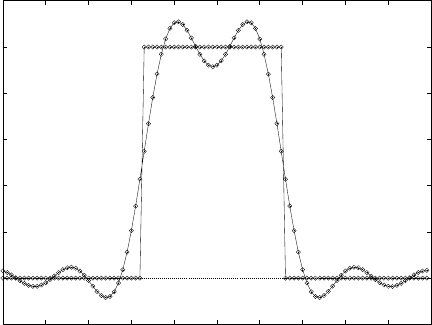
Chapter 15: Fast Fourier Transforms (FFTs) 174
-0.2
0
0.2
0.4
0.6
0.8
1
1.2
0 10 20 30 40 50 60 70 80 90 100
Low-pass filtered version of a real pulse,
output from the example program.
15.8 References and Further Reading
A good starting point for learning more about the FFT is the review article Fast Fourier
Transforms: A Tutorial Review and A State of the Art by Duhamel and Vetterli,
P. Duhamel and M. Vetterli. Fast fourier transforms: A tutorial review and a state of
the art. Signal Processing, 19:259–299, 1990.
To find out about the algorithms used in the GSL routines you may want to consult the
document GSL FFT Algorithms (it is included in GSL, as ‘doc/fftalgorithms.tex’). This
has general information on FFTs and explicit derivations of the implementation for each
routine. There are also references to the relevant literature. For convenience some of the
more important references are reproduced below.
There are several introductory books on the FFT with example programs, such as The Fast
Fourier Transform by Brigham and DFT/FFT and Convolution Algorithms by Burrus and
Parks,
E. Oran Brigham. The Fast Fourier Transform. Prentice Hall, 1974.
C. S. Burrus and T. W. Parks. DFT/FFT and Convolution Algorithms. Wiley, 1984.
Both these introductory books cover the radix-2 FFT in some detail. The mixed-radix
algorithm at the heart of the fftpack routines is reviewed in Clive Temperton’s paper,
Clive Temperton. Self-sorting mixed-radix fast fourier transforms. Journal of Compu-
tational Physics, 52(1):1–23, 1983.
The derivation of FFTs for real-valued data is explained in the following two articles,
Henrik V. Sorenson, Douglas L. Jones, Michael T. Heideman, and C. Sidney Bur-
rus. Real-valued fast fourier transform algorithms. IEEE Transactions on Acoustics,
Speech, and Signal Processing, ASSP-35(6):849–863, 1987.
Clive Temperton. Fast mixed-radix real fourier transforms. Journal of Computational
Physics, 52:340–350, 1983.
In 1979 the IEEE published a compendium of carefully-reviewed Fortran FFT programs in
Programs for Digital Signal Processing. It is a useful reference for implementations of many
different FFT algorithms,
Chapter 15: Fast Fourier Transforms (FFTs) 175
Digital Signal Processing Committee and IEEE Acoustics, Speech, and Signal Process-
ing Committee, editors. Programs for Digital Signal Processing. IEEE Press, 1979.
For large-scale FFT work we recommend the use of the dedicated FFTW library by Frigo
and Johnson. The FFTW library is self-optimizing—it automatically tunes itself for each
hardware platform in order to achieve maximum performance. It is available under the
GNU GPL.
FFTW Website, http://www.fftw.org/
The source code for fftpack is available from Netlib,
FFTPACK, http://www.netlib.org/fftpack/
Chapter 16: Numerical Integration 176
16 Numerical Integration
This chapter describes routines for performing numerical integration (quadrature) of a func-
tion in one dimension. There are routines for adaptive and non-adaptive integration of
general functions, with specialised routines for specific cases. These include integration
over infinite and semi-infinite ranges, singular integrals, including logarithmic singularities,
computation of Cauchy principal values and oscillatory integrals. The library reimplements
the algorithms used in quadpack, a numerical integration package written by Piessens,
Doncker-Kapenga, Uberhuber and Kahaner. Fortran code for quadpack is available on
Netlib.
The functions described in this chapter are declared in the header file
‘gsl_integration.h’.
16.1 Introduction
Each algorithm computes an approximation to a definite integral of the form,
I=Zb
a
f(x)w(x)dx
where w(x) is a weight function (for general integrands w(x) = 1). The user provides
absolute and relative error bounds (epsabs,epsrel ) which specify the following accuracy
requirement,
|RESULT −I| ≤ max(epsabs,epsrel |I|)
where RESULT is the numerical approximation obtained by the algorithm. The algorithms
attempt to estimate the absolute error ABSERR =|RESULT −I|in such a way that the
following inequality holds,
|RESULT −I| ≤ ABSERR ≤max(epsabs,epsrel |I|)
In short, the routines return the first approximation which has an absolute error smaller
than epsabs or a relative error smaller than epsrel.
Note that this is an either-or constraint, not simultaneous. To compute to a specified
absolute error, set epsrel to zero. To compute to a specified relative error, set epsabs to
zero. The routines will fail to converge if the error bounds are too stringent, but always
return the best approximation obtained up to that stage.
The algorithms in quadpack use a naming convention based on the following letters,
Q- quadrature routine
N- non-adaptive integrator
A- adaptive integrator
G- general integrand (user-defined)
W- weight function with integrand
S- singularities can be more readily integrated
P- points of special difficulty can be supplied

Chapter 16: Numerical Integration 177
I- infinite range of integration
O- oscillatory weight function, cos or sin
F- Fourier integral
C- Cauchy principal value
The algorithms are built on pairs of quadrature rules, a higher order rule and a lower order
rule. The higher order rule is used to compute the best approximation to an integral over a
small range. The difference between the results of the higher order rule and the lower order
rule gives an estimate of the error in the approximation.
16.1.1 Integrands without weight functions
The algorithms for general functions (without a weight function) are based on Gauss-
Kronrod rules.
A Gauss-Kronrod rule begins with a classical Gaussian quadrature rule of order m. This
is extended with additional points between each of the abscissae to give a higher order
Kronrod rule of order 2m+ 1. The Kronrod rule is efficient because it reuses existing
function evaluations from the Gaussian rule.
The higher order Kronrod rule is used as the best approximation to the integral, and the
difference between the two rules is used as an estimate of the error in the approximation.
16.1.2 Integrands with weight functions
For integrands with weight functions the algorithms use Clenshaw-Curtis quadrature rules.
A Clenshaw-Curtis rule begins with an n-th order Chebyshev polynomial approximation
to the integrand. This polynomial can be integrated exactly to give an approximation to
the integral of the original function. The Chebyshev expansion can be extended to higher
orders to improve the approximation and provide an estimate of the error.
16.1.3 Integrands with singular weight functions
The presence of singularities (or other behavior) in the integrand can cause slow convergence
in the Chebyshev approximation. The modified Clenshaw-Curtis rules used in quadpack
separate out several common weight functions which cause slow convergence.
These weight functions are integrated analytically against the Chebyshev polynomials to
precompute modified Chebyshev moments. Combining the moments with the Chebyshev
approximation to the function gives the desired integral. The use of analytic integration for
the singular part of the function allows exact cancellations and substantially improves the
overall convergence behavior of the integration.
16.2 QNG non-adaptive Gauss-Kronrod integration
The QNG algorithm is a non-adaptive procedure which uses fixed Gauss-Kronrod-Patterson
abscissae to sample the integrand at a maximum of 87 points. It is provided for fast
integration of smooth functions.
[Function]int gsl_integration_qng (const gsl function * f, double a, double b,
double epsabs, double epsrel, double * result, double * abserr, size t *
neval )
This function applies the Gauss-Kronrod 10-point, 21-point, 43-point and 87-point
integration rules in succession until an estimate of the integral of fover (a, b) is

Chapter 16: Numerical Integration 178
achieved within the desired absolute and relative error limits, epsabs and epsrel. The
function returns the final approximation, result, an estimate of the absolute error,
abserr and the number of function evaluations used, neval. The Gauss-Kronrod rules
are designed in such a way that each rule uses all the results of its predecessors, in
order to minimize the total number of function evaluations.
16.3 QAG adaptive integration
The QAG algorithm is a simple adaptive integration procedure. The integration region is
divided into subintervals, and on each iteration the subinterval with the largest estimated
error is bisected. This reduces the overall error rapidly, as the subintervals become con-
centrated around local difficulties in the integrand. These subintervals are managed by a
gsl_integration_workspace struct, which handles the memory for the subinterval ranges,
results and error estimates.
[Function]gsl_integration_workspace *
gsl_integration_workspace_alloc (size t n)
This function allocates a workspace sufficient to hold ndouble precision intervals,
their integration results and error estimates.
[Function]void gsl_integration_workspace_free (gsl integration workspace *
w)
This function frees the memory associated with the workspace w.
[Function]int gsl_integration_qag (const gsl function * f, double a, double b,
double epsabs, double epsrel, size t limit, int key,
gsl integration workspace * workspace, double * result, double * abserr )
This function applies an integration rule adaptively until an estimate of the integral
of fover (a, b) is achieved within the desired absolute and relative error limits, epsabs
and epsrel. The function returns the final approximation, result, and an estimate of
the absolute error, abserr. The integration rule is determined by the value of key,
which should be chosen from the following symbolic names,
GSL_INTEG_GAUSS15 (key = 1)
GSL_INTEG_GAUSS21 (key = 2)
GSL_INTEG_GAUSS31 (key = 3)
GSL_INTEG_GAUSS41 (key = 4)
GSL_INTEG_GAUSS51 (key = 5)
GSL_INTEG_GAUSS61 (key = 6)
corresponding to the 15, 21, 31, 41, 51 and 61 point Gauss-Kronrod rules. The
higher-order rules give better accuracy for smooth functions, while lower-order rules
save time when the function contains local difficulties, such as discontinuities.
On each iteration the adaptive integration strategy bisects the interval with the largest
error estimate. The subintervals and their results are stored in the memory provided
by workspace. The maximum number of subintervals is given by limit, which may
not exceed the allocated size of the workspace.

Chapter 16: Numerical Integration 179
16.4 QAGS adaptive integration with singularities
The presence of an integrable singularity in the integration region causes an adaptive routine
to concentrate new subintervals around the singularity. As the subintervals decrease in size
the successive approximations to the integral converge in a limiting fashion. This approach
to the limit can be accelerated using an extrapolation procedure. The QAGS algorithm
combines adaptive bisection with the Wynn epsilon-algorithm to speed up the integration
of many types of integrable singularities.
[Function]int gsl_integration_qags (const gsl function * f, double a, double b,
double epsabs, double epsrel, size tlimit, gsl integration workspace *
workspace, double * result, double * abserr )
This function applies the Gauss-Kronrod 21-point integration rule adaptively until
an estimate of the integral of fover (a, b) is achieved within the desired absolute
and relative error limits, epsabs and epsrel. The results are extrapolated using the
epsilon-algorithm, which accelerates the convergence of the integral in the presence
of discontinuities and integrable singularities. The function returns the final approx-
imation from the extrapolation, result, and an estimate of the absolute error, abserr.
The subintervals and their results are stored in the memory provided by workspace.
The maximum number of subintervals is given by limit, which may not exceed the
allocated size of the workspace.
16.5 QAGP adaptive integration with known singular points
[Function]int gsl_integration_qagp (const gsl function * f, double * pts, size t
npts, double epsabs, double epsrel, size tlimit, gsl integration workspace
*workspace, double * result, double * abserr )
This function applies the adaptive integration algorithm QAGS taking account of the
user-supplied locations of singular points. The array pts of length npts should contain
the endpoints of the integration ranges defined by the integration region and locations
of the singularities. For example, to integrate over the region (a, b) with break-points
at x1, x2, x3(where a < x1< x2< x3< b) the following pts array should be used
pts[0] = a
pts[1] = x_1
pts[2] = x_2
pts[3] = x_3
pts[4] = b
with npts = 5.
If you know the locations of the singular points in the integration region then this
routine will be faster than QAGS.
16.6 QAGI adaptive integration on infinite intervals
[Function]int gsl_integration_qagi (gsl function * f, double epsabs, double
epsrel, size tlimit, gsl integration workspace * workspace, double *
result, double * abserr )
This function computes the integral of the function fover the infinite interval
(−∞,+∞). The integral is mapped onto the semi-open interval (0,1] using the

Chapter 16: Numerical Integration 180
transformation x= (1 −t)/t,
Z+∞
−∞
dx f(x) = Z1
0
dt (f((1 −t)/t) + f(−(1 −t)/t))/t2.
It is then integrated using the QAGS algorithm. The normal 21-point Gauss-Kronrod
rule of QAGS is replaced by a 15-point rule, because the transformation can generate
an integrable singularity at the origin. In this case a lower-order rule is more efficient.
[Function]int gsl_integration_qagiu (gsl function * f, double a, double
epsabs, double epsrel, size tlimit, gsl integration workspace *
workspace, double * result, double * abserr )
This function computes the integral of the function fover the semi-infinite interval
(a, +∞). The integral is mapped onto the semi-open interval (0,1] using the trans-
formation x=a+ (1 −t)/t,
Z+∞
a
dx f(x) = Z1
0
dt f(a+ (1 −t)/t)/t2
and then integrated using the QAGS algorithm.
[Function]int gsl_integration_qagil (gsl function * f, double b, double
epsabs, double epsrel, size tlimit, gsl integration workspace *
workspace, double * result, double * abserr )
This function computes the integral of the function fover the semi-infinite interval
(−∞, b). The integral is mapped onto the semi-open interval (0,1] using the trans-
formation x=b−(1 −t)/t,
Zb
−∞
dx f(x) = Z1
0
dt f(b−(1 −t)/t)/t2
and then integrated using the QAGS algorithm.
16.7 QAWC adaptive integration for Cauchy principal
values
[Function]int gsl_integration_qawc (gsl function * f, double a, double b,
double c, double epsabs, double epsrel, size t limit,
gsl integration workspace * workspace, double * result, double * abserr )
This function computes the Cauchy principal value of the integral of fover (a, b),
with a singularity at c,
I=Zb
a
dx f(x)
x−c= lim
ǫ→0(Zc−ǫ
a
dx f(x)
x−c+Zb
c+ǫ
dx f(x)
x−c)
The adaptive bisection algorithm of QAG is used, with modifications to ensure that
subdivisions do not occur at the singular point x=c. When a subinterval contains
the point x=cor is close to it then a special 25-point modified Clenshaw-Curtis rule
is used to control the singularity. Further away from the singularity the algorithm
uses an ordinary 15-point Gauss-Kronrod integration rule.

Chapter 16: Numerical Integration 181
16.8 QAWS adaptive integration for singular functions
The QAWS algorithm is designed for integrands with algebraic-logarithmic singularities at
the end-points of an integration region. In order to work efficiently the algorithm requires
a precomputed table of Chebyshev moments.
[Function]gsl_integration_qaws_table *
gsl_integration_qaws_table_alloc (double alpha, double beta, int mu,
int nu )
This function allocates space for a gsl_integration_qaws_table struct describing
a singular weight function W(x) with the parameters (α, β, µ, ν),
W(x) = (x−a)α(b−x)βlogµ(x−a) logν(b−x)
where α > −1, β > −1, and µ= 0,1, ν= 0,1. The weight function can take four
different forms depending on the values of µand ν,
W(x) = (x−a)α(b−x)β(µ= 0, ν = 0)
W(x) = (x−a)α(b−x)βlog(x−a) (µ= 1, ν = 0)
W(x) = (x−a)α(b−x)βlog(b−x) (µ= 0, ν = 1)
W(x) = (x−a)α(b−x)βlog(x−a) log(b−x) (µ= 1, ν = 1)
The singular points (a, b) do not have to be specified until the integral is computed,
where they are the endpoints of the integration range.
The function returns a pointer to the newly allocated table gsl_integration_qaws_
table if no errors were detected, and 0 in the case of error.
[Function]int gsl_integration_qaws_table_set (gsl integration qaws table *
t, double alpha, double beta, int mu, int nu )
This function modifies the parameters (α, β, µ, ν) of an existing gsl_integration_
qaws_table struct t.
[Function]void gsl_integration_qaws_table_free (gsl integration qaws table
*t)
This function frees all the memory associated with the gsl_integration_qaws_table
struct t.
[Function]int gsl_integration_qaws (gsl function * f, const double a, const
double b, gsl integration qaws table * t, const double epsabs, const double
epsrel, const size t limit, gsl integration workspace * workspace, double *
result, double * abserr )
This function computes the integral of the function f(x) over the interval (a, b) with
the singular weight function (x−a)α(b−x)βlogµ(x−a) logν(b−x). The parameters
of the weight function (α, β, µ, ν) are taken from the table t. The integral is,
I=Zb
a
dx f(x)(x−a)α(b−x)βlogµ(x−a) logν(b−x).
The adaptive bisection algorithm of QAG is used. When a subinterval contains one
of the endpoints then a special 25-point modified Clenshaw-Curtis rule is used to
control the singularities. For subintervals which do not include the endpoints an
ordinary 15-point Gauss-Kronrod integration rule is used.

Chapter 16: Numerical Integration 182
16.9 QAWO adaptive integration for oscillatory functions
The QAWO algorithm is designed for integrands with an oscillatory factor, sin(ωx) or
cos(ωx). In order to work efficiently the algorithm requires a table of Chebyshev moments
which must be pre-computed with calls to the functions below.
[Function]gsl_integration_qawo_table *
gsl_integration_qawo_table_alloc (double omega, double L, enum
gsl integration qawo enum sine, size t n)
This function allocates space for a gsl_integration_qawo_table struct and its asso-
ciated workspace describing a sine or cosine weight function W(x) with the parameters
(ω, L),
W(x) = sin(ωx)
cos(ωx)
The parameter Lmust be the length of the interval over which the function will be
integrated L=b−a. The choice of sine or cosine is made with the parameter sine
which should be chosen from one of the two following symbolic values:
GSL_INTEG_COSINE
GSL_INTEG_SINE
The gsl_integration_qawo_table is a table of the trigonometric coefficients re-
quired in the integration process. The parameter ndetermines the number of levels
of coefficients that are computed. Each level corresponds to one bisection of the
interval L, so that nlevels are sufficient for subintervals down to the length L/2n.
The integration routine gsl_integration_qawo returns the error GSL_ETABLE if the
number of levels is insufficient for the requested accuracy.
[Function]int gsl_integration_qawo_table_set (gsl integration qawo table *
t, double omega, double L, enum gsl integration qawo enum sine )
This function changes the parameters omega,Land sine of the existing workspace t.
[Function]int gsl_integration_qawo_table_set_length
(gsl integration qawo table * t, double L)
This function allows the length parameter Lof the workspace tto be changed.
[Function]void gsl_integration_qawo_table_free (gsl integration qawo table
*t)
This function frees all the memory associated with the workspace t.
[Function]int gsl_integration_qawo (gsl function * f, const double a, const
double epsabs, const double epsrel, const size tlimit,
gsl integration workspace * workspace, gsl integration qawo table * wf,
double * result, double * abserr )
This function uses an adaptive algorithm to compute the integral of fover (a, b) with
the weight function sin(ωx) or cos(ωx) defined by the table wf,
I=Zb
a
dx f(x)sin(ωx)
cos(ωx)

Chapter 16: Numerical Integration 183
The results are extrapolated using the epsilon-algorithm to accelerate the convergence
of the integral. The function returns the final approximation from the extrapolation,
result, and an estimate of the absolute error, abserr. The subintervals and their
results are stored in the memory provided by workspace. The maximum number
of subintervals is given by limit, which may not exceed the allocated size of the
workspace.
Those subintervals with “large” widths dwhere dω > 4 are computed using a 25-point
Clenshaw-Curtis integration rule, which handles the oscillatory behavior. Subintervals
with a “small” widths where dω < 4 are computed using a 15-point Gauss-Kronrod
integration.
16.10 QAWF adaptive integration for Fourier integrals
[Function]int gsl_integration_qawf (gsl function * f, const double a, const
double epsabs, const size t limit, gsl integration workspace * workspace,
gsl integration workspace * cycle_workspace, gsl integration qawo table *
wf, double * result, double * abserr )
This function attempts to compute a Fourier integral of the function fover the semi-
infinite interval [a, +∞).
I=Z+∞
a
dx f(x)sin(ωx)
cos(ωx)
The parameter ωand choice of sin or cos is taken from the table wf (the length L
can take any value, since it is overridden by this function to a value appropriate for
the fourier integration). The integral is computed using the QAWO algorithm over
each of the subintervals,
C1= [a, a +c]
C2= [a+c, a + 2c]
...=...
Ck= [a+ (k−1)c, a +kc]
where c= (2 floor(|ω|) + 1)π/|ω|. The width cis chosen to cover an odd number of
periods so that the contributions from the intervals alternate in sign and are mono-
tonically decreasing when fis positive and monotonically decreasing. The sum of this
sequence of contributions is accelerated using the epsilon-algorithm.
This function works to an overall absolute tolerance of abserr. The following strategy
is used: on each interval Ckthe algorithm tries to achieve the tolerance
T OLk=ukabserr
where uk= (1−p)pk−1and p= 9/10. The sum of the geometric series of contributions
from each interval gives an overall tolerance of abserr.
If the integration of a subinterval leads to difficulties then the accuracy requirement
for subsequent intervals is relaxed,
T OLk=ukmax(abserr,max
i<k {Ei})

Chapter 16: Numerical Integration 184
where Ekis the estimated error on the interval Ck.
The subintervals and their results are stored in the memory provided by workspace.
The maximum number of subintervals is given by limit, which may not exceed the
allocated size of the workspace. The integration over each subinterval uses the memory
provided by cycle workspace as workspace for the QAWO algorithm.
16.11 Error codes
In addition to the standard error codes for invalid arguments the functions can return the
following values,
GSL_EMAXITER
the maximum number of subdivisions was exceeded.
GSL_EROUND
cannot reach tolerance because of roundoff error, or roundoff error was detected
in the extrapolation table.
GSL_ESING
a non-integrable singularity or other bad integrand behavior was found in the
integration interval.
GSL_EDIVERGE
the integral is divergent, or too slowly convergent to be integrated numerically.
16.12 Examples
The integrator QAGS will handle a large class of definite integrals. For example, consider
the following integral, which has an algebraic-logarithmic singularity at the origin,
Z1
0
x−1/2log(x)dx =−4
The program below computes this integral to a relative accuracy bound of 1e-7.
#include <stdio.h>
#include <math.h>
#include <gsl/gsl_integration.h>
double f (double x, void * params) {
double alpha = *(double *) params;
double f = log(alpha*x) / sqrt(x);
return f;
}
int
main (void)
{
gsl_integration_workspace * w
= gsl_integration_workspace_alloc (1000);
double result, error;
Chapter 16: Numerical Integration 185
double expected = -4.0;
double alpha = 1.0;
gsl_function F;
F.function = &f;
F.params = α
gsl_integration_qags (&F, 0, 1, 0, 1e-7, 1000,
w, &result, &error);
printf ("result = % .18f\n", result);
printf ("exact result = % .18f\n", expected);
printf ("estimated error = % .18f\n", error);
printf ("actual error = % .18f\n", result - expected);
printf ("intervals = %d\n", w->size);
gsl_integration_workspace_free (w);
return 0;
}
The results below show that the desired accuracy is achieved after 8 subdivisions.
$ ./a.out
result = -3.999999999999973799
exact result = -4.000000000000000000
estimated error = 0.000000000000246025
actual error = 0.000000000000026201
intervals = 8
In fact, the extrapolation procedure used by QAGS produces an accuracy of almost twice as
many digits. The error estimate returned by the extrapolation procedure is larger than the
actual error, giving a margin of safety of one order of magnitude.
16.13 References and Further Reading
The following book is the definitive reference for quadpack, and was written by the original
authors. It provides descriptions of the algorithms, program listings, test programs and
examples. It also includes useful advice on numerical integration and many references to
the numerical integration literature used in developing quadpack.
R. Piessens, E. de Doncker-Kapenga, C.W. Uberhuber, D.K. Kahaner. quadpack A
subroutine package for automatic integration Springer Verlag, 1983.
Chapter 17: Random Number Generation 186
17 Random Number Generation
The library provides a large collection of random number generators which can be accessed
through a uniform interface. Environment variables allow you to select different generators
and seeds at runtime, so that you can easily switch between generators without needing to
recompile your program. Each instance of a generator keeps track of its own state, allowing
the generators to be used in multi-threaded programs. Additional functions are available for
transforming uniform random numbers into samples from continuous or discrete probability
distributions such as the Gaussian, log-normal or Poisson distributions.
These functions are declared in the header file ‘gsl_rng.h’.
17.1 General comments on random numbers
In 1988, Park and Miller wrote a paper entitled “Random number generators: good ones
are hard to find.” [Commun. ACM, 31, 1192–1201]. Fortunately, some excellent random
number generators are available, though poor ones are still in common use. You may
be happy with the system-supplied random number generator on your computer, but you
should be aware that as computers get faster, requirements on random number generators
increase. Nowadays, a simulation that calls a random number generator millions of times
can often finish before you can make it down the hall to the coffee machine and back.
A very nice review of random number generators was written by Pierre L’Ecuyer, as
Chapter 4 of the book: Handbook on Simulation, Jerry Banks, ed. (Wiley, 1997). The
chapter is available in postscript from L’Ecuyer’s ftp site (see references). Knuth’s volume
on Seminumerical Algorithms (originally published in 1968) devotes 170 pages to random
number generators, and has recently been updated in its 3rd edition (1997). It is brilliant, a
classic. If you don’t own it, you should stop reading right now, run to the nearest bookstore,
and buy it.
A good random number generator will satisfy both theoretical and statistical properties.
Theoretical properties are often hard to obtain (they require real math!), but one prefers
a random number generator with a long period, low serial correlation, and a tendency not
to “fall mainly on the planes.” Statistical tests are performed with numerical simulations.
Generally, a random number generator is used to estimate some quantity for which the
theory of probability provides an exact answer. Comparison to this exact answer provides
a measure of “randomness”.
17.2 The Random Number Generator Interface
It is important to remember that a random number generator is not a “real” function like
sine or cosine. Unlike real functions, successive calls to a random number generator yield
different return values. Of course that is just what you want for a random number generator,
but to achieve this effect, the generator must keep track of some kind of “state” variable.
Sometimes this state is just an integer (sometimes just the value of the previously generated
random number), but often it is more complicated than that and may involve a whole array
of numbers, possibly with some indices thrown in. To use the random number generators,
you do not need to know the details of what comprises the state, and besides that varies
from algorithm to algorithm.

Chapter 17: Random Number Generation 187
The random number generator library uses two special structs, gsl_rng_type which
holds static information about each type of generator and gsl_rng which describes an
instance of a generator created from a given gsl_rng_type.
The functions described in this section are declared in the header file ‘gsl_rng.h’.
17.3 Random number generator initialization
[Function]gsl_rng * gsl_rng_alloc (const gsl rng type * T)
This function returns a pointer to a newly-created instance of a random number gener-
ator of type T. For example, the following code creates an instance of the Tausworthe
generator,
gsl_rng * r = gsl_rng_alloc (gsl_rng_taus);
If there is insufficient memory to create the generator then the function returns a null
pointer and the error handler is invoked with an error code of GSL_ENOMEM.
The generator is automatically initialized with the default seed, gsl_rng_default_
seed. This is zero by default but can be changed either directly or by using the
environment variable GSL_RNG_SEED (see Section 17.6 [Random number environment
variables], page 189).
The details of the available generator types are described later in this chapter.
[Function]void gsl_rng_set (const gsl rng * r, unsigned long int s)
This function initializes (or ‘seeds’) the random number generator. If the generator
is seeded with the same value of son two different runs, the same stream of random
numbers will be generated by successive calls to the routines below. If different
values of s≥1 are supplied, then the generated streams of random numbers should
be completely different. If the seed sis zero then the standard seed from the original
implementation is used instead. For example, the original Fortran source code for the
ranlux generator used a seed of 314159265, and so choosing sequal to zero reproduces
this when using gsl_rng_ranlux.
When using multiple seeds with the same generator, choose seed values greater than
zero to avoid collisions with the default setting.
Note that the most generators only accept 32-bit seeds, with higher values being
reduced modulo 232. For generators with smaller ranges the maximum seed value will
typically be lower.
[Function]void gsl_rng_free (gsl rng * r)
This function frees all the memory associated with the generator r.
17.4 Sampling from a random number generator
The following functions return uniformly distributed random numbers, either as integers or
double precision floating point numbers. Inline versions of these functions are used when
HAVE_INLINE is defined. To obtain non-uniform distributions see Chapter 19 [Random
Number Distributions], page 206.

Chapter 17: Random Number Generation 188
[Function]unsigned long int gsl_rng_get (const gsl rng * r)
This function returns a random integer from the generator r. The minimum and
maximum values depend on the algorithm used, but all integers in the range [min,max]
are equally likely. The values of min and max can determined using the auxiliary
functions gsl_rng_max (r) and gsl_rng_min (r).
[Function]double gsl_rng_uniform (const gsl rng * r)
This function returns a double precision floating point number uniformly distributed
in the range [0,1). The range includes 0.0 but excludes 1.0. The value is typically
obtained by dividing the result of gsl_rng_get(r) by gsl_rng_max(r) + 1.0 in dou-
ble precision. Some generators compute this ratio internally so that they can provide
floating point numbers with more than 32 bits of randomness (the maximum number
of bits that can be portably represented in a single unsigned long int).
[Function]double gsl_rng_uniform_pos (const gsl rng * r)
This function returns a positive double precision floating point number uniformly
distributed in the range (0,1), excluding both 0.0 and 1.0. The number is obtained
by sampling the generator with the algorithm of gsl_rng_uniform until a non-zero
value is obtained. You can use this function if you need to avoid a singularity at 0.0.
[Function]unsigned long int gsl_rng_uniform_int (const gsl rng * r,
unsigned long int n)
This function returns a random integer from 0 to n−1 inclusive by scaling down
and/or discarding samples from the generator r. All integers in the range [0, n −1]
are produced with equal probability. For generators with a non-zero minimum value
an offset is applied so that zero is returned with the correct probability.
Note that this function is designed for sampling from ranges smaller than the range
of the underlying generator. The parameter nmust be less than or equal to the range
of the generator r. If nis larger than the range of the generator then the function
calls the error handler with an error code of GSL_EINVAL and returns zero.
In particular, this function is not intended for generating the full range of unsigned
integer values [0,232 −1]. Instead choose a generator with the maximal integer range
and zero mimimum value, such as gsl_rng_ranlxd1,gsl_rng_mt19937 or gsl_rng_
taus, and sample it directly using gsl_rng_get. The range of each generator can be
found using the auxiliary functions described in the next section.
17.5 Auxiliary random number generator functions
The following functions provide information about an existing generator. You should use
them in preference to hard-coding the generator parameters into your own code.
[Function]const char * gsl_rng_name (const gsl rng * r)
This function returns a pointer to the name of the generator. For example,
printf ("r is a ’%s’ generator\n",
gsl_rng_name (r));
would print something like r is a ’taus’ generator.
[Function]unsigned long int gsl_rng_max (const gsl rng * r)
gsl_rng_max returns the largest value that gsl_rng_get can return.

Chapter 17: Random Number Generation 189
[Function]unsigned long int gsl_rng_min (const gsl rng * r)
gsl_rng_min returns the smallest value that gsl_rng_get can return. Usually this
value is zero. There are some generators with algorithms that cannot return zero,
and for these generators the minimum value is 1.
[Function]void * gsl_rng_state (const gsl rng * r)
[Function]size_t gsl_rng_size (const gsl rng * r)
These functions return a pointer to the state of generator rand its size. You can
use this information to access the state directly. For example, the following code will
write the state of a generator to a stream,
void * state = gsl_rng_state (r);
size_t n = gsl_rng_size (r);
fwrite (state, n, 1, stream);
[Function]const gsl_rng_type ** gsl_rng_types_setup (void)
This function returns a pointer to an array of all the available generator types, ter-
minated by a null pointer. The function should be called once at the start of the
program, if needed. The following code fragment shows how to iterate over the array
of generator types to print the names of the available algorithms,
const gsl_rng_type **t, **t0;
t0 = gsl_rng_types_setup ();
printf ("Available generators:\n");
for (t = t0; *t != 0; t++)
{
printf ("%s\n", (*t)->name);
}
17.6 Random number environment variables
The library allows you to choose a default generator and seed from the environment variables
GSL_RNG_TYPE and GSL_RNG_SEED and the function gsl_rng_env_setup. This makes it easy
try out different generators and seeds without having to recompile your program.
[Function]const gsl_rng_type * gsl_rng_env_setup (void)
This function reads the environment variables GSL_RNG_TYPE and GSL_RNG_SEED and
uses their values to set the corresponding library variables gsl_rng_default and
gsl_rng_default_seed. These global variables are defined as follows,
extern const gsl_rng_type *gsl_rng_default
extern unsigned long int gsl_rng_default_seed
The environment variable GSL_RNG_TYPE should be the name of a generator, such
as taus or mt19937. The environment variable GSL_RNG_SEED should contain the
desired seed value. It is converted to an unsigned long int using the C library
function strtoul.
If you don’t specify a generator for GSL_RNG_TYPE then gsl_rng_mt19937 is used as
the default. The initial value of gsl_rng_default_seed is zero.
Chapter 17: Random Number Generation 190
Here is a short program which shows how to create a global generator using the envi-
ronment variables GSL_RNG_TYPE and GSL_RNG_SEED,
#include <stdio.h>
#include <gsl/gsl_rng.h>
gsl_rng * r; /* global generator */
int
main (void)
{
const gsl_rng_type * T;
gsl_rng_env_setup();
T = gsl_rng_default;
r = gsl_rng_alloc (T);
printf ("generator type: %s\n", gsl_rng_name (r));
printf ("seed = %lu\n", gsl_rng_default_seed);
printf ("first value = %lu\n", gsl_rng_get (r));
gsl_rng_free (r);
return 0;
}
Running the program without any environment variables uses the initial defaults, an
mt19937 generator with a seed of 0,
$ ./a.out
generator type: mt19937
seed = 0
first value = 4293858116
By setting the two variables on the command line we can change the default generator and
the seed,
$ GSL_RNG_TYPE="taus" GSL_RNG_SEED=123 ./a.out
GSL_RNG_TYPE=taus
GSL_RNG_SEED=123
generator type: taus
seed = 123
first value = 2720986350
17.7 Copying random number generator state
The above methods do not expose the random number ‘state’ which changes from call to
call. It is often useful to be able to save and restore the state. To permit these practices, a
few somewhat more advanced functions are supplied. These include:

Chapter 17: Random Number Generation 191
[Function]int gsl_rng_memcpy (gsl rng * dest, const gsl rng * src )
This function copies the random number generator src into the pre-existing generator
dest, making dest into an exact copy of src. The two generators must be of the same
type.
[Function]gsl_rng * gsl_rng_clone (const gsl rng * r)
This function returns a pointer to a newly created generator which is an exact copy
of the generator r.
17.8 Reading and writing random number generator state
The library provides functions for reading and writing the random number state to a file as
binary data.
[Function]int gsl_rng_fwrite (FILE * stream, const gsl rng * r)
This function writes the random number state of the random number generator r
to the stream stream in binary format. The return value is 0 for success and GSL_
EFAILED if there was a problem writing to the file. Since the data is written in the
native binary format it may not be portable between different architectures.
[Function]int gsl_rng_fread (FILE * stream, gsl rng * r)
This function reads the random number state into the random number generator r
from the open stream stream in binary format. The random number generator r
must be preinitialized with the correct random number generator type since type
information is not saved. The return value is 0 for success and GSL_EFAILED if there
was a problem reading from the file. The data is assumed to have been written in the
native binary format on the same architecture.
17.9 Random number generator algorithms
The functions described above make no reference to the actual algorithm used. This is de-
liberate so that you can switch algorithms without having to change any of your application
source code. The library provides a large number of generators of different types, including
simulation quality generators, generators provided for compatibility with other libraries and
historical generators from the past.
The following generators are recommended for use in simulation. They have extremely
long periods, low correlation and pass most statistical tests. For the most reliable source of
uncorrelated numbers, the second-generation ranlux generators have the strongest proof
of randomness.
[Generator]gsl_rng_mt19937
The MT19937 generator of Makoto Matsumoto and Takuji Nishimura is a variant
of the twisted generalized feedback shift-register algorithm, and is known as the
“Mersenne Twister” generator. It has a Mersenne prime period of 219937 −1 (about
106000) and is equi-distributed in 623 dimensions. It has passed the diehard statisti-
cal tests. It uses 624 words of state per generator and is comparable in speed to the
other generators. The original generator used a default seed of 4357 and choosing s
equal to zero in gsl_rng_set reproduces this. Later versions switched to 5489 as the
default seed, you can choose this explicitly via gsl_rng_set instead if you require it.
Chapter 17: Random Number Generation 192
For more information see,
Makoto Matsumoto and Takuji Nishimura, “Mersenne Twister: A 623-
dimensionally equidistributed uniform pseudorandom number generator”. ACM
Transactions on Modeling and Computer Simulation, Vol. 8, No. 1 (Jan. 1998),
Pages 3–30
The generator gsl_rng_mt19937 uses the second revision of the seeding procedure
published by the two authors above in 2002. The original seeding procedures could
cause spurious artifacts for some seed values. They are still available through the
alternative generators gsl_rng_mt19937_1999 and gsl_rng_mt19937_1998.
[Generator]gsl_rng_ranlxs0
[Generator]gsl_rng_ranlxs1
[Generator]gsl_rng_ranlxs2
The generator ranlxs0 is a second-generation version of the ranlux algorithm of
L¨uscher, which produces “luxury random numbers”. This generator provides single
precision output (24 bits) at three luxury levels ranlxs0,ranlxs1 and ranlxs2, in
increasing order of strength. It uses double-precision floating point arithmetic inter-
nally and can be significantly faster than the integer version of ranlux, particularly
on 64-bit architectures. The period of the generator is about 10171. The algorithm has
mathematically proven properties and can provide truly decorrelated numbers at a
known level of randomness. The higher luxury levels provide increased decorrelation
between samples as an additional safety margin.
[Generator]gsl_rng_ranlxd1
[Generator]gsl_rng_ranlxd2
These generators produce double precision output (48 bits) from the ranlxs genera-
tor. The library provides two luxury levels ranlxd1 and ranlxd2, in increasing order
of strength.
[Generator]gsl_rng_ranlux
[Generator]gsl_rng_ranlux389
The ranlux generator is an implementation of the original algorithm developed by
L¨uscher. It uses a lagged-fibonacci-with-skipping algorithm to produce “luxury ran-
dom numbers”. It is a 24-bit generator, originally designed for single-precision IEEE
floating point numbers. This implementation is based on integer arithmetic, while
the second-generation versions ranlxs and ranlxd described above provide floating-
point implementations which will be faster on many platforms. The period of the
generator is about 10171. The algorithm has mathematically proven properties and it
can provide truly decorrelated numbers at a known level of randomness. The default
level of decorrelation recommended by L¨uscher is provided by gsl_rng_ranlux, while
gsl_rng_ranlux389 gives the highest level of randomness, with all 24 bits decorre-
lated. Both types of generator use 24 words of state per generator.
For more information see,
M. L¨uscher, “A portable high-quality random number generator for lattice field
theory calculations”, Computer Physics Communications, 79 (1994) 100–110.
Chapter 17: Random Number Generation 193
F. James, “RANLUX: A Fortran implementation of the high-quality pseudo-
random number generator of L¨uscher”, Computer Physics Communications, 79
(1994) 111–114
[Generator]gsl_rng_cmrg
This is a combined multiple recursive generator by L’Ecuyer. Its sequence is,
zn= (xn−yn) mod m1
where the two underlying generators xnand ynare,
xn= (a1xn−1+a2xn−2+a3xn−3) mod m1
yn= (b1yn−1+b2yn−2+b3yn−3) mod m2
with coefficients a1= 0, a2= 63308, a3=−183326, b1= 86098, b2= 0, b3=−539608,
and moduli m1= 231 −1 = 2147483647 and m2= 2145483479.
The period of this generator is lcm(m3
1−1, m3
2−1), which is approximately 2185 (about
1056). It uses 6 words of state per generator. For more information see,
P. L’Ecuyer, “Combined Multiple Recursive Random Number Generators”, Op-
erations Research, 44, 5 (1996), 816–822.
[Generator]gsl_rng_mrg
This is a fifth-order multiple recursive generator by L’Ecuyer, Blouin and Coutre. Its
sequence is,
xn= (a1xn−1+a5xn−5) mod m
with a1= 107374182, a2=a3=a4= 0, a5= 104480 and m= 231 −1.
The period of this generator is about 1046. It uses 5 words of state per generator.
More information can be found in the following paper,
P. L’Ecuyer, F. Blouin, and R. Coutre, “A search for good multiple recursive
random number generators”, ACM Transactions on Modeling and Computer
Simulation 3, 87–98 (1993).
[Generator]gsl_rng_taus
[Generator]gsl_rng_taus2
This is a maximally equidistributed combined Tausworthe generator by L’Ecuyer.
The sequence is,
xn= (s1
n⊕s2
n⊕s3
n)
where,
s1
n+1 = (((s1
n&4294967294) ≪12) ⊕(((s1
n≪13) ⊕s1
n)≫19))
s2
n+1 = (((s2
n&4294967288) ≪4) ⊕(((s2
n≪2) ⊕s2
n)≫25))
s3
n+1 = (((s3
n&4294967280) ≪17) ⊕(((s3
n≪3) ⊕s3
n)≫11))
computed modulo 232. In the formulas above ⊕denotes “exclusive-or”. Note that
the algorithm relies on the properties of 32-bit unsigned integers and has been imple-
mented using a bitmask of 0xFFFFFFFF to make it work on 64 bit machines.
The period of this generator is 288 (about 1026). It uses 3 words of state per generator.
For more information see,
Chapter 17: Random Number Generation 194
P. L’Ecuyer, “Maximally Equidistributed Combined Tausworthe Generators”,
Mathematics of Computation, 65, 213 (1996), 203–213.
The generator gsl_rng_taus2 uses the same algorithm as gsl_rng_taus but with
an improved seeding procedure described in the paper,
P. L’Ecuyer, “Tables of Maximally Equidistributed Combined LFSR Genera-
tors”, Mathematics of Computation, 68, 225 (1999), 261–269
The generator gsl_rng_taus2 should now be used in preference to gsl_rng_taus.
[Generator]gsl_rng_gfsr4
The gfsr4 generator is like a lagged-fibonacci generator, and produces each number
as an xor’d sum of four previous values.
rn=rn−A⊕rn−B⊕rn−C⊕rn−D
Ziff (ref below) notes that “it is now widely known” that two-tap registers (such
as R250, which is described below) have serious flaws, the most obvious one being
the three-point correlation that comes from the definition of the generator. Nice
mathematical properties can be derived for GFSR’s, and numerics bears out the
claim that 4-tap GFSR’s with appropriately chosen offsets are as random as can be
measured, using the author’s test.
This implementation uses the values suggested the example on p392 of Ziff’s article:
A= 471, B= 1586, C= 6988, D= 9689.
If the offsets are appropriately chosen (such as the one ones in this implementation),
then the sequence is said to be maximal; that means that the period is 2D−1, where
Dis the longest lag. (It is one less than 2Dbecause it is not permitted to have all
zeros in the ra[] array.) For this implementation with D= 9689 that works out to
about 102917.
Note that the implementation of this generator using a 32-bit integer amounts to 32
parallel implementations of one-bit generators. One consequence of this is that the
period of this 32-bit generator is the same as for the one-bit generator. Moreover,
this independence means that all 32-bit patterns are equally likely, and in particular
that 0 is an allowed random value. (We are grateful to Heiko Bauke for clarifying for
us these properties of GFSR random number generators.)
For more information see,
Robert M. Ziff, “Four-tap shift-register-sequence random-number generators”,
Computers in Physics, 12(4), Jul/Aug 1998, pp 385–392.
17.10 Unix random number generators
The standard Unix random number generators rand,random and rand48 are provided as
part of GSL. Although these generators are widely available individually often they aren’t
all available on the same platform. This makes it difficult to write portable code using them
and so we have included the complete set of Unix generators in GSL for convenience. Note
that these generators don’t produce high-quality randomness and aren’t suitable for work
requiring accurate statistics. However, if you won’t be measuring statistical quantities and
just want to introduce some variation into your program then these generators are quite
acceptable.
Chapter 17: Random Number Generation 195
[Generator]gsl_rng_rand
This is the BSD rand generator. Its sequence is
xn+1 = (axn+c) mod m
with a= 1103515245, c= 12345 and m= 231. The seed specifies the initial value,
x1. The period of this generator is 231, and it uses 1 word of storage per generator.
[Generator]gsl_rng_random_bsd
[Generator]gsl_rng_random_libc5
[Generator]gsl_rng_random_glibc2
These generators implement the random family of functions, a set of linear feedback
shift register generators originally used in BSD Unix. There are several versions of
random in use today: the original BSD version (e.g. on SunOS4), a libc5 version
(found on older GNU/Linux systems) and a glibc2 version. Each version uses a
different seeding procedure, and thus produces different sequences.
The original BSD routines accepted a variable length buffer for the generator state,
with longer buffers providing higher-quality randomness. The random function imple-
mented algorithms for buffer lengths of 8, 32, 64, 128 and 256 bytes, and the algorithm
with the largest length that would fit into the user-supplied buffer was used. To sup-
port these algorithms additional generators are available with the following names,
gsl_rng_random8_bsd
gsl_rng_random32_bsd
gsl_rng_random64_bsd
gsl_rng_random128_bsd
gsl_rng_random256_bsd
where the numeric suffix indicates the buffer length. The original BSD random func-
tion used a 128-byte default buffer and so gsl_rng_random_bsd has been made equiv-
alent to gsl_rng_random128_bsd. Corresponding versions of the libc5 and glibc2
generators are also available, with the names gsl_rng_random8_libc5,gsl_rng_
random8_glibc2, etc.
[Generator]gsl_rng_rand48
This is the Unix rand48 generator. Its sequence is
xn+1 = (axn+c) mod m
defined on 48-bit unsigned integers with a= 25214903917, c= 11 and m= 248. The
seed specifies the upper 32 bits of the initial value, x1, with the lower 16 bits set to
0x330E. The function gsl_rng_get returns the upper 32 bits from each term of the
sequence. This does not have a direct parallel in the original rand48 functions, but
forcing the result to type long int reproduces the output of mrand48. The function
gsl_rng_uniform uses the full 48 bits of internal state to return the double precision
number xn/m, which is equivalent to the function drand48. Note that some versions
of the GNU C Library contained a bug in mrand48 function which caused it to produce
different results (only the lower 16-bits of the return value were set).
Chapter 17: Random Number Generation 196
17.11 Other random number generators
The generators in this section are provided for compatibility with existing libraries. If you
are converting an existing program to use GSL then you can select these generators to
check your new implementation against the original one, using the same random number
generator. After verifying that your new program reproduces the original results you can
then switch to a higher-quality generator.
Note that most of the generators in this section are based on single linear congruence
relations, which are the least sophisticated type of generator. In particular, linear congru-
ences have poor properties when used with a non-prime modulus, as several of these routines
do (e.g. with a power of two modulus, 231 or 232). This leads to periodicity in the least
significant bits of each number, with only the higher bits having any randomness. Thus if
you want to produce a random bitstream it is best to avoid using the least significant bits.
[Generator]gsl_rng_ranf
This is the CRAY random number generator RANF. Its sequence is
xn+1 = (axn) mod m
defined on 48-bit unsigned integers with a= 44485709377909 and m= 248. The seed
specifies the lower 32 bits of the initial value, x1, with the lowest bit set to prevent
the seed taking an even value. The upper 16 bits of x1are set to 0. A consequence
of this procedure is that the pairs of seeds 2 and 3, 4 and 5, etc produce the same
sequences.
The generator compatible with the CRAY MATHLIB routine RANF. It produces
double precision floating point numbers which should be identical to those from the
original RANF.
There is a subtlety in the implementation of the seeding. The initial state is reversed
through one step, by multiplying by the modular inverse of amod m. This is done
for compatibility with the original CRAY implementation.
Note that you can only seed the generator with integers up to 232, while the original
CRAY implementation uses non-portable wide integers which can cover all 248 states
of the generator.
The function gsl_rng_get returns the upper 32 bits from each term of the sequence.
The function gsl_rng_uniform uses the full 48 bits to return the double precision
number xn/m.
The period of this generator is 246.
[Generator]gsl_rng_ranmar
This is the RANMAR lagged-fibonacci generator of Marsaglia, Zaman and Tsang.
It is a 24-bit generator, originally designed for single-precision IEEE floating point
numbers. It was included in the CERNLIB high-energy physics library.
[Generator]gsl_rng_r250
This is the shift-register generator of Kirkpatrick and Stoll. The sequence is based
on the recurrence
xn=xn−103 ⊕xn−250
Chapter 17: Random Number Generation 197
where ⊕denotes “exclusive-or”, defined on 32-bit words. The period of this generator
is about 2250 and it uses 250 words of state per generator.
For more information see,
S. Kirkpatrick and E. Stoll, “A very fast shift-register sequence random number
generator”, Journal of Computational Physics, 40, 517–526 (1981)
[Generator]gsl_rng_tt800
This is an earlier version of the twisted generalized feedback shift-register generator,
and has been superseded by the development of MT19937. However, it is still an
acceptable generator in its own right. It has a period of 2800 and uses 33 words of
storage per generator.
For more information see,
Makoto Matsumoto and Yoshiharu Kurita, “Twisted GFSR Generators II”, ACM
Transactions on Modelling and Computer Simulation, Vol. 4, No. 3, 1994, pages
254–266.
[Generator]gsl_rng_vax
This is the VAX generator MTH$RANDOM. Its sequence is,
xn+1 = (axn+c) mod m
with a= 69069, c= 1 and m= 232. The seed specifies the initial value, x1. The
period of this generator is 232 and it uses 1 word of storage per generator.
[Generator]gsl_rng_transputer
This is the random number generator from the INMOS Transputer Development
system. Its sequence is,
xn+1 = (axn) mod m
with a= 1664525 and m= 232. The seed specifies the initial value, x1.
[Generator]gsl_rng_randu
This is the IBM RANDU generator. Its sequence is
xn+1 = (axn) mod m
with a= 65539 and m= 231. The seed specifies the initial value, x1. The period of
this generator was only 229. It has become a textbook example of a poor generator.
[Generator]gsl_rng_minstd
This is Park and Miller’s “minimal standard” minstd generator, a simple linear con-
gruence which takes care to avoid the major pitfalls of such algorithms. Its sequence
is,
xn+1 = (axn) mod m
with a= 16807 and m= 231 −1 = 2147483647. The seed specifies the initial value,
x1. The period of this generator is about 231.
This generator is used in the IMSL Library (subroutine RNUN) and in MATLAB
(the RAND function). It is also sometimes known by the acronym “GGL” (I’m not
sure what that stands for).
Chapter 17: Random Number Generation 198
For more information see,
Park and Miller, “Random Number Generators: Good ones are hard to find”,
Communications of the ACM, October 1988, Volume 31, No 10, pages 1192–1201.
[Generator]gsl_rng_uni
[Generator]gsl_rng_uni32
This is a reimplementation of the 16-bit SLATEC random number generator RUNIF.
A generalization of the generator to 32 bits is provided by gsl_rng_uni32. The
original source code is available from NETLIB.
[Generator]gsl_rng_slatec
This is the SLATEC random number generator RAND. It is ancient. The original
source code is available from NETLIB.
[Generator]gsl_rng_zuf
This is the ZUFALL lagged Fibonacci series generator of Peterson. Its sequence is,
t=un−273 +un−607
un=t−floor(t)
The original source code is available from NETLIB. For more information see,
W. Petersen, “Lagged Fibonacci Random Number Generators for the NEC SX-
3”, International Journal of High Speed Computing (1994).
[Generator]gsl_rng_knuthran2
This is a second-order multiple recursive generator described by Knuth in Seminu-
merical Algorithms, 3rd Ed., page 108. Its sequence is,
xn= (a1xn−1+a2xn−2) mod m
with a1= 271828183, a2= 314159269, and m= 231 −1.
[Generator]gsl_rng_knuthran2002
[Generator]gsl_rng_knuthran
This is a second-order multiple recursive generator described by Knuth in Seminu-
merical Algorithms, 3rd Ed., Section 3.6. Knuth provides its C code. The updated
routine gsl_rng_knuthran2002 is from the revised 9th printing and corrects some
weaknesses in the earlier version, which is implemented as gsl_rng_knuthran.
[Generator]gsl_rng_borosh13
[Generator]gsl_rng_fishman18
[Generator]gsl_rng_fishman20
[Generator]gsl_rng_lecuyer21
[Generator]gsl_rng_waterman14
These multiplicative generators are taken from Knuth’s Seminumerical Algorithms,
3rd Ed., pages 106–108. Their sequence is,
xn+1 = (axn) mod m
where the seed specifies the initial value, x1. The parameters aand mare as follows,
Borosh-Niederreiter: a= 1812433253, m= 232, Fishman18: a= 62089911, m=
Chapter 17: Random Number Generation 199
231 −1, Fishman20: a= 48271, m= 231 −1, L’Ecuyer: a= 40692, m= 231 −249,
Waterman: a= 1566083941, m= 232.
[Generator]gsl_rng_fishman2x
This is the L’Ecuyer–Fishman random number generator. It is taken from Knuth’s
Seminumerical Algorithms, 3rd Ed., page 108. Its sequence is,
zn+1 = (xn−yn) mod m
with m= 231 −1. xnand ynare given by the fishman20 and lecuyer21 algorithms.
The seed specifies the initial value, x1.
[Generator]gsl_rng_coveyou
This is the Coveyou random number generator. It is taken from Knuth’s Seminumer-
ical Algorithms, 3rd Ed., Section 3.2.2. Its sequence is,
xn+1 = (xn(xn+ 1)) mod m
with m= 232. The seed specifies the initial value, x1.
17.12 Performance
The following table shows the relative performance of a selection the available random
number generators. The fastest simulation quality generators are taus,gfsr4 and mt19937.
The generators which offer the best mathematically-proven quality are those based on the
ranlux algorithm.
1754 k ints/sec, 870 k doubles/sec, taus
1613 k ints/sec, 855 k doubles/sec, gfsr4
1370 k ints/sec, 769 k doubles/sec, mt19937
565 k ints/sec, 571 k doubles/sec, ranlxs0
400 k ints/sec, 405 k doubles/sec, ranlxs1
490 k ints/sec, 389 k doubles/sec, mrg
407 k ints/sec, 297 k doubles/sec, ranlux
243 k ints/sec, 254 k doubles/sec, ranlxd1
251 k ints/sec, 253 k doubles/sec, ranlxs2
238 k ints/sec, 215 k doubles/sec, cmrg
247 k ints/sec, 198 k doubles/sec, ranlux389
141 k ints/sec, 140 k doubles/sec, ranlxd2
1852 k ints/sec, 935 k doubles/sec, ran3
813 k ints/sec, 575 k doubles/sec, ran0
787 k ints/sec, 476 k doubles/sec, ran1
379 k ints/sec, 292 k doubles/sec, ran2
17.13 Examples
The following program demonstrates the use of a random number generator to produce
uniform random numbers in the range [0.0, 1.0),
#include <stdio.h>
#include <gsl/gsl_rng.h>
Chapter 17: Random Number Generation 200
int
main (void)
{
const gsl_rng_type * T;
gsl_rng * r;
int i, n = 10;
gsl_rng_env_setup();
T = gsl_rng_default;
r = gsl_rng_alloc (T);
for (i = 0; i < n; i++)
{
double u = gsl_rng_uniform (r);
printf ("%.5f\n", u);
}
gsl_rng_free (r);
return 0;
}
Here is the output of the program,
$ ./a.out
0.99974
0.16291
0.28262
0.94720
0.23166
0.48497
0.95748
0.74431
0.54004
0.73995
The numbers depend on the seed used by the generator. The default seed can be changed
with the GSL_RNG_SEED environment variable to produce a different stream of numbers.
The generator itself can be changed using the environment variable GSL_RNG_TYPE. Here is
the output of the program using a seed value of 123 and the multiple-recursive generator
mrg,
$ GSL_RNG_SEED=123 GSL_RNG_TYPE=mrg ./a.out
GSL_RNG_TYPE=mrg
GSL_RNG_SEED=123
0.33050
0.86631
Chapter 17: Random Number Generation 201
0.32982
0.67620
0.53391
0.06457
0.16847
0.70229
0.04371
0.86374
17.14 References and Further Reading
The subject of random number generation and testing is reviewed extensively in Knuth’s
Seminumerical Algorithms.
Donald E. Knuth, The Art of Computer Programming: Seminumerical Algorithms (Vol
2, 3rd Ed, 1997), Addison-Wesley, ISBN 0201896842.
Further information is available in the review paper written by Pierre L’Ecuyer,
P. L’Ecuyer, “Random Number Generation”, Chapter 4 of the Handbook on Simula-
tion, Jerry Banks Ed., Wiley, 1998, 93–137.
http://www.iro.umontreal.ca/~lecuyer/papers.html in the file ‘handsim.ps’.
The source code for the diehard random number generator tests is also available online,
DIEHARD source code G. Marsaglia,
http://stat.fsu.edu/pub/diehard/
A comprehensive set of random number generator tests is available from nist,
NIST Special Publication 800-22, “A Statistical Test Suite for the Validation of Ran-
dom Number Generators and Pseudo Random Number Generators for Cryptographic
Applications”.
http://csrc.nist.gov/rng/
17.15 Acknowledgements
Thanks to Makoto Matsumoto, Takuji Nishimura and Yoshiharu Kurita for making the
source code to their generators (MT19937, MM&TN; TT800, MM&YK) available under
the GNU General Public License. Thanks to Martin L¨uscher for providing notes and source
code for the ranlxs and ranlxd generators.

Chapter 18: Quasi-Random Sequences 202
18 Quasi-Random Sequences
This chapter describes functions for generating quasi-random sequences in arbitrary di-
mensions. A quasi-random sequence progressively covers a d-dimensional space with a set
of points that are uniformly distributed. Quasi-random sequences are also known as low-
discrepancy sequences. The quasi-random sequence generators use an interface that is simi-
lar to the interface for random number generators, except that seeding is not required—each
generator produces a single sequence.
The functions described in this section are declared in the header file ‘gsl_qrng.h’.
18.1 Quasi-random number generator initialization
[Function]gsl_qrng * gsl_qrng_alloc (const gsl qrng type * T, unsigned int d)
This function returns a pointer to a newly-created instance of a quasi-random sequence
generator of type Tand dimension d. If there is insufficient memory to create the
generator then the function returns a null pointer and the error handler is invoked
with an error code of GSL_ENOMEM.
[Function]void gsl_qrng_free (gsl qrng * q)
This function frees all the memory associated with the generator q.
[Function]void gsl_qrng_init (gsl qrng * q)
This function reinitializes the generator qto its starting point. Note that quasi-
random sequences do not use a seed and always produce the same set of values.
18.2 Sampling from a quasi-random number generator
[Function]int gsl_qrng_get (const gsl qrng * q, double x[])
This function stores the next point from the sequence generator qin the array x. The
space available for xmust match the dimension of the generator. The point xwill lie
in the range 0 < xi<1 for each xi. An inline version of this function is used when
HAVE_INLINE is defined.
18.3 Auxiliary quasi-random number generator functions
[Function]const char * gsl_qrng_name (const gsl qrng * q)
This function returns a pointer to the name of the generator.
[Function]size_t gsl_qrng_size (const gsl qrng * q)
[Function]void * gsl_qrng_state (const gsl qrng * q)
These functions return a pointer to the state of generator rand its size. You can
use this information to access the state directly. For example, the following code will
write the state of a generator to a stream,
void * state = gsl_qrng_state (q);
size_t n = gsl_qrng_size (q);
fwrite (state, n, 1, stream);

Chapter 18: Quasi-Random Sequences 203
18.4 Saving and resorting quasi-random number generator
state
[Function]int gsl_qrng_memcpy (gsl qrng * dest, const gsl qrng * src )
This function copies the quasi-random sequence generator src into the pre-existing
generator dest, making dest into an exact copy of src. The two generators must be
of the same type.
[Function]gsl_qrng * gsl_qrng_clone (const gsl qrng * q)
This function returns a pointer to a newly created generator which is an exact copy
of the generator q.
18.5 Quasi-random number generator algorithms
The following quasi-random sequence algorithms are available,
[Generator]gsl_qrng_niederreiter_2
This generator uses the algorithm described in Bratley, Fox, Niederreiter, ACM Trans.
Model. Comp. Sim. 2, 195 (1992). It is valid up to 12 dimensions.
[Generator]gsl_qrng_sobol
This generator uses the Sobol sequence described in Antonov, Saleev, USSR Comput.
Maths. Math. Phys. 19, 252 (1980). It is valid up to 40 dimensions.
[Generator]gsl_qrng_halton
[Generator]gsl_qrng_reversehalton
These generators use the Halton and reverse Halton sequences described in J.H. Hal-
ton, Numerische Mathematik 2, 84-90 (1960) and B. Vandewoestyne and R. Cools
Computational and Applied Mathematics 189, 1&2, 341-361 (2006). They are valid
up to 1229 dimensions.
18.6 Examples
The following program prints the first 1024 points of the 2-dimensional Sobol sequence.
#include <stdio.h>
#include <gsl/gsl_qrng.h>
int
main (void)
{
int i;
gsl_qrng * q = gsl_qrng_alloc (gsl_qrng_sobol, 2);
for (i = 0; i < 1024; i++)
{
double v[2];
gsl_qrng_get (q, v);
printf ("%.5f %.5f\n", v[0], v[1]);
}
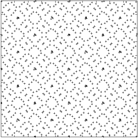
Chapter 18: Quasi-Random Sequences 204
gsl_qrng_free (q);
return 0;
}
Here is the output from the program,
$ ./a.out
0.50000 0.50000
0.75000 0.25000
0.25000 0.75000
0.37500 0.37500
0.87500 0.87500
0.62500 0.12500
0.12500 0.62500
....
It can be seen that successive points progressively fill-in the spaces between previous points.
The following plot shows the distribution in the x-y plane of the first 1024 points from
the Sobol sequence,
0
0.1
0.2
0.3
0.4
0.5
0.6
0.7
0.8
0.9
1
0 0.1 0.2 0.3 0.4 0.5 0.6 0.7 0.8 0.9 1
Distribution of the first 1024 points
from the quasi-random Sobol sequence
18.7 References
The implementations of the quasi-random sequence routines are based on the algorithms
described in the following paper,
Chapter 18: Quasi-Random Sequences 205
P. Bratley and B.L. Fox and H. Niederreiter, “Algorithm 738: Programs to Gener-
ate Niederreiter’s Low-discrepancy Sequences”, ACM Transactions on Mathematical
Software, Vol. 20, No. 4, December, 1994, p. 494–495.
Chapter 19: Random Number Distributions 206
19 Random Number Distributions
This chapter describes functions for generating random variates and computing their prob-
ability distributions. Samples from the distributions described in this chapter can be ob-
tained using any of the random number generators in the library as an underlying source
of randomness.
In the simplest cases a non-uniform distribution can be obtained analytically from the
uniform distribution of a random number generator by applying an appropriate transfor-
mation. This method uses one call to the random number generator. More complicated
distributions are created by the acceptance-rejection method, which compares the desired
distribution against a distribution which is similar and known analytically. This usually
requires several samples from the generator.
The library also provides cumulative distribution functions and inverse cumulative distri-
bution functions, sometimes referred to as quantile functions. The cumulative distribution
functions and their inverses are computed separately for the upper and lower tails of the
distribution, allowing full accuracy to be retained for small results.
The functions for random variates and probability density functions described in this sec-
tion are declared in ‘gsl_randist.h’. The corresponding cumulative distribution functions
are declared in ‘gsl_cdf.h’.
Note that the discrete random variate functions always return a value of type unsigned
int, and on most platforms this has a maximum value of 232 −1≈4.29 ×10⁹. They should
only be called with a safe range of parameters (where there is a negligible probability of a
variate exceeding this limit) to prevent incorrect results due to overflow.
19.1 Introduction
Continuous random number distributions are defined by a probability density function,
p(x), such that the probability of xoccurring in the infinitesimal range xto x+dx is p dx.
The cumulative distribution function for the lower tail P(x) is defined by the integral,
P(x) = Zx
−∞
dx′p(x′)
and gives the probability of a variate taking a value less than x.
The cumulative distribution function for the upper tail Q(x) is defined by the integral,
Q(x) = Z+∞
x
dx′p(x′)
and gives the probability of a variate taking a value greater than x.
The upper and lower cumulative distribution functions are related by P(x) + Q(x) = 1
and satisfy 0 ≤P(x)≤1, 0 ≤Q(x)≤1.
The inverse cumulative distributions, x=P−1(P) and x=Q−1(Q) give the values of x
which correspond to a specific value of Por Q. They can be used to find confidence limits
from probability values.
For discrete distributions the probability of sampling the integer value kis given by
p(k), where Pkp(k) = 1. The cumulative distribution for the lower tail P(k) of a discrete
Chapter 19: Random Number Distributions 207
distribution is defined as,
P(k) = X
i≤k
p(i)
where the sum is over the allowed range of the distribution less than or equal to k.
The cumulative distribution for the upper tail of a discrete distribution Q(k) is defined
as
Q(k) = X
i>k
p(i)
giving the sum of probabilities for all values greater than k. These two definitions satisfy
the identity P(k) + Q(k) = 1.
If the range of the distribution is 1 to ninclusive then P(n) = 1, Q(n) = 0 while
P(1) = p(1), Q(1) = 1 −p(1).
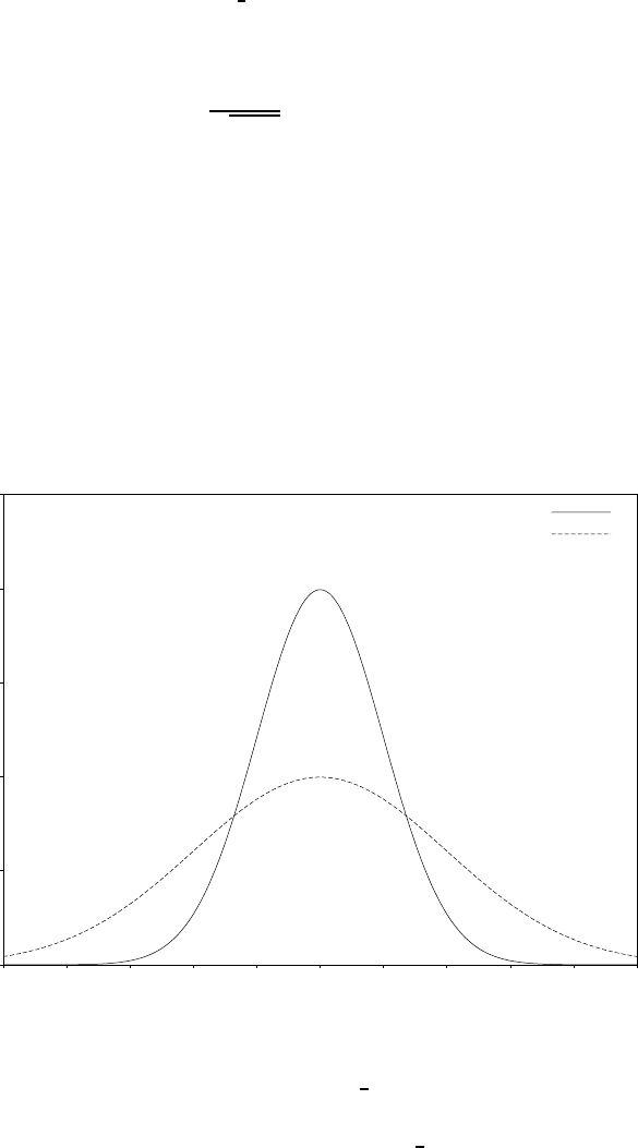
Chapter 19: Random Number Distributions 208
19.2 The Gaussian Distribution
[Function]double gsl_ran_gaussian (const gsl rng * r, double sigma )
This function returns a Gaussian random variate, with mean zero and standard de-
viation sigma. The probability distribution for Gaussian random variates is,
p(x)dx =1
√2πσ2exp(−x2/2σ2)dx
for xin the range −∞ to +∞. Use the transformation z=µ+xon the numbers
returned by gsl_ran_gaussian to obtain a Gaussian distribution with mean µ. This
function uses the Box-Muller algorithm which requires two calls to the random number
generator r.
[Function]double gsl_ran_gaussian_pdf (double x, double sigma )
This function computes the probability density p(x) at xfor a Gaussian distribution
with standard deviation sigma, using the formula given above.
σ= 2
σ= 1
Gaussian Distribution
x
p(x)
543210-1-2-3-4-5
0.5
0.4
0.3
0.2
0.1
0
[Function]double gsl_ran_gaussian_ziggurat (const gsl rng * r, double
sigma )
[Function]double gsl_ran_gaussian_ratio_method (const gsl rng * r, double
sigma )
This function computes a Gaussian random variate using the alternative Marsaglia-
Tsang ziggurat and Kinderman-Monahan-Leva ratio methods. The Ziggurat algo-
rithm is the fastest available algorithm in most cases.

Chapter 19: Random Number Distributions 209
[Function]double gsl_ran_ugaussian (const gsl rng * r)
[Function]double gsl_ran_ugaussian_pdf (double x)
[Function]double gsl_ran_ugaussian_ratio_method (const gsl rng * r)
These functions compute results for the unit Gaussian distribution. They are equiv-
alent to the functions above with a standard deviation of one, sigma = 1.
[Function]double gsl_cdf_gaussian_P (double x, double sigma )
[Function]double gsl_cdf_gaussian_Q (double x, double sigma )
[Function]double gsl_cdf_gaussian_Pinv (double P, double sigma )
[Function]double gsl_cdf_gaussian_Qinv (double Q, double sigma )
These functions compute the cumulative distribution functions P(x), Q(x) and their
inverses for the Gaussian distribution with standard deviation sigma.
[Function]double gsl_cdf_ugaussian_P (double x)
[Function]double gsl_cdf_ugaussian_Q (double x)
[Function]double gsl_cdf_ugaussian_Pinv (double P)
[Function]double gsl_cdf_ugaussian_Qinv (double Q)
These functions compute the cumulative distribution functions P(x), Q(x) and their
inverses for the unit Gaussian distribution.
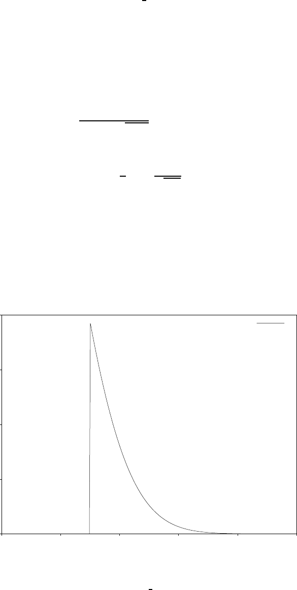
Chapter 19: Random Number Distributions 210
19.3 The Gaussian Tail Distribution
[Function]double gsl_ran_gaussian_tail (const gsl rng * r, double a, double
sigma )
This function provides random variates from the upper tail of a Gaussian distribution
with standard deviation sigma. The values returned are larger than the lower limit a,
which must be positive. The method is based on Marsaglia’s famous rectangle-wedge-
tail algorithm (Ann. Math. Stat. 32, 894–899 (1961)), with this aspect explained in
Knuth, v2, 3rd ed, p139,586 (exercise 11).
The probability distribution for Gaussian tail random variates is,
p(x)dx =1
N(a;σ)√2πσ2exp(−x2/2σ2)dx
for x > a where N(a;σ) is the normalization constant,
N(a;σ) = 1
2erfc a
√2σ2.
[Function]double gsl_ran_gaussian_tail_pdf (double x, double a, double
sigma )
This function computes the probability density p(x) at xfor a Gaussian tail dis-
tribution with standard deviation sigma and lower limit a, using the formula given
above.
σ= 1, a = 1.5
Gaussian Tail Distribution
x
p(x)
543210
2
1.5
1
0.5
0
[Function]double gsl_ran_ugaussian_tail (const gsl rng * r, double a)
Chapter 19: Random Number Distributions 211
[Function]double gsl_ran_ugaussian_tail_pdf (double x, double a)
These functions compute results for the tail of a unit Gaussian distribution. They
are equivalent to the functions above with a standard deviation of one, sigma = 1.
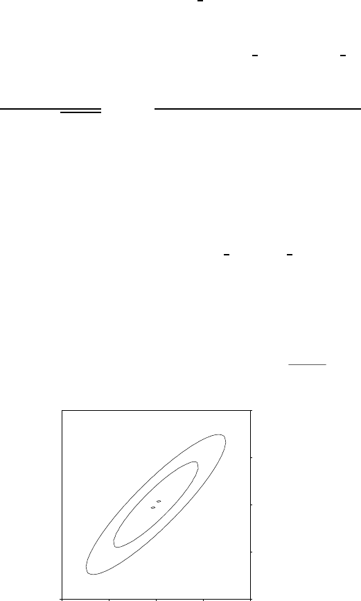
Chapter 19: Random Number Distributions 212
19.4 The Bivariate Gaussian Distribution
[Function]void gsl_ran_bivariate_gaussian (const gsl rng * r, double
sigma_x, double sigma_y, double rho, double * x, double * y)
This function generates a pair of correlated Gaussian variates, with mean zero, cor-
relation coefficient rho and standard deviations sigma xand sigma y in the xand y
directions. The probability distribution for bivariate Gaussian random variates is,
p(x, y)dxdy =1
2πσxσy√1−ρ2exp −(x2/σ2
x+y2/σ2
y−2ρxy/(σxσy))
2(1 −ρ2)!dxdy
for x, y in the range −∞ to +∞. The correlation coefficient rho should lie between 1
and −1.
[Function]double gsl_ran_bivariate_gaussian_pdf (double x, double y,
double sigma_x, double sigma_y, double rho )
This function computes the probability density p(x, y) at (x,y) for a bivariate Gaus-
sian distribution with standard deviations sigma x,sigma y and correlation coeffi-
cient rho, using the formula given above.
y
x
σx= 1, σy= 1, ρ = 0.9
Bivariate Gaussian Distribution
0.70.60.50.40.30.20.10
2
1
0
-1
-2
210-1-2
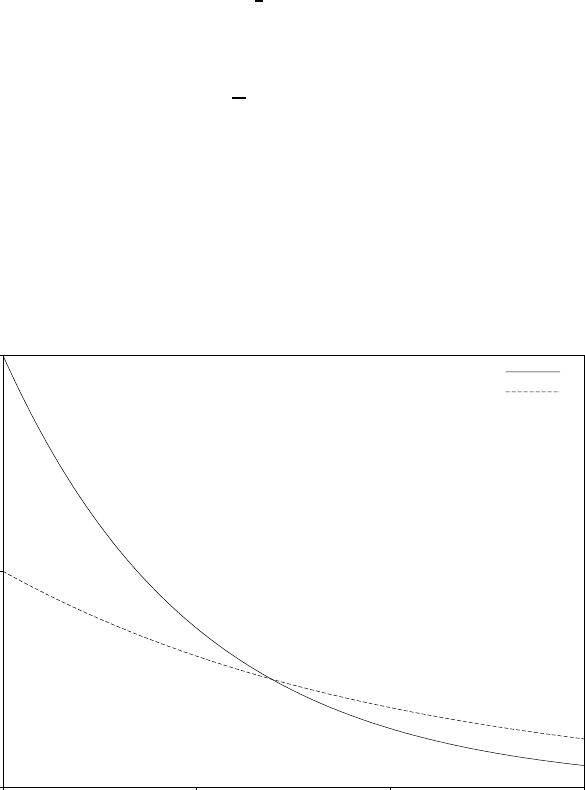
Chapter 19: Random Number Distributions 213
19.5 The Exponential Distribution
[Function]double gsl_ran_exponential (const gsl rng * r, double mu )
This function returns a random variate from the exponential distribution with mean
mu. The distribution is,
p(x)dx =1
µexp(−x/µ)dx
for x≥0.
[Function]double gsl_ran_exponential_pdf (double x, double mu )
This function computes the probability density p(x) at xfor an exponential distribu-
tion with mean mu, using the formula given above.
µ= 2
µ= 1
Exponential Distribution
x
p(x)
3210
1
0.5
0
[Function]double gsl_cdf_exponential_P (double x, double mu )
[Function]double gsl_cdf_exponential_Q (double x, double mu )
[Function]double gsl_cdf_exponential_Pinv (double P, double mu )
[Function]double gsl_cdf_exponential_Qinv (double Q, double mu )
These functions compute the cumulative distribution functions P(x), Q(x) and their
inverses for the exponential distribution with mean mu.
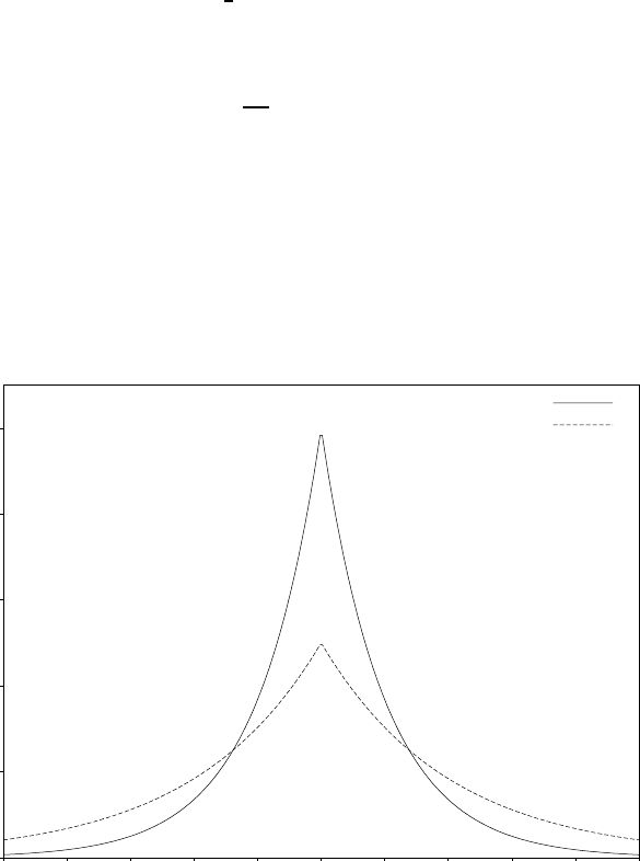
Chapter 19: Random Number Distributions 214
19.6 The Laplace Distribution
[Function]double gsl_ran_laplace (const gsl rng * r, double a)
This function returns a random variate from the Laplace distribution with width a.
The distribution is,
p(x)dx =1
2aexp(−|x/a|)dx
for −∞ < x < ∞.
[Function]double gsl_ran_laplace_pdf (double x, double a)
This function computes the probability density p(x) at xfor a Laplace distribution
with width a, using the formula given above.
a= 2
a= 1
Laplace Distribution (Two-sided Exponential)
x
p(x)
543210-1-2-3-4-5
0.5
0.4
0.3
0.2
0.1
0
[Function]double gsl_cdf_laplace_P (double x, double a)
[Function]double gsl_cdf_laplace_Q (double x, double a)
[Function]double gsl_cdf_laplace_Pinv (double P, double a)
[Function]double gsl_cdf_laplace_Qinv (double Q, double a)
These functions compute the cumulative distribution functions P(x), Q(x) and their
inverses for the Laplace distribution with width a.
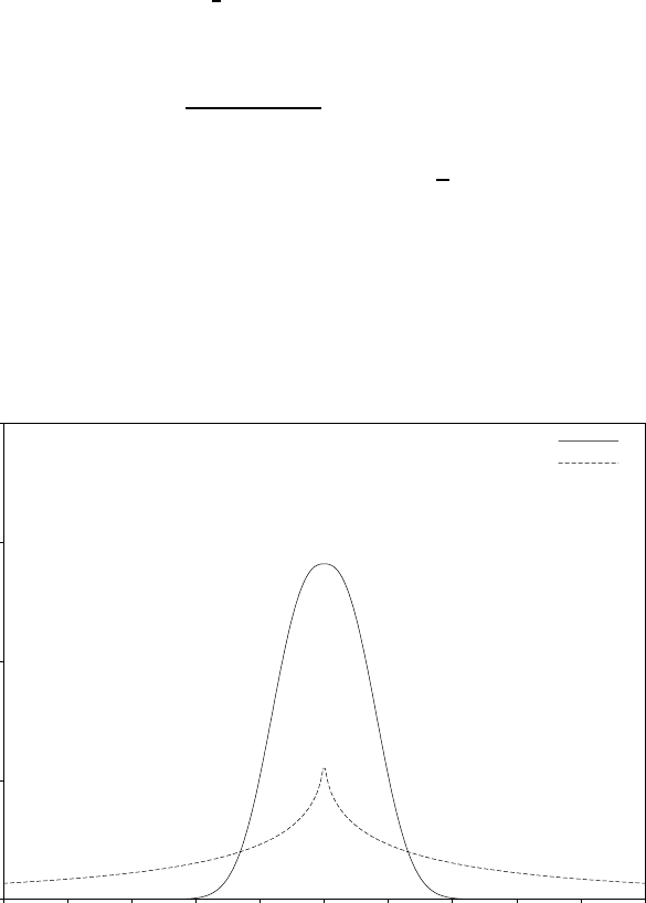
Chapter 19: Random Number Distributions 215
19.7 The Exponential Power Distribution
[Function]double gsl_ran_exppow (const gsl rng * r, double a, double b)
This function returns a random variate from the exponential power distribution with
scale parameter aand exponent b. The distribution is,
p(x)dx =1
2aΓ(1 + 1/b)exp(−|x/a|b)dx
for x≥0. For b= 1 this reduces to the Laplace distribution. For b= 2 it has the
same form as a gaussian distribution, but with a=√2σ.
[Function]double gsl_ran_exppow_pdf (double x, double a, double b)
This function computes the probability density p(x) at xfor an exponential power
distribution with scale parameter aand exponent b, using the formula given above.
a= 1, b = 0.5
a= 1, b = 2.5
Exponential Power Distribution
x
p(x)
543210-1-2-3-4-5
0.8
0.6
0.4
0.2
0
[Function]double gsl_cdf_exppow_P (double x, double a, double b)
[Function]double gsl_cdf_exppow_Q (double x, double a, double b)
These functions compute the cumulative distribution functions P(x), Q(x) for the
exponential power distribution with parameters aand b.
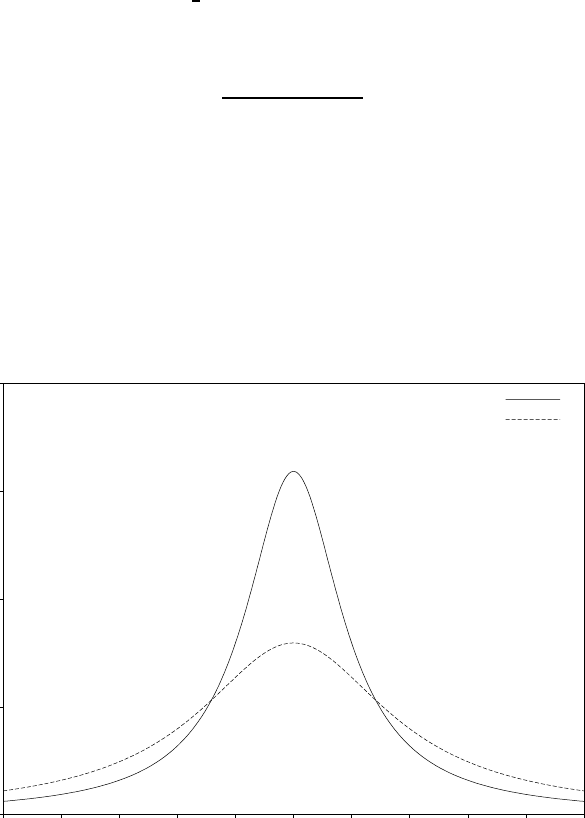
Chapter 19: Random Number Distributions 216
19.8 The Cauchy Distribution
[Function]double gsl_ran_cauchy (const gsl rng * r, double a)
This function returns a random variate from the Cauchy distribution with scale pa-
rameter a. The probability distribution for Cauchy random variates is,
p(x)dx =1
aπ(1 + (x/a)2)dx
for xin the range −∞ to +∞. The Cauchy distribution is also known as the Lorentz
distribution.
[Function]double gsl_ran_cauchy_pdf (double x, double a)
This function computes the probability density p(x) at xfor a Cauchy distribution
with scale parameter a, using the formula given above.
a= 2
a= 1
Cauchy Distribution
x
p(x)
543210-1-2-3-4-5
0.4
0.3
0.2
0.1
0
[Function]double gsl_cdf_cauchy_P (double x, double a)
[Function]double gsl_cdf_cauchy_Q (double x, double a)
[Function]double gsl_cdf_cauchy_Pinv (double P, double a)
[Function]double gsl_cdf_cauchy_Qinv (double Q, double a)
These functions compute the cumulative distribution functions P(x), Q(x) and their
inverses for the Cauchy distribution with scale parameter a.
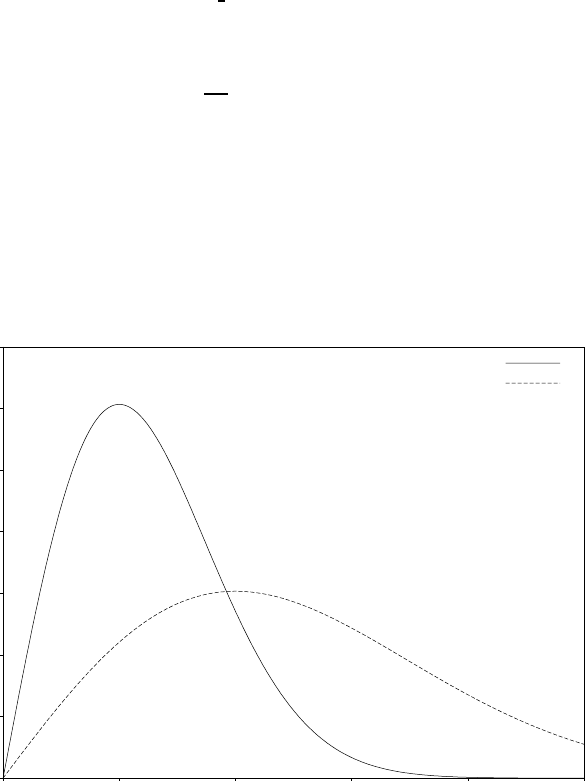
Chapter 19: Random Number Distributions 217
19.9 The Rayleigh Distribution
[Function]double gsl_ran_rayleigh (const gsl rng * r, double sigma )
This function returns a random variate from the Rayleigh distribution with scale
parameter sigma. The distribution is,
p(x)dx =x
σ2exp(−x2/(2σ2))dx
for x > 0.
[Function]double gsl_ran_rayleigh_pdf (double x, double sigma )
This function computes the probability density p(x) at xfor a Rayleigh distribution
with scale parameter sigma, using the formula given above.
σ= 2
σ= 1
Rayleigh Distribution
x
p(x)
543210
0.7
0.6
0.5
0.4
0.3
0.2
0.1
0
[Function]double gsl_cdf_rayleigh_P (double x, double sigma )
[Function]double gsl_cdf_rayleigh_Q (double x, double sigma )
[Function]double gsl_cdf_rayleigh_Pinv (double P, double sigma )
[Function]double gsl_cdf_rayleigh_Qinv (double Q, double sigma )
These functions compute the cumulative distribution functions P(x), Q(x) and their
inverses for the Rayleigh distribution with scale parameter sigma.
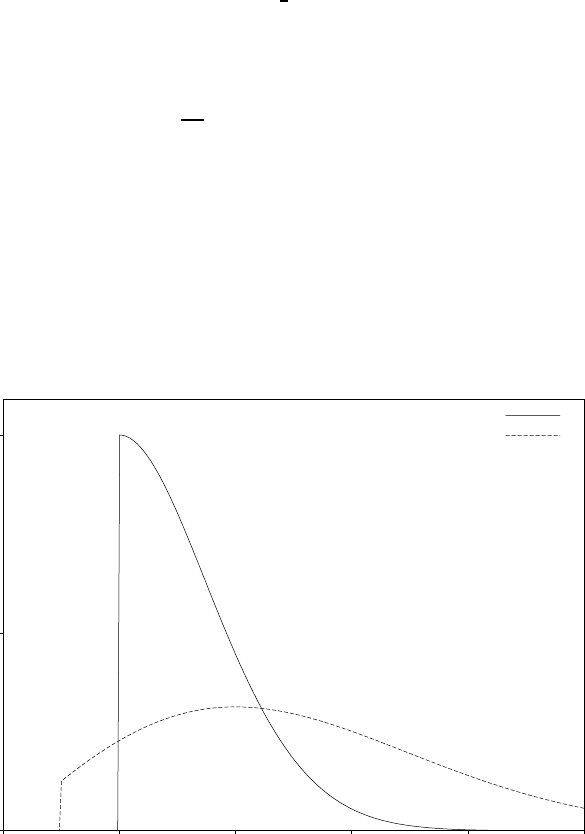
Chapter 19: Random Number Distributions 218
19.10 The Rayleigh Tail Distribution
[Function]double gsl_ran_rayleigh_tail (const gsl rng * r, double a, double
sigma )
This function returns a random variate from the tail of the Rayleigh distribution with
scale parameter sigma and a lower limit of a. The distribution is,
p(x)dx =x
σ2exp((a2−x2)/(2σ2))dx
for x > a.
[Function]double gsl_ran_rayleigh_tail_pdf (double x, double a, double
sigma )
This function computes the probability density p(x) at xfor a Rayleigh tail distribu-
tion with scale parameter sigma and lower limit a, using the formula given above.
a= 0.5, σ = 2
a= 1, σ = 1
Rayleigh Tail Distribution
x
p(x)
543210
1
0.5
0
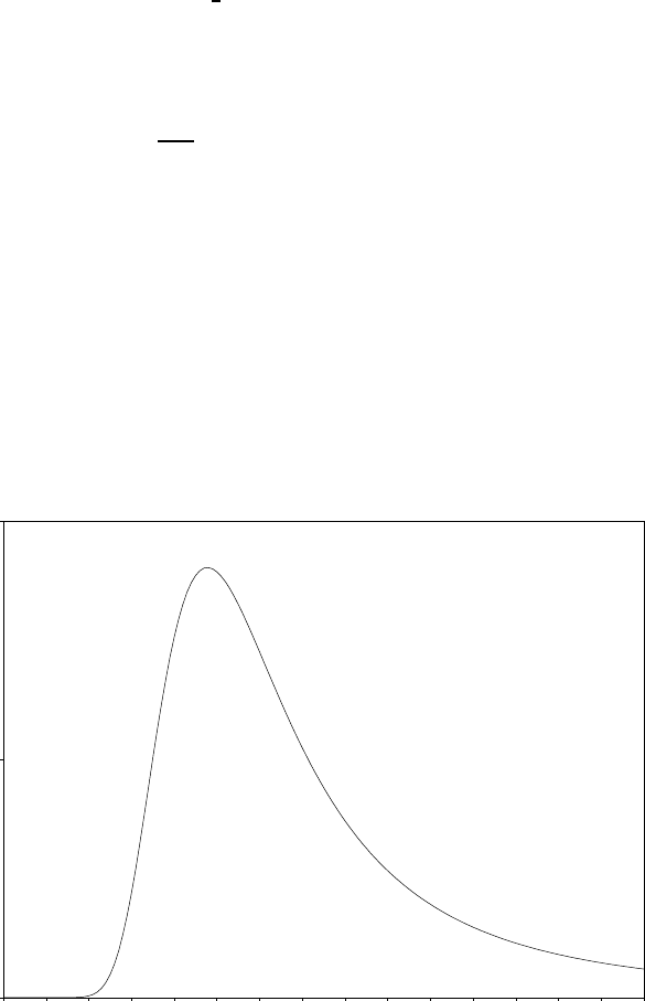
Chapter 19: Random Number Distributions 219
19.11 The Landau Distribution
[Function]double gsl_ran_landau (const gsl rng * r)
This function returns a random variate from the Landau distribution. The proba-
bility distribution for Landau random variates is defined analytically by the complex
integral,
p(x) = 1
2πi Zc+i∞
c−i∞
ds exp(slog(s) + xs)
For numerical purposes it is more convenient to use the following equivalent form of
the integral,
p(x) = (1/π)Z∞
0
dt exp(−tlog(t)−xt) sin(πt).
[Function]double gsl_ran_landau_pdf (double x)
This function computes the probability density p(x) at xfor the Landau distribution
using an approximation to the formula given above.
Landau Distribution
x
p(x)
109876543210-1-2-3-4-5
0.2
0.1
0
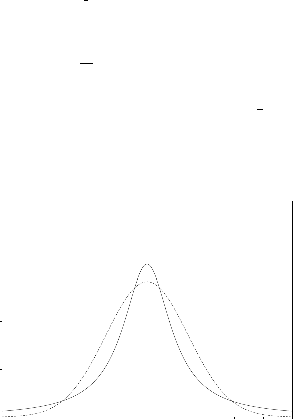
Chapter 19: Random Number Distributions 220
19.12 The Levy alpha-Stable Distributions
[Function]double gsl_ran_levy (const gsl rng * r, double c, double alpha )
This function returns a random variate from the Levy symmetric stable distribution
with scale cand exponent alpha. The symmetric stable probability distribution is
defined by a fourier transform,
p(x) = 1
2πZ+∞
−∞
dt exp(−itx −|ct|α)
There is no explicit solution for the form of p(x) and the library does not define
a corresponding pdf function. For α= 1 the distribution reduces to the Cauchy
distribution. For α= 2 it is a Gaussian distribution with σ=√2c. For α < 1 the
tails of the distribution become extremely wide.
The algorithm only works for 0 < α ≤2.
c= 1, α = 2.0
c= 1, α = 1.0
Levy Distribution
x
p(x)
543210-1-2-3-4-5
0.4
0.3
0.2
0.1
0
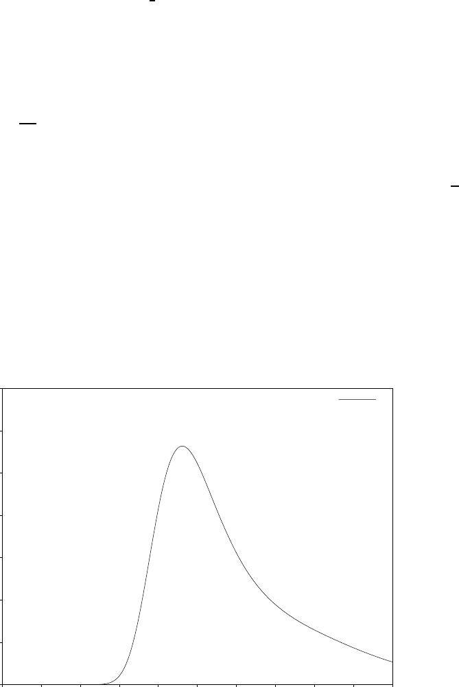
Chapter 19: Random Number Distributions 221
19.13 The Levy skew alpha-Stable Distribution
[Function]double gsl_ran_levy_skew (const gsl rng * r, double c, double alpha,
double beta )
This function returns a random variate from the Levy skew stable distribution with
scale c, exponent alpha and skewness parameter beta. The skewness parameter must
lie in the range [−1,1]. The Levy skew stable probability distribution is defined by a
fourier transform,
p(x) = 1
2πZ+∞
−∞
dt exp(−itx − |ct|α(1 −iβsign(t) tan(πα/2)))
When α= 1 the term tan(πα/2) is replaced by −(2/π) log |t|. There is no explicit
solution for the form of p(x) and the library does not define a corresponding pdf
function. For α= 2 the distribution reduces to a Gaussian distribution with σ=√2c
and the skewness parameter has no effect. For α < 1 the tails of the distribution
become extremely wide. The symmetric distribution corresponds to β= 0.
The algorithm only works for 0 < α ≤2.
The Levy alpha-stable distributions have the property that if Nalpha-stable variates
are drawn from the distribution p(c, α, β) then the sum Y=X1+X2+...+XNwill also
be distributed as an alpha-stable variate, p(N1/αc, α, β).
c= 1, α = 1.0, β = 1.0
Levy Skew Distribution
x
p(x)
543210-1-2-3-4-5
0.35
0.3
0.25
0.2
0.15
0.1
0.05
0
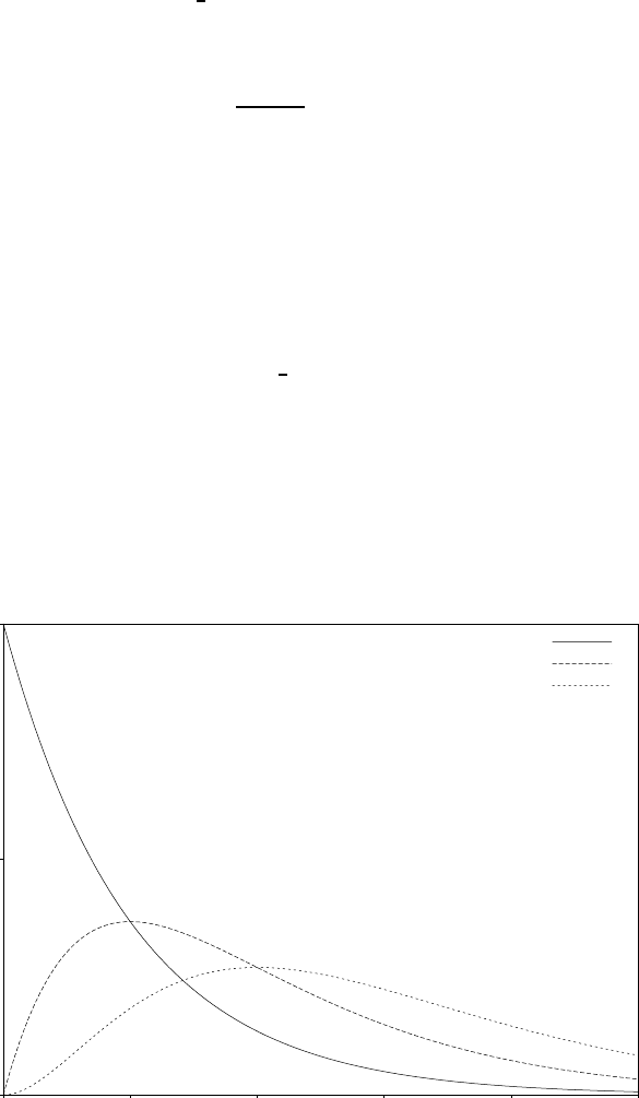
Chapter 19: Random Number Distributions 222
19.14 The Gamma Distribution
[Function]double gsl_ran_gamma (const gsl rng * r, double a, double b)
This function returns a random variate from the gamma distribution. The distribution
function is,
p(x)dx =1
Γ(a)baxa−1e−x/bdx
for x > 0.
The gamma distribution with an integer parameter ais known as the Erlang distri-
bution.
The variates are computed using the Marsaglia-Tsang fast gamma method. This
function for this method was previously called gsl_ran_gamma_mt and can still be
accessed using this name.
[Function]double gsl_ran_gamma_knuth (const gsl rng * r, double a, double b)
This function returns a gamma variate using the algorithms from Knuth (vol 2).
[Function]double gsl_ran_gamma_pdf (double x, double a, double b)
This function computes the probability density p(x) at xfor a gamma distribution
with parameters aand b, using the formula given above.
a= 3
a= 2
a= 1
Gamma Distribution
x
p(x)
543210
1
0.5
0
[Function]double gsl_cdf_gamma_P (double x, double a, double b)
[Function]double gsl_cdf_gamma_Q (double x, double a, double b)
[Function]double gsl_cdf_gamma_Pinv (double P, double a, double b)
Chapter 19: Random Number Distributions 223
[Function]double gsl_cdf_gamma_Qinv (double Q, double a, double b)
These functions compute the cumulative distribution functions P(x), Q(x) and their
inverses for the gamma distribution with parameters aand b.

Chapter 19: Random Number Distributions 224
19.15 The Flat (Uniform) Distribution
[Function]double gsl_ran_flat (const gsl rng * r, double a, double b)
This function returns a random variate from the flat (uniform) distribution from ato
b. The distribution is,
p(x)dx =1
(b−a)dx
if a≤x < b and 0 otherwise.
[Function]double gsl_ran_flat_pdf (double x, double a, double b)
This function computes the probability density p(x) at xfor a uniform distribution
from ato b, using the formula given above.
a= 1.2, b = 4.8
a= 0.5, b = 2.5
Flat Distribution
x
p(x)
543210
1
0.5
0
[Function]double gsl_cdf_flat_P (double x, double a, double b)
[Function]double gsl_cdf_flat_Q (double x, double a, double b)
[Function]double gsl_cdf_flat_Pinv (double P, double a, double b)
[Function]double gsl_cdf_flat_Qinv (double Q, double a, double b)
These functions compute the cumulative distribution functions P(x), Q(x) and their
inverses for a uniform distribution from ato b.
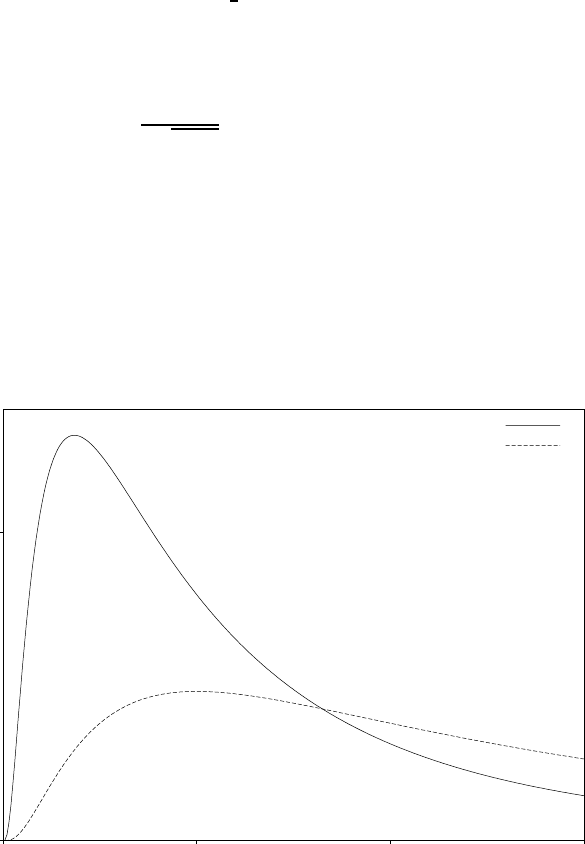
Chapter 19: Random Number Distributions 225
19.16 The Lognormal Distribution
[Function]double gsl_ran_lognormal (const gsl rng * r, double zeta, double
sigma )
This function returns a random variate from the lognormal distribution. The distri-
bution function is,
p(x)dx =1
x√2πσ2exp(−(ln(x)−ζ)2/2σ2)dx
for x > 0.
[Function]double gsl_ran_lognormal_pdf (double x, double zeta, double
sigma )
This function computes the probability density p(x) at xfor a lognormal distribution
with parameters zeta and sigma, using the formula given above.
ζ= 1, σ = 1
ζ= 0, σ = 1
Lognormal Distribution
x
p(x)
3210
0.5
0
[Function]double gsl_cdf_lognormal_P (double x, double zeta, double sigma )
[Function]double gsl_cdf_lognormal_Q (double x, double zeta, double sigma )
[Function]double gsl_cdf_lognormal_Pinv (double P, double zeta, double
sigma )
[Function]double gsl_cdf_lognormal_Qinv (double Q, double zeta, double
sigma )
These functions compute the cumulative distribution functions P(x), Q(x) and their
inverses for the lognormal distribution with parameters zeta and sigma.
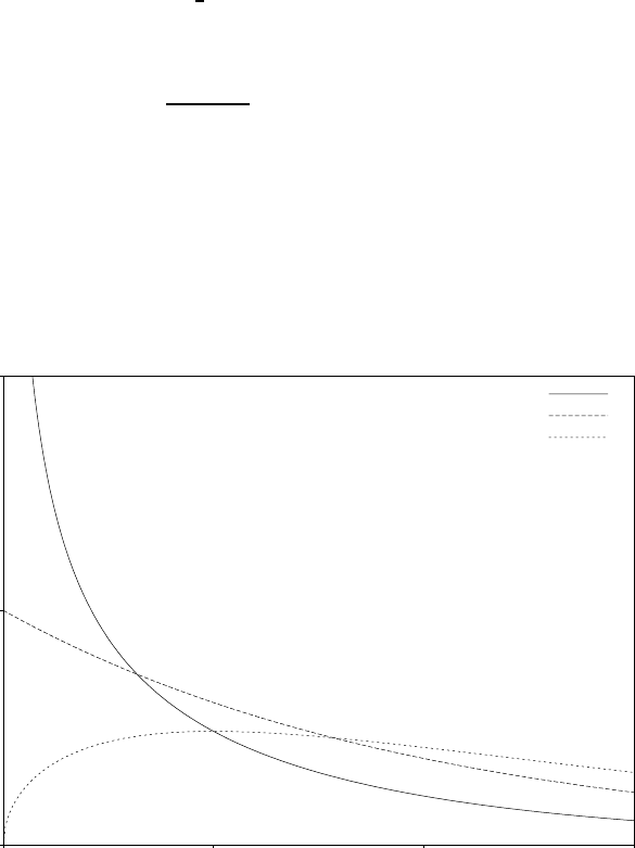
Chapter 19: Random Number Distributions 226
19.17 The Chi-squared Distribution
The chi-squared distribution arises in statistics. If Yiare nindependent gaussian random
variates with unit variance then the sum-of-squares,
Xi=X
i
Y2
i
has a chi-squared distribution with ndegrees of freedom.
[Function]double gsl_ran_chisq (const gsl rng * r, double nu )
This function returns a random variate from the chi-squared distribution with nu
degrees of freedom. The distribution function is,
p(x)dx =1
2Γ(ν/2)(x/2)ν/2−1exp(−x/2)dx
for x≥0.
[Function]double gsl_ran_chisq_pdf (double x, double nu )
This function computes the probability density p(x) at xfor a chi-squared distribution
with nu degrees of freedom, using the formula given above.
ν= 3
ν= 2
ν= 1
Chi-squared Distribution
x
p(x)
3210
1
0.5
0
[Function]double gsl_cdf_chisq_P (double x, double nu )
[Function]double gsl_cdf_chisq_Q (double x, double nu )
[Function]double gsl_cdf_chisq_Pinv (double P, double nu )
[Function]double gsl_cdf_chisq_Qinv (double Q, double nu )
These functions compute the cumulative distribution functions P(x), Q(x) and their
inverses for the chi-squared distribution with nu degrees of freedom.

Chapter 19: Random Number Distributions 227
19.18 The F-distribution
The F-distribution arises in statistics. If Y1and Y2are chi-squared deviates with ν1and ν2
degrees of freedom then the ratio,
X=(Y1/ν1)
(Y2/ν2)
has an F-distribution F(x;ν1, ν2).
[Function]double gsl_ran_fdist (const gsl rng * r, double nu1, double nu2 )
This function returns a random variate from the F-distribution with degrees of free-
dom nu1 and nu2. The distribution function is,
p(x)dx =Γ((ν1+ν2)/2)
Γ(ν1/2)Γ(ν2/2) νν1/2
1νν2/2
2xν1/2−1(ν2+ν1x)−ν1/2−ν2/2
for x≥0.
[Function]double gsl_ran_fdist_pdf (double x, double nu1, double nu2 )
This function computes the probability density p(x) at xfor an F-distribution with
nu1 and nu2 degrees of freedom, using the formula given above.
ν1= 3, ν2= 2
ν1= 1, ν2= 1
F-Distribution
x
p(x)
210
1
0.5
0
[Function]double gsl_cdf_fdist_P (double x, double nu1, double nu2 )
[Function]double gsl_cdf_fdist_Q (double x, double nu1, double nu2 )
[Function]double gsl_cdf_fdist_Pinv (double P, double nu1, double nu2 )
Chapter 19: Random Number Distributions 228
[Function]double gsl_cdf_fdist_Qinv (double Q, double nu1, double nu2 )
These functions compute the cumulative distribution functions P(x), Q(x) and their
inverses for the F-distribution with nu1 and nu2 degrees of freedom.

Chapter 19: Random Number Distributions 229
19.19 The t-distribution
The t-distribution arises in statistics. If Y1has a normal distribution and Y2has a chi-
squared distribution with νdegrees of freedom then the ratio,
X=Y1
pY2/ν
has a t-distribution t(x;ν) with νdegrees of freedom.
[Function]double gsl_ran_tdist (const gsl rng * r, double nu )
This function returns a random variate from the t-distribution. The distribution
function is,
p(x)dx =Γ((ν+ 1)/2)
√πνΓ(ν/2) (1 + x2/ν)−(ν+1)/2dx
for −∞ < x < +∞.
[Function]double gsl_ran_tdist_pdf (double x, double nu )
This function computes the probability density p(x) at xfor a t-distribution with nu
degrees of freedom, using the formula given above.
ν1= 5
ν1= 1
Student’s t distribution
x
p(x)
43210-1-2-3-4
0.5
0.4
0.3
0.2
0.1
0
[Function]double gsl_cdf_tdist_P (double x, double nu )
[Function]double gsl_cdf_tdist_Q (double x, double nu )
[Function]double gsl_cdf_tdist_Pinv (double P, double nu )
Chapter 19: Random Number Distributions 230
[Function]double gsl_cdf_tdist_Qinv (double Q, double nu )
These functions compute the cumulative distribution functions P(x), Q(x) and their
inverses for the t-distribution with nu degrees of freedom.
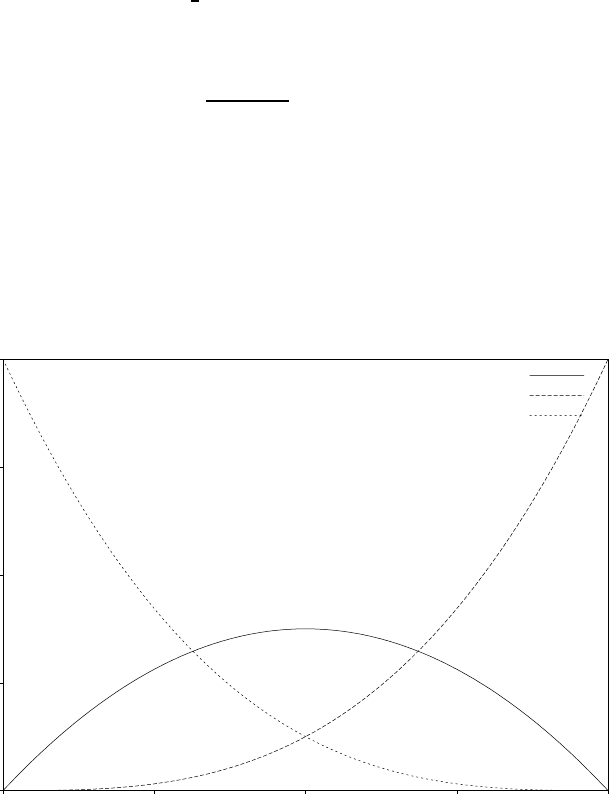
Chapter 19: Random Number Distributions 231
19.20 The Beta Distribution
[Function]double gsl_ran_beta (const gsl rng * r, double a, double b)
This function returns a random variate from the beta distribution. The distribution
function is,
p(x)dx =Γ(a+b)
Γ(a)Γ(b)xa−1(1 −x)b−1dx
for 0 ≤x≤1.
[Function]double gsl_ran_beta_pdf (double x, double a, double b)
This function computes the probability density p(x) at xfor a beta distribution with
parameters aand b, using the formula given above.
a= 1, b = 4
a= 4, b = 1
a= 2, b = 2
Beta Distribution
x
p(x)
10.750.50.250
4
3
2
1
0
[Function]double gsl_cdf_beta_P (double x, double a, double b)
[Function]double gsl_cdf_beta_Q (double x, double a, double b)
[Function]double gsl_cdf_beta_Pinv (double P, double a, double b)
[Function]double gsl_cdf_beta_Qinv (double Q, double a, double b)
These functions compute the cumulative distribution functions P(x), Q(x) and their
inverses for the beta distribution with parameters aand b.
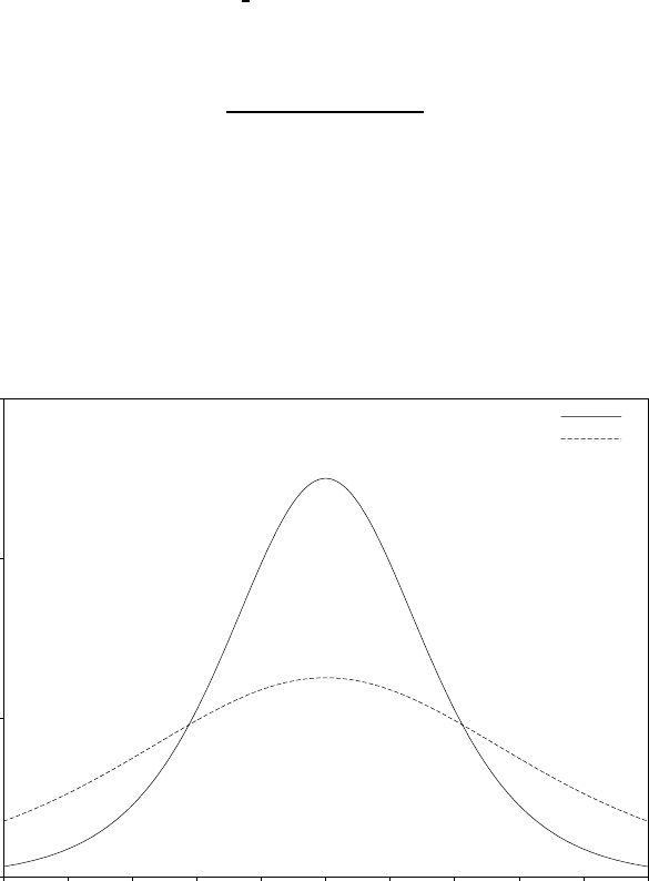
Chapter 19: Random Number Distributions 232
19.21 The Logistic Distribution
[Function]double gsl_ran_logistic (const gsl rng * r, double a)
This function returns a random variate from the logistic distribution. The distribution
function is,
p(x)dx =exp(−x/a)
a(1 + exp(−x/a))2dx
for −∞ < x < +∞.
[Function]double gsl_ran_logistic_pdf (double x, double a)
This function computes the probability density p(x) at xfor a logistic distribution
with scale parameter a, using the formula given above.
a= 2
a= 1
Logistic Distribution
x
p(x)
543210-1-2-3-4-5
0.3
0.2
0.1
0
[Function]double gsl_cdf_logistic_P (double x, double a)
[Function]double gsl_cdf_logistic_Q (double x, double a)
[Function]double gsl_cdf_logistic_Pinv (double P, double a)
[Function]double gsl_cdf_logistic_Qinv (double Q, double a)
These functions compute the cumulative distribution functions P(x), Q(x) and their
inverses for the logistic distribution with scale parameter a.
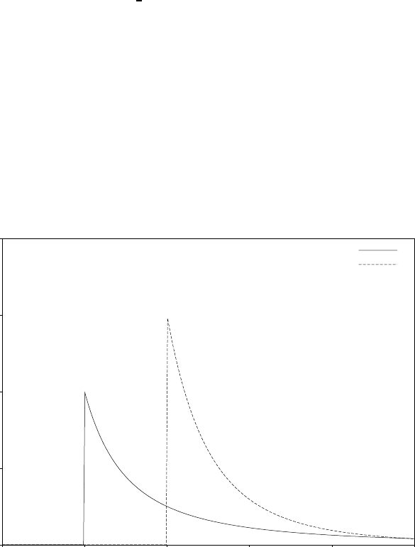
Chapter 19: Random Number Distributions 233
19.22 The Pareto Distribution
[Function]double gsl_ran_pareto (const gsl rng * r, double a, double b)
This function returns a random variate from the Pareto distribution of order a. The
distribution function is,
p(x)dx = (a/b)/(x/b)a+1dx
for x≥b.
[Function]double gsl_ran_pareto_pdf (double x, double a, double b)
This function computes the probability density p(x) at xfor a Pareto distribution
with exponent aand scale b, using the formula given above.
a= 3, b = 2
a= 1, b = 1
Pareto Distribution
x
p(x)
543210
2
1.5
1
0.5
0
[Function]double gsl_cdf_pareto_P (double x, double a, double b)
[Function]double gsl_cdf_pareto_Q (double x, double a, double b)
[Function]double gsl_cdf_pareto_Pinv (double P, double a, double b)
[Function]double gsl_cdf_pareto_Qinv (double Q, double a, double b)
These functions compute the cumulative distribution functions P(x), Q(x) and their
inverses for the Pareto distribution with exponent aand scale b.

Chapter 19: Random Number Distributions 234
19.23 Spherical Vector Distributions
The spherical distributions generate random vectors, located on a spherical surface. They
can be used as random directions, for example in the steps of a random walk.
[Function]void gsl_ran_dir_2d (const gsl rng * r, double * x, double * y)
[Function]void gsl_ran_dir_2d_trig_method (const gsl rng * r, double * x,
double * y)
This function returns a random direction vector v= (x,y) in two dimensions. The
vector is normalized such that |v|2=x2+y2= 1. The obvious way to do this is
to take a uniform random number between 0 and 2πand let xand ybe the sine
and cosine respectively. Two trig functions would have been expensive in the old
days, but with modern hardware implementations, this is sometimes the fastest way
to go. This is the case for the Pentium (but not the case for the Sun Sparcstation).
One can avoid the trig evaluations by choosing xand yin the interior of a unit
circle (choose them at random from the interior of the enclosing square, and then
reject those that are outside the unit circle), and then dividing by √x2+y2. A much
cleverer approach, attributed to von Neumann (See Knuth, v2, 3rd ed, p140, exercise
23), requires neither trig nor a square root. In this approach, uand vare chosen
at random from the interior of a unit circle, and then x= (u2−v2)/(u2+v2) and
y= 2uv/(u2+v2).
[Function]void gsl_ran_dir_3d (const gsl rng * r, double * x, double * y, double
*z)
This function returns a random direction vector v= (x,y,z) in three dimensions. The
vector is normalized such that |v|2=x2+y2+z2= 1. The method employed is due to
Robert E. Knop (CACM 13, 326 (1970)), and explained in Knuth, v2, 3rd ed, p136.
It uses the surprising fact that the distribution projected along any axis is actually
uniform (this is only true for 3 dimensions).
[Function]void gsl_ran_dir_nd (const gsl rng * r, size t n, double * x)
This function returns a random direction vector v= (x1, x2, . . . , xn) in ndimensions.
The vector is normalized such that |v|2=x2
1+x2
2+···+x2
n= 1. The method
uses the fact that a multivariate gaussian distribution is spherically symmetric. Each
component is generated to have a gaussian distribution, and then the components are
normalized. The method is described by Knuth, v2, 3rd ed, p135–136, and attributed
to G. W. Brown, Modern Mathematics for the Engineer (1956).
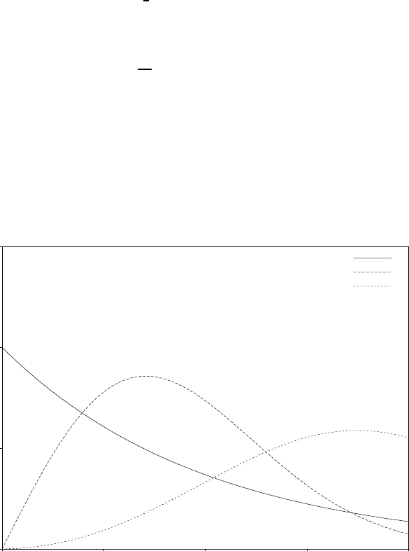
Chapter 19: Random Number Distributions 235
19.24 The Weibull Distribution
[Function]double gsl_ran_weibull (const gsl rng * r, double a, double b)
This function returns a random variate from the Weibull distribution. The distribu-
tion function is,
p(x)dx =b
abxb−1exp(−(x/a)b)dx
for x≥0.
[Function]double gsl_ran_weibull_pdf (double x, double a, double b)
This function computes the probability density p(x) at xfor a Weibull distribution
with scale aand exponent b, using the formula given above.
a= 2, b = 3
a= 1, b = 2
a= 1, b = 1
Weibull Distribution
x
p(x)
21.510.50
1.5
1
0.5
0
[Function]double gsl_cdf_weibull_P (double x, double a, double b)
[Function]double gsl_cdf_weibull_Q (double x, double a, double b)
[Function]double gsl_cdf_weibull_Pinv (double P, double a, double b)
[Function]double gsl_cdf_weibull_Qinv (double Q, double a, double b)
These functions compute the cumulative distribution functions P(x), Q(x) and their
inverses for the Weibull distribution with scale aand exponent b.
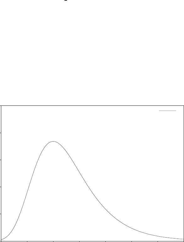
Chapter 19: Random Number Distributions 236
19.25 The Type-1 Gumbel Distribution
[Function]double gsl_ran_gumbel1 (const gsl rng * r, double a, double b)
This function returns a random variate from the Type-1 Gumbel distribution. The
Type-1 Gumbel distribution function is,
p(x)dx =ab exp(−(bexp(−ax) + ax))dx
for −∞ < x < ∞.
[Function]double gsl_ran_gumbel1_pdf (double x, double a, double b)
This function computes the probability density p(x) at xfor a Type-1 Gumbel dis-
tribution with parameters aand b, using the formula given above.
Type 1, a= 1, b = 1
Type 1 Gumbel Distribution
x
p(x)
543210-1-2
0.5
0.4
0.3
0.2
0.1
0
[Function]double gsl_cdf_gumbel1_P (double x, double a, double b)
[Function]double gsl_cdf_gumbel1_Q (double x, double a, double b)
[Function]double gsl_cdf_gumbel1_Pinv (double P, double a, double b)
[Function]double gsl_cdf_gumbel1_Qinv (double Q, double a, double b)
These functions compute the cumulative distribution functions P(x), Q(x) and their
inverses for the Type-1 Gumbel distribution with parameters aand b.
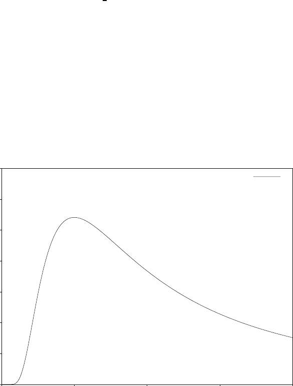
Chapter 19: Random Number Distributions 237
19.26 The Type-2 Gumbel Distribution
[Function]double gsl_ran_gumbel2 (const gsl rng * r, double a, double b)
This function returns a random variate from the Type-2 Gumbel distribution. The
Type-2 Gumbel distribution function is,
p(x)dx =abx−a−1exp(−bx−a)dx
for 0 < x < ∞.
[Function]double gsl_ran_gumbel2_pdf (double x, double a, double b)
This function computes the probability density p(x) at xfor a Type-2 Gumbel dis-
tribution with parameters aand b, using the formula given above.
Type 2, a= 1, b = 1
Type 2 Gumbel Distribution
x
p(x)
21.510.50
0.7
0.6
0.5
0.4
0.3
0.2
0.1
0
[Function]double gsl_cdf_gumbel2_P (double x, double a, double b)
[Function]double gsl_cdf_gumbel2_Q (double x, double a, double b)
[Function]double gsl_cdf_gumbel2_Pinv (double P, double a, double b)
[Function]double gsl_cdf_gumbel2_Qinv (double Q, double a, double b)
These functions compute the cumulative distribution functions P(x), Q(x) and their
inverses for the Type-2 Gumbel distribution with parameters aand b.

Chapter 19: Random Number Distributions 238
19.27 The Dirichlet Distribution
[Function]void gsl_ran_dirichlet (const gsl rng * r, size t K, const double
alpha [], double theta [])
This function returns an array of Krandom variates from a Dirichlet distribution of
order K-1. The distribution function is
p(θ1,...,θK)dθ1···dθK=1
Z
K
Y
i=1
θαi−1
iδ(1 −
K
X
i=1
θi)dθ1···dθK
for θi≥0 and αi>0. The delta function ensures that Pθi= 1. The normalization
factor Zis
Z=QK
i=1 Γ(αi)
Γ(PK
i=1 αi)
The random variates are generated by sampling Kvalues from gamma distributions
with parameters a=αi,b= 1, and renormalizing. See A.M. Law, W.D. Kelton,
Simulation Modeling and Analysis (1991).
[Function]double gsl_ran_dirichlet_pdf (size tK, const double alpha [], const
double theta [])
This function computes the probability density p(θ1,...,θK) at theta[K] for a Dirich-
let distribution with parameters alpha[K], using the formula given above.
[Function]double gsl_ran_dirichlet_lnpdf (size tK, const double alpha [],
const double theta [])
This function computes the logarithm of the probability density p(θ1,...,θK) for a
Dirichlet distribution with parameters alpha[K].

Chapter 19: Random Number Distributions 239
19.28 General Discrete Distributions
Given Kdiscrete events with different probabilities P[k], produce a random value kconsis-
tent with its probability.
The obvious way to do this is to preprocess the probability list by generating a cumulative
probability array with K+ 1 elements:
C[0] = 0
C[k+ 1] = C[k] + P[k].
Note that this construction produces C[K] = 1. Now choose a uniform deviate ubetween
0 and 1, and find the value of ksuch that C[k]≤u < C[k+ 1]. Although this in principle
requires of order log Ksteps per random number generation, they are fast steps, and if you
use something like ⌊uK⌋as a starting point, you can often do pretty well.
But faster methods have been devised. Again, the idea is to preprocess the probability
list, and save the result in some form of lookup table; then the individual calls for a random
discrete event can go rapidly. An approach invented by G. Marsaglia (Generating discrete
random variables in a computer, Comm ACM 6, 37–38 (1963)) is very clever, and readers
interested in examples of good algorithm design are directed to this short and well-written
paper. Unfortunately, for large K, Marsaglia’s lookup table can be quite large.
A much better approach is due to Alastair J. Walker (An efficient method for generating
discrete random variables with general distributions, ACM Trans on Mathematical Software
3, 253–256 (1977); see also Knuth, v2, 3rd ed, p120–121,139). This requires two lookup
tables, one floating point and one integer, but both only of size K. After preprocessing,
the random numbers are generated in O(1) time, even for large K. The preprocessing
suggested by Walker requires O(K2) effort, but that is not actually necessary, and the
implementation provided here only takes O(K) effort. In general, more preprocessing leads
to faster generation of the individual random numbers, but a diminishing return is reached
pretty early. Knuth points out that the optimal preprocessing is combinatorially difficult
for large K.
This method can be used to speed up some of the discrete random number generators be-
low, such as the binomial distribution. To use it for something like the Poisson Distribution,
a modification would have to be made, since it only takes a finite set of Koutcomes.
[Function]gsl_ran_discrete_t * gsl_ran_discrete_preproc (size tK, const
double * P)
This function returns a pointer to a structure that contains the lookup table for the
discrete random number generator. The array P[] contains the probabilities of the
discrete events; these array elements must all be positive, but they needn’t add up
to one (so you can think of them more generally as “weights”)—the preprocessor will
normalize appropriately. This return value is used as an argument for the gsl_ran_
discrete function below.
[Function]size_t gsl_ran_discrete (const gsl rng * r, const gsl ran discrete t *
g)
After the preprocessor, above, has been called, you use this function to get the discrete
random numbers.

Chapter 19: Random Number Distributions 240
[Function]double gsl_ran_discrete_pdf (size t k, const gsl ran discrete t * g)
Returns the probability P[k] of observing the variable k. Since P[k] is not stored as
part of the lookup table, it must be recomputed; this computation takes O(K), so if
Kis large and you care about the original array P[k] used to create the lookup table,
then you should just keep this original array P[k] around.
[Function]void gsl_ran_discrete_free (gsl ran discrete t * g)
De-allocates the lookup table pointed to by g.
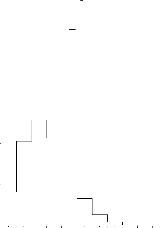
Chapter 19: Random Number Distributions 241
19.29 The Poisson Distribution
[Function]unsigned int gsl_ran_poisson (const gsl rng * r, double mu )
This function returns a random integer from the Poisson distribution with mean mu.
The probability distribution for Poisson variates is,
p(k) = µk
k!exp(−µ)
for k≥0.
[Function]double gsl_ran_poisson_pdf (unsigned int k, double mu )
This function computes the probability p(k) of obtaining kfrom a Poisson distribution
with mean mu, using the formula given above.
µ= 2.5
Poisson Distribution
k
p(k)
109876543210
0.3
0.2
0.1
0
[Function]double gsl_cdf_poisson_P (unsigned int k, double mu )
[Function]double gsl_cdf_poisson_Q (unsigned int k, double mu )
These functions compute the cumulative distribution functions P(k), Q(k) for the
Poisson distribution with parameter mu.

Chapter 19: Random Number Distributions 242
19.30 The Bernoulli Distribution
[Function]unsigned int gsl_ran_bernoulli (const gsl rng * r, double p)
This function returns either 0 or 1, the result of a Bernoulli trial with probability p.
The probability distribution for a Bernoulli trial is,
p(0) = 1 −p
p(1) = p
[Function]double gsl_ran_bernoulli_pdf (unsigned int k, double p)
This function computes the probability p(k) of obtaining kfrom a Bernoulli distribu-
tion with probability parameter p, using the formula given above.
p= 0.7
Bernoulli Trial
k
p(k)
10
1
0.5
0
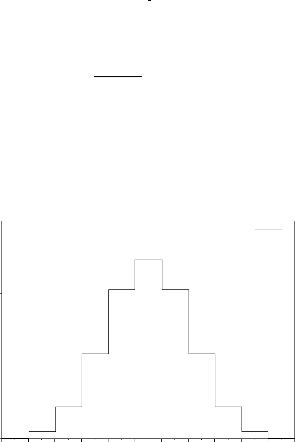
Chapter 19: Random Number Distributions 243
19.31 The Binomial Distribution
[Function]unsigned int gsl_ran_binomial (const gsl rng * r, double p,
unsigned int n)
This function returns a random integer from the binomial distribution, the number
of successes in nindependent trials with probability p. The probability distribution
for binomial variates is,
p(k) = n!
k!(n−k)!pk(1 −p)n−k
for 0 ≤k≤n.
[Function]double gsl_ran_binomial_pdf (unsigned int k, double p, unsigned int
n)
This function computes the probability p(k) of obtaining kfrom a binomial distribu-
tion with parameters pand n, using the formula given above.
p= 0.5, n = 9
Binomial Distribution
k
p(k)
109876543210
0.3
0.2
0.1
0
[Function]double gsl_cdf_binomial_P (unsigned int k, double p, unsigned int n)
[Function]double gsl_cdf_binomial_Q (unsigned int k, double p, unsigned int n)
These functions compute the cumulative distribution functions P(k), Q(k) for the
binomial distribution with parameters pand n.

Chapter 19: Random Number Distributions 244
19.32 The Multinomial Distribution
[Function]void gsl_ran_multinomial (const gsl rng * r, size t K, unsigned int N,
const double p[], unsigned int n[])
This function computes a random sample n[] from the multinomial distribution formed
by Ntrials from an underlying distribution p[K]. The distribution function for n[] is,
P(n1, n2,···, nK) = N!
n1!n2!···nK!pn1
1pn2
2···pnK
K
where (n1,n2,...,nK) are nonnegative integers with PK
k=1 nk=N, and
(p1, p2,...,pK) is a probability distribution with Ppi= 1. If the array p[K] is not
normalized then its entries will be treated as weights and normalized appropriately.
The arrays n[] and p[] must both be of length K.
Random variates are generated using the conditional binomial method (see C.S. Davis,
The computer generation of multinomial random variates, Comp. Stat. Data Anal.
16 (1993) 205–217 for details).
[Function]double gsl_ran_multinomial_pdf (size tK, const double p[], const
unsigned int n[])
This function computes the probability P(n1, n2,...,nK) of sampling n[K] from a
multinomial distribution with parameters p[K], using the formula given above.
[Function]double gsl_ran_multinomial_lnpdf (size tK, const double p[], const
unsigned int n[])
This function returns the logarithm of the probability for the multinomial distribution
P(n1, n2,...,nK) with parameters p[K].

Chapter 19: Random Number Distributions 245
19.33 The Negative Binomial Distribution
[Function]unsigned int gsl_ran_negative_binomial (const gsl rng * r,
double p, double n)
This function returns a random integer from the negative binomial distribution, the
number of failures occurring before nsuccesses in independent trials with probability
pof success. The probability distribution for negative binomial variates is,
p(k) = Γ(n+k)
Γ(k+ 1)Γ(n)pn(1 −p)k
Note that nis not required to be an integer.
[Function]double gsl_ran_negative_binomial_pdf (unsigned int k, double p,
double n)
This function computes the probability p(k) of obtaining kfrom a negative binomial
distribution with parameters pand n, using the formula given above.
p= 0.5, n = 3.5
Negative Binomial Distribution
k
p(k)
109876543210
0.3
0.2
0.1
0
[Function]double gsl_cdf_negative_binomial_P (unsigned int k, double p,
double n)
[Function]double gsl_cdf_negative_binomial_Q (unsigned int k, double p,
double n)
These functions compute the cumulative distribution functions P(k), Q(k) for the
negative binomial distribution with parameters pand n.
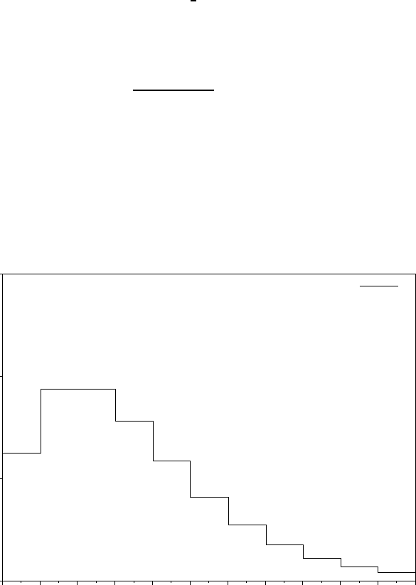
Chapter 19: Random Number Distributions 246
19.34 The Pascal Distribution
[Function]unsigned int gsl_ran_pascal (const gsl rng * r, double p, unsigned
int n)
This function returns a random integer from the Pascal distribution. The Pascal
distribution is simply a negative binomial distribution with an integer value of n.
p(k) = (n+k−1)!
k!(n−1)! pn(1 −p)k
for k≥0
[Function]double gsl_ran_pascal_pdf (unsigned int k, double p, unsigned int n)
This function computes the probability p(k) of obtaining kfrom a Pascal distribution
with parameters pand n, using the formula given above.
p= 0.5, n = 3
Pascal Distribution
k
p(k)
109876543210
0.3
0.2
0.1
0
[Function]double gsl_cdf_pascal_P (unsigned int k, double p, unsigned int n)
[Function]double gsl_cdf_pascal_Q (unsigned int k, double p, unsigned int n)
These functions compute the cumulative distribution functions P(k), Q(k) for the
Pascal distribution with parameters pand n.
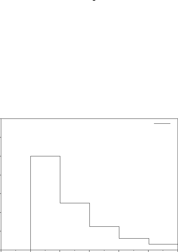
Chapter 19: Random Number Distributions 247
19.35 The Geometric Distribution
[Function]unsigned int gsl_ran_geometric (const gsl rng * r, double p)
This function returns a random integer from the geometric distribution, the num-
ber of independent trials with probability puntil the first success. The probability
distribution for geometric variates is,
p(k) = p(1 −p)k−1
for k≥1. Note that the distribution begins with k= 1 with this definition. There is
another convention in which the exponent k−1 is replaced by k.
[Function]double gsl_ran_geometric_pdf (unsigned int k, double p)
This function computes the probability p(k) of obtaining kfrom a geometric distri-
bution with probability parameter p, using the formula given above.
p= 0.5
Geometric Distribution
k
p(k)
543210
0.7
0.6
0.5
0.4
0.3
0.2
0.1
0
[Function]double gsl_cdf_geometric_P (unsigned int k, double p)
[Function]double gsl_cdf_geometric_Q (unsigned int k, double p)
These functions compute the cumulative distribution functions P(k), Q(k) for the
geometric distribution with parameter p.
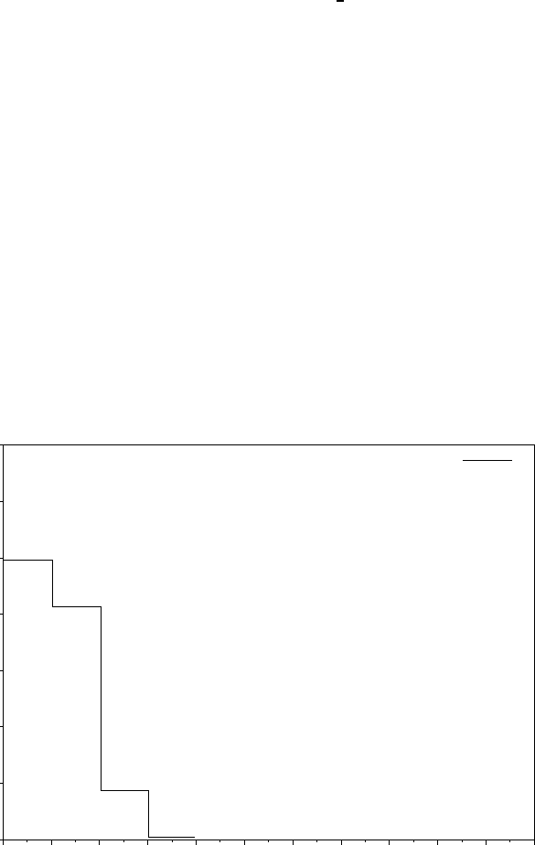
Chapter 19: Random Number Distributions 248
19.36 The Hypergeometric Distribution
[Function]unsigned int gsl_ran_hypergeometric (const gsl rng * r, unsigned
int n1, unsigned int n2, unsigned int t)
This function returns a random integer from the hypergeometric distribution. The
probability distribution for hypergeometric random variates is,
p(k) = C(n1, k)C(n2, t −k)/C(n1+n2, t)
where C(a, b) = a!/(b!(a−b)!) and t≤n1+n2. The domain of kis max(0, t −
n2),...,min(t, n1).
If a population contains n1elements of “type 1” and n2elements of “type 2” then the
hypergeometric distribution gives the probability of obtaining kelements of “type 1”
in tsamples from the population without replacement.
[Function]double gsl_ran_hypergeometric_pdf (unsigned int k, unsigned int
n1, unsigned int n2, unsigned int t)
This function computes the probability p(k) of obtaining kfrom a hypergeometric
distribution with parameters n1,n2,t, using the formula given above.
n1 = 5, n2 = 20, t = 3
Hypergeometric Distribution
k
p(k)
109876543210
0.7
0.6
0.5
0.4
0.3
0.2
0.1
0
[Function]double gsl_cdf_hypergeometric_P (unsigned int k, unsigned int n1,
unsigned int n2, unsigned int t)
[Function]double gsl_cdf_hypergeometric_Q (unsigned int k, unsigned int n1,
unsigned int n2, unsigned int t)
These functions compute the cumulative distribution functions P(k), Q(k) for the
hypergeometric distribution with parameters n1,n2 and t.
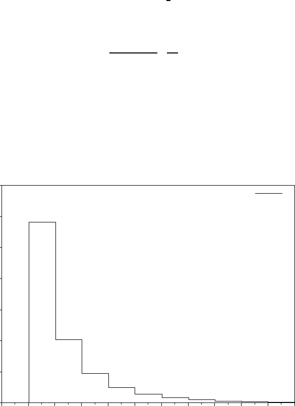
Chapter 19: Random Number Distributions 249
19.37 The Logarithmic Distribution
[Function]unsigned int gsl_ran_logarithmic (const gsl rng * r, double p)
This function returns a random integer from the logarithmic distribution. The prob-
ability distribution for logarithmic random variates is,
p(k) = −1
log(1 −p) pk
k!
for k≥1.
[Function]double gsl_ran_logarithmic_pdf (unsigned int k, double p)
This function computes the probability p(k) of obtaining kfrom a logarithmic distri-
bution with probability parameter p, using the formula given above.
p= 0.7
Logarithmic Distribution
k
p(k)
109876543210
0.7
0.6
0.5
0.4
0.3
0.2
0.1
0

Chapter 19: Random Number Distributions 250
19.38 Shuffling and Sampling
The following functions allow the shuffling and sampling of a set of objects. The algorithms
rely on a random number generator as a source of randomness and a poor quality generator
can lead to correlations in the output. In particular it is important to avoid generators
with a short period. For more information see Knuth, v2, 3rd ed, Section 3.4.2, “Random
Sampling and Shuffling”.
[Function]void gsl_ran_shuffle (const gsl rng * r, void * base, size t n, size t
size )
This function randomly shuffles the order of nobjects, each of size size, stored in the
array base[0..n-1]. The output of the random number generator ris used to produce
the permutation. The algorithm generates all possible n! permutations with equal
probability, assuming a perfect source of random numbers.
The following code shows how to shuffle the numbers from 0 to 51,
int a[52];
for (i = 0; i < 52; i++)
{
a[i] = i;
}
gsl_ran_shuffle (r, a, 52, sizeof (int));
[Function]int gsl_ran_choose (const gsl rng * r, void * dest, size t k, void *
src, size tn, size t size )
This function fills the array dest[k] with kobjects taken randomly from the nelements
of the array src[0..n-1]. The objects are each of size size. The output of the random
number generator ris used to make the selection. The algorithm ensures all possible
samples are equally likely, assuming a perfect source of randomness.
The objects are sampled without replacement, thus each object can only appear once
in dest[k]. It is required that kbe less than or equal to n. The objects in dest will be
in the same relative order as those in src. You will need to call gsl_ran_shuffle(r,
dest, n, size) if you want to randomize the order.
The following code shows how to select a random sample of three unique numbers
from the set 0 to 99,
double a[3], b[100];
for (i = 0; i < 100; i++)
{
b[i] = (double) i;
}
gsl_ran_choose (r, a, 3, b, 100, sizeof (double));

Chapter 19: Random Number Distributions 251
[Function]void gsl_ran_sample (const gsl rng * r, void * dest, size t k, void *
src, size tn, size t size )
This function is like gsl_ran_choose but samples kitems from the original array of
nitems src with replacement, so the same object can appear more than once in the
output sequence dest. There is no requirement that kbe less than nin this case.
19.39 Examples
The following program demonstrates the use of a random number generator to produce
variates from a distribution. It prints 10 samples from the Poisson distribution with a
mean of 3.
#include <stdio.h>
#include <gsl/gsl_rng.h>
#include <gsl/gsl_randist.h>
int
main (void)
{
const gsl_rng_type * T;
gsl_rng * r;
int i, n = 10;
double mu = 3.0;
/* create a generator chosen by the
environment variable GSL_RNG_TYPE */
gsl_rng_env_setup();
T = gsl_rng_default;
r = gsl_rng_alloc (T);
/* print n random variates chosen from
the poisson distribution with mean
parameter mu */
for (i = 0; i < n; i++)
{
unsigned int k = gsl_ran_poisson (r, mu);
printf (" %u", k);
}
printf ("\n");
gsl_rng_free (r);
return 0;
}
Chapter 19: Random Number Distributions 252
If the library and header files are installed under ‘/usr/local’ (the default location) then
the program can be compiled with these options,
$ gcc -Wall demo.c -lgsl -lgslcblas -lm
Here is the output of the program,
$ ./a.out
2 5 5 2 1 0 3 4 1 1
The variates depend on the seed used by the generator. The seed for the default generator
type gsl_rng_default can be changed with the GSL_RNG_SEED environment variable to
produce a different stream of variates,
$ GSL_RNG_SEED=123 ./a.out
GSL_RNG_SEED=123
4 5 6 3 3 1 4 2 5 5
The following program generates a random walk in two dimensions.
#include <stdio.h>
#include <gsl/gsl_rng.h>
#include <gsl/gsl_randist.h>
int
main (void)
{
int i;
double x = 0, y = 0, dx, dy;
const gsl_rng_type * T;
gsl_rng * r;
gsl_rng_env_setup();
T = gsl_rng_default;
r = gsl_rng_alloc (T);
printf ("%g %g\n", x, y);
for (i = 0; i < 10; i++)
{
gsl_ran_dir_2d (r, &dx, &dy);
x += dx; y += dy;
printf ("%g %g\n", x, y);
}
gsl_rng_free (r);
return 0;
}
Here is some output from the program, four 10-step random walks from the origin,
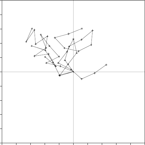
Chapter 19: Random Number Distributions 253
Random walks
543210-1-2-3-4-5
5
4
3
2
1
0
-1
-2
-3
-4
-5
The following program computes the upper and lower cumulative distribution functions
for the standard normal distribution at x= 2.
#include <stdio.h>
#include <gsl/gsl_cdf.h>
int
main (void)
{
double P, Q;
double x = 2.0;
P = gsl_cdf_ugaussian_P (x);
printf ("prob(x < %f) = %f\n", x, P);
Q = gsl_cdf_ugaussian_Q (x);
printf ("prob(x > %f) = %f\n", x, Q);
x = gsl_cdf_ugaussian_Pinv (P);
printf ("Pinv(%f) = %f\n", P, x);
x = gsl_cdf_ugaussian_Qinv (Q);
printf ("Qinv(%f) = %f\n", Q, x);
return 0;
}
Here is the output of the program,
Chapter 19: Random Number Distributions 254
prob(x < 2.000000) = 0.977250
prob(x > 2.000000) = 0.022750
Pinv(0.977250) = 2.000000
Qinv(0.022750) = 2.000000
19.40 References and Further Reading
For an encyclopaedic coverage of the subject readers are advised to consult the book Non-
Uniform Random Variate Generation by Luc Devroye. It covers every imaginable distribu-
tion and provides hundreds of algorithms.
Luc Devroye, Non-Uniform Random Variate Generation, Springer-Verlag, ISBN 0-387-
96305-7. Available online at http://cg.scs.carleton.ca/~luc/rnbookindex.html.
The subject of random variate generation is also reviewed by Knuth, who describes algo-
rithms for all the major distributions.
Donald E. Knuth, The Art of Computer Programming: Seminumerical Algorithms (Vol
2, 3rd Ed, 1997), Addison-Wesley, ISBN 0201896842.
The Particle Data Group provides a short review of techniques for generating distributions
of random numbers in the “Monte Carlo” section of its Annual Review of Particle Physics.
Review of Particle Properties R.M. Barnett et al., Physical Review D54, 1 (1996)
http://pdg.lbl.gov/.
The Review of Particle Physics is available online in postscript and pdf format.
An overview of methods used to compute cumulative distribution functions can be found
in Statistical Computing by W.J. Kennedy and J.E. Gentle. Another general reference is
Elements of Statistical Computing by R.A. Thisted.
William E. Kennedy and James E. Gentle, Statistical Computing (1980), Marcel
Dekker, ISBN 0-8247-6898-1.
Ronald A. Thisted, Elements of Statistical Computing (1988), Chapman & Hall, ISBN
0-412-01371-1.
The cumulative distribution functions for the Gaussian distribution are based on the fol-
lowing papers,
Rational Chebyshev Approximations Using Linear Equations, W.J. Cody, W. Fraser,
J.F. Hart. Numerische Mathematik 12, 242–251 (1968).
Rational Chebyshev Approximations for the Error Function, W.J. Cody. Mathematics
of Computation 23, n107, 631–637 (July 1969).

Chapter 20: Statistics 255
20 Statistics
This chapter describes the statistical functions in the library. The basic statistical functions
include routines to compute the mean, variance and standard deviation. More advanced
functions allow you to calculate absolute deviations, skewness, and kurtosis as well as the
median and arbitrary percentiles. The algorithms use recurrence relations to compute
average quantities in a stable way, without large intermediate values that might overflow.
The functions are available in versions for datasets in the standard floating-point
and integer types. The versions for double precision floating-point data have the prefix
gsl_stats and are declared in the header file ‘gsl_statistics_double.h’. The versions
for integer data have the prefix gsl_stats_int and are declared in the header file
‘gsl_statistics_int.h’. All the functions operate on C arrays with a stride parameter
specifying the spacing between elements.
20.1 Mean, Standard Deviation and Variance
[Function]double gsl_stats_mean (const double data [], size tstride, size t n)
This function returns the arithmetic mean of data, a dataset of length nwith stride
stride. The arithmetic mean, or sample mean, is denoted by ˆµand defined as,
ˆµ=1
NXxi
where xiare the elements of the dataset data. For samples drawn from a gaussian
distribution the variance of ˆµis σ2/N.
[Function]double gsl_stats_variance (const double data [], size tstride,
size t n)
This function returns the estimated, or sample, variance of data, a dataset of length
nwith stride stride. The estimated variance is denoted by ˆσ2and is defined by,
ˆσ2=1
(N−1) X(xi−ˆµ)2
where xiare the elements of the dataset data. Note that the normalization factor of
1/(N−1) results from the derivation of ˆσ2as an unbiased estimator of the population
variance σ2. For samples drawn from a gaussian distribution the variance of ˆσ2itself
is 2σ4/N.
This function computes the mean via a call to gsl_stats_mean. If you have already
computed the mean then you can pass it directly to gsl_stats_variance_m.
[Function]double gsl_stats_variance_m (const double data [], size tstride,
size t n, double mean )
This function returns the sample variance of data relative to the given value of mean.
The function is computed with ˆµreplaced by the value of mean that you supply,
ˆσ2=1
(N−1) X(xi−mean)2
[Function]double gsl_stats_sd (const double data [], size tstride, size t n)

Chapter 20: Statistics 256
[Function]double gsl_stats_sd_m (const double data [], size t stride, size t n,
double mean )
The standard deviation is defined as the square root of the variance. These functions
return the square root of the corresponding variance functions above.
[Function]double gsl_stats_tss (const double data [], size tstride, size t n)
[Function]double gsl_stats_tss_m (const double data [], size t stride, size t n,
double mean )
These functions return the total sum of squares (TSS) of data about the mean. For
gsl_stats_tss_m the user-supplied value of mean is used, and for gsl_stats_tss it
is computed using gsl_stats_mean.
TSS = X(xi−mean)2
[Function]double gsl_stats_variance_with_fixed_mean (const double
data [], size tstride, size t n, double mean )
This function computes an unbiased estimate of the variance of data when the pop-
ulation mean mean of the underlying distribution is known a priori. In this case the
estimator for the variance uses the factor 1/N and the sample mean ˆµis replaced by
the known population mean µ,
ˆσ2=1
NX(xi−µ)2
[Function]double gsl_stats_sd_with_fixed_mean (const double data [], size t
stride, size tn, double mean )
This function calculates the standard deviation of data for a fixed population mean
mean. The result is the square root of the corresponding variance function.
20.2 Absolute deviation
[Function]double gsl_stats_absdev (const double data [], size tstride, size t
n)
This function computes the absolute deviation from the mean of data, a dataset of
length nwith stride stride. The absolute deviation from the mean is defined as,
absdev =1
NX|xi−ˆµ|
where xiare the elements of the dataset data. The absolute deviation from the mean
provides a more robust measure of the width of a distribution than the variance. This
function computes the mean of data via a call to gsl_stats_mean.
[Function]double gsl_stats_absdev_m (const double data [], size tstride,
size tn, double mean )
This function computes the absolute deviation of the dataset data relative to the
given value of mean,
absdev =1
NX|xi−mean|

Chapter 20: Statistics 257
This function is useful if you have already computed the mean of data (and want to
avoid recomputing it), or wish to calculate the absolute deviation relative to another
value (such as zero, or the median).
20.3 Higher moments (skewness and kurtosis)
[Function]double gsl_stats_skew (const double data [], size tstride, size t n)
This function computes the skewness of data, a dataset of length nwith stride stride.
The skewness is defined as,
skew =1
NXxi−ˆµ
ˆσ3
where xiare the elements of the dataset data. The skewness measures the asymmetry
of the tails of a distribution.
The function computes the mean and estimated standard deviation of data via calls
to gsl_stats_mean and gsl_stats_sd.
[Function]double gsl_stats_skew_m_sd (const double data [], size tstride,
size t n, double mean, double sd )
This function computes the skewness of the dataset data using the given values of the
mean mean and standard deviation sd,
skew =1
NXxi−mean
sd 3
These functions are useful if you have already computed the mean and standard
deviation of data and want to avoid recomputing them.
[Function]double gsl_stats_kurtosis (const double data [], size tstride,
size tn)
This function computes the kurtosis of data, a dataset of length nwith stride stride.
The kurtosis is defined as,
kurtosis = 1
NXxi−ˆµ
ˆσ4!−3
The kurtosis measures how sharply peaked a distribution is, relative to its width. The
kurtosis is normalized to zero for a gaussian distribution.
[Function]double gsl_stats_kurtosis_m_sd (const double data [], size t
stride, size t n, double mean, double sd )
This function computes the kurtosis of the dataset data using the given values of the
mean mean and standard deviation sd,
kurtosis =1
N Xxi−mean
sd 4!−3
This function is useful if you have already computed the mean and standard deviation
of data and want to avoid recomputing them.

Chapter 20: Statistics 258
20.4 Autocorrelation
[Function]double gsl_stats_lag1_autocorrelation (const double data [],
const size tstride, const size t n)
This function computes the lag-1 autocorrelation of the dataset data.
a1=Pn
i=1(xi−ˆµ)(xi−1−ˆµ)
Pn
i=1(xi−ˆµ)(xi−ˆµ)
[Function]double gsl_stats_lag1_autocorrelation_m (const double data [],
const size tstride, const size t n, const double mean )
This function computes the lag-1 autocorrelation of the dataset data using the given
value of the mean mean.
20.5 Covariance
[Function]double gsl_stats_covariance (const double data1 [], const size t
stride1, const double data2 [], const size tstride2, const size t n)
This function computes the covariance of the datasets data1 and data2 which must
both be of the same length n.
covar =1
(n−1)
n
X
i=1
(xi−ˆx)(yi−ˆy)
[Function]double gsl_stats_covariance_m (const double data1 [], const size t
stride1, const double data2 [], const size t stride2, const size t n, const
double mean1, const double mean2 )
This function computes the covariance of the datasets data1 and data2 using the
given values of the means, mean1 and mean2. This is useful if you have already
computed the means of data1 and data2 and want to avoid recomputing them.
20.6 Correlation
[Function]double gsl_stats_correlation (const double data1 [], const size t
stride1, const double data2 [], const size t stride2, const size t n)
This function efficiently computes the Pearson correlation coefficient between the
datasets data1 and data2 which must both be of the same length n.
r=cov(x, y)
ˆσxˆσy
=
1
n−1P(xi−ˆx)(yi−ˆy)
q1
n−1P(xi−ˆx)2q1
n−1P(yi−ˆy)2
20.7 Weighted Samples
The functions described in this section allow the computation of statistics for weighted
samples. The functions accept an array of samples, xi, with associated weights, wi. Each
sample xiis considered as having been drawn from a Gaussian distribution with variance
σ2
i. The sample weight wiis defined as the reciprocal of this variance, wi= 1/σ2
i. Setting
a weight to zero corresponds to removing a sample from a dataset.

Chapter 20: Statistics 259
[Function]double gsl_stats_wmean (const double w[], size t wstride, const
double data [], size tstride, size t n)
This function returns the weighted mean of the dataset data with stride stride and
length n, using the set of weights wwith stride wstride and length n. The weighted
mean is defined as,
ˆµ=Pwixi
Pwi
[Function]double gsl_stats_wvariance (const double w[], size twstride, const
double data [], size tstride, size t n)
This function returns the estimated variance of the dataset data with stride stride and
length n, using the set of weights wwith stride wstride and length n. The estimated
variance of a weighted dataset is calculated as,
ˆσ2=Pwi
(Pwi)2−P(w2
i)Xwi(xi−ˆµ)2
Note that this expression reduces to an unweighted variance with the familiar 1/(N−
1) factor when there are Nequal non-zero weights.
[Function]double gsl_stats_wvariance_m (const double w[], size twstride,
const double data [], size tstride, size t n, double wmean )
This function returns the estimated variance of the weighted dataset data using the
given weighted mean wmean.
[Function]double gsl_stats_wsd (const double w[], size twstride, const double
data [], size tstride, size t n)
The standard deviation is defined as the square root of the variance. This function
returns the square root of the corresponding variance function gsl_stats_wvariance
above.
[Function]double gsl_stats_wsd_m (const double w[], size twstride, const
double data [], size tstride, size t n, double wmean )
This function returns the square root of the corresponding variance function gsl_
stats_wvariance_m above.
[Function]double gsl_stats_wvariance_with_fixed_mean (const double w[],
size t wstride, const double data [], size t stride, size t n, const double
mean )
This function computes an unbiased estimate of the variance of the weighted dataset
data when the population mean mean of the underlying distribution is known a priori.
In this case the estimator for the variance replaces the sample mean ˆµby the known
population mean µ,
ˆσ2=Pwi(xi−µ)2
Pwi
[Function]double gsl_stats_wsd_with_fixed_mean (const double w[], size t
wstride, const double data [], size t stride, size t n, const double mean )
The standard deviation is defined as the square root of the variance. This function
returns the square root of the corresponding variance function above.

Chapter 20: Statistics 260
[Function]double gsl_stats_wtss (const double w[], const size t wstride, const
double data [], size tstride, size t n)
[Function]double gsl_stats_wtss_m (const double w[], const size t wstride,
const double data [], size t stride, size t n, double wmean )
These functions return the weighted total sum of squares (TSS) of data about the
weighted mean. For gsl_stats_wtss_m the user-supplied value of wmean is used,
and for gsl_stats_wtss it is computed using gsl_stats_wmean.
TSS = Xwi(xi−wmean)2
[Function]double gsl_stats_wabsdev (const double w[], size twstride, const
double data [], size t stride, size t n)
This function computes the weighted absolute deviation from the weighted mean of
data. The absolute deviation from the mean is defined as,
absdev =Pwi|xi−ˆµ|
Pwi
[Function]double gsl_stats_wabsdev_m (const double w[], size twstride, const
double data [], size tstride, size t n, double wmean )
This function computes the absolute deviation of the weighted dataset data about
the given weighted mean wmean.
[Function]double gsl_stats_wskew (const double w[], size twstride, const
double data [], size tstride, size t n)
This function computes the weighted skewness of the dataset data.
skew =Pwi((xi−ˆx)/ˆσ)3
Pwi
[Function]double gsl_stats_wskew_m_sd (const double w[], size twstride,
const double data [], size tstride, size t n, double wmean, double wsd )
This function computes the weighted skewness of the dataset data using the given
values of the weighted mean and weighted standard deviation, wmean and wsd.
[Function]double gsl_stats_wkurtosis (const double w[], size twstride, const
double data [], size tstride, size t n)
This function computes the weighted kurtosis of the dataset data.
kurtosis =Pwi((xi−ˆx)/ˆσ)4
Pwi−3
[Function]double gsl_stats_wkurtosis_m_sd (const double w[], size twstride,
const double data [], size tstride, size t n, double wmean, double wsd )
This function computes the weighted kurtosis of the dataset data using the given
values of the weighted mean and weighted standard deviation, wmean and wsd.

Chapter 20: Statistics 261
20.8 Maximum and Minimum values
The following functions find the maximum and minimum values of a dataset (or their
indices). If the data contains NaNs then a NaN will be returned, since the maximum or
minimum value is undefined. For functions which return an index, the location of the first
NaN in the array is returned.
[Function]double gsl_stats_max (const double data [], size tstride, size t n)
This function returns the maximum value in data, a dataset of length nwith stride
stride. The maximum value is defined as the value of the element xiwhich satisfies
xi≥xjfor all j.
If you want instead to find the element with the largest absolute magnitude you will
need to apply fabs or abs to your data before calling this function.
[Function]double gsl_stats_min (const double data [], size tstride, size t n)
This function returns the minimum value in data, a dataset of length nwith stride
stride. The minimum value is defined as the value of the element xiwhich satisfies
xi≤xjfor all j.
If you want instead to find the element with the smallest absolute magnitude you will
need to apply fabs or abs to your data before calling this function.
[Function]void gsl_stats_minmax (double * min, double * max, const double
data [], size tstride, size t n)
This function finds both the minimum and maximum values min,max in data in a
single pass.
[Function]size_t gsl_stats_max_index (const double data [], size t stride,
size tn)
This function returns the index of the maximum value in data, a dataset of length
nwith stride stride. The maximum value is defined as the value of the element xi
which satisfies xi≥xjfor all j. When there are several equal maximum elements
then the first one is chosen.
[Function]size_t gsl_stats_min_index (const double data [], size tstride,
size t n)
This function returns the index of the minimum value in data, a dataset of length n
with stride stride. The minimum value is defined as the value of the element xiwhich
satisfies xi≥xjfor all j. When there are several equal minimum elements then the
first one is chosen.
[Function]void gsl_stats_minmax_index (size t * min_index, size t *
max_index, const double data [], size tstride, size t n)
This function returns the indexes min index,max index of the minimum and maxi-
mum values in data in a single pass.
20.9 Median and Percentiles
The median and percentile functions described in this section operate on sorted data. For
convenience we use quantiles, measured on a scale of 0 to 1, instead of percentiles (which
use a scale of 0 to 100).

Chapter 20: Statistics 262
[Function]double gsl_stats_median_from_sorted_data (const double
sorted_data [], size tstride, size t n)
This function returns the median value of sorted data, a dataset of length nwith
stride stride. The elements of the array must be in ascending numerical order. There
are no checks to see whether the data are sorted, so the function gsl_sort should
always be used first.
When the dataset has an odd number of elements the median is the value of element
(n−1)/2. When the dataset has an even number of elements the median is the mean
of the two nearest middle values, elements (n−1)/2 and n/2. Since the algorithm for
computing the median involves interpolation this function always returns a floating-
point number, even for integer data types.
[Function]double gsl_stats_quantile_from_sorted_data (const double
sorted_data [], size tstride, size t n, double f)
This function returns a quantile value of sorted data, a double-precision array of
length nwith stride stride. The elements of the array must be in ascending numerical
order. The quantile is determined by the f, a fraction between 0 and 1. For example,
to compute the value of the 75th percentile fshould have the value 0.75.
There are no checks to see whether the data are sorted, so the function gsl_sort
should always be used first.
The quantile is found by interpolation, using the formula
quantile = (1 −δ)xi+δxi+1
where iis floor((n−1)f) and δis (n−1)f−i.
Thus the minimum value of the array (data[0*stride]) is given by fequal to zero,
the maximum value (data[(n-1)*stride]) is given by fequal to one and the median
value is given by fequal to 0.5. Since the algorithm for computing quantiles involves
interpolation this function always returns a floating-point number, even for integer
data types.
20.10 Examples
Here is a basic example of how to use the statistical functions:
#include <stdio.h>
#include <gsl/gsl_statistics.h>
int
main(void)
{
double data[5] = {17.2, 18.1, 16.5, 18.3, 12.6};
double mean, variance, largest, smallest;
mean = gsl_stats_mean(data, 1, 5);
variance = gsl_stats_variance(data, 1, 5);
largest = gsl_stats_max(data, 1, 5);
smallest = gsl_stats_min(data, 1, 5);
Chapter 20: Statistics 263
printf ("The dataset is %g, %g, %g, %g, %g\n",
data[0], data[1], data[2], data[3], data[4]);
printf ("The sample mean is %g\n", mean);
printf ("The estimated variance is %g\n", variance);
printf ("The largest value is %g\n", largest);
printf ("The smallest value is %g\n", smallest);
return 0;
}
The program should produce the following output,
The dataset is 17.2, 18.1, 16.5, 18.3, 12.6
The sample mean is 16.54
The estimated variance is 4.2984
The largest value is 18.3
The smallest value is 12.6
Here is an example using sorted data,
#include <stdio.h>
#include <gsl/gsl_sort.h>
#include <gsl/gsl_statistics.h>
int
main(void)
{
double data[5] = {17.2, 18.1, 16.5, 18.3, 12.6};
double median, upperq, lowerq;
printf ("Original dataset: %g, %g, %g, %g, %g\n",
data[0], data[1], data[2], data[3], data[4]);
gsl_sort (data, 1, 5);
printf ("Sorted dataset: %g, %g, %g, %g, %g\n",
data[0], data[1], data[2], data[3], data[4]);
median
= gsl_stats_median_from_sorted_data (data,
1, 5);
upperq
= gsl_stats_quantile_from_sorted_data (data,
1, 5,
0.75);
lowerq
= gsl_stats_quantile_from_sorted_data (data,
1, 5,
Chapter 20: Statistics 264
0.25);
printf ("The median is %g\n", median);
printf ("The upper quartile is %g\n", upperq);
printf ("The lower quartile is %g\n", lowerq);
return 0;
}
This program should produce the following output,
Original dataset: 17.2, 18.1, 16.5, 18.3, 12.6
Sorted dataset: 12.6, 16.5, 17.2, 18.1, 18.3
The median is 17.2
The upper quartile is 18.1
The lower quartile is 16.5
20.11 References and Further Reading
The standard reference for almost any topic in statistics is the multi-volume Advanced
Theory of Statistics by Kendall and Stuart.
Maurice Kendall, Alan Stuart, and J. Keith Ord. The Advanced Theory of Statistics
(multiple volumes) reprinted as Kendall’s Advanced Theory of Statistics. Wiley, ISBN
047023380X.
Many statistical concepts can be more easily understood by a Bayesian approach. The
following book by Gelman, Carlin, Stern and Rubin gives a comprehensive coverage of the
subject.
Andrew Gelman, John B. Carlin, Hal S. Stern, Donald B. Rubin. Bayesian Data
Analysis. Chapman & Hall, ISBN 0412039915.
For physicists the Particle Data Group provides useful reviews of Probability and Statistics
in the “Mathematical Tools” section of its Annual Review of Particle Physics.
Review of Particle Properties R.M. Barnett et al., Physical Review D54, 1 (1996)
The Review of Particle Physics is available online at the website http://pdg.lbl.gov/.
Chapter 21: Histograms 265
21 Histograms
This chapter describes functions for creating histograms. Histograms provide a convenient
way of summarizing the distribution of a set of data. A histogram consists of a set of
bins which count the number of events falling into a given range of a continuous variable
x. In GSL the bins of a histogram contain floating-point numbers, so they can be used
to record both integer and non-integer distributions. The bins can use arbitrary sets of
ranges (uniformly spaced bins are the default). Both one and two-dimensional histograms
are supported.
Once a histogram has been created it can also be converted into a probability distri-
bution function. The library provides efficient routines for selecting random samples from
probability distributions. This can be useful for generating simulations based on real data.
The functions are declared in the header files ‘gsl_histogram.h’ and
‘gsl_histogram2d.h’.
21.1 The histogram struct
A histogram is defined by the following struct,
[Data Type]gsl_histogram
size_t n This is the number of histogram bins
double * range
The ranges of the bins are stored in an array of n+ 1 elements pointed
to by range.
double * bin
The counts for each bin are stored in an array of nelements pointed to
by bin. The bins are floating-point numbers, so you can increment them
by non-integer values if necessary.
The range for bin[i] is given by range[i] to range[i+1]. For nbins there are n+ 1 entries
in the array range. Each bin is inclusive at the lower end and exclusive at the upper end.
Mathematically this means that the bins are defined by the following inequality,
bin[i] corresponds to range[i] ≤x < range[i+1]
Here is a diagram of the correspondence between ranges and bins on the number-line for x,
[ bin[0] )[ bin[1] )[ bin[2] )[ bin[3] )[ bin[4] )
---|---------|---------|---------|---------|---------|--- x
r[0] r[1] r[2] r[3] r[4] r[5]
In this picture the values of the range array are denoted by r. On the left-hand side of
each bin the square bracket ‘[’ denotes an inclusive lower bound (r≤x), and the round
parentheses ‘)’ on the right-hand side denote an exclusive upper bound (x < r). Thus any
samples which fall on the upper end of the histogram are excluded. If you want to include
this value for the last bin you will need to add an extra bin to your histogram.
The gsl_histogram struct and its associated functions are defined in the header file
‘gsl_histogram.h’.

Chapter 21: Histograms 266
21.2 Histogram allocation
The functions for allocating memory to a histogram follow the style of malloc and free.
In addition they also perform their own error checking. If there is insufficient memory
available to allocate a histogram then the functions call the error handler (with an error
number of GSL_ENOMEM) in addition to returning a null pointer. Thus if you use the library
error handler to abort your program then it isn’t necessary to check every histogram alloc.
[Function]gsl_histogram * gsl_histogram_alloc (size t n)
This function allocates memory for a histogram with nbins, and returns a pointer to a
newly created gsl_histogram struct. If insufficient memory is available a null pointer
is returned and the error handler is invoked with an error code of GSL_ENOMEM. The
bins and ranges are not initialized, and should be prepared using one of the range-
setting functions below in order to make the histogram ready for use.
[Function]int gsl_histogram_set_ranges (gsl histogram * h, const double
range [], size t size )
This function sets the ranges of the existing histogram husing the array range of
size size. The values of the histogram bins are reset to zero. The range array should
contain the desired bin limits. The ranges can be arbitrary, subject to the restriction
that they are monotonically increasing.
The following example shows how to create a histogram with logarithmic bins with
ranges [1,10), [10,100) and [100,1000).
gsl_histogram * h = gsl_histogram_alloc (3);
/* bin[0] covers the range 1 <= x < 10 */
/* bin[1] covers the range 10 <= x < 100 */
/* bin[2] covers the range 100 <= x < 1000 */
double range[4] = { 1.0, 10.0, 100.0, 1000.0 };
gsl_histogram_set_ranges (h, range, 4);
Note that the size of the range array should be defined to be one element bigger than
the number of bins. The additional element is required for the upper value of the
final bin.
[Function]int gsl_histogram_set_ranges_uniform (gsl histogram * h, double
xmin, double xmax )
This function sets the ranges of the existing histogram hto cover the range xmin to
xmax uniformly. The values of the histogram bins are reset to zero. The bin ranges
are shown in the table below,
bin[0] corresponds to xmin ≤x < xmin +d
bin[1] corresponds to xmin +d≤x < xmin + 2d
... ... ...
bin[n-1] corresponds to xmin + (n−1)d≤x < xmax
where dis the bin spacing, d= (xmax −xmin)/n.

Chapter 21: Histograms 267
[Function]void gsl_histogram_free (gsl histogram * h)
This function frees the histogram hand all of the memory associated with it.
21.3 Copying Histograms
[Function]int gsl_histogram_memcpy (gsl histogram * dest, const gsl histogram
*src )
This function copies the histogram src into the pre-existing histogram dest, making
dest into an exact copy of src. The two histograms must be of the same size.
[Function]gsl_histogram * gsl_histogram_clone (const gsl histogram * src )
This function returns a pointer to a newly created histogram which is an exact copy
of the histogram src.
21.4 Updating and accessing histogram elements
There are two ways to access histogram bins, either by specifying an xcoordinate or by using
the bin-index directly. The functions for accessing the histogram through xcoordinates use
a binary search to identify the bin which covers the appropriate range.
[Function]int gsl_histogram_increment (gsl histogram * h, double x)
This function updates the histogram hby adding one (1.0) to the bin whose range
contains the coordinate x.
If xlies in the valid range of the histogram then the function returns zero to indicate
success. If xis less than the lower limit of the histogram then the function returns
GSL_EDOM, and none of bins are modified. Similarly, if the value of xis greater than
or equal to the upper limit of the histogram then the function returns GSL_EDOM, and
none of the bins are modified. The error handler is not called, however, since it is
often necessary to compute histograms for a small range of a larger dataset, ignoring
the values outside the range of interest.
[Function]int gsl_histogram_accumulate (gsl histogram * h, double x, double
weight )
This function is similar to gsl_histogram_increment but increases the value of the
appropriate bin in the histogram hby the floating-point number weight.
[Function]double gsl_histogram_get (const gsl histogram * h, size t i)
This function returns the contents of the i-th bin of the histogram h. If ilies outside
the valid range of indices for the histogram then the error handler is called with an
error code of GSL_EDOM and the function returns 0.
[Function]int gsl_histogram_get_range (const gsl histogram * h, size t i,
double * lower, double * upper )
This function finds the upper and lower range limits of the i-th bin of the histogram
h. If the index iis valid then the corresponding range limits are stored in lower and
upper. The lower limit is inclusive (i.e. events with this coordinate are included in the
bin) and the upper limit is exclusive (i.e. events with the coordinate of the upper limit
are excluded and fall in the neighboring higher bin, if it exists). The function returns
0 to indicate success. If ilies outside the valid range of indices for the histogram then
the error handler is called and the function returns an error code of GSL_EDOM.

Chapter 21: Histograms 268
[Function]double gsl_histogram_max (const gsl histogram * h)
[Function]double gsl_histogram_min (const gsl histogram * h)
[Function]size_t gsl_histogram_bins (const gsl histogram * h)
These functions return the maximum upper and minimum lower range limits and the
number of bins of the histogram h. They provide a way of determining these values
without accessing the gsl_histogram struct directly.
[Function]void gsl_histogram_reset (gsl histogram * h)
This function resets all the bins in the histogram hto zero.
21.5 Searching histogram ranges
The following functions are used by the access and update routines to locate the bin which
corresponds to a given xcoordinate.
[Function]int gsl_histogram_find (const gsl histogram * h, double x, size t * i)
This function finds and sets the index ito the bin number which covers the coordinate
xin the histogram h. The bin is located using a binary search. The search includes
an optimization for histograms with uniform range, and will return the correct bin
immediately in this case. If xis found in the range of the histogram then the function
sets the index iand returns GSL_SUCCESS. If xlies outside the valid range of the
histogram then the function returns GSL_EDOM and the error handler is invoked.
21.6 Histogram Statistics
[Function]double gsl_histogram_max_val (const gsl histogram * h)
This function returns the maximum value contained in the histogram bins.
[Function]size_t gsl_histogram_max_bin (const gsl histogram * h)
This function returns the index of the bin containing the maximum value. In the case
where several bins contain the same maximum value the smallest index is returned.
[Function]double gsl_histogram_min_val (const gsl histogram * h)
This function returns the minimum value contained in the histogram bins.
[Function]size_t gsl_histogram_min_bin (const gsl histogram * h)
This function returns the index of the bin containing the minimum value. In the case
where several bins contain the same maximum value the smallest index is returned.
[Function]double gsl_histogram_mean (const gsl histogram * h)
This function returns the mean of the histogrammed variable, where the histogram
is regarded as a probability distribution. Negative bin values are ignored for the
purposes of this calculation. The accuracy of the result is limited by the bin width.
[Function]double gsl_histogram_sigma (const gsl histogram * h)
This function returns the standard deviation of the histogrammed variable, where the
histogram is regarded as a probability distribution. Negative bin values are ignored
for the purposes of this calculation. The accuracy of the result is limited by the bin
width.

Chapter 21: Histograms 269
[Function]double gsl_histogram_sum (const gsl histogram * h)
This function returns the sum of all bin values. Negative bin values are included in
the sum.
21.7 Histogram Operations
[Function]int gsl_histogram_equal_bins_p (const gsl histogram * h1, const
gsl histogram * h2 )
This function returns 1 if the all of the individual bin ranges of the two histograms
are identical, and 0 otherwise.
[Function]int gsl_histogram_add (gsl histogram * h1, const gsl histogram * h2 )
This function adds the contents of the bins in histogram h2 to the corresponding bins
of histogram h1, i.e. h′
1(i) = h1(i) + h2(i). The two histograms must have identical
bin ranges.
[Function]int gsl_histogram_sub (gsl histogram * h1, const gsl histogram * h2 )
This function subtracts the contents of the bins in histogram h2 from the correspond-
ing bins of histogram h1, i.e. h′
1(i) = h1(i)−h2(i). The two histograms must have
identical bin ranges.
[Function]int gsl_histogram_mul (gsl histogram * h1, const gsl histogram * h2 )
This function multiplies the contents of the bins of histogram h1 by the contents of
the corresponding bins in histogram h2, i.e. h′
1(i) = h1(i)∗h2(i). The two histograms
must have identical bin ranges.
[Function]int gsl_histogram_div (gsl histogram * h1, const gsl histogram * h2 )
This function divides the contents of the bins of histogram h1 by the contents of the
corresponding bins in histogram h2, i.e. h′
1(i) = h1(i)/h2(i). The two histograms
must have identical bin ranges.
[Function]int gsl_histogram_scale (gsl histogram * h, double scale )
This function multiplies the contents of the bins of histogram hby the constant scale,
i.e. h′
1(i) = h1(i)∗scale.
[Function]int gsl_histogram_shift (gsl histogram * h, double offset )
This function shifts the contents of the bins of histogram hby the constant offset, i.e.
h′
1(i) = h1(i) + offset.
21.8 Reading and writing histograms
The library provides functions for reading and writing histograms to a file as binary data
or formatted text.
[Function]int gsl_histogram_fwrite (FILE * stream, const gsl histogram * h)
This function writes the ranges and bins of the histogram hto the stream stream
in binary format. The return value is 0 for success and GSL_EFAILED if there was a
problem writing to the file. Since the data is written in the native binary format it
may not be portable between different architectures.

Chapter 21: Histograms 270
[Function]int gsl_histogram_fread (FILE * stream, gsl histogram * h)
This function reads into the histogram hfrom the open stream stream in binary
format. The histogram hmust be preallocated with the correct size since the function
uses the number of bins in hto determine how many bytes to read. The return value is
0 for success and GSL_EFAILED if there was a problem reading from the file. The data
is assumed to have been written in the native binary format on the same architecture.
[Function]int gsl_histogram_fprintf (FILE * stream, const gsl histogram * h,
const char * range_format, const char * bin_format )
This function writes the ranges and bins of the histogram hline-by-line to the stream
stream using the format specifiers range format and bin format. These should be one
of the %g,%e or %f formats for floating point numbers. The function returns 0 for
success and GSL_EFAILED if there was a problem writing to the file. The histogram
output is formatted in three columns, and the columns are separated by spaces, like
this,
range[0] range[1] bin[0]
range[1] range[2] bin[1]
range[2] range[3] bin[2]
....
range[n-1] range[n] bin[n-1]
The values of the ranges are formatted using range format and the value of the bins
are formatted using bin format. Each line contains the lower and upper limit of the
range of the bins and the value of the bin itself. Since the upper limit of one bin is
the lower limit of the next there is duplication of these values between lines but this
allows the histogram to be manipulated with line-oriented tools.
[Function]int gsl_histogram_fscanf (FILE * stream, gsl histogram * h)
This function reads formatted data from the stream stream into the histogram h. The
data is assumed to be in the three-column format used by gsl_histogram_fprintf.
The histogram hmust be preallocated with the correct length since the function uses
the size of hto determine how many numbers to read. The function returns 0 for
success and GSL_EFAILED if there was a problem reading from the file.
21.9 Resampling from histograms
A histogram made by counting events can be regarded as a measurement of a probability
distribution. Allowing for statistical error, the height of each bin represents the probability
of an event where the value of xfalls in the range of that bin. The probability distribution
function has the one-dimensional form p(x)dx where,
p(x) = ni/(Nwi)
In this equation niis the number of events in the bin which contains x,wiis the width of
the bin and Nis the total number of events. The distribution of events within each bin is
assumed to be uniform.
21.10 The histogram probability distribution struct
The probability distribution function for a histogram consists of a set of bins which measure
the probability of an event falling into a given range of a continuous variable x. A probability

Chapter 21: Histograms 271
distribution function is defined by the following struct, which actually stores the cumulative
probability distribution function. This is the natural quantity for generating samples via the
inverse transform method, because there is a one-to-one mapping between the cumulative
probability distribution and the range [0,1]. It can be shown that by taking a uniform
random number in this range and finding its corresponding coordinate in the cumulative
probability distribution we obtain samples with the desired probability distribution.
[Data Type]gsl_histogram_pdf
size_t n This is the number of bins used to approximate the probability distribu-
tion function.
double * range
The ranges of the bins are stored in an array of n+ 1 elements pointed
to by range.
double * sum
The cumulative probability for the bins is stored in an array of nelements
pointed to by sum.
The following functions allow you to create a gsl_histogram_pdf struct which represents
this probability distribution and generate random samples from it.
[Function]gsl_histogram_pdf * gsl_histogram_pdf_alloc (size t n)
This function allocates memory for a probability distribution with nbins and returns
a pointer to a newly initialized gsl_histogram_pdf struct. If insufficient memory
is available a null pointer is returned and the error handler is invoked with an error
code of GSL_ENOMEM.
[Function]int gsl_histogram_pdf_init (gsl histogram pdf * p, const
gsl histogram * h)
This function initializes the probability distribution pwith the contents of the his-
togram h. If any of the bins of hare negative then the error handler is invoked with
an error code of GSL_EDOM because a probability distribution cannot contain negative
values.
[Function]void gsl_histogram_pdf_free (gsl histogram pdf * p)
This function frees the probability distribution function pand all of the memory
associated with it.
[Function]double gsl_histogram_pdf_sample (const gsl histogram pdf * p,
double r)
This function uses r, a uniform random number between zero and one, to compute
a single random sample from the probability distribution p. The algorithm used to
compute the sample sis given by the following formula,
s= range[i] + δ∗(range[i+ 1] −range[i])
where iis the index which satisfies sum[i]≤r < sum[i+ 1] and delta is (r−
sum[i])/(sum[i+ 1] −sum[i]).
Chapter 21: Histograms 272
21.11 Example programs for histograms
The following program shows how to make a simple histogram of a column of numerical
data supplied on stdin. The program takes three arguments, specifying the upper and
lower bounds of the histogram and the number of bins. It then reads numbers from stdin,
one line at a time, and adds them to the histogram. When there is no more data to read it
prints out the accumulated histogram using gsl_histogram_fprintf.
#include <stdio.h>
#include <stdlib.h>
#include <gsl/gsl_histogram.h>
int
main (int argc, char **argv)
{
double a, b;
size_t n;
if (argc != 4)
{
printf ("Usage: gsl-histogram xmin xmax n\n"
"Computes a histogram of the data "
"on stdin using n bins from xmin "
"to xmax\n");
exit (0);
}
a = atof (argv[1]);
b = atof (argv[2]);
n = atoi (argv[3]);
{
double x;
gsl_histogram * h = gsl_histogram_alloc (n);
gsl_histogram_set_ranges_uniform (h, a, b);
while (fscanf (stdin, "%lg", &x) == 1)
{
gsl_histogram_increment (h, x);
}
gsl_histogram_fprintf (stdout, h, "%g", "%g");
gsl_histogram_free (h);
}
exit (0);
}
Here is an example of the program in use. We generate 10000 random samples from a
Cauchy distribution with a width of 30 and histogram them over the range -100 to 100,
using 200 bins.
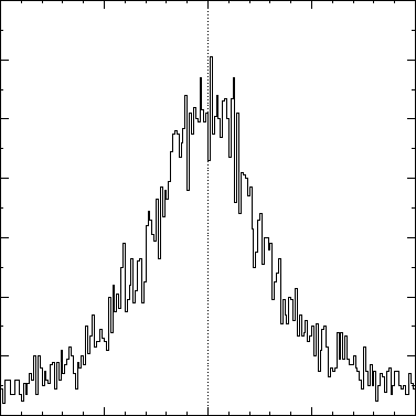
Chapter 21: Histograms 273
$ gsl-randist 0 10000 cauchy 30
| gsl-histogram -100 100 200 > histogram.dat
A plot of the resulting histogram shows the familiar shape of the Cauchy distribution and
the fluctuations caused by the finite sample size.
$ awk ’{print $1, $3 ; print $2, $3}’ histogram.dat
| graph -T X
−100 −50 0 50 100
0
20
40
60
80
100
120
140
21.12 Two dimensional histograms
A two dimensional histogram consists of a set of bins which count the number of events
falling in a given area of the (x, y) plane. The simplest way to use a two dimensional
histogram is to record two-dimensional position information, n(x, y). Another possibility is
to form a joint distribution by recording related variables. For example a detector might
record both the position of an event (x) and the amount of energy it deposited E. These
could be histogrammed as the joint distribution n(x, E).
21.13 The 2D histogram struct
Two dimensional histograms are defined by the following struct,
[Data Type]gsl_histogram2d
size_t nx, ny
This is the number of histogram bins in the x and y directions.
double * xrange
The ranges of the bins in the x-direction are stored in an array of nx + 1
elements pointed to by xrange.
double * yrange
The ranges of the bins in the y-direction are stored in an array of ny + 1
elements pointed to by yrange.

Chapter 21: Histograms 274
double * bin
The counts for each bin are stored in an array pointed to by bin. The bins
are floating-point numbers, so you can increment them by non-integer
values if necessary. The array bin stores the two dimensional array of
bins in a single block of memory according to the mapping bin(i,j) =
bin[i * ny + j].
The range for bin(i,j) is given by xrange[i] to xrange[i+1] in the x-direction and
yrange[j] to yrange[j+1] in the y-direction. Each bin is inclusive at the lower end and
exclusive at the upper end. Mathematically this means that the bins are defined by the
following inequality,
bin(i,j) corresponds to xrange[i]≤x < xrange[i+ 1]
and yrange[j]≤y < yrange[j+ 1]
Note that any samples which fall on the upper sides of the histogram are excluded. If you
want to include these values for the side bins you will need to add an extra row or column
to your histogram.
The gsl_histogram2d struct and its associated functions are defined in the header file
‘gsl_histogram2d.h’.
21.14 2D Histogram allocation
The functions for allocating memory to a 2D histogram follow the style of malloc and free.
In addition they also perform their own error checking. If there is insufficient memory
available to allocate a histogram then the functions call the error handler (with an error
number of GSL_ENOMEM) in addition to returning a null pointer. Thus if you use the library
error handler to abort your program then it isn’t necessary to check every 2D histogram
alloc.
[Function]gsl_histogram2d * gsl_histogram2d_alloc (size tnx, size t ny )
This function allocates memory for a two-dimensional histogram with nx bins in the
x direction and ny bins in the y direction. The function returns a pointer to a newly
created gsl_histogram2d struct. If insufficient memory is available a null pointer is
returned and the error handler is invoked with an error code of GSL_ENOMEM. The bins
and ranges must be initialized with one of the functions below before the histogram
is ready for use.
[Function]int gsl_histogram2d_set_ranges (gsl histogram2d * h, const double
xrange [], size t xsize, const double yrange [], size t ysize )
This function sets the ranges of the existing histogram husing the arrays xrange and
yrange of size xsize and ysize respectively. The values of the histogram bins are reset
to zero.
[Function]int gsl_histogram2d_set_ranges_uniform (gsl histogram2d * h,
double xmin, double xmax, double ymin, double ymax )
This function sets the ranges of the existing histogram hto cover the ranges xmin
to xmax and ymin to ymax uniformly. The values of the histogram bins are reset to
zero.

Chapter 21: Histograms 275
[Function]void gsl_histogram2d_free (gsl histogram2d * h)
This function frees the 2D histogram hand all of the memory associated with it.
21.15 Copying 2D Histograms
[Function]int gsl_histogram2d_memcpy (gsl histogram2d * dest, const
gsl histogram2d * src )
This function copies the histogram src into the pre-existing histogram dest, making
dest into an exact copy of src. The two histograms must be of the same size.
[Function]gsl_histogram2d * gsl_histogram2d_clone (const gsl histogram2d
*src )
This function returns a pointer to a newly created histogram which is an exact copy
of the histogram src.
21.16 Updating and accessing 2D histogram elements
You can access the bins of a two-dimensional histogram either by specifying a pair of
(x, y) coordinates or by using the bin indices (i, j) directly. The functions for accessing
the histogram through (x, y) coordinates use binary searches in the x and y directions to
identify the bin which covers the appropriate range.
[Function]int gsl_histogram2d_increment (gsl histogram2d * h, double x,
double y)
This function updates the histogram hby adding one (1.0) to the bin whose x and y
ranges contain the coordinates (x,y).
If the point (x, y) lies inside the valid ranges of the histogram then the function
returns zero to indicate success. If (x, y) lies outside the limits of the histogram then
the function returns GSL_EDOM, and none of the bins are modified. The error handler
is not called, since it is often necessary to compute histograms for a small range of a
larger dataset, ignoring any coordinates outside the range of interest.
[Function]int gsl_histogram2d_accumulate (gsl histogram2d * h, double x,
double y, double weight )
This function is similar to gsl_histogram2d_increment but increases the value of
the appropriate bin in the histogram hby the floating-point number weight.
[Function]double gsl_histogram2d_get (const gsl histogram2d * h, size t i,
size t j)
This function returns the contents of the (i,j)-th bin of the histogram h. If (i,j) lies
outside the valid range of indices for the histogram then the error handler is called
with an error code of GSL_EDOM and the function returns 0.
[Function]int gsl_histogram2d_get_xrange (const gsl histogram2d * h, size t
i, double * xlower, double * xupper )
[Function]int gsl_histogram2d_get_yrange (const gsl histogram2d * h, size t
j, double * ylower, double * yupper )
These functions find the upper and lower range limits of the i-th and j-th bins in the
x and y directions of the histogram h. The range limits are stored in xlower and

Chapter 21: Histograms 276
xupper or ylower and yupper. The lower limits are inclusive (i.e. events with these
coordinates are included in the bin) and the upper limits are exclusive (i.e. events
with the value of the upper limit are not included and fall in the neighboring higher
bin, if it exists). The functions return 0 to indicate success. If ior jlies outside the
valid range of indices for the histogram then the error handler is called with an error
code of GSL_EDOM.
[Function]double gsl_histogram2d_xmax (const gsl histogram2d * h)
[Function]double gsl_histogram2d_xmin (const gsl histogram2d * h)
[Function]size_t gsl_histogram2d_nx (const gsl histogram2d * h)
[Function]double gsl_histogram2d_ymax (const gsl histogram2d * h)
[Function]double gsl_histogram2d_ymin (const gsl histogram2d * h)
[Function]size_t gsl_histogram2d_ny (const gsl histogram2d * h)
These functions return the maximum upper and minimum lower range limits and the
number of bins for the x and y directions of the histogram h. They provide a way of
determining these values without accessing the gsl_histogram2d struct directly.
[Function]void gsl_histogram2d_reset (gsl histogram2d * h)
This function resets all the bins of the histogram hto zero.
21.17 Searching 2D histogram ranges
The following functions are used by the access and update routines to locate the bin which
corresponds to a given (x, y) coordinate.
[Function]int gsl_histogram2d_find (const gsl histogram2d * h, double x,
double y, size t * i, size t * j)
This function finds and sets the indices iand jto the to the bin which covers the
coordinates (x,y). The bin is located using a binary search. The search includes
an optimization for histograms with uniform ranges, and will return the correct bin
immediately in this case. If (x, y) is found then the function sets the indices (i,j) and
returns GSL_SUCCESS. If (x, y) lies outside the valid range of the histogram then the
function returns GSL_EDOM and the error handler is invoked.
21.18 2D Histogram Statistics
[Function]double gsl_histogram2d_max_val (const gsl histogram2d * h)
This function returns the maximum value contained in the histogram bins.
[Function]void gsl_histogram2d_max_bin (const gsl histogram2d * h, size t * i,
size t * j)
This function finds the indices of the bin containing the maximum value in the his-
togram hand stores the result in (i,j). In the case where several bins contain the
same maximum value the first bin found is returned.
[Function]double gsl_histogram2d_min_val (const gsl histogram2d * h)
This function returns the minimum value contained in the histogram bins.

Chapter 21: Histograms 277
[Function]void gsl_histogram2d_min_bin (const gsl histogram2d * h, size t * i,
size t * j)
This function finds the indices of the bin containing the minimum value in the his-
togram hand stores the result in (i,j). In the case where several bins contain the
same maximum value the first bin found is returned.
[Function]double gsl_histogram2d_xmean (const gsl histogram2d * h)
This function returns the mean of the histogrammed x variable, where the histogram
is regarded as a probability distribution. Negative bin values are ignored for the
purposes of this calculation.
[Function]double gsl_histogram2d_ymean (const gsl histogram2d * h)
This function returns the mean of the histogrammed y variable, where the histogram
is regarded as a probability distribution. Negative bin values are ignored for the
purposes of this calculation.
[Function]double gsl_histogram2d_xsigma (const gsl histogram2d * h)
This function returns the standard deviation of the histogrammed x variable, where
the histogram is regarded as a probability distribution. Negative bin values are ig-
nored for the purposes of this calculation.
[Function]double gsl_histogram2d_ysigma (const gsl histogram2d * h)
This function returns the standard deviation of the histogrammed y variable, where
the histogram is regarded as a probability distribution. Negative bin values are ig-
nored for the purposes of this calculation.
[Function]double gsl_histogram2d_cov (const gsl histogram2d * h)
This function returns the covariance of the histogrammed x and y variables, where the
histogram is regarded as a probability distribution. Negative bin values are ignored
for the purposes of this calculation.
[Function]double gsl_histogram2d_sum (const gsl histogram2d * h)
This function returns the sum of all bin values. Negative bin values are included in
the sum.
21.19 2D Histogram Operations
[Function]int gsl_histogram2d_equal_bins_p (const gsl histogram2d * h1,
const gsl histogram2d * h2 )
This function returns 1 if all the individual bin ranges of the two histograms are
identical, and 0 otherwise.
[Function]int gsl_histogram2d_add (gsl histogram2d * h1, const
gsl histogram2d * h2 )
This function adds the contents of the bins in histogram h2 to the corresponding
bins of histogram h1, i.e. h′
1(i, j) = h1(i, j) + h2(i, j). The two histograms must have
identical bin ranges.

Chapter 21: Histograms 278
[Function]int gsl_histogram2d_sub (gsl histogram2d * h1, const
gsl histogram2d * h2 )
This function subtracts the contents of the bins in histogram h2 from the correspond-
ing bins of histogram h1, i.e. h′
1(i, j) = h1(i, j)−h2(i, j). The two histograms must
have identical bin ranges.
[Function]int gsl_histogram2d_mul (gsl histogram2d * h1, const
gsl histogram2d * h2 )
This function multiplies the contents of the bins of histogram h1 by the contents of
the corresponding bins in histogram h2, i.e. h′
1(i, j) = h1(i, j)∗h2(i, j). The two
histograms must have identical bin ranges.
[Function]int gsl_histogram2d_div (gsl histogram2d * h1, const
gsl histogram2d * h2 )
This function divides the contents of the bins of histogram h1 by the contents of
the corresponding bins in histogram h2, i.e. h′
1(i, j) = h1(i, j)/h2(i, j). The two
histograms must have identical bin ranges.
[Function]int gsl_histogram2d_scale (gsl histogram2d * h, double scale )
This function multiplies the contents of the bins of histogram hby the constant scale,
i.e. h′
1(i, j) = h1(i, j)∗scale.
[Function]int gsl_histogram2d_shift (gsl histogram2d * h, double offset )
This function shifts the contents of the bins of histogram hby the constant offset, i.e.
h′
1(i, j) = h1(i, j) + offset.
21.20 Reading and writing 2D histograms
The library provides functions for reading and writing two dimensional histograms to a file
as binary data or formatted text.
[Function]int gsl_histogram2d_fwrite (FILE * stream, const gsl histogram2d
*h)
This function writes the ranges and bins of the histogram hto the stream stream
in binary format. The return value is 0 for success and GSL_EFAILED if there was a
problem writing to the file. Since the data is written in the native binary format it
may not be portable between different architectures.
[Function]int gsl_histogram2d_fread (FILE * stream, gsl histogram2d * h)
This function reads into the histogram hfrom the stream stream in binary format.
The histogram hmust be preallocated with the correct size since the function uses
the number of x and y bins in hto determine how many bytes to read. The return
value is 0 for success and GSL_EFAILED if there was a problem reading from the file.
The data is assumed to have been written in the native binary format on the same
architecture.
[Function]int gsl_histogram2d_fprintf (FILE * stream, const gsl histogram2d
*h, const char * range_format, const char * bin_format )
This function writes the ranges and bins of the histogram hline-by-line to the stream
stream using the format specifiers range format and bin format. These should be one

Chapter 21: Histograms 279
of the %g,%e or %f formats for floating point numbers. The function returns 0 for
success and GSL_EFAILED if there was a problem writing to the file. The histogram
output is formatted in five columns, and the columns are separated by spaces, like
this,
xrange[0] xrange[1] yrange[0] yrange[1] bin(0,0)
xrange[0] xrange[1] yrange[1] yrange[2] bin(0,1)
xrange[0] xrange[1] yrange[2] yrange[3] bin(0,2)
....
xrange[0] xrange[1] yrange[ny-1] yrange[ny] bin(0,ny-1)
xrange[1] xrange[2] yrange[0] yrange[1] bin(1,0)
xrange[1] xrange[2] yrange[1] yrange[2] bin(1,1)
xrange[1] xrange[2] yrange[1] yrange[2] bin(1,2)
....
xrange[1] xrange[2] yrange[ny-1] yrange[ny] bin(1,ny-1)
....
xrange[nx-1] xrange[nx] yrange[0] yrange[1] bin(nx-1,0)
xrange[nx-1] xrange[nx] yrange[1] yrange[2] bin(nx-1,1)
xrange[nx-1] xrange[nx] yrange[1] yrange[2] bin(nx-1,2)
....
xrange[nx-1] xrange[nx] yrange[ny-1] yrange[ny] bin(nx-1,ny-1)
Each line contains the lower and upper limits of the bin and the contents of the bin.
Since the upper limits of the each bin are the lower limits of the neighboring bins
there is duplication of these values but this allows the histogram to be manipulated
with line-oriented tools.
[Function]int gsl_histogram2d_fscanf (FILE * stream, gsl histogram2d * h)
This function reads formatted data from the stream stream into the histogram h. The
data is assumed to be in the five-column format used by gsl_histogram2d_fprintf.
The histogram hmust be preallocated with the correct lengths since the function uses
the sizes of hto determine how many numbers to read. The function returns 0 for
success and GSL_EFAILED if there was a problem reading from the file.
21.21 Resampling from 2D histograms
As in the one-dimensional case, a two-dimensional histogram made by counting events can
be regarded as a measurement of a probability distribution. Allowing for statistical error,
the height of each bin represents the probability of an event where (x,y) falls in the range
of that bin. For a two-dimensional histogram the probability distribution takes the form
p(x, y)dxdy where,
p(x, y) = nij /(NAij )
In this equation nij is the number of events in the bin which contains (x, y), Aij is the area
of the bin and Nis the total number of events. The distribution of events within each bin
is assumed to be uniform.
[Data Type]gsl_histogram2d_pdf
size_t nx, ny
This is the number of histogram bins used to approximate the probability
distribution function in the x and y directions.

Chapter 21: Histograms 280
double * xrange
The ranges of the bins in the x-direction are stored in an array of nx + 1
elements pointed to by xrange.
double * yrange
The ranges of the bins in the y-direction are stored in an array of ny + 1
pointed to by yrange.
double * sum
The cumulative probability for the bins is stored in an array of nx*ny
elements pointed to by sum.
The following functions allow you to create a gsl_histogram2d_pdf struct which represents
a two dimensional probability distribution and generate random samples from it.
[Function]gsl_histogram2d_pdf * gsl_histogram2d_pdf_alloc (size tnx,
size t ny )
This function allocates memory for a two-dimensional probability distribution of size
nx-by-ny and returns a pointer to a newly initialized gsl_histogram2d_pdf struct.
If insufficient memory is available a null pointer is returned and the error handler is
invoked with an error code of GSL_ENOMEM.
[Function]int gsl_histogram2d_pdf_init (gsl histogram2d pdf * p, const
gsl histogram2d * h)
This function initializes the two-dimensional probability distribution calculated p
from the histogram h. If any of the bins of hare negative then the error handler
is invoked with an error code of GSL_EDOM because a probability distribution cannot
contain negative values.
[Function]void gsl_histogram2d_pdf_free (gsl histogram2d pdf * p)
This function frees the two-dimensional probability distribution function pand all of
the memory associated with it.
[Function]int gsl_histogram2d_pdf_sample (const gsl histogram2d pdf * p,
double r1, double r2, double * x, double * y)
This function uses two uniform random numbers between zero and one, r1 and r2, to
compute a single random sample from the two-dimensional probability distribution
p.
Chapter 21: Histograms 281
21.22 Example programs for 2D histograms
This program demonstrates two features of two-dimensional histograms. First a 10-by-10
two-dimensional histogram is created with x and y running from 0 to 1. Then a few sample
points are added to the histogram, at (0.3,0.3) with a height of 1, at (0.8,0.1) with a height
of 5 and at (0.7,0.9) with a height of 0.5. This histogram with three events is used to
generate a random sample of 1000 simulated events, which are printed out.
#include <stdio.h>
#include <gsl/gsl_rng.h>
#include <gsl/gsl_histogram2d.h>
int
main (void)
{
const gsl_rng_type * T;
gsl_rng * r;
gsl_histogram2d * h = gsl_histogram2d_alloc (10, 10);
gsl_histogram2d_set_ranges_uniform (h,
0.0, 1.0,
0.0, 1.0);
gsl_histogram2d_accumulate (h, 0.3, 0.3, 1);
gsl_histogram2d_accumulate (h, 0.8, 0.1, 5);
gsl_histogram2d_accumulate (h, 0.7, 0.9, 0.5);
gsl_rng_env_setup ();
T = gsl_rng_default;
r = gsl_rng_alloc (T);
{
int i;
gsl_histogram2d_pdf * p
= gsl_histogram2d_pdf_alloc (h->nx, h->ny);
gsl_histogram2d_pdf_init (p, h);
for (i = 0; i < 1000; i++) {
double x, y;
double u = gsl_rng_uniform (r);
double v = gsl_rng_uniform (r);
gsl_histogram2d_pdf_sample (p, u, v, &x, &y);
printf ("%g %g\n", x, y);
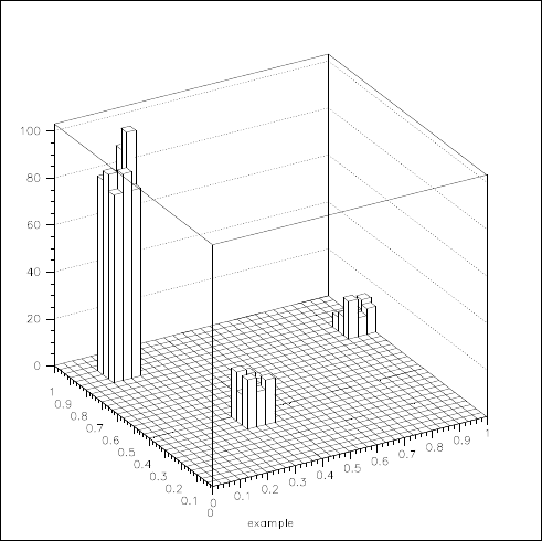
Chapter 21: Histograms 282
}
gsl_histogram2d_pdf_free (p);
}
gsl_histogram2d_free (h);
gsl_rng_free (r);
return 0;
}
The following plot shows the distribution of the simulated events. Using a higher resolution
grid we can see the original underlying histogram and also the statistical fluctuations caused
by the events being uniformly distributed over the area of the original bins.

Chapter 22: N-tuples 283
22 N-tuples
This chapter describes functions for creating and manipulating ntuples, sets of values as-
sociated with events. The ntuples are stored in files. Their values can be extracted in any
combination and booked in a histogram using a selection function.
The values to be stored are held in a user-defined data structure, and an ntuple is created
associating this data structure with a file. The values are then written to the file (normally
inside a loop) using the ntuple functions described below.
A histogram can be created from ntuple data by providing a selection function and a
value function. The selection function specifies whether an event should be included in the
subset to be analyzed or not. The value function computes the entry to be added to the
histogram for each event.
All the ntuple functions are defined in the header file ‘gsl_ntuple.h’
22.1 The ntuple struct
Ntuples are manipulated using the gsl_ntuple struct. This struct contains information on
the file where the ntuple data is stored, a pointer to the current ntuple data row and the
size of the user-defined ntuple data struct.
typedef struct {
FILE * file;
void * ntuple_data;
size_t size;
} gsl_ntuple;
22.2 Creating ntuples
[Function]gsl_ntuple * gsl_ntuple_create (char * filename, void *
ntuple_data, size tsize )
This function creates a new write-only ntuple file filename for ntuples of size size
and returns a pointer to the newly created ntuple struct. Any existing file with the
same name is truncated to zero length and overwritten. A pointer to memory for the
current ntuple row ntuple data must be supplied—this is used to copy ntuples in and
out of the file.
22.3 Opening an existing ntuple file
[Function]gsl_ntuple * gsl_ntuple_open (char * filename, void *
ntuple_data, size t size )
This function opens an existing ntuple file filename for reading and returns a pointer
to a corresponding ntuple struct. The ntuples in the file must have size size. A pointer
to memory for the current ntuple row ntuple data must be supplied—this is used to
copy ntuples in and out of the file.

Chapter 22: N-tuples 284
22.4 Writing ntuples
[Function]int gsl_ntuple_write (gsl ntuple * ntuple )
This function writes the current ntuple ntuple->ntuple data of size ntuple->size to
the corresponding file.
[Function]int gsl_ntuple_bookdata (gsl ntuple * ntuple )
This function is a synonym for gsl_ntuple_write.
22.5 Reading ntuples
[Function]int gsl_ntuple_read (gsl ntuple * ntuple )
This function reads the current row of the ntuple file for ntuple and stores the values
in ntuple->data.
22.6 Closing an ntuple file
[Function]int gsl_ntuple_close (gsl ntuple * ntuple )
This function closes the ntuple file ntuple and frees its associated allocated memory.
22.7 Histogramming ntuple values
Once an ntuple has been created its contents can be histogrammed in various ways using the
function gsl_ntuple_project. Two user-defined functions must be provided, a function to
select events and a function to compute scalar values. The selection function and the value
function both accept the ntuple row as a first argument and other parameters as a second
argument.
The selection function determines which ntuple rows are selected for histogramming. It
is defined by the following struct,
typedef struct {
int (* function) (void * ntuple_data, void * params);
void * params;
} gsl_ntuple_select_fn;
The struct component function should return a non-zero value for each ntuple row that is
to be included in the histogram.
The value function computes scalar values for those ntuple rows selected by the selection
function,
typedef struct {
double (* function) (void * ntuple_data, void * params);
void * params;
} gsl_ntuple_value_fn;
In this case the struct component function should return the value to be added to the
histogram for the ntuple row.
[Function]int gsl_ntuple_project (gsl histogram * h, gsl ntuple * ntuple,
gsl ntuple value fn * value_func, gsl ntuple select fn * select_func )
This function updates the histogram hfrom the ntuple ntuple using the functions
value func and select func. For each ntuple row where the selection function se-
lect func is non-zero the corresponding value of that row is computed using the func-
tion value func and added to the histogram. Those ntuple rows where select func
Chapter 22: N-tuples 285
returns zero are ignored. New entries are added to the histogram, so subsequent calls
can be used to accumulate further data in the same histogram.
22.8 Examples
The following example programs demonstrate the use of ntuples in managing a large dataset.
The first program creates a set of 10,000 simulated “events”, each with 3 associated values
(x, y, z). These are generated from a gaussian distribution with unit variance, for demon-
stration purposes, and written to the ntuple file ‘test.dat’.
#include <gsl/gsl_ntuple.h>
#include <gsl/gsl_rng.h>
#include <gsl/gsl_randist.h>
struct data
{
double x;
double y;
double z;
};
int
main (void)
{
const gsl_rng_type * T;
gsl_rng * r;
struct data ntuple_row;
int i;
gsl_ntuple *ntuple
= gsl_ntuple_create ("test.dat", &ntuple_row,
sizeof (ntuple_row));
gsl_rng_env_setup ();
T = gsl_rng_default;
r = gsl_rng_alloc (T);
for (i = 0; i < 10000; i++)
{
ntuple_row.x = gsl_ran_ugaussian (r);
ntuple_row.y = gsl_ran_ugaussian (r);
ntuple_row.z = gsl_ran_ugaussian (r);
gsl_ntuple_write (ntuple);
}
Chapter 22: N-tuples 286
gsl_ntuple_close (ntuple);
gsl_rng_free (r);
return 0;
}
The next program analyses the ntuple data in the file ‘test.dat’. The analysis procedure
is to compute the squared-magnitude of each event, E2=x2+y2+z2, and select only those
which exceed a lower limit of 1.5. The selected events are then histogrammed using their
E2values.
#include <math.h>
#include <gsl/gsl_ntuple.h>
#include <gsl/gsl_histogram.h>
struct data
{
double x;
double y;
double z;
};
int sel_func (void *ntuple_data, void *params);
double val_func (void *ntuple_data, void *params);
int
main (void)
{
struct data ntuple_row;
gsl_ntuple *ntuple
= gsl_ntuple_open ("test.dat", &ntuple_row,
sizeof (ntuple_row));
double lower = 1.5;
gsl_ntuple_select_fn S;
gsl_ntuple_value_fn V;
gsl_histogram *h = gsl_histogram_alloc (100);
gsl_histogram_set_ranges_uniform(h, 0.0, 10.0);
S.function = &sel_func;
S.params = &lower;
V.function = &val_func;
V.params = 0;
gsl_ntuple_project (h, ntuple, &V, &S);
Chapter 22: N-tuples 287
gsl_histogram_fprintf (stdout, h, "%f", "%f");
gsl_histogram_free (h);
gsl_ntuple_close (ntuple);
return 0;
}
int
sel_func (void *ntuple_data, void *params)
{
struct data * data = (struct data *) ntuple_data;
double x, y, z, E2, scale;
scale = *(double *) params;
x = data->x;
y = data->y;
z = data->z;
E2 = x * x + y * y + z * z;
return E2 > scale;
}
double
val_func (void *ntuple_data, void *params)
{
struct data * data = (struct data *) ntuple_data;
double x, y, z;
x = data->x;
y = data->y;
z = data->z;
return x * x + y * y + z * z;
}
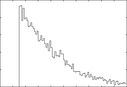
Chapter 22: N-tuples 288
The following plot shows the distribution of the selected events. Note the cut-off at the
lower bound.
0
50
100
150
200
250
012345678910
n
E2
22.9 References and Further Reading
Further information on the use of ntuples can be found in the documentation for the cern
packages paw and hbook (available online).
Chapter 23: Monte Carlo Integration 289
23 Monte Carlo Integration
This chapter describes routines for multidimensional Monte Carlo integration. These in-
clude the traditional Monte Carlo method and adaptive algorithms such as vegas and
miser which use importance sampling and stratified sampling techniques. Each algorithm
computes an estimate of a multidimensional definite integral of the form,
I=Zxu
xl
dx Zyu
yl
dy ...f(x, y, ...)
over a hypercubic region ((xl, xu), (yl, yu), ...) using a fixed number of function calls. The
routines also provide a statistical estimate of the error on the result. This error estimate
should be taken as a guide rather than as a strict error bound—random sampling of the
region may not uncover all the important features of the function, resulting in an underes-
timate of the error.
The functions are defined in separate header files for each routine, ‘gsl_monte_plain.h’,
‘gsl_monte_miser.h’ and ‘gsl_monte_vegas.h’.
23.1 Interface
All of the Monte Carlo integration routines use the same general form of interface. There is
an allocator to allocate memory for control variables and workspace, a routine to initialize
those control variables, the integrator itself, and a function to free the space when done.
Each integration function requires a random number generator to be supplied, and re-
turns an estimate of the integral and its standard deviation. The accuracy of the result is
determined by the number of function calls specified by the user. If a known level of accu-
racy is required this can be achieved by calling the integrator several times and averaging
the individual results until the desired accuracy is obtained.
Random sample points used within the Monte Carlo routines are always chosen strictly
within the integration region, so that endpoint singularities are automatically avoided.
The function to be integrated has its own datatype, defined in the header file
‘gsl_monte.h’.
[Data Type]gsl_monte_function
This data type defines a general function with parameters for Monte Carlo integration.
double (* f) (double * x, size_t dim, void * params )
this function should return the value f(x, params) for the argument xand
parameters params, where xis an array of size dim giving the coordinates
of the point where the function is to be evaluated.
size_t dim
the number of dimensions for x.
void * params
a pointer to the parameters of the function.
Here is an example for a quadratic function in two dimensions,
f(x, y) = ax2+bxy +cy2

Chapter 23: Monte Carlo Integration 290
with a= 3, b= 2, c= 1. The following code defines a gsl_monte_function F which you
could pass to an integrator:
struct my_f_params { double a; double b; double c; };
double
my_f (double x[], size_t dim, void * p) {
struct my_f_params * fp = (struct my_f_params *)p;
if (dim != 2)
{
fprintf (stderr, "error: dim != 2");
abort ();
}
return fp->a * x[0] * x[0]
+ fp->b * x[0] * x[1]
+ fp->c * x[1] * x[1];
}
gsl_monte_function F;
struct my_f_params params = { 3.0, 2.0, 1.0 };
F.f = &my_f;
F.dim = 2;
F.params = ¶ms;
The function f(x) can be evaluated using the following macro,
#define GSL_MONTE_FN_EVAL(F,x)
(*((F)->f))(x,(F)->dim,(F)->params)
23.2 PLAIN Monte Carlo
The plain Monte Carlo algorithm samples points randomly from the integration region to
estimate the integral and its error. Using this algorithm the estimate of the integral E(f;N)
for Nrandomly distributed points xiis given by,
E(f;N) = Vhfi=V
N
N
X
i
f(xi)
where Vis the volume of the integration region. The error on this estimate σ(E;N) is
calculated from the estimated variance of the mean,
σ2(E;N) = V
N
N
X
i
(f(xi)− hfi)2.
For large Nthis variance decreases asymptotically as Var(f)/N, where Var(f) is the true
variance of the function over the integration region. The error estimate itself should decrease
as σ(f)/√N. The familiar law of errors decreasing as 1/√Napplies—to reduce the error
by a factor of 10 requires a 100-fold increase in the number of sample points.

Chapter 23: Monte Carlo Integration 291
The functions described in this section are declared in the header file
‘gsl_monte_plain.h’.
[Function]gsl_monte_plain_state * gsl_monte_plain_alloc (size tdim )
This function allocates and initializes a workspace for Monte Carlo integration in dim
dimensions.
[Function]int gsl_monte_plain_init (gsl monte plain state* s)
This function initializes a previously allocated integration state. This allows an ex-
isting workspace to be reused for different integrations.
[Function]int gsl_monte_plain_integrate (gsl monte function * f, const
double xl [], const double xu [], size tdim, size t calls, gsl rng * r,
gsl monte plain state * s, double * result, double * abserr )
This routines uses the plain Monte Carlo algorithm to integrate the function fover
the dim-dimensional hypercubic region defined by the lower and upper limits in the
arrays xl and xu, each of size dim. The integration uses a fixed number of function
calls calls, and obtains random sampling points using the random number generator
r. A previously allocated workspace smust be supplied. The result of the integration
is returned in result, with an estimated absolute error abserr.
[Function]void gsl_monte_plain_free (gsl monte plain state * s)
This function frees the memory associated with the integrator state s.
23.3 MISER
The miser algorithm of Press and Farrar is based on recursive stratified sampling. This
technique aims to reduce the overall integration error by concentrating integration points
in the regions of highest variance.
The idea of stratified sampling begins with the observation that for two disjoint regions
aand bwith Monte Carlo estimates of the integral Ea(f) and Eb(f) and variances σ2
a(f)
and σ2
b(f), the variance Var(f) of the combined estimate E(f) = 1
2(Ea(f) + Eb(f)) is given
by,
Var(f) = σ2
a(f)
4Na
+σ2
b(f)
4Nb
.
It can be shown that this variance is minimized by distributing the points such that,
Na
Na+Nb
=σa
σa+σb
.
Hence the smallest error estimate is obtained by allocating sample points in proportion to
the standard deviation of the function in each sub-region.
The miser algorithm proceeds by bisecting the integration region along one coordinate
axis to give two sub-regions at each step. The direction is chosen by examining all dpossible
bisections and selecting the one which will minimize the combined variance of the two sub-
regions. The variance in the sub-regions is estimated by sampling with a fraction of the
total number of points available to the current step. The same procedure is then repeated
recursively for each of the two half-spaces from the best bisection. The remaining sample
points are allocated to the sub-regions using the formula for Naand Nb. This recursive

Chapter 23: Monte Carlo Integration 292
allocation of integration points continues down to a user-specified depth where each sub-
region is integrated using a plain Monte Carlo estimate. These individual values and their
error estimates are then combined upwards to give an overall result and an estimate of its
error.
The functions described in this section are declared in the header file
‘gsl_monte_miser.h’.
[Function]gsl_monte_miser_state * gsl_monte_miser_alloc (size tdim )
This function allocates and initializes a workspace for Monte Carlo integration in dim
dimensions. The workspace is used to maintain the state of the integration.
[Function]int gsl_monte_miser_init (gsl monte miser state* s)
This function initializes a previously allocated integration state. This allows an ex-
isting workspace to be reused for different integrations.
[Function]int gsl_monte_miser_integrate (gsl monte function * f, const
double xl [], const double xu [], size t dim, size t calls, gsl rng * r,
gsl monte miser state * s, double * result, double * abserr )
This routines uses the miser Monte Carlo algorithm to integrate the function fover
the dim-dimensional hypercubic region defined by the lower and upper limits in the
arrays xl and xu, each of size dim. The integration uses a fixed number of function
calls calls, and obtains random sampling points using the random number generator
r. A previously allocated workspace smust be supplied. The result of the integration
is returned in result, with an estimated absolute error abserr.
[Function]void gsl_monte_miser_free (gsl monte miser state * s)
This function frees the memory associated with the integrator state s.
The miser algorithm has several configurable parameters which can be changed using
the following two functions.1
[Function]void gsl_monte_miser_params_get (const gsl monte miser state * s,
gsl monte miser params * params )
This function copies the parameters of the integrator state into the user-supplied
params structure.
[Function]void gsl_monte_miser_params_set (gsl monte miser state * s, const
gsl monte miser params * params )
This function sets the integrator parameters based on values provided in the params
structure.
Typically the values of the parameters are first read using gsl_monte_miser_params_
get, the necessary changes are made to the fields of the params structure, and the values are
copied back into the integrator state using gsl_monte_miser_params_set. The functions
use the gsl_monte_miser_params structure which contains the following fields:
1The previous method of accessing these fields directly through the gsl_monte_miser_state struct is now
deprecated.

Chapter 23: Monte Carlo Integration 293
[Variable]double estimate_frac
This parameter specifies the fraction of the currently available number of function
calls which are allocated to estimating the variance at each recursive step. The
default value is 0.1.
[Variable]size_t min_calls
This parameter specifies the minimum number of function calls required for each
estimate of the variance. If the number of function calls allocated to the estimate using
estimate frac falls below min calls then min calls are used instead. This ensures that
each estimate maintains a reasonable level of accuracy. The default value of min calls
is 16 * dim.
[Variable]size_t min_calls_per_bisection
This parameter specifies the minimum number of function calls required to pro-
ceed with a bisection step. When a recursive step has fewer calls available than
min calls per bisection it performs a plain Monte Carlo estimate of the current sub-
region and terminates its branch of the recursion. The default value of this parameter
is 32 * min_calls.
[Variable]double alpha
This parameter controls how the estimated variances for the two sub-regions of a
bisection are combined when allocating points. With recursive sampling the over-
all variance should scale better than 1/N, since the values from the sub-regions will
be obtained using a procedure which explicitly minimizes their variance. To accom-
modate this behavior the miser algorithm allows the total variance to depend on a
scaling parameter α,
Var(f) = σa
Nα
a
+σb
Nα
b
.
The authors of the original paper describing miser recommend the value α= 2 as
a good choice, obtained from numerical experiments, and this is used as the default
value in this implementation.
[Variable]double dither
This parameter introduces a random fractional variation of size dither into each bisec-
tion, which can be used to break the symmetry of integrands which are concentrated
near the exact center of the hypercubic integration region. The default value of dither
is zero, so no variation is introduced. If needed, a typical value of dither is 0.1.
23.4 VEGAS
The vegas algorithm of Lepage is based on importance sampling. It samples points from
the probability distribution described by the function |f|, so that the points are concentrated
in the regions that make the largest contribution to the integral.
In general, if the Monte Carlo integral of fis sampled with points distributed according
to a probability distribution described by the function g, we obtain an estimate Eg(f;N),
Eg(f;N) = E(f/g;N)

Chapter 23: Monte Carlo Integration 294
with a corresponding variance,
Varg(f;N) = Var(f/g;N).
If the probability distribution is chosen as g=|f|/I(|f|) then it can be shown that the
variance Vg(f;N) vanishes, and the error in the estimate will be zero. In practice it is not
possible to sample from the exact distribution gfor an arbitrary function, so importance
sampling algorithms aim to produce efficient approximations to the desired distribution.
The vegas algorithm approximates the exact distribution by making a number of passes
over the integration region while histogramming the function f. Each histogram is used to
define a sampling distribution for the next pass. Asymptotically this procedure converges
to the desired distribution. In order to avoid the number of histogram bins growing like
Kdthe probability distribution is approximated by a separable function: g(x1, x2,...) =
g1(x1)g2(x2)...so that the number of bins required is only Kd. This is equivalent to locating
the peaks of the function from the projections of the integrand onto the coordinate axes.
The efficiency of vegas depends on the validity of this assumption. It is most efficient
when the peaks of the integrand are well-localized. If an integrand can be rewritten in a
form which is approximately separable this will increase the efficiency of integration with
vegas.
vegas incorporates a number of additional features, and combines both stratified sam-
pling and importance sampling. The integration region is divided into a number of “boxes”,
with each box getting a fixed number of points (the goal is 2). Each box can then have a
fractional number of bins, but if the ratio of bins-per-box is less than two, Vegas switches
to a kind variance reduction (rather than importance sampling).
[Function]gsl_monte_vegas_state * gsl_monte_vegas_alloc (size tdim )
This function allocates and initializes a workspace for Monte Carlo integration in dim
dimensions. The workspace is used to maintain the state of the integration.
[Function]int gsl_monte_vegas_init (gsl monte vegas state* s)
This function initializes a previously allocated integration state. This allows an ex-
isting workspace to be reused for different integrations.
[Function]int gsl_monte_vegas_integrate (gsl monte function * f, double
xl [], double xu [], size tdim, size t calls, gsl rng * r, gsl monte vegas state
*s, double * result, double * abserr )
This routines uses the vegas Monte Carlo algorithm to integrate the function fover
the dim-dimensional hypercubic region defined by the lower and upper limits in the
arrays xl and xu, each of size dim. The integration uses a fixed number of function
calls calls, and obtains random sampling points using the random number generator
r. A previously allocated workspace smust be supplied. The result of the integration
is returned in result, with an estimated absolute error abserr. The result and its error
estimate are based on a weighted average of independent samples. The chi-squared per
degree of freedom for the weighted average is returned via the state struct component,
s->chisq, and must be consistent with 1 for the weighted average to be reliable.
[Function]void gsl_monte_vegas_free (gsl monte vegas state * s)
This function frees the memory associated with the integrator state s.

Chapter 23: Monte Carlo Integration 295
The vegas algorithm computes a number of independent estimates of the integral inter-
nally, according to the iterations parameter described below, and returns their weighted
average. Random sampling of the integrand can occasionally produce an estimate where
the error is zero, particularly if the function is constant in some regions. An estimate with
zero error causes the weighted average to break down and must be handled separately.
In the original Fortran implementations of vegas the error estimate is made non-zero by
substituting a small value (typically 1e-30). The implementation in GSL differs from this
and avoids the use of an arbitrary constant—it either assigns the value a weight which
is the average weight of the preceding estimates or discards it according to the following
procedure,
current estimate has zero error, weighted average has finite error
The current estimate is assigned a weight which is the average weight of the
preceding estimates.
current estimate has finite error, previous estimates had zero error
The previous estimates are discarded and the weighted averaging procedure
begins with the current estimate.
current estimate has zero error, previous estimates had zero error
The estimates are averaged using the arithmetic mean, but no error is computed.
The convergence of the algorithm can be tested using the overall chi-squared value of
the results, which is available from the following function:
[Function]double gsl_monte_vegas_chisq (const gsl monte vegas state * s)
This function returns the chi-squared per degree of freedom for the weighted estimate
of the integral. The returned value should be close to 1. A value which differs
significantly from 1 indicates that the values from different iterations are inconsistent.
In this case the weighted error will be under-estimated, and further iterations of the
algorithm are needed to obtain reliable results.
[Function]void gsl_monte_vegas_runval (const gsl monte vegas state * s,
double * result, double * sigma )
This function returns the raw (unaveraged) values of the integral result and its error
sigma from the most recent iteration of the algorithm.
The vegas algorithm is highly configurable. Several parameters can be changed using
the following two functions.
[Function]void gsl_monte_vegas_params_get (const gsl monte vegas state * s,
gsl monte vegas params * params )
This function copies the parameters of the integrator state into the user-supplied
params structure.
[Function]void gsl_monte_vegas_params_set (gsl monte vegas state * s, const
gsl monte vegas params * params )
This function sets the integrator parameters based on values provided in the params
structure.

Chapter 23: Monte Carlo Integration 296
Typically the values of the parameters are first read using gsl_monte_vegas_params_
get, the necessary changes are made to the fields of the params structure, and the values are
copied back into the integrator state using gsl_monte_vegas_params_set. The functions
use the gsl_monte_vegas_params structure which contains the following fields:
[Variable]double alpha
The parameter alpha controls the stiffness of the rebinning algorithm. It is typically
set between one and two. A value of zero prevents rebinning of the grid. The default
value is 1.5.
[Variable]size_t iterations
The number of iterations to perform for each call to the routine. The default value
is 5 iterations.
[Variable]int stage
Setting this determines the stage of the calculation. Normally, stage = 0 which begins
with a new uniform grid and empty weighted average. Calling vegas with stage =
1retains the grid from the previous run but discards the weighted average, so that
one can “tune” the grid using a relatively small number of points and then do a large
run with stage = 1 on the optimized grid. Setting stage = 2 keeps the grid and the
weighted average from the previous run, but may increase (or decrease) the number
of histogram bins in the grid depending on the number of calls available. Choosing
stage = 3 enters at the main loop, so that nothing is changed, and is equivalent to
performing additional iterations in a previous call.
[Variable]int mode
The possible choices are GSL_VEGAS_MODE_IMPORTANCE,GSL_VEGAS_MODE_
STRATIFIED,GSL_VEGAS_MODE_IMPORTANCE_ONLY. This determines whether vegas
will use importance sampling or stratified sampling, or whether it can pick on
its own. In low dimensions vegas uses strict stratified sampling (more precisely,
stratified sampling is chosen if there are fewer than 2 bins per box).
[Variable]int verbose
[Variable]FILE * ostream
These parameters set the level of information printed by vegas. All information is
written to the stream ostream. The default setting of verbose is -1, which turns off
all output. A verbose value of 0prints summary information about the weighted
average and final result, while a value of 1also displays the grid coordinates. A value
of 2prints information from the rebinning procedure for each iteration.
The above fields and the chisq value can also be accessed directly in the gsl_monte_
vegas_state but such use is deprecated.
23.5 Examples
The example program below uses the Monte Carlo routines to estimate the value of the
following 3-dimensional integral from the theory of random walks,
I=Z+π
−π
dkx
2πZ+π
−π
dky
2πZ+π
−π
dkz
2π
1
(1 −cos(kx) cos(ky) cos(kz)).
Chapter 23: Monte Carlo Integration 297
The analytic value of this integral can be shown to be I= Γ(1/4)4/(4π3) =
1.393203929685676859.... The integral gives the mean time spent at the origin by a
random walk on a body-centered cubic lattice in three dimensions.
For simplicity we will compute the integral over the region (0,0,0) to (π, π, π) and
multiply by 8 to obtain the full result. The integral is slowly varying in the middle of the
region but has integrable singularities at the corners (0,0,0), (0, π, π), (π, 0, π) and (π, π, 0).
The Monte Carlo routines only select points which are strictly within the integration region
and so no special measures are needed to avoid these singularities.
#include <stdlib.h>
#include <gsl/gsl_math.h>
#include <gsl/gsl_monte.h>
#include <gsl/gsl_monte_plain.h>
#include <gsl/gsl_monte_miser.h>
#include <gsl/gsl_monte_vegas.h>
/* Computation of the integral,
I = int (dx dy dz)/(2pi)^3 1/(1-cos(x)cos(y)cos(z))
over (-pi,-pi,-pi) to (+pi, +pi, +pi). The exact answer
is Gamma(1/4)^4/(4 pi^3). This example is taken from
C.Itzykson, J.M.Drouffe, "Statistical Field Theory -
Volume 1", Section 1.1, p21, which cites the original
paper M.L.Glasser, I.J.Zucker, Proc.Natl.Acad.Sci.USA 74
1800 (1977) */
/* For simplicity we compute the integral over the region
(0,0,0) -> (pi,pi,pi) and multiply by 8 */
double exact = 1.3932039296856768591842462603255;
double
g (double *k, size_t dim, void *params)
{
double A = 1.0 / (M_PI * M_PI * M_PI);
return A / (1.0 - cos (k[0]) * cos (k[1]) * cos (k[2]));
}
void
display_results (char *title, double result, double error)
{
printf ("%s ==================\n", title);
printf ("result = % .6f\n", result);
printf ("sigma = % .6f\n", error);
printf ("exact = % .6f\n", exact);
printf ("error = % .6f = %.2g sigma\n", result - exact,
fabs (result - exact) / error);
}
int
main (void)
{
double res, err;
double xl[3] = { 0, 0, 0 };
double xu[3] = { M_PI, M_PI, M_PI };
Chapter 23: Monte Carlo Integration 298
const gsl_rng_type *T;
gsl_rng *r;
gsl_monte_function G = { &g, 3, 0 };
size_t calls = 500000;
gsl_rng_env_setup ();
T = gsl_rng_default;
r = gsl_rng_alloc (T);
{
gsl_monte_plain_state *s = gsl_monte_plain_alloc (3);
gsl_monte_plain_integrate (&G, xl, xu, 3, calls, r, s,
&res, &err);
gsl_monte_plain_free (s);
display_results ("plain", res, err);
}
{
gsl_monte_miser_state *s = gsl_monte_miser_alloc (3);
gsl_monte_miser_integrate (&G, xl, xu, 3, calls, r, s,
&res, &err);
gsl_monte_miser_free (s);
display_results ("miser", res, err);
}
{
gsl_monte_vegas_state *s = gsl_monte_vegas_alloc (3);
gsl_monte_vegas_integrate (&G, xl, xu, 3, 10000, r, s,
&res, &err);
display_results ("vegas warm-up", res, err);
printf ("converging...\n");
do
{
gsl_monte_vegas_integrate (&G, xl, xu, 3, calls/5, r, s,
&res, &err);
printf ("result = % .6f sigma = % .6f "
"chisq/dof = %.1f\n", res, err, gsl_monte_vegas_chisq (s));
}
while (fabs (gsl_monte_vegas_chisq (s) - 1.0) > 0.5);
display_results ("vegas final", res, err);
gsl_monte_vegas_free (s);
}
gsl_rng_free (r);
return 0;
}
Chapter 23: Monte Carlo Integration 299
With 500,000 function calls the plain Monte Carlo algorithm achieves a fractional error of
1%. The estimated error sigma is roughly consistent with the actual error–the computed
result differs from the true result by about 1.4 standard deviations,
plain ==================
result = 1.412209
sigma = 0.013436
exact = 1.393204
error = 0.019005 = 1.4 sigma
The miser algorithm reduces the error by a factor of four, and also correctly estimates the
error,
miser ==================
result = 1.391322
sigma = 0.003461
exact = 1.393204
error = -0.001882 = 0.54 sigma
In the case of the vegas algorithm the program uses an initial warm-up run of 10,000
function calls to prepare, or “warm up”, the grid. This is followed by a main run with
five iterations of 100,000 function calls. The chi-squared per degree of freedom for the five
iterations are checked for consistency with 1, and the run is repeated if the results have not
converged. In this case the estimates are consistent on the first pass.
vegas warm-up ==================
result = 1.392673
sigma = 0.003410
exact = 1.393204
error = -0.000531 = 0.16 sigma
converging...
result = 1.393281 sigma = 0.000362 chisq/dof = 1.5
vegas final ==================
result = 1.393281
sigma = 0.000362
exact = 1.393204
error = 0.000077 = 0.21 sigma
If the value of chisq had differed significantly from 1 it would indicate inconsistent results,
with a correspondingly underestimated error. The final estimate from vegas (using a sim-
ilar number of function calls) is significantly more accurate than the other two algorithms.
23.6 References and Further Reading
The miser algorithm is described in the following article by Press and Farrar,
W.H. Press, G.R. Farrar, Recursive Stratified Sampling for Multidimensional Monte
Carlo Integration, Computers in Physics, v4 (1990), pp190–195.
The vegas algorithm is described in the following papers,
G.P. Lepage, A New Algorithm for Adaptive Multidimensional Integration, Journal of
Computational Physics 27, 192–203, (1978)
Chapter 23: Monte Carlo Integration 300
G.P. Lepage, VEGAS: An Adaptive Multi-dimensional Integration Program, Cornell
preprint CLNS 80-447, March 1980

Chapter 24: Simulated Annealing 301
24 Simulated Annealing
Stochastic search techniques are used when the structure of a space is not well understood or
is not smooth, so that techniques like Newton’s method (which requires calculating Jacobian
derivative matrices) cannot be used. In particular, these techniques are frequently used to
solve combinatorial optimization problems, such as the traveling salesman problem.
The goal is to find a point in the space at which a real valued energy function (or cost
function) is minimized. Simulated annealing is a minimization technique which has given
good results in avoiding local minima; it is based on the idea of taking a random walk
through the space at successively lower temperatures, where the probability of taking a
step is given by a Boltzmann distribution.
The functions described in this chapter are declared in the header file ‘gsl_siman.h’.
24.1 Simulated Annealing algorithm
The simulated annealing algorithm takes random walks through the problem space, looking
for points with low energies; in these random walks, the probability of taking a step is
determined by the Boltzmann distribution,
p=e−(Ei+1−Ei)/(kT )
if Ei+1 > Ei, and p= 1 when Ei+1 ≤Ei.
In other words, a step will occur if the new energy is lower. If the new energy is higher,
the transition can still occur, and its likelihood is proportional to the temperature Tand
inversely proportional to the energy difference Ei+1 −Ei.
The temperature Tis initially set to a high value, and a random walk is carried out
at that temperature. Then the temperature is lowered very slightly according to a cooling
schedule, for example: T→T /µTwhere µTis slightly greater than 1.
The slight probability of taking a step that gives higher energy is what allows simulated
annealing to frequently get out of local minima.
24.2 Simulated Annealing functions
[Function]void gsl_siman_solve (const gsl rng * r, void * x0_p,
gsl siman Efunc t Ef, gsl siman step t take_step, gsl siman metric t
distance, gsl siman print t print_position, gsl siman copy t copyfunc,
gsl siman copy construct t copy_constructor, gsl siman destroy t
destructor, size t element_size, gsl siman params t params )
This function performs a simulated annealing search through a given space. The space
is specified by providing the functions Ef and distance. The simulated annealing steps
are generated using the random number generator rand the function take step.
The starting configuration of the system should be given by x0 p. The routine offers
two modes for updating configurations, a fixed-size mode and a variable-size mode.
In the fixed-size mode the configuration is stored as a single block of memory of size
element size. Copies of this configuration are created, copied and destroyed internally
using the standard library functions malloc,memcpy and free. The function pointers
copyfunc,copy constructor and destructor should be null pointers in fixed-size mode.

Chapter 24: Simulated Annealing 302
In the variable-size mode the functions copyfunc,copy constructor and destructor are
used to create, copy and destroy configurations internally. The variable element size
should be zero in the variable-size mode.
The params structure (described below) controls the run by providing the temperature
schedule and other tunable parameters to the algorithm.
On exit the best result achieved during the search is placed in *x0_p . If the annealing
process has been successful this should be a good approximation to the optimal point
in the space.
If the function pointer print position is not null, a debugging log will be printed to
stdout with the following columns:
#-iter #-evals temperature position energy best_energy
and the output of the function print position itself. If print position is null then no
information is printed.
The simulated annealing routines require several user-specified functions to define the con-
figuration space and energy function. The prototypes for these functions are given below.
[Data Type]gsl_siman_Efunc_t
This function type should return the energy of a configuration xp.
double (*gsl_siman_Efunc_t) (void *xp)
[Data Type]gsl_siman_step_t
This function type should modify the configuration xp using a random step taken
from the generator r, up to a maximum distance of step size.
void (*gsl_siman_step_t) (const gsl_rng *r, void *xp,
double step_size)
[Data Type]gsl_siman_metric_t
This function type should return the distance between two configurations xp and yp.
double (*gsl_siman_metric_t) (void *xp, void *yp)
[Data Type]gsl_siman_print_t
This function type should print the contents of the configuration xp.
void (*gsl_siman_print_t) (void *xp)
[Data Type]gsl_siman_copy_t
This function type should copy the configuration source into dest.
void (*gsl_siman_copy_t) (void *source, void *dest)
[Data Type]gsl_siman_copy_construct_t
This function type should create a new copy of the configuration xp.
void * (*gsl_siman_copy_construct_t) (void *xp)
[Data Type]gsl_siman_destroy_t
This function type should destroy the configuration xp, freeing its memory.
void (*gsl_siman_destroy_t) (void *xp)
Chapter 24: Simulated Annealing 303
[Data Type]gsl_siman_params_t
These are the parameters that control a run of gsl_siman_solve. This structure
contains all the information needed to control the search, beyond the energy function,
the step function and the initial guess.
int n_tries
The number of points to try for each step.
int iters_fixed_T
The number of iterations at each temperature.
double step_size
The maximum step size in the random walk.
double k, t_initial, mu_t, t_min
The parameters of the Boltzmann distribution and cooling schedule.
24.3 Examples
The simulated annealing package is clumsy, and it has to be because it is written in C, for C
callers, and tries to be polymorphic at the same time. But here we provide some examples
which can be pasted into your application with little change and should make things easier.
24.3.1 Trivial example
The first example, in one dimensional cartesian space, sets up an energy function which is a
damped sine wave; this has many local minima, but only one global minimum, somewhere
between 1.0 and 1.5. The initial guess given is 15.5, which is several local minima away
from the global minimum.
#include <math.h>
#include <stdlib.h>
#include <string.h>
#include <gsl/gsl_siman.h>
/* set up parameters for this simulated annealing run */
/* how many points do we try before stepping */
#define N_TRIES 200
/* how many iterations for each T? */
#define ITERS_FIXED_T 1000
/* max step size in random walk */
#define STEP_SIZE 1.0
/* Boltzmann constant */
#define K 1.0
/* initial temperature */
#define T_INITIAL 0.008
/* damping factor for temperature */
#define MU_T 1.003
#define T_MIN 2.0e-6
gsl_siman_params_t params
Chapter 24: Simulated Annealing 304
= {N_TRIES, ITERS_FIXED_T, STEP_SIZE,
K, T_INITIAL, MU_T, T_MIN};
/* now some functions to test in one dimension */
double E1(void *xp)
{
double x = * ((double *) xp);
return exp(-pow((x-1.0),2.0))*sin(8*x);
}
double M1(void *xp, void *yp)
{
double x = *((double *) xp);
double y = *((double *) yp);
return fabs(x - y);
}
void S1(const gsl_rng * r, void *xp, double step_size)
{
double old_x = *((double *) xp);
double new_x;
double u = gsl_rng_uniform(r);
new_x = u * 2 * step_size - step_size + old_x;
memcpy(xp, &new_x, sizeof(new_x));
}
void P1(void *xp)
{
printf ("%12g", *((double *) xp));
}
int
main(int argc, char *argv[])
{
const gsl_rng_type * T;
gsl_rng * r;
double x_initial = 15.5;
gsl_rng_env_setup();
T = gsl_rng_default;
r = gsl_rng_alloc(T);
gsl_siman_solve(r, &x_initial, E1, S1, M1, P1,
NULL, NULL, NULL,
sizeof(double), params);
gsl_rng_free (r);
return 0;
}
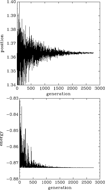
Chapter 24: Simulated Annealing 305
Here are a couple of plots that are generated by running siman_test in the following
way:
$ ./siman_test | awk ’!/^#/ {print $1, $4}’
| graph -y 1.34 1.4 -W0 -X generation -Y position
| plot -Tps > siman-test.eps
$ ./siman_test | awk ’!/^#/ {print $1, $5}’
| graph -y -0.88 -0.83 -W0 -X generation -Y energy
| plot -Tps > siman-energy.eps
Example of a simulated annealing run: at higher temperatures (early in the
plot) you see that the solution can fluctuate, but at lower temperatures it
converges.
24.3.2 Traveling Salesman Problem
The TSP (Traveling Salesman Problem) is the classic combinatorial optimization problem.
I have provided a very simple version of it, based on the coordinates of twelve cities in the
southwestern United States. This should maybe be called the Flying Salesman Problem,
Chapter 24: Simulated Annealing 306
since I am using the great-circle distance between cities, rather than the driving distance.
Also: I assume the earth is a sphere, so I don’t use geoid distances.
The gsl_siman_solve routine finds a route which is 3490.62 Kilometers long; this is
confirmed by an exhaustive search of all possible routes with the same initial city.
The full code can be found in ‘siman/siman_tsp.c’, but I include here some plots
generated in the following way:
$ ./siman_tsp > tsp.output
$ grep -v "^#" tsp.output
| awk ’{print $1, $NF}’
| graph -y 3300 6500 -W0 -X generation -Y distance
-L "TSP - 12 southwest cities"
| plot -Tps > 12-cities.eps
$ grep initial_city_coord tsp.output
| awk ’{print $2, $3}’
| graph -X "longitude (- means west)" -Y "latitude"
-L "TSP - initial-order" -f 0.03 -S 1 0.1
| plot -Tps > initial-route.eps
$ grep final_city_coord tsp.output
| awk ’{print $2, $3}’
| graph -X "longitude (- means west)" -Y "latitude"
-L "TSP - final-order" -f 0.03 -S 1 0.1
| plot -Tps > final-route.eps
This is the output showing the initial order of the cities; longitude is negative, since it is
west and I want the plot to look like a map.
# initial coordinates of cities (longitude and latitude)
###initial_city_coord: -105.95 35.68 Santa Fe
###initial_city_coord: -112.07 33.54 Phoenix
###initial_city_coord: -106.62 35.12 Albuquerque
###initial_city_coord: -103.2 34.41 Clovis
###initial_city_coord: -107.87 37.29 Durango
###initial_city_coord: -96.77 32.79 Dallas
###initial_city_coord: -105.92 35.77 Tesuque
###initial_city_coord: -107.84 35.15 Grants
###initial_city_coord: -106.28 35.89 Los Alamos
###initial_city_coord: -106.76 32.34 Las Cruces
###initial_city_coord: -108.58 37.35 Cortez
###initial_city_coord: -108.74 35.52 Gallup
###initial_city_coord: -105.95 35.68 Santa Fe
The optimal route turns out to be:
# final coordinates of cities (longitude and latitude)
###final_city_coord: -105.95 35.68 Santa Fe
###final_city_coord: -103.2 34.41 Clovis
###final_city_coord: -96.77 32.79 Dallas
###final_city_coord: -106.76 32.34 Las Cruces
###final_city_coord: -112.07 33.54 Phoenix
###final_city_coord: -108.74 35.52 Gallup
###final_city_coord: -108.58 37.35 Cortez
###final_city_coord: -107.87 37.29 Durango
###final_city_coord: -107.84 35.15 Grants
###final_city_coord: -106.62 35.12 Albuquerque
###final_city_coord: -106.28 35.89 Los Alamos
###final_city_coord: -105.92 35.77 Tesuque
###final_city_coord: -105.95 35.68 Santa Fe
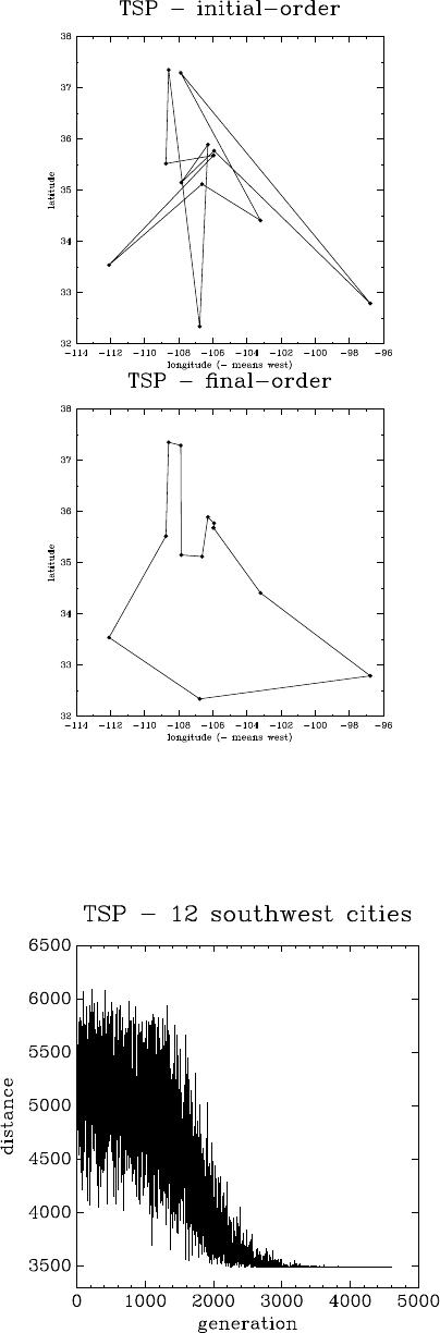
Chapter 24: Simulated Annealing 307
Initial and final (optimal) route for the 12 southwestern cities Flying Salesman
Problem.
Here’s a plot of the cost function (energy) versus generation (point in the calculation at
which a new temperature is set) for this problem:
Example of a simulated annealing run for the 12 southwestern cities Flying
Salesman Problem.
Chapter 24: Simulated Annealing 308
24.4 References and Further Reading
Further information is available in the following book,
Modern Heuristic Techniques for Combinatorial Problems, Colin R. Reeves (ed.),
McGraw-Hill, 1995 (ISBN 0-07-709239-2).

Chapter 25: Ordinary Differential Equations 309
25 Ordinary Differential Equations
This chapter describes functions for solving ordinary differential equation (ODE) initial
value problems. The library provides a variety of low-level methods, such as Runge-Kutta
and Bulirsch-Stoer routines, and higher-level components for adaptive step-size control. The
components can be combined by the user to achieve the desired solution, with full access
to any intermediate steps.
These functions are declared in the header file ‘gsl_odeiv.h’.
25.1 Defining the ODE System
The routines solve the general n-dimensional first-order system,
dyi(t)
dt =fi(t, y1(t),...yn(t))
for i= 1,...,n. The stepping functions rely on the vector of derivatives fiand the Jacobian
matrix, Jij =∂fi(t, y(t))/∂yj. A system of equations is defined using the gsl_odeiv_system
datatype.
[Data Type]gsl_odeiv_system
This data type defines a general ODE system with arbitrary parameters.
int (* function) (double t, const double y[], double dydt[], void *
params)
This function should store the vector elements fi(t, y, params) in the array
dydt, for arguments (t,y) and parameters params. The function should
return GSL_SUCCESS if the calculation was completed successfully. Any
other return value indicates an error.
int (* jacobian) (double t, const double y[], double * dfdy, double
dfdt[], void * params);
This function should store the vector of derivative elements
∂fi(t, y, params)/∂t in the array dfdt and the Jacobian matrix Jij in
the array dfdy, regarded as a row-ordered matrix J(i,j) = dfdy[i *
dimension + j] where dimension is the dimension of the system. The
function should return GSL_SUCCESS if the calculation was completed
successfully. Any other return value indicates an error.
Some of the simpler solver algorithms do not make use of the Jacobian
matrix, so it is not always strictly necessary to provide it (the jacobian
element of the struct can be replaced by a null pointer for those algo-
rithms). However, it is useful to provide the Jacobian to allow the solver
algorithms to be interchanged—the best algorithms make use of the Ja-
cobian.
size_t dimension;
This is the dimension of the system of equations.
void * params
This is a pointer to the arbitrary parameters of the system.

Chapter 25: Ordinary Differential Equations 310
25.2 Stepping Functions
The lowest level components are the stepping functions which advance a solution from time
tto t+hfor a fixed step-size hand estimate the resulting local error.
[Function]gsl_odeiv_step * gsl_odeiv_step_alloc (const gsl odeiv step type
*T, size t dim )
This function returns a pointer to a newly allocated instance of a stepping function
of type Tfor a system of dim dimensions.
[Function]int gsl_odeiv_step_reset (gsl odeiv step * s)
This function resets the stepping function s. It should be used whenever the next use
of swill not be a continuation of a previous step.
[Function]void gsl_odeiv_step_free (gsl odeiv step * s)
This function frees all the memory associated with the stepping function s.
[Function]const char * gsl_odeiv_step_name (const gsl odeiv step * s)
This function returns a pointer to the name of the stepping function. For example,
printf ("step method is ’%s’\n",
gsl_odeiv_step_name (s));
would print something like step method is ’rkf45’.
[Function]unsigned int gsl_odeiv_step_order (const gsl odeiv step * s)
This function returns the order of the stepping function on the previous step. This
order can vary if the stepping function itself is adaptive.
[Function]int gsl_odeiv_step_apply (gsl odeiv step * s, double t, double h,
double y[], double yerr [], const double dydt_in [], double dydt_out [], const
gsl odeiv system * dydt )
This function applies the stepping function sto the system of equations defined by
dydt, using the step size hto advance the system from time tand state yto time t+h.
The new state of the system is stored in yon output, with an estimate of the absolute
error in each component stored in yerr. If the argument dydt in is not null it should
point an array containing the derivatives for the system at time ton input. This is
optional as the derivatives will be computed internally if they are not provided, but
allows the reuse of existing derivative information. On output the new derivatives of
the system at time t+hwill be stored in dydt out if it is not null.
If the user-supplied functions defined in the system dydt return a status other than
GSL_SUCCESS the step will be aborted. In this case, the elements of ywill be restored
to their pre-step values and the error code from the user-supplied function will be
returned. The step-size hwill be set to the step-size which caused the error. If the
function is called again with a smaller step-size, e.g. h/10, it should be possible
to get closer to any singularity. To distinguish between error codes from the user-
supplied functions and those from gsl_odeiv_step_apply itself, any user-defined
return values should be distinct from the standard GSL error codes.
The following algorithms are available,

Chapter 25: Ordinary Differential Equations 311
[Step Type]gsl_odeiv_step_rk2
Embedded Runge-Kutta (2, 3) method.
[Step Type]gsl_odeiv_step_rk4
4th order (classical) Runge-Kutta. The error estimate is obtained by halving the step-
size. For more efficient estimate of the error, use the Runge-Kutta-Fehlberg method
described below.
[Step Type]gsl_odeiv_step_rkf45
Embedded Runge-Kutta-Fehlberg (4, 5) method. This method is a good general-
purpose integrator.
[Step Type]gsl_odeiv_step_rkck
Embedded Runge-Kutta Cash-Karp (4, 5) method.
[Step Type]gsl_odeiv_step_rk8pd
Embedded Runge-Kutta Prince-Dormand (8,9) method.
[Step Type]gsl_odeiv_step_rk2imp
Implicit 2nd order Runge-Kutta at Gaussian points.
[Step Type]gsl_odeiv_step_rk4imp
Implicit 4th order Runge-Kutta at Gaussian points.
[Step Type]gsl_odeiv_step_bsimp
Implicit Bulirsch-Stoer method of Bader and Deuflhard. This algorithm requires the
Jacobian.
[Step Type]gsl_odeiv_step_gear1
M=1 implicit Gear method.
[Step Type]gsl_odeiv_step_gear2
M=2 implicit Gear method.
25.3 Adaptive Step-size Control
The control function examines the proposed change to the solution produced by a stepping
function and attempts to determine the optimal step-size for a user-specified level of error.
[Function]gsl_odeiv_control * gsl_odeiv_control_standard_new (double
eps_abs, double eps_rel, double a_y, double a_dydt )
The standard control object is a four parameter heuristic based on absolute and
relative errors eps abs and eps rel, and scaling factors a y and a dydt for the system
state y(t) and derivatives y′(t) respectively.
The step-size adjustment procedure for this method begins by computing the desired
error level Difor each component,
Di=ǫabs +ǫrel ∗(ay|yi|+adydth|y′
i|)
and comparing it with the observed error Ei=|yerri|. If the observed error E
exceeds the desired error level Dby more than 10% for any component then the

Chapter 25: Ordinary Differential Equations 312
method reduces the step-size by an appropriate factor,
hnew =hold ∗S∗(E/D)−1/q
where qis the consistency order of the method (e.g. q= 4 for 4(5) embedded RK),
and Sis a safety factor of 0.9. The ratio E/D is taken to be the maximum of the
ratios Ei/Di.
If the observed error Eis less than 50% of the desired error level Dfor the maximum
ratio Ei/Dithen the algorithm takes the opportunity to increase the step-size to bring
the error in line with the desired level,
hnew =hold ∗S∗(E/D)−1/(q+1)
This encompasses all the standard error scaling methods. To avoid uncontrolled
changes in the stepsize, the overall scaling factor is limited to the range 1/5 to 5.
[Function]gsl_odeiv_control * gsl_odeiv_control_y_new (double eps_abs,
double eps_rel )
This function creates a new control object which will keep the local error on each
step within an absolute error of eps abs and relative error of eps rel with respect to
the solution yi(t). This is equivalent to the standard control object with ay=1 and
a dydt=0.
[Function]gsl_odeiv_control * gsl_odeiv_control_yp_new (double
eps_abs, double eps_rel )
This function creates a new control object which will keep the local error on each
step within an absolute error of eps abs and relative error of eps rel with respect to
the derivatives of the solution y′
i(t). This is equivalent to the standard control object
with ay=0 and a dydt=1.
[Function]gsl_odeiv_control * gsl_odeiv_control_scaled_new (double
eps_abs, double eps_rel, double a_y, double a_dydt, const double
scale_abs [], size t dim )
This function creates a new control object which uses the same algorithm as gsl_
odeiv_control_standard_new but with an absolute error which is scaled for each
component by the array scale abs. The formula for Difor this control object is,
Di=ǫabssi+ǫrel ∗(ay|yi|+adydth|y′
i|)
where siis the i-th component of the array scale abs. The same error control heuristic
is used by the Matlab ode suite.
[Function]gsl_odeiv_control * gsl_odeiv_control_alloc (const
gsl odeiv control type * T)
This function returns a pointer to a newly allocated instance of a control function of
type T. This function is only needed for defining new types of control functions. For
most purposes the standard control functions described above should be sufficient.

Chapter 25: Ordinary Differential Equations 313
[Function]int gsl_odeiv_control_init (gsl odeiv control * c, double eps_abs,
double eps_rel, double a_y, double a_dydt )
This function initializes the control function cwith the parameters eps abs (absolute
error), eps rel (relative error), a y (scaling factor for y) and a dydt (scaling factor
for derivatives).
[Function]void gsl_odeiv_control_free (gsl odeiv control * c)
This function frees all the memory associated with the control function c.
[Function]int gsl_odeiv_control_hadjust (gsl odeiv control * c, gsl odeiv step
*s, const double y[], const double yerr [], const double dydt [], double * h)
This function adjusts the step-size husing the control function c, and the current
values of y,yerr and dydt. The stepping function step is also needed to determine
the order of the method. If the error in the y-values yerr is found to be too large then
the step-size his reduced and the function returns GSL_ODEIV_HADJ_DEC. If the error
is sufficiently small then hmay be increased and GSL_ODEIV_HADJ_INC is returned.
The function returns GSL_ODEIV_HADJ_NIL if the step-size is unchanged. The goal
of the function is to estimate the largest step-size which satisfies the user-specified
accuracy requirements for the current point.
[Function]const char * gsl_odeiv_control_name (const gsl odeiv control * c)
This function returns a pointer to the name of the control function. For example,
printf ("control method is ’%s’\n",
gsl_odeiv_control_name (c));
would print something like control method is ’standard’
25.4 Evolution
The highest level of the system is the evolution function which combines the results of a
stepping function and control function to reliably advance the solution forward over an
interval (t0, t1). If the control function signals that the step-size should be decreased the
evolution function backs out of the current step and tries the proposed smaller step-size.
This process is continued until an acceptable step-size is found.
[Function]gsl_odeiv_evolve * gsl_odeiv_evolve_alloc (size tdim )
This function returns a pointer to a newly allocated instance of an evolution function
for a system of dim dimensions.
[Function]int gsl_odeiv_evolve_apply (gsl odeiv evolve * e, gsl odeiv control *
con, gsl odeiv step * step, const gsl odeiv system * dydt, double * t, double
t1, double * h, double y[])
This function advances the system (e,dydt) from time tand position yusing the
stepping function step. The new time and position are stored in tand yon output.
The initial step-size is taken as h, but this will be modified using the control function
cto achieve the appropriate error bound if necessary. The routine may make several
calls to step in order to determine the optimum step-size. An estimate of the local
error for the step can be obtained from the components of the array e->yerr[]. If the
step-size has been changed the value of hwill be modified on output. The maximum

Chapter 25: Ordinary Differential Equations 314
time t1 is guaranteed not to be exceeded by the time-step. On the final time-step the
value of twill be set to t1 exactly.
If the user-supplied functions defined in the system dydt return a status other than
GSL_SUCCESS the step will be aborted. In this case, tand ywill be restored to their
pre-step values and the error code from the user-supplied function will be returned.
To distinguish between error codes from the user-supplied functions and those from
gsl_odeiv_evolve_apply itself, any user-defined return values should be distinct
from the standard GSL error codes.
[Function]int gsl_odeiv_evolve_reset (gsl odeiv evolve * e)
This function resets the evolution function e. It should be used whenever the next
use of ewill not be a continuation of a previous step.
[Function]void gsl_odeiv_evolve_free (gsl odeiv evolve * e)
This function frees all the memory associated with the evolution function e.
Where a system has discontinuous changes in the derivatives at known times it is ad-
visable to evolve the system between each discontinuity in sequence. For example, if a
step-change in an external driving force occurs at times ta, tb, tc,... then evolving over the
ranges (t0, ta), (ta, tb), . . . , (tc, t1) is more efficient than using the single range (t0, t1).
Evolving the system directly through a discontinuity with a strict tolerance may result
in extremely small steps being taken at the edge of the discontinuity (e.g. down to the limit
of machine precision). In this case it may be necessary to impose a minimum step size hmin
suitable for the problem:
while (t < t1)
{
gsl_odeiv_evolve_apply (e, c, s, &sys, &t, t1, &h, y);
if (h < hmin) { h = hmin; } ;
}
The value of hreturned by gsl_odeiv_evolve_apply is always a suggested value and
can be modified whenever needed.
25.5 Examples
The following program solves the second-order nonlinear Van der Pol oscillator equation,
x′′(t) + µx′(t)(x(t)2−1) + x(t) = 0
This can be converted into a first order system suitable for use with the routines described
in this chapter by introducing a separate variable for the velocity, y=x′(t),
x′=y
y′=−x+µy(1 −x2)
The program begins by defining functions for these derivatives and their Jacobian,
#include <stdio.h>
#include <gsl/gsl_errno.h>
#include <gsl/gsl_matrix.h>
#include <gsl/gsl_odeiv.h>
Chapter 25: Ordinary Differential Equations 315
int
func (double t, const double y[], double f[],
void *params)
{
double mu = *(double *)params;
f[0] = y[1];
f[1] = -y[0] - mu*y[1]*(y[0]*y[0] - 1);
return GSL_SUCCESS;
}
int
jac (double t, const double y[], double *dfdy,
double dfdt[], void *params)
{
double mu = *(double *)params;
gsl_matrix_view dfdy_mat
= gsl_matrix_view_array (dfdy, 2, 2);
gsl_matrix * m = &dfdy_mat.matrix;
gsl_matrix_set (m, 0, 0, 0.0);
gsl_matrix_set (m, 0, 1, 1.0);
gsl_matrix_set (m, 1, 0, -2.0*mu*y[0]*y[1] - 1.0);
gsl_matrix_set (m, 1, 1, -mu*(y[0]*y[0] - 1.0));
dfdt[0] = 0.0;
dfdt[1] = 0.0;
return GSL_SUCCESS;
}
int
main (void)
{
const gsl_odeiv_step_type * T
= gsl_odeiv_step_rk8pd;
gsl_odeiv_step * s
= gsl_odeiv_step_alloc (T, 2);
gsl_odeiv_control * c
= gsl_odeiv_control_y_new (1e-6, 0.0);
gsl_odeiv_evolve * e
= gsl_odeiv_evolve_alloc (2);
double mu = 10;
gsl_odeiv_system sys = {func, jac, 2, &mu};
double t = 0.0, t1 = 100.0;
double h = 1e-6;
double y[2] = { 1.0, 0.0 };
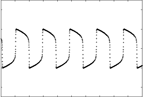
Chapter 25: Ordinary Differential Equations 316
while (t < t1)
{
int status = gsl_odeiv_evolve_apply (e, c, s,
&sys,
&t, t1,
&h, y);
if (status != GSL_SUCCESS)
break;
printf ("%.5e %.5e %.5e\n", t, y[0], y[1]);
}
gsl_odeiv_evolve_free (e);
gsl_odeiv_control_free (c);
gsl_odeiv_step_free (s);
return 0;
}
For functions with multiple parameters, the appropriate information can be passed in
through the params argument using a pointer to a struct.
The main loop of the program evolves the solution from (y, y′) = (1,0) at t= 0 to
t= 100. The step-size his automatically adjusted by the controller to maintain an absolute
accuracy of 10−6in the function values y.
-4
-2
0
2
4
0 10 20 30 40 50 60 70 80 90 100
Numerical solution of the Van der Pol oscillator equation
using Prince-Dormand 8th order Runge-Kutta.
To obtain the values at user-specified positions, rather than those chosen automatically by
the control function, the main loop can be modified to advance the solution from one chosen
point to the next. For example, the following main loop prints the solution at the points
ti= 0,1,2,...,100,
for (i = 1; i <= 100; i++)
{
Chapter 25: Ordinary Differential Equations 317
double ti = i * t1 / 100.0;
while (t < ti)
{
gsl_odeiv_evolve_apply (e, c, s,
&sys,
&t, ti, &h,
y);
}
printf ("%.5e %.5e %.5e\n", t, y[0], y[1]);
}
Note that arbitrary values of tican be used for each stage of the integration. The equally
spaced points in this example are just used as an illustration.
It is also possible to work with a non-adaptive integrator, using only the stepping function
itself. The following program uses the rk4 fourth-order Runge-Kutta stepping function with
a fixed stepsize of 0.01,
int
main (void)
{
const gsl_odeiv_step_type * T
= gsl_odeiv_step_rk4;
gsl_odeiv_step * s
= gsl_odeiv_step_alloc (T, 2);
double mu = 10;
gsl_odeiv_system sys = {func, jac, 2, &mu};
double t = 0.0, t1 = 100.0;
double h = 1e-2;
double y[2] = { 1.0, 0.0 }, y_err[2];
double dydt_in[2], dydt_out[2];
/* initialise dydt_in from system parameters */
GSL_ODEIV_FN_EVAL(&sys, t, y, dydt_in);
while (t < t1)
{
int status = gsl_odeiv_step_apply (s, t, h,
y, y_err,
dydt_in,
dydt_out,
&sys);
if (status != GSL_SUCCESS)

Chapter 25: Ordinary Differential Equations 318
break;
dydt_in[0] = dydt_out[0];
dydt_in[1] = dydt_out[1];
t += h;
printf ("%.5e %.5e %.5e\n", t, y[0], y[1]);
}
gsl_odeiv_step_free (s);
return 0;
}
The derivatives must be initialized for the starting point t= 0 before the first step is taken.
Subsequent steps use the output derivatives dydt out as inputs to the next step by copying
their values into dydt in.
25.6 References and Further Reading
Many of the basic Runge-Kutta formulas can be found in the Handbook of Mathematical
Functions,
Abramowitz & Stegun (eds.), Handbook of Mathematical Functions, Section 25.5.
The implicit Bulirsch-Stoer algorithm bsimp is described in the following paper,
G. Bader and P. Deuflhard, “A Semi-Implicit Mid-Point Rule for Stiff Systems of
Ordinary Differential Equations.”, Numer. Math. 41, 373–398, 1983.

Chapter 26: Interpolation 319
26 Interpolation
This chapter describes functions for performing interpolation. The library provides a vari-
ety of interpolation methods, including Cubic splines and Akima splines. The interpolation
types are interchangeable, allowing different methods to be used without recompiling. In-
terpolations can be defined for both normal and periodic boundary conditions. Additional
functions are available for computing derivatives and integrals of interpolating functions.
These interpolation methods produce curves that pass through each datapoint. To in-
terpolate noisy data with a smoothing curve see Chapter 38 [Basis Splines], page 415.
The functions described in this section are declared in the header files ‘gsl_interp.h’
and ‘gsl_spline.h’.
26.1 Introduction
Given a set of data points (x1, y1)...(xn, yn) the routines described in this section compute
a continuous interpolating function y(x) such that y(xi) = yi. The interpolation is piecewise
smooth, and its behavior at the end-points is determined by the type of interpolation used.
26.2 Interpolation Functions
The interpolation function for a given dataset is stored in a gsl_interp object. These are
created by the following functions.
[Function]gsl_interp * gsl_interp_alloc (const gsl interp type * T, size t
size )
This function returns a pointer to a newly allocated interpolation object of type T
for size data-points.
[Function]int gsl_interp_init (gsl interp * interp, const double xa [], const
double ya [], size t size )
This function initializes the interpolation object interp for the data (xa,ya) where xa
and ya are arrays of size size. The interpolation object (gsl_interp) does not save
the data arrays xa and ya and only stores the static state computed from the data.
The xa data array is always assumed to be strictly ordered, with increasing xvalues;
the behavior for other arrangements is not defined.
[Function]void gsl_interp_free (gsl interp * interp )
This function frees the interpolation object interp.
26.3 Interpolation Types
The interpolation library provides six interpolation types:
[Interpolation Type]gsl_interp_linear
Linear interpolation. This interpolation method does not require any additional mem-
ory.
[Interpolation Type]gsl_interp_polynomial
Polynomial interpolation. This method should only be used for interpolating small
numbers of points because polynomial interpolation introduces large oscillations, even

Chapter 26: Interpolation 320
for well-behaved datasets. The number of terms in the interpolating polynomial is
equal to the number of points.
[Interpolation Type]gsl_interp_cspline
Cubic spline with natural boundary conditions. The resulting curve is piecewise
cubic on each interval, with matching first and second derivatives at the supplied
data-points. The second derivative is chosen to be zero at the first point and last
point.
[Interpolation Type]gsl_interp_cspline_periodic
Cubic spline with periodic boundary conditions. The resulting curve is piecewise
cubic on each interval, with matching first and second derivatives at the supplied
data-points. The derivatives at the first and last points are also matched. Note that
the last point in the data must have the same y-value as the first point, otherwise the
resulting periodic interpolation will have a discontinuity at the boundary.
[Interpolation Type]gsl_interp_akima
Non-rounded Akima spline with natural boundary conditions. This method uses the
non-rounded corner algorithm of Wodicka.
[Interpolation Type]gsl_interp_akima_periodic
Non-rounded Akima spline with periodic boundary conditions. This method uses the
non-rounded corner algorithm of Wodicka.
The following related functions are available:
[Function]const char * gsl_interp_name (const gsl interp * interp )
This function returns the name of the interpolation type used by interp. For example,
printf ("interp uses ’%s’ interpolation.\n",
gsl_interp_name (interp));
would print something like,
interp uses ’cspline’ interpolation.
[Function]unsigned int gsl_interp_min_size (const gsl interp * interp )
This function returns the minimum number of points required by the interpolation
type of interp. For example, Akima spline interpolation requires a minimum of 5
points.
26.4 Index Look-up and Acceleration
The state of searches can be stored in a gsl_interp_accel object, which is a kind of
iterator for interpolation lookups. It caches the previous value of an index lookup. When
the subsequent interpolation point falls in the same interval its index value can be returned
immediately.
[Function]size_t gsl_interp_bsearch (const double x_array [], double x, size t
index_lo, size tindex_hi )
This function returns the index iof the array x array such that x_array[i] <= x <
x_array[i+1]. The index is searched for in the range [index lo,index hi]. An inline
version of this function is used when HAVE_INLINE is defined.

Chapter 26: Interpolation 321
[Function]gsl_interp_accel * gsl_interp_accel_alloc (void)
This function returns a pointer to an accelerator object, which is a kind of iterator
for interpolation lookups. It tracks the state of lookups, thus allowing for application
of various acceleration strategies.
[Function]size_t gsl_interp_accel_find (gsl interp accel * a, const double
x_array [], size t size, double x)
This function performs a lookup action on the data array x array of size size, using
the given accelerator a. This is how lookups are performed during evaluation of
an interpolation. The function returns an index isuch that x_array[i] <= x < x_
array[i+1]. An inline version of this function is used when HAVE_INLINE is defined.
[Function]int gsl_interp_accel_reset (gsl interp accel * acc );
This function reinitializes the accelerator object acc. It should be used when the
cached information is no longer applicable—for example, when switching to a new
dataset.
[Function]void gsl_interp_accel_free (gsl interp accel* acc )
This function frees the accelerator object acc.
26.5 Evaluation of Interpolating Functions
[Function]double gsl_interp_eval (const gsl interp * interp, const double xa [],
const double ya [], double x, gsl interp accel * acc )
[Function]int gsl_interp_eval_e (const gsl interp * interp, const double xa [],
const double ya [], double x, gsl interp accel * acc, double * y)
These functions return the interpolated value of yfor a given point x, using the
interpolation object interp, data arrays xa and ya and the accelerator acc.
[Function]double gsl_interp_eval_deriv (const gsl interp * interp, const
double xa [], const double ya [], double x, gsl interp accel * acc )
[Function]int gsl_interp_eval_deriv_e (const gsl interp * interp, const
double xa [], const double ya [], double x, gsl interp accel * acc, double * d)
These functions return the derivative dof an interpolated function for a given point
x, using the interpolation object interp, data arrays xa and ya and the accelerator
acc.
[Function]double gsl_interp_eval_deriv2 (const gsl interp * interp, const
double xa [], const double ya [], double x, gsl interp accel * acc )
[Function]int gsl_interp_eval_deriv2_e (const gsl interp * interp, const
double xa [], const double ya [], double x, gsl interp accel * acc, double * d2 )
These functions return the second derivative d2 of an interpolated function for a
given point x, using the interpolation object interp, data arrays xa and ya and the
accelerator acc.
[Function]double gsl_interp_eval_integ (const gsl interp * interp, const
double xa [], const double ya [], double a, double b, gsl interp accel * acc )

Chapter 26: Interpolation 322
[Function]int gsl_interp_eval_integ_e (const gsl interp * interp, const
double xa [], const double ya [], double a, double b, gsl interp accel * acc,
double * result )
These functions return the numerical integral result of an interpolated function over
the range [a,b], using the interpolation object interp, data arrays xa and ya and the
accelerator acc.
26.6 Higher-level Interface
The functions described in the previous sections required the user to supply pointers to the
xand yarrays on each call. The following functions are equivalent to the corresponding
gsl_interp functions but maintain a copy of this data in the gsl_spline object. This
removes the need to pass both xa and ya as arguments on each evaluation. These functions
are defined in the header file ‘gsl_spline.h’.
[Function]gsl_spline * gsl_spline_alloc (const gsl interp type * T, size t
size )
[Function]int gsl_spline_init (gsl spline * spline, const double xa [], const
double ya [], size t size )
[Function]void gsl_spline_free (gsl spline * spline )
[Function]const char * gsl_spline_name (const gsl spline * spline )
[Function]unsigned int gsl_spline_min_size (const gsl spline * spline )
[Function]double gsl_spline_eval (const gsl spline * spline, double x,
gsl interp accel * acc )
[Function]int gsl_spline_eval_e (const gsl spline * spline, double x,
gsl interp accel * acc, double * y)
[Function]double gsl_spline_eval_deriv (const gsl spline * spline, double x,
gsl interp accel * acc )
[Function]int gsl_spline_eval_deriv_e (const gsl spline * spline, double x,
gsl interp accel * acc, double * d)
[Function]double gsl_spline_eval_deriv2 (const gsl spline * spline, double x,
gsl interp accel * acc )
[Function]int gsl_spline_eval_deriv2_e (const gsl spline * spline, double x,
gsl interp accel * acc, double * d2 )
[Function]double gsl_spline_eval_integ (const gsl spline * spline, double a,
double b, gsl interp accel * acc )
[Function]int gsl_spline_eval_integ_e (const gsl spline * spline, double a,
double b, gsl interp accel * acc, double * result )
26.7 Examples
The following program demonstrates the use of the interpolation and spline functions. It
computes a cubic spline interpolation of the 10-point dataset (xi, yi) where xi=i+ sin(i)/2
and yi=i+ cos(i2) for i= 0 ...9.
Chapter 26: Interpolation 323
#include <stdlib.h>
#include <stdio.h>
#include <math.h>
#include <gsl/gsl_errno.h>
#include <gsl/gsl_spline.h>
int
main (void)
{
int i;
double xi, yi, x[10], y[10];
printf ("#m=0,S=2\n");
for (i = 0; i < 10; i++)
{
x[i] = i + 0.5 * sin (i);
y[i] = i + cos (i * i);
printf ("%g %g\n", x[i], y[i]);
}
printf ("#m=1,S=0\n");
{
gsl_interp_accel *acc
= gsl_interp_accel_alloc ();
gsl_spline *spline
= gsl_spline_alloc (gsl_interp_cspline, 10);
gsl_spline_init (spline, x, y, 10);
for (xi = x[0]; xi < x[9]; xi += 0.01)
{
yi = gsl_spline_eval (spline, xi, acc);
printf ("%g %g\n", xi, yi);
}
gsl_spline_free (spline);
gsl_interp_accel_free (acc);
}
return 0;
}
The output is designed to be used with the gnu plotutils graph program,
$ ./a.out > interp.dat
$ graph -T ps < interp.dat > interp.ps
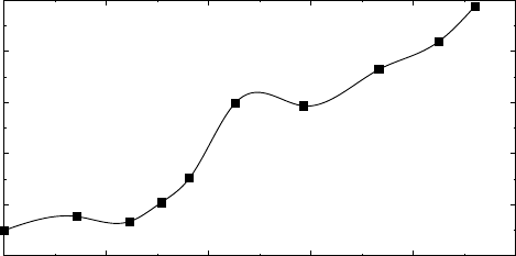
Chapter 26: Interpolation 324
0246810
0
2
4
6
8
10
The result shows a smooth interpolation of the original points. The interpolation method
can be changed simply by varying the first argument of gsl_spline_alloc.
The next program demonstrates a periodic cubic spline with 4 data points. Note that
the first and last points must be supplied with the same y-value for a periodic spline.
#include <stdlib.h>
#include <stdio.h>
#include <math.h>
#include <gsl/gsl_errno.h>
#include <gsl/gsl_spline.h>
int
main (void)
{
int N = 4;
double x[4] = {0.00, 0.10, 0.27, 0.30};
double y[4] = {0.15, 0.70, -0.10, 0.15};
/* Note: y[0] == y[3] for periodic data */
gsl_interp_accel *acc = gsl_interp_accel_alloc ();
const gsl_interp_type *t = gsl_interp_cspline_periodic;
gsl_spline *spline = gsl_spline_alloc (t, N);
int i; double xi, yi;
printf ("#m=0,S=5\n");
for (i = 0; i < N; i++)
{
printf ("%g %g\n", x[i], y[i]);
}
printf ("#m=1,S=0\n");
gsl_spline_init (spline, x, y, N);
for (i = 0; i <= 100; i++)
{
xi = (1 - i / 100.0) * x[0] + (i / 100.0) * x[N-1];
yi = gsl_spline_eval (spline, xi, acc);
printf ("%g %g\n", xi, yi);
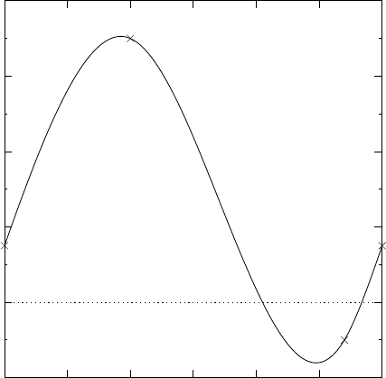
Chapter 26: Interpolation 325
}
gsl_spline_free (spline);
gsl_interp_accel_free (acc);
return 0;
}
The output can be plotted with gnu graph.
$ ./a.out > interp.dat
$ graph -T ps < interp.dat > interp.ps
0.00 0.05 0.10 0.15 0.20 0.25 0.30
−0.2
0.0
0.2
0.4
0.6
0.8
The result shows a periodic interpolation of the original points. The slope of the fitted
curve is the same at the beginning and end of the data, and the second derivative is also.
26.8 References and Further Reading
Descriptions of the interpolation algorithms and further references can be found in the
following books:
C.W. Ueberhuber, Numerical Computation (Volume 1), Chapter 9 “Interpolation”,
Springer (1997), ISBN 3-540-62058-3.
D.M. Young, R.T. Gregory A Survey of Numerical Mathematics (Volume 1), Chapter
6.8, Dover (1988), ISBN 0-486-65691-8.

Chapter 27: Numerical Differentiation 326
27 Numerical Differentiation
The functions described in this chapter compute numerical derivatives by finite differencing.
An adaptive algorithm is used to find the best choice of finite difference and to estimate
the error in the derivative. These functions are declared in the header file ‘gsl_deriv.h’.
27.1 Functions
[Function]int gsl_deriv_central (const gsl function * f, double x, double h,
double * result, double * abserr )
This function computes the numerical derivative of the function fat the point x
using an adaptive central difference algorithm with a step-size of h. The derivative is
returned in result and an estimate of its absolute error is returned in abserr.
The initial value of his used to estimate an optimal step-size, based on the scaling of
the truncation error and round-off error in the derivative calculation. The derivative
is computed using a 5-point rule for equally spaced abscissae at x−h,x−h/2, x,
x+h/2, x+h, with an error estimate taken from the difference between the 5-point
rule and the corresponding 3-point rule x−h,x,x+h. Note that the value of the
function at xdoes not contribute to the derivative calculation, so only 4-points are
actually used.
[Function]int gsl_deriv_forward (const gsl function * f, double x, double h,
double * result, double * abserr )
This function computes the numerical derivative of the function fat the point x
using an adaptive forward difference algorithm with a step-size of h. The function
is evaluated only at points greater than x, and never at xitself. The derivative is
returned in result and an estimate of its absolute error is returned in abserr. This
function should be used if f(x) has a discontinuity at x, or is undefined for values less
than x.
The initial value of his used to estimate an optimal step-size, based on the scaling of
the truncation error and round-off error in the derivative calculation. The derivative
at xis computed using an “open” 4-point rule for equally spaced abscissae at x+h/4,
x+h/2, x+ 3h/4, x+h, with an error estimate taken from the difference between
the 4-point rule and the corresponding 2-point rule x+h/2, x+h.
[Function]int gsl_deriv_backward (const gsl function * f, double x, double h,
double * result, double * abserr )
This function computes the numerical derivative of the function fat the point x
using an adaptive backward difference algorithm with a step-size of h. The function
is evaluated only at points less than x, and never at xitself. The derivative is returned
in result and an estimate of its absolute error is returned in abserr. This function
should be used if f(x) has a discontinuity at x, or is undefined for values greater than
x.
This function is equivalent to calling gsl_deriv_forward with a negative step-size.
Chapter 27: Numerical Differentiation 327
27.2 Examples
The following code estimates the derivative of the function f(x) = x3/2at x= 2 and at
x= 0. The function f(x) is undefined for x < 0 so the derivative at x= 0 is computed
using gsl_deriv_forward.
#include <stdio.h>
#include <gsl/gsl_math.h>
#include <gsl/gsl_deriv.h>
double f (double x, void * params)
{
return pow (x, 1.5);
}
int
main (void)
{
gsl_function F;
double result, abserr;
F.function = &f;
F.params = 0;
printf ("f(x) = x^(3/2)\n");
gsl_deriv_central (&F, 2.0, 1e-8, &result, &abserr);
printf ("x = 2.0\n");
printf ("f’(x) = %.10f +/- %.10f\n", result, abserr);
printf ("exact = %.10f\n\n", 1.5 * sqrt(2.0));
gsl_deriv_forward (&F, 0.0, 1e-8, &result, &abserr);
printf ("x = 0.0\n");
printf ("f’(x) = %.10f +/- %.10f\n", result, abserr);
printf ("exact = %.10f\n", 0.0);
return 0;
}
Here is the output of the program,
$ ./a.out
f(x) = x^(3/2)
x = 2.0
f’(x) = 2.1213203120 +/- 0.0000004064
exact = 2.1213203436
x = 0.0
f’(x) = 0.0000000160 +/- 0.0000000339
exact = 0.0000000000
Chapter 27: Numerical Differentiation 328
27.3 References and Further Reading
The algorithms used by these functions are described in the following sources:
Abramowitz and Stegun, Handbook of Mathematical Functions, Section 25.3.4, and
Table 25.5 (Coefficients for Differentiation).
S.D. Conte and Carl de Boor, Elementary Numerical Analysis: An Algorithmic Ap-
proach, McGraw-Hill, 1972.

Chapter 28: Chebyshev Approximations 329
28 Chebyshev Approximations
This chapter describes routines for computing Chebyshev approximations to univariate
functions. A Chebyshev approximation is a truncation of the series f(x) = PcnTn(x),
where the Chebyshev polynomials Tn(x) = cos(narccos x) provide an orthogonal basis of
polynomials on the interval [−1,1] with the weight function 1/√1−x2. The first few
Chebyshev polynomials are, T0(x) = 1, T1(x) = x,T2(x) = 2x2−1. For further information
see Abramowitz & Stegun, Chapter 22.
The functions described in this chapter are declared in the header file ‘gsl_chebyshev.h’.
28.1 Definitions
A Chebyshev series is stored using the following structure,
typedef struct
{
double * c; /* coefficients c[0] .. c[order] */
int order; /* order of expansion */
double a; /* lower interval point */
double b; /* upper interval point */
...
} gsl_cheb_series
The approximation is made over the range [a, b] using order+1 terms, including the coeffi-
cient c[0]. The series is computed using the following convention,
f(x) = c0
2+X
n=1
cnTn(x)
which is needed when accessing the coefficients directly.
28.2 Creation and Calculation of Chebyshev Series
[Function]gsl_cheb_series * gsl_cheb_alloc (const size tn)
This function allocates space for a Chebyshev series of order nand returns a pointer
to a new gsl_cheb_series struct.
[Function]void gsl_cheb_free (gsl cheb series * cs )
This function frees a previously allocated Chebyshev series cs.
[Function]int gsl_cheb_init (gsl cheb series * cs, const gsl function * f, const
double a, const double b)
This function computes the Chebyshev approximation cs for the function fover the
range (a, b) to the previously specified order. The computation of the Chebyshev
approximation is an O(n2) process, and requires nfunction evaluations.
28.3 Auxiliary Functions
The following functions provide information about an existing Chebyshev series.
[Function]size_t gsl_cheb_order (const gsl cheb series * cs )
This function returns the order of Chebyshev series cs.

Chapter 28: Chebyshev Approximations 330
[Function]size_t gsl_cheb_size (const gsl cheb series * cs )
[Function]double * gsl_cheb_coeffs (const gsl cheb series * cs )
These functions return the size of the Chebyshev coefficient array c[] and a pointer
to its location in memory for the Chebyshev series cs.
28.4 Chebyshev Series Evaluation
[Function]double gsl_cheb_eval (const gsl cheb series * cs, double x)
This function evaluates the Chebyshev series cs at a given point x.
[Function]int gsl_cheb_eval_err (const gsl cheb series * cs, const double x,
double * result, double * abserr )
This function computes the Chebyshev series cs at a given point x, estimating both
the series result and its absolute error abserr. The error estimate is made from the
first neglected term in the series.
[Function]double gsl_cheb_eval_n (const gsl cheb series * cs, size t order,
double x)
This function evaluates the Chebyshev series cs at a given point x, to (at most) the
given order order.
[Function]int gsl_cheb_eval_n_err (const gsl cheb series * cs, const size t
order, const double x, double * result, double * abserr )
This function evaluates a Chebyshev series cs at a given point x, estimating both the
series result and its absolute error abserr, to (at most) the given order order. The
error estimate is made from the first neglected term in the series.
28.5 Derivatives and Integrals
The following functions allow a Chebyshev series to be differentiated or integrated, pro-
ducing a new Chebyshev series. Note that the error estimate produced by evaluating the
derivative series will be underestimated due to the contribution of higher order terms being
neglected.
[Function]int gsl_cheb_calc_deriv (gsl cheb series * deriv, const
gsl cheb series * cs )
This function computes the derivative of the series cs, storing the derivative coeffi-
cients in the previously allocated deriv. The two series cs and deriv must have been
allocated with the same order.
[Function]int gsl_cheb_calc_integ (gsl cheb series * integ, const
gsl cheb series * cs )
This function computes the integral of the series cs, storing the integral coefficients in
the previously allocated integ. The two series cs and integ must have been allocated
with the same order. The lower limit of the integration is taken to be the left hand
end of the range a.
Chapter 28: Chebyshev Approximations 331
28.6 Examples
The following example program computes Chebyshev approximations to a step function.
This is an extremely difficult approximation to make, due to the discontinuity, and was cho-
sen as an example where approximation error is visible. For smooth functions the Chebyshev
approximation converges extremely rapidly and errors would not be visible.
#include <stdio.h>
#include <gsl/gsl_math.h>
#include <gsl/gsl_chebyshev.h>
double
f (double x, void *p)
{
if (x < 0.5)
return 0.25;
else
return 0.75;
}
int
main (void)
{
int i, n = 10000;
gsl_cheb_series *cs = gsl_cheb_alloc (40);
gsl_function F;
F.function = f;
F.params = 0;
gsl_cheb_init (cs, &F, 0.0, 1.0);
for (i = 0; i < n; i++)
{
double x = i / (double)n;
double r10 = gsl_cheb_eval_n (cs, 10, x);
double r40 = gsl_cheb_eval (cs, x);
printf ("%g %g %g %g\n",
x, GSL_FN_EVAL (&F, x), r10, r40);
}
gsl_cheb_free (cs);
return 0;
}
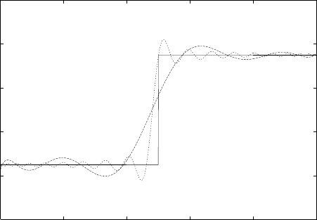
Chapter 28: Chebyshev Approximations 332
The output from the program gives the original function, 10-th order approximation and
40-th order approximation, all sampled at intervals of 0.001 in x.
0
0.2
0.4
0.6
0.8
1
0 0.2 0.4 0.6 0.8 1
28.7 References and Further Reading
The following paper describes the use of Chebyshev series,
R. Broucke, “Ten Subroutines for the Manipulation of Chebyshev Series [C1] (Algo-
rithm 446)”. Communications of the ACM 16(4), 254–256 (1973)

Chapter 29: Series Acceleration 333
29 Series Acceleration
The functions described in this chapter accelerate the convergence of a series using the
Levin u-transform. This method takes a small number of terms from the start of a series
and uses a systematic approximation to compute an extrapolated value and an estimate
of its error. The u-transform works for both convergent and divergent series, including
asymptotic series.
These functions are declared in the header file ‘gsl_sum.h’.
29.1 Acceleration functions
The following functions compute the full Levin u-transform of a series with its error estimate.
The error estimate is computed by propagating rounding errors from each term through to
the final extrapolation.
These functions are intended for summing analytic series where each term is known to
high accuracy, and the rounding errors are assumed to originate from finite precision. They
are taken to be relative errors of order GSL_DBL_EPSILON for each term.
The calculation of the error in the extrapolated value is an O(N2) process, which is
expensive in time and memory. A faster but less reliable method which estimates the error
from the convergence of the extrapolated value is described in the next section. For the
method described here a full table of intermediate values and derivatives through to O(N)
must be computed and stored, but this does give a reliable error estimate.
[Function]gsl_sum_levin_u_workspace * gsl_sum_levin_u_alloc (size t n)
This function allocates a workspace for a Levin u-transform of nterms. The size of
the workspace is O(2n2+ 3n).
[Function]void gsl_sum_levin_u_free (gsl sum levin u workspace * w)
This function frees the memory associated with the workspace w.
[Function]int gsl_sum_levin_u_accel (const double * array, size t
array_size, gsl sum levin u workspace * w, double * sum_accel, double *
abserr )
This function takes the terms of a series in array of size array size and computes the
extrapolated limit of the series using a Levin u-transform. Additional working space
must be provided in w. The extrapolated sum is stored in sum accel, with an estimate
of the absolute error stored in abserr. The actual term-by-term sum is returned in
w->sum_plain. The algorithm calculates the truncation error (the difference between
two successive extrapolations) and round-off error (propagated from the individual
terms) to choose an optimal number of terms for the extrapolation. All the terms of
the series passed in through array should be non-zero.
29.2 Acceleration functions without error estimation
The functions described in this section compute the Levin u-transform of series and attempt
to estimate the error from the “truncation error” in the extrapolation, the difference between
the final two approximations. Using this method avoids the need to compute an intermediate
table of derivatives because the error is estimated from the behavior of the extrapolated

Chapter 29: Series Acceleration 334
value itself. Consequently this algorithm is an O(N) process and only requires O(N) terms
of storage. If the series converges sufficiently fast then this procedure can be acceptable.
It is appropriate to use this method when there is a need to compute many extrapolations
of series with similar convergence properties at high-speed. For example, when numerically
integrating a function defined by a parameterized series where the parameter varies only
slightly. A reliable error estimate should be computed first using the full algorithm described
above in order to verify the consistency of the results.
[Function]gsl_sum_levin_utrunc_workspace *
gsl_sum_levin_utrunc_alloc (size tn)
This function allocates a workspace for a Levin u-transform of nterms, without error
estimation. The size of the workspace is O(3n).
[Function]void gsl_sum_levin_utrunc_free (gsl sum levin utrunc workspace *
w)
This function frees the memory associated with the workspace w.
[Function]int gsl_sum_levin_utrunc_accel (const double * array, size t
array_size, gsl sum levin utrunc workspace * w, double * sum_accel,
double * abserr_trunc )
This function takes the terms of a series in array of size array size and computes
the extrapolated limit of the series using a Levin u-transform. Additional working
space must be provided in w. The extrapolated sum is stored in sum accel. The
actual term-by-term sum is returned in w->sum_plain. The algorithm terminates
when the difference between two successive extrapolations reaches a minimum or is
sufficiently small. The difference between these two values is used as estimate of the
error and is stored in abserr trunc. To improve the reliability of the algorithm the
extrapolated values are replaced by moving averages when calculating the truncation
error, smoothing out any fluctuations.
29.3 Examples
The following code calculates an estimate of ζ(2) = π2/6 using the series,
ζ(2) = 1 + 1/22+ 1/32+ 1/42+...
After Nterms the error in the sum is O(1/N ), making direct summation of the series
converge slowly.
#include <stdio.h>
#include <gsl/gsl_math.h>
#include <gsl/gsl_sum.h>
#define N 20
int
main (void)
{
double t[N];
double sum_accel, err;
Chapter 29: Series Acceleration 335
double sum = 0;
int n;
gsl_sum_levin_u_workspace * w
= gsl_sum_levin_u_alloc (N);
const double zeta_2 = M_PI * M_PI / 6.0;
/* terms for zeta(2) = \sum_{n=1}^{\infty} 1/n^2 */
for (n = 0; n < N; n++)
{
double np1 = n + 1.0;
t[n] = 1.0 / (np1 * np1);
sum += t[n];
}
gsl_sum_levin_u_accel (t, N, w, &sum_accel, &err);
printf ("term-by-term sum = % .16f using %d terms\n",
sum, N);
printf ("term-by-term sum = % .16f using %d terms\n",
w->sum_plain, w->terms_used);
printf ("exact value = % .16f\n", zeta_2);
printf ("accelerated sum = % .16f using %d terms\n",
sum_accel, w->terms_used);
printf ("estimated error = % .16f\n", err);
printf ("actual error = % .16f\n",
sum_accel - zeta_2);
gsl_sum_levin_u_free (w);
return 0;
}
The output below shows that the Levin u-transform is able to obtain an estimate of the
sum to 1 part in 1010 using the first eleven terms of the series. The error estimate returned
by the function is also accurate, giving the correct number of significant digits.
$ ./a.out
term-by-term sum = 1.5961632439130233 using 20 terms
term-by-term sum = 1.5759958390005426 using 13 terms
exact value = 1.6449340668482264
accelerated sum = 1.6449340668166479 using 13 terms
estimated error = 0.0000000000508580
actual error = -0.0000000000315785
Chapter 29: Series Acceleration 336
Note that a direct summation of this series would require 1010 terms to achieve the same
precision as the accelerated sum does in 13 terms.
29.4 References and Further Reading
The algorithms used by these functions are described in the following papers,
T. Fessler, W.F. Ford, D.A. Smith, hurry: An acceleration algorithm for scalar se-
quences and series ACM Transactions on Mathematical Software, 9(3):346–354, 1983.
and Algorithm 602 9(3):355–357, 1983.
The theory of the u-transform was presented by Levin,
D. Levin, Development of Non-Linear Transformations for Improving Convergence of
Sequences, Intern. J. Computer Math. B3:371–388, 1973.
A review paper on the Levin Transform is available online,
Herbert H. H. Homeier, Scalar Levin-Type Sequence Transformations,
http://arxiv.org/abs/math/0005209.

Chapter 30: Wavelet Transforms 337
30 Wavelet Transforms
This chapter describes functions for performing Discrete Wavelet Transforms (DWTs). The
library includes wavelets for real data in both one and two dimensions. The wavelet func-
tions are declared in the header files ‘gsl_wavelet.h’ and ‘gsl_wavelet2d.h’.
30.1 Definitions
The continuous wavelet transform and its inverse are defined by the relations,
w(s, τ) = Z∞
−∞
f(t)∗ψ∗
s,τ (t)dt
and,
f(t) = Z∞
0
ds Z∞
−∞
w(s, τ)∗ψs,τ (t)dτ
where the basis functions ψs,τ are obtained by scaling and translation from a single function,
referred to as the mother wavelet.
The discrete version of the wavelet transform acts on equally-spaced samples, with fixed
scaling and translation steps (s,τ). The frequency and time axes are sampled dyadically on
scales of 2jthrough a level parameter j. The resulting family of functions {ψj,n}constitutes
an orthonormal basis for square-integrable signals.
The discrete wavelet transform is an O(N) algorithm, and is also referred to as the fast
wavelet transform.
30.2 Initialization
The gsl_wavelet structure contains the filter coefficients defining the wavelet and any
associated offset parameters.
[Function]gsl_wavelet * gsl_wavelet_alloc (const gsl wavelet type * T, size t
k)
This function allocates and initializes a wavelet object of type T. The parameter
kselects the specific member of the wavelet family. A null pointer is returned if
insufficient memory is available or if a unsupported member is selected.
The following wavelet types are implemented:
[Wavelet]gsl_wavelet_daubechies
[Wavelet]gsl_wavelet_daubechies_centered
The is the Daubechies wavelet family of maximum phase with k/2 vanishing moments.
The implemented wavelets are k= 4,6,...,20, with keven.
[Wavelet]gsl_wavelet_haar
[Wavelet]gsl_wavelet_haar_centered
This is the Haar wavelet. The only valid choice of kfor the Haar wavelet is k= 2.
[Wavelet]gsl_wavelet_bspline
[Wavelet]gsl_wavelet_bspline_centered
This is the biorthogonal B-spline wavelet family of order (i, j). The implemented
values of k= 100 ∗i+jare 103, 105, 202, 204, 206, 208, 301, 303, 305 307, 309.

Chapter 30: Wavelet Transforms 338
The centered forms of the wavelets align the coefficients of the various sub-bands on edges.
Thus the resulting visualization of the coefficients of the wavelet transform in the phase
plane is easier to understand.
[Function]const char * gsl_wavelet_name (const gsl wavelet * w)
This function returns a pointer to the name of the wavelet family for w.
[Function]void gsl_wavelet_free (gsl wavelet * w)
This function frees the wavelet object w.
The gsl_wavelet_workspace structure contains scratch space of the same size as the
input data and is used to hold intermediate results during the transform.
[Function]gsl_wavelet_workspace * gsl_wavelet_workspace_alloc (size t
n)
This function allocates a workspace for the discrete wavelet transform. To perform a
one-dimensional transform on nelements, a workspace of size nmust be provided. For
two-dimensional transforms of n-by-nmatrices it is sufficient to allocate a workspace
of size n, since the transform operates on individual rows and columns.
[Function]void gsl_wavelet_workspace_free (gsl wavelet workspace * work )
This function frees the allocated workspace work.
30.3 Transform Functions
This sections describes the actual functions performing the discrete wavelet transform. Note
that the transforms use periodic boundary conditions. If the signal is not periodic in the
sample length then spurious coefficients will appear at the beginning and end of each level
of the transform.
30.3.1 Wavelet transforms in one dimension
[Function]int gsl_wavelet_transform (const gsl wavelet * w, double * data,
size tstride, size t n, gsl wavelet direction dir, gsl wavelet workspace *
work )
[Function]int gsl_wavelet_transform_forward (const gsl wavelet * w, double *
data, size tstride, size t n, gsl wavelet workspace * work )
[Function]int gsl_wavelet_transform_inverse (const gsl wavelet * w, double *
data, size tstride, size t n, gsl wavelet workspace * work )
These functions compute in-place forward and inverse discrete wavelet transforms
of length nwith stride stride on the array data. The length of the transform nis
restricted to powers of two. For the transform version of the function the argument
dir can be either forward (+1) or backward (−1). A workspace work of length n
must be provided.
For the forward transform, the elements of the original array are replaced by the
discrete wavelet transform fi→wj,k in a packed triangular storage layout, where jis
the index of the level j= 0 . . . J −1 and kis the index of the coefficient within each
level, k= 0 ...2j−1. The total number of levels is J= log2(n). The output data
has the following form,
(s−1,0, d0,0, d1,0, d1,1, d2,0,···, dj,k,···, dJ−1,2J−1−1)

Chapter 30: Wavelet Transforms 339
where the first element is the smoothing coefficient s−1,0, followed by the detail co-
efficients dj,k for each level j. The backward transform inverts these coefficients to
obtain the original data.
These functions return a status of GSL_SUCCESS upon successful completion. GSL_
EINVAL is returned if nis not an integer power of 2 or if insufficient workspace is
provided.
30.3.2 Wavelet transforms in two dimension
The library provides functions to perform two-dimensional discrete wavelet transforms on
square matrices. The matrix dimensions must be an integer power of two. There are
two possible orderings of the rows and columns in the two-dimensional wavelet transform,
referred to as the “standard” and “non-standard” forms.
The “standard” transform performs a complete discrete wavelet transform on the rows
of the matrix, followed by a separate complete discrete wavelet transform on the columns
of the resulting row-transformed matrix. This procedure uses the same ordering as a two-
dimensional fourier transform.
The “non-standard” transform is performed in interleaved passes on the rows and
columns of the matrix for each level of the transform. The first level of the transform
is applied to the matrix rows, and then to the matrix columns. This procedure is
then repeated across the rows and columns of the data for the subsequent levels of the
transform, until the full discrete wavelet transform is complete. The non-standard form of
the discrete wavelet transform is typically used in image analysis.
The functions described in this section are declared in the header file ‘gsl_wavelet2d.h’.
[Function]int gsl_wavelet2d_transform (const gsl wavelet * w, double * data,
size ttda, size t size1, size t size2, gsl wavelet direction dir,
gsl wavelet workspace * work )
[Function]int gsl_wavelet2d_transform_forward (const gsl wavelet * w,
double * data, size t tda, size t size1, size t size2, gsl wavelet workspace *
work )
[Function]int gsl_wavelet2d_transform_inverse (const gsl wavelet * w,
double * data, size t tda, size t size1, size t size2, gsl wavelet workspace *
work )
These functions compute two-dimensional in-place forward and inverse discrete
wavelet transforms in standard form on the array data stored in row-major form
with dimensions size1 and size2 and physical row length tda. The dimensions must
be equal (square matrix) and are restricted to powers of two. For the transform
version of the function the argument dir can be either forward (+1) or backward
(−1). A workspace work of the appropriate size must be provided. On exit, the
appropriate elements of the array data are replaced by their two-dimensional wavelet
transform.
The functions return a status of GSL_SUCCESS upon successful completion. GSL_
EINVAL is returned if size1 and size2 are not equal and integer powers of 2, or if
insufficient workspace is provided.
[Function]int gsl_wavelet2d_transform_matrix (const gsl wavelet * w,
gsl matrix * m, gsl wavelet direction dir, gsl wavelet workspace * work )

Chapter 30: Wavelet Transforms 340
[Function]int gsl_wavelet2d_transform_matrix_forward (const gsl wavelet *
w, gsl matrix * m, gsl wavelet workspace * work )
[Function]int gsl_wavelet2d_transform_matrix_inverse (const gsl wavelet *
w, gsl matrix * m, gsl wavelet workspace * work )
These functions compute the two-dimensional in-place wavelet transform on a matrix
a.
[Function]int gsl_wavelet2d_nstransform (const gsl wavelet * w, double *
data, size t tda, size t size1, size t size2, gsl wavelet direction dir,
gsl wavelet workspace * work )
[Function]int gsl_wavelet2d_nstransform_forward (const gsl wavelet * w,
double * data, size ttda, size t size1, size t size2, gsl wavelet workspace *
work )
[Function]int gsl_wavelet2d_nstransform_inverse (const gsl wavelet * w,
double * data, size ttda, size t size1, size t size2, gsl wavelet workspace *
work )
These functions compute the two-dimensional wavelet transform in non-standard
form.
[Function]int gsl_wavelet2d_nstransform_matrix (const gsl wavelet * w,
gsl matrix * m, gsl wavelet direction dir, gsl wavelet workspace * work )
[Function]int gsl_wavelet2d_nstransform_matrix_forward (const
gsl wavelet * w, gsl matrix * m, gsl wavelet workspace * work )
[Function]int gsl_wavelet2d_nstransform_matrix_inverse (const
gsl wavelet * w, gsl matrix * m, gsl wavelet workspace * work )
These functions compute the non-standard form of the two-dimensional in-place
wavelet transform on a matrix a.
30.4 Examples
The following program demonstrates the use of the one-dimensional wavelet transform func-
tions. It computes an approximation to an input signal (of length 256) using the 20 largest
components of the wavelet transform, while setting the others to zero.
#include <stdio.h>
#include <math.h>
#include <gsl/gsl_sort.h>
#include <gsl/gsl_wavelet.h>
int
main (int argc, char **argv)
{
int i, n = 256, nc = 20;
double *data = malloc (n * sizeof (double));
double *abscoeff = malloc (n * sizeof (double));
size_t *p = malloc (n * sizeof (size_t));
FILE * f;
gsl_wavelet *w;
Chapter 30: Wavelet Transforms 341
gsl_wavelet_workspace *work;
w = gsl_wavelet_alloc (gsl_wavelet_daubechies, 4);
work = gsl_wavelet_workspace_alloc (n);
f = fopen (argv[1], "r");
for (i = 0; i < n; i++)
{
fscanf (f, "%lg", &data[i]);
}
fclose (f);
gsl_wavelet_transform_forward (w, data, 1, n, work);
for (i = 0; i < n; i++)
{
abscoeff[i] = fabs (data[i]);
}
gsl_sort_index (p, abscoeff, 1, n);
for (i = 0; (i + nc) < n; i++)
data[p[i]] = 0;
gsl_wavelet_transform_inverse (w, data, 1, n, work);
for (i = 0; i < n; i++)
{
printf ("%g\n", data[i]);
}
gsl_wavelet_free (w);
gsl_wavelet_workspace_free (work);
free (data);
free (abscoeff);
free (p);
return 0;
}
The output can be used with the gnu plotutils graph program,
$ ./a.out ecg.dat > dwt.dat
$ graph -T ps -x 0 256 32 -h 0.3 -a dwt.dat > dwt.ps
The graphs below show an original and compressed version of a sample ECG recording
from the MIT-BIH Arrhythmia Database, part of the PhysioNet archive of public-domain
of medical datasets.
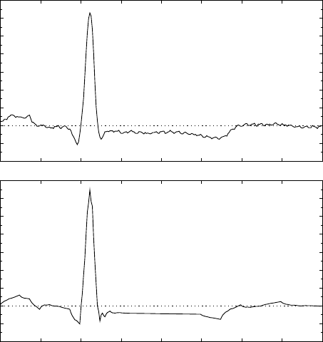
Chapter 30: Wavelet Transforms 342
0 32 64 96 128 160 192 224 256
−0.4
−0.2
0.0
0.2
0.4
0.6
0.8
1.0
1.2
1.4
0 32 64 96 128 160 192 224 256
−0.4
−0.2
0.0
0.2
0.4
0.6
0.8
1.0
1.2
1.4
Original (upper) and wavelet-compressed (lower) ECG signals, using the 20
largest components of the Daubechies(4) discrete wavelet transform.
30.5 References and Further Reading
The mathematical background to wavelet transforms is covered in the original lectures by
Daubechies,
Ingrid Daubechies. Ten Lectures on Wavelets. CBMS-NSF Regional Conference Series
in Applied Mathematics (1992), SIAM, ISBN 0898712742.
An easy to read introduction to the subject with an emphasis on the application of the
wavelet transform in various branches of science is,
Paul S. Addison. The Illustrated Wavelet Transform Handbook. Institute of Physics
Publishing (2002), ISBN 0750306920.
For extensive coverage of signal analysis by wavelets, wavelet packets and local cosine bases
see,
S. G. Mallat. A wavelet tour of signal processing (Second edition). Academic Press
(1999), ISBN 012466606X.
The concept of multiresolution analysis underlying the wavelet transform is described in,
S. G. Mallat. Multiresolution Approximations and Wavelet Orthonormal Bases of
L2(R). Transactions of the American Mathematical Society, 315(1), 1989, 69–87.
S. G. Mallat. A Theory for Multiresolution Signal Decomposition—The Wavelet Repre-
sentation. IEEE Transactions on Pattern Analysis and Machine Intelligence, 11, 1989,
674–693.
The coefficients for the individual wavelet families implemented by the library can be found
in the following papers,
I. Daubechies. Orthonormal Bases of Compactly Supported Wavelets. Communica-
tions on Pure and Applied Mathematics, 41 (1988) 909–996.
Chapter 30: Wavelet Transforms 343
A. Cohen, I. Daubechies, and J.-C. Feauveau. Biorthogonal Bases of Compactly Sup-
ported Wavelets. Communications on Pure and Applied Mathematics, 45 (1992) 485–
560.
The PhysioNet archive of physiological datasets can be found online at
http://www.physionet.org/ and is described in the following paper,
Goldberger et al. PhysioBank, PhysioToolkit, and PhysioNet: Components of a New
Research Resource for Complex Physiologic Signals. Circulation 101(23):e215-e220
2000.

Chapter 31: Discrete Hankel Transforms 344
31 Discrete Hankel Transforms
This chapter describes functions for performing Discrete Hankel Transforms (DHTs). The
functions are declared in the header file ‘gsl_dht.h’.
31.1 Definitions
The discrete Hankel transform acts on a vector of sampled data, where the samples are
assumed to have been taken at points related to the zeroes of a Bessel function of fixed
order; compare this to the case of the discrete Fourier transform, where samples are taken
at points related to the zeroes of the sine or cosine function.
Specifically, let f(t) be a function on the unit interval. Then the finite ν-Hankel transform
of f(t) is defined to be the set of numbers gmgiven by,
gm=Z1
0
tdt Jν(jν,mt)f(t),
so that,
f(t) =
∞
X
m=1
2Jν(jν,mx)
Jν+1(jν,m)2gm.
Suppose that fis band-limited in the sense that gm= 0 for m > M. Then we have the
following fundamental sampling theorem.
gm=2
j2
ν,M
M−1
X
k=1
fjν,k
jν,M Jν(jν,mjν,k /jν,M )
Jν+1(jν,k )2.
It is this discrete expression which defines the discrete Hankel transform. The kernel in
the summation above defines the matrix of the ν-Hankel transform of size M−1. The
coefficients of this matrix, being dependent on νand M, must be precomputed and stored;
the gsl_dht object encapsulates this data. The allocation function gsl_dht_alloc returns
agsl_dht object which must be properly initialized with gsl_dht_init before it can be
used to perform transforms on data sample vectors, for fixed νand M, using the gsl_
dht_apply function. The implementation allows a scaling of the fundamental interval, for
convenience, so that one can assume the function is defined on the interval [0, X], rather
than the unit interval.
Notice that by assumption f(t) vanishes at the endpoints of the interval, consistent with
the inversion formula and the sampling formula given above. Therefore, this transform
corresponds to an orthogonal expansion in eigenfunctions of the Dirichlet problem for the
Bessel differential equation.
31.2 Functions
[Function]gsl_dht * gsl_dht_alloc (size tsize )
This function allocates a Discrete Hankel transform object of size size.
[Function]int gsl_dht_init (gsl dht * t, double nu, double xmax )
This function initializes the transform tfor the given values of nu and xmax.

Chapter 31: Discrete Hankel Transforms 345
[Function]gsl_dht * gsl_dht_new (size t size, double nu, double xmax )
This function allocates a Discrete Hankel transform object of size size and initializes
it for the given values of nu and xmax.
[Function]void gsl_dht_free (gsl dht * t)
This function frees the transform t.
[Function]int gsl_dht_apply (const gsl dht * t, double * f_in, double * f_out )
This function applies the transform tto the array f in whose size is equal to the size
of the transform. The result is stored in the array fout which must be of the same
length.
[Function]double gsl_dht_x_sample (const gsl dht * t, int n)
This function returns the value of the n-th sample point in the unit interval,
(jν,n+1/jν,M )X. These are the points where the function f(t) is assumed to be
sampled.
[Function]double gsl_dht_k_sample (const gsl dht * t, int n)
This function returns the value of the n-th sample point in “k-space”, jν,n+1/X.
31.3 References and Further Reading
The algorithms used by these functions are described in the following papers,
H. Fisk Johnson, Comp. Phys. Comm. 43, 181 (1987).
D. Lemoine, J. Chem. Phys. 101, 3936 (1994).
Chapter 32: One dimensional Root-Finding 346
32 One dimensional Root-Finding
This chapter describes routines for finding roots of arbitrary one-dimensional functions.
The library provides low level components for a variety of iterative solvers and convergence
tests. These can be combined by the user to achieve the desired solution, with full access to
the intermediate steps of the iteration. Each class of methods uses the same framework, so
that you can switch between solvers at runtime without needing to recompile your program.
Each instance of a solver keeps track of its own state, allowing the solvers to be used in
multi-threaded programs.
The header file ‘gsl_roots.h’ contains prototypes for the root finding functions and
related declarations.
32.1 Overview
One-dimensional root finding algorithms can be divided into two classes, root bracketing and
root polishing. Algorithms which proceed by bracketing a root are guaranteed to converge.
Bracketing algorithms begin with a bounded region known to contain a root. The size of
this bounded region is reduced, iteratively, until it encloses the root to a desired tolerance.
This provides a rigorous error estimate for the location of the root.
The technique of root polishing attempts to improve an initial guess to the root. These
algorithms converge only if started “close enough” to a root, and sacrifice a rigorous error
bound for speed. By approximating the behavior of a function in the vicinity of a root they
attempt to find a higher order improvement of an initial guess. When the behavior of the
function is compatible with the algorithm and a good initial guess is available a polishing
algorithm can provide rapid convergence.
In GSL both types of algorithm are available in similar frameworks. The user provides
a high-level driver for the algorithms, and the library provides the individual functions
necessary for each of the steps. There are three main phases of the iteration. The steps are,
•initialize solver state, s, for algorithm T
•update susing the iteration T
•test sfor convergence, and repeat iteration if necessary
The state for bracketing solvers is held in a gsl_root_fsolver struct. The updating
procedure uses only function evaluations (not derivatives). The state for root polishing
solvers is held in a gsl_root_fdfsolver struct. The updates require both the function and
its derivative (hence the name fdf) to be supplied by the user.
32.2 Caveats
Note that root finding functions can only search for one root at a time. When there are
several roots in the search area, the first root to be found will be returned; however it is
difficult to predict which of the roots this will be. In most cases, no error will be reported
if you try to find a root in an area where there is more than one.
Care must be taken when a function may have a multiple root (such as f(x) = (x−x0)2or
f(x) = (x−x0)3). It is not possible to use root-bracketing algorithms on even-multiplicity
roots. For these algorithms the initial interval must contain a zero-crossing, where the
function is negative at one end of the interval and positive at the other end. Roots with

Chapter 32: One dimensional Root-Finding 347
even-multiplicity do not cross zero, but only touch it instantaneously. Algorithms based on
root bracketing will still work for odd-multiplicity roots (e.g. cubic, quintic, . . . ). Root
polishing algorithms generally work with higher multiplicity roots, but at a reduced rate
of convergence. In these cases the Steffenson algorithm can be used to accelerate the
convergence of multiple roots.
While it is not absolutely required that fhave a root within the search region, numerical
root finding functions should not be used haphazardly to check for the existence of roots.
There are better ways to do this. Because it is easy to create situations where numerical root
finders can fail, it is a bad idea to throw a root finder at a function you do not know much
about. In general it is best to examine the function visually by plotting before searching
for a root.
32.3 Initializing the Solver
[Function]gsl_root_fsolver * gsl_root_fsolver_alloc (const
gsl root fsolver type * T)
This function returns a pointer to a newly allocated instance of a solver of type T.
For example, the following code creates an instance of a bisection solver,
const gsl_root_fsolver_type * T
= gsl_root_fsolver_bisection;
gsl_root_fsolver * s
= gsl_root_fsolver_alloc (T);
If there is insufficient memory to create the solver then the function returns a null
pointer and the error handler is invoked with an error code of GSL_ENOMEM.
[Function]gsl_root_fdfsolver * gsl_root_fdfsolver_alloc (const
gsl root fdfsolver type * T)
This function returns a pointer to a newly allocated instance of a derivative-based
solver of type T. For example, the following code creates an instance of a Newton-
Raphson solver,
const gsl_root_fdfsolver_type * T
= gsl_root_fdfsolver_newton;
gsl_root_fdfsolver * s
= gsl_root_fdfsolver_alloc (T);
If there is insufficient memory to create the solver then the function returns a null
pointer and the error handler is invoked with an error code of GSL_ENOMEM.
[Function]int gsl_root_fsolver_set (gsl root fsolver * s, gsl function * f,
double x_lower, double x_upper )
This function initializes, or reinitializes, an existing solver sto use the function fand
the initial search interval [xlower,x upper].
[Function]int gsl_root_fdfsolver_set (gsl root fdfsolver * s, gsl function fdf *
fdf, double root )
This function initializes, or reinitializes, an existing solver sto use the function and
derivative fdf and the initial guess root.

Chapter 32: One dimensional Root-Finding 348
[Function]void gsl_root_fsolver_free (gsl root fsolver * s)
[Function]void gsl_root_fdfsolver_free (gsl root fdfsolver * s)
These functions free all the memory associated with the solver s.
[Function]const char * gsl_root_fsolver_name (const gsl root fsolver * s)
[Function]const char * gsl_root_fdfsolver_name (const gsl root fdfsolver *
s)
These functions return a pointer to the name of the solver. For example,
printf ("s is a ’%s’ solver\n",
gsl_root_fsolver_name (s));
would print something like s is a ’bisection’ solver.
32.4 Providing the function to solve
You must provide a continuous function of one variable for the root finders to operate on,
and, sometimes, its first derivative. In order to allow for general parameters the functions
are defined by the following data types:
[Data Type]gsl_function
This data type defines a general function with parameters.
double (* function) (double x, void * params )
this function should return the value f(x, params) for argument xand
parameters params
void * params
a pointer to the parameters of the function
Here is an example for the general quadratic function,
f(x) = ax2+bx +c
with a= 3, b= 2, c= 1. The following code defines a gsl_function F which you could
pass to a root finder:
struct my_f_params { double a; double b; double c; };
double
my_f (double x, void * p) {
struct my_f_params * params
= (struct my_f_params *)p;
double a = (params->a);
double b = (params->b);
double c = (params->c);
return (a * x + b) * x + c;
}
gsl_function F;
struct my_f_params params = { 3.0, 2.0, 1.0 };
Chapter 32: One dimensional Root-Finding 349
F.function = &my_f;
F.params = ¶ms;
The function f(x) can be evaluated using the following macro,
#define GSL_FN_EVAL(F,x)
(*((F)->function))(x,(F)->params)
[Data Type]gsl_function_fdf
This data type defines a general function with parameters and its first derivative.
double (* f) (double x, void * params )
this function should return the value of f(x, params) for argument xand
parameters params
double (* df) (double x, void * params )
this function should return the value of the derivative of fwith respect
to x,f′(x, params), for argument xand parameters params
void (* fdf) (double x, void * params, double * f, double * df )
this function should set the values of the function fto f(x, params) and
its derivative df to f′(x, params) for argument xand parameters params.
This function provides an optimization of the separate functions for f(x)
and f′(x)—it is always faster to compute the function and its derivative
at the same time.
void * params
a pointer to the parameters of the function
Here is an example where f(x) = exp(2x):
double
my_f (double x, void * params)
{
return exp (2 * x);
}
double
my_df (double x, void * params)
{
return 2 * exp (2 * x);
}
void
my_fdf (double x, void * params,
double * f, double * df)
{
double t = exp (2 * x);
*f = t;
*df = 2 * t; /* uses existing value */
}

Chapter 32: One dimensional Root-Finding 350
gsl_function_fdf FDF;
FDF.f = &my_f;
FDF.df = &my_df;
FDF.fdf = &my_fdf;
FDF.params = 0;
The function f(x) can be evaluated using the following macro,
#define GSL_FN_FDF_EVAL_F(FDF,x)
(*((FDF)->f))(x,(FDF)->params)
The derivative f′(x) can be evaluated using the following macro,
#define GSL_FN_FDF_EVAL_DF(FDF,x)
(*((FDF)->df))(x,(FDF)->params)
and both the function y=f(x) and its derivative dy =f′(x) can be evaluated at the same
time using the following macro,
#define GSL_FN_FDF_EVAL_F_DF(FDF,x,y,dy)
(*((FDF)->fdf))(x,(FDF)->params,(y),(dy))
The macro stores f(x) in its yargument and f′(x) in its dy argument—both of these should
be pointers to double.
32.5 Search Bounds and Guesses
You provide either search bounds or an initial guess; this section explains how search bounds
and guesses work and how function arguments control them.
A guess is simply an xvalue which is iterated until it is within the desired precision of
a root. It takes the form of a double.
Search bounds are the endpoints of an interval which is iterated until the length of the
interval is smaller than the requested precision. The interval is defined by two values, the
lower limit and the upper limit. Whether the endpoints are intended to be included in the
interval or not depends on the context in which the interval is used.
32.6 Iteration
The following functions drive the iteration of each algorithm. Each function performs one
iteration to update the state of any solver of the corresponding type. The same func-
tions work for all solvers so that different methods can be substituted at runtime without
modifications to the code.
[Function]int gsl_root_fsolver_iterate (gsl root fsolver * s)
[Function]int gsl_root_fdfsolver_iterate (gsl root fdfsolver * s)
These functions perform a single iteration of the solver s. If the iteration encounters
an unexpected problem then an error code will be returned,
GSL_EBADFUNC
the iteration encountered a singular point where the function or its deriva-
tive evaluated to Inf or NaN.

Chapter 32: One dimensional Root-Finding 351
GSL_EZERODIV
the derivative of the function vanished at the iteration point, preventing
the algorithm from continuing without a division by zero.
The solver maintains a current best estimate of the root at all times. The bracketing
solvers also keep track of the current best interval bounding the root. This information can
be accessed with the following auxiliary functions,
[Function]double gsl_root_fsolver_root (const gsl root fsolver * s)
[Function]double gsl_root_fdfsolver_root (const gsl root fdfsolver * s)
These functions return the current estimate of the root for the solver s.
[Function]double gsl_root_fsolver_x_lower (const gsl root fsolver * s)
[Function]double gsl_root_fsolver_x_upper (const gsl root fsolver * s)
These functions return the current bracketing interval for the solver s.
32.7 Search Stopping Parameters
A root finding procedure should stop when one of the following conditions is true:
•A root has been found to within the user-specified precision.
•A user-specified maximum number of iterations has been reached.
•An error has occurred.
The handling of these conditions is under user control. The functions below allow the user
to test the precision of the current result in several standard ways.
[Function]int gsl_root_test_interval (double x_lower, double x_upper,
double epsabs, double epsrel )
This function tests for the convergence of the interval [xlower,x upper] with absolute
error epsabs and relative error epsrel. The test returns GSL_SUCCESS if the following
condition is achieved,
|a−b|<epsabs +epsrel min(|a|,|b|)
when the interval x= [a, b] does not include the origin. If the interval includes the
origin then min(|a|,|b|) is replaced by zero (which is the minimum value of |x|over
the interval). This ensures that the relative error is accurately estimated for roots
close to the origin.
This condition on the interval also implies that any estimate of the root rin the
interval satisfies the same condition with respect to the true root r∗,
|r−r∗|<epsabs +epsrel r∗
assuming that the true root r∗is contained within the interval.
[Function]int gsl_root_test_delta (double x1, double x0, double epsabs,
double epsrel )
This function tests for the convergence of the sequence . . . , x0,x1 with absolute
error epsabs and relative error epsrel. The test returns GSL_SUCCESS if the following
condition is achieved,
|x1−x0|<epsabs +epsrel |x1|
Chapter 32: One dimensional Root-Finding 352
and returns GSL_CONTINUE otherwise.
[Function]int gsl_root_test_residual (double f, double epsabs )
This function tests the residual value fagainst the absolute error bound epsabs. The
test returns GSL_SUCCESS if the following condition is achieved,
|f|<epsabs
and returns GSL_CONTINUE otherwise. This criterion is suitable for situations where
the precise location of the root, x, is unimportant provided a value can be found
where the residual, |f(x)|, is small enough.
32.8 Root Bracketing Algorithms
The root bracketing algorithms described in this section require an initial interval which is
guaranteed to contain a root—if aand bare the endpoints of the interval then f(a) must
differ in sign from f(b). This ensures that the function crosses zero at least once in the
interval. If a valid initial interval is used then these algorithm cannot fail, provided the
function is well-behaved.
Note that a bracketing algorithm cannot find roots of even degree, since these do not
cross the x-axis.
[Solver]gsl_root_fsolver_bisection
The bisection algorithm is the simplest method of bracketing the roots of a function.
It is the slowest algorithm provided by the library, with linear convergence.
On each iteration, the interval is bisected and the value of the function at the midpoint
is calculated. The sign of this value is used to determine which half of the interval does
not contain a root. That half is discarded to give a new, smaller interval containing
the root. This procedure can be continued indefinitely until the interval is sufficiently
small.
At any time the current estimate of the root is taken as the midpoint of the interval.
[Solver]gsl_root_fsolver_falsepos
The false position algorithm is a method of finding roots based on linear interpolation.
Its convergence is linear, but it is usually faster than bisection.
On each iteration a line is drawn between the endpoints (a, f(a)) and (b, f (b)) and
the point where this line crosses the x-axis taken as a “midpoint”. The value of the
function at this point is calculated and its sign is used to determine which side of the
interval does not contain a root. That side is discarded to give a new, smaller interval
containing the root. This procedure can be continued indefinitely until the interval
is sufficiently small.
The best estimate of the root is taken from the linear interpolation of the interval on
the current iteration.
[Solver]gsl_root_fsolver_brent
The Brent-Dekker method (referred to here as Brent’s method) combines an interpo-
lation strategy with the bisection algorithm. This produces a fast algorithm which is
still robust.

Chapter 32: One dimensional Root-Finding 353
On each iteration Brent’s method approximates the function using an interpolating
curve. On the first iteration this is a linear interpolation of the two endpoints. For
subsequent iterations the algorithm uses an inverse quadratic fit to the last three
points, for higher accuracy. The intercept of the interpolating curve with the x-axis
is taken as a guess for the root. If it lies within the bounds of the current interval
then the interpolating point is accepted, and used to generate a smaller interval. If
the interpolating point is not accepted then the algorithm falls back to an ordinary
bisection step.
The best estimate of the root is taken from the most recent interpolation or bisection.
32.9 Root Finding Algorithms using Derivatives
The root polishing algorithms described in this section require an initial guess for the
location of the root. There is no absolute guarantee of convergence—the function must be
suitable for this technique and the initial guess must be sufficiently close to the root for it
to work. When these conditions are satisfied then convergence is quadratic.
These algorithms make use of both the function and its derivative.
[Derivative Solver]gsl_root_fdfsolver_newton
Newton’s Method is the standard root-polishing algorithm. The algorithm begins
with an initial guess for the location of the root. On each iteration, a line tangent to
the function fis drawn at that position. The point where this line crosses the x-axis
becomes the new guess. The iteration is defined by the following sequence,
xi+1 =xi−f(xi)
f′(xi)
Newton’s method converges quadratically for single roots, and linearly for multiple
roots.
[Derivative Solver]gsl_root_fdfsolver_secant
The secant method is a simplified version of Newton’s method which does not require
the computation of the derivative on every step.
On its first iteration the algorithm begins with Newton’s method, using the derivative
to compute a first step,
x1=x0−f(x0)
f′(x0)
Subsequent iterations avoid the evaluation of the derivative by replacing it with a
numerical estimate, the slope of the line through the previous two points,
xi+1 =xi−f(xi)
f′
est
where f′
est =f(xi)−f(xi−1)
xi−xi−1
When the derivative does not change significantly in the vicinity of the root the
secant method gives a useful saving. Asymptotically the secant method is faster than
Newton’s method whenever the cost of evaluating the derivative is more than 0.44
times the cost of evaluating the function itself. As with all methods of computing a
numerical derivative the estimate can suffer from cancellation errors if the separation
of the points becomes too small.

Chapter 32: One dimensional Root-Finding 354
On single roots, the method has a convergence of order (1 + √5)/2 (approximately
1.62). It converges linearly for multiple roots.
[Derivative Solver]gsl_root_fdfsolver_steffenson
The Steffenson Method1provides the fastest convergence of all the routines. It com-
bines the basic Newton algorithm with an Aitken “delta-squared” acceleration. If the
Newton iterates are xithen the acceleration procedure generates a new sequence Ri,
Ri=xi−(xi+1 −xi)2
(xi+2 −2xi+1 +xi)
which converges faster than the original sequence under reasonable conditions. The
new sequence requires three terms before it can produce its first value so the method
returns accelerated values on the second and subsequent iterations. On the first
iteration it returns the ordinary Newton estimate. The Newton iterate is also returned
if the denominator of the acceleration term ever becomes zero.
As with all acceleration procedures this method can become unstable if the function
is not well-behaved.
32.10 Examples
For any root finding algorithm we need to prepare the function to be solved. For this
example we will use the general quadratic equation described earlier. We first need a
header file (‘demo_fn.h’) to define the function parameters,
struct quadratic_params
{
double a, b, c;
};
double quadratic (double x, void *params);
double quadratic_deriv (double x, void *params);
void quadratic_fdf (double x, void *params,
double *y, double *dy);
We place the function definitions in a separate file (‘demo_fn.c’),
double
quadratic (double x, void *params)
{
struct quadratic_params *p
= (struct quadratic_params *) params;
double a = p->a;
double b = p->b;
double c = p->c;
return (a * x + b) * x + c;
1J.F. Steffensen (1873–1961). The spelling used in the name of the function is slightly incorrect, but has
been preserved to avoid incompatibility.

Chapter 32: One dimensional Root-Finding 355
}
double
quadratic_deriv (double x, void *params)
{
struct quadratic_params *p
= (struct quadratic_params *) params;
double a = p->a;
double b = p->b;
double c = p->c;
return 2.0 * a * x + b;
}
void
quadratic_fdf (double x, void *params,
double *y, double *dy)
{
struct quadratic_params *p
= (struct quadratic_params *) params;
double a = p->a;
double b = p->b;
double c = p->c;
*y = (a * x + b) * x + c;
*dy = 2.0 * a * x + b;
}
The first program uses the function solver gsl_root_fsolver_brent for Brent’s method
and the general quadratic defined above to solve the following equation,
x2−5 = 0
with solution x=√5 = 2.236068...
#include <stdio.h>
#include <gsl/gsl_errno.h>
#include <gsl/gsl_math.h>
#include <gsl/gsl_roots.h>
#include "demo_fn.h"
#include "demo_fn.c"
int
main (void)
{
int status;
Chapter 32: One dimensional Root-Finding 356
int iter = 0, max_iter = 100;
const gsl_root_fsolver_type *T;
gsl_root_fsolver *s;
double r = 0, r_expected = sqrt (5.0);
double x_lo = 0.0, x_hi = 5.0;
gsl_function F;
struct quadratic_params params = {1.0, 0.0, -5.0};
F.function = &quadratic;
F.params = ¶ms;
T = gsl_root_fsolver_brent;
s = gsl_root_fsolver_alloc (T);
gsl_root_fsolver_set (s, &F, x_lo, x_hi);
printf ("using %s method\n",
gsl_root_fsolver_name (s));
printf ("%5s [%9s, %9s] %9s %10s %9s\n",
"iter", "lower", "upper", "root",
"err", "err(est)");
do
{
iter++;
status = gsl_root_fsolver_iterate (s);
r = gsl_root_fsolver_root (s);
x_lo = gsl_root_fsolver_x_lower (s);
x_hi = gsl_root_fsolver_x_upper (s);
status = gsl_root_test_interval (x_lo, x_hi,
0, 0.001);
if (status == GSL_SUCCESS)
printf ("Converged:\n");
printf ("%5d [%.7f, %.7f] %.7f %+.7f %.7f\n",
iter, x_lo, x_hi,
r, r - r_expected,
x_hi - x_lo);
}
while (status == GSL_CONTINUE && iter < max_iter);
gsl_root_fsolver_free (s);
return status;
}
Chapter 32: One dimensional Root-Finding 357
Here are the results of the iterations,
$ ./a.out
using brent method
iter [ lower, upper] root err err(est)
1 [1.0000000, 5.0000000] 1.0000000 -1.2360680 4.0000000
2 [1.0000000, 3.0000000] 3.0000000 +0.7639320 2.0000000
3 [2.0000000, 3.0000000] 2.0000000 -0.2360680 1.0000000
4 [2.2000000, 3.0000000] 2.2000000 -0.0360680 0.8000000
5 [2.2000000, 2.2366300] 2.2366300 +0.0005621 0.0366300
Converged:
6 [2.2360634, 2.2366300] 2.2360634 -0.0000046 0.0005666
If the program is modified to use the bisection solver instead of Brent’s method, by changing
gsl_root_fsolver_brent to gsl_root_fsolver_bisection the slower convergence of the
Bisection method can be observed,
$ ./a.out
using bisection method
iter [ lower, upper] root err err(est)
1 [0.0000000, 2.5000000] 1.2500000 -0.9860680 2.5000000
2 [1.2500000, 2.5000000] 1.8750000 -0.3610680 1.2500000
3 [1.8750000, 2.5000000] 2.1875000 -0.0485680 0.6250000
4 [2.1875000, 2.5000000] 2.3437500 +0.1076820 0.3125000
5 [2.1875000, 2.3437500] 2.2656250 +0.0295570 0.1562500
6 [2.1875000, 2.2656250] 2.2265625 -0.0095055 0.0781250
7 [2.2265625, 2.2656250] 2.2460938 +0.0100258 0.0390625
8 [2.2265625, 2.2460938] 2.2363281 +0.0002601 0.0195312
9 [2.2265625, 2.2363281] 2.2314453 -0.0046227 0.0097656
10 [2.2314453, 2.2363281] 2.2338867 -0.0021813 0.0048828
11 [2.2338867, 2.2363281] 2.2351074 -0.0009606 0.0024414
Converged:
12 [2.2351074, 2.2363281] 2.2357178 -0.0003502 0.0012207
The next program solves the same function using a derivative solver instead.
#include <stdio.h>
#include <gsl/gsl_errno.h>
#include <gsl/gsl_math.h>
#include <gsl/gsl_roots.h>
#include "demo_fn.h"
#include "demo_fn.c"
int
main (void)
{
int status;
int iter = 0, max_iter = 100;
const gsl_root_fdfsolver_type *T;
gsl_root_fdfsolver *s;
double x0, x = 5.0, r_expected = sqrt (5.0);
gsl_function_fdf FDF;
struct quadratic_params params = {1.0, 0.0, -5.0};
FDF.f = &quadratic;
Chapter 32: One dimensional Root-Finding 358
FDF.df = &quadratic_deriv;
FDF.fdf = &quadratic_fdf;
FDF.params = ¶ms;
T = gsl_root_fdfsolver_newton;
s = gsl_root_fdfsolver_alloc (T);
gsl_root_fdfsolver_set (s, &FDF, x);
printf ("using %s method\n",
gsl_root_fdfsolver_name (s));
printf ("%-5s %10s %10s %10s\n",
"iter", "root", "err", "err(est)");
do
{
iter++;
status = gsl_root_fdfsolver_iterate (s);
x0 = x;
x = gsl_root_fdfsolver_root (s);
status = gsl_root_test_delta (x, x0, 0, 1e-3);
if (status == GSL_SUCCESS)
printf ("Converged:\n");
printf ("%5d %10.7f %+10.7f %10.7f\n",
iter, x, x - r_expected, x - x0);
}
while (status == GSL_CONTINUE && iter < max_iter);
gsl_root_fdfsolver_free (s);
return status;
}
Here are the results for Newton’s method,
$ ./a.out
using newton method
iter root err err(est)
1 3.0000000 +0.7639320 -2.0000000
2 2.3333333 +0.0972654 -0.6666667
3 2.2380952 +0.0020273 -0.0952381
Converged:
4 2.2360689 +0.0000009 -0.0020263
Note that the error can be estimated more accurately by taking the difference between the
current iterate and next iterate rather than the previous iterate. The other derivative solvers
can be investigated by changing gsl_root_fdfsolver_newton to gsl_root_fdfsolver_
secant or gsl_root_fdfsolver_steffenson.
Chapter 32: One dimensional Root-Finding 359
32.11 References and Further Reading
For information on the Brent-Dekker algorithm see the following two papers,
R. P. Brent, “An algorithm with guaranteed convergence for finding a zero of a func-
tion”, Computer Journal, 14 (1971) 422–425
J. C. P. Bus and T. J. Dekker, “Two Efficient Algorithms with Guaranteed Convergence
for Finding a Zero of a Function”, ACM Transactions of Mathematical Software, Vol.
1 No. 4 (1975) 330–345
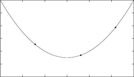
Chapter 33: One dimensional Minimization 360
33 One dimensional Minimization
This chapter describes routines for finding minima of arbitrary one-dimensional functions.
The library provides low level components for a variety of iterative minimizers and conver-
gence tests. These can be combined by the user to achieve the desired solution, with full
access to the intermediate steps of the algorithms. Each class of methods uses the same
framework, so that you can switch between minimizers at runtime without needing to re-
compile your program. Each instance of a minimizer keeps track of its own state, allowing
the minimizers to be used in multi-threaded programs.
The header file ‘gsl_min.h’ contains prototypes for the minimization functions and
related declarations. To use the minimization algorithms to find the maximum of a function
simply invert its sign.
33.1 Overview
The minimization algorithms begin with a bounded region known to contain a minimum.
The region is described by a lower bound aand an upper bound b, with an estimate of the
location of the minimum x.
(a)
(b)
(x)
0
2
4
6
8
10
12
-3 -2 -1 0 1 2 3
The value of the function at xmust be less than the value of the function at the ends of
the interval,
f(a)> f(x)< f(b)
This condition guarantees that a minimum is contained somewhere within the interval. On
each iteration a new point x′is selected using one of the available algorithms. If the new
point is a better estimate of the minimum, i.e. where f(x′)< f(x), then the current estimate
of the minimum xis updated. The new point also allows the size of the bounded interval
to be reduced, by choosing the most compact set of points which satisfies the constraint
f(a)> f(x)< f(b). The interval is reduced until it encloses the true minimum to a desired
tolerance. This provides a best estimate of the location of the minimum and a rigorous
error estimate.
Several bracketing algorithms are available within a single framework. The user provides
a high-level driver for the algorithm, and the library provides the individual functions
necessary for each of the steps. There are three main phases of the iteration. The steps are,
•initialize minimizer state, s, for algorithm T

Chapter 33: One dimensional Minimization 361
•update susing the iteration T
•test sfor convergence, and repeat iteration if necessary
The state for the minimizers is held in a gsl_min_fminimizer struct. The updating pro-
cedure uses only function evaluations (not derivatives).
33.2 Caveats
Note that minimization functions can only search for one minimum at a time. When there
are several minima in the search area, the first minimum to be found will be returned;
however it is difficult to predict which of the minima this will be. In most cases, no error
will be reported if you try to find a minimum in an area where there is more than one.
With all minimization algorithms it can be difficult to determine the location of the
minimum to full numerical precision. The behavior of the function in the region of the
minimum x∗can be approximated by a Taylor expansion,
y=f(x∗) + 1
2f′′(x∗)(x−x∗)2
and the second term of this expansion can be lost when added to the first term at finite
precision. This magnifies the error in locating x∗, making it proportional to √ǫ(where
ǫis the relative accuracy of the floating point numbers). For functions with higher order
minima, such as x4, the magnification of the error is correspondingly worse. The best that
can be achieved is to converge to the limit of numerical accuracy in the function values,
rather than the location of the minimum itself.
33.3 Initializing the Minimizer
[Function]gsl_min_fminimizer * gsl_min_fminimizer_alloc (const
gsl min fminimizer type * T)
This function returns a pointer to a newly allocated instance of a minimizer of type
T. For example, the following code creates an instance of a golden section minimizer,
const gsl_min_fminimizer_type * T
= gsl_min_fminimizer_goldensection;
gsl_min_fminimizer * s
= gsl_min_fminimizer_alloc (T);
If there is insufficient memory to create the minimizer then the function returns a
null pointer and the error handler is invoked with an error code of GSL_ENOMEM.
[Function]int gsl_min_fminimizer_set (gsl min fminimizer * s, gsl function *
f, double x_minimum, double x_lower, double x_upper )
This function sets, or resets, an existing minimizer sto use the function fand the
initial search interval [xlower,x upper], with a guess for the location of the minimum
xminimum.
If the interval given does not contain a minimum, then the function returns an error
code of GSL_EINVAL.

Chapter 33: One dimensional Minimization 362
[Function]int gsl_min_fminimizer_set_with_values (gsl min fminimizer * s,
gsl function * f, double x_minimum, double f_minimum, double x_lower,
double f_lower, double x_upper, double f_upper )
This function is equivalent to gsl_min_fminimizer_set but uses the values
fminimum,f lower and f upper instead of computing f(x_minimum),f(x_lower)
and f(x_upper).
[Function]void gsl_min_fminimizer_free (gsl min fminimizer * s)
This function frees all the memory associated with the minimizer s.
[Function]const char * gsl_min_fminimizer_name (const gsl min fminimizer *
s)
This function returns a pointer to the name of the minimizer. For example,
printf ("s is a ’%s’ minimizer\n",
gsl_min_fminimizer_name (s));
would print something like s is a ’brent’ minimizer.
33.4 Providing the function to minimize
You must provide a continuous function of one variable for the minimizers to operate on.
In order to allow for general parameters the functions are defined by a gsl_function data
type (see Section 32.4 [Providing the function to solve], page 348).
33.5 Iteration
The following functions drive the iteration of each algorithm. Each function performs one
iteration to update the state of any minimizer of the corresponding type. The same functions
work for all minimizers so that different methods can be substituted at runtime without
modifications to the code.
[Function]int gsl_min_fminimizer_iterate (gsl min fminimizer * s)
This function performs a single iteration of the minimizer s. If the iteration encounters
an unexpected problem then an error code will be returned,
GSL_EBADFUNC
the iteration encountered a singular point where the function evaluated
to Inf or NaN.
GSL_FAILURE
the algorithm could not improve the current best approximation or
bounding interval.
The minimizer maintains a current best estimate of the position of the minimum at all
times, and the current interval bounding the minimum. This information can be accessed
with the following auxiliary functions,
[Function]double gsl_min_fminimizer_x_minimum (const gsl min fminimizer *
s)
This function returns the current estimate of the position of the minimum for the
minimizer s.

Chapter 33: One dimensional Minimization 363
[Function]double gsl_min_fminimizer_x_upper (const gsl min fminimizer * s)
[Function]double gsl_min_fminimizer_x_lower (const gsl min fminimizer * s)
These functions return the current upper and lower bound of the interval for the
minimizer s.
[Function]double gsl_min_fminimizer_f_minimum (const gsl min fminimizer *
s)
[Function]double gsl_min_fminimizer_f_upper (const gsl min fminimizer * s)
[Function]double gsl_min_fminimizer_f_lower (const gsl min fminimizer * s)
These functions return the value of the function at the current estimate of the mini-
mum and at the upper and lower bounds of the interval for the minimizer s.
33.6 Stopping Parameters
A minimization procedure should stop when one of the following conditions is true:
•A minimum has been found to within the user-specified precision.
•A user-specified maximum number of iterations has been reached.
•An error has occurred.
The handling of these conditions is under user control. The function below allows the user
to test the precision of the current result.
[Function]int gsl_min_test_interval (double x_lower, double x_upper,
double epsabs, double epsrel )
This function tests for the convergence of the interval [x lower,x upper] with absolute
error epsabs and relative error epsrel. The test returns GSL_SUCCESS if the following
condition is achieved,
|a−b|<epsabs +epsrel min(|a|,|b|)
when the interval x= [a, b] does not include the origin. If the interval includes the
origin then min(|a|,|b|) is replaced by zero (which is the minimum value of |x|over
the interval). This ensures that the relative error is accurately estimated for minima
close to the origin.
This condition on the interval also implies that any estimate of the minimum xmin
the interval satisfies the same condition with respect to the true minimum x∗
m,
|xm−x∗
m|<epsabs +epsrel x∗
m
assuming that the true minimum x∗
mis contained within the interval.
33.7 Minimization Algorithms
The minimization algorithms described in this section require an initial interval which is
guaranteed to contain a minimum—if aand bare the endpoints of the interval and xis an
estimate of the minimum then f(a)> f (x)< f (b). This ensures that the function has at
least one minimum somewhere in the interval. If a valid initial interval is used then these
algorithm cannot fail, provided the function is well-behaved.

Chapter 33: One dimensional Minimization 364
[Minimizer]gsl_min_fminimizer_goldensection
The golden section algorithm is the simplest method of bracketing the minimum of a
function. It is the slowest algorithm provided by the library, with linear convergence.
On each iteration, the algorithm first compares the subintervals from the endpoints to
the current minimum. The larger subinterval is divided in a golden section (using the
famous ratio (3 −√5)/2 = 0.3189660. . . ) and the value of the function at this new
point is calculated. The new value is used with the constraint f(a′)> f(x′)< f (b′)
to a select new interval containing the minimum, by discarding the least useful point.
This procedure can be continued indefinitely until the interval is sufficiently small.
Choosing the golden section as the bisection ratio can be shown to provide the fastest
convergence for this type of algorithm.
[Minimizer]gsl_min_fminimizer_brent
The Brent minimization algorithm combines a parabolic interpolation with the golden
section algorithm. This produces a fast algorithm which is still robust.
The outline of the algorithm can be summarized as follows: on each iteration Brent’s
method approximates the function using an interpolating parabola through three
existing points. The minimum of the parabola is taken as a guess for the minimum.
If it lies within the bounds of the current interval then the interpolating point is
accepted, and used to generate a smaller interval. If the interpolating point is not
accepted then the algorithm falls back to an ordinary golden section step. The full
details of Brent’s method include some additional checks to improve convergence.
[Minimizer]gsl_min_fminimizer_quad_golden
This is a variant of Brent’s algorithm which uses the safeguarded step-length algorithm
of Gill and Murray.
33.8 Examples
The following program uses the Brent algorithm to find the minimum of the function f(x) =
cos(x) + 1, which occurs at x=π. The starting interval is (0,6), with an initial guess for
the minimum of 2.
#include <stdio.h>
#include <gsl/gsl_errno.h>
#include <gsl/gsl_math.h>
#include <gsl/gsl_min.h>
double fn1 (double x, void * params)
{
return cos(x) + 1.0;
}
int
main (void)
{
int status;
int iter = 0, max_iter = 100;
Chapter 33: One dimensional Minimization 365
const gsl_min_fminimizer_type *T;
gsl_min_fminimizer *s;
double m = 2.0, m_expected = M_PI;
double a = 0.0, b = 6.0;
gsl_function F;
F.function = &fn1;
F.params = 0;
T = gsl_min_fminimizer_brent;
s = gsl_min_fminimizer_alloc (T);
gsl_min_fminimizer_set (s, &F, m, a, b);
printf ("using %s method\n",
gsl_min_fminimizer_name (s));
printf ("%5s [%9s, %9s] %9s %10s %9s\n",
"iter", "lower", "upper", "min",
"err", "err(est)");
printf ("%5d [%.7f, %.7f] %.7f %+.7f %.7f\n",
iter, a, b,
m, m - m_expected, b - a);
do
{
iter++;
status = gsl_min_fminimizer_iterate (s);
m = gsl_min_fminimizer_x_minimum (s);
a = gsl_min_fminimizer_x_lower (s);
b = gsl_min_fminimizer_x_upper (s);
status
= gsl_min_test_interval (a, b, 0.001, 0.0);
if (status == GSL_SUCCESS)
printf ("Converged:\n");
printf ("%5d [%.7f, %.7f] "
"%.7f %+.7f %.7f\n",
iter, a, b,
m, m - m_expected, b - a);
}
while (status == GSL_CONTINUE && iter < max_iter);
gsl_min_fminimizer_free (s);
Chapter 33: One dimensional Minimization 366
return status;
}
Here are the results of the minimization procedure.
$ ./a.out
0 [0.0000000, 6.0000000] 2.0000000 -1.1415927 6.0000000
1 [2.0000000, 6.0000000] 3.2758640 +0.1342713 4.0000000
2 [2.0000000, 3.2831929] 3.2758640 +0.1342713 1.2831929
3 [2.8689068, 3.2831929] 3.2758640 +0.1342713 0.4142862
4 [2.8689068, 3.2831929] 3.2758640 +0.1342713 0.4142862
5 [2.8689068, 3.2758640] 3.1460585 +0.0044658 0.4069572
6 [3.1346075, 3.2758640] 3.1460585 +0.0044658 0.1412565
7 [3.1346075, 3.1874620] 3.1460585 +0.0044658 0.0528545
8 [3.1346075, 3.1460585] 3.1460585 +0.0044658 0.0114510
9 [3.1346075, 3.1460585] 3.1424060 +0.0008133 0.0114510
10 [3.1346075, 3.1424060] 3.1415885 -0.0000041 0.0077985
Converged:
11 [3.1415885, 3.1424060] 3.1415927 -0.0000000 0.0008175
33.9 References and Further Reading
Further information on Brent’s algorithm is available in the following book,
Richard Brent, Algorithms for minimization without derivatives, Prentice-Hall (1973),
republished by Dover in paperback (2002), ISBN 0-486-41998-3.
Chapter 34: Multidimensional Root-Finding 367
34 Multidimensional Root-Finding
This chapter describes functions for multidimensional root-finding (solving nonlinear sys-
tems with nequations in nunknowns). The library provides low level components for a
variety of iterative solvers and convergence tests. These can be combined by the user to
achieve the desired solution, with full access to the intermediate steps of the iteration. Each
class of methods uses the same framework, so that you can switch between solvers at run-
time without needing to recompile your program. Each instance of a solver keeps track of
its own state, allowing the solvers to be used in multi-threaded programs. The solvers are
based on the original Fortran library minpack.
The header file ‘gsl_multiroots.h’ contains prototypes for the multidimensional root
finding functions and related declarations.
34.1 Overview
The problem of multidimensional root finding requires the simultaneous solution of nequa-
tions, fi, in nvariables, xi,
fi(x1,...,xn) = 0 for i= 1 . . . n.
In general there are no bracketing methods available for ndimensional systems, and no way
of knowing whether any solutions exist. All algorithms proceed from an initial guess using
a variant of the Newton iteration,
x→x′=x−J−1f(x)
where x,fare vector quantities and Jis the Jacobian matrix Jij =∂fi/∂xj. Additional
strategies can be used to enlarge the region of convergence. These include requiring a
decrease in the norm |f|on each step proposed by Newton’s method, or taking steepest-
descent steps in the direction of the negative gradient of |f|.
Several root-finding algorithms are available within a single framework. The user pro-
vides a high-level driver for the algorithms, and the library provides the individual functions
necessary for each of the steps. There are three main phases of the iteration. The steps are,
•initialize solver state, s, for algorithm T
•update susing the iteration T
•test sfor convergence, and repeat iteration if necessary
The evaluation of the Jacobian matrix can be problematic, either because programming the
derivatives is intractable or because computation of the n2terms of the matrix becomes too
expensive. For these reasons the algorithms provided by the library are divided into two
classes according to whether the derivatives are available or not.
The state for solvers with an analytic Jacobian matrix is held in a gsl_multiroot_
fdfsolver struct. The updating procedure requires both the function and its derivatives
to be supplied by the user.
The state for solvers which do not use an analytic Jacobian matrix is held in a gsl_
multiroot_fsolver struct. The updating procedure uses only function evaluations (not
derivatives). The algorithms estimate the matrix Jor J−1by approximate methods.

Chapter 34: Multidimensional Root-Finding 368
34.2 Initializing the Solver
The following functions initialize a multidimensional solver, either with or without deriva-
tives. The solver itself depends only on the dimension of the problem and the algorithm
and can be reused for different problems.
[Function]gsl_multiroot_fsolver * gsl_multiroot_fsolver_alloc (const
gsl multiroot fsolver type * T, size t n)
This function returns a pointer to a newly allocated instance of a solver of type Tfor
a system of ndimensions. For example, the following code creates an instance of a
hybrid solver, to solve a 3-dimensional system of equations.
const gsl_multiroot_fsolver_type * T
= gsl_multiroot_fsolver_hybrid;
gsl_multiroot_fsolver * s
= gsl_multiroot_fsolver_alloc (T, 3);
If there is insufficient memory to create the solver then the function returns a null
pointer and the error handler is invoked with an error code of GSL_ENOMEM.
[Function]gsl_multiroot_fdfsolver * gsl_multiroot_fdfsolver_alloc
(const gsl multiroot fdfsolver type * T, size t n)
This function returns a pointer to a newly allocated instance of a derivative solver
of type Tfor a system of ndimensions. For example, the following code creates an
instance of a Newton-Raphson solver, for a 2-dimensional system of equations.
const gsl_multiroot_fdfsolver_type * T
= gsl_multiroot_fdfsolver_newton;
gsl_multiroot_fdfsolver * s =
gsl_multiroot_fdfsolver_alloc (T, 2);
If there is insufficient memory to create the solver then the function returns a null
pointer and the error handler is invoked with an error code of GSL_ENOMEM.
[Function]int gsl_multiroot_fsolver_set (gsl multiroot fsolver * s,
gsl multiroot function * f, const gsl vector * x)
[Function]int gsl_multiroot_fdfsolver_set (gsl multiroot fdfsolver * s,
gsl multiroot function fdf * fdf, const gsl vector * x)
These functions set, or reset, an existing solver sto use the function for function and
derivative fdf, and the initial guess x. Note that the initial position is copied from x,
this argument is not modified by subsequent iterations.
[Function]void gsl_multiroot_fsolver_free (gsl multiroot fsolver * s)
[Function]void gsl_multiroot_fdfsolver_free (gsl multiroot fdfsolver * s)
These functions free all the memory associated with the solver s.
[Function]const char * gsl_multiroot_fsolver_name (const
gsl multiroot fsolver * s)
[Function]const char * gsl_multiroot_fdfsolver_name (const
gsl multiroot fdfsolver * s)
These functions return a pointer to the name of the solver. For example,
Chapter 34: Multidimensional Root-Finding 369
printf ("s is a ’%s’ solver\n",
gsl_multiroot_fdfsolver_name (s));
would print something like s is a ’newton’ solver.
34.3 Providing the function to solve
You must provide nfunctions of nvariables for the root finders to operate on. In order to
allow for general parameters the functions are defined by the following data types:
[Data Type]gsl_multiroot_function
This data type defines a general system of functions with parameters.
int (* f) (const gsl_vector * x, void * params, gsl_vector * f)
this function should store the vector result f(x, params) in ffor argument
xand parameters params, returning an appropriate error code if the
function cannot be computed.
size_t n the dimension of the system, i.e. the number of components of the vectors
xand f.
void * params
a pointer to the parameters of the function.
Here is an example using Powell’s test function,
f1(x) = Ax0x1−1, f2(x) = exp(−x0) + exp(−x1)−(1 + 1/A)
with A= 104. The following code defines a gsl_multiroot_function system Fwhich you
could pass to a solver:
struct powell_params { double A; };
int
powell (gsl_vector * x, void * p, gsl_vector * f) {
struct powell_params * params
= *(struct powell_params *)p;
const double A = (params->A);
const double x0 = gsl_vector_get(x,0);
const double x1 = gsl_vector_get(x,1);
gsl_vector_set (f, 0, A * x0 * x1 - 1);
gsl_vector_set (f, 1, (exp(-x0) + exp(-x1)
- (1.0 + 1.0/A)));
return GSL_SUCCESS
}
gsl_multiroot_function F;
struct powell_params params = { 10000.0 };
F.f = &powell;
F.n = 2;
F.params = ¶ms;
Chapter 34: Multidimensional Root-Finding 370
[Data Type]gsl_multiroot_function_fdf
This data type defines a general system of functions with parameters and the corre-
sponding Jacobian matrix of derivatives,
int (* f) (const gsl_vector * x, void * params, gsl_vector * f)
this function should store the vector result f(x, params) in ffor argument
xand parameters params, returning an appropriate error code if the
function cannot be computed.
int (* df) (const gsl_vector * x, void * params, gsl_matrix * J)
this function should store the n-by-nmatrix result Jij =
∂fi(x, params)/∂xjin Jfor argument xand parameters params,
returning an appropriate error code if the function cannot be computed.
int (* fdf) (const gsl_vector * x, void * params, gsl_vector * f,
gsl_matrix * J)
This function should set the values of the fand Jas above, for arguments
xand parameters params. This function provides an optimization of the
separate functions for f(x) and J(x)—it is always faster to compute the
function and its derivative at the same time.
size_t n the dimension of the system, i.e. the number of components of the vectors
xand f.
void * params
a pointer to the parameters of the function.
The example of Powell’s test function defined above can be extended to include analytic
derivatives using the following code,
int
powell_df (gsl_vector * x, void * p, gsl_matrix * J)
{
struct powell_params * params
= *(struct powell_params *)p;
const double A = (params->A);
const double x0 = gsl_vector_get(x,0);
const double x1 = gsl_vector_get(x,1);
gsl_matrix_set (J, 0, 0, A * x1);
gsl_matrix_set (J, 0, 1, A * x0);
gsl_matrix_set (J, 1, 0, -exp(-x0));
gsl_matrix_set (J, 1, 1, -exp(-x1));
return GSL_SUCCESS
}
int
powell_fdf (gsl_vector * x, void * p,
gsl_matrix * f, gsl_matrix * J) {
struct powell_params * params
= *(struct powell_params *)p;
const double A = (params->A);

Chapter 34: Multidimensional Root-Finding 371
const double x0 = gsl_vector_get(x,0);
const double x1 = gsl_vector_get(x,1);
const double u0 = exp(-x0);
const double u1 = exp(-x1);
gsl_vector_set (f, 0, A * x0 * x1 - 1);
gsl_vector_set (f, 1, u0 + u1 - (1 + 1/A));
gsl_matrix_set (J, 0, 0, A * x1);
gsl_matrix_set (J, 0, 1, A * x0);
gsl_matrix_set (J, 1, 0, -u0);
gsl_matrix_set (J, 1, 1, -u1);
return GSL_SUCCESS
}
gsl_multiroot_function_fdf FDF;
FDF.f = &powell_f;
FDF.df = &powell_df;
FDF.fdf = &powell_fdf;
FDF.n = 2;
FDF.params = 0;
Note that the function powell_fdf is able to reuse existing terms from the function when
calculating the Jacobian, thus saving time.
34.4 Iteration
The following functions drive the iteration of each algorithm. Each function performs one
iteration to update the state of any solver of the corresponding type. The same func-
tions work for all solvers so that different methods can be substituted at runtime without
modifications to the code.
[Function]int gsl_multiroot_fsolver_iterate (gsl multiroot fsolver * s)
[Function]int gsl_multiroot_fdfsolver_iterate (gsl multiroot fdfsolver * s)
These functions perform a single iteration of the solver s. If the iteration encounters
an unexpected problem then an error code will be returned,
GSL_EBADFUNC
the iteration encountered a singular point where the function or its deriva-
tive evaluated to Inf or NaN.
GSL_ENOPROG
the iteration is not making any progress, preventing the algorithm from
continuing.
The solver maintains a current best estimate of the root s->x and its function value
s->f at all times. This information can be accessed with the following auxiliary functions,

Chapter 34: Multidimensional Root-Finding 372
[Function]gsl_vector * gsl_multiroot_fsolver_root (const
gsl multiroot fsolver * s)
[Function]gsl_vector * gsl_multiroot_fdfsolver_root (const
gsl multiroot fdfsolver * s)
These functions return the current estimate of the root for the solver s, given by s->x.
[Function]gsl_vector * gsl_multiroot_fsolver_f (const gsl multiroot fsolver
*s)
[Function]gsl_vector * gsl_multiroot_fdfsolver_f (const
gsl multiroot fdfsolver * s)
These functions return the function value f(x) at the current estimate of the root for
the solver s, given by s->f.
[Function]gsl_vector * gsl_multiroot_fsolver_dx (const
gsl multiroot fsolver * s)
[Function]gsl_vector * gsl_multiroot_fdfsolver_dx (const
gsl multiroot fdfsolver * s)
These functions return the last step dx taken by the solver s, given by s->dx.
34.5 Search Stopping Parameters
A root finding procedure should stop when one of the following conditions is true:
•A multidimensional root has been found to within the user-specified precision.
•A user-specified maximum number of iterations has been reached.
•An error has occurred.
The handling of these conditions is under user control. The functions below allow the user
to test the precision of the current result in several standard ways.
[Function]int gsl_multiroot_test_delta (const gsl vector * dx, const
gsl vector * x, double epsabs, double epsrel )
This function tests for the convergence of the sequence by comparing the last step
dx with the absolute error epsabs and relative error epsrel to the current position x.
The test returns GSL_SUCCESS if the following condition is achieved,
|dxi|<epsabs +epsrel |xi|
for each component of xand returns GSL_CONTINUE otherwise.
[Function]int gsl_multiroot_test_residual (const gsl vector * f, double
epsabs )
This function tests the residual value fagainst the absolute error bound epsabs. The
test returns GSL_SUCCESS if the following condition is achieved,
X
i|fi|<epsabs
and returns GSL_CONTINUE otherwise. This criterion is suitable for situations where
the precise location of the root, x, is unimportant provided a value can be found
where the residual is small enough.
Chapter 34: Multidimensional Root-Finding 373
34.6 Algorithms using Derivatives
The root finding algorithms described in this section make use of both the function and its
derivative. They require an initial guess for the location of the root, but there is no absolute
guarantee of convergence—the function must be suitable for this technique and the initial
guess must be sufficiently close to the root for it to work. When the conditions are satisfied
then convergence is quadratic.
[Derivative Solver]gsl_multiroot_fdfsolver_hybridsj
This is a modified version of Powell’s Hybrid method as implemented in the hybrj
algorithm in minpack. Minpack was written by Jorge J. Mor´e, Burton S. Garbow and
Kenneth E. Hillstrom. The Hybrid algorithm retains the fast convergence of Newton’s
method but will also reduce the residual when Newton’s method is unreliable.
The algorithm uses a generalized trust region to keep each step under control. In order
to be accepted a proposed new position x′must satisfy the condition |D(x′−x)|< δ,
where Dis a diagonal scaling matrix and δis the size of the trust region. The
components of Dare computed internally, using the column norms of the Jacobian
to estimate the sensitivity of the residual to each component of x. This improves the
behavior of the algorithm for badly scaled functions.
On each iteration the algorithm first determines the standard Newton step by solving
the system Jdx =−f. If this step falls inside the trust region it is used as a trial step
in the next stage. If not, the algorithm uses the linear combination of the Newton
and gradient directions which is predicted to minimize the norm of the function while
staying inside the trust region,
dx =−αJ−1f(x)−β∇|f(x)|2.
This combination of Newton and gradient directions is referred to as a dogleg step.
The proposed step is now tested by evaluating the function at the resulting point, x′.
If the step reduces the norm of the function sufficiently then it is accepted and size of
the trust region is increased. If the proposed step fails to improve the solution then
the size of the trust region is decreased and another trial step is computed.
The speed of the algorithm is increased by computing the changes to the Jacobian ap-
proximately, using a rank-1 update. If two successive attempts fail to reduce the resid-
ual then the full Jacobian is recomputed. The algorithm also monitors the progress
of the solution and returns an error if several steps fail to make any improvement,
GSL_ENOPROG
the iteration is not making any progress, preventing the algorithm from
continuing.
GSL_ENOPROGJ
re-evaluations of the Jacobian indicate that the iteration is not making
any progress, preventing the algorithm from continuing.
[Derivative Solver]gsl_multiroot_fdfsolver_hybridj
This algorithm is an unscaled version of hybridsj. The steps are controlled by a
spherical trust region |x′−x|< δ, instead of a generalized region. This can be useful
if the generalized region estimated by hybridsj is inappropriate.

Chapter 34: Multidimensional Root-Finding 374
[Derivative Solver]gsl_multiroot_fdfsolver_newton
Newton’s Method is the standard root-polishing algorithm. The algorithm begins
with an initial guess for the location of the solution. On each iteration a linear
approximation to the function Fis used to estimate the step which will zero all the
components of the residual. The iteration is defined by the following sequence,
x→x′=x−J−1f(x)
where the Jacobian matrix Jis computed from the derivative functions provided by
f. The step dx is obtained by solving the linear system,
J dx =−f(x)
using LU decomposition.
[Derivative Solver]gsl_multiroot_fdfsolver_gnewton
This is a modified version of Newton’s method which attempts to improve global
convergence by requiring every step to reduce the Euclidean norm of the residual,
|f(x)|. If the Newton step leads to an increase in the norm then a reduced step of
relative size,
t= (√1 + 6r−1)/(3r)
is proposed, with rbeing the ratio of norms |f(x′)|2/|f(x)|2. This procedure is re-
peated until a suitable step size is found.
34.7 Algorithms without Derivatives
The algorithms described in this section do not require any derivative information to be
supplied by the user. Any derivatives needed are approximated by finite differences. Note
that if the finite-differencing step size chosen by these routines is inappropriate, an explicit
user-supplied numerical derivative can always be used with the algorithms described in the
previous section.
[Solver]gsl_multiroot_fsolver_hybrids
This is a version of the Hybrid algorithm which replaces calls to the Jacobian function
by its finite difference approximation. The finite difference approximation is computed
using gsl_multiroots_fdjac with a relative step size of GSL_SQRT_DBL_EPSILON.
Note that this step size will not be suitable for all problems.
[Solver]gsl_multiroot_fsolver_hybrid
This is a finite difference version of the Hybrid algorithm without internal scaling.
[Solver]gsl_multiroot_fsolver_dnewton
The discrete Newton algorithm is the simplest method of solving a multidimensional
system. It uses the Newton iteration
x→x−J−1f(x)
where the Jacobian matrix Jis approximated by taking finite differences of the func-
tion f. The approximation scheme used by this implementation is,
Jij = (fi(x+δj)−fi(x))/δj

Chapter 34: Multidimensional Root-Finding 375
where δjis a step of size √ǫ|xj|with ǫbeing the machine precision (ǫ≈2.22 ×10⁻¹⁶).
The order of convergence of Newton’s algorithm is quadratic, but the finite differences
require n2function evaluations on each iteration. The algorithm may become unstable
if the finite differences are not a good approximation to the true derivatives.
[Solver]gsl_multiroot_fsolver_broyden
The Broyden algorithm is a version of the discrete Newton algorithm which attempts
to avoids the expensive update of the Jacobian matrix on each iteration. The changes
to the Jacobian are also approximated, using a rank-1 update,
J−1→J−1−(J−1df −dx)dxTJ−1/dxTJ−1df
where the vectors dx and df are the changes in xand f. On the first iteration
the inverse Jacobian is estimated using finite differences, as in the discrete Newton
algorithm.
This approximation gives a fast update but is unreliable if the changes are not small,
and the estimate of the inverse Jacobian becomes worse as time passes. The algorithm
has a tendency to become unstable unless it starts close to the root. The Jacobian is
refreshed if this instability is detected (consult the source for details).
This algorithm is included only for demonstration purposes, and is not recommended
for serious use.
34.8 Examples
The multidimensional solvers are used in a similar way to the one-dimensional root finding
algorithms. This first example demonstrates the hybrids scaled-hybrid algorithm, which
does not require derivatives. The program solves the Rosenbrock system of equations,
f1(x, y) = a(1 −x), f2(x, y) = b(y−x2)
with a= 1, b = 10. The solution of this system lies at (x, y) = (1,1) in a narrow valley.
The first stage of the program is to define the system of equations,
#include <stdlib.h>
#include <stdio.h>
#include <gsl/gsl_vector.h>
#include <gsl/gsl_multiroots.h>
struct rparams
{
double a;
double b;
};
int
rosenbrock_f (const gsl_vector * x, void *params,
gsl_vector * f)
{
double a = ((struct rparams *) params)->a;
double b = ((struct rparams *) params)->b;
Chapter 34: Multidimensional Root-Finding 376
const double x0 = gsl_vector_get (x, 0);
const double x1 = gsl_vector_get (x, 1);
const double y0 = a * (1 - x0);
const double y1 = b * (x1 - x0 * x0);
gsl_vector_set (f, 0, y0);
gsl_vector_set (f, 1, y1);
return GSL_SUCCESS;
}
The main program begins by creating the function object f, with the arguments (x,y)
and parameters (a,b). The solver sis initialized to use this function, with the hybrids
method.
int
main (void)
{
const gsl_multiroot_fsolver_type *T;
gsl_multiroot_fsolver *s;
int status;
size_t i, iter = 0;
const size_t n = 2;
struct rparams p = {1.0, 10.0};
gsl_multiroot_function f = {&rosenbrock_f, n, &p};
double x_init[2] = {-10.0, -5.0};
gsl_vector *x = gsl_vector_alloc (n);
gsl_vector_set (x, 0, x_init[0]);
gsl_vector_set (x, 1, x_init[1]);
T = gsl_multiroot_fsolver_hybrids;
s = gsl_multiroot_fsolver_alloc (T, 2);
gsl_multiroot_fsolver_set (s, &f, x);
print_state (iter, s);
do
{
iter++;
status = gsl_multiroot_fsolver_iterate (s);
print_state (iter, s);
Chapter 34: Multidimensional Root-Finding 377
if (status) /* check if solver is stuck */
break;
status =
gsl_multiroot_test_residual (s->f, 1e-7);
}
while (status == GSL_CONTINUE && iter < 1000);
printf ("status = %s\n", gsl_strerror (status));
gsl_multiroot_fsolver_free (s);
gsl_vector_free (x);
return 0;
}
Note that it is important to check the return status of each solver step, in case the algorithm
becomes stuck. If an error condition is detected, indicating that the algorithm cannot
proceed, then the error can be reported to the user, a new starting point chosen or a
different algorithm used.
The intermediate state of the solution is displayed by the following function. The solver
state contains the vector s->x which is the current position, and the vector s->f with
corresponding function values.
int
print_state (size_t iter, gsl_multiroot_fsolver * s)
{
printf ("iter = %3u x = % .3f % .3f "
"f(x) = % .3e % .3e\n",
iter,
gsl_vector_get (s->x, 0),
gsl_vector_get (s->x, 1),
gsl_vector_get (s->f, 0),
gsl_vector_get (s->f, 1));
}
Here are the results of running the program. The algorithm is started at (−10,−5) far from
the solution. Since the solution is hidden in a narrow valley the earliest steps follow the
gradient of the function downhill, in an attempt to reduce the large value of the residual.
Once the root has been approximately located, on iteration 8, the Newton behavior takes
over and convergence is very rapid.
iter = 0 x = -10.000 -5.000 f(x) = 1.100e+01 -1.050e+03
iter = 1 x = -10.000 -5.000 f(x) = 1.100e+01 -1.050e+03
iter = 2 x = -3.976 24.827 f(x) = 4.976e+00 9.020e+01
iter = 3 x = -3.976 24.827 f(x) = 4.976e+00 9.020e+01
iter = 4 x = -3.976 24.827 f(x) = 4.976e+00 9.020e+01
iter = 5 x = -1.274 -5.680 f(x) = 2.274e+00 -7.302e+01
iter = 6 x = -1.274 -5.680 f(x) = 2.274e+00 -7.302e+01
iter = 7 x = 0.249 0.298 f(x) = 7.511e-01 2.359e+00
iter = 8 x = 0.249 0.298 f(x) = 7.511e-01 2.359e+00
iter = 9 x = 1.000 0.878 f(x) = 1.268e-10 -1.218e+00
Chapter 34: Multidimensional Root-Finding 378
iter = 10 x = 1.000 0.989 f(x) = 1.124e-11 -1.080e-01
iter = 11 x = 1.000 1.000 f(x) = 0.000e+00 0.000e+00
status = success
Note that the algorithm does not update the location on every iteration. Some iterations
are used to adjust the trust-region parameter, after trying a step which was found to be
divergent, or to recompute the Jacobian, when poor convergence behavior is detected.
The next example program adds derivative information, in order to accelerate the solu-
tion. There are two derivative functions rosenbrock_df and rosenbrock_fdf. The latter
computes both the function and its derivative simultaneously. This allows the optimization
of any common terms. For simplicity we substitute calls to the separate fand df functions
at this point in the code below.
int
rosenbrock_df (const gsl_vector * x, void *params,
gsl_matrix * J)
{
const double a = ((struct rparams *) params)->a;
const double b = ((struct rparams *) params)->b;
const double x0 = gsl_vector_get (x, 0);
const double df00 = -a;
const double df01 = 0;
const double df10 = -2 * b * x0;
const double df11 = b;
gsl_matrix_set (J, 0, 0, df00);
gsl_matrix_set (J, 0, 1, df01);
gsl_matrix_set (J, 1, 0, df10);
gsl_matrix_set (J, 1, 1, df11);
return GSL_SUCCESS;
}
int
rosenbrock_fdf (const gsl_vector * x, void *params,
gsl_vector * f, gsl_matrix * J)
{
rosenbrock_f (x, params, f);
rosenbrock_df (x, params, J);
return GSL_SUCCESS;
}
The main program now makes calls to the corresponding fdfsolver versions of the func-
tions,
int
main (void)
Chapter 34: Multidimensional Root-Finding 379
{
const gsl_multiroot_fdfsolver_type *T;
gsl_multiroot_fdfsolver *s;
int status;
size_t i, iter = 0;
const size_t n = 2;
struct rparams p = {1.0, 10.0};
gsl_multiroot_function_fdf f = {&rosenbrock_f,
&rosenbrock_df,
&rosenbrock_fdf,
n, &p};
double x_init[2] = {-10.0, -5.0};
gsl_vector *x = gsl_vector_alloc (n);
gsl_vector_set (x, 0, x_init[0]);
gsl_vector_set (x, 1, x_init[1]);
T = gsl_multiroot_fdfsolver_gnewton;
s = gsl_multiroot_fdfsolver_alloc (T, n);
gsl_multiroot_fdfsolver_set (s, &f, x);
print_state (iter, s);
do
{
iter++;
status = gsl_multiroot_fdfsolver_iterate (s);
print_state (iter, s);
if (status)
break;
status = gsl_multiroot_test_residual (s->f, 1e-7);
}
while (status == GSL_CONTINUE && iter < 1000);
printf ("status = %s\n", gsl_strerror (status));
gsl_multiroot_fdfsolver_free (s);
gsl_vector_free (x);
return 0;
}
Chapter 34: Multidimensional Root-Finding 380
The addition of derivative information to the hybrids solver does not make any signifi-
cant difference to its behavior, since it able to approximate the Jacobian numerically with
sufficient accuracy. To illustrate the behavior of a different derivative solver we switch to
gnewton. This is a traditional Newton solver with the constraint that it scales back its step
if the full step would lead “uphill”. Here is the output for the gnewton algorithm,
iter = 0 x = -10.000 -5.000 f(x) = 1.100e+01 -1.050e+03
iter = 1 x = -4.231 -65.317 f(x) = 5.231e+00 -8.321e+02
iter = 2 x = 1.000 -26.358 f(x) = -8.882e-16 -2.736e+02
iter = 3 x = 1.000 1.000 f(x) = -2.220e-16 -4.441e-15
status = success
The convergence is much more rapid, but takes a wide excursion out to the point
(−4.23,−65.3). This could cause the algorithm to go astray in a realistic application. The
hybrid algorithm follows the downhill path to the solution more reliably.
34.9 References and Further Reading
The original version of the Hybrid method is described in the following articles by Powell,
M.J.D. Powell, “A Hybrid Method for Nonlinear Equations” (Chap 6, p 87–114) and
“A Fortran Subroutine for Solving systems of Nonlinear Algebraic Equations” (Chap 7,
p 115–161), in Numerical Methods for Nonlinear Algebraic Equations, P. Rabinowitz,
editor. Gordon and Breach, 1970.
The following papers are also relevant to the algorithms described in this section,
J.J. Mor´e, M.Y. Cosnard, “Numerical Solution of Nonlinear Equations”, ACM Trans-
actions on Mathematical Software, Vol 5, No 1, (1979), p 64–85
C.G. Broyden, “A Class of Methods for Solving Nonlinear Simultaneous Equations”,
Mathematics of Computation, Vol 19 (1965), p 577–593
J.J. Mor´e, B.S. Garbow, K.E. Hillstrom, “Testing Unconstrained Optimization Soft-
ware”, ACM Transactions on Mathematical Software, Vol 7, No 1 (1981), p 17–41
Chapter 35: Multidimensional Minimization 381
35 Multidimensional Minimization
This chapter describes routines for finding minima of arbitrary multidimensional functions.
The library provides low level components for a variety of iterative minimizers and con-
vergence tests. These can be combined by the user to achieve the desired solution, while
providing full access to the intermediate steps of the algorithms. Each class of methods
uses the same framework, so that you can switch between minimizers at runtime without
needing to recompile your program. Each instance of a minimizer keeps track of its own
state, allowing the minimizers to be used in multi-threaded programs. The minimization
algorithms can be used to maximize a function by inverting its sign.
The header file ‘gsl_multimin.h’ contains prototypes for the minimization functions
and related declarations.
35.1 Overview
The problem of multidimensional minimization requires finding a point xsuch that the
scalar function,
f(x1,...,xn)
takes a value which is lower than at any neighboring point. For smooth functions the
gradient g=∇fvanishes at the minimum. In general there are no bracketing methods
available for the minimization of n-dimensional functions. The algorithms proceed from an
initial guess using a search algorithm which attempts to move in a downhill direction.
Algorithms making use of the gradient of the function perform a one-dimensional line
minimisation along this direction until the lowest point is found to a suitable tolerance. The
search direction is then updated with local information from the function and its derivatives,
and the whole process repeated until the true n-dimensional minimum is found.
Algorithms which do not require the gradient of the function use different strategies.
For example, the Nelder-Mead Simplex algorithm maintains n+ 1 trial parameter vectors
as the vertices of a n-dimensional simplex. On each iteration it tries to improve the worst
vertex of the simplex by geometrical transformations. The iterations are continued until
the overall size of the simplex has decreased sufficiently.
Both types of algorithms use a standard framework. The user provides a high-level driver
for the algorithms, and the library provides the individual functions necessary for each of
the steps. There are three main phases of the iteration. The steps are,
•initialize minimizer state, s, for algorithm T
•update susing the iteration T
•test sfor convergence, and repeat iteration if necessary
Each iteration step consists either of an improvement to the line-minimisation in the current
direction or an update to the search direction itself. The state for the minimizers is held in
agsl_multimin_fdfminimizer struct or a gsl_multimin_fminimizer struct.

Chapter 35: Multidimensional Minimization 382
35.2 Caveats
Note that the minimization algorithms can only search for one local minimum at a time.
When there are several local minima in the search area, the first minimum to be found will
be returned; however it is difficult to predict which of the minima this will be. In most
cases, no error will be reported if you try to find a local minimum in an area where there
is more than one.
It is also important to note that the minimization algorithms find local minima; there is
no way to determine whether a minimum is a global minimum of the function in question.
35.3 Initializing the Multidimensional Minimizer
The following function initializes a multidimensional minimizer. The minimizer itself de-
pends only on the dimension of the problem and the algorithm and can be reused for
different problems.
[Function]gsl_multimin_fdfminimizer *
gsl_multimin_fdfminimizer_alloc (const
gsl multimin fdfminimizer type * T, size t n)
[Function]gsl_multimin_fminimizer * gsl_multimin_fminimizer_alloc
(const gsl multimin fminimizer type * T, size t n)
This function returns a pointer to a newly allocated instance of a minimizer of type T
for an n-dimension function. If there is insufficient memory to create the minimizer
then the function returns a null pointer and the error handler is invoked with an error
code of GSL_ENOMEM.
[Function]int gsl_multimin_fdfminimizer_set (gsl multimin fdfminimizer * s,
gsl multimin function fdf * fdf, const gsl vector * x, double step_size,
double tol )
This function initializes the minimizer sto minimize the function fdf starting from
the initial point x. The size of the first trial step is given by step size. The accuracy
of the line minimization is specified by tol. The precise meaning of this parameter
depends on the method used. Typically the line minimization is considered successful
if the gradient of the function gis orthogonal to the current search direction pto a
relative accuracy of tol, where p·g < tol|p||g|. A tol value of 0.1 is suitable for most
purposes, since line minimization only needs to be carried out approximately. Note
that setting tol to zero will force the use of “exact” line-searches, which are extremely
expensive.
[Function]int gsl_multimin_fminimizer_set (gsl multimin fminimizer * s,
gsl multimin function * f, const gsl vector * x, const gsl vector * step_size )
This function initializes the minimizer sto minimize the function f, starting from the
initial point x. The size of the initial trial steps is given in vector step size. The
precise meaning of this parameter depends on the method used.
[Function]void gsl_multimin_fdfminimizer_free (gsl multimin fdfminimizer *
s)
[Function]void gsl_multimin_fminimizer_free (gsl multimin fminimizer * s)
This function frees all the memory associated with the minimizer s.

Chapter 35: Multidimensional Minimization 383
[Function]const char * gsl_multimin_fdfminimizer_name (const
gsl multimin fdfminimizer * s)
[Function]const char * gsl_multimin_fminimizer_name (const
gsl multimin fminimizer * s)
This function returns a pointer to the name of the minimizer. For example,
printf ("s is a ’%s’ minimizer\n",
gsl_multimin_fdfminimizer_name (s));
would print something like s is a ’conjugate_pr’ minimizer.
35.4 Providing a function to minimize
You must provide a parametric function of nvariables for the minimizers to operate on.
You may also need to provide a routine which calculates the gradient of the function and a
third routine which calculates both the function value and the gradient together. In order
to allow for general parameters the functions are defined by the following data types:
[Data Type]gsl_multimin_function_fdf
This data type defines a general function of nvariables with parameters and the
corresponding gradient vector of derivatives,
double (* f) (const gsl_vector * x, void * params )
this function should return the result f(x, params) for argument xand
parameters params. If the function cannot be computed, an error value
of GSL_NAN should be returned.
void (* df) (const gsl_vector * x, void * params, gsl_vector * g)
this function should store the n-dimensional gradient
gi=∂f(x, params)/∂xiin the vector gfor argument xand
parameters params, returning an appropriate error code if the function
cannot be computed.
void (* fdf) (const gsl_vector * x, void * params, double * f, gsl_vector *
g)
This function should set the values of the fand gas above, for arguments
xand parameters params. This function provides an optimization of the
separate functions for f(x) and g(x)—it is always faster to compute the
function and its derivative at the same time.
size_t n the dimension of the system, i.e. the number of components of the vectors
x.
void * params
a pointer to the parameters of the function.
[Data Type]gsl_multimin_function
This data type defines a general function of nvariables with parameters,
double (* f) (const gsl_vector * x, void * params )
this function should return the result f(x, params) for argument xand
parameters params. If the function cannot be computed, an error value
of GSL_NAN should be returned.
Chapter 35: Multidimensional Minimization 384
size_t n the dimension of the system, i.e. the number of components of the vectors
x.
void * params
a pointer to the parameters of the function.
The following example function defines a simple two-dimensional paraboloid with five pa-
rameters,
/* Paraboloid centered on (p[0],p[1]), with
scale factors (p[2],p[3]) and minimum p[4] */
double
my_f (const gsl_vector *v, void *params)
{
double x, y;
double *p = (double *)params;
x = gsl_vector_get(v, 0);
y = gsl_vector_get(v, 1);
return p[2] * (x - p[0]) * (x - p[0]) +
p[3] * (y - p[1]) * (y - p[1]) + p[4];
}
/* The gradient of f, df = (df/dx, df/dy). */
void
my_df (const gsl_vector *v, void *params,
gsl_vector *df)
{
double x, y;
double *p = (double *)params;
x = gsl_vector_get(v, 0);
y = gsl_vector_get(v, 1);
gsl_vector_set(df, 0, 2.0 * p[2] * (x - p[0]));
gsl_vector_set(df, 1, 2.0 * p[3] * (y - p[1]));
}
/* Compute both f and df together. */
void
my_fdf (const gsl_vector *x, void *params,
double *f, gsl_vector *df)
{
*f = my_f(x, params);
my_df(x, params, df);
}

Chapter 35: Multidimensional Minimization 385
The function can be initialized using the following code,
gsl_multimin_function_fdf my_func;
/* Paraboloid center at (1,2), scale factors (10, 20),
minimum value 30 */
double p[5] = { 1.0, 2.0, 10.0, 20.0, 30.0 };
my_func.n = 2; /* number of function components */
my_func.f = &my_f;
my_func.df = &my_df;
my_func.fdf = &my_fdf;
my_func.params = (void *)p;
35.5 Iteration
The following function drives the iteration of each algorithm. The function performs one
iteration to update the state of the minimizer. The same function works for all minimizers
so that different methods can be substituted at runtime without modifications to the code.
[Function]int gsl_multimin_fdfminimizer_iterate
(gsl multimin fdfminimizer * s)
[Function]int gsl_multimin_fminimizer_iterate (gsl multimin fminimizer *
s)
These functions perform a single iteration of the minimizer s. If the iteration encoun-
ters an unexpected problem then an error code will be returned.
The minimizer maintains a current best estimate of the minimum at all times. This infor-
mation can be accessed with the following auxiliary functions,
[Function]gsl_vector * gsl_multimin_fdfminimizer_x (const
gsl multimin fdfminimizer * s)
[Function]gsl_vector * gsl_multimin_fminimizer_x (const
gsl multimin fminimizer * s)
[Function]double gsl_multimin_fdfminimizer_minimum (const
gsl multimin fdfminimizer * s)
[Function]double gsl_multimin_fminimizer_minimum (const
gsl multimin fminimizer * s)
[Function]gsl_vector * gsl_multimin_fdfminimizer_gradient (const
gsl multimin fdfminimizer * s)
[Function]double gsl_multimin_fminimizer_size (const
gsl multimin fminimizer * s)
These functions return the current best estimate of the location of the minimum, the
value of the function at that point, its gradient, and minimizer specific characteristic
size for the minimizer s.
[Function]int gsl_multimin_fdfminimizer_restart
(gsl multimin fdfminimizer * s)
This function resets the minimizer sto use the current point as a new starting point.

Chapter 35: Multidimensional Minimization 386
35.6 Stopping Criteria
A minimization procedure should stop when one of the following conditions is true:
•A minimum has been found to within the user-specified precision.
•A user-specified maximum number of iterations has been reached.
•An error has occurred.
The handling of these conditions is under user control. The functions below allow the user
to test the precision of the current result.
[Function]int gsl_multimin_test_gradient (const gsl vector * g, double
epsabs )
This function tests the norm of the gradient gagainst the absolute tolerance epsabs.
The gradient of a multidimensional function goes to zero at a minimum. The test
returns GSL_SUCCESS if the following condition is achieved,
|g|<epsabs
and returns GSL_CONTINUE otherwise. A suitable choice of epsabs can be made from
the desired accuracy in the function for small variations in x. The relationship between
these quantities is given by δf =g δx.
[Function]int gsl_multimin_test_size (const double size, double epsabs )
This function tests the minimizer specific characteristic size (if applicable to the used
minimizer) against absolute tolerance epsabs. The test returns GSL_SUCCESS if the
size is smaller than tolerance, otherwise GSL_CONTINUE is returned.
35.7 Algorithms with Derivatives
There are several minimization methods available. The best choice of algorithm depends
on the problem. The algorithms described in this section use the value of the function and
its gradient at each evaluation point.
[Minimizer]gsl_multimin_fdfminimizer_conjugate_fr
This is the Fletcher-Reeves conjugate gradient algorithm. The conjugate gradient
algorithm proceeds as a succession of line minimizations. The sequence of search
directions is used to build up an approximation to the curvature of the function in
the neighborhood of the minimum.
An initial search direction pis chosen using the gradient, and line minimization is
carried out in that direction. The accuracy of the line minimization is specified by
the parameter tol. The minimum along this line occurs when the function gradient
gand the search direction pare orthogonal. The line minimization terminates when
p·g < tol|p||g|. The search direction is updated using the Fletcher-Reeves formula
p′=g′−βg where β=−|g′|2/|g|2, and the line minimization is then repeated for the
new search direction.
[Minimizer]gsl_multimin_fdfminimizer_conjugate_pr
This is the Polak-Ribiere conjugate gradient algorithm. It is similar to the Fletcher-
Reeves method, differing only in the choice of the coefficient β. Both methods work
well when the evaluation point is close enough to the minimum of the objective
function that it is well approximated by a quadratic hypersurface.

Chapter 35: Multidimensional Minimization 387
[Minimizer]gsl_multimin_fdfminimizer_vector_bfgs2
[Minimizer]gsl_multimin_fdfminimizer_vector_bfgs
These methods use the vector Broyden-Fletcher-Goldfarb-Shanno (BFGS) algorithm.
This is a quasi-Newton method which builds up an approximation to the second
derivatives of the function fusing the difference between successive gradient vectors.
By combining the first and second derivatives the algorithm is able to take Newton-
type steps towards the function minimum, assuming quadratic behavior in that region.
The bfgs2 version of this minimizer is the most efficient version available, and is a
faithful implementation of the line minimization scheme described in Fletcher’s Prac-
tical Methods of Optimization, Algorithms 2.6.2 and 2.6.4. It supercedes the original
bfgs routine and requires substantially fewer function and gradient evaluations. The
user-supplied tolerance tol corresponds to the parameter σused by Fletcher. A value
of 0.1 is recommended for typical use (larger values correspond to less accurate line
searches).
[Minimizer]gsl_multimin_fdfminimizer_steepest_descent
The steepest descent algorithm follows the downhill gradient of the function at each
step. When a downhill step is successful the step-size is increased by a factor of two.
If the downhill step leads to a higher function value then the algorithm backtracks
and the step size is decreased using the parameter tol. A suitable value of tol for
most applications is 0.1. The steepest descent method is inefficient and is included
only for demonstration purposes.
35.8 Algorithms without Derivatives
The algorithms described in this section use only the value of the function at each evaluation
point.
[Minimizer]gsl_multimin_fminimizer_nmsimplex2
[Minimizer]gsl_multimin_fminimizer_nmsimplex
These methods use the Simplex algorithm of Nelder and Mead. Starting from the
initial vector x=p0, the algorithm constructs an additional nvectors piusing the
step size vector s=step size as follows:
p0= (x0, x1,···, xn)
p1= (x0+s0, x1,···, xn)
p2= (x0, x1+s1,···, xn)
...=...
pn= (x0, x1,···, xn+sn)
These vectors form the n+ 1 vertices of a simplex in ndimensions. On each iteration
the algorithm uses simple geometrical transformations to update the vector corre-
sponding to the highest function value. The geometric transformations are reflection,
reflection followed by expansion, contraction and multiple contraction. Using these
transformations the simplex moves through the space towards the minimum, where
it contracts itself.

Chapter 35: Multidimensional Minimization 388
After each iteration, the best vertex is returned. Note, that due to the nature of the
algorithm not every step improves the current best parameter vector. Usually several
iterations are required.
The minimizer-specific characteristic size is calculated as the average distance from
the geometrical center of the simplex to all its vertices. This size can be used as
a stopping criteria, as the simplex contracts itself near the minimum. The size is
returned by the function gsl_multimin_fminimizer_size.
The nmsimplex2 version of this minimiser is a new O(N) implementation of the earlier
O(N2)nmsimplex minimiser. It uses the same underlying algorithm, but the simplex
updates are computed more efficiently for high-dimensional problems. In addition,
the size of simplex is calculated as the rms distance of each vertex from the center
rather than the mean distance, allowing a linear update of this quantity on each step.
[Minimizer]gsl_multimin_fminimizer_nmsimplex2rand
This method is a variant of nmsimplex2 which initialises the simplex around the
starting point xusing a randomly-oriented set of basis vectors instead of the fixed
coordinate axes. The final dimensions of the simplex are scaled along the coordinate
axes by the vector step size. The randomisation uses a simple deterministic generator
so that repeated calls to gsl_multimin_fminimizer_set for a given solver object will
vary the orientation in a well-defined way.
35.9 Examples
This example program finds the minimum of the paraboloid function defined earlier. The
location of the minimum is offset from the origin in xand y, and the function value at the
minimum is non-zero. The main program is given below, it requires the example function
given earlier in this chapter.
int
main (void)
{
size_t iter = 0;
int status;
const gsl_multimin_fdfminimizer_type *T;
gsl_multimin_fdfminimizer *s;
/* Position of the minimum (1,2), scale factors
10,20, height 30. */
double par[5] = { 1.0, 2.0, 10.0, 20.0, 30.0 };
gsl_vector *x;
gsl_multimin_function_fdf my_func;
my_func.n = 2;
my_func.f = my_f;
my_func.df = my_df;
my_func.fdf = my_fdf;
my_func.params = par;
/* Starting point, x = (5,7) */
x = gsl_vector_alloc (2);
gsl_vector_set (x, 0, 5.0);
Chapter 35: Multidimensional Minimization 389
gsl_vector_set (x, 1, 7.0);
T = gsl_multimin_fdfminimizer_conjugate_fr;
s = gsl_multimin_fdfminimizer_alloc (T, 2);
gsl_multimin_fdfminimizer_set (s, &my_func, x, 0.01, 1e-4);
do
{
iter++;
status = gsl_multimin_fdfminimizer_iterate (s);
if (status)
break;
status = gsl_multimin_test_gradient (s->gradient, 1e-3);
if (status == GSL_SUCCESS)
printf ("Minimum found at:\n");
printf ("%5d %.5f %.5f %10.5f\n", iter,
gsl_vector_get (s->x, 0),
gsl_vector_get (s->x, 1),
s->f);
}
while (status == GSL_CONTINUE && iter < 100);
gsl_multimin_fdfminimizer_free (s);
gsl_vector_free (x);
return 0;
}
The initial step-size is chosen as 0.01, a conservative estimate in this case, and the line
minimization parameter is set at 0.0001. The program terminates when the norm of the
gradient has been reduced below 0.001. The output of the program is shown below,
x y f
1 4.99629 6.99072 687.84780
2 4.98886 6.97215 683.55456
3 4.97400 6.93501 675.01278
4 4.94429 6.86073 658.10798
5 4.88487 6.71217 625.01340
6 4.76602 6.41506 561.68440
7 4.52833 5.82083 446.46694
8 4.05295 4.63238 261.79422
9 3.10219 2.25548 75.49762
10 2.85185 1.62963 67.03704
11 2.19088 1.76182 45.31640
12 0.86892 2.02622 30.18555
Minimum found at:
13 1.00000 2.00000 30.00000
Note that the algorithm gradually increases the step size as it successfully moves downhill,
as can be seen by plotting the successive points.
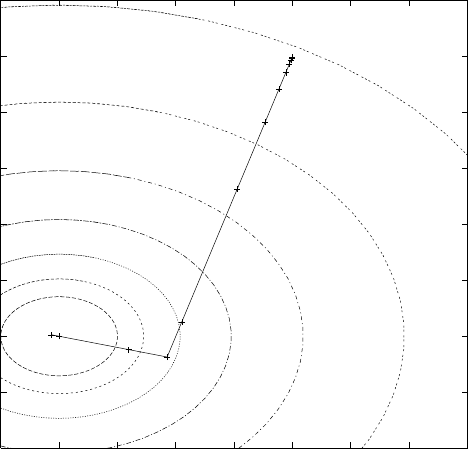
Chapter 35: Multidimensional Minimization 390
0
1
2
3
4
5
6
7
8
0 1 2 3 4 5 6 7 8
The conjugate gradient algorithm finds the minimum on its second direction because the
function is purely quadratic. Additional iterations would be needed for a more complicated
function.
Here is another example using the Nelder-Mead Simplex algorithm to minimize the same
example object function, as above.
int
main(void)
{
double par[5] = {1.0, 2.0, 10.0, 20.0, 30.0};
const gsl_multimin_fminimizer_type *T =
gsl_multimin_fminimizer_nmsimplex2;
gsl_multimin_fminimizer *s = NULL;
gsl_vector *ss, *x;
gsl_multimin_function minex_func;
size_t iter = 0;
int status;
double size;
/* Starting point */
x = gsl_vector_alloc (2);
gsl_vector_set (x, 0, 5.0);
gsl_vector_set (x, 1, 7.0);
/* Set initial step sizes to 1 */
ss = gsl_vector_alloc (2);
gsl_vector_set_all (ss, 1.0);
/* Initialize method and iterate */
minex_func.n = 2;
minex_func.f = my_f;
minex_func.params = par;
s = gsl_multimin_fminimizer_alloc (T, 2);
Chapter 35: Multidimensional Minimization 391
gsl_multimin_fminimizer_set (s, &minex_func, x, ss);
do
{
iter++;
status = gsl_multimin_fminimizer_iterate(s);
if (status)
break;
size = gsl_multimin_fminimizer_size (s);
status = gsl_multimin_test_size (size, 1e-2);
if (status == GSL_SUCCESS)
{
printf ("converged to minimum at\n");
}
printf ("%5d %10.3e %10.3e f() = %7.3f size = %.3f\n",
iter,
gsl_vector_get (s->x, 0),
gsl_vector_get (s->x, 1),
s->fval, size);
}
while (status == GSL_CONTINUE && iter < 100);
gsl_vector_free(x);
gsl_vector_free(ss);
gsl_multimin_fminimizer_free (s);
return status;
}
The minimum search stops when the Simplex size drops to 0.01. The output is shown below.
1 6.500e+00 5.000e+00 f() = 512.500 size = 1.130
2 5.250e+00 4.000e+00 f() = 290.625 size = 1.409
3 5.250e+00 4.000e+00 f() = 290.625 size = 1.409
4 5.500e+00 1.000e+00 f() = 252.500 size = 1.409
5 2.625e+00 3.500e+00 f() = 101.406 size = 1.847
6 2.625e+00 3.500e+00 f() = 101.406 size = 1.847
7 0.000e+00 3.000e+00 f() = 60.000 size = 1.847
8 2.094e+00 1.875e+00 f() = 42.275 size = 1.321
9 2.578e-01 1.906e+00 f() = 35.684 size = 1.069
10 5.879e-01 2.445e+00 f() = 35.664 size = 0.841
11 1.258e+00 2.025e+00 f() = 30.680 size = 0.476
12 1.258e+00 2.025e+00 f() = 30.680 size = 0.367
13 1.093e+00 1.849e+00 f() = 30.539 size = 0.300
14 8.830e-01 2.004e+00 f() = 30.137 size = 0.172
15 8.830e-01 2.004e+00 f() = 30.137 size = 0.126
16 9.582e-01 2.060e+00 f() = 30.090 size = 0.106
17 1.022e+00 2.004e+00 f() = 30.005 size = 0.063
18 1.022e+00 2.004e+00 f() = 30.005 size = 0.043
19 1.022e+00 2.004e+00 f() = 30.005 size = 0.043
20 1.022e+00 2.004e+00 f() = 30.005 size = 0.027
Chapter 35: Multidimensional Minimization 392
21 1.022e+00 2.004e+00 f() = 30.005 size = 0.022
22 9.920e-01 1.997e+00 f() = 30.001 size = 0.016
23 9.920e-01 1.997e+00 f() = 30.001 size = 0.013
converged to minimum at
24 9.920e-01 1.997e+00 f() = 30.001 size = 0.008
The simplex size first increases, while the simplex moves towards the minimum. After a
while the size begins to decrease as the simplex contracts around the minimum.
35.10 References and Further Reading
The conjugate gradient and BFGS methods are described in detail in the following book,
R. Fletcher, Practical Methods of Optimization (Second Edition) Wiley (1987), ISBN
0471915475.
A brief description of multidimensional minimization algorithms and more recent refer-
ences can be found in,
C.W. Ueberhuber, Numerical Computation (Volume 2), Chapter 14, Section 4.4 “Min-
imization Methods”, p. 325–335, Springer (1997), ISBN 3-540-62057-5.
The simplex algorithm is described in the following paper,
J.A. Nelder and R. Mead, A simplex method for function minimization, Computer
Journal vol. 7 (1965), 308–313.

Chapter 36: Least-Squares Fitting 393
36 Least-Squares Fitting
This chapter describes routines for performing least squares fits to experimental data using
linear combinations of functions. The data may be weighted or unweighted, i.e. with known
or unknown errors. For weighted data the functions compute the best fit parameters and
their associated covariance matrix. For unweighted data the covariance matrix is estimated
from the scatter of the points, giving a variance-covariance matrix.
The functions are divided into separate versions for simple one- or two-parameter regres-
sion and multiple-parameter fits. The functions are declared in the header file ‘gsl_fit.h’.
36.1 Overview
Least-squares fits are found by minimizing χ2(chi-squared), the weighted sum of squared
residuals over nexperimental datapoints (xi, yi) for the model Y(c, x),
χ2=X
i
wi(yi−Y(c, xi))2
The pparameters of the model are c={c0, c1,...}. The weight factors wiare given by
wi= 1/σ2
i, where σiis the experimental error on the data-point yi. The errors are assumed
to be gaussian and uncorrelated. For unweighted data the chi-squared sum is computed
without any weight factors.
The fitting routines return the best-fit parameters cand their p×pcovariance matrix.
The covariance matrix measures the statistical errors on the best-fit parameters resulting
from the errors on the data, σi, and is defined as Cab =hδcaδcbiwhere hi denotes an average
over the gaussian error distributions of the underlying datapoints.
The covariance matrix is calculated by error propagation from the data errors σi. The
change in a fitted parameter δcacaused by a small change in the data δyiis given by
δca=X
i
∂ca
∂yi
δyi
allowing the covariance matrix to be written in terms of the errors on the data,
Cab =X
i,j
∂ca
∂yi
∂cb
∂yjhδyiδyji
For uncorrelated data the fluctuations of the underlying datapoints satisfy hδyiδyji=σ2
iδij ,
giving a corresponding parameter covariance matrix of
Cab =X
i
1
wi
∂ca
∂yi
∂cb
∂yi
When computing the covariance matrix for unweighted data, i.e. data with unknown errors,
the weight factors wiin this sum are replaced by the single estimate w= 1/σ2, where σ2is
the computed variance of the residuals about the best-fit model, σ2=P(yi−Y(c, xi))2/(n−
p). This is referred to as the variance-covariance matrix.
The standard deviations of the best-fit parameters are given by the square root of the
corresponding diagonal elements of the covariance matrix, σca=√Caa. The correlation
coefficient of the fit parameters caand cbis given by ρab =Cab/√CaaCbb.

Chapter 36: Least-Squares Fitting 394
36.2 Linear regression
The functions described in this section can be used to perform least-squares fits to a straight
line model, Y(c, x) = c0+c1x.
[Function]int gsl_fit_linear (const double * x, const size txstride, const
double * y, const size t ystride, size t n, double * c0, double * c1, double *
cov00, double * cov01, double * cov11, double * sumsq )
This function computes the best-fit linear regression coefficients (c0,c1) of the model
Y=c0+c1Xfor the dataset (x,y), two vectors of length nwith strides xstride and
ystride. The errors on yare assumed unknown so the variance-covariance matrix for
the parameters (c0,c1) is estimated from the scatter of the points around the best-fit
line and returned via the parameters (cov00,cov01,cov11). The sum of squares of
the residuals from the best-fit line is returned in sumsq. Note: the correlation coeffi-
cient of the data can be computed using gsl_stats_correlation (see Section 20.6
[Correlation], page 258), it does not depend on the fit.
[Function]int gsl_fit_wlinear (const double * x, const size t xstride, const
double * w, const size t wstride, const double * y, const size t ystride,
size tn, double * c0, double * c1, double * cov00, double * cov01, double *
cov11, double * chisq )
This function computes the best-fit linear regression coefficients (c0,c1) of the model
Y=c0+c1Xfor the weighted dataset (x,y), two vectors of length nwith strides
xstride and ystride. The vector w, of length nand stride wstride, specifies the weight
of each datapoint. The weight is the reciprocal of the variance for each datapoint in
y.
The covariance matrix for the parameters (c0,c1) is computed using the weights and
returned via the parameters (cov00,cov01,cov11). The weighted sum of squares of
the residuals from the best-fit line, χ2, is returned in chisq.
[Function]int gsl_fit_linear_est (double x, double c0, double c1, double
cov00, double cov01, double cov11, double * y, double * y_err )
This function uses the best-fit linear regression coefficients c0,c1 and their covariance
cov00,cov01,cov11 to compute the fitted function yand its standard deviation yerr
for the model Y=c0+c1Xat the point x.
36.3 Linear fitting without a constant term
The functions described in this section can be used to perform least-squares fits to a straight
line model without a constant term, Y=c1X.
[Function]int gsl_fit_mul (const double * x, const size txstride, const double *
y, const size tystride, size t n, double * c1, double * cov11, double *
sumsq )
This function computes the best-fit linear regression coefficient c1 of the model Y=
c1Xfor the datasets (x,y), two vectors of length nwith strides xstride and ystride.
The errors on yare assumed unknown so the variance of the parameter c1 is estimated
from the scatter of the points around the best-fit line and returned via the parameter
cov11. The sum of squares of the residuals from the best-fit line is returned in sumsq.

Chapter 36: Least-Squares Fitting 395
[Function]int gsl_fit_wmul (const double * x, const size t xstride, const double
*w, const size twstride, const double * y, const size t ystride, size t n,
double * c1, double * cov11, double * sumsq )
This function computes the best-fit linear regression coefficient c1 of the model Y=
c1Xfor the weighted datasets (x,y), two vectors of length nwith strides xstride and
ystride. The vector w, of length nand stride wstride, specifies the weight of each
datapoint. The weight is the reciprocal of the variance for each datapoint in y.
The variance of the parameter c1 is computed using the weights and returned via the
parameter cov11. The weighted sum of squares of the residuals from the best-fit line,
χ2, is returned in chisq.
[Function]int gsl_fit_mul_est (double x, double c1, double cov11, double * y,
double * y_err )
This function uses the best-fit linear regression coefficient c1 and its covariance cov11
to compute the fitted function yand its standard deviation y err for the model
Y=c1Xat the point x.
36.4 Multi-parameter fitting
The functions described in this section perform least-squares fits to a general linear model,
y=Xc where yis a vector of nobservations, Xis an nby pmatrix of predictor variables,
and the elements of the vector care the punknown best-fit parameters which are to be
estimated. The chi-squared value is given by χ2=Piwi(yi−PjXij cj)2.
This formulation can be used for fits to any number of functions and/or variables by
preparing the n-by-pmatrix Xappropriately. For example, to fit to a p-th order polynomial
in x, use the following matrix,
Xij =xj
i
where the index iruns over the observations and the index jruns from 0 to p−1.
To fit to a set of psinusoidal functions with fixed frequencies ω1,ω2, . . . , ωp, use,
Xij = sin(ωjxi)
To fit to pindependent variables x1,x2, . . . , xp, use,
Xij =xj(i)
where xj(i) is the i-th value of the predictor variable xj.
The functions described in this section are declared in the header file ‘gsl_multifit.h’.
The solution of the general linear least-squares system requires an additional working
space for intermediate results, such as the singular value decomposition of the matrix X.
[Function]gsl_multifit_linear_workspace * gsl_multifit_linear_alloc
(size tn, size t p)
This function allocates a workspace for fitting a model to nobservations using p
parameters.
[Function]void gsl_multifit_linear_free (gsl multifit linear workspace *
work )
This function frees the memory associated with the workspace w.

Chapter 36: Least-Squares Fitting 396
[Function]int gsl_multifit_linear (const gsl matrix * X, const gsl vector * y,
gsl vector * c, gsl matrix * cov, double * chisq, gsl multifit linear workspace
*work )
[Function]int gsl_multifit_linear_svd (const gsl matrix * X, const gsl vector *
y, double tol, size t * rank, gsl vector * c, gsl matrix * cov, double * chisq,
gsl multifit linear workspace * work )
These functions compute the best-fit parameters cof the model y=Xc for the obser-
vations yand the matrix of predictor variables X. The variance-covariance matrix of
the model parameters cov is estimated from the scatter of the observations about the
best-fit. The sum of squares of the residuals from the best-fit, χ2, is returned in chisq.
If the coefficient of determination is desired, it can be computed from the expression
R2= 1 −χ2/T SS, where the total sum of squares (TSS) of the observations ymay
be computed from gsl_stats_tss.
The best-fit is found by singular value decomposition of the matrix Xusing the pre-
allocated workspace provided in work. The modified Golub-Reinsch SVD algorithm
is used, with column scaling to improve the accuracy of the singular values. Any
components which have zero singular value (to machine precision) are discarded from
the fit. In the second form of the function the components are discarded if the ratio
of singular values si/s0falls below the user-specified tolerance tol, and the effective
rank is returned in rank.
[Function]int gsl_multifit_wlinear (const gsl matrix * X, const gsl vector * w,
const gsl vector * y, gsl vector * c, gsl matrix * cov, double * chisq,
gsl multifit linear workspace * work )
[Function]int gsl_multifit_wlinear_svd (const gsl matrix * X, const gsl vector
*w, const gsl vector * y, double tol, size t * rank, gsl vector * c, gsl matrix *
cov, double * chisq, gsl multifit linear workspace * work )
This function computes the best-fit parameters cof the weighted model y=Xc
for the observations ywith weights wand the matrix of predictor variables X. The
covariance matrix of the model parameters cov is computed with the given weights.
The weighted sum of squares of the residuals from the best-fit, χ2, is returned in
chisq. If the coefficient of determination is desired, it can be computed from the
expression R2= 1 −χ2/W T SS, where the weighted total sum of squares (WTSS) of
the observations ymay be computed from gsl_stats_wtss.
The best-fit is found by singular value decomposition of the matrix Xusing the
preallocated workspace provided in work. Any components which have zero singular
value (to machine precision) are discarded from the fit. In the second form of the
function the components are discarded if the ratio of singular values si/s0falls below
the user-specified tolerance tol, and the effective rank is returned in rank.
[Function]int gsl_multifit_linear_est (const gsl vector * x, const gsl vector *
c, const gsl matrix * cov, double * y, double * y_err )
This function uses the best-fit multilinear regression coefficients cand their covariance
matrix cov to compute the fitted function value yand its standard deviation yerr
for the model y=x.c at the point x.

Chapter 36: Least-Squares Fitting 397
[Function]int gsl_multifit_linear_residuals (const gsl matrix * X, const
gsl vector * y, const gsl vector * c, gsl vector * r)
This function computes the vector of residuals r=y−Xc for the observations y,
coefficients cand matrix of predictor variables X.
36.5 Examples
The following program computes a least squares straight-line fit to a simple dataset, and
outputs the best-fit line and its associated one standard-deviation error bars.
#include <stdio.h>
#include <gsl/gsl_fit.h>
int
main (void)
{
int i, n = 4;
double x[4] = { 1970, 1980, 1990, 2000 };
double y[4] = { 12, 11, 14, 13 };
double w[4] = { 0.1, 0.2, 0.3, 0.4 };
double c0, c1, cov00, cov01, cov11, chisq;
gsl_fit_wlinear (x, 1, w, 1, y, 1, n,
&c0, &c1, &cov00, &cov01, &cov11,
&chisq);
printf ("# best fit: Y = %g + %g X\n", c0, c1);
printf ("# covariance matrix:\n");
printf ("# [ %g, %g\n# %g, %g]\n",
cov00, cov01, cov01, cov11);
printf ("# chisq = %g\n", chisq);
for (i = 0; i < n; i++)
printf ("data: %g %g %g\n",
x[i], y[i], 1/sqrt(w[i]));
printf ("\n");
for (i = -30; i < 130; i++)
{
double xf = x[0] + (i/100.0) * (x[n-1] - x[0]);
double yf, yf_err;
gsl_fit_linear_est (xf,
c0, c1,
cov00, cov01, cov11,
&yf, &yf_err);
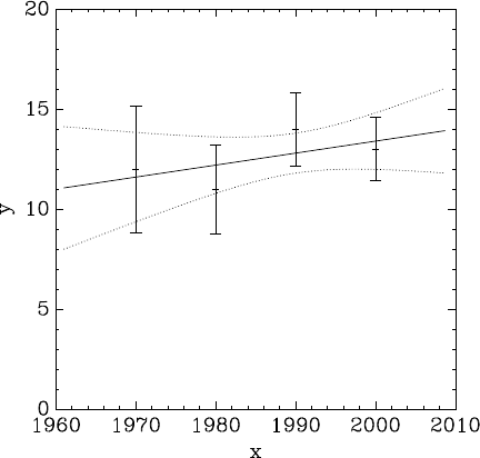
Chapter 36: Least-Squares Fitting 398
printf ("fit: %g %g\n", xf, yf);
printf ("hi : %g %g\n", xf, yf + yf_err);
printf ("lo : %g %g\n", xf, yf - yf_err);
}
return 0;
}
The following commands extract the data from the output of the program and display it
using the gnu plotutils graph utility,
$ ./demo > tmp
$ more tmp
# best fit: Y = -106.6 + 0.06 X
# covariance matrix:
# [ 39602, -19.9
# -19.9, 0.01]
# chisq = 0.8
$ for n in data fit hi lo ;
do
grep "^$n" tmp | cut -d: -f2 > $n ;
done
$ graph -T X -X x -Y y -y 0 20 -m 0 -S 2 -Ie data
-S 0 -I a -m 1 fit -m 2 hi -m 2 lo
The next program performs a quadratic fit y=c0+c1x+c2x2to a weighted dataset
using the generalised linear fitting function gsl_multifit_wlinear. The model matrix X
Chapter 36: Least-Squares Fitting 399
for a quadratic fit is given by,
X=
1x0x2
0
1x1x2
1
1x2x2
2
... ... ...
where the column of ones corresponds to the constant term c0. The two remaining columns
corresponds to the terms c1xand c2x2.
The program reads nlines of data in the format (x,y,err) where err is the error (standard
deviation) in the value y.
#include <stdio.h>
#include <gsl/gsl_multifit.h>
int
main (int argc, char **argv)
{
int i, n;
double xi, yi, ei, chisq;
gsl_matrix *X, *cov;
gsl_vector *y, *w, *c;
if (argc != 2)
{
fprintf (stderr,"usage: fit n < data\n");
exit (-1);
}
n = atoi (argv[1]);
X = gsl_matrix_alloc (n, 3);
y = gsl_vector_alloc (n);
w = gsl_vector_alloc (n);
c = gsl_vector_alloc (3);
cov = gsl_matrix_alloc (3, 3);
for (i = 0; i < n; i++)
{
int count = fscanf (stdin, "%lg %lg %lg",
&xi, &yi, &ei);
if (count != 3)
{
fprintf (stderr, "error reading file\n");
exit (-1);
}
Chapter 36: Least-Squares Fitting 400
printf ("%g %g +/- %g\n", xi, yi, ei);
gsl_matrix_set (X, i, 0, 1.0);
gsl_matrix_set (X, i, 1, xi);
gsl_matrix_set (X, i, 2, xi*xi);
gsl_vector_set (y, i, yi);
gsl_vector_set (w, i, 1.0/(ei*ei));
}
{
gsl_multifit_linear_workspace * work
= gsl_multifit_linear_alloc (n, 3);
gsl_multifit_wlinear (X, w, y, c, cov,
&chisq, work);
gsl_multifit_linear_free (work);
}
#define C(i) (gsl_vector_get(c,(i)))
#define COV(i,j) (gsl_matrix_get(cov,(i),(j)))
{
printf ("# best fit: Y = %g + %g X + %g X^2\n",
C(0), C(1), C(2));
printf ("# covariance matrix:\n");
printf ("[ %+.5e, %+.5e, %+.5e \n",
COV(0,0), COV(0,1), COV(0,2));
printf (" %+.5e, %+.5e, %+.5e \n",
COV(1,0), COV(1,1), COV(1,2));
printf (" %+.5e, %+.5e, %+.5e ]\n",
COV(2,0), COV(2,1), COV(2,2));
printf ("# chisq = %g\n", chisq);
}
gsl_matrix_free (X);
gsl_vector_free (y);
gsl_vector_free (w);
gsl_vector_free (c);
gsl_matrix_free (cov);
return 0;
}
A suitable set of data for fitting can be generated using the following program. It outputs
a set of points with gaussian errors from the curve y=exin the region 0 < x < 2.
#include <stdio.h>
Chapter 36: Least-Squares Fitting 401
#include <math.h>
#include <gsl/gsl_randist.h>
int
main (void)
{
double x;
const gsl_rng_type * T;
gsl_rng * r;
gsl_rng_env_setup ();
T = gsl_rng_default;
r = gsl_rng_alloc (T);
for (x = 0.1; x < 2; x+= 0.1)
{
double y0 = exp (x);
double sigma = 0.1 * y0;
double dy = gsl_ran_gaussian (r, sigma);
printf ("%g %g %g\n", x, y0 + dy, sigma);
}
gsl_rng_free(r);
return 0;
}
The data can be prepared by running the resulting executable program,
$ ./generate > exp.dat
$ more exp.dat
0.1 0.97935 0.110517
0.2 1.3359 0.12214
0.3 1.52573 0.134986
0.4 1.60318 0.149182
0.5 1.81731 0.164872
0.6 1.92475 0.182212
....
To fit the data use the previous program, with the number of data points given as the first
argument. In this case there are 19 data points.
$ ./fit 19 < exp.dat
0.1 0.97935 +/- 0.110517
0.2 1.3359 +/- 0.12214
...
# best fit: Y = 1.02318 + 0.956201 X + 0.876796 X^2
# covariance matrix:
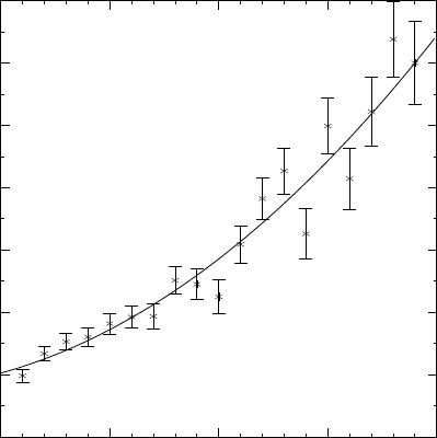
Chapter 36: Least-Squares Fitting 402
[ +1.25612e-02, -3.64387e-02, +1.94389e-02
-3.64387e-02, +1.42339e-01, -8.48761e-02
+1.94389e-02, -8.48761e-02, +5.60243e-02 ]
# chisq = 23.0987
The parameters of the quadratic fit match the coefficients of the expansion of ex, taking
into account the errors on the parameters and the O(x3) difference between the exponential
and quadratic functions for the larger values of x. The errors on the parameters are given
by the square-root of the corresponding diagonal elements of the covariance matrix. The
chi-squared per degree of freedom is 1.4, indicating a reasonable fit to the data.
0.0 0.5 1.0 1.5 2.0
0
1
2
3
4
5
6
7
36.6 References and Further Reading
A summary of formulas and techniques for least squares fitting can be found in the “Statis-
tics” chapter of the Annual Review of Particle Physics prepared by the Particle Data Group,
Review of Particle Properties, R.M. Barnett et al., Physical Review D54, 1 (1996)
http://pdg.lbl.gov/
The Review of Particle Physics is available online at the website given above.
The tests used to prepare these routines are based on the NIST Statistical Reference
Datasets. The datasets and their documentation are available from NIST at the following
website,
http://www.nist.gov/itl/div898/strd/index.html.

Chapter 37: Nonlinear Least-Squares Fitting 403
37 Nonlinear Least-Squares Fitting
This chapter describes functions for multidimensional nonlinear least-squares fitting. The
library provides low level components for a variety of iterative solvers and convergence tests.
These can be combined by the user to achieve the desired solution, with full access to the
intermediate steps of the iteration. Each class of methods uses the same framework, so that
you can switch between solvers at runtime without needing to recompile your program.
Each instance of a solver keeps track of its own state, allowing the solvers to be used in
multi-threaded programs.
The header file ‘gsl_multifit_nlin.h’ contains prototypes for the multidimensional
nonlinear fitting functions and related declarations.
37.1 Overview
The problem of multidimensional nonlinear least-squares fitting requires the minimization
of the squared residuals of nfunctions, fi, in pparameters, xi,
Φ(x) = 1
2||F(x)||2=1
2
n
X
i=1
fi(x1,...,xp)2
All algorithms proceed from an initial guess using the linearization,
ψ(p) = ||F(x+p)|| ≈ ||F(x) + Jp ||
where xis the initial point, pis the proposed step and Jis the Jacobian matrix Jij =
∂fi/∂xj. Additional strategies are used to enlarge the region of convergence. These include
requiring a decrease in the norm ||F|| on each step or using a trust region to avoid steps
which fall outside the linear regime.
To perform a weighted least-squares fit of a nonlinear model Y(x, t) to data (ti,yi) with
independent gaussian errors σi, use function components of the following form,
fi=(Y(x, ti)−yi)
σi
Note that the model parameters are denoted by xin this chapter since the non-linear least-
squares algorithms are described geometrically (i.e. finding the minimum of a surface). The
independent variable of any data to be fitted is denoted by t.
With the definition above the Jacobian is Jij = (1/σi)∂Yi/∂xj, where Yi=Y(x, ti).
37.2 Initializing the Solver
[Function]gsl_multifit_fsolver * gsl_multifit_fsolver_alloc (const
gsl multifit fsolver type * T, size t n, size t p)
This function returns a pointer to a newly allocated instance of a solver of type T
for nobservations and pparameters. The number of observations nmust be greater
than or equal to parameters p.
If there is insufficient memory to create the solver then the function returns a null
pointer and the error handler is invoked with an error code of GSL_ENOMEM.

Chapter 37: Nonlinear Least-Squares Fitting 404
[Function]gsl_multifit_fdfsolver * gsl_multifit_fdfsolver_alloc
(const gsl multifit fdfsolver type * T, size t n, size t p)
This function returns a pointer to a newly allocated instance of a derivative solver of
type Tfor nobservations and pparameters. For example, the following code creates
an instance of a Levenberg-Marquardt solver for 100 data points and 3 parameters,
const gsl_multifit_fdfsolver_type * T
= gsl_multifit_fdfsolver_lmder;
gsl_multifit_fdfsolver * s
= gsl_multifit_fdfsolver_alloc (T, 100, 3);
The number of observations nmust be greater than or equal to parameters p.
If there is insufficient memory to create the solver then the function returns a null
pointer and the error handler is invoked with an error code of GSL_ENOMEM.
[Function]int gsl_multifit_fsolver_set (gsl multifit fsolver * s,
gsl multifit function * f, const gsl vector * x)
This function initializes, or reinitializes, an existing solver sto use the function fand
the initial guess x.
[Function]int gsl_multifit_fdfsolver_set (gsl multifit fdfsolver * s,
gsl multifit function fdf * fdf, const gsl vector * x)
This function initializes, or reinitializes, an existing solver sto use the function and
derivative fdf and the initial guess x.
[Function]void gsl_multifit_fsolver_free (gsl multifit fsolver * s)
[Function]void gsl_multifit_fdfsolver_free (gsl multifit fdfsolver * s)
These functions free all the memory associated with the solver s.
[Function]const char * gsl_multifit_fsolver_name (const gsl multifit fsolver
*s)
[Function]const char * gsl_multifit_fdfsolver_name (const
gsl multifit fdfsolver * s)
These functions return a pointer to the name of the solver. For example,
printf ("s is a ’%s’ solver\n",
gsl_multifit_fdfsolver_name (s));
would print something like s is a ’lmder’ solver.
37.3 Providing the Function to be Minimized
You must provide nfunctions of pvariables for the minimization algorithms to operate on.
In order to allow for arbitrary parameters the functions are defined by the following data
types:
[Data Type]gsl_multifit_function
This data type defines a general system of functions with arbitrary parameters.
int (* f) (const gsl_vector * x, void * params, gsl_vector * f)
this function should store the vector result f(x, params) in ffor argument
xand arbitrary parameters params, returning an appropriate error code
if the function cannot be computed.

Chapter 37: Nonlinear Least-Squares Fitting 405
size_t n the number of functions, i.e. the number of components of the vector f.
size_t p the number of independent variables, i.e. the number of components of
the vector x.
void * params
a pointer to the arbitrary parameters of the function.
[Data Type]gsl_multifit_function_fdf
This data type defines a general system of functions with arbitrary parameters and
the corresponding Jacobian matrix of derivatives,
int (* f) (const gsl_vector * x, void * params, gsl_vector * f)
this function should store the vector result f(x, params) in ffor argument
xand arbitrary parameters params, returning an appropriate error code
if the function cannot be computed.
int (* df) (const gsl_vector * x, void * params, gsl_matrix * J)
this function should store the n-by-pmatrix result Jij =
∂fi(x, params)/∂xjin Jfor argument xand arbitrary parameters
params, returning an appropriate error code if the function cannot be
computed.
int (* fdf) (const gsl_vector * x, void * params, gsl_vector * f,
gsl_matrix * J)
This function should set the values of the fand Jas above, for arguments
xand arbitrary parameters params. This function provides an optimiza-
tion of the separate functions for f(x) and J(x)—it is always faster to
compute the function and its derivative at the same time.
size_t n the number of functions, i.e. the number of components of the vector f.
size_t p the number of independent variables, i.e. the number of components of
the vector x.
void * params
a pointer to the arbitrary parameters of the function.
Note that when fitting a non-linear model against experimental data, the data is passed
to the functions above using the params argument and the trial best-fit parameters through
the xargument.
37.4 Iteration
The following functions drive the iteration of each algorithm. Each function performs one
iteration to update the state of any solver of the corresponding type. The same func-
tions work for all solvers so that different methods can be substituted at runtime without
modifications to the code.
[Function]int gsl_multifit_fsolver_iterate (gsl multifit fsolver * s)
[Function]int gsl_multifit_fdfsolver_iterate (gsl multifit fdfsolver * s)
These functions perform a single iteration of the solver s. If the iteration encounters
an unexpected problem then an error code will be returned. The solver maintains a
current estimate of the best-fit parameters at all times.

Chapter 37: Nonlinear Least-Squares Fitting 406
The solver struct scontains the following entries, which can be used to track the progress
of the solution:
gsl_vector * x
The current position.
gsl_vector * f
The function value at the current position.
gsl_vector * dx
The difference between the current position and the previous position, i.e. the
last step, taken as a vector.
gsl_matrix * J
The Jacobian matrix at the current position (for the gsl_multifit_fdfsolver
struct only)
The best-fit information also can be accessed with the following auxiliary functions,
[Function]gsl_vector * gsl_multifit_fsolver_position (const
gsl multifit fsolver * s)
[Function]gsl_vector * gsl_multifit_fdfsolver_position (const
gsl multifit fdfsolver * s)
These functions return the current position (i.e. best-fit parameters) s->x of the
solver s.
37.5 Search Stopping Parameters
A minimization procedure should stop when one of the following conditions is true:
•A minimum has been found to within the user-specified precision.
•A user-specified maximum number of iterations has been reached.
•An error has occurred.
The handling of these conditions is under user control. The functions below allow the user
to test the current estimate of the best-fit parameters in several standard ways.
[Function]int gsl_multifit_test_delta (const gsl vector * dx, const gsl vector
*x, double epsabs, double epsrel )
This function tests for the convergence of the sequence by comparing the last step
dx with the absolute error epsabs and relative error epsrel to the current position x.
The test returns GSL_SUCCESS if the following condition is achieved,
|dxi|<epsabs +epsrel |xi|
for each component of xand returns GSL_CONTINUE otherwise.
[Function]int gsl_multifit_test_gradient (const gsl vector * g, double
epsabs )
This function tests the residual gradient gagainst the absolute error bound epsabs.
Mathematically, the gradient should be exactly zero at the minimum. The test returns
GSL_SUCCESS if the following condition is achieved,
X
i|gi|<epsabs

Chapter 37: Nonlinear Least-Squares Fitting 407
and returns GSL_CONTINUE otherwise. This criterion is suitable for situations where
the precise location of the minimum, x, is unimportant provided a value can be found
where the gradient is small enough.
[Function]int gsl_multifit_gradient (const gsl matrix * J, const gsl vector *
f, gsl vector * g)
This function computes the gradient gof Φ(x) = (1/2)||F(x)||2from the Jacobian
matrix Jand the function values f, using the formula g=JTf.
37.6 Minimization Algorithms using Derivatives
The minimization algorithms described in this section make use of both the function and
its derivative. They require an initial guess for the location of the minimum. There is no
absolute guarantee of convergence—the function must be suitable for this technique and
the initial guess must be sufficiently close to the minimum for it to work.
[Derivative Solver]gsl_multifit_fdfsolver_lmsder
This is a robust and efficient version of the Levenberg-Marquardt algorithm as im-
plemented in the scaled lmder routine in minpack. Minpack was written by Jorge
J. Mor´e, Burton S. Garbow and Kenneth E. Hillstrom.
The algorithm uses a generalized trust region to keep each step under control. In order
to be accepted a proposed new position x′must satisfy the condition |D(x′−x)|< δ,
where Dis a diagonal scaling matrix and δis the size of the trust region. The
components of Dare computed internally, using the column norms of the Jacobian
to estimate the sensitivity of the residual to each component of x. This improves the
behavior of the algorithm for badly scaled functions.
On each iteration the algorithm attempts to minimize the linear system |F+Jp|
subject to the constraint |Dp|<∆. The solution to this constrained linear system is
found using the Levenberg-Marquardt method.
The proposed step is now tested by evaluating the function at the resulting point,
x′. If the step reduces the norm of the function sufficiently, and follows the predicted
behavior of the function within the trust region, then it is accepted and the size of
the trust region is increased. If the proposed step fails to improve the solution, or
differs significantly from the expected behavior within the trust region, then the size
of the trust region is decreased and another trial step is computed.
The algorithm also monitors the progress of the solution and returns an error if the
changes in the solution are smaller than the machine precision. The possible error
codes are,
GSL_ETOLF
the decrease in the function falls below machine precision
GSL_ETOLX
the change in the position vector falls below machine precision
GSL_ETOLG
the norm of the gradient, relative to the norm of the function, falls below
machine precision

Chapter 37: Nonlinear Least-Squares Fitting 408
GSL_CONTINUE
the routine has made 10 or more attempts to find a suitable trial step
without success (but subsequent calls can be made to continue the search).
These error codes indicate that further iterations will be unlikely to change the solu-
tion from its current value.
[Derivative Solver]gsl_multifit_fdfsolver_lmder
This is an unscaled version of the lmder algorithm. The elements of the diagonal
scaling matrix Dare set to 1. This algorithm may be useful in circumstances where
the scaled version of lmder converges too slowly, or the function is already scaled
appropriately.
37.7 Minimization Algorithms without Derivatives
There are no algorithms implemented in this section at the moment.
37.8 Computing the covariance matrix of best fit
parameters
[Function]int gsl_multifit_covar (const gsl matrix * J, double epsrel,
gsl matrix * covar )
This function uses the Jacobian matrix Jto compute the covariance matrix of the
best-fit parameters, covar. The parameter epsrel is used to remove linear-dependent
columns when Jis rank deficient.
The covariance matrix is given by,
C= (JTJ)−1
and is computed by QR decomposition of J with column-pivoting. Any columns of R
which satisfy
|Rkk| ≤ epsrel|R11|
are considered linearly-dependent and are excluded from the covariance matrix (the
corresponding rows and columns of the covariance matrix are set to zero).
If the minimisation uses the weighted least-squares function fi= (Y(x, ti)−yi)/σi
then the covariance matrix above gives the statistical error on the best-fit parameters
resulting from the gaussian errors σion the underlying data yi. This can be verified
from the relation δf =Jδc and the fact that the fluctuations in ffrom the data yi
are normalised by σiand so satisfy hδf δfTi=I.
For an unweighted least-squares function fi= (Y(x, ti)−yi) the covariance matrix
above should be multiplied by the variance of the residuals about the best-fit σ2=
P(yi−Y(x, ti))2/(n−p) to give the variance-covariance matrix σ2C. This estimates
the statistical error on the best-fit parameters from the scatter of the underlying data.
For more information about covariance matrices see Section 36.1 [Fitting Overview],
page 393.

Chapter 37: Nonlinear Least-Squares Fitting 409
37.9 Examples
The following example program fits a weighted exponential model with background to
experimental data, Y=Aexp(−λt) + b. The first part of the program sets up the functions
expb_f and expb_df to calculate the model and its Jacobian. The appropriate fitting
function is given by,
fi= ((Aexp(−λti) + b)−yi)/σi
where we have chosen ti=i. The Jacobian matrix Jis the derivative of these functions
with respect to the three parameters (A,λ,b). It is given by,
Jij =∂fi
∂xj
where x0=A,x1=λand x2=b.
/* expfit.c -- model functions for exponential + background */
struct data {
size_t n;
double * y;
double * sigma;
};
int
expb_f (const gsl_vector * x, void *data,
gsl_vector * f)
{
size_t n = ((struct data *)data)->n;
double *y = ((struct data *)data)->y;
double *sigma = ((struct data *) data)->sigma;
double A = gsl_vector_get (x, 0);
double lambda = gsl_vector_get (x, 1);
double b = gsl_vector_get (x, 2);
size_t i;
for (i = 0; i < n; i++)
{
/* Model Yi = A * exp(-lambda * i) + b */
double t = i;
double Yi = A * exp (-lambda * t) + b;
gsl_vector_set (f, i, (Yi - y[i])/sigma[i]);
}
return GSL_SUCCESS;
}
Chapter 37: Nonlinear Least-Squares Fitting 410
int
expb_df (const gsl_vector * x, void *data,
gsl_matrix * J)
{
size_t n = ((struct data *)data)->n;
double *sigma = ((struct data *) data)->sigma;
double A = gsl_vector_get (x, 0);
double lambda = gsl_vector_get (x, 1);
size_t i;
for (i = 0; i < n; i++)
{
/* Jacobian matrix J(i,j) = dfi / dxj, */
/* where fi = (Yi - yi)/sigma[i], */
/* Yi = A * exp(-lambda * i) + b */
/* and the xj are the parameters (A,lambda,b) */
double t = i;
double s = sigma[i];
double e = exp(-lambda * t);
gsl_matrix_set (J, i, 0, e/s);
gsl_matrix_set (J, i, 1, -t * A * e/s);
gsl_matrix_set (J, i, 2, 1/s);
}
return GSL_SUCCESS;
}
int
expb_fdf (const gsl_vector * x, void *data,
gsl_vector * f, gsl_matrix * J)
{
expb_f (x, data, f);
expb_df (x, data, J);
return GSL_SUCCESS;
}
The main part of the program sets up a Levenberg-Marquardt solver and some simulated
random data. The data uses the known parameters (1.0,5.0,0.1) combined with gaussian
noise (standard deviation = 0.1) over a range of 40 timesteps. The initial guess for the
parameters is chosen as (0.0, 1.0, 0.0).
#include <stdlib.h>
#include <stdio.h>
#include <gsl/gsl_rng.h>
#include <gsl/gsl_randist.h>
#include <gsl/gsl_vector.h>
Chapter 37: Nonlinear Least-Squares Fitting 411
#include <gsl/gsl_blas.h>
#include <gsl/gsl_multifit_nlin.h>
#include "expfit.c"
#define N 40
void print_state (size_t iter, gsl_multifit_fdfsolver * s);
int
main (void)
{
const gsl_multifit_fdfsolver_type *T;
gsl_multifit_fdfsolver *s;
int status;
unsigned int i, iter = 0;
const size_t n = N;
const size_t p = 3;
gsl_matrix *covar = gsl_matrix_alloc (p, p);
double y[N], sigma[N];
struct data d = { n, y, sigma};
gsl_multifit_function_fdf f;
double x_init[3] = { 1.0, 0.0, 0.0 };
gsl_vector_view x = gsl_vector_view_array (x_init, p);
const gsl_rng_type * type;
gsl_rng * r;
gsl_rng_env_setup();
type = gsl_rng_default;
r = gsl_rng_alloc (type);
f.f = &expb_f;
f.df = &expb_df;
f.fdf = &expb_fdf;
f.n = n;
f.p = p;
f.params = &d;
/* This is the data to be fitted */
for (i = 0; i < n; i++)
{
double t = i;
y[i] = 1.0 + 5 * exp (-0.1 * t)
+ gsl_ran_gaussian (r, 0.1);
Chapter 37: Nonlinear Least-Squares Fitting 412
sigma[i] = 0.1;
printf ("data: %u %g %g\n", i, y[i], sigma[i]);
};
T = gsl_multifit_fdfsolver_lmsder;
s = gsl_multifit_fdfsolver_alloc (T, n, p);
gsl_multifit_fdfsolver_set (s, &f, &x.vector);
print_state (iter, s);
do
{
iter++;
status = gsl_multifit_fdfsolver_iterate (s);
printf ("status = %s\n", gsl_strerror (status));
print_state (iter, s);
if (status)
break;
status = gsl_multifit_test_delta (s->dx, s->x,
1e-4, 1e-4);
}
while (status == GSL_CONTINUE && iter < 500);
gsl_multifit_covar (s->J, 0.0, covar);
#define FIT(i) gsl_vector_get(s->x, i)
#define ERR(i) sqrt(gsl_matrix_get(covar,i,i))
{
double chi = gsl_blas_dnrm2(s->f);
double dof = n - p;
double c = GSL_MAX_DBL(1, chi / sqrt(dof));
printf("chisq/dof = %g\n", pow(chi, 2.0) / dof);
printf ("A = %.5f +/- %.5f\n", FIT(0), c*ERR(0));
printf ("lambda = %.5f +/- %.5f\n", FIT(1), c*ERR(1));
printf ("b = %.5f +/- %.5f\n", FIT(2), c*ERR(2));
}
printf ("status = %s\n", gsl_strerror (status));
gsl_multifit_fdfsolver_free (s);

Chapter 37: Nonlinear Least-Squares Fitting 413
gsl_matrix_free (covar);
gsl_rng_free (r);
return 0;
}
void
print_state (size_t iter, gsl_multifit_fdfsolver * s)
{
printf ("iter: %3u x = % 15.8f % 15.8f % 15.8f "
"|f(x)| = %g\n",
iter,
gsl_vector_get (s->x, 0),
gsl_vector_get (s->x, 1),
gsl_vector_get (s->x, 2),
gsl_blas_dnrm2 (s->f));
}
The iteration terminates when the change in x is smaller than 0.0001, as both an absolute
and relative change. Here are the results of running the program:
iter: 0 x=1.00000000 0.00000000 0.00000000 |f(x)|=117.349
status=success
iter: 1 x=1.64659312 0.01814772 0.64659312 |f(x)|=76.4578
status=success
iter: 2 x=2.85876037 0.08092095 1.44796363 |f(x)|=37.6838
status=success
iter: 3 x=4.94899512 0.11942928 1.09457665 |f(x)|=9.58079
status=success
iter: 4 x=5.02175572 0.10287787 1.03388354 |f(x)|=5.63049
status=success
iter: 5 x=5.04520433 0.10405523 1.01941607 |f(x)|=5.44398
status=success
iter: 6 x=5.04535782 0.10404906 1.01924871 |f(x)|=5.44397
chisq/dof = 0.800996
A = 5.04536 +/- 0.06028
lambda = 0.10405 +/- 0.00316
b = 1.01925 +/- 0.03782
status = success
The approximate values of the parameters are found correctly, and the chi-squared value
indicates a good fit (the chi-squared per degree of freedom is approximately 1). In this
case the errors on the parameters can be estimated from the square roots of the diagonal
elements of the covariance matrix.
If the chi-squared value shows a poor fit (i.e. χ2/(n−p)≫1) then the error estimates
obtained from the covariance matrix will be too small. In the example program the error
estimates are multiplied by pχ2/(n−p) in this case, a common way of increasing the errors
for a poor fit. Note that a poor fit will result from the use an inappropriate model, and the
scaled error estimates may then be outside the range of validity for gaussian errors.
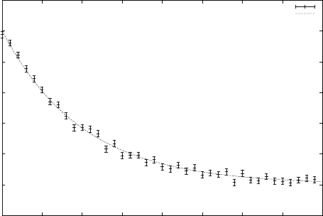
Chapter 37: Nonlinear Least-Squares Fitting 414
0
1
2
3
4
5
6
7
0 5 10 15 20 25 30 35 40
y
t
’data’ using 2:3:4
f(x)
37.10 References and Further Reading
The minpack algorithm is described in the following article,
J.J. Mor´e, The Levenberg-Marquardt Algorithm: Implementation and Theory, Lecture
Notes in Mathematics, v630 (1978), ed G. Watson.
The following paper is also relevant to the algorithms described in this section,
J.J. Mor´e, B.S. Garbow, K.E. Hillstrom, “Testing Unconstrained Optimization Soft-
ware”, ACM Transactions on Mathematical Software, Vol 7, No 1 (1981), p 17–41.

Chapter 38: Basis Splines 415
38 Basis Splines
This chapter describes functions for the computation of smoothing basis splines (B-splines).
A smoothing spline differs from an interpolating spline in that the resulting curve is not
required to pass through each datapoint. See Chapter 26 [Interpolation], page 319, for
information about interpolating splines.
The header file ‘gsl_bspline.h’ contains the prototypes for the bspline functions and
related declarations.
38.1 Overview
B-splines are commonly used as basis functions to fit smoothing curves to large data sets.
To do this, the abscissa axis is broken up into some number of intervals, where the end-
points of each interval are called breakpoints. These breakpoints are then converted to
knots by imposing various continuity and smoothness conditions at each interface. Given a
nondecreasing knot vector t={t0, t1,...,tn+k−1}, the nbasis splines of order kare defined
by
Bi,1(x) = 1, ti≤x < ti+1
0, else
Bi,k(x) = (x−ti)
(ti+k−1−ti)Bi,k−1(x) + (ti+k−x)
(ti+k−ti+1)Bi+1,k−1(x)
for i= 0,...,n −1. The common case of cubic B-splines is given by k= 4. The above
recurrence relation can be evaluated in a numerically stable way by the de Boor algorithm.
If we define appropriate knots on an interval [a, b] then the B-spline basis functions form
a complete set on that interval. Therefore we can expand a smoothing function as
f(x) =
n−1
X
i=0
ciBi,k(x)
given enough (xj, f (xj)) data pairs. The coefficients cican be readily obtained from a
least-squares fit.
38.2 Initializing the B-splines solver
The computation of B-spline functions requires a preallocated workspace of type gsl_
bspline_workspace. If B-spline derivatives are also required, an additional gsl_bspline_
deriv_workspace is needed.
[Function]gsl_bspline_workspace * gsl_bspline_alloc (const size tk, const
size tnbreak )
This function allocates a workspace for computing B-splines of order k. The number
of breakpoints is given by nbreak. This leads to n=nbreak +k−2 basis functions.
Cubic B-splines are specified by k= 4. The size of the workspace is O(5k+nbreak).
[Function]void gsl_bspline_free (gsl bspline workspace * w)
This function frees the memory associated with the workspace w.

Chapter 38: Basis Splines 416
[Function]gsl_bspline_deriv_workspace * gsl_bspline_deriv_alloc
(const size tk)
This function allocates a workspace for computing the derivatives of a B-spline basis
function of order k. The size of the workspace is O(2k2).
[Function]void gsl_bspline_deriv_free (gsl bspline deriv workspace * w)
This function frees the memory associated with the derivative workspace w.
38.3 Constructing the knots vector
[Function]int gsl_bspline_knots (const gsl vector * breakpts,
gsl bspline workspace * w)
This function computes the knots associated with the given breakpoints and stores
them internally in w->knots.
[Function]int gsl_bspline_knots_uniform (const double a, const double b,
gsl bspline workspace * w)
This function assumes uniformly spaced breakpoints on [a, b] and constructs the cor-
responding knot vector using the previously specified nbreak parameter. The knots
are stored in w->knots.
38.4 Evaluation of B-splines
[Function]int gsl_bspline_eval (const double x, gsl vector * B,
gsl bspline workspace * w)
This function evaluates all B-spline basis functions at the position xand stores them
in the vector B, so that the i-th element is Bi(x). The vector Bmust be of length
n=nbreak +k−2. This value may also be obtained by calling gsl_bspline_
ncoeffs. Computing all the basis functions at once is more efficient than computing
them individually, due to the nature of the defining recurrence relation.
[Function]int gsl_bspline_eval_nonzero (const double x, gsl vector * Bk, size t
*istart, size t * iend, gsl bspline workspace * w)
This function evaluates all potentially nonzero B-spline basis functions at the position
xand stores them in the vector Bk, so that the i-th element is B(istart+i)(x). The last
element of Bk is Biend(x). The vector Bk must be of length k. By returning only the
nonzero basis functions, this function allows quantities involving linear combinations
of the Bi(x) to be computed without unnecessary terms (such linear combinations
occur, for example, when evaluating an interpolated function).
[Function]size_t gsl_bspline_ncoeffs (gsl bspline workspace * w)
This function returns the number of B-spline coefficients given by n=nbreak +k−2.
38.5 Evaluation of B-spline derivatives
[Function]int gsl_bspline_deriv_eval (const double x, const size tnderiv,
gsl matrix * dB, gsl bspline workspace * w, gsl bspline deriv workspace * dw )
This function evaluates all B-spline basis function derivatives of orders 0 through
nderiv (inclusive) at the position xand stores them in the matrix dB. The (i, j)-th

Chapter 38: Basis Splines 417
element of dB is djBi(x)/dxj. The matrix dB must be of size n=nbreak +k−2
by nderiv + 1. The value nmay also be obtained by calling gsl_bspline_ncoeffs.
Note that function evaluations are included as the zeroth order derivatives in dB.
Computing all the basis function derivatives at once is more efficient than computing
them individually, due to the nature of the defining recurrence relation.
[Function]int gsl_bspline_deriv_eval_nonzero (const double x, const size t
nderiv, gsl matrix * dB, size t * istart, size t * iend, gsl bspline workspace
*w, gsl bspline deriv workspace * dw )
This function evaluates all potentially nonzero B-spline basis function derivatives of
orders 0 through nderiv (inclusive) at the position xand stores them in the matrix
dB. The (i, j)-th element of dB is djB(istart+i)(x)/dxj. The last row of dB contains
djBiend(x)/dxj. The matrix dB must be of size kby at least nderiv + 1. Note that
function evaluations are included as the zeroth order derivatives in dB. By return-
ing only the nonzero basis functions, this function allows quantities involving linear
combinations of the Bi(x) and their derivatives to be computed without unnecessary
terms.
38.6 Greville abscissae
The Greville abscissae are defined to be the mean location of k−1 consecutive knots in
the knot vector for each basis spline function of order k. Note that the first and last
knots in the knot vector are excluded when applying this definition; consequently there
are gsl_bspline_ncoeffs Greville abscissa. They are often used in B-spline collocation
applications and may also be called Marsden-Schoenberg points.
The above definition is undefined for k= 1. The implementation chooses to return
interval midpoints in the degenerate k= 1 case.
[Function]double gsl_bspline_greville_abscissa (size ti,
gsl bspline workspace *w);
Returns the location of the i-th Greville abscissa for the given spline basis. Here,
i= 0, ..., gsl_bspline_ncoeffs(w).
38.7 Examples
The following program computes a linear least squares fit to data using cubic B-spline
basis functions with uniform breakpoints. The data is generated from the curve y(x) =
cos (x) exp (−x/10) on the interval [0,15] with gaussian noise added.
#include <stdio.h>
#include <stdlib.h>
#include <math.h>
#include <gsl/gsl_bspline.h>
#include <gsl/gsl_multifit.h>
#include <gsl/gsl_rng.h>
#include <gsl/gsl_randist.h>
#include <gsl/gsl_statistics.h>
/* number of data points to fit */
Chapter 38: Basis Splines 418
#define N 200
/* number of fit coefficients */
#define NCOEFFS 12
/* nbreak = ncoeffs + 2 - k = ncoeffs - 2 since k = 4 */
#define NBREAK (NCOEFFS - 2)
int
main (void)
{
const size_t n = N;
const size_t ncoeffs = NCOEFFS;
const size_t nbreak = NBREAK;
size_t i, j;
gsl_bspline_workspace *bw;
gsl_vector *B;
double dy;
gsl_rng *r;
gsl_vector *c, *w;
gsl_vector *x, *y;
gsl_matrix *X, *cov;
gsl_multifit_linear_workspace *mw;
double chisq, Rsq, dof, tss;
gsl_rng_env_setup();
r = gsl_rng_alloc(gsl_rng_default);
/* allocate a cubic bspline workspace (k = 4) */
bw = gsl_bspline_alloc(4, nbreak);
B = gsl_vector_alloc(ncoeffs);
x = gsl_vector_alloc(n);
y = gsl_vector_alloc(n);
X = gsl_matrix_alloc(n, ncoeffs);
c = gsl_vector_alloc(ncoeffs);
w = gsl_vector_alloc(n);
cov = gsl_matrix_alloc(ncoeffs, ncoeffs);
mw = gsl_multifit_linear_alloc(n, ncoeffs);
printf("#m=0,S=0\n");
/* this is the data to be fitted */
for (i = 0; i < n; ++i)
{
double sigma;
double xi = (15.0 / (N - 1)) * i;
double yi = cos(xi) * exp(-0.1 * xi);
Chapter 38: Basis Splines 419
sigma = 0.1 * yi;
dy = gsl_ran_gaussian(r, sigma);
yi += dy;
gsl_vector_set(x, i, xi);
gsl_vector_set(y, i, yi);
gsl_vector_set(w, i, 1.0 / (sigma * sigma));
printf("%f %f\n", xi, yi);
}
/* use uniform breakpoints on [0, 15] */
gsl_bspline_knots_uniform(0.0, 15.0, bw);
/* construct the fit matrix X */
for (i = 0; i < n; ++i)
{
double xi = gsl_vector_get(x, i);
/* compute B_j(xi) for all j */
gsl_bspline_eval(xi, B, bw);
/* fill in row i of X */
for (j = 0; j < ncoeffs; ++j)
{
double Bj = gsl_vector_get(B, j);
gsl_matrix_set(X, i, j, Bj);
}
}
/* do the fit */
gsl_multifit_wlinear(X, w, y, c, cov, &chisq, mw);
dof = n - ncoeffs;
tss = gsl_stats_wtss(w->data, 1, y->data, 1, y->size);
Rsq = 1.0 - chisq / tss;
fprintf(stderr, "chisq/dof = %e, Rsq = %f\n",
chisq / dof, Rsq);
/* output the smoothed curve */
{
double xi, yi, yerr;
printf("#m=1,S=0\n");
for (xi = 0.0; xi < 15.0; xi += 0.1)
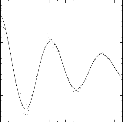
Chapter 38: Basis Splines 420
{
gsl_bspline_eval(xi, B, bw);
gsl_multifit_linear_est(B, c, cov, &yi, &yerr);
printf("%f %f\n", xi, yi);
}
}
gsl_rng_free(r);
gsl_bspline_free(bw);
gsl_vector_free(B);
gsl_vector_free(x);
gsl_vector_free(y);
gsl_matrix_free(X);
gsl_vector_free(c);
gsl_vector_free(w);
gsl_matrix_free(cov);
gsl_multifit_linear_free(mw);
return 0;
} /* main() */
The output can be plotted with gnu graph.
$ ./a.out > bspline.dat
chisq/dof = 1.118217e+00, Rsq = 0.989771
$ graph -T ps -X x -Y y -x 0 15 -y -1 1.3 < bspline.dat > bspline.ps
0 2 4 6 8 10 12 14
−1.0
−0.5
0.0
0.5
1.0
x
y
Chapter 38: Basis Splines 421
38.8 References and Further Reading
Further information on the algorithms described in this section can be found in the following
book,
C. de Boor, A Practical Guide to Splines (1978), Springer-Verlag, ISBN 0-387-90356-9.
Further information of Greville abscissae and B-spline collocation can be found in the
following paper,
Richard W. Johnson, Higher order B-spline collocation at the Greville abscissae. Ap-
plied Numerical Mathematics. vol. 52, 2005, 63–75.
A large collection of B-spline routines is available in the pppack library available at
http://www.netlib.org/pppack, which is also part of slatec.
Chapter 39: Physical Constants 422
39 Physical Constants
This chapter describes macros for the values of physical constants, such as the speed of
light, c, and gravitational constant, G. The values are available in different unit systems,
including the standard MKSA system (meters, kilograms, seconds, amperes) and the CGSM
system (centimeters, grams, seconds, gauss), which is commonly used in Astronomy.
The definitions of constants in the MKSA system are available in the
file ‘gsl_const_mksa.h’. The constants in the CGSM system are defined in
‘gsl_const_cgsm.h’. Dimensionless constants, such as the fine structure constant, which
are pure numbers are defined in ‘gsl_const_num.h’.
The full list of constants is described briefly below. Consult the header files themselves
for the values of the constants used in the library.
39.1 Fundamental Constants
GSL_CONST_MKSA_SPEED_OF_LIGHT
The speed of light in vacuum, c.
GSL_CONST_MKSA_VACUUM_PERMEABILITY
The permeability of free space, µ0. This constant is defined in the MKSA
system only.
GSL_CONST_MKSA_VACUUM_PERMITTIVITY
The permittivity of free space, ǫ0. This constant is defined in the MKSA system
only.
GSL_CONST_MKSA_PLANCKS_CONSTANT_H
Planck’s constant, h.
GSL_CONST_MKSA_PLANCKS_CONSTANT_HBAR
Planck’s constant divided by 2π, ¯h.
GSL_CONST_NUM_AVOGADRO
Avogadro’s number, Na.
GSL_CONST_MKSA_FARADAY
The molar charge of 1 Faraday.
GSL_CONST_MKSA_BOLTZMANN
The Boltzmann constant, k.
GSL_CONST_MKSA_MOLAR_GAS
The molar gas constant, R0.
GSL_CONST_MKSA_STANDARD_GAS_VOLUME
The standard gas volume, V0.
GSL_CONST_MKSA_STEFAN_BOLTZMANN_CONSTANT
The Stefan-Boltzmann radiation constant, σ.
GSL_CONST_MKSA_GAUSS
The magnetic field of 1 Gauss.
Chapter 39: Physical Constants 423
39.2 Astronomy and Astrophysics
GSL_CONST_MKSA_ASTRONOMICAL_UNIT
The length of 1 astronomical unit (mean earth-sun distance), au.
GSL_CONST_MKSA_GRAVITATIONAL_CONSTANT
The gravitational constant, G.
GSL_CONST_MKSA_LIGHT_YEAR
The distance of 1 light-year, ly.
GSL_CONST_MKSA_PARSEC
The distance of 1 parsec, pc.
GSL_CONST_MKSA_GRAV_ACCEL
The standard gravitational acceleration on Earth, g.
GSL_CONST_MKSA_SOLAR_MASS
The mass of the Sun.
39.3 Atomic and Nuclear Physics
GSL_CONST_MKSA_ELECTRON_CHARGE
The charge of the electron, e.
GSL_CONST_MKSA_ELECTRON_VOLT
The energy of 1 electron volt, eV .
GSL_CONST_MKSA_UNIFIED_ATOMIC_MASS
The unified atomic mass, amu.
GSL_CONST_MKSA_MASS_ELECTRON
The mass of the electron, me.
GSL_CONST_MKSA_MASS_MUON
The mass of the muon, mµ.
GSL_CONST_MKSA_MASS_PROTON
The mass of the proton, mp.
GSL_CONST_MKSA_MASS_NEUTRON
The mass of the neutron, mn.
GSL_CONST_NUM_FINE_STRUCTURE
The electromagnetic fine structure constant α.
GSL_CONST_MKSA_RYDBERG
The Rydberg constant, Ry, in units of energy. This is related to the Rydberg
inverse wavelength R∞by Ry =hcR∞.
GSL_CONST_MKSA_BOHR_RADIUS
The Bohr radius, a0.
GSL_CONST_MKSA_ANGSTROM
The length of 1 angstrom.
Chapter 39: Physical Constants 424
GSL_CONST_MKSA_BARN
The area of 1 barn.
GSL_CONST_MKSA_BOHR_MAGNETON
The Bohr Magneton, µB.
GSL_CONST_MKSA_NUCLEAR_MAGNETON
The Nuclear Magneton, µN.
GSL_CONST_MKSA_ELECTRON_MAGNETIC_MOMENT
The absolute value of the magnetic moment of the electron, µe. The physical
magnetic moment of the electron is negative.
GSL_CONST_MKSA_PROTON_MAGNETIC_MOMENT
The magnetic moment of the proton, µp.
GSL_CONST_MKSA_THOMSON_CROSS_SECTION
The Thomson cross section, σT.
GSL_CONST_MKSA_DEBYE
The electric dipole moment of 1 Debye, D.
39.4 Measurement of Time
GSL_CONST_MKSA_MINUTE
The number of seconds in 1 minute.
GSL_CONST_MKSA_HOUR
The number of seconds in 1 hour.
GSL_CONST_MKSA_DAY
The number of seconds in 1 day.
GSL_CONST_MKSA_WEEK
The number of seconds in 1 week.
39.5 Imperial Units
GSL_CONST_MKSA_INCH
The length of 1 inch.
GSL_CONST_MKSA_FOOT
The length of 1 foot.
GSL_CONST_MKSA_YARD
The length of 1 yard.
GSL_CONST_MKSA_MILE
The length of 1 mile.
GSL_CONST_MKSA_MIL
The length of 1 mil (1/1000th of an inch).
Chapter 39: Physical Constants 425
39.6 Speed and Nautical Units
GSL_CONST_MKSA_KILOMETERS_PER_HOUR
The speed of 1 kilometer per hour.
GSL_CONST_MKSA_MILES_PER_HOUR
The speed of 1 mile per hour.
GSL_CONST_MKSA_NAUTICAL_MILE
The length of 1 nautical mile.
GSL_CONST_MKSA_FATHOM
The length of 1 fathom.
GSL_CONST_MKSA_KNOT
The speed of 1 knot.
39.7 Printers Units
GSL_CONST_MKSA_POINT
The length of 1 printer’s point (1/72 inch).
GSL_CONST_MKSA_TEXPOINT
The length of 1 TeX point (1/72.27 inch).
39.8 Volume, Area and Length
GSL_CONST_MKSA_MICRON
The length of 1 micron.
GSL_CONST_MKSA_HECTARE
The area of 1 hectare.
GSL_CONST_MKSA_ACRE
The area of 1 acre.
GSL_CONST_MKSA_LITER
The volume of 1 liter.
GSL_CONST_MKSA_US_GALLON
The volume of 1 US gallon.
GSL_CONST_MKSA_CANADIAN_GALLON
The volume of 1 Canadian gallon.
GSL_CONST_MKSA_UK_GALLON
The volume of 1 UK gallon.
GSL_CONST_MKSA_QUART
The volume of 1 quart.
GSL_CONST_MKSA_PINT
The volume of 1 pint.
Chapter 39: Physical Constants 426
39.9 Mass and Weight
GSL_CONST_MKSA_POUND_MASS
The mass of 1 pound.
GSL_CONST_MKSA_OUNCE_MASS
The mass of 1 ounce.
GSL_CONST_MKSA_TON
The mass of 1 ton.
GSL_CONST_MKSA_METRIC_TON
The mass of 1 metric ton (1000 kg).
GSL_CONST_MKSA_UK_TON
The mass of 1 UK ton.
GSL_CONST_MKSA_TROY_OUNCE
The mass of 1 troy ounce.
GSL_CONST_MKSA_CARAT
The mass of 1 carat.
GSL_CONST_MKSA_GRAM_FORCE
The force of 1 gram weight.
GSL_CONST_MKSA_POUND_FORCE
The force of 1 pound weight.
GSL_CONST_MKSA_KILOPOUND_FORCE
The force of 1 kilopound weight.
GSL_CONST_MKSA_POUNDAL
The force of 1 poundal.
39.10 Thermal Energy and Power
GSL_CONST_MKSA_CALORIE
The energy of 1 calorie.
GSL_CONST_MKSA_BTU
The energy of 1 British Thermal Unit, btu.
GSL_CONST_MKSA_THERM
The energy of 1 Therm.
GSL_CONST_MKSA_HORSEPOWER
The power of 1 horsepower.
39.11 Pressure
GSL_CONST_MKSA_BAR
The pressure of 1 bar.
GSL_CONST_MKSA_STD_ATMOSPHERE
The pressure of 1 standard atmosphere.
Chapter 39: Physical Constants 427
GSL_CONST_MKSA_TORR
The pressure of 1 torr.
GSL_CONST_MKSA_METER_OF_MERCURY
The pressure of 1 meter of mercury.
GSL_CONST_MKSA_INCH_OF_MERCURY
The pressure of 1 inch of mercury.
GSL_CONST_MKSA_INCH_OF_WATER
The pressure of 1 inch of water.
GSL_CONST_MKSA_PSI
The pressure of 1 pound per square inch.
39.12 Viscosity
GSL_CONST_MKSA_POISE
The dynamic viscosity of 1 poise.
GSL_CONST_MKSA_STOKES
The kinematic viscosity of 1 stokes.
39.13 Light and Illumination
GSL_CONST_MKSA_STILB
The luminance of 1 stilb.
GSL_CONST_MKSA_LUMEN
The luminous flux of 1 lumen.
GSL_CONST_MKSA_LUX
The illuminance of 1 lux.
GSL_CONST_MKSA_PHOT
The illuminance of 1 phot.
GSL_CONST_MKSA_FOOTCANDLE
The illuminance of 1 footcandle.
GSL_CONST_MKSA_LAMBERT
The luminance of 1 lambert.
GSL_CONST_MKSA_FOOTLAMBERT
The luminance of 1 footlambert.
39.14 Radioactivity
GSL_CONST_MKSA_CURIE
The activity of 1 curie.
GSL_CONST_MKSA_ROENTGEN
The exposure of 1 roentgen.
GSL_CONST_MKSA_RAD
The absorbed dose of 1 rad.
Chapter 39: Physical Constants 428
39.15 Force and Energy
GSL_CONST_MKSA_NEWTON
The SI unit of force, 1 Newton.
GSL_CONST_MKSA_DYNE
The force of 1 Dyne = 10−5Newton.
GSL_CONST_MKSA_JOULE
The SI unit of energy, 1 Joule.
GSL_CONST_MKSA_ERG
The energy 1 erg = 10−7Joule.
39.16 Prefixes
These constants are dimensionless scaling factors.
GSL_CONST_NUM_YOTTA
1024
GSL_CONST_NUM_ZETTA
1021
GSL_CONST_NUM_EXA
1018
GSL_CONST_NUM_PETA
1015
GSL_CONST_NUM_TERA
1012
GSL_CONST_NUM_GIGA
109
GSL_CONST_NUM_MEGA
106
GSL_CONST_NUM_KILO
103
GSL_CONST_NUM_MILLI
10−3
GSL_CONST_NUM_MICRO
10−6
GSL_CONST_NUM_NANO
10−9
GSL_CONST_NUM_PICO
10−12
GSL_CONST_NUM_FEMTO
10−15
Chapter 39: Physical Constants 429
GSL_CONST_NUM_ATTO
10−18
GSL_CONST_NUM_ZEPTO
10−21
GSL_CONST_NUM_YOCTO
10−24
39.17 Examples
The following program demonstrates the use of the physical constants in a calculation. In
this case, the goal is to calculate the range of light-travel times from Earth to Mars.
The required data is the average distance of each planet from the Sun in astronomical
units (the eccentricities and inclinations of the orbits will be neglected for the purposes of
this calculation). The average radius of the orbit of Mars is 1.52 astronomical units, and for
the orbit of Earth it is 1 astronomical unit (by definition). These values are combined with
the MKSA values of the constants for the speed of light and the length of an astronomical
unit to produce a result for the shortest and longest light-travel times in seconds. The
figures are converted into minutes before being displayed.
#include <stdio.h>
#include <gsl/gsl_const_mksa.h>
int
main (void)
{
double c = GSL_CONST_MKSA_SPEED_OF_LIGHT;
double au = GSL_CONST_MKSA_ASTRONOMICAL_UNIT;
double minutes = GSL_CONST_MKSA_MINUTE;
/* distance stored in meters */
double r_earth = 1.00 * au;
double r_mars = 1.52 * au;
double t_min, t_max;
t_min = (r_mars - r_earth) / c;
t_max = (r_mars + r_earth) / c;
printf ("light travel time from Earth to Mars:\n");
printf ("minimum = %.1f minutes\n", t_min / minutes);
printf ("maximum = %.1f minutes\n", t_max / minutes);
return 0;
}
Here is the output from the program,
light travel time from Earth to Mars:
minimum = 4.3 minutes
Chapter 39: Physical Constants 430
maximum = 21.0 minutes
39.18 References and Further Reading
The authoritative sources for physical constants are the 2006 CODATA recommended val-
ues, published in the article below. Further information on the values of physical constants
is also available from the NIST website.
P.J. Mohr, B.N. Taylor, D.B. Newell, “CODATA Recommended Values of the Funda-
mental Physical Constants: 2006”, Reviews of Modern Physics, 80(2), pp. 633–730
(2008).
http://www.physics.nist.gov/cuu/Constants/index.html
http://physics.nist.gov/Pubs/SP811/appenB9.html
Chapter 40: IEEE floating-point arithmetic 431
40 IEEE floating-point arithmetic
This chapter describes functions for examining the representation of floating point numbers
and controlling the floating point environment of your program. The functions described
in this chapter are declared in the header file ‘gsl_ieee_utils.h’.
40.1 Representation of floating point numbers
The IEEE Standard for Binary Floating-Point Arithmetic defines binary formats for single
and double precision numbers. Each number is composed of three parts: a sign bit (s), an
exponent (E) and a fraction (f). The numerical value of the combination (s, E, f) is given
by the following formula,
(−1)s(1 ·ff fff . . .)2E
The sign bit is either zero or one. The exponent ranges from a minimum value Emin to
a maximum value Emax depending on the precision. The exponent is converted to an
unsigned number e, known as the biased exponent, for storage by adding a bias parameter,
e=E+bias. The sequence f f ff f... represents the digits of the binary fraction f. The
binary digits are stored in normalized form, by adjusting the exponent to give a leading
digit of 1. Since the leading digit is always 1 for normalized numbers it is assumed implicitly
and does not have to be stored. Numbers smaller than 2Emin are be stored in denormalized
form with a leading zero,
(−1)s(0 ·ff fff . . .)2Emin
This allows gradual underflow down to 2Emin −pfor pbits of precision. A zero is encoded
with the special exponent of 2Emin −1and infinities with the exponent of 2Emax +1.
The format for single precision numbers uses 32 bits divided in the following way,
seeeeeeeefffffffffffffffffffffff
s = sign bit, 1 bit
e = exponent, 8 bits (E_min=-126, E_max=127, bias=127)
f = fraction, 23 bits
The format for double precision numbers uses 64 bits divided in the following way,
seeeeeeeeeeeffffffffffffffffffffffffffffffffffffffffffffffffffff
s = sign bit, 1 bit
e = exponent, 11 bits (E_min=-1022, E_max=1023, bias=1023)
f = fraction, 52 bits
It is often useful to be able to investigate the behavior of a calculation at the bit-level and
the library provides functions for printing the IEEE representations in a human-readable
form.
[Function]void gsl_ieee_fprintf_float (FILE * stream, const float * x)
[Function]void gsl_ieee_fprintf_double (FILE * stream, const double * x)
These functions output a formatted version of the IEEE floating-point number pointed
to by xto the stream stream. A pointer is used to pass the number indirectly, to
avoid any undesired promotion from float to double. The output takes one of the
following forms,
Chapter 40: IEEE floating-point arithmetic 432
NaN the Not-a-Number symbol
Inf, -Inf positive or negative infinity
1.fffff...*2^E, -1.fffff...*2^E
a normalized floating point number
0.fffff...*2^E, -0.fffff...*2^E
a denormalized floating point number
0, -0 positive or negative zero
The output can be used directly in GNU Emacs Calc mode by preceding it with 2#
to indicate binary.
[Function]void gsl_ieee_printf_float (const float * x)
[Function]void gsl_ieee_printf_double (const double * x)
These functions output a formatted version of the IEEE floating-point number pointed
to by xto the stream stdout.
The following program demonstrates the use of the functions by printing the single and
double precision representations of the fraction 1/3. For comparison the representation of
the value promoted from single to double precision is also printed.
#include <stdio.h>
#include <gsl/gsl_ieee_utils.h>
int
main (void)
{
float f = 1.0/3.0;
double d = 1.0/3.0;
double fd = f; /* promote from float to double */
printf (" f="); gsl_ieee_printf_float(&f);
printf ("\n");
printf ("fd="); gsl_ieee_printf_double(&fd);
printf ("\n");
printf (" d="); gsl_ieee_printf_double(&d);
printf ("\n");
return 0;
}
The binary representation of 1/3 is 0.01010101.... The output below shows that the IEEE
format normalizes this fraction to give a leading digit of 1,
f= 1.01010101010101010101011*2^-2
fd= 1.0101010101010101010101100000000000000000000000000000*2^-2
d= 1.0101010101010101010101010101010101010101010101010101*2^-2
Chapter 40: IEEE floating-point arithmetic 433
The output also shows that a single-precision number is promoted to double-precision by
adding zeros in the binary representation.
40.2 Setting up your IEEE environment
The IEEE standard defines several modes for controlling the behavior of floating point
operations. These modes specify the important properties of computer arithmetic: the
direction used for rounding (e.g. whether numbers should be rounded up, down or to the
nearest number), the rounding precision and how the program should handle arithmetic
exceptions, such as division by zero.
Many of these features can now be controlled via standard functions such as fpsetround,
which should be used whenever they are available. Unfortunately in the past there has been
no universal API for controlling their behavior—each system has had its own low-level way
of accessing them. To help you write portable programs GSL allows you to specify modes
in a platform-independent way using the environment variable GSL_IEEE_MODE. The library
then takes care of all the necessary machine-specific initializations for you when you call
the function gsl_ieee_env_setup.
[Function]void gsl_ieee_env_setup ()
This function reads the environment variable GSL_IEEE_MODE and attempts to set up
the corresponding specified IEEE modes. The environment variable should be a list
of keywords, separated by commas, like this,
GSL_IEEE_MODE ="keyword,keyword,..."
where keyword is one of the following mode-names,
single-precision
double-precision
extended-precision
round-to-nearest
round-down
round-up
round-to-zero
mask-all
mask-invalid
mask-denormalized
mask-division-by-zero
mask-overflow
mask-underflow
trap-inexact
trap-common
If GSL_IEEE_MODE is empty or undefined then the function returns immediately and
no attempt is made to change the system’s IEEE mode. When the modes from GSL_
IEEE_MODE are turned on the function prints a short message showing the new settings
to remind you that the results of the program will be affected.

Chapter 40: IEEE floating-point arithmetic 434
If the requested modes are not supported by the platform being used then the function
calls the error handler and returns an error code of GSL_EUNSUP.
When options are specified using this method, the resulting mode is based on a default
setting of the highest available precision (double precision or extended precision, de-
pending on the platform) in round-to-nearest mode, with all exceptions enabled apart
from the inexact exception. The inexact exception is generated whenever rounding
occurs, so it must generally be disabled in typical scientific calculations. All other
floating-point exceptions are enabled by default, including underflows and the use of
denormalized numbers, for safety. They can be disabled with the individual mask-
settings or together using mask-all.
The following adjusted combination of modes is convenient for many purposes,
GSL_IEEE_MODE="double-precision,"\
"mask-underflow,"\
"mask-denormalized"
This choice ignores any errors relating to small numbers (either denormalized, or
underflowing to zero) but traps overflows, division by zero and invalid operations.
Note that on the x86 series of processors this function sets both the original x87 mode
and the newer mxcsr mode, which controls SSE floating-point operations. The SSE
floating-point units do not have a precision-control bit, and always work in double-
precision. The single-precision and extended-precision keywords have no effect in this
case.
To demonstrate the effects of different rounding modes consider the following program which
computes e, the base of natural logarithms, by summing a rapidly-decreasing series,
e= 1 + 1
2! +1
3! +1
4! +...= 2.71828182846...
#include <stdio.h>
#include <gsl/gsl_math.h>
#include <gsl/gsl_ieee_utils.h>
int
main (void)
{
double x = 1, oldsum = 0, sum = 0;
int i = 0;
gsl_ieee_env_setup (); /* read GSL_IEEE_MODE */
do
{
i++;
oldsum = sum;
sum += x;
x = x / i;
Chapter 40: IEEE floating-point arithmetic 435
printf ("i=%2d sum=%.18f error=%g\n",
i, sum, sum - M_E);
if (i > 30)
break;
}
while (sum != oldsum);
return 0;
}
Here are the results of running the program in round-to-nearest mode. This is the IEEE
default so it isn’t really necessary to specify it here,
$ GSL_IEEE_MODE="round-to-nearest" ./a.out
i= 1 sum=1.000000000000000000 error=-1.71828
i= 2 sum=2.000000000000000000 error=-0.718282
....
i=18 sum=2.718281828459045535 error=4.44089e-16
i=19 sum=2.718281828459045535 error=4.44089e-16
After nineteen terms the sum converges to within 4 ×10⁻¹⁶ of the correct value. If we now
change the rounding mode to round-down the final result is less accurate,
$ GSL_IEEE_MODE="round-down" ./a.out
i= 1 sum=1.000000000000000000 error=-1.71828
....
i=19 sum=2.718281828459041094 error=-3.9968e-15
The result is about 4 ×10⁻¹⁵ below the correct value, an order of magnitude worse than
the result obtained in the round-to-nearest mode.
If we change to rounding mode to round-up then the final result is higher than the
correct value (when we add each term to the sum the final result is always rounded up,
which increases the sum by at least one tick until the added term underflows to zero). To
avoid this problem we would need to use a safer converge criterion, such as while (fabs(sum
- oldsum) > epsilon), with a suitably chosen value of epsilon.
Finally we can see the effect of computing the sum using single-precision rounding, in
the default round-to-nearest mode. In this case the program thinks it is still using double
precision numbers but the CPU rounds the result of each floating point operation to single-
precision accuracy. This simulates the effect of writing the program using single-precision
float variables instead of double variables. The iteration stops after about half the number
of iterations and the final result is much less accurate,
$ GSL_IEEE_MODE="single-precision" ./a.out
....
i=12 sum=2.718281984329223633 error=1.5587e-07
with an error of O(10−7), which corresponds to single precision accuracy (about 1 part in
107). Continuing the iterations further does not decrease the error because all the subse-
quent results are rounded to the same value.
Chapter 40: IEEE floating-point arithmetic 436
40.3 References and Further Reading
The reference for the IEEE standard is,
ANSI/IEEE Std 754-1985, IEEE Standard for Binary Floating-Point Arithmetic.
A more pedagogical introduction to the standard can be found in the following paper,
David Goldberg: What Every Computer Scientist Should Know About Floating-Point
Arithmetic. ACM Computing Surveys, Vol. 23, No. 1 (March 1991), pages 5–48.
Corrigendum: ACM Computing Surveys, Vol. 23, No. 3 (September 1991), page 413.
and see also the sections by B. A. Wichmann and Charles B. Dunham in Surveyor’s
Forum: “What Every Computer Scientist Should Know About Floating-Point Arith-
metic”. ACM Computing Surveys, Vol. 24, No. 3 (September 1992), page 319.
A detailed textbook on IEEE arithmetic and its practical use is available from SIAM
Press,
Michael L. Overton, Numerical Computing with IEEE Floating Point Arithmetic,
SIAM Press, ISBN 0898715717.
Appendix A: Debugging Numerical Programs 437
Appendix A Debugging Numerical Programs
This chapter describes some tips and tricks for debugging numerical programs which use
GSL.
A.1 Using gdb
Any errors reported by the library are passed to the function gsl_error. By running your
programs under gdb and setting a breakpoint in this function you can automatically catch
any library errors. You can add a breakpoint for every session by putting
break gsl_error
into your ‘.gdbinit’ file in the directory where your program is started.
If the breakpoint catches an error then you can use a backtrace (bt) to see the call-tree,
and the arguments which possibly caused the error. By moving up into the calling function
you can investigate the values of variables at that point. Here is an example from the
program fft/test_trap, which contains the following line,
status = gsl_fft_complex_wavetable_alloc (0, &complex_wavetable);
The function gsl_fft_complex_wavetable_alloc takes the length of an FFT as its first
argument. When this line is executed an error will be generated because the length of an
FFT is not allowed to be zero.
To debug this problem we start gdb, using the file ‘.gdbinit’ to define a breakpoint in
gsl_error,
$ gdb test_trap
GDB is free software and you are welcome to distribute copies
of it under certain conditions; type "show copying" to see
the conditions. There is absolutely no warranty for GDB;
type "show warranty" for details. GDB 4.16 (i586-debian-linux),
Copyright 1996 Free Software Foundation, Inc.
Breakpoint 1 at 0x8050b1e: file error.c, line 14.
When we run the program this breakpoint catches the error and shows the reason for it.
(gdb) run
Starting program: test_trap
Breakpoint 1, gsl_error (reason=0x8052b0d
"length n must be positive integer",
file=0x8052b04 "c_init.c", line=108, gsl_errno=1)
at error.c:14
14 if (gsl_error_handler)
The first argument of gsl_error is always a string describing the error. Now we can look
at the backtrace to see what caused the problem,
(gdb) bt
#0 gsl_error (reason=0x8052b0d
"length n must be positive integer",
file=0x8052b04 "c_init.c", line=108, gsl_errno=1)
at error.c:14
#1 0x8049376 in gsl_fft_complex_wavetable_alloc (n=0,
wavetable=0xbffff778) at c_init.c:108
#2 0x8048a00 in main (argc=1, argv=0xbffff9bc)
Appendix A: Debugging Numerical Programs 438
at test_trap.c:94
#3 0x80488be in ___crt_dummy__ ()
We can see that the error was generated in the function gsl_fft_complex_wavetable_
alloc when it was called with an argument of n=0. The original call came from line 94 in
the file ‘test_trap.c’.
By moving up to the level of the original call we can find the line that caused the error,
(gdb) up
#1 0x8049376 in gsl_fft_complex_wavetable_alloc (n=0,
wavetable=0xbffff778) at c_init.c:108
108 GSL_ERROR ("length n must be positive integer", GSL_EDOM);
(gdb) up
#2 0x8048a00 in main (argc=1, argv=0xbffff9bc)
at test_trap.c:94
94 status = gsl_fft_complex_wavetable_alloc (0,
&complex_wavetable);
Thus we have found the line that caused the problem. From this point we could also print
out the values of other variables such as complex_wavetable.
A.2 Examining floating point registers
The contents of floating point registers can be examined using the command info float
(on supported platforms).
(gdb) info float
st0: 0xc4018b895aa17a945000 Valid Normal -7.838871e+308
st1: 0x3ff9ea3f50e4d7275000 Valid Normal 0.0285946
st2: 0x3fe790c64ce27dad4800 Valid Normal 6.7415931e-08
st3: 0x3ffaa3ef0df6607d7800 Spec Normal 0.0400229
st4: 0x3c028000000000000000 Valid Normal 4.4501477e-308
st5: 0x3ffef5412c22219d9000 Zero Normal 0.9580257
st6: 0x3fff8000000000000000 Valid Normal 1
st7: 0xc4028b65a1f6d243c800 Valid Normal -1.566206e+309
fctrl: 0x0272 53 bit; NEAR; mask DENOR UNDER LOS;
fstat: 0xb9ba flags 0001; top 7; excep DENOR OVERF UNDER LOS
ftag: 0x3fff
fip: 0x08048b5c
fcs: 0x051a0023
fopoff: 0x08086820
fopsel: 0x002b
Individual registers can be examined using the variables $reg, where reg is the register
name.
(gdb) p $st1
$1 = 0.02859464454261210347719
A.3 Handling floating point exceptions
It is possible to stop the program whenever a SIGFPE floating point exception occurs. This
can be useful for finding the cause of an unexpected infinity or NaN. The current handler
settings can be shown with the command info signal SIGFPE.
(gdb) info signal SIGFPE
Signal Stop Print Pass to program Description
SIGFPE Yes Yes Yes Arithmetic exception
Appendix A: Debugging Numerical Programs 439
Unless the program uses a signal handler the default setting should be changed so that
SIGFPE is not passed to the program, as this would cause it to exit. The command handle
SIGFPE stop nopass prevents this.
(gdb) handle SIGFPE stop nopass
Signal Stop Print Pass to program Description
SIGFPE Yes Yes No Arithmetic exception
Depending on the platform it may be necessary to instruct the kernel to generate signals
for floating point exceptions. For programs using GSL this can be achieved using the GSL_
IEEE_MODE environment variable in conjunction with the function gsl_ieee_env_setup as
described in see Chapter 40 [IEEE floating-point arithmetic], page 431.
(gdb) set env GSL_IEEE_MODE=double-precision
A.4 GCC warning options for numerical programs
Writing reliable numerical programs in C requires great care. The following GCC warning
options are recommended when compiling numerical programs:
gcc -ansi -pedantic -Werror -Wall -W
-Wmissing-prototypes -Wstrict-prototypes
-Wconversion -Wshadow -Wpointer-arith
-Wcast-qual -Wcast-align
-Wwrite-strings -Wnested-externs
-fshort-enums -fno-common -Dinline= -g -O2
For details of each option consult the manual Using and Porting GCC. The following table
gives a brief explanation of what types of errors these options catch.
-ansi -pedantic
Use ANSI C, and reject any non-ANSI extensions. These flags help in writing
portable programs that will compile on other systems.
-Werror Consider warnings to be errors, so that compilation stops. This prevents warn-
ings from scrolling off the top of the screen and being lost. You won’t be able
to compile the program until it is completely warning-free.
-Wall This turns on a set of warnings for common programming problems. You need
-Wall, but it is not enough on its own.
-O2 Turn on optimization. The warnings for uninitialized variables in -Wall rely
on the optimizer to analyze the code. If there is no optimization then these
warnings aren’t generated.
-W This turns on some extra warnings not included in -Wall, such as missing return
values and comparisons between signed and unsigned integers.
-Wmissing-prototypes -Wstrict-prototypes
Warn if there are any missing or inconsistent prototypes. Without prototypes
it is harder to detect problems with incorrect arguments.
-Wconversion
The main use of this option is to warn about conversions from signed to unsigned
integers. For example, unsigned int x = -1. If you need to perform such a
conversion you can use an explicit cast.
Appendix A: Debugging Numerical Programs 440
-Wshadow This warns whenever a local variable shadows another local variable. If two
variables have the same name then it is a potential source of confusion.
-Wpointer-arith -Wcast-qual -Wcast-align
These options warn if you try to do pointer arithmetic for types which don’t
have a size, such as void, if you remove a const cast from a pointer, or if you
cast a pointer to a type which has a different size, causing an invalid alignment.
-Wwrite-strings
This option gives string constants a const qualifier so that it will be a compile-
time error to attempt to overwrite them.
-fshort-enums
This option makes the type of enum as short as possible. Normally this makes
an enum different from an int. Consequently any attempts to assign a pointer-
to-int to a pointer-to-enum will generate a cast-alignment warning.
-fno-common
This option prevents global variables being simultaneously defined in different
object files (you get an error at link time). Such a variable should be defined
in one file and referred to in other files with an extern declaration.
-Wnested-externs
This warns if an extern declaration is encountered within a function.
-Dinline=
The inline keyword is not part of ANSI C. Thus if you want to use -ansi with
a program which uses inline functions you can use this preprocessor definition
to remove the inline keywords.
-g It always makes sense to put debugging symbols in the executable so that you
can debug it using gdb. The only effect of debugging symbols is to increase the
size of the file, and you can use the strip command to remove them later if
necessary.
A.5 References and Further Reading
The following books are essential reading for anyone writing and debugging numerical pro-
grams with gcc and gdb.
R.M. Stallman, Using and Porting GNU CC, Free Software Foundation, ISBN
1882114388
R.M. Stallman, R.H. Pesch, Debugging with GDB: The GNU Source-Level Debugger,
Free Software Foundation, ISBN 1882114779
For a tutorial introduction to the GNU C Compiler and related programs, see
B.J. Gough, An Introduction to GCC, Network Theory Ltd, ISBN 0954161793
Appendix B: Contributors to GSL 441
Appendix B Contributors to GSL
(See the AUTHORS file in the distribution for up-to-date information.)
Mark Galassi
Conceived GSL (with James Theiler) and wrote the design document. Wrote
the simulated annealing package and the relevant chapter in the manual.
James Theiler
Conceived GSL (with Mark Galassi). Wrote the random number generators
and the relevant chapter in this manual.
Jim Davies
Wrote the statistical routines and the relevant chapter in this manual.
Brian Gough
FFTs, numerical integration, random number generators and distributions, root
finding, minimization and fitting, polynomial solvers, complex numbers, physi-
cal constants, permutations, vector and matrix functions, histograms, statistics,
ieee-utils, revised cblas Level 2 & 3, matrix decompositions, eigensystems, cu-
mulative distribution functions, testing, documentation and releases.
Reid Priedhorsky
Wrote and documented the initial version of the root finding routines while at
Los Alamos National Laboratory, Mathematical Modeling and Analysis Group.
Gerard Jungman
Special Functions, Series acceleration, ODEs, BLAS, Linear Algebra, Eigensys-
tems, Hankel Transforms.
Mike Booth
Wrote the Monte Carlo library.
Jorma Olavi T¨ahtinen
Wrote the initial complex arithmetic functions.
Thomas Walter
Wrote the initial heapsort routines and cholesky decomposition.
Fabrice Rossi
Multidimensional minimization.
Carlo Perassi
Implementation of the random number generators in Knuth’s Seminumerical
Algorithms, 3rd Ed.
Szymon Jaroszewicz
Wrote the routines for generating combinations.
Nicolas Darnis
Wrote the cyclic functions and the initial functions for canonical permutations.
Jason H. Stover
Wrote the major cumulative distribution functions.
Appendix B: Contributors to GSL 442
Ivo Alxneit
Wrote the routines for wavelet transforms.
Tuomo Keskitalo
Improved the implementation of the ODE solvers.
Lowell Johnson
Implementation of the Mathieu functions.
Patrick Alken
Implementation of non-symmetric and generalized eigensystems and B-splines.
Thanks to Nigel Lowry for help in proofreading the manual.
The non-symmetric eigensystems routines contain code based on the LAPACK linear
algebra library. LAPACK is distributed under the following license:
Copyright (c) 1992-2006 The University of Tennessee. All rights reserved.
Redistribution and use in source and binary forms, with or without modification, are permitted pro-
vided that the following conditions are met:
•Redistributions of source code must retain the above copyright notice, this list of conditions and the
following disclaimer.
•Redistributions in binary form must reproduce the above copyright notice, this list of conditions and
the following disclaimer listed in this license in the documentation and/or other materials provided
with the distribution.
•Neither the name of the copyright holders nor the names of its contributors may be used to endorse
or promote products derived from this software without specific prior written permission.
THIS SOFTWARE IS PROVIDED BY THE COPYRIGHT HOLDERS AND CONTRIBUTORS
“AS IS” AND ANY EXPRESS OR IMPLIED WARRANTIES, INCLUDING, BUT NOT LIMITED
TO, THE IMPLIED WARRANTIES OF MERCHANTABILITY AND FITNESS FOR A PARTIC-
ULAR PURPOSE ARE DISCLAIMED. IN NO EVENT SHALL THE COPYRIGHT OWNER OR
CONTRIBUTORS BE LIABLE FOR ANY DIRECT, INDIRECT, INCIDENTAL, SPECIAL, EX-
EMPLARY, OR CONSEQUENTIAL DAMAGES (INCLUDING, BUT NOT LIMITED TO, PRO-
CUREMENT OF SUBSTITUTE GOODS OR SERVICES; LOSS OF USE, DATA, OR PROFITS;
OR BUSINESS INTERRUPTION) HOWEVER CAUSED AND ON ANY THEORY OF LIABIL-
ITY, WHETHER IN CONTRACT, STRICT LIABILITY, OR TORT (INCLUDING NEGLIGENCE
OR OTHERWISE) ARISING IN ANY WAY OUT OF THE USE OF THIS SOFTWARE, EVEN IF
ADVISED OF THE POSSIBILITY OF SUCH DAMAGE.
Appendix C: Autoconf Macros 443
Appendix C Autoconf Macros
For applications using autoconf the standard macro AC_CHECK_LIB can be used to link with
GSL automatically from a configure script. The library itself depends on the presence of
acblas and math library as well, so these must also be located before linking with the
main libgsl file. The following commands should be placed in the ‘configure.ac’ file to
perform these tests,
AC_CHECK_LIB([m],[cos])
AC_CHECK_LIB([gslcblas],[cblas_dgemm])
AC_CHECK_LIB([gsl],[gsl_blas_dgemm])
It is important to check for libm and libgslcblas before libgsl, otherwise the tests will
fail. Assuming the libraries are found the output during the configure stage looks like this,
checking for cos in -lm... yes
checking for cblas_dgemm in -lgslcblas... yes
checking for gsl_blas_dgemm in -lgsl... yes
If the library is found then the tests will define the macros HAVE_LIBGSL,HAVE_
LIBGSLCBLAS,HAVE_LIBM and add the options -lgsl -lgslcblas -lm to the variable
LIBS.
The tests above will find any version of the library. They are suitable for general use,
where the versions of the functions are not important. An alternative macro is available in
the file ‘gsl.m4’ to test for a specific version of the library. To use this macro simply add
the following line to your ‘configure.in’ file instead of the tests above:
AX_PATH_GSL(GSL_VERSION,
[action-if-found],
[action-if-not-found])
The argument GSL_VERSION should be the two or three digit major.minor or
major.minor.micro version number of the release you require. A suitable choice for
action-if-not-found is,
AC_MSG_ERROR(could not find required version of GSL)
Then you can add the variables GSL_LIBS and GSL_CFLAGS to your Makefile.am files to
obtain the correct compiler flags. GSL_LIBS is equal to the output of the gsl-config --
libs command and GSL_CFLAGS is equal to gsl-config --cflags command. For example,
libfoo_la_LDFLAGS = -lfoo $(GSL_LIBS) -lgslcblas
Note that the macro AX_PATH_GSL needs to use the C compiler so it should appear in the
‘configure.in’ file before the macro AC_LANG_CPLUSPLUS for programs that use C++.
To test for inline the following test should be placed in your ‘configure.in’ file,
AC_C_INLINE
if test "$ac_cv_c_inline" != no ; then
AC_DEFINE(HAVE_INLINE,1)
AC_SUBST(HAVE_INLINE)
fi
and the macro will then be defined in the compilation flags or by including the file ‘config.h’
before any library headers.
Appendix C: Autoconf Macros 444
The following autoconf test will check for extern inline,
dnl Check for "extern inline", using a modified version
dnl of the test for AC_C_INLINE from acspecific.mt
dnl
AC_CACHE_CHECK([for extern inline], ac_cv_c_extern_inline,
[ac_cv_c_extern_inline=no
AC_TRY_COMPILE([extern $ac_cv_c_inline double foo(double x);
extern $ac_cv_c_inline double foo(double x) { return x+1.0; };
double foo (double x) { return x + 1.0; };],
[ foo(1.0) ],
[ac_cv_c_extern_inline="yes"])
])
if test "$ac_cv_c_extern_inline" != no ; then
AC_DEFINE(HAVE_INLINE,1)
AC_SUBST(HAVE_INLINE)
fi
The substitution of portability functions can be made automatically if you use autoconf.
For example, to test whether the BSD function hypot is available you can include the
following line in the configure file ‘configure.in’ for your application,
AC_CHECK_FUNCS(hypot)
and place the following macro definitions in the file ‘config.h.in’,
/* Substitute gsl_hypot for missing system hypot */
#ifndef HAVE_HYPOT
#define hypot gsl_hypot
#endif
The application source files can then use the include command #include <config.h> to
substitute gsl_hypot for each occurrence of hypot when hypot is not available.
Appendix D: GSL CBLAS Library 445
Appendix D GSL CBLAS Library
The prototypes for the low-level cblas functions are declared in the file ‘gsl_cblas.h’.
For the definition of the functions consult the documentation available from Netlib (see
Section 12.3 [BLAS References and Further Reading], page 127).
D.1 Level 1
[Function]float cblas_sdsdot (const int N, const float alpha, const float * x,
const int incx, const float * y, const int incy )
[Function]double cblas_dsdot (const int N, const float * x, const int incx, const
float * y, const int incy )
[Function]float cblas_sdot (const int N, const float * x, const int incx, const
float * y, const int incy )
[Function]double cblas_ddot (const int N, const double * x, const int incx, const
double * y, const int incy )
[Function]void cblas_cdotu_sub (const int N, const void * x, const int incx,
const void * y, const int incy, void * dotu )
[Function]void cblas_cdotc_sub (const int N, const void * x, const int incx,
const void * y, const int incy, void * dotc )
[Function]void cblas_zdotu_sub (const int N, const void * x, const int incx,
const void * y, const int incy, void * dotu )
[Function]void cblas_zdotc_sub (const int N, const void * x, const int incx,
const void * y, const int incy, void * dotc )
[Function]float cblas_snrm2 (const int N, const float * x, const int incx )
[Function]float cblas_sasum (const int N, const float * x, const int incx )
[Function]double cblas_dnrm2 (const int N, const double * x, const int incx )
[Function]double cblas_dasum (const int N, const double * x, const int incx )
[Function]float cblas_scnrm2 (const int N, const void * x, const int incx )
[Function]float cblas_scasum (const int N, const void * x, const int incx )
[Function]double cblas_dznrm2 (const int N, const void * x, const int incx )
[Function]double cblas_dzasum (const int N, const void * x, const int incx )
[Function]CBLAS_INDEX cblas_isamax (const int N, const float * x, const int
incx )
[Function]CBLAS_INDEX cblas_idamax (const int N, const double * x, const int
incx )
[Function]CBLAS_INDEX cblas_icamax (const int N, const void * x, const int incx )
[Function]CBLAS_INDEX cblas_izamax (const int N, const void * x, const int incx )
Appendix D: GSL CBLAS Library 446
[Function]void cblas_sswap (const int N, float * x, const int incx, float * y, const
int incy )
[Function]void cblas_scopy (const int N, const float * x, const int incx, float * y,
const int incy )
[Function]void cblas_saxpy (const int N, const float alpha, const float * x, const
int incx, float * y, const int incy )
[Function]void cblas_dswap (const int N, double * x, const int incx, double * y,
const int incy )
[Function]void cblas_dcopy (const int N, const double * x, const int incx, double
*y, const int incy )
[Function]void cblas_daxpy (const int N, const double alpha, const double * x,
const int incx, double * y, const int incy )
[Function]void cblas_cswap (const int N, void * x, const int incx, void * y, const
int incy )
[Function]void cblas_ccopy (const int N, const void * x, const int incx, void * y,
const int incy )
[Function]void cblas_caxpy (const int N, const void * alpha, const void * x, const
int incx, void * y, const int incy )
[Function]void cblas_zswap (const int N, void * x, const int incx, void * y, const
int incy )
[Function]void cblas_zcopy (const int N, const void * x, const int incx, void * y,
const int incy )
[Function]void cblas_zaxpy (const int N, const void * alpha, const void * x, const
int incx, void * y, const int incy )
[Function]void cblas_srotg (float * a, float * b, float * c, float * s)
[Function]void cblas_srotmg (float * d1, float * d2, float * b1, const float b2,
float * P)
[Function]void cblas_srot (const int N, float * x, const int incx, float * y, const
int incy, const float c, const float s)
[Function]void cblas_srotm (const int N, float * x, const int incx, float * y, const
int incy, const float * P)
[Function]void cblas_drotg (double * a, double * b, double * c, double * s)
[Function]void cblas_drotmg (double * d1, double * d2, double * b1, const double
b2, double * P)
[Function]void cblas_drot (const int N, double * x, const int incx, double * y,
const int incy, const double c, const double s)
[Function]void cblas_drotm (const int N, double * x, const int incx, double * y,
const int incy, const double * P)

Appendix D: GSL CBLAS Library 447
[Function]void cblas_sscal (const int N, const float alpha, float * x, const int
incx )
[Function]void cblas_dscal (const int N, const double alpha, double * x, const
int incx )
[Function]void cblas_cscal (const int N, const void * alpha, void * x, const int
incx )
[Function]void cblas_zscal (const int N, const void * alpha, void * x, const int
incx )
[Function]void cblas_csscal (const int N, const float alpha, void * x, const int
incx )
[Function]void cblas_zdscal (const int N, const double alpha, void * x, const int
incx )
D.2 Level 2
[Function]void cblas_sgemv (const enum CBLAS ORDER order, const enum
CBLAS TRANSPOSE TransA, const int M, const int N, const float alpha,
const float * A, const int lda, const float * x, const int incx, const float beta,
float * y, const int incy )
[Function]void cblas_sgbmv (const enum CBLAS ORDER order, const enum
CBLAS TRANSPOSE TransA, const int M, const int N, const int KL, const int
KU, const float alpha, const float * A, const int lda, const float * x, const int
incx, const float beta, float * y, const int incy )
[Function]void cblas_strmv (const enum CBLAS ORDER order, const enum
CBLAS UPLO Uplo, const enum CBLAS TRANSPOSE TransA, const enum
CBLAS DIAG Diag, const int N, const float * A, const int lda, float * x, const
int incx )
[Function]void cblas_stbmv (const enum CBLAS ORDER order, const enum
CBLAS UPLO Uplo, const enum CBLAS TRANSPOSE TransA, const enum
CBLAS DIAG Diag, const int N, const int K, const float * A, const int lda,
float * x, const int incx )
[Function]void cblas_stpmv (const enum CBLAS ORDER order, const enum
CBLAS UPLO Uplo, const enum CBLAS TRANSPOSE TransA, const enum
CBLAS DIAG Diag, const int N, const float * Ap, float * x, const int incx )
[Function]void cblas_strsv (const enum CBLAS ORDER order, const enum
CBLAS UPLO Uplo, const enum CBLAS TRANSPOSE TransA, const enum
CBLAS DIAG Diag, const int N, const float * A, const int lda, float * x, const
int incx )
[Function]void cblas_stbsv (const enum CBLAS ORDER order, const enum
CBLAS UPLO Uplo, const enum CBLAS TRANSPOSE TransA, const enum
CBLAS DIAG Diag, const int N, const int K, const float * A, const int lda,
float * x, const int incx )

Appendix D: GSL CBLAS Library 448
[Function]void cblas_stpsv (const enum CBLAS ORDER order, const enum
CBLAS UPLO Uplo, const enum CBLAS TRANSPOSE TransA, const enum
CBLAS DIAG Diag, const int N, const float * Ap, float * x, const int incx )
[Function]void cblas_dgemv (const enum CBLAS ORDER order, const enum
CBLAS TRANSPOSE TransA, const int M, const int N, const double alpha,
const double * A, const int lda, const double * x, const int incx, const double
beta, double * y, const int incy )
[Function]void cblas_dgbmv (const enum CBLAS ORDER order, const enum
CBLAS TRANSPOSE TransA, const int M, const int N, const int KL, const int
KU, const double alpha, const double * A, const int lda, const double * x,
const int incx, const double beta, double * y, const int incy )
[Function]void cblas_dtrmv (const enum CBLAS ORDER order, const enum
CBLAS UPLO Uplo, const enum CBLAS TRANSPOSE TransA, const enum
CBLAS DIAG Diag, const int N, const double * A, const int lda, double * x,
const int incx )
[Function]void cblas_dtbmv (const enum CBLAS ORDER order, const enum
CBLAS UPLO Uplo, const enum CBLAS TRANSPOSE TransA, const enum
CBLAS DIAG Diag, const int N, const int K, const double * A, const int lda,
double * x, const int incx )
[Function]void cblas_dtpmv (const enum CBLAS ORDER order, const enum
CBLAS UPLO Uplo, const enum CBLAS TRANSPOSE TransA, const enum
CBLAS DIAG Diag, const int N, const double * Ap, double * x, const int
incx )
[Function]void cblas_dtrsv (const enum CBLAS ORDER order, const enum
CBLAS UPLO Uplo, const enum CBLAS TRANSPOSE TransA, const enum
CBLAS DIAG Diag, const int N, const double * A, const int lda, double * x,
const int incx )
[Function]void cblas_dtbsv (const enum CBLAS ORDER order, const enum
CBLAS UPLO Uplo, const enum CBLAS TRANSPOSE TransA, const enum
CBLAS DIAG Diag, const int N, const int K, const double * A, const int lda,
double * x, const int incx )
[Function]void cblas_dtpsv (const enum CBLAS ORDER order, const enum
CBLAS UPLO Uplo, const enum CBLAS TRANSPOSE TransA, const enum
CBLAS DIAG Diag, const int N, const double * Ap, double * x, const int
incx )
[Function]void cblas_cgemv (const enum CBLAS ORDER order, const enum
CBLAS TRANSPOSE TransA, const int M, const int N, const void * alpha,
const void * A, const int lda, const void * x, const int incx, const void * beta,
void * y, const int incy )
[Function]void cblas_cgbmv (const enum CBLAS ORDER order, const enum
CBLAS TRANSPOSE TransA, const int M, const int N, const int KL, const int
KU, const void * alpha, const void * A, const int lda, const void * x, const int
incx, const void * beta, void * y, const int incy )

Appendix D: GSL CBLAS Library 449
[Function]void cblas_ctrmv (const enum CBLAS ORDER order, const enum
CBLAS UPLO Uplo, const enum CBLAS TRANSPOSE TransA, const enum
CBLAS DIAG Diag, const int N, const void * A, const int lda, void * x, const
int incx )
[Function]void cblas_ctbmv (const enum CBLAS ORDER order, const enum
CBLAS UPLO Uplo, const enum CBLAS TRANSPOSE TransA, const enum
CBLAS DIAG Diag, const int N, const int K, const void * A, const int lda,
void * x, const int incx )
[Function]void cblas_ctpmv (const enum CBLAS ORDER order, const enum
CBLAS UPLO Uplo, const enum CBLAS TRANSPOSE TransA, const enum
CBLAS DIAG Diag, const int N, const void * Ap, void * x, const int incx )
[Function]void cblas_ctrsv (const enum CBLAS ORDER order, const enum
CBLAS UPLO Uplo, const enum CBLAS TRANSPOSE TransA, const enum
CBLAS DIAG Diag, const int N, const void * A, const int lda, void * x, const
int incx )
[Function]void cblas_ctbsv (const enum CBLAS ORDER order, const enum
CBLAS UPLO Uplo, const enum CBLAS TRANSPOSE TransA, const enum
CBLAS DIAG Diag, const int N, const int K, const void * A, const int lda,
void * x, const int incx )
[Function]void cblas_ctpsv (const enum CBLAS ORDER order, const enum
CBLAS UPLO Uplo, const enum CBLAS TRANSPOSE TransA, const enum
CBLAS DIAG Diag, const int N, const void * Ap, void * x, const int incx )
[Function]void cblas_zgemv (const enum CBLAS ORDER order, const enum
CBLAS TRANSPOSE TransA, const int M, const int N, const void * alpha,
const void * A, const int lda, const void * x, const int incx, const void * beta,
void * y, const int incy )
[Function]void cblas_zgbmv (const enum CBLAS ORDER order, const enum
CBLAS TRANSPOSE TransA, const int M, const int N, const int KL, const int
KU, const void * alpha, const void * A, const int lda, const void * x, const int
incx, const void * beta, void * y, const int incy )
[Function]void cblas_ztrmv (const enum CBLAS ORDER order, const enum
CBLAS UPLO Uplo, const enum CBLAS TRANSPOSE TransA, const enum
CBLAS DIAG Diag, const int N, const void * A, const int lda, void * x, const
int incx )
[Function]void cblas_ztbmv (const enum CBLAS ORDER order, const enum
CBLAS UPLO Uplo, const enum CBLAS TRANSPOSE TransA, const enum
CBLAS DIAG Diag, const int N, const int K, const void * A, const int lda,
void * x, const int incx )
[Function]void cblas_ztpmv (const enum CBLAS ORDER order, const enum
CBLAS UPLO Uplo, const enum CBLAS TRANSPOSE TransA, const enum
CBLAS DIAG Diag, const int N, const void * Ap, void * x, const int incx )

Appendix D: GSL CBLAS Library 450
[Function]void cblas_ztrsv (const enum CBLAS ORDER order, const enum
CBLAS UPLO Uplo, const enum CBLAS TRANSPOSE TransA, const enum
CBLAS DIAG Diag, const int N, const void * A, const int lda, void * x, const
int incx )
[Function]void cblas_ztbsv (const enum CBLAS ORDER order, const enum
CBLAS UPLO Uplo, const enum CBLAS TRANSPOSE TransA, const enum
CBLAS DIAG Diag, const int N, const int K, const void * A, const int lda,
void * x, const int incx )
[Function]void cblas_ztpsv (const enum CBLAS ORDER order, const enum
CBLAS UPLO Uplo, const enum CBLAS TRANSPOSE TransA, const enum
CBLAS DIAG Diag, const int N, const void * Ap, void * x, const int incx )
[Function]void cblas_ssymv (const enum CBLAS ORDER order, const enum
CBLAS UPLO Uplo, const int N, const float alpha, const float * A, const int
lda, const float * x, const int incx, const float beta, float * y, const int incy )
[Function]void cblas_ssbmv (const enum CBLAS ORDER order, const enum
CBLAS UPLO Uplo, const int N, const int K, const float alpha, const float *
A, const int lda, const float * x, const int incx, const float beta, float * y,
const int incy )
[Function]void cblas_sspmv (const enum CBLAS ORDER order, const enum
CBLAS UPLO Uplo, const int N, const float alpha, const float * Ap, const
float * x, const int incx, const float beta, float * y, const int incy )
[Function]void cblas_sger (const enum CBLAS ORDER order, const int M,
const int N, const float alpha, const float * x, const int incx, const float * y,
const int incy, float * A, const int lda )
[Function]void cblas_ssyr (const enum CBLAS ORDER order, const enum
CBLAS UPLO Uplo, const int N, const float alpha, const float * x, const int
incx, float * A, const int lda )
[Function]void cblas_sspr (const enum CBLAS ORDER order, const enum
CBLAS UPLO Uplo, const int N, const float alpha, const float * x, const int
incx, float * Ap )
[Function]void cblas_ssyr2 (const enum CBLAS ORDER order, const enum
CBLAS UPLO Uplo, const int N, const float alpha, const float * x, const int
incx, const float * y, const int incy, float * A, const int lda )
[Function]void cblas_sspr2 (const enum CBLAS ORDER order, const enum
CBLAS UPLO Uplo, const int N, const float alpha, const float * x, const int
incx, const float * y, const int incy, float * A)
[Function]void cblas_dsymv (const enum CBLAS ORDER order, const enum
CBLAS UPLO Uplo, const int N, const double alpha, const double * A, const
int lda, const double * x, const int incx, const double beta, double * y, const
int incy )
Appendix D: GSL CBLAS Library 451
[Function]void cblas_dsbmv (const enum CBLAS ORDER order, const enum
CBLAS UPLO Uplo, const int N, const int K, const double alpha, const
double * A, const int lda, const double * x, const int incx, const double beta,
double * y, const int incy )
[Function]void cblas_dspmv (const enum CBLAS ORDER order, const enum
CBLAS UPLO Uplo, const int N, const double alpha, const double * Ap, const
double * x, const int incx, const double beta, double * y, const int incy )
[Function]void cblas_dger (const enum CBLAS ORDER order, const int M,
const int N, const double alpha, const double * x, const int incx, const double
*y, const int incy, double * A, const int lda )
[Function]void cblas_dsyr (const enum CBLAS ORDER order, const enum
CBLAS UPLO Uplo, const int N, const double alpha, const double * x, const
int incx, double * A, const int lda )
[Function]void cblas_dspr (const enum CBLAS ORDER order, const enum
CBLAS UPLO Uplo, const int N, const double alpha, const double * x, const
int incx, double * Ap )
[Function]void cblas_dsyr2 (const enum CBLAS ORDER order, const enum
CBLAS UPLO Uplo, const int N, const double alpha, const double * x, const
int incx, const double * y, const int incy, double * A, const int lda )
[Function]void cblas_dspr2 (const enum CBLAS ORDER order, const enum
CBLAS UPLO Uplo, const int N, const double alpha, const double * x, const
int incx, const double * y, const int incy, double * A)
[Function]void cblas_chemv (const enum CBLAS ORDER order, const enum
CBLAS UPLO Uplo, const int N, const void * alpha, const void * A, const int
lda, const void * x, const int incx, const void * beta, void * y, const int
incy )
[Function]void cblas_chbmv (const enum CBLAS ORDER order, const enum
CBLAS UPLO Uplo, const int N, const int K, const void * alpha, const void *
A, const int lda, const void * x, const int incx, const void * beta, void * y,
const int incy )
[Function]void cblas_chpmv (const enum CBLAS ORDER order, const enum
CBLAS UPLO Uplo, const int N, const void * alpha, const void * Ap, const
void * x, const int incx, const void * beta, void * y, const int incy )
[Function]void cblas_cgeru (const enum CBLAS ORDER order, const int M,
const int N, const void * alpha, const void * x, const int incx, const void * y,
const int incy, void * A, const int lda )
[Function]void cblas_cgerc (const enum CBLAS ORDER order, const int M,
const int N, const void * alpha, const void * x, const int incx, const void * y,
const int incy, void * A, const int lda )
[Function]void cblas_cher (const enum CBLAS ORDER order, const enum
CBLAS UPLO Uplo, const int N, const float alpha, const void * x, const int
incx, void * A, const int lda )
Appendix D: GSL CBLAS Library 452
[Function]void cblas_chpr (const enum CBLAS ORDER order, const enum
CBLAS UPLO Uplo, const int N, const float alpha, const void * x, const int
incx, void * A)
[Function]void cblas_cher2 (const enum CBLAS ORDER order, const enum
CBLAS UPLO Uplo, const int N, const void * alpha, const void * x, const int
incx, const void * y, const int incy, void * A, const int lda )
[Function]void cblas_chpr2 (const enum CBLAS ORDER order, const enum
CBLAS UPLO Uplo, const int N, const void * alpha, const void * x, const int
incx, const void * y, const int incy, void * Ap )
[Function]void cblas_zhemv (const enum CBLAS ORDER order, const enum
CBLAS UPLO Uplo, const int N, const void * alpha, const void * A, const int
lda, const void * x, const int incx, const void * beta, void * y, const int
incy )
[Function]void cblas_zhbmv (const enum CBLAS ORDER order, const enum
CBLAS UPLO Uplo, const int N, const int K, const void * alpha, const void *
A, const int lda, const void * x, const int incx, const void * beta, void * y,
const int incy )
[Function]void cblas_zhpmv (const enum CBLAS ORDER order, const enum
CBLAS UPLO Uplo, const int N, const void * alpha, const void * Ap, const
void * x, const int incx, const void * beta, void * y, const int incy )
[Function]void cblas_zgeru (const enum CBLAS ORDER order, const int M,
const int N, const void * alpha, const void * x, const int incx, const void * y,
const int incy, void * A, const int lda )
[Function]void cblas_zgerc (const enum CBLAS ORDER order, const int M,
const int N, const void * alpha, const void * x, const int incx, const void * y,
const int incy, void * A, const int lda )
[Function]void cblas_zher (const enum CBLAS ORDER order, const enum
CBLAS UPLO Uplo, const int N, const double alpha, const void * x, const int
incx, void * A, const int lda )
[Function]void cblas_zhpr (const enum CBLAS ORDER order, const enum
CBLAS UPLO Uplo, const int N, const double alpha, const void * x, const int
incx, void * A)
[Function]void cblas_zher2 (const enum CBLAS ORDER order, const enum
CBLAS UPLO Uplo, const int N, const void * alpha, const void * x, const int
incx, const void * y, const int incy, void * A, const int lda )
[Function]void cblas_zhpr2 (const enum CBLAS ORDER order, const enum
CBLAS UPLO Uplo, const int N, const void * alpha, const void * x, const int
incx, const void * y, const int incy, void * Ap )

Appendix D: GSL CBLAS Library 453
D.3 Level 3
[Function]void cblas_sgemm (const enum CBLAS ORDER Order, const enum
CBLAS TRANSPOSE TransA, const enum CBLAS TRANSPOSE TransB,
const int M, const int N, const int K, const float alpha, const float * A, const int
lda, const float * B, const int ldb, const float beta, float * C, const int ldc )
[Function]void cblas_ssymm (const enum CBLAS ORDER Order, const enum
CBLAS SIDE Side, const enum CBLAS UPLO Uplo, const int M, const int N,
const float alpha, const float * A, const int lda, const float * B, const int ldb,
const float beta, float * C, const int ldc )
[Function]void cblas_ssyrk (const enum CBLAS ORDER Order, const enum
CBLAS UPLO Uplo, const enum CBLAS TRANSPOSE Trans, const int N,
const int K, const float alpha, const float * A, const int lda, const float beta,
float * C, const int ldc )
[Function]void cblas_ssyr2k (const enum CBLAS ORDER Order, const enum
CBLAS UPLO Uplo, const enum CBLAS TRANSPOSE Trans, const int N,
const int K, const float alpha, const float * A, const int lda, const float * B,
const int ldb, const float beta, float * C, const int ldc )
[Function]void cblas_strmm (const enum CBLAS ORDER Order, const enum
CBLAS SIDE Side, const enum CBLAS UPLO Uplo, const enum
CBLAS TRANSPOSE TransA, const enum CBLAS DIAG Diag, const int M,
const int N, const float alpha, const float * A, const int lda, float * B, const int
ldb )
[Function]void cblas_strsm (const enum CBLAS ORDER Order, const enum
CBLAS SIDE Side, const enum CBLAS UPLO Uplo, const enum
CBLAS TRANSPOSE TransA, const enum CBLAS DIAG Diag, const int M,
const int N, const float alpha, const float * A, const int lda, float * B, const int
ldb )
[Function]void cblas_dgemm (const enum CBLAS ORDER Order, const enum
CBLAS TRANSPOSE TransA, const enum CBLAS TRANSPOSE TransB,
const int M, const int N, const int K, const double alpha, const double * A,
const int lda, const double * B, const int ldb, const double beta, double * C,
const int ldc )
[Function]void cblas_dsymm (const enum CBLAS ORDER Order, const enum
CBLAS SIDE Side, const enum CBLAS UPLO Uplo, const int M, const int N,
const double alpha, const double * A, const int lda, const double * B, const
int ldb, const double beta, double * C, const int ldc )
[Function]void cblas_dsyrk (const enum CBLAS ORDER Order, const enum
CBLAS UPLO Uplo, const enum CBLAS TRANSPOSE Trans, const int N,
const int K, const double alpha, const double * A, const int lda, const double
beta, double * C, const int ldc )

Appendix D: GSL CBLAS Library 454
[Function]void cblas_dsyr2k (const enum CBLAS ORDER Order, const enum
CBLAS UPLO Uplo, const enum CBLAS TRANSPOSE Trans, const int N,
const int K, const double alpha, const double * A, const int lda, const double
*B, const int ldb, const double beta, double * C, const int ldc )
[Function]void cblas_dtrmm (const enum CBLAS ORDER Order, const enum
CBLAS SIDE Side, const enum CBLAS UPLO Uplo, const enum
CBLAS TRANSPOSE TransA, const enum CBLAS DIAG Diag, const int M,
const int N, const double alpha, const double * A, const int lda, double * B,
const int ldb )
[Function]void cblas_dtrsm (const enum CBLAS ORDER Order, const enum
CBLAS SIDE Side, const enum CBLAS UPLO Uplo, const enum
CBLAS TRANSPOSE TransA, const enum CBLAS DIAG Diag, const int M,
const int N, const double alpha, const double * A, const int lda, double * B,
const int ldb )
[Function]void cblas_cgemm (const enum CBLAS ORDER Order, const enum
CBLAS TRANSPOSE TransA, const enum CBLAS TRANSPOSE TransB,
const int M, const int N, const int K, const void * alpha, const void * A, const int
lda, const void * B, const int ldb, const void * beta, void * C, const int ldc )
[Function]void cblas_csymm (const enum CBLAS ORDER Order, const enum
CBLAS SIDE Side, const enum CBLAS UPLO Uplo, const int M, const int N,
const void * alpha, const void * A, const int lda, const void * B, const int ldb,
const void * beta, void * C, const int ldc )
[Function]void cblas_csyrk (const enum CBLAS ORDER Order, const enum
CBLAS UPLO Uplo, const enum CBLAS TRANSPOSE Trans, const int N,
const int K, const void * alpha, const void * A, const int lda, const void *
beta, void * C, const int ldc )
[Function]void cblas_csyr2k (const enum CBLAS ORDER Order, const enum
CBLAS UPLO Uplo, const enum CBLAS TRANSPOSE Trans, const int N,
const int K, const void * alpha, const void * A, const int lda, const void * B,
const int ldb, const void * beta, void * C, const int ldc )
[Function]void cblas_ctrmm (const enum CBLAS ORDER Order, const enum
CBLAS SIDE Side, const enum CBLAS UPLO Uplo, const enum
CBLAS TRANSPOSE TransA, const enum CBLAS DIAG Diag, const int M,
const int N, const void * alpha, const void * A, const int lda, void * B, const
int ldb )
[Function]void cblas_ctrsm (const enum CBLAS ORDER Order, const enum
CBLAS SIDE Side, const enum CBLAS UPLO Uplo, const enum
CBLAS TRANSPOSE TransA, const enum CBLAS DIAG Diag, const int M,
const int N, const void * alpha, const void * A, const int lda, void * B, const
int ldb )
[Function]void cblas_zgemm (const enum CBLAS ORDER Order, const enum
CBLAS TRANSPOSE TransA, const enum CBLAS TRANSPOSE TransB,
const int M, const int N, const int K, const void * alpha, const void * A, const int
lda, const void * B, const int ldb, const void * beta, void * C, const int ldc )

Appendix D: GSL CBLAS Library 455
[Function]void cblas_zsymm (const enum CBLAS ORDER Order, const enum
CBLAS SIDE Side, const enum CBLAS UPLO Uplo, const int M, const int N,
const void * alpha, const void * A, const int lda, const void * B, const int ldb,
const void * beta, void * C, const int ldc )
[Function]void cblas_zsyrk (const enum CBLAS ORDER Order, const enum
CBLAS UPLO Uplo, const enum CBLAS TRANSPOSE Trans, const int N,
const int K, const void * alpha, const void * A, const int lda, const void *
beta, void * C, const int ldc )
[Function]void cblas_zsyr2k (const enum CBLAS ORDER Order, const enum
CBLAS UPLO Uplo, const enum CBLAS TRANSPOSE Trans, const int N,
const int K, const void * alpha, const void * A, const int lda, const void * B,
const int ldb, const void * beta, void * C, const int ldc )
[Function]void cblas_ztrmm (const enum CBLAS ORDER Order, const enum
CBLAS SIDE Side, const enum CBLAS UPLO Uplo, const enum
CBLAS TRANSPOSE TransA, const enum CBLAS DIAG Diag, const int M,
const int N, const void * alpha, const void * A, const int lda, void * B, const
int ldb )
[Function]void cblas_ztrsm (const enum CBLAS ORDER Order, const enum
CBLAS SIDE Side, const enum CBLAS UPLO Uplo, const enum
CBLAS TRANSPOSE TransA, const enum CBLAS DIAG Diag, const int M,
const int N, const void * alpha, const void * A, const int lda, void * B, const
int ldb )
[Function]void cblas_chemm (const enum CBLAS ORDER Order, const enum
CBLAS SIDE Side, const enum CBLAS UPLO Uplo, const int M, const int N,
const void * alpha, const void * A, const int lda, const void * B, const int ldb,
const void * beta, void * C, const int ldc )
[Function]void cblas_cherk (const enum CBLAS ORDER Order, const enum
CBLAS UPLO Uplo, const enum CBLAS TRANSPOSE Trans, const int N,
const int K, const float alpha, const void * A, const int lda, const float beta,
void * C, const int ldc )
[Function]void cblas_cher2k (const enum CBLAS ORDER Order, const enum
CBLAS UPLO Uplo, const enum CBLAS TRANSPOSE Trans, const int N,
const int K, const void * alpha, const void * A, const int lda, const void * B,
const int ldb, const float beta, void * C, const int ldc )
[Function]void cblas_zhemm (const enum CBLAS ORDER Order, const enum
CBLAS SIDE Side, const enum CBLAS UPLO Uplo, const int M, const int N,
const void * alpha, const void * A, const int lda, const void * B, const int ldb,
const void * beta, void * C, const int ldc )
[Function]void cblas_zherk (const enum CBLAS ORDER Order, const enum
CBLAS UPLO Uplo, const enum CBLAS TRANSPOSE Trans, const int N,
const int K, const double alpha, const void * A, const int lda, const double
beta, void * C, const int ldc )

Appendix D: GSL CBLAS Library 456
[Function]void cblas_zher2k (const enum CBLAS ORDER Order, const enum
CBLAS UPLO Uplo, const enum CBLAS TRANSPOSE Trans, const int N,
const int K, const void * alpha, const void * A, const int lda, const void * B,
const int ldb, const double beta, void * C, const int ldc )
[Function]void cblas_xerbla (int p, const char * rout, const char * form, ...)
D.4 Examples
The following program computes the product of two matrices using the Level-3 blas func-
tion sgemm,
0.11 0.12 0.13
0.21 0.22 0.23
1011 1012
1021 1022
1031 1032
=367.76 368.12
674.06 674.72
The matrices are stored in row major order but could be stored in column major order if
the first argument of the call to cblas_sgemm was changed to CblasColMajor.
#include <stdio.h>
#include <gsl/gsl_cblas.h>
int
main (void)
{
int lda = 3;
float A[] = { 0.11, 0.12, 0.13,
0.21, 0.22, 0.23 };
int ldb = 2;
float B[] = { 1011, 1012,
1021, 1022,
1031, 1032 };
int ldc = 2;
float C[] = { 0.00, 0.00,
0.00, 0.00 };
/* Compute C = A B */
cblas_sgemm (CblasRowMajor,
CblasNoTrans, CblasNoTrans, 2, 2, 3,
1.0, A, lda, B, ldb, 0.0, C, ldc);
printf ("[ %g, %g\n", C[0], C[1]);
printf (" %g, %g ]\n", C[2], C[3]);
Appendix D: GSL CBLAS Library 457
return 0;
}
To compile the program use the following command line,
$ gcc -Wall demo.c -lgslcblas
There is no need to link with the main library -lgsl in this case as the cblas library is an
independent unit. Here is the output from the program,
$ ./a.out
[ 367.76, 368.12
674.06, 674.72 ]
Appendix D: Free Software Needs Free Documentation 458
Free Software Needs Free Documentation
The following article was written by Richard Stallman, founder of the GNU
Project.
The biggest deficiency in the free software community today is not in the software—it is
the lack of good free documentation that we can include with the free software. Many of our
most important programs do not come with free reference manuals and free introductory
texts. Documentation is an essential part of any software package; when an important free
software package does not come with a free manual and a free tutorial, that is a major gap.
We have many such gaps today.
Consider Perl, for instance. The tutorial manuals that people normally use are non-free.
How did this come about? Because the authors of those manuals published them with
restrictive terms—no copying, no modification, source files not available—which exclude
them from the free software world.
That wasn’t the first time this sort of thing happened, and it was far from the last.
Many times we have heard a GNU user eagerly describe a manual that he is writing, his
intended contribution to the community, only to learn that he had ruined everything by
signing a publication contract to make it non-free.
Free documentation, like free software, is a matter of freedom, not price. The problem
with the non-free manual is not that publishers charge a price for printed copies—that in
itself is fine. (The Free Software Foundation sells printed copies of manuals, too.) The
problem is the restrictions on the use of the manual. Free manuals are available in source
code form, and give you permission to copy and modify. Non-free manuals do not allow
this.
The criteria of freedom for a free manual are roughly the same as for free software.
Redistribution (including the normal kinds of commercial redistribution) must be permitted,
so that the manual can accompany every copy of the program, both on-line and on paper.
Permission for modification of the technical content is crucial too. When people mod-
ify the software, adding or changing features, if they are conscientious they will change
the manual too—so they can provide accurate and clear documentation for the modified
program. A manual that leaves you no choice but to write a new manual to document a
changed version of the program is not really available to our community.
Some kinds of limits on the way modification is handled are acceptable. For example,
requirements to preserve the original author’s copyright notice, the distribution terms, or
the list of authors, are ok. It is also no problem to require modified versions to include
notice that they were modified. Even entire sections that may not be deleted or changed
are acceptable, as long as they deal with nontechnical topics (like this one). These kinds of
restrictions are acceptable because they don’t obstruct the community’s normal use of the
manual.
However, it must be possible to modify all the technical content of the manual, and then
distribute the result in all the usual media, through all the usual channels. Otherwise, the
restrictions obstruct the use of the manual, it is not free, and we need another manual to
replace it.
Please spread the word about this issue. Our community continues to lose manuals
to proprietary publishing. If we spread the word that free software needs free reference
Appendix D: Free Software Needs Free Documentation 459
manuals and free tutorials, perhaps the next person who wants to contribute by writing
documentation will realize, before it is too late, that only free manuals contribute to the
free software community.
If you are writing documentation, please insist on publishing it under the GNU Free
Documentation License or another free documentation license. Remember that this deci-
sion requires your approval—you don’t have to let the publisher decide. Some commercial
publishers will use a free license if you insist, but they will not propose the option; it is up
to you to raise the issue and say firmly that this is what you want. If the publisher you
are dealing with refuses, please try other publishers. If you’re not sure whether a proposed
license is free, write to licensing@gnu.org.
You can encourage commercial publishers to sell more free, copylefted manuals and
tutorials by buying them, and particularly by buying copies from the publishers that paid
for their writing or for major improvements. Meanwhile, try to avoid buying non-free
documentation at all. Check the distribution terms of a manual before you buy it, and
insist that whoever seeks your business must respect your freedom. Check the history of
the book, and try reward the publishers that have paid or pay the authors to work on it.
The Free Software Foundation maintains a list of free documentation published by other
publishers:
http://www.fsf.org/doc/other-free-books.html
Appendix D: GNU General Public License 460
GNU General Public License
Version 3, 29 June 2007
Copyright c
2007 Free Software Foundation, Inc. http://fsf.org/
Everyone is permitted to copy and distribute verbatim copies of this
license document, but changing it is not allowed.
Preamble
The GNU General Public License is a free, copyleft license for software and other kinds of works.
The licenses for most software and other practical works are designed to take away your freedom to share and
change the works. By contrast, the GNU General Public License is intended to guarantee your freedom to share
and change all versions of a program–to make sure it remains free software for all its users. We, the Free Software
Foundation, use the GNU General Public License for most of our software; it applies also to any other work released
this way by its authors. You can apply it to your programs, too.
When we speak of free software, we are referring to freedom, not price. Our General Public Licenses are designed
to make sure that you have the freedom to distribute copies of free software (and charge for them if you wish), that
you receive source code or can get it if you want it, that you can change the software or use pieces of it in new free
programs, and that you know you can do these things.
To protect your rights, we need to prevent others from denying you these rights or asking you to surrender
the rights. Therefore, you have certain responsibilities if you distribute copies of the software, or if you modify it:
responsibilities to respect the freedom of others.
For example, if you distribute copies of such a program, whether gratis or for a fee, you must pass on to the
recipients the same freedoms that you received. You must make sure that they, too, receive or can get the source
code. And you must show them these terms so they know their rights.
Developers that use the GNU GPL protect your rights with two steps: (1) assert copyright on the software, and
(2) offer you this License giving you legal permission to copy, distribute and/or modify it.
For the developers’ and authors’ protection, the GPL clearly explains that there is no warranty for this free
software. For both users’ and authors’ sake, the GPL requires that modified versions be marked as changed, so that
their problems will not be attributed erroneously to authors of previous versions.
Some devices are designed to deny users access to install or run modified versions of the software inside them,
although the manufacturer can do so. This is fundamentally incompatible with the aim of protecting users’ freedom
to change the software. The systematic pattern of such abuse occurs in the area of products for individuals to use,
which is precisely where it is most unacceptable. Therefore, we have designed this version of the GPL to prohibit
the practice for those products. If such problems arise substantially in other domains, we stand ready to extend this
provision to those domains in future versions of the GPL, as needed to protect the freedom of users.
Finally, every program is threatened constantly by software patents. States should not allow patents to restrict
development and use of software on general-purpose computers, but in those that do, we wish to avoid the special
danger that patents applied to a free program could make it effectively proprietary. To prevent this, the GPL assures
that patents cannot be used to render the program non-free.
The precise terms and conditions for copying, distribution and modification follow.
TERMS AND CONDITIONS
0. Definitions.
“This License” refers to version 3 of the GNU General Public License.
“Copyright” also means copyright-like laws that apply to other kinds of works, such as semiconductor masks.
“The Program” refers to any copyrightable work licensed under this License. Each licensee is addressed as
“you”. “Licensees” and “recipients” may be individuals or organizations.
To “modify” a work means to copy from or adapt all or part of the work in a fashion requiring copyright
permission, other than the making of an exact copy. The resulting work is called a “modified version” of the
earlier work or a work “based on” the earlier work.
A “covered work” means either the unmodified Program or a work based on the Program.
To “propagate” a work means to do anything with it that, without permission, would make you directly or sec-
ondarily liable for infringement under applicable copyright law, except executing it on a computer or modifying
a private copy. Propagation includes copying, distribution (with or without modification), making available to
the public, and in some countries other activities as well.
Appendix D: GNU General Public License 461
To “convey” a work means any kind of propagation that enables other parties to make or receive copies. Mere
interaction with a user through a computer network, with no transfer of a copy, is not conveying.
An interactive user interface displays “Appropriate Legal Notices” to the extent that it includes a convenient
and prominently visible feature that (1) displays an appropriate copyright notice, and (2) tells the user that
there is no warranty for the work (except to the extent that warranties are provided), that licensees may convey
the work under this License, and how to view a copy of this License. If the interface presents a list of user
commands or options, such as a menu, a prominent item in the list meets this criterion.
1. Source Code.
The “source code” for a work means the preferred form of the work for making modifications to it. “Object
code” means any non-source form of a work.
A “Standard Interface” means an interface that either is an official standard defined by a recognized standards
body, or, in the case of interfaces specified for a particular programming language, one that is widely used
among developers working in that language.
The “System Libraries” of an executable work include anything, other than the work as a whole, that (a) is
included in the normal form of packaging a Major Component, but which is not part of that Major Component,
and (b) serves only to enable use of the work with that Major Component, or to implement a Standard Interface
for which an implementation is available to the public in source code form. A “Major Component”, in this
context, means a major essential component (kernel, window system, and so on) of the specific operating
system (if any) on which the executable work runs, or a compiler used to produce the work, or an object code
interpreter used to run it.
The “Corresponding Source” for a work in object code form means all the source code needed to generate,
install, and (for an executable work) run the object code and to modify the work, including scripts to control
those activities. However, it does not include the work’s System Libraries, or general-purpose tools or generally
available free programs which are used unmodified in performing those activities but which are not part of the
work. For example, Corresponding Source includes interface definition files associated with source files for the
work, and the source code for shared libraries and dynamically linked subprograms that the work is specifically
designed to require, such as by intimate data communication or control flow between those subprograms and
other parts of the work.
The Corresponding Source need not include anything that users can regenerate automatically from other parts
of the Corresponding Source.
The Corresponding Source for a work in source code form is that same work.
2. Basic Permissions.
All rights granted under this License are granted for the term of copyright on the Program, and are irrevocable
provided the stated conditions are met. This License explicitly affirms your unlimited permission to run the
unmodified Program. The output from running a covered work is covered by this License only if the output, given
its content, constitutes a covered work. This License acknowledges your rights of fair use or other equivalent,
as provided by copyright law.
You may make, run and propagate covered works that you do not convey, without conditions so long as your
license otherwise remains in force. You may convey covered works to others for the sole purpose of having them
make modifications exclusively for you, or provide you with facilities for running those works, provided that you
comply with the terms of this License in conveying all material for which you do not control copyright. Those
thus making or running the covered works for you must do so exclusively on your behalf, under your direction
and control, on terms that prohibit them from making any copies of your copyrighted material outside their
relationship with you.
Conveying under any other circumstances is permitted solely under the conditions stated below. Sublicensing
is not allowed; section 10 makes it unnecessary.
3. Protecting Users’ Legal Rights From Anti-Circumvention Law.
No covered work shall be deemed part of an effective technological measure under any applicable law fulfilling
obligations under article 11 of the WIPO copyright treaty adopted on 20 December 1996, or similar laws
prohibiting or restricting circumvention of such measures.
When you convey a covered work, you waive any legal power to forbid circumvention of technological measures
to the extent such circumvention is effected by exercising rights under this License with respect to the covered
work, and you disclaim any intention to limit operation or modification of the work as a means of enforcing,
against the work’s users, your or third parties’ legal rights to forbid circumvention of technological measures.
4. Conveying Verbatim Copies.
You may convey verbatim copies of the Program’s source code as you receive it, in any medium, provided
that you conspicuously and appropriately publish on each copy an appropriate copyright notice; keep intact all
notices stating that this License and any non-permissive terms added in accord with section 7 apply to the code;
keep intact all notices of the absence of any warranty; and give all recipients a copy of this License along with
the Program.
Appendix D: GNU General Public License 462
You may charge any price or no price for each copy that you convey, and you may offer support or warranty
protection for a fee.
5. Conveying Modified Source Versions.
You may convey a work based on the Program, or the modifications to produce it from the Program, in the
form of source code under the terms of section 4, provided that you also meet all of these conditions:
a. The work must carry prominent notices stating that you modified it, and giving a relevant date.
b. The work must carry prominent notices stating that it is released under this License and any conditions
added under section 7. This requirement modifies the requirement in section 4 to “keep intact all notices”.
c. You must license the entire work, as a whole, under this License to anyone who comes into possession
of a copy. This License will therefore apply, along with any applicable section 7 additional terms, to the
whole of the work, and all its parts, regardless of how they are packaged. This License gives no permission
to license the work in any other way, but it does not invalidate such permission if you have separately
received it.
d. If the work has interactive user interfaces, each must display Appropriate Legal Notices; however, if the
Program has interactive interfaces that do not display Appropriate Legal Notices, your work need not
make them do so.
A compilation of a covered work with other separate and independent works, which are not by their nature
extensions of the covered work, and which are not combined with it such as to form a larger program, in or
on a volume of a storage or distribution medium, is called an “aggregate” if the compilation and its resulting
copyright are not used to limit the access or legal rights of the compilation’s users beyond what the individual
works permit. Inclusion of a covered work in an aggregate does not cause this License to apply to the other
parts of the aggregate.
6. Conveying Non-Source Forms.
You may convey a covered work in object code form under the terms of sections 4 and 5, provided that you also
convey the machine-readable Corresponding Source under the terms of this License, in one of these ways:
a. Convey the object code in, or embodied in, a physical product (including a physical distribution medium),
accompanied by the Corresponding Source fixed on a durable physical medium customarily used for
software interchange.
b. Convey the object code in, or embodied in, a physical product (including a physical distribution medium),
accompanied by a written offer, valid for at least three years and valid for as long as you offer spare
parts or customer support for that product model, to give anyone who possesses the object code either
(1) a copy of the Corresponding Source for all the software in the product that is covered by this License,
on a durable physical medium customarily used for software interchange, for a price no more than your
reasonable cost of physically performing this conveying of source, or (2) access to copy the Corresponding
Source from a network server at no charge.
c. Convey individual copies of the object code with a copy of the written offer to provide the Corresponding
Source. This alternative is allowed only occasionally and noncommercially, and only if you received the
object code with such an offer, in accord with subsection 6b.
d. Convey the object code by offering access from a designated place (gratis or for a charge), and offer
equivalent access to the Corresponding Source in the same way through the same place at no further
charge. You need not require recipients to copy the Corresponding Source along with the object code. If
the place to copy the object code is a network server, the Corresponding Source may be on a different
server (operated by you or a third party) that supports equivalent copying facilities, provided you maintain
clear directions next to the object code saying where to find the Corresponding Source. Regardless of what
server hosts the Corresponding Source, you remain obligated to ensure that it is available for as long as
needed to satisfy these requirements.
e. Convey the object code using peer-to-peer transmission, provided you inform other peers where the object
code and Corresponding Source of the work are being offered to the general public at no charge under
subsection 6d.
A separable portion of the object code, whose source code is excluded from the Corresponding Source as a
System Library, need not be included in conveying the object code work.
A “User Product” is either (1) a “consumer product”, which means any tangible personal property which is
normally used for personal, family, or household purposes, or (2) anything designed or sold for incorporation
into a dwelling. In determining whether a product is a consumer product, doubtful cases shall be resolved in
favor of coverage. For a particular product received by a particular user, “normally used” refers to a typical or
common use of that class of product, regardless of the status of the particular user or of the way in which the
particular user actually uses, or expects or is expected to use, the product. A product is a consumer product
regardless of whether the product has substantial commercial, industrial or non-consumer uses, unless such uses
represent the only significant mode of use of the product.
Appendix D: GNU General Public License 463
“Installation Information” for a User Product means any methods, procedures, authorization keys, or other
information required to install and execute modified versions of a covered work in that User Product from
a modified version of its Corresponding Source. The information must suffice to ensure that the continued
functioning of the modified object code is in no case prevented or interfered with solely because modification
has been made.
If you convey an object code work under this section in, or with, or specifically for use in, a User Product, and
the conveying occurs as part of a transaction in which the right of possession and use of the User Product is
transferred to the recipient in perpetuity or for a fixed term (regardless of how the transaction is characterized),
the Corresponding Source conveyed under this section must be accompanied by the Installation Information.
But this requirement does not apply if neither you nor any third party retains the ability to install modified
object code on the User Product (for example, the work has been installed in ROM).
The requirement to provide Installation Information does not include a requirement to continue to provide
support service, warranty, or updates for a work that has been modified or installed by the recipient, or for
the User Product in which it has been modified or installed. Access to a network may be denied when the
modification itself materially and adversely affects the operation of the network or violates the rules and protocols
for communication across the network.
Corresponding Source conveyed, and Installation Information provided, in accord with this section must be in a
format that is publicly documented (and with an implementation available to the public in source code form),
and must require no special password or key for unpacking, reading or copying.
7. Additional Terms.
“Additional permissions” are terms that supplement the terms of this License by making exceptions from one
or more of its conditions. Additional permissions that are applicable to the entire Program shall be treated as
though they were included in this License, to the extent that they are valid under applicable law. If additional
permissions apply only to part of the Program, that part may be used separately under those permissions, but
the entire Program remains governed by this License without regard to the additional permissions.
When you convey a copy of a covered work, you may at your option remove any additional permissions from
that copy, or from any part of it. (Additional permissions may be written to require their own removal in certain
cases when you modify the work.) You may place additional permissions on material, added by you to a covered
work, for which you have or can give appropriate copyright permission.
Notwithstanding any other provision of this License, for material you add to a covered work, you may (if
authorized by the copyright holders of that material) supplement the terms of this License with terms:
a. Disclaiming warranty or limiting liability differently from the terms of sections 15 and 16 of this License;
or
b. Requiring preservation of specified reasonable legal notices or author attributions in that material or in
the Appropriate Legal Notices displayed by works containing it; or
c. Prohibiting misrepresentation of the origin of that material, or requiring that modified versions of such
material be marked in reasonable ways as different from the original version; or
d. Limiting the use for publicity purposes of names of licensors or authors of the material; or
e. Declining to grant rights under trademark law for use of some trade names, trademarks, or service marks;
or
f. Requiring indemnification of licensors and authors of that material by anyone who conveys the material
(or modified versions of it) with contractual assumptions of liability to the recipient, for any liability that
these contractual assumptions directly impose on those licensors and authors.
All other non-permissive additional terms are considered “further restrictions” within the meaning of section
10. If the Program as you received it, or any part of it, contains a notice stating that it is governed by this
License along with a term that is a further restriction, you may remove that term. If a license document contains
a further restriction but permits relicensing or conveying under this License, you may add to a covered work
material governed by the terms of that license document, provided that the further restriction does not survive
such relicensing or conveying.
If you add terms to a covered work in accord with this section, you must place, in the relevant source files, a
statement of the additional terms that apply to those files, or a notice indicating where to find the applicable
terms.
Additional terms, permissive or non-permissive, may be stated in the form of a separately written license, or
stated as exceptions; the above requirements apply either way.
8. Termination.
You may not propagate or modify a covered work except as expressly provided under this License. Any attempt
otherwise to propagate or modify it is void, and will automatically terminate your rights under this License
(including any patent licenses granted under the third paragraph of section 11).
Appendix D: GNU General Public License 464
However, if you cease all violation of this License, then your license from a particular copyright holder is
reinstated (a) provisionally, unless and until the copyright holder explicitly and finally terminates your license,
and (b) permanently, if the copyright holder fails to notify you of the violation by some reasonable means prior
to 60 days after the cessation.
Moreover, your license from a particular copyright holder is reinstated permanently if the copyright holder
notifies you of the violation by some reasonable means, this is the first time you have received notice of violation
of this License (for any work) from that copyright holder, and you cure the violation prior to 30 days after your
receipt of the notice.
Termination of your rights under this section does not terminate the licenses of parties who have received copies
or rights from you under this License. If your rights have been terminated and not permanently reinstated, you
do not qualify to receive new licenses for the same material under section 10.
9. Acceptance Not Required for Having Copies.
You are not required to accept this License in order to receive or run a copy of the Program. Ancillary
propagation of a covered work occurring solely as a consequence of using peer-to-peer transmission to receive
a copy likewise does not require acceptance. However, nothing other than this License grants you permission
to propagate or modify any covered work. These actions infringe copyright if you do not accept this License.
Therefore, by modifying or propagating a covered work, you indicate your acceptance of this License to do so.
10. Automatic Licensing of Downstream Recipients.
Each time you convey a covered work, the recipient automatically receives a license from the original licensors, to
run, modify and propagate that work, subject to this License. You are not responsible for enforcing compliance
by third parties with this License.
An “entity transaction” is a transaction transferring control of an organization, or substantially all assets of
one, or subdividing an organization, or merging organizations. If propagation of a covered work results from
an entity transaction, each party to that transaction who receives a copy of the work also receives whatever
licenses to the work the party’s predecessor in interest had or could give under the previous paragraph, plus a
right to possession of the Corresponding Source of the work from the predecessor in interest, if the predecessor
has it or can get it with reasonable efforts.
You may not impose any further restrictions on the exercise of the rights granted or affirmed under this License.
For example, you may not impose a license fee, royalty, or other charge for exercise of rights granted under
this License, and you may not initiate litigation (including a cross-claim or counterclaim in a lawsuit) alleging
that any patent claim is infringed by making, using, selling, offering for sale, or importing the Program or any
portion of it.
11. Patents.
A “contributor” is a copyright holder who authorizes use under this License of the Program or a work on which
the Program is based. The work thus licensed is called the contributor’s “contributor version”.
A contributor’s “essential patent claims” are all patent claims owned or controlled by the contributor, whether
already acquired or hereafter acquired, that would be infringed by some manner, permitted by this License, of
making, using, or selling its contributor version, but do not include claims that would be infringed only as a
consequence of further modification of the contributor version. For purposes of this definition, “control” includes
the right to grant patent sublicenses in a manner consistent with the requirements of this License.
Each contributor grants you a non-exclusive, worldwide, royalty-free patent license under the contributor’s
essential patent claims, to make, use, sell, offer for sale, import and otherwise run, modify and propagate the
contents of its contributor version.
In the following three paragraphs, a “patent license” is any express agreement or commitment, however de-
nominated, not to enforce a patent (such as an express permission to practice a patent or covenant not to sue
for patent infringement). To “grant” such a patent license to a party means to make such an agreement or
commitment not to enforce a patent against the party.
If you convey a covered work, knowingly relying on a patent license, and the Corresponding Source of the work is
not available for anyone to copy, free of charge and under the terms of this License, through a publicly available
network server or other readily accessible means, then you must either (1) cause the Corresponding Source to
be so available, or (2) arrange to deprive yourself of the benefit of the patent license for this particular work,
or (3) arrange, in a manner consistent with the requirements of this License, to extend the patent license to
downstream recipients. “Knowingly relying” means you have actual knowledge that, but for the patent license,
your conveying the covered work in a country, or your recipient’s use of the covered work in a country, would
infringe one or more identifiable patents in that country that you have reason to believe are valid.
If, pursuant to or in connection with a single transaction or arrangement, you convey, or propagate by procuring
conveyance of, a covered work, and grant a patent license to some of the parties receiving the covered work
authorizing them to use, propagate, modify or convey a specific copy of the covered work, then the patent license
you grant is automatically extended to all recipients of the covered work and works based on it.
A patent license is “discriminatory” if it does not include within the scope of its coverage, prohibits the exercise
of, or is conditioned on the non-exercise of one or more of the rights that are specifically granted under this
Appendix D: GNU General Public License 465
License. You may not convey a covered work if you are a party to an arrangement with a third party that
is in the business of distributing software, under which you make payment to the third party based on the
extent of your activity of conveying the work, and under which the third party grants, to any of the parties who
would receive the covered work from you, a discriminatory patent license (a) in connection with copies of the
covered work conveyed by you (or copies made from those copies), or (b) primarily for and in connection with
specific products or compilations that contain the covered work, unless you entered into that arrangement, or
that patent license was granted, prior to 28 March 2007.
Nothing in this License shall be construed as excluding or limiting any implied license or other defenses to
infringement that may otherwise be available to you under applicable patent law.
12. No Surrender of Others’ Freedom.
If conditions are imposed on you (whether by court order, agreement or otherwise) that contradict the conditions
of this License, they do not excuse you from the conditions of this License. If you cannot convey a covered work
so as to satisfy simultaneously your obligations under this License and any other pertinent obligations, then as
a consequence you may not convey it at all. For example, if you agree to terms that obligate you to collect a
royalty for further conveying from those to whom you convey the Program, the only way you could satisfy both
those terms and this License would be to refrain entirely from conveying the Program.
13. Use with the GNU Affero General Public License.
Notwithstanding any other provision of this License, you have permission to link or combine any covered work
with a work licensed under version 3 of the GNU Affero General Public License into a single combined work,
and to convey the resulting work. The terms of this License will continue to apply to the part which is the
covered work, but the special requirements of the GNU Affero General Public License, section 13, concerning
interaction through a network will apply to the combination as such.
14. Revised Versions of this License.
The Free Software Foundation may publish revised and/or new versions of the GNU General Public License
from time to time. Such new versions will be similar in spirit to the present version, but may differ in detail to
address new problems or concerns.
Each version is given a distinguishing version number. If the Program specifies that a certain numbered version
of the GNU General Public License “or any later version” applies to it, you have the option of following the
terms and conditions either of that numbered version or of any later version published by the Free Software
Foundation. If the Program does not specify a version number of the GNU General Public License, you may
choose any version ever published by the Free Software Foundation.
If the Program specifies that a proxy can decide which future versions of the GNU General Public License can
be used, that proxy’s public statement of acceptance of a version permanently authorizes you to choose that
version for the Program.
Later license versions may give you additional or different permissions. However, no additional obligations are
imposed on any author or copyright holder as a result of your choosing to follow a later version.
15. Disclaimer of Warranty.
THERE IS NO WARRANTY FOR THE PROGRAM, TO THE EXTENT PERMITTED BY APPLICABLE
LAW. EXCEPT WHEN OTHERWISE STATED IN WRITING THE COPYRIGHT HOLDERS AND/OR
OTHER PARTIES PROVIDE THE PROGRAM “AS IS” WITHOUT WARRANTY OF ANY KIND, EITHER
EXPRESSED OR IMPLIED, INCLUDING, BUT NOT LIMITED TO, THE IMPLIED WARRANTIES OF
MERCHANTABILITY AND FITNESS FOR A PARTICULAR PURPOSE. THE ENTIRE RISK AS TO THE
QUALITY AND PERFORMANCE OF THE PROGRAM IS WITH YOU. SHOULD THE PROGRAM PROVE
DEFECTIVE, YOU ASSUME THE COST OF ALL NECESSARY SERVICING, REPAIR OR CORRECTION.
16. Limitation of Liability.
IN NO EVENT UNLESS REQUIRED BY APPLICABLE LAW OR AGREED TO IN WRITING WILL ANY
COPYRIGHT HOLDER, OR ANY OTHER PARTY WHO MODIFIES AND/OR CONVEYS THE PRO-
GRAM AS PERMITTED ABOVE, BE LIABLE TO YOU FOR DAMAGES, INCLUDING ANY GENERAL,
SPECIAL, INCIDENTAL OR CONSEQUENTIAL DAMAGES ARISING OUT OF THE USE OR INABIL-
ITY TO USE THE PROGRAM (INCLUDING BUT NOT LIMITED TO LOSS OF DATA OR DATA BEING
RENDERED INACCURATE OR LOSSES SUSTAINED BY YOU OR THIRD PARTIES OR A FAILURE
OF THE PROGRAM TO OPERATE WITH ANY OTHER PROGRAMS), EVEN IF SUCH HOLDER OR
OTHER PARTY HAS BEEN ADVISED OF THE POSSIBILITY OF SUCH DAMAGES.
17. Interpretation of Sections 15 and 16.
If the disclaimer of warranty and limitation of liability provided above cannot be given local legal effect according
to their terms, reviewing courts shall apply local law that most closely approximates an absolute waiver of all
civil liability in connection with the Program, unless a warranty or assumption of liability accompanies a copy
of the Program in return for a fee.
END OF TERMS AND CONDITIONS
Appendix D: GNU General Public License 466
How to Apply These Terms to Your New Programs
If you develop a new program, and you want it to be of the greatest possible use to the public, the best way to achieve
this is to make it free software which everyone can redistribute and change under these terms.
To do so, attach the following notices to the program. It is safest to attach them to the start of each source file to
most effectively state the exclusion of warranty; and each file should have at least the “copyright” line and a pointer
to where the full notice is found.
one line to give the program’s name and a brief idea
of what it does.
Copyright (C) year name of author
This program is free software: you can redistribute it and/or modify
it under the terms of the GNU General Public License as published by
the Free Software Foundation, either version 3 of the License, or (at
your option) any later version.
This program is distributed in the hope that it will be useful, but
WITHOUT ANY WARRANTY; without even the implied warranty of
MERCHANTABILITY or FITNESS FOR A PARTICULAR PURPOSE. See the GNU
General Public License for more details.
You should have received a copy of the GNU General Public License
along with this program. If not, see http://www.gnu.org/licenses/.
Also add information on how to contact you by electronic and paper mail.
If the program does terminal interaction, make it output a short notice like this when it starts in an interactive
mode:
program Copyright (C) year name of author
This program comes with ABSOLUTELY NO WARRANTY; for details type ‘show w’.
This is free software, and you are welcome to redistribute it
under certain conditions; type ‘show c’ for details.
The hypothetical commands ‘show w’ and ‘show c’ should show the appropriate parts of the General Public License.
Of course, your program’s commands might be different; for a GUI interface, you would use an “about box”.
You should also get your employer (if you work as a programmer) or school, if any, to sign a “copyright disclaimer”
for the program, if necessary. For more information on this, and how to apply and follow the GNU GPL, see
http://www.gnu.org/licenses/.
The GNU General Public License does not permit incorporating your program into proprietary programs. If your
program is a subroutine library, you may consider it more useful to permit linking proprietary applications with the
library. If this is what you want to do, use the GNU Lesser General Public License instead of this License. But first,
please read http://www.gnu.org/philosophy/why-not-lgpl.html.
Appendix D: GNU Free Documentation License 467
GNU Free Documentation License
Version 1.3, 3 November 2008
Copyright c
2000, 2001, 2002, 2007, 2008 Free Software Foundation, Inc.
http://fsf.org/
Everyone is permitted to copy and distribute verbatim copies of this license document, but changing it is
not allowed.
0. PREAMBLE
The purpose of this License is to make a manual, textbook, or other functional and useful document free in the
sense of freedom: to assure everyone the effective freedom to copy and redistribute it, with or without modifying
it, either commercially or noncommercially. Secondarily, this License preserves for the author and publisher a
way to get credit for their work, while not being considered responsible for modifications made by others.
This License is a kind of “copyleft”, which means that derivative works of the document must themselves be
free in the same sense. It complements the GNU General Public License, which is a copyleft license designed
for free software.
We have designed this License in order to use it for manuals for free software, because free software needs free
documentation: a free program should come with manuals providing the same freedoms that the software does.
But this License is not limited to software manuals; it can be used for any textual work, regardless of subject
matter or whether it is published as a printed book. We recommend this License principally for works whose
purpose is instruction or reference.
1. APPLICABILITY AND DEFINITIONS
This License applies to any manual or other work, in any medium, that contains a notice placed by the copyright
holder saying it can be distributed under the terms of this License. Such a notice grants a world-wide, royalty-
free license, unlimited in duration, to use that work under the conditions stated herein. The “Document”,
below, refers to any such manual or work. Any member of the public is a licensee, and is addressed as “you”.
You accept the license if you copy, modify or distribute the work in a way requiring permission under copyright
law.
A “Modified Version” of the Document means any work containing the Document or a portion of it, either
copied verbatim, or with modifications and/or translated into another language.
A “Secondary Section” is a named appendix or a front-matter section of the Document that deals exclusively
with the relationship of the publishers or authors of the Document to the Document’s overall subject (or to
related matters) and contains nothing that could fall directly within that overall subject. (Thus, if the Document
is in part a textbook of mathematics, a Secondary Section may not explain any mathematics.) The relationship
could be a matter of historical connection with the subject or with related matters, or of legal, commercial,
philosophical, ethical or political position regarding them.
The “Invariant Sections” are certain Secondary Sections whose titles are designated, as being those of Invariant
Sections, in the notice that says that the Document is released under this License. If a section does not fit the
above definition of Secondary then it is not allowed to be designated as Invariant. The Document may contain
zero Invariant Sections. If the Document does not identify any Invariant Sections then there are none.
The “Cover Texts” are certain short passages of text that are listed, as Front-Cover Texts or Back-Cover Texts,
in the notice that says that the Document is released under this License. A Front-Cover Text may be at most
5 words, and a Back-Cover Text may be at most 25 words.
A “Transparent” copy of the Document means a machine-readable copy, represented in a format whose spec-
ification is available to the general public, that is suitable for revising the document straightforwardly with
generic text editors or (for images composed of pixels) generic paint programs or (for drawings) some widely
available drawing editor, and that is suitable for input to text formatters or for automatic translation to a
variety of formats suitable for input to text formatters. A copy made in an otherwise Transparent file format
whose markup, or absence of markup, has been arranged to thwart or discourage subsequent modification by
readers is not Transparent. An image format is not Transparent if used for any substantial amount of text. A
copy that is not “Transparent” is called “Opaque”.
Examples of suitable formats for Transparent copies include plain ascii without markup, Texinfo input format,
LaT
EX input format, SGML or XML using a publicly available DTD, and standard-conforming simple HTML,
PostScript or PDF designed for human modification. Examples of transparent image formats include PNG,
XCF and JPG. Opaque formats include proprietary formats that can be read and edited only by proprietary
word processors, SGML or XML for which the DTD and/or processing tools are not generally available, and
the machine-generated HTML, PostScript or PDF produced by some word processors for output purposes only.
The “Title Page” means, for a printed book, the title page itself, plus such following pages as are needed to
hold, legibly, the material this License requires to appear in the title page. For works in formats which do not
Appendix D: GNU Free Documentation License 468
have any title page as such, “Title Page” means the text near the most prominent appearance of the work’s
title, preceding the beginning of the body of the text.
The “publisher” means any person or entity that distributes copies of the Document to the public.
A section “Entitled XYZ” means a named subunit of the Document whose title either is precisely XYZ or
contains XYZ in parentheses following text that translates XYZ in another language. (Here XYZ stands for
a specific section name mentioned below, such as “Acknowledgements”, “Dedications”, “Endorsements”, or
“History”.) To “Preserve the Title” of such a section when you modify the Document means that it remains a
section “Entitled XYZ” according to this definition.
The Document may include Warranty Disclaimers next to the notice which states that this License applies to
the Document. These Warranty Disclaimers are considered to be included by reference in this License, but only
as regards disclaiming warranties: any other implication that these Warranty Disclaimers may have is void and
has no effect on the meaning of this License.
2. VERBATIM COPYING
You may copy and distribute the Document in any medium, either commercially or noncommercially, provided
that this License, the copyright notices, and the license notice saying this License applies to the Document
are reproduced in all copies, and that you add no other conditions whatsoever to those of this License. You
may not use technical measures to obstruct or control the reading or further copying of the copies you make
or distribute. However, you may accept compensation in exchange for copies. If you distribute a large enough
number of copies you must also follow the conditions in section 3.
You may also lend copies, under the same conditions stated above, and you may publicly display copies.
3. COPYING IN QUANTITY
If you publish printed copies (or copies in media that commonly have printed covers) of the Document, numbering
more than 100, and the Document’s license notice requires Cover Texts, you must enclose the copies in covers
that carry, clearly and legibly, all these Cover Texts: Front-Cover Texts on the front cover, and Back-Cover
Texts on the back cover. Both covers must also clearly and legibly identify you as the publisher of these copies.
The front cover must present the full title with all words of the title equally prominent and visible. You may add
other material on the covers in addition. Copying with changes limited to the covers, as long as they preserve
the title of the Document and satisfy these conditions, can be treated as verbatim copying in other respects.
If the required texts for either cover are too voluminous to fit legibly, you should put the first ones listed (as
many as fit reasonably) on the actual cover, and continue the rest onto adjacent pages.
If you publish or distribute Opaque copies of the Document numbering more than 100, you must either include
a machine-readable Transparent copy along with each Opaque copy, or state in or with each Opaque copy a
computer-network location from which the general network-using public has access to download using public-
standard network protocols a complete Transparent copy of the Document, free of added material. If you use
the latter option, you must take reasonably prudent steps, when you begin distribution of Opaque copies in
quantity, to ensure that this Transparent copy will remain thus accessible at the stated location until at least
one year after the last time you distribute an Opaque copy (directly or through your agents or retailers) of that
edition to the public.
It is requested, but not required, that you contact the authors of the Document well before redistributing any
large number of copies, to give them a chance to provide you with an updated version of the Document.
4. MODIFICATIONS
You may copy and distribute a Modified Version of the Document under the conditions of sections 2 and 3
above, provided that you release the Modified Version under precisely this License, with the Modified Version
filling the role of the Document, thus licensing distribution and modification of the Modified Version to whoever
possesses a copy of it. In addition, you must do these things in the Modified Version:
A. Use in the Title Page (and on the covers, if any) a title distinct from that of the Document, and from those
of previous versions (which should, if there were any, be listed in the History section of the Document).
You may use the same title as a previous version if the original publisher of that version gives permission.
B. List on the Title Page, as authors, one or more persons or entities responsible for authorship of the
modifications in the Modified Version, together with at least five of the principal authors of the Document
(all of its principal authors, if it has fewer than five), unless they release you from this requirement.
C. State on the Title page the name of the publisher of the Modified Version, as the publisher.
D. Preserve all the copyright notices of the Document.
E. Add an appropriate copyright notice for your modifications adjacent to the other copyright notices.
F. Include, immediately after the copyright notices, a license notice giving the public permission to use the
Modified Version under the terms of this License, in the form shown in the Addendum below.
G. Preserve in that license notice the full lists of Invariant Sections and required Cover Texts given in the
Document’s license notice.
Appendix D: GNU Free Documentation License 469
H. Include an unaltered copy of this License.
I. Preserve the section Entitled “History”, Preserve its Title, and add to it an item stating at least the
title, year, new authors, and publisher of the Modified Version as given on the Title Page. If there is no
section Entitled “History” in the Document, create one stating the title, year, authors, and publisher of
the Document as given on its Title Page, then add an item describing the Modified Version as stated in
the previous sentence.
J. Preserve the network location, if any, given in the Document for public access to a Transparent copy of the
Document, and likewise the network locations given in the Document for previous versions it was based
on. These may be placed in the “History” section. You may omit a network location for a work that was
published at least four years before the Document itself, or if the original publisher of the version it refers
to gives permission.
K. For any section Entitled “Acknowledgements” or “Dedications”, Preserve the Title of the section, and
preserve in the section all the substance and tone of each of the contributor acknowledgements and/or
dedications given therein.
L. Preserve all the Invariant Sections of the Document, unaltered in their text and in their titles. Section
numbers or the equivalent are not considered part of the section titles.
M. Delete any section Entitled “Endorsements”. Such a section may not be included in the Modified Version.
N. Do not retitle any existing section to be Entitled “Endorsements” or to conflict in title with any Invariant
Section.
O. Preserve any Warranty Disclaimers.
If the Modified Version includes new front-matter sections or appendices that qualify as Secondary Sections and
contain no material copied from the Document, you may at your option designate some or all of these sections
as invariant. To do this, add their titles to the list of Invariant Sections in the Modified Version’s license notice.
These titles must be distinct from any other section titles.
You may add a section Entitled “Endorsements”, provided it contains nothing but endorsements of your Modified
Version by various parties—for example, statements of peer review or that the text has been approved by an
organization as the authoritative definition of a standard.
You may add a passage of up to five words as a Front-Cover Text, and a passage of up to 25 words as a Back-
Cover Text, to the end of the list of Cover Texts in the Modified Version. Only one passage of Front-Cover
Text and one of Back-Cover Text may be added by (or through arrangements made by) any one entity. If the
Document already includes a cover text for the same cover, previously added by you or by arrangement made
by the same entity you are acting on behalf of, you may not add another; but you may replace the old one, on
explicit permission from the previous publisher that added the old one.
The author(s) and publisher(s) of the Document do not by this License give permission to use their names for
publicity for or to assert or imply endorsement of any Modified Version.
5. COMBINING DOCUMENTS
You may combine the Document with other documents released under this License, under the terms defined in
section 4 above for modified versions, provided that you include in the combination all of the Invariant Sections
of all of the original documents, unmodified, and list them all as Invariant Sections of your combined work in
its license notice, and that you preserve all their Warranty Disclaimers.
The combined work need only contain one copy of this License, and multiple identical Invariant Sections may be
replaced with a single copy. If there are multiple Invariant Sections with the same name but different contents,
make the title of each such section unique by adding at the end of it, in parentheses, the name of the original
author or publisher of that section if known, or else a unique number. Make the same adjustment to the section
titles in the list of Invariant Sections in the license notice of the combined work.
In the combination, you must combine any sections Entitled “History” in the various original documents, forming
one section Entitled “History”; likewise combine any sections Entitled “Acknowledgements”, and any sections
Entitled “Dedications”. You must delete all sections Entitled “Endorsements.”
6. COLLECTIONS OF DOCUMENTS
You may make a collection consisting of the Document and other documents released under this License, and
replace the individual copies of this License in the various documents with a single copy that is included in the
collection, provided that you follow the rules of this License for verbatim copying of each of the documents in
all other respects.
You may extract a single document from such a collection, and distribute it individually under this License,
provided you insert a copy of this License into the extracted document, and follow this License in all other
respects regarding verbatim copying of that document.
7. AGGREGATION WITH INDEPENDENT WORKS
A compilation of the Document or its derivatives with other separate and independent documents or works, in
or on a volume of a storage or distribution medium, is called an “aggregate” if the copyright resulting from the
Appendix D: GNU Free Documentation License 470
compilation is not used to limit the legal rights of the compilation’s users beyond what the individual works
permit. When the Document is included in an aggregate, this License does not apply to the other works in the
aggregate which are not themselves derivative works of the Document.
If the Cover Text requirement of section 3 is applicable to these copies of the Document, then if the Document
is less than one half of the entire aggregate, the Document’s Cover Texts may be placed on covers that bracket
the Document within the aggregate, or the electronic equivalent of covers if the Document is in electronic form.
Otherwise they must appear on printed covers that bracket the whole aggregate.
8. TRANSLATION
Translation is considered a kind of modification, so you may distribute translations of the Document under
the terms of section 4. Replacing Invariant Sections with translations requires special permission from their
copyright holders, but you may include translations of some or all Invariant Sections in addition to the original
versions of these Invariant Sections. You may include a translation of this License, and all the license notices
in the Document, and any Warranty Disclaimers, provided that you also include the original English version of
this License and the original versions of those notices and disclaimers. In case of a disagreement between the
translation and the original version of this License or a notice or disclaimer, the original version will prevail.
If a section in the Document is Entitled “Acknowledgements”, “Dedications”, or “History”, the requirement
(section 4) to Preserve its Title (section 1) will typically require changing the actual title.
9. TERMINATION
You may not copy, modify, sublicense, or distribute the Document except as expressly provided under this
License. Any attempt otherwise to copy, modify, sublicense, or distribute it is void, and will automatically
terminate your rights under this License.
However, if you cease all violation of this License, then your license from a particular copyright holder is
reinstated (a) provisionally, unless and until the copyright holder explicitly and finally terminates your license,
and (b) permanently, if the copyright holder fails to notify you of the violation by some reasonable means prior
to 60 days after the cessation.
Moreover, your license from a particular copyright holder is reinstated permanently if the copyright holder
notifies you of the violation by some reasonable means, this is the first time you have received notice of violation
of this License (for any work) from that copyright holder, and you cure the violation prior to 30 days after your
receipt of the notice.
Termination of your rights under this section does not terminate the licenses of parties who have received copies
or rights from you under this License. If your rights have been terminated and not permanently reinstated,
receipt of a copy of some or all of the same material does not give you any rights to use it.
10. FUTURE REVISIONS OF THIS LICENSE
The Free Software Foundation may publish new, revised versions of the GNU Free Documentation License from
time to time. Such new versions will be similar in spirit to the present version, but may differ in detail to
address new problems or concerns. See http://www.gnu.org/copyleft/.
Each version of the License is given a distinguishing version number. If the Document specifies that a particular
numbered version of this License “or any later version” applies to it, you have the option of following the terms
and conditions either of that specified version or of any later version that has been published (not as a draft)
by the Free Software Foundation. If the Document does not specify a version number of this License, you may
choose any version ever published (not as a draft) by the Free Software Foundation. If the Document specifies
that a proxy can decide which future versions of this License can be used, that proxy’s public statement of
acceptance of a version permanently authorizes you to choose that version for the Document.
11. RELICENSING
“Massive Multiauthor Collaboration Site” (or “MMC Site”) means any World Wide Web server that publishes
copyrightable works and also provides prominent facilities for anybody to edit those works. A public wiki that
anybody can edit is an example of such a server. A “Massive Multiauthor Collaboration” (or “MMC”) contained
in the site means any set of copyrightable works thus published on the MMC site.
“CC-BY-SA” means the Creative Commons Attribution-Share Alike 3.0 license published by Creative Commons
Corporation, a not-for-profit corporation with a principal place of business in San Francisco, California, as well
as future copyleft versions of that license published by that same organization.
“Incorporate” means to publish or republish a Document, in whole or in part, as part of another Document.
An MMC is “eligible for relicensing” if it is licensed under this License, and if all works that were first published
under this License somewhere other than this MMC, and subsequently incorporated in whole or in part into the
MMC, (1) had no cover texts or invariant sections, and (2) were thus incorporated prior to November 1, 2008.
The operator of an MMC Site may republish an MMC contained in the site under CC-BY-SA on the same site
at any time before August 1, 2009, provided the MMC is eligible for relicensing.
Appendix D: GNU Free Documentation License 471
ADDENDUM: How to use this License for your documents
To use this License in a document you have written, include a copy of the License in the document and put the
following copyright and license notices just after the title page:
Copyright (C) year your name.
Permission is granted to copy, distribute and/or modify
this document under the terms of the GNU Free
Documentation License, Version 1.3 or any later version
published by the Free Software Foundation; with no
Invariant Sections, no Front-Cover Texts, and no
Back-Cover Texts. A copy of the license is included in
the section entitled ‘‘GNU Free Documentation License’’.
If you have Invariant Sections, Front-Cover Texts and Back-Cover Texts, replace the “with. . . Texts.” line with
this:
with the Invariant Sections being list their
titles, with the Front-Cover Texts being list, and
with the Back-Cover Texts being list.
If you have Invariant Sections without Cover Texts, or some other combination of the three, merge those two
alternatives to suit the situation.
If your document contains nontrivial examples of program code, we recommend releasing these examples in parallel
under your choice of free software license, such as the GNU General Public License, to permit their use in free software.
Appendix D: Function Index 472
Function Index
C
cblas_caxpy ..... ...... .......... ...... .... 446
cblas_ccopy ..... ...... .......... ...... .... 446
cblas_cdotc_sub . ....... ......... .......... 445
cblas_cdotu_sub . ....... ......... .......... 445
cblas_cgbmv ..... ...... .......... ...... .... 448
cblas_cgemm ..... ...... .......... ...... .... 454
cblas_cgemv ..... ...... .......... ...... .... 448
cblas_cgerc ..... ...... .......... ...... .... 451
cblas_cgeru ..... ...... .......... ...... .... 451
cblas_chbmv ..... ...... .......... ...... .... 451
cblas_chemm ..... ...... .......... ...... .... 455
cblas_chemv ..... ...... .......... ...... .... 451
cblas_cher .............. ...... ...... ...... 451
cblas_cher2 ..... ...... .......... ...... .... 452
cblas_cher2k . ........ ......... .......... .. 455
cblas_cherk ..... ...... .......... ...... .... 455
cblas_chpmv ..... ...... .......... ...... .... 451
cblas_chpr .............. ...... ...... ...... 452
cblas_chpr2 ..... ...... .......... ...... .... 452
cblas_cscal ..... ...... .......... ...... .... 447
cblas_csscal . ........ ......... .......... .. 447
cblas_cswap ..... ...... .......... ...... .... 446
cblas_csymm ..... ...... .......... ...... .... 454
cblas_csyr2k . ........ ......... .......... .. 454
cblas_csyrk ..... ...... .......... ...... .... 454
cblas_ctbmv ..... ...... .......... ...... .... 449
cblas_ctbsv ..... ...... .......... ...... .... 449
cblas_ctpmv ..... ...... .......... ...... .... 449
cblas_ctpsv ..... ...... .......... ...... .... 449
cblas_ctrmm ..... ...... .......... ...... .... 454
cblas_ctrmv ..... ...... .......... ...... .... 449
cblas_ctrsm ..... ...... .......... ...... .... 454
cblas_ctrsv ..... ...... .......... ...... .... 449
cblas_dasum ..... ...... .......... ...... .... 445
cblas_daxpy ..... ...... .......... ...... .... 446
cblas_dcopy ..... ...... .......... ...... .... 446
cblas_ddot .............. ...... ...... ...... 445
cblas_dgbmv ..... ...... .......... ...... .... 448
cblas_dgemm ..... ...... .......... ...... .... 453
cblas_dgemv ..... ...... .......... ...... .... 448
cblas_dger .............. ...... ...... ...... 451
cblas_dnrm2 ..... ...... .......... ...... .... 445
cblas_drot .............. ...... ...... ...... 446
cblas_drotg ..... ...... .......... ...... .... 446
cblas_drotm ..... ...... .......... ...... .... 446
cblas_drotmg . ........ ......... .......... .. 446
cblas_dsbmv ..... ...... .......... ...... .... 451
cblas_dscal ..... ...... .......... ...... .... 447
cblas_dsdot ..... ...... .......... ...... .... 445
cblas_dspmv ..... ...... .......... ...... .... 451
cblas_dspr .............. ...... ...... ...... 451
cblas_dspr2 ..... ...... .......... ...... .... 451
cblas_dswap ..... ...... .......... ...... .... 446
cblas_dsymm ..... ...... .......... ...... .... 453
cblas_dsymv ..... ...... .......... ...... .... 450
cblas_dsyr .............. ...... ...... ...... 451
cblas_dsyr2 . . . . . . . . . . . . . . . . . . . . . . . . . . . . . . . 451
cblas_dsyr2k . . . . . . . . . . . . . . . . . . . . . . . . . . . . . . 454
cblas_dsyrk . . . . . . . . . . . . . . . . . . . . . . . . . . . . . . . 453
cblas_dtbmv . . . . . . . . . . . . . . . . . . . . . . . . . . . . . . . 448
cblas_dtbsv . . . . . . . . . . . . . . . . . . . . . . . . . . . . . . . 448
cblas_dtpmv . . . . . . . . . . . . . . . . . . . . . . . . . . . . . . . 448
cblas_dtpsv . . . . . . . . . . . . . . . . . . . . . . . . . . . . . . . 448
cblas_dtrmm . . . . . . . . . . . . . . . . . . . . . . . . . . . . . . . 454
cblas_dtrmv . . . . . . . . . . . . . . . . . . . . . . . . . . . . . . . 448
cblas_dtrsm . . . . . . . . . . . . . . . . . . . . . . . . . . . . . . . 454
cblas_dtrsv . . . . . . . . . . . . . . . . . . . . . . . . . . . . . . . 448
cblas_dzasum . . . . . . . . . . . . . . . . . . . . . . . . . . . . . . 445
cblas_dznrm2 . . . . . . . . . . . . . . . . . . . . . . . . . . . . . . 445
cblas_icamax . . . . . . . . . . . . . . . . . . . . . . . . . . . . . . 445
cblas_idamax . . . . . . . . . . . . . . . . . . . . . . . . . . . . . . 445
cblas_isamax . . . . . . . . . . . . . . . . . . . . . . . . . . . . . . 445
cblas_izamax . . . . . . . . . . . . . . . . . . . . . . . . . . . . . . 445
cblas_sasum . . . . . . . . . . . . . . . . . . . . . . . . . . . . . . . 445
cblas_saxpy . . . . . . . . . . . . . . . . . . . . . . . . . . . . . . . 446
cblas_scasum . . . . . . . . . . . . . . . . . . . . . . . . . . . . . . 445
cblas_scnrm2 . . . . . . . . . . . . . . . . . . . . . . . . . . . . . . 445
cblas_scopy . . . . . . . . . . . . . . . . . . . . . . . . . . . . . . . 446
cblas_sdot . . . . . . . . . . . . . . . . . . . . . . . . . . . . . . . . 445
cblas_sdsdot . . . . . . . . . . . . . . . . . . . . . . . . . . . . . . 445
cblas_sgbmv . . . . . . . . . . . . . . . . . . . . . . . . . . . . . . . 447
cblas_sgemm . . . . . . . . . . . . . . . . . . . . . . . . . . . . . . . 453
cblas_sgemv . . . . . . . . . . . . . . . . . . . . . . . . . . . . . . . 447
cblas_sger . . . . . . . . . . . . . . . . . . . . . . . . . . . . . . . . 450
cblas_snrm2 . . . . . . . . . . . . . . . . . . . . . . . . . . . . . . . 445
cblas_srot . . . . . . . . . . . . . . . . . . . . . . . . . . . . . . . . 446
cblas_srotg . . . . . . . . . . . . . . . . . . . . . . . . . . . . . . . 446
cblas_srotm . . . . . . . . . . . . . . . . . . . . . . . . . . . . . . . 446
cblas_srotmg . . . . . . . . . . . . . . . . . . . . . . . . . . . . . . 446
cblas_ssbmv . . . . . . . . . . . . . . . . . . . . . . . . . . . . . . . 450
cblas_sscal . . . . . . . . . . . . . . . . . . . . . . . . . . . . . . . 447
cblas_sspmv . . . . . . . . . . . . . . . . . . . . . . . . . . . . . . . 450
cblas_sspr . . . . . . . . . . . . . . . . . . . . . . . . . . . . . . . . 450
cblas_sspr2 . . . . . . . . . . . . . . . . . . . . . . . . . . . . . . . 450
cblas_sswap . . . . . . . . . . . . . . . . . . . . . . . . . . . . . . . 446
cblas_ssymm . . . . . . . . . . . . . . . . . . . . . . . . . . . . . . . 453
cblas_ssymv . . . . . . . . . . . . . . . . . . . . . . . . . . . . . . . 450
cblas_ssyr . . . . . . . . . . . . . . . . . . . . . . . . . . . . . . . . 450
cblas_ssyr2 . . . . . . . . . . . . . . . . . . . . . . . . . . . . . . . 450
cblas_ssyr2k . . . . . . . . . . . . . . . . . . . . . . . . . . . . . . 453
cblas_ssyrk . . . . . . . . . . . . . . . . . . . . . . . . . . . . . . . 453
cblas_stbmv . . . . . . . . . . . . . . . . . . . . . . . . . . . . . . . 447
cblas_stbsv . . . . . . . . . . . . . . . . . . . . . . . . . . . . . . . 447
cblas_stpmv . . . . . . . . . . . . . . . . . . . . . . . . . . . . . . . 447
cblas_stpsv . . . . . . . . . . . . . . . . . . . . . . . . . . . . . . . 448
cblas_strmm . . . . . . . . . . . . . . . . . . . . . . . . . . . . . . . 453
cblas_strmv . . . . . . . . . . . . . . . . . . . . . . . . . . . . . . . 447
cblas_strsm . . . . . . . . . . . . . . . . . . . . . . . . . . . . . . . 453
cblas_strsv . . . . . . . . . . . . . . . . . . . . . . . . . . . . . . . 447
cblas_xerbla . . . . . . . . . . . . . . . . . . . . . . . . . . . . . . 456
cblas_zaxpy . . . . . . . . . . . . . . . . . . . . . . . . . . . . . . . 446
cblas_zcopy . . . . . . . . . . . . . . . . . . . . . . . . . . . . . . . 446
cblas_zdotc_sub . ........ ......... ......... 445
Appendix D: Function Index 473
cblas_zdotu_sub . ....... ......... .......... 445
cblas_zdscal . ........ ......... .......... .. 447
cblas_zgbmv ..... ...... .......... ...... .... 449
cblas_zgemm ..... ...... .......... ...... .... 454
cblas_zgemv ..... ...... .......... ...... .... 449
cblas_zgerc ..... ...... .......... ...... .... 452
cblas_zgeru ..... ...... .......... ...... .... 452
cblas_zhbmv ..... ...... .......... ...... .... 452
cblas_zhemm ..... ...... .......... ...... .... 455
cblas_zhemv ..... ...... .......... ...... .... 452
cblas_zher .............. ...... ...... ...... 452
cblas_zher2 ..... ...... .......... ...... .... 452
cblas_zher2k . ........ ......... .......... .. 456
cblas_zherk ..... ...... .......... ...... .... 455
cblas_zhpmv ..... ...... .......... ...... .... 452
cblas_zhpr .............. ...... ...... ...... 452
cblas_zhpr2 ..... ...... .......... ...... .... 452
cblas_zscal ..... ...... .......... ...... .... 447
cblas_zswap ..... ...... .......... ...... .... 446
cblas_zsymm ..... ...... .......... ...... .... 455
cblas_zsyr2k . ........ ......... .......... .. 455
cblas_zsyrk ..... ...... .......... ...... .... 455
cblas_ztbmv ..... ...... .......... ...... .... 449
cblas_ztbsv ..... ...... .......... ...... .... 450
cblas_ztpmv ..... ...... .......... ...... .... 449
cblas_ztpsv ..... ...... .......... ...... .... 450
cblas_ztrmm ..... ...... .......... ...... .... 455
cblas_ztrmv ..... ...... .......... ...... .... 449
cblas_ztrsm ..... ...... .......... ...... .... 455
cblas_ztrsv ..... ...... .......... ...... .... 450
G
gsl_acosh .......... ......... ...... ....... .. 17
gsl_asinh .......... ......... ...... ....... .. 17
gsl_atanh .......... ......... ...... ....... .. 17
gsl_blas_caxpy . ......... ............. ..... 119
gsl_blas_ccopy . ......... ............. ..... 119
gsl_blas_cdotc . ......... ............. ..... 118
gsl_blas_cdotu . ......... ............. ..... 118
gsl_blas_cgemm . ......... ............. ..... 123
gsl_blas_cgemv . ......... ............. ..... 120
gsl_blas_cgerc . ......... ............. ..... 121
gsl_blas_cgeru . ......... ............. ..... 121
gsl_blas_chemm . ......... ............. ..... 123
gsl_blas_chemv . ......... ............. ..... 121
gsl_blas_cher . ......... ......... ......... . 122
gsl_blas_cher2 . ......... ............. ..... 122
gsl_blas_cher2k . ....... ......... .......... 126
gsl_blas_cherk . ......... ............. ..... 125
gsl_blas_cscal . ......... ............. ..... 119
gsl_blas_csscal . ....... ......... .......... 119
gsl_blas_cswap . ......... ............. ..... 118
gsl_blas_csymm . ......... ............. ..... 123
gsl_blas_csyr2k . ....... ......... .......... 125
gsl_blas_csyrk . ......... ............. ..... 125
gsl_blas_ctrmm . ......... ............. ..... 124
gsl_blas_ctrmv . ......... ............. ..... 120
gsl_blas_ctrsm . ......... ............. ..... 124
gsl_blas_ctrsv . ......... ............. ..... 120
gsl_blas_dasum . ......... ............. ..... 118
gsl_blas_daxpy . . . . . . . . . . . . . . . . . . . . . . . . . . . . 119
gsl_blas_dcopy . . . . . . . . . . . . . . . . . . . . . . . . . . . . 119
gsl_blas_ddot . ......... .......... ......... 117
gsl_blas_dgemm . . . . . . . . . . . . . . . . . . . . . . . . . . . . 123
gsl_blas_dgemv . . . . . . . . . . . . . . . . . . . . . . . . . . . . 120
gsl_blas_dger . ......... .......... ......... 121
gsl_blas_dnrm2 . . . . . . . . . . . . . . . . . . . . . . . . . . . . 118
gsl_blas_drot . ......... .......... ......... 119
gsl_blas_drotg . . . . . . . . . . . . . . . . . . . . . . . . . . . . 119
gsl_blas_drotm . . . . . . . . . . . . . . . . . . . . . . . . . . . . 120
gsl_blas_drotmg . ........ ......... ......... 119
gsl_blas_dscal . . . . . . . . . . . . . . . . . . . . . . . . . . . . 119
gsl_blas_dsdot . . . . . . . . . . . . . . . . . . . . . . . . . . . . 117
gsl_blas_dswap . . . . . . . . . . . . . . . . . . . . . . . . . . . . 118
gsl_blas_dsymm . . . . . . . . . . . . . . . . . . . . . . . . . . . . 123
gsl_blas_dsymv . . . . . . . . . . . . . . . . . . . . . . . . . . . . 121
gsl_blas_dsyr . ......... .......... ......... 122
gsl_blas_dsyr2 . . . . . . . . . . . . . . . . . . . . . . . . . . . . 122
gsl_blas_dsyr2k . ........ ......... ......... 125
gsl_blas_dsyrk . . . . . . . . . . . . . . . . . . . . . . . . . . . . 125
gsl_blas_dtrmm . . . . . . . . . . . . . . . . . . . . . . . . . . . . 124
gsl_blas_dtrmv . . . . . . . . . . . . . . . . . . . . . . . . . . . . 120
gsl_blas_dtrsm . . . . . . . . . . . . . . . . . . . . . . . . . . . . 124
gsl_blas_dtrsv . . . . . . . . . . . . . . . . . . . . . . . . . . . . 120
gsl_blas_dzasum . ........ ......... ......... 118
gsl_blas_dznrm2 . ........ ......... ......... 118
gsl_blas_icamax . ........ ......... ......... 118
gsl_blas_idamax . ........ ......... ......... 118
gsl_blas_isamax . ........ ......... ......... 118
gsl_blas_izamax . ........ ......... ......... 118
gsl_blas_sasum . . . . . . . . . . . . . . . . . . . . . . . . . . . . 118
gsl_blas_saxpy . . . . . . . . . . . . . . . . . . . . . . . . . . . . 119
gsl_blas_scasum . ........ ......... ......... 118
gsl_blas_scnrm2 . ........ ......... ......... 118
gsl_blas_scopy . . . . . . . . . . . . . . . . . . . . . . . . . . . . 119
gsl_blas_sdot . ......... .......... ......... 117
gsl_blas_sdsdot . ........ ......... ......... 117
gsl_blas_sgemm . . . . . . . . . . . . . . . . . . . . . . . . . . . . 123
gsl_blas_sgemv . . . . . . . . . . . . . . . . . . . . . . . . . . . . 120
gsl_blas_sger . ......... .......... ......... 121
gsl_blas_snrm2 . . . . . . . . . . . . . . . . . . . . . . . . . . . . 118
gsl_blas_srot . ......... .......... ......... 119
gsl_blas_srotg . . . . . . . . . . . . . . . . . . . . . . . . . . . . 119
gsl_blas_srotm . . . . . . . . . . . . . . . . . . . . . . . . . . . . 120
gsl_blas_srotmg . ........ ......... ......... 119
gsl_blas_sscal . . . . . . . . . . . . . . . . . . . . . . . . . . . . 119
gsl_blas_sswap . . . . . . . . . . . . . . . . . . . . . . . . . . . . 118
gsl_blas_ssymm . . . . . . . . . . . . . . . . . . . . . . . . . . . . 123
gsl_blas_ssymv . . . . . . . . . . . . . . . . . . . . . . . . . . . . 121
gsl_blas_ssyr . ......... .......... ......... 122
gsl_blas_ssyr2 . . . . . . . . . . . . . . . . . . . . . . . . . . . . 122
gsl_blas_ssyr2k . ........ ......... ......... 125
gsl_blas_ssyrk . . . . . . . . . . . . . . . . . . . . . . . . . . . . 125
gsl_blas_strmm . . . . . . . . . . . . . . . . . . . . . . . . . . . . 124
gsl_blas_strmv . . . . . . . . . . . . . . . . . . . . . . . . . . . . 120
gsl_blas_strsm . . . . . . . . . . . . . . . . . . . . . . . . . . . . 124
gsl_blas_strsv . . . . . . . . . . . . . . . . . . . . . . . . . . . . 120
gsl_blas_zaxpy . . . . . . . . . . . . . . . . . . . . . . . . . . . . 119
gsl_blas_zcopy . . . . . . . . . . . . . . . . . . . . . . . . . . . . 119
gsl_blas_zdotc . . . . . . . . . . . . . . . . . . . . . . . . . . . . 118
gsl_blas_zdotu . . . . . . . . . . . . . . . . . . . . . . . . . . . . 118
Appendix D: Function Index 474
gsl_blas_zdscal . ....... ......... .......... 119
gsl_blas_zgemm . ......... ............. ..... 123
gsl_blas_zgemv . ......... ............. ..... 120
gsl_blas_zgerc . ......... ............. ..... 121
gsl_blas_zgeru . ......... ............. ..... 121
gsl_blas_zhemm . ......... ............. ..... 123
gsl_blas_zhemv . ......... ............. ..... 121
gsl_blas_zher . ......... ......... ......... . 122
gsl_blas_zher2 . ......... ............. ..... 122
gsl_blas_zher2k . ....... ......... .......... 126
gsl_blas_zherk . ......... ............. ..... 125
gsl_blas_zscal . ......... ............. ..... 119
gsl_blas_zswap . ......... ............. ..... 118
gsl_blas_zsymm . ......... ............. ..... 123
gsl_blas_zsyr2k . ....... ......... .......... 125
gsl_blas_zsyrk . ......... ............. ..... 125
gsl_blas_ztrmm . ......... ............. ..... 124
gsl_blas_ztrmv . ......... ............. ..... 120
gsl_blas_ztrsm . ......... ............. ..... 124
gsl_blas_ztrsv . ......... ............. ..... 120
gsl_block_alloc . ....... ......... .......... . 76
gsl_block_calloc . ........ ............ ...... 76
gsl_block_fprintf . ........... ............. . 76
gsl_block_fread . ....... ......... .......... . 76
gsl_block_free . ......... ............. ...... 76
gsl_block_fscanf . ........ ............ ...... 77
gsl_block_fwrite . ........ ............ ...... 76
gsl_bspline_alloc . ............ ............ 415
gsl_bspline_deriv_alloc ....... ...... ..... 416
gsl_bspline_deriv_eval ...... ...... ....... 416
gsl_bspline_deriv_eval_nonzero . ........ .. 417
gsl_bspline_deriv_free ...... ...... ....... 416
gsl_bspline_eval . ........ ............ ..... 416
gsl_bspline_eval_nonzero ........ ...... ... 416
gsl_bspline_free . ........ ............ ..... 415
gsl_bspline_greville_abscissa . . . . . . . . . . . . 417
gsl_bspline_knots . ............ ............ 416
gsl_bspline_knots_uniform . ....... ...... .. 416
gsl_bspline_ncoeffs. . ............ ......... 416
gsl_cdf_beta_P . ......... ............. ..... 231
gsl_cdf_beta_Pinv . ............ ............ 231
gsl_cdf_beta_Q . ......... ............. ..... 231
gsl_cdf_beta_Qinv . ............ ............ 231
gsl_cdf_binomial_P . ............ ...... ..... 243
gsl_cdf_binomial_Q . ............ ...... ..... 243
gsl_cdf_cauchy_P . ........ ............ ..... 216
gsl_cdf_cauchy_Pinv. . ............ ......... 216
gsl_cdf_cauchy_Q . ........ ............ ..... 216
gsl_cdf_cauchy_Qinv. . ............ ......... 216
gsl_cdf_chisq_P . ....... ......... .......... 226
gsl_cdf_chisq_Pinv . ............ ...... ..... 226
gsl_cdf_chisq_Q . ....... ......... .......... 226
gsl_cdf_chisq_Qinv . ............ ...... ..... 226
gsl_cdf_exponential_P ............... ..... 213
gsl_cdf_exponential_Pinv ........ ...... ... 213
gsl_cdf_exponential_Q ............... ..... 213
gsl_cdf_exponential_Qinv ........ ...... ... 213
gsl_cdf_exppow_P . ........ ............ ..... 215
gsl_cdf_exppow_Q . ........ ............ ..... 215
gsl_cdf_fdist_P . ....... ......... .......... 227
gsl_cdf_fdist_Pinv . ............ ...... ..... 227
gsl_cdf_fdist_Q . ........ ......... ......... 227
gsl_cdf_fdist_Qinv . .......... ............ . 227
gsl_cdf_flat_P . . . . . . . . . . . . . . . . . . . . . . . . . . . . 224
gsl_cdf_flat_Pinv . ............ ............ 224
gsl_cdf_flat_Q . . . . . . . . . . . . . . . . . . . . . . . . . . . . 224
gsl_cdf_flat_Qinv . ............ ............ 224
gsl_cdf_gamma_P . ........ ......... ......... 222
gsl_cdf_gamma_Pinv . .......... ............ . 222
gsl_cdf_gamma_Q . ........ ......... ......... 222
gsl_cdf_gamma_Qinv . .......... ............ . 222
gsl_cdf_gaussian_P . .......... ............ . 209
gsl_cdf_gaussian_Pinv ................ .... 209
gsl_cdf_gaussian_Q . .......... ............ . 209
gsl_cdf_gaussian_Qinv ................ .... 209
gsl_cdf_geometric_P. . ............. ........ 247
gsl_cdf_geometric_Q. . ............. ........ 247
gsl_cdf_gumbel1_P . ............ ............ 236
gsl_cdf_gumbel1_Pinv. .. ...... ...... ....... 236
gsl_cdf_gumbel1_Q . ............ ............ 236
gsl_cdf_gumbel1_Qinv. .. ...... ...... ....... 236
gsl_cdf_gumbel2_P . ............ ............ 237
gsl_cdf_gumbel2_Pinv. .. ...... ...... ....... 237
gsl_cdf_gumbel2_Q . ............ ............ 237
gsl_cdf_gumbel2_Qinv. .. ...... ...... ....... 237
gsl_cdf_hypergeometric_P ........ ....... .. 248
gsl_cdf_hypergeometric_Q ........ ....... .. 248
gsl_cdf_laplace_P . ............ ............ 214
gsl_cdf_laplace_Pinv. .. ...... ...... ....... 214
gsl_cdf_laplace_Q . ............ ............ 214
gsl_cdf_laplace_Qinv. .. ...... ...... ....... 214
gsl_cdf_logistic_P . .......... ............ . 232
gsl_cdf_logistic_Pinv ................ .... 232
gsl_cdf_logistic_Q . .......... ............ . 232
gsl_cdf_logistic_Qinv ................ .... 232
gsl_cdf_lognormal_P. . ............. ........ 225
gsl_cdf_lognormal_Pinv .... ...... ...... ... 225
gsl_cdf_lognormal_Q. . ............. ........ 225
gsl_cdf_lognormal_Qinv .... ...... ...... ... 225
gsl_cdf_negative_binomial_P . ......... .... 245
gsl_cdf_negative_binomial_Q . ......... .... 245
gsl_cdf_pareto_P . ........ ............. .... 233
gsl_cdf_pareto_Pinv. . ............. ........ 233
gsl_cdf_pareto_Q . ........ ............. .... 233
gsl_cdf_pareto_Qinv. . ............. ........ 233
gsl_cdf_pascal_P . ........ ............. .... 246
gsl_cdf_pascal_Q . ........ ............. .... 246
gsl_cdf_poisson_P . ............ ............ 241
gsl_cdf_poisson_Q . ............ ............ 241
gsl_cdf_rayleigh_P . .......... ............ . 217
gsl_cdf_rayleigh_Pinv ................ .... 217
gsl_cdf_rayleigh_Q . .......... ............ . 217
gsl_cdf_rayleigh_Qinv ................ .... 217
gsl_cdf_tdist_P . ........ ......... ......... 229
gsl_cdf_tdist_Pinv . .......... ............ . 229
gsl_cdf_tdist_Q . ........ ......... ......... 229
gsl_cdf_tdist_Qinv . .......... ............ . 229
gsl_cdf_ugaussian_P. . ............. ........ 209
gsl_cdf_ugaussian_Pinv .... ...... ...... ... 209
gsl_cdf_ugaussian_Q. . ............. ........ 209
gsl_cdf_ugaussian_Qinv .... ...... ...... ... 209
gsl_cdf_weibull_P . ............ ............ 235
Appendix D: Function Index 475
gsl_cdf_weibull_Pinv. . ...... ....... ...... . 235
gsl_cdf_weibull_Q . ............ ............ 235
gsl_cdf_weibull_Qinv. . ...... ....... ...... . 235
gsl_cheb_alloc . ......... ............. ..... 329
gsl_cheb_calc_deriv. . ............ ......... 330
gsl_cheb_calc_integ. . ............ ......... 330
gsl_cheb_coeffs . ....... ......... .......... 330
gsl_cheb_eval . ......... ......... ......... . 330
gsl_cheb_eval_err . ............ ............ 330
gsl_cheb_eval_n . ....... ......... .......... 330
gsl_cheb_eval_n_err. . ............ ......... 330
gsl_cheb_free . ......... ......... ......... . 329
gsl_cheb_init . ......... ......... ......... . 329
gsl_cheb_order . ......... ............. ..... 329
gsl_cheb_size . ......... ......... ......... . 330
gsl_combination_alloc ............... ..... 106
gsl_combination_calloc ...... ...... ....... 106
gsl_combination_data. . ...... ....... ...... . 107
gsl_combination_fprintf ....... ...... ..... 108
gsl_combination_fread ............... ..... 108
gsl_combination_free. . ...... ....... ...... . 106
gsl_combination_fscanf ...... ...... ....... 108
gsl_combination_fwrite ...... ...... ....... 108
gsl_combination_get. . ............ ......... 107
gsl_combination_init_first . ........ ...... 106
gsl_combination_init_last . ....... ...... .. 106
gsl_combination_k . ............ ............ 107
gsl_combination_memcpy ...... ...... ....... 107
gsl_combination_n . ............ ............ 107
gsl_combination_next. . ...... ....... ...... . 107
gsl_combination_prev. . ...... ....... ...... . 107
gsl_combination_valid ............... ..... 107
gsl_complex_abs . ....... ......... .......... . 22
gsl_complex_abs2 . ........ ............ ...... 22
gsl_complex_add . ....... ......... .......... . 22
gsl_complex_add_imag. .... ......... ......... 23
gsl_complex_add_real. .... ......... ......... 22
gsl_complex_arccos . ............ ...... ...... 25
gsl_complex_arccos_real ....... ...... ...... 25
gsl_complex_arccosh . ............. ...... .... 26
gsl_complex_arccosh_real ....... ....... .... 26
gsl_complex_arccot . ............ ...... ...... 25
gsl_complex_arccoth . ............. ...... .... 26
gsl_complex_arccsc . ............ ...... ...... 25
gsl_complex_arccsc_real ....... ...... ...... 25
gsl_complex_arccsch . ............. ...... .... 26
gsl_complex_arcsec . ............ ...... ...... 25
gsl_complex_arcsec_real ....... ...... ...... 25
gsl_complex_arcsech . ............. ...... .... 26
gsl_complex_arcsin . ............ ...... ...... 24
gsl_complex_arcsin_real ....... ...... ...... 24
gsl_complex_arcsinh . ............. ...... .... 26
gsl_complex_arctan . ............ ...... ...... 25
gsl_complex_arctanh . ............. ...... .... 26
gsl_complex_arctanh_real ....... ....... .... 26
gsl_complex_arg . ....... ......... .......... . 22
gsl_complex_conjugate ............... ...... 23
gsl_complex_cos . ....... ......... .......... . 24
gsl_complex_cosh . ........ ............ ...... 25
gsl_complex_cot . ....... ......... .......... . 24
gsl_complex_coth . ........ ............ ...... 26
gsl_complex_csc . . . . . . . . . . . . . . . . . . . . . . . . . . . . 24
gsl_complex_csch . ........ ............. ..... 26
gsl_complex_div . . . . . . . . . . . . . . . . . . . . . . . . . . . . 22
gsl_complex_div_imag. ..... ......... ........ 23
gsl_complex_div_real. ..... ......... ........ 23
gsl_complex_exp . . . . . . . . . . . . . . . . . . . . . . . . . . . . 23
gsl_complex_inverse . .......... ............. 23
gsl_complex_log . . . . . . . . . . . . . . . . . . . . . . . . . . . . 24
gsl_complex_log_b . ............ ............. 24
gsl_complex_log10 . ............ ............. 24
gsl_complex_logabs . ............. ...... ..... 22
gsl_complex_mul . . . . . . . . . . . . . . . . . . . . . . . . . . . . 22
gsl_complex_mul_imag. ..... ......... ........ 23
gsl_complex_mul_real. ..... ......... ........ 22
gsl_complex_negative. ..... ......... ........ 23
gsl_complex_polar . ............ ............. 21
gsl_complex_poly_complex_eval . ........... . 28
gsl_complex_pow . . . . . . . . . . . . . . . . . . . . . . . . . . . . 23
gsl_complex_pow_real. ..... ......... ........ 23
gsl_complex_rect . ........ ............. ..... 21
gsl_complex_sec . . . . . . . . . . . . . . . . . . . . . . . . . . . . 24
gsl_complex_sech . ........ ............. ..... 25
gsl_complex_sin . . . . . . . . . . . . . . . . . . . . . . . . . . . . 24
gsl_complex_sinh . ........ ............. ..... 25
gsl_complex_sqrt . ........ ............. ..... 23
gsl_complex_sqrt_real ............... ...... 23
gsl_complex_sub . . . . . . . . . . . . . . . . . . . . . . . . . . . . 22
gsl_complex_sub_imag. ..... ......... ........ 23
gsl_complex_sub_real. ..... ......... ........ 22
gsl_complex_tan . . . . . . . . . . . . . . . . . . . . . . . . . . . . 24
gsl_complex_tanh . ........ ............. ..... 25
gsl_deriv_backward . .......... ............ . 326
gsl_deriv_central . ............ ............ 326
gsl_deriv_forward . ............ ............ 326
gsl_dht_alloc . ......... .......... ......... 344
gsl_dht_apply . ......... .......... ......... 345
gsl_dht_free . . . . . . . . . . . . . . . . . . . . . . . . . . . . . . 345
gsl_dht_init . . . . . . . . . . . . . . . . . . . . . . . . . . . . . . 344
gsl_dht_k_sample . ........ ............. .... 345
gsl_dht_new . . . . . . . . . . . . . . . . . . . . . . . . . . . . . . . 345
gsl_dht_x_sample . ........ ............. .... 345
gsl_eigen_gen . ......... .......... ......... 150
gsl_eigen_gen_alloc. . ............. ........ 150
gsl_eigen_gen_free . .......... ............ . 150
gsl_eigen_gen_params. .. ...... ...... ....... 150
gsl_eigen_gen_QZ . ........ ............. .... 150
gsl_eigen_genherm . ............ ............ 149
gsl_eigen_genherm_alloc ........ ...... .... 148
gsl_eigen_genherm_free .... ...... ...... ... 148
gsl_eigen_genhermv . .......... ............ . 149
gsl_eigen_genhermv_alloc ........ ....... .. 149
gsl_eigen_genhermv_free ........ ...... .... 149
gsl_eigen_genhermv_sort ........ ...... .... 152
gsl_eigen_gensymm . ............ ............ 148
gsl_eigen_gensymm_alloc ........ ...... .... 148
gsl_eigen_gensymm_free .... ...... ...... ... 148
gsl_eigen_gensymmv . .......... ............ . 148
gsl_eigen_gensymmv_alloc ........ ....... .. 148
gsl_eigen_gensymmv_free ........ ...... .... 148
gsl_eigen_gensymmv_sort ........ ...... .... 152
gsl_eigen_genv . . . . . . . . . . . . . . . . . . . . . . . . . . . . 151
Appendix D: Function Index 476
gsl_eigen_genv_alloc. . ...... ....... ...... . 151
gsl_eigen_genv_free. . ............ ......... 151
gsl_eigen_genv_QZ . ............ ............ 151
gsl_eigen_genv_sort. . ............ ......... 152
gsl_eigen_herm . ......... ............. ..... 145
gsl_eigen_herm_alloc. . ...... ....... ...... . 145
gsl_eigen_herm_free. . ............ ......... 145
gsl_eigen_hermv . ....... ......... .......... 145
gsl_eigen_hermv_alloc ............... ..... 145
gsl_eigen_hermv_free. . ...... ....... ...... . 145
gsl_eigen_hermv_sort. . ...... ....... ...... . 151
gsl_eigen_nonsymm . ............ ............ 146
gsl_eigen_nonsymm_alloc ....... ...... ..... 146
gsl_eigen_nonsymm_free ...... ...... ....... 146
gsl_eigen_nonsymm_params ........ ...... ... 146
gsl_eigen_nonsymm_Z. . ............ ......... 147
gsl_eigen_nonsymmv . ............ ...... ..... 147
gsl_eigen_nonsymmv_alloc ........ ...... ... 147
gsl_eigen_nonsymmv_free ....... ...... ..... 147
gsl_eigen_nonsymmv_sort ....... ...... ..... 152
gsl_eigen_nonsymmv_Z. . ...... ....... ...... . 147
gsl_eigen_symm . ......... ............. ..... 144
gsl_eigen_symm_alloc. . ...... ....... ...... . 144
gsl_eigen_symm_free. . ............ ......... 144
gsl_eigen_symmv . ....... ......... .......... 144
gsl_eigen_symmv_alloc ............... ..... 144
gsl_eigen_symmv_free. . ...... ....... ...... . 144
gsl_eigen_symmv_sort. . ...... ....... ...... . 151
GSL_ERROR .......... ......... ...... ....... .. 13
GSL_ERROR_VAL . ......... ......... ......... .. 14
gsl_expm1 .......... ......... ...... ....... .. 17
gsl_fcmp. ...... ...... ...... ...... ...... ..... 20
gsl_fft_complex_backward ........ ...... ... 164
gsl_fft_complex_forward ....... ...... ..... 164
gsl_fft_complex_inverse ....... ...... ..... 164
gsl_fft_complex_radix2_backward . . . . . . . . . . 160
gsl_fft_complex_radix2_dif_backward ..... 160
gsl_fft_complex_radix2_dif_forward . . . . . . 160
gsl_fft_complex_radix2_dif_inverse . . . . . . 160
gsl_fft_complex_radix2_dif_transform . . . . 160
gsl_fft_complex_radix2_forward . ........ .. 160
gsl_fft_complex_radix2_inverse . ........ .. 160
gsl_fft_complex_radix2_transform. ... ..... 160
gsl_fft_complex_transform . ....... ...... .. 164
gsl_fft_complex_wavetable_alloc . . . . . . . . . . 163
gsl_fft_complex_wavetable_free . ........ .. 163
gsl_fft_complex_workspace_alloc . . . . . . . . . . 164
gsl_fft_complex_workspace_free . ........ .. 164
gsl_fft_halfcomplex_radix2_backward ..... 168
gsl_fft_halfcomplex_radix2_inverse . . . . . . 168
gsl_fft_halfcomplex_radix2_unpack ....... 168
gsl_fft_halfcomplex_transform . . . . . . . . . . . . 171
gsl_fft_halfcomplex_unpack . ........ ...... 171
gsl_fft_halfcomplex_wavetable_alloc ..... 170
gsl_fft_halfcomplex_wavetable_free . . . . . . 170
gsl_fft_real_radix2_transform . . . . . . . . . . . . 167
gsl_fft_real_transform ...... ...... ....... 171
gsl_fft_real_unpack. . ............ ......... 171
gsl_fft_real_wavetable_alloc . ............ 170
gsl_fft_real_wavetable_free . ......... .... 170
gsl_fft_real_workspace_alloc . ............ 170
gsl_fft_real_workspace_free . ......... .... 171
gsl_finite . . . . . . . . . . . . . . . . . . . . . . . . . . . . . . . . . 17
gsl_fit_linear . . . . . . . . . . . . . . . . . . . . . . . . . . . . 394
gsl_fit_linear_est . .......... ............ . 394
gsl_fit_mul . . . . . . . . . . . . . . . . . . . . . . . . . . . . . . . 394
gsl_fit_mul_est . ........ ......... ......... 395
gsl_fit_wlinear . ........ ......... ......... 394
gsl_fit_wmul . . . . . . . . . . . . . . . . . . . . . . . . . . . . . . 395
gsl_frexp . . . . . . . . . . . . . . . . . . . . . . . . . . . . . . . . . . 18
gsl_heapsort . . . . . . . . . . . . . . . . . . . . . . . . . . . . . . 110
gsl_heapsort_index . .......... ............ . 111
gsl_histogram_accumulate ........ ....... .. 267
gsl_histogram_add . ............ ............ 269
gsl_histogram_alloc. . ............. ........ 266
gsl_histogram_bins . .......... ............ . 268
gsl_histogram_clone. . ............. ........ 267
gsl_histogram_div . ............ ............ 269
gsl_histogram_equal_bins_p . ......... ..... 269
gsl_histogram_find . .......... ............ . 268
gsl_histogram_fprintf ................ .... 270
gsl_histogram_fread. . ............. ........ 270
gsl_histogram_free . .......... ............ . 267
gsl_histogram_fscanf. .. ...... ...... ....... 270
gsl_histogram_fwrite. .. ...... ...... ....... 269
gsl_histogram_get . ............ ............ 267
gsl_histogram_get_range ........ ...... .... 267
gsl_histogram_increment ........ ...... .... 267
gsl_histogram_max . ............ ............ 268
gsl_histogram_max_bin ................ .... 268
gsl_histogram_max_val ................ .... 268
gsl_histogram_mean . .......... ............ . 268
gsl_histogram_memcpy. .. ...... ...... ....... 267
gsl_histogram_min . ............ ............ 268
gsl_histogram_min_bin ................ .... 268
gsl_histogram_min_val ................ .... 268
gsl_histogram_mul . ............ ............ 269
gsl_histogram_pdf_alloc ........ ...... .... 271
gsl_histogram_pdf_free .... ...... ...... ... 271
gsl_histogram_pdf_init .... ...... ...... ... 271
gsl_histogram_pdf_sample ........ ....... .. 271
gsl_histogram_reset. . ............. ........ 268
gsl_histogram_scale. . ............. ........ 269
gsl_histogram_set_ranges ........ ....... .. 266
gsl_histogram_set_ranges_uniform. . . . . . . . . 266
gsl_histogram_shift. . ............. ........ 269
gsl_histogram_sigma. . ............. ........ 268
gsl_histogram_sub . ............ ............ 269
gsl_histogram_sum . ............ ............ 269
gsl_histogram2d_accumulate . ......... ..... 275
gsl_histogram2d_add. . ............. ........ 277
gsl_histogram2d_alloc ................ .... 274
gsl_histogram2d_clone ................ .... 275
gsl_histogram2d_cov. . ............. ........ 277
gsl_histogram2d_div. . ............. ........ 278
gsl_histogram2d_equal_bins_p . .......... .. 277
gsl_histogram2d_find. .. ...... ...... ....... 276
gsl_histogram2d_fprintf ........ ...... .... 278
gsl_histogram2d_fread ................ .... 278
gsl_histogram2d_free. .. ...... ...... ....... 275
gsl_histogram2d_fscanf .... ...... ...... ... 279
gsl_histogram2d_fwrite .... ...... ...... ... 278
Appendix D: Function Index 477
gsl_histogram2d_get. . ............ ......... 275
gsl_histogram2d_get_xrange . ........ ...... 275
gsl_histogram2d_get_yrange . ........ ...... 275
gsl_histogram2d_increment . ....... ...... .. 275
gsl_histogram2d_max_bin ....... ...... ..... 276
gsl_histogram2d_max_val ....... ...... ..... 276
gsl_histogram2d_memcpy ...... ...... ....... 275
gsl_histogram2d_min_bin ....... ...... ..... 277
gsl_histogram2d_min_val ....... ...... ..... 276
gsl_histogram2d_mul. . ............ ......... 278
gsl_histogram2d_nx . ............ ...... ..... 276
gsl_histogram2d_ny . ............ ...... ..... 276
gsl_histogram2d_pdf_alloc . ....... ...... .. 280
gsl_histogram2d_pdf_free ........ ...... ... 280
gsl_histogram2d_pdf_init ........ ...... ... 280
gsl_histogram2d_pdf_sample . ........ ...... 280
gsl_histogram2d_reset ............... ..... 276
gsl_histogram2d_scale ............... ..... 278
gsl_histogram2d_set_ranges . ........ ...... 274
gsl_histogram2d_set_ranges_uniform . . . . . . 274
gsl_histogram2d_shift ............... ..... 278
gsl_histogram2d_sub. . ............ ......... 278
gsl_histogram2d_sum. . ............ ......... 277
gsl_histogram2d_xmax. . ...... ....... ...... . 276
gsl_histogram2d_xmean ............... ..... 277
gsl_histogram2d_xmin. . ...... ....... ...... . 276
gsl_histogram2d_xsigma ...... ...... ....... 277
gsl_histogram2d_ymax. . ...... ....... ...... . 276
gsl_histogram2d_ymean ............... ..... 277
gsl_histogram2d_ymin. . ...... ....... ...... . 276
gsl_histogram2d_ysigma ...... ...... ....... 277
gsl_hypot .......... ......... ...... ....... .. 17
gsl_hypot3 .............. ...... ...... ...... . 17
gsl_ieee_env_setup . ............ ...... ..... 433
gsl_ieee_fprintf_double ....... ...... ..... 431
gsl_ieee_fprintf_float ...... ...... ....... 431
gsl_ieee_printf_double ...... ...... ....... 432
gsl_ieee_printf_float ............... ..... 432
GSL_IMAG. ...... ...... ...... ...... ...... ..... 21
gsl_integration_qag. . ............ ......... 178
gsl_integration_qagi. . ...... ....... ...... . 179
gsl_integration_qagil ............... ..... 180
gsl_integration_qagiu ............... ..... 180
gsl_integration_qagp. . ...... ....... ...... . 179
gsl_integration_qags. . ...... ....... ...... . 179
gsl_integration_qawc. . ...... ....... ...... . 180
gsl_integration_qawf. . ...... ....... ...... . 183
gsl_integration_qawo. . ...... ....... ...... . 182
gsl_integration_qawo_table_alloc. ... ..... 182
gsl_integration_qawo_table_free . . . . . . . . . . 182
gsl_integration_qawo_table_set . ........ .. 182
gsl_integration_qawo_table_set_length . . . 182
gsl_integration_qaws. . ...... ....... ...... . 181
gsl_integration_qaws_table_alloc. ... ..... 181
gsl_integration_qaws_table_free . . . . . . . . . . 181
gsl_integration_qaws_table_set . ........ .. 181
gsl_integration_qng. . ............ ......... 177
gsl_integration_workspace_alloc . . . . . . . . . . 178
gsl_integration_workspace_free . ........ .. 178
gsl_interp_accel_alloc ...... ...... ....... 321
gsl_interp_accel_find ............... ..... 321
gsl_interp_accel_free ................ .... 321
gsl_interp_accel_reset .... ...... ...... ... 321
gsl_interp_akima . ........ ............. .... 320
gsl_interp_akima_periodic . ........ ...... . 320
gsl_interp_alloc . ........ ............. .... 319
gsl_interp_bsearch . .......... ............ . 320
gsl_interp_cspline . .......... ............ . 320
gsl_interp_cspline_periodic . ......... .... 320
gsl_interp_eval . ........ ......... ......... 321
gsl_interp_eval_deriv ................ .... 321
gsl_interp_eval_deriv_e ........ ...... .... 321
gsl_interp_eval_deriv2 .... ...... ...... ... 321
gsl_interp_eval_deriv2_e ........ ....... .. 321
gsl_interp_eval_e . ............ ............ 321
gsl_interp_eval_integ ................ .... 321
gsl_interp_eval_integ_e ........ ...... .... 321
gsl_interp_free . ........ ......... ......... 319
gsl_interp_init . ........ ......... ......... 319
gsl_interp_linear . ............ ............ 319
gsl_interp_min_size. . ............. ........ 320
gsl_interp_name . ........ ......... ......... 320
gsl_interp_polynomial ................ .... 319
GSL_IS_EVEN . . . . . . . . . . . . . . . . . . . . . . . . . . . . . . . . 19
GSL_IS_ODD . . . . . . . . . . . . . . . . . . . . . . . . . . . . . . . . . 18
gsl_isinf . . . . . . . . . . . . . . . . . . . . . . . . . . . . . . . . . . 17
gsl_isnan . . . . . . . . . . . . . . . . . . . . . . . . . . . . . . . . . . 17
gsl_ldexp . . . . . . . . . . . . . . . . . . . . . . . . . . . . . . . . . . 18
gsl_linalg_balance_matrix . ........ ...... . 141
gsl_linalg_bidiag_decomp ........ ....... .. 138
gsl_linalg_bidiag_unpack ........ ....... .. 138
gsl_linalg_bidiag_unpack_B . ......... ..... 138
gsl_linalg_bidiag_unpack2 . ........ ...... . 138
gsl_linalg_cholesky_decomp . ......... ..... 134
gsl_linalg_cholesky_invert . ......... ..... 135
gsl_linalg_cholesky_solve . ........ ...... . 135
gsl_linalg_cholesky_svx ........ ...... .... 135
gsl_linalg_complex_cholesky_decomp ...... 134
gsl_linalg_complex_cholesky_solve ....... 135
gsl_linalg_complex_cholesky_svx . ......... 135
gsl_linalg_complex_householder_hm ....... 138
gsl_linalg_complex_householder_hv ....... 139
gsl_linalg_complex_householder_mh ....... 139
gsl_linalg_complex_householder_transform
. . . . . . . . . . . . . . . . . . . . . . . . . . . . . . . . . . . . . . . 138
gsl_linalg_complex_LU_decomp . .......... .. 128
gsl_linalg_complex_LU_det . ........ ...... . 129
gsl_linalg_complex_LU_invert . .......... .. 129
gsl_linalg_complex_LU_lndet . ......... .... 129
gsl_linalg_complex_LU_refine . .......... .. 129
gsl_linalg_complex_LU_sgndet . .......... .. 129
gsl_linalg_complex_LU_solve . ......... .... 128
gsl_linalg_complex_LU_svx . ........ ...... . 128
gsl_linalg_hermtd_decomp ........ ....... .. 136
gsl_linalg_hermtd_unpack ........ ....... .. 136
gsl_linalg_hermtd_unpack_T . ......... ..... 136
gsl_linalg_hessenberg_decomp . .......... .. 136
gsl_linalg_hessenberg_set_zero . .......... 137
gsl_linalg_hessenberg_unpack . .......... .. 137
gsl_linalg_hessenberg_unpack_accum ...... 137
gsl_linalg_hesstri_decomp . ........ ...... . 137
gsl_linalg_HH_solve. . ............. ........ 139
Appendix D: Function Index 478
gsl_linalg_HH_svx . ............ ............ 139
gsl_linalg_householder_hm . ....... ...... .. 138
gsl_linalg_householder_hv . ....... ...... .. 139
gsl_linalg_householder_mh . ....... ...... .. 139
gsl_linalg_householder_transform. ... ..... 138
gsl_linalg_LU_decomp. . ...... ....... ...... . 128
gsl_linalg_LU_det . ............ ............ 129
gsl_linalg_LU_invert. . ...... ....... ...... . 129
gsl_linalg_LU_lndet. . ............ ......... 129
gsl_linalg_LU_refine. . ...... ....... ...... . 129
gsl_linalg_LU_sgndet. . ...... ....... ...... . 129
gsl_linalg_LU_solve. . ............ ......... 128
gsl_linalg_LU_svx . ............ ............ 128
gsl_linalg_QR_decomp. . ...... ....... ...... . 130
gsl_linalg_QR_lssolve ............... ..... 130
gsl_linalg_QR_QRsolve ............... ..... 131
gsl_linalg_QR_QTmat. . ............ ......... 131
gsl_linalg_QR_QTvec. . ............ ......... 130
gsl_linalg_QR_Qvec . ............ ...... ..... 131
gsl_linalg_QR_Rsolve. . ...... ....... ...... . 131
gsl_linalg_QR_Rsvx . ............ ...... ..... 131
gsl_linalg_QR_solve. . ............ ......... 130
gsl_linalg_QR_svx . ............ ............ 130
gsl_linalg_QR_unpack. . ...... ....... ...... . 131
gsl_linalg_QR_update. . ...... ....... ...... . 131
gsl_linalg_QRPT_decomp ...... ...... ....... 132
gsl_linalg_QRPT_decomp2 ....... ...... ..... 132
gsl_linalg_QRPT_QRsolve ....... ...... ..... 132
gsl_linalg_QRPT_Rsolve ...... ...... ....... 133
gsl_linalg_QRPT_Rsvx. . ...... ....... ...... . 133
gsl_linalg_QRPT_solve ............... ..... 132
gsl_linalg_QRPT_svx. . ............ ......... 132
gsl_linalg_QRPT_update ...... ...... ....... 133
gsl_linalg_R_solve . ............ ...... ..... 131
gsl_linalg_R_svx . ........ ............ ..... 131
gsl_linalg_solve_cyc_tridiag . ............ 140
gsl_linalg_solve_symm_cyc_tridiag ....... 140
gsl_linalg_solve_symm_tridiag . . . . . . . . . . . . 140
gsl_linalg_solve_tridiag ........ ...... ... 139
gsl_linalg_SV_decomp. . ...... ....... ...... . 133
gsl_linalg_SV_decomp_jacobi . ......... .... 134
gsl_linalg_SV_decomp_mod ........ ...... ... 134
gsl_linalg_SV_solve. . ............ ......... 134
gsl_linalg_symmtd_decomp ........ ...... ... 135
gsl_linalg_symmtd_unpack ........ ...... ... 135
gsl_linalg_symmtd_unpack_T . ........ ...... 135
gsl_log1p .......... ......... ...... ....... .. 17
gsl_matrix_add . ......... ............. ...... 94
gsl_matrix_add_constant ....... ...... ...... 94
gsl_matrix_alloc . ........ ............ ...... 87
gsl_matrix_calloc . ........... ............. . 87
gsl_matrix_column . ........... ............. . 92
gsl_matrix_const_column ....... ...... ...... 92
gsl_matrix_const_diagonal . ....... ...... ... 92
gsl_matrix_const_ptr. .... ......... ......... 88
gsl_matrix_const_row. .... ......... ......... 91
gsl_matrix_const_subcolumn . ........ ...... . 92
gsl_matrix_const_subdiagonal . ............ . 92
gsl_matrix_const_submatrix . ........ ...... . 89
gsl_matrix_const_subrow ....... ...... ...... 92
gsl_matrix_const_superdiagonal . ........ ... 93
gsl_matrix_const_view_array . ......... ..... 90
gsl_matrix_const_view_array_with_tda . . . . . 90
gsl_matrix_const_view_vector . .......... ... 90
gsl_matrix_const_view_vector_with_tda . . . . 91
gsl_matrix_diagonal . .......... ............. 92
gsl_matrix_div_elements ........ ...... ..... 94
gsl_matrix_fprintf . ............. ...... ..... 89
gsl_matrix_fread . ........ ............. ..... 89
gsl_matrix_free . . . . . . . . . . . . . . . . . . . . . . . . . . . . 87
gsl_matrix_fscanf . ............ ............. 89
gsl_matrix_fwrite . ............ ............. 89
gsl_matrix_get . ....... ......... .......... .. 88
gsl_matrix_get_col . ............. ...... ..... 93
gsl_matrix_get_row . ............. ...... ..... 93
gsl_matrix_isneg . ........ ............. ..... 95
gsl_matrix_isnonneg . .......... ............. 95
gsl_matrix_isnull . ............ ............. 95
gsl_matrix_ispos . ........ ............. ..... 95
gsl_matrix_max . ....... ......... .......... .. 94
gsl_matrix_max_index. ..... ......... ........ 95
gsl_matrix_memcpy . ............ ............. 93
gsl_matrix_min . ....... ......... .......... .. 95
gsl_matrix_min_index. ..... ......... ........ 95
gsl_matrix_minmax . ............ ............. 95
gsl_matrix_minmax_index ........ ...... ..... 95
gsl_matrix_mul_elements ........ ...... ..... 94
gsl_matrix_ptr . ....... ......... .......... .. 88
gsl_matrix_row . ....... ......... .......... .. 91
gsl_matrix_scale . ........ ............. ..... 94
gsl_matrix_set . ....... ......... .......... .. 88
gsl_matrix_set_all . ............. ...... ..... 88
gsl_matrix_set_col . ............. ...... ..... 93
gsl_matrix_set_identity ........ ...... ..... 88
gsl_matrix_set_row . ............. ...... ..... 93
gsl_matrix_set_zero . .......... ............. 88
gsl_matrix_sub . ....... ......... .......... .. 94
gsl_matrix_subcolumn. ..... ......... ........ 92
gsl_matrix_subdiagonal .... ...... ...... .... 92
gsl_matrix_submatrix. ..... ......... ........ 89
gsl_matrix_subrow . ............ ............. 92
gsl_matrix_superdiagonal ........ ...... .... 93
gsl_matrix_swap . . . . . . . . . . . . . . . . . . . . . . . . . . . . 93
gsl_matrix_swap_columns ........ ...... ..... 94
gsl_matrix_swap_rowcol .... ...... ...... .... 94
gsl_matrix_swap_rows. ..... ......... ........ 93
gsl_matrix_transpose. ..... ......... ........ 94
gsl_matrix_transpose_memcpy . ......... ..... 94
gsl_matrix_view_array ............... ...... 90
gsl_matrix_view_array_with_tda . ........... 90
gsl_matrix_view_vector .... ...... ...... .... 90
gsl_matrix_view_vector_with_tda . ......... . 91
GSL_MAX. . . . . . . . . . . . . . . . . . . . . . . . . . . . . . . . . . . . . 19
GSL_MAX_DBL . . . . . . . . . . . . . . . . . . . . . . . . . . . . . . . . 19
GSL_MAX_INT . . . . . . . . . . . . . . . . . . . . . . . . . . . . . . . . 19
GSL_MAX_LDBL . . . . . . . . . . . . . . . . . . . . . . . . . . . . . . . 19
GSL_MIN. . . . . . . . . . . . . . . . . . . . . . . . . . . . . . . . . . . . . 19
GSL_MIN_DBL . . . . . . . . . . . . . . . . . . . . . . . . . . . . . . . . 19
gsl_min_fminimizer_alloc ........ ....... .. 361
gsl_min_fminimizer_brent ........ ....... .. 364
gsl_min_fminimizer_f_lower . ......... ..... 363
gsl_min_fminimizer_f_minimum . .......... .. 363
Appendix D: Function Index 479
gsl_min_fminimizer_f_upper . ........ ...... 363
gsl_min_fminimizer_free ....... ...... ..... 362
gsl_min_fminimizer_goldensection. ... ..... 364
gsl_min_fminimizer_iterate . ........ ...... 362
gsl_min_fminimizer_name ....... ...... ..... 362
gsl_min_fminimizer_quad_golden . ........ .. 364
gsl_min_fminimizer_set ...... ...... ....... 361
gsl_min_fminimizer_set_with_values . . . . . . 362
gsl_min_fminimizer_x_lower . ........ ...... 363
gsl_min_fminimizer_x_minimum . ............ 362
gsl_min_fminimizer_x_upper . ........ ...... 363
GSL_MIN_INT ..... ...... .......... ...... ..... 19
GSL_MIN_LDBL ......... ...... ...... ....... ... 19
gsl_min_test_interval ............... ..... 363
gsl_monte_miser_alloc ............... ..... 292
gsl_monte_miser_free. . ...... ....... ...... . 292
gsl_monte_miser_init. . ...... ....... ...... . 292
gsl_monte_miser_integrate . ....... ...... .. 292
gsl_monte_miser_params_get . ........ ...... 292
gsl_monte_miser_params_set . ........ ...... 292
gsl_monte_plain_alloc ............... ..... 291
gsl_monte_plain_free. . ...... ....... ...... . 291
gsl_monte_plain_init. . ...... ....... ...... . 291
gsl_monte_plain_integrate . ....... ...... .. 291
gsl_monte_vegas_alloc ............... ..... 294
gsl_monte_vegas_chisq ............... ..... 295
gsl_monte_vegas_free. . ...... ....... ...... . 294
gsl_monte_vegas_init. . ...... ....... ...... . 294
gsl_monte_vegas_integrate . ....... ...... .. 294
gsl_monte_vegas_params_get . ........ ...... 295
gsl_monte_vegas_params_set . ........ ...... 295
gsl_monte_vegas_runval ...... ...... ....... 295
gsl_multifit_covar . ............ ...... ..... 408
gsl_multifit_fdfsolver_alloc . ............ 404
gsl_multifit_fdfsolver_free . ......... .... 404
gsl_multifit_fdfsolver_iterate . ........ .. 405
gsl_multifit_fdfsolver_lmder . ............ 408
gsl_multifit_fdfsolver_lmsder . . . . . . . . . . . . 407
gsl_multifit_fdfsolver_name . ......... .... 404
gsl_multifit_fdfsolver_position . . . . . . . . . . 406
gsl_multifit_fdfsolver_set . ........ ...... 404
gsl_multifit_fsolver_alloc . ........ ...... 403
gsl_multifit_fsolver_free . ....... ...... .. 404
gsl_multifit_fsolver_iterate . ............ 405
gsl_multifit_fsolver_name . ....... ...... .. 404
gsl_multifit_fsolver_position . . . . . . . . . . . . 406
gsl_multifit_fsolver_set ........ ...... ... 404
gsl_multifit_gradient ............... ..... 407
gsl_multifit_linear. . ............ ......... 396
gsl_multifit_linear_alloc . ....... ...... .. 395
gsl_multifit_linear_est ....... ...... ..... 396
gsl_multifit_linear_free ........ ...... ... 395
gsl_multifit_linear_residuals . . . . . . . . . . . . 397
gsl_multifit_linear_svd ....... ...... ..... 396
gsl_multifit_test_delta ....... ...... ..... 406
gsl_multifit_test_gradient . ........ ...... 406
gsl_multifit_wlinear. . ...... ....... ...... . 396
gsl_multifit_wlinear_svd ........ ...... ... 396
gsl_multimin_fdfminimizer_alloc . . . . . . . . . . 382
gsl_multimin_fdfminimizer_conjugate_fr . . 386
gsl_multimin_fdfminimizer_conjugate_pr . . 386
gsl_multimin_fdfminimizer_free . .......... 382
gsl_multimin_fdfminimizer_gradient ...... 385
gsl_multimin_fdfminimizer_iterate ....... 385
gsl_multimin_fdfminimizer_minimum ....... 385
gsl_multimin_fdfminimizer_name . .......... 383
gsl_multimin_fdfminimizer_restart ....... 385
gsl_multimin_fdfminimizer_set . ........... 382
gsl_multimin_fdfminimizer_steepest_descent
. . . . . . . . . . . . . . . . . . . . . . . . . . . . . . . . . . . . . . . 387
gsl_multimin_fdfminimizer_vector_bfgs . . . 387
gsl_multimin_fdfminimizer_vector_bfgs2 . . 387
gsl_multimin_fdfminimizer_x . ......... .... 385
gsl_multimin_fminimizer_alloc . ........... 382
gsl_multimin_fminimizer_free . .......... .. 382
gsl_multimin_fminimizer_iterate . ......... 385
gsl_multimin_fminimizer_minimum . ......... 385
gsl_multimin_fminimizer_name . .......... .. 383
gsl_multimin_fminimizer_nmsimplex ....... 387
gsl_multimin_fminimizer_nmsimplex2 ...... 387
gsl_multimin_fminimizer_nmsimplex2rand . . 388
gsl_multimin_fminimizer_set . ......... .... 382
gsl_multimin_fminimizer_size . .......... .. 385
gsl_multimin_fminimizer_x . ........ ...... . 385
gsl_multimin_test_gradient . ......... ..... 386
gsl_multimin_test_size .... ...... ...... ... 386
gsl_multiroot_fdfsolver_alloc . ........... 368
gsl_multiroot_fdfsolver_dx . ......... ..... 372
gsl_multiroot_fdfsolver_f . ........ ...... . 372
gsl_multiroot_fdfsolver_free . .......... .. 368
gsl_multiroot_fdfsolver_gnewton . ......... 374
gsl_multiroot_fdfsolver_hybridj . ......... 373
gsl_multiroot_fdfsolver_hybridsj. . . . . . . . . 373
gsl_multiroot_fdfsolver_iterate . ......... 371
gsl_multiroot_fdfsolver_name . .......... .. 368
gsl_multiroot_fdfsolver_newton . .......... 374
gsl_multiroot_fdfsolver_root . .......... .. 372
gsl_multiroot_fdfsolver_set . ......... .... 368
gsl_multiroot_fsolver_alloc . ......... .... 368
gsl_multiroot_fsolver_broyden . ........... 375
gsl_multiroot_fsolver_dnewton . ........... 374
gsl_multiroot_fsolver_dx ........ ....... .. 372
gsl_multiroot_fsolver_f ........ ...... .... 372
gsl_multiroot_fsolver_free . ......... ..... 368
gsl_multiroot_fsolver_hybrid . .......... .. 374
gsl_multiroot_fsolver_hybrids . ........... 374
gsl_multiroot_fsolver_iterate . ........... 371
gsl_multiroot_fsolver_name . ......... ..... 368
gsl_multiroot_fsolver_root . ......... ..... 372
gsl_multiroot_fsolver_set . ........ ...... . 368
gsl_multiroot_test_delta ........ ....... .. 372
gsl_multiroot_test_residual . ......... .... 372
gsl_ntuple_bookdata. . ............. ........ 284
gsl_ntuple_close . ........ ............. .... 284
gsl_ntuple_create . ............ ............ 283
gsl_ntuple_open . ........ ......... ......... 283
gsl_ntuple_project . .......... ............ . 284
gsl_ntuple_read . ........ ......... ......... 284
gsl_ntuple_write . ........ ............. .... 284
gsl_odeiv_control_alloc ........ ...... .... 312
gsl_odeiv_control_free .... ...... ...... ... 313
gsl_odeiv_control_hadjust . ........ ...... . 313
Appendix D: Function Index 480
gsl_odeiv_control_init ...... ...... ....... 313
gsl_odeiv_control_name ...... ...... ....... 313
gsl_odeiv_control_scaled_new . ............ 312
gsl_odeiv_control_standard_new . ........ .. 311
gsl_odeiv_control_y_new ....... ...... ..... 312
gsl_odeiv_control_yp_new ........ ...... ... 312
gsl_odeiv_evolve_alloc ...... ...... ....... 313
gsl_odeiv_evolve_apply ...... ...... ....... 313
gsl_odeiv_evolve_free ............... ..... 314
gsl_odeiv_evolve_reset ...... ...... ....... 314
gsl_odeiv_step_alloc. . ...... ....... ...... . 310
gsl_odeiv_step_apply. . ...... ....... ...... . 310
gsl_odeiv_step_bsimp. . ...... ....... ...... . 311
gsl_odeiv_step_free. . ............ ......... 310
gsl_odeiv_step_gear1. . ...... ....... ...... . 311
gsl_odeiv_step_gear2. . ...... ....... ...... . 311
gsl_odeiv_step_name. . ............ ......... 310
gsl_odeiv_step_order. . ...... ....... ...... . 310
gsl_odeiv_step_reset. . ...... ....... ...... . 310
gsl_odeiv_step_rk2 . ............ ...... ..... 311
gsl_odeiv_step_rk2imp ............... ..... 311
gsl_odeiv_step_rk4 . ............ ...... ..... 311
gsl_odeiv_step_rk4imp ............... ..... 311
gsl_odeiv_step_rk8pd. . ...... ....... ...... . 311
gsl_odeiv_step_rkck. . ............ ......... 311
gsl_odeiv_step_rkf45. . ...... ....... ...... . 311
gsl_permutation_alloc ............... ...... 99
gsl_permutation_calloc ...... ...... ...... .. 99
gsl_permutation_canonical_cycles. ... ..... 103
gsl_permutation_canonical_to_linear ..... 103
gsl_permutation_data. . ...... ....... ...... . 100
gsl_permutation_fprintf ....... ...... ..... 102
gsl_permutation_fread ............... ..... 101
gsl_permutation_free. .... ......... ......... 99
gsl_permutation_fscanf ...... ...... ....... 102
gsl_permutation_fwrite ...... ...... ....... 101
gsl_permutation_get. . ............ ......... 100
gsl_permutation_init. .... ......... ......... 99
gsl_permutation_inverse ....... ...... ..... 100
gsl_permutation_inversions . ........ ...... 103
gsl_permutation_linear_cycles . . . . . . . . . . . . 103
gsl_permutation_linear_to_canonical ..... 102
gsl_permutation_memcpy ...... ...... ...... .. 99
gsl_permutation_mul. . ............ ......... 101
gsl_permutation_next. . ...... ....... ...... . 100
gsl_permutation_prev. . ...... ....... ...... . 100
gsl_permutation_reverse ....... ...... ..... 100
gsl_permutation_size. . ...... ....... ...... . 100
gsl_permutation_swap. . ...... ....... ...... . 100
gsl_permutation_valid ............... ..... 100
gsl_permute ..... ...... .......... ...... .... 101
gsl_permute_inverse. . ............ ......... 101
gsl_permute_vector . ............ ...... ..... 101
gsl_permute_vector_inverse . ........ ...... 101
gsl_poly_complex_eval ............... ...... 28
gsl_poly_complex_solve ...... ...... ...... .. 30
gsl_poly_complex_solve_cubic . ............ . 30
gsl_poly_complex_solve_quadratic . ......... 29
gsl_poly_complex_workspace_alloc . ......... 30
gsl_poly_complex_workspace_free . ........ .. 30
gsl_poly_dd_eval . ........ ............ ...... 28
gsl_poly_dd_init . ........ ............. ..... 28
gsl_poly_dd_taylor . ............. ...... ..... 29
gsl_poly_eval . . . . . . . . . . . . . . . . . . . . . . . . . . . . . . 28
gsl_poly_eval_derivs. ..... ......... ........ 28
gsl_poly_solve_cubic. ..... ......... ........ 29
gsl_poly_solve_quadratic ........ ...... .... 29
gsl_pow_2 . . . . . . . . . . . . . . . . . . . . . . . . . . . . . . . . . . 18
gsl_pow_3 . . . . . . . . . . . . . . . . . . . . . . . . . . . . . . . . . . 18
gsl_pow_4 . . . . . . . . . . . . . . . . . . . . . . . . . . . . . . . . . . 18
gsl_pow_5 . . . . . . . . . . . . . . . . . . . . . . . . . . . . . . . . . . 18
gsl_pow_6 . . . . . . . . . . . . . . . . . . . . . . . . . . . . . . . . . . 18
gsl_pow_7 . . . . . . . . . . . . . . . . . . . . . . . . . . . . . . . . . . 18
gsl_pow_8 . . . . . . . . . . . . . . . . . . . . . . . . . . . . . . . . . . 18
gsl_pow_9 . . . . . . . . . . . . . . . . . . . . . . . . . . . . . . . . . . 18
gsl_pow_int . . . . . . . . . . . . . . . . . . . . . . . . . . . . . . . . 18
gsl_qrng_alloc . . . . . . . . . . . . . . . . . . . . . . . . . . . . 202
gsl_qrng_clone . . . . . . . . . . . . . . . . . . . . . . . . . . . . 203
gsl_qrng_free . ......... .......... ......... 202
gsl_qrng_get . . . . . . . . . . . . . . . . . . . . . . . . . . . . . . 202
gsl_qrng_halton . ........ ......... ......... 203
gsl_qrng_init . ......... .......... ......... 202
gsl_qrng_memcpy . ........ ......... ......... 203
gsl_qrng_name . ......... .......... ......... 202
gsl_qrng_niederreiter_2 ........ ...... .... 203
gsl_qrng_reversehalton .... ...... ...... ... 203
gsl_qrng_size . ......... .......... ......... 202
gsl_qrng_sobol . . . . . . . . . . . . . . . . . . . . . . . . . . . . 203
gsl_qrng_state . . . . . . . . . . . . . . . . . . . . . . . . . . . . 202
gsl_ran_bernoulli . ............ ............ 242
gsl_ran_bernoulli_pdf ................ .... 242
gsl_ran_beta . . . . . . . . . . . . . . . . . . . . . . . . . . . . . . 231
gsl_ran_beta_pdf . ........ ............. .... 231
gsl_ran_binomial . ........ ............. .... 243
gsl_ran_binomial_pdf. .. ...... ...... ....... 243
gsl_ran_bivariate_gaussian . ......... ..... 212
gsl_ran_bivariate_gaussian_pdf . .......... 212
gsl_ran_cauchy . . . . . . . . . . . . . . . . . . . . . . . . . . . . 216
gsl_ran_cauchy_pdf . .......... ............ . 216
gsl_ran_chisq . ......... .......... ......... 226
gsl_ran_chisq_pdf . ............ ............ 226
gsl_ran_choose . . . . . . . . . . . . . . . . . . . . . . . . . . . . 250
gsl_ran_dir_2d . . . . . . . . . . . . . . . . . . . . . . . . . . . . 234
gsl_ran_dir_2d_trig_method . ......... ..... 234
gsl_ran_dir_3d . . . . . . . . . . . . . . . . . . . . . . . . . . . . 234
gsl_ran_dir_nd . . . . . . . . . . . . . . . . . . . . . . . . . . . . 234
gsl_ran_dirichlet . ............ ............ 238
gsl_ran_dirichlet_lnpdf ........ ...... .... 238
gsl_ran_dirichlet_pdf ................ .... 238
gsl_ran_discrete . ........ ............. .... 239
gsl_ran_discrete_free ................ .... 240
gsl_ran_discrete_pdf. .. ...... ...... ....... 240
gsl_ran_discrete_preproc ........ ....... .. 239
gsl_ran_exponential. . ............. ........ 213
gsl_ran_exponential_pdf ........ ...... .... 213
gsl_ran_exppow . . . . . . . . . . . . . . . . . . . . . . . . . . . . 215
gsl_ran_exppow_pdf . .......... ............ . 215
gsl_ran_fdist . ......... .......... ......... 227
gsl_ran_fdist_pdf . ............ ............ 227
gsl_ran_flat . . . . . . . . . . . . . . . . . . . . . . . . . . . . . . 224
gsl_ran_flat_pdf . ........ ............. .... 224
gsl_ran_gamma . ......... .......... ......... 222
Appendix D: Function Index 481
gsl_ran_gamma_knuth. . ............ ......... 222
gsl_ran_gamma_pdf . ............ ............ 222
gsl_ran_gaussian . ........ ............ ..... 208
gsl_ran_gaussian_pdf. . ...... ....... ...... . 208
gsl_ran_gaussian_ratio_method . . . . . . . . . . . . 208
gsl_ran_gaussian_tail ............... ..... 210
gsl_ran_gaussian_tail_pdf . ....... ...... .. 210
gsl_ran_gaussian_ziggurat . ....... ...... .. 208
gsl_ran_geometric . ............ ............ 247
gsl_ran_geometric_pdf ............... ..... 247
gsl_ran_gumbel1 . ....... ......... .......... 236
gsl_ran_gumbel1_pdf. . ............ ......... 236
gsl_ran_gumbel2 . ....... ......... .......... 237
gsl_ran_gumbel2_pdf. . ............ ......... 237
gsl_ran_hypergeometric ...... ...... ....... 248
gsl_ran_hypergeometric_pdf . ........ ...... 248
gsl_ran_landau . ......... ............. ..... 219
gsl_ran_landau_pdf . ............ ...... ..... 219
gsl_ran_laplace . ....... ......... .......... 214
gsl_ran_laplace_pdf. . ............ ......... 214
gsl_ran_levy . ........ ......... .......... .. 220
gsl_ran_levy_skew . ............ ............ 221
gsl_ran_logarithmic. . ............ ......... 249
gsl_ran_logarithmic_pdf ....... ...... ..... 249
gsl_ran_logistic . ........ ............ ..... 232
gsl_ran_logistic_pdf. . ...... ....... ...... . 232
gsl_ran_lognormal . ............ ............ 225
gsl_ran_lognormal_pdf ............... ..... 225
gsl_ran_multinomial. . ............ ......... 244
gsl_ran_multinomial_lnpdf . ....... ...... .. 244
gsl_ran_multinomial_pdf ....... ...... ..... 244
gsl_ran_negative_binomial . ....... ...... .. 245
gsl_ran_negative_binomial_pdf . . . . . . . . . . . . 245
gsl_ran_pareto . ......... ............. ..... 233
gsl_ran_pareto_pdf . ............ ...... ..... 233
gsl_ran_pascal . ......... ............. ..... 246
gsl_ran_pascal_pdf . ............ ...... ..... 246
gsl_ran_poisson . ....... ......... .......... 241
gsl_ran_poisson_pdf. . ............ ......... 241
gsl_ran_rayleigh . ........ ............ ..... 217
gsl_ran_rayleigh_pdf. . ...... ....... ...... . 217
gsl_ran_rayleigh_tail ............... ..... 218
gsl_ran_rayleigh_tail_pdf . ....... ...... .. 218
gsl_ran_sample . ......... ............. ..... 251
gsl_ran_shuffle . ....... ......... .......... 250
gsl_ran_tdist . ......... ......... ......... . 229
gsl_ran_tdist_pdf . ............ ............ 229
gsl_ran_ugaussian . ............ ............ 209
gsl_ran_ugaussian_pdf ............... ..... 209
gsl_ran_ugaussian_ratio_method . ........ .. 209
gsl_ran_ugaussian_tail ...... ...... ....... 210
gsl_ran_ugaussian_tail_pdf . ........ ...... 210
gsl_ran_weibull . ....... ......... .......... 235
gsl_ran_weibull_pdf. . ............ ......... 235
GSL_REAL. ...... ...... ...... ...... ...... ..... 21
gsl_rng_alloc . ......... ......... ......... . 187
gsl_rng_borosh13 . ........ ............ ..... 198
gsl_rng_clone . ......... ......... ......... . 191
gsl_rng_cmrg . ........ ......... .......... .. 193
gsl_rng_coveyou . ....... ......... .......... 199
gsl_rng_env_setup . ............ ............ 189
gsl_rng_fishman18 . ............ ............ 198
gsl_rng_fishman20 . ............ ............ 198
gsl_rng_fishman2x . ............ ............ 199
gsl_rng_fread . ......... .......... ......... 191
gsl_rng_free . . . . . . . . . . . . . . . . . . . . . . . . . . . . . . 187
gsl_rng_fwrite . . . . . . . . . . . . . . . . . . . . . . . . . . . . 191
gsl_rng_get . . . . . . . . . . . . . . . . . . . . . . . . . . . . . . . 188
gsl_rng_gfsr4 . ......... .......... ......... 194
gsl_rng_knuthran . ........ ............. .... 198
gsl_rng_knuthran2 . ............ ............ 198
gsl_rng_knuthran2002. .. ...... ...... ....... 198
gsl_rng_lecuyer21 . ............ ............ 198
gsl_rng_max . . . . . . . . . . . . . . . . . . . . . . . . . . . . . . . 188
gsl_rng_memcpy . . . . . . . . . . . . . . . . . . . . . . . . . . . . 191
gsl_rng_min . . . . . . . . . . . . . . . . . . . . . . . . . . . . . . . 189
gsl_rng_minstd . . . . . . . . . . . . . . . . . . . . . . . . . . . . 197
gsl_rng_mrg . . . . . . . . . . . . . . . . . . . . . . . . . . . . . . . 193
gsl_rng_mt19937 . ........ ......... ......... 191
gsl_rng_name . . . . . . . . . . . . . . . . . . . . . . . . . . . . . . 188
gsl_rng_r250 . . . . . . . . . . . . . . . . . . . . . . . . . . . . . . 196
gsl_rng_rand . . . . . . . . . . . . . . . . . . . . . . . . . . . . . . 195
gsl_rng_rand48 . . . . . . . . . . . . . . . . . . . . . . . . . . . . 195
gsl_rng_random_bsd . .......... ............ . 195
gsl_rng_random_glibc2 ................ .... 195
gsl_rng_random_libc5. .. ...... ...... ....... 195
gsl_rng_randu . ......... .......... ......... 197
gsl_rng_ranf . . . . . . . . . . . . . . . . . . . . . . . . . . . . . . 196
gsl_rng_ranlux . . . . . . . . . . . . . . . . . . . . . . . . . . . . 192
gsl_rng_ranlux389 . ............ ............ 192
gsl_rng_ranlxd1 . ........ ......... ......... 192
gsl_rng_ranlxd2 . ........ ......... ......... 192
gsl_rng_ranlxs0 . ........ ......... ......... 192
gsl_rng_ranlxs1 . ........ ......... ......... 192
gsl_rng_ranlxs2 . ........ ......... ......... 192
gsl_rng_ranmar . . . . . . . . . . . . . . . . . . . . . . . . . . . . 196
gsl_rng_set . . . . . . . . . . . . . . . . . . . . . . . . . . . . . . . 187
gsl_rng_size . . . . . . . . . . . . . . . . . . . . . . . . . . . . . . 189
gsl_rng_slatec . . . . . . . . . . . . . . . . . . . . . . . . . . . . 198
gsl_rng_state . ......... .......... ......... 189
gsl_rng_taus . . . . . . . . . . . . . . . . . . . . . . . . . . . . . . 193
gsl_rng_taus2 . ......... .......... ......... 193
gsl_rng_transputer . .......... ............ . 197
gsl_rng_tt800 . ......... .......... ......... 197
gsl_rng_types_setup. . ............. ........ 189
gsl_rng_uni . . . . . . . . . . . . . . . . . . . . . . . . . . . . . . . 198
gsl_rng_uni32 . ......... .......... ......... 198
gsl_rng_uniform . ........ ......... ......... 188
gsl_rng_uniform_int. . ............. ........ 188
gsl_rng_uniform_pos. . ............. ........ 188
gsl_rng_vax . . . . . . . . . . . . . . . . . . . . . . . . . . . . . . . 197
gsl_rng_waterman14 . .......... ............ . 198
gsl_rng_zuf . . . . . . . . . . . . . . . . . . . . . . . . . . . . . . . 198
gsl_root_fdfsolver_alloc ........ ....... .. 347
gsl_root_fdfsolver_free ........ ...... .... 348
gsl_root_fdfsolver_iterate . ......... ..... 350
gsl_root_fdfsolver_name ........ ...... .... 348
gsl_root_fdfsolver_newton . ........ ...... . 353
gsl_root_fdfsolver_root ........ ...... .... 351
gsl_root_fdfsolver_secant . ........ ...... . 353
gsl_root_fdfsolver_set .... ...... ...... ... 347
gsl_root_fdfsolver_steffenson . ........... 354
Appendix D: Function Index 482
gsl_root_fsolver_alloc ...... ...... ....... 347
gsl_root_fsolver_bisection . ........ ...... 352
gsl_root_fsolver_brent ...... ...... ....... 352
gsl_root_fsolver_falsepos . ....... ...... .. 352
gsl_root_fsolver_free ............... ..... 348
gsl_root_fsolver_iterate ........ ...... ... 350
gsl_root_fsolver_name ............... ..... 348
gsl_root_fsolver_root ............... ..... 351
gsl_root_fsolver_set. . ...... ....... ...... . 347
gsl_root_fsolver_x_lower ........ ...... ... 351
gsl_root_fsolver_x_upper ........ ...... ... 351
gsl_root_test_delta. . ............ ......... 351
gsl_root_test_interval ...... ...... ....... 351
gsl_root_test_residual ...... ...... ....... 352
GSL_SET_COMPLEX . ....... ......... .......... . 21
gsl_set_error_handler ............... ...... 13
gsl_set_error_handler_off . ....... ...... ... 13
GSL_SET_IMAG ......... ...... ...... ....... ... 22
GSL_SET_REAL ......... ...... ...... ....... ... 22
gsl_sf_airy_Ai . ......... ............. ...... 34
gsl_sf_airy_Ai_deriv. .... ......... ......... 35
gsl_sf_airy_Ai_deriv_e ...... ...... ...... .. 35
gsl_sf_airy_Ai_deriv_scaled . ......... ..... 35
gsl_sf_airy_Ai_deriv_scaled_e . .......... .. 35
gsl_sf_airy_Ai_e . ........ ............ ...... 34
gsl_sf_airy_Ai_scaled ............... ...... 35
gsl_sf_airy_Ai_scaled_e ....... ...... ...... 35
gsl_sf_airy_Bi . ......... ............. ...... 34
gsl_sf_airy_Bi_deriv. .... ......... ......... 35
gsl_sf_airy_Bi_deriv_e ...... ...... ...... .. 35
gsl_sf_airy_Bi_deriv_scaled . ......... ..... 35
gsl_sf_airy_Bi_deriv_scaled_e . .......... .. 35
gsl_sf_airy_Bi_e . ........ ............ ...... 34
gsl_sf_airy_Bi_scaled ............... ...... 35
gsl_sf_airy_Bi_scaled_e ....... ...... ...... 35
gsl_sf_airy_zero_Ai . ............. ...... .... 35
gsl_sf_airy_zero_Ai_deriv . ....... ...... ... 36
gsl_sf_airy_zero_Ai_deriv_e . ......... ..... 36
gsl_sf_airy_zero_Ai_e ............... ...... 35
gsl_sf_airy_zero_Bi . ............. ...... .... 35
gsl_sf_airy_zero_Bi_deriv . ....... ...... ... 36
gsl_sf_airy_zero_Bi_deriv_e . ......... ..... 36
gsl_sf_airy_zero_Bi_e ............... ...... 35
gsl_sf_angle_restrict_pos . ....... ...... ... 71
gsl_sf_angle_restrict_pos_e . ......... ..... 71
gsl_sf_angle_restrict_symm . ........ ...... . 71
gsl_sf_angle_restrict_symm_e . ............ . 71
gsl_sf_atanint . ......... ............. ...... 54
gsl_sf_atanint_e . ........ ............ ...... 54
gsl_sf_bessel_I0 . ........ ............ ...... 37
gsl_sf_bessel_I0_e . ............ ...... ...... 37
gsl_sf_bessel_i0_scaled ....... ...... ...... 40
gsl_sf_bessel_I0_scaled ....... ...... ...... 37
gsl_sf_bessel_i0_scaled_e . ....... ...... ... 40
gsl_sf_bessel_I0_scaled_e . ....... ...... ... 37
gsl_sf_bessel_I1 . ........ ............ ...... 37
gsl_sf_bessel_I1_e . ............ ...... ...... 37
gsl_sf_bessel_i1_scaled ....... ...... ...... 40
gsl_sf_bessel_I1_scaled ....... ...... ...... 37
gsl_sf_bessel_i1_scaled_e . ....... ...... ... 40
gsl_sf_bessel_I1_scaled_e . ....... ...... ... 37
gsl_sf_bessel_i2_scaled ........ ...... ..... 40
gsl_sf_bessel_i2_scaled_e . ........ ...... .. 40
gsl_sf_bessel_il_scaled ........ ...... ..... 41
gsl_sf_bessel_il_scaled_array . ........... . 41
gsl_sf_bessel_il_scaled_e . ........ ...... .. 41
gsl_sf_bessel_In . ........ ............. ..... 37
gsl_sf_bessel_In_array .... ...... ...... .... 37
gsl_sf_bessel_In_e . ............. ...... ..... 37
gsl_sf_bessel_In_scaled ........ ...... ..... 38
gsl_sf_bessel_In_scaled_array . ........... . 38
gsl_sf_bessel_In_scaled_e . ........ ...... .. 38
gsl_sf_bessel_Inu . ............ ............. 42
gsl_sf_bessel_Inu_e . .......... ............. 42
gsl_sf_bessel_Inu_scaled ........ ...... .... 42
gsl_sf_bessel_Inu_scaled_e . ......... ...... 42
gsl_sf_bessel_j0 . ........ ............. ..... 39
gsl_sf_bessel_J0 . ........ ............. ..... 36
gsl_sf_bessel_j0_e . ............. ...... ..... 39
gsl_sf_bessel_J0_e . ............. ...... ..... 36
gsl_sf_bessel_j1 . ........ ............. ..... 39
gsl_sf_bessel_J1 . ........ ............. ..... 36
gsl_sf_bessel_j1_e . ............. ...... ..... 39
gsl_sf_bessel_J1_e . ............. ...... ..... 36
gsl_sf_bessel_j2 . ........ ............. ..... 39
gsl_sf_bessel_j2_e . ............. ...... ..... 39
gsl_sf_bessel_jl . ........ ............. ..... 39
gsl_sf_bessel_jl_array .... ...... ...... .... 39
gsl_sf_bessel_jl_e . ............. ...... ..... 39
gsl_sf_bessel_jl_steed_array . .......... ... 39
gsl_sf_bessel_Jn . ........ ............. ..... 36
gsl_sf_bessel_Jn_array .... ...... ...... .... 36
gsl_sf_bessel_Jn_e . ............. ...... ..... 36
gsl_sf_bessel_Jnu . ............ ............. 41
gsl_sf_bessel_Jnu_e . .......... ............. 41
gsl_sf_bessel_K0 . ........ ............. ..... 38
gsl_sf_bessel_K0_e . ............. ...... ..... 38
gsl_sf_bessel_k0_scaled ........ ...... ..... 41
gsl_sf_bessel_K0_scaled ........ ...... ..... 38
gsl_sf_bessel_k0_scaled_e . ........ ...... .. 41
gsl_sf_bessel_K0_scaled_e . ........ ...... .. 38
gsl_sf_bessel_K1 . ........ ............. ..... 38
gsl_sf_bessel_K1_e . ............. ...... ..... 38
gsl_sf_bessel_k1_scaled ........ ...... ..... 41
gsl_sf_bessel_K1_scaled ........ ...... ..... 38
gsl_sf_bessel_k1_scaled_e . ........ ...... .. 41
gsl_sf_bessel_K1_scaled_e . ........ ...... .. 38
gsl_sf_bessel_k2_scaled ........ ...... ..... 41
gsl_sf_bessel_k2_scaled_e . ........ ...... .. 41
gsl_sf_bessel_kl_scaled ........ ...... ..... 41
gsl_sf_bessel_kl_scaled_array . ........... . 41
gsl_sf_bessel_kl_scaled_e . ........ ...... .. 41
gsl_sf_bessel_Kn . ........ ............. ..... 38
gsl_sf_bessel_Kn_array .... ...... ...... .... 38
gsl_sf_bessel_Kn_e . ............. ...... ..... 38
gsl_sf_bessel_Kn_scaled ........ ...... ..... 39
gsl_sf_bessel_Kn_scaled_array . ........... . 39
gsl_sf_bessel_Kn_scaled_e . ........ ...... .. 39
gsl_sf_bessel_Knu . ............ ............. 42
gsl_sf_bessel_Knu_e . .......... ............. 42
gsl_sf_bessel_Knu_scaled ........ ...... .... 42
gsl_sf_bessel_Knu_scaled_e . ......... ...... 42
Appendix D: Function Index 483
gsl_sf_bessel_lnKnu . ............. ...... .... 42
gsl_sf_bessel_lnKnu_e ............... ...... 42
gsl_sf_bessel_sequence_Jnu_e . ............ . 42
gsl_sf_bessel_y0 . ........ ............ ...... 40
gsl_sf_bessel_Y0 . ........ ............ ...... 36
gsl_sf_bessel_y0_e . ............ ...... ...... 40
gsl_sf_bessel_Y0_e . ............ ...... ...... 36
gsl_sf_bessel_y1 . ........ ............ ...... 40
gsl_sf_bessel_Y1 . ........ ............ ...... 37
gsl_sf_bessel_y1_e . ............ ...... ...... 40
gsl_sf_bessel_Y1_e . ............ ...... ...... 37
gsl_sf_bessel_y2 . ........ ............ ...... 40
gsl_sf_bessel_y2_e . ............ ...... ...... 40
gsl_sf_bessel_yl . ........ ............ ...... 40
gsl_sf_bessel_yl_array ...... ...... ...... .. 40
gsl_sf_bessel_yl_e . ............ ...... ...... 40
gsl_sf_bessel_Yn . ........ ............ ...... 37
gsl_sf_bessel_Yn_array ...... ...... ...... .. 37
gsl_sf_bessel_Yn_e . ............ ...... ...... 37
gsl_sf_bessel_Ynu . ........... ............. . 42
gsl_sf_bessel_Ynu_e . ............. ...... .... 42
gsl_sf_bessel_zero_J0 ............... ...... 43
gsl_sf_bessel_zero_J0_e ....... ...... ...... 43
gsl_sf_bessel_zero_J1 ............... ...... 43
gsl_sf_bessel_zero_J1_e ....... ...... ...... 43
gsl_sf_bessel_zero_Jnu ...... ...... ...... .. 43
gsl_sf_bessel_zero_Jnu_e ....... ....... .... 43
gsl_sf_beta ..... ...... .......... ...... ..... 59
gsl_sf_beta_e . ......... ......... ......... .. 59
gsl_sf_beta_inc . ....... ......... .......... . 59
gsl_sf_beta_inc_e . ........... ............. . 59
gsl_sf_Chi .............. ...... ...... ...... . 54
gsl_sf_Chi_e ......... ...... ...... ....... ... 54
gsl_sf_choose . ......... ......... ......... .. 58
gsl_sf_choose_e . ....... ......... .......... . 58
gsl_sf_Ci .......... ......... ...... ....... .. 54
gsl_sf_Ci_e ..... ...... .......... ...... ..... 54
gsl_sf_clausen . ......... ............. ...... 43
gsl_sf_clausen_e . ........ ............ ...... 43
gsl_sf_complex_cos_e. .... ......... ......... 70
gsl_sf_complex_dilog_e ...... ...... ...... .. 47
gsl_sf_complex_log_e. .... ......... ......... 66
gsl_sf_complex_logsin_e ....... ...... ...... 70
gsl_sf_complex_sin_e. .... ......... ......... 70
gsl_sf_conicalP_0 . ........... ............. . 64
gsl_sf_conicalP_0_e . ............. ...... .... 64
gsl_sf_conicalP_1 . ........... ............. . 65
gsl_sf_conicalP_1_e . ............. ...... .... 65
gsl_sf_conicalP_cyl_reg ....... ...... ...... 65
gsl_sf_conicalP_cyl_reg_e . ....... ...... ... 65
gsl_sf_conicalP_half. .... ......... ......... 64
gsl_sf_conicalP_half_e ...... ...... ...... .. 64
gsl_sf_conicalP_mhalf ............... ...... 64
gsl_sf_conicalP_mhalf_e ....... ...... ...... 64
gsl_sf_conicalP_sph_reg ....... ...... ...... 65
gsl_sf_conicalP_sph_reg_e . ....... ...... ... 65
gsl_sf_cos .............. ...... ...... ...... . 70
gsl_sf_cos_e ......... ...... ...... ....... ... 70
gsl_sf_cos_err_e . ........ ............ ...... 71
gsl_sf_coulomb_CL_array ....... ...... ...... 45
gsl_sf_coulomb_CL_e . ............. ...... .... 45
gsl_sf_coulomb_wave_F_array . ......... ..... 44
gsl_sf_coulomb_wave_FG_array . .......... ... 44
gsl_sf_coulomb_wave_FG_e ........ ...... .... 44
gsl_sf_coulomb_wave_FGp_array . ........... . 45
gsl_sf_coulomb_wave_sphF_array . ........... 45
gsl_sf_coupling_3j . ............. ...... ..... 45
gsl_sf_coupling_3j_e. ..... ......... ........ 45
gsl_sf_coupling_6j . ............. ...... ..... 46
gsl_sf_coupling_6j_e. ..... ......... ........ 46
gsl_sf_coupling_9j . ............. ...... ..... 46
gsl_sf_coupling_9j_e. ..... ......... ........ 46
gsl_sf_dawson . . . . . . . . . . . . . . . . . . . . . . . . . . . . . . 46
gsl_sf_dawson_e . . . . . . . . . . . . . . . . . . . . . . . . . . . . 46
gsl_sf_debye_1 . ....... ......... .......... .. 46
gsl_sf_debye_1_e . ........ ............. ..... 46
gsl_sf_debye_2 . ....... ......... .......... .. 47
gsl_sf_debye_2_e . ........ ............. ..... 47
gsl_sf_debye_3 . ....... ......... .......... .. 47
gsl_sf_debye_3_e . ........ ............. ..... 47
gsl_sf_debye_4 . ....... ......... .......... .. 47
gsl_sf_debye_4_e . ........ ............. ..... 47
gsl_sf_debye_5 . ....... ......... .......... .. 47
gsl_sf_debye_5_e . ........ ............. ..... 47
gsl_sf_debye_6 . ....... ......... .......... .. 47
gsl_sf_debye_6_e . ........ ............. ..... 47
gsl_sf_dilog . . . . . . . . . . . . . . . . . . . . . . . . . . . . . . . 47
gsl_sf_dilog_e . ....... ......... .......... .. 47
gsl_sf_doublefact . ............ ............. 57
gsl_sf_doublefact_e . .......... ............. 57
gsl_sf_ellint_D . . . . . . . . . . . . . . . . . . . . . . . . . . . . 49
gsl_sf_ellint_D_e . ............ ............. 49
gsl_sf_ellint_E . . . . . . . . . . . . . . . . . . . . . . . . . . . . 49
gsl_sf_ellint_E_e . ............ ............. 49
gsl_sf_ellint_Ecomp . .......... ............. 49
gsl_sf_ellint_Ecomp_e ............... ...... 49
gsl_sf_ellint_F . . . . . . . . . . . . . . . . . . . . . . . . . . . . 49
gsl_sf_ellint_F_e . ............ ............. 49
gsl_sf_ellint_Kcomp . .......... ............. 49
gsl_sf_ellint_Kcomp_e ............... ...... 49
gsl_sf_ellint_P . . . . . . . . . . . . . . . . . . . . . . . . . . . . 49
gsl_sf_ellint_P_e . ............ ............. 49
gsl_sf_ellint_Pcomp . .......... ............. 49
gsl_sf_ellint_Pcomp_e ............... ...... 49
gsl_sf_ellint_RC . ........ ............. ..... 50
gsl_sf_ellint_RC_e . ............. ...... ..... 50
gsl_sf_ellint_RD . ........ ............. ..... 50
gsl_sf_ellint_RD_e . ............. ...... ..... 50
gsl_sf_ellint_RF . ........ ............. ..... 50
gsl_sf_ellint_RF_e . ............. ...... ..... 50
gsl_sf_ellint_RJ . ........ ............. ..... 50
gsl_sf_ellint_RJ_e . ............. ...... ..... 50
gsl_sf_elljac_e . . . . . . . . . . . . . . . . . . . . . . . . . . . . 50
gsl_sf_erf . . . . . . . . . . . . . . . . . . . . . . . . . . . . . . . . . 51
gsl_sf_erf_e . . . . . . . . . . . . . . . . . . . . . . . . . . . . . . . 51
gsl_sf_erf_Q . . . . . . . . . . . . . . . . . . . . . . . . . . . . . . . 51
gsl_sf_erf_Q_e . ....... ......... .......... .. 51
gsl_sf_erf_Z . . . . . . . . . . . . . . . . . . . . . . . . . . . . . . . 51
gsl_sf_erf_Z_e . ....... ......... .......... .. 51
gsl_sf_erfc . . . . . . . . . . . . . . . . . . . . . . . . . . . . . . . . 51
gsl_sf_erfc_e . . . . . . . . . . . . . . . . . . . . . . . . . . . . . . 51
gsl_sf_eta . . . . . . . . . . . . . . . . . . . . . . . . . . . . . . . . . 72
Appendix D: Function Index 484
gsl_sf_eta_e ......... ...... ...... ....... ... 72
gsl_sf_eta_int . ......... ............. ...... 72
gsl_sf_eta_int_e . ........ ............ ...... 72
gsl_sf_exp .............. ...... ...... ...... . 52
gsl_sf_exp_e ......... ...... ...... ....... ... 52
gsl_sf_exp_e10_e . ........ ............ ...... 52
gsl_sf_exp_err_e . ........ ............ ...... 53
gsl_sf_exp_err_e10_e. .... ......... ......... 53
gsl_sf_exp_mult . ....... ......... .......... . 52
gsl_sf_exp_mult_e . ........... ............. . 52
gsl_sf_exp_mult_e10_e ............... ...... 52
gsl_sf_exp_mult_err_e ............... ...... 53
gsl_sf_exp_mult_err_e10_e . ....... ...... ... 53
gsl_sf_expint_3 . ....... ......... .......... . 54
gsl_sf_expint_3_e . ........... ............. . 54
gsl_sf_expint_E1 . ........ ............ ...... 53
gsl_sf_expint_E1_e . ............ ...... ...... 53
gsl_sf_expint_E2 . ........ ............ ...... 53
gsl_sf_expint_E2_e . ............ ...... ...... 53
gsl_sf_expint_Ei . ........ ............ ...... 54
gsl_sf_expint_Ei_e . ............ ...... ...... 54
gsl_sf_expint_En . ........ ............ ...... 53
gsl_sf_expint_En_e . ............ ...... ...... 53
gsl_sf_expm1 ......... ...... ...... ....... ... 52
gsl_sf_expm1_e . ......... ............. ...... 52
gsl_sf_exprel . ......... ......... ......... .. 52
gsl_sf_exprel_2 . ....... ......... .......... . 52
gsl_sf_exprel_2_e . ........... ............. . 52
gsl_sf_exprel_e . ....... ......... .......... . 52
gsl_sf_exprel_n . ....... ......... .......... . 52
gsl_sf_exprel_n_e . ........... ............. . 52
gsl_sf_fact ..... ...... .......... ...... ..... 57
gsl_sf_fact_e . ......... ......... ......... .. 57
gsl_sf_fermi_dirac_0. .... ......... ......... 55
gsl_sf_fermi_dirac_0_e ...... ...... ...... .. 55
gsl_sf_fermi_dirac_1. .... ......... ......... 55
gsl_sf_fermi_dirac_1_e ...... ...... ...... .. 55
gsl_sf_fermi_dirac_2. .... ......... ......... 55
gsl_sf_fermi_dirac_2_e ...... ...... ...... .. 55
gsl_sf_fermi_dirac_3half ....... ....... .... 55
gsl_sf_fermi_dirac_3half_e . ........ ...... . 55
gsl_sf_fermi_dirac_half ....... ...... ...... 55
gsl_sf_fermi_dirac_half_e . ....... ...... ... 55
gsl_sf_fermi_dirac_inc_0 ....... ....... .... 56
gsl_sf_fermi_dirac_inc_0_e . ........ ...... . 56
gsl_sf_fermi_dirac_int ...... ...... ...... .. 55
gsl_sf_fermi_dirac_int_e ....... ....... .... 55
gsl_sf_fermi_dirac_m1 ............... ...... 55
gsl_sf_fermi_dirac_m1_e ....... ...... ...... 55
gsl_sf_fermi_dirac_mhalf ....... ....... .... 55
gsl_sf_fermi_dirac_mhalf_e . ........ ...... . 55
gsl_sf_gamma ......... ...... ...... ....... ... 56
gsl_sf_gamma_e . ......... ............. ...... 56
gsl_sf_gamma_inc . ........ ............ ...... 58
gsl_sf_gamma_inc_e . ............ ...... ...... 58
gsl_sf_gamma_inc_P . ............ ...... ...... 59
gsl_sf_gamma_inc_P_e. .... ......... ......... 59
gsl_sf_gamma_inc_Q . ............ ...... ...... 59
gsl_sf_gamma_inc_Q_e. .... ......... ......... 59
gsl_sf_gammainv . ....... ......... .......... . 57
gsl_sf_gammainv_e . ........... ............. . 57
gsl_sf_gammastar . ........ ............. ..... 57
gsl_sf_gammastar_e . ............. ...... ..... 57
gsl_sf_gegenpoly_1 . ............. ...... ..... 59
gsl_sf_gegenpoly_1_e. ..... ......... ........ 59
gsl_sf_gegenpoly_2 . ............. ...... ..... 59
gsl_sf_gegenpoly_2_e. ..... ......... ........ 59
gsl_sf_gegenpoly_3 . ............. ...... ..... 59
gsl_sf_gegenpoly_3_e. ..... ......... ........ 60
gsl_sf_gegenpoly_array .... ...... ...... .... 60
gsl_sf_gegenpoly_n . ............. ...... ..... 60
gsl_sf_gegenpoly_n_e. ..... ......... ........ 60
gsl_sf_hazard . . . . . . . . . . . . . . . . . . . . . . . . . . . . . . 51
gsl_sf_hazard_e . . . . . . . . . . . . . . . . . . . . . . . . . . . . 51
gsl_sf_hydrogenicR . ............. ...... ..... 44
gsl_sf_hydrogenicR_1. ..... ......... ........ 43
gsl_sf_hydrogenicR_1_e .... ...... ...... .... 43
gsl_sf_hydrogenicR_e. ..... ......... ........ 44
gsl_sf_hyperg_0F1 . ............ ............. 60
gsl_sf_hyperg_0F1_e . .......... ............. 60
gsl_sf_hyperg_1F1 . ............ ............. 60
gsl_sf_hyperg_1F1_e . .......... ............. 60
gsl_sf_hyperg_1F1_int ............... ...... 60
gsl_sf_hyperg_1F1_int_e ........ ...... ..... 60
gsl_sf_hyperg_2F0 . ............ ............. 61
gsl_sf_hyperg_2F0_e . .......... ............. 61
gsl_sf_hyperg_2F1 . ............ ............. 61
gsl_sf_hyperg_2F1_conj .... ...... ...... .... 61
gsl_sf_hyperg_2F1_conj_e ........ ...... .... 61
gsl_sf_hyperg_2F1_conj_renorm . ........... . 61
gsl_sf_hyperg_2F1_conj_renorm_e . ......... . 61
gsl_sf_hyperg_2F1_e . .......... ............. 61
gsl_sf_hyperg_2F1_renorm ........ ...... .... 61
gsl_sf_hyperg_2F1_renorm_e . ......... ...... 61
gsl_sf_hyperg_U . . . . . . . . . . . . . . . . . . . . . . . . . . . . 61
gsl_sf_hyperg_U_e . ............ ............. 61
gsl_sf_hyperg_U_e10_e ............... ...... 61
gsl_sf_hyperg_U_int . .......... ............. 60
gsl_sf_hyperg_U_int_e ............... ...... 60
gsl_sf_hyperg_U_int_e10_e . ........ ...... .. 60
gsl_sf_hypot . . . . . . . . . . . . . . . . . . . . . . . . . . . . . . . 70
gsl_sf_hypot_e . ....... ......... .......... .. 70
gsl_sf_hzeta . . . . . . . . . . . . . . . . . . . . . . . . . . . . . . . 72
gsl_sf_hzeta_e . ....... ......... .......... .. 72
gsl_sf_laguerre_1 . ............ ............. 62
gsl_sf_laguerre_1_e . .......... ............. 62
gsl_sf_laguerre_2 . ............ ............. 62
gsl_sf_laguerre_2_e . .......... ............. 62
gsl_sf_laguerre_3 . ............ ............. 62
gsl_sf_laguerre_3_e . .......... ............. 62
gsl_sf_laguerre_n . ............ ............. 62
gsl_sf_laguerre_n_e . .......... ............. 62
gsl_sf_lambert_W0 . ............ ............. 62
gsl_sf_lambert_W0_e . .......... ............. 62
gsl_sf_lambert_Wm1 . ............. ...... ..... 62
gsl_sf_lambert_Wm1_e. ..... ......... ........ 62
gsl_sf_legendre_array_size . ......... ...... 64
gsl_sf_legendre_H3d . .......... ............. 65
gsl_sf_legendre_H3d_0 ............... ...... 65
gsl_sf_legendre_H3d_0_e ........ ...... ..... 65
gsl_sf_legendre_H3d_1 ............... ...... 65
gsl_sf_legendre_H3d_1_e ........ ...... ..... 65
Appendix D: Function Index 485
gsl_sf_legendre_H3d_array . ....... ...... ... 66
gsl_sf_legendre_H3d_e ............... ...... 65
gsl_sf_legendre_P1 . ............ ...... ...... 62
gsl_sf_legendre_P1_e. .... ......... ......... 63
gsl_sf_legendre_P2 . ............ ...... ...... 62
gsl_sf_legendre_P2_e. .... ......... ......... 63
gsl_sf_legendre_P3 . ............ ...... ...... 63
gsl_sf_legendre_P3_e. .... ......... ......... 63
gsl_sf_legendre_Pl . ............ ...... ...... 63
gsl_sf_legendre_Pl_array ....... ....... .... 63
gsl_sf_legendre_Pl_deriv_array . ........ ... 63
gsl_sf_legendre_Pl_e. .... ......... ......... 63
gsl_sf_legendre_Plm . ............. ...... .... 63
gsl_sf_legendre_Plm_array . ....... ...... ... 64
gsl_sf_legendre_Plm_deriv_array . ........ .. 64
gsl_sf_legendre_Plm_e ............... ...... 63
gsl_sf_legendre_Q0 . ............ ...... ...... 63
gsl_sf_legendre_Q0_e. .... ......... ......... 63
gsl_sf_legendre_Q1 . ............ ...... ...... 63
gsl_sf_legendre_Q1_e. .... ......... ......... 63
gsl_sf_legendre_Ql . ............ ...... ...... 63
gsl_sf_legendre_Ql_e. .... ......... ......... 63
gsl_sf_legendre_sphPlm ...... ...... ...... .. 64
gsl_sf_legendre_sphPlm_array . ............ . 64
gsl_sf_legendre_sphPlm_deriv_array ....... 64
gsl_sf_legendre_sphPlm_e ....... ....... .... 64
gsl_sf_lnbeta . ......... ......... ......... .. 59
gsl_sf_lnbeta_e . ....... ......... .......... . 59
gsl_sf_lnchoose . ....... ......... .......... . 58
gsl_sf_lnchoose_e . ........... ............. . 58
gsl_sf_lncosh . ......... ......... ......... .. 71
gsl_sf_lncosh_e . ....... ......... .......... . 71
gsl_sf_lndoublefact . ............. ...... .... 58
gsl_sf_lndoublefact_e ............... ...... 58
gsl_sf_lnfact . ......... ......... ......... .. 57
gsl_sf_lnfact_e . ....... ......... .......... . 57
gsl_sf_lngamma . ......... ............. ...... 56
gsl_sf_lngamma_complex_e ....... ....... .... 57
gsl_sf_lngamma_e . ........ ............ ...... 56
gsl_sf_lngamma_sgn_e. .... ......... ......... 56
gsl_sf_lnpoch . ......... ......... ......... .. 58
gsl_sf_lnpoch_e . ....... ......... .......... . 58
gsl_sf_lnpoch_sgn_e . ............. ...... .... 58
gsl_sf_lnsinh . ......... ......... ......... .. 71
gsl_sf_lnsinh_e . ....... ......... .......... . 71
gsl_sf_log .............. ...... ...... ...... . 66
gsl_sf_log_1plusx . ........... ............. . 66
gsl_sf_log_1plusx_e . ............. ...... .... 66
gsl_sf_log_1plusx_mx. .... ......... ......... 66
gsl_sf_log_1plusx_mx_e ...... ...... ...... .. 66
gsl_sf_log_abs . ......... ............. ...... 66
gsl_sf_log_abs_e . ........ ............ ...... 66
gsl_sf_log_e ......... ...... ...... ....... ... 66
gsl_sf_log_erfc . ....... ......... .......... . 51
gsl_sf_log_erfc_e . ........... ............. . 51
gsl_sf_mathieu_a . ........ ............ ...... 67
gsl_sf_mathieu_a_array ...... ...... ...... .. 67
gsl_sf_mathieu_alloc. .... ......... ......... 67
gsl_sf_mathieu_b . ........ ............ ...... 67
gsl_sf_mathieu_b_array ...... ...... ...... .. 67
gsl_sf_mathieu_ce . ........... ............. . 67
gsl_sf_mathieu_ce_array ........ ...... ..... 67
gsl_sf_mathieu_free . .......... ............. 67
gsl_sf_mathieu_Mc . ............ ............. 68
gsl_sf_mathieu_Mc_array ........ ...... ..... 68
gsl_sf_mathieu_Ms . ............ ............. 68
gsl_sf_mathieu_Ms_array ........ ...... ..... 68
gsl_sf_mathieu_se . ............ ............. 67
gsl_sf_mathieu_se_array ........ ...... ..... 67
gsl_sf_multiply_e . ............ ............. 48
gsl_sf_multiply_err_e ............... ...... 48
gsl_sf_poch . . . . . . . . . . . . . . . . . . . . . . . . . . . . . . . . 58
gsl_sf_poch_e . . . . . . . . . . . . . . . . . . . . . . . . . . . . . . 58
gsl_sf_pochrel . ....... ......... .......... .. 58
gsl_sf_pochrel_e . ........ ............. ..... 58
gsl_sf_polar_to_rect. ..... ......... ........ 71
gsl_sf_pow_int . ....... ......... .......... .. 68
gsl_sf_pow_int_e . ........ ............. ..... 68
gsl_sf_psi . . . . . . . . . . . . . . . . . . . . . . . . . . . . . . . . . 69
gsl_sf_psi_1 . . . . . . . . . . . . . . . . . . . . . . . . . . . . . . . 69
gsl_sf_psi_1_e . ....... ......... .......... .. 69
gsl_sf_psi_1_int . ........ ............. ..... 69
gsl_sf_psi_1_int_e . ............. ...... ..... 69
gsl_sf_psi_1piy . . . . . . . . . . . . . . . . . . . . . . . . . . . . 69
gsl_sf_psi_1piy_e . ............ ............. 69
gsl_sf_psi_e . . . . . . . . . . . . . . . . . . . . . . . . . . . . . . . 69
gsl_sf_psi_int . ....... ......... .......... .. 68
gsl_sf_psi_int_e . ........ ............. ..... 68
gsl_sf_psi_n . . . . . . . . . . . . . . . . . . . . . . . . . . . . . . . 69
gsl_sf_psi_n_e . ....... ......... .......... .. 69
gsl_sf_rect_to_polar. ..... ......... ........ 71
gsl_sf_Shi . . . . . . . . . . . . . . . . . . . . . . . . . . . . . . . . . 54
gsl_sf_Shi_e . . . . . . . . . . . . . . . . . . . . . . . . . . . . . . . 54
gsl_sf_Si . . . . . . . . . . . . . . . . . . . . . . . . . . . . . . . . . . 54
gsl_sf_Si_e . . . . . . . . . . . . . . . . . . . . . . . . . . . . . . . . 54
gsl_sf_sin . . . . . . . . . . . . . . . . . . . . . . . . . . . . . . . . . 70
gsl_sf_sin_e . . . . . . . . . . . . . . . . . . . . . . . . . . . . . . . 70
gsl_sf_sin_err_e . ........ ............. ..... 71
gsl_sf_sinc . . . . . . . . . . . . . . . . . . . . . . . . . . . . . . . . 70
gsl_sf_sinc_e . . . . . . . . . . . . . . . . . . . . . . . . . . . . . . 70
gsl_sf_synchrotron_1. ..... ......... ........ 69
gsl_sf_synchrotron_1_e .... ...... ...... .... 69
gsl_sf_synchrotron_2. ..... ......... ........ 69
gsl_sf_synchrotron_2_e .... ...... ...... .... 69
gsl_sf_taylorcoeff . ............. ...... ..... 58
gsl_sf_taylorcoeff_e. ..... ......... ........ 58
gsl_sf_transport_2 . ............. ...... ..... 69
gsl_sf_transport_2_e. ..... ......... ........ 69
gsl_sf_transport_3 . ............. ...... ..... 69
gsl_sf_transport_3_e. ..... ......... ........ 69
gsl_sf_transport_4 . ............. ...... ..... 70
gsl_sf_transport_4_e. ..... ......... ........ 70
gsl_sf_transport_5 . ............. ...... ..... 70
gsl_sf_transport_5_e. ..... ......... ........ 70
gsl_sf_zeta . . . . . . . . . . . . . . . . . . . . . . . . . . . . . . . . 72
gsl_sf_zeta_e . . . . . . . . . . . . . . . . . . . . . . . . . . . . . . 72
gsl_sf_zeta_int . . . . . . . . . . . . . . . . . . . . . . . . . . . . 72
gsl_sf_zeta_int_e . ............ ............. 72
gsl_sf_zetam1 . . . . . . . . . . . . . . . . . . . . . . . . . . . . . . 72
gsl_sf_zetam1_e . . . . . . . . . . . . . . . . . . . . . . . . . . . . 72
gsl_sf_zetam1_int . ............ ............. 72
gsl_sf_zetam1_int_e . .......... ............. 72
Appendix D: Function Index 486
GSL_SIGN. ...... ...... ...... ...... ...... ..... 18
gsl_siman_solve . ....... ......... .......... 301
gsl_sort ............ ....... ...... ...... ... 111
gsl_sort_index . ......... ............. ..... 111
gsl_sort_largest . ........ ............ ..... 112
gsl_sort_largest_index ...... ...... ....... 112
gsl_sort_smallest . ............ ............ 112
gsl_sort_smallest_index ....... ...... ..... 112
gsl_sort_vector . ....... ......... .......... 111
gsl_sort_vector_index ............... ..... 111
gsl_sort_vector_largest ....... ...... ..... 112
gsl_sort_vector_largest_index . . . . . . . . . . . . 112
gsl_sort_vector_smallest ........ ...... ... 112
gsl_sort_vector_smallest_index . ........ .. 112
gsl_spline_alloc . ........ ............ ..... 322
gsl_spline_eval . ....... ......... .......... 322
gsl_spline_eval_deriv ............... ..... 322
gsl_spline_eval_deriv_e ....... ...... ..... 322
gsl_spline_eval_deriv2 ...... ...... ....... 322
gsl_spline_eval_deriv2_e ........ ...... ... 322
gsl_spline_eval_e . ............ ............ 322
gsl_spline_eval_integ ............... ..... 322
gsl_spline_eval_integ_e ....... ...... ..... 322
gsl_spline_free . ....... ......... .......... 322
gsl_spline_init . ....... ......... .......... 322
gsl_spline_min_size. . ............ ......... 322
gsl_spline_name . ....... ......... .......... 322
gsl_stats_absdev . ........ ............ ..... 256
gsl_stats_absdev_m . ............ ...... ..... 256
gsl_stats_correlation ............... ..... 258
gsl_stats_covariance. . ...... ....... ...... . 258
gsl_stats_covariance_m ...... ...... ....... 258
gsl_stats_kurtosis . ............ ...... ..... 257
gsl_stats_kurtosis_m_sd ....... ...... ..... 257
gsl_stats_lag1_autocorrelation . ........ .. 258
gsl_stats_lag1_autocorrelation_m. ... ..... 258
gsl_stats_max . ......... ......... ......... . 261
gsl_stats_max_index. . ............ ......... 261
gsl_stats_mean . ......... ............. ..... 255
gsl_stats_median_from_sorted_data ....... 262
gsl_stats_min . ......... ......... ......... . 261
gsl_stats_min_index. . ............ ......... 261
gsl_stats_minmax . ........ ............ ..... 261
gsl_stats_minmax_index ...... ...... ....... 261
gsl_stats_quantile_from_sorted_data ..... 262
gsl_stats_sd . ........ ......... .......... .. 255
gsl_stats_sd_m . ......... ............. ..... 255
gsl_stats_sd_with_fixed_mean . ............ 256
gsl_stats_skew . ......... ............. ..... 257
gsl_stats_skew_m_sd. . ............ ......... 257
gsl_stats_tss . ......... ......... ......... . 256
gsl_stats_tss_m . ....... ......... .......... 256
gsl_stats_variance . ............ ...... ..... 255
gsl_stats_variance_m. . ...... ....... ...... . 255
gsl_stats_variance_with_fixed_mean . . . . . . 256
gsl_stats_wabsdev . ............ ............ 260
gsl_stats_wabsdev_m. . ............ ......... 260
gsl_stats_wkurtosis. . ............ ......... 260
gsl_stats_wkurtosis_m_sd ........ ...... ... 260
gsl_stats_wmean . ....... ......... .......... 259
gsl_stats_wsd . ......... ......... ......... . 259
gsl_stats_wsd_m . ........ ......... ......... 259
gsl_stats_wsd_with_fixed_mean . ........... 259
gsl_stats_wskew . ........ ......... ......... 260
gsl_stats_wskew_m_sd. .. ...... ...... ....... 260
gsl_stats_wtss . . . . . . . . . . . . . . . . . . . . . . . . . . . . 260
gsl_stats_wtss_m . ........ ............. .... 260
gsl_stats_wvariance. . ............. ........ 259
gsl_stats_wvariance_m ................ .... 259
gsl_stats_wvariance_with_fixed_mean ..... 259
gsl_strerror . . . . . . . . . . . . . . . . . . . . . . . . . . . . . . . 12
gsl_sum_levin_u_accel ................ .... 333
gsl_sum_levin_u_alloc ................ .... 333
gsl_sum_levin_u_free. .. ...... ...... ....... 333
gsl_sum_levin_utrunc_accel . ......... ..... 334
gsl_sum_levin_utrunc_alloc . ......... ..... 334
gsl_sum_levin_utrunc_free . ........ ...... . 334
gsl_vector_add . ....... ......... .......... .. 83
gsl_vector_add_constant ........ ...... ..... 83
gsl_vector_alloc . ........ ............. ..... 78
gsl_vector_calloc . ............ ............. 78
gsl_vector_complex_const_imag . ........... . 82
gsl_vector_complex_const_real . ........... . 81
gsl_vector_complex_imag ........ ...... ..... 82
gsl_vector_complex_real ........ ...... ..... 81
gsl_vector_const_ptr. ..... ......... ........ 79
gsl_vector_const_subvector . ......... ...... 80
gsl_vector_const_subvector_with_stride . . . 81
gsl_vector_const_view_array . ......... ..... 82
gsl_vector_const_view_array_with_stride . . 82
gsl_vector_div . ....... ......... .......... .. 83
gsl_vector_fprintf . ............. ...... ..... 80
gsl_vector_fread . ........ ............. ..... 80
gsl_vector_free . . . . . . . . . . . . . . . . . . . . . . . . . . . . 78
gsl_vector_fscanf . ............ ............. 80
gsl_vector_fwrite . ............ ............. 79
gsl_vector_get . ....... ......... .......... .. 79
gsl_vector_isneg . ........ ............. ..... 84
gsl_vector_isnonneg . .......... ............. 84
gsl_vector_isnull . ............ ............. 84
gsl_vector_ispos . ........ ............. ..... 84
gsl_vector_max . ....... ......... .......... .. 84
gsl_vector_max_index. ..... ......... ........ 84
gsl_vector_memcpy . ............ ............. 83
gsl_vector_min . ....... ......... .......... .. 84
gsl_vector_min_index. ..... ......... ........ 84
gsl_vector_minmax . ............ ............. 84
gsl_vector_minmax_index ........ ...... ..... 84
gsl_vector_mul . ....... ......... .......... .. 83
gsl_vector_ptr . ....... ......... .......... .. 79
gsl_vector_reverse . ............. ...... ..... 83
gsl_vector_scale . ........ ............. ..... 83
gsl_vector_set . ....... ......... .......... .. 79
gsl_vector_set_all . ............. ...... ..... 79
gsl_vector_set_basis. ..... ......... ........ 79
gsl_vector_set_zero . .......... ............. 79
gsl_vector_sub . ....... ......... .......... .. 83
gsl_vector_subvector. ..... ......... ........ 80
gsl_vector_subvector_with_stride . ......... 81
gsl_vector_swap . . . . . . . . . . . . . . . . . . . . . . . . . . . . 83
gsl_vector_swap_elements ........ ...... .... 83
gsl_vector_view_array ............... ...... 82
Appendix D: Function Index 487
gsl_vector_view_array_with_stride. ... ..... 82
gsl_wavelet_alloc . ............ ............ 337
gsl_wavelet_bspline. . ............ ......... 337
gsl_wavelet_bspline_centered . ............ 337
gsl_wavelet_daubechies ...... ...... ....... 337
gsl_wavelet_daubechies_centered . . . . . . . . . . 337
gsl_wavelet_free . ........ ............ ..... 338
gsl_wavelet_haar . ........ ............ ..... 337
gsl_wavelet_haar_centered . ....... ...... .. 337
gsl_wavelet_name . ........ ............ ..... 338
gsl_wavelet_transform ............... ..... 338
gsl_wavelet_transform_forward . . . . . . . . . . . . 338
gsl_wavelet_transform_inverse . . . . . . . . . . . . 338
gsl_wavelet_workspace_alloc . ......... .... 338
gsl_wavelet_workspace_free . ........ ...... 338
gsl_wavelet2d_nstransform . ........ ...... . 340
gsl_wavelet2d_nstransform_forward ....... 340
gsl_wavelet2d_nstransform_inverse ....... 340
gsl_wavelet2d_nstransform_matrix. . . . . . . . . 340
gsl_wavelet2d_nstransform_matrix_forward
. . . . . . . . . . . . . . . . . . . . . . . . . . . . . . . . . . . . . . . 340
gsl_wavelet2d_nstransform_matrix_inverse
. . . . . . . . . . . . . . . . . . . . . . . . . . . . . . . . . . . . . . . 340
gsl_wavelet2d_transform ........ ...... .... 339
gsl_wavelet2d_transform_forward . ......... 339
gsl_wavelet2d_transform_inverse . ......... 339
gsl_wavelet2d_transform_matrix . .......... 339
gsl_wavelet2d_transform_matrix_forward . . 339
gsl_wavelet2d_transform_matrix_inverse . . 340
Appendix D: Variable Index 488
Variable Index
A
alpha ......... ......... ...... ...... ... 293, 296
D
dither ........ ....... ...... ...... ...... .... 293
E
estimate_frac . ......... ......... ......... . 293
G
GSL_C99_INLINE . ....... .......... ......... 6, 79
gsl_check_range . ....... ......... .......... . 79
GSL_EDOM. ...... ...... ...... ...... ...... ..... 12
GSL_EINVAL .............. ...... ...... ...... . 12
GSL_ENOMEM .............. ...... ...... ...... . 12
GSL_ERANGE .............. ...... ...... ...... . 12
GSL_IEEE_MODE . ......... ......... ......... . 433
GSL_NAN. .. ...... ...... ...... ....... ...... ... 17
GSL_NEGINF .............. ...... ...... ...... . 16
GSL_POSINF .............. ...... ...... ...... . 16
GSL_RANGE_CHECK_OFF . ............. ...... .... 78
gsl_rng_default . ....... ......... .......... 189
gsl_rng_default_seed . ........... ..... 187, 189
GSL_RNG_SEED . ......... .......... ...... 187, 189
GSL_RNG_TYPE . . . . . . . . . . . . . . . . . . . . . . . . . . . . . . 189
H
HAVE_INLINE . . . . . . . . . . . . . . . . . . . . . . . . . . . . . . . . . 6
I
iterations . . . . . . . . . . . . . . . . . . . . . . . . . . . . . . . . 296
M
min_calls . . . . . . . . . . . . . . . . . . . . . . . . . . . . . . . . . 293
min_calls_per_bisection ........ ...... .... 293
mode . . . . . . . . . . . . . . . . . . . . . . . . . . . . . . . . . . . . . . . 296
O
ostream. . . . . . . . . . . . . . . . . . . . . . . . . . . . . . . . . . . . 296
S
stage . . . . . . . . . . . . . . . . . . . . . . . . . . . . . . . . . . . . . . 296
V
verbose. . . . . . . . . . . . . . . . . . . . . . . . . . . . . . . . . . . . 296
Appendix D: Type Index 489
Type Index
gsl_block .......... ......... ...... ....... .. 75
gsl_bspline_deriv_workspace . ......... .... 416
gsl_bspline_workspace ............... ..... 415
gsl_cheb_series . ....... ......... .......... 329
gsl_combination . ....... ......... .......... 106
gsl_complex ..... ...... .......... ...... ..... 21
gsl_dht. ..... ...... ...... ....... ...... ..... 344
gsl_eigen_gen_workspace ....... ...... ..... 150
gsl_eigen_genherm_workspace . ......... .... 148
gsl_eigen_genhermv_workspace . ............ 149
gsl_eigen_gensymm_workspace . ......... .... 148
gsl_eigen_gensymmv_workspace . ............ 148
gsl_eigen_genv_workspace ........ ...... ... 151
gsl_eigen_herm_workspace ........ ...... ... 145
gsl_eigen_hermv_workspace . ....... ...... .. 145
gsl_eigen_nonsymm_workspace . ......... .... 146
gsl_eigen_nonsymmv_workspace . ............ 147
gsl_eigen_symm_workspace ........ ...... ... 144
gsl_eigen_symmv_workspace . ....... ...... .. 144
gsl_error_handler_t . ............. ...... .... 12
gsl_fft_complex_wavetable . ....... ...... .. 164
gsl_fft_complex_workspace . ....... ...... .. 164
gsl_fft_halfcomplex_wavetable . . . . . . . . . . . . 170
gsl_fft_real_wavetable ...... ...... ....... 170
gsl_fft_real_workspace ...... ...... ....... 170
gsl_function . ........ ......... .......... .. 348
gsl_function_fdf . ........ ............ ..... 349
gsl_histogram . ......... ......... ......... . 265
gsl_histogram_pdf . ............ ............ 271
gsl_histogram2d . ....... ......... .......... 273
gsl_histogram2d_pdf. . ............ ......... 279
gsl_integration_qawo_table . ........ ...... 182
gsl_integration_qaws_table . ........ ...... 181
gsl_integration_workspace . ....... ...... .. 178
gsl_interp .............. ...... ...... ...... 319
gsl_interp_accel . ........ ............ ..... 321
gsl_interp_type . ....... ......... .......... 319
gsl_matrix .............. ...... ...... ...... . 86
gsl_matrix_const_view ............... ...... 89
gsl_matrix_view . ....... ......... .......... . 89
gsl_min_fminimizer . ............ ...... ..... 361
gsl_min_fminimizer_type ....... ...... ..... 361
gsl_monte_function . ............ ...... ..... 289
gsl_monte_miser_state ............... ..... 292
gsl_monte_plain_state ............... ..... 291
gsl_monte_vegas_state ............... ..... 294
gsl_multifit_fdfsolver ...... ...... ....... 404
gsl_multifit_fdfsolver_type . ......... .... 404
gsl_multifit_fsolver. . ...... ....... ...... . 403
gsl_multifit_fsolver_type . ....... ...... .. 403
gsl_multifit_function ............... ..... 404
gsl_multifit_function_fdf . ....... ...... .. 405
gsl_multifit_linear_workspace . . . . . . . . . . . . 395
gsl_multimin_fdfminimizer . ........ ...... . 382
gsl_multimin_fdfminimizer_type . .......... 382
gsl_multimin_fminimizer ........ ...... .... 382
gsl_multimin_fminimizer_type . .......... .. 382
gsl_multimin_function ................ .... 383
gsl_multimin_function_fdf . ........ ...... . 383
gsl_multiroot_fdfsolver ........ ...... .... 368
gsl_multiroot_fdfsolver_type . .......... .. 368
gsl_multiroot_fsolver ................ .... 368
gsl_multiroot_fsolver_type . ......... ..... 368
gsl_multiroot_function .... ...... ...... ... 369
gsl_multiroot_function_fdf . ......... ..... 370
gsl_ntuple . . . . . . . . . . . . . . . . . . . . . . . . . . . . . . . . 283
gsl_ntuple_select_fn. .. ...... ...... ....... 284
gsl_ntuple_value_fn. . ............. ........ 284
gsl_odeiv_control . ............ ............ 311
gsl_odeiv_control_type .... ...... ...... ... 311
gsl_odeiv_evolve . ........ ............. .... 313
gsl_odeiv_step . . . . . . . . . . . . . . . . . . . . . . . . . . . . 310
gsl_odeiv_step_type. . ............. ........ 310
gsl_odeiv_system . ........ ............. .... 309
gsl_permutation . . . . . . . . . . . . . . . . . . . . . . . . . . . . 99
gsl_poly_complex_workspace . ......... ...... 30
gsl_qrng . . . . . . . . . . . . . . . . . . . . . . . . . . . . . . . . . . 202
gsl_qrng_type . ......... .......... ......... 202
gsl_ran_discrete_t . .......... ............ . 239
gsl_rng. . . . . . . . . . . . . . . . . . . . . . . . . . . . . . . . . . . . 187
gsl_rng_type . . . . . . . . . . . . . . . . . . . . . . . . . . . . . . 186
gsl_root_fdfsolver . .......... ............ . 347
gsl_root_fdfsolver_type ........ ...... .... 347
gsl_root_fsolver . ........ ............. .... 347
gsl_root_fsolver_type ................ .... 347
gsl_sf_mathieu_workspace ........ ...... .... 67
gsl_sf_result . . . . . . . . . . . . . . . . . . . . . . . . . . . . . . 33
gsl_sf_result_e10 . ............ ............. 33
gsl_siman_copy_construct_t . ......... ..... 302
gsl_siman_copy_t . ........ ............. .... 302
gsl_siman_destroy_t. . ............. ........ 302
gsl_siman_Efunc_t . ............ ............ 302
gsl_siman_metric_t . .......... ............ . 302
gsl_siman_params_t . .......... ............ . 303
gsl_siman_print_t . ............ ............ 302
gsl_siman_step_t . ........ ............. .... 302
gsl_spline . . . . . . . . . . . . . . . . . . . . . . . . . . . . . . . . 322
gsl_sum_levin_u_workspace . ........ ...... . 333
gsl_sum_levin_utrunc_workspace . .......... 334
gsl_vector . . . . . . . . . . . . . . . . . . . . . . . . . . . . . . . . . 77
gsl_vector_const_view ............... ...... 80
gsl_vector_view . . . . . . . . . . . . . . . . . . . . . . . . . . . . 80
gsl_wavelet . . . . . . . . . . . . . . . . . . . . . . . . . . . . . . . 337
gsl_wavelet_type . ........ ............. .... 337
gsl_wavelet_workspace ................ .... 338
Appendix D: Concept Index 490
Concept Index
$
$, shell prompt . .......... ...... ...... ...... .. 3
2
2D histograms ... ....... ...... ...... ...... .. 273
2D random direction vector..... ...... ...... . 234
3
3-j symbols ........ ...... ...... ...... ...... .. 45
3D random direction vector..... ...... ...... . 234
6
6-j symbols ........ ...... ...... ...... ...... .. 45
9
9-j symbols ........ ...... ...... ...... ...... .. 45
A
acceleration of series .... ...... ...... ...... .. 333
acosh ........ ...... ...... ....... ...... ...... 17
Adaptive step-size control, differential equations
......... ...... ...... ....... ...... ..... 311
Ai(x) ...... ...... ...... ....... ...... ...... .. 34
Airy functions ...... ...... ...... ....... ...... 34
Akima splines .... ...... ...... ...... ...... .. 320
aliasing of arrays. .... ...... ...... ......... .... 9
alternative optimized functions .. ...... ....... . 7
AMAX, Level-1 BLAS ... ...... ...... ...... . 118
Angular Mathieu Functions..... ...... ...... .. 67
angular reduction ...... ....... ...... ...... ... 71
ANSI C, use of ......... ...... ....... ...... ... 4
Apell symbol, see Pochammer symbol ......... 58
approximate comparison of floating point numbers
......... ...... ...... ....... ...... ...... 20
arctangent integral.. ...... ...... ...... ....... 54
argument of complex number ......... ...... .. 22
arithmetic exceptions ....... ....... ...... ... 433
asinh ......... ...... ...... .......... ...... .. 17
astronomical constants .......... .......... .. 423
ASUM, Level-1 BLAS .... .......... ...... ... 118
atanh ........ ...... ...... ...... ....... ...... 17
atomic physics, constants . ...... ...... ....... 423
autoconf, using with GSL ..... ...... ...... .. 443
AXPY, Level-1 BLAS ... ...... ....... ...... . 119
B
B-spline wavelets ............ ...... ...... ... 337
Bader and Deuflhard, Bulirsch-Stoer method.
......... ...... ...... ....... ...... ..... 311
balancing matrices ..... ....... ...... ...... .. 140
Basic Linear Algebra Subroutines (BLAS) ... 116,
445
basis splines, B-splines ..... ....... ...... .... 415
basis splines, derivatives..... ......... ...... . 416
basis splines, evaluation .... ......... ...... .. 416
basis splines, examples ....... ...... ....... .. 417
basis splines, Greville abscissae ........... ... 417
basis splines, initializing ...... ...... ...... ... 415
basis splines, overview. ..... ....... ...... .... 415
Bernoulli trial, random variates .. ....... ..... 242
Bessel functions ....... ...... ....... ...... ... 36
Bessel Functions, Fractional Order ..... ....... 41
best-fit parameters, covariance .......... ..... 408
Beta distribution ....... ...... ...... ........ 231
Beta function. . . . . . . . . . . . . . . . . . . . . . . . . . . . . . . . 59
Beta function, incomplete normalized ......... 59
BFGS algorithm, minimization ............. . 387
Bi(x) . . . . . . . . . . . . . . . . . . . . . . . . . . . . . . . . . . . . . . . 34
bias, IEEE format ............ ...... ....... . 431
bidiagonalization of real matrices ....... ..... 137
binning data . . . . . . . . . . . . . . . . . . . . . . . . . . . . . . . 265
Binomial random variates ..... ....... ...... . 243
biorthogonal wavelets ........... ...... ...... 337
bisection algorithm for finding roots . . . . . . . . . . 352
Bivariate Gaussian distribution ........ ...... 212
BLAS. . . . . . . . . . . . . . . . . . . . . . . . . . . . . . . . . . . . . . 116
BLAS, Low-level C interface ......... ...... .. 445
blocks . . . . . . . . . . . . . . . . . . . . . . . . . . . . . . . . . . . . . . 75
bounds checking, extension to GCC . ..... ..... 78
breakpoints . . . . . . . . . . . . . . . . . . . . . . . . . . . . . . . . 437
Brent’s method for finding minima ... ...... .. 364
Brent’s method for finding roots .. ...... ..... 352
Broyden algorithm for multidimensional roots
. . . . . . . . . . . . . . . . . . . . . . . . . . . . . . . . . . . . . . . 375
BSD random number generator ..... ...... ... 195
bug-gsl mailing list....... ....... ...... ...... .. 3
bugs, how to report .. ...... ......... ....... ... 3
Bulirsch-Stoer method ..... ...... ....... .... 311
C
C extensions, compatible use of ... ....... ...... 4
C++, compatibility .. ...... ...... ...... ...... .. 9
C99, inline keyword ..... ....... ...... ...... ... 6
Carlson forms of Elliptic integrals ..... ....... . 48
Cash-Karp, Runge-Kutta method ........ .... 311
Cauchy distribution ..... ...... ...... ...... .. 216
Cauchy principal value, by numerical quadrature
. . . . . . . . . . . . . . . . . . . . . . . . . . . . . . . . . . . . . . . 180
CBLAS . . . . . . . . . . . . . . . . . . . . . . . . . . . . . . . . . . . . 116
CBLAS, Low-level interface ............ ..... 445
CDFs, cumulative distribution functions . . . . . . 206
ce(q, x), Mathieu function .... ....... ......... 67
Chebyshev series. . . . . . . . . . . . . . . . . . . . . . . . . . . . 329
checking combination for validity ............ 107
checking permutation for validity ..... ...... . 100
Chi(x) . . . . . . . . . . . . . . . . . . . . . . . . . . . . . . . . . . . . . . 54
Appendix D: Concept Index 491
Chi-squared distribution .... ....... ......... 226
Cholesky decomposition ....... ...... ...... .. 134
Ci(x) ......... ....... ...... ...... ...... ..... 54
Clausen functions ..... ....... ...... ...... .... 43
Clenshaw-Curtis quadrature ... ......... ..... 177
CMRG, combined multiple recursive random
number generator . ...... ...... ....... .. 193
code reuse in applications ......... ...... ..... 10
combinations .... ....... ...... ...... ...... .. 106
combinatorial factor C(m,n) .... ....... ....... 58
combinatorial optimization ...... ...... ...... 301
comparison functions, definition........ ...... 110
compatibility . .... ...... ...... ...... ...... .... 4
compiling programs, include paths . ....... ..... 4
compiling programs, library paths ... ...... ..... 4
complementary incomplete Gamma function . . . 59
complete Fermi-Dirac integrals... ...... ...... . 55
complex arithmetic .......... ...... ...... .... 22
complex cosine function, special functions ..... 70
Complex Gamma function ..... ......... ...... 57
complex hermitian matrix, eigensystem . . . . . . . 145
complex log sine function, special functions . . . . 70
complex numbers .......... ...... ...... ...... 21
complex sinc function, special functions ....... 70
complex sine function, special functions ....... 70
confluent hypergeometric function.... ......... 62
confluent hypergeometric functions ...... ...... 60
conical functions ....... ...... ...... ...... .... 62
Conjugate gradient algorithm, minimization . . 386
conjugate of complex number ............ ..... 23
constant matrix ... ......... ....... ...... .... 88
constants, fundamental. ...... ...... ...... ... 422
constants, mathematical—defined as macros . . . 16
constants, physical .......... ....... ......... 422
constants, prefixes ..... ...... ....... ...... .. 428
contacting the GSL developers ..... ...... ...... 3
conventions, used in manual ................ ... 3
convergence, accelerating a series ............ 333
conversion of units .. ...... ...... ......... ... 422
cooling schedule ......... ...... ...... ...... . 301
COPY, Level-1 BLAS ... ...... ....... ...... . 119
correlation, of two datasets . ...... ...... ..... 258
cosine function, special functions .... ....... ... 70
cosine of complex number ...... .......... .... 24
cost function ........ ....... ...... ...... .... 301
Coulomb wave functions. ..... ...... ....... ... 43
coupling coefficients .... ...... ...... ....... ... 45
covariance matrix, from linear regression ..... 394
covariance matrix, linear fits ...... ...... ..... 393
covariance matrix, nonlinear fits .... ......... 408
covariance, of two datasets ......... ......... 258
CRAY random number generator, RANF . . . . . 196
cubic equation, solving ..... ....... ...... ..... 29
cubic splines ...... ...... ......... ...... .... 320
cumulative distribution functions (CDFs) . . . . . 206
Cylindrical Bessel Functions ......... ...... ... 36
D
Daubechies wavelets ......... ....... ...... .. 337
Dawson function ..... ...... ....... ...... ..... 46
DAXPY, Level-1 BLAS .. ...... ....... ...... 119
debugging numerical programs . ....... ...... . 437
Debye functions ..... ...... .......... ...... .. 46
denormalized form, IEEE format ........ ..... 431
deprecated functions ..... ...... ...... ...... .. 10
derivatives, calculating numerically. ...... .... 326
determinant of a matrix, by LU decomposition
. . . . . . . . . . . . . . . . . . . . . . . . . . . . . . . . . . . . . . . 129
Deuflhard and Bader, Bulirsch-Stoer method.
. . . . . . . . . . . . . . . . . . . . . . . . . . . . . . . . . . . . . . . 311
DFTs, see FFT . . . . . . . . . . . . . . . . . . . . . . . . . . . . . 158
diagonal, of a matrix .... .......... ...... ..... 92
differential equations, initial value problems... 309
differentiation of functions, numeric .......... 326
digamma function ......... ...... ...... ...... 68
dilogarithm . . . . . . . . . . . . . . . . . . . . . . . . . . . . . . . . . 47
direction vector, random 2D ... ......... ..... 234
direction vector, random 3D ... ......... ..... 234
direction vector, random N-dimensional . . . . . . 234
Dirichlet distribution........ ...... ...... .... 238
discontinuities, in ODE systems. ....... ...... 314
Discrete Fourier Transforms, see FFT ....... . 158
discrete Hankel transforms ........ ...... .... 344
Discrete Newton algorithm for multidimensional
roots . . . . . . . . . . . . . . . . . . . . . . . . . . . . . . . . . . 374
Discrete random numbers ...... ...... ... 239, 240
Discrete random numbers, preprocessing. . . . . . 239
divided differences, polynomials ...... ...... ... 28
division by zero, IEEE exceptions . ...... ..... 433
dollar sign $, shell prompt ... ....... ...... ..... 3
DOT, Level-1 BLAS ...... ...... ....... ..... 117
double factorial . . . . . . . . . . . . . . . . . . . . . . . . . . . . . . 57
double precision, IEEE format ....... ...... .. 431
downloading GSL ........ ...... ...... ....... .. 2
DWT initialization. ....... ......... ......... 337
DWT, mathematical definition.... ...... ..... 337
DWT, one dimensional .... ...... ...... ...... 338
DWT, see wavelet transforms ...... ...... .... 337
DWT, two dimensional. ...... ...... ...... ... 339
E
e, defined as a macro ... .......... ...... ...... 16
E1(x), E2(x), Ei(x) ......... ...... ...... ..... 53
eigenvalues and eigenvectors . ... ...... ...... . 144
elementary functions .... ....... ...... ...... .. 16
elementary operations ...... ...... ...... ...... 48
elliptic functions (Jacobi)....... ....... ...... . 50
elliptic integrals . . . . . . . . . . . . . . . . . . . . . . . . . . . . . 48
energy function . . . . . . . . . . . . . . . . . . . . . . . . . . . . . 301
energy, units of . . . . . . . . . . . . . . . . . . . . . . . . . . . . . 426
erf(x) . . . . . . . . . . . . . . . . . . . . . . . . . . . . . . . . . . . . . . . 51
erfc(x) . . . . . . . . . . . . . . . . . . . . . . . . . . . . . . . . . . . . . . 51
Erlang distribution ......... ...... ...... .... 222
error codes . . . . . . . . . . . . . . . . . . . . . . . . . . . . . . . . . . 11
error codes, reserved ...... ....... ...... ...... 11
error function . . . . . . . . . . . . . . . . . . . . . . . . . . . . . . . 51
Error handlers . . . . . . . . . . . . . . . . . . . . . . . . . . . . . . . 12
error handling . . . . . . . . . . . . . . . . . . . . . . . . . . . . . . . 11
error handling macros ..... ....... ...... ...... 13
Errors . . . . . . . . . . . . . . . . . . . . . . . . . . . . . . . . . . . . . . 11

Appendix D: Concept Index 492
estimated standard deviation ......... ...... . 255
estimated variance .. ....... ...... ......... .. 255
Eta Function ........... ...... ....... ...... .. 72
euclidean distance function, hypot ... ......... 17
Euler’s constant, defined as a macro. .... ...... 16
evaluation of polynomials.. ...... ...... ....... 28
evaluation of polynomials, in divided difference
form.... ...... ...... ....... ...... ...... . 28
examples, conventions used in......... ...... ... 3
exceptions, C++ ..... ...... ......... ...... ..... 9
exceptions, floating point ... ...... ...... ..... 438
exceptions, IEEE arithmetic ..... ...... ...... 433
exchanging permutation elements ......... ... 100
exp ....... ...... ...... ......... ....... ...... 52
expm1 ..... ...... ...... ...... ...... ....... .. 17
exponent, IEEE format ........... ....... ... 431
Exponential distribution ....... ...... ...... . 213
exponential function ...... ...... ...... ...... . 52
exponential integrals .......... ...... ...... ... 53
Exponential power distribution .......... .... 215
exponential, difference from 1 computed accurately
......... ...... ...... ....... ...... ...... 17
exponentiation of complex number . . . . . . . . . . . . 23
extern inline... ...... ....... ...... ...... .... 6
F
F-distribution ......... ...... ...... ...... ... 227
factorial. .... ...... ...... ...... ....... ...... . 57
factorization of matrices. ..... ...... ....... .. 128
false position algorithm for finding roots . . . . . . 352
Fast Fourier Transforms, see FFT ........ .... 158
Fehlberg method, differential equations ....... 311
Fermi-Dirac function . ......... ...... ...... ... 55
FFT ...... ...... ...... ...... ....... ...... .. 158
FFT mathematical definition ........ ...... .. 158
FFT of complex data, mixed-radix algorithm. . 162
FFT of complex data, radix-2 algorithm . . . . . . 160
FFT of real data ......... ...... ....... ..... 166
FFT of real data, mixed-radix algorithm. . . . . . 169
FFT of real data, radix-2 algorithm .... ...... 167
FFT, complex data ... .......... ...... ...... 159
finding minima ....... ...... ...... ....... ... 360
finding roots ... ......... ...... ...... ....... 346
finding zeros ...... ...... ...... ....... ...... 346
fits, multi-parameter linear ..... ...... ...... . 395
fitting ...... ...... ....... ...... ...... ...... 393
fitting, using Chebyshev polynomials . . . . . . . . . 329
Fj(x), Fermi-Dirac integral ........... ...... .. 55
Fj(x,b), incomplete Fermi-Dirac integral .... ... 56
flat distribution.... ...... ...... ....... ...... 224
Fletcher-Reeves conjugate gradient algorithm,
minimization ....... ...... ...... ....... . 386
floating point exceptions .. ......... ....... .. 438
floating point numbers, approximate comparison
......... ...... ...... ....... ...... ...... 20
floating point registers ......... ...... ...... . 438
force and energy, units of ..... .......... ..... 428
Fortran range checking, equivalent in gcc . . . . . . 78
Four-tap Generalized Feedback Shift Register
......... ...... ...... ....... ...... ..... 194
Fourier integrals, numerical..... ...... ....... 183
Fourier Transforms, see FFT ..... ...... ..... 158
Fractional Order Bessel Functions ..... ...... .. 41
free documentation ....... ....... ......... .. 458
free software, explanation of .... ...... ....... .. 1
frexp . . . . . . . . . . . . . . . . . . . . . . . . . . . . . . . . . . . . . . . 18
functions, numerical differentiation .... ....... 326
fundamental constants .......... ...... ...... 422
G
Gamma distribution ........ .......... ...... 222
gamma functions . . . . . . . . . . . . . . . . . . . . . . . . . . . . 56
Gauss-Kronrod quadrature ....... ...... ..... 177
Gaussian distribution ......... ...... ...... .. 208
Gaussian distribution, bivariate ..... ....... .. 212
Gaussian Tail distribution .... ...... ....... .. 210
gcc extensions, range-checking ............ .... 78
gcc warning options ..... ...... ...... ...... .. 439
gdb . . . . . . . . . . . . . . . . . . . . . . . . . . . . . . . . . . . . . . . . 437
Gear method, differential equations .... ...... 311
Gegenbauer functions ... ....... ...... ...... .. 59
GEMM, Level-3 BLAS ...... ...... ....... ... 123
GEMV, Level-2 BLAS .... ...... ....... ..... 120
general polynomial equations, solving ... ...... 30
generalized eigensystems ....... ...... ....... 149
generalized hermitian definite eigensystems ... 148
generalized symmetric eigensystems . . . . . . . . . . 147
Geometric random variates.. .......... .. 247, 248
GER, Level-2 BLAS .... ....... ...... ...... . 121
GERC, Level-2 BLAS ..... ...... ...... ...... 122
GERU, Level-2 BLAS ..... ...... ...... ...... 121
Givens Rotation, BLAS ....... ...... ...... .. 119
Givens Rotation, Modified, BLAS ...... ...... 119
GNU General Public License ...... ...... ...... 1
golden section algorithm for finding minima... 364
GSL C99 INLINE ......... ...... ....... ...... 6
GSL_RNG_SEED . . . . . . . . . . . . . . . . . . . . . . . . . . . . . . 187
gsl sf result . . . . . . . . . . . . . . . . . . . . . . . . . . . . . . . . . 33
gsl sf result e10 ......... ...... ...... ........ 33
Gumbel distribution (Type 1) ....... ...... .. 236
Gumbel distribution (Type 2) ....... ...... .. 237
H
Haar wavelets . . . . . . . . . . . . . . . . . . . . . . . . . . . . . . 337
Hankel transforms, discrete ... ...... ......... 344
HAVE INLINE . . . . . . . . . . . . . . . . . . . . . . . . . . . . . . . 6
hazard function, normal distribution ....... ... 51
HBOOK . . . . . . . . . . . . . . . . . . . . . . . . . . . . . . . . . . . 288
header files, including .... ...... ...... ...... ... 4
heapsort . . . . . . . . . . . . . . . . . . . . . . . . . . . . . . . . . . . 110
HEMM, Level-3 BLAS ....... ...... ....... .. 123
HEMV, Level-2 BLAS ..... ....... ...... .... 121
HER, Level-2 BLAS ..... ....... ...... ...... 122
HER2, Level-2 BLAS .... ....... ...... ...... 122
HER2K, Level-3 BLAS ....... ....... ...... .. 126
HERK, Level-3 BLAS ..... ....... ...... ..... 125
hermitian matrix, complex, eigensystem . . . . . . 145
hessenberg decomposition ............ ....... 136
hessenberg triangular decomposition ...... ... 137

Appendix D: Concept Index 493
histogram statistics ....... ...... ...... ...... 268
histogram, from ntuple ........... ...... ..... 284
histograms ...... ...... ...... ....... ...... .. 265
histograms, random sampling from ..... ...... 270
Householder linear solver ..... ...... ...... ... 139
Householder matrix ....... ....... ...... ..... 138
Householder transformation .......... ....... 138
Hurwitz Zeta Function ........... ...... ...... 72
HYBRID algorithm, unscaled without derivatives
......... ...... ...... ....... ...... ..... 374
HYBRID algorithms for nonlinear systems . . . . 373
HYBRIDJ algorithm .... ...... ....... ...... . 373
HYBRIDS algorithm, scaled without derivatives
......... ...... ...... ....... ...... ..... 374
HYBRIDSJ algorithm. ..... ...... ...... ..... 373
hydrogen atom .... ...... ...... .......... .... 43
hyperbolic cosine, inverse ........... ...... .... 17
hyperbolic functions, complex numbers . . . . . . . . 25
hyperbolic integrals .... ....... ...... ...... ... 54
hyperbolic sine, inverse ... ...... ...... ....... . 17
hyperbolic space .... ......... ...... ....... ... 62
hyperbolic tangent, inverse ........ ...... ..... 17
hypergeometric functions ...... ...... ...... ... 60
hypergeometric random variates .... ...... ... 248
hypot ........ ...... ...... ...... ...... ....... 17
hypot function, special functions ... ...... ..... 70
I
i(x), Bessel Functions ......... ...... ...... ... 40
I(x), Bessel Functions ........ ...... ....... ... 37
identity matrix ....... ...... ...... ...... ..... 88
identity permutation .............. ...... ..... 99
IEEE exceptions ...... ...... ......... ...... . 433
IEEE floating point .... ...... ...... ....... .. 431
IEEE format for floating point numbers . . . . . . 431
IEEE infinity, defined as a macro ..... ...... .. 16
IEEE NaN, defined as a macro. .... ...... ..... 16
illumination, units of... ...... ....... ...... .. 427
imperial units .... ...... ....... ......... .... 424
importance sampling, VEGAS ......... ...... 293
including GSL header files ..... ....... ...... ... 4
incomplete Beta function, normalized ......... 59
incomplete Fermi-Dirac integral ...... ...... ... 56
incomplete Gamma function ...... ....... ..... 59
indirect sorting ..... ....... ...... ...... ..... 111
indirect sorting, of vector elements ...... ..... 111
infinity, defined as a macro ........ ...... ..... 16
infinity, IEEE format ....... ...... ....... ... 431
info-gsl mailing list. ..... ....... ...... ...... ... 2
initial value problems, differential equations. . . 309
initializing matrices ..... ...... ...... ...... ... 88
initializing vectors ............. ...... ...... .. 79
inline functions ..... ....... ...... ...... ...... . 6
integer powers .. ....... ...... ...... ...... .... 68
integrals, exponential ........... ...... ...... . 53
integration, numerical (quadrature) .... ...... 176
interpolation ............ ...... ...... ....... 319
interpolation, using Chebyshev polynomials . . . 329
inverse complex trigonometric functions ....... 24
inverse cumulative distribution functions ..... 206
inverse hyperbolic cosine .... ...... .......... . 17
inverse hyperbolic functions, complex numbers
. . . . . . . . . . . . . . . . . . . . . . . . . . . . . . . . . . . . . . . . 26
inverse hyperbolic sine ...... ...... ...... ..... 17
inverse hyperbolic tangent ........... ....... .. 17
inverse of a matrix, by LU decomposition . . . . . 129
inverting a permutation ............ ...... ... 100
Irregular Cylindrical Bessel Functions ....... .. 36
Irregular Modified Bessel Functions, Fractional
Order. . . . . . . . . . . . . . . . . . . . . . . . . . . . . . . . . . . 42
Irregular Modified Cylindrical Bessel Functions
. . . . . . . . . . . . . . . . . . . . . . . . . . . . . . . . . . . . . . . . 38
Irregular Modified Spherical Bessel Functions . . 41
Irregular Spherical Bessel Functions ........ ... 40
iterating through combinations ...... ...... .. 107
iterating through permutations ............ .. 100
iterative refinement of solutions in linear systems
. . . . . . . . . . . . . . . . . . . . . . . . . . . . . . . . . . . . . . . 129
J
j(x), Bessel Functions ......... ....... ...... .. 39
J(x), Bessel Functions ......... ....... ...... .. 36
Jacobi elliptic functions ........ ...... ...... .. 50
Jacobi orthogonalization ........ ...... ...... 134
Jacobian matrix, fitting ..... ...... ...... .... 403
Jacobian matrix, ODEs ..... ...... ...... .... 309
Jacobian matrix, root finding ...... ...... .... 367
K
k(x), Bessel Functions ........... ...... ...... . 41
K(x), Bessel Functions ......... ...... ...... .. 38
knots, basis splines...... ...... ...... ...... .. 416
kurtosis . . . . . . . . . . . . . . . . . . . . . . . . . . . . . . . . . . . . 257
L
Laguerre functions ....... ....... ...... ...... . 62
Lambert function ...... ....... ...... ...... ... 62
Landau distribution... ...... ...... ....... ... 219
LAPACK . . . . . . . . . . . . . . . . . . . . . . . . . . . . . . . . . . 156
Laplace distribution... ...... ......... ...... . 214
LD LIBRARY PATH ....... ...... ...... ...... 5
ldexp . . . . . . . . . . . . . . . . . . . . . . . . . . . . . . . . . . . . . . . 18
leading dimension, matrices. ..... ...... ....... 86
least squares fit. ...... ...... .......... ...... 393
least squares fitting, nonlinear ..... ...... .... 403
least squares, covariance of best-fit parameters
. . . . . . . . . . . . . . . . . . . . . . . . . . . . . . . . . . . . . . . 408
Legendre forms of elliptic integrals ............ 48
Legendre functions.... ...... ...... ...... ..... 62
Legendre polynomials ..... ...... .......... ... 62
length, computed accurately using hypot . . . . . . 17
Levenberg-Marquardt algorithms. ..... ...... . 407
Levin u-transform ......... ....... ...... .... 333
Levy distribution .......... ...... ...... ..... 220
Levy distribution, skew ........... ...... .... 221
libraries, linking with . .......... ...... ...... .. 4
libraries, shared...... ...... ...... ....... ...... 5
license of GSL . . . . . . . . . . . . . . . . . . . . . . . . . . . . . . . . 1
Appendix D: Concept Index 494
light, units of. ...... ......... ...... ...... ... 427
linear algebra...... ...... ....... ...... ...... 128
linear algebra, BLAS ...... ....... ...... ..... 116
linear interpolation .......... ...... ......... 319
linear regression ....... ...... ....... ...... .. 394
linear systems, refinement of solutions . . . . . . . . 129
linear systems, solution of .... ...... ....... .. 128
linking with GSL libraries ... ...... ...... ...... 4
LMDER algorithm. . ...... ....... ...... ..... 407
log1p ............ ...... ....... ...... ........ 17
logarithm and related functions .... ...... ..... 66
logarithm of Beta function......... ...... ..... 59
logarithm of combinatorial factor C(m,n) . . . . . . 58
logarithm of complex number ............ ..... 24
logarithm of cosh function, special functions . . . 71
logarithm of double factorial ... ......... ...... 58
logarithm of factorial. ........ ......... ....... 57
logarithm of Gamma function....... ...... .... 56
logarithm of Pochhammer symbol ... ...... .... 58
logarithm of sinh function, special functions ... 71
logarithm of the determinant of a matrix . . . . . 129
logarithm, computed accurately near 1 .. ...... 17
Logarithmic random variates ..... ...... ..... 249
Logistic distribution .......... ...... ........ 232
Lognormal distribution ......... ...... ...... . 225
long double.. ...... ...... ...... ....... ...... .. 6
low discrepancy sequences .... ...... ....... .. 202
Low-level CBLAS ..... ...... ...... .......... 445
LU decomposition ...... ...... ...... ...... .. 128
M
macros for mathematical constants .. ...... .... 16
magnitude of complex number ............ .... 22
mailing list archives ......... ....... ...... ..... 3
mailing list for GSL announcements ............ 2
mailing list, bug-gsl .... ...... ....... ...... .... 3
mantissa, IEEE format ...... ...... ...... .... 431
mass, units of ....... ...... ...... ...... ..... 426
mathematical constants, defined as macros. . . . . 16
mathematical functions, elementary ........... 16
Mathieu Function Characteristic Values ....... 67
Mathieu functions ....... ...... ....... ...... . 66
matrices .... ......... ....... ...... ...... . 75, 86
matrices, initializing ........ ...... ....... .... 88
matrices, range-checking.. ...... ....... ...... . 88
matrix determinant ............ ...... ...... . 129
matrix diagonal. ...... ....... ......... ...... . 92
matrix factorization . ...... .......... ........ 128
matrix inverse ... ...... ...... ....... ........ 129
matrix square root, Cholesky decomposition . . 134
matrix subdiagonal ......... ...... ...... ..... 92
matrix superdiagonal..... ...... ...... ....... . 93
matrix, constant .... ...... .......... ...... ... 88
matrix, identity........... ...... ...... ...... . 88
matrix, operations ... ...... ...... ...... ..... 116
matrix, zero ..... ...... ....... ...... ...... ... 88
max ....... ...... ...... ....... ...... ....... 255
maximal phase, Daubechies wavelets ....... .. 337
maximization, see minimization .... ...... .... 360
maximum of two numbers ......... ...... ..... 19
maximum value, from histogram .... ...... ... 268
mean . . . . . . . . . . . . . . . . . . . . . . . . . . . . . . . . . . . . . . 255
mean value, from histogram ........ ....... .. 268
Mills’ ratio, inverse ............ .......... .... 51
min. . . . . . . . . . . . . . . . . . . . . . . . . . . . . . . . . . . . . . . . 255
minimization, BFGS algorithm .......... .... 387
minimization, caveats .... ....... ...... ...... 361
minimization, conjugate gradient algorithm . . . 386
minimization, multidimensional ..... ...... ... 381
minimization, one-dimensional ...... ......... 360
minimization, overview ......... ...... ....... 360
minimization, Polak-Ribiere algorithm. ....... 386
minimization, providing a function to minimize
. . . . . . . . . . . . . . . . . . . . . . . . . . . . . . . . . . . . . . . 362
minimization, simplex algorithm ........ ..... 387
minimization, steepest descent algorithm ..... 387
minimization, stopping parameters .... ...... . 363
minimum finding, Brent’s method .... ...... .. 364
minimum finding, golden section algorithm . . . 364
minimum of two numbers ..... ...... ...... ... 19
minimum value, from histogram ............ . 268
MINPACK, minimization algorithms. . . . . 373, 407
MISCFUN . . . . . . . . . . . . . . . . . . . . . . . . . . . . . . . . . . 74
MISER monte carlo integration ..... ...... ... 291
Mixed-radix FFT, complex data ..... ........ 162
Mixed-radix FFT, real data ...... ....... .... 169
Modified Bessel Functions, Fractional Order . . . 42
Modified Clenshaw-Curtis quadrature ..... ... 177
Modified Cylindrical Bessel Functions ........ . 37
Modified Givens Rotation, BLAS ..... ....... 119
Modified Newton’s method for nonlinear systems
. . . . . . . . . . . . . . . . . . . . . . . . . . . . . . . . . . . . . . . 374
Modified Spherical Bessel Functions ......... .. 40
Monte Carlo integration ..... ...... ...... .... 289
MRG, multiple recursive random number generator
. . . . . . . . . . . . . . . . . . . . . . . . . . . . . . . . . . . . . . . 193
MT19937 random number generator. . . . . . . . . . 191
multi-parameter regression ............ ...... 395
multidimensional integration. ..... ...... ..... 289
multidimensional root finding, Broyden algorithm
. . . . . . . . . . . . . . . . . . . . . . . . . . . . . . . . . . . . . . . 375
multidimensional root finding, overview . . . . . . 367
multidimensional root finding, providing a function
to solve . . . . . . . . . . . . . . . . . . . . . . . . . . . . . . . . 369
Multimin, caveats. ..... ...... ....... ...... .. 382
Multinomial distribution ........ ....... ..... 244
multiplication . . . . . . . . . . . . . . . . . . . . . . . . . . . . . . . 48
N
N-dimensional random direction vector ....... 234
NaN, defined as a macro ........ ....... ...... 16
nautical units . . . . . . . . . . . . . . . . . . . . . . . . . . . . . . 425
Negative Binomial distribution, random variates
. . . . . . . . . . . . . . . . . . . . . . . . . . . . . . . . . . . . . . . 245
Nelder-Mead simplex algorithm for minimization
. . . . . . . . . . . . . . . . . . . . . . . . . . . . . . . . . . . . . . . 387
Newton algorithm, discrete ..... ....... ...... 374
Newton algorithm, globally convergent ....... 374
Newton’s method for finding roots .. ...... ... 353
Appendix D: Concept Index 495
Newton’s method for systems of nonlinear
equations ....... ...... ....... ...... .... 374
Niederreiter sequence .... ...... ...... ...... . 202
NIST Statistical Reference Datasets . . . . . . . . . . 402
non-normalized incomplete Gamma function . . . 58
nonlinear equation, solutions of .... ...... .... 346
nonlinear fitting, stopping parameters . . . . . . . . 406
nonlinear functions, minimization ......... ... 360
nonlinear least squares fitting .... ...... ...... 403
nonlinear least squares fitting, overview ...... 403
nonlinear systems of equations, solution of . . . . 367
nonsymmetric matrix, real, eigensystem . . . . . . 145
normalized form, IEEE format ...... ...... ... 431
normalized incomplete Beta function ........ .. 59
Not-a-number, defined as a macro. ... ...... ... 16
NRM2, Level-1 BLAS ... ....... ...... ...... . 118
ntuples ........... ...... ...... ...... ....... 283
nuclear physics, constants ........ ...... ..... 423
numerical constants, defined as macros . . . . . . . . 16
numerical derivatives......... ...... ...... ... 326
numerical integration (quadrature) .......... . 176
O
obtaining GSL. ..... ....... ......... ...... .... 2
ODEs, initial value problems . ...... ...... ... 309
optimization, combinatorial. ... ......... ..... 301
optimization, see minimization .... ...... ..... 360
optimized functions, alternatives ........ ....... 7
ordering, matrix elements ......... .......... . 86
ordinary differential equations, initial value
problem ......... ....... ...... ...... ... 309
oscillatory functions, numerical integration of
......... ...... ...... ....... ...... ..... 182
overflow, IEEE exceptions . ...... ...... ...... 433
P
Pareto distribution...... ...... ...... ...... .. 233
PAW ..... ...... ....... ...... ...... ...... .. 288
permutations .... ...... ...... .......... ...... 99
physical constants ......... ....... ...... .... 422
physical dimension, matrices .... ....... ...... . 86
pi, defined as a macro .. ...... ....... ...... ... 16
plain monte carlo . ...... ....... ...... ...... . 290
Pochhammer symbol ..... ...... ...... ....... . 58
Poisson random numbers ...... ....... ....... 241
Polak-Ribiere algorithm, minimization. . . . . . . . 386
polar form of complex numbers ....... ...... .. 21
polar to rectangular conversion .... ....... .... 71
polygamma functions ..... ...... ......... .... 68
polynomial evaluation ... ...... ...... ......... 28
polynomial interpolation ............ ...... .. 319
polynomials, roots of ...... ...... ...... ...... . 28
power function .... ....... ...... ......... .... 68
power of complex number .... ...... ...... .... 23
power, units of .......... ...... ...... ....... 426
precision, IEEE arithmetic ........ ...... .... 433
prefixes ...... ...... ....... ...... ...... ..... 428
pressure, units of ...... ....... ...... ...... .. 426
Prince-Dormand, Runge-Kutta method ...... . 311
printers units . . . . . . . . . . . . . . . . . . . . . . . . . . . . . . . 425
probability distribution, from histogram . . . . . . 270
probability distributions, from histograms . . . . 270
projection of ntuples ........... ...... ...... . 284
psi function . . . . . . . . . . . . . . . . . . . . . . . . . . . . . . . . . 68
Q
QAG quadrature algorithm .... ...... ....... . 178
QAGI quadrature algorithm .... ...... ....... 179
QAGP quadrature algorithm ............ .... 179
QAGS quadrature algorithm. .. ...... ...... .. 179
QAWC quadrature algorithm ....... ...... ... 180
QAWF quadrature algorithm ...... ...... .... 183
QAWO quadrature algorithm ... ....... ...... 182
QAWS quadrature algorithm ........... ..... 181
QNG quadrature algorithm ....... ...... ..... 177
QR decomposition ........ ....... ...... ..... 130
QR decomposition with column pivoting. . . . . . 132
QUADPACK . . . . . . . . . . . . . . . . . . . . . . . . . . . . . . . 176
quadratic equation, solving ...... ...... ...... . 29
quadrature . . . . . . . . . . . . . . . . . . . . . . . . . . . . . . . . . 176
quantile functions... ....... ...... ...... ..... 206
quasi-random sequences ....... ...... ...... .. 202
R
R250 shift-register random number generator. . 196
Racah coefficients.. ...... ...... ...... ....... . 45
Radial Mathieu Functions .......... ...... .... 68
radioactivity, units of .. ...... ...... ....... .. 427
Radix-2 FFT for real data .... ....... ...... .. 167
Radix-2 FFT, complex data ..... ...... ...... 160
rand, BSD random number generator . . . . . . . . 194
rand48 random number generator . .... ....... 195
random number distributions ... ...... ...... . 206
random number generators .. ...... ...... .... 186
random sampling from histograms ........... 270
RANDU random number generator ..... ..... 197
RANF random number generator .... ...... .. 196
range . . . . . . . . . . . . . . . . . . . . . . . . . . . . . . . . . . . . . . 255
range-checking for matrices . ...... ....... ..... 88
range-checking for vectors ......... ....... .... 78
RANLUX random number generator .... ..... 192
RANLXD random number generator . . . . . . . . . 192
RANLXS random number generator ..... .... 192
RANMAR random number generator . . . . 196, 197
Rayleigh distribution........ ...... ...... .... 217
Rayleigh Tail distribution ......... ...... .... 218
real nonsymmetric matrix, eigensystem . . . . . . . 145
real symmetric matrix, eigensystem .......... 144
Reciprocal Gamma function ...... .......... .. 57
rectangular to polar conversion ..... ...... .... 71
recursive stratified sampling, MISER ..... .... 291
reduction of angular variables. .... ...... ...... 71
refinement of solutions in linear systems . . . . . . 129
regression, least squares .. ......... ....... ... 393
Regular Bessel Functions, Fractional Order . . . . 41
Regular Bessel Functions, Zeros of .. ....... ... 43
Appendix D: Concept Index 496
Regular Cylindrical Bessel Functions ......... . 36
Regular Modified Bessel Functions, Fractional
Order............ ...... ...... ...... ..... 42
Regular Modified Cylindrical Bessel Functions. . 37
Regular Modified Spherical Bessel Functions . . . 40
Regular Spherical Bessel Functions ....... ..... 39
Regulated Gamma function..... ......... ..... 57
relative Pochhammer symbol ..... ...... ...... 58
reporting bugs in GSL .... ...... ...... ........ 3
representations of complex numbers ........ ... 21
resampling from histograms .... ......... .... 270
residual, in nonlinear systems of equations ... 372,
406
reversing a permutation .......... ...... ..... 100
Riemann Zeta Function ............ ...... .... 72
RK2, Runge-Kutta method ..... ...... ...... . 311
RK4, Runge-Kutta method ..... ...... ...... . 311
RKF45, Runge-Kutta-Fehlberg method ... .... 311
root finding .... ...... ...... ...... ....... ... 346
root finding, bisection algorithm ....... ...... 352
root finding, Brent’s method .... ...... ...... . 352
root finding, caveats .. ...... .......... ...... 346
root finding, false position algorithm ......... 352
root finding, initial guess ... ...... ...... ..... 350
root finding, Newton’s method .... ...... ..... 353
root finding, overview . ...... ...... ...... .... 346
root finding, providing a function to solve . . . . 348
root finding, search bounds .......... ...... .. 350
root finding, secant method...... ....... ..... 353
root finding, Steffenson’s method ....... ..... 354
root finding, stopping parameters. . . . . . . . 351, 372
roots ... ...... ....... ......... ...... ...... . 346
ROTG, Level-1 BLAS..... ...... ...... ...... 119
rounding mode . ...... ...... ...... ....... ... 433
Runge-Kutta Cash-Karp method ....... ...... 311
Runge-Kutta methods, ordinary differential
equations ....... ...... ....... ...... .... 311
Runge-Kutta Prince-Dormand method .... ... 311
S
safe comparison of floating point numbers . . . . . 20
safeguarded step-length algorithm. ..... ...... 364
sampling from histograms ..... ...... ...... .. 270
SAXPY, Level-1 BLAS........ ...... ...... .. 119
SCAL, Level-1 BLAS .. ...... ....... ...... .. 119
schedule, cooling. .. ....... ...... ...... ...... 301
se(q, x), Mathieu function ......... ......... .. 67
secant method for finding roots . ...... ...... . 353
selection function, ntuples ............ ...... . 284
series, acceleration . .... ...... ...... ...... ... 333
shared libraries .... ...... ....... ...... ...... .. 5
shell prompt...... ...... ....... ...... ...... ... 3
Shi(x) ...... ...... ...... ....... ...... ...... . 54
shift-register random number generator. ... ... 196
Si(x) ........ ...... ......... ....... ...... .... 54
sign bit, IEEE format ..... ...... ......... ... 431
sign of the determinant of a matrix ..... ..... 129
simplex algorithm, minimization ....... ...... 387
simulated annealing .... ...... ....... ...... .. 301
sin, of complex number ....... ...... ......... . 24
sine function, special functions .... ...... ...... 70
single precision, IEEE format ....... ...... ... 431
singular functions, numerical integration of . . . 181
singular points, specifying positions in quadrature
. . . . . . . . . . . . . . . . . . . . . . . . . . . . . . . . . . . . . . . 179
singular value decomposition ..... ......... .. 133
Skew Levy distribution ....... ...... ...... ... 221
skewness . . . . . . . . . . . . . . . . . . . . . . . . . . . . . . . . . . . 257
slope, see numerical derivative ........ ...... . 326
Sobol sequence .... ...... ....... ...... ...... 202
solution of linear system by Householder
transformations ..... ...... ....... ...... 139
solution of linear systems, Ax=b ........... .. 128
solving a nonlinear equation ........ ...... ... 346
solving nonlinear systems of equations ..... ... 367
sorting . . . . . . . . . . . . . . . . . . . . . . . . . . . . . . . . . . . . . 110
sorting eigenvalues and eigenvectors . . . . . . . . . . 151
sorting vector elements ........... ...... ..... 111
source code, reuse in applications ........ ..... 10
special functions ....... ....... ...... ...... ... 33
Spherical Bessel Functions .......... ...... .... 39
spherical harmonics ....... ....... ...... ...... 62
spherical random variates, 2D ..... ...... .... 234
spherical random variates, 3D ..... ...... .... 234
spherical random variates, N-dimensional . . . . . 234
spline . . . . . . . . . . . . . . . . . . . . . . . . . . . . . . . . . . . . . . 319
splines, basis . . . . . . . . . . . . . . . . . . . . . . . . . . . . . . . 415
square root of a matrix, Cholesky decomposition
. . . . . . . . . . . . . . . . . . . . . . . . . . . . . . . . . . . . . . . 134
square root of complex number .. ...... ....... 23
standard deviation ......... ...... ...... ..... 255
standard deviation, from histogram .......... 268
standards conformance, ANSI C .... ...... ..... 4
Statistical Reference Datasets (StRD) .... .... 402
statistics . . . . . . . . . . . . . . . . . . . . . . . . . . . . . . . . . . . 255
statistics, from histogram. ...... ...... ...... . 268
steepest descent algorithm, minimization ..... 387
Steffenson’s method for finding roots . . . . . . . . . 354
stratified sampling in monte carlo integration. . 289
stride, of vector index ... ...... .......... ..... 77
Student t-distribution ...... ....... ...... .... 229
subdiagonal, of a matrix. ..... ....... ...... ... 92
summation, acceleration . ......... .......... . 333
superdiagonal, matrix ...... .......... ...... .. 93
SVD . . . . . . . . . . . . . . . . . . . . . . . . . . . . . . . . . . . . . . . 133
SWAP, Level-1 BLAS ........... ...... ...... 118
swapping permutation elements .......... .... 100
SYMM, Level-3 BLAS ... ....... ...... ...... 123
symmetric matrix, real, eigensystem ........ .. 144
SYMV, Level-2 BLAS ..... .......... ...... .. 121
synchrotron functions ... ...... ....... ...... .. 69
SYR, Level-2 BLAS ..... ....... ...... ....... 122
SYR2, Level-2 BLAS. ...... ....... ...... .... 122
SYR2K, Level-3 BLAS ....... ...... ...... ... 125
SYRK, Level-3 BLAS ........ ...... ...... ... 125
systems of equations, nonlinear ....... ...... . 367
T
t-distribution . . . . . . . . . . . . . . . . . . . . . . . . . . . . . . . 229
t-test . . . . . . . . . . . . . . . . . . . . . . . . . . . . . . . . . . . . . . 255
Appendix D: Concept Index 497
tangent of complex number ....... ....... ..... 24
Tausworthe random number generator. . . . . . . . 193
Taylor coefficients, computation of ........ .... 58
testing combination for validity ........... ... 107
testing permutation for validity .... ...... .... 100
thermal energy, units of ........ ...... ...... . 426
time units ...... ....... ...... ...... ...... ... 424
trailing dimension, matrices .... ...... ....... . 86
transformation, Householder ..... ...... ...... 138
transforms, Hankel....... ......... ...... .... 344
transforms, wavelet .. ...... ...... ...... ..... 337
transport functions ........ ....... ...... ..... 69
traveling salesman problem ... ....... ...... .. 305
tridiagonal decomposition . .... ...... .... 135, 136
tridiagonal systems ........ ...... ...... ..... 139
trigonometric functions. ...... ......... ...... . 70
trigonometric functions of complex numbers . . . 24
trigonometric integrals .. ...... ...... ....... .. 54
TRMM, Level-3 BLAS ...... ...... ....... ... 124
TRMV, Level-2 BLAS . ...... ....... ...... .. 120
TRSM, Level-3 BLAS ... ...... ....... ...... . 124
TRSV, Level-2 BLAS .... .......... ...... ... 121
TSP ........ ...... ...... ...... ....... ...... 305
TT800 random number generator .. ....... ... 197
two dimensional Gaussian distribution. . . . . . . . 212
two dimensional histograms .... ....... ...... 273
two-sided exponential distribution... ...... ... 214
Type 1 Gumbel distribution, random variates
......... ...... ...... ....... ...... ..... 236
Type 2 Gumbel distribution ... ....... ...... . 237
U
u-transform for series ......... ...... ...... .. 333
underflow, IEEE exceptions . ...... ......... . 433
uniform distribution ........ ....... ...... ... 224
units, conversion of .. ......... ....... ...... . 422
units, imperial.. ...... ....... ...... ...... ... 424
Unix random number generators, rand ..... .. 194
Unix random number generators, rand48 ..... 194
unnormalized incomplete Gamma function ..... 58
unweighted linear fits .... .......... ...... ... 393
usage, compiling application programs . . . . . . . . . . 4
V
value function, ntuples .......... ...... ...... 284
Van der Pol oscillator, example .... ...... .... 314
variance. . . . . . . . . . . . . . . . . . . . . . . . . . . . . . . . . . . . 255
variance, from histogram .... ...... ...... .... 268
variance-covariance matrix, linear fits ...... .. 393
VAX random number generator .... ...... .... 197
vector, operations...... ...... ...... ....... .. 116
vector, sorting elements of .. ...... ...... ..... 111
vectors . . . . . . . . . . . . . . . . . . . . . . . . . . . . . . . . . . 75, 77
vectors, initializing.. ...... ...... ....... ...... 79
vectors, range-checking .. ...... ...... ...... ... 78
VEGAS monte carlo integration .......... ... 293
viscosity, units of ....... ...... ....... ...... . 427
volume units . . . . . . . . . . . . . . . . . . . . . . . . . . . . . . . 425
W
W function . . . . . . . . . . . . . . . . . . . . . . . . . . . . . . . . . . 62
warning options . . . . . . . . . . . . . . . . . . . . . . . . . . . . 439
warranty (none) ... ...... ....... ...... ........ 2
wavelet transforms .. ...... ...... ...... ...... 337
website, developer information ..... ...... ...... 3
Weibull distribution. ...... .......... ...... .. 235
weight, units of . . . . . . . . . . . . . . . . . . . . . . . . . . . . . 426
weighted linear fits..... ...... ....... ........ 393
Wigner coefficients ..... ....... ...... ......... 45
Y
y(x), Bessel Functions ........... ...... ...... . 40
Y(x), Bessel Functions ......... ...... ...... .. 36
Z
zero finding . . . . . . . . . . . . . . . . . . . . . . . . . . . . . . . . 346
zero matrix. . . . . . . . . . . . . . . . . . . . . . . . . . . . . . . . . . 88
zero, IEEE format ...... ...... ...... ....... . 431
Zeros of Regular Bessel Functions ........ ..... 43
Zeta functions . . . . . . . . . . . . . . . . . . . . . . . . . . . . . . . 72
Ziggurat method. . . . . . . . . . . . . . . . . . . . . . . . . . . . 208
