GPU Pro 360 Guide To Rendering
User Manual:
Open the PDF directly: View PDF ![]() .
.
Page Count: 589 [warning: Documents this large are best viewed by clicking the View PDF Link!]
- Cover
- Half Title
- Title
- Copyright
- Contents
- Introduction�������������������
- Web Materials��������������������
- Chapter 1 Quadtree Displacement Mapping with Height Blending
- 1.1 Overview
- 1.2 Introduction�����������������������
- 1.3 Overview of Ray-Tracing Algorithms���������������������������������������������
- 1.4 Quadtree Displacement Mapping����������������������������������������
- 1.5 Self-Shadowing�������������������������
- 1.6 Ambient Occlusion����������������������������
- 1.7 Surface Blending���������������������������
- 1.8 General Advice�������������������������
- 1.9 Conclusion���������������������
- Bibliography�������������������
- Chapter 2 NPR Effects Using the Geometry Shader
- Chapter 3 Alpha Blending as a Post-Process
- 3.1 Introduction
- 3.2 The Alternatives���������������������������
- 3.3 The Source Artwork�����������������������������
- 3.4 Initial Attempts���������������������������
- 3.5 The Screen-Space Alpha Mask��������������������������������������
- 3.6 Alpha Reference Issues���������������������������������
- 3.7 Rendering Pipeline Integration�����������������������������������������
- 3.8 Conclusion���������������������
- 3.9 Demo���������������
- 3.10 Acknowledgments���������������������������
- 3.11 Source Code�����������������������
- Bibliography�������������������
- Chapter 4 Virtual Texture Mapping 101
- Chapter 5 Pre-Integrated Skin Shading
- Eric Penner and George Borshukov 5.1 Introduction���������������������������������������������������������
- 5.2 Background and Previous Work���������������������������������������
- 5.3 Pre-Integrating the Effects of Scattering����������������������������������������������������
- 5.4 Scattering and Diffuse Light���������������������������������������
- 5.5 Scattering and Normal Maps�������������������������������������
- 5.6 Shadow Scattering����������������������������
- 5.7 Conclusion and Future Work�������������������������������������
- 5.8 Appendix A: Lookup Textures��������������������������������������
- 5.9 Appendix B: Simplified Skin Shader���������������������������������������������
- Bibliography�������������������
- Chapter 6 Implementing Fur Using Deferred Shading
- Donald Revie 6.1 Deferred Rendering�������������������������������������������
- 6.2 Fur��������������
- 6.3 Techniques���������������������
- 6.4 Fur Implementation Details�������������������������������������
- 6.5 Conclusion���������������������
- 6.6 Acknowledgments��������������������������
- Bibliography�������������������
- Chapter 7 Large-Scale Terrain Rendering for Outdoor Games
- Ferenc Pint´er 7.1 Introduction���������������������������������������
- 7.2 Content Creation and Editing���������������������������������������
- 7.3 Runtime Shading��������������������������
- 7.4 Performance����������������������
- 7.5 Possible Extensions������������������������������
- 7.6 Acknowledgments��������������������������
- Bibliography�������������������
- Chapter 8 Practical Morphological Antialiasing
- Jorge Jimenez, Belen Masia, Jose I. Echevarria, Fernando Navarro, and Diego Gutierrez 8.1 Overview�����������������������������������������������������������������������������������������������������������
- 8.2 Detecting Edges��������������������������
- 8.3 Obtaining Blending Weights�������������������������������������
- 8.4 Blending with the Four-Neighborhood����������������������������������������������
- 8.5 Results������������������
- 8.6 Discussion���������������������
- 8.7 Conclusion���������������������
- 8.8 Acknowledgments��������������������������
- Bibliography�������������������
- Chapter 9 Volume Decals
- Chapter 10 Practical Elliptical Texture Filtering on the GPU
- Pavlos Mavridis and Georgios Papaioannou 10.1 Introduction������������������������������������������������������������������
- 10.2 Elliptical Filtering��������������������������������
- 10.3 Elliptical Footprint Approximation����������������������������������������������
- 10.4 Results�������������������
- 10.5 Conclusions�����������������������
- 10.6 Acknowledgments���������������������������
- Bibliography�������������������
- Chapter 11 An Approximation to the Chapman Grazing-Incidence Function for Atmospheric Scattering
- Christian Sch¨uler 11.1 Introduction��������������������������������������������
- 11.2 Atmospheric Scattering����������������������������������
- 11.3 The Chapman Function��������������������������������
- 11.4 Towards a Real-Time Approximation���������������������������������������������
- 11.5 Implementation��������������������������
- 11.6 Putting the Chapman Function to Use�����������������������������������������������
- 11.7 Conclusion����������������������
- 11.8 Appendix��������������������
- Bibliography�������������������
- Chapter 12 Volumetric Real-Time Water and Foam Rendering
- Daniel Scherzer, Florian Bagar, and Oliver Mattausch 12.1 Introduction������������������������������������������������������������������������������
- 12.2 Simulation����������������������
- 12.3 Rendering���������������������
- 12.4 Artist Control��������������������������
- 12.5 Conclusion����������������������
- Bibliography�������������������
- Chapter 13 Inexpensive Antialiasing of Simple Objects
- Chapter 14 Practical Planar Reflections Using Cubemaps and Image Proxies
- S´ebastien Lagarde and Antoine Zanuttini 14.1 Introduction������������������������������������������������������������������
- 14.2 Generating Reflection Textures������������������������������������������
- 14.3 Using Reflection Textures�������������������������������������
- 14.4 Conclusion and Future Work��������������������������������������
- 14.5 Acknowledgments���������������������������
- Bibliography�������������������
- Chapter 15 Real-Time Ptex and Vector Displacement
- Karl Hillesland 15.1 Introduction�����������������������������������������
- 15.2 Packed Ptex�����������������������
- 15.3 Runtime Implementation����������������������������������
- 15.4 Adding Displacement�������������������������������
- 15.5 Performance Costs�����������������������������
- 15.6 Memory Costs������������������������
- 15.7 Alternatives and Future Work����������������������������������������
- 15.8 Conclusion����������������������
- 15.9 Acknowledgments���������������������������
- Bibliography�������������������
- Chapter 16 Decoupled Deferred Shading on the GPU
- G´abor Liktor and Carsten Dachsbacher 16.1 Introduction���������������������������������������������������������������
- 16.2 Decoupled Sampling in a Rasterization Pipeline����������������������������������������������������������
- 16.3 Shading Reuse for Deferred Shading����������������������������������������������
- 16.4 Implementation��������������������������
- 16.5 Results�������������������
- 16.6 Acknowledgments���������������������������
- Bibliography�������������������
- Chapter 17 Tiled Forward Shading
- Markus Billeter, Ola Olsson, and Ulf Assarsson 17.1 Introduction������������������������������������������������������������������������
- 17.2 Recap: Forward, Deferred, and Tiled Shading�������������������������������������������������������
- 17.3 Tiled Forward Shading: Why��������������������������������������
- 17.4 Basic Tiled Forward Shading���������������������������������������
- 17.5 Supporting Transparency�����������������������������������
- 17.6 Support for MSAA����������������������������
- 17.7 Supporting Different Shaders����������������������������������������
- 17.8 Conclusion and Further Improvements�����������������������������������������������
- Bibliography�������������������
- Chapter 18 Forward+: A Step Toward Film-Style Shading in Real Time
- Takahiro Harada, Jay McKee, and Jason C. Yang 18.1 Introduction�����������������������������������������������������������������������
- 18.2 Forward�������������������
- 18.3 Implementation and Optimization�������������������������������������������
- 18.4 Results�������������������
- 18.5 Forward+ in the AMD Leo Demo����������������������������������������
- 18.6 Extensions����������������������
- 18.7 Conclusion����������������������
- 18.8 Acknowledgments���������������������������
- Bibliography�������������������
- Chapter 19 Progressive Screen-Space Multichannel Surface Voxelization
- Athanasios Gaitatzes and Georgios Papaioannou 19.1 Introduction�����������������������������������������������������������������������
- 19.2 Overview of Voxelization Method�������������������������������������������
- 19.3 Progressive Voxelization for Lighting�������������������������������������������������
- 19.4 Implementation��������������������������
- 19.5 Performance and Evaluation��������������������������������������
- 19.6 Limitations�����������������������
- 19.7 Conclusion����������������������
- 19.8 Acknowledgments���������������������������
- Bibliography�������������������
- Chapter 20 Rasterized Voxel-Based Dynamic Global Illumination
- Hawar Doghramachi 20.1 Introduction�������������������������������������������
- 20.2 Overview��������������������
- 20.3 Implementation��������������������������
- 20.4 Handling Large Environments���������������������������������������
- 20.5 Results�������������������
- 20.6 Conclusion����������������������
- Bibliography�������������������
- Chapter 21 Per-Pixel Lists for Single Pass A-Buffer
- Sylvain Lefebvre, Samuel Hornus, and Anass Lasram 21.1 Introduction���������������������������������������������������������������������������
- 21.2 Linked Lists with Pointers (Lin-alloc�������������������������������������������������
- 21.3 Lists with Open Addressing (Open-alloc��������������������������������������������������
- 21.4 Post-sort and Pre-sort����������������������������������
- 21.5 Memory Management�����������������������������
- 21.6 Implementation��������������������������
- 21.7 Experimental Comparisons������������������������������������
- 21.8 Conclusion����������������������
- 21.9 Acknowledgments���������������������������
- Bibliography�������������������
- Chapter 22 Reducing Texture Memory Usage by 2-Channel Color Encoding
- Krzysztof Kluczek 22.1 Introduction�������������������������������������������
- 22.2 Texture Encoding Algorithm��������������������������������������
- 22.3 Decoding Algorithm������������������������������
- 22.4 Encoded Image Quality���������������������������������
- 22.5 Conclusion����������������������
- Bibliography�������������������
- Chapter 23 Particle-Based Simulation of Material Aging
- Tobias G¨unther, Kai Rohmer, and Thorsten Grosch 23.1 Introduction��������������������������������������������������������������������������
- 23.2 Overview��������������������
- 23.3 Simulation����������������������
- 23.4 Preview Rendering�����������������������������
- 23.5 Results�������������������
- 23.6 Conclusions�����������������������
- Bibliography�������������������
- Chapter 24 Simple Rasterization-Based Liquids
- Martin Guay 24.1 Overview���������������������������������
- 24.2 Introduction������������������������
- 24.3 Simple Liquid Model�������������������������������
- 24.4 Splatting���������������������
- 24.5 Grid Pass���������������������
- 24.6 Particle Update���������������������������
- 24.7 Rigid Obstacles���������������������������
- 24.8 Examples��������������������
- 24.9 Conclusion����������������������
- Bibliography�������������������
- Chapter 25 Next-Generation Rendering in Thief
- Peter Sikachev, Samuel Delmont, Uriel Doyon, and Jean-Normand Bucci 25.1 Introduction���������������������������������������������������������������������������������������������
- 25.2 Reflections�����������������������
- 25.3 Contact-Hardening Shadows�������������������������������������
- 25.4 Lit Particles�������������������������
- 25.5 Compute-Shader-Based Postprocessing�����������������������������������������������
- 25.6 Conclusion����������������������
- 25.7 Acknowledgments���������������������������
- Bibliography�������������������
- Chapter 26 Grass Rendering and Simulation with LOD
- Chapter 27 Hybrid Reconstruction Antialiasing
- Micha l Drobot 27.1 Introduction����������������������������������������
- 27.2 Overview��������������������
- 27.3 Related Work������������������������
- 27.4 Hybrid Antialiasing Overview����������������������������������������
- 27.5 Temporally Stable Edge Antialiasing�����������������������������������������������
- 27.6 Temporal Super-Sampling�����������������������������������
- 27.7 Temporal Antialiasing (TAA��������������������������������������
- 27.8 Final Implementation��������������������������������
- 27.9 Results Discussion������������������������������
- 27.10 Conclusion�����������������������
- Bibliography�������������������
- Chapter 28 Real-Time Rendering of Physically Based Clouds Using Precomputed Scattering
- Egor Yusov 28.1 Introduction������������������������������������
- 28.2 Light Transport Theory����������������������������������
- 28.3 Precomputed Solutions���������������������������������
- 28.4 Volume-Aware Blending���������������������������������
- 28.5 Implementation��������������������������
- 28.6 Results and Discussion����������������������������������
- 28.7 Conclusion����������������������
- Bibliography�������������������
- Chapter 29 Sparse Procedural Volume Rendering
- Doug McNabb 29.1 Introduction�������������������������������������
- 29.2 Overview of Current Techniques������������������������������������������
- 29.3 Overview��������������������
- 29.4 Metavoxels����������������������
- 29.5 Algorithm���������������������
- 29.6 Conclusion����������������������
- Bibliography�������������������
- Chapter 30 Adaptive Virtual Textures
- Ka Chen 30.1 Introduction���������������������������������
- 30.2 Procedural Virtual Textures Basics����������������������������������������������
- 30.3 Adaptive Virtual Textures�������������������������������������
- 30.4 Virtual Texture Best Practices������������������������������������������
- 30.5 Conclusion����������������������
- Bibliography�������������������
- Chapter 31 Deferred Coarse Pixel Shading
- Rahul P. Sathe and Tomasz Janczak 31.1 Overview�������������������������������������������������������
- 31.2 Introduction and Background���������������������������������������
- 31.3 Algorithm���������������������
- 31.4 Performance�����������������������
- 31.5 Conclusion����������������������
- Bibliography�������������������
- Chapter 32 Progressive Rendering Using Multi-frame Sampling
- Daniel Limberger, Karsten Tausche, Johannes Linke, and J¨urgen D¨ollner 32.1 Introduction�������������������������������������������������������������������������������������������������
- 32.2 Approach��������������������
- 32.3 Multi-frame Rendering Techniques��������������������������������������������
- 32.4 Conclusion and Future Work��������������������������������������
- 32.5 Acknowledgment��������������������������
- Bibliography�������������������
- About the Contributors�����������������������������
GPU Pro 360
Guide to Rendering

GPU Pro 360
Guide to Rendering
Edited by Wolfgang Engel

CRC Press
Taylor & Francis Group
6000 Broken Sound Parkway NW, Suite 300
Boca Raton, FL 33487-2742
c
⃝2018 by Taylor & Francis Group, LLC
CRC Press is an imprint of Taylor & Francis Group, an Informa business
No claim to original U.S. Government works
Printed on acid-free paper
International Standard Book Number-13: 978-0-8153-6550-1 (Paperback)
International Standard Book Number-13: 978-0-8153-6551-8 (Hardback)
This book contains information obtained from authentic and highly regarded sources. Reasonable efforts have
been made to publish reliable data and information, but the author and publisher cannot assume responsibility
for the validity of all materials or the consequences of their use. The authors and publishers have attempted to
trace the copyright holders of all material reproduced in this publication and apologize to copyright holders if
permission to publish in this form has not been obtained. If any copyright material has not been acknowledged
please write and let us know so we may rectify in any future reprint.
Except as permitted under U.S. Copyright Law, no part of this book may be reprinted, reproduced, transmitted,
or utilized in any form by any electronic, mechanical, or other means, now known or hereafter invented,
including photocopying, microfilming, and recording, or in any information storage or retrieval system, without
written permission from the publishers.
For permission to photocopy or use material electronically from this work, please access www.copyright.com
(http://www.copyright.com/) or contact the Copyright Clearance Center, Inc. (CCC), 222 Rosewood Drive,
Danvers, MA 01923, 978-750-8400. CCC is a not-for-profit organization that provides licenses and registration
for a variety of users. For organizations that have been granted a photocopy license by the CCC, a separate
system of payment has been arranged.
Trademark Notice: Product or corporate names may be trademarks or registered trademarks, and are used
only for identification and explanation without intent to infringe.
Library of Congress Cataloging-in-Publication Data
Names: Engel, Wolfgang F., editor.
Title: GPU pro 360 guide to rendering / [edited by] Wolfgang Engel.
Description: Boca Raton : Taylor & Francis, CRC Press, 2018 |Includes bibliographical references.
Identifiers: LCCN 2017060380|ISBN ISBN 9780815365518 (hardback : acid-free paper)
|ISBN 9780815365501 (pbk. : acid-free paper)
Subjects: LCSH: Computer graphics. |Rendering (Computer graphics) |Graphics processing
units--Programming. |Pocket computers--Programming. |Mobile computing.
Classification: LCC T385 .G68887 2018 |DDC 006.6--dc23
LC record available at https://lccn.loc.gov/2017060380
Visit the eResources: www.crcpress.com/9780815365501
Visit the Taylor & Francis Web site at
http://www.taylorandfrancis.com
and the CRC Press Web site at
http://www.crcpress.com

Contents
Introduction xv
Web Materials xxi
1 Quadtree Displacement Mapping with Height Blending 1
Micha l Drobot
1.1 Overview.............................. 1
1.2 Introduction............................ 3
1.3 Overview of Ray-Tracing Algorithms . . . . . . . . . . . . . . 4
1.4 Quadtree Displacement Mapping . . . . . . . . . . . . . . . . 9
1.5 Self-Shadowing .......................... 18
1.6 AmbientOcclusion ........................ 22
1.7 SurfaceBlending ......................... 23
1.8 GeneralAdvice .......................... 30
1.9 Conclusion............................. 31
Bibliography ............................... 32
2 NPR Effects Using the Geometry Shader 33
Pedro Hermosilla and Pere-Pau V´
azquez
2.1 Introduction............................ 33
2.2 PreviousWork........................... 33
2.3 Silhouette Rendering . . . . . . . . . . . . . . . . . . . . . . . 35
2.4 PencilRendering ......................... 43
2.5 Acknowledgments......................... 48
Bibliography ............................... 48
3 Alpha Blending as a Post-Process 51
Benjamin Hathaway
3.1 Introduction............................ 51
3.2 TheAlternatives ......................... 52
3.3 TheSourceArtwork........................ 53
3.4 InitialAttempts.......................... 54
v

vi Contents
3.5 The Screen-Space Alpha Mask . . . . . . . . . . . . . . . . . . 54
3.6 Alpha Reference Issues . . . . . . . . . . . . . . . . . . . . . . 63
3.7 Rendering Pipeline Integration . . . . . . . . . . . . . . . . . . 65
3.8 Conclusion............................. 65
3.9 Demo................................ 66
3.10 Acknowledgments......................... 67
3.11 SourceCode............................ 67
Bibliography ............................... 67
4 Virtual Texture Mapping 101 69
Matth¨
aus G. Chajdas, Christian Eisenacher, Marc Stamminger, and
Sylvain Lefebvre
4.1 Introduction............................ 69
4.2 Virtual Texture Mapping . . . . . . . . . . . . . . . . . . . . . 69
4.3 Implementation Details . . . . . . . . . . . . . . . . . . . . . . 73
4.4 Conclusion............................. 77
4.5 ShaderCode............................ 77
4.6 Acknowledgments......................... 78
Bibliography ............................... 78
5 Pre-Integrated Skin Shading 81
Eric Penner and George Borshukov
5.1 Introduction............................ 81
5.2 Background and Previous Work . . . . . . . . . . . . . . . . . 82
5.3 Pre-Integrating the Effects of Scattering . . . . . . . . . . . . 82
5.4 Scattering and Diffuse Light . . . . . . . . . . . . . . . . . . . 84
5.5 Scattering and Normal Maps . . . . . . . . . . . . . . . . . . . 87
5.6 ShadowScattering......................... 88
5.7 Conclusion and Future Work . . . . . . . . . . . . . . . . . . . 91
5.8 Appendix A: Lookup Textures . . . . . . . . . . . . . . . . . . 92
5.9 Appendix B: Simplified Skin Shader . . . . . . . . . . . . . . . 93
Bibliography ............................... 94
6 Implementing Fur Using Deferred Shading 97
Donald Revie
6.1 DeferredRendering........................ 97
6.2 Fur ................................. 99
6.3 Techniques............................. 101
6.4 Fur Implementation Details . . . . . . . . . . . . . . . . . . . 108
6.5 Conclusion............................. 114
6.6 Acknowledgments......................... 114
Bibliography ............................... 114

Contents vii
7 Large-Scale Terrain Rendering for Outdoor Games 117
Ferenc Pint´
er
7.1 Introduction............................ 117
7.2 Content Creation and Editing . . . . . . . . . . . . . . . . . . 119
7.3 RuntimeShading ......................... 124
7.4 Performance............................ 130
7.5 PossibleExtensions........................ 131
7.6 Acknowledgments......................... 133
Bibliography ............................... 133
8 Practical Morphological Antialiasing 135
Jorge Jimenez, Belen Masia, Jose I. Echevarria, Fernando Navarro, and
Diego Gutierrez
8.1 Overview.............................. 137
8.2 DetectingEdges.......................... 138
8.3 Obtaining Blending Weights . . . . . . . . . . . . . . . . . . . 140
8.4 Blending with the Four-Neighborhood . . . . . . . . . . . . . 145
8.5 Results............................... 146
8.6 Discussion ............................. 150
8.7 Conclusion............................. 151
8.8 Acknowledgments......................... 152
Bibliography ............................... 152
9 Volume Decals 155
Emil Persson
9.1 Introduction............................ 155
9.2 DecalsasVolumes......................... 155
9.3 Conclusions ............................ 160
Bibliography ............................... 160
10 Practical Elliptical Texture Filtering on the GPU 161
Pavlos Mavridis and Georgios Papaioannou
10.1 Introduction............................ 161
10.2 Elliptical Filtering . . . . . . . . . . . . . . . . . . . . . . . . . 162
10.3 Elliptical Footprint Approximation . . . . . . . . . . . . . . . 167
10.4 Results............................... 171
10.5 Conclusions ............................ 173
10.6 Acknowledgments......................... 173
Bibliography ............................... 173

viii Contents
11 An Approximation to the Chapman Grazing-Incidence Function for
Atmospheric Scattering 175
Christian Sch¨
uler
11.1 Introduction............................ 175
11.2 Atmospheric Scattering . . . . . . . . . . . . . . . . . . . . . . 175
11.3 The Chapman Function . . . . . . . . . . . . . . . . . . . . . . 177
11.4 Towards a Real-Time Approximation . . . . . . . . . . . . . . 179
11.5 Implementation .......................... 181
11.6 Putting the Chapman Function to Use . . . . . . . . . . . . . 184
11.7 Conclusion............................. 185
11.8 Appendix.............................. 187
Bibliography ............................... 187
12 Volumetric Real-Time Water and Foam Rendering 189
Daniel Scherzer, Florian Bagar, and Oliver Mattausch
12.1 Introduction............................ 189
12.2 Simulation............................. 190
12.3 Rendering ............................. 192
12.4 ArtistControl........................... 199
12.5 Conclusion............................. 201
Bibliography ............................... 201
13 Inexpensive Antialiasing of Simple Objects 203
Mikkel Gjøl and Mark Gjøl
13.1 Introduction............................ 203
13.2 Antialiasing via Smoothed Lines . . . . . . . . . . . . . . . . . 203
13.3 RenderingLines.......................... 205
13.4 Discussion ............................. 209
13.5 Conclusion............................. 210
13.6 Acknowledgments......................... 211
Bibliography ............................... 211
14 Practical Planar Reflections Using Cubemaps and Image Proxies 213
S´
ebastien Lagarde and Antoine Zanuttini
14.1 Introduction............................ 213
14.2 Generating Reflection Textures . . . . . . . . . . . . . . . . . 214
14.3 Using Reflection Textures . . . . . . . . . . . . . . . . . . . . 225
14.4 Conclusion and Future Work . . . . . . . . . . . . . . . . . . . 228
14.5 Acknowledgments......................... 229
Bibliography ............................... 229

Contents ix
15 Real-Time Ptex and Vector Displacement 231
Karl Hillesland
15.1 Introduction............................ 231
15.2 PackedPtex............................ 232
15.3 Runtime Implementation . . . . . . . . . . . . . . . . . . . . . 234
15.4 Adding Displacement . . . . . . . . . . . . . . . . . . . . . . . 237
15.5 PerformanceCosts ........................ 238
15.6 MemoryCosts........................... 240
15.7 Alternatives and Future Work . . . . . . . . . . . . . . . . . . 241
15.8 Conclusion............................. 241
15.9 Acknowledgments......................... 242
Bibliography ............................... 242
16 Decoupled Deferred Shading on the GPU 243
G´
abor Liktor and Carsten Dachsbacher
16.1 Introduction............................ 243
16.2 Decoupled Sampling in a Rasterization Pipeline . . . . . . . . 244
16.3 Shading Reuse for Deferred Shading . . . . . . . . . . . . . . . 246
16.4 Implementation .......................... 249
16.5 Results............................... 255
16.6 Acknowledgments......................... 259
Bibliography ............................... 259
17 Tiled Forward Shading 261
Markus Billeter, Ola Olsson, and Ulf Assarsson
17.1 Introduction............................ 261
17.2 Recap: Forward, Deferred, and Tiled Shading . . . . . . . . . 263
17.3 Tiled Forward Shading: Why? . . . . . . . . . . . . . . . . . . 266
17.4 Basic Tiled Forward Shading . . . . . . . . . . . . . . . . . . . 266
17.5 Supporting Transparency . . . . . . . . . . . . . . . . . . . . . 268
17.6 SupportforMSAA ........................ 271
17.7 Supporting Different Shaders . . . . . . . . . . . . . . . . . . . 273
17.8 Conclusion and Further Improvements . . . . . . . . . . . . . 273
Bibliography ............................... 275
18 Forward+: A Step Toward Film-Style Shading in Real Time 277
Takahiro Harada, Jay McKee, and Jason C. Yang
18.1 Introduction............................ 277
18.2 Forward+ ............................. 278
18.3 Implementation and Optimization . . . . . . . . . . . . . . . . 279
18.4 Results............................... 285
18.5 Forward+ in the AMD Leo Demo . . . . . . . . . . . . . . . . 286

xContents
18.6 Extensions............................. 289
18.7 Conclusion............................. 295
18.8 Acknowledgments......................... 296
Bibliography ............................... 296
19 Progressive Screen-Space Multichannel Surface Voxelization 299
Athanasios Gaitatzes and Georgios Papaioannou
19.1 Introduction............................ 299
19.2 Overview of Voxelization Method . . . . . . . . . . . . . . . . 300
19.3 Progressive Voxelization for Lighting . . . . . . . . . . . . . . 305
19.4 Implementation .......................... 307
19.5 Performance and Evaluation . . . . . . . . . . . . . . . . . . . 307
19.6 Limitations............................. 314
19.7 Conclusion............................. 315
19.8 Acknowledgments......................... 315
Bibliography ............................... 315
20 Rasterized Voxel-Based Dynamic Global Illumination 317
Hawar Doghramachi
20.1 Introduction............................ 317
20.2 Overview.............................. 317
20.3 Implementation .......................... 318
20.4 Handling Large Environments . . . . . . . . . . . . . . . . . . 330
20.5 Results............................... 330
20.6 Conclusion............................. 331
Bibliography ............................... 333
21 Per-Pixel Lists for Single Pass A-Buffer 335
Sylvain Lefebvre, Samuel Hornus, and Anass Lasram
21.1 Introduction............................ 335
21.2 Linked Lists with Pointers (Lin-alloc) ............ 338
21.3 Lists with Open Addressing (Open-alloc) .......... 343
21.4 Post-sort and Pre-sort .................... 346
21.5 Memory Management . . . . . . . . . . . . . . . . . . . . . . . 348
21.6 Implementation .......................... 349
21.7 Experimental Comparisons . . . . . . . . . . . . . . . . . . . . 350
21.8 Conclusion............................. 353
21.9 Acknowledgments......................... 354
Bibliography ............................... 354

Contents xi
22 Reducing Texture Memory Usage by 2-Channel Color Encoding 357
Krzysztof Kluczek
22.1 Introduction............................ 357
22.2 Texture Encoding Algorithm . . . . . . . . . . . . . . . . . . . 357
22.3 DecodingAlgorithm........................ 363
22.4 Encoded Image Quality . . . . . . . . . . . . . . . . . . . . . . 363
22.5 Conclusion............................. 365
Bibliography ............................... 366
23 Particle-Based Simulation of Material Aging 367
Tobias G¨
unther, Kai Rohmer, and Thorsten Grosch
23.1 Introduction............................ 367
23.2 Overview.............................. 368
23.3 Simulation............................. 369
23.4 Preview Rendering . . . . . . . . . . . . . . . . . . . . . . . . 381
23.5 Results............................... 383
23.6 Conclusions ............................ 384
Bibliography ............................... 385
24 Simple Rasterization-Based Liquids 387
Martin Guay
24.1 Overview.............................. 387
24.2 Introduction............................ 387
24.3 Simple Liquid Model . . . . . . . . . . . . . . . . . . . . . . . 388
24.4 Splatting.............................. 389
24.5 GridPass ............................. 391
24.6 ParticleUpdate .......................... 392
24.7 RigidObstacles .......................... 392
24.8 Examples.............................. 393
24.9 Conclusion............................. 395
Bibliography ............................... 395
25 Next-Generation Rendering in Thief 397
Peter Sikachev, Samuel Delmont, Uriel Doyon, and Jean-Normand Bucci
25.1 Introduction............................ 397
25.2 Reflections............................. 398
25.3 Contact-Hardening Shadows . . . . . . . . . . . . . . . . . . . 411
25.4 LitParticles ............................ 417
25.5 Compute-Shader-Based Postprocessing . . . . . . . . . . . . . 417
25.6 Conclusion............................. 420
25.7 Acknowledgments......................... 420
Bibliography ............................... 421

xii Contents
26 Grass Rendering and Simulation with LOD 423
Dongsoo Han and Hongwei Li
26.1 Introduction............................ 423
26.2 Render Grass Blades . . . . . . . . . . . . . . . . . . . . . . . 424
26.3 Simulation............................. 426
26.4 Conclusion............................. 432
Bibliography ............................... 432
27 Hybrid Reconstruction Antialiasing 433
Micha l Drobot
27.1 Introduction............................ 433
27.2 Overview.............................. 433
27.3 RelatedWork ........................... 434
27.4 Hybrid Antialiasing Overview . . . . . . . . . . . . . . . . . . 436
27.5 Temporally Stable Edge Antialiasing . . . . . . . . . . . . . . 437
27.6 Temporal Super-Sampling . . . . . . . . . . . . . . . . . . . . 450
27.7 Temporal Antialiasing (TAA) . . . . . . . . . . . . . . . . . . 461
27.8 Final Implementation . . . . . . . . . . . . . . . . . . . . . . . 464
27.9 ResultsDiscussion......................... 465
27.10Conclusion............................. 467
Bibliography ............................... 469
28 Real-Time Rendering of Physically Based Clouds Using
Precomputed Scattering 473
Egor Yusov
28.1 Introduction............................ 473
28.2 Light Transport Theory . . . . . . . . . . . . . . . . . . . . . . 474
28.3 Precomputed Solutions . . . . . . . . . . . . . . . . . . . . . . 476
28.4 Volume-Aware Blending . . . . . . . . . . . . . . . . . . . . . 478
28.5 Implementation .......................... 479
28.6 Results and Discussion . . . . . . . . . . . . . . . . . . . . . . 493
28.7 Conclusion............................. 496
Bibliography ............................... 496
29 Sparse Procedural Volume Rendering 499
Doug McNabb
29.1 Introduction............................ 499
29.2 Overview of Current Techniques . . . . . . . . . . . . . . . . . 499
29.3 Overview.............................. 500
29.4 Metavoxels............................. 502
29.5 Algorithm ............................. 504
29.6 Conclusion............................. 512
Bibliography ............................... 512

Contents xiii
30 Adaptive Virtual Textures 513
Ka Chen
30.1 Introduction............................ 513
30.2 Procedural Virtual Textures Basics . . . . . . . . . . . . . . . 513
30.3 Adaptive Virtual Textures . . . . . . . . . . . . . . . . . . . . 513
30.4 Virtual Texture Best Practices . . . . . . . . . . . . . . . . . . 519
30.5 Conclusion............................. 525
Bibliography ............................... 526
31 Deferred Coarse Pixel Shading 527
Rahul P. Sathe and Tomasz Janczak
31.1 Overview.............................. 527
31.2 Introduction and Background . . . . . . . . . . . . . . . . . . 527
31.3 Algorithm ............................. 528
31.4 Performance............................ 533
31.5 Conclusion............................. 533
Bibliography ............................... 535
32 Progressive Rendering Using Multi-frame Sampling 537
Daniel Limberger, Karsten Tausche, Johannes Linke, and J¨
urgen D¨
ollner
32.1 Introduction............................ 537
32.2 Approach.............................. 538
32.3 Multi-frame Rendering Techniques . . . . . . . . . . . . . . . 542
32.4 Conclusion and Future Work . . . . . . . . . . . . . . . . . . . 551
32.5 Acknowledgment ......................... 552
Bibliography ............................... 552
About the Contributors 555

Introduction
This book is a reflection of some of the latest developments in the field of real-
time rendering. Thanks to the flexibility of today’s GPUs, we have witnessed an
explosion in the number of methods and techniques used to sample real-world
phenomenon or to model special effects from our own minds. It is great to see
that almost every new game today holds a number of rendering recipes that gives
it its unique look and feel. But it is even much greater that the makers of those
products actually share their work with the entire community.
The chapters in this book cover a wide selection of topics, from surface ren-
dering to stylization to post-processing to rendering systems.
We start with the chapter, “Quadtree Displacement Mapping with Height
Blending,” by Micha l Drobot. This is a complete production-proof surface ren-
dering solution with a multitude of powerful capabilities. The technique provides
an accelerated approach to render displaced surfaces via smart use of a quad-tree
structure during height-field ray tracing. The author covers the details of ren-
dering dynamic displaced surfaces with multiple layers, soft-shadowing, ambient
occlusion, and LOD support. This entire combination is achievable on current-
generation hardware and consoles with a small memory footprint in comparison
to basic normal mapping.
The next chapter is “NPR Effects Using the Geometry Shader,” by Pedro
Hermosilla and Pere-Pau V´azquez. This is a new real-time implementation of non-
photorealistic rendering effects by relying on the geometry shader stage in recent
GPUs. The authors show how to calculate proper textured silhouettes, which
gives the capability to specify stylized outline ink types. A special discussion on
pencil shading is also included.
The chapter, “Alpha Blending as a Post-Process,” by Benjamin Hathaway
introduces a novel and inspiring technique to render correct alpha-blended geom-
etry without the need for depth sorting. It is a multi-pass approach that relies on
a separate buffer for alpha-blending accumulation, which is then combined with
the scene’s render target in a single post-processing step.
The fourth chapter in the book is “Virtual Texture Mapping 101,” written
by Matth¨aus G. Chajdas, Christian Eisenacher, Marc Stamminger, and Sylvain
Lefebvre. In this introductory chapter, the authors show the basics of a rendering
xv

xvi Introduction
system that supports rendering with a virtually unlimited set of textures while
still utilizing a fixed amount of texture memory on the graphics card. The system
manages streaming and paging textures into the GPU based on visible scene
contents. The chapter discusses the system’s implementation details, including
texture filtering issues and other important considerations.
The chapter “Pre-Integrated Skin Shading,” by Eric Penner and George Bor-
shukov, presents an interesting and very efficient shading model for rendering
realistic skin. It can be evaluated entirely in a pixel shader and does not require
extra rendering passes for blurring, thus making it a very scalable skin-rendering
technique.
Our next chapter is “Implementing Fur Using Deferred Shading,” by Donald
Revie. The popularity of deferred shading has increased dramatically in recent
years. One of the limitations of working in a deferred-rendering engine is that
techniques involving alpha blending, such as fur rendering, become difficult to
implement. In this chapter we learn a number of tricks that enable fur to be
rendered in a deferred-shading environment.
The chapter “Large-Scale Terrain Rendering for Outdoor Games,” by Ferenc
Pint´er, presents a host of production-proven techniques that allow for large, high-
quality terrains to be rendered on resource-constrained platforms such as current-
generation consoles. This chapter provides practical tips for all areas of real-time
terrain rendering, from the content-creation pipeline to final rendering.
The next chapter is “Practical Morphological Antialiasing,” by Jorge Jimenez,
Belen Masia, Jose I. Echevarria, Fernando Navarro, and Diego Gutierrez. The
authors take a new, high-quality, antialiasing algorithm and demonstrate a highly
optimized GPU implementation. This implementation is so efficient that it com-
petes quite successfully with hardware-based antialiasing schemes in both perfor-
mance and quality. This technique is particularly powerful because it provides a
natural way to add antialiasing to a deferred-shading engine.
Emil Persson’s “Volume Decals” is a practical technique to render surface
decals without the need to generate special geometry for every decal. Instead,
the GPU performs the entire projection operation. The author shows how to
use volume textures to render decals on arbitrary surfaces while avoiding texture
stretching and shearing artifacts.
The chapter “Practical Elliptical Texture Filtering on the GPU,” by Pavlos
Mavridis and Georgios Papaioannou, presents a useful technique for achieving
high-quality, shader-based texture filtering on the GPU. The authors provide a
reference implementation that can easily be integrated into an existing renderer.
The next chapter is “An Approximation to the Chapman Grazing-Incidence
Function for Atmospheric Scattering,” by Christian Sch¨uler. This chapter de-
scribes an inexpensive approximation to atmospheric scattering and will be of
particular interest to those interested in physically based, fully dynamic, virtual
environments in which both visual realism and computational efficiency are of
high importance.

Introduction xvii
The next chapter is “Volumetric Real-Time Water and Foam Rendering,” by
Daniel Scherzer, Florian Bagar, and Oliver Mattausch. This chapter presents a
dynamic, multilayered approach for rendering fluids and foam. This technique is
presented in the context of a GPU-based fluid simulation, but it is compatible
with other forms of fluid simulation as well.
The chapter “Inexpensive Antialiasing of Simple Objects,” by Mikkel Gjøl
and Mark Gjøl, explores the use of discontinuity edge overdraw for antialiasing
simple objects on mobile phones. The essence of this technique is to render a
“smooth” line on top of aliasing primitive edges to cover the aliasing edge.
The chapter “Practical Planar Reflections Using Cubemaps and Image Prox-
ies,” by S´ebastien Lagarde and Antoine Zanuttini, discusses a very fast and effi-
cient system for approximating dynamic glossy and specular reflections on planar
surfaces. The authors discuss the art tools, strategies, and runtime requirements
for the their system and provide code snippets to help readers integrate a similar
system into their own engine. The authors also provide a video of their techniques
in the accompanying web material.
Our next chapter is “Real-Time Ptex and Vector Displacement,” by Karl
Hillesland. This chapter discusses a technique for overcoming issues introduced
by texture seams particularly in the application of displacement maps where
small texturing errors can result in very noticeable surface artifacts and cracks.
An additional benefit of this system is that it eliminates the need for an explicit
UV space.
In “Decoupled Deferred Shading on the GPU,” G´abor Liktor and Carsten
Dachsbacher describe a technique that leverages a unique G-Buffer structure to
reduce the amount of shading computation and memory footprint of an antialias-
ing deferred renderer that matches the quality of hardware multisample antialias-
ing (MSAA). The authors discuss an implementation that includes a stochastic
rasterization framework.
Our next chapter, “Tiled Forward Shading,” is by Markus Billeter, Ola Ols-
son, and Ulf Assarsson. The authors describe a new and powerful rendering
system that combines the flexibility of forward shading with the efficiency of de-
ferred rendering. In addition to greater flexibility, this system also natively sup-
ports hardware MSAA, transparency, and heterogeneous materials. The authors
provide a detailed description of their implementation (full demo source code
available in the web material) as well as a very thorough performance analysis.
Next is “Forward+: A Step Toward Film-Style Shading in Real Time,” by
Takahiro Harada, Jay McKee, and Jason C. Yang. This chapter builds on the
previous chapter by discussing an advanced tiled forward renderer that was used
in a full production environment. The authors go on to describe many extensions
to tiled forward rendering such as exploiting the latest GPU hardware features,
indirect lighting, advanced tile culling, and hybrid raytraced shadows.
“Progressive Screen-Space Multichannel Surface Voxelization,” by Athanasios
Gaitatzes and Georgios Papaioannou, describes a new technique for computing

xviii Introduction
scene voxelizations that can be used for real-time global illumination computa-
tion. The key idea of their chapter is that a voxelization is built incrementally
across frames from geometry present in the depth buffer, combining the perfor-
mance of screen-space approaches with improved volume coverage comparable to
full-scene voxelization.
“Rasterized Voxel-Based Dynamic Global Illumination,” by Hawar Doghra-
machi, presents an approximate global illumination technique, again building on
a voxel representation: the scene is rendered into a 3D read-write buffer using
atomic functions. Next, the illumination of each voxel is computed and it is then
treated as an indirect (virtual) light source. After propagating its contribution
through the grid (similar to light propagation volumes (LDVs)), the scene can be
indirectly lit.
The next chapter is “Per-Pixel Lists for Single Pass A-Buffer,” by Sylvain
Lefebvre, Samuel Hornus, and Anass Lasram. Identifying all the surfaces pro-
jecting into a pixel has many important applications in computer graphics, such
as computing transparency. They often also require ordering of the fragments in
each pixel. This chapter discusses a very fast and efficient approach for recording
and simultaneously sorting of all fragments that fall within a pixel in a single
geometry pass.
Next is “Reducing Texture Memory Usage by 2-Channel Color Encoding,” by
Krzysztof Kluczek. This chapter discusses a technique for compactly encoding
and efficiently decoding color images using only 2-channel textures. The chapter
details the estimation of the respective 2D color space and provides example
shaders ready for use.
“Particle-Based Simulation of Material Aging,” by Tobias G¨unther, Kai Roh-
mer, and Thorsten Grosch, describes a GPU-based, interactive simulation of ma-
terial aging processes. Their approach enables artists to interactively control the
aging process and outputs textures encoding surface properties such as precipi-
tate, normals, and height directly usable during content creation.
“Simple Rasterization-Based Liquids,” by Martin Guay, describes a powerful
yet simple way of simulating particle-based liquids on the GPU. These simulations
typically involve sorting the particles into spatial acceleration structures to resolve
inter-particle interactions. In this chapter, the author details how this costly step
can be sidestepped with splatting particles onto textures, i.e., making use of the
rasterization pipeline, instead of sorting them.
In “Next-Generation Rendering in Thief” by Peter Sikachev, Samuel Del-
mont, Uriel Doyon, and Jean-Normand Bucci, a number of advanced render-
ing techniques, specifically designed for the new generation of gaming consoles,
are presented. The authors discuss real-time reflections, contact shadows, and
compute-shader-based postprocessing techniques.
Next is “Grass Rendering and Simulation with LOD” by Dongsoo Han and
Hongwei Li. In this chapter, the authors present a GPU-based system for grass
simulation and rendering. This system is capable of simulating and rendering

Introduction xix
more than 100,000 blades of grass, entirely on the GPU, and is based on earlier
work related to character hair simulation.
“Hybrid Reconstruction Antialiasing” by Micha l Drobot provides the reader
with a full framework of antialiasing techniques specially designed to work ef-
ficiently with AMD’s GCN hardware architecture. The author presents both
spatial and temporal antialiasing techniques and weighs the pros and cons of
many different implementation strategies.
Egor Yusov’s “Real-Time Rendering of Physically Based Clouds Using Pre-
computed Scattering” provides a physically based method for rendering highly
realistic and efficient clouds. Cloud rendering is typically very expensive, but here
the author makes clever use of lookup tables and other optimizations to simulate
scattered light within a cloud in real time.
In “Sparse Procedural Volume Rendering” by Doug McNabb, a powerful tech-
nique for volumetric rendering is presented. Hierarchical data structures are used
to efficiently light and render complex volumetric effects in real time. The author
also discusses methods in which artists can control volumetric forms and thus
provide strong direction on the ultimate look of volumetric effects.
The chapter “Adaptive Virtual Textures,” by Ka Chen, presents a technique
for large, open world texturing. This technique is able to achieve very high
resolution textures and also supports dynamically composited decals that help
create unique and complex-looking surfaces.
Next, we have “Deferred Coarse Pixel Shading” by Rahul P. Sathe and Tomasz
Janczak. In this chapter the authors present an optimization technique in which
regions of low visual complexity may be shaded at less than the pixel frequency.
The performance benefits demonstrated by the authors are quite impressive!
Finally, we have “Progressive Rendering Using Multi-frame Sampling” by
Daniel Limberger, Karsten Tausche, Johannes Linke, and J¨urgen D¨ollner. In
this chapter the authors present a framework for achieving very high quality
rendered results by distributing sampling work across multiple frames. The au-
thors demonstrate their framework in the context of antialiasing, depth of field,
screen-space ambient occlusion, and order-independent transparency.
I would like to thank all our authors for sharing their exciting new work with
the graphics community. We hope that these ideas encourage readers to further
extend the state of the art in real-time rendering, and we look forward to the new
advances that these ideas inspire!

Web Materials
Example programs and source code to accompany some of the chapters are avail-
able on the CRC Press website: go to https://www.crcpress.com/9780815365501
and click on the “Downloads” tab.
The directory structure follows the book structure by using the chapter num-
bers as the name of the subdirectory.
General System Requirements
The material presented in this book was originally published between 2010 and
2016, and the most recent developments have the following system requirements:
•The DirectX June 2010 SDK (the latest SDK is installed with Visual Studio
2012).
•DirectX 11 or DirectX 12 capable GPUs are required to run the examples.
The chapter will mention the exact requirement.
•The OS should be Microsoft Windows 10, following the requirement of
DirectX 11 or 12 capable GPUs.
•Visual Studio C++ 2012 (some examples might require older versions).
•2GB RAM or more.
•The latest GPU driver.
xxi

1
Quadtree Displacement Mapping
with Height Blending
Micha l Drobot
1.1 Overview
This article presents an overview and comparison of current surface rendering
techniques, and introduces a novel approach outperforming existing solutions in
terms of performance, memory usage, and multilayer blending. Algorithms and
ideas researched during Two Worlds 2 development are shared, and the article
proposes strategies for tackling problems of realistic terrain, surface and decal
visualization considering limited memory, and computational power on current-
generation consoles. Moreover, problems of functionality, performance, and aes-
thetics are discussed, providing guidelines for choosing the proper technique, con-
tent creation, and authoring pipeline.
We focus on various view and light-dependant visual clues important for cor-
rect surface rendering such as displacement mapping, self-shadowing with approx-
imate penumbra shadows, ambient occlusion, and surface correct texture blend-
ing, while allowing real-time surface changes. Moreover, all presented techniques
are valid for high quality real-time rendering on current generation hardware as
well as consoles (as Xbox 360 was the main target platform during research).
First, existing parallax mapping techniques are compared and contrasted with
real-life demands and possibilities. Then we present a state-of-the-art algorithm
yielding higher accuracy with very good performance, scaling well with large
height fields. It makes use of empty space skipping techniques and utilizes tex-
ture MIP levels for height quadtree storage, which can be prepared at render
time. Second, a soft shadows computation method is proposed, which takes ad-
vantage of the quadtree. We expand upon this to calculate an ambient-occlusion
term. Next, we introduce an LOD technique which allows higher performance and
1
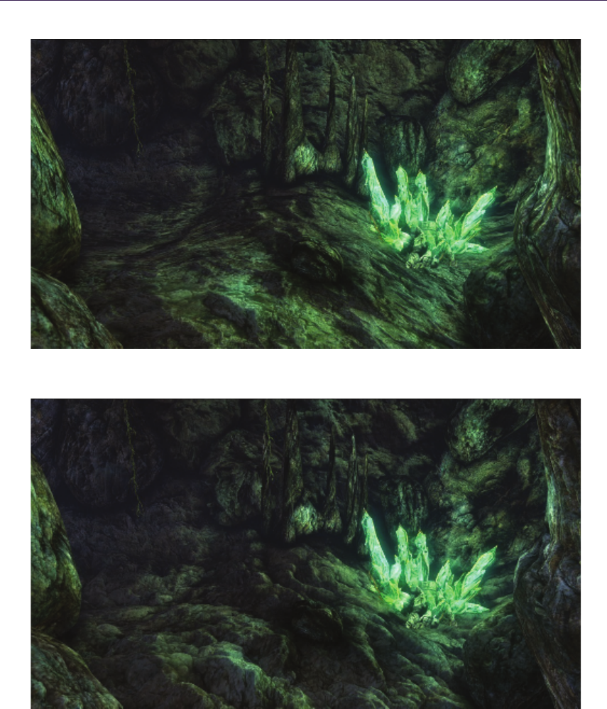
21. Quadtree Displacement Mapping with Height Blending
Figure 1.1. Normal mapped environment.
Figure 1.2. Fully featured surface rendering using the methods proposed in this article.

1.2. Introduction 3
quality for minification. Then we focus on surface blending methods, proposing
a new method that exhibits better resemblance to real life and allows aggressive
optimization during blended height-field displacement mapping. The proposed
methods—depending on combinations and implementation—guarantee fast, scal-
able, and accurate displacement mapping of blended surfaces, including visually
pleasing ambient occlusion and soft penumbra soft shadowing (compare Figures
1.1 and 1.2). Specific attention will be given to the various implementations and
the proper choice of rendering method and asset authoring pipeline.
1.2 Introduction
During the last change of console generation we have seen a dramatic improve-
ment in graphics rendering quality. With modern GPUs pushing millions of
triangles per second, we are looking for more fidelity in areas that are still being
impractical for performance reasons. One of those is surface rendering, which is
one of the most fundamental building blocks of believable virtual world.
Each surface at its geometric level has a number of complex properties such as
volume, depth, and various frequency details that together model further visual
clues like depth parallax, self-shadowing, self-occlusion, and light reactivity. The
topic of light interactions depending on surface microstructure is well researched
and so many widely used solutions are provided (such as Cook-Torrance’s lighting
model and its optimizations). However, correct geometry rendering is still prob-
lematic. The brute force approach of rendering every geometry detail as a triangle
mesh is still impractical because it would have to consist of millions of vertices,
thus requiring too much memory and computations. Moreover, surface blending
such as widely seen on terrain (i.e., sand mixing with rocks) only complicate the
situation in terms of blend quality and additional performance impact. Last but
not least, we would like to manipulate surface geometric properties at render time
(i.e., dynamic water erosion simulation, craters forming after meteor strike).
To sum up, we would like our surface rendering method to support:
•accurate depth at all angles (depth parallax effect);
•self-shadowing;
•ambient occlusion;
•fast blending;
•dynamic geometric properties;
•current-generation hardware (taking console performance into account);
•minimal memory footprint compared to common normal mapping.

41. Quadtree Displacement Mapping with Height Blending
Common normal mapping techniques (those which create the illusion of de-
tailed surface by performing light computation on precalculated normal data set)
fail to meet our demands, as they do not model visual geometry clues. However,
we still find it useful in light interaction calculations, thus complementing more
sophisticated rendering solutions.
The only rendering method class that is able to suit all our needs are height-
field-based ray-tracing algorithms. The idea behind those algorithms is to walk
along a ray that entered the surface volume, finding the correct intersection of
the ray with the surface. They operate on grayscale images representing height
values of surfaces, thus exchanging vertex for pixel transformations, which suits
our hardware better in terms of performance and memory usage. Moreover,
they mix well with existing normal mapping and are performing better as GPUs
become more general processing units. However, none of them are aimed at high
performance surface blending or ambient occlusion calculation.
During our research we were seeking for the best possible rendering method
meeting our demands, being robust, functional and fast as we were aiming for
Xbox360-class hardware. As our scenario involved fully-featured rendering of
outdoor terrain with many objects and indoor cave systems, we were forced to
take special care for an automatic LOD system. Several methods were compared
and evaluated, finally ending with the introduction of a new solution that proved
to be suiting all our needs. We describe our research and the motivation behind it,
going in detail with each building block of the Quadtree Displacement Mapping
with Height Blending technique.
1.3 Overview of Ray-Tracing Algorithms
Every height-field-based ray-tracing algorithm is working with additional dis-
placement data, commonly encoded in height map format (grayscale image scaled
to [0; 1] range). Calculations are done in tangent space to allow computations for
arbitrary surfaces. Correct surface depth is calculated by finding the intersection
between viewing ray and height field. That ensures correct parallax offset for
further color and lighting calculations.
Figure 1.3 illustrates the depth parallax effect and presents the general inter-
section calculation.
General height-field ray-tracing algorithms can be summarized as follows:
1. Calculate tangent-space normalized view vector V per-vertex, and interpo-
late for pixel shader.
2. Ray cast the view ray to compute intersection with the height field, ac-
quiring the texture coordinate offset required for arriving at the correct
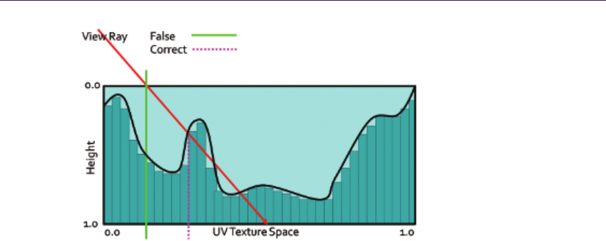
1.3. Overview of Ray-Tracing Algorithms 5
Figure 1.3. Height-field ray-trace scheme.
surface point. We start at texture input T1 coordinates, sampling along
the surface’s profile, finally computing new texture coordinates T2.
3. Compute the normal lighting equation using surface attributes sampled at
the new texture coordinates T2.
The following algorithms implement various methods for intersection computa-
tion, varying in speed, accuracy and use of additional precomputed data.
1.3.1 Online Algorithms
Relief mapping. Relief mapping [Policarpo 2005] performs intersection calculation
by linear search in two-dimensional height-field space followed by binary search.
We want to find the intersection point (p, r). We start by calculating point
(u, v), which is the two-dimensional texture coordinate of the surface point where
the viewing ray reaches a depth = 1.0. The point (u, v) is computed based on
initial texture coordinates (x, y) on the transformed view direction with scaling
factor applied. Then we search for (p, r) by sampling the height field between
(x, y) and (u, v). We check for intersections by comparing ray depth with the
stored depth at the current sampling point. When the latter is smaller, we
have found the intersection and we can refine it using binary search. Figure 1.4
illustrates the process.
Binary search is taking advantage of texture filtering and operates in mini-
mized space around the found intersection point. That ensures fast convergence
and high accuracy. However, using that kind of search utilizes dependant reads
on the GPU, thus vastly affecting performance. While a linear- and binary-search
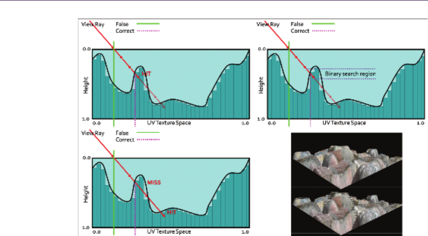
61. Quadtree Displacement Mapping with Height Blending
Figure 1.4. Relief Mapping. Top left: linear search. Top right: binary search around
point found in linear search. Bottom left: possible miss of linear search. Bottom right:
resulting aliasing artifacts as opposed to correct rendering.
combo is a known and proven solution, its linear part is prone to aliasing due to
under sampling. During the search, when there are not enough search steps (step
length is too big), we might miss important surface features as shown in Fig-
ure 1.4. Increasing search steps potentially minimizes the problem but severely
affects performance, making this algorithm highly unreliable when sampling large
height fields or surfaces exhibiting very large displacement scales. Nonetheless, it
is still very effective in simple scenarios that do not require high sampling count,
as the performance is saved on ALU instructions.
Parallax occlusion mapping. Several researchers tried to optimize this algorithm
by omitting the expensive binary search. Parallax occlusion mapping [Tatarchuk
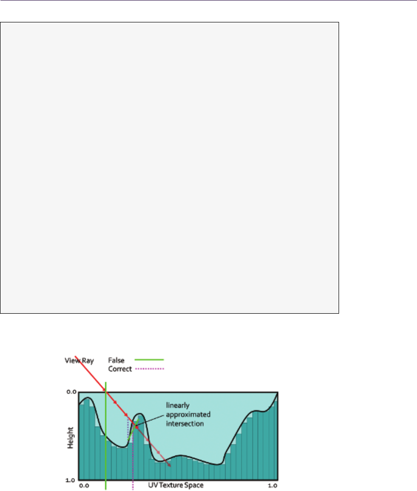
2006] relies on accurate high-precision intersection calculation (see Figure 1.5).
A normal linear search is performed finding point (p, r) and last step point (k, l).
Then the ray is tested against a line made of (p, r) and (k, l), effectively approx-
imating the height profile as a piecewise linear curve. Moreover, solutions for
additional LOD and soft shadows were proposed. POM, while being accurate
enough and faster than relief mapping, is still prone to aliasing and so exhibits
the same negative traits of linear search (Listing 1.1).
1.3. Overview of Ray-Tracing Algorithms 7
fl oat Size = 1.0 / L inearS e archSt e ps ;
flo at Depth = 1.0;
int S tepI ndex = 0;
flo at CurrD = 0.0;
flo at PrevD = 1.0;
float 2 p1 = 0.0;
float2 p2 = 0.0;
wh ile ( St epInd ex < Line ar Se archSt ep s )
{
Dep th -= Size ; // move the ray
floa t4 T Co or d = f lo at 2 ( p +( v * De pt h ) ) ; // new s ampl ing pos
Cu rrD = tex 2D ( texSMP , TCoord ).a; // new hei ght
if ( Cur rD > D epth ) // check for inte r sect i on
{
p1 = f lo at2 ( Depth , C urr D ) ;
p2 = f loat 2 ( Depth + Size , Pre vD ); // store last step
Ste pInd ex = Linea rS earch St eps ; // b reak the loop
}
Ste pInd ex ++;
Pr evD = Cur rD ;
}
// Lin ear appr o xima t ion using c urrent and last step
// ins tea d of binary search , oppos ed to relief mapp ing .
fl oat d2 = p 2 .x - p2 . y ;
fl oat d1 = p 1 .x - p1 . y ;
retur n ( p1 . x * d2 - p 2 .x * d1 ) / ( d 2 - d1 ) ;
Listing 1.1. POM code.
Figure 1.5. POM.
81. Quadtree Displacement Mapping with Height Blending
1.3.2 Algorithms Using Precomputed Data
In response to the arising problem of performance and accuracy, several solutions
were proposed that make use of additional data to ensure skipping of empty space
and prohibit missing surface features. However, additional memory footprint or
preprocessing computation time limits their usefulness.
Per-pixel displacement with distance function. Per-pixel displacement with distance
function [Donelly 2005] uses precalculated three-dimensional texture representa-
tion of the surface’s profile. Each texel represents a sphere whose radius is equal
to the nearest surface point. We are exchanging the well-known linear search for
sphere tracing. With each sample taken we know how far we can march our ray
without missing any possible intersection. Traversing that kind of structure al-
lows skipping large space areas and ensures that we will not miss the intersection
point. Moreover, the intersection search part is very efficient. However, memory
requirements and precomputation time for this method make it impractical for
real-time game environments. As stated in [Donelly 2005], even simple surfaces
may require a three-dimensional texture size of 256 ×256 ×16 with dimensions
rising fast for more complex and accurate rendering. That increase in memory
footprint is unacceptable for the limited memory of current consoles and PC
hardware, not to mention the prohibitive preprocessing time.
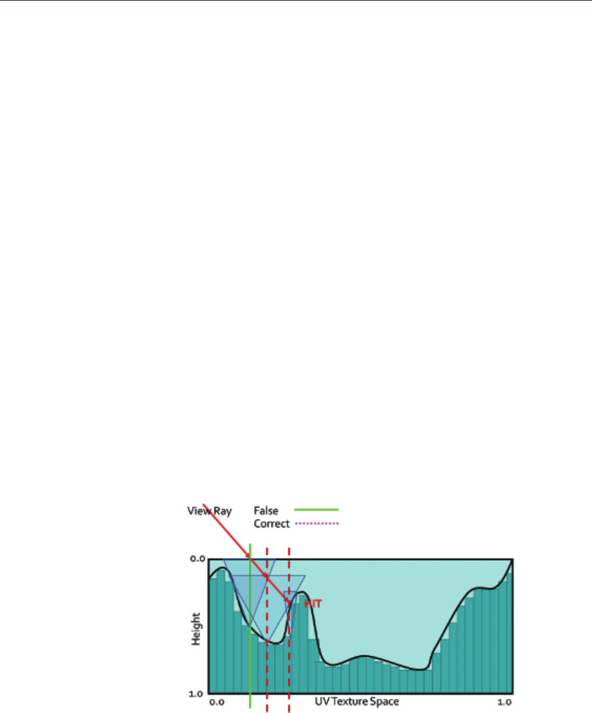
Cone step mapping (CSM). CSM [Dummer 2006] is based on a similar idea. It
uses a cone map that associates a circular cone with each texel of the height-
field texture. The cone angle is calculated so that the cone is the largest one
not intersecting the height field (see Figure 1.6). This information allows us
Figure 1.6. CSM. Ray traversal by cone radius distance.

1.4. Quadtree Displacement Mapping 9
to calculate a safe distance during sampling, as in per-pixel displacement with
distance function. Consequently, the ray may skip empty spaces and never miss
the correct intersection. Due to its conservative nature, the algorithm may require
too many steps to actually converge. For performance reasons, it is required to
set a maximum number of steps, which often results in stopping the ray trace too
early and returning incorrect texture coordinates for further rendering.
Cone step mapping performance varies widely depending on the spatial co-
herency of the height field. Generally, it outperforms linear search algorithms
while guaranteeing less noticeable errors. Its memory footprint is quite bearable
as it requires only one additional 8-bit texture for cone maps. However, its pre-
processing time makes it impossible to alter the height field at render time, as this
would require recompilation of the cone map with every change. The precompu-
tation algorithm is of complexity O(n2), where ndenotes number of height-field
texels, making it impractical on current GPUs. Moreover, properties of the cone
map prohibit correct and easy surface blending.
Relaxed cone step mapping (RCSM). RCSM [Policarpo 2007] takes CSM one step
further, making it less conservative. The idea is to use larger cones that intersect
the height field only once. The search is performed the same way as in CSM.
When the intersection is found, the correct point is searched, using binary search
in space restricted by the last cone radius, therefore converging very quickly. The
combination leads to more efficient space leaping, while remaining accurate, due
to final refinement. Furthermore, an LOD scheme is proposed which, while it
lacks accuracy, provides performance gains. In practice, RCSM is currently the
fastest ray-tracing algorithm available, making it very useful in scenarios where
neither long preprocessing times, disability of efficient blending, and dynamic
height-field alteration are irrelevant.
1.4 Quadtree Displacement Mapping
We introduce a GPU-optimized version of the classic [Cohen and Shaked 1993]
hierarchical ray-tracing algorithm for terrain rendering on CPU, using height-field
pyramid, with bounding information stored in mipmap chain. It was presented
on recent hardware by [OH 2006], yielding good accuracy and performance, but
at the same time was less adequate for game scenario use. We describe our
implementation, optimized for current GPUs, with an automatic LOD solution
and accurate filtering. Moreover, we expand it for optimized surface blending,
soft shadowing and ambient occlusion calculation.
QDM uses the mipmap structure for resembling a dense quadtree, storing
maximum heights above the base plane of the height field (it is worth noting
that our implementation is actually using depth maps as 0 value representing
10 1. Quadtree Displacement Mapping with Height Blending
maximum displacement, as we are storing depth measured under the reference
plane. In consequence, maximum heights are minimum depths, stored in our data
structure). We traverse it to skip empty space and not to miss any detail. During
traversal we are moving the ray from cell boundary to cell boundary, until level 0
is reached—hence valid intersection region. While moving through the hierarchy,
we compute the proper hierarchy level change. Finally, we use refinement search
in the region of intersection to find the accurate solution when needed.
Gf 8800 256251221024220482
Quad tree 0.15ms 0.25ms 1.15ms 2.09ms
CSM <2min <14min <8h /
Table 1.1. Data preprocessing time.
1.4.1 Quadtree Construction
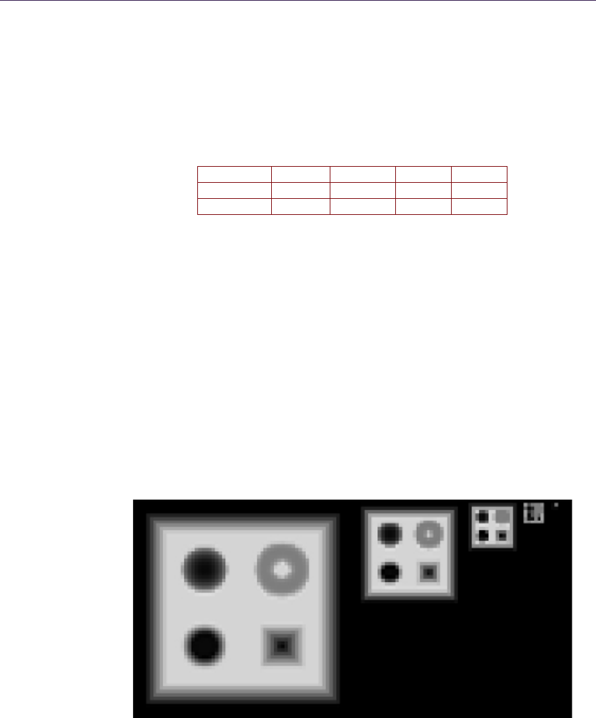
The quadtree is represented by a hierarchical collection of images in a mipmap.
The construction is simple, as it requires generating mipmaps with the min
operator instead of average as during normal mipmapping. As a result, MIP
level 0 (2n) represents the original height field with the following levels 1 (2n−1),
2 (2n−2), . . . containing the minimum value of the four nearest texels from levels
above. The entire process can be run on the GPU. Due to hardware optimization,
quadtree construction is very fast. The timings in Table 1.1 were obtained on a
PC equipped with Intel Core 2 Duo 2.4 GHz and GeForce 8800. For comparison,
timings for RCSM are given. The quadtree was computed on the GPU, while the
cone map was on the CPU due to algorithm requirements.
Figure 1.7. Generated QDM on mipmaps.

1.4. Quadtree Displacement Mapping 11
As we can see, quadtree computation time is negligible, even for on-the-fly
generation, whereas cone maps could even be problematic for off-line rendering
during texture authoring (see Figure 1.7).
1.4.2 Quadtree Traversal
The general steps of intersection search are shown by the pseudocode in List-
ing 1.2. We start the computation at the highest mipmap level. The stopping
condition of the main loop is to reach the lowest hierarchy level, which effec-
tively means finding the intersection region where the linear approximation can
be performed. At each step, we determine if we can move the ray further or if
there is a need for further refinement. We algebraically perform the intersection
test between the ray and the cell bounding planes and the minimum depth plane.
In case the ray does not intersect the minimum plane, then the current cell is
blocking our trace. We have to refine the search by descending in the hierarchy
by one level. In the other case, we have to find the first intersection of the ray
with the minimum plane or the cell boundary. When the right intersection is
computed, we move the ray to the newly acquired point. In case we have to
cross the cell boundary, then we choose the next cell via the nearest-neighbor
method, thus minimizing error. At this point, we perform hierarchy level update
for optimization (see the optimization section).
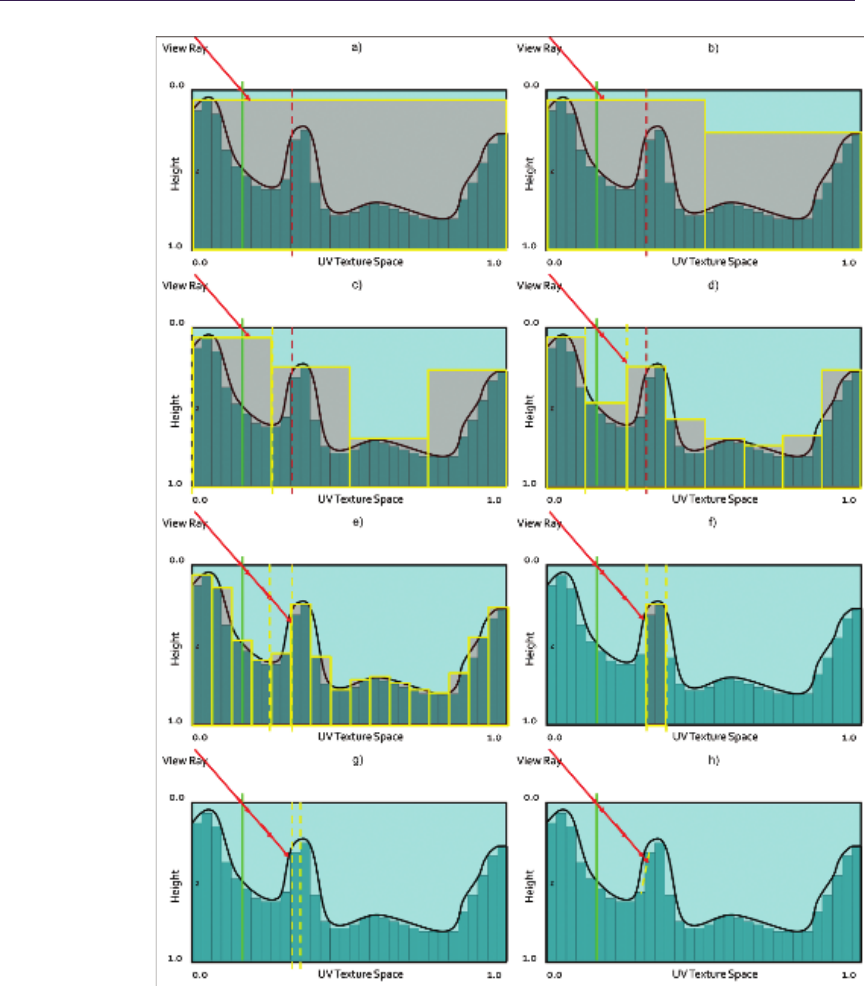
Figure 1.8 presents step-by-step ray traversal in QDM: Step (a) shows a ray
coming from the initial geometry plane and stopping at the maximum level or
minimum plane. Steps (b) and (c) illustrate further refinement while the search
descends to lower hierarchy levels. Step (d) presents where the ray must cross
the cell in order to progress. While the minimum plane of the current cell is not
blocking the way, we have to move the ray to the nearest cell boundary. Steps
(e) and (f) show further ray traversal while refining the search while (g) presents
the main loop’s stopping condition, as the ray has reached level 0. Therefore, we
can proceed to linear interpolation between the nearest texels in Step (h).
Wh ile ( hiera rc hy_le vel > 0)
de pth = get_ ma xi mu m_ de pt h ( po sitio n , h ie rarch y lev el )
If ( ra y _d ep th < de pt h )
move_ray_to_cell_boundry_or_minimum_depth_plane
else
descend_one_hierarchy_level
end
find_intersection_using_linear_interpolation
Listing 1.2. General QDM search steps.
12 1. Quadtree Displacement Mapping with Height Blending
Figure 1.8. QDM traversal.

1.4. Quadtree Displacement Mapping 13
It is important to correctly calculate sampling positions since we are working
with a discrete data structure. For correct results, we should use point-filtering on
the GPU and integer math. However, if we cannot afford an additional sampler for
the same texture using POINT and LINEAR, it is possible to use linear filtering
with enough care taken for correct calculations. As SM 3.0 only emulates integer
operations, we have to account for possible errors in calculations (using SM 4.0
is preferable, due to the presence of real integer math).
Listing 1.3 is heavily commented to explain the algorithm’s steps in detail.
co nst int MaxL evel = M axMip Lvl ;
co nst int Node Count = pow (2.0 , M axLe vel );
co nst flo at Hal fTex el = 1.0 / Node Coun t / 2.0;
fl oat d ;
float 3 p2 = p ;
int Level = Max Level ;
// We c alcul at e ray m ov emen t v ecto r in inter - cel l num bers .
in t2 D ir Si gn = sig n (v. xy );
// Main loop
wh ile ( Lev el >= 0)
{
// We get current cell min imum pla ne using tex 2Dlo d .
d = t ex 2D lo d ( He ig ht Te xt ur e , f lo at 4 ( p2 . xy , 0 .0 , L ev el )) . w;
// If we are not blocked by the cel l we move the ray .
if ( d > p2 . z )
{
// We calc ulate pred ic tive new ray posi tion .
float 3 tmpP2 = p + v * d ;
// We com pute cur rent and p redic tive pos ition .
// Calcu latio ns are perf orme d in cell inte ger n umbe rs .
int No deC ou nt = pow (2 , ( M ax Le ve l - Le ve l ));
in t4 N od eI D = in t4 (( p2 . xy , t mp P2 . xy ) * N od eC ou n t );
// We test if both posi tions are still in the same cell .
// If not , we hav e to move the ray to nea rest cell
// b ound ary .
if ( Nod eID .x != NodeID . z || N odeID .y != NodeID . w)
{
// We co mpute the dist ance to curre nt cell bou ndar y .
// We per form the c alcula ti ons in cont in uous s pace .
flo at 2 a = ( p 2 . xy - p . xy ) ;
flo at 2 p3 = ( N od eI D . xy + D ir Si gn ) / N od eC o un t ;
flo at 2 b = ( p 3 . xy - p . xy ) ;

14 1. Quadtree Displacement Mapping with Height Blending
// We are cho osing the nea rest cel l
// by cho os ing sma ller dis tance .
floa t2 dN C = ab s ( p2 . z * b / a ) ;
d= m in (d , mi n ( dNC .x , dNC . y ));
// Dur ing cell cro ssin g we ascend in hie rarc hy .
Lev el +=2;
// Pre dict i ve refi n emen t
tm pP2 = p + v * d ;
}
// Fi nal ray m ovem ent
p2 = t mpP 2 ;
}
// Defaul t descent in hier arch y
// null ifie d by ascend in case of cell cros sing
Level - -;
}
retur n p2 ;
Listing 1.3. QDM search steps.
1.4.3 Optimizations
Convergence speed-up. It is worth noting that during traversal, the ray can only
descend in the hierarchy. Therefore, we are not taking full advantage of the
quadtree. The worst-case scenario occurs when the ray descends to lower levels
and passes by an obstacle really close, consequently degenerating further traver-
sal to the linear search. To avoid that problem, we should optimally compute
the correct level higher in the hierarchy during cell crossing. However, current
hardware is not optimized for such dynamic flow. A simple one step up move
in the hierarchy should be enough. For more complicated surfaces which require
many iterations, we discovered that this optimization increases performance by
30% (tested on a case requiring >64 iterations).
Fixed search step count. While the algorithm tends to converge really quickly, it
may considerably slow down at grazing angles on complex high-resolution height
fields. Therefore, an upper bound on iterations speeds up rendering without very
noticeable artifacts. The number of iterations should be exposed to technical
artists to find optimal values.
Linear filtering step. Depending on surface magnification and the need for accurate
results, final refinement may be used. One can utilize the well-know binary
search which would converge quickly (five sampling points is enough for most

1.4. Quadtree Displacement Mapping 15
purposes) due to the tight search range. However, we propose linear interpolation
for piecewise surface approximation, similar to the one proposed in POM. This
approach proves to be accurate on par with binary search (considering limited
search range), while being optimal for current hardware.
After finding the correct cell of intersection (at hierarchy level 0), we sam-
ple the height field in direction of the ray cast, one texel before and one texel
after the cell. Then we find the intersection point between the ray and linearly
approximated curve created by sampled points.
LOD scheme. Here we propose a mixed automatic level of detail scheme. First,
we dynamically compute the number of iterations based on the simple observation
that parallax is larger at grazing angles, thus requiring more samples, so we can
express the correct value as a function of the angle between the view vector
and the geometric normal. Notice that the minimum sampling number should
not be less than the total number of hierarchy levels, otherwise the algorithm
will not be able to finish traversal even without any cell crossing. Moreover, we
observed that with diminishing pixel size on screen, parallax depth details become
less visible. Thus, we can stop our quadtree traversal at a fixed hierarchy level
without significant loss of detail. We determine the right level by computing the
mipmap level per pixel scaled by an artist-directed factor. For correct blending
between levels, we linearly interpolate between depth values from the nearest
hierarchy level by the fractional part of the calculated mipmap level. After an
artist-specified distance we blend parallax mapping to normal mapping.
This combined solution guarantees high accuracy via a dynamic sampling rate,
and it guarantees high performance due to quadtree pruning, thus giving a stable
solution overall. For performance and quality comparisons, see the results section.
Storage. For precision reasons, it is required that the stored quadtree is accurate.
A problem arises when we want to store it with textures. Generally, textures com-
pressed with DXT compression result in a significant speedup and memory foot-
print reduction. DXT is a lossy compression scheme; thus it is not recommended
for accurate data storage (as opposed to, e.g., diffuse textures). However, we
noticed that in the general case, storing the quadtree in the alpha channel of a
DXT5-compressed texture results in minor artifacts (it highly depends on the sur-
face’s profile, so it must be done with care). Still, the preferable solution is to take
the memory hit and store the additional data in 1-channel 8-bit lossless textures.
Comparison. Performance tests were conducted on a test machine equipped with
Intel quad core 2.8Ghz CPU and GeForce 260 GTX in full HD, using three various
levels from early beta of TW2. The results can be seen in Tables 1.2,1.3, and 1.4.
Scenarios contained fully featured levels, using various height fields of reso-
lution 5122to 10242. Each scene pushed around one million triangles, with the
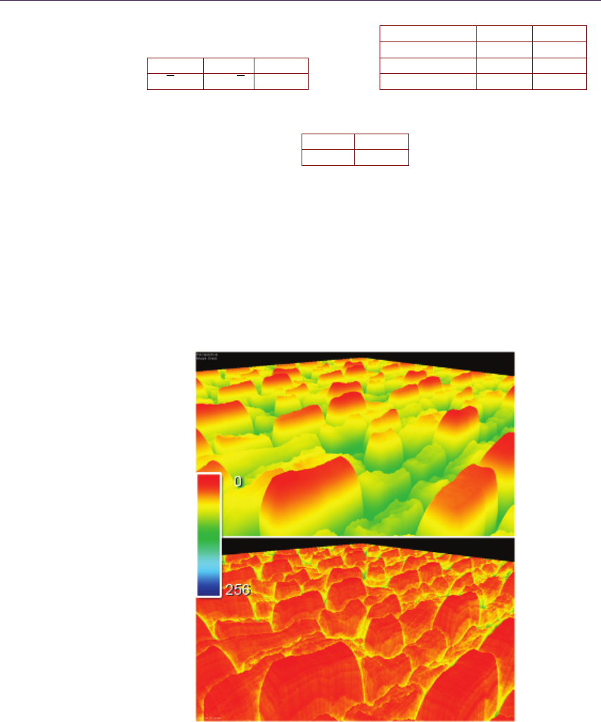
16 1. Quadtree Displacement Mapping with Height Blending
Relief CSM QDM
√n≤√nlog n
Table 1.2. Analytical performance.
Depth Scale POM QDM
1.0 5ms 5.7ms
1.5 6.65ms 6.7ms
5.0 18.9ms 9ms
Table 1.3. General scenario performance.
POM QDM
73ms 14ms
Table 1.4. Extreme high detail performance.
parallax displacement method of choice, covering the entire screen. Depth scale
dependence was measured, and iteration count was set for close quality match
between methods. Table 1.4 shows the timing for ultra-high resolution and com-
plexity case of the height field. Figures 1.9 and 1.10 show results for various
implementations of ray- and height-field-intersection algorithms.
Figure 1.9. Convergence comparison.
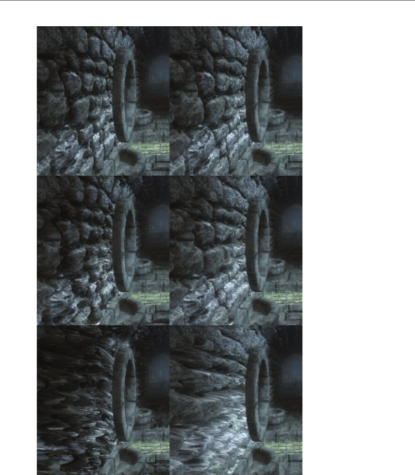
1.4. Quadtree Displacement Mapping 17
Figure 1.10. Quality comparison. Left POM. Right QDM. Depth Scale: 1.0, 1.5, 5.0.
From depth scale 1.5 and above artifacts are visible while using POM.
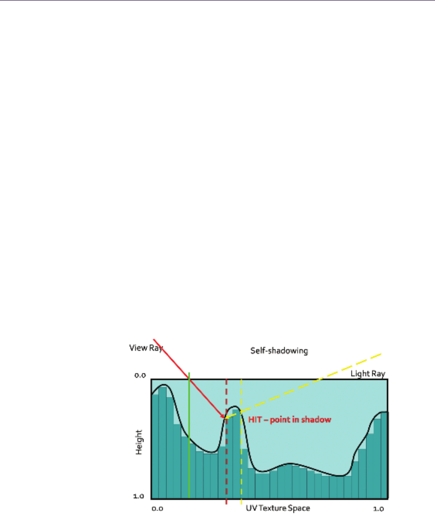
18 1. Quadtree Displacement Mapping with Height Blending
As we can see, QDM is converging in a pace similar to RCSM, but results in
worse performance due to higher ALU cost and less efficient texture cache usage
(as many dependant samples, from various MIP levels tend to cause cache misses).
However, it is still comparably fast compared to linear search algorithms, outper-
forming them when the height-field’s complexity, depth, or resolution increases.
After further research we discovered that QDM is a faster solution onwards from
512×512 high-complexity textures or for any 1024×1024 and larger sizes. More-
over, an additional advantage is visible with depth scale increase. We do not
take into consideration RCSM for resolutions higher than 1024 ×1024 as the
preprocessing time becomes impractical.
1.5 Self-Shadowing
1.5.1 General Self-Shadowing
The general algorithm for self-shadowing [Policarpo 2005] involves ray tracing
along the vector from L (light source) to P (calculated parallax offset position),
then finding its intersection PL with the height field. Then we simply compare
PL with P to determine whether the light is visible from P or not. If not, then
that means we are in shadow. See Figure 1.11 for illustration.
This method generates hard shadows using any intersection search method,
thus suffering from the same disadvantages as the chosen algorithm (i.e., aliasing
with linear search). Moreover, the cost is the same as view and height-field
Figure 1.11. Shadow test.
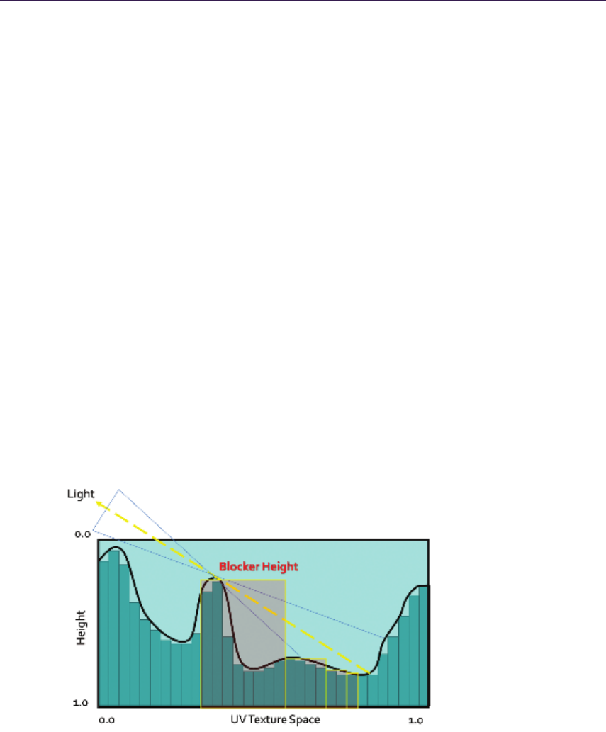
1.5. Self-Shadowing 19
intersection computations. When we are looking for soft shadows, we would
have to perform several ray casts of the light vector, which is impractical for
performance reasons.
A good approximation for soft shadow calculation was proposed in POM.
We can cast a ray towards the light source from point P and perform horizon
visibility queries of the height profile along the light direction. We sample the
height profile at a fixed number of steps to determine the occlusion coefficient
by subtracting sampled depth from original point P depth. This allows us to
determine the penumbra coefficient by calculating blocker-to-receiver ratio (the
closer the blocker is to the surface, the smaller the resulting penumbra). We
scale each sample’s contribution by the distance from P and use the maximum
value, then we use the visibility coefficient in the lighting equation for smooth
shadow generation. The algorithm makes use of linear sampling and produces
well-behaving soft shadows. However, the alias-free shadow range is limited by
the fixed sampling rate, so real shadows cannot be generated without searching
through the entire height field, which effectively degenerates the algorithm to a
linear search.
1.5.2 Quadtree Soft Shadowing
Fast horizon approximation. We propose a new algorithm based on POM soft
shadowing. This algorithm makes use of the quadtree used in QDM.
First we introduce the algorithm for fast horizon visibility approximation. We
use a method similar to POM by performing horizon visibility queries along a
Figure 1.12. QDM horizon approximation.

20 1. Quadtree Displacement Mapping with Height Blending
given direction. The maximum height is taken from the calculated samples and
is subtracted from the initial starting point P, thus giving the horizon visibility
coefficient. See Figure 1.12 for illustration.
We use the observation that small scale details at distance have negligible
impact on the result (especially during any lighting calculations). Thus we can
approximate further lying profile features by using the maximum height data
from higher levels of the quadtree. That way we can calculate the approximated
horizon angle with a minimized number of queries. The full profile can be ob-
tained in log nsteps as opposed to nsteps in POM, where nis the number of
height-field texels along a given direction D. In all further solutions, we are using
a slightly modified version of this algorithm, which is weighting each sample by
a distance function. That makes it more suitable for penumbra light calculation
as samples far away from P are less important.
QDM shadowing. For shadowing, we use a fast horizon visibility approximation
using the parallax offset point P and the normalized light vector L. Accuracy
and performance is fine-tuned by technical artists setting the plausible number
of iterations (log nis the maximum number, where nis the height-field’s largest
dimension) and light vector scale coefficient as shown in Listing 1.4.
// Light di rec ti on
f loa t2 l Dir = ( f loa t2 ( l .x , - l .y )) * d Sca le ;
// In it ial displaced point
float h0 = t ex 2Dl od ( h ei ght Tex tur e , fl oat 4 (P , 0 ,0 )). w ;
float h = h0 ;
// Hor izon visib il it y sa mples
// w 1 .. w5 - - - di st an ce w e igh ts
h = m in (1 , w 1 * t ex 2D lo d ( h eigh t , f lo at 4 ( P + 1.0 * lDir ,0 , 3.6 6)) . w );
h = m in (h , w 2 * t ex 2D lo d ( h eigh t , f lo at 4 ( P + 0.8 * lDir ,0 , 3.0 0)) . w );
h = m in (h , w 3 * t ex 2D lo d ( h eigh t , f lo at 4 ( P + 0.6 * lDir , 0 , 2. 33) ). w );
h = m in (h , w 4 * t ex 2D lo d ( h eigh t , f lo at 4 ( P + 0.4 * lDir ,0 , 1.6 6)) . w );
h = m in (h , w 5 * t ex 2D lo d ( h eigh t , f lo at 4 ( P + 0.2 * lDir ,0 , 1.0 0)) . w );
// Vi si bility a pp ro ximat io n
float s had ow = 1.0 - s atu ra te (( h0 - h) * se lf Sh ad owS tr en gt h );
return shadow;
Listing 1.4. QDM soft shadows, fast, hard-coded solution.
Results. As we can see in Table 1.5, plausible soft shadows using the quadtree are
significantly faster than traditional methods while delivering similar quality (see
Figure 1.13). For further optimization we calculate shadows only when N·L≥0.
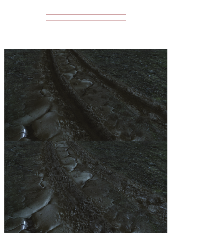
1.5. Self-Shadowing 21
POM Shadows QDM Shadows
1.6ms 0.5ms
Table 1.5. One light shadows calculation time for the test scene.
Figure 1.13. Soft shadows ON/OFF.

22 1. Quadtree Displacement Mapping with Height Blending
Figure 1.14. Generated high quality AO.
1.6 Ambient Occlusion
Ambient occlusion is computed by integrating the visibility function over the
hemisphere H with respect to a projected solid angle:
A0=1
π∑
H
Vp,ω(N·ω)dω,
where Vp,ω is the visibility function at p, such as Vp,ω is 0 when occluded in
direction ωand 1 otherwise.
Ambient occlusion adds a great deal of lighting detail to rendered images (see
Figure 1.14). It is especially useful for large-scale terrain scenarios, where objects
can take the occlusion value from the terrain (i.e., darkening buildings lying in a
valley).
1.6.1 QDM Ambient Occlusion
Dynamically calculating ambient occlusion for surfaces was thought to be im-
practical for performance reasons, as the visibility function and the integration
were too slow to be useful. Now with fast horizon visibility approximation we
can tackle that problem in a better way.
We approximate the true integral by integrating the visibility function in
several fixed directions. We discovered that for performance reasons integration in
four to eight directions lying in the same angle intervals yields acceptable results.
Moreover, we can increase quality by jittering and/or rotating the directions by
a random value for every pixel.

1.7. Surface Blending 23
Accuracy AO
4 directions 2.1ms
8 directions 6.3ms
4 jittered 2.6ms
Table 1.6. AO calculation time.
1.6.2 Performance
As we can see from Table 1.6, the algorithm requires substantial processing power,
being even less efficient with randomized directions (as it is hurting GPU paral-
lelism, but it is still faster than integrating more directions). However, it is used
only when the surface height field is changing. Moreover, it can be accumulated
throughout several frames, amortizing the cost.
1.7 Surface Blending
1.7.1 Alpha Blending
Blending is commonly used for surface composites, such as terrain, where several
varied textures have to mix together (e.g., rocky coast with sand).
Typically, surface blends are done using the alpha-blending algorithm given
by the following equation:
Blend = (v1, . . . , vn)·(w1, . . . , wn)
(1, . . . , 1) ·(w1, . . . , wn),
where (w1, . . . , wn) is the blend weight vector and (v1, . . . , vn) denotes the value
vector.
Commonly, the blend vector for a given texel is supplied by vertex interpola-
tion, stored at vertex attributes (thus being low frequency). During pixel shading,
interpolated values are used to perform the blending.
1.7.2 Raytracing Blended Surfaces
Any height-field intersection algorithm can be used in such a scenario. We should
compute the parallax offset for each surface and finally blend them together using
the blend vector. However, it is worth noting that the computational cost for such
blending would be n-times higher than one surface, where nis the total number
of surfaces. Moreover, using vertex-interpolated values results in view-dependant
surfaces floating near blend zones. Figure 1.15 illustrates the problem. However,
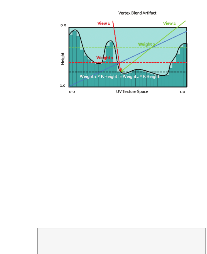
24 1. Quadtree Displacement Mapping with Height Blending
Figure 1.15. Depth floating artifact using vertex blend.
with enough care taken to minimize depth scale near blend zones, it should not
be too distracting.
One possible solution is to use per-pixel blend weights that would modify the
surface on-the-fly during intersection search. However, this would require sam-
pling an additional weight texture with every iteration, thus doubling the sample
count.
Let us consider four surface blends. Optimally, we can encode up to four blend
weights in one RGBA 32-bit texture, so with each sample we get four weights.
The blend texture can be fairly low-resolution, as generally it should resemble
per-vertex blending (it can be even generated on the fly from vertex weights).
Having a four-scalar blend vector, we can perform the intersection search on the
dynamically modified height field simply by sampling all four height fields with
each step and blending them by the blend vector. Moreover, we can compose all
four height fields into one RGBA 32-bit texture, thus finally optimizing the blend
intersection search.
The pseudocode in Listing 1.5 shows the modification for the intersection
search method of choice.
d = te x2 D ( H ei gh tT ex tu re ,p. x y ). xy zw ;
b = te x2 D ( B le nd Te xt ur e , p . xy ). xy zw ;
d = dot (d , b ) ;
Listing 1.5. Height profile blend code.

1.7. Surface Blending 25
Modification requires only one additional sample and one dot product. How-
ever, we are sampling four channels twice instead of one channel (as in the single
surface algorithm).
This solution is therefore very fast but lacks robustness, as it would require
us to preprocess height-field composites, creating possibly dozens of new textures
containing all possible height profiles composites. We can of course try sampling
the data without composites, but that would result in additional sampling cost
and cache misses (as four samplers would have to be used simultaneously, which
would most probably result in a bandwidth bottleneck).
Another problem is that we cannot use this method for algorithms using
precomputed distance data, as it would require us to recompute the distance
fields (i.e., cone maps) for blend modified height fields, which effectively prohibits
using advanced ray-casting algorithms.
1.7.3 Height Blending
To overcome the aforementioned problems, we introduce a new method for surface
blending, which seems to fit the task more naturally, and it guarantees faster
convergence.
First, let us consider typical alpha blending for surface mixing. In real life,
surfaces do not blend. What we see is actually the highest material (the material
on the top of the surface).
Therefore, we propose to use height information as an additional blend co-
efficient, thus adding more variety to blend regions and a more natural look as
shown in Listing 1.6.
This method is not computationally expensive, and it can add much more
detail as opposed to vertex-blended surfaces (as can be seen in Figure 1.16).
The most important feature is that we pick the highest surface, so during the
intersection search phase, we need only to find the highest point.
Therefore, the new height field is produced by the new blend equation:
Blend = max(h1, . . . , hn).
Using this blend equation we are interested only in finding the intersection
point with the highest surface profile modified by its blend weight. That effec-
tively means taking a minimal number of steps, as we will stop the ray cast at
Relief Mapping POM POM with HB
3ms 2.5ms 1.25ms
Table 1.7. Surface blend performance comparison.
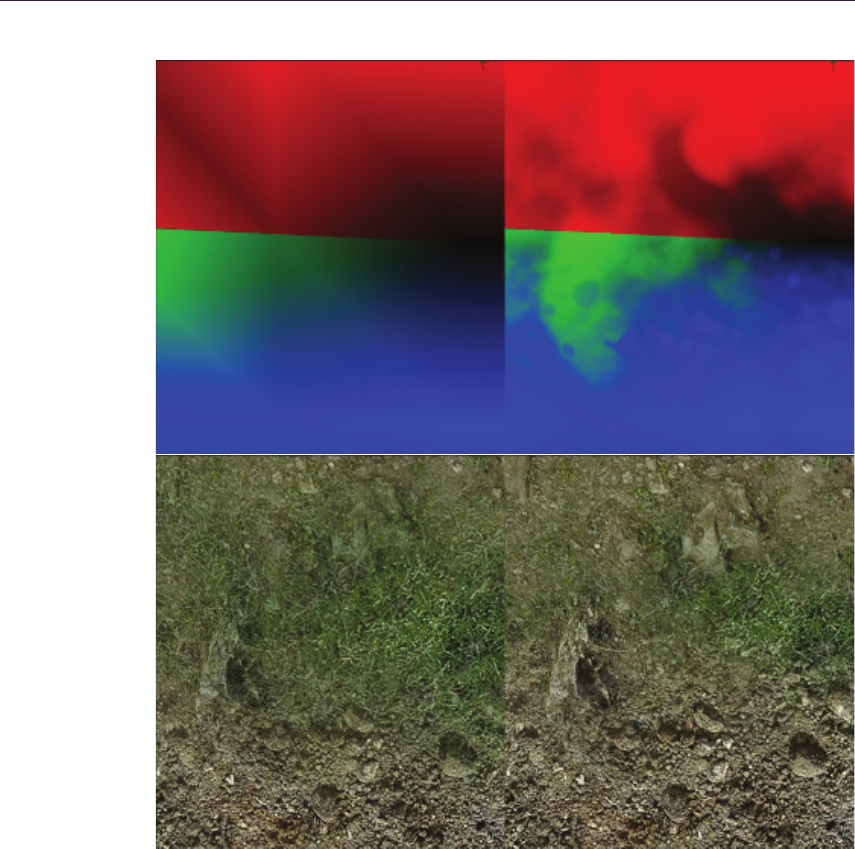
26 1. Quadtree Displacement Mapping with Height Blending
Figure 1.16. Vertex blend and height blend comparison.

1.7. Surface Blending 27
float4 FinalH;
float 4 f1 , f2 , f3 , f4;
// Get surfac e sam ple .
f1 = t ex 2D ( T ex0S am pl er , TE XU V . xy ) . r gba ;
//Get height weight.
Final H .a = 1.0 - f1 .a ;
f2 = t ex 2D ( T ex1S am pl er , TE XU V . xy ) . r gba ;
Final H .b = 1.0 - f2 .a ;
f3 = t ex 2D ( T ex2S am pl er , TE XU V . xy ) . r gba ;
Final H .g = 1.0 - f3 .a ;
f4 = t ex 2D ( T ex3S am pl er , TE XU V . xy ) . r gba ;
Final H .r = 1.0 - f4 .a ;
// M odify h eight wei ght s by blend weig hts .
// Per - v er te x b le nd w ei gh ts s to re d in IN . Alp haB len ds
Fin al H *= I N . A lp ha Ble n ds ;
// N ormal ize .
fl oat B lend = dot ( Fin alH , 1.0) + e ps il on ;
Final H /= Ble nd ;
// Get fi nal ble nd .
Fin alT ex = F inalH . a * f1 + Fin alH .b * f2 + FinalH .g * f3 +
Fin al H . r * f4 ;
Listing 1.6. Surface blend code.
the first intersection with highest blend weight modified height profile, which—by
definition—is the first one to be pierced by the ray.
With each intersection search step, we reconstruct the height-field profile using
the new blend operator as shown in Listing 1.7.
As can be seen in Table 1.7, this method proved to minimize the convergence
rate by 25% on average in our scenario without sacrificing visual quality (see
Figure 1.17, and is more plausible for our new height blend solution. It can be
used with blend textures or vertex blending, as well as every intersection search
algorithm.
d = te x2 D ( H ei gh tT ex tu re ,p. x y ). xy zw ;
b = te x2 D ( B le nd Te xt ur e , p . xy ). xy zw ;
d *= b ;
d = max ( d .x , max (d.y , ma x (d .z , d.w)) ) ;}
Listing 1.7. Surface height blend code.
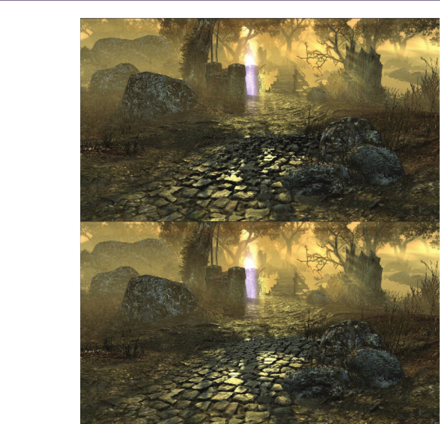
28 1. Quadtree Displacement Mapping with Height Blending
Figure 1.17. Surface blend quality comparison. Top: relief. Bottom: POM with height
blending.
1.7.4 QDM with Height Blending
We still cannot use the height blend operator directly for algorithms based on
precomputed data. However, QDM is based on depth data, so it is relatively easy

1.7. Surface Blending 29
to obtain new correct data structure. Note that
max(x1, x2, . . . , xn)·max(w1, w2, . . . , wn)≥
max([(x1, x2, . . . , xn)·(w1, w2, . . . , wn)]).
Thus multiplying one min/max quadtree by another gives us a conservative quad-
tree, and that is exactly what we need for correct surface blending. We can
pack up to four blend quadtrees in one RGBA 32-bit texture with mipmaps
containing blend vector quadtrees. Then in QDM, to reconstruct the blended
surface quadtree, we simply sample and blend it at the correct position and level,
and compute the dot product between it and the height-field vector sampled from
the height-field composite.
The blend texture should map quadtree texels as close as possible. However,
we discovered that while using hardware linear sampling and accepting small
artifacts we can use sizes as small as 322(while blending 10242height fields)
when the weight gradients are close to linear. Such blended quadtrees can be
constructed on the fly in negligible time, allowing dynamic surface alterations.
Effectively, we can use QDM with all its benefits while blending surfaces
for artifact-free rendering (see Figure 1.18). Convergence will be slower, due
to the conservative quadtree, and more iterations may be needed depending on
the height-field’s complexity. In practice, the conservative approach needs <10%
more iterations than what should be really used. This method proves to be the
fastest method for dynamic accurate surface rendering of high complexity height
fields.
In our implementation we decided to use vertex blending to avoid high texture
cache misses. However, we were forced to accept small depth-floating artifacts.
As QDM is converging really fast in empty space regions, the algorithm can
make the best use of faster convergence, due to height blending.
1.7.5 Self-Shadowing and Ambient Occlusion for Blended Surfaces
Self shadowing and ambient occlusion can be done while rendering blended sur-
faces. However, a na¨ıve approach of calculating shadowing terms for each surface
and blending the results is simply impractical for current generation hardware.
We propose to use QDM and the height blend and perform computations for the
highest modified height profile only. Proper height-field selection requires ad-
ditional dynamic branching, further restricting GPU parallelism. Consequently,
self shadowing and/or ambient occlusion are viable only for high-end hardware.
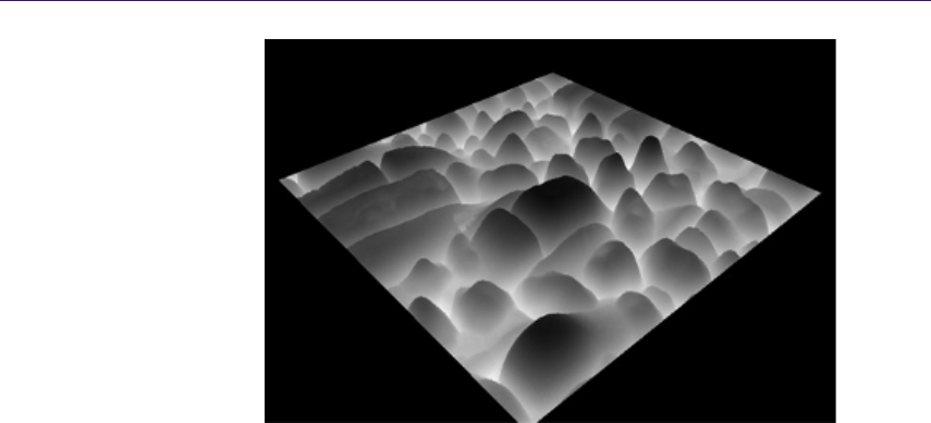
30 1. Quadtree Displacement Mapping with Height Blending
Figure 1.18. QDM height blend surface.
1.8 General Advice
In this article we proposed and discussed several battle-proven surface rendering
methods, varying in ALU/Texture sampling performance, accuracy, and flexi-
bility. Most solutions were introduced as general building blocks from which,
depending on requirements, an optimal solution can be built.
1.8.1 Case Study
During Two Worlds 2 production we decided to settle on several solutions used
under specific circumstances. We present a case study of each method used:
General terrain blend. Our terrain exhibits small-scale height features such as
cracks, small rocks, etc. The maximum number of blending surfaces was capped
at four to allow texture packing. We are using linear search with linear piece-
wise approximation, automatic LOD, and height blend optimization. Blending is
done on a per-vertex basis. Depending on texture configuration, parallax can be
switched off for each surface individually. The specular term and normal vectors
are generated on-the-fly due to the Xbox360’s memory restrictions.
Special terrain features. Several extreme detail terrain paths were excluded as
additional decal planes. We are rendering them at ultra-high quality (high res-
olution, high accuracy) and alpha-blending them with existing terrain. Decal
planes may present roads, paths, muddy ponds, and craters, etc. For rendering,

1.9. Conclusion 31
we are using QDM with automatic LOD and soft shadows. Where needed, QDM
per-pixel height blending is used. Blend-based decals are for PC only.
General object surface. For general surface rendering, we are using linear search
with linear piecewise approximation and automatic LOD. Soft shadows are used
at the artist’s preference. Surfaces with extreme complexity, depth scale, or
resolutions over 10242are checked, and using QDM is optimal. The same method
is used on Xbox360 and PC.
1.8.2 Surface Rendering Pipeline
During asset finalization, technical artists optimized height-field-based textures,
checking whether high resolution or additional details (such as soft shadows)
are really needed. It is worth noting that low frequency textures tend to con-
verge faster during the intersection search, so blurring height fields when possible
is better for performance and accuracy reasons when using linear search-based
methods.
One important feature of our surface rendering pipeline is the preference for
generation of additional surface properties on-the-fly, as it allows us to save mem-
ory and performance on texture-fetch-hungry shaders.
Texture-heavy locations (such as cities) are using mostly two 24-bit RGB com-
pressed textures per object. The specular term is generated from the diffuse color
and is modified by an artist on a per-material-specified function such as inversion,
power, or scale. The generated coefficient generally exhibits high quality.
Data generation is taken to the extreme during terrain rendering as individual
terrain texture is using only 32-bit RGBA DXT5 textures, from which per-pixel
normal vectors, specular roughness, and intensities (as the default lighting model
is a simplified Cook-Torrance BRDF) are generated.
1.9 Conclusion
We have discussed and presented various surface rendering techniques with sev-
eral novel improvements for industry proven approaches. Combinations of paral-
lax mapping, soft shadowing, ambient occlusion, and surface blending methods
were proposed to be in specific scenarios aiming for maximum quality/perfor-
mance/memory usage ratio. Furthermore, a novel solution—Quadtree Displace-
ment Mapping with Height Blending—was presented. Our approach proves to be
significantly faster for ultra-high quality surfaces that use complex, high resolu-
tion height fields. Moreover, we proposed solutions for efficient surface blending,
soft shadowing, ambient occlusion, and automatic LOD schemes using the intro-
duced quadtree structures. In practice, our techniques tend to produce higher

32 1. Quadtree Displacement Mapping with Height Blending
quality results with less iterations and texture samples. This is an advantage,
as we are trading iteration ALU cost for texture fetches, making it more useful
for GPU generations to come, as computation performance scales faster than
bandwidth.
Surface rendering techniques research allowed us to make vast graphic im-
provements in our next-gen engine, thus increasing quality and performance. We
hope to see the techniques described herein being used in more upcoming titles.
Bibliography
[Cohen and Shaked 1993] D. Cohen and A. Shaked. “Photo-Realistic Imaging of
Digital Terrains.” Computer Graphics Forum 12:3 (1993), 363–373.
[Donelly 2005] W. Donelly. “Per-Pixel Displacement Mapping with Distance
Functions.” In GPU Gems 2, edited by Matt Pharr, pp. 123–36. Reading,
MA: Addison-Wesley, 2005.
[Dummer 2006] J. Dummer. “Cone Step Mapping: An Iterative Ray-Heightfield
Intersection Algorithm.” 2006. Available at http://www.lonesock.net/files/
ConeStepMapping.pdf.
[OH 2006] K. Oh, H. Ki, and C. H. Lee. “Pyramidal Displacement Mapping: a
GPU based Artifacts-Free Ray Tracing through Image Pyramid.” In VRST
’06: Proceedings of the ACM symposium on Virtual Reality Software and
Technology (2006), 75–82.
[Policarpo 2005] F. Policarpo, M. M. Oliveira, and J. L. D. Comba. “Real Time
Relief Mapping on Arbitrary Polygonal Surfaces.” In Proceedings of I3D’05
(2005), 155–162.
[Policarpo 2007] F. Policarpo and M. M. Oliveira. “Relaxed Cone Step Mapping
for Relief Mapping.” In GPU Gems 3, edited by Hubert Nguyen, pp. 409–428.
Reading, MA: Addison-Wesley Professional, 2007.
[Tatarchuk 2006] N. Tatarchuk. “Practical Parallax Occlusion Mapping with Ap-
proximate Soft Shadow.” In ShaderX5. Brookline, MA: Charles River Media,
2006.

2
NPR Effects Using the
Geometry Shader
Pedro Hermosilla and Pere-Pau V´
azquez
2.1 Introduction
Non-photorrealistic rendering (NPR) techniques [Achorn et al. 03, Gooch and
Gooch 01] have been here for quite a while [Saito and Takahashi 90]. In contrast
to traditional rendering, these techniques deal with geometric entities such as
silhouettes, which makes them not easily amenable to GPU algorithms, although
some papers already address some NPR algorithms in hardware [Dietrich 00,
Mitchell et al. 02,Everitt 02,Card and Mitchell 02]. With the arrival of more
modern graphics hardware that includes the geometry shader stage, some of these
techniques can be implemented in hardware, making them real time in many cases
[McGuire and Hughes 04,Dyken et al. 08,Doss 08]. In this chapter we present a
set of techniques that can be implemented using the GPU by taking advantage of
the geometry shader pipeline stage. Concretely, we show how to make use of the
geometry shader in order to render objects and their silhouettes in a single pass,
and to imitate pencil drawing.
2.2 Previous Work
Silhouette rendering has been studied extensively. Two major groups of algo-
rithms require the extraction of silhouettes in real time: shadow volume-based
approaches and non-photorealistic rendering [Gooch and Gooch 01].
From the literature, we may extract two different approaches: object-space
and image-space algorithms. However, most modern algorithms work in either
image space or hybrid space. For the purposes of this chapter, we are inter-
ested in GPU-based algorithms, and these are the ones we will present. We
33

34 2. NPR Effects Using the Geometry Shader
refer the interested reader to the works of [Isenberg et al. 03] and [Hartner
et al. 03] for overviews and deep comparisons on CPU-based silhouette extraction
algorithms.
GPU-assisted algorithms may compute the silhouette either using multiple
rendering passes [Mitchell et al. 02] or in a single pass. Single pass methods
usually use some sort of precomputation in order to store adjacency information
into the vertices [Card and Mitchell 02], or make use of the geometry shader
feature [Doss 08], as this may query adjacency information. These algorithms
generate the silhouette in a single rendering pass, though still a first geometry
pass is required for the object itself.
One of the first attempts to extract silhouettes using hardware is due to
[Raskar 01], where a new stage at the rendering pipeline is introduced: the prim-
itive shader. At this stage, polygons are treated as single primitives, similar to the
way actual geometric shaders do. Raskar’s proposal also requires modification of
the incoming geometry. For instance, extending back faces to render silhouettes,
and adding polygons in order to render ridges and valleys.
[Card and Mitchell 02] pack adjacent normals into the texture coordinates of
vertices and render edges as degenerated quads, which expand if they are detected
to belong to a silhouette edge in the vertex processor. This is a single pass
algorithm that requires rendering extra geometry for the silhouette extraction.
This approach is also used by [Achorn et al. 03]. [McGuire and Hughes 04] extend
this technique to store the four vertices of the two faces adjacent to each edge,
instead of explicit face normals. This allows the authors to construct correct face
normals under animation and add textures to generate artistic strokes.
In [Ashikhmin 04], silhouettes are generated without managing adjacency in-
formation through a multiple rendering passes algorithm that reads back the
frame buffer in order to determine face visibility. More recently, [Dyken et al. 08]
extract silhouettes from a triangle mesh and perform an adaptive tessellation
in order to visualize the silhouette with smooth curvature. However, this system
neither textures the silhouettes nor extrudes the silhouette geometry. [Doss 08] de-
velops an algorithm similar to the one presented here: he extrudes the silhouettes,
but with no guarantee of continuity between the extrusions generated from differ-
ent edges; consequently, gaps are easily noticeable as the silhouette width grows.
A completely different approach is used by [Gooch et al. 99], as they note that
environment maps can be used to darken the contour edges of a model but, as
a result, the rendered lines have uncontrolled variable thickness. The same idea
was refined by [Dietrich 00], who took advantage of the GPU hardware available
at that moment (GeForce 256). [Everitt 02] used MIP-maps to achieve similar
effects. In all of these cases, it is difficult to fine-tune an artistic style because
there is no support geometry underlying the silhouette.
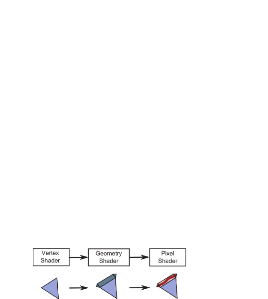
2.3. Silhouette Rendering 35
The approach presented here is conceptually similar to [Raskar 01], but takes
advantage of modern hardware. We also borrow ideas from [Doss 08] and [McGuire
and Hughes 04] for silhouette geometry generation. In contrast to these ap-
proaches, we generate both the silhouette and the object in a single pass, and we
present an algorithm for correct texturing with coherent and continuous texture
coordinates along the entire silhouette.
2.3 Silhouette Rendering
Silhouette rendering is a fundamental element in most NPR effects, as it plays
an important role in object shape understanding. In this section we present a
novel approach for the detection, generation, and texturing of a model in a single
rendering pass. First we will present an overview of our algorithm, and then we
will detail how each of the steps is implemented.
2.3.1 Algorithm Overview
In order to carry out the entire process in a single step, we will take advantage of
some of the modern features of GPUs; concretely, we will make an extensive use
of the geometry shader. This stage permits triangle operations, with knowledge
of adjacent triangles, and the generation of new triangles to the geometry.
Our process for silhouette rendering performs the following steps at the dif-
ferent stages of the pipeline (Figure 2.1):
•Vertex shader. Vertices are transformed in the usual way to camera space.
•Geometry shader. In this stage, edges that belong to the silhouette are
detected by using the information of the current triangle and its adjacency,
and the corresponding geometry is generated.
Figure 2.1. Pipeline overview: the vertex shader (left) transforms the vertex coordinates
of the incoming geometry; the second step (geometry shader) generates new geometry
for the silhouette of the object. Finally, the fragment shader generates correct texture
coordinates.
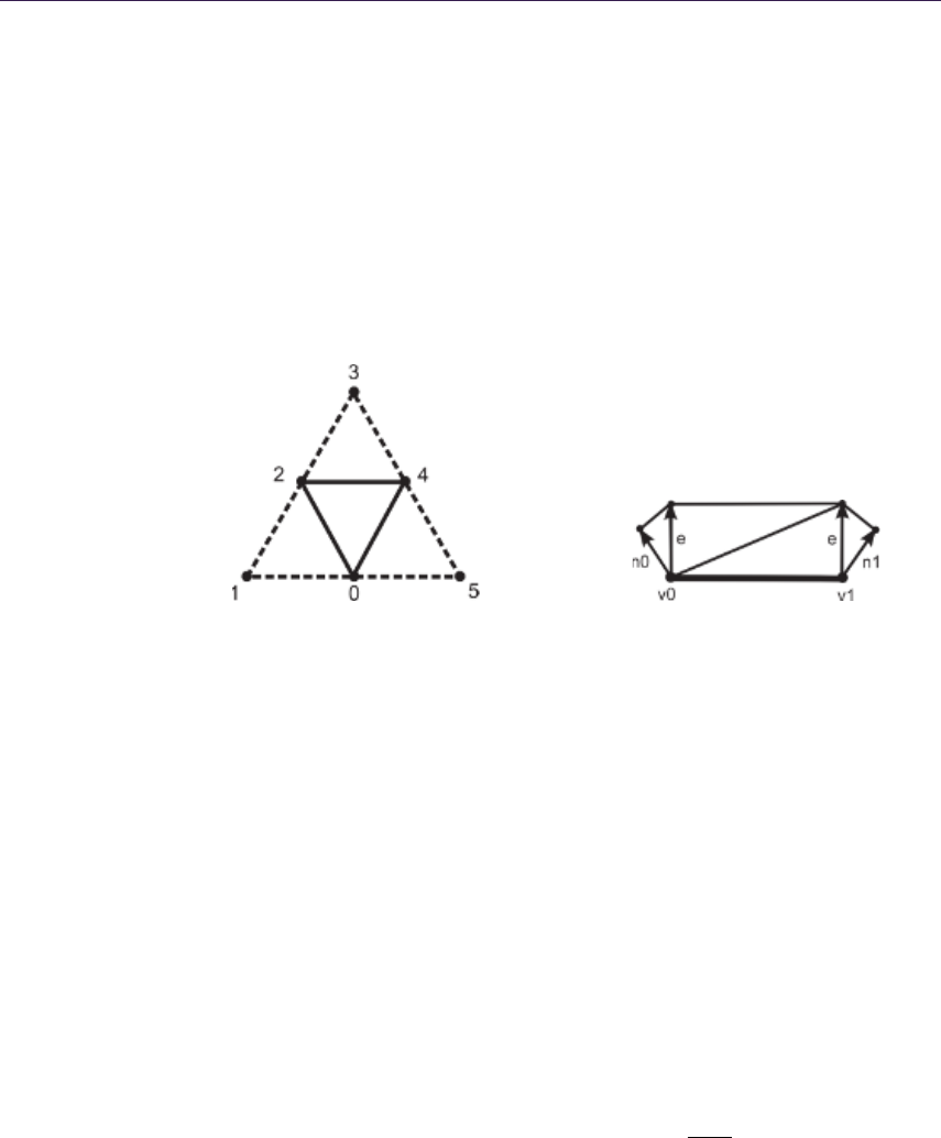
36 2. NPR Effects Using the Geometry Shader
•Pixel shader. For each rasterized fragment, its texture coordinates are
generated and pixels are shaded according to the color obtained from the
texture.
Before we may send a mesh throughout the pipeline, we first perform a special
reordering of the indices of the triangles. This will make the adjacency informa-
tion available at the geometry shader level. In order to access such information,
we send six indices per triangle (instead of the normal three), ordered as depicted
in Figure 2.2. The central triangle, identified by indices 0, 4, and 2 is the one to
be analyzed. The remaining adjacent triangles are needed to show if any of the
edges of the central triangle belong to the silhouette.
Figure 2.2. Index sort. Figure 2.3. Edge geometry.
2.3.2 Silhouette Detection and Geometry Generation
We consider a closed triangle mesh with consistently oriented triangles. The set of
triangles is denoted, T1. . . TN. The set of vertices is v1. . . vnin ℜ3, and normals
are given by triangles: ntis the normal of a triangle Tt= [vi, vj, vk], using the
notation by [Dyken et al. 08]. This triangle normal is defined as the normalization
of the vector (vj−vi)×(vk−vi). Given an observer at position x∈ ℜ3, we may
say a triangle is front facing in vif (v−x)·n≤0, otherwise it is back facing. The
silhouette of a triangle mesh is the set of edges where one of the adjacent triangles
is front facing while the other is back facing. In order to detect a silhouette in
a triangulated mesh we need to process any triangle, together with the triangles
that share an edge with it. This test is performed at the geometry shader level for
each edge of the triangle being processed. In order to avoid duplicate silhouettes
when processing both the front facing and the back facing triangles, we only
generate silhouettes for the front-facing triangles. The code in Listing 2.1 shows
how to detect a silhouette edge at the geometry shader level.
As shown in Figure 2.3, once an edge (indicated by v0v1) has been determined
as a silhouette one, we generate the geometry that will act as the silhouette by

2.3. Silhouette Rendering 37
[maxvertexcount( 21) ]
void m ain ( t ri an gl ea dj V ER TEXi n inp ut [6] ,
in out Tria ngl eStream < VERTE Xout > TriS trea m )
{
// C alcul ate the tri angl e nor mal and view dire ctio n .
float3 n or m al T ri a n = ge t No r ma l ( i np u t [ 0] . Po s . xyz ,
in pu t [2]. P os . xyz , i nput [ 4]. P os . xyz ) ;
float3 vie wDir e ct = normalize(- in put [0 ]. Pos . xyz
- i nput [ 2]. Pos . xyz - i np ut [4 ]. Po s . xyz ) ;
// If the tria ngle is fron tf acing
[branch]if (do t (normalTr ian , view Direc t ) > 0.0 f)
{
[lo op ]for (uint i = 0; i < 6; i +=2)
{
// C alcul ate the normal for this tri angle .
fl oat a ux In de x = ( i +2) %6;
float3 aux Norm al = get Norm al ( input [i ]. Pos .xyz ,
in pu t [i + 1]. Pos . xyz , inp ut [ a ux In de x ]. Po s . xyz ) ;
float3 aux Dire ct = normalize( - i np ut [ i ]. Po s . xyz
- i nput [ i +1 ]. Po s . xyz - in put [ a uxIn de x ]. Pos . xy z );
// If the tria ngle is bac kf acing
[branch]if (do t (auxNormal , aux Direc t ) <= 0.0 f)
{
// Here we have a si l houe tte edge .
}
}
}
}
Listing 2.1. Geometry shader silhouette detection code.
applying the algorithm in [McGuire and Hughes 04]. It consists of four triangles.
The central triangles forming the quad are generated by extruding the edges’
vertices using as the extrusion direction of a vector orthogonal to the edge and
view directions. The remaining triangles are generated by extruding the vertices
from the edge in the direction of the vertex normal as projected on screen. The
generation of such geometry can be done either in world space or in screen space.
We usually use screen space because this way is easier to obtain a silhouette
geometry of constant size in screen. The code needed to generate this geometry
appears in Listing 2.2.

38 2. NPR Effects Using the Geometry Shader
// T ransf orm the p ositi ons to scree n space .
float4 tra nsPo s1 = mul ( i np ut [ i ]. Pos , pro jMa tri x );
tran sPos1 = t rans Pos1 / tr ansPo s1 .w;
float4 tra nsPo s2 = mul ( i npu t [ aux In de x ]. Pos , p ro jM at ri x );
tran sPos2 = t rans Pos2 / tr ansPo s2 .w;
// C alcul ate the edge d irect io n in screen spa ce .
float2 edg e Direc t ion = normalize( t ra ns Pos 2 . xy - t ra ns Po s 1 . xy ) ;
// C alcul ate the e xtru de vec tor in screen spa ce .
float 4 extrudeDirection = float4(normalize(
float2( - e dg eDi r ec ti o n . y , e dg eD i re ct i on . x )) ,0 .0 f , 0. 0 f );
// Calc ulat e the e xtrude v ect or a long the vertex
// n orma l in screen sp ace .
float4 normExtrude1 = mul ( i np ut [ i ]. Po s + i nput [ i ]. N or ma l
,pro jMat r ix );
normExtrude1 = normExtrude1 / normExtrude1.w;
nor m Extr u de1 = no r mExtr ude1 - transP os1 ;
normExtrude1 = float4(normalize( n or m Ex tr u de 1 . xy ) ,0. 0f , 0.0 f );
float 4 normExtrude2 = mul ( in put [ auxI ndex ]. Pos
+ in put [ aux In dex ]. Normal , p ro jMatr ix );
normExtrude2 = normExtrude2 / normExtrude2.w;
nor m Extr u de2 = no r mExtr ude2 - transP os2 ;
normExtrude2 = float4(normalize( n or m Ex tr u de 2 . xy ) ,0. 0f , 0.0 f );
// Scale the ext rude dire ct io ns with th e edge size .
nor m Extr u de1 = no r mExtr ude1 * edgeS ize ;
nor m Extr u de2 = no r mExtr ude2 * edgeS ize ;
extrudeDirection = extrudeDirection * edgeSize;
// C alcul ate the extrude d vert ices .
float 4 normV erte x 1 = tran sPos 1 + normE x trud e 1 ;
float 4 extru Verte x1 = tran sPos1 + e xt rudeD irectio n ;
float 4 normV erte x 2 = tran sPos 2 + normE x trud e 2 ;
float 4 extru Verte x2 = tran sPos2 + e xt rudeD irectio n ;
// Create the o utput polygon s .
VER TEXou t out Vert ;
out Ve rt . Pos = float4( n o rm V er t e x1 . xyz , 1.0 f );
TriS tream . Append( o utVe rt );
outV er t . Pos = float4( extr uVert ex1 . xyz ,1.0 f );
Tri Strea m . Append( outV ert );
out Ve rt . Pos = float4( t r an s Po s1 . xyz , 1. 0 f );
TriS tream . Append( o utVe rt );
outV er t . Pos = float4( extr uVert ex2 . xyz ,1.0 f );
TriS tream . Append( o utVe rt );
out Ve rt . Pos = float4( t r an s Po s2 . xyz , 1. 0 f );
TriS tream . Append( o utVe rt );
outV er t . Pos = float4( no r mV e r te x 2 . xyz , 1. 0 f );
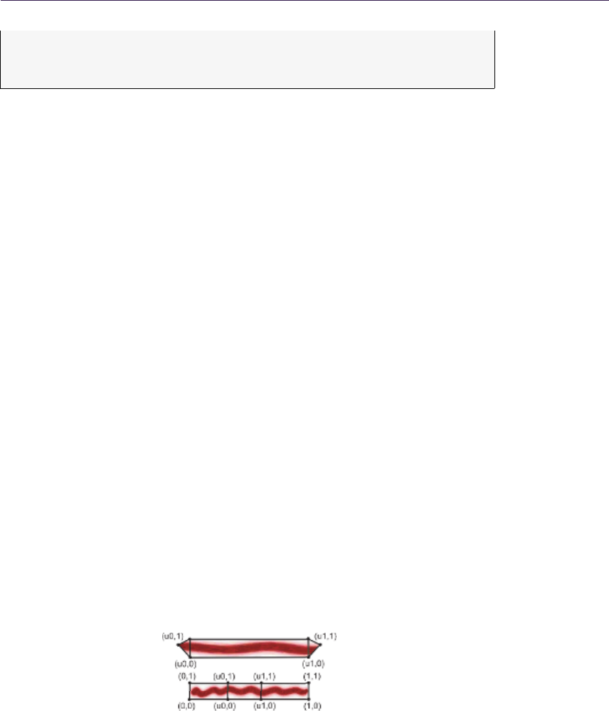
2.3. Silhouette Rendering 39
Tri Strea m . Append( outV ert );
Tri Strea m . Restar tStrip ();
Listing 2.2. Geometry shader silhouette generation.
In some cases, this solution may produce an error when the extrusion direction
has a different direction than the projected normal version. There are several ways
to solve this. One of the simplest ones consists of changing the direction of the
projected normal, as commented in [Hermosilla and V´azquez 09]. Some cases
also might require different silhouette geometry (see [McGuire and Hughes 04]
for more details).
2.3.3 Silhouette Texturing
Once the silhouette geometry has been generated, it becomes obvious that tex-
turing this geometry will increase the number of effects that can be achieved. In
order to properly texture the silhouette geometry, we need to generate texture
coordinates. Texture coordinates generation is a bit tricky, as we need to generate
continuous coordinates along the entire silhouette. Therefore we may not simply
assign coordinates from 0 to 1 for each edge, as this would cause irregular coor-
dinate distribution if the edges are not created all with the same length. Instead
we need a global strategy for coordinate generation because each triangle of the
silhouette will not be aware of the neighbor triangles’ coordinates.
From the two texture coordinates uand v, coordinate vcan be simply defined,
because it changes from zero to one as long as we go away from the object, as
depicted in Figure 2.4.
Coordinate uhas to be generated in such a way that its value is continu-
ous along the silhouette of the object. In order to make sure that two adjacent
edges will generate coherent texture coordinates, we will build a function that
depends on the position of the projection of the vertices on screen. As a conse-
quence, the coordinates will be continuous because neighbor edges share a vertex.
Figure 2.4. The v-coordinate has a value of 0 for the edge vertex and 1 for the extruded
vertices.

40 2. NPR Effects Using the Geometry Shader
Figure 2.5. The u-coordinates are generated from the edge vertex coordinates in screen
space. The first vertex of the edge and the vertex extruded from the first vertex nor-
mal gets the u-coordinate from the coordinates of the first vertex (a) The other edge
endpoint, and the vertex extruded from the second vertex normal gets the u-coordinate
from the coordinates of the second vertex (b) The vertices extruded from the extrusion
vector (e1 & e2) obtain their u-coordinates by interpolation, as show in Equation (2.1).
This is achieved when the geometry shader sends the x- and y-coordinates of the
generated vertices in screen, together with v-coordinate. The pixel shader will re-
ceive such coordinates as interpolated values, and will generate the corresponding
uvalue. Figure 2.5 shows how this information is used.
Vertices ereceive their coordinates from linear interpolation as shown in the
following equations:
e1.ux =xa+ (|⃗
ab| ∗ ((d∗da)/(da+db+dc)))
e1.uy =ya+ (|⃗
ab| ∗ ((d∗da)/(da+db+dc)))
e1.v = 0
e2.ux =xb+ (|⃗
ba| ∗ ((d∗da)/(da+db+dc)))
e2.uy =xb+ (|⃗
ba| ∗ ((d∗da)/(da+db+dc)))
e2.v = 0.
(2.1)
The pixel shader will receive those coordinates interpolated and will use them
to compute the final texture coordinates.
In order to compute the final ucomponent, we will transform components
xand yinto polar coordinates. The reference system will be the screen space
position of the center of the bounding box of the object, and the x- and y- axes will
be those of the viewport. Therefore, we will have polar coordinates computed as
•Polar angle: αwill be the angle between the x-axis, and the vector with
initial point at the origin of the coordinates system, and final point at (x, y).
•Distance: dis the distance from (x, y) to the origin of the coordinates
system.

2.3. Silhouette Rendering 41
float4 ma in ( PIX ELin in Put ): SV_Target
{
// Init ial t ext ure c oordi nate .
float2 co ord = float2(0 .0 f , i nP ut . UV . z );
// Vector from the pr ojec ted ce nte r b ounding box to
// the loc ation .
float2 ve ct = in Pu t . UV . xy - aab bP os ;
// C alcu late the polar c oord inate .
fl oat ang le = atan ( v ect . y/ vect . x );
an gl e = ( ve ct . x < 0. 0 f )? a ng le + PI :
( vect . y < 0.0 f )? ang le + (2* PI ): angle ;
// Assign the angle plus dis tanc e to the u t ext ure coo rdina te .
co ord .x = (( angle / (2* PI )) + ( length ( ve ct )* l en gthP er ))* s cal e ;
// Get the tex ture col or .
float4 col = t exure Di ff . Sample( samLi nea r , co ord );
// Alpha test .
if ( col . a < 0.1 f )
discard;
// R etur n color .
return col ;
}
Listing 2.3.Silhouette texturing.
Finally, we compute uas indicated in the following equation:
u= ( α
2∗π) + (k∗d).
As we may see, the polar angle is divided by 2πin order to transform it
into a value in the [0..1] range. The distance is weighted by a factor kthat
may be changed interactively. For objects of a sphere-like shape, kvalue can be
set to close to 0, but for objects with edges that roughly point to the origin of
coordinates, the value kmust be different from 0. Otherwise, texture coordinates
at both ends of those edges would be similar. The code that implements this is
shown in Listing 2.3.
This algorithm may produce small artifacts in edges that are projected on the
screen close to the center of the bounding box. However, these are not visible in
most of the models we tested.

42 2. NPR Effects Using the Geometry Shader
2.3.4 Single Pass Geometry and Silhouette Rendering
Most silhouette rendering algorithms perform two passes, one for the geometry,
and another one for the silhouettes. This means that the geometry is sent two
times into the rendering pipeline. We can avoid this by taking further advantage
of the geometry shader with little modifications to the original code. This is
achieved by simply rendering the triangle being analyzed by the geometry shader,
even if it does not have any edge belonging to the silhouette. This can be done
thanks to the fact that the geometry shader may output more than a single
triangle.
So far, the pixel shader code deals only with edges and textures them accord-
ingly. In order to render the triangles belonging to the geometry in a single pass,
we must inform the pixel shader of the sort of triangle that originated the raster-
ized fragment: silhouette or geometry. We encode this information in the texture
coordinates. As we are passing three coordinates, we will use one of them—in
this case the v-coordinate—to encode this information. For triangles belonging
to this geometry, we assign the value 2. This way, the pixel shader can easily
distinguish between both kinds of triangles, and shade them accordingly.
2.3.5 Results
We can see some results of our algorithm in Figure 2.6. The algorithm presented
here achieves real-time performance, as can be seen in Table 2.1. These results
were obtained on a 6 GB Quad Core PC equipped with a GeForce 9800 GX2
GPU. The viewport resolution (key for image space algorithms) was 1680×1050.
Note that even complex objects (such as the Buddha model), with more than 1M
polygons, achieve interactive framerates.
Models Triangles FPS
Buddha 1087716 8.50
Armadillo 345944 21.07
Asian Dragon 225588 25.75
Dragon 100000 60.07
Bunny 69666 110.78
Atenea 15014 337.59
Table 2.1. Framerates obtained with the textured silhouette algorithm on a GeForce
9800 GX2 GPU with a viewport resolution of 1680 ×1050.
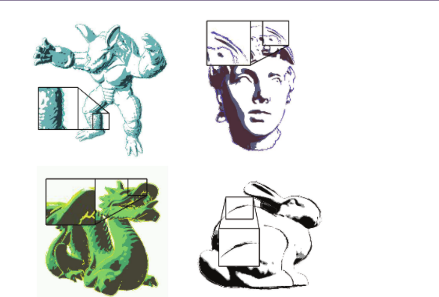
2.4. Pencil Rendering 43
Figure 2.6. Images showing the algorithm in action. Silhouettes have been generated
and textured in real time.
2.4 Pencil Rendering
In this section we will present how to implement pencil rendering in the geometry
shader. This is based on the technique presented by [Lee et al. 06].
2.4.1 Algorithm Overview
The original technique by [Lee et al. 06] works in the following way. First, the
minimal curvature at each vertex is computed. Then, triangles are sent through
the pipeline with this value as a texture coordinate for each vertex. In order to
shade the interior of a triangle, the curvatures at the vertices are used to rotate
a pencil texture in screen space. This texture is rotated three times in screen
space, one for each curvature, and the result is combined with blending. Several
textures with different tones are used at the same time, stored in an array of
textures. The correct one is selected according to illumination.

44 2. NPR Effects Using the Geometry Shader
Figure 2.7. Pipeline overview: the vertex shader transforms the vertices to screen space;
the geometry shader assigns the vertex curvatures of the triangle to the three vertices.
Finally, the pixel shader generates texture coordinates for the three curvatures and
calculates the final color.
We may implement this algorithm using the GPU pipeline in the following
way (Figure 2.7):
•Vertex shader. Vertices are transformed to screen coordinates. Vertex cur-
vature is transformed too, and only x- and y-components are passed through
as a two-dimensional vector.
•Geometry shader. The curvature values are assigned to each vertex as
texture coordinates.
•Pixel shader. Final color is computed.
2.4.2 Geometry Shader Optimization
This technique has an important shortcoming: It is necessary to make a copy of
each vertex for each triangle that shares it. This is because each pixel receives the
interpolated curvature by using each vertex, and the three curvatures are required
unchanged. Each duplicated vertex is assigned the three curvatures of the vertices
of the triangle in order to make each fragment get the three exact curvatures.
In order to avoid vertex duplication, we will use the geometry shader. At the
geometry shader level, we receive the three vertices of a triangle, with its corre-
sponding curvatures. These curvatures are assigned as three texture coordinates
to the vertices of the output triangle in the same order. Thus, the fragment shader
will receive the three values without interpolation. The code corresponding to
the geometry shader appears in Listing 2.4.
2.4.3 Pixel Texturing
The final color composition is performed in the following way: the fragment
shader receives the coordinates of the fragment, together with the curvatures.
We will use components xand yof the fragment in screen space as texture
coordinates. These coordinates are scaled to the range [0..1].

2.4. Pencil Rendering 45
[maxve rtexc o unt (3) ]
void ma in ( tri angle V ER TE Xin i nput [3] ,
ino ut Tr iangl eStr eam < V ERT EXo ut > T ri Stre am )
{
// Ass ign t rian gle curv ature s to the three v ertices .
VER TEXou t outVert ;
outV er t . Pos = inp ut [0]. Pos ;
outV ert . no rm = i nput [ 0]. n orm ;
outV ert . curv1 = inp ut [0]. c urv ;
outV ert . curv2 = inp ut [1]. c urv ;
out Vert . cur v3 = i nput [ 2]. c urv ;
TriS tream . Append( o utVe rt );
out Ve rt . Pos = in put [ 1]. P os ;
out Vert . no rm = inpu t [1]. n orm ;
outV ert . curv1 = inp ut [0]. c urv ;
outV ert . curv2 = inp ut [1]. c urv ;
out Vert . cur v3 = i nput [ 2]. c urv ;
Tri Strea m . Append( outV ert );
out Ve rt . Pos = in put [ 2]. P os ;
out Vert . no rm = inpu t [2]. n orm ;
out Vert . cur v1 = i nput [ 0]. c urv ;
out Vert . cur v2 = i nput [ 1]. c urv ;
out Vert . cur v3 = i nput [ 2]. c urv ;
Tri Strea m . Append( outV ert );
T ri St re am . Re s ta rt S tr ip ( ) ;
}
Listing 2.4. Pencil geometry shader.
In order to orient the texture according to the surface curvature, and to avoid
deformations inside large triangles, the paper texture is oriented by using the
three curvatures at the vertices, and blending them with equal weights. The
implementation has three steps: First, the angles between curvatures and the
x-axis are computed. Then, three two-dimensional rotation matrices are built
using these angles. Finally, these matrices are used to transform the texture
coordinates obtained from the fragment coordinates, and this yields three new
texture coordinates. These are the ones used for final texturing.
The model may be shaded by using the dot product between the light direction
and the surface normal in order to access a texture array of different tones. We use
a single texture but modified with a function that changes brightness and contrast
according to the incident illumination at each point. We use the following func-
tion:
p= 1 .0 - { max }({ dot }( light , n ormal ) ,0. 0)
col or De st = { p ow }( c olo rSrc , p* S + O ) .
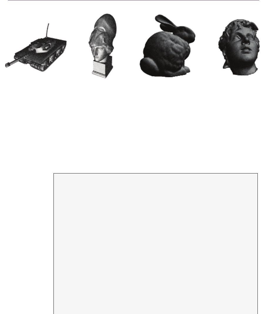
46 2. NPR Effects Using the Geometry Shader
O= 5; S= 0.15 O= 5; S= 0.15 O= 5; S= 1 O= 5; S= 1
Figure 2.8. Pencil rendering results.
The resulting color of texture mapping is powered to a value in the range
[O..S +O]. This value is determined from the dot product between the light and
normal vectors. This will darken dark regions and lighten lighter regions, as can
be seen in Figure 2.8 where we show the comparison using different values of O
and S. The code corresponding to the geometry shader is shown in Listing 2.5.
float4 ma in ( PIX EL in inPut ) : SV_Target
{
float2 xdir = float2(1 .0 f ,0 .0 f ) ;
flo at2x 2 rotMat ;
// C alcu late the pixel c oord inate s .
float2 uv = float2( in Put . Po s .x / width , inP ut . Pos . y/ hei ght ) ;
// C alcu late the rot ated coo rdina tes .
float2 uv Dir = normalize( inP ut . curv1 ) ;
fl oat angle = atan( uvDi r .y / uv Dir . x);
an gl e = ( uvD ir . x < 0. 0 f) ? a ng le + PI :
( uv Dir .y < 0.0 f)? an gle +(2* PI ): angle ;
fl oat cosVal = co s ( angle );
fl oat sinVal = si n ( angle );
rotMat[0][0] = cosVal;
rotMat[1][0] = -sinVal;
rotMat[0][1] = sinVal;
rotMat[1][1] = cosVal;
float2 uv1 = mul (uv , ro tMat ) ;
uv Dir = normalize( inP ut . curv2 ) ;
an gle = atan( uvD ir . y/ uvD ir . x) ;
an gl e = ( uvD ir . x < 0. 0 f) ? a ng le + PI :
( uv Dir .y < 0.0 f)? an gle +(2* PI ): angle ;
2.4. Pencil Rendering 47
cosVal = c os ( an gle ) ;
sinVal = s in ( an gle ) ;
rotMat[0][0] = cosVal;
rotM at [ 1] [0 ] = - sin Va l ;
rotMat[0][1] = sinVal;
rotMat[1][1] = cosVal;
float2 uv2 = mul (uv , ro tMat ) ;
uvD ir = normalize( inPu t . curv3 );
ang le = atan ( u vDi r .y / uvDir . x) ;
an gle = ( u vDir . x < 0.0 f)? angle + PI :
( uv Dir .y < 0.0 f)? an gle +(2* PI ): angle ;
cosVal = c os ( an gle ) ;
sinVal = s in ( an gle ) ;
rotMat[0][0] = cosVal;
rot Ma t [1 ][ 0] = - si nV al ;
rotMat[0][1] = sinVal;
rotMat[1][1] = cosVal;
float 2 uv3 = mu l (uv , r otMa t );
// Calc ulate the light i ncide nt at this p ixel .
fl oat p erce n = 1. 0 f - ma x (dot (normalize( i nP ut . no rm ) ,
lig ht Di r ) ,0.0) ;
// C ombi ne the thr ee colors .
float 4 color = ( texP encil . Sample( samLi nea r , uv1 ) *0.333 f )
+( texP encil . Sample( samLinear , uv2 ) *0.333 f)
+( texP encil . Sample( samLinear , uv3 ) *0.333 f);
// Calc ulate the final c olo r .
perce n = ( percen *S ) + O ;
c ol or . xy z = po w ( c ol or . xyz , float3(percen , percen , per cen ));
retur n col or ;
}
Listing 2.5. Pencil pixel shader.
Models Triangles FPS
Buddha 1087716 87.71
Armadillo 345944 117.22
Asian Dragon 225588 199.20
Dragon 100000 344.28
Bunny69666 422.20
Atenea 15014 553.55
Table 2.2. Framerates obtained with our implementation of the pencil rendering al-
gorithm on a GeForce 9800 GX2 GPU graphics card and a viewport resolution of
1680 ×1050.

48 2. NPR Effects Using the Geometry Shader
2.4.4 Results
Table 2.2 shows the framerates obtained with the pencil rendering technique.
Note that we obtain high framerates because the implementation is relatively
cheap, and that from the numbers we can deduce that the timings depend strongly
on vertex count rather than rasterized fragments count.
2.5 Acknowledgments
The authors want to thank the reviewers for their valuable comments. This work
has been supported by project TIN2007-67982-C02-01 of the Spanish Government.
Bibliography
[Achorn et al. 03] Brett Achorn, Daniel Teece, M. Sheelagh T. Carpendale,
Mario Costa Sousa, David Ebert, Bruce Gooch, Victoria Interrante, Lisa M.
Streit, and Oleg Veryovka. “Theory and Practice of Non-Photorealistic
Graphics: Algorithms, Methods, and Production Systems.” In SIGGRAPH
2003. ACM Press, 2003.
[Ashikhmin 04] Michael Ashikhmin. “Image-Space Silhouettes for Unprocessed
Models.” In GI ’04: Proceedings of Graphics Interface 2004, pp. 195–202.
School of Computer Science, University of Waterloo, Waterloo, Ontario,
Canada: Canadian Human-Computer Communications Society, 2004.
[Card and Mitchell 02] Drew Card and Jason L. Mitchell. “Non-Photorealistic
Rendering with Pixel and Vertex Shaders.” In Direct3D ShaderX: Vertex
and Pixel Shader Tips and Tricks, edited by Wolfgang Engel. Plano, Texas:
Wordware, 2002.
[Dietrich 00] Sim Dietrich. “Cartoon Rendering and Advanced Texture Features
of the GeForce 256 Texture Matrix, Projective Textures, Cube Maps, Tex-
ture Coordinate Generation and Dotproduct3 Texture Blending.” Technical
report, NVIDIA, 2000.
[Doss 08] Joshua Doss. “Inking the Cube: Edge Detection with Direct3D 10.”
http://www.gamasutra.com/visualcomputing/archive, 2008.
[Dyken et al. 08] Christopher Dyken, Martin Reimers, and Johan Seland. “Real-
Time GPU Silhouette Refinement Using Adaptively Blended B´ezier Patches.”
Computer Graphics Forum 27:1 (2008), 1–12.

Bibliography 49
[Everitt 02] Cass Everitt. “One-Pass Silhouette Rendering with GeForce and
GeForce2.” White paper, NVIDIA Corporation, 2002.
[Gooch and Gooch 01] Amy A. Gooch and Bruce Gooch. Non-Photorealistic
Rendering. A K Peters, 2001. ISBN: 1568811330, 250 pages.
[Gooch et al. 99] Bruce Gooch, Peter-Pike J. Sloan, Amy A. Gooch, Peter
Shirley, and Richard Riesenfeld. “Interactive Technical Illustration.” In 1999
ACM Symposium on Interactive 3D Graphics, pp. 31–38, 1999.
[Hartner et al. 03] Ashley Hartner, Mark Hartner, Elaine Cohen, and Bruce
Gooch. “Object Space Silhouette Algorithms.”, 2003. Unpublished.
[Hermosilla and V´azquez 09] Pedro Hermosilla and Pere-Pau V´azquez. “Single
Pass GPU Stylized Edges.” In Proceedings of IV Iberoamerican Symposium
in Computer Graphics, pp. 47–54, 2009.
[Isenberg et al. 03] Tobias Isenberg, Bert Freudenberg, Nick Halper, Stefan
Schlechtweg, and Thomas Strothotte. “A Developer’s Guide to Silhouette
Algorithms for Polygonal Models.” IEEE Comput. Graph. Appl. 23:4 (2003),
28–37.
[Lee et al. 06] Hyunjun Lee, Sungtae Kwon, and Seungyong Lee. “Real-Time
Pencil Rendering.” In NPAR ’06: Proceedings of the 4th International Sym-
posium on Non-photorealistic Animation and Rendering, pp. 37–45. New
York: ACM, 2006.
[McGuire and Hughes 04] Morgan McGuire and John F. Hughes. “Hardware-
Determined Feature Edges.” In NPAR ’04: Proceedings of the 3rd Interna-
tional Symposium on Non-photorealistic Animation and Rendering, pp. 35–
47. New York: ACM, 2004.
[Mitchell et al. 02] Jason L. Mitchell, Chris Brennan, and Drew Card. “Real-
Time Image-Space Outlining for Non-Photorealistic Rendering.” In Siggraph
02, 2002.
[Raskar 01] Ramesh Raskar. “Hardware Support for Non-photorealistic Render-
ing.” In 2001 SIGGRAPH / Eurographics Workshop on Graphics Hardware,
pp. 41–46. ACM Press, 2001.
[Saito and Takahashi 90] Takafumi Saito and Tokiichiro Takahashi. “Compre-
hensible Rendering of 3-D Shapes.” SIGGRAPH90 24:3 (1990), 197–206.
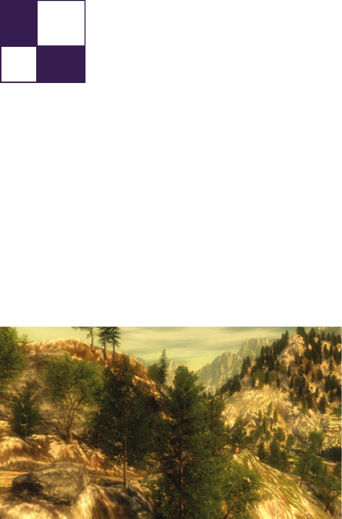
3
Alpha Blending as a Post-Process
Benjamin Hathaway
3.1 Introduction
In this article we will present a novel alpha-blending technique that was developed
for the off-road racing game Pure (see Figure 3.1). Pure was released in the
summer of 2008 for the Xbox360, PS3, and PC platforms and featured races that
subjected the player to extreme elevations, revealing detailed vistas stretching
out to a distance of over 30 kilometers. With the art direction set on a photo-
realistic look and locations taken from around the globe—some would require a
high degree of foliage cover to be at all believable, or even recognizable.
Figure 3.1. A typical scene from Pure (post tone mapping & bloom effects).
51

52 3. Alpha Blending as a Post-Process
During development it became apparent that we were going to need alpha
blending, and lots of it! Unfortunately, alpha blending is one aspect of computer
graphics that is difficult to get right, and trade-offs between performance and
visual quality are often made; indeed, reluctance to risk performance has led to
some game titles avoiding the use of alpha blending altogether. For a thorough
introduction to the issues posed by alpha blended rendering, the reader is referred
to the [Thibieroz 08] paper on advanced rendering techniques and the seminal
work [Porter and Duff 84].
3.2 The Alternatives
Pure was destined to run on several platforms, each being equipped with at least
one Dx9 class GPU (supporting shader model 3). This immediately presented us
with several (hardware assisted) options for rendering our foliage geometry.
Alpha blending. Alpha blending uses a scalar value output by the pixel shader
(alpha-value) to blend a rendered fragment with the destination pixel data.
When rendering layers of foliage with alpha blending, z-buffering artifacts
are common. This can largely be resolved if the rendered primitives are sorted
to draw furthest from the camera first. Sorting primitives before rendering is
usually a prohibitive CPU cost for game rendering, and in the case of intersecting
primitives there may indeed be no single correct draw order.
Alpha testing. Alpha testing uses a binary value output by the pixel shader to
determine if the output fragment is visible or not. Alpha testing is usually com-
bined with z-buffering techniques, which can either negate the need for geometric
depth sorting or provide fill-rate optimizations (by way of z-rejection) when the
scene is sorted in a front-to-back order.
Alpha testing is one of the most commonly used solutions to date; however
the technique is prone to aliasing at the alpha edges.
Alpha-to-coverage. Alpha-to-coverage converts the alpha value output by the pixel
shader into a coverage mask. This coverage mask is combined with the standard
multisample coverage mask to determine which samples should be updated.
When alpha-to-coverage is combined with alpha testing, softer edges can be
rendered whilst maintaining all the technical benefits afforded by alpha test ren-
dering, i.e., sort independence and z-rejection opportunities. Although this is an
improvement on simple alpha testing, the resulting alpha gradients can be of a
poor quality compared to those obtained in alpha blending. This is particularly
true when using a low number of samples or on hardware that does not support
flexible coverage masks.
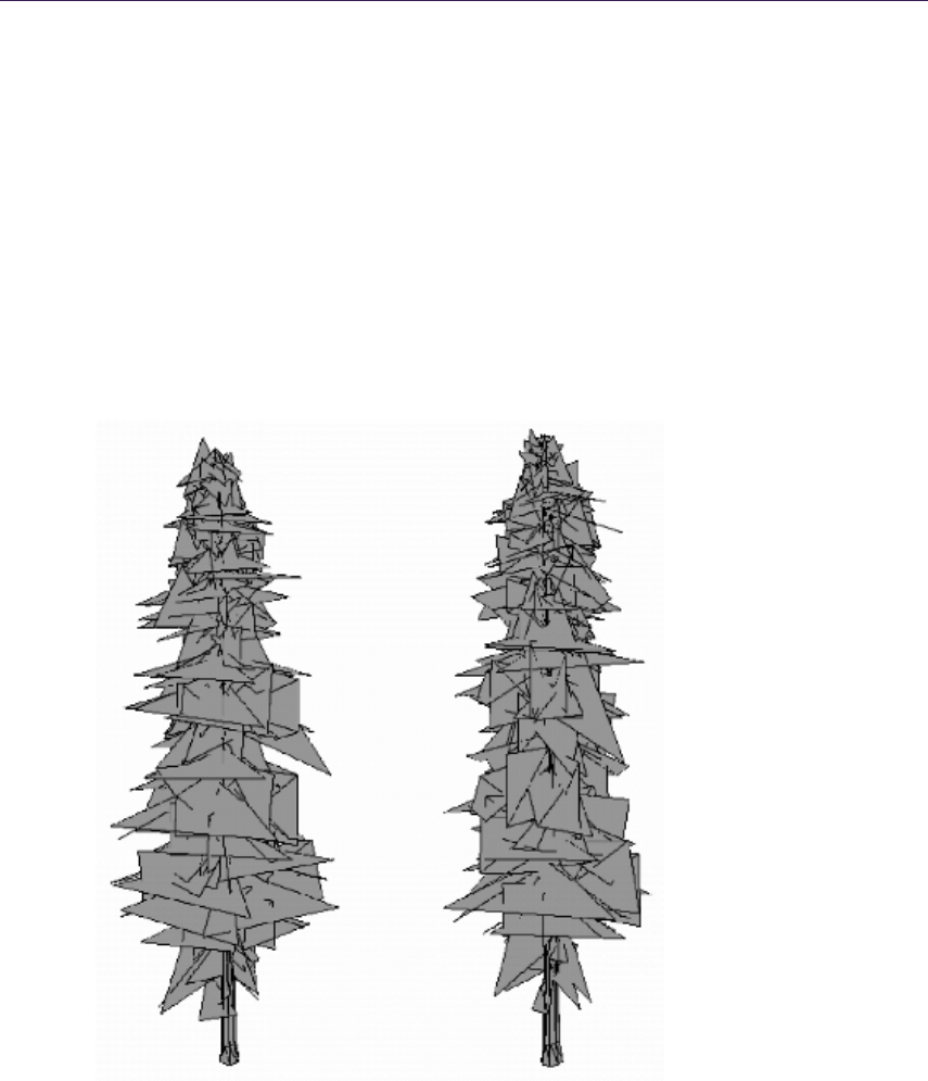
3.3. The Source Artwork 53
3.3 The Source Artwork
To try and emulate the richness of natural foliage, each tree and bush was con-
structed from a multitude of polygonal planes. The planes were oriented as
randomly as possible, thus increasing the perceived density of foliage.
As can be seen in Figure 3.2, this leads to a great deal of primitive intersection,
which raises two issues:
1. How are we to correctly sort all the intersecting primitives?
2. How are we going to deal with the high degree of depth complexity present
within a single foliage model?
Figure 3.2. Geometric structure of a typical tree model rendered in Pure (shown from
the front and side).

54 3. Alpha Blending as a Post-Process
To correctly depth sort the primitives would require that we split the prim-
itives along all the intersections. However, this would have increased the vertex
count substantially and put a heavy burden on our memory budget, while also
increasing memory bandwidth usage.
These issues are further exacerbated when the foliage is allowed to react to
dynamic influences such as the wind, or physical collisions. Such influences may
even cause neighboring foliage models to overlap rather unpredictably, and would
therefore be impossible to optimize off-line, instead requiring a more costly, real-
time solution.
3.4 Initial Attempts
Due to the high levels of primitive interpenetration within the artwork, we initially
implemented our foliage renderer in the simplest manner possible, by using a
combination of z-buffering and alpha-test techniques. After auditioning a number
of variations of the alpha-reference value, we managed to achieve some reasonable
results, although the overall look of the foliage tended to appear a little harsh,
or synthetic, at times.
The most objectionable effect occurred when the camera performed slow trans-
lational motions from side-to-side (for example, during the pre-race camera se-
quences). As the camera moved, the alpha-channeled holes & edges within the
foliage would begin to sparkle (due to the binary nature of alpha testing) and
would often be exaggerated by the high degree of depth complexity present within
each foliage model.
Next, we turned our attention towards the alpha-to-coverage feature. Alpha-
to-coverage rendering integrates alpha-testing techniques with multi-sample ren-
dering; it produces softer edges while maintaining all the technical benefits of
alpha-test rendering. While initial results were favorable and the sparkling arti-
facts were indeed attenuated, we struggled to reproduce consistent results across
all of our platforms. We also suffered from the increased fill-rate and bandwidth
costs incurred by rendering the foliage at MSAA resolutions.
Neither approach seemed to deliver a high enough visual quality and it seemed
a shame to quantize all those beautiful alpha-textures so heavily. Something new
was needed—and we felt the answer was hiding in the silhouette of the foliage.
3.5 The Screen-Space Alpha Mask
The solution we devised—screen-space alpha masking (SSAM)—is a multi-pass
approach (see the overview in Figure 3.3) implemented with rendering techniques
that negate the need for any depth sorting or geometry splitting. Our solution can
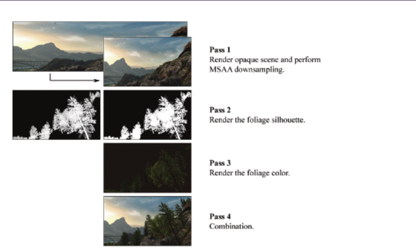
3.5. The Screen-Space Alpha Mask 55
Figure 3.3. Diagram showing an overview of screen-space alpha masking.
yield results on par with alpha blending while correctly resolving internal overlaps
(and depth intersections) on a per-pixel basis, using alpha-testing techniques.
We effectively performed deferred alpha blending using a full-screen post-
process that resembles frame-buffer blending with the blend-operation set to
ADD; the source and destination arguments are set to SRCALPHA and INVSRCALPHA,
respectively. The inputs to the blend are rendered into three separate render tar-
gets and are then bound to texture samplers, referenced by the final combination
post-process pixel shader (see Listing 3.2 in Section 3.11).
In terms of memory resources, we need at least three screen-resolution render-
targets, two having at least three color channels (rtOpaque &rtFoliage), one
with a minimum of two channels (rtMask), and a single depth buffer (rtDepth).
Note: this is in addition to any MSAA render-target memory requirements.
3.5.1 The Opaque Pass
During the first pass we rendered all our opaque scene elements into the color
render target: rtOpaque (see Figure 3.4); the depth information generated was
also kept and stored in the depth buffer: rtDepth (see Figure 3.5).
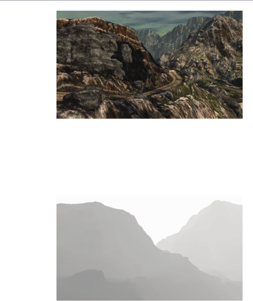
56 3. Alpha Blending as a Post-Process
Figure 3.4. The opaque scene (color) written to rtOpaque.
For Pure, we rendered the opaque scene at 2×MSAA resolution and both the
color and depth buffers were down sampled into screen-resolution render targets.
Care had to be taken when down sampling the depth information, as incorrect
samples were obtained when filtering was applied.
Figure 3.5. The opaque scene (depth) written to rtDepth.
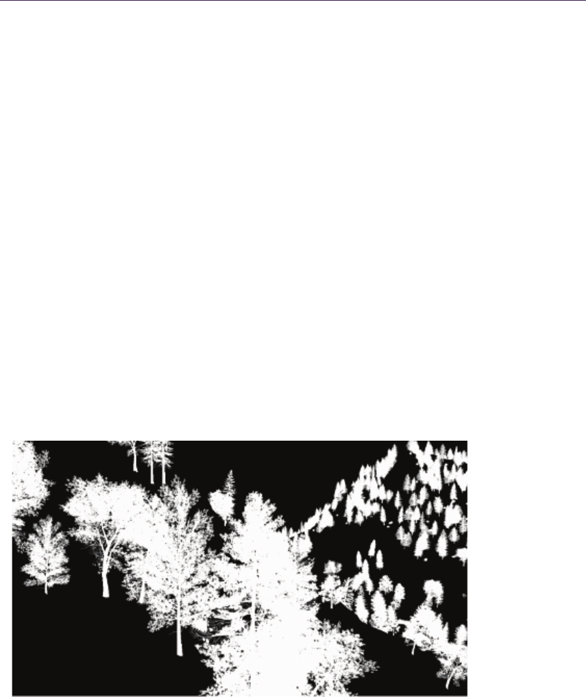
3.5. The Screen-Space Alpha Mask 57
Instead, we read a number of samples from the depth buffer (two, in the case
of 2×MSAA), compared them, and simply retained the sample that was closest
to the observer. For a more complete description of the solution adopted for
Pure, the reader is referred to the work of [Iain Cantlay 04].
From this point onwards, we continued to render at non-MSAA resolutions, as
it was observed that MSAA contributed little or nothing towards the quality of
alpha generated edges—only those of a geometric nature. At this point, and de-
pending on platform architecture, it may be necessary to copy the down sampled
images back in to VRAM (repopulation) before further rendering can continue.
Additionally, at this point steps may need to be taken to update any
hierarchical-z (hi-z) information that might be associated with rtDepth, and
potentially optimize any subsequent draw calls that are depth occluded.
Note: Detailed information regarding the repopulation of depth information and
restoration of Hi-Z can be obtained from the platform vendors and is unfortu-
nately outside the scope of this article.
3.5.2 The Mask Generation Pass
In the second pass we generated a silhouette, or mask, of the foliage we wanted
to render (see Figure 3.6). The silhouette image was rendered into our second
render-target, rtFoliage, and we used the previously generated depth buffer,
rtDepth, to correctly resolve any depth occlusions caused by the opaque scene.
Figure 3.6. Additively accumulated foliage alpha mask.
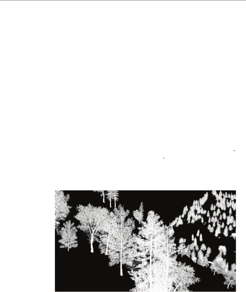
58 3. Alpha Blending as a Post-Process
The mask is a monochromatic image of the alpha-channel values that would
normally be used during regular alpha blending. The alpha-values are additively
blended onto a black background, during which, we enabled depth testing, and
disabled both back-face culling and depth writes.
As the additive blending of two primitives produces the same result regardless
of the draw order, it seemed to be the ideal option for efficient mask generation.
However, some artifacts were evident when the mask was used: as-is, (as the blend
factor) due to the limited bit depth of the render-targets being used, during the
final combination pass, the additively accumulated values would quickly saturate
towards white—even at a modest depth complexity. The saturation was most
evident when foliage close to the observer was expected to possess low-order
opacity, but is rendered in an area of high foliage depth complexity.
To generate as high quality a mask as possible, we needed to obtain as much
detail from our silhouette as we could; we therefore set the alpha-reference render-
state to zero during this pass, to avoid the rejection low opacity alpha-values.
A refinement on additive blending was the use of the max-blending mode. In
this case we built up an image of the single highest alpha-value to have been
written to each pixel, in effect acting as an alpha-z-buffer. As with additive
blending, we set the source and destination blend arguments to D3DBLEND ONE,
but change the blend operation to D3DBLENDOP MAX.
As can be seen in Figure 3.7, the max-blended mask contains a higher degree
of structural information (than the additively blended mask) while still retaining
the subtle alpha gradients located towards the outer edges of the foliage.
Figure 3.7. MAX blended foliage alpha mask.

3.5. The Screen-Space Alpha Mask 59
Despite these attractive qualities, when the max-blended mask was used as
the blend factor during the final combination pass, the foliage took on a wholly
transparent look. We were left feeling that perhaps the solution lay somewhere
in between the two approaches. And it did—quite literally.
The thought was that perhaps some linear combination of both masks would
be the answer. Perhaps the saturation of the additive blending would compensate
for the transparency of the max blending? And correspondingly, would the subtle
alpha-gradients of the max-blended image reduce the saturation evident in the
low-opacity, high-depth-complexity areas of the additive mask?
Fortunately the answer proved to be yes in both cases, and luckily for us all
the platforms we were working with provided a method that could generate both
of our masks in a single pass!
Separate alpha blend enable. Most DX9 class hardware supports the ability to
specify separate blend operations and arguments for both the color and alpha
channels, independently.
By enabling D3DRS SEPARATEALPHABLENDENABLE and setting the correct
series of operation and arguments, it is possible to simultaneously write the
max-blended mask to the rgb channels (as a monochromatic image), and the
additively-blended mask to the alpha channel (see Table 3.1).
Note: Both masks are combined at a later stage, prior to their use as the blend-
factor in the final composition pass.
In order to send the alpha values to both blending units, we needed to repli-
cate the alpha values across to all the color channels. This required a small
modification to the end of the foliage shaders that resembled
Out.Color.xyzw = Out.Color.wwww;
Render State Value
D3DRS ALPHABLENDENABLE TRUE
D3DRS SEPERATEALPHABLENDENABLE TRUE
D3DRS BLENDOP D3DBLENDOP MAX
D3DRS BLENDOPALPHA D3DBLENDOP ADD
D3DRS SRCBLEND D3DBLEND ONE
D3DRS SRCBLENDALPHA D3DBLEND ONE
D3DRS DESTBLEND D3DBLEND ONE
D3DRS DESTBLENDALPHA D3DBLEND ONE
Table 3.1. The blend-related render states used during mask generation.

60 3. Alpha Blending as a Post-Process
The modification not only performed the replication, but also had the added
benefit of optimizing the foliage-alpha rendering shader without us needing any
prior knowledge of how the alpha value was generated. For example: to what
sampler stage the alpha-texture-source was bound, etc.
All of the optimizing shader compilers we tested performed some form of dead-
code stripping, see: [“Dead Code” 09]. This optimization removed any code that
did not directly contribute to the output value, substantially increasing fill-rate
efficiency, in this case, removing all of the color-related lighting equations and
texture-fetch instructions that were not common to the generation of the alpha
value.
HLSL source code for a typical mask rendering shader is provided in Listing 3.1
in Section 3.11.
3.5.3 The Color Pass
For the third rendering pass, we rendered an image of the foliage color into our
final render-target: rtFoliage (see Figure 3.8), and again we use the depth buffer
obtained during the opaque pass, stored in rtDepth (see Figure 3.9).
In order to maintain correct depth ordering (as is necessary in the case of
the color image), we disabled both back-face culling and alpha blending, while
enabling alpha test rendering, depth testing, and depth writes. Enabling depth
writes during this pass also ensured that any subsequently rendered transparen-
cies would be correctly depth sorted with the foliage.
When rendering the foliage color with alpha testing enabled, a suitable alpha
reference value had to be chosen and we exposed the color-pass alpha reference
value to the artists for tweaking.
The final value ended up being a trade-off between two values. First was
a value high enough to produce visually pleasing alpha-test edges—for Pure, a
value of ≈128. Second was a value low enough to minimize certain blending
artifacts (that will be covered in Section 3.6), which for Pure, ended up being a
value of ≈64.
3.5.4 The Final Composition Pass
In the fourth and final pass, we rendered a full screen post-process that essentially
performed a linear interpolation of our opaque and foliage-color images, using the
mask image as the blend-factor (see Figure 3.10).
The final composition blend equation resembled
finalColor = rtOpaque + (rtFoliage - rtOpaque) * rtMask;
Application of the post-process consisted of the rendering of an orthographi-
cally projected, quadrilateral polygon mapped over the entire screen onto which
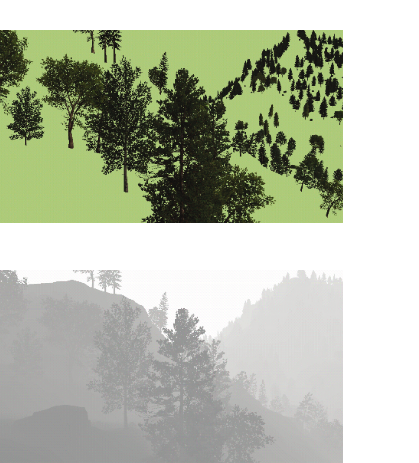
3.5. The Screen-Space Alpha Mask 61
Figure 3.8. The foliage-color image written to rtFoliage.
Figure 3.9. The foliage-depth (alpha-tested) written into rtDepth.
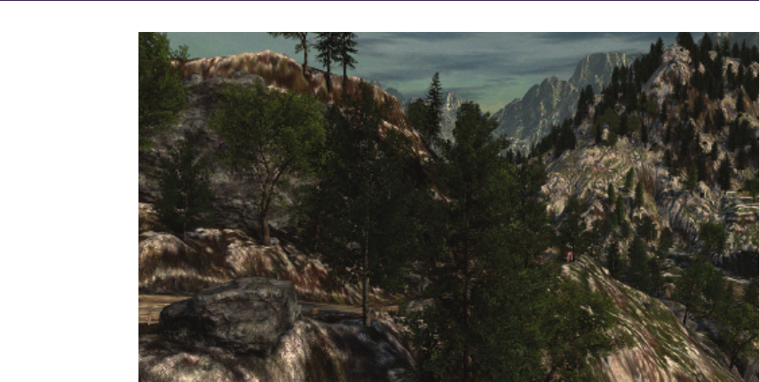
62 3. Alpha Blending as a Post-Process
Figure 3.10. The image produced by the final-combination pixel shader.
we applied a pixel shader to actually perform the blending work. To ensure
that we only sampled one texel per screen pixel, we took the platform’s texture-
sampling center into account and adjusted texture coordinates accordingly.
We now had two mask images to process, the max and additively blended
masks, which needed to be combined in some way into a scalar blend-factor. For
our implementation we chose to combine the masks using linear interpolation (or
in HLSL, the lerp operation).
The final-composition blend equation, with linearly blended masks resembled
mask = rtMask.a + (rtMask.r - rtMask.a) * maskLerp;
rtResult = rtOpaque + (rtFoliage - rtOpaque) * mask;
The interpolation of the two masks introduced the value maskLerp, for which
a value must be selected. Like the alpha-reference value, this is chosen on purely
artistic grounds and was also exposed to the art team for experimentation. The
final value for Pure was 0.85 (which produces a blend-factor composed of: 85%
additive mask and 15% max-blended mask).
With maskLerp equal to 0.85, just enough max-blended mask is brought in
to reduce the saturation artifacts without making the foliage too transparent.
In fact, it should be noted that some degree of transparency was found to
be desirable. The slight transparency of the max contribution revealed distant
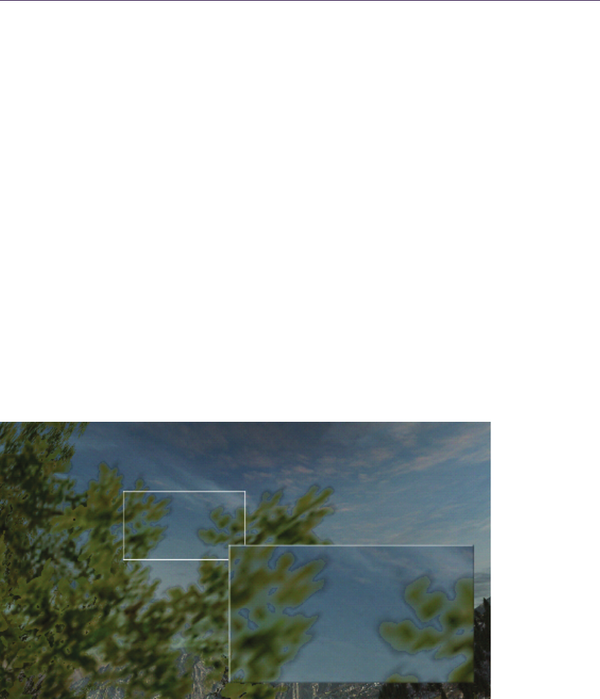
3.6. Alpha Reference Issues 63
structure (such as trunks and branches) belonging to foliage that would have
otherwise have been completely occluded by near foliage (adding a certain richness
to the forest scenes).
The full HLSL source for the final composition pixel shader is given in List-
ing 3.2 in Section 3.11.
3.6 Alpha Reference Issues
As alpha test rendering was employed during the foliage color pass, an alpha-
reference value was chosen—one that was high enough to stop overlapping edges
from appearing too chunky (as mentioned, for Pure a value was chosen somewhere
between ≈64 and ≈128). As a consequence, halo-like blending artifacts are some-
times visible where the foliage blended into the opaque image (see Figure 3.11).
3.6.1 The Clear-Screen Color Fix
Due to the alpha-reference value being set to a higher value during the color pass
than that set during the mask-generation pass (for which the alpha-reference value
was actually zero), moving outwards along an alpha gradient (from a value of one
to zero), you can actually run out of foliage-color pixels before the mask-intensity
reaches zero. This would reveal a proportion of the color-pass background color
Figure 3.11. Image showing blending artifacts caused by a non-zero alpha reference
value during the foliage-color pass.
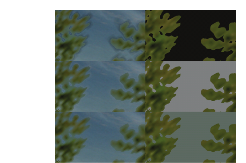
64 3. Alpha Blending as a Post-Process
Figure 3.12. The effect of different clear screen colors (from top to bottom): too dark,
too light, and just right.
in pixels whose mask intensity fell below the color-pass alpha reference value. The
solution employed for Pure was to expose the foliage color passes’ clear screen
color to the artists, the idea being that by adjusting the color, you could lighten
the artifact until it was hardly visible (see Figure 3.12).
The technique worked well but felt less than optimum, especially as the artists
could only choose one color per level. The color also tended to affect the overall
color balance of the scene and would have to work for foliage rendered in both
the lightest and darkest of conditions—very much a compromise.
3.6.2 The Squared Alpha Trick
A small modification made to the last line of the final composition pixel shader
substantially improved the quality of the blending, almost entirely compensating
for the aforementioned alpha-reference artifacts (see Figure 3.13). If the final

3.7. Rendering Pipeline Integration 65
Figure 3.13. A close-up of the just-right clear screen color fix and the squared-alpha
modification applied together.
mask value is numerically squared, the foliage alpha will roll off to black a little
quicker while correctly maintaining areas of solid opacity.
return lerp(opaquePixel, foliagePixel, mask * mask);
It should be noted that while squaring the alpha channel does contract the fo-
liage silhouette a little, a slight reduction in the foliage-color pass alpha-reference
value should compensate for this.
3.7 Rendering Pipeline Integration
Foliage rendering is by no means the final step in rendering a game. There are
many other alpha-blended elements to be integrated into the scene: grass, light
shafts, and particle effects, to name but a few. Integration with these other stages
is actually pretty straightforward, largely due to the fact that depth writing was
enabled during the foliage-color pass.
This ensured that any subsequent depth testing would correctly resolve any
depth-wise occlusions caused by the foliage (and/or opaque) scene elements.
3.8 Conclusion
In this article we have presented a novel (cross-platform) solution to the alpha
blending of foliage, a solution that increases the quality of a wide range of alpha-
test-class renderings, giving them the appearance of true alpha blending.

66 3. Alpha Blending as a Post-Process
The use of SSAM within the game Pure had a profound effect on the overall
perceived quality of the environments. The effect yielded a soft natural look
without sacrificing any of the detail and contrast present in the source artwork.
Below we list a few of the pros & cons to using SSAM:
Pros:
•Foliage edges are blended smoothly with the surrounding environment.
•Internally overlapping and interpenetrating primitives are sorted on a per-
pixel basis using alpha testing techniques.
•The effect is implemented using simple, low-cost rendering techniques that
do not require any geometric sorting or splitting (only consistency in prim-
itive dispatch order is required).
•The final blending operations are performed at a linear cost (once per pixel)
regardless of scene complexity and over-draw.
•The effect integrates well with other alpha-blending stages in the rendering
pipeline (Particles, etc).
•When combined with other optimizations such as moving lighting to the
vertex shader, and optimizing the shaders for each pass, overall performance
can be higher than that of MSAA-based techniques.
Cons:
•The overhead of rendering the extra passes.
•Memory requirements are higher, as we need to store three images.
•The technique cannot be used to sort large collections of semi-transparent,
glass-like surfaces (or soft alpha gradients that span large portions of the
screen) without potentially exhibiting visual artifacts.1
3.9 Demo
A RenderMonkey scene, as well as several instructional .PSD files, are available
in the book’s web materials on the CRC Press website.
1There are occasional opacity-related artifacts visible within overlapping alpha-gradients
(when the alpha-foliage-mask is either: >0 or, <1). Fortunately, the foliage-color pass always
yields the nearest, and therefore the most visually correct, surface color.

3.10. Acknowledgments 67
3.10 Acknowledgments
I would like to say a big thank you to everyone at Black Rock Studio who con-
tributed to this article, particularly: Jeremy Moore and Tom Williams (for push-
ing me to write the article in the first place), and Damyan Pepper and James
Callin for being there to bounce ideas off during the initial development.
An extra special thank you goes to Caroline Hathaway, Nicole Ancel, and
Wessam Bahnassi for proofreading and editing the article.
3.11 Source Code
sa mp le r2 D f oliag eT extur e : re gis ter ( s 0 ) ;
struct PS _I NP UT
{
half2 Te xCo ord : TE XCO ORD 0 ;
};
ha lf 4 mai n ( P S_ IN PU T I n ) : CO LOR
{
return te x2D ( f oli ag eTe xtu re , In . T exC oo rd ) . wwww ;
}
Listing 3.1. HLSL source code for a typical mask rendering pixel shader.
sa mp le r2 D rtMask : r egi ste r ( s0 ) ;
sa mp le r2 D r tO pa qu e : re gis ter ( s 1 );
sa mp le r2 D r tF ol ia ge : r egi ste r ( s2 ) ;
hal f m as kL er p : re gis ter ( c 0 ); // 0.85 h
ha lf4 m ain ( fl oat 2 te xC oor d : T EX COO RD 0 ) : CO LOR
{
ha lf4 m ask Pi xel = tex 2D ( rt Mask , te xCoord ) ;
ha lf4 o pa que Pi xel = tex 2D ( r tOpa que , t ex Coo rd ) ;
ha lf4 f ol ia geP ix el = t ex2D ( rtF olia ge , te xC oor d );
hal f m ask = lerp ( ma skP ixe l .x , ma skPixel .w , m ask Ler p);
return ler p ( opa que Pix el , fo lia geP ixe l , mas k * mask ) ;
}
Listing 3.2. HLSL source code for the final composition pixel shader.
Bibliography
[“Dead Code” 09] “Dead Code Elimination.” Wikipedia. Available at http://en.
wikipedia.org/wiki/Dead code elimination, 2009.

68 3. Alpha Blending as a Post-Process
[Iain Cantlay 04] Iain Cantlay. “High-Speed, Off-Screen Particles.” In GPU
Gems 3, edited by Hubert Nguyen. Reading, MA: Addison-Wesley Profes-
sional, 2007.
[Thibieroz 08] Nicolas Thibieroz. “Robust Order-Independent Transparency via
Reverse Depth Peeling in DirectX10.” In ShaderX6: Advanced Rendering
Techniques (2008).
[Porter and Duff 84] Thomas Porter and Tom Duff. “Compositing Digital
Images.” Computer Graphics 18:3 (1984): 253–59.

4
Virtual Texture Mapping 101
Matth¨
aus G. Chajdas, Christian Eisenacher,
Marc Stamminger, and Sylvain Lefebvre
4.1 Introduction
Modern games and applications use large amounts of texture data; the num-
ber and the resolution of textures also continues to grow quickly. However, the
amount of available graphics memory is not growing at the same pace and, in
addition to textures, GPU memory is also used for complex post-processing ef-
fects and lighting calculations. Virtual texture mapping (VTM) is a technique to
reduce the amount of graphics memory required for textures to a point where it
is only dependent on the screen resolution: for a given viewpoint we only keep
the visible parts of the textures in graphics memory, at the appropriate MIP map
level (see Figure 4.1).
In this chapter, we will investigate how to implement a fully functional VTM
system. Readers already familiar with VTM might want to skip right to Sec-
tion 4.3, which covers several non-obvious implementation aspects. Our tutorial
implementation follows this article very closely, so we encourage you to look at
the relevant code for each section.
4.2 Virtual Texture Mapping
While early texture management schemes were designed for a single large tex-
ture [Tanner et al. 98], recent VTM systems are more flexible and mimic the
virtual memory management of the OS: textures are divided into small tiles, or
pages [Kraus and Ertl 02,Lefebvre et al. 04]. Those are automatically cached and
loaded onto the GPU as required for rendering the current viewpoint. However,
it is necessary to redirect accesses to missing data to a fallback texture. This
69
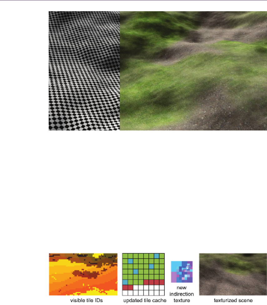
70 4. Virtual Texture Mapping 101
Figure 4.1. Uniquely textured terrain rendering using a single virtual texture.
prevents “holes” from appearing in the rendering, or blocking and waiting until
the load request finishes.
Our implementation is inspired by the GDC talk of Sean Barrett [Barret 08]
and we suggest watching the video of his presentation while reading this section.
As illustrated in Figure 4.2, we begin each frame by determining which tiles are
visible. We identify the ones not cached and request them from disk. After
the tiles have been uploaded into the tile cache on the GPU, we update an
indirection texture, or page table. Eventually, we render the scene, performing an
initial lookup into the indirection texture to determine where to sample in the tile
cache.
Figure 4.2. We render tile IDs, then identify and upload newly visible tiles into the tile
cache (red), possibly overwriting ones that are no longer visible (blue). We update the
indirection texture and render the texturized surfaces.

4.2. Virtual Texture Mapping 71
The indirection texture is a scaled down version of the complete virtual tex-
ture, where each texel points to a tile in the tile cache. In our case, the tile cache
is simply one large texture on the GPU, containing small, square tiles of identi-
cal resolution. This means tiles from different MIP map levels cover differently
sized areas of the virtual texture, but simplifies the management of the tile cache
considerably.
4.2.1 Page Fault Generation
For each frame we determine the visible tiles, identify the ones not yet loaded
onto the GPU, and request them from disk. Future hardware might simplify this
with native page faults [Seiler et al. 08], but we still need to determine visible
tiles, substitute data and redirect memory accesses.
A simple approach is to render the complete scene with a special shader that
translates the virtual texture coordinates into a tile ID. By rendering the actual
geometry of the scene, we trivially handle occlusion. The framebuffer is then
read back and processed on the CPU along with other management tasks. As
tiles typically cover several pixels, it is possible to render tile IDs at a lower
resolution to reduce bandwidth and processing costs. Also, in order to pre-fetch
tiles that will be visible “soon,” the field of view can be slightly increased. The
corresponding shader code can be found in Section 4.5.2.
4.2.2 Page Handler
The page handler loads requested tiles from disk, uploads them onto the GPU,
and updates the indirection texture. Depending on disk latency and camera
movement, loading the tiles might become a bottleneck. To illustrate this we fly
over a large terrain covered by a single virtual texture and graph the time per
frame in Figure 4.3. Given a reasonably large tile cache, very few tiles are re-
quested and on average we need less than ten ms per frame for I/O and rendering.
However, in frame 512 we turn the camera 180 degrees and continue backwards.
This u-turn requests over 100 tiles, taking 350 ms to load.
To ensure smooth rendering we simply limit the number of updated tiles
per frame. For requests not served in the same frame we adjust the indirection
texture and redirect texture access to the finest parent tile available in the tile
cache. The coarsest level is always present, and this distributes load spikes over
several frames. If the update limit is larger than the average number of requested
tiles, we are guaranteed to catch up with the requests eventually. For our example
we request fewer than five tiles in 95% of the frames, and set the upload limit to
a very conservative 20 tiles.
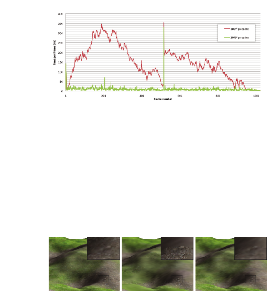
72 4. Virtual Texture Mapping 101
Figure 4.3. We fly over a terrain with one large virtual texture and record the time
per frame. In frame 512 we turn the camera 180 ◦and continue backwards. This turn
is a worst case scenario for VTM: many new tiles—which are no longer in the cache—
become visible and have to be loaded. While sufficiently large caches prevent thrashing,
they help little in this challenging event.
Of course the missing tiles reduce visual quality. Therefore we upload the
requested tiles with all their ancestors, prioritized from coarse to fine. This
increases the total number of cache updates, but as Figure 4.4 shows, image
quality is restored in a more balanced fashion—very similar to progressive JPEG.
As more ancestors are present in the cache, this also improves quality in less
challenging situations and reduces artifacts when rendering tile IDs with a very
low resolution.
Figure 4.4. Half a second after the u-turn. Left: waiting for all tiles provides superior
image quality but stalls for 330 ms. Middle: limiting the uploads per frame and using
coarser MIP map levels as fallback provides smooth frame rates, but MIP levels vary
strongly. Right: using prioritized loading of ancestors improves fallback, and image
quality is much more balanced after the same time.

4.3. Implementation Details 73
4.2.3 Rendering
When texturing the surface we perform a fast unfiltered lookup into the indirec-
tion texture, using the uv-coordinate of the fragment in virtual texture space.
This provides the position of the target tile in the cache and the actual resolution
of its MIP map level in the pyramid of the indirection texture. The latter might
be different from the resolution computed from the fragment’s MIP map level
due to our tile upload limit. We add the offset inside the tile to the tile position
and sample from the tile cache. The offset is simply the fractional part of the
uv-coordinate scaled by the actual resolution:
offset := frac(uv ×actualResolution) = frac(uv ×2indTexEntry.z).
Note that storing the actual resolution as log2(actualResolution) allows us to use
8-bit textures. The complete shader code including the computation of correct
texture gradients (see Section 4.3.3) can be found in Section 4.5.3.
4.3 Implementation Details
In this section we will investigate various implementation issues with a strong
emphasis on texture filtering. Again we will follow the processing of one frame,
from page fault generation over page handling to rendering.
4.3.1 Page Fault Generation
MIP map level. To compute the tile ID in the tile shader we need the virtual
texture coordinates and the current MIP map level. The former are directly the
interpolated uvs used for texturing, but on DX 9 and 10 hardware, we have to
compute the latter manually using gradient instructions [Ewins et al. 98,Wu 98]:
let ddx = (δu
δx ,δv
δx ) and ddy = (δu
δy ,δv
δy ) be the uv gradients in x- and y-direction.
Using their maximal length we compute the MIP map level as
MIP = log2(max(|ddx|,|ddy|).
The corresponding shader code can be found in Section 4.5.1.
DX 10.1 provides the HLSL function CalculateLevelOfDetail(). Further
DX 11 gives access to coarse gradients (dd{x|y}coarse()) which might provide
an even faster alternative to the level of detail function.
4.3.2 Page Handler
Compressed tiles. For efficient rendering it is desirable to have a DXTC com-
pressed tile cache. It requires less memory on the GPU and reduces the upload

74 4. Virtual Texture Mapping 101
and rendering bandwidth. However, as the compression ratio of DXTC is fixed
and quite low, we store the tiles using JPEG and transcode them to DXTC be-
fore we upload them. This also allows us to reduce quality selectively and e.g.,
compress tiles of inaccessible areas stronger.
Disk I/O. For our tutorial implementation we store tiles as individual JPEG files
for the sake of simplicity. However, reading many small files requires slow seeks
and wastes bandwidth. Packing the tiles into a single file is thus very important,
especially for slow devices with large sectors like DVDs.
It is possible to cut down the storage requirements by storing only every
second MIP map level and computing two additional MIP maps for each tile: if
an intermediate level is requested, we load the corresponding four pages from the
finer level instead. More ideas about storage and loading can be found in [van
Waveren 08].
Cache saturation. Unused tiles are overwritten with newly requested tiles using an
LRU policy. However, the current working set might still not fit into the cache. In
this case we remove tiles that promise low impact on visual quality. We replace the
tiles with the finest resolution with their lower-resolution ancestors. This plays
nicely with our progressive update strategy and quickly frees the tile cache. Other
good candidates for removal are tiles with low variance or small screen space area.
Tile upload. Uploading the tiles to the GPU should be fast, with minimum
stalling. Using DX 9, we create a managed texture and let the driver handle the
upload to the GPU. Other approaches for DX 9 are described in detail by [Mit-
tring 08]. For DX 10 and 11, we create a set of intermediate textures and update
these in turn. The textures are copied individually into the tile cache [Thi-
bieroz 08]. DX 11 adds the possibility to update the tiles concurrently, which
further increases performance.
Indirection texture update. After the tiles have been uploaded, we update the
indirection texture by recreating it from scratch. We start by initializing the top
Figure 4.5. Creating the indirection texture for a camera looking over a large terrain:
initializing the top level with the lowest resolution tile, we copy parent entries into the
next finer level and add entries for tiles present in the cache.
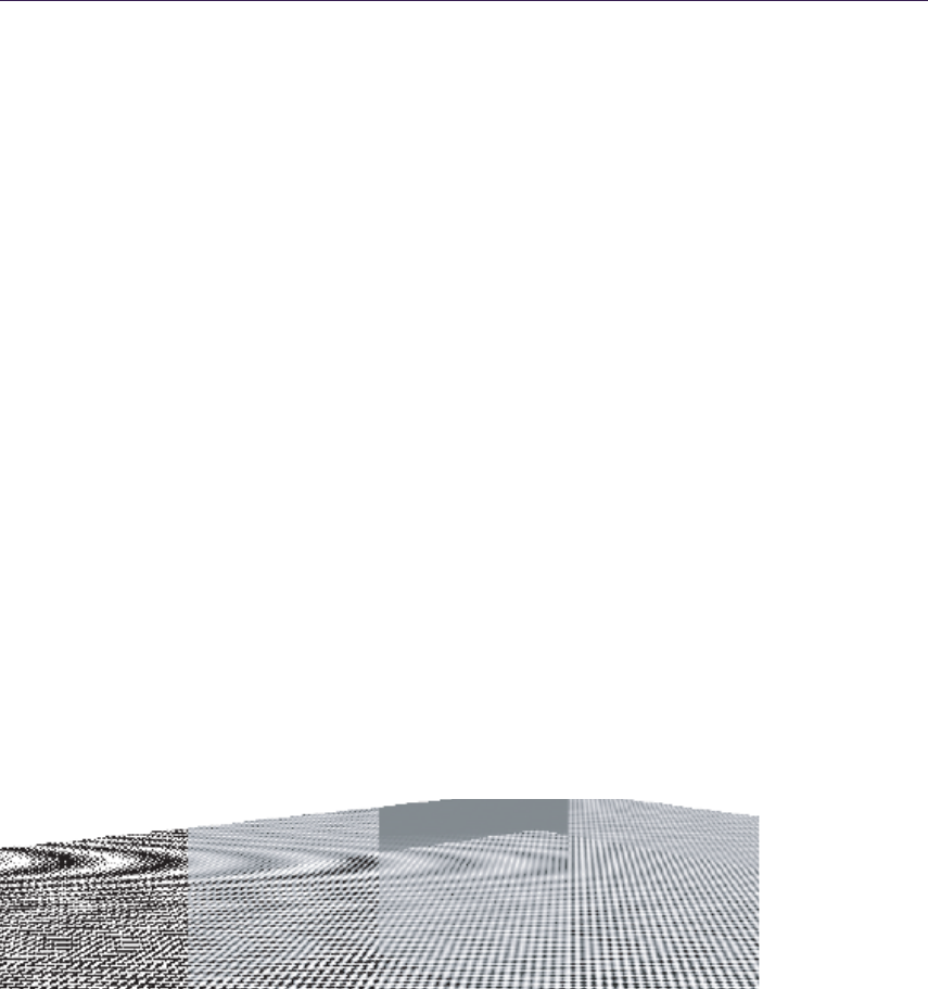
4.3. Implementation Details 75
of its MIP map pyramid with an entry for the tile with the lowest resolution, so
each fragment has a valid fallback. For each finer level we copy the entries of the
parent texels, but replace the copy with entries for tiles from that level, should
they reside in the cache. We continue this process until the complete indirection
texture pyramid is filled (see Figure 4.5).
If tiles are usually seen at a single resolution, we can upload only the finest
level to the GPU. This reduces the required upload bandwidth, simplifies the
lookup, and improves performance. This is sufficient when every object uses an
unique texture, in particular for terrain rendering.
4.3.3 Rendering
While rendering with a virtual texture is straight forward, correct filtering, es-
pecially at tile edges, is less obvious. Neighboring tiles in texture space are very
likely not adjacent to each other in the tile cache. Filtering is especially challeng-
ing if the hardware filtering units should be used, as those rely on having MIP
maps and correct gradients available. The following paragraphs describe how to
use HW filtering with an anisotropy of up to 4:1 as shown in Figure 4.6. The
corresponding shader code can be found in Section 4.5.3.
Texture gradients. When two adjacent tiles in texture space are not adjacent in
the tile cache, as shown in Figure 4.7, the uv-coordinates for the final texture
lookup will vary a great deal between neighboring fragments. This results in
large texture gradients and the graphics hardware will use a very wide filter for
sampling, producing blurry seams. To address this, we manually compute the
Figure 4.6. From left to right: Hardware point (175 fps), bilinear (170 fps), trilinear
(170 fps), and 4:1 anisotropic filtering (165 fps) on an NVIDIA 9700M GT. The transition
between tiles is especially pronounced with trilinear filtering. A single tile has to serve
several MIP map levels in this example, but only one additional MIP map level is
available for filtering per tile. All other methods seem to not use MIP maps at all with
the tested driver version.
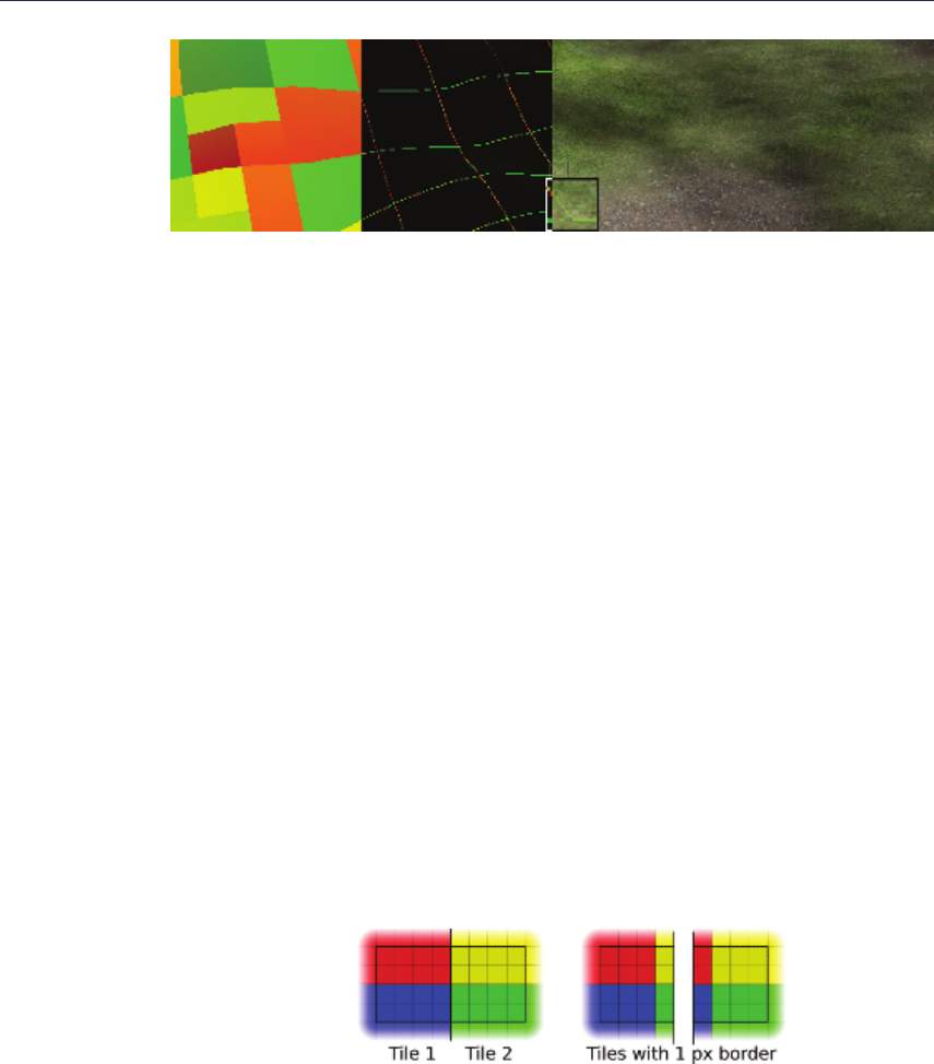
76 4. Virtual Texture Mapping 101
Figure 4.7. Even though the surface has a continuous mapping, the arrangement of
the tiles in the cache causes discontinuities. From left to right: direct visualization
of the lookup position into the tile cache; uv gradients, wrong across tile edges; blurry
seams resulting from too wide filters when sampling. Manually scaled gradients fix this
artifact.
gradients from the original virtual texture coordinates, scale them depending on
the MIP map level of the tile and pass them on to the texture sampler.
Tile borders. Even with correct texture gradients, we still have to filter into neigh-
boring pages, which very likely contain a completely different part of the virtual
texture. To avoid the resulting color bleeding we need to add borders. Depending
on what constraints we want to place on the size of the tile, we can use inner or
outer borders.
We use the latter and surround our 1282tiles with a four-pixel border, making
them 1362. This keeps the resolution a multiple of four, allowing us to compress
them using DXTC and perform 4:1 anisotropic filtering in hardware.
DXTC border blocks. As Figure 4.8 illustrates, adding a border to tiles might lead
to different DXTC blocks at the edges of tiles. As the different blocks will be
compressed differently, texels that represent the same points in virtual texture
space will not have the same values in both tiles. This leads to color bleeding
across tile edges, despite the border. By using a four-pixel outer border, these
compression related artifacts vanish.
Figure 4.8. Adding a one-pixel border around a tile creates different DXTC blocks
for neighboring tiles. Depending on the texture they might be compressed differently,
leading to visible seams in the virtual texture despite having borders.

4.4. Conclusion 77
4.4 Conclusion
In this chapter, we described a basic virtual texture mapping system. It is simple
and fast, even on older hardware. We gave a few pointers on how to further
improve performance, should your application or game require it. Even with
newer hardware that might natively support page faults, strategies for loading,
compressing and filtering textures will still be required. We hope this article
and our tutorial implementation will help you to get started with VTM. You can
integrate it into your own application or just play with different parameters and
strategies.
4.5 Shader Code
4.5.1 MIP Map Calculation
fl oat C om pu te Mi pMapLev el ( flo at2 UV_ pixel s , f loat sc ale )
{
flo at2 x _d er iv = ddx ( UV_ pi xe ls ) ;
flo at2 y _d er iv = ddy ( UV_ pi xe ls ) ;
fl oat d = max ( le ngth ( x_de riv ) , le ngth ( y _der iv ) );
retur n max ( lo g2 ( d) - log2 ( sc ale ) , 0) ;
}
4.5.2 Tile ID Shader
floa t2 U V_ p ix el s = In . U V * V TM Re so lu ti on ,
fl oat m ipLev el = C om pu te Mi pM ap Le vel ( UV_pi xel s , sub Sa mp le Fa ct or );
mipL ev el = flo or ( min ( mi pLe vel , M ax Mip Ma pLe vel ));
float4 tileID;
til eI D . rg = f lo or ( U V_ pi x el s / ( T il eR es * ex p2 ( m ip Le ve l ) ));
tileID . b = mip Leve l ;
tileID . a = Tex tureI D ;
return tileID;

78 4. Virtual Texture Mapping 101
4.5.3 Virtual Texture Lookup
flo at 3 t il e En tr y = I nd Te x . Sa mp le ( P oi nt Sa mp le r , I n . UV );
fl oat a ctualR es olution = exp2 ( ti leEnt ry .z);
flo at 2 o ff se t = f rac ( In . UV * a ct ual R es o lu ti o n ) * T il eR es ;
fl oat sca le = actu al Re soluti on * T ileR es ;
flo at 2 d dx_ c or re ct = d dx ( In . UV ) * s ca le ;
flo at 2 d dy_ c or re ct = d dy ( In . UV ) * s ca le ;
return Til eCac he . Samp leGra d ( Text ure Samp ler ,
t il eE nt ry . xy + o ffs et ,
ddx_correct ,
ddy _corr ect );
4.6 Acknowledgments
We’d like to thank J.M.P van Waveren for generously sharing his insights on
virtual texture mapping.
Bibliography
[Barret 08] Sean Barret. “Sparse Virtual Textures.” 2008. http://silverspaceship.
com/src/svt/.
[Ewins et al. 98] JP Ewins, MD Waller, M. White, and PF Lister. “MIP-Map
Level Selection For Texture Mapping.” Visualization and Computer Graph-
ics, IEEE Transactions on 4:4 (1998), 317–329.
[Kraus and Ertl 02] Martin Kraus and Thomas Ertl. “Adaptive Texture Maps.”
In HWWS ’02: Proceedings of the ACM SIGGRAPH/EUROGRAPHICS
Conference on Graphics Hardware, pp. 7–15. Aire-la-Ville, Switzerland,
Switzerland: Eurographics Association, 2002.
[Lefebvre et al. 04] Sylvain Lefebvre, Jerome Darbon, and Fabrice Neyret. “Uni-
fied Texture Management for Arbitrary Meshes.” Technical Report RR5210,
INRIA, 2004. Available online (http://www-evasion.imag.fr/Publications/
2004/LDN04).
[Mittring 08] Martin Mittring. “Advanced Virtual Texture Topics.” 2008.
http://ati.amd.com/developer/SIGGRAPH08/Chapter02-Mittring
-Advanced Virtual Texture Topics.pdf.

Bibliography 79
[Seiler et al. 08] Larry Seiler, Doug Carmean, Eric Sprangle, Tom Forsyth,
Michael Abrash, Pradeep Dubey, Stephen Junkins, Adam Lake, Jeremy Sug-
erman, Robert Cavin, Roger Espasa, Ed Grochowski, Toni Juan, and Pat
Hanrahan. “Larrabee: A Many-Core x86 Architecture for Visual Comput-
ing.” ACM Trans. Graph. 27:3 (2008), 1–15.
[Tanner et al. 98] C.C. Tanner, C.J. Migdal, and M.T. Jones. “The Clipmap: A
Virtual Mipmap.” In Proceedings of the 25th Annual Conference on Com-
puter Graphics and Interactive Techniques, pp. 151–158. ACM New York,
1998.
[Thibieroz 08] Nicolas Thibieroz. “Ultimate Graphics Performance for Di-
rectX 10 Hardware.” GDC Presentation, 2008.
[van Waveren 08] J. M. P. van Waveren. “Geospatial Texture Streaming
from Slow Storage Devices.” 2008. http://software.intel.com/en-us/articles/
geospatial-texture-streaming-from-slow-storage-devices/.
[Wu 98] Kevin Wu. “Direct Calculation of MIP-Map Level for Faster Texture
Mapping.” Hewlett-Packard Laboratories, 1998. http://www.hpl.hp.com/
techreports/98/HPL-98-112.html.

5
Pre-Integrated Skin Shading
Eric Penner and George Borshukov
5.1 Introduction
Rendering realistic skin has always been a challenge in computer graphics. Human
observers are particularly sensitive to the appearance of faces and skin, and skin
exhibits several complex visual characteristics that are difficult to capture with
simple shading models. One of the defining characteristics of skin is the way
light bounces around in the dermis and epidermis layers. When rendering using
a simple diffuse model, the light is assumed to immediately bounce equally in all
directions after striking the surface. While this is very fast to compute, it gives
surfaces a very “thin” and “hard” appearance. In order to make skin look more
“soft” it is necessary to take into account the way light bounces around inside
a surface. This phenomenon is known as subsurface scattering, and substantial
recent effort has been spent on the problem of realistic, real-time rendering with
accurate subsurface scattering.
Current skin-shading techniques usually simulate subsurface scattering during
rendering by either simulating light as it travels through skin, or by gathering
incident light from neighboring locations. In this chapter we discuss a differ-
ent approach to skin shading: rather than gathering neighboring light, we pre-
integrate the effects of scattered light. Pre-integrating allows us to achieve the
nonlocal effects of subsurface scattering using only locally stored information and
a custom shading model. What this means is that our skin shader becomes just
that: a simple pixel shader. No extra passes are required and no blurring is
required, in texture space nor screen space. Therefore, the cost of our algorithm
scales directly with the number of pixels shaded, just like simple shading models
such as Blinn-Phong, and it can be implemented on any hardware, with minimal
programmable shading support.
81

82 5. Pre-Integrated Skin Shading
5.2 Background and Previous Work
Several offline and real-time approaches have been based on an approach, taken
from film, called texture-space diffusion (TSD). TSD stores incoming light in
texture space and uses a blurring step to simulate diffusion. The first use of this
technique was by [Borshukov and Lewis 03,Borshukov and Lewis 05] in the Matrix
sequels. They rendered light into a texture-space map and then used a custom
blur kernel to gather scattered light from all directions. Based on extensive
reference to real skin, they used different blur kernels for the red, green, and blue
color channels, since different wavelengths of light scatter differently through
skin. Since the texture-space diffusion approach used texture-blur operations,
it was a very good fit for graphics hardware and was adopted for use in real-
time rendering [Green 04,Gosselin et al. 04]. While TSD approaches achieved
much more realistic results, the simple blurring operations performed in real
time couldn’t initially achieve the same level of quality of the expensive, original,
nonseparable blurs used in film.
A concept that accurately describes how light diffuses in skin and other
translucent materials is known as the diffusion profile. For a highly scattering
translucent material it is assumed that light scatters equally in all directions as
soon as it hits the surface. A diffusion profile can be thought of as a simple plot
of how much of this diffused light exits the surface as a function of the distance
from the point of entry. Diffusion profiles can be calculated using measured scat-
tering parameters via mathematical models known as dipole [Jensen et al. 01] or
multipole [Donner and Jensen 05] diffusion models. The dipole model works for
simpler materials, while the multipole model can simulate the effect of several
layers, each with different scattering parameters.
The work by [d’Eon and Luebke 07] sets the current high bar in real-time
skin rendering, combining the concept of fast Gaussian texture-space diffusion
with the rigor of physically based diffusion profiles. Their approach uses a sum
of Gaussians to approximate a multipole diffusion profile for skin, allowing a very
large diffusion profile to be simulated using several separable Gaussian blurs.
More recent approaches have achieved marked performance improvements. For
example, [Hable et al. 09] have presented an optimized texture-space blur kernel,
while [Jimenez et al. 09] have applied the technique in screen space.
5.3 Pre-Integrating the Effects of Scattering
We have taken a different approach to the problem of subsurface scattering in
skin and have departed from texture-space diffusion (see Figure 5.1). Instead, we
wished to see how far we could push realistic skin rendering while maintaining the
benefits of a local shading model. Local shading models have the advantage of
not requiring additional rendering passes for each object, and scale linearly with
the number of pixels shaded. Therefore, rather than trying to achieve subsur-
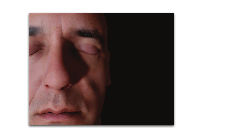
5.3. Pre-Integrating the Effects of Scattering 83
Figure 5.1. Our pre-integrated skin-shading approach uses the same diffusion profiles
as texture-space diffusion, but uses a local shading model. Note how light bleeds over
lighting boundaries and into shadows. (Mesh and textures courtesy of XYZRGB.)
face scattering by gathering incoming light from nearby locations (performing an
integration during runtime), we instead seek to pre-integrate the effects of sub-
surface scattering in skin. Pre-integration is used in many domains and simply
refers to integrating a function in advance, such that calculations that rely on the
function’s integral can be accelerated later. Image convolution and blurring are
just a form of numerical integration.
The obvious caveat of pre-integration is that in order to pre-integrate a func-
tion, we need to know that it won’t change in the future. Since the incident light
on skin can conceivably be almost arbitrary, it seems as though precomputing this
effect will prove difficult, especially for changing surfaces. However, by focusing
only on skin rather than arbitrary materials, and choosing specifically where and
what to pre-integrate, we found what we believe is a happy medium. In total, we
pre-integrate the effect of scattering in three special steps: on the lighting model,
on small surface details, and on occluded light (shadows). By applying all of
these in tandem, we achieve similar results to texture-space diffusion approaches
in a completely local pixel shader, with few additional constraints.
To understand the reasoning behind our approach, it first helps to picture a
completely flat piece of skin under uniform directional light. In this particular
case, no visible scattering will occur because the incident light is the same ev-
erywhere. The only three things that introduce visible scattering are changes in

84 5. Pre-Integrated Skin Shading
the surrounding mesh curvature, bumps in the normal map, and occluded light
(shadows). We deal with each of these phenomena separately.
5.4 Scattering and Diffuse Light
If we take our previously flat surface with no visible scattering and start to make it
a smooth and curvy surface, like skin (we will keep it smooth for now), scattering
will start to become visible. This occurs due to the changes in incident light
across the surface. The Lambert diffuse-lighting model assumes that diffuse light
scatters equally in all directions, and the amount of incident light is proportional
to the cosine of the angle between the surface normal and light direction (N·L).
Since N·Lfalloff is a primary cause of changing incident light, and thus
visible scattering, there have been several rendering tricks that attempt to add
the look of scattering by altering the N·Lfall-off itself. This involves making
the falloff wrap around the back of objects, or by letting each wavelength of light
(r,g, and b) fall off differently as N·Lapproaches zero. What we found to
be the big problem with such approaches is that they aren’t based on physical
measurements of real skin-like diffusion profiles; and if you tune them to look
nice for highly curved surfaces, then there will be a massive falloff for almost-flat
surfaces (and vice versa).
To address both issues, we precompute the effect of diffuse light scattering.
We do this in a fashion similar to measured bidirectional reflectance distribution
functions (BRDFs). Measured BRDFs use physically measured data from real
surfaces to map incoming to outgoing light. This is as opposed to analytical
BRDFs such as Blinn-Phong that are analytical approximations for an assumed
micro-facet structure. Typical measured BRDFs don’t incorporate N·Lsince
N·Ljust represents the amount of incoming light and isn’t part of the surface’s
reflectance. We are concerned only with N·L(diffuse light), as this is the light
that contributes to subsurface scattering.
One approach we considered to precompute the effect of scattered light at any
point on a surface, was to simulate lighting from all directions and compress that
data using spherical harmonics. Unfortunately, spherical harmonics can efficiently
represent only very low frequency changes or would require too many coefficients.
Thus, instead of precomputing the effect of scattering at all locations, we chose
to precompute the scattering falloff for a subset of surface shapes and determine
the best falloff during forward rendering. As discussed above, one characteristic
that we can calculate in a shader is surface curvature, which largely determines
the effect of scattering on smooth surfaces.
To measure the effect of surface curvature on scattering, we add curvature
as the second parameter to our measured diffuse falloff. The skin diffusion pro-
files from [d’Eon and Luebke 07] on flat skin can be used to simulate the effect
of scattering on different curvatures. We simply light a spherical surface of a

5.4. Scattering and Diffuse Light 85
given curvature from one direction and measure the accumulated light at each
angle with respect to the light (see Figures 5.2 and 5.3). This results in a two-
dimensional lookup texture that we can use at runtime. More formally, for each
skin curvature and for all angles θbetween Nand L, we perform the integration
in Equation (5.1):
D(θ, r) = Rπ
-πcos(θ+x)·R(2rsin(x/2))dx
Rπ
-πR(2 sin(x/2))dx (5.1)
The first thing to note is that we have approximated a spherical integration
with integration on a ring. We found the difference was negligible and the ring
integration fits nicely into a shader that is used to compute the lookup texture.
The variable R() refers to the diffusion profile, for which we used the sum of
Gaussians from [d’Eon and Luebke 07] (see Table 5.1). Rather than performing
an expensive arccos() operation in our shader to calculate the angle, we push
this into the lookup, so our lookup is indexed by N·Ldirectly. This is fine in
our case, as the area where scattering occurs has plenty of space in the lookup.
Figures 5.2 and 5.3 illustrate how to compute and use the diffuse lookup texture.
While this measured skin model can provide some interesting results on its
own, it still has a few major flaws. Primarily, it assumes that all skin resembles
a sphere, when, in fact, skin can have fairly arbitrary topology. Stated another
way, it assumes that scattered light arriving at a given point depends on the
curvature of that point itself. In actuality it depends on the curvature of all of
the surrounding points on the surface. Thus, this approximation will work very
well on smooth surfaces without fast changes in curvature, but breaks down when
curvature changes too quickly. Thankfully, most models of skin are broken up
into two detail levels: smooth surfaces represented using geometry, and surface
1.99
0.007 0.007
7.41
0.6490.0064
0.0
0
0.233
0.004
0.078
0.118
0.366
0.0
0.567
0.198
0.1000.0484
0.0
0.455
0.113
0.187
0.358
0.344
Red BlueVariance Green
Table 5.1. The weights used by [d’Eon and Luebke 07] for texture-space diffusion.
Although we aren’t limited to the sum of Gaussians approximations, we use the same
profile for comparison.
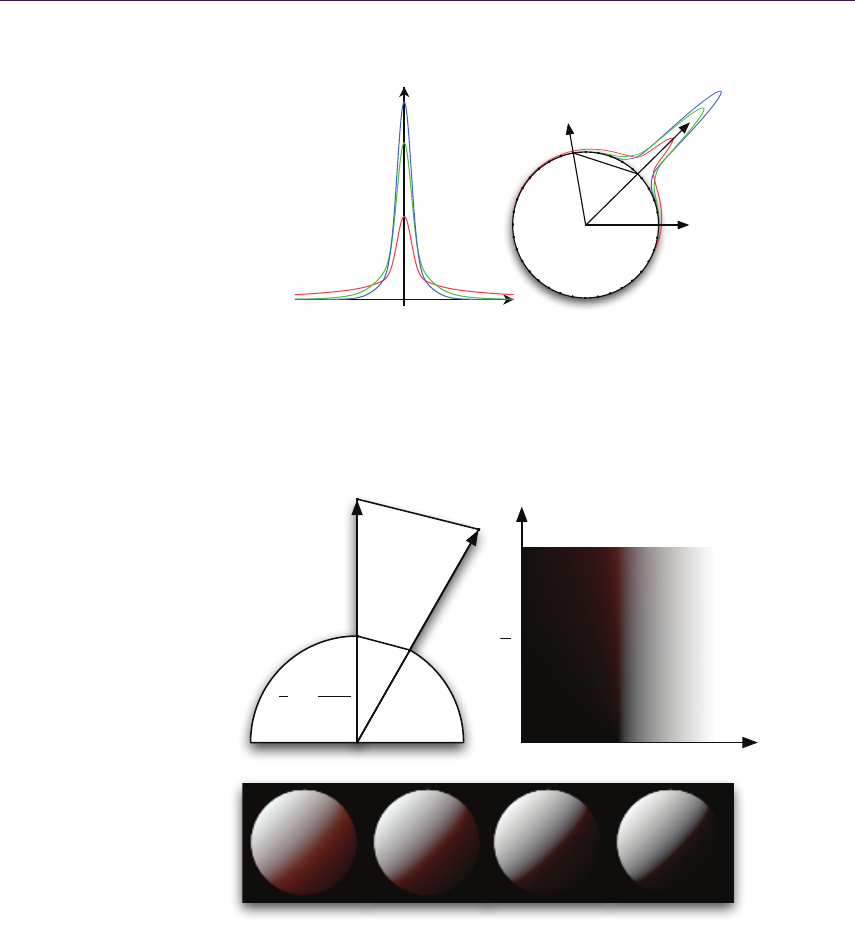
86 5. Pre-Integrated Skin Shading
L
N
2rsin(θ/2))
N+θ
R(x)
Distance(mm)
Figure 5.2. The graph (left) illustrates the diffusion profile of red, green, and blue light
in skin, using the sum of Gaussians from Table 5.1. The diagram (right) illustrates
how we pre-integrate the effect of scattering into a diffuse BRDF lookup. The diffusion
profile for skin (overlaid radially for one angle) is used to blur a simple diffuse BRDF
for all curvatures of skin.
∆N
∆p
|N|=1
r=4
r=2
r=8
r= 16
N·L
1
r=∆N
∆p
1
r
Figure 5.3. The diagram (top left) illustrates how we calculate curvature while rendering
using two derivatives. The diffuse BRDF lookup, indexed by curvature (sphere radius)
and N·L(top right). Spheres of different sized renderings using the new BRDF lookup
(bottom).

5.5. Scattering and Normal Maps 87
details represented in a normal map. We take advantage of this and let the
measured diffuse falloff be chosen at the smooth geometry level, while adding
another approach to deal with creases and small bumps in normal maps, which
are responsible for quick changes in curvature.
5.5 Scattering and Normal Maps
We now turn to the effect of scattering on small wrinkles and pores that are usu-
ally represented with a normal map. Since the normal from a small crease always
returns to the dominant surface normal, the reflected scattered light coming from
that crease will look very similar to light reflected from a nonscattering surface
with a physically broader (or blurred-out) crease. Coincidentally, one way of ap-
proximating the look of scattered-over small creases and bumps is to simply blur
the creases and bumps themselves! Most important however, this effect will be
different for each wavelength of light, because of their different diffusion profiles.
Interestingly, the inverse of this phenomenon was noted when capturing nor-
mals from a real subject, using image-based lighting. Ma et al. [Ma et al. 07]
noted that, when captured using spherical gradient lighting, normals become
bent toward the dominant-surface normal, depending on the wavelength of light
used to capture them (red was more bent than green, etc.). They also noted that
a local skin-shading model was improved by using all the normals they captured
instead of only one. In this case the image-based normal capture was physically
integrating all the scattered light when determining the best normal to fit the
data. Since we have only one set of normal maps to begin with, we essentially
work in reverse. We assume that our original normal map is the accurate surface
normal map and blur it several times for each wavelength, resulting in a separate
normal map for each color, and for specular reflection. As mentioned by previous
authors [d’Eon and Luebke 07,Hable et al. 09,Jimenez et al. 09], care should be
taken to make sure the original normal map has not been blurred already in an
attempt to get a smoother look.
While it might seem to make sense to simply blur the normal map using the
diffusion profile of skin, this approach is not completely valid since lighting is not a
linear process with regard to the surface normal. What we really want to have is a
representation of the normal which can be linearly filtered, much in the same way
that shadow maps can be filtered linearly using a technique like variance shadow
mapping. Interestingly, there has been some very recent work in linear normal
map filtering. Linear efficient antialiased normal (LEAN) mapping [Olano and
Baker 10] represents the first and second moments of bumps in surface-tangent
space. Olano and Baker focused primarily on representing specular light but
also suggest a diffuse-filtering approximation from [Kilgard 00] which simply uses
the linearly filtered unnormalized normal and standard diffuse lighting. It is
noteworthy that the unnormalized normal is actually a valid approximation when

88 5. Pre-Integrated Skin Shading
a bump self-shadowing and incident/scattered lighting term is constant over the
normal-map filtering region. In that case,
1
nΣn
i=1(KdiffuseL·Ni) = KdiffuseL·(1
nΣn
i=1Ni).
The reason this isn’t always the case is that diffuse lighting incorporates a self-
shadowing term max(0, N ·L) instead of simply N·L. This means back-facing
bumps will actually contribute negative light when linearly filtered. Nonetheless,
using the unnormalized normal will still be valid when all bumps are unshadowed
or completely shadowed, and provides a better approximation than the normal-
ized normal in all situations, according to [Kilgard 00].
Although we would prefer a completely robust method of pre-integrating nor-
mal maps that supports even changes in incident/scattered light over the filtering
region, we found that blurring, using diffusion profiles, provided surprisingly good
results (whether or not we renormalize). In addition, since using four normals
would require four transformations into tangent space and four times the mem-
ory, we investigated an approximation using only one mipmapped normal map.
When using this optimization, we sample the specular normal as usual, but also
sample a red normal clamped below a tunable miplevel in another sampler. We
then transform those two normals into tangent space and blend between them
to get green and blue normals. The resulting diffuse-lighting calculations must
then be performed three times instead of once. The geometry normal can even
be used in place of the second normal map sample, if the normal map contains
small details exclusively. If larger curves are present, blue/green artifacts will
appear where the normal map and geometry normal deviate, thus the second
mipmapped sample is required.
We found that this approach to handling normal maps complements our cus-
tom diffuse falloff very well. Since the red normal becomes more heavily blurred,
the surface represented by the blurred normal becomes much more smooth, which
is the primary assumption made in our custom diffuse falloff. Unfortunately, there
is one caveat to using these two approaches together. Since we have separate nor-
mals for each color, we need to perform three diffuse lookups resulting in three
texture fetches per light. We discuss a few approaches to optimizing this in
Section 5.7.
5.6 Shadow Scattering
Although we can now represent scattering due to small- and large-scale features,
we are still missing scattering over occluded light boundaries (shadows). The
effect of light scattering into shadows is one of the most noticeable features of
realistically rendered skin. One would think that scattering from shadows is much
more difficult since they are inherently nonlocal to the surface. However, by using
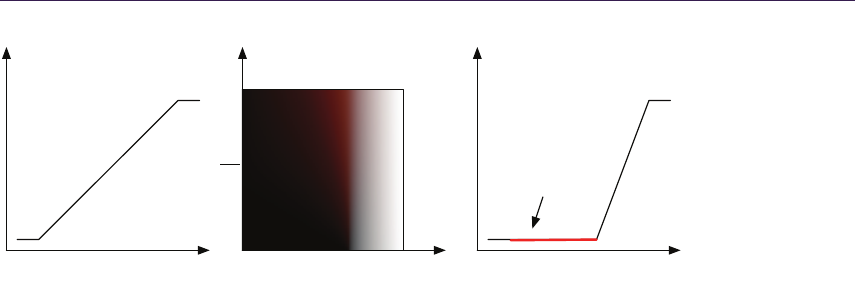
5.6. Shadow Scattering 89
Scattering
Original Penumbra Pre-Integrated Penumbrae New Penumbra
s
1
w
Figure 5.4. Illustration of pre-integrated scattering falloff from shadows. A typical
shadow falloff from a box-filtered shadow map (left). A smaller penumbra that we
pre-integrate against the diffusion profile of skin (right). The lookup maps the first
penumbra into the second but also stores additional scattered light. The lookup is
parameterized by the original shadow value and the width of the penumbra in world
space (center).
a small trick, we found we could pre-integrate the effect of scattering over shadow
boundaries in the same way we represent scattering in our lighting model.
The trick we use for shadows is to think of the results of our shadow map-
ping algorithm as a falloff function rather than directly as a penumbra. When
the falloff is completely black or white, we know we are completely occluded or
unoccluded, respectively. However, we can choose to reinterpret what happens
between those two values. Specifically, if we ensure the penumbra size created
by our shadow map filter is of adequate width to contain most of the diffusion
profile, we can choose a different (smaller) size for the penumbra and use the
rest of the falloff to represent scattering according to the diffusion profile (see
Figure 5.4).
To calculate an accurate falloff, we begin by using the knowledge of the shape
of our shadow mapping blur kernel to pre-integrate a representative shadow
penumbra against the diffusion profile for skin. We define the representative
shadow penumbra P() as a one-dimensional falloff from filtering a straight shadow
edge (a step function) against the shadow mapping blur kernel. Assuming a mono-
tonically decreasing shadow mapping kernel, the representative shadow falloff is
also a monotonically decreasing function and is thus invertible within the penum-
bra. Thus, for a given shadow value we can find the position within the repre-
sentative penumbra using the inverse P−1(). As an example, for the simple case
of a box filter, the shadow will be a linear ramp, for which the inverse is also a
linear ramp. More complicated filters have more complicated inverses and need
to be derived by hand or by using software like Mathematica. Using the inverse,
we can create a lookup texture that maps the original falloff back to its location
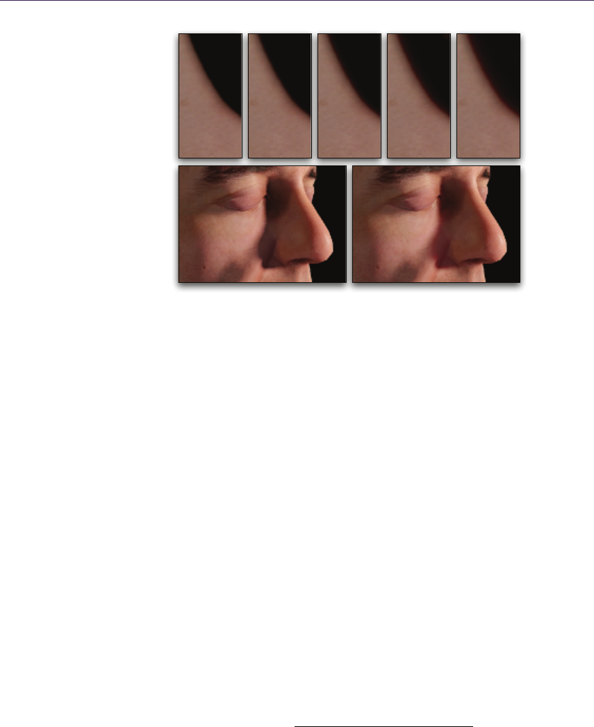
90 5. Pre-Integrated Skin Shading
Figure 5.5. Illustration of pre-integrated scattering falloff from shadows. Controlled
scattering based on increased penumbra width, such as a penumbra cast onto a highly
slanted surface (top). Comparison with and without shadow scattering (bottom).
in the penumbra and then to a completely different falloff. Specifically, we can
make the new shadow falloff smaller and use the remainder to represent subsur-
face scattering from the new penumbra. In the end, we are left with a simple
integration to perform that we can use as a lookup during rendering, exactly like
our diffuse falloff.
We should note at this point that we could run into problems if our as-
sumptions from above are invalidated. We found that a two-dimensional shadow
falloff was not noticeably different from a one-dimensional one, but we have also
assumed that all shadow transitions are sharp. For example, if something like
a screen door were to cast a shadow, it might result in a constant penumbra
value between zero and one. In that case, we would assume there is scattering
from a falloff that isn’t there. Additionally, we have assumed projection onto a
flat surface. If the surface is highly slanted, then the true penumbra size will
be much larger than the one we used during pre-integration. For this reason
we add a second dimension to our shadow falloff texture, which represents the
size of the penumbra in world space. This is similar to the way we pre-integrate
lighting against all sphere sizes. In the end, our two-dimensional shadow-lookup
integration is a simple convolution:
PS(s, w) = R∞
-∞P0(P−1(s) + x)R(x/w)dx
R∞
-∞R(x/w)dx ,
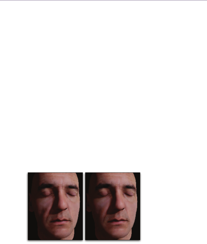
5.7. Conclusion and Future Work 91
where P−1() is the inverse of our representative falloff, P0() is the new, smaller
penumbra, R() is the diffusion profile, and sand ware the shadow value and
penumbra width in world space, respectively. Penumbra width can be detected
using either the angle of the surface with respect to the light, or potentially the
derivative of the shadow value itself. Since creating a large penumbra is expensive
using conventional shadow filtering (although, see the Pixel Quad Amortization
chapter), having the penumbra stretched over a slanted surface provides a larger
space for scattering falloff and thus can actually be desirable if the initial shadow
penumbra isn’t wide enough. In this case the lookup can be clamped to insure
that the falloff fits into the space provided.
5.7 Conclusion and Future Work
We have presented a new local skin-shading approach based on pre-integration
that approximates the same effects found in more expensive TSD-based ap-
proaches. Our approach can be implemented by adding our custom diffuse- and
shadow-falloff textures to a typical skin shader (see Figure 5.6).
Although we found that our approach worked on a large variety of models,
there are still a few drawbacks that should be mentioned. When approximating
curvature using pixel shader derivatives, triangle edges may become visible where
curvature changes quickly. Depending on how the model was created we also
found that curvature could change rapidly or unnaturally in some cases. We are
looking into better approaches to approximating curvature in these cases. This is
much more easily done with geometry shaders that can utilize surface topology.
Pre-Integration
Texture Space Diffusion
Figure 5.6. Comparison of our approach with texture-space diffusion using an optimized
blur kernel from [Hable et al. 09]. (Mesh and textures courtesy of XYZRGB.)

92 5. Pre-Integrated Skin Shading
We would also like to look at the effect of using more than one principal axis
of curvature. For models where curvature discontinuities occur, we generate a
curvature map that can be blurred and further edited by hand, similar to a
stretch map in TSD.
Another challenge we would like to meet is to efficiently combine our normal
map and diffuse-lighting approaches. When using three diffuse normals, we cur-
rently need three diffuse-texture lookups. We found we could use fewer lookups
depending on the number of lights and the importance of each light. We have also
found it promising to approximate the diffuse and shadow falloffs using analytical
approximations that can be evaluated without texture lookups.
We would also like to apply our technique to environment mapping. It
should be straightforward to support diffuse-environment mapping via an ar-
ray of diffuse-environment maps that are blurred based on curvature, in the same
manner as our diffuse-falloff texture.
5.8 Appendix A: Lookup Textures
fl oat G aussi an ( float v , float r)
{
return 1. 0/ s qrt (2 .0* PI *v ) * ex p (-( r* r) /( 2* v));
}
float 3 S catt er ( float r)
{
// C oe ff ic ie nt s from GP U G ems 3 - ‘‘ Ad va nc ed Sk in Ren de ri ng
.’’
return Gau ss ia n (0 .0 06 4 * 1. 414 , r ) * f loat 3
(0.233 ,0.455 ,0.649) +
Gau ss ia n (0. 04 84 * 1.414 , r ) * f lo at3
(0.100 ,0.336 ,0.344) +
Gau ss ia n (0. 18 70 * 1.414 , r ) * f lo at3
(0.118 ,0.198 ,0.000) +
Gau ss ia n (0 .5 67 0 * 1. 414 , r ) * f loat 3
(0.113 ,0.007 ,0.007) +
Gau ss ia n (1 .9 90 0 * 1. 414 , r ) * f loat 3
(0.358 ,0.004 ,0.000) +
Gau ss ia n (7. 41 00 * 1.414 , r ) * f lo at3
(0.078 ,0.000 ,0.000) ;
}
float 3 i nt egr at eSh ad owS cat te rin g ( fl oat p enu mbra Loca tion ,
fl oat p enumb raWidt h )
{
float 3 t otalW eight s = 0;
float 3 t otal Light = 0;

5.9. Appendix B: Simplified Skin Shader 93
fl oat a = - P RO FI LE _W IDT H ;
wh ile ( a <= P RO FI LE _W IDTH )
wh ile ( a <= P RO FI LE _W IDTH )
{
fl oat light = ne wPenu mbra ( pen um braLoc at ion + a/
pen um braW idth );
fl oat s am pl eD is t = abs ( a);
float 3 wei ghts = S catt er ( samp leDis t );
tot al Weight s += w eigh ts ;
tot alLig ht += l igh t * wei ghts ;
a += in c ;
}
return tot alLig ht / tota lWeigh ts ;
}
float 3 i nte gra teD iff use Sca tte rin gOn Rin g ( float c osThe ta , float
ski nRadi us )
{
// Angle from lig htin g dire ction .
fl oat t het a = acos ( cos Th eta ) ;
float 3 t otalW eight s = 0;
float 3 t otal Light = 0;
fl oat a = -( PI /2 ) ;
wh ile ( a <=( PI /2) )
wh ile ( a <=( PI /2) )
{
fl oat s ampl e Angl e = theta + a;
fl oat d if fu se = sat ur at e ( cos ( s amp le An gle ) ) ;
fl oat s am pl eD is t = abs (2. 0* s ki nR ad iu s * si n (a * 0. 5) ) ;
// D istance .
float 3 wei ghts = S catt er ( samp leDis t );
// P rofi le Weight .
tot al Weight s += w eigh ts ;
tot alLig ht += diffus e * weights ;
a += in c ;
}
return tot alLig ht / tota lWeigh ts ;
}
Listing 5.1. Shader code to precompute skin falloff textures.
5.9 Appendix B: Simplified Skin Shader
float 3 Skin Diffus e ( float curv , flo at3 N dotL )
{
float 3 lookup = NdotL * 0.5 + 0.5;
float 3 dif fuse ;

94 5. Pre-Integrated Skin Shading
diffus e .r = tex 2D ( Ski nD iffus eSamp ler , f loat2 ( lookup .r , curv
) ).r;
diffus e .g = tex 2D ( Ski nD iffus eSamp ler , f loat2 ( lookup .g , curv
) ).g;
diffus e .b = tex 2D ( Ski nD iffus eSamp ler , f loat2 ( lookup .b , curv
) ).b;
return diffuse;
}
float 3 Skin Shado w ( float shad , float width )
{
return te x2 D ( Sk in Sh ad ow Sa mp le r , flo at 2 ( shad , w id th ) ) . rgb ;
}
...
// Simple c urvat ure cal culati on .
fl oat c urvat ure = sat urat e ( leng th ( fwi dth ( Normal )) /
lengt h ( fwid th ( Wor ldPos ) ) * tun eC ur vature ) ;
...
// S pecul ar / Dif fuse Nor mals .
flo at 4 n o rm Ma pH i gh = te x2 D ( N or m al Sa mp le r Hi gh , Uv ) * 2. 0 -
1.0;
float 4 n ormM apLow = tex2D ( Norm a lSamp l erLow , Uv ) * 2.0 -
1.0;
float 3 N_high = mul ( normMa pHigh . xyz , T angen tToWor ld ) ;
float 3 N_low = mul ( normM apLow . xyz , T angent ToWorl d );
float3 rS = N_high;
float 3 rN = lerp (N_high , N_low , tun eNorma lBlur .r);
float 3 gN = lerp (N_high , N_low , tun eNorma lBlur .g);
float 3 bN = lerp (N_high , N_low , tun eNorma lBlur .b);
...
// Dif fuse l ight ing
flo at3 N dotL = flo at 3 ( do t (rN , L) , dot ( gN , L) , dot (bN , L) );
float 3 diff use = S kinDi ffus e ( curvature , NdotL ) * Ligh tCol or *
Ski nShad ow ( S am pleSha do wMap ( Sha dowU V ) ) ;
Listing 5.2. Skin shader example.
Bibliography
[Borshukov and Lewis 03] George Borshukov and J.P. Lewis. “Realistic Human
Face Rendering for The Matrix Reloaded.” In ACM Siggraph Sketches and
Applications. New York: ACM, 2003.
[Borshukov and Lewis 05] George Borshukov and J.P. Lewis. “Fast Subsurface
Scattering.” In ACM Siggraph Course on Digital Face Cloning. New York:
ACM, 2005.
[d’Eon and Luebke 07] E. d’Eon and D. Luebke. “Advanced Techniques for Re-
alistic Real-Time Skin Rendering.” In GPU Gems 3, Chapter 14. Reading,
MA: Addison Wesley, 2007.

Bibliography 95
[Donner and Jensen 05] Craig Donner and Henrik Wann Jensen. “Light Diffusion
in Multi-Layered Translucent Materials.” ACM Trans. Graph. 24 (2005),
1032–1039.
[Gosselin et al. 04] D. Gosselin, P.V. Sander, and J.L. Mitchell. “Real-Time
Texture-Space Skin Rendering.” In ShaderX3: Advanced Rendering with
DirectX and OpenGl. Hingham, MA: Charles River Media, 2004.
[Green 04] Simon Green. “Real-Time Approximations to Subsurface Scattering.”
In GPU Gems, pp. 263–278. Reading, MA: Addison-Wesley, 2004.
[Hable et al. 09] John Hable, George Borshukov, and Jim Hejl. “Fast Skin Shad-
ing.” In ShaderX7: Advanced Rendering Techniques, Chapter II.4. Hingham,
MA: Charles River Media, 2009.
[Jensen et al. 01] Henrik Jensen, Stephen Marschner, Mark Levoy, and Pat Han-
rahan. “A Practical Model for Subsurface Light Transport.” In Proceedings
of the 28th Annual Conference on Computer Graphics and Interactive Tech-
niques,SIGGRAPH ’01, pp. 511–518. New York: ACM, 2001.
[Jimenez et al. 09] Jorge Jimenez, Veronica Sundstedt, and Diego Gutierrez.
“Screen-Space Perceptual Rendering of Human Skin.” ACM Transactions
on Applied Perception 6:4 (2009), 23:1–23:15.
[Kilgard 00] Mark J. Kilgard. “A Practical and Robust Bump-Mapping Tech-
nique for Today’s GPUs.” In GDC 2000, 2000.
[Ma et al. 07] W.C. Ma, T. Hawkins, P. Peers, C.F. Chabert, M. Weiss, and
P. Debevec. “Rapid Acquisition of Specular and Diffuse Normal Maps from
Polarized Spherical Gradient Illumination.” In Eurographics Symposium on
Rendering. Aire-la-Ville, Switzerland: Eurographics Association, 2007.
[Olano and Baker 10] Marc Olano and Dan Baker. “LEAN mapping.” In ACM
Siggraph Symposium on Interactive 3D Graphics and Games, pp. 181–188.
New York: ACM, 2010.

6
Implementing Fur Using
Deferred Shading
Donald Revie
This chapter is concerned with implementing a visually pleasing approximation of
fur using deferred shading rather than attempting to create an accurate physical
simulation. The techniques presented can also be used to create a number of
materials that are traditionally difficult to render in deferred shading.
6.1 Deferred Rendering
For the purposes of this chapter, the term deferred rendering can be extended
to any one of a group of techniques characterized by the separation of light-
ing calculations from the rendering of light-receiving objects within the scene,
including deferred shading [Valient 07], deferred lighting [Mittring 09], inferred
lighting [Kircher 09], and light-prepass rendering [Engel 09]. The fur-rendering
technique being presented has been implemented in deferred shading but should
be applicable to any rendering solution based on one of these techniques.
This separation of light-receiving objects from light sources is achieved by
storing all relevant information about light-receiving objects in the scene as tex-
ture data, collectively referred to as a geometry buffer or G-buffer because it
represents the geometric scene.
When rendering the lights, we can treat the G-buffer as a screen-aligned
quad with per-pixel lighting information. Rendering the G-buffer discards all
occluded geometry, effectively reducing the three-dimensional scene into a con-
tinuous screen-facing surface (Figure 6.1). By using the two-dimensional screen
position, depth, and normal information, a pixel shader can reconstruct any visi-
ble point in the scene from its corresponding pixel. It is this surface information
that is used to calculate lighting values per pixel rather than the original scene
geometry.
97
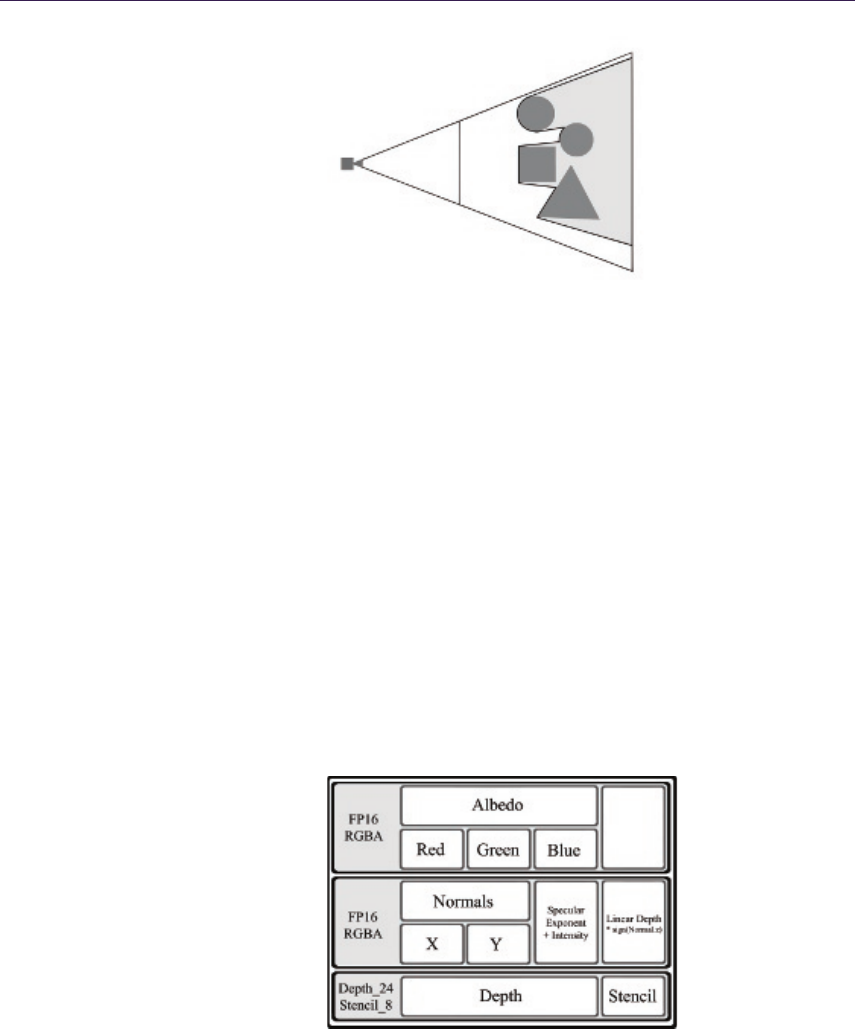
98 6. Implementing Fur Using Deferred Shading
Figure 6.1. G-buffer surface.
In deferred rendering the format of the G-buffer (Figure 6.2) defines a standard
interface between all light-receiving materials and all light sources. Each object
assigned a light-receiving material writes a uniform set of data into the G-buffer,
which is then interpreted by each light source with no direct information regarding
the original object. One key advantage to maintaining this interface is that
geometric complexity is decoupled from lighting complexity.
This creates a defined pipeline (Figure 6.3) in which we render all geome-
try to the G-buffer, removing the connection between the geometric data and
individual objects, unless we store this information in the G-buffer. We then
calculate lighting from all sources in the scene using this information, creating
a light-accumulation buffer that again discards all information about individual
lights. We can revisit this information in a material pass, rendering individual
meshes again and using the screen-space coordinates to identify the area of the
light-accumulation buffer and G-buffer representing a specific object. This ma-
terial phase is required in deferred lighting, inferred lighting, and light pre-pass
rendering to complete the lighting process since the G-buffer for these techniques
Figure 6.2. Our G-buffer format.

6.2. Fur 99
Figure 6.3. General deferred rendering pipeline.
does not include surface color. After this, a post-processing phase acts upon the
contents of the composition buffer, again without direct knowledge of individual
lights or objects.
This stratification of the deferred rendering pipeline allows for easy extensi-
bility in the combination of different materials and lights. However, adherence to
the interfaces involved also imposes strict limitations on the types of materials
and lights that can be represented. In particular, deferred rendering solutions
have difficulty representing transparent materials, because information regard-
ing surfaces seen through the material would be discarded. Solutions may also
struggle with materials that reflect light in a nontypical manner, potentially in-
creasing the complexity of all lighting calculations and the amount of information
required within the G-buffer. Choosing the right phases and buffer formats are
key to maximizing the power of deferred rendering solutions.
We describe techniques that address the limitations of rendering such materi-
als while continuing to respect the interfaces imposed by deferred rendering. To
illustrate these techniques and demonstrate ways in which they might be com-
bined to form complex materials, we outline in detail a solution for implementing
fur in deferred shading.
6.2 Fur
Fur has a number of characteristics that make it difficult to represent using the
same information format commonly used to represent geometry in deferred ren-
dering solutions.
Fur is a structured material composed of many fine strands forming a complex
volume rather than a single continuous surface. This structure is far too fine to
describe each strand within the G-buffer on current hardware; the resolution
required would be prohibitive in both video memory and fragment processing.
As this volumetric information cannot be stored in the G-buffer, the fur must
be approximated as a continuous surface when receiving light. We achieve this
by ensuring that the surface exhibits the observed lighting properties that would
normally be created by the structure.
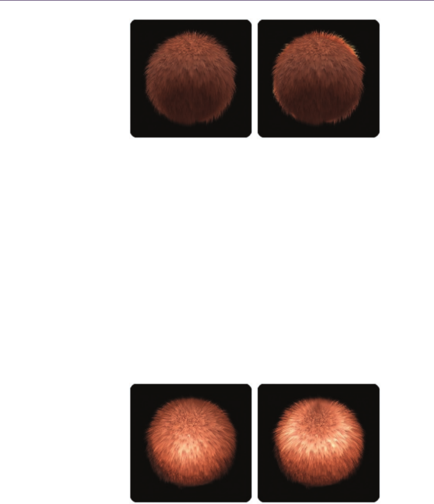
100 6. Implementing Fur Using Deferred Shading
(a) (b)
Figure 6.4. Fur receiving light from behind (a) without scattering and (b) with scat-
tering approximation.
The diffuse nature of fur causes subsurface scattering; light passing into the
volume of the fur is reflected and partially absorbed before leaving the medium
at a different point. Individual strands are also transparent, allowing light to
pass through them. This is often seen as a halo effect; fur is silhouetted against
a light source that illuminates the fur layer from within, effectively bending light
around the horizon of the surface toward the viewer. This is best seen in fur with
a loose, “fluffy” structure (see Figure 6.4).
The often-uniform, directional nature of fur in combination with the struc-
ture of individual strands creates a natural grain to the surface being lit. The
reflectance properties of the surface are anisotropic, dependent on the grain di-
rection. Anisotropy occurs on surfaces characterized by fine ridges following the
grain of the surface, such as brushed metal, and causes light to reflect according
to the direction of the grain. This anisotropy is most apparent in fur that is
“sleek” with a strong direction and a relatively unbroken surface (see Figure 6.5).
(a) (b)
Figure 6.5. Fur receiving light (a) without anisotropy and (b) with anisotropy approx-
imation.
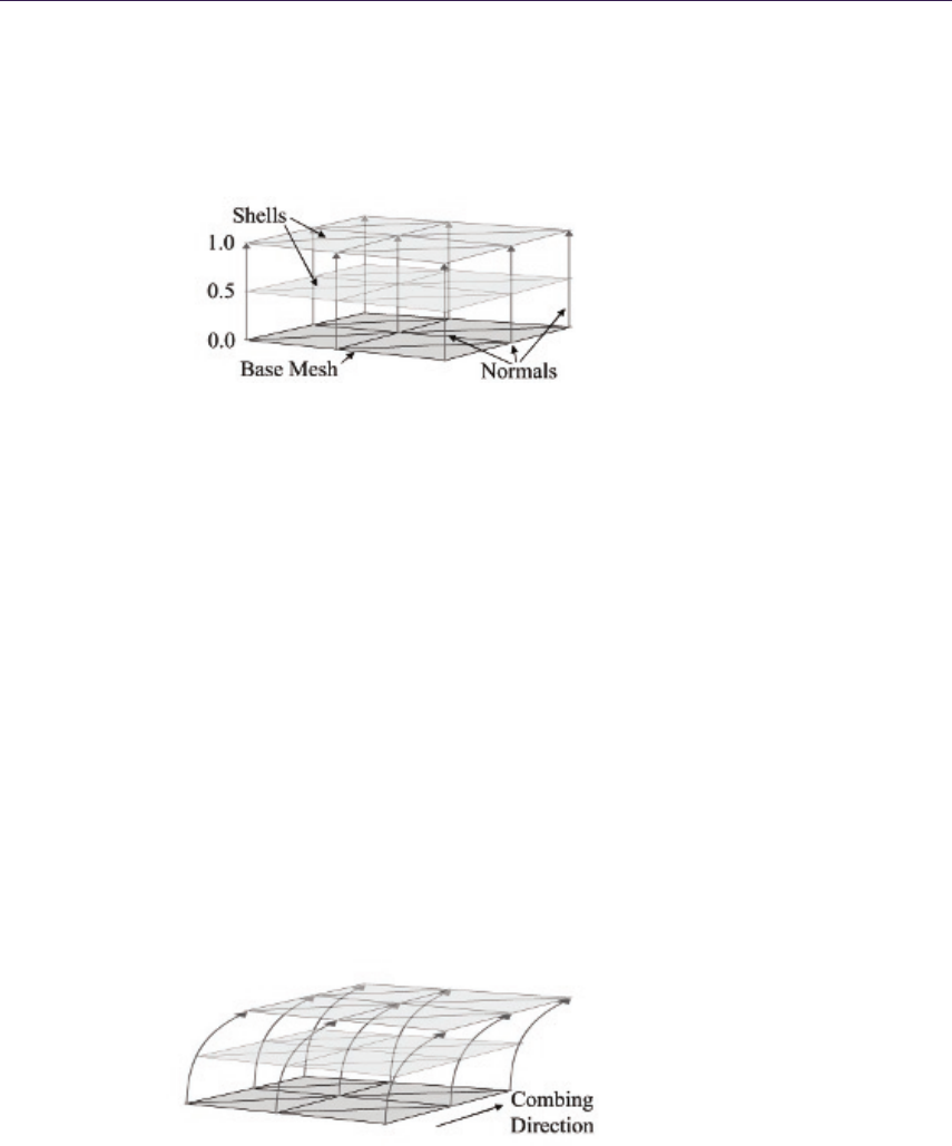
6.3. Techniques 101
6.3 Techniques
We look at each of the characteristics of fur separately so that the solutions dis-
cussed can be reused to represent other materials that share these characteristics
and difficulties when implemented within deferred rendering.
Figure 6.6. Concentric shells.
6.3.1 Volumetric Fur Rendering Using Concentric Shells
It is common to render volumetric structures in real time by rendering dis-
crete slices of volumetric texture data into the scene and using alpha blend-
ing to combine the results, such as light interacting with dust particles in the
air [Mitchell 04]. Provided enough slices are rendered, the cumulative result
gives the appearance of a continuous volume featuring correct perspective, par-
allax, and occlusion.
The concentric shells method of rendering fur [Lengyel 01] represents the
volumetric layer of fur as a series of concentric shells around the base mesh; each
shell is a slice through the layer of fur parallel to the surface. These shells are
constructed by rendering the base mesh again and pushing the vertices out along
the normal of the vertex by a fraction of the fur layer depth; the structure of the
fur is represented by a volume texture containing a repeating section of fur (see
Figure 6.6). By applying an offset parallel to the mesh surface in addition to the
normal we can comb the fur volume (see Figure 6.7,Listing 6.1).
Figure 6.7. Combing.

102 6. Implementing Fur Using Deferred Shading
// Get shell depth as nor maliz ed dist anc e b etw een base and
// outer s urfa ce .
fl oat s hell Dept h = s hell Inde x * (1. f / num Shel ls );
// Get o ffset d irec tion vector
flo at 3 di r = I N . no rm al . xyz + ( I N . d ir ec ti on . x yz * _ s he ll D ep th );
dir . xyz = n or ma li ze ( d ir . xyz );
// Offset vertex p osition a long fur d irec tion .
OUT . posit ion = IN . pos itio n ;
OUT . pos it io n . xyz = ( d ir . xyz * _ s he ll De pt h * f ur De pt h
* IN . f ur Le ngt h );
OUT . pos it io n = mul ( w or ld Vi ew Pr oj ec ti on , OU T . po si ti on );
Listing 6.1. Vertex offsetting.
This method of fur rendering can be further augmented with the addition of
fins, slices perpendicular to the surface of the mesh, which improve the quality of
silhouette edges. However, fin geometry cannot be generated from the base mesh
as part of a vertex program and is therefore omitted here (details on generating
fin geometry can be found in [Lengyel 01]).
This technique cannot be applied in the geometry phase because the structure
of fur is constructed from a large amount of subpixel detail that cannot be stored
in the G-buffer where each pixel must contain values for a discrete surface point.
Therefore, in deferred shading we must apply the concentric shell method in the
material phase, sampling the lighting and color information for each hair from a
single point in the light-accumulation buffer. The coordinates for this point can
be found by transforming the vertex position of the base mesh into screen space
in the same way it was transformed originally in the geometry phase (Listing 6.2).
// Vertex shader.
// See ( Li sti ng 3.1.1) for omitted content.
// O utput scr een p osit ion of base mesh vertex .
OUT . s cr ee nPos = m ul ( w or ld Vi ew Pr oj ec ti on , IN . pos it io n ) ;
// ----------------------------
// Pixel s hade r .
IN . sc r ee nP os /= IN . s cr ee nPo s . w ;
// B rin g val ues into ran ge (0 ,1) fr om ( -1 ,1) .
float2 s cr ee n Co or d = ( IN . sc r ee nP os . xy + 1. f . xx ) * 0. 5 f . xx ;
// Sam ple lit mesh color
color = tex2D(lightAccumulationTexture , screenCoord).
Listing 6.2. Sampling lit objects.
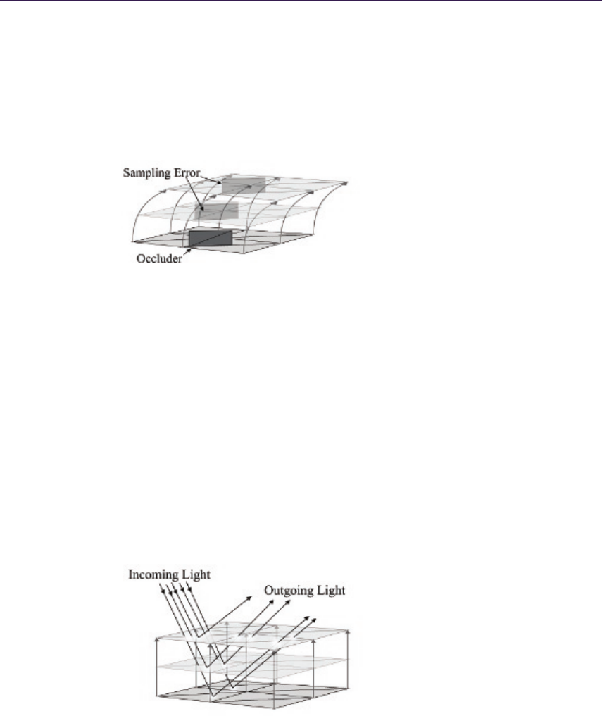
6.3. Techniques 103
This sampling of lighting values can cause an issue specific to rendering the
fur. As fur pixels are offset from the surface being sampled, it is possible for the
original point to have been occluded by other geometry and thus be missing from
the G-buffer. In this case the occluding geometry, rather than the base mesh,
would contribute to the coloring of the fur leading to visual artifacts in the fur
(Figure 6.8). We explore a solution to this in Sections 6.3.4 and 6.4.4 of this
article.
Figure 6.8. Occlusion error.
6.3.2 Subsurface Scattering
Scattering occurs in materials wherein light enters the surface at one point, is
transmitted through the medium beneath the surface being reflected and refracted
by internal structures and is partially absorbed, before exiting the surface at a
different point (Figure 6.9). This light exiting the surface softens the appearance
of lighting on the surface by creating a subtle glow.
Much work has been done on the approximation of subsurface scattering prop-
erties in skin that is constructed of discrete layers, each with unique reflectance
properties. One such solution is to apply a weighted blur to the light accumulated
on the surface [Hable 09,Green 04]. In existing forward shaded solutions, this
blurring is typically applied in texture space.
Figure 6.9. Simple subsurface scattering.
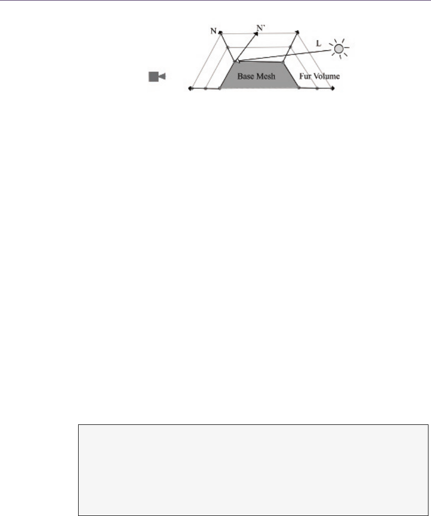
104 6. Implementing Fur Using Deferred Shading
Figure 6.10. Rim glow (N.L <0) (N‘.L >0).
In deferred rendering, this technique can be applied in both the geometry
phase and the material phase. In the geometry phase the scattering can be
approximated by blurring the surface normals written into the G-buffer or by
recalculating the mesh normals as a weighted sum of neighboring vertex normals
[Patro 07].
Blurring can be performed in the material phase, in texture space, by sampling
the accumulated lighting in the same manner as that used for the fur rendering.
The texture coordinates of the mesh would then be used as vertex positions
to write those values into the mesh’s texture space before applying a blur. Once
blurred, these values are written back into the light-accumulation buffer by revers-
ing the process. Alternatively, the material-phase blurring could be performed in
screen space by orienting the blur kernel to the local surface, using the normals
stored in the G-buffer at each pixel.
One issue with this solution is that scattering beneath a surface will also allow
light entering the back faces of an object to be transmitted through the medium
and exit the surface facing the viewer. In materials such as skin and fur, which
form a scattering layer over a more solid structure, this transfer of light appears
most often around the silhouette edges of the object. We can adjust for this by
bending normals at the silhouette edge of the mesh to point away from the viewer
and sample lighting from behind the object (see Figure 6.10 and Listing 6.3). In
doing so, these pixels will no longer receive direct lighting correctly; this must
then be accounted for during the blur phase (see Sections 6.3.4 and 6.4.4 for
details of our solution).
// Get normal based for back face s amples .
// Glow s trength and f all off are s uppl ied by mater ial value s .
ha lf N do tV = sa tu ra te ( dot ( nor mal . xyz , - vie w );
half r imWe ight = gl owSt renth * pow (1. f - NdotV ), glo wFall off );
nor mal . xyz += vie w . xyz * rim We ig ht ;
norma l .xyz = n ormal ize ( nor mal . xyz );
Listing 6.3. Pushing edge pixels around edges.
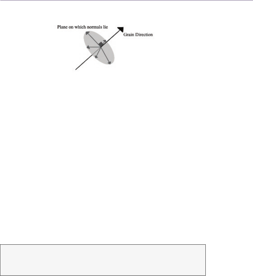
6.3. Techniques 105
Figure 6.11. Strand normals.
6.3.3 Anisotropy
Anisotropic light reflection occurs on surfaces where the distribution of surface
normals is dependent on the surface direction; such surfaces are often character-
ized by fine ridges running in a uniform direction across the surface, forming a
“grain.” The individual strands in fur and hair can create a surface that exhibits
this type of lighting [Scheuermann 04].
This distinctive lighting is created because in anisotropic surfaces the ridges
or, in this case, the strands are considered to be infinitely fine lines running
parallel to the grain. These lines do not have a defined surface normal but instead
have an infinite number of possible normals radiating out perpendicularly to their
direction (see Figure 6.11). Therefore, the lighting calculation at any point on the
surface must integrate the lighting for all the normals around the strand. This
is not practical in a pixel shader; the best solution is to choose a single normal
that best represents the lighting at this point [Wyatt 07].
In forward shading, anisotropy is often implemented using a different lighting
calculation from those used to describe other surfaces (Listing 6.4) [Heidrich 98].
This algorithm calculates lighting based on the grain direction of the surface
rather than the normal.
Diffus e = sqrt (1 - ( < L ,T >) ˆ2)
Spe cular = sqrt (1 - ( < L ,T >) ˆ2) sqrt (1 - ( < V , T > ) ˆ2)
- < L , T > < V , T >
Listing 6.4. Anisotropic light calculation.
In deferred shading we cannot know in the geometry phase the nature of any
light sources that might contribute to the lighting on the surface and are bound
by the interface of the G-buffer to provide a surface normal. Therefore, we define
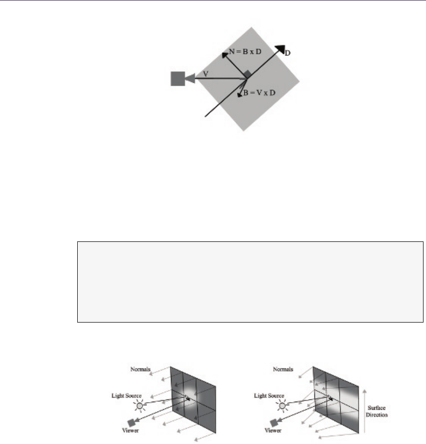
106 6. Implementing Fur Using Deferred Shading
Figure 6.12. Normal as tangent to plane.
the most significant normal as the normal that is coplanar with the grain direction
and the eye vector at that point (see Figure 6.12). We calculate the normal of
this plane as the cross product of the eye vector and the grain direction, the
normal for lighting is then the cross product of the plane’s normal and the grain
direction (see Listing 6.5).
// G enerate n ormal from fur dir ectio n .
IN . di r ec ti on = IN . di re cti on -( d ot ( IN . d ir ec ti on , n or ma l ) * no rm al ) ;
IN . di r ec ti on . xyz = no r ma li ze ( IN . dir ec t io n . x yz );
ha lf 3 b in or m = c ro ss ( I N . ey eV ect or , IN . d ir ec ti on ) ;
ha lf 3 g rai nN o rm = cro ss ( bin orm , IN . dir ec t io n ) ;
nor maliz e ( grain Norm );
Listing 6.5. Anisotropic normal calculation.
(a) (b)
Figure 6.13. (a) Isotropic highlight and (b) anisotropic highlight.
By calculating surface normals in this way we create the effect of curving
the surface around the view position, resulting in the lighting being stretched
perpendicular to the surface grain (Figure 6.13). While this method does not
perfectly emulate the results of the forward-shading solution, it is able to generate
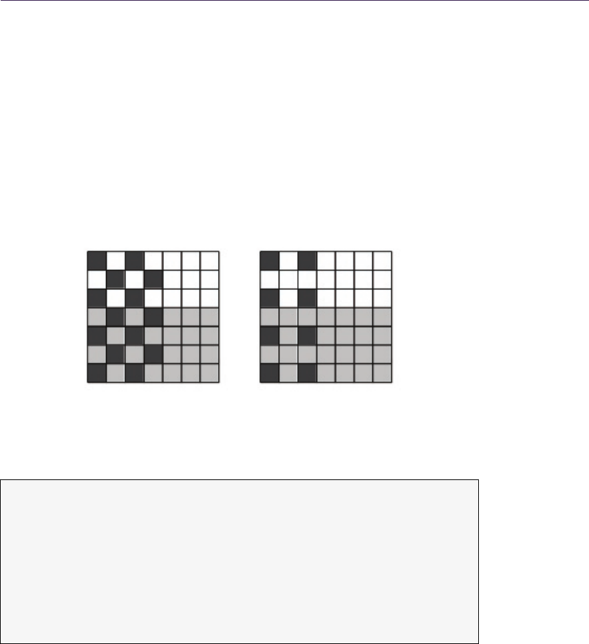
6.3. Techniques 107
this characteristic of stretched lighting for all light sources, including image-based
lights.
6.3.4 Stippled Rendering
Stippled rendering is a technique in which only some pixels of an image are
written into the frame buffer, leaving other pixels with their original values. This
technique was originally inspired by the stippled alpha transparencies used in
games before the widespread availability of hardware alpha blending, also referred
to as screen-door transparency [Mulder 98]. The values for the transparent object
are written to only some of the pixels covered by the object so as not to completely
obscure the scene behind it (see Figure 6.14 and Listing 6.6).
(a) (b)
Figure 6.14. Stipple patterns (a) 1 in 2 and (b) 1 in 4.
// G et s cr ee n c oo r di na t es in r an ge (0 , 1) .
float2 s cr ee n Co or d = (( IN . sc r ee nP os . xy / IN . s cr ee nPo s . w )
+ 1. f. x x ) * 0. 5 h . xx ;
// C onve rt c oordin ates i nto pixels .
in t2 s am pl e = s cr e en Co o rd . xy * float2(1 28 0. f , 7 20. f );
// If p ix el i s n ot th e to p le ft in a 2 x2 t ile d is ca rd it .
int2 til eI ndice s = int2 ( sa mple . x \% 2, sa mple . y \% 2) ;
if (( t ileIn dice s .x != 0) || ( tile Indi c es .y != 0) )
discard;
Listing 6.6. One in four Stipple pattern generation.
In deferred shading, transparent objects are written into the G-buffer using
a stipple pattern. During the material phase, the values of pixels containing
data for the transparent surface are blended with neighboring pixels containing

108 6. Implementing Fur Using Deferred Shading
information on the scene behind. By varying the density of the stipple pattern,
different resolutions of data can be interleaved, allowing for multiple layers of
transparency. This technique is similar to various interlaced rendering methods
for transparent surfaces [Pangerl 09,Kircher 09].
The concept of stippled rendering can be extended further to blend multiple
definitions of a single surface together. By rendering the same mesh multiple
times but writing distinctly different data in alternating pixels, we can assign
multiple lighting values for each point on the object at a reduced resolution.
During the material phase the object is rendered again, and this information
is deinterlaced and combined to allow for more complex lighting models. For
example, a skin material could write separate values for a subsurface scattering
pass and a specular layer, as interleaved samples. The material pass would then
additively blend the specular values over the blurred result of the diffuse lighting
values.
6.4 Fur Implementation Details
Ease of use and speed of implementation were key considerations when developing
the fur solution. We found that to enable artists to easily apply the fur material
to meshes, it was important to provide flexibility through a fine degree of control,
coupled with real-time feedback. We also wished to ensure minimal changes to
existing assets and work methods. It was also important that the technique have
minimal impact on our rendering framework, and that it work well with our
existing asset-creation pipeline.
To this end, the solution has been implemented with minimal code support;
all shader code is implemented within a single effect file with multiple passes for
the geometry and material phases of rendering. Annotations provide the renderer
with information on when and where to render passes. For real-time feedback,
a separate technique is provided within the effect file that renders the fur in a
forward-shaded fashion suitable for use within various asset-creation packages.
6.4.1 Asset Preparation
Combing direction. The fur solution is applicable to any closed mesh with per-
vertex position, normal, tangent, binormal, and a single set of two-dimensional
texture coordinates. This is a fairly standard vertex format for most asset-
creation packages.
In addition, we require an RGBA color per vertex to define the combing direc-
tion and length of fur at a given vertex (see Figure 6.15). The RGB components
encode combing direction as a three-component vector in the object’s local space
compressing a range of [−1,1] to [0,1]; this vector is also used to describe the
surface direction when generating the anisotropic surface normals. The alpha
channel of the color is used to scale the global fur length locally at each vertex.
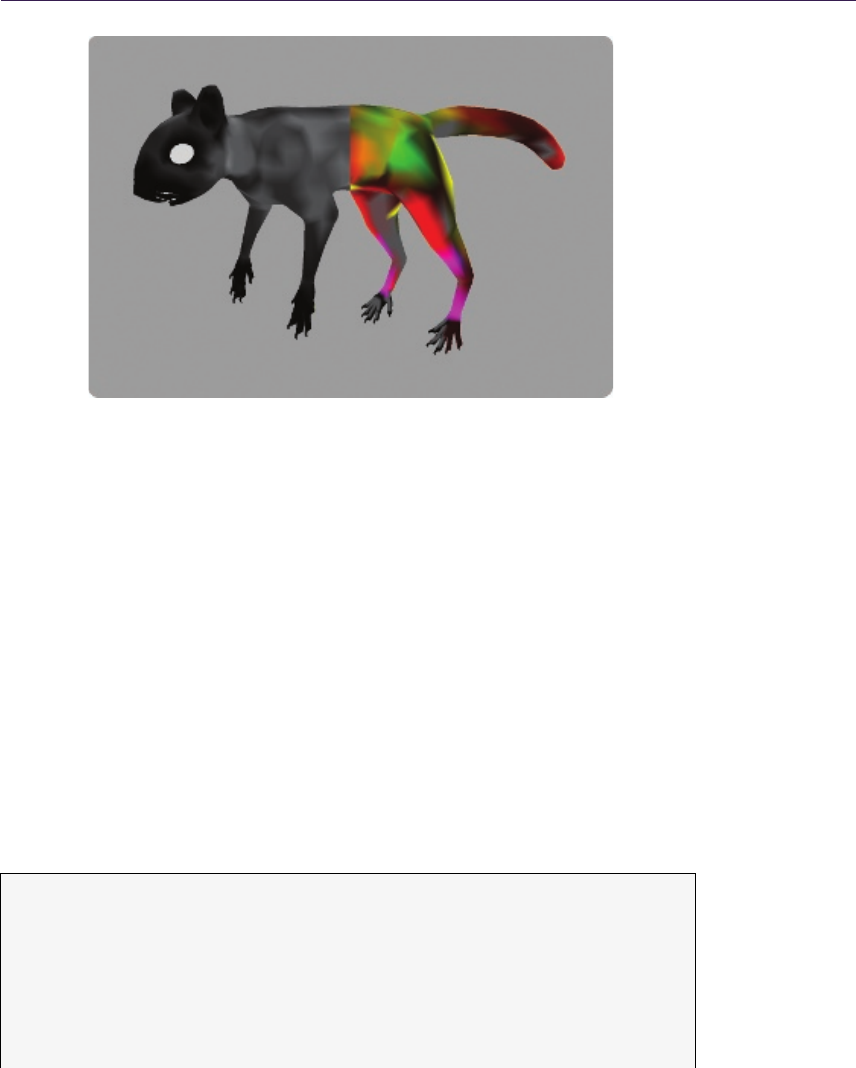
6.4. Fur Implementation Details 109
Figure 6.15. Fur length (left) and direction (right) encoded as color.
A color set was chosen to encode this data for a number of reasons. First,
many asset-creation tools allow for easy “painting” of vertex colors while viewing
the shaded mesh in real time. This effectively allows the author to choose a
direction represented as a color and then comb sections of the fur appropriately
using the tool, setting an alpha component to the color trims the length of the fur
locally. Second, the approach of encoding direction as color is already familiar to
most authors through the process of generating world- and tangent-space normal
maps. The process has proven to be quite intuitive and easy to use.
As part of the loading process, we transform the vectors encoded in this
color channel from the local space of the mesh into its tangent space and at the
same time orthonormalize them, making them tangential to the mesh surface.
Thus when the mesh is deformed during animation, the combing direction of the
fur will remain constant in relation to the surface orientation. This is the only
engine side code that was required to fully support the fur-rendering technique
(see Listing 6.7).
// Build local to ta nge nt space mat rix .
Matrix tangentSpace;
tangentSpace.LoadIdentity();
t an ge nt Spa ce . S et Co l (0 , t an ge nt ) ;
t an ge nt Spa ce . S et Co l (1 , b in or ma l ) ;
t an ge nt Spa ce . S et Co l (2 , n or ma l );
t an ge n tS pa c e . T r an sp os e () ;
// C onve rt col or into vector .

110 6. Implementing Fur Using Deferred Shading
Vector 3 dir ( pColou r [0] , pCo lou r [1] , pCo lour [ 2]) ;
dir = ( dir * 2. f) - Vec tor3 (1. f) ;
// Gram S chmi dt ortho no rmali za tion .
dir = di r - ( do t (dir , nor mal ) * no rm al ) ; d ir . N or mali se () ;
// T ra nsfor m vector i nto t ange nt space .
tan gen tS pac e . T ran sfo rmI nPl ace ( dir ) ;
// C onver t vec tor into c olo r .
dir = ( dir + Vec tor3 (1. f) ) * 0.5;
p Co lo ur [ 0] = di r . g etX () ;
p Co lo ur [ 1] = di r . g etY () ;
p Co lo ur [ 2] = di r . g etZ () ;
Listing 6.7. Processing of fur directions.
Texture data. To provide the G-buffer with the necessary surface information, the
material is assigned an RGB albedo map and a lighting map containing per pixel
normal information and specular intensity and exponent at any given pixel. In
addition to this, a second albedo map is provided to describe the changes applied
to lighting as it passes deeper into the fur; over the length of the strands, the
albedo color that is used is blended from this map to the surface color. This
gives the author a high degree of control over how the ambient occlusion term is
applied to fur across the whole surface, allowing for a greater variation.
To represent the fur volume required for the concentric shell rendering, a
heightfield was chosen as an alternative to generating a volumetric data set.
While this solution restricts the types of volume that can be described, it requires
considerably less texture information to be stored and accessed in order to render
the shells. It is more flexible in that it can be sampled using an arbitrary number
of slices without the need to composite slices when undersampling the volume,
and it is far simpler to generate with general-image authoring tools.
6.4.2 Geometry Phase
The geometry phase is split into two passes for the purpose of this technique. The
first pass renders the base mesh to the G-buffer. In the vertex shader the position,
tangent, and normal are transformed into view space and the combing direction
is brought into local space in the range [-1, 1]. The pixel shader generates a new
normal, which is coplanar to the eye and combing vectors to achieve anisotropic
highlights (Figure 6.16).
The second pass renders the top layer of the fur in a stipple pattern, rendering
to one in every four pixels on screen. The vertex shader is identical to the first
pass, but pushes the vertex positions out along the vertex normals offset by the
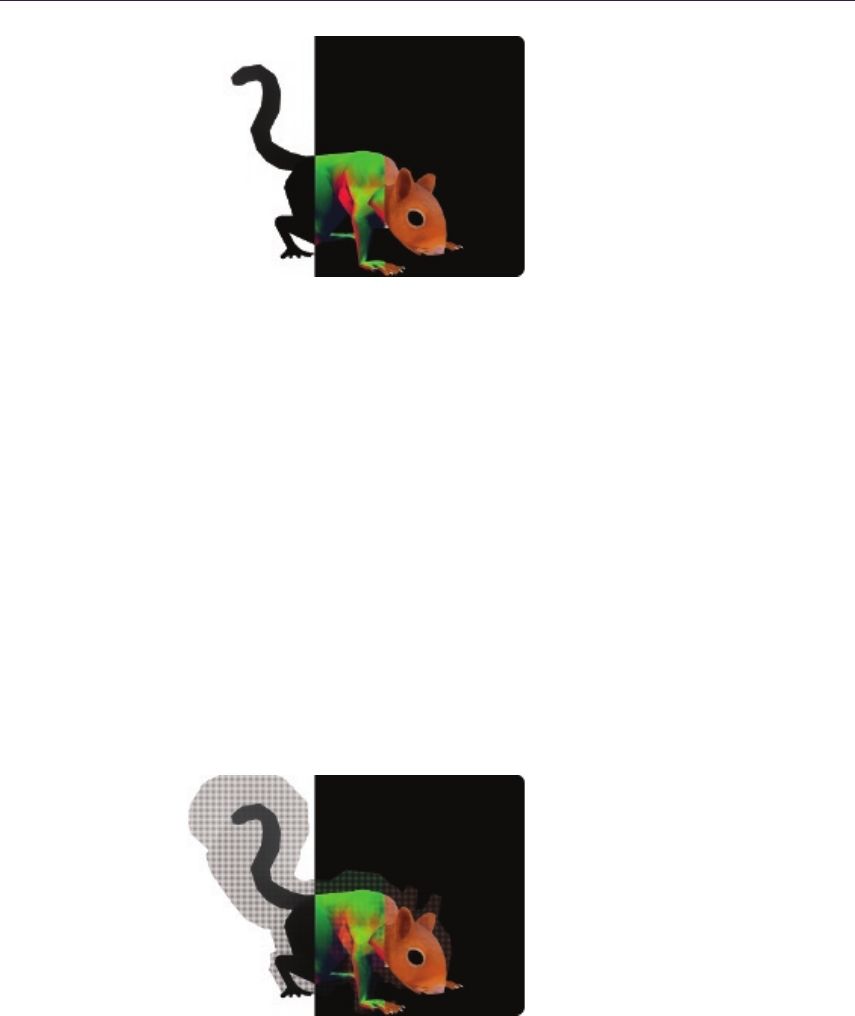
6.4. Fur Implementation Details 111
Figure 6.16. Geometry pass 1 (depth/normals/albedo).
global fur length scaled by the vertex color alpha. The pixel shader identifies
likely silhouette edges using the dot product of the view vector and the surface
normals; the normals at these points are adjusted by adding the view vector
scaled by this weight value. The unmodified normals are recalculated to use the
anisotropic normals like those of the first pass (Figure 6.17).
This second pass solves the occlusion issue when constructing concentric fur
shells from the light-accumulation buffer, since both samples are unlikely to be
occluded simultaneously while any part of the strand is still visible. The second
pass allows light calculations to be performed for both the surface of the mesh
and also the back faces where light entering the reverse faces may be visible.
In order to avoid incorrect results from screen-space ambient occlusion (SSAO),
edge detection, and similar techniques that rely on discontinuities in the G-buffer,
these should be calculated before the second pass since the stipple pattern will
create artifacts.
Figure 6.17. Geometry pass 2 (depth/normals/albedo).
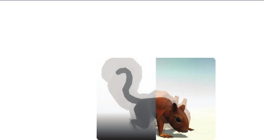
112 6. Implementing Fur Using Deferred Shading
6.4.3 Light Phase
During the light phase both the base and stipple samples within the G-buffer
receive lighting in the same manner as all other values in the G-buffer, adherence
to a common interface allows the fur to receive lighting from a wide range of
sources.
Figure 6.18. Light-accumulation buffer.
6.4.4 Material Phase
The material phase of rendering involves reading the values from the light-
accumulation buffer and interpreting these based on specific qualities of the ma-
terial, in this case by constructing shells of fur. In deferred shading, since the
majority of the lighting values are already correct in the light-accumulation buffer,
a copy of these values is required onto which the material phase of the fur can be
composited (see Figure 6.18).
The stipple values, being distributed on the outermost shell of the fur, will
occlude the layers of fur beneath. To correct this, all fur surfaces must be ren-
dered again using the outermost shell, while sampling color values from the light-
accumulation buffer and depth values from the linear depth stored in the G-buffer
(see Figure 6.19). For most pixels, these color and depth values are written di-
rectly into the composition buffer, however, where a stipple value would be sam-
pled the neighboring pixel is used instead, effectively erasing all stipple values
from the light-accumulation and depth buffers.
The buffer now contains the base mesh of the object only, providing a basis on
which to composite the volumetric layer of fur. Rendering of the fur is performed
by a series of passes, each pass rendering a concentric shell by offsetting the vertex
positions. The pass also constructs positions in screen space, from which both
the sample corresponding to the base mesh and the stipple sample corresponding
to the outermost shell can be obtained.
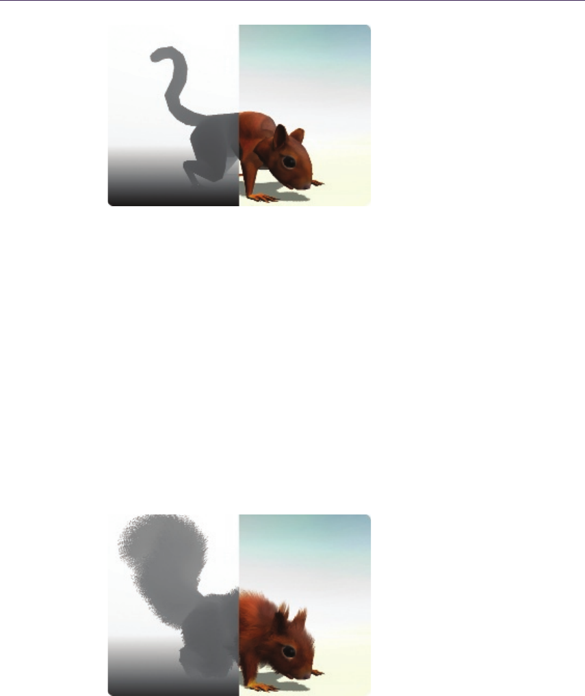
6.4. Fur Implementation Details 113
Figure 6.19. Stipple obliteration pass.
In the pixel shader these two samples are retrieved from the light-accumulation
buffer, their respective linear depths in the G-buffer are also sampled to compare
against the depth of the sample coordinates and thus correct for occlusion errors.
If both samples are valid, the maximum of the two is chosen to allow for the halo
effect of scattering around the edges of the object without darkening edges where
there is no back lighting. The contribution of the albedo map to the accumulated
light values is removed by division and then reapplied as a linear interpolation
of the base and top albedo maps to account for ambient occlusion by the fur.
The heightfield for the fur volume is sampled at a high frequency by applying
an arbitrary scale to the mesh UVs in the material. The smoothstep function is
used to fade out pixels in the current shell as the interpolation factor equals and
exceeds the values stored in the heightfield, thus individual strands of fur fade
out at different rates, creating the impression of subpixel detail (see Figure 6.20).
Figure 6.20. Shell pass (16 shells).

114 6. Implementing Fur Using Deferred Shading
Figure 6.21. Final image.
6.5 Conclusion
This article has described a series of techniques used to extend the range of
materials that can be presented in a deferred rendering environment, particularly
a combination of these techniques that can be used to render aesthetically pleasing
fur at real-time speeds.
6.6 Acknowledgments
Thanks to everyone at Cohort Studios for showing their support, interest, and enthu-
siasm during the development of this technique, especially Bruce McNeish and Gordon
Bell, without whom there would be no article.
Special thanks to Steve Ions for patiently providing excellent artwork and feedback
while this technique was still very much in development, to Baldur Karlsson and Gordon
McLean for integrating the fur, helping track down the (often humorous) bugs, and
bringing everything to life, and to Shaun Simpson for all the sanity checks.
Bibliography
[Engel 09] W. Engel. “The Light Pre-Pass Renderer.” In ShaderX7, pp. 655–666. Hing-
ham, MA: Charles River Media, 2009.
[Green 04] S. Green. “Real-Time Approximations to Sub-Surface Scattering.” In GPU
Gems, pp. 263–278. Reading, MA: Addison Wesley, 2004.
[Hable 09] J. Hable, G. Borshakov, and J. Heil. “Fast Skin Shading.” In ShaderX7, pp.
161–173. Hingham, MA: Charles River Media, 2009.
[Heidrich 98] W. Heidrich and Hans-Peter Seidel. “Efficient Rendering of Anisotropic
Surfaces Using Computer Graphics Hardware.” In Proceedings of Image and Multi-
Dimensional Digital Signal Processing Workshop,Washington, DC: IEEE, 1998.

Bibliography 115
[Kircher 09] S. Kircher and A Lawrance. “Inferred Lighting: Fast Dynamic Lighting
and Shadows for Opaque and Translucent Objects.” In Proceedings of the 2009
ACM SIGGRAPH Symposium on Video Games, Sandbox ’09, pp. 39–45. New
York: ACM, 2009.
[Lengyel 01] J. Lengyel, E. Praun, A. Finkelstein, and H. Hoppe. “Real-Time Fur Over
Arbitrary Surfaces.” In I3D ’01 Proceedings of the 2001 Symposium on Interactive
3D Graphics, pp. 227–232. New York, ACM Press, 2001.
[Mitchell 04] J. Mitchell. “Light Shafts: Rendering Shadows in Participating Media.”
Game Developers Conference, 2004. Availablwe online at http://developer.amd.
com/media/gpu assets/Mitchell LightShafts.pdf.
[Mittring 09] M. Mittring. “A Bit More Deferred - CryEngine3.” Triangle Game Con-
ference, 2009.
[Mulder 98] J. D. Mulder, F. C. A. Groen, and J. J. van Wijk. “Pixel Masks for Screen-
Door Transparency.” In Proceedings of the Conference on Visualization ’98, pp.
351–358. Los Alamitos, CA: IEEE Computer Society Press, 1998.
[Pangerl 09] D. Pangerl. “Deferred Rendering Transparency,” In ShaderX7, pp. 217–
224. Hingham, MA: Charles River Media, 2009.
[Patro 07] R. Patro, “Real-Time Approximate Subsurface Scattering,” Available at
http://www.cs.umd.edu/\simrob/Documents/sss.pdf, 2007.
[Scheuermann 04] T. Scheuermann, “Hair Rendering and Shading.” Game Developer’s
Conference, 2004.
[Wyatt 07] R. Wyatt, “Custom Shaders and Effects.” Available at http://www.
insomniacgames.com/research dev/, 2007.
[Valient 07] M. Valient. “Deferred Rendering in Killzone 2.” Develop Conference, July
2007.

7
Large-Scale Terrain Rendering
for Outdoor Games
Ferenc Pint´
er
7.1 Introduction
Visualizing large scale (above 10 km2) landscapes on current generation consoles
is a challenging task, because of the restricted amount of memory and processing
power compared with high-end PCs. This article describes in detail how we
approach both limitations and deal with the different content creation, rendering,
and performance issues. After a short explanation of the decisions and trade-
offs we made, terrain-content generation and rendering methods will follow. We
conclude by listing the pros and cons of our technique, measured implementation
performance, as well as possible extensions.
Figure 7.1. In-game screenshot of a 10 km2canyon area. ( c
2010 Digital Reality.)
117

118 7. Large-Scale Terrain Rendering for Outdoor Games
A variety of industry solutions exist for both representing terrain geometry
and texturing its surface. Our choices were made with regard to our requirements,
which were: a small memory footprint (<20 MB), good rendering performance
(<6 ms), easy in-editor (re)painting without UV distortions, and large view dis-
tances (>10km), as in Figure 7.1.
7.1.1 Geometry Choice
We opted for mesh-based terrain, which allows for steep, distortion-free slopes and
vastly different resolution levels, with complete artist control (as compared with
heightfields with vertex-texture fetching, or render to vertex buffer (R2VB) [An-
dersson 07]-heightfields, which, however, can provide in-editor/runtime modifi-
able geometry). We also chose to store the compressed vertex and triangle data
instead of performing on-the-fly mesh construction and the caching, which is
sometimes found in planetary rendering engines [Brebion 08,Kemen 08]. Our
scale is smaller, and once again we opted for greater artist flexibility.
7.1.2 Texturing Choice
Our solution is based on per-pixel splatting from tiling atlas texture elements,
thus it reuses texels over the entire surface of the terrain. This is similar to tech-
niques implemented in other games (Battlestations: Pacific [Eidos 08], Figure 7.2,
and Infinity [Brebion 08]), but instead of using just height- and slope-based rules
with additional noise to determine the terrain type at any given pixel, it also re-
lies on precomputed data. This way our artists can paint over the entire terrain,
even on uniquely modeled mesh objects. Since the terrain’s UVs are unique and
relaxed, no distortion appears, even on vertical or slightly overhanging walls.
This method has two main advantages over streaming ultrahigh resolution
maps [van Waveren 09,Mittring 08,Barrett 08,van Rossen 08]. First, the re-
quired storage space is very low (<15 MB). Second, it does not saturate streaming
or bus transfer bandwidth. Instant switching between cameras located far from
each other is also solved due to the runtime evaluation of shading and texturing.
Another advantage is complete artist control of the texturing, which might be
more difficult when relying only on procedural or fractal-based methods [Bre-
bion 08,Kemen 08,Eidos 08]. On the other hand, not using unique texture data
does result in less variance, though we did not find this to be noticeable.
Extending our asset creation and rendering by using procedural techniques
proved to be invaluable. The techniques helped create the basis for various out-
door art assets (foliage, detail object, and terrain texturing) through subtle pa-
rameter changes, thus saving time. They also cut memory and bandwidth usage
too, emphasizing the fact that GPUs are much faster at doing math than fetching
from memory.
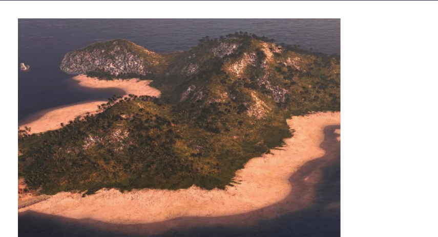
7.2. Content Creation and Editing 119
Figure 7.2. Screenshot from Battlestations: Pacific, released on XBOX 360 and PC.
(c
2008 Square Enix Europe.)
7.2 Content Creation and Editing
7.2.1 Workflow
Our terrain assets originate from multiple DCC tools. Artists create the base
terrain layout and simple mesh objects with which designers can test level func-
tionality. After this first phase is complete, the base terrain model gets greater
morphological and soil-type detail using erosion tools. Artists can iteratively re-
touch the detailed models if needed, and can also bake ambient occlusion (AO)
values to the mesh vertices. Parallel to advancing in geometry, textures repre-
senting different soil-types get authored and used by the terrain shader. The
following steps happen in our in-game editor, after the meshes have been im-
ported from COLLADA format. During this import step, the base terrain gets
split into smaller chunks, and level-of-detail (LOD) levels are generated. We also
use smaller, paintable, and reuseable objects for rock formations, referred to as
mesh objects later on. The next step in content creation is additional manual
painting for both the base terrain and the mesh objects in the game editor. The
finest detail in soil-type information and color tinting is determined in this phase.
Finally, mesh and texture assets go through different compression paths for each
platform. The complete process is illustrated in Figure 7.3.
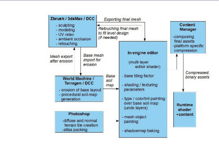
120 7. Large-Scale Terrain Rendering for Outdoor Games
Figure 7.3. Terrain content pipeline/art workflow. ( c
2010 Digital Reality.)
7.2.2 Determining Soil Type
Multiple approaches may be used to decide which soil type to apply to a given
region of the terrain. Since this information does not change during gameplay it
may be precomputed and stored offline.
7.2.3 Procedural Rules Stored in a Lookup Table
Alookup table (LUT) may be used to determine which terrain type shall occur
at different terrain slope and height values. The LUT can be stored as a two-
dimensional texture parameterized by terrain slope and height along the uand v
axes. Addressing the table at runtime requires using slope-height pairs, interpo-
lated data coming from the vertex shader [Eidos 08,Brebion 08]. Its advantage
is fast iteration times, and simple implementation, though it has its drawbacks
too. Because the LUT is applied globally to the terrain, it does not allow the
artists to have local control over the terrain’s texturing. Moreover, because the
LUT is completely decoupled from the position of terrain in the game world, we
cannot store local shading or color-tint information such as local soil types in it.
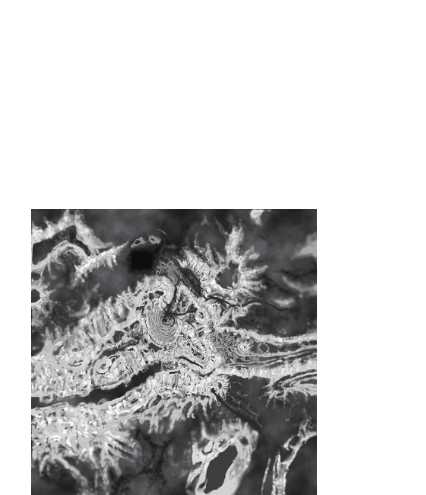
7.2. Content Creation and Editing 121
We found these drawbacks too restricting, and chose to go with the approaches
listed below.
7.2.4 Procedural and Manual Painting Stored in a UV-Space Tilemap
Alternatively, we can use tile-index texture that covers the entire terrain and can
be sampled using the unique, relaxed UV. In our case, we used a 4-channel map,
encoding a color-tint value in three channels (to break repetitive patterns), and
the terrain-type index in the fourth (see Figure 7.4). This method has multiple
advantages over the first: it can be locally controlled by art needs, separate
regions within the map can be edited concurrently by multiple artists, and it can
also use procedural methods as its basis. The only drawback is that is uses a fixed
resolution for terrain-type data, but this never proved to be a problem for us.
Figure 7.4. Alpha channel of the painted 5122tilemap, containing terrain-type info.
(c
2010 Digital Reality.)
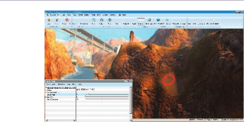
122 7. Large-Scale Terrain Rendering for Outdoor Games
Figure 7.5. Editor-artist interface for painting the tilemap, red ring indicating brush
position. ( c
2010 Digital Reality.)
Creating the tilemap is very intuitive. Its terrain-index part can be based on
either soil-type maps exported from many commercial terrain-generation/erosion
software programs (though you might need to convert the world-space type values
to relaxed UV space), or global terrain height- and slope-based rules, enhanced
by noise.
The base for the color part can again originate from DCC tools, from shadow
maps, or can be simply desaturated color noise. Over this base, artists can
easily paint or modify the chosen terrain-type values using simple brushes, and
temporary layers. Ray casting is used to determine which tilemap texels the
brush touches. The editor interface (see Figure 7.5) can also support multiple
undo-levels (by caching paint commands), soft brushes, or paint limitations (to
allow painting only over regions within desired height/slope limits).
At runtime, hardware bilinear filtering of the tilemap indices automatically
solves type-blending problems present in the LUT method, and different nearby
tile-index values will get smoothly interpolated over the terrain pixels. We can
also compress the tilemap using DXT5 texture compression. Since this format
compresses the three color channels independently from the alpha channel, we
can keep most of the index resolution while shrinking memory usage.
Note: Suppose we have sand encoded as tile-index value 0, grass as 1, and rock
as 2. Now, due to filtering, rock can never be visible near sand, but only through
an intermediate grass area. This can be avoided by duplicating types with

7.2. Content Creation and Editing 123
different neighbors in the atlas, backed by a bit more complex atlas-sampling
math. We did not need this, however.
7.2.5 Procedural and Manual Painting Stored in Mesh Vertices
We can also detach geometry containing holes, overhangs, twists, or other hard-
to-relax regions from the general terrain mesh, or create any geometry and use it
as a paintable terrain-mesh object. Apart from better fitting into the base terrain,
we can spare quite a lot of texture memory by using shared atlases and a slightly
modified terrain shader here too, instead of unique maps. Artists can UV-map
the meshes using arbitrary methods and DCC tools, producing a nonoverlapping
unique UV, with seams and connections moved to less noticeable areas.
DCC tools do not have direct view of relative asset extents and spatial pro-
portions inside the game. To help artists with UV mapping and proper tiling
factors, we multiply the base UV during editor import with a constant value.
This value is determined by the total geometrical surface of the object divided by
its total UV-space surface. This way, tiling matches perfectly on all objects and
the terrain, no matter how much UV space is used inside the 0 . . . 1 region for
the given object in the DCC tool. Another feature implemented to help artists
is that which allows already-painted mesh objects to reuse their respective paint-
ings if their geometry gets modified again in the DCC tools. This functionality
stores the painting of every object also as a texture that gets saved from the
editor automatically, along with mesh data. It is used only in the editor, and its
texels contain UV and soil-type information, one texel for every vertex. Reapply-
ing paintings is merely finding a UV match between the vertices of the modified
mesh, and the saved texels. If the majority of vertices kept their original UVs
after the DCC mesh modification, most painting information can be reused.
After geometry authoring is done for a mesh, its procedural and manual paint-
ing follows in the editor. Manual painting works similarly to painting the base
terrain (illustrated in Figure 7.6). By using ray casting, we can figure out which
object, thus which shared-mesh vertex buffer to modify, and with a simple vertex-
distance-based spherical three-dimensional brush, artists can encode soil-type in-
formation into the mesh vertices. (This can sometimes be hidden for free in an
unused byte of a compressed vertex, like in the wcomponent of position or normal
data.)
Soil-type continuity where the mesh objects meet the terrain is almost as im-
portant as matching normals near the connection region. Because mesh paintings
are shared between instances of the same object, and terrain painting is unique
due to the tilemap, the latter can be easily retrofitted to match the objects at
the connection region. Also, by using a second pair of diffuse/normal atlases for
the mesh objects, (containing only a few redundant tiles from the main terrain
atlas for connections) greater soil variance can be achieved. Because of complete
UV control, we can use tiles that have dominant directional features too.
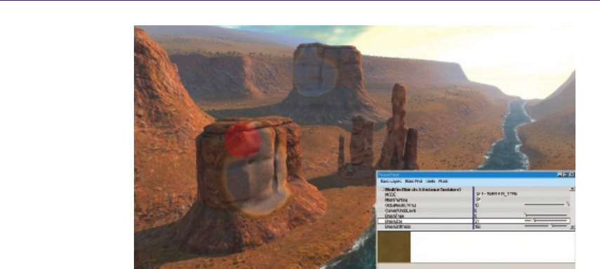
124 7. Large-Scale Terrain Rendering for Outdoor Games
Figure 7.6. Editor-artist interface for painting mesh objects, red sphere indicating brush
volume. ( c
2010 Digital Reality.)
On the base terrain, UV relaxing causes tiles to be mapped in different direc-
tions based on which side of a hill they are on—UV derivatives change directions
with respect to world-space coordinates—thus tiles with heavy direction depen-
dency might be used properly on only one side of a hill, or by putting multiple
rotated versions in the atlas.
If required, color-tint or luminance information such as AO can also be painted
(or computed in-editor) and baked into mesh vertices.
7.3 Runtime Shading
The base of the runtime rendering solution is texture splatting on a per-pixel
level. Using some per-pixel input data, and a unique, relaxed UV channel, the
shader can sample different tiling-terrain textures, and blend among them.
To reduce the count of textures the shader needs to sample from, these tiling
textures—corresponding to different soil types—can be packed into textures at-
lases (see Figure 7.7), or texture arrays on XBOX 360 and DX10/11 architec-
tures [Brebion 08, Wloka 03]. Care shall be taken when generating miplevels for
the atlas though, as the individual tile-mipmap texels must not get mixed with
their neighbors. Creating the compressed and mipmapped tiles first, and then
packing them to an atlas is one solution. Anisotropic filtering also becomes more
complex when using atlases [van Waveren 09].
If we choose the atlas method, we want the tiling to wrap around in a smaller
UV region (hence this is sometimes referred to as subtiling), say 0 . . . 0.25 if
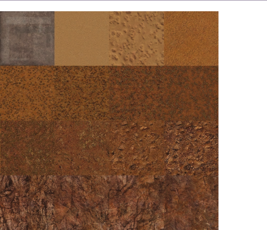
7.3. Runtime Shading 125
Figure 7.7. A packed 20482diffuse-texture atlas, containing 16 different terrain types.
(c
2010 Digital Reality.)
we have a 4 ×4 atlas. This also means that we cannot rely on hardware tex-
ture wrapping; this must be performed manually in the shader. As we will see,
this causes problems in hardware miplevel selection (texture arrays do not need
these corrections, however). For this to work correctly, one must know how the
hardware calculates which mip levels to use. GPUs use the first derivatives of
screen-space texture coordinates in any given 2×2 pixel block and the dimensions
of the texture itself to determine the pixel-to-texel projection ratio, and thus find
the appropriate miplevel to use. To access a tile from the atlas for any pixel, we
need to emulate the hardware wrapping for the tile. By using the frac() hlsl

126 7. Large-Scale Terrain Rendering for Outdoor Games
intrinsic, we break the screenspace UV derivative continuity for the pixel quads
at tile borders. Since the derivatives will be very large, the hardware will pick the
largest miplevel from the chain, which in turn results in a one-pixel-wide seam
whenever the subtiling wraps around. Fortunately, we have many options here:
we can balance the GPU load between texture filtering, arithmetic logic unit
(ALU) cost, shader thread counts, texture stalls, and overall artifact visibility.
The safest but slowest option is to calculate the mip level manually in the
shader, right before sampling from the atlas [Wloka 03,Brebion 08]. This pro-
duces the correct result, but the extra ALU cost is high since we need to issue
gradient instructions that require extra GPU cycles, and textures need to be sam-
pled with manually specified mip levels, which reduces the sampling rate on many
architectures. As a side effect, texture stalls begin to appear in the pipeline. We
can use multiple methods to shorten these stalls. Some compilers and platforms
allow for explicitly setting the maximum number of general purpose GPU regis-
ters (GPRs) a compiled shader can use. (They try to optimize the shader code
to meet the specified limit, sometimes by issuing more ALUs to move temporary
shader data around with fewer registers.) If a shader uses fewer GPRs, more
shading cores can run it in parallel, thus the number of simultaneous threads
increases. Using more threads means that stalling all of them is less probable.
On systems using unified shader architectures, one can also increase pixel shader
GPR count by reducing the available GPRs for the vertex shader. Some platforms
also have shader instructions that explicitly return the mip level the hardware
would use at a given pixel, thus saving you from having to compute it yourself in
a shader. Using dynamic branching and regular hardware mipmapping on pixel
quads far from the frac() region as speedup might also prove useful.
Branch performance might degrade for faraway fragments though, where tiling
UV values and derivatives vary fast, and pixels in the same GPU-pixel-processing
vector must take different branches. Branching might be disabled for distant
fragments, since stall problems are also most relevant on up close terrain, which
fills most screen area and uses the first few mip levels.
One option for estimating the correct mip level is to construct a texture that
encodes the mip index in the texture itself (for example, the first mip level encodes
“0” in all its texels, the second mip level encodes “1” in all its texels, etc.). This
texture should have the same dimensions as the atlas tile. You can then use a
normal texture fetch to sample this texture and allow the hardware to choose the
appropriate mip level. The value of the texel that is fetched will indicate which
mip level was chosen by the hardware and then can be used to issue a tex2dlod
instruction on the atlas tile. Dynamic branching is a viable option here too.
We chose to go with a third option, which is the fastest, but does result
in some minor artifacts which we deemed acceptable. We simply sample using
regular tex2D, but we generate only the first four mipmaps of the mip chain. This
means that the GPU has to filter a bit more, but our measurements have shown
that only 7–10% of texels fall into the larger miplevels, thus the performance
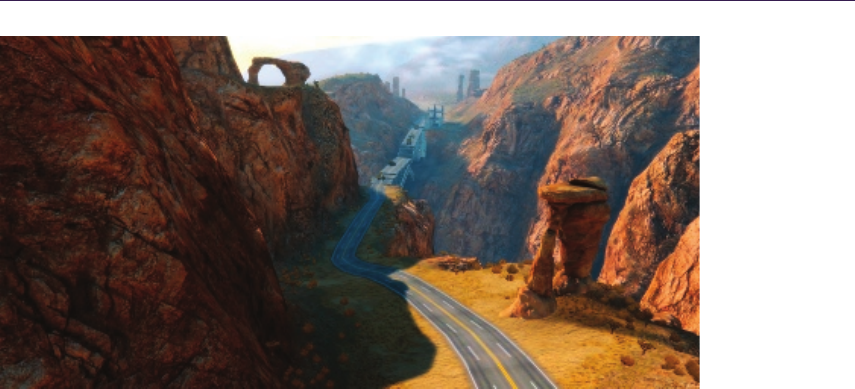
7.3. Runtime Shading 127
Figure 7.8. Screenshot from the canyon, with 100x UV tiling factor (note the lack of
UV distortions on walls). ( c
2010 Digital Reality.)
impact is considered to be minimal compared to using reduced-speed tex2Dlods.
The visual artifacts are minimized because the seam will always use the fourth
mip level, and colors differ much less between the first and last levels. We also
switched to texture atlases of 1 ×16 dimensions instead of 4 ×4, thus we can
use hardware texture wrapping for one direction, halving mip level errors arising
from using frac(), while also using fewer ALU operations to address the atlases.
At this point, we have diffuse and normal atlases ready to be sampled in
the shader. To improve quality, we blend between two nearby tiles—using the
fractional part of the interpolated tile index—by reading twice from the same
atlas, with respective UV offsets. Shading the terrain and the painted meshes is
identical, and is based on simple per-pixel lambertian diffuse, and hemispherical
ambient terms. Shadow contribution is composed of a lookup into a precomputed
and blurred static-shadow map, cross-fading with a cascaded dynamic and blurred
exponential shadow map (ESM), and AO baked into vertices. There are many
ways to experiment with more complex lighting models, however, correctly set
atmospheric settings, fog, high dynamic range (HDR), fake scattering [Quilez 09],
and soil-type maps can provide a solid impression already. See Figure 7.8 for
reference.
For your convenience, the runtime per-pixel, texture-splatting shader code is
listed in Listing 3.1. Note that editor-mode paint layers, brush-ring-overlay paint
functionality, vertex unpacking, shadows, and fog calculations are omitted for
clarity.

128 7. Large-Scale Terrain Rendering for Outdoor Games
// Run time ter rain shader with tilemap - bas ed per - pixe l
// s platt in g usi ng atl as es ( tangen t - sp ace l ig ht in g ).
stati c con st floa t T ILEMA P_ SI ZE = 5 12. 0 f;
stati c con st floa t T IL ES _I N_ ROW = 4.0 f;
stati c con st floa t M AX_TIL E_ VA LUE = T ILES_ IN _ROW * TILES_IN_RO W -1;
struct sVS Input
{
float 4 Posi tion : P OSIT ION ;
float 3 Nor mal : NO RMAL ;
float 2 UV : TEX COORD 0 ;
float 3 Tan gent : T EXCOO RD1 ;
};
struct sVS Outp ut
{
float 4 Pro jPos : P OSIT ION ;
float 2 UV : TEX COORD 0 ;
float 3 Normal : T EXCOO RD1 ;
float 3 TgLi ghtVe c : T EXCOORD2 ;
};
flo at4x3 c Worl dMatri x ;
flo at4x4 c ViewP rojMatr ix ;
fl oat c UVmul tiplie r ; // Terrain - textur e til ing factor .
float 3 cCam eraPo s ;
float 3 cSunD irecti on ;
float 3 cSun Color ;
// Lig ht ing is in tan gent spa ce .
flo at3x 3 M ak eW or ld To Ta ng en t ( floa t3 iT angent , flo at3 i Norm al )
{
flo at3x3 T angen tToLoc al =
flo at3x 3 (iTangent , cr oss ( iNormal , iTan gent ) , iN orm al );
flo at3x3 T angen tToWor ld =
mul ( Tan ge nt ToLo ca l ,( f lo at 3x 3 ) c Wo rl dM at ri x );
flo at3x3 W orldTo Tangen t = t ransp ose ( Tan ge ntToWo rl d );
return Worl dToTan gent ;
}
s VS Ou tp ut v pm ai n ( sV SI n pu t In )
{
sVS Ou tp ut Out ;
flo at 3 W or l dP os = m ul ( In . Po sit io n , c Wo rl d Ma tr i x ) ;
Out . Pro jP os = mul ( f loat 4 ( Wo rld Pos ,1) , c Vie wPr ojM atr ix );
Ou t . N or ma l = m ul ( In . No rm al . xyz , ( fl o at 3x 3 ) c W or ldM a tr ix ) ;
Ou t . UV = In . U V * c UV mu l ti pli e r ;

7.3. Runtime Shading 129
flo at3x3 W orldT oTange nt =
M ak e Wo rl d To T an g en t ( I n . Tan ge nt , In . N or ma l );
Out . T gL ig ht Ve c = m ul ( c Su nD ir ec tio n . xyz , W or ldT oT ang ent );
return Ou t ;
}
sam pler2 D D iffA tlas ;
sam pler2 D N ormA tlas ;
sam pler2 D T ileT able ;
fl oat G etMip Le vel ( float2 iUV , float2 i Te xtureS ize )
{
float 2 dx = ddx ( iUV * iTex tureS ize .x );
float 2 dy = ddy ( iUV * iTex tureS ize .y );
fl oat d = m ax ( dot ( dx , dx ), dot ( dy , dy ) ) ;
return 0. 5 * lo g2 ( d );
}
flo at 4 f pm ai n ( s V SO ut pu t In ) : C OL OR
{
flo at 4 T il e Ma pT e x = te x2 D ( T ile Ta bl e , In . U V/ c UV m ul ti p li er ) ;
float 3 Colo rTint = T ileMa pTex . xyz ;
fl oat T ileI ndex = T ileMa pTex .w * M AX _TILE_ VA LUE ;
fl oat M IP = G et Mip Lev e l ( In . UV , T I LE MA P _S IZ E . x x );
flo at 2 f ra cU V = f rac ( In . UV );
float 2 D if fC or re ct UV = fra cUV / 4.0 f ;
// B lend typ es and blend r ati o .
fl oat t ype_A = floo r ( Ti leInd ex );
fl oat t ype_ B = ce il ( T ileIn de x );
fl oat factor = T ileIn de x - typ e_A ;
fl oat tmp = floor ( typ e_A / 4);
float 2 UV_A = D if fCorre ct UV + flo at2 ( type_A - tmp *4 , tmp )/4;
tmp = flo or ( typ e_B /4) ;
float 2 UV_B = D if fCorre ct UV + flo at2 ( type_B - tmp *4 , tmp )/4;
// 2 L ookups needed , for ble nding b etwe en lay ers .
flo at 4 c olA = te x2D lo d ( Di ff Atl as , fl oa t4 ( UV_ A ,0 , MIP ) );
flo at 4 c olB = te x2D lo d ( Di ff Atl as , fl oa t4 ( UV_ B ,0 , MIP ) );
flo at 4 D i ff us e Co lo r = l erp ( colA , c olB , f ac to r ) ;
flo at 4 n or mA = t ex 2D l od ( No rm At las , f lo at 4 ( UV_A ,0 , MI P ) );
flo at 4 n or mB = t ex 2D l od ( No rm At las , f lo at 4 ( UV_B ,0 , MI P ) );
flo at 4 n or mtex = le rp ( no rmA , n ormB , f acto r );
// Ext ra ct n orma l ma p .
f lo at 3 n or m = 2 *( n or m te x . rgb - 0 .5 );

130 7. Large-Scale Terrain Rendering for Outdoor Games
float 3 t gn orma l = no rm al iz e ( norm );
fl oat NdotL =
s at ur at e ( d ot ( t gnor mal , n or ma li ze ( In . T gL ig ht V ec ) )) ;
float 3 S u nDiff u seCol o r = NdotL * c SunC olor ;
flo at3 A lb edo = Dif fus eC olo r . xy z * Col or Ti nt * 2;
float 3 Ambie ntCol or = 0. 5;
float 3 LitA lbedo = Albedo * ( Ambie ntCol or + S un Diffu se Color );
return float 4 ( LitAlb edo ,1);
}
Listing 7.1. Simplified runtime shaders including manual mipmap computation.
7.4 Performance
The system load for rendering the base terrain mesh spanning a 10 km2area,
and consisting of 600 k triangles is 14 MB memory, and 6 ms frame time, on
XBOX 360. This includes geometry vertex and index data, LODs, diffuse, normal,
shadow, and terrain type maps, while not using any streaming bandwidth. To
reach the desired rendering time and memory footprint, a couple of optimizations
are required.
To allow using 16-bit indices in the triangle list, the terrain had to be sliced
into blocks no larger than 65 k vertices, during COLLADA import. Using blocks
with <1 km2area also helps our static KD-tree based culling. Balancing between
better culling and fewer draw calls can be done by adjusting block count and
block size. LODs are also generated at import time, since they are essential to
reduce vertex load, and also keep the pixel quad efficiency high. If the LODs
are generated by skipping vertices, only index data needs to be extended by
a small amount (say, 33%, if each consecutive level contains a quarter of the
previous version, with regard to triangle count), and each new LOD can refer
to the original, untouched vertex buffer. Keeping silhouettes and vertices at
block boundaries regardless of LOD are important in order to prevent holes from
appearing in places where differed LODs meet. To help pre- and post-transform
vertex and index caches, vertex and index reordering is also done at the import
phase.
Vertex compression is also heavily used to reduce the required amount of
memory and transfer bandwidth. We can store additional information in the
vertices. AO and soil-type indices are valid choices, but color-tint values, shadow
terms, or bent normals for better shading are still possible.
Texture atlases are also compressed. We found atlases of 4 ×4 5122tiles
to contain enough variation and resolution too. The diffuse atlas can use the
DXT1 format, while the normal atlas can use better, platform-specific 2-channel

7.5. Possible Extensions 131
compressed formats where available. The tilemap can also be compressed to
DXT5, keeping most information of the tile indices in the alpha channel, while
heavily compressing color-tint data. The static shadow map can also be com-
pressed to DXT1, or luminance of multiple shadow texels can be packed into one
texel of a two-channel map. (ATI1N (BC4/DXT5A), ATI2N (BC5/3Dc), DXN,
and CTX1 formats are easy choices.) Using floating-point depth buffers and
depth pre-pass for rejecting pixels, and occlusion queries or conditional rendering
to entirely skip draw calls can also prove to be helpful.
7.5 Possible Extensions
Many aspects of the described system can be improved or extended. Some of the
methods listed below are general improvements, some are platform specific, while
some trade flexibility for faster rendering or less resource usage.
Heightmap-based geometry can provide a more compact, though computa-
tionally more expensive representation of the terrain. Representing steep slopes
without texture distortions might be possible if we store three component-position
offsets of vertices of relaxed UV space grid, like mesh textures. More aggres-
sive vertex compression is also still possible, even without using heightmaps.
Using more blocks of terrain with smaller block sizes, or using triplanar map-
ping [Geiss 07] might yield better compression opportunities.
Texturing can be enhanced in multiple ways, though most of them put more
texture fetch and filtering burden on the GPU. Using a large tiling factor can
either result in visible tiling of soil types, or not having the ability to visualize
larger terrain features, originating from the atlas. A solution is to sample the
atlases twice, with two very different tiling factors, and cross fade their color
and normal data. This enhances large details in the far regions, lending unique
character to the terrain, while it provides detail up close where tiling is less visible.
Large details dissolve as the camera moves close, but this is barely noticeable.
Figure 7.9 illustrates the concept.
Another option is reducing the tiling factor, and blending in desaturated detail
textures up close. This allows a choice among different detail maps, based on
the general terrain soil-type. Using noise (defined by interpolated height and
slope data) to perturb the soil-type on per-pixel level in the shader with ALU
instructions is also a possibility to reduce tiling or add up close detail. The
inverse of this method is also viable, and has been the de facto standard for
terrain texturing for many years. We can stream a large, unique, diffuse, and
normal map for far details, and blend in the per-pixel splatting as close-up or
mid-range detail. Transition regions between different soil types can also be
enhanced by using blend maps, which can be efficiently packed into the alpha
channel of the diffuse atlas [Hardy 09]]. Yet another option is to use more soil-
type textures in the atlas to give more variance. Soil-type information can also
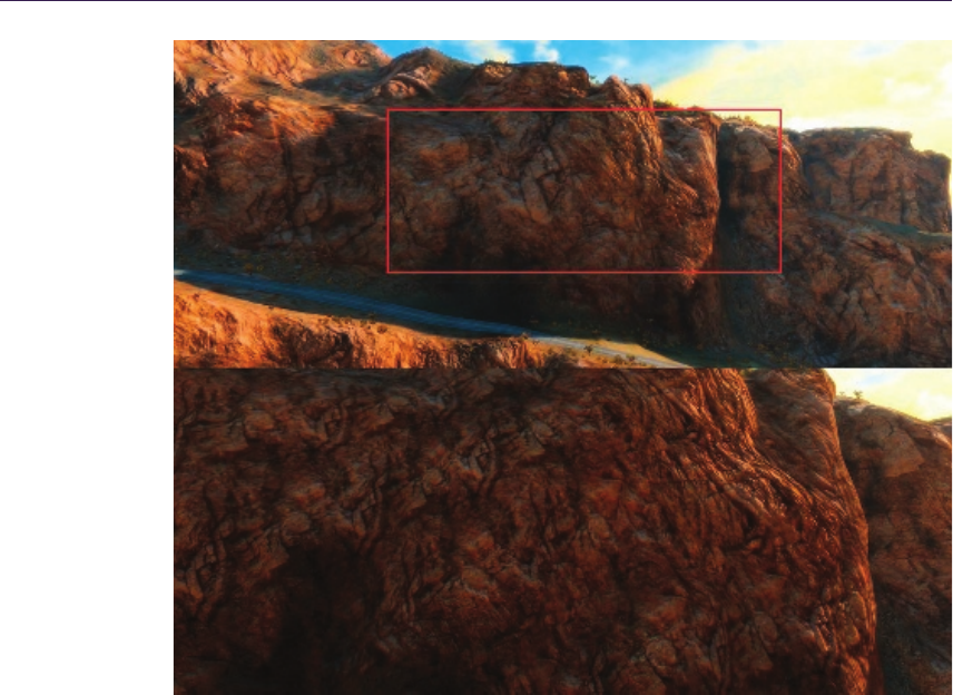
132 7. Large-Scale Terrain Rendering for Outdoor Games
Figure 7.9. Screenshot of a canyon wall, with distance-dependant atlas tiling factor.
(c
2010 Digital Reality.)
drive collision-particle generation, or procedural placement of detail object and
foliage [Andersson 07].
We can use ambient aperture lighting to give bump maps some shadow-
ing [Persson 06], and image-based ambient and diffuse lighting using bent nor-
mals. Specular reflections can also be added where surfaces are wet, for example,
riverbanks [Geiss 07]. Atmospheric scattering with volumetric light/fog (or fak-
ing it [Quilez 09]) is also an option to enhance realism of the rendered terrain.
Enhancing normal mapping by using more complex parallax effects might also be
feasible.
Finally, caching previously computed fragment data (composed albedo or final
normal data), either in screen space, or around the camera in relaxed UV space
can speed up rendering [Herzog et al. 10].

7.6. Acknowledgments 133
7.6 Acknowledgments
First, I would like to thank Bal´azs T¨or¨ok, my friend and colleague, for his helpful
suggestions and for the initial idea of contributing to the book. I would also like
to thank the art team at Digital Reality for their excellent work, on which I based
my illustrations. Also, special thanks to my love T´ımea Kapui for her endless
patience and support.
Bibliography
[Andersson 07] Johan Andersson. “Terrain Rendering in Frostbite Using Proce-
dural Shader Splatting.” In ACM SIGGRAPH 2007 courses. New York:
ACM, 2007. Available online (http://ati.amd.com/developer/SIGGRAPH07/
Chapter5-Andersson-Terrain Rendering in Frostbite.pdf).
[Barrett 08] Sean Barrett. “Sparse Virtual Textures blog.” 2008. Available online (http:
//www.silverspaceship.com/src/svt/).
[Brebion 08] Flavien Brebion. “Journal of Ysaneya, gamedev.net.” 2008. Available on-
line (http://www.gamedev.net/community/forums/mod/journal/journal.asp?jn=
263350).
[Dudash 07] Bryan Dudash. “DX10 Texture Arrays, nVidia SDK.” 2007.
Available online (http://developer.download.nvidia.com/SDK/10/Samples/
TextureArrayTerrain.zip).
[Eidos 08] Eidos, Square Enix Europe. “Battlestations: Pacific.” 2008. Available online
(http://www.battlestations.net).
[Geiss 07] Ryan Geiss. “Generating Complex Procedural Terrains Using the GPU.” In
GPU Gems 3. Reading, MA: Addison Wesley, 2007. Available online (http://http.
developer.nvidia.com/GPUGems3/gpugems3 ch01.html).
[Hardy 09] Alexandre Hardy. “Blend Maps: Enhanced Terrain Texturing.” 2009. Avail-
able online (http://www.ahardy.za.net/Home/blendmaps).
[Herzog et al. 10] Robert Herzog, Elmar Eisemann, Karol Myszkowski, and H-P. Seidel.
“Spatio-Temporal Upsampling on the GPU.” In Proceedings of the 2010 ACM SIG-
GRAPH symposium on Interactive 3D Graphics and Games, I3D ’10, pp. 91–98.
New York: ACM, 2010.
[Kemen 08] Brano Kemen. “Journal of Lethargic Programming, Cameni’s gamedev.net
blog, July 2008.” 2008. Available online (http://www.gamedev.net/community/
forums/mod/journal/journal.asp?jn=503094&cmonth=7&cyear=2008).
[Mittring 08] Martin Mittring. “Advanced Virtual Texturing Topics.” In ACM SIG-
GRAPH 2008 Classes SIGGRAPH ’08, pp. 23–51. New York, NY, USA: ACM,
2008.

134 7. Large-Scale Terrain Rendering for Outdoor Games
[Pangilinan and Ruppel 10] Erick Pangilinan and Robh Ruppel. “Uncharted 2 Art di-
rection.” GDC 2010. Available online (http://www.gdcvault.com/free/category/
280/conference/).
[Persson 06] Emil Persson. “Humus, Ambient Aperture Lighting.” 2006. Available online
(http://www.humus.name/index.php?page=3D&ID=71).
[Quilez 09] Inigo Quilez. “Behind Elevated.” Function 2009. Available online (http://
www.iquilezles.org/www/material/function2009/function2009.pdf).
[Schueler 06] Christian Schueler. “Normal Mapping without Pre-Computed Tangents.”
In ShaderX5: Advanced Rendering Techniques, Chapter II.6. Hingham, MA:
Charles River Media, 2006. Available online (http://www.shaderx5.com/TOC.
html).
[van Rossen 08] Sander van Rossen. “Sander’s Blog on Virtual Texturing.” 2008.
Available online (http://sandervanrossen.blogspot.com/2009/08/virtual-texturing
-part-1.html).
[van Waveren 09] J. M. P. van Waveren. “idTech5 Challeges: From Texture Virtualiza-
tion to Massive Parallelization.” Siggraph 2009. Available online (http://s09.idav.
ucdavis.edu/talks/05-JP id Tech 5 Challenges.pdf).
[Wetzel 07] Mikey Wetzel. “Under The Hood: Revving Up Shader Perfor-
mance.” Microsoft Gamefest Unplugged Europe, 2007. Available online
(http://www.microsoft.com/downloads/details.aspx?FamilyId=74DB343E-E8FF
-44E9-A43E-6F1615D9FCE0&displaylang=en).
[Wloka 03] Matthias Wloka. “Improved Batching Via Texture Atlases.” In ShaderX3.
Hingham, MA: Charles River Media, 2003. Available online (http://www.shaderx3.
com/Tables%20of%20Content.htm).

8
Practical Morphological
Antialiasing
Jorge Jimenez, Belen Masia, Jose I. Echevarria,
Fernando Navarro, and Diego Gutierrez
The use of antialiasing techniques is crucial when producing high quality graphics.
Up to now, multisampling antialiasing (MSAA) has remained the most advanced
solution, offering superior results in real time. However, there are important
drawbacks to the use of MSAA in certain scenarios. First, the increase in pro-
cessing time it consumes is not negligible at all. Further, limitations of MSAA
include the impossibility, in a wide range of platforms, of activating multisam-
pling when using multiple render targets (MRT), on which fundamental techniques
such as deferred shading [Shishkovtsov 05,Koonce 07] rely. Even on platforms
where MRT and MSAA can be simultaneously activated (i.e., DirectX 10), imple-
mentation of MSAA is neither trivial nor cost free [Thibieroz 09]. Additionally,
MSAA poses a problem for the current generation of consoles. In the case of the
Xbox 360, memory constraints force the use of CPU-based tiling techniques in
case high-resolution frame buffers need to be used in conjunction with MSAA;
whereas on the PS3 multisampling is usually not even applied. Another drawback
of MSAA is its inability to smooth nongeometric edges, such as those resulting
from the use of alpha testing, frequent when rendering vegetation. As a result,
when using MSAA, vegetation can be antialiased only if alpha to coverage is
used. Finally, multisampling requires extra memory, which is always a valuable
resource, especially on consoles.
In response to the limitations described above, a series of techniques have im-
plemented antialiasing solutions in shader units, the vast majority of them being
based on edge detection and blurring. In S.T.A.L.K.E.R. [Shishkovtsov 05], edge
detection is performed by calculating differences in the eight-neighborhood depth
values and the four-neighborhood normal angles; then, edges are blurred using
a cross-shaped sampling pattern. A similar, improved scheme is used in Tabula
Rasa [Koonce 07], where edge detection uses threshold values that are resolution
135
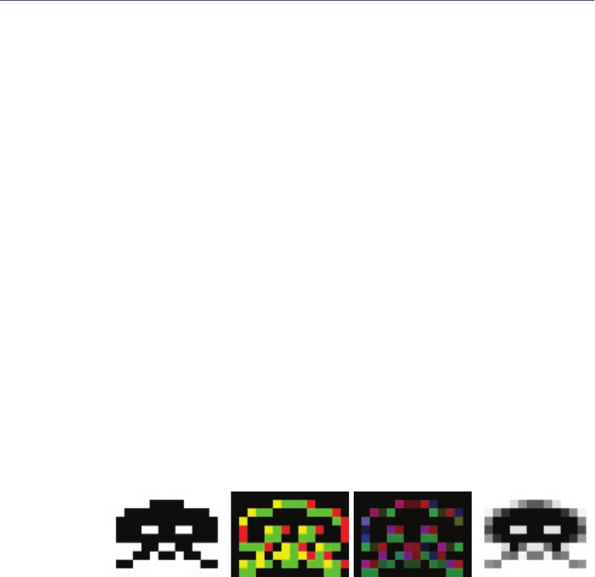
136 8. Practical Morphological Antialiasing
independent, and the full eight-neighborhood of the pixel is considered for dif-
ferences in the normal angles. In Crysis [Sousa 07], edges are detected by using
depth values, and rotated triangle samples are used to perform texture lookups
using bilinear filtering. These solutions alleviate the aliasing problem but do not
mitigate it completely. Finally, in Killzone 2, samples are rendered into a double
horizontal resolution G-buffer. Then, in the lighting pass, two samples of the
G-buffer are queried for each pixel of the final buffer. The resulting samples are
then averaged and stored in the final buffer. However, this necessitates executing
the lighting shader twice per final pixel.
In this article we present an alternative technique that avoids most of the prob-
lems described above. The quality of our results lies between 4xand 8xMSAA
at a fraction of the time and memory consumption. It is based on morphological
antialiasing [Reshetov 09], which relies on detecting certain image patterns to
reduce aliasing. However, the original implementation is designed to be run in a
CPU and requires the use of list structures that are not GPU-amenable.
Since our goal is to achieve real-time practicality in games with current main-
stream hardware, our algorithm implements aggressive optimizations that provide
an optimal trade-off between quality and execution times. Reshetov searches for
specific patterns (U-shaped, Z-shaped, and L-shaped patterns), which are then
decomposed into simpler ones, an approach that would be impractical on a GPU.
We realize that the pattern type, and thus the antialiasing to be performed, de-
pends on only four values, which can be obtained for each edge pixel (edgel) with
only two memory accesses. This way, the original algorithm is transformed so
that it uses texture structures instead of lists (see Figure 8.1). Furthermore, this
approach allows handling of all pattern types in a symmetric way, thus avoiding
the need to decompose them into simpler ones. In addition, precomputation of
Original image Edges texture Blending weights
texture Antialiased image
Figure 8.1. Starting from an aliased image (left), edges are detected and stored in the
edges texture (center left). The color of each pixel depicts where edges are: green pixels
have an edge at their top boundary, red pixels at their left boundary, and yellow pixels
have edges at both boundaries. The edges texture is then used in conjunction with the
precomputed area texture to produce the blending weights texture (center right) in the
second pass. This texture stores the weights for the pixels at each side of an edgel in the
RGBA channels. In the third pass, blending is performed to obtain the final antialiased
image (right).

8.1. Overview 137
certain values into textures allows for an even faster implementation. Finally,
in order to accelerate calculations, we make extensive use of hardware bilinear
interpolation for smartly fetching multiple values in a single query and provide
means of decoding the fetched values into the original unfiltered values. As a
result, our algorithm can be efficiently executed by a GPU, has a moderate mem-
ory footprint, and can be integrated as part of the standard rendering pipeline of
any game architecture.
Some of the optimizations presented in this work may seem to add complexity
at a conceptual level, but as our results show, their overall contribution makes
them worth including. Our technique yields image quality between 4xand 8x
MSAA, with a typical execution time of 3.79 ms on Xbox 360 and 0.44 ms on a
NVIDIA GeForce 9800 GTX+, for a resolution of 720p. Memory footprint is 2x
the size of the backbuffer on Xbox 360 and 1.5xon the 9800 GTX+. According
to our measurements, 8xMSAA takes an average of 5 ms per image on the same
GPU at the same resolution, that is, our algorithm is 11.80xfaster.
In order to show the versatility of our algorithm, we have implemented the
shader both for Xbox 360 and PC, using DirectX 9 and 10 respectively. The code
presented in this article is that of the DirectX 10 version.
8.1 Overview
The algorithm searches for patterns in edges which then allow us to reconstruct
the antialiased lines. This can, in general terms, be seen as a revectorization of
edges. In the following we give a brief overview of our algorithm.
First, edge detection is performed using depth values (alternatively, lumi-
nances can be used to detect edges; this will be further discussed in Section 8.2.1).
We then compute, for each pixel belonging to an edge, the distances in pixels from
it to both ends of the edge to which the edgel belongs. These distances define
the position of the pixel with respect to the line. Depending on the location of
the edgel within the line, it will or will not be affected by the antialiasing pro-
cess. In those edges which have to be modified (those which contain yellow or
green areas in Figure 8.2 (left)) a blending operation is performed according to
Equation (8.1):
cnew = (1 −a)·cold +a·copp,(8.1)
where cold is the original color of the pixel, copp is the color of the pixel on the
other side of the line, cnew is the new color of the pixel, and ais the area shown
in yellow in Figure 8.2 (left). The value of ais a function of both the pattern
type of the line and the distances to both ends of the line. The pattern type is
defined by the crossing edges of the line, i.e., edges which are perpendicular to
the line and thus define the ends of it (vertical green lines in Figure 8.2). In order
to save processing time, we precompute this area and store it as a two-channel
texture that can be seen in Figure 8.2 (right) (see Section 8.3.3 for details).
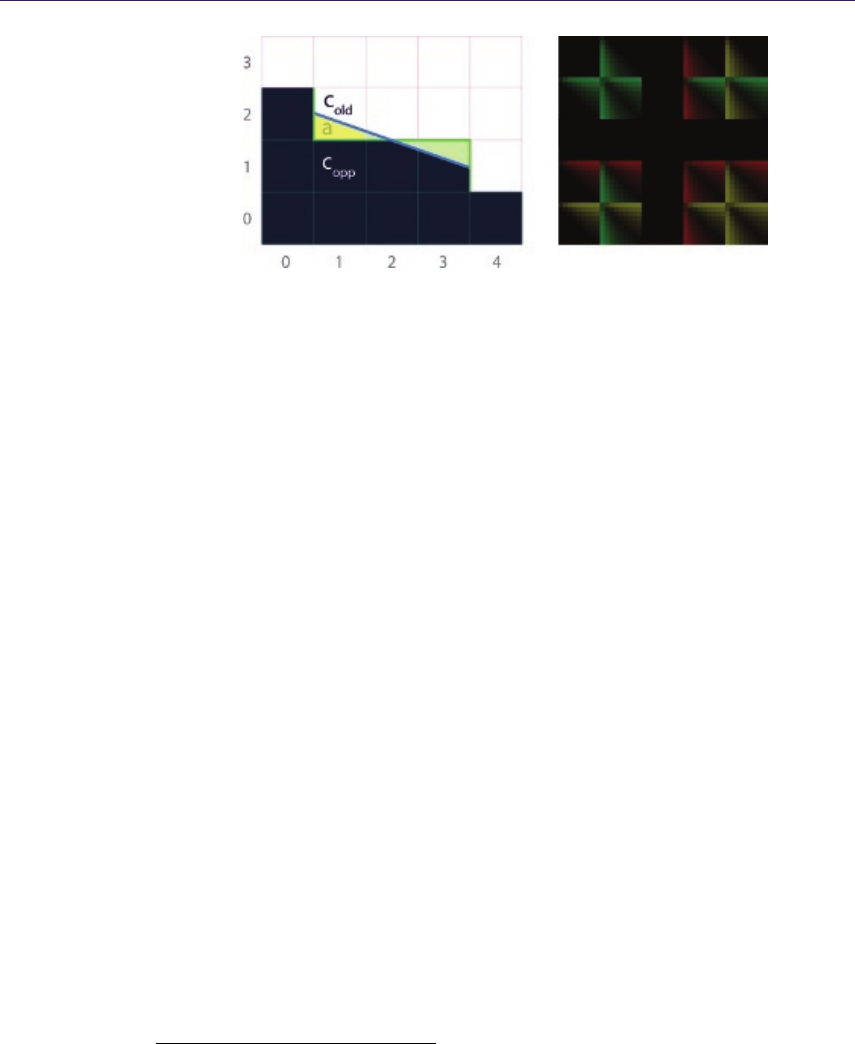
138 8. Practical Morphological Antialiasing
Figure 8.2. Antialiasing process (left). Color copp bleeds into cold according to the area
abelow the blue line. Texture containing the precomputed areas (right). The texture
uses two channels to store areas at each side of the edge, i.e., for a pixel and its opposite
(pixels (1,1) and (1,2) on the left). Each 9 ×9 subtexture corresponds to a pattern
type. Inside each of these subtextures, (u, v) coordinates encode distances to the left
and to the right, respectively.
The algorithm is implemented in three passes, which are explained in detail
in the following sections. In the first pass, edge detection is performed, yielding
a texture containing edges (see Figure 8.1 (center left)). In the second pass the
corresponding blending weight1(that is, value a) for each pixel adjacent to the
edge being smoothed is obtained (see Figure 8.1 (center right)). To do this, we
first detect the pattern types for each line passing through the north and west
boundaries of the pixel and then calculate the distances of each pixel to the
crossing edges; these are then used to query the precomputed area texture. The
third and final pass involves blending each pixel with its four-neighborhood using
the blending weights texture obtained in the previous pass.
The last two passes are performed separately to spare calculations, taking
advantage of the fact that two adjacent pixels share the same edgel. To do this,
in the second pass, pattern detection and the subsequent area calculation are
performed on a per-edgel basis. Finally, in the third pass, the two adjacent pixels
will fetch the same information.
Additionally, using the stencil buffer allows us to perform the second and third
passes only for the pixels which contain an edge, considerably reducing processing
times.
8.2 Detecting Edges
We perform edge detection using the depth buffer (or luminance values if depth
information is not available). For each pixel, the difference in depth with respect
to the pixel on top and on the left is obtained. We can efficiently store the edges
1Throughout the article blending weight and area will be used interchangeably.

8.2. Detecting Edges 139
for all the pixels in the image this way, given the fact that two adjacent pixels
have a common boundary. This difference is thresholded to obtain a binary value,
which indicates whether an edge exists in a pixel boundary. This threshold, which
varies with resolution, can be made resolution independent [Koonce 07]. Then,
the left and top edges are stored, respectively, in the red and green channels of
the edges texture, which will be used as input for the next pass.
Whenever using depth-based edge detection, a problem may arise in places
where two planes at different angles meet: the edge will not be detected because
of samples having the same depth. A common solution to this is the addition of
information from normals. However, in our case we found that the improvement
in quality obtained when using normals was not worth the increase in execution
time it implied.
8.2.1 Using Luminance Values for Edge Detection
An alternative to depth-based edge detection is the use of luminance information
to detect image discontinuities. Luminance values are derived from the CIE XYZ
(color space) standard:
L= 0.2126 ·R+ 0.7152 ·G+ 0.0722 ·B.
Then, for each pixel, the difference in luminance with respect to the pixel on top
and on the left is obtained, the implementation being equivalent to that of depth-
based detection. When thresholding to obtain a binary value, we found 0.1 to be
an adequate threshold for most cases. It is important to note that using either
luminance- or depth-based edge detection does not affect the following passes.
Although qualitywise both methods offer similar results, depth-based detec-
tion is more robust, yielding a more reliable edges texture. And, our technique
takes, on average, 10% less time when using depth than when using luminance
values. Luminance values are useful when depth information cannot be accessed
and thus offer a more universal approach. Further, when depth-based detection
is performed, edges in shading will not be detected, whereas luminance-based
detection allows for antialias shading and specular highlights. In general terms,
one could say that luminance-based detection works in a more perceptual way be-
cause it smoothes visible edges. As an example, when dense vegetation is present,
using luminance values is faster than using depth values (around 12% faster for
the particular case shown in Figure 8.5 (bottom row)), since a greater number of
edges are detected when using depth values. Optimal results in terms of quality,
at the cost of a higher execution time, can be obtained by combining luminance,
depth, and normal values.
Listing 8.1 shows the source code of this pass, using depth-based edge detec-
tion. Figure 8.1 (center left) is the resulting image of the edge-detection pass,
in this particular case, using luminance-based detection, as depth information is
not available.

140 8. Practical Morphological Antialiasing
float4 Edge De te ct io nP S ( float4 pos itio n : SV_POSITION ,
float2 tex coor d : TEXC OORD0 ): SV_TARGET {
fl oat D = d epth Tex . SampleLevel(PointSampler ,
texcoord , 0);
fl oat Dleft = d epthT ex . SampleLevel(PointSampler ,
texcoord , 0, -int2(1, 0));
fl oat Dtop = de pthTe x . SampleLevel(PointSampler ,
texcoord , 0, -int2(0, 1));
// We need these for upda tin g the ste ncil b uff er .
fl oat Dright = d epthT ex . SampleLevel(PointSampler ,
texcoord , 0, int2(1, 0));
fl oat Dbot tom = de pthT ex . SampleLevel(PointSampler ,
texcoord , 0, int2(0, 1));
float4 de lta = a bs (D. xxxx -
float4( Dle ft , Dtop , Dr ight , D bo tt om ) );
float4 ed ges = step( thre shold . xxxx , delta );
if (dot ( edges , 1.0) == 0.0) {
discard;
}
return ed ges ;
}
Listing 8.1. Edge detection shader.
8.3 Obtaining Blending Weights
In order to calculate the blending weights we first search for the distances to the
ends of the line the edgel belongs to, using the edges texture obtained in the
previous pass (see Section 8.3.1). Once these distances are known, we can use
them to fetch the crossing edges at both ends of the line (see Section 8.3.2). These
crossing edges indicate the type of pattern we are dealing with. The distances to
the ends of the line and the type of pattern are used to access the precalculated
texture (see Section 8.3.3) in which we store the areas that are used as blending
weights for the final pass.
As mentioned before, to share calculations between adjacent pixels, we take
advantage of the fact that two adjacent pixels share the same boundary, and

8.3. Obtaining Blending Weights 141
float4 Blend in g WeightC al c ulatio nP S (
float4 pos itio n : SV_POSITION ,
float2 tex coor d : TEXC OORD0 ): SV _TAR GET {
float4 weight s = 0.0;
float2 e = edg esTe x . SampleLevel(PointSampler ,
te xc oor d , 0 ). rg ;
[branch]
if ( e . g) { // Edge at n ort h .
float2 d = float2( Se archX Left ( te xcoord ),
Sea rc hXRi gh t ( texc oor d ));
// I nstead of samp ling b etwe en edges , we sample at -0.25 ,
// to be able to discer n what value eac h edgel has .
float4 coords = mad (float4(d.x , -0.25 , d.y + 1.0 , -0.25) ,
P IX EL _S I ZE . xyxy , t ex co or d . xy xy );
fl oat e1 = edg esTe x . SampleLevel( Line arSa mpler ,
coo rds . xy , 0) . r;
fl oat e2 = edg esTe x . SampleLevel( Line arSa mpler ,
coo rds . zw , 0) . r;
w ei gh ts . r g = Ar ea ( abs ( d) , e1 , e2 );
}
[branch]
if ( e . r) { // Edge at west .
float2 d = float2( Se archY Up ( texcoor d ),
Sea rchYDo wn ( texc oord ));
float4 coords = mad (float4( -0. 25 , d .x , - 0.25 , d .y + 1. 0) ,
P IX EL _S I ZE . xyxy , t ex co or d . xy xy );
fl oat e1 = edg esTe x . SampleLevel( Line arSa mpler ,
coo rds . xy , 0) . g;
fl oat e2 = edg esTe x . SampleLevel( Line arSa mpler ,
coo rds . zw , 0) . g;
w ei gh ts . b a = Ar ea ( abs ( d) , e1 , e2 );
}
return weight s ;
}
Listing 8.2. Blending weights calculation shader.

142 8. Practical Morphological Antialiasing
we perform area calculation on a per-edgel basis. However, even though two
adjacent pixels share the same calculation, the resulting avalue is different for
each of them: only one has a blending weight a, whereas for the opposite one, a
equals zero (pixels (1,2) and (1,1), respectively, in Figure 8.2). The one exception
to this is the case in which the pixel lies at the middle of a line of odd length
(as pixel (2,1) in Figure 8.2); in this case both the actual pixel and its opposite
have a nonzero value for a. As a consequence, the output of this pass is a texture
which, for each pixel, stores the areas at each side of its corresponding edges
(by the areas at each side we refer to those of the actual pixel and its opposite).
This yields two values for north edges and two values for west edges in the final
blending weights texture. Finally, the weights stored in this texture will be used
in the third pass to perform the final blending. Listing 8.2 shows the source code
of this pass; Figure 8.1 (center right) is the resulting image.
8.3.1 Searching for Distances
The search for distances to the ends of the line is performed using an itera-
tive algorithm, which in each iteration checks whether the end of the line has
been reached. To accelerate this search, we leverage the fact that the informa-
tion stored in the edges texture is binary—it simply encodes whether an edgel
exists—and query from positions between pixels using bilinear filtering for fetch-
ing two pixels at a time (see Figure 8.3). The result of the query can be: a)
0.0, which means that neither pixel contains an edgel, b) 1.0, which implies an
edgel exists in both pixels, or c) 0.5, which is returned when just one of the two
pixels contains an edgel. We stop the search if the returned value is lower than
one.2By using a simple approach like this, we are introducing two sources of
inaccuracy:
1. We do not stop the search when encountering an edgel perpendicular to the
line we are following, but when the line comes to an end;
2. When the returned value is 0.5 we cannot distinguish which of the two
pixels contains an edgel.
Although an error is introduced in some cases, it is unnoticeable in practice—
the speed-up is considerable since it is possible to jump two pixels per iteration.
Listing 8.3 shows one of the distance search functions.
In order to make the algorithm practical in a game environment, we limit
the search to a certain distance. As expected, the greater the maximum length,
the better the quality of the antialiasing. However, we have found that, for the
majority of cases, distance values between 8 and 12 pixels give a good trade-off
between quality and performance.
2In practice we use 0.9 due to bilinear filtering precision issues.

8.3. Obtaining Blending Weights 143
Figure 8.3. Hardware bilinear filtering is used when searching for distances from each
pixel to the end of the line. The color of the dot at the center of each pixel represents
the value of that pixel in the edges texture. In the case shown here, distance search of
the left end of the line is performed for the pixel marked with a star. Positions where
the edges texture is accessed, fetching pairs of pixels, are marked with rhombuses. This
allows us to travel twice the distance with the same number of accesses.
In the particular case of the Xbox 360 implementation, we make use of the
tfetch2D assembler instruction, which allows us to specify an offset in pixel
units with respect to the original texture coordinates of the query. This in-
struction is limited to offsets of −8 and 7.5, which constrains the maximum
distance that can be searched. When searching for distances greater than eight
pixels, we cannot use the hardware as efficiently and the performance is affected
negatively.
fl oat S ea rchXL ef t ( float2 te xco ord ) {
tex coord -= float2(1.5 , 0.0) * P IXEL _SIZE ;
fl oat e = 0.0;
// We offset by 0.5 to sample b etw een edges , thus f etch ing
// two in a r ow .
for (int i = 0; i < m ax Se ar chS tep s ; i ++) {
e = edg esTe x . SampleLevel( Lin ea rSam pl er , texc oor d , 0). g ;
// We com pare with 0.9 to pre ven t b ilinear access p reci sion
// p roblems .
[flatten] if (e < 0.9) break ;
tex coord -= float2(2.0 , 0.0) * P IXEL _SIZE ;
}
// When we exit the loop w ithout fin ding the end , we return
// -2 * maxSe archSt eps .
retur n max ( -2 .0 * i - 2 .0 * e , -2.0 * m ax Se a rc h St ep s );
}
Listing 8.3. Distance search function (search in the left direction case).
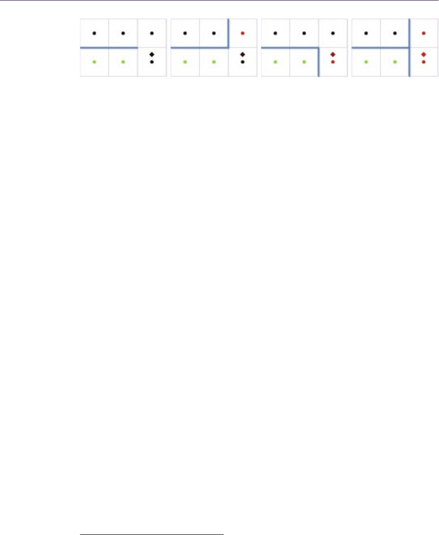
144 8. Practical Morphological Antialiasing
0.0 0.25 0.75 1.0
Figure 8.4. Examples of the four possible types of crossing edge and corresponding
value returned by the bilinear query of the edges texture. The color of the dot at
the center of each pixel represents the value of that pixel in the edges texture. The
rhombuses, at a distance of 0.25 from the center of the pixel, indicate the sampling
position, while their color represents the value returned by the bilinear access.
8.3.2 Fetching Crossing Edges
Once the distances to the ends of the line are calculated, they are used to obtain
the crossing edges. A naive approach for fetching the crossing edge of an end of
a line would be to query two edges. A more efficient approach is to use bilinear
filtering for fetching both edges at one time, in a manner similar to the way the
distance search is done. However, in this case we must be able to distinguish
the actual value of each edgel, so we query with an offset of 0.25, allowing us
to distinguish which edgel is equal to 1.0 when only one of the edges is present.
Figure 8.4 shows the crossing edge that corresponds to each of the different values
returned by the bilinear query.
8.3.3 The Precomputed Area Texture
With distance and crossing edges information at hand, we now have all the re-
quired inputs to calculate the area corresponding to the current pixel. As this is
an expensive operation, we opt to precompute it in a four-dimensional table which
is stored in a conventional two-dimensional texture (see Figure 8.2 (right)).3This
texture is divided into subtextures of size 9 ×9, each of them corresponding to a
pattern type (codified by the fetched crossing edges e1 and e2 at each end of the
line). Inside each of these subtextures, (u, v) coordinates correspond to distances
to the ends of the line, eight being the maximum distance reachable. Resolution
can be increased if a higher maximum distance is required. See Listing 8.4 for
details on how the precomputed area texture is accessed.
To query the texture, we first convert the bilinear filtered values e1 and e2 to
an integer value in the range 0..4. Value 2 (which would correspond to value 0.5
for e1 or e2) cannot occur in practice, which is why the corresponding row and
column in the texture are empty. Maintaining those empty spaces in the texture
3The code to generate this texture is available in the web material.

8.4. Blending with the Four-Neighborhood 145
#define NUM_DISTANCES 9
#define AR EA_SI ZE ( NUM _D ISTA NC ES * 5)
float2 Area(float2 distance , float e1 , floa t e2 ) {
// * By di vidi ng by AREA _SIZ E - 1.0 bel ow we are
// i mplic it ely o ffset ti ng to alw ays fall i nside a pixel .
// * Ro undi ng prev ents b ilin ear access p recis ion problem s .
float2 pix coord = NUM_ DISTA N CES *
ro und (4.0 * float2( e1 , e2 )) + d ista nc e ;
float2 tex coord = pix coor d / ( AREA _SIZ E - 1.0);
return areaTex.SampleLevel( P oi nt Samp le r , te xc oor d , 0 ). r g ;
}
Listing 8.4. Precomputed area texture access function.
allows for a simpler and faster indexing. The round instruction is used to avoid
possible precision problems caused by the bilinear filtering.
Following the same reasoning (explained at the beginning of the section) by
which we store area values for two adjacent pixels in the same pixel of the final
blending weights texture, the precomputed area texture needs to be built on a
per-edgel basis. Thus, each pixel of the texture stores two avalues, one for a
pixel and one for its opposite. (Again, awill be zero for one of them in all cases
with the exception of those pixels centered on lines of odd length.)
8.4 Blending with the Four-Neighborhood
In this last pass, the final color of each pixel is obtained by blending the actual
color with its four neighbors, according to the area values stored in the weights
texture obtained in the previous pass. This is achieved by accessing three posi-
tions of the blending weights texture:
1. the current pixel, which gives us the north and west blending weights;
2. the pixel at the south;
3. the pixel at the east.
Once more, to exploit hardware capabilities, we use four bilinear filtered accesses
to blend the current pixel with each of its four neighbors. Finally, as one pixel can
belong to four different lines, we find an average of the contributing lines. List-
ing 8.5 shows the source code of this pass; Figure 8.1 (right) shows the resulting
image.

146 8. Practical Morphological Antialiasing
float4 NeighborhoodBlendingPS(
float4 pos itio n : SV_POSITION ,
float2 tex coor d : TEXC OORD0 ): SV_TARGET {
float4 topLef t = blen dTex . SampleLevel(PointSampler ,
texcoord , 0);
fl oat right = blen dTex . SampleLevel(PointSampler ,
texcoord , 0,
in t2 (0 , 1 )) . g;
fl oat bottom = blendT ex . SampleLevel(PointSampler ,
texcoord , 0,
in t2 (1 , 0 )) . a;
float4 a = float4( topLe ft .r, right , to pLef t .b , bottom );
fl oat sum = dot ( a , 1 .0);
[branch]
if ( sum > 0 .0) {
float4 o = a * P IXEL_ SI ZE . y yxx ;
float4 co lor = 0.0;
co lor = mad( col orTex . SampleLevel(LinearSampler ,
tex coord + float2( 0 .0 , -o . r ), 0 ) , a . r , c olor );
co lor = mad( col orTex . SampleLevel(LinearSampler ,
tex coord + float2( 0 .0 , o . g ), 0) , a .g , c ol or );
co lor = mad( col orTex . SampleLevel(LinearSampler ,
tex coord + float2( -o. b , 0 .0) , 0 ) , a . b , c olo r ) ;
co lor = mad( col orTex . SampleLevel(LinearSampler ,
tex coord + float2( o .a , 0. 0) , 0) , a . a , c ol or );
return co lo r / sum ;
}else {
return col orTe x . SampleLevel( L inea rSam pler , te xcoord , 0);
}
}
Listing 8.5. Four-neighborhood blending shader.
8.5 Results
Qualitywise, our algorithm lies between 4xand 8xMSAA, requiring a memory
consumption of only 1.5xthe size of the backbuffer on a PC and of 2xon Xbox
360.4Figure 8.5 shows a comparison between our algorithm, 8xMSAA, and
no antialiasing at all on images from Unigine Heaven Benchmark. A limitation
of our algorithm with respect to MSAA is the impossibility of recovering subpixel
4The increased memory cost in the Xbox 360 is due to the fact that two-channel render
targets with 8-bit precision cannot be created in the framework we used for that platform,
forcing the usage of a four-channel render target for storing the edges texture.
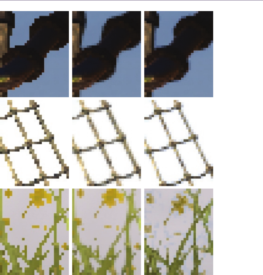
8.5. Results 147
Without antialiasing With our algorithm With 8xMSAA
Figure 8.5. Examples of images without antialiasing, processed with our algorithm, and
with 8xMSAA. Our algorithm offers similar results to those of 8xMSAA. A special
case is the handling of alpha textures (bottom row). Note that in the grass shown
here, alpha to coverage is used when MSAA is activated, which provides additional
detail, hence the different look. As the scene is animated, there might be slight changes
in appearance from one image to another. (Images from Unigine Heaven Benchmark
courtesy of Unigine Corporation.)
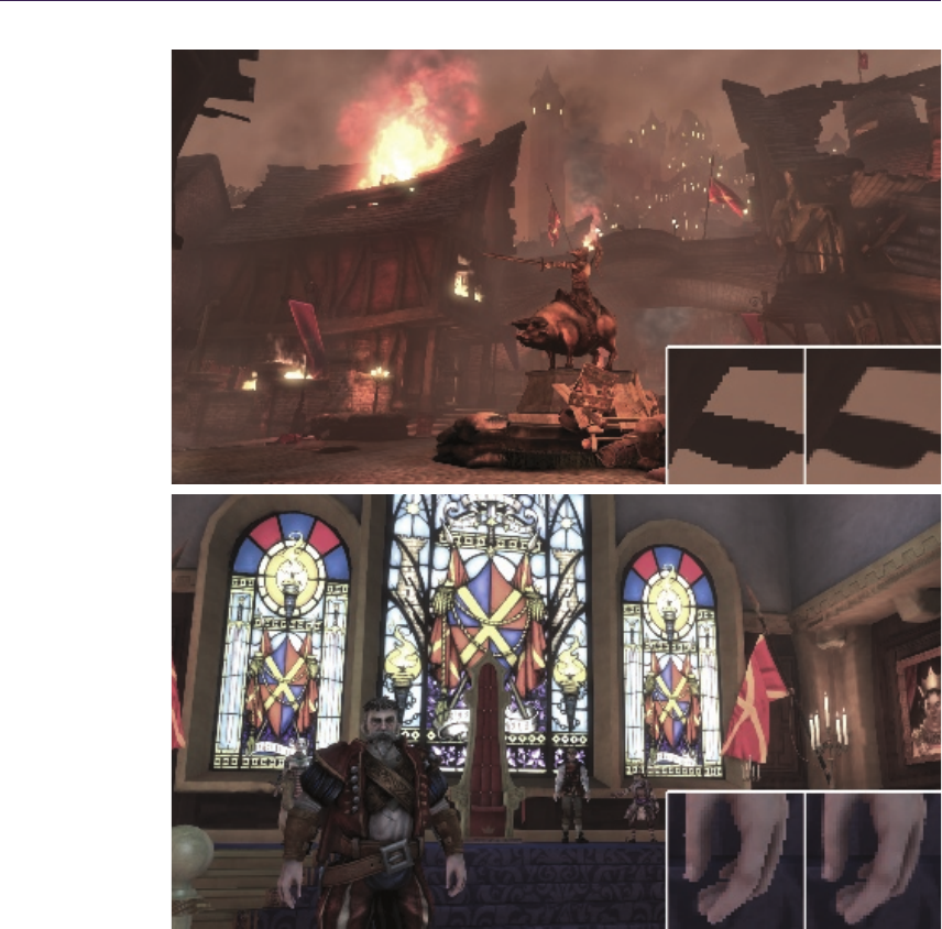
148 8. Practical Morphological Antialiasing
Figure 8.6. Images obtained with our algorithm. Insets show close-ups with no
antialiasing at all (left) and processed with our technique (right). (Images from Fable
III courtesy of Lionhead Studios.)
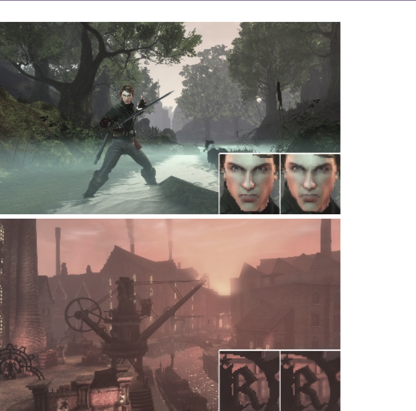
8.5. Results 149
Figure 8.7. More images showing our technique in action. Insets show close-ups with
no antialiasing at all (left) and processed with our technique (right). (Images from Fable
III courtesy of Lionhead Studios.)

150 8. Practical Morphological Antialiasing
Xbox 360 GeForce 9800 GTX+
Avg. Std. Dev. Avg. Std. Dev. Speed-up
Assassin’s Creed 4.37 ms 0.61 ms 0.55 ms 0.13 ms 6.31x?
Bioshock 3.44 ms 0.09 ms 0.37 ms 0.00 ms n/a
Crysis 3.92 ms 0.10 ms 0.44 ms 0.02 ms 14.80x
Dead Space 3.65 ms 0.45 ms 0.39 ms 0.03 ms n/a
Devil May Cry 4 3.46 ms 0.34 ms 0.39 ms 0.04 ms 5.75x
GTA IV 4.11 ms 0.23 ms 0.47 ms 0.04 ms n/a
Modern Warfare 2 4.38 ms 0.80 ms 0.57 ms 0.17 ms 2.48x?
NFS Shift 3.54 ms 0.35 ms 0.42 ms 0.04 ms 14.84x
Split/Second 3.85 ms 0.27 ms 0.46 ms 0.05 ms n/a
S.T.A.L.K.E.R. 3.18 ms 0.05 ms 0.36 ms 0.01 ms n/a
Grand Average 3.79 ms 0.33 ms 0.44 ms 0.05 ms 11.80x
Table 8.1. Average times and standard deviations for a set of well-known commercial
games. A column showing the speed-up factor of our algorithm with respect to 8x
MSAA is also included for the PC/DirectX 10 implementation. Values marked with ?
indicate 4xMSAA, since 8xwas not available, and the grand average of these includes
values only for 8xMSAA.
features. Further results of our technique, on images from Fable III, are shown
in Figures 8.6 and 8.7. Results of our algorithm in-game are available in the web
material.
As our algorithm works as a post-process, we have run it on a batch of screen-
shots of several commercial games in order to gain insight about its performance
in different scenarios. Given the dependency of the edge detection on image
content, processing times are variable. We have noticed that each game has a
more or less unique “look-and-feel,” so we have taken a representative sample of
five screenshots per game. Screenshots were taken at 1280 ×720 as the typical
case in the current generation of games. We used the slightly more expensive
luminance-based edge detection, since we did not have access to depth informa-
tion. Table 8.1 shows the average time and standard deviation of our algorithm
on different games and platforms (Xbox 360/DirectX 9 and PC/DirectX 10),
as well as the speed-up factor with respect to MSAA. On average, our method
implies a speed-up factor of 11.80xwith respect to 8xMSAA.
8.6 Discussion
This section includes a brief compilation of possible alternatives that we tried,
in the hope that it would be useful for programmers employing this algorithm in
the future.
Edges texture compression. This is perhaps the most obvious possible optimiza-
tion, saving memory consumption and bandwidth. We tried two different alterna-
tives: a) using 1 bit per edgel, and b) separating the algorithm into a vertical and
a horizontal pass and storing the edges of four consecutive pixels in the RGBA

8.7. Conclusion 151
channels of each pixel of the edges texture (vertical and horizontal edges sepa-
rately). This has two advantages: first, the texture uses less memory; second, the
number of texture accesses is lower since several edges are fetched in each query.
However, storing the values and—to a greater extent—querying them later, be-
comes much more complex and time consuming, given that bitwise operations
are not available in all platforms. Nevertheless, the use of bitwise operations in
conjunction with edges texture compression could further optimize our technique
in platforms where they are available, such as DirectX 10.
Storing crossing edges in the edges texture. Instead of storing just the north and
west edges of the actual pixel, we tried storing the crossing edges situated at the
left and at the top of the pixel. The main reason for doing this was that we
could spare one texture access when detecting patterns; but we realized that by
using bilinear filtering we could also spare the access, without the need to store
those additional edges. The other reason for storing the crossing edges was that,
by doing so, when we searched for distances to the ends of the line, we could
stop the search when we encountered a line perpendicular to the one we were
following, which is an inaccuracy of our approach. However, the current solution
yields similar results, requires less memory, and processing time is lower.
Two-pass implementation. As mentioned in Section 8.1, a two-pass implementa-
tion is also possible, joining the last two passes into a single pass. However, this
would be more inefficient because of the repetition of calculations.
Storing distances instead of areas. Our first implementation calculated and stored
only the distances to the ends of the line in the second pass, and they were then
used in the final pass to calculate the corresponding blending weights. However,
directly storing areas in the intermediate pass allows us to spare calculations,
reducing execution time.
8.7 Conclusion
In this chapter, we have presented an algorithm crafted for the computation of
antialiasing. Our method is based on three passes that detect edges, determine
the position of each pixel inside those image features, and produce an antialiased
result that selectively blends the pixel with its neighborhood according to its
relative position within the line it belongs to. We also take advantage of hardware
texture filtering, which allows us to reduce the number of texture fetches by half.
Our technique features execution times that make it usable in actual game
environments, and that are far shorter than those needed for MSAA. The method
presented has a minimal impact on existing rendering pipelines and is entirely
implemented as an image post-process. Resulting images are between 4xand

152 8. Practical Morphological Antialiasing
8xMSAA in quality, while requiring a fraction of their time and memory con-
sumption. Furthermore, it can antialias transparent textures such as the ones
used in alpha testing for rendering vegetation, whereas MSAA can smooth vege-
tation only when using alpha to coverage. Finally, when using luminance values
to detect edges, our technique can also handle aliasing belonging to shading and
specular highlights.
The method we are presenting solves most of the drawbacks of MSAA, which
is currently the most widely used solution to the problem of aliasing; the pro-
cessing time of our method is one order of magnitude below that of 8xMSAA.
We believe that the quality of the images produced by our algorithm, its speed,
efficiency, and pluggability, make it a good choice for rendering high quality im-
ages in today’s game architectures, including platforms where benefiting from
antialiasing, together with outstanding techniques like deferred shading, was dif-
ficult to achieve. In summary, we present an algorithm which challenges the
current gold standard for solving the aliasing problem in real time.
8.8 Acknowledgments
Jorge would like to dedicate this work to his eternal and most loyal friend Kaz´an. The
authors would like to thank the colleagues at the lab for their valuable comments, and
Christopher Oat and Wolfgang Engel for their editing efforts and help in obtaining
images. Thanks also to Lionhead Studios and Microsoft Games Studios for granting
permission to use images from Fable III. We are very grateful for the support and
useful suggestions provided by the Fable team during the production of this work. We
would also like to express our gratitude to Unigine Corporation, and Denis Shergin in
particular, for providing us with images and material for the video (available in the web
material) from their Unigine Heaven Benchmark. This research has been funded by a
Marie Curie grant from the 7th Framework Programme (grant agreement no.: 251415),
the Spanish Ministry of Science and Technology (TIN2010-21543) and the Gobierno de
Arag´on (projects OTRI 2009/0411 and CTPP05/09). Jorge Jimenez and Belen Masia
are also funded by grants from the Gobierno de Arag´on.
Bibliography
[Koonce 07] Rusty Koonce. “Deferred Shading in Tabula Rasa.” In GPU Gems 3,
pp. 429–457. Reading, MA: Addison Wesley, 2007.
[Reshetov 09] Alexander Reshetov. “Morphological Antialiasing.” In HPG ’09: Pro-
ceedings of the Conference on High Performance Graphics 2009, pp. 109–116. New
York: ACM, 2009. Available online (http://visual-computing.intel-research.net/
publications/papers/2009/mlaa/mlaa.pdf).
[Shishkovtsov 05] Oles Shishkovtsov. “Deferred Shading in S.T.A.L.K.E.R.” In GPU
Gems 2, pp. 143–166. Reading, MA: Addison Wesley, 2005.

Bibliography 153
[Sousa 07] Tiago Sousa. “Vegetation Procedural Animation and Shading in Crysis.” In
GPU Gems 3, pp. 373–385. Reading, MA: Addison Wesley, 2007.
[Thibieroz 09] Nicolas Thibieroz. “Deferred Shading with Multisampling Anti-Aliasing
in DirectX 10.” In ShaderX7, pp. 225–242. Hingham, MA: Charles River Media,
2009.

9
Volume Decals
Emil Persson
9.1 Introduction
Decals are often implemented as textured quads that are placed on top of the
scene geometry. While this implementation works well enough in many cases,
it can also provide some challenges. Using decals as textured quads can cause
Z-fighting problems. The underlying geometry may not be flat, causing the decal
to cut into the geometry below it. The decal may also overhang an edge, com-
pletely ruining its effect. Dealing with this problem often involves clipping the
decal to the geometry or discarding it entirely upon detecting the issue. Alterna-
tively, very complex code is needed to properly wrap the decal around arbitrary
meshes, and access to vertex data is required. On a PC this could mean that
system-memory copies of geometry are needed to maintain good performance.
Furthermore, disturbing discontinuities can occur, as in the typical case of shoot-
ing a rocket into a corner and finding that only one of the walls got a decal or
that the decals do not match up across the corner. This article proposes a tech-
nique that overcomes all of these challenges by projecting a decal volume onto
the underlying scene geometry, using the depth buffer.
9.2 Decals as Volumes
9.2.1 Finding the Scene Position
The idea behind this technique is to render the decal as a volume around the
selected area. Any convex volume shape can be used, but typical cases would be
spheres and boxes. The fragment shader computes the position of the underlying
geometry by sampling the depth buffer. This can be accomplished as follows:
// texCoord is the pixel’s normalized screen position
float depth = DepthTex.Sample(Filter, texCoord);
float4 scrPos = float4(texCoord, depth, 1.0f);
float4 wPos = mul(scrPos, ScreenToWorld);
155
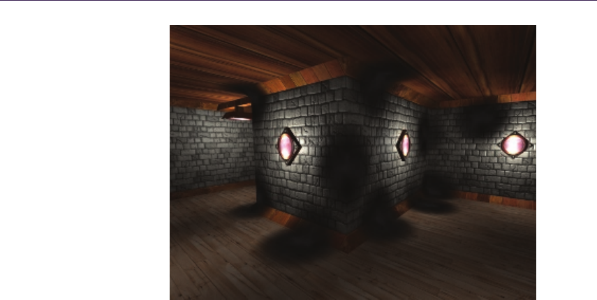
156 9. Volume Decals
Figure 9.1. Example decal rendering.
float3 pos = wPos.xyz / wPos.w;
// pos now contains pixel position in world space
The ScreenToWorld matrix is a composite matrix of two transformations:
namely the transformation from screen coordinates to clip space and then from
clip space to world space. Transforming from world space to clip space is done
with the regular ViewProjection matrix, so transforming in the other direction
is done with the inverse of this matrix. Clip space ranges from −1 to 1 in x
and y, whereas the provided texture coordinates are in the range of 0 to 1, so
we also need an initial scale-bias operation baked into the matrix. The matrix
construction code could look something like this:
float4 ScaleToWorld = Scale(2, -2, 1) *
Translate(-1, 1, 0) * Inverse(ViewProj);
What we are really interested in, though, is the local position relative to
the decal volume. The local position is used as a texture coordinate used to
sample a volume texture containing a volumetric decal (see Figure 9.1). Since
the decal is a volumetric texture, it properly wraps around nontrivial geometry
with no discontinuities (see Figure 9.2). To give each decal a unique appearance,
a random rotation can also be baked into the matrix for each decal. Since we
do a matrix transformation we do not need to change the shader code other
than to name the matrix more appropriately as ScreenToLocal, which is then
constructed as follows:
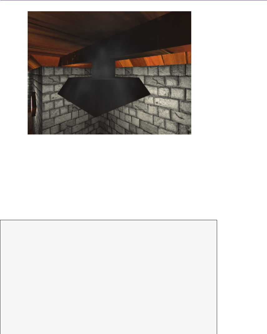
9.2. Decals as Volumes 157
Figure 9.2. Proper decal wrapping around nontrivial geometry.
float4 ScreenToLocal = Scale(2, -2, 1) *
Translate(-1, 1, 0) * Inverse(ViewProj) *
DecalTranslation * DecalScale * DecalRotation;
The full fragment shader for this technique is listed below and a sample with
full source code is available in the web materials.
Tex ture 2D <float > D ept hTex ;
Sam plerSt ate D epth Filter ;
Tex ture 3D <float4 > Deca lTe x ;
Sam plerSt ate D ecal Filter ;
cbuffe r Cons tant s
{
flo at4x4 Scre enToLo cal ;
float2 Pix elSiz e ;
};
float4 ma in ( Ps In In ) : S V_ Ta rg et
{
// Compute nor mali z ed screen positio n
float2 t ex Co or d = In . P os it io n . xy * P ix el Si ze ;

158 9. Volume Decals
// Compute l ocal p osition of scene g eom etry
fl oat depth = D epthT ex . Sam ple ( De pth Filter , tex Coord );
float4 scrPos = float4( t exC oo rd , dep th , 1 .0 f );
float4 wP os = m ul ( scrPo s , S cr een ToL oc al );
// Sam ple decal
float3 co ord = wPo s .xyz / wPos .w;
retur n Deca lTex . Sa mple ( DecalF ilter , coo rd );
}
Listing 9.1. The full fragment shader.
9.2.2 Implementation and Issues
In a deferred-rendering system [Thibieroz 04] this technique fits perfectly. The
decals can be applied after the geometry buffer (G-buffer) pass and the relevant
attributes, such as diffuse color and specularity, can simply be updated, and then
lighting can be applied as usual. This technique also works well with a light pre-
pass renderer [Engel 09], in which case lighting information is readily available
for use in the decal pass.
In a forward rendering system the decals will be applied after lighting. In
many cases this is effective also, for instance, for burn marks after explosions,
in which case the decals can simply be modulated with the destination buffer.
With more complicated situations, such as blending with alpha, as is typically
the case for bullet holes, for instance, the decal application may have to take
lighting into account. One solution is to store the overall lighting brightness into
alpha while rendering the scene; the decal can then pre-multiply source color
with alpha in the shader and multiply with destination alpha in the blender to
get reasonable lighting. This will not take light color into account, but may look
reasonable if lighting generally is fairly white. Another solution is to simply go
by the attenuation of the closest light and not take any normal into account.
Alternatively, a normal can be computed from the depth buffer, although this is
typically slow and has issues of robustness [Persson 09].
One issue with this technique is that it applies the decal on everything within
the decal volume. This is not a problem for static objects, but if you have a large
decal volume and dynamic objects move into it they will get the decal smeared
onto them, for instance, if you previously blew a bomb in the middle of the road
and a car is passing through at a later time. This problem can be solved by
drawing dynamic objects after the decal pass. A more elaborate solution is to
render decals and dynamic objects in chronological order so that objects that are
moved after the decal is added to the scene will not be affected by the decal. This
will allow dynamic objects to be affected by decals as well. Another solution is to
use object IDs. The decal can store the IDs of objects that intersected the decal

9.2. Decals as Volumes 159
volume at the time it was added to the scene and cull for discarded pixels that
do not belong to any of those objects.
9.2.3 Optimizations
On platforms where the depth-bounds test is supported, the depth-bounds test
can be used to improve performance. On other platforms, dynamic branching can
be used to emulate this functionality by comparing the sample depth to the depth
bounds. However, given that the shader is relatively short and typically a fairly
large number of fragments survive the test, it is recommended to benchmark to
verify that it actually improves performance. In some cases it may in fact be
faster to not attempt to cull anything.
9.2.4 Variations
In some cases it is desirable to use a two-dimensional texture instead of a volume
decal. Volume textures are difficult to author and consume more memory. Not
all cases translate well from a two-dimensional case to three dimensions. A bullet
hole decal can be swept around to a spherical shape in the three-dimensional
case and can then be used in any orientation, but this is not possible for many
kinds of decals; an obvious example is a decal containing text, such as a logo or
graffiti tag.
An alternate technique is to sample a two-dimensional texture using just the
x, y components of the final coordinates. The zcomponent can be used for fading.
When a volume texture is used, you can get an automatic fade in all directions
by letting the texture alpha fade to zero toward the edges and using a border
color with an alpha of zero. In the 2D case you will have to handle the zdirection
yourself.
Two-dimensional decals are not rotation invariant so when placing them in
the scene they must be oriented such that they are projected sensibly over the un-
derlying geometry. The simplest approach would be to just align the decal plane
with the normal of the geometry at the decal’s center point. Some problematic
cases exist though, such as when wrapping over a corner of a wall. If it is placed
flat against the wall you will get a perpendicular projection on the other side of
the corner with undesirable texture-stretching as a result.
An interesting use of the two-dimensional case is to simulate a blast in a
certain direction. This can be accomplished by using a pyramid or frustum shape
from the point of the blast. When the game hero shoots a monster you place a
frustum from the bullet-impact point on the monster to the wall behind it in the
direction of the bullet and you will get the effect of blood and slime smearing onto
the wall. The projection matrix of this frustum will have to be baked into the
ScreenToLocal matrix to get the proper projection of the texture coordinates.

160 9. Volume Decals
The blast technique can also be varied for a cube decal scenario. This would
better simulate the effect of a grenade blast. In this case a cube or sphere would be
rendered around the site of the blast and a cubemap lookup is performed with the
final coordinates. Fading can be effected using the length of the coordinate vector.
To improve the blast effect you can use the normals of underlying geometry
to eliminate the decal on back-facing geometry. For the best results, a shad-
owmapesque technique can be used to make sure only the surfaces closest to the
front get smeared with the decal. This “blast-shadow map” typically has to be
generated only once at the time of the blast and can then be used for the rest
of the life of the decal. Using the blast-shadow map can ensure splatter happens
only in the blast shadow of monsters and other explodable figures, whereas areas
in the blast-shadow map that contain static geometry only get scorched. This
requires storing a tag in the shadow buffer for pixels belonging to monsters, how-
ever. Creative use of the shadow map information also can be used to vary the
blood-splatter intensity over the distance from the blast to the monster and from
the monster to the smeared wall.
9.3 Conclusions
An alternate approach for decal rendering has been shown that suggests solu-
tions to many problems of traditional decal-rendering techniques. Using vol-
umes instead of flat decal geometry allows for continal decals across nontrivial
geometry. It also eliminates potentially expensive buffer locks or the need for
system-memory buffer copies.
Bibliography
[Thibieroz 04] Nicolas Thibieroz. “Deferred Shading with Multiple Render Targets.”
In ShaderX2: Shader Programming Tips and Tricks with DirectX 9, edited by
Wolfgang Engel, pp. 251–269. Plano, TX: Wordware Publishing, 2004.
[Engel 09] Wolfgang Engel. “Designing a Renderer for Multiple Lights - The Light Pre-
Pass Renderer.” In ShaderX7: Advanced Rendering Techniques, edited by Wolfgang
Engel, pp. 655–666. Hingham, MA: Charles River Media, 2009.
[Persson 09] Emil Persson. “Making It Large, Beautiful, Fast and Consistent: Lessons
Learned Developing Just Cause 2.” in GPU Pro: Advanced Rendering Techniques,
pp. 571–596. Natick, MA: A K Peters, 2010.
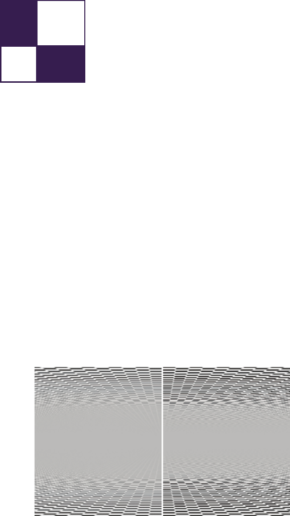
10
Practical Elliptical Texture
Filtering on the GPU
Pavlos Mavridis and Georgios Papaioannou
10.1 Introduction
Hardware texture filtering, even on state-of-the-art graphics hardware, suffers
from several aliasing artifacts, in both the spatial and temporal domain. These
artifacts are mostly evident in extreme conditions, such as grazing viewing angles,
highly warped texture coordinates, or extreme perspective, and become especially
annoying when animation is involved. Poor texture filtering is evident as excessive
blurring or moir´e patterns in the spatial domain and as pixel flickering in the
temporal domain, as can be seen in Figure 10.1 and the accompanying demo
application.
Figure 10.1. A benchmark scene consisting of two infinite planes demonstrating the
improvement of elliptical filtering (left) over the native hardware texture filtering (right).
161

162 10. Practical Elliptical Texture Filtering on the GPU
In this chapter, we present a series of simple and effective methods to perform
high quality texture filtering on modern GPUs. We base our methods on the the-
ory behind the elliptical weighted average (EWA) filter [Greene and Heckbert 86].
EWA is regarded as one of the highest quality texture filtering algorithms and
is used as a benchmark to test the quality of other algorithms. It is often used
in offline rendering to eliminate texture aliasing in the extreme conditions men-
tioned above, but due to the high computational cost it is not widely adopted in
real-time graphics.
We first present an exact implementation of the EWA filter that smartly
uses the underlying bilinear filtering hardware to gain a significant speedup. We
then proceed with an approximation of the EWA filter that uses the underlying
anisotropic filtering hardware of the GPU to construct a filter that closely matches
the shape and the properties of the EWA filter, offering vast improvements in the
quality of the texture mapping. To further accelerate the method, we also intro-
duce a spatial and temporal sample distribution scheme that reduces the number
of required texture fetches and the memory bandwidth consumption, without re-
ducing the perceived image quality. We believe that those characteristics make
our method practical for use in games and other interactive applications, as well
as applications that require increased fidelity in texture mapping, like GPU ren-
derers and image manipulation programs. We first described these methods at the
2011 Symposium on Interactive 3D Graphics and Games [Mavridis and Papaioan-
nou 11]. This chapter reviews the main ideas of that paper with an emphasis on
small, yet important implementation details.
10.2 Elliptical Filtering
This section provides an overview of the theory behind texture filtering and the
elliptical weighted average (EWA) filter.
In computer graphics the pixels are point samples. The pixels do not have an
actual shape, since they are points, but we often assign an area to them. This
area is the footprint (the nonzero areas) of the filter that is used to reconstruct
the final continuous image from these point samples, according to the sampling
theorem. As discussed in [Smith 95], high quality reconstruction filters, like a
truncated sinc or Gaussian, have a circular footprint, so a high quality texture
filtering method should assume circular overlapping pixels.
The projection of a pixel with circular footprint to texture space is an ellipse
with arbitrary orientation, as illustrated in Figure 10.2. In degenerate cases, like
extreme grazing viewing angles, the projection is actually an arbitrary conic sec-
tion, but for our purposes an elliptical approximation suffices, since, for these
cases, any visible surface detail is lost anyway. A texture filtering algorithm
should return a convolution of the texels (texture point samples) inside the pro-
jected area Sof the pixel with the projection of the reconstruction filter Hin

10.2. Elliptical Filtering 163
S
Figure 10.2. The projection of a pixel with circular footprint on a surface covers an
elliptical region.
texture space. In particular, it should compute the following equation:
Cf(s, t) = ∑
u,v∈S
H(u, v)C(u, v),
where C(u, v) is the color of the texel at the (u, v) texture coordinates and Cf(s, t)
is the filtered texture color. In the above equation His normalized.
The EWA algorithm approximates the projected pixel footprint with an ellip-
tical region, defined by the following equation [Heckbert 89]:
d2(u, v) = Au2+Buv +Cv2,
where the center of the pixel is assumed to be at (0,0) in texture space and
A=Ann/F,
B=Bnn/F,
C=Cnn/F,
F=AnnCnn −B2
nn/4,
Ann = (∂v/∂x)2+ (∂v/∂y)2,
Bnn =−2∗(∂u/∂x ∗∂v/∂x +∂u/∂y ∗∂v/∂y),
Cnn = (∂u/∂x)2+ (∂u/∂y)2.
The partial derivatives (∂u/∂x, ∂u/∂y, ∂v/∂x, ∂v/∂y) represent the rate of
change of the texture coordinates relative to changes in screen space. The quan-
tity d2denotes the squared distance of the texel (u, v) from the pixel center when
projected back into screen space. The algorithm scans the bounding box of the
elliptical region in texture space and determines which texels reside inside the
ellipse (d2≤1). These samples contribute to the convolution sum, with weights

164 10. Practical Elliptical Texture Filtering on the GPU
// Co mp ut es the Ellip ti ca l W ei gh te d Average f ilter
// p are the sa mp li ng coo rd in at es
// du / dv are the d er ivati ve s of the te xt ur e c oo rd inates
ve c4 e wa Fi lt er ( sa mp le r2 D tex , ve c2 p , vec 2 du , ve c2 dv )
{
// c omp ut e e ll ips e c oe f fi ci en ts A , B , C , F :
float A , B ,C , F ;
A = du . t* du . t + dv . t* dv . t +1 ;
...
// Co mpute the e llipse ’s bounding box in text ur e sp ace
int u_min , u_max , v_min , v _max ;
u_min = int ( f loor ( p .s - 2. / ( -B* B +4. 0* C* A)*
s qrt ( ( - B * B + 4. 0* C * A ) * C* F ) ) );
...
// It erate ove r the e llipse ’s bounding box and
// ca lcu lat e Ax ˆ2+ Bxy *Cy ˆ2; when this value
// is l es s t ha n F , we ’ re in sid e the e ll ip se .
vec 4 color = 0;
float den = 0;
for (int v = v_mi n ; v <= v_m ax ; ++ v )
{
float q = A*u*u+B*u*v*C*v*v;
for (int u = u_ min ; u <= u _max ; ++ u)
if (q < F )
{
float d = q / F ;
float weight = Filter(d);
co lor += we igh t * t ex tur e2 D (tex , vec2 ( u +0.5 , v + 0.5 ) / size ) ;
den += we igh t ;
}
}
return co lor *( 1./ den ) ;
}
Listing 10.1. Pseudocode implementation of the EWA filter.
proportional to the distance d.Listing 10.1 outlines this idea. Filter(d) de-
notes the reconstruction filter. [Greene and Heckbert 86] propose the usage of a
Gaussian filter, but in practice any reconstruction filter can be used.
10.2.1 Bounding the Runtime Cost
The runtime of the brute-force algorithm is directly proportional to the area of the
ellipse in texture space and the number of texels it includes. To reduce the number
of the texture samples in this area, a mip-map pyramid is used and sampling is
performed from the mip-map level in which the minor ellipse radius is between
one and three pixels, depending on the required quality and performance. Even
when using mip-maps, the area of a highly eccentric ellipse can be arbitrarily
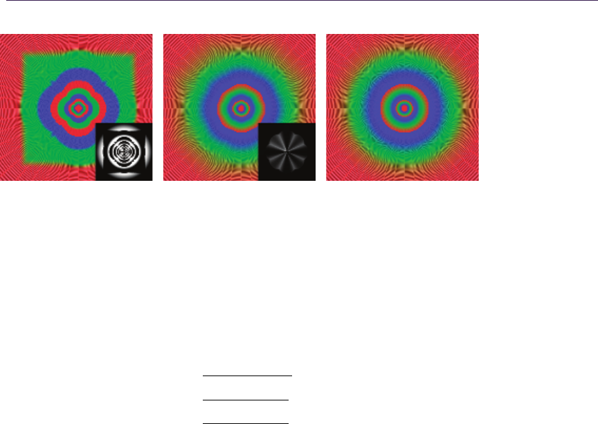
10.2. Elliptical Filtering 165
Figure 10.3. Comparison of the lod calculation of an Nvidia Fermi card when using
the lowest quality settings in the drivers (left), the highest possible quality settings
(middle), and the optimal lod calculations (right).
high, resulting in unacceptably long running times. To avoid this, the maximum
eccentricity of the ellipse is clamped to a predefined maximum. Taking these two
measures ensures a bounded runtime for the algorithm.
Computing the mip-map level (lod) and clamping ellipses with high eccentric-
ity requires the computation of the minor (Rminor) and major (Rmajor) radius of
the ellipse
r=√(A−C)2+B2,
Rmajor =√2/(A+C−r),
Rminor =√2/(A+C+r),
lod = log2(Rminor/texels-per-pixel.) (10.1)
Instead of computing the lod level based on the minor ellipse radius, we have
investigated the option to use the lod values calculated explicitly by the hardware.
On newer hardware this can be done using the appropriate shading language func-
tion (textureQueryLOD() in GLSL), or in older hardware by fetching a texel from
a texture with color-coded lod levels. Figure 10.3 visualizes the lod selection on
the latest Nvidia graphics cards and compares it with the ideal lod selection based
on the ellipse minor radius. We observe that Nvidia’s hardware, at the highest
quality settings, performs a piecewise approximation of the optimal calculations,
resulting in suboptimal lod selection on pixels depending on their angle and that
the measured deviation (shown in the insets of Figure 10.3) peaks at intervals of
45 degrees. An overestimation of the lod level will result in excessive blurriness,
while underestimation will result in longer runtimes. In practice, we have ob-
served that using the hardware lod calculations does not result in visible quality
degradation, while the performance of the method is increased.
Hardware trilinear filtering interpolates between the closest two lod levels, in
order to avoid discontinuities. We have found that it is much more preferable
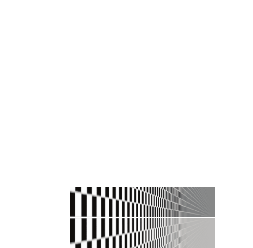
166 10. Practical Elliptical Texture Filtering on the GPU
to perform better filtering in the high detail lod level (by using more samples),
than to compute two inferior estimates and interpolate between them. In that
case, discontinuities from the lod selection can only be observed in very extreme
cases, and even then can be dealt with using more projected texels in each pixel
(Equation (10.1)).
10.2.2 Filtering sRGB Textures
A very important implementation detail that is often omitted, is that all the tex-
ture filtering and antialiasing operations should be done in linear color space. On
the other hand, 8 bits-per-component textures are usually stored in sRGB color
space, in order to better take advantage of the available precision, by taking into
account the characteristics of human vision. Therefore, the texture data should
be first converted to a linear color space before the filtering operations. And, after
the shading operations, colors should be converted back to sRGB for display in
the output device. Fortunately, the latest graphics hardware can do this conver-
sion using specialized fixed-function hardware, without any additional overhead.
In OpenGL in particular, this can be done by using the GL EXT texture sRGB
and GL EXT framebuffer sRGB extensions, while Direct3D provides similar mech-
anisms. Furthermore, all the prefiltered mip-maps should also be computed in
linear color space. The importance of filtering in the proper color space is demon-
strated in Figure 10.4. (All the images in this chapter were produced with filtering
in linear color space.)
Figure 10.4. Texture filtering using mip-maps computed in sRGB color space (top).
Proper filtering in linear color space (bottom). Filtering in nonlinear color space leads
to incorrect darkening when the lowest mip-map levels are used.
10.2.3 GPU Optimizations
A na¨ıve direct implementation of the EWA filter on the GPU would read every
texel in the bounding box of the elliptical region, and if it were located inside
the ellipse, it would be weighted and accumulated. A much better approach is to

10.3. Elliptical Footprint Approximation 167
use the linear filtering of the graphics hardware to reduce the number of fetches
to one half, by smartly fetching two texels at a time using one bilinear fetch.
For two neighboring texels Ciand Ci+1, with weights wiand wi+1, respectively,
the following weighted sum can be replaced by a single bilinear texture fetch
operation at position xbetween the two texel centers:
wiCi+wi+1Ci+1 =Cx(wi+wi+1),
x=i+wi+1
wi+wi+1
,
0≤wi+1
wi+wi+1 ≤1.
The last inequality is always true for reconstruction filters with positive weights,
like the Gaussian one. In our case, the texel weight wiis derived from the recon-
struction filter (Filter(d) in Listing 10.1) and the distance dof the texel to the
filter center, as explained in Section 10.2. The for loop in Listing 10.1 should be
adjusted to process two texels at a time. An important implementation detail is
that when using this technique, we should take into account the exact coordinates
of the texel centers. In the case of OpenGL, texel centers are assumed to be at
the centers of a grid (meaning that texels are located at coordinates integer+0.5).
This technique assumes that the cost of one texture fetch with bilinear filtering
is less than the cost of two fetches with point sampling plus the time to combine
them. Our experiments confirm that this assumption is true. The results from
this method should be identical with the ones from the reference implementation,
but slight deviations may occur due to the difference in the precision in which
operations are performed by the shader units and by the fixed-function bilinear
filtering units.
Extending the same principle in two dimensions, we can replace four weighted
texture fetches with a single fetch from the appropriate position. While it is trivial
to find this position in the case of a box filter, in the case of a Gaussian filter the
weights can only be approximated. In other words, we can calculate the position
that best approximates the Gaussian weights and perform a single texture fetch
from that position. In practice we did not observe any significant performance
gain from this method, while on the other hand it imposes significant constraints
on the nature of the reconstruction filters that can be used.
10.3 Elliptical Footprint Approximation
In the same spirit as the Feline algorithm [McCormack et al. 99], we present a
method that uses simpler shapes to closely match the shape of the ideal elliptical
filter. Instead of using simple trilinear probes like in the Feline algorithm, we
propose the usage of the anisotropic probes provided by the graphics hardware.
We place the probes on a line along the major axis of the ellipse, as shown in
Figure 10.5. The length of the line Land the number of probes Nprobes are given
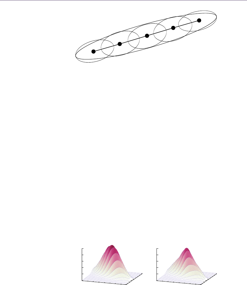
168 10. Practical Elliptical Texture Filtering on the GPU
n=-1
n=0
n=-2
n=+1
n=+2
Figure 10.5. The basic idea of our method: approximating a highly eccentric ellipse
with many ellipses of low eccentricity. This way we can overcome the limits imposed by
the hardware and better filter elliptical footprints with high degrees of anisotropy.
by the following equations
Nprobes = 2 ∗(Rmajor/(α∗Rminor)) −1,
L= 2 ∗(Rmajor −α∗Rminor),(10.2)
where αis the degree of anisotropy of the underlying hardware probes. For α= 1
our algorithm is equivalent to Feline. For simplicity, an odd number of probes is
considered. Similar to Feline, probes are placed around the midpoint (um, vm) of
the filter, as follows:
θ= atan(B/(A−C))/2,
du = cos(θ)∗L/(Nprobes −1),
dv = sin(θ)∗L/(Nprobes −1),
(un, vn) = (um, vm) + n/2∗(du, dv), n = 0,±2,±4. . . , (10.3)
where (un, vn) is the position of n-th probe. To better match the shape of the
EWA filter, the probes are weighted proportionally to their distance from the
center of the footprint, according to a Gaussian function. The shape of the filter
in texture space compared to an exact EWA filter is shown in Figure 10.6.
U U
-4
0
0.2
0.4
0.6
0.8
1
-4
0
0.2
0.4
0.6
0.8
1
V V
Figure 10.6. Comparison of the exact EWA filter (left) with our approximation using
three elliptical probes (right).
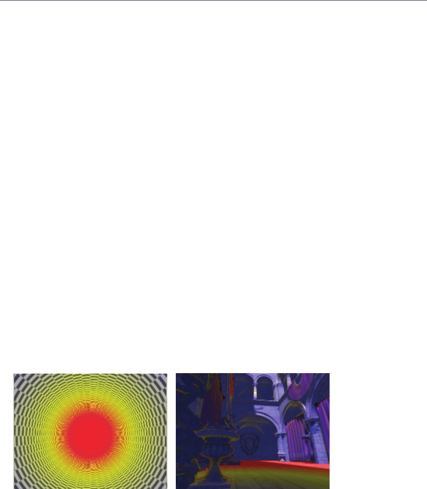
10.3. Elliptical Footprint Approximation 169
We don’t have any strong guarantees about the quality or the shape of those
probes, since the OpenGL specification does not explicitly enforce any particular
method for anisotropic filtering. The only hint given by the hardware imple-
mentation is that the probes approximate an anisotropic area with maximum
anisotropy of N. In the above analysis, we have assumed that the hardware
anisotropic probes are elliptical, but in practice, to compensate for their poten-
tial imperfections in shape and to better cover the area of the elliptical filter,
we just increase the number of probes depending on the desired quality. Using
an adaptive number of probes creates an irregular workload per pixel for the
graphics hardware scheduler, which should be avoided. In practice, setting the
number of probes to a constant number gives better performance. In our tests,
using five probes eliminated all the visible artifacts on the Nvidia hardware (with
high quality texture filtering enabled). For more than five probes, no significant
improvement in image quality could be measured.
If the probes fail to cover the ellipse, then aliasing will occur. On the other
hand, if the probes exceed the extents of the ellipse (e.g., by placing them beyond
half the length of the central line in each direction) then blurring will occur. Our
method always avoids the second case, but the first case can still happen in
extreme cases, since we have clamped the maximum number of probes. Still, our
method always provides an improvement over hardware texture filtering.
10.3.1 Spatial Filter
After some investigation of the benchmark scenes, we have observed that the
regions where the hardware filtering fails are limited. For the majority of a
scene, the quality of the image is free of any aliasing artifacts. As expected, the
problematic regions are regions with high anisotropy, and, in particular, on the
Figure 10.7. Regions in red denote areas with anisotropy greater than 16, the limit
in current hardware implementations. An infinite tunnel benchmark scene (left). A
typical game scene (right).

170 10. Practical Elliptical Texture Filtering on the GPU
Nvidia hardware, regions with anisotropy greater than 16, which is the advertised
maximum anisotropy of the hardware unit. Figure 10.7 highlights the problematic
regions on the benchmark scene and one typical game scene.
After this observation, we perform high-quality filtering only in the regions
highlighted with red, and for the rest of the scene we use hardware filtering. The
anisotropy of a pixel is accurately measured using Equations (10.1). To eliminate
any visible seams between the two regions, areas close to the threshold level use
a blend of hardware and software filtering. This approach creates exactly two
different workloads for the hardware, one high and one low. In the majority of
cases, the two different sampling methods are used in spatially coherent pixel
clusters within a frame. Therefore, compared to a completely adaptive sample
selection, our tests indicate that this case is handled more efficiently by the GPU
hardware scheduler and results in a sizable performance gain.
10.3.2 Temporal Sample Distribution
In order to further improve the runtime performance of our filtering algorithm
in games and other real-time applications that display many rendered images
at high frame rates, we present a temporal sample distribution scheme, where
texture filtering samples are distributed among successive frames.
In particular, the nanisotropic samples (probes) of Equation (10.3) are dis-
tributed in two successive frames. The first frame uses samples 0,±4,±8. . . and
the next one 0,±2,±6. . . . The sample at the center of the filter (sample 0) is
included in both frames to minimize the variance between the two. When the
frames are displayed in quick succession, the human eye perceives the average of
the two frames.
For this technique to work, the application should maintain a stable and ver-
tical sync-locked frame rate of 60 Hz or more. The usage of vertical sync is
mandatory; otherwise the rate of the rendered frames will not match the rate at
which they are displayed and are perceived by the human eye, and the method
naturally fails. This is a shortcoming, but we should note that in the era of high-
performing graphics hardware, rendering without vertical sync makes little sense,
since it introduces visible tearing. Obviously the method can be extended to dis-
tribute samples in more than two frames when the refresh rate of the application
and the output device is high enough.
Using this method, the quality of texture filtering is enhanced considerably for
static or distant objects, but fast-moving objects receive fewer samples. This is
hardly objectionable, since in that case potential aliasing artifacts are difficult to
notice. In our tests, the usage of temporal sample distribution always improved
the perceived image quality for a given number of samples.
Overall, this temporal method is very simple to implement, does not require
additional memory, and always provides a constant speedup. The obvious short-
coming is that the application should maintain a high frame rate. The success
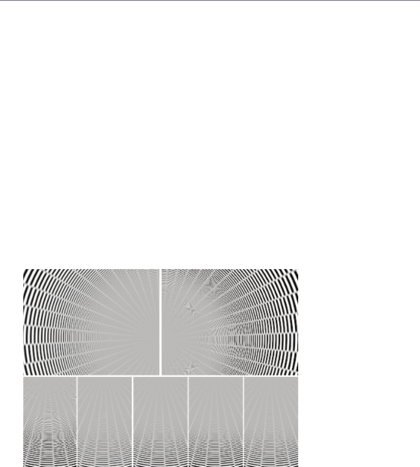
10.4. Results 171
of the method is also highly dependent on the ability of the output device to be
synchronized with the graphics hardware. We had great success when using PC
monitors, but some projection equipment might fail in the synchronization with
the graphics hardware.
10.4 Results
Figure 10.8 demonstrates the improvement our method produces in a benchmark
scene consisting of an infinite tunnel with a checkerboard texture. To better as-
sess the extent of the improvement, the reader is highly encouraged to run the
accompanying demo application, since the aliasing artifacts are highly objection-
able in motion. The same figure also shows the resulting filtering from all the
filtering methods we have presented in this chapter.
Figure 10.9 demonstrates the improvement from increasing the maximum de-
grees of anisotropy. A higher maximum degree of anisotropy offers more detail at
grazing angles. We observe that direct convolution filtering with an anisotropic
ratio of 64:1 preserves more detail at the center of the tunnel. An ideal filter-
ing algorithm would show the lines to converge at the center of the left image,
Figure 10.8. Top: A benchmark scene consisting of an infinite tunnel demonstrating
the improvement of elliptical filtering (left) over the native hardware texture filtering
(right). Close-up comparisons of the various texture filtering methods (bottom). From
left to right: hardware filtering, elliptical, approximated filter, spatial filter, temporal
filter (average of two frames).
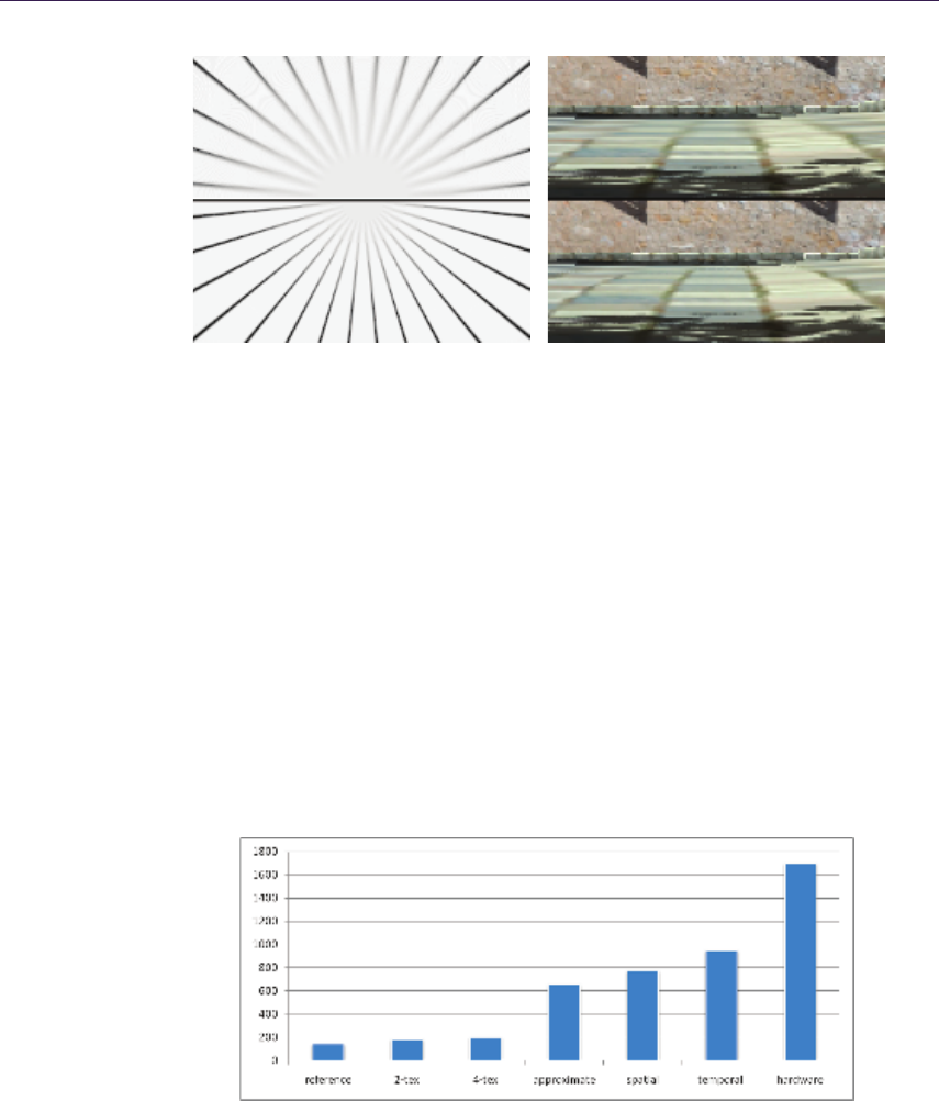
172 10. Practical Elliptical Texture Filtering on the GPU
Figure 10.9. Close-ups demonstrating the improved clarity when increasing the maxi-
mum degrees of anisotropy from 16 (up) to 64 (down).
but in practice this is very difficult because an infinite anisotropy level would be
required. Apart from the increased clarity, in practice we also observe that the
elliptical filtering eliminates the occasional pixel flickering (temporal aliasing) of
the hardware implementation.
10.4.1 Performance Measurements
Figure 10.10 presents comprehensive performance and quality measurements for
all the methods presented in this chapter. The spatial and temporal sample dis-
tribution schemes can be used to accelerate both the direct convolution methods
and the ellipse approximation method, but since we are interested in the highest
possible performance, we only present results when distributing the samples of
the ellipse approximation method. The performance of the method was mea-
Figure 10.10. The performance of the methods presented in this chapter measured in
Mtexes/sec on an Nvidia GTX460.

10.5. Conclusions 173
sured on the tunnel scene of the accompanying demo application on a middle
range graphics card. We observe that the direct convolution methods (reference,
2-tex, 4-tex) are an order of magnitude slower than the approximating ones,
making their applicability for real-time applications rather limited.
10.4.2 Integration with Game Engines
The proposed texture filtering algorithms can be implemented as a direct re-
placement to the built-in texture lookup functions, making the integration with
game engines trivial. In the accompanying material of this book, we provide our
proof-of-concept implementation in GLSL. In the case of temporal filtering, the
current frame number should be exposed inside the shaders. One integration
option is to globally replace all the texturing function calls with the enhanced
ones, but this method is probably an overkill. Alternatively, at content-creation
time, the enhanced texture filtering could selectively be applied only on certain
problematic surfaces. The second option can lead to better runtime performance,
but at the cost of increased authoring time.
10.5 Conclusions
We have shown that high-quality elliptical filtering is practical on today’s GPUs,
by employing several methods to speed up the reference algorithm. Texture fil-
tering quality is one issue that separates the offline production rendering from the
real-time one, and this work can provide a viable texture filtering improvement
for hardware-accelerated rendering applications.
10.6 Acknowledgments
The authors would like to thank Matt Pharr for providing a sample CPU implementation
of the EWA filter on his website, which was a starting point for this project, and Inigo
Quilez for providing the GLSL code to ray-trace the infinite plane and tunnel test scenes,
as part of Shader Toy.
Bibliography
[Greene and Heckbert 86] Ned Greene and Paul S. Heckbert. “Creating Raster Omni-
max Images from Multiple Perspective Views Using the Elliptical Weighted Average
Filter.” IEEE Comput. Graph. Appl. 6:6 (1986), 21–27.
[Heckbert 89] Paul S. Heckbert. “Fundamentals of texture mapping and image warp-
ing.” Technical Report UCB/CSD-89-516, EECS Department, University of Cali-
fornia, Berkeley, 1989.

174 10. Practical Elliptical Texture Filtering on the GPU
[Mavridis and Papaioannou 11] Pavlos Mavridis and Georgios Papaioannou. “High
Quality Elliptical Texture Filtering on GPU.” In Symposium on Interactive 3D
Graphics and Games,I3D ’11, pp. 23–30. New York: ACM Press, 2011.
[McCormack et al. 99] Joel McCormack, Ronald Perry, Keith I. Farkas, and Norman P.
Jouppi. “Feline: Fast Elliptical Lines for Anisotropic Texture Mapping.” In Proceed-
ings of SIGGRAPH ’99, Proceedings, Annual Conference Series, edited by Alyn
Rockwood, pp. 243–250. Reading, MA: ACM Press/Addison-Wesley Publishing,
1999.
[Smith 95] Alvy Ray Smith. “A pixel is not a little square, a pixel is not a little square,
a pixel is not a little square! (And a voxel is not a little cube).” Technical report,
Technical Memo 6, Microsoft Research, 1995.

11
An Approximation to the Chapman
Grazing-Incidence Function for
Atmospheric Scattering
Christian Sch¨
uler
11.1 Introduction
Atmospheric scattering for computer graphics is the treatment of the atmosphere
as a participating medium, essentially “calculating the color of the sky.” This is
interesting for any application where the time of day, the season, or the proper-
ties of the atmosphere are not known in advance, or the viewpoint may not be
restricted to a point on the earth’s surface. It is a historically difficult effect to
render, especially at planetary scale.
Early attempts at atmospheric scattering can be found in [Klassen 87] and
[Nishita et al. 93]. Recent implementations with an emphasis on real time are
[Hoffmann and Preetham 02], [O’Neil 05], and [Bruneton and Neyret 08]. A
common theme of all these approaches is finding ways to efficiently evaluate or
precompute the Chapman function, Ch(x, χ). This is the density integral for a
ray in a spherically symmetric, exponentially decreasing atmosphere.
The Chapman function has been subject to extensive treatment in the physics
literature. Approximations and tabulations have been published, most of it with
a focus on precision. This article explores a different direction for its evaluation:
an approximation so cheap that Ch(x, χ) can be considered a commodity, while
still being accurate enough for our graphics needs.
11.2 Atmospheric Scattering
This section is a brief review of atmospheric scattering and a definition of terms.
When light travels through air, it will be partly absorbed and partly scattered
into other directions. This gives rise to the phenomenon of aerial perspective. The
175

176 11. An Approximation to the Chapman Grazing-Incidence Function for Atmospheric Scattering
N
L0
L
T(t)S(t)
atmosphere
surface
Tsun(t)
Esun
Figure 11.1. Atmospheric scattering 101. See the text for an explanation of the symbols.
fraction of light that is unimpeded along a path is the transmittance T, and the
amount that is added into the path due to scattering is the in-scatter S(see
Figure 11.1). Thus, the aerial perspective of a distant source of radiance L0is
seen by an observer as the radiance L:
L=L0T+S.
To arrive at the total in-scatter S, in general one would have to integrate it
along the path. Then, the in-scatter at a particular point S(t) would have to be
calculated from the local irradiance field Eover the entire sphere of directions Ω
with an atmosphere-dependent phase function f(θ):
S=ZS(t)T(t)dt,
S(t) = Z
Ω
E(t)f(θ)dΩ.
The irradiance is usually discretized as a sum of individual contributions.
Especially during the day, the single most important contributor is the sun, which
can be simplified to a directional point source Esun, for the irradiance arriving
at the outer atmosphere boundary; Esun is attenuated by the transmittance Tsun
for the path from the atmosphere boundary towards point S(t):
S(t) = Esun Tsun(t)f(θ).
The transmittance itself is an exponentially decreasing function of the airmass
mtimes an extinction coefficient β. The latter is a property of the scattering
medium, possibly wavelength dependent. The airmass is an integral of the air
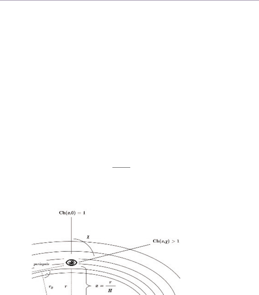
11.3. The Chapman Function 177
density ρ(t) along the path:
T= exp (−βm),
m=Zρ(t)dt.
To complete the calculation, we need a physical model for βand f. There
exists Rayleigh theory and Mie theory, which have been discussed in depth in
previous publications, e.g., [Nishita et al. 93] and [Hoffmann and Preetham 02].
It is beyond the scope of this article to provide more detail here.
11.3 The Chapman Function
In order to reduce the algorithmic complexity, it would be nice to have an efficient
way to calculate transmittances along rays. It turns out that this reduces to an
evaluation of the Chapman function.
Without loss of generality, let’s start a ray at an observer inside the atmo-
sphere and extend it to infinity (see Figure 11.2). The ray can be traced back to
a point of lowest altitude r0. We take the liberty to call this point the periapsis
even though the path is not an orbit. Here we define t= 0, and the altitude for
any point along the ray as follows:
r(t) = qr2
0+t2.
Let’s further assume a spherically symmetric atmosphere with an exponen-
tially decreasing density, characterized by a scale height H. We normalize the
Figure 11.2. The Chapman function. Relative airmass in an exponentially decreasing
atmosphere with scale height H, normalized observer altitude xand incidence angle χ.
The lowest altitude is at r0.

178 11. An Approximation to the Chapman Grazing-Incidence Function for Atmospheric Scattering
density to a reference density ρ0at reference altitude R. The density at any
altitude is then
ρ(r) = ρ0exp R−r
H.
Combining these expressions yields an integral for the airmass along the entire
ray. The integration boundary is trigonometrically related to the observer altitude
rand the incidence angle χ:
m=ρ0
∞
Z
rcos χ
exp R−pr2
0+t2
H!dt,
r0=rsin χ.
This integral does not have a simple solution, except when looking straight
upwards into the zenith (χ= 0). In this case, the mass along the ray is just
the mass of the air column above the observer. This is, by the definition of the
density distribution, one scale height times the density at the observer. Let’s call
that mass m⊥:
m⊥=ρ0Hexp R−r
H.
Can we possibly have a function that relates m⊥to m? We can, for this
is the Chapman function Ch(x, χ), named after the physicist who was the first
to formulate this problem [Chapman 31]. We write the Chapman function as
follows:
m=m⊥Ch(x, χ),
with
x=r
H.
The arguments are historically named xfor normalized altitude and the Greek
letter chi for incidence angle (don’t blame me for that). The function is indepen-
dent of scale and is usually tabulated or approximated numerically. For conve-
nience, an analytic expression is given below. This has been stripped down from
a more general solution found in [Kocifaj 96]:
Ch(x, χ) = 1
2"cos(χ)+
+ exp xcos2χ
2erfc rxcos2χ
2!1
x+ 2 −cos2χrπx
2#.
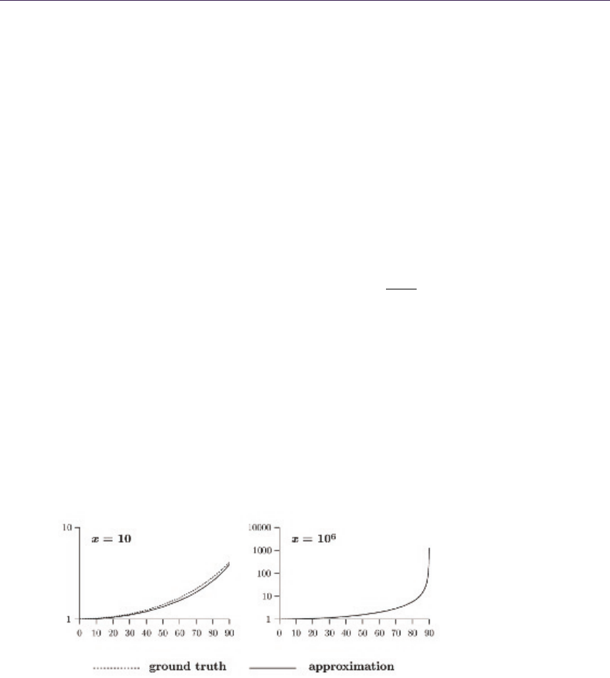
11.4. Towards a Real-Time Approximation 179
The above expression is not practical for real-time evaluation, for several rea-
sons: it contains the complementary error function, erfc, which needs a numerical
approximation for itself. It has bad numerical behavior for large xand small χ,
where the exp-term becomes very large and the erfc-term virtually zero. We use
this expression, however, as our ground-truth standard, evaluated with arbitrary
precision math software.
11.4 Towards a Real-Time Approximation
To better understand the Chapman function, we will plot a graph of it (see
Figure 11.3) and observe a number of important properties:
The function is even wrt. χ; Ch(x, χ) = Ch(x, −χ).
There is unity at χ= 0; Ch(x, 0) = 1.
There is a limit for large x; lim
x→∞ Ch(x, χ) = 1
cos χ.
These properties are easily explained. The even symmetry follows from the
problem specification. Only the cosine of the incidence angle appears in the
expression. This allows us to reduce the covered range to 0 < χ < 180◦. Second,
since Ch(x, χ) relates m⊥to m, its value must approach unity for small incidence
angles. And finally, in the limit of a flat earth, the Chapman function must
approach the secant function.
These properties can be used to engineer our approximation, Ch0. The limit
for large xsuggests a rational approximation, as we are going to cope with a
pole. Runtime efficiency demands the lowest possible order. So we are going to
Figure 11.3. Graph of the Chapman function. Ch(x, χ) is plotted on a logarithmic
scale as a function of incidence angle χ, for two extreme cases of x. An observer on the
earth’s surface with an atmosphere scale height of 8.4 km would correspond to an xof
r⊕
/8.4'760.

180 11. An Approximation to the Chapman Grazing-Incidence Function for Atmospheric Scattering
look for a first-order rational function of cos χ, approaching unity on the left and
the value of Chk(x) on the right, where Chk(x) is used as a shorthand for the
Chapman function evaluated at χ= 90◦. There is only one possibility for such a
rational function:
Ch0(c, χ) = c
(c−1) cos(χ)+1 |χ|<90◦,
with
c= Chk(x).
As it turns out, this low-order function is a pretty good approximation. The
useful range for χis, however, limited to below 90◦. Beyond that angle, the
approximation grows hyperbolically to a pole at infinity, while the exact Chapman
function grows exponentially, and always stays finite. We will look for ways to
handle χ > 90◦, but we must first turn our attention to the coefficient c.
11.4.1 At the Horizon
If the observer altitude is fixed, we could precalculate a value for c. However, for
a moving observer, and in the absence of a Chapman function to fall back on, we
need an approximation for citself. Let’s take a look at Chk(x):
Chk(x) = 1
2x+ 1rπx
2.
This is already a lot simpler than the full Chapman function, but still requires
a square root and a division. To simplify it further, we assume that xis usually
large and neglect the term 1
/2xto get a function that is purely proportional to
√x. Using the value pπ
/2'1.2533 as a coefficient results in
Chk(x)'1.2533 √xx > 10.
11.4.2 Beyond the Horizon
Consider Figure 11.4. The airmass mLalong an entire line is the airmass along
the forward ray plus the airmass along the backward ray:
mL=ρhCh(x, χ) + Ch(x, 180◦−χ)i.
The above equation must be true for any point along the line. We can move
the observer to the periapsis, where both the forward and the backward ray are
horizontal. Using trigonometry, the altitude at the periapsis is x0=xsin χand
density follows as ρexp(x−x0). Another way of expressing mLis therefore
mL= 2 ρexp(x−x0) Chk(x0).
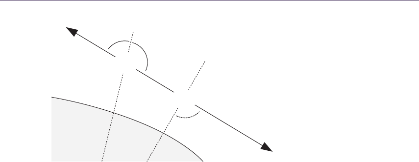
11.5. Implementation 181
N
N
·
χ
180° – χ
x
x0
Figure 11.4. Airmass along an entire line. A virtual observer is placed at the periapsis.
Combining the above equations, it is possible to arrive at an identity that
expresses the Chapman function in terms of itself with a reflected incidence angle:
Ch(x, χ) = 2 exp(x−xsin χ) Chk(xsin χ)−Ch(x, 180◦−χ).
If the Chapman function is known for 0 < χ < 90◦, it is therefore known for
all χ.
11.5 Implementation
See Listing 11.1 for an implementation of the approximate Chapman function
in C. It consists of a branch on the value of χ, either applying the identity or
not. The code differs from the mathematical formulae in three aspects, which are
discussed in Sections 11.5.1–11.5.3.
11.5.1 Numeric Range
First, a numeric range problem must be resolved, which happens when xis large
and x0is small. The identity formula contains the exponential exp(x−x0),
which overflows. To remedy this situation, we introduce a modified function
Chh(X, h, χ):
Chh(X, h, χ) = Ch(X+h, χ) exp(−h).
This function takes a reference altitude Xand the corresponding observer
height h, and includes the factor exp(−h). This factor would have to be applied
anyway to calculate the airmass. By including it in the function, the range
problem cancels out, since exp(x−x0) exp(−h) = exp(X−x0).

182 11. An Approximation to the Chapman Grazing-Incidence Function for Atmospheric Scattering
float c hap man _h ( float X , float h , flo at coschi )
{
// The ap pr ox imate Ch apman f un ction
// Ch (X+ h , chi ) time s e xp2 (- h)
// X - altitu de of unit d en sity
// h - observ er altitude relative to X
// co schi - cosine of in ci de nc e angle chi
// X and h are give n un its of the 50% - he ig ht
float c = sqr t ( X + h ) ;
if ( coschi >= 0. )
{
// chi a bove h or iz on
return c / ( c * c os chi + 1. ) * e xp2 ( -h ) ;
}
else
{
// chi be low hori zon , mus t use i dentity
float x0 = sqrt ( 1. - cos ch i * co sc hi ) * ( X + h );
float c0 = sqrt ( x0 ) ;
return
2. * c0 * ex p2 ( X - x0 ) -
c / ( 1. - c * cosc hi ) * exp2 ( -h ) ;
}
}
Listing 11.1. The approximate Chapman function in C, with modifications discussed
in the text.
11.5.2 Distance Differences
The second modification relates to the ability of the approximation to stay faithful
to sums and differences of path lengths. Special attention is drawn to the case
of an observer who is close above a reflective surface. Consider Figure 11.5.
Assuming near-horizontal angles, the airmasses mA,mB, and mCfor the three
segments can be simplified to
mA∼Ch(x, χ),
mB∼Ch(x, 180◦−χ)−Ch(x0,180◦−χ),
mC∼Ch(x0, χ).
The question is now, does the approximation satisfy mA=mB+mC? This
would be required for an exact color match at the horizon above a water sur-
face. The short answer is that the original approximation does not hold for this
property. The form of the denominator in the rational function, as well as the
factor 1.2533, stand in the way. The approximation must be rigged to enable this
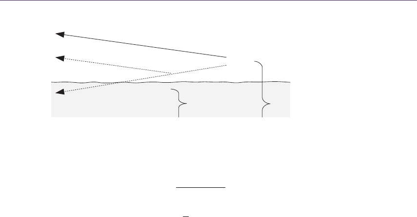
11.5. Implementation 183
A
N
BC
xx'
Figure 11.5. The Chapman function on a reflected ray. Is the approximation going to
stay true to sums and differences of path lengths?
property; this new approximation is even simpler:
Ch0(c, χ) = c
ccos(χ)+1,
with
c=√x.
Dropping the factor of 1.2533 hardly makes a difference in the visual result.
The change in the denominator is more severe, causing the approximation to fall
below unity for small incidence angles. However, for typical uses with xwell in
the hundreds, the visual impact is again negligible. If needed, the loss can be
compensated by an increase of the β-coefficients.
11.5.3 Using exp2
The code will make exclusive use of the dual exponential 2xinstead of the natural
exponential ex. We will therefore need all scales converted to the dual logarithm.
We need a 50%-height H50 instead of the scale height H; we need 50%-extinction
coefficients, and so on:
H50 =Hln 2,
β50 =βln 2,
. . . .
The reason for this change is that exp2 is usually the more efficient function
to compute. To optimize even more, an implementation can employ a fast exp2
function for all scattering calculations. An example of such a fast exp2 function
is presented in the appendix (Section 11.8). It is a definitive win when the
calculation is CPU-based, especially if it is vectorized with SIMD, calculating
four values at once. On the GPU, there have been assembly instructions for a
fast version (called exp2pp for “partial precision”) or the shader compiler takes it
as a hint if a call to exp2 has both a low-precision argument and a low-precision
result.

184 11. An Approximation to the Chapman Grazing-Incidence Function for Atmospheric Scattering
ve c3 t ra n sm it ta nc e ( ve c3 r , v ec3 v ie wd ir )
{
// ca lc ul at e the t ransm it ta nce a long a ray
// fr om poin t r to wards i nf in it y
float r sq = dot ( r , r) ;
float i nvrl = inve rse sqr t ( rsq );
float len = rsq * i nvrl ;
float x = len * in vH50 ;
float h = x - X50 ;
float c oschi = dot ( r , viewdi r ) * invrl ;
return exp 2 ( - beta5 0 * H50 * ch apman_h ( X50 , h , co schi ) );
}
Listing 11.2. Function for the transmittance along a ray.
11.6 Putting the Chapman Function to Use
Finally, in this section we are going to explore the ways in which we can use our
shiny new tool. You should consult the example code on the website since not
all listings are shown here.
11.6.1 Airmass and Transmittance
The airmass is calculated easily with the modified Chapman function. You need
to know the observer height against some reference altitude (conveniently, this is
the planet radius, or mean sea level), and the scale height of the atmosphere:
m=H Chh(X, h, χ).
It is a small step from the airmass to the transmittance, since T= exp(−βm).
See Listing 11.2 for a function to calculate the transmittance along a straight line
through the atmosphere. The scale height and the extinction coefficients must
be available globally. In the complete fragment program, this function is used to
calculate the local sun color for surface shading.
11.6.2 Aerial Perspective
The full aerial perspective function has two colors as a result: the transmittance
and the in-scatter. The function is too long to be listed here, but is included in
the fragment program on the website. The signature is as follows:
void a er ia l _p er s pe ct i ve ( out v ec3 T , out v ec3 S ,
in vec3 r0 , in vec3 r1 , in bool in fin ite ) ;

11.7. Conclusion 185
The function calculates the aerial perspective from point r0 to point r1, or
alternatively, from point r0 along the ray through r1 to infinity. The resulting
transmittance is written to argument Tand the in-scatter is written to argu-
ment S.
Here is a short explanation of the algorithm: In a first step, the function
intersects the ray with the atmosphere boundary to get the integration interval,
which is subdivided into a fixed number of segments. It then iterates over all
segments in reverse order (back to front). For each segment, the Chapman func-
tion is called to calculate airmass, transmittance, and in-scatter. The in-scatter
is then propagated along the ray in a way similar to alpha-blending.
11.6.3 The Example Raytracer
The accompanying online material for this article contains a shader (fragment-
and vertex program) that implements a fully ray-traced, atmospheric single-
scattering solution in real time. See the color images in Figure 11.6. You should
be able to load the shader into a shader authoring tool (RenderMonkey, FX-
Composer) and apply it on a unit sphere. If you are on the Mac, there is a
ShaderBuilder project that you can simply double click.
The code assumes a planet centered at the origin of variable radius, with a
Rayleigh atmosphere. For each pixel that hits the atmosphere, aerial
perspective is called once to get the in-scatter against the black background
of space. The transmittance is not needed. For each pixel that hits the surface,
the aerial perspective function is called twice, one time for the view ray, and
a second time for the ocean reflection.
To give a realistic appearance, the β-values were calculated for a situation
similar to Earth. A little bit of orange absorption was added to account for the
effect of atmospheric ozone, which is significant at twilight (see [Nielsen 03]). The
landmass is shaded according to the Lommel-Seeliger law, which is a good model
for rough surfaces, avoiding the typical Lambertian limb darkening. The specular
reflection of the sun in the ocean is shaded with an approximate microfacet model
(see [Sch¨uler 09]). The final color is then tone mapped with an exponential soft
saturation and 2.2 display gamma.
11.7 Conclusion
This article shows a way to accelerate atmospheric scattering calculations, by
making the Chapman function an efficient commodity. This allows a strength
reduction of the numerical integration, up to the point where the full single-
scattering solution can be run in real time in a shader program.
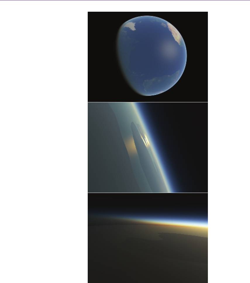
186 11. An Approximation to the Chapman Grazing-Incidence Function for Atmospheric Scattering
Figure 11.6. Color images from the example ray tracer. View of the Atlantic
Ocean (top). Sun reflection, which is yellow due to transmittance (middle). Earth
shadow, which is implicit in the solution (bottom).

11.8. Appendix 187
float exp2pp( float x )
{
// pa rtial pr ecision exp2 , ac cu ra te to 12 bits
const float c [ 3] = { 5.7 9525 , 12 .52 461 , - 2.8 8611 };
int e = round ( x) ;
float t = x - e;
float m = ( t * t + c [0]* t + c [1] ) / ( c [2]* t + c[1] ) ;
return l dex p ( m , e ) ;
}
Listing 11.3. An example of a fast exp2 function.
11.8 Appendix
11.8.1 A Fast exp2 Function
Listing 11.3 shows an example for a fast exp2 function for use in atmospheric-
scattering calculations. It is a low-order rational function in the range −1/2
to +1/2 together with the usual range reduction and scaling. Although it is
an approximation, it does preserve the property that 1 −exp(−x) is strictly
positive if x > 0, which is important for the scattering calculations. The function
is dependent on an efficient way to assemble a floating point number from a
mantissa and an exponent. For the sake of brevity, this part is expressed here in
terms of the standard C-function ldexp. The optimal method would be a direct
bit-manipulation, using language-specific constructs.
Bibliography
[Bruneton and Neyret 08]´
Eric Bruneton and Fabrice Neyret. “Precomputed Atmo-
spheric Scattering.” Comput. Graph. Forum. Proceedings of the 19th Eurographics
Symposium on Rendering 2008 27:4 (2008), 1079–1086. Special Issue.
[Chapman 31] Sydney Chapman. “The Absorption and Dissociative or Ionizing Effect
of Monochromatic Radiation in an Atmosphere on a Rotating Earth.” Proceedings
of the Physical Society 43:1 (1931), 26. Available online (http://stacks.iop.org/
0959-5309/43/i=1/a=305).
[Hoffmann and Preetham 02] Naty Hoffmann and Arcot J. Preetham. “Rendering out-
door light scattering in real time.” Technical report, ATI Technologies, Inc., 2002.
Available online (http://www.ati.com/developer).
[Klassen 87] R. Victor Klassen. “Modeling the Effect of the Atmosphere on Light.”
ACM Trans. Graph. 6 (1987), 215–237. Available online (http://doi.acm.org/10.
1145/35068.35071).

188 11. An Approximation to the Chapman Grazing-Incidence Function for Atmospheric Scattering
[Kocifaj 96] M. Kocifaj. “Optical Air Mass and Refraction in a Rayleigh Atmosphere.”
Contributions of the Astronomical Observatory Skalnate Pleso 26:1 (1996), 23–
30. Available online (http://www.ta3.sk/caosp/Eedition/Abstracts/1996/Vol 26/
No 1/pp23-30 abstract.html).
[Nielsen 03] R. S. Nielsen. “Real Time Rendering of Atmospheric Scattering Effects
for Flight Simulators.” Master’s thesis, Informatics and Mathematical Modelling,
Technical University of Denmark, 2003. Available online (http://www2.imm.dtu.
dk/pubdb/p.php?2554).
[Nishita et al. 93] Tomoyuki Nishita, Takao Sirai, Katsumi Tadamura, and Eihachiro
Nakamae. “Display of the Earth Taking into Account Atmospheric Scattering.”
In Proceedings of SIGGRAPH ’93, Proceedings, Annual Conference Series, edited
by James T. Kajiya, pp. 175–182. New York: ACM Press, 1993. Available online
(http://doi.acm.org/10.1145/166117.166140).
[O’Neil 05] Sean O’Neil. “Accurate Atmospheric Scattering.” In GPU Gems 2, edited by
Matt Pharr and Randima Fernando, pp. 253–268. Reading, MA: Addison-Wesley,
2005.
[Sch¨uler 09] Christian Sch¨uler. “An Efficient and Physically Plausible Real-Time Shad-
ing Model.” In ShaderX7: Advanced Rendering Techniques, edited by Wolfgang
Engel, Chapter 2.5, pp. 175–187. Hingham, MA: Charles River Media, 2009.
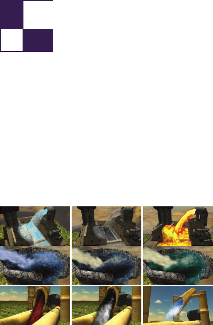
12
Volumetric Real-Time Water and
Foam Rendering
Daniel Scherzer, Florian Bagar, and
Oliver Mattausch
12.1 Introduction
Over the last decade, simulation and rendering of complex natural phenomena
such as fire, smoke, clouds, and fluids have been an active and most diverse
research area in computer graphics. Among these phenomena, water may be
the most fascinating and challenging problem, due to the familiarity that even a
Figure 12.1. The proposed algorithm allows water to be rendered in many ways.
189

190 12. Volumetric Real-Time Water and Foam Rendering
casual observer has with the phenomenon. Although the visual quality of water
rendering is continually improving, we are still a long way from capturing all the
physical properties of real water, like the forming of foam and droplets and their
interaction with the environment.
In this chapter we present a method for creating a fully dynamic multilayered
real-time water rendering approach. This approach can represent the volumetric
properties of water and the physical formation of volumetric foam, thereby creat-
ing much higher visual fidelity than previous real-time approaches. It is based on
a very fast particle-based fluid simulation that is fully hardware-accelerated using
Nvidia PhysX and rendering in OpenGL, and therefore easily runs at real-time
frame rates. The algorithm has a small memory footprint and is simple to imple-
ment and integrate into existing rendering engines. Additionally, our method is
highly configurable from an artistic point of view, and thus can produce a multi-
plicity of visual appearances to help to create the desired atmosphere for a scene
(see Figure 12.1).
12.2 Simulation
In order to render believable water, we first have to simulate its behavior. The
dynamics of water as an incompressible fluid can be described by a version of
the Navier–Stokes equations, which apply Newton’s second law (conservation of
momentum) and conservation of mass to fluid motion. These equations relate the
body forces (gravity) and the contact forces (pressure and stress) that act on a
fluid. This results in nonlinear partial differential equations that are very hard to
solve (assuming that an exact solution for a given case even exists). As we do not
need an exact solution, but are mainly concerned with speed, we are fine with an
approximate numerical solution. Approximations in this problem domain mainly
use Euler integration. (There are more accurate methods, such as Runge-Kutta
or midpoint, but these take more time to evaluate.)
12.2.1 Smoothed-Particle Hydrodynamics
Smoothed-particle hydrodynamics (SPH) is a robust and fast way for simulat-
ing the behavior of water [Desbrun and Gascuel 96]. The main idea here is to
approximate a fluid by a particle system (a division of the fluid into discrete
elements) to calculate its dynamic behavior. Each particle has a mass and ad-
ditional properties, such as position, density, velocity, and lifetime. In classic
particle systems, each particle is updated based only on its properties, disregard-
ing particle-particle interaction for the sake of speed. For the simulation of fluids
this will not suffice because of the contact forces. Each particle can potentially
affect all other particles, which results in a computational complexity in the order
of O(n2)—too slow for practical purposes if we use tens of thousands of particles.

12.2. Simulation 191
struct FluidParticle
{
Ve cto r3 po sit ion ;
float density;
Ve cto r3 ve loc ity ;
float l ife tim e ;
un si gn ed in t id ; // uni qu e numb er id en tifyi ng the particle
float foam;
};
Listing 12.1. Structure representing the properties of a single particle.
In practice, particles influence each other depending on the distance between
them. So it makes sense to define an interaction cut-off distance, inside which
a kernel function is applied to weight the influence of the individual particles
on each other. This effectively reduces calculation complexity to O(n). Note
that this cut-off distance is also called the smoothing length because it gives the
volume over which properties are “smoothed” by the kernel function (hence the
name smoothed-particle hydrodynamics).
All major physics engines already include a solver for SPH. We have used
PhysX [Nvidia 11] because of its hardware acceleration, but any other physics
engine would do as well.
The fluid simulation is created by passing a fluid description structure to the
physics engine, which defines the behavior of the SPH simulation. The simulation
data is a nonsorted 3D point cloud and each of the particles has the properties as
shown in Listing 12.1. Note that for our use the particle structure also includes
a foam parameter that is updated as described in Section 12.2.2. The physics
engine updates and returns this point cloud by applying the SPH simulation.
12.2.2 Foam
We want to be able to simulate not only water particles, but also foam. Foam is a
substance that is formed by trapping air bubbles inside a liquid (see Figure 12.4).
Note that this can be as spray or bubbles above the surface of the fluid, but also
deep inside a fluid, as in the case of a waterfall. The formation of foam can be
described by the Weber number. It is defined as the ratio of the kinetic energy
to the surface energy:
W e =ρv2l
σ,
where ρis the density, vis the relative velocity between the liquid and the sur-
rounding gas, lis the droplet diameter, and σis the surface tension. If W e is
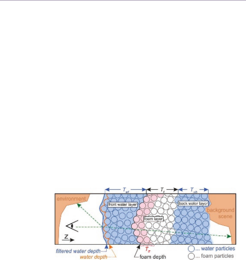
192 12. Volumetric Real-Time Water and Foam Rendering
large, the kinetic energy is greater than the surface energy, which causes water
to mix with the surrounding gas (air), and the result is foam. For our purposes,
we use the particle size as the droplet diameter and use a constant value for the
surface tension. We also assume that the air is not moving, and that therefore
the relative velocity is equal to the velocity of the liquid at this point.
The Weber number for each particle can now be calculated by using each
particle’s ρand vfrom the physics engine. This number is then compared to
a user-defined threshold that describes how easily this fluid forms foam. Thus,
particles can be separated into water particles and foam particles. Thus, foam
(from the viewpoint of the simulation) is not a totally different phenomenon, but
is just a state of water particles [Bagar et al. 10].
With all these simulation parts in place we now have to tackle the problem of
how to render the water.
12.3 Rendering
Rendering water with a scanline renderer in an efficient manner is a twofold
problem: first, a water surface has to be extracted from the simulation data and
second, the shading of this surface has to take into account the volumetric prop-
erties of water. Due to the fact that real-time physics engines are often limited
to 64 K particles, while offline systems, as used in movies, often use hundreds
of millions of particles, our particle sizes will be much larger; we therefore must
take extra care to render believable water surfaces.
Figure 12.2. A cross section of our layered water model: the volumetric appearance of
the result is achieved by accounting for water thickness Twb, foam thickness Tf, and the
thickness of water in front of the foam Twf at each pixel. We also partition foam into two
differently colored layers (Tf f ) to achieve more interesting foam. See also Figure 12.5
for renderings of the individual layers.

12.3. Rendering 193
12.3.1 Splatting
One method for extracting surfaces from particles is to use a marching cubes
method. This has a number of disadvantages: First, as the surface of the water is
expected to change continually, the surface may exhibit temporal aliasing. Sec-
ond, marching cubes is very computationally expensive, and third, the resulting
geometry will likely be very complex, especially when incorporating foam effects.
A method that avoids these disadvantages and works well on current hardware
is splatting: the idea is to splat each particle by using a certain kernel shape (for
instance, a sphere) into a depth (and thickness) buffer (see Figures 12.2 and 12.6).
By using a 3D kernel, we create volumetric particles. Splatting particles into a
depth buffer (with depth test on) results in a screen-space approximation of the
water surface (see Listing 12.2). While additively splatting (adding up sphere
radii, see Listing 12.3) into a thickness buffer creates an approximation of the
water thickness for each pixel (which we will later use for shading the surface).
Accumulating water thickness this way is an acceptable approximation because
the particles from the physics simulation can be assumed to be largely nonover-
lapping.
1FragShaderOutput FluidSplattingFP( float2 te xCoord : T EXC OOR D0 ,
2float4 ey eSp ace : TEXCOO RD1 )
3{
4FragShaderOutput OUT;
5// ca lc ula te eye - s pace no rmal fro m tex tur e co or dina tes
6float3 n;
7n . xy = te xC oo rd . x y * float2( 2.0 f , - 2.0 f ) + float2( -1 .0 f , 1 .0 f );
8float r2 = dot(n . xy , n . xy );
9// kill pixels o ut side circ le
10 if ( r2 > 1 .0 f ) discard;
11 // ca lc ul at e rad ius
12 n.z = sqrt(1 .0 f - r2 );
13 // position of this p ixel on s phere in eye space
14 float4 ey eS pacePos = float4( e yeS pac e .x yz + n* eyeSpace .w , 1.0 f);
15 float4 clipSpacePos = m ul ( gls tate . ma tri x . proj ect ion , eyeS pac ePos );
16 // ou tpu t eye - sp ace dept h
17 OUT . c ol or = float4( e ye Sp ac eP os .z , 0 .0 f , 0. 0 f , 0 .0 f );
18 OUT . d ep th = ( c l ipS pa ce Po s . z / cl ip Sp ac eP os . w) * 0.5 f + 0.5 f ;
19 return OUT ;
20 }
Listing 12.2. Pixel shader for splatting the particle data as spheres into the depth
texture.
// calculate th ic kn es s with e xpone nt ia l f al lo ff b ased on radi us
float t hi ck ne ss = n .z * p ar ticle Si ze * 2.0 f * e xp ( - r2 * 2.0 f ) ;
OU T . co lo r = f lo at4 ( th ick nes s , 0 .0 f , 0 .0 f , 0 .0 f );
Listing 12.3. Splatting the particle data into the thickness texture. (Note: This shader
is based on the shader shown in Listing 12.2 and replaces lines 13–18.)
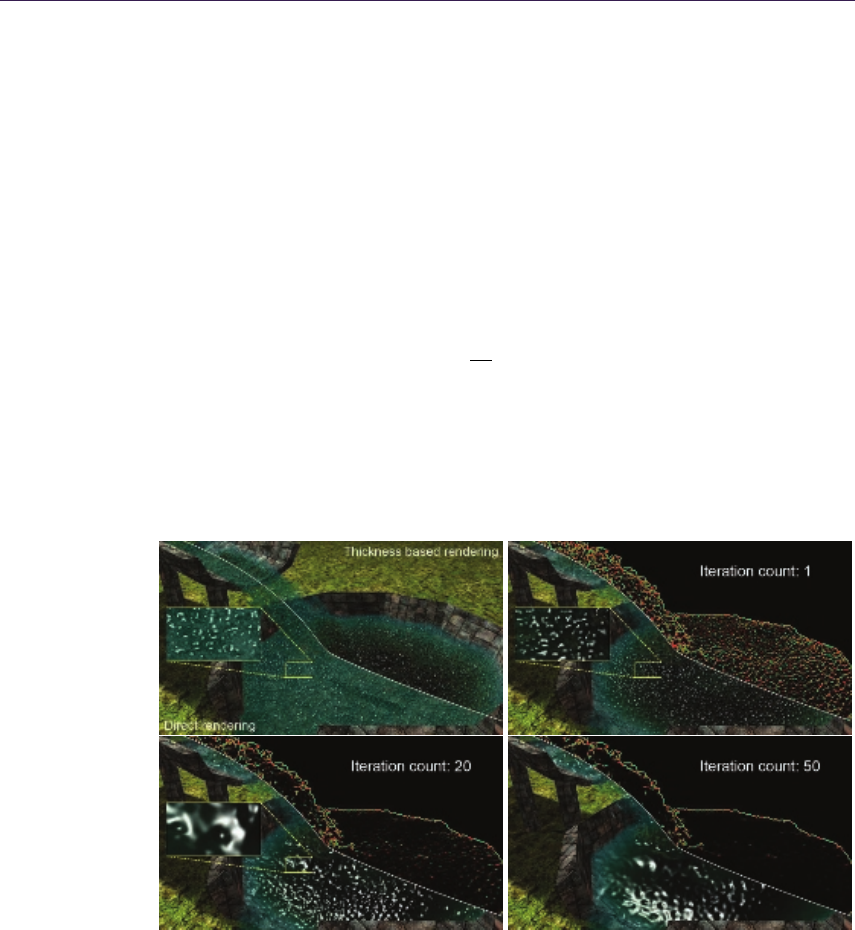
194 12. Volumetric Real-Time Water and Foam Rendering
12.3.2 Adaptive Screen-Space Curvature Flow Filtering
If we use a sphere-shaped kernel to splat the particles, the result of directly
rendering is often unconvincing (see Figure 12.3, upper-left image). The sphere
geometry of the individual particles is clearly visible due to the large particle
size. Making particles smaller and thereby requiring more particles for adequate
simulation of these scenes is not an option because we already operate near the
maximum of 64 K particles, and more particles also make the simulation and the
rendering slower. Another solution is to smooth the depth buffer that contains
the splatted particles in a way that avoids high curvature. This is the idea behind
curvature flow filtering [van der Laan et al. 09]. Here, a surface is shifted along
its normal vector depending on the mean curvature of the surface:
∂z
∂t =H,
where zis the depth (as found in the depth buffer), tis a smoothing time step,
and His the mean curvature. For a surface in 3D space, the mean curvature is
defined as follows:
2H=∇ · ˆn, (12.1)
Figure 12.3. Directly rendering the particles from the simulation as spheres results in
jelly-like water. Shading of the water can be improved by using the thickness of the
water to attenuate the water color (upper-left). Iteratively smoothing the depth buffer
by applying screen-space curvature flow filtering reduces the curvature of the water and
leads to more convincing results.

12.3. Rendering 195
where ˆnis the unit normal of the surface. The normal is calculated by taking the
cross product between the derivatives of the viewspace position Pin x- and y-
directions, resulting in a representation of the unit normal [van der Laan et al. 09]:
ˆn(x, y) = n(x, y)
|n(x, y)|=(−Cy∂z
∂x ,−Cx∂z
∂y , Cyz)T
√D,(12.2)
where
D=C2
y∂z
∂x 2
+C2
x∂z
∂y 2
+C2
xC2
yz2.
Finite differencing is used to calculate the spatial derivatives, and Cxand Cy
are the viewpoint parameters in the x- and y-directions, respectively. They are
computed from the field of view and the size of the viewport Vxand Vy, as shown
in Equations (12.3) and (12.4):
Cx=2
Vxtan F OV
2,(12.3)
Cy=2
Vytan F OV
2.(12.4)
The unit normal ˆnfrom Equation (12.2) is substituted into Equation (12.1),
which enables the derivation of H, leading to
2H=∂ˆnx
∂x +∂ˆny
∂y =CyEx+CxEy
D3
2
,
in which
Ex=1
2
∂z
∂x
∂D
∂x −∂2z
∂x2D,
Ey=1
2
∂z
∂y
∂D
∂y −∂2z
∂y2D.
The GLSL shader in Listing 12.4 performs this operation in screen space.
The effect of applying this filter repeatedly is shown in Figure 12.3. Iterative
filtering leads to a greater smoothing effect. If we want to maintain a certain
level of smoothness for water that is at the same time near and distant to the
viewer, the number of iterations has to be adjusted adaptively for each pixel.
We found that the number of iterations is indirectly proportional to the eye-
space distance—water nearby needs more iterations—far-away water needs fewer
iterations. Details regarding this derivation can be found in our paper [Bagar
et al. 10].
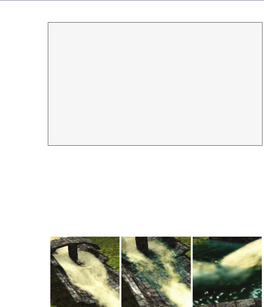
196 12. Volumetric Real-Time Water and Foam Rendering
// sa mp les f or fi nit e di ff er en ci ng ( vsp = vi ew sp ace po si tio n )
float d epth = texRECT( de pth Map , v sp . xy ). x ;
float d ep th_d = t exR ECT ( d epth Map , v sp . xy + fl oa t2 ( 0 .0 f , -1.0 f ) ). x;
float d ep th_l = t exR ECT ( d epth Map , v sp . xy + fl oa t2 ( -1.0 f , 0.0 f ) ). x;
float d ep th_r = t exR ECT ( d epth Map , v sp . xy + fl oa t2 ( 1 .0 f, 0.0 f )) . x;
float d ep th_u = t exR ECT ( d epth Map , v sp . xy + fl oa t2 ( 0 .0 f, 1.0 f )) . x;
// de ri vat iv es ( fin ite di ff ere nc ing )
float dx = ( 0.5 f * ( de pth _r - d ept h_l ));
float dy = ( 0.5 f * ( de pth _u - d ept h_d ));
// se cond d erivati ve s
float d xx = ( d ep th_ l - 2.0 f * dep th + d ept h_ r );
float d yy = ( d ep th_ d - 2.0 f * dep th + d ept h_ u );
// co ns ta nt s
const float d x2 = d x * dx ; co nst float d y2 = dy * dy ;
const float C x2 = C x * Cx ; co nst float C y2 = Cy * Cy ;
// ca lc ul at e c ur va tu re
float D = Cy2 * dx 2 + C x2 * dy2 + Cx2 * C y2 * de pth * d ept h ;
float H = Cy * d xx * D - C y * dx *( C y2 * dx * d xx + C x2 * C y2 * d ept h * dx )
+ Cx * dy y *D - Cx * dy *( Cx2 * dy * dyy + Cx2 * C y2 * de pth * dy );
H /= pow( D , 3. 0 f /2 .0 f );
// cu rv at ur e d ep en de nt sh ift
OUT . color = de pth + epsilon * H;
Listing 12.4. This pixel shader code performs one step in the iterative process of screen-
space curvature flow filtering.
12.3.3 Foam and Layers
Up to now we have discussed the problem of how to create a surface for our water.
What remains is to provide this surface with realistic shading and to add foam
effects.
Figure 12.4. The three cases of foam formation that are handled by our rendering model:
foam without water (left), foam on water (middle), and foam inside water (right).
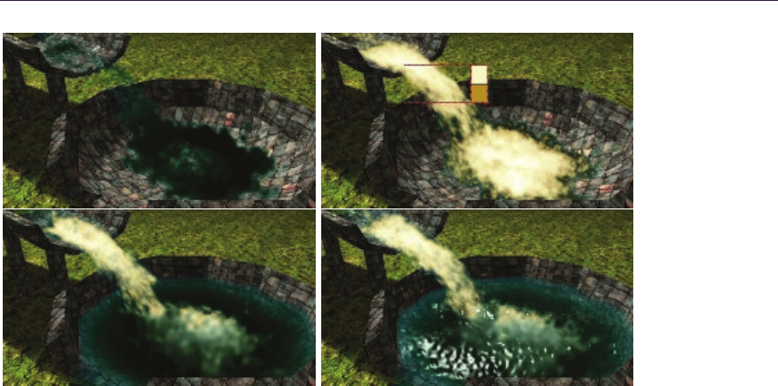
12.3. Rendering 197
Figure 12.5. The individual layers of our water model: back water layer (upper-left),
foam layer with the two user-defined colors that define the look of the foam as in-
lay (upper-right), front water layer (lower-left), and reflections and specular highlights
(lower-right).
We have investigated the different scenarios where foam occurs and have found
three main cases for a single pixel: foam without water, foam in front with water
behind, and foam inside water (see Figure 12.4). We disregard more complex
scenarios, like multiple layers of foam, because in practice the visual difference
compared with a single foam layer will be negligible. These cases can be cast into
a three-layered model (see Figures 12.2 and 12.5).
12.3.4 Steps of the Algorithm
To put this model into practice, our algorithm separates water and foam particles
and splats them into different buffers. The complete algorithm performs the
following steps in each frame (see Figure 12.6):
•Update the physics simulation.
•Render the background scene into a depth and color buffer.
•Calculate foam depth by splatting foam particles into a depth buffer.
•Calculate the front water depth by splatting water particles that are in
front of the foam.
•Calculate the filtered front water depth by applying adaptive curvature flow
filtering.
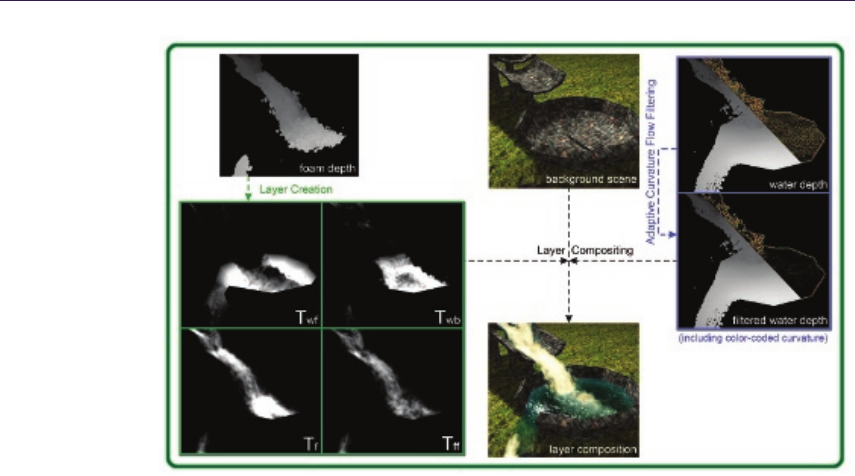
198 12. Volumetric Real-Time Water and Foam Rendering
Figure 12.6. Overview of the buffers used in our method. Twf denotes the thickness of
the water in front of the foam, Twb denotes the thickness of the water behind the foam,
Tfdenotes the foam thickness, and Tf f denotes the thickness of the front foam layer.
•Calculate the thickness of
◦the foam Tf,
◦the water in front of the foam Twf ,
◦the water behind the foam Twb,
◦the front foam layer Tff .
•Perform volumetric compositing
We use a sphere kernel for water particles and multiply the sphere kernel with
a Perlin noise texture for foam particles to get more details. Smoothing is only
applied to the front-most water layer, because the surface of water behind a
layer of foam will be obfuscated anyway. The front foam layer thickness Tf f is
an artificial construct that accumulates only foam particles within a user-defined
distance behind the foam depth. We found this to create more interesting looking
foam.
We have already discussed the basics behind each of the steps, except for the
final one, volumetric compositing, that builds on top of all the other steps.
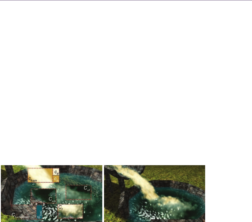
12.4. Artist Control 199
12.3.5 Volumetric Compositing
The difference between the usual compositing of layers and volumetric composit-
ing is that we take the thickness of each layer into account to attenuate a viewing
ray. Compositing along a viewing ray back to front, we have (see Figure 12.2):
Cwb = lerp(cfluid, Cbackground, e−Twb ),
Cfoam = lerp(cfb, cff , e−Tf f ),
Cf= lerp(Cfoam, Cwb, e−Tf),
Cwf = lerp(cfluid, Cf, e−Twf ),
where cfluid is the water color and cf f and cf b are two user-defined colors that
are blended together to create more freedom in designing the look of the foam.
After attenuation, we calculate highlights at the front water surface, as well as
reflection and refraction (including the Fresnel Term). Here, refraction considers
the whole water (front and back water layer) as one volume, so Cbackground is
sampled from the scene background texture perturbed along the normal vector,
scaled using Twb +Twf [van der Laan et al. 09].
Figures 12.5 and 12.7 show the individual steps and colors used in the com-
positing, and Listing 12.5 shows the GLSL pixel shader.
Figure 12.7. User-defined colors (cfluid ,cf f ,cf b ), and resulting colors from the com-
positing steps (Cbackground,Cwb,Cfoam ,Cf,Cwf ) (left) and final shading results (right).
12.4 Artist Control
We have introduced a number of user-controllable parameters into our algorithm
to allow artists to produce a multiplicity of visual appearances (see Figure 12.1).
The visual appearance of water is controlled by the fluid/water color (cfluid),
which is combined during the composition depending on the different water thick-
nesses (twb, twf ) and a user-defined falloff scale. Additionally, the specular color
and specular shininess, as well as the Fresnel bias, scale, and power, which are

200 12. Volumetric Real-Time Water and Foam Rendering
1// su rface propertie s ( v = view vector , h = half angle vecto r )
2float s pe cu la r = po w ( max ( 0.0 , dot ( n orm al , h )) , f l ui d Sh i ni ne s s ) ;
3// bias , scale , and pow er = user - defined p arameters to tune
4// the F re sn el Term
5float f re snelTer m = bias + sc ale * pow (1.0 + dot(v , no rma l ) , p ow er ) ;
6float3 c _r ef le ct = texCUBE( cub eMap , mul(( fl oa t3x 3 ) inv View ,
7reflect( -v , n or ma l ) ));
8...
9// at te nu ati on fa cto rs ( inc l . use r - d ef ine d fa llo ff s cal es )
10 float att_wb = s atu rate (ex p (- t_ wb * fa ll of fS cal e ) );
11 float a tt _f oa m = sa tur ate (e xp (-t_f * foamFalloffScale));
12 float att_ff = s atu rate (ex p (- t_ ff * fo am Sca le ));
13 float att_wf = s atu rate (ex p (- t_ wf * fa ll of fS cal e ) );
14 // co mp os iti on ( fr ag = fr agm en t po sit io n in s cre en s pace
15 float3 c_background = texRECT( scene , f rag . xy + no rma l .x y *( t_w b + t_wf ));
16 float3 c_ wb = lerp(c_fluid , c_background , att_wb);
17 float3 c_foam = lerp( c_fb , c_ff , att_ff );
18 float3 c_f = le rp ( c_fo am , c_ wb , a tt _f oam );
19 float3 c_ wf = lerp( c_f luid , c_f , a tt_ wf ) ;
20 // calculate f actor to suppress s pe cu la r h ig hlights if
21 // foam is the f ro nt mo st visu al element
22 float spw = satura te ( 1.0 f - att_wf + a tt _f oa m ) * (1 .0 f - a tt_wf );
23 // combine w ith f re snel and s pe cu la r highlight
24 float3 surfaceColor = lerp(c_wf , c_ ref lec t , min ( f resne lTerm , spw ))
25 + flu id Spe cu lar Co lor * s pecular * spw ;
Listing 12.5. Pixel shader for compositing along a viewing ray: lighting (lines 2–7),
thickness dependent attenuation (lines 9–19), and final color (lines 20–25).
used to control the approximation of the Fresnel equations, are exposed to be
used by artists. The approximation of the Fresnel equations is then used to com-
bine the reflection and the thickness-dependent attenuation of our algorithm (see
Listing 12.5).
The reflection itself can be influenced by an artist by modifying or replacing
the cubic environment map (cubeMap) of the corresponding scene. Note that
the cubic environment map has a large influence on the visual appearance of our
algorithm because it is blended directly with the thickness-dependent attenuation
and furthermore, it describes the static illumination of the scene.
The visual appearance of the foam is composed of a foam back color (cf b) and
a foam front color (cf f ), which are blended depending on the thickness of the
front foam layer (tff ) (see Figure 12.7) and a user-defined scale factor. Again,
as for the water, a user-defined falloff scale is used to control the overall opacity
of the foam. The final parameter that should be exposed to artists is the Weber
number threshold. As mentioned earlier, this user-defined threshold controls how
easily the simulated fluid forms foam.

12.5. Conclusion 201
12.5 Conclusion
We have presented a physically based water (fluid) and foam rendering algorithm
that can handle arbitrary dynamic scenes where water is allowed to freely interact
and flow everywhere, but which also allows artists to fine-tune the look of the
result. This algorithm runs easily in real time (on average 16 ms rendering time)
on modern hardware and integrates well with rendering engines (especially with
deferred shading).
For more theoretical details and exhaustive benchmarks for the presented
method, please refer to the paper [Bagar et al. 10] and the thesis [Bagar 10] on
which this work is based.
Bibliography
[Bagar et al. 10] Florian Bagar, Daniel Scherzer, and Michael Wimmer. “A Layered
Particle-Based Fluid Model for Real-Time Rendering of Water.” Computer Graph-
ics Forum (Proceedings EGSR 2010) 29:4 (2010), 1383–1389.
[Bagar 10] Florian Bagar. “A Layered Particle-Based Fluid Model for Real-Time Ren-
dering of Water.” Master’s thesis (Diplomarbeit), Vienna University of Technology,
Austria, 2010.
[Desbrun and Gascuel 96] Mathieu Desbrun and Marie-Paule Gascuel. “Smoothed Par-
ticles: A New Paradigm for Animating Highly Deformable Bodies.” In Pro-
ceedings of the Eurographics Workshop on Computer Animation and Simulation
’96, pp. 61–76. New York: Springer-Verlag New York, 1996. Available online
(http://dl.acm.org/citation.cfm?id=274976.274981).
[Nvidia 11] Nvidia. “NVIDIA PhysX.” http://developer.nvidia.com/physx, 2011.
[van der Laan et al. 09] Wladimir J. van der Laan, Simon Green, and Miguel Sainz.
“Screen Space Fluid Rendering with Curvature Flow.” In I3D ’09: Proceedings of
the 2009 Symposium on Interactive 3D Graphics and Games, pp. 91–98. New York:
ACM Press, 2009.

13
Inexpensive Antialiasing of
Simple Objects
Mikkel Gjøl and Mark Gjøl
13.1 Introduction
In the age of mobile devices, every algorithm gets a second chance. This article
explores a use of discontinuity edge overdraw [Sander et al. 01] for antialiasing
simple objects on 3D-capable mobile devices. The essence of this technique is to
render a “smooth” line on top of aliasing primitive edges in order to cover the
aliasing edge.
The method is trivially useful for rendering objects whose outline is geomet-
rically defined or easily derived. This applies to everything from GUI-elements
to 2D objects positioned in 3D, or even simple 3D-objects—anything where the
outline is defined by geometry. For textured 2D-elements, the usual way to deal
with antialiasing is to use textures with a translucent edge, relying on texture-
sampling to produce a smooth transition at the boundary. While this is a good
solution, it requires careful construction of the mip-chain to avoid artifacts during
scaling or when viewed at steep angles.
13.2 Antialiasing via Smoothed Lines
The founding observation of [Sander et al. 01] was that aliasing in 3D scenes
appears mostly at geometric silhouette edges and crease edges, and so only pixels
along these lines require antialiasing. As these boundaries can be described as
lines, and since line smoothing is widely available in hardware, aliasing can be
reduced by rendering smooth lines on top of the aliasing edges. The main contri-
bution of [Sander et al. 01] was an algorithm to find the aliasing edges. For some
applications, the potentially aliasing edges are trivially available, allowing us to
use this method easily. It is worth noting that the resulting algorithm does not
work for translucent objects, and does nothing to improve upon texture-aliasing,
203

204 13. Inexpensive Antialiasing of Simple Objects
Figure 13.1. Basic rendering setup.
including aliasing when rendering 2D sprites. Hardware texture filtering mostly
solves this issue however, and is available on the majority of modern mobile GPUs.
Applying the algorithm consists of just two steps (see Figure 13.1):
1. Determine the geometric edges that are causing aliasing.
2. Render aliasing edges as smooth lines.
In the general case it is not trivial to determine which edges cause aliasing, and
we refer readers to the exhaustive discussion in [Sander et al. 01]. In summary,
three sets of geometric edges should be considered for any visible object:
•silhouette edges,
•discontinuous edges, e.g., “hard” edges or texture seams,
•intersection-edges between geometric objects.
While discontinuous edges are typically static for a triangle mesh and can
be precomputed, silhouette edges change with the viewer. Dealing with scenes
constructed entirely of triangles, a geometric approach to finding silhouette edges
is to locate all edges where one of the adjacent triangles faces towards the viewer
and the other faces away. Computing exact intersections between geometric ob-
jects is computationally expensive, and a solution was not presented in [Sander
et al. 01].
When rendering lines to cover the detected aliasing edges, “over” alpha-
blending is applied (src_alpha,one_minus_src_alpha), and depth buffering is
used to achieve correct occlusion. While the rendered lines are potentially sub-
ject to z-fighting, the fighting pixels have the same color as the object on which
they are rendered. Since the main contribution of the smooth lines is outside
the aliasing object, z-fighting causes minimal issues. Rendering multiple layers
of alpha-blended pixels necessitates composition in a back-to-front manner. This
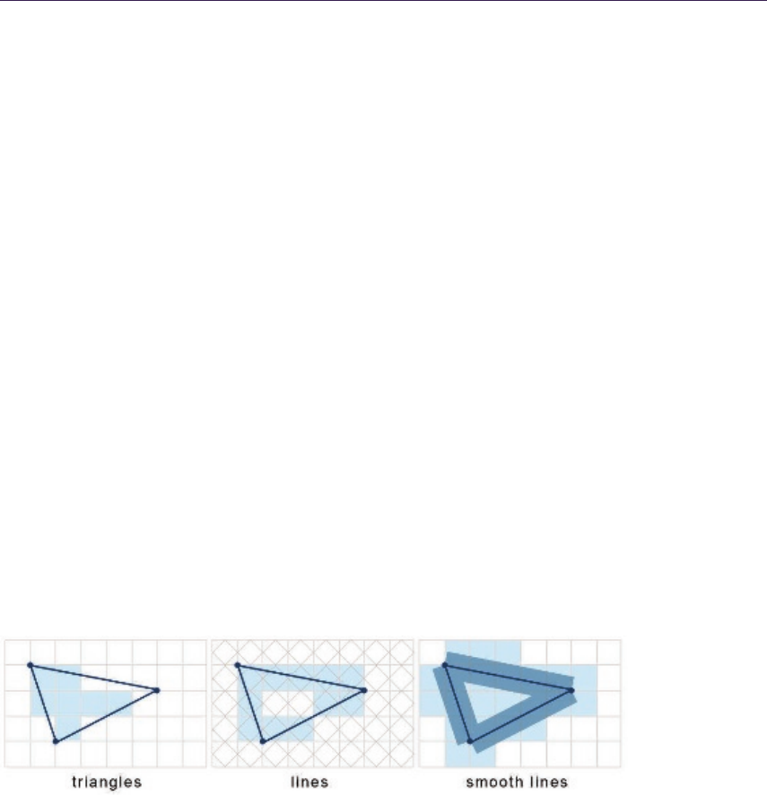
13.3. Rendering Lines 205
is an issue only at the few pixels where the smooth lines overlap, making the
errors caused by incorrect depth sorting mostly unnoticeable. Doing only an ap-
proximate per-object sort is sufficient for most purposes, and skipping sorting
altogether could be considered.
Shading of the lines should be done identically to the aliasing edges, applying
lighting and texturing as for the underlying object. The same vertex program
and fragment program should similarly be applied during rendering of smoothed
lines (see also Section 1.3.3). Since the aliasing edge is an edge in the rendered
mesh, the original vertex data can be used for the smooth line. For ambiguous
cases where multiple sets of vertex data are associated with an edge, one set must
be selected. Again, we refer to [Sander et al. 01] for treatment of the general case,
but in summary, blending between two versions of the edge data is needed in all
but the trivial case in order to alleviate popping.
13.3 Rendering Lines
Lines and triangles are rasterized fundamentally differently: while triangles gen-
erate fragments where a fragment center is contained within the triangle, lines
generate fragments where they pass through a “diamond” centered around the
fragment center (see Figure 13.2). In the case of triangles, vertex values are lin-
early interpolated to the fragment center, while line-generated fragments always
receive the value at the rasterized point projected onto the center of the line.
OpenGL|ES defines the coverage of a fragment to be the exact area of overlap
between the fragment and the rectangle centered around the line. Rendered lines
thus give perfect coverage values for the affected fragments, making them ideal
for antialiasing purposes. It is worth noting that the specification does allow
variations in the implementation, so the exact outcome may vary.
Figure 13.2. Rasterization rules for various primitives.
13.3.1 OpenGL|ES 1.x
The OpenGL|ES 1.x specification includes the functionality of rendering smoothed
points and lines, as also available in “regular” OpenGL (see Listing 13.1).

206 13. Inexpensive Antialiasing of Simple Objects
gl . g l Li ne Wi dt h (1. 0 f );
gl . gl En abl e ( GL1 0 . GL _L INE _S MO OT H );
gl . gl Bl en dFu nc ( G L10 . G L_S RC_ ALP HA , GL1 0 . GL _O NE _M IN US _S RC _A LP HA ) ;
gl . glE nable ( G L10 . GL _BL END ) ;
Listing 13.1. Enabling line smoothing in OpenGL|ES 1.x.
Implementations are not required to provide line widths beyond one pixel,
however for this method wider lines are not required. While line smoothing
is present on most phones exclusively supporting OpenGL|ES1.x, some phones
supporting OpenGL|ES 1.x, as well as OpenGL|ES 2.x, did not provide line-
smoothing functionality. The emulator for the iPhone provides smoothed lines,
but alas the device itself does not [Flaherty 10].
13.3.2 OpenGL|ES 2.x
For OpenGL|ES 2.0, point- and line-smoothing were removed from the specifi-
cation, and multisample-antialiasing (MSAA) was introduced, to allow for an-
tialiasing of all primitives.1Not all OpenGL|ES2.x hardware supports MSAA,
but where it is supported, it should be easily implemented and provides a very
flexible solution.
Using multisampling does, however, significantly increase the number of pro-
cessed fragments, while also increasing the memory used by depth and color
buffers to store the multisampled buffers.2This overhead might not be accept-
able for all applications, for reasons related to memory and performance, as well
as to battery-life.
13.3.3 General Solution to Smoothed Line Rendering
Rather than rely on specific hardware capabilities, there are several methods avail-
able for manual rendering of antialiased lines [Bærentzen et al. 08,Texture 04].
The following three are of particular interest (see Figure 13.3):
1. Render an extra band of geometry along an edge, setting vertex alpha to 0
along the border.
2. Render with a masking alpha texture to smooth edges (optionally using a
distance-field).
3. Analytically calculate the distance to a line segment in the pixel shader and
use the mapped distance as an alpha-mask.
1MSAA is supported on the iPhone via the extension APPLE framebuffer multisample, while
on Android EGL SAMPLE BUFFERS is passed to eglChooseConfig to determine the number of
samples.
2Note that on some architectures, there is no memory overhead [IMG 11].
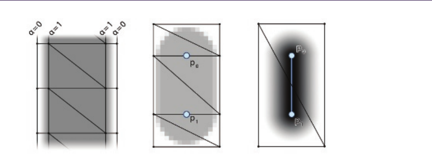
13.3. Rendering Lines 207
Figure 13.3. Vertex-alpha (left), texture-alpha (middle), and analytical distance (right).
For rendering lines with a width of only a few pixels like the ones sought
here, rendering an extra strip of translucent vertices is impractical as it generates
numerous small, thin triangles. First, it is not guaranteed that any fragment
centers are contained within the triangles, requiring wide falloffs to guarantee
smoothness. Second, because hardware often shades pixels in quads of 2 ×2 pix-
els, processing may be wasted on nonvisible fragments. Additionally, the method
does not deal correctly with endpoints. At best, adding an end segment would
produce bi-linearly interpolated areas, causing unsightly artifacts.
Using a simple alpha texture as a mask relies on the texture filtering and
pre-filtered mip-maps to produce a smooth result. Using a texture easily allows
us to specify a custom falloff for the line, allowing increased control over the
smoothness. As the texture can be very small, e.g., a grayscale 32 ×32 pixels,
memory is not a concern. In order to produce properly filtered lines at all scales,
it is important to provide a mip-map for the texture. Applying the alpha texture
can be done using either shaders or register combiners—having the final texture
combiner replace the alpha for the masked texture alpha.
The third option for analytically calculating the distance provides the most
accurate result, but can only be easily implemented using shaders. While the
per-fragment distance calculations require more ALU instructions than using a
texture lookup, it is still a viable option, as only a few fragments are touched
using this shader. If the base shader is bandwidth bound, it may even be the
preferred option. A hybrid of the second and third methods is possible, sampling
a distance texture and mapping it to an alpha value, potentially providing yet
more control over the falloff.
It is worth noting the importance of generating lines with a constant screen-
space antialiasing footprint. Also, the rendered lines should have valid depths to
be useful for depth culling. The following options are available for producing the
needed geometry:
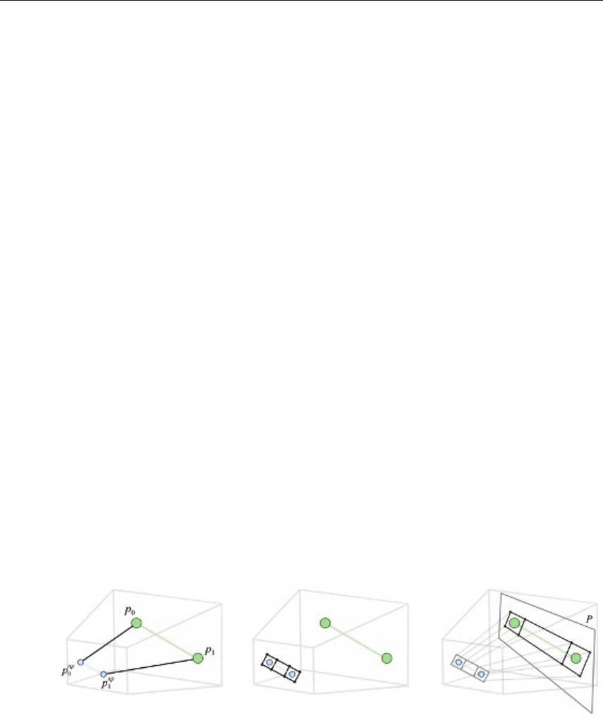
208 13. Inexpensive Antialiasing of Simple Objects
1. Project all points to screen space, extrude line geometry, and project back
to world space.
2. Directly render collapsed triangles in world space, and do the expansion
after projection within the vertex-shader.
3. For hardware with geometry-shaders, render line segments and expand ver-
tices in the geometry shader.
Depending on hardware and the specific case, any of these methods could be
preferable. The second method requires access to shaders, and results in only
a small memory overhead to store vertex IDs. Geometry shaders, while not
currently available on mobile hardware, would provide the most flexible solution,
requiring very few changes compared to ordinary line rendering. In order to main-
tain backwards compatibility, we opted for generating all line geometry directly
in world space, on the CPU. The downside to this is the overhead of creating new
positions and texture coordinates whenever the view changes.
The method for generating line geometry is fairly straight forward, but is
provided here for completeness (see Figure 13.4):
For each aliasing line segment {p0, p1}
1. Project {p0, p1}to the near plane {pnp
0, pnp
1}.
2. Expand {p0, p1}to eight vertices vn0−n7forming lines on the near plane.
3. Generate plane Pfrom the three points p0, p1, and p0+~v ×(p0−p1),where
~v is the view vector in world coordinates.
4. Project vn0−n7on to P, thus obtaining world-space vertices.
Recalling that triangle rasterization only affects fragments whose center lies
within the triangle, it is necessary to render lines wider than the targeted width,
in order to affect the same fragments touched by smooth line rendering. The
minimum line width required to affect the same fragments as a 1-pixel antialiased
Figure 13.4. Generating world-space line geometry in three stages.
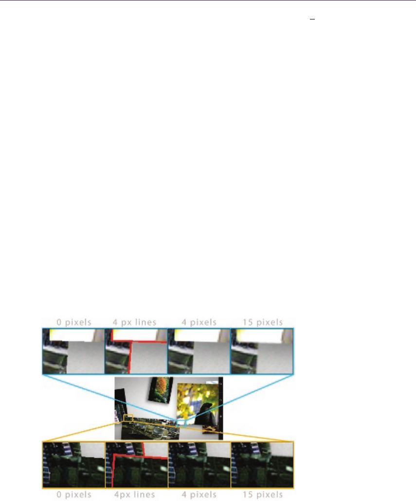
13.4. Discussion 209
line depends on angle and offset. To cover the worst case, a width of 2√2=2.8
pixels can be used. If desired, a bias towards a smoother result can be introduced
by artificially increasing the width of the lines.
During rendering, we want the alpha mask texture interpolation to happen in
screen space. In other words, we want to do screen-space linear interpolation of
the texture coordinates. OpenGL|ES does not currently support noperspective
interpolation, but the same result is achievable using shaders, by negating the
perspective transform as follows, see [Bærentzen et al. 08]: in the vertex shader,
multiply the texcoords with the w-component of the clip space vertex position—
then in the fragment shader, multiply the interpolated texture coordinates by the
interpolated 1/w.
Recalling that the lines should be rendered with the same lighting and tex-
tures as the object itself, it is generally sufficient to bind an extra vertex stream
supplying the texture coordinates for the masking texture. If using shaders, spe-
cific variants of the vertex and fragment programs should be created that apply
the extra alpha mask.
13.4 Discussion
Manual rendering of smooth lines was implemented in the Android application
Floating Image. The application renders simple photos in a gallery-type manner.
All potentially aliasing edges are static, and thus this application lends itself well
to this particular method of antialiasing. It is a very simple application, and
several other methods of antialiasing could also have been used—the simplest
Figure 13.5. Floating image with varying widths of smooth lines.

210 13. Inexpensive Antialiasing of Simple Objects
9 photos(no AA) 9 photos+AA (36 lines) AA Cost
HTC Magic (320x480) 56Hz 22Hz 27.59ms
Nexus One (480x800) 52Hz 49Hz 1.17ms
Samsung Galaxy S (480x800) 56Hz 56Hz “0ms”
27 photos (no AA) 27 photos+AA (108 lines) AA Cost
HTC Magic (480x320) 25Hz 9Hz 71ms
Nexus One (480x800) 34Hz 32Hz 1.8ms
Samsung Galaxy S (480x800) 56Hz 56Hz “0ms”
Table 13.1. Performance timings on various Android devices. MSAA was not supported
on these devices for comparison.
being to introduce a band of one translucent pixel around the edge of every
mip-level in the photo texture. While occlusions could, and normally should, be
handled using the depth buffer, Floating Image does manual compositing via the
painter’s algorithm for device-compatibility reasons, rendering all objects back-
to-front.
The implementation uses an alpha texture to render smooth lines, and slightly
biases towards blurriness by using a texture with a large falloff and oversized lines.
Figure 13.5 shows the result achieved, along with a much over-blurred version.
It is worth noting that the method always slightly expands the silhouette of
objects: whereas a lot of FSAA techniques blend with a background pixel of a
color assumed identical to one of the pixel neighbors, discontinuity edge overdraw
always adds occluding pixels on top.
Due to the choice between generating lines directly in world space and ren-
dering via a texture alpha mask, vertex-buffer data needs to be regenerated per
frame. Opting for performance over compatibility, vertex-shader expansion of the
lines could be used for line expansion, similar to what is often done for billboards.
We have tested the implementation on several devices with varying capabili-
ties. None of the devices were capable of MSAA, and only the Nexus One sup-
ported GL LINE SMOOTH. Using the smooth lines method we were able to achieve
antialiasing on all the devices. The performance has only been tested na¨ıvely, by
varying the number of photos displayed and noting the framerate (see Table 13.1).
Adding smooth edges hardly impacts performance of the Nexus One, while the
HTC is likely CPU-bound due to the line-expansion. The fastest of the devices
remains capped at refresh-rate.
13.5 Conclusion
The main drawback of the algorithm is that it depends on the geometric com-
plexity of the rendered scene. Traversing all geometry very quickly becomes
impractical, thus limiting use of the method to reasonably simple setups. Fur-
thermore, the need to track aliasing lines per frame makes it necessary to keep all

13.6. Acknowledgments 211
geometry accessible to the CPU. Even though many modern mobile GPUs use a
shared memory architecture, the APIs make it difficult to get around duplicating
data.
While the algorithm is not complicated to set up, and is arguably trivial if
line smoothing is available in hardware, it is challenging to make it scale with
increasing geometric complexity. Any object where outlines are trivially found,
or as in our example, are entirely static, is an obvious candidate. In general,
2D elements lend themselves well to the technique, whether in screen space or
positioned in a 3D scene. For complex 3D scenes, other solutions will likely yield
better results.
13.6 Acknowledgments
We would like to thank Jos´e Esteve, Romain Toutain, and Andreas Bærentzen for their
feedback on this chapter.
Floating Image is available on the Android Market at https://market.android.
com/details?id=dk.nindroid.rss and source code is available under GPL at http:
//code.google.com/p/floatingimage/.
Bibliography
[Bærentzen et al. 08] Jakob Andreas Bærentzen, Steen Munk-Lund, Mikkel Gjøl, and
Bent Dalgaard Larsen. “Two Methods for Antialiased Wireframe Drawing with
Hidden Line Removal.” Proceedings of the Spring Conference in Computer Graph-
ics, edited by Karol Myszkowski, pp. 171–177. Bratislava, Slovakia: Comenius
University, 2008.
[Flaherty 10] Adam Flaherty. “How to Render Anti-Aliased Lines with Textures in iOS
4.” O’Reilly Answers. June 24, 2010. Available at http://answers.oreilly.com/topic/
1669-how-to-render-anti-aliased-lines-with-textures-in-ios-4/.
[IMG 11] “POWERVR Series5 Graphics: SGX Architecture Guide for Developers.”
Imagination Technologies. July 5, 2011. Available at http://www.imgtec.com/
powervr/insider.
[OpenGL 08] “OpenGL ES Common/Common-Lite Profile Specification: Version
1.1.12.” Edited by David Blythe, Aaftab Munshi, and Jon Leech. The Khronos
Group and Silicon Graphics. April 24, 2008. Available at http://www.khronos.org/
registry/gles/specs/1.1/es full spec 1.1.12.pdf.
[OpenGL 10] “OpenGL ES Common Profile Specification: Version 2.0.25.” Edited by
Aaftab Munshi and Jon Leech. The Khronos Group. November 2, 2010. Available
at http://www.khronos.org/registry/gles/specs/2.0/es full spec 2.0.25.pdf.
[Rasterization 11] “Rasterization Rules (Direct3D 10).” msdn. Microsoft. 2011. Avail-
able at http://msdn.microsoft.com/en-us/library/cc627092(v=vs.85).aspx.

212 13. Inexpensive Antialiasing of Simple Objects
[Sander et al. 01] P. Sander, H. Hoppe, J. Snyder, and S. Gortler. “Discontinuity Edge
Overdraw.” In I3D ’01 Proceedings of the 2001 Symposium on Interactive 3D Graph-
ics, pp. 167–174. New York: ACM Press, 2001.
[Texture 04] “Texture AntiAliasing.” Apple. 2004. Available at http://homepage.mac.
com/arekkusu/bugs/invariance/TexAA.html.

14
Practical Planar Reflections Using
Cubemaps and Image Proxies
S´
ebastien Lagarde and Antoine Zanuttini
14.1 Introduction
Rendering scenes with glossy and specular reflections has always been a challenge
in the field of real-time rendering. Due to their importance in assessing image
quality, many techniques have been developed to simulate reflections. These
techniques can be classified in four categories:
1. Real-time techniques, such as dynamic environment mapping, with all kinds
of parameterization: cubemaps, 2D mirror planes, dual paraboloid. Dy-
namic reflections of this type are accurate but costly because they require
resending the whole scene to the graphics pipeline. Many optimizations
have been devised to speed up the process, such as mesh or shader simpli-
fications, but it still induces a significant overhead.
2. Precomputed techniques, such as static environment mapping with all kinds
of parameterization: cube maps, sphere maps, dual paraboloid, etc. Static
reflections lack the accuracy of dynamic reflection but are far cheaper to
use.
3. Screen-space techniques, such as screen-space local reflection [Tiago et al. 12],
often come at a manageable cost for pleasant localized results, but fail where
on-screen information is missing.
4. Real-time ray-tracing techniques such as the image-based reflections found
in Epic’s Samaritan demo [Mittring and Dudash 11] are promising tech-
niques, but they require support for features not available on older graphics
hardware.
213

214 14. Practical Planar Reflections Using Cubemaps and Image Proxies
For our game Remember Me, targeting current generation console hardware (DX9/
PS3/Xbox 360), we tried to find a reflection technique similar in cost to precom-
puted techniques, but with improved accuracy and realism.
This chapter introduces a new algorithm with a set of artist tools that allow
simulating planar glossy/specular reflections. The goal of our method is to replace
the accurate but costly real-time planar reflection with a cheaper approximation
that does not require re-rendering the scene geometry. In our game, we mostly
use these tools for ground reflections.
The principle of the algorithm is to render an approximation of the reflected
scene into a 2D reflection texture, then use this texture during the scene rendering.
In order to build the approximated reflected scene, we provide our artists with
several tools that let them combine the reflected scene with offline-generated
elements: environment maps and image proxies. To increase quality, we parallax-
correct elements of the reflected scene for the current view when they are rendered
in the reflection texture. In order to update the parallax-correction, the reflection
texture is updated for each frame.
We will start the description of our algorithm and tools with the generation
of the reflection texture. We will describe how our algorithm fits within a local
image-based lighting (IBL) strategy, following the work we presented in [Lagarde
and Zanuttini 12]. We will conclude with the processing and usage of this 2D
reflection texture for the scene rendering.
14.2 Generating Reflection Textures
14.2.1 Cubemap Reflection Environment
Our algorithm begins by generating an approximation of the reflected scene. We
are trying to avoid the cost of re-rendering the scene geometry at runtime. In
this case, the common technique for approximating reflections is to create an
environment map, such as a cubemap, that is the parameterization of choice
due to its hardware efficiency. However, the reflection stored in the cubemap is
correct only from a single point in space. Applying a cubemap onto a planar
geometry such as a ground surface creates visual issues in part due to lack of
parallax (Figure 14.3). The graphics literature proposes several algorithms to fix
this problem. All these algorithms share the requirement of a geometry proxy
to represent the reflection environment: simple sphere volumes [Bjorke 04], box
volumes [Czuba 10] or cube depth buffers [Szirmay-Kalos et al. 05]. The reflected
view vector by the surface normal is used to intersect the proxy geometry. A cor-
rected reflected view vector is created from the pixel’s world position, which can
then be used to fetch the right cubemap sample. Cost and quality increase with
the geometry proxy’s complexity. For completeness, we note that other cheap
parallax correction methods without a geometry proxy are available [Geiss 05,
Brennan 02], but they require manual tuning for each object. Our solution to
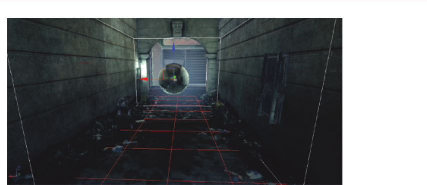
14.2. Generating Reflection Textures 215
Figure 14.1. Cubemap with a box volume (white) and reflection plane (red) matching
a rectangular room environment.
the parallax problem is unique in that we don’t use the scene’s geometry since
we cannot access the pixel’s world position when we render into the 2D reflection
texture. Moreover, we limit ourselves to planar reflections.
We developed tools for our artists to allow placing cubemaps in levels and
associating them with a geometry proxy: a convex volume approximating the
reflection environment. For example, in a rectangular room an artist can place
a cubemap in the center of the room and define a box volume to approximate
the room boundaries. The center of the box volume doesn’t need to match the
position of the cubemap. As we target planar reflections, we also require having
a reflection plane for the cubemap (Figure 14.1). The reflection plane could be
specified as a distance from the cubemap position and oriented by the cubemap’s
up axis or extracted from a game’s entity.
In order to correct for parallax, we make the following observation (see Fig-
ure 14.2):
Consider a scene with a ground surface (hashed line), a reflection environment
(yellow) approximated by a proxy geometry (box volume in green) and a camera.
The camera looks at a position on the ground. The reflected view vector ⃗
Ris
used to get the intersection Pwith the proxy geometry. Pis then used with
the cubemap that was captured at center Cto recover the cubemap’s sample
direction ⃗
D. If we reflect the camera about the reflection plane, the new view
vector ⃗
Vof the reflected camera matches the previous ⃗
Rvector and intersects the
same point P. From this observation, we deduce that in order to fix the parallax
issue we could simply project the cubemap onto its geometry proxy, and then
render the geometry from the point of view of the reflected camera.
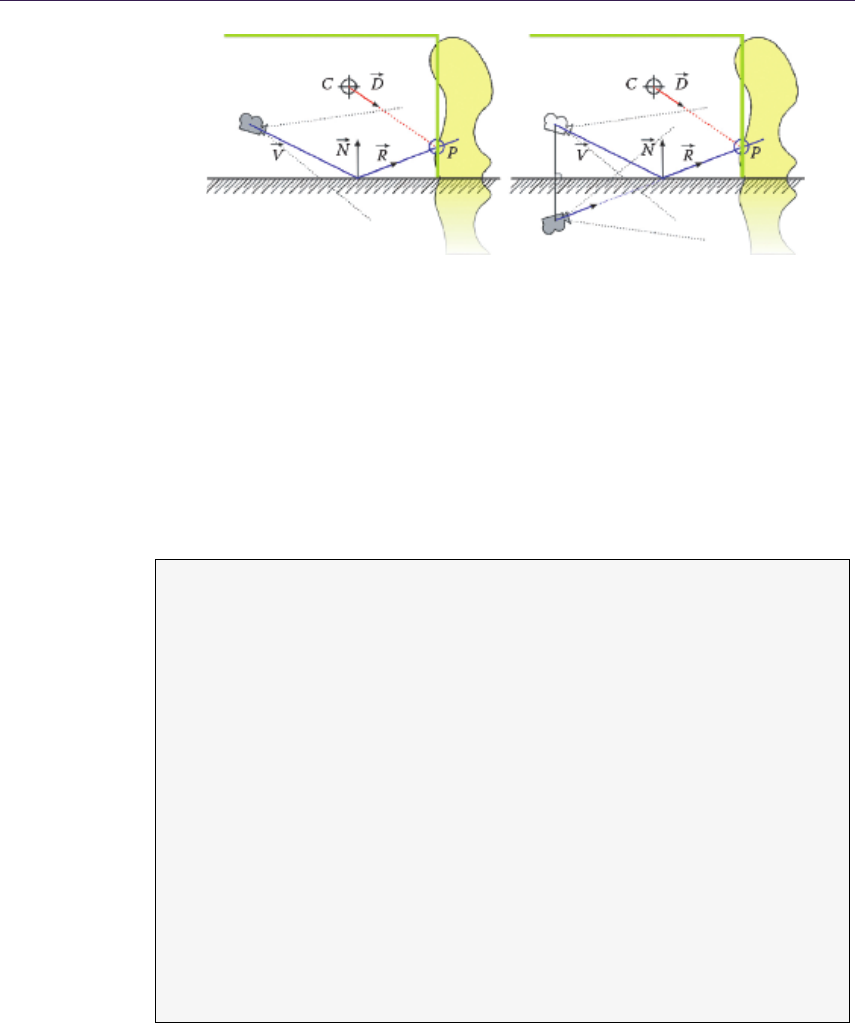
216 14. Practical Planar Reflections Using Cubemaps and Image Proxies
Figure 14.2. The view vector of the reflected camera equals the reflected view vector of
the camera.
The rendering process is similar to standard real-time planar reflection ren-
dering. We build a ViewProjection matrix by mirroring the View matrix by
the reflection plane and compose it with an oblique near clipping plane matrix
[Lengyel 07]. We then render the back face of the geometry proxy with this View-
Projection matrix. As we reflect the camera, we must inverse the winding order.
C++ pseudocode and shader code are provided in Listing 14.1.
// C + + p s eu do co de
Matrix Mirror = Cr eate Mi rror Mat rix ( Re fle ctio nPl aneW S );
Matrix R ef lectVie w = Mi rror * View ;
Matrix C lipPro jec tion = Ne arObli queM at rix ( Re fle ctio nPl aneV S );
Matrix ViewProjection = View * ClipProjection;
// Render back face but re me mb er to i nverse c ul li ng order
SetInverseFrontFaceCulling();
DrawConvexVolume();
// Sh ader code
fl oat 4x4 Lo calT oWo rld ;
fl oat 4x4 Vi ewPr oje ctio n ;
Ve rt ex Main () {
float4 Po si ti on WS = mu l ( Loc alT oW orl d , I nPo si ti on OS ) ;
float4 Po si ti on SS = mu l ( Vi ewP roj ec tio n , P os iti on WS ) ;
OutPosition = PositionSS;
// Cur rent direction sampling direction
O utD ir ec ti on = P os it io nW S . xyz - C ub eC en te rWS . xyz ;
}
Pi xe lM ai n () {
Ou tCo lor = te xCU BE ( Cub eTe xtur e , Ou tD irec tio n );
}
Listing 14.1. Pseudocode of parallax-corrected cubemap.
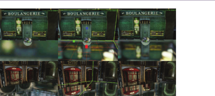
14.2. Generating Reflection Textures 217
Figure 14.3. Box (top) and convex (bottom) room with a specular ground reflecting the
environment with a cubemap. With parallax issue (left) and with correction (right).
Our algorithm allows for the rendering of accurate reflections for any space
matching the convex volume used as a geometry proxy (Figure 14.3). It is possible
to use concave volumes as geometry proxies but it will result in artifacts because
we don’t use the Z-buffer during the drawing. Additionally, some information will
not be captured in the cubemap. In the next section, we will present a technique
to add information into the 2D reflection texture to complete the cubemap that
can be used to hide these artifacts.
14.2.2 Image Proxies
The previous section described the projection of a parallax-corrected cubemap
onto a 2D reflection texture to approximate the reflected scene. This kind of
rendering has its limits because it can miss or lose information: dynamic elements
may disappear, the 2D texture resolution can be too low, causing flickering or the
disappearance of bright small elements, and concave volumes used as geometry
proxies will occlude details. It is possible to enhance the cubemap’s contribution
to the rendering of the reflected scene with image proxies in the spirit of the light
cards used in the AMD’s Whiteout demo [Wiley and Scheuermann 07] or the
billboards from Epic’s Samaritan demo [Mittring and Dudash 11]. The addition
of image proxies to our algorithm is easy. We use a quad as a geometry proxy
for an image representing a part of the reflected scene, then we render the quad
as in the previous section. A detailed description of the creation, rendering and
usage of image proxies follows.

218 14. Practical Planar Reflections Using Cubemaps and Image Proxies
Figure 14.4. Editor view showing the link between an image proxy and a cubemap
(left) and the orthogonal frustum for a 2D scene capture (right).
Creating image proxies. An image proxy is a quad textured with an authored
image or a 2D capture from the scene. The quad is used as a geometric approxi-
mation of the reflection environment a.k.a. the geometry proxy.
We developed tools for our artists to allow placing image proxies in levels,
customizing the quad size, customizing the texture resolution and performing 2D
scene captures (Figure 14.4). The 2D capture is done with an orthogonal frustum
set up inside our game editor. The capture considers empty areas (pixels that
have not been touched during rendering) as transparent.
Image proxies are very similar to sprite particles and they can share many
properties. We decided to take a subset of sprite particles functionality. Image
proxies can
•always face the camera, resulting in a spherical billboard;
•define a constraint axis and try to face the camera but rotate along that
axis, resulting in a cylindrical billboard;
•use different blending modes (interpolative, additive).
Note that we restrict ourselves to quad image proxies for efficiency, but other
plane shapes could apply here.
Rendering image proxies. All image proxies are transparent objects (this choice
will be explained later in this section) and thus need to be sorted back to front
before rendering since we do not use a Z-buffer. We use the distance from the
camera to the image proxies as a criterion for sorting. For an accurate rendering,
particularly in the case of overlapping image proxies, we should perform a binary
space partitioning (BSP) of the quads but we found out that using a priority
system to force the rendering order was sufficient in our case. Rendering image
proxies is similar to cubemap rendering. We also allow image proxies to be two
sided. C++ pseudocode and shader code are provided in Listing 14.2.

14.2. Generating Reflection Textures 219
// C + + p s eu do co de
Matrix Mirror = Cr eate Mi rror Mat rix ( Re fle ctio nPl an eW S );
Matrix R ef lectVie w = Mi rror * View ;
Matrix C lipPro jec tion = Ne arObli queMat rix ( Re fle ctio nPl aneV S );
Matrix ViewProjection = View * ClipProjection;
// Image proxy sp ec if ic
Vector R efl ec tVi ew Ori gi n = Mirr or * V ie wO rigin ;
M atr ix I n ve r se Re f le ct Vi e w = R ef le ct Vi ew . I nve rs e ( ) ;
Ve ctor Vi ewUp = - Inve rse Re fle ct View * Vec tor (0 ,1 ,0) ;
// Following is done for each IP ( Image proxy )
// Calc X and Y sp rite v ec tor b ased on o ption .
V ect or Y Ve ct or = I P - > L oc al T oW or ld * V ec to r (0 , 1 , 0 ) ;
if (IP -> b Cam eraFac ing ) {
float S c al eF ac to r = Y Ve ct or . Le ngt h ( ) ;
YV ect or = Came raU p . Normalize () * Scale Fac tor ;
}
Ve ctor Ca me raD irW S = ( C ame raW S - IP - > Loc ati on ). No rma liz e () ;
V ect or X Ve ct or = IP -> L o ca lT o Wo rl d * Ve ct or ( 1 , 0 , 0 ) ;
if (IP -> bCame raF aci ng || IP - > bCam er aF ac ingR efle ctio nA xis ) {
float S c al eF ac to r = X Ve ct or . Le ngh t ( ) ;
XV ect or = C ame raD ir ˆ Y Vec tor ;
XV ector = XVect or . No rm alize () * Sca le Factor ;
}
// Sh ader code
fl oat 4x4 Lo calT oWo rld ;
fl oat 4x4 Vi ewPr oje ctio n ;
float3 IP Pos ition ;
Ve rt ex Main () {
float3 VP os it io n = IP Po sition + InPo si ti on .x * XVe ct or -
In Position . y * YV ector ;
float4 Po si ti on SS = mu l ( Vie wP roj ec tio n , float4( V Pos iti on , 1) ) ;
Ou tPositio n = Po sit ion SS ;
UV Ou t = U V ;
}
float4 IPColor ;
Pi xe lM ai n () {}
Ou tC olo r = IP Col or * t ex2D ( Sp rit eTe xtu re , I nUV ) ;
}
Listing 14.2. Pseudocode for parallax-corrected rendering of image proxies.
A disturbing problem of naively rendering image proxies as presented here is
temporal aliasing. The low resolution of our textures (both 2D reflection textures
and image proxy textures) causes severe aliasing along the edges of image proxies,
especially when the camera moves near the boundaries of the geometry proxy.
To minimize aliasing we set the alpha value of image proxy texture borders to be
fully translucent, forcing us to render the image proxies as transparent objects
(Figure 14.5). It would also be possible to set this value from within the shader.
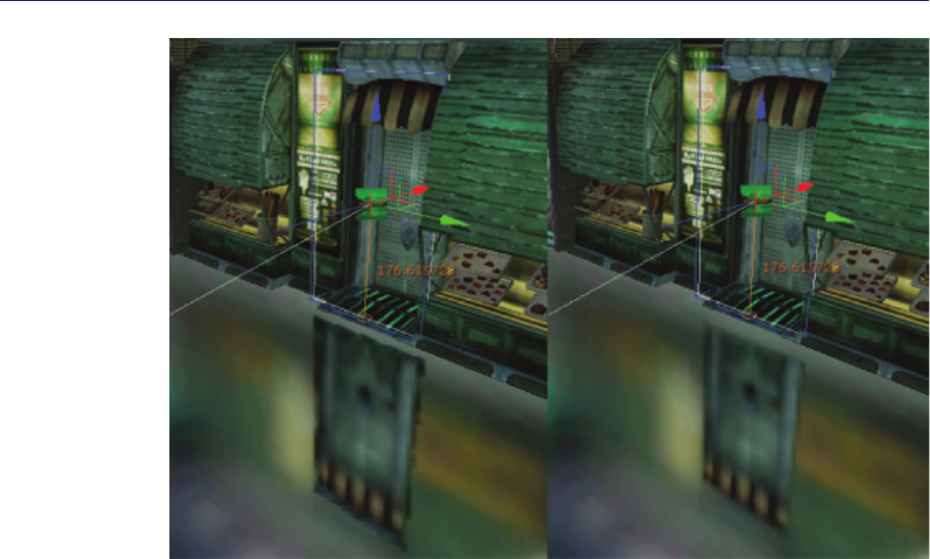
220 14. Practical Planar Reflections Using Cubemaps and Image Proxies
Figure 14.5. An image proxy of a door rendered with aliasing (left). The floor is flat
and specular to highlight the aliasing issue. The same with fully transparent texture
borders (right).
It should be noted that the choice of a quad geometry simplifies this step: a more
complex geometry would require more efforts in order to deal with aliasing.
Using image proxies for dynamic reflections. An image proxy is not restricted to a
static quad. By dynamically updating its position (for instance by attaching it to
a game entity), it is possible to handle gameplay events such as an opening door
(Figure 14.6). In this case the cubemap must not contain the scene geometry
represented by the image proxies, i.e., the door must not be present when gen-
erating the cubemap. We provide flags to our artists to specify the scene object
visibility based on the type of rendering (2D capture, cubemap, or scene).
We also use dynamic updates of image proxies to simulate character reflec-
tions. Character image proxies are just image proxies linked to the character’s
main bones with a constraint along each bone’s axis. In this case we use an
authored texture that consists in just a white sphere that can be tinted by char-
acters. During gameplay we update the character’s image proxies based on the
transformation of their attached bones and link them to the current cubemap
(Figure 14.7).
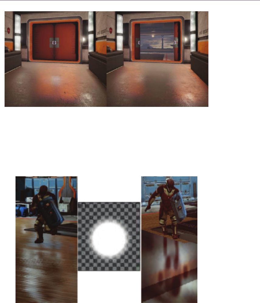
14.2. Generating Reflection Textures 221
Figure 14.6. Image proxies can be moved in real-time to match the action.
Best practices. Image proxies are powerful tools, but they require production
time from the artists. There are plenty of creative ways to use them to enhance
reflections and we present some best practices here. Figure 14.8 shows screenshots
of typical use cases with only the cubemap applied and with the contribution of
the image proxies:
Figure 14.7. Character proxies (left), the texture used for the main bones (center), and
the character proxies on a flat mirror, highlighting the coarse approximation (right).

222 14. Practical Planar Reflections Using Cubemaps and Image Proxies
1. Rendering small light sources inside small resolution cubemap is problem-
atic. They can flicker or completely drop out. Image proxies can compen-
sate for the low resolution.
2. Control the brightness strength of the cubemap: As a cubemap is a single
texture generated in the engine, it is painful to boost the brightness in only
a part of it. Image proxies can control their brightness individually.
3. Enhance lights: in order to emulate a stretch highlight on a wet ground
similar to the Blinn-Phong lighting model, artists can create a cylinder
billboard image proxy with an authored texture instead of a capture of
that part of the scene.
4. Hide undesirable reflections: by placing a 2D scene capture proxy at the
appropriate position, it is possible to hide reflection elements either in the
cubemap or in another image proxy.
5. Handle multiple reflection planes: Standard real-time reflection can only
reflect for one plane at a time. By settings image proxies at different height
with their quad geometries parallel to the reflection plane, we could simulate
multiple plane reflections inside one texture.
6. Hide concave geometry proxy artifacts: if the cubemap captures a corner
corridor, image proxies can be used to hide the missing information caused
by occlusions.
Another useful property of image proxies arises when dealing with multiple
cubemaps at the same time, as will be shown in the next section.
14.2.3 Local Image-Based Lighting
Our game uses a local image-based lighting (IBL) system. Our local IBL provides
accurate environment lighting information that can be used for glossy and/or
specular reflections and has the additional advantage of smooth lighting tran-
sitions between objects. The system has been covered in detail in the authors’
SIGGRAPH 2012 talk [Lagarde and Zanuttini 12] and personal blog [Lagarde 12].
It consists of blending multiple cubemaps in the neighborhood of a point of in-
terest (the camera, the player. . . ) and using the blended cubemap for indirect
lighting on scene objects. The blending weights are authored by artists as in-
fluence regions around a cubemap. We extend the previous work by blending
cubemaps inside a 2D reflection texture instead of a cubemap and by adding im-
age proxies to the mix. The move from a cubemap to a 2D texture is motivated
by performance requirements since we need to handle only one view instead of six.
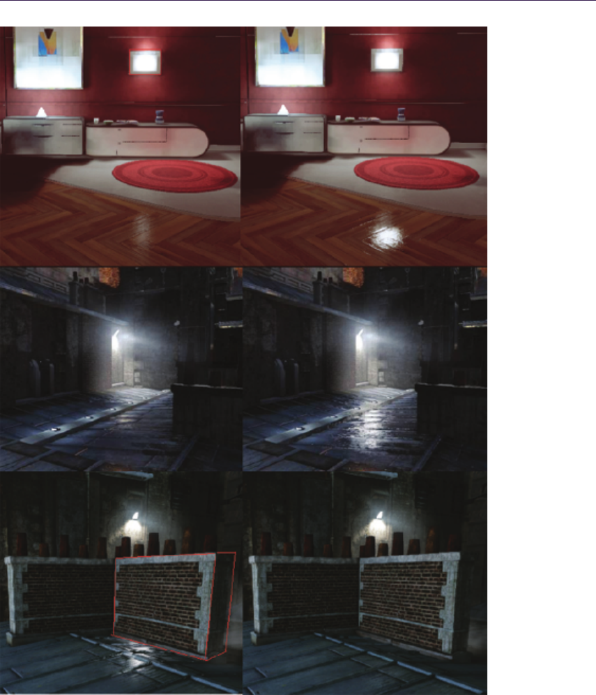
14.2. Generating Reflection Textures 223
Figure 14.8. Examples of best practices. Top to bottom: cases 2, 3, and 4. On the left,
the scene with only the cubemap reflection and the image proxy capture frustum (red
box). on the right, the enhancement resulting from image proxy use.

224 14. Practical Planar Reflections Using Cubemaps and Image Proxies
Rendering multiple cubemaps and image proxies. In order to render multiple cube-
maps correctly, we should render each cubemap and its linked image proxy sep-
arately and then blend the result. This is because of the reflection plane, the
sorting order and the blending mode of the image proxies. This has both a mem-
ory and a computational cost. As a performance optimization, we chose to first
render all cubemaps sorted by increasing blend weight with additive blending,
then render all sorted image proxies. This can cause trouble when mixing cube-
maps with different reflection planes but we let artists manage this case. Other
artifacts are less noticeable.
Extra care needs to be taken for character image proxies as these are dynami-
cally linked to the cubemaps. In the blending case, they must be linked to all the
gathered cubemaps in order to be fully visible (the sum of their blending weights
will equal 100%). We render them in each cubemap rather than at the end to
get smoother transitions when a cubemap with a different reflection plane comes
into the mix.
Similarly to character proxies, other image proxies may be shared by multiple
cubemaps. If the image proxy uses interpolative blending, this could result in a
final image intensity that is lower than expected because of repeated interpolation.
This can be fixed in the shader by tweaking the alpha value according to the
blending weight.
Image proxy best practices with local IBL. Our local IBL approach provides seam-
less transitions between lighting environments represented by cubemaps. A sim-
ple example of a corridor environment has been presented in our SIGGRAPH
talk. This still applies to our planar reflection. We set up three cubemaps in
the corridor with overlapping influence regions and identical geometry proxies.
For clarity, only the geometry proxies (the box volumes in red, green, and blue)
are shown, with a small scale so that they are all visible. This setup and our
planar reflection technique provide detailed reflections and smooth transitions
(Figure 14.9). There is a video in the web material accompanying this article
showing the result when the camera moves.
Image proxies are of great help in more complex cases. Again, artists must be
creative, and we help by presenting some best practices. Figure 14.9 shows the
setup of geometry proxies and screenshots of typical usage (refer to the video for
better visualization). Purple lines are image proxies; red, green and blue boxes
are geometry proxies of cubemaps:
1. Corner corridor: The set of geometry proxies include a concave volume.
Artists use image proxies to hide the artifacts. The image proxies are
captures of the walls.
2. Two successive rooms, separated by an opening door: The geometry proxies
overlap and include the two rooms. The image proxies are captures of the
separating walls. Walls should not be included in the cubemap generation.
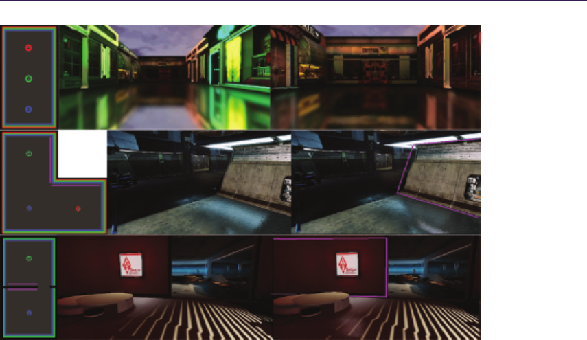
14.3. Using Reflection Textures 225
Figure 14.9. Top view of the scene’s cubemap setup (left) and the resulting rendition
(right). From top to bottom: corridor case from the SIGGRAPH talk, best case 1, and
best case 2.
14.3 Using Reflection Textures
14.3.1 Glossy Material Support
We saw how to generate a 2D reflection texture to approximate a reflected scene.
This texture is better suited for specular materials like perfect mirrors. In order
to support glossy material we store preconvolved versions of the base texture in
the mipmaps (Figure 14.10). This is similar to a preconvolved cubemap [Kautz
et al. 00]. Each mipmap level maps to a different glossiness. A highly glossy re-
flection (more detailed) will look up a lower mipmap level, a less glossy reflection
(more blurred) will look up the average of a large number of pixels. We exper-
imented with two ways of generating the mipmaps: by rendering the reflected
scene for each mipmap, and by successively blurring base mipmaps.
Rendering the reflected scene in each mipmap. We first try to re-render the ap-
proximated reflected scene for each mipmap. For better results, we should use
both preconvolved cubemaps and preconvolved image proxies. At rendering time,
the current mipmap level to render is used to sample the current mipmap level
of the texture applied on the cubemap or image proxies. The difficulty of this

226 14. Practical Planar Reflections Using Cubemaps and Image Proxies
Figure 14.10. Different mipmap levels matching different roughness strengths.
approach lies in the generation of accurate preconvolved image proxies, which is
impossible because of the lack of information outside of the 2D texture. The low
resolution of the mipmap is also problematic: small image proxies will contribute
too few pixels. Finally, if there are several characters in a scene then the num-
ber of draw calls can increase significantly. Since we know we cannot achieve
sufficient accuracy anyway, we choose a cheaper approach.
Convolving base mipmaps. A simpler approach consists of recursively blurring
mipmap textures. Each mipmap stores the result of convolving the previous
lower mipmap level with a specified blurring kernel. We use a Gaussian blur that
we found to be sufficient for our needs.
Aliasing. Aliasing is an important issue that our method must address. The
reader may notice that in Listing 14.1 a texCUBE instruction is used instead
of texCUBElod that would force a fetch from the base cubemap. This reduces
aliasing even if mipmaps are generated in a subsequent step. For completeness,
it should be added that a better way would be to use the texCUBElod instruc-
tion and, at scene rendering time, compute the required hardware mipmap level
and the desired mipmap level based on roughness, then chose the larger of the
two values [Scheuermann and Isidoro 05]. We decided against this approach for
performance reasons.
14.3.2 Applying the 2D Reflection Texture
The preconvolved 2D reflection texture can now be used on any planar objects
lying at the same height as the reflection plane used to generate the texture. The
rendering process for our texture is similar to the mirror surface case. We use
the texture to provide the reflection value by performing a texture lookup with
the actual screen coordinates as the texture coordinates. We approximate rough
surfaces by offsetting the texture coordinates along the XY components of the
surface normal with an artist-controlled parameter for the distortion strength.
We also use the glossiness of the surface to select the right mipmap level to use
(Listing 14.3). It is possible to divide the distortion value by the post-perspective
Z-coordinate. The distortion will vary with distance but we did not find it to
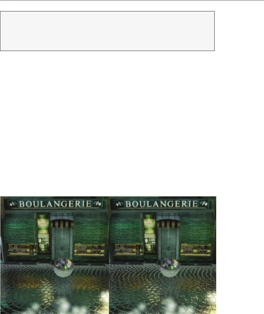
14.3. Using Reflection Textures 227
float2 Sc re en UV = S cr ee nPo si ti on . xy / Sc re enPos it ion .w *
float2( 0.5 f , -0.5 f ) + 0.5 f ;
float2 R = S cr ee nU V + T an ge nt N or ma l . xy * D i st or ti o nS tr e ng ht ;
return tex2Dlod ( ReflectionTexture , float4( R , 0 .0 f , S c al eB ia s . x *
Gl os si ne ss + S ca le Bia s . y )). r gb ;
Listing 14.3. High-level shading language (HLSL) pseudocode to use a 2D reflection
texture.
improve the final quality in our case. Note that for performance reasons, we do not
transform the normal to view-space but keep it in tangent space, implying that
we could not distort in the correct direction. In practice the result is good enough
and the correct result would still be an approximation anyway (Figure 14.11).
14.3.3 Cost
We provide some performance measurements of our implementation with a 128×
128 ×6 cubemap stored using DXT1 compression, 128 ×128 image proxies using
DXT5, and a 256×256 2D reflection texture. Image proxies use DXT5 to support
the alpha pixel border we add for antialiasing. We provide our performance
measurements as ranges since timings vary with the number of cubemaps, image
proxies and pixels clipped by the reflection plane. The typical case includes two
cubemaps and 10 to 15 image proxies. The whole process is in HDR format.
Figure 14.11. The influence of the distortion strength on the reflection.
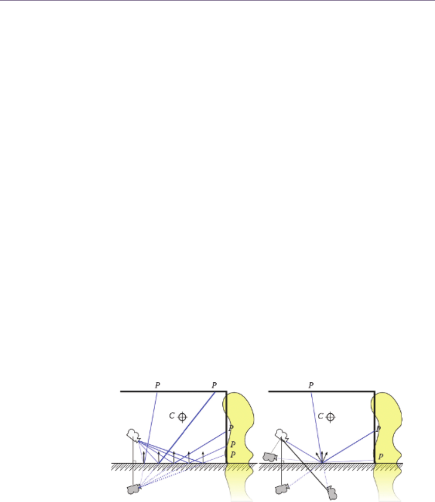
228 14. Practical Planar Reflections Using Cubemaps and Image Proxies
On the PlayStation 3, we generate the reflection texture in the RGBA half16
format. The texture generation costs between 0.10 ms and 0.33 ms, with an
average of 0.17 ms. The mipmap generation costs 0.16 ms. The process is render-
output-bound due to the use of RGBA half16.
On the Xbox 360 we use the 10-bit float 7e3 format. The texture generation
costs between 0.06 ms and 0.24 ms with an average of 0.1 ms. The mipmap
generation costs 0.09 ms.
14.4 Conclusion and Future Work
We have presented a good alternative to real-time 2D reflections applied to planar
objects to simulate specular and/or glossy materials. Our approach is fast and
practical and can be used in conjunction with other techniques such as local IBL.
It has been used in production in our game targeting current generation consoles.
A video showing various best practices and use cases of our technique is available
in the accompanying web material.
The technique is satisfying but could be improved in a number of ways:
First, using a cubemap reflection texture instead of a 2D reflection texture
will improve the accuracy of the reflection distortion with rough surfaces at the
cost of doing the process six times and requiring more time to generate mipmap.
It should be highlighted that this still does not provide the correct result because
we are generating the cubemap reflection texture only for normals perpendicular
to the reflection plane. Using it for shifted normals introduces a distortion that
increases with the angle between the normal and the plane normal (Figure 14.12)
[Lagarde and Zanuttini 12]. Another parameterization, more efficient but with
the same benefits, could be a dual paraboloid map [Scherzer et al. 12]. This will
require tessellating our geometry proxies to limit the projection warping artifacts
and rotating the lighting to local space aligned on the reflection plane’s normal.
Figure 14.12. Our cubemap reflection is only valid for pixels with a normal vector
perpendicular to the ground (left). For perturbed normals, the intersection requires
moving the reflected camera’s position (right).

14.5. Acknowledgments 229
Second, anisotropic reflections could be emulated by stretching image proxies
based on some physical properties. A more physically based approach could be
developed for the mipmap generation step.
Finally image reflections as used in Epic’s Samaritan demo [Mittring and
Dudash 11] also are an interesting future development.
14.5 Acknowledgments
The screenshots in Figures 14.1,14.4,14.5,14.6,14.8, and 14.11 are Remember
Me gameplay images from the game demo at Gamescom 2012. Images courtesy
of Capcom U.S.A., Inc., c
⃝Capcom Co. Ltd. 2013, all rights reserved.
Bibliography
[Bjorke 04] Kevin Bjorke. “Image base lighting.” In GPU Gems, edited by
Randima Fernando, pp. 307–321. Reading, MA: Addison-Wesley, 2004.
[Brennan 02] Chris Brennan. “Accurate Environment Mapped Reflections and
Refractions by Adjusting for Object Distance.” In ShaderX, edited by Wolf-
gang Engel, pp. 290–294. Plano, TX: Wordware Inc., 2002.
[Czuba 10] Bartosz Czuba. “Box Projected Cubemap Environ
ment Mapping.” Gamedev.net.http://www.gamedev.net/topic/
568829-box-projected-cubemap-environment-mapping/, April 20, 2010.
[Geiss 05] Ryan Geiss. “The Naked Truth Behind NVIDIA’s Demos.” Exhibitor
Tech Talk, ACM SIGGRAPH 2005, Los Angeles, CA, 2005.
[Kautz et al. 00] Jan Kautz, Pere-Pau V´azquez, Wolfgang Heidrich, and Hans-
Peter Seidel. “Unified Approach to Prefiltered Environment Maps.” In
Proceedings of the Eurographics Workshop on Rendering Techniques 2000,
pp. 185–196. London: Springer-Verlag, 2000.
[Lagarde 12] S´ebastien Lagarde. “Image-Based Lighting Approaches
and Parallax-Corrected Cubemap.” Random Thoughts about
Graphics in Games.http://seblagarde.wordpress.com/2012/09/29/
image-based-lighting-approaches-and-parallax-corrected-cubemap/,
September 29, 2012.
[Lagarde and Zanuttini 12] S´ebastien Lagarde and Antoine Zanuttini. “Local
Image-Based Lighting with Parallax-Corrected Cubemap.” In ACM SIG-
GRAPH 2012 Talks, article no. 36. New York: ACM, 2012.
[Lengyel 07] Eric Lengyel. “Projection Matrix Tricks.” Presentation, Game De-
velopers Conference 2007, San Francisco, CA, 2007.

230 14. Practical Planar Reflections Using Cubemaps and Image Proxies
[Mittring and Dudash 11] Martin Mittring and Bryan Dudash. “The Technol-
ogy Behind the DirectX 11 Unreal Engine ‘Samaritan’ Demo.” Presentation,
Game Developers Coneference 2001, San Francisco, CA, 2011.
[Scherzer et al. 12] Daniel Scherzer, Chuong H. Nguyen, Tobias Ritschel, and
Hans-Peter Seidel. “Pre-convolved Radiance Caching.” Eurographics Sym-
posium on Rendering: Computer Graphics Forum 31:4 (2012), 1391–1397.
[Scheuermann and Isidoro 05] Thorsten Scheuermann and John Isidoro. “Cube-
map filtering with CubeMapGen.” Presentation, Game Developers Confer-
ence, San Francisco, CA, 2005.
[Szirmay-Kalos et al. 05] L´aszl´o Szirmay-Kalos, Barnab´as Asz´odi, Istv´an
Laz´anyi, and M´aty´as Premecz. “Approximate Ray-Tracing on the GPU with
Distance Impostors.” Computer Graphics Forum 24:3 (2005), 695–704.
[Tiago et al. 12] Tiago Sousa, Nickolay Kasyan, and Nicolas Schulz.
“CryENGINE 3: Three Years of Work in Review.” In GPU Pro 3,
edited by Wolfgang Engel, pp. 133–168. Boca Raton, FL: CRC Press, 2012.
[Wiley and Scheuermann 07] Abe Wiley and Thorsten Scheuermann. “The Art
and Technology of Whiteout.” Presentation, ACM SIGGRAPH 2007, San
Diego, CA, 2007.

15
Real-Time Ptex and
Vector Displacement
Karl Hillesland
15.1 Introduction
A fundamental texture authoring problem is that it’s difficult to unwrap a mesh
with arbitrary topology onto a continuous 2D rectangular texture domain. Meshes
are broken into pieces that are unwrapped into “charts” and packed into a rect-
angular texture domain as an “atlas” as shown in Figure 15.4(b). Artists spend
time setting up UVs to minimize distortion and wasted space in the texture when
they should ideally be focusing on the actual painting and modeling.
Another problem is that edges of each chart in the atlas introduce seam arti-
facts. This seam problem becomes much worse when the texture is a displacement
map used for hardware tessellation, as any discrepancy manifests as a crack in
the surface.
This chapter describes an implicit texture parametrization system to solve
these problems that we call packed Ptex. It builds on the Ptex method developed
by Disney Animation Studios for production rendering [Burley and Lacewell 08].
Ptex associates a small independent texture map with each face of the mesh.
Each texture map has its own mip chain. In the original Ptex method, adjacency
information is used for filtering across the edge of one face texture and into the
next.
There are two main advantages of Ptex relative to conventional texture atlas-
ing. First, there is no need for explicit UV. Second, there are no seaming issues
arising from unwrapping a complete mesh of arbitrary topology onto a single-
texture domain. These are the two main advantages of the original Ptex method
that we preserve in our adaptation.
The drawbacks of packed Ptex relative to conventional texture atlasing are
additional runtime computation, additional texture filtering expense, and changes
in asset production. The main change in asset production is that our method cur-
231
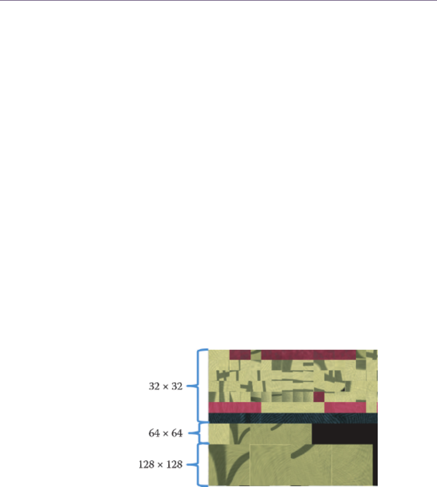
232 15. Real-Time Ptex and Vector Displacement
rently targets meshes consisting of quads. There can either be additional memory
cost or savings relative to conventional texture atlasing methods depending on
the particular circumstances.
Although this approach works for many texture types, it works particularly
well for vector displacement mapping. The lack of seam issues is particularly
valuable for this application, while many of the drawbacks of the approach are
irrelevant.
There are two barriers to real-time performance in the original Ptex method.
First, it’s typically not practical to have an individual texture for each primitive.
Second, the indirection required when a filter kernel crosses from one face to
another is costly in performance, and precludes the use of any hardware texture
filtering. The next section describes the offline process to address these issues.
Then we follow up with how to use this at runtime and some details related to
displacement mapping. We finish by discussing the tradeoffs of this method as
well as some possible alternatives.
15.2 Packed Ptex
To reduce the number of textures required, we pack all face textures and their
mip chains into a single texture atlas (Figure 15.1). The atlas is divided into
blocks of the same resolution. Within the block, the face textures are packed one
after another in rows. Because the atlas width generally is not a multiple of the
face-texture width, there will be unused texels at the end of each row. There will
be additional empty space at the end of the last row, because it generally will
not be filled to capacity.
Figure 15.1. This is a portion of a packed Ptex atlas. There are four faces that have
128 ×128 base (level 0) resolution and one with 64 ×64 base resolution. The block of
64 ×64 contains both the one level 0 for the 64 ×64 face texture, and the four level 1
mips from the 128 ×128 face textures.

15.2. Packed Ptex 233
Figure 15.2. Faces that are adjacent in model space are not generally adjacent in texture
space. A filter kernel that spills over the edge of a face must pick up texels from the
adjacent face, which will generally be somewhere else in the texture atlas. We copy
border texels from adjacent face textures to handle this case.
Just as in the original Ptex system, each face texture has its own mip chain.
We sort the faces by their base (level 0) resolution to create the packing we de-
scribe here, and for runtime as described in Section 15.3.2. Since we are including
face textures with different base resolutions, a given block will include different
mip levels (Figure 15.1).
15.2.1 Borders for Filtering
Texture filtering hardware assumes that neighbors in texture space are also neigh-
bors in model space. Generally, this is not true either for conventional texture
atlasing methods nor for Ptex. It’s the reason conventional texture atlasing meth-
ods often come with seam artifacts.
For our method, we copy texels from the border of a neighboring face to
solve this problem (Figure 15.2). That way, there will be data available when
the texture filter crosses the edge of the face texture. The padding on each side
will be equal to at least half the filter width. This is a common solution to the
problem, particularly for situations like tile-based textures for terrain. However,
the memory overhead for this solution is generally much higher for Ptex than for
conventional texture atlasing methods. This is one disadvantage in using Ptex;
anisotropic filtering quickly becomes too expensive in terms of memory cost.
15.2.2 Texture Compression
Current GPUs have hardware support for texture compression. The compression
relies on coherency within 4 ×4 texel blocks. For this reason, it is best not to
have a 4 ×4 block span face textures. We have already discussed adding a single-
texel border to support hardware bilinear filtering. To get good results with
compression, we add an additional border to get to a multiple of 4×4. Generally,
this means two-texel borders for compressed textures.

234 15. Real-Time Ptex and Vector Displacement
15.3 Runtime Implementation
In the original Ptex system, texture lookups were done by first finding which face
you are in and then finding where you are within the face. The real-time version
essentially starts with the same steps, but with an additional mapping into the
texture atlas space. This section walks through each of these steps in detail. For
trilinear filtered lookups, the basic outline is the following:
1. Select the texture level of detail (LOD) (Section 15.3.1).
2. Compute the location within atlas for each LOD level and perform a hard-
ware, bilinear lookup for each (Section 15.3.2).
3. Lerp in the shader for a final trilinear value.
For nonfiltered lookups, the sequence is easier; all that’s required is to find
the location in the atlas and do a single lookup. We will discuss the first two
steps in detail.
15.3.1 Texture LOD Selection
The first step in a trilinear filtered, packed Ptex lookup is to determine which res-
olution of face texture is desired. In conventional hardware trilinear filtering, this
is done for you automatically by the GPU. However, hardware trilinear filtering
assumes the derivative of texture space with respect to screen space is continuous
everywhere. This is not the case for a texture atlas in general, although it’s often
“good enough” for conventional texture atlasing with some tweaking. However,
tiled textures like real-time Ptex often require manual texture LOD selection.
The code for this is given in Listing 15.1.
15.3.2 Packed Ptex Lookup
Once we know which resolution we want, we clamp it to the maximum resolution
available for that face (i.e., mip level 0). Table 15.1 demonstrates how to look up
the maximum resolution for a face texture without having to resort to any per-
face information. The method uses a sorted ordering according to face texture
resolution and prefix sums.
The next step is to find the location of the resolution block within the atlas.
This is possible by lookup into a table indexed by resolution.
The sorted ordering and prefix sum are used again to find the index of the
face within the block. In general, not all faces will have a representation in the
resolution block, as some face-texture base resolutions will be higher than others.
Again, Table 15.1 describes the procedure.
We can find the face texture origin within the block using the index of the
face within the resolution block. If the texture width is Wand the face texture
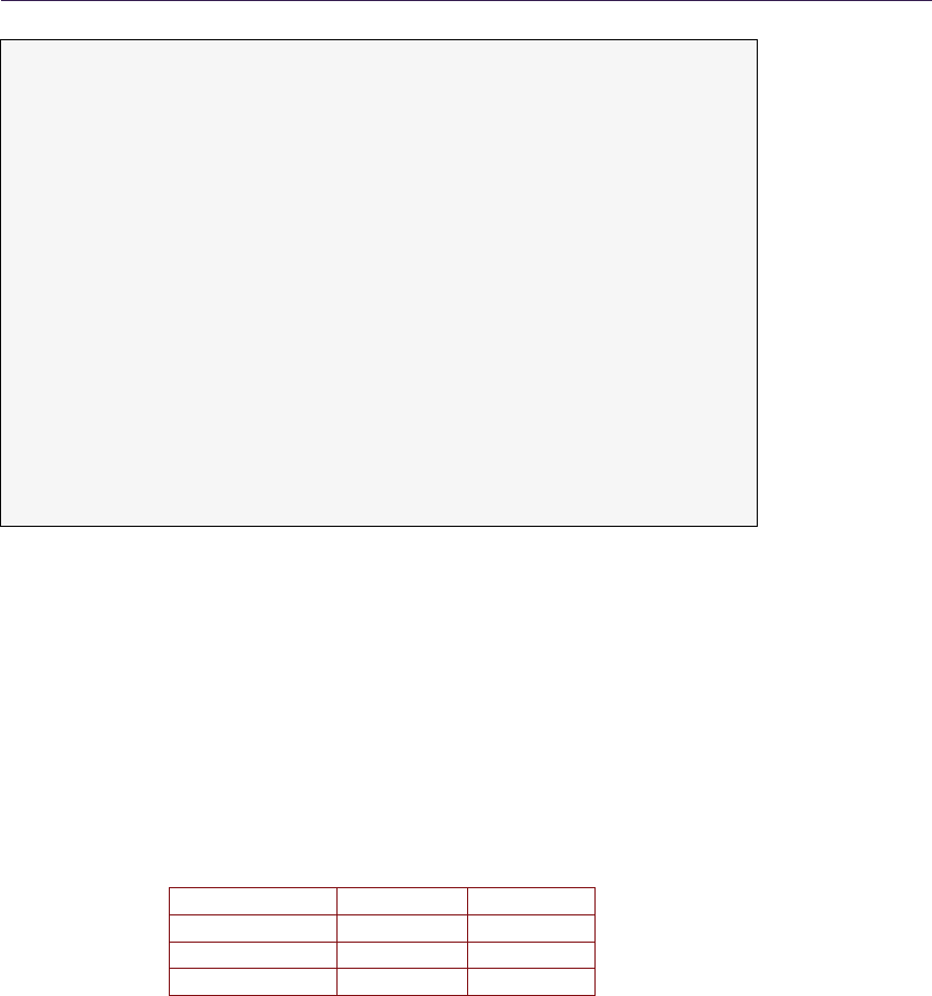
15.3. Runtime Implementation 235
float ComputeLO D ( float2 vUV , flo at nMi pL ev el s )
{
float2 vDx = dd x ( vUV ) ;
float2 vDy = dd y ( vUV ) ;
// Comp ut e du and dv ma gn it ud e a cross quad
float2 vD Coo rds ;
vDC oo rd s = v Dx * vDx ;
vD Co or ds += vDy * vDy ;
// St an da rd mip mapp in g uses max h ere
float fMa xTex Coo rd Delt a = max ( vD Coo rds . x, vD Coo rds . y) ;
float fMipLevelPower;
if( fM axTe xCoord Delt a == 0)
fMi pLe ve lP owe r = nM ip Le ve ls -1;
else
{
// 0.5 is for the s qu are root
fM ipLe ve lPo wer = 0.5 * lo g2 (1.0 / f Ma xTex Co ordD elt a );
}
float m i pL e ve l = cl am p ( f M ip Le ve lP ow er , 0 , n M i pL ev e ls -1) ;
return nM ipLe vel s - 1 - mi pLe vel ;
}
Listing 15.1. Texture LOD Selection. Allowing for nonsquare textures simply requires
a scale by aspect ratio on one of the directions.
width including borders is w, then the number of faces in a row is n=⌊W/w⌋.
Using ias the index within the block, we can compute the row as ⌊i/n⌋and the
column as i%n.
Each face has its own implicit UV parametrization. We adopt a convention
with respect to the order of the vertices in the quad. For example, we choose
the first index to be (0,0), the next is (1,0) and the last as (0,1). These can be
assigned in the hull-shader stage. The pixel shader will receive the interpolated
coordinate, which we call the “face UV.” We also need the primitive ID, which is
also defined in the hull-shader stage.
Max Resolution Face Count Prefix Sum
16 ×16 5 5
32 ×32 5 10
64 ×64 3 13
Table 15.1. If faces are sorted by resolution, and you have the prefix sum of face count
for each resolution bin, you can look up the resolution for any given face from the index
in the sorting. In this example, a face of index 7 would have a maximum resolution of
32 ×32 because it is greater than 5 and less than 10. If we want the index of that face
within that bin, it is 7 −5 = 2.

236 15. Real-Time Ptex and Vector Displacement
float2 Co mpu teU V (
uin t faceID , // From SV_PrimitiveID
float2 faceUV , // P os it ion with in the fac e
uin t nLog2 , // Log2 of the r es ol ut ion we want
int texWidth , // A tlas t exture w idth
int resOffset , // P refix sum for this resolut io n
int rowOffset , // S tar t of resolut io n bloc k in atlas
int b or de rS iz e ) // Texel t hi ck ne ss of bor der on each face
{
// Her e we assu me a s quare a spe ct ra tio .
// A non - s quare asp ec t wou ld simply s cale the he ight
// re lat ive to wi dth a ccording ly .
float f aceW idt h = 1 << n Log2 ;
float f ace Height = faceWidth ;
float b orde redF ace Wi dth = fa ceW idt h + 2* bo rde rSize ;
float b ord er edF ac eHe ig ht = bo rd ere dF aceWi dt h ;
int n Fa ce sE ac hR ow = ( i nt ) t exW id th / ( i nt )borderedFaceWidth;
int i Face Wit hi nBl oc k = fac eID - resOffset ;
float2 fa ce Or igin = float2(
( i Fac eW ithin Bl ock % n Fa ce sEach Ro w ) * borderedFaceWidth ,
( i Fac eW ithin Bl ock / n Fa ce sEach Ro w ) * bo rd ere dF ace He igh t
+ ro wO ff se t );
// Take face UV into a cc ount .
// Still in t exel units , but general ly not
// an int ege r value for bilinear fi lte rin g pu rpo ses .
float2 uv = float2( fa ceWi dth , fa ceH ei ght ) * fa ceU V ;
uv += float2( nB ord erS ize , nB ord er Siz e );
uv += faceOrig in ;
// Fin al ly scal e by t ex tu re widt h and heigh t to get
// value in [0 ,1].
return float2( uv ) / float2( tex Widt h , tex He ig ht ) ;
}
Listing 15.2. Go from face UV to atlas UV.
Scale and offsets are applied to get the face UV range of [0,1] mapped into
the atlas UV, including an offset to get to the right resolution block and another
to put the face texture origin (0,0) inside the face border. Listing 15.2 details the
process of computing a UV within the packed Ptex atlas.
The last steps are to do the bilinear filtered lookup for each LOD we need,
and the final trilinear lerp between them.
15.3.3 Resolution Discrepancies
There are discrepancies in resolution that translate to discontinuities when ap-
proaching a polygon edge from either side. This is illustrated in Figure 15.3.
This can happen when the gradient used for mip selection changes as the edge of
a polygon is crossed. However, this is not particular to packed Ptex and is fur-

15.4. Adding Displacement 237
Figure 15.3. (a) Resolution discrepency (b) Bilinear lookup into border from view of left
face. (c) Bilinear lookup into border from view of right face. (d) Changing the border
on the left face to resolve resolution discrepancy by downsampling. (e) The solution for
displacement when values must match exactly is to replicate at the lower resolution.
ther mitigated by the final lerp of trilinear filtering. In cases when we have used
packed Ptex with trilinear filtering we have not seen any problems yet; therefore
we have not pursued more sophisticated solutions.
The second cause for resolution discrepancy is capping to different resolu-
tions due to different maximum (mip level 0) resolutions. The problem of max
resolution discrepancy is mitigated by effectively clamping borders to the lower
resolution when padding (Figure 15.3).
15.4 Adding Displacement
Displacement mapping adds geometric detail to a coarser mesh. Each polygon of
the coarse mesh is tessellated further at runtime, and the vertices are displaced
according to values stored in a displacement texture map. Displacement mapping
provides a method of geometric LOD. The model can be rendered without the
displacement for the lowest poly model, and different tessellations can be applied
for higher quality models.
In classical displacement mapping, there is just a single scalar per texel. How-
ever, we have pursued vector displacement, which uses a 3D vector to specify
displacement. This technique is much more expressive, but at greater memory
cost on a per texel basis.
Authoring displacement maps in a conventional texture atlas without cracks
can be quite diffcult. If a shirt, for example, is unwrapped onto a texture, the
edges where the charts meet on the model must match in value at every location.
This is why games typically only apply displacement maps to flat objects like
terrain, and why even Pixar’s RenderMan, which is considered well engineered
for displacement mapping, still performs a messy procedural crack-fill step during
rendering [Apodaca and Gritz 99]. By contrast, you can export Ptex vector
displacement maps from Autodesk Mudbox, and apply them without the need
for manual fixup or runtime crack patching.

238 15. Real-Time Ptex and Vector Displacement
For displacement maps, we treat the borders and corners a little differently
than described in Section 15.2.1. First of all, we do not need an extra border for
filtering, as we use point sampling. However, adjacent faces must have identical
values along their shared border to avoid cracks when using hardware tessellation.
So instead of copying in a border from an adjacent face, we change the original
borders by averaging them as shown in Figure 15.3.
Corners of a face texture correspond to a vertex in the model. Similar to
how we handle borders, we walk the mesh around the vertex, gathering all corner
values and average them. This value is then written back to all corners that share
this vertex so that they are consistent and do not produce cracks. Note that it’s
necessary that this value is exactly the same. If you recompute this average
for each quad, remember you are using floating-point math, and therefore must
accumulate in the same order for each quad.
Displacement mapping is done in object space in the domain shader. In our
implementation, we point sample from the highest resolution displacement map
regardless of tessellation level. Becauseweare not filtering, the filter-related issues
of packed Ptex are not relevant, and there is both less compute and bandwidth
cost than for the typical texture map application in a pixel shader.
15.5 Performance Costs
To give a general idea of the cost difference between packed Ptex and conventional
texturing, we measured the difference between a packed-Ptex and a conventionally
textured version of the character shown in Figure 15.4(a). The AO, specular,
albedo, normal and displacement maps are packed Ptex. GPU render time is 3.6
ms on an AMD Radeon HD 7970. If we change the AO, specular, albedo and
normal maps to conventional texture lookups (all but displacement) we find the
time goes down by an average of 0.6 ms.
The main cost is the search for maximum resolution in this implementation,
for which there are plenty of opportunities for optimization we have not yet ex-
plored. We could, for example, move the computation as far up as the hull
constant shader. There is also a cost due to reduced texture cache efficiency, as
packed Ptex will generally not have as good locality of reference relative to con-
ventional texturing. The entire UV computation was repeated for each texture,
which should also not generally be necessary in practice.
Given the difficulty in authoring a valid displacement map for a model like
the character in Figure 15.4(a) we measured packed Ptex displacement map-
ping against no displacement mapping at all. This model is made from 5,504
quads and tessellated up to 99,072 triangles. The cost of vector displacement
with packed Ptex on this model is 0.14 ms. This is with 16-bit floats for each
component, which is on the high end of what should normally be necessary in
practice.
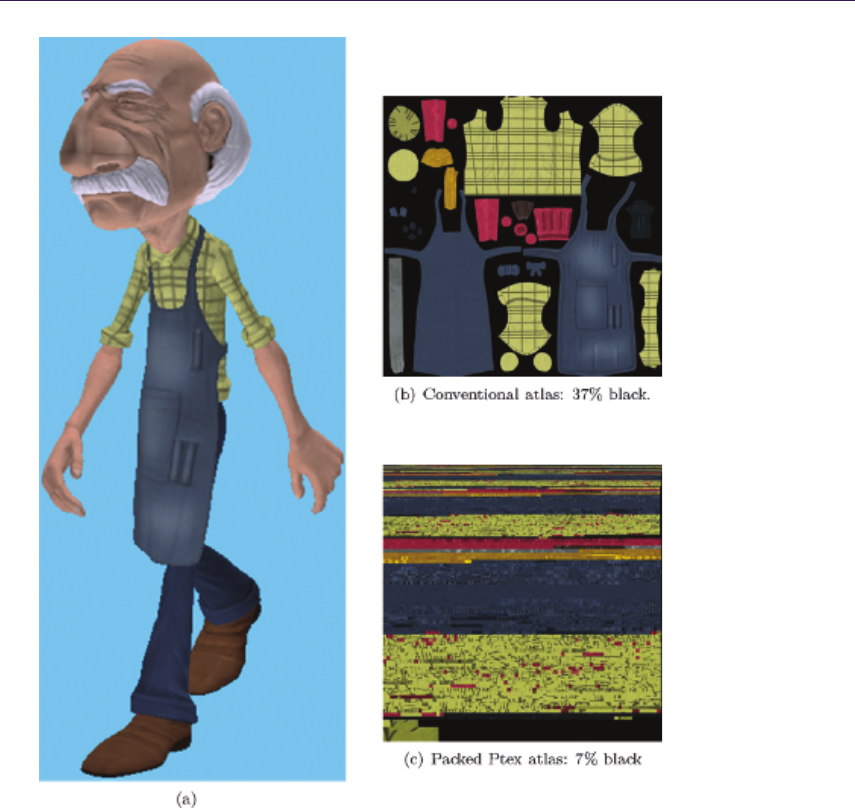
15.5. Performance Costs 239
Figure 15.4. All textures for the model in (a) are in the packed Ptex format: Albedo,
AO, specular, normal, and vector displacement: (b) an example of a conventional texture
map and (c) an equivalent packed Ptex texture map.
We have a second model, shown in Figure 15.5, that uses packed Ptex only
for vector displacement. It has a total of 86,954 quads in the base mesh and
is animated with both skinning and blend shapes. When tessellated up to 1.6
million triangles, the cost of displacement lookup is 2.7 ms out of a total of 14.2 ms
with our current implementation.
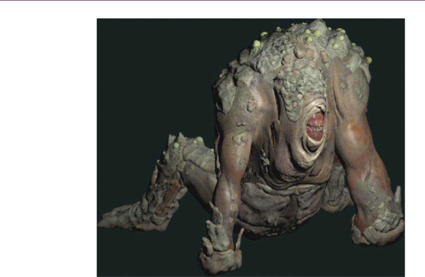
240 15. Real-Time Ptex and Vector Displacement
Figure 15.5. Model with vector displacement.
15.6 Memory Costs
Conventional texture atlases are often difficult to author without wasting texture
space between the charts. In Figure 15.4(b) we see a typical example where 37%
of the space is wasted. Ptex, by contrast, is built completely from rectangular
pieces and is therefore much easier to pack into a rectangular domain. We make
no special effort to find the optimal resolution to pack the face textures into, and
yet the waste in our experience has been only around 7% (Figure 15.4(c)).
The greater memory overhead for packed Ptex is in the use of borders. Funda-
mentally, the border cost goes up proportional to the square root of the area. Here
we give some formulas and concrete numbers to give an idea of what the overhead
is. Each face of square resolution rand border size nBwastes (2nB+r)2−r2
texels. Table 15.2 shows example costs as a percentage of waste due to borders
in packed Ptex. Two items are worth mentioning here. First, we can see more
concretely how high the per-face resolution should be to keep memory overhead
down. Second, we also see why borders beyond a couple texels, as would be
required for anisotropic filtering, is too expensive in memory cost.

15.7. Alternatives and Future Work 241
Border Size
Resolution 1 2 4
4×4 56/56% 75/75% 89/89%
8×8 36/41% 56/62% 75/80%
16 ×16 21/24% 36/41% 56/62%
32 ×32 11/13% 21/23% 36/40%
64 ×64 6.0/6.4% 11/12% 21/23%
128 ×128 3.1/3.2% 6.0/6.2% 11/12%
Table 15.2. This table shows memory overhead for borders. The first percentage in
each pair is for a single resolution, and the second is for mip chains down to 4 ×4.
These values should be weighed against the waste inherent in a conventional texture
atlas, such as the 37% illustrated in Figure 15.4(b).
15.7 Alternatives and Future Work
One way to avoid having a separate texture per face is to put each per-face texture
in its own texture array slice [McDonald and Burley 11, McDonald 12]. This
simplifies the texture addressing to some extent. However, there are limitations
in the number of texture array slices, and resolutions cannot be mixed within a
single texture array. Therefore, what would be a single texture in the conventional
or packed Ptex approach would be split into multiple textures, one for each
resolution, with further splitting as required for texture array limits. The amount
of texture data used in the shader does not increase, excepting perhaps due to
alignment or other per-texture costs, but the amount of conditional reads is
significantly higher.
Rather than computing per-face texture information, we could store it in a
resource indexed by face ID, and possibly by mip level [McDonald and Burley 11,
McDonald 12].
Ptex takes the extreme approach of assigning an individual texture map to
each primitive. The paper by B. Purnomo, et al. describes similar solutions
to what is described here, but they group multiple primitives into rectangular
patches in texture space for packing and handling seams [Purnomo et al. 04].
This reduces the overhead for borders, which would make larger filter kernels
feasible. A next step might be to integrate some of the ideas from that paper.
15.8 Conclusion
Packed Ptex enables the main advantages of the original Ptex method while en-
abling real-time use. Authoring effort is saved first by eliminating the need for
explicit UV assignment and second by naturally avoiding seaming issues that nor-
mally arise when trying to unwrap a 3D surface into at 2D rectangular domain.
It does, however, require modeling with quads in its current implementation.

242 15. Real-Time Ptex and Vector Displacement
Packed Ptex also incurs higher runtime cost than conventional texture mapping.
Memory costs can actually be lower relative to conventional texturing, depending
primarily on the per-face texture resolution, filter kernel width, and the savings
relative to the waste inherent with conventional texture atlases. Although packed
Ptex can be applied to many different texture types, the most promising is prob-
ably displacement mapping, where the relative overhead is lower and the benefit
of seamlessness is greatest.
15.9 Acknowledgments
The techniques described here were developed in collaboration with Sujeong Kim
and Justin Hensley. Tim Heath, Abe Wiley, Exigent and Zoic helped on the art
side. This work was done under the management and support of Jason Yang and
David Hoff. Sujeong Kim, Takahiro Harada and Christopher Oat all provided
valuable feedback in writing this article.
Bibliography
[Apodaca and Gritz 99] Anthony A. Apodaca and Larry Gritz. Advanced Ren-
derMan: Creating CGI for Motion Picture, First edition. San Francisco:
Morgan Kaufmann Publishers Inc., 1999.
[Burley and Lacewell 08] Brent Burley and Dylan Lacewell. “Ptex: Per-Face
Texture Mapping for Production Rendering.” In Proceedings of the Nine-
teenth Eurographics conference on Rendering, pp. 1155–1164. Aire-la-Ville,
Switzerland: Eurographics Association, 2008.
[McDonald 12] John McDonald. “Practical Ptex for Games.” Game Developer
Magazine 19:1 (2012), 39–44.
[McDonald and Burley 11] John McDonald, Jr and Brent Burley. “Per-face Tex-
ture Mapping for Real-Time Rendering.” In ACM SIGGRAPH 2011 Talks,
article no. 10. New York: ACM, 2011.
[Purnomo et al. 04] Budirijanto Purnomo, Jonathan D. Cohen, and Subodh Ku-
mar. “Seamless Texture Atlases.” In Proceedings of the 2004 Eurographic-
s/ACM SIGGRAPH Symposium on Geometry Processing, pp. 65–74. New
York: ACM, 2004.

16
Decoupled Deferred Shading
on the GPU
G´
abor Liktor and Carsten Dachsbacher
Deferred shading provides an efficient solution to reduce the complexity of image
synthesis by separating the shading process itself from the visibility computa-
tions. This technique is widely used in real-time rendering pipelines to evaluate
complex lighting, and recently gained increasing focus of research with the advent
of computational rendering.
The core idea of the technique is to presample visible surfaces into a G-buffer
prior to shading. However, antialiasing is complicated with deferred shading,
as supersampling the G-buffer leads to tremendous growth in memory band-
width and shading cost. There are several post-processing methods that are
mostly based on smoothing discontinuities in the G-buffer [Reshetov 09,Chajdas
et al. 11], but these result in inferior antialiasing quality compared to forward
rendering with multisample antialiasing (MSAA) or do not address the problem
of memory requirements.
16.1 Introduction
In this article we discuss decoupled deferred shading, a technique that uses a
novel G-buffer structure to reduce the number of shading computations while
keeping the antialiasing quality high. Our edge antialiasing is an exact match
of hardware MSAA, while shading is evaluated at a per-pixel (or application-
controlled) frequency, as shown in Figure 16.1.
Our G-buffer implementation stores visibility samples and shading samples
in independent memory locations, where a visibility sample corresponds to a
subsample tested by the rasterizer, while shading samples contain surface infor-
mation, which has been previously stored on a subsample level. Using decoupled
sampling, several visibility samples can refer to a single shading sample. We do
not seek to skip the shading of G-buffer samples in order to reduce shading costs,
243
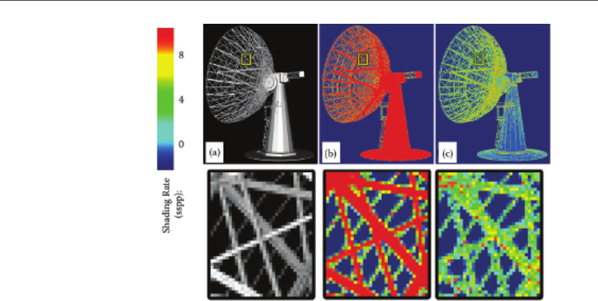
244 16. Decoupled Deferred Shading on the GPU
Figure 16.1. In this example our deferred shading method (a) achieves equivalent
antialiasing quality to 8×MSAA, but (c) significantly reduces the number of shader
evaluations. (b) To the same antialiasing quality, classic deferred shading needs a super-
sampled G-buffer.
instead we deduplicate the data itself, ensuring that a visible surface is shaded
only once, regardless of the number of subsamples it covers.
This article is based on our recent research paper, presented at the 2012 ACM
Symposium on Interactive 3D Graphics and Games [Liktor and Dachsbacher 12].
We cover the basic theory of decoupled sampling, and then focus on the imple-
mentation details of our new G-buffer in the OpenGL pipeline.
16.2 Decoupled Sampling in a Rasterization Pipeline
16.2.1 The Nature of Aliasing
To understand the motivation of decoupled sampling, let us consider the ren-
dering of a 2D image as a signal-processing problem. Rasterization uses point
sampling to capture visible surfaces that causes problems if the sampled signal is
not band-limited: frequencies higher than the sampling frequency lead to aliasing
in the rendered image. Antialiasing methods can prefilter the signal to eliminate
frequencies above the sampling limit, increase the frequency of sampling, or al-
ternatively apply reconstruction filters to supress aliasing artifacts.
Any rendering method using point sampling must first solve the visibility
problem to find the surface points that determine the colors at each sample.

16.2. Decoupled Sampling in a Rasterization Pipeline 245
Discontinuities, such as surface silhouettes, are the primary sources of aliasing.
The second type of aliasing is the possible undersampling of surface shading. Un-
like visibility, shading is often treated as a continuous signal on a given surface,
thus it can be prefiltered (e.g., by using texture mipmaps). It is therefore a tempt-
ing idea to save computations by sampling visibility and shading information at
different granularities.
16.2.2 Decoupled Sampling
In a modern rasterization pipeline this problem is addressed by MSAA. The ras-
terizer invokes a single fragment shader for each covered pixel; however, there are
multiple subsample locations per pixel, which are tested for primitive coverage.
Shading results are then copied into covered locations. This is an elegant solution
for supersampling visibility without increasing the shading cost.
Decoupled sampling [Ragan-Kelley et al. 11] is a generalization of this idea.
Shading and visibility are sampled in separate domains. In rasterization, the
visibility domain is equivalent to subsamples used for coverage testing, while
the shading domain can be any parameterization over the sampled primitive
itself, such as screen-space coordinates, 2D patch-parameters, or even texture
coordinates. A decoupling map assigns each visibility sample to a coordinate in
the shading domain. If this mapping is a many-to-one projection, the shading
can be reused over visibility samples.
Case study: stochastic rasterization. Using stochastic sampling, rasterization can
be extended to accurately render effects such as depth of field and motion blur.
Each coverage sample is augmented with temporal and lens parameters. Defo-
cused or motion blurred triangles are bounded in screen space according to their
maximum circle of confusion and motion vectors. A deeper introduction of this
method is outside the scope of this article, but we would like to refer the in-
terested reader to [McGuire et al. 10] for implementation details. In short, the
geometry shader is used to determine the potentially covered screen region, the
fragment shader then generates a ray corresponding to each stochastic sample,
and intersects the triangle.
We now illustrate decoupled sampling using the example of motion blur: if
the camera samples over a finite shutter interval, a moving surface is visible
at several different locations on the screen. A na¨ıve rendering algorithm would
first determine the barycentics of each stochastic sample covered by a triangle,
and evaluate the shading accordingly. In many cases, we can assume that the
observed color of a surface does not change significantly over time (even offline
renderers often do this). MSAA or post-processing methods cannot solve this
issue, as corresponding coverage samples might be scattered over several pixels
of the noisy image. We can, however, rasterize a sharp image of the triangle at
a fixed shading time, and we can find corresponding shading for each visibility
sample by projecting them into the pixels of this image.

246 16. Decoupled Deferred Shading on the GPU
Figure 16.2. The idea of the memoization cache. Decoupled sampling uses visibility and
shading samples in separate domains. Assuming constant shading over a short exposure
time, multiple visibility samples can refer to the identical shading sample. Recently
computed shading samples are cached during rasterization, to avoid redundant shader
execution.
Memoization cache. This concept is illustrated in Figure 16.2. Note that the
second rasterization step mentioned above does not actually happen, it is only
used to define a shading grid on the triangle, a discretization of the shading
domain. A shading sample corresponds to one cell of the shading grid, and we
can then assign a linear index to each shading sample. Using this indexing,
Ragan-Kelley et al. augmented the conventional rasterization pipeline with a
memoization cache [Ragan-Kelley et al. 11]. In their extended pipeline, each
visibility sample requests its shading sample from the cache using the decoupling
map, and fragment shaders are only executed on a cache miss. Unfortunately,
this method is not directly applicable to the current hardware architecture.
16.3 Shading Reuse for Deferred Shading
Conventional deferred shading methods couple visibility and surface data in the
G-buffer. After the geometry sampling pass it is no longer trivial to determine
which samples in the G-buffer belong to the same surface. Stochastic rasterization
further increases the complexity of the problem by adding significant noise to
visibility samples, preventing the use of any edge-based reconstruction.
The memory footprint is one of the most severe problems of deferred shad-
ing. As all shading data must be stored for each subsample in the G-buffer,
even if one could save computation by reusing shading among these samples, the
supersampling quality would still be bounded by memory limitations. Current
real-time applications typically limit their deferred multisampling resolution to
2×/4×MSAA, then apply reconstruction filters. It has been demonstrated that
accurate rendering of motion blur or depth of field would require an order of
magnitude larger sample count with stochastic sampling [McGuire et al. 10].
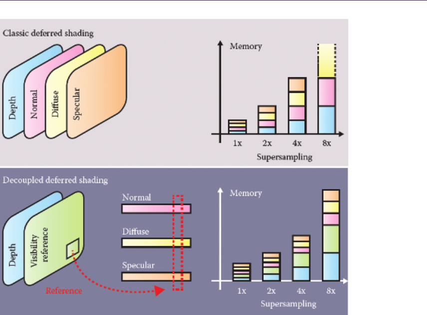
16.3. Shading Reuse for Deferred Shading 247
Figure 16.3. The G-buffer stores shading data at full supersampled resolution before
shading and resolving. We introduce a visibility buffer that references shading data in
compact linear buffers. Due to our shading reuse scheme, the size of the compact buffers
does not scale with the supersampling density.
Compact geometry buffer. Instead of trying to use reconstruction filters or sparse
shading of the supersampled G-buffer, we can avoid any shading and memory
consumption overhead by not storing redundant shading data in the first place.
We address this problem with a novel data structure, the compact G-buffer, a
decoupled storage for deferred shading. It has the same functionality as the G-
buffer, storing the inputs of shaders for delayed evaluation. However, instead of
storing this information in the framebuffer, we collect shading samples in compact
linear buffers. The contents of the framebuffer are purely visibility samples, each
sample storing its depth value and a reference to a shading sample in the linear
buffers. We compare this data layout to the conventional G-buffer in Figure 16.3.
Akin to classic deferred shading, our methods can render images in three main
stages.
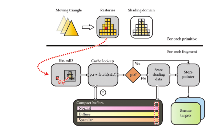
248 16. Decoupled Deferred Shading on the GPU
Figure 16.4. The outline of decoupled deferred shading in a rasterization pipeline.
Prior to rasterization, each primitive is bound and projected to a shading grid. During
fragment processing, the fragments are mapped to their corresponding cells on the
shading grid. Shading reuse is implemented by referencing the same data from multiple
samples in the render targets.
16.3.1 Algorithm Outline
Sampling stage. We rasterize all surfaces into the compact geometry buffer (CG-
buffer). Figure 16.4 shows the outline of this sampling stage. During rasterization
each fragment is assigned to a shading sample ID (ssID), which is searched in the
cache. If the shading data was found, we only store a pointer to its address in
the memory. In case of a miss, we also need to allocate a new slot in the compact
buffers and store the data in addition to referencing it.
In Section 16.2.2 we have already introduced the concept of a shading grid. In
our pipeline, we use this grid to allocate an ssID range for each primitive. This
virtual address space ensures that shading sample keys of concurrently raster-
ized primitives do not overlap, and the sampler can use these ssIDs to uniquely
reference a cached shading sample entry.
We provide further implementation details in the next section. In fact, we
only made a small modification in the decoupled sampling pipeline. While the

16.4. Implementation 249
CG-buffer itself could be directly used as a global memoization cache, it would
be very inefficient to search for shading samples directly in it, especially that a
cached entry is only relevant for the currently rasterized primitives in flight.
Shading and resolving stages. The collected samples in the compact buffers are
then shaded using GPU compute kernels. These kernels only execute for shading
samples that are marked visible (see the next section). Finally each visibility
sample can gather its final color value in a full-screen pass. This method trivially
extends to an arbitrary number of render targets, supporting efficient shading
reuse for multiview rasterization as well.
16.4 Implementation
In this section we focus on how to implement decoupled deferred shading on a
modern GPU. In our examples we provide OpenGL Shading Language (GLSL)
source code snippets. We use global atomics and scatter operations, therefore
a minimum version of OpenGL 4.2 is required for our application. The imple-
mentation could also be done in DirectX 11.1, which supports unordered access
binding to all shader stages.
The primary problem for our example is the lack of hardware support for
decoupled shading reuse, which is an architectural limitation. The hardware
version of the memoization cache, as described in Section 16.2.2, is a fast on-chip
least recently used (LRU) cache assigned to each rasterizer unit. Of course, every
component of the pipeline (ultimately even rasterization) can be implemented in
software, but only with reduced performance compared to dedicated hardware.
From now on we assume that our renderer still uses the hardware rasterizer,
though this technique could be also integrated into a full software implementation,
such as [Laine and Karras 11].
16.4.1 Architectural Considerations
Note that the implementation of decoupled sampling for a forward renderer would
be very inefficient on current GPUs. First, using hardware rasterization, we can
only simulate the caching behavior from fragment shaders. Unfortunately we
cannot prevent the execution of redundant shaders, like the proposed architecture
of [Ragan-Kelley et al. 11] does. The rasterizer will launch fragment shaders for
each covered pixel or subsample and we can only terminate redundant instances
afterwards. This introduces at least one new code path into the shading code,
breaking its coherency.
The second problem is how to avoid redundant shading. Shading reuse can
be regarded as an election problem: shader instances corresponding to the same
shading sample must elect one instance that will evaluate the shading, the others
need to wait for the result. This can only be solved using global synchronization,

250 16. Decoupled Deferred Shading on the GPU
as current hardware does not allow local on-chip memory usage in rasterization
mode, and the execution of fragment shaders is nondeterministic. Furthermore,
waiting for the result would mean a significant delay for a complex shader.
With our modification we can move the shader evaluation into a deferred
stage, which results in a more coherent fragment shader execution. While we
cannot avoid using the global memory to simulate the memoization cache, the
overhead of decoupled sampling is independent from the shading complexity. This
is the key difference that makes our algorithm feasible even for current GPUs:
if the shading computation is “expensive enough,” the constant overhead of our
caching implementation will be less than the performance gain of reduced shading.
Furthermore, we can utilize our CG-buffer to keep the memory footprint of the
shading data minimal.
16.4.2 Decoupling Shading Samples
We now discuss a method that implements the sampling stage of decoupled de-
ferred shading in a single rasterization pass. The first problem we need to solve
is how to assign shading samples to fragments. Prior to rasterization, each prim-
itive needs to be processed to determine its shading domain (see Section 16.3.1
in vec2 in _s cr Po s []; // screen - s pace po sition s
fla t o ut ive c4 do mai n ; // s ha di ng g rid of the t ri an gl e
fla t out uint s ta rt ID ; // ID of the first sa mple in the sh . grid
uniform float s had ingRat e ;
// gl obal SSID c ou nt er array
la yout ( siz e1x 32 ) uni for m ui mage Buf fer uCtr SSI D ;
voi d ma in ( ) {
// projec t screen po si ti on to the shading grid
vec 2 gri dPo s0 = scrP os [0] * sh adi ngRate ; [.. .]
vec 2 minCorner = min ( gridPos0 , min (gridPos1 , gridPos2 ));
vec 2 maxCorner = max ( gridPos0 , max (gridPos1 , gridPos2 ));
// sh ading gri d : xy - top left corner , zw - grid s ize
domain .x = int ( minCorner . x) - 1;
domain .y = int ( minCorner . y) - 1;
domain .z = int (( maxCorne r . x)) - d omain .x + 1;
domain .w = int (( maxCorne r . y)) - d omain .y + 1;
// we all oca te the ssID range wit h an atom ic coun ter .
uin t re ser ved = u int (( do main .z ) * ( d omain . w) );
st art ID = i ma ge At om icA dd ( uCt rSSI D , 0 , res er ved ) ;
}
Listing 16.1. The geometry shader generates a shading grid for each triangle, and
ensures globally unique ssIDs using an atomic counter.

16.4. Implementation 251
for details). As we only consider triangles, we can conveniently implement this
functionality in a geometry shader.
Listing 16.1 is an extract from the geometry shader code that assigns a shading
grid for each rasterized triangle. In our implementation, the geometry shader
might also set up conservative bounds for stochastically rasterized triangles.
Listing 16.2 shows the pseudocode of the fragment shader, implementing the
remainder of our pipeline. As we described before, the output of this shader
is only a pointer to the corresponding shader data. Note that due to driver
limitations on integer multisampling, we need to store the references in floating
point, using the intBitsToFloat GLSL function. The shading samples are stored
using image buffers.
We omit the details of visibility testing, which might be standard multi-
sampled rasterization, or the implementation of stochastic rasterization, which
casts randomly distributed rays inside the conservative screen space bounds of the
triangles. We only assume that the visibility method returned the barycentrics of
the intersection point. The visibility sample is then assigned to a shading sample,
using the grid provided by the geometry shader.
la you t ( loc ati on = 0 , in dex = 0) out floa t FragPtr;
// sh ader in puts : po sition , normal , texcoords
fla t in vec 3 vpos0 ...
// pa cked CG - b uffer da ta
la you t ( rg32ui ) un ifo rm u im age Bu ffe r u Colo rNor malB uf fer ;
la yout ( rgb a32 f ) unifor m ui ma geB uf fer u Vie wP osB uf fer ;
voi d ma in ( ) {
// hw - in terpo la ti on or stocha st ic ray ca sting ...
ve c3 b ar yC oo rd s = g e tV ie wS a mp le Po s () ;
// get n ea re st sh ading samp le
uin t lo cal ID = p roje ctT oG ri d ( bar yCoo rds , sh ad ing Ra te ) ;
uin t g lo ba lI D = st artID + local ID ;
boo l ne edS tore = f alse ;
int a ddr es s = ge tC ac he dAd dr es s ( glo balI D , ne edS to re ) ;
Fr agP tr = i ntB it sToF loa t ( addre ss ) ;
if ( ne edS tore ) {
// for each textur e ...
t ex t ur eG r ad s In Sh a di ng S pa c e ( l ocal ID , dx , dy ) ;
ve c4 d if fus e = t ex tu re G ra d ( t ex Dif fus e , te xCoo rd , dx , d y );
[...]
// pack color , normal , view po si ti on s in to the CG bu ff er
im ag eSt or e ( uC ol orN or mal Bu ffe r , ad dres s , . ..) ;
}
}
Listing 16.2. The fragment shader implements the decoupling map and the chaching
mechanism for shading samples.

252 16. Decoupled Deferred Shading on the GPU
uin t pr oj ec tT oGr id ( v ec3 b ary Coor ds , floa t sh ad in gRate ){
vec 3 vpos = coords .x * vpos0 + coor ds .y * vpos1 + co or ds .z * vpos2 ;
vec 2 sc re enP os = p ro jT oS cre en ( v pos );
ivec2 gr idPos = ive c2 ( sc re en Po s * sha di ng Ra te + vec2 ( 0.5 f)) - domain
. xy ;
return uin t ( domain . z * gr idP os . y + gridP os . x);
}
Listing 16.3. The decoupling map is a simple projection to a regular grid. The density
of this grid is determined by the shading rate.
The method projectToGrid assigns the fragment to a shading sample, as we
show in Listing 16.3. The local index of the shading sample is the linearized index
of the closest shading grid cell to the visibility sample. Later, when the shading
data is interpolated, some shading samples might fall outside the triangle. These
are snapped to the edges (by clamping the barycentrics to 0 or 1, respectively),
otherwise some shading values would be extrapolated.
The computation of the texture mip levels also needs special attention. Nor-
mally, this is done by the hardware, generating texture gradients of 2×2 fragment
blocks. Depending on the shading rate, the shading space gradients can be differ-
ent. For example, a shading rate of 0.5 would mean that 2 ×2 fragments might
use the same shading sample, which would be detected (incorrectly) as the most
detailed mip level by the hardware. Therefore we manually compute the mip
level, using the textureGrad function.
In Listing 16.2 we have also tried to minimize the divergence of fragment
shader threads. The method getCachedAddress returns the location of a shading
sample in the global memory. In case of a cache miss, a new slot is reserved
in the CG-buffer (see below), but the shading data is only written later, if the
needStore boolean was set.
16.4.3 Global Shading Cache
For a moment let us consider the cache as a “black box” and focus on the im-
plementation of the CG-buffer. If a shading sample is not found in the cache,
we need to append a new entry to the compact linear buffers, as shown in Fig-
ure 16.4. The CG-buffer linearly grows as more samples are being stored. We can
implement this behavior using an atomic counter that references the last shading
data element:
ad dress = int ( a tomi cCo un te rInc reme nt ( bu ffe rTa il )) ;
The streaming nature of the GPU suggests that even a simple first-in, first-out
(FIFO) cache could be quite efficient as only the recently touched shading samples

16.4. Implementation 253
are “interesting” for the fragments. We therefore did not attempt to simulate an
LRU cache, as suggested by Ragan-Kelley et al. On a current GPU there can
be several thousand fragments rasterized in parallel, thus the global cache should
also be able to hold a similar magnitude of samples to achieve a good hit rate.
In a na¨
Ive implementation, a thread could query the buffer tail, and check the
last Nitems in the CG-buffer. Of course the latency of the iterative memory
accesses would be prohibitively high. We now show a cache implementation that
performs cache lookups with only one buffer load and an atomic lock.
The concept of the shading grid already creates indices for shading samples
that are growing approximately linearly with the rasterized fragments. Thus the
FIFO cache could also be implemented by simply storing the last NssID values.
Consequently, instead of linearly searching in a global buffer, we could introduce
a bucketed hash array. The full implementation of our optimized algorithm is
shown in Listing 16.4.
The hash function (hashSSID) is a simple modulo operation with the number
of buckets. This evenly distributes queries from rasterized fragments over the
buckets, which is important to minimize cache collisions (when threads with
different ssIDs compete for the same bucket). In case of a cache miss, multiple
threads compete for storing the shading samples in the same bucket, therefore
we use a per-bucket locking mechanism (uBucketLocks). Note that we try to
minimize the number of instructions between obtaining and releasing a lock: the
computation of a shading sample does not happen inside the critical section, but
we only set the needStore flag to perform the storage later.
As the execution order of fragments is nondeterministic, there is no guarantee
that all threads obtain the lock in a given number of steps. In practice we
have very rarely experienced cases when the fragment shader execution froze for
starving fragment shaders. While we hope this will change on future architectures,
we have limited the spinlock iterations, and in case of failure the fragment shader
falls back to storing the shading sample without shading reuse. In our experiments
this only happened to a negligible fraction of fragments.
One other interesting observation was that if the number of cache buckets is
high enough, we can really severely limit the bucket size. As the reader can see in
the source code, a bucket stores only a single uvec4 element, which corresponds to
two shading samples: a cache entry is a tuple of an ssID and a memory address.
This is a very important optimization, because instead of searching inside the
cache, we can look up any shading sample with a single load operation using its
hash value.
In our first implementation, each bucket in the cache has been stored as
a linked list of shading sample addresses, similarly to the per-pixel linked list
algorithm of [Yang et al. 10]. When we have made experiments to measure the
necessary length of this list, we have found that in most cases even a single element
per bucket is sufficient, and we did not have any cache misses when we considered
only two elements per bucket. This is why we could discard the expensive linked

254 16. Decoupled Deferred Shading on the GPU
lay out ( r gba 32u i ) u nif orm ui ma geB uf fer u Shad erC ac he ;
lay out ( r 32ui ) un iform volati le ui ma geB uf fer u Buc ke tLo ck s ;
int g et Cac he dA dd re ss ( u int ssID , ino ut boo l ne ed Sto re ){
int ha sh = ha sh SSI D ( s sID );
uve c4 bu cket = im ageLoa d ( uShade rCa che , hash );
int a dd re ss = s e ar ch Bu c ke t ( ssID , bu ck et ) ;
// cache mis s
whi le ( addre ss < 0 && iAt tem pt ++ < M AX _AT TEMP TS ){
// th is thread is c om pe ti ng for s to ring a sample
uint loc k = ima ge Ato mi cCo mp Swa p ( uBu cketLoc ks , hash , FREE , LOCKE D
);
if( lo ck == FR EE ){
add ress = i nt ( at omic Cou nt er Incr emen t ( bu ffe rTa il ));
// update the cac he
bu cke t = s to re Bu ck et ( ssID , hash , bu ck et ) ;
ima geSt ore ( u Sha der Cache , hash , bu cke t );
ne ed Sto re = t rue ;
me moryB ar ri er (); // release the lo ck
im ageS tor e ( uBu cke tLo cks , hash , FR EE );
}
if ( lo ck = = L OCK ED ){
wh ile ( lo ck == LOC KED && l oc kAt te mp t ++ < M AX _LO CK _A TT EM PT S )
loc k = imageLoad (uBuck etLocks , hash ).x;
// now try to get the addr es s a gain
bu cke t = imageLoa d ( uShade rCa che , hash );
a ddr es s = s ea rc hB u ck et ( s sID , b uc ke t );
}
// if everythi ng failed , store a the da ta r ed undantl y
if ( ad dre ss < 0){
ad dress = int ( a tomi cCo un ter In cr emen t ( buf fer Tai l ));
ne ed Sto re = t rue ;
}
}
}
Listing 16.4. Implementation of the global shading cache.
list behavior and pack all buffers in a single vector. However, this optimization
only works if the hash function uniformly distributes cache requests (like ours),
and the number of buckets is high. In our examples we use a bucket count of
32,768.
16.4.4 Shading and Resolving
While the sampling stage described above successfully eliminates all duplicate
shading samples, the resulting CG-buffer might still hold redundant information.
Depending on the rasterization order of triangles, several samples in the compact

16.5. Results 255
buffers might not belong to any visible surfaces. Even filling up the z-buffer in a
depth prepass might not solve the problem: if early z-testing is disabled a z-culled
fragment can still write data into a uniform image buffer. We therefore execute
another pass that marks visible shading samples, and optionally removes invisible
data from the CG-buffer.
Visibility. Marking visible samples is surprisingly easy. After the sampling stage is
finished, we render a full-screen quad with subsample fragment shader execution,
and each fragment shader stores a visibility flag corresponding to its shading
sample. There is no synchronization needed, as each thread stores the same value.
To evaluate the quality of shading reuse, we used a variant of this technique,
which counts visibility samples per-shading sample. In the diagnostics code we
atomically increment a per-shading sample counter for each subsample in the
framebuffer. The heatmap visualizations in this article were generated using this
method.
Compaction. Because of the rasterization order, there is no explicit bound on
the size of the compact buffers. Using the visibility flags, we can perform a
stream compaction on the shading data before shading. Besides efficient memory
footprint this also increases the execution coherence during the shading process.
In this article we do not provide implementation details for shading, as it is
orthogonal to our decoupling method. The final pixel colors are evaluated by
rendering a full-screen quad and gathering all shaded colors for each visibility
sample. This is the same behavior as the resolve pass of a standard multisampled
framebuffer, except for the location of subsample colors.
16.5 Results
In this section we discuss possible application of our method in deferred rendering.
While current GPU architectures do not have hardware support for decoupled
sampling, the overhead of our global cache management can be amortized by the
reduction of shader evaluations. We focus on stochastic sampling, a rendering
problem especially challenging for deferred shading.
While the software overhead of decoupled sampling makes our method rather
interactive than real time, we demonstrate significant speedup for scenes with
complex shading. All images in this article were rendered at 1280 ×720 pixels on
an Nvidia GTX580 GPU and Intel Core i7 920 CPU.
Adaptive shading. We have computed the average shading rate of these images,
to roughly estimate the shading speedup compared to supersampled deferred
shading. We save further computation by reducing the density of the shading
grid of blurry surfaces. Our adaptive shading rate implementation is only a
proof-of-concept based entirely on empirically chosen factors. For better quality,
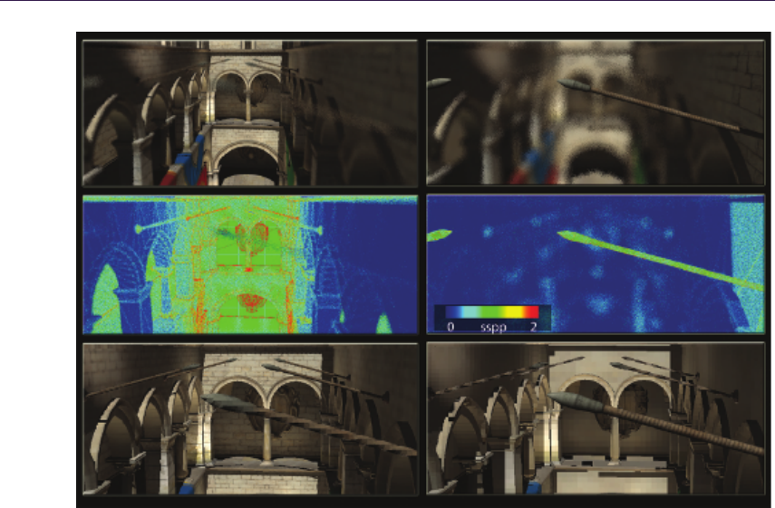
256 16. Decoupled Deferred Shading on the GPU
Figure 16.5. Focusing from the background (left column) to a foreground object (right
column), our adaptive method concentrates shading samples on sharp surfaces. The
motivation is to prefilter shading more agressively, as defocus is similar to a low-pass
filter over the image. The middle row visualizes the shading rate. In the bottom row we
show how the same surface shading would appear from a pinhole camera. The texture
filtering matches the shading resolution.
our method could be easily extended with the recent results of [Vaidyanathan et
al. 12], who presented a novel anisotropic sampling algorithm, based on image
space frequency analysis.
Depth of field. Figure 16.5 shows two renderings of the Crytek Sponza Atrium
scene from the same viewing angle, but different focusing distance. In this exam-
ple the most expensive component of rendering is the computation of the single-
bounce global illumination, using 256 virtual point lights (VPLs), generated from
a reflective shadow map (RSM) [Dachsbacher and Stamminger 05].
We do not only avoid supersampling the G-buffer, but also reduce the shading
frequency of surfaces using the minimum circle of confusion inside each primitive.
This approach prefilters shading of defocused triangles, causing slight overblurring
of textures, however, we found this effect even desirable if the number of visibility
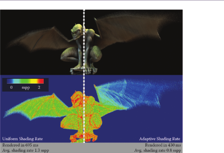
16.5. Results 257
Figure 16.6. A motion blurred character rendered with eight times stochastic supersam-
pling. Deferred shading is computed using 36 ambient occlusion samples per shading
sample. The shading rate stays close to one shading sample per pixel (sspp) despite the
supersampling density (left side). We can save further ∼30% of the rendering time by
adaptively reducing sampling of fast-moving surfaces (right side).
samples is small (it effectively reduces the apparent noise of surfaces). The images
were rendered using four times supersampling, the stochastic sampling stage took
90 ms, and the shading with 256 VPLs took 160 ms.
Motion blur. Figure 16.6 presents an animated character, rendered with motion
blur. This example features ray-traced ambient occlusion and image-based light-
ing, using the Nvidia OptiX raytracing engine. When using hardware rasteriza-
tion, high-performance ray tracing is only possible in a deferred computational
shading pass. Here we demonstrate adaptive shading again, by reducing the
shading rate of fast-moving triangles. We scale the shading grid based on the x
and ycomponent of the triangle motion vectors. Our results (and the reduction
of shading) can be significantly improved by using the anisotropic shading grid
of [Vaidyanathan et al. 12].
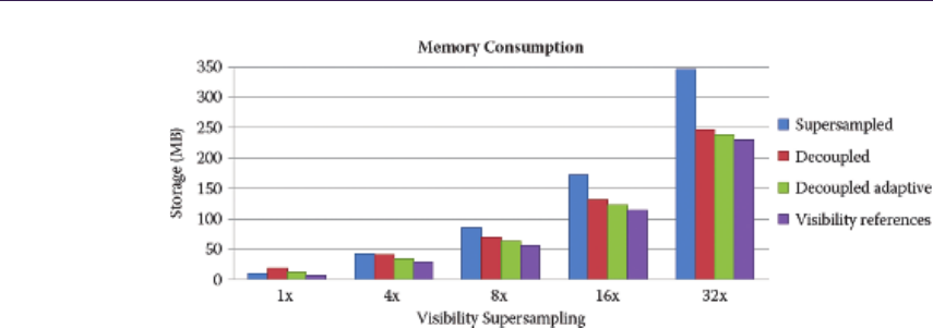
258 16. Decoupled Deferred Shading on the GPU
Figure 16.7. Storage requirements of the CG-buffer compared to a standard deferred
G-buffer. Only the size of the visibility data grows with supersampling. We rendered
the Sponza scene at 1,280 ×720 pixels.
16.5.1 Memory Consumption
We have analyzed the memory consumption of our method, compared to super-
sampled deferred shading. We save storage by essentially deduplicating shading
data in the G-buffer. However, as a shading sample might not coincide with
any visibility samples on the surface, we cannot reconstruct the surface positions
based on a subpixel depth value. While other solutions are possible, we assume
that we are forced to store the view space position of each shading sample.
We assume that the ground truth deferred method uses 12 bytes per subsample
in the G-buffer: 32 bits for depth-stencil and two RGBA8 textures for normals
and material information. In fact, most modern deferred renderers use typically
more bytes per subsample. The memory footprint of our CG-buffer can be divided
into per-visibility and per-shading sample costs. In the former we need to store
an integer pointer besides the 32-bit depth-stencil. We need 16 bytes per shading
sample: the view positions are packed into 8 bytes (16 bits for x−yand 32 bits
for z), and we store the same normal and material information.
If the shading rate is one and there is no multisampling, our method uses twice
as much memory as conventional techniques. However, the number of shading
samples does not scale with the supersampling resolution. At 4×MSAA, our
memory consumption matches the supersampled G-buffer’s, and we save signif-
icant storage above this sample count. Our measurements on the Sponza scene
are summarized in Figure 16.7.
16.5.2 Conclusion
In this chapter we presented a decoupled deferred shading method for high-quality
antialiased rendering. To our knowledge this is the first deferred shading method

16.6. Acknowledgments 259
designed for stochastic rasterization. Unfortunately on current GPUs we need
to implement stochastic rasterization and the shading cache using shaders, to
overcome the limitations of the hardware pipeline. We consider our results ben-
eficial for interactive applications, where shading cost dominates the rendering,
however, the overhead of the global cache implementation is generally too high
for real-time rendering.
We expect that the major synchronization bottleneck will disappear in future
rendering architectures. While we cannot predict whether future GPUs would
have a hardware-accelerated version of the memoization cache, some way of lo-
cal synchronization among fragement shaders would already remove most of the
overhead. Using a tile-based rendering architecture instead of sort-last-fragment
would allow us to use a more efficient, per-tile on-chip shading cache.
In our examples we have assumed that the visible color of surfaces remains
constant in a single frame, and shading can be prefiltered. This might cause ar-
tifacts on fast-moving surfaces, therefore we could extend our method to support
interpolation among temporal shading samples. In the future it will be interesting
to separate the frequency content of shading itself: a hard shadow edge in fact
cannot be prefiltered, but there are low-frequency components of shading, e.g.,
diffuse indirect illumination, where sparse shading can bring relevant speedup.
16.6 Acknowledgments
We would like to thank Anton Kaplanyan and Bal’azs T’oth for the helpful discus-
sions during the development of this project. G´abor Liktor is funded by Crytek
GmbH.
Bibliography
[Chajdas et al. 11] Matth¨aus G. Chajdas, Morgan McGuire, and David Luebke.
“Subpixel Reconstruction Antialiasing for Deferred Shading.” In Proceedings
of Symposium on Interactive 3D Graphics and Games, pp. 15–22. New York:
ACM, 2011.
[Dachsbacher and Stamminger 05] Carsten Dachsbacher and Marc Stamminger.
“Reflective Shadow Maps.” In Proceedings of the 2005 Symposium on Inter-
active 3D Graphics and Games, pp. 203–231. New York: ACM, 2005.
[Laine and Karras 11] Samuli Laine and Tero Karras. “High-Performance Soft-
ware Rasterization on GPUs.” In Proceedings of the ACM SIGGRAPH Sym-
posium on High Performance Graphics, pp. 79–88. New York: ACM, 2011.
[Liktor and Dachsbacher 12] G´abor Liktor and Carsten Dachsbacher. “Decou-
pled Deferred Shading for Hardware Rasterization.” In Proceedings of the

260 16. Decoupled Deferred Shading on the GPU
ACM Symposium on Interactive 3D Graphics and Games, pp. 143–150. New
York: ACM, 2012.
[McGuire et al. 10] M. McGuire, E. Enderton, P. Shirley, and D. Luebke. “Real-
Time Stochastic Rasterization on Conventional GPU Architectures.” In Pro-
ceedings of the Conference on High Performance Graphics, pp. 173–182. Aire-
la-Ville, Switzerland: Eurographics Association, 2010.
[Ragan-Kelley et al. 11] J. Ragan-Kelley, J. Lehtinen, J. Chen, M. Doggett, and
F. Durand. “Decoupled Sampling for Graphics Pipelines.” ACM Transactions
on Graphics 30:3 (2011), article no. 17.
[Reshetov 09] Alexander Reshetov. “Morphological Antialiasing.” In Proceedings
of the Conference on High Performance Graphics 2009, pp. 109–116. New
York: ACM, 2009.
[Vaidyanathan et al. 12] Karthik Vaidyanathan, Robert Toth, Marco Salvi,
Solomon Boulos, and Aaron E. Lefohn. “Adaptive Image Space Shading
for Motion and Defocus Blur.” In Proceedings of the Fourth ACM SIG-
GRAPH/Eurographics Conference on High Performance Graphics, pp. 13–
21. Aire-la-Ville, Switzerland: Eurographics Association, 2012.
[Yang et al. 10] Jason C. Yang, Justin Hensley, Holger Gr¨un, and Nicolas
Thibieroz. “Real-Time Concurrent Linked List Construction on the GPU.”
Computer Graphics Forum 29:4 (2010), 1297–1304.

17
Tiled Forward Shading
Markus Billeter, Ola Olsson, and Ulf Assarsson
17.1 Introduction
We will explore the tiled forward shading algorithm in this chapter. Tiled forward
shading is an extension or modification of tiled deferred shading [Balestra and
Engstad 08,Swoboda 09,Andersson 09,Lauritzen 10,Olsson and Assarsson 11],
which itself improves upon traditional deferred shading methods [Hargreaves and
Harris 04,Engel 09].
Deferred shading has two main features: decoupling of lighting and shading
from geometry management and minimization of the number of lighting computa-
tions performed [Hargreaves and Harris 04]. The former allows for more efficient
geometry submission and management [Shishkovtsov 05] and simplifies shaders
and management of shader resources. However the latter is becoming less of an
issue on modern GPUs, which allow complex flow control in shaders, and support
uniform buffers and more complex data structures in GPU memory.
Traditional forward pipelines typically render objects one by one and consider
each light for each rasterized fragment. In deferred shading, one would instead
render a representation of the geometry into a screen-sized G-buffer [Saito and
Takahashi 90], which contains shading data for each pixel, such as normal and
depth/position. Then, in a separate pass, the lighting and shading is computed
by, for example, rendering light sources one by one (where each light source is
represented by a bounding volume enclosing the light’s influence region). For
each generated fragment during this pass, data for the corresponding pixel is
fetched from the G-buffer, shading is computed, and the results are blended into
an output buffer. The number of lighting computations performed comes very
close to the optimum of one per light per visible sample (somewhat depending
on the bounding volumes used to represent light sources).
Deferred shading thereby succeeds in reducing the amount of computations
needed for lighting, but at the cost of increased memory requirements (the G-
buffer is much larger than a color buffer) and much higher memory bandwidth
usage. Tiled deferred shading fixes the latter (Section 17.2), but still requires
large G-buffers.
261
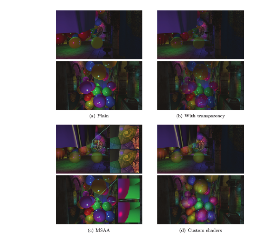
262 17. Tiled Forward Shading
Figure 17.1. We explore tiled forward shading in this article. (a) While tiled deferred
shading outperforms tiled forward shading in the plain (no transparency, no multisample
antialiasing (MSAA)) case by approximately 25%, (b) tiled forward shading enables use
of transparency. Additionally, (c) we can use hardware supported MSAA, which, when
emulated in deferred shading requires large amounts of memory. Furthermore, at 4×
MSAA, tiled forward shading outperforms deferred with equal quality by 1.5 to 2 times.
The image shows 8×MSAA, which we were unable to emulate for deferred rendering
due to memory constraints. (d) Finally, we discuss custom shaders. As with standard
forward rendering, shaders can be attached to geometry chunks. The scene contains
1,024 randomly placed lights, and the demo is run on an NVIDIA GTX480 GPU.

17.2. Recap: Forward, Deferred, and Tiled Shading 263
Tiled forward shading attempts to combine one of the main advantages of
(tiled) deferred rendering, i.e., the reduced amount of lighting computations done,
with the advantages of forward rendering. Besides reduced memory requirements
(forward rendering does not need a large G-buffer), it also enables transparency
[Kircher and Lawrance 09,Enderton et al. 10] (Section 17.5), enables multisam-
pling schemes [Swoboda 09,Lauritzen 10] (Section 17.6), and does not force the
use of ¨ubershaders if different shading models must be supported (Section 17.7).
See the images in Figure 17.1 for a demonstration of these different aspects.
17.2 Recap: Forward, Deferred, and Tiled Shading
The terms forward,deferred, and tiled shading will be appearing quite frequently
in this chapter. Therefore, let us define what we mean, since usage of these terms
sometimes varies slightly in the community. The definitions we show here are
identical to the ones used by [Olsson and Assarsson 11].
With forward shading, we refer to the process of rendering where lighting
and shading computations are performed in the same pass as the geometry is
rasterized. This corresponds to the standard setup consisting of a vertex shader
that transforms geometry and a fragment shader that computes a resulting color
for each rasterized fragment.
Deferred shading splits this process into two passes. First, geometry is ras-
terized, but, in contrast to forward shading, geometry attributes are output into
a set of geometry buffers (G-buffers). After all geometry has been processed this
way, an additional pass that computes the lighting or full shading is performed
using the data stored in the G-buffers.
In its very simplest form, the second pass (the lighting pass) may look some-
thing like following:
for each G-buffer sample {
sa mp le_attr = load att ri bu te s from G - b uf fer
for each ligh t {
co lor += sh ade ( sa mpl e_a ttr , lig ht )
}
ou tpu t pix el co lor ;
}
Sometimes, the order of the loops is reversed. The deferred algorithm de-
scribed in Section 17.1 is an example of this.
The light pass shown above requires O(Nlights ·Nsamples) lighting computa-
tions. If we somehow know which lights were affecting what samples, we could
reduce this number significantly [Trebilco 09].

264 17. Tiled Forward Shading
Tiled deferred shading does this by dividing samples into tiles of N×Nsam-
ples. (We have had particularly good successes with N= 32, but this should
be somewhat hardware and application dependent.) Lights are then assigned to
these tiles. We may optionally compute the minimum and maximum Z-bounds
of each tile, which allows us to further reduce the number of lights affecting each
tile (more discussion on this in Section 17.4).
Benefits of tiled deferred shading [Olsson and Assarsson 11] are the following:
•The G-buffers are read only once for each lit sample.
•The framebuffer is written to once.
•Common terms of the rendering equation can be factored out and computed
once instead of recomputing them for each light.
•The work becomes coherent within each tile; i.e., each sample in a tile
requires the same amount of work (iterates over the same lights), which
allows for efficient implementation on SIMD-like architectures (unless, of
course, the shader code contains many branches).
For tiled deferred shading (and most deferred techniques) to be worthwhile, most
lights must have a limited range. If all lights potentially affect all of the scene,
there is obviously no benefit to the tiling (Figure 17.2(a)).
Tiled deferred shading can be generalized into Tiled Shading, which includes
both the deferred and forward variants. The basic tiled shading algorithm looks
like the following:
1. Subdivide screen into tiles.
2. Optional: find minimum and maximum Z-bounds for each tile.
3. Assign lights to each tile.
4. For each sample: process all lights affecting the current sample’s tile.
Step 1 is basically free; if we use regular N×Ntiles, the subdivision is implicit.
Finding minimum and maximum Z-bounds for each tile is optional (Step 2).
For instance, a top-down view on a scene with low depth complexity may not
allow for additional culling of lights in the Z-direction. Other cases, however, can
benefit from tighter tile Z-bounds, since fewer lights are found to influence that
tile (Figure 17.2(b)).
In tiled deferred shading, the samples in Step 4 are fetched from the G-buffers.
In tiled forward shading, the samples are generated during rasterization. We will
explore the latter in the rest of the article.
We recently presented an extension to tiled shading, called clustered shad-
ing [Olsson et al. 12b]. Clustered shading is an extension of tiled shading that
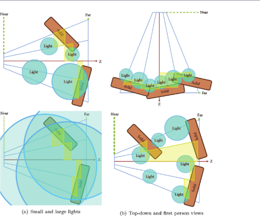
17.2. Recap: Forward, Deferred, and Tiled Shading 265
Figure 17.2. (a) The effect of having lights that are too large (bottom image): there is
no gain from the tiling, as all light sources affect all tiles (drawn in yellow), compared
to the top image, where there is one light per tile on average. (b) Comparison of a
top-down view and a first-person view. In the top-down view (top), all lights are close
to the ground, which has only small variations in the Z-direction. In this case, not much
is gained from computing minimum and maximum Z-bounds. In the first-person view
(bottom), the bounds help (three lights in the image affect no tiles at all).
handles complex light and geometry configurations more robustly with respect
to performance. However, tiled forward shading is significantly simpler to im-
plement, and works on a much broader range of hardware. We will discuss the
clustered shading extension and how it interacts with the tiled forward shading
presented here in Section 17.8.

266 17. Tiled Forward Shading
17.3 Tiled Forward Shading: Why?
The main strength of deferred techniques, including tiled deferred shading, is that
over-shading due to over-draw is eliminated. However, most deferred techniques
suffer from the following weaknesses when compared to forward rendering:
•Transparency/blending is tricky, since traditional G-buffers only allow stor-
age of a single sample at each position in the buffer.
•The memory storage and bandwidth requirements are higher and become
even worse with MSAA and related techniques (Section 17.6).
Forward rendering, on the other hand, has good support for
•transparency via alpha blending,
•MSAA and related techniques through hardware features (much less mem-
ory storage is required).
In addition, forward rendering trivially supports different shaders and materials
for different geometries. Deferred techniques would generally need to fall back to
¨ubershaders (or perform multiple shading passes).
A special advantage for tiled forward shading is its low requirements on GPU
hardware. It is possible to implement a tiled forward renderer without compute
shaders and other (relatively) recent hardware features. In fact, it is possible
to implement a tiled forward renderer on any hardware that supports depen-
dent texture lookups in the fragment shader. On the other hand, if compute
shaders are available, we can take advantage of this during, say, light assignment
(Section 17.4).
In the following sections, we first present a tiled forward shading renderer
to which we add support for transparency, MSAA and finally experiment with
having a few different shaders for different objects. We compare performance
and resource consumption to a reference tiled deferred shading renderer and show
where the tiled forward renderer wins.
17.4 Basic Tiled Forward Shading
We listed the basic algorithm for all tiled shading variants in Section 17.2. For
clarity, it is repeated here including any specifics for the forward variant.
1. Subdivide screen into tiles
2. Optional: pre-Z pass—render geometry and store depth values for each
sample in the standard Z-buffer.
3. Optional: find minimum and/or maximum Z-bounds for each tile.

17.4. Basic Tiled Forward Shading 267
4. Assign lights to each tile.
5. Render geometry and compute shading for each generated fragment.
Subdivision of screen. We use regular N×Npixel tiles (e.g., N= 32). Having
very large tiles creates a worse light assignment; each tile will be affected by
more light sources that affect a smaller subset of samples in the tile. Creating
very small tiles makes the light assignment more expensive and increases the
required memory storage—especially when the tiles are small enough that many
adjacent tiles are found to be affected by the same light sources.
Optional pre-Z pass. An optional pre-Z pass can help in two ways. First, it is
required if we wish to find the Z-bounds for each tile in the next step. Secondly,
in the final rendering pass it can reduce the number of samples that need to be
shaded through early-Z tests and similar hardware features.
The pre-Z pass should, of course, only include opaque geometry. Transparent
geometry is discussed in Section 17.5.
Though a pre-Z pass is scene and view dependent, in our tests we have found
that adding it improves performance significantly. For instance, for the images in
Figure 17.1(a), rendering time is reduced from 22.4 ms (upper view) and 37.9 ms
(lower view) to 15.6 ms and 18.7 ms, respectively.
Optional minimum or maximum Z-bounds. If a depth buffer exists, e.g., from the
pre-Z pass described above, we can use this information to find (reduce) the ex-
tents of each tile in the Z-direction (depth). This yields smaller per-tile bounding
volumes, reducing the number of lights that affect a tile during light assignment.
Depending on the application, finding only either the minimum or the max-
imum bounds can be sufficient (if bounds are required at all). Again, trans-
parency (Section 17.5) interacts with this, as do various multisampling schemes
(Section 17.6).
In conjunction with the pre-Z test above, the minimum or maximum reduction
yields a further significant improvement for the views in Figure 17.1(a). Render-
ing time with both pre-Z and minimum or maximum reduction is 10.9 ms (upper)
and 13.8 ms (lower), respectively—which is quite comparable to the performance
of tiled deferred shading (8.5 ms and 10.9 ms). The reduction itself is imple-
mented using a loop in a fragment shader (for simplicity) and currently takes
about 0.75 ms (for 1,920 ×1,080 resolution).
Light assignment. Next, we must assign lights to tiles. Basically, we want to
efficiently find which lights affect samples in which tiles. This requires a few
choices and considerations.
In tiled shading, where the number of tiles is relatively small (for instance,
a resolution of 1,920 ×1,080 with 32 ×32 tiles yields just about 2,040 tiles), it
can be feasible to do the assignment on the CPU. This is especially true if the

268 17. Tiled Forward Shading
number of lights is relatively small (e.g., a few thousand). On the CPU, a simple
implementation is to find the screen-space axis-aligned bounding boxes (AABBs)
for each light source and loop over all the tiles that are contained in the 2D region
of the AABB. If we have computed the minimum and maximum depths for each
tile, we need to perform an additional test to discard lights that are outside of
the tile in the Z-direction.
On the GPU, a simple brute-force variant works for moderate amounts of
lights (up to around 10,000 lights). In the brute-force variant, each tile is checked
against all light sources. If each tile gets its own thread group, the implementation
is fairly simple and performs relatively well. Obviously, the brute-force algorithm
does not scale very well. In our clustered shading implementation [Olsson et
al. 12b], we build a simple light hierarchy (a BVH) each frame and test the tiles
(clusters) against this hierarchy. We show that this approach can scale up to at
least one million lights in real time. The same approach is applicable for tiled
shading as well.
Rendering and shading. The final step is to render all geometry. The pipeline for
this looks almost like a standard forward rendering pipeline; different shaders and
related resources may be attached to different chunks of geometry. There are no
changes to the stages other than the fragment shader.
The fragment shader will, for each generated sample, look up which lights
affect that sample by checking what lights are assigned to the sample’s tile (List-
ing 17.1).
17.5 Supporting Transparency
As mentioned in the beginning of this article, deferred techniques have some
difficulty dealing with transparency since traditional G-buffers only can store
attributes from a single sample at each buffer location [Thibieroz and Gr¨un 10].
However, with forward rendering, we never need to store attributes for samples.
Instead we can simply blend the resulting colors using standard alpha-blending.
Note that we are not solving the order-dependent transparency problem.
Rather, we support, unlike many deferred techniques, standard alpha-blending
where each layer is lit correctly. The application must, however, ensure that
transparent objects are drawn in the correct back-to-front order.
We need to make the following changes, compared to the basic tiled forward
shading algorithm (Section 17.4).
Optional minimum or maximum Z-bounds. We need to consider transparent geom-
etry here, as nonoccluded transparent objects will affect a tile’s bounds inasmuch
that it moves a tile’s minimum Z-bound (“near plane”) closer to the camera.
We ended up using two different sets of tiles for opaque and transparent
geometries, rather than extending a single set of tiles to include both opaque and

17.5. Supporting Transparency 269
// 1 D t ext ure h old ing per - til e lig ht li sts
un iform isa mp leB uffer t ex_t ile Ligh tLists ;
// un iform bu ffer h olding each tile ’s lig ht c oun t and
// st ar t of fse t of t he ti le ’ s l ig ht li st ( i n
// tex_tileLightIndices)
uniform TileLightListRanges
{
ivec2 u_l igh tLis tRa nge [ MA X_N UM_T ILE S ];
}
voi d sh adin g_f unct ion ( in out Fra gm ent Data aF rag Dat a )
{
// ...
// find fr ag me nt ’s tile usin g g l_ Fr agCoo rd
iv ec 2 ti le Co or d = i vec 2 ( g l _F ra gC oo rd . xy )
/ i vec 2 ( TILE _SI ZE_ X , TI LE_S IZE _Y ) ;
int t ileIdx = ti leC oord . x
+ tileCoord .y * LIG HT_ GR ID_S IZE _X ;
// fet ch ti le ’s ligh t data sta rt o ffset (. y ) and
// nu mber of li gh ts (. x )
iv ec 2 l ig ht Li st R an ge = u_ li g ht Li s tR an ge [ t ile Id x ] . xy ;
// it er ate over ligh ts af fe ct in g this tile
for (int i = 0; i < li gh tList Ra nge .x ; ++ i )
{
int l igh tIn dex = li ghtL ist Range .y + i ;
// fetch gl ob al light ID
int g lob alLi ght Id = texelFetch (
te x_ ti le Li gh tL is ts , li gh tI ndex ). x;
// get the l ight ’s dat a ( position , colors , ...)
Li ght Dat a li ght Data ;
li ght_ get _data ( lightDa ta , gl obal Lig htId );
// co mp ute shad in g fr om the lig ht
sh ade ( aFr agDa ta , li gh tDa ta );
}
// ...
}
Listing 17.1. GLSL pseudocode that demonstrates how lights affecting a given sample
are fetched. First, we find the fragment’s associated tile (tileIdx) based on its position
in the framebuffer. For each tile we store two integers (u_lightListRange array), one
indicating the number of lights affecting the tile, and the other describes the offset
into the global per-tile light list buffer (tex_tileLightLists). The light list buffer stores
a number of integers per tile, each integer identifying a globally unique light that is
affecting the tile.
transparent geometries. The Z-bounds for tiles used with opaque geometry are
computed as described in Section 17.4, which gives a good light assignment for
the opaque geometry (Figure 17.3(a)).
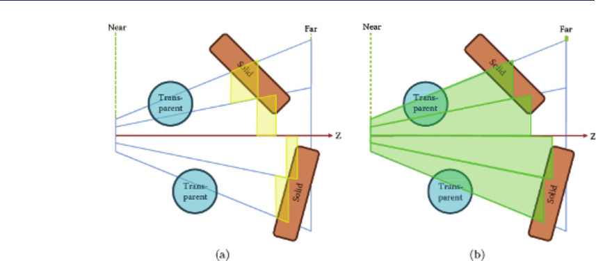
270 17. Tiled Forward Shading
Figure 17.3. Z-bounds used for (a) opaque and (b) transparent geometries.
For transparent geometry, we would like to find the transparent objects’ min-
imum Z-value and the minimum of the transparent objects’ and opaque objects’
respective maximum Z-values. However, this is somewhat cumbersome, requir-
ing several passes over the transparent geometry; therefore, we simply use the
maximum Z-value from the opaque geometry to cap the tiles in the far direction.
This discards lights that are hidden by opaque geometry. In the near direction,
we extend the tiles to the camera’s near plane, as shown in Figure 17.3(b).
Using separate bounds turned out to be slightly faster than using the same tile
bounds for both opaque and transparent geometry; in Figure 17.1(b), when using
separate bounds, rendering takes 15.1 ms (upper) and 21.9 ms (lower), compared
to 16.1 ms and 23.5 ms when using the extended bounds for both opaque and
transparent geometries.
We would like to note that this is, again, scene dependent. Regardless of
whether we use the approximate variant or the exact one, we can still use the
depth buffer from the opaque geometry during the final render in order to enable
early-Z and similar optimizations. If we do not use the minimum or maximum
reduction to learn a tile’s actual bounds, no modifications are required to support
transparency.
Light assignment. If separate sets of tiles are used, light assignment must be done
twice. In our case, a special optimization is possible: we can first assign lights in
two dimensions and then discard lights that lie behind opaque geometry (use the
maximum Z-bound from the tiles only). This yields the light lists for transparent
geometry. For opaque geometry, we additionally discard lights based on the
minimum Z-bound information (Listing 17.2).

17.6. Support for MSAA 271
// assign lights to 2 D t ile s
ti les2D = bui ld _2 d_t il es ();
li ght Lists2 D = a ssig n_li ght s_ to _2d_ tile s ( ti les 2D );
// draw opaque g eo me tr y in pre -Z pass and find tiles ’
// e xte nt s in t he Z - d i re ct io n
de pt hBuffer = re nd er_ pr eZ_ pa ss ( );
ti le ZBounds = r ed uce _z _boun ds ( tiles2D , de pt hB uf fer );
// for tran sp ar en t geometry , prune li ghts ag ai ns t ma ximum Z - d irection
li ght Li st sTr an s
= pr un e_li gh ts_max ( li ghtLi sts2D , tile ZBo und s );
// for o paque geometry a dd ition al ly pr une ligh ts ag ainst
// m ini mu m Z - d i re ct io n
lightListsOpaque
= pr un e_li gh ts_min ( li ght ListsTrans , t il eZB oun ds );
// ...
// later : re nd eri ng
dra w ( o paq ue ge omet ry , li gh tL is ts Op aqu e );
dra w ( t ra spa re nt ge omet ry , l ig ht Lis ts Tr an s ) ;
Listing 17.2. Pseudocode describing the rendering algorithm used to support trans-
parency, as shown in Figure 17.1(b). We perform the additional optimization where we
first prune lights based on the maximum Z-direction, which gives the light assignment
for transparent geometry. Then, we prune lights in the minimum Z-direction, which
gives us light lists for opaque geometry.
Rendering and shading. No special modifications are required here, other than
using the appropriate set of light lists for opaque and transparent geometries, re-
spectively. First, all opaque geometry should be rendered. Then the transparent
geometry is rendered back to front.1
17.6 Support for MSAA
Supporting MSAA and similar schemes is very simple with tiled forward shading.
We mainly need to ensure that all render targets are created with MSAA enabled.
Additionally we need to consider all (multi)samples during the optional minimum
or maximum Z-reduction step.
We show the effect of MSAA on render time in Figure 17.4. As we compare to
tiled deferred shading, which does not support transparency, Figure 17.4 includes
timings for tiled forward both with (Figure 17.1(b)) and without (Figure 17.1(a))
transparency. Additionally, we compare memory usage between our forward and
deferred implementations.
1In our demo, we sort on a per-object basis, which obviously causes some artifacts when
transparent objects overlap. This is not a limitation in the technique but rather one in our
implementation.
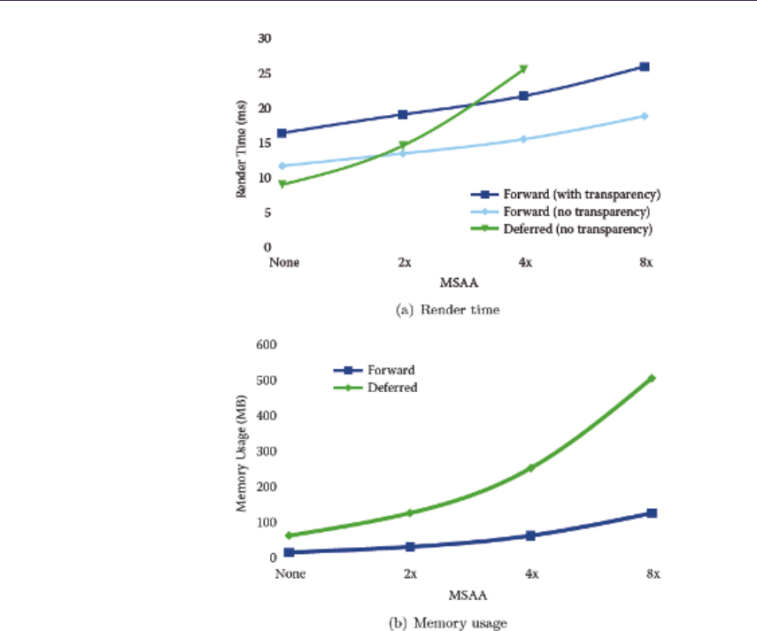
272 17. Tiled Forward Shading
Figure 17.4. (a) Render time and (b) memory usage for tiled forward and tiled deferred
shading with varying MSAA settings. We were unable to allocate the 8×MSAA frame-
buffer for deferred, which is why no timing results are available for that configuration.
Memory usage estimates are based on a G-buffer with 32-bit depth, 32-bit ambient, and
64-bit normal, diffuse, and specular components (using the RGBA16F format).
One interesting note is that our unoptimized Z-reduction scales almost linearly
with the number of samples: from 0.75 ms when using one sample to 5.1 ms with
8×MSAA. At that point, the contribution of the Z-reduction is quite significant
with respect to the total frame time. However, it still provides a speedup in
our tests. It is also likely possible to optimize the Z-reduction step further, for
instance, by using compute shaders instead of a fragment shader.

17.7. Supporting Different Shaders 273
17.7 Supporting Different Shaders
Like all forward rendering, we can attach different shaders and resources (tex-
tures, uniforms, etc.) to different chunks of geometry. Of course, if desired, we
can still use the ¨ubershader approach in the forward rendering.
We have implemented three different shader types to test this, as seen in
Figure 17.1(d): a default diffuse-specular shader, a shader emulating two-color
car paint (see transparent bubbles and lion), and a rim-light shader (see large
fabric in the middle of the scene).
The forward renderer uses the different shaders, compiled as different shader
programs, with different chunks of geometry. For comparison, we implemented
this as an ¨ubershader for deferred rendering. An integer identifying which shader
should be used is stored in the G-buffer for each sample. (There were some
unused bits available in the G-buffer, so we did not have to allocate additional
storage.) The deferred shading code selects the appropriate shader at runtime
using runtime branches in GLSL.
Performance degradation for using different shaders seems to be slightly smaller
for the forward renderer; switching from diffuse-specular shading only to using
the different shaders described above caused performance to drop by 1.4 ms on
average. For the deferred shader, the drop was around 2.2 ms. However, the vari-
ations in rendering time for different views are in the same order of magnitude.
17.8 Conclusion and Further Improvements
We have explored tiled forward shading in this chapter. Tiled forward shading
combines advantages from both tiled deferred shading and standard forward ren-
dering. It is quite adaptable to different conditions, by, for instance, omitting
steps in the algorithm made unnecessary by application-specific knowledge. An
example is the optional computation of minimum and/or maximum Z-bounds for
top-down views.
An extension that we have been exploring recently is clustered shading. Tiled
shading (both forward and deferred) mainly considers 2D groupings of samples,
which, while simple, cause performance and robustness issues in some scene and
view configurations. One example of this is in scenes with first-person-like cam-
eras where many discontinuities occur in the Z-direction (Figure 17.5). In clus-
tered shading, we instead consider 3D groupings of samples, which handle this
case much more gracefully.
Clustered shading’s main advantage is a much lower view dependency, deliver-
ing more predictable performance in scenes with high or unpredictable complexity
in the Z-direction. The disadvantages are increased complexity, requirements on
hardware (we rely heavily on compute shaders/CUDA), and several new constant
costs. For instance, with tiled shading, the subdivision of the screen into tiles is
basically free. In clustered shading, this step becomes much more expensive—in
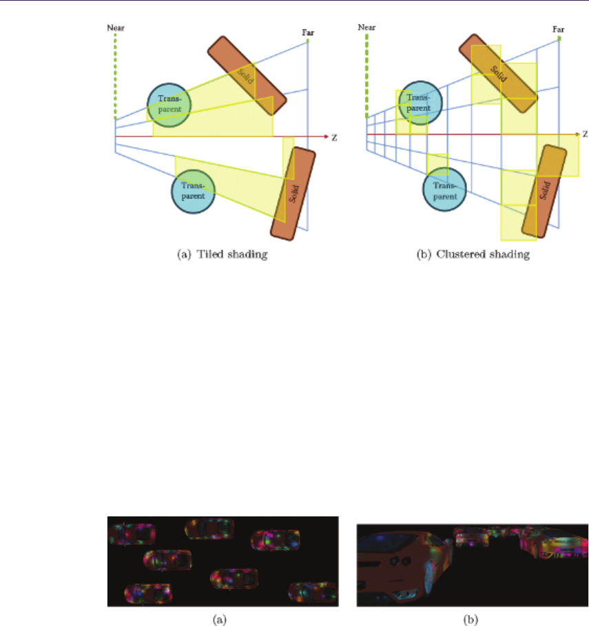
274 17. Tiled Forward Shading
Figure 17.5. Comparison between volumes created by (a) the tiling explored in this
article and (b) clustering, as described in [Olsson et al. 12b]. Finding the tiled vol-
umes is relatively simple and can be done in standard fragment shaders. Clustering is
implemented with compute shaders, as is the light assignment to clusters.
fact, in some cases it offsets time won in the shading from the better light-to-
sample mapping offered by clustering (Figure 17.6). We are also further exploring
clustered forward shading [Olsson et al. 12a], which shows good promise on mod-
ern high-end GPUs with compute shader capabilities. Tiled forward shading, on
the other hand, is implementable on a much wider range of hardware.
Figure 17.6. Comparison between tiled forward shading and clustered forward shad-
ing. (a) In the top-down view, tiled forward outperforms our current clustered forward
implementation (6.6 ms versus 9.3 ms). (b) In the first-person-like view, tiled forward
becomes slightly slower (9.4 ms versus 9.1 ms). While somewhat slower in the first view,
one of the main features of clustered shading is its robust performance. There are 1,024
randomly placed light sources.

Bibliography 275
Bibliography
[Andersson 09] Johan Andersson. “Parallel Graphics in Frostbite - Current &
Future.” SIGGRAPH Course: Beyond Programmable Shading, New Or-
leans, LA, August 6, 2009. (Available at http://s09.idav.ucdavis.edu/talks/
04-JAndersson-ParallelFrostbite-Siggraph09.pdf.)
[Balestra and Engstad 08] Christophe Balestra and P˚al-Kristian Engstad. “The
Technology of Uncharted: Drake’s Fortune.” Presentation, Game Developer
Conference, San Francisco, CA, 2008. (Available at http://www.naughtydog.
com/docs/Naughty-Dog-GDC08-UNCHARTED-Tech.pdf.)
[Enderton et al. 10] Eric Enderton, Erik Sintorn, Peter Shirley, and David Lue-
bke. “Stochastic Transparency.” In I3D 10: Proceedings of the 2010 ACM
SIGGRAPH Symposium on Interactive 3D Graphics and Games, pp. 157–
164. New York: ACM, 2010.
[Engel 09] Wolfgang Engel. “The Light Pre-Pass Renderer: Renderer Design
for Efficient Support of Multiple Lights.” SIGGRAPH Course: Advances
in Real-Time Rendering in 3D Graphics and Games, New Orleans, LA,
August 3, 2009. (Available at http://www.bungie.net/News/content.aspx?
type=opnews&link=Siggraph 09.)
[Hargreaves and Harris 04] Shawn Hargreaves and Mark Harris. “De-
ferred Shading.” Presentation, NVIDIA Developer Conference: 6800
Leagues Under the Sea, London, UK, June 29, 2004. (Available
at http://http.download.nvidia.com/developer/presentations/2004/
6800 Leagues/6800 Leagues Deferred Shading.pdf.)
[Kircher and Lawrance 09] Scott Kircher and Alan Lawrance. “Inferred Lighting:
Fast Dynamic Lighting and Shadows for Opaque and Translucent Objects.”
In Sandbox ‘09: Proceedings of the 2009 ACM SIGGRAPH Symposium on
Video Games, pp. 39–45. New York: ACM, 2009.
[Lauritzen 10] Andrew Lauritzen. “Deferred Rendering for Current and Future
Rendering Pipelines.” SIGGRAPH Course: Beyond Programmable Shading,
Los Angeles, CA, July 29, 2010. (Available at http://bps10.idav.ucdavis.edu/
talks/12-lauritzen DeferredShading BPS SIGGRAPH2010.pdf.)
[Olsson and Assarsson 11] Ola Olsson and Ulf Assarsson. “Tiled Shading.” Jour-
nal of Graphics, GPU, and Game Tools 15:4 (2011), 235–251. (Available at
http://www.tandfonline.com/doi/abs/10.1080/2151237X.2011.621761.)
[Olsson et al. 12a] Ola Olsson, Markus Billeter, and Ulf Assarsson. “Clustered
and Tiled Forward Shading: Supporting Transparency and MSAA.” In SIG-
GRAPH ‘12: ACM SIGGRAPH 2012 Talks, article no. 37. New York: ACM,
2012.

276 17. Tiled Forward Shading
[Olsson et al. 12b] Ola Olsson, Markus Billeter, and Ulf Assarsson. “Clustered
Deferred and Forward Shading.” In HPG ‘12: Proceedings of the Fourth
ACD SIGGRPAH/Eurographics Conference on High Performance Graphics,
pp. 87–96. Aire-la-Ville, Switzerland: Eurogaphics, 2012.
[Saito and Takahashi 90] Takafumi Saito and Tokiichiro Takahashi. “Compre-
hensible Rendering of 3D Shapes.” SIGGRAPH Comput. Graph. 24:4 (1990),
197-206.
[Shishkovtsov 05] Oles Shishkovtsov. “Deferred Shading in S.T.A.L.K.E.R.” In
GPU Gems 2, edited by Matt Pharr and Randima Fernando, pp. 143–166.
Reading, MA: Addison-Wesley, 2005.
[Swoboda 09] Matt Swoboda. “Deferred Lighting and Post Processing on
PLAYSTATION 3.” Presentation, Game Developer Conference, San
Francisco, 2009. (Available at http://www.technology.scee.net/files/
presentations/gdc2009/DeferredLightingandPostProcessingonPS3.ppt.)
[Thibieroz and Gr¨un 10] Nick Thibieroz and Holger Gr¨un. “OIT and GI Using
DX11 Linked Lists.” Presentation, Game Developer Conference, San
Francisco, CA, 2010. (Available at http://developer.amd.com/gpu assets/
OIT%20and%20Indirect%20Illumination%20using%20DX11%20Linked%
20Lists forweb.ppsx.)
[Trebilco 09] Damian Trebilco. “Light Indexed Deferred Rendering.” In
ShaderX7: Advanced Rendering Techniques, edited by Wolfgang Engel,
pp. 243–256. Hingham, MA: Charles River Media, 2009.

18
Forward+: A Step Toward
Film-Style Shading in Real Time
Takahiro Harada, Jay McKee, and Jason C. Yang
18.1 Introduction
Modern GPU hardware along with the feature set provided by the DirectX 11
API provides developers more flexibility to choose among a variety of rendering
pipelines. In order to exploit the performance of modern GPUs, we believe it is
important to choose a pipeline that takes advantage of GPU hardware features,
scales well, and provides flexibility for artists, tech artists, and programmers to
achieve high-quality rendering with unique visuals. The ability to differentiate a
game’s visual look from today’s games, which modern computer-generated (CG)
films are extremely good at doing, likely will be a key for game graphics in the
future. However, the ability to produce high-quality renderings that approach
the styling in CG films will require great flexibility to support arbitrary data
formats and shaders for more sophisticated rendering of surface materials and
special effects.
Our goal was to find a rendering pipeline that would best meet these objec-
tives. We boiled things down to a few specific requirements:
•Materials may need to be both physically and nonphysically based. Tech
artists will want to build large trees of materials made of arbitrary complex-
ity. Material types will likely be similar to those found in offline renderers
such as RenderMan, mental ray, and Maxwell Render shading systems.
•Artists want complete freedom regarding the number of lights that can be
placed in a scene at once.
•Rendering data should be decoupled from the underlying rendering engine.
Artists and programmers should be able to write shaders and new materials
freely at runtime for quick turnaround—going from concept to seeing results
277

278 18. Forward+: A Step Toward Film-Style Shading in Real Time
should be fast and easy. The architecture should be simple and not get in
the way of creative expression.
We have devised a rendering pipeline that we believe meets these objectives well
and is a good match for modern GPU hardware going into the foreseeable future.
We refer to it as the Forward+ rendering pipeline [Harada et al. 11].
18.2 Forward+
The Forward+ rendering pipeline requires three stages:
•Z prepass. Z prepass is an option for forward rendering, but it is essential
for Forward+ to reduce the pixel overdraws of the final shading step. This
is especially expensive for Forward+ due to the possible traversal of many
lights per pixel, which we will detail later in this section.
•Light culling. Light culling is a stage that calculates the list of lights affecting
a pixel.
•Final shading. Final shading, which is an extension to the shading pass in
forward rendering, shades the entire surface. A required change is the way
to pass lights to shaders. In Forward+, any lights in a scene have to be
accessible from shaders rather than binding some subset of lights for each
objects as is typical of traditional forward rendering.
18.2.1 Light Culling
The light-culling stage is similar to the light-accumulation step of deferred light-
ing. Instead of calculating lighting components, light culling calculates a list of
light indices overlapping a pixel. The list of lights can be calculated for each
pixel, which is a better choice for final shading.
However, storing a per-pixel light list requires a large memory footprint and
significant computation at the light-culling stage. Instead, the screen is split into
tiles and light indices are calculated on a per-tile basis (Figure 18.1). Although
tiling can add false positives to the list for a pixel in a tile, it reduces the overall
memory footprint and computation time necessary for generating the light lists.
Thus we are making a tradeoff between light-index buffer memory and final shader
efficiency.
By utilizing the computing capability of modern GPUs, light culling can be
implemented entirely on the GPU as detailed in Section 18.3. Therefore, the
whole lighting pipeline can be executed entirely on the GPU.
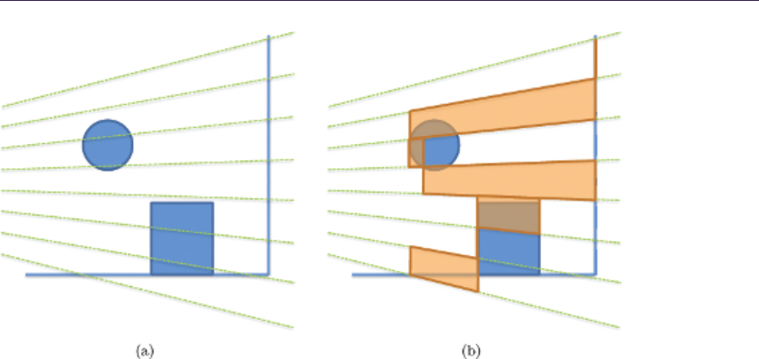
18.3. Implementation and Optimization 279
Figure 18.1. Illustration of light culling in 2D. (a) A camera is placed on the left,
and green lines indicate tile borders. (b) Light culling creates a frustum for each tile
bounded by minimum and maximum depth of pixels in a tile.
18.2.2 Shading
Whereas light culling creates the list of lights overlapping each pixel, final shading
loops through the list of lights and evaluates materials using material parameters
describing the surface properties of the rendered object along with information
stored for each light. With unordered access view (UAV) support, per-material
instance information can be stored and accessed in linear structured buffers passed
to material shaders. Therefore, at least in theory, the full render equation can
be satisfied without limitation because light accumulation and shading happen
simultaneously in one place with complete material and light information.
Use of complex materials and more accurate lighting models to improve visual
quality is not constrained other than by the GPU computational cost, which is
largely determined by the average number of overlapping lights on each pixel
multiplied by the average cost for material calculation.
With this method, high pixel overdraw can kill performance; therefore, a Z
prepass is critical to minimize the cost of final shading.
18.3 Implementation and Optimization
A standard forward rendering pipeline can be converted to a Forward+ ren-
dering pipeline by adding the light-culling stage and modifying existing pixel
shaders to make them implement Forward+’s final shading stage as described

280 18. Forward+: A Step Toward Film-Style Shading in Real Time
in Section 18.2. No modification is necessary for the Z prepass, so we do not
describe its implementation. The light-culling stage can be implemented in sev-
eral ways thanks to the flexibility of current GPUs. Specifically, direct compute
and read-writable structure data buffers or UAVs are the key features to utilizing
Forward+. In this section, we first describe which features of DirectX 11 are
essential to making Forward+ work well on modern GPUs. Then we explain a
light-culling implementation that works well for a scene with thousands of lights.
If there are more lights, we might be better off considering other implementations
such as those described in [Harada et al. 11]. This section concludes by describing
modifications for final shading.
18.3.1 Gather-Based Light Culling
During light culling, the computation is done on a by-tile basis. Therefore, it is
natural to execute a thread group for a tile. A thread group can share data using
thread group shared memory (called shared memory from now on), which can
reduce a lot of redundant computation in a thread group. The computation is
identical for each tile; therefore, we explain the computation for a single tile.
The compute shader for light culling is executed as a two-dimensional (2D)
work group. A thread group is assigned a unique 2D index, and a thread in a
thread group is assigned a unique 2D index in the group.
In the pseudocode in this subsection, the following macros are used for these
variables:
•GET_GROUP_IDX: thread group index in X direction (SV_GroupID);
•GET_GROUP_IDY: thread group index in Y direction (SV_GroupID);
•GET_GLOBAL_IDX: global thread index in X direction (SV_DispatchThreadID);
•GET_GLOBAL_IDY: global thread index in Y direction (SV_DispatchThreadID);
•GET_LOCAL_IDX: local thread index in X direction (SV_GroupThreadID);
•GET_LOCAL_IDY: local thread index in Y direction (SV_GroupThreadID).
The first step is computation of the frustum of a tile in view space. To reconstruct
four side faces, we need to calculate the view-space coordinates of the four corner
points of the tile. With these four points and the origin, four side planes can be
constructed.
float4 frus tu m [4] ;
{// c on st ru ct f rustum
fl oat 4 v [4 ];
v [0 ]= pr oj ToV ie w ( 8* G ET_ GR OUP _I DX , 8* G ET _GR OUP _I DY ,1 . f) ) ;
v [1 ]= projToV ie w (8* ( GE T_GRO UP _I DX +1) , 8* GET_GRO UP _IDY ,1. f) ) ;
v [2 ]= projT oV ie w (8*( GET_G RO UP _ID X +1) ,8*( GE T_GRO UP _IDY +1) ,1. f ));

18.3. Implementation and Optimization 281
v[ 3]= p ro jT o Vi ew (8 * G E T_ GR OU P_ ID X , 8*( G ET _ GR OU P _I D Y + 1) ,1. f ) ) ;
float4 o = ma ke_float 4 (0. f ,0. f ,0.f ,0. f) ;
for (int i =0; i < 4; i + +)
fru stum [i ] = crea te Eq uat io n ( o , v [i] , v [( i +1) &3] ) ;
}
projToView() is a function that takes screen-space pixel indices and depth value
and returns coordinates in view space. createEquation() creates a plane equation
from three vertex positions.
The frustum at this point has infinite length in the depth direction; however,
we can clip the frustum by using the maximum and minimum depth values of the
pixels in the tile. To obtain the depth extent, a thread first reads the depth value
of the assigned pixel from the depth buffer, which is created in the depth prepass.
Then it is converted to the coordinate in view space. To select the maximum and
minimum values among threads in a group, we used atomic operations to shared
memory. We cannot use this feature if we do not launch a thread group for
computation of a tile.
float d ept h = dep th In . Lo ad (
uint3 ( G ET_ GLO BAL _IDX , G ET_ GLO BAL _ID Y ,0) );
float4 v iewPos = projT oV ie w ( GET _G LOBAL_IDX , G ET _G LOBAL_I DY ,
de pth ) ;
int lIdx = G ET_ LO CA L_IDX + GE T_ LO CAL _I DY *8;
{// ca lc ul at e boun d
if ( l Id x = = 0 ) // i ni ti al iz e
{
ld sZMax = 0;
ld sZMin = 0 xffffffff ;
}
GroupMemoryBarrierWithGroupSync();
u32 z = a suint ( v iewPos . z ) ;
if ( depth != 1. f )
{
At omMax ( ldsZMax , z );
At omMin ( ldsZMin , z );
}
GroupMemoryBarrierWithGroupSync();
maxZ = asflo at ( lds ZMa x ) ;
minZ = asflo at ( lds ZMi n ) ;
}
ldsZMax and ldsZMin store maximum and minimum z coordinates, which are
bounds of a frustum in the z direction, in shared memory. Once a frustum is
constructed, we are ready to go through all the lights in the scene. Because there
are several threads executed per tile, we can cull several lights at the same time.
We used 8 ×8 for the size of a thread group; thus, 64 lights are processed in
parallel. The code for the test is as follows:

282 18. Forward+: A Step Toward Film-Style Shading in Real Time
for (int i =0; i < nBodi es ; i += 64)
{
int il = lI dx + i;
if ( il < n Bo dies )
{
if ( o v erl ap s ( frus tum , g L ig ht Ge om e tr y [ il ] ) )
{
a pp en d Li gh t To Li st ( il );
}
}
}
In overlaps(), a light-geometry overlap is checked against a frustum using the
separating axis theorem [Ericson 04]. If a light is overlapping the frustum, the
light index is stored to the list of the overlapping lights in appendLightToList().
There are several data structures we can use to store the light list. The obvious
way would be to build a linked list using a few atomic operations [Yang et al. 10].
However, this approach is relatively expensive: we need to use a few global
atomic operations to insert a light, and a global memory write is necessary when-
ever an overlapping light is found. Therefore, we took another approach in which
a memory write is performed in two steps. A tile is computed by a thread group,
and so we can use shared memory for the first level storage. Light index storage
and counter for the storage is allocated as follows:
gr ou pshared u32 ld sL ig ht Idx [ LI GHT_C AP ACI TY ];
gr oup shared u32 lds Lig ht Id xCou nte r ;
In our implementation, we set LIGHT_CAPACITY to 256. The appendLightToList()
is implemented as follows:
voi d appendLightToList( int i )
{
u32 d stIdx = 0;
In terl ock edAdd ( l dsL igh tId xCo unt er , 1, d stIdx ) ;
if ( ds tI dx < LIG HT _CAPA CI TY )
ld sL igh tIdx [ d stIdx ] = i ;
}
With this implementation, no global memory write is necessary until all the lights
are tested.
After testing all the lights against a frustum, indices of lights overlapping that
frustum are collected in the shared memory. The last step of the kernel is to write
these to the global memory.
For the storage of light indices in the global memory, we allocated two buffers:
gLightIdx, which is a memory pool for the indices, and gLightIdxCounter, which

18.3. Implementation and Optimization 283
is a memory counter for the memory pool. Memory sections for light indices
for a tile are not allocated in advance. Thus, we first need to reserve memory
in gLightIdx. This is done by an atomic operation to gLightIdxCounter using a
thread in the thread group.
Once a memory offset is obtained, we just fill the light indices to the assigned
contiguous memory of gLightIdx using all the threads in a thread group. The
code for doing this memory write is as follows:
{// wr ite back
u32 s tartOff se t = 0;
if( l Idx == 0 )
{// re se rve me mo ry
if( ld sL igh tI dxC ou nte r != 0 )
Int erlo cke dAdd ( gL ightIdxCounter , ldsLightIdx Co unt er ,
sta rt Offse t );
ptL ow erB ound [ t ile Idx ] = st artO ffs et ;
ld sLig htIdxS tart = star tOf fse t ;
}
GroupMemoryBarrierWithGroupSync();
st art Offset = ld sLi ghtI dxS tart ;
for (in t i= l Idx ; i < l ds Li gh tI dx Co un ter ; i + =64 )
{
gL igh tId x [ startOff set + i] = ld sLight Idx [ i];
}
}
This light-culling kernel reads light geometry (for spherical lights, that includes
the location of the light and its radius). There are several options for the structure
of the light buffer. Of course, we can pack light geometry and lighting properties,
such as intensity and falloff, to a single structure. However, this is not a good idea
for our light-culling approach because all the necessary data for the light culling
is padded with light properties, which are not used in the light culling. A GPU
usually reads data by page. Therefore, it is likely to transfer lighting properties
as well as light geometry although they are not read by the kernel when this data
structure is employed for the lights.
A better choice for the data structure is to separate the light geometry and
lighting properties into two separate buffers. The light-culling kernel only touches
the light geometry buffer, increasing the performance because we do not have to
read unnecessary data.
18.3.2 Final Shading
For final shading, all objects in the camera frustum are rendered with their au-
thored materials. This is different than forward rendering because we need to
iterate through the lights overlapping each tile.

284 18. Forward+: A Step Toward Film-Style Shading in Real Time
To write a pixel shader, we created “building blocks” of common operations
for different shaders. This design makes it easy to write shaders, as we will show
now. The most important building blocks are the following two, implemented as
macros:
# define LIGHT_LOOP_BEGIN
int tileIndex = GetT ile Inde x ( scr een Pos ) ;
uint start Inde x , endIndex ;
Get Tile Off sets ( tileIn dex , star tInd ex , en dIn dex );
for ( uint lig htL istI dx = s tar tId x ;
li gh tLi st Idx < endId x ;
li ghtList Id x ++ )
{
int l ightIdx = Li ght Inde xBuffe r [ lightLis tId x ];
Li ghtParam s di rec tLight ;
Li ght Params indir ect Light ;
if ( isI nd ir ect Li ght ( lig ht Id x ) )
{
Fe tc hInd irec tLi gh t ( lightId x , ind ire ctLi ght ) ;
}
els e
{
Fe tch Di rec tL ig ht ( li ghtIndex , d ir ec tLight );
}
# de fine LIGHT_LOOP_END
}
LIGHT_LOOP_BEGIN first calculates the tile index of the pixel using its screen-space
position. Then it opens a loop to iterate all the lights overlapping the tile and
fills light parameters for direct and indirect light. LIGHT_LOOP_END is a macro to
close the loop.
By using these building blocks, an implementation of a pixel shader is simple
and looks almost the same as a pixel shader used in forward rendering. For
example, a shader for a microfacet surface is implemented as follows:
float4 PS ( PSI np ut i ) : SV_TARGET
{
float3 co lo rO ut = 0;
#LIGHT_LOOP_BEGIN
col or Ou t += Ev alu at eMi cr ofa ce t ( d irect Light , i nd irect Li ght );
#LIGHT_LOOP_END
re tur n fl oa t4 ( c ol orO ut , 1 . f ) ;
}
Other shaders can be implemented by just changing the lines between the two
macros. This building block also allows us to change the implementation easily
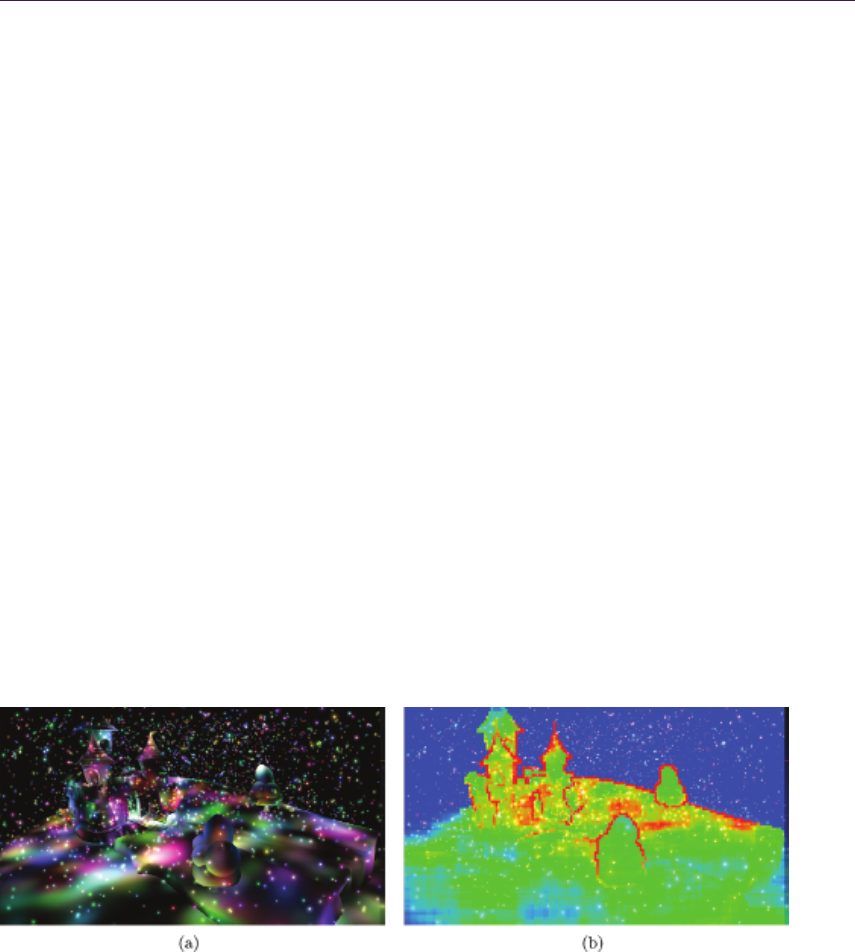
18.4. Results 285
based on performance needs. For instance, we can change LIGHT_LOOP_BEGIN to
iterate a few lights on a slower platform.
An optimization we can do for the host side is to sort all render draw calls
by material type and render all triangles that belong to each unique material at
the same time. This reduces GPU state change and makes good use of the cache
because all pixels needing the same data will be rendered together.
18.4 Results
We implemented Forward+ using DirectX 11 and benchmarked using the scene
shown in Figure 18.2 to compare the performance of Forward+ to compute-based
deferred lighting [Andersson 11].
In short, Forward+ was faster on both the AMD Radeon HD 6970 and HD
7970 (Figure 18.3). Once we compare the memory transfer size and the amount of
computing, it makes sense. Three timers are placed in a frame of the benchmark
to measure time for prepass, light processing, and final shading. In Forward+,
these three are depth prepass, light culling, and final shading. In compute-based
deferred, they are geometry pass (or G-pass), which exports geometry information
to full screen buffers, light culling, screen-space light accumulation, and final
shading.
Prepass. Forward+ writes a screen-sized depth buffer while deferred writes a
depth buffer and another float4 buffer that packs the normal vector of the visible
pixel. The specular coefficient can be stored in the W component of the buffer,
too. Therefore, Forward+ writes less than deferred and is faster on prepass.
Figure 18.2. A scene with 3,072 dynamic lights rendered in 1,280 ×720 resolution.
(a) Using diffuse lighting. (b) Visualization of number of lights overlapping each tile.
Blue, green and red tiles have 0, 25, and 50 lights, respectively. The numbers in between
are shown as interpolated colors. The maximum number is clamped to 50.

286 18. Forward+: A Step Toward Film-Style Shading in Real Time
Figure 18.3. Breakdown of the computation time for three stages of Forward+ and
deferred on an AMD Radeon HD 6970 GPU and an AMD Radeon HD 7970 GPU.
Light processing. Forward+ reads the depth and light geometry buffers. Deferred
also reads them, but the float4 buffer storing normal vectors and lighting prop-
erties has to be read as well because lighting is done at this stage. Therefore,
Forward+ has less memory read compared to deferred.
As for the amount of the computation, Forward+ culls lights. On the other
hand, deferred not only culls lights but also performs lighting computation. For-
ward+ has less computation.
For the memory write, Forward+ writes light indices, the sizes of which de-
pend on the scene and tile size. If 8 ×8 tiles are used, deferred has to write
8×8×4 bytes if a float4 data is written for each pixel. With this data size,
Forward+ can write 256 (8 ×8×4) light indices for a tile; if the number of lights
is less than 256 per tile, Forward+ writes less. In our test scene, there was no
tile overlapped with more than 256 lights.
To summarize this stage, Forward+ is reading, computing, and writing less
than deferred. This is why Forward+ is so fast at this stage.
Final shading. It is obvious that Forward+ takes more time compared to deferred
at shading because it has to iterate through all the lights in the pixel shader.
This is a disadvantage in terms of the performance, but it is designed this way
to get more freedom.
18.5 Forward+ in the AMD Leo Demo
We created the AMD Leo demo to show an implementation of Forward+ in real-
time in a real-world setting. A screenshot from the demo is shown in Figure 18.4.
We chose scene geometry on the order of what can be found in current PC-based
video games (one to two million polygons). We also had the objective of rendering
with a unique stylized look that could be characterized as “CGish” in that it uses
material types that resemble those found in an offline renderer. There are more
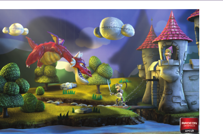
18.5. Forward+ in the AMD Leo Demo 287
Figure 18.4. A screenshot from the AMD Leo Demo.
than 150 lights in the scenes. Artists created about 50 lights by hand. Other
lights are dynamically spawned at runtime for one-bounce indirect illumination
lighting using the technique described in this section. Although Forward+ is ca-
pable of using thousands of dynamic lights, a few hundred lights were more than
enough for our artists to achieve their lighting goals, especially for a single-room
indoor scene.
We use a material system in which a material consists of N layers where
each layer can have M weighted BRDF models along with other physically based
constants like those involving transmission, absorption, refraction, and reflections
of incoming light.
Material parameters for a single layer include physical properties for lighting
such as coefficients for a microfacet surface and a refractive index as well as many
modifiers for standard lighting parameters. We deliberately allow numeric ranges
to go beyond the “physically correct” values to give artists freedom to bend the
rules for a given desired effect.
For lighting, artists can dynamically create and place any number of omnidi-
rectional lights and spotlights into a scene. The light data structure contains a
material index mask. This variable is used to filter lights to only effect specific
material types. While not physically correct, this greatly helps artists fine-tune
lighting without unwanted side effects.
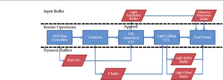
288 18. Forward+: A Step Toward Film-Style Shading in Real Time
Figure 18.5. Forward+ render passes and GPU buffers in the AMD Leo Demo.
18.5.1 One-Bounce Indirect Illumination
As a unique extension of the light-culling system, lights can be used as what we
call an indirect light to generate one-bounce indirect illumination in the scene.
If a given light is tagged to be an indirect light, the following will occur for that
light before any rendering passes at runtime:
•Generate a reflective shadow map (RSM) of the scene from the point of
view of the light [Dachsbacher and Stamminger 05]. Normal buffer, color
buffer, and world-space buffers are generated.
•A compute shader is executed to create spotlights at the location captured
in the RSM. The generated spotlights are appended to the main light list.
The direction of the spotlight will be the reflection of the vector from the
world position to the original indirect light around the normal. Set other
parameters for the new spotlight that conforms to the settings for the indi-
rect light. We added art-driven parameters to control the effect of indirect
lighting.
This new “indirect” light type is used by artists to spawn virtual spotlights that
represent one-bounce lighting from the environment. This method seems to give
artists good control over all aspects of lighting without requiring them to hand-
place thousands or millions of lights or prebake lightmaps. Each indirect light can
spawn N×Nvirtual spotlights, so it takes only a handful to create a nice indirect
lighting effect. Once virtual lights are spawned in the compute shader, they go
through the same light-culling process as all the other lights in the system. Thus,
we could keep the entire rendering pipeline simple. Figure 18.5 illustrates the
rendering pipeline used in the AMD Leo demo.
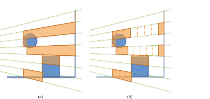
18.6. Extensions 289
Figure 18.6. Illustration of 2.5D culling. (a) Frustum culling creates a long frustum
for a tile with foreground and background. (b) 2.5D culling—splitting depth into eight
cells—does not capture lights falling between foreground and background.
18.6 Extensions
18.6.1 2.5D Culling
At the light-culling stage of Forward+, light geometries are tested against a frus-
tum of each tile that is clipped by the maximum and minimum depth values of
a tile. This light culling works well if there is little variance in the depth in a
tile. Otherwise, it can create a long frustum for a tile. This results in capturing
a lot of lights for a tile, as we can see at the edge of geometries in Figure 18.3(b),
although some lights have no influence on any of the pixels in a tile if they fall
at the void space in the frustum.
As the number of lights reported for a tile increases, the computational cost of
final shading increases. This is critical especially when the shading computation
for a light is expensive. This is often the case because one of the motivations of
employing Forward+ is its ability to use sophisticated BRDFs for shading.
One obvious way to improve the efficiency of culling is to cull the lights using
a 3D grid. However, this increases the computation as well as the size of the data
to be exported. It is possible to develop sophisticated and expensive culling, but
it shouldn’t be overkill. Our proposed 2.5D culling constructs a nonuniform 3D
grid without adding a lot of computation or stressing the memory bandwidth.
The idea is illustrated in Figure 18.6. This approach first constructs a frustum
for a tile in the same way as the screen-space culling described in Section 18.3.

290 18. Forward+: A Step Toward Film-Style Shading in Real Time
Then the extent of a frustum is split into cells; for each pixel in a tile, we flag a
cell to which the pixel belongs. We call the data we construct for a tile a frustum
and an array of occupancy flags a depth mask.
To check overlap of light geometry on the tile, the light geometry first is
checked against the frustum. If the light overlaps, a depth mask is created for
the light. This is done by calculating the extent of the light geometry in the depth
direction of the frustum and flagging the cells to that extent. By comparing the
depth mask for a light to the depth mask for the tile, we can cull the light in the
depth direction. Overlap of the light is reported only if there is at least one cell
flagged by both depth masks.
If a tile has a foreground and background, the 2.5D culling can detect and
drop lights that fall between these two surfaces, thus reducing the number of
lights to be processed at the final shading.
Implementation. The 2.5D culling splits a frustum into 32 cells, and so the occu-
pancy information is stored in a 32-bit value. This cell data is allocated in shared
memory to make it available to all threads in a group. The first modification to
the light-culling kernel is the construction of an occupancy mask of the surface.
This is performed after calculating the frustum extent in the depth direction.
The pitch of a cell is calculated from the extent.
Once the pitch and the minimum depth value are obtained, any depth value
can be converted to a cell index. To create the depth mask for a tile, we iterate
through all the pixels in the tile and calculate a cell index for each pixel. Then
a flag for the occupied cell is created by a bit shift, which is used to mark the
depth mask in shared memory using an atomic logical-or operation.
Once we find a light overlapping the frustum, a depth mask is created for the
light. The minimum and maximum depth values of the geometry are calculated
and converted to cell indices. Once the cell indices are calculated, two bit-shift
operations and a bit-and operation are necessary to create the depth mask for
the light. If the light and surface occupy the same cell, both have the same flag
at the cell. Thus taking logical and operation between these two masks is enough
to check the overlap.
Results. We took several scenes and counted the number of lights per tile with
the original Forward+ and Forward+ with our proposed 2.5D culling. The first
benchmark is performed against the scene in Figure 18.7(a), which has a large
variance in the depth. Figures 18.7(b) and 18.7(c) visualize the number of lights
overlapping each tile using Forward+ with frustum culling and the proposed 2.5D
culling.
Figure 18.7(b) makes clear that tiles that contain an object’s edge capture a
large number of lights. The number of overlapping lights is reduced dramatically
when 2.5D culling is used (Figure 18.7(c)). We also counted the number of lights
overlapping each tile and quantitatively compared these two culling methods
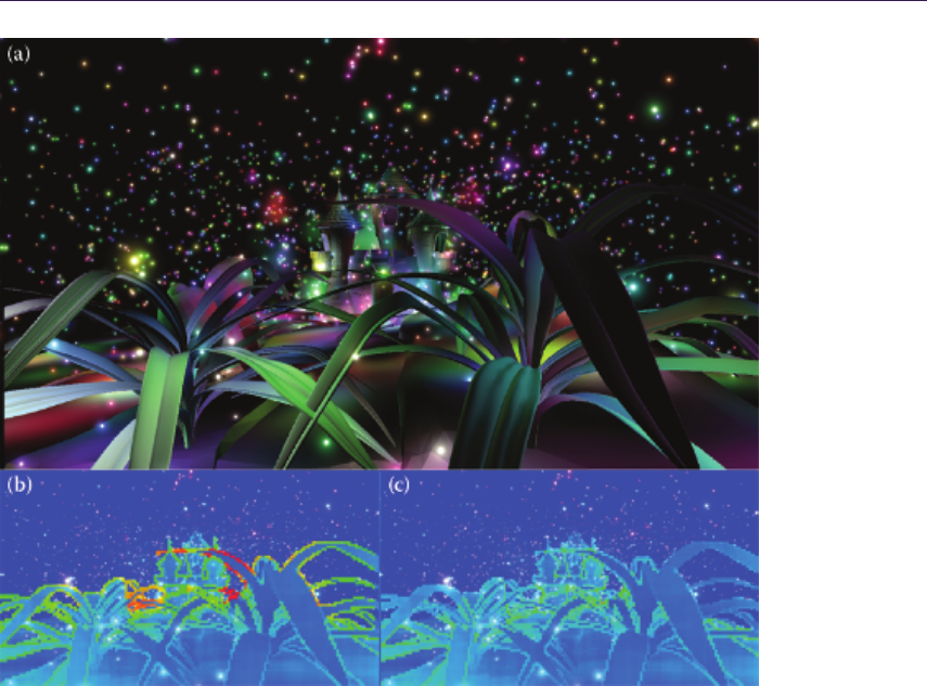
18.6. Extensions 291
Figure 18.7. (a) A scene with a large depth variance that the original Forward+ could
not process efficiently. (b) Visualization of the number of lights per tile using frustum
culled with maximum and minimum depth values in a tile. (c) Visualization of the
number of lights per tile using the proposed 2.5D culling.
(Figure 18.9(a)). Without the proposed method, there are a lot of tiles with more
than 200 lights overlapping. However, by using the 2.5D culling, a tile has at most
120 overlapping lights. The benefit we can get from final shading depends on the
implementation of shader, but culling eliminates a lot of unnecessary memory
reads and computation for the final shader.
We also performed a test on the scene shown in Figure 18.8(a), which does not
have as much depth variance as the scene in Figure 18.7(a). Because the depth
difference is not large in these scenes, the number of lights overlapping a tile,
including an edge of an object, is less than in the previous scene. However, color
temperature is low when the 2.5D culling is used. A quantitative comparison
is shown in Figure 18.9(b). Although the improvement is not as large as the
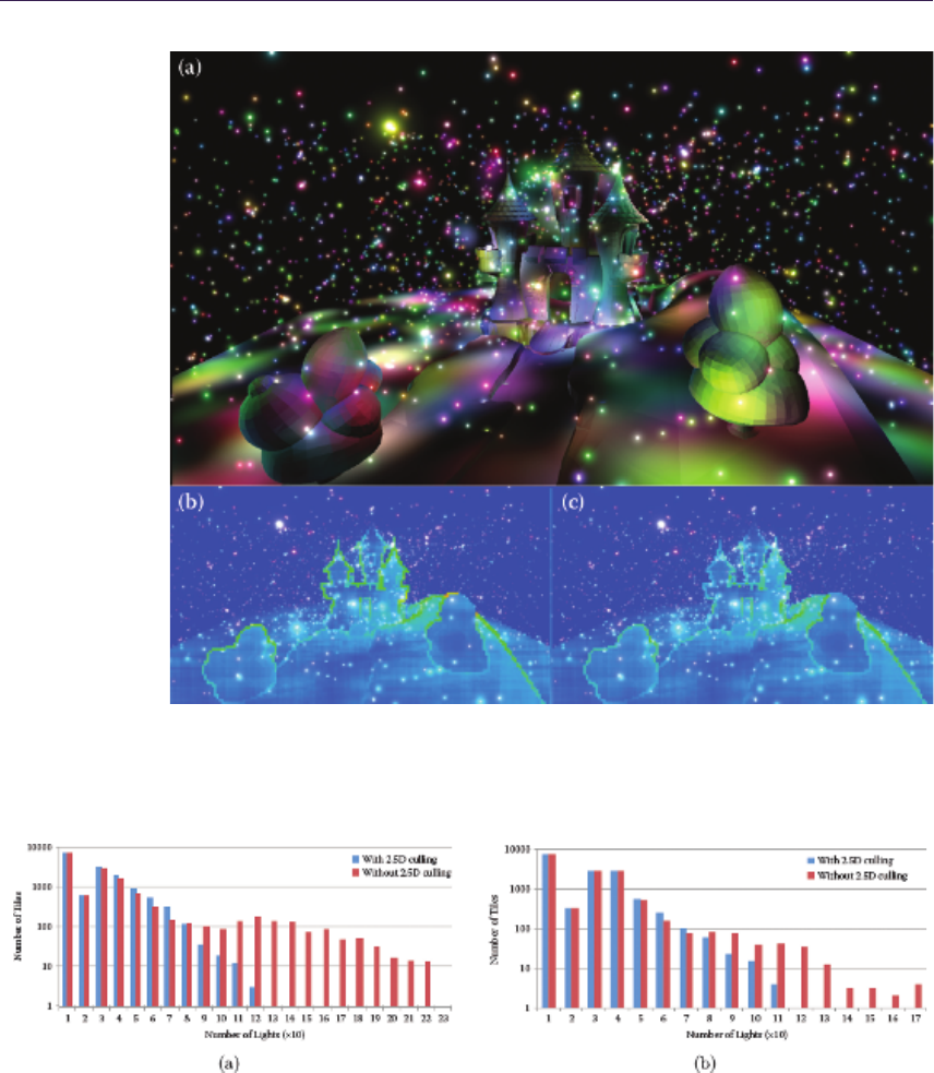
292 18. Forward+: A Step Toward Film-Style Shading in Real Time
Figure 18.8. (a) A scene without a large depth variance. (b) Visualization of the number
of lights per tile using frustum culled with maximum and minimum depth values in a
tile. (c) Visualization of the number of lights per tile using the proposed 2.5D culling.
Figure 18.9. The count of tiles in terms of the number of lights for the scenes shown in
Figures 18.7(a) and 18.8(a), respectively.
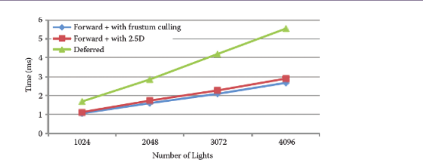
18.6. Extensions 293
Figure 18.10. Comparison of computation time for the light-culling stage of Forward+
using frustum culling only and frustum culling plus 2.5D culling by changing the num-
ber of lights in the scene shown in Figure 18.7(a). Computation time for the light
accumulation in compute-based deferred lighting is also shown.
previous scene, the proposed method could reduce the number of overlapping
lights on tiles.
Figure 18.10 compares the computation time for the light-culling stage for the
scene of Figure 18.1(a) as measured on an AMD Radeon HD 7970 GPU. This
comparison indicates the overhead of additional computation in 2.5D culling is
less than 10% of the time without the culling; when there are 1,024 lights, the
overhead is about 5%. The 2.5D culling is effective regardless of the number of
the light in the scene.
Figure 18.10 also contains the light accumulation time of the compute-based
deferred lighting. We can see that the light-culling stage with the 2.5D culling in
Forward+ is much faster than its counterpart in deferred lighting.
18.6.2 Shadowing from Many Lights
Shadows from a light can be calculated by a shadow map, with which we can get
occlusion from the light in the pixel shader when the forward-rendering pipeline
is used. We can calculate shadows in the same way for Forward+.
Because Forward+ is capable of using hundreds of lights for lighting, it is
natural to wonder how we can use all of those lights in the scene as shadow-
casting lights. One option is use a shadow map for each light. This solution is
not practical because shadow map creation—the cost of which is linear to scene
complexity—can be prohibitively expensive.
We can reduce the shadow map resolution, but this results in low-quality
shadows.

294 18. Forward+: A Step Toward Film-Style Shading in Real Time
Another option relies on rasterization and also borrows an idea from ray
tracing. To check the visibility to a light, we can cast a ray to the light. If
the light is local, the length of the ray is short. This means we do not have to
traverse much in the scene; the cost is not as high as the cost of ray casting a
long ray in full ray tracing.
In this subsection, we describe how ray casting can be integrated in Forward+
to add shadows from hundreds of lights and show that a perfect shadow from hun-
dreds of lights can be obtained in real time. After adding this feature, Forward+
is not just an extension of forward-rendering pipeline but a hybrid of forward,
deferred-rendering pipelines and ray tracing.
Implementation. To ray cast against the scene, we need the position and normal
vector of a primary ray hit and the acceleration data structure for ray casting.
The position of a primary ray hit can be reconstructed from the depth buffer
by applying inverse projection. The normal vector of the entire visible surface,
which is used to avoid casting rays to a light that is at the back of the surface and
to offset the ray origin, can be written at the depth prepass. The prepass is no
longer writing only the depth value, and so it is essentially identical to a G-pass
in the deferred-rendering pipeline. The acceleration structure has to be updated
every frame for a dynamic scene; however, this is a more extensive research topic
and we do not explore it in this chapter. Instead, we just assume that the data
structure is built already.
After the prepass, implementing a ray-cast shadow is straightforward. In a
pixel shader, we have access to all the information about lights, which includes
light position. A shadow ray can be created by the light position and surface
location. Then we can cast the ray against the acceleration structure for an
intersection test. If the ray is intersecting, contribution from the light is masked.
Although this naive implementation is easy to implement, it is far from prac-
tical in terms of performance. The issue is a legacy of the forward-rendering
pipeline. The number of rays to be cast for each pixel is not constant, which
means the computational load or time can vary considerably among pixels even
if they belong to the same surface. This results in a poor utilization of the GPU.
An alternative is to separate ray casting from pixel shading for better perfor-
mance. After separating ray casting from pixel shading, the pipeline looks like
this:
•G-pass,
•light culling,
•ray-cast job creation,
•ray casting,
•final shading.

18.7. Conclusion 295
After indices of lights overlapping each tile are calculated in the light-culling stage,
ray-cast jobs are created and accumulated in a job buffer by iterating through
all the screen pixels. This is a screen-space computation in which a thread is
executed for a pixel and goes through the list of lights. If a pixel overlaps a light,
a ray-cast job is created. To create a ray in the ray-casting stage, we need a pixel
index to obtain surface position and normal, and a light index against which the
ray is cast. These two indices are packed into a 32-bit value and stored in the
job buffer.
After creating all the ray-cast jobs in a buffer, we dispatch a thread for each
ray-cast job. Then it does not have the issue of uneven load balancing we expe-
rience when rays are cast in a pixel shader. Each thread is casting a ray. After
identifying whether a shadow ray is blocked, the information has to be stored
somewhere to pass to a pixel shader. We focused only on a hard shadow, which
means the output from a ray cast is a binary value. Therefore, we have packed
results from 32 rays into one 32-bit value.
But in a scene with hundreds of lights, storing a mask for all of them takes
too much space even after the compression. We took advantage of the fact that
we have a list of lights per tile; masks for lights in the list of a tile are only stored.
We limit the number of rays to be cast per pixel to 128, which means the mask
can be encoded as an int4 value. At the ray-casting stage, the result is written
to the mask of the pixel using an atomic OR operation to flip the assigned bit.
After separating ray casting from pixel shading, we can keep the final shading
almost the same in Forward+. We only need to read the shadow mask for each
pixel; whenever a light is processed, the mask is read to get the occlusion.
Results. Figure 18.11 is a screenshot of a scene with 512 shadow-casting lights.
We can see legs of chairs are casting shadows from many dynamic lights in the
scene. The screen resolution was 1,280 ×720. The number of rays cast for this
scene was more than 7 million. A frame computation time is about 32 ms on
an AMD Radeon HD 7970 GPU. G-pass and light culling took negligible time
compared to ray-cast job creation and ray casting, each of which took 11.57 ms
and 19.91 ms for this frame. This is another example of hybrid ray-traced and
rasterized graphics.
18.7 Conclusion
We have presented Forward+, a rendering pipeline that adds a GPU compute-
based light-culling stage to the traditional forward-rendering pipeline to handle
many lights while keeping the flexibility for material usage. We also presented
the implementation detail of Forward+ using DirectX 11, and its performance.
We described how the Forward+ rendering pipeline is extended to use an indirect
illumination technique in the AMD Leo Demo.
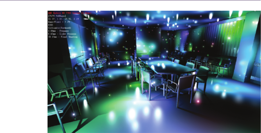
296 18. Forward+: A Step Toward Film-Style Shading in Real Time
Figure 18.11. Dynamic shadowing from 512 lights in a scene with 282,755 triangles.
Because of its simplicity and flexibility, there are many avenues to extend
Forward+. We have described two extensions in this chapter: a 2.5D culling,
which improves the light-culling efficiency, and dynamic shadowing from many
lights.
18.8 Acknowledgments
We would like to thank to members of AMD GPU Tech initiatives and other
people who worked on the AMD Leo demo.
Bibliography
[Andersson 11] J. Andersson. “DirectX 11 Rendering in Battlefield 3.” Presenta-
tion, Game Developers Conference, San Francisco, CA, 2011.
[Dachsbacher and Stamminger 05] C. Dachsbacher and M. Stamminger. “Reflec-
tive Shadow Maps.” In Symposium on Interactive 3D Graphics and Games
(I3D), pp. 203–231. New York: ACM, 2005.
[Ericson 04] C. Ericson. Real-Time Collision Detection. San Francisco: Morgan
Kaufmann, 2004.

Bibliography 297
[Harada et al. 11] T. Harada, J. McKee, and J. C. Yang. “Forward+: Bringing
Deferred Lighting to the Next Level,” Eurographics Short Paper, Cagliari,
Italy, May 15, 2012.
[Yang et al. 10] J. C. Yang, J. Hensley, H. Grun, and N. Thibieroz. “Real-Time
Concurrent Linked List Construction on the GPU.” Computer Graphics Fo-
rum 29:4 (2010), 1297–1304.

19
Progressive Screen-Space
Multichannel Surface Voxelization
Athanasios Gaitatzes and Georgios Papaioannou
19.1 Introduction
An increasing number of techniques for real-time global illumination effects rely
on volume data. Such representations allow the fast, out-of-order access to spa-
tial data from any deferred shading graphics pipeline stage as in [Thiedemann
et al. 11,Mavridis and Papaioannou 11,Kaplanyan and Dachsbacher 10]. For
dynamic environments where both the geometry of the scene and the illumination
can arbitrarily change between frames, these calculations must be performed in
real time. However, when the per frame time budget is limited due to other,
more important operations that must take place while maintaining a high frame
rate, the fidelity of full-scene voxelization has to be traded for less accurate but
faster techniques. This is especially true for video games, where many hun-
dreds of thousands of triangles must be processed in less than 2–3 ms. In this
chapter we present the novel concept of progressive voxelization, an incremental
image-based volume generation scheme for fully dynamic scenes that addresses
the view-dependency issues of image-based voxelization within the above time
constraints.
Screen-space volume generation methods provide very fast and guaranteed
response times compared to geometry-based techniques but suffer from view-
dependency. More specifically, any technique that is performed entirely in screen
space (as in deferred shading) considers only geometry that has been rendered
into the depth buffer and thus has the following strong limitations: First, it
ignores geometry located outside the field of view. Second, it ignores geometry
that is inside the view frustum but occluded by other objects. Yet these geometry
parts may have a significant influence on the desired final result (see our indirect
illumination case study in this article).
In single-frame screen-space voxelization, volume attributes already available
as fragment data in view-dependent image buffers are transformed and rasterized
299

300 19. Progressive Screen-Space Multichannel Surface Voxelization
(injected) into the volume buffer to form a partial volume of the observed space.
These commonly include the view camera G-buffers like depth, albedo, normals,
and the light sources’ reflective shadow maps (RSMs) [Dachsbacher and Stam-
minger 05]. The injection procedure is explained in more detail in [Kaplanyan 09]
and Section 19.2.2 Since the only volume samples that can be produced in each
frame are the ones that are visible in at least one of the images available in the
rendering pipeline, each time the (camera or light) view changes, a new set of
sample points becomes available and the corresponding voxels are generated from
scratch to reflect the newly available image samples. Thus the generated volume
will never contain a complete voxelization of the scene. This leads to significant
frame-to-frame inconsistencies and potentially inadequate volume representations
for the desired volume-based effect, especially when the coverage of the scene in
the available image buffers is limited.
To alleviate the problems of screen-space voxelization techniques, but main-
tain their benefit of predictable, controllable, and bound execution time relative
to full-scene volume generation methods, we introduce the concept of progressive
voxelization (PV). The volume representation is incrementally updated to include
the newly discovered voxels and discard the set of invalid voxels, which are not
present in any of the current image buffers. Using the already available camera
and light source buffers, a combination of volume injection and voxel-to-depth-
buffer reprojection scheme continuously updates the volume buffer and discards
invalid voxels, progressively constructing the final voxelization.
The algorithm is lightweight and operates on complex dynamic environments
where geometry, materials, and lighting can change arbitrarily. Compared to
single-frame screen-space voxelization, our method provides improved volume
coverage (completeness) over nonprogressive methods while maintaining its high
performance merits.
We demonstrate our technique by applying it as an alternative voxeliza-
tion scheme for the light propagation volumes (LPV) diffuse global illumination
method of [Kaplanyan and Dachsbacher 10]. However, being a generic multiat-
tribute scalar voxelization method, it can be used in any other real-time volume
generation problem.
19.2 Overview of Voxelization Method
Our progressive voxelization scheme is able to produce stable and valid volume
data in a geometry-independent manner. As the user interacts with the environ-
ment and dynamic objects move or light information changes, new voxel data are
accumulated into the initial volume and old voxels are invalidated or updated
if their projection in any of the image buffers (camera or light) proves inconsis-
tent with the respective available recorded depth. For a schematic overview see
Figure 19.1, and for a resulting voxelization see Figures 19.4 and 19.5.
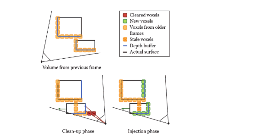
19.2. Overview of Voxelization Method 301
Figure 19.1. Schematic overview of the algorithm. During the cleanup phase each voxel
is tested against the available depth images. If the projected voxel center lies in front
of the recorded depth, it is cleared; otherwise it is retained. During the injection phase,
voxels are “turned-on” based on the RSM-buffers and the camera-based depth buffer.
In each frame, two steps are performed: First, in a cleanup stage, the volume
is swept voxel-by-voxel and the center of each voxel is transformed to the eye-
space coordinate system of the buffer and tested against the available depth image
value, which is also projected to eye-space coordinates. If the voxel lies closer to
the image buffer viewpoint than the recorded depth, the voxel is invalidated and
removed. Otherwise, the current voxel attributes are maintained. The update of
the volume is performed by writing the cleared or retained values into a separate
volume in order to avoid any atomic write operations and thus make the method
fast and a very broadly applicable one. At the end of each cleanup cycle, the
two volume buffers are swapped. After the cleanup phase, samples from all the
available image buffers are injected into the volume (similar to the LPV method
[Kaplanyan 09]).
When multiple image buffers are available, the cleanup stage is repeated for
each image buffer, using the corresponding depth buffer as input for voxel invali-
dation. Each time, the currently updated (read) and output (written) buffers are
swapped. The current image buffer attributes are then successively injected in
the currently updated volume. The whole process is summarized in Figure 19.1.

302 19. Progressive Screen-Space Multichannel Surface Voxelization
in vec3 vo xel_posi tio n , vo xel_ tex _coo rd ;
uniform float voxel_r; // vo xel ra dius
un iform sa mpler3D vol_shR , vol_s hG , vol_shB , vo l_ no rmals ;
voi d mai n ( vo id )
{
vec 4 vox el _p os_wc s = ve c4 ( v ox el _position , 1.0) ;
ve c3 v ox el_ po s_ cs s = P oi nt WCS 2C SS ( v ox el _p os _w cs . x yz );
ve c3 v ox el_ po s_ ec s = P oi nt WCS 2E CS ( v ox el _p os _w cs . x yz );
vec 3 zbuffer_ ss = MAP_ -1 To1_0To1 ( v oxe l_po s_c ss );
float d ep th = S am pl eB uf ( z buff er , z bu ff er _s s . xy ) . x;
vec 3 zbuff er _c ss = ve c3 ( vox el_ po s_ css .xy , 2 .0* depth - 1.0) ;
vec 3 z bu ffer_ec s = Po in tC SS2EC S ( z bu ff er_css ) ;
vec 3 v ox el_mf _w cs = v oxel_ po s_wcs .xyz + voxel _r * vec3 (1. 0) ;
vo xe l_m f_ wcs = max ( v oxe l_m f_wc s ,
vo xel_po s_w cs . xyz + v oxel_h alf _siz e );
ve c3 v oxe l_ mb _w cs = vo xe l_ po s_ wcs . xyz + v oxe l_ r * vec 3 ( - 1.0) ;
vo xe l_m b_ wcs = min ( v oxe l_m b_wc s ,
vo xel_po s_w cs . xyz - v oxel_h alf _siz e );
vec3 voxel_mf_ecs = PointWCS2ECS (voxel_mf_wcs);
vec3 voxel_mb_ecs = PointWCS2ECS (voxel_mb_wcs);
float b ias = d ist anc e ( voxe l_m f_ecs , vo xel _m b_e cs ) ;
vec 4 s hR _v al ue = S am pl eB uf ( vol_shR , vox el _te x_ co ord );
vec 4 s hG _v al ue = S am pl eB uf ( vol_shG , vox el _te x_ co ord );
vec 4 s hB _v al ue = S am pl eB uf ( vol_shB , vox el _te x_ co ord );
vec 4 n ormal _v al ue = S am pl eB uf ( vol_no rmals , v oxel_ te x_c oo rd );
if ( v ox el_ po s_ ecs .z > z buf fe r_e cs . z + b ias ) { // discard
no rmal _va lue = vec 4 (0 ,0 ,0 ,0) ;
sh R_ va lu e = sh G_ va lu e = sh B_value = vec4 (0 ,0 ,0 ,0);
}
// keep
gl _Fr agData [0] = normal _va lue ;
gl _FragD ata [1] = shR_value ;
gl _FragD ata [2] = shG_value ;
gl _FragD ata [3] = shB_value ;
}
Listing 19.1. Cleanup phase fragment shader.
19.2.1 Cleanup Phase
Throughout the entire voxelization process, each voxel goes through three state
transitions: “turn-on,” “turn-off,” and “keep” (see Listing 19.1). The “turn-on”
state change is determined during the injection phase. During the cleanup stage
we need to be able to determine if the state of the voxel will be retained or turned
off (cleared). For each one of the available depth buffers, each voxel center pv
is transformed to eye-space coordinates p′
v; accordingly the corresponding image
buffer depth Z(p′) is transformed to eye-space coordinates ze.
Expressing the coordinates in the eye reference frame (Figure 19.2), if p′
v,z > ze
the voxel must be cleared, as it lies in front of the recorded depth boundary in the
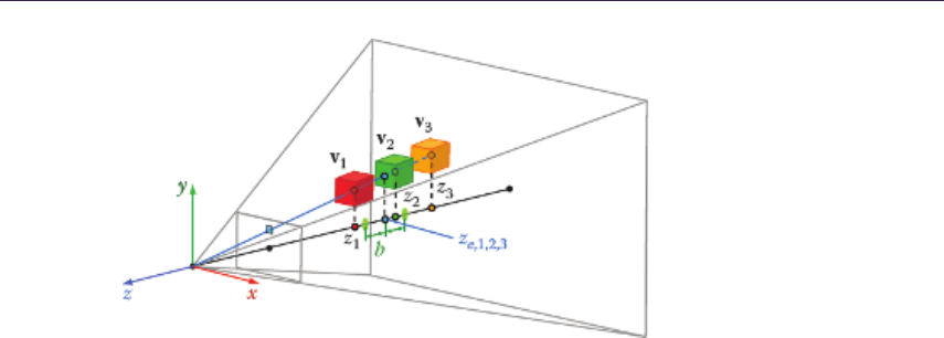
19.2. Overview of Voxelization Method 303
Figure 19.2. Cleanup stage: Voxels beyond the boundary depth zone are retained
(orange), while voxels closer to the buffer center of projection are rejected (red). Voxels
that correspond to the depth value registered in the buffer must be updated (green).
image buffer. However, the spatial data are quantized according to the volume
resolution and therefore a bias bhas to be introduced in order to avoid rejecting
boundary samples. Since the depth comparison is performed in eye-space, bis
equal to the voxel’s pvradius (half diagonal) clamped by the voxel boundaries in
each direction. Therefore the rejection condition becomes
P′
v,z > ze +b.
The example in Figure 19.2 explains the cleanup and update state changes
of a voxel with respect to the available depth information in an image buffer.
All voxels in the figure correspond to the same image buffer sample with eye-
space value ze,1,2,3. Voxel v1is rejected (cleared) because z1is greater than
ze,1,2,3+b. Voxel v2must be updated since it lies within the boundary depth
zone [ze,1,2,3−b, ze,1,2,3+b]. Finally, voxel v3is retained, since it lies beyond the
registered depth value.
19.2.2 Injection Phase
In the injection phase, a rectangular grid of point primitives corresponding to
each depth image buffer is sent to a vertex shader that offsets the points ac-
cording to the stored depth. The points are subsequently transformed to world
space and finally to volume-clip space. If world-space or volume clip-space co-
ordinates are already available in the buffers, they are directly assigned to the
corresponding injected points. The volume clip-space depth is finally used to
determine the slice in the volume where the point sample attributes are accu-
mulated (see Listing 19.2). At the end of this stage, the previous version of the
scene’s voxel representation has been updated to include a partial voxelization

304 19. Progressive Screen-Space Multichannel Surface Voxelization
// Verte x - Shade r Sta ge
fla t out vec2 t ex _coord ;
un ifo rm sampl er2 D zbuffer ;
voi d mai n ( vo id )
{
t ex _c oo rd = g l_ Ve rt ex . xy ;
float d ept h = Sa mp le Bu f ( zbuffer , tex_c oo rd ). x;
// scr een spa ce --> can on ic al sc re en space
vec 3 pos _cs s = MAP_0To1_ -1 T o1 ( vec3 ( g l_V ert ex .xy , de pth ) );
// canonical screen sp ace --> obj ect spa ce
vec 3 p os_wcs = Po intCS S2 WC S ( z buffe r_ cs s ) ;
// w orld space -- > clip s pace
gl _P osition = g l_M ode lV iew Pro je c ti onM atr ix *
ve c4 ( po s_wc s , 1 .0) ;
}
// Geo metry - Shad er St age
la you t ( poin ts ) in ;
layout ( points , ma x_ver ti ce s = 1) out ;
uniform int v ol_ dep th ;
fla t in vec 2 t ex _c oo rd [];
fla t out vec2 g tex_coord ;
voi d mai n ( vo id )
{
gt ex _c oord = te x_coord [0];
gl _P osition = gl _P os iti on In [ 0];
gl _L ay er = int ( v ol_ dep th * MAP_ -1 To1_0T o1 ( gl _Po sition . z) );
E mi tV er te x ( ) ;
}
Listing 19.2. Injection phase using a geometry shader to select the destination slice of
the volume for the point samples.
of the scene based on the newly injected point samples. The resolution of the
grid of 2D points determines how much detail of the surfaces represented by the
depth buffer is transferred into the volume and whether or not the geometry is
sparsely sampled. If too few points are injected, the resulting volume will have
gaps. This may be undesirable for certain application cases, such as the LPV
method [Kaplanyan 09] or algorithms based on ray marching.
19.2.3 Single-Pass Progressive Algorithm
In order to transfer the geometric detail present in the G-buffers to the volume
representation and ensure a dense population of the resulting volume, a large res-
olution for the grid of injected points must be used. However, the injection stage

19.3. Progressive Voxelization for Lighting 305
involves rendering the point grid using an equal number of texture lookups and, in
some implementations, a geometry shader. This has a potentially serious impact
on performance (see Figure 19.8), especially for multiple injection viewpoints.
We can totally forgo the injection phase of the algorithm and do both opera-
tions in one stage. Using the same notation as before, the logic of the algorithm
remains practically the same. If the projected voxel center lies in front of the
recorded depth (i.e., p′
v,z > ze+b), it is still cleared. If the projected voxel
center lies behind the recorded depth (i.e., p′
v,z < ze−b), the voxel is retained;
otherwise it is turned-on (or updated) using the attribute buffers information.
The last operation practically replaces the injection stage.
As we are effectively sampling the geometry at the volume resolution instead of
doing so at higher, image-size-dependent rate and then down-sampling to volume
resolution, the resulting voxelization is expected to degrade. However, since usu-
ally depth buffers are recorded from multiple views, missing details are gradually
added. A comparison of the method variations and analysis of their respective
running times is given in Section 19.5.
19.3 Progressive Voxelization for Lighting
As a case study, we applied progressive voxelization to the problem of comput-
ing indirect illumination for real-time rendering. When using the technique for
lighting effects, as in the case of the LPV algorithm of [Kaplanyan 09] or the ray
marching techniques of [Thiedemann et al. 11,Mavridis and Papaioannou 11],
the volume attributes must include occlusion information (referred to as geome-
try volume in [Kaplanyan 09]), sampled normal vectors, direct lighting (VPLs),
and optionally surface albedo in the case of secondary indirect light bounces.
Direct illumination and other accumulated directional data are usually encoded
and stored as low-frequency spherical harmonic coefficients (see [Sloan et al. 02]).
Virtual point lights (VPLs) are points in space that act as light sources and
encapsulate light reflected off a surface at a given location. In order to correctly
accumulate VPLs in the volume, during the injection phase, a separate volume
buffer is used that is cleared in every frame in order to avoid erroneous accumu-
lation of lighting. For each RSM, all VPLs are injected and additively blended.
Finally, the camera attribute buffers are injected to provide view-dependent dense
samples of the volume. If lighting from the camera is also exploited (as in our
implementation), the injected VPLs must replace the corresponding values in the
volume, since the camera direct lighting buffer provides cumulative illumination.
After the cleanup has been performed on the previous version of the attribute
volume Vprev, nonempty voxels from the separate injection buffer replace corre-
sponding values in Vcurr. This ensures that potentially stale illumination on valid
volume cells from previous frames is not retained in the final volume buffer. In
Figure 19.3 we can see the results of progressive voxelization and its application
to diffuse indirect lighting.
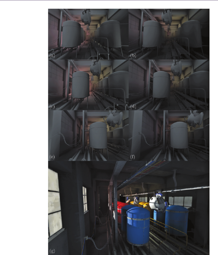
306 19. Progressive Screen-Space Multichannel Surface Voxelization
Figure 19.3. (a–f) As the camera moves left to right, we observe correct indirect illu-
mination. (g) Final rendering of the room.

19.4. Implementation 307
19.4 Implementation
The progressive voxelization method runs entirely on the GPU and has been
implemented in a deferred shading renderer using basic OpenGL 3.0 operations
on a NVIDIA GTX 285 card with 1 GB of memory. We have implemented two
versions of the buffer storage mechanism in order to test their respective speed.
The first uses 3D volume textures along with a geometry shader that sorts injected
fragments to the correct volume slice. The second unwraps the volume buffers
into 2D textures and dispenses with the expensive geometry processing (respective
performance can be seen in Figure 19.8).
The texture requirements are two volume buffers for ping-pong rendering
(Vprev,Vcurr). Each volume buffer stores N-dimensional attribute vectors aand
corresponds to a number of textures (2D or 3D) equal to ⌈N/4⌉, for 4-channel
textures. For the reasons explained in Section 19.3 an additional N-dimensional
volume buffer is required for lighting applications. In our implementation we
need to store surface normals and full color spherical harmonics coefficients for
incident flux in each volume buffer, which translates to 3 ×4 textures in total.
In terms of volume generation engine design, the user has the option to re-
quest several attributes to be computed and stored into floating-point buffers for
later use. Among them are surface attributes like albedo and normals, but also
dynamic lighting information and radiance values in the form of low-order spher-
ical harmonics (SH) coefficients representation (either monochrome radiance or
full color encoding, i.e., separate radiance values per color band). In our im-
plementation the radiance of the corresponding scene location is calculated and
stored as a second-order spherical harmonic representation for each voxel. For
each color band, four SH coefficients are computed and encoded as RGBA float
values.
19.5 Performance and Evaluation
In terms of voxelization robustness, our algorithm complements single-frame
screen-space voxelization and supports both moving image viewpoints and fully
dynamic geometry and lighting. This is demonstrated in Figures 19.4 and 19.5. In
addition, in Figure 19.6, a partial volume representation of the Crytek Sponza II
Atrium model is generated at a 643resolution and a 1282-point injection grid
using single-frame and progressive voxelization. Figures 19.6(a) and (b) are the
single-frame volumes from two distinct viewpoints. Figure 19.6(c) is the progres-
sive voxelization after the viewpoint moves across several frames. Using the par-
tial single-frame volumes for global illumination calculation, we observe abrupt
changes in lighting as the camera reveals more occluding geometry (e.g., left ar-
cade wall and floor in Figures 19.6(d) and (e)). However, the situation is gradually
remedied in the case of progressive voxelization, since newly discovered volume
data are retained for use in following frames (Figures 19.6(f) and (g)).
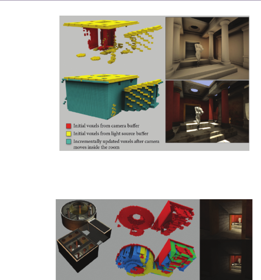
308 19. Progressive Screen-Space Multichannel Surface Voxelization
Figure 19.4. Left: Screen-space voxelization after one step of the process having injected
the camera and light buffers (top), and voxelization of the scene after the camera has
moved for several frames (bottom). Right: Example of resulting indirect illumination
(top) and final illumination (bottom).
Figure 19.5. Progressive voxelization of a scene. Red voxels correspond to screen-space
voxelization using image buffers from the current frame only, while other colors refer to
voxels generated during previous frames using PV. On the right, volume-based global
illumination results using the corresponding volumes. PV (top) achieves more correct
occlusion and stable lighting.
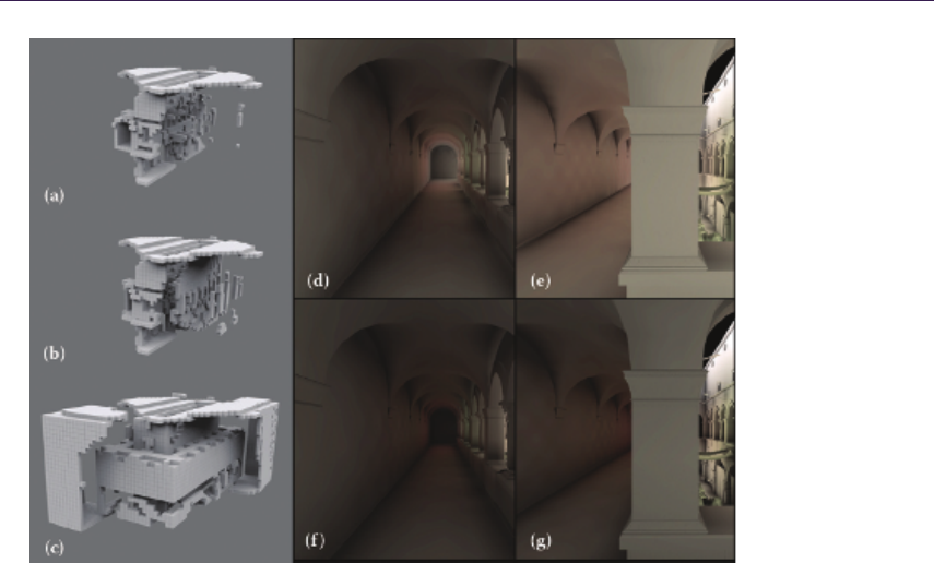
19.5. Performance and Evaluation 309
Figure 19.6. Comparison of the voxelization of the Crytek Sponza II Atrium.
(a, b) Single-frame screen-space voxelization from two distinct viewpoints where it is
not possible to capture all environment details as no information exists in the buffers.
(c) Progressive voxelization produced over several frames. (d, e) Indirect lighting buffers
corresponding to the single frame voxelization of (a) and (b). (f, g) PV indirect lighting
buffers (of the voxelization in (c)).
Figure 19.7 demonstrates progressive voxelization in a dynamic environment
in real time. In particular, it shows an animated sequence of a scene with moving
and deformable objects, as well as the corresponding voxelization from the camera
viewpoint. Observe how the wall behind the closed door is not initially present
in the volume, but after the door opens, it is gradually added to the volume
and remains there even after the door swings back. The same holds true for
the geometry behind the character. Notice also how the voxels representing the
articulated figure correctly change state as the figure moves.
Figure 19.8 shows a decomposition of the total algorithm running time into
the cleanup and injection stage times respectively versus different volume buffer
resolutions for three different injection grid sizes using the 3D volume textures
implementation (left) and the 2D textures implementation (center). For fixed
injection grid resolutions, we have observed that injection times are not mono-
tonically increasing with respect to volume size as one would expect. The per-
formance also decreases when the buffer viewpoint moves close to geometry.
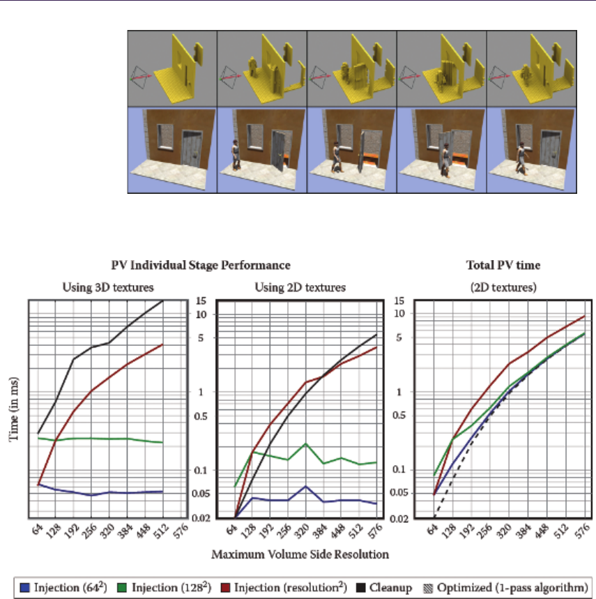
310 19. Progressive Screen-Space Multichannel Surface Voxelization
Figure 19.7. Screen-space voxelization of a dynamic scene containing an articulated
object using only camera-based injection.
Figure 19.8. Running time (in ms) for the cleanup and injection stages against different
volume resolutions for the Crytek Sponza II Atrium model using the 3D volume tex-
tures implementation (left) and the 2D textures implementation (center). We used a
single G-buffer (camera) as input and one multiple render target (four floats) as output.
Injection is measured for three different grid sizes, one being proportional to the vol-
ume side. We also show the total progressive voxelization times (right). Note that the
performance of the optimized progressive voxelization is identical to that of the cleanup
stage.

19.5. Performance and Evaluation 311
We attribute this to the common denominator of both cases, namely the fact
that pixel overdraw is induced, as points are rasterized in the same voxel loca-
tions. This is particularly evident in the blue curve of the 642injection stage
graph of Figure 19.8 (left). Note that this behavior is an inherent attribute of
injection techniques in general; screen-space voxelization methods depend heavily
on the sampling rate used. When this rate is incompatible with the voxel space
resolution, holes might appear (undersampling). To ensure adequate coverage of
the voxel grid, dense screen-space point samples are drawn, which in turn leads
to overdraw problems in many cases. One can use an injection grid proportional
to the volume resolution, which partially alleviates the overdraw issue but in turn
decreases performance as can be seen in the red curve of the injection graph of
Figure 19.8 (left and center).
The time required for a single-frame screen-space voxelization (one G-buffer)
equals the time of our injection stage plus a very small overhead to clear the
volume buffer, since the two operations are equivalent. Thus, the only difference
in the execution time of progressive voxelization is the cleanup stage time. With
regard to the quality of the two methods, PV offers more stable and accurate
results as new viewpoints gradually improve the volume.
The total voxelization time (Figure 19.8, right) is the sum of the cleanup and
injection stages. As the cleanup stage performance depends only on the volume
resolution and not on the injection grid size, it vastly improves the voxelization
quality compared to using only screen-space injection from isolated frames, at
a constant overhead per frame. Especially when applied to global illumination
calculations, where small volumes are typically used, the version of the algorithm
that uses 2D textures (Figure 19.8, center) has a significantly lower execution
footprint. This is because it is not influenced by the geometry shader execution
of the 3D textures version (Figure 19.8, left), though both methods are affected
by pixel overdraw during injection.
The performance of the optimized progressive voxelization is identical to that
of the cleanup stage as expected, since it is essentially a modified cleanup stage.
It follows that the dual stage version performance will always be slower than the
optimized one.
The maximum volume resolution reported is due to hardware resource limita-
tions on the number and size of the allocated buffers and not algorithm bounds.
In Table 19.1 we report the voxelization performance results for several scenes
using our method and the geometry-based multichannel full scene voxelization
method of [Gaitatzes et al. 11], which, as ours, is based on the rendering pipeline
(GPU). We show a big speed improvement even when adding to the whole process
the G-buffers creation time.
In Table 19.2 we report on the quality of our voxelization method. The cam-
era was moved around the mesh for several frames, in order for the algorithm
to progressively compute the best possible voxelization. For several models and
resolutions we show the Hausdorff distance between the original mesh and the
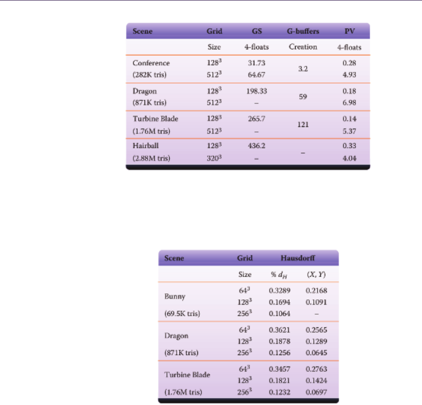
312 19. Progressive Screen-Space Multichannel Surface Voxelization
Table 19.1. Voxelization timings (in ms) of various scenes using progressive voxelization
(PV) and the geometry slicing (GS) method of [Gaitatzes et al. 11] with 11 output
vertices. We present the total (injection + cleanup) performance values of our 2D
textures implementation using an injection grid proportional to the volume size, which
is our algorithm’s worst case as can be seen from the red plot of Figure 19.8.
Table 19.2. Comparison of a full voxelization. We record the normalized (with respect
to the mesh bounding box diagonal) average Hausdorff distance (percent). Mesh Xis
the original mesh to be voxelized and Yis the point cloud consisting of the voxel centers
of the voxelization using PV (column 3) and a geometry-based full scene voxelization
(column 4).
resulting voxelization using the PV method (see column 3). We notice that our
voxelized object (voxel centers) is on average 0.1% different from the original
mesh. In addition, we report the Hausdorff distance between the original mesh
and the geometry-based full scene voxelization of [Gaitatzes et al. 11] (see col-
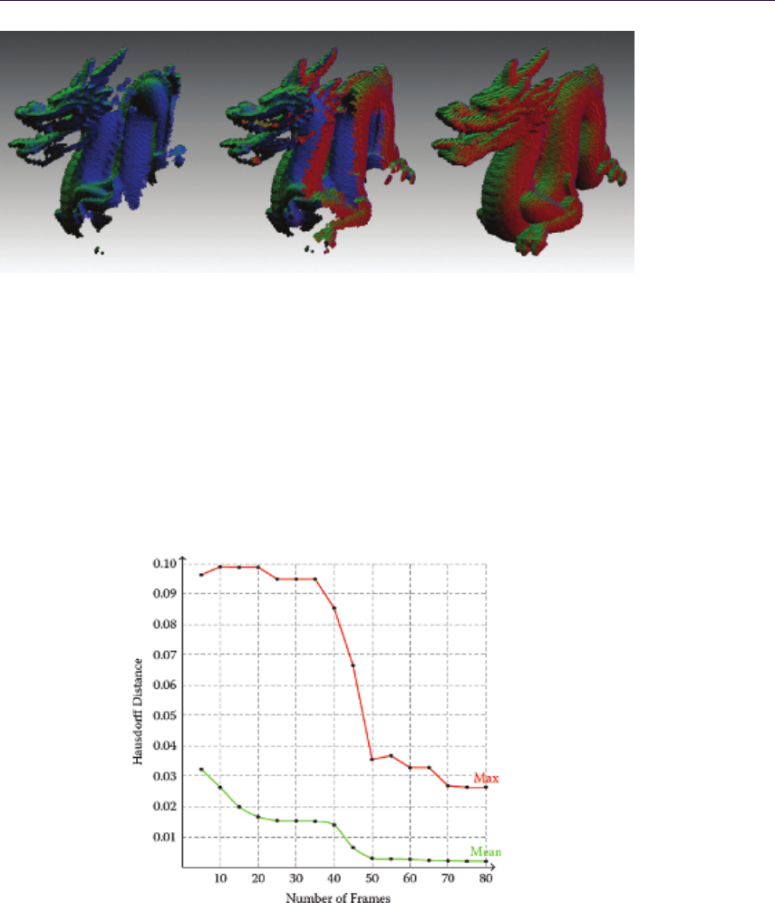
19.5. Performance and Evaluation 313
Figure 19.9. A series of voxelizations of the dragon model at 1283resolution showing
the normal vectors. The voxelization is incrementally updated over several frames as
the camera moves around the model.
umn 4). We observe that the difference between the corresponding volumes is in
the 0.01% range.
In Figure 19.9 we show a series of voxelizations of the dragon model using only
the camera G-buffers. In addition, we show the respective Hausdorff distance
between the original dragon model and the computed voxel centers (see plot
in Figure 19.10). The voxelization is incrementally updated and improved over
Figure 19.10. The decreasing Hausdorff distance between the original dragon model
and the computed progressive voxelizations of Figure 19.9.
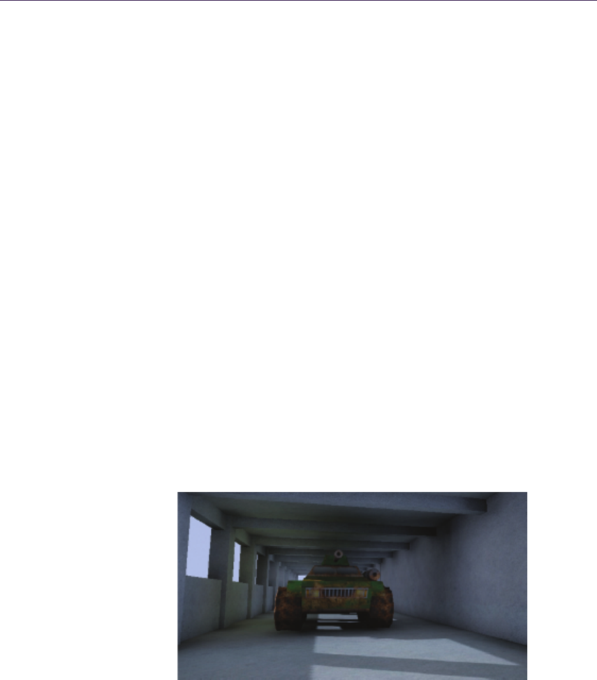
314 19. Progressive Screen-Space Multichannel Surface Voxelization
several frames as the camera does a complete rotation around each of the principal
axis for an equal amount of frames. As the animation progresses, we observe that
the Hausdorff distance decreases as the process converges to a full voxelization.
19.6 Limitations
One limitation of our method is that the cleanup phase will only remove invalid
voxels that are visible in any of the current image buffers (camera multiple ren-
der targets and light RSMs). The visible invalid voxels will be removed from the
voxelization the next time they appear in the image buffers. However, the cor-
rectness of the voxelization cannot be guaranteed for existing voxels that are not
visible in any buffer. For moving geometry, some progressively generated voxels
may become stale, as shown in the case of the bottom right of Figure 19.1. Nev-
ertheless, in typical dynamic scenes, the stale voxels are often eliminated either
in subsequent frames due to their invalidation in the moving camera buffer or
due to their invalidation in other views in the same frame (see Figure 19.11).
Another limitation is that the extents of the voxelization region must remain
constant throughout volume updates; otherwise computations are performed with
stale buffer boundaries. When the bounding box of the scene is modified or the
scene changes abruptly or it is reloaded, the attribute volumes must be deleted
and progressively populated again. This is also the reason why the cascaded
light propagation volumes method of [Kaplanyan and Dachsbacher 10] could not
take advantage of progressive voxelization for the cascades near the user, as the
method assumes that they follow the user around, constantly modifying the cur-
rent volume extents.
Figure 19.11. Correct indirect shadowing effects and color bleeding: Stale voxels from
one view (behind the tank) are effectively invalidated in other views (reflective shadow
map).

19.7. Conclusion 315
19.7 Conclusion
We have presented a novel screen-space method to progressively build a vox-
elization data structure on the GPU. Our method achieves improved quality
over nonprogressive methods, while it maintains the high performance merits of
screen-space techniques.
19.8 Acknowledgments
The Atrium Sponza II Palace in Dubrovnik model was remodeled by Frank Meinl
at Crytek. The original Sponza model was created by Marko Dabrovic in early
2002. The Bunny and Dragon models are provided courtesy of the Stanford
University Computer Graphics Laboratory.
Bibliography
[Dachsbacher and Stamminger 05] Carsten Dachsbacher and Marc Stamminger.
“Reflective Shadow Maps.” In Symposium on Interactive 3D Graphics and
Games (I3D), pp. 203–231. New York: ACM, 2005.
[Gaitatzes et al. 11] Athanasios Gaitatzes, Pavlos Mavridis, and Georgios Pa-
paioannou. “Two Simple Single-Pass GPU Methods for Multi-channel Sur-
face Voxelization of Dynamic Scenes.” In Pacific Conference on Computer
Graphics and Applications—Short Papers (PG), pp. 31–36. Aire-la-Ville,
Switzerland: Eurographics Association, 2011.
[Kaplanyan 09] Anton Kaplanyan. “Light Propagation Volumes in CryEngine 3.”
SIGGRAPH Course: Advances in Real-Time Rendering in 3D Graphics and
Games, SIGGRAPH 2009, New Orleans, LA, August 3, 2009.
[Kaplanyan and Dachsbacher 10] Anton Kaplanyan and Carsten Dachsbacher.
“Cascaded Light Propagation Volumes for Real-Time Indirect Illumination.”
In Symposium on Interactive 3D Graphics and Games (I3D), pp. 99–107.
New York: ACM, 2010.
[Mavridis and Papaioannou 11] Pavlos Mavridis and Georgios Papaioannou.
“Global Illumination Using Imperfect Volumes.” Presentation, International
Conference on Computer Graphics Theory and Applications (GRAPP), Al-
garve, Portugal, 2011.
[Sloan et al. 02] Peter-Pike Sloan, Jan Kautz, and John Snyder. “Precomputed
Radiance Transfer for Real-Time Rendering in Dynamic, Low-Frequency
Lighting Environments.” In 29th Conference on Computer Graphics and In-
teractive Techniques (SIGGRAPH), pp. 527–536. New York: ACM, 2002.

20
Rasterized Voxel-Based
Dynamic Global Illumination
Hawar Doghramachi
20.1 Introduction
For modern games it becomes more and more important to offer a realistic envi-
ronment, where a convincing illumination plays a central role. Therefor, not only
direct illumination but also indirect illumination has to be taken into account. At
the same time modern games increasingly offer the player the possibility to inter-
act with the game world, i.e., move objects around, destroy buildings, or change
the lighting dynamically. This is where dynamic global illumination comes into
play; in contrast to static precalculated solutions, it does account for highly dy-
namic environments.
Rasterized voxel-based dynamic global illumination takes into consideration
that scenes, especially indoor, can contain a large number of light sources of
different types (e.g., point, spot, and directional lights). At the same time it
produces visually good and stable results while maintaining high interactive frame
rates.
20.2 Overview
This technique efficiently utilizes features, which were introduced by DirectX 11
hardware, to accomplish the above stated results.
In the first step a voxel grid representation is created for the scene by using
the hardware rasterizer. Here the scene is rendered without depth testing into
a small 2D render-target, but instead of outputting the results into the bound
render-target, the rasterized pixels are written into a 3D read-write buffer by
using atomic functions. In this way the rasterizer is turned into a “voxelizer,”
creating efficiently a highly populated 3D grid representation of the scene. This
voxel grid contains the diffuse albedo and normal information of the geometry
317

318 20. Rasterized Voxel-Based Dynamic Global Illumination
and is used later to generate the indirect illumination and to test for geometry
occlusion. Since the voxel grid is recreated each frame, the proposed technique
is fully dynamic and does not rely on any precalculations.
In the second step, the voxels inside the grid are illuminated by each light
source. The illumination is then converted into virtual point lights (VPLs), stored
as second-order spherical harmonics coefficients (SH-coefficients). The graphics
hardware is utilized again by using the built in blending stage, in order to com-
bine the results of each light source. Later the generated VPLs are propagated
within the grid, in order to generate the indirect illumination. In contrast to
the light propagation volume (LPV) technique, as proposed by [Kaplanyan and
Dachsbacher 10], it is required neither to create a reflective shadow map for each
light source nor to inject VPLs into a grid afterwards. Furthermore, there is no
need to generate occlusion information separately. Yet the obtained information
will be more precise than, e.g., information obtained from depth peeling.
20.3 Implementation
The proposed technique can be subdivided into five distinct steps.
20.3.1 Create Voxel Grid Representation of the Scene
We first need to define the properties of a cubic voxel grid, i.e., its extents,
position, and view-/projection-matrices. The grid is moved synchronously with
the viewer camera and snapped permanently to the grid cell boundaries to avoid
flickering due to the discrete voxel grid representation of the scene. To correctly
map our scene to a voxel grid, we need to use an orthographic projection; thus,
we will use three view-matrices to get a higher coverage of the scene: one matrix
for the back-to-front view, one matrix for the right-to-left view, and one for the
top-to-down view. All other calculations will be done entirely on the GPU.
Next we render the scene geometry that is located inside the grid boundaries
with disabled color writing and without depth testing into a small 2D render-
target. We will use a 32 ×32 ×32 grid; for this it is entirely enough to use a
64 ×64 pixel render-target with the smallest available pixel format, since we will
output the results into a read-write buffer anyway. Basically we pass the triangle
vertices through the vertex shader to the geometry shader. In the geometry
shader the view-matrix is chosen at which the triangle is most visible, in order
to achieve the highest number of rasterized pixels for the primitive. Additionally
the triangle size in normalized device coordinates is increased by the texel size
of the currently bound render-target. In this way, pixels that would have been
discarded due to the low resolution of the currently bound render-target will
still be rasterized. The rasterized pixels are written atomically into a 3D read-
write structured buffer in the pixel shader. In this way, in contrast to [Mavridis
and Papaioannou 11], there is no need to amplify geometry within the geometry

20.3. Implementation 319
shader in order to obtain a highly populated 3D grid representation of the scene.
Listing 20.1 shows how this is done for DirectX 11 in HLSL.
// vertex shader
VS _O UTP UT m ain ( V S_I NP UT in put )
{
VS _OU TP UT outp ut ;
ou tpu t . p osi tio n = fl oat 4 ( inpu t . posi tion ,1 .0 f);
ou tput . t exC oords = input . t exC oor ds ;
ou tpu t . normal = inp ut . nor mal ;
return output;
}
// ge om et ry sh ader
static float3 v iewDi re ction s [3] =
{
f lo at3 (0 .0 f , 0. 0 f , - 1.0 f ) , // back to fr ont
float3 ( -1.0f ,0.0 f ,0.0 f), // ri ght to left
f lo at3 (0 .0 f , -1.0 f , 0 .0 f ) // top to down
};
int G e tV ie wI nd ex ( in fl oat 3 no rm al )
{
fl oat 3x3 d ire ctio nM atrix ;
d ire ct io nM at ri x [ 0] = - v ie wD ir ec ti on s [ 0];
d ire ct io nM at ri x [ 1] = - v ie wD ir ec ti on s [ 1];
d ire ct io nM at ri x [ 2] = - v ie wD ir ec ti on s [ 2];
fl oa t3 d ot Pr odu ct s = abs ( m ul ( di re cti on Mat ri x , nor ma l ));
float m axi mum = max ( max ( do tProdu cts . x, d otP roduct s .y), dotPr odu cts . z);
int i ndex ;
if ( ma xim um == do tPro duc ts . x)
index = 0;
el se if ( maxim um == dotPr odu cts .y )
index = 1;
els e
index = 2;
return in dex ;
}
[maxvertexcount(3)]
voi d mai n ( tr ia ng le VS _OU TP UT input [3] , inout Tr iangleSt ream < GS_OUTPUT >
outputStream)
{
fl oat 3 fa ceN orm al = normalize ( inp ut [ 0]. n orm al + input [1]. n orm al +
input [2]. normal );
// Get view , at whi ch the cu rr en t t ri angle is mos t vis ible , in order to
// ac hieve h igh est po ssi ble raste riz atio n of the pr imi tiv e .
int v iew Ind ex = G etView Ind ex ( faceN orm al );
GS _O UT PU T output [3];
[ un roll ]
for (int i =0; i < 3; i ++)
{
output [i ]. position = mul ( cons tB uff er . gr idVi ewP ro jM atri ces [ v iew In dex ] ,
in pu t [ i ]. p os it io n ) ;
o utp ut [ i ]. po si ti on W S = in put [ i ]. po si ti on . x yz ; // worl d - s pac e positio n
o utp ut [ i ]. te xC oo rd s = in pu t [ i ]. t ex Co or ds ;
o utp ut [ i ]. no rma l = in pu t [ i ]. n or mal ;
}

320 20. Rasterized Voxel-Based Dynamic Global Illumination
// Increase size of t ri an gl e in n ormalized device c oo rdina te s by the
// tex el si ze of th e c ur ren tly bo und render - ta rget .
float2 side0N = n or ma li ze ( output [ 1]. p os it io n .xy - output [0]. po si ti on . xy );
float2 side1N = n or ma li ze ( output [ 2]. p os it io n .xy - output [1]. po si ti on . xy );
float2 side2N = n or ma li ze ( output [ 0]. p os it io n .xy - output [2]. po si ti on . xy );
float t exe lS iz e = 1.0 f / 64. 0 f;
ou tpu t [0] . po sition . xy += n or mal ize ( - si de0N + sid e2N )* t exe lSi ze ;
out put [1] . po sit ion . xy += normalize ( side0N - side1 N )* texelSize ;
ou tput [2]. p osi tio n .xy += n orm ali ze ( side1N - si de2N )* t exe lSi ze ;
[unroll
for (int j =0; j <3 ; j ++)
out pu tSt re am . Ap pen d ( out put [ j ]);
outputStream.RestartStrip();
}
// pixel sh ader
struct VOXEL
{
uin t colorMask ; // en co de d co lor
uint4 no rmalMa sks ; // enc od ed no rm al s
uin t occlusion ; // voxel only co nt ai ns geomet ry info if oc cl us io n > 0
};
R WSt ru ct ur ed Buf fe r < VOXEL > g ri dB uf fe r : r egi ste r ( u1 );
// no rm alized dir ec ti on s of fou r faces of a tetra he dr on
static fl oat3 f aceVe ct or s [4] =
{
f lo at3 (0 .0 f , - 0 .57 73 50 26 f ,0 . 81 64 96 6 1 f ) ,
float3 (0.0 f , -0.5773 5026 f , -0.81 649661 f ),
float3 ( -0 .816496 61 f ,0.57 73 50 26 f ,0.0 f) ,
fl oat 3 (0 .8 16 496 61 f ,0 .5 77 35 02 6 f ,0. 0 f)
};
int G e tN or ma l In de x ( in f lo at3 n orma l , out float do tPr odu ct )
{
fl oat 4x3 faceMatri x ;
fa ce Ma trix [0] = fac eV ec to rs [0];
fa ce Ma trix [1] = fac eV ec to rs [1];
fa ce Ma trix [2] = fac eV ec to rs [2];
fa ce Ma trix [3] = fac eV ec to rs [3];
fl oat 4 d ot Pro du ct s = mul ( f ace Mat rix , n orm al ) ;
float m ax imu m = max ( max ( d ot Pr od uct s . x, do tP rod uc ts . y ),
max ( do tP ro duc ts .z , d ot Pro du ct s . w ));
int i ndex ;
if ( ma xim um == do tPro duc ts . x)
index = 0;
els e i f ( max imu m == d otPr odu cts .y )
index = 1;
el se if ( maxim um == dot Pro duc ts . z)
index = 2;
els e
index = 3;
dot Pr odu ct = do tPr od uct s [ ind ex ];
return in dex ;
}
void m ain ( G S_ OUT PUT in put )
{
flo at3 b ase = colorMap . Sampl e ( col orM apSam pler , in put . t exC oor ds ). rgb ;

20.3. Implementation 321
// Encod e color int o the lowe r 24 bit of an u ns ig ne d int eger , using
// 8 bit for each c olor ch ann el .
uin t co lor Mas k = E nc ode Co lor ( bas e . rgb );
// Ca lcu late col or - c han nel cont rast of co lor and wri te value int o the
// hi ghe st 8 bit of the c olo r mask .
float c ont ras t = le ngt h ( bas e .rrg - bas e . gbb )/
( sq rt (2 .0 f )+ ba se .r + bas e .g + base . b );
int iContrast = i nt ( c on tr as t *25 5. 0 f );
co lor Mas k |= iContra st < <24;
// Encode normal int o the lowe r 27 bit of an u ns ig ne d int eger , using
// for each axis 8 bit for the valu e and 1 bit for the si gn .
flo at3 no rma l = no rma liz e ( input . n orm al );
uint norma lMa sk = E nc ode No rma l ( no rmal . xyz );
// Ca lc ul at e to which fac e of a tetra he dr on curren t normal is c losest
// and writ e c or re spo nd in g dot prod uc t into the high es t 5 bit of the
// no rma l mask .
float dotProduc t ;
int n or ma lI nd ex = G et No rm al In de x ( nor mal , d ot Pr od uct );
int i Do tP roduct = in t ( sa tu ra te ( do t Pr od uc t ) * 31. 0 f );
no rma lMask |= iDo tPro duct < <27;
// Get o ffs et int o vox el gr id .
fl oat 3 off set = ( in put . po sit ionW S - c on stB uf fer . sn ap pe dGr id Ce nt er )*
co nst Buffer . inv Gri dCel lSi ze ;
of fse t = rou nd ( offse t );
// Get p osi ti on in vox el gr id .
int 3 vo xel Po s = int3 (1 6 ,16 ,1 6)+ i nt3 ( o ffs et );
// Onl y out put vo xel s that are in sid e the b oun da ries of the g rid .
if (( v oxe lPo s .x > -1)&&( v oxe lPo s .x <3 2)& &( v oxe lPo s .y > -1)&&
( vo xel Pos . y <32 )&& ( voxelPos .z > -1)&& ( vo xel Pos .z <32))
{
// Get in dex i nto v oxel gri d .
int g rid Ind ex = ( v oxe lPo s .z *1024)+( v oxe lPo s .y *3 2)+ vo xel Pos .x ;
// Ou tpu t col or .
In terl ock ed Max ( g ridBuf fer [ g rid Ind ex ]. c olor Mask , colorMask );
// Ou tpu t nor mal ac cordin g to n orm al in dex .
In terl ock edMa x ( gri dBuffer [ gridIndex ]. n orm alMask s [ nor malIndex ] ,
no rm al Mask );
// Mark voxel t hat co nta ins ge ome tr y i nf orm ati on .
In terl ock ed Max ( g ridBuf fer [ g rid Ind ex ]. o cclu sion ,1);
}
}
Listing 20.1. Generation of the voxel grid.
To avoid race conditions between multiple threads that write into the same
location, atomic functions have to be used. Since atomic operations are only
supported in DirectX 11 for integer types, all values have to be converted into
integers. Among the variety of DirectX 11 buffers, the RWStructuredBuffer is
chosen, since this is the only way to hold multiple integer variables in one single
buffer and at the same time perform atomic operations on them.
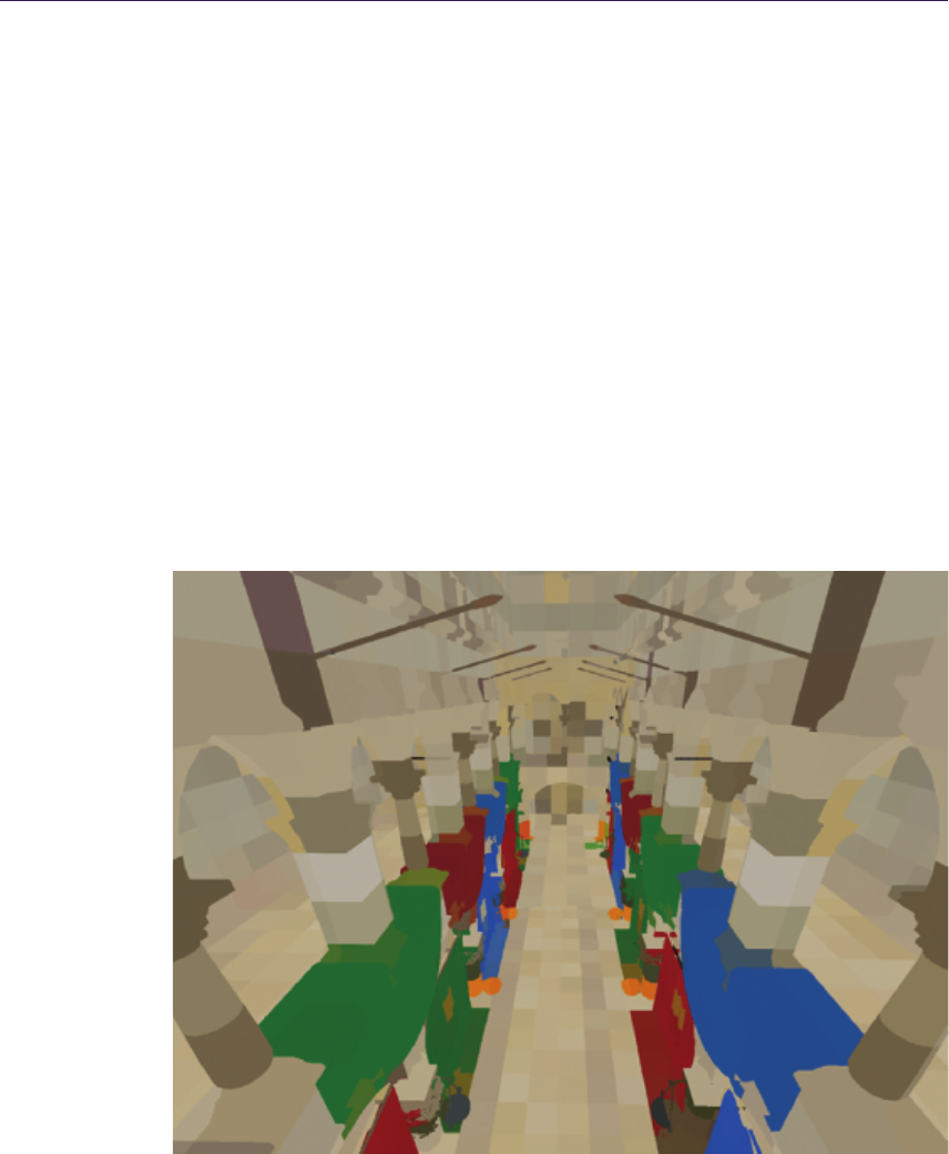
322 20. Rasterized Voxel-Based Dynamic Global Illumination
Since voxels are a simplified representation of the actual scene, detailed geo-
metric information is lost. In order to amplify color bleeding in the final global
illumination output, colors with high difference in their color channels (“con-
trast”) are preferred. By writing the contrast value into the highest 8 bit of the
integer color mask, colors with the highest contrast will dominate automatically,
since we write the results with an InterlockedMax() into the voxel grid. Since,
e.g., thin geometry can have opposite normals in one single voxel, not only the
color but also the normal has to be carefully written into the voxels. Therefore
it is determined to which face of a tetrahedron the current normal is closest. By
writing the corresponding dot product into the highest 5 bit of the integer normal
mask, the closest normal to each tetrahedron face is selected automatically since
we again write the results with an InterlockedMax(). According to the retrieved
tetrahedron face, the normal is written into the corresponding normal channel of
the voxel. Later on, when the voxels are illuminated, the closest normal to the
light vector is chosen so that the best illumination can be obtained. In this way
sometimes it is possible that the normal is taken from a different geometry face
as the color. However, since voxels condense information from the actual geome-
try within its boundaries, this is completely fine and will not have any negative
impact on the global illumination result.
Figure 20.1. Visualization for the voxel grid representation of the Sponza scene.

20.3. Implementation 323
Since all operations are performed using a very small render-target (64 ×64
pixels), this generation step is surprisingly fast. Figure 20.1 shows a screenshot
in which the voxel grid representation of the Sponza scene is visualized. To
create this image for each visible pixel of the rendered scene, the word-space
position is reconstructed. With the help of the reconstructed position, we can
determine the location of the corresponding voxel inside the grid. Finally, each
visible pixel will be colored with the diffuse albedo information that is stored
inside the corresponding voxel. In order to cover the entire scene, two nested
voxel grids have been used: a fine-resolution grid for the area near to the viewer
and a coarse-resolution grid for the distant area.
20.3.2 Create VPLs in Voxel Space
In this step we create VPLs entirely from the previously generated voxel grid.
For each light source that is located inside the boundaries of the grid, we render
a small quad of 32 ×32 pixels. By using hardware instancing, for each quad we
are able to render 32 instances with a single draw call. After passing the vertices
through the vertex shader, the geometry shader will choose the corresponding
render-target slice in the currently bound 2D texture arrays. The pixel shader
will then illuminate all voxels that contain geometry information according to
the type of the current light source. Finally, the illuminated voxels are converted
into a second-order spherical harmonic representation of VPLs. By using additive
hardware blending, the results of all light sources are automatically combined.
Listing 20.2 generically shows how this is done for DirectX 11 in HLSL.
// vertex shader
VS _O UTP UT m ain ( V S_I NP UT input , uin t in st anc eI D : S V_ In st anc eI D )
{
VS _OU TP UT outp ut ;
ou tpu t . po sit io n = flo at4 ( inp ut . po siti on ,1 .0 f );
output . in sta nceID = instanc eID ;
return output ;
}
// ge om et ry sh ader
struct GS_OUTPUT
{
fl oat4 po sit ion : SV_ POS ITI ON ;
uint rtIndex: SV_RenderTargetArrayIndex;
};
[maxvertexcount(4)]
voi d mai n ( line VS _O UTP UT i npu t [2] , i nou t Tr ian gle Str ea m < G S_OU TPUT >
outputStream)
{
// Ge ner ate a quad f rom two c orner v ert ice s .
GS _O UT PU T output [4];

324 20. Rasterized Voxel-Based Dynamic Global Illumination
// lower - l eft v ert ex
ou tpu t [ 0] . p o si tio n = f lo at4 ( in put [0 ]. po si ti on . x , in pu t [ 0]. p os it io n .y ,
in put [0 ]. po si tio n . z , 1.0 f ) ;
// lower - r ight ve rte x
ou tpu t [ 1] . p o si tio n = f lo at4 ( in put [1 ]. po si ti on . x , in pu t [ 0]. p os it io n .y ,
in put [0 ]. po si tio n . z , 1.0 f ) ;
// upper - l eft v ert ex
o utp ut [2 ]. po si tio n = f lo at4 ( in put [0 ]. po si ti on . x , in pu t [ 1]. p os it ion .y ,
in put [0 ]. po si tio n . z , 1.0 f ) ;
// upper - r ight ve rte x
ou tpu t [ 3] . p o si tio n = f lo at4 ( in put [1 ]. po si ti on . x , in pu t [ 1]. p os it io n .y ,
in put [0 ]. po si tio n . z , 1.0 f ) ;
// By u sing h ar dw are in stancing , the g eo me tr y shad er will be inv ok ed 32
// ti mes w ith t he c or re sp on di n g i nst an ce ID . For ea ch i nv oc at io n th e
// in st an ce ID is used to determine into wh ich slice of a 2D te xt ure
// arr ay the c urrent quad sh ould be rasterize d .
[unroll]
for (in t i =0; i < 4; i ++)
{
o utp ut [ i ]. rt In de x = inp ut [0] . in st an ce ID ;
ou tp utS tr eam . Appen d ( out put [ i ]);
}
ou tputSt rea m . Restar tSt rip ();
}
// pixel sh ader
S tru ct ur edB uf fe r < V OXEL > gr id Bu ff er : re gis ter ( t 0 );
struct FS _O UTPUT
{
fl oat4 fragC olo r0 : SV_TARGE T0 ; // red SH - coef fic ien ts
fl oat4 fragC olo r1 : SV_TARGE T1 ; // blue SH - c oef ficien ts
fl oat4 fragC olo r2 : SV_TARGE T2 ; // gr een SH - co effi cie nts
};
// Ca lc ula te se cond - o rder SH - c oe ffi ci ent s for c lam ped co sin e lobe fu nctio n .
f loa t4 C l am p ed Co s in eS H Co ef f s ( in f loa t3 d ir )
{
float4 coeffs;
co eff s .x = P I /(2 .0 f * sqrt ( PI ) );
c oef fs . y = -( (2.0 f * PI )/3 .0 f ) * sq rt (3. 0 f / (4. 0 f * PI )) ;
co eff s .z = ((2 .0 f* PI ) /3. 0 f)* sqr t (3. 0 f /(4. 0 f* PI ));
c oef fs . w = -( (2.0 f * PI )/3 .0 f ) * sq rt (3. 0 f / (4. 0 f * PI )) ;
coeffs . wyz *= dir ;
return coeffs;
}
// Determine which of the four s pe ci fi ed normal s is closest to th e
// sp eci fie d di rec tio n . The f unc tio n returns the c los est norma l and as
// output p ara met er the co rres pon ding dot pr odu ct .
f loa t3 G e tC lo s es tN o rm al ( in u in t4 n orm al Mas ks , in fl oa t3 d ire cti on , out flo at
do tPr oduct )
{
fl oat 4x3 no rmal Mat rix ;
nor malMat rix [0] = De cod eNorma l ( nor mal Masks .x );
no rmalMa tri x [1] = D ecod eNo rma l ( normal Mas ks .y);
nor malMat rix [2] = De cod eNorma l ( nor mal Masks .z );
nor malMat rix [3] = De cod eNorma l ( nor mal Masks .w );
flo at4 d ot Pro du ct s = mul ( n orm al Mat rix , d ir ec ti on ) ;
float m axi mum = m ax ( ma x ( do tP ro du ct s .x , d ot Pr odu ct s . y) ,
max ( d ot Pr od uc ts . z , do tP ro duc ts .w )) ;

20.3. Implementation 325
int in dex ;
if( ma xim um == do tPr od uct s .x )
index = 0;
els e i f ( max imu m == d otP roduct s .y )
index = 1;
els e i f ( max imu m == d otP roduct s .z )
index = 2;
els e
index = 3;
dot Pr odu ct = do tPr od uct s [ ind ex ];
return nor mal Ma trix [ i ndex ];
}
PS_ OU TPU T mai n ( GS _OU TP UT i npu t )
{
PS_ OUTPUT o utp ut ;
// Get in dex of curr ent vo xel .
int3 vo xe lPo s = int3 ( i npu t . pos iti on . xy , in put . r tIn dex );
int g rid Ind ex = ( v oxe lPo s .z *1 024 )+( v oxe lPo s .y *32)+ v oxe lPo s .x ;
// Get vo xel data and ea rly out , if vo xel has no geometry in fo rmation .
VOXEL voxel = gridBu ffe r [ gri dIn dex ];
if ( vo xel . o ccl us ion == 0)
di sca rd ;
// Get world - sp ace p osi ti on of vox el .
int 3 of fset = samplePos - int3 (16 ,16 , 16);
fl oat 3 posit ion = ( f loat3 ( of fse t )* c ons tB uff er . g ri dCe ll Siz e )+
co nst Buf fer . snap ped Gr id Cent er ;
// De cod e col or of voxel .
fl oat 3 alb edo = De cod eC olo r ( vo xel . c olo rMa sk );
// Get norm al of vox el that is clo ses t to the light d ire cti on .
float n Dot L ;
fl oat 3 nor mal = Ge tC lo ses tN or ma l ( vox el . norma lMa sks , li ghtV ecN , nD otL );
// Ca lc ula te di ffu se l igh ti ng a cc ord ing to cur re nt li ght t ype .
fl oa t3 d iff us e = Ca lc Di f fu se Li gh ti ng ( a lbed o , nD otL );
# if def U SE _SHADOW S
// Ca lc ul at e s ha dow ter m according to current ligh t type with the h elp
// of a s had ow map .
float s had owTerm = Co mput eSh ad owTe rm ( po sit ion );
di ffuse *= shado wTe rm ;
# endif
// Ca lc ul ate c lam ped co si ne lo be SH - co ef fi ci ent s fo r VP L .
fl oat 4 coe ffs = Cl am ped Co si ne SHC oe ff s ( nor mal );
// Output SH - coef fic ient s for each co lor c han nel .
out put . f rag Col or 0 = coe ffs * d iff ues . r;
ou tput . fr agC olo r1 = c oef fs * diffuse . g;
out put . f rag Col or 2 = coe ffs * d iff use . b;
return output;
}
Listing 20.2. VPL creation.

326 20. Rasterized Voxel-Based Dynamic Global Illumination
To output the second-order SH-coefficients for all three color channels, we
render this time into three 2D texture arrays with half floating-point precision.
Since all calculations are done entirely in voxel space and are limited to voxels,
which actually contain geometry information, this technique scales very well with
an increasing number of light sources of all different types.
In many situations we can even abandon the use of shadow maps for point
lights and spotlights without noticeably affecting the final render output. How-
ever, for large point lights, spotlights, and directional lights, we do need to use
shadow maps to avoid light leaking. Here we can simply reuse the shadow maps
that have already been created for the direct illumination step.
20.3.3 Propagate VPLs
In this step the previously created VPLs are propagated iteratively across the grid
according to the LPV technique proposed by [Kaplanyan and Dachsbacher 10].
Basically each VPL cell propagates its light along the three axes of a Cartesian
coordinate system to its surrounding six neighbor cells. While doing this propa-
gation, the voxel grid from the first step is used to determine how strongly the
light transport to the neighbor cells is occluded. The results from the first prop-
agation step are then used to perform a second propagation step. This is done
iteratively until we get a visually satisfying light distribution. In the first iter-
ation no occlusion is used, in order to initially let the light distribute; from the
second iteration on, we use the geometry occlusion in order to avoid light leaking.
The iterative propagation is performed in DirectX 11 by utilizing a compute
shader since we do not need the rasterization pipeline for this job. Listing 20.3
demonstrates this.
// co mp ute sh ad er
Te xture2 DAr ray i np utRe dS HTex tu re : register ( t0 ) ;
Te xture2 DAr ray i npu tGre enSH Te xtur e : re gis ter ( t 1 );
Te xture2 DAr ray i npu tBlu eSH Te xt ure : r egi ste r ( t2 );
S tru ct ur edB uf fe r < V OXEL > gr id Bu ff er : re gis ter ( t 3 );
RW Te xt ure 2D Arr ay < fl oat4 > o ut pu tR ed SH Te xt ur e : register ( u0 ) ;
RW Te xt ure 2D Arr ay < fl oat4 > o ut pu tG re en SH Te x tu re : re gis ter ( u 1 );
RW Te xt ure 2D Arr ay < fl oat4 > o ut pu tB lu eS HT ex tu re : r egi ste r ( u2 );
// dir ec ti on s to six neighbor ce ll c enters
static float3 d ir ec ti ons [6] =
{
float3 (0.0 f ,0.0f ,1.0 f) , floa t3 (1 .0 f ,0.0 f ,0.0 f) , f loat3 (0.0 f ,0.0f , -1.0 f),
float3 ( -1.0f ,0.0 f ,0.0 f), f loat3 (0 .0 f ,1.0 f ,0.0 f) , f loat3 (0.0 f , -1.0f ,0.0 f)
};
// SH - co eff ici en ts for six fa ces ( Cla mp edCo si neSH Co effs ( direction s [0 -5])
static float4 f ac eC oe ffs [6] =
{
f loa t4 ( P I / (2* sqr t ( PI ) ) ,0 .0 f , (( 2* P I ) /3. 0 f )* s qr t ( 3.0 f /(4 * PI ) ) , 0.0 f ) ,
f loa t4 ( P I / (2* sqr t ( PI ) ) ,0 .0 f , 0.0 f , -( (2* PI )/ 3.0 f ) * s qrt (3. 0 f / (4* P I ))) ,
float4 ( PI /(2* sqrt (PI )) ,0.0 f , -((2* PI )/3.0 f)* sqrt (3.0 f /(4* PI )) ,0.0 f),
f loa t4 ( P I / (2* sqr t ( PI ) ) ,0 .0 f , 0.0 f ,(( 2* P I ) /3 .0 f )* sqr t ( 3.0 f /(4 * PI ) )) ,

20.3. Implementation 327
fl oat 4 ( PI /(2* sq rt ( PI ) ) , -((2* PI ) /3 .0 f )* sqr t ( 3.0 f /(4 * PI ) ) , 0.0 f , 0.0 f ) ,
flo at4 ( PI /(2 * sqr t ( PI )) ,((2 * PI ) /3.0 f )* sqr t (3. 0 f /(4* PI )) ,0.0 f , 0.0 f )
};
// offs et s to six ne ig hb or cell c en ters
static int 3 of fs et s [6] =
{
int 3 (0 ,0 ,1) , int 3 (1 ,0 ,0) , int 3 (0 ,0 , -1) ,
int 3 ( -1 ,0 ,0) , i nt3 (0 ,1 ,0) , in t3 (0 , -1 , 0)
};
[ nu mthreads (8 ,8 ,8)]
void m ain ( u int 3 Gro up ID : S V_G rou pID , ui nt3 Di sp at ch Th rea dI D :
SV_ Di spa tch Th rea dI D , u int3 Gro upT hr ea dID : S V_ Gr oup Th re ad ID ,
uint GroupInde x : SV_ Gro upInde x )
{
// Get gr id po si tio n o f c urr ent ce ll .
int 3 el em ent Po s = D is pa tc hT hr ea dI D . xyz ;
// In it ial iz e SH - co effi cie nt s wit h va lues fr om cu rre nt c ell .
fl oat 4 su mR ed SH Coe ff s = i np ut Re dSH Te xt ur e . Loa d ( int4 ( e lem ent Pos ,0 ));
fl oat 4 su mG re en SH Co eff s = i np ut Gr ee nS HT ex tur e . Lo ad ( int 4 ( ele men tPos ,0 ));
fl oat 4 su mB lu eS HC oef fs = in pu tB lu eS HT ex tu re . Lo ad ( int 4 ( ele men tPos , 0));
[ un rol l ]
for (in t i =0; i < 6; i ++)
{
// Get grid p os it io n of six neighbor ce lls .
in t3 s am pl eP os = e l em en tP os + of fs et s [ i ];
// contin ue , if c ell is out of bo unds
if (( s amp leP os .x <0)|| ( samplePos .x >3 1)||( samplePos .y <0)||
( sa mpl ePo s .y >31)|| ( sampl ePo s .z <0 )||( s amp leP os .z > 31))
co nti nue ;
// Loa d SH - c oe ffi ci ent s for ne igh bo r cell .
fl oat 4 re dS HC oef fs = in pu tR ed SHT ex tu re . L oad ( in t4 ( sa mple Pos ,0 ));
fl oat 4 gr ee nS HC oef fs = in pu tG re en SH Te xtu re . Loa d ( int4 ( s amp lePo s ,0 ));
fl oat 4 bl ue SH Coe ff s = i np ut Blu eS HT ex tu re . L oad ( in t4 ( sam ple Pos , 0)) ;
# if def USE_OCCLUSION
float4 o cclusi onC oeff s = floa t4 (0.0 f ,0.0 f ,0.0f ,0.0 f );
// Get in dex of c orre spo nd ing vo xel .
int g rid Ind ex = ( s amp leP os .z *1024 )+( s amp lePos .y *3 2)+ samplePos . x;
VOXEL voxel = gridBuff er [ gr idI nde x ];
// If v oxel c on tains geometry infor mation , f ind cl osest no rmal to
// cu rrent di rec tio n . In th is way the h igh est oc clu sio n can be
// ge ner ated . Then ca lcu late SH - co ef fic ient s for r etr iev ed n ormal .
if( vo xel . o ccl us ion > 0)
{
float d otP roduct ;
fl oat 3 oc cl us ion No rm al = G et Cl os est No rm al ( v oxel . n orm alM asks ,
- d ire ct io ns [ i ], d ot Pr od uc t );
occ lusi onC oeff s = Cl am pedC osi ne SHC oe ffs ( oc clus ion Norm al );
}
# endif
[unroll]
for (int j =0; j <6 ; j ++)
{
// Get d ir ec ti on for f ace of c ur rent c ell to c ur rent ne ighbor
// cell ce nter .
fl oat 3 n ei g hb or C el lC en t er = d i re ct io ns [i ];

328 20. Rasterized Voxel-Based Dynamic Global Illumination
flo at3 fa ce Posi tio n = d ire ct ion s [j ] *0. 5 f;
float3 dir = face Positi on - n eigh borC ell Cent er ;
float f Len gth = le ngt h ( dir );
dir /= fL eng th ;
// Get c orre spo nd ing so lid a ngle .
float s oli dA ng le = 0. 0 f;
if ( fL ength > 0.5 f )
sol idA ngle = ( fL ength >=1.5 f ) ? (2 2.9 566 8 f /(4 *18 0.0 f)) :
(2 4. 26 083 f /( 4* 18 0.0 f ));
// Ca lcu lat e SH - coe ffi cie nts for d ire cti on .
fl oat 4 dir SH ;
res ult . x = 1.0 f / (2* s qrt ( PI )) ;
res ult . y = - sqrt (3 .0 f /(4 * PI ));
res ult . z = sq rt ( 3.0 f /(4 * PI )) ;
res ult . w = - sqrt (3 .0 f /(4 * PI ));
result . wyz *= dir ;
// Ca lc ula te f lux fr om ne ig hbo r cel l to fa ce of cu rre nt ce ll .
flo at3 f lux ;
fl ux . r = d ot ( re dSH Coe ffs , d irS H );
fl ux . g = d ot ( gr een SH Coe ffs , d ir SH );
fl ux . b = d ot ( bl ueS HCo ef fs , dir SH ) ;
fl ux = ma x ( 0.0 f , f lu x ) * s o li dA ng le ;
# if def USE_OCCLUSION
// apply oc cl usion
float o c c lu si on = 1 .0 f - s a t ur at e ( d ot ( oc cl us io n Co ef fs , d i rS H ) );
flu x *= o ccl usi on ;
# en dif
// Add c on tri bu ti on to SH - co ef fic ie nt s sum s .
f loa t4 c oe ff s = fa ce Co ef f s [ j ];
su mR ed SH Coe ff s += co eff s * flux . r;
su mG re en SH Co eff s += co eff s * flux . g ;
su mB lu eS HC oef fs += c oef fs * fl ux .b ;
}
}
// Write out ge ner ate d red , green , and bl ue SH - coeff ici ent s .
ou tp utRe dSH Te xtu re [ e lem entPos ] = su mRed SHC oe ffs ;
ou tp utGr eenS HTe xt ure [ el eme ntP os ] = su mGre enS HC oef fs ;
ou tp utBl ueS HT extu re [ element Pos ] = sum Blu eSHC oeff s ;
}
Listing 20.3. Propagation of VPLs.
For each propagation step the compute shader is dispatched with 4 ×4×4
thread groups so that altogether 32 ×32 ×32 threads are utilized, which corre-
sponds to the total cell count of the grid.
20.3.4 Apply Indirect Lighting
In this step the previously propagated VPLs are finally applied to the scene. For
this we need a depth buffer from which the world-space position of the visible pix-
els can be reconstructed, as well as a normal buffer that contains the perturbed
normal information for each pixel. Obviously, deferred rendering as a direct illu-
mination approach is perfectly fitted for our case since both pieces of information
are already available and no extra work has to be done.

20.3. Implementation 329
While rendering a full-screen quad, the pixel shader reconstructs the world-
space position and the normal for each pixel. According to the world-space po-
sition, the previously generated grid (in the form of three 2D texture arrays) is
sampled with linear hardware filtering. Therefore we manually only have to per-
form a filtering in the third dimension so that we retrieve smooth results. With
the help of the sampled SH-coefficients and the surface normal, we can perform
an SH-lighting for each pixel. See Listing 20.4 for details.
// pixel sh ader
Te xture2 DAr ray i np utRe dS HTex tu re : register ( t0 ) ;
Te xture2 DAr ray i npu tGre enSH Te xtur e : re gis ter ( t 1 );
Te xture2 DAr ray i npu tBlu eSH Te xt ure : r egi ste r ( t2 );
PS _O UTP UT m ain ( G S_O UT PUT in put )
{
PS _OU TP UT outp ut ;
float d epth = de pt hBu ff er . Sa mpl e ( de pth Buff erS amp le r , inpu t . tex Co ord s ). r;
fl oat 4 po sit ion = Re co ns tr uc tP os iti on Fr om De pt h ( dep th );
fl oat 3 alb edo = colorMa p . Sa mpl e ( col orM apS ample r , i npu t . tex Co ord s ). rgb ;
float3 normal =
no rm alB uf fer . Sam ple ( no rma lBu ff erS amp le r , inpu t . tex Coords ). xyz ;
// Get o ffs et int o gri d .
fl oat3 offse t = ( position . xyz - c onstBu ffe r . sn appe dGr id Cent er )*
co nst Buffer . inv Gri dCel lSi ze ;
// Get tex Co or ds int o Tex tu re2 DArr ay .
f loa t3 t e xC oo rd s = fl oa t3 (16 .5 f ,16 .5 f , 16 .0 f ) + o ff set ;
t ex Co or ds . x y /= 32 .0 f ;
// Get te xC oo rd s for t ri li ne ar sampling .
int lowZ = f loor ( t exC oor ds .z);
int high Z = min ( lowZ +1 ,32 -1);
float h ig hZ Wei gh t = te xC oor ds . z- l owZ ;
float l o wZ We ig ht = 1 .0 f - h ig hZ We ig ht ;
fl oat 3 tcL ow = f loa t3 ( t exC oor ds . xy , lo wZ );
fl oat3 tc High = fl oat3 ( tex Coords . xy , h ighZ );
// Pe rform tr ili nea r sa mpling of red , green , and blue SH - c oef fici ent s
// from Texture2DArray.
float4 r ed SHCoeff s =
lo wZWe igh t * in pu tRe dS HT extu re . Samp le ( li nea rSa mpl er , t cLo w )+
hi gh ZWe ight * i np ut Red SH Te xtu re . S amp le ( li nea rSampl er , tc Hig h );
float4 g re enS HC oe ffs =
lo wZWeig ht * i npu tG re enS HT ex ture . S ample ( li nea rSa mpl er , tcL ow )+
hi gh ZWe ight * i np ut Gre en SH Text ur e . Sam ple ( l ine arSamp ler , t cHi gh );
float4 blueSHCoeffs =
lo wZWe igh t * in pu tBlu eSHT extu re . S ampl e ( lin ear Sam ple r , tcLo w )+
hi gh ZWe ight * inp ut Blu eS HT ext ur e . Sampl e ( lin ear Sam ple r , tc Hig h );
// Calculate clamped c os ine lobe SH - c oeffi ci en ts for surfa ce n ormal .
fl oat 4 su rf ace No rm alL ob e = C lamp ed Cos in eS HCoe ff s ( nor mal );
// Pe rfo rm diff use SH - li ght ing .
float3 d iffu seG lo ba lIll um ;
di ffus eGloba lIll um . r = dot ( redSHC oeff s , sur fa ceNo rm alLo be );

330 20. Rasterized Voxel-Based Dynamic Global Illumination
d if fu se Gl ob al Il lu m . g = d ot ( gr ee nSH Coe ff s , s u rf ac eN or ma lL ob e );
d if fu se Gl ob al Il lu m . b = d ot ( bl ueS HC oef fs , s ur fa ce No rm al Lo be );
d if fu s eI ll u m = max ( d i ff us eIl lu m , fl oat 3 (0. 0 f , 0.0 f ,0. 0 f )) ;
d if fu s eG lo b al Il l um /= PI ;
output . fr ag Col or = flo at4 ( dif fu seGl oba lI ll um * albedo ,1. 0 f);
return output;
}
Listing 20.4. Indirect lighting.
As can be seen in the above listing, only the diffuse indirect illumination is
calculated. However there is the possibility to extract a dominant light source
from SH-coefficients [Sloan 08]. With the help of this extracted light source, a
conventional specular lighting can be performed. This gives us the possibility to
add a fast, but coarse, approximation of specular indirect lighting.
20.3.5 Clear the Voxel Grid
In this final step the RWStructuredBuffer used for the voxel grid is cleared by
using a simple compute shader. Just like for the propagation step, the compute
shader is dispatched with 4 ×4×4 thread groups, whereby each thread group
runs 8×8×8 threads, so that 32×32×32 threads are utilized, which corresponds
to the total voxel count of the grid.
20.4 Handling Large Environments
Since we are using a 32×32×32 voxel grid, it is quite obvious that this alone can-
not deal with realistic large game environments. According to the use of multiple
cascades in the LPV technique proposed by [Kaplanyan and Dachsbacher 10],
several nested voxel grids can be used. Each grid will have the same number
of cells, but the size of the grid cells will increase. In this way detailed indirect
lighting can be maintained in the vicinity of the viewer, while in the distance
still sufficient coarse indirect lighting is used. However, a linear interpolation
should be performed between the grids to avoid a harsh transition at the borders
between them. This can be done in the step when indirect lighting is applied to
each visible pixel. Therefor across the border area the global illumination value
is calculated for both adjoining grids. The distance of the world-space position
of the current pixel to the center of the higher-resolution grid can be used to
linearly interpolate between both global illumination values.
20.5 Results
Table 20.1 shows the performance results using the proposed technique in the
Sponza scene. All lights were fully dynamic and contributed to the indirect
illumination.
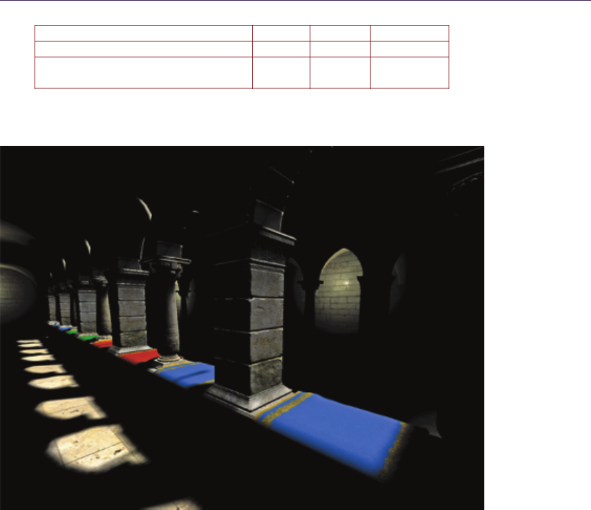
20.6. Conclusion 331
Min fps Max fps Average fps
1 directional light 63 90 71
1 directional light +12 medium-sized 61 89 70
moving point lights
Table 20.1. Performance results in the Sponza scene (∼280,000 triangles) using two
grid cascades (on a Nvidia Geforce 485 GTX Mobile with 1,280 ×720 resolution).
Figure 20.2. Sponza scene with direct illumination only.
Figures 20.2–20.4 show how this technique can improve the appearance of
a scene. For the screenshots the same Sponza scene has been used as for the
previous performance results.
20.6 Conclusion
By utilizing new DirectX 11 features, this technique is capable of producing
visually good and stable results for a high number of light sources contained
in realistic game environments while maintaining high interactive frame rates.
Moreover the video memory consumption is kept at a low level.
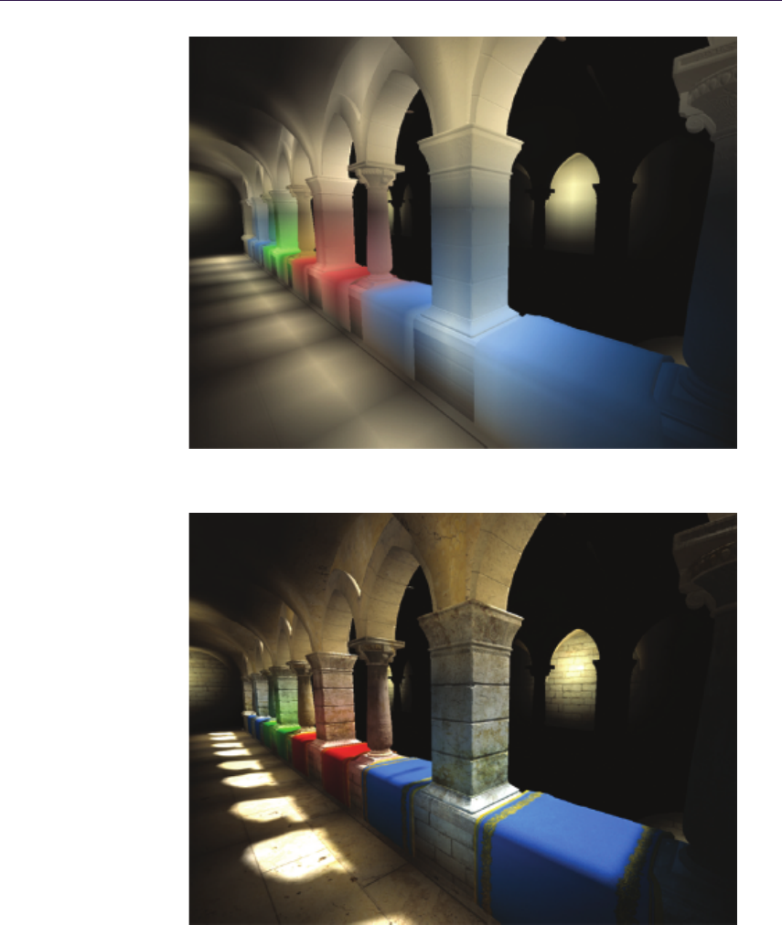
332 20. Rasterized Voxel-Based Dynamic Global Illumination
Figure 20.3. Sponza scene with indirect illumination only.
Figure 20.4. Final combined output of the Sponza scene.

Bibliography 333
However, besides the fact that this approach will only run on DirectX 11 or
higher hardware, it requires also a depth and a normal buffer for reconstructing
the position and normal of the visible pixels. Therefore it is best fitted for direct
illumination approaches such as deferred rendering.
Bibliography
[Kaplanyan and Dachsbacher 10] Anton Kaplanyan and Carsten Dachsbacher.
“Cascaded Light Propagation Volumes for Real-Time Indirect Illumination.”
In Symposium on Interactive 3D Graphics and Games (I3D), pp. 99–107.
New York: ACM, 2010.
[Mavridis and Papaioannou 11] Pavlos Mavridis and Georgios Papaioannou.
“Global Illumination Using Imperfect Volumes.” Presentation, International
Conference on Computer Graphics Theory and Applications (GRAPP), Al-
garve, Portugal, 2011.
[Sloan 08] Peter-Pike Sloan. “Stupid Spherical Harmonics (SH) Tricks.” Compan-
ion to Game Developers Conference 2008 lecture, http://www.ppsloan.org/
publications/StupidSH36.pdf, February 2008.
21
Per-Pixel Lists for
Single Pass A-Buffer
Sylvain Lefebvre, Samuel Hornus,
and Anass Lasram
21.1 Introduction
Real-time effects such as transparency strongly benefit interactive modeling and
visualization. Some examples can be seen Figure 21.1. The rightmost image is
a screenshot of our parametric Constructive Solid Geometry (CSG) modeler for
3D printing, IceSL [Lefebvre 13]. Modeled objects are rendered in real time with
per-pixel boolean operations between primitives.
Figure 21.1. Left: Joystick model rendered with the Pre-Open A-buffer technique
described in this chapter, on a GeForce Titan. 539236 fragments, max depth: 16, FPS:
490. Middle: Dinosaur in Egg, rendered with transparent surfaces and shadows using
two A-buffers. Right: A robot body modeled with 193 solid primitives in boolean oper-
ations (CSG), rendered interactively with the Pre-Open A-buffer technique (modeler:
IceSL). [Joystick by Srepmup (Thingiverse, 30198), Egg Dinosaur by XXRDESIGNS
(Thingiverse, 38463), Spidrack by Sylefeb (Thingiverse, 103765).]
335

336 21. Per-Pixel Lists for Single Pass A-Buffer
These effects have always been challenging for real-time rasterization. When
the scene geometry is rasterized, each triangle generates a number of fragments.
Each fragment corresponds to a screen pixel. It is a small surface element po-
tentially visible through this pixel. In a classical rasterizer only the fragment
closest to the viewer is kept: the rasterizer blindly rejects all fragments that are
farther away than the current closest, using the Z-buffer algorithm. Instead, al-
gorithms dealing with transparency or CSG have to produce ordered lists of all
the fragments falling into each pixel. This is typically performed in two stages:
First, a list of fragments is gathered for each pixel. Second, the lists are sorted
by depth and rendering is performed by traversing the lists, either accumulat-
ing opacity and colors (for transparency effects), or applying boolean operations
to determine which fragment is visible (for rendering a CSG model). The data
structure is recreated at every frame, and therefore has to be extremely efficient
and integrate well with the rasterizer.
A large body of work has been dedicated to this problem. Most techniques
for fragment accumulation implement a form of A-buffer [Carpenter 84]. The
A-buffer stores in each pixel the list of fragments that cover that pixel. The frag-
ments are sorted by depth and the size of the list is called the depth-complexity,
as visualized in Figure 21.3 (top-right). For a review of A-buffer techniques for
transparency we refer the reader to the survey by Maule et al. [Maule et al. 11].
In this chapter we introduce and compare four different techniques to build
and render from an A-buffer in real time. One of these techniques is well known
while the others are, to the best of our knowledge, novel. We focus on scenes
with moderate or sparse depth complexity; the techniques presented here will not
scale well on extreme transparency scenarios. In exchange, their implementation
is simple and they integrate directly in the graphics API; a compute API is not
necessary. All our techniques build the A-buffer in a single geometry pass: the
scene geometry is rasterized once per frame.
A drawback of storing the fragments first and sorting them later is that some
fragments may in fact be unnecessary: in a transparency application the opacity
of the fragments may accumulate up to a point where anything located behind
makes no contribution to the final image. Two of the techniques proposed here
afford for a conservative early-culling mechanism: inserted fragments are always
sorted in memory, enabling detection of opaque accumulation.
The companion code includes a full implementation and benchmarking frame-
work.
21.1.1 Overview
An A-buffer stores a list of fragments for each pixel. Sorting them by increasing
or decreasing depth are both possible. However, the sorting technique that we
describe in Section 21.3 is easier to explain and implement for decreasing values
as we walk along the list. Adding to that, early culling of negligible fragments

21.1. Introduction 337
is possible for transparency rendering only when the fragments are sorted front-
to-back. In order to meet both requirements for the described techniques, we
consistently sort in decreasing order and obtain a front-to-back ordering by in-
verting the usual depth value of a fragment: if the depth zof a fragment is a
float in the range [−1,1], we transform it in the pixel shader into the integer
⌊S(1 −z)/2⌋, where Sis a scaling factor (typically 232 −1 or 224 −1).
Our techniques rely on a buffer in which all the fragments are stored. We
call it the main buffer. Each fragment is associated with a cell in the main
buffer where its information is recorded. Our techniques comprise three passes:
aClear pass is used to initialize memory, then a Build pass assembles a list of
fragments for each pixel and finally a Render pass accumulates the contribution
of the fragments and writes colors to the framebuffer.
The four techniques differ along two axes. The first axis is the scheduling
of the sort: when do we spend time on depth-sorting the fragments associated
with each pixel? The second axis is the memory allocation strategy used for
incrementally building the per-pixel lists of fragments. We now describe these
two axes in more detail.
21.1.2 Sort Strategies
We examine two strategies for sorting the fragments according to their depth.
The first one, Post-sort, stores all the fragments during the Build pass and
sorts them only just prior to accumulation in the Render pass: the GLSL shader
copies the pixel fragments in local memory, sorts them in place, and performs in-
order accumulation to obtain the final color.
The second strategy, Pre-sort, implements an insertion-sort during the
Build pass, as the geometric primitives are rasterized. At any time during the
rasterization, it is possible to traverse the fragments associated with a given pixel
in depth order.
Both strategies are summarized in Table 21.1.
Each has pros and cons: In the Pre-sort method, insertion-sort is done in
the slower global memory, but the method affords for early culling of almost
invisible fragments. It is also faster when several Render passes are required on
the same A-buffer, since the sort is done only once. This is for instance the case
when CSG models are sliced for 3D printing [Lefebvre 13].
Pass Rasterized geometry Post-sort Pre-sort
Clear fullscreen quad clear clear
Build scene triangles insert insertion-sort
Render fullscreen quad sort, accumulate accumulate
Table 21.1. Summary of the Post-sort and Pre-sort sorting strategies.

338 21. Per-Pixel Lists for Single Pass A-Buffer
In the Post-sort method, sorting happens in local memory, which is faster
but limits the maximum number of fragments associated with a pixel to a few
hundred. Allocating more local memory for sorting more fragments increases
register pressure and reduces parallelism and performance.
21.1.3 Allocation Strategies
In addition to the scheduling of the sort, we examine two strategies for allocating
cells containing fragment information in the main buffer. The first one, Lin-
alloc, stores fragments in per-pixel linked-lists and allocates fresh cells linearly
from the start of the buffer to its end. Since many allocations are done concur-
rently, the address of a fresh cell is obtained by atomically incrementing a global
counter. Additional memory is necessary to store the address of the first cell
(head) of the list of fragments of each pixel. Section 21.2 details the Lin-alloc
strategy.
The second strategy that we examine, Open-alloc, is randomized and some-
what more involved. To each pixel pwe associate a pseudo-random sequence of
cell positions in the main buffer: (h(p, i))i≥1, for iranging over the integers. In
the spirit of the “open addressing” techniques for hash tables, the cells at posi-
tions h(p, i) are examined by increasing value of iuntil an empty one is found.
A non-empty cell in this sequence may store another fragment associated with
pixel por with a different pixel q. Such a collision between fragments must be
detected and handled correctly. Section 21.3 details the Open-alloc strategy.
The combination of two allocation strategies (Lin-alloc and Open-alloc)
with two schedules for sorting (Post-sort and Pre-sort) gives us four varia-
tions for building an A-buffer: Post-Lin (Sections 21.2.1 and 21.2.2), Pre-Lin
(Section 21.2.3), Post-Open (Section 21.3.2) and Pre-Open (Section 21.3.3).
Section 21.4.1 details how fragments are sorted in local memory in the Ren-
der pass of the Post-sort method. Some memory management issues, includ-
ing buffer resizing, are addressed in Section 21.5, and information about our
implementation is given in Section 21.6. In Section 21.7, we compare these four
variations, as implemented on a GeForce 480 and a GeForce Titan.
21.2 Linked Lists with Pointers (Lin-alloc)
The first two approaches we describe construct linked lists in each pixel, allocating
data for new fragments linearly in the main buffer. A single cell contains the depth
of the fragment and the index of the next cell in the list. Since no cell is ever
removed from a list, there is no need for managing a free list: allocating a new
cell simply amounts to incrementing a global counter firstFreeCell that stores the
index of the first free cell in the buffer. The counter firstFreeCell is initialized to
zero. The increment is done atomically to guarantee that every thread allocating
new cells concurrently does obtain a unique memory address. A second array,

21.2. Linked Lists with Pointers (Lin-alloc)339
called heads, is necessary to store the address of the head cell of the linked list of
each pixel.
Having a lot of threads increment a single global counter would be a bot-
tleneck in a generic programing setting (compute API). Fortunately, GLSL frag-
ment shaders feature dedicated counters for this task, via the ARB_shader_atomic_
counters extension. If these are not available, it is possible to relieve some of the
contention on the counter by allocating Kcells at once for a list (typically K= 4).
To obtain such a paged allocation scheme, the thread atomically increases the
global counter by Kand uses a single bit in each head pointer as a local mutex
when inserting fragments in this page of Kcells. The technique is described
in full detail by Crassin [Crassin 10], and is implemented in the accompanying
code (see implementations.fp, function allocate_paged). In our tests, the dedi-
cated counters always outperformed the paging mechanism. However, if a generic
atomic increment is used instead then the paging mechanism is faster. We use a
single dedicated atomic counter in all our performance tests (Section 21.7).
We now describe the two techniques based on the Lin-alloc cell allocation
strategy: Post-Lin and Pre-Lin.
21.2.1 Building Unsorted Lists (Post-Lin)
The simplest approach to building an unsorted list of fragments is to insert new
fragments at the head of the pixel list. A sample implementation is provided in
Listing 21.1.
In line 7, a cell position fresh is reserved and the counter is incremented.
The operation must be done atomically so that no two threads reserve the same
position in the buffer. It is then safe to fill the cell with relevant fragment data
in lines 8 and 9. Finally, indices are exchanged so that the cell buffer[fresh]
becomes the new head of the list.
Later, in Section 21.4.1, we describe how the fragments associated with each
pixel are gathered in a thread’s local memory and sorted before rendering.
1const int gS creenSi ze = gS cr ee nW * g Sc reenH ;
2at om ic_uint first Fr eeCel l = 0;
3int h eads [ gS cr een Si ze ];
4Li nk edLi stCe ll_t bu ffer [ gB uff er Siz e ];
5
6voi d i ns er tF ro nt (x , y , float dep th , Da ta da ta ) {
7const int fresh = at omic Coun ter In crem ent ( fi rstFre eCe ll );
8bu ffe r [ fres h ]. d epth = d ept h ;
9bu ffe r [ fre sh ]. dat a = data ;
10 bu ffer [ fres h ]. nex t = at omic Exc ha nge (& head s[x +y * gScre enW ] , f resh );
11 }
Listing 21.1. Insertion at the head of a linked list.

340 21. Per-Pixel Lists for Single Pass A-Buffer
1at omi c_uint first Fre eCel l = gS cre enS ize ;
2Dat a data buf [ g Buff erS ize ];
3ui nt 64 _t buffer [ gBuf fe rS iz e + gScreen Si ze ];
4
5ui nt 64_ t pac k ( ui nt3 2_t d epth , ui nt3 2_ t n ext ) {
6return (( u in t64 _t ) d ept h < < 3 2) | n ext ;
7}
8
9voi d i ns er tF r on tP ac k ( x , y , ui nt 32 _t de pth , d at a ) {
10 const int fresh = at omic Coun ter In crem ent ( fi rstFre eCe ll );
11 da tabuf [ fresh - g Scre enS ize ] = data ;
12 bu ffe r [fre sh ] = ato mic Ex chan ge ( bu ffe r +x +y * gScr eenW ,
13 pa ck ( dept h , f res h ) );
14 }
Listing 21.2. Insertion at the head of a linked list with packing.
21.2.2 Packing depth and next Together
In order to facilitate the understanding of later sections and render the exposition
more uniform with Section 21.3, this section introduces specific changes to the
buffer layout. We illustrate this new layout by describing an alternative way to
build unsorted linked-lists.
The following changes are done: First, all fragment data except depth are
segregated in a specific data buffer, that we call databuf. Second, the depth and
the next fields are packed in a single 64-bits word. Third, the main buffer is
enlarged with as many cells as pixels on screen. These additional cells at the
beginning of the buffer are used just like the heads array in Listing 21.1.
Listing 21.2 shows the new insertion procedure. Two observations should be
kept in mind:
•We must follow the next index n−1 times to access the depth of the nth
fragment, and ntimes to access its other data.
•Notice the new initial value of firstFreeCell and the offset needed when
accessing the fragment data.
We keep this buffer layout throughout the remainder of the chapter.
The following diagram illustrates the position of four fragments fi, i = 1,2,3,4,
inserted in this order, with depth ziand data di, associated with a pixel with
coordinates (x, y). Observe how each cell of the main buffer packs the depth zi
of a fragment and the index niof the next item in the list. Note that with this
layout the index niof the fragment following finever changes.
z4
n4
z1
n1
n1n2n3n4
d1d2d3d4
z2
n2
z3
n3
0
0
x + y × gScreen Width
databuf (oset by gScreen Size):
· · ·· · ·
· · · · · ·
· · ·
· · ·
· · ·
· · ·
used as heads
buer

21.2. Linked Lists with Pointers (Lin-alloc)341
1ui nt _32 _t g et Nex t ( ui nt6 4_ t cel l ) {
2return cel l ; // e xt ra ct l east s ig nifican t 32 bits
3}
4
5voi d i ns er tS or te d ( x , y , ui nt 32 _t de pth , D ata d ata ) {
6const int fresh = at omic Coun ter In crem ent ( fi rstFre eCe ll );
7bu ffe r [ fres h ] = 0; // 64 - b it s z ero
8m em or yB a rr ie r ( ) ; // make s ure init is vi si ble
9da tab uf [ fr esh ] = dat a ;
10 ui nt6 4_ t rec ord = p ack ( depth , fre sh ) , old , po s;
11 pos = g Sc re en W * y + x; // s tart of the s earch
12 while (( old = atomi cMa x64 ( buffe r +pos , rec ord ) ) > 0) {
13 if ( old > record ) { // go to next
14 pos = g et Nex t ( old ) ;
15 }els e {// inserted! update record itself
16 pos = g etN ext ( r eco rd );
17 re cor d = old ;
18 } } }
Listing 21.3. Insertion-sort in a linked list.
21.2.3 Building Sorted Lists with Insertion-Sort (Pre-Lin)
It is also possible to perform parallel insertions at any position inside a linked
list, and therefore, to implement a parallel version of “insertion-sort.” General
solutions to this problem have been proposed. In particular, our approach is
inspired by that of Harris [Harris 01], albeit in a simplified setting since there is
no deletion of single items. A sample implementation is provided in Listing 21.3.
The idea is to walk along the linked list until we find the proper place to
insert the fragment. Contrary to the implementation of Harris, which relies on
an atomic compare-and-swap, we use an atomic max operation on the cells of the
main buffer at each step of the walk (line 12). Since the depth is packed in the
most significant bits of a cell (line 10), the atomicMax operation will overwrite the
fragment stored in the buffer if and only if the new fragment depth is larger. In
all cases the value in the buffer prior to the max is returned in the variable old.
If the new fragment has smaller depth (line 13) then the buffer has not changed
and the new fragment has to be inserted further down the list: we advance to the
next cell (line 14).
If the new fragment has a larger depth (line 15) then it has been inserted
by the atomicMax. At this point the new fragment has been inserted, but the
remainder of the list has been cut out: the new fragment has no follower (line 7).
We therefore restart the walk (line 16), this time trying to insert old as the
next element of record (line 17). That walk will often succeed immediately: the
atomicMax operation will be applied at the end of the first part of the list and
will return zero (line 12). This single operation will merge back both parts of
the list. However there is an exception: another thread may have concurrently
inserted more elements, in which case the walk will continue until all elements
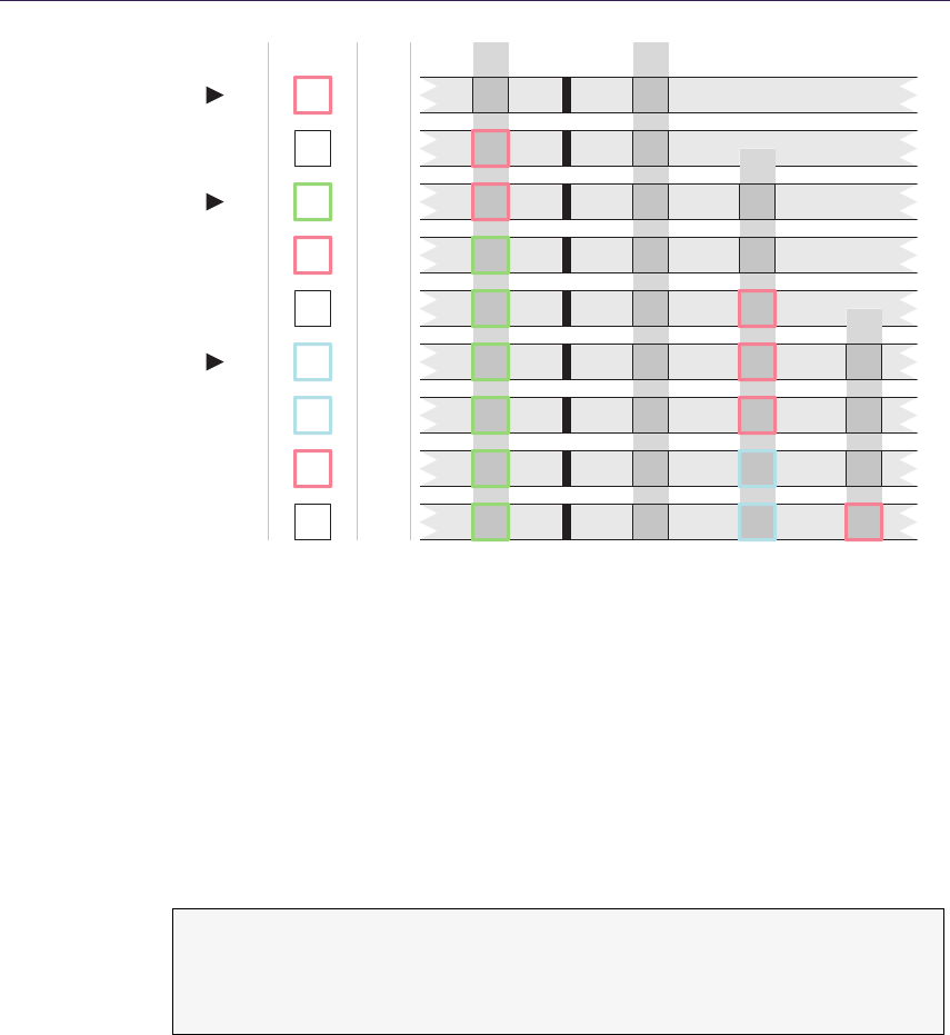
342 21. Per-Pixel Lists for Single Pass A-Buffer
0
0
p
0
0
0
00
0
n2
n1
0
00
0
0
0
0
00
0
0
00
0
0
00
0
0
0
0
0
0
0
0
0
0
0
0
0
Line
12
18
1212
12
12
12
12
18
18
p
p
n2
p
n2
n3
Pos
p
p
n2
n3
Record
z1
n1
z1
n1
z1
n1
z1
n1
z1
n1
z1
n1
z1
n1
z1
n1
z1
n1
z2
n2
z2
n2
z2
n2
z2
n2
z3
n3
z3
n3
z3
n3
z3
n3
n3
z2
n2
z2
n2
z2
n2
Figure 21.2. Insertion of three fragments into the list of pixel p. Their respective depths
are z1,z2and z3with z2> z3> z1. The triangles on the left indicate the start of the
insertion of a new fragment. Each line is a snapshot of the variables and main buffer
state at each iteration of the while loop at lines 12 or 18 of Listing 21.3.
have been properly re-inserted. Figure 21.2 illustrates the insertion of three
fragments associated with a single pixel p.
Compared to the approach of [Harris 01] based on a 32-bit atomic compare
and swap, our technique has the advantage of compactness and does not require
synchronization in the main loop. In particular the loop in Listing 21.3 can be
rewritten as follows:
1while (( old = ato mic Max6 4 ( buf fer + pos , re cord )) > 0) {
2po s = ge t Ne xt ( max ( o ld , re co rd ) ) ;
3re cor d = min (old , reco rd );
4}
Please refer to the accompanying source code for an implementation of both
approaches (file implementations.fp, functions insert_prelin_max64 and
insert_prelin_cas32).

21.3. Lists with Open Addressing (Open-alloc)343
21.3 Lists with Open Addressing (Open-alloc)
In the previous section, a cell was allocated by incrementing a global counter,
and each cell in a list had to store the index of the next cell in that list. This is
the traditional linked-list data structure.
In this section, we describe a different way to allocate cells in the main buffer
and traverse the list of fragments associated with a given pixel. This technique
frees us from storing the index of the next cell, allowing more fragments to fit in
the same amount of memory. It does come with some disadvantages as well, in
particular the inability to store more that 32 bits of data per fragment.
We start with a general introduction of this allocation strategy and then
introduce the two techniques based on it, Post-Open and Pre-Open.
21.3.1 Insertion
For each pixel p, we fix a sequence of cell positions in the main buffer, (h(p, i))i≥1
and call it a probe sequence. The function his defined as
h(p, i) = p+oimod H,
or, in Cspeak, (p + offsets[i]) % gBufferSize.
where H=gBufferSize is the size of the main buffer. The sequence (oi)i≥1
should ideally be a random permutation of the set of integers [0..H −1], so that
the probe sequence (h(p, i))i≥1covers all the cells of the main buffer. We call
(oi)i≥1the sequence of offsets. In practice this sequence is represented with a
fixed-length array of random integers, which we regenerate before each frame.
The fragments associated with pixel pare stored in the main buffer at locations
indicated by the probe sequence. When a fragment covering pixel pis stored
at position h(p, i), we say that it has age i, or that iis the age of this stored
fragment.
There are two interesting consequences to using the probe sequence defined
by function h. First, note that the sequence of offsets is independent of the pixel
position p. This means that the probe sequence for pixel qis a translation of the
probe sequence for pixel pby the vector q−p. During the rasterization, neigh-
boring threads handle neighboring pixels and in turn access neighboring memory
locations as each is traversing the probe sequence of its corresponding pixel. This
coherence in the memory access pattern eases the stress of the GPU memory
bus and increases memory bandwidth utilization. It was already exploited by
Garc´ıa et al. for fast spatial hashing [Garc´ıa et al. 11].
Second, assuming that His greater than the total number of screen pixels,
then the function hbecomes invertible in the sense that knowing h(p, i) and iis

344 21. Per-Pixel Lists for Single Pass A-Buffer
enough to recover pas
p=h(p, i)−oimod H,
or, in Cspeak, (hVal + gBufferSize - offsets[i]) % gBufferSize.
Let us define h−1(v, i) = v−oimod H. The function h−1lets us recover the
pixel p, which is covered by a fragment of age istored in cell vof the main
buffer: p=h−1(v, i). In order to compute this inverse given v, the age of a
fragment stored in the main buffer must be available. Hence, we reserve a few
bits (typically 8) to store that age in the buffer, together with the depth and data
of the fragment.
When inserting the fragments, we should strive to minimize the age of the
oldest fragment, i.e., the fragment with the largest age. This is particularly
important to ensure that when walking along lists of fragments for several pixels in
parallel, the slowest thread—accessing old fragments—does not penalize the other
threads too much. This maximal-age minimization is achieved during insertion:
old fragments are inserted with a higher priority, while young fragments must
continue the search of a cell in which to be written.
We define the load-factor of the main buffer as the ratio of the number of
fragments inserted to the total size of the main buffer.
Collisions. A collision happens when a thread tries to insert a fragment in a cell
that already contains a fragment. Collisions can happen since the probe sequence
that we follow is essentially random. When the main buffer is almost empty (the
load-factor is low), collisions rarely happen. But as the load-factor increases, the
chance of collisions increases as well. The open addressing scheme that we have
just described works remarkably well even when the load-factor is as high as 0.95.
A collision happens when a thread tries to insert a fragment fpcovering pixel
pat position h(p, i) for some i, but the cell at that position already contains a
fragment fqfor some other pixel q. We then have h(p, i) = h(q, j) and solve the
collision depending on the value of iand j:
•If j=i, then q=p. The fragment fqcovers the same pixel p; we keep it
there and try to insert fragment fpat the next position h(p, i+1). Alterna-
tively, as in Section 21.3.3, we might compare the depths of both fragments
to decide which one to keep at that position and which one to move.
•If j̸=i, then pixels pand qare different pixels. In that case, we store
the fragment with the largest age in that cell and continue along the probe
sequence of the other fragment. More precisely, if i > j then the older
fragment fpreplaces fqin the main buffer and the insertion of the younger
fragment fqis restarted at age j+ 1, i.e., at position h(q, j + 1) in the
main buffer. Note that the value qis not known in advance and must be
computed as q=h−1(h(p, i), j). If i<j, then fragment fqdoes not move
21.3. Lists with Open Addressing (Open-alloc)345
and the search for a free cell for fpproceeds at age i+ 1 in the probe
sequence of pixel p.
This eviction mechanism, whereby an “old” fragment evicts a younger fragment,
has been demonstrated to effectively reduce the maximum age of the fragments
stored in the main buffer, over all pixels. This property was discovered by Celis
and Munro in their technique called Robin Hood Hashing [Celis et al. 85].
21.3.2 Building Unsorted Lists (Post-Open)
In this section, we give the full details of the construction of unsorted lists of
fragments using the allocation scheme described above.
In the rest of this chapter, we assume that a cell of the main buffer occupies
64 bits, which lets us use atomic operations on a cell, and that the age of a
fragment is stored in the most significant bits of the cell:
MSB
age: 8 bits empty: 24 bits data: 32 bits
LSB
.
In this way, the eviction mechanism described above can be safely accomplished
using a single call to atomicMax.
We use an auxiliary 2D table Athat stores, for each pixel p, the age of the
oldest fragment associated with pin the main buffer. Thus, A[p] indicates the
end of the list of p’s fragments; from which we can start the search for an empty
cell for the new fragment fpto be inserted.
The insertion procedure is shown in Listing 21.4. It increments a counter age
starting from A[p] + 1 (line 2) until it finds an empty cell at position h(p, age)
1voi d i ns er tB ac kO A ( p , de pth , d at a ) {
2uin t age = A[ p ] + 1;
3ui nt 64_ t re cor d = OA _PA CK ( age , dep th , dat a );
4int iter = 0;
5while ( i ter ++ < M AX _IT ER ) {
6uvec2 h = ( p + off se ts [age ] ) % gBufS z ;
7ui nt6 4_t old = a tomicM ax (& buf fer [ h] , r eco rd );
8if ( old < r ec ord ) {
9a to mi cM ax (& A[ p ], age ) ;
10 if ( old == 0) bre ak ;
11 ui nt 32 _t oa ge = O A_ GET _A GE ( o ld ) ;
12 p = ( h + gBu fSz - of fse ts [ oa ge ]) % gB ufS z ;
13 ag e = A [ p ];
14 r ec or d = O A_ WR I TE _ AG E ( old , a ge ) ;
15 }
16 ++ a ge ;
17 record = re cord + O A_ IN C_ AG E ;
18 } }
Listing 21.4. Insertion in a list with open addressing.

346 21. Per-Pixel Lists for Single Pass A-Buffer
in which the record is successfully inserted (line 10). The record is tentatively
inserted in the buffer at line 7. If the insertion fails, the insertion proceeds in the
next cell along the probe sequence (lines 16 and 17). If it succeeds, the table A
is updated and if another fragment f′was evicted (old != 0), the pixel qcovered
by f′is computed from the age of f′(line 11) and function h−1(line 12). The
insertion of f′continues from the end of the list of fragments for pixel q, given
by A[q] + 1.
The macro OA_PACK packs the age, depth and data of a fragment in a 64-
bits word. The age occupies the 8 most significant bits. The macro OA_WRITE_AGE
updates the 8 most significant bits without touching the rest of the word. Finally,
the constant OA_INC_AGE = ((uint64_t)1<<56) is used to increment the age in the
packed record.
21.3.3 Building Sorted Lists with Insertion-Sort (Pre-Open)
In this section, we modify the construction algorithm above so as to keep the list
of fragments sorted by depth, by transforming it into an insertion-sort algorithm.
Let fpbe the fragment, associated with pixel p, that we are inserting in the
main buffer. When a collision occurs at age iwith a stored fragment f′
passociated
with the same pixel p, we know that both fragments currently have the same age.
Therefore, the atomicMax operation will compare the cell bits that are lower than
the bits used for storing the age. If the higher bits, among these lower bits,
encode the depth of the fragment then we ensure that the fragment with largest
depth is stored in the main buffer after the atomic operation:
MSB
age: 8 bits depth: 24 bits data: 32 bits
LSB
.
Further, it is possible to show that during the insertion of fragment fpat age i, if
a collision occurs with a fragment fqwith h(q, j) = h(p, i), then i≤j. Thus, the
insertion procedure will skip over all stored fragments that are not associated with
pixel p(since i̸=j⇒q̸=p) and will correctly keep the fragments associated
with psorted by decreasing depth along the probe sequence of p. The interested
reader will find more detail and a proof of correctness of the insertion-sort with
open addressing in our technical report [Lefebvre and Hornus 13].
Thus, we obtain an insertion-sort with open addressing simply by packing the
depth of the fragment right after its age and always starting the insertion of a
fragment at the beginning of the probe sequence. A sample implementation is
given in Listing 21.5.
21.4 Post-sort and Pre-sort
In this section we discuss details depending on the choice of scheduling for the
sort. We discuss the sort in local memory required for Post-Lin and Post-
Open, as well as how to perform early culling with Pre-Lin and Pre-Open.

21.4. Post-sort and Pre-sort 347
1voi d i ns er tS o rt ed OA (p , d epth , d at a ) {
2uin t age = 1;
3ui nt 64_ t re cor d = OA _PA CK ( age , dep th , dat a );
4int iter = 0;
5while ( i ter ++ < M AX _IT ER ) {
6uvec2 h = ( p + off se ts [age ] ) % gBufS z ;
7ui nt6 4_t old = a tomicM ax (& buf fer [ h] , r eco rd );
8if ( old < r ec ord ) {
9a to mi cM ax (& A[ p ], age ) ;
10 if ( old == 0) bre ak ;
11 age = O A_ GE T_ AG E ( old ) ;
12 p = ( h + gB ufS z - of fse ts [ a ge ]) % gB ufS z ;
13 re cor d = old ;
14 }
15 ++ a ge ;
16 record = re cord + O A_ IN C_ AG E ;
17 } }
Listing 21.5. Insertion-sort with open addressing.
21.4.1 Post-sort: Sorting in Local Memory
In the Post-sort method, the Build pass accumulates the fragments of each
pixel in a list, without sorting them. The Render pass should then sort the
fragments prior to accumulating their contributions. This is done in a pixel
shader invoked by rasterizing a fullscreen quad. The shader for a given pixel
pfirst gathers all the fragments associated with pin a small array allocated in
local memory. The array is then sorted using bubble-sort, in a manner similar
to [Crassin 10]. Insertion-sort could also be used and benefit cases where the
transparent fragments are rasterized roughly in back-to-front order.
In contrast to the Post-sort techniques, the Pre-sort approaches perform
sorting during the Build pass. This allows for early culling of unnecessary frag-
ments, as described in the next section.
21.4.2 Pre-sort: Early Culling
The Pre-sort method has the unique advantage of keeping the fragments sorted
at all times. In a transparency application, when a fragment is inserted in a sorted
list it is possible to accumulate the opacity of the fragments in front of it in the
list. If this opacity reaches a given threshold, we know that the color of fragment
fwill contribute little to the final image and we can decide to simply discard
it. This early culling mechanism is possible only when the lists of fragments
are always sorted, and it provides an important performance improvement as
illustrated in Section 21.7.

348 21. Per-Pixel Lists for Single Pass A-Buffer
21.5 Memory Management
All four techniques use the main buffer for storing fragments. We discuss in
Section 21.5.1 how to initialize the buffer at each new frame. All implementations
assumed so far that the buffer is large enough to hold all incoming fragments.
This may not be true depending on the selected viewpoint, and we therefore
discuss how to manage memory and deal with an overflow of the main buffer in
Section 21.5.2.
21.5.1 The Clear Pass
With the Lin-alloc strategy, the beginning of the main buffer that stores the
heads of the lists has to be zeroed. This is implemented by rasterizing a fullscreen
quad. The global counter for cell allocation has to be initially set to gScreenSize.
In addition, when using the paged allocation scheme with the Pre-Lin method,
an additional array containing for each pixel the free cell index in its last page
has to be cleared as well.
With the Open-alloc strategy the entire main buffer has to be cleared: the
correctness of the insertion algorithm relies on reading a zero value to recognize
a free cell. The array Aused to store the per-pixel maximal age has to be cleared
as well.
Figure 21.3 shows a breakout of the timings of each pass. As can be seen, the
Clear pass is only visible for the Open-alloc techniques, but remains a small
percentage of the overall frame time.
21.5.2 Buffer Overflow
None of the techniques we have discussed require us to count the number of
fragments before the Build pass. Therefore, it is possible for the main buffer
to overflow when too many fragments are inserted within a frame. Our current
strategy is to detect overflow during frame rendering, so that rendering can be
interrupted. When the interruption is detected by the host application, the main
buffer size is increased, following a typical size-doubling strategy, and the frame
rendering is restarted from scratch.
When using linked lists we conveniently detect an overflow by testing if the
global allocation counter exceeds the size of the main buffer. In such a case, the
fragment shader discards all subsequent fragments.
The use of open addressing requires a slightly different strategy. We similarly
keep track of the number of inserted fragments by incrementing a global counter.
We increment this counter at the end of the insertion loop, which largely hides
the cost of the atomic increment. With open addressing, the cost of the insertion
grows very fast as the load-factor of the main buffer nears one (Figure 21.4). For
this reason, we interrupt the Build pass when the load-factor gets higher than
10/16.
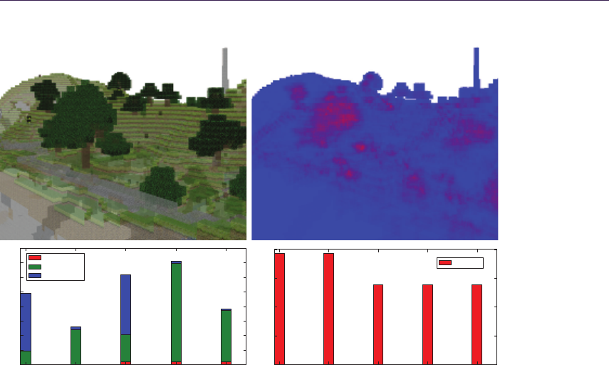
21.6. Implementation 349
Postlin-naive Prelin-naive Postopen Preopen Preopen-ec
0
5
10
15
20
25
30
35
40
Time
Time clear
Time build
Time render
Postlin-naive Prelin-naive Postopen Preopen Preopen-ec
0.0
0.5
1.0
1.5
2.0
Memory
1e8
Byte size
Figure 21.3. The lost empire scene, modeled with Minecraft by Morgan McGuire. The
top row (left) shows the textured rendering, with 0.5 opacity (alpha from textures is
ignored). The trees appear solid due to a large number of quads. The top row (right)
shows a color coded image of the depth complexity. Full red corresponds to 64 fragments
(average: 10.3, maximum: 46). The left chart gives the timing breakout for each pass
and each technique. The Clear pass (red) is negligible for Lin-alloc techniques.
Post-sort techniques are characterized by a faster Build (green) but a significantly
longer Render (blue) due to the sort. preopen-ec uses early culling, strongly reducing
the cost of Build (threshold set to 0.95 cumulated opacity). The right chart shows
the memory cost of each technique, assuming the most compact implementation. Load-
factor: 0.4.
21.6 Implementation
We implement all techniques in GLSL fragment programs, using the extension
NV_shader_buffer_store on NVIDIA hardware to access GPU memory via point-
ers. We tested our code on both a GeForce GTX 480 (Fermi) and a GeForce
Titan (Kepler), using NVIDIA drivers 320.49. We designed our implementation
to allow for easy swapping of techniques: each different approach is compiled as a
separate DLL. Applications using the A-buffer use a common interface abstract-
ing the A-buffer implementation (see abuffer.h).

350 21. Per-Pixel Lists for Single Pass A-Buffer
0.4 0.5 0.6 0.7 0.8 0.9 1.0
Load Factor
2
4
6
8
10
12
14
Time
Postopen
Preopen
Figure 21.4. Frame time (ms) versus load-factor for open addressing techniques. Note
the significant performance drop as the load-factor increases. GeForce Titan, 320.49,
2.5M fragments, average depth complexity: 2.9.
An important benefit of the techniques presented here is that they directly
fit in the graphics pipeline, and do not require switching to a compute API.
Therefore, the Build pass is the same as when rendering without an A-buffer,
augmented with a call to the insertion code. This makes the techniques easy to
integrate in existing pipelines. In addition all approaches require fewer than 30
lines of GLSL code.
Unfortunately implementation on current hardware is not as straightforward
as it could be, for two reasons: First, the hardware available to us does not
natively support atomicMax on 64 bits in GLSL (Kepler supports it natively on
CUDA). Fortunately the atomicMax 64 bits can be emulated via an atomicCompSwap
instruction in a loop. We estimated the performance impact to approximately
30% by emulating a 32 bits atomicMax with a 32 bits atomicCompSwap (on a GeForce
GTX480). The second issue is related to the use of atomic operations in loops,
inside GLSL shaders. The current compiler seems to generate code leading to
race conditions that prevent the loops from operating properly. Our current
implementation circumvents this by inserting additional atomic operations having
no effect on the algorithm result. This, however, incurs in some algorithms a
penalty that is difficult to quantify.
21.7 Experimental Comparisons
We now compare each of the four versions and discuss their performance.

21.7. Experimental Comparisons 351
21.7.1 3D Scene Rendering
We developed a first application for rendering transparent, textured scenes. It is
included in the companion source code (bin/seethrough.exe). Figure 21.3 shows
a 3D rendering of a large scene with textures and transparency. It gives the
timings breakout for each pass and each technique, as well as their memory cost.
21.7.2 Benchmarking
For benchmarking we developed an application rendering transparent, front fac-
ing quads in orthographic projection. The position and depth of the quads are
randomized and change every frame. All measures are averaged over six sec-
onds of running time. We control the size and number of quads, as well as their
opacity. We use the ARB_timer_query extension to measure the time to render a
frame. This includes the Clear,Build, and Render passes as well as checking
for the main buffer overflow. All tests are performed on a GeForce GTX480 and
a GeForce Titan using drivers 320.49. We expect these performance numbers
to change with future driver revisions due to issues mentioned in Section 21.6.
Nevertheless, our current implementation exhibits performance levels consistent
across all techniques as well as between Fermi and Kepler.
The benchmarking framework is included in the companion source code (bin/
benchmark.exe). The python script runall.py launches all benchmarks.
Number of fragments. For a fixed depth complexity, the per-frame time is ex-
pected to be linear in the number of fragments. This is verified by all imple-
mentations as illustrated Figure 21.5. We measure this by rendering a number
of quads perfectly aligned on top of each other, in randomized depth order. The
number of quads controls the depth complexity. We adjust the size of the quads
to vary the number of fragments only.
Depth complexity. In this experiment we compare the overall performance for a
fixed number of fragments but a varying depth complexity. As the size of the per-
pixel lists increases, we expect a quadratic increase in frame rendering time. This
is verified Figure 21.6. The technique Pre-Open is the most severely impacted
by the increase in depth complexity. The main reason is that the sort occurs in
global memory, and each added fragment leads to a full traversal of the list via
the eviction mechanism.
Early culling. In scenes with a mix of transparent and opaque objects, early culling
fortunately limits the depth complexity per pixel. The techniques Pre-Open and
Pre-Lin both afford for early culling (see Section 21.4.2). Figure 21.7 demon-
strates the benefit of early culling. The threshold is set up to ignore all fragments
after an opacity of 0.95 is reached (1 being fully opaque).
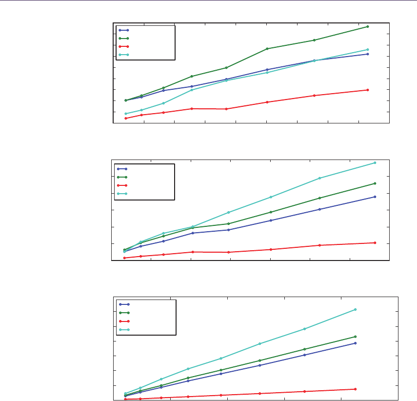
352 21. Per-Pixel Lists for Single Pass A-Buffer
0 200000 400000 600000 800000 1000000 1200000 1400000 1600000 1800000
Num Frags
0.0
0.5
1.0
1.5
2.0
2.5
3.0
3.5
4.0
4.5
Time
Postlin-naive
Postopen
Prelin-naive
Preopen
0 1000000 2000000 3000000 4000000 5000000 6000000 7000000
Num Frags
0
5
10
15
20
25
30
Time
Postlin-naive
Postopen
Prelin-naive
Preopen
0.0 0.5 1.0 1.5 2.0 2.5
Num Frags 1e7
0
50
100
150
200
250
300
350
Time
Postlin-naive
Postopen
Prelin-naive
Preopen
Figure 21.5. Frame time (ms) versus number of fragments. From top to bottom, the
depth complexity is 5, 20, and 63 in all pixels covered by the quads. Increase in frame
time is linear in number of fragments.
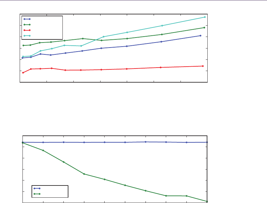
21.8. Conclusion 353
34 5 678 9 10
AvgDepth
0
2
4
6
8
10
12
Time
Postlin-naive
Postopen
Prelin-naive
Preopen
Figure 21.6. Frame time (ms) versus average depth complexity. GeForce Titan, driver
320.49, load-factor: 0.5, 2.5M fragments.
0.1 0.2 0.3 0.4 0.5 0.6 0.7 0.8 0.9 1.0
Opacity
10
20
30
40
50
60
70
Time
Preopen
Preopen-ec
Figure 21.7. Frame time versus opacity for Pre-Open with and without early culling.
Early culling (green) quickly improves performance when opacity increases. GeForce
Titan, driver 320.49, load-factor: 0.5, 9.8M fragments.
21.8 Conclusion
Our tests indicate that Pre-Lin has a significant advantage over other techniques,
while the Open-alloc cell allocation strategy falls behind. This is, however,
not a strong conclusion. Indeed, all of these methods, with the exception of
Post-Lin, are penalized by the emulation of the atomic max 64 bits. More
importantly, the implementation of the Open-alloc techniques currently suffers
from unnecessary atomic operations introduced to avoid race conditions.
The Lin-alloc cell allocation strategy strongly benefits from the dedicated
increment atomic counters. Our tests indicate that without these, the Build

354 21. Per-Pixel Lists for Single Pass A-Buffer
performance is about three times slower (using paged allocation, which is then
faster), making Pre-Open competitive again. This implies that in a non-GLSL
setting the performance ratios are likely to differ.
Finally, the Post-sort techniques could benefit from a smarter sort, bubble-
sort having the advantage of fitting well in the Render pass due to its straight-
forward execution pattern. Using a more complex algorithm would be especially
beneficial for larger depth complexities. However, increasing the number of frag-
ments per-pixel implies increasing the reserved temporary memory. This impedes
performance: for the rendering of Figure 21.3, allocating a temporary array of size
64 gives a Render time of 20 ms, while using an array with 256 entries increases
the Render time to 57 ms. This is for the exact same rendering: reserving more
memory reduces parallelism. In contrast, the Pre-sort techniques suffer no such
limitations and support early fragment culling.
For updates on code and results please visit http://www.antexel.com/research/
gpupro5.
21.9 Acknowledgments
We thank NVIDIA for hardware donation as well as Cyril Crassin for discussions
and feedback on GPU programming. This work was funded by ERC ShapeForge
(StG-2012-307877).
Bibliography
[Carpenter 84] Loren Carpenter. “The A-buffer, an Antialiased Hidden Surface
Method.” SIGGRAPH 18:3 (1984), 103–108.
[Celis et al. 85] Pedro Celis, Per-˚
Ake Larson, and J. Ian Munro. “Robin Hood
Hashing (Preliminary Report).” In Proceedings of the 25th Annual Sympo-
sium on Foundations of Computer Science, pp. 281–288. Washington, DC:
IEEE, 1985.
[Crassin 10] Cyril Crassin. “OpenGL 4.0+ A-buffer V2.0: Linked
lists of fragment pages.” http://blog.icare3d.org/2010/07/
opengl-40-abuffer-v20-linked-lists-of.html, 2010.
[Garc´ıa et al. 11] Ismael Garc´ıa, Sylvain Lefebvre, Samuel Hornus, and Anass
Lasram. “Coherent Parallel Hashing.” ACM Transactions on Graphics 30:6
(2011), Article no. 161.
[Harris 01] Timothy L. Harris. “A Pragmatic Implementation of Non-blocking
Linked-Lists.” In Proceedings of the 15th International Conference on Dis-
tributed Computing,DISC ’01, pp. 300–314. London: Springer-Verlag, 2001.

Bibliography 355
[Lefebvre and Hornus 13] Sylvain Lefebvre and Samuel Hornus. “HA-Buffer: Co-
herent Hashing for Single-Pass A-buffer.” Technical Report 8282, Inria, 2013.
[Lefebvre 13] Sylvain Lefebvre. “IceSL: A GPU Accelerated Modeler and Slicer.”
In Distributed Computing: 15th International Conference, DISC 2001, Lis-
bon, Portugal, October 3–5, 2001, Proceedings,Lecture Notes in Computer
Science 2180, pp. 300–314. Berlin: Springer-Verlag, 2013.
[Maule et al. 11] Marilena Maule, Jo˜ao Luiz Dihl Comba, Rafael P. Torchelsen,
and Rui Bastos. “A Survey of Raster-Based Transparency Techniques.” Com-
puters & Graphics 35:6 (2011), 1023–1034.

22
Reducing Texture Memory Usage
by 2-Channel Color Encoding
Krzysztof Kluczek
22.1 Introduction
In modern games, textures are the primary means of storing information about
the appearance of materials. While often a single texture is applied to an entire
3D mesh containing all materials, they equally often represent individual materi-
als, e.g., textures of walls, terrain, vegetation, debris, and simple objects. These
single-material textures often do not exhibit large color variety and contain a lim-
ited range of hues, while using a full range of brightness resulting from highlights
and dark (e.g., shadowed), regions within the material surface. These observa-
tions, along with web articles noticing very limited color variety in Hollywood
movies [Miro 10] and next-gen games, coming as far as the proposal of using only
two color channels for the whole framebuffer [Mitton 09], were the motivation for
the technique presented in this chapter.
The method presented here follows these observations and aims to encode any
given texture into two channels: one channel preserving full luminance informa-
tion and the other one dedicated to hue/saturation encoding.
22.2 Texture Encoding Algorithm
Figure 22.1 presents the well-known RGB color space depicted as a unit cube.
Each source texel color corresponds to one point in this cube. Approximating
this space with two channels effectively means that we have to find a surface
(two-dimensional manifold) embedded within this unit cube that lies as close as
possible to the set of texels from the source texture. To simplify the decoding
algorithm, we can use a simple planar surface or, strictly speaking, the intersec-
tion of a plane with the RGB unit cube (right image of Figure 22.1). Because we
have already decided that luminance information should be encoded losslessly in
a separate channel, the color plane should pass through the RGB space’s origin
357

358 22. Reducing Texture Memory Usage by 2-Channel Color Encoding
B B
G G
R R
Figure 22.1. RGB color space as unit cube (left) and its intersection with a plane
(right).
of zero luminance (black). Therefore, the simplified color space for the 2-channel
compression is defined by a single three-dimensional vector—the plane normal.
22.2.1 Color Plane Estimation
Fitting a plane to approximate a set of 3D points is a common task and various
algorithms exist. In order to find the best plane for color simplification we have
to take the following preparatory steps.
First, we have to remember that RGB pixel color values in most image file
formats do not represent linear base color contribution. For the purpose of this
algorithm, we want to operate in the linear RGB color space. Most common file
formats provide values in sRGB space [Stokes 96]. While being internally more
complex, this representation can be approximated with gamma 2.2, i.e., after
raising RGB values to power of 2.2 we obtain approximately linear light stimuli
for red, green, and blue. We can approximate this with a gamma value of 2, which
allows a simple use of multiplication and square root for conversion between sRGB
and approximate linear RGB spaces. Strictly speaking, we will then be operating
in a RGB space with a gamma of 1.1. While this slight nonlinearity will have
only a minor impact on the estimation and the encoding, it is important to use
the same simplified gamma value of 2 during the conversion back to the sRGB
space after decoding for the final presentation to avoid change in the luminance
levels.
After (approximately) converting color values to the linear RGB space, the
other thing we have to remember is the fact that the hue perception is a result
of the relation between the RGB components and is not linear. To correctly
match hues as closely as possible, we could ideally use a perceptually linear color
space (e.g., L*a*b*, explained in [Hoffmann 03]). However, this results in a much
more costly decoding stage and thus we will limit ourselves to the linear RGB
color space, accepting potential minor hue errors. Still, to minimize the impact

22.2. Texture Encoding Algorithm 359
of not operating in a perceptually correct linear RGB space, we can apply non-
uniform scaling to the space before estimating the plane. This affects the error
distribution across the RGB channels, allowing some hues to be represented more
closely at the cost of others. The result of this non-uniform scaling is that as RGB
components shrink, their influence on the color plane shrinks, because distances
along the shrunk axis are shortened. Due to the hue perception’s nonlinearity,
it is not easy to define the scaling factors once for all potential textures, and in
our tests they were set experimentally based on the sample texture set. First we
tried the RGB component weights used in the luminance computation (putting
most importance on G and barely any on B), but experiments showed that some
material textures are better represented when the estimation is done with more
balanced weighting. To achieve acceptable results for various textures, we used
an experimentally chosen weight set of 1/2 for red, 1 for green and 1/4 for blue,
which lies between the classic luminance component weights and the equally
weighted component average. Fortunately, the perceived difference in pixel hues
after the encoding changes is barely noticeable with these scaling factors. Still,
the scaling factors may be used to improve texture representation by fine tuning
them separately for each texture.
With the two above operations, the whole initial pixel color processing can be
expressed as
r′
i=rγ
iwr,
g′
i=gγ
iwg,
b′
i=bγ
iwb,
where γis the gamma value used to transition from the input color space to
the linear color space, and wr,wgand wbare the color component importance
weights.
Having taken into account the above considerations, the color of every texel
represents a single point in 3D space. The optimal approximating color plane
will be the plane that minimizes the sum of squared distances between the plane
and each point. Because the plane is assumed to be passing by the point (0,0,0),
we can express it by its normal. In effect, the point-plane distance computation
reduces to a dot product. Note that since we are using the RGB space, the vector
components are labeled r,g, and binstead of the usual x,y, and z:
di=N·Pi=nrr′
i+ngg′
i+nbb′
i.
The optimal plane normal vector is the vector, which minimizes the point-
plane distances. Such problems can be solved using least squared fit method that
aims to minimize sum of squared distances. The approximation error we want to
minimize is expressed as
err =
i
d2
i=
i
(N·Pi)2=
i
(nrr′
i+ngg′
i+nbb′
i)2,

360 22. Reducing Texture Memory Usage by 2-Channel Color Encoding
which after simple transformations becomes
err =n2
r
i
r′2
i+n2
g
i
g′2
i+n2
b
i
b′2
i
+ 2nrng
i
r′
ig′
i+ 2nrnb
i
r′
ib′
i+ 2ngnb
i
g′
ib′
i.
For minimalistic implementation, we can use the above equation to compute
all six partial sums depending only on the texel colors. Then we can use a brute
force approach to test a predefined set of potential normal vectors to find the
one minimizing the total approximation error. Because each test is carried out
in linear time, costing only several multiplications and additions, this approach
is still tolerably fast.
The final step after finding the optimal color plane is to revert the color
space distortion caused by the color component weighting by scaling using the
reciprocal weights. Because the plane normal is a surface normal vector, the usual
rule of non-uniform space scaling for normals applies and we have to multiply the
normal by the inverse transpose of the matrix we would use otherwise. While the
transposition does not affect the scaling matrix, the matrix inversion does and
the final scaling operation is using non-reciprocal weights again:
N′=N
1/wr0 0
0 1/wg0
0 0 1/wb
−1
T
=N
wr0 0
0wg0
0 0 wb
.
As all subsequent computation is typically done in the linear RGB space, we
do not have to convert into sRGB (which would be nonlinear transform anyway).
22.2.2 Computing Base Colors
The important parameters for the encoding and the decoding process are the two
base colors. The color plane cutting through the RGB unit cube forms a triangle
or a quadrilateral, with one of the corners placed at the point (0,0,0). The two
corners neighboring the point (0,0,0) in this shape are defined as the base colors
for the planar color space, as shown on Figure 22.2. Every other color available
on the plane lies within the angle formed by the point (0,0,0) and the two base
color points. Because the color plane starts at (0,0,0) and enters the unit cube,
the base color points will always lie on the silhouette of the unit cube, as seen
from the point (0,0,0). To find the base colors, we can simply compute the plane
intersection with the silhouette edges, resulting in the desired pair of points. We
have to bear in mind that the plane can slice through the silhouette vertices, or
even embed a pair of silhouette edges. Therefore, to compute the points we can

22.2. Texture Encoding Algorithm 361
B
G
R
bc2
bc1
(0,0,0)
Figure 22.2. Base colors on the color plane.
use an algorithm, which walks around the silhouette computing the two points
in which the silhouette crosses the plane.
The key observation now is that we can represent a hue value as the angle
to the vectors spanning the plane or, alternatively, using a linear interpolation
between the two base colors. In order to compute the final color, we only have
to adjust the luminance and perform any required final color space conversions.
22.2.3 Luminance Encoding
The luminance of the color being encoded is stored directly. After colors have
been transformed into the linear RGB space, we can use a classic equation for
obtaining perceived luminance value derived from the sRGB to XYZ color space
transformation in [Stokes 96]:
L= 0.2126 ·R+ 0.7152 ·G+ 0.0722 ·B.
Because the weighting coefficients sum up to 1, the luminance value ranges from
zero to one. Since the luminance has its own dedicated channel in the 2-channel
format, it can now be stored directly. However, as luminance perception is not
linear, we are using a gamma value of 2 for the luminance storage. This is close
enough to the standard gamma 2.2 and gives the same benefits—dark colors have
improved luminance resolution at the cost of unnoticeably reduced quality of
highlights. Also the gamma value of 2 means that luminance can simply have its
square root computed while encoding and will simply be squared while decoding.
22.2.4 Hue Estimation and Encoding
To encode the hue of the color, we have to find the closest suitable color on the
approximating plane and then find the proportion with which we should mix the
base colors to obtain the proper hue. The hue encoding process is demonstrated
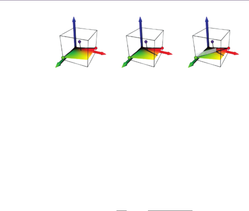
362 22. Reducing Texture Memory Usage by 2-Channel Color Encoding
B
RRR
GGG
B B
bc2
bc1 bc1
bc2 bc2
(0,0,0) (0,0,0) (0,0,0)
Figure 22.3.Hue encoding process.
in Figure 22.3 and can be outlined as follows:
1. Project the color point in the linear RGB space onto the color plane.
2. Compute the 2D coordinates of the point on the plane.
3. Find a 2D line on plane passing through (0,0,0) and the point.
4. Find the proportion in which the line crosses the 2D line between the base
color points, i.e., determine the blend factor for the base colors.
The first step is a simple geometric operation. From the second step on,
we have to perform geometric operations on 2D coordinates embedded within
the plane. Having the two base color points Aand B, we can compute the 2D
coordinate frame of the plane as
Fx=A
∥A∥Fy=B−(Fx·B)Fx
∥B−(Fx·B)Fx∥
and then compute 2D coordinates of any point within the plane using the dot
product:
(xi, yi) = (Pi·Fx, Pi·Fy).
Please note that we do not actually need the explicit RGB coordinates of the
point on the plane nearest to the color being encoded, but only its 2D coordinates
within the plane, xiand yi. As both the original point and the point projected
onto the plane will have the same 2D coordinates, we can skip step 1 in the
outlined algorithm completely. The projection onto the plane is a side effect of
the reduction to only two dimensions.
The problem of computing the base color blend factor for hue, when consid-
ering the points embedded within the color plane, is now reduced to the problem
of intersection of two lines: a line connecting both base color points and a line

22.3. Decoding Algorithm 363
float3 texture_decode( float2 data , float3 bc1 , float3 bc2 )
{
float3 co lor = l erp ( bc1 , bc2 , dat a .y ) ;
float c ol or _l um = dot ( color , float3(0. 21 26 , 0. 7152 ,0.072 2) ) ;
float t ar get _l um = d ata . x * d ata . x;
color *= t arg et_ lum / color_lum ;
return co lor ;
}
Listing 22.1. Two-channel texture decoding algorithm.
passing through the origin and the point on the plane being encoded. This gives
us the following line-line intersection equation:
A+t(B−A) = sP.
Solving this linear equation for tgives us the result—the base color blend
factor resulting in a hue most closely matching the hue of the encoded point. This
blend factor is then simply stored directly in the second channel, completing the
2-channel encoding process.
22.3 Decoding Algorithm
The decoding algorithm is simple and best described by the actual decoding
shader code in Listing 22.1.
First, the base colors bc1 and bc2, which are passed as constant data, are
blended with a blend factor coming from the second channel of data, resulting in
a color having the desired hue, but wrong luminance. This luminance is computed
as color_lum. Next, we compute the desired luminance target_lum as a value of
first channel of data squared (because we stored the luminance with gamma 2).
As the resulting color is in a linear color space, we can adjust the luminance by
simply dividing the color by the current luminance and then multiplying it by
the desired one. If needed, we can of course convert the computed color to a
nonlinear color space for presentation purposes.
22.4 Encoded Image Quality
Figures 22.4,22.5, and 22.6 show examples of the encoding and decoding process.
The example textures are taken from the CGTextures texture library and were
selected because of their relatively rich content and variety.
Figure 22.4 presents a 2-channel approximation result of a dirt texture with
grass patches. Both dirt and grass are reproduced with slight, but mostly unno-
ticeable differences in color. As the method is designed with limited-color material
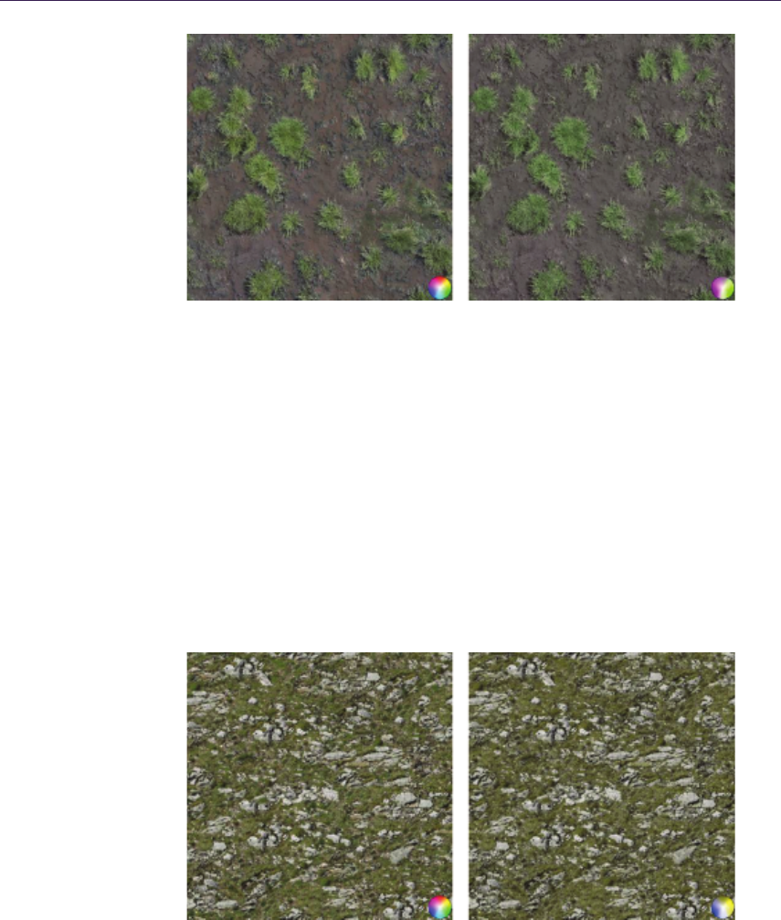
364 22. Reducing Texture Memory Usage by 2-Channel Color Encoding
Figure 22.4. Grass and dirt texture example. Original image (left) and result after the
encoding/decoding process (right).
textures in mind, the color probe added on the image is of course severely de-
graded, but clearly shows that the estimation algorithm picked the green-purple
color plane as fitting the image best. These extreme colors may not be used
directly on the texture, but we should remember that all colors resulting from
blending green and purple are available at this stage and this includes colors with
reduced saturation in the transition zone. Because of the separate treatment of
pixel luminance, the luminance values are unaffected except for processing and
storage rounding errors.
Figures 22.5 and 22.6 show two examples of textures with mixed materials.
This time, the estimation process has chosen a blue-yellow for the first and a
Figure 22.5. Rock and stone texture example. Original image (left) and result after the
encoding/decoding process (right).
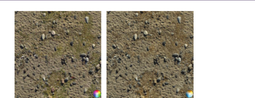
22.5. Conclusion 365
Figure 22.6. Sand, dead grass, and rocks texture example. Original image (left) and
the decoded result after 2-channel compression (right).
teal-orange plane for the second image. While the stone and grass texture mostly
remains unaffected, the sand, grass, and stones texture required finding a compro-
mise resulting in some grass discoloration and smaller off-color elements changing
color completely.
22.5 Conclusion
The encoding and decoding methods presented in this chapter allow storing tex-
tures with low color variety using only two texture channels. Apart from the
obvious savings, this opens additional possibilities. For example, considering
that most texture sampler implementations support 4-channel textures, the two
remaining channels can be used for other purposes, e.g., storing xand ycompo-
nents of the material normal map, resulting in a compact material representation
with just a single texture image. Even if not using this feature, the fact that
the proposed 2-channel color encoding relies on a luminance-hue decomposition
allows custom texture compression algorithms. We can assign higher priority
to luminance information during texture compression, accumulating most of the
compression error in hue, to changes to which the human eye is less sensitive,
increasing the overall compressed image quality. We should also note that the
proposed encoding scheme can be used directly with existing mip-mapping solu-
tions, because averaging luminance-values and hue-blend factors is a good approx-
imation of averaging color values. We should only be aware that the luminance
values are stored with a gamma of 2 and may require a custom mip-map chain
generation if we require fully linear color processing in the whole lighting pipeline.

366 22. Reducing Texture Memory Usage by 2-Channel Color Encoding
Bibliography
[Hoffmann 03] Gernot Hoffmann. CIELab Color Space.http://docs-hoffmann.de/
cielab03022003.pdf, 2003.
[Miro 10] Todd Miro. Teal and Orange—Hollywood, Please Stop the
Madness.http://theabyssgazes.blogspot.com/2010/03/teal-and-orange
-hollywood-please-stop.html, 2010.
[Mitton 09] Richard Mitton. Two-Channel Framebuffers for Next-Gen Color
Schemes.http://www.codersnotes.com/notes/two-channel, 2009.
[Stokes 96] Michael Stokes, Matthew Anderson, Srinivasan Chandrasekar, and
Ricardo Motta. A Standard Default Color Space for the Internet—sRGB. http:
//www.w3.org/Graphics/Color/sRGB, 1996.
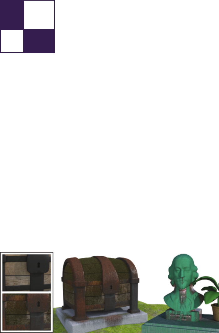
23
Particle-Based Simulation
of Material Aging
Tobias G¨
unther, Kai Rohmer,
and Thorsten Grosch
23.1 Introduction
The composition of detailed textures, facilitating weathered and aged looks, is
an everyday task for content artists in game and movie production. Examples of
aged scenes are shown in Figure 23.1. In the process of meticulously editing tex-
tures, each inaccuracy or later change in the scenery can cause implausibility and
quickly break the immersion. Therefore, interactively steerable, automatic simu-
lations that favor the plausibility of aging effects, caused by interacting objects,
e.g., dripping of rust, are vitally needed. This chapter describes implementation
details of a GPU-assisted material aging simulation, which is based on customiz-
able aging rules and material transport through particles. The chapter is based on
Figure 23.1. Interactively aged scene, exported and rendered in a DCC tool.
367
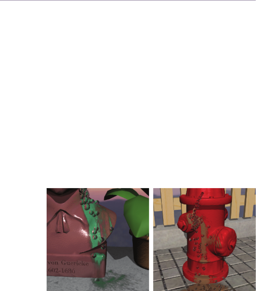
368 23. Particle-Based Simulation of Material Aging
our paper [G¨unther et al. 12], where further results and discussions can be found.
The simulation machinery is partly CUDA-based and partly rasterization-based
to exploit the advantages of both sides. In fact, it is driven by an interplay of
a number of modern GPU features, including GPU ray tracing, dynamic shader
linkage, tessellation, geometry shaders, rasterization-based splatting and trans-
form feedback, which are described in the following.
23.2 Overview
Our simulation of weathering effects is based on material transporting particles—
so-called gammatons, introduced in [Chen et al. 05]. Gammatons are emitted
from sources, such as clouds or roof gutters, to drip and distribute material, as
shown in Figure 23.2. On impact, material is deposited or taken away, and the
gammaton either bounces, floats, or is absorbed (see Figure 23.3). Eventually,
resting material is subject to aging rules, for instance, turning metal into rust or
spreading lichen growth. For this, the resting material is stored in a texture atlas,
which we call material atlas; see later in Section 23.3.1 for a detailed discription
of its content.
The simulation pipeline is illustrated in Figure 23.4. The particle movement
and collision detection are done in CUDA, using Nvidia’s ray tracing engine Op-
tiX [Parker et al. 10]. Thus, in the simulation step a CUDA kernel is called, which
emits and traces gammatons (elaborated in Section 23.3.2). In the following two
stages, the surface update and the gammaton update, the material is transferred
Figure 23.2. Patina and dirt being transported by gammatons. A subset of the gam-
matons are rendered as spheres. [Appeared in [G¨unther et al. 12] and reproduced by kind
permission of the Eurographics Association.]
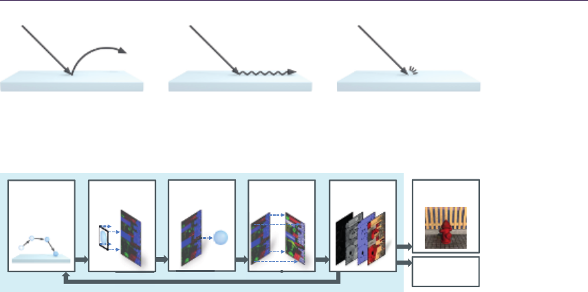
23.3. Simulation 369
Figure 23.3. Depiction of collision responses, left to right: bounce, float, absorb. [Ap-
peared in [G¨unther et al. 12] and reproduced by kind permission of the Eurographics
Association.]
Simulation
step
Surface
update
Gammaton
update
Aging
process
Composition Preview
rendering
Export aged
textures
Figure 23.4. Illustration of the simulation pipeline. [Appeared in [G¨unther et al. 12]
and reproduced by kind permission of the Eurographics Association.]
between the gammatons and the hit surfaces (detailed in Section 23.3.3). This
happens in two consecutive steps: a rasterization pass to drop material into the
material atlas and a transform feedback pass to update the gammaton material.
Moreover, we determine the subsequent behavior of the gammatons by Russian
Roulette (e.g., float, bounce, or absorb) and specify their velocity for the next
iteration. In the following stage, the aging process, aging rules are applied, e.g.,
rusting in the presence of water and metal. To select the rule set, we use dynamic
shader linkage, further explained in Section 23.3.4. Based on the material stored
in the material atlas (Section 23.3.1) we compose texture maps for the aged dif-
fuse color, shininess, surface normal, and height in the composition stage (Section
23.3.5). These maps can be used for preview rendering (Section 23.4) and can be
exported (alongside all additional material atlas data), for instance, for external
use in game engines or DCC tools.
23.3 Simulation
23.3.1 The Material Atlas
In order to decouple the weathering operations from the scene complexity, we
maintain all simulation-relevant material, surface, and normalization data in
a texture atlas, which we refer to as material atlas, depicted in Figure 23.5.
Thereby, the amount of material carried by gammatons or resting on a surface—
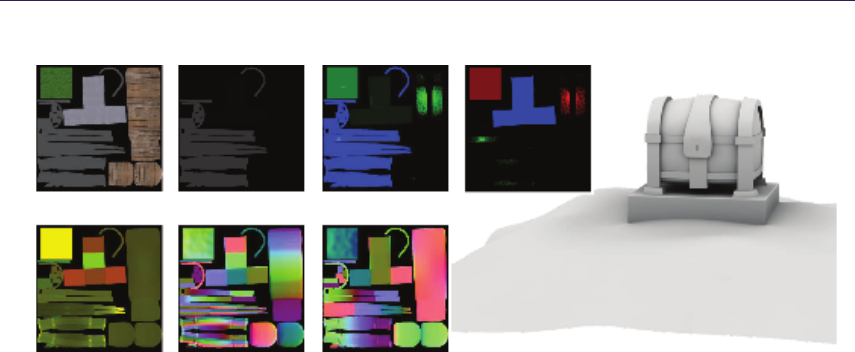
370 23. Particle-Based Simulation of Material Aging
Original color Shininess Materials (1) Materials (2)
Texel-to-world Normals Tangents
Figure 23.5. The material atlas contains all surface information. In this image a subset of the atlas
textures is shown for the Chest scene.
the latter is stored in texels of the atlas—is assignable to eight available slots. In
our examples, we needed only seven slots for water, dirt, metal, wood, organic,
rust, and stone. All in all, the material atlas contains color + shininess (RGBA8),
geometric normals and tangents (2 ×RGB16F), shading normals (RGB16F),
original and current height (2 ×R16F), eight material amounts (ping-pong of
2×RGBA8), eight original material amounts (2 ×RGBA8), and a texture-to-
world scale (RG16F), used later for equally-sized splatting. Thus, a parameteri-
zation is required for a one-to-one relation between surface points and respective
atlas coordinates, which we obtain semi-automatically using standard DCC tools.
For this, UV maps already present in game and movie production can be reused.
The atlas resolution is the dominant factor in trading visual quality for per-
formance. To decrease the memory consumption, we reduced the amounts of
our materials to 256 discrete steps each, thus 2 ×RGBA8 textures are used for
storage.
23.3.2 Gammaton Transport—The Simulation Step
To attain interactive frame rates, we only compute a fixed number of simulation
steps each frame. Gammatons that are midair are marked as such and do not yet
participate in material transport. The data stored for the gammatons is shown
in Listing 23.1, including the payload carried by a gammaton during ray tracing,
which is later passed into CUDA kernels as prd =payload record data, and the
persistent data stored on the OptiX side alone (position) or shared with D3D
(atlas texture coordinates of hit, material, etc.).

23.3. Simulation 371
// I nf or mation a ga mm aton ca rries d uring tr ac in g
struct GammaPayload
{
uin t ray_index ; // index in the hit bu ffers
uin t ray_depth ; // numb er of ray in di recti on s
float s pee d ; // s peed ( mu ltiplied wit h dir ection )
};
// Hit b uffer data th at is us ed by Opti X only .
struct GammaHitOptix
{
fl oat3 po sit ion ; // position of the ga mm at on
};
// Hit bu ffer data th at is share d betwee n Direct X and O ptiX
struct GammaHitShared
{
fl oat3 ve loc ity ; // ve lo ci ty ve ctor
int f lags ; // m id air ( ye s / no ) , a ct ive ( ye s / no )
fl oat2 te xco ord ; // at las coord at l ast hit surfac e
uint2 car ri edMate ria l ; // 8 bytes = 8 materia l slot s
int r and omS eed ; // se ed for ra ndom n umber gener at io n
};
Listing 23.1. Data stored for the gammatons.
Recursive ray tracing. The CUDA entry program that launches the gammatons
is shown in Listing 23.2 and works as follows: If a gammaton is active, i.e., it is
currently midair or received a new direction in response to a collision, we continue
the tracing from its last known position. Otherwise a gammaton is not active,
i.e., it left the simulation domain, came to a halt on a nearly horizontal surface, or
was absorbed. In that case, a new gammaton is emitted. This entry program is
executed for each gammaton source in turn, using customizable emission parame-
ters, e.g., position, direction, speed, and distribution. For the subsequent parallel
processing of all gammatons, we assign each source an exclusive range of memory
of a shared gammaton stream. Therefore, we set for each source a start offset
g_SourceRayIndexOffset, as shown in Figure 23.6. The gammaton trajectory is
traced as a recursive series of linear steps, each reporting a hit or miss. In OptiX,
kernels are called for the respective events, as shown in Listings 23.3 and 23.4.
In each step, we add gravity according to the traveled distance, which results in
parabolic trajectories. For floating particles, gravity is acting tangentially. We
trace a fixed number of linear steps per iteration until either a surface got hit,
the gammaton left the domain, or the maximum recurrence depth is reached. In
the latter case, we mark the gammaton as midair (flag). The material transport
that is issued on impact of a gammaton is described later in Section 23.3.3. The
collision response is selected by Russian Roulette on the events bouncing, float-
ing, and absorbing (see Figure 23.3), according to their associated probabilities.
Bouncing and floating particles are reflected by the tangent plane orthogonal to
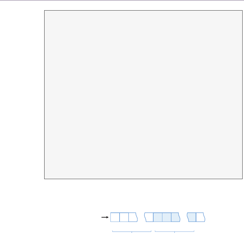
372 23. Particle-Based Simulation of Material Aging
voi d gammaton_entry_program()
{
// in it ialize payl oa d
Ray ra y ; G am ma Pa yl oa d prd ;
prd . ra y_i nd ex = l au nc h_ in de x + g _S ou rc eR ay In de x Of fs et ;
prd . ra y_d ep th = 0; // co unts r ecursions
// get g amm at on da ta ( p ing po ng )
Ga mmaHi tS hared & hitsha re d_ i = HitSh ar ed _In [ prd . r ay _i nd ex ];
G amm aH it Sh ar ed & h it sh ar ed_ o = H it Sh ar ed _O ut [ p rd . ra y_ in dex ];
// if gam ma to n is alive , co nt in ue the ray
if ( IS _A LIV E ( hi ts har ed _i . fl ags ) )
{
// continue from las t position
ray . o ri gin = Hi tOp ti x [ prd . r ay _i nde x ]. po si tio n ;
ray . direction = nor malize ( h its hare d_i . v elo cit y );
prd . s pee d = le ngt h ( h it sh are d_ i . v el oci ty ) ;
hi tshared_ o . car ri edM ater ial = hi tshare d_i . c arri edM at eri al ;
}
els e // else emit a new ra y
{
ra y . or ig in = g e ne r at eR a nd om P os it i on () ;
ray . di rec ti on = ge ne ra te Ra nd o mD ir ec ti on ()
prd . s pee d = g _I ni ti al Ve lo ci ty ;
hi tshared_ o . car ri edM ater ial = g_S tar tMat eri al ;
}
SE T_ALIV E ( hi tsh ar ed_ o . fla gs ) // set al ive
SE T_ BOU NC E ( hi tsh ar ed_ o . fl ags ) // flying freely
hi tshared_ o . ran dom See d = hitshar ed_ i . ran domSeed ; // pass se ed
float m ax Dis t = prd . s pee d * g _I nt eg ra ti on St e pS iz e ;
o p ti x Tr a ce G am m at o n ( ray , p rd , m ax D is t ) ; // la unch ray
}
Listing 23.2. OptiX/CUDA entry program for gammaton emission and continue.
…
1st emitter 2nd emitter
…
1 2 3 n 123m
…
Oset = nOset = 0
Consecutive
buer
Figure 23.6. All gammaton emitters share an output gammaton stream. For each
emitter a contiguous memory block is reserved to store the respective particles (here, n
and m). Each gammaton keeps its address, even when inactive.
the estimated surface normal (see Section 23.3.5), and the outgoing direction is
randomized by Phong lobe sampling for spreading material. For floating particles
the resulting velocity vector is projected back into the tangent plane.

23.3. Simulation 373
void gammaton_closest_hit()
{
Ga mmaH itS hare d & h its har ed = H itShar ed_ Out [ prd . ray _in dex ];
fl oat 3 v = r ay . dir ec tio n * prd . sp eed ; // v el oc it y
fl oat 3 ph it = ray . o rig in + t _hit * r ay . d ire ct io n :
float3 pn ew = phit + a tt r_ no rmal * EP SI LO N ; // mov e up
// pick up velocity by fa llen d is ta nc e
float s = le ngt h (pnew - ray . ori gin ) ;
float d t = s / prd . s pee d ; // ti me = d istance / speed
v += dt * gr av ity ;
if ( is Too Slow ( v) ) // too sl ow ?
SE T_D EAD ( h its har ed . flags ) ; // set i na ct iv e
SE T_H IT ( h its har ed . f lags ) ; // we hit a su rf ac e
hi tsh ared . te xcoor d = attr_ tex co ord ;
hi tshare d . vel ocity = no rm ali ze ( v) * prd . spe ed ;
// Re me mb er po si ti on un til next la un ch
G amm aH it Op ti x & ga mm aSt at e = G am ma Hi tO pt ix Ma p [ prd . r ay _i nd ex ] ;
ga mm aSt at e . po si tio n = pne w ;
// plant w ith p ro bab ilit y ( e xpl ained la ter ) .
pl an tl et Pla ce me nt ( h its ha red . r and omSe ed , pnew , at tr_t exc oo rd ) ;
}
Listing 23.3. OptiX/CUDA gammmaton closest hit program. Attributes, e.g.,
attr_normal and attr_texcoord, are passed by the intersection test program.
Numerical considerations of floating particles. We apply a numerical offset ϵto the
gammaton’s position to avoid a self-intersection at the launch position. Since a
floating particle moves tangentially to the surface, it virtually hovers above the
surface. To create an intersection in the next iteration we let the ray aim at the
surface by pulling the ray direction along the negated normal by the amount h
(see Figure 23.7). The resulting speed of the floating gammatons depends on both
v
εn
(a)
v
vt
εn
(b)
−hn
vt
w
εn
(c)
Figure 23.7. (a) Apply offset ϵin normal direction to the hit position. (b) Project
the velocity v(•) into the tangential plane giving vt. (c) Pull vtin negated normal
direction by the amount of h, which yields a new direction w(•). [Appeared in [G¨unther
et al. 12] and reproduced by kind permission of the Eurographics Association.]

374 23. Particle-Based Simulation of Material Aging
voi d ga mm ato n_ mi ss ()
{
// co mp ute position of gammaton
float dt = g _I nt egra tio nS te pSiz e ;
fl oat 3 vo ld = ray . d ir ect io n * prd . s pee d ;
float3 pn ew = ray . origi n + dt * vold ;
float3 vn ew = vo ld + dt * gr avity ;
G amm aH it Sh ar ed & h it sha re d = H it Sh are d_ Ou t [ pr d . ra y_i nd ex ];
if ( l eft Do ma in ( pn ew )) { // if o ut side bo unding box
SE T_D EA D ( hi tsh are d . fl ags ) ;
return;
}
// Fl oa ti ng pa rt ic le mo ved ove r edge
if ( IS _F LOA T ( hi tsh are d . fla gs ) ) { // f loa t
vne w = m ake _float3 (0 ,0 ,0); // let ga mm aton f all
SE T_ BOU NCE ( hi tsh ar ed . fl ags ) ; // free fall
}
// gammaton stil l ali ve afte r ma ximum dep th
prd . ra y_d ep th ++;
if ( prd . ra y_ dep th >= MA X_ _G AM M AT ON __ DE PT H ) {
Hi tO pt ix [ pr d . ra y_i nd ex ]. p os iti on = p new ;
hi tsh are d . velocit y = vnew ;
SE T_A LIV E ( hit shared . fl ags );
SE T_ MID AIR ( hi tsh ar ed . fl ags ) ;
return;
}
prd . s pee d = l eng th ( vne w );
Ra y r ay ( pnew , no rm al iz e ( v ne w )) ;
float m axD ist = dt * prd . s peed ;
o p ti x Tr a ce G am m at o n ( ray , p rd , m ax D is t ) ; // la un ch ray
}
Listing 23.4. OptiX/CUDA gammaton miss program.
the numerical offset ϵas well as h. Floating particles can flow bottom up and
around overhangs (see Figure 23.8). If a bounce event occurs or no intersection is
found at an overhang, we let the gammaton fall down. On impact the resulting
velocity typically acts only tangentially, but to further speed up the distribution
of material, we allow the artist to alter the loss of energy of impacting particles.
To approximate friction, both bouncing and floating gammatons are slowed down
by a specific rate.
23.3.3 Material Transport
Our approach is based on the transport of materials by floating and bouncing
gammatons. Thus, we let gammatons that hit a surface issue material transfer,
for which both the material on the surface as well as the material carried by the
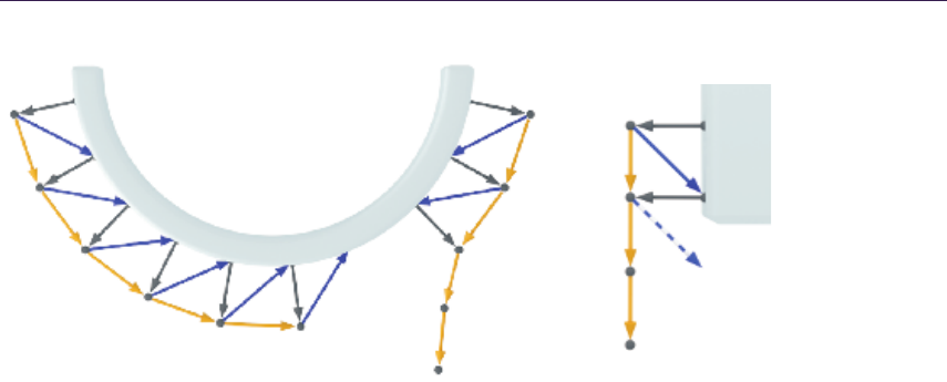
23.3. Simulation 375
Floating
Floating Floating
Fall down Fall down
Miss
Bounce
event
Figure 23.8. The visible course (•) of a gammaton floating around an overhang (left)
and when dripping off a cliff (right). In the first, the gammaton on the right falls due to
a bounce event. In the latter, the blue dashed ray misses and in response the gammaton
falls down.
gammaton are sequentially updated. First, the gammatons are splatted into the
material atlas to deposit material. Afterwards, a separate transform feedback
pass is executed to update the material of the gammatons. (Modern graphics
APIs allow for unordered access from all shader stages, making it possible to
implement both update procedures in one pass. Legacy implementations require
two separate steps.)
Determining transfer rates. The amount of material that is picked up depends first
on the material type, for instance, to accommodate that water is more volatile
than stone, and second on the material already present on the surface. The
initial material on the surfaces is assigned by presets. The coefficients required
for modeling volatileness g_volatileness are stored per material and can be part
of an asset library. They are set once prior to the simulation for each material
and can be stored and reused in other scenes. At runtime one degree of freedom
remains: the pick-up ratio g_pickUpRatio between the amount of material picked
up from the surface and added to the gammaton (and vice versa). A ratio of
zero means that material is only picked up, whereas a ratio of one means all is
dropped. Naturally, we obtain material preservation if this ratio is 1:1. Exposing
this ratio to the artist allows both to speed up the aging process and to reverse
it by washing away material, i.e., picking up more material than depositing (see
Figure 23.9).
The amount of material to transfer is determined by the method in List-
ing 23.5.
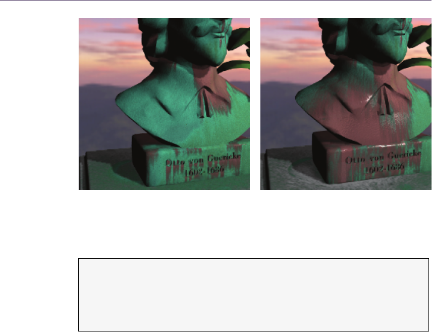
376 23. Particle-Based Simulation of Material Aging
Figure 23.9. Picking up more material than despositing allows for washing away mate-
rial (left: before, right: after). [Appeared in [G¨unther et al. 12] and reproduced by kind
permission of the Eurographics Association.]
fl oat 4 tr ans fe rRa te ( f loa t4 su rfac eMat , fl oat4 ga mma Mat )
{
fl oa t4 d elt a = s ur fa ce Ma t * (1 - g _p ic kU pR at io )
- g ammaMat * g_ pickUp Rat io ;
return delta * g_volatileness;
}
Listing 23.5. Determination of transfer rates for four materials at once.
Transport from gammaton to atlas. In order to transfer material from the gam-
matons into the atlas, we expand all gammatons that hit a surface to quads and
splat the transferred material into the material atlas textures, using multiple ren-
der targets. The procedure is outlined in Listing 23.6. An issue to deal with is the
varying area covered by texels of the atlas texture, since more space is reserved for
detailed areas. To ensure that splats are equally sized in world space, we scale the
quads in the geometry shader by the aforementioned, precomputed texel-to-world
scale. Note that the clamping to the original material (last line in Listing 23.6)
preserves the original material on the surface. This prevents the material from
being washed away completely and thus continuously provides material input to
the aging simulation.
Transport from atlas to gammaton. The gammaton material is updated afterwards
in a separate transform feedback pass by feeding the gammatons into the ren-

23.3. Simulation 377
voi d PS_SurfaceUpdate(
in float4 g am maPos : SV _Posi tion , // a tlas pos of gammaton
in float4 g am maMat : MAT ERI AL , // ma te ri al of g am ma ton
out f loat4 newMat : SV _Ta rge t0 ) // new s urface m at er ia l
{
// get cu rr ent and initia l material on sur face
fl oat 4 cu rMa t = g_ Te xMa tC ur . Lo ad ( g amm aPo s ) ;
fl oat 4 or gMa t = g_ Te xMa tO rg . Lo ad ( g amm aPo s ) ;
// ca lc ul at e t ra ns fe r rates and update ma te ri al
ne wMa t = cu rMa t - t ra nsf er Ra te ( c urMat , ga mma Ma t );
ne wMa t = max ( or gMat , ne wM at ) ; // c lamp
}
Listing 23.6. Gammatons are expanded to quads in a geometry shader and are splatted
into the atlas. This pixel shader removes material from the surface. Here, four material
slots are updated at once.
dering pipeline as point list. In a geometry shader the material to transfer is
calculated again and is added to the gammatons. Additionally, we chose this
shader to handle collisions, i.e., to compute new bounce and float directions for
the gammatons. Doing this in OptiX is possible as well. The respective geometry
shader is outlined in Listing 23.7. We decided to keep inactive gammatons in the
stream, as it eases launching of new gammatons.
23.3.4 Aging Rules
Aside from the transport of material by gammatons, the actual aging process is
the other key aspect of our system. The idea is to model the temporal aging
phenomena that take place if certain materials co-occur, by a set of generic rules.
In our system, rules are implementations of a shader interface that alter a material
set. In the simulation, we assign the chosen rule permutation by dynamic shader
linkage. This concept is an advance from uber-shaders, for which registers are
always allocated for the worst case branch, and sets of specialized shader files,
which are hard to maintain due to their combinatorial growth. Dynamic shader
linkage draws a profit from inlining selected functions (e.g., chosen rules) at bind
time, thus enabling an optimal register allocation, while providing object-oriented
aspects for the definition of rules. We chose to apply the rules to every material
atlas texel by rendering a fullscreen quad, i.e., by using a pixel shader. The
parameters of the rules are again stored in presets and are fetched at runtime
from a single constant buffer. The interface, a sample implementation and the
respective pixel shader are outlined in Listing 23.8. Practice showed that for
many involved processes plausible approximations can be found by means of
simple rules, as described next.

378 23. Particle-Based Simulation of Material Aging
[maxvertexcount(1)]
voi d GS _G am mat on Up da te ( poi nt G amma Hit Sh ar ed i nput [1] ,
inout Point Strea m < GammaH it Sh ared > PntStream )
{
Ga mmaHi tS hared ou tput = inpu t [0] ;
if ( IS_ MI DA IR ( input [0]. Flags ) || IS_DEA D ( input [0]. Flag s ) ) {
Pn tSt re am . Ap pen d ( output ) ; // no n eed to act
return;
}
// get ma te ri al at su rf ac e and gammaton
float4 s urfMat = g_ TexMat Cur . S amp leLevel (
g_L ine ar , gammaton .texcoor d , 0) ;
float4 g ammaMat = unpa ckF romU int ( g ammaton . carr ied Mate ria l );
// ca lc ul at e t ra ns fe r rates and update ma te ri al
ga mm aMa t += tr an sfe rR at e ( sur fMat , g am maM at ) ;
ga mma Mat = saturate ( gamm aMa t ); // clamp
ga mma ton . c ar ried Mat er ial = pa ckToUint ( g amm aMa t );
float r ou let te = rnd ( o ut put . S eed ) ; // r an dom value in [ 0..1)
if (roulette < g_BounceProbability) {
SE T_ BOU NCE ( ou tput . Fla gs ); // set boun ce
Ph on gLob eBou nce ( outpu t ); // ha nd les bo un ce
}
els e if (roulette < g_BounceProbability+g_FloatProbability) {
SE T_FLOA T ( out put . F lags ) ; // set fl oat
Ph on gLob eBou nce ( outpu t ); // ha nd les fl oat
}
els e SE T_D EAD ( outpu t . Fla gs ); // absorb
Pn tSt re am . Ap pen d ( output ) ;
}
Listing 23.7. Geometry shader, used in the transform feedback loop to update both the
gammaton material and the rebound direction. For simplicity, this listing shows the
update of four materials. Note that both bouncing and floating gammatons are handled
by the PhongLobeBounce method, depending on the value of output.Flags.
Rust. The first rule corrodes metal in the presence of water. We limit the cor-
rosion speed by the rarer material. Therefore, we set the strength of the rust
generation to the minimum of the amount of water and metal, as shown in List-
ing 23.8. An additional speed parameter provides user control to adjust aging
processes relative to one another, e.g., to accommodate that corrosion is slower
than lichen growth. Finally, the created amount of rust is added to the already
existing rust on the surface.
Decay. The second rule is used to produce organic material and dirt. Here, the
amount of created material depends on the currently present water and wood.
The implementation is similar to the previous rule, with the difference that two
materials are generated instead of one.
Evaporation. We added an additional rule that evaporates water over time; in
part to model the phenomenon but also for a practical reason: as a gammaton

23.3. Simulation 379
struct Ru le Pa rams {
float Chance;
float S pee d ;
/* op tio nal : fu rth er par ame ter s */
};
in te rf ac e IRul e {
Ma tP roperty Apply ( Ma tProper ty mat , Ru le Pa rams p) ;
};
class IRust : IRul e {
Ma tP roperty Apply ( Ma tProper ty mat , Ru le Pa rams p) ;
{
mat . R ust += min ( m at . Water , mat . M eta l ) * p . Sp eed ;
return mat ;
}
};
IR ust p Rust ;
/* other rules */
IRule pR ules [ N UM_ RULES ] = { pRust , /* other in st ances */ }
OU TPU T PS _A gi ng Pro ce ss ( i nt3 a tl asC oo rd )
{
Ma tPropert y mat = R EAD _S URFA CE_ MA TERI AL ( atlasCo ord ) ;
uin t s eed = R EAD _R AND OM _SE ED ( a tla sCo ord );
for (int r =0; r < N UM _R UL ES ; r ++ )
if ( r nd ( se ed ) < g _R ul e Pa ra me t er s [ r ]. C ha nc e )
ma t = p Rul es [ r ]. Ap ply ( mat , g_ R ul eP a ra me te r s [ r ]) ;
OU TP UT . M at eri al = ma t ;
OU TPU T . Ra nd omS ee d = see d ;
}
Listing 23.8. Aging rules are implementions of an interface and are bound using dynamic
shader linkage. Rules are applied at a customizable probability.
source constantly emits water, we want to keep the amount of water in the scene
limited to better control where aging takes place.
Since our material amounts are discretized to 256 steps each, we invoke the
aging rules at a customizable probability to allow for slow corrosion speeds as well.
The therefore required random numbers are generated by a linear congruence
generator, thus the modified random seed is written on output to be input to the
next iteration.
23.3.5 Composition
The composition stage is used to produce aged textures and is implemented in two
subsequent rasterization passes. In the first pass, aged colors, shininess, and the
height map are computed based on the amount of material resting on the ground.
In the second pass, we estimate normals based on the height (see Figure 23.10).
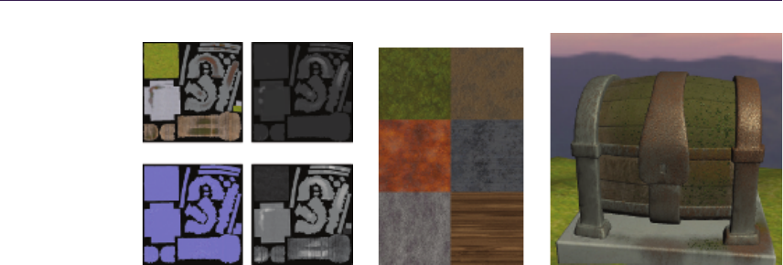
380 23. Particle-Based Simulation of Material Aging
Color Shininess
Normals Heights
Material type textures
Grass
Rust
Stone
Dirt
Iron
Wood
Figure 23.10. Composed textures (left), textures associated with the material types
(center), composed aged chest (right). While the left side of the model is aged only
slightly the amount of rust, dirt, and organic material increases to the right.
Depending on the needs of the artists or production standards, the composition
processes might need to be adapted and further material information might need
to be exported. For preview rendering purposes, we used the Phong reflection
model and used the same output textures for a high-quality rendering in a DCC
tool (see Figure 23.1). The initial material on the surface is already visually
represented in the original diffuse texture. Thus, for compositing we only need to
consider the amount of newly added material by taking the difference between the
currently present material mcurr and the initial material minit. To assemble the
resulting diffuse color, we blend the original surface texture with color textures
sirepresenting the individual material types (see Figure 23.10, center). The
appearance pattern of the deposited material color cdeposit is controlled by a base
strength biand a random variation vi:
cdeposit =
i
max(0,mcurr,i −minit,i)·si·(bi+vi·ξi),
whereas ξidenotes a uniformly destributed random number. This allows modeling
a wider range of appearances, including homogeneous patina of copper or noisy
rust stains on iron surfaces.
The resulting diffuse color is computed by the weighted sum of the deposited
colors of all material types:
cdiffuse = lerp corg ,cdeposit ,saturate
i
(bi+vi·ξi).
The shininess is estimated similarly, leaving out the color textures. The height
map is computed based on the amount of material resting on the surface, which
is then used in a second pass to estimate surface normals from neighboring texels.
The parameters of the composition can be changed during or after the simulation.

23.4. Preview Rendering 381
23.4 Preview Rendering
Once the weathered textures are composed, we can start with the preview render-
ing, which serves two purposes: First, it is a preview for the eventually employed
renderer, thus needs to resemble it closely. Ideally, the simulation system should
be integrated into a content creation system, running on top of the eventually
used rendering engine. For our demo, we render the scene with forward shading
and apply the output textures from the composition stage, i.e., the aged color,
normals, height, and shininess. Second, the preview rendering needs to make the
amounts of material visible to give the content artist feedback. Therefore, we use
distance-dependent tessellation and displacement mapping to display the height
and place billboards to visualize lichen growth.
float d tf ( fl oat 3 pos ) // dist ance - de pendent tes s fac tor
{
return le rp ( g_ Min Te ssF act or , g_ Max Tes sFa ct or ,
sm oo th step ( g _M inTessD is t , g _M axTessD is t , dist (g_Eye , pos )));
}
H S_ _C O NS TA N T_ _D A TA C o ns ta nt HS ( i n I np ut Pat ch < floa t3 , 3 > Pos ,
out floa t Edges [3] : SV_Tess Fa ctor ,
out floa t Inside [1] : SV _I ns ideT ess Fact or )
{
HS __ CO NST AN T_ _DA TA ou tpu t ;
// co mp ute tes se ll ation fa ct or s for each v er tex
fl oat 3 te ss = fl oat 3 ( dtf ( Po s [0 ]) , d tf ( Pos [ 1]) , d tf ( Pos [2] ) );
// set f ac to rs for the e dges and the i nt er io r
Ed ges [0] = max ( t ess .y , tes s .z );
Ed ges [1] = max ( t ess .x , tes s .z );
Ed ges [2] = max ( t ess .x , tes s .y );
In sid e [0] = m ax ( tess . x, Ed ges [0 ]) ;
}
[ do mai n (" tri " )]
PS _IN PUT Do main Sha der ( H S__C ONSTAN T__D ATA input ,
float3 UV : SV _D om ai nL oc at io n ,
const O utput Patch < DS_INPUT , 3> controlPn t )
{
// Ba rycentr ic int er polat io n of cont ro l points
fl oat 3 ou tP os = c o nt ro lP nt [0 ]. P os * U V .x
+c on tr ol Pn t [1] . Po s * UV . y
+c on tr ol Pn t [2] . Po s * UV . z;
/* Ba rycentr ic int er polat io n of normal , t angents , .. . */
/* Displace surface poin t o utPos in n ormal direction ... */
return P S_I NP UT ( ou tPos , nor mal , tan gent s , . ..) ;
}
Listing 23.9. We employ distance-dependent tessellation in the preview rendering to
display the amount of material on the surface by displacement mapping.
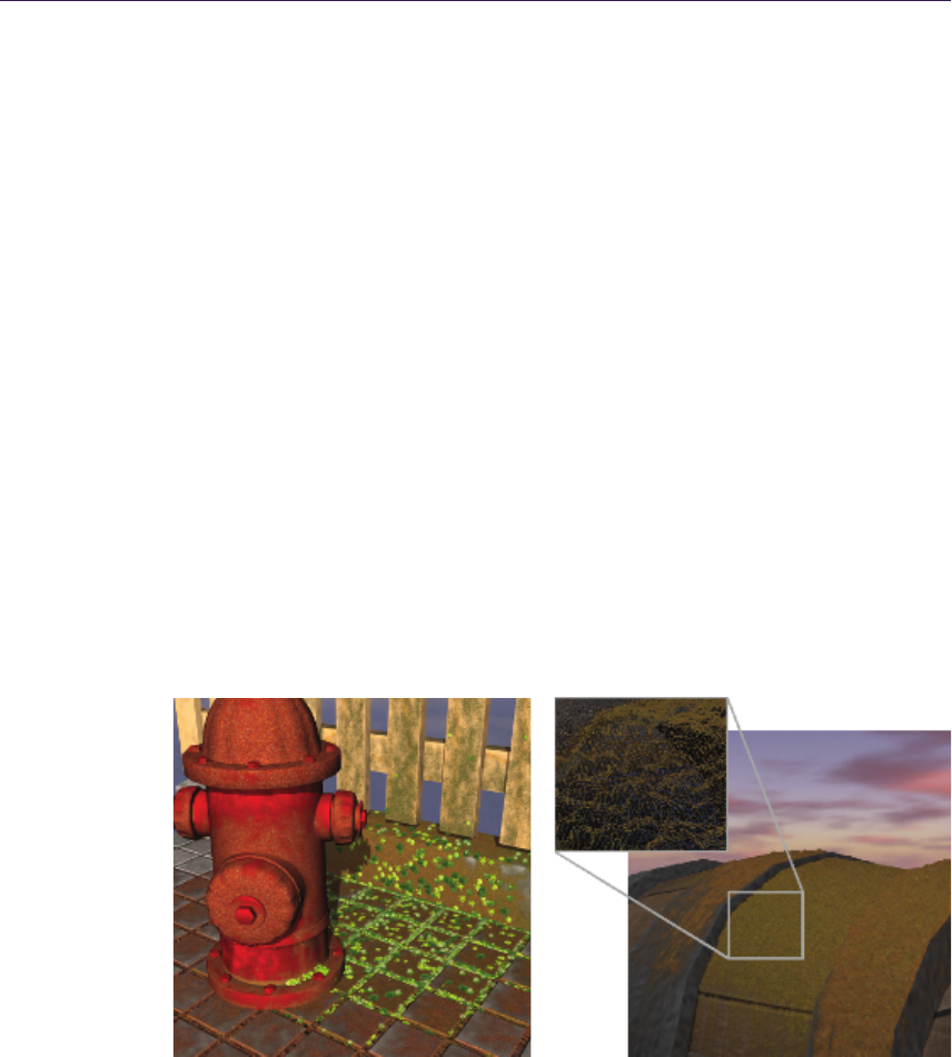
382 23. Particle-Based Simulation of Material Aging
23.4.1 Displaying Height
Tessellation shaders allow for adaptive subdivision of the surface geometry by
introducing two new shader stages after the vertex shader: a hull and a domain
shader. The hull shader is typically used to perform calculations for each control
point of a surface patch. In our case, both the vertex and hull shader by-pass posi-
tions, normals, and texture coordinates. The function ConstantHS in Listing 23.9
is executed once per control patch to compute the distance-dependent tessellation
factors. Based on these factors, a fixed-function tessellation engine subdivides the
patches. The domain shader is executed for each vertex of the refined mesh and
is used to interpolate properties from the control points, i.e., positions, normals,
tangents, and so on. Additionally, we apply a vertex displacement by the value
in the height map, which originates in the amount of material on the surface.
Eventually, the pixel shader shades the surface using normal mapping.
23.4.2 Displaying Lichen
To visualize the spread of lichen, we place and scale plantlet billboards according
to the concentration of organic material, shown in Figure 23.11. To maintain a
constant number of plantlets we randomly reseed them to adapt to the current
organic distribution in the scene. Thereby, each gammaton is responsible for
one plantlet, see function plantletPlacement in Listing 23.10, as called from the
closest hit program in Listing 23.3. For the billboards we expand the quads in
view space using a geometry shader.
Figure 23.11. Depictions of the intermediate output. Left: plantlets distributed in
regions of high lichen growth. Right: Distance-dependent tessellation with displacement
mapping, depending on the amount of rust and organic material. [Appeared in [G¨unther
et al. 12] and reproduced by kind permission of the Eurographics Association.]
23.5. Results 383
// Data st ored per p la nt le t ( share d betw ee n Dire ct X and OptiX )
struct PlantletShared {
fl oat3 Po sit ion ; // Position of the pl ant let .
uin t RayInde x ; // Use d to se lect t ex ture .
float2 A tla sCoord ; // Atl as co ordinate of the pl ant let .
};
voi d plantletPlacement(int rndS eed , fl oat3 pos , float 2 te xco ord )
{
if ( rnd ( rn dSe ed ) < g _S ee dP ro ba bi li ty ) {
P lan tl et Sh ar ed & p la ntl et = P l ant le tS ha re d [ pr d . ra y_i nd ex ];
pl an tl et . P os iti on = p os ;
pl ant let . R ayI nde x = prd . ra y_i nde x ;
pl ant let . A tlasCo ord = texcoord ;
}
}
Listing 23.10. CUDA device function for placing plantlets.
23.5 Results
The polishing of textures to attain weathered looks is a building brick in most
content creation pipelines, one that was previously subject to manual processing
alone. In Figure 23.12, we show a time series of our aging simulation and for
Figure 23.1 we exported the composed textures and rendered the scenes in a
standard DCC tool.
Our system presents intermediate output and allows for interactive modifica-
tion of parameters (simulation, aging rules, composition, etc.) and the interactive
movement of gammaton sources. Timing results are given in Table 23.1 for an
Intel Core i7-2600K CPU and an Nvidia GeForce GTX 560 Ti GPU. The com-
position is the slowest component, though optional to the simulation pipeline. It
may be broken down, to be carried out over a span of multiple frames in order to
adjust to the narrow time budget of real-time applications, e.g., modern games.
Step Chest Hydrant Otto
Simulation Step 2.57 1.72 2.25
Surface Update 0.03 0.03 0.03
Gammaton Update 0.03 0.03 0.03
Aging Process 0.25 0.25 0.25
Composition 7.19 7.11 7.01
Preview Rendering 2.32 2.08 1.82
Total Time 12.39 11.22 11.39
Table 23.1. Timing breakdown in milliseconds for the pipeline stages at an atlas reso-
lution of 1K ×1K, 5K gammatons per iteration and a screen resolution of 800 ×800
pixels.
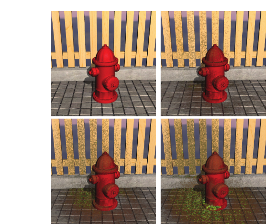
384 23. Particle-Based Simulation of Material Aging
Figure 23.12. Aging of a selected part of the hydrant scene, shown at different time
steps. [Appeared in [G¨unther et al. 12] and reproduced by kind permission of the Euro-
graphics Association.]
Further discussions on user interface decisions, the impact of the atlas resolution
on memory consumption and visual quality, as well as texture seam handling can
be found in our paper [G¨unther et al. 12].
23.6 Conclusions
In this chapter, we presented an interactive material aging simulation based on
gammaton tracing on the GPU. We used a simple yet powerful set of rules to
obtain the most common aging effects, including dirt, rust, organic, and water

Bibliography 385
precipitate, and displayed those in a few seconds in which the scene progressively
and visibly ages. Open for further investigation is the simulation on large scenes.
For now, our approach is limited to a few objects chosen by the content artist as a
region of interest, since the memory consumption limits the material atlas size and
thus the visual quality. A number of extensions to our approach are imaginable.
If more memory was available, e.g., by compression, it would be possible to add
multiple layers of material, not only one as we do now. Related to this is the
gradual peeling of layers [Paquette et al. 02], possibly initiating a more distinctive
deformation of the surface, which could go beyond the capabilities of a single-
pass tessellation shader. Another direction to look into is the implementation of
a more detailed temporal aging behavior, since many materials are subject to a
nonlinear aging process [Gu et al. 06]. On the GPU, discrete time steps could be
easily encoded in a 3D texture, whereas the third dimension is time.
Bibliography
[Chen et al. 05] Yanyun Chen, Lin Xia, Tien-Tsin Wong, Xin Tong, Hujun Bao,
Baining Guo, and Heung-Yeung Shum. “Visual Simulation of Weathering
by Gammaton tracing.” ACM Transactions on Graphics 24:3 (2005), 1127–
1133.
[Gu et al. 06] Jinwei Gu, Chien-I Tu, Ravi Ramamoorthi, Peter Belhumeur, Wo-
jciech Matusik, and Shree Nayar. “Time-varying Surface Appearance: Ac-
quisition, Modeling and Rendering.” ACM Transactions on Graphics 25:3
(2006), 762–771.
[G¨unther et al. 12] Tobias G¨unther, Kai Rohmer, and Thorsten Grosch. “GPU-
Accelerated Interactive Material Aging.” In Proceedings of the Vision, Mod-
eling and Visualization Workshop 2012, pp. 63–70. Genevea: Eurographics
Association, 2012.
[Paquette et al. 02] Eric Paquette, Pierre Poulin, and George Drettakis. “The
Simulation of Paint Cracking and Peeling.” In Graphics Interface 2002,
pp. 59–68. Natick, MA: Canadian Human-Computer Communications So-
ciety and A K Peters, Ltd., 2002.
[Parker et al. 10] Steven G Parker, James Bigler, Andreas Dietrich, Heiko
Friedrich, Jared Hoberock, David Luebke, David McAllister, and Martin
Stich. “OptiX: A General Purpose Ray Tracing Engine.” ACM Transactions
on Graphics 29:4 (2010), 1–13.

24
Simple
Rasterization-Based Liquids
Martin Guay
24.1 Overview
Rasterization pipelines are ubiquitous today. They can be found in most of our
personal computers as well as in smaller, hand-held devices—like smart phones—
with lower-end hardware. However, simulating particle-based liquids requires
sorting the particles, which is cumbersome when using a rasterization pipeline.
In this chapter, we describe a method to simulate liquids without having to sort
the particles. Our method was specifically designed for these architectures and
low shader model specifications (starting from shader model 3 for 3D liquids).
Instead of sorting the particles, we splat them onto a grid (i.e., a 3D or 2D
texture) and solve the inter-particle dynamics directly on the grid. Splatting is
simple to perform in a rasterization pipeline, but can also be costly. Thanks to
the simplified pass on the grid, we only need to splat the particles once.
The grid also provides additional benefits: we can easily add artificial obstacles
for the particles to interact with, we can ray cast the grid directly to render the
liquid surface, and we can even gain a speed up over sort-based liquid solvers—
such as the optimized solver found in the DirectX 11 SDK.
24.2 Introduction
Simulating liquids requires dealing with two phases of fluid—the liquid and the
air—which can be tricky to model as special care may be required for the interface
between the two phases depending on the fluid model. In computer graphics,
there are mainly two popular formulations for fluids: strongly incompressible
and weakly incompressible.
The strong formulation is usually more complex as it requires a hard constraint
(e.g., solving a Poisson equation), but it is more accurate and therefore more
387

388 24. Simple Rasterization-Based Liquids
visually pleasing. Because it is more complex, it is often used along simple,
regular grid discretizations [Stam 99]. For liquids, several intermediate steps are
required for the surface to behave adequately [Enright et al. 02]. Implementing
these steps using rasterization APIs is challenging. For instance, [Crane et al. 07]
only partially implements them and the fluid behaves more like a single phase
fluid. Furthermore, the strong formulation requires a surface representation like a
level-set density field, which requires its own set of specificities (re-initialization).
Again, in [Crane et al. 07] the level-set method is only partially implemented
and had to be hacked into staying at a certain height; preventing them from
generating such scenarios as the water jet shown in Figure 24.3.
The weak formulation on the other hand, requires only a simple soft con-
straint to keep the fluid from compressing. It is much simpler, but also less
accurate. It is often used along particle discretizations and mesh-free numeri-
cal schemes like Smooth Particles Hydrodynamics (SPH) [Desbrun and Cani 96].
The advantage of the weak formulation along particles is really for liquids. This
combination allowed reproducing the behavior of liquids without computing any
surface boundary conditions similar to [Enright et al. 02]. Additionally, the par-
ticles can be used directly to render the liquid surface and there is no need for a
level-set. The drawback however, is that particles require finding their neighbors,
in order to compute forces ensuring they keep at a minimal distance. Typically
buckets or other spacial sorting algorithms are used to cluster the particles into
groups [Amada et al. 04,Rozen et al. 08,Bayraktar et al. 08], which can be cum-
bersome to implement using rasterization APIs.
Instead of sorting the particles, our method makes use of rasterization ca-
pabilities. First, we rasterize, or splat, the particle density onto a grid. Then,
we use simple finite difference to compute all the interacting forces—including
the soft incompressibility constraint—on the grid, in a single pass. Some have
considered splatting before [Kolb and Cuntz 05] but had to splat for each force
(pressure and viscosity), while we only need to splat once—for all the forces. Fi-
nally, the particles are corrected and moved by sampling the grid—which in turn
can also be used directly to render the liquid surface by ray casting the splatted
density. Overall, our method allows treating each particle independently while
making sure they automatically repulse one another and avoid rigid obstacles in
the domain.
24.3 Simple Liquid Model
Our liquid model is best described as follows: particles are allowed to move
freely in the domain while their mass and kinetic energy remains conserved. For
instance, if we add gravity it should translate into velocity u. To keep the particles
from interpenetrating, we add a soft incompressibility constraint Pderived from

24.4. Splatting 389
the density ρof particles and the resulting force is the negative gradient of P:
Dρ
Dt = 0,
Du
Dt =−∇P+g+fext,(24.1)
where ggravity and fext accounts for external forces such as user interactions.
The terms Dρ
Dt and Du
Dt account for the transport of density and velocity. There
is never any density added nor removed, it is only transported and held by the
particles leading to Dρ
Dt = 0. Energy added to the velocity—like gravity—needs
to be conserved as well, resulting in equation (24.1). Next we define the incom-
pressibility constraint Pand how to compute the density of particles ρ.
24.3.1 Pressure Constraint
To keep the fluid from compressing and the particles from inter-penetrating, we
penalize high density: P=kρ [Desbrun and Cani 96], where kis a stiffness
parameter that makes the particles repulse one another more strongly (but can
also make the simulation unstable if too large). Hence, by minimizing the density,
the particles will move in the direction that reduces density the most and thereby
avoid each other. At the same time, gravity and boundary conditions, like the
walls, will act to keep the particles from simply flying away.
Keeping the particles from inter-penetrating is crucial in particle-based liquid
simulations. To give strict response to the particles that are close to colliding,
we can make the density nonlinear leading to the pressure constraint [Becker and
Teschner 07]: P=kρ
ρ0γ, where γis an integer (5 in our case). Dividing by the
initial density ρ0comes in handy for stability; it becomes easier to control the
magnitude of the force through the parameter kand thereby keep the simulation
stable.
Setting the initial ρ0can be tricky. It should be a proportional evaluation of
ρat an initial rest configuration, i.e., with a uniform distribution of particles. In
practice, however, we can set it manually. We approximate ρby performing a
convolution, which we pre-compute on a texture by rasterizing, or splatting the
kernels of each particle.
24.4 Splatting
To evaluate the density of particles smoothly, we perform a convolution: the den-
sity is the weighted average of the surrounding discrete samples, in this case the
particles. The weight is given by a kernel function, which falls off exponentially
with distance, as shown in Figure 24.1. Instead of sampling the nearby particles,
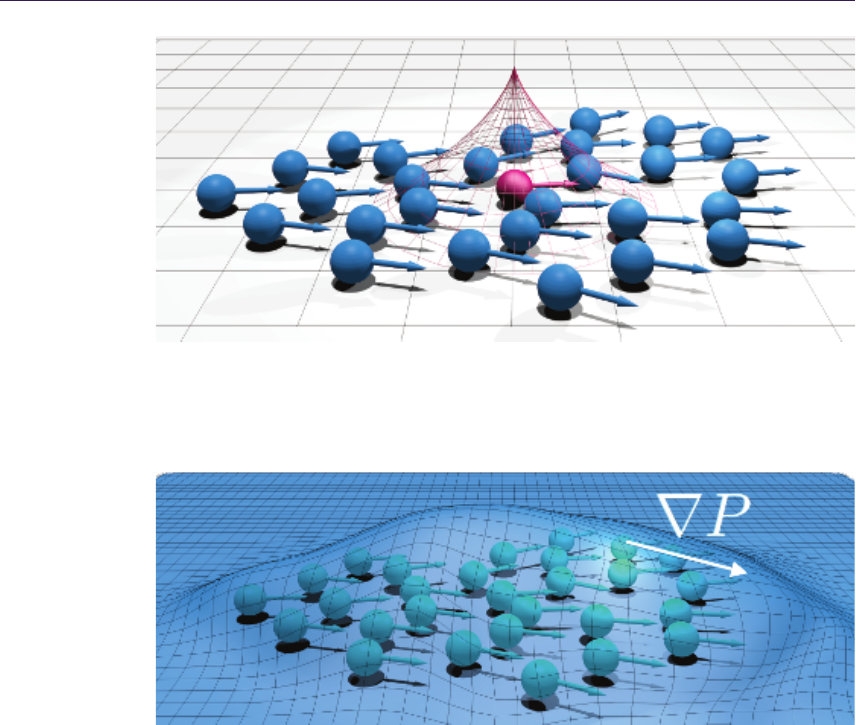
390 24. Simple Rasterization-Based Liquids
Figure 24.1. Splatting consists in rasterizing the smooth kernel function, the 2D case
shown here in red. In Figure 24.2, we see the sum of all the kernel functions; a scalar
field representing the density of particles.
Figure 24.2. Illustrating the scalar density field used to define the pressure constraint.
The pressure force is proportional to the density gradient pushing the particles toward
minimum density. For simplicity, we show the idea in 2D with density shown as a height
field—which can also be used as the liquid surface in Shallow Water simulations (see
Figure 24.4).
we rasterize the kernel function centered at each particle. The final result is a
smooth density grid (texture)—like the one shown in Figure 24.2—that is equiv-
alent to a convolution evaluation at each point on the texture. We could say also
that we now have a virtual particle on each grid cell.

24.5. Grid Pass 391
24.4.1 Rasterizing Kernel Functions
To update the velocity on the grid, we need to transfer both the density of the
particles—to compute pressure—and their velocity. Hence, the first step in our
algorithm is to rasterize the smooth kernel function (red in Figure 24.1) and the
weighted velocity of each particle. We render the particles as points and create
quad slices—spanning a cube—in the geometry shader. For each corner vertex
xi, we write the distance d=∥xi−xp∥to the center of the particle xp, and
let the rasterizer perform the interpolation between vertices. Then, in a pixel
shader, we render the smooth kernel value w(d, r) to the alpha channel, and the
weighted velocity w(d, r)upto the other three channels—in an additive fashion.
Finally, the density on the grid can be sampled by multiplying the sum of kernel
weights by the mass, and the velocity by dividing the sum of weighted velocities
by the sum of weights:
ρ(xi) = mi
p
w(∥xi−xp∥, r),u(xi) = pw(∥xi−xp∥, r)up
pw(∥xi−xp∥, r),
where idenotes texture indices, pparticle indices, and rthe kernel radius. We
used the following convolution kernel:
w(d, r) = 1−d2
r23
.
Next we update the velocity field on the grid to make the particles move in a
direction that keeps them from compressing, by computing a pressure force from
the density of particles and adding it to the velocity.
24.5 Grid Pass
In the grid pass, we update the splatted velocity field with the pressure force,
gravity, and artificial pressure for obstacles (see Section 24.7). We compute the
pressure gradient using a finite difference approximation and add forces to the
velocity field using forward Euler integration:
un+1 =un−∆tP(xi+1)−P(xi−1)
∆x,P(xj+1)−P(xj−1)
∆y,
where ∆tis the time step, ∆xthe spatial resolution of grid, and nthe temporal
state of the simulation.
While we update the velocity, we set the velocity on the boundary cells of
the grid to a no-slip boundary condition by setting the component of the velocity
that is normal to the boundary to 0. This is a simple boundary test; before
writing the final velocity value, we check if the neighbor is a boundary and set
the component of the velocity in that direction to 0.

392 24. Simple Rasterization-Based Liquids
24.6 Particle Update
We update the position and velocity of particles following the Particle-In-Cell
(PIC) and Fluid-In-Particle (FLIP) approaches that mix particles and grids [Zhu
and Bridson 05]. The main idea with these numerical schemes is that instead of
sampling the grid to assign new values (e.g., velocities) to the particles, we can
recover only the differences to their original values.
24.6.1 Particle Velocity
In PIC, the particle’s velocity is taken directly from the grid, which tends to
be very dissipative, viscous and leads to damped flow. For more lively features
and better energy conservation, FLIP assigns only the difference in velocities;
the difference between the splatted velocity and the updated splatted velocity
discussed in Section 24.5.
By combining both PIC and FLIP, the liquid can be made very viscous like
melting wax, or it can be made very energetic like water. A parameter rlets the
user control the amount of each:
up=run+1(xp) + (1 −r)(up−∆u),with ∆u=un(xp)−un+1(xp),
where unand un+1 are grid velocities before and after the velocity update in
Section 24.5, and xp,upare the particle’s position and velocity. Using a bit of
PIC (r= 0.05) is useful in stabilizing the simulation performed with explicit
Euler integration, which can become unstable if the time step is too large.
24.6.2 Particle Position
While we update the particle velocity, we also update the particle positions. We
integrate the particle position using two intermediate steps of Runge-Kutta 2
(RK2), each time sampling the velocity on the grid. The second-order scheme
is only approximate in our case because the velocity field on the grid is kept
constant during integration. At each intermediate step, we keep the particles
from leaving the domain by clamping their positions near the box boundaries:
xn+1
p= ∆tun+1(xn+1
2
p),with xn+1
2
p= 0.5∆tun+1(xn
p).
Note that we never modify the density value of the particles.
24.7 Rigid Obstacles
We can prevent the particles from penetrating rigid obstacles in the domain by
adding an artificial pressure constraint where the objects are. This follows the
same logic as with the particle density. We define a smooth distance field to
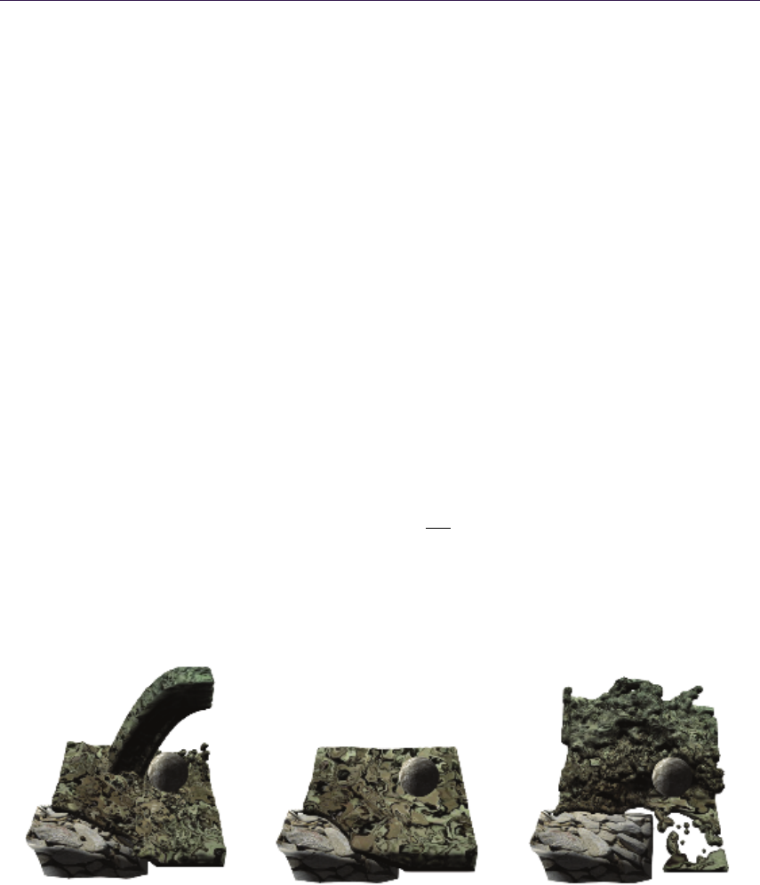
24.8. Examples 393
the surface of the object, which can also be viewed as a density field. We can
use analytical functions for primitives like spheres to approximate the shape of
the objects. This avoids rasterizing volumes or voxelizing meshes on the GPU.
Alternatively, one could approximate shapes using Metaballs [Blinn 82] and im-
plicit surfaces that naturally provide a distance field. No matter which approach
we choose, the gradient of these distance fields ρObstacle can be computed ana-
lytically or numerically and plugged into the velocity update formula covered in
Section 24.5.
When looking at the Shallow Water Equations (SWE), we find similarities
with the equations outlined in this chapter. In fact, by looking at the density
field as the height field of a liquid surface, we can imagine using our method
directly for height field simulations shown in Figure 24.4. On the other hand,
there is usually a ground height term in the SWE. This in turn can be interpreted
in 3D as a distance field for rigid objects as we mentioned above.
24.8 Examples
We show a few simulation examples implemented with HLSL, compiled as level
4 shaders. They include a 3D liquid with rigid objects in the domain, a 2D
shallow water height field simulation, and a 2D simulation comparing with the
optimized Direct Compute implementation of SPH available in the DirectX 11
SDK. Measures include both simulation and rendering. We splat particles with
a radius of 3 cells on 16-bit floating point textures without any significant loss in
visual quality. In general we used a grid size close to d
√NPtexels per axis, where
dis the domain dimension (2 or 3) and NPis the total number of particles.
In Figure 24.3, we rendered the fluid surface by raycasting the density directly.
We perform a fixed number of steps and finish with an FXAA antialiasing pass
(framebuffer size 1024 ×768). We used 125k particles on a 963texture and the
Figure 24.3. A 3D liquid simulation with obstacles in the domain implemented using the rasterization
pipeline. The simulation runs at 35 FPS using 125k particles on a Quadro 2000M graphics card.
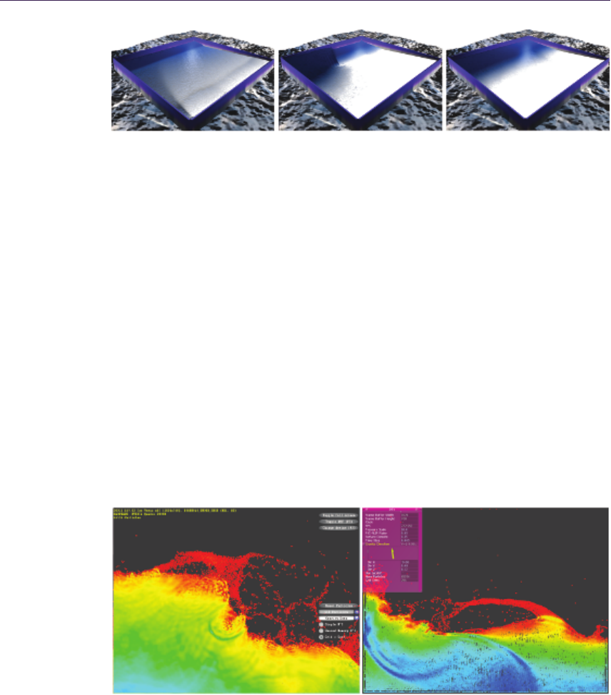
394 24. Simple Rasterization-Based Liquids
Figure 24.4. The shallow water equations describe the evolution of water height over
time. By looking at the height as the density of a 2D fluid, we see the equations
becoming similar. Hence, our method can be used directly to simulate height fields.
This figure shows a SWE simulation with 42k particles using our method.
simulation performs at 35 frames per second (FPS) on a Quadro 2000M graphics
card.
In Figure 24.4, we see a shallow water simulation using 42k particles on a
2562grid. The simulation and rendering together run at 130 FPS using the same
graphics card.
We compared our solver qualitatively with the SPH GPU implementation in
the DirectX 11 SDK (Figure 24.5). Their solver is implemented using the Direct
Compute API, has shared memory optimizations and particle neighbor search
acceleration. Ours uses HLSL shaders only. In Table 24.1, we compare the
performance of both methods with different particle quantities. We can see that
our method scales better with the number of particles involved for a given grid
size and splatting radius on the hardware we used.
Figure 24.5. Comparison between an optimized SPH solver implemented with Compute
Shaders on the left and our method implemented with rasterization APIs. Our method
performs at 296 FPS using while the optimized SPH solver runs at 169 FPS.

24.9. Conclusion 395
Particle Grid Size Our Method DX SDK 11 Speedup
Amount Dim(ϕ, u) (FPS) (FPS) Ratio
64,000 2562296 169 1.75
32,000 2562510 325 1.55
16,000 2562830 567 1.45
Table 24.1. Comparison between our method and the optimized SPH solver found in
the DirectX 11 SDK.
24.9 Conclusion
In GPU Pro 2, we described the $1 fluid solver: by combining the simplicity
of weakly incompressible fluids with the simplicity of grids, we could simulate
a single phase fluid (smoke or fire) in a single pass [Guay et al. 11]. In this
chapter, we described the $1 liquid solver for rasterization APIs by combining
the simplicity of the particles for dealing with liquids with the simplicity of the
grids to compute the forces. This is useful in getting a liquid solver running
quickly on platforms that do not necessarily implement compute APIs.
Bibliography
[Amada et al. 04] T. Amada, M. Imura, Y. Yasumoto, Y. Yamabe, and K. Chi-
hara. “Particle-Based Fluid Simulation on GPU.” In ACM Workshop
on General-Purpose Computing on Graphics Processors, pp. 228–235. New
York: ACM, 2004.
[Bayraktar et al. 08] S. Bayraktar, U. G¨ud¨ukbay, and B. ¨
Ozg¨u¸c. “GPU-Based
Neighbor-Search Algorithm for Particle Simulations.” Journal of Graphics,
GPU, and Game Tools 14:1 (2008), 31–42.
[Becker and Teschner 07] M. Becker and M. Teschner. “Weakly compress-
ible SPH for free surface flows.” In Proceedings of the 2007 ACM SIG-
GRAPH/Eurographics Symposium on Computer Animation, pp. 209–218.
Aire-la-Ville, Switzerland: Eurographics Association, 2007.
[Blinn 82] J. F. Blinn. “A Generalization of Algebraic Surface Drawing.” ACM
Transactions on Graphics (TOG) 1:3 (1982), 235–256.
[Crane et al. 07] K. Crane, I. Llamas, and S. Tariq. “Real-Time Simulation and
Rendering of 3D Fluids.” In GPU Gems 3, edited by Hubert Nguyen. Upper
Saddle River, NJ: Addison-Wesley, 2007.
[Desbrun and Cani 96] M. Desbrun and M.P. Cani. “Smoothed Particles: A
New Paradigm for Animating Highly Deformable Bodies.” In Proceedings of

396 24. Simple Rasterization-Based Liquids
Eurographics Workshop on Computer Animation and Simulation, pp. 61–76.
New York: Springer, 1996.
[Enright et al. 02] D. Enright, S. Marschner, and R. Fedkiw. “Animation and
Rendering of Complex Water Surfaces.” In Proceedings of the 29th Annual
Conference on Computer Graphics and Interactive Techniques (SIGGRAPH
’02), pp. 736–744. New York: ACM, 2002.
[Guay et al. 11] M. Guay, F. Colin, and R. Egli. “Simple and Fast Fluids.” In
GPU Pro 2, edited by Wolfgang Engel, pp. 433–444. Natick, MA: A K Peters,
Ltd., 2011.
[Kolb and Cuntz 05] A. Kolb and N. Cuntz. “Dynamic Particle Coupling for
GPU-Based Fluid Simulation.” Presentation, Symposium on Simulation
Technique, Wuppertal, Germany, March, 2005.
[Rozen et al. 08] T. Rozen, K. Boryczko, and W. Alda. “GPU Bucket Sort Al-
gorithm with Applications to Nearest-Neighbour Search.” Journal of the
16th Int. Conf. in Central Europe on Computer Graphics, Visualization and
Computer Vision 16:1-3 (2008), 161–167.
[Stam 99] J. Stam. “Stable Fluids.” In Proceedings of the 26th ACM SIGGRAPH
Conference, pp. 121–128. New York: ACM Press, 1999.
[Zhu and Bridson 05] Y. Zhu and R. Bridson. “Animating Sand as a Fluid.” In
Proceedings of ACM SIGGRAPH 2005, pp. 965–972. New York: ACM, 2005.

25
Next-Generation Rendering
in Thief
Peter Sikachev, Samuel Delmont, Uriel Doyon, and
Jean-Normand Bucci
25.1 Introduction
In this chapter we present the rendering techniques used in Thief, which was
developed by Eidos Montreal for PC, Playstation 3, Playstation 4, Xbox 360,
and Xbox One. Furthermore, we concentrate solely on techniques, developed
exclusively for the next-generation platforms, i.e., PC, Playstation 4, and Xbox
One.
We provide the reader with implementation details and our experience on a
range of rendering methods. In Section 25.2, we discuss our reflection rendering
system. We describe each tier of our render strategy as well as final blending and
postprocessing.
In Section 25.3, we present a novel contact-hardening shadow (CHS) approach
based on the AMD CHS sample. Our method is optimized for Shader Model 5.0
and is capable of rendering high-quality large shadow penumbras at a relatively
low cost. Section 25.4 describes our approach toward lit transparent particles
rendering.
Compute shaders (CSs) are a relatively new feature in graphics APIs, intro-
duced first in the DirectX 11 API. We have been able to gain substantial benefits
for postprocessing using CSs. We expound upon our experience with CSs in
Section 25.5.
Performance results are presented in the end of each section. Finally, we
conclude and indicate further research directions in Section 25.6.
397

398 25. Next-Generation Rendering in Thief
25.2 Reflections
Reflections rendering has always been a tricky subject for game engines. As long
as the majority of games are rasterization based, there is no cheap way to get
correct reflections rendered in the most general case. That being said, several
methods for real-time reflection rendering produce plausible results in special
cases.
25.2.1 Related Methods
One of the first reflection algorithms used for real-time applications, was real-
time planar reflection (RTPR) rendering [Lengyel 11]. This method yields an
accurate solution for geometry reflected over a plane and is typically used for
water or mirror reflections. The method involves rendering objects, or proxies
of them, as seen through the reflection plane. Depending on the number of
things rendered in the reflection scene, it is possible to balance performance
and quality, but the technique is generally considered to be expensive. The
main drawback of this method is that in practice, several planes of different
heights and orientations would be required to model correctly the environment
view surrounding the player, which would be unacceptably expensive to process.
This prevents the technique from being used across a wide range of environments.
Cube map reflections are another approach that has been used for many
years [NVIDIA Corporation 99]. Though they are very fast and they can han-
dle nonplanar objects, cube maps have their limitations, too. They usually lack
resolution and locality compared to other techniques. One also usually needs
to precompute cube maps in advance, as it is usually prohibitively expensive to
generate cube maps dynamically at runtime. This could additionally complicate
an asset pipeline. Precomputed cube maps will not reflect a change in lighting or
dynamic objects. Moreover, cube maps do not produce high-quality reflections
when applied to planar surfaces, which was one of our main scenarios.
Screen-space reflection (SSR) is a relatively new technique that has grown
quickly in popularity [Uludag 14]. It has a moderate performance cost and is easy
to integrate. Moreover, it provides great contact reflections (i.e., reflections that
occur when an object stands on a reflecting surface; these reflections “ground” an
object) hardly achieved by other techniques. However, SSR is prone to numerous
artifacts and fails to reflect invisible (or offscreen) parts of a scene. Therefore, it
is usually used in combination with some backup technique.
Image-based reflection (IBR) is a method that utilizes planar proxies in order
to approximate complex geometries to accelerate ray tracing [Wright 11]. It was
developed and shown off in the Unreal Engine 3 Samaritan demo. IBR can
achieve good results in reflection locality and allows an arbitrary orientation of
a reflector. However, the complexity grows linearly with the number of proxies,
which could become prohibitive for large scenes.

25.2. Reflections 399
Figure 25.1. From left to right: cube map reflections only, SSR + cube maps, IBR +
cube maps, and SSR + IBR + cube maps. [Image courtesy Square Enix Ltd.]
Numerous variations of the methods discussed above have been proposed and
used in real-time rendering. For instance, localized, or parallax-corrected cube
maps [Lagarde and Zanuttini 13] are arguably becoming an industry standard.
In the next sections, we will describe the reflection system we used in Thief.
25.2.2 Thief Reflection System Overview
Creating a reflection system that perfectly handles every surface type, in real
time, is a very difficult problem. Therefore, together with the art department, we
developed a specification of requirements and limitations for the Thief reflection
system. Given that Thief was originally designed for the Xbox 360 and Playsta-
tion 3 generation of platforms, we had quite a generous performance budget for
the reflection system on the next-generation platforms: 5 ms. Beforehand, we
implemented the real-time planar reflection method, which ran at 10 ms. This
running time was obviously unacceptable; moreover, this technique could render
reflections for only one plane.
The majority of reflections in the game world come from the ground (wet
spots, tile, etc.), therefore we limited ourselves to quasi-horizontal surfaces. How-
ever, since Thief is a multilevel game (e.g., you can make your way across rooftops
instead of streets), unlike [Lagarde and Zanuttini 13], we could not be limited to
a single reflection plane. As mentioned above, we performed tests with PRTR
and the single reflection plane limitation was insufficient for our assets.
The target was to accurately capture human-sized objects and contact reflec-
tions. In addition, we also wanted to capture principal landmarks (e.g., large
buildings). Finally, as torches and bonfires are a typical light source in the world
of Thief, we needed a way to render reflection from certain transparent geometry
as well.
To achieve these goals, we came up with a multitier reflection system, outlined
in Figure 25.1. The reflection system of Thief consists of the following tiers:
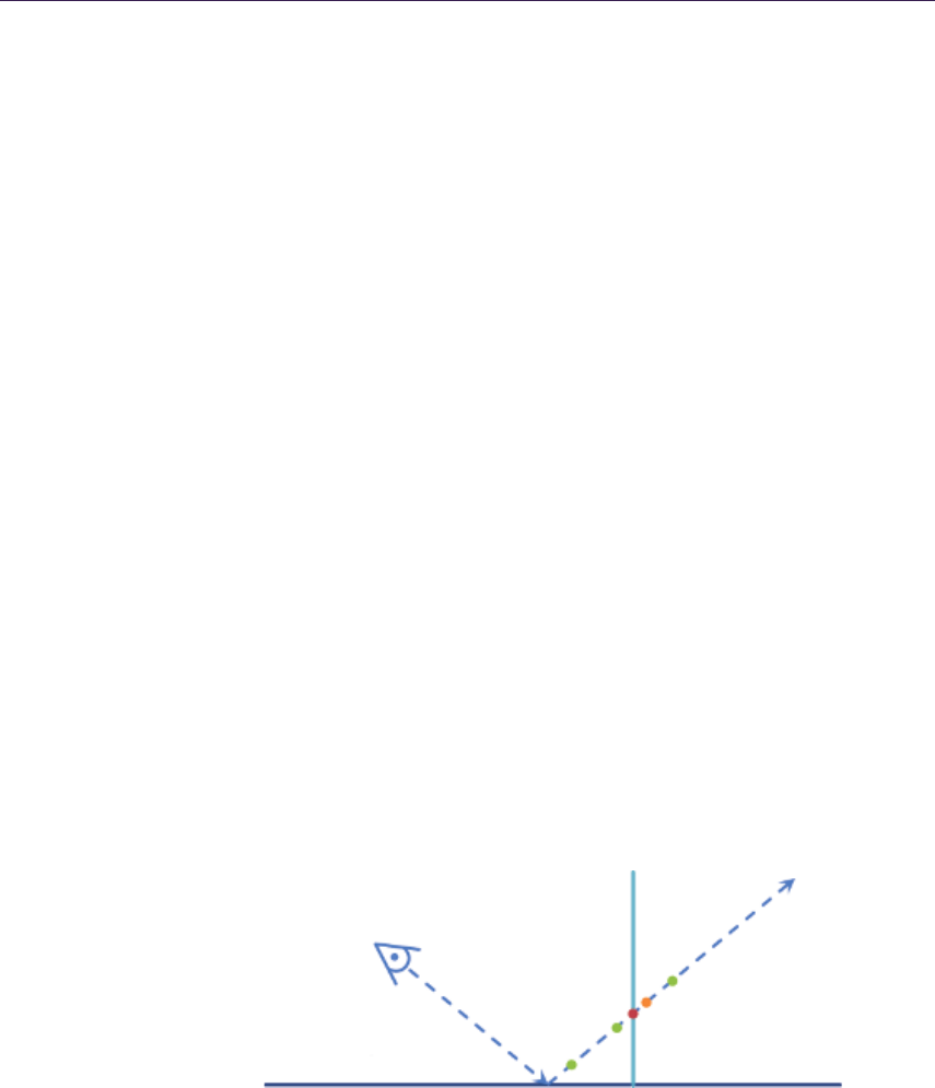
400 25. Next-Generation Rendering in Thief
•screen-space reflections (SSR) for opaque objects, dynamic and static, within
a human height of a reflecting surface;
•image-based reflections (IBR) for walls and far away landmarks;
•localized cube map reflections to fill the gaps between IBR proxies;
•global cube map reflections, which are mostly for view-independent sky-
boxes.
Each tier serves as a fallback solution to the previous one. First, SSR ray-marches
the depth buffer. If it does not have sufficient information to shade a fragment
(i.e., the reflected ray is obscured by some foreground object), it falls back to
image-based reflection. If none of the IBR proxies are intersected by the reflection
ray, the localized cube map reflection system comes into play. Finally, if no
appropriate localized cube map is in proximity, the global cube map is fetched.
Transition between different tiers is done via smooth blending, as described in
Section 25.2.6.
25.2.3 Screen-Space Reflections
SSR is an image-based reflection technique based on ray-marching through the
depth buffer [Kasyan et al. 11]. We use the lit color buffer, the normal buffer,
and the depth buffer from the current frame. SSR is applied before rendering
translucent geometry in order to avoid perspective artifacts.
At each fragment we reconstruct the camera-space position, using the screen
uv-coordinates, the fetched depth, and the projection matrix. Afterward, we ray-
march with a constant step along the reflected ray until the analytical depth of
the fetch along the ray is more than the depth buffer fetch from the same screen-
space position. Finally, the intersection location is refined with several binary
search steps, as shown in Figure 25.2.
Reflected object
Reflected surface
Figure 25.2. Screen-space reflections linear steps (green) and binary search steps (orange
and then red).

25.2. Reflections 401
This method yields very accurate reflections at the contact of a reflective
surface and a reflected object. There are, however, several major issues with
SSR. First, this method is very expensive: at each fragment we need to make
several potentially uncoalesced (due to the discrepancy of reflection rays) texture
fetches, some of which are even view-dependent (binary search). Second, reflected
information is often missing: it’s either out of screen or obscured by a closer
object.
We address the first issue with several optimization techniques, described
below in this subsection. The second issue is addressed by falling back to the
subsequent tier of the reflection system.
We decrease the memory traffic by approximating the normal at the fragment
with a normal pointing vertically up. This dramatically increases the number of
texture fetches at neighboring fragments that might be coalesced and processed
within a single dynamic random-access memory (DRAM) burst. However, this
naturally results in ideal mirror-like reflections without any normal perturbation.
We address this issue further in Section 25.2.7.
Moreover, we use dynamic branching to employ early exit for the constant
step loop when the first intersection with the depth buffer is found. Although
it might result in false ray-depth buffer collision detection, we compromise on
accuracy in order to further save on bandwidth.
Another optimization is decreasing the number of samples for the distant
fragments. We came up with an empirical formula that decreases the number of
steps proportional to the exponent of the distance:
Nlinear samples = max(1, k1e−k2d),
where depth is denoted with d,k1is the linear factor, and k2is the exponential
factor.
Additionally, we use a bunch of early-outs for the whole shader. We check
if the surface has a reflective component and if a reflection vector points to the
camera. The latter optimization does not significantly deteriorate visual quality,
as in these situations SSR rarely yields high-quality results anyway and the re-
flection factor due to the Fresnel equation is already low. Moreover, this reduces
the SSR GPU time in the case when IBR GPU time is high, thus balancing the
total.
However, one should be very careful when implementing such an optimization.
All fetches inside the if-clause should be done with a forced mipmap level; all
variables used after should be initialized with a meaningful default value, and
the if-clause should be preceded with a [branch] directive. The reason is that a
shader compiler might otherwise try to generate a gradient-requiring instruction
(i.e., tex2D) and, therefore, flatten a branch, making the optimizations useless.

402 25. Next-Generation Rendering in Thief
25.2.4 Image-Based Reflections
Image-based reflections are a reflection technique implemented in [Wright 11].
The key idea is to introduce one or more planar quad reflection proxies and pre-
render an object of interest into it. During fragment shading, we just ray-trace
the reflected ray against an array of proxies in the pixel shader. A similar idea
is utilized in [Lagarde and Zanuttini 13]. However, in the latter, the reflections
are rendered only for planes at a single height. Therefore, we were unable to use
optimizations proposed in [Lagarde and Zanuttini 13].
In Thief, our ambition was to have around 50 IBR proxies per scene. IBR
back-face culling effectively reduces the visible proxy count by half. A straightfor-
ward approach resulted in well over 8 ms of GPU time at the target configuration,
which was totally unacceptable. Therefore, we employed a series of acceleration
techniques, described below.
First, we utilized the same approach for normal approximation as for SSR to
increase memory coalescing. This allowed the following optimizations:
•rejecting planes not facing the player,
•rejecting planes behind the player,
•tile-based IBR rendering (discussed below).
Bump perturbation was then performed for SSR and IBR together.
Second, we introduced tile-based IBR. Because we have limited ourselves to
quasi-horizontal reflections, we divided the entire screen space into a number of
vertical tiles. Our experiments have proven 16 tiles to be an optimal number.
After that, for each reflection proxy, we calculate the screen-space coordinates
for each vertex. If a vertex is in front of the near clip plane, we flip the wsign
before perspective divide in order to handle close proxies. Then x-coordinates
of the transformed vertices might be used as minimum and maximum values to
determine the tiles covered by the proxy’s reflection.
However, due to perspective projection, this method would result in reflections
being cut, especially when a proxy approaches the screen borders. To fix that,
we introduce the following workaround. For each of two vertical sides of the
proxy, we extend them to the intersections with top and bottom screen borders
as shown in Figure 25.3. The resultant x-coordinates are used to decrease the
minimum and/or increase the maximum. The pseudocode of this method is shown
in Algorithm 25.1.
The above mentioned optimization decreases GPU time dramatically; how-
ever, if a player looks straight down, all the proxies start occupying almost all
tiles due to high perspective distortions. To alleviate performance drops in this
case, we use a bounding sphere test in the pixel shader for an early-out before
the actual high-cost tracing. While this check deteriorates the performance in the
most common cases, it increases GPU performance in the worst cases, resulting
in a more consistent frame rate.
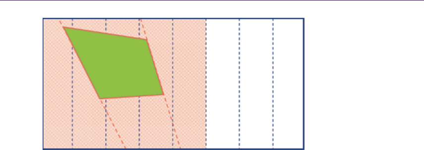
25.2. Reflections 403
Figure 25.3. IBR tile-based rendering optimization. IBR proxy is shown in orange.
Tiles are shown in dotted blue lines, and vertical sides extensions are shown in orange
dotted lines. The affected tiles are shaded with thin red diagonal lines.
1: xmin = 1
2: xmax =−1
3: for all IBR proxies in front of player and facing player do
4: find AABB of the current proxy
5: for all vertices of AABB do
6: calculate vertex coordinate in homogeneous clip space
7: w:= |w|
8: calculate vertex coordinate in screen clip space
9: xmin := min(x, xmin)
10: xmax := max(x, xmax)
11: end for
12: for all vertical edges of AABB in screen space do
13: calculate intersections x1and x2with top and bottom of the screen
14: xmin := min(x1, x2, xmin)
15: xmax := max(x1, x2, xmax)
16: end for
17: for all IBR tiles do
18: if the tile overlaps with [xmin, xmax]then
19: add the proxy to the tile
20: end if
21: end for
22: end for
Algorithm 25.1. Algorithm for finding affected tiles for an IBR proxy.
Additionally, in order to limit the number of active IBR proxies in the frame,
we introduced the notion of IBR rooms. Essentially, an IBR room defines an
AABB so that a player can see IBR reflections only from the IBR proxies in
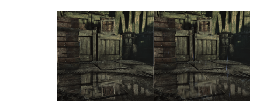
404 25. Next-Generation Rendering in Thief
Figure 25.4. Non-glossy reflection rendering (left) and CHGR (right). [Image courtesy
Square Enix Ltd.]
the same room. Moreover, the lower plane of an IBR room’s AABB defines the
maximum reflection extension of each of the proxies inside it. This allowed us to
drastically limit the number of reflections when a player is looking down.
As a side note, Thief has a very dynamic lighting environment. In order to
keep the IBR reflection in sync with the dynamic lights, IBR had to be scaled
down based on the light intensity. This makes the IBR planes disappear from
reflection when lights are turned off. Although this is inaccurate since the IBR
textures are generated from the default lighting setup, it was not possible to know
which parts of the plane were actually affected by dynamic lighting.
Also, IBRs were captured with particles and fog disabled. Important particles,
like fire effects, were simulated with their own IBRs. Fog was added accordingly
to the fog settings and the reflection distance after blending SSR and IBR.
25.2.5 Contact-Hardening Glossy Reflections
Because the majority of the reflecting surfaces in Thief are not perfect mirror
reflectors, we decided to simulate glossy reflections. Glossy SSR reflections are
not a new feature, having been first implemented in [Andreev 13]. We decided to
take SSR a step further and render contact-hardening glossy reflections (CHGRs).
An example of a CHGR is shown in Figure 25.4.
The main phenomena we wish to capture is that a reflection is sharpest near
the contact point of the reflected object and the reflecting surface. The reflection
grows more blurry as these two surfaces get farther away from each other.
The algorithm for CHGR rendering is as follows. First, we output the distance
between the reflecting surface and the point where the reflected ray hits the
reflected object. Because we want to limit the size of the render targets, we

25.2. Reflections 405
// Worl d - s pac e u nit is 1 ce nt ime te r
int d is ta nc eL o = i nt ( wo rld Spac eDis ta nce ) % 256;
int d is ta nc eH i = i nt ( wo rld Spac eDis ta nce ) / 256;
pa ck ed Dis ta nc e = float 2 ( flo at ( d is t an ce Lo ) / 25 5. 0 f ,
fl oat ( distanc eHi ) / 255.0 f );
Listing 25.1. Reflection distance packing.
float3 r efl ect ed Cam er aTo Wor ld =
re fle ct ( ca meraTo Wor ld , wo rld Sp aceN orm al ) ;
float reflectionVectorLength =
max ( lengt h( re flec ted Ca mer aT oW orld ) , FP_ EP SIL ON );
float w orl dS pac eD ist an ce = 255.0 f * ( pac ke dD ist an ce . x +
25 6.0 f * p ack ed Di sta nc e .y ) /
reflectionVectorLength;
...
// Reflection s or ti ng and blending
...
float4 s cre enS pac eR efl ect ed P os iti on =
mul ( f lo at4 ( re fl ect ed Po sit io n , 1) , w or ld To Sc re en ) ;
sc r ee nSp ace Re f le cte dPo si tio n /= scr een Sp a ce Ref lec te dPo sit ion .w ;
Re flec tio nDis tan ce = l ength ( sc reen Spac eRef lect ed Po si tion . xy -
s cr e en Sp a ce F ra gm e nt P os it i on . xy );
Listing 25.2. Reflection distance unpacking.
utilize R8G8B8A8 textures for color and depth information. As 8 bits does not
provide enough precision for distance, we pack the distance in two 8-bit channels
during the SSR pass, as shown in Listing 25.1.
The IBR pass unpacks the depth, performs blending, and then converts this
world-space distance into screen-space distance as shown in Listing 25.2. The
reason for this is twofold. First, the screen-space distance fits naturally into the
[0,1] domain. As we do not need much precision for the blurring itself, we can
re-pack it into a single 8-bit value, ensuring a natural blending. Second, the
screen-space distance provides a better cue for blur ratio: the fragments farther
away from the viewer should be blurred less than closer ones, if both have the
same reflection distance.
The second step is to dilate the distance information. For each region, we
select the maximum distance of all the pixels covered by the area of our blur
kernel. The reason for this is that the distance value can change suddenly from one
pixel to the next (e.g., when a close reflection proxy meets a distant background
pixel). We wish to blur these areas with the maximum blur coefficient from
the corresponding area. This helps avoid sharp silhouettes of otherwise blurry
objects. This problem is very similar to issues encountered with common depth-
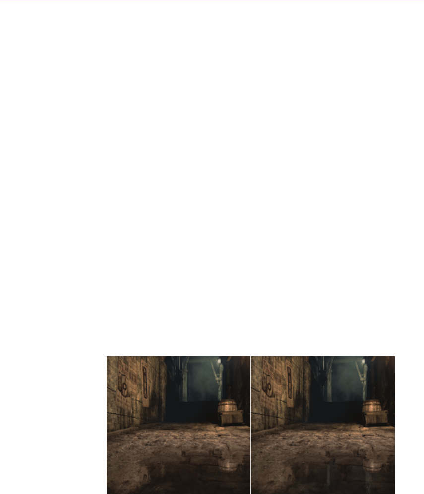
406 25. Next-Generation Rendering in Thief
of-field rendering algorithms. In order to save on memory bandwidth, we apply a
two-pass, separable dilation maximum filter. This provides us with an acceptable
approximation.
Finally, we perform the blur with the adjustable separable kernel. In addition
to selecting the Gaussian parameters based on the distance value, we also apply
the following tricks. First, we ignore the samples with zero specular intensity in
order to avoid bleeding at the silhouette of an object. This requires on-the-fly
adjustment of the kernel in the shader. Second, we follow the same heuristic as
in [Andersson 13], so we blur the image more in the vertical direction than in the
horizontal direction, achieving more plausible visual results.
25.2.6 Reflection Blending
As our reflection system consists of several tiers, we need to define how we blend
between them. In addition to the distance factor, our SSR pass also outputs a
blending factor. This factor depends on the following:
•height (the longer we cast a reflection ray, the less contribution it makes),
•tracing accuracy (depth delta between the ray coordinate and the fetched
depth),
•surface tilt (the more the surface normal diverges from vertical, the less
SSR should contribute),
•Reflection ray going toward camera or out of screen.
Afterward, IBR is merged on top, outputting a cumulative blending factor. Fi-
nally, the cube map is applied. Figure 25.5 shows seamless blending between SSR
and IBR.
Figure 25.5. SSR only (left) and SSR blended with IBR (right). [Image courtesy Square
Enix Ltd.]

25.2. Reflections 407
Figure 25.6. Reflection blending without sorting (left) and with sorting (right). [Image
courtesy Square Enix Ltd.]
However, this approach causes certain problems in cases when a transparent
IBR proxy is in front of the object that could be potentially reflected with SSR.
Figure 25.6 shows the issue. To address this problem, instead of simply blending
SSR and IBR, we perform layer sorting beforehand. We create a small (three to
four entries) array of reflection layers in the IBR shader and inject SSR results
into it as the first element. The array is kept sorted when we add every subsequent
IBR trace result. Thus, we end up with the closest intersections only.
25.2.7 Bump as a Postprocess
As mentioned above, we assume that the normal is pointing up for SSR and IBR
rendering in order to apply acceleration techniques. Furthermore, in order to
reduce memory bandwidth, we render reflection at half resolution. Together, this
diminishes high-frequency details, which are crucial for reflections, especially on
highly bumped surfaces. To alleviate this, we apply a bump effect as a postprocess
when upscaling the reflection buffer to full resolution.
The main idea is very similar to the generic refraction approach [Sousa 05].
We use the difference between the vertical normal and the per-pixel normal to
offset the UV in the rendered reflection texture. To fight reflection leaking, we
revert to the original fetch if the new fetch is significantly closer than the old one.
Figure 25.7 shows the benefits of applying reflection bump.
25.2.8 Localized Cube Map Reflections
In the SSR, IBR, and cube map reflection strategies, the cube map would ideally
only contain the skybox and some far away geometry since the playable envi-
ronment would be mapped by IBR planes. In this situation, only one cube map
would be required. In practice, the IBR planes have many holes and do not con-
nect perfectly to each other. This is a consequence of how our IBR planes are
generated using renderable textures.
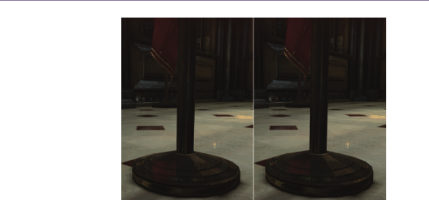
408 25. Next-Generation Rendering in Thief
Figure 25.7. Reflection without bump (left) and with bump as a postprocess (right).
[Image courtesy Square Enix Ltd.]
When a reflected ray enters into one of these cracks and hits the skybox,
it results in a bright contrast pixel because most Thief scenes typically use a
skybox that is much brighter than the rest of the environment. To fix this, we
used localized cube maps taken along the playable path. Any primitive within
reach of a localized cube map would then use it in the main render pass as the
reflected environment color.
Technically, the cube map could be mapped and applied in screen space using
cube map render volumes, but we chose to simply output the cube map sample
into a dedicated render target. This made the cube map material-bound and
removed its dependency with the localized cube map mapping system.
The main render pass in Thief would output the following data for reflective
primitives:
•material lit color (sRGB8),
•environment reflection color + diffuse lighting intensity (sRGB8),
•world normal + reflectivity (RGB8).
After generating the IBR and SSR half-resolution reflection texture, the fi-
nal color is computed by adding SSR, IBR, and finally the environment reflec-
tion color (i.e., cube map color). If the material or platform does not support
IBR/SSR, the color would simply be added to the material-lit color and the extra
render targets are not needed.

25.2. Reflections 409
Figure 25.8. Creation of the multiple volumes for covering the whole environment.
[Image courtesy Square Enix Ltd.]
Note here that we needed the diffuse lighting intensity to additionally scale
down the IBR and cube map color because they were captured with the default
lighting setup, which could be very different from the current in-game lighting
setup. This scale was not required for the SSR because it is real-time and accu-
rate, while the IBR proxies and cube maps are precomputed offline.
25.2.9 Art Pipeline Implications
For each level in Thief, we set a default cube map. This one is used by all
the geometry that has reflective materials. This cube map is pretty generic and
reflects the most common area of the level.
We then identify the areas where we require a more precise cube map defini-
tion. The decision is often based on lighting conditions or the presence of water
puddles. For an area that could benefit from a more precise cube map, artists add
a localized cube map, which comes with its own scene capture preview sphere.
This is shown in the Figure 25.8.
We then built our entire environment using these volumes that enhance the
look of the level. After using a build process, we generated all the cube maps for
the volumes created. Figure 25.9 shows the additional build process created with
the different resources generated.
Thief ’s reflection systems strongly enhanced the visual quality and next-
generation look of the game. It was deeply embedded into the artistic direction
of the title. The water puddles, in particular, helped create the unique look our
artists wanted for the game. This also contributed to the gameplay of Thief.
Because light and shadows are so important to our gameplay, the reflective water
puddles became an additional challenge the player must manage when trying to
stay hidden in the shadows.
For Thief, we dedicated a budget of 5 ms for the reflection pipeline. Given the
allocated budget and the production stage at which we pushed the data in, we had
to make clever choices, sometimes using all available techniques and other times
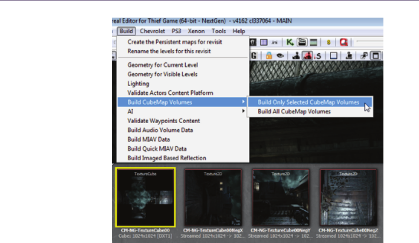
410 25. Next-Generation Rendering in Thief
Figure 25.9. Build process generating the individual cube map captures. [Image cour-
tesy Square Enix Ltd.]
using only one, given the rendering stresses of an environment. For example,
certain environment condition might force us to use only one technique. Poor
lighting condition could be a good example where you do not want to pay the
extra cost of an expensive cube map or IBR planes.
We found that screen-space reflections were very easy for our art team to
integrate. For this reason, we used SSR as our base tool for most of our reflection
needs. This would then dictate where some of our IBR planes should go; it was
a fallback solution when SSR failed.
25.2.10 Results
We came up with a robust and fast reflection system that is ready for the next-
generation consoles. Both SSR and IBR steps take around 1–1.5 ms on Playsta-
tion 4 (1080p) and Xbox One (900p). However, these are worst case results, i.e.,
taken on a synthetic scene with an SSR surface taking up the whole screen and 50
IBR proxies visible. For a typical game scene, the numbers are usually lower than
that. Reflection postprocessing is fairly expensive (around 2 ms). However, we
did not have time to implement it using compute shaders, which could potentially
save a lot of bandwidth.
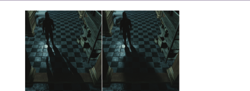
25.3. Contact-Hardening Shadows 411
Figure 25.10. Shadow with ordinary filtering (left) and with contact-hardening shadows
(right). [Image courtesy Square Enix Ltd.]
Our reflection system does not support rough reflections. Taking into account
the emerging interest in physically based rendering solutions, we are looking into
removing this limitation. Reprojection techniques also look appealing both for
quality enhancement and bandwidth reduction.
25.3 Contact-Hardening Shadows
Contact-hardening shadows (CHSs), similar to percentage-closer soft shadows
(PCSSs) [Fernando 05], are a shadow-mapping method to simulate the dynamic
shadows from area lights. The achieved effect is a sharper shadow as the shadow
caster and the receiver are closer to each other and a blurrier (softer) shadow as
the caster and the receiver are farther from each other (see Figure 25.10). The
implementation in Thief is based on the method from the AMD SDK [Gruen 10].
This method is easy to integrate because it uses the shadow map generated
by a single light source and can just replace ordinary shadow filtering. One of the
main drawbacks in this technique is the extensive texture fetching, and in Thief
we implemented an optimized method for Shader Model 5.0 that drastically limits
the access to the shadow map. The CHS process is divided into three steps, which
are the blocker search, the penumbra estimation, and the filtering.
25.3.1 Blocker Search
The first step consists of computing the average depth of the blockers inside a
search region around the shaded point (that we will reference as average blocker
depth). A kernel grid of N×Ntexels centered at the shaded point covers this
search region. A blocker is a texel in the shadow map representing a point closer
to the light than the currently computed fragment, as shown in Figure 25.11.
This average-blocker-depth value will be used in the penumbra estimation.
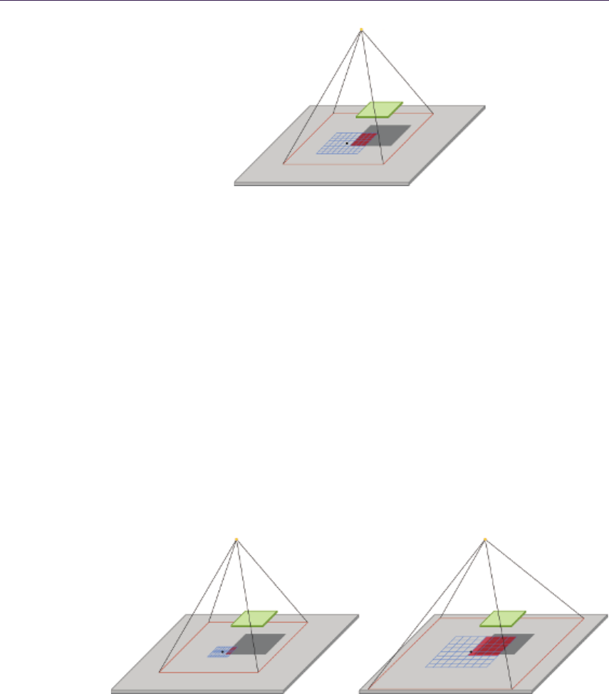
412 25. Next-Generation Rendering in Thief
Light source
Caster
Shadow map
Search region
Figure 25.11.Blockers in a 8 ×8 search grid.
Shader Model 5.0’s new intrinsic GatherRed() accelerates this step by sampling
four values at once. In Thief, we decided to use a 8×8 kernel size, which actually
performs 16 samples instead of 64 for a Shader Model 4.0 implementation (see
Listing 25.4). Increasing the size of the kernel will allow a larger penumbra,
since points that are farther from the shaded one can be tested, but it obviously
increases the cost as the number of texture fetches grows.
Because the penumbra width (or blurriness) is tightly related to the size of
the kernel, which depends on the shadow map resolution and its projection in
world space, this leads to inconsistent and variable penumbra width when the
shadow map resolution or the shadow frustum’s FOV changes for the same light
caster/receiver setup. Figure 25.12 shows the issue.
To fix this issue in Thief, we extended the CHS by generating mips for the
shadow map in a prepass before the CHS application by downsizing it iteratively.
Those downsizing operations are accelerated with the use of the GatherRed()
intrinsic as well. Then, in the CHS step, we dynamically chose the mip that gives
Figure 25.12. For the same 8 ×8 search grid, a smaller search region due to higher
resolution shadow map (left) and a bigger search region due to wider shadow frustum
(right).
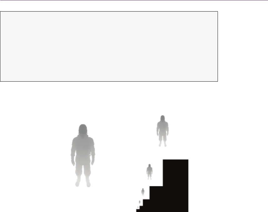
25.3. Contact-Hardening Shadows 413
#define KERN EL _S IZ E 8
float wantedTexelSizeAt1UnitDist =
wantedPenumbraWidthAt1UnitDist / KERNEL_SIZE;
float texelSizeAt1UnitDist =
2* T anF OVSe mi Ang le / sha dowM ap Reso lut ion ;
float MaxShadowMip =
- log ( t ex e lS iz eA t1 Un it Di st / w an te dT ex el Si ze A t1 Un it Di st )/ l og (2) ;
MaxShadowMip = min(flo at ( M IPS _COU NT - 1) , max ( M axS had ow Mip ,0 .0) ) ;
// both B lkS ea r ch Sha do wMi pIn de x and M ax Sh adowM ip are p as sed
// to the sh ad er as par am et er s
int B lkSe arch Shad owMi pInd ex = ceil ( Ma xSha dow Mip ) ;
Listing 25.3. Algorithm for choosing a mip from a user-defined penumbra width, the
shadow map resolution, and the FOV angle of the shadow frustum.
Figure 25.13. Shadow-map mips layout. [Image courtesy Square Enix Ltd.]
a kernel size in world space that is closer to a user-defined parameter. Listing 25.3
shows how the mip index is computed from this user-defined parameter, the
shadow map resolution, and the FOV angle of the shadow frustum. This process
can be done on the CPU and the result is passed to a shader as a parameter.
Unfortunately, the GatherRed() intrinsic does not allow mip selection. There-
fore, the mips are stored in an atlas, as shown in Figure 25.13, and we offset the
texture coordinates to sample the desired mip. This is achieved by applying a
simple offset scale to the coordinates in texture space (see Listing 25.4).
In order to save on fragment instructions, the function returns, as an early
out, a value of 0.0 (fully shadowed) if the average blocker depth is equal to 1.0
(found a blocker for all samples in the search region) or returns 1.0 (fully lit) if
the average blocker depth is equal to 0.0 (no blocker found). Listing 25.4 shows
the details of the average-blocker-depth compute.

414 25. Next-Generation Rendering in Thief
# define K ER NE L_SIZE 8
# define BFS2 ( KE RNE L_S IZE - 1) / 2
flo at3 bl kTc = f loa t3 ( in Tc .xy , in De pth ) ;
// Tc Bi asS ca le is a st ati c arr ay hold ing the of fset - s cale
in the s hadow map for ev ery m ips .
fl oat4 bl kTc BS = T cBi asS cale [ B lkSe arch Shad owMi pInd ex ];
bl kTc . x y = b lk TcB S . xy + b lkT c . xy * bl kT cB S . zw ;
// g _v S ha do wM a pD im s . xy is the s ha dow m ap r es ol ut io n
// g _v Sh a do wM a pD im s . zw is the s ha dow m ap te xel s ize
f loa t2 b lk Ab sT c = ( g _v S ha do wM a pD im s . x y * bl kTc . x y ) ;
float2 fc = blk Ab sT c - floor ( blk Ab sT c );
bl kTc . x y = b lkT c . xy - ( f c * g _ vS ha do w Ma pD im s . z w ) ;
float bl kC ou nt = 0; fl oat a vgB lo ckerD ep th = 0;
[lo op ] for (int row = - BFS2 ; row <= BFS 2 ; r ow += 2 )
{
fl oat 2 t c = b lkT c . xy + fl oa t2 ( - B FS2 * g_ v Sh ad ow M ap Di m s .z ,
row * g _ vS ha do wM ap Di me ns io n s .w ) ;
[unroll]f or (int co l = -B FS2 ; col <= BFS2 ; col += 2 )
{
f loa t4 d ep th 4 = sh ad ow Te x . G a th er Re d ( p oi nt Sam pl er , tc . xy ) ;
fl oat 4 blk 4 = ( b lkT c . zzz z <= de pth 4 ) ?(0 ) . xxxx :( 1) . xxx x ;
float4 fcVec = 0;
if ( r ow = = - B FS2 )
{
if ( c ol = = - B FS2 )
fc Ve c = fl oat 4 ( (1. 0 - f c .y ) * (1.0 - fc . x ) ,
(1. 0 - f c .y ) , 1 , (1 .0 - f c .x ) );
els e if ( c ol = = B FS2 )
fc Ve c = fl oat 4 ( (1. 0 - f c .y ) , (1. 0 - f c .y ) * fc .x , f c .x , 1) ;
els e
fc Ve c = fl oat 4 ( (1. 0 - f c .y ) , (1. 0 - f c .y ) , 1 , 1) ;
}
els e if ( r ow = = B FS2 )
{
if ( c ol = = - B FS2 )
fc Ve c = fl oat 4 ( (1. 0 - f c .x ) , 1 , fc . y , (1. 0 - f c .x ) * fc . y) ;
els e if ( c ol = = B FS2 )
fc Ve c = fl oat 4 (1 , fc .x , f c .x * f c .y , fc . y );
els e
f cVe c = fl oa t4 (1 , 1 , f c .y , f c .y ) ;
}
els e
{
if ( c ol = = - B FS2 )
fc Ve c = fl oat 4 ( (1. 0 - f c .x ) , 1 , 1 , ( 1.0 - fc . x) ) ;
els e if ( c ol = = B FS2 )
fc Vec = f lo at 4 (1 , f c .x , fc . x , 1 ) ;
else
fcVec = floa t4 (1 ,1 ,1 ,1) ;
}
bl kC oun t + = dot ( blk4 , fc Vec . x yzw ) ;
av gB lo ck er Dep th += do t (d epth4 , f cVe c . xyzw * b lk4 ) ;
tc . x + = 2 .0 * g _ vS h ad ow Ma p Di ms .z ;
}
}
if ( b lk Co un t == 0.0 ) // Early out - full y lit
return 1.0 f ;
else if ( b lkC oun t == K ERN EL_SIZ E * KER NEL_SIZE ) // Fully s ha do we d
return 0.0 f ;
avg Bl ock er Dept h /= b lkC oun t ;
Listing 25.4. Average-blocker-depth compute.
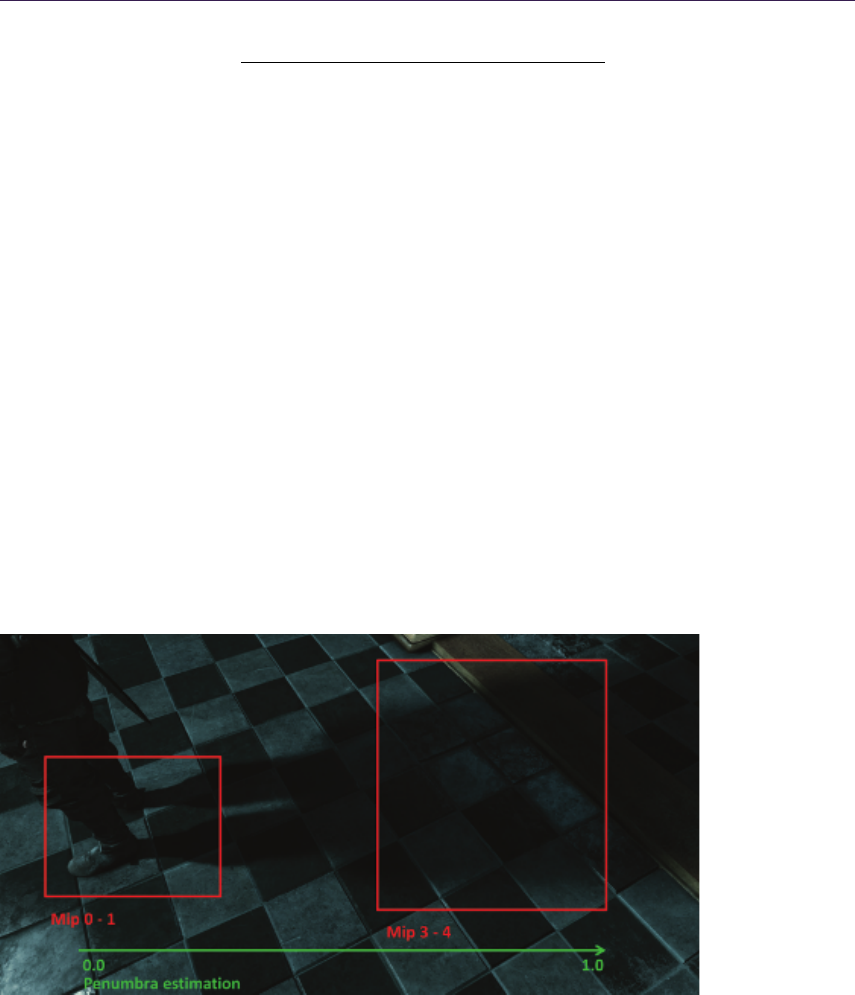
25.3. Contact-Hardening Shadows 415
widthpenumbra =(depthreceiver −avgBlockerDepth)·widthlight
avgBlockerDepth
Algorithm 25.2. Algorithm for computing the penumbra estimation.
25.3.2 Penumbra Estimation
Based on the average-blocker-depth value from the previous step and the user-
defined light width, a factor (the penumbra estimation) is computed. Algo-
rithm 25.2 is pretty straightforward and is the same as many other PCSS im-
plementation.
25.3.3 Filtering
The final CHS step consists of applying a dynamic filter to the shadow map to
obtain the light attenuation term. In this step, we also take advantage of the
shadow-map mips. The main idea is to use higher-resolution mips for the sharp
area of the shadow and lower-resolution mips for the blurry area. In order to
have a continuous and unnoticeable transition between the different mips, we use
two mips selected from the penumbra estimation and perform one filter operation
for each mip before linearly blending the two results (see Figure 25.14). Doing
Figure 25.14. Mips used for the filtering, depending on the user-defined region search
width and the penumbra estimation. [Image courtesy Square Enix Ltd.]

416 25. Next-Generation Rendering in Thief
#define KERNEL_SIZE 8
#define FS2 ( KE RN EL _S IZE - 1) / 2
float R atio = pe num braWid th ;
float c la mp ed Te xR at io = m ax ( M ax Sha do wM ip - 0 .001 , 0 .0) ;
float t ex Ra tio = m in ( M ax Sh ad owM ip * R atio , cl am pe dT ex Ra ti o ) ;
float t ex Rat ioFc = t ex Rat io - fl oor ( t exR at io );
ui nt t ex tu r eI nd ex = m in ( u int ( te xR at io ) , M IP S_ COU NT - 2) ;
float4 h ig hMipTcB S = Tc Bi as Scale [ te xture In de x ]; // hig her res
float4 l owM ipT cBS = T cBi asS cale [ textu reI ndex +1]; // low er res
// P ack m ips Tc in to a float4 , xy for hi gh mip , zw for lo w mip
f loa t4 M ip sT c = fl oat 4 ( h i gh Mi pT cB S . x y + in Tc . xy * h i gh Mi pT cB S . zw ,
l ow Mi pT cB S . xy + in Tc . xy * l o wM ip Tc BS . zw );
float4 M ips Abs Tc = ( g _vSh ado wMap Dims . xyx y * Mi psTc );
fl oat4 Mi psFc = Mi psAbsTc - f loor ( Mip sAb sTc );
Mi psT c = Mi psT c - ( M ips Fc * g _v Sh ado wM ap Di ms . z wzw ) ;
...
// Apply the sam e dy namic w eigh t mat rix to both mips
// usin g ratio a lon g wit h the corre sp on din g Mi ps Tc and M ipsFc
...
return ler p ( hig hMi pTe rm , l owM ipTe rm , t ex Ra tio Fc ) ;
Listing 25.5. Shadow mips filtering and blending.
so gives a realistic effect with variable levels of blurriness, using the same kernel
size (8 ×8 in Thief ) through the whole filtering. The highest mip index possible
(which corresponds to a penumbra estimation of 1.0) is the same one used in the
blocker search step.
As described above, we need to get the attenuation terms for both selected
mips before blending them. A dynamic weight matrix is computed by feeding
four matrices into a cubic B´ezier function, depending only on the penumbra
estimation, and used to filter each mip (not covered here; see [Gruen 10] for the
details). Like the previous steps, this is accelerated using the GatherCmpRed()
intrinsic [Gruen and Story 09]. Listing 25.5 shows how to blend the filtered mips
to obtain the final shadow attenuation term.
The number of shadow map accesses for the blocker search is 16 (8 ×8 kernel
with the use of GatherCmpRed()) and 2×16 for the filter step (8×8 kernel for each
mip with the use of GatherCmpRed()), for a total of 48 texture fetches, producing
very large penumbras that are independent from the shadow resolution (though
the sharp areas still are dependent). A classic implementation in Shader Model
4.0 using a 8 ×8 kernel with no shadow mipmapping would perform 128 accesses
for smaller penumbras, depending on the shadow resolution.
Performance-wise, on an NVIDIA 770 GTX and for a 1080p resolution, the
CHS takes 1–2 ms depending on the shadow exposure on the screen and the
shadow map resolution. The worst case corresponds to a shadow covering the
whole screen.
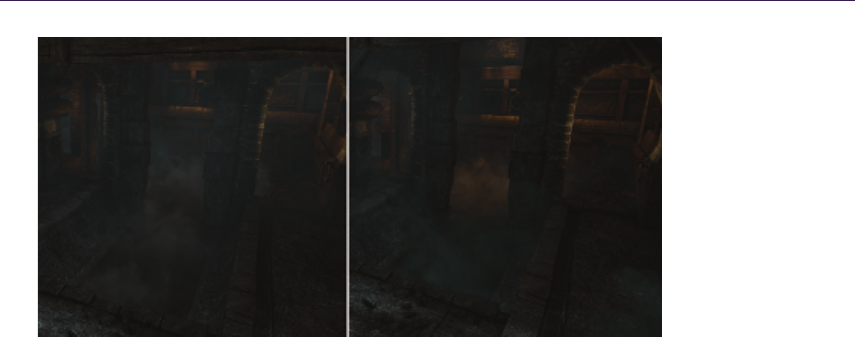
25.4. Lit Particles 417
Figure 25.15. Old-generation Thief particles rendering (left) and next-generation ver-
sion (right). Notice the color variation of the fog due to different lighting. [Image
courtesy Square Enix Ltd.]
25.4 Lit Particles
Another addition made for the next-generation version of Thief was the support
for lit particles. Prior to this, our particle system colors had to be tweaked by
hand, and this meant that particles could not react to lighting changes. With
lighting support, particles look much more integrated into the environment and
they appear to react more dynamically to changes in lighting.
The lighting feature set for particles included static light maps, static shadow
maps, projected textures, and up to four dynamic lights. We experimented with
having dynamic shadow maps, but it revealed too much about the geometry used
to render the visual effects (it made it obvious that we were using camera-aligned
sprites). Each sprite would have a well-defined shadow mapped as a plane, while
the texture used for the particle is usually meant to fake a cloud-like shape.
This issue was not visible with static light maps and shadow maps because they
were mapped as 3D textures across the particle bounds. Figure 25.15 shows a
comparison between old- and next-generation versions of particle rendering in
Thief.
25.5 Compute-Shader-Based Postprocessing
One of the major novelties of the DirectX 11 API and the next-generation con-
soles’ hardware is the support of compute shaders. One particular feature of
compute shaders is the introduction of local data storage (LDS), a.k.a. thread
group shared memory (TGSM). LDS is a cache-like on-chip memory, which is
generally faster than VRAM but slower than register memory. One can use LDS
to exchange data between shader threads running within the same thread group.
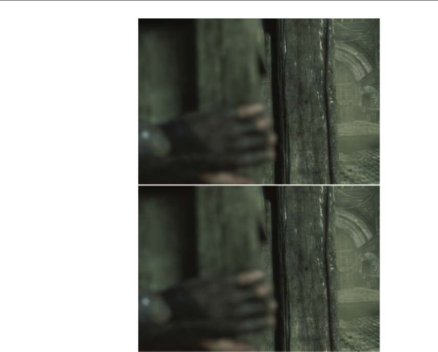
418 25. Next-Generation Rendering in Thief
Figure 25.16. Gaussian-based DoF with circular bokeh (top) and DoF with hexagonal
bokeh (bottom). [Image courtesy Square Enix Ltd.]
This functionality can be used for numerous applications. One obvious use
case is decreasing bandwidth for postprocesses, which computes a convolution
of a fairly large radius. In Thief, we used this feature for depth-of-field (DoF)
computations, as will be described below.
25.5.1 Depth-of-Field Rendering
For our DoF algorithm we used two approaches: Gaussian blur for the round-
shaped bokeh and [White and Barr´e-Brisebois 11] for hexagonal bokeh. Fig-
ure 25.16 shows examples of these techniques. Both approaches result in two
separable filter passes. DoF is texture-fetch limited, as kernels take a big number
of samples to accommodate a large radius bokeh.
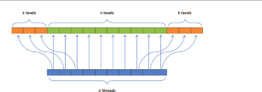
25.5. Compute-Shader-Based Postprocessing 419
Figure 25.17. Fetching of texels with a filter kernel using local data storage.
25.5.2 Improving Bandwidth by Using Local Data Storage
In order to reduce the texture bandwidth for the DoF pass, we use LDS. The
main idea is for a filter of radius kand nthreads to prefetch 2k+nsamples
as shown in Figure 25.17. Each of the nthreads loads a texel; additionally,
every thread close to the thread group boundaries loads another texel. Then,
each thread stores the values it loaded into LDS. Finally, to compute the ker-
nel, each thread reads values from LDS instead of DRAM, hence the bandwidth
reduction.
Initially, we used the code from Listing 25.6 to load and store from LDS.
However, this resulted in even worse performance than not using LDS at all. The
reason for this is a four-way LDS memory bank conflict, which we introduced.
As bank size on the majority of the video cards is 32-bits wide, each thread will
make a strided access with stride = 4. To fix that, we needed to de-vectorize our
code, as shown in Listing 25.7.
25.5.3 Results
To understand the LDS win, we tested different implementations of the DoF ker-
nel filters. For a DoF pass using a kernel with radius = 15 for a FP16 render
target, we got 0.15 ms without LDS, 0.26 with vectorized LDS structure, and
0.1 ms for de-vectorized LDS on AMD HD7970. Both next-generation consoles
have shown a speedup with a similar factor. In contrast, using LDS on NVIDIA
GPUs (GeForce 660 GTX) resulted in no speedup at all in the best case. As a
result, on AMD GPUs (which include next-generation consoles), using compute
shaders with LDS can result in a significant (33%) speedup if low-level perfor-
mance considerations (e.g., banked memory) are taken into account.

420 25. Next-Generation Rendering in Thief
gro up shared floa t4 fCach e [ NR_THREADS + 2 * KE RN EL _RADI US ];
Tex tu re 2D inp ut Te xture : r egi ste r ( t0 );
RWT ext ure 2D < flo at4 > ou tp ut Te xt ur e : re gis ter ( u 0 );
[n um th re ad s ( N R_ THR EA DS , 1 , 1 ) ]
voi d mai n ( uin t3 g rou pT hr ea dID : SV _Gr ou pTh rea dI D ,
uint3 d ispa tc hThr ea dID : SV_ Disp at chTh rea dI D )
{
// Rea d te xture to LDS
int c ounter = 0;
for (int t = gr oupT hre adID . x;
t< N R_T HRE ADS + 2 * KE RNEL_R ADI US ;
t+= NR_THREA DS , co unt er += NR _TH REA DS )
{
int x = cla mp (
dis patc hTh read ID .x + co unter - KE RNEL_R ADIUS ,
0, in put Te xtu re . L ength . x - 1) ;
fC ach e [ t ] = in pu t Te xt ur e [ i nt2 ( x , di s pa tc hT h re ad ID .y ) ];
}
GroupMemoryBarrierWithGroupSync();
...
// Do the a ctual bl ur
...
o ut pu tT e xt ur e [ d i sp a tc hT h re ad ID . xy ] = v Ou tC ol or ;
}
Listing 25.6. Initial kernel implementation. Notice a single LDS allocation.
25.6 Conclusion
In this chapter, we gave a comprehensive walkthrough for the rendering tech-
niques we implemented for the next-generation versions of Thief. We presented
our reflection system, the contact-hardening shadow algorithm, particles lighting
approach, and compute shader postprocesses. Most of these techniques were inte-
grated during the later stages of Thief production, therefore they were used less
extensively in the game than we wished. However, we hope that this postmortem
will help game developers to start using the techniques, which were not practical
on the previous console generation.
25.7 Acknowledgments
We would like to thank Robbert-Jan Brems, David Gallardo, Nicolas Longchamps,
Francis Maheux, and the entire Thief team.

Bibliography 421
gr ou pshared floa t fC ach eR [ NR _TH READ S + 2 * KE RNE L_ RAD IU S ];
gr ou pshared floa t fC ach eG [ NR _TH READ S + 2 * KE RNE L_ RAD IU S ];
gr ou pshared floa t fC ach eB [ NR _TH READ S + 2 * KE RNE L_ RAD IU S ];
gr ou pshared floa t fC ach eA [ NR _TH READ S + 2 * KE RNE L_ RAD IU S ];
Te xt ur e2 D i np utTex tu re : r egi ste r ( t0 );
RW Tex tur e2 D < fl oat4 > o ut pu tT ex tur e : r egi ste r ( u0 );
[ nu mth reads ( NR_THR EADS , 1 , 1) ]
voi d mai n ( uin t3 g ro upT hr ea dI D : SV _Gr ou pTh rea dI D ,
uint3 dis pa tchT hr eadID : S V_Di sp atch Thr eadI D )
{
// Read text ure to LDS
int c ounter = 0;
for (int t = gro upT hreadI D .x;
t < NR_THREADS + 2 * KE RN EL _RADI US ;
t += NR _THR EADS , co unt er += NR _TH REA DS )
{
int x = cl amp (
di spat chT hrea dID . x + co unter - K ERNEL_ RAD IUS ,
0, i np utT extu re . Le ngt h .x - 1) ;
f loa t4 te x = in pu t Te xt ur e [ i nt2 ( x , di s pa tc hT h re ad ID .y ) ];
fC ac heR [t ] = tex . r;
fC ac heG [t ] = tex . g;
fC ac heB [t ] = tex . b;
fC ac heA [t ] = tex . a;
}
GroupMemoryBarrierWithGroupSync();
...
// Do the a ctual bl ur
...
o ut pu tT e xt ur e [ d i sp a tc hT hr e ad ID . xy ] = v Ou tC ol or ;
}
Listing 25.7. Final kernel implementation. Notice that we make a separate LDS
allocation for each channel.
Bibliography
[Andersson 13] Zap Andersson. “Everything You Always Wanted to Know About
mia material.” Presented in Physically Based Shading in Theory and Prac-
tice, SIGGRAPH Course, Anaheim, CA, July 21–25, 2013.
[Andreev 13] Dmitry Andreev. “Rendering Tricks in Dead Space 3.” Game De-
velopers Conference course, San Francisco, CA, March 25–29, 2013.
[Fernando 05] Randima Fernando. “Percentage-Closer Soft Shadows.” In ACM
SIGGRAPH 2005 Sketches, p. article 35. New York: ACM, 2005.
[Gruen and Story 09] Holger Gruen and Jon Story. “Taking Advantage of Di-
rect3D 10.1 Features to Accelerate Performance and Enhance Quality.” Pre-

422 25. Next-Generation Rendering in Thief
sented at AMD sponsored session, Eurographics, Munich, Germany, March
30–April 3, 2009.
[Gruen 10] Holger Gruen. “Contact Hardening Shadows 11.” AMD Radeon
SDK, http://developer.amd.com/tools-and-sdks/graphics-development/
amd-radeon-sdk/archive/, 2010.
[Kasyan et al. 11] Nick Kasyan, Nicolas Schulz, and Tiago Sousa. “Secrets
of CryENGINE 3 Graphics Technology.” SIGGRAPH course, Vancouver,
Canada, August 8, 2011.
[Lagarde and Zanuttini 13] S´ebastien Lagarde and Antoine Zanuttini. “Practical
Planar Reflections Using Cubemaps and Image Proxies.” In GPU Pro 4:
Advanced Rendering Techniques, edited by Wolfgang Engel, pp. 51–68. Boca
Raton, FL: CRC Press, 2013.
[Lengyel 11] Eric Lengyel. Mathematics for 3D Game Programming and Com-
puter Graphics, Third edition. Boston: Cengage Learning PTR, 2011.
[NVIDIA Corporation 99] NVIDIA Corporation. “Cube Map OpenGL Tutorial.”
http://www.nvidia.com/object/cube map ogl tutorial.html, 1999.
[Sousa 05] Tiago Sousa. “Generic Refraction Simulation.” In GPU Gems 2,
edited by Matt Farr, pp. 295–305. Reading, MA: Addison-Wesley Profes-
sional, 2005.
[Uludag 14] Yasin Uludag. “Hi-Z Screen-Space Cone-Traced Reflections.” In
GPU Pro 5: Advanced Rendering Techniques, edited by Wolfgang Engel,
pp. 149–192. Boca Raton, FL: CRC Press, 2014.
[White and Barr´e-Brisebois 11] John White and Colin Barr´e-Brisebois. “More
Performance! Five Rendering Ideas from Battlefield 3 and Need For Speed:
The Run.” Presented in Advances in Real-Time Rendering in Games, SIG-
GRAPH Course, Vancouver, August 7–11, 2011.
[Wright 11] Daniel Wright. “Image Based Reflections.” http://udn.epicgames.
com/Three/ImageBasedReflections.html, 2011.
26
Grass Rendering and Simulation
with LOD
Dongsoo Han and Hongwei Li
26.1 Introduction
Grass rendering and simulation are challenging topics for video games because
grass can cover large open areas and require heavy computation for simulation.
As an extension of our previous hair technology, TressFX [Tre 13], we chose
grass because it has unique challenges. (See Figure 26.1.) Our initial plan was
to support rendering many individual grass blades covering a wide terrain and
simulating their interactions using rigid bodies and wind.
To satisfy our requirements, we developed an efficient and scalable level-of-
detail (LOD) system for grass using DirectX 11. In addition to LOD, a master-
and-slave system reduces simulation computation dramatically but still preserves
the quality of the simulation.
Figure 26.1. Grass rendering and simulation with balls.
423

424 26. Grass Rendering and Simulation with LOD
Figure 26.2. Five grass blade types generated by an in-house tool.
26.2 Render Grass Blades
To make the grass look natural, it is vital to acquire a natural shape for the
grass blades. We first adopted the method described in [Bouatouch et al. 06],
where they generate grass blade in a procedural manner. For each grass blade,
its stem is defined as a parabolic curve formed by tracking the motion of a point,
shooting from the root vertex, with a random initial speed and angle. This
method is simple yet effective, but cannot provide a rich variance in the grass
blade geometric appearance as they are always parabolic curves, tall or low,
curved or straight. It is difficult to generate complex and natural-looking grass
blades using this approach since the blades are poorly described by a quadratic
curve alone.
We find instancing can tackle this variance problem very well. First, we
generate a few grass blade types, each of which has a fixed number of knots.
In our application, the number of knots is 16, which balances the efficiency of
simulation and the smoothness of blade shape. Also, we have experimented with
different numbers of types and find five is good enough to create a grass lawn
with rich variance. More types do not hurt the performance but do not increase
the visual quality much either. Figure 26.2 shows five blade types that we created
using an in-house tool.
To further increase the variance, when we instantiate these blade types and
plant them in the scene (we call it the growing process), we randomize orien-
tations, lengths, widths, and textures of instantiated blades. For example, for
the fifth blade type, its length can vary between 0.1 m and 0.15 m. When it is
instantiated, its length will be set to a number between 0.1 m and 0.15 m with
regards to the normal distribution. Each knot on the blade is linearly scaled to
this new length. The range of length for each blade type is hard coded. The vari-
ance is further enhanced by distributing blade types unevenly. Some of them will
be used more often than others. The probability of instantiating one particular
blade type is tweaked for the best look in the final scene.
The grass blade created by hand or tool only describes the blade stem. The
stem is expanded to a blade in the runtime so that we can set the width of each
blade separately. Each line segment in the stem becomes a quad, i.e., two tri-
angles. There are 16 knots and thus there are 15 quads or 30 triangles. The

26.2. Render Grass Blades 425
2*(i+1)+1 2*(i+1) 2*(i+1)+1 2*(i+1)
2*i2*i+1
Expansion
2*i+1 2*i
Figure 26.3. Expand the stem to grass blade in vertex shader. The two overlapping
vertices from two triangles are dragged to opposite positions in the vertex shader.
expansion direction follows the binormal of the grass blade, and the expansion
width is chosen by the user. Moreover, we reduce the expansion width gradually
from bottom knots to top in order to make a sharp blade tip. This geometry
expansion was firstly implemented in a geometry shader, but the performance
was not satisfying. We then adopted the approach presented in TressFX, where
they do the geometry expansion in the vertex shader by expanding two degraded
triangles to normal, nondegenerate triangles. Figure 26.3 illustrates the process
of expanding the degenerate triangles. We also modified our in-house blade mod-
eling tool so that its output became a triangle strip: each knot in the stem is
duplicated into two vertices at the same coordinate as the knot, and one line
segment becomes two triangles. At runtime, we upgrade triangles by translating
two overlapping vertices at the knot position in opposite directions determined
by the modulo 2 result of the vertex ID, e.g., SV_VertexID.
Regarding the rendering, we do not have much freedom in choosing a shading
model for the grass blade for there are thousands of blades to be rendered in one
frame. It must be a lightweight shading model that still can create a promising,
natural appearance for the grass blade. Under this constraint, we adopt the con-
ventional Phong model and replace its ambient component with Hemispherical
Ambient Light [Wilhelmsen 09]. Hemispherical ambient light is a good approx-
imation of the true ambient color of grass in lieu of the more precise ambient
occlusion and color, which can be very expensive to generate. It is computed as
the sum of sky light and earth light as shown in following equation:
ambient =skylight ×ratio +earthlight ×(1 −ratio),
where ratio is defined by the dot product between the hemisphere’s “up” direction
and the vertex normal.
We also investigated screen-space translucency [Jimenez and Gutierrez 10],
but the increase in the visual quality is minor, and it added an extra 50 shader
instructions, so we did not use it.
Besides the lighting model, a grass blade has both a front and a back face, and
thus we cannot disable face culling on the GPU. We rely on DirectX’s semantic

426 26. Grass Rendering and Simulation with LOD
SV_IsFrontFace to tell us whether the current pixel is now facing forward or
backward. If it is the back face, we invert the normal and use the back surface
texture in the shading computation.
26.3 Simulation
Like hair simulation in TressFX, each grass blade is represented as vertices and
edges. We usually use 16 vertices for each blade and 64 for the thread group size
for compute shaders, but it is possible to change the thread group size to 32 or
128.
For hair simulation in TressFX, three constraints (edge length, global shape,
and local shape) are applied after integrating gravity. The TressFX hair simula-
tion includes a “head”İ transform. This is required in a hair simulation since the
character’s head can change its position and orientation, but we do not require
this transform for grass. We can also skip applying the global shape constraint
because grass gets much less force due to the absence of head movement. For the
edge length constraint and the local shape constraint, two to three iterations are
usually good enough.
The last step of simulation before going to LOD is to run a kernel to prevent
grass blades from going under the ground. This can be done simply by moving
each vertex position above the position of the blade root vertex position.
26.3.1 Master-and-Slave System
Master blades are the grass blades that are actively simulated. During the process
of growing blades procedurally, we arrange master blade vertex positions followed
by slave vertex positions. In our demo, we typically use a 1:4 ratio of master to
slave blades, but that ratio can be easily changed during the growing process.
After simulating master blades, we copy the master vertex positions to their
slaves. The important part of this process is that we should add perturbations so
that slave blades are not exactly showing the same motion of their master. The
perturbations become larger along the vertices toward the tip so that blades can
be separated wider between tips and avoid parallel patterns. It is also possible
to increase or decrease the perturbations based on the master blade’s velocity so
that if the master moves faster, the slaves will be farther behind.
26.3.2 Distance-Based Sorting
For LOD, two new read/write buffers (QuantizedLODDistance and LODSortedStrand
Index) were added to TressFX. QuantizedLODDistance is to store the distances
from the camera to each blade. LODSortedStrandIndex is to store the blade index
for QuantizedLODDistance. Basically, these two buffers make key and value pairs
for sorting.
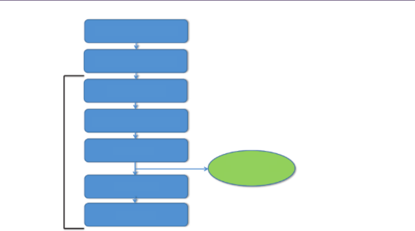
26.3. Simulation 427
Dispatch Simulation Kernels
Compute Camera Distance
Histogram Table
Column Scan Histogram Table
Prefix Scan
Prefix Scan Table
Rearrange
Radix
Sort Read prefix scan
to CPU and
calculate LOD ratio
Figure 26.4. Kernel execution flow chart of radix sort.
The sorting algorithm we choose must run on the GPU efficiently and support
key and value pairs. Also, we need to count how many keys are less than a given
distance threshold so that we can determine the work item size for dispatch.
Choosing radix sort could give us an extra benefit that, if we quantize the distance
value in 8 bits, we need only one pass. Normally, radix sort needs four passes to
sort 32-bit keys with an 8-bit radix; see Figure 26.4.
After simulating master blades and updating slave vertices, ComputeCamera
Distance in Listing 26.1 calculates the distance from the camera position to each
blade. Also, frustum culling is performed here, and a negative distance value
will be assigned if the blade is outside of the camera’s frustum. We quantize the
distance values to 8 bits using the maximum distance given as user input.
Listings 26.2, 26.3, and 26.4 show the full code of radix sort. The inputs
of radix sort are QuantizedLODDistance and LODSortedStrandIndex.PrefixScan
performs a prefix scan of all the elements of QuantizedLODDistance. Before running
the next kernels of radix sort, we read the prefix scan data on the CPU and
compute the LOD ratio, which is a ratio of the number of valid blades to the
number of total blades. We use this LOD ratio to compute the thread group size
for simulation during the next frame.
Listing 26.5 shows how we can use a prefix scan to get the LOD ratio. We
first calculate the quantized distance threshold and simply read the value of the
prefix-scan array using the quantized distance threshold as an index; the prefix
scan stores counts of values.

428 26. Grass Rendering and Simulation with LOD
# define THREAD_GROUP_SIZE 64
RW St ru ct ur ed Bu ff er < uint > Q ua n ti ze d LO DD i st an c e : register ( u6 ) ;
RW St ru ct ur ed Bu ff er < uint > L OD S or te d St ra n dI nd e x : register ( u7 ) ;
// cam era Pos , ca mer aDir , and ma xD ist are give n thro ug h
// const bu ffer .
[ nu mth reads ( THREAD_GROUP_SIZE , 1 , 1) ]
void C om pu te Ca me ra Di st an ce ( u int G Ind ex : SV _G rou pIn dex ,
uint3 GId : SV_Group ID ,
uint3 DT id : S V_Di spa tchT hrea dID )
{
uint gl oba lBl adedIndex , glo bal Ro ot Vert exI nd ex ;
// Ca lc ula te i nd ice s abo ve he re .
float4 pos = g _Hai rVe rtex Posi tion s [ gl obal Root Ve rtex Inde x +1];
float di st = dot ( ( pos . xy z - ca mer aP os . x yz ) , c am er aD ir . xy z );
// Per fo rm frustum cu ll in g and ass ig n negative distance
// if t his b lade is out of f rus tum her e .
// Qu an ti ze di sta nc e into 8 bits (0 ˜ 2ˆ8 -1)
// so that r adix so rt can sort it in one pa ss .
if ( dist < 0 || dist > max Dist )
dis t = max Dis t ;
ui nt qu an ti ze dDi st = ( ui nt ) (( dis t / max Di st ) * 2 55. f );
Qu an ti zedL ODDi st ance [ g lobalB lade dI ndex ] = qu antize dDi st ;
LO DS or tedS tran dI ndex [ g lobalB lade dI ndex ] = gl obal Bladed Inde x ;
}
Listing 26.1. Compute camera distance kernel.
# de fine RADIX 8 // 8 bit
# de fine RA DIC ES (1 << R ADI X ) // 256 or 0 x 100
# de fine RA DI X_M ASK ( RADI CES - 1) // 255 or 0 x FF
# de fine THR EA D_G RO UP_ SI ZE RAD IC ES
cb uffer C BR adixSor t : re gis ter ( b0 )
{
int n umE lem ent ;
int b its ;
float d ummy [2];
}
// UAVs
RW St ru ct ur ed Bu ff er < uint > Q ua n ti ze d LO DD i st an c e : register ( u0 ) ;
RW St ru ct ur ed Bu ff er < uint > his to gr amT ab le : reg ist er ( u1 ) ;
RWS tr uc tu re dB uf fe r < uint > p art ic ial ly Sor te d Da ta : reg ist er ( u2 ) ;
RW St ru ct ur ed Bu ff er < uint > p re fi xS ca n : re gis ter ( u 3 );
RW St ru ct ur ed Bu ff er < uint > L OD S or te d St ra n dI nd e x : register ( u4 ) ;
RW St ru ct ur ed Bu ff er < uint > p ar t ic ia l ly So r te dV a lu e : regi ster ( u5 ) ;
gro upsh are d uin t sharedMem [ RADIC ES ];
gro upsh are d uin t sh ared MemP refi xSca n [ RAD ICE S ];

26.3. Simulation 429
uin t p ow2 ( ui nt a )
{
return ( (( uin t ) 1) << a ) ;
}
// Eac h thr ead ( wo rk ite m ) wo rks on one e le men t .
[ n u mt hr ea ds ( TH RE AD _G RO UP _S IZ E , 1 , 1 ) ]
void H is to gr am Tab le ( uin t G Ind ex : S V_G rou pIn de x ,
uint3 GId : SV_Group ID ,
uint3 DT id : S V_Di spa tchT hrea dID )
{
uint lo cal Id = G Index ;
uin t gr oup Id = GI d .x ;
uint gr oupSiz e = RAD ICE S ;
uint gl ob al Id = g ro up Si ze * gro up Id + l ocalId ;
// In itiali ze shar ed memo ry .
sha red Mem [ local Id ] = 0;
GroupMemoryBarrierWithGroupSync();
pa rt ic ial ly Sort ed Dat a [ gl oba lId ]
= Qu anti zedL ODDi stan ce [ gl obalI d ];
pa rt ic ial ly So rte dV al ue [ global Id ]
= LO DSor tedS tran dInd ex [ gl obalI d ];
uin t value = p ar tici ally Sort edD at a [ globa lId ];
value = ( valu e >> bits ) & R AD IX _M AS K ;
In terl ock ed Add ( s haredMem [ value ] , 1);
GroupMemoryBarrierWithGroupSync();
uin t inde x = RADICES * g ro up Id + localId ;
hi st og ram Ta bl e [ index ] = sh are dMe m [ lo cal Id ];
}
Listing 26.2. Constant buffer, UAVs, and histogram table kernels in radix sort.
// Th ere is o nly one th re ad g roup and the each t hread
// ( w ork it em ) w orks on e ach c olu mn on hi sto gr am t able .
[ n u mt hr ea ds ( TH RE AD _G RO UP _S IZ E , 1 , 1 ) ]
voi d Co lu mn Sc an Hi st og ra mT ab le ( u int G Ind ex : S V_G rou pIn dex ,
uint3 GId : SV_Group ID ,
uint3 D Tid : S V_D ispa tchT hr eadI D )
{
uin t local Id = G Index ;
uin t n umHis to gr ams = n um El em en t / THR EA D_G RO UP_ SI ZE ;
uin t sum = 0;
for ( uint i = 0; i < nu mHi st og rams ; i ++ )
{
sum += hi sto gr am Tab le [ RA DI CE S * i + loca lI d ];
hi st ogr am Tab le [ R ADI CES * i + loca lId ] = sum ;
}
}
// The re is onl y on e t hre ad grou p .
[n um th re ad s ( T H RE AD _G RO UP _SI ZE , 1 , 1 ) ]
void P re fi xSc an ( u int G Ind ex : SV _G rou pIn dex ,
uint3 GId : S V_Gro upI D ,

430 26. Grass Rendering and Simulation with LOD
uint3 DT id : S V_Di spa tchT hrea dID )
{
uint lo cal Id = G Index ;
uint numHi st ogram s = nu mE le ment / TH RE AD_ GR OUP _S IZE ;
sha re dM emP re fi xSc an [ l oca lId ]
=hi stog ram Tabl e [RADIC ES * ( num His togram s - 1) + l ocalId ];
sh are dMem [ localI d ] = sh ar ed Mem Pr ef ixS ca n [ loc alI d ];
GroupMemoryBarrierWithGroupSync();
uin t i ter = ( ui nt )( l og2 (2 56) ) ;
uin t k = loc alI d ;
for ( uint i = 0; i < it er ; i ++ )
{
if( k >= pow2 ( i) )
sha red Mem [ k] = s har ed MemP ref ix Scan [ k]
+sh ar ed Me mP re fi xS ca n [k - pow 2 (i ) ];
GroupMemoryBarrierWithGroupSync();
s ha re d Me mP r ef ix S ca n [ k ] = sh ar ed Me m [ k ];
GroupMemoryBarrierWithGroupSync();
}
if ( loc al Id > 0 )
pr efixSc an [ lo cal Id ] = s hare dMem Pref ixSc an [ loc alId -1];
els e
pr efixSc an [ lo cal Id ] = 0;
}
Listing 26.3. Column scan histogram table and prefix scan kernels in radix sort.
// Eac h thr ead ( wo rk ite m ) wo rks on one e le men t .
[ nu mth reads ( THREAD_GROUP_SIZE , 1 , 1) ]
voi d Pr ef ix Sc an Tab le ( uin t G Ind ex : S V_G rou pIn de x ,
uint3 GId : SV_Group ID ,
uint3 D Tid : S V_D ispa tchT hr eadI D )
{
uin t local Id = G Index ;
ui nt gr ou pId = G Id .x ;
uin t inde x = RADICES * g ro up Id + localId ;
sh ar edM em [ l oca lId ] = h ist og ra mTa bl e [ index ];
GroupMemoryBarrierWithGroupSync();
sh are dMem [ localI d ] += p re fix Sca n [ local Id ];
hi st og ram Ta bl e [ index ] = sh are dMe m [ lo cal Id ];
}
// One t hre ad ( w ork it em ) w ork s on on e e le men t .
[nu mth reads ( THREAD_GROUP_SIZE , 1 , 1)]
voi d Re ar ran ge ( u int G Ind ex : SV _Gr oup In dex ,
uint3 GId : S V_Gro upI D ,
uint3 DT id : S V_Di spa tchT hrea dID )
{
uint lo cal Id = G Index ;
uin t gr oup Id = GId . x ;
if( loc al Id == 0 )

26.3. Simulation 431
{
for (int i = 0; i < R ADICES ; i ++ )
{
uint el eme nt = p ar tici ally Sort ed Dat a [ gr oup Id
*R ADI CE S + i ] ;
uint value = ( e lement >> bits ) & RA DI X_ MASK ;
uint in dex ;
if( gro up Id == 0 )
{
ind ex = pr ef ixS ca n [ val ue ];
pr ef ixS ca n [ val ue ] ++;
}
else
{
index = h is to gra mT able [ RADICES * ( groupId - 1) + value ];
his to gr am Ta bl e [ RA DIC ES * ( g roupI d - 1) + val ue ]++ ;
}
Qua nt iz ed LO DDis ta nce [ index ] =
pa rti cia ll ySo rt edD at a [ gr oupId * RADIC ES + i];
LO DS or te dS tran dI ndex [ i nde x ] =
p ar t ic ia l ly So r te dV a lu e [ g r ou pId * R A DI CES + i ] ;
}
}
}
Listing 26.4. Prefix scan table and rearrange kernels in radix sort.
// dis tT hresh ol dLO D is a d is ta nc e t hr es ho ld for LOD
// and ma xDist an ceLOD is the maximum d is ta nc e for q ua nt iz ation .
un si gn ed int quantizedDistThresholdLod =
(un si gn ed in t )(( dis tT hresho ldLOD / ma xDi stan ce LOD ) * 255. f);
int coun t = pref ixS can [ q ua ntiz edDi stTh resh oldL od +1];
LO DRa ti o = ( fl oat ) co unt / ( f loa t ) num Mast erB lade s ;
Listing 26.5. Calulating the LOD ratio.
26.3.3 Wind
There are two kinds of wind motions: local ambient and global tidal motions.
Local ambient motion is small scale and is independent of neighboring blades.
In TressFX, wind was applied to each vertex by calculating the force from the
wind and edge vectors. In grass, we simplified this by grabbing the tip vertex and
moving it along the wind vector. This simple method works as well as the force-
based approach. The amount of displacement is controlled by the magnitude of
the wind. To prevent a visible directional pattern, perturbations are added into
the wind directions and magnitudes.
Global tidal motion is also simple. This is wavy motion and neighbor blades
should work together. In our grass, we simply sweep the grass field with large
cylindrical bars and the collision handling system generates the nice wave motion.

432 26. Grass Rendering and Simulation with LOD
26.4 Conclusion
With 32,768 master blades and 131,072 slave blades, simulating an entire grass
field takes around 2.3 ms without LODs. Because radix sort takes around 0.3 ms,
we see that simulation time can easily drop by more than 50% with LODs using
reasonable distance thresholds.
In our test, we applied only one distance threshold. However, it is also possible
to use multiple distance thresholds. This would allow us to smoothly change
between LOD regions and reduce popping problems during camera movement.
Bibliography
[Bouatouch et al. 06] Kadi Bouatouch, K´evin Boulanger, and Sumanta Pat-
tanaik. “Rendering Grass in Real Time with Dynamic Light Sources.” Rap-
port de recherche RR-5960, INRIA, 2006.
[Jimenez and Gutierrez 10] Jorge Jimenez and Diego Gutierrez. “Screen-Space
Subsurface Scattering.” In GPU Pro: Advanced Rendering Techniques,
edited by Wolfgang Engel, pp. 335–351. Natick, MA: A K Peters, Ltd., 2010.
[Tre 13] “TressFX 2.0.” http://developer.amd.com/tools-and-sdks/graphics
-development/amd-radeon-sdk/, accessed November 13, 2013.
[Wilhelmsen 09] Petri Wilhelmsen. “Hemispheric Ambient Light.” http://
digitalerr0r.wordpress.com/2009/05/09/xna-shader-programming-tutorial
-19-hemispheric-ambient-light/, accessed May 9, 2009.

27
Hybrid Reconstruction
Antialiasing
Micha l Drobot
27.1 Introduction
In this article, we present the antialiasing (AA) solution used in the Xbox One
and Playstation 4 versions of Far Cry 4, developed by Ubisoft Montreal: hybrid
reconstruction antialiasing (HRAA). We present a novel framework that utilizes
multiple approaches to mitigate aliasing issues with a tight performance budget
in mind.
The Xbox One, Playstation 4, and most AMD graphics cards based on the
GCN architecture share a similar subset of rasterizer and data interpolation fea-
tures. We propose several new algorithms, or modern implementations of known
ones, making use of the aforementioned hardware features. Each solution is tack-
ling a single aliasing issue: efficient spatial super-sampling, high-quality edge
antialiasing, and temporal stability. All are based around the principle of data
reconstruction. We discuss each one separately, identifying potential problems,
benefits, and performance considerations. Finally, we present a combined solu-
tion used in an actual production environment. The framework we demonstrate
was fully integrated into the Dunia engine’s deferred renderer. Our goal was
to render a temporarily stable image, with quality surpassing 4×rotated-grid
super-sampling, at a cost of 1 ms at a resolution of 1080p on the Xbox One and
Playstation 4 (see Figure 27.1).
27.2 Overview
Antialiasing is a crucial element in high-quality rendering. We can divide most
aliasing artifacts in rasterization-based rendering into two main categories: tem-
poral and spatial. Temporal artifacts occur as flickering under motion when de-
tails fail to get properly rendered due to missing the rasterization grid on certain
433
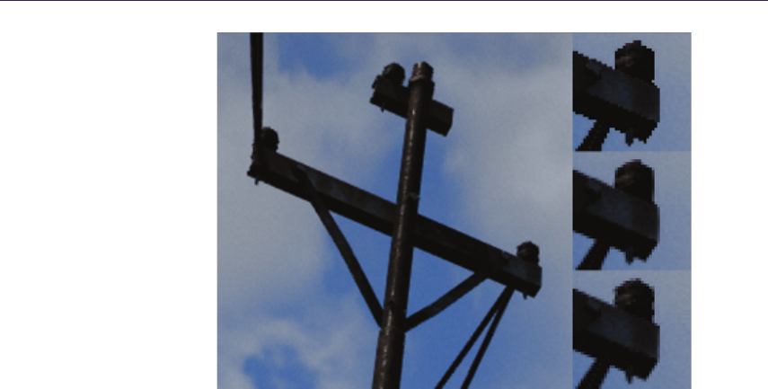
434 27. Hybrid Reconstruction Antialiasing
Figure 27.1. The crops on the right show no AA (top), SMAA (middle), and the
presented HRAA (bottom) results. Only HRAA is capable of reconstructing additional
details while providing high-quality antialiasing.
frames. Spatial artifacts result from signal under-sampling when dealing with a
single, static image. Details that we try to render are just too fine to be properly
resolved at the desired resolution, which mostly manifests itself as jagged edges.
Both sources of aliasing are directly connected with errors of signal under-
sampling and occur together. However, there are multiple approaches targeting
different aliasing artifacts that vary in both performance and quality. We can
divide these solutions into analytical, temporal, and super-sampling–based ap-
proaches.
In this article, we present a novel algorithm that builds upon all these ap-
proaches. By exploring the new hardware capabilities of modern GPUs (we will
base our findings on AMD’s GCN architecture), we optimize each approach and
provide a robust framework that shares the benefits of each algorithm while min-
imizing their shortcomings.
27.3 Related Work
A typical antialiasing solution used in offline rendering is to super-sample (SSAA)
the image; render at a higher resolution and then perform a resolve step, which
is a down-sampling filter into the desired final resolution [Burley 07]. If enough
samples are used, then this type of antialiasing tackles all the aliasing problems

27.3. Related Work 435
mentioned earlier. Unfortunately, it requires effectively rendering the image mul-
tiple times and is of limited usefulness for real-time rendering.
An optimized version of super-sampling is provided by graphics hardware in
the form of multi-sampled antialiasing (MSAA) [Kirkland et al. 99]. Instead of
shading all pixels at higher resolution, only samples along triangle edges are ras-
terized multiple times (but only shaded once), which is followed by an optimized
resolve. MSAA proves to be a valid solution to spatial aliasing issues, but is
strictly limited to triangle edges. All samples need to be stored in an additional
framebuffer until they are resolved, therefore making this method very expensive
in terms of memory consumption. As a result, not many games use it as the main
antialiasing solution on performance-limited platforms.
It is worth noting that the number of gradient steps on antialiased edges
is strictly correlated to the number of samples that MSAA or SSAA uses (i.e.,
4×MSAA can provide a maximum of five gradients depending on the sampling
pattern and edge orientation).
On the previous generation of consoles (Xbox 360 and Playstation 3), we
observed a rise in popularity of image-based, postprocessing, morphological an-
tialiasing solutions such as FXAA [Lottes 09], MLAA [Reshetov 09], and SMAA
[Jimenez et al. 11]. These algorithms provided excellent results, with perceptual
quality comparable to extremely high levels of MSAA rendering at a fraction
of the cost of MSAA. A typical morphological filter derives visually perceivable
edges from the current image and performs edge re-vectorization. Unfortunately
the result still relies only on the final rasterized image data, which can suffer
from temporal and spatial aliasing. In practice, static images that are pro-
cessed with these algorithms look much better than what the hardware-based
MSAA can achieve. Unfortunately the quality degrades dramatically under mo-
tion, where spatial and temporal under-sampling result in “wobbly” edges and
temporal flicker of high-contrast details.
It is clear that morphological methods alone will not achieve the high-quality
spatio-temporal results of super-sampling. This sparked research in two differ-
ent directions: analytical- and temporal-based antialiasing. Several researchers
experimented with postprocessing methods, augmented by additional informa-
tion, derived from actual triangle-edge equation. Probably the most well known
is GBAA [Persson 11], which calculates per-pixel signed distance to the closest
triangle edge. This information is stored in an additional buffer and is used later
during a postprocessing pass to effectively rerasterize triangle edge-pixel inter-
sections analytically. This method can provide a high level of quality and perfect
temporal stability of triangle edges. Unfortunately, due to its use of a geometry
shader pass to gather triangle information, it exhibits poor performance and thus
never gained widespread adoption. It is also hindered by multiple other issues
that we will discuss in-depth in Section 27.5.
Another approach gaining popularity is based on temporal algorithms that
try to perform filtering using previously rendered frames utilizing image temporal

436 27. Hybrid Reconstruction Antialiasing
coherency [Nehab et al. 07]. This effectively allows multi-sampled algorithms to
be amortized over time [Yang et al. 09]. Several titles use temporal resolves to
augment SSAO [Bavoil and Andersson 12,Drobot 11] or to stabilize the final
image in motion [Sousa 13]. Some engines experiment with temporal super-
sampling [Malan 12]; however, due to a lack of robust sample rejection methods,
those approaches are rather conservative, i.e., accumulating only two frames using
a limited subset of visible pixels [Sousa 11].
Recently Killzone: Shadow Fall used a robust temporal up-sampling method,
effectively rendering images with 2×super-sampling. It also used previously re-
constructed frames to stabilize images in motion in order to avoid image flickering
[Valient 14].
Several researchers have tried to combine the benefits of hardware-based
MSAA, temporal sampling and morphological filtering into one combined so-
lution. This resulted in 4×SMAA [Jimenez et al. 12], which combines the quality
of SMAA edge gradients with the temporal stability of 2×MSAA and 2×temporal
super-sampling. Unfortunately, not many console titles can afford this due to the
use of expensive 2×MSAA.
One more research direction has been toward optimizing sampling patterns
for multi-sampled approaches [Akenine-M¨oller 03]. Unfortunately, this approach
didn’t get much traction in the real-time rendering field due to a lack of hard-
ware and software support for custom sampling patterns. Only a few predefined
sampling patterns are supported in hardware-based MSAA modes.
Another hardware-based solution involves augmenting the standard MSAA
pipeline with coverage samples that can be evaluated with minimal performance
and memory overhead. This solution was, up to this point, a part of the fixed
GPU pipeline in the form of EQAA [AMD 11] and CSAA [Young 06].
27.4 Hybrid Antialiasing Overview
Our antialiasing solution can be divided into several components. Each one can
stand on its own and can be freely mixed with any other approach.
The aim of each component is to tackle a different source of aliasing, so each
algorithm can be used to its best effect in limited use-case scenarios.
Our framework is built around the following components:
•temporally stable edge antialiasing,
•temporal super-sampling,
•temporal antialiasing.
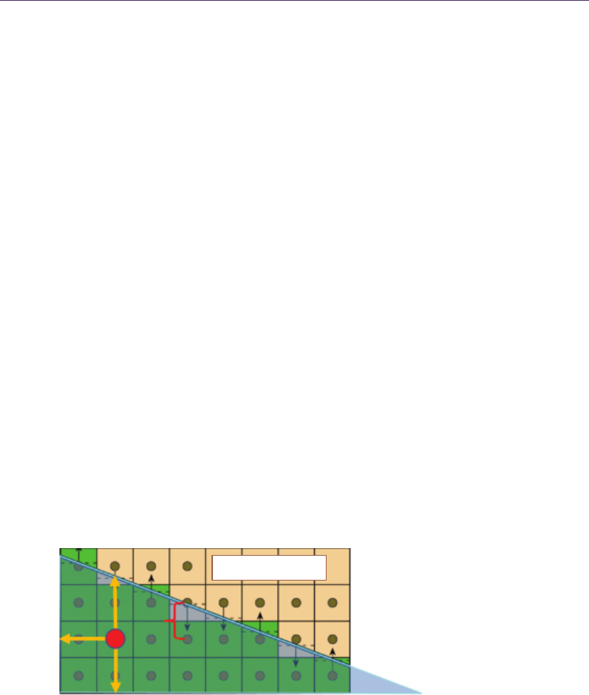
27.5. Temporally Stable Edge Antialiasing 437
27.5 Temporally Stable Edge Antialiasing
The aim of this component is to provide perceptually plausible gradients, for
geometric edges, that remain stable under motion. We do not need to worry
about pixel discontinuities that come from texture data or lighting, as that source
of aliasing will be taken care of by a different framework component.
In Section 27.3, we briefly discussed potential algorithms that would suit our
needs for high-quality edge rendering: morphological and analytical. However,
only the latter can provide temporally stable antialiasing. Unfortunately, all
purely analytical methods exhibit problems, including performance issues.
We would like to propose a new implementation based on AMD’s GCN archi-
tecture that makes analytical edge antialiasing virtually free. In Section 27.5.1,
we propose several extensions as well as real production issues connected with the
method itself. Section 27.5.2 offers a brief introduction to EQAA’s inner work-
ings. It also introduces a new algorithm—coverage reconstruction antialiasing—
that uses coverage samples from hardware-based EQAA to analytically estimate
the edge orientation as well as triangle spatial coverage, building upon previous
analytical-only algorithms.
27.5.1 Analytical Edge Antialiasing (AEAA)
The original GBAA algorithm relies on a geometry shader to pass down geometry
information to the pixel shader. Interpolators are used to store the distance
to the edge in the major direction. Then, the pixel shader selects the closest
signed distance to the currently rasterized pixel and outputs it into an additional
offscreen buffer. Distance data needs to contain the major axis and the actual
signed distance value in range [−1,1], where 0 is considered to be at the rasterized
pixel center. Later, a fullscreen postprocessing pass searches for each pixel’s
immediate neighbor’s closest edges. After an edge crossing the pixel is found, we
use its orientation and distance to blend the two nearest pixels accordingly (see
Figure 27.2).
D = min3 (d0, d1, d2)
d2
d1
d0
D
Figure 27.2. In analytical distance-to-edge techniques, every triangle writes out the
distance to the closest edge used to antialias pixels in a postprocessing pass.
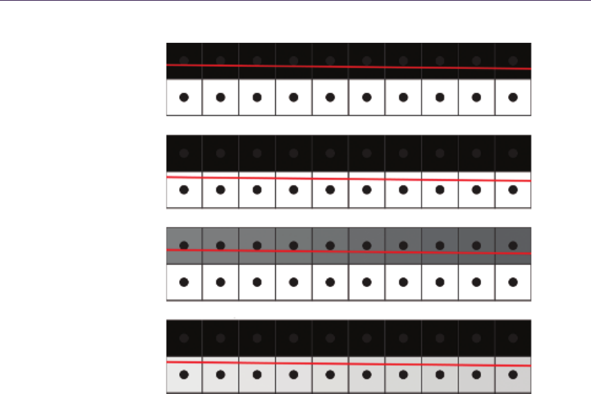
438 27. Hybrid Reconstruction Antialiasing
Morphological Frame A
Analytical Frame B
Analytical Frame A
Morphological Frame B
Figure 27.3. Antialiased edge changes in motion when using analytical data. Note that
every morphological solution will fail as no gradient change will be detected due to the
same results of rasterization. This gets more problematic with shorter feature search
distance.
Such methods provide temporally stable edge antialiasing, as the blend factor
relies on continuous triangle information rather than discrete rasterization results
(see Figure 27.3).
Gradient length is limited only by storage. In practice, it is enough to store
additional data in 8 bits: 1 bit for the major axis and 7 bits for signed distance,
providing 64 effective gradient steps.
This algorithm also deals efficiently with alpha-tested silhouettes, if a mean-
ingful distance to an edge can be estimated. This proves to be relatively easy
with nonbinary alpha channels. Alpha test derivatives can be used to estimate
the distance to a cutout edge. A better solution would be to use signed distance
fields for alpha testing and directly output the real distance to the edge.
Both methods are fast and easy to implement in practice. It is worth noting
that the final distance to the edge should be the minimum of the geometric
distance to the triangle edge and the edge derived from the alpha channel.

27.5. Temporally Stable Edge Antialiasing 439
We implemented GBAA and optimized it to take advantage of the benefits
of the new hardware features found in modern GPUs. AMD’s GCN architecture
allows pixel shaders to sample vertex data from the triangle descriptors used to
rasterize the current pixel. This means that we no longer need the expensive
geometry-shader stage to access vertex data in order to calculate the distance to
the edge as shown by [Drobot 14].
The snippet in Listing 27.1 shows the improved GBAA algorithm with offsets
directly evaluated in the pixel shader. The final postprocess resolve step remains
unchanged from the original algorithm.
// Calculate cl os est axis distance betwee n po int X
// and line AB. Che ck a ga inst know n di st an ce and di re ct io n
float ComputeAxisClosestDist(float2 inX ,
float2 inA ,
float2 inB ,
inout uint i oMa jorDi r ,
inout f loa t io Axi sDist )
{
float2 AB = n or ma li ze ( in B - i nA );
float2 no rm al AB = float2( - AB .y , A B .x ) ;
float d i st = do t ( inA , n o rm al AB ) - d ot ( i nX , n or ma l AB ) ;
boo l major Dir = ( abs ( no rma lAB . x) > ab s( n orm alA B .y ));
float a xis Dis t = dis t * rcp ( major Dir ? normalAB .x : no rma lAB . y );
if ( ax isD ist < io Axi sDis t ) ioAxi sDi st = a xis Dis t ;
if ( ax isD ist < io Axi sDis t ) ioMaj orD ir = m ajo rDi r ;
}
voi d GetGeometricDistance(float2 inScreenCoord ,
out floa t oDistance ,
out bool o Maj orDir )
{
// G et Pa ram et er X are HW imp le menta ti on d ep en da nt
float2 sc = GetParameterInterpolated( inScreenCoord );
float2 sc0 = GetParameterP0( inScreenCoord )
float2 sc1 = GetParameterP1( inScreenCoord );
float2 sc2 = GetParameterP2( inScreenCoord );
oD ist ance = F LT_ MAX ;
Co mp ut eAxi sCl os es tDis t (sc , sc0 , sc1 , oMajor Dir , oD ist anc e );
Co mp ut eAxi sCl os es tDis t (sc , sc1 , sc2 , oMajor Dir , oD ist anc e );
Co mp ut eAxi sCl os es tDis t (sc , sc2 , sc0 , oMajor Dir , oD ist anc e );
}
// in Al pha is resul t of AlphaTest ,
// i.e . , Al pha - A lp ha Re f
// We assu me alpha is a di st an ce field
voi d GetSignedDistanceFromAlpha(f loa t inAlpha ,
out floa t oDistance ,
out bool o Grad ien tDi r )
{
// Find alpha test g ra di en t
float x Gra dient = dd x_fin e ( inAlp ha );
float y Gra dient = dd y_fin e ( inAlp ha );
o Gra di en tD ir = ab s ( xG ra die nt ) > a bs ( y Gra di en t );
// Co mp ut e sign ed di st an ce to where a lph a r eaches zero
oD is ta nc e = -inA lp ha * rcp ( oG radie nt Di r ? xGradient : yGradient );
}

440 27. Hybrid Reconstruction Antialiasing
voi d Ge tA na ly ti ca lD is ta nc eToE dg e ( flo at in Alpha ,
float2 inScreenCoord ,
out floa t oDistance ,
out bool o Ma jo rD ir )
{
bool alphaMajorAxis; float al pha Distan ce ;
G et Si gn ed Di st an ce Fr om Al ph a ( inA lpha ,
alphaDistance ,
alphaMajorAxis)
Ge tG eo metr icDi stan ce ( i nScree nCo ord ,
oDistance ,
oM aj or Di r );
if ( a lphaD is ta nce < oD is ta nc e ) o Di st an ce = alph aD istan ce ;
if (alphaDistance < oDistance) alphaMajorAxis = alphaMajorAxis;
}
Listing 27.1. Optimized GBAA distance to edge shader. This uses direct access to
vertex data from within the pixel shader.
In terms of quality, the analytical methods beat any morphological approach.
Unfortunately, this method proves to be very problematic in many real-world
scenarios. Malan developed a very similar antialiasing solution and researched
further into the practical issues [Malan 10].
The main problem stems from subpixel triangles, which are unavoidable in
a real game production environment. If an actual silhouette edge is composed
of multiple small or thin triangles, then only one of them will get rasterized per
pixel. Therefore, its distance to the edge might not be the actual distance to the
silhouette that we want to antialias. In this case, the resulting artifact will show
up as several improperly smoothed pixels on an otherwise antialiased edge, which
tends to be very visually distracting (see Figure 27.4 and Figure 27.5).
Malan proposed several ways of dealing with this problem [Malan 10]. How-
ever, none of these solutions are very practical if not introduced at the very
beginning of the project, due to complex mesh processing and manual tweaking.
Another issue comes again from the actual data source. Hints for antialiasing
come from a single triangle, therefore it is impossible to correctly detect and pro-
cess intersections between triangles. Many assets in a real production scenario
have intersecting triangles (i.e., a statue put into the ground will have side trian-
gles intersecting with the terrain mesh). GPU rasterization solves intersections
by depth testing before and after rendering a triangle’s pixels. Therefore, there
is no analytical information about the edge created due to intersection. In effect,
the distance to the closest edge does not represent the distance to the intersection
edge, which results in a lack of antialiasing.
27.5.2 Coverage Reconstruction Antialiasing (CRAA)
In order to improve upon the techniques and results shared in Section 27.5.1, we
would like to find a way to determine more information about a triangle’s actual
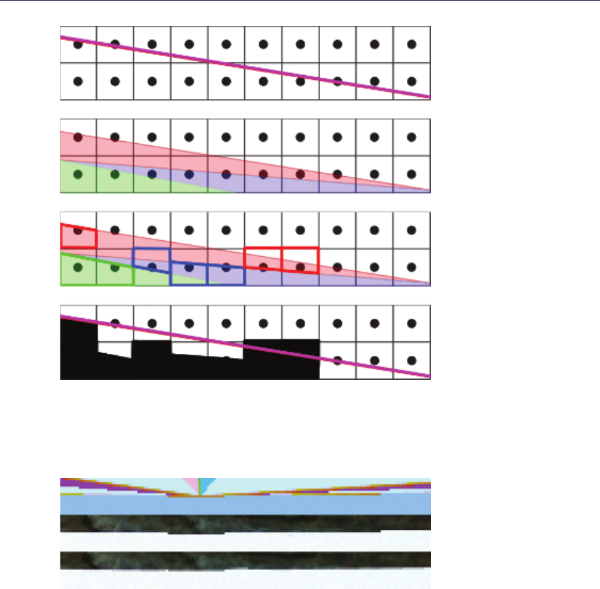
27.5. Temporally Stable Edge Antialiasing 441
Figure 27.4. False distance to a silhouette edge due to subpixel triangles. Taking a
single triangle into account would result in rerasterization of a false edge (blue) instead
of the real silhouette edge (red).
Figure 27.5. Top to bottom: a visualization of analytical distance to edge, rasterized
edge, analytically antialiased edge, an edge using 5-bit gradients, and an edge showing
minor artifacts when multiple triangles intersect one pixel.
intersections and edges within a pixel. With this information, we could partially
address most of the aforementioned issues. Fortunately, EQAA provides exactly
the information we are interested in by using AMD’s hardware EQAA.

442 27. Hybrid Reconstruction Antialiasing
EQAA overview. The enhanced quality antialiasing (EQAA) framework augments
the standard MSAA color/depth resolve with coverage samples. The rasterizer,
while processing triangles, can do cheap analytical sample coverage tests within
a triangle. The results of such tests are saved into a compressed buffer called a
fragment mask (FMask). The FMask acts as an indirection table that associates
sample locations with color fragments that were rasterized and stored in the
fragment buffer (as in normal MSAA). The number of samples can be higher
than the number of stored fragments. In order to accomidate this, a sample in
FMask may be marked as “unknown” if it is associated with a fragment that
cannot be stored in the fragment buffer (see Figure 27.6).
An important aspect of coverage rendering is correct depth testing. Normally,
incoming coverage samples need to be tested against depth fragments stored in
the MSAA depth buffer. In order to get correct coverage information, normal
MSAA would require a depth buffer that stores of the same number of depth
fragments as the number of coverage samples (we can get away with storing
fewer color fragments because FMask allows us to associate a single fragment
with multiple samples). Fortunately, one feature of AMD’s GCN architecture is
an ability to work with a compressed depth buffer, which is stored as a set of
plane equations. When this mode is enabled, EQAA uses these plane equations
to do correct depth testing by analytically deriving depth values for all coverage
samples. This means that it is possible to get correct coverage information, even
if depth and color information is evaluated and stored as a single fragment (thus
MSAA is effectively turned off for all render targets).
Another important requirement for correctly resolving coverage is to sort tri-
angles from front to back. Otherwise, due to the rules of rasterization, it is
possible for a triangle to partially overlap a pixel and not get rasterized. If that
happens, then that pixel’s coverage value might not get updated. Therefore, it
is essential to sort objects from front to back (which most rendering engines do
already). Fragment sorting is mostly taken care of by GCN hardware. Unfortu-
nately, it is still possible to get incorrect results due to subpixel triangles that
won’t get rasterized and therefore can’t correctly update pixel coverage informa-
tion.
The memory footprint of FMask is directly proportional to number of unique
fragments and samples used. For every sample, we need enough bits to index any
of the fragment stored for that pixel and also an additional flag for an unknown
value. For the sake of this article, we will focus on use cases with one fragment
and eight samples (1F8S)—which require 1 bit per sample, thus 8 bits per pixel
total (see Figure 27.7). Such a setup proved to be optimal with regard to EQAA
performance as well as the FMask’s memory footprint.
CRAA setup. Our goal is to use part of the EQAA pipeline to acquire coverage
information at a high resolution (8 samples per pixel) without paying the com-
putational and memory overhead of full MSAA rendering. We would like to use
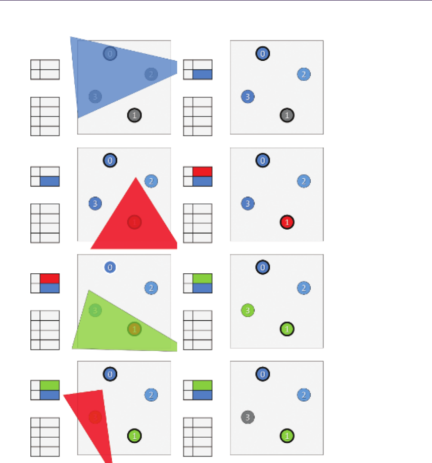
27.5. Temporally Stable Edge Antialiasing 443
3
2
1
0
1
0
Color
Fragments
1
0
Color
Fragments
FMask
2
2
2
2
3
2
1
0
FMask
0
0
0
1
0
Color
Fragments
3
2
1
0
FMask
0
0
1
0
1
0
Color
Fragments
3
2
1
0
FMask
1
0
1
0
3
2
1
0
1
0
Color
Fragments
1
0
Color
Fragments
FMask
0
0
2
0
3
2
1
0
FMask
0
0
1
0
1
0
Color
Fragments
3
2
1
0
FMask
1
0
1
0
1
0
Color
Fragments
3
2
1
0
FMask
2
0
1
0
Figure 27.6. The steps here illustrate an updated FMask as new triangles are rasterized.
Important note: in the last step, the red triangle does not need to evict Sample 3 if
it would fail a Z-test against the sample. (This, however, depends on the particular
hardware setup and is beyond the scope of this article.)
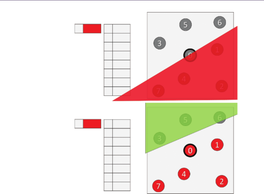
444 27. Hybrid Reconstruction Antialiasing
0 7
6
5
4
3
2
1
0
0
1
1
0
1
0
0
0
Color
Fragments FMask
0 7
6
5
4
3
2
1
0
0
1
1
0
1
0
0
0
Color
Fragments FMask
Figure 27.7. Simple rasterization case and corresponding FMask.
information recovered from the coverage data to derive blending hints in a similar
fashion to AEAA.
In our simplified case of 1F8S we know that FMask will be an 8-bit value,
where the nth bit being set to 0 represents the nth sample being associated with
the rasterized fragment (therefore it belongs to the current pixel’s triangle and
would pass depth testing), while 1 informs us that this sample is unknown—i.e.,
it was occluded by another triangle.
We can think of FMask as a subset of points that share the same color. If
we were to rasterize the current pixel with this newly acquired information, we
would need to blend the current pixel’s fragment weighted by the number of
its known coverage samples, with the other fragment represented by “unknown”
coverage samples. Without adding any additional rendering costs, we could infer
the unknown color fragments from neighboring pixels. We assume that the depth
buffer is working in a compressed mode and that EQAA is using analytical depth
testing, thus providing perfectly accurate coverage information.
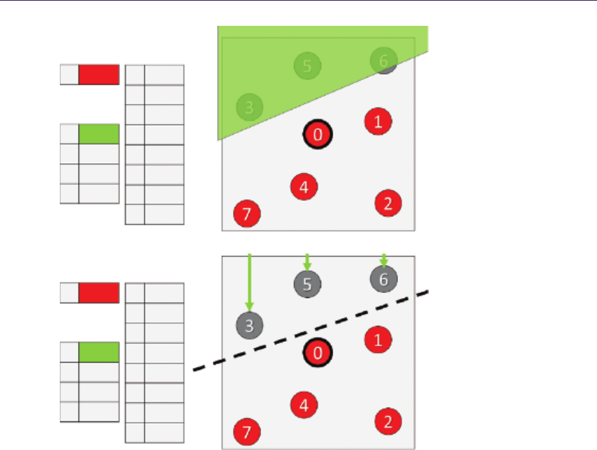
27.5. Temporally Stable Edge Antialiasing 445
0 7
6
5
4
3
2
1
0
U
B
L
R
U
B
L
R
0
1
1
0
1
0
0
0
Color
Fragments FMask
0 7
6
5
4
3
2
1
0
0
1
1
0
1
0
0
0
Color
Fragments
Neighbor
Fragments
FMask
Figure 27.8. Here we illustrate the process of finding an edge that divides a set of
samples into “known” and “unknown” samples. Later, this half plane is used to find an
appropriate neighboring pixel for deriving the unknown color value.
Single edge scenario. We can apply the same strategy behind AEAA to a simple
case in which only a single edge has crossed the pixel. In this case, the pixel’s
FMask provides a clear division of coverage samples: those that passed will be on
one side of the edge, while failed samples will be on the other side. Using a simple
line-fitting algorithm, we can find an edge that splits our set of samples into two
subsets—passed and failed. This edge approximates the real geometric edge of the
triangle that crossed the pixel. In the same spirit of the GBAA algorithm, we find
the major axis of the edge as well as its distance from the pixel’s center. Then we
just need to blend the nearest neighboring pixel color with the current fragment
using the edge distance as a weight. Thus, this technique infers the unknown
samples from the pixel closest to the derived half plane (see Figure 27.8).

446 27. Hybrid Reconstruction Antialiasing
float4 CRAA( Texture2DMS <float4 > in Color ,
Te xtu re2 D < uin t2 > i nFMa sk ,
uint2 in Te xc or d )
{
// R ead FMask / HW de pe nd an t
uin t iF Mas k = in FMa sk . Lo ad ( u int 3 ( vi Tex coor d , 0 ) ) ;
uin t un kn ow nC ov = 0;
float2 hP = 0. 0;
// Av er age all d irections to u nk nown samples
// to a pproxim at e ed ge h al fp la ne
for (uint i Sample = 0; iSample < NUM _S AM PL ES ; ++ iSa mp le )
if ( ge tF Ma s kV al ue Fo rS am pl e ( iF Mask , iS am ple ) = = U NK NO WN _C OD E )
{
hP += TexC olo rMS . Ge tS ampl ePo si ti on ( iS amp le );
un kno wn Co ver ag e ++;
}
// Fin d fragment of fs et to pixe l on the othe r side of edge
in t2 fO ff = in t2 ( 1 , 0) ;
if ( a bs ( hP . x) > a bs ( hP . y ) & & hP . x <= 0 .0) f Off = in t2 ( -1 , 0 ) ;
if ( a bs ( hP . x) <= a bs ( hP . y) & & hP . x > 0 .0 ) f Of f = i nt2 ( 0 , 1) ;
if ( a bs ( hP . x) <= a bs ( hP . y) & & hP . x <= 0 .0) f Off = in t2 ( 0 , -1) ;
// Blend in i nf er re d s ample
float k now nCov = NUM_S AMP LES -- un know nC overag e ;
float4 color = inC ol or . Load ( viTexc oord , 0 ) * k no wn Co v ;
color += inColor . Load ( viT ex coord + fOff , 0 ) * u nk no wn Cov ;
return color /= N UM_ SAMPLES ;
}
Listing 27.2. A simple shader for finding the half plane that approximates the
orientation of the “unknown” subset of samples. The half plane is then used to find the
closest pixel on the other side of the edge in order to infer the unknown sample’s color.
The resolve we have described is akin to GBAA with a limited number of
gradient steps (the number of steps is equal to the number of samples used by
EQAA). An important thing to note is that our resolve does not need to know
anything about the neighboring geometric data (all the information that is needed
for reconstruction is contained within the pixel). This is an important difference,
because we can reconstruct an edge that was created as the result of rasterizating
multiple overlapping triangles; GBAA can only recreate the edge of a single
triangle.
Our resolve can be efficiently implemented at runtime by approximating the
half plane (see Listing 27.2) while still providing quality comparable to MSAA
with the same sampling ratio (see Figure 27.9).
Complex scenario. Following what we learned about resolving simple edges using
FMask, we would now like to apply similar ideas to resolving more complex
situations in which multiple edges cross a given pixel. In order to achieve this, we
would like to be able to group together “failed” samples from different triangles
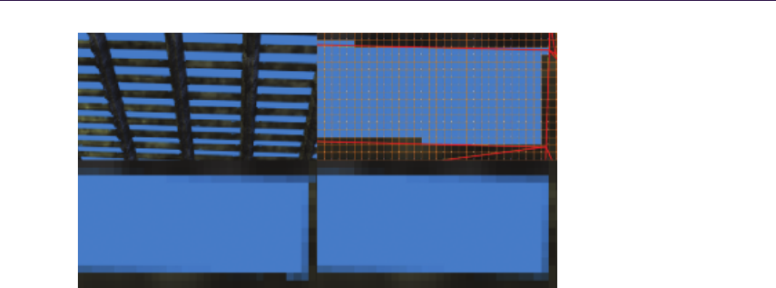
27.5. Temporally Stable Edge Antialiasing 447
Figure 27.9. A challenging rendering scenario for antialiasing (top left). Rasterization
grid and edge layout (top right). Simple 8×CRAA resulting in edge antialiasing compa-
rable to 8×MSAA apart from pixels that are intersected by multiple triangles (bottom
left). The results of 8×MSAA (bottom right).
into multiple disconnected sets. For every disconnected set, we find edges (up
to two edges in our implementation) that split it off from other sets. Then we
use the acquired edges to find major directions that should be used for subset
blending. For every subset of unknown fragments, we blend in a color from the
neighboring fragment associated with that subset and weighted by the subset’s
area coverage within the pixel. Finally, we sum all the color values for each
subset and blend this with the current fragment’s known color weighted by the
percentage of passing coverage samples. This way, we can partially reconstruct
the subpixel data using the current pixel’s surrounding neighborhood (see Figure
27.10).
Using precomputed LUT. Clearly, our algorithm could be rewritten to provide a
set of weights for blending colors from the surrounding 3 ×3 pixel neighborhood.
The blend weights rely only on the data present in FMask, and thus our blend
weights can be precomputed and stored in a look up table (LUT), which is indexed
directly by a pixel’s FMask bit pattern.
In our 1F8S case, the LUT would only need 256 entries. Our implementation
uses only top, bottom, left, and right neighboring pixels and uses only 4-bit
gradients or blend weights. Therefore, the whole LUT requires 256×4×4 = 512-
byte array, which easily fits entirely within the cache.
We also experimented with more complex LUT creation logic. FMask can be
evaluated in a morphological fashion to distinguish shapes, thus calculating more
accurate and visually plausible gradients. Unfortunately, due to our project’s time
constraints, we did not have time to properly pursue this direction of research.
We believe that a significant quality improvement can be gained from smarter
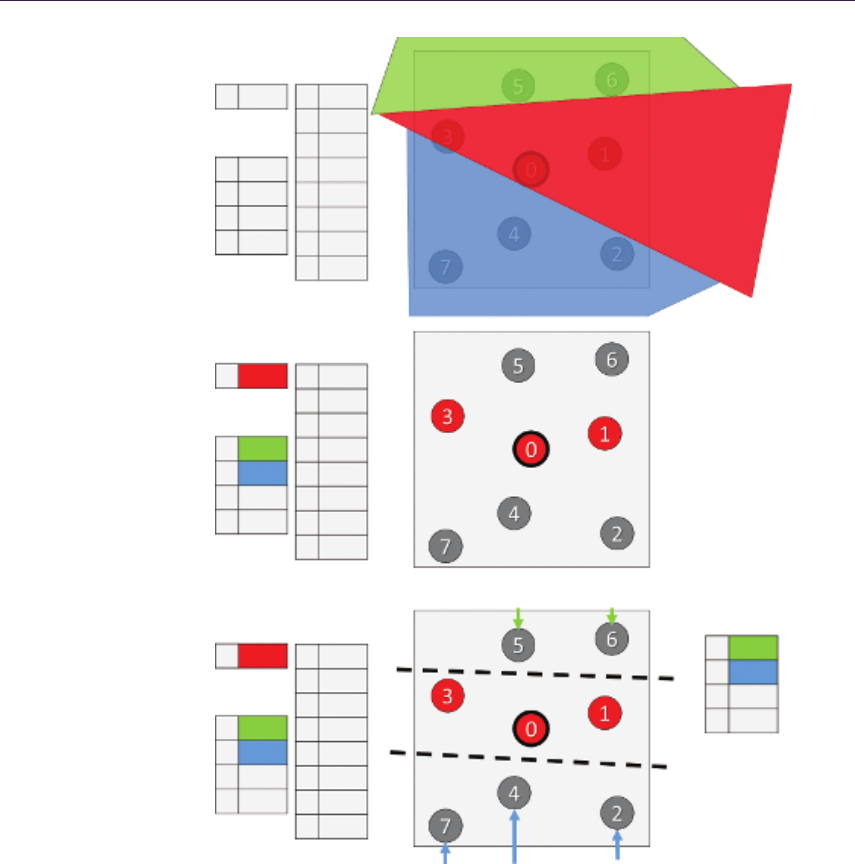
448 27. Hybrid Reconstruction Antialiasing
0 7
6
5
4
3
2
1
0
1
1
1
1
1
1
1
1
Color
Fragments
Neighbor
Fragments
Neighbor
Fragments
FMask
0
U
B
L
R
U
B
L
R
7
6
5
4
3
2
1
0
1
1
1
1
0
1
1
0
Color
Fragments FMask
Neighbor
Fragments
0
U
B
L
R
U
B
L
R
7
6
5
4
3
2
1
0
1
1
1
1
0
1
1
0
2
3
0
0
Color
Fragments FMask CLUT[01101111]
Figure 27.10. One of the possible methods for finding blend weights for sample subsets.
The bottom image illustrates a blend weight resolve using a lookup table.
FMask analysis. Using 1F16S would also provide significantly better precision
and subpixel handling.
It is worth noting that even the simple logic presented in this section allows for
significant aliasing artifact reduction on thin triangles. Figure 27.11 illustrates a

27.5. Temporally Stable Edge Antialiasing 449
Figure 27.11. Top to bottom: edge layout, rasterized edge, simple 8×CRAA resolve,
and 8×CRAA LUT correctly resolving subpixel artifacts.
problematic case for AEAA, where our simple CRAA resolve correctly antialiased
the edge. Unfortunately, when there are too many subpixel triangles that don’t
pass rasterization, CRAA may also fail due to incorrect coverage information. In
practice, this heavily depends on the exact rendering situation, and still CRAA
has much more relaxed restrictions than AEAA.
The code snippet in Listing 27.3 illustrates the CRAA LUT resolve properly
resolving minor subpixel details (see Figure 27.10).
float4 CR AA _L UT ( Te xtu re2 DMS < flo at4 > inColor ,
Te xtu re2 D < uin t2 > i nFMa sk ,
Texture1D <uint > inCRAALUT ,
uint2 in Te xc or d )
{
// R ead FMask / HW de pe ndant
uin t iF Mas k = in FMa sk . Lo ad ( u int 3 ( vi Tex coor d , 0 ) ) ;
uin t LU TR Es ul t = in CR AA LU T [ iFM ask ];
float wC , wN , wE , wS , wW ;
// LUT is p acked as 8 bit in te ger w ei ghts
// North 8b | We st 8b | South 8b | East 8b
// Can also pac k whole neigh bo rh ood we ights in 4 bit s
Ex ctra ct LUTW ei ght s (LUTRes ult , wC , wN , wE , wS , wW );
float4 co lor = i nCo lo r . Load ( v iTe xc oor d + in t2 ( 0 , 0) * wC ;
co lor += in Co lor . L oad ( vi Te xco or d + int 2 ( 0 , -1) * wN ;
co lor += in Co lor . L oad ( vi Te xco or d + int 2 ( 0 , 1) * w E;
co lor += in Co lor . L oad ( vi Te xco or d + int 2 ( 0 , 1) * w S;
c olo r + = i n Co lo r . L oad ( v iT ex co or d + i nt2 ( -1 , 0) * w W ;
return co lor ;
}
Listing 27.3. CRAA LUT implementation.

450 27. Hybrid Reconstruction Antialiasing
27.6 Temporal Super-Sampling
27.6.1 Overview
Temporal super-sampling can be succinctly described by the following simple
algorithm:
1. Every frame, offset the projection matrix by a subpixel offset.
2. Use the current frame’s Nmotion vectors to reproject data from frame
N−kto time step N.
3. Test if the reprojected data is valid:
•No occlusion occurred.
•The data comes from the same source (i.e., object or triangle).
•The data is not stale (i.e., due to lighting changes).
4. Accumulate data from frame Nwith data reprojected from frame N−k.
5. Repeat steps 2–4 for kframes back in time.
The number kdictates the number of unique subpixel offsets used for jitter in
order to get spatially unbiased results after converging by accumulation of all the
ksamples. However, it is easy to see that by increasing the number kof frames of
history, the algorithm has a much higher complexity and therefore a much higher
chance of failure.
The most proper (and expensive) approach would be to hold the last kframes
in memory along with their motion vectors and additional data required to verify
sample validity. Then we would need to evaluate a series of dependent reads
and checks to verify if reprojected pixels were valid back in both the spatial and
temporal domains. For a given pixel, we could only accumulate as many samples
as managed to pass these checks until we encountered the first failure. This
approach would guarantee a very high-quality result [Yang et al. 09], however the
cost when k > 1 is prohibitively expensive for real-time, performance-oriented
scenarios, such as games.
Other solutions rely on a so-called history buffer that holds all the accumu-
lated samples, thus simplifying the previously described method to the k= 1 case.
Unfortunately, this solution can’t guarantee convergence as it is impossible to re-
move stale samples from the history buffer without discarding it totally. Also,
the validation functions need to be much more conservative in order to prevent
incoherent samples from entering the history buffer. This approach, when used
for super-sampling, results in a somewhat unstable image with possible “fizzing”
high-contrast pixels since they can’t converge [Malan 12]. Very similar approaches
can be used to stabilize the image over time (instead of super-sampling), as shown
in [Sousa 13] and [Valient 14]. We will be discussing this more in Section 27.7.
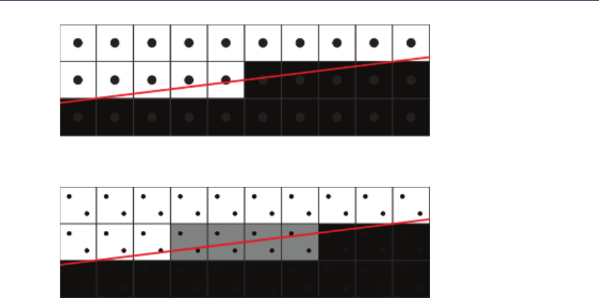
27.6. Temporal Super-Sampling 451
Figure 27.12.One sample centroid rasterization pattern.
Figure 27.13. Two rotated samples from a standard 2×MSAA pattern.
Taking all pros and cons into account, we decided to pursue the highest pos-
sible quality with k= 1. This means that we are only dealing with one frame of
history, and for every single frame we have two unique samples at our disposal
(assuming that our history sample was accepted as valid); we would like to get
as much data from them as possible.
27.6.2 Sampling Patterns
A single sample resolve can’t provide any gradients (see Figure 27.12 for a baseline
reference).
As discussed in Section 27.6.1, we want to maximize the resolve quality while
using only two unique samples. One possible way to achieve this is through a
more complex resolve and sampling pattern. Currently, common implementations
of 2×super-sampling use the 2×MSAA sampling pattern (see Figure 27.13).
One possible improvement upon this is to use a quincunx sampling pattern
[NVIDIA 01]. This pattern relies on sharing a noncentral sample with adjacent
pixels; thus, the resolve kernel needs to sample corner data from neighboring
pixels (see Figure 27.14).
In practice, quincunx sample positions are not very beneficial. Having sam-
pling points on regular pixel rows and columns minimizes the number of potential
edges that can be caught. In general, a good pattern should be optimized for
maximum pixel row and column coverage. The 4×rotated-grid pattern is a good
example (see Figure 27.15).
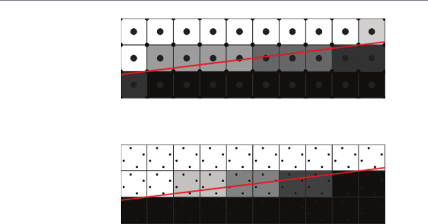
452 27. Hybrid Reconstruction Antialiasing
Figure 27.14. Quincunx sampling and resolve pattern guarantees higher-quality results
than 2×MSAA while still keeping the sample count at 2.
Figure 27.15. The 4×rotated-grid super-sampling pattern maximizes row and column
coverage.
27.6.3 FLIPQUAD
[Akenine-M¨oller 03] proposed several other low-sample-cost patterns such as FLIP-
TRI and FLIPQUAD. We will focus on FLIPQUAD as it perfectly matches our
goal of using just two unique samples. This sampling pattern is similar to quin-
cunx in its reuse of samples between pixels. However, a massive quality improve-
ment comes from putting sampling points on pixel edges in a fashion similar to
the rotated-grid sampling patterns. This provides unique rows and columns for
each sample, therefore guaranteeing the maximum possible quality.
The FLIPQUAD pattern requires a custom per-pixel resolve kernel as well as
custom per-pixel sampling positions (see Figure 27.16). An important observation
is that the pattern is mirrored, therefore every single pixel quad is actually the
same.
The article [Laine and Aila 06] introduced a unified metric for sampling pat-
tern evaluation and proved FLIPQUAD to be superior to quincunx, even sur-
passing the 4×rotated-grid pattern when dealing with geometric edges (see Fig-
ure 27.17 and Table 27.1).
We can clearly see that the resolve kernel is possible in a typical pixel shader.
However, the per-pixel sampling offsets within a quad were not supported in hard-
ware until modern AMD graphic cards exposed the EQAA rasterization pipeline
extensions. This feature is exposed on Xbox One and Playstation 4, as well as
through an OpenGL extension on PC [Alnasser 11].
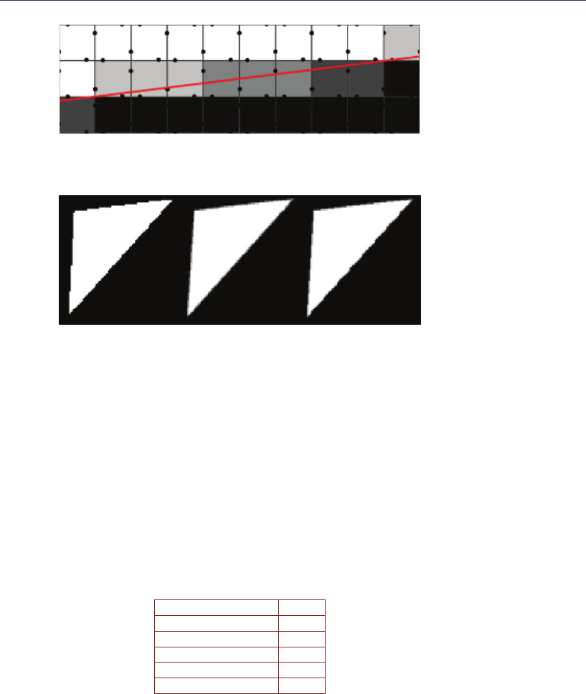
27.6. Temporal Super-Sampling 453
Figure 27.16. FLIPQUAD provides optimal usage of two samples matching quality of
4×rotated-grid resolve.
Figure 27.17. Left to right: single sample, FLIPQUAD, and quincunx. [Image courtesy
[Akenine 03].]
The implementation of the FLIPQUAD pattern is fairly straightforward using
2×MSAA. The snippets in Listings 27.4 and 27.5 give sampling positions for pixels
within a quad and the reconstruction kernel.
27.6.4 Temporal FLIPQUAD
In Section 27.6.3 we discussed implementing FLIPQUAD sampling and recon-
struction on modern hardware. However, in the context of temporal super-
sampling, we need to adapt our pattern and resolve kernel. We decided to split
the pattern into two subsets—one that will be used to render even frames (blue)
and one used on odd frames (red) (see Figure 27.18).
Pattern E
1×Centroid >1.0
2×2 Uniform Grid 0.698
2×2 Rotated Grid 0.439
Quincunx 0.518
FLIPQUAD 0.364
Table 27.1. Error metric (E) comparison against a 1024-sample reference image as
reported by [Laine and Aila 06] (lower is better).
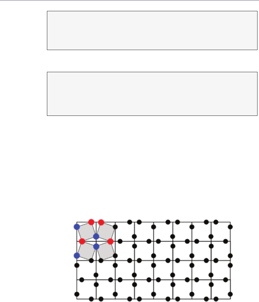
454 27. Hybrid Reconstruction Antialiasing
// In de xed [ S AMP LE S LO CA TI ONS ] i n n / 16 pix el o ff set s
in t2 gF Q_Q 00 [2] = { int 2 ( -8 , -2) , i nt2 ( 2 , -8) };
in t2 gF Q_Q 10 [2] = { int 2 ( -8 , 2) , i nt2 ( -2 , -8) };
in t2 gF Q_Q 01 [2] = { int 2 ( -8 , 2) , i nt2 ( -2 , -8) };
in t2 gF Q_Q 11 [2] = { int 2 ( -8 , -2) , i nt2 ( 2 , -8) };
Listing 27.4. FLIPQUAD sample array.
s0 = Cu rr en tFr am eMS . Sampl e ( Poi ntS ampler , UV , 0) ;
s1 = Cu rr en tFr am eMS . Sampl e ( Poi ntS ampler , UV , 1) ;
s2 = Cu rr en tFr am eMS . Sampl e ( Poi ntS ampler , int 2 ( 1, 0) , 0);
s3 = Cu rr en tFr am eMS . Sampl e ( Poi ntS ampler , int 2 ( 0, 1) , 1);
return 0. 25 * ( s 0 + s1 + s2 + s 3 ) ;}
Listing 27.5. FLIPQUAD reconstruction kernel.
To resolve this sampling scheme properly, we need two resolve kernels—one for
even and one for odd frames (see Listings 27.6 and 27.7). Due to the alternating
patterns, in each frame the kernel will be guaranteed to properly resolve horizontal
or vertical edges. If data from the previous frame is accepted, a full pattern will
be properly reconstructed.
It is worth noting that an incorrect (or missing) FLIPQUAD reconstruction
pass will result in jigsaw edges, which are a direct result of a nonuniform sampling
grid (see Figure 27.19).
1
1
0
0
2
1
3
2
3
3
2
0
Figure 27.18. Temporal FLIPQUAD pattern. Red samples are rendered on even frames.
Blue samples are rendered on odd frames.

27.6. Temporal Super-Sampling 455
// In de xed [ FRA ME ] [ SA MP LES LO CA TI ONS ] in n / 16 pix el o ffs et s
// BLU E RED
int2 gTempFQ_Q 0 [2] [1 ] = { int2 ( -8 , -2) , int2 ( 2 , -8) };
int 2 gT emp FQ _Q 1 [ 2][ 1] = { int 2 ( -8 , 2 ) , i nt2 ( -2 , -8) };
int 2 gT emp FQ _Q 2 [ 2][ 1] = { int 2 ( -8 , 2 ) , i nt2 ( -2 , -8) };
int2 gTempFQ_Q 3 [2] [1 ] = { int2 ( -8 , -2) , int2 ( 2 , -8) };
Listing 27.6. Temporal FLIPQUAD sample array.
# ifde fin ed ( ODD_ FRA ME ) // RED
// Ho ri zo ntal pa tt er n for fram e [1]
in t2 o ff se t0 = in t2 (0 , 1) ;
in t2 o ff se t1 = in t2 (1 , 0) ;
# els e if d efi ned ( EVE N_F RAM E ) // B LUE
in t2 o ff se t0 = in t2 (1 , 0) ;
in t2 o ff se t1 = in t2 (0 , 1) ;
# en dif
s0 = Cu rr ent Fr ame . Sampl e ( Poi ntS ampler , UV);
s1 = Cu rr ent Fr ame . Sampl e ( Poi ntS ampler , UV , of fse t0 ) ;
s2 = Pr ev ious Fra me . S amp le ( Linea rSa mpl er , prev iou sUV );
s3 = Pr ev ious Fra me . S amp le ( Linea rSa mpl er , p reviou sUV , off set 1 );
return 0 .25 * ( s 0 + s1 + s 2 + s 3 ) ;}
Listing 27.7. Temporal FLIPQUAD reconstruction kernel.
Rasterization should happen at sample locations in order to take full advan-
tage of FLIPQUAD. This can be easily achieved by using the sample prefix in
HLSL’s interpolator definition. This way, texture data will be offset properly,
resulting in a correctly super-sampled image.
Figure 27.19. Top to bottom: edge rasterized on an even frame and then an odd frame
and the final edge after temporal FLIPQUAD reconstruction kernel.

456 27. Hybrid Reconstruction Antialiasing
// Qua d def in ed as ( s amp le p osi ti ons wi thi n qua d )
// s00 s10
// s01 s11
DDX [ f ( s00 ) ] = [ f ( s00 ) - - f ( s10 ) ]/ dx , dx = | s0 0 - - s 10 |
DDY [ f ( s00 ) ] = [ f ( s00 ) - - f ( s01 ) ]/ dy , dy = | s0 0 - - s 01 |
// Ha rd wa re as su mes dx = dy = 1
// In ca se of s am pl in g patter n from L is ting 6. dx != dy
// Foo tpri nt - bas ed s amp lin g pi cks ba se mip l evel
// Ba sed on max ( ddx , ddy )
// Fr ame A ma x (ddx , d dy ) != Fr ame B ma x (ddx , d dy )
// Implies non te mporari ly cohe re nt mip se le ct io n
// Ca lcu lat ed in 1/16 th of pixe l
// Fr ame A ( B LUE )
dx = | -8 -- (16 + ( -8))| = 16
dy = | -2 -- (16 + ( 2) )| = 20
ba seMip ˜ max (dx , dy) = 20
// Fr ame B ( R ED )
dx = | 2 -- (16 + ( -2) )| = 12
dy = | -8 -- (16 + ( -8))| = 16
b ase Mi p ˜ max ( dx , dy ) = 16}
Listing 27.8. Default method for derivative calculation.
27.6.5 Temporal FLIPQUAD and Gradients
One side effect of using the temporal FLIPQUAD pattern is a nonuniform dis-
tance between samples within a quad. This causes problems for the gradient
calculation and mipmap selection. Graphics cards rely on calculating per-pixel
(or per-quad) derivatives using differentials within a quad. This process is fairly
straightforward (see Listing 27.8).
As an optimization, spatial distances, used to normalize the differential, are
assumed to be 1. However, if we look at our temporal FLIPQUAD pattern,
we clearly see that distances between samples are different between the x- and
y-axes, and we alternate from frame to frame (see Listing 27.8).
Nonuniform distances will result in a biased mipmap level-of-detail calcula-
tion, as ddx(uv) or ddy(uv) will be increasing faster than it should. In effect,
the textures will appear sharper or blurrier than they should be. In the worst
case, a single texture can select different mipmap levels, under the same viewing
direction, when rendering even and odd frames. This would lead to temporal in-
stability since bilinear filtering picks the mipmap based on max(ddx, ddy), which,
in this case, would result in differences between frames (see Figure 27.20).
One way to solve this issue would be to switch all texture samples to a
gradient-based texture read (i.e., tex2Dgrad in HLSL) and to calculate the gradi-
ents analytically taking sample distance into account. Unfortunately, this com-
plicates all shaders and can have significant performance overhead.
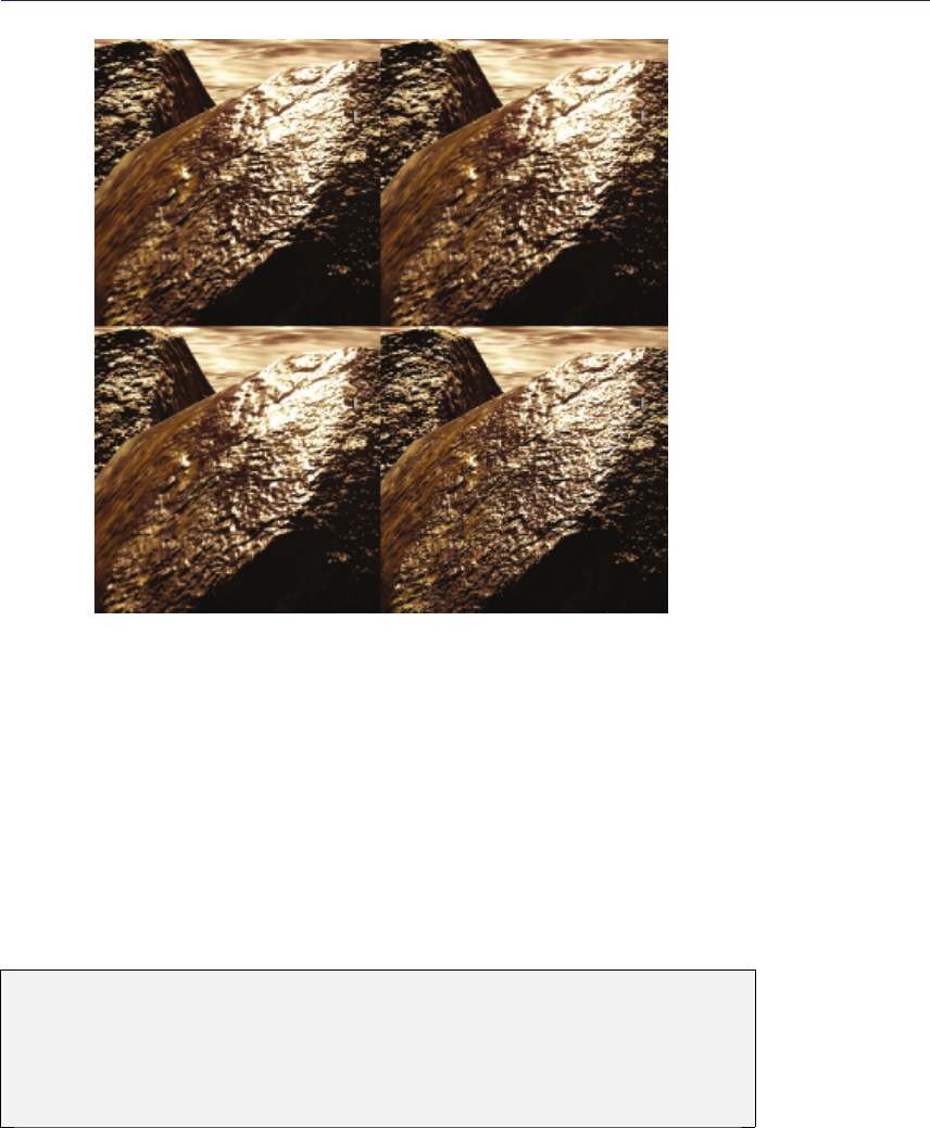
27.6. Temporal Super-Sampling 457
Figure 27.20. The top row shows even and odd frames of the reordered Temporal
FLIPQUAD pattern. The bottom row shows the default temporal FLIPQUAD pat-
tern clearly suffering from mipmap level mismatches. (The bottom right represents an
oversharpened odd frame.)
Another option is to change the pattern in order to minimize frame-to-frame
sample distance variance. While this will not provide correct results, the error
may not be noticeable in practice as long as it is temporarily stable (see Figure
27.20). Please note that this also requires different offsets (kernel and projec-
tion matrix offsets) to shift samples outside the pixel window (see Listings 27.9
and 27.10 for details).
// In de xed [ FRA ME ] [ SA MP LES L OCA TI ON S ] in n / 16 pix el o ffs et s
in t2 g T em pF Q_ Q0 [ 2] [1] = { in t2 ( 0 , -2) , i nt2 ( -2 , 0) };
int 2 gTempFQ _Q 1 [2][1 ] = { int2 ( 0 , 2) , in t2 ( 2, 0) };
int 2 gTempFQ _Q 2 [2][1 ] = { int2 ( 0 , 2) , in t2 ( 2, 0) };
in t2 g T em pF Q_ Q3 [ 2] [1] = { in t2 ( 0 , -2) , i nt2 ( -2 , 0) };
in t2 g P ro jM at Of f [2 ][ 1] = { i nt2 ( -8 , 0 ) , i nt2 ( 0 , 8 ) } ;}
Listing 27.9. Reordered temporal FLIPQUAD with additional projection matrix offsets.

458 27. Hybrid Reconstruction Antialiasing
# if de fin ed ( OD D_F RAM E ) // RED
// Ho ri zo ntal pa tt er n for fram e [1]
in t2 o ff set 0 = in t2 ( 0 , -1) ;
in t2 o ff set 1 = in t2 (1 , 0) ;
# els e if d efi ned ( E VEN_FR AME ) // BLUE
in t2 o ff set 0 = in t2 (1 , 0) ;
in t2 o ff set 1 = in t2 ( 0 , -1) ;
# en dif
s0 = Cu rr ent Fr ame . Sampl e ( Poi ntS ampler , UV);
s1 = Cu rr ent Fr ame . Sampl e ( Poi ntS ampler , UV , of fse t0 ) ;
s2 = Pr ev iou sF ram e . Sa mple ( L ine arS amp ler , pr evio usU V );
s3 = Pr ev iou sF ram e . Sa mple ( L ine arS amp ler , pre viousU V , offse t1 ) ;
return 0. 25 * ( s 0 + s1 + s2 + s 3 ) ;}
Listing 27.10. Reordered temporal FLIPQUAD reconstruction kernel.
27.6.6 History Sample Acceptance Method
Our acceptance method for history samples is based on the algorithm used in
Killzone: Shadow Fall [Valient 14].
The history sample from frame N−1 is valid only if
•the motion flow between frame Nand N−1 is coherent,
•the color flow between frames Nand N−2 is coherent. (Note that N−2
and Nhave the same subpixel jitter.)
The first constraint guarantees that a sample was not occluded and was moving
in a similar direction. The second constraint guarantees that there was no major
change in lighting conditions between frames with the same subpixel jitter. Both
tests use a 3 ×3 neighborhood using the sum of absolute differences to estimate
the degree of similarity between frames. It is possible to achieve reasonable
results using a smaller neighborhood, however, testing might need to be more
conservative.
If any constraint fails, then we fall back to clamping history samples to the
current frame color bounding box, as described in Section 27.7. This guarantees
no ghosting and enhanced temporal stability. It is worth noting that the color
flow constraint is very important in a real production environment. It enables
the unrestricted usage of animated textures and particle effects as well as lighting
changes. Another important benefit is that it grants convergence in the event that
the viewport becomes fixed.
27.6.7 Resampling
Any reprojection method is prone to numerical diffusion errors. When a frame
is reprojected using motion vectors and newly acquired sampling coordinates do

27.6. Temporal Super-Sampling 459
not land exactly on a pixel, a resampling scheme must be used. Typically, most
methods resort to simple bilinear sampling. However, bilinear sampling will result
in over-smoothing. If we would like to use a history buffer in order to accumulate
multiple samples, we will also accumulate resampling errors, which can lead to
serious image quality degradation (see Figure 27.22). Fortunately, this problem is
very similar to well-researched fluid simulation advection optimization problems.
In fluid simulation, the advection step is very similar to our problem of image
reprojection. A data field of certain quantities (i.e., pressure and temperature)
has to be advected forward in time by a motion field. In practice, both fields
are stored in discretized forms; thus, the advection step needs to use resampling.
Assuming that the operation is a linear transform, this situation is equal to the
problem of reprojection.
Under these circumstances, a typical semi-Lagrangian advection step would be
equal to reprojection using bilinear resampling. A well-known method to prevent
over-smoothing is to use second order methods for advection. There are several
known methods to optimize this process, assuming that the advection operator is
reversible. One of them is the MacCormack scheme and its derivation: back and
forth error compensation and correction (BFECC). This method enables one to
closely approximate the second order accuracy using only two semi-Lagrangian
steps [Dupont and Liu 03].
BFECC is very intuitive. In short, we advect the solution forward and back-
ward in time using advection operator Aand its reverse, AR. Operator error is
estimated by comparing the original value against the newly acquired one. The
original value is corrected by error (φn−φn
2) and finally advected forward into the
next step of the solution (see Algorithm 27.1 and Figure 27.21 for an illustration).
In the context of reprojection, our advection operator is simply a bilinear
sample using a motion vector offset. It is worth noting that the function described
by the motion vector texture is not reversible (i.e., multiple pixels might move to
same discretized position).
A correct way to acquire a reversible motion vector offset would be through a
depth-buffer–based reprojection using an inverse camera matrix. Unfortunately,
this would limit the operator to pixels subject to camera motion only. Also, the
operator would be invalid on pixels that were occluded during the previous time
step.
1: φn+1 =A(φn).
2: φn=AR(φn+1).
3: ¯φ=φn+φn−φn
2.
4: φn+1 =A( ¯φ).
Algorithm 27.1. Original BFECC method.

460 27. Hybrid Reconstruction Antialiasing
1: φn+1 =A(φn).
2: φn=AR(.φn+1).
3: φn+1 =φn+1 +φn−φn
2.
Algorithm 27.2. Simplified BFECC method.
Another option is to assume a high-coherency motion vector field (texture)
and just use a negative motion vector for the reverse operator. However, this
approach would break under perspective correction (i.e., high slopes) as well as
with complex motion.
In practice, we used a mix of both approaches. The reverse operator is ac-
quired through depth-based reprojection for static pixels and reversing motion
vectors for pixels from dynamic objects. For us, this proved to be both efficient
and visually plausible (even if not always mathematically correct).
Another important optimization we used was inspired by the simplified BFECC
method by [Selle et al. 08]. In this approach, it is proven that the error is not
time dependent; therefore the results from frame n+ 1 can be directly com-
pensated by an error estimate. This simplifies the original BFECC by one full
semi-Lagrangian (see Algorithm 27.2).
Unfortunately, the proposed method requires reading φn,φn, and φn+1 in
order to evaluate φn+1. However, as we already assumed that the error estimate
is time invariant, we can as use the values from step n+ 1 to estimate the error.
Therefore, we can calculate φn+1 using only φn+1 and
φn+1, where
φn+1 is easy
to acquire in a shader (see Algorithm 27.3,Listing 27.11, and Figure 27.21 for
details).
One last thing worth mentioning is that BFECC, by default, is not uncon-
ditionally stable. There are multiple ways of dealing with this problem, but we
found bounding by local minima and maxima to be the most practical [Dupont
and Liu 03,Selle et al. 08]. Listing 27.11 presents the simplest implementation
of our optimized BFECC, and Figure 27.22 demonstrates the results.
1: φn+1 =A(φn).
2: φn=AR(φn+1).
3:
φ
n+1 =A(φn).
4: φn+1 =φn+1 +φn+1 −
φ
n+1
2.
Algorithm 27.3. Shader optimized simplified BFECC method.

27.7. Temporal Antialiasing (TAA) 461
// Pass outputs ph iH atN 1T extur e
// A ( ) o pe ra to r us es m oti on v ec to r te xt ur e
voi d GetPhiHatN1(float2 inUV , int2 i nVP OS )
{
float2 mo ti on Ve cto r = M ot io nV ect or sT . Loa d ( int3( i nVP OS , 0) ) . xy ;
float2 fo rwa rdProj = i nUV + m oti onV ecto r ;
// P erf or m a dv ec ti on by o pe ra to r A ()
return P rev io us Fr am eT . Sa mp le Le ve l ( Line ar , f or war dPr oj , 0) . rgb ;
}
// Pass outputs p hiH at Te xture
// AR () operator uses ne ga ti ve v alue fro m motio n ve ctor text ur e
// ph iH at N1 te xt ure is ge ne ra te d by pr ev io us pas s GetPh iH at N1 ()
voi d Ge tPhiHa tN ( float2 inUV , int2 inVPO S )
{
float2 mo ti on Ve cto r = M ot io nV ect or sT . Loa d ( int3( i nVP OS , 0) ) . xy ;
float2 backwardProj = inUV - motionVector;
// Pe rfo rm r eve rse ad ve cti on by op erator AR ()
return ph iH at N1T . S amp le Le ve l ( Line ar , ba ckw ard Pro j , 0) . rgb ;
}
// Fi nal opera ti on to get cor re ct ly re sampled p hiN1
// A ( ) o pe ra to r us es m oti on v ec to r te xt ur e
// phiHatN1 and phi Ha tN te xt ur es are ge ne ra te d by previ ou s pass es
voi d GetResampledValueBFECC(float2 inUV , int 2 inV POS )
{
float3 ph iH atN 1 = ph iH atN 1T . L oad ( int3( inVP OS , 0) ) . rgb ;
// Find local mini ma and ma xi ma
float3 minima , ma xim a ;
Ge tL imi ts RGB ( ph iHa tN1 Tex tur e , inUV , mi nima , ma xim a );
float2 mo ti onVec to r = Mo tio nV ec tors . L oad (int3( inV POS , 0 ) ). xy ;
float2 A = inUV + m otion Ve ct or ;
// P erf or m a dv ec ti on by o pe ra to r A ()
float3 p hi Ha tH at N1 = ph iH atT . S am pl eL ev el ( Line ar , A , 0) . rgb ;
// Pe rf orm BF ECC
float3 phiN1 = 1.5 * phiHatN1 - 0.5 * ph iHatHat N1 ;
// Limit the re su lt to mini ma and ma xi ma
phiN1 = cl amp ( ph iN1 , m inima , m ax im a );
return ph iN1 ;
}
Listing 27.11. Reordered temporal FLIPQUAD reconstruction kernel.
27.7 Temporal Antialiasing (TAA)
27.7.1 Overview
In Sections 27.5 and 27.6, we presented methods for improving spatial and tem-
poral stability and resolution of antialiased images. However, even when using
4×rotated-grid super-sampling and dedicated edge antialiasing, disturbing tem-
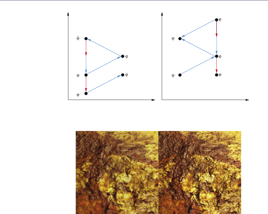
462 27. Hybrid Reconstruction Antialiasing
2
1
3
n
n
n
–
n + 1
ˆ
n + 1
34
2
1
3
n
ˆ
n
n + 1
ˆ
n + 1
ˆ
ˆ
n + 1
3
Figure 27.21. Conceptual scheme of the original BFCE method (left) and of the shader
optimized BFCE used for texture resampling (right).
Figure 27.22. Continuous resampling of 30 frames using a history buffer. The camera is
in motion, panning from left to right. Using bilinear sampling shows numerical diffusion
errors resulting in a blurry image (left). Using optimized linear BFCE helps to minimizes
blurring (right).
poral artifacts may occur. Ideally we would like to accumulate more frames
over time to further improve image quality. Unfortunately, as described in Sec-
tions 27.6.1 and 27.6.6, it is very hard to provide a robust method that will work
in real-world situations, while also using multiple history samples, without other
artifacts. Therefore, several methods rely on super-sampling only in certain local
contrast regions of an image [Malan 12,Sousa 13,Valient 14]. These approaches
rely on visually plausible temporal stabilization (rather than super-sampling).
We would like to build upon these approaches to further improve our results.
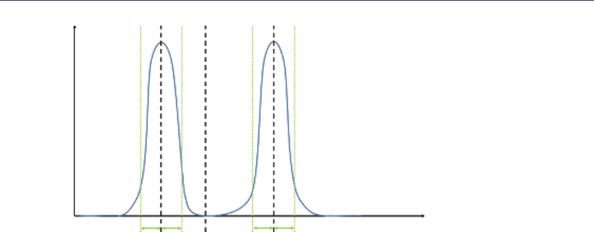
27.7. Temporal Antialiasing (TAA) 463
Min
Max
Mean
δ δ δ δ Value
Acceptance
Figure 27.23. Frequency-based acceptance function plot.
27.7.2 Frequency-Based Acceptance Metric
A simple temporal antialiasing scheme can be described as a cumulative blend
between the current frame and an accumulation buffer of previous frames (history
data). However, finding the correct blend factor is difficult. We would like to
stabilize the data such that we avoid fluctuations over time and enhance the
image quality by accumulating new information. On the other hand, we need to
detect when data becomes stale or invalid.
We build a color bounding box of fresh data by sampling the 3 ×3 spatial
neighborhood from the current frame. From this data we evaluate the local
minima, maxima, and mean value per RGB channel.
We follow a reasoning grounded in signal frequency analysis. If our history
data is too similar to the local mean, it does not bring much new information
to the current frame and might even diffuse the result if it contains accumulated
errors (i.e., due to sampling errors). The more “different” the data is from mean,
the more important it is. However, certain information might just be a fluctuation
that skews the data. With all of this in mind, we can treat information that is in
close proximity to fresh data’s local minima and maxima as valid (to a degree).
Therefore, we could plot our function of history data acceptance as two peaks
centered at a local minima and maxima, with a slope curve steered by a user
controlled δvalue (see Figure 27.23).
To reduce incorrectly accepted samples even further, we utilize motion-based
constraints as described in Section 27.6.6. This combination method minimizes
the possible reprojection artifacts to a 3 ×3 pixel neighborhood (i.e., ghosting)
while still guaranteeing a very high level of temporal stabilization. It’s worth not-
ing that this method can’t provide convergence in the context of super-sampling
(or jittered rendering), as sample acceptance relies on local data changes. See
Listing 27.12 for details.

464 27. Hybrid Reconstruction Antialiasing
// curMin , curMax , cu rMean are e st im at ed from 3 x3 neig hb or hood
float3 getTAA(float2 inC urtMotionVe c ,
float2 in Pr evMotionVec ,
float3 inCur tMean ,
float3 inCurtMin ,
float3 inCurtMax ,
float3 in CurtV alue ,
float3 in Pre vValue )
{
// Mo tion c oh erency we ight
float mot ion Delt a = len gth ( in CurM oti on Vec - i nPr ev Moti onVe c );
float mot ion Co here nce = sa tur ate ( c _mot ion Sens * mo tio nDe lt a ));
// Ca lc ul at e colo r wi nd ow r ange
float3 range = inCutMi n - in Cur Max ;
// Of fset the wi ndow b ounds by del ta pe rc en ta ge
float3 ex tO ffs et = c _d el ta Co lo rW indo wO ff set * ra nge ;
float3 e xt B ox Mi n = ma x ( i n Cu rM in - e x tO f fs et . r gb , 0 .0 );
float3 ex tdBoxMax = in CurMax + extOf fs et ;
// Ca lc ul at e d eltas be tw ee n previous and c urrent c olo r wind ow
float3 va lDi ff = saturate ( extBoxMin - inP rev Val ue );
va lDi ff += saturate ( i nPr ev iou sV alu e - extBoxMax );
float3 clampedPrevVal = c lamp ( i nPr evValu e , ext BoxM in , ex tB oxM ax );
// Ca lc ul at e d eltas for c ur rent p ixel agains t p re vi ou s
float3 m ean We ig ht = ab s ( in Cu rV alu e - i nP reV al ue );
float l oCo ntrast = l ength ( meanWeigh t )* c_lo Wei ght ;
float h iCon tra st = l eng th ( va lDi ff ) * c_h iWe igh t ;
// Ca lc ul at e fina l weig ht s
float d enom = max (( l oCo ntr ast - hiContr ast ) , 0. 0);
float f in al We ig ht = s at ur ate ( rcp ( d eno m + ep sil on ));
// Check blend we ight a ga in st mi nimum bo und
// Pr ev en ts the algorithm f rom st al li ng
// in a ’ sa dd le ’ d ue to nu me ri ca l i mp re ci si on
// Regulates minimum blend of c ur re nt d ata
f in al We ig ht = m ax ( c _ min Li mit er , w );
// Co rr ect previous sa mp le s a cc or di ng to mot ion coherency we ights
fi nalW eig ht = s atu rat e ( fina lWe ight - mo tio nC ohe re nce );
// Final value blend
return le rp ( inC urV alu e , cl amp edP rev Va l , fi na lWe ig ht );
}
Listing 27.12. Temporal antialiasing using our frequency-based acceptance metric.
27.8 Final Implementation
Our final framework’s implementation can be split into two main stages:
•temporally stable edge antialiasing, which includes
◦SMAA,
27.9. Results Discussion 465
Frame N Temporarily Stable
Edge Anti-aliasing
FLIPQUAD
Reconstruction
& Temporal
Anti-aliasing
Frame N-1 Stable Super-
sampled Frame
Frame N-2
Accumulation
History Buer
Figure 27.24. Data flow graph in our implementation of the HRAA pipeline.
◦CRAA,
◦AEAA (GBAA);
•Temporal FLIPQUAD reconstruction combined with temporal antialiasing
(TAA) (see Listing 27.13).
Figure 27.24 illustrates the data flow inside the framework.
During production, we implemented and optimized all three approaches to
temporarily stable edge antialiasing.
SMAA was implemented with geometric edge detection based on depth and
normal buffers. Edges were refined by a predicated threshold based on the lumi-
nescence contrast. Our edge-detection algorithm choice was dictated by making
the resolve as temporally stable as possible.
CRAA and AEAA used the implementations described in Sections 27.5.1 and
27.5.2. Our EQAA setup used a 1F8S configuration, while our AEAA offset buffer
was compressed down to 5 bits (utilizing the last remaining space in our tightly
packed G-buffer).
The results of either edge antialiasing pass were used as N,N−1, and N−2
frame sources in the last pass. The history buffer used by TAA at frame Nwas
the output buffer of TAA from frame N−1.
27.9 Results Discussion
Our packing/performance scheme resulted in fairly low-quality gradients coming
out of edge antialiasing (only 3 bits for steps). However, FLIPQUAD reconstruc-
tion provided two to four times the edge gradients virtually for free. In prac-
tice, the whole system provided excellent results, matching a 4×rotated-grid
super-sampled reference while providing much higher-quality edge antialiasing
and temporal stability at minimal cost.

466 27. Hybrid Reconstruction Antialiasing
// Un op timized pseudoc od e for f inal
// T em po ra l F LI PQ UAD r ec on str uc tion & TAA
// Fr ame s N & N -2 are a ssume d
// To ha ve sa me j itter of fs et s
float3 getFLIPQUADTaa()
{
float3 cur Min , currMax , c urM ean ;
Get Lim its ( cu rre ntV alue Tex tur e , curMin , curMax , cu rMe an );
float3 pr evVal = R esa mple ( pr evV alue Tex ture ) ;
float3 prevPre vV al = Resample ( prev Prev Va lueT ext ure );
// Get sums of a bs ol ut e d ifference
float3 curSAD = GetS AD ( cu rVa lueT ext ure );
float3 pr ev Pre vSAD = G etS AD ( p rev Pr ev Valu eT ext ur e );
// Motion c oh er en cy we ight
float moCoh ere nce = Get Moti onCo here ncy ( cu rMo tio nTe xtu re ,
pre vMot ion Text ure );
// Color co herency w ei ght
float c ol Co he re nc e = G et Co lo rC oh er en cy ( c urSAD , p re vP re vS AD ) ;
// FL IP QU AD parts
float3 FQ Cur Par t = Ge tCur FLI PQUA D ( cur Valu eTe xtur e );
float3 FQ PrevPart = Ge tP revFLI PQU AD ( pre vVa lueT ext ure );
float F QC oherenc y = mo tionC oh ere nc e + color Co heren ce ;
float3 clampFQ Pr ev = cl amp ( F QPre vPa rt , curM in , cur Max ) ;
// This le rp a llows full c on ve rganc e
// If c olo r f low (N -2 to N ) is c ohe ren t
FQ Pr evP ar t = ler p ( FQP revP art , cl ampF QPr ev , co lCo he re nc e );
// Final rec on st ruc ti on blend
float3 FL IP QUA D = ler p ( FQCu rPa rt , FQP rev Par t ,0 .5* mo Co he ren ce ) ;
float3 hi storyVal = Res amp le ( hi storyV alue Te xtur e );
return ge tTA A ( cur Mot ionText ure , p rev Mot ion Texture ,
curMin , curMax , c urMean ,
FLI PQUAD , hi sto ryVal )
}
Listing 27.13. Pseudocode for the combined temporal FLIPQUAD reconstruction and
temporal antialiasing.
While temporal FLIPQUAD and TAA remained stable and reliable compo-
nents of the framework, the choice of the edge antialiasing solution proved to be
problematic.
SMAA provided the most visually plausible results on static pixels under any
circumstances. The gradients were always smooth and no edge was left without
antialiasing. Unfortunately, it sometimes produced distracting gradient wobble
while in motion. The wobble was partially mitigated by the FLIPQUAD and
TAA resolves. Unfortunately, SMAA had the highest runtime cost out of the
whole framework.

27.10. Conclusion 467
AEAA provided excellent stability and quality, even in close-ups where tri-
angles are very large on screen. Unfortunately, objects with very high levels
of tessellation resulted in very objectionable visual noise or even a total loss of
antialiasing on some edges. Even though this was the fastest method for edge
antialiasing, it proved too unreliable for our open world game. It is worth noting
that our AEAA implementation required us to modify every single shader that
writes out to the G-buffer. This might be prohibitively expensive in terms of
developer maintainability and runtime performance.
CRAA mitigated most of the issues seen with AEAA and was also the easiest
technique to implement. Unfortunately, on the current generation of hardware,
there is a measurable cost for using even a simple EQAA setup and the cost scales
with the number of rendered triangles and their shader complexity. However,
in our scenario, it was still faster than SMAA alone. Even though we were
able to solve multiple issues, we still found some finely tessellated content that
was problematic with this technique and resulted in noisy artifacts on edges.
These artifacts could be effectively filtered by temporal FLIPQUAD and TAA.
Unfortunately the cost of outputting coverage data from pixel shaders was too
high for our vegetation-heavy scenarios. We did not experiment with manual
coverage output (i.e., not hardware based).
At the time of writing, we have decided to focus on two main approaches for
our game: SMAA with AEAA used for alpha-tested geometry or CRAA with
AEAA used for alpha-tested geometry. SMAA with AEAA is the most expensive
and most reliable while also providing the lowest temporal stability. CRAA with
AEAA provides excellent stability and performance with medium quality and
medium reliability. The use of AEAA for alpha-tested objects seems to provide
the highest quality, performance, and stability in both use cases; therefore, we in-
tegrated its resolve filter into the SMAA and CRAA resolves. See the performance
and image quality comparisons of the full HRAA framework in Figure 27.25 and
Table 27.2.
27.10 Conclusion
We provided a production proven hybrid reconstruction antialiasing framework
along with several new algorithms, as well as modern implementations of well-
known algorithms. We believe that the temporal FLIPQUAD super-sampling
as well as temporal antialiasing will gain wider adoption due to their low cost,
simplicity, and quality. Our improvements to distance-to-edge–based methods
might prove useful for some projects. Meanwhile, CRAA is another addition to
the temporally stable antialiasing toolbox. Considering its simplicity of imple-
mentation and its good performance, we believe that with additional research it
might prove to be a viable, widely adopted edge antialiasing solution. We hope
that the ideas presented here will inspire other researchers and developers and
provide readers with valuable tools for achieving greater image quality in their
projects.
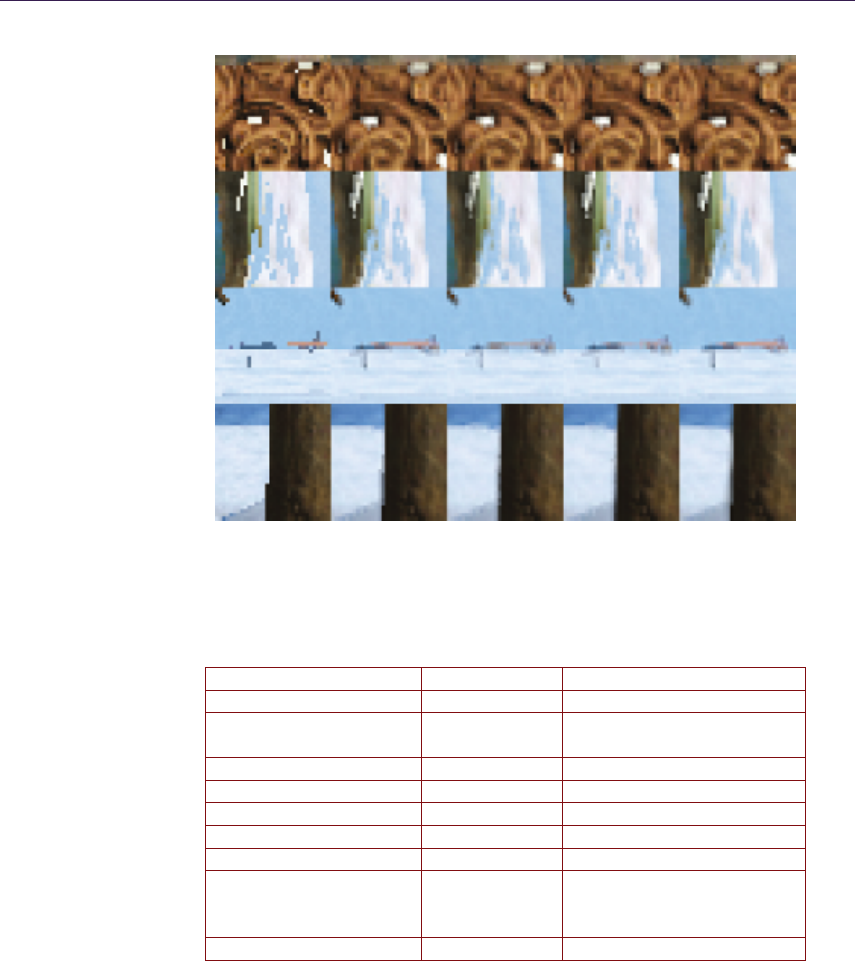
468 27. Hybrid Reconstruction Antialiasing
Figure 27.25. Comparison of different HRAA setups showing different scenarios based
on actual game content. From left to right: centroid sampling (no antialiasing), temporal
FLIPQUAD (TFQ), AEAA + TFQ, CRAA + TFQ, and SMAA + TFQ.
Single Pass Timing (ms) G-Buffer Overhead (%)
BFECC single value 0.3 N/A
Temporal FLIPQUAD
(TFQ)
0.2 N/A
AEAA 0.25 <1% C
8×CRAA 0.25 <8% HW/C
SMAA 0.9 N/A
TAA 0.6 N/A
TFQ + TAA 0.62 N/A
AEAA(alpha test) +
8×CRAA + TFQ +
TAA
0.9 <3% HW/C
SMAA + TFQ + TAA 1.4 N/A
Table 27.2. Different HRAA passes and timings measured on an AMD Radeon HD 7950
at 1080p resolution, operating on 32-bit image buffers. “C” means content dependent
and “HW” means hardware type or setup dependent.

Bibliography 469
Bibliography
[Akenine-M¨oller 03] T. Akenine-M¨oller. “An Extremely Inexpensive Multisam-
pling Scheme.” Technical Report No. 03-14, Ericsson Mobile Platforms AB,
2003.
[AMD 11] AMD Developer Relations. “EQAA Modes for AMD 6900 Se-
ries Graphics Cards.” http://developer.amd.com/wordpress/media/2012/10/
EQAAModesforAMDHD6900SeriesCards.pdf, 2011.
[Alnasser 11] M. Alnasser, G. Sellers, and N. Haemel. “AMD Sample Positions.”
OpenGL Extension Registry,https://www.opengl.org/registry/specs/AMD/
sample positions.txt, 2011.
[Bavoil and Andersson 12] L. Bavoil and J. Andersson. “Stable SSAO in Bat-
tlefield 3 with Selective Temporal Filtering.” Game Developer Conference
Course, San Francisco, CA, March 5–9, 2012.
[Burley 07] B. Burley. “Filtering in PRMan.” Renderman Repository,
https://web.archive.org/web/20130915064937/http:/www.renderman.
org/RMR/st/PRMan Filtering/Filtering In PRMan.html, 2007. (Original
URL no longer available.)
[Drobot 11] M. Drobot. “A Spatial and Temporal Coherence Framework for Real-
Time Graphics.” In Game Engine Gems 2, edited by Eric Lengyel, pp. 97–
118. Boca Raton, FL: CRC Press, 2011.
[Drobot 14] M. Drobot. “Low Level Optimizations for AMD GCN Architecture.”
Presented at Digital Dragons Conference, Krak`ow, Poland, May 8–9, 2014.
[Dupont and Liu 03] T. Dupont and Y. Liu. “Back and Forth Error Compen-
sation and Correction Methods for Removing Errors Induced by Uneven
Gradients of the Level Set Function.” J. Comput. Phys. 190:1 (2003), 311–
324.
[Jimenez et al. 11] J. Jimenez, B. Masia, J. Echevarria, F. Navarro, and D.
Gutierrez. “Practical Morphological Antialiasing.” In GPU Pro 2: Advanced
Rendering Techniques, edited by Wolfgang Engel, pp. 95–114. Natick, MA:
A K Peters, 2011.
[Jimenez et al. 12] J. Jimenez, J. Echevarria, D. Gutierrez, and T. Sousa.
“SMAA: Enhanced Subpixel Morphological Antialiasing.” Computer Graph-
ics Forum: Proc. EUROGRAPHICS 2012 31:2 (2012), 355–364.
[Kirkland et al. 99] Dale Kirkland, Bill Armstrong, Michael Gold, Jon Leech, and
Paula Womack. “ARB Multisample.” OpenGL Extension Registry,https://
www.opengl.org/registry/specs/ARB/multisample.txt, 1999.

470 27. Hybrid Reconstruction Antialiasing
[Laine and Aila 06] S. Laine and T. Aila. “A Weighted Error Metric and Opti-
mization Method for Antialiasing Patterns.” Computer Graphics Forum 25:1
(2006), 83–94.
[Lottes 09] T. Lottes. “FXAA.” NVIDIA white paper, 2009.
[Malan 10] H. Malan. “Edge Anti-aliasing by Post-Processing.” In GPU Pro: Ad-
vanced Rendering Techniques, edited by Wolfgang Engel, pp. 265–290. Nat-
ick, MA: A K Peters, 2010.
[Malan 12] H. Malan. “Realtime global illumination and reflections in Dust 514.”
Advances in Real-Time Rendering in Games: Part 1, SIGGRAPH Course,
Los Angeles, CA, August 5–9, 2012.
[NVIDIA 01] NVIDIA Corporation. “HRAA: High-Resolution Antialiasing
Through Multisampling”. Technical report, 2001.
[Nehab et al. 07] D. Nehab, P. V. Sander, J. Lawrence, N. Tararchuk, and J.
R. Isidoro. “Accelerating Real-Time Shading with Reverse Reprojection
Caching.” In Proceedings of the 22nd ACM SIGGRAPH/EUROGRAPHICS
Symposium on Graphics Hardware, edited by Dieter Fellner and Stephen
Spencer, pp. 25–35. Aire-la-Ville, Switzerland: Eurographics Association,
2007.
[Persson 11] E. Persson. “Geometric Buffer Antialiasing.” Presented at SIG-
GRAPH, Vancouver, Canada, August 7–11, 2011.
[Reshetov 09] A. Reshetov. “Morphological Antialiasing.” In Proceedings of the
Conference on High Performance Graphics, edited by S. N. Spencer, David
McAllister, Matt Pharr, and Ingo Wald, pp. 109–116. New York: ACM,
2009.
[Selle et al. 08] A. Selle, R. Fedkiw, B. Kim, Y. Liu, and J. Rossignac. “An Un-
conditionally Stable MacCormack Method.” J. Scientific Computing 35:2–3
(2008), 350–371.
[Sousa 11] T. Sousa. “Anti-aliasing Methods in CryENGINE3.” Presented at SIG-
GRAPH 2011, Vancouver, Canada, August 7–11, 2011.
[Sousa 13] T. Sousa T. “CryENGINE 3 Graphics Gems.” Presented at SIG-
GRAPH 2013, Anaheim, CA, July 21–25, 2013.
[Valient 14] M. Valient. “Taking Killzone Shadow Fall Image Quality into the
Next Generation.” Presented at Game Developers Conference, San Francisco,
CA, March 17–21, 2014.

28
Real-Time Rendering of
Physically Based Clouds Using
Precomputed Scattering
Egor Yusov
28.1 Introduction
Rendering realistic clouds has always been a desired feature for a variety of appli-
cations, from computer games to flight simulators. Clouds consist of innumerable
tiny water droplets that scatter light. Rendering clouds is challenging because
photons are typically scattered multiple times before they leave the cloud. De-
spite the impressive performance of today’s GPUs, accurately modeling multiple
scattering effects is prohibitively expensive, even for offline renderers. Thus, real-
time methods rely on greatly simplified models.
Using camera-facing billboards is probably the most common real-time method
[Dobashi et al. 00,Wang 04,Harris and Lastra 01,Harris 03]. However, bill-
boards are flat, which breaks the volumetric experience under certain conditions.
These methods have other limitations: lighting is precomputed resulting in static
clouds [Harris and Lastra 01], multiple scattering is ignored [Dobashi et al. 00],
or lighting is not physically based and requires tweaking by artists [Wang 04].
Volume rendering techniques are another approach to render clouds [Schpok
et al. 03,Miyazaki et al. 04,Riley et al. 04]. To avoid aliasing artifacts, many
slices usually need to be rendered, which can create a bottleneck, especially
on high-resolution displays. More physically accurate methods exist [Bouthors
et al. 06,Bouthors et al. 08], which generate plausible visual results, but are
difficult to reproduce and computationally expensive.
We present a new physically based method to efficiently render realistic ani-
mated clouds. The clouds are comprised of scaled and rotated copies of a single
particle called the reference particle. During the preprocessing stage, we precom-
pute optical depth as well as single and multiple scattering integrals describing
473

474 28. Real-Time Rendering of Physically Based Clouds Using Precomputed Scattering
the light transport in the reference particle for all possible camera positions and
view directions and store the results in lookup tables. At runtime, we load the
data from the lookup tables to approximate the light transport in the cloud in
order to avoid costly ray marching or slicing. In this chapter, we elaborate upon
our previous work [Yusov 14b]. In particular, the following improvements have
been implemented:
•a better real-time shading model based on precomputed lookup tables,
•an improved method to calculate light attenuation in the body of the cloud
using a 3D grid,
•a new particle generation algorithm,
•performance optimization, including GPU-based particle sorting.
We briefly review the main concepts of this method, but we will concentrate on
implementation details and improvements. Additional information can be found
in the original paper [Yusov 14b].
28.2 Light Transport Theory
Now we will briefly introduce the main concepts of the light transport in a partic-
ipating medium. More information can be found in [Riley et al. 04,Bouthors 08].
There are three phenomena that can be found in a participating medium: scatter-
ing, absorption, and emission. Scattering only changes the direction of a photon
traveling through the medium. Absorption eliminates the photon by transform-
ing its energy into other forms, while emission does the opposite. The intensity
of these processes is described by scattering, absorption, and emission coeffi-
cients βSc,βAb, and βEm, respectively. Absorption and scattering both reduce
the intensity of light traveling through the medium. The extinction coefficient
βEx =βAb +βSc describes the net attenuation. In the cloud body, emission and
absorption are negligible: βEm =βAb = 0. As a result, both scattering and
extinction can be described by the same coefficient: βSc =βEx =β.
The intensity of light traveling from point Ato point Binside the cloud is
reduced by a factor of e−τ(A,B).τ(A,B), called optical depth, is the integral of
the extinction coefficient over the path from Ato B:
τ(A,B) = B
A
β(P)·ds, (28.1)
where P=A+B−A
||B−A|| ·sis the current integration point.
To determine the intensity of single scattered light, we need to step along
the view ray and accumulate all the differential amounts of sunlight scattered at
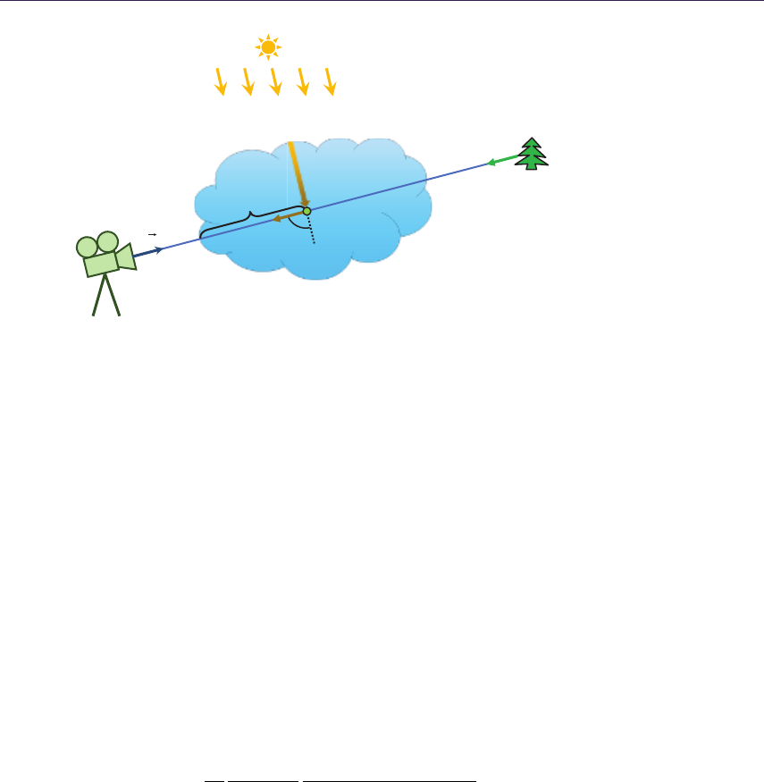
28.2. Light Transport Theory 475
Lsum
Q
P1
P0
C
v
P
θ
S
LB
Figure 28.1. Single scattering.
every point toward the camera:
L(1)
In (C, ⃗v) = P1
P0
β(P)·LSun ·e−τ(Q,P)·e−τ(P,P0)·P(θ)·ds. (28.2)
In this equation, Cis the camera position and ⃗v is the view direction. P0and
P1are the points where the view ray enters and leaves the cloud body, LSun is
the intensity of sunlight outside the cloud, and Qis the point through which the
sunlight reaches the current integration point P(Figure 28.1). P(θ) is the phase
function that defines how much energy is scattered from the incident direction
to the outgoing direction, with θbeing the angle between the two. Note that
the sunlight is attenuated twice before it reaches the camera: by the factor of
e−τ(Q,P)on the way from the entry point Qto the scattering point P, and by
the factor of e−τ(P,P0)on the way from the scattering point to the camera.
The phase function for cloud droplets is very complex [Bohren and Huff-
man 98]. In real-time methods, it is common to approximate it using the Cornette-
Shanks function [Cornette and Shanks 92]:
P(θ)≈1
4π
3(1 −g2)
2(2 + g2)
(1 + cos2(θ))
(1 + g2−2gcos(θ))3/2. (28.3)
Using the intensity L(1)
In of single scattering, we can compute secondary scat-
tering L(2)
In , then third-order scattering L(3)
In , and so on. The nth-order scattering
intensity measured at point Cwhen viewing in direction ⃗v is given by the follow-
ing integral:
L(n)
In (C, ⃗v) = P1
P0
J(n)(P, ⃗v)·e−τ(P,P0)·ds. (28.4)
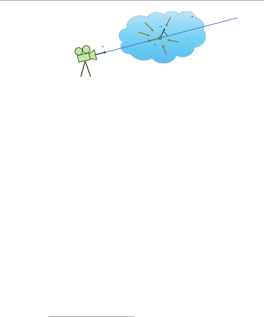
476 28. Real-Time Rendering of Physically Based Clouds Using Precomputed Scattering
(P, ω)
C
v
LIn
(n–1)
(P, v)J(n)
ωθ
Figure 28.2. Multiple scattering.
In Equation (28.4), J(n)(C, ⃗v) is the net intensity of order n−1 light L(n−1)
In (C, ⃗v)
that is scattered in the view direction:
J(n)(P, ⃗v) = β(P)·Ω
L(n−1)
In (P, ⃗ω)·P(θ)·dω, (28.5)
where integration is performed over the whole sphere of directions Ω, and θis the
angle between ⃗ω and ⃗v (see Figure 28.2).1
The total in-scattering intensity is found by calculating the sum of all scat-
tering orders:
LIn(C, ⃗v) =
∞
n=1
L(n)
In (C, ⃗v). (28.6)
The final radiance measured at the camera is the sum of in-scattered intensity
and background radiance LB(see Figure 28.1) attenuated in the cloud:
L(C, ⃗v) = LIn(C, ⃗v) + e−τ(P0,P1)·LB. (28.7)
28.3 Precomputed Solutions
Equations (28.1)–(28.7) are very complex and cannot be solved at runtime. Our
solution to this problem is to model the light transport in a reference volumetric
particle at preprocess time and to solve all the equations for that particle. We
store the resulting information in lookup tables and use it at runtime to compute
shading.
28.3.1 Optical Depth
Consider some inhomogeneous volumetric particle with known density distribu-
tion (Figure 28.3 (left)). Our goal is to precompute the optical depth integral in
1Strictly speaking, θis the angle between the incident direction −⃗ω and the outgoing direc-
tion −⃗v, which is the same.
28.3. Precomputed Solutions 477
θv
θs
v
vS
S
Figure 28.3. Volumetric particle (left) and 4D parameterization (middle and right).
Equation (28.1) through the particle for every camera position and view direc-
tion. To describe every ray piercing the particle, we need 4D parameterization.2
The first two parameters are the azimuth φS∈[0,2π] and zenith θS∈[0, π]
angles of the point Swhere the view ray enters the particle’s bounding sphere
(Figure 28.3 (middle)). The other two parameters are the azimuth φv∈[0,2π]
and zenith θv∈[0, π/2] angles of the view ray in the tangent frame constructed
at the entry point S(Figure 28.3 (right)). The z-axis of this frame is pointing
toward the sphere center. Note that we only need to consider the rays going
inside the sphere; thus, the maximum value for θvis π/2.
To precompute the optical depth integral, we go through all possible values
of φS,θS,φv, and θvand numerically evaluate the integral in Equation (28.1).
Section 28.5.1 provides additional details.
28.3.2 Single Scattering
In contrast to optical depth, we cannot precompute scattering inside the inho-
mogeneous particle. The reason for this is that we also need to account for the
light direction, and this would require five parameters, which is impractical. So
we precompute scattering in a homogeneous spherical particle. We assume that
the light is shining in the positive zdirection. Due to the symmetry of the prob-
lem, the light field is symmetrical with respect to the light direction, so the φS
parameter can be dropped. On the other hand, to compute Equation (28.5), we
need to know the light field in the entire volume, not only on the sphere’s sur-
face. We thus use the distance from the sphere center to the start point as the
fourth parameter. Our parameterization for computing single scattering is then
θS∈[0, π], φv∈[0,2π], θv∈[0, π], r∈[0,1]. Note that because we now need to
cover the entire sphere of directions, the maximum value for θvis π.
Precomputing single scattering is then implemented by going through all the
parameter values and numerically evaluating Equation (28.2). Since the particle is
assumed to be homogeneous, β(P)≡β. Sun intensity, LSun, and phase function,
P(θ), are factored out and evaluated separately. Additional details can be found
in Section 28.5.1.
2We assume that the camera is always located outside the particle’s bounding sphere.

478 28. Real-Time Rendering of Physically Based Clouds Using Precomputed Scattering
28.3.3 Multiple Scattering
We use the same parameterization for the multiple scattering lookup table as for
the single scattering. To precompute multiple scattering, we process scattering
orders one by one, and for every order we perform three steps:
1. compute the J(n)term using the previous order L(n−1) for all parameter
values according to Equation (28.5);
2. compute the current order L(n)according to Equation (28.4);
3. accumulate the current scattering order.
Implementation details are given in Section 28.5.1.
After each scattering order is processed, we retain only the light field on the
surface, discarding the rest of the data. It must be noted that in contrast to
optical depth, scattering is not linear with respect to density and particle radius.
In our original method, we precomputed scattering for a number of densities and
encoded the resulting information in a 4D lookup table with the fourth parameter
being the particle density scale. This, however, required additional storage and
two fetches from a 3D texture. We found out that using just one density still
works reasonably well and simplifies the algorithm.
Computing cloud shading using the precomputed lookup tables is discussed
in Section 28.5.3.
28.4 Volume-Aware Blending
Our clouds consists of a collection of individual particles and we need to merge
them together into a continuous medium. A typical way to achieve this would be
using alpha blending. This method, however, is primarily intended for blending
“thin” objects such as glass or tree leaves. Our particles are volumetric enti-
ties, and there is no way to account for their intersections using standard alpha
blending. To solve the problem, we propose a new technique, which we call
volume-aware blending. The key idea of this technique is to keep track of the
volumetric element closest to the camera, for each pixel, and blend every new
particle against this representation.
The algorithm starts by clearing the closest element buffer and the back buffer.
It then renders all volumetric particles back to front. Each particle’s extent is
tested against the current closest element. If the particle is closer to the camera,
then the closest element’s color is written into the back buffer using alpha blending
and the new particle replaces the closest element (see Figure 28.4). If the particle
is located farther from the camera, then its color is blended into the back buffer
and the closest element is retained.
If the particle extent intersects the current closest element, then things be-
come a bit more involved. First, the tail is alpha-blended into the back buffer
28.5. Implementation 479
Pixel
color
Closest
element
Over blend
Pixel
color
Closest
element
Figure 28.4. Volume-aware blending when the new particle does not intersect the closest
element.
Pixel
color
Closest
element
Over blend
Pixel
color
Closest
element
Figure 28.5. Volume-aware blending when the new particle intersects the closest element.
(Figure 28.5). Next, the color of the intersection is computed using the density-
weighted average:
Ti=e−(ρ0+ρ1)·di·β, (28.8)
Ci=C0·ρ0+C1·ρ1
ρ0+ρ1·(1 −Ti), (28.9)
where C0,C1,ρ0, and ρ1are non–alpha-premultiplied colors and densities, and
diis the intersection length. The color of the front part is then alpha-blended
with the resulting color Ci, and the new merged element is written back as shown
in Figure 28.5 (right). Section 28.5.4 provides additional details.
28.5 Implementation
We implemented our method in C++ using the Direct3D 11 API. The full source
code can be found in the supplemental materials to this book. It is also available
at https://github.com/GameTechDev/CloudsGPUPro6.
28.5.1 Precomputing Light Transport
Our precomputed data constitute a 4D and a 3D lookup table. The optical depth
integral is stored in a 32×16×32×16 (NφS= 32, NθS= 16, Nφv= 32, Nθv= 16)
8-bit lookup table. Multiple scattering is stored in a 32 ×64 ×16 (NθS= 32,
Nφv= 64, Nθv= 16) 16-bit float lookup table. The first table requires 0.25 MB
of storage, while the latter requires 64 KB. Note that in contrast to our base

480 28. Real-Time Rendering of Physically Based Clouds Using Precomputed Scattering
method, we use a different approach to approximate single scattering that does
not rely on a precomputed lookup table.
Because current graphics hardware does not natively support 4D textures, we
implement them with 3D textures, such that a X×Y×Z×W4D texture is
stored as a X×Y×Z·W3D texture. We perform manual filtering for the fourth
coordinate as shown below:
#define SAMPLE_4D ( tex3DLUT , LUT_DIM , f4LU TCoor ds , fLOD , Re sult ) \
{ \
float3 f3UVW0; \
f 3UV W0 . x y = f 4L UT Co or d s . xy ; \
float f QSl ice = f4 LUT Coor ds .w * LU T_D IM .w - 0 .5; \
float f Q0S lic e = floor ( f QSl ice ) ; \
float f QWe igh t = fQSlice - fQ 0Sl ice ; \
f3UVW0 . z = ( fQ0Slice + f4LUT Co or ds .z ) / LUT_DIM .w; \
/* frac () assur es w ra pa ro und filtering of w c oo rd in ate */ \
float3 f3UVW1 = frac(f3UVW0 + float3(0 ,0 ,1/ LU T_D IM .w )) ; \
Re sul t = ler p ( \
t ex 3D LUT . S am pl eL ev el ( sa mL in ea rWr ap , f 3UV W0 , f LO D ) , \
t ex 3D LUT . S am pl eL ev el ( sa mL in ea rWr ap , f 3UV W1 , f LO D ) , \
fQ Wei ght ) ; \
}
Note that φSand φvcoordinates require wraparound filtering to avoid arti-
facts. We use the frac() function to achieve this for the fourth coordinate. Also
note that the z-coordinate cannot be filtered with wraparound mode.
The precomputation process can be summarized as follows:
1. Precompute the optical depth integral.
2. Precompute single scattering in the whole volume and store the data in the
temporary 32-bit float lookup table.
3. For scattering order nfrom 2 to N,
(a) evaluate the J(n)term in the whole volume,
(b) evaluate L(n)
In in the whole volume,
(c) accumulate L(n)
In in the multiple scattering lookup table.
4. Copy multiple scattering radiance on the sphere’s surface from the tempo-
rary lookup table into the final 16-bit float table
The rest of this subsection gives details on each step.
Optical depth. Precomputing the optical depth integral as discussed in Sec-
tion 28.3.1 is implemented by a shader that renders slices of the lookup table one
by one. The shader code is shown in Listing 28.1.
The shader first computes the start position and the ray direction from the
input 4D coordinates using the OpticalDepthLUTCoordsToWorldParams() function

28.5. Implementation 481
1f loa t2 P r e co mp u te Op t ic al D ep t hP S ( SQ ua dV SO u tp ut In ) : SV _T ar ge t
2{
3fl oat3 f3S tartPo s , f3RayDir ;
4// Con ve rt lookup tabl e 4 D coordi na te s into the sta rt
5// po si ti on and view direction
6OpticalDepthLUTCoordsToWorldParams(
7f loa t4 ( Pr oj To UV ( I n . m _f 2P os PS ) , g_ At tr ib s . f 4 Par am . x y ) ,
8f3Sta rtP os , f3RayDir ) ;
9
10 // In te rs ec t the view ray with the u nit sphere
11 float2 f 2Ra yIsecs ;
12 // f3 StartPos is l ocated ex act ly on the su rfa ce ; sli ght ly
13 // mov e it ins id e the s ph ere to avoid p re cision is su es
14 G et Ra y Sp he re I nt er se ct i on ( f3 St ar tP os + f 3 Ray Di r *1 e -4 , f3R ayD ir ,
15 0 , 1 .f , f 2R ay Is ec s ) ;
16
17 float3 f 3E nd Pos = f3 St ar tP os + f3RayDir * f2Ra yI se cs .y ;
18 float f Num Ste ps = NU M_IN TEG RATI ON_S TEP S ;
19 fl oat3 f3Ste p = ( f3EndPos - f3 Sta rtPos ) / fN umSteps ;
20 float f To tal De ns ity = 0;
21 for (floa t fS tep Num =0 .5; f Ste pNu m < fN umS teps ; ++ fS tep Num )
22 {
23 float3 f 3C ur rP os = f3S ta rt Po s + f3 Step * fStepNum ;
24 float f Den sit y = Co mput eDe nsit y ( f3C urr Pos );
25 fT otal Den si ty += fD ens ity ;
26 }
27
28 return fT otal Den sity / f Num Ste ps ;
29 }
Listing 28.1. Precomputing optical depth integral.
(lines 3–8). The first two components come from the pixel position, the other
two are stored in the g_Attribs.f4Param.xy uniform variable. The shader then
intersects the ray with the unit sphere (lines 11–15) and finds the ray exit point
(line 17). The GetRaySphereIntersection() function takes the ray start position
and direction, sphere center (which is 0), and radius (which is 1) as inputs and
returns the distances from the start point to the intersections in its fifth argu-
ment (the smallest value always go first). Finally, the shader performs numerical
integration of Equation (28.1). Instead of storing the integral itself, we store the
normalized average density along the ray, which always lies in the range [0,1]
and can be sufficiently represented with an 8-bit UNorm value. Optical depth
is reconstructed by multiplying that value by the ray length and extinction co-
efficient. The ComputeDensity() function combines several 3D noises to evaluate
density at the current point.
Single scattering. Precomputing single scattering (Section 28.3.2) is performed by a
pixel shader as presented in Listing 28.2. Note that single scattering is computed
inside the entire volume, not only on the surface, and a temporary 4D lookup table
is used to store it. The fourth coordinate of this table encodes the distance from
the sphere center and is provided by the uniform variable g_Attribs.f4Param.y.

482 28. Real-Time Rendering of Physically Based Clouds Using Precomputed Scattering
1float P re c om p ut eS i ng le S ct rP S ( SQ ua d VS Ou tp ut I n ) : SV _T ar ge t
2{
3flo at3 f 3Entry Point , f3ViewRay , f3 Lig htD ir ;
4Sca tt eri ng LU TToW orld Para ms (
5fl oat 4 ( P r ojT oU V ( In . m_ f2 Po sP S ) , g _A tt ri bs . f4 Pa ra m . xy ) ,
6g_ At tr ib s . f 4P ar am . z , f 3E nt ryP oi nt , f 3V iew Ray , f3 Li gh tD ir );
7
8// In te rs ec t the view ray with the unit s ph ere
9fl oat2 f2Ray Ise cs ;
10 Get Ra yS ph ereI nt erse ct ion ( f3 Entr yPo int , f3V iewR ay ,
11 0 , 1 .f , f 2R ay Is ec s ) ;
12 float3 f3EndPos = f3 En tr yPoin t + f3 Vi ew Ra y * f2 Ra yIsecs . y;
13
14 float fNumSteps = NU M_ INTE GRA TI ON _STE PS ;
15 flo at3 f 3Step = ( f 3En dPo s - f3 Ent ry Poi nt ) / fN umS tep s ;
16 float fS tepLen = l eng th ( f3Ste p );
17 float fCl ou dMa ss ToC am era = 0;
18 float fPa rti cl eRa di us = g _At tri bs . R efP ar ticl eRa di us ;
19 float fInsc at terin g = 0;
20 for (floa t fS tep Num =0 .5; f Ste pNu m < fN umS teps ; ++ fS tep Num )
21 {
22 fl oat3 f3 Cur rPos = f3En try Poin t + f3S tep * fStep Num ;
23 Ge tR ay Sp he re In te rs ec tio n ( f3 CurrPo s , f 3Li ghtDir ,
24 0 , 1 .f , f 2R ay Is ec s ) ;
25 float f Clou dMas sTo Li ght = f2RayIs ecs . x * fP ar tic leRa dius ;
26 float f At te nu at io n = exp (
27 - g _At tr ib s . f At te nu at io n Co ef f *
28 ( f Clo ud Mas sT oLigh t + fClou dM ass To Cam era ) );
29
30 fI nscat te ri ng += fA tt en uatio n * g_Attribs . fSc at te rin gC oef f ;
31 fC loud Mass ToC am er a += fSt epL en * f Partic leR adiu s ;
32 }
33
34 return fInsc att ering * fStepLen * fP arti cle Radi us ;
35 }
Listing 28.2. Precomputing single scattering.
The shader numerically integrates Equation (28.2). Note that the phase func-
tion P(θ) and the sun intensity LSun are omitted. Thus, at every step, the shader
needs to compute the following integrand: β(P)·e−τ(Q,P)·e−τ(P,P0). The scatter-
ing/extinction coefficient β(P) is assumed to be constant and is provided by the
g_Attribs.fScatteringCoeff variable. We use β= 0.07 as the scattering/extinc-
tion coefficient and a reference particle radius of 200 meters. Extinction e−τ(Q,P)
from the current point to the light entry point is evaluated by intersecting the ray
going from the current point toward the light with the sphere (lines 23–25). Ex-
tinction e−τ(P,P0)toward the camera is computed by maintaining the total cloud
mass from the camera to the current point in the fCloudMassToCamera variable
(line 31).
Multiple scattering. After single scattering, we compute up to N= 18 scattering
orders. During this process, we use three temporary 4D 32-bit float lookup tables:

28.5. Implementation 483
one to store the J(n)term, the other to store the current order scattering L(n)
In ,
and the third to accumulate higher-order scattering. Note that these intermediate
tables cover the entire volume.
Computing every scattering order consists of three steps, as discussed in
Section 28.3.3. The first step is evaluating the J(n)term according to Equa-
tion (28.5). This step is implemented by the shader shown in Listing 28.3.
The first step in this shader, like the prior shaders, retrieves the world-
space parameters from the 4D texture coordinates (lines 3–6). In the next
step, the shader constructs local frame for the ray starting point by calling the
ConstructLocalFrameXYZ() function (lines 8–10). The function gets two direc-
tions as inputs and constructs orthonormal basis. The first direction is used as
the z-axis. Note that the resulting z-axis points toward the sphere center (which
is 0).
The shader then runs two loops going through the series of zenith θand
azimuth φangles (lines 18–19), which sample the entire sphere of directions. On
every step, the shader constructs a sample direction using the (θ,φ) angles (lines
23–25), computes lookup coordinates for this direction (lines 26–28), and loads
the order n−1 scattering using these coordinates (lines 29–31). Remember that
the precomputed single scattering does not comprise the phase function and we
need to apply it now, if necessary (lines 32–34). g_Attribs.f4Param.w equals 1
if we are processing the second-order scattering and 0 otherwise. After that, we
need to account for the phase function P(θ) in Equation (28.5) (line 35). For
single scattering, we use anisotropy factor g= 0.9, and for multiple scattering
we use g= 0.7 to account for light diffusion in the cloud. Finally, we need to
compute the dω =dθ ·dφ ·sin(θ) term (lines 37–40).
After the J(n)term is evaluated, we can compute nth scattering order accord-
ing to Equation (28.4). The corresponding shader performing this task is very
similar to the shader computing single scattering (Listing 28.4). The difference
is that in the integration loop we load J(n)from the lookup table (lines 19–23)
instead of computing sunlight attenuation in the particle. We also use trapezoidal
integration to improve accuracy.
In the third stage, the simple shader accumulates the current scattering order
in the net multiple scattering lookup table by rendering every slice with additive
blending.
28.5.2 Particle Generation
We wanted to efficiently control the level of detail and provide high fidelity for
close clouds, while still being able to render distant clouds. To do this, we use
a nested grid structure inspired by the geometry clipmaps method [Losasso and
Hoppe 04]. The grid consists of a number of rings. Particles in each next outer
ring are twice the size of particles in the inner ring and have twice the spacing
interval. We refer to this structure as a cell grid (Figure 28.6 (left)). Each cell

484 28. Real-Time Rendering of Physically Based Clouds Using Precomputed Scattering
1float G a th e rS ca tt e ri ng P S ( S Q ua dV SO u tp ut In ) : SV _T ar ge t
2{
3float3 f3St artP os , f3ViewRay , f3 LightDir ;
4ScatteringLUTToWorldParams(
5f loa t4 ( Pr oj To UV ( I n . m _f 2P os PS ) , g_ At tr ib s . f 4 Par am . x y ),
6f3Sta rtP os , f3ViewRay , f3 Li gh tDir );
7
8fl oat3 f3L ocalX , f3LocalY , f3Lo calZ ;
9Co ns truc tLoc alFr ameX YZ ( - nor mal ize ( f 3StartPo s ), f3Ligh tDir ,
10 f3L oca lX , f3LocalY , f3 Lo ca lZ );
11
12 float fJ = 0;
13 float fTotalSolidAngle = 0;
14 const f loa t fNu mZe ni thA ngle s = SC TR_LUT _DI M .z ;
15 const f loa t fNu mAzimu thAn gle s = SCTR_ LUT _DIM . y;
16 const f loa t f Ze ni th S pa n = P I ;
17 const f loa t fAzimuthSpan = 2*PI;
18 for (floa t Zen = 0 .5; Zen < f N um Ze ni th An gl es ; + + Zen )
19 for (floa t Az = 0.5; Az < f Num Az imu th Ang le s ; ++ Az )
20 {
21 float f Ze nit h = Zen / f N um Ze ni th An gle s * f Ze ni th Sp an ;
22 float f A zi mut h = ( A z / f Nu m Az im ut h An gl e s - 0.5 ) * f Az im ut hS pa n ;
23 float3 f 3C ur rD ir =
24 Ge t Di rec tio nI nLo cal Fr a me XYZ ( f3L oca lX , f3Local Y , f3LocalZ ,
25 fZenith , fAzimuth );
26 float4 f 4Cu rr Dir LU TCo or ds =
27 Wo rl dP ar am sT oS cat te ri ng LU T ( f3S tar tPos , f3C urrD ir ,
28 f3 Li gh tDir );
29 float fCurrDirSctr = 0;
30 SA MPL E_4 D ( g_tex3DP rev Sct rOrder , SCTR_ LUT _DIM ,
31 f4 Cu rr Di rL UT Co or ds , 0 , fCu rr Di rS ctr );
32 if ( g_Attrib s . f4P aram .w == 1 )
33 fC urrDir Sct r *= HGPh ase Fun c ( dot ( -f3Curr Dir , f 3LightDir ),
34 0.9 );
35 f Cur rD ir Sc tr *= H GP ha se Fu nc ( dot ( f 3Cur rDi r , f3 Vi ew Ray ), 0.7 );
36
37 float f dZ eni th An gle = fZe ni th Sp an / fN um Zen it hA ngl es ;
38 float f dAzim ut hAngl e = fA zi muthS pa n / fNumA zi mut hA ngl es *
39 sin ( Ze ni th Ang le );
40 float fDiffSolidAngle = fdZenithAngle * fdAzimuthAngle;
41 fTotalSolidAngle += fDiffSolidAngle;
42 fJ += fCur rDi rSc tr * fDif fSo lidA ngl e ;
43 }
44
45 // Total so lid ang le shou ld be 4* PI . Ren ormal iz e to fix
46 // di scr et iz ati on issu es
47 fJ *= 4*PI / fTotalSolidAngle;
48
49 return fJ ;
50 }
Listing 28.3. Computing Jterm.
in the grid contains a predefined number of layers. Each voxel of a resulting
3D structure can potentially contain a particle. We refer to this structure as a
particle lattice (Figure 28.6 (right)). To facilitate particle generation and lighting,
28.5. Implementation 485
1float C om p ut e Sc at t er in g Or d er PS ( S Qu ad VS O ut pu t In ) : S V_ Ta rg et
2{
3// Tr an sf or m l ookup co ordin at es into the w orld p ar am et er s
4// In te rs ec t the ray with the sphere , co mpute
5// start and end p oi nts
6...
7
8float fP revJ = 0;
9SA MPL E_4 D ( g_ tex 3DGa the redS cat teri ng , SCT R_L UT_DIM ,
10 f4S tar tP oi ntL UT Co ord s , 0, f PrevJ );
11 for (floa t fS tep Num =1; fS tep Num <= fNumSteps ; ++ f Ste pNu m )
12 {
13 float3 f 3C ur rP os = f3Sta rt Po s + f3 Step * fStepNum ;
14
15 fCl oudM assT oCa mera += f Ste pLen * f Pa rticle Rad ius ;
16 float f At te nu at io n To Ca me ra = e xp ( - g _At tr ib s . f At te nu at io n Co ef f *
17 fCl oud Ma ssT oC ame ra );
18
19 float4 f 4C urr Di rLU TC oor ds =
20 Wo rl dP ar am sT oS ca tt er in gL UT ( f3 Cur rPos , f3V iewR ay , f 3Li gh tDi r );
21 float fJ = 0;
22 SA MPL E_4 D ( g_te x3D Gath ere dSca tte ring , SC TR_LUT _DIM ,
23 f4 CurrDi rLU TCo or ds , 0 , fJ );
24 fJ *= fA tten ua tion ToC am er a ;
25
26 fI nscat te ri ng += ( fJ + fP revJ ) / 2;
27 f Pre vJ = f J ;
28 }
29
30 return fInsc at te rin g * fStepLen * fPart ic leR ad iu s *
31 g_ Att rib s . fS catt er ingCoe ff ;
32 }
Listing 28.4. Computing order-nscattering.
Figure 28.6. Cell grid (left) and 3D lattice (right).
we maintain two additional 3D structures: cloud density 3D lattice and light
attenuation 3D lattice. These two structures have twice the resolution of the
particle lattice in each dimension and are implemented as 3D textures.

486 28. Real-Time Rendering of Physically Based Clouds Using Precomputed Scattering
The steps for particle generation and processing are as follows:
1. Process the 2D cell grid to build a list of valid nonempty cells, and compute
the cell attributes.
2. Compute the density for each voxel of the cloud density lattice located in
the nonempty cells.
3. Process the visible voxels of the light attenuation lattice located in the
nonempty cells and compute attenuation for each voxel.
4. Process the particle lattice and generate particles for visible cells whose
density is above the threshold.
5. Process the particles and store lighting information.
6. Sort the particles.
Every step mentioned above is implemented by a compute shader. We use
a GPU-based implementation, thus the CPU does not know how many GPU
threads need to be executed for each compute kernel. We use the Dispatch
Indirect() function to let the GPU assign work to itself. This function takes
the same arguments as the regular Dispatch() function, but these arguments are
stored in a GPU buffer. What is important is that other compute kernels can
write data to that buffer, thus allowing the GPU to control itself. We discuss
each step in detail below.
Processing cell grid. The processing cell grid is performed by a compute shader
that executes one thread for every cell. It computes the cell center and size based
on the camera world position and the location of the cell in the grid. Using
the cell center, the shader then computes the base cell density by combining
two 2D noise functions. If the resulting value is above the threshold, the cell is
said to be valid (Figure 28.7). The shader adds indices of all valid cells to the
append buffer (g_ValidCellsAppendBuf), which at the end of the stage contains
an unordered list of all valid cells. If a cell is also visible in the camera frustum,
the shader also adds the cell to another buffer (g_VisibleCellsAppendBuf) that
collects valid visible cells.
Processing cloud density lattice. In the next stage, we need to process only those
voxels of the lattice that are located within the valid cells of the cloud grid. To
compute the required number of GPU threads, we execute a simple one-thread
compute shader:
RWBuffer <uint > g_DispatchArgsRW : re gis ter ( u0 ) ;
[ n u mt hr ea ds (1 , 1 , 1) ]
voi d ComputeDispatchArgsCS()
28.5. Implementation 487
Low density
Medium density
High density
Valid cell
Visible valid cell
Figure 28.7. Valid cells.
{
uin t s = g _G loba lClo ud Attr ibs . u iD en sity Buff er Scal e ;
g_ Dis pa tch Ar gs RW [0] = ( g_ Va lid Ce lls Co unt er . Load (0) * s* s*s *
g_ Gl obal Clo ud Attr ibs . ui Max Layers + THREAD_GROUP_SIZE -1) /
TH READ _GR OUP_ SIZE ;
}
The number of elements previously written into the append buffer can be copied
into a resource suitable for reading (g_ValidCellsCounter) with the CopyStructure
Count() function. The buffer previously bound as UAV to g_DispatchArgsRW is
then passed to the DispatchIndirect() function to generate the required number
of threads. Each thread then reads the index of the valid cell it belongs to from
g_ValidCellsUnorderedList, populated at the previous stage, and finds out its
location within that cell. Then the shader combines two 3D noise functions with
the cell base density to create volumetric noise. The noise amplitude decreases
with altitude to create typical cumulus cloud shapes with wider bottoms and
narrower tops.
Light attenuation. Light attenuation is computed for every voxel inside the visible
grid cells. To compute the required number of threads, we use the same simple
compute shader used in the previous stage, but this time provide the number of
valid and visible cells in the g_ValidCellsCounter variable. Light attenuation is
then computed by casting a ray from the voxel center toward the light and ray
marching through the density lattice. We perform a fixed number of 16 steps.
Instead of storing light attenuation, we opt to store the attenuating cloud mass
because it can be properly interpolated.

488 28. Real-Time Rendering of Physically Based Clouds Using Precomputed Scattering
Particle generation. The next stage consists of processing valid and visible voxels
of the cloud lattice and generating particles for some of them. To generate the
required number of threads, we again use the simple one-thread compute shader.
The particle generation shader loads the cloud density from the density lattice
and, if it is not zero, it creates a particle. The shader randomly displaces the
particle from the voxel center and adds a random rotation and scale to eliminate
repeating patterns. The shader writes the particle attributes, such as position,
density, and size, into the particle info buffer and adds the particle index into
another append buffer (g_VisibleParticlesAppendBuf).
Processing visible particles. This is required to compute lighting information. In
particular, we compute the color of the sunlight reaching the center of the particle,
ignoring occlusion by the cloud and the intensity of ambient skylight. We also
sample the light-attenuating mass texture to compute the light occlusion. We use
the value on the particle surface to compute attenuation for multiple scattering
and the value in the particle center for single scattering. Moreover, we scale the
light-attenuating mass by a factor of 0.25 to account for strong forward scattering
when computing attenuation for multiple scattering.
Sorting. Sorting particles back to front is the final stage before they can be ren-
dered and is necessary for correct blending. In our original work, we sorted all
the voxels of the particle lattice on the CPU and then streamed out only valid
visible voxels on the GPU. This approach had a number of drawbacks. First, it
required active CPU–GPU communication. Second, due to random offsets, par-
ticle order could slightly differ from voxel order. But the main problem was that
all voxels were always sorted even though many of them were actually empty,
which resulted in significant CPU overhead.
We now sort particles entirely on the GPU using the merge sort algorithm by
Satish et al. [Satish et al. 09] with a simplified merge procedure. We begin by
subdividing the visible particle list into subsequences of 128 particles and sorting
each subsequence with a bitonic sort implemented in a compute shader. Then we
perform a number of merge stages to get the single sorted list. When executing
the binary search of an element to find its rank, we directly access global memory.
Because the number of particles that need to be sorted is relatively small (usually
not greater than 50,000), the entire list can fit into the cache and merging is still
very efficient even though we do not use shared memory.
An important aspect is that we do not know how many particles were gen-
erated on the GPU and how many merge passes we need to execute. Thus, we
perform enough passes to sort the maximum possible number of particles. The
compute shader performs an early exit, with very little performance cost, when
no more work needs to be done.

28.5. Implementation 489
28.5.3 Rendering
After visible particles are generated, processed, and sorted, they are ready for
rendering. Since only the GPU knows how many particles were generated, we
use the DrawInstancedIndirect() function. It is similar to DrawInstanced(), but
reads its arguments from a GPU buffer. We render one point primitive per
visible particle. The geometry shader reads the particle attributes and generates
the particle bounding box, which is then sent to the rasterizer.
In the pixel shader, we reconstruct the view ray and intersect it with the
ellipsoid enclosed in the particle’s bounding box. If the ray misses the ellip-
soid, we discard the pixel. Otherwise, we apply our shading model based on the
precomputed lookup tables, as shown in Listing 28.5.
Our first step is to compute the normalized density along the view ray using
the optical depth lookup table (lines 2–10). We randomly rotate the particle
around the vertical axis to eliminate repetitive patterns (line 6). f3EntryPoint
USSpace and f3ViewRayUSSpace are the coordinates of the entry point and the view
ray direction transformed into the particle space (which is unit sphere space, thus
the US suffix). Next, we compute the transparency (lines 14–17).
Our real-time model consists of three components: single scattering, multiple
scattering, and ambient light. We compute single scattering in lines 20–27. It
is a product of a phase function, sunlight attenuation (computed as discussed
in Section 28.5.2), and the sunlight intensity. Because single scattering is most
noticeable where cloud density is low, we multiply the value by the transparency.
Next, we evaluate multiple scattering by performing a lookup into the precom-
puted table (lines 30–39). We multiply the intensity with the light attenuation.
Since multiple scattering happens in dense parts of the cloud, we also multiply
the intensity with the opacity (1-fTransparency).
Finally, we use an ad hoc approximation for ambient light (lines 42–52). We
use the following observation: ambient light intensity is stronger on the top
boundary of the cloud and decreases toward the bottom. Figure 28.8 shows
different components and the final result.
Figure 28.8. From left to right, single scattering, multiple scattering, ambient, and all
components.

490 28. Real-Time Rendering of Physically Based Clouds Using Precomputed Scattering
1// Co mp ute lo ok up co or dinates
2float4 f 4LU TCoord s ;
3Wo rl dP aram sT oOpt ical De pthL UTCo or ds ( f3Ent ryP oin tUS Space ,
4f3 Vi ew Ra yUSSpace , f4 LU TCoor ds );
5// Ra nd om ly ro tate the spher e
6f4 LUT Coords . y += P arti cle Attrs . fR ndAzim uthBia s ;
7// Get the no rm al ized dens it y along the view ray
8float f N or m al iz ed D en si t y = 1 . f;
9SA MPLE_4 D_L UT ( g_tex 3DP articl eDe nsityL UT , OPTI CAL _DE PTH _LUT_DIM ,
10 f4LUT Coord s , 0 , fN orm al ize dD ens it y );
11
12 // Co mp ut e a ctual cl oud mas s by multi pl yi ng the no rm al ized
13 // de ns ity with ray l en gth
14 fC lo ud Mass = fN or mal iz edD en sit y * fR ayLength ;
15 fC lou dMas s *= P arti cle Attr s . fDe nsi ty ;
16 // Compute transparency
17 fT ransp ar en cy = exp ( -fC lo ud Ma ss * g _A tt ri bs . f At ten ua tio nC oef f );
18
19 // Ev al ua te phase fu nc ti on for s ingle scatt er in g
20 float f Co sT het a = dot ( - f 3Vi ew Ray US Sp ace , f 3L ig ht Di rU SS pa ce );
21 float P ha seF unc = HG Ph ase Fu nc ( f CosT heta , 0.8 );
22
23 float2 f 2At tenuat ion = Pa rtic leL ight in g . f2Su nL ight Atte nu atio n ;
24 // Co mp ute intensi ty of s ingle sc attering
25 float3 f 3Si ng leS ca tte ri ng =
26 fT rans par ency * Par tic leLi ghti ng . f4 Sun Light . rgb *
27 f2 Atte nua ti on .x * Ph ase Fun c ;
28
29 // Co mp ute lo ok up co or dinates for multiple scatterin g
30 float4 f4MultSctrLUTCoords =
31 Wo rl dPar am sTo Sc at ter in gL UT ( f3 EntryPoi ntU SSp ace ,
32 f3 Vi ew Ra yUSSpace , f3Lig ht Dir USS pa ce );
33 // Load m ul ti ple s ca tt ering from the lo ok up t able
34 float fMultipleScattering =
35 g_ te x3 DSca tter ingL UT . S amp le Lev el ( s amLine arW rap ,
36 f4MultSctrLUTCoords.xyz, 0);
37 float3 f3MultipleScattering =
38 (1 - f T ra ns pa re nc y ) * f Mu lt ip le S ca tt er i ng *
39 f 2At te nu at io n . y * Pa rt ic le Li gh ti ng . f4 Su nL ig ht . rg b ;
40
41 // Co mp ute ambi en t light
42 fl oa t3 f 3E ar th C en tr e = fl oat 3 (0 , - g_ At tr ibs . fE ar thR ad ius , 0 );
43 float f En tt ryP oi nt Al tit ud e = le ngt h ( f3En try Po in tWS - f3 Ea rth Ce ntr e );
44 float fCloudBottomBoundary =
45 g_ Att rib s . fE art hRad ius + g_ Att rib s . fC lou dAlt itu de -
46 g_ At tr ibs . f Cl ou dT hi ck nes s /2. f ;
47 float fAmbientStrength =
48 (fEnttryPointAltitude - fCloudBottomBoundary) /
49 g_ Att rib s . fC loud Thi ck nes s ;
50 fA mb ie nt Str en gt h = cla mp ( fAmb ie ntS tre ng th , 0.3 , 1);
51 fl oa t3 f 3A mb ie nt = ( 1 - f Tr an sp ar en cy ) * f Am bi en tS t re ng th *
52 Pa rtic leL ight ing . f 4Amb ien tLight . rgb ;
Listing 28.5. Real-time shading.
28.5.4 Volume-Aware Blending
Blending is the final stage after all particle shading attributes are computed. To
implement the volume-aware blending technique described in Section 28.4, we use

28.5. Implementation 491
an unordered access view, which enables the pixel shader to read and write to
arbitrary memory locations. For each pixel on the screen, we store the following
information about the closest element: minimal/maximal distance along the view
ray, optical mass (which is the cloud mass times the scattering coefficient), and
color:
struct SParticleLayer
{
float2 f2MinMaxDist;
float fOpticalMass;
float3 f3Color;
};
The pixel shader implements the merging scheme described in Section 28.4
and is shown in the code snippet given in Listing 28.6. The shader creates an
array of two layers. The properties of one layer are taken from the attributes of
the current particle (lines 8–10). The other layer is read from the appropriate
position in the buffer (lines 12–17). Then the layers are merged (lines 20–23),
and the merged layer is written back (line 26) while color f4OutColor is passed
to the output merger unit to be blended with the back buffer.
1// Init e xt en si ons
2In telEx t_ In it ();
3...
4// Pr ocess cu rr en t particle and c ompute its col or f 3Ne wColo r ,
5// mass fCloudMa ss , and e xtents fNewM inD ist / fN ewM axDist
6
7SP artic le Layer La yers [2];
8La yer s [1] . f 2Mi nM axD is t = fl oat2 ( fNe wMi nDis t , fNewM axD is t );
9Layers [1]. fOp tic alMass = fCloudMa ss * g_Attribs . f At tenu ati onCo eff ;
10 Layers [ 1]. f 3Co lor = f3NewColor ;
11
12 ui nt 2 ui 2P ix e lI J = I n . f4 Pos . x y ;
13 uint uiLayerDataInd =
14 ( ui 2Pi xelIJ .x + ui2Pixe lIJ . y * g_ Att rib s . ui Bac kB uff er Wid th );
15 // Ena ble pix el shad er o rd er in g
16 IntelExt_BeginPixelShaderOrdering();
17 Layers [0] = g_r wbuf Pa rtic leLa yers [ u iLa yerDat aIn d ];
18
19 // Merge two laye rs
20 SP arti cle Laye r Me rgedLaye r ;
21 float4 f 4Ou tColor ;
22 Me rgeP ar tic leLa ye rs ( Layers [0] , Layers [1] , Merge dLaye r ,
23 f4 Out Color .rgb , f4 Out Color .a );
24
25 // Store up da ted laye rs
26 g_ rw buf Pa rtic leL ay ers [ ui Lay erDa taI nd ] = Me rge dLayer ;
Listing 28.6. Volume-aware blending.

492 28. Real-Time Rendering of Physically Based Clouds Using Precomputed Scattering
Particle info buffer g_rwbufParticleLayers is declared as a read/write buffer:
RW Str ucturedBuf fer < S Par tic leL ayer > g _r wbu fP ar ticl eLay ers ;
It must be noted that the algorithm described above would not work as ex-
pected on standard DirectX 11–class graphics hardware. The reason is that
we are trying to read from the same memory in parallel from different pixel
shader threads, modify data, and write it back. There is no efficient way on
DirectX 11 to serialize such operations. Intel graphics chips, starting with the
Intel HD Graphics 5000, can solve this problem. They contain a special exten-
sion, called pixel shader ordering. When it is enabled, it guarantees that all
read–modify–write operations from different pixel shader instances, which map
to the same pixel, are performed atomically. Moreover, the pixel shader in-
stances are executed in the same order in which primitives were submitted for
rasterization. The second condition is very important to ensure temporally sta-
ble results. In DirectX 11, the extensions are exposed through two functions.
IntelExt_Init() tells the compiler that the shader is going to use extensions, and
after the call to IntelExt_BeginPixelShaderOrdering(), all instructions that ac-
cess UAVs get appropriately ordered. It is worth mentioning that this capability
will be a standard feature of DirectX 12, where it will be called rasterizer ordered
views.
After all particles are rendered, the closest volume buffer needs to be merged
with the back buffer. We render a screen-size quad and perform the required
operations in the pixel shader.
During rendering, we generate three buffers: cloud color, transparency, and
the distance to the closest cloud. To improve performance, we render the clouds to
a quarter resolution buffers (1/2×1/2) and then upscale to the original resolution
using a bilateral filter.
28.5.5 Integration with Atmospheric Effects
To render the earth’s atmosphere, we use the method described in our earlier
work [Yusov 14a]. To create the effect of light shafts, we employ a light-space
cloud transparency buffer. This buffer is populated by projecting the 2D noise
(Section 28.5.2) onto the light projection plane. The buffer has the same structure
as a cascaded shadow map. We use this buffer to attenuate the sunlight. We
assume that the cloud altitude is fixed. Then, at each step, we check if the
current sample on the ray is below or above this altitude. If it is, we sample the
light-space attenuation texture to get the amount of light that reaches the point
through the cloud. We use the same minimum–maximum structure to accelerate
the ray traversal. To eliminate artifacts, we reduce the step size to one texel
when crossing the cloud altitude. We also use screen-space cloud transparency
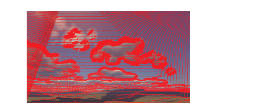
28.6. Results and Discussion 493
Figure 28.9. Sample refinement takes cloud transparency into account.
and distance to the cloud to attenuate the light samples along the view ray (please
refer to [Yusov 14b] for more details).
One important missing detail is sample refinement (see [Yusov 14a]), which
needs to account for screen-space cloud transparency. When computing coarse
unoccluded in-scattering, we take the screen-space cloud transparency and dis-
tance to attenuate the current sample. This automatically gives the desired effect
(Figure 28.9) with a minimal increase in performance cost.
28.6 Results and Discussion
Figure 28.10 shows some images generated using our method under different
lighting conditions. To evaluate the performance, we used two test platforms.
The first platform is an Ultrabook powered by an Intel Core i5 CPU and an Intel
HD Graphics 5200 GPU (47 W shared between CPU and GPU). Our second
test platform is a desktop workstation powered by an Intel Core i7 CPU and an
NVIDIA GeForce GTX 680 GPU (195 W TDP). The viewport resolution was
set to 1280 ×720 on the first platform and to 1920 ×1080 on the second. Note
also that the NVIDIA GPU does not support pixel shader ordering, so images
were rendered with volume-aware blending disabled. Also note that this feature
is going to be exposed in DirectX 12, so it will soon be available on a wide range
of graphics hardware.
We used four quality settings: low, medium, high, and highest (Table 28.1).
Figure 28.11 compares images rendered by our algorithm in each setting.
Table 28.2 summarizes the performance of different stages of the algorithm
on our first test platform.
Rendering particles takes the most time, about 70% of the rendering time,
in all cases. The main sticking point is sampling the precomputed optical depth
texture. Reducing its resolution can significantly improve performance at the
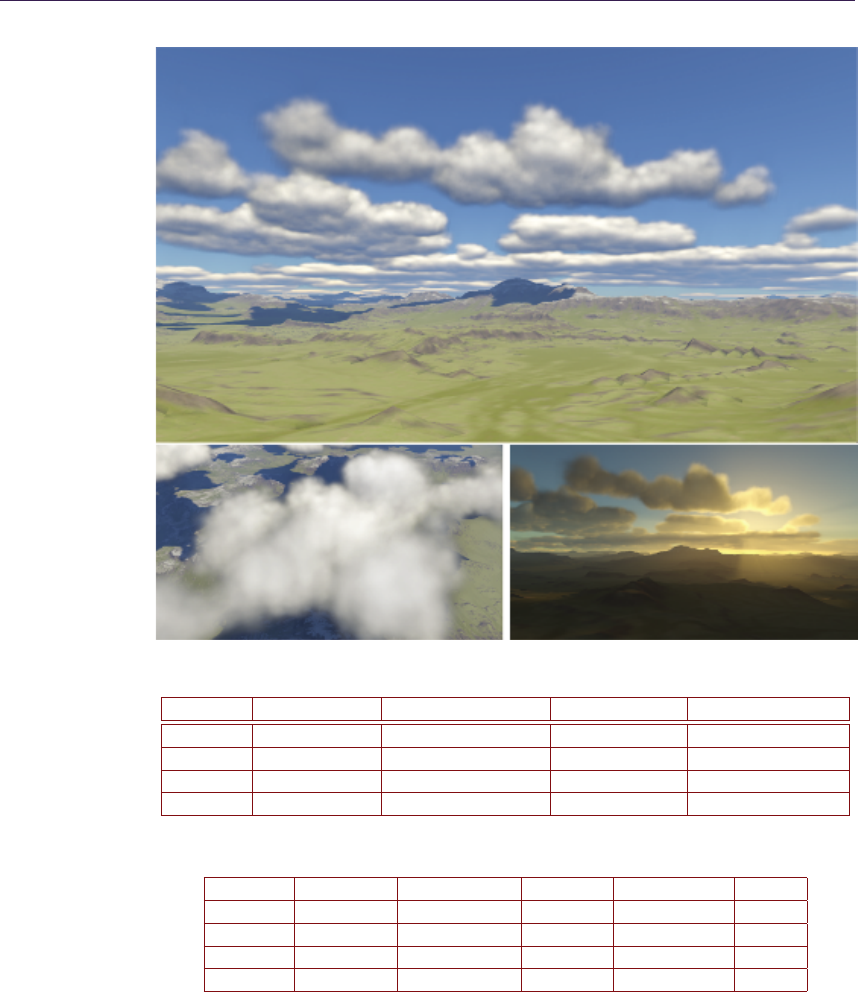
494 28. Real-Time Rendering of Physically Based Clouds Using Precomputed Scattering
Figure 28.10. Images generated by our algorithm.
Profile Num. rings Ring dimension Num. layers Num. particles
Low 4 120 3 2919
Medium 5 136 4 7103
High 5 168 6 15,725
Highest 5 216 8 33,702
Table 28.1. Quality profiles.
Profile Clearing Processing Sorting Rendering Total
Low0.62 0.63 0.24 4.22 5.71
Medium 1.31 1.00 0.31 8.72 11.34
High 2.98 2.07 0.48 15.73 21.26
Highest 6.53 4.62 0.83 26.5 28.48
Table 28.2. Performance of the algorithm on Intel HD Graphics 5200, 1280 ×720
resolution (times in ms).
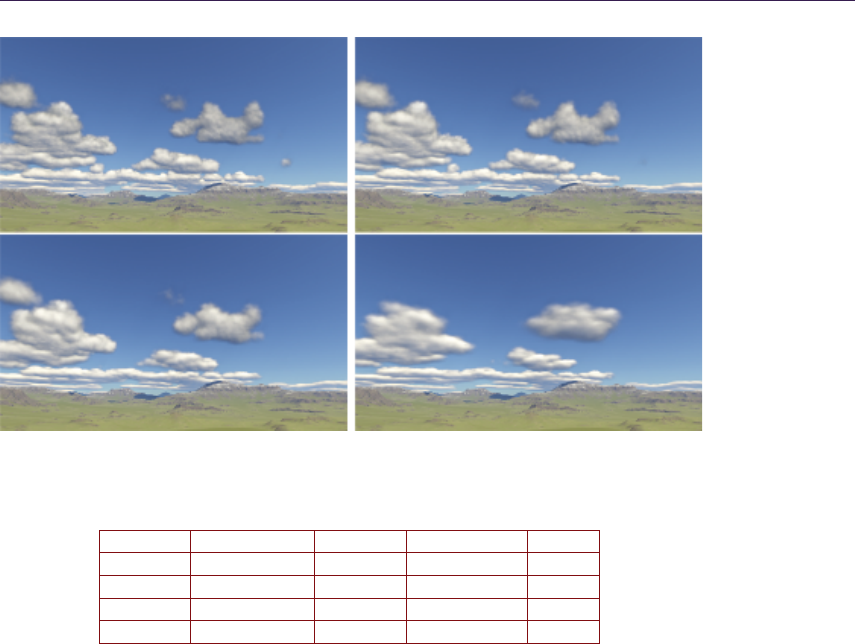
28.6. Results and Discussion 495
Figure 28.11. Test scene rendered in different quality profiles: highest (top left), high
(top right), medium (bottom left), and low (bottom right).
Profile Processing Sorting Rendering Total
Low 0.38 0.1 1.74 2.22
Medium 0.65 0.11 3.73 4.49
High 1.39 0.14 6.53 8.06
Highest 2.97 0.24 10.72 13.93
Table 28.3. Performance of the algorithm on NVIDIA GeForce GTX 680, 1920 ×1080
resolution (times in ms).
cost of lower quality. The processing stage includes all the steps discussed in
Section 28.5.2 except sorting, which is shown in a separate column. The clearing
column shows the amount of time required to clear the cloud density and light
attenuation 3D textures to initial values. This step takes almost the same time
as processing itself. This is because of the low memory bandwidth of the GPU.
Rendering light scattering effects takes an additional 5.8 ms. In the medium-
quality profile, the total required time is less than 20 ms, which guarantees real-
time frame rates.
Performance results on our high-end test platform are given in Table 28.3.
Because our second GPU has much higher memory bandwidth, the performance
of the algorithm is significantly better. It takes less than 2.3 ms to render the
clouds in low profile and less than 4.5 ms to render in medium profile at full
HD resolution. Since clearing the 3D textures takes much less time, we do not

496 28. Real-Time Rendering of Physically Based Clouds Using Precomputed Scattering
separate this step in Table 28.3. Computing atmospheric light scattering takes an
additional 3.0 ms of processing time. Also note that the GTX 680 is a relatively
old GPU. Recent graphics hardware provides higher memory bandwidth, which
will improve the performance of our method.
28.6.1 Limitations
Our method is physically based, not physically accurate. We make two main
simplifications when approximating shading: scattering is precomputed in a ho-
mogeneous spherical particle, and energy exchange between particles is ignored.
Precomputing the scattering inside an inhomogeneous particle would require a
5D table. It is possible that some degrees of that table can allow point sampling,
which would reduce the lookup into the table to two fetches from a 3D texture.
This is an interesting direction for future research.
The other limitation of our method is that our volume-aware blending can
precisely handle the intersection of only two particles. When more than three
particles intersect, the method can fail. However, visual results are acceptable in
most cases. We also believe that our method gives a good use-case example for
the capabilities of upcoming GPUs.
28.7 Conclusion
In this chapter we presented a new method for rendering realistic clouds. The
key idea of our approach is to precompute optical depth and single and multiple
scattering for a reference particle at preprocess time and to store the resulting
information in lookup tables. The data is then used at runtime to compute cloud
shading without the need for ray marching or slicing. We also presented a new
technique for controlling the level of detail as well as a method to blend the
particles accounting for their volumetric intersection. We believe that our idea
of precomputing scattering is promising and can be further improved in future
research. The idea of precomputing transparency can also be used for rendering
different kinds of objects such as distant trees in forests.
Bibliography
[Bohren and Huffman 98] C. Bohren and D. R. Huffman. Absorption and Scat-
tering of Light by Small Particles. Berlin: Wiley-VCH, 1998.
[Bouthors et al. 06] Antoine Bouthors, Fabrice Neyret, and Sylvain Lefebvre.
“Real-Time Realistic Illumination and Shading of Stratiform Clouds.” In
Proceedings of the Second Eurographics Conference on Natural Phenomena,
pp. 41–50. Aire-la-Ville, Switzerland: Eurographics Association, 2006.

Bibliography 497
[Bouthors et al. 08] Antoine Bouthors, Fabrice Neyret, Nelson Max, Eric Brune-
ton, and Cyril Crassin. “Interactive Multiple Anisotropic Scattering in
Clouds.” In SI3D, edited by Eric Haines and Morgan McGuire, pp. 173–
182. New York: ACM, 2008.
[Bouthors 08] Antoine Bouthors. “Real-Time Realistic Rendering of Clouds.”
PhD thesis, Universit´e Joseph Fourier, 2008.
[Cornette and Shanks 92] W.M. Cornette and J.G. Shanks. “Physical Reason-
able Analytic Expression for the Single-Scattering Phase Function.” Applied
Optics 31:16 (1992), 3152–3160.
[Dobashi et al. 00] Yoshinori Dobashi, Kazufumi Kaneda, Hideo Yamashita,
Tsuyoshi Okita, and Tomoyuki Nishita. “A Simple, Efficient Method for
Realistic Animation of Clouds.” In Proceedings of the 27th Annual Con-
ference on Computer Graphics and Interactive Techniques, pp. 19–28. New
York: ACM Press/Addison-Wesley, 2000.
[Harris and Lastra 01] Mark J. Harris and Anselmo Lastra. “Real-Time Cloud
Rendering.” Comput. Graph. Forum 20:3 (2001), 76–85.
[Harris 03] Mark Jason Harris. “Real-Time Cloud Simulation and Rendering.”
Ph.D. thesis, The University of North Carolina at Chapel Hill, 2003.
[Losasso and Hoppe 04] Frank Losasso and Hugues Hoppe. “Geometry
Clipmaps: Terrain Rendering Using Nested Regular Grids.” ACM Trans.
Graph. 23:3 (2004), 769–776.
[Miyazaki et al. 04] Ryo Miyazaki, Yoshinori Dobashi, and Tomoyuki Nishita. “A
Fast Rendering Method of Clouds Using Shadow-View Slices.” In Proceed-
ing of Computer Graphics and Imaging 2004, August 17–19, 2004, Kauai,
Hawaii, USA, pp. 93–98. Calgary: ACTA Press, 2004.
[Riley et al. 04] Kirk Riley, David S. Ebert, Martin Kraus, Jerry Tessendorf, and
Charles Hansen. “Efficient Rendering of Atmospheric Phenomena.” In Pro-
ceedings of the Fifteenth Eurographics Conference on Rendering Techniques,
pp. 375–386. Aire-la-Ville, Switzerland: Eurographics Association, 2004.
[Satish et al. 09] Nadathur Satish, Mark Harris, and Michael Garland. “Design-
ing Efficient Sorting Algorithms for Manycore GPUs.” In Proceedings of
the 2009 IEEE International Symposium on Parallel&Distributed Process-
ing,IPDPS ’09, pp. 1–10. Washington, DC: IEEE Computer Society, 2009.
[Schpok et al. 03] Joshua Schpok, Joseph Simons, David S. Ebert, and Charles
Hansen. “A Real-time Cloud Modeling, Rendering, and Animation System.”
In Proceedings of the 2003 ACM SIGGRAPH/Eurographics Symposium on

498 28. Real-Time Rendering of Physically Based Clouds Using Precomputed Scattering
Computer Animation, pp. 160–166. Aire-la-Ville, Switzerland: Eurographics
Association, 2003.
[Wang 04] Niniane Wang. “Realistic and Fast Cloud Rendering.” J. Graphics,
GPU, and Game Tools 9:3 (2004), 21–40.
[Yusov 14a] Egor Yusov. “High Performance Outdoor Light Scattering using
Epipolar Sampling.” In GPU Pro 5: Advanced Rendering Techniques, edited
by Wolfgang Engel, pp. 101–126. Boca Raton, FL: CRC Press, 2014.
[Yusov 14b] Egor Yusov. “High-Performance Rendering of Realistic Cumulus
Clouds Using Pre-computed Lighting.” In Proceedings of High-Performance
Graphics 2014, edited by Ingo Wald and Jonathan Ragan-Kelley, pp. 127–
136. Lyon, France: Eurographics Association, 2014.

29
Sparse Procedural
Volume Rendering
Doug McNabb
29.1 Introduction
The capabilities and visual quality of real-time rendered volumetric effects dis-
proportionately lag those of film. Many other real-time rendering categories have
seen recent dramatic improvements. Lighting, shadowing, and postprocessing
have come a long way in just the past few years. Now, volumetric rendering
is ripe for a transformation. We now have enough compute to build practical
implementations that approximate film-style effects in real time. This chapter
presents one such approach.
29.2 Overview of Current Techniques
There are many different kinds of volumetric effects, and games render them with
several different techniques. We cover a few of them here.
Many games render volumetric effects with 2D billboard sprites. Sprites can
produce a wide range of effects, from smoke and fire to water splashes, froth,
and foam. They have been around for years, and talented artists are constantly
getting better at using them. But, the sprite techniques have limits and are begin-
ning to show their age. The growing excitement for virtual reality’s stereoscopic
rendering is particularly difficult because the billboard trick is more apparent
when viewed in stereo, challenging the illusion. We need a better approximation.
The techniques presented here help improve the illusion. (See the example in
Figure 29.1.)
There have been several recent advancements in rendering light scattering in
homogeneous media, enabling effects like skies, uniform smoke, and fog. These
techniques leverage the volume’s uniformity to simplify the light-scattering ap-
proximations. They’re now fast enough to approximate multiple scattering in
499
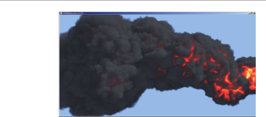
500 29. Sparse Procedural Volume Rendering
Figure 29.1. Sparse procedural volume rendering example.
real time with amazing visual quality [Yusov 14]. Light scattering in heteroge-
neous participating media is the more-general problem, and correspondingly is
more expensive. Our technique approximates single scattering in heterogeneous
media and can look very good. It is worth noting that our scattering model is
simpler than the typical homogeneous counterparts to accommodate the added
complexity from heterogeneous media.
Fluid simulation is another mechanism for generating volumetric effects. The
results are often stunning, particularly where accuracy and realism are required.
But, the costs can be high in both performance and memory. Developers typically
use these simulations to fill a volume with “stuff” (e.g., smoke, fire, water, etc.),
and then render that volume by marching rays originating from the eye’s point of
view. They periodically (e.g., every frame) update a 3D voxel array of properties.
Each voxel has properties like pressure, mass, velocity, color, temperature, etc.
Our technique fills the volume differently, avoiding most of the traditional sim-
ulation’s computation and memory costs. We can use less memory than typical
fluid simulations by directly populating the volume from a small set of data. We
can further reduce the memory requirements by filling the volume on demand,
processing only the parts of the volume that are covered by volume primitives.
This volume-primitive approach is also attractive to some artists as it gives good
control over sculpting the final effect.
29.3 Overview
Our goal for rendering the volume is to approximate efficiently how much light
propagates through the volume and reaches the eye. We perform a three-step

29.3. Overview 501
process to produce our results:
1. Fill a volume with procedural volume primitives.
2. Propagate lighting through the volume.
3. Ray-march the volume from the eye’s point of view.
Before we compute how much light propagates through a volume, we need
to know the volume’s contents; we need to fill the volume with interesting stuff.
Volume primitives are an inexpensive, expressive option for describing a volume’s
contents [Wrennige and Zafar 11]. Different volume primitive types are charac-
terized by their different mechanisms for describing and controlling the contents.
Procedural volume primitives describe the contents with algorithms controlled by
a set of parameters (e.g., size, position, radius, etc.). We can populate a volume
with multiple primitives, sculpting more-complex results. There are many possi-
ble volume primitive types. Our system implements a single “displaced sphere”
procedural volume primitive. We often refer to them interchangeably as particles
and displaced spheres.
Rendering a single volume primitive is interesting, but a system that can ren-
der many and varied overlapping volume primitives is much more useful. We need
to render many volume primitives within a unified volume; they need to correctly
shadow and occlude each other. Supporting translucent volume primitives is par-
ticularly useful. We satisfy these requirements by decoupling the volume “filling”
step from the light propagation step. We fill a metavoxel with all relevant volume
primitives before we propagate lighting by ray-marching through the volume. We
simplify light propagation by supporting only a single directional light (e.g., the
sun), allowing us to orient the volume to align with the light’s direction. This
enables us to traverse trivially the volume one voxel at a time along the light’s
direction. Each light propagation step illuminates the current voxel with the
current light intensity. At each step, the intensity is attenuated to account for
absorption and scattering. Note that we propagate only the light intensity. This
process can be extended (at additional cost) to accommodate colored light by in-
dependently propagating each of the red, green, and blue wavelength intensities.
We capture the volume’s lit color and density (or opacity) at each voxel. Note
that our model doesn’t include light scattered from the neighboring volume. This
could presumably be added at additional cost in time and complexity. Our model
does account for shadows cast by the rest of the scene onto the volume, and for
casting the volume’s shadow onto the rest of the scene.
When the eye sees the lit volume, the amount of light it sees at each voxel is
reduced by any other voxels between the lit volume and the eye. This is similar to
propagating light through the volume with a couple of important differences. The
eye view is a perspective view, in contrast to the directional light’s orthographic
view. And, each voxel along the eye ray can both occlude more-distant voxels
and contribute light (if the voxel is emissive, or lit by the light).
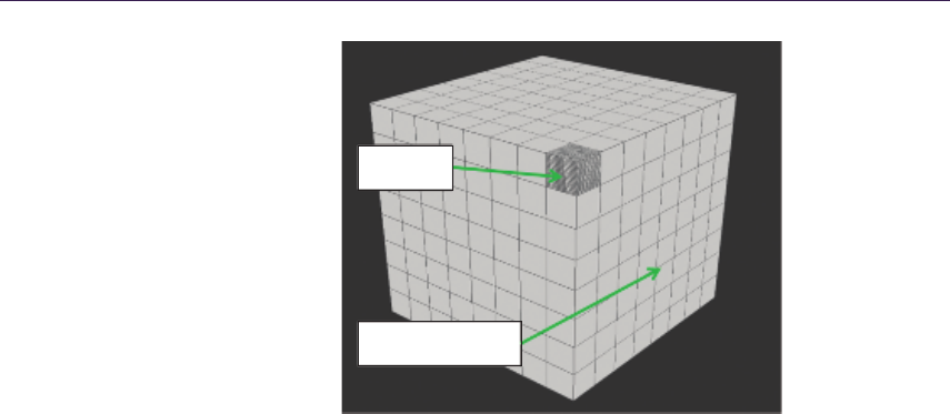
502 29. Sparse Procedural Volume Rendering
Voxels
Metavoxels
Figure 29.2. A large volume composed of metavoxels, which are composed of voxels.
The volume may also occlude the background; the amount of light from the
background that reaches the eye can be absorbed and scattered by the volume.
Our approach separates these two eye-view contributions. We determine the
lit volume’s contribution with a pixel shader and attenuate the background’s
contribution with alpha blending.
29.4 Metavoxels
The key point of our approach is that we can gain efficiency by avoiding un-
occupied parts of the volume. Each of our tasks can be made significantly less
expensive: we can fill fewer voxels, propagate light through fewer voxels, and
ray-march fewer voxels. We accomplish this by logically subdividing the volume
into a uniform grid of smaller volumes. Each of these smaller volumes is in turn
a collection of voxels, which we call a metavoxel. (See Figure 29.2.)
The metavoxel enables us to efficiently fill and light the volume. Most im-
portantly, it allows us to avoid working on empty metavoxels. It also allows pro-
cessing multiple metavoxels in parallel (filling can be parallel; lighting has some
dependencies). It allows us to switch back and forth between filling metavox-
els and ray-marching them, choosing our working set size to balance performance
against memory size and bandwidth. Using a small set improves locality. Reusing
the same memory over many metavoxels can reduce the total memory required
and may reduce bandwidth (depending on the hardware). It also improves ray-
marching efficiency, as many rays encounter the same voxels.
Figure 29.3 shows a few variations of a simple scene and the related metavox-
els. The first pane shows a few stand-in spheres, a camera, and a light. The
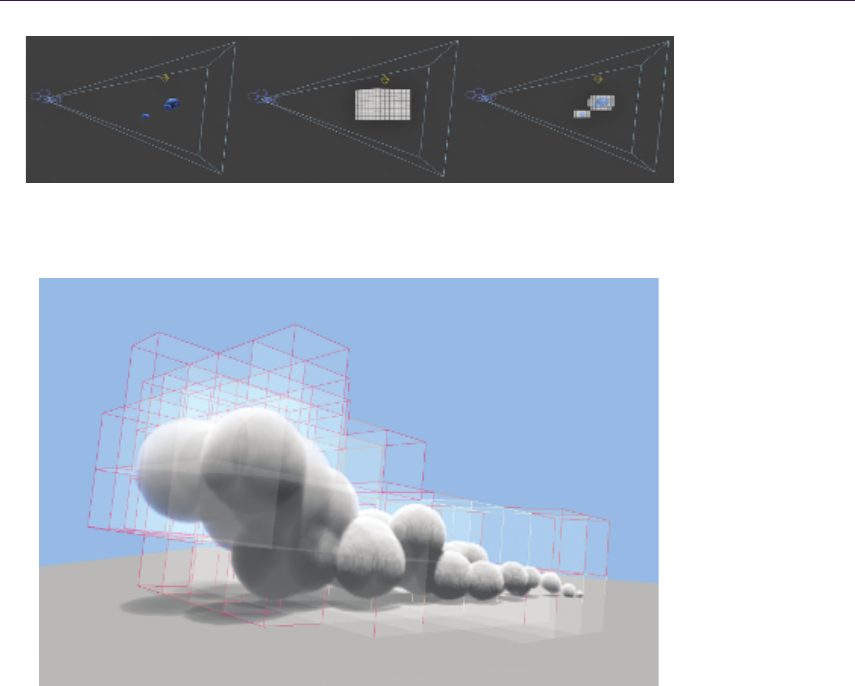
29.4. Metavoxels 503
Figure 29.3. A simple scene (left), with all metavoxels (middle) and with only interest-
ing/occupied metavoxels (right).
Figure 29.4. Multiple spheres and the metavoxels they cover.
second pane shows a complete volume containing the spheres. The third pane
shows the scene with only those metavoxels covered by one or more spheres.
This simplified example shows a total volume of 512(83) metavoxels. It requires
processing only 64 of them, culling 7/8 of the volume.
Figure 29.4 shows a stream of simple spheres and a visualization of the
metavoxels they cover. Note how the metavoxels are tilted toward the light.
Orienting the volume this way allows for independently propagating light along
each voxel column. The lighting for any individual voxel depends only on the
voxel above it in the column (i.e., the next voxel closer to the light) and is unre-
lated to voxels in neighboring columns.
Computers get more efficient every year. But memory bandwidth isn’t pro-
gressing as rapidly as compute efficiency. Operating on cache-friendly metavoxels
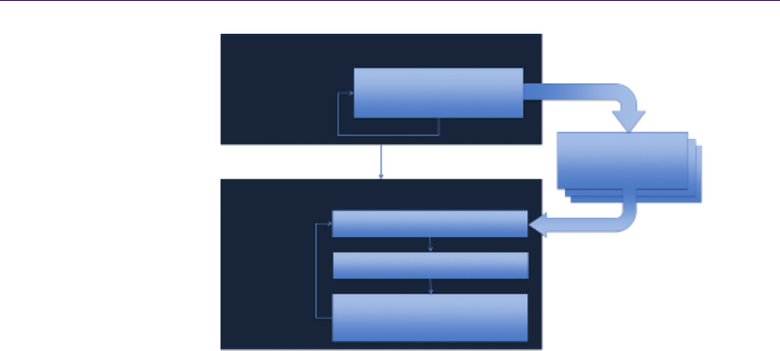
504 29. Sparse Procedural Volume Rendering
Bin Particles
Render Metavoxels
For each metavoxel
covered
for each particle
For each
nonempty
metavoxel
Append Particle to
Metavoxel’s Bin
Fill Metavoxel
Pre-metavoxel
Particle Bin
Propagate Light
Raymarch Metavoxel
from Eye
Figure 29.5. High-level algorithm.
may be more useful in the coming years as compute efficiency will almost certainly
continue to outpace bandwidth efficiency. Ray-marching multiple metavoxels one
at a time can be more efficient than ray-marching a larger volume. The metavoxel
localizes the sample points to a relatively small volume, potentially improving
cache hit rates and minimizing expensive off-chip bandwidth.
We fill a metavoxel by testing its voxels against the set of particles that cover
the metavoxel. For each of the voxels covered by a particle, we compute the
particle’s color and density at the covered location. Limiting this test to the
metavoxel’s set of voxels is more efficient than filling a much larger volume;
choosing a metavoxel size such that it fits in the cache(s) can reduce expen-
sive off-chip bandwidth. Processing a single voxel multiple times, e.g., once for
each particle, can also be more efficient if the voxel’s intermediate values are in
the cache. Populating the metavoxel with one particle type at a time allows us
to maintain separate shaders, which each process different particle types. Note
that we currently populate the volume with only a single particle type (displaced
sphere). But, composing an effect from multiple particle types is a desirable fea-
ture and may be simplified through sharing intermediate results versus a system
that requires that a single shader support every particle type.
29.5 Algorithm
Our goal is to render the visible, nonempty metavoxels. Figure 29.5 shows that
we loop over each of these interesting metavoxels, filling them with particles (i.e.,
our displaced sphere volume primitive), and then ray-marching them from the
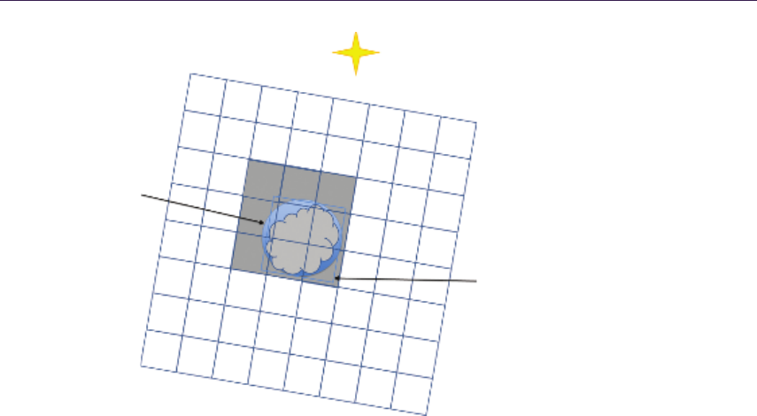
29.5. Algorithm 505
Bounding
Sphere
Bounding
Box
Figure 29.6. Visualization of binning rules.
eye. It’s worth noting that “visible” here means visible either from the eye’s view
or the light’s view. We consider the light’s view when culling because even if
a metavoxel lies outside the eye view, it may still lie between the light and the
eye’s view such that the metavoxels that are within the eye’s view may receive
its shadows. We need to propagate lighting through all parts of the volume that
contribute to the final scene.
29.5.1 Binning
We determine the interesting metavoxels using a binning process. Binning adds a
small amount of extra work but it reduces the overall workload. We can quickly
generate a list for each metavoxel containing the indices for the particles that
cover the metavoxel, and only those particles. It also allows us to completely
avoid metavoxels that aren’t covered by any particles.
Each bin holds a list of particle indices. We populate the bin with an index
for every particle that covers the metavoxel. We maintain an array of bins—one
bin for every metavoxel. (For example, were we to subdivide our total volume
into 32 ×32 ×32 metavoxels, then we would have a 32 ×32 ×32 array of bins.)
A typical sparsely populated volume will involve a small fraction of these, though
the algorithm does not inherently impose a limit.
We bin a particle by looping over the metavoxels covered by the particle’s
bounding box. (See Figure 29.6.) We refine the approximation and improve over-

506 29. Sparse Procedural Volume Rendering
// De te rm in e the particle ’s extents
min = particleCenter - particleRadius
max = particleCenter + particleRadius
// Loop ov er each me ta vo xe l w it hin the e xt ents
// Ap pend the pa rt ic le to t hose bins for the
// met av ox el s also c ov ered by the b ou nd in g s phere
for Z in m in .Z to m ax .Z
for Y in m in .Y to m ax .Y
for X in m in .X to m ax .X
if p ar t ic le B ou n di ng S ph er e c ov er s m et av ox el [ Z ,Y , X ]
a ppe nd p ar ti cl e to me t av ox el Bi n [ Z ,Y , X ]}
Listing 29.1. Binning pseudocode.
all efficiency by testing each of these metavoxels against the particle’s bounding
sphere. If the particle’s bounding sphere covers the metavoxels, then we append
the particle to the metavoxel’s bin.
Listing 29.1 shows simple pseudocode for binning a particle.
29.5.2 Filling Metavoxels
Our goal is to ray-march the metavoxels from the eye’s point of view. Before we
can do that, we need a metavoxel through which to march rays. We populate
a metavoxel by testing each of its voxels against each volume-primitive particle.
We say the voxel is covered by the particle if and only if the voxel is inside the
volume primitive.
We reduce the number of tests by testing each metavoxel only against the par-
ticles that cover it; many more particles may participate in the system, but they
may cover only other metavoxels. There are many more potential optimizations
for reducing the total number of tests (e.g., progressive/hierarchical traversal).
Some of these strategies can be explored within this framework, but some of them
encourage fundamental changes. We look forward to future improvements.
Our task for filling the metavoxel has two goals:
1. a final density value for every voxel,
2. a final color value for every voxel.
We use a simple model for combining particle densities and colors:
densityfinal =
n
1
densityn,
colorfinal = max(color0. . . colorn).
The final density is given by a simple sum of the densities for every particle
that covers the voxel. Color is more complex. We could blend colors together
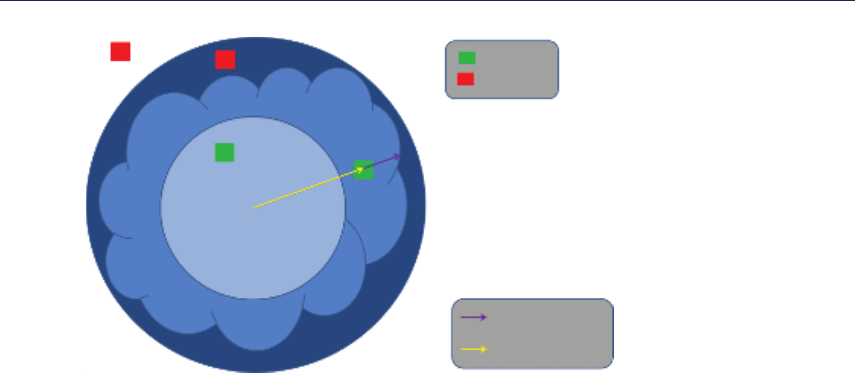
29.5. Algorithm 507
Inside
Center to
displaced surface
Center to voxel
Outside
Figure 29.7. Determining coverage.
proportionally to particle density (i.e., a dense particle affects the final color more
than a less-dense particle). In practice, simply accepting the maximum between
two colors produces plausible results and is computationally inexpensive. This
won’t work for every effect, but it efficiently produces good results for some.
Different color components may be required for different effects. For example,
fire is emissive with color ranging from white through yellow and orange to red,
then black as the intensity drops. Smoke is often constant color and not emissive.
The diffuse color is modulated by light and shadow, while the emissive color is
not.
We compute the density by performing a coverage test. Figure 29.7 shows
our approach. We determine the particle’s density at each voxel’s position. If a
voxel is inside the displaced sphere, then we continue and compute the particle’s
color and density. Voxels outside the displaced sphere are unmodified. Note
that the displacement has a limited range; there are two potentially interesting
radii—inner and outer. If the voxel is inside the inner radius, then we can be
sure it’s inside the displaced sphere. If the voxel is outside the outer radius, then
we can be sure that it’s outside the displaced sphere. Coverage for voxels that lie
between these two points is defined by the displacement amount.
We radially displace the sphere. The position of each point on the displaced
sphere’s surface is given by the length of the vector from the sphere’s center to
the surface. If the vector from the sphere’s center to the voxel is shorter than
this displacement, then the voxel is inside the sphere; otherwise it’s outside.
Note a couple of optimizations. First, the dot product inexpensively computes
length2:A·A= length2(A). Using distance2allows us to avoid the potentially
expensive square-root operations. The second optimization comes from storing
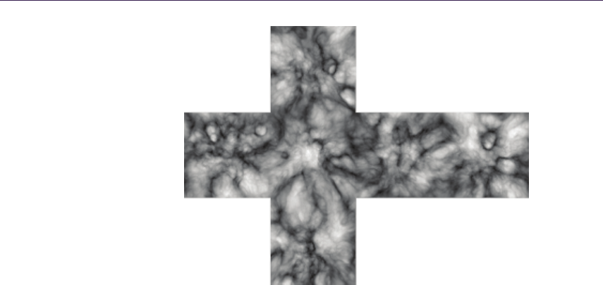
508 29. Sparse Procedural Volume Rendering
Figure 29.8. Example cube map: 3D noise sampled at sphere surface, projected to cube
map faces.
our displacement values in a cube map. The cube map, like the displacement
is defined over the sphere’s surface. Given a voxel at position (X, Y, Z) and the
sphere’s center at (0,0,0), the displacement is given by cubeMap[X, Y, Z].
We don’t currently support dynamically computed noise. We suspect that a
dynamic solutions would benefit from using a cube map for intermediate storage
as an optimization; the volume is 3D while the cube map is 2D (cube map lo-
cations are given by three coordinates, but they project to a flat, 2D surface as
seen in Figure 29.8). The number of expensive dynamic-noise calculations can be
reduced this way.
We determine each voxel’s lit color by determining how much light reaches
it and multiplying by the unlit color. We propagate the lighting through the
volume to determine how much light reaches each voxel. (See Figure 29.9.)
There are many possible ways to compute the color: constant, radial gradient,
polynomial, texture gradient, cube map, noise, etc. We leave this choice to the
reader. We note a couple of useful approximations: Figure 29.10 shows the results
of using the displacement map as an ambient occlusion approximation and using
the radial distance as a color ramp (from very bright red-ish at the center to dark
gray further out). The ambient occlusion approximation can help a lot to provide
form to the shadowed side.
Many of the displaced sphere’s properties can be animated over time: position,
orientation, scale, opacity, color, etc. This is a similar paradigm to 2D billboards,
only with 3D volume primitives.
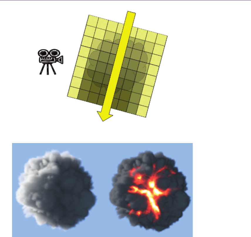
29.5. Algorithm 509
Figure 29.9. Propagating light through a metavoxel’s voxels.
Figure 29.10. Procedural colors.
29.5.3 Light Propagation
We propagate light through the metavoxel with a simple loop. We use the ras-
terizer and pixel shader to perform the work. We draw one pixel for each of the
metavoxel’s voxel columns—i.e., a two-triangle quad covering one pixel for each
of our voxel columns (e.g., for a 32 ×32 ×32 metavoxel, we draw a 32 ×32 pixel
square). Our pixel/fragment shader loops over each voxel in the corresponding
voxel column.

510 29. Sparse Procedural Volume Rendering
// 100% light p ro pa ga te s to star t
pr opa ga te dLi gh t = 1
// Loop over all voxels in the co lumn
for Z in 0 to METAVOXEL_HEIGHT
// Lig ht th is vo xel
co lor [ Z] *= pr op ag ate dL ig ht
// At te nu at e the lig ht l ea ving this v oxel
p ro pa g at ed Li g ht /= (1 + d en si ty [ Z ])
Listing 29.2. Light propagation pseudocode.
Listing 29.2 shows pseudocode for propagating lighting through the metavoxel.
At each step, we light the current voxel and attenuate the light for subsequent
voxels.
29.5.4 Eye-View Ray March
We march along the eye rays, through the metavoxel, accumulating color from
the metavoxel’s lit voxels and attenuating according to the voxel’s density.
We implement the eye-view ray march by drawing a cube (i.e., 6 quads =
12 triangles) with the rasterizer from the eye’s point of view. The pixel shader
executes once for each pixel covered by the cube. Listing 29.3 gives pseudocode
for the pixel shader. It loops along a ray from the eye through the pixel, sampling
// The ray starts at the eye and goes t hr ou gh the
// near p lan e at the cu rr ent pixe l
ray = pixel Po sitio n - e yePosit io n
// Compute the st art and end p oints wh ere the ray
// en ters and exits t his me ta vo xe l
start = in ter sec tFar ( ray , metavoxe l )
end = int er se ctNea r ( ray , met av ox el )
// Cl amp the ray to the eye position
end = max ( eyeP ositi on , end )
// Start as su mi ng vo lume is empt y
// == black , and 100% tr ans mi tt ance
re su ltColor = 0
resultTransmittance = 1
// step along the ray , accum ul at ing and at tenua ti ng
for step in star t to end
co lor = v olu me [ st ep ]. rg b
d ens it y = v olu me [ step ]. a
bl endF act or = 1/(1 + d ens ity )
re su ltColor = lerp ( color , resul tColo r , b lendFac to r )
re sul tT ran sm itt ance *= bl en dFact or
Listing 29.3. Ray march pseudocode.
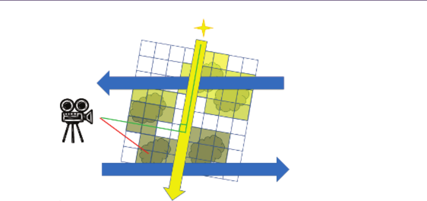
29.5. Algorithm 511
Figure 29.11. Metavoxel sort order.
the volume as a 3D texture at each step. It accumulates lighting from the sample’s
color and attenuates it by the sample’s alpha (i.e., density). The end result is a
color and an alpha we can use with alpha blending to composite with our back
buffer.
Note that we draw this box with front-face culling. If the eye is inside the box,
then it sees only back faces. If we were to use back-face culling, then the pixels
wouldn’t draw and no ray marching would occur. We also don’t want to draw
without culling because that would potentially cause our pixels to unnecessarily
draw twice.
29.5.5 Metavoxel Sort Order
Lastly, we need to render the metavoxels in the correct order for the alpha blend-
ing to be correct. We render the metavoxels one at a time, propagating light and
ray-marching each one. The results blend to a shared render target. Because the
metavoxels can contain semitransparent voxels, order matters.
Figure 29.11 demonstrates why we need to process our metavoxels from the
top to bottom (with respect to the light) and back to front (with respect to
the eye). Light propagation dictates the top-to-bottom order because an indi-
vidual metavoxel’s final colors depend on how much light propagates through
any metavoxels nearer the light. Similarly, we need to blend each metavoxel’s
eye-view ray march results with those of previously rendered metavoxels.
There’s a twist, however. Rendering from top to bottom and back to front can
produce incorrect results for those metavoxels below the perpendicular (the green

512 29. Sparse Procedural Volume Rendering
line from the camera). The eye is looking down on those metavoxels. So, the
eye can see through some previously rendered metavoxels. In this case, we need
to render the more-recent metavoxel behind the previously rendered metavoxel.
The solution is to process all of the metavoxels above the perpendicular before
processing those below. We also switch sort order and render those metavoxels
below the line sorted front to back.
The different sort orders require different alpha-blending modes. We render
back to front with over blending. We render front to back with under blending
[Ikits et al. 04].
It is possible to render all metavoxels sorted front to back with under blending.
That requires maintaining at least one column of metavoxels. Light propagation
requires processing from top to bottom. Sorting front to back can require render-
ing a metavoxel before those above it have been processed. In that case, we would
still propagate the lighting through the entire column before ray-marching them.
Consistently sorting front to back like this could potentially allow us to “early
out,” avoiding future work populating and ray-marching fully occluded voxels.
29.6 Conclusion
Computers are now fast enough for games to include true volumetric effects.
One way is to fill a sparse volume with volume primitives and ray-march it from
the eye. Efficiently processing a large volume can be achieved by breaking it
into smaller metavoxels in which we process only the occupied metavoxels that
contribute to the final image. Filling the metavoxels with volume primitives
allows us to efficiently populate the volume with visually interesting contents.
Finally, sampling the metavoxels from a pixel shader as 3D textures delivers an
efficient ray-marching technique.
Bibliography
[Ikits et al. 04] Milan Ikits, Joe Kniss, Aaron Lefohn, and Charles Hansen. “Vol-
ume Rendering Techniques.” In GPU Gems, edited by Randima Fernando,
Chapter 39. Reading, MA: Addison-Wesley Professional, 2004.
[Wrennige and Zafar 11] Magnus Wrennige and Nafees Bin Zafar “Production
Volume Rendering Fundamentals.” SIGGRAPH Course, Vancouver, Canada,
August 7–11, 2011.
[Yusov 14] Egor Yusov. “High Performance Outdoor Light Scattering using
Epipolar Sampling” In GPU Pro 5: Advanced Rendering Techniques, edited
by Wolfgang Engel, pp. 101–126. Boca Raton, FL: CRC Press, 2014.

30
Adaptive Virtual Textures
Ka Chen
30.1 Introduction
Adaptive Virtual Textures (AVT) are an improvement upon Procedural Virtual
Textures. This technique can be applied to a large open world and can achieve
a much higher texture resolution when needed. With AVT, the artist can place
thousands of projected decals with high-resolution textures on the terrain surface
These decals will be baked together with terrain materials into virtual textures
at runtime. Once baked, the rendering engine will directly display the virtual
textures instead of rendering terrain materials and decals. Thus, the render
performance is greatly improved.
30.2 Procedural Virtual Textures Basics
Procedural Virtual Textures are mipmapped texture caches that store the recent
rendering result of terrain material blending and projected decals. In a deferred
rendering engine, these virtual textures store the composite using the G-buffer’s
format, which can then be used directly when rendering subsequent frames. It is
a powerful optimization technique because the rendering engine can simply skip
the expensive terrain material blending once it has been cached in the virtual
textures. (See [Widmark 12] for more details.)
30.3 Adaptive Virtual Textures
30.3.1 Goals
The standard virtual textures technique allocates a large mipmapped texture,
which is then uniformly applied onto the whole terrain world. The actual texture
resolution can be calculated as
texel ratio = TextureSize.xy
WorldSize.xy .
513

514 30. Adaptive Virtual Textures
Although usually a very large virtual texture (such as 512K×512K) is allocated,
sometimes the texture resolution is not high enough when it is applied on a large
open world such as a 10KM×10KM world. In this case the texel ratio is only 0.5
texels/cm. Such a low texture resolution limits the potential usage of procedural
virtual textures in next-generation games. In order to prevent the look of low-
resolution terrain, an additional detail material layer has to be applied on top of
procedural virtual textured terrain.
In this chapter, we will present Adaptive Virtual Textures (AVT), which
greatly improve the texture resolution in a very large world. We will discuss
the practical implementation of AVT and how we overcame those challenges in
our game.
30.3.2 Overview
By using a 512K ×512K resolution virtual texture, we would like to achieve a
high texture resolution such as 10 texels/cm in a 10KM ×10KM world. Such a
high texel ratio is only needed for terrain surfaces that may appear very close to
the camera. For terrain surfaces that are a bit farther away, a lower texel ratio
such as 5 texels/cm is sufficient. We would require even less texture resolution
for surfaces that are much farther away. The key is to find a solution to apply
the virtual texture based on the distance from the camera to the terrain surface.
We divide the game world into multiple sectors and each sector has a pre-
defined size (such as 64 ×64 meters), as shown in Figure 30.1. Every sector is
allocated with a virtual image inside the virtual texture. The size of the virtual
image is calculated based on the distance from the camera. The closest sectors
are allocated with the maximum virtual image size, for example 64K ×64K. Far-
ther sectors are allocated with smaller sizes, such as 32K ×32K or 16K ×16K.
The minimum size can be 1K ×1K.
After allocating all the sectors in the world, our virtual texture becomes a
texture atlas for all the virtual images with different sizes The closest sector has
the maximum resolution of 10 texels/cm calculated as
texel ratio = 64K
64 meters = 10 texels/cm.
Farther sectors have lower resolutions such as 5 texels/cm and so on. It is im-
portant to note that these virtual image sizes will be adjusted dynamically at
runtime based on camera distance whenever the camera moves.
30.3.3 Allocate Virtual Texture Atlas
As mentioned at the end of Section 30.3.2, we need to adjust the size of each
virtual image dynamically at runtime. It is important to have a good texture
atlasing algorithm so that the performance of AVT is maximized and space frag-
mentation is kept to a minimum. We use a quad-tree scheme to allocate the
30.3. Adaptive Virtual Textures 515
Figure 30.1. World divided into multiple sectors.
virtual images. This scheme makes sure that the image is always allocated at the
location where the UV address is aligned with image size. Figure 30.2 shows the
allocation of three virtual images inside the virtual texture atlas.
30.3.4 Adjust Virtual Image Size at Runtime
In each frame we calculate a target virtual image size based on its distance from
the camera. If the target size is different than the current size of the sector, we
will insert a new image with the target size into the atlas and remove the old
one. Listings 30.1 and 30.2 show the code to calculate and adjust, respectively,
the size of virtual images for sectors in the world.
For example, as shown in Figure 30.3, when the camera moves and Sector B
becomes farther away from the camera, it will be allocated using a smaller image
size of 32K ×32K. Sector C becomes closer to the camera, so it will be allocated
with a larger image size of 64K ×64K.
30.3.5 Remap the Indirection Texture
Indirection texture Our virtual texture system uses an indirection texture to trans-
late from the virtual UV address to the physical UV address. (For the basic
virtual texture technique and information about indirection textures, please refer
to [Mittring 08].) When virtual image are moved and scaled, we have to update
the indirection texture so that the new virtual UV address will reuse the existing
pages in the physical texture caches. The format of our indirection texture is 32
bit and it is defined as in Figure 30.4.
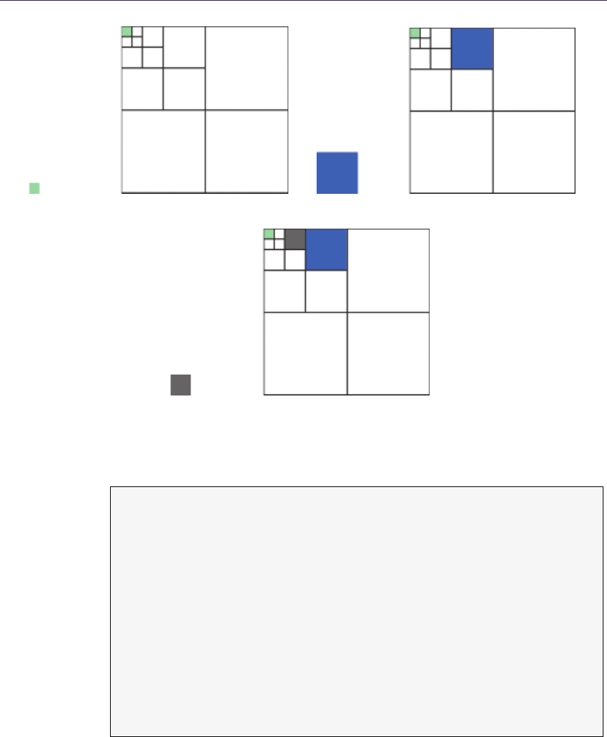
516 30. Adaptive Virtual Textures
(a) (b)
(c)
Figure 30.2. (a) First, insert a virtual image of size 16 ×16 for Sector A. (b) Then, insert a virtual image
of size 64 ×64 for Sector B. (c) Then, insert a virtual image of size 32 ×32 for Sector C.
ty pedef unsigned int U 32 ;
const U32 hig he stR es olu ti on = 64 * 1 024;
U32 CalculateTargetImageSize(cons t Se cto rInfo & sectorI nfo , c onst
Ve cto r3 & ca mer aP osi ti on )
{
//Get sectorPosition.
......
// Di st anc e be twe en s ect or an d c ame ra in top - do wn vie w .
float d ist ance = - ( se ctor Pos ition - c ame raPo si tio n ). GetLe ngt h2 ();
U32 t = ( U32 )( d is ta nc e / s wi tchDi st ance );
// Ca lculate the LOD of v irt ual im age .
U32 lodImage = 0;
if(t >= 1)
{
lod Im age = s td :: lo g2 (t ) + 1;
}
U32 v ir tua lI mag eS ize = hig he stR es olu ti on >> lodImage ;
return virtualImageSize;
}
Listing 30.1. Calculating the virtual image size.
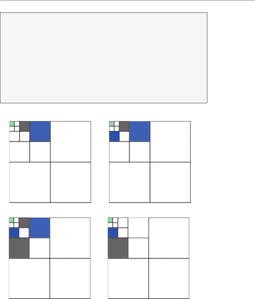
30.3. Adaptive Virtual Textures 517
std :: v ector < Secto rInf o > d ela ye dR em ov eS ect or s ;
for (au to & se ct or In fo : m _A ll Secto rs )
{
vir tu al Imag eSiz e = C alc ul at eT ar ge tIma ge Size ( s ect orIn fo ,
cameraPosition);
If ( v irt ua lIm ag eSi ze != s ect orI nfo . m_ Virt ualI mag eS ize )
{
m_A tla s . In sert Ima ge ( s ecto rIn fo , v irt ua lI mage Size ) ;
de la yedR emo ve Sect ors . pu sh_ bac k ( sec tor Info ) ;
}
}
for (au to & remo vin gSecto r : de laye dRem ov eSec tors )
{
m_A tlas . Remove Ima ge ( re movi ngS ector );
}
d el a ye dR em o ve Se c to rs . cl ea r () ;
Listing 30.2. Adjusting the virtual image size.
(a) Original virtual texture atlas. (b) Insert new image for Sector B.
(c) Insert new image for Sector C. (d) Remove old images for Sectors B and C.
Figure 30.3. Adjusting the size of two virtual images.
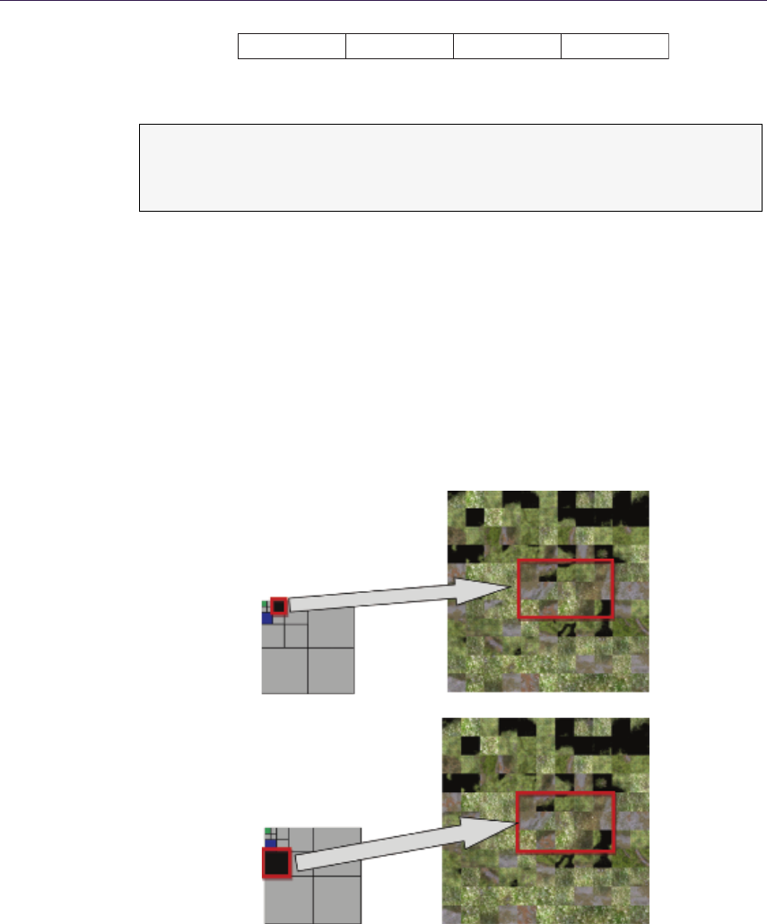
518 30. Adaptive Virtual Textures
PageOffsetX : 8 PageOffsetY : 8 Mip : 8 Debug : 8
Figure 30.4. Indirection texture format.
sc ale = ( vi rtu al t ex tur e siz e / ph ysi ca l te xt ure s ize ) >> m ip ;
bia s = ph ys ic al page offset - virtual page of fset * sc ale ;
ph ys ic al uv = vi rt ual uv * scale + bias ;
Listing 30.3. Calculating the physical texture UV address from the indirection texture
and the virtual UV address.
PageOffsetX and PageOffsetY are the UV offsets of the physical page pointed
to by the current virtual page. Mip describes the available mipmap level for the
current virtual page. The final physical texture UV address is calculated as shown
in Listing 30.3.
Remap the indirection texture when the image is up-scaled The update of the in-
direction texture for Sector B is shown in Figure 30.5.
Physical texture
Indirection texture
Physical texture
Indirection texture
Figure 30.5. Indirection texture (left) and physical texture cache (right) before update
(top) and after update (bottom).

30.4. Virtual Texture Best Practices 519
For ev ery mip ma p level of the in di rection texture ,
{
// The fo llo win g part is e xec ute d by a c ompute sh ader going
// thr ough all indire ct io n textur e ent ries , with the number of
// thr eads se t as the nu mber of en tr ie s in the X and Y
// dim en sio ns .
For ever y en try en cl os ed by new image in that mipmap level ,
{
If ( c urrent mi pmap level is greate r tha n 0)
{
Cop y the content fr om 1 mip l evel high er old image
( Page Offse tX , PageO ffset Y , Mip ) and in cr ea se Mip by 1
The ne w e ntry co nte nt b eco mes ( Pa geO ffsetX ,
PageO ffset Y , Mip + 1) ;
}
els e
{
Cop y the c ontent from 1 mip level h igher old image ,
The ne w e ntry co nte nt b eco mes ( Pa geO ffsetX ,
Pa geO ffs etY , Mip ) ;
}
}
}
Listing 30.4. Pseudocode to update the indirection texture for a newly allocated virtual
image.
The work involved in updating the indirection texture is shown in Listing 30.4.
The remapping of an up-scaled virtual image can be viewed in Figure 30.6.
In this case the image size is up-scaled from 32K to 64K. We can conclude that
the indirection entries for the new image should point to the exact same entries
of one mip level higher in the old image, as shown by the red arrows. As the mip
level 0 of the new image doesn’t exist in the old image, we will set the entries of
mip level 0 in the new image to lower mip level physical texture pages to prevent
visual popping in the current frame.
Remap the indirection texture when image is down-scaled Remapping a down-scaled
virtual image is just to reverse the steps of up-scaling a virtual image, as shown
in Figure 30.7.
30.4 Virtual Texture Best Practices
In the previous section we discussed the key features of AVT and how to handle
updating the virtual texture atlas and indirection texture when dynamic adjust-
ments of the image size happens in real time. In this section we will talk about
some practical implementation details of AVT.
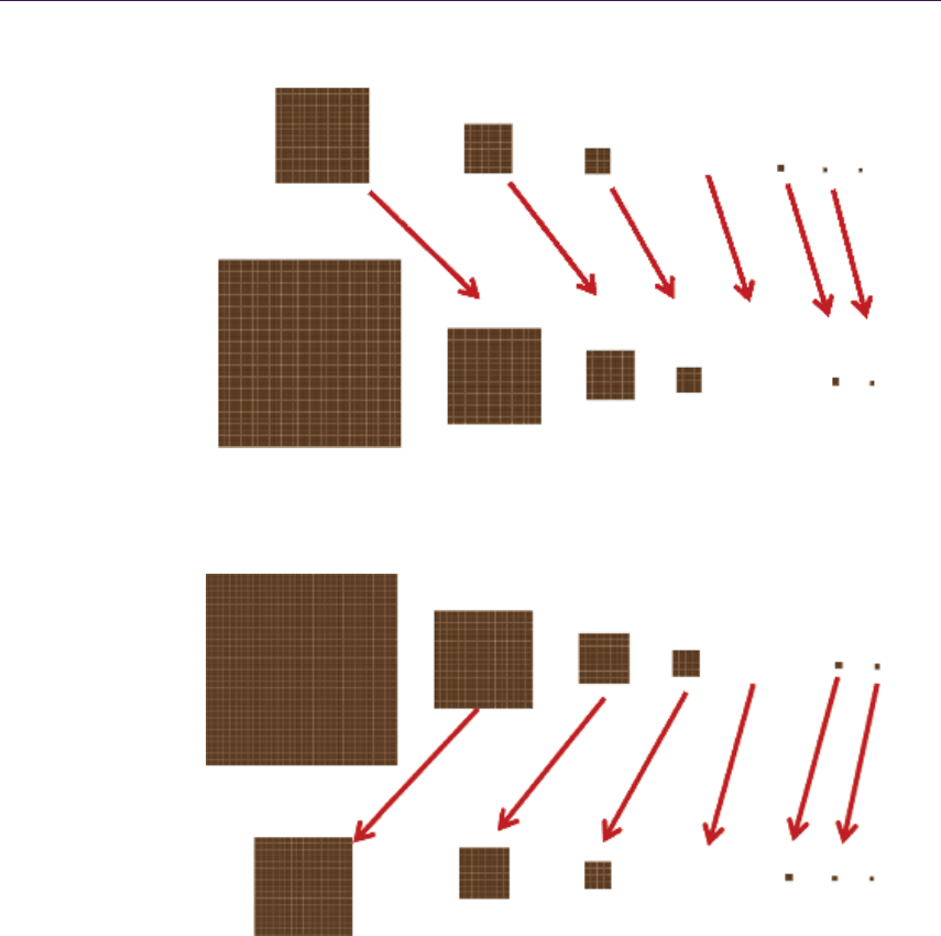
520 30. Adaptive Virtual Textures
Old virtual image: 32K × 32K
New virtual image: 64K ×
64K
Mip 10
Mip 10
Mip 9
Mip 4 ... Mip 8
Mip 8Mip 3 ... Mip 7
. . . . . .
. . . . . .
Mip 2
Mip 2
Mip 1
Mip 1
Mip 0
Mip 0
Mip 9
Mip 3
Figure 30.6. Remapping of an up-scaled virtual image.
Old virtual image: 64K × 64K
New virtual image: 32K ×
32K
Mip 10
Mip 10
Mip 9
Mip 4 ... Mip 8
Mip 8Mip 3 ... Mip 7
. . . . . .
. . . . . .
Mip 3
Mip 2
Mip 2
Mip 1
Mip 1
Mip 0
Mip 0
Mip 9
Figure 30.7. Remapping a down-scaled virtual image.
30.4.1 Output Page IDs
Virtual textures are divided into multiple 256×256 sized virtual pages. For every
pixel on the screen, we calculate to which virtual page it is related and output
the page information into a read/write buffer during the G-buffer rendering pass.
We call this buffer the Page ID buffer.

30.4. Virtual Texture Best Practices 521
PageID X : 12 PageID Y : 12 Mip : 4 Size : 4
Figure 30.8. The format of the page ID.
#define PAGEID_DOWNSCALE 8
voi d OutputPageID(VTextureArgs vArgs, float2 screenPos )
{
// Writ e to page ID read / w rite b uf fer
ui nt2 vp os = ( u int2 ) sc ree nPo s ;
ui nt2 v pos 2 = (( u int2 ) vp os ) % P AGE ID _D OW NS CA LE ;
uin t vi rt ual Pa ge ID = p ac k_p ag eid ( v Arg s );
if ( vp os2 . x == ( uint) g_V irtu alSe cto rs Inf o . Virt ual Dither . x &&
vpos2 .y == ( uint) g _Vir tua lS ect or sIn fo . V irt ualDit her . y)
Pa geI DO utp ut Tex ture [(( uint2 ) vpo s ) / PA GEI D_ DOWNS CA LE ] =
vi rtua lPa geID ;
}
Listing 30.5. Writing to 1/8×1/8 Page ID buffer in the G-buffer rendering shader.
The page information for every pixel is written as a 32-bit integer as shown
in Figure 30.8.
PageID and Size are calculated as
PageID.xy =Virtual UV.xy
virtual page size,
Size = log2(virtual page size).
The size of the Page ID buffer is 1/8 of the G-buffer texture in both directions in
order to reduce the memory overhead. Listing 30.5 is the fragment shader used
to output the page ID to the small read/write buffer.
Note that g_VirtualSectorsInfo.VirtualDither.xy is the shader parameter
passed in from the rendering engine, and its value ranges from 0 to 7 and changes
according to a predefined pattern in every frame. Since we only pick one pixel
out of 64 to output, if a page ID is missed in one frame, it will be processed
during a subsequent frame.
30.4.2 Physical Textures and Compressing
We allocate three physical textures for deferred rendering purposes. These are the
albedo texture, normal map texture, and specular texture. Table 30.1 provides
the color channel information for these textures.
Every physical texture page is compressed at runtime by a compute shader on
the GPU. We modified the sample code provided by Microsoft for the Xbox One
to compress three different types of physical texture pages in one pass. For the
normal map texture, we choose the BC5 format to compress only the X and Y

522 30. Adaptive Virtual Textures
Physical Texture Channels Representation Compress Format
Albedo Texture RGB Albedo Color BC1
Normal Map
Texture
RG Tangent Space Normal BC5
Specular Texture RGB Glossness, Specular
Intensity, Normal Map
Scale
BC1
Table 30.1. Physical textures’ channel information.
// Out pu t te rr ai n G - b uf fe r co lor by f et ch in g ph ys ic al t e xt ure c ac he .
gb uffer . al bedo = Dif fuse Phys ical Text ure . Sample Gra d (
Te xt ure Sa mpl er , phy sic al_ uv , dx , d y ). xyz ;
g buf fe r . n or ma l . xy = N or m al Ph y si ca l Te xt u re . Sa mp l eG ra d (
Te xtu reS amp ler , ph ysi cal_uv , dx , dy ). xy ;
gb uff er . no rma l .xy = g buf fer . n orm al . xy * 2 - 1;
gb uff er . no rma l .z = s qrt ( sa turate (1 - dot ( gbu ffe r . nor mal . xy ,
g buf fe r . n or ma l . xy ) )) ;
float3 GlossnessSpecularIntensity =
Sp ec ul arPh ysic al Tex tu re . S ampleG rad ( T ext ure Sam ple r ,
ph ysi cal _u v , dx , d y ). xyz ;
gb uf fer . no rma l . xyz *= G lo ss ne ss Sp ec ul a rI nt en si ty .z ;
gb uff er . glo ss ness _s pec ul ar In tens ity =
GlossnessSpecularIntensity.xy;
Listing 30.6. Calculating the final G-buffer colors from virtual textures.
channels of the normal map into a separated 4 bits-per-pixel block. This gives a
much less blocky result than with the BC1 format. In some situations the normal
vector saved in the virtual texture is not unit length. For example, when the pixel
is on a big slope on the terrain surface, the final normal vector might be scaled by
the slope angle or a mask texture. We save the scale of the normal vector in the
Z channel of the Specular Physical Texture during compression. Later on, when
we fetch the virtual textures, we reapply the scale to the normal vector coming
from the physical texture. Listing 30.6 shows the HLSL shader for calculating
the final G-buffer colors.
30.4.3 Improve Performance by Distributed Rendering
The performance of virtual texture rendering may vary depending on how many
virtual pages are visible in a given frame. When the camera is moving or turn-
ing very fast, it could take significant time to cache the physical textures. We
can spread the rendering of virtual pages into multiple frames to alleviate this
problem. We call this method distributed rendering.
On the CPU we read the Page ID buffer that is output from the GPU, collect
the visible virtual pages, and remove the duplicated pages. We then sort the

30.4. Virtual Texture Best Practices 523
struct PageIDSortPredicate
{
bo ol o pe ra to r () ( c onst u ns ig ne d id0 , cons t unsigned i d1 ) c ons t
{
V Te xtu re Pa ge ID ke y0 ( id0 ) ;
V Te xtu re Pa ge ID ke y1 ( id1 ) ;
// key . size is s aved in Lo g2 space , so it is in the same
// s pace as the mi pmap level .
return ( key 0 . size - k ey0 . mi p) < ( ke y1 . siz e - k ey1 . mip ) ;
}
};
std :: sor t ( pag eID s . Beg in () , pa geI Ds . End () , P ageK ey Sor tP re di ca te () ) ;
Listing 30.7. Sorting the visible pages.
visible pages according to their image sizes scaled by mipmap level, as shown in
Listing 30.7.
For each sorted virtual page starting from the first page, we first search for
its physical page in the physical texture cache and allocate one if it is not already
there; then, we render the fully composited terrain material into the page. At
the same time we record the actual rendering time for virtual textures. If the
accumulated rendering time for the current frame is longer than a threshold, we
skip the rendering of the remaining pages in the list. The skipped pages will be
rendered during the next frame.
We always sort the virtual pages such that we render the page with the small-
est image size first. This guarantees that the terrain is always displayed on
screen even if some pages have been skipped. Some parts of the image may ap-
pear blurry in the current frame if they have been skipped, but these areas will
become sharper later, once they are updated. In practice this is generally not
noticeable because it happens very quickly from one frame to the next.
30.4.4 Virtual Texture Filtering
Anisotropic filtering Our Adaptive Virtual Texutres support 8X anisotropic fil-
tering. This means that the pixel shader may access neighboring pixels up to
4 pixels away If the shader accesses a pixel lying on the border of the page, its
neighboring pixel could reside in another physical page and it might not be the
correct neighboring pixel in the world space. This would cause color bleeding
problems between pages.
To fix this problem, we allocate a 4-pixel-wide border on each side of the
physical texture page. For a 256×256 virtual page, its physical page size becomes
264 ×264. When rendering into the physical page, the viewport is also enlarged
to 264 ×264 so that the neighboring pixels at the border are rendered. (See
Figure 30.9.)
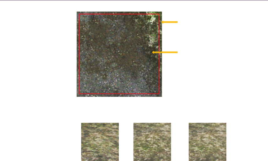
524 30. Adaptive Virtual Textures
256 × 256 original
page content
4-texel border
Enlarged viewport 264 × 264
Figure 30.9. A 4-pixel border on a physical page.
(a) Bi-linear. (b) Anisotropic. (c) Tri-linear anisotroic.
Figure 30.10. Comparison of three filtering methods.
Tri-linear filtering Software tri-linear filtering is also supported by simply fetching
the indirection texture twice with a higher mipmap level and a lower mipmap level
to get two sets of physical UV addresses, then fetching from the physical textures
twice and blending between them according to the calculated ratio between the
mipmap levels.
Another approach is to use hardware tri-linear filtering with virtual textures.
For every physical texture we have, we can create an additional quarter size
physical texture as mipmap level 1 and render into this mipmap level 1 page
whenever the mipmap 0 page is rendered. This method requires 25% more video
memory for the physical texture caches. It also increases the GPU overhead
because the mipmap level 1 cache must be synced with the mipmap level 0 all
the time.
Figure 30.10 shows a comparison between bi-linear filtering, anisotropic filter-
ing, and tri-linear anisotropic filtering when looking at the ground with a sharp
view angle. The image looks blurred with bi-linear filtering. With anisotropic
filtering alone, the image looks much sharper but there is a visible seam where
mipmap levels change. With tri-linear anisotropic filtering, both problems are
solved.

30.5. Conclusion 525
(a) Render terrain materi-
als.
(b) Render a decal on top
of terrain.
(c) Render next decal. (d) Render the third decal.
Figure 30.11. Rendering terrain and decals into a virtual texture page.
30.4.5 Combine with Projected Decals
Adaptive Virtual Textures become very powerful when they are combined with
projected decals on terrain. The G-buffer properties (albedo, normal, and specu-
lar) of the decals can be baked into the same virtual page where terrain surfaces
are rendered. Thus rendering of projected decals becomes almost free with Adap-
tive Virtual Textures. Since AVT supports very high virtual texture resolutions
(10 texels/cm), level artists can put thousands of high-detail projected decals on
the ground, and this vastly improves the visual appearance for next-generation
games.
The rendering pipeline for projected decals in adaptive virtual textures is
quite straight forward:
For every visible page collected and sorted from the Page ID buffer,
1. find or allocate a physical texture page,
2. render terrain surface materials into the physical page,
3. find decals belonging to this page in the world space,
4. render decals into the physical page by projecting them into the virtual
texture.
Figure 30.11 shows the steps to render terrain materials and decals into a
virtual texture page.
30.5 Conclusion
This chapter described a new technique called Adaptive Virtual Textures for
rendering terrain and decals with a high resolution in an open world. AVT is an
improvement upon Procedural Virtual Textures. The main contribution of this

526 30. Adaptive Virtual Textures
technique is that it supports a very high virtual texture resolution at close range
and can be used to render thousands of decals very efficiently.
Bibliography
[Mittring 08] Martin Mittring. “Advanced Virtual Texture Topics.” In ACM SIG-
GRAPH 2008 Games, pp. 23–51. New York: ACM, 2008.
[Widmark 12] Mattias Widmark. “Terrain in Battlefield 3.” Paper presented at
Game Developers Conference, San Francisco, CA, March 5–9, 2012.

31
Deferred Coarse Pixel Shading
Rahul P. Sathe and Tomasz Janczak
31.1 Overview
Deferred shading has become a popular rendering technique in the games industry
to avoid redundant shading of occluded pixels. With increasing screen resolutions
and DPI, one can reduce the frequency of slowly varying components of the
rendering equation to something lower than once per pixel without a perceivable
difference in visual quality. Recent research addresses this issue and proposes
hardware solutions like Coarse Pixel Shading [Vaidyanathan et al. 14]. Although
an elegant solution, the Coarse Pixel Shader does not fit well into the deferred
shading pipeline. Lauritzen proposed a solution for deferred shading engines that
identifies the pixels where pixel rate shading is not enough and shades them at
the sample rate using a compute shader [Lauritzen 10]. We extend the later idea
further, but in the reverse direction by identifying the regions of the screen where
one can reduce the shading to a rate lower than pixel frequency (e.g., 2 ×2 pixel
sized blocks). With our technique we are able show about 40–50% reduction in
shading time with a slight increase in the G-buffer generation time.
31.2 Introduction and Background
Shading calculations often involve multiple components, e.g., ambient occlusion,
diffused lighting, and specular highlights. Some of these components have a
lower spatial frequency than others. When these slowly changing components
are evaluated at a rate lower than once per pixel, the image artifacts are hardly
noticeable on a high DPI screen. A large percentage of the power consumed by
the graphics processors is due to pixel shading [Pool 12]. As a result, reducing
the pixel shader usage directly translates to a power savings. Vaidyanathan et
al. proposed a solution that is well suited for the forward rendering pipeline
[Vaidyanathan et al. 14]. In their approach, one shades primitives in screen space
at different rates: coarse pixels (e.g., 2 ×2 block of pixels), pixels, and then
samples. But this does not extend well to the deferred shading or postprocessing
passes because at the time of deferred shading, the notion of primitive is not
527

528 31. Deferred Coarse Pixel Shading
present. Moreover, the primitive might have been partly occluded with one or
more additional primitives.
Lauretzen proposed a compute shader-based solution for deferred shading
that works well with multisample antialiasing (MSAA) [Lauritzen 10]. In his
approach, the G-buffer is rendered at the MSAA resolution and contains the
view-space derivatives and the normal, in addition to other surface data used for
shading. He then analyzes the G-buffer samples within a pixel to find if that
pixel needs to be shaded at the sample frequency. He uses the triangle inequality
of the view-space depth derivatives along with the normal variation to find out
which pixels need to be shaded at the sample rate. We expand upon his idea,
but in the opposite direction.
31.3 Algorithm
31.3.1 G-Buffer Generation
Just like in a normal deferred shading engine, our algorithm starts off by gener-
ating a G-buffer by writing out shading inputs at the pixel center. The G-buffer
stores derivatives of the view-space Z values in addition to the other surface data
(position, normal, UVs, TBN basis, etc.) required for evaluating the BRDF dur-
ing the shading pass. View-space Z derivatives are calculated by first multiplying
the position with the camera-world-view matrix and evaluating ddx_coarse and
ddy_coarse instructions. We use the spherical encoding to encode the surface
normal into float2 to save some G-buffer space and bandwidth. Other types
of encoding [Pranckeviˇcius 09] are possible, but we chose a spherical encoding
because that works well with the optimization discussed at the end of Section
31.3.2. We pack the specular intensity and the specular power in the other two
components to occupy a full float4. The G-buffer layout is as follows:
struct GBuffer
{
float4 no rmal _sp ec ula r : SV_Target 0 ; // Encode d n ormal and
// sp ecu lar po wer / i nte nsi ty .
float4 albedo : SV_Targ et1 ; // Albedo.
float4 bi ased _al bedo : SV_Ta rge t2 ; // Albe do sa mpled with
// the bias ed samp ler .
float2 po siti onZ Grad : SV_Ta rge t3 ; // ddx , ddy of view - spa ce Z .
float p osi tio nZ : SV _Target4 ; // View - sp ace Z.
};
31.3.2 Shading Pass
For the shading pass, we use a tiled compute shader similar to the one proposed
by Lauritzen [Lauritzen 10]. Our compute shader is launched such that one
thread processes one coarse region of the screen (e.g., 2 ×2 or 4 ×4 pixels region,

31.3. Algorithm 529
henceforth referred to as a coarse pixel). One thread group works on a larger
screen-space region containing multiple coarse regions (henceforth referred to as
atile). Our compute shader is conceptually divided in multiple phases:
1. light tiling phase,
2. analysis phase,
3. coarse pixel shading phase,
4. pixel shading phase.
At the end of each phase, the threads within the thread group synchronize.
Listing 31.1 shows the pseudocode for the shading pass. Figure 31.1 shows the
flowchart for the same.
We will now describe each of the phases in detail.
Light tiling phase When the renderer has a large number of lights to deal with,
the bandwidth required to read the light data structures can be a substantial. To
alleviate this problem, it is common practice to find the lights that intersect a
particular tile. Once found, the indices to the lights that intersect a particular tile
are maintained in the shared local memory. Subsequent portions of the shading
pass deal with only the lights that hit at least one pixel in that tile. Further
details about light culling can be found in [Lauritzen 10].
Analysis phase The goal of this phase is to determine the coarse pixels at which
the shading rate can be lowered. To that end, each thread reads the normals and
the view-space depth derivatives for all the pixels within the coarse pixel. We then
analyze the G-buffer data at each of the pixels in the coarse pixel with respect
to a reference pixel (e.g., the top-left pixel in each region). During the analysis,
similar to that of Lauritzen [Lauritzen 10], we use the triangle inequality to
check if the shading rate can be reduced to once per coarse pixel. The underlying
principle in using this criterion is to check if the entire region belongs to the same
triangle. The maximum possible range of Z in a given region is calculated as
the region’s span (e.g., √2Nfor N×Npixels) times the sum of the absolute
values of the view-space derivatives of the reference sample. We use the triangle
inequality to see if the absolute difference of the view-space Z is greater than the
maximum possible Z range over that region. Alternatively, one could store a 3-
tuple (DrawcallId,InstanceId,PrimitiveId) to identify if the coarse pixel belongs
to a single primitive, but this consumes more memory and bandwidth.
Having the coarse pixel belong to one triangle is necessary, but it is not a
sufficient condition for us to be able to reduce the shading rate. We also check if
the maximum variation of the surface normal with respect to the reference pixel is
under some predefined threshold (e.g., 2 degrees). If other G-buffer components
contribute to BRDF in any meaningful way, we check to see if their variance from
a reference sample is within the acceptable threshold.

530 31. Deferred Coarse Pixel Shading
# de fine GR OU P_ DI M 16
# define G RO UP _S IZ E ( G ROUP_DIM * GROUP_DIM )
gr ou pshared uint sMi nZ , s MaxZ ; // Z - min and - max for the tile .
// Li ght li st for the t ile .
gro up share d uint sT ileL igh tI ndic es [ MA X_LIGHTS ];
gr ou pshared uint sTileNumLights;
// Lis t of coa rse - pixe ls th at re qui re per - p ixe l sha din g .
// W e e nc od e t wo 1 6 - bit x / y c o or di na te s i n o ne uin t to s ave s ha red m em or y spa ce .
gro up share d uint s Pe rP ix el CP s [ GR OU P_ S IZ E /( N * N )];
gro up share d uint sN umP erPi xel CPs ;
[ nu mth reads ( GROU P_D IM /N , GR OUP _DI M /N , 1)] // Coa rse pi xel is NxN .
voi d Co mpu te Sha de rTi le CS (.. .)
{
// Loa d t he su rf ace d ata fo r a ll the pi xe ls w ith in NxN .
// C al cu la te t he Z - bo und s wi th in th e co ars e pi xe l .
// Calculate min and max for the entir e tile an d store it in sMinZ , sMaxZ .
// One thre ad p roc es ses o ne lig ht .
for ( li ghtIndex = group In de x .. to talLigh ts ){
// If th e light in te rs ects the tile , ap pend it to sT ileLi gh tIn di ces [].
}
Gr ou ps yn c ();
// Read the ligh ts that touch this til e fro m the g ro upshare d memory .
// Ev al uat e and a cc umu la te th e l ig hti ng fo r e ver y lig ht for th e top - lef t pix el .
// Check to see if per - pixe l li ght ing is r equir ed .
boo l pe rPi xelS had ing = I sPe rPix elShad ing ( su rf aceSam ple s );
if ( pe rPix elS hadi ng ) {
// At om ica ll y in cr eme nt sN um Pe rP ixe lC Ps w ith the read bac k .
// Append the pixel to s Pe rP ixelC Ps [].
}els e {
// St ore the r es ul ts in the i nterm ed ia te buff er in g ro upshare d or
// global memory ,
// OR if no per - pi xel co mponent , splat the top - left pixe l ’ s color to other
// pi xel s in N xN .
}
Gr ou pS yn c ();
uin t gl ob alS am pl es = s Nu mPe rS amp le Pix el s * (N * N -1);
for ( sa mpl e = g ro up In de x . . g lo b al Sa mp le s .. s am ple += G RO UP _S I ZE /( N* N ))
{
// Rea d th e l igh ts that to uch this tile from th e g ro ups hared me mor y .
// Ac cumu lat e the l igh tin g for the s ample .
// Write out the result s .
}
Gr ou pS yn c ();
// Pr oce ss the per - pix el c omp on ent f or eve ry pi xel in NxN , and add the resul ts
// to t he in te rme di at e re sul ts c al cu lat ed f or t he top - le ft pix el .
}
Listing 31.1. Pseudocode for the shading pass. It has four phases: light culling phase, analysis phase,
coarse pixel shading phase, and pixel shading phase. Phases are separated by a groupsync().
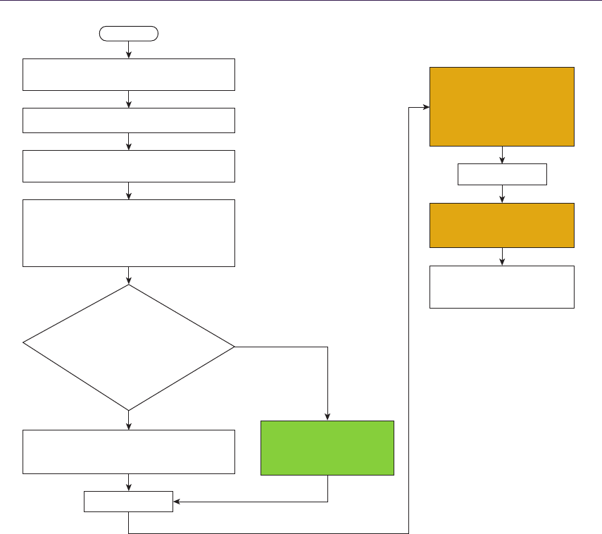
31.3. Algorithm 531
Generate G-buffer with view space Z, and ddx
ddy of view space Z, and other surface data
Start one compute shader per N×N pixels region
Load view space Z, ddx(viewSpaceZ)
and ddy(viewSpaceZ) for all samples
Using a ref pixel, calculate maximum
allowable view space Z-delta =
abs(ddx(viewSpaceZ)) + abs(ddy(viewSpaceZ))
Calculate maximum allowable normal variation
(could be loaded from constant buffer)
abs(viewSpaceZ[pixel] -
viewSpaceZ[refPixel]) >
N*√2*maxviewSpaceZDelta
OR
Normal variation >
maxNormalVariation
Yes
No
Calculate the low frequency
shading component only once
per N×N and save the results
to intermediate buffer
Process every N×N that requires
per pixel shading by
processing one such region
(or pixel) per thread
and save the results to
intermediate buffer
Start
Per pixel processing is required.
Append the pixel to append buffer by atomically
incrementing the index in groupshared memory
GroupSync()
GroupSync()
Add the results to corresponding
low frequency shading data from
intermediate buffer
Process every pixel per thread
for high frequency
component of the shading
Figure 31.1. Overview of the shading pass. The items in green are evaluated at lower frequency (once per
N×Npixels) and the items in orange are executed at once-per-pixel frequency.
Coarse pixel shading phase Regardless of whether we are able to reduce the shad-
ing frequency of the slowly varying shading term to the coarse rate or not, we
evaluate it at the top-left pixel. Using the analysis described for the analysis
phase, we find out where a shading term can be evaluated at the coarse rate and
we store its results in memory (groupshared or global). If the DPI is high enough
and there is no shading term that must be evaluated at the pixel rate, we can
splat the intermediate results to the other pixels in that coarse pixel. For the
other threads, we append their thread IDs to an append buffer in the groupshared

532 31. Deferred Coarse Pixel Shading
memory, indicating that the shading term needs to be evaluated at the other pix-
els in that coarse pixel. All threads within the group wait at the synchronization
point. By structuring the code this way, we have moved the shading term eval-
uation (often expensive) out of the control flow and reduced the control flow
divergence.
For the regions where we could not lower the shading rate, we change the
axis of parallelism from one thread per coarse pixel to one thread per pixel and
evaluate the shading term. The threads that evaluated the shading term at the
coarse rate wait at the group synchronization point. If the DPI is high enough,
there may be no need to do per-pixel shading. In this situation, the next phase
can be skipped altogether.
Pixel shading phase If there is a shading component that must be evaluated at
the pixel rate (or if the DPI is not high enough), we change the axis of parallelism
to one thread per coarse pixel again but now each thread processes all the pixels
in that coarse pixel and adds the results to the ones calculated in the previous
step.
31.3.3 Biasing the Sampler
Texturing is typically done in the forward passes and is not deferred. The G-
buffer was generated at a pixel frequency (with the assumption that shading will
be done once per pixel). However, we try to reduce the shading rate to once per
coarse pixel wherever possible during the shading pass. This introduces temporal
artifacts like shimmering. Possible solutions to this are
1. to sample the textures using a biased sampler (biased by log2N) during
the forward pass for the regions where the shading rate will be lowered;
2. to filter the texture data on the fly during the rendering pass.
The latter can increase the bandwidth significantly (depending on the size of
N). So, we propose to introduce an additional G-buffer component per tex-
ture that uses a biased sampler. This does add some cost to the G-buffer
generation.
The DirectX 11.2 Tier 2 specifications introduced minimum/maximum filter-
ing along with tiled resources. One way to optimize this algorithm even further
is to offload the minimum/maximum bounds calculation of the N×Nregion of
the G-buffer to a texture sampling unit. This frees the shader cores from loading
all the values and calculating the minimum/maximum. Shader cores reduce the
shading rate when the difference in the minimum and maximum is less than some
acceptable threshold. This technique might invoke some false positives because
it is more conservative than the one proposed in the shader-based solution.

31.4. Performance 533
Loop Count Power Plant Sponza
Pixel Coarse Pixel Savings Pixel Coarse Pixel Savings
(ms) (ms) (%) (ms) (ms) (%)
0 22.7 11.2 50.7 12.5 9.4 24.9
100 50.3 21.1 58.1 26.8 17.6 34.3
500 87.7 34.9 60.2 43.6 27.7 36.5
Table 31.1. Shading time (ms) when shading was reduced to 2×2 pixel blocks wherever
possible compared to when shading was performed every pixel.
31.4 Performance
We measured our performance on a system with Windows 8.1, running with an
Intel HD 5500 integrated GPU. We used scenes that we felt were representative
of game assets. We used two scenes, the power plant scene and the Sponza scene.
Each scene was lit with 1024 colored point lights. Our rendering equation consists
of the diffuse and the specular terms. We tried to reduce the frequency at which
the entire rendering equation is evaluated to once per coarse pixel of the size 2×2
pixels. We could do that because our DPI was high enough at 1920×1080 pixels.
At this DPI, we did not have a shading term that had to be evaluated at the pixel
rate. To mimic how the performance would change for more expensive shaders,
such as AO cone tracing, we added a dummy loop inside our shader to make
it more compute intensive and varied the loop length as a parameter. In some
cases, users may want to evaluate certain coefficients in the rendering equation
at the lower rate, but the actual rendering equation could be evaluated at the
higher rate. The algorithm proposed here is fully generic and one can lower the
frequency of only some parts of the rendering equation.
Table 31.1 summarizes the performance benefits of reducing the shading rate
as a function of shader length. We see anywhere from 25% to 60% improvement
in the shading time depending upon the shader complexity. For a given scene,
we see higher gains if the shader is more complex. However, sampling the albedo
texture using a biased sampler and storing that as an extra G-buffer component
increases the G-buffer generation time only by 2.2 ms and 1.9 ms for the power
plant and the Sponza scenes, respectively. (See Figure 31.2.) As a result, we see
this technique as a net win.
31.5 Conclusion
We have presented a technique to reduce the shading costs during deferred shad-
ing. The same technique is applicable to postprocessing passes, too. With this
technique developers can apply their postprocessing effects at a reduced rate with
minimal impact to image quality.
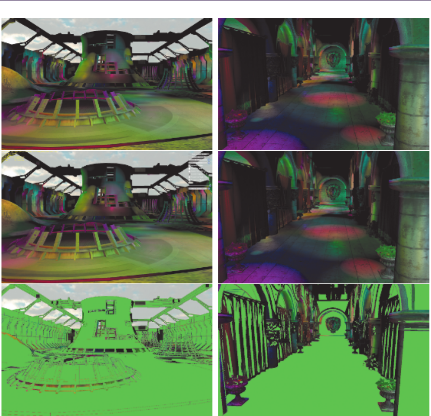
534 31. Deferred Coarse Pixel Shading
Figure 31.2. The power plant scene (left) and the Sponza scene (right). Coarse pixel size was 2 ×2 pixels.
Top row images were rendered at the full pixel resolution. Middle row images were rendered with coarse
pixel shading wherever possible. Bottom row shows in green the regions where shading was reduced to
coarse pixel rate.
Demo
A real-time demo implemented using DirectX shader Model 5.0 will be available
on the Intel Developer Zone (https://software.intel.com/en-us).

Bibliography 535
Bibliography
[Lauritzen 10] A. Lauritzen. “Deferred Rendering for Current and Future Ren-
dering Pipelines.” SIGGRAPH Course: Beyond Programmable Shading, Los
Angeles, CA, July 29, 2010.
[Pool 12] J. Pool. “Energy-Precision Tradeoffs in the Graphics Pipeline.” PhD
thesis, Univeristy of North Carolina, Chapel Hill, NC, 2012.
[Pranckeviˇcius 09] A. Pranckeviˇcius. “Compact Normal Storage for Small G-
Buffers.” http://aras-p.info/texts/CompactNormalStorage.html, 2009.
[Vaidyanathan et al. 14] K. Vaidyanathan, M. Salvi, R. Toth, T. Foley, T.
Akenine-Moller, J. Nilsson, J., et al. “Coarse Pixel Shading.” Paper presented
at High Performance Graphics, Lyon, France, June 23–25, 2014.

32
Progressive Rendering Using
Multi-frame Sampling
Daniel Limberger, Karsten Tausche,
Johannes Linke, and J¨
urgen D¨
ollner
32.1 Introduction
This chapter presents an approach that distributes sampling over multiple, con-
secutive frames and, thereby, enables sampling-based, real-time rendering tech-
niques to be implemented for most graphics hardware and systems in a less com-
plex, straightforward way. This systematic, extensible schema allows developers
to effectively handle the increasing implementation complexity of advanced, so-
phisticated, real-time rendering techniques, while improving responsiveness and
reducing required hardware resources.
The approach is motivated by the following observations related to 3D system
and application development:
•Creating advanced rendering techniques and computer graphics systems is
intriguing in the case of target platforms equipped with the latest graphics
hardware. Business and industry applications, however, are often strongly
constrained in terms of both hardware and API support: software and hard-
ware adapt slowly to new APIs and are often limited in terms of available
processing power and video memory, e.g., with regards to high-resolution
image generation. Thus, it sometimes takes years for state-of-the-art, real-
time rendering techniques to become a core part of 3D systems and appli-
cations in business and industry.
•Many 3D systems and applications do not require a strictly continuous
stream of high-quality images. For example, in interactive visualization of
static data, which is common for digital-content-creation tools, the render-
ing process can be partially paused as user interactions and data changes
537

538 32. Progressive Rendering Using Multi-frame Sampling
occur less frequently. Thus, strict real-time, high-quality imaging con-
straints can sometimes be lessened.
•The adoption of the latest rendering techniques in 3D systems and applica-
tions is faced with increasing software complexity and increasing hardware
requirements due to their single-frame design, e.g., designing, implementing,
and testing complex, shader-based, multi-platform rendering techniques. In
particular, this phenomenon increases financial and technical risks in system
and application development.
The key idea of our approach, multi-frame sampling, is based on, technically
speaking, the following idea: Instead of rendering a single frame in response
to an update request, multiple frames are rendered and accumulated. Thereby,
every accumulation result can be immediately displayed while the frame qual-
ity progressively increases. We demonstrate our approach for a variety of ren-
dering techniques, i.e., antialiasing (AA), depth of field (DoF), soft shadows,
and screen-space ambient occlusion (SSAO), as well as order-independent trans-
parency (OIT). Progressive rendering using multi-frame sampling allows us to
use rather simple implementations of rendering techniques to produce state-of-
the-art effects. Furthermore, the multi-frame approach usually reduces memory
usage, decreases rendering cost per frame (lower response time), allows for better
maintainable implementations, and provides more comprehensible parameteriza-
tions.
32.2 Approach
An integral part of today’s hardware-accelerated, real-time rendering technolo-
gies is built on sampling, as the “process of rendering images is inherently a sam-
pling task” [Akenine-M¨oller et al. 08]. Sampling is generally used to approximate
continuous characteristics and signals, e.g., reducing aliasing artifacts caused by
insufficient depictions of continuous domains. For single-frame rendering, sam-
pling is limited to a single frame. Increasing the number of samples improves the
resulting image quality but also increases the rendering costs per frame in terms
of time and memory.
Our multi-frame sampling approach distributes samples over a well-defined
number nMF of consecutive frames. With each frame we progressively increase
image quality while having reduced cost per frame and still being able to process
massive amounts of samples. Each frame generated during multi-frame sampling
uses a unique subset of samples of a well-defined set of samples called the kernel.
Consecutive frames are accumulated until nMF frames are generated and the
rendering finally pauses. On any update request, the accumulation process is
restarted.

32.2. Approach 539
Multi-frame:
1 LowRes Shadow Map
1× res Color/Depth
3 G-/Accum-Buffers
Single-frame:
4 HighRes Shadow Maps
4x res Color/Depth
4 G-Buffers
Shadow Mapping, 4 lights
Accumulation 1
Geometry Rendering,
2 draw calls, 4x SSAA
DoF separatedShading
SSAO,
24 samples, separated blur
Composition
tTime
SSAO, 8 samples, no blur
Accumulation nMF
...
Figure 32.1. Conceptual illustration of a typical single-frame rendering structure transformed into a multi-
frame rendering structure: Only one shadow pass instead of four, and 8 SSAO samples instead of 24, are
used. DoF and AA are inherently available due to camera and NDC (normalized device coordinate) space
shifting. The required resources are reduced, and to increase quality, more frames can be rendered and
accumulated.
Assumptions The application of multi-frame sampling in 3D systems and appli-
cations is based on the following assumptions:
•The underlying rendering uses sampling as one of its elements.
•Rendering update requests are less frequent, and responsiveness in terms of
frames per second is favored over intermediate frame quality.
•The converging image quality is not disruptive to the use cases or usability
of 3D systems and applications.
Implementation To transform a given single-frame, sampling-based technique into
a multi-frame technique, we proceed as follows:
1. We identify segments within the technique that are processed repeatedly.
A parameterization that controls an iteration per frame (e.g., number of
samples) often indicates such segments. These iterations are unrolled, which
causes samples to be distributed over consecutive frames (Figure 32.1).
2. We have to verify that (a) an increase in number of executions of a segment
results in better quality and (b) each segment’s result can be accumulated
throughout multiple consecutive frames.
3. We adapt the original technique such that it supports an appropriate sam-
pling characteristic: the sampling type (single or multiple samples per
frame) and the spatio-temporal distribution of samples.

540 32. Progressive Rendering Using Multi-frame Sampling
When multi-frame sampling is used with multiple techniques simultaneously,
depending on their assembly, there might be combinations that require special
attention, for example, stochastic per-fragment discarding combined with screen-
space ambient occlusion.
The remainder of this chapter describes sampling strategies and frame ac-
cumulation. For a variety of rendering techniques, associated multi-frame ap-
proaches are discussed (Section 32.3). Within each of these sections, results are
discussed and brief performance remarks are given. All code snippets are based
on GLSL and C++ using the OpenGL API.
32.2.1 Sampling Strategies
For multi-frame sampling we distinguish between techniques processing either
one or multiple samples per frame. A single sample per frame is taken from a
kernel, which is precomputed on the CPU and provided as a uniform (usually
float,vec2, or vec3). For every subsequent frame, the uniform is updated (per
technique). When using multiple samples per frame, the kernel is precomputed
on the CPU as well but then uploaded to the GPU encoded as a uniform buffer,
texture, or buffer (depending on kernel’s size and shader capability). Since the
rendering can unfold over multiple frames, most rendering techniques can be
reduced to their core concept. Neither performance-related caching nor other
optimization strategies are required. Furthermore, some techniques are virtually
for free because they are inherent to multi-frame rendering (e.g., AA, DoF).
Nevertheless, the final rendering quality and especially the convergence speed
and its “temporal tranquility” strongly depend on a well-designed kernel. The
kernel’s characteristics include
•required number of samples for targeted quality,
•spatial distribution or value-based distribution,
•sample regularity and completeness for finite accumulation,
•temporal convergence constraints regarding the sequence of samples,
•additional per-fragment randomization.
Since we do not use GPU-based pseudo-randomness and all samples are typ-
ically precomputed and designed for a specific multi-frame number nMF, accu-
mulating additional frames on top of that is futile. Especially when passing low
multi-frame numbers, this may lead to temporal clustering. The presented tech-
niques have been implemented based on the open-source, header-only libraries
glm [Riccio 15] and glkernel [Limberger 15] used for dynamic computation of
kernels of required characteristics at runtime.

32.2. Approach 541
1// w eight = 1.0 / n, with n e nu me rating the c ur re nt multi - f rame .
2un iform flo at weight;
3...
4{
5...
6vec 3 a = texture( a cc umB uff er , v_ uv ). r gb ;
7vec 3 c = texture( f ra meB uff er , v_ uv ). r gb ;
9// av erage is pointing to the ac cu mulatio n t arget .
10 av erage = mix ( a , c , we igh t ) ;
11 }
Listing 32.1. Example of an accumulation GLSL fragment shader adding the last frame
to the overall average; frameBuffer contains the nth frame’s color and accumBuffer the
last average. Texture filtering is set to nearest filtering for both texture objects.
32.2.2 Frame Accumulation
The accumulation of consecutive frames can be implemented using hardware-
accelerated blending. Alternatively, the accumulation can be executed as an
additional postprocessing pass. Either a screen-aligned triangle with a fragment
shader or, if available, a compute shader can be used to average all existing
frames. For this, the accumulation buffer is set up as an input texture and a
color attachment of the target framebuffer object simultaneously. The current
frame is provided as a second input texture. The color cof the nth frame is read
and added to the previous average a:a=c/n +a(1 −1/n). This works with a
single accumulation buffer (no ping pong; reduced memory footprint) as long as
no adjacent fragments are processed (Listing 32.1).
On update requests, multi-frame rendering is reset to a multi-frame number
of 1 and accumulation is just blitting this frame; accumulation is skipped and
the frame is rendered into the accumulation buffer directly. The accumulation
buffer’s texture format should support sufficient accuracy (16I or 32F) because
the weight for frame averaging gets subsequently smaller (Figure 32.2).
Since the scene and its underlying data is assumed to be static during accu-
mulation, the time per frame is roughly constant for subsequent frames. Thus,
individual sampling characteristics can be adapted ad hoc for the second and
all subsequent frames to approach the constrained frame time (e.g., decrease or
increase number of samples per frame). Alternatively, vertical synchronization
can be turned off during accumulation. In our tests we experienced no tearing
artifacts because the expected, consecutive differences converge to zero. Apart
from that, extensions for application-controlled synchronization could be used to
exclude artifacts entirely.

542 32. Progressive Rendering Using Multi-frame Sampling
R11FG11FB10F RGB16F RGB8 RGB16 RGB32F
Figure 32.2. Accumulation results (test scene, AA and DoF) for 1024 frames using
various texture formats. From left to right, the quality is (obviously) increasing.
32.3 Multi-frame Rendering Techniques
One motivation for multi-frame sampling is to have better control of the adjust-
ment of the rendering quality, while implementing against older, limited APIs
and conserving as many GPU resources as possible. Even though the techniques
discussed in this section do not always reflect state-of-the-art techniques, they
have been picked to express the required (re)thinking when creating multi-frame
rendering techniques. They are intended as blueprints for the transformation of
other sampling-based techniques.
32.3.1 Multi-frame Antialiasing
Without taking specific countermeasures, image synthesis based on rasterization
depicts a continuous domain and, thus, usually contains aliasing artifacts like
jagged edges and moir´e patterns. Antialiasing is commonly applied to mitigate
these artifacts, e.g., super-sampling and multi-sampling: Color or depth buffers
are rendered at a higher resolution than the output resolution. While these buffers
provide good results for single-frame-constrained applications, they use a lot of
processing power and memory. Alternatively, several sampling strategies for post-
processing have been created, e.g., AMD’s MLAA, NVIDIA’s FXAA, and Intel’s
CMAA. Varying in their performance and quality, these all provide a comparably
low memory footprint. With temporal antialiasing, another type of antialiasing
was introduced recently: NVIDIA’s TXAA and subsequently MFAA [NVIDIA 15]
claim to result in better quality and increased performance in comparison to
MSAA. Temporal antialiasing already uses varying sampling patterns and infor-
mation from multiple consecutive frames, albeit limited (two subsequent frames)
as they are still designed for single-frame rendering.
Approach For our implementation, a sampling offset in [−0.5,+0.5] is semi-
randomly chosen per frame. The offset is then transformed into a subpixel off-
set and added to the vertices’ xy-coordinates in normalized device coordinates

32.3. Multi-frame Rendering Techniques 543
1in vec3 a _ve rte x ;
2un iform mat4 mvp ; // Model view pr oj ec tion
3// Per - frame offse t in [ -0.5 ,+0.5] , pre - multiplied by
4// 1.0 / v iew por t si ze .
5un iform vec2 ndcOffset ;
6...
7vec 4 nd cV er te x = mvp * vec4(a_vertex , 1.0);
9// Shift the vie w fru stu m withi n the subpixel ex tent .
10 nd cV er te x . xy += n dc Of fs et * n dc Vertex .w;
11 gl _P osition = nd cVe rtex ;
Listing 32.2. A GLSL vertex shader for progressive multi-frame antialiasing.
(NDC), effectively shifting the complete NDC space (Listing 32.2). Note that
shifting the camera’s position and center in world space does not work due to the
parallax effect.
Sampling characteristics Pseudo-randomly chosen offsets within a square work
surprisingly well. The convergence can be speed up by using uniform, shuf-
fled samples or common sampling patterns [Akenine-M¨oller et al. 08]. For our
implementation we use shuffled Poisson-disk sampling to generate a uniform dis-
tribution of offsets for a specific number of frames (Listing 32.3). This prevents
clustering of “pure” random sampling and provides better convergence than reg-
ular patterns for a large number of samples (e.g., eight or more), which are
nontrivial to calculate for an arbitrary number of samples. Due to the random
distance between consecutive offsets, the image tends to shift noticeably by up
to one pixel during the first few frames. This can be almost eliminated by con-
straining the first sample to the center of the pixel (offset [0.0,0.0]). Sorting all
offsets by their length (i.e., the distance to the pixel center) is not recommended:
Although it reduces the subtle shifting further, it also results in temporal clus-
tering. Finally, to avoid clustering at pixel edges and corners of adjacent pixels,
we use a tile-based Poisson-disk sampling (Figure 32.3).
Performance and remarks Accumulation of only a few frames usually results in
decent antialiasing. With Poisson-disk sampling, it takes about 16 frames for a
result that appears optimal and about 64 frames until subsequent frames yield
no visual improvements anymore. In comparison, pseudo-random sampling takes
about 1.3 times longer to yield comparable quality and, additionally, is less pre-
dictable due to clustering. As an addition, blurring can be applied by increasing
the offsets and using an appropriate distribution.
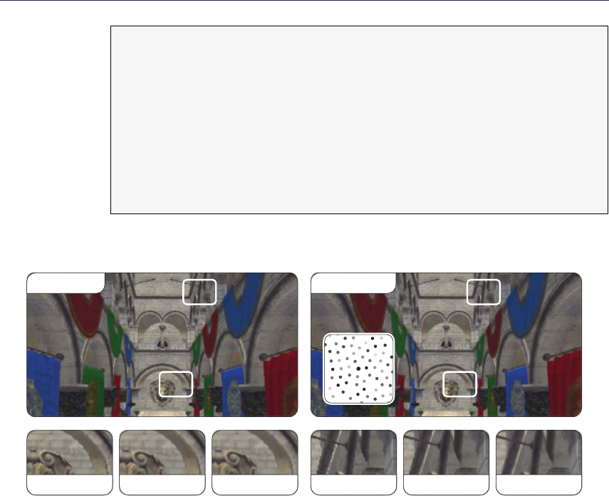
544 32. Progressive Rendering Using Multi-frame Sampling
1// 3 D array of glm :: vec2 values wi th e xtent : 64 x1x1 ( gl ke rnel )
2aut o aa Sam ples = g lke rnel :: ke rne l2 { 64 };
3g lk er nel :: s a mpl e : : p oi s so n_ sq u ar e ( a aSa mpl es , -.5 f , . 5 f );
4gl ke rn el :: s huffle :: rand om ( aaSamples , 1); // From index 1 to last
6wh ile ( rendering )
7{
8...
9const auto n dc Of fs et = a aS am ples [ a ccumCount ] / view po rt ;
10 pr ogr am . se tUnifo rm (" n dc Of fs e t " , n dc Of fs et );
11 ...
12 }
Listing 32.3. C++ example for an AA sample computation using glkernel.
1st frame 64th frame
1 sample 4 samples 16 samples 1 sample 4 samples 16 samples
Figure 32.3. Sponza scene rendered with multi-frame AA (shuffled Poisson). The dots depict a 64-sample
kernel, encoding its sequence from dark to light gray, starting at the center (big circle).
32.3.2 Multi-frame Depth of Field
Depth of field is an effect that can be used to guide a users attention to a certain
region within a scene. The effect blurs objects depending on their distance to a
chosen focal plane or point, which usually lies on an object or region of interest.
DoF is often implemented at postprocessing, mixing the sharp focus field with
one or two (near and far field) blurry color buffers per fragment, based on the
fragment’s distance to the focal point or plane [Bukowski et al. 13]. More ad-
vanced techniques are also available, usually reducing boundary discontinuities
and intensity leakage artifacts as well as accounting for partial occlusion by using
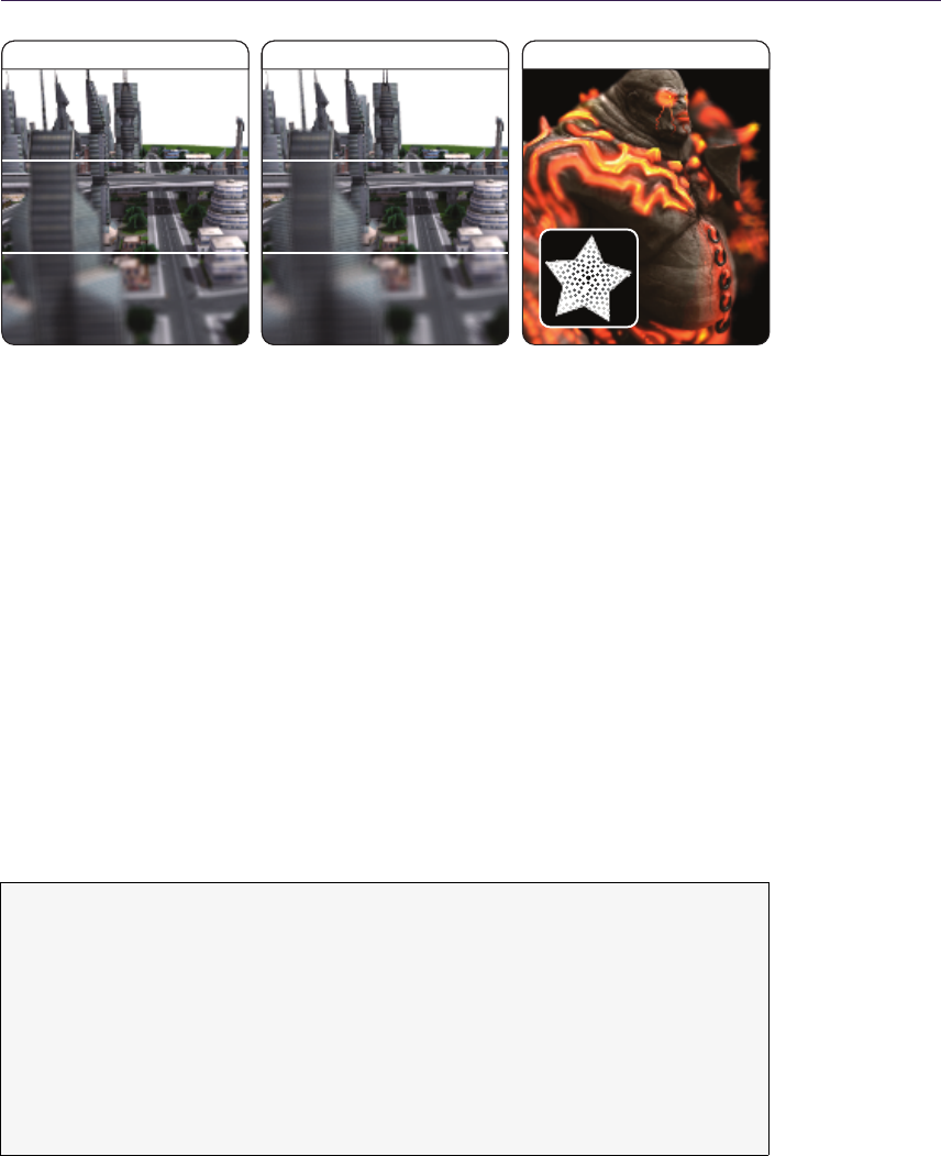
32.3. Multi-frame Rendering Techniques 545
Medium circle of confusion Large circle of confusion Bokeh DoF, 128 samples
Figure 32.4. Multi-frame DoF with (top to bottom) 4, 16, and 64 samples for medium
and large CoC. The sequence of 128 samples is depicted from dark to light gray.
multiple focus layers [Schedl and Michael 13,Selgrad et al. 15]. Even though
multi-layer approaches can be adapted to multi-frame rendering, we present a
minimal approach favoring rendering speed over convergence time and enabling
high-quality DoF.
Approach For DoF we use a random two-dimensional vector on a unit disc as per-
frame sample. This vector indicates for each point in a scene, where on its circle
of confusion (CoC ) it should be rendered on the image plane. With subsequent
sampling, each point gradually covers its circle of confusion. Similar to our AA
approach, the sample vector is added to the vertices’ xy-coordinates in a vertex
shader, this time, however, in view space before applying the projection matrix.
It is scaled with the vertices’ z-distance to the chosen focal plane. Additional
postprocessing passes per frame, e.g., separated blurring, are not required. (See
Figure 32.4.)
1// z - d i sta nc e to t he c ame ra at w hic h ob je ct s are s har p
2un iform flo at f oca lDi st ;
3// Point in c ircle of co nf us io n ( opt . pre - mu lt ip lied by scale )
4un iform vec2 cocPoint ;
5...
6{
7...
8vec4 vi ew Ve rtex = modelView * vec4(a_vertex , 1.0);
9vi ewV ertex .xy += cocPoint * ( v iew Vertex . z + focalD ist ) ;
10 gl_Position = pr ojection * vi ew Ve rt ex ;
11 }

546 32. Progressive Rendering Using Multi-frame Sampling
Sampling characteristics Similar to multi-frame antialiasing, random sampling
works but results in comparatively long convergence times. Furthermore, frag-
ments of points distant from the focal plane are spread widely on the screen,
causing substantially unsteady output in the first few frames. To prevent this,
Poisson-disk samples are sorted by the distance to the center. The center is used
as the initial sample again, omitting shifting for consecutive update requests. By
that, the effect gradually increases until all samples have been processed. Arbi-
trary Bokeh shapes can be easily accounted for by masking the samples with the
desired shape:
1auto dofSam ple s = gl ker nel :: k ern el2 { 128 };
2g lk er nel :: s a mpl e : : p oi s so n_ sq u ar e ( d of Sam ple s , - 1.f , 1. f ) ;
3// Opt . mas k e ver y sa mpl e by i ts po si tio n us ing a b it fi eld
4gl ker ne l :: ma sk :: b y_v alue ( do fSa mple s , bi tma sk );
5// Sort by di st to ref
6g lk er nel :: s or t :: di st an ce ( d of Sa mpl es , 0. f , 0 . f );
Performance and remarks The number of required samples to produce an “artifact-
free” image depends on the largest CoC any point in the scene has, which in
turn is proportional to the desired effect scale as well as the point’s distance to
the focal plane. Although it may seem counterintuitive, scaling the number of
required samples linearly with the CoC’s radius, at least for reasonably large
CoCs, results in sufficient image quality. We found a sample count (and thus,
frame count) about ten times the radius in pixels to be sufficient. While this can
mean a few seconds to full convergence in extreme cases, keep in mind that the
effect’s strength gradually increases over time.
For implementing a focal point instead of a focal area, one can scale the
sample by the vertices’ distance to that point. If a strong blurriness for out-of-
focus objects in combination with a large focal area is desired, the vertex shader
could be extended accordingly.
32.3.3 Multi-frame Soft Shadows
Shadow mapping is an omnipresent technique in real-time computer graphics.
The original approach renders distances as seen from a light. Advanced variations
improve on problems like heavy aliasing and hard edges at the cost of additional
texture lookups per fragment, more computations, or additional passes. While
soft shadows cast by occluders of large distance to the receiver can be handled
well, correctly and efficiently modeling shadow casting of area lights is still a
problem for single-frame techniques.
Approach For our approach, we use the most-basic shadow mapping and take
only a small number of lights into account per frame. For multi-frame shadow

32.3. Multi-frame Rendering Techniques 547
mapping, the lights’ surfaces are randomly sampled: For each frame, a random
position on each of the selected lights is used for shadow map rendering as well
as scene lighting and shading. Accumulating multiple frames results in realistic
and aliasing-free soft shadows with large penumbras.
Sampling characteristics Good convergence is achieved by uniformly sampling the
surfaces of all lights. For very large area or volumetric lights, we used an approach
similar to the previously described multi-frame DoF, starting with sampling the
light in its center and slowly progressing toward its edges, gradually increasing
the penumbras. If multiple light sources of various areas/volumes are used, each
light should be accounted for at least once per frame. Lights of larger surfaces
should be sampled preferentially.
Performance and remarks The convergence time depends on the maximum penum-
bra width, which in turn depends on the size of the area lights and their relation
to occluding and receiving scene objects. Similar to DoF, we experienced that
the number of samples required for a completely banding-free result correlates to
the largest penumbra width in the screen space. Convergence can be greatly im-
proved, e.g., by applying variance shadow mapping [Donnelly and Lauritzen 06]
combined with perspective shadow maps [Stamminger and Drettakis 02]. We also
found that surprisingly low shadow map resolutions can provide visually pleasing
shadows: A resolution of 128 ×128 pixels, for example, does not result in any
distracting artifacts, although smaller objects and scene details were not captured
and contact shadows were inadequate (Figure 32.5).
Since our approach relies on sampling light surfaces, all lights should show
at least a certain surface (larger for lower shadow map resolutions). Even for
hard cases (imagine a large TV illuminating a room with nearby occluders), the
presented approach is able to provide correct shadows of high quality, albeit with
increased convergence times. For a correct illumination induced by large numbers
of local lights, our basic frame accumulation of non-HDR lights currently conflicts
with partial light sampling.
32.3.4 Multi-frame Screen-Space Ambient Occlusion
The complex interactions of real-world objects and lights pose a significant chal-
lenge even for today’s most sophisticated real-time rendering engines. SSAO
is typically used to capture local effects of real-world lighting. Since Crytek’s
initial concept, numerous variants and enhancements have been proposed (e.g.,
HBAO+, SSDO). Due to the performance-intensive nature of these effects, they
use different optimizations at the cost of quality: e.g., blurring the occlusion map
to mask the noise (and its resulting shower-door artifacts) is usually suggested.
Multi-frame approaches can also be found: For example, using reverse repro-
jection provides higher temporal coherence but introduces additional complexity
and resource requirements (history buffers) and utilizes only the previous frame.
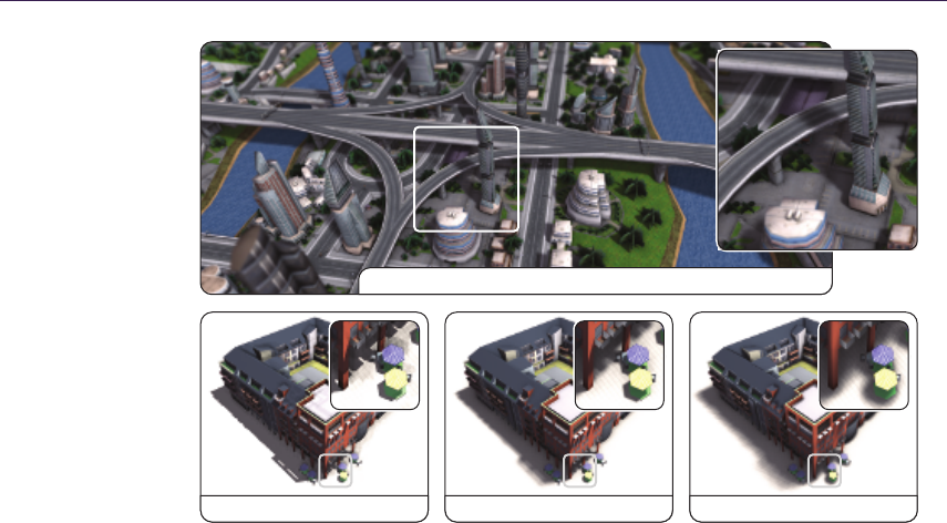
548 32. Progressive Rendering Using Multi-frame Sampling
10242 px, 1st frame 10242 px, 16 frames 1282 px, 64 frames
32 frames for 10242 px shadow map sampling an area light
Figure 32.5. Soft shadows using area light sampling and basic shadow mapping.
Approach We use the original SSAO as the basis for our multi-frame approach.
In order to mitigate banding artifacts produced by using the same sampling
kernel for all pixels, the original implementation randomly rotates the kernel per
pixel. This in turn introduces noise to the image, which is masked by blurring.
When using multi-frame sampling, the noise is mitigated within a few frames
even without blurring. In fact, removing the blur pass results in a better final
image quality. The random rotation can also be removed, although the banding
artifacts are more noticeable and result in a more unsteady image during the first
few frames.
Sampling characteristics We use Poisson-disk sampling with best-candidate opti-
mization to uniformly distribute points in a unit sphere that are used as sampling
offsets. Compared to a single-frame approach, a lower sample count per frame
can be used to accommodate for low-end devices. If desired, all samples can be
assigned a random length within the unit sphere and can be sorted by this to
account for local ambient occlusion effects for early frames. As for DoF, this
reduces noise and banding artifacts resulting in a less disruptive effect.
Performance and remarks For this effect the number of frames required for a con-
verging image is again dependent on its desired parameters, more specifically
its radius. For moderate settings we found that about 480 samples provided a
nearly artifact-free result, i.e., 60 frames when using 8 samples per frame. For

32.3. Multi-frame Rendering Techniques 549
small radii, removing the random rotation actually improves convergence times,
reducing the adequate number of samples by two thirds. Since the more recent
screen-space ambient occlusion and obscurance approaches rely on sampling the
depth buffer multiple times per frame as well, they should be similarly easy to
adapt to multi-frame sampling.
32.3.5 Multi-frame Transparency
Rendering transparent objects is often avoided in real-time rendering systems.
Most approaches either achieve high performance by neglecting correctness and
thus quality, or produce credible results by using many rendering passes or super-
sampling while lowering rendering performance. Additionally, they are hard to
integrate into deferred rendering systems (except that k-buffer rendering is avail-
able).
Screen-door transparency [Mulder et al. 98] applies a threshold pattern to
small groups of fragments; within each group, fragments with an opacity value
lower than their threshold are discarded. Drawbacks comprise highly visible
patterns and insufficient accuracy. Stochastic transparency [Enderton et al. 10]
improves on that by applying random patterns per pixel using multi-sampling,
but still produces slightly noisy output for a single frame. The suggested multiple
passes per frame can be transformed to a 1:1 frame mapping for multi-frame
rendering of fast converging transparency.
Approach We discard super-sampling (color and coverage sampling) due to the
heavy resource implications. Instead, transparent fragments are discarded based
on a single random opacity threshold per fragment or object at a time. (See Fig-
ure 32.6.) Thus, using per-fragment thresholding with back-face culling disabled,
we achieve correct order-independent transparency.
Sampling characteristics The technique’s implementation is straightforward, but
special care must be taken to generate “good” per-fragment randomness. Based
on stochastic transparency, a mapping of ndistinct opacity values in the range
[0,1] to associated bitmasks is precomputed on the CPU and provided to the
GPU (Figure 32.7). For example, for an opacity of 0.8 and bitmask size of 1024,
a bitmask of about 0.8·1024 = 819 uniformly distributed (avoiding clusters)
bits is computed. Additionally, random, fragment-specific offsets can be used to
shuffle the threshold access between adjacent fragments over time. For object-
based transparency, no objects should be discarded within the first frame. Thus,
all objects are initially opaque and gradually converge toward their individual
opacity (limiting minimal opacity to 1/n for nframes). For all consecutive frames,
the object-based bit masking skips the draw call or discards fragments based on
an object ID (Figure 32.7).
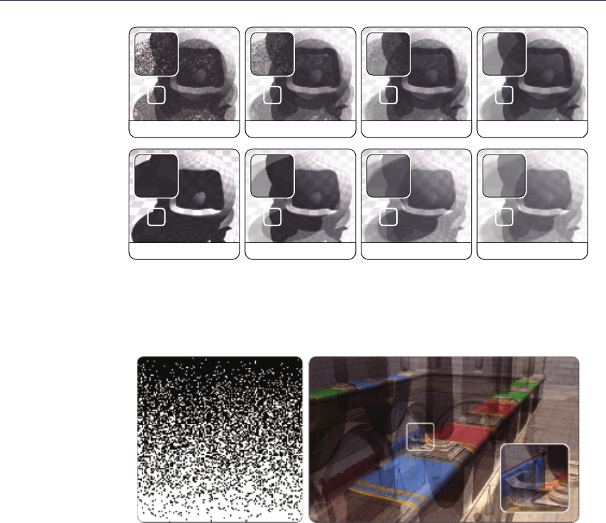
550 32. Progressive Rendering Using Multi-frame Sampling
1st frag. samples 4 frag. samples 16 frag. samples 1024 frag. samples
1st obj. samples 4 obj. samples 16 obj. samples 1024 obj. samples
Figure 32.6. Convergence for per-fragment (top row) and per-object (bottom row)
transparency thresholding. For per-fragment thresholding, back-face culling is on. Note
the two distinct shadows resulting from the inner and out sphere.
Figure 32.7. Kernel used for transparency masking. Left: For 128 opacity values from 0
(top) to 1 (bottom), 128 uniformly distributed bits (left to right) are computed. Right:
This kernel can be used for per-fragment as well as per-object discarding, the latter
shown here, but with 1024 instead of 128 bits per mask.
Performance and remarks Stochastic transparency usually requires full multi-
sampling within a single pass with up to 16 coverage samples per fragment,
requiring extreme amounts of memory. In contrast, multi-frame transparency
requires no additional memory at all. The amount of frames required for a low-
noise transparency is dependent on the depth complexity of the current scene
and camera angle. While direct use of more advanced techniques like stochastic
transparency might lead to shorter convergence times, we prefer the more basic
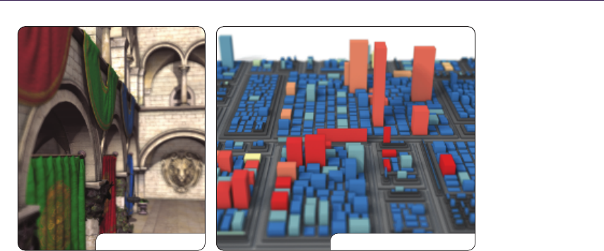
32.4. Conclusion and Future Work 551
2.5D Treemap, 16 framesSponza, 16 frames
Figure 32.8. Multi-frame sampling applying the presented techniques all together.
approach for its low memory footprint, minimal performance overhead per frame,
and implementation simplicity.
A major drawback for pixel-based transparency is that it can hardly be com-
bined with some postprocessing techniques, e.g., SSAO, as the G-buffers of indi-
vidual frames are highly noisy and do not show coherent surfaces. In contrast,
though still not completely accurate, object-based transparency shows SSAO re-
sults on transparent objects and even on objects overlaid by them; this is usually
difficult to achieve in conventional real-time rendering. Using object-based trans-
parency, however, (1) opacity cannot be determined via texturing anymore, and
(2) back-faces as well as concave objects cannot be rendered adequately (at least,
not without additional draw calls) and might result in inaccuracies.
32.4 Conclusion and Future Work
We have presented an approach to transform and integrate sampling-based ren-
dering techniques into a progressive multi-frame rendering system (Figure 32.8).
It allows us to focus on sampling and its characteristics instead of optimizations
necessary for satisfying single-frame limitations. It favors low response times and
low-level APIs over per-frame quality. Furthermore, at least for the discussed
techniques, a better maintainability and simpler, easy-to-understand parameter-
ization in terms of target quality and effect characteristics is derived. From a
software-engineering perspective, our approach reduces the implementation com-
plexity of 3D systems and applications that need to combine independent, real-
time rendering techniques.
The current limitations and future challenges include the following topics:
When using multiple multi-frame techniques simultaneously, sampling parame-

552 32. Progressive Rendering Using Multi-frame Sampling
terization of all effects is to be coordinated for the targeted number of frames.
In addition, some techniques might not be used in combination (e.g., pixel-based
transparency with SSAO), and interaction issues arise for, e.g., picking or coor-
dinate retrieval because depth and ID buffers cannot be accumulated in a mean-
ingful way.
For future work, automatically adapting kernel parameterization to hardware
and frame rendering times is desirable. Additional research comprises strategies
for optimal convergence, a generic multi-frame rendering template for sampling-
based rendering techniques, and finally, the evaluation of other techniques’ appli-
cability (e.g., image-based reflections, translucency, massive lighting, subsurface
scattering).
32.5 Acknowledgment
This work was funded by the Federal Ministry of Education and Research
(BMBF), Germany, within the InnoProfile Transfer research group “4DnDVis”
(www.4dndvis.de).
Bibliography
[Akenine-M¨oller et al. 08] Tomas Akenine-M¨oller, Eric Heines, and Naty Hoff-
man. Real-Time Rendering, Third edition. Natick, MA: A K Peters, Ltd.,
2008.
[Bukowski et al. 13] Mike Bukowski, Padraic Hennessy, Brian Osman, and Mor-
gan McGuire. “The Skylanders SWAP Force Depth-of-Field Shader.” In
GPU Pro 4, edited by Wolfgang Engel, pp. 175–184. Boca Raton, FL: A K
Peters/CRC Press, 2013.
[Donnelly and Lauritzen 06] William Donnelly and Andrew Lauritzen. “Variance
Shadow Maps.” In Proceedings of the 2006 Symposium on Interactive 3D
Graphics and Games,I3D ’06, pp. 161–165. New York: ACM, 2006.
[Enderton et al. 10] Eric Enderton, Erik Sintorn, Peter Shirley, and David Lue-
bke. “Stochastic Transparency.” In Proc. of the 2010 ACM SIGGRAPH
Symposium on Interactive 3D Graphics and Games,I3D ’10, pp. 157–164.
ACM, 2010.
[Limberger 15] Daniel Limberger. “Kernel Utilities for OpenGL (glkernel).”
https://github.com/cginternals/glkernel, 2015.
[Mulder et al. 98] Jurriaan D. Mulder, Frans C. A. Groen, and Jarke J. van Wijk.
“Pixel Masks for Screen-Door Transparency.” In Proceedings of the Confer-
ence on Visualization ’98,VIS ’98, pp. 351–358. Los Alamitos, CA: IEEE
Computer Society Press, 1998.

Bibliography 553
[NVIDIA 15] NVIDIA. “Multi-frame Sampled Anti-aliasing (MFAA).” http://
www.geforce.com/hardware/technology/mfaa/technology, 2015.
[Riccio 15] Christophe Riccio. “OpenGL Mathematics (GLM).” http://glm.
g-truc.net/, 2015.
[Schedl and Michael 13] David Schedl and Wimmer Michael. “Simulating Partial
Occlusion in Post-Processing Depth-of-Field Methods.” In GPU Pro 4, edited
by Wolfgang Engel, pp. 187–200. Boca Raton, FL: A K Peters/CRC Press,
2013.
[Selgrad et al. 15] Kai Selgrad, Christian Reintges, Dominik Penk, Pascal Wag-
ner, and Marc Stamminger. “Real-time Depth of Field Using Multi-layer
Filtering.” In Proceedings of the 19th Symposium on Interactive 3D Graph-
ics and Games,i3D ’15, pp. 121–127. New York: ACM, 2015.
[Stamminger and Drettakis 02] Marc Stamminger and George Drettakis. “Per-
spective Shadow Maps.” In Proceedings of the 29th Annual Conference on
Computer Graphics and Interactive Techniques,SIGGRAPH ’02, pp. 557–
562. New York: ACM, 2002.

About the Contributors
Ulf Assarsson is an associate professor at Chalmers University of Technology. His
main research interests are real-time shading, hard and soft shadows—including
shadows in hair, fur, smoke, and volumetric participating media—GPGPU algo-
rithms, GPU ray tracing, and real-time global illumination. He is also coauthor
of the book Real-Time Shadows (2011).
Florian Bagar is a Rendering Software Engineer at Havok Inc., in Southern Ger-
many. He previously worked as a Senior Programmer at Sproing Interactive
Media GmbH. He studied computer graphics and digital image processing at the
Vienna University of Technology, where he received an MSc degree in 2010. His
current interests include real-time rendering, game development, multi-platform
development, optimization, and engine design.
Markus Billeter holds an MSc degree in physics and complex adaptive systems.
He is currently completing his PhD in the computer graphics research group at
Chalmers University of Technology (Gothenburg, Sweden), where he participates
in research in real-time rendering and high-performance and highly-parallel algo-
rithms for GPGPU applications. In late 2012 and early 2013, he interned at the
Robert Bosch Research and Technology Center in Palo Alto, California.
George Borshukov is CTO of embodee, a technology company that helps anyone
find, select, and personalize apparel using a fun yet useful process. He holds an
MS from the University of California, Berkeley, where he was one of the creators
of The Campanile Movie and real-time demo (1997). He was technical designer
for the “bullet time” sequences in The Matrix (1999) and received an Academy
Scientific and Technical Achievement Award for the image-based rendering tech-
nology used in the film. Borshukov led the development of photoreal digital actors
for The Matrix sequels (2003) and received a Visual Effects Society Award for
the design and application of the universal capture system in those films. He is
also a co-inventor of the UV pelting approach for parameterization and seamless
texturing of polygonal or subdivision surfaces. He joined Electronic Arts in 2004
to focus on setting a new standard for facial capture, animation, and rendering in
next-generation interactive entertainment. As director of creative R&D for EA
555

556 About the Contributors
SPORTS he led a team focused on expanding the label’s brand and its interactive
entertainment offerings through innovation in hi-fidelity graphics and new forms
of interactivity, including 3D camera devices.
Jean-Normand Bucci is managing a multi-disciplinary team of seven engineers
and two technical artists as the director of Labs, Eidos-Montr`eal’s research-and-
development department. The team’s mandate is to work on innovation for the
portfolio of all the western studios of Square-Enix Europe: Eidos-Montr`eal, Io
Interactive, and Crystal Dynamics. Prior to Labs, Jean-Normand, technical art
director at the time, shipped Thief for both past and present generations of
consoles. He worked in close collaboration with the lead 3D and programming
director in finding the best visual improvements for the game given the con-
straints. With ten years of experience working on major AAA games at both
Ubisoft Montr`eal and Eidos-Montr`eal, Jean-Normand feels comfortable and per-
forms well in pipeline, feature, and tool brainstorming/creation roles.
Matth¨
aus G. Chajdas is a starting PhD student at TU MÃijnchen. He recently
graduated from the University of Erlangen, having worked on virtual texture map-
ping and automatic texturing methods, the latter in cooperation with REVES/IN-
RIA. He is mainly interested in improving the quality of real-time graphics
through novel rendering algorithms and simplified content generation.
Ka Chen started his career as a 3D programmer at Ubisoft Shanghai in 1998.
In 2006 he moved to Ubisoft Montreal and continued his game developing effort,
focusing on graphics rendering. He has helped develop multiple games such as
F1 Championship 2000,Splinter Cell: Pandora Tomorrow,Splint Cell: Double
Agent,Rainbow Six: Vegas, and Ghost Recon. From 2011 to 2015, he took a new
role as central technique architect and focused on identifying and researching
advanced rendering technologies for his company. His work includes Adaptive
Virtual Texturing in Far Cry 4 and Temporal Re-Projection Rendering in Rain-
bow Six: Siege. He is currently working at EA Motive.
Carsten Dachsbacher is a full professor at the Karlsruhe Institute of Technol-
ogy. His research focuses on real-time computer graphics, global illumination,
scientific visualization, and perceptual rendering, on which he published articles
at various conferences and journals including SIGGRAPH, IEEE VIS, EG, and
EGSR. He has been a tutorial speaker at SIGGRAPH, Eurographics, and the
Game Developers Conference.
Samuel Delmont is a graphics programmer at Eidos Montr`eal. He graduated in
computer science at ESIEE Paris in 2007, and he worked in the game industry
on several engines as an R&D programmer. In 2013 he joined Eidos Montr`eal to
work on Thief and is now a research programmer in Eidos Montr`eal’s Labs, an
R&D group dedicated to new graphic technologies.

About the Contributors 557
Hawar Doghramachi studied dental medicine at the Semmelweis University in Bu-
dapest and received in 2003 the doctor of dental medicine (DMD) title. After
working for a while as a dentist, he decided to turn his lifetime passion for pro-
gramming into his profession. After he studied 3D programming at the Games
Academy in Frankfurt, from 2010 he worked as an Engine-Programmer in the
Vision team of Havok. Currently he is working as a Graphics-Programmer in the
R&D team of Eidos Montreal. He is particularly interested in finding solutions
for common real-time rendering problems in modern computer games.
J¨
urgen D¨
ollner is a full professor at the Hasso Plattner Institute at the University
of Potsdam, where he is leading the computer graphics and visualization depart-
ment. He studied mathematics and computer science at the University of Siegen,
Germany and got his PhD in computer science from the University of M¨unster,
Germany, in 1996. He also received there his habilitation degree in 2001. His
major research areas are in information visualization, software visual analytics,
and geospatial visual analytics. In particular, his research is focused on concepts,
tools, and techniques for complex software systems and graphics-based systems.
He is an author of more than 200 papers in computer graphics and visualiza-
tion (for an overview of publications, see http://www.hpi3d.de). He serves as
a reviewer to a number of international and national journals, conferences, and
workshops.
Uriel Doyon is a 3D programmer at Eidos Montreal. He studied computer en-
gineering at Ecole Polytechnique de Montreal, during which he made several
internships at Matrox Graphics. He joined Ubisoft Montreal in 2004 as a 3D pro-
grammer and worked on several titles on the GameCube, Wii, and Playstation
3. In 2009, he started working at Eidos Montreal as the lead 3D programmer on
Thief. He is currently working in Labs, which is an R&D group dedicated to new
graphic technologies.
Micha l Drobot is a principal rendering engineer at Infinity Ward, Activision. He
most recently helped design and optimize the 3D renderer in Far Cry 4 at Ubisoft
Montreal. Prior to that, he worked at Guerrilla Games, designing and optimizing
the rendering pipeline for the Playstation 4 launch title Killzone: Shadow Fall. He
likes sharing his work at conferences as well as spending time writing publications
about art and technology. He finds fast and pretty pixels exciting.
Jose I. Echevarria received his MS degree in computer science from the Universi-
dad de Zaragoza, Spain, where he is currently doing research in computer graph-
ics. His research fields range from real-time to off-line rendering, including ap-
pearance acquisition techniques.
Athanasios Gaitatzes received his PhD in 2012 from the University of Cyprus.
He received his master of science in computer science, with a specialization in

558 About the Contributors
computer graphics, in 1989 from Purdue University. He has developed virtual
reality exhibits at the cultural center of the Foundation of the Hellenic World
(FHW) in Greece, worked as a project manager of the virtual reality stereoscopic
production “The Battle of Chaeronia,” and worked as a software engineer at
the Advanced Systems Division of IBM. Based on his extensive experience in
the design and development of software, he has taken part in several European
research projects. His research interests include real-time computer graphics,
photorealistic visualization, and real-time rendering techniques.
Mark Gjøl is a systems developer at Zylinc, with a focus on mobipe platforms.
This interest has initially been realized as the spare-time project Floating Image
for Android, which has achieved a rating of 4.3/5.0 with more than 950,000
downloads. He received an MS degree in computer graphics from the Danish
Technical University in 2007.
Mikkel Gjøl is a graphics programmer at Splash Damage, a UK-based company
that recently released the game Brink on the Xbox360, Playstation3, and PC. He
received an MS degree in computer graphics from the Danish Technical University
in 2005.
Thorsten Grosch is a junior professor of computational visualistics at the Univer-
sity of Magdeburg, Germany. Prior to this appointment he worked as a post-
doctoral fellow at MPI Informatik in Saarbruecken. Thorsten received his PhD
at the University of Koblenz-Landau; his main research interest is in both the
areas of physically accurate and real-time global illumination.
Martin Guay is a PhD student at INRIA Grenoble where he is conducting re-
search on computer animation. His work includes techniques for physically based
simulation as well as character control. Before graduate school, Martin worked
as a graphics programmer at the game studio Cyanide in Montreal.
Tobias G¨
unther received his master’s degree in computer science at the University
of Magdeburg in 2013. He is currently a scientific researcher at the Department
of Simulation and Graphics in Magdeburg, working on his PhD. His research
interests include scientific visualization, real-time rendering, and physically-based
global illumination.
Diego Gutierrez is a tenured associate professor at the Universidad de Zaragoza,
where he got his PhD in computer graphics in 2005. He now leads his group’s
research on graphics, perception, and computational photography. He is an asso-
ciate editor of three journals, has chaired and organized several conferences, and
has served on numerous committees, including the SIGGRAPH and Eurographics
conferences.

About the Contributors 559
Dongsoo Han works as a researcher in AMD’s GPU Tech Initiatives Group. At
AMD, he focuses on developing physics simulations such as rigid body, fluid, cloth,
hair, and grass for real-time applications. His research focuses on parallelizing
physics simulation algorithms on GPUs. His hair simulation technique is a part of
TressFX and has been used for several games and demos. He earned his master’s
degree in computer science at University of Pennsylvania, where he focused on
various fluid simulation methods.
Takahiro Harada is a researcher and the architect of a GPU global illumination
renderer called Firerender at AMD. He developed Forward+ and the GPU rigid
body simulation solver that is used as a base of Bullet 3.0. Before joining AMD,
he engaged in research and development on real-time physics simulation on PC
and game consoles at Havok. Before coming to the industry, he was in academia
as an assistant professor at the University of Tokyo, where he also earned his
PhD in engineering.
Benjamin Hathaway is an experienced graphics programmer who has programmed
everything from the Spectrum to the mighty PS3. He began his career as a frus-
trated artist who was unable to draw objects that rotated and who set about
writing something that could. . . he has never looked back since. With over 14
years of industry experience, Benjamin has worked for the likes of Bits Stu-
dios (engine/lead Xbox programmer), Criterion (RenderWare core graphics en-
gineer), Criterion Games (post processing: Burnout Paradise), Electronic Arts
(Core Tech), and Rockstar. He can currently be found at Black Rock Studio,
specializing in low-level optimization, post-processing, and generally achieving
parity between the PS3 and Xbox 360 (Pure and Split/Second).
Pedro Hermosilla is an MS student at Universitat Polit`ecnica de Catalunya in
Barcelona. He worked at McNeel during 2008 and now works with the Mov-
ing Graphics Group. He is interested in real-time rendering, non-photorealistic
rendering, and illumination techniques.
Karl Hillesland creates GPU product demos and graphics research for AMD. Prior
to AMD, Karl worked in physics middleware (Pixelux’s Digital Molecular Matter
or DMM) and game development (Maxis, Electronic Arts). His PhD in computer
science is from the University of North Carolina at Chapel Hill.
Samuel Hornus is a researcher at Inria in Nancy, France. He is interested in
geometric problems that arise in computer graphics.
Tomasz Janczak is a principal engineer working at the Intel Corporation site
located in Gdansk, Poland. His professional work focuses on analyzing and mod-
eling new 3D rendering features for the upcoming processor graphics products,
covering both software and hardware aspects. He received his PhD in 2004 and

560 About the Contributors
has authored a number of technical papers, as well as several patent applica-
tions. In his private life, he enjoys traveling around the world with his family and
visiting places of diverse cultures and climates.
Jorge Jimenez is a real-time graphics researcher at the Universidad de Zaragoza,
in Spain, where he received his BSc and MSc degrees, and where he is pursuing
a PhD in real-time graphics. His passion for graphics started after watching
old school demos in his brother’s Amiga A1000. His interests include real-time
photorealistic rendering, special effects, and squeezing rendering algorithms to
be practical in game environments. He has numerous contributions in books and
journals, including Transactions on Graphics, where his skin renderings made
the front cover of the SIGGRAPH Asia 2010 issue. He loves challenges, playing
games, working out in the gym, and more than anything, breaking in the street.
Krzysztof Kluczek Krzysztof got his Masters degree in Computer Science at Gdansk
University of Technology. Then, having worked for 5 years at Intel as a Graphics
Software Engineer he set off to become a self-employed indie game developer. He
is also currently pursuing his PhD degree at Gdansk University of Technology and
doing graphics research. In his free time he is enjoying learning new technologies,
making games, being a part of gamedev.pl community and Polish Demoscene.
S´
ebastien Lagarde is a senior engine/graphics programmer who has been in the
game industry for ten years. He has been credited on several games includ-
ing casual and AAA titles on different platforms (PS2, GameCube, Nintendo
DS, Xbox 360, PS3, PC), and he developed the 3D stereoscopic Trioviz SDK
technology that has been integrated in several games (Batman Arkham Asylum,
Batman Arkham City,Assassin’s Creed 2 and 3,Gear of War 3, etc.). He has
worked for several companies—Neko entertainment (video game), Dark-Works
(video game), Piranese (architecture), Trioviz (stereoscopy middleware)—and
now, he is using his expertise at DONTNOD entertainment in France on Re-
member Me, edited by Capcom. Passionate about rendering technologies, he
has a blog (http://seblagarde.wordpress.com/) where he publishes some graphics
articles.
Anass Lasram received his PhD in computer science from INRIA in 2012 then
joined Advanced Micro Devices, Inc. (AMD), where he develops software to in-
teract with future GPUs. He is interested in hardware-accelerated rendering and
animation.
Sylvain Lefebvre is a researcher at INRIA, France. He completed his PhD in
2004, on the topic of texturing and procedural texture generation using GPUs.
He joined Microsoft Research (Redmond, WA) as a postdoctoral researcher in
2005. In 2006 he was recruited by INRIA as a permanent researcher. He is
currently a member of the team ALICE in the Nancy Grand-Est INRIA center.

About the Contributors 561
His main research focuses are in procedural content generation—often starting
from examples—end-user content manipulation, and compact GPU-friendly data
structures for interactive applications, games, and 3D printing.
Hongwei Li received his PhD in computer science from Hong Kong University of
Science and Technology. He was a researcher in AMD advanced graphics research
group, focusing on real-time rendering and GPGPU applications. He is also very
active in the open source community and is the main contributor of a rendering
engine for mobile platforms.
G´
abor Liktor is a PhD student at the Karlsruhe Institute of Technology (KIT),
Germany. He received his diploma in computer science from the Budapest Uni-
versity of Technology and Economics (BUTE), Hungary. As a member of the
computer graphics research group first at VISUS, University of Stuttgart, then
at KIT, he is working in collaboration with Crytek GmbH. His primary areas of
interest are real-time rendering architectures, volume rendering, adaptive shad-
ing, and geometry subdivision.
Daniel Limberger is a PhD student at the Hasso Plattner Institute at the Uni-
versity of Potsdam. His research interests include interactive image process-
ing and stylization, rendering system design and architecture, and visualiza-
tion of massive, multi-dimensional data in real time. He has been involved as
a graphics engineer in the industry for over ten years and lately manages the
development of various open-source graphics libraries, applications, and services
(https://github.com/cginternals).
Johannes Linke received his BA in IT systems engineering in 2014 at the Hasso
Plattner Institute in Potsdam, Germany. After interning at the rendering de-
partment of Unity Technologies, he joined the Master program at said institute,
specializing in real-time rendering and GPU computing.
Belen Masia received her MS degree in computer science and systems engineering
from the Universidad de Zaragoza, Spain, where she is currently a PhD student.
Her research interests lie somewhere between the fields of computer graphics
and computer vision, currently focusing on image processing and computational
photography. Her work has already been published in several venues, including
Transactions on Graphics.
Oliver Mattausch is currently employed as a post doctorate in the VMML Lab
of the University of Zurich, working on processing and visualizing large datasets.
Previously he worked as a computer graphics researcher at the Vienna University
of Technology and at the University of Tokyo/ERATO. He received his MSc in
2004 and his PhD in 2010 from Vienna University of Technology. His research
interests are real-time rendering, visibility and shadows, global illumination, and
geometry processing.

562 About the Contributors
Pavlos Mavridis is a software engineer at the Foundation of the Hellenic World,
where he is working on the design and implementation of real-time rendering
techniques for virtual reality installations. He received his BSc and MSc degrees in
computer science from the University of Athens, Greece. He is currently pursuing
his PhD in real-time computer graphics at the Department of Informatics of the
Athens University of Economics and Business. His current research interests
include real-time photorealistic rendering, global illumination algorithms, texture
compression, and texture filtering techniques.
Jay McKee is a senior engineer in the Advanced Technology Initiatives group at
AMD. There he conducts research on real-time rendering techniques and develops
graphics-related tools and demos. He was the technical lead for AMD’s 2012
“Leo” demo. He received a BS in computer science from the University of West
Florida.
Doug McNabb is currently a game developer’s voice inside Intel. He’s currently
creating new technologies to help advance the state of the art in visual computing.
He was previously the CTO and rendering system architect at 2XL Games and
the rendering system architect at Rainbow Studios. He contributed to more than
a dozen games, with the most-recent being Baja: Edge of Control. You can find
him on twitter @mcnabbd.
Fernando Navarro works as lead technical artist for Lionhead Studios (Microsoft
Games Studios). Prior to that he directed the R&D departments of different
production houses. His experience covers vfx, feature films, commercials, and
games. He has a MSc from the Universidad de Zaragoza and is currently pursuing
a PhD in computer science, focused on advanced rendering algorithms.
Ola Olsson is currently a PhD student at Chalmers University of Technology in
Gothenburg, Sweden. He’s a member of the computer graphics group and spends
most of his time these days forcing pixels into boxes of various shapes and sizes.
His primary research focus is algorithms for managing and shading thousands of
lights in real time, resulting in several influential publications on tiled and, later,
clustered shading. Before becoming a PhD student, Ola was a game programmer
for around ten years with roles ranging from game-play programmer on Ty the
Tasmanian Tiger to lead rendering programmer on Race Pro.
Georgios Papaioannou is currently an assistant professor of computer graphics
at the Department of Informatics of the Athens University of Economics and
Business. He received a BSc in computer science and a PhD in computer graphics
and pattern recognition, both from the University of Athens, Greece. In the past,
he has worked as a research fellow in many research and development projects,
and as a virtual reality software engineer at the Foundation of the Hellenic World.
His research is focused on real-time computer graphics algorithms, photorealistic

About the Contributors 563
rendering, virtual reality systems, and three-dimensional pattern recognition. He
has contributed many scientific papers in the above fields and has coauthored one
international and two Greek computer graphics textbooks. He is also a member of
IEEE, ACM, SIGGRAPH, and Eurographics Association and has been a member
of the program committees of many computer graphics conferences.
Eric Penner is a rendering engineer at Electronic Arts and a research associate
at the Hotchkiss Brain Institute Imaging Informatics lab at the University of
Calgary. He holds a MSc degree from the University of Calgary, Alberta, where
he worked on GPU-accelerated medical volume rendering algorithms. Eric’s MSc
work is being commercialized by Calgary Scientific Inc. At Electronic Arts Eric
has filled the roles of lead programmer on a Creative R&D team focused on
cutting edge rendering and new forms of controller free interaction, as well as
rendering engineer on the NHL series of games. Prior to working at Electronic
Arts, Eric was a rendering engineer on the Advanced Technology group at Radical
Entertainment and worked on the popular games Prototype and Scarface.
Emil Persson is the Head of Research at Avalanche Studios, where he is con-
ducting forward-looking research, with the aim to be relevant and practical for
game development, as well as setting the future direction for the Avalanche En-
gine. Previously, he was an ISV Engineer in the Developer Relations team at
ATI/AMD. He assisted tier-one game developers with the latest rendering tech-
niques, identifying performance problems and applying optimizations. He also
made major contributions to SDK samples and technical documentation.
Ferenc Pint´
er is an engine programmer at Digital Reality’s Technology Team. Af-
ter working on network congestion control systems for Ericsson, he joined Eidos
Hungary to create Battlestations: Pacific for PC and X360. His passion for out-
door rendering, procedurally aided content creation, and artist-friendly graphics
tools has only been getting more fueled ever since.
Donald Revie graduated from the University of Abertay with a BSc (Hons) in
computer games technology before joining Cohort Studios in late 2006. He worked
on Cohort’s Praetorian Tech platform from its inception, designing and imple-
menting much of its renderer and core scene representation. He also worked
individually and with others to develop shaders and graphics techniques across
many of the company’s projects. Since leaving Cohort Studios in early 2011 he
has continued refining his ideas on engine architecture and pursuing his wider
interests in game design and writing.
Kai Rohmer works as a scientific researcher at the Department of Simulation and
Graphics at the University of Magdeburg, Germany. His research interests in-
clude physically based real-time rendering as well as augmented reality on mobile
devices. He received his MSc in computer science with distinction in 2012.

564 About the Contributors
Rahul P. Sathe works as a senior software engineer at Intel Corporation. His
current role involves defining and prototyping the next-generation technologies
in Intel Graphics Performance Analyzer. Prior to this role, he worked in various
capacities in research and product groups at Intel. He is passionate about all
aspects of 3D graphics and its hardware underpinnings. He holds several patents
in rendering and game physics. Prior to joining Intel, he studied at Clemson
University and University of Mumbai. While not working on the rendering-related
things, he likes running and enjoying good food with his family and friends.
Daniel Scherzer is professor of visual computing at the University of Applied
Sciences Ravensburg-Weingarten. He has also worked at MPI, KAUST, the Uni-
versity of Applied Sciences Hagenberg, the Ludwig Boltzmann Institute for Ar-
chaeological Prospection and Virtual Archaeology, and the Institute of Computer
Graphics and Algorithms of the Vienna University of Technology, where he re-
ceived an MSc in 2005, an MSocEcSc in 2008, and a PhD in 2009. His current re-
search interests include global illumination, temporal coherence methods, shadow
algorithms, modeling, and level-of-detail approaches for real-time rendering. He
has authored and coauthored several papers in these fields.
Christian Sch¨
uler has been in the games industry since 2001 in various roles as
engine programmer, technical lead, and consultant, contributing to a total of
seven shipped games. He has an interest in 3D and shading algorithms as well
as in sound synthesis. He is currently self-employed, doing serious games and
simulation for naval training at the time of this writing.
Peter Sikachev graduated from Lomonosov Moscow State University in 2009,
majoring in applied mathematics and computer science. He started his career
game development in 2011 at Mail.Ru Games as a graphics programmer. He
contributed to a range of rendering features of the Skyforge next-generation
MMORPG. In 2013 he joined Eidos Montreal as a research-and-development
graphics programmer. He helped ship Thief and Rise of the Tomb Raider and
contributed to Deus Ex: Universe. Peter has been an author of multiple entries
in the GPU Pro series and a speaker at ACM SIGGRAPH courses. He now holds
a senior graphics programmer position at Rockstar Toronto.
Marc Stamminger is a professor for computer graphics at the University of
Erlangen-Nuremberg, Germany, since 2002. After finishing his PhD thesis on
finite element methods for global illumination in 1999, he was a post doctorate at
MPI Informatics in Saarbr¨ucken, Germany, and at the INRIA Sophia-Antipolis,
France. In his research he investigates novel algorithms to exploit the power of
current graphics hardware for rendering, geometry processing, and medical vi-
sualization. He participates in the program committees of all major computer
graphics conferences and was program co-chair of Eurographics 2009 and the Eu-

About the Contributors 565
rographics Rendering Symposium 2010. Since 2012, he is head of the DFG-funded
Research Training Group “Heterogeneous Image Systems.”
Karsten Tausche is a student at the Hasso Plattner Institute, enrolled in the
Master program of IT systems engineering, focusing on visualization techniques
and GPU computing.
Pere-Pau V´
azquez is an associate professor at the Universitat Polit`ecnica de Cata-
lunya in Barcelona. His research interests are illustrative visualization, GPU-
accelerated rendering, and the applications of information theory to computer
graphics.
Jason C. Yang is senior manager of the Advanced Technology Initiatives group
at AMD, which develops new graphics algorithms, real-time physics technologies,
and GPU demos. He received his BS and PhD in electrical engineering and
computer science from MIT.
Egor Yusov is a senior graphics software engineer in Visual Computing Engineer-
ing group at Intel, where he has worked on a variety of 3D technologies including
deformable terrain, physically based water rendering, shadows, and volumetric
and postprocess effects. He received his PhD in computer science from Nizhny
Novgorod State Technical University, Russia, in 2011. His research interests
include real-time visualization and rendering, data compression, GPU-based al-
gorithms, and shader programming.
Antoine Zanuttini works for DONTNOD Entertainment as a software engineer.
He received his PhD in 2012 from the Arts and Technologies of Image Depart-
ment of Universit´e Paris 8. His research interests include material lighting, fluids
simulation, depth of field, and expressive rendering.


