GPstuff Manual
GPstuffManual
User Manual:
Open the PDF directly: View PDF ![]() .
.
Page Count: 77
- Introduction
- Gaussian process models
- Conditional posterior and predictive distributions
- Marginal likelihood given parameters
- Marginalization over parameters
- Getting started with GPstuff: regression and classification
- Other single latent models
- Multilatent models
- Mean functions
- Sparse Gaussian processes
- Modifying the covariance functions
- State space inference
- Model assessment and comparison
- Bayesian optimization
- Adding new features in the toolbox
- Discussion
- Comparison of features in GPstuff, GPML and FBM
- Covariance functions
- Observation models
- Priors
- Transformation of hyperparameters
- Developer appendix

Bayesian Modeling with Gaussian Processes using the GPstuff
Toolbox
Jarno Vanhatalo∗jarno.vanhatalo@helsinki.fi
Department of Environmental Sciences
University of Helsinki
P.O. Box 65, FI-00014 Helsinki, Finland
Jaakko Riihimäki†
Jouni Hartikainen†
Pasi Jylänki†
Ville Tolvanen†
Aki Vehtari‡aki.vehtari@aalto.fi
Helsinki Institute for Information Technology HIIT, Department of Computuer Science
Aalto University School of Science
P.O. Box 15400, FI-00076 Aalto, Finland
Abstract
Gaussian processes (GP) are powerful tools for probabilistic modeling purposes. They
can be used to define prior distributions over latent functions in hierarchical Bayesian
models. The prior over functions is defined implicitly by the mean and covariance function,
which determine the smoothness and variability of the function. The inference can then
be conducted directly in the function space by evaluating or approximating the posterior
process. Despite their attractive theoretical properties GPs provide practical challenges
in their implementation. GPstuff is a versatile collection of computational tools for GP
models compatible with Linux and Windows MATLAB and Octave. It includes, among
others, various inference methods, sparse approximations and tools for model assessment.
In this work, we review these tools and demonstrate the use of GPstuff in several models.
Last updated 2015-10-12.
Keywords: Gaussian process, Bayesian hierarchical model, nonparametric Bayes
∗. Work done mainly while at the Department of Biomedical Engineering and Computational Science, Aalto
University
†. Not anymore in Aalto University
‡. Corresponding author
Contents
1 Introduction 4
2 Gaussian process models 6
2.1 Gaussianprocessprior............................... 6
2.2 Conditioning on the observations . . . . . . . . . . . . . . . . . . . . . . . . . 7
3 Conditional posterior and predictive distributions 8
3.1 Gaussian observation model: the analytically tractable case . . . . . . . . . . 8
3.2 Laplaceapproximation............................... 9
3.3 Expectation propagation algorithm . . . . . . . . . . . . . . . . . . . . . . . . 9
3.4 Markov chain Monte Carlo . . . . . . . . . . . . . . . . . . . . . . . . . . . . . 10
4 Marginal likelihood given parameters 10
5 Marginalization over parameters 11
5.1 Maximum a posterior estimate of parameters . . . . . . . . . . . . . . . . . . 12
5.2 Gridintegration................................... 12
5.3 Monte Carlo integration . . . . . . . . . . . . . . . . . . . . . . . . . . . . . . 12
5.4 Central composite design . . . . . . . . . . . . . . . . . . . . . . . . . . . . . . 13
6 Getting started with GPstuff: regression and classification 14
6.1 Gaussian process regression . . . . . . . . . . . . . . . . . . . . . . . . . . . . 14
6.1.1 Constructing the model . . . . . . . . . . . . . . . . . . . . . . . . . . 14
6.1.2 MAP estimate for the parameters . . . . . . . . . . . . . . . . . . . . . 15
6.1.3 Marginalization over parameters with grid integration . . . . . . . . . 16
6.1.4 Marginalization over parameters with MCMC . . . . . . . . . . . . . . 17
6.2 Gaussian process classification . . . . . . . . . . . . . . . . . . . . . . . . . . . 17
6.2.1 Constructing the model . . . . . . . . . . . . . . . . . . . . . . . . . . 17
6.2.2 Inference with Laplace approximation . . . . . . . . . . . . . . . . . . 18
6.2.3 Inference with expectation propagation . . . . . . . . . . . . . . . . . . 18
6.2.4 Inference with MCMC . . . . . . . . . . . . . . . . . . . . . . . . . . . 18
6.2.5 Marginal posterior corrections . . . . . . . . . . . . . . . . . . . . . . . 19
7 Other single latent models 19
7.1 Robustregression.................................. 19
7.1.1 Student-tobservationmodel........................ 19
7.1.2 Laplace observation model . . . . . . . . . . . . . . . . . . . . . . . . . 20
7.2 Countdata ..................................... 21
7.2.1 Poisson ................................... 21
7.2.2 Negative binomial . . . . . . . . . . . . . . . . . . . . . . . . . . . . . 21
7.2.3 Binomial................................... 22
7.2.4 Hurdlemodel................................ 22
7.3 Log-Gaussian Cox process . . . . . . . . . . . . . . . . . . . . . . . . . . . . . 22
7.4 Accelerated failure time survival models . . . . . . . . . . . . . . . . . . . . . 23
7.4.1 Weibull ................................... 24
7.4.2 Log-Gaussian................................ 24
7.4.3 Log-logistic ................................. 24
7.5 Derivative observations in GP regression . . . . . . . . . . . . . . . . . . . . . 25
7.6 QuantileRegression ................................ 25
8 Multilatent models 26
8.1 Multiclass classification . . . . . . . . . . . . . . . . . . . . . . . . . . . . . . 26
8.2 Multinomial..................................... 27
8.3 Cox proportional hazard model . . . . . . . . . . . . . . . . . . . . . . . . . . 27
8.4 Zero-inflated negative binomial . . . . . . . . . . . . . . . . . . . . . . . . . . 28
8.5 Density estimation and regression . . . . . . . . . . . . . . . . . . . . . . . . . 29
8.6 Input dependent models . . . . . . . . . . . . . . . . . . . . . . . . . . . . . . 30
8.6.1 Input-dependent Noise . . . . . . . . . . . . . . . . . . . . . . . . . . . 30
8.6.2 Input-dependent overdispersed Weibull . . . . . . . . . . . . . . . . . . 30
8.7 Monotonicity constraint . . . . . . . . . . . . . . . . . . . . . . . . . . . . . . 31
9 Mean functions 31
9.1 Explicit basis functions . . . . . . . . . . . . . . . . . . . . . . . . . . . . . . . 31
10 Sparse Gaussian processes 34
10.1 Compactly supported covariance functions . . . . . . . . . . . . . . . . . . . . 34
10.1.1 Compactly supported covariance functions in GPstuff . . . . . . . . . 35
10.2 FIC and PIC sparse approximations . . . . . . . . . . . . . . . . . . . . . . . 36
10.2.1 FIC sparse approximation in GPstuff . . . . . . . . . . . . . . . . . . . 37
10.2.2 PIC sparse approximation in GPstuff . . . . . . . . . . . . . . . . . . . 37
10.3 Deterministic training conditional, subset of regressors and variational sparse
approximation.................................... 37
10.3.1 Variational, DTC and SOR sparse approximation in GPstuff . . . . . . 38
10.4 Sparse GP models with non-Gaussian likelihoods . . . . . . . . . . . . . . . . 39
10.5 Predictive active set selection for classification . . . . . . . . . . . . . . . . . . 39
11 Modifying the covariance functions 39
11.1Additivemodels................................... 39
11.1.1 Additive models in GPstuff . . . . . . . . . . . . . . . . . . . . . . . . 40
11.2 Additive covariance functions with selected variables . . . . . . . . . . . . . . 41
11.3 Product of covariance functions . . . . . . . . . . . . . . . . . . . . . . . . . . 41
12 State space inference 41
13 Model assessment and comparison 43
13.1Marginallikelihood................................. 43
13.2Cross-validation................................... 43
13.3DIC ......................................... 44
13.4WAIC ........................................ 45
13.5 Model assessment demos . . . . . . . . . . . . . . . . . . . . . . . . . . . . . . 46
14 Bayesian optimization 47
15 Adding new features in the toolbox 48
16 Discussion 49
A Comparison of features in GPstuff, GPML and FBM 61
B Covariance functions 61
C Observation models 66
D Priors 69
E Transformation of hyperparameters 71
F Developer appendix 72
F.1 lik functions .................................... 72
F.1.1 lik_negbin ................................. 72
F.1.2 lik_t .................................... 73
F.2 gpcf functions ................................... 74
F.2.1 gpcf_sexp .................................. 74
F.3 prior functions................................... 76
F.4 Optimisation functions . . . . . . . . . . . . . . . . . . . . . . . . . . . . . . . 77
F.5 Other inference methods . . . . . . . . . . . . . . . . . . . . . . . . . . . . . . 77
1. Introduction
This work reviews a free open source toolbox GPstuff (version 4.6) which implements a
collection of inference methods and tools for inference for various Gaussian process (GP)
models. The toolbox is compatible with Unix and Windows MATLAB (Mathworks, 2010)
(r2009b or later, earlier versions may work, but has not been tested extensively) and Octave
(Octave community, 2012) (3.6.4 or later, compact support covariance functions are not
currently working in Octave). It is available from http://becs.aalto.fi/en/research/
bayes/gpstuff/. If you find GPstuff useful, please use the reference (Vanhatalo et al., 2013)
Jarno Vanhatalo, Jaakko Riihimäki, Jouni Hartikainen, Pasi Jylänki, Ville Tolvanen
and Aki Vehtari (2013). GPstuff: Bayesian Modeling with Gaussian Processes. Jour-
nal of Machine Learning Research, 14:1175-1179
and appropriate references mentioned in this text or in the GPstuff functions you are using.
GP is a stochastic process, which provides a powerful tool for probabilistic inference
directly on distributions over functions (e.g. O’Hagan, 1978) and which has gained much
attention in recent years (Rasmussen and Williams, 2006). In many practical GP models,
the observations y= [y1, ..., yn]Trelated to inputs (covariates) X={xi= [xi,1, ..., xi,d]T}n
i=1
are assumed to be conditionally independent given a latent function (or predictor) f(x)so
that the likelihood p(y|f) = Qn
i=1 p(yi|fi), where f= [f(x1), ..., f (xn)]T, factorizes over
cases. GP prior is set for the latent function after which the posterior p(f|y,X)is solved
and used for prediction. GP defines the prior over the latent function implicitly through the
mean and covariance function, which determine, for example, the smoothness and variability
of the latent function. Usually, the model hierarchy is extended to the third level by giving
also prior for the parameters of the covariance function and the observation model.
Most of the models in GPstuff follow the above definition and can be summarized as:
Observation model: y|f, φ ∼
n
Y
i=1
p(yi|fi, φ)(1)
GP prior: f(x)|θ∼ GP m(x), k(x,x0|θ)(2)
hyperprior: θ, φ ∼p(θ)p(φ).(3)
Here θdenotes the parameters in the covariance function k(x,x0|θ), and φthe parameters in
the observation model. We will call the function value f(x)at fixed xa latent variable and for
brevity we sometimes denote all the covariance function and observation model parameters
with ϑ= [θ, φ]. For the simplicity of presentation the mean function is considered zero,
m(x)≡0, throughout this paper. We will also denote both the observation model and
likelihood by p(y|f, φ)and assume the reader is able to distinguish between these two from
the context. The likelihood naming convention is used in the toolbox for both likelihood
and observation model related functionalities which follows the naming convention used, for
example, in INLA (Rue et al., 2009) and GPML (Rasmussen and Nickisch, 2010) software
packages. There are also models with multiple latent processes and likelihoods where each
factor depens on multiple latent values. These are discussed in Section 8.
Early examples of GP models can be found, for example, in time series analysis and
filtering (Wiener, 1949) and in geostatistics (e.g. Matheron, 1973). GPs are still widely used
in these fields and useful overviews are provided in (Cressie, 1993; Grewal and Andrews,
2001; Diggle and Ribeiro, 2007; Gelfand et al., 2010). O’Hagan (1978) was one of the firsts
to consider GPs in a general probabilistic modeling context and provided a general theory of
GP prediction. This general regression framework was later rediscovered as an alternative
for neural network models (Williams and Rasmussen, 1996; Rasmussen, 1996) and extended
for other problems than regression (Neal, 1997; Williams and Barber, 1998). This machine
learning perspective is comprehensively summarized by Rasmussen and Williams (2006).
Nowadays, GPs are used, for example, in weather forecasting (Fuentes and Raftery,
2005; Berrocal et al., 2010), spatial statistics (Best et al., 2005; Kaufman et al., 2008;
Banerjee et al., 2008; Myllymäki et al., 2014), computational biology (Honkela et al., 2011),
reinforcement learning (Deisenroth et al., 2009, 2011), healthcare applications (Stegle et al.,
2008; Vanhatalo et al., 2010; Rantonen et al., 2012, 2014), survival analysis (Joensuu et al.,
2012, 2014) industrial applications (Kalliomäki et al., 2005), computer model calibration
and emulation (Kennedy and O’Hagan, 2001; Conti et al., 2009), prior elicitation (Moala
and O’Hagan, 2010) and density estimation (Tokdar and Ghosh, 2007; Tokdar et al., 2010;
Riihimäki and Vehtari, 2014) to name a few. Despite their attractive theoretical properties
and wide range of applications, GPs provide practical challenges in implementation.
GPstuff provides several state-of-the-art inference algorithms and approximative meth-
ods that make the inference easier and faster for many practically interesting models. GP-
stuff is a modular toolbox which combines inference algorithms and model structures in an
easily extensible format. It also provides various tools for model checking and comparison.
These are essential in making model assessment and criticism an integral part of the data
analysis. Many algorithms and models in GPstuff are proposed by others but reimplemented
for GPstuff. In each case, we provide reference to the original work but the implementation
of the algorithm in GPstuff is always unique. The basic implementation of two important
algorithms, the Laplace approximation and expectation propagation algorithm (discussed
in Section 3), follow the pseudocode from (Rasmussen and Williams, 2006). However, these
are later generalized and improved as described in (Vanhatalo et al., 2009, 2010; Vanhatalo
and Vehtari, 2010; Jylänki et al., 2011; Riihimäki et al., 2013; Riihimäki and Vehtari, 2014).
There are also many other toolboxes for GP modelling than GPstuff freely available.
Perhaps the best known packages are nowadays the Gaussian processes for Machine Learning
GPML toolbox (Rasmussen and Nickisch, 2010) and the flexible Bayesian modelling (FBM)
toolbox by Radford Neal. A good overview of other packages can be obtained from the
Gaussian processes website http://www.gaussianprocess.org/ and the R Archive Network
http://cran.r-project.org/. Other GP softwares have some overlap with GPstuff and
some of them include models that are not implemented in GPstuff. The main advantages
of GPstuff over other GP software are its versatile collection of models and computational
tools as well as modularity which allows easy extensions. A comparison between GPstuff,
GPML and FBM is provided in the Appendix A.
Three earlier GP and Bayesian modelling packages have influenced our work. Structure
of GPstuff is mostly in debt to the Netlab toolbox (Nabney, 2001), although it is far from be-
ing compatible. The GPstuff project was started in 2006 based on the MCMCStuff-toolbox
(1998-2006) (http://becs.aalto.fi/en/research/bayes/mcmcstuff/). MCMCStuff for
its part was based on Netlab and it was also influenced by the FBM. The INLA software
package by Rue et al. (2009) has also motivated some of the technical details in the tool-
box. In addition to these, some technical implementations of GPstuff rely on the sparse
matrix toolbox SuiteSparse (Davis, 2005) (http://www.cise.ufl.edu/research/sparse/
SuiteSparse/).
This work concentrates on discussing the essential theory and methods behind the im-
plementation of GPstuff. We explain important parts of the code, but the full code demon-
strating the important features of the package (including also data creation and such), are
included in the demonstration files demo_* to which we refer in the text.
2. Gaussian process models
2.1 Gaussian process prior
GP prior over function f(x)implies that any set of function values f, indexed by the input
coordinates X, have a multivariate Gaussian distribution
p(f|X, θ) = N(f|0,Kf,f),(4)
where Kf,fis the covariance matrix. Notice, that the distribution over functions will
be denoted by GP(·,·), whereas the distribution over a finite set of latent variables will
be denoted by N(·,·). The covariance matrix is constructed by a covariance function,
[Kf,f]i,j =k(xi,xj|θ), which characterizes the correlation between different points in the
process. Covariance function can be chosen freely as long as the covariance matrices pro-
duced are symmetric and positive semi-definite (vTKf,fv≥0,∀v∈ <n). An example of a

stationary covariance function is the squared exponential
kse(xi,xj|θ) = σ2
se exp(−r2/2),(5)
where r2=Pd
k=1(xi,k −xj,k)2/l2
kand θ= [σ2
se, l1, ..., ld]. Here, σ2
se is the scaling parameter,
and lkis the length-scale, which governs how fast the correlation decreases as the distance
increases in the direction k. Other common covariance functions are discussed, for example,
by Diggle and Ribeiro (2007), Finkenstädt et al. (2007) and Rasmussen and Williams (2006)
and the covariance functions in GPstuff are summarized in the appendix B.
Assume that we want to predict the values ˜
fat new input locations ˜
X. The joint prior
for latent variables fand ˜
fis
f
˜
f|X,˜
X, θ ∼N 0,"Kf,fKf,˜
f
K˜
f,fK˜
f,˜
f#!,(6)
where Kf,f=k(X,X|θ),Kf,˜
f=k(X,˜
X|θ)and K˜
f,˜
f=k(˜
X,˜
X|θ). Here, the covariance
function k(·,·)denotes also vector and matrix valued functions k(x,X) : <d×<d×n→ <1×n,
and k(X,X) : <d×n× <d×n→ <n×n. By definition of GP the marginal distribution of ˜
fis
p(˜
f|˜
X, θ) = N(˜
f|0,K˜
f,˜
f)similar to (4). The conditional distribution of ˜
fgiven fis
˜
f|f,X,˜
X, θ ∼N(K˜
f,fK-1
f,ff,K˜
f,˜
f−K˜
f,fK-1
f,fKf,˜
f),(7)
where the mean and covariance of the conditional distribution are functions of input vector
˜
xand Xserves as a fixed parameter. Thus, the above distribution generalizes to GP
with mean function m(˜
x|θ) = k(˜
x,X|θ)K-1
f,ffand covariance k(˜
x,˜
x0|θ) = k(˜
x,˜
x0|θ)−
k(˜
x,X|θ)K-1
f,fk(X,˜
x0|θ), which define the conditional distribution of the latent function
f(˜
x).
2.2 Conditioning on the observations
The cornerstone of the Bayesian inference is Bayes’ theorem by which the conditional prob-
ability of the latent function and parameters after observing the data can be solved. This
posterior distribution contains all information about the latent function and parameters
conveyed from the data D={X,y}by the model. Most of the time we cannot solve the
posterior but need to approximate it. GPstuff is built so that the first inference step is to
form (either analytically or approximately) the conditional posterior of the latent variables
given the parameters
p(f|D, θ, φ) = p(y|f, φ)p(f|,X, θ)
Rp(y|f, φ)p(f|X, θ)df,(8)
which is discussed in the section 3. After this, we can (approximately) marginalize over the
parameters to obtain the marginal posterior distribution for the latent variables
p(f|D) = Zp(f|D, θ, φ)p(θ, φ|D)dθdφ (9)
treated in the section 5. The posterior predictive distributions can be obtained similarly by
first evaluating the conditional posterior predictive distribution, for example p(˜
f|D, θ, φ, ˜
x),
and then marginalizing over the parameters. The joint predictive distribution p(˜
y|D, θ, φ, ˜
x)
would require integration over possibly high dimensional distribution p(˜
f|D, θ, φ, ˜
x). How-
ever, usually we are interested only on the marginal predictive distribution for each ˜yi
separately which requires only one dimensional integrals
p(˜yi|D,˜
xi, θ, φ) = Zp( ˜yi|˜
fi, φ)p(˜
fi|D,˜
xi, θ, φ)d˜
fi.(10)
If the parameters are considered fixed, GP’s marginalization and conditionalization
properties can be exploited in the prediction. Given the conditional posterior distribu-
tion p(f|D, θ, φ), which in general is not Gaussian, we can evaluate the posterior predictive
mean from the conditional mean E˜
f|f,θ,φ[f(˜
x)] = k(˜
x,X)K-1
f,ff(see equation (7) and the
text below it). Since this holds for any ˜
f, we obtain a parametric posterior mean function
mp(˜
x|D, θ, φ) = ZE˜
f|f,θ,φ[f(˜
x)]p(f|D, θ, φ)df=k(˜
x,X|θ)K-1
f,fEf|D,θ,φ[f].(11)
The posterior predictive covariance between any set of latent variables, ˜
fis
Cov˜
f|D,θ,φ[˜
f] = Ef|D,θ,φ hCov˜
f|f[˜
f]i+ Covf|D,θ,φ hE˜
f|f[˜
f]i,(12)
where the first term simplifies to the conditional covariance in equation (7) and the second
term to k(˜
x,X)K-1
f,fCovf|D,θ,φ[f]K-1
f,fk(X,˜
x0). The posterior covariance function is then
kp(˜
x,˜
x0|D, θ, φ) = k(˜
x,˜
x0|θ)−k(˜
x,X|θ)K-1
f,f−K-1
f,fCovf|D,θ,φ[f]K-1
f,fk(X,˜
x0|θ).(13)
From now on the posterior predictive mean and covariance will be denoted mp(˜
x)and
kp(˜
x,˜
x0).
Even if the exact posterior p(˜
f|D, θ, φ)is not available in closed form, we can still ap-
proximate its posterior mean and covariance functions if we can approximate Ef|D,θ,φ and
Covf|D,θ,φ[f]. A common practice to approximate the posterior p(f|D, θ, φ)is either with
Markov chain Monte Carlo (MCMC) (e.g. Neal, 1997, 1998; Diggle et al., 1998; Kuss and
Rasmussen, 2005; Christensen et al., 2006) or by giving an analytic approximation to it
(e.g. Williams and Barber, 1998; Gibbs and Mackay, 2000; Minka, 2001; Csató and Opper,
2002; Rue et al., 2009). The analytic approximations considered here assume a Gaussian
form in which case it is natural to approximate the predictive distribution with a Gaussian
as well. In this case, the equations (11) and (13) give its mean and covariance. Detailed
considerations on the approximation error and the asymptotic properties of the Gaussian
approximation are presented, for example, by Rue et al. (2009) and Vanhatalo et al. (2010).
3. Conditional posterior and predictive distributions
3.1 Gaussian observation model: the analytically tractable case
With a Gaussian observation model, yi∼N(fi, σ2), where σ2is the noise variance, the
conditional posterior of the latent variables can be evaluated analytically. Marginalization
over fgives the marginal likelihood
p(y|X, θ, σ2) = N(y|0,Kf,f+σ2I).(14)
Setting this in the denominator of the equation (8), gives a Gaussian distribution also for
the conditional posterior of the latent variables
f|D, θ, σ2∼N(Kf,f(Kf,f+σ2I)−1y,Kf,f−Kf,f(Kf,f+σ2I)−1Kf,f).(15)
Since the conditional posterior of fis Gaussian, the posterior process, or distribution
p(˜
f|D), is also Gaussian. By placing the mean and covariance from (15) in the equations
(11) and (13) we obtain the predictive distribution
˜
f|D, θ, σ2∼ GP mp(˜
x), kp(˜
x,˜
x0),(16)
where the mean is mp(˜
x) = k(˜
x,X)(Kf,f+σ2I)−1yand covariance is kp(˜
x,˜
x0) = k(˜
x,˜
x0)−
k(˜
x,X)(Kf,f+σ2I)−1k(X,˜
x0). The predictive distribution for new observations ˜
ycan be
obtained by integrating p(˜
y|D, θ, σ2) = Rp(˜
y|˜
f, σ2)p(˜
f|D, θ, σ2)d˜
f. The result is, again,
Gaussian with mean E˜
f|D,θ[˜
f]and covariance Cov˜
f|D,θ[˜
f] + σ2I.
3.2 Laplace approximation
With a non-Gaussian likelihood the conditional posterior needs to be approximated. The
Laplace approximation is constructed from the second order Taylor expansion of log p(f|y, θ, φ)
around the mode ˆ
f, which gives a Gaussian approximation to the conditional posterior
p(f|D, θ, φ)≈q(f|D, θ, φ) = N(f|ˆ
f,Σ),(17)
where ˆ
f= arg maxfp(f|D, θ, φ)and Σ−1is the Hessian of the negative log conditional
posterior at the mode (Gelman et al., 2013; Rasmussen and Williams, 2006):
Σ−1=−∇∇log p(f|D, θ, φ)|f=ˆ
f=K-1
f,f+W,(18)
where Wis a diagonal matrix with entries Wii =∇fi∇filog p(y|fi, φ)|fi=ˆ
fi. We call the
approximation scheme Laplace method following Williams and Barber (1998), but essentially
the same approximation is named Gaussian approximation by Rue et al. (2009).
Setting Ef|D,θ[f] = ˆ
fand Covf|D,θ[f] = (K-1
f,f+W)−1into (11) and (13) respectively,
gives after rearrangements and using K-1
f,fˆ
f=∇log p(y|f)|f=ˆ
f, the approximate posterior
predictive distribution
˜
f|D, θ, φ ∼ GP mp(˜
x), kp(˜
x,˜
x0).(19)
Here the mean and covariance are mp(˜
x) = k(˜
x,X)∇log p(y|f)|f=ˆ
fand kp(˜
x,˜
x0) = k(˜
x,˜
x0)−
k(˜
x,X)(Kf,f+W)−1k(X,˜
x0). The approximate conditional predictive density of ˜yican now
be evaluated, for example, with quadrature integration over each ˜
fiseparately
p(˜yi|D, θ, φ)≈Zp(˜yi|˜
fi, φ)q(˜
fi|D, θ, φ)d˜
fi.(20)
3.3 Expectation propagation algorithm
The Laplace method constructs a Gaussian approximation at the posterior mode and ap-
proximates the posterior covariance via the curvature of the log density at that point. The

expectation propagation (EP) algorithm (Minka, 2001), for its part, tries to minimize the
Kullback-Leibler divergence from the true posterior to its approximation
q(f|D, θ, φ) = 1
ZEP
p(f|θ)
n
Y
i=1
ti(fi|˜
Zi,˜µi,˜σ2
i),(21)
where the likelihood terms have been replaced by site functions ti(fi|˜
Zi,˜µi,˜σ2
i) = ˜
ZiN(fi|˜µi,˜σ2
i)
and the normalizing constant by ZEP. Detailed description of the algorithm is provided, for
example by Rasmussen and Williams (2006) and Jylänki et al. (2011). EP’s conditional
posterior approximation is
q(f|D, θ, φ) = N(f|Kf,f(Kf,f+˜
Σ)−1˜µ, Kf,f−Kf,f(Kf,f+˜
Σ)−1Kf,f),(22)
where ˜
Σ = diag[˜σ2
1, ..., ˜σ2
n]and ˜µ= [˜µ1, ..., ˜µn]T. The predictive mean and covariance are
again obtained from equations (11) and (13) analogically to the Laplace approximation.
From equations (15), (17), and (22) it can be seen that the Laplace and EP approxima-
tions are similar to the exact solution with the Gaussian likelihood. The diagonal matrices
W−1and ˜
Σcorrespond to the noise variance σ2Iand, thus, these approximations can be
interpreted as Gaussian approximations to the likelihood (Nickisch and Rasmussen, 2008).
3.4 Markov chain Monte Carlo
The accuracy of the approximations considered so far is limited by the Gaussian form of
the approximating function. An approach, which gives exact solution in the limit of an
infinite computational time, is the Monte Carlo integration (Robert and Casella, 2004).
This is based on sampling from p(f|D, θ, φ)and using the samples to represent the posterior
distribution.
In MCMC methods (Gilks et al., 1996), one constructs a Markov chain whose station-
ary distribution is the posterior distribution and uses the Markov chain samples to obtain
Monte Carlo estimates. GPstuff provides, for example, a scaled Metropolis Hastings algo-
rithm (Neal, 1998) and Hamiltonian Monte Carlo (HMC) (Duane et al., 1987; Neal, 1996)
with variable transformation discussed in (Christensen et al., 2006; Vanhatalo and Vehtari,
2007) to sample from p(f|D, θ, φ). The approximations to the conditional posterior of fare
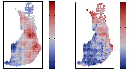
illustrated in Figure 1.
After having the posterior sample of latent variables, we can sample from the poste-
rior predictive distribution of any set of ˜
fsimply by sampling with each f(i)one ˜
f(i)from
p(˜
f|f(i), θ, φ), which is given in the equation (7). Similarly, we can obtain a sample of ˜
yby
drawing one ˜
y(i)for each ˜
f(i)from p(˜
y|˜
f, θ, φ).
4. Marginal likelihood given parameters
The marginal likelihood given the parameters, p(D|θ, φ) = Rp(y|f, φ)p(f|X, θ)df, is an
important quantity when inferring the parameters as discussed in the next section. With a
Gaussian likelihood it has an analytic solution (14) which gives the log marginal likelihood
log p(D|θ, σ) = −n
2log(2π)−1
2log |Kf,f+σ2I| − 1
2yT(Kf,f+σ2I)−1y.(23)
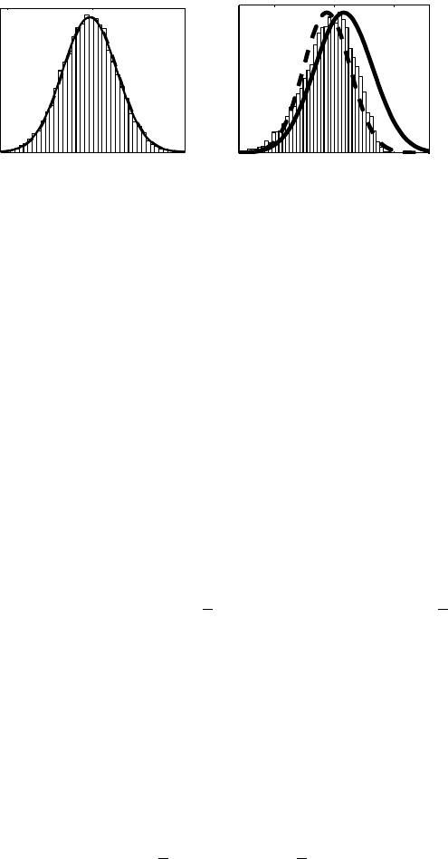
−0.8 −0.55 −0.3
(a) Disease mapping
−10 −5 0
(b) Classification
Figure 1: Illustration of the Laplace approximation (solid line), EP (dashed line)
and MCMC (histogram) for the conditional posterior of a latent variable p(fi|D, θ)
in two applications. On the left, a disease mapping problem with Poisson likelihood
(used in Vanhatalo et al., 2010) where the Gaussian approximation works well. On
the right, a classification problem with probit likelihood (used in Vanhatalo and
Vehtari, 2010) where the posterior is skewed and the Gaussian approximation is
not so good.
If the likelihood is not Gaussian, the marginal likelihood needs to be approximated. The
Laplace approximation to the marginal likelihood is constructed, for example, by making a
second order Taylor expansion for the integrand p(y|f, φ)p(f|X, θ)around ˆ
f. This gives a
Gaussian integral over fmultiplied by a constant, and results in the log marginal likelihood
approximation
log p(D|θ, φ)≈log q(D|θ, φ)∝ −1
2ˆ
fTK-1
f,fˆ
f+ log p(y|ˆ
f, φ)−1
2log |B|,(24)
where |B|=|I+W1/2Kf,fW1/2|. See also (Tierney and Kadane, 1986; Rue et al., 2009;
Vanhatalo et al., 2009) for more discussion.
EP’s marginal likelihood approximation is the normalization constant
ZEP =Zp(f|X, θ)
n
Y
i=1
˜
ZiN(fi|˜µi,˜σ2
i)dfi(25)
in equation (21). This is a Gaussian integral multiplied by a constant Qn
i=1 ˜
Zi, giving
log p(D|θ, φ)≈log ZEP =−1
2log |K+˜
Σ| − 1
2˜µTK+˜
Σ−1˜µ+CEP,(26)
where CEP collects the terms that are not explicit functions of θor φ(there is an implicit
dependence through the iterative algorithm, though). For more discussion on EP’s marginal
likelihood approximation see (Seeger, 2005; Nickisch and Rasmussen, 2008).
5. Marginalization over parameters
The previous section treated methods to evaluate exactly (the Gaussian case) or approxi-
mately (Laplace and EP approximations) the log marginal likelihood given parameters. Now,
we describe approaches for estimating parameters or integrating numerically over them.
5.1 Maximum a posterior estimate of parameters
In a full Bayesian approach we should integrate over all unknowns. Given we have integrated
over the latent variables, it often happens that the posterior of the parameters is peaked
or predictions are unsensitive to small changes in parameter values. In such case, we can
approximate the integral over p(θ, φ|D)with the maximum a posterior (MAP) estimate
{ˆ
θ, ˆ
φ}= arg max
θ,φ
p(θ, φ|D) = arg min
θ,φ
[−log p(D|θ, φ)−log p(θ, φ)] .(27)
In this approximation, the parameter values are given a point mass one at the posterior
mode, and the marginal of the latent function is approximated as p(f|D)≈p(f|D,ˆ
θ, ˆ
φ).
The log marginal likelihood, and its approximations, are differentiable with respect to the
parameters (Seeger, 2005; Rasmussen and Williams, 2006). Thus, also the log posterior is
differentiable, which allows gradient based optimization. The advantage of MAP estimate is
that it is relatively easy and fast to evaluate. According to our experience good optimization
algorithms need usually at maximum tens of optimization steps to find the mode. However,
it underestimates the uncertainty in parameters.
5.2 Grid integration
Grid integration is based on weighted sum of points evaluated on grid
p(f|D)≈
M
X
i=1
p(f|D, ϑi)p(ϑi|D)∆i.(28)
Here ϑ= [θT, φT]Tand ∆idenotes the area weight appointed to an evaluation point ϑi.
The implementation follows INLA (Rue et al., 2009) and is discussed in detail by Vanhatalo
et al. (2010). The basic idea is to first locate the posterior mode and then to explore the log
posterior surface so that the bulk of the posterior mass is included in the integration (see
Figure 2(a)). The grid search is feasible only for a small number of parameters since the
number of grid points grows exponentially with the dimension of the parameter space d.
5.3 Monte Carlo integration
Monte Carlo integration scales better than the grid integration in large parameter spaces
since its error decreases with a rate that is independent of the dimension (Robert and
Casella, 2004). There are two options to find a Monte Carlo estimate for the marginal
posterior p(f|D). The first option is to sample only the parameters from their marginal
posterior p(ϑ|D)or from its approximation (see Figure 2(b)). In this case, the posterior
marginal of the latent variable is approximated with mixture distribution as in the grid
integration. The alternative is to sample both the parameters and the latent variables.
The full MCMC is performed by alternate sampling from the conditional posteriors
p(f|D, ϑ)and p(ϑ|D,f). Possible choices to sample from the conditional posterior of the
parameters are, e.g., HMC, no-U-turn sampler (Hoffman and Gelman, 2014), slice sampling
(SLS) (Neal, 2003; Thompson and Neal, 2010). Sampling both the parameters and latent
variables is usually slow since due to the strong correlation between them (Vanhatalo and

Vehtari, 2007; Vanhatalo et al., 2010). Surrogate slice sampling by Murray and Adams
(2010) can be used to sample both the parameters and latent variables at the same time.
Sampling from the (approximate) marginal, p(ϑ|D), is an easier task since the parameter
space is smaller. The parameters can be sampled from their marginal posterior (or its
approximation) with HMC, SLS (Neal, 2003; Thompson and Neal, 2010) or via importance
sampling (Geweke, 1989). In importance sampling, we use a Gaussian or Student-tproposal
distribution g(ϑ)with mean ˆ
ϑand covariance approximated with the negative Hessian of
the log posterior, and approximate the integral with
p(f|D)≈1
PM
i=1 wi
M
X
i=1
q(f|D, ϑi)wi,(29)
where wi=q(ϑ(i))/g(ϑ(i))are the importance weights. In some situations the naive Gaussian
or Student-tproposal distribution is not adequate since the posterior distribution q(ϑ|D)may
be non-symmetric or the covariance estimate is poor. An alternative for these situations is
the scaled Student-tproposal distribution (Geweke, 1989) which is adjusted along each main
direction of the approximate covariance. The implementation of the importance sampling
is discussed in detail by Vanhatalo et al. (2010).
The problem with MCMC is that we are not able to draw independent samples from
the posterior. Even with a careful tuning of Markov chain samplers the autocorrelation is
usually so large that the required sample size is in thousands, which is a clear disadvantage
compared with, for example, the MAP estimate.
5.4 Central composite design
Rue et al. (2009) suggest a central composite design (CCD) for choosing the representative
points from the posterior of the parameters when the dimensionality of the parameters, d,
is moderate or high. In this setting, the integration is considered as a quadratic design
problem in a ddimensional space with the aim at finding points that allow to estimate the
curvature of the posterior distribution around the mode. The design used in GPstuff is the
fractional factorial design (Sanchez and Sanchez, 2005) augmented with a center point and
a group of 2dstar points. The design points are all on the surface of a d-dimensional sphere
and the star points consist of 2dpoints along each axis, which is illustrated in Figure 2(c).
The integration is then a finite sum (28) with special weights (Vanhatalo et al., 2010).
CCD integration speeds up the computations considerably compared to the grid search
or Monte Carlo integration since the number of the design points grows very moderately.
The accuracy of the CCD is between the MAP estimate and the full integration with the grid
search or Monte Carlo. Rue et al. (2009) report good results with this integration scheme,
and it has worked well in moderate dimensions in our experiments as well. Since CCD is
based on the assumption that the posterior of the parameter is (close to) Gaussian, the
densities p(ϑi|D)at the points on the circumference should be monitored in order to detect
serious discrepancies from this assumption. These densities are identical if the posterior is
Gaussian and we have located the mode correctly, and thereby great variability on their
values indicates that CCD has failed. The posterior of the parameters may be far from a
Gaussian distribution but for a suitable transformation, which is made automatically in the
toolbox, the approximation may work well.
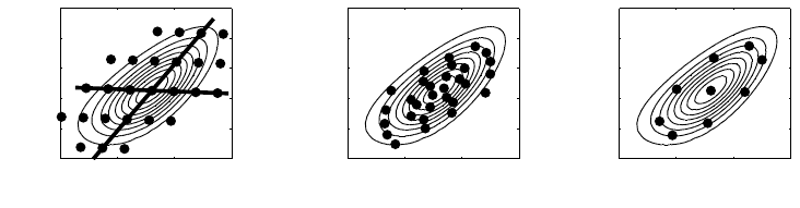
log(length−scale)
log(magnitude)
z1
z2
2.8 3 3.2 3.4
−3
−2.5
−2
−1.5
−1
−0.5
(a) Grid based
log(length−scale)
log(magnitude)
2.8 3 3.2 3.4
−3
−2.5
−2
−1.5
−1
−0.5
(b) Monte Carlo
log(length−scale)
log(magnitude)
2.8 3 3.2 3.4
−3
−2.5
−2
−1.5
−1
−0.5
(c) Central composite design
Figure 2: The grid based, Monte Carlo and central composite design integration.
Contours show the posterior density q(log(ϑ)|D)and the integration points are
marked with dots. The left figure shows also the vectors zalong which the points
are searched in the grid integration and central composite design. The integration
is conducted over q(log(ϑ)|D)rather than q(ϑ|D)since the former is closer to
Gaussian. Reproduced from (Vanhatalo et al., 2010).
6. Getting started with GPstuff: regression and classification
6.1 Gaussian process regression
The demonstration program demo_regression1 considers a simple regression problem yi=
f(xi) + i, where i∼N(0, σ2). We will show how to construct the model with a squared
exponential covariance function and how to conduct the inference.
6.1.1 Constructing the model
The model construction requires three steps: 1) Create structures that define likelihood and
covariance function, 2) define priors for the parameters, and 3) create a GP structure where
all the above are stored. These steps are done as follows:
lik = lik_gaussian(’sigma2’, 0.2^2);
gpcf = gpcf_sexp(’lengthScale’, [1.1 1.2], ’magnSigma2’, 0.2^2)
pn=prior_logunif();
lik = lik_gaussian(lik, ’sigma2_prior’, pn);
pl = prior_unif();
pm = prior_sqrtunif();
gpcf = gpcf_sexp(gpcf, ’lengthScale_prior’, pl, ’magnSigma2_prior’, pm);
gp = gp_set(’lik’, lik, ’cf’, gpcf);
Here lik_gaussian initializes Gaussian likelihood function and its parameter values and
gpcf_sexp initializes the squared exponential covariance function and its parameter values.
lik_gaussian returns structure lik and gpcf_sexp returns gpcf that contain all the in-
formation needed in the evaluations (function handles, parameter values etc.). The next
five lines create the prior structures for the parameters of the observation model and the
covariance function, which are set in the likelihood and covariance function structures. The
last line creates the GP structure by giving it the likelihood and covariance function.
Using the constructed GP structure, we can evaluate basic summaries such as covari-
ance matrices, make predictions with the present parameter values etc. For example, the
covariance matrices Kf,fand C=Kf,f+σ2Ifor three two-dimensional input vectors are:
example_x = [-1 -1 ; 0 0 ; 1 1];
[K, C] = gp_trcov(gp, example_x)
K =
0.0400 0.0187 0.0019
0.0187 0.0400 0.0187
0.0019 0.0187 0.0400
C =
0.0800 0.0187 0.0019
0.0187 0.0800 0.0187
0.0019 0.0187 0.0800
6.1.2 MAP estimate for the parameters
gp_optim works as a wrapper for usual gradient based optimization functions. It is used as
follows:
opt=optimset(’TolFun’,1e-3,’TolX’,1e-3,’Display’,’iter’);
gp=gp_optim(gp,x,y,’opt’,opt);
gp_optim takes a GP structure, training input x, training target y(which are defined in
demo_regression1) and options, and returns a GP structure with parameter values opti-
mized to their MAP estimate. By default gp_optim uses fminscg function, but gp_optim can
use also, for example, fminlbfgs or fminunc. Optimization options are set with optimset
function. It is also possible to set optimisation options as
opt=struct(’TolFun’,1e-3,’TolX’,1e-3,’Display’,’iter’);
which is useful when using an optimiser not supported by optimset. All the estimated
parameter values can be easily checked using the function gp_pak, which packs all the
parameter values from all the covariance function structures in a vector, usually using log-
transformation (other transformations are also possible). The second output argument of
gp_pak lists the labels for the parameters:
[w,s] = gp_pak(gp);
disp(s), disp(exp(w))
’log(sexp.magnSigma2)’
’log(sexp.lengthScale x 2)’
’log(gaussian.sigma2)’
2.5981 0.8331 0.7878 0.0427
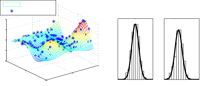
−2
0
2
−2
0
2
−4
−2
0
2
4
predicted surface
data point
(a) The predictive mean and training data.
0 0.5 1
−1 −0.5
(b) The marginal posterior predictive
distributions p(fi|D).
Figure 3: The predictive mean surface, training data, and the marginal posterior for
two latent variables in demo_regression1. Histograms show the MCMC solution
and the grid integration solution is drawn with a line.
It is also possible to set the parameter vector of the model to desired values using gp_unpak.
gp_pak and gp_unpak are used internally to allow use of generic optimisation and sampling
functions, which take the parameter vector as an input argument.
Predictions for new locations ˜
x, given the training data (x,y), are done by gp_pred
function, which returns the posterior predictive mean and variance for each f(˜
x)(see equa-
tion (16)). This is illustrated below where we create a regular grid where the posterior mean
and variance are computed. The posterior mean mp(˜
x)and the training data points are
shown in Figure 3.
[xt1,xt2]=meshgrid(-1.8:0.1:1.8,-1.8:0.1:1.8);
xt=[xt1(:) xt2(:)];
[Eft_map, Varft_map] = gp_pred(gp, x, y, xt);
6.1.3 Marginalization over parameters with grid integration
To integrate over the parameters we can use any method described in the section 5. The
grid integration is performed with the following line:
[gp_array, P_TH, th, Eft_ia, Varft_ia, fx_ia, x_ia] = ...
gp_ia(gp, x, y, xt, ’int_method’, ’grid’);
gp_ia returns an array of GPs (gp_array) for parameter values th ([ϑi]M
i=1) with weights
P_TH ([p(ϑi|D)∆i]M
i=1). Since we use the grid method the weights are proportional to the
marginal posterior and ∆i≡1∀i(see section 5.2). Ef_ia and Varf_ia contain the predictive
mean and variance at the prediction locations. The last two output arguments can be used
to plot the predictive distribution p(˜
fi|D)as demonstrated in Figure 3. x_ia(i,:) contains
a regular grid of values ˜
fiand fx_ia(i,:) contains p(˜
fi|D)at those values.

6.1.4 Marginalization over parameters with MCMC
The main function for conducting Markov chain sampling is gp_mc, which loops through all
the specified samplers in turn and saves the sampled parameters in a record structure. In
later sections, we will discuss models where also latent variables are sampled, but now we
concentrate on the covariance function parameters, which are sampled as follows:
[gp_rec,g,opt] = gp_mc(gp, x, y, ’nsamples’, 220);
gp_rec = thin(gp_rec, 21, 2);
[Eft_s, Varft_s] = gpmc_preds(rfull, x, y, xt);
[Eft_mc, Varft_mc] = gp_pred(gp_rec, x, y, xt);
The gp_mc function generates nsamples (here 220) Markov chain samples. At each iter-
ation gp_mc runs the actual samplers. The function thin removes the burn-in from the
sample chain (here 21) and thins the chain more (here by 2). This way we can decrease the
autocorrelation between the remaining samples. GPstuff provides also diagnostic tools for
Markov chains. See, for example, (Gelman et al., 2013; Robert and Casella, 2004) for discus-
sion on convergence and other Markov chain diagnostics. The function gpmc_preds returns
the conditional predictive mean and variance for each sampled parameter value. These are
Ep(f|X,D,ϑ(s))[˜
f], s = 1, ..., M and Varp(f|X,D,ϑ(s))[˜
f], s = 1, ..., M, where Mis the number of
samples. Marginal predictive mean and variance are computed directly with gp_pred.
6.2 Gaussian process classification
We will now consider a binary GP classification (see demo_classific) with observations,
yi∈ {−1,1}, i = 1, ..., n, associated with inputs X={x}n
i=1. The observations are consid-
ered to be drawn from a Bernoulli distribution with a success probability p(yi= 1|xi). The
probability is related to the latent function via a sigmoid function that transforms it to a
unit interval. GPstuff provides a probit and logit transformation, which give
pprobit(yi|f(xi)) = Φ(yif(xi)) = Zyif(xi)
−∞
N(z|0,1)dz (30)
plogit(yi|f(xi)) = 1
1 + exp(−yif(xi)).(31)
Since the likelihood is not Gaussian we need to use approximate inference methods, discussed
in the section 3.
6.2.1 Constructing the model
The model construction for the classification follows closely the steps presented in the pre-
vious section. The model is constructed as follows:
lik = lik_probit();
gpcf = gpcf_sexp(’lengthScale’, [0.9 0.9], ’magnSigma2’, 10);
gp = gp_set(’lik’, lik, ’cf’, gpcf, ’jitterSigma2’, 1e-9);
The above lines first initialize the likelihood function, the covariance function and the GP
structure. Since we do not specify parameter priors, the default priors are used. The model
construction and the inference with logit likelihood (lik_logit) would be similar with probit
likelihood. A small jitter value is added to the diagonal of the training covariance to make
certain matrix operations more stable (this is not usually necessary but is shown here for
illustration).
6.2.2 Inference with Laplace approximation
The MAP estimate for the parameters can be found using gp_optim as
gp = gp_set(gp, ’latent_method’, ’Laplace’);
gp = gp_optim(gp,x,y,’opt’,opt);
The first line defines which inference method is used for the latent variables. It initializes the
Laplace algorithm and sets needed fields in the GP structure. The default method for latent
variables is Laplace, so this line could be omitted. gp_optim uses the default optimization
function, fminscg, with the same options as above in the regression example.
gp_pred provides the mean and variance for the latent variables (first two outputs), the
log predictive probability for a test observation (third output), and mean and variance for
the observations (fourth and fifth output) at test locations xt.
[Eft_la, Varft_la, lpyt_la, Eyt_la, Varyt_la] = ...
gp_pred(gp, x, y, xt, ’yt’, ones(size(xt,1),1) );
The first four input arguments are the same as in the section 6.1. The fifth and sixth argu-
ments are a parameter-value pair where yt tells that we give test observations ones(size(xt,1),1)
related to xt as an optional input, in which case gp_pred evaluates their marginal posterior
log predictive probabilities lpyt_la. Here we evaluate the probability to observe class 1and
thus we give a vector of ones as test observations.
6.2.3 Inference with expectation propagation
EP works as the Laplace approximation. We only need to set the latent method to ’EP’
but otherwise the commands are the same as above:
gp = gp_set(gp, ’latent_method’, ’EP’);
gp = gp_optim(gp,x,y,’opt’,opt);
[Eft_ep, Varft_ep, lpyt_ep, Eyt_ep, Varyt_ep] = ...
gp_pred(gp, x, y, xt, ’yt’, ones(size(xt,1),1) );
6.2.4 Inference with MCMC
With MCMC we sample both the latent variables and the parameters:
gp = gp_set(gp, ’latent_method’, ’MCMC’, ’jitterSigma2’, 1e-6);
[gp_rec,g,opt]=gp_mc(gp, x, y, ’nsamples’, 220);
gp_rec=thin(gp_rec,21,2);
[Ef_mc, Varf_mc, lpy_mc, Ey_mc, Vary_mc] = ...
gp_pred(gp_rec, x, y, xt, ’yt’, ones(size(xt,1),1) );
For MCMC we need to add a larger jitter on the diagonal to prevent numerical problems.
By default sampling from the latent value distribution p(f|θ, D)is done with the ellipti-
cal slice sampling (Murray et al., 2010). Other samplers provided by the GPstuff are a
scaled Metropolis Hastings algorithm (Neal, 1998) and a scaled HMC scaled_hmc (Vanhat-
alo and Vehtari, 2007). From the user point of view, the actual sampling and prediction
are performed similarly as with the Gaussian likelihood. The gp_mc function handles the
sampling so that it first samples the latent variables from p(f|θ, D)after which it samples
the parameters from p(θ|f,D). This is repeated until nsamples samples are drawn.
In classification model MCMC is the most accurate inference method, then comes EP
and Laplace approximation is the worst. However, the inference times line up in the opposite
order. The difference between the approximations is not always this large. For example,
with Poisson likelihood, discussed in the section 7.2, Laplace and EP approximations work,
in our experience, practically as well as MCMC.
6.2.5 Marginal posterior corrections
GPstuff also provides methods for marginal posterior corrections using either Laplace or EP
as a latent method (Cseke and Heskes, 2011). Provided correction methods are either cm2
or fact for Laplace and fact for EP. These methods are related to methods proposed by
Tierney and Kadane (1986) and Rue et al. (2009).
Univariate marginal posterior corrections can be computed with function gp_predcm
which returns the corrected marginal posterior distributtion for the given indices of in-
put/outputs:
[pc, fvec, p] = gp_predcm(gp,x,y,’ind’, 1, ’fcorr’, ’fact’);
The returned value pc corresponds to corrected marginal posterior for the latent value
f1,fvec corresponds to vector of grid points where pc is evaluated and pis the orig-
inal Gaussian posterior distribution evaluated at fvec. Marginal posterior corrections
can also be used for predictions in gp_pred and sampling of latent values in gp_rnd (see
demo_improvedmarginals1 and demo_improvedmarginals2). gp_rnd uses univariate marginal
corrections with Gaussian copula to sample from the joint marginal posterior of several latent
values.
7. Other single latent models
In this section, we desribe other likelihood functions, which factorize so that each factor
depend only on single latent value.
7.1 Robust regression
7.1.1 Student-tobservation model
A commonly used observation model in the GP regression is the Gaussian distribution.
This is convenient since the marginal likelihood is analytically tractable. However, a known
limitation with the Gaussian observation model is its non-robustness, due which outlying
observations may significantly reduce the accuracy of the inference (see Figure 4). A well-
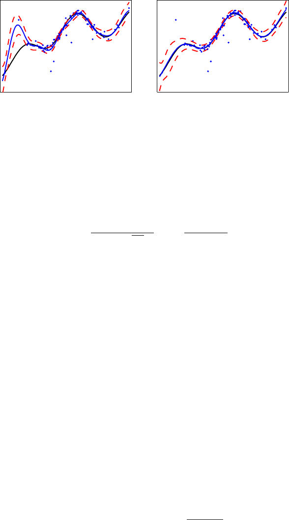
(a) Gaussian model. (b) Student-tmodel.
Figure 4: An example of regression with outliers from (Neal, 1997). On the left
Gaussian and on the right the Student-tmodel. The real function is plotted with
black line.
known robust observation model is the Student-tdistribution (O’Hagan, 1979)
y|f, ν, σt∼
n
Y
i=1
Γ((ν+ 1)/2)
Γ(ν/2)√νπσt1 + (yi−fi)2
νσ2
t−(ν+1)/2
,(32)
where νis the degrees of freedom and σtthe scale parameter. The Student-tdistribution
can be utilized as such or it can be written via the scale mixture representation
yi|fi, α, Ui∼N(fi, αUi)(33)
Ui∼Inv-χ2(ν, τ 2),(34)
where each observation has its own noise variance αUithat is Inv-χ2distributed (Neal, 1997;
Gelman et al., 2013). The degrees of freedom νcorresponds to the degrees of freedom in
the Student-tdistribution and ατ corresponds to σt.
In GPstuff both of the representations are implemented. The scale mixture represen-
tation is implemented in lik_gaussiansmt and can be inferred only with MCMC (as de-
scribed by Neal, 1998). The Student-tmodel is implemented in lik_t and can be inferred
with Laplace and EP approximation and MCMC (as described by Vanhatalo et al., 2009;
Jylänki et al., 2011). These are demonstrated in demo_regression_robust.
7.1.2 Laplace observation model
Besides the Student-T observation model, Laplace distribution is another robust alternative
to the normal Gaussian observation model
y|f, σ ∼
n
Y
i=1
(2σ)−1exp −|yi−fi|
σ,(35)
where σis the scale parameter of the Laplace distribution.
In GPstuff, the Laplace observation model implementation is in lik_laplace. It should
be noted that since the Laplace distribution is not differentiable with respect to fin the
mode, only EP approximation or MCMC can be used for inference.
0.7
0.8
0.9
1
1.1
1.2
1.3
1.4
(a) The posterior mean.
0.005
0.01
0.015
0.02
0.025
0.03
(b) The posterior variance.
Figure 5: The posterior predictive mean and variance of the relative risk in the
demo_spatial1 data set obtained with FIC.
7.2 Count data
Count data are observed in applications. One such common application is spatial epidemi-
ology, which concerns both describing and understanding the spatial variation in the disease
risk in geographically referenced health data. One of the most common tasks in spatial epi-
demiology is disease mapping, where the aim is to describe the overall disease distribution
on a map and, for example, highlight areas of elevated or lowered mortality or morbidity risk
(e.g. Lawson, 2001; Richardson, 2003; Elliot et al., 2001). Here we build a disease mapping
model following the general approach discussed, for example, by Best et al. (2005). The
data are aggregated into areas with coordinates xi. The mortality/morbidity in an area is
modeled with a Poisson, negative binomial or binomial distribution with mean eiµi, where
eiis the standardized expected number of cases (e.g. Ahmad et al., 2000), and µiis the
relative risk, whose logarithm is given a GP prior. The aim is to infer the relative risk. The
implementation of these models in GPstuff is discussed in (Vanhatalo and Vehtari, 2007;
Vanhatalo et al., 2010).
7.2.1 Poisson
The Poisson model is implemented in likelih_poisson and it is
y|f,e∼
n
Y
i=1
Poisson(yi|exp(fi)ei)(36)
where the vector ycollects the numbers of deaths for each area. Here µ= exp(f)and its
posterior predictive mean and variance solved in the demo demo_spatial1 are shown in
Figure 5.
7.2.2 Negative binomial
The negative binomial distribution is a robust version of the Poisson distribution similarly
as Student-tdistribution can be considered as a robustified Gaussian distribution (Gelman

et al., 2013). In GPstuff it is parametrized as
y|f,e, r ∼
n
Y
i=1
Γ(r+yi)
yi!Γ(r)r
r+µirµi
r+µiyi
,(37)
where µi=eiexp(f(xi)) and ris the dispersion parameter governing the variance. The
model is demonstrated in demo_spatial2.
7.2.3 Binomial
In disease mapping, the Poisson distribution is used to approximate the true binomial dis-
tribution. This approximation works well if the background population, corresponding to
the number of trials in the binomial distribution, is large. Sometimes this assumption is not
adequate and we need to use the exact binomial observation model
y|f,z∼
n
Y
i=1
zi!
yi!(zi−yi)!pyi
i(1 −pi)(zi−yi),(38)
where pi= exp(f(xi))/(1+exp(f(xi))) is the probability of success, and the vector zdenotes
the number of trials. The binomial observation model is not limited to spatial modeling but
is an important model for other problems as well. The observation model is demonstrated
in demo_binomial1 with a one dimensional simulated data and demo_binomial_apc demon-
strates the model in an incidence risk estimation.
7.2.4 Hurdle model
Hurdle models can be used to model excess number of zeros compared to usual Poisson and
negative binomial count models. Hurdle models assume a two-stage process, where the first
process determines whether the count is larger than zero, and the second process determines
the non-zero count (Mullahy, 1986). These processes factorize, and thus hurdle model can
be implemented using two independent GPs in GPstuff. lik_probit or lik_logit can be
used for the zero process and lik_negbinztr can be used for the count part. lik_negbinztr
provides zero truncated negative binomial model, which can be used also to approximate
zero-truncated Poisson model by using high dispersion parameter value. Construction of a
hurdle model is demonstrated in demo_hurdle. Gaussian process model with logit negative
binomial hurdle model implemented using GPstuff was used in reference (Rantonen et al.,
2011) to model sick absence days due to low back symptoms.
Alternative way to model excess number of zeros is to couple the zero and count processes
as in zero-inflated negative binomial model described in section 8.4.
7.3 Log-Gaussian Cox process
Log-Gaussian Cox-process is an inhomogeneous Poisson process model used for point data,
with unknown intensity function λ(x), modeled with log-Gaussian process so that f(x) =
log λ(x)(see Rathbun and Cressie, 1994; Møller et al., 1998). If the data are points X=xi;
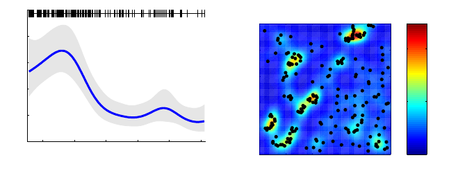
1860 1880 1900 1920 1940 1960
0
1
2
3
4
5
Year
Intensity
(a) Coal mine disasters.
0 0.2 0.4 0.6 0.8 1
0
0.2
0.4
0.6
0.8
1
0
500
1000
(b) Redwood data.
Figure 6: Two intensity surfaces estimated with log-Gaussian Cox process. The
figures are from the demo_lgcp, where the aim is to study an underlying intensity
surface of a point process. On the left a temporal and on the right a spatial point
process.
i= 1,2, . . . , n on a finite region Vin <d, then the likelihood of the unknown function fis
p(X|f) = exp (−ZV
exp(f(x))dx+
n
X
i=1
f(xi)).(39)
Evaluation of the likelihood would require nontrivial integration over the exponential of GP.
Møller et al. (1998) propose to discretise the region Vand assume locally constant intensity
in subregions. This transforms the problem to a form equivalent to having Poisson model
for each subregion. Likelihood after the discretisation is
p(X|f)≈
K
Y
k=1
Poisson(yk|exp(f(˙
xk))),(40)
where ˙
xis the coordinate of the kth sub-region and ykis the number of data points in it.
Tokdar and Ghosh (2007) proved the posterior consistency in limit when sizes of subregions
go to zero.
The log-Gaussian Cox process with Laplace and EP approximation is implemented in
the function lgcp for one or two dimensional input data. The usage of the function is
demonstrated in demo_lgcp. This demo analyzes two data sets. The first one is one dimen-
sional case data with coal mine disasters (from R distribution). The data contain the dates
of 191 coal mine explosions that killed ten or more men in Britain between 15 March 1851
and 22 March 1962. The analysis is conducted using expectation propagation and CCD
integration over the parameters and the results are shown in Figure 6. The second data are
the redwood data (from R distribution). This data contain 195 locations of redwood trees
in two dimensional lattice. The smoothed intensity surface is shown in Figure 6.
7.4 Accelerated failure time survival models
The accelerated failure time survival models are demonstrated in demo_survival_aft. These
models can be used to model also other positive continuous data with or without censoring.

7.4.1 Weibull
The Weibull distribution is a widely used parametric baseline hazard function in survival
analysis (Ibrahim et al., 2001). The hazard rate for the observation iis
hi(y) = h0(y) exp(f(xi)),(41)
where y > 0and the baseline hazard h0(y)is assumed to follow the Weibull distribution
parametrized in GPstuff as
h0(y) = ryr−1,(42)
where r > 0is the shape parameter. This follows the parametrization used in Martino et al.
(2011). The likelihood is defined as
L=
n
Y
i=1
r1−zie−(1−zi)f(xi)y(1−zi)(r−1)
ie−yr
i/ef(xi)(43)
where zis a vector of censoring indicators with zi= 0 for uncensored event and zi= 1 for
right censored event for observation i. In case of censoring yidenotes the time of censoring.
Here we present only the likelihood function because we don’t have observation model for
the censoring. Another common parameterization of Weibull model is through shape, r, and
scale, λparameters. The parameterization in GPstuff corresponds to Weibull model with
input dependent scale λ(xi) = ef(xi)/r, so that λ(xi)r=ef(xi). Hence the Weibull model
for an uncensored observation yiis
p(yi|f(xi), r) = r
λ(xi)yi
λ(xi)r−1
e−(yi/λ(xi))r(44)
7.4.2 Log-Gaussian
With Log-Gaussian survival model the logarithms of survival times are assumed to be nor-
mally distributed.
The likelihood is defined as
L=
n
Y
i=1
(2πσ2)−(1−zi)/2y1−zi
iexp −1
2σ2(1 −zi)(log(yi)−f(xi))2(45)
×1−Φlog(yi)−f(xi)
σzi
where σis the scale parameter.
7.4.3 Log-logistic
The log-logistic likelihood is defined as
L=
n
Y
i=1 ryr−1
exp(f(xi))1−zi1 + y
exp(f(xi))rzi−2
,(46)
where ris the shape parameter and zithe censoring indicators.

7.5 Derivative observations in GP regression
Incorporating derivative observations in GP regression is fairly straightforward, because a
derivative of Gaussian process is a Gaussian process. In short, derivative observation are
taken into account by extending covariance matrices to include derivative observations. This
is done by forming joint covariance matrices of function values and derivatives. Following
equations (Rasmussen and Williams, 2006) state how the covariances between function values
and derivatives, and between derivatives are calculated
Cov(fi,∂fj
∂xdj
) = ∂k(xi,xj
∂xdj
),Cov( ∂fi
∂xdi
,∂fj
∂xej
) = ∂2k(xi,xj
∂xdi∂xej
.
The joint covariance matrix for function values and derivatives is of the following form
K=Kff KfD
KDf KDD
Kij
ff =k(xi,xj),
Kij
Df =∂k(xi,xj)
∂xdi
,
KfD = (KDf )>,
Kij
DD =∂2k(xi,xj)
∂xdi∂xej
,
Prediction is done as usual but with derivative observations joint covariance matrices are to
be used instead of the normal ones.
Using derivative observations in GPstuff requires two steps: when initializing the GP
structure one must set option ’derivobs’ to ’on’. The second step is to form right sized
observation vector. With input size n×mthe observation vector with derivatives should
be of size n+m·n. The observation vector is constructed by adding partial derivative
observations after function value observations
yobs =
y(x)
∂y(x)
∂x1
.
.
.
∂y(x)
∂xm
.(47)
Different noise level could be assumed for function values and derivative observations but
at the moment the implementation allows only same noise for all the observations. The use
of derivative observations is demonstrated in demo_derivativeobs.
Derivative process can be also used to construct a monotonicity constraint as described
in section 8.7.
7.6 Quantile Regression
Quantile regression is used for estimating quantiles of the response variable as a function of
input variables (Boukouvalas et al., 2012).

The likelihood is defines as
p(y|f, σ, τ) = τ(1 −τ)
σexp −y−f
σ(τ−I(y≤f)),(48)
where τis the quantile of interest and σis the standard deviation. I(y≤f)is 1 if the
condition inside brackets is true and 0 otherwise. Because the logarithm of the likelihood
is not twice differentiable at the mode, Laplace approximation cannot be used for inference
with Quantile Regression. Quantile Regression with EP and MCMC is demonstrated in
demo_qgp with toy data.
8. Multilatent models
The multilatent models consist of models where individual likelihood factors depend on
multiple latent variables. In this section we shortly summarize such models in GPstuff.
8.1 Multiclass classification
In multiclass classification problems the target variables have more than two possible class
labels, yi∈ {1, . . . , c}, where c > 2is the number of classes. In GPstuff, multi-class classifi-
cation can be made either using the softmax likelihood (lik_softmax)
p(yi|fi) = exp(fyi
i)
Pc
j=1 exp(fj
i),(49)
where fi=f1
i, . . . , fc
iT, or the multinomial probit likelihood (lik_multinomialprobit)
p(yi|fi) = Ep(ui)
c
Y
j=1,j6=yi
Φ(ui+fyi
i−fj
i)
,(50)
where the auxiliary variable uiis distributed as p(ui) = N(ui|0,1), and Φ(x)denotes the
cumulative density function of the standard normal distribution. In Gaussian process liter-
ature for multiclass classification, a common assumption is to introduce cindependent prior
processes that are associated with cclasses (see, e.g., Rasmussen and Williams, 2006). By
assuming zero-mean Gaussian processes for latent functions associated with different classes,
we obtain a zero-mean Gaussian prior
p(f|X) = N(f|0, K),(51)
where f=f1
1, . . . , f1
n, f2
1, . . . , f2
n, . . . , fc
1, . . . , fc
nTand Kis a cn ×cn block-diagonal covari-
ance matrix with matrices K1, K2, . . . , Kc(each of size n×n) on its diagonal.
Inference for softmax can be made with MCMC or Laplace approximation. As de-
scribed by Williams and Barber (1998) and Rasmussen and Williams (2006), using the
Laplace approximation for the softmax likelihood with the uncorrelated prior processes,
the posterior computations can be done efficiently in a way that scales linearly in c, which
is also implemented in GPstuff. Multiclass classification with softmax is demonstrated in
demo_multiclass.

Inference for multinomial probit can be made with expectation propagation by using a
nested EP approach that does not require numerical quadratures or sampling for estimation
of the tilted moments and predictive probabilities, as proposed by Riihimäki et al. (2013).
Similarly to softmax with Laplace’s method, the nested EP approach leads to low-rank
site approximations which retain all posterior couplings but results in linear computational
scaling with respect to c. Multiclass classification with the multinomial probit likelihood is
demonstrated in demo_multiclass_nested_ep.
8.2 Multinomial
The multinomial model (lik_multinomial) is an extension of the multiclass classifica-
tion to situation where each observation consist of counts of class observations. Let yi=
[yi,1, . . . , yi,c], where c > 2, be a vector of counts of class observations related to inputs xi
so that
yi∼Multinomial([pi,1, . . . , pi,c], ni)(52)
where ni=Pc
j=1 yi,j. The propability to observe class jis
pi,j =exp(fj
i)
Pc
j=1 exp(fj
i),(53)
where fi=f1
i, . . . , fc
iT. As in multiclass classification we can introduce cindependent prior
processes that are associated with cclasses. By assuming zero-mean Gaussian processes for
latent functions associated with different classes, we obtain a zero-mean Gaussian prior
p(f|X) = N(f|0, K),(54)
where f=f1
1, . . . , f1
n, f2
1, . . . , f2
n, . . . , fc
1, . . . , fc
nTand Kis a cn ×cn block-diagonal covari-
ance matrix with matrices K1, K2, . . . , Kc(each of size n×n) on its diagonal. This model is
demonstrated in demo_multinomial and it has been used, for example, in (Juntunen et al.,
2012).
8.3 Cox proportional hazard model
For the individual i, where i= 1, . . . , n, we have observed survival time yi(possibly right
censored) with censoring indicator δi, where δi= 0 if the ith observation is uncensored and
δi= 1 if the observation is right censored. The traditional approach to analyze continuous
time-to-event data is to assume the Cox proportional hazard model (Cox, 1972).
hi(t) = h0(t) exp(xT
iβ),(55)
where h0is the unspecified baseline hazard rate, xiis the d×1vector of covariates for the
ith patient and βis the vector of regression coefficients. The matrix X= [x1,...,xn]Tof
size n×dincludes all covariate observations.
The Cox model with linear predictor can be extended to more general form to enable,
for example, additive and non-linear effects of covariates (Kneib, 2006; Martino et al., 2011).
We extend the proportional hazard model by
hi(t) = exp(log(h0(t)) + ηi(xi)),(56)
where the linear predictor is replaced with the latent predictor ηidepending on the covariates
xi. By assuming a Gaussian process prior over η= (η1, . . . , ηn)T, smooth nonlinear effects
of continuous covariates are possible, and if there are dependencies between covariates, GP
can model these interactions implicitly.
A piecewise log-constant baseline hazard (see, e.g. Ibrahim et al., 2001; Martino et al.,
2011) is assumed by partitioning the time axis into Kintervals with equal lengths: 0 =
s0< s1< s2< . . . < sK, where sK> yifor all i= 1, . . . , n. In the interval k(where
k= 1, . . . , K), hazard is assumed to be constant:
h0(t) = λkfor t∈(sk−1, sk].(57)
For the ith individual the hazard rate in the kth time interval is then
hi(t) = exp(fk+ηi(xi)), t ∈(sk−1, sk],(58)
where fk= log(λk). To assume smooth hazard rate functions, we place another Gaussian
process prior for f= (f1, . . . , fK)T. We define a vector containing the mean locations of K
time intervals as τ= (τ1, . . . , τK)T.
The likelihood contribution for the possibly right censored ith observation (yi, δi)is
assumed to be
li=hi(yi)(1−δi)exp −Zyi
0
hi(t)dt.(59)
Using the piecewise log-constant assumption for the hazard rate function, the contribution
of the observation ifor the likelihood results in
li= [λkexp(ηi)](1−δi)exp
−[(yi−sk−1)λk+
k−1
X
g=1
(sg−sg−1)λg] exp(ηi)
,(60)
where yi∈(sk−1, sk](Ibrahim et al., 2001; Martino et al., 2011). By applying the Bayes
theorem, the prior information and likelihood contributions are combined, and the posterior
distribution of the latent variables can be computed. Due to the form of the likelihood
function, the resulting posterior becomes non-Gaussian and analytically exact inference is
intractable. GPstuff supports MCMC and Laplace approximation to integrate over the latent
variables. The use of Gaussian process Cox proportional hazard model is demonstrated in
demo_survival_coxph. The Gaussian process Cox proportional hazard model implemented
with GPstuff was used in reference (Joensuu et al., 2012) to model risk of gastrointestinal
stromal tumour recurrence after surgery.
8.4 Zero-inflated negative binomial
Zero-inflated negative binomial model is suitable for modelling count variables with excessive
number of zero observations compared to usual Poisson and negative binomial count models.
Zero-inflated negative binomial models assume a two-stage process, where the first process
determines whether the count is larger than zero, and the second process determines the
non-zero count (Mullahy, 1986). In GPstuff, these processes are assumed independent a

priori, but they become a posteriori dependent through the likelihood function
p+(1 −p)NegBin(y|y= 0),when y= 0 (61)
(1 −p)NegBin(y|y > 0),when y > 0,(62)
where the probability p is given by a binary classifier with logit likelihood. NegBin is the
Negative-binomial distribution parametrized for the i’th observation as
y|f,e, r ∼
n
Y
i=1
Γ(r+yi)
yi!Γ(r)r
r+µirµi
r+µiyi
,(63)
where µi=eiexp(f(xi)) and ris the dispersion parameter governing the variance. In
GPstuff, the latent value vector f= [fT
1fT
2]Thas length 2N, where Nis the number of
observations. The latents f1are associated with the classification process and the latents f2
with the negative-binomial count process.
8.5 Density estimation and regression
Logistic Gaussian process can be used for flexible density estimation and density regression.
GPstuff includes implementation based on Laplace (and MCMC) approximation as described
in (Riihimäki and Vehtari, 2012).
The likelihood is defined as
p(x|f) =
n
Y
i=1
exp(fi)
Pn
j=1 exp(fj).(64)
For the latent function f, we assume the model f(x) = g(x) + h(x)Tβ, where the GP prior
g(x)is combined with the explicit basis functions h(x). Regression coefficients are denoted
with β, and by placing a Gaussian prior β∼ N(b, B)with mean band covariance B, the
parameters βcan be integrated out from the model, which results in the following GP prior
for f:
f(x)∼ GP h(x)Tb, κ(x,x0) + h(x)TBh(x0).(65)
For the explicit basis functions, we use the second-order polynomials which leads to a GP
prior that can favour density estimates where the tails of the distribution go eventually to
zero.
We use finite-dimensional approximation and evaluate the integral and the Gaussian
process in a grid. We approximate inference for logistic Gaussian process density estimation
in a grid using Laplace’s method or MCMC to integrate over the non-Gaussian posterior
distribution of latent values (see details in Riihimäki and Vehtari, 2012).
Logistic Gaussian processes are also suitable for estimating conditional densities p(t|x),
where tis a response variable. We discretize both input and target space in a finite region
to model the conditional densities with the logistic GP. To approximate the resulting non-
Gaussian posterior distribution, we use again Laplace’s method.
1D and 2D density estimation and density regression are implemented in the function
lgpdens. The usage of the function is demonstrated in demo_lgpdens.
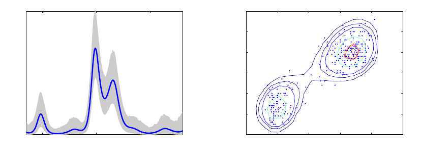
10000 20000 30000
(a) Galaxy data.
1 2 3 4 5 6
40
50
60
70
80
90
100
(b) Old faithful data.
Figure 7: Density estimates for two different distributions. Figures are from
demo_lgpdens. On the left blue line is density estimation of Galaxy data while
gray area is 95% mean region and on the right is 2D density estimation with coun-
tours based on Old faithful data.
8.6 Input dependent models
In input-dependent models more than one latent variables are used for modeling different
parameters of the distribution. Additional latent variables in turn enable modeling depen-
dencies between inputs and parameters.
8.6.1 Input-dependent Noise
Input-dependent noise model (Goldberg et al., 1997) can be used to model regression data.
The model assumes Gaussian distributed data with latent variables defining both mean and
variance of the Gaussian distribution instead of just the mean like in the standard Gaussian
likelihood. Setting independent GP priors for the two latent variables, it is possible to infer
non-constant noise, e.g. input-dependent, in the data.
The likelihood is defined as
p(y|f(1),f(2), σ2) =
n
Y
i=1
N(yi|f(1)
i, σ2exp(f(2)
i)),(66)
with latent function f(1) defining the mean and f(2) defining the variance. Input-dependent
noise is demonstrated in demo_inputdependentnoise with both heteroscedastic and con-
stant noise.
8.6.2 Input-dependent overdispersed Weibull
In input-dependent Weibull model additional latent variable is used for modeling shape
parameter rof the standard Weibull model.
The likelihood is defined as
p(y|f(1),f(2),z) =
n
Y
i=1
r1−zi
ie−(1−zi)f(1)
iy(1−zi)(ri−1)
ie−yri
i/ef(1)
i(67)
where zis a vector of censoring indicators with zi= 0 for uncensored event and zi= 1 for
right censored event for observation i. Latent variable f2is used for modeling the shape
parameter here. Because the dispersion parameter is constrained to be greater than 0,
it must be computed through exp(f2)to ensure positiveness. Input-dependent Weibull is
demonstrated in demo_inputdependentweibull.
8.7 Monotonicity constraint
.
Riihimäki and Vehtari (2010) presented how a monotonicity constraint for GP can be
introduced with virtual derivative observations, and the resulting posterior can be approxi-
mated with expectation propagation.
Currently GPstuff supports monotonicity constraint for models which have Gaussian
likelihood or fully factoring likelihoods with EP inference and which use covariance functions
gpcf_constant,gpcf_linear and gpcf_sexp. Riihimäki and Vehtari (2010) used type
II MAP estimate for the hyperparameters, but GPstuff allows easy integration over the
hyperparameters with any method described in Section 5.
GP model with monotonicity constraints on one or many covariates can be easily con-
structed with the function gp_monotonic. Monotonicity constraint is demonstrated in
demo_monotonic and demo_monotonic2.
Figure 8 displays the predictions with models with and without the monotonicity con-
straint. The monotonicity constraint allows inclusion of sensible prior information that death
rate increases as age increases. The effect is shown most clearly for larger ages where there
is less observations, but also overall reduction in uncertainty related to the latent function
can be seen.
9. Mean functions
In the standard GP regression a zero mean function is assumed for the prior process. This
is convenient but there are nonetheless some advantages in using a specified mean function.
The basic principle in doing GP regression with a mean function is to apply a zero mean
GP for the difference between observations and the mean function.
9.1 Explicit basis functions
Here we follow closely the presentation of (Rasmussen and Williams, 2006) about the subject
and briefly present the main results. A mean function can be specified as a weighted sum
of some basis functions h
m=h(x)>β,
with weights β. The target of modeling, the underlying process g, is assumed to be a sum
of mean function and a zero mean GP.
g=h(x)>β+GP(0,K).
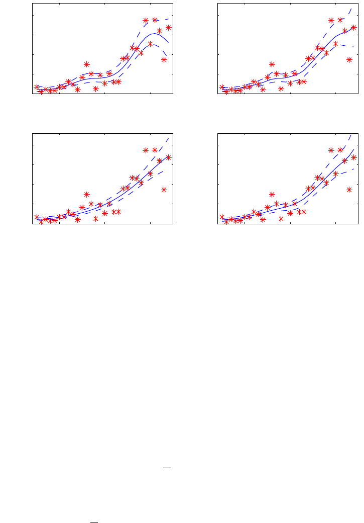
40 50 60
0
5
10
15
20
Age
Deaths/1000
sexp
40 50 60
0
5
10
15
20
Age
Deaths/1000
sexp + monot.
40 50 60
0
5
10
15
20
Age
Deaths/1000
lin + sexp
40 50 60
0
5
10
15
20
Age
Deaths/1000
lin + sexp + monot.
Figure 8: Illustration how the monotonicity constraint of the latent function affects
the predictions. Mortality rate data from Broffitt (1988).
By assuming Gaussian prior for the weights β∼ N(b,B),the weight parameters can be
integrated out and the prior for gis another GP
prior g∼ GP h(x)>b,K+h(x)>B h(x).
The predictive equations are obtained by using the mean and covariance of the prior (68)
in the zero mean GP predictive equations (15)
E(g∗) = E(f∗) + R>β,(68)
Cov(g∗) = Cov(f∗) + R>B−1+HK−1
yH>R,(69)
β=B−1+HK−1
yH>−1B−1b+HK−1
yy,
R=H∗−HK−1
yK∗,
H=
h1(x)
h2(x)
.
.
.
hk(x)
,xis row vector.

If the prior assumptions about the weights are vague then B−1→O, (Ois a zero matrix)
and the predictive equations (68) and (69) don’t depend on bor B
E(g∗) = E(f∗) + R>βv,(70)
Cov(g∗) = Cov(f∗) + R>HK−1
yH>R,(71)
βv=HK−1
yH>−1HK−1
yy,
Corresponding the exact and vague prior for the basis functions’ weights there are two
versions of the marginal likelihood. With exact prior the marginal likelihood is
log p(y|X,b,B) = −1
2M>N−1M−1
2log |Ky| − 1
2log |B| − 1
2log |A| − n
2log 2π,
M=H>b−y,
N=Ky+H>BH,
A=B−1+HK−1
yH>,
where nis the amount of observations. Its derivative with respect to hyperparameters are
∂
∂θi
log p(y|X,b,B) = + 1
2M>N−1∂Ky
∂θi
N−1M>
−1
2tr K−1
y
∂Ky
∂θi−1
2tr A−1∂A
∂θi,
∂A
∂θi
=−HK−1
y
∂Ky
∂θi
K−1
yH>.
With a vague prior the marginal likelihood is
log p(y|X) = −1
2y>K−1
yy+1
2y>Cy
−1
2log |Ky| − 1
2log |Av| − n−m
2log 2π,
Av=HK−1
yH>
C=K−1
yH>A−1
vHK−1
y,
where mis the rank of H>. Its derivative is
∂
∂θi
log p(y|X) = 1
2y>Py +1
2−y>PG −G>Py +G>PG(72)
−1
2tr K−1
y
∂Ky
∂θi−1
2tr A−1
v
∂Av
∂θi,
P=K−1
y
∂Ky
∂θi
K−1
y,
G=H>A−1HK−1
yy,
where has been used the fact that matrices K−1
y,∂Ky
∂θiand Avare symmetric. The above
expression (72) could be simplified a little further because y>PG +G>Py = 2 ·y>PG.
The use of mean functions is demonstrated in demo_regression_meanf.

10. Sparse Gaussian processes
The evaluation of the inverse and determinant of the covariance matrix in the log marginal
likelihood (or its approximation) and its gradient scale as O(n3)in time. This restricts the
implementation of GP models to moderate size data sets. However, the unfavorable scaling
in computational time can be alleviated with sparse approximations to GP and compactly
supported (CS) covariance functions. The sparse approximations scale as O(nm2), where
m < n and the CS covariance functions lead to computations which scale, in general,
as O(n3)but with a smaller constant than with traditional globally supported covariance
functions. Many sparse GPs are proposed in the literature and some of them are build into
GPstuff.
10.1 Compactly supported covariance functions
A CS covariance function gives zero correlation between data points whose distance exceeds
a certain threshold. This leads to a sparse covariance matrix. The challenge with construct-
ing CS covariance functions is to guarantee their positive definiteness and much literature
has been devoted on the subject (see e.g. Sansò and Schuh, 1987; Wu, 1995; Wendland,
1995; Gaspari and Cohn, 1999; Gneiting, 1999, 2002; Buhmann, 2001) The CS functions im-
plemented in GPstuff are Wendland’s piecewise polynomials kpp,q (Wendland, 2005), such
as
kpp,2=σ2
pp
3(1 −r)j+2
+(j2+ 4j+ 3)r2+ (3j+ 6)r+ 3,(73)
where j=bd/2c+ 3. These functions correspond to processes that are qtimes mean square
differentiable and are positive definite up to an input dimension d. Thus, the degree of
the polynomial has to be increased alongside the input dimension. The dependence of CS
covariance functions to the input dimension is very fundamental. There are no radial CS
functions that are positive definite on every <d(see e.g. Wendland, 1995, theorem 9.2).
The key idea with CS covariance functions is that, roughly speaking, only the nonzero
elements of the covariance matrix are used in the calculations. This may speed up the
calculations substantially since in some situations only a fraction of the elements of the
covariance matrix are non-zero (see e.g. Vanhatalo and Vehtari, 2008; Rue et al., 2009). In
practice, efficient sparse matrix routines are needed (Davis, 2006). These are nowadays a
standard utility in many statistical computing packages or available as an additional package
for them. GPstuff utilizes the sparse matrix routines from SuiteSparse written by Tim Davis
(http://www.cise.ufl.edu/research/sparse/SuiteSparse/) and this package should be
installed before using CS covariance functions.
The CS covariance functions have been rather widely studied in the geostatistics applica-
tions (see e.g. Gneiting, 2002; Furrer et al., 2006; Moreaux, 2008). There the computational
speed-up relies on efficient linear solvers for the predictive mean [˜
f] = K˜
f,f(Kf,f+σ2)−1y.
The parameters are either fitted to the empirical covariance, optimized using a line search
in one dimension (Kaufman et al., 2008) or sampled with Metropolis Hastings. The benefits
from a sparse covariance matrix have been immediate since the problems collapse to solving
sparse linear systems. However, utilizing the gradient of the log posterior of the parameters,
as is done in GPstuff needs extra sparse matrix tools. These are introduced and discussed
by Vanhatalo and Vehtari (2008). EP algorithm requires also special considerations with
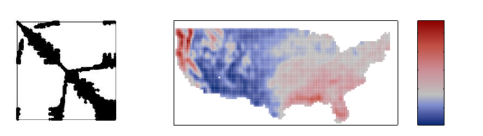
(a) The nonzero ele-
ments of Kf,f.
500
1000
1500
2000
2500
(b) The posterior predictive mean surface.
Figure 9: The nonzero elements of Kf,fwith kpp,2 function, and the posterior
predictive mean of the latent function in the US precipitation data set.
CS covariance functions. The posterior covariance in EP (22) does not remain sparse, and
thereby it has to be expressed implicitly. This issue is discussed by Vanhatalo and Vehtari
(2010) and Vanhatalo et al. (2010).
10.1.1 Compactly supported covariance functions in GPstuff
The demo demo_regression_ppcs contains a regression example with CS covariance func-
tion kpp,2(gpcf_ppcs2). The data contain US annual precipitation summaries from year
1995 for 5776 observation stations. The user interface of GPstuff makes no difference be-
tween globally and compactly supported covariance functions but the code is optimized to
use sparse matrix routines whenever the covariance matrix is sparse. Thus, we can construct
the model, find the MAP estimate for the parameters and predict to new input locations in
a familiar way:
pn = prior_t(’nu’, 4, ’s2’, 0.3);
lik = lik_gaussian(’sigma2’, 1, ’sigma2_prior’, pn);
pl2 = prior_gamma(’sh’, 5, ’is’, 1);
pm2 = prior_sqrtt(’nu’, 1, ’s2’, 150);
gpcf2 = gpcf_ppcs2(’nin’, nin, ’lengthScale’, [1 2], ’magnSigma2’, 3, ...
’lengthScale_prior’, pl2, ’magnSigma2_prior’, pm2);
gp = gp_set(’lik’, lik, ’cf’, gpcf2, ’jitterSigma2’, 1e-6);
gp = gp_optim(gp,x,y,’opt’,opt);
Eft = gp_pred(gp, x, y, xx);
With this data the covariance matrix is rather sparse since only about 5% of its elements are
non-zero. The structure of the covariance matrix is plotted after the approximate minimum
degree (AMD) permutation (Davis, 2006) in Figure 9. The demo demo_spatial2 illustrates
the use of compactly supported covariance functions with a non-Gaussian likelihood.
10.2 FIC and PIC sparse approximations
Snelson and Ghahramani (2006) proposed a sparse pseudo-input GP (SPGP), which Quinonero-
Candela and Rasmussen (2005) named later fully independent conditional (FIC). The par-
tially independent conditional (PIC) sparse approximation is an extension of FIC (Quinonero-
Candela and Rasmussen, 2005; Snelson and Ghahramani, 2007), and they are both treated
here following Quinonero-Candela and Rasmussen (2005). See also (Vanhatalo and Vehtari,
2008; Vanhatalo et al., 2010) for further discussion. The approximations are based on in-
troducing an additional set of latent variables u={ui}m
i=1, called inducing variables. These
correspond to a set of input locations Xu, called inducing inputs. The latent function prior
is approximated as
p(f|X, θ)≈q(f|X,Xu, θ) = Zq(f|X,Xu,u, θ)p(u|Xu, θ)du,(74)
where q(f|X,Xu,u, θ)is an inducing conditional. The above decomposition leads to the
exact prior if the true conditional f|X,Xu,u, θ ∼N(Kf,uK-1
u,uu,Kf,f−Kf,u K-1
u,uKu,f)is
used. However, in FIC framework the latent variables are assumed to be conditionally
independent given u, in which case the inducing conditional factorizes q(f|X,Xu,u, θ) =
Qqi(fi|X,Xu,u, θ). In PIC latent variables are set in blocks which are conditionally inde-
pendent of each others, given u, but the latent variables within a block have a multivariate
normal distribution with the original covariance. The approximate conditionals of FIC and
PIC can be summarized as
q(f|X,Xu,u, θ, M) = N(f|Kf,uK-1
u,uu,mask Kf,f−Kf,u K-1
u,uKu,f|M),(75)
where the function Λ= mask (·|M), with matrix Mof ones and zeros, returns a matrix Λof
size Mand elements Λij = [·]ij if Mij = 1 and Λij = 0 otherwise. An approximation with
M=Icorresponds to FIC and an approximation where Mis block diagonal corresponds
to PIC. The inducing variables are given a zero-mean Gaussian prior u|θ, Xu∼N(0,Ku,u)
so that the approximate prior over latent variables is
q(f|X,Xu, θ, M) = N(f|0,Kf,u K-1
u,uKu,f +Λ).(76)
The matrix Kf,u K-1
u,uKu,f is of rank mand Λis a rank n(block) diagonal matrix. The
prior covariance above can be seen as a non-stationary covariance function of its own where
the inducing inputs Xuand the matrix Mare free parameters similar to parameters, which
can be optimized alongside θ(Snelson and Ghahramani, 2006; Lawrence, 2007).
The computational savings are obtained by using the Woodbury-Sherman-Morrison
lemma (e.g. Harville, 1997) to invert the covariance matrix in (76) as
(Kf,u K-1
u,uKu,f +Λ)−1=Λ−1−VVT,(77)
where V=Λ−1Kf,uchol[(Ku,u+Ku,fΛ−1Kf,u)−1]. There is a similar result also for the
determinant. With FIC the computational time is dominated by the matrix multiplications,
which need time O(m2n). With PIC the cost depends also on the sizes of the blocks in Λ.
If the blocks were of equal size b×b, the time for inversion of Λwould be O(n/b ×b3) =
O(nb2). With blocks at most the size of the number of inducing inputs, that is b=m, the
computational cost in PIC and FIC are similar. PIC approaches FIC in the limit of a block
size one and the exact GP in the limit of a block size n(Snelson, 2007).
10.2.1 FIC sparse approximation in GPstuff
The same data that were discussed in the section 6.1 is analyzed with sparse approximations
in the demo demo_regression_sparse1. The sparse approximation is a property of the GP
structure and we can construct the model similarly to the full GP models:
gp_fic = gp_set(’type’, ’FIC’, ’lik’, lik, ’cf’, gpcf, ’X_u’, X_u)
The difference is that we have to define the type of the sparse approximation, here ’FIC’, and
set the inducing inputs X_u in the GP structure. Since the inducing inputs are considered
as extra parameters common to all of the covariance functions (there may be more than
one covariance function in additive models) they are set in the GP structure instead of
the covariance function structure. If we want to optimize the inducing inputs alongside
the parameters they need to have a prior as well. GP structure initialization gives them a
uniform prior by default.
We can optimize all the parameters, including the inducing inputs, as with a full GP.
Sometimes, for example in spatial problems, it is better to fix the inducing inputs (Vanhatalo
et al., 2010) or it may be more efficient to optimize the parameters and inducing inputs sep-
arately, so that we iterate the separate optimization steps until convergence (demonstrated
in demo_regression_sparse1). The parameters to be optimized are defined by the field
infer_params in the GP structure. This field regulates which parameters are considered
fixed and which are inferred in the group level (covariance function, inducing inputs, like-
lihood). We may also want to fix one of the parameters inside these groups. For example,
covariance function magnitude. If this is the case, then the parameter to be fixed should be
given an empty prior (prior_fixed). If the parameter has a prior structure it is an indicator
that we want to infer that parameter.
10.2.2 PIC sparse approximation in GPstuff
In PIC, in addition to defining the inducing inputs, we need to appoint every data point in a
block. The block structure is common to all covariance functions, similarly to the inducing
inputs, for which reason the block information is stored in the GP structure. After the
blocking and initialization of the inducing inputs the GP structure is constructed as follows:
gp_pic = gp_set(’type’,’PIC’,’lik’,lik,’cf’,gpcf,’X_u’,X_u,’tr_index’,trindex);
Above, the cell array trindex contains the block index vectors for training data. It means
that, for example, the inputs and outputs x(trindex{i},:) and y(trindex{i},:) belong
to the i’th block. The optimization of parameters and inducing inputs is done the same way
as with FIC or a full GP model. In prediction, however, we have to give one extra input,
tstindex, for gp_pred. This defines how the prediction inputs are appointed in the blocks
in a same manner as trindex appoints the training inputs.
Eft_pic = gp_pred(gp_pic, x, y, xt, ’tstind’, tstindex);
10.3 Deterministic training conditional, subset of regressors and variational
sparse approximation
The deterministic training conditional is based on the works by Csató and Opper (2002)
and Seeger et al. (2003) and was earlier called Projected Latent Variables (see Quinonero-

Candela and Rasmussen, 2005, for more details). The approximation can be constructed
similarly as FIC and PIC by defining the inducing conditional, which in the case of DTC is
q(f|X,Xu,u, θ) = N(f|Kf,uK-1
u,uu,0).(78)
This implies that the approximate prior over latent variables is
q(f|X,Xu, θ) = N(f|0,Kf,u K-1
u,uKu,f).(79)
The deterministic training conditional is not strictly speaking a proper GP since it uses
different covariance function for the latent variables appointed to the training inputs and
for the latent variables at the prediction sites, ˜
f. The prior covariance for ˜
fis the true
covariance K˜
f,˜
finstead of K˜
f,uK-1
u,uKu,˜
f. This does not affect the predictive mean since
the cross covariance Cov[f,˜
f] = Kf,uK-1
u,uKu,˜
f, but it gives a larger predictive variance.
An older version of DTC is the subset of regressors (SOR) sparse approximation which
utilizes K˜
f,uK-1
u,uKu,˜
f. However, this resembles a singular Gaussian distribution and thus
the predictive variance may be negative. DTC tries to fix this problem by using K˜
f,˜
f(see
Quinonero-Candela and Rasmussen, 2005). DTC and SOR are identical in other respects
than in the predictive variance evaluation. In spatial statistics, SOR has been used by
Banerjee et al. (2008) with a name Gaussian predictive process model.
The approximate prior of the variational approximation by Titsias (2009) is exactly
the same as that of DTC. The difference between the two approximations is that in the
variational setting the inducing inputs and covariance function parameters are optimized
differently. The inducing inputs and parameters can be seen as variational parameters that
should be chosen to maximize the variational lower bound between the true GP posterior
and the sparse approximation. This leads to optimization of modified log marginal likelihood
V(θ, Xu) = log[N(y|0, σ2I+Qf,f)] −1
2σ2tr(Kf,f−Kf,uK-1
u,uKu,f)(80)
with Gaussian likelihood. With non-Gaussian likelihood, the variational lower bound is
similar but σ2Iis replaced by W−1(Laplace approximation) or ˜
Σ(EP).
10.3.1 Variational, DTC and SOR sparse approximation in GPstuff
The variational, DTC and SOR sparse approximations are constructed similarly to FIC.
Only the type of the GP changes:
gp_var = gp_set(’type’, ’VAR’, ’lik’, lik, ’cf’, gpcf, ’X_u’, X_u);
gp_dtc = gp_set(’type’, ’DTC’, ’lik’, lik, ’cf’, gpcf, ’X_u’, X_u);
gp_sor = gp_set(’type’, ’SOR’, ’lik’, lik, ’cf’, gpcf, ’X_u’, X_u);
The sparse GP approximations are compared in the demo demo_regression_sparse2, and,
for example, Quinonero-Candela and Rasmussen (2005), Snelson (2007), Titsias (2009), and
Alvarez et al. (2010) treat them in more detail.
10.4 Sparse GP models with non-Gaussian likelihoods
The extension of sparse GP models to non-Gaussian likelihoods is straightforward in GPstuff.
User can define the sparse GP just as described in the previous two sections and then continue
with the construction of likelihood exactly the same way as with a full GP. The Laplace
approximation, EP and integration methods can be used with the same commands as with
full GP. This is demonstrated in demo_spatial1.
10.5 Predictive active set selection for classification
Predictive active set selection for Gaussian processes (PASS-GP, Henao and Winther, 2012)
is a sparse approximation for classification models. PASS-GP uses predictive distributions
to estimate which data points to include in the active set, so that it will include points with
potentially high impact to the classifier decision process while removing those that are less
relevant. Function passgp accepts classification GP with latent method set to EP or Laplace,
and selects the active set and optimises the hyperparameters. Its use is demonstrated in
demo_passgp.
11. Modifying the covariance functions
11.1 Additive models
In many practical situations, a GP prior with only one covariance function may be too re-
strictive since such a construction can model effectively only one phenomenon. For example,
the latent function may vary rather smoothly across the whole area of interest, but at the
same time it can have fast local variations. In this case, a more reasonable model would
be f(x) = g(x) + h(x), where the latent value function is a sum of two functions, slow and
fast varying. By placing a separate GP prior for both of the functions gand hwe obtain an
additive prior
f(x)|θ∼ GP(0, kg(x,x0) + kh(x,x0)).(81)
The marginal likelihood and posterior distribution of the latent variables are as before with
Kf,f=Kg,g +Kh,h. However, if we are interested on only, say, phenomenon g, we can
consider the hpart of the latent function as correlated noise and evaluate the predictive
distribution for g, which with the Gaussian likelihood would be
˜g(˜
x)|D, θ ∼ GP kg(˜
x,X)(Kf,f+σ2I)−1y, kg(˜
x,˜
x0)−kg(˜
x,X)(Kf,f+σ2I)−1kg(X,˜
x0).
(82)
With non-Gaussian likelihood, the Laplace and EP approximations for this are similar since
only σ2Iand (Kf,f+σ2I)−1ychange in the approximations.
The multiple length-scale model can be formed also using specific covariance functions.
For example, a rational quadratic covariance function (gpcf_rq) can be seen as a scale
mixture of squared exponential covariance functions (Rasmussen and Williams, 2006), and
could be useful for data that contain both local and global phenomena. However, using
sparse approximations with the rational quadratic would prevent it from modeling local
phenomena. The additive model (81) suits better for sparse GP formalism since it enables
to combine FIC with CS covariance functions.
As discussed in section 10.2, FIC can be interpreted as a realization of a special kind of
covariance function. Vanhatalo and Vehtari (2008) proposed to add FIC with CS covariance
function which leads to a latent variable prior
f|X,Xu, θ ∼N(0,Kf,uK-1
u,uKu,f+ˆ
Λ),(83)
referred as CS+FIC. Here, the matrix ˆ
Λ=Λ+kpp,q(X,X)is sparse with the same sparsity
structure as in kpp,q(X,X)and it is fast to use in computations and cheap to store.
11.1.1 Additive models in GPstuff
The additive models are demonstrated in demo_periodic and demo_regression_additive1.
Their construction follows closely the steps introduced in the previous sections. Consider
that we want to construct a GP with a covariance function that is a sum of squared expo-
nential and piecewise polynomial kse(x,x0) + kpp,2(x,x0). In GPstuff this is done as follows:
gpcf1 = gpcf_sexp();
gpcf2 = gpcf_ppcs2(’nin’, 2);
lik = lik_gaussian(’sigma2’, 0.1);
gp = gp_set(’lik’, lik, ’cf’, {gpcf1, gpcf2});
The difference to previous models is that we give more than one covariance function structure
in cell array for the gp_set. The inference with additive model is conducted the same way as
earlier. If we want to make predictions for the two components kse and kpp,2independently
we can do it by giving an extra parameter-value pair for the gp_pred as
[Ef_sexp, Varf_sexp] = gp_pred(gp, x, y, x, ’predcf’, 1);
[Ef_ppcs2, Varf_ppcs2] = gp_pred(gp, x, y, x, ’predcf’, 2);
Additive models are constructed analogously with sparse approximations by changing
the type of the GP model. CS+FIC is a special kind of GP structure and has its own type
definition:
gp = gp_set(’type’, ’CS+FIC’, ’lik’, lik, ’cf’, {gpcf1, gpcf2}, ’X_u’, Xu);
It is worth mentioning few things that should be noticed in relation to sparse approxi-
mations. In general, FIC is able to model only phenomena whose length-scale is long enough
compared to the distance between adjacent inducing inputs. PIC on the other hand is able
to model also fast varying phenomena inside the blocks. Its drawback, however, is that the
correlation structure is discontinuous which may result in discontinuous predictions. The
CS+FIC model corrects these deficiencies. In FIC and PIC the inducing inputs are pa-
rameters of every covariance function, which means that all the correlations are induced
through the inducing inputs and the shortest length-scale the GP is able to model is defined
by the locations of the inducing inputs. In CS+FIC, the CS covariance functions do not
utilise inducing inputs but evaluate the covariance exactly for which reason both the long
and short length-scale phenomena can be captured. If there are more than two covariance
functions in CS+FIC all the globally supported functions utilize inducing inputs and all the
CS functions are added to ˆ
Λ. A detailed treatment on the subject is given in (Vanhatalo
and Vehtari, 2008, 2010; Vanhatalo et al., 2010)
11.2 Additive covariance functions with selected variables
In the demo (demo_regression_additive2), we demonstrate how covariance functions can
be modified so that they are functions of only a subset of inputs. We model an artificial 2D
regression data with additive covariance functions that use only either the first or second
input variable. That is, the covariance is k1(x1, x0
1|θ1) + k2(x2, x0
2|θ2) : <2×<27→ <, where
the covariance functions are of type k1(x1, x0
1|θ1) : <×< 7→ <. In the example the covariance
is a sum of a squared exponential, which is a function of the first input dimension x1, and
a linear covariance function, which is a function of the second input dimension x2. The
covariance functions are constructed as follows:
gpcf_s1 = gpcf_sexp(’selectedVariables’, 1, ’lengthScale’,0.5, ...
’magnSigma2’, 0.15);
gpcf_l2 = gpcf_linear(’selectedVariables’, 2);
The smaller set of inputs is chosen with the field input variable pair ’selectedVariables’,1.
11.3 Product of covariance functions
A product of two or more covariance functions k1(x,x0)·k2(x,x0)... is a valid covariance
function as well. Such constructions may be useful in situations where the phenomenon is
assumed to be separable. Combining covariance functions into product form is done with a
special covariance function gpcf_prod. For example, multiplying exponential and Mátern
covariance functions to produce separable spatio-temporal model k(x,x0) = k1(x1, x0
1)·
k2([x2, x3]T,[x0
2, x0
3]T)where the temporal component has covariance function k1and the
spatial components k2is done as follows:
gpcf1 = gpcf_exp(’selectedVariables’, 1);
gpcf2 = gpcf_matern32(’selectedVariables’, [2 3];
gpcf = gpcf_prod(’cf’, {gpcf1, gpcf2});
The product covariance gpcf_prod can also be used to combine categorical covariance
gpcf_cat with other covariance functions to build hierarchical linear and non-linear models,
as illustrated in demo_regression_hier.
12. State space inference
By Arno Solin, Jukka Koskenranta, and Simo Särkkä.
For one-dimensional Gaussian processes, instead of directly working with the usual kernel
formalism,f∼ GP(0, k(t, t0)), of the Gaussian process, certain classes of covariance functions
allow to work with the mathematical dual (Särkkä et al., 2013), where the Gaussian process
is though of as a solution to a mth order linear stochastic differential equation (SDE). The
corresponding inference problem can then solved with Kalman filtering type of methods
(Grewal and Andrews, 2001; Särkkä, 2013), where the computational complexity is O(m3n)
making this formulation beneficial for long (often temporal) data sets.

The state space model corresponding to the GP regression problem can be given as a
linear time-invariant stochastic differential equation of the following form:
df(t)
dt=Ff(t) + Lw(t)
yk=Hf(tk) + εk, εk∼N(0, σ2
n),
(84)
where f(t) = f1(t), f2(t), . . . , fm(t)Tholds the mstochastic processes, and w(t)is a multi-
dimensional white noise process with spectral density Qc. The model is defined by the
feedback matrix Fand the noise effect matrix L.
The continuous-time linear time-invariant model (84) can be solved for discrete points.
This is the closed-form solution to the SDE at the specified time points, and it is given as
fk+1 =Akfk+qk,qk∼N(0,Qk),(85)
where f(tk) = fk, and the state transition and process noise covariance matrices can be
solved analytically (see, e.g., Särkkä et al., 2013). They are given as:
Ak=Φ(∆tk),(86)
Qk=Z∆tk
0
Φ(∆tk−τ)LQcLTΦ(∆tk−τ)Tdτ, (87)
where ∆tk=tk+1 −tk. The iteration is started form the stationary state f0∼N(0,P∞),
where P∞is a solution to the Lyapunov equation: FP∞+P∞FT+LQcLT=0. For
more details on the connection between state space models and Gaussian processes, see,
e.g., Särkkä et al. (2013).
The inference problem is now directly solvable using Kalman filtering and Rauch-Tung-
Striebel smoothing methods (Grewal and Andrews, 2001; Särkkä, 2013). The marginal
likelihood and analytic gradients for conjugate gradient optimization can be calculated in
closed form. The sequential nature of the state space solution is not well handled by Mat-
lab/Octave, and thus this formulation becomes appealing when the number of data points
becomes very large (in thousands).
In GPstuff, the following covariance functions are currently supported (details on how
the conversion is done are given in the accompanying references):
Constant covariance function.
Noise covariance function.
Linear covariance function.
Exponential (Ornstein-Uhlenbeck) covariance function.
Matérn covariance function (for ν= 3/2and ν= 5/2).
Squared exponential covariance function (as presented in Hartikainen and Särkkä,
2010).
Periodic covariance function both with and without decay (quasi-periodicity) (as pre-
sented in Solin and Särkkä, 2014a).
Rational quadratic covariance function (as presented in Solin and Särkkä, 2014b).
Sums and products of covariance functions (as given in Solin and Särkkä, 2014a).
These methods can be accessed by specifying the model type to ‘kalman’, that is
gp = gp_set(gp,’type’,’KALMAN’);
Currently the ‘kalman’ option is only supported for one-dimensional GP regression, which
can be performed by the usual workflow in GPstuff after specifying the model type. For
a more practical introduction, see the demos ‘demo_kalman1’ (a simple one-dimensional
regression problem) and ‘demo_kalman2’ (periodic modeling of the Mauna Loa CO2data,
following Solin and Särkkä, 2014a).
13. Model assessment and comparison
There are various means to assess the goodness of the model and its predictive performance.
For an extensive review of the predictive performance assessment methods see Vehtari and
Ojanen (2012) and for a shorter review comparing cross-validation, DIC and WAIC see
Gelman et al. (2014). GPstuff provides four basic approaches: marginal likelihood, cross-
validation, deviance information criterion (DIC) and widely applicable information criterion
(WAIC).
13.1 Marginal likelihood
Marginal likelihood is often used for model selection (see, e.g. Kass and Raftery, 1995). It
corresponds to ML II or with model priors to MAP II estimate in the model space, selecting
the model with the highest marginal likelihood or highest marginal posterior probability.
In GPstuff the marginal posterior and marginal likelihood (or its approximation in case of
non-Gaussian likelihood) given the parameters are computed by function gp_e.
13.2 Cross-validation
Cross-validation (CV) is an approach to estimate the predictive performance for the future
observations while avoiding the double use of the data. The ith observation (xi, yi)in the
training data is left out, and then the predictive distribution for yiis computed with a model
that is fitted to all of the observations except (xi, yi). By repeating this for every point in
the training data, we get a collection of leave-one-out cross-validation (LOO-CV) predictive
densities. For discussion of Bayesian cross-validation see Vehtari and Lampinen (2002);
Vehtari and Ojanen (2012); Gelman et al. (2014) and for comparison of fast approximations
for latent Gaussian variable models see Vehtari et al. (2014).
For GP with given hyperparameters the LOO-CV predictions can be computed in case
of Gaussian likelihood using an analytical solution (Sundararajan and Keerthi, 2001) and
in case of non-Gaussian likelihood using EP approximation (Opper and Winther, 2000;
Rasmussen and Williams, 2006) or Laplace approximation using linear response approach
(Vehtari et al., 2014), which have been implemented in gp_loopred.
If set of hyperparameters have been obtained using gp_mc or gp_ia LOO-posterior can
be approximated using importance sampling or weighting (Gelfand et al., 1992; Vehtari
and Lampinen, 2002), which is also implemented in gp_loopred. We use an integrated
approach following Vehtari (2001, p. 40) where leave-one-out predictive densities given
hyperparameters
p(yi|xi, D−i, ϑ) = Zp(yi|fi, ϑ)p(fi|xi, D−i, ϑ)dfi(88)
are obtained using the analytic solution, or the Laplace or EP approximation as mentioned
above (see also Held et al., 2010). Thus the importance weighting is made only for the
hyperparameters. This reduces the variance of importance sampling estimate significantly
making it useful in practice. With these approximations LOO-CV is very fast to compute
in GPstuff. We also use Pareto smoothed importance sampling (Vehtari and Gelman, 2015;
Vehtari et al., 2015) to further reduce the variance of the estimate.
LOO-CV in GPstuff does not currently work for some multilatent models. In such
case or if there is reason to doubt the reliability of the leave-one-out approximations, it
is best to compute the non-approximated cross-validation predictive densities. To reduce
computation time, in k-fold-CV, 1/k part of the training data is left out, and then the
predictive distribution is computed with a model that is fitted to all of the observations
except that part. Since the k-fold-CV predictive densities are based on smaller training
data sets than the full data set, the estimate is slightly biased. In GPstuff first order bias
correction proposed by Burman (1989) is used. GPstuff provides gp_kfcv, which computes
k-fold-CV and bias-corrected k-fold-CV with log-score and root mean squared error (RMSE).
The function gp_kfcv provides also basic variance estimates for the predictive performance
estimates. The variance is computed from the estimates for each fold (see, e.g., Dietterich,
1998). See Vehtari and Lampinen (2002); Vehtari and Ojanen (2012) for more details on
estimating the uncertainty in performance estimates.
13.3 DIC
Deviance information criterion (DIC) is another very popular model selection criterion
(Spiegelhalter et al., 2002). DIC is not fully Bayesian approach as it estimates the pre-
dictive performance if the predictions were made using point-estimate (plug-in estimate) for
the unknowns, instead of using posterior predictive distribution. Additionally DIC is defined
only for regular models and thus fails for singular models. DIC is included in GPstuff to
allow comparisons and better alternative WAIC is described in the next section.
With parametric models without any hierarchy DIC is usually written as
peff = Eθ|D[D(y, θ)] −D(y,Eθ|D[θ]) (89)
DIC = Eθ|D[D(y, θ)] + peff,(90)
where peff is the effective number of parameters and D=−2 log(p(y|θ)) is the deviance.
Since our models are hierarchical we need to decide the parameters on focus (see Spiegelhalter
et al., 2002, for discussion on this). The parameters on the focus are those over which the
expectations are taken when evaluating the effective number of parameters and DIC. In the
above equations, the focus is in the parameters and in the case of a hierarchical GP model
of GPstuff the latent variables would be integrated out before evaluating DIC. If we have a

MAP estimate for the parameters, we may be interested to evaluate DIC statistics with the
focus on the latent variables. In this case the above formulation would be
pD(θ) = Ef|D,θ[D(y,f)] −D(y,Ef|D,θ[f]) (91)
DIC = Ef|D,θ[D(y,f)] + pD(θ).(92)
Here the effective number of parameters is denoted differently with pD(θ)since now we are
approximating the effective number of parameters in fconditionally on θ, which is different
from the peff.pD(θ)is a function of the parameters and it measures to what extent the
prior correlations are preserved in the posterior of the latent variables given θ. For non-
informative data pD(θ)=0and the posterior is the same as the prior. The greater pD(θ)is
the more the model is fitted to the data and large values compared to nindicate potential
overfit. Also, large pD(θ)indicates that we cannot assume that the conditional posterior
approaches normality by central limit theorem. Thus, pD(θ)can be used for assessing the
goodness of the Laplace or EP approximation for the conditional posterior of the latent
variables as discussed by Rue et al. (2009) and Vanhatalo et al. (2010). The third option is
to evaluate DIC with focus on all the variables, [f, θ]. In this case the expectations are over
p(f, θ|D).
13.4 WAIC
Watanabe (2009, 2010a,b) presented widely applicable information criterion (WAIC) and
gave a formal proof of its properties as an estimate for the predictive performance of posterior
predictive distributions for both regular and singular models. A criterion of similar form
was independently proposed by Richardson (2002) as a version of DIC, but without formal
justification.
Other information criteria are based on Fisher’s asymptotic theory assuming a regular
model for which the likelihood or the posterior converges to a single point and MLE, MAP,
and plug-in estimates are asymptotically equivalent. With singular models the set of true
parameters consists of more than one point, the Fisher information matrix is not positive
definite, plug-in estimates are not representative of the posterior and the distribution of the
deviance does not converge to a χ2
νdistribution.
Watanabe shows that the Bayesian generalization utility can be estimated by a criterion
WAICG=BUt−2(BUt−GUt),(93)
where BUtis Bayes training utility
BUt=1
n
n
X
i=1
log p(yi|D, Mk)(94)
and GUtis Gibbs training utility
GUt=1
n
n
X
i=1 Zlog p(yi|θ, Mk)p(θ|D, Mk)dθ (95)
WAIC can also be given as a functional variance form
WAICV=BUt−V /n, (96)
where the functional variance
V=
n
X
i=1 (Eθ|D,Mkh(log p(yi|xi, θ, Mk))2i
−Eθ|D,Mk[log p(yi|xi, θ, Mk)]2),(97)
describes the fluctuation of the posterior distribution.
WAIC is asymptotically equal to the true logarithmic utility in both regular and singular
statistical models and the error in a finite case is o(1/n). Watanabe (2010b) shows also that
the WAIC estimate is asymptotically equal to the Bayesian cross-validation estimate (section
13.2). WAICGand WAICVare asymptotically equal, but the series expansion of W AICV
has closer resemblance to the series expansion of the logarithmic leave-one-out utility.
13.5 Model assessment demos
The model assessment methods are demonstrated with the functions demo_modelassesment1
and demo_modelassesment2. The former compares the sparse GP approximations to the
full GP with regression data and the latter compares the logit and probit likelihoods in GP
classification.
Assume that we have built our regression model with a Gaussian noise and used opti-
mization method to find the MAP estimate for the parameters. We evaluate the effective
number of latent variables, DIC and WAIC
p_eff_latent = gp_peff(gp, x, y);
[DIC_latent, p_eff_latent2] = gp_dic(gp, x, y, ’focus’, ’latent’);
WAIC = gp_waic(gp,x,y);
where peff is evaluated with two different approximations. Since we have the MAP estimate
for the parameters the focus is on the latent variables. In this case we can also use gp_peff
which returns the effective number of parameters approximated as
pD(θ)≈n−tr(K-1
f,f(K-1
f,f+σ−2I)−1)(98)
(Spiegelhalter et al., 2002). When the focus is on the latent variables, the function gp_dic
evaluates the DIC statistics and the effective number of parameters as described by the
equations (91) and (92).
The k-fold-CV expected utility estimate can be evaluated as follows:
cvres = gp_kfcv(gp, x, y);
The gp_kfcv takes the ready made model structure gp and the training data xand y.
The function divides the data into kgroups, conducts inference separately for each of the
training groups and evaluates the expected utilities with the test groups. Since no optional
parameters are given the inference is conducted using MAP estimate for the parameters.
The default division of the data is into 10 groups. The expected utilities and their variance
estimates are stored in the structure cvres.gp_kfcv returns also other statistics if more
information is needed and the function can be used to save the results automatically.
Assume now that we have a record structure from gp_mc function with Markov chain
samples of the parameters stored in it. In this case, we have two options how to evaluate
the DIC statistics. We can set the focus on the parameters or all the parameters (that
is parameters and latent variables). The two versions of DIC and the effective number of
parameters and WAIC are evaluated as follows:
rgp = gp_mc(gp, x, y, opt);
[DIC, p_eff] = gp_dic(rgp, x, y, ’focus’, ’param’);
[DIC2, p_eff2] = gp_dic(rgp, x, y, ’focus’, ’all’);
WAIC = gp_waic(gp,x,y);
Here the first line performs the MCMC sampling with options opt. The next two lines
evaluate the DIC statistics and the last line evaluates WAIC. With Markov chain samples,
we cannot use the gp_peff function to evaluate pD(θ)since that is a special function for
models with fixed parameters.
The functions gp_peff,gp_dic and gp_kfcv work similarly for non-Gaussian likelihoods
as for a Gaussian one. The only difference is that the integration over the latent variables
is done approximately. The way the latent variables are treated is defined in the field
latent_method of the GP structure and this is initialized when constructing the model as
discussed in the section 6.2. The effective number of parameters returned by gp_peff is
evaluated as in the equation (98) with the modification that σ−2Iis replaced by Win the
case of Laplace approximation and ˜
Σ−1in the case of EP.
14. Bayesian optimization
Bayesian optimization is a sequential design strategy for global optimization of black-box
functions (e.g., Jones et al., 1998). The objective function is given a GP prior and af-
ter running the objective function the prior is updated to form a posterior conditional to
the function runs so far. An acquisition function, which depends on the posterior for the
objective function, is used to decide what the next query point should be. The Bayesian
optimization is illustrated by demo_bayesoptimization.
More specifically, assume we have run the objective function ntimes providing us the
data {fi,xi}n
i=1 where ficorresponds to the function value at input location xi. We give a
(zero mean) GP prior for the objective function f(x)∼GP (0, k(x,x0)) and calculate the
posterior distribution for the objective function f(x)|y,X∼GP (µp
f(x), kp
f(x, x0)) where
µp
f(x)and kp
f(x, x0)are the posterior mean and covariance functions summarized in equation
(7) and paragraph below it. Next we need an acquisition function a(x) : <d→ < which
determines the next point to be evaluated via an optimization xnext = arg maxxa(x). Several
acquisition functions have been proposed and here we consider the expected improvement.
Let fmin = min(f1, ..., fn)be the current best function value. The improvement from the
current best at the point xis I(x) = max(fmin −f(x),0) where f(x)is a random variable.

Hence, the expected improvement at the point xis (Jones et al., 1998)
E[I(x)] = E[max(fmin −f(x),0)] (99)
= (fmin −µp
f(x))Φ
fmin −µp
f(x)
qkp
f(x, x0)
+qkp
f(x, x0)φ
fmin −µp
f(x)
qkp
f(x, x0)
,(100)
where Φ(·)and φ(·)denote, respectively, the standard Gaussian cumulative distribution and
the density functions. The gradient of the expected improvement with respect to xcan be
solved analytically which enables gradient based optimization of this acquisition function.
Since Matlab optimizers seek for the function minimum we use negative expected improve-
ment in GPstuff. Moreover, in the two dimensional example in demo_bayesoptimization
we demonstrate also how the exploration of the search space can be improved by alternat-
ing between searching for the maximum expected improvement and the maximum posterior
variance (every fifth iteration in the demo).
Gelbart et al. (2014) treat Bayesian optimization under unknown constraints. There the
problem is to find the optimum of the objective function while fulfilling a set of unknown
functional constraints at the same time. GPstuff allows constraint functions of type f:<d→
<with lower and upper limits. Let us denote cconstraint functions and the corresponding
lower and upper limits by fc
1, ..., fc
c,lc
1, ..., lc
cand uc
1, ..., uc
c. We give a (zero mean) GP prior
for each of the constraint functions so that fc
k∼GP (0, kfc
k(x,x0)). After evaluating the
constraint functions at training points xc
k,1, ..., xc
k,nkwe can calculate the posterior for each
of the constraint functions. Note that the training set for each constraint and objective
function can be different. After calculating the posterior of all the constraint functions and
the objective function, the expected improvement under constraints (EIC) can be calculated
as
EIC = E[I(x)]
c
Y
k=1
Pr (lc
k< fc
k(x)< uc
k)(101)
= E[I(x)]
c
Y
k=1
Φ
ukc−µp
fc
k(x)
qkp
fc
k(x, x0)
−Φ
lkc−µp
fc
k(x)
qkp
fc
k(x, x0)
.(102)
We can again use gradient based optimization to find the maximum of EIC. In GPstuff both
negative EI and negative EIC are implemented in expectedimprovement_eg.m.
15. Adding new features in the toolbox
As described in the previous sections, GPstuff is build modularly so that the full model
is constructed by combining separate building blocks. Each building block, such as the
covariance function or likelihood, is written in a m-file which contains all the functions
and parameters specific to it. This construction makes it easier to add new model blocks
in the package. For example, new covariance functions can be written by copying one of
the existing functions to a new file and modifying all the subfunctions and parameters
according to the new covariance function. With likelihoods it should be remembered that
GPstuff assumes currently that they factorize as described in the equation (1). All the
inference methods should work for log-concave likelihoods. However, likelihood functions
that are not log-concave may lead to problems with Laplace approximation and EP since
the conditional posterior of the latent variables may be multimodal and the diagonal matrices
Wand ˜
Σmay contain negative elements (Vanhatalo et al., 2009). For example, Student-t
observation model leads to a likelihood, which is not log-concave, and requires some specific
modifications to the Laplace approximation and EP algorithm (see Jylänki et al., 2011).
Using MCMC should, however, be straightforward with non-log-concave likelihoods as well.
See Appendix F for technical details of lik,gpcf and prior functions, and argument
interface for optimisation and sampling functions.
The package is not as modular with respect to the computational techniques as to the
model blocks. Usually, each inference method requires specific summaries from the model
blocks. For example, the EP algorithm requires that each likelihood has a function to
evaluate integrals such as Rfip(yi|fi, φ)N(fi|µ, σ2)dfiwhereas the Laplace approximation
requires the Hessian of the log likelihood, ∇2
flog p(y|f, φ). For this reason adding, for exam-
ple, variational approximation would require modifications also in the likelihood functions.
16. Discussion
Broadly thinking, GPs have been researched intensively for decades and many disciplines
have contributed to their study. They have not, necessarily, been called GP but, for ex-
ample, spatial statistics, signal processing and filtering literature have their own naming
conventions. The point of view taken in GPstuff comes mainly from the machine learning
literature where the subject has flourished to a hot topic since late 1990’s. Our aim in the
GPstuff package has been to collect existing and create new practical tools for analyzing GP
models. We acknowledge that many of the basic models and algorithms have been proposed
by others. However, the implementation in GPstuff is unique and contains several practical
solutions for computational problems that are not published elsewhere. Our own contribu-
tion on GP theory that is included in GPstuff is described mainly in (Vehtari, 2001; Vehtari
and Lampinen, 2002; Vanhatalo and Vehtari, 2007, 2008, 2010; Vanhatalo et al., 2009, 2010;
Jylänki et al., 2011; Riihimäki and Vehtari, 2012; Joensuu et al., 2012; Riihimäki et al.,
2013; Joensuu et al., 2014; Riihimäki and Vehtari, 2014)
Our intention has been to create a toolbox with which useful, interpretable results can be
produced in a sensible time. GPstuff provides approximations with varying level of accuracy.
The approximation to be used needs to be chosen so that it approximates well enough
the essential aspects in the model. Thus, the choice is always data, model, and problem
dependent. For example, MCMC methods are often praised for their asymptotic properties
and seemingly easy implementation. Algorithms, such as Metropolis-Hastings, are easy to
implement for most models. The problem, however, is that as a data set grows they may
not give reliable results in a finite time. With GP models this problem is faced severely. For
example, currently problems with over 10 000 data points would be impractical to analyse
with a standard office PC using MCMC since the convergence rate and mixing of the sample
chain would be too slow. For this reason it is important to have also faster, but perhaps
less accurate, methods. The choice of the method is then a compromise between time and
accuracy. The inference is the fastest when using MAP estimate for the parameters and a
Gaussian function for the conditional posterior. With a Gaussian likelihood, the Gaussian
conditional distribution is exact and the only source of imprecision is the point estimate
for the parameters. If the likelihood is other than Gaussian, the conditional distribution
is an approximation, whose quality depends on how close to Gaussian the real conditional
posterior is, and how well the mean and covariance are approximated. The form of the real
posterior depends on many things for which reason the Gaussian approximation has to be
assessed independently for every data.
One of our aims with GPstuff has been to provide an easy way to detect model mis-
specifications. This requires the model assessment tools discussed in the section 13 and an
easy way to test alternative model structures. The model misfit most often relates either to
the likelihood or GP prior. For example, if the data contained outliers or observations with
clearly higher variance than what the Gaussian or Poisson observation model predicts, the
posterior of the latent function would be highly compromised. For this reason, robust alter-
natives for traditional models, such as Student-tor negative binomial distribution should be
easily testable. Even though the GP prior is very flexible and only the mean and covariance
need to be fixed, it still contains rather heavy assumptions. For example, GP associated
with the squared exponential covariance function is indefinitely mean square differentiable.
This is a very strong assumption on the smoothness of the latent function. In fact it is rather
peculiar how little attention other covariance functions have gained in machine learning lit-
erature. One of the reasons may be that often machine learning problems take place in high
dimensional input spaces where data are enforced to lie sparsely and for which reason the
possible solutions are smooth. However, the covariance function sometimes does influence
the results (see e.g. Vanhatalo and Vehtari, 2008; Vanhatalo et al., 2010).
In statistics, inference in the parameters is a natural concern but in machine learning
literature they are left in less attention. An indicator of this is the usual approach to
maximize the marginal likelihood which implies uniform prior for the parameters. GPstuff
provides an easy way to define priors explicitly so that people would really use them (this
principle is also in line with reasoning by Gelman, 2006). We want to stress a few reasons
for explicitly defining a prior. In spatial statistics, it is well known that the length-scale
and magnitude are underidentifiable and the proportion σ2/l is more important to the
predictive performance than their individual values (Diggle et al., 1998; Zhang, 2004; Diggle
and Ribeiro, 2007). These results are shown for Matérn class of covariance functions but
according to our experiments they seem to apply for Wendland’s piecewise polynomials as
well. With them, the property can be taken advantage of since by giving more weight to
short length-scales one favors sparser covariance matrices that are faster in computations.
Other advantage is that priors make the inference problem easier by narrowing the posterior
and making the parameters more identifiable. This is useful especially for MCMC methods
but optimization and other integration approximations gain from the priors as well. These
two reasons are rather practical. More fundamental reason is that in Bayesian statistics
leaving prior undefined (meaning uniform prior) is a prior statement as well, and sometimes
it may be really awkward. For example, uniform prior works very badly for the parameters
of the Student-tdistribution. Thus, it is better to spend some time thinking what the prior
actually says than blindly use the uniform.
There are also other analytic approximations than the Laplace approximation or EP pro-
posed in the literature. Most of these are based on some kind of variational approximation
(Gibbs and Mackay, 2000; Csató and Opper, 2002; Tipping and Lawrence, 2005; Kuss, 2006;
Opper and Archambeau, 2009). Laplace approximation and EP were chosen to GPstuff for
a few reasons. They both are, in theory, straightforward to implement for any factoriz-
able likelihood (although sometimes there are practical problems with the implementation).
Laplace approximation is also fast and EP is shown to work well in many problems. Here,
we have considered parametric observation models but non-parametric versions are possible
as well. Examples of possible extensions to that direction are provided by Snelson et al.
(2004) and Tokdar et al. (2010).
GPstuff is an ongoing project and the package will be updated whenever new function-
alities are ready. The latest version of the toolbox is available from http://becs.aalto.
fi/en/research/bayes/gpstuff/.
Acknowledgments
The research leading to GPstuff has been funded by the Academy of Finland (grant 218248),
Finnish Funding Agency for Technology and Innovation (TEKES), and the Graduate School
in Electronics and Telecommunications and Automation (GETA). The first author also
thanks the Finnish Foundation for Economic and Technology Sciences KAUTE, Finnish
Cultural Foundation, and Emil Aaltonen Foundation for supporting his post graduate studies
during which the code package was prepared.
The package contains pieces of code written by other people than the authors. In the
Department of Biomedical Engineering and Computational Science at Aalto University these
persons are (in alphabetical order): Toni Auranen, Pasi Jylänki, Jukka Koskenranta, Enrique
Lelo de Larrea Andrade, Tuomas Nikoskinen, Tomi Peltola, Eero Pennala, Heikki Peura,
Ville Pietiläinen, Markus Siivola, Arno Solin, Simo Särkkä and Ernesto Ulloa. People outside
Aalto University are (in alphabetical order): Christopher M. Bishop, Timothy A. Davis,
Matthew D. Hoffman, Kurt Hornik, Dirk-Jan Kroon, Iain Murray, Ian T. Nabney, Radford
M. Neal and Carl E. Rasmussen. We want to thank them all for sharing their code under a
free software license.
References
Milton Abramowitz and Irene A. Stegun. Handbook of mathematical functions. Dover
Publications, Inc., 1970.
Omar B. Ahmad, Cynthia Boschi-Pinto, Alan D. Lopez, Christopher J.L. Murray, Rafael
Lozano, and Mie Inoue. Age standardization of rates: A new WHO standard. GPE
Discussion Paper Series, 31, 2000.
M. A. Alvarez, D. Luengo, M. K. Titsias, and N. D. Lawrence. Efficient multioutput Gaus-
sian processes through variational inducing kernels. JMLR Workshop and conference
proceedings, 9:25–32, 2010.
Sudipto Banerjee, Alan E. Gelfand, Andrew O. Finley, and Huiyan Sang. Gaussian predictive
process models for large spatial data sets. Journal of the Royal Statistical Society B, 70
(4):825–848, 2008.
Veronica J. Berrocal, Adrian E. Raftery, Tilmann Gneiting, and Richard C. Steed. Proba-
bilistic weather forecasting for winter road maintenance. Journal of the American Statis-
tical Association, 105(490):522–537, 2010.
Nicky Best, Sylvia Richardson, and Andrew Thomson. A comparison of Bayesian spatial
models for disease mapping. Statistical Methods in Medical Research, 14:35–59, 2005.
Alexis Boukouvalas, Remi Barillec, and Dan Cornford. Gaussian process quantile regression
using expectation propagation. arXiv preprint arXiv:1206.6391, 2012.
J. D. Broffitt. Increasing and increasing convex bayesian graduation. Transactions of the
Society of Actuaries, 40(1):115–148, 1988.
M. D. Buhmann. A new class of radial basis functions with compact support. Mathematics
of Computation, 70(233):307–318, January 2001.
Prabir Burman. A comparative study of ordinary cross-validation, v-fold cross-validation
and the repeated learning-testing methods. Biometrika, 76(3):503–514, 1989.
Ole F. Christensen, Gareth O. Roberts, and Martin Sköld. Robust Markov chain Monte
Carlo methods for spatial generalized linear mixed models. Journal of Computational and
Graphical Statistics, 15:1–17, 2006.
Stefano Conti, John Paul Gosling, Jeremy Oakley, and Anthony O’Hagan. Gaussian process
emulation of dynamic computer codes. Biometrika, 96:663–676, 2009.
David R Cox. Regression models and life-tables. Journal of the Royal Statistical Society.
Series B (Methodological), 34(2):187–220, 1972.
Noel A. C. Cressie. Statistics for Spatial Data. John Wiley & Sons, Inc., 1993.
Lehel Csató and Manfred Opper. Sparse online Gaussian processes. Neural Computation,
14(3):641–669, 2002.
Botond Cseke and Tom Heskes. Approximate marginals in latent Gaussian models. Journal
of Machine Learning Research, 12:417–454, 2 2011. ISSN 1532-4435.
Timothy A. Davis. Algorithm 849: A concise sparse Cholesky factorization package. ACM
Trans. Math. Softw., 31:587–591, December 2005.
Timothy A. Davis. Direct Methods for Sparse Linear Systems. SIAM, 2006.
Marc Peter Deisenroth, Carl Edward Rasmussen, and Jan Peters. Gaussian process dynamic
programming. Neurocomputing, 72(7–9):1508–1524, 2009.
Marc Peter Deisenroth, Carl Edward Rasmussen, and Dieter Fox. Learning to control a
low-cost manipulator using data-efficient reinforcement learning. In In 9th International
Conference on Robotics: Science & Systems, 2011.
Thomas G. Dietterich. Approximate statistical tests for comparing supervised classification
learning algorithms. Neural Computation, 10(7):1895–1924, 1998.
P. J. Diggle, J. A. Tawn, and R. A. Moyeed. Model-based geostatistics. Journal of the Royal
Statistical Society. Series C (Applied Statistics), 47(3):299–350, 1998.
Peter J. Diggle and Paulo J. Ribeiro. Model-based Geostatistics. Springer Science+Business
Media, LLC, 2007.
Simon Duane, A.D. Kennedy, Brian J. Pendleton, and Duncan Roweth. Hybrid Monte
Carlo. Physics Letters B, 195(2):216–222, 1987.
P. Elliot, Jon Wakefield, Nicola Best, and David Briggs, editors. Spatial Epidemiology
Methods and Applications. Oxford University Press, 2001.
Bärbel Finkenstädt, Leonhard Held, and Valerie Isham. Statistical Methods for Spatio-
Temporal Systems. Chapman & Hall/CRC, 2007.
Montserrat Fuentes and Adrian E. Raftery. Model evaluation and spatial interpolation by
Bayesian combination of observations with outputs from numerical models. Biometrics,
66:36–45, 2005.
Reinhard Furrer, Marc G. Genton, and Douglas Nychka. Covariance tapering for interpola-
tion of large spatial datasets. Journal of Computational and Graphical Statistics, 15(3):
502–523, September 2006.
G. Gaspari and S.E. Cohn. Construction of correlation functions in two and three dimensions.
Quarterly Journal of the Royal Meteorological Society, 125(554):723–757, January 1999.
Michael A. Gelbart, Jasper Snoek, and Ryan P. Adams. Bayesian Optimization with Un-
known Constraints, 2014. URL http://arxiv.org/pdf/1403.5607v1.pdf.
Alan E. Gelfand, D. K. Dey, and H. Chang. Model determination using predictive distri-
butions with implementation via sampling-based methods (with discussion). In J. M.
Bernardo, J. O. Berger, A. P. Dawid, and A. F. M. Smith, editors, Bayesian Statistics 4,
pages 147–167. Oxford University Press, 1992.
Alan E. Gelfand, Peter J. Diggle, Montserrat Fuentes, and Peter Guttorp. Handbook of
Spatial Statistics. CRC Press, 2010.
Andrew Gelman. Prior distributions for variance parameters in hierarchical models.
Bayesian Analysis, 1(3):515–533, 2006.
Andrew Gelman, John B. Carlin, Hal S. Stern, David B. Dunson, Aki Vehtari, and Donald B.
Rubin. Bayesian Data Analysis. Chapman & Hall/CRC, third edition, 2013.
Andrew Gelman, Jessica Hwang, and Aki Vehtari. Understanding predictive information
criteria for Bayesian models. Statistics and Computing, 24(6):997–1016, 2014.
John Geweke. Bayesian inference in econometric models using Monte Carlo integration.
Econometrica, 57(6):721–741, 1989.
Mark N. Gibbs and David J. C. Mackay. Variational Gaussian process classifiers. IEEE
Transactions on Neural Networks, 11(6):1458–1464, 2000.
W.R. Gilks, S. Richardson, and D.J. Spiegelhalter. Markov Chain Monte Carlo in Practice.
Chapman & Hall, 1996.
Tilmann Gneiting. Correlation functions for atmospheric data analysis. Quarterly Journal
of the Royal Meteorological Society, 125:2449–2464, 1999.
Tilmann Gneiting. Compactly supported correlation functions. Journal of Multivariate
Analysis, 83:493–508, 2002.
Paul W Goldberg, Christopher KI Williams, and Christopher M Bishop. Regression with
input-dependent noise: A Gaussian process treatment. In Y. Weiss, B. Schölkopf, and
J. Platt, editors, Advances in Neural Information Processing Systems, volume 10, pages
493–499, 1997.
Mohinder S. Grewal and Angus P. Andrews. Kalman Filtering: Theory and Practice Using
Matlab. Wiley Interscience, second edition, 2001.
Jouni Hartikainen and Simo Särkkä. Kalman filtering and smoothing solutions to temporal
Gaussian process regression models. In Proceedings of IEEE International Workshop on
Machine Learning for Signal Processing (MLSP), 2010.
David A. Harville. Matrix Algebra From a Statistician’s Perspective. Springer-Verlag, 1997.
Leonhard Held, Birgit Schrödle, and Håvard Rue. Posterior and cross-validatory predictive
checks: A comparison of MCMC and INLA. In Thomas Kneib and Gerhard Tutz, editors,
Statistical Modelling and Regression Structures, pages 91–110. Springer, 2010.
Ricardo Henao and Ole Winther. Predictive active set selection methods for Gaussian
processes. Neurocomputing, 80(0):10–18, 2012.
Matt D Hoffman and Andrew Gelman. The no-U-turn sampler: Adaptively setting path
lengths in Hamiltonian Monte Carlo. Journal of Machine Learning Research, 15:1593–
1623, Apr 2014.
Antti Honkela, Pei Gao, Jonatan Ropponen, Magnus Rattray, and Neil D. Lawrence. tigre:
Transcription factor inference through gaussian process reconstruction of expression for
bioconductor. Bioinformatics, 27(7):1026–1027, 2011.
Joseph G. Ibrahim, Ming-Hui Chen, and Debajyoti Sinha. Bayesian Survival Analysis.
Springer, 2001.
Heikki Joensuu, Aki Vehtari, Jaakko Riihimäki, Toshirou Nishida, Sonja E Steigen, Peter
Brabec, Lukas Plank, Bengt Nilsson, Claudia Cirilli, Chiara Braconi, Andrea Bordoni,
Magnus K Magnusson, Zdenek Linke, Jozef Sufliarsky, Federico Massimo, Jon G Jonasson,
Angelo Paolo Dei Tos, and Piotr Rutkowski. Risk of gastrointestinal stromal tumour
recurrence after surgery: an analysis of pooled population-based cohorts. The Lancet
Oncology, 13(3):265–274, 2012.
Heikki Joensuu, Peter Reichardt, Mikael Eriksson, Kirsten Sundby Hall, and Aki Vehtari.
Gastrointestinal stromal tumor: A method for optimizing the timing of CT scans in the
follow-up of cancer patients. Radiology, 271(1):96–106, 2014.
Donald R. Jones, Matthias Schonlau, and William J. Welch. Efficient global optimization
of expensive black-box functions. Journal of Global optimization, 13(4):455–492, 1998.
Teppo Juntunen, Jarno Vanhatalo, Heikki Peltonen, and Samu Mäntyniemi. Bayesian spatial
multispecies modelling to assess pelagic fish stocks from acoustic- and trawl-survey data.
ICES Journal of Marine Science, 69(1):95–104, 2012.
Pasi Jylänki, Jarno Vanhatalo, and Aki Vehtari. Robust Gaussian process regression with
a Student-tlikelihood. Journal of Machine Learning Research, 12:3227–3257, 2011.
Ilkka Kalliomäki, Aki Vehtari, and Jouko Lampinen. Shape analysis of concrete aggregates
for statistical quality modeling. Machine Vision and Applications, 16(3):197–201, 2005.
Robert E. Kass and Adrian E. Raftery. Bayes factors. Journal of the American Statistical
Association, 90(430):773–795, 1995.
Cari G. Kaufman, Mark J. Schervish, and Douglas W. Nychka. Covariance tapering for
likelihood-based estimation in large spatial data sets. Journal of the American Statistical
Association, 103(484):1545–1555, 2008.
Mark C. Kennedy and Anthony O’Hagan. Bayesian calibration of computer models. Journal
of the Royal Statistical Society, B, 63(3):425–464, 2001.
Thomas Kneib. Mixed model-based inference in geoadditive hazard regression for interval
censored survival times. Computational Statistics and Data Analysis, 51(2):777–792, 2006.
M. Kot. Elements of Mathematical Ecology. Cambridge University Press, 2001.
Malte Kuss. Gaussian Process Models for Robust Regression, Classification, and Reinforce-
ment Learning. PhD thesis, Technische Universität Darmstadt, 2006.
Malte Kuss and Carl Edward Rasmussen. Assessing approximate inference for binary Gaus-
sian process classification. Journal of Machine Learning Research, 6:1679–1704, October
2005.
Neil Lawrence. Learning for larger datasets with the Gaussian process latent variable model.
In M. Meila and X. Shen, editors, Proceedings of the Eleventh International Workshop on
Artificial Intelligence and Statistics. Omnipress, 2007.
Andrew B. Lawson. Statistical Methods in Spatial Epidemology. John Wiley & Sons, Ltd,
2001.
Sara Martino, Rupali Akerkar, and Håvard Rue. Approximate Bayesian inference for survival
models. Scandinavian Journal of Statistics, 38(3):514–528, 2011.
G. Matheron. The intrinsic random functions and their applications. Advances in Applied
Probability, 5(3):439–468, December 1973.
Mathworks. MATLAB Getting Started Quide. The MathWorks, Inc., fifteenth edition, 2010.
Thomas Minka. A Family of Algorithms for Approximate Bayesian Inference. PhD thesis,
Massachusetts Institute of Technology, 2001.
Jesper Møller, Anne Randi Syversveen, and Rasmus Plenge Waagepetersen. Log Gaussian
Cox processes. Scandinavian Journal of Statistics, 25:451–482, September 1998.
Fernando A Moala and Anthony O’Hagan. Elicitation of multivariate prior distributions:
a nonparametric Bayesian approach. Journal of Statistical Planning and Inference, 140:
1635–1655, 2010.
G. Moreaux. Compactly supported radial covariance functions. Journal of Geodecy, 82(7):
431–443, July 2008.
J Mullahy. Specification and testing of some modified count data models. Journal of Econo-
metrics, 33:341–365, 1986.
Iain Murray and Ryan Prescott Adams. Slice sampling covariance hyperparameters of latent
Gaussian models. In J. Lafferty, C. K. I. Williams, R. Zemel, J. Shawe-Taylor, and
A. Culotta, editors, Advances in Neural Information Processing Systems 23, pages 1732–
1740, 2010.
Iain Murray, Ryan Prescott Adams, and David J.C. MacKay. Elliptical slice sampling.
JMLR: Workshop and Conference Proceedings, 9:541–548, 2010.
Mari Myllymäki, Aila Särkkä, and Aki Vehtari. Hierarchical second-order analysis of repli-
cated spatial point patterns with non-spatial covariates. Spatial Statistics, 8:104–121,
2014.
Ian T. Nabney. NETLAB: Algorithms for Pattern Recognition. Springer, 2001.
Radford Neal. Regression and classification using Gaussian process priors. In J. M. Bernardo,
J. O. Berger, A. P. David, and A. P. M. Smith, editors, Bayesian Statistics 6, pages 475–
501. Oxford University Press, 1998.
Radford M. Neal. Bayesian Learning for Neural Networks. Springer, 1996.
Radford M. Neal. Monte Carlo Implementation of Gaussian Process Models for Bayesian
Regression and Classification. Technical Report 9702, Dept. of statistics and Dept. of
Computer Science, University of Toronto, January 1997.
Radford M. Neal. Slice sampling. The Annals of Statistics, 31(3):705–767, 2003.
Hannes Nickisch and Carl Edward Rasmussen. Approximations for binary Gaussian process
classification. Journal of Machine Learning Research, 9:2035–2078, October 2008.
Octave community. GNU/Octave, 2012. URL www.gnu.org/software/octave/.
Anthony O’Hagan. Curve fitting and optimal design for prediction. Journal of the Royal
Statistical Society. Series B., 40(1):1–42, 1978.
Anthony O’Hagan. On outlier rejection phenomena in Bayes inference. Journal of the Royal
Statistical Society. Series B., 41(3):358–367, 1979.
Manfred Opper and Cédric Archambeau. The variational Gaussian approximation revisited.
Neural Computation, 21(3):786–792, March 2009.
Manfred Opper and Ole Winther. Gaussian processes for classification: Mean-field algo-
rithms. Neural Computation, 12(11):2655–2684, 2000.
Joaquin Quinonero-Candela and Carl Edward Rasmussen. A unifying view of sparse approxi-
mate Gaussian process regression. Journal of Machine Learning Research, 6(3):1939–1959,
December 2005.
Jarmo Rantonen, Aki Vehtari, Jaro Karppinen, Satu Luoto, Eira Viikari-Juntura, Markku
Hupli, Antti Malmivaara, and Simo Taimela. The effectiveness of two active interven-
tions compared to self-care advice in employees with non-acute low back symptoms. A
randomised, controlled trial with a 4-year follow-up in the occupational health setting.
Occupational and Environmental Medicine, 69(1):12–20, 2012.
Jarmo Rantonen, Aki Vehtari, Jaro Karppinen, Satu Luoto, Eira Viikari-Juntura, Markku
Hupli, Antti Malmivaara, and Simo Taimela. Face-to-face information in addition to a
booklet versus a booklet alone for treating mild back pain, a randomized controlled trial.
Scandinavian journal of Work Environment and Health, 40(2):156–166, 2014.
Jorma Rantonen, Satu Luoto, Aki Vehtari, Markku Hupli, Jaro Karppinen, Antti Malmi-
vaara, and Simo Taimela. The effectiveness of two active interventions compared to
self-care advice in employees with non-acute low back symptoms. a randomised, con-
trolled trial with a 4-year follow-up in the occupational health setting. Occupational and
Environmental Medicine, 2011.
Carl Edward Rasmussen. Evaluations of Gaussian Processes and Other Methods for Non-
linear Regression. PhD thesis, University of Toronto, 1996.
Carl Edward Rasmussen and Hannes Nickisch. Gaussian processes for machine learning
(GPML) toolbox. Journal of Machine Learning Research, 11:3011–3015, September 2010.
Carl Edward Rasmussen and Christopher K. I. Williams. Gaussian Processes for Machine
Learning. The MIT Press, 2006.
Stephen L. Rathbun and Noel Cressie. Asymptotic properties of estimators for the param-
eters of spatial inhomogeneous poisson point processes. Advances in Applied Probability,
26(1):122–154, March 1994.
Sylvia Richardson. Discussion to ‘bayesian measures of model complexity and fit’ by spiegel-
halter et al. Journal of the Royal Statistical Society. Series B (Statistical Methodology),
64(4):626–627, 2002.
Sylvia Richardson. Spatial models in epidemiological applications. In Peter J. Green, Nils Lid
Hjort, and Sylvia Richardson, editors, Highly Structured Stochastic Systems, pages 237–
259. Oxford University Press, 2003.
Riihimäki and Aki Vehtari. Laplace approximation for logistic gp density estimation. Tech-
nical report, Department of Biomedical Engineering and Computational Science, Aalto
University, 2012. arXiv preprint arXiv:1211.0174.
Riihimäki and Aki Vehtari. Laplace approximation for logistic Gaussian process density
estimation and regression. Bayesian analysis, 9(2):425–448, 2014.
Jaakko Riihimäki and Aki Vehtari. Gaussian processes with monotonicity information.
Journal of Machine Learning Research: Workshop and Conference Proceedings, 9:645–
652, 2010.
Jaakko Riihimäki, Pasi Jylänki, and Aki Vehtari. Nested expectation propagation for Gaus-
sian process classification with a multinomial probit likelihood. Journal of Machine Learn-
ing Research, 14:75–109, 2013.
Christian P. Robert and George Casella. Monte Carlo Statistical Methods. Springer, second
edition, 2004.
Håvard Rue, Sara Martino, and Nicolas Chopin. Approximate Bayesian inference for latent
Gaussian models by using integrated nested Laplace approximations. Journal of the Royal
statistical Society B, 71(2):1–35, 2009.
Susan M. Sanchez and Paul J. Sanchez. Very large fractional factorials and central composite
designs. ACM Transactions on Modeling and Computer Simulation, 15:362–377, 2005.
F. Sansò and W.-D. Schuh. Finite covariance functions. Journal of Geodesy, 61(4):331–347,
1987.
Simo Särkkä. Bayesian Filtering and Smoothing, volume 3 of Institute of Mathematical
Statistics Textbooks. Cambridge University Press, 2013.
Simo Särkkä, Arno Solin, and Jouni Hartikainen. Spatiotemporal learning via infinite-
dimensional Bayesian filtering and smoothing. IEEE Signal Processing Magazine, 30(4):
51–61, 2013.
Mathias Seeger, Christopher K. I. Williams, and Neil Lawrence. Fast forward selection to
speed up sparse Gaussian process regression. In Christopher M. Bishop and Brendan J.
Frey, editors, Ninth International Workshop on Artificial Intelligence and Statistics. Soci-
ety for Artificial Intelligence and Statistics, 2003.
Matthias Seeger. Expectation propagation for exponential families. Technical report, Max
Planck Institute for Biological Cybernetics, Tübingen, Germany, 2005.
Edward Snelson. Flexible and Efficient Gaussian Process Models for Machine Learning. PhD
thesis, University College London, 2007.
Edward Snelson and Zoubin Ghahramani. Sparse Gaussian process using pseudo-inputs. In
Y. Weiss, B. Schölkopf, and J. Platt, editors, Advances in Neural Information Processing
Systems 18. The MIT Press, 2006.
Edward Snelson and Zoubin Ghahramani. Local and global sparse Gaussian process ap-
proximations. In Marina Meila and Xiaotong Shen, editors, Artificial Intelligence and
Statistics 11. Omnipress, 2007.
Edward Snelson, Carl Edward Rasmussen, and Zoubin Ghahramani. Warped Gaussian
processes. In T. G. Diettrich, S. Becker, and Z. Ghahramani, editors, Advances in Neural
Information Processing Systems 14. The MIT Press, 2004.
Arno Solin and Simo Särkkä. Explicit link between periodic covariance functions and state
space models. In Proceedings of the Seventeenth International Conference on Artificial
Intelligence and Statistics, volume 33 of JMLR W&CP, pages 904–912, 2014a.
Arno Solin and Simo Särkkä. Gaussian quadratures for state space approximation of scale
mixtures of squared exponential covariance functions. In Proceedings of IEEE Interna-
tional Workshop on Machine Learning for Signal Processing (MLSP), 2014b.
David J. Spiegelhalter, Nicola G. Best, Bradley P. Carlin, and Angelika van der Linde.
Bayesian measures of model complexity and fit. Journal of the Royal Statistical Society
B, 64(4):583–639, 2002.
Oliver Stegle, Sebastian V. Fallert, David J. C. MacKay, and Søren Brage. Gaussian process
robust regression for noisy heart rate data. Biomedical Engineering, IEEE Transactions
on, 55(9):2143–2151, September 2008. ISSN 0018-9294.
S. Sundararajan and S. S. Keerthi. Predictive approaches for choosing hyperparameters in
Gaussian processes. Neural Computation, 13(5):1103–1118, May 2001.
Madeleine Thompson and Radford M Neal. Covariance-adaptive slice sampling. arXiv
preprint arXiv:1003.3201, 2010.
Luke Tierney and Joseph B. Kadane. Accurate approximations for posterior moments and
marginal densities. Journal of the American Statistical Association, 81(393):82–86, 1986.
Michael E. Tipping and Neil D. Lawrence. Variational inference for Student-tmodels:
Robust Bayesian interpolation and generalised component analysis. Neurocomputing, 69:
123–141, 2005.
Michalis K. Titsias. Variational learning of inducing variables in sparse Gaussian processes.
JMLR Workshop and Conference Proceedings, 5:567–574, 2009.
Surya T. Tokdar and Jayanta K. Ghosh. Posterior consistency of logistic Gaussian process
priors in density estimation. Journal of Statistical Planning and Inference, 137:34–42,
2007.
Surya T. Tokdar, Yu M. Zhu, and Jayanta K. Ghosh. Bayesian density regression with
logistic Gaussian process and subspace projection. Bayesian Analysis, 5(2):319–344, 2010.
Jarno Vanhatalo and Aki Vehtari. Sparse log Gaussian processes via MCMC for spatial
epidemiology. JMLR Workshop and Conference Proceedings, 1:73–89, 2007.

Jarno Vanhatalo and Aki Vehtari. Modelling local and global phenomena with sparse Gaus-
sian processes. In David A. McAllester and Petri Myllymäki, editors, Proceedings of the
24th Conference on Uncertainty in Artificial Intelligence, pages 571–578, 2008.
Jarno Vanhatalo and Aki Vehtari. Speeding up the binary Gaussian process classification.
In Peter GrÃ1
4nwald and Peter Spirtes, editors, Proceedings of the 26th Conference on
Uncertainty in Artificial Intelligence, pages 1–9, 2010.
Jarno Vanhatalo, Pasi Jylänki, and Aki Vehtari. Gaussian process regression with student-t
likelihood. In Y. Bengio, D. Schuurmans, J. Lafferty, C. K. I. Williams, and A. Culotta,
editors, Advances in Neural Information Processing Systems 22, pages 1910–1918. NIPS
foundation, 2009.
Jarno Vanhatalo, Ville Pietiläinen, and Aki Vehtari. Approximate inference for disease
mapping with sparse Gaussian processes. Statistics in Medicine, 29(15):1580–1607, 2010.
Jarno Vanhatalo, Jaakko Riihimäki, Jouni Hartikainen, Pasi Jylänki, Ville Tolvanen, and
Aki Vehtari. GPstuff: Bayesian modeling with Gaussian processes. Journal of Machine
Learning Research, 14:1175–1179, 2013.
Aki Vehtari. Bayesian Model Assessment and Selection Using Expected Utilities. PhD thesis,
Helsinki University of Technology, 2001.
Aki Vehtari and Andrew Gelman. Pareto smoothed importance sampling. arXiv:1507.02646,
2015.
Aki Vehtari and Jouko Lampinen. Bayesian model assessment and comparison using cross-
validation predictive densities. Neural Computation, 14(10):2439–2468, 2002.
Aki Vehtari and Janne Ojanen. A survey of Bayesian predictive methods for model assess-
ment, selection and comparison. Statistics Surveys, 6:142–228, 2012.
Aki Vehtari, Tommi Mononen, Ville Tolvanen, and Ole Winther. Bayesian leave-one-
out cross-validation approximations for Gaussian latent variable models. arXiv preprint
arXiv:1412.7461, 2014.
Aki Vehtari, Andrew Gelman, and Jonah Gabry. Efficient implementation of leave-one-out
cross-validation and WAIC for evaluating fitted Bayesian models. arXiv:1507.04544, 2015.
Sumio Watanabe. Algebraic Geometry and Statistical Learning Theory. Cambridge Univer-
sity Press, 2009.
Sumio Watanabe. Equations of states in singular statistical estimation. Neural Networks,
23(1):20–34, 2010a.
Sumio Watanabe. Asymptotic equivalence of Bayes cross validation and widely applicable
information criterion in singular learning theory. Journal of Machine Learning Research,
11:3571–3594, 2010b.

Holger Wendland. Piecewise polynomial, positive definite and compactly supported radial
functions of minimal degree. Advances in Computational Mathematics, 4(1):389–396,
December 1995.
Holger Wendland. Scattered Data Approximation. Cambridge University Press, 2005.
Norbert Wiener. Extrapolation, Interpolation, and Smoothing of Stationary Time Series.
MIT Press, 1949.
C. K. I. Williams and C. E. Rasmussen. Gaussian processes for regression. In D. S. Touretzky,
M. C. Mozer, and M. E. Hasselmo, editors, Advances in Neural Information Processing
Systems 8, pages 514–520. MIT Press, 1996.
Christopher K. I. Williams. Computing with infinite networks. In Michael C. Mozer,
Michael I. Jordan, and Thomas Petsche, editors, Advances in Neural Information Pro-
cessing Systems, volume 9. The MIT Press, 1996.
Christopher K. I. Williams. Computation with infinite neural networks. Neural Computation,
10(5):1203–1216, 1998.
Christopher K. I. Williams and David Barber. Bayesian classification with Gaussian pro-
cesses. IEEE Transactions on Pattern Analysis and Machine Intelligence, 20(12):1342–
1351, December 1998.
Zongmin Wu. Compactly supported positive definite radial functions. Advances in Compu-
tational Mathematics, 4(1):283–292, 1995.
Hao Zhang. Inconsistent estimation and asymptotically equal interpolations in model-based
geostatistics. Journal of the American Statistical Association, 99(465):250–261, 2004.
Appendix A. Comparison of features in GPstuff, GPML and FBM
Table 1 shows comparison of features in GPstuff, GPML and FBM.
Appendix B. Covariance functions
In this section we summarize all the covariance functions in the GPstuff package.
Squared exponential covariance function (gpcf_sexp)
Probably the most widely-used covariance function is the squared exponential (SE)
k(xi,xj) = σ2
sexp exp −1
2
d
X
k=1
(xi,k −xj,k)2
l2
k!.(103)
The length scale lkgoverns the correlation scale in input dimension kand the magnitude
σ2
sexp the overall variability of the process. A squared exponential covariance function leads
to very smooth GPs that are infinitely times mean square differentiable.

GPstuff GPML FBM
Covariance functions
number of elementary functions 16 10 4
sums of elements, masking of inputs x x x
delta distance x x
products, positive scaling of elements x x
Mean functions
number of elementary functions 4 4 0
sums of elements, masking of inputs x x
products, power, scaling of elements x
marginalized parameters x
Single latent likelihood/observation models
Gaussian x x x
logistic/logit, erf/probit x x MCMC
Poisson x LA/EP/MCMC MCMC
Gaussian scale mixture MCMC MCMC
Student-tx LA/VB/MCMC
Laplacian x EP/VB/MCMC
mixture of likelihoods LA/EP/MCMC
sech-squared, uniform for classification x
derivative observations for sexp covf only
binomial, negative binomial, zero-trunc. negative binomial, log-Gaussian
Cox process; Weibull, log-Gaussian and log-logistic with censoring
x
quantile regression MCMC/EP
Multilatent likelihood/observation models
multinomial, Cox proportional hazard model, density estimation, density
regression, input dependent noise, input dependent overdispersion in
Weibull, zero-inflated negative binomial
MCMC/LA
multinomial logit (softmax) MCMC/LA MCMC
multinomial probit EP MCMC
monotonicity EP
Priors for parameters (ϑ)
several priors, hierarchical priors x x
Sparse models
FITC x exact/EP/LA
CS, FIC, CS+FIC, PIC, VAR, DTC, SOR x
PASS-GP LA/EP
Latent inference
exact (Gaussian only) x x x
scaled Metropolis, HMC x x
LA, EP, elliptical slice sampling x x
variational Bayes (VB) x
scaled HMC (with inverse of prior cov.) x
scaled HMC (whitening with approximate posterior covariance) x
parallel EP, Robust-EP x
marginal corrections (cm2 and fact) x
state space inference (1D for some covariance functions) x
Hyperparameter inference
type II ML x x x
type II MAP, Metropolis, HMC x x
LOO-CV for Gaussian x x
least squares LOO-CV for non-Gaussian some likelihoods
LA/EP LOO-CV for non-Gaussian, k-fold CV x
NUTS, slice sampling (SLS), surrogate SLS, shrinking-rank SLS,
covariance-matching SLS, grid, CCD, importance sampling
x
Model assessment
marginal likelihood MAP,ML ML
LOO-CV for fixed hyperparameters x x
LOO-CV for integrated hyperparameters, k-fold CV, WAIC, DIC x
average predictive comparison x
Table 1: The comparison of features in GPstuff (v4.5), GPML (v3.2) and FBM
(2004-11-10) toolboxes. In case of model blocks the notation x means that it can
be inferred with any inference method (EP, LA (Laplace), MCMC and in case of
GPML also with VB). In case of sparse approximations, inference methods and
model assessment methods x means that the method is available for all model
blocks.

Exponential covariance function (gpcf_exp)
Exponential covariance function is defined as
k(xi,xj) = σ2
exp exp
−v
u
u
t
d
X
k=1
(xi,k −xj,k)2
l2
k
.(104)
The parameters lkand σ2
exp have similar role as with the SE covariance function. The expo-
nential covariance function leads to very rough GPs that are not mean square differentiable.
Matérn class of covariance functions (gpcf_maternXX)
The Matérn class of covariance functions is given by
kν(xi,xj) = σ2
m
21−ν
Γ(ν)√2νrνKν√2νr,(105)
where r=Pd
k=1
(xi,k−xj,k )2
l2
k1/2. The parameter νgoverns the smoothness of the process,
and Kνis a modified Bessel function (Abramowitz and Stegun, 1970, sec. 9.6). The Matérn
covariance functions can be represent in a simpler form when νis a half integer. The Matérn
covariance functions with ν= 3/2(gpcf_matern32) and ν= 5/2(gpcf_matern52) are:
kν=3/2(xi,xj) = σ2
m1 + √3rexp −√3r(106)
kν=5/2(xi,xj) = σ2
m1 + √5r+5r2
3exp −√5r.(107)
Neural network covariance function (gpcf_neuralnetwork)
A neural network with suitable transfer function and prior distribution converges to a GP
as the number of hidden units in the network approaches to infinity (Neal, 1996; Williams,
1996, 1998; Rasmussen and Williams, 2006). A nonstationary neural network covariance
function is
k(xi,xj) = 2
πsin−1 2˜xT
iΣ˜xj
(1 + 2˜xT
iΣ˜xi)(1 + 2˜xT
jΣ˜xj)!,(108)
where ˜x = (1, x1, . . . , xd)Tis an input vector augmented with 1. Σ = diag(σ2
0, σ2
1, . . . , σ2
d)is
a diagonal weight prior, where σ2
0is a variance for bias parameter controlling the functions
offset from the origin. The variances for weight parameters are σ2
1, . . . , σ2
d, and with small
values for weights, the neural network covariance function produces smooth and rigid looking
functions. The larger values for the weight variances produces more flexible solutions.
Constant covariance function (gpcf_constant)
Perhaps the simplest covariance function is the constant covariance function
k(xi,xj) = σ2(109)
with variance parameter σ2. This function can be used to implement the constant term in
the dot-product covariance function (Rasmussen and Williams, 2006) reviewed below.
Linear covariance function (gpcf_linear)
The linear covariance function is
k(xi,xj) = xT
iΣxj(110)
where the diagonal matrix Σ = diag(σ2
1, . . . , σ2
D)contains the prior variances of the linear
model coefficients. Combining this with the constant function above we can form covariance
function Rasmussen and Williams (2006), which calls a dot-product covariance function
k(xi,xj) = σ2+xT
iΣxj.(111)
Michelis-Menten covariance function (gpcf_linearMichelismenten)
The Michelis-Menten functional form (equivalently Type-II functional response or Monod
form, (Kot, 2001)) is given by
h(x) = bx/(a+x)(112)
where bis asymptote of the function and athe half-saturation point defining at which point
the function is half of the asymptotic level. By giving a zero mean Gaussian prior for
asymptote, b∼N(0, σ2)the prior for h(x)is h(x)∼N(0, H(x)H(x)Tσ2)where H(x) =
[x1/(a+x1, ..., xn/(a+xn]T. Hence, the covariance function related to the Michelis-Menten
mean function in case of Dinputs is
k(xi,xj) = H(xi)ΣH(xj)T,(113)
where the diagonal matrix Σ = diag(σ2
1, . . . , σ2
D)contains the prior variances of the bdterms.
Logistic mean covariance function (gpcf_linearLogistic)
The logistic functional form is given by
h(x) = w(logit−1(ax +b)−0.5) (114)
where wis the weight of the mean function, bis the intercept of the linear part and a
regression coefficient of linear part. By giving a zero mean Gaussian prior for weight, w∼
N(0, σ2)the prior for h(x)is h(x)∼N(0, H(x)H(x)Tσ2)where H(x)=[h(x1), ..., h(xn)]T.
Hence, the covariance function related to the logistic mean function in case of Dinputs is
k(xi,xj) = H(xi)ΣH(xj)T,(115)
where the diagonal matrix Σ = diag(σ2
1, . . . , σ2
D)contains the prior variances of the bdterms.

Piecewise polynomial functions (gpcf_ppcsX)
The piecewise polynomial functions are the only compactly supported covariance functions
(see section 10) in GPstuff. There are four of them with the following forms
kpp0(xi,xj) =σ2(1 −r)j
+(116)
kpp1(xi,xj) =σ2(1 −r)j+1
+((j+ 1)r+ 1) (117)
kpp2(xi,xj) =σ2
3(1 −r)j+2
+((j2+ 4j+ 3)r2+ (3j+ 6)r+ 3) (118)
kpp3(xi,xj) =σ2
15 (1 −r)j+3
+((j3+ 9j2+ 23j+ 15)r3+
(6j2+ 36j+ 45)r2+ (15j+ 45)r+ 15) (119)
where j=bd/2c+q+ 1. These functions correspond to processes that are 2qtimes mean
square differentiable at the zero and positive definite up to the dimension d(Wendland,
2005). The covariance functions are named gpcf_ppcs0,gpcf_ppcs1,gpcf_ppcs2, and
gpcf_ppcs3.
Rational quadratic covariance function (gpcf_rq)
The rational quadratic (RQ) covariance function (Rasmussen and Williams, 2006)
kRQ(xi,xj) = 1 + 1
2α
d
X
k=1
(xi,k −xj,k)2
l2
k!−α
(120)
can be seen as a scale mixture of squared exponential covariance functions with different
length-scales. The smaller the parameter α > 0is the more diffusive the length-scales of the
mixing components are. The parameter lk>0characterizes the typical length-scale of the
individual components in input dimension k.
Periodic covariance function (gpcf_periodic)
Many real world systems exhibit periodic phenomena, which can be modelled with a periodic
covariance function. One possible construction (Rasmussen and Williams, 2006) is
k(xi,xj) = exp −
d
X
k=1
2 sin2(π(xi,k −xj,k)/γ)
l2
k!,(121)
where the parameter γcontrols the inverse length of the periodicity and lkthe smoothness
of the process in dimension k.
Product covariance function (gpcf_product)
A product of two or more covariance functions, k1(x,x0)·k2(x,x0)..., is a valid covariance
function as well. Combining covariance functions in a product form can be done with
gpcf_prod, for which the user can freely specify the covariance functions to be multiplied
with each other from the collection of covariance functions implemented in GPstuff.

Categorical covariance function (gpcf_cat)
Categorical covariance function gpcf_cat returns correlation 1 if input values are equal and
0 otherwise.
k(xi,xj) = (1if xi−xj= 0
0otherwise (122)
Categorical covariance function can be combined with other covariance functions using
gpcf_prod, for example, to produce hierarchical models.
Appendix C. Observation models
Here, we summarize all the observation models in GPstuff. Most of them are implemented in
files lik_* which reminds that at the inference step they are considered likelihood functions.
Gaussian (lik_gaussian)
The i.i.d Gaussian noise with variance σ2is
y|f, σ2∼N(f, σ2I).(123)
Student-t(lik_t,lik_gaussiansmt)
The Student-tobservation model (implemented in lik_t) is
y|f, ν, σt∼
n
Y
i=1
Γ((ν+ 1)/2)
Γ(ν/2)√νπσt1 + (yi−fi)2
νσ2
t−(ν+1)/2
,(124)
where νis the degrees of freedom and σthe scale parameter. The scale mixture version of
the Student-tdistribution is implemented in lik_gaussiansmt and it is parametrized as
yi|fi, α, Ui∼N(fi, αUi)(125)
Ui∼Inv-χ2(ν, τ 2),(126)
where each observation has its own noise variance αUi(Neal, 1997; Gelman et al., 2013).
Logit (lik_logit)
The logit transformation gives the probability for yiof being 1or −1as
plogit(yi|fi) = 1
1 + exp(−yifi).(127)
Probit (lik_probit)
The probit transformation gives the probability for yiof being 1or −1as
pprobit(yi|fi) = Φ(yif(xi)) = Zyif(xi)
−∞
N(z|0,1)dz. (128)

Poisson (lik_poisson)
The Poisson observation model with expected number of cases eis
y|f,e∼
n
Y
i=1
Poisson(yi|exp(fi)ei).(129)
Negative-Binomial (lik_negbin)
The negative-binomial is a robustified version of the Poisson distribution. It is parametrized
y|f,e, r ∼
n
Y
i=1
Γ(r+yi)
yi!Γ(r)r
r+µirµi
r+µiyi
(130)
where µi=eexp(fi),ris the dispersion parameter governing the variance, eiis the expected
number of cases and yiis positive integer telling the observed count.
Binomial (lik_binomial)
The binomial observation model with the probability of success pi= exp(fi)/(1 + exp(fi))
is
y|f,z∼
N
Y
i=1
zi!
yi!(zi−yi)!pyi
i(1 −pi)(zi−yi).(131)
Here, zidenotes the number of trials and yiis the number of successes.
Weibull (lik_weibull)
The Weibull likelihood is defined as
L=
n
Y
i=1
r1−ziexp ((1 −zi)f(xi) + (1 −zi)(r−1) log(yi)−exp(f(xi))yr
i),(132)
where zis a vector of censoring indicators with zi= 0 for uncensored event and zi= 1 for
right censored event for observation iand ris the shape parameter. Here we present only
the likelihood function because we don’t have observation model for the censoring.
Log-Gaussian (lik_loggaussian)
The Log-Gaussian likelihood is defined as
L=
n
Y
i=1
(2πσ2)−(1−zi)/2y1−zi
iexp −1
2σ2(1 −zi)(log(yi)−f(xi))2(133)
×1−Φlog(yi)−f(xi)
σzi
where σis the scale parameter.

Log-logistic (lik_loglogistic)
The log-logistic likelihood is defined as
L=
n
Y
i=1 ryr−1
exp(f(xi))1−zi1 + y
exp(f(xi))rzi−2
(134)
Cox proportional hazard model (lik_coxph)
The likelihood contribution for the possibly right censored ith observation (yi, δi)is assumed
to be
li=hi(yi)(1−δi)exp −Zyi
0
hi(t)dt.(135)
Using the piecewise log-constant assumption for the hazard rate function, the contribution
of the observation ifor the likelihood results in
li= [λkexp(ηi)](1−δi)exp
−[(yi−sk−1)λk+
k−1
X
g=1
(sg−sg−1)λg] exp(ηi)
,(136)
where yi∈(sk−1, sk]
Input-dependent noise (lik_inputdependentnoise)
The input-dependent noise observation model is defined as
y|f(1),f(2), σ2∼
n
Y
i=1
N(yi|f(1)
i, σ2exp(f(2)
i)),(137)
with latent function f(1) defining the mean and f(2) defining the variance.
Input-dependent Weibull (lik_inputdependentweibull)
The input-dependent Weibull observation model is defined as
y|f(1),f(2),z∼
n
Y
i=1
exp(f(2)
i)1−ziexp (1 −zi)f(1)
i(138)
+ (1 −zi)(exp(f(2)
i)−1) log(yi) exp(f(1)
i)yexp(f(2)
i)
i,
where zis a vector of censoring indicators with zi= 0 for uncensored event and zi= 1 for
right censored event for observation i.
Zero-inflated Negative-Binomial (lik_zinegbin)
The Zero-Inflated Negative-Binomial observation model is defined as
y|f,e, r ∼
n
Y
i=1
Γ(r+yi)
yi!Γ(r)r
r+µirµi
r+µiyi
,(139)
where µi=eiexp(f(xi)) and ris the dispersion parameter governing the variance.

Appendix D. Priors
This appendix lists all the priors implemented in the GPstuff package.
Gaussian prior (prior_gaussian)
The Gaussian distribution is parametrized as
p(θ) = 1
√2πσ2exp −1
2σ2(θ−µ)2(140)
where µis a location parameter and σ2is a scale parameter.
Log-Gaussian prior (prior_loggaussian)
The log-Gaussian distribution is parametrized as
p(θ) = 1
θ√2πσ2exp −1
2σ2(log(θ)−µ)2(141)
where µis a location parameter and σ2is a scale parameter.
Laplace prior (prior_laplace)
The Laplace distribution is parametrized as
p(θ) = 1
2σexp −|θ−µ|
σ(142)
where µis a location parameter and σ > 0is a scale parameter.
Student-tprior (prior_t)
The Student-tdistribution is parametrized as
p(θ) = Γ((ν+ 1)/2)
Γ(ν/2)√νπσ21 + (θ−µ)2
νσ2−(ν+1)/2
(143)
where µis a location parameter, σ2is a scale parameter and ν > 0is the degrees of freedom.
Square root Student-tprior (prior_sqrtt)
The square root Student-tdistribution is parametrized as
p(θ1/2) = Γ((ν+ 1)/2)
Γ(ν/2)√νπσ21 + (θ−µ)2
νσ2−(ν+1)/2
(144)
where µis a location parameter, σ2is a scale parameter and ν > 0is the degrees of freedom.

Scaled inverse-χ2prior (prior_sinvchi2)
The scaled inverse-χ2distribution is parametrized as
p(θ) = (ν/2)ν/2
Γ(ν/2) (s2)ν/2θ−(ν/2+1)e−νs2/(2θ)(145)
where s2is a scale parameter and ν > 0is the degrees of freedom parameter.
Gamma prior (prior_gamma)
The gamma distribution is parametrized as
p(θ) = βα
Γ(α)θα−1e−βθ (146)
where α > 0is a shape parameter and β > 0is an inverse scale parameter.
Inverse-gamma prior (prior_invgamma)
The inverse-gamma distribution is parametrized as
p(θ) = βα
Γ(α)θ−(α+1)e−β/θ (147)
where α > 0is a shape parameter and β > 0is a scale parameter.
Uniform prior (prior_unif)
The uniform prior is parametrized as
p(θ)∝1.(148)
Square root uniform prior (prior_sqrtunif)
The square root uniform prior is parametrized as
p(θ1/2)∝1.(149)
Log-uniform prior (prior_logunif)
The log-uniform prior is parametrized as
p(log(θ)) ∝1.(150)
Log-log-uniform prior (prior_loglogunif)
The log-log-uniform prior is parametrized as
p(log(log(θ))) ∝1.(151)

Appendix E. Transformation of hyperparameters
The inference on the parameters of covariance functions is conducted mainly transformed
space. Most of ten used transformation is log-transformation, which has the advantage that
the parameter space (0,∞)is transformed into (−∞,∞). The change of parametrization
has to be taken into account in the evaluation of the probability densities of the model. If
parameter θwith probability density pθ(θ)is transformed into the parameter w=f(θ)with
equal number of components, the probability density of wis given by
pw(w) = |J|pθ(f−1(w)),(152)
where Jis the Jacobian of the transformation θ=f−1(w). The parameter transformations
are discussed shortly, for example, in Gelman et al. (2013)[p. 21].
Due to the log transformation w= log(θ)transformation the probability densities pθ(θ)
are changed to the densities
pw(w) = |J|pθ(exp(w)) = |J|pθ(θ),(153)
where the Jacobian is J=∂exp(w)
∂w = exp(w) = θ. Now, given Gaussian observation model
(see Section 3.1) the posterior of wcan be written as
pw(w|D)∝p(y|X, θ)p(θ|γ)θ, (154)
which leads to energy function
E(w) = −log p(y|X, θ)−log p(θ|γ)−log(|θ|).
=E(θ)−log(θ),
where the absolute value signs are not shown explicitly around θbecause it is strictly positive.
Thus, the log transformation just adds term −log θin the energy function.
The inference on wrequires also the gradients of an energy function E(w). These can
be obtained easily with the chain rule
∂E(w)
∂w =∂
∂θ [E(θ)−log(|J|)] ∂θ
∂w
=∂E(θ)
∂θ −∂log(|J|)
∂θ ∂θ
∂w
=∂E(θ)
∂θ −1
|J|
∂|J|
∂θ J. (155)
Here we have used the fact that the last term, derivative of θwith respect to w, is the same
as the Jacobian J=∂θ
∂w =∂f−1
∂w . Now in the case of log transformation the Jacobian can be
replaced by θand the gradient is gotten an easy expression
∂E(w)
∂w =∂E(θ)
∂θ θ−1.(156)
Appendix F. Developer appendix
This section provides additional description of lik,gpcf and prior functions, and argument
interface for optimisation and sampling functions.
F.1 lik functions
New likelihoods can be added by copying and modifying one of the existing lik functions.
We use lik_negbin as an example of log-concave likelihood and lik_t as an example of
non-log-concave likelihood. Note that adding a new non-log-concave likelihood is more
challenging as the posterior of the latent values may be multimodal, which makes it more
difficult to implement stable Laplace and EP methods (see, e.g., Vanhatalo et al., 2009;
Jylänki et al., 2011).
F.1.1 lik_negbin
inputParser is used to make argument checks and set some default values. If the new
likelihood does not have parameters, see for example, lik_poisson.
ip=inputParser;
ip.FunctionName = ’LIK_NEGBIN’;
ip.addOptional(’lik’, [], @isstruct);
ip.addParamValue(’disper’,10, @(x) isscalar(x) && x>0);
ip.addParamValue(’disper_prior’,prior_logunif(), @(x) isstruct(x) || isempty(x));
ip.parse(varargin{:});
lik=ip.Results.lik;
...
Function handles to the subfunctions provide object-oriented behaviour (at time when
GPstuff project was started, real classes in Matlab were too inefficient and Octave still lacks
proper support). If some of the subfunctions have not been implemented, corresponding
function handles should not be defined.
if init
% Set the function handles to the subfunctions
lik.fh.pak = @lik_negbin_pak;
lik.fh.unpak = @lik_negbin_unpak;
lik.fh.lp = @lik_negbin_lp;
lik.fh.lpg = @lik_negbin_lpg;
lik.fh.ll = @lik_negbin_ll;
lik.fh.llg = @lik_negbin_llg;
lik.fh.llg2 = @lik_negbin_llg2;
lik.fh.llg3 = @lik_negbin_llg3;
lik.fh.tiltedMoments = @lik_negbin_tiltedMoments;
lik.fh.siteDeriv = @lik_negbin_siteDeriv;
lik.fh.predy = @lik_negbin_predy;
lik.fh.predprcty = @lik_negbin_predprcty;
lik.fh.invlink = @lik_negbin_invlink;
lik.fh.recappend = @lik_negbin_recappend;
end
end
lik_negbin_pak and lik_negbin_unpak functions are used to support generic optimiza-
tion and sampling functions, which assume that the parameters are presented as a vector.
Parameters which have empty prior ([]) are ignored. These subfunctions are mandatory
(even if there are no parameters).
lik_negbin_lp and lik_negbin_lpg compute the log prior density of the parameters
and its gradient with respect to parameters. Parameters which have empty prior ([]) are
ignored. These subfunctions are needed if there are likelihood parameters.
lik_negbin_ll and lik_negbin_llg compute the log likelihood and its gradient with
respect to parameters and latents. Parameters which have empty prior ([]) are ignored.
These subfunctions are mandatory.
lik_negbin_llg2 computes second gradients of the log likelihood. This subfunction is
needed when using Laplace approximation or EP for inference with non-Gaussian likelihoods.
lik_negbin_llg3 computes third gradients of the log likelihood. This subfunction is
needed when using Laplace approximation for inference with non-Gaussian likelihoods.
lik_negbin_tiltedMoments returns the marginal moments for the EP algorithm. This
subfunction is needed when using EP for inference with non-Gaussian likelihoods.
lik_negbin_siteDeriv evaluates the expectation of the gradient of the log likelihood
term with respect to the likelihood parameters for EP. This subfunction is needed when
using EP for inference with non-Gaussian likelihoods and there are likelihood parameters.
lik_negbin_predy returns the predictive mean, variance and density of y. This subfunc-
tion is needed when computing posterior predictive distributions for future observations.
lik_negbin_predprcty returns the percentiles of predictive density of y. This subfunc-
tion is needed when using function gp_predprcty.
lik_negbin_init_negbin_norm is a private function for lik_negbin. It returns function
handle to a function evaluating Negative-Binomial * Gaussian which is used for evaluating
(likelihood * cavity) or (likelihood * posterior). This subfunction is needed by subfunctions
lik_negbin_tiltedMoments,lik_negbin_siteDeriv and lik_negbin_predy. Note that
this is not needed for those likelihoods for which integral over the likelihood times Gaussian
is computed using other than quadrature integration.
lik_negbin_invlink returns values of inverse link function. This subfunction is needed
when using function gp_predprctmu.
lik_negbin_recappend This subfunction is needed when using MCMC sampling (gp_mc).
F.1.2 lik_t
lik_t includes some additional subfunctions useful for non-log-concave likelihoods.
lik_t_tiltedMoments2 returns the marginal moments for the EP algorithm. This sub-
function is needed when using robust-EP for inference with non-Gaussian likelihoods.
lik_t_siteDeriv2 evaluates the expectation of the gradient of the log likelihood term
with respect to the likelihood parameters for EP. This subfunction is needed when using
robust-EP for inference with non-Gaussian likelihoods and there are likelihood parameters.
lik_t_optimizef function to optimize the latent variables with EM algorithm. This
subfunction is needed when using likelihood specific optimization method for mode finding
in the Laplace algorithm.
F.2 gpcf functions
New covariance functions can be added by copying and modifying one of the existing gpcf
functions. We use gpcf_sexp as an example.
F.2.1 gpcf_sexp
inputParser is used to make argument checks and set some default values. If the new
covariance function does not have parameters, corresponding lines can be removed (see,
e.g., lik_cat).
ip=inputParser;
ip.FunctionName = ’GPCF_SEXP’;
ip.addOptional(’gpcf’, [], @isstruct);
ip.addParamValue(’magnSigma2’,0.1, @(x) isscalar(x) && x>0);
ip.addParamValue(’lengthScale’,1, @(x) isvector(x) && all(x>0));
ip.addParamValue(’metric’,[], @isstruct);
ip.addParamValue(’magnSigma2_prior’, prior_logunif(), ...
@(x) isstruct(x) || isempty(x));
ip.addParamValue(’lengthScale_prior’,prior_t(), ...
@(x) isstruct(x) || isempty(x));
ip.addParamValue(’selectedVariables’,[], @(x) isempty(x) || ...
(isvector(x) && all(x>0)));
ip.parse(varargin{:});
gpcf=ip.Results.gpcf;
...
Optional ’metric’ can be used to replace default simple euclidean metric. Currently it is
possible to use delta distance or group covariates to have common lengthScale parameters.
Other potential metrics could be, for example, Manhattan or distance matrix based metrics.
The metric function is called only if it has been explicitly set. This adds some additional
code branches to the code, but avoids extra overhead in computation when using simple
euclidean metric case.
Function handles to the subfunctions provide object-oriented behaviour (at time when
GPstuff project was started, real classes in Matlab were too inefficient and Octave still lacks
proper support). If some of the subfunctions have not been implemented, corresponding
function handles should not be defined.
if init
% Set the function handles to the subfunctions
gpcf.fh.pak = @gpcf_sexp_pak;
gpcf.fh.unpak = @gpcf_sexp_unpak;
gpcf.fh.lp = @gpcf_sexp_lp;
gpcf.fh.lpg= @gpcf_sexp_lpg;
gpcf.fh.cfg = @gpcf_sexp_cfg;
gpcf.fh.cfdg = @gpcf_sexp_cfdg;
gpcf.fh.cfdg2 = @gpcf_sexp_cfdg2;
gpcf.fh.ginput = @gpcf_sexp_ginput;
gpcf.fh.ginput2 = @gpcf_sexp_ginput2;
gpcf.fh.ginput3 = @gpcf_sexp_ginput3;
gpcf.fh.ginput4 = @gpcf_sexp_ginput4;
gpcf.fh.cov = @gpcf_sexp_cov;
gpcf.fh.trcov = @gpcf_sexp_trcov;
gpcf.fh.trvar = @gpcf_sexp_trvar;
gpcf.fh.recappend = @gpcf_sexp_recappend;
end
gpcf_sexp_pak and gpcf_sexp_unpak functions are used to support generic optimization
and sampling functions, which assume that parameters are presented as a vector. Parameters
which have empty prior ([]) are ignored. These subfunctions are mandatory (even if there
are no parameters).
gpcf_sexp_lp and gpcf_sexp_lpg compute the log prior density of the parameters and
its gradient with respect to parameters. Parameters which have empty prior ([]) are ignored.
These subfunctions are mandatory.
gpcf_sexp_cov evaluates covariance matrix between two input vectors. This is a manda-
tory subfunction used for example in prediction and energy computations.
gpcf_sexp_trcov evaluates training covariance matrix of inputs. This is a manda-
tory subfunction used for example in prediction and energy computations. If available,
gpcf_sexp_trcov uses faster C-implementation trcov for covariance computation (see lin-
uxCsource/trcov.c). trcov includes C-code implementation for all currently available co-
variance functions. If trcov is not available, gpcf_sexp_trcov uses M-code computation.
gpcf_sexp_trvar evaluates training variance vector. This is a mandatory subfunction
used for example in prediction and energy computations.
gpcf_sexp_cfg evaluates gradient of covariance function with respect to the parameters.
gpcf_sexp_cfg has four different calling syntaxes. First one is a mandatory used in gradient
computations. Second and third are needed when using sparse approximations (e.g. FIC).
Fourth one is needed when using memory save option in gp_set (without memory save
option, all matrix derivatives with respect to all covariance parameters are computed at
once, which may take lot of memory if nis large and there are many parameters).
gpcf_sexp_cfdg evaluates gradient of covariance function, of which has been taken par-
tial derivative with respect to x, with respect to parameters. This subfunction is needed
when using derivative observations.
gpcf_sexp_cfdg2 evaluates gradient of covariance function, of which has been taken
partial derivative with respect to both input variables x, with respect to parameters. This
subfunction is needed when using derivative observations.
gpcf_sexp_ginput evaluates gradient of covariance function with respect to x. This
subfunction is needed when computing gradients with respect to inducing inputs in sparse
approximations.
gpcf_sexp_ginput2 evaluates gradient of covariance function with respect to both input
variables x and x2. This subfunction is needed when computing gradients with respect to
both input variables x and x2 (in same dimension). This subfunction is needed when using
derivative observations.
gpcf_sexp_ginput3 evaluates gradient of covariance function with respect to both input
variables x and x2. This subfunction is needed when computing gradients with respect to
both input variables x and x2 (in different dimensions). This subfunction is needed when
using derivative observations.
gpcf_sexp_ginput4 evaluates gradient of covariance function with respect to x. Sim-
plified and faster version of sexp_ginput, returns full matrices. This subfunction is needed
when using derivative observations.
gpcf_sexp_recappend is needed when using MCMC sampling (gp_mc).
F.3 prior functions
New priors can be added by copying and modifying one of the existing prior functions. We
use prior_t as an example.
inputParser is used to make argument checks and set some default values. If the new
prior does not have parameters, corresponding lines can be removed (see, e.g., prior_unif).
ip=inputParser;
ip.FunctionName = ’PRIOR_T’;
ip.addOptional(’p’, [], @isstruct);
ip.addParamValue(’mu’,0, @(x) isscalar(x));
ip.addParamValue(’mu_prior’,[], @(x) isstruct(x) || isempty(x));
ip.addParamValue(’s2’,1, @(x) isscalar(x) && x>0);
ip.addParamValue(’s2_prior’,[], @(x) isstruct(x) || isempty(x));
ip.addParamValue(’nu’,4, @(x) isscalar(x) && x>0);
ip.addParamValue(’nu_prior’,[], @(x) isstruct(x) || isempty(x));
ip.parse(varargin{:});
p=ip.Results.p;
...
Function handles to the subfunctions provide object-oriented behaviour (at time when
GPstuff project was started, real classes in Matlab were too inefficient and Octave still lacks
proper support). If some of the subfunctions have not been implemented, corresponding
function handles should not be defined.
if init
% set functions
p.fh.pak = @prior_t_pak;
p.fh.unpak = @prior_t_unpak;
p.fh.lp = @prior_t_lp;
p.fh.lpg = @prior_t_lpg;
p.fh.recappend = @prior_t_recappend;
end
prior_t_pak and prior_t_unpak functions are used to support generic optimization and
sampling functions, which assume that parameters are presented as a vector. Parameters
which have empty prior ([]) are ignored. These subfunctions are mandatory (even if there
are no parameters).
prior_t_lp and prior_t_lpg compute the log prior density of the parameters and its
gradient with respect to parameters. Parameters which have empty prior ([]) are ignored.
These subfunctions are mandatory.
prior_t_recappend This subfunction is needed when using MCMC sampling (gp_mc).
F.4 Optimisation functions
Adding new optimisation functions is quite easy as covariance function and likelihood pa-
rameters and inducing inputs can be optimised using any optimisation function using same
syntax as, for example, fminunc by Mathworks or fminscg and fminlbfgs included in
GPstuff.
Syntax is
X = FMINX(FUN, X0, OPTIONS)
where FUN accepts input X and returns a scalar function value F and its scalar or vector
gradient G evaluated at X, X0 is initial value and OPTIONS is option structure.
Then new optimisation algorithm can be used with code
gp=gp_optim(gp,x,y,’opt’,opt,’optimf’,@fminx);
F.5 Other inference methods
Adding new Monte Carlo sampling functions is more complicated. gp_mc function is used to
allow the use of different sampling methods for covariance function parameters, likelihood
parameters and latent values with one function call. Thus adding new sampling method
requires modification of gp_mc. Note also the subfunctions gpmc_e and gpmc_g, which return
energy (negative log posterior density) and its gradient while handling infer_params option
properly. See gp_mc for further information.
Adding new analytic approximation, for example, variational Bayes approach, would
require major effort implementing many inference related functions. To start see functions
with name starting gpla_ or gpep_ and gp_set.
