GVDB Programming Guide
User Manual:
Open the PDF directly: View PDF ![]() .
.
Page Count: 84
NVIDIA®
GVDB Voxels
Programming Guide
Version 1.0
5/2/2017

ii NVIDIA® GVDB Voxels - Programming Guide
Table of Contents
CHAPTER 1. INTRODUCTION ................................................................................................................. 1
1.1. GVDB VOXELS OVERVIEW .......................................................................................................... 1
1.1.1. Motivation............................................................................................................................ 2
1.1.2. Design for Computation .................................................................................................... 2
1.1.3. Design for Rendering ........................................................................................................ 7
CHAPTER 2. PROGRAMMING OVERVIEW ........................................................................................ 9
2.1. TOPOLOGY & DATA ..................................................................................................................... 9
2.1.1. Topology ............................................................................................................................. 9
2.1.2. VDB Configuration ............................................................................................................10
2.1.3. Atlas Data ..........................................................................................................................11
2.1.4. Implementation .................................................................................................................12
2.2. BASIC API DESIGN ......................................................................................................................12
2.3. INITIALIZATION ..............................................................................................................................13
2.4. DATA PREPARATION ....................................................................................................................13
CHAPTER 3. SCENE SETTINGS ...........................................................................................................17
3.1. SCENE ..........................................................................................................................................17
3.2. CAMERA .......................................................................................................................................18
3.3. LIGHTS .........................................................................................................................................19
3.4. POLYGONAL MODELS ..................................................................................................................19
3.5. TRANSFER FUNCTIONS ................................................................................................................20
CHAPTER 4. DATA STRUCTURES .......................................................................................................22
4.1. SPATIAL LAYOUT ..........................................................................................................................22
4.1.1. World & Index Space .......................................................................................................22
4.1.2. Atlas Space .......................................................................................................................23
4.1.3. Brick Space .......................................................................................................................25
4.1.4. Extents and Effective Resolution ...................................................................................27
4.2. TOPOLOGY STRUCTURES ............................................................................................................27
4.2.1. Nodes .................................................................................................................................27
4.2.2. Memory Pools ...................................................................................................................30
4.3. ATLAS STRUCTURES ....................................................................................................................31
4.3.1. Channels ............................................................................................................................31
4.3.2. Voxel Size ..........................................................................................................................32
4.3.3. Atlas Size ...........................................................................................................................32
CHAPTER 5. COMPUTE API...................................................................................................................33
5.1. BUILT-IN COMPUTE ......................................................................................................................33
5.2. DESIGN GOALS ............................................................................................................................34
5.3. APRON VOXELS ...........................................................................................................................35
5.4. CUSTOM KERNELS .......................................................................................................................37
5.5. MODULES .....................................................................................................................................43
CHAPTER 6. RAYTRACING API ............................................................................................................45
6.1. RENDER BUFFERS .......................................................................................................................45
6.1.1. OpenGL Readback ...........................................................................................................46
6.1.2. Depth Buffers ....................................................................................................................47
NVIDIA® GVDB Voxels - Programming Guide iii
6.1.3. Writing to Buffers ..............................................................................................................47
6.2. CUDA RAYTRACING ....................................................................................................................48
6.2.1. Native Shading Kernels ...................................................................................................51
6.3. OPTIX RAYTRACING ....................................................................................................................52
6.3.1. OptiX Scene Helper..........................................................................................................53
6.3.2. GVDB Intersectors............................................................................................................54
6.3.3. Mixed Polygon-Voxel Raytracing ...................................................................................56
6.4. CUSTOM SHADING KERNELS .......................................................................................................56
6.5. EXPLICIT RAYTRACING ................................................................................................................59
6.5.1. Defining Rays ....................................................................................................................59
6.5.2. Tracing Rays .....................................................................................................................60
CHAPTER 7. POINT CLOUDS & MESHES ..........................................................................................61
7.1. POINT CLOUD VOXELIZATION ......................................................................................................61
7.1.1. Defining Point Data ..........................................................................................................61
7.1.2. Point Insertion ...................................................................................................................63
7.1.3. Point Scatter and Gather .................................................................................................64
7.2. MESH VOXELIZATION ...................................................................................................................66
7.2.1. Voxelization Channel .......................................................................................................67
7.2.2. Implementation .................................................................................................................68
CHAPTER 8. DYNAMIC TOPOLOGY ....................................................................................................69
8.1. OVERVIEW ....................................................................................................................................69
8.2. TOPOLOGY BUILDING ...................................................................................................................70
8.2.1. Activate Space ..................................................................................................................70
8.2.2. Finish Topology .................................................................................................................70
8.3. ATLAS REBUILD............................................................................................................................71
8.3.1. Update Atlas ......................................................................................................................71
8.3.2. Clear Channels .................................................................................................................71
8.3.3. Rebuilding Channels ........................................................................................................72
8.4. LIMITATIONS .................................................................................................................................72
CHAPTER 9. DATA MANAGEMENT .....................................................................................................73
9.1. ALLOCATION .................................................................................................................................73
9.2. DATA TRANSFERS ........................................................................................................................73
9.3. DATA HANDLES ............................................................................................................................74
9.4. DATAPTR STRUCT .......................................................................................................................76
CHAPTER 10. HOST & DEVICE ACCESS API ....................................................................................77
10.1. HOST ACCESS .............................................................................................................................77
10.2. DEVICE ACCESS ..........................................................................................................................78
Revision History
Version
Author
Date
Created
1.0
Rama Hoetzlein
5/1/2017

NVIDIA® GVDB Voxels - Programming Guide 1
Introduction
1.1. GVDB Voxels Overview
NVIDIA® GVDB Voxels is a framework for large scale data storage,
computation, simulation and rendering of sparse volumetric data on GPUs.
Inspired by the award-winning open source OpenVDB data structure, GVDB
Voxels uses a sparse hierarchy of grids to efficiently represent large data
volumes. Taking advantage of CUDA for GPU computation enables developers
to create massively parallel simulations and rendering engines that scale with
future NVIDIA hardware.
GVDB Voxels envisions sparse structures and voxel data as a fundamental unit
for data computation and thus has widespread applicability to motion pictures,
3D printing, scientific simulation and data visualization. GVDB Voxels is based
on computation at its core with the only dependency being CUDA. With this
premise, GVDB Voxels introduces two distinct programming APIs for compute
and rendering. The Compute API allows for sparse computation, simulaton and
analysis without any dependency on a graphics APIs. When efficient rendering
or visualization is desired, the Raytracing API provides both a native CUDA
raycasting engine and integration with NVIDIA OptiX for high quality
raytracing. This focus on computation allows GVDB Voxels to be easily ported
to headless graphics systems such as the Tesla architecture for massive
supercomputing applications, or to devices such as the Jetson TX1/TX2 with
Tegra for embedded applications. An emphasis on computation allows the
application developer to decide when and how to visualize results.
GVDB Voxels was designed with the idea that sparse 3D computation can be
broadly applied while the underlying data type is flexible. Therefore, while voxels
are the most common data type, GVDB can be used in other applications where
sparse acceleration is needed. For example, entity tracking as applied to crowd
simulation may track people moving in a three dimensional space as points
moving on a sparse grid, making use of topology acceleration without the need
for voxels. Other applications, such as 3D printing may involve transforming
between different geometry primitives such as polygons and voxels.
Overall, the design of NVIDIA® GVDB Voxels meets an increasing demand
for efficient storage, simulation and rendering of very large data stored on grid
structures.
2 NVIDIA® GVDB Voxels - Programming Guide
1.1.1. Motivation
Increasing demands for large scale data representations can be found in many
applications areas. In the motion pictures industry, the need for high quality
fluid and smoke simulations motivates efficient computation with massive
volumetric data. In additive manufacturing there is an growing need for part
analysis and model processing, in addition to rendering, which motivates the
need for flexible large-scale computation. In scientific visualization, modern
instruments enable the collection of extremely large, out-of-core data sets that
are difficult to manipulate, analyze and render with classical techniques.
The goal of NVIDIA® GVDB Voxels is to enable a range of applications in
multiple disciplines where there is a need for large scale computation with the
greatest flexibility at the point of computation.
1.1.2. Design for Computation
The desire to create a broad framework for computation influenced several
design choices for NVIDIA® GVDB Voxels. Some of the most important
among these factors are:
- Core computation on sparse 3D grids
- Minimal external dependencies
- Easy to build and deploy on many architectures
- Flexible and easy authoring of compute kernels,
without sacrificing performance
- Customization at level of both the library and user level
- No strict dependency on graphics (while still providing it)
Core Computation
The core of NVIDIA® GVDB Voxels consists of a CUDA-based engine which
maintains a sparse topology and multiple atlases of data.
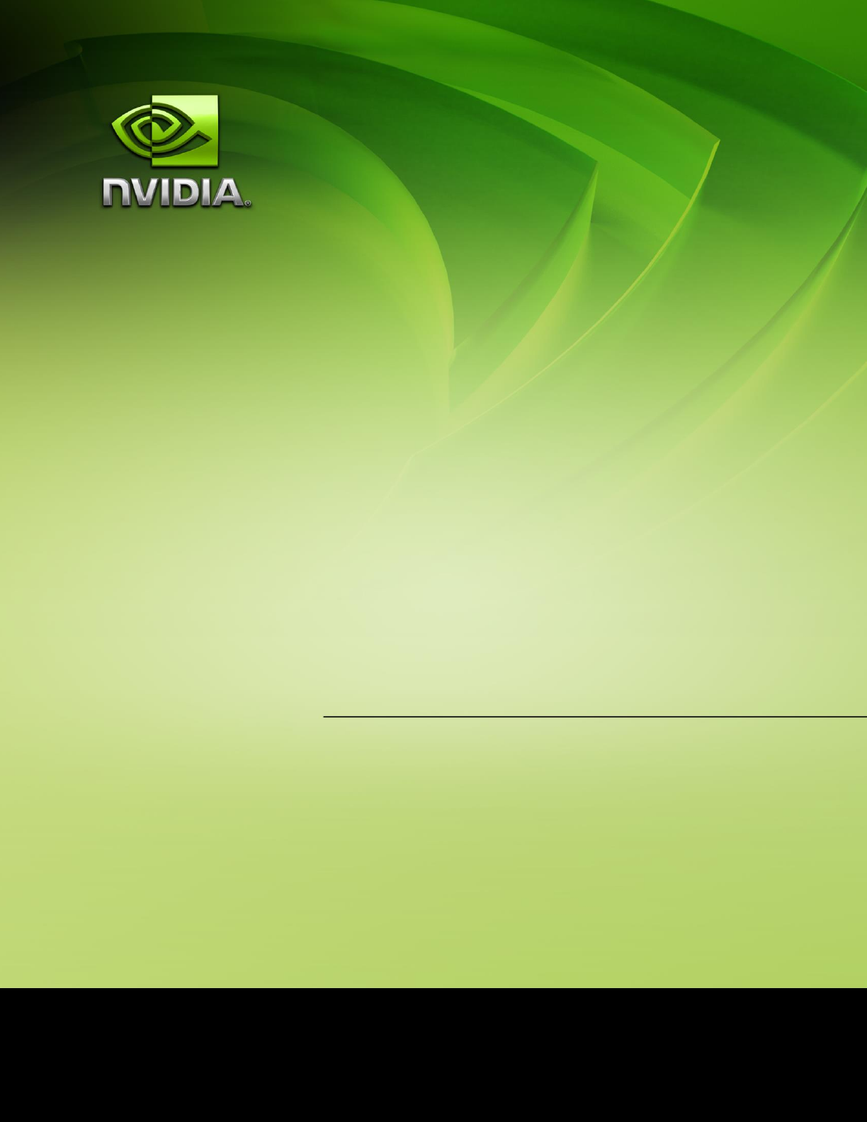
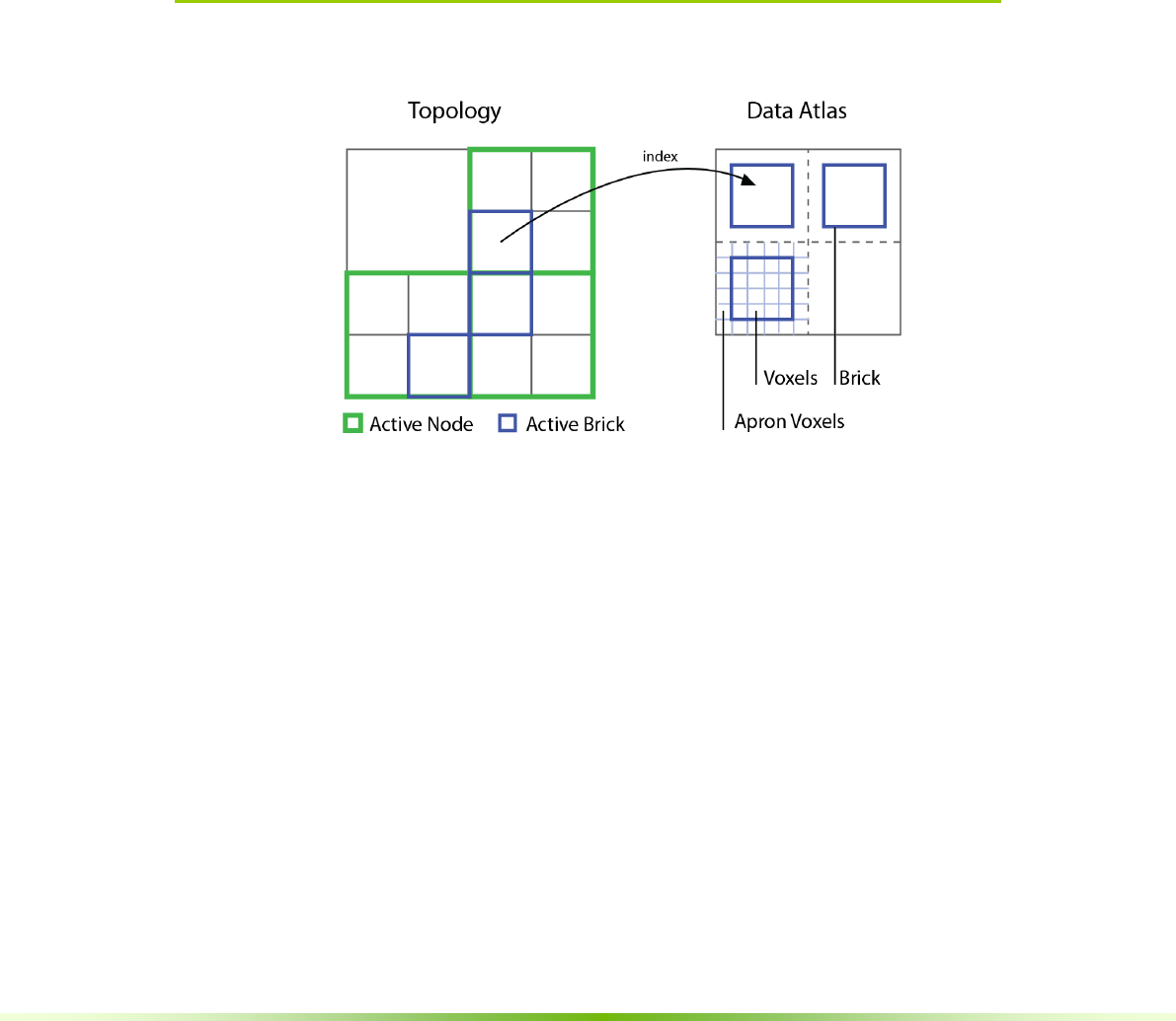
Figure 1.1. The VDB topology is an acceleration structure that indexes into
voxel data stored in an atlas. A group of voxels in an atlas is a brick.
The topology represents a 3D spatial layout of potentially very large data sets,
and the sparse quality implies this data is stored only near interesting features.
NVIDIA® GVDB Voxels - Programming Guide 3
Although GVDB Voxels is ideally suited to strongly sparse data, it still provides
several benefits in accelerating dense data (see Chapter 3.2).
An atlas represents voxel data as a set of bricks, where each brick is a small unit
of data – often 163 or 323 voxels – whose size is choosen to balance
performance and memory. A voxel atlas, similar to a texture atlas, is a collection
of bricks packed into 3D texture memory for easy access.
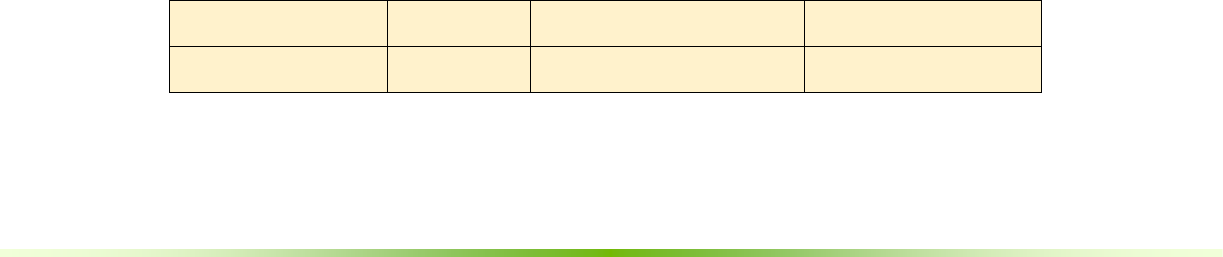
Figure 1.2. Multiple atlases are used to store channels of data, or per-voxel
attributes. A brick has the same index in each channel.
Multiple atlases are used to implement voxel data channels. Each data channel
has a specific type, such as a float, unsigned char, or float3 (vector). Together,
these multiple channels provide an arbitrary set of per-voxel attributes over the
entire volume. With this flexibility, it is possible to author complex fluid
simulations, generative computations, and many other applications.
1.1.2.1. Computing with Virtual Neighbors
Performing massively parallel computations is the premise of GVDB Voxels.
While the benefit of sparse volumes is greater efficiency and lower memory
footprint, a common criticism is that this increases complexity for the developer.
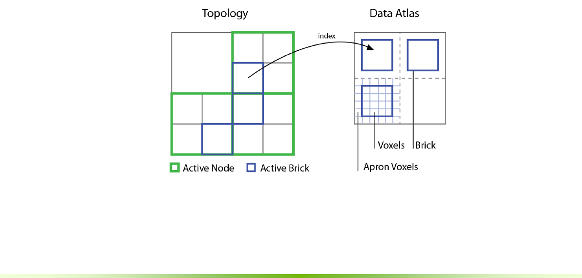
Figure 1.3. Dense computation gives easy access to neighbors (left), but performs
too many calculations. Sparse computation is efficient but makes neighbor
lookup across brick boundaries more difficult (right).
GVDB Voxels eliminates kernel code complex by allowing developers to write
voxel-based computations as if they were on a dense grid. We refer to this as
computing with virtual neighbors, a method which internally optimizes
neighbor lookups so you don’t have to and presents kernels with fast access to
neighbors even at brick boundaries. This frees the developer to focus on the

4 NVIDIA® GVDB Voxels - Programming Guide
details of computation and write kernels with simple neighbor stencil operators
without conditions. This is accomplished with apron voxels and a generic
method for apron updates interspersed with user kernels.
Virtual neighbors is a key feature in the development of optimized simulations
as one can write stencil kernels that make implicit use of shared memory,
equalize the occupancy of interior and brick-boundary voxels, and create
balanced, branch-free threads – all with simple finite difference style kernels.
Addition details on the implementation of virtual neighbors computing can be
found in Chapter 5, Compute API.
Customization
To provide the greatest flexibility, NVIDIA® GVDB Voxels is released as open
source software. This gives developers significant freedom in modifying GVDB
Voxels to suit the needs of any given application.
For complex applications, it may be necessary to taylor the GVDB structures to
suit a particular problem. Influenced by the pioneering work of OpenVDB we
anticipated that as a general computing framework GVDB could not support
multiple disciplines without being open source since the number of algorithms
and their variations grows rapidly. Therefore, GVDB can be modified at every
level so that developers can meet their particular needs.
For simpler applications, one should not have to modify deep structures within
GVDB in order to achieve customization of functionality. Therefore, we
designed GVDB Voxels with several layers. First, GVDB Voxels is implemented
as a library, and the simplest applications make API calls to perform build-in
functions such as smoothing or rendering.
At the next level, users can implement custom kernels for either computation
or rendering. These CUDA kernels are written and compiled in the application
code but launched from special GVDB functions (named ComputeKernel and
RenderKernel). This allows the user-code to reside outside the library, while the
GVDB library still has the ability to perform acceleration and boundary-free
computing. The gRenderKernel sample shows how to implement a custom
kernel for rendering. Beyond the use of custom kernels, application developers
can call lower level functions, such as changing topology to perform GVDB
operations without modifying the library.
At deeper layers, the GVDB Library can be modified as needed. The simplest
of these changes is to modify or write new algorithms over the data structures
already provided by GVDB. For example, one might write a raytracing algorithm
that uses two channels simulatenously - one for density, another for material ID.
The most extreme changes to GVDB involve modifying the underlying
representation of topology, or nodes, of the tree. Multiple channels can achieve
most goals where voxel attributes are needed, but it could be necessary to
modify nodes themselves when implementing complex features such as out-of-
core rendering (e.g. to track brick residency). As open source software, all of
these levels of GVDB are available to the developer.

NVIDIA® GVDB Voxels - Programming Guide 5
1.1.2.2. Computational Geometry
Many applications require complex interoperation between different types of
geometry. For example, rigid body and fluid simulations in Motion Pictures
often utilize both point clouds and voxel grids to perform efficient, and
accurate, simulations. 3D Printing often involves a conversion from a polygonal
mesh to a voxel grid. One of the most challenging aspects of general GPU-
computing is that each combination of geometry and data suggests a very
specific parallel algorithm.
NVIDIA® GVDB Voxels helps to alleviate this difficult problem by observing
that each geometry – points, polygons, or voxels – lends itself to a particular
GPU representation that aids in issues such as coherency and locality. For
example, a common pattern established for dynamic point clouds (such as SPH
fluids) is to perform a binning and sorting operation that reduces the problem
size for neighbor search. For voxels, the division of space into bricks helps to
localize computation for the GPU while eliminating unnecessary calculations
when the data is sparse. Naturally it is not possible address every combination
of geometry and acceleration structure, therefore we present a generic approach
that can be specialized as needed.
Figure 1.4. Computation is accelerated with auxiliary buffers. For example,
directly inserting a point cloud into a volume is inefficient. Parallel computation
suggests pre-sorting by brick for coherence. Multiple auxiliary buffers are used
for pre-processing, and points are inserted from these.
GVDB Voxels introduces auxiliary buffers to help accelerate any computation
performed with geometry other than voxels, or in relation to voxels. Auxiliary
buffers provide memory management and CPU-GPU transfer for arbitrary
types of data. They have a wide variety of uses, from point cloud insertion to
polygonal conversion. GVDB natively implements several API functions for
computational geometry. These include:
- Polygon-to-Voxel conversion
- Point Cloud insertion and lookup
- Point Cloud-to-Voxel scattering and gathering
- Tracing of Rays with arbitrary origin & direction
Each technique may utilize several auxiliary buffers to achieve high GPU
performance. For example, Point Cloud insertion utilizes one aux buffer to
insert points into a grid, then another to perform a prefix scan for data locality,

6 NVIDIA® GVDB Voxels - Programming Guide
and a third aux buffer as a deep copy for data coherence. This principle is
applied throughout GVDB Voxels, where scan and reduction on auxiliary
buffers are performed as needed to accelerate a wide variety of geometric types
in a relatively uniform way.
1.1.2.3. Memory Management
Memory management in GVDB Voxels was designed to eliminate many of the
common issues often associated with GPU-computing, while also providing
flexibility to advanced developers seeking greater control over peformance.
Among the most difficult challenges for new projects is management of both
CPU and GPU memory. With CUDA 6, NVIDIA introduced Unified Memory,
or managed memory, to provide a single memory space so that applications no
longer concern themselves with the CPU-GPU memory barrier. The latest
Pascal Architecture, with CUDA 8, provides way to optimize the locality of data
and provide hints to improve performance.
Figure 1.5. Typical memory usage in GVDB Voxels. The CPU and GPU both
store the entire topology, with a typical size around 5-10 MB. Only the
GPU stores the atlas data, which can occupy several gigabytes.
NVIDIA® GVDB Voxels uses an explicit memory allocation layer that results in
identical data on both the CPU and GPU, and does not make use of Unified
Memory. The topology of GVDB uses indices so that transfers are easy and
transparent to the user. The atlas data is selectively transferred to the GPU, and
often has no backing store on the CPU to conserve memory. Brick transfers,
which can occur often in out-of-core applications, are more easily accomplished
if the data representation can reside on both CPU or GPU without translation.
GVDB Voxels provides an explicit, seamless, memory allocator with API
functions to allow the developer to decide exactly when to perform transfers
without having to examine or modify the data.
1.1.2.4. Distributed Computing
NVIDIA® GVDB Voxels is well suited as a core engine for distributed
computing, but does provide any explicitly features in this area. The focus of
GVDB Voxels is to provide the best performance and scaling on single-GPUs
so that distributed applications that wish to use GVDB will scale accordingly.
Several design decisions make GVDB Voxels a good choice as the core

NVIDIA® GVDB Voxels - Programming Guide 7
framework for distributed applications. First, GVDB depends only on CUDA,
make it suitable for Tesla, GRID and supercomputing architectures without
graphics output. Second, voxel operations scale naturally in GVDB with better
per-node hardware. Finally, the structure of a VDB grid naturally partitions
space which requires only minimal transfer of data between nodes in distrubted
computing environments.
In the future NVIDIA® GVDB Voxels may provide addition features to
facilitate brick-level transfers between GPUs, transfer of node boundaries
between GPUs, or other features that enable distributed computing. In this
current release, GVDB Voxels focuses on single-GPU scaling and performance.
1.1.2.5. Flexible Architecture
The current version of NVIDIA® GVDB Voxels implements a VDB topology
over 3D texture-based atlases. Due to the connection between topology and
data, it should be relatively easy (compared to other frameworks) for developers
to drop in a different topology, or different data storage.
The current atlases are stored using 3D textures with CUDA bindless texture
objects, allowing multiple channels to be accessed simultaneously from a single
kernel. However, it may be useful to experiment with linear memory, or sparse
hardware textures, as the atlas storage type. Currently, GVDB can already switch
between OpenGL generated 3D textures and textures created as CUarrays
(cuArrayCreate3D). As the code is available, developers are welcome to
experiment with other storage methods.
The topology is the most central aspect of GVDB Voxels. However, the API
was designed to facilitate operations that would be applicable to many different
topologies. The VDB grid itself is already capable of imitating several different
layouts such as octrees, N-ary trees and tilemaps. However, it may be desirable
to drop in specific alternatives such as optimized hash tables (tilemaps) or
explicit octrees. The GVDB Voxels API abstracts such operations a spatial
coverage (ActivateSpace), topology completion (FinishTopology) and atlas
updates. We recommend that developers pursuing alternative methods follow
these API patterns as they lend themselves to sweep-based parallel computation.
1.1.3. Design for Rendering
The motivation of NVIDIA® GVDB Voxels for rendering is to provide basic
high quality, accelerated raytracing of voxel data essentially for free, with the
ability to extend to more complex rendering as desired. In scientific computing
the primary effort is often the simulation, where one often wishes to visualize
the result without fuss (for “free”) but with sufficiently high quality to resolve
details. To that end, the GVDB Voxels provides native CUDA and OptiX
rendering pathways with previsualization or high quality rendering.
In many applications the goal may be to improve on rendering quality. Thus, in
addition to the native pathways, GVDB Voxels provides a custom rendering
pathway which enables the developer to author kernels that seamlessly integrate
with GVDB sparse acceleration.

8 NVIDIA® GVDB Voxels - Programming Guide
1.1.3.1. CUDA & OptiX Rendering
GVDB Voxels provides two pathways for rendering volumes. The first is a
CUDA-only raycasting renderer that gives previsualization quality with high
performance. The second is an OptiX-integrated raytracer that allows for high
quality multiple scattering at interactive rates. Both rendering engines are capable
of switch modes to render with volumetric deep sampling (ray-sampling),
rendering isosurfaces with on-the-fly trilinear or tricubic filtering, rendering level
sets, and rendering voxel previews (tiny cubes).
GVDB Voxels is primarily written in CUDA, with the same raytracing kernels
being used for OptiX since the latter is also based on CUDA. The only addition
in GVDB Voxels to support OptiX is an alternative pathway for declaring and
accessing variables which is handled via header files. The code pathways are
otherwise identical. For the sake of simplicity, GVDB Voxels itself does not link
to OptiX or contain any host code for OptiX. Instead we have included a
sample, gInteractiveOptiX, which contains an integration OptixScene class that
handles the communication between OptiX and GVDB.
1.1.3.2. Customization
Developers who wish to explore new methods in rendering have several options
for customization. The most basic customization is to provide a Custom Render
Kernel (see Chapter 6.4) that shades a return hit point, allowing GVDB to
perform the raycast. At the next level, users can write kernels to modify the way
points are sampled within a deep volume. A more complex customization would
access multiple channels of data to mix additional per-voxel attributes such as
color or material ID. Finally, the GVDB ray tracing technique is open source so
that developers can modify the tree traversal itself, typically to return or pass
new information between leves. These customizations are described in
Chapters 5.4 and 6.4.
1.1.3.3. Interaction with OpenGL
For greatest flexibility, GVDB Voxels uses multiple CUDA buffers for output
results. These are maintained by the API with render buffers that are requested
before hand. We have provided an interop mechanism that allows applications
to return render buffers an OpenGL textures. This gives a simple way to
integrate CUDA or OptiX rendering into interactive applications. For example,
several demos render GVDB volumes to a full screen texture and then overlay
additional OpenGL GUI widgets in the sample.
For proper integration of volumes into OpenGL scenes, it is necessary to return
a depth buffer so that OpenGL objects can be mixed with volumes based on
depth. GVDB Voxels provides a mechanism to use depth as input during
volume rendering, and to return depth buffers as output.
NVIDIA® GVDB Voxels - Programming Guide 9
Chapter 2.
Programming
Overview
The GVDB API is designed as a C++ class interface with built-in functions for
common operations. More advanced users can access the host and GPU device
API separately with custom compute and rendering kernels.
2.1. Topology & Data
Figure 2.1. The GVDB paradigm separates the topology from the data to provide
several benefits in flexibility. Data is maintained in multiple channels, stored in
memory with 3D textures called atlases.
NVIDIA® GVDB Voxels makes a separation between the topology and atlas
of sparse voxel data. The topology must still refer to data in the atlas via some
mechanism and, unlike tree implementations using pointers, GVDB Voxels uses
indices both for tree nodes and atlas indexing.
2.1.1. Topology
The topology, as used in GVDB Voxels, describes an acceleration structure
over a spatial domain. For example, a BVH, an octree, and an n-ary tree are all
acceleration structures with different properties, splitting conditions and
branching factors. The topology implemented by GVDB is a hierarchy of grids
based on [Hoetzlein 2016] and [Museth 2013], which has advantages over other
structures for dynamic changes. A unique feature of a VDB topology is that it
generalizes many other structures, including octress and n-ary trees. In this
document the topology typically refers to the GVDB hierarchy of grids unless
otherwise noted.

10 NVIDIA® GVDB Voxels - Programming Guide
A topology is composed of multiple nodes, and the lowest level of the tree
consists of nodes which refer to bricks, and which have no children. For any
given level, all the nodes at that level will have the same resolution.
2.1.2. VDB Configuration
The key feature of a VDB topology is its configuration, which specifies in
shorthand the resolution of the nodes at each layer of hierarchy of grids. The
configuration is a vector which gives the log2-dimension of each level.
Figure 2.2. Configuration of a <2, 4, 3> tree. Each component is the log2dim of
that level. For example, the interior (middle) level has logdim = 4, resulting in
(24)3 or 163 node resolution. All bricks at that level will be 163 voxel.
In GVDB Voxels, the configuration can be specified at run-time. The maximum
number of levels defaults to 5, although most scenarios will use fewer levels.
Unused levels contain 1 or 0 nodes. Nearly all use cases can be covered with five
level trees, as the maximum addressable space is (10^12)3 voxels using
an <8,8,8,8,8> tree.
The only scenario in which more levels are needed is when using a very large
domain with very small bricks. For example, an octree quickly requires more
than 5 levels. To increase the maximum beyond five, the GVDB Library can be
rebuilt with a higher limit.
The maxmum resolution of a VDB grid can be found by multiplying the node
resolutions at each level. For the example in Figure 2.2.
Maximum Res = [ (2^2)*(2^4)*(2^3) ]3
= [4 * 16 * 8] 3
= 5123
Thus, the <2,4,3> tree is equivalent to a 5123 volume.
The VDB configuration can be specified with Configure():
gvdb.Configure ( 3, 3, 3, 3, 5 );
NVIDIA® GVDB Voxels - Programming Guide 11
A recommended VDB grid configuration for most scenarios is the <3,3,3,3,5>
grid. This is based on research by Hoetzlein [2016], which shows that smaller
upper levels, and larger bricks, are more efficient for raytracing traversal. This
configuration has a maximum resolution of 131,0723
2.1.3. Atlas Data
The atlas data refers to the actual storage of voxels or other entities. The atlas
is composed of a number of bricks which are dynamically allocated at run-
time. Each brick is a small, cubic sub-domain of voxels for a single attribute. A
common size for bricks is 163, 323 or 643
The key feature of an atlas is its type and size. An atlas is allocated in GVDB as
a 3D texture (or CUarray) of a specific data type. The overall size of the atlas
determines the maximum number of bricks it can contain.
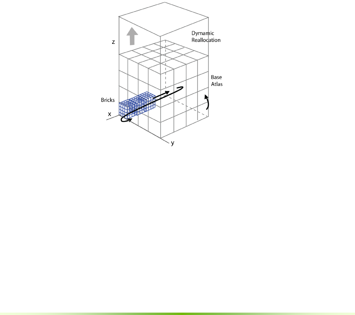
Figure 2.3. Atlas structure with bricks allocated along X, then Y, then Z. When
more bricks are needed, the atlas will be dynamically resized along the Z-axis.
The atlas also contains apron voxels (not shown) for neighbor lookups.
An atlases stores bricks in arbitrary order with no correlation to world space.
GVDB assigns bricks along the X and Y axes, and then continues to stack them
upward in Z. To allow for dynamic topology, the atlas may be reallocated with a
higher Z-height in order to accommodate more bricks.
Maintaining data in atlases, distinct from the topology, enables a number of
unique benefits. First, multiple atlases can be introduced to store different types
of data at each spatial location, called channels in GVDB. Second, since the data
is typically much larger than the topology, it is possible to move large amounts
of data for manipulation, computation, or I/O, without touching the topology.
Third, as the topology is somewhat independent of the data, it is possible to
experiment with the performance of different topology configurations without
altering the data. These benefits and others motivate the distinction between
topology and atlas data.

12 NVIDIA® GVDB Voxels - Programming Guide
2.1.4. Implementation
Figure 2.4. Internal representation of a GVDB grid uses multiple node pools;
one per level (e.g. blue, green, red). Each level is divided into two groups. Group
P0 contains node data & bitmasks, group P1 contains child lists. Each leaf node
indexes into a brick in a data atlas. [Hoetzein 2016].
Internally, the topology of GVDB is implemented using a set of memory pools
as described in [Hoetzlein 2016]. This design significantly improves
performance for dynamic brick allocation and simplifies data transfers between
CPU and GPU.
2.2. Basic API Design
NVIDIA GVDB is designed as a simple, command-based API for common
functional tasks. These tasks operate on the topology and data of a sparse
volume. Every GVDB application makes use of the basic API to prepare,
populate and manipulate data whether using built-in or custom kernels.
The main API categories are:
▪ Initialization – Functions that start or prepare GVDB
▪ Data Preparation – Functions, including file I/O and compute operations,
that load, manipulate, or process volumetric data.
▪ Scene Settings – Functions that initialize common settings for volume
rendering such as lights and cameras.
▪ Render Buffers – Functions that maintain one or more render buffers used
for rendered output, depth buffers, or depth inputs.
▪ Raytracing – Functions that perform built-in or custom raytracing of
volumetric data with different styles.
▪ Points & Polygons – Functions that convert to or from point clouds,
polygons and voxels, with algorithms for transforming between them.
▪ Dynamic API – Functions that rebuild a topology or allow for dynamic
topology changes over time.
▪ Accessor API – Functions for low-level manipulation of the GVDB
topology and data values available on both the host and device.
These API categories are covered in increasing complexity in this Programming
Guide. This chapter addresses the most basic API use of common built-in
functions to perform simple tasks.

NVIDIA® GVDB Voxels - Programming Guide 13
2.3. Initialization
Initialization of GVDB is achieved by linking your application to the GVDB
Library and declaring a VolumeGVDB object. The primary interface for GVDB
is the VolumeGVDB class, which can be initialized as follows:
#include “gvdb.h”
using namespace nvdb;
VolumeGVDB gvdb;
The VolumeGVDB object resides in the nvdb namespace, so it is common to
use this namespace to access the object.
Once created, the VolumeGVDB object is used to initialize GVDB as follows:
int devid = -1;
gvdb.SetVerbose ( true );
gvdb.SetProfile ( false );
gvdb.SetCudaDevice ( devid );
gvdb.Initialize ();
SetVerbose turns on or off verbose output from GVDB, including
measurement of the performance statistics discussed in section 3.3.
SetProfile turns on or off profiling, which enabled nvtx performance markers
for GPU Profiling with NVIDIA NSight, and also CPU Profiling with high
performance counters output to a console window.
SetCudaDevice specifies which CUDA Device should be used by GVDB. A
value of -1 indicates that GVDB is free to initialize the first CUDA Device it
finds. Other values can be specified after enumerating devices.
The Initialize function starts GVDB itself and prepares all necessary internal
structures, but does not create a topology or atlas data.
StartRasterGL is used to initialize OpenGL with GVDB, and is only needed
when using functionality that requires an OpenGL context. This should be
called after the application creates an OpenGL context. Such functions, like
PolyToVoxelsGL are suffixed by GL. An example of these function in use can
be found in the g3DPrint sample.
2.4. Data Preparation
Data preparation refers to several different methods available to build a GVDB
topology and populate atlases with data. Several key concepts are involved in
preparing a GVDB with data for rendering or further processing. These steps
Limitation: In this release, only a single VolumeGVDB object may
be created per program as a singleton.

14 NVIDIA® GVDB Voxels - Programming Guide
usually occur in order, although some many be repeated when working with
dynamic data.
• Configuration – Specifying the structure and shape of a topology,
without creating any nodes.
• Adding Channels – Specifying the data format and number of data
channels, without adding any data
• Activating Space – Requesting GVDB to add topology nodes to
define the sparse regions of the spatial domain to be covered.
• Update Atlas – Requesting GVDB to expand or restructure the atlas
channels to support the changes in topology.
• Adding Data – Steps to create, generate, or import actual data into
channels.
• Output/Rendering – Making output data or creating rendered images
of the stored data.
Every application with perform these steps in some way, although often several
of these steps will be hidden inside simpler built-in functions. For example,
LoadVBX performs all steps above except rendering. A few different use cases
for data preparation are worth nothing.
Case 1. Load existing Topology and Data
The simplest method of data preparation is to read volumetric data from disk
using a load function. These are described in detail in chapter 10, and include
support for VBX, RAW and OpenVDB files formats.
The native format of GVDB is the VBX format, which can be loaded with
LoadVBX.
gvdb.LoadVBX ( “data.vbx” );
Loading a data file from VBX or OpenVDB automatically reads the
configuration, atlas definition, node layout and atlas data, thereby making a
scene ready for rendering.

NVIDIA® GVDB Voxels - Programming Guide 15
Case 2. User Configuration, Generated Nodes and Data
In many applications, the user will configure the topology and voxel size to
achieve a specific performance or quality goal. Then, the application might call
GVDB functions that will generate nodes and atlas data automatically. A good
example, shown here, is the SolidVoxelize function for converting a polygonal
mesh to voxels.
The first steps are to configure the tree, add data channels, and set
the voxel size (or resolution):
gvdb.Configure ( 3, 3, 3, 3, 5 );
gvdb.AddChannel ( 0, T_UCHAR, 1 );
gvdb.SetVoxelSize ( 0.4, 0.4, 0.4 );
The Configure function defines the shape of the topology and initializes it to an
empty tree with no nodes. See section 3.1 for details on topology configuration.
For many applications, the <3,3,3,3,5> configuration is suitable.
The AddChannel function defines the data type for a given channel, and
initializes these with empty atlases containing no data. This can be called
multiple times to create additional channels. See section 3.2 for details on atlas
definition.
The SetVoxelSize function defines the size of a voxel in world units. This
allows for direct control over the voxel resolution, and defines the smallest size
of a voxel. A corresponding function SetVoxelRes can be used instead, if it is
more natural to specify the overall effective resolution of the world domain. See
section 3.3 for details on resolution.
Once the tree is configured, and channels are specified, it is possible to call
functions such as SolidVoxelize to generate nodes and data. Note that with
automatically perform the steps of activating space, updating the atlas, and
adding data, but leaves the earlier configuration steps to the user.
Model* m = gvdb.getScene()->getModel(0);
gvdb.SolidVoxelize ( 0, m, &xform );
This function takes the polygonal mesh (m) applies the transform (xform), and
voxelizes the model into the atlas channel #0. Notice the function does not take
the resolution as input, but relies on the earlier setup to determine the rasterized
resolution of the model.
Case 3. User-Specified Configuration, Topology and Data
The most generic use case is when the configuration, activation of sparse
regions of space, and data creation are all performed by the developer. A good
example of this is the authoring of a novel fluid simulation technique where the
developer requires explicit control over the sparse dynamics and multiple
channels of data. Another example is authoring a custom data format for
import into GVDB.

16 NVIDIA® GVDB Voxels - Programming Guide
gvdb.Configure ( 3, 3, 3, 3, 5, Vector3DF(1,1,1), 1);
gvdb.AddChannel ( 0, T_FLOAT, 1 );
gvdb.SetVoxelSize ( 0.4, 0.4, 0.4 );
gvdb.ClearTopology ();
for (int n=0; n < num_pnts; n++ ) {
gvdb.ActivateSpace ( pnt[n] );
}
gvdb.FinishTopology ();
gvdb.UpdateAtlas ();
gvdb.ClearAtlas ();
The functions for ClearTopology, ActivateSpace, and FinishTopology request
that spatial domains are added to the topology of the tree. ActivateSpace will
generate all the nodes in the GVDB tree required to ensure that the incoming
world point is covered by brick data. See Chapter 8.2 on Topology Rebuild.
The functions UpdateAtlas, ClearAtlas ensure that the atlas channels provide
data storage for the nodes, creating bricks as need, and clearing those bricks by
zeroing them out. See Chapter 8.3 on Atlas Rebuild.
Summary
NVIDIA® GVDB Voxels allows the steps for data preparation to be performed
at any stage in the application for the greatest flexibility. Simple applications can
make use of built-in functions, such as load/save, which perform many of these
steps internally. More complex applications are able to generate their own
topological coverage, update data stored in atlases, dynamically change
resolution, or even add and remove data channels at run-time.

NVIDIA® GVDB Voxels - Programming Guide 17
Chapter 3.Scene Settings
Scene settings are required to perform native GVDB rendering. Once a VDB
configuration is specific, and data is prepared, scene settings provide minimal
information on lights, cameras and transfer functions for rendering.
When using built-in rendering fuctionality, settings for lights and cameras are
needed to setup a scene. Unlike NVIDIA OptiX, whose goal is to provide a
scene graph hierarchy with a complete set of objects, transformations, and
multiple cameras and light sources, the scene structure of NVIDIA GVDB is a
simple fixed list of cameras and lights. GVDB Voxels was not designed as a
scene graph system, but rather as a basic primitive to fit into other scene systems
(including OptiX itself). The scene lights and cameras in GVDB are only used
by the built-in CUDA rendering functionality, which provides a limited range of
shading choices.
For complete flexibility in rendering, see section 4.3 on Custom Rendering
Kernels, which allows the user to write arbitrarily complex CUDA kernels or
OptiX programs to achieve any desired look. The definition of complex
cameras, lights and other scene objects is left to the application developer to
pass into these custom render kernels.
3.1. Scene
Scenes are accessed using the nvdb::Scene object, which can be retrieved from
the GVDB object.
using namespace nvdb;
Scene* scn = gvdb.getScene();
There is only one scene object per GVDB object.
The scene object provides access to:
• Cameras
• Lights
• Polygonal Models (for polygon-to-voxel conversion, etc)
• Transfer Functions
• Volume Raycast Settings

18 NVIDIA® GVDB Voxels - Programming Guide
3.2. Camera
Cameras are allocated and managed by the caller. The current camera to be used
for GVDB rendering is specified with SetCamera().
using namespace nvdb;
Scene* scn = gvdb.getScene();
Camera3D* cam = new Camera3D;
cam->setFov ( 30.0 );
cam->setOrbit( Vector3DF(50,30,0), Vector3DF(150,70,150),
400, 1.0 );
scn->SetCamera ( cam );
This specifies an orbiting-style camera with orbit angles of (50,30,0) (angle, tilt,
pitch), a target loction at (150,70,150), with a orbit distance of 400.0
and dolly of 1.0. For a complete list of the Camera3D functions, see the file
gvdb_camera.h in \source\gvdb_library.
The function scn->SetCamera( cam ) indicates that this camera is to be used
during GVDB rendering. Since the caller maintains cameras, it is possible to
create several cameras and switch between them to perform multiple renderings,
for example when implementing multiple views.
Interactive rendering is possible by updating the camera parameters and
performing a GVDB rendering on each frame, as demonstrated in the
gInteractiveGL sample.

NVIDIA® GVDB Voxels - Programming Guide 19
3.3. Lights
Lights are also allocated and managed by the caller.
Scene* scn = gvdb.getScene();
Light* lgt = new Light;
lgt->setOrbit( Vector3DF(0,40,0),
Vector3DF(250,250,250), 500, 1.0 );
scn->SetLight ( 0, lgt );
The function scn->SetLight( index, Light* ) assigns a light to the given index
number. This allows multiple light sources to be specified.
Lights are used for shadowing and simple shading when using
built-in CUDA-based rendering functions via gvdb.Render.
3.4. Polygonal Models
Models are used to provide polygonal geometry for poly-to-voxel and solid
voxelization functions in GVDB.
Scene* scn = gvdb.getScene();
scn->AddModel ( “lucy.obj”, scale, tx, ty, tz );
scn->CommitGeometry ( 0 );
The AddModel function loads an .OBJ formatted polygonal model file from
disk a saves it into the next available model slot. The ‘scale’ is pre-computation
that scales the model vertices, and ‘tx/ty/tz’ are pre-computed translation
applied directly to the incoming vertices during load. Multiple models can be
loaded into the indexed list by calling AddModel repeatedly.
The CommitGeometry function transfers the polygonal model into an
OpenGL vertex buffer object (VBO) for using the on the GPU. The argument
indicates which model slot to commit, base 0. Since polygonal models are
accelerated with OpenGL VBOs, the StartRasterGL function must be called
during initialization to provide an OpenGL context.
Models in GVDB are not a suitable location for storing models used in mixed
polygon rendering, or as a means to store data for generic scene graphs. Rather,
models should be viewed as a temporary holding location for polygon-voxel
operations.

20 NVIDIA® GVDB Voxels - Programming Guide
3.5. Transfer Functions
A transfer function is a common way to describe how a volumetric model with
various densities should be rendered on screen. Transfer functions are often
using in medical and scientific imaging to highlight specific features in
volumetric data. Whispy smoke may have a white color with a very low opacity
over all density ranges, while a rolling fire might have red, yellow and black
colors with high opacity. The purpose of the transfer function is to map, or
transfer, the incoming data to a visibile color scheme.
Transfer functions are defined in GVDB Voxels via the Scene object.
LinearTransferFunc ( t-start, t-end, color-start, color-end );
For generality, a LinearTransferFunc call is used to specify a piecewise-linear
section of a transfer function. This can be invoked multiple times to define the
complete transfer function in small sections with arbitrary detail over the
domain range from 0.0 to 1.0.
scn->LinearTransferFunc ( 0.0, 1.0,
Vector4DF(0,0,0,0), Vector4DF(1,1,1,0.5)
The simplest transfer function specifies a single linear change over
the entire range from 0 to 1. Notice the start and end are 0 and 1.0 respectively.
The left-most color is black, no opacity (transparent), and the right-most color is
white with half opacity.
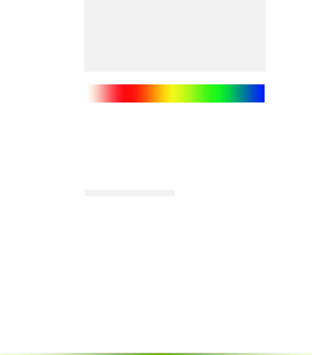
Figure 3.1. Linear transfer function from black to white over the range [0,1]
Values outside the range of 0.0 to 1.0 are ignored by the transfer function.
However, the volume data may contain densities or values outside this range.
The SetVolumeRange function is used to map the actual data value to a
transfer function value in the range of 0 to 1, which then determines the color
and opacity.
SetVolumeRange ( iso-value, min-value, max-value)
scn->SetVolumeRange ( 0.1, -1.0, 2.0 );
This indicates the density channel contains values from -1.0 to 2.0, and will
remap these to [0,1] before transfer. The value 0.1 gives an isovalue used as a
threshold when doing surface rendering.
NVIDIA® GVDB Voxels - Programming Guide 21
Several linear functions can be combined to create arbitrarily complex transfer
functions.
scn->LinearTransferFunc ( 0.00f, 0.25f,
Vector4DF(1,1,1,0), Vector4DF(1,0,0,0.1f) );
scn->LinearTransferFunc ( 0.25f, 0.50f,
Vector4DF(1,0,0,.1f), Vector4DF(1,1,0,0.2f) );
scn->LinearTransferFunc ( 0.50f, 0.75f,
Vector4DF(1,1,0,.1f), Vector4DF(0,1,0,0.3f) );
scn->LinearTransferFunc ( 0.75f, 1.00f,
Vector4DF(0,1,0,.3f), Vector4DF(0,0,1,0.5f) );
gvdb.CommitTransferFunc ();
Figure 3.2. Transfer function created from linear piecewise sections using the
code above. Notice the t-values can be shifted to compress portions function or
make discontinuities, and the alpha channel can be modified with the color.
For an example of using transfer functions in practice see the gRenderToFile or
gInteractiveGL samples.
Commit Transfer Function
After specifying a transfer function, it is necessary to commit the function to
GPU so that it can be used for raytracing. This is accomplished with
CommitTransferFunc().
gvdb.CommitTransferFunc();
To rewrite the transfer function, overwrite the values with new calls to
LinearTransferFunc over the domain [0,1] and call CommitTransferFunc again.
For information on using transfer functions in OptiX, see Chapter 6.2
on OptiX Raytracing.
22 NVIDIA® GVDB Voxels - Programming Guide
Chapter 4.
Data Structures
4.1. Spatial Layout
Voxels exist in a world space, which are represented in GVDB using a topology
of nodes that have a location in index space. Together these define the
position of voxels in a 3D world. As mentioned in Chapter 2, the actual storage
of voxels is resides in an atlas composed of bricks. Two additional spaces helps
to acceleration calculation: atlas space and bricks space. The motivation for
these spaces, and transformations between them are describe here.
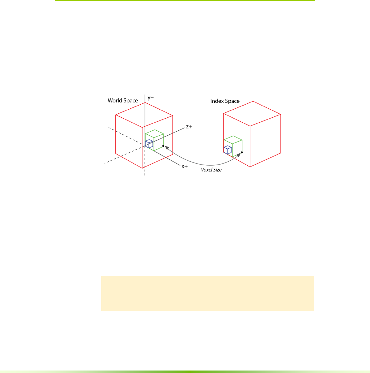
4.1.1. World & Index Space
Figure 4.1. World and Index Space
A voxel has a real 3D position in world space. This position a real number
where the distance from voxel to voxel is the voxel size.
The index space of a voxel is an integer index which is found by dividing world
space by voxel size.
Ivox = Wvox/ voxelsize
The position of all nodes in GVDB Voxels are stored using index space, since
this allows for precise sub-division of the world into a hierarchy of grids. Notice
that both Wvox and Ivox can be negative in order to cover the negative domain.
Limitation: The transformation between world and index space is
ideally an arbitrary 4x4 matrix. In this release, world and index
space are related by the 3D scaling vector voxel size.
NVIDIA® GVDB Voxels - Programming Guide 23
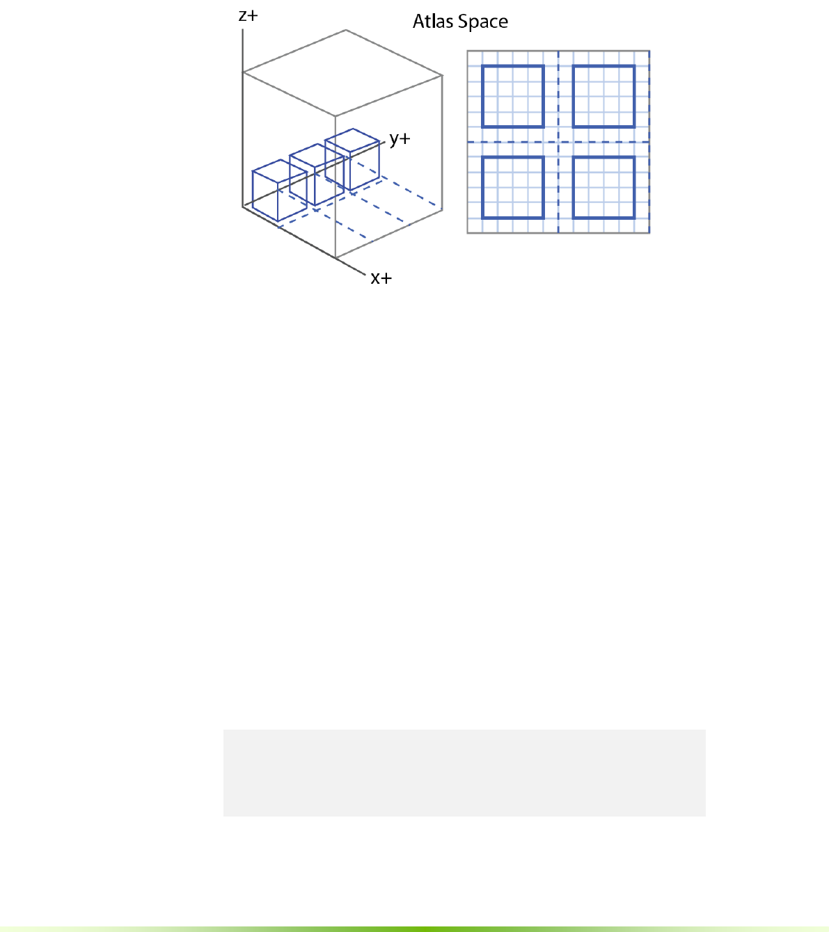
4.1.2. Atlas Space
Figure 4.2. Atlas Space. The is the space defined by the texture atlas storing
voxel bricks.
Atlas space referes to points or voxels referenced in the data atlas.
The primary purpose of atlas space is to perform efficient calculations on the
entire sparse volume. Consider the goal of adding noise to each voxel by adding
a random value. An inefficient, non-sparse way would be to scan over the entire
world space, then find each voxel as stored in the atlas space, and add a
random number to it. A better, but still inefficient way, would be to launch a
kernel for each brick in the atlas, and add a random value to each voxel in the
brick.
The most efficient way is to modify only sparse voxels, ignoring the rest of the
world. This is exactly what is stored in the data atlas. To perform efficient sparse
calculations over an entire volume, GVDB Voxels launches a kernel over atlas
space voxels.
Operations performed using gvdb.Compute all work in this way. There is a
single kernel launch over all voxels in the atlas. Voxel operators such as
smoothing or noise begin by identifying the atlas space voxel for the current
thread. This is common enough that a device macro, GVDB_VOX, is provided
to give the atlas space voxel. (See cuda_gvdb_operators.cuh)
GVDB_VOX:
uint3 vox = blockIdx * blockDim + threadIdx +make_uint3(1,1,1);
if ( vox.x >= res.x|| vox.y >= res.y || vox.z >= res.z )
return;

24 NVIDIA® GVDB Voxels - Programming Guide
For many operations, like adding noise, the world position of the
voxel is not needed. One only needs to read and write the voxel values:
__global___ gvdbOpNoise ( int3 res, uchar chan )
{
GVDB_VOX
float v = tex3D<float> ( volIn[chan], vox.x, vox.y, vox.z );
v += noise();
surf3Dwrite ( v, volOut[chan], vox.x*sizeof(float), vox.y,
vox.z);
}
This simple kernel adds noise to the entire sparse volume. The GVDB_VOX
macro sets the ‘vox’ variable for the atlas space voxel in this thread.
Atlas-to-World Space
Often while performing a full volume calculation it is necessary to have the
world position of a voxel. Again it is more efficient to launch kernels over the
atlas space and then compute their world space than to go the other way. An
example is computing the per-voxel distance for each voxel to a world-space
object like a sphere.
The device function getAtlasToWorld transforms from atlas to world space.
__global___ gvdbOpDistToSphere ( int3 res, uchar chan )
{
GVDB_VOX
float3 wpos;
if ( !getAtlasToWorld ( vox, wpos )) return;
float v = wpos – sphere.pos; // distance to sphere
surf3Dwrite ( v, volOut[chan], vox.x*sizeof(float), vox.y,
vox.z);
}
getAtlasToWorld returns true if the world point exists, and false if the atlas
voxel does not currently map to a brick in the world. The value of ‘wpos’ is set
upon return to the world space position of the atlas voxel.
Additional device functions help to perform tasks in atlas space:
- getAtlasToWorld return the world position from an atlas position
- getAtlasToWorldID returns the brick ID at an atlas position
- getAtlasNode returns a brick map from an atlas position
- getNodeAtPoint return the VDB Node at a world position
See Chapter 5, Compute API, for more details.

NVIDIA® GVDB Voxels - Programming Guide 25
4.1.3. Brick Space
Figure 4.2. Brick Space is a local coordinate system relative to a specific brick.
Brick space referes to a local coordinate inside a specific brick. Recall that a
brick is a small, cubic subset of voxels stored in the atlas.
Brick space is used primarily during raytracing. Whereas atlas space is useful
when one wishes to perform calculations over all the voxels in a sparse volume,
during raytracing one may only know the entry and exit locations for a brick,
leaving the rest of the raytracing up to the rendering engine.
Raytracing is more efficient on bricks because one can quickly access and test
the data atlas with a brick coordinate. GVDB Voxels uses brick functions to
perform these calculations, which are internal or customized functions that
return the results for a given ray inside a brick. See Chapter 6, Raytracing API,
for further details on efficient raytracing with bricks.
World-to-Brick Space
The raytracer will enter a brick function with a starting ‘t’ value (parametric
coordinate along the ray) along a specific ray, requesting a hit or sample value, as
in Figure 4.2. The ‘t’ value gives the starting world coordinate of the entry point.
To march through brick space one first converts the ‘t’ value of a world
coordinate, and then transforms from world-to-brick space with the following:
P = (W – Bworld) / vdel
The point in the brick is denoted as P. (Figure 4.2). The range of P is 0 ≤ P <
Bres. Thus the brick coordinate P has no meaning outside the resolution of the
brick, which may include apron voxels.
The world coordinate of the point is W, the world coordinate of the bottom
corner of the brick is Bworld, and vdel is the voxel size at node level 0.
Recall that the purpose is to very quickly scan through a brick during raytracing.
The inner loop should therefore do very few calculations.

26 NVIDIA® GVDB Voxels - Programming Guide
Here is a simplfieid example from the rayDeepBrick function which does
sample-based volumetric raytracing:
__device__ void rayDeepBrick ( char shade, int nodeid, float3
t, float3 rpos, float3 rdir, float3& pstep, float3& hit,
float3& norm, float4& clr )
{
VDBNode* node = getNode ( 0, nodeid, &vmin );
float3 W = rpos + t.x * rdir; // world space
float3 p = (W-vmin) / gvdb.vdel[0]; // brick space
float3 o = make_float3( node->mValue );
float val = 0;
for (iter=0; iter < MAX_ITER && inBounds(p); iter++)
{
val += tex3D(volTexIn, p.x+o.x, p.y+o.y, p.z+o.z);
p += SCN_PSTEP * rdir;
}
}
The value (‘val’) is the desired accumulated sampling along the ray.
First, the starting position in world space (W) is computed from the ray position
(rpos), the ray direction (rdir) and the ‘t’ value. Next, the starting brick space
coordinate (P) is found using the world-to-brick transformation. Finally, the
inner loop scan in PSTEPS (dP) along the ray direction, sampling the data atlas
at each sample using the brick coordinates. The offset ‘o’ is the location of the
brick in the atlas, and (P+o) gives the coordinate of the current sample in atlas
space for direct texture lookup using tex3D.
This technique is common in GVDB Voxels and results in very efficient
raytracing as the inner loop is greatly simplified. GVDB takes care of the sparse
processing of rays as they traverse the hierarchy and travel in and out of bricks,
allowing the developer to write concise, efficient brick functions.
Brick-to-World Space
At times it is necessary to convet from brick space back to world space. This
may occur when a ray hits a point and one wishes to return the world hit
location. The inverse transformation is:
W = Bworld + P * vdel
An example of this can be found in the raySurfaceTrilinearBrick function, which
is a brick function that returns the first hit isosurface in a brick of voxels.
__device__ void raySurfaceTrilinearBrick ( … )
{
..
for (iter=0; iter < MAX_ITER && inbounds(P); iter++ ) {
// check if voxel is above is isoval, if so..
if tex3D(volTexIn, p.x+o.x, p.y+o.y, p.z+o.z ) > thresh)
{
hit = p * gvdb.vdel[0] + vmin; // compute world hit
return; // (vmin = Bworld)
}
p += SCN_PSTEP*dir; // next sample
}
}

NVIDIA® GVDB Voxels - Programming Guide 27
4.1.4. Extents and Effective Resolution
Working with actual volume data in GVDB Voxels will cover a finite, sparse 3D
volume of the world. A common bound on this data is the bounding box,
which defines the minimum and maximum extents of the active data in world
space. GVDB Voxels uses extents to refers to the same bounding box in index
space for a given volume.
When using dense 3D textures for voxel data, the texture has a a maximum
resolution. However, sparse volumes do not have a maximum since they can
expand to cover more space as needed. Instead, a useful description of a sparse
data set is its effective resolution, which is the number of active voxels along
each axis. This can be computed as the size of the extents:
Effective Resolution = Emax - Emin
Since the extents E are related to the bounding box by voxel size, we notice that
the effective resolution is also equal to:
Effective Resolution = (Bmax – Bmin) / voxelsize
This gives a very useful relationship between the resolution (detail) of a data
set, its bounding box in the 3D world, and the voxel size.
This calculation comes up frequently in 3D Printing, for example. Let’s assume
the voxel size is set to the layer thickness of 0.1 mm (10 microns) of a 3D
Printer, e.g. voxelsize = <0.1, 0.1, 0.1mm>. Now, the user has requested that the
model be printed with a height of 100mm (about 4 inches). This means we can
compute the effective resolution, or detail, of the data set required for printing
using this equation:
Effective Resolution (Z) = (100mm – 0mm) / 0.1mm = 1000 voxels
Thus, the given parameters result in a volume 1000 voxels high, which can be
related to memory footprint and output quality.
4.2. Topology Structures
4.2.1. Nodes
The GVDB Voxels topology is stored as a set of nodes residing in memory
pools. The same node struct is used at every level of the hierarchy to simplify
the design with uniform computation.
For the most part, developers do to not need to understand nodes in order to
make use of GVDB. The compute API givers direct access to voxels for
computation, and the raytracing API provides user-customizable brick functions
to traverse rays through brick and atlas space. An understanding of nodes is
helpful when dealing with dynamic topology, for raytracing customization, or
when extending GVDB with new functionality.

28 NVIDIA® GVDB Voxels - Programming Guide
The GVDB Node structure is:
struct ALIGN(16) GVDB_API Node {
public:
uchar mLev; // Tree Level 1 byte
uchar mFlags; // Flags 1 byte
uchar mPriority; // Priority 1 byte
uchar pad; // Padding 1 byte
Vector3DI mPos; // Pos in Index-space 12 byte
Vector3DI mValue; // Value in Atlas 12 byte
Vector3DF mVRange; // Value min, max, ave 12 byte
ulong mParent; // Parent ID 8 byte
ulong mChildList; // Child List 8 byte
uint64 mMask; // Start of BITMASK bytes
}
The node header, not including the mask bytes, is 56 bytes.
With 16-byte alignment the actual node header size is 64 bytes.
Note that a Node struct is never allocated outright, but always preallocated with
additional bytes for the bitmask at the end of the node.
See VolumeGVDB::Configure for examples of how PoolCreate is used to
allocate actual nodes.
Node variables have the following meaning:
RESERVED = For future use.
mLev Level of the node in the tree. Level 0 is the brick.
mFlags [RESERVED] Flags for residency, etc.
mPriority [RESERVED] Priority for ray-guided rendering or out-
of-core residency swap calculations
pad [RESERVED] Padding byte for future functionality
mPos Position of bottom corner of the node in index space.
mValue The ‘value’ of the node as an an atlas space position.
mVRange [RESERVED] The minimum, maximum and average range of
values for a node. To be recalculated as needed for a given
channel ID
mParent Index of the parent node (into pool group 0)
mChildList Index of the child list (into pool group 1)
mMask Starting byte of the node bitmask. Not actually stored.
Location, Size & Extent
The range, or index-space size, of a node is determined by the node level:
Nrange = gvdb.getRange ( node.mLev );
The cover, or world-space size, of a node is determined with the voxel size:
Ncover = gvdb.getCover ( node.mLev );
The mPos expresses the index-space bottom corner of a node. The opposite
top corner index-space is given by:
Nimax = node.mPos + Nrange

NVIDIA® GVDB Voxels - Programming Guide 29
The world space bounding box of a node can be found by transforming the
node from index-to-world.
Nwmin = node.mPos * voxelsize = getWorldMin ( node );
Nwmax = (node.mPos + Nrange)*voxelsize = getWorldMax ( node );
Bricks and Values
The value of a node relates the topology to a data brick in the atlas. Presently,
every node in the GVDB hierarchy has a value variable, but only those at level 0
are utilized. This is to allow for future growth in the area of level-of-detail
where data bricks might exist at different levels of the hierarchy.
A value of -1 indicates a node has not yet been assigned a brick in the atlas, but
is a leaf node residing in world space. That is the topology covers a 3D space
with a node but does not yet contain data.
When non-negative, the value is an atlas-space position of the brick containing
data in the atlas. This position skips the outer apron and refers to the bottom
corner of the first actual data voxel.
Parent Node
The parent variable (mParent) is a reference to the parent of the current node.
References are encoded as a pool group, level and index, packed into a 64-bit
value.
ref = Elem ( group, level, index )
= uint64(group) | (unit64(lev) << 8) | (uint64(index) << 16)
The parent of a node always resides in group=0.
The null, or undefined reference value is:
#define ID_UNDEFL 0xFFFFFFFF
This null value is found for the parent of the root node, and in other contexts.
Children List & Bitmask
The children variable is a reference to a list-of-children found in pool group 1.
The list-of-children is decoded using the bitmask located in the memory space
at the end of the current node. Within the subdivided space of the node, the
bitmask indicates which child nodes are active. Those with active bits will have a
child present in the list-of-children.
The size of the node bitmask is the number of potential nodes is contains, which
is given by the log2-dimension of the VDB configuration. For example, with a
<2, 4, 3> configuration, all nodes at level 1 have a log2dim=4, which means that
all nodes at this level are subdivided with (24)3 = 163 voxels = 4096 voxels. This
is the number of bits which can be active or inactive. The bitmask will
therefore contain 4096 bits = 512 bytes.
GVDB Voxels has a number of functions to access and traverse children.
See Chapter 8, Host & Device Access, for details.

30 NVIDIA® GVDB Voxels - Programming Guide
4.2.2. Memory Pools
The GVDB Voxels topology is stored in two memory pool groups as
described in [Hoetzlein 2016]. Each group is a set of separately allocated
memory pools residing on both the CPU and GPU, with one allocation for each
level of the tree. The following is for reference on the current implementation:
Pool Group 0 – Nodes & Masks
Pool 0 stores the nodes and bitmasks for each level of the topology.
A single pool is allocated per level of the hierarchy, and multiple nodes reside
within each level. Since, by VDB definition all the nodes at a given level have the
same dimensions, the bitmask size at a specific level will be constant (per level).
Therefore, it is possible to allocate a pool group with a fixed width and height as
follows:
P0 ( group, level ) = width * height
= (NodeHeader(level) + BitmaskSize(level)) *
maximum_nodes_at_level
The maximum number of nodes at each level (pool height) is initialized to a
small value, typically 4. When more nodes are needed the pools will dynamically
expand by powers-of-two to contain additional nodes.
Pool Group 1 – Children Lists
Pool 1 stores the lists-of-children for each node in Pool 0.
Since this list may change size itself, a separate pool group is used.
A list-of-children pool is allocated for each level of the hierarchy. Each child
entry is a 64-bit reference back into Pool 0 at the next lower level.
The maximum number of references in the list-of-children is equal to the
number of bits (voxels) in the bitmask for that level.
Limitation:
Consistent with OpenVDB, the original intent of Pool Group 1 was
to minimize the extra space needed for children by compacting
them and using bit counting. However, compaction introduces
runtime overhead and the added space of storing complete child
lists is not significantly different than compacted lists. Additionally,
non-compacted lists would eliminate the need for the bitmask
entirely and improve performance by removing bit counting.
Currently, Pool Group 1 is compacted (children stored next to one
another in order) but with maximum width.
Future versions of GVDB may eliminate Pool Group 1 entirely and
merge the children lists with the bitmask. We welcome analysis
and feedback on this topic.

NVIDIA® GVDB Voxels - Programming Guide 31
4.3. Atlas Structures
Voxel data is contains in multiple atlases, where an atlas is stored in device
memory as a 3D Texture allocated as either a a CUarray, or less typically as an
OpenGL 3D Texture. Allocation of atlases with OpenGL is required when
using OptiX, and CUDA-GL interop is performed to acquire a CUarray in that
case.
4.3.1. Channels
A channel is the concept of a per-voxel attribute, and is central to computation
using GVDB Voxels. The need for many voxel attributes arises in many
situations. In fluid simulation, it may be necessary to store density, color, velocity
and pressure at each voxel cell. These are attributes defined as channels.
Each channel is implemented as another atlas. There is a one-to-one mapping
from a channel to an atlas. However, the atlas is a more generic concept which
can be applied to other problem as well. For example, three atlases may be used
for a density, color and velocity channel. Five additional atlas might be used to
express the level-of-detail data for just density. Atlas is thus a more generic
concept for a “store of voxels”, whatever its usage, while channel is the concept
of “per-voxel attributes”. Currently the only use of atlases in GVDB is
channels, but this is expected to change in future versions.
Channels can be allocated or destroyed at runtime:
gvdb.AddChannel ( channel ID, data type, apron )
gvdb.DestroyChannels();
gvdb.AddChannel ( 0, T_FLOAT, 1 ); // density
gvdb.AddChannel ( 1, T_UCHAR4, 1 ); // color
DestroyChannels() removes all previous channels and associated data.
AddChannel() takes the new channel ID, requested data type, and the number
of apron voxels (one sided).
Channels can be cleared to a value using FillChannel():
gvdb.FillChannel ( 0, Vector4DF(0,0,0,0));
For flexibility, the second argument to FillChannel is a Vec4F. In single-value
channels of type T_FLOAT or T_UCHAR, only the first element is used.
Color Channels
The native rendering in GVDB Voxels uses one channel by default, a density
channel at location #0. Colored volume rendering, where each voxel has a
unique color, is also supported by indicating the color channel with
SetColorChannel.
gvdb.SetColorChannel ( 1 ); // channel ID

32 NVIDIA® GVDB Voxels - Programming Guide
When SetColorChannel is used, that channel must be added as a T_UCHAR4
type to be interpreted as RGBA values.
4.3.2. Voxel Size
The global voxel size is specified with SetVoxelSize().
The default is (1,1,1).
gvdb.SetVoxelSize ( 0.1, 0.1, 0.1)
4.3.3. Atlas Size
An atlas is resized to contain resident bricks.
As described in Chapter 2.1, the dimensions of an atlas determine the maximum
number of bricks it can contain. As the number of bricks increases (more data),
the atlas will dynamically resize along the Z-axis to accommodate more bricks.
The maximum texture size of a given GPU device determines the limits of the
atlas size. This can be found by querying cuDevuceGetAttribute with the
following CUdevice attributes:
CU_DEVICE_ATTRIBUTE_MAXIMUM_TEXTURE3D_WIDTH
CU_DEVICE_ATTRIBUTE_MAXIMUM_TEXTURE3D_HEIGHT
CU_DEVICE_ATTRIBUTE_MAXIMUM_TEXTURE3D_DEPTH
Keep in mind the width, height and depth refer to the number of voxels along
each axis, not the number of bricks.
For an atlas with width/height/depth in voxels, the maximum number of
supported bricks can be calculated as:
Maximum bricks = width*height*depth / (brickres+apron*2)3
When UpdateAtlas() is called, GVDB Voxels will reallocate the atlas, increasing
height until the required number of bricks can be met. If the maximum texture
height is reached, the call may fail. Additionally, it can fail when GPU memory is
exceeded. To maintain some control over the failure due to dimensions, GVD
provides a function, SetChannelDefaults to indicate the desired base
dimensions of the atlas in bricks.
gvdb.SetChannelDefaults ( 16, 16, 16 );
Sets the default allocation to 16x16x16 bricks. This is suitable for larger data sets
where the number of bricks would meet or exceed 163. Since the brick
dimensions are known, it is possible to calculate good defaults using the GPU
device limits queried above.
Limitation: The native rendering pathways currently require that
density is present in channel #0. In the future, this limitation will be
removed so that any channel can be specified as primary. (See
SetupAtlasAccess)

NVIDIA® GVDB Voxels - Programming Guide 33
Chapter 5.
Compute API
The Compute API for GVDB Voxels implements a workflow to enable sparse
calculations to be performed as if they were on a dense grid. Developers can
make use of the built-in compute operations, or more commonly, author
custom kernels.
5.1. Built-In Compute
Performing simple calculations such as smoothing or additive noise can be done
using built-in compute functions. A single API function, gvdb.Compute(),
launches built-in functions with enums to select the function.
Compute ( func_id, channel, iteratons, Vec3DF params, update );
The arguments are:
- func_id The enum ID of the function to be called.
- channel The voxel channel ID to preform the computation on.
- iterations Number of times to repeat the calculation
- params Vector3DF with three parameters specific to the function
- update A boolean indicating whether to update the apron
after each iteration
The currently available built-in functions are:
FUNC_SMOOTH Smoothing with a 7-point stencil kernel
FUNC_NOISE Add noise to a float channel
FUNC_GROW Increase a level-set function by adding
to all non-zero voxels.
FUNC_CLR_EXPAND Expand a color channel (UCHAR4) outward
while preserving existing colors.
FUNC_EXPANDC Expand a single-byte (UCHAR) channel
outward with another value
The list of built-in functions is intentionally short as we expect that most
developers will choose to author their own compute kernels. The built-in
functions are intended to grow, through open source sharing, as a set of
compute kernels for common operations. They also offer examples of how to
write simple kernels for these sparse compute tasks.
The meaning of the 3-vector parameters vary with each function. Due to virtual
neighbors, most kernels are no longer than 10 lines. The easiest way is to
examine these is by looking at the gvdbOp{..} functions found in
\source\cuda_gvdb_operators.cuh
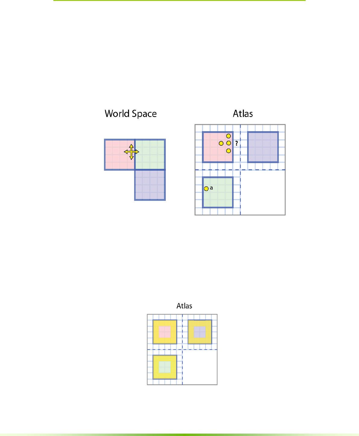
34 NVIDIA® GVDB Voxels - Programming Guide
5.2. Design Goals
Several goals motivate the solution for sparse computation in GVD Voxels.
These are:
- Efficient access to neighbor voxels
- Efficient kernel launches (one for the entire volume)
- Equalize workload of interior and border voxels of a brick
- High thread occupancy
It is instructive to examine these goals to understand how computation is
performed by GVDB Voxels. This will later help to describe the workflow.
Figure 5.1. A key challenge in sparse computation is to compute stencil
operations (neighbor lookup) at all active voxels. In world space (left) these are
physically adjacent voxels. When stored in a data atlas (right), neighbor voxels
may not be nearby in memory. In this example the right-side neighbor lies in
another brick (point ‘a’) and must be accessed differently.
The benefit of sparse computation is that no calculations are perform on
unoccupied space. However, neighbor lookups are more difficult (see Figure 5.1)
as the neighbors of boundary voxels reside elsewhere in the data atlas, within
other bricks.
Figure 5.2. Trivial (inefficient) solution to neighbor lookups on sparse grids.
Boundary voxels, highlighted, could directly locate the adjacent voxels in other
bricks through indirection. Yet this leaves interior voxels mostly idle.
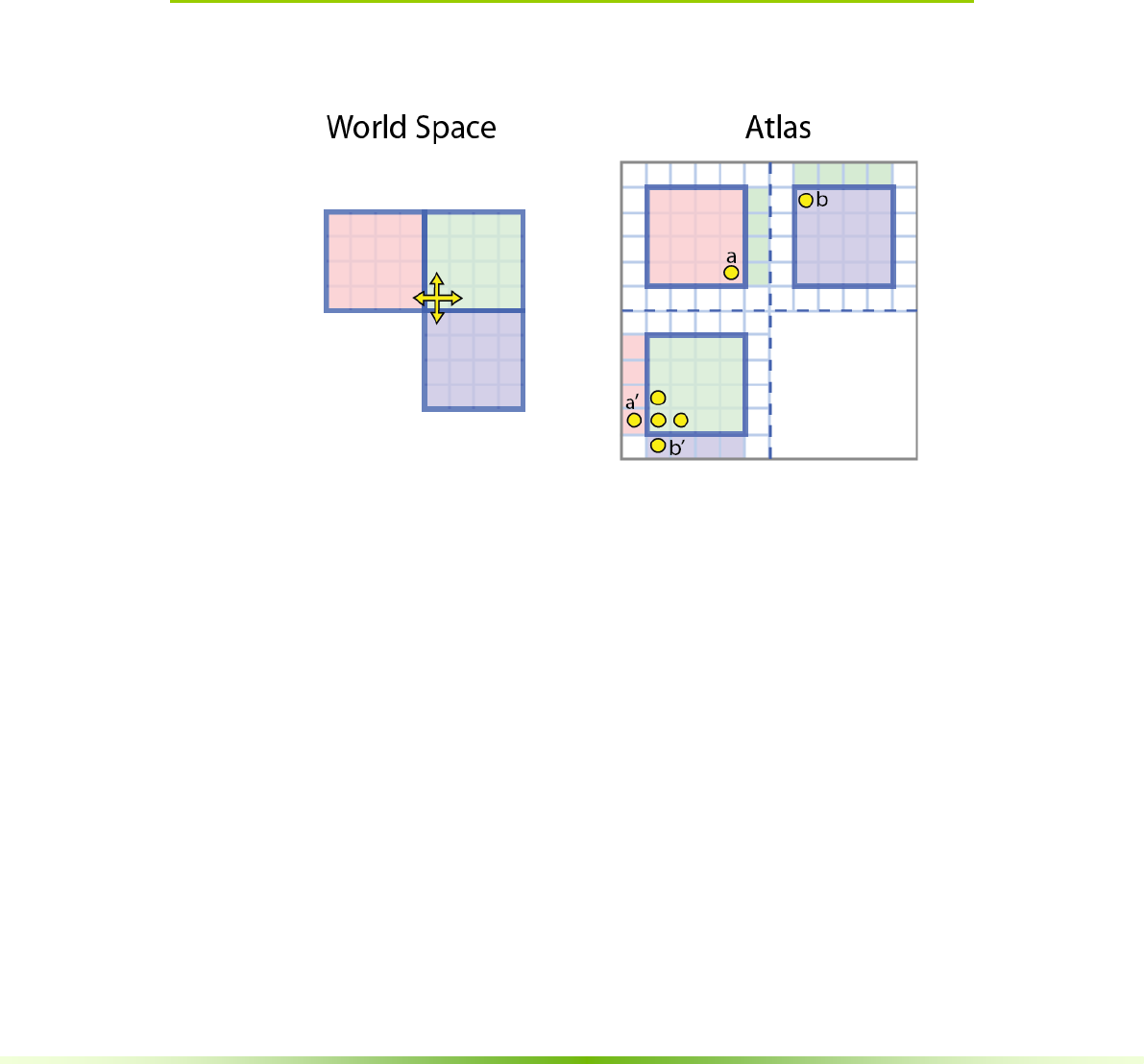
NVIDIA® GVDB Voxels - Programming Guide 35
A trivial solution is to perform extra operations at the boundary voxels to search
the atlas for their values. However this introduces GPU inefficiency.
The search for neighbors at boundary voxels, highlighted in Figure 5.2, can
require multiple indirections and conditional checks to find the correct voxel.
This search is not necessary for interior voxels which are able to access
neighbors directly, and introduces an imbalance in GPU thread occupancy as
interior voxels will complete their work before boundary voxels. Since there are
many more interior voxels, most threads will remain idle while the boundary
voxels search for neighbors. Thus the GPU will be idle most of the time.
GVDB Voxels uses a common, improved solution called apron voxels, where
neighbors are directly accessible via additional atlas storage.
5.3. Apron Voxels
Figure 5.3. The ideal solution is each voxel has direct access to its neighbors. To
enable this, apron voxels are stored with each brick. The apron voxels are
correct world space neighbors at the brick boundaries.
Ideal GPU computations perform the same amount of work on every voxel,
which is the work desired by the user. To accomplish this each voxel must have
direct access to its neighbors. This is solved with apron voxels, shown in Figure
5.3. From the perspective of the target voxel (left), the neighbors are two green,
one red and one blue voxel. The green ones are already accessible. The correct
values for red and blue are at points a and b in the atlas (right). These are copied
into the locations a’ and b’ so they are directly adjacent to the target voxel.
Apron voxels allow all voxels to directly access neighbors.
Kernel launches for compute are be performed over atlas space instead of
world space. This assigns a GPU thread to each voxel in the atlas. User kernels
can then perform calculations with direct neighbor lookups.

36 NVIDIA® GVDB Voxels - Programming Guide
5.3.1. Apron Width
The width of the apron determines the size of stencil operations that can be
peformed efficiently. More apron voxels support bigger stencils but at the cost
of memory overhead. For example, a 1-width apron (on each side) can support
all 3x3 stencil kernels, and a 2-width apron supports 5x5 stencil kernels. To
implement a 5x5 kernel with only a 1-width apron requires the slower direct-
lookup technique at boundaries, which is also available in GVDB Voxels.
Apron voxels require extra space in the data atlas. The ratio of brick voxels to
apron voxels determines this overhead. Here is a quick summary of apron
overheads for different brick sizes.
Brick Size Apron Width Apron Voxels Memory Overhead
83 1 392 76%
163 1 1,544 37%
323 1 6,152 18%
643 1 24,584 9%
83 2 832 162%
163 2 3,136 76%
323 2 12,352 37%
643 2 49,216 18%
Figure 5.4. Effect of brick size and apron width on memory overhead. Larger
bricks require more apron voxels, but significantly reduce overhead because the
number of interior voxels grows as n3 while the number of apron voxels grows
as n2. Less memory is used overall with larger bricks.
Keep in mind that apron voxels are duplicates of other voxels in the atlas, and
present solely for the purpose of efficient computation. Thus we want to
minimize the number of apron voxels required. We can change this overhead
with careful selection of brick size and apron width. Figure 5.4 shows the
memory overhead for common settings.
The apron width is specified when adding a channel.
gvdb.AddChannel ( channel, data_type, apron_width );
5.3.2. Apron Updates
Apron voxels must typically be updated after every compute operation, before
performing a new calculation. When voxel values change due to a computation
their neighbors also change. Since the apron voxels are duplicates of neighbors
at boundary voxel they must be updated to reflect any changes.
Two compute API functions quickly update apron voxels:
UpdateApron( channel ) Updates apron voxels in a specific channel
UpdateApron() Updates apron voxels in all channels

NVIDIA® GVDB Voxels - Programming Guide 37
5.4. Custom Kernels
The most common way to perform computations for motion pictures, 3D
volume processing, or scientific simulation in GVDB Voxels is with custom
kernels in the Compute API. Custom kernels allow one to author and compile
a kernel in user code which is then launched by the GVDB library.
The typical workflow with custom kernels is as follows:
- Kernel Authoring Kernels are written and compiled with CUDA
on the application side.
- Kernel Loading Kernels are loaded in the application with
common CUDA functions such as cuModuleLoad,
cuModuleGetFunction and cuModuleGetGlobal
- GVDB Configuration GVDB is initialized and configured with the
desired topology and voxel size.
- Channels (Aprons) Add channels for voxel attributes. Specify the
apron width to be applied to that channel.
- Compute kernels The custom kernels defined in steps above
are launched with gvdb.ComputeKernel ( .. )
by passing a CUfunction pointer to GVDB.
- Update Aprons Apron voxels are updated by calling
gvdb.UpdateApron.
Additional compute operations are performed with repeated calls to
ComputeKernel followed by UpdateApron as needed. Many compute kernels
can be defined in a single application-side .cu file and loaded together with
cuModuelGetFunciton. As long as these kernels conform to GVDB
requirements, they can be passed as custom kernels to the gvdb.ComputeKernel
function which will launch the kernel over every voxel in the sparse volume.
5.4.1. Voxel Kernels
GVDB voxel compute kernels are CUDA kernels with just a few minor
differences and constraints. Voxel kernels must take only two arguments, an int3
for the atlas resolution, and a uchar for the channel they operate on. Any other
function variables can be accessed with global device variables in the user
CUDA code that are read by the kernel. There are no other restrictions in the
style of CUDA code. Structures, classes, share memory and calling other device
functions are all permitted in voxel compute kernels.
One must remember that voxel kernels are launched over all voxels
in atlas space. Some computations, such as adding noise or 3x3 stencils, do not
require knowledge of world space. Therefore calculations can be performed
entire with atlas space voxels and neighbors.
The following example reads a voxel, adds noise to it, and writes the voxel:

38 NVIDIA® GVDB Voxels - Programming Guide
__global___ gvdbOpNoise ( int3 res, uchar chan )
{
GVDB_VOX
float v = tex3D<float> ( volIn[chan], vox.x, vox.y, vox.z );
v += noise();
surf3Dwrite ( v, volOut[chan], vox.x*sizeof(float), vox.y,
vox.z);
}
In other calculations it may be necessary to have the world position of a voxel.
An example is computing the per-voxel distance for each voxel to a world-space
object like a sphere.
The device function getAtlasToWorld transforms from atlas to world space.
Here is an example that gets the world position of the current voxel, determines
the distance to a user-defined sphere (global structure), and writes that value:
__device__ Sphere sphere;
__global___ gvdbOpDistToSphere ( int3 res, uchar chan )
{
GVDB_VOX
float3 wpos;
if ( !getAtlasToWorld ( vox, wpos )) return;
float v = wpos – sphere.pos; // distance to sphere
surf3Dwrite ( v, volOut[chan], vox.x*sizeof(float), vox.y,
vox.z);
}
As described in Chapter 4.1.2 (Atlas Space), the macro GVDB_VOX is
shorthand for setting the 'vox' variable for the voxel assigned to the current
thread.
5.4.2. Neighbor Access
Kernel macros are provided to facilitate writing efficient voxel kernels.
These are included with the cuda_gvdb_operators.cuh header file.
The following kernel macros are available:
GVDB_VOX Sets the 'vox' variable for the atlas voxel of the
current thread
GVDB_COPY_SMEM_F Sets up a 'vox', and also 'svox' shared memory
variable for lookup of the voxel neighbors.
GVDB_COPY_SMEM_UC/4 Sets up a 'vox' and 'svox' similar to _SMEM_F,
but for UCHAR and UCHAR4 channel types.
These macros arrange fast access to neighbors by creating a shared memory
array 'svox' that contains the neighbors for the current thread block.
Thread blocks in GVDB Voxels are fixed at 8x8x8 and for efficiency they do
not correspond to brick sizes. The distinction between thread blocks and

NVIDIA® GVDB Voxels - Programming Guide 39
GVDB blocks is described further in the Implementation section below.
The shared memory array 'svox' gives access to neighbors:
__global__ void gvdbOpSmooth ( int3 res, uchar chan, float p1,
float p2, float p3 )
{
GVDB_COPY_SMEM_F
float v = p1 * svox[ndx.x][ndx.y][ndx.z];
v += svox[ndx.x-1][ndx.y][ndx.z];
v += svox[ndx.x+1][ndx.y][ndx.z];
v += svox[ndx.x][ndx.y-1][ndx.z];
v += svox[ndx.x][ndx.y+1][ndx.z];
v += svox[ndx.x][ndx.y][ndx.z-1];
v += svox[ndx.x][ndx.y][ndx.z+1];
v = v / (p1 + 6.0) + p2;
surf3Dwrite ( v, volOut[chan], vox.x*sizeof(float),
vox.y, vox.z );
}
This is the entire kernel for a 7-point smoothing function. The first line,
GVDB_COPY_SMEM_F sets up the variable 'svox', 'ndx' and 'vox':
svox A shared memory table for the neighbors of the current voxel
ndx A variable for offset access to the 'svox' neighbor values
vox A variable for the voxel coordinates in atlas space
wpos Computed by calling getAtlasToWorld, gives the world space
position of 'vox'
The variable 'vox' is used when performing read/write into the target atlas
texture with tex3D or surf3Dwrite.
The variable 'ndx' is used when accessing the +/- axis neighbor voxels values of
the current voxel.
The variable 'wpos' is used when the world position of the voxel is needed.

40 NVIDIA® GVDB Voxels - Programming Guide
5.4.3. Channel Read/Write
The primary channel (#0) can be read/written using the global access variables
volTexIn and volTexOut. These are texture and surface references (texref,
surfref) for accessing 3D textures in CUDA.
float v = tex3D( volTexIn, vox.x, vox.y, vox.z );
surf3Dwrite( v, volTexOut, vox.x*sizeof(float), vox.y, vox.z);
The variables volTexIn and volTexOut are texture references and surface
references (see the CUDA Texture Reference API, 3.2.11.1.2). The texture atlas
is bound to these references automatically by GVDB Voxels. However, an
important limitation of texture references is that their type must be defined at
compile time. Since the 3D texture atlas is owned by GVDB, this greatly
restricts their usefulness. Thus only the primary channel, when it is used as a
float channel, can be accessed in this way. The texture/surface reference access
to GVDB textures was maintained for compatibility. A more generic solution is
texture objects.
All channels can be read/written with global access arrays volIn and volOut.
These variables are texture objects (see the CUDA Texture Object API,
3.2.11.1.1). Texture objects correspond to bindless textures as they do not need
to be bound to a specific type. This implies they can be used for access to voxels
channels with different types defined at run-time.
float v = tex3D<float> ( volIn[chan], vox.x, vox.y, vox.z );
surf3Dwrite( v, volOut[chan], vox.x*sizeof(float),vox.y,vox.z);
Notice how the tex3D function for Texture Objects differs from the above. It
accepts a template type <float>, and the texture is specified with the channel ID
given by 'chan'. Thus a voxel kernels can read voxel attributes from any channel,
which can be of arbitrary type.
The surf3Dwrite function is also flexible since its type is baked into the width as
a stride multiplier, sizeof(float). Write operations can take either texture
references or texture objects, so there is no type templating like tex3D.

NVIDIA® GVDB Voxels - Programming Guide 41
5.4.4. Kernel Loading
Custom voxel kernels are compiled with CUDA and loaded by the application at
any time using cuModuleLoad, cuModuleGetFunction and
cuModuleGetGlobal. The following complete example shows how to generate
a density functions with a customer kernel.
HOST CODE
CUmodule cuGenerateModule; // app module
CUfunction cuGenerateDensity; // app function
CUdeviceptr cuDensity; // app global var
cuModuleLoad ( &cuGenerateModule, "generate.ptx" );
cuModuleGetFunction ( &cuGenerateDensity, cuGenerateModule,
"myDensityFunc" );
cuModuleGetGlobal ( &cuDensity, &sz, cuGenerateModule,
"gDensity");
gvdb.Initialize ();
gvdb.AddChannel ( 0, T_FLOAT, 1 ); // voxel density
gvdb.AddChannel ( 1, T_UCHAR, 1 ); // voxel status
float density = 0.25;
cuMemcpyHtoD ( cuDensity, &density, sizeof(float) );
gvdb.ComputeKernel ( cuGenerateModule, cuGenerateDensity,
1, true );
The host code for loading a voxel kernel declares a module for the application,
and CUfunction variables for each kernel function. Additional global variables
used in the kernel are declare by the host as CUdeviceptr.
The .cu kernel source is compiled to a .ptx by CUDA (nvcc), which is then
loaded by cuModuleLoad. The custom voxel kernel is called "myDensityFunc",
and is loaded into a variable with cuModuleGetFunction. This follows typical
patterns from the CUDA Device API for loading modules and functions.
After creating channels used by the voxel kernel, we send any global variables to
the kernel using cuMemcpyHtoD for each variable or structure.
Finally, gvdb.ComputeKernel is called with the application module and the
custom voxel kernel. Two additional arguments specify the primary channel to
operate on, and whether an apron update should be performed.
ComputeKernel ( CUmodule, CUfunction, int channel, bool update_apron);
The custom voxel kernel is launched over all the voxels in atlas space.
Notice that the code for loading modules, kernels and variables follows
basic CUDA patterns without restriction. GVDB Voxels accepts the module
and function, and a primary channel. Any other specialized variables used by the
kernel are left to the application and set with cuMemcpyHtoD.

42 NVIDIA® GVDB Voxels - Programming Guide
DEVICE CODE
//-------------------------------- GVDB Includes
#define CUDA_PATHWAY
#include "cuda_gvdb_scene.cuh" // GVDB Scene
#include "cuda_gvdb_nodes.cuh" // GVDB Node structure
#include "cuda_gvdb_geom.cuh" // GVDB Geom helpers
#include "cuda_gvdb_operators.cuh" // GVDB Operator macros
//--------------------------------
__device__ float gDensity;
__global__ void myDensityFunc ( int3 res, uchar chan )
{
GVDB_COPY_SMEM_UC // macro to setup neighbors
uchar v = tex3D<uchar>( volIn[chan], vox.x,vox.y,vox.z);
if ( v==0 ) return; // return if
surf3Dwrite ( gDensity, volOut[0],
vox.x*sizeof(float), vox.y, vox.z);
}
Let's examine the device code for the above example. The GVDB Includes give
access to the GVDB data structures, helpers, and macros for neighbor lookups.
gDensity is an application (user-side) variable specific to this example, and is set
prior to calling gvdb.ComputeKernel. The voxel kernel must take an int3 for
atlas resolution, and a uchar for the primary channel, with no return value.
The macro GVDB_COPY_SMEM_UC sets up the local variables 'vox', 'ndx', and
'svox' for access to the current voxel, and the neighbor tables. The channel
'chan' must correspond to the input channel type for the neighbor macro.
The next line, tex3D<uchar>, reads a voxel from the input channel (1), at the
current thread's voxel location (vox), as an unsigned char. This voxel attribute is
being used as the status of the voxel, so that a voxel status = 0 indicates an
inactive voxels -- resulting in a return. Other values may have different meaning,
but this kernel only cares that the voxel is active (non-zero status).
The last line takes the user-specified global density and, if the voxel is active,
sets it using the volOut texture for the output channel 0, which in this case is a
float channel for voxel density.
Two channels are present, one for voxel density (float), another for voxel status
(uchar). Since we are using texture objects, volIn and volOut, we can read/write
to either of these from the kernel. However, only one is passed in as the primary
input (chan) to prepare neighbor macros.

NVIDIA® GVDB Voxels - Programming Guide 43
5.4.5. Compute Kernel
Custom voxel kernels are launched with gvdb.ComputeKernel:
ComputeKernel ( CUmodule, CUfunction, int channel, bool update_apron);
- CUmodule Indicates the application module for the kernel
- CUfunction Indicates the CUDA function which follows the
guidelines for a GVDB Voxel's custom kernel
- Channel The primary channel for input. This channel
will be used to prepare neighbor voxels arrays.
- Update Apron A boolean indicating whether an UpdateApron
should be performed after the kernel finishes.
The 'channel' passed to ComputeKernel is for simple kernels that typically
read/write to only one channel. For voxel kernels that wish to access or modify
multiple channels, the application and user device code should track additional
input/output channels with global device variables. In this case, the channel
variable is used to indicate the input channel for shared neighbor voxels.
The ComputeKernel function always launches with one thread per sparse voxel
in the atlas. It is thus suitable for calculations that might touch (read or write) all
sparse voxels.
If you wish to launch a thread over some custom object (thread-per-polygon, or
thead-per-point), or if you wish to process a small subset of the volume, you
may want to directly launch the kernel as describe in the next section on
Modules.
5.5. Modules
The GVDB Library and user Application reside in different module spaces
according to CUDA. This is how custom functions are pass to a precompiled
and linked GVDB library. Therefore, the GVDB module for built-in compute
functions is different than the module for application kernels. Yet both desire
access to the same GVDB volume data.
The Compute API of GVDB Voxels has functions for switching the GVDB
and application modules.
gvdb.SetModule ();
The SetModule function, without arguments, returns GVDB to the default
GVDB Library module. With this module set GVDB can perform built-in
compute tasks, apron updates and CUDA raytracing. Any kernel function that is
part of the GVDB Library itself requires the default module. As this is the
default setting, normally this is transparent to the user of GVDB Voxels when
no other application kernels/modules are defined.
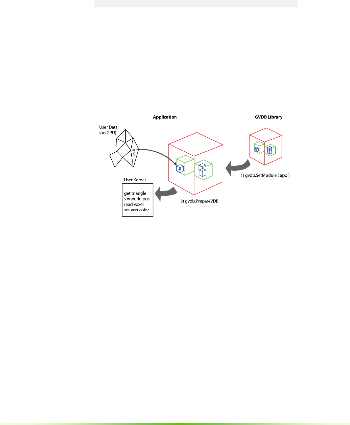
44 NVIDIA® GVDB Voxels - Programming Guide
gvdb.SetModule ( CUmodule );
When an argument is provided, SetModule sets the GVDB module to the
Application module given. Now each time a custom voxel kernel is launched
with ComputeKernel, GVDB Voxels will first set the module to the application,
and then assign the GVDB topology data to it. In this way, both the user
Application and GVDB Library have access to the GVDB topology and data on
the GPU across the library boundary.
Note that gvdb.SetModule is specific to GVDB Voxels. You can still launch
arbitrary CUDA kernels on the application without calling SetModule each time.
Typically, you would call SetModule when you want to guarantee that GVDB is
delivering GVDB topology & data to a specific kernel.
Directly Launched Kernels
Figure 5.5. A complex task between a user data structure, a polygonal mesh on
GPU, and a sparse volume in GVDB Voxels. Step 1 gives the application access
to the GVDB topology & data which is typically owned by the GVDB Library.
Step 2 prepares the current GVDB data, which may have changed by other calls
to GVDB, for the user kernel. Finally the kernel is launched with cuLaunch,
since only the application knows how to assign threads per triangle.
The only time to call SetModule explicitly is when launching user kernels that
are directly launched by your application, as in Figure 5.5. For example,
perhaps you wish to perform a novel calculation over a different data structure
such as a polygonal surface -- but using data from GVDB Voxels. In this case,
you would not call ComputeKernel, because it is only for computations where
the input/output is the voxel volume. Threads of ComputeKernel correspond
to all sparse voxels.
Your custom kernel has threads which correspond to polygons, not voxels. In
this case, you call gvdb.SetModule(..) with your application module, and call
gvdb.PrepareVDB(). Then you can launch the kernel yourself with cuLaunch.
Your kernel will still have accces to the GVDB Voxel data structures even
though it operates on voxels. The kernel could, for example, get the world
position of the polygon's vertices, and then perform a GVDB atlas lookup to
get the voxel color. In this way, you would 'paint' the volume onto a polygonal
model. This process for direct launch is not needed with ComputeKernels,
since that function internally sets the module for you, prepares GVDB data, and
launches your custom kernel over all sparse voxels.

NVIDIA® GVDB Voxels - Programming Guide 45
Chapter 6.
Raytracing API
Rendering with NVIDIA® GVDB Voxels is accomplished with either the pure
CUDA Raytracing pathway or with OptiX integrated Raytracing. In both cases,
custom raytracing kernels can be authored to create a specific look. Native
pathways support raytracing of isosurfaces with trilinear or tricubic filtering,
volumetric sampling with transfer functions, level set raytracing, and voxel
rendering mode.
6.1. Render Buffers
Rendering outputs and inputs are placed into render buffers. These are two
dimensional linear buffers (not textures) that typically contain RGBA values.
Multiple render buffers may be used for additional depth buffers or for
intermediate shading outputs, e.g. diffuse, etc.
Render buffers are created during initialization with AddRenderBuf():
AddRenderBuf ( render_chan, width, height, bytes_per_pixel );
The following example creates a primary render buffer for color output:
gvdb.AddRenderBuf ( 0, 1920, 1080, 4 ); // 32-bit color (RGBA)
During viewport resize, it may be necessary to resize a render buffer.
gvdb.ResizeRenderBuf ( 0, width, height, 4 );
To return the results of a render buffer from GPU to CPU as linear memory,
use the following:
ReadRenderBuf ( render_chan, uchar* bytes );
One must pre-allocate the destination data before calling ReadRenderBuf:
uchar* dat = (uchar*) malloc ( width*height*4 );
gvdb.ReadRenderBuf ( 0, dat );
// use dat here
free ( dat );
The render channel is not the same thing as a GVDB Atlas channel. Atlas
channels contain per-voxel attributes stored in 3D textures. Render channels are
list of 2D buffers in linear GPU memory.

46 NVIDIA® GVDB Voxels - Programming Guide
Another use for render buffers is to store additional image results from other
views. For example, the g3DPrint sample uses one render buffer for the primary
3D rendering, and a second one to generate the 2D cross-section slices that are
sent to a 3D printer.
ReadRenderBuf can be used to retrieve the output data. The sample utilities
(\sample_utils) contains an image helper class which can write out PNG images:
nvImg img;
img.Create ( res_x, res_y, IMG_RGBA);
uchar* dat = img.getData(); // get pixel pointer
gvdb.ReadRenderBuf ( 1, dat ); // get render buffer #1
char sname[1024];
sprintf ( sname, "slice_%d.png", y );
img.FlipY ();
img.SavePng ( sname ); // save as png
Render buffers may also be used as inputs. For example, a depth buffer may be
written by OpenGL and then used by GVDB Voxels to perform depth-based
volumetric compositing.
6.1.1. OpenGL Readback
For interactive applications, it is desirable to place the GVDB Voxel rendering
output into a 2D OpenGL texture for on-screen display. All GVDB render
buffers are allocated with CUDA linear memory. However, utility functions are
provided to transfer this into OpenGL textures.
Typically, the application generates an OpenGL texture of the same size as the
render buffer. Then one uses ReadRenderTexGL to transfer the GVDB Voxel
results into it.
gvdb.AddRenderBuf ( 0, width, height, 4 );
GLuint output_glid;
glGenTextures ( 1, &output_glid );
glBindTexture ( GL_TEXTURE_2D, output_glid );
glTexImage2D ( GL_TEXTURE_2D, 0, GL_RGBA8, width, height, 0, GL_RGBA,
GL_UNSIGNED_BYTE, 0 );
gvdb.ReadRenderTexGL ( 0, output_glid ); // return render chan 0
After ReadRenderTexGL the application can use the OpenGL texture for on-
screen display or other purposes. Each time a new gvdb.Render() is performed,
the render buffers will change. So, although one generates the 2D texture once,
it is necessary to call ReadRenderTexGL after each render to update the
OpenGL texture.
One can also write OpenGL textures to GVDB render buffers for use as inputs.
gvdb.WriteRenderTexGL ( 0, input_glid ); // send render chan 0
Render buffer inputs must be read using custom render kernels since the native
volume rendering pathways do not make use of this.

NVIDIA® GVDB Voxels - Programming Guide 47
6.1.2. Depth Buffers
Special render buffers are used as depth buffers for reading and writing depth
maps. These buffers reside in the same slot locations as render buffers
(technically, they are also render buffers, but with special allocation).
A set of functions is provided, similar to render buffers, for creating, reading
and writing depth buffers.
AddDepthBuf ( int render_chan, int w, int h ); // Add a depth
buffer
ResizeDepthBuf ( int render_chan, int w, int h ); // Resize a depth
buffer
WriteDepthTexGL ( int render_chan, int glid ); // Write depth from
GL
Depth buffers are special, handled differently from other render buffers,
because they create OpenGL Depth textures automatically, in addition to linear
CUDA memory. Since CUDA-GL interop requires that depth textures are
always created in OpenGL and mapped to CUDA linear memory (interop
cannot be performed in the other direction), this would require multiple interop
calls and an extra transfer. For performance reasons, GVDB depth buffer
generate OpenGL Depth textures first and perform the interop once. Both the
OpenGL texture and the CUDA memory are owned by GVDB.
WriteDepthTexGL uses framebuffer objects (FBOs) to efficiently transfer depth
buffer data from the input GL texture to the GVDB depth buffer with
a GPU-to-GPU copy.
6.1.3. Writing to Buffers
The primary render buffer is passed by argument to native rendering kernels.
Output color is written directly to the rendering buffer.
__global__ void gvdbRaytrace ( uchar4* outBuf )
{
// get pixel for this thread
int x = blockIdx.x * blockDim.x + threadIdx.x;
int y = blockIdx.y * blockDim.y + threadIdx.y;
if ( x >= scn.width || y >= scn.height ) return;
float4 clr = make_float4(1,1,1,1);
// .. perform raytracing ..
outBuf[ y*scn.width + x ] =
make_uchar4(clr.x*255, clr.y*255, clr.z*255, clr.w*255);
}
Since the type of outBuf is a pointer to uchar4 the pixel stride is already
included. The width of the render buffer is given in CUDA render kernels
by scn.width, scn.height.
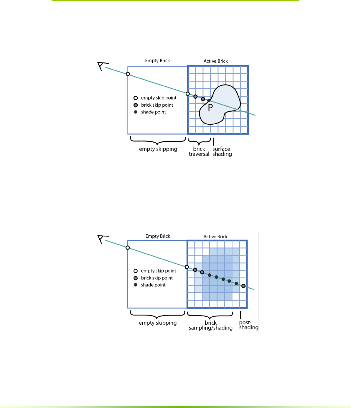
48 NVIDIA® GVDB Voxels - Programming Guide
6.2. CUDA Raytracing
The GVDB Raytracing API is primarily a CUDA pathway for native and custom
rendering of sparse volumes. GVDB Voxels distinguishes between surface
rendering, which occurs at a hit point, and volume rendering, in which voxels
are sampled and shaded at many points along the ray.
Figure 6.1. Surface rendering a sparse volume consists of a) empty skipping, b)
brick traversal, and c) surface shading at the hit point.
The basics of surface rendering for sparse voxels are showin Figure 6.1. In
this type of rendering the voxel data is treated as an isosurface or level set
surface. The camera ray travels through the volume, skipping empty space in the
VDB tree, and arriving at a brick. At the brick, sample testing rejects individual
voxels until a hit surface is detected. At the hit point (P), the normal is
computed and the surface point is shaded.
Figure 6.2. Volume rendering a sparse volume consists of a) empty skipping, b)
brick sampling/shading, and c) post-shading. Unlike surface rendering, volume
rendering may sample and shade many points in the volume.
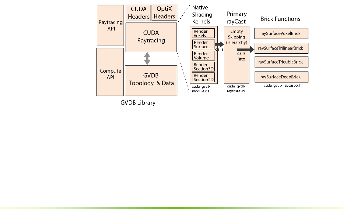
NVIDIA® GVDB Voxels - Programming Guide 49
The basics of volume rendering are showin Figure 621. This style of rendering
treats the volume as a density field with differing opacity at each voxel. Example
of such volumes are smoke, fire and gases. Camera rays travel through the
volume skipping empty space. At the brick, the ray continues and each voxel
sample contributes some accumulated shading to final output color. Finally, the
background is blended in to give the pixel color.
GVDB Voxels was designed to support both surface and volume rendering in
a consistent way. We notice that empty skipping is identical in both, whereas
brick traversal and shader are different. Therefore, GVDB consists of the
following components:
- Empty skipping Efficient traversal of the GVDB hierarchy
- Brick functions Brick-level functions for rendering different types
of volumetric data. (isosurface, deep, level sets)
- Native shading Built-in examples of specific shading kernels
and styles
- Helper functions Perform useful operations for
custom brick functions.
Empty skipping is highly optimized for GVDB hierarchy traversal on the GPU,
and is provided as a generic starting-point for a ray. Brick functions are specific
to the style and type of voxel data, such as level sets or semi-opaque volumes.
Native shading functions provide built-in examples of shading styles which may
be customized with custom render kernels.
Figure 6.3. Overview of CUDA raytracing in GVDB Voxels. The Raytracing and
Compute APIs are the outward facing functions called by applications. The
internal design of the CUDA raytracing pathway is shown here.
An overview of the CUDA Raytracing pathway is shown in Figure 6.3.
Rendering begins in shading kernels, which initiates a ray and then calls the
rayCast function, pass it a CUfunction pointer to a brick function. The rayCast
function performs empty space skipping in a generic way, and then calls into the
provided brick function for traversal and sampling. Results are returned to the
shading kernel for final shading.

50 NVIDIA® GVDB Voxels - Programming Guide
To render volume data with GVDB, one first prepares a light, camera and
transfer function as described in Chapter 3. Additionally, at least one render
buffer is needed for output, as described in Chapter 6.1 (Render Buffers).
Once volume data is loaded or created, native rendering is done
with the Render function:
Render ( render_chan, style, filtering, frame,
sample, max_sample, shadow_amt, depth_chan );
- render_chan The render buffer ID for output
- style Style of rendering desired. Can be one of:
SHADE_VOXEL
SHADE_SECTION2D
SHADE_SECTION3D
SHADE_EMPTYSKIP
SHADE_TRILINEAR
SHADE_TRICUBIC
SHADE_LEVELSET
SHADE_VOLUME
SHADE_OFF
- filtering Filtering mode/amount. [unused in native render]
- frame Current render frame. [unused in native render]
- sample Current accumulated sample. [unused in native render]
- max_sample Maximum number of samples. [unused in native render]
- shadow_amt Shadow darkness, 0 to 1
- depth_chan Option render buffer ID for a depth channel.
The render_chan ID must be an RGBA (4 byte) output when using the
native render function. The Render function produces a specific look based on a
single light source, with Phong shading for surfaces, and a piecewise Transfer
function for deep volumes. For different looks, see Custom Render Kernels
(Chapter 6.4). Notice the arguments for filtering, frame, sample and
max_sample have no effect on native rendering, but can be read when used in
custom kernels. When shadow_amt is 0, no shadow rays are cast, otherwise
there is an additional ray cost for the shadow.
Upon completion, it is common to retrieve the output either as a CPU buffer or
into an OpenGL texture for display.
gvdb.Render ( 0, SHADE_VOXEL, 0, 0, 1, 1, 1.0 );
gvdb.ReadRenderTexGL ( 0, output_glid );

NVIDIA® GVDB Voxels - Programming Guide 51
6.2.1. Native Shading Kernels
All rays are initiated in a shading kernel, which generates the ray, casts it into a
volume, and performs shading. Native shading kernels are built in to GVDB
Voxels to provide sample styles based on a single light source. Custom shading
kernels are build by the user to achieve a specific look.
A native shading kernels is selected with the 'style' argument to
the Render function. The following styles are available:
SHADE_VOXEL Function: gvdbRaySurfaceVoxel
Voxel style with each voxel rendered as a cube.
Single light source with Phong shading and shadows.
SHADE_SECTION2D Function: gvdbSection2D
Renders a cross-section of the volume directly into the 2D render
buffer. The transfer function is applied, and the cross-section plane is
defined with gvdb.SetCrossSection.
SHADE_SECTION3D Function: gvdbSection3D
Renders the scene in 3D similar to SHADE_TRILINEAR, but
with a 2D cross-section cutting the model. Single light source,
trilinear surface shading is used on the model, and the transfer function
is applied to the cross-section.
SHADE_EMPTYSKIP Function: gvdbRayEmptySkip
Renders the scene up to the GVDB bricks, but does not traverse
into the brick. Bricks are colored by world position. This mode is
useful for profiling empty skipping.
SHADE_TRILINEAR Function: gvdbRaySurfaceTrilinear
Renders the volume data as an isosurface with trilinear smoothing
and normals, Phong shading, and one light source. The isovalue is
set using scene SetVolumeRange ( iso, vmin, vmax).
SHADE_TRICUBIC Function: gvdbRaySurfaceTricubic
Renders the volume data as an isosurface with tricubic smoothing.
Note that the voxel data must be prepared using AddChannel with
an apron=2 for this to work, since tricubic sampling requires
a 5x5 neighborhood.
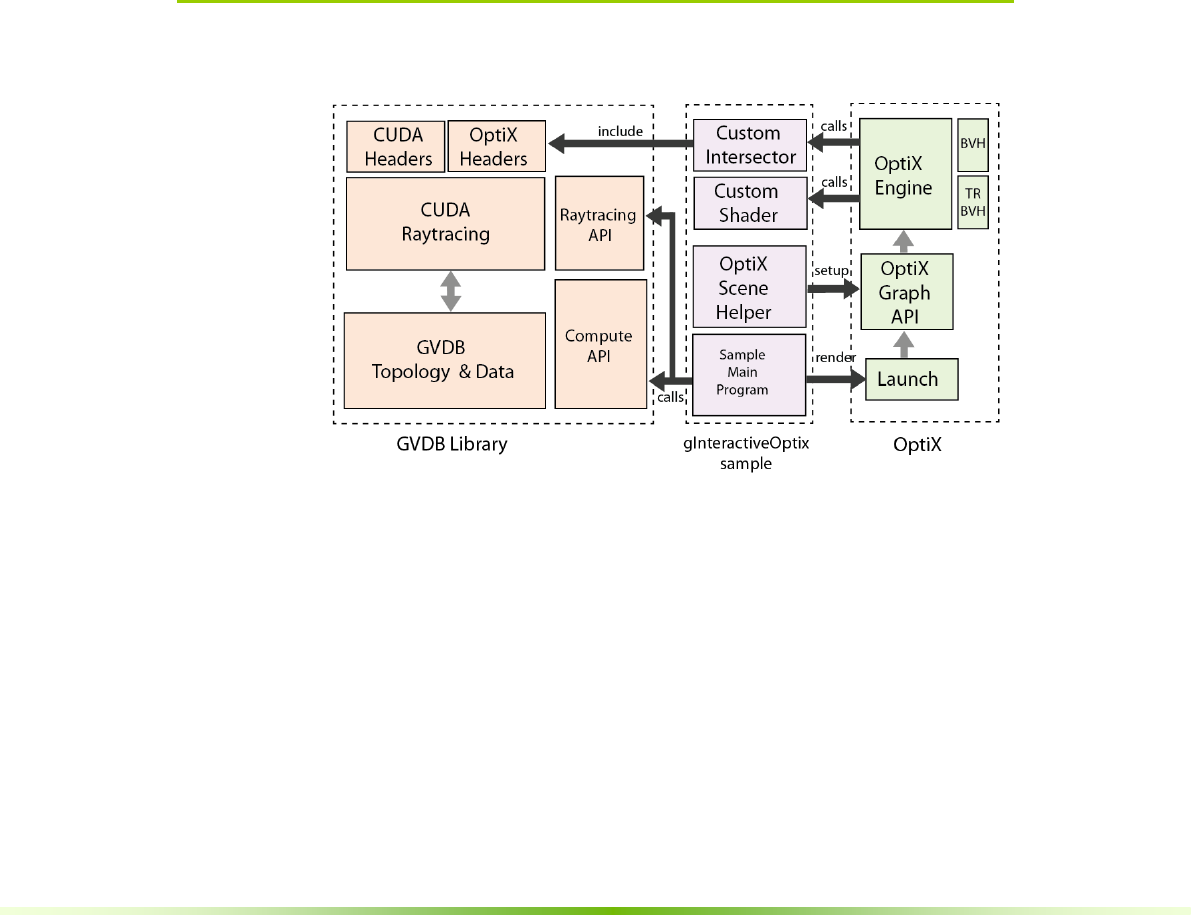
52 NVIDIA® GVDB Voxels - Programming Guide
SHADE_LEVELSET Function: gvdbRayLevelSet
Renders the volume as a level set surface. Outside values are +1,
and inside values are -1. Displays with Phong shading, one light source.
SHADE_DEEP Function: gvdbRayDeep
Renders the data as a semi-transparent volume with deep,
accumulated sampling. The transfer function is applied to
each sample point. Use scene.SetSteps(..) to set the voxel-to-voxel
sample spacing for render quality, use scene.SetCutoff() to define
the minimum contributing voxel value and the alpha cutoff value,
and use scene.SetExtinct(..) to set the extinction and albedo
for accumulation. Use scene.SetBackgroundClr(..) to set the
background color value for semi-transparent rays.
The functions listed above which implement these styles are found in
cuda_gvdb_module.cu. When authoring custom kernels these often serve as a
useful reference.
6.3. OptiX Raytracing
Figure 6.4. Overview of the relationships between the GVDB Library, the OptiX
Library, and the gInteractiveOptiX sample.
NVIDIA® GVDB Voxels has an OptiX raytracing pathway for rendering
volumes with high quality, multi-scattering via communication with NVIDIA®
OptiX. An overview of the components of GVDB-OptiX raytracing are shown
in Figure 6.4. Notice that GVDB does not contain OptiX code, and nor does
OptiX contain GVDB code. This was done to simplify and maintain
independence of both SDKs. Instead, the gInteractiveOptiX sample which
comes with GVDB Voxels includes a generic OptiX Scene Helper which
connects GVDB to OptiX. This generic class can be used in any applications
that wish to render GVDB sparse volumes with OptiX.

NVIDIA® GVDB Voxels - Programming Guide 53
Since both NVIDIA® OptiX and NVIDIA® GVDB Voxels are built on
CUDA, the core GVDB raytracing functions for empty skipping and brick
traversal are the same in both pathways. The only functions that must be
handled differently are the shading kernels, which must be implemented as
OptiX shadering programs.
From the perspective of OptiX, the GVDB volume is handled with a new
custom intersector program that is able to traverse and hit voxels. This can be
found in optix_vol_interactive.cu file in the gInteractiveOptiX sample. The
intersector program calls the primary rayCast function of GVDB.
Since OptiX performs shading, the native shading kernels of GVDB Voxels are
not used. Instead, OptiX launches rays, performs intersections with the GVDB
custom intersector, and does shading with a custom OptiX shading program.
OptiX requires that 3D textures are provided by OpenGL and declared using
rtTextureSampler<float, 3> (this is found in cuda_gvdb_nodes.cuh). Therefore,
the GVDB Voxels atlas data must be created using OpenGL by calling the
UseOpenGLAtlas() function during initialization.
gvdb.UseOpenGLAtlas ( true );
6.3.1. OptiX Scene Helper
The OptiX Scene class, found in the gInteractiveOptix sample, contains generic
functions for adding GVDB Voxels to an OptiX scene graph. The following
shows the sequence of steps performed by RebuildOptixGraph in this sample,
which makes use of the OptixScene class.
OptixScene optx; // declare the OptiX Scene helper
optx.InitializeOptix (w, h); // Initialize OptiX with width, height.
optx.ClearGraph(); // Clear the OptiX scene graph
optx.AddMaterial ( .. ); // Adds a material based on a custom
// OptiX shading program.
optx.AddVolume (..); // Adds a GVDB volume to the OptiX graph
optx.AddPolygons (..); // Adds a polygonal model to OptiX graph
optx.SetTransferFunc (..); // Sets the GVDB transfer functions for
// use by OptiX
optx.ValidateGraph (..); // Validates the OptiX graph
optx.AssignGVDB (..); // Assigns the GVDB data to OptiX
See main_interactive_optix.cpp in gInteractiveOptiX sample for details.
See optix_scene.cpp in gInteractiveOptiX for the implementation.

54 NVIDIA® GVDB Voxels - Programming Guide
The function AddVolume creates a simple sub-graph in which GVDB Voxels is
a geometric bounding box in the OptiX acceleration BVH. The GVDB volume
sub-graph consists of the following:
- Transform A transformation applied to the entire volume
- GeometryGroup A group with only one child, the GeometryInstance,
and an SBVH acceleration structure.
- GeometryInstance The geometry instance holds the OptiX materal ID
for the GVDB volume. Other OptiX objects,
such as polygonal models, will have different IDs
- Geometry The geometry node contains a simple bounding box
for the GVDB volume. The OptiX intersector
program is set based on whether the volume is an
isosurface, a level set, or semi-transparent data.
OptiX will cast rays throughout the scene. When the Geometry node for the
GVDB volume is found, it will test the bounding box of the volume. If a hit is
found, then the GVDB custom intersector program will takeover traversal of
the sparse voxels. Rays may also start inside the bounding box, which is also
handled by the GVDB intersector.
The final step of optx.AddVolume is to create an OptiX Texture Sample so
that the GVDB atlas data is available to OptiX programs as a 3D texture. The
OptiX context function createTextureSamplerFromGLImage is called with
the OpenGL ID of the 3D texture for the atlas. The GVDB Raytracing
functions will then use this atlas data as the "volTexIn" OptiX variable.
6.3.2. GVDB Intersectors
A GVDB Intersector is a custom OptiX intersection program for tracing into
sparse volumes. These functions, vol_intersect, vol_deep and vol_levelset, can
be found in optix_vol_intersect.cu in the gInteractiveOptix sample.
Surface Intersector
Intersection programs are expected to return and report potential intersections.
For isosurfaces, this is naturally accomplished using the GVDB rayCast
function with a surface brick function.
Limitation:
The OptixScene class currently creates only one Texture Sampler.
Therefore, multiple channels are not supported by GVDB Voxel
raytracing with OptiX. The only voxel attribute read is the primary
channel (#0) for density. Color is achieved via surface materials and
transfer functions.

NVIDIA® GVDB Voxels - Programming Guide 55
The surface intersector program is:
RT_PROGRAM void vol_intersect( int primIdx )
{
float3 hit = make_float3(NOHIT,NOHIT,NOHIT);
float3 norm = make_float3(0,0,0);
float4 clr = make_float4(0,0,0,0);
float t;
// GVDB raycasting
float4 hclr;
rayCast ( SCN_SHADE, gvdb.top_lev, 0, ray.origin,
ray.direction, hit, norm, hclr, raySurfaceBrick );
if ( hit.z == NOHIT) return;
t = length ( hit - ray.origin );
// Report intersection to optix
if ( rtPotentialIntersection( t ) ) {
shading_normal = norm;
geometric_normal = norm;
front_hit_point = hit + shading_normal*gvdb.voxelsize;
back_hit_point= hit - shading_normal*gvdb.voxelsize*5;
deep_color = make_float4(1,1,1,1);
if ( prd_radiance.rtype == SHADOW_RAY ) deep_color.w =
(hit.x==NOHIT) ? 1 : 0;
rtReportIntersection( mat_id );
}
}
Notice this intersection program calls GVDB rayCast to perform empty
skipping and brick intersection on voxel data. The result is a hit point and
surface normal for the volume isosurface, which are reported as an intersection
to OptiX.
Deep Intersector
For volume rendering of semi-transparent voxels there is no hit surface to
return to OptiX. However, OptiX raytracing performance (with polygonal
models) is based on the notion of skip-hit-shade, in which rays quickly traverse
empty space with BVH acceleration, and then perform shading at surface hit
points which may spawn additional rays.
Adopting this paradigm to volumetric sampling would imply a per-voxel shading
program with the capability to spawn new rays at each voxel. However, this
breaks the performance advantage of skip-hit-shade since every voxel sample in
the volume could potentially cast N new rays. Therefore the approach taken by
the deep intersection program in GVDB Voxels is to return the first voxel above
a threshold as the "hit" point, but to also return a deeply sampled color which is
the accumulated sample along the volume ray.
For secondary scattering in semi-transparent volumes with OptiX, developers
are encouraged to pursue a wavefront based approach with GVDB Voxels
rather than per-sample spawning of rays. This technique may be explored in
future releases of GVDB Voxels.

56 NVIDIA® GVDB Voxels - Programming Guide
6.3.3. Mixed Polygon-Voxel Raytracing
Mixed raytracing in this context refers to rendering scenes which contain both
polygonal and voxel models toegether.
Figure 6.5. Mixed polygon-voxel rendering in the gInteractiveOptix sample.
Notice the blue reflections and shadows in the polygonal model caused by
reflections of the illuminated semi-transparent volume.
An OptiX shading program is agnostic with respect to the type of object that is
hit, so long as intersector programs are able to return hit points and normals (or
deep colors). Therefore it is possible to build OptiX graphs that contain both
traditional polygonal models and GVDB sparse volumes. OptiX will
automatically test the mesh-intersector to hit triangles, and test the GVDB-
intersectors to hit volumetric data.
Rendering with mixed polygon-voxel raytracing results in interesting effects.
Volumes can cast shadows on polygons, and polygons can show diffuse
reflections of volumes. These mixed object interactions are visible in the
gInteractiveOptix sample, Figure 6.5. In addition to AddVolume, the OptixScene
class has an AddPolygons function to add polygonal meshes to the scene.
6.4. Custom Shading Kernels
Shading kernels define the look and appearance of surface rendering by
specifying how to perform shading at the hit point of isosurfaces or level sets
defined by sparse voxels.
Brick functions define the look and appearance of volume rendering by
specifying how to perform shading at each sample voxel within a semi-
transparent volume.
Users can provide custom shading or brick kernels to create a specific look
or style. Similar to the compute API, custom shading kernels are compiled on
the application side and passed to GVDB Voxels as CUfunctions for rendering.
Custom shading kernels will typically call the generic rayCast function to allow
GVDB to handle hierarchy traversal for empty skipping, greatly simplifying
shading kernels.
Custom shading kernels are launched using gvdb.RenderKernel().

NVIDIA® GVDB Voxels - Programming Guide 57
RenderKernel ( render_chan, CUfunction, shading,
filtering, frame, samples, max_samples, shadow
);
The CUfunction is an application-side CUDA function loaded using
cuModuleGetFunction. The same rules for modules apply to the Rendering API
and they do for the Compute API. See chapter 5.5 (Modules) for details.
The remaining arguments can be specified at each rendering launch and read by
the custom kernel using the 'scn' device variable.
- shading scn.shading
- filtering scn.filtering
- frame scn.frame
- samples scn.samples
- shadow scn.shadow_amt
These variables can have whatever meaning is desired by the kernel.
Additional user data for the custom shading kernel is managed using standard
CUDA global device variables and set with cuMemcpyHtoD.
Running a custom kernel requires loading the module, getting the kernel
function, setting the module, and calling RenderKernel.
CUmodule cuCustom; // App module
CUfunction cuMyRaycast; // App kernel
cuModuleLoad ( &cuCustom, "render_custom.ptx" );
cuModuleGetFunction ( &cuMyRaycast, cuCustom, "my_raycast" );
gvdb.getScene()->SetSteps ( 0.2, 16, 0.2 ); // Set render vars
gvdb.getScene()->SetVolumeRange ( 0.1, 0.0, 1.0 );
gvdb.SetModule ( cuCustom ); // Set GVDB to custom module
gvdb.RenderKernel ( 0, cuMyRaycast, SHADE_TRILINEAR,
0, 0, 1, 1, 1 ); // Call MyRaycast
The argument SHADE_TRILINEAR set the global scn.shading, and may be
optionally used by custom shading kernels.
Notice that SetModule must be called explicitly by the application before
RenderKernel. This is for performance reasons since switching the CUDA
module incurs an overhead cost and it may be desireable to call RenderKernel
multiple times for each frame. Thus one would call SetModule once and
RenderKernel many times so long as other GVDB functions are not called in
between. If other GVDB compute/raytrace functions are called, then the
application should call SetModule() (no arguments) before them to reset the
module to GVDB.
An example of custom shader kernel loading and device code can be found in
the gRenderKernel sample.

58 NVIDIA® GVDB Voxels - Programming Guide
Raytracing Device Code
//-------------------------------- GVDB Headers
#define CUDA_PATHWAY
#include "cuda_gvdb_scene.cuh" // GVDB Scene
#include "cuda_gvdb_nodes.cuh" // GVDB Node structure
#include "cuda_gvdb_geom.cuh" // GVDB Geom helpers
#include "cuda_gvdb_dda.cuh" // GVDB DDA
#include "cuda_gvdb_raycast.cuh" // GVDB Raycasting
//--------------------------------
__global__ void MyShadingKernel ( uchar4* outBuf )
{
// Get pixel x,y
int x = blockIdx.x * blockDim.x + threadIdx.x;
int y = blockIdx.y * blockDim.y + threadIdx.y;
if ( x >= scn.width || y >= scn.height ) return;
float3 hit = make_float3(NOHIT,NOHIT,NOHIT);
float4 clr = make_float4(1,1,1,1);
float3 norm;
// Generate view ray
float3 rdir = normalize ( getViewRay (
(float(x)+0.5)/scn.width, (float(y)+0.5)/scn.height ) );
// Ask GVDB to perform empty skipping
rayCast ( SCN_SHADE, gvdb.top_lev, 0, scn.campos, rdir, hit,
norm, clr, raySurfaceTrilinearBrick );
if ( hit.z != NOHIT) {
float3 lightdir = normalize ( scn.light_pos - hit );
float3 eyedir = normalize ( scn.campos - hit );
float3 R = normalize ( reflect3 ( eyedir, norm ) );
float diffuse = max(0.0f, dot( norm, lightdir ));
float refl = min(1.0f, max(0.0f, R.y ));
clr = diffuse*0.6 + refl * make_float4(0,0.3,0.7, 1.0);
} else {
clr = make_float4 ( 0.0, 0.0, 0.1, 1.0 );
}
outBuf [ y*scn.width + x ] =
make_uchar4( clr.x*255, clr.y*255, clr.z*255, 255 );
}
Custom GVDB shading kernels follow a few guidelines. An example is shown in
the code above. First, like compute kernels, all GVDB kernels must contain the
GVDB header block. Custom shading functions must have only one argument
(uchar4) for the output buffer and no return value.
Each thread is expected to handle a single pixel in the output. Therefore the
beginning of the shading kernel should compute the pixel x,y as shown. Next
the kernel typically generates a view ray from the pixel. This is not strictly
required as kernels can do whatever they like with the pixel, but is common.
The rayCast function can be called to perform empty skipping in GVDB with a
specific brick function. Here, raySurfaceTrilinearBrick is used to get a surface hit
and normal for an isosurface. One can also author and send customize brick
functions into rayCast, and would usually write them just above the shading
kernel (in the same .cu file). This gives a great deal of flexibility in handling
brick-level sampling while still allowing GVDB Voxels to perform efficient
sparse traversal.

NVIDIA® GVDB Voxels - Programming Guide 59
Custom shading can be as complex as desired. This example generates a
reflection vector and uses it to give a metallic like appearance to the volume
isosurface. Another shading effect might be to implement multiple light sources.
The last step in custom shading should be to write the color value to the
provided output buffer using outBuf, a linear array of type UCHAR4.
6.5. Explicit Raytracing
Typical GVDB rendering with CUDA or OptiX launches a kernel over a render
buffer with a thread for each pixel. Explicit raytracing allows an application to
launch a kernel over the rays themselves. This distinction lets the user cast rays
from arbitrary locations (not pixels), and in arbitrary directions, into a sparse
volume.
One use of explicit raytracing might be to implement monte-carlo path
tracing with GVDB Voxels. Path tracing is a physically realistic rendering
technique were rays are randomly cast from either a light source or a camera and
with additional rays building multiple light paths through a scene. Path tracing
could be implemented with explicit raytracing as a set of wavefronts where each
bundle of rays adds another segment to all light paths.
Another use of explicit raytracing is provided in the gSprayDeposit sample,
which simulates the spray deposition of a particulate material onto a CAD part.
Here, rays are generated randomly from a source to emulate molecules being
ejected from a wand which then strike and stick to a 3D model. The angle and
occlusion of the particle rays determine how the spray surface builds up.
Applications can perform many kinds of tasks on sparse voxels with explicit
raytracing, and are not limited to rendering only.
6.5.1. Defining Rays
To perform explicit raytracing the rays must be individually defined.
The GVDB API functions for AllocData, getDataPtr and CommitData are used
to create, retrieve, and send ray data to the GPU. For details on data functions,
see Chapter 9 (Host & Device Access).
A public structure, ScnRay, is given by GVDB Voxels to specify a ray.
This data structure is:
struct ALIGN(16) ScnRay {
float3 hit; // hit point
float3 normal; // hit normal
float3 orig; // ray origin
float3 dir; // ray direction
uint clr; // ray color
uint pnode; // internal
uint pndx; // internal
};

60 NVIDIA® GVDB Voxels - Programming Guide
The first step is to allocate memory for the rays:
DataPtr m_rays;
m_numrays = 1000;
gvdb.AllocData ( m_rays, m_numrays, sizeof(ScnRay) );
GVDB is used for allocation as the data can reside on CPU, GPU or both.
A basic application will retrieve a CPU pointer to set ray origins and directions:
// get CPU pointer to first ray
ScnRay* ray = (ScnRay*) gvdb.getDataPtr( 0, m_rays );
for (int n=0; n < m_numrays; n++ ) {
// ray origin at 0
ray->orig = Vector3DF(0,0,0);
// random direction
ray->dir.Random ( -1,1, -1,1, -1,1 );
ray->dir.Normalize ();
ray++; // next ray
}
Ray data created on the CPU must be committed to the GPU:
gvdb.CommitData ( m_rays );
Ideally, for performance, rays might be initialized using CUDA kernels that write
ray data directly to GPU memory.
6.5.2. Tracing Rays
Once the application has defined ray origins and directions, and made this
available in GPU memory, then the gvdb.Raytrace function is called:
Raytrace ( DataPtr rays, float bias );
All rays given by the 'rays' dataptr will be traced in parallel.
The bias will shift resulting hit points back along the ray direction by a small
constant amount.
After rays have been traced, each ray 'hit' and 'normal' will be set. These results
can be used directly on the GPU in other CUDA kernels, or they can be
retrieved back to the CPU for other uses:
gvdb.RetrieveData ( m_rays );
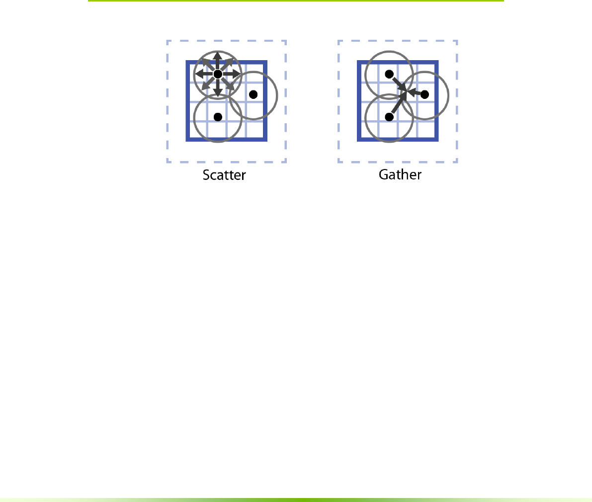
NVIDIA® GVDB Voxels - Programming Guide 61
Chapter 7.
Point Clouds &
Meshes
A useful operation is to voxelize a point cloud or a polygonal model to a sparse
volume. Voxelization (voxel rasterization) is the process of identifying all the
voxels touched by a set of points or polygons. GVDB Voxels supports both
point cloud and polygon voxelization with efficient GPU acceleration.
7.1. Point Cloud Voxelization
Figure 7.1. Point cloud voxelization may be performed as either a scatter, from
points to voxels, or as a gather from voxels to points.
Point cloud voxelization identifies or shades all the voxels touched by a set of
points within a given radius. The size of the problem depends on both the voxel
grid resolution and on the number of points. Two techniques for point
voxelization are shown in Figure 7.1. Point scattering begins with each points
and identifies all the neighboring voxels touched by it. Point gathering begins
with each voxel and finds all the neighboring points touched by it. Each method
has certain advantages and disadvantages while both are supported by GVDB
Voxels.
7.1.1. Defining Point Data
Points are defined using the Data access API by calling AllocData, getDataPtr
and CommitData.. See Chapter 9 for details. When loading point clouds from
disk, points typically reside in CPU memory first. They are transferred to GPU
with the CommitData function.

62 NVIDIA® GVDB Voxels - Programming Guide
// Allocate GPU and GPU memory
int numpnts;
DataPtr pntpos, pntclr;
gvdb.AllocData ( pntpos, numpnts, sizeof(Vector3DF), true);
gvdb.AllocData ( pntclr, numpnts, sizeof(uint), true );
// Get CPU pointers
Vector3DF* pos = (Vector3DF*) gvdb.getDataPtr( 0, pntpos );
uint* clr = (uint*) gvdb.getDataPtr( 0, pntclr );
// .. load points into CPU here ..
// Commit point data to GPU
gvdb.CommitData ( pntpos, m_numpnts, (char*) m_pntpos.cpu,
0, sizeof(Vector3DF) );
gvdb.CommitData ( pntclr, m_numpnts, (char*) m_pntclr.cpu,
0, sizeof(uint) );
AllocData has the following arguments:
AllocData ( DataPtr, int count, int stride, bool bAlsoCPU );
The last argument to AllocData indicates that we want point buffers to reside on
both the CPU and GPU. For point voxelization the point data must be loaded
into separate buffers for position and color, where the stride of the point
locations is Vector3DF and the stride of the point color is uint (RGBA).
Since the data must reside on the GPU for point voxelization we call
CommitData to perform the transfer.
The last step in defining point clouds for GVDB Voxels is to inform GVDB
which data buffers will be used for subsequence voxelization steps.
SetPoints ( DataPtr pos, DataPtr clr );
SetPoints takes two DataPtr buffers as input: point positions and colors. The
number of points is defined during AllocData or reallocation. The DataPtrs
contain all the information necessary for voxelization.
Direct-from-GPU Data
In many cases, such as during a simulation, the point cloud data may already
reside on the GPU. In this case we want to avoid the bidirectional GPU-CPU
transfer since CPU buffers are not needed.
GVDB Voxels supports user-defined data buffers where the DataPtr becomes a
handle rather than an owner of the point data. The functions SetDataCPU and
SetDataGPU are used to initialize a DataPtr with an explicit source.
SetDataCPU ( DataPtr, int count, char* cpuptr, int offset, int
stride );
SetDataGPU ( DataPtr, int count, CUdeviceptr gpu, offset,
stride );
Notice that SetDataCPU takes a CPU pointer, and SetDataGPU takes a GPU
pointer for the source data. The returned DataPtr is a handle, and points to the
original data which is still owned by the application.
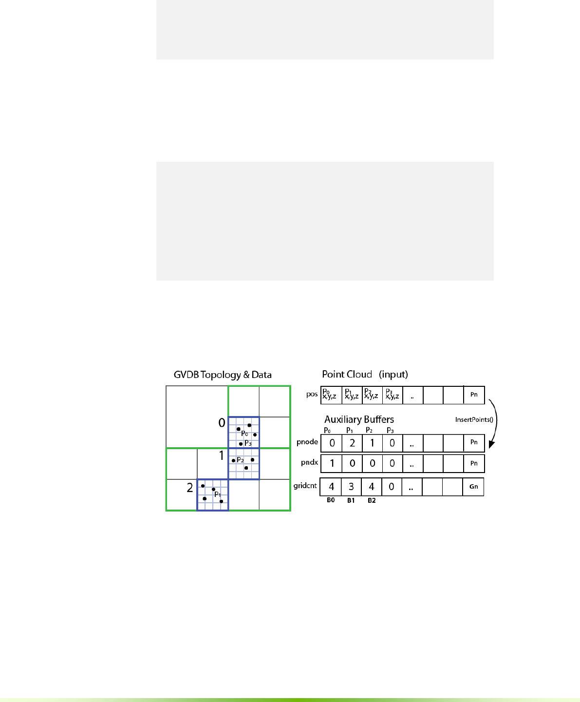
NVIDIA® GVDB Voxels - Programming Guide 63
DataPtr pntpos, pntclr;
gvdb.SetDataGPU ( pntpos, numpnts, my_gpu_points,
0, sizeof(Vector3DF) );
gvdb.SetDataGPU ( pntclr, numpnts, my_gpu_colors,
0, sizeof(uint) );
In this example two separate, existing GPU pointers are given from the
application as input for the point positions and colors. The stride of each is the
size of a single element in the array.
The offset argument is useful when the application point data resides in
structures rather than separate arrays:
struct TPnt {
Vector3DF pos;
Vector3DF velocity;
uint clr;
} MyPnt;
DataPtr pntpos, pntclr;
gvdb.SetDataGPU ( pntpos, numpnts, my_gpu_points,
0, sizeof(MyPnt) );
gvdb.SetDataGPU ( pntclr, numpnts, my_gpu_colors,
24, sizeof(MyPnt) );
Here the offset is used to indicate where in the structure the position and color
values reside. The stride of each is the size of the entire structure.
7.1.2. Point Insertion
Figure 7.2. Pre-processing point clouds for efficient voxelization with point
insertion. Auxiliary buffers are used to improve performance.
Efficient parallel voxelization is possible when the points are pre-sorted into
GVDB bricks. This pre-processing step is performed by InsertPoints(). The
details of InsertPoints can be seen in Figure 7.2. Each point is assigned to a brick
(pnode), and its index within the brick is recorded (pndx). With this
information, it is possible to count the total points-per-brick (gricnt) and
optionally the grid offsets (as a prefix scan). The technique is fully described in
the GTC 2014 talk "Fast Fixed-Radius Nearest Neighbors" [Hoetzlein 2014].
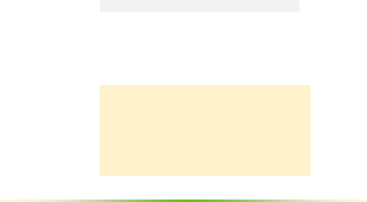
64 NVIDIA® GVDB Voxels - Programming Guide
An application performs point insertion by simply called InsertPoints.
InsertPoints ( int count, Vector3DF translate, bool prefix );
It is necessary to call this function before an point voxelization and is often the
first step in other operations using point clouds.
- count Indiates the number of points to insert
- translate A world translation factor applied to all points.
This is useful, when needed, to ensure that the points
all reside in the positive domain.
- prefix A boolean indicating whether a brick prefix scan should
be performed. This is required for some point cloud
operations.
7.1.3. Point Scatter and Gather
Scatter Voxelization
The scattering method for point voxelization is accomplished with the function:
ScatterPointDensity ( int count, float radius, float amp, Vector3DF
translate,
bool expand, bool averageColor );
ScatterPointDensity uses the scattering method for voxelization. With this
method points are not able to identify target voxels across brick boundaries, but
can write to apron voxels, therefore the maximum radius supported by
ScatterPointDensity is 3.0. Larger values are also possible but may introduce
boundary clipping.
gvdb.InsertPoints ( numpnts, translate, false );
gvdb.ScatterPointDensity ( numpnts, 3.0, 1.0, translate );
The 'false' argument in InsertPoints indicates that no prefix scan is needed
before calling ScatterPointDensity. The 'amp' sets the peak value written to a
voxel which is centered on a point, with linear falloff. ScatterPointDensity
typically writes to the primary channel, but will also write to a color channel
when the SetColorChannel function (to indicate which channel will hold per-
voxel color output attributes), and when gvdb.SetPoints indicates both position
and color data (which holds the input per-point color attributes).
Limitation:
ScatterPointDensity is a suitable technique when the support
radius is small. For radii above 2 voxels, the parallel scatter method
implies that many points will attempt to write to the same voxel.
Since this operation is not atomic on 3D textures some writes may
be skipped. ScatterPointDensity should not be used when the
accumulated values must be an exact sum. This method is best
suited for fast, point cloud pre-visualization. Often a smoothing
step is performed afterward for hole filling.
pported by GVDB Voxel raytracing with OptiX. The only voxel
attribute read is the primary channel (#0) for density. Color is
achieved via surface materials and transfer functions.

NVIDIA® GVDB Voxels - Programming Guide 65
Gather Voxelization
The gathering method of point voxelization is accomplished with:
GatherPointDensity ( int count, float raidus, int channel );
GatherPointDensity is used to perform point voxelization with larger radii, and
to compute exact sums at voxel locations. For example, this method is ideal for
FLIP-type fluid simulations where point density must be projected onto a sparse
voxel grid. Unlike ScatterPointDensity, this technique does require a prefix scan
during insertion.
gvdb.InsertPoints ( numpnts, translate, true );
gvdb.GatherPointDensity ( numpnts, 5.0, 0 );
Figure 7.3. Examples of the scatter (left) and gather (right) techniques for point
cloud voxelization from the gFluidSurface sample.
An example of scatter and gather point voxelization can be found in
the gFluidSurface sample, which performs an SPH (Smoothed Particle
Hydrodynamics) particle simulation and then voxelizes the points to create a
rendered surface.
Limitation:
GatherPointDensity is still experimental in GVDB SDK release 1.0,
with improvements expected into future releases.

66 NVIDIA® GVDB Voxels - Programming Guide
7.2. Mesh Voxelization
GVDB Voxels introduces a novel technique for efficient, hieararchical solid
mesh voxelization to determine the voxels touched by a triangle mesh. The
output for each voxel may be one of three values: inside, outside, or surface.
Surface voxelization sets all the voxels which intersect a polygonal mesh, thus
creating a voxel surface with an empty interior. Solid voxelization fills the
interior voxels of a watertight polygonal mesh. The SolidVoxelize() function of
GVDB Voxels generates both results at the same time.
The technique used for mesh voxelization was designed with several
goals and features:
- Interior & Surface Voxelizes both the surface and interior voxels
simultaneously
- Exact Result Solid voxelization in GVDB is exact. Unlike graphics
raster methods which may produce a voxelization
with holes, or might be overly conservative, this
technique generates the exact set of voxels which are
touched by any part of a triangle.
- Out-of-Core Sweep-based methods of mesh voxelization depend
on the results of neighboring bricks. The technique in
GVDB Voxels is out-of-core friendly, where the
results of any sub-volume in space can be
computed independently.
- Hierarchical For performance the voxelization is hierarchical.
Empty space will not be voxelized at the brick level.
- GPU Efficient Mesh voxelization should be efficient for
large models and high resolution volumes.
This is achieved with GPU polygon binning and sort.
Polygonal voxelization is performed with the function:
SolidVoxelize( chan, Model*, Matrix4F xform, surface_value
,inside_value );
The arguments are:
- channel This must be a UCHAR channel which will
receive the results of voxelization.
- Model* A pointer to the polygonal model, typically loaded
using scene.AddModel().
- xform A transformation applied to the model. This allows
for arbitrary scaling and orientation of the model
with respect to the voxel grid.
- surface_val Value to be set in the channel when the voxel
is a surface voxel (any part touches a polygon).
- inside_val Value to be set in the channel when the voxel
is an interior voxel (fully inside the watertight mesh).
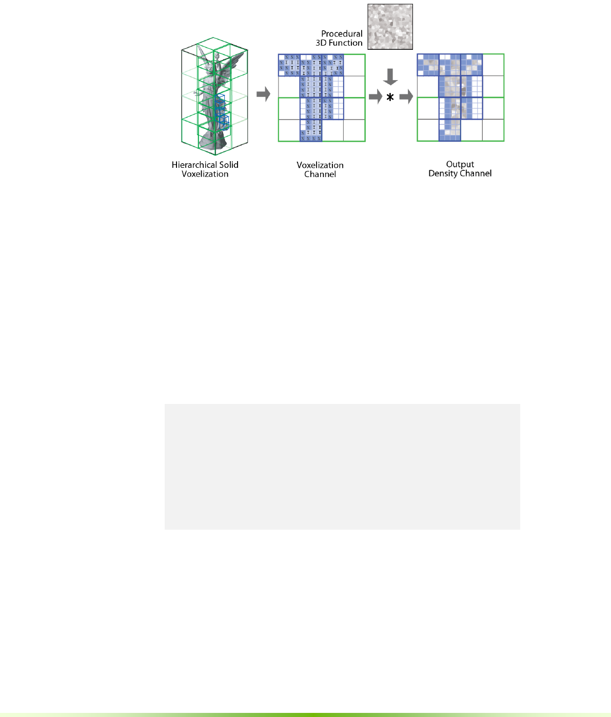
NVIDIA® GVDB Voxels - Programming Guide 67
7.2.1. Voxelization Channel
Figure 7.4. Solid voxelization writes to a voxelization channel to give the most
flexibility to applications. Surface voxels are tagged ('S') separately from interior
voxels ('I'). In this example, multiplying the voxelization channel by a 3D
procedural function results in an 3D sparse voxel model with a procedurally
defined interior density defined.
The output of solid voxelization is written to a voxelization channel which
must be added as a UCHAR channel. Rather than writing density directly, this
design gives applications the greatest flexibility in utilizing the result. The
voxelization channel may be manipulated directly, or it can be multiplied by
other 3D volumes to produce density which is only defined on the interior of a
mesh. An example is the generation of complex in-filling for 3D printing where
the model has a solid surface with a custom interior (see Figure 7.4). Typically,
applications will write custom compute kernels that take advantage of the
voxelization channel to produce additional results.
gvdb.Configure ( 3, 3, 3, 3, 5 );
gvdb.AddChannel ( 0, T_FLOAT, 1 ); // density
gvdb.AddChannel ( 1, T_UCHAR, 1 ); // mesh voxelization
// Solid Voxelize
Matrix4F xform;
Model* m = gvdb.getScene()->getModel(0);
gvdb.SolidVoxelize ( 1, m, &xform, 1, 128 );
// Expand surface border by 1 voxel
gvdb.Compute ( FUNC_EXPANDC, 1, 1,
Vector3DF(1, 255, 0), true );
This code example has two channels, density and the mesh voxelization result.
The SolidVoxelize function indicates that surface voxels should be 1, and
interior voxels have the value 128. The native operation FUNC_EXPANDC is
called using the Compute API to perform a voxel expansion (grow outward) by
one voxel. This function takes two parameters, which are the existing value ('1'),
and the expanded voxel value ('255'). Since the value 1 represents surface voxels,
the result is an extra layer of voxels surrounding the surface of the model that
will have the new value '255'.
Another use of the voxelization channel is to cache results using
Load/SaveVBX to store channels independently.
68 NVIDIA® GVDB Voxels - Programming Guide
7.2.2. Implementation
Figure 7.5. Algorithm used by SolidVoxelize. Triangles are sorted and inserted
into stacked XY bins along the Z-axis. A thread-per-voxel kernel is launched
over all sparse voxels which then examine the bins to test a subset of triangles.
The implementation details of solid voxelization are given here for reference.
The steps in the algorithm are:
1) Triangle sorting - Triangles in the input mesh are sorted and inserted into
horizontal bins that are stacked along the Z-axis. Any triangle that crosses a bin
is inserted into both of them. Auxiliary buffers are used to maintain the sorted
triangles.
2) Hierarchical activation - Voxelization is performed hierarchically with upper
nodes of the VDB tree processed first. This produces a solid/interior result that
indicates which children nodes should be activated. Nodes are processed at each
level (breadth first) until all relevant voxel bricks have been identified.
3) Per-Voxel computation - A primary voxelization kernel is launched over all
sparse voxels in the data atlas. This avoids processing voxels in empty space.
Each voxel first checks if it is a surface voxel with the Schwarz-Seidel test or the
Akenine-Moller test. These are exact tests to determine if a polygon touches a
voxel. If the test fails, the voxel performs an Inside-Outside test to determine if
it is an interior voxel. The resulting value is placed into the output channel.
To accelerate voxel testing only the polygons in the sorted bin corresponding to
a given brick are checked. The parity test requires that all polygons along a ray
extending from the voxel are included in its odd-even count, which is met since
bins contain triangles that cross multiple bins but avoid those which are
completely outside.
Since all tests are performed on the original polygonal data the result is an exact
voxelization which is locally complete. This permits the same voxelization
algorithm to be applied to different levels of the VDB hierarchy, or to additional
bricks anywhere in space which may be stored on disk incrementally.

NVIDIA® GVDB Voxels - Programming Guide 69
Chapter 8.
Dynamic
Topology
There are many scenarios in which a 3D volume varies over time. Simulations
performed on sparse grids will activate new space as the fluid or smoke
advances. Medical and scientific data might consist of a 3D volumetric time
series, in which case the active space could vary from frame-to-frame. Dynamic
topology refers to any application where the activate space changes over time,
which requires that the GVDB topology updates.
Currently, dynamic topology in GVDB SDK release 1.0 is implemented
on CPU only. Since the GVDB uses indexing, and the topology typically has a
low footprint (<10 MB), transferring to new topology to the GPU is quick and
efficient.
8.1. Overview
The dynamic topology API is separated into phases to improve application
design and performance. The sequence of stages as typically appear in an
application are as follows:
1. Topology rebuilding Updating a topology without affecting
the data atlases
1a. Clear Clear the entire topology (optional)
1b. AcitvateSpace Activate new space to be covered
1c. FinishTopology Finalize topology changes prior to
updating the atlas.
2. Atlas rebuilding Updating the data atlases
without affecting topology
2a. UpdateAtlas Allocate additiona bricks if needed
2b. ClearAtlas Clear all voxel data (optional)
The concept of activating space is a request to GVDB Voxels to generate the
covering nodes of a point in space from the root down to the brick. After
activating space additional leaf nodes are guaranteed to cover the requested
points. However, prior to atlas rebuilding these nodes specify bricks which do
not yet exist in the data atlas. This intermediate leaf node state allows changes to
the GVDB topology to be completed prior to any changes in voxel allocation.
Once the atlas update is performed, any new leaf nodes will be allocated a new
place in the data atlas. Thus the topology stage guarantees that new world space
is covered (but without voxel data), and the atlas stage guarantees that new voxel
data is allocated for covering nodes.

70 NVIDIA® GVDB Voxels - Programming Guide
8.2. Topology Building
8.2.1. Activate Space
To change the VDB topology, the ActivateSpace function is called with a 3D
world position to be covered (by a brick).
ActivateSpace ( Vector3DF pos );
In SDK release 1.0 this is a CPU-only function, and should be called repeatedly
to activate space over multiple points. Future releases may introduce a GPU
version that activates a list of points simultaneously.
An example of activating space can be found in the gFluidSurface sample,
where a set of points moves over time based on an SPH simulation. As the
points move, the VDB topology must dynamically reconfigure to cover them.
On each frame, the VDB grid is cleared and reconfigured with ActivateSpace.
ActivateSpace will generate new interior and leaf nodes, and may create a new
root or increased the tree depth if needed to cover the point(s). Space can be
covered out to the maximum addressable extents of the volume (see Chapter
2.1.2).
Although the input to ActivateSpace is a point, this does not imply that only
point clouds can activate space. When performing a grid-based fluid simulation
new space might be activated as fluid voxels advect to touch brick boundaries.
An application could detect when a boundry is touched by examining changes in
apron voxels and recording neighboring inactive bricks. These bricks indicate
3D positions which can be activated by calling ActivateSpace with any point
inside the brick space.
8.2.2. Finish Topology
Finish topology should be called after all new space has been activated.
FinishToplogy ();
This function performs a few important tasks for topology maintainence.
These are:
- Recompute bounding box The bounding box of the GVDB Volume
is recomputed from the new topology.
- Commit topology to GPU The new topology is transferred to the GPU
for access by other tasks.
- Update request Internally, a flag is set indicating that
new VDB data is available during compute
and rendering.
Notice that FinishTopology does not modify the data atlas, which remains in its
previous state. At this point some leaf nodes (level 0) may indicate new bricks
that are not yet allocated. These nodes will have a mValue attribute of -1, which
is a request to allocate new voxel data.

NVIDIA® GVDB Voxels - Programming Guide 71
8.3. Atlas Rebuild
8.3.1. Update Atlas
Once the topology has been updated, atlas rebuild will allocate new voxels in
the data atlas. Two versions of UpdateAtlas are provided, one which updates a
specific channel, and another which updates all channels.
UpdateAtlas();
UpdateAtlas( channel );
Typically all channels must be updated since GVDB does not track bricks
separately by channel.
UpdateAtlas performs several steps to ensure that new voxels are allocated to all
leaf nodes in the space:
- Resize atlas All data atlases are dynamically resized to
accommodate new leaf nodes. This resize step
preserves previous data by expanding the atlas
along the Z-axis. See chapter 2.1.3 for details.
- Assign bricks New nodes are assigned to bricks in the atlas.
Whereas a node is an abstract entity covering space,
a brick contains the voxel data.
- Atlas map update The atlas map is used internally in GVDB to
provide reverse mapping from atlas-space to
world-space. This data structure is updated on GPU.
- Commit to GPU The new topology, with assigned brick values,
are sent to GPU. In addition, the atlas accessors
volIn/volOut are update to give kernels access
to the data atlases in case their location in memory
has changed.
Following UpdateAtlas all leaf nodes covering a space must have a valid mValue
referring to a brick location in the atlas, since GVDB Voxels release 1.0 does not
yet support non-resident (out-of-core) bricks.
8.3.2. Clear Channels
During each frame it may be necessary to clear previous voxel data. This should
be done after UpdateAtlas has reallocated bricks. To clear a specific channel use
the function FillChannel;
FillChannel ( uchar channel, Vector4DF value );
The value is a Vector4F to cover all possible channel types. Single component
channels (T_FLOAT, T_UCHAR) will read value.x. Multi-component
channels (T_FLOAT4, T_UCHAR4) will use all components of value.

72 NVIDIA® GVDB Voxels - Programming Guide
To clear voxel data in all channels, one calls ClearAtlas ();
ClearAtlas ();
8.3.3. Rebuilding Channels
GVDB Voxels allows applications to destroy and rebuild voxel attribute
channels at run-time. The function DestroyChannels removes all channels
from memory and their associated atlases. Afterward, the application should
rebuild the channels with AddChannel.
DestroyChannels should be called infrequently, since it incurs the overhead of
tearing down and rebuilding all atlases. The only time to rebuild channels is
when per-voxel attributes must be added or removed.
In a dynamic simulation the voxel attributes are typically fixed ahead of time -
e.g. position, velocity, density. Thus changes in topology can be achieved with
topology and atlas updates without adding, removing or destroying channels.
This will be more efficient since GVDB will dynamically reallocate atlases to
preserve prior data.
8.4. Limitations
Dynamic topology has several limitations in GVDB SDK release 1.0 which may
be addressed in future releases. These are:
1. CPU only ActivateSpace is currently CPU-only. However,
transfer of the new topology to GPU is efficient.
2. Full residence All leaf nodes must be resident in data atlases
following UpdateAtlas. This limitation may be
removed in the future to allow for non-resident bricks
and out-of-core techniques.
3. DeactivateSpace Deletion of bricks, or removal of space, is not yet
supported. Currently applications may need to clear
and reactivate all points. (See gFluidSurface example)
4. DeleteChannel Deletion of channels at run-time is not yet
supported. Applications can call DestroyChannels to
remove all channels and rebuild the with AddChannel.

NVIDIA® GVDB Voxels - Programming Guide 73
Chapter 9.
Data
Management
Data management is a generic API for handling CPU and GPU data provided to
GVDB Voxels. Data may be used for point clouds (Chapter 7.1), triangle
meshes (Chapter 7.2), rays (Chapter 6.5) or other entities that are inputs or
outputs to GVDB. These functions implement smart points for memory
management.
9.1. Allocation
Generic data is allocated on the GPU, and optionally on CPU, with AllocData.
AllocData ( DataPtr ptr, int count, int stride, bool onCPU );
The arguments are:
- DataPtr The DataPtr handle that will be setup by this call.
- count The number of elements to pre-allocate
- stride The stride of each element. Typically sizeof(some struct)
- onCPU A boolean indicating if CPU memory should also be allocated.
AllocData always allocates GPU linear memory.
When making repeated calls to AllocData with the same DataPtr object, any
memory previously associated with either the CPU or the GPU are freed before
new memory is allocated. The resulting DataPtr records the stride, count and
CPU and GPU pointers for the requested memory.
9.2. Data Transfers
Data is transferred to/from the GPU with RetrieveData and CommitData.
RetrieveData ( DataPtr ptr );
RetrieveData transfers data from the GPU to the CPU for the given DataPtr.
Note this implies that the DataPtr must have been allocated with onCPU true.
The total amount of memory transferred is count*stride.
CommitData ( DataPtr ptr );
CommitData transfers data from the CPU to the GPU for the given DataPtr.
Note this implies that the DataPtr must have been allocated with onCPU true,
and the CPU data is owned by this DataPtr.

74 NVIDIA® GVDB Voxels - Programming Guide
CommitData ( DataPtr ptr, cnt, cpu_ptr, offs, stride)
An alterate version of CommitData transfers arbitrary CPU data to GPU.
The target GPU memory is given by the DataPtr.
The source CPU memory is given by the CPU pointer argument. The caller
must specify the count, starting offset, and stride of the source memory.
This function does not require the DataPtr has been allocated with onCPU true.
9.3. Data Handles
The typical usage of data management is to create DataPtr objects by
calling AllocData with the number and stride of new elements to allocate. In
this case, the DataPtr owns the data which is allocated.
DataPtr structs can also be used as data handles. In this usage, a DataPtr
represents a handle, or reference, to memory which is allocated and owned by
the application itself. The purpose of data handles is to provide GVDB Voxels
with lists of points, rays or triangles that are managed by the application.
DataPtr handles are created using SetDataCPU and SetDataGPU.
SetDataCPU ( DataPtr, int count, char* cpuptr, int offset, int
stride );
SetDataGPU ( DataPtr, int count, CUdeviceptr gpu, offset,
stride );
The given DataPtr should not be previously used for anything else.
Notice that SetDataCPU takes a CPU pointer, and SetDataGPU takes a GPU
pointer for the source data. The returned DataPtr references (points to) the
original data which is still owned by the application.
For flexibility, data handles support application data which is given either as a
structure-of-arrays or as an array-of-structures.
Structure-of-Arrays
Vector3DF* pos; // list of positions
Vector3DF* vel; // list of velocities
uint* clr; // list of colors
LoadData ( pos, vel, clr ); // application allocated
DataPtr p1, p2, p3; // new handles
gvdb.SetDataCPU ( p1, num, pos, 0, sizeof(Vector3DF) );
gvdb.SetDataCPU ( p2, num, vel, 0, sizeof(Vector3DF) );
gvdb.SetDataCPU ( p3, num, clr, 0, sizeof(uint) );
When using DataPtr handles for a structure-of-arrays, the offsets are typically all
zero, and the strides match the stride of each individual input array.
Notice that no data is allocated or freed. Also, since the DataPtr was not created
with AllocData, there is no GPU pointer. The primary use of data handles is to
present the data to GVDB Voxels function.

NVIDIA® GVDB Voxels - Programming Guide 75
Array-of-Structures
An array-of-structures is a list of elements with attributes located together and
grouped by a structure.
struct Pnt {
Vector3DF* pos; // position
Vector3DF* vel; // velocity
uint* clr; // color
}
Pnt* pnts; // list of points
LoadData ( pnts ); // application allocated
DataPtr p1, p2, p3; // new handles
gvdb.SetDataCPU ( p1, num, pnts, 0, sizeof(Pnt) );
gvdb.SetDataCPU ( p2, num, pnts, 12, sizeof(Pnt) );
gvdb.SetDataCPU ( p3, num, pnts, 24, sizeof(Pnt) );
When making DataPtr handles from an array-of-structures, the offsets refer to
the starting byte of each variable, and the strides are all set to the width of the
containing structure.
GPU Handles
Applications that allocate their own GPU memory with CUDA functions
cuMemAlloc and cuMemFree can make data handles using SetDataGPU.
CUdeviceptr posGPU; // position data
CUdeviceptr velGPU; // velocity data
int num = 2000;
// application allocates GPU data
cuMemAlloc ( &pos, sizeof(Vector3DF)*num );
cuMemAlloc ( &vel, sizeof(Vector3DF)*num );
// application creates data
LoadData ( pos, vel );
DataPtr p1, p2, p3; // new handles
gvdb.SetDataGPU ( p1, num, posGPU, 0, sizeof(Vector3DF) );
gvdb.SetDataGPU ( p2, num, velGPU, 0, sizeof(Vector3DF) );
Remember that a data handle does not own the memory it refers to. Therefore
applications should not call AllocData, RetrieveData or CommitData on data
handles.
For an example usage of data handles, see Chapter 7.1.1 (Point Cloud
Voxelization).

76 NVIDIA® GVDB Voxels - Programming Guide
9.4. DataPtr Struct
The DataPtr struct is a smart handle to memory which resides on both
the GPU and CPU. Additionally, it contains members to keep track of the count
and maximum of a number of elements with a given stride. This makes it
suitable for managing simple data such as a fixed array of points or triangles.
A DataPtr is:
struct DataPtr {
char type; // Data type (T_UCHAR, T_FLOAT, etc)
char apron; // Apron size (Used by atlases)
uint64 num; // Number of elements
uint64 max; // Maximum element count
uint64 size; // Total amount of memory in bytes
uint64 stride; // Stride of the data
Vec3DI subdim; // Sub-dimensions of the data.
(Used by atlases)
Allocator* alloc; // Pointer to the Pool allocator which
owns this memory heap.
char* cpu; // CPU Pointer to data
int glid; // GPU OpenGL ID to data as 3D texture
CUgraphicsResource grsc; // GPU Graphics Resource (CUDA)
CUarray garray; // GPU CUarray (CUDA) to data on GPU
CUdeviceptr gpu; // GPU Linear memory (CUDA) pointer
}
The DataPtr is also used internally by GVDB Voxels to maintain both data
atlases and node memory pools, with member variables to handle CUDA
interop, OpenGL 3D textures, and to record atlas dimensions and type. Many
of these variables are not used when creating simple linear memory
with AllocData.
A DataPtr is a public struct, so applications that call AllocData can directly
access the CPU memory via data.cpu, or read/write the number of elements
with data.num. Care must be taken when directly modifying a DataPtr object.

NVIDIA® GVDB Voxels - Programming Guide 77
Chapter 10.
Host & Device
Access API
The Access API is a set of functions, on host and device, that allow an
application to query and traverse the GVDB Topology and Data. This API is
useful for authoring custom compute and custom render kernels.
10.1. Host Access
The Host access functions are:
* See gvdb_volume_gvdb.h for function arguments
getNearestAbsVox
Gets the nearest voxel in index-space
getLD
Gets the node log2dim for the given level
getRes
Gets the node resolution for the given level
getVoxCnt
Gets the total voxel count for a node at given level
getMaskSize
Gets the bitmask size, in bytes, for a node at level
getBitPos
Gets the bit position for a point in local index-space
for node at level
getPosFromBit
Gets the local index-space position from a bit
getCover
Gets the world-space covering size of
a node at the given level
getRange
Gets the index-space covering size of
a node at the given level
getRes3DI
Gets the resolution of a node as a Vec3I
getVolMin/Max
Gets the min/max bounding box of
the entire sparse volume
getTransferPtr
Gets the transfer function as a DataPtr
getTransferFuncGPU
Gets the transfer function as a CUDA CUdeviceptr
getScene
Gets the GVDB scene object
getNumNodes
Gets number of nodes at a given level
getNode
Gets a Node struct from a group, level and index
getNode ( nodeid)
Gets the Node struct from a node reference
getNodeAtlLevel
Gets the Node struct at a specific level and index
78 NVIDIA® GVDB Voxels - Programming Guide
isLeaf
Returns true if the node is at level=0
getChildNode
Gets the child node reference at the specific bit
position of the given parent node
getChildOffset
Gets the bit position of the given child node within
the given parent node
getPosInNode
Returns true if the index-space position is inside the
given node (and its bit), or false if outside
getVDBSize
Gets the size of the VDBInfo struct
getVDBInfo
Gets a pointer to the current VDBInfo struct
getWorldMin
Gets the world space bounding box min of the given
node
getWorldMax
Gets the world space bounding box max of the given
node
getVoxelSize
Gets the current global voxel size
10.2. Device Access
The Device access functions are:
* See cuda_gvdb_nodes.cuh for function arguments
numBitsOn
Counts the number of bits on in a 64-bit word
countOn
Counts the number of bits on in the given VDB
node up to bit 'n'
isBitOn
Returns true if child bit 'n' is set (active) in
the given VDB node
getAtlasNode (brickpos)
Gets a VDBAtlasNode* for the given
brick-space position
getAtlasNodeFromIndex
Gets a VDBAtlasNode* for the given brick ID
getAtlasToWorld
Gets the world-space position from the atlas-
space voxel. False if the atlas-space voxel is an
unused brick (invalid).
getAtlasToWorldID
Gets the same results as getAtlasToWorld, but
also gives the level-0 node ID for the point.
getChild
Gets the child index for the VDB node for the
given bit count 'b'
getAtlasPos
Gets the atlas-space bottom corner ('value') for
the given brick ID.
getBitPos
Gets the bit position for a point in local index-
space for node at level
getNode (lev, n, vmin)
Gets a Node at the given level and index. Also
returns the world-space position of the node.
getNodeAtPoint
Gets a brick Node covering the
given world-position. (recursive)
getTricubic
Gets a tricubic interpolated value for the given
local index-space in a node

NVIDIA® GVDB Voxels - Programming Guide 79
getTrilinear
Gets a trilinear interpolated atlas value for the
given local index-space in a node
getVolSampleC
Gets a uchar value for a T_UCHAR channel at
the given world position.
getVolSampleF
Gets a float value for a T_FLOAT channel at
the given world position.
getGradient
Gets the trilinear gradient at the given
atlas-space point
getGradientLevelSet
Gets a level set gradient at the given
local index-space point.
getGradientTricubic
Gets a tricubic gradient at the given
local index-space point.
rayTricubic
Casts a fine-stepping ray for a tricubic surface
inside the given node starting from the local point.
rayTrilinear
Casts a fine-stepping ray for a trilinear surface
inside the given node starting from the local point
rayLevelSet
Casts a fine-stepping ray for a level set surface
inside the given node starting from the local point
getColor
Gets a uchar4 value for a T_UCHAR4 color
channel at the given atlas-space point
getColorF
Gets a float4 value (by casting) for a T_UCHAR4
color channel at the given atlas-space point
getLinearDepth
Gets the linear depth from an OpenGL depth
buffer value

80 NVIDIA® GVDB Voxels - Programming Guide
Appendix A.
