Gascoigne3D Manual

Gascoigne3D_manual

Gascoigne3D_manual

User Manual:

Open the PDF directly: View PDF .
Page Count: 42

Introduction to

Gascoigne 3D

High Performance Adaptive Finite Element Toolkit

Tutorial and manuscript by Thomas Richter

thomas.richter@iwr.uni-heidelberg.de

March 9, 2014

2

Contents

1 Introduction 5

1.1 Installation ..................................... 5

1.2 A minimal example solving a partial differential equation . . . . . . . . . . . 7

2 The parameter file 13

3 Description of the problem 15

3.1 Therighthandside ................................ 15

3.2 BoundaryData................................... 16

3.2.1 Dirichlet boundary data . . . . . . . . . . . . . . . . . . . . . . . . . . 17

3.2.2 Neumann conditions . . . . . . . . . . . . . . . . . . . . . . . . . . . . 18

3.2.3 Robinconditions.............................. 19

3.3 Definition of the partial differential equations . . . . . . . . . . . . . . . . . . 19

3.3.1 Nonlinear equations . . . . . . . . . . . . . . . . . . . . . . . . . . . . 21

3.3.2 Equations on the boundary & Robin boundary data . . . . . . . . . . 22

3.4 Exact Solution and Evaluation of Errors . . . . . . . . . . . . . . . . . . . . . 23

3.5 Systems of partial differential equations . . . . . . . . . . . . . . . . . . . . . 24

3.5.1 Modification of the right hand side . . . . . . . . . . . . . . . . . . . . 24

3.5.2 Modification of Dirichlet data . . . . . . . . . . . . . . . . . . . . . . . 25

3.5.3 Modification for the equation, form and matrix . . . . . . . . . . . . . 25

4 Time dependent problems 27

4.1 Time discretization of the heat equation . . . . . . . . . . . . . . . . . . . . . 27

4.2 Time dependent problem data . . . . . . . . . . . . . . . . . . . . . . . . . . . 30

4.3 Non standard time-discretizations . . . . . . . . . . . . . . . . . . . . . . . . . 30

5 Mesh handling 33

5.1 Definition of coarse meshes . . . . . . . . . . . . . . . . . . . . . . . . . . . . 33

5.2 Curvedboundaries ................................. 35

5.3 Adaptive refinement of meshes . . . . . . . . . . . . . . . . . . . . . . . . . . 37

5.3.1 Estimating the Energy-Error . . . . . . . . . . . . . . . . . . . . . . . 37

5.3.2 Picking Nodes for Refinement . . . . . . . . . . . . . . . . . . . . . . . 38

6 Flow problems and stabilization 39

6.1 The function point ................................. 39

6.2 Stabilization of the Stokes system . . . . . . . . . . . . . . . . . . . . . . . . . 39

6.3 Stabilization of convective terms . . . . . . . . . . . . . . . . . . . . . . . . . 40

6.4 LPSStabilization.................................. 41

3

Contents

4

1 Introduction

When referring to files, the following directories are used:

HOME Your home directory

GAS The base-directory of Gascoigne. For the workshop:

GAS/src The source- and include-files of Gascoigne.

Gascoigne is a software-library written in C++. To solve a partial differential equation with

Gascoigne, a small program has to be written using the routines provided by Gascoigne. All

functionality is gathered in the library-file File: libGascoigneStd . This library is linked

to every application.

1.1 Installation

In this section we explain the usage of Gascoigne as a library for own applications.

Gascoigne requires a configuration file:

File: HOME/.gascoignerc

Here, some setting like “where is Gascoigne”, “where are the libraries” are given. The

minimal file looks like:

1#############################################

2SET(GASCOIGNE STD ” ˜/ Softw are / s r c / Ga sc oi gne ” )

3

4#############################################

5#Gascoigne L i b r a r i e s & B i n a ri es

6SET(GASCOIGNE LIBRARY OUTPUT PATH ” ˜/ So ftw are / x86 64 / l i b ” )

7SET(GASCOIGNE EXECUTABLE OUTPUT PATH ” . ” )

You need a file like this in the home directory. To build an application using Gascoigne at

least two files and directories are required:

File: TEST/bin/

File: TEST/src/main.cc

File: TEST/src/CMakeLists.txt

5

1 Introduction

The first directory will be used to store the executable file for this application. The other

two files are the source code of the application and a file to control the compilation of the

application. This could look like:

File: TEST/src/CMakeLists.txt

1INCLUDE($ENV{HOME}/ . g a s c o i g n e r c )

2

3INCLUDE( ${GASCOIGNE STD}/CMakeGlobal . tx t )

4LINK LIBRARIES( ${GASCOIGNE LIBS})

5

6ADD EXECUTABLE( ” Test ” main . cc )

In the first line, the user’s config file is read. The following two lines set global parame-

ters for Gascoigne. The variable GASCOIGNE STD is provided in the config-file, the variable

GASCOIGNE LIBS is given in the file CMakeGlobal.txt. The last line indicates the name of

the application: Test, and lists all code-files to be compiled into the application.

A minimal example for a code-file (it does not really calculate something) looks like this:

File: TEST/src/main.cc

1#include <iostream>

2#include ” s t d l o o p . h”

3

4int main ( int argc , char ∗∗ argv)

5{

6std : : cout << ” Create a Gascoigne Loop ! ” << std : : endl ;

7Gascoigne : : StdLoop Loop ;

8}

For building the application we use the program cmake to generate Makefiles. In the directory

TEST/bin/ type:

1cmake . . / s r c

2make

The first line creates the File: TEST/bin/Makefile . It reads the File: CMakeLists.txt

to put everything together. The second command starts the compilation and linking of the

application and if everything works out, File: TEST/bin/Test should be the executable

file which then can be started.

The command cmake is only needed to create new Makefiles. This is necessary, if new

code-files are added to the application. If only source code is changed, e.g. the file File:

TEST/src/main.cc , you only need to call make in the directory TEST/bin.

6

1.2 A minimal example solving a partial differential equation

1.2 A minimal example solving a partial differential equation

Assume there exists a directory FIRSTEXAMPLE with sub-dirs FIRSTEXAMPLE/bin and

FIRSTEXAMPLE/src. In the src-directory you need the files File: main.cc and File:

CMakeLists.txt . in the bin-directory you call cmake ../src for configuration and then

make for compilation.

File: FIRSTEXAMPLE/src/main.cc

1#include ” s t d l o o p . h”

2#include ” p r o b l e m d e s c r i p t o r b a s e . h”

3#include ”constantrighthandside .h”

4#include ”zerodirichletdata .h”

5#include ” l a p l a c e 2 d . h”

6

7using namespace Gascoigne ;

8

9class Problem : public ProblemDescriptorBase

10 {

11 public :

12 std : : s t r i n g GetName ( ) const {return ” F i r s t Problem” ; }

13 void BasicInit(const ParamFile∗p a r a m f i l e )

14 {

15 GetEquationPointer () = new Laplace2d ;

16 GetRightHandSidePointer ( ) = new OneRightHandSideData ( 1 ) ;

17 GetDirichletDataPointer () = new Z e r o D i r i c h l e t D a t a ;

18

19 ProblemDescriptorBase : : B a s i c I n i t ( p a ra mf i le ) ;

20 }

21 };

22

23 int main ( int argc , char ∗∗ argv )

24 {

25 ParamFile p a r a m f i l e ( ” f i r s t . param” ) ;

26 i f ( argc >1) p a r a m f i l e . SetName ( ar gv [ 1 ] ) ;

27

28 Problem PD;

29 PD. B a s i c I n i t (& pa ra mf i le ) ;

30

31 ProblemContainer PC;

32 PC. AddProblem ( ” l a p l a c e ” , &PD) ;

33

34 StdLoop l o op ;

35 lo op . B a s i c I n i t (& pa ramf i l e , &PC) ;

36 lo op . run ( ” l a p l a c e ” ) ;

37 }

7

1 Introduction

The Problem

Here, the problem to be solved is defined. The Problem gathers all information on the

problem to be solved. This is: which pde, what kind of boundary data, what is the right

hand side, and so on.

By PD.BasicInit() we initialize the problem (will be described later on). This problem is

then added to another class, the ProblemContainer. Here, we can gather different problems,

each together with a keyword, which is laplace in this case. There are applications where

it is necessary to solve different problems in the same program.

The problem set pointers to a large variety of classes. Here, we define the equation to be of

type Laplace2d, an implementation of the two dimensional Laplace equation. For right hand

side and Dirichlet data we define self written classes (will be explained later). In Gascoigne

a very large set of parameters can be set for a problem, all in form of pointers. However these

three classes, Equation,RightHandSide and DirichletData are necessary for every instance

of Gascoigne. The class Problem is derived from the base-class ProblemDescriptorBase:

File: GAS/src/Problem/problemdescriptorbase.h

The equation Laplace2d is part of the Gascoigne-Library:

File: GAS/src/Problem/laplace2d.h

This is explained in detail in Section 3.

The Loop

Then, a Loop is specified, the loop is the class controlling what is happening at run-time.

and what Gascoigne is doing: this is usually a sequence like: initialize, solve a pde, write

the solution to the disk, evaluate functionals, compute errors, refine the mesh and start over.

In BasicInit() we initialize the most basic structure and read data from parameter files.

Here we also pass the ProblemContainer to the different instances.

Finally, the equation is solved by calling loop.run("laplace"), where the keyword laplace

indicates what problem to solve. Let us now have a closer look at this function which is

defined in

File: FIRSTEXAMPLE/src/loop.cc

First, in run(), we define two vectors u,f for storing the solution and the right hand side.

Then, in the for-loop we initialize the problem, solve the problem, write out the solution and

refine the mesh. This is very typical for every program run, since for a reliable simulation it

is necessary to observe the convergence of the solution on a sequence of meshes. Next, we

have a closer look at every step of the inner loop:

8

1.2 A minimal example solving a partial differential equation

1G e tM u l ti L ev e l So l ve r ()−>ReInit(problemlabel );

2G e tM u l ti L ev e l So l ve r ()−>R eI n i tV e ct o r ( u ) ;

3G e tM u l ti L ev e l So l ve r ()−>Re I n i t V ector ( f ) ;

4

5GetSolverInfos()−>GetNLInfo ( ) . c o n t r o l ( ) . mat rixm ustb ebui ld ( ) = 1 ;

The first line initializes the basic ingredients of Gascoigne. In particular, we pass the equa-

tion to be solved and all the necessary data to different parts like “Solver”, “Discretization”.

Then, by GetMultiLevelSolver()->ReInitVector(u) we initialize the vector on the cur-

rent mesh. This basically means that we resize the vector to match the number of degrees

of freedom (which changes with the mesh-size).

Finally, in the last line we tell Gascoigne to assemble the system matrix. This is necessary

whenever the system matrix changes, which is the case if the mesh changes, or if the matrix

depends on the solution uitself.

File: Template1/src/loop.cc

1S o lv e ( u , f , ” R e s u l t s /u” ) ;

2GetMeshAgent()−>global refine ();

By calling Solve(u,f) we solve the PDE. The subsequent line refines the mesh.

File: Template1/src/loop.cc

1s t r i n g Loop : : S ol ve ( V e c t o r I n t e r f a c e& u , V e c t o r I n t e r f a c e& f , s t r i n g

2name)

3{

4G e tM u l ti L ev e l So l ve r ()−>GetS olver ()−>Zero ( f ) ;

5G e tM u l ti L ev e l So l ve r ()−>GetS olver ()−>Rhs ( f ) ;

6

7G e tM u l ti L ev e l So l ve r ()−>GetS olver ()−>SetBoundaryVector( f );

8G e tM u l ti L ev e l So l ve r ()−>GetS olver ()−>SetBoundaryVector(u);

9

10 s t r i n g s t a t us = G et MultiLeve lS olver ()−>

11 S ol v e ( u , f , G e t S o l v e r I n f o s ()−>GetNLInfo ( ) ) ;

12

13 Output ( u , name ) ;

14 }

Here, we first assemble the right hand side fof our problem. Then, we need to initialize

Dirichlet boundary values. Finally, we tell the multigrid solver to solve the equation.

In the last line, we write the solution into a file for visualization.

9

1 Introduction

Output of Gascoigne

After starting the code, Gascoigne first prints out some information on the current mesh,

solver, Discretization and problem data.

Then, for every iteration of the inner loop the output looks like:

...

================== 2 ================ [l,n,c] 5 1089 1024

0: 9.77e-04

M 1: 7.73e-09 [0.00 0.00] - 6.26e-08 [0.012] {3}

[u.00002.vtk]

...

In the first line the current iteration count (2) , the number of mesh-refinemenet levels (5),

the number of mesh nodes (1089) and the number of mesh elements (quads) (1024) is given.

Then, Gascoigne prints control and stastic data for the solution of the algebraic systems.

Gascoigne solves every equation with a Newton-method, even linear ones. This is for reasons

of simplicity as well as having a defect correction method for a better treatment of roundoff

errors. On the left side of the output the convergence history of the newton method is

printed. Here we only need one Newton step. Before this step, the residual of the equation

was 9.77e−4, after this one step the residual was reduced to 7.73e−9. The letter Mindicates

that Gascoigne assembled a new system matrix in this step. The folling two numbers [0.00

0.00] indicate the convergance rates of the newton iteration by printing the factor, by which

the residual was reduced. We only print the first 2 digits, hence Gascoigne gives a 0. The

first number is the reduction rate in the current step, the second number is the average

reduction rate over all Newton steps.

On the right side, the convergence history of the linear multigrid solver is printed. Here,

the values indicate that in newton step 1 we needed {3}iteration of the multigrid solver. In

every of these three steps the error was reduced by a factor of [0.012] and after these three

steps the residual had the value 6.26e-08.

Finally Gascoigne prints the name of the output file. You can visualize it by calling

visusimple u.00002.vtk in the terminal window.

The parameter file

In this directory you can also specify the parameter-file

File: FIRSTEXAMPLE/src/first.param

1// Block Loop

2niter 5

3

4// Block Mesh

5dimension 2

10

1.2 A minimal example solving a partial differential equation

6gridname sq uare . inp

7prerefine 3

8

9// Block BoundaryManager

10 d i r i c h l e t 4 1 2 3 4

11

12 d i r i c h l e t c o m p 1 1 0

13 d i r i c h l e t c o m p 2 1 0

14 d i r i c h l e t c o m p 3 1 0

15 d i r i c h l e t c o m p 4 1 0

16

17 // Block Nix

This minimal example tells Gascoigne the dimension of the problem, which domain to use,

where to apply boundary data.

When starting the program, Gascoigne reads in a parameter file. Here, different parameters

controlling the behaviour of the code can be supplied. For instance in //Block Loop of this

file you can change the values of niter, which tells, how many times Gascoigne solves the

equation and refine the mesh.

In //Block Mesh we supply the mesh file as well as the number of refinement steps realized

before solving the first problem. You can change this parameter in prerefine. Thoe //Block

BoundaryManager will be explained in detail in Section 3.2

11

1 Introduction

12

2 The parameter file

Gascoigne can process a parameter file during runtime. Here, we can set some parameters

and options that can be changed at run-time without need for recompilation of the program.

For the file to be processed, go to the directory containing the parameter file and call

1. . / bin / Test t e s t . param

The data in the param-file is organized in blocks which are read at different points of the

code. A sample parameter file could look like: File: TEST/src/test.param

1// Block S e t t i n g s

2month 10

3year 2009

4name FirstTestOfGascoigne

5

6// Bl ock S o l v e r

7. . .

8

9// Block Nix

Each block has to be initialized by the line

1// Block <blockname>

Note that the slashes in front of the blocks are not treated as a comment here. The parameter

file has to end with a dummy-block, e.g. //Block Nix.

In Gascoigne, the parameter file is stored in the class ParamFile. Reading values from

the parameter-file is done using the classes FileScanner and DataFormatHandler. These

classes are declared in the header File: filescanner.h . Here is a modified File: main.cc

reading values from the parameter file:

File: TEST/src/main.cc

1#include <iostream>

2#include ” s t d l o o p . h”

3#include ” f i l e s c a n n e r . h”

4#include ” p a r a m f i l e . h”

5

6using namespace Gascoigne ;

7using namespace st d ;

8

13

2 The parameter file

9int main ( int argc , char ∗∗ argv)

10 {

11 i f ( argc <2)

12 {c e r r << ” c a l l : T est p a r a m f i l e ! ! ” << end l ;

13 ab ort ( ) ; }

14 ParamFile p a r a m f i l e ;

15 p a r a m f i l e . SetName ( a rgv [ 1 ] ) ;

16

17 int month , year ;

18 s t r i n g name ;

19 DataFormatHandler DFH;

20 DFH. i n s e r t ( ”month” ,&month ) ;

21 DFH. i n s e r t ( ” yea r ” , &year , 2009 ) ;

22 DFH. i n s e r t ( ”name” ,&name , ” t e s t ” ) ;

23 F i l e S c a n n e r FS(DFH, &p a r a m f i le , ” S e t t i n g s ” ) ;

24 cout << month << ”/” << year << ”\t ” << name << end l ;

25 }

To read in one block, we first initialize a DataFormatHandler (line 19). Next, we tell the

DataFormatHandler which keywords to look for using the function insert. The first ar-

gument of the insert function is the keyword we are searching, the second argument the

variable that its value will be written to. Optionally, we can specify a default value as a

third argument which is used if the keyword is not present in the parameter file. Finally, we

initialize an object FileScanner passing the DataFormatHandler, a parameter file and the

block to be read. Note that only this block is read! To read from a different block within

one file, we have to define a second DataFormatHandler.

14

3 Description of the problem

File: GAS/src/Problem/problemdescriptorbase.h

The class ProblemDescriptor provides all information necessary to set up an application.

This includes all problem data like: equation, boundary data, right hand side, initial con-

dition, etc. The most important function is ProblemDescriptor::BasicInit(), where the

problem is defined by setting pointers to the describing classes. A minimal example might

be:

1void Lo calPr oblem Desc ripto r : : B a s i c I n i t ( const ParamFile∗pf )

2{

3GetEquationPointer () = new LocalEquation ;

4GetRightHandSidePointer ( ) = new LocalRightHandSide ;

5GetDirichletDataPointer () = new LocalDirichletData ;

6

7ProblemDescriptorBase : : B a s i c I n i t ( pf ) ;

8}

For an problem to be well defined, at least the equation and the Dirichlet data have to be

specified. All possible pointers to be set are listed in

File: GAS/src/Problem/problemdescriptorbase.h

For the most basic problems Gascoigne provides predefined classes, e.g.

1GetEquationPointer () = new Laplace2d ;

2GetRightHandSidePointer ( ) = new OneRightHanSideData ( 1 ) ;

3GetDirichletDataPointer () = new Z e r o D i r i c h l e t D a t a ;

which defines the Laplace problem with homogeneous Dirichlet data and constant right-hand

side f= 1.

In the following we describe the classes needed to specify the most common ingredients of a

problem.

3.1 The right hand side

File: GAS/src/Interface/domainrighthandside.h

The interface class to specify a function f: Ω →Ras right hand side for the problem is

DomainRightHandSide. Let f(x, y) = sin(x) cos(y) be the right hand side:

15

3 Description of the problem

1class LocalRightHandSide : public DomainRightHandSide

2{

3public :

4int GetNcomp ( ) const {return 1 ; }

5

6std : : s t r i n g GetName ( ) const {return ” Lo cal Right Hand Side ” ; }

7

8double operator ( ) ( in t c , const Vertex2d& v ) const

9{

10 return s i n ( v . x ( ) ) ∗c os ( v . y ( ) ) ;

11 }

12 }

The most important function of this class is double operator()(int c, const Vertex2d&

v) const, here, the value of the right hand side function fat point v∈Ω is returned. The

class Vertex2d is explained in File: GAS/src/Common/vertex.h . For three dimensional

problems the operator double operator()(int c, const Vertex3d& v) const has to be

written.

The second parameter int c as well as the function int GetNcomp() const is only needed

if we solve a system of equations. This is explained in detail in Section 3.5.

A function called GetName() is necessary in every class used in the ProblemDescriptor to

provide a label.

3.2 Boundary Data

In the geometry file, a certain color is assigned to every boundary part of the mesh, see

Section 5. You can visualize meshes (inp-files) with the program visusimple. Here you can

also look at the boundary data, use Select->Scalar. In the parameter file we specify all

boundary colors where Dirichlet boundary conditions are used.

To assign Dirichlet boundary condition to a certain boundary color, the parameter file has

to contain:

1// Block BoundaryManager

2d i r i c h l e t 2 4 8

3d i r i c h l e t c o m p 4 1 0

4d i r i c h l e t c o m p 8 1 0

This definition lets the boundaries with colors 4and 8have Dirichlet condition. The param-

eter dirichlet is given as a vector: the first value is the number of Dirichlet colors, then

the colors follow. If only the color 4is picked for Dirichlet it would look like:

1// Block BoundaryManager

2d i r i c h l e t 1 4

3d i r i c h l e t c o m p 4 1 0

16

3.2 Boundary Data

We have to specify a second parameter dirichletcomp for every boundary color used with

Dirichlet values. Here, we choose the components of the solution where Dirichlet conditions

shall be used. These values are again given as vectors: First the color is specified, then the

number of solution components that have Dirichlet values on this color. Finally the solution

components are listed. For scalar equations with only one component, the last two values

are always 1 0. See Section 3.5 for using Dirichlet colors for systems of partial differential

equations with more than one solution component.

Every boundary color, that is not listed as Dirichlet boundary uses natural boundary condi-

tions given due to integration by parts. For the Laplace Equation

(−∆u, φ)Ω+h∂nu, φiΓ= (∇u, ∇φ)Ω,

this is the homogeneous Neumann condition ∂nu= 0. How to use non-homogeneous Neu-

mann is explained in Section 3.2.2 and details on Robin-boundary conditions are given in

Section 3.2.3.

3.2.1 Dirichlet boundary data

File: src/Problem/diricheltdata.h

Assume, that the colors 4and 8are picked as Dirichlet boundary colors in the parameter

file.

The Dirichlet values to be used for the boundaries with colors specified in the parameter file

are described in the class DirichletData, see File: GAS/src/Interface/dirichletdata.h

Here we show an example how to define a class LocalDirichletData that sets Dirichlet

values

1

2#include ”dirichletdata .h”

3

4class LocalDirichletData : public DirichletData

5{

6public :

7std : : s t r i n g GetName ( ) const {return ” Lo cal D i r i c h l e t Data ; ” }

8void operator ()( DoubleVector& b, const Vertex2d& v , int c o l ) const

9{

10 b . zer o ( ) ;

11 i f ( c o l ==4) b [ 0 ] = 0 . 0 ;

12 i f ( c o l ==8) b [ 0 ] = v . x ( ) + v . y ( ) ;

13 }

14 }

This example sets the boundary value to zero on the boundary with color 4and to the

function g(x, y) = x+yon color 8. The values are not returned as in the case of the right hand

side, but written in the vector b. The value b[i] defines the Dirichlet value of the i-th solution

17

3 Description of the problem

component. For scalar pde’s we only set b[0]. The parameter Vertex2d& v gives the

coordinate and the parameter col gives the color of the node. In three dimensions, the same

operator exists using a Vertex3d& v to indicate the coordinate. In the ProblemDescriptor

we need to set a pointer to this new class: File: TEST/src/problem.h

1class ProblemDescriptor : public ProblemDescriptorBase

2{

3// . . .

4void BasicInit( const ParamFile∗p a r a m f i l e )

5{

6// . . .

7GetDirichletDataPointer () =

8new LocalDirichletData ;

9}

10 // . . .

11 };

3.2.2 Neumann conditions

For non-homogenous Neumann conditions of the type

h∂nu, φiΓN=hgN, φiΓN,

we have to add the term (gN, φ) to the right hand side. In Gascoigne, this Neumann

right hand side is derived from the class BoundaryRightHandSide specified in the File:

GAS/src/Interface/boundaryrighthandside.h . An example for a 2d scalar problem is

given by

1#include ”boundaryrighthandside .h”

2

3class LocalBoundaryRightHandSide : public BoundaryRightHandSide

4{

5public :

6int GetNcomp ( ) const {return 1 ; }

7s t r i n g GetName ( ) const {return ” Lo cal B−RHS” ; }

8

9double operator ( ) ( in t c , const Vertex2d& v , const Vertex2d& n ,

10 int c o l o r ) const

11 {

12 i f ( c o l o r ==0) return 1.0;

13 i f ( c o l o r ==1) return v . x ( ) ∗n . x ( ) + v . y ( ) ∗n . y ( ) ;

14 }

15

16 };

Here, we define Neumann data on two different parts of the boundary with colors 0and 1:

g0(x) = 1, g1(x) = n(x)·x,

18

3.3 Definition of the partial differential equations

where n(x) is the outward unit-normal vector in the point x.

Boundary right hand sides need to be specified in the parameter file in //Block BoundaryManager.

Otherwise these boundary terms are not taken into account: File: TEST/src/test.param

1// Block BoundaryManager

2d i r i c h l e t 1 4

3d i r i c h l e t c o m p 4 1 0

4righthandside 2 0 1

The new parameter righthandside specifies a vector. Here it tells Gascoigne that 2bound-

ary colors have Neumann data. These are the colors 0and 1. In the ProblemDescriptor

we need to set a pointer to this new class: File: TEST/src/problem.h

1class ProblemDescriptor : public ProblemDescriptorBase

2{

3// . . .

4void BasicInit( const ParamFile∗p a r a m f i l e )

5{

6// . . .

7GetBoundaryRightHandSidePointer () =

8new LocalBoundaryRightHandSide ;

9}

10 // . . .

11 };

3.2.3 Robin conditions

Robin boundary data includes very general conditions to be fulfilled on the boundary of the

domain. We can have:

hG(u), φiΓR= 0,

where G(·) can be some operator, e.g. G(u) = ∂nu+u2. Hence, Robin boundary data

means that we have an additional equation that is valid on the boundary. We will explain

this concept in detail after explaining how to specify equations. See Section 3.3.2.

3.3 Definition of the partial differential equations

File: GAS/src/Interface/equation.h

Let the pde to be solved be given in the weak formulation

a(u)(φ)=(f, φ)∀φ,

19

3 Description of the problem

where a(·)(·) is a semi-linear form, linear in the second argument. Gascoigne solves every

problem with a Newton method (also linear problems). With an initial guess u0updates wk

are defined by

a0(uk)(wk, φ)=(f, φ)−a(uk)(φ)∀φ, uk+1 := uk+wk.

The Jacobi matrix is the matrix of the directional derivatives of a(·)(·) in the point ukand

defined by

a0(u)(w, φ) := d

dsa(u+sw)(φ)







s=0

.

For linear problems, it holds

a(u)(w, φ) = a(w)(φ).

To solve, Gascoigne needs to know about the form a(uk)(φ) and its derivative, the matrix

a0(uk)(wk, φ). Form and matrix are given in the class Equation:

1class LocalEquation : public Equation

2{

3public :

4

5int GetNcomp ( ) const ;

6s t r i n g GetName ( ) const ;

7

8void po in t ( double h , const Vertex2d& v ) const ;

9void po in t ( double h , const Vertex3d& v ) const ;

10

11 void Form(VectorIterator b, const FemFunction& U,

12 TestFunction& N) const ;

13 void Matrix ( EntryMatrix& A, const FemFunction& U,

14 const TestFunction& M, const TestFunction& N) const ;

15

16 };

The first function GetNcomp() returns the number of solution components for systems of

partial differential equations. For scalar equations, this function returns 1. GetName() is

a label for the equation. The most important functions are Form(b,U,N), which defines

a(u)(φ) and Matrix(A,U,M,N) which gives the derivative a0(u)(w, φ). The parameters band

Aare the return values, Uis the last approximation u,Nis the test-function φand Mstands

for the direction w. The function point() is meant to set parameters depending on the

mesh size hor on the coordinate v.point is called before each call of Form() or Matrix()

and can be used to set local variables.

For the Laplace equation, the implementation is given by

1void Form(VectorIterator b, const FemFunction& U,

2const , TestFunction& N) const

3{

20

3.3 Definition of the partial differential equations

4b [ 0 ] += U [ 0 ] . x ( ) ∗N. x ( ) + U [ 0 ] . y ( ) ∗N. y ( ) ;

5}

6

7void Matrix ( EntryMatrix& A, const FemFunction& U,

8const TestFunction& M, const TestFunction& N) const

9{

10 A( 0 , 0 ) += M. x ( ) ∗N. x ( ) + M. y ( ) ∗N. y ( ) ;

11 }

The class TestFunction describes the values and derivatives of a discrete function in a

certain point. By N.m() the value is accessed, by N.x(),N.y() and N.z() the directional

derivatives. The class FemFunction is a vector of TestFunctions and used for the solution

function u. For systems of partial differential equations, the index gives the number of the

solution component. For scalar equations, it is always U[0].m().

3.3.1 Nonlinear equations

As example we now consider the nonlinear partial differential equation given by

a(u)(φ)=(∇u, ∇φ)+(h∇u, ∇ui, φ),hx, yi:= Xxiyi.

The form is given by

1void Form(VectorIterator b, const FemFunction& U,

2const , TestFunction& N) const

3{

4b [ 0 ] += U [ 0 ] . x ( ) ∗N. x ( ) + U [ 0 ] . y ( ) ∗N. y ( )

5+ (U [ 0 ] . x ( ) ∗U [ 0 ] . x ( ) + U [ 0 ] . y ( ) ∗U [ 0 ] . y ( ) ) ∗N.m( ) ;

6}

To define the matrix we first build the derivative:

a0(u)(w, φ) = d

dsa(u+sw)(φ)|s=0

=d

ds∇(u+sw),∇φ+d

dsh∇(u+sw),∇(u+sw)i, φ|s=0

= (∇w, ∇φ)+(h∇(u+sw),∇wi, φ)+(h∇w, ∇(u+sw)i, φ)|s=0

= (∇w, ∇φ) + 2(h∇u, ∇wi, φ).

The matrix function is then given by

1void Matrix ( EntryMatrix& A, const FemFunction& U,

2const TestFunction& M, const TestFunction& N) const

3{

4A( 0 , 0 ) += M. x ( ) ∗N. x ( ) + M. y ( ) ∗N. y ( ) ;

5A( 0 , 0 ) += 2 . 0 ∗(U [ 0 ] . x ( ) ∗M. x ( ) + U [ 0 ] . y ( ) ∗M. y ) ∗N.m( ) ;

6}

21

3 Description of the problem

3.3.2 Equations on the boundary & Robin boundary data

Robin boundary data is realized by setting an equation on the boundary. First, we need to

tell Gascoigne to include boundary equations. Herefore, section //Block BoundaryManager

of the parameter file needs to know on what boundary colors we set an equation: File:

TEST/src/test.param

1// Block BoundaryManager

2d i r i c h l e t 1 4

3d i r i c h l e t c o m p 4 1 0

4equ a t i o n 1 1

Here we tell Gascoigne to use the equation on 1color, the color 1. The actual equation is

of type BoundaryEquation defined in the File: GAS/src/Interface/boundaryequation.h

The boundary equation is declared as the equation: you need to specify the Form and the

Matrix. Major difference is that these two function get the outward unit normal vector

and the color of the boundary line in addition. Boundary equations are then defined in the

ProblemDescriptor by setting: File: TEST/src/problem.h

1class ProblemDescriptor : public ProblemDescriptorBase

2{

3// . . .

4void BasicInit( const ParamFile∗p a r a m f i l e )

5{

6// . . .

7GetBoundaryEquationPointer () =

8new LocalBoundaryEquation ;

9}

10 // . . .

11 };

We next give an example of a boundary equation which will realize the Robin data ∂nu+u2=

0, see File: TEST/src/problem.h

1#include ” boundaryequation . h”

2

3

4class LocalBoundaryEquation : public BoundaryEquation

5{

6public :

7

8int GetNcomp ( ) const {return 1 ; }

9s t r i n g GetName ( ) const {return ” Lo cal B−EQ” ; }

10

11 void pointboundary ( double h , const Vertex2d& v , const V ertex2d& n )

12 const

13 {}

14

22

3.4 Exact Solution and Evaluation of Errors

15 void Form(VectorIterator b, const FemFunction& U,

16 TestFunction& N, i nt c o l ) const

17 {

18 i f ( c o l ==1) b [ 0 ] += U [ 0 ] .m( ) ∗U [ 0 ] .m( ) ∗N.m( ) ;

19 }

20

21 void Matrix ( EntryMatrix& A, const FemFunction& U,

22 const TestFunction& M, const TestFunction& N, i nt c o l )

23 const

24 {

25 i f ( c o l ==1) A( 0 , 0 ) += 2 . 0 ∗U[ 0 ] .m( ) ∗M.m( ) ∗N.m( ) ;

26 }

27

28 };

3.4 Exact Solution and Evaluation of Errors

If an analytic solution is known it can be added to the ProblemDescriptor and then be

used for evaluating the error in the L2,H1and L∞norms. The operator in the class

ExactSolution is used to define the solution function. The parameter int c specifies the

solution component for systems of pdes.

File: ../src/problem.h

1#i n c l ud e ” e x a c t s o l u t i o n . h”

2

3class MyExactSolution : public ExactSolution

4{

5public :

6std : : s t r i n g GetName ( ) const {return ”My e xa ct s o l u t i o n ” ; }

7double operator ( ) ( in t c , const Vertex2d& v ) const

8{

9return v . x ( ) ∗v . y ( ) ;

10 }

11 };

12 class Problem : public ProblemDescriptorBase

13 {

14 . . .

15 public :

16 void BasicInit(const ParamFile∗p f )

17 {

18 . . .

19 GetExactSolutionPointer () = new MyExactSolution ;

20 }

21 };

23

3 Description of the problem

The function ComputeGlobalErrors which calculates the L2, L∞and H1norm error has to

be called in the Loop after solving the equation with: File: ../src/myloop.cc

1. . .

2Sol v e (u , f ) ;

3ComputeGlobalErrors(u);

4. . .

3.5 Systems of partial differential equations

One of the main features of Gascoigne is the efficient solution of large systems of partial

differential equations. We call the number of equations in a system (and thus the number

of solution variables) the number of components, denoted by ncomp in Gascoigne. Nearly all

classes have the number of components as member. As example we discuss the two-equation

system in Ω:

(∇u0,∇φ0)+(u0u1, φ0) = (f0, φ0),

(∇u1,∇φ1)+(u0sin(u1), φ1) = (f1, φ1),

u0= 0 on Γ4∪Γ8,

u1= 1 on Γ4,

∂nu1= 0 on Γ8.

Γ8

Γ4

Γ4

Γ8

Ω

Several modifications are necessary:

3.5.1 Modification of the right hand side

See 3.1 for comparison. The right hand side has to know the number of equations, in this

case:

1int GetNcomp ( ) const {return 2 ; }

The operator for specifying the functions f0and f1gets the current component as first

argument. As an example, let us set f0(x, y) = 5 and f1(x, y) = xy:

1double operator ( ) ( in t c , const Vertex2d& v ) const

2{

3i f ( c==0) return 5 ;

4i f ( c==1) return v . x ( ) ∗v . y ( ) ;

5return 0.0;

6}

24

3.5 Systems of partial differential equations

3.5.2 Modification of Dirichlet data

For Dirichlet data two separate issues have to be considered: first the declaration in the

parameter file has to be modified. Second, the function specifying the Dirichlet data has to

be altered. In this example, where the component u0has Dirichlet data on both and u1just

on one boundary color, we set:

1// Block BoundaryManager

2d i r i c h l e t 2 4 8

3d i r i c h l e t c o m p 4 2 0 1

4d i r i c h l e t c o m p 8 1 0

This is to be read as: there are 2 dirichlet colors, the colors 4 and 8. Dirichlet color 4 is

applied to 2 components, components 0 and 1. And so on. Gascoigne uses 0 as index for the

first component. The implementation of the boundary data is as follows:

1class LocalDirichletData : public DirichletData

2{

3public :

4std : : s t r i n g GetName ( ) const {return ” L ocal D i r i c h l e t Data ; ” }

5void operator ()( DoubleVector& b, const Vertex2d& v , int c o l ) const

6{

7b . zer o ( ) ;

8i f ( c o l ==4) b [ 0 ] = 0 . 0 ;

9i f ( c o l ==4) b [ 1 ] = 1 . 0 ;

10 i f ( c o l ==8) b [ 0 ] = 0 . 0 ;

11 }

12 };

Here, the values are sorted into a vector whose components correspond to the components

of the solution u.

3.5.3 Modification for the equation, form and matrix

Like the right hand side, the equation needs to know about the number of solution compo-

nents given in the header file as

1int GetNcomp ( ) const {return 2 ; }

In both functions, Form and Matrix the last approximate solution Uis given as a parameter.

This parameter is a vector and U[c] specifies component cof the solution. The modifications

for the Form are straight-forward, the values for i-th equation are written to the component

b[i]. The test function Nis the same for all equations. We give an example:

1void Form(VectorIterator& b, const FemFunction& U,

2const TestFunction& N) const

3{

25

3 Description of the problem

4b [ 0 ] += U [ 0 ] . x ( ) ∗N. x ( ) + U [ 0 ] . y ( ) ∗N. y ( ) ;

5b [ 0 ] += U [ 0 ] .m( ) ∗U [ 1 ] .m( ) ∗N.m( ) ;

6

7b [ 1 ] += U [ 1 ] . x ( ) ∗N. x ( ) + U [ 1 ] . y ( ) ∗N. y ( ) ;

8b [ 1 ] += U [ 0 ] .m( ) ∗s i n (U [ 1 ] .m( ) ) ∗N.m( ) ;

9}

The Matrix works in a simular way. We assemble a local matrix of size ncomp times ncomp,

where A(i,c) specifies the derivative of equation iwith respect to the component U[c]. In

this example:

A00 =d

ds(∇(u0+sw),∇φ0) + ((u0+sw)u1, φ0)

s=0 = (∇w, ∇φ0)+(wu1, φ0).

A01 =d

ds(∇u0,∇φ0)+(u0(u1+sw), φ0)

s=0 = (u0w, φ0)

A10 =d

ds(∇u1,∇φ1) + ((u0+sw) sin(u1), φ1) = (wsin(u1), φ1),

A11 =d

ds(∇u1,∇φ1)+(u0sin(u1+sw), φ1) = (∇w, ∇φ1)+(u0cos(u1)w, φ1),

and the implementation:

1void Matrix ( EntryMatrix& A, const FemFunction& U,

2const TestFunction& M, const TestFunction& N) const

3{

4A( 0 , 0 ) += M. x ( ) ∗N. x ( ) + M. y ( ) ∗N. y ( ) ;

5A( 0 , 0 ) += M.m( ) ∗U [ 1 ] .m( ) ∗N.m( ) ;

6A( 0 , 1 ) += U [ 0 ] .m( ) ∗M.m( ) ∗N.m( ) ;

7

8A( 1 , 0 ) += M.m( ) ∗s i n (U [ 0 ] .m( ) ) ∗N.m( ) ;

9A( 1 , 1 ) += M. x ( ) ∗N. x ( ) + M. y ( ) ∗N. y ( ) ;

10 A( 1 , 1 ) += U [ 0 ] .m( ) ∗cos (U [ 1 ] .m( ) ) ∗M.m( ) ∗N.m( ) ;

11 }

26

4 Time dependent problems

Gascoigne provides a simple technique for the modeling of time-dependent partial differential

equations like

∂tu+A(u) = fin [0, T ]×Ω,

with a spatial differential operator A(u). Time-discretization is accomplished with Rothe’s

method by first discretizing in time with simple time-stepping methods. For time-dependent

problems, we must provide some additional information:

•We must supply an initial value u(x, 0) = u0(x).

•All problem data like the right hand side, boundary values and differential operator

can depend on the time t∈[0, T ].

•We must describe the time-stepping scheme and choose a time-step size.

4.1 Time discretization of the heat equation

Here, we examplarily demonstrate the time discretization of the heat equation

∂tu−∆u=fin [0, T ]×Ω,

with Dirichlet boundary

u=gon [0, T ]×Ω,

and the initial value

u(·,0) = u0(·) on Ω.

In Gascoigne, time discretization is based on the general θ-scheme

1

θk (um, φ) + a(um, φ)=(f(tm), φ) + 1−θ

θ(f(tm−1), φ) + 1

θk (um−1, φ)−1−θ

θa(um−1, φ),

where θ∈(0,1]. For θ=1

2, this scheme corresponds to the Crank-Nicolson method, for

θ= 1 to the implicit Euler method.

The class StdTimeLoop includes a simple loop for time-stepping problems and replaces the

StdLoop:

27

4 Time dependent problems

1void StdTimeLoop : : run ( const std : : s t r i n g& pro b l em l a be l )

2{

3[ . . . ]

4for ( i t e r =1; i t e r <= n i t e r ; i t e r ++)

5{

6[ . . . ]

7t i m e i n f o . SpecifyScheme ( i t e r ) ;

8TimeInfoBroadcast ();

9

10 // RHS

11 G e tM u l ti L ev e l So l ve r ()−>GetS olver ()−>GetGV( f ) . z e r o ( ) ;

12 G e tM u l ti L ev e l So l ve r ()−>GetS olver ()−>TimeRhsOperator ( f ,u ) ;

13 G e tM u l ti L ev e l So l ve r ()−>GetS olver ()−>TimeRhs ( 1 , f ) ;

14

15 t i m e i n f o . i t e r a t i o n ( i t e r ) ;

16 TimeInfoBroadcast ();

17

18 G e tM u l ti L ev e l So l ve r ()−>GetS olver ()−>TimeRhs ( 2 , f ) ;

19

20 // SOLVE

21 SolveTimePrimal(u, f );

22

23 [ . . . ]

24 }

25 }

Every time-step is treated as a stationary problem. The differential operator evaluated at

the old time step is known in advance and thus, Gascoigne automatically includes it when

assembling the right-hand side, if θ < 1. The function TimeInfoBroadcast() announces the

current time tand the time-step k.

The class StdTimeSolver is used instead of StdSolver. It has to be invoked by the op-

tion solver instat in block //Block MultiLevelSolver of the parameter file. Gascoigne

assembles the time-dependent matrix

1

θk M+A,

where Mis the mass matrix and Athe stiffness matrix which has to be specified as usual

in the class Equation.

1void StdTimeSolver : : AssembleMatrix ( const VectorInterface& gu, double d )

2{

3S td So lv er : : AssembleMatrix ( gu , d ) ;

4

5double s c a l e = d /( dt ∗t h e t a ) ;

6GetMatrix()−>AddM assWithD iff erent Ste ncil ( GetMassMatrix ( ) ,

7GetTimePattern ( ) , s c a l e ) ;

28

4.1 Time discretization of the heat equation

8}

First, the main part regarding a(·,·) is assembled. Then, the part regarding the time-

derivative is added with the proper scaling depending on the time-step kand parameter θ.

The parameters θand the time-step kare provided in the parameter file within the //Block

Loop

1// Block Loop

2scheme Theta

3t h et a 0 . 5

4dt 0 . 0 1

5neuler 0

By the option neuler we can tell Gascoigne to start with a number of neuler initial steps

using the implicit Euler scheme. In this way irregular initial data may be smoothened which

can be necessary for stability reasons. By setting neuler 0, no Euler steps are used and the

loop directly starts with the θ-time-stepping scheme.

The function GetTimePattern() tells Gascoigne, on which solution components the mass-

matrix will act. This TimePattern is specified in the Equation by a further function:

1void HeatEquation : : SetTimePattern ( TimePattern& TP) const

2{

3TP( 0 , 0 ) = 1 . ;

4}

TimePattern TP is a matrix of size ncomp times ncomp. Typically, this matrix is the diagonal

unit-matrix. See Section 4.3 for special choices of the TimePattern.

Time dependent problems usually are initial-boundary value problems and require some

initial data, like

u(x, 0) = u0(x),

at time t= 0. The initial data is specified via the function GetInitialConditionPointer()

in the class ProblemDescriptor. The initial condition can be set in the same way as the

right-hand side:

1class M y I n i t i a l : public DomainRightHandSide

2{

3public :

4std : : s t r i n g GetName ( ) const {return ” I n i t i a l Conditi on ” ; }

5int GetNcomp ( ) const {return 1 ; }

6

7double operator ( ) ( in t c , const Vertex2d& v ) const

8{

9return v . x () ∗v . y ( ) ;

10 }

11 };

12

29

4 Time dependent problems

13 [ . . . ]

14

15 class ProblemDescriptor : public ProblemDescriptorBase

16 {

17 public :

18 std : : s t r i n g GetName ( ) const {return ”Time−Dependent”;}

19 void BasicInit(const ParamFile∗p f )

20 {

21 [ . . . ]

22 GetInitialConditionPointer () = new M y I n i t i a l ;

23 ProblemDescriptorBase : : B a s i c I n i t ( pf ) ;

24 }

25 };

4.2 Time dependent problem data

The problem data like boundary data and right hand side can depend on time. Let us for

example consider the right hand side

f(x, t) = sin(πt)(1 −x2)(1 −y2).

All data classes like DomainRightHandSide,DirichletData or Equation are derived from

the class Application. We can access the current time and the time step via the functions

double GetTime() const and double GetTimeStep() const.

1class RHS : public DomainRightHandSide

2{

3public :

4int GetNcomp ( ) const {return 1 ; }

5s t r i n g GetName ( ) const {return ”RHS” ; }

6

7double operator ( ) ( in t c , const Vertex2d& v ) const

8{

9double t = GetTime ( ) ;

10 return s i n ( M PI ∗t ) ∗( 1 . 0 −v . x ( )∗v . x ( ) ) ∗(1.0 −v . y () ∗v . y ( ) ) ;

11 }

12 };

4.3 Non standard time-discretizations

As example for a non-standard time-depending problem we consider the following system of

partial differential equations

∂tu1+∂tu2−∆u1=f1

∂tu2+u1−∆u2=f2

30

4.3 Non standard time-discretizations

For the implementation of this system, Matrix,Form and SetTimePattern must be given

as:

1void EQ : : Form ( . . . )

2{

3b [ 0 ] += U [ 0 ] . x ( ) ∗N. x ( ) + U [ 0 ] . y ( ) ∗N. y ( ) ;

4

5b [ 1 ] += U [ 0 ] .m( ) ∗N.m( ) ;

6b [ 1 ] += U [ 1 ] . x ( ) ∗N. x ( ) + U [ 1 ] . y ( ) ∗N. y ( ) ;

7}

8

9void EQ : : Matrix ( . . . )

10 {

11 A( 0 , 0 ) += M. x ( ) ∗N. x ( ) + M. y ( ) ∗N. y ( ) ;

12

13 A( 1 , 0 ) += M.m( ) ∗N.m( ) ;

14 A( 1 , 1 ) += M. x ( ) ∗N. x ( ) + M. y ( ) ∗N. y ( ) ;

15 }

16

17 void EQ : : S etTimePat tern ( TimePattern& TP) const

18 {

19 TP( 0 , 0 ) = 1 . ;

20 TP( 0 , 1 ) = 1 . ;

21 TP( 1 , 1 ) = 1 . ;

22 }

31

4 Time dependent problems

32

5 Mesh handling

Mesh handling includes definition of the domain Ω, refinement of meshes, managing of curved

boundaries, input and output of meshes.

The mesh to be used in the calculation is indicated in the parameter file. In the Section

//Block Mesh the mesh to be read is specified:

1// Block Mesh

2

3dimension 2

4gridname mesh . inp

5prerefine 3

Gascoigne distinguishes two types of meshes: inp-files are coarse meshes describing the do-

main Ω. They are user-specified and the file format is explained in Section 5.1. These meshes

are usually as coarse as possible. Refinement is applied during run-time. The parameter

prerefine declares global refinements to be executed before the first solution cycle. It is

also possible to write out and read in locally refines meshes. These meshes are given in the

gup-format:

1// Block Mesh

2

3dimension 2

4gridname mesh . gup

5prerefine 0

During run-time all mesh handling like I/O and refinement is done by the class MeshAgent.

The MeshAgent is a member of the class Loop and is created in the Loop::BasicInit. The

MeshAgent takes care of the mesh refinement hierarchy HierarchicalMesh, it creates the

sequence of multigrid meshes GascoigneMultigridMesh and it finally provides the meshes

on every level used for the computation, the GascoigneMeshes. See the files with the same

names in File: GAS/src/Mesh/* .

If domains with curved boundaries are used, the shape definition is also done in the class

MeshAgent.

5.1 Definition of coarse meshes

Coarse meshes are specified in the inp-format. We indicate the nodes of the mesh, the

elements (that are quadrilaterals in two and hexahedrals in three dimensions) and finally

33

5 Mesh handling

the boundary elements. In two dimensions, these are the lines of quadrilaterals that touch

the boundary, in three dimensions we lists the quadrilaterals that are boundaries of the

domain and of elements. We never list interior lines (or quadrilaterals in three dimensions),

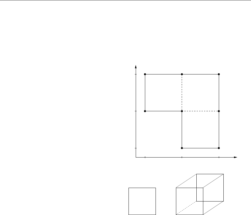
as these are not needed for the calculation. The following example is the coarse mesh for

the L-shaped domain:

811000

00-10

11-10

2-100

3000

4100

5-110

6010

7110

00quad0143

10quad2365

20quad3476

0 4 line 0 1

1 4 line 1 4

2 4 line 4 7

3 4 line 0 3

4 2 line 2 3

5 2 line 2 5

6 8 line 5 6

7 8 line 6 7

−1 10

1

0

−1 0 1

32 4

567

n1n0

n4 n5

n6n7

n2

n3

n3 n2

n0 n1

The file format is very simple: in the row, first the number of nodes in the coarse mesh is

given, followed by the sum of mesh elements plus elements on the boundary. The last three

values are always zero. This example has 8 nodes, 3 quads and 8 lines on the boundary.

After the header line all nodes of the mesh are declared in the format:

nxyz

where nis the index of the node (starting with zero) and xyzare the coordinates. We

always have to give all three coordinates (also in two dimensions).

The nodes are followed by the mesh elements. In two dimensions the format is:

n 0 quad n0 n1 n2 n3

where nis a consecutive index starting with 0. The second parameter is not used, thus

always 0. The mesh element, always quad is indicated by the third entry. The last four

values give the nodes describing the quadrilateral in counter-clockwise sense.

In three spatial dimension, the format is:

34

5.2 Curved boundaries

n 0 hex n0 n1 n2 n3 n4 n5 n6 n7

Here, first the nodes n0 to n3 in the front are given in counter-clock wise sense followed by

the nodes in the back.

Finally, all the boundary elements are given. In two dimensional meshes, these are all lines,

where both nodes are on the boundary. In three dimensions the boundary elements are all

quads with four nodes on the boundary. The format is:

n c line n0 n1

in two dimensions and

n c quad n0 n1 n2 n3

in three dimensions. nis again an iteration index. This index starts with 0. The value c

defines a color for the boundary element. These colors are necessary to distinguish between

different types of boundary conditions, see Sections 3.2.1 and 3.2.2. In two dimensions, the

order of the two nodes n0 n1 is arbitrary. In three dimensions however the four nodes have to

be given in a counter clock-wise sense seen from the outside of the domain! This is necessary

to get a unique definition of the normal vectors on the boundary. Thus, for the hex shown

in Picture above, the inp-file would be:

87000

0000

1100

2110

3010

4001

5101

6111

7011

00hex01234567

04quad0123

14quad1562

24quad3267

34quad4037

44quad5476

54quad4510

5.2 Curved boundaries

A part of the boundary can be assigned a curved boundary function. The idea is easy: Let

the boundary with color col be a curved boundary. We specify a function Rd→Rwhich

has the desired curved boundary as zero-iso-contour. For instance if the boundary Γ of the

domain should have the shape of a circle with radius rand midpoint (mx, my), one possible

function fcircle would be

fcircle(x, y) = (x−mx)2+ (y−my)2−r2.

Whenever an element with boundary nodes on a line with color col is refined, the newly gen-

erated nodes on the boundary line are then pulled onto the zero-iso-contour of the boundary

function. This is done by solving for the root of fcircle with Newton’s method.

35

5 Mesh handling

Adjust Curved BoundaryRefine

In Gascoigne boundary functions are described by the class BoundaryFunction<DIM> in

File: GAS/src/Mesh/BoundaryFunction . The circle is given by:

1class Circle : public BoundaryFunction<2>

2{

3double r , mx , my ;

4public :

5Circle(double r , double mx, double my) : r ( r ) , mx (mx) , my (my)

6{ }

7

8double operator ( ) ( const Vertex2d& v ) const

9{

10 return ( v . x()−mx ) ∗( v . x()−mx )+( v . y ()−my ) ∗( v . y()−my)−r∗r ;

11 }

12 }

The boundary function object has to be passed to the MeshAgent. For this, a derived mesh

agent class has to be specified and created in the Loop. The following minimal steps have to

be taken:

1class LocalMeshAgent : public MeshAgent

2{

3C i r c l e c i r c l e ;

4public :

5LocalMeshAgent ( ) : MeshAgent ( )

6{

7AddShape ( 4 , & c i r c l e ) ;

8}

9};

10

11 class LocalLoop : public StdLoop

12 {

13 public :

14

15 void BasicInit(const ParamFile∗p a r a m f i l e ,

16 const ProblemContainer∗PC,

17 const FunctionalContainer∗FC=NULL)

18 {

36

5.3 Adaptive refinement of meshes

19 GetMeshAgentPointer () = new LocalMeshAgent ( ) ;

20 StdLoop : : B a s i c I n i t ( p aramf i l e , PC, FC ) ;

21 }

22 };

In this example, the boundary with color 4is used as curved boundary.

5.3 Adaptive refinement of meshes

For local refinement, the MeshAgent has the function refine nodes(nodes). The nvector<int>

nodes contains indices of mesh nodes to be refined. If a node is to be refined, all elements

having this node as a corner node will be refined.

File: ../src/myloop.cc

1for ( i t e r =1; i t e r <n i t e r ;++ i t e r )

2{

3. . .

4Sol v e (u , f ) ;

5. . .

6// Estimate Error

7nvector<int>r e f ;

8// p i c k nodes f o r r e fi n em e nt i n r e f

9GetMeshAgent()−>r e f i n e n o d e s ( r e f ) ;

10 }

5.3.1 Estimating the Energy-Error

The class DwrQ1Q2 contains a function for estimation of an energy-error. It can be used in

the following way:

File: ../src/myloop.cc

1#include ”dwrq1q2 . h”

2. . .

3for ( i t e r =1; i t e r <n i t e r ;++ i t e r )

4{

5. . .

6Sol v e (u , f ) ;

7. . .

8// Estimate Error

9DoubleVector eta ;

10 DwrQ1Q2 dwr ( ∗Ge t M ul t iL e v el S o lv e r ()−>Get Solve r ( ) ) ;

11 dwr . EstimatorEnergy ( eta , f , u ) ;

12 . . .

13 }

37

5 Mesh handling

Now, for each node of the mesh the vector ηcontains a measure for the local contribution

to the total energy error.

5.3.2 Picking Nodes for Refinement

There are several methods for picking nodes for refinement. Common to all is to choose nodes

nwith large estimator values eta[n]. The class MalteAdaptor uses a global optimization

scheme for picking nodes:

File: ../src/myloop.cc

1#include ”malteadaptor .h ’ ’

2. . .

3for ( i t e r =1; i t e r <n i t e r ;++ i t e r )

4{

5. . .

6Sol v e (u , f ) ;

7. . .

8// Estimate Error

9DoubleVector eta ;

10 DwrQ1Q2 dwr ( G e t M ul t i Le v el S o lv e r ()−>Get Sol ver ( ) ) ;

11 dwr . EstimatorEnergy ( eta , f , u ) ;

12

13 // Pick Elements

14 nvector<int>refnodes ;

15 MalteAdaptor A( p a r a m f i l e , e t a ) ;

16 A. r e f i n e ( r e f n o d e s ) ;

17

18 // Re fin e

19 GetMeshAgent()−>r e f i n e n o d e s ( r e f n o d e s ) ;

20 }

38

6 Flow problems and stabilization

In order to discretize the Stokes or Navier-Stokes systems one can either use inf-sup- stable

finite element pairs for pressure and velocity which fulfill an inf-sup condition or include

stabilization terms in the equations that ensure uniqueness of the solution and stability.

Gascoigne always uses equal-order elements which are not inf-sup stable, in combination

with different pressure stabilization techniques. If in the Navier-Stokes case the convective

term is dominating (high Reynolds number) further stabilization is required.

6.1 The function point

To set element-wise constants in Gascoigne, the function point is needed:

1void Equation : :

2po in t ( double h , const FemFunction& U, const Vertex2d& v ) const

3{

4

5}

This function is called before every call of Matrix and Form and here the local mesh-size

hand the coordinates of the node vare given as a parameter. That way one can specify

certain criteria for the equation based on location or local mesh width.

To stabilize a given equation or system of equations (like Stokes and Navier-Stokes) one

usually modifies it by adding certain stabilizing terms. These terms often depend on the

local mesh width and have therefore to be defined in this function.

Since the function point is defined as const no class members can be altered. Thus, every

variable which shall be modified here has to be defined as mutable in the header file:

1mutable double variable ;

6.2 Stabilization of the Stokes system

The Stokes equations are given by

∇ · v= 0,−ν∆v+∇p=fin Ω.

39

6 Flow problems and stabilization

The simplest stabilization technique is the addition of an artificial diffusion. Stability is

ensured by modifying the divergence equation to

(∇ · v, ξ) + X

K∈Ωh

αK(∇p, ∇ξ)K,

where αKis an element-wise constant that can be chosen as

αK=α0

h2

K

6ν.

To get the local cell size hKof an element K, we use the function point which is called

before each call of Form and Matrix. In point we can calculate the value αKand save it to

a local variable:

1void St o kes : :

2po in t ( double h , const FemFunction& U, const Vertex2d& v ) const

3{

4al ph aK = a l p h a 0 ∗h∗h / 6. 0/ n u ;

5}

The parameter alpha0 can be read from the parameter file. The variable alphaK has to

be defined as mutable in the header file:

1mutable double alphaK ;

6.3 Stabilization of convective terms

The Navier-Stokes system

∇ · v= 0, v · ∇v−ν∆v+∇p=fin Ω,

needs additional stabilization of the convective term if the viscosity is low. One popular

approach consists of adding diffusion in streamline direction (Streamline Upwind Petrov-

Galerkin (SUPG) method). In combination with the artificial diffusion ansatz for pressure

stabilization, the full stabilized system reads

(∇ · v, ξ) + X

K

(αK∇p, ∇ξ)K= 0,

(v· ∇v, φ) + ν(∇v, ∇φ)−(p, ·∇φ) + X

K

(δKv· ∇v, v · ∇φ)K= (f, φ).

The parameters αKand δKare set to

αK=α06ν

h2

K

+kvkK,∞

hK−1

, δK=δ06ν

h2

K

+kvkK,∞

hK−1

,

40

6.4 LPS Stabilization

where kvkK,∞is the norm of the local velocity vector. The parameters might be chosen as

α0=δ0≈1

2.

For programming the Matrix it is usually not necessary to implement all derivatives. It

should be sufficient to have:

1void Equation : : Matrix ( . . . )

2{

3

4. . .

5// d e r i v a t i v e o f t h e c o nv ec ti on s t a b i l i z a t i o n terms

6A( 1 , 1 ) += d e l t a ∗(U [ 1 ] .m( ) ∗M. x ( ) + U [ 2 ] .m( ) ∗M. y ( ) )

7∗(U [ 1 ] .m( ) ∗N. x ( ) + U [ 2 ] .m( ) ∗N. y ( ) ) ;

8A( 2 , 2 ) += d e l t a ∗(U [ 1 ] .m( ) ∗M. x ( ) + U [ 2 ] .m( ) ∗M. y ( ) )

9∗(U [ 1 ] .m( ) ∗N. x ( ) + U [ 2 ] .m( ) ∗N. y ( ) ) ;

10 . . .

11 }

6.4 LPS Stabilization

Another way to stabilize these equations is the so called Local Projection Stabilization (LPS).

The idea is to suppress local fluctuations by adding the difference between the function itself

and its projection onto a coarser grid.

We use the fluctuation operator

π=id −i2h

where i2his a projection to the coarser grid. The LPS stabilized formulation for the Stokes

system reads

(∇ · v, ξ) + X

K∈Ωh

αK(∇πp, ∇πξ)K= 0

and for the Navier-Stokes systems

(∇ · v, ξ) + X

K

(αK∇πp, ∇πξ)K= 0,

(v· ∇v, φ) + ν(∇v, ∇φ)−(p, ·∇φ) + X

K

(δKv· ∇πv, v · ∇πφ)K= (f, φ).

αKand δKcan be taken from above.

To implement the projection in Gascoigne, one has to use the class LpsEquation instead of

Equation. It provides the additional functions

41

6 Flow problems and stabilization

1void lpspoint(double h , const FemFunction& U,

2const Vertex2d& v ) const {. . . }

3void StabForm ( V e c t o r I t e r a t o r b , const FemFunction& U,

4const FemFunction& UP, const TestFunction& Np)

5const {. . . }

6void StabMatrix ( EntryMatrix& A, const FemFunction& U,

7const TestFunction& Np, const TestFunction& Mp)

8const {. . . }

which have to be used for the stabilizing terms.

The variables UP,Np and Mp stand for the fluctuation operator πapplied to Nand M.Gas-

coigne provides these fluctuation operators if the discretization specified by the keyword

discname in the parameterfile is chosen Q1 or Q2Lps.

Similar as in the case of the SUPG method, it should be sufficient to implement the following

terms in the StabMatrix

1void LpsEquation : : StabMatrix ( . . . )

2{

3

4. . .

5// d e r i v a t i v e o f t h e c o nv ec ti on s t a b i l i z a t i o n terms

6A( 1 , 1 ) += d e l t a ∗(U [ 1 ] .m( ) ∗Mp. x ( ) + U [ 2 ] .m( ) ∗Mp. y ( ) )

7∗(U [ 1 ] .m( ) ∗Np. x ( ) + U [ 2 ] .m( ) ∗Np . y ( ) ) ;

8A( 2 , 2 ) += d e l t a ∗(U [ 1 ] .m( ) ∗Mp. x ( ) + U [ 2 ] .m( ) ∗Mp. y ( ) )

9∗(U [ 1 ] .m( ) ∗Np. x ( ) + U [ 2 ] .m( ) ∗Np . y ( ) ) ;

10 . . .

11 }

42