Gesture Motion Tracking Introduction Manual
User Manual:
Open the PDF directly: View PDF ![]() .
.
Page Count: 55
- Preparation
- 5 Mpu6050
- 6 Principle of motion tracking control
- 7. Protocol
- 8.2 Bluetooth communication mode control
1
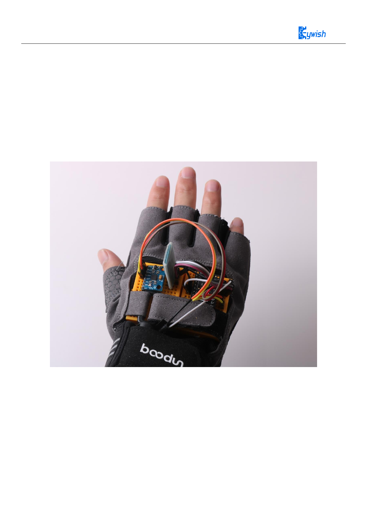
Gesture-MotionTracking
Introduction Manual
Github https://github.com/keywish/Gesture-MotionTracking

2
Chang history
Date
Version
Description
Author
2018-5-25
V.1.0
Create
Jason.Yang
2018-7-4
V.1.1
Review
Ken.chen
2019-4-8
V1.3
Fix NRF24L01+ connect error
Ken.chen

3
Contents
Preparation ......................................................................................................................................................... 5
1. Device list introduction .......................................................................................................................... 5
2.NANO Processor Introduction ................................................................................................................ 6
2.1 Power Supply.............................................................................................................................. 6
2.2 Memory.......................................................................................................................................... 6
2.3 Input and Output...................................................................................................................... 6
2.4 Communication Interface........................................................................................................ 7
2.5 Downloader.................................................................................................................................. 7
2.6 Attention................................................................................................................................... 7
3. Wireless communication module introduction(JDY-16) ................................................................. 7
3.2 Operating Steps ............................................................................................................................ 8
3.4 Connection method of Nano and JDY-16 .................................................................................. 11
4、NRF24L01 Wireless Module Introduction ........................................................................................ 11
4.1 Module Features................................................................................................................................. 12
4.2 Experimental Purpose ........................................................................................................................ 13
5、Introduction ........................................................................................................................................ 16
Features .................................................................................................................................................... 16
5.2 Module Schematic ..................................................................................................................... 17
Figure 11: Schematic of the mpu6050 module ........................................................................................ 17
5.3 Communication between Nano and mpu6050 ........................................................................... 17
1.2 Reading Data from MPU-6050 .................................................................................................. 19
1.3 Specific Implementation ............................................................................................................ 19
II. MPU6050 Data Format ..................................................................................................................... 19
Experiment 1 Reading Accelerometer ............................................................................................. 20
5.4.2 Experiment 2 Reading data from Gyro ................................................................................... 26
5.5 Motion Data Analysis ........................................................................................................................ 30
3.1 Accelerometer Model................................................................................................................. 30
3.2 Roll-pitch-yaw model and attitude calculation .......................................................................... 32
3.3 Yaw Angle Problem ................................................................................................................... 34
5.6 Data Processing and Implementation................................................................................................. 34
5.6.1 Experiment 3 imu_kalman gets Roll and Pitch ............................................................................... 34
5.6.2 Experiment Code................................................................................................................... 34

4
6、Principle of motion tracking control .......................................................................................................... 40
6.1 Racing direction coordinate angle model .......................................................................................... 40
7. Protocol ........................................................................................................................................................ 49
8.1 Nrf24L01 wireless control ................................................................................................................. 51
8.1.1 Gesture control Hummer-bot smart car .................................................................................. 51
8.1.2 Gesture Control Beetle-bot Smart Car .................................................................................... 52
8.2 Bluetooth communication mode control .................................................................................................... 52
8.2.1 Gesture control Aurora-Racing ....................................................................................................... 53
8.2.2 Gesture control Panther-tank .......................................................................................................... 54
8.2.3 Gesture control balance car ............................................................................................................. 55
5
Preparation
1. Device list introduction
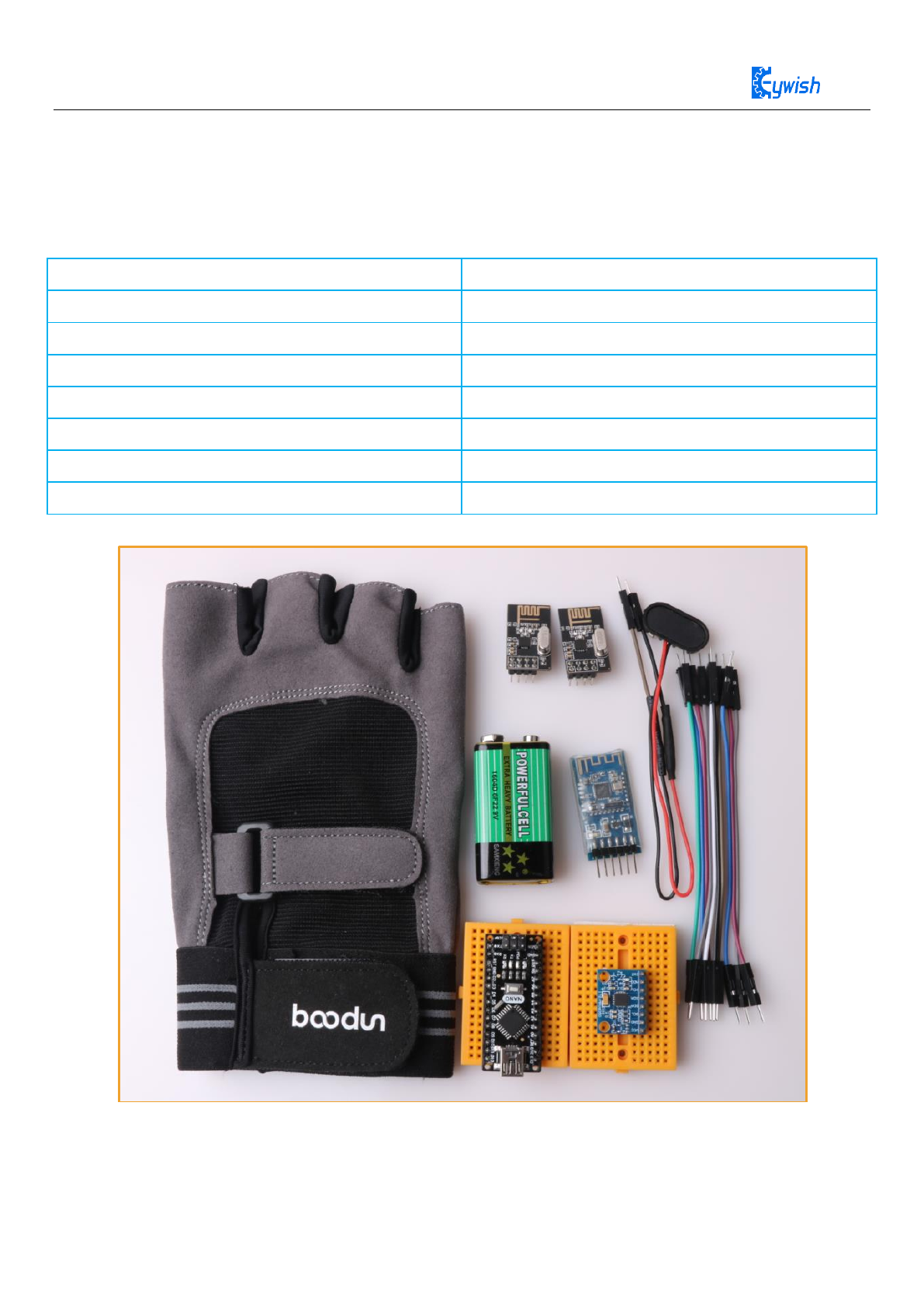
The required kits are shown in the table below.
MPU6050 Module
1
JDY-16 Bluetooth Module
1
NRF24L01+ Module
2
Arduino NANO Main Control Board
1
mini Bread Board
2
Gloves
1
Male to Female DuPont line
Several
Battery
1
Figure 1: Device List

6
2. NANO Processor Introduction
◆ The Arduino Nano microprocessor is ATmega328 (Nano3.0) with USB-mini interface, which has 14
digital input/output pins (6 of which can be used as PWM output), 8 analog inputs, and a 16 MHz ceramic
resonator, 1 mini-B USB connection, an ICSP header and a reset button.
◆ The processor ATmega328
◆ Working voltage 5v
◆ Input voltage (recommended) 7-12v
◆ Input voltage (range) 6-20v
◆ Digital IO pin 14 (6 of which can be used as PWM output)
◆ Analog input pin 6
◆ IO pin DC 40 mA
◆ Flash Memory 16 or 32 KB (in which 2 KB for bootloader)
◆ SRAM 1KB or 2KB
◆ EEPROM 0.5 KB or 1KB (ATmega328)
◆ CH340 USB to serial port chip
◆ Clock 16 MHz
2.1 Power Supply
Arduino Nano power supply mode: mini-B USB interface power supply and external vin connection
7~12V external DC power supply
2.2 Memory
ATmega168/ATmega328 includes on-chip 16KB/32KB Flash, of which 2KB is used for Bootloader. There
are also 1KB/2KB SRAM and 0.5KB/1KB EEPROM.
2.3 Input and Output
◆ 14 digital input and output ports: The working voltage is 5V, and each channel can output and access
the maximum current of 40mA. Each channel is equipped with a 20-50K ohm internal pull-up resistance
(not connected by default). In addition, some pins have specific functions.
◆ Serial signal RX (0), TX (1): It provides serial port receiving signal with TTL voltage level, connected
to the corresponding pin of FT232Rl.
◆ External Interrupt (No. 2 and No. 3): Trigger interrupt pin, which can be set to rising edge, falling edge
or simultaneous trigger.
◆ Pulse Width Modulation PWM (3, 5, 6, 9, 10, 11): Provides 6 channel, 8-bit PWM outputs.
◆ SPI(10(SS),11(MOSI),12(MISO),13(SCK):SPI Communication Interface.

7
◆ LED (No. 13): Arduino is specially used to test the reserved interface of the LED. When the output is
high, the LED is lit. When the output is low, the LED is off.
◆ 6 analog inputs A0 to A5: Each channel has a resolution of 10 bits (that is, the input has 1024 different
values), the default input signal range is 0 to 5V, and the input upper limit can be adjusted by AREF. In
addition, some pins have specific functions.
◆ TWI interface (SDA A4 and SCL A5): Supports communication interface (compatible with I2C bus).
◆ AREF: The reference voltage of the analog input signal.
◆ Reset:The microcontroller chip is reset when the signal is low.
2.4 Communication Interface
Serial port: The built-in UART of ATmega328 can communicate with external serial port through digital
port 0 (RX) and 1 (TX).
2.5 Downloader
The MCU on the Arduino Nano has a bootloader program, so you can download the program directly from
the Arduino software. You can also directly download the program to the MCU through the ICSP header on
the Nano.
2.6 Attention
The Arduino Nano provides an automatic reset design that can be reset by the host. In this way, the software
can be automatically reset by the Arduino software in the program to the Nano, without pressing the reset
button.
3. Wireless communication module introduction(JDY-16)
This design adopts the JDY-16 master-slave Bluetooth module, which has the following features:
◆ BLE high speed transparent transmission supports 8K Bytes rate communication.
◆ Send and receive data without byte limit, support 115200 baud rate continuously send and receive data.
◆ Support 3 modes of work (see the description of AT+STARTEN instruction function).
◆ Support (serial port, IO, APP) sleep wake up
◆ Support WeChat Airsync, WeChat applet and APP communication.
◆ Support 4 channel IO port control and high precision RTC clock.
◆ Support PWM function (can be controlled by UART, IIC, APP, etc.).
◆ Support UART and IIC communication mode, default to UART communication.
◆ iBeacon mode (support WeChat shake protocol and Apple iBeacon protocol).
◆ Host transparent transmission mode (transmission of data between application modules, host and slave
communication).
8
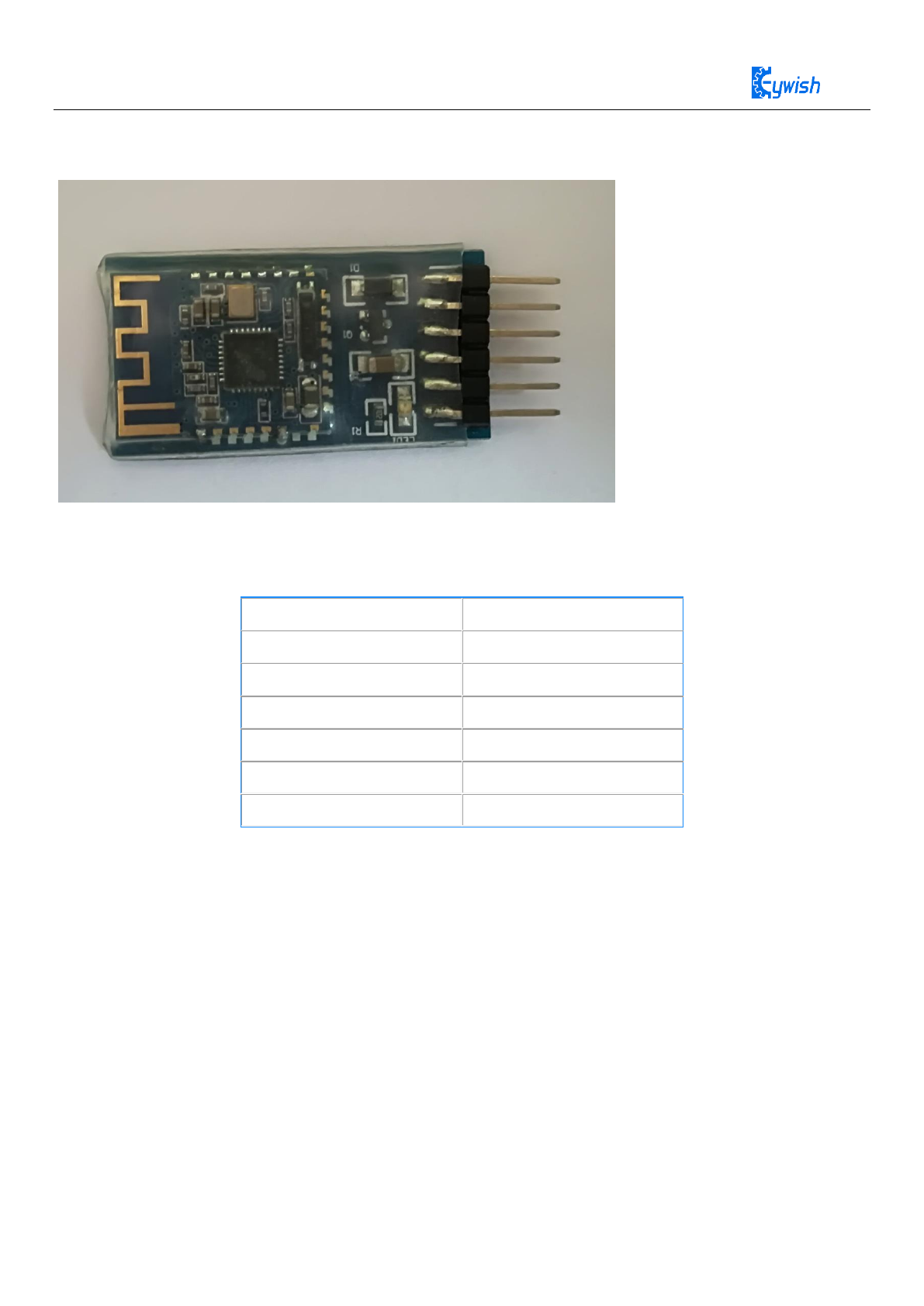
Wireless communication module configuration
Figure 2: JDY-16 module physical map
(1) The cable of Nano and JDY-16
JDY-16 Module
Arduino NANO
VCC
5V
GND
GND
RXD
D2
TXD
D3
STAT
NC
PWRC
NC
Download program MotionTrack\JDY-16\AT_CMD\ AT_CMD.ino
(2) Configuration requirements:
Implement master-slave binding of two JDY-16 Bluetooth modules.
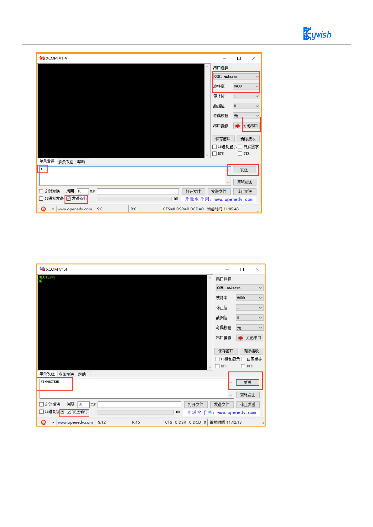
3.2 Operating Steps
1. Connect the Nano and JDY-16 modules with the DuPont line.
2. Enter the AT command mode
Connect the downloader to the computer and open the serial port assistant. Set the baud rate to 9600, the
data bit to 8 bits, the stop bit to 1 bit, and no parity bit.
Test communication:
Send: AT
Back: OK
9
Figure 3: Send AT Command Diagram
3. Send: AT+HOSTEN1\r\n ----------- Set Bluetooth as the main mode
Back: OK
Back: OK
Figure 4: Setting Host Mode
4. Scan the surrounding JDY-16 Bluetooth:
1. Slave transmission: AT+SCAN\r\n------------ Query the slave's own address
Back: OK
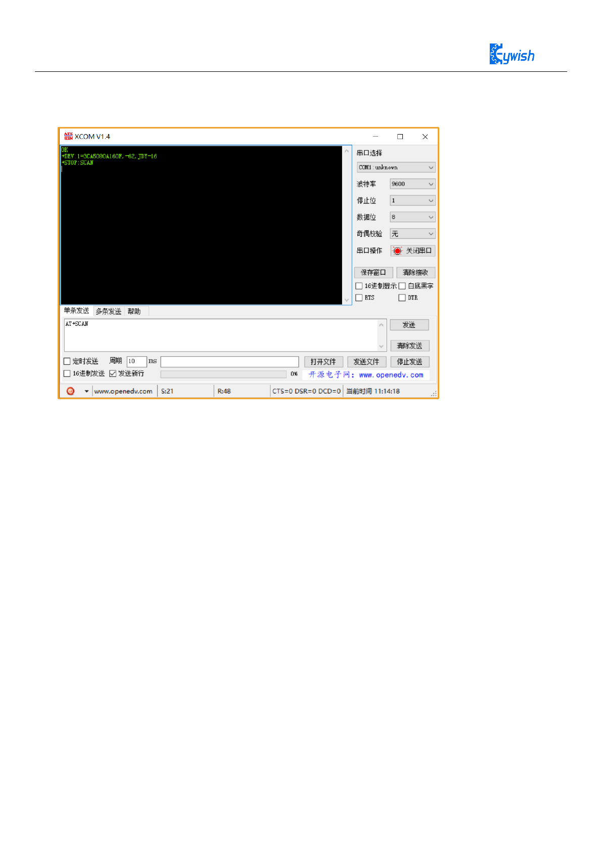
10
+DEV:1=3CA5090A160F, -62, JDY-16
+STOP:SCAN
Figure 5: Querying peripheral Bluetooth devices
5. Connect Bluetooth
Host sends: AT+CONN3CA5090A160F\r\n ------------ Host binding slave address
Back: OK
Connected to the power supply, the two Bluetooth can be connected to each other, send data through the
host Bluetooth, the slave Bluetooth can receive the same data.
Or you can directly program the prepared master-slave configuration procedure to set the master-slave
Bluetooth, then the host programs the connection procedure and automatically connects. (Note that only the
Bluetooth module of JDY-16 can be automatically connected at present)
11
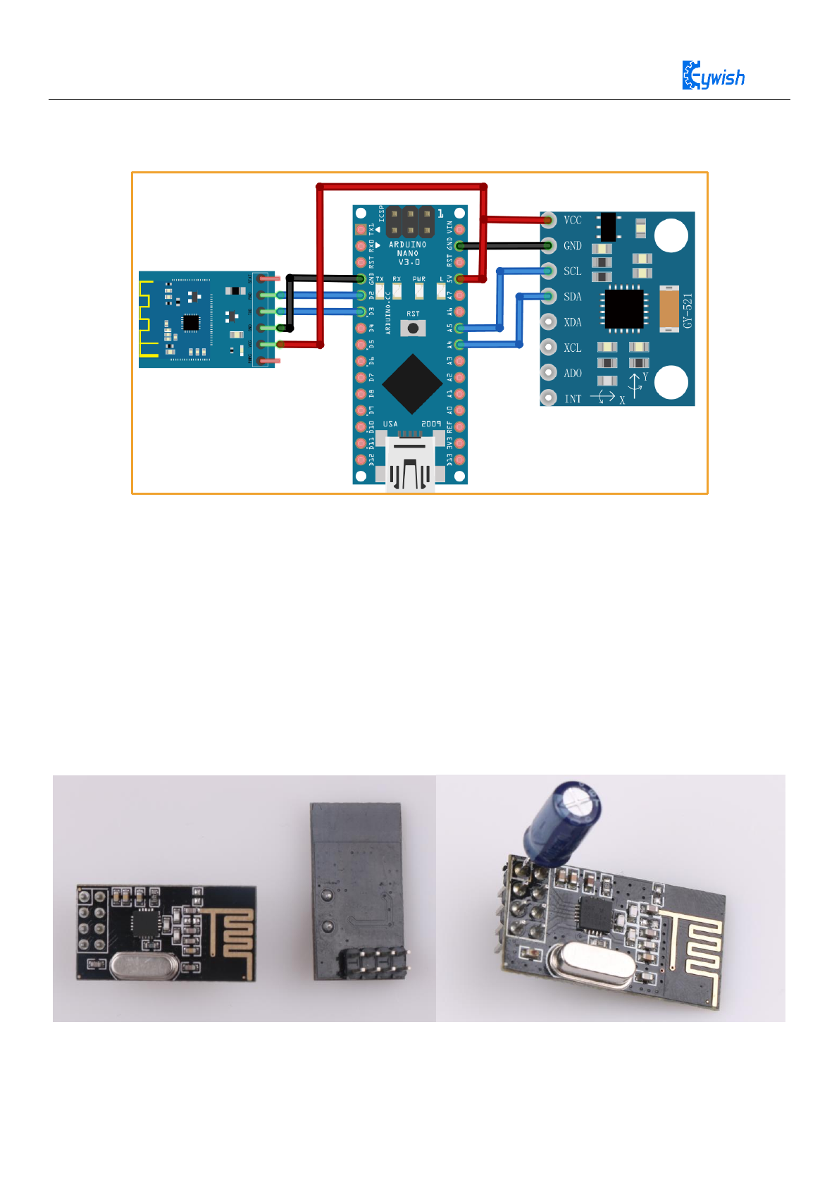
3.4 Connection method of Nano and JDY-16
Figure 6: Nano and JDY-16 connection diagram
4.NRF24L01 Wireless Module Introduction
The nRF24L01+ module is a 2.4G wireless communication module developed by Nordic based on the
nRF24L01 chip. Adopt FSK modulation and integrate Nordic's own Enhanced Short Burst protocol.
Point-to-point or 1-to-6 wireless communication can be achieved. Wireless communication speed can reach
up to 2M (bps). The NRF24L01 has four operating modes: transceiver mode, configuration mode, idle mode,
and shutdown mode. The physical map used in this experiment is on the left side of Figure 7. For the stable
reception of the Nrf24L01 receipt, it is recommended to connect the 10uf capacitor between VCC and GUD
as shown on the right.
Figure 7: Nrf24l01+ physical map and solder diagram

12
4.1 Module Features
◆ 2.4GHz ,small size,15x29mm(including antenna)
◆ Support six-channel data reception
◆ Low working voltage: 1.9~3.6V
◆ Data transfer rate supports: 1Mbps、2Mbps
◆ Low power consumption design,working current at receiving is 12.3mA, 11.3mA at 0dBm power
emission, 900nA at power-down mode
◆ Automatic retransmission function, automatic detection and retransmission of lost data packets,
retransmission time and retransmission times can be controlled by software
◆ Automatic response function, after receiving valid data, the module automatically sends an answer
signal
◆ Built-in hardware CRC error detection and point-to-multipoint communication address control
◆ NRF24L01 chip details please refer to《nRF24L01 Datasheet.pdf》
13
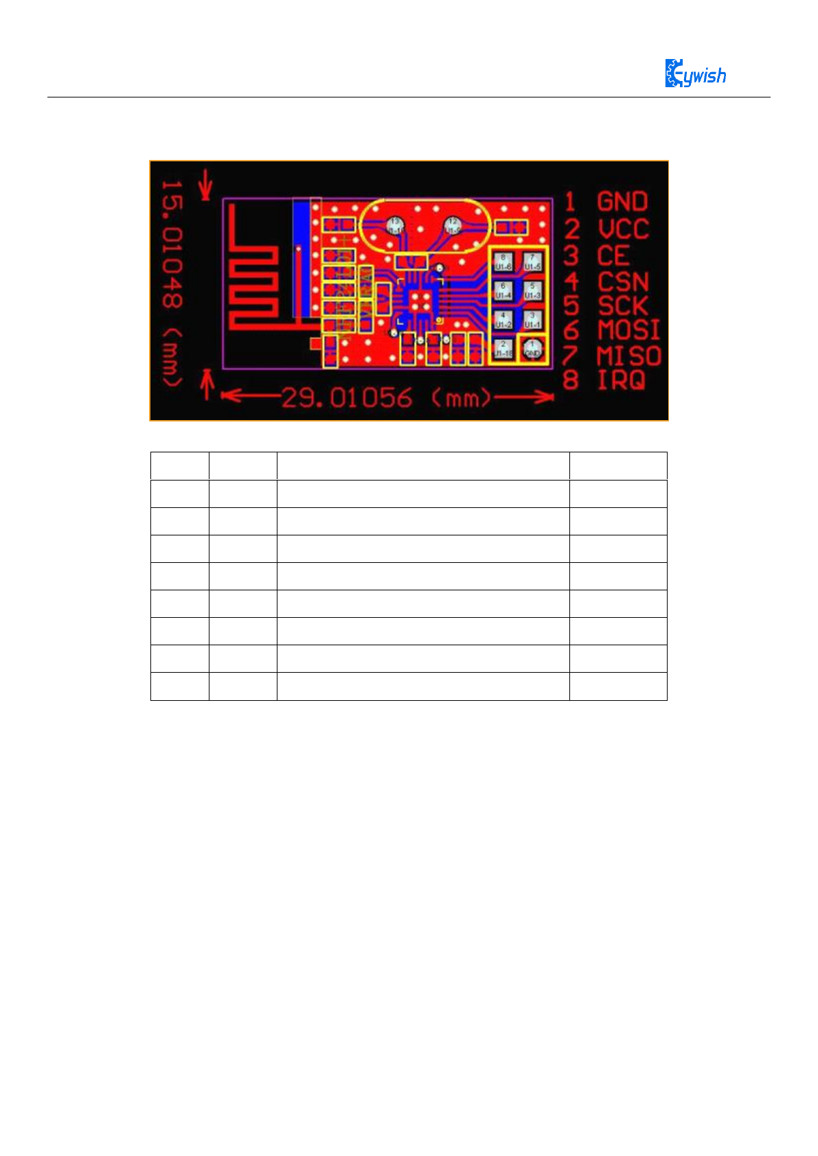
Pin information
Figure 8: Nrf24L01 pin information diagram
Pin
Symbol
Function
Direction
1
GND
GND
2
+5V
Power Supply
3
CE
Control Line At Working Mode
IN
4
CSN
Chip Select Signal, Low Level Working
IN
5
SCK
SPI Clock
IN
6
MOSI
SPI Input
IN
7
MISO
SPI Output
OUT
8
IPQ
Interrupt Output
OUT+
4.2 Experimental Purpose
1. Learn about nRF24L01+module and how to connect with Arduino.
2. How to use arduino and nRF24L01+ module to finish receiving and sending data.
4.3 The components needed for this experiment
◆ Arduino UNO R3 Motherboard
◆ Arduino NANO Motherboard
◆ nRF24L01 Module*2
◆ Several wires
4.4 Experimental schematic diagram
14
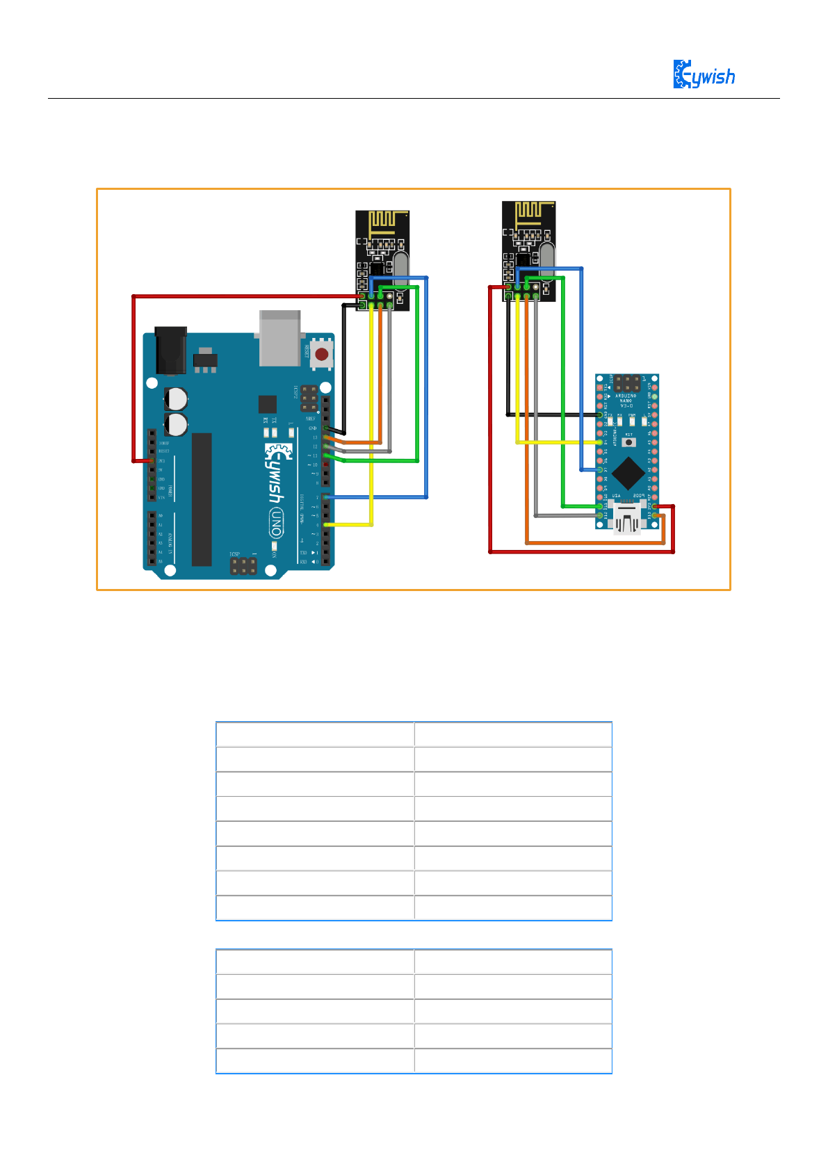
Experimental connection diagram
Figure 9: Nano and Nrf24L01 connection diagram
Arduino and NRF24L01 mode of connection
arduino Nano
nRF24L01
+3.3V
VCC
GND
GND
7pin
4pin CSN
4pin
3pin CE
11pin
6pin MOSI
12pin
7pin MISO
13pin
5pin SCK
arduino Uno
nRF24L01
+3.3V
VCC
GND
GND
7
4pin CSN
4
3pin CE

15
11pin
6pin MOSI
12pin
7pin MISO
13pin
5pin SCK
4.4 Program principle
Launch process
1、Firstly, configure the nRF24L01 to transmit mode.
2、Then write the address TX_ADDR of the receiving end and the data TX_PLD to be sent into the
nRF24L01 buffer area by the SPI port in time sequence.
3、Arduino configures the CE to be high for at least 10 μs and transmits data after a delay of 130 μs. If the
auto answer is on, the nRF24L01 enters the receive mode immediately after transmitting the data and
receives the answer signal. If a reply is received, the communication is considered successful.
4、NRF24L01 will automatically set TX_DS high and the TX_PLD will be cleared from the transmit stack.
If no response is received, the data will be automatically retransmitted. If the number of retransmissions
(ARC_CNT) reaches the upper limit, MAX_RT is set high and TX_PLD will not be cleared; MAX_RT
When TX_DS is set high, IRQ goes low to trigger MCU interrupt. When the last transmission is successful,
if the CE is low, the nRF24L01 will enter standby mode.
5、If there is data in the transmission stack and CE is high, the next transmission is started; if there is no data
in the transmission stack and CE is high, the nRF24L01 will enter standby mode 2.
Receive data process
1、When the nRF24L01 receives data, please configure the nRF24L01 to receive mode firstly.
2、Then delay 130μs into the receiving state to wait for the arrival of data. When the receiver detects a valid
address and CRC, it stores the data packet in the receiver stack. At the same time, the interrupt sign RX_DR
is set high and the IRQ goes low to notify the MCU to fetch the data.
3、If auto-response is turned on at this time, the receiver will enter the transmit status echo response signal at
the same time. When the last reception is successful, if CE goes low, the nRF24L01 will go into idle mode
1.
nRF24L01 transceiver test program please refer to "Gesture-MotionTracking\nRF24l01+\program”
16
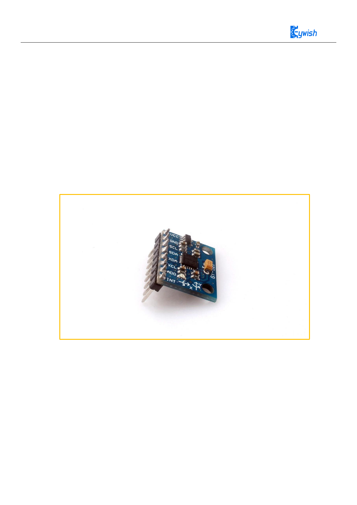
5 Mpu6050
5.1 Introduction
MPU6050 is the world's first 6-axis motion processing component with integrated 3-axis
gyroscope and 3-axis accelerator. It can connect to other magnetic sensors or other sensors'
digital motion processing (DMP) via a second I2C port. The hardware acceleration engine
mainly outputs a complete 9-axis fusion calculation technique to the host MCU in the form of
a single data stream by the I2C port.
MPU6050 chip comes with a data processing sub module DMP, has built-in hardware
filtering algorithm, using DMP output data has been able to meet the requirements well in
many applications. We don't need our software to do the filtering. This course will build a
complete sports gloves based on reading DMP as output data through Arduino.
Figure 10: mpu6050 module physical map
Features
◆ The integrated calculus data of digital output of 6 axis or 9 axis rotation matrix, quaternion and Euler
angle format.
◆ 3-axis angular velocity sensor (gyroscope) with 131 LSBs/°/sec sensitivity and full-range sensing range
of ±250, ±500, ±1000, and ±2000°/sec.
◆ Programmable control, 3-axis accelerator with program control range of ±2g, ±4g, ±8g, and ±16g.
◆ The Digital Motion Processing (DMP) engine reduces the load of complex fusion calculation data,
sensor synchronization, and gesture sensing.
◆ The motion processing database supports Android, Linux, and Windows.
17
◆ Built-in calibration techniques for operating time deviations and magnetic sensor eliminates the uses’
additional need for calibration.
◆ Digital output temperature sensor.
◆ The supply voltage of VDD is 2.5V±5%、3.0V±5%、3.3V±5%, and VDDIO is 1.8V± 5%.
◆ Gyro operating current: 5mA, gyroscope standby current: 8A; accelerator operating current: 8A,
accelerator power saving mode current: 8A@10Hz.
◆ Up to 400kHz fast mode I2C, or up to 20MHz SPI serial host interface.
◆ Smallest and thinnest tailored package for the portable product (4x4x0.9mm QFN).
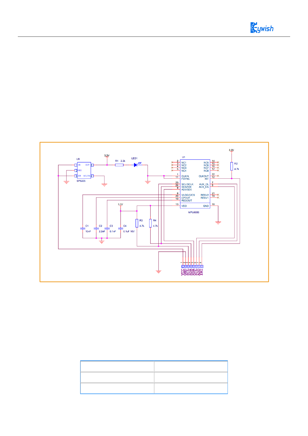
5.2 Module Schematic
Figure 11: Schematic of the mpu6050 module
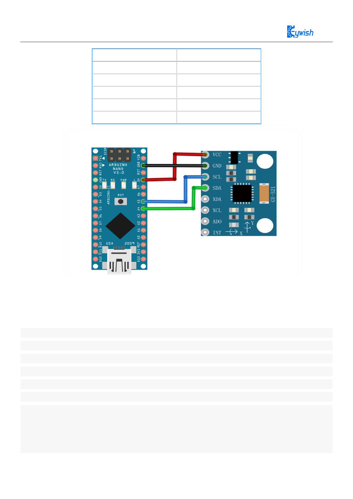
5.3 Communication between Nano and mpu6050
5.3.1 Circuit Connection
The data interface of the integrated MPU6050 module uses the I2C bus protocol, so we
need the help of the Wire library to communicate between NANO and the MPU6050. The
corresponding connection of the NANO board is as follows:
MPU6050 Module
Arduino NANO
VCC
5V
GND
GND
18
SCL
A5
SDA
A4
XDA
NC
XCL
NC
ADD
NC
INT
NC/GND
Figure 12: Connection diagram of Nano and mpu6050
MPU6050 writing and reading data are realized by the chip's internal registers, the
register addresses are all 1 byte, namely, 8 bits of the address space. Please refer to
"RM-MPU-6000A.pdf" 1.1.
Before write data to the device every time, firstly turn on the wire transfer mode and specify
the bus address of the device. The bus address of the MPU6050 is 0x68 (the address is 0x69
when the AD0 pin is high). Then write a byte of the register start address, and then write data
of any length. These data will be continuously written to the specified start address, and the
current register length will be written to the register of the following address. Turn off the wire
transfer mode after writing is complete. The following sample code writes a byte 0 to the 0x6B
register of the MPU6050.
Wire.beginTransmission(0x68); // Strat the transmission of the MPU6050
Wire.write(0x6B); // Specify register address
Wire.write(0); // Write one byte of data

19
Wire.endTransmission(true); // End transfer, true means release bus
Reading Data from MPU-6050
Reading and writing are alike, firstly opening the Wire transfer mode, and then writing a
byte of the register start address. Nextly, reading the data of the specified address into the
cache of the Wire library and turn off the transport mode. Finally, reading the data from the
cache. The following example code starts with the 0x3B register of MPU6050 and reads 2
bytes of data:
Wire.beginTransmission(0x68); // Strat the transmission of the MPU6050
Wire.write(0x3B); // Specify register address
Wire.requestFrom(0x68, 2, true); // Read the data to the cache
Wire.endTransmission(true); // Close transmission mode
int val = Wire.read() << 8 | Wire.read(); // Two bytes form a 16-bit integer
Specific Implementation
The Wire library usually should be initialized in the setup function:
Wire.begin();
You must start the device before you perform any operations on the MPU6050, and
writing a byte to its 0x6B will be enough. It is usually done in the setup function, as shown in
section 1.1.
MPU6050 Data Format
The data we are interested in is in the 14 byte register of 0x3B to 0x48. These data will be
dynamically updated with an update frequency of up to 1000HZ. The address of the
underlying register and the name of the data are listed below. Note that each data is 2 bytes.
0x3B, the X axis component of the accelerometer is ACC_X
0x3D, the Y axis component of the accelerometer is ACC_Y
0x3F, the Z axis component of the accelerometer is ACC_Z
0x41, the current temperature is TEMP
0x43, angular velocity around the X axis GYR_X
0x45, angular velocity around the Y axis GYR_Y
0x47, angular velocity around the Z axis GYR_Z
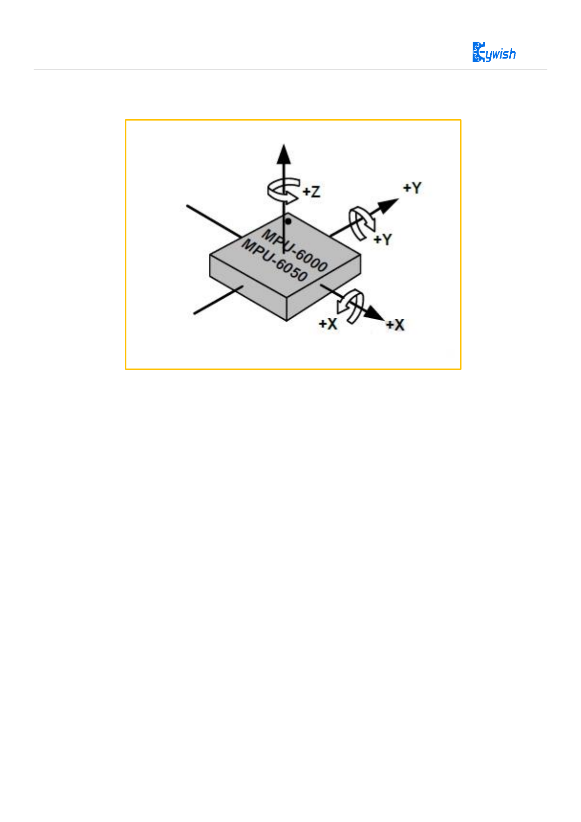
The coordinate definition of the MPU6050 chip is: face the chip toward itself and turn the
surface text to the correct angle. At this time, the center of the chip is taken as the origin, the
20
horizontal to the right is the X axis, and the vertical is the Y axis, pointing your own is the Z
axis, as shown as the below:
Figure 13: mpu6050 rotation and angular velocity diagram
We only care about the meaning of accelerometer and angular velocity meter data.Now we are familiar with
the use of mpu6050 through two experiments.
Experiment 1 Reading Accelerometer
The three axes components of accelerometer, ACC_X, ACC_Y and ACC_Z are all 16-bit
signed integers, which indicate the acceleration of the device in three axial directions. When
the negative value is taken, the acceleration is negative along the coordinate axis and the
positive value is positive.
The three acceleration components are all in multiples of the gravitational acceleration g,
and the range of acceleration that can be expressed, that is, the magnification can be uniformly
set, and there are four optional magnifications: 2g, 4g, 8g, and 16g. Taking ACC_X as an
example, if the magnification is set to 2g (default), it means that when ACC_X takes the
minimum value -32768, the current acceleration is 2 times the gravitational acceleration along
the positive direction of the X axis, and so on. Obviously, the lower the magnification, the
better the accuracy, and the higher the magnification, the larger the range, which is set
according to the specific application.
21
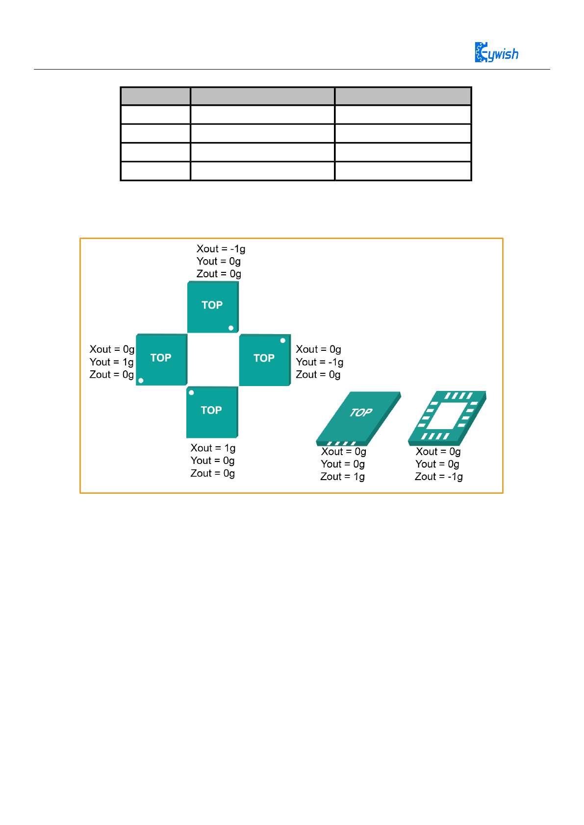
The relationship between the rotation direction of the three-axis accelerometer and the module
is as follows:
Figure 14: Mpu6050 module rotation and acceleration pattern
The data read by the MPU6050 is fluctuating, so it needs to be verified. That is, when the chip is in a
stationary state, this reading should theoretically be zero. But it tends to have an offset. For example, we read
200 values at 10ms intervals and then average them. This value is called zero offset. The calibrated reading is
obtained by subtracting the zero offset from each reading. Since the theoretical value of ACC_X and ACC_Y
should be zero, the two reading offsets can be calibrated by statistical mean. ACC_Z needs to be processed in
one step. In the process of statistical offset, the gravitation acceleration g of the Z axis is subtracted for each
reading. If the acceleration magnification is 2g, then 16384 is subtracted, and then the statistical mean
calibration is performed. General calibration can be done each time the system is started, then you should
make a trade-off between accuracy and start-up time.
Experimental Purpose
By rotating the mpu6050 to observe the output data relation between the three axes of the
accelerometer.
AFS_SEL Full Scale Range LSB Sensitivity
0 ±2 16384LSB/
1 ±4 8192LSB/
2 ±8 4096LSB/
3 ±16 2048LSB/
g g
g g
g g
g g

22
Experiment Code
Code Location:MotionTrack\Lesson\mpu6050_accel\ mpu6050_accel.ino

23
#include "Wire.h"
// I2Cdev and MPU6050 must be installed as libraries, or else the .cpp/.h
files
// for both classes must be in the include path of your project
#include "I2Cdev.h"
#include "MPU6050.h"
#define LED_PIN 13
MPU6050 accelgyro;
struct RAW_type
{
uint8_t x;
uint8_t y;
uint8_t z;
};
int16_t ax, ay, az;
int16_t gx, gy, gz;
struct RAW_type accel_zero_offsent;
char str[512];
bool blinkState = false ;
float AcceRatio = 16384.0;
float accx,accy,accz;
void setup() {
int i ;
int32_t ax_zero = 0,ay_zero = 0,az_zero = 0 ;
// join I2C bus (I2Cdev library doesn't do this automatically)
Wire.begin();
Serial.begin(115200);
// initialize device
Serial.println("Initializing I2C devices...");
accelgyro.initialize();
delay(500) ;
accelgyro.setFullScaleAccelRange(MPU6050_ACCEL_FS_2);
Serial.println("Testing device connections...");
Serial.println(accelgyro.testConnection() ? "MPU6050 connection
successful" : "MPU6050 connection failed");

24
1. Rotate 90 degrees around the X axis
for( i = 0 ; i < 200 ; i++)
{
accelgyro.getMotion6(&ax, &ay, &az, &gx, &gy, &gz);
ax_zero += ax ;
ay_zero += ay ;
az_zero += az ;
}
accel_zero_offsent.x = ax_zero/200 ;
accel_zero_offsent.y = ay_zero/200 ;
accel_zero_offsent.z = az_zero/200 ;
Serial.print(accel_zero_offsent.x); Serial.print("\t");
Serial.print(accel_zero_offsent.y); Serial.print("\t");
Serial.print(accel_zero_offsent.z); Serial.print("\n");
pinMode(LED_PIN, OUTPUT);
}
void loop() {
// read raw accel/gyro measurements from device
delay(1000);
accelgyro.getMotion6(&ax, &ay, &az, &gx, &gy, &gz);
sprintf(str,"%d,%d,%d\n",ax-accel_zero_offsent.x,
ay-accel_zero_offsent.y ,az-accel_zero_offsent.z);
Serial.print(str);
accx = (float)( ax-accel_zero_offsent.x )/AcceRatio;
accy = (float)( ay-accel_zero_offsent.y )/AcceRatio ;
accz = (float)( az-accel_zero_offsent.z )/AcceRatio ;
Serial.print(accx);Serial.print("g\t");
Serial.print(accy);Serial.print("g\t");
Serial.print(accz);Serial.print("g\n");
blinkState = !blinkState;
digitalWrite(LED_PIN, blinkState);
}
25
When the X axis is rotated 90 degrees, the Y axis is slowly upward and the Z axis is
slowly downward. When the axis reaches exactly 90 degrees, since the Y axis is in the
opposite direction to the gravity, the output of the Y axis is 1g (1g==9.8m/s^2), while the
value of the Z axis decreases from 1 to 0.
2. Back to the initial position and reverse rotation 90 degrees
When you get back to the initial position, the Y axis value is slowly reduced to 0, while
the Z axis is slowly increasing to 1. Then turn 90 degrees in reverse direction, and the Y axis
decreases gradually until -1, because the Y axis is in accordance with the gravity direction,
and the acceleration value should be negative. The Z axis decreases slowly to 0.
3. Back to the initial position
Explain as follows: Then return to the initial position from the reverse 90 degrees. At this
time, the data of the Y-axis and the Z-axis are slowly restored to the initial value, the Y-axis
is 0, and the Z-axis is 1.
After analyzing the rotation of the X-axis, the rotation of the Y-axis is similar, so we won’t talk about it in
details. Now let's talk about the Z axis, because when rotating around the Z axis, it is equivalent to swinging
90 degrees to the left and right. At this time, the output of the Z axis is always 1, and the X axis and the Y
axis are orthogonal to the gravity axis, so the output values are all It is 0, of course, this is the value under
relatively static conditions. If the device is installed on a vehicle, the X and Y axes may not necessarily be 0
when the car is turning left and right.
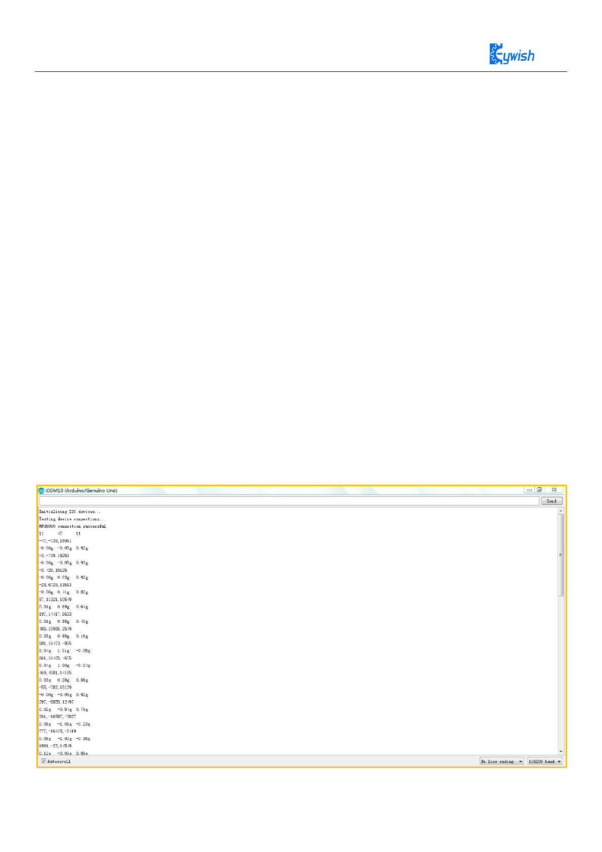
Experimental Result

26
Experiment 2 Reading data from Gyro
The angular velocity components GYR_X, GYR_Y and GYR_Z, which rotate around three coordinate
axes of X, Y and Z, are all 1-bit signed integers. From the origin to the axis of rotation, the value is positive
for the clockwise rotation and negative for the counterclockwise rotation.
The three angular velocity components are all in degrees/second. The angular velocity range that can be
expressed, that is, the magnification can be uniformly set. There are 4 optional magnifications: 250
degrees/second, 500 degrees/second, 1000 degrees/second, 2000. Degrees/second. Taking GYR_X as an
example, if the magnification is set to 250 degrees/second, it means that when the GYR takes a positive
maximum value of 32768, the current angular velocity is 250 degrees/second clockwise; if it is set to 500
degrees/second, the current value of 32768 indicates the current the angular velocity is 500 degrees/second
clockwise. Obviously, the lower the magnification, the better the accuracy, and the higher the magnification,
the larger the range.
Program Location “MotionTrack\Lesson\mpu6050_gryo\ mpu6050_gryo.ino”
AFS_SEL Full Scale Range LSB Sensitivity
0 ±250°/s 131LSB/°/s
1 ±500°/s 65.5LSB/
2 ±1000°/s 32.8LSB/
3 ±2000°/s 16.4LSB/
°/s
°/s
°/s

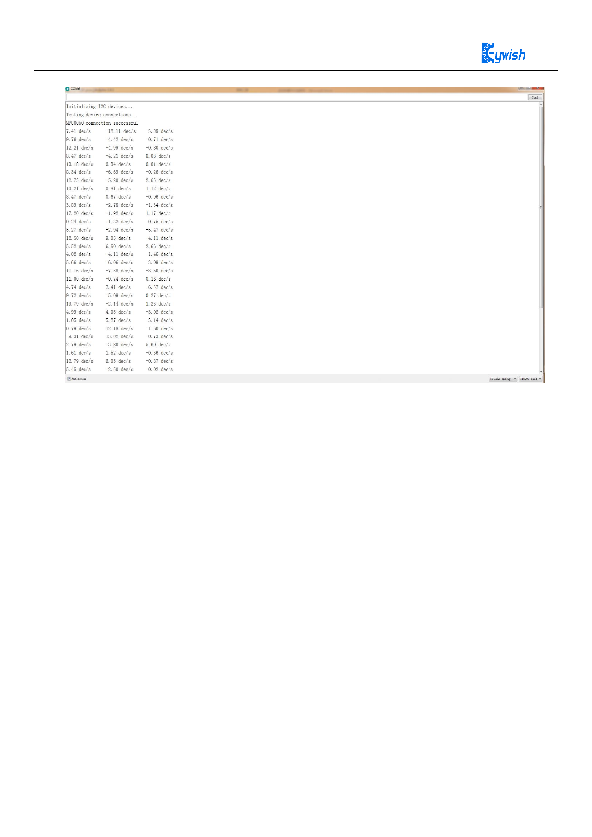
27
Experiment
Code
#include "Wire.h"
// I2Cdev and MPU6050 must be installed as libraries, or else the .cpp/.h
files
// for both classes must be in the include path of your project
#include "I2Cdev.h"
#include "MPU6050.h"
#define LED_PIN 13
MPU6050 accelgyro;
struct RAW_type
{
uint8_t x;
uint8_t y;
uint8_t z;
};
int16_t ax, ay, az;
int16_t gx, gy, gz;
struct RAW_type accel_zero_offsent ,gyro_zero_offsent;
bool blinkState = false;
char str[512];

28
float pi = 3.1415926;
float AcceRatio = 16384.0;
float GyroRatio = 131.0;
float Rad = 57.3 ; //180.0/pi;
float gyrox,gyroy,gyroz;
void setup() {
int i ;
int32_t ax_zero = 0,ay_zero = 0,az_zero = 0,gx_zero =0 ,gy_zero =
0,gz_zero = 0 ;
// join I2C bus (I2Cdev library doesn't do this automatically)
Wire.begin();
Serial.begin(115200);
// initialize device
// Serial.println("Initializing I2C devices...");
accelgyro.initialize();
delay(500) ;
accelgyro.setFullScaleGyroRange(MPU6050_GYRO_FS_250);
Serial.println("Testing device connections...");
Serial.println(accelgyro.testConnection() ? "MPU6050 connection
successful" : "MPU6050 connection failed");
for( i = 0 ; i < 200 ; i++)
{
accelgyro.getMotion6(&ax, &ay, &az, &gx, &gy, &gz);
gx_zero += gx ;
gy_zero += gy ;
gz_zero += gz ;
}
gyro_zero_offsent.x = gx_zero/200 ;
gyro_zero_offsent.y = gy_zero/200 ;

29
When we rotate in the positive direction of the x-axis, we see that the printed gyrox data is positive,
otherwise it is negative.
gyro_zero_offsent.z = gz_zero/200;
pinMode(LED_PIN, OUTPUT);
}
void loop() {
// read raw accel/gyro measurements from device
accelgyro.getMotion6(&ax, &ay, &az, &gx, &gy, &gz);
//sprintf(str,"%d,%d,%d\n",
gx-gyro_zero_offsent.x ,gy-gyro_zero_offsent.y,
gz-gyro_zero_offsent.z);
//Serial.print(str);
gyrox = (float)(gx-gyro_zero_offsent.x)/AcceRatio;
gyroy = (float)(gy-gyro_zero_offsent.y)/AcceRatio ;
gyroz = (float)(gz-gyro_zero_offsent.z)/AcceRatio ;
Serial.print(gyrox);Serial.print("g\t");
Serial.print(gyroy);Serial.print("g\t");
Serial.print(gyroz);Serial.print("g\n");
delay(100);
// blink LED to indicate activity
blinkState = !blinkState;
digitalWrite(LED_PIN, blinkState);
}
30
5.4 Motion Data Analysis
After converting the reading data of the accelerometer and the angular speed meter and
them to physical values, the data are interpreted differently according to different
applications. In this chapter, the aircraft motion model is taken as an example to calculate the
current flight attitude based on acceleration and angular velocity.
5.4.1 Accelerometer Model
We can think of the accelerometer as a ball in a positive cube box that is held in the center of
the cube by a spring. When the box is moving, the value of the current acceleration can be
calculated from the position of the imaginary ball as shown as below:
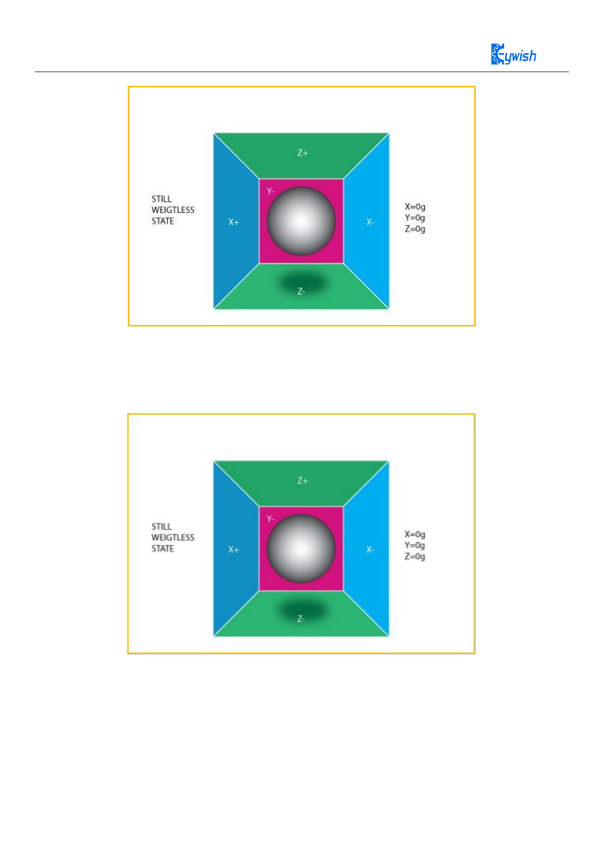
31
Figure 15: Weight loss state acceleration value
If we impose a horizontal left force on the box, then obviously the box will have a left
acceleration, then the imaginary ball in the box will stick to the right side of the box due to
inertia. As shown in the following figure:
Figure 16: Acceleration of an object moving to the right
In order to ensure the physical meaning of the data, the MPU6050 accelerometer marks
the opposite values in three axes of imaginary ball as real acceleration. When the imaginary
ball position is biased toward the forward of an axis, the acceleration of the axis is negative,
and when the imaginary ball position is biased toward a negative axis, the axis's acceleration
reading is positive. According to the above analysis, when we put the MPU6050 chip on the
32
local level, the chip surface is toward the sky, at this time due to the gravity, the position of
the ball is toward the negative direction of Z axis, thus the Z axis acceleration reading should
be positive, and ideally should be “g”. Note that this is not the gravitational acceleration but
the acceleration of physical motion, this can be understood: the acceleration of gravity is
equal to its own movement acceleration value, but in the opposite direction, that is why the
chip can remain stationary.
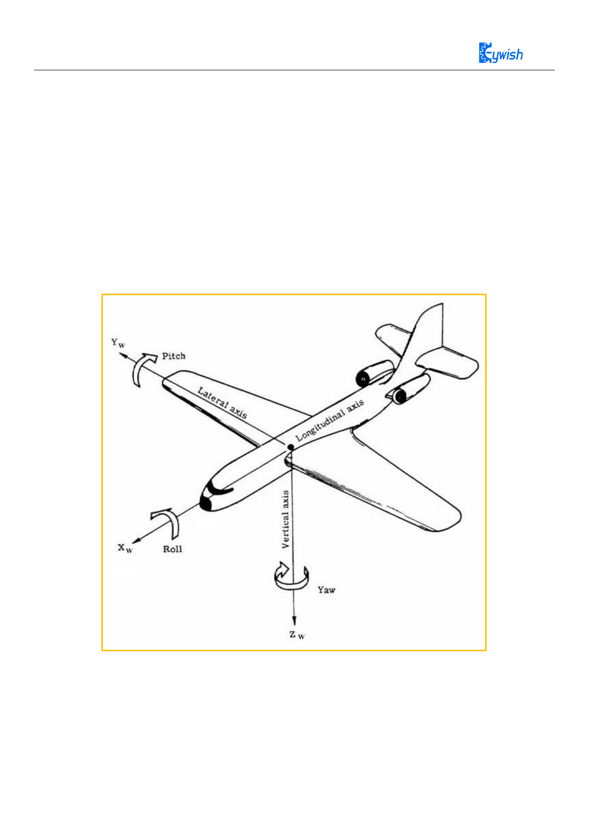
5.4.2 Roll-pitch-yaw model and attitude calculation
A general model for representing the current flight attitude of an aircraft is to establish
the coordinate system as shown below and representing the rotation of the X axis by “Roll”,
the rotation of the Y axis by “Pitch”, the rotation of the Z axis by “Yaw”.
Figure 17: Roll-pitch-yaw model
Since MPU6050 can obtain the upward acceleration of three axes and gravity is always
vertical down, we can calculate the current attitude according to the acceleration of gravity
relative to the chip. For the sake of convenience, we have the chip facing down on the plane
shown above, and the coordinates are in perfect coincidence with the coordinate system of
33
the aircraft. The acceleration in the three axes forms an acceleration vector “a (x, y, z)”.
Assuming that the chip is in a state of uniform linear motion, then the “a” should be
perpendicular to the ground, namely, the negative direction of Z axis, and the length is
|a|=g=\sqrt{x^2+y^2+z^2} (equal to the acceleration of gravity but the opposite direction,
seeing in Section 3.1). If the chip (coordinate system) rotates, the negative direction of the Z
axis will no longer coincide with the “a” because the acceleration vector a is still up
vertically. Seeing below.
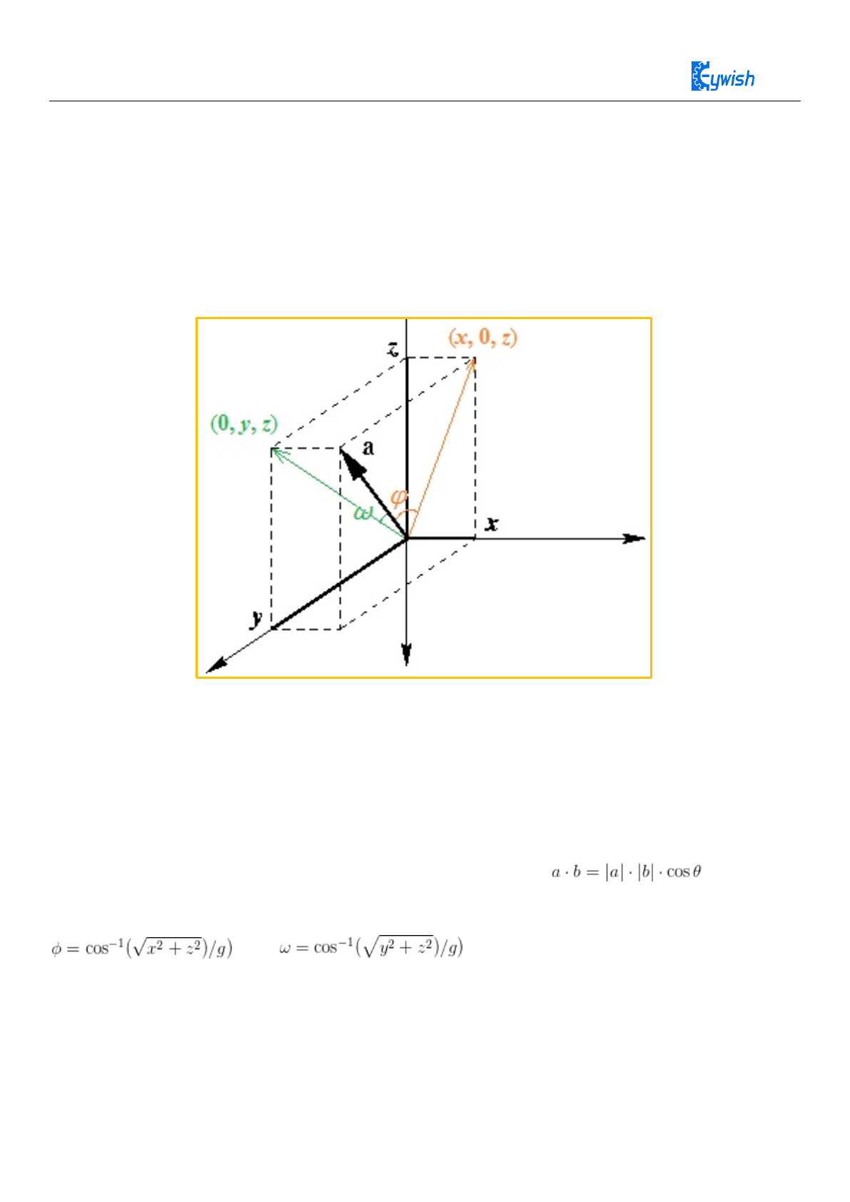
Figure 18: Attitude angle calculation model
For the sake of convenience, the the positive direction of Z axis of the coordinate system
above is (the belly and the front of the chip) downward, and the X axis is toward to the right
(the direction of the plane flying). At this point, the Roll angle “φ” (yellow) of the chip is
formed by the acceleration vector and its projection (x, 0, z) on the XZ plane, the Pitch angle
“ω” (green) is formed by the acceleration vector and its projection on the YZ plane. The dot
product formula can calculate the angle between two vectors: . After
simple deduction:
and .
Note that since the arccos function can only return positive values, you need to take the
positive and negative values of the angle according to different circumstances. When the y
axis is positive, the Roll angle takes a negative value, and when the X axis is negative, the
Pitch angle is negative.

34
5.4.3 Yaw Angle Problem
Since there is no reference, the absolute current angle of the Yaw can’t be calculated, we
can only obtain the variation of Yaw, namely, angular velocity GYR_Z. Of course, we can
use the method of GYR_Z integral to calculate the current Yaw angle (according to the
initial value), by virtue of measurement accuracy, the calculated value is drifting, it is
completely meaningless after a period of time. However, in most applications, such as UAVs,
only GRY_Z is required.
If you have to get the absolute angle of Yaw, then choose MPU9250, a 9-axis motion
tracking chip, it can provide 3-axis compass additional data, so we can calculate the Yaw
angle according to the direction of the earth's magnetic field, the specific method is not
mentioned here.
5.5 Data Processing and Implementation
MPU6050 chip provides data with a serious noise, when the chip is processing in a static
state, the data may swing more than 2%. In addition to the noise, there still exists other
offsets, that is to say, the data does not swing around the static working point, so the data
offset should be calibrated firstly, and then eliminating the noise by filtering algorithm. The
effect of the Kalman filter is undoubtedly the best for data with a large amount of noise. Here
we don’t consider algorithmic details, you can refer to
http://www.starlino.com/imu_guide.html.
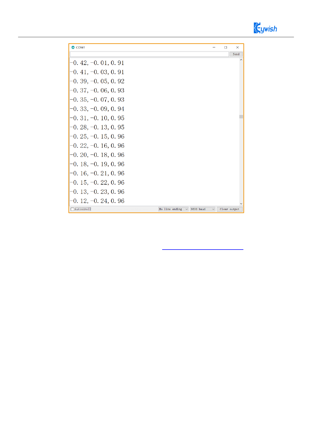
5.5.1 Experiment 3 imu_kalman gets Roll and Pitch
The aim is to display the 3D motion state of the mpu6050 in real-time by reading the mpu6050, and
transmitting the real-time acceleration ACCEL_X, ACCEL_Y, ACCEL_Z data and gyro data GYRO_X,
GYRO_Y, and GYRO_Z to the processing program.
5.5.2 Experiment Code
Arduino experiment code “MotionTrack\Lesson\mpu6050\mpu6050.ino” can get roll and pitch。
Running result is as follows:
35
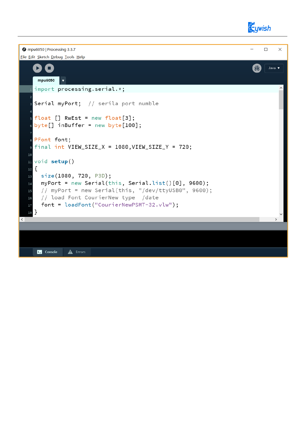
After uploading the program to the Arduino NANO main control board, open the
Processing program “MotionTrack\Processing_demo\mpu6050\mpu6050.pde”
with Processing software (download address https://www.processing.org).
Note that the number in "[]" is not the port number of Arduino NANO, but the serial
number of the communication port. You need to open the device manager of the computer to
view the serial number. For example, my display is COM1, and the serial port used for our
processing. It starts with the subscript 0. So I changed the value in "[ ]" in the Processing
main program to 0. Once the changes are complete, click Run Sketch to run Processing..
36

37
import processing.serial.*;
Serial myPort; // serila port numble
float [] RwEst = new float[3];
byte[] inBuffer = new byte[100];
PFont font;
final int VIEW_SIZE_X = 1080,VIEW_SIZE_Y = 720;
void setup()
{
size(1080, 720, P3D);
myPort = new Serial(this, Serial.list()[0], 9600);
// myPort = new Serial(this, "/dev/ttyUSB0", 9600);
// load Font CourierNew type /date
font = loadFont("CourierNewPSMT-32.vlw");
}
void readSensors() {
if (myPort.available() > 0) {
if (myPort.readBytesUntil('\n', inBuffer) > 0) {
String inputString = new String(inBuffer);
String [] inputStringArr = split(inputString,',');
RwEst[0] = float(inputStringArr[0]);
RwEst[1] = float(inputStringArr[1]);
RwEst[2] = float(inputStringArr[2]);
}
}
}

38
void buildBoxShape() {
//box(60, 10, 40);
noStroke();
beginShape(QUADS);
//Z+
fill(#00ff00);
vertex(-30, -5, 20);
vertex(30, -5, 20);
vertex(30, 5, 20);
vertex(-30, 5, 20);
//Z-
fill(#0000ff);
vertex(-30, -5, -20);
vertex(30, -5, -20);
vertex(30, 5, -20);
vertex(-30, 5, -20);
//X-
fill(#ff0000);
vertex(-30, -5, -20);
vertex(-30, -5, 20);
vertex(-30, 5, 20);
vertex(-30, 5, -20);
//X+
fill(#ffff00);
vertex(30, -5, -20);
vertex(30, -5, 20);
vertex(30, 5, 20);
vertex(30, 5, -20);
//Y-
fill(#ff00ff);
vertex(-30, -5, -20);
vertex(30, -5, -20);
vertex(30, -5, 20);
vertex(-30, -5, 20);

39
//Y+
fill(#00ffff);
vertex(-30, 5, -20);
vertex(30, 5, -20);
vertex(30, 5, 20);
vertex(-30, 5, 20);
endShape();
}
void drawCube() {
pushMatrix();
// normalize3DVec(RwEst);
translate(300, 450, 0);
scale(4, 4, 4);
rotateX(HALF_PI * -RwEst[1]);
//rotateY(HALF_PI * -0.5);
rotateZ(HALF_PI * -RwEst[0]);
buildBoxShape();
popMatrix();
}
void draw() {
// getInclination();
readSensors();
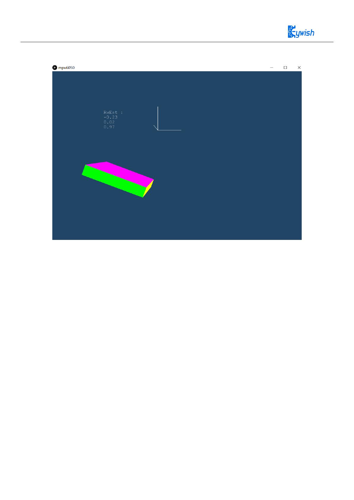
background(#214565);
fill(#ffffff);
textFont(font, 20);
text("RwEst :\n" + RwEst[0] + "\n" + RwEst[1] + "\n" + RwEst[2], 220, 180);
// display axes
pushMatrix();
translate(450, 250, 0);
stroke(#ffffff);
// scale(100, 100, 100);
line(0, 0, 0, 100, 0, 0);
line(0, 0, 0, 0, -100, 0);
line(0, 0, 0, 0, 0, 100);
line(0, 0, 0, -RwEst[0], RwEst[1], RwEst[2]);
popMatrix();
drawCube();
}
40
We can see that our running results are as follows:
Figure 19: Processing presentation renderings
6 Principle of motion tracking control
Through the previous data acquisition of mpu6050 to get the Roll angle and Pitch, we establish the
following correspondence.
Control the lower machine moving object: We can control any lower machine object by getting the speed
and direction through mpu6050.
By reading the mpu6050 real-time verified acceleration ACCEL_X, ACCEL_Y, ACCEL_Z data and
gyroscope data GYRO_X, GYRO_Y, GYRO_Z data are transmitted to the quaternion processing function,
the program displays the Roller and Pitch angle states of the mpu6050 in real time.
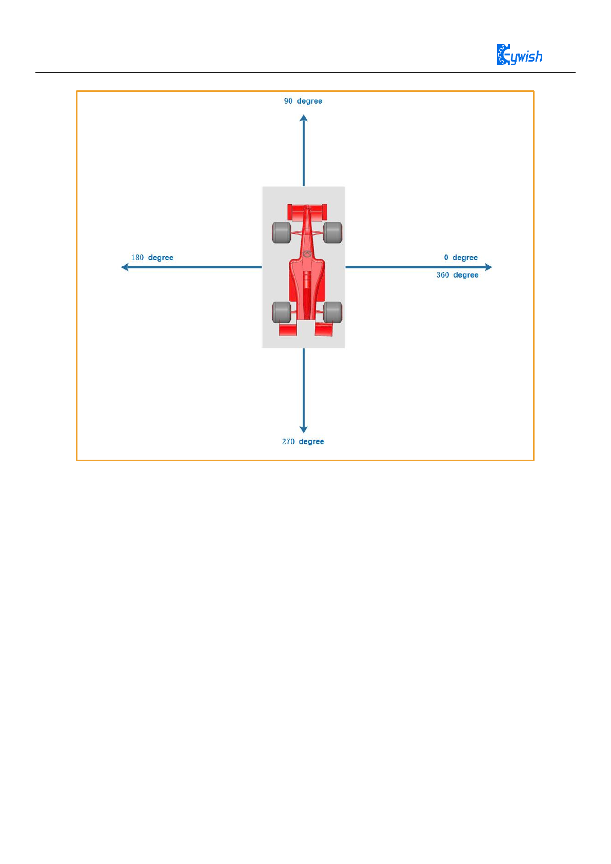
6.1 Racing direction coordinate angle model
In order to facilitate the control of the car, we now establish the following model of the direction of the
motor with the coordinate angle
41
Figure 20: Racing direction angle coordinates
As shown above, we define the front of the car as 90 degrees, 270 degrees to the rear, 180 degrees to the
right, and 0/360 degrees to the left.
0~90 stands for the right front direction. 90~180 stands for the left front 180~270 for the left rear and
270~360 for the right rear.
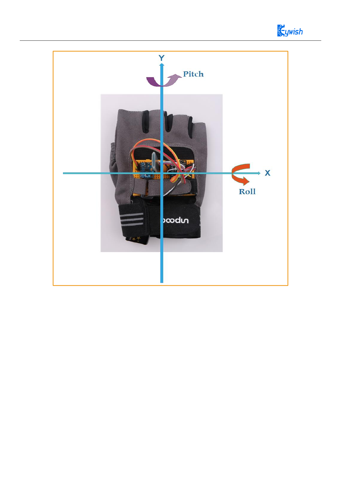
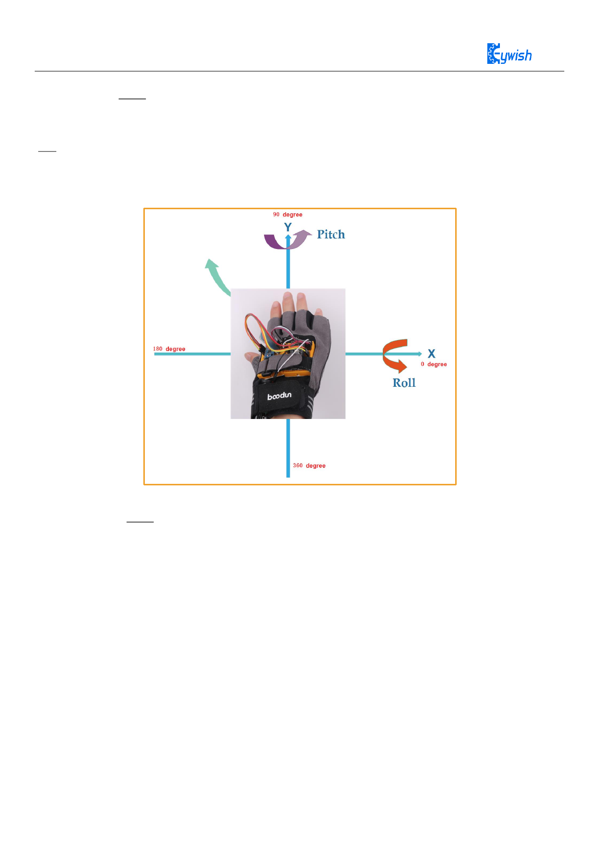
Similarly, we installed the mpu6050 on the sports gloves. We built the following motion model.
42
Figure 21: Directional coordinates of the sports gloves
Through the 5.5.2 Roll-pitch-yaw data model, the sports gloves rotate around the figure Y (turning the back
of the hand left and right) and we get the Pitch angle.
Rotating around X (flip back and forth) we get the Roll angle.
Now that we have an understanding of the coordinates of the attitude angle and the angular coordinates of
the car, we will now describe it to the scene.
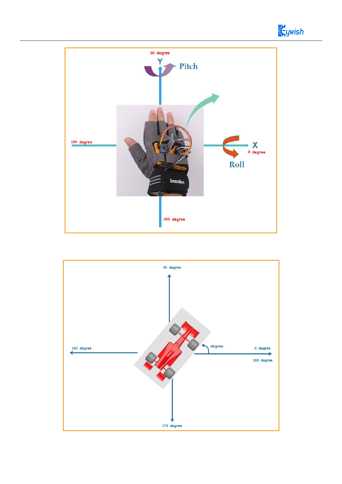
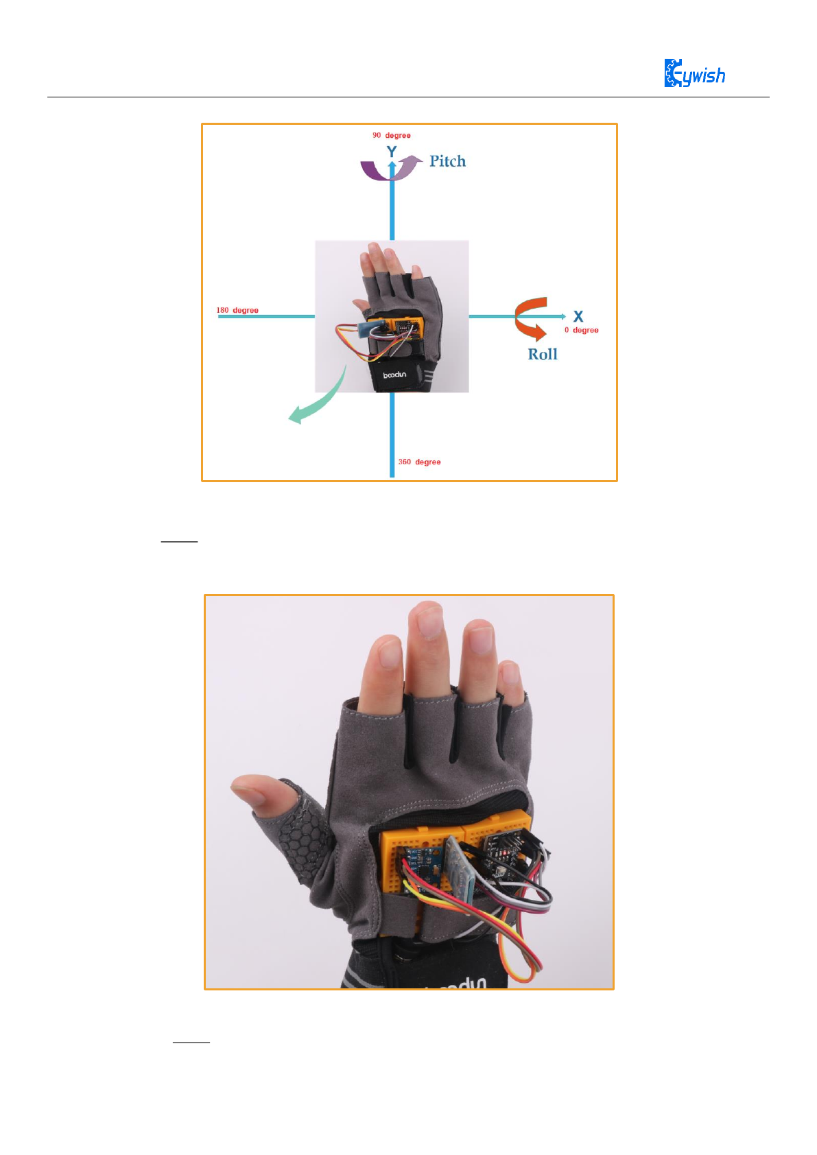
When the sports gloves are tilted to the right front direction, as shown in the figure below, if they are in the
coordinate system, they are inclined to the 0 to 90 degree area.
43
Figure 22: Schematic diagram of the sports gloves tilting to the right front direction
The corner corresponding to the below car is as follows
Figure 23: Schematic diagram of the right front movement of the car
44
Through the attitude of the sports gloves, we need to calculate the angle degree of the movement of the
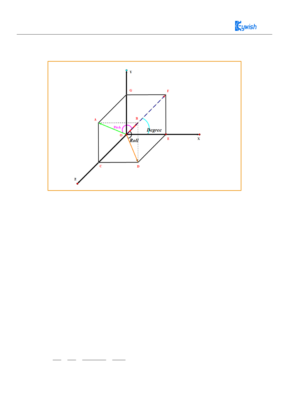
lower machine. So we built the following three-dimensional model
Figure 24: Stereo model diagram based on sports gloves
For convenience of representation, the Z-axis positive direction of the upper coordinate system (the front of
the moving glove) is upward, and the positive X-axis direction (the right side of the sports glove) is to the
right.
In the initial state, the sports gloves remain the same lever with XY .
At this time, the direction in which the sports gloves is tilted is represented by OB, and the Roll angle (black)
is the angle between the acceleration vector OB and its projection (x, 0, z) on the XZ plane, and the Pitch
angle (purple) is its projection on the YZ plane ( The angle between 0, y, and z). The blue color is degree at
which the sports gloves project the projection (x, o, y) on the XY plane. We use this angle to control the
steering angle of the lower car.
We have already got Roll and Pitch through the previous 5.6.1 experiment. Now we calculate the degree by
the following formula.
In the Figure:
BA OA⊥
sin( )AB OB Pitch=
BD OD⊥
B sin( )BD O Roll=
( )
sin( )
sin( )
FE BD R
tan oll Roll
OE AB P
degree itch Pitch
= = =
45
arctand )e (g Roll
P
ree itch
=
Above we have got the steering cosine angle, we need to multiply the coefficient into the coordinate degree.
180 57.3
=
The above analysis is only an angle analysis when tilted like the upper right. Similarly, when the sports
gloves are tilted to the left front
Figure 25: Schematic diagram of the sports gloves tilting to the left front direction
0
arctan( )*57. 9g 0de 3
Pitc
re h
R ll
eo
= − +
Similarly, when the sports gloves are tilted to the left
46
Figure 26: Schematic diagram of the left rear direction of the sports gloves
0
arctan( )*57.3 180deg Roll
Pitc
rh
ee =+
Similarly, when the sports gloves are tilted to the lower right
Figure 27: Schematic diagram of the right rear direction of the sports gloves
0
arctan( )*57.3 270deg Pitc
re h
Roll
e= − +
47
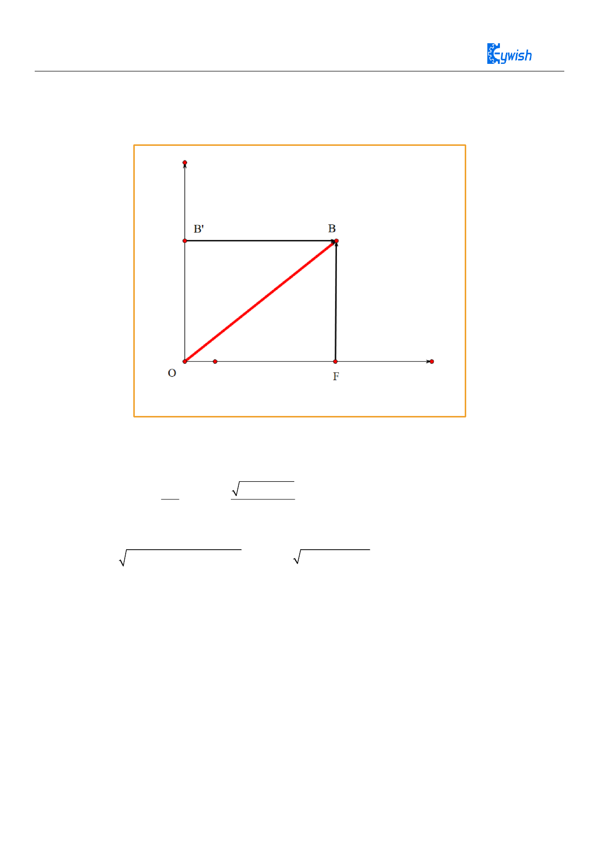
Now let's talk about how to control the speed of the car.
From the above figure we can see that for the sports gloves in the mpu6050 and the plane XY plane tilt
angle, we use the following plane to represent
B'OB
is the angle of inclination relative to the initial state,using this degree of tilt to control the speed of
the car.
22
B'OB= ( ) ( )
OF OE EF
OBF arcsin arcsin
OB OB
+
= =
EF=BD OE=AB
2 2 2 2
( sin ( ) sin ( )) ( )OBF arcsin Roll Pitch arcsin Roll Pitch = + +
The above is the arc angle. We also need to multiply the coefficient. The range of this angle is (0~90). We
directly use this angle as the control speed of the car.

48
float CalculateSpeed(float roll, float pitch)
{
float inclination = asin(sqrt(roll*roll +pitch*pitch))*Rad;
return inclination;
}
void HandInclination(void)
{
static int count = 0;
static int SendSpeed = 0, SendDegree = 0;
count++;
speed = CalculateSpeed(roll, pitch);
if ((-0.2 <= pitch) && (pitch <= 0.2) && (-0.2 <= roll) && (roll <= 0.2)) {
degree = 90;
SendSpeed = 0;
SendDegree += 90;
} else if (pitch < 0 && roll < 0) {
degree = atan(roll/pitch)*Rad;
SendDegree += ((unsigned int)(degree/10))*10;
} else if (pitch > 0 && roll < 0) {
degree = atan(-pitch/roll)*Rad + 90;
SendDegree += ((unsigned int)(degree/10))*10;
} else if (pitch > 0 && roll > 0) {
degree = atan(roll/pitch)*Rad + 180;
} else if (pitch < 0 && roll > 0) {
degree = atan(-pitch/roll)*Rad + 270;
SendDegree += ((unsigned int)(degree/10))*10;
} else {
degree = 90;
SendSpeed = 0;
SendDegree = 90;
}
SendDegree = (int)(speed/10)*10;
if (degree < 30 || degree > 330) {
SendDegree = 0;
}
if (count >= 3) {
count = 0;
Send_Direction(SendDegree/3);
Send_Speed(SendSpeed);
SendDegree = 0;
SendSpeed = 0;
}
}

49
7. Protocol
Use Bluetooth to control the car, in fact is using the Android app to send instructions to the Arduino
serial port via Bluetooth to control the car. Since it involves wireless communication, one of the essential
problems is the communication between the two devices. But there is no common "language" between them,
so it is necessary to design communication protocols to ensure perfect interaction between Android and
Arduino. The main process is: The Android recognizes the control command and package it into the
corresponding packet, then sent to the Bluetooth module (JDY-16), JDY-16 received data and send to
Arduino, then Arduino analysis the data then perform the corresponding action. The date format that the
Android send as below, mainly contains 8 fields.
Protocol
Header
Data Length
Device Type
Device
Address
Function
Code
Control
Data
Check
Sum
Protocol
End Code
In the 8 fields above, we use a structural body to represent.
“Protocol Header” means the beginning of the packet, such as the uniform designation of 0xAA.
“Data length” means except the valid data length of the start and end codes of the data.
“Device type” means the type of device equipment
“Device address” means the address that is set for control
“Function code” means the type of equipment functions that need to be controlled, the function types we
currently support as follows.
typedef struct
{
unsigned char start_code; // 8bit 0xAA
unsigned char len;
unsigned char type;
unsigned char addr;
unsigned short int function; // 16 bit
unsigned char *data; // n bit
unsigned short int sum; // check sum
unsigned char end_code; // 8bit 0x55
}ST_protocol;

50
“Data” means the specific control value of a car, such as speed, angle.
“Checksum” is the result of different or calculated data bits of the control instruction.
“Protocol end code ” is the end part of the data bag when receiving this data ,it means that the data pack has
been sent, and is ready for receiving the next data pack, here we specified it as 0x55.
For example, a complete packet can be such as "AA 070101065000 5F55", in which:
"07" is Transmission Data Length 7 bytes.
"06" is the "device type", such as motor, LED, buzzer and so on. The 06 here refers to the transmission speed,
and the 05 refers to the transmission direction.
"50 (or 0050)" is the controlling data, 0x50 in hexadecimal is 80 when converted to binary, which means the
speed value is 80. If the data is 05, it means the controlling direction, that is 80 degrees (forward).
“005F” is a checksum that is 0x07+0x01+0x01+0x06+0x50=0x5F.
“55” is the end code of the Protocol, indicating the end of data transfer.
typedef enum
{
E_BATTERY = 1,
E_LED = 2,
E_BUZZER = 3,
E_INFO = 4,
E_ROBOT_CONTROL = 5,
E_ROBOT_CONTROL_SPEED = 6,
E_TEMPERATURE = 7,
E_IR_TRACKING = 8,
E_ULTRASONIC = 9,
E_VERSION = 10,
E_UPGRADE = 11,
}E_CONTOROL_FUNC ;
51
8. Comprehensive experiment:
8.1 Nrf24L01 wireless control
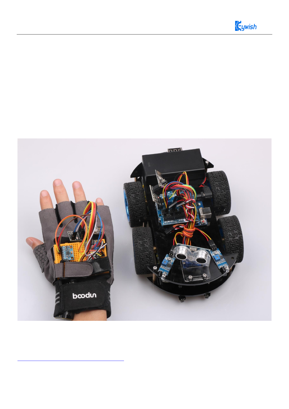
8.1.1 Gesture control Hummer-bot smart car
Connect according to the connection line of the previous chapter, then connect the 9v dry battery to the
Arduino NANO, and download the program. After power-on, the Nrf24L01 module sends data to the
Hummer-Bot Nrf24L01, and then adjust the position of the glove to control the Hummer-Bot multi-function
car, so the car controlled by the sports gloves is born!!
Figure 28: Gesture control hummer-bot
Program link of the lower computer: https://github.com/keywish/keywish-hummer-bot
Hummer-Bot Multi-function car purchase link:Buy on Amazon:
https://www.amazon.com/dp/B078WM15DK
Control demo video Gesture-MotionTracking\video\Control_Hunner-bot.mp4
52
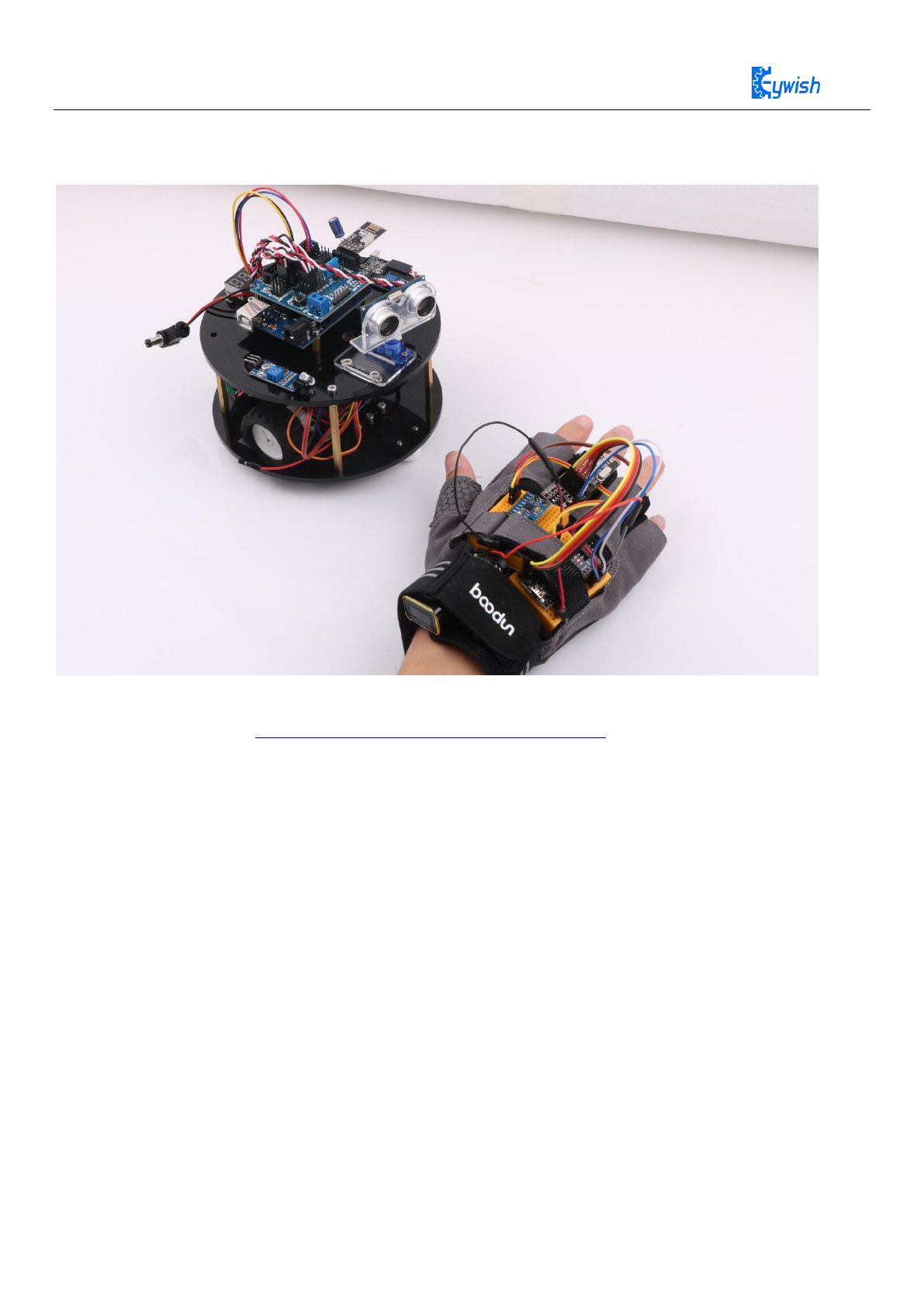
8.1.2 Gesture Control Beetle-bot Smart Car
Figure 29: Gesture Control Beetle-bot
Information on Beetle-bot https://github.com/keywish/keywish-beetle-bot
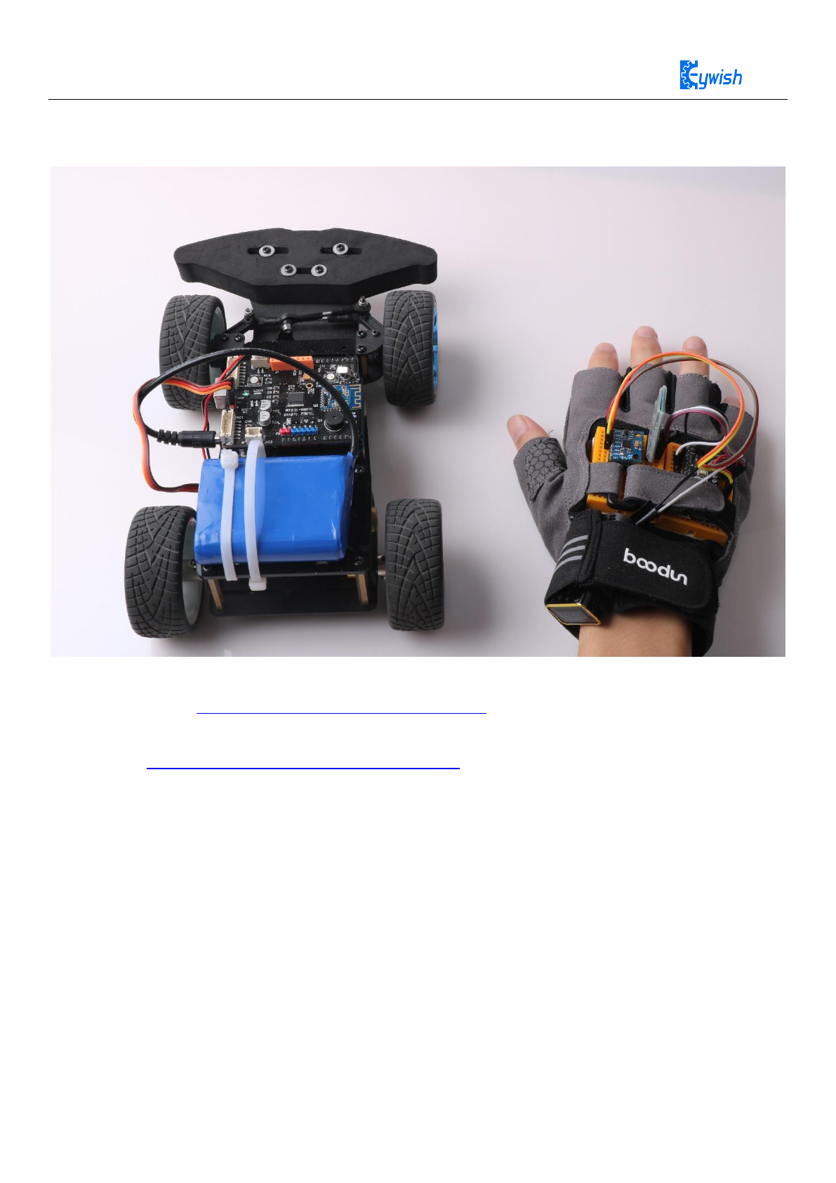
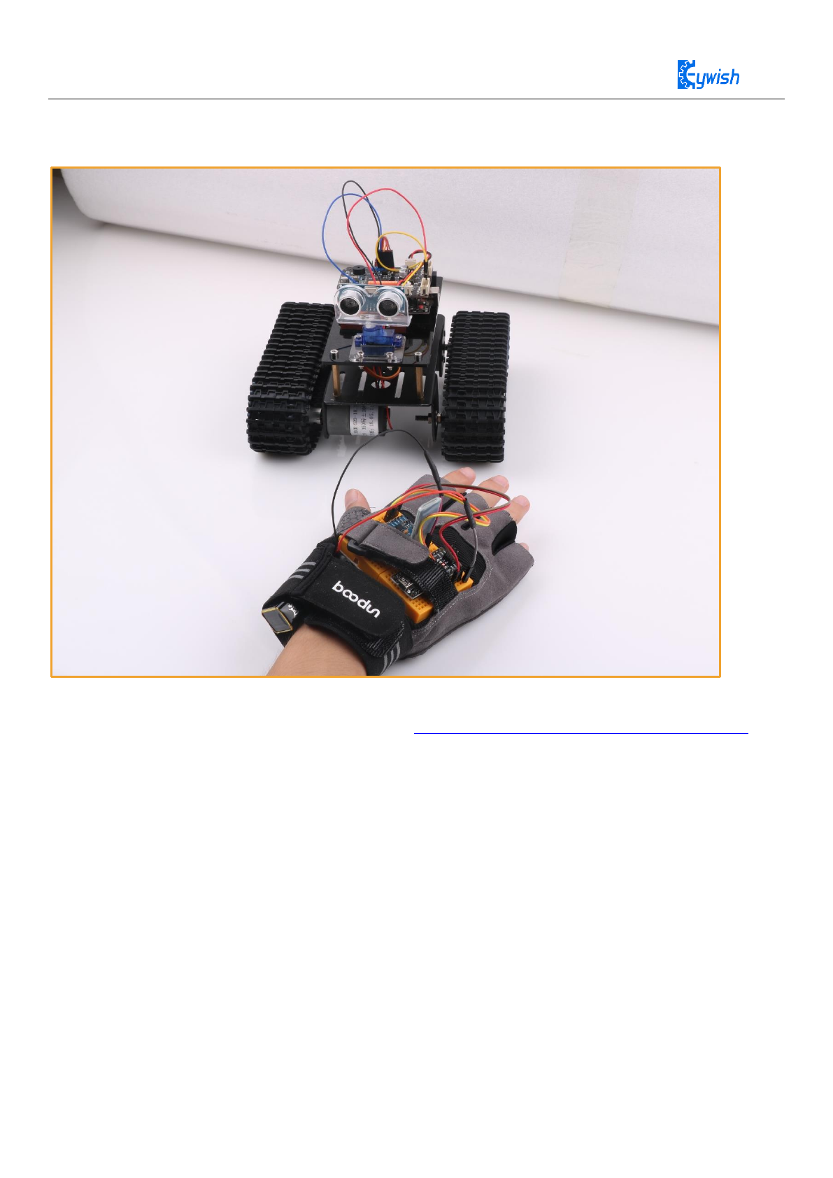
8.2 Bluetooth communication mode control
Connect according to the Bluetooth cable, then connect the 9v dry battery to the Arduino NANO and
download the program (MotionTrack\Lesson\MotionTrack_Bluetooth\ MotionTrack_Bluetooth.ino).
Note that you need to modify the MAC address of the Bluetooth of the lower computer. After power-on, the
sports gloves automatically connect to the Bluetooth module of the car.
55
8.2.3 Gesture control balance car
Figure 32: Gesture Control Mini balance-car
For Balance product information, please refer to https://github.com/keywish/mini-balance-car
