Glue Users Guide Version 4.7
User Manual:
Open the PDF directly: View PDF ![]() .
.
Page Count: 10
1
Guidelines for Installing and Running GLUE Program
Jianqiang He, Cheryl Porter, Paul Wilkens, and James W. Jones
Updated by Gerrit Hoogenboom
September 1, 2017
July 7, 2010
1. Overview
The GLUE (Generalized Likelihood Uncertainty Estimation) program is used to
estimate genotype-specific coefficients for the DSSAT crop models. It is a Bayesian
estimation method that uses Monte Carlo sampling from prior distributions of the
coefficients and a Gaussian likelihood function to determine the best coefficients based
on the data that are used in the estimation process. The GLUE program allows users to
select a crop, then a cultivar to be estimated. The program will then identify all
experiments and treatments in the DSSAT data files for the crop that have measurements
for that cultivar. The user then can select one or more experiments and treatments that
will actually be used in the coefficient estimation process. Another option for the user
is to specify whether to estimate only those coefficients that control phenological
development, only those that deal with expansive and dry matter growth, or both sets.
Generally, one would want to estimate all parameters. What happens then is that the
GLUE program will make 3,000 simulation runs for phenology coefficients and another
3,000 runs for growth coefficients. The program randomly generates parameters that
are being estimated (either phenology or growth) from the prior distribution of
parameter values and runs the model for each. The model outputs are used to select the
parameter set with the maximum likelihood value based on comparison of simulated vs.
observed variables, first for phenology parameters, then for growth parameters. The
program also computes the uncertainties of the estimates (variances) for each parameter.
The maximum likelihood coefficients are written to a file in the same format as the
cultivar file for the selected crop. These values can be copied into the CUL file (e.g.,
MZCER045.CUL or SBGRO045.CUL, etc.) to operate for routine DSSAT applications
and further model evaluations.
What measurements are used to estimate the coefficients? For the development
coefficients, measurements of first flower, physiological maturity, and first
reproductive organ appearance dates are all used. For growth coefficients, final grain
yield, above ground biomass, maximum leaf area during the season, final pod weight,
final main stem leaf number, and unit grain weight are used. Thus, the measurements
that go into File – A in DSSAT are used; these are variables measured only one time
during the season, most of which were measured at harvest.
There are several assumptions that may have important effects on the resulting
parameters. First are the prior distributions of coefficients, which are stored in a file
called ParameterProperty.csv. This file has information for all of the DSSAT v4.7 crops.
We assumed that the parameters have uniform distributions with minimum and
2
maximum values. This is a conservative assumption, and values are provided in the
files based on previous work with the models. A second assumption is that the final
errors between simulated and observed values are normally distributed and are unbiased.
The assumed values of the variances are given in files named
MeasurementVariance_All.csv and others. This assumption may be a problem,
particularly if the model is not able to describe responses for a particular experiment
very well or if observations are not reliable. Another problem will occur if the
experiment had water, nutrient, or other stresses that are either not in the model or that
the model does not represent well. Users should only use treatments that are near stress-
free conditions, if possible, to minimize these problems. Coefficients estimated using
treatments with moderate to severe stress effects will not be reliable. In any case, users
should carefully check results from any estimation process to make sure that results are
realistic and provide good comparisons to observations used in estimation.
There are other cautions that users should be aware of. For example, results from an
estimation process provide conditional estimates of coefficients. That means that the
coefficients are the best set given the measurements that were used, but the coefficients
also depend on the set of observations used in the process. Our aim is for the coefficients
to be robust and useful across environments, but this may not be the case. Another
caution is that coefficients estimated from end of season measurements may not
reproduce observed time series results very well if such measurements were made. We
have seen this occur in various experiments when only end of season measurements are
used, whether using GLUE or other estimation procedures. If users have time series
data, these data can be used manually to refine the coefficients estimated from the
GLUE procedure. It is possible to use in-season measurements and simulations in this
type of Bayesian estimation process, but there are certain complications that make it
difficult to create a robust and reliable automated procedure.
The GLUE program is one of two tools in DSSAT for estimating cultivar coefficients
for the different crops. The first tool, developed by L. A. Hunt and others, evolved from
the GENCALC software available in DSSAT v3.5. There are advantages and
disadvantages of using each. Disadvantages of the GLUE technique is that it may
require a lot of time for the computations, depending on the number of treatments
selected for the estimation process. If there are only 2-5 measurement data sets, one
would expect the GLUE procedure to finish its calculations in less than 2 hours.
However, if there are many measurement data sets, say more than 15, the GLUE method
will likely require several hours of calculations. This is a practical limit. On the other
hand, the GLUE method can be used, without intervention by users, to produce a set of
estimated coefficients. It also provides estimates of the uncertainties of the parameters.
This method does not depend on heuristic rules, making it simple to implement for
additional crops as they are added to DSSAT.
3
2. Installation of the GLUE Program
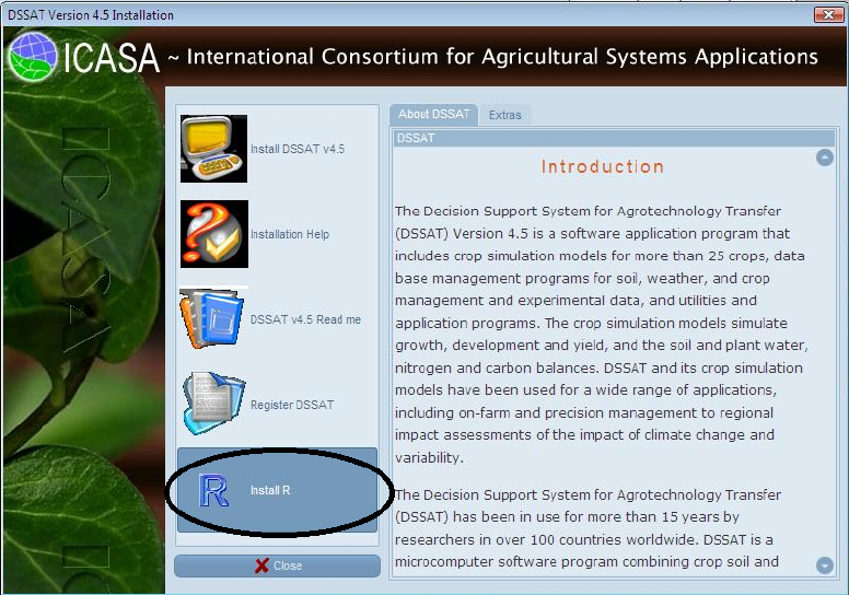
The GLUE program was developed using the R statistical programming language.
You should have R installed on your computer before proceeding. The DSSAT
installation disk has an option to install R, as shown below. You should select the
“Install R” button so that R will be available for use in estimating genetic coefficients
using the GLUE program.
3. Use of the GLUE Procedure to Estimate Genetic Coefficients
3.1 Setting conditions for GLUE to estimate coefficients
The GlueSelect program was written by Paul Wilkens (IFDC) as a tool in DSSAT v4.7.
This tool uses much of the code that he and L. A. Hunt developed for GenSelect, which
is a rule-based estimator of cultivar coefficients. Currently, the GLUE program operates
on most crops (except those legacy crops that are not converted to v4.7 standards).
However, we are more confident of the program correctly estimating cultivar
coefficients for the following crops: maize, soybean, peanut, millet, sorghum, chickpea,
cotton, fababean, sweet corn, tomato, green beans, rice, wheat, and drybean. Users
should check the coefficients carefully before using them. This can be done by putting
the estimated parameters in the appropriate CUL file and simulating the crop
interactively for comparison with observed data.
The file that has definitions of genetic coefficients and their ranges of uncertainty for
all crops is “ParameterProperty.csv” (see Appendix A for details), and
“MeasurementVariance_All.csv” (see Appendix B). These files are stored in the
4
directory “C:\DSSAT45\Tools\GLUE\”. Advanced model users can modify them to set
other ranges of parameters, change parameters to be estimated, introduce parameters
for new crops, and change the order in which they are estimated.
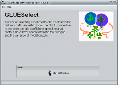
The GLUE program is integrated into the
DSSAT45 shell, and the user runs the
GlueSelect program from the DSSAT
Tools menu to start the process as shown
at right.
5
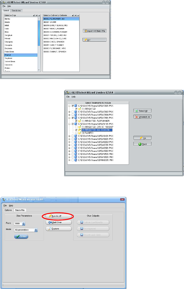
The second GlueSelect screen
shows all of the crops. A user
selects a crop, such as peanut as
shown at left, and then a
particular cultivar that is to be
estimated (“FLORUNNER, std”
in this example). After selecting
“Go” on this screen, a list of
experiments and treatments will
appear as shown below. In this
example, three growing seasons
were selected from three
different years and experiments. These treatments will be simulated, using the GLUE
method to estimate the
coefficients that give the
maximum likelihood for
both phenology and growth
measurements.
The third GlueSelect screen
shows the console for
operating the actual GLUE
calculations and viewing
the results (below). In this
example, there are to be
3,000 runs for all
parameters, which means that there will be 3,000 runs for phenology parameters and
another 3,000 for growth parameters. This number can be changed to a few, say 10, to
make sure that the
program is operating ok.
However, results from
runs less than 3,000
would not likely give
reliable results. So, if the
number is changed from
3,000 to test the
procedure, then it must be
changed back to 3,000 (or
more) in order to get
reliable results. It is ok to
increase this number to
further refine the results,
but more time will be required if this is done.
3.2. Running GLUE
The figure above shows how users initiate the simulation runs to estimate the

6
coefficients using the “Run GLUE” button. Before running GLUE, you may want to
disable on-access scanning of files by your anti-virus software. Our experience is that
the system will operate much faster when virus scanning is disabled for the DSSAT-
generated files. GLUE runs may take some time, possibly from 0.5 to 2 hours for
example, depending on how many seasons are selected for estimating the coefficients.
From this screen, one can view the final estimated coefficients and copy them to put
into the appropriate cultivar file (.CUL in the DSSAT45\Genetics directory) and also to
review statistics (mean, maximum likelihood, and standard deviation of the estimated
coefficients.
3.3 GLUE Results
The main results that users will be interested in can be seen by selecting the “View
Cultivar Coefficient” button on the main screen. This will open an editor with the final
values of the estimated coefficients in it. The format of the file is the same as the CUL
file for the selected crop, so one can copy this new set of cultivar coefficients into the
appropriate CUL file to use in additional simulations. Note that one should use the
DSSAT feature to “Update all Lists” after adding a new cultivar to any CUL file.
All of the outputs of DSSAT and GLUE running are saved in the
“C:\DSSAT45\GLWork\” directory. The contents of main output files are briefly
described as follows:
(a) Optimal Parameters. The optimal parameter set that was chosen through GLUE
procedure was saved as a “CUL” file named according to the name and ID of the
selected cultivar when generating the batch file. For example, if the selected cultivar
was soybean “COBB”, then the “CUL” file is “SBIB0002 COBB.CUL” (Table 1 in
Appendix E).
(b) Statistics of Posterior Distributions (Mean, Standard Deviation, and Maximum
Likelihood Values). The two files identified as “PosteriorDistribution_1.txt” and
“PosteriorDistribution_2.txt” (Table 2 and 3 in Appendix E) store the posterior
distributions for each round of GLUE, including the mean values, standard
deviations, and the parameter set that has the highest likelihood value in that round
of GLUE.
(c) Empirical Distribution of Parameter Tables. The two files identified as
“RandomParameterSetsAndProbability_1.txt” and “RandomParameterSetsAnd
Probability_2.txt” (Table 4 and 5, Appendix E) store the really used parameter sets
and their corresponding probabilities or normalized likelihood values for each
round of GLUE.
(d) Generated Parameter Sets. The two files identified as “RealRandomSets_1.txt”
and “RealRandomSets_2.txt” store the really used parameter set in each round of
GLUE.
(e) Last Model Run Results. “Evaluate_output.txt” stores the content of output file
“Evaluate.OUT” of DSSAT for each model run. Since the “Evaluate_output.txt” is
processed after each model run, only the result of last model run will be available
in the “Evaluate_output.txt” file after the GLUE procedure. This file is not needed
for result analysis, but it is described here because it will be in the directory and

7
model users should ignore it.
(f) Results for Computing Likelihood Values. The two files “EvaluateFrame_1.txt”
and “EvaluateFrame_2.txt” store the appended data of the processed
“Evaluate_output.txt” files for the two rounds of GLUE. In each file, the simulated
and measured outputs are saved for each treatment and each model run.
(g) Combined Likelihood Value for Each Parameter Set. The two files identified as
“IntegratedLikelihoodMatrix_Frame_1.txt”, and “IntegratedLikelihoodMatrix_Frame_2.txt”
(not shown) store the combined likelihood values for all treatments in each model
run or for reach parameter set. For example, in the file
“IntegratedLikelihoodMatrix_Frame_1.txt”, it stores the combined likelihood
values for observations “ADAP”, “MDAP”, and “PD1P” for the first round GLUE.
In “IntegratedLikelihoodMatrix_Frame_2.txt”, it stores the combined likelihood
values for observations “PWAM”, “HWAM”, “CWAM”, “LAIX”, and “L#SM” for
the second round GLUE. When the combined likelihood value is “1” in one column,
it means the observation is absent.
(h) Combined Likelihood Value for Each Experiment Treatment. If there are only two
treatments in the experiment for GLUE procedure, then the following files,
“IntegratedLikelihoodTreatment_1_1.txt”, “IntegratedLikelihoodTreatment_1_2.txt”,
“IntegratedLikelihoodTreatment_2_1.txt”, and “IntegratedLikelihoodTreatment_2_2.txt”,
respectively, store the combined likelihood values for each treatment in each round
of GLUE. The “IntegratedLikelihoodTreatment_1_1.txt” file, for example, stores
the combined likelihood value for GLUE 1 and treatment 1 for all generated
parameter sets, so do other files. One can see these files in the DSSAT45/GLWork
directory after any GLUE estimation procedure is run.
4. How to Add a New Crop
When a new crop is added to DSSAT, cultivar coefficients for this crop can also be
estimated after adding appropriate information in the ParameterProperty.csv file if the
naming conventions for measurements and simulated outputs are standardized and the
same as for other crops. However, if headers are different for a new crop, then additional
information must be added to MeasurementVariance_All.csv file. The
MeasurementVariance_All.csv file shows how additional sheets in the spreadsheet must
be set up for the crop.

8
Appendices
Appendix A
Example Genotype Parameters and Ranges from ParameterProperty.csv File for
Maize and Soybean
Minimum Maximum Fla
g
1
MZ 6 6 6
MZ_P1 5 450 1
MZ_P2 0 2 1
MZ_P5 580 999 1
MZ_G2 248 990 2
MZ_G3 5 16.5 2
MZ_PHINT 49 49 0
SB 18 18 18
SB_CSDL 11.78 14.6 0
SB_PPSEN 0.100 0.385 1
SB_EM.FL 9 23.5 1
SB_FL.SH 10 10 0
SB_FL.SD 12 16 1
SB_SD.PM 29 37.7 1
SB_FL.LF 18 18 0
SB_LFMAX 0.95 1.15 2
SB_SLAVR 300 400 2
SB_SIZLF 140 230 2
SB_XFRT 1 1 0
SB_WTPSD 0.158 0.195 2
SB_SFDUR 17 25.5 2
SB_SDPDV 1.7 2.44 2
SB_PODUR 10 10 0
SB_THRSH 78 78 0
SB_SDPRO 0.4 0.4 0
SB_SDLIP 0.2 0.2 0
1The FLAG column indicates which coefficients are to be estimated using phenology measurements
(FLAG=1), which are to be estimated using growth measurements (FLAG=2) and which
coefficients are not to be estimated (FLAG=0).

9
Appendix B
Variances of Observations for Most Crops
STD Variance CV Flag Description
ADAP 3 9 1 Anthesis day (dap).
MDAP 7 49 1 Physiological maturity day (dap).
PD1T 4 16 1 First pod date (YrDoy).
PWAM 0.3 2 Pod/Ear/Panicle weight at maturity (kg [dm]/ha).
HWAM 0.3 2 Yield at harvest maturity (kg [dm]/ha).
CWAM 0.3 2 Tops weight at maturity (kg [dm]/ha).
LAIX 0.4 2 Leaf area index, maximum.
HWUM 0.1 2 Grain unit weight at maturity (g/seed)
L.SM 3 9 2 Leaf number per stem at maturity. The symbol "#" was changed to ".", since it
is the s
y
mbol of comments in R.
Appendix C
Batch File “COBB.SBC” Created with GLUESelect
$BATCH(CULTIVAR):SBIB0002 COBB
@FILEX TRTNO RP SQ OP
CO
C:\DSSAT45\Soybean\UFGA8101.SBX 1 0 0
0 0
C:\DSSAT45\Soybean\UFGA8501.SBX 1 0 0
0 0
Appendix D
Batch File “GLUE.BAT”
C:\Progra~1\R\R-2.10.1\bin\Rterm --slave <
C:\DSSAT45\Tools\GLUE\GLUE.r
10
Appendix E
Output Files of GLUE Procedure
1. Optimal parameter set saved as a CUL file (SBIB0002 COBB.CUL)
IB0002 COBB (8) . SB0801 12.54 0.373 23.83 9.200 20.11 32.63 18.00 1.090 346.0 162.7 1.000 0.184 17.16 1.846 10.00 78.00 0.400 0.200
2. Posterior distribution in first round GLUE (PosteriorDistribution_1.csv)
Param SB_CSDL SB_PPSEN SB_EM.FL SB_FL.SH SB_FL.SD SB_SD.PM SB_FL.LF SB_LFMAX SB_SLAVR SB_SIZLF SB_XFRT SB_WTPSD SB_SFDUR SB_SDPDV SB_PODUR SB_THRSH SB_SDPRO SB_SDLIP
Mean 12.174 0.303 23.286 9.2 18.558 31.511 18 1.03 375 190 1 0.158 23 1.9 10 78 0.4 0.2
STDEV 0.327 0.073 3.602 0 2.587 2.99 0 0 0 0 0 0 0 0 0 0 0 0
MaxProbability 12.538 0.373 23.831 9.2 20.113 32.635 18 1.03 375 190 1 0.158 23 1.9 10 78 0.4 0.2
3. Posterior distribution in second round GLUE (PosteriorDistribution_2.csv)
Param SB_CSDL SB_PPSEN SB_EM.FL SB_FL.SH SB_FL.SD SB_SD.PM SB_FL.LF SB_LFMAX SB_SLAVR SB_SIZLF SB_XFRT SB_WTPSD SB_SFDUR SB_SDPDV SB_PODUR SB_THRSH SB_SDPRO SB_SDLIP
Mean 12.538 0.373 23.831 9.2 20.113 32.635 18 1.187 345.327 178.795 1 0.184 18.651 2.042 10 78 0.4 0.2
STDEV 0 0 0 0 0 0 0 0.105 25.85 27.183 0 0.008 1.324 0.22 0 0 0 0
MaxProbability 12.538 0.373 23.831 9.2 20.113 32.635 18 1.09 346.041 162.69 1 0.184 17.165 1.846 10 78 0.4 0.2
4. Example random parameter sets and their Likelihood values and in first round GLUE (RandomParameterSetsAndProbability_1.txt)
CSDL PPSEN EM.FL FL.SH FL.SD SD.PM FL.LF LFMAX SLAVR SIZLF XFRT WTPSD SFDUR SDPDV PODUR THRSH SDPRO SDLIP Probability
12.538 0.373 23.831 9.200 20.113 32.635 18.000 1.030 375.000 190.000 1.000 0.158 23.000 1.900 10.000 78.000 0.400 0.200 0.227
12.549 0.364 26.064 9.200 21.883 29.549 18.000 1.030 375.000 190.000 1.000 0.158 23.000 1.900 10.000 78.000 0.400 0.200 0.117
11.791 0.200 26.731 9.200 15.802 34.909 18.000 1.030 375.000 190.000 1.000 0.158 23.000 1.900 10.000 78.000 0.400 0.200 0.115
11.895 0.187 27.931 9.200 16.092 34.792 18.000 1.030 375.000 190.000 1.000 0.158 23.000 1.900 10.000 78.000 0.400 0.200 0.103
11.784 0.262 21.206 9.200 13.915 29.413 18.000 1.030 375.000 190.000 1.000 0.158 23.000 1.900 10.000 78.000 0.400 0.200 0.095
12.339 0.376 19.642 9.200 19.395 28.400 18.000 1.030 375.000 190.000 1.000 0.158 23.000 1.900 10.000 78.000 0.400 0.200 0.085
5. Example random parameter sets and their Likelihood values and in second round GLUE (RandomParameterSetsAndProbability_2.txt)
CSDL PPSEN EM.FL FL.SH FL.SD SD.PM FL.LF LFMAX SLAVR SIZLF XFRT WTPSD SFDUR SDPDV PODUR THRSH SDPRO SDLIP Probability
12.538 0.373 23.831 9.200 20.113 32.635 18.000 1.090 346.041 162.690 1.000 0.184 17.165 1.846 10.000 78.000 0.400 0.200 0.016
12.538 0.373 23.831 9.200 20.113 32.635 18.000 1.029 342.632 189.759 1.000 0.186 17.602 1.775 10.000 78.000 0.400 0.200 0.015
12.538 0.373 23.831 9.200 20.113 32.635 18.000 1.110 330.573 174.342 1.000 0.186 17.317 2.364 10.000 78.000 0.400 0.200 0.015
12.538 0.373 23.831 9.200 20.113 32.635 18.000 1.011 307.951 203.991 1.000 0.190 17.585 2.005 10.000 78.000 0.400 0.200 0.015
12.538 0.373 23.831 9.200 20.113 32.635 18.000 1.082 339.885 225.893 1.000 0.194 18.123 1.792 10.000 78.000 0.400 0.200 0.015
12.538 0.373 23.831 9.200 20.113 32.635 18.000 1.150 375.298 163.908 1.000 0.191 17.539 1.719 10.000 78.000 0.400 0.200 0.014
