Guide To La Te X Kopka, Helmut Et Al
Guide%20to%20LaTeX%20-%20Kopka%2C%20Helmut%20et%20al
Guide%20to%20LaTeX%20-%20Kopka%2C%20Helmut%20et%20al
Guide%20to%20LaTeX%20-%20Kopka%2C%20Helmut%20et%20al
User Manual:
Open the PDF directly: View PDF ![]() .
.
Page Count: 658 [warning: Documents this large are best viewed by clicking the View PDF Link!]
- Title
- Preface vii
- Contents
- I Basics
- 1 Introduction
- 2 Text, Symbols, and Commands
- 3 Document Layout and Organization
- 4 Displayed Text
- 4.10 Footnotes and marginal notes
- 4.11 Comments within text
- 5 Mathematical Formulas
- 6 Graphics Inclusion and Color
- 7 Floating tables and figures
- 8 User Customizations
- II Beyond the Basics
- 9 Document Management
- 10 PostScript and PDF
- 11 Multilingual LATEX
- 12 Math Extensions with AMS-LATEX
- 13 Drawing with LATEX
- 14 Bibliographic Databases and BIBTEX
- 15 Presentation Material
- 16 Letters
- Appendices
- A The New Font Selection Scheme (NFSS)
- B The LATEX Clockwork
- C Error Messages
- D LATEX Programming
- E LATEX and World Wide Web
- F Obsolete LATEX
- G TEX Fonts
- H Command Summary
- H.1 Brief description of the LATEX commands
- H.2 Summary tables and figures
- Bibliography
- Index
- List of Tables
- 10.1 The psnfss packages and their fonts
- 10.2 Acrobat menu actions
- A.1 The NFSS encoding schemes
- A.2 The NFSS series attributes
- A.3 Attributes of the Computer Modern fonts
- D.1 Input coding schemes for inputenc package
- D.2 Alternative commands for special symbols
- G.1 Computer Modern text fonts
- G.2 Root names of the 35 standard PostScript fonts
- G.3 Encoding suffixes
- H.1 Font attribute commands
- H.2 Math alphabet commands
- H.3 Font sizes
- H.4 LATEX 2.09 font declarations
- H.5 Dimensions
- H.6 Accents
- H.7 Special letters from other languages
- H.8 Special symbols
- H.9 Command symbols
- H.10 Greek letters
- H.11 Binary operation symbols
- H.12 Relational symbols
- H.13 Negated relational symbols
- H.14 Brackets
- H.15 Arrows
- H.16 Miscellaneous symbols
- H.17 Mathematical symbols in two sizes
- H.18 Function names
- H.19 Math accents
- H.20 AMS arrows
- H.21 AMS binary operation symbols
- H.22 AMS Greek and Hebrew letters
- H.23 AMS delimiters
- H.24 AMS relational symbols
- H.25 AMS negated relational symbols
- H.26 Miscellaneous AMS symbols
- List of Figures
- 1.1 Sample display with the WinEdt editor
- 3.1 Page layout parameters
- 3.2 Sample title page
- 4.1 The list parameters
- 6.1 An embellished image file
- 10.1 Output produced by pdfTEX with the hyperref package
- 13.1 Comparison of eepic with eepicemu
- 15.2 Title page of a pdfscreen document
- B.1 The TEXLive welcome
- B.2 The TEXLive documentation browser
- B.3 The TDS directory tree
- B.4 Partial directory tree of CTAN servers
- E.1 Example of TEX4ht and techexplorer output
- H.1 Single column page format
- H.2 Double column page format
- H.3 Format of the list environment

A Guide to
L
A
T
EX
and Electronic Publishing
Fourth edition
Helmut Kopka
Patrick W. Daly
Addison-Wesley
Harlow, England Reading, Massachusetts Menlo Park, California
New York Don Mills, Ontario Amsterdam Bonn Sydney Singapore
Tokyo Madrid San Juan Milan Mexico City Seoul Taipei
©Addison Wesley Longman Limited 2004
Addison Wesley Longman Limited
Edinburgh Gate
Harlow
Essex CM20 2JE
England
and Associated Companies throughout the World.
The rights of Helmut Kopka and Patrick W. Daly to be identified as authors of
this Work have been asserted by them in accordance with the Copyright,
Designs and Patents Act 1988.
All rights reserved. No part of this publication may be reproduced, stored in a
retrieval system, or transmitted in any form or by any means, electronic,
mechanical, photocopying, recording or otherwise, without either the prior
written permission of the publisher or a licence permitting restricted copying in
the United Kingdom issued by the Copyright Licensing Agency Ltd,
90 Tottenham Court Road, London W1P 9HE.
The programs in this book have been included for their instructional value.
They have been tested with care but are not guaranteed for any particular
purpose. The publisher does not offer any warranties or representations nor
does it accept any liabilities with respect to the programs.
Many of the designations used by manufacturers and sellers to distinguish their
products are claimed as trademarks. Addison Wesley Longman Limited has
made every attempt to supply trademark information about manufacturers and
their products mentioned in this book. A list of the trademark designations and
their owners appears on page v.
Cover designed by Designers & Partners, Oxford
Typeset by the authors with the L
A
T
EX Documentation System
Printed in Great Britain by Henry Ling Ltd, at the Dorset Press, Dorchester,
Dorset
First published 1993
Second edition 1995
Third edition 1999. Reprinted 1999, 2000
Fourth edition 2004
ISBN ????????????
British Library Cataloguing-in-Publication Data
A catalogue record for this book is available from the British Library
Library of Congress Cataloging-in-Publication Data
Kopka, Helmut.
A guide to L
A
T
EX : and Electronic Publishing
/ Helmut Kopka, Patrick W. Daly -- 4th ed.
p. cm.
Includes bibliographical references and index.
ISBN 0-201-39825-7
1. L
A
T
EX (Computer file) 2. Computerized typesetting. I. Daly,
Patrick W. II. Title.
????????????
??????????? ???????
CIP
v
Trademark notices
METAFONT™is a trademark of Addison-Wesley Publishing Company.
T
EX™,AMS-T
EX™, and AMS-L
A
T
EX™are trademarks of the American
Mathematical Society.
Lucida™is a trademark of Bigelow & Holmes.
Microsoft , MS-DOS , Windows , Internet Explorer are registered
trademarks of Microsoft Corporation.
PostScript , Acrobat Reader , Acrobat logo are registered trademarks and
PDF™a trademark of Adobe Systems Incorporated.
UNIX is a registered trademark in the United States and other countries,
licensed exclusively through X/Open Company, Limited.
VAX™and VMS™are trademarks of Digital Equipment Corporation.
IBM is a registered trademark and techexplorer Hypermedia Browser™a
trademark of International Business Machines Corporation.
Netscape™and Netscape Navigator™are trademarks of Netscape
Communications Corporation.
TrueType™is a trademark and Apple and Macintosh are registered
trademarks of Apple Computer Inc.
Preface
A new edition to A Guide to L
A
T
EXbegs the fundamental question: Has
L
A
T
EX changed so much since the appearance of the third edition in 1999
that a new release of this manual is justified?
The simple answer to that question is ‘Well . . . .’ In 1994, the L
A
T
EX world
was in upheaval with the issue of the new version L
A
T
EX 2ε, and the second
edition of the Guide came out just then to act as the bridge between the
old and new versions. By 1998, the initial teething problems had been
worked out and corrected through semi-annual releases, and the third
edition could describe an established, working system. However, homage
was still paid to the older 2.09 version since many users still employed its
familiar syntax, although they were most likely to be using it in a L
A
T
EX 2ε
environment. L
A
T
EX has now reached a degree of stability that since 2000
the regular updates have been reduced to annual events, which often
appear months after the nominal date, something that does not worry
anyone. The old version 2.09 is obsolete and should no longer play any
role in such a manual. In this fourth edition, it is reduced to an appendix
just to document its syntax and usage.
But if L
A
T
EX itself has not changed substantially since 1999, many of its
peripherals have. The rise of programs like pdfT
EX and dvipdfm for PDF
output adds new possibilities, which are realized, not in L
A
T
EX directly, but
by means of more modern packages to extend the basic features. The
distribution of T
EX/L
A
T
EX installations has changed, such that most users
are given a complete, ready-to-run setup, with all the ‘extras’ that one
used to have to obtain oneself. Those extras include user-contributed
packages, many of which are now considered indispensable. Today ‘the
L
A
T
EX system’ includes much more than the basic kernel by Leslie Lamport,
encompassing the contributions of hundreds of other people. This edition
reflects this increase in breadth.
The changes to the fourth edition are mainly those of emphasis.
1. The material has been reorganized into ‘Basics’ and ‘Beyond the
Basics’ (‘advanced’ sounds too intimidating) while the appendices
contain topics that really can be skipped by most everyday users.
Exception: Appendix H is an alphabetized command summary that
many people find extremely useful (including ourselves).
This reorganizing is meant to stress certain aspects over others. For
vii
viii Preface
example, the section on graphics inclusion and color was originally
treated as an exotic freak, relegated to an appendix on extensions;
in the third edition, it moved up to be included in a front chapter
along with the picture environment and floats; now it dominates
Chapter 6 all on its own, the floats come in the following Chapter 7,
and picture is banished to the later Chapter 13. This is not to say
that the picture features are no good, but only that they are very
specialized. We add descriptions of additional drawing possibilities
there too.
2. It is stressed as much as possible that L
A
T
EX is a markup language,
with separation of content and form. Typographical settings should
be placed in the preamble, while the body contains only logical
markup. This is in keeping with the modern ideas of XML, where
form and content are radically segregated.
3. Throughout this edition, contributed packages are explained at that
point in the text where they are most relevant. The fancyhdr
package comes in the section on page styles, natbib where literature
citations are explained. This stresses that these ‘extensions’ are part
of the L
A
T
EX system as a whole. However, to remind the user that
they must still be explicitly loaded, a marginal note is placed at the
start of their descriptions.
4. PDF output is taken for granted throughout the book, in addition
to the classical DVI format. This means that the added possibilities
of pdfT
EX and dvipdfm are explained where they are relevant. A
separate Chapter 10 on PostScript and PDF is still necessary, and the
best interface to PDF output, the hyperref package by Sebastian
Rahtz, is explained in detail. PDF is also included in Chapter 15 on
presentation material.
On the other hand, the other Web output formats, HTML and XML,
are only dealt with briefly in Appendix E, since these are large topics
treated in other books, most noticeably the L
A
T
EX Web Companion.
5. This book is being distributed with the T
EXLive CD, with the kind
permission of Sebastian Rahtz who maintains it for the T
EX Users
Group. It contains a full T
EX and L
A
T
EX installation for Windows,
Macintosh, and Linux, plus many of the myriad extensions that
exist.
We once again express our hope that this Guide will prove more than
useful to all those who wish to find their way through the intricate world
of L
A
T
EX. And with the addition of the T
EXLive CD, that world is brought
even closer to their doorsteps.
Helmut Kopka and Patrick W. Daly
June, 2003
Contents
Preface vii
I Basics 1
1 Introduction 3
1.1 Just what is L
A
T
EX?.......................... 3
1.2 MarkupLanguages ......................... 4
1.3 T
EXanditsoffspring........................ 6
1.4 How to use this book . . . . . . . . . . . . . . . . . . . . . . . . 10
1.5 Basics of a L
A
T
EXfile......................... 11
1.6 T
EX processing procedure . . . . . . . . . . . . . . . . . . . . . 14
2 Text, Symbols, and Commands 17
2.1 Command names and arguments . . . . . . . . . . . . . . . . 17
2.2 Environments ............................ 19
2.3 Declarations ............................. 20
2.4 Lengths ................................ 21
2.5 Special characters . . . . . . . . . . . . . . . . . . . . . . . . . . 22
2.6 Exercises ............................... 27
2.7 Fine-tuningtext........................... 28
2.8 Worddivision ............................ 34
3 Document Layout and Organization 37
3.1 Documentclass........................... 37
3.2 Pagestyle............................... 42
3.3 Parts of the document . . . . . . . . . . . . . . . . . . . . . . . 52
3.4 Tableofcontents .......................... 58
4 Displayed Text 61
4.1 Changingfont............................ 61
4.2 Centering and indenting . . . . . . . . . . . . . . . . . . . . . . 67
4.3 Lists .................................. 69
4.4 Generalizedlists .......................... 74
4.5 Theorem-like declarations . . . . . . . . . . . . . . . . . . . . 80
ix
x CONTENTS
4.6 Tabulatorstops ........................... 81
4.7 Boxes ................................. 85
4.8 Tables................................. 95
4.9 Printing literal text . . . . . . . . . . . . . . . . . . . . . . . . . 110
4.10 Footnotes and marginal notes . . . . . . . . . . . . . . . . . . 112
4.11 Comments within text . . . . . . . . . . . . . . . . . . . . . . . 118
5 Mathematical Formulas 119
5.1 Mathematical environments . . . . . . . . . . . . . . . . . . . 119
5.2 Main elements of math mode . . . . . . . . . . . . . . . . . . 120
5.3 Mathematical symbols . . . . . . . . . . . . . . . . . . . . . . . 124
5.4 Additional elements . . . . . . . . . . . . . . . . . . . . . . . . 130
5.5 Fine-tuning mathematics . . . . . . . . . . . . . . . . . . . . . 145
5.6 Beyond standard L
A
T
EX....................... 151
6 Graphics Inclusion and Color 153
6.1 The graphics packages...................... 153
6.2 Addingcolor............................. 166
7 Floating tables and figures 169
7.1 Floatplacement........................... 169
7.2 Postponingfloats.......................... 171
7.3 Style parameters for floats . . . . . . . . . . . . . . . . . . . . 171
7.4 Floatcaptions ............................ 173
7.5 Floatexamples............................ 174
7.6 References to figures and tables in text . . . . . . . . . . . . 177
7.7 Some float packages . . . . . . . . . . . . . . . . . . . . . . . . 178
8 User Customizations 181
8.1 Counters ............................... 181
8.2 Lengths ................................ 184
8.3 User-defined commands . . . . . . . . . . . . . . . . . . . . . . 185
8.4 User-defined environments . . . . . . . . . . . . . . . . . . . . 195
8.5 Some comments on user-defined structures . . . . . . . . . 200
II Beyond the Basics 205
9 Document Management 207
9.1 Processing parts of a document . . . . . . . . . . . . . . . . . 207
9.2 In-text references . . . . . . . . . . . . . . . . . . . . . . . . . . 213
9.3 Bibliographies ............................ 216
9.4 Keywordindex............................ 225
CONTENTS xi
10 PostScript and PDF 231
10.1 L
A
T
EXandPostScript ........................ 231
10.2 Portable Document Format . . . . . . . . . . . . . . . . . . . . 236
11 Multilingual L
A
T
E
X251
11.1 The babel system ......................... 252
11.2 Contents of the language.dat file............... 256
12 Math Extensions with AMS-L
A
T
E
X257
12.1 Invoking AMS-L
A
T
EX ........................ 258
12.2 Standard features of AMS-L
A
T
EX................. 258
12.3 Further AMS-L
A
T
EXpackages................... 280
12.4 The AMSfonts ........................... 283
13 Drawing with L
A
T
E
X287
13.1 The picture environment .................... 287
13.2 Extended pictures . . . . . . . . . . . . . . . . . . . . . . . . . . 302
13.3 Other drawing packages . . . . . . . . . . . . . . . . . . . . . . 307
14 Bibliographic Databases and BIBT
E
X309
14.1 The BIBT
EXprogram......................... 309
14.2 Creating a bibliographic database . . . . . . . . . . . . . . . . 311
14.3 Customizing bibliography styles . . . . . . . . . . . . . . . . 321
15 Presentation Material 323
15.1 Slide production with SLIT
EX ................... 324
15.2 Slide production with seminar ................. 330
15.3 Electronic documents for screen viewing . . . . . . . . . . . 340
15.4 Special effects with PDF . . . . . . . . . . . . . . . . . . . . . . 343
16 Letters 351
16.1 The L
A
T
EXletter class....................... 351
16.2 A house letter style . . . . . . . . . . . . . . . . . . . . . . . . . 356
16.3 A model letter customization . . . . . . . . . . . . . . . . . . 359
Appendices
A The New Font Selection Scheme (NFSS) 367
A.1 Font attributes under NFSS . . . . . . . . . . . . . . . . . . . . 368
A.2 Simplified font selection . . . . . . . . . . . . . . . . . . . . . . 370
A.3 Installing fonts with NFSS . . . . . . . . . . . . . . . . . . . . . 372
xii CONTENTS
B The L
A
T
E
X Clockwork 381
B.1 Installing L
A
T
EX............................ 381
B.2 Obtaining the Adobe euro fonts . . . . . . . . . . . . . . . . . 387
B.3 T
EX directory structure . . . . . . . . . . . . . . . . . . . . . . . 387
B.4 TheCTANserver .......................... 389
B.5 Additional standard files . . . . . . . . . . . . . . . . . . . . . 391
B.6 The various L
A
T
EXfiles ....................... 396
C Error Messages 401
C.1 Basic structure of error messages . . . . . . . . . . . . . . . . 401
C.2 Some sample errors . . . . . . . . . . . . . . . . . . . . . . . . 409
C.3 List of L
A
T
EX error messages . . . . . . . . . . . . . . . . . . . . 415
C.4 T
EXerrormessages......................... 424
C.5 Warnings ............................... 429
C.6 Search for subtle errors . . . . . . . . . . . . . . . . . . . . . . 435
D L
A
T
E
X Programming 437
D.1 Class and package files . . . . . . . . . . . . . . . . . . . . . . 437
D.2 L
A
T
EX programming commands . . . . . . . . . . . . . . . . . . 440
D.3 Samplepackages .......................... 451
D.4 Changing preprogrammed text . . . . . . . . . . . . . . . . . 459
D.5 Direct typing of special letters . . . . . . . . . . . . . . . . . . 461
D.6 Alternatives for special symbols . . . . . . . . . . . . . . . . . 462
D.7 Managing code and documentation . . . . . . . . . . . . . . . 462
E L
A
T
E
X and World Wide Web 475
E.1 Converting to HTML . . . . . . . . . . . . . . . . . . . . . . . . 476
E.2 The Extensible Markup Language: XML . . . . . . . . . . . . . 478
E.3 The techexplorer Hypermedia Browser . . . . . . . . . . . 481
F Obsolete L
A
T
E
X483
F.1 The 2.09 preamble . . . . . . . . . . . . . . . . . . . . . . . . . 483
F.2 Fontselection ............................ 484
F.3 Obsolete means obsolete . . . . . . . . . . . . . . . . . . . . . 485
G T
E
X Fonts 487
G.1 Font metrics and bitmaps . . . . . . . . . . . . . . . . . . . . . 487
G.2 Computer Modern fonts . . . . . . . . . . . . . . . . . . . . . . 488
G.3 The METAFONT program ..................... 497
G.4 Extended Computer fonts . . . . . . . . . . . . . . . . . . . . . 498
G.5 PostScriptfonts........................... 503
G.6 Computer Modern as PostScript fonts . . . . . . . . . . . . . 505
LIST OF TABLES xiii
H Command Summary 507
H.1 Brief description of the L
A
T
EX commands . . . . . . . . . . . . 507
H.2 Summary tables and figures . . . . . . . . . . . . . . . . . . . 595
Bibliography 605
Index 607
List of Tables
10.1 The psnfss packages and their fonts . . . . . . . . . . . . . 234
10.2 Acrobat menu actions . . . . . . . . . . . . . . . . . . . . . . . 248
A.1 The NFSS encoding schemes . . . . . . . . . . . . . . . . . . . 368
A.2 The NFSS series attributes..................... 369
A.3 Attributes of the Computer Modern fonts . . . . . . . . . . . 370
D.1 Input coding schemes for inputenc package . . . . . . . . . 462
D.2 Alternative commands for special symbols . . . . . . . . . . 463
G.1 Computer Modern text fonts . . . . . . . . . . . . . . . . . . . 491
G.2 Root names of the 35 standard PostScript fonts . . . . . . . 504
G.3 Encodingsuffixes.......................... 505
H.1 Font attribute commands . . . . . . . . . . . . . . . . . . . . . 595
H.2 Math alphabet commands . . . . . . . . . . . . . . . . . . . . . 595
H.3 Fontsizes............................... 595
H.4 L
A
T
EX 2.09 font declarations . . . . . . . . . . . . . . . . . . . . 595
H.5 Dimensions.............................. 596
H.6 Accents ................................ 596
H.7 Special letters from other languages . . . . . . . . . . . . . . 596
H.8 Specialsymbols........................... 596
H.9 Commandsymbols......................... 596
H.10Greekletters............................. 596
H.11 Binary operation symbols . . . . . . . . . . . . . . . . . . . . . 597
H.12 Relational symbols . . . . . . . . . . . . . . . . . . . . . . . . . 597
H.13 Negated relational symbols . . . . . . . . . . . . . . . . . . . . 597
H.14Brackets................................ 597
H.15Arrows ................................ 598
H.16 Miscellaneous symbols . . . . . . . . . . . . . . . . . . . . . . 598
H.17 Mathematical symbols in two sizes . . . . . . . . . . . . . . . 598
H.18Functionnames........................... 598
H.19Mathaccents............................. 599
H.20 AMSarrows............................. 599
H.21 AMSbinary operation symbols . . . . . . . . . . . . . . . . . 599
xiv CONTENTS
H.22 AMSGreek and Hebrew letters . . . . . . . . . . . . . . . . . 600
H.23 AMSdelimiters........................... 600
H.24 AMSrelational symbols . . . . . . . . . . . . . . . . . . . . . . 600
H.25 AMSnegated relational symbols . . . . . . . . . . . . . . . . 601
H.26 Miscellaneous AMSsymbols................... 601
List of Figures
1.1 Sample display with the WinEdt editor . . . . . . . . . . . . . 16
3.1 Page layout parameters . . . . . . . . . . . . . . . . . . . . . . 48
3.2 Sampletitlepage .......................... 53
4.1 The list parameters ....................... 76
6.1 An embellished image file . . . . . . . . . . . . . . . . . . . . . 160
10.1 Output produced by pdfT
EX with the hyperref package . . 240
13.1 Comparison of eepic with eepicemu ............. 306
15.2 Title page of a pdfscreen document.............. 341
B.1 The T
EXLivewelcome........................ 383
B.2 The T
EXLive documentation browser . . . . . . . . . . . . . . 384
B.3 The TDS directory tree . . . . . . . . . . . . . . . . . . . . . . . 388
B.4 Partial directory tree of CTAN servers . . . . . . . . . . . . . 390
E.1 Example of T
EX4ht and techexplorer output . . . . . . . . 482
H.1 Single column page format . . . . . . . . . . . . . . . . . . . . 602
H.2 Double column page format . . . . . . . . . . . . . . . . . . . 603
H.3 Format of the list environment . . . . . . . . . . . . . . . . 604
Part I
Basics

1
Introduction
1.1 Just what is L
A
T
E
X?
To summarize very briefly:
•L
A
T
EX is a comprehensive set of markup commands used with the
powerful typesetting program T
EX for the preparation of a wide
variety of documents, from scientific articles, reports, to complex
books.
•L
A
T
EX like T
EX is an open software system, available free of charge.
Its core is maintained by the L
A
T
EX3 Project Group but it also benefits
from extensions written by hundreds of user/contributors, with all
the advantages and disadvantages of such a democracy.
•A L
A
T
EX document consists of one or more source files contain-
ing plain text characters, the actual textual content plus markup
commands. These include instructions which can insert graphical
material produced by other programs.
•It is processed by the T
EX program to produce a binary file in DVI
(device independent) format, containing precise directions for the
typesetting of each character. This in turn can be viewed on a moni-
tor, or converted into printer instructions, or some other electronic
form such as PostScript, HTML, XML, or PDF.
•A variant on the T
EX program called pdfT
EX produces PDF output
directly from the source file without going through the DVI inter-
mediary. With this, L
A
T
EX can automatically include internal links
and bookmarks with little or no extra effort, plus PDF buttons and
external links, in addition to graphics in a wide range of common
formats.
•T
EX activities are coordinated by the T
EX Users Group, TUG (www.
tug.org) who distribute a set of CDs, called T
EXLive, annually to its
3
4 Chapter 1. Introduction
members, containing a T
EX/L
A
T
EX installation for various computer
types.
The rest of this book attempts to fill in the gaps in the above summary.
With the help of the included T
EXLive CD for Windows, Macintosh, and
Linux, which also contains a directory specific to this book (\books\
Kopka_and_Daly\), we hope that the user will have additional pleasure
in learning the joys of L
A
T
EX.
1.2 Markup Languages
1.2.1 Typographical markup
In the days before computers, an author would prepare a manuscript
either by hand or by typewriter, which he or she would submit to a pub-
lisher. Once accepted for publication (and after several rounds of correc-
tions and modifications, each requiring a rewrite of the paper manuscript),
it would be sent to a copy editor, a human being who would decorate the
manuscript with markup, marginal notes that inform the typesetter (an-
other human being) which fonts and spacings and other typographical
features should be used to convert it to the final printed form that one
expects of books and articles.
Electronic processing of text today follows a similar procedure, except
that the humans have been replaced by computer programs. (So far the
author has avoided this fate, but they are working on it.) The markup
is normally included directly in the manuscript in such a way that it is
converted immediately to its output form and displayed on the computer
monitor. This is known as WYSIWYG, or ‘what you see is what you get’.
However, what you see is not always what you’ve got. An alternative
that is used more and more by major publishers is markup languages,
in which the raw text is interspersed with indicators ‘for the typesetter.’
The result as seen on the monitor is much the same as a typewritten
manuscript, except that the markup is no longer abbreviated marginal
notes, but cryptic code within the actual text. This source text, which
can be prepared by a simple, dumb text editor program, is converted into
typographically set output by a separate program.
For example, to code the line
He took a bold step forward.
with HTML, the classical markup language of the World Wide Web, one
enters in the source text:
He took a <b>bold step</b> forward.
In Plain T
EX, the same sentence would be coded as:
1.2. Markup Languages 5
He took a {\bf bold step} forward.
The first example is to be processed (displayed) by a Web browser program
that decides to set everything between <b> and </b> as bold face. The
second example is intended for the T
EX program (Section 1.3). The markup
in these two examples follow different rules, different syntax, but the
functionality is the same.
1.2.2 Logical markup
The above examples illustrate typographical markup, where the inserted
commands or tags give direct instructions to alter the appearance of the
output, here a change of font. An alternative is to indicate the purpose
of the text. For example, HTML recognizes several levels of headings; to
place a title into the highest level one enters:
<h1>Logical Markup</h1>
The equivalent L
A
T
EX entry would be:
\section{Logical Markup}
With this logical markup, the author concentrates entirely on the con-
tent and leaves the typographical considerations to the experts. One
merely marks the structure of the document, and has no means of con-
trolling how the logical elements, like section titles, are to be rendered
typographically. This information is put into HTML style sheets or L
A
T
EX
classes and packages, which are external to the actual source file. This
means that the entire layout of a document can be overhauled with only
minimal or even no alterations to the source file.
Today much effort is being put into XML, the Extensible Markup Lan-
guage, as the ultimate markup system, since it allows the markup, or
tags, to be defined as needed, without any indication of how they are to
be implemented. That is left to XSL, the Extensible Stylesheet Language.
It must be emphasized that neither XML nor XSL are programs at all; they
are specifications for how documents and databases may be marked up,
and how the markup tags may be translated into real output. Programs
still need to be found to do the actual job.
And that is the fundamental idea behind markup languages: that the
source text indicates the logical structure of its contents. Such source
files, being written in plain ascii text, are extremely robust, not being
married to any particular software package or computer type.
What does all this have to do with L
A
T
EX? In the next Section we outline
the development of T
EX and L
A
T
EX, and go on to show that L
A
T
EX, a product
of the mid 1980’s, is a programmable markup language that is ideally
suited for the modern world of electronic publishing.
6 Chapter 1. Introduction
1.3 T
E
X and its offspring
The most powerful formatting program for producing book quality text
of scientific and technical works is that of Donald E. Knuth (Knuth, 1986a,
1986b, 1986c, 1986d, 1986e). The program is called T
EX, which is a
rendering in capitals of the Greek letters τχ. For this reason the last
letter is pronounced not as an x, but as the ch in Scottish loch or German
ach, or as the Spanish jor Russian kh. The name is meant to emphasize
that the printing of mathematical texts is an integral part of the program
and not a cumbersome add-on. In addition to T
EX, the same author has
developed a further program called METAFONT for the production of
character fonts. The standard T
EX program package contains 75 fonts
in various design sizes, each of which is also available in up to eight
magnification steps. All these fonts were produced with the program
METAFONT. With additional applications, further character fonts have
been created, such as for Cyrillic, Chinese, and Japanese, with which texts
in these alphabets can be printed in book quality.
The T
EX program is free, and the source code is readily available.
Anybody may take it and modify it as they like, provided they call the
result something other than T
EX. This indeed has occurred, and several
T
EX variants do exist, including pdfT
EX which we deal with later in this
Chapter. Only Knuth is allowed to alter T
EX itself, which he does only to
correct any obvious bugs. Otherwise, he considers T
EX to be completed;
the current version number is 3.14159, and with his death, the code will
be frozen for all time, and the version number will become exactly π.
1.3.1 The T
E
X program
The basic T
EX program only understands a set of very primitive com-
mands that are adequate for the simplest of typesetting operations and
programming functions. However, it does allow more complex, higher-
level commands to be defined in terms of the primitive ones. In this way,
a more user-friendly environment can be constructed out of the low-level
building blocks.
During a processing run, the program first reads in a so-called format
file which contains the definitions of the higher-level commands in terms
of the primitive ones, and which also contains the hyphenation patterns
for word division. Only then does it read in the author’s source file con-
taining the actual text to be processed, including formatting commands
that are predefined in the format file.
Creating new formats is something that should be left to very knowl-
edgeable programmers. The definitions are written to a source file which
is then processed with a special version of the T
EX program called initex.
It stores the new format file in a compact manner so that it can be read
in quickly by the regular T
EX program.
1.3. T
E
X and its offspring 7
Although the normal user will almost never write such a format, he
or she may be presented with a new format source file that will need to
be installed with initex. For example, this is just what must be done to
upgrade L
A
T
EX periodically. How to do this is described in Appendix B.
1.3.2 Plain T
E
X
Knuth has provided a basic format named Plain T
E
Xto interact with T
EX
at its simplest level. This is such a fundamental part of T
EX processing
that one tends to forget the distinction between the actual processing
program T
EX and this particular format. Most people who claim to ‘work
only with T
EX’ really mean that they only work with Plain T
EX.
Plain T
EX is also the basis of every other format, something that only
reinforces the impression that T
EX and Plain T
EX are one and the same.
1.3.3 L
A
T
E
X
The emphasis of Plain T
EX is still very much at the typesetter’s level,
rather than the author’s. Furthermore, the exploitation of all its poten-
tial demands considerable experience with programming techniques. Its
application thus remains the exclusive domain of typographic and pro-
gramming professionals.
For this reason, the American computer scientist Leslie Lamport has
developed the L
A
T
EX format (Lamport, 1985), which provides a set of
higher-level commands for the production of complex documents. With
it, even the user with no knowledge of typesetting or programming is in
a position to take extensive advantage of the possibilities offered by T
EX,
and to be able to produce a variety of text outputs in book quality within
a few days, if not hours. This is especially true for the production of
complex tables and mathematical formulas.
As pointed out in Section 1.2.2, L
A
T
EX is very much more a logical
markup language than the original Plain T
EX, on which it is based. It
contains provisions for automatic running heads, sectioning, tables of
contents, cross-referencing, equation numbering, citations, floating tables
and figures, without the author having to know just how these are to be
formatted. The layout information is stored in additional class files which
are referred to but not included in the input text. The predefined layouts
may be accepted as they are, or replaced by others with minimal changes
to the source file.
Since its introduction in the mid-1980s, L
A
T
EX has been periodically
updated and revised, like all software products. For many years the
version number was fixed at 2.09 and the revisions were only identified
by their dates. The last major update occurred on December 1, 1991, with
some minor corrections up to March 25, 1992, at which point L
A
T
EX 2.09
became frozen.
8 Chapter 1. Introduction
1.3.4 L
A
T
E
X 2ε
The enormous popularity of L
A
T
EX and its expansion into fields for which
it was not originally intended, together with improvements in computer
technology, especially dealing with cheap but powerful laser printers, had
created a diversity of formats bearing the L
A
T
EX label. In an effort to
re-establish a genuine, improved standard, the L
A
T
EX3 Project was set up
in 1989 by Leslie Lamport, Frank Mittelbach, Chris Rowley, and Rainer
Sch¨
opf. Their goal was to construct an optimized and efficient set of
basic commands complemented by various packages to add specific func-
tionality as needed.
As the name of the project implies, its aim is to achieve a version 3
for L
A
T
EX. However, since that is the long-term goal, a first step towards it
was the release of L
A
T
EX 2εin mid-1994 together with the publication of
the second edition of Lamport’s basic manual (Lamport, 1994) and of an
additional book (Goossens et al., 1994) describing many of the extension
packages available and L
A
T
EX programming in the new system. Since then,
two further books have appeared, Goossens et al. (1997) dealing with the
inclusion of graphics and color, and Goossens and Rahtz (1999) explaining
how L
A
T
EX may be used with the World Wide Web. Both these topics are
also dealt with in this Guide.
Initially updates to L
A
T
EX 2εwere issued twice a year, in June and
December, but it has now become so stable that since 2000 the changes
are released only once a year, nominally in June.
L
A
T
EX 2εis now the standard version, and L
A
T
EX 2.09 is considered
obsolete, although source files intended for the older version may still be
processed with the newer one. In this book, unless otherwise indicated,
‘L
A
T
EX’ will always mean L
A
T
EX 2ε.
1.3.5 T
E
X fonts
T
EX initially made use of its own set of fonts, called Computer Modern
generated by Knuth’s METAFONT program. The reason for doing this
was that printers at that time (and even today) may contain their own
preloaded fonts, but they are often slightly different from printer to
printer. Furthermore, they lacked the mathematical character sets that
are essential to T
EX’s main hallmark, mathematical typesetting. So Knuth
created pixel fonts that could be sent to every printer ensuring the same
results everywhere.
Today the situation with fonts has changed dramatically. Outline fonts
(also known as type 1 fonts) are more compact and versatile than the pixel
fonts (type 3). They also have a far superior appearance and are drawn
much faster in PDF files. The original Computer Modern fonts have been
converted to outline fonts, but there is no reason to stick with them,
except possibly for the mathematical symbols. It is L
A
T
EX 2εwith its New
1.3. T
E
X and its offspring 9
Font Selection Scheme that freed T
EX from its rigid marriage to Computer
Modern.
Fonts are discussed in more detail in Appendix G.
1.3.6 The L
A
T
E
X bazaar: user contributions
Like the T
EX program on which is relies, L
A
T
EX is freeware. There may be
a prejudice that what is free in not worth anything, but there are other
examples in the computer world to contradict this statement. And since
the L
A
T
EX macros are provided in files containing plain text, there is no
problem to exchange, modify, and supplement them. In other words, the
user can participate in extending the basic L
A
T
EX system.
Taking advantage of a mechanism in L
A
T
EX 2.09 that allowed options
to the default layouts to be contained in so-called style option files, many
users began writing their own ‘options’ to provide additional features to
the basic L
A
T
EX. They then made these available to other users via the
Internet. Many were intended for very specific problems, but many more
proved to be of such general usefulness that they have become part of the
standard L
A
T
EX installation. In this way, the users themselves have built
up a system that meets their needs.
With L
A
T
EX 2ε, these user contributions acquired official status: they
became known as packages, they could be entered directly into the docu-
ment and not by the back door, guidelines were issued for writing them,
and additional commands were introduced to assist package program-
ming. Package files bear the extension.sty from L
A
T
EX 2.09 days, so that
the older style option files may still function as packages today.
Those packages that have established themselves as indispensable
for sophisticated L
A
T
EX processing are described in this book in those
sections where they are most relevant. This does not imply that other
packages are less worthwhile, but simply that this book does have to
make a selection. Many other packages are described fully in The L
A
T
E
X
Companion (Goossens et al., 1994) and it would go beyond the bounds of
this book to reproduce it here.
1.3.7 L
A
T
E
X and electronic publishing
The most significant development in computer usage in the last decade
is the rise of the World Wide Web (or the hijacking of the Internet by the
glitzy society). L
A
T
EX makes its own contribution here with
•programs to convert L
A
T
EX files to HTML (Appendix E);
•means of creating PDF output, with hypertext features such as links,
bookmarks, active buttons (Chapter 10);

10 Chapter 1. Introduction
•interfacing to XML both by acting as an engine to render XML doc-
uments and with programs to convert L
A
T
EX to XML and vice versa
(Appendix E).
All these forms of electronic publishing are alternatives to traditional
paper output. We do not expect paper to disappear entirely so quickly,
but it is rapidly being replaced by electronic forms, which can always
reproduce the paper whenever needed.
1.4 How to use this book
This Guide is meant to be a mixture of textbook and reference manual.
It explains all the essential elements of the current standard L
A
T
EX 2ε, but
compared to Lamport (1985, 1994), it goes into more detail, offers more
examples and exercises, and describes many ‘tricks’ based on the authors’
experiences. It explains not only the core L
A
T
EX installation, but also many
of the contributed packages that have become essential to modern L
A
T
EX
processing, and thus quasi-standard. We necessarily have to be selective,
for we cannot go to the same extend as The L
A
T
EX Companion (Goossens et
al., 1994), The L
A
T
EX Graphics Companion (Goossens et al., 1997), and The
L
A
T
EX Web Companion (Goossens and Rahtz, 1999), which are still valid
companions to this book.
The first part of the book is entitled The Basics, and deals with the more
fundamental aspects of L
A
T
EX: inputting text and symbols, document or-
ganization, lists and tables, entering mathematics, and customizations by
the user. The second part is called Beyond the Basics, meaning it presents
concepts which may be more advanced but which are still essential to
producing complex, sophisticated documents. The distinction is rather
arbitrary. Finally, the appendices contain topics that are not directly part
of L
A
T
EX itself, but useful for understanding its applications: installation,
error messages, creating packages, World Wide Web, fonts. Appendix H
is an alphabetized summary of most of the commands and their use,
cross-referenced to their locations in the main text.
1.4.1 Some conventions
In the description of command syntax, typewriter type is used to indicate
those parts that must be entered exactly as given, while italic is reserved
for those parts that are variable or for the text itself. For example, the
command to produce tables is presented as follows:
\begin{tabular}{col form}lines \end{tabular}
The parts in typewriter type are obligatory, while col form stands for the
definition of the column format that must be inserted here. The allowed

1.5. Basics of a L
A
T
E
X file 11
values and their combinations are given in the detailed descriptions of
the commands. In the above example, lines stands for the line entries in
the table and are thus part of the text itself.
Sections describing a package, an extension to basic L
A
T
EX, have the
Package:
sample name of that package printed as a marginal note, as demonstrated here
for this paragraph. In this way, you are reminded that you must include
it with \usepackage (Section 3.1.2) in order to obtain the additional
features. Without it, you are likely to get an error message about undefined
commands.
Sections of text that are printed in a smaller typeface together with the boxed
!exclamation mark at the left are meant as an extension to the basic description.
They may be skipped over on a first reading. This information presents deeper
insight into the workings of L
A
T
EX than is necessary for everyday usage, but which
is invaluable for creating more refined control over the output.
1.5 Basics of a L
A
T
E
X file
1.5.1 Text and commands
The source file for L
A
T
EX processing, or simply the L
A
T
E
X file, contains the
source text that is to be processed to produce the printed output. Splitting
the text up into lines of equal width, formatting it into paragraphs, and
breaking it into pages with page numbers and running heads are all
functions of the processing program and not of the input text itself.
For example, words in the source text are strings of letters terminated
by some non-letter, such as punctuation,blanks, or end-of-lines (hard
end-of-lines, ones that are really there, not the soft ones that move with
the window width); whereas punctuation marks will be transferred to the
output, blanks and end-of-lines merely indicate a gap between words.
Multiple blanks in the input, or blanks at the beginning of a line, have no
effect on the interword spacing in the output.
Similarly, a new paragraph is indicated in the input text by an empty
line; multiple empty lines have the same effect as a single one. In the
output, the paragraph may be formatted either by indentation of the first
line, or by extra interline spacing, but this is not affected in any way by
the number of blank lines or extra spaces in the input.
The source file contains more than just text, however; it is also inter-
spersed with markup commands that control the formatting or indicate
the structure. It is therefore necessary for the author to be able to rec-
ognize what is text and what is a command. Commands consist either
of certain single characters that cannot be used as text characters, or of
words preceded immediately by a special character, the backslash (\).
The syntax of source text is explained in detail in Chapter 2.
12 Chapter 1. Introduction
1.5.2 Contents of a L
A
T
E
X source file
Every L
A
T
EX file contains a preamble and a body.
The preamble is a collection of commands that specify the global
processing parameters for the following text, such as the paper format,
the height and width of the text, the form of the output page with its
pagination and automatic page heads and footlines. As a minimum, the
preamble must contain the command \documentclass to specify the
document’s overall processing type. This is the first command in the
preamble.
If there are no other commands in the preamble, L
A
T
EX selects standard
values for the line width, margins, paragraph spacing, page height and
width, and much more. By default, these specifications are tailored to
the American norms. For European requirements, built-in options exist to
alter the text height and width to the A4 standard. Furthermore, there are
language-specific packages to translate certain headings such as ‘Chapter’
and ‘Abstract’.
The preamble ends with \begin{document}. Everything that follows
this command is interpreted as body. It consists of the actual text mixed
with markup commands. In contrast to those in the preamble, these
commands have only a local effect, meaning they apply only to a part of
the text, such as indentation,equations, temporary change of font, and so
on. The body ends with the command \end{document}. This is normally
the end of the file as well.
The general syntax of a L
A
T
EX file is as follows:
\documentclass[options]{class}
Further global commands and specifications
\begin{document}
Text mixed with additional commands of local effect
\end{document}
The possible options and classes that may appear in the \documentclass
command are presented in Section 3.1.1.
A minimal L
A
T
EX file named hi.tex contains just the following lines:
\documentclass{article}
\begin{document}
Hi!
\end{document}
1.5.3 Extending L
A
T
E
X with packages
Packages are a very important feature of L
A
T
EX. These are extensions to
the basic L
A
T
EX commands that are written to files with names that end
in.sty and are loaded with the command \usepackage in the preamble.
Packages can be classified by their origin:
1.5. Basics of a L
A
T
E
X file 13
core packages are an integral part of the L
A
T
EX basic installation and are
therefore fully standard;
tools packages are a set written by members of the L
A
T
EX3 Team, and
should always be in the installation;
graphics packages are a standardized set for including pictures gener-
ated by other programs, and for handling color; they are on the same
level as the tools packages;
AMS-L
A
T
E
Xpackages published by the American Mathematical Society,
should be in any installation;
contributed packages have been submitted by actual users; certain of
these have established themselves as ‘essential’ to standard L
A
T
EX
usage, but all are useful.
Only a limited number of these packages are described in this book, those
that we consider indispensable. However, there is nothing to prevent
the user from obtaining and incorporating any others that should prove
beneficial for his or her purposes.
There are over 1000 contributed packages on the included T
EXLive CD.
How can one begin to get an overview of what they offer? Graham Williams
has compiled a list of brief descriptions which can be found online and
on the T
EXLive CD at
\texmf\doc\html\catalogue\catalogue.html
How to load packages into the L
A
T
EX source file is explained in Sec-
tion 3.1.2.
Documentation of contributed packages is somewhat haphazard, de-
pending on how much the author has put into it. The preferred method
for distributing packages is to integrate the documentation with the
code into a single file with extension .dtx. A special program DocStrip
(Section D.7.1) is used to extract the actual package file or files, while
L
A
T
EXing the original .dtx file produces the instruction manual. Most
ready-to-run installations will already have done all this for the user,
with the resulting manuals stored as DVI or PDF files somewhere in
\texmf\doc\latex\. . . . However, you might have to generate the doc-
umentation output yourself by processing the.dtx file, which should be
found in \texmf\source\latex\. . . . (Section B.3 explains the organiza-
tion of the T
EX directory system.)
Some package authors write their manuals as an extra .tex file, the
output of which may or may not be prestored in DVI or PDF form. Others
provide HTML files. And still others simply add the instructions as
comments in the package file itself. (This illustrates some of the joys of
an open system.)

14 Chapter 1. Introduction
1.6 T
E
X processing procedure
Since L
A
T
EX is a set of definitions for the T
EX program, L
A
T
EX processing itself
is in fact T
EX processing with the L
A
T
EX format. What T
EX does with this is
the same as for any other of the many formats available (of which L
A
T
EX is
perhaps the most popular). All the typesetting work is done by T
EX, while
L
A
T
EX handles the conversion from the logical markup to the typesetting
commands. It also enables cross-referencing, running headlines, table
of contents, literature citations and bibliography, indexing, and more.
However, the processing of the source file to final output is T
EX’s task,
regardless of the format being used.
1.6.1 In the good old days
T
EX arose over 20 years ago before there were such things as PCs, graphical
displays, and before computers were infected with windows or mice. T
EX
and its support programs were invoked from a command line, not with
a mouse click. This may sound very old fashioned, but it did guarantee
portability to all computer types.
The processing steps that were taken in those days still exist with
today’s graphical interfaces, but are now executed more conveniently.
One can still open a ‘command prompt window’ and run them from the
command line.
The first step is of course to use a text editor program to write the
source file containing the actual text and markup. The rules for entering
this source text are explained in Chapter 2. It goes into a text file, or what
is often called an ‘ascii’ file containing only standard punctuation marks,
numbers, unaccented letters, upper and lower case. In other words, the
text is that which can be produced from a standard English typewriter.
The name of the source file normally has the extension.tex; it is then
processed by T
EX to produce a new file with the same base name and the
extension.dvi, for device independent file. This is a binary file (all codes
possible, not a text file) containing precise instructions for the selection
and placement of every symbol, a coded description of the final printed
page. The command to invoke T
EX with the source file hi.tex is
tex &latex hi
meaning run the T
EX program with the format latex. Usually the instal-
lation has defined a shortcut named latex to do this, so
latex hi
should be sufficient. It is only necessary to specify the extension of the
source file name if it is something other than.tex.
During the processing, T
EX writes information, warnings, error mes-
sages to the computer monitor, and to a transcript file with the extension
.log. It is well worth inspecting this file when unexpected results appear.
1.6. T
E
X processing procedure 15
The final step is to produce the printed pages from the DVI file. This
requires another program, a driver, to generate the instructions specific
to the given printer. For example, to produce a PostScript file, one runs
dvips hi
to obtain hi.ps from hi.dvi. And then one sends hi.ps to the PostScript
printer with the regular command for that computer system.
Previewing the DVI file on a computer monitor before printing was
a later development, requiring high quality graphics displays. These
programs are essentially special drivers that send the output directly to
the monitor rather than to a printer or printer file. One very popular
previewer is called with
xdvi hi
to view hi.dvi before committing it to paper.
1.6.2 And today
The various steps for L
A
T
EX processing described above are still necessary
today, and one can open up a command prompt window and carry them
out just as before. However, there now exist intelligent editors with L
A
T
EX-
savvy that not only assist writing the source text, but also will call the
various programs, T
EX, previewer, printer driver, BIBT
EX, MakeIndex (these
are explained later) with a mouse click.
One such editor for Windows, available on the enclosed T
EXLive CD in
the support directory, is called WinShell, written by Ingo H. de Boer (www.
winshell.de). Although free of charge, its author appreciates donations
to offset his expenses.
Another such editor and L
A
T
EX interface is WinEdt by Aleksander Si-
monic (www.winedt.com). A sample window with the opening text of this
chapter is shown in Figure 1.1. This program is available for a 30-day trial
period, after which one must pay a nominal fee to obtain a licence. It is
the editor that we ourselves use and we can highly recommend it.
An alternative is LyX, a free, open source software for document pro-
cessing in near WYSIWYG, acting as a front-end to L
A
T
EX, where the user
need not know anything about L
A
T
EX. See its home page at www.lyx.org.
It must be stressed that all the above are interfaces to an existing L
A
T
EX
installation. On the other hand, there are also commercial packages which
include both the T
EX/L
A
T
EX installation and a graphics interface. These are
listed in Section B.1.1.
1.6.3 Alternative to T
E
X: pdfT
E
X
As we mentioned earlier, it is permitted to use the T
EX source code to
generate something else, as long as it bears another name. One such

16 Chapter 1. Introduction
Figure 1.1: Sample display with the WinEdt editor for interfacing to L
A
T
EX.
modification is called pdfT
EX, created by H`
an Thˆ
e
´Th`
anh. This program
does everything T
EX does, but it optionally writes its output directly to a
PDF file, bypassing the DVI output of regular T
EX. It therefore combines
the T
EX program with a DVI-to-PDF driver program. Normally this option
is also the default.
There are many advantages to producing PDF output directly this way,
apart from saving a step. The PDF file is generated in exactly the same way
as the DVI file with T
EX, and can be viewed immediately with the Acrobat
Reader or other PDF viewer. The results can be sent directly to a printer
without going through the DVI-to-Printer program. It is also much easier
to include the hypertext features of a true active PDF file, as we explain in
Section 10.2.4.
Adding the L
A
T
EX macros to pdfT
EX produces something one could call
pdfL
A
T
EX. This distinction is only meaningful for invoking the program-
plus-format to process the L
A
T
EX source file. Except for some things that
we note in Section 10.2.3, L
A
T
EX commands are identical whether used with
T
EX or with pdfT
EX. This makes the conversion extremely easy.
The rest of this book deals essentially with L
A
T
EX itself, regardless of
what the end product is to be: paper, HTML, XML, or PDF.
2
Text, Symbols, and
Commands
The text that is to be the input to a L
A
T
EX processing run is written to a
source file with a name ending in.tex, the file name extension. This file is
prepared with a text editor, either one that handles straightforward plain
text, or one that is configured to assist the writing and processing of L
A
T
EX
files. In either case, the contents of this file are plain ascii characters
only, with no special symbols, no accented letters, preferably displayed in
a fixed width typewriter font, with no frills like bold or italics, all in one
size. All these aspects of true typesetting are produced afterwards by
the T
EX processing program with the help of markup commands inserted
visibly into the actual text. It is therefore vital to know how commands
are distinguished from text that is to be printed, and, of course, how they
function.
(However, for languages other than English, native keyboard input may
indeed be used, as shown in Section 2.5.9.)
2.1 Command names and arguments
Acommand is an instruction to L
A
T
EX to do something special, like print
some symbol or text not available to the restricted character set used
in the input file, or to change the current typeface or other formatting
properties. There are three types of command names:
•the single characters #$&˜_ˆ%{}all have special meanings
that are explained later in this chapter;
•the backslash character \plus a single non-letter character; for
example \$ to print the $sign; all the special characters listed above
have a corresponding two-character command to print them literally;
•the backslash character \plus a sequence of letters, ending with the
first non-letter; for example, \large to switch to a larger typeface.
17

18 Chapter 2. Text, Symbols, and Commands
Command names are case sensitive, so \large,\Large and \LARGE
are distinct commands.
Many commands operate on some short piece of text, which then
appears as an argument in curly braces following the command name.
For example, \emph{stress} is given to print the word stress in an
emphasized typeface (here italic) as stress. Such arguments are said to be
mandatory because they must always be given.
Some commands take optional arguments, which are normally em-
ployed to modify the effects of the command somehow. The optional
arguments appear in square braces.
In this book we present the general syntax of commands as
\name[optional]{mandatory}
where typewriter characters must be typed exactly as illustrated and
italic text indicates something that must be substituted for. Optional
arguments are put into square brackets [ ] and the mandatory ones into
curly braces { }. A command may have several optional arguments, each
one in its set of brackets in the specified sequence. If none of the optional
arguments is used, the square brackets may be omitted. Any number of
blanks, or even a single new line, may appear between the command name
and the arguments, to improve legibility.
Some commands have several mandatory arguments. Each one must
be put into a { } pair and their sequence must be maintained as given in
the command description. For example,
\rule[lift]{width}{height}
produces a black rectangle of size width and height, raised by an amount
lift above the current baseline. A rectangle of width 10 mm and height
3 mm is made with \rule{10mm}{3mm}. Since the optional argument lift
is omitted, the rectangle is set on the baseline with no lifting, as .
The arguments must appear in the order specified by the syntax and may
not be interchanged.
Some commands have a so-called *-form in addition to their normal
appearance. A * is added to their name to modify their functionality
somehow. For example, the \section command has a *-form \section*
which, unlike the regular form, does not print an automatic section num-
ber. For each such command, the difference between the normal and
*-form will be explained in the description of the individual commands.
Command names consist only of letters, with the first non-letter indi-
cating the end of the name. If there are optional or mandatory arguments
following the command name, then it ends before the [or {bracket,
since these characters are not letters. Many commands, however, possess
no arguments and are composed of only a name, such as the command
\LaTeX to produce the L
A
T
EX logo. If such a command is followed by
2.2. Environments 19
a punctuation mark, such as comma or period, it is obvious where the
command ends. If it is followed by a normal word, the blank between
the command name and the next word is interpreted as the command
terminator: The \LaTeX logo results in ‘The L
A
T
EXlogo’, that is, the blank
was seen only as the end of the command and not as spacing between
two words. This is a result of the special rules for blanks, described in
Section 2.5.1.
In order to insert a space after a command that consists only of a name,
either an empty structure {} or a space command (\and blank) must be
placed after the command. The proper way to produce ‘The L
A
T
EX logo’ is
to type either The \LaTeX{} logo or The \LaTeX\ logo. Alternatively,
the command itself may be put into curly braces, as The {\TeX} logo,
which also yields the right output with the inserted blank: ‘The T
EX logo’.
Incidentally, the L
A
T
EX 2εlogo is produced with \LaTeXe. Can you see why
this logo command cannot be named \LaTeX2e?
2.2 Environments
An environment is initiated with the command \begin{name}and is
terminated by \end{name}.
An environment has the effect that the text within it is treated dif-
ferently according to the environment parameters. It is possible to alter
(temporarily) certain processing features, such as indentation, line width,
typeface, and much more. The changes apply only within the environ-
ment. For example, with the quote environment,
previous text
\begin{quote}
text1 \small text2 \bfseries text3
\end{quote}
following text
the left and right margins are increased relative to those of the previous
and following texts. In the example, this applies to the three texts text1,
text2, and text3. After text1 comes the command \small, which has the
effect of setting the next text in a smaller typeface. After text2, there is an
additional command \bfseries to switch to bold face type. Both these
commands only remain in effect up to the \end{quote}.
The three texts within the quote environment are indented on
both sides relative to the previous and following texts. The
text1 appears in the normal typeface, the same one as outside
the environment. The text2 and text3 appear in a smaller typeface,
and text3 furthermore appears in bold face.
After the end of the quote environment, the subsequent text appears in
the same typeface that was in effect beforehand.
20 Chapter 2. Text, Symbols, and Commands
Note that if the names of the environment in the \begin{..} \end{..}
pair do not match, an error message will be issued on processing.
Most declaration command names (see next section) may also be used
as environment names. In this case the command name is used without
the preceding \character. For example, the command \em switches to
an emphatic typeface, usually italic, and the corresponding environment
\begin{em} will set all the text in italic until \end{em} is reached.
A nameless environment can be simulated by a {...} pair. The effect
of any command within it ends with the closing curly brace.
The user can even create his or her own environments, as described in
Section 8.4.
2.3 Declarations
Adeclaration is a command that changes the values or meanings of
certain parameters or commands without printing any text. The effect of
the declaration begins immediately and ends when another declaration
of the same type is encountered. However, if the declaration occurs
within an environment or a {...} pair, its scope extends only to the
corresponding \end command, or to the closing brace }. The commands
\bfseries and \small mentioned in the previous section are examples
of such non-printing declarations that alter the current typeface.
Some declarations have associated arguments, such as the command
\setlength which assigns a value to a length parameter (see Sections 2.4
and 8.2).
Examples:
{\bfseries This text appears in bold face} The \bfseries dec-
laration changes the typeface: This text appears in bold face. The
effect of this declaration ends with the closing brace }.
\setlength{\parindent}{0.5cm} The paragraph indentation is set to
0.5 cm. The effect of this declaration ends with the next encounter
of the command \setlength{\parindent}, or at the latest with
the \end command that terminates the current environment.
\pagenumbering{roman} The page numbering is to be printed in Roman
numerals.
Some declarations, such as the last example, are global, that is, their
effects are not limited to the current environment. The following decla-
rations are of this nature, the meanings of which are given later:
\newcounter \pagenumbering \newlength
\setcounter \thispagestyle \newsavebox
\addtocounter

2.4. Lengths 21
Declarations made with these commands are effective right away and
remain so until they are overridden by a new declaration of the same type.
In the last example above, page numbering will be done in Roman numerals
until countermanded by a new \pagenumbering{arabic} command.
2.4 Lengths
2.4.1 Fixed lengths
Lengths consist of a decimal number with a possible sign in front (+or
-) followed by a mandatory dimensional unit. Permissible units and their
abbreviated names are:
cm centimeter,
mm millimeter,
in inch (1 in = 2.54 cm),
pt point (1 in = 72.27 pt),
bp big point (1 in = 72 bp),
pc pica (1 pc = 12 pt),
dd didˆ
ot point (1157 dd = 1238 pt),
cc cicero (1 cc = 12 dd),
em a font-specific size, the width of the capital M,
ex another font-related size, the height of the letter x.
Decimal numbers in T
EX and L
A
T
EX may be written in either the English
or European manner, with a period or a comma: both 12.5cm and 12,5cm
are permitted.
Note that 0is not a legitimate length since the unit specification is
missing. To give a zero length it is necessary to add some unit, such as
0pt or 0cm.
Values are assigned to a length parameter by means of the L
A
T
EX com-
mand \setlength, which is described in Section 8.2 along with other
commands for dealing with lengths. Its syntax is:
\setlength{\length name}{length spec}
For example, the width of a line of text is specified by the parameter
\textwidth, which is normally set to a default value depending on the
class, paper type, and font size. To change the line width to be 12.5 cm,
one would give:
\setlength{\textwidth}{12.5cm}
2.4.2 Rubber lengths
Some parameters expect a rubber length. These are lengths that can be
stretched or shrunk by a certain amount. The syntax for a rubber length
is:
22 Chapter 2. Text, Symbols, and Commands
nominal value plus stretch value minus shrink value
where the nominal value, stretch value, and shrink value are each a length.
For example,
\setlength{\parskip}{1ex plus0.5ex minus0.2ex}
means: the extra line spacing between paragraphs, called \parskip, is to
be the height of the xin the current font, but it may be increased to 1.5
or reduced to 0.8 times that size.
One special rubber length is \fill. This has the natural length of
zero but can be stretched to any size.
2.5 Special characters
2.5.1 Spaces
The space or blank character has some properties different from those
of normal characters, some of which have already been mentioned in
Section 2.1. During processing, blanks in the input text are replaced by
rubber lengths (Section 2.4.2) in order to allow the line to fill up to the
full line width. As a result, some peculiar effects can occur if one is not
aware of the following rules:
•one blank is the same as a thousand, only the first one counts;
•blanks at the beginning of an input line are ignored;
•blanks terminating a command name are removed;
•the end of a line is treated as a blank.
Some of the consequences of these rules are that there may be as many
blanks as desired between words or at the beginning of a line (to make
the input text more legible) and that a word may come right at the end of
a line without the spacing between it and the next word disappearing. To
force a space to appear where it would otherwise be ignored, one must
give the command \(a \followed by a space character, made visible here
by the symbol ).
To ensure that certain words remain together on the same line, a pro-
tected space is inserted between them with the ˜character (Section 2.7.1,
page 28). Multiple protected spaces are all printed out, in contrast to
normal spaces.
Sometimes it is necessary to suppress the space that appears because
of the new line. In this case, the last character in the line must be the
comment character %(Section 4.11).
Paragraphs are separated in the source text by blank lines. As for
blank characters, one blank line is the same as a thousand.
2.5. Special characters 23
Instead of a blank line, the command \par may also be used to indicate
the end of a paragraph.
2.5.2 Quotation marks
The quotation marks found on the typewriter "are not used in book
printing. Instead different characters are used at the beginning and end,
such as ‘single quotes’ and “double quotes”. Single quotes are produced
with ‘and ’, while double quotes are made by typing the respective
characters twice: ‘‘ for “ and ’’ for ”. Furthermore the typewriter
character "will also generate the double closing quote ”. However, it
should be avoided since it can lead to confusion.
2.5.3 Hyphens and dashes
In book printing, the character that appears on the typewriter as -comes
in various lengths: -, –, —. The smallest of these, the hyphen, is used
for compound words such as father-in-law and for word division at the
end of a line; the middle-sized one, the en dash, is used in ranges of
numbers, for example, pages 33–36; and the largest, the em dash, is used
as punctuation—what is normally called the dash. These are generated
by typing the hyphen character one, two, or three times, so that -yields
-, while -- makes –, and --- produces —. A fourth type of dash is the
minus sign −, which is entered in math mode as $-$ (Chapter 5).
2.5.4 Printing command characters
As mentioned in Section 2.1, the characters #$˜_ˆ%{}are inter-
preted as commands. To print them as text, one must give a command
consisting of \plus that character.
$=\$ & = \& % = \% # = \# =\_ {=\{ }=\}
2.5.5 The special characters , , , , and
These special characters do not exist on the computer keyboard. They
can however be generated by special commands as follows:
§=\S †=\dag ‡=\ddag ¶=\P ©=\copyright £=\pounds
The production of Greek letters and other mathematical symbols is
described in Chapter 5.
24 Chapter 2. Text, Symbols, and Commands
2.5.6 Non-English letters
Special letters that exist in languages other than English can also be
generated with T
EX. These are:
œ={\oe} Œ={\OE} æ={\ae} Æ={\AE} ˚
a={\aa} ˚
A ={\AA} ¡ =!‘
ø ={\o} Ø ={\O} ł ={\l} Ł ={\L} ß={\ss} SS={\SS} ¿=?‘
˚
Angstrøm may be written as {\AA}ngstr{\o}m while Karlstraße can be
input as Karlstra{\ss}e. The ‘letter’ \SS is the upper case equivalent
of \ss, used for automatic conversion between upper and lower case.
However, see Section 2.5.9 for the possibility of entering such charac-
ters directly.
2.5.7 Accents
In non-English languages, there is a multiplicity of diacritical marks or
accents, most of which can be printed with T
EX:
`
o =\‘{o} ´
o=\’{o} ˆ
o=\ˆ{o} ¨
o=\"{o} ˜
o=\˜{o}
¯
o =\={o} ˙
o=\.{o} ˘
o=\u{o} ˇ
o=\v{o} ˝
o=\H{o}
oo=\t{oo} o¸=\c{o} o
.=\d{o} o
¯=\b{o} ˚
o=\r{o}
The oabove is given merely as an example: any letter may be used. With
iand jit should be pointed out that the dot must first be removed. This
is carried out by prefixing these letters with a backslash: the commands
\i and \j yield ı and . In this way ˘
ı and ˝
are formed by typing \u{\i}
and \H{\j}.
The accent commands consisting of a non-letter may also be given
without the curly braces:
`
o=\‘o ´
o=\’o ˆ
o=\ˆo ¨
o=\"o ˜
o=\˜o ¯
o=\=o ˙
o=\.o
The letter accent commands should always be used with the curly braces.
2.5.8 The euro symbol
The euro symbol €(or e) is too new to be part of the original L
A
T
EX, but it
can be produced with the help of some additional fonts and contributed
packages. Just which package you may use depends on your installation,
and whether you have access to these additional fonts.
The Text Companion fonts, described in Section G.4.4, do contain a
euro symbol. Since these fonts should be part of every modern L
A
T
EX
installation, you should be able to use their euro symbol if all else fails.
The package textcomp must be loaded in the preamble with
Package:
textcomp
\usepackage{textcomp}
2.5. Special characters 25
which defines many commands including \texteuro to print the symbol
€. Since the European Commission originally dictated that it should only
be printed in a sans serif font, it is better to issue \textsf{\texteuro} to
produce €. (The font selection commands are described in Section 4.1.4.)
If you are going to use this very frequently, you might want to define a
shortcut named \euro with
\newcommand{\euro}{\textsf{\texteuro}}
as described in Section 8.3 on defining commands.
A better solution is presented by the eurosym package by Henrik
Package:
eurosym Theiling and the associated fonts that come with it, which bear the names
feymr10,feybr10, and so on. This package defines the \euro command
to print e, which changes automatically to bold eand slanted eas
needed.
The europs package by Joern Clausen interfaces to the type 1 (Post-
Package:
europs Script) euro fonts published by Adobe. For licensing reasons, these fonts
may only be obtained from Adobe directly, even though free of charge
(see Section B.2). This package provides the command \EUR for a symbol
that varies with font family (Roman €25, sans serif €25, and typewriter
€25) as well as for bold €25 and slanted €25. There is also a command
\EURofc for the invariable symbol €.
Finally, the package eurosans by Walter Schmidt also addresses the
Package:
eurosans Adobe euro fonts, again with the command \euro, with the same behavior
as that of eurosym: always sans serif family, but changes with the other
font attributes.
The table below summarizes the above packages:
Package Command Fonts Notes
textcomp \texteuro Text Companion Non standard symbol
eurosym \euro Eurosym Sans serif, variable
europs \EUR PostScript Varies with font family
\EURofc Invariable, official
eurosans \euro PostScript Sans serif, variable
So which package should one use? That really depends on the fonts
available. Since the Adobe fonts can never be distributed with a T
EX
installation, they must be actively fetched and installed. However, it is
worth doing so, because the European Commission has revised its initial
directive and now allows the euro symbol to be typographically matched to
the text, which is also standard practice in Europe today. This strengthens
the case for the europs package and the \EUR command for €, at least for
Roman fonts.
26 Chapter 2. Text, Symbols, and Commands
2.5.9 Typing special symbols directly
The commands for producing the special characters and accented letters in
!the previous sections may be suitable for typing isolated ‘foreign’ words, but
become quite tedious for inputting large amounts of text making regular use of
such characters. Most computer systems provide non-English keyboards with
appropriate fonts for typing these national variants directly. Unfortunately, the
coding of such extra symbols is by no means standard, depending very much on
the computer system.
For example, the text Gauß meets Amp`
ere entered with an MS-DOS editor
(code page 437 or 850) appears in a Windows application as Gau´
a meets Ampˇ
Sre
and on a Macintosh as Gau meets Amp¨
are. Since L
A
T
EX is intended to run on
all systems, it simply ignores all such extra character codes on the grounds that
they are not properly defined.
The inputenc package solves this problem. It not only informs L
A
T
EX which
Package:
inputenc input coding scheme is being used, it also tells it what to do with the extra
characters. One invokes it with
\usepackage[code]{inputenc}
where code is the name of the coding scheme to be used. The current list of
allowed values for code (more are added with each L
A
T
EX update) can be found in
Table D.1 on page 462. For most users, the most interesting codes are:
cp437 IBM code page 437 (DOS, North America)
cp850 IBM code page 850 (DOS, Western Europe)
applemac Macintosh encoding
ansinew Windows ANSI encoding
In short, you should select applemac for a Macintosh, and ansinew for Windows,
and one of the others if you are working with DOS.
Documents making use of this package are fully portable to other computer
systems. The source text produced with a DOS editor may still look very strange
to a human user reading it on a Macintosh, but when the Macintosh L
A
T
EX processes
it, the proper DOS interpretations will be applied so that the end result is what
the author intended.
See Section D.5 for more details.
2.5.10 Ligatures
In book printing, certain combinations of letters are not printed as in-
dividuals but as a single symbol, a so-called ligature. T
EX processes the
letter combinations ff,fi,fl,ffi, and ffl not as
ff, fi, fl, ffi, ffl but rather as ff, fi, fl, ffi, ffl
Ligatures may be broken, that is, forced to be printed as separate letters,
by inserting \/ between the letters. This is sometimes desired for such
words as shelfful (shelf\/ful), which looks rather strange when printed
with the normal ffligature, shelfful.

2.6. Exercises 27
2.5.11 The date
The current date can be placed at any point in the text with the command
\today. The standard form for the date is the American style of month,
day, year (for example, January 15, 2004). The British form (15th January
2004) or the date in other languages can be generated with the help of the
T
EX commands \day,\month, and \year, which return the current values
of these parameters as numbers. Examples of how such a new \today
command may be made are shown on page 461 in Section D.4.2.
It is in fact better to enter the date explicitly, rather than to rely
on \today. Reprocessing a two-year-old L
A
T
EX source file will yield a
document with the processing date, not the date when the text was
written.
2.6 Exercises
Exercise 2.1: This exercise tests the basic operations of running the L
A
T
EX program
with a short piece of text. A few simple commands are also included. Use a text
editor to produce the following source text and store it in a file named exer.tex.
\documentclass{article}
\begin{document}
Today (\today) the rate of exchange between the British
pound and American dollar is \pounds 1 = \$1.58, an
increase of 1\% over yesterday.
\end{document}
Process this source file with L
A
T
EX by clicking the appropriate icon, or by
issuing latex exer in a command window. If the processing occurs without any
error messages, the .dvi file exer.dvi will have been successfully created and
may be viewed by a dvi previewer or sent to a printer. The final printed result
should look as follows except that your current date will appear:
Today (January 15, 2004) the rate of exchange between the British pound and
American dollar is £1 = $1.58, an increase of 1% over yesterday.
Note the following points about the commands used:
no blank is necessary after \today because the )suffices to terminate it;
the blank after \pounds is optional and it is not printed in the output;
the commands \$ and \% do not require blanks to terminate them; if blanks
are given, they will be printed.
Exercise 2.2: Take some text of about 3/4 of a page long out of a book or journal
article and type it into a L
A
T
EX source file. Pay attention that the paragraphs are
separated by blank lines. Use the same set of commands as in Exercise 2.1, that
is, put the text between the commands \begin{document}...\end{document}
and repeat the procedures for obtaining the output.

28 Chapter 2. Text, Symbols, and Commands
Exercise 2.3: If you are likely to need the euro symbol in your work, try redoing
Exercise 2.1 as follows:
\documentclass{article}
\usepackage{eurosym}
\begin{document}
Today (\today) the rate of exchange between the British
pound and European euro is \pounds 1 = \euro1.46, an
increase of 1\% over yesterday.
\end{document}
If this fails, try one of the other packages described in Section 2.5.8, substituting
\textsf{\texteuro} or \EUR for \euro as required.
2.7 Fine-tuning text
The subject of the section concerns pure typographical markup, and has
nothing to do with the logical markup that we wish to stress in this book.
Unfortunately, there are times when the author or editor does have to
help the typesetting program to achieve good appearance.
2.7.1 Word and character spacing
The spacing between words and characters is normally set automatically
by T
EX, which not only makes use of the natural width of the characters
but also takes into account alterations for certain character combinations.
For example, an A followed by a V does not appear as AV but rather as AV;
that is, they are moved together slightly for a more pleasing appearance.
Interword spacing within one line is uniform, and is chosen so that the
right and left ends match exactly with the side margins. This is called
left and right justification. T
EX also attempts to keep the word spacing for
different lines as nearly the same as possible.
Words that end with a punctuation mark are given extra spacing,
depending on the character: following a period ‘.’ or exclamation mark ‘!’,
there is more space than after a comma ‘,’. This corresponds to the rule in
English typesetting that there should be extra spacing between sentences.
In certain cases, the automatic procedures do not work properly, or it is
desirable to override them, as described in the next sections.
Sentence termination and periods
T
EX interprets a period following a lower case letter to be the end of a
sentence where additional interword spacing is to be inserted. This leads
to confusion with abbreviations such as i. e.,Prof. Jones, or Phys. Rev.,
where the normal spacing is required. This can be achieved by using
the characters ˜or \instead of the normal blank. (The character is
2.7. Fine-tuning text 29
simply a symbol for the blank which is otherwise invisible.) Both these
methods insert the normal interword spacing; in addition, ˜is a protected
space that prevents the line from being broken at this point. The above
examples should be typed in as i.˜e.,Prof.˜Jones, and Phys.\ Rev.,
producing i. e.,Prof. Jones, and Phys. Rev. with the correct spacing and
forcing the first two to be all on one line. In the third case, there is nothing
wrong with putting Phys. and Rev. on different lines.
A period following an upper case letter is not interpreted as the end
of a sentence, but as an abbreviation. If it really is the end of a sentence,
then it is necessary to add \@ before the period in order to achieve the
extra spacing. For example, this sentence ends with NASA. It is typed in
as This sentence ends with NASA\@.
French spacing
The additional interword spacing between sentences can be switched
off with the command \frenchspacing, which remains in effect until
countermanded with \nonfrenchspacing. In this case, the command \@
is ignored and may be omitted. This paragraph has been printed with
\frenchspacing turned on, so that all word spacings within one line are
the same. It corresponds to the normal rule for non-English typesetting.
Character combinations “ ‘ and ’ ”
A small spacing is produced with the command \,. This may be used, for
example, to separate the double quotes “ and ” from the corresponding
single quotes ‘ and ’ when they appear together. For example, the text
‘‘\,‘Beginning’ and ‘End’\,’’ produces “ ‘Beginning’ and ‘End’ ”.
Inserting arbitrary spacing
Spacing of any desired size may be inserted into the text with the com-
mands
\hspace{space}
\hspace*{space}
where space is the length specification for the amount of spacing, for
example 1.5cm or 3em. (Recall that one em is the width of the letter M in
the current typeface.)
This command puts blank space of width space at that point in the
text where it appears. The standard form (without *) has no effect if it
should come at the beginning of an output line, just as normal blanks are
removed at the beginning of lines. The *-form, on the other hand, inserts
the spacing no matter where it occurs.
A blank before or after the command will also be included:

30 Chapter 2. Text, Symbols, and Commands
This is\hspace{1cm}1cm This is 1cm
This is \hspace{1cm}1cm This is 1cm
This is \hspace{1cm} 1cm This is 1cm
The length specification may be negative, in which case the command
works as a backspace for overprinting characters with other ones, or
moving them closer together. For example, there is an energy unit in
physics called electron volt, abbreviated ‘eV’, which looks much better if
the two letters are nearer together, as ‘eV’, with e\hspace{-.12em}V.
The command \hfill is an abbreviation for \hspace{\fill} (see
Section 2.4.2). It inserts enough space at that point to force the text
on either side to be pushed over to the left and right margins. With
Left\hfill Right one produces
Left Right
Multiple occurrences of \hfill within one line will each insert the
same amount of spacing so that the line becomes left and right justified.
For example, the text Left\hfill Center\hfill Right generates
Left Center Right
If \hfill comes at the beginning of a line, the spacing is suppressed
in accordance with the behavior of the standard form for \hspace. If
a rubber space is really to be added at the beginning or end of a line,
\hspace*{\fill} must be used instead. However, L
A
T
EX also offers a
number of commands and environments to simplify most such applica-
tions (see Section 4.2.2).
A number of other fixed horizontal spacing commands are available:
\quad and \qquad
The command \quad inserts a horizontal space equal to the current type
size, that is, 10 pt for a 10 pt typeface, whereas \qquad inserts twice as
much.
Inserting variable . . . . . . and sequences
Two commands that work exactly the same way as \hfill are
\dotfill and \hrulefill
Instead of inserting empty space, these commands fill the gap with dots
or a ruled line, as follows:
Start \dotfill\ Finish\\ and
Left \hrulefill\ Center \hrulefill\ Right\\ produce
Start ................................................................... Finish
Left Center Right

2.7. Fine-tuning text 31
Any combination of \hfill,\dotfill, and \hrulefill may be given
on one line. If any of these commands appears more than once at one
location, the corresponding filling will be printed that many more times
than for a single occurrence.
Departure \dotfill\dotfill\dotfill\ 8:30 \hfill\hfill
Arrival \hrulefill\ 11:45\\
Departure . . . . . . . . . . . . . . . . . . . . . 8:30 Arrival 11:45
2.7.2 Line breaking
Breaking text into lines is done automatically in T
EX and L
A
T
EX. However,
there are times when a line break must be forced or encouraged, or when
a line break is to be suppressed.
The command \\
A new line with or without additional line spacing can be achieved with
the command \\. Its syntax is
\\[space]
\\*[space]
The optional argument space is a length that specifies how much addi-
tional line spacing is to be put between the lines. If it is necessary to start
a new page, the additional line spacing is not included and the new page
begins with the next line of text. The *-form prevents a new page from
occurring between the two lines.
With \\*[10cm], the current line is ended and a vertical spacing of
10 cm is inserted before the next line, which is forced to be on the same
page as the current line. If a page break is necessary, it will be made
before the current line, which is then positioned at the top of the new
page together with the 10 cm vertical spacing and the next text line.
The command \newline is identical to \\ without the option space.
That is, a new line is started with no additional spacing and a page break
is possible at that point.
Both commands may be given only within a paragraph, and not between
them where they would be meaningless.
Further line-breaking commands
The command \linebreak is used to encourage or force a line break at
a certain point in the text. Its form is
\linebreak[num]
32 Chapter 2. Text, Symbols, and Commands
where num is an optional argument, a number between 0 and 4 that
specifies how important a line break is. The command recommends a line
break, and the higher the number the stronger the recommendation. A
value of 0 allows a break where it otherwise would not occur (like in the
middle of a word), whereas 4 compels a line break, as does \linebreak
without num. The difference between this command and \\ or \newline
is that the current line will be fully justified, that is, interword spacing will
be added so that the text fills the line completely. With \\ and \newline,
however, the line is filled with empty space after the last word and the
interword spacing remains normal.
The opposite command
\nolinebreak[num]
discourages a line break at the given position, with num specifying the
degree of discouragement. Again, \nolinebreak without a num argu-
ment has the same effect as \nolinebreak[4], that is, a line break is
absolutely impossible here.
Another way of forcing text to stay together on one line is with the com-
mand \mbox{text}. This is convenient for expressions such as ‘Voyager-1’
to stop a line break at the hyphen.
2.7.3 Vertical spacing
It is possible to add extra vertical spacing of amount space between
particular paragraphs using the commands
\vspace{space}
\vspace*{space}
The *-form will add the extra space even when a new page occurs, or
when the command appears at the top of a new page. The standard form
ignores the extra vertical spacing in these situations.
If these commands are given within a paragraph, the extra space is
inserted after the current line, which is right and left justified as usual.
The space parameter may even be negative, in order to move the
following text higher up the page than where it would normally be printed.
The command \vfill is an abbreviation for \vspace{\fill} (see
Section 2.4.2). This is the equivalent of \hfill for vertical spacing,
inserting enough blank vertical space to make the top and bottom of the
text match up exactly with the upper and lower margins. The comments
on multiple occurrences of \hfill also apply to \vfill. If this command
is given at the beginning of a page, it is ignored, just like the standard
form of \vspace{\fill}. If a rubber space is to be put at the top of a
page, the *-form \vspace*{\fill} must be used.
Further commands for increasing the spacing between paragraphs are
2.7. Fine-tuning text 33
\bigskip \medskip \smallskip
which add vertical spacing depending on the font size declared in the
document class.
2.7.4 Page breaking
Breaking text into pages occurs automatically in T
EX and L
A
T
EX, just as
for line breaking. Here again, it may be necessary to interfere with the
program’s notion of where a break should take place.
Normal pages
The commands
\pagebreak[num]
\nopagebreak[num]
are the equivalents of \linebreak and \nolinebreak for page breaking.
If \pagebreak appears between two paragraphs, a new page will be forced
at that point. If it comes within a paragraph, the new page will be
implemented after the current line is completed. This line will be right
and left justified as usual.
The command \nopagebreak has the opposite effect: between para-
graphs, it prevents a page break from occurring there, and within a
paragraph, it stops a page break that might take place at the end of the
current line.
Optional numbers between 0 and 4 express the degree of encourage-
ment or discouragement for a page break. The analogy with the command
\linebreak goes further: just as the line before the break is left and right
justified with extra interword spacing, in the same way the page before
the break is expanded with interline spacing to make it top and bottom
justified.
The proper command to end a page in the middle, fill it with blank
spacing, and go on to a new page is
\newpage
which is equivalent to \newline with regard to page breaking.
Pages with figures and tables
If the text contains tables, pictures, or reserved space for figures, these
are inserted at the location of the corresponding command, provided that
there is enough room for them on the current page. If there is not enough
space, the text continues and the figure or table is stored to be put on a
following page.
The command
34 Chapter 2. Text, Symbols, and Commands
\clearpage
ends the current page like \newpage and in addition outputs all the
pending figures and tables on one or more extra pages (Chapter 7).
Two-column pages
If the document class option twocolumn has been chosen, or the com-
mand \twocolumn is in effect, then the two commands \pagebreak and
\newpage end the current column and begin a new one, treating columns
as pages. On the other hand, \clearpage and \cleardoublepage (see
below) terminate the current page, inserting an empty right column if
necessary.
Two-sided pages
An additional page-breaking command is available when the document
class option twoside has been selected:
\cleardoublepage
which functions exactly the same as \clearpage (the current page is
terminated, all pending figures and tables are output) but in addition, the
next text will be put on to an odd-numbered page. If necessary, an empty
page with an even number is printed to achieve this.
Controlling page breaks
L
A
T
EX provides the possibility of increasing the height of the current page
slightly with commands
\enlargethispage{size}
\enlargethispage*{size}
which add the length size to \textheight for this one page only. Some-
times the difference of a few points is all that is necessary to avoid a
bad page break. The *-form of the command also shrinks any interline
spacing as needed to maximize the amount of text on the page.
2.8 Word division
When a line is to be right and left justified, it often turns out that the
break cannot be made between whole words without either shoving the
text too close together or inserting huge gaps between the words. It is
then necessary to split a word. This fundamental task is performed by
T
EX, the underlying basis of L
A
T
EX, by means of a word-dividing algorithm
2.8. Word division 35
that works (almost) perfectly for English text, which is more than can
be said for most authors. Nevertheless, even it makes mistakes at times
which need to be corrected by human intervention.
If normal T
EX/L
A
T
EX is used for other languages, or if foreign words ap-
pear in English text, incorrect hyphenations are very likely to appear. (See
Section 2.8.4 and Chapter 11 for more about L
A
T
EX with other languages.)
In these cases too, something must be done to override T
EX’s hyphenation
rules, as described below.
2.8.1 Manual hyphenation
The simplest way to correct a wrongly divided word is to include a \-
command at the right place within the word. The word manuscript, for
example, will not be hyphenated at all, so if it causes problems with
breaking a line, write it as man\-u\-script. This tells T
EX to divide the
word as necessary either as man-uscript or as manu-script, and to ignore
its normal rules.
The \- command merely makes hyphenation possible at the indicated
locations; it does not force it. If the author absolutely insists in dividing a
word at a certain point, say between the uand sin manuscript, he or she
can type manu-\linebreak script to achieve this. However, this brute
force method is not recommended, because the line break will always
occur here even if the text is later changed.
For English text, the spelling of a word remains the same when it is
hyphenated, something that is not true in other languages. In traditional
German spelling, for example, if ck is split, it becomes k-k. T
EX allows
such behavior with the general hyphenation command
\discretionary{before}{after}{without}
where before and after are the letters (with hyphen) that come on either
side of the break if division takes place, and without is the normal text
with no hyphenation. Thus Boris Becker’s name should be typed as
Boris Be\discretionary{k-}{k}{ck}er
something that one only wants to do in exceptional situations. Inciden-
tally, the \- command is shorthand for \discretionary{-}{}{}.
Note: In today’s new German spelling, ck is never split. This reformed
spelling is still controversial however.
2.8.2 Hyphenation list
Words that are incorrectly hyphenated and that appear frequently within
the document can be put into a list of exceptions in the preamble, to avoid
laboriously inserting \- every time:

36 Chapter 2. Text, Symbols, and Commands
\hyphenation{list}
The list consists of a set of words, separated by blanks or new lines, with
the allowed division points indicated by hyphens. For example,
\hyphenation{man-u-script com-pu-ter gym-na-sium
coun-try-man re-sus-ci-tate ... }
The list may contain only words with the normal letters a–z, with no
special characters or accents. However, if the inputenc package is loaded,
then the directly typed letters are also be included in the automatic
hyphenation.
2.8.3 Suppressing hyphenation
Another means of avoiding bad word divisions is to turn hyphenation off,
at least for a paragraph or two. Actually the command
\begin{sloppypar} paragraph text \end{sloppypar}
does not prevent word division, but does permit larger interword spacings
without giving a warning message. This means that practically all lines are
broken between words. It is also possible to put the command \sloppy
in the preamble or in the current environment to reduce the number of
word divisions in the whole document or within the environment scope.
This is recommended when the line width is rather narrow.
When the command \sloppy is in effect, it is possible to undo it
temporarily and to turn hyphenation back on with the command \fussy.
2.8.4 Word division with multilingual text
Multiple hyphenation lists may be included in the T
EX format, making it possible
!to switch hyphenation schemes within one document, using the T
EX command
\language. This command may be used as part of language-specific adaptations
to translate certain explicit English words in the output (such as ‘Contents’), to
simplify accents or punctuation, and to alter the definition of the date command
\today. This topic is treated in more detail in Chapter 11.

3
Document Layout and
Organization
3.1 Document class
The first command in the preamble of a L
A
T
EX file determines the global
processing format for the entire document. Its syntax is:
\documentclass[options]{class}
where some value of class must be given, while [options]may be omitted
if default values are acceptable.
The standard values of class, of which one and only one may be given,
are: book,report,article, or letter. (The properties of the letter
class are explained in Chapter 16.) The basic differences between these
classes lie not only in the page layouts, but also in the organization. An
article may contain parts,sections,subsections, and so on, while a report
can also have chapters. A book also has chapters, but treats even and
odd pages differently; also, it prints running heads on each page with the
chapter and section titles.
Other classes besides the standard ones exist, as contributions for
specific journals, or for book projects. These will have their own set of
options and additional commands, which should be described in separate
documentation or instructions. However, since they are normally mod-
ifications of one of the standard classes, most of the following options
apply to them too.
3.1.1 Standard class options
The options available allow various modifications to be made to the for-
matting. They can be grouped as follows.
Selecting font size
The basic font size is selected with one of the options
37
38 Chapter 3. Document Layout and Organization
10pt 11pt 12pt
This is the size of the font in which the normal text in the document will
be set. The default is 10pt, which means that this is the value assumed if
no size option is specified. All other font size declarations are relative to
this standard size, so that the section titles, footnotes, and so on will all
change size automatically if a different basic font size is selected.
Specifying paper size
L
A
T
EX calculates the text line width and lines per page according to the
selected font size and paper mode. It also sets the margins so that the
text is centered both horizontally and vertically. In order to do this, it
needs to know which paper format is being used. This is specified by one
of the following options:
letterpaper (11 ×8.5 in) a4paper (29.7×21 cm)
legalpaper (14 ×8.5 in) a5paper (21 ×14.8 cm)
executivepaper (10.5×7.25 in) b5paper (25 ×17.6 cm)
The default is letterpaper, American letter size paper, 11 ×8.5 in.
Normally, the paper format is such that the longer dimension is the
vertical one, the so-called portrait mode. With the option
landscape
the shorter dimension becomes the vertical one, the landscape mode.
(One still has to ensure that the output is printed as landscape; see for
example page 232.)
Page formats
The text on the page may be formatted into one or two columns with the
options
onecolumn twocolumn
The default is onecolumn. In the case of the twocolumn option, the
separation between the columns as well as the width of any rule between
them may be specified by \columnsep and \columnseprule, described
below.
The even- and odd-numbered pages may be printed differently accord-
ing to the options
oneside twoside
With oneside, all pages are printed the same; however, with twoside, the
running heads are such that the page number appears on the right on odd
3.1. Document class 39
pages and on the left on even pages. It does not force the printer to output
double-sided. The idea is that when these are later printed back-to-back,
the page numbers are always on the outside where they are more easily
noticed. This is the default for the book class. For article and report,
the default is oneside.
With the book class, chapters normally start on a right-hand, odd-num-
bered page. The options
openright openany
control this feature: with openany a chapter always starts on the next
page, but with openright, the default, a blank page may be inserted if
necessary.
Normally the title of a book or report will go on a separate page, while
for an article, it is placed on the same page as the first text. With the
options
notitlepage titlepage
this standard behavior may be overruled. See Sections 3.3.1 and 3.3.2.
Further options
The remaining standard options are:
leqno Equation numbers in displayed formulas will appear on the left
instead of the normal right side (Section 5.1).
fleqn Displayed formulas will be set flush left instead of centered
(Section 5.1). The amount of indentation may be set with the
parameter \mathindent described below.
openbib
The format of bibliographies may be changed so that segments
are set on new lines. By default, the texts for each entry are run
together.
draft If the L
A
T
EX line-breaking mechanism does not function properly
and text must stick out into the right margin, then this is marked
with a thick black bar, to make it noticeable.
final The opposite of draft, and the default. Lines of text that are too
wide are not marked in any way.
If multiple options are to be given, they are separated by commas, as
for example, \documentclass[11pt,twoside,fleqn]{article}. The
order of the options is unimportant. If two conflicting options are spec-
ified, say oneside and twoside, it is not obvious which one will be
effective. That depends entirely on the definitions in the class file itself,
so it would be best to avoid such situations.
40 Chapter 3. Document Layout and Organization
Parameters associated with some options
Some options make use of parameters that have been given certain default
values:
\mathindent
specifies the indentation from the left margin for the equation
numbers when fleqn is selected (Section 5.1);
\columnsep
specifies the space between the two columns for the twocolumn
option (see Figure H.2 on page 603);
\columnseprule
determines the width of the vertical line between the two columns
for the twocolumn option. The default is zero width, that is, no
vertical rule (see Figure H.2).
The standard values of these parameters may be changed with the
L
A
T
EX command \setlength. For example, to change \mathindent to
2.5 cm, give
\setlength{\mathindent}{2.5cm}
These parameters may be assigned values either in the preamble or
at any place in the document. Parameters in the preamble apply to the
entire document, whereas those within the text are in effect until the next
change or until the end of the environment in which they were made
(Section 2.3). In the latter case, the previous values become effective once
more.
Exercise 3.1: Take your text file from Exercise 2.2 and change the initial com-
mand \documentclass{article} first to \documentclass[11pt]{article}
and then to \documentclass[12pt]{article} and print the results of each
L
A
T
EX processing. Compare the line breaking of these outputs with that of Exer-
cise 2.2.
Note: if there are some improper word divisions, you call tell L
A
T
EX where the cor-
rect division should occur with the command \-, for example, man\-u\-script.
(This is one of the few words that the T
EX English word divider does not handle
properly.) Additional means of modifying word division are given in Section 2.8.
If there are warnings of the sort Overfull \hbox ... during the L
A
T
EX process-
ing, T
EX was not able to break the lines cleanly. In the output, these lines will
extend beyond the right margin. The usual cause is that T
EX was not able to
divide some word, either because it is indivisible or because T
EX’s word division
routines were not adequate. Here again a suggested hyphenation in the text can
solve the problem. Other solutions will be given shortly.
Exercise 3.2: Now employ \documentclass[twocolumn]{article} in your text
file. If you now receive a number of warnings with Underfull \hbox ..., then
these lines will indeed be left and right justified but will have too much empty

3.1. Document class 41
space between the words. Check the output yourself to see whether the word
spacing is acceptable. If not, try giving some hyphenation suggestions in the first
words of the next line.
Note: if you use the classes book or report instead of article in the preceding
exercises, you will notice no difference in the outputs. These classes affect
the subsequent structural elements of the document. Basically, you should use
article for short articles (say 10–20 pages) and report for longer reports that
are to be organized into chapters. The chapters always begin on a new page. The
class book is available for producing books.
3.1.2 Loading packages
In Section 1.5.3 we explained how L
A
T
EX can be extended by packages which
are either part of the core installation or contributed by engaged users.
How to write your own packages is described in Appendix D.
A package is nothing more than a set of L
A
T
EX (or T
EX) commands
stored in a file with the extension .sty, although there are some special
commands that may only appear within them. To invoke a package, simply
call
\usepackage{package}
in the preamble, where package is the root name of the file. More than one
package may be loaded with one call to \usepackage. For example, two
packages provided with standard L
A
T
EX are stored in files makeidx.sty
(Section 9.4.3) and ifthen.sty (Section 8.3.5). They may be read in
together with
\usepackage{makeidx,ifthen}
A package may have options associated with it, which may be selected
in the same way as for document classes: by including the option names
within square braces. The general syntax is thus:
\usepackage[opt1,opt2. . . ]{package1,package2,. . . }
where all the listed options will be applied to all the selected packages.
If any of the packages does not understand one of the options, a warning
message is output to the monitor.
3.1.3 Global and local options
One interesting feature about options specified with the \documentclass com-
!mand is that they also apply to any packages that follow. This means that
if several packages all take the same option, it is only necessary to declare it
once in \documentclass. For example, one might design a package to modify
article for generating a local house style that might do different things for
single or double column text; this package could make use of the class options
onecolumn and twocolumn to achieve this. Or it could elaborate on the draft

42 Chapter 3. Document Layout and Organization
option to produce double line spacing, as for a manuscript. Alternatively, sev-
eral packages might have language-dependent features that could be activated
with options like french or german; it is sufficient to list such options only in
\documentclass to apply them to all packages. Such options are called global,
for they are passed on to all subsequent packages automatically.
Global options need not be limited to the standard class options listed in
Section 3.1.1. A warning message is printed only if neither the class nor any
of the packages understand one or more of them. By contrast, any options
specified with \usepackage will be applied only to those packages listed in that
one command; and it is applied to all of them. A warning is printed if one or
more of those packages does not recognize any one of these local options.
3.1.4 Class and package versions
Class and package files normally have an internal version specification in the
!form of their release date, as yyyy/mm/dd. If you wish to make use of some
feature that you know was added on a certain date, you include that date in
square brackets after the class or package name. An example of this is shown in
Section 3.2.4 on page 46.
The version date may also be added to the \documentclass command to
ensure that the right version of the class file is being employed. The reason for
doing this is to ensure that the source files are processed properly, say on other
systems.
3.2 Page style
The basic page format is determined by the page style. With one exception,
this command is normally given in the preamble. Its form is:
\pagestyle{style}
The mandatory argument style takes on one of the following values:
plain The page head is empty, the foot contains the centered page
number. This is the default for the article and report classes
when no \pagestyle is given in the preamble.
empty Both head and footlines are empty; no page numbers are printed.
headings
The head contains the page number as well as title information
(chapter and section headings); the foot is empty. This is the
default for book class.
myheadings
The same as headings except that the page titles in the head are
not chosen automatically but rather are given explicitly by the
commands \markright or \markboth (see below).
3.2. Page style 43
The command
\thispagestyle{style}
functions exactly as \pagestyle except that it affects only the current
page. For example, the page numbering may be suppressed for just the
current page with the command \thispagestyle{empty}. It is only the
printing of the page number that is suppressed; the next page will be
numbered just as though the command had never been given.
3.2.1 Heading declarations
For the page styles headings and myheadings, the information appearing
in the headline may be given with the declarations
\markright{right head}
\markboth{left head}{right head}
The declaration \markboth is used with the document class option
twoside, with even-numbered pages considered to be on the left and
odd-numbered pages on the right. Furthermore, the page number is
printed on the left side of the head for a left page and on the right side
for a right page.
For one-sided output, all pages are considered to be right-handed. In
this case, the declaration \markright is appropriate. It may also be used
with two-sided output to overwrite the right head given in \markboth.
With the page style headings, the standard titles in the page head-
line are the chapter, section, or subsection headings, depending on the
document and page style, according to the following scheme:
Style Left Page Right Page
book, report one-sided — Chapter
two-sided Chapter Section
article one-sided — Section
two-sided Section Subsection
If there are more than one \section or \subsection on a page, it is
the heading of the last one that appears in the page head.
3.2.2 Customized head and footlines
The standard page styles described in Section 3.2 select how the head and
Package:
fancyhdr footlines are to appear, and what information they contain. This is a very
limited choice, and the fancyhdr package by Piet van Oostrum offers the
user considerable more flexibility.
This package makes available an additional page style named fancy
which the user can easily redefine. Head and footlines consist each of
44 Chapter 3. Document Layout and Organization
three parts, left, center, right, each of which can be individually defined
with
\lhead{Left head} \chead{Center head} \rhead{Right head}
\lfoot{Left foot} \cfoot{Center foot} \rfoot{Right foot}
where the various texts may be explicit, or a command like \thepage to
print the current page number. Both head and footlines may be decorated
with a rule, the widths of which are set by commands \headrulewidth
and \footrulewidth. By default, the fancy head and footlines are much
the same as for the headings page style, but the head rule is set to 0.4 pt
and the foot rule set to 0 (no rule). The rules may be redefined with, for
example,
\renewcommand{\footrulewidth}{0.4pt}
to turn the foot rule on.
The above defining commands are in fact specific examples of the
more general commands \fancyhead and \fancyfoot, where
\lhead{..} is \fancyhead[L]{..}
\cfoot{..} is \fancyfoot[C]{..}
and so on, with LCRstanding for ‘left’, ‘center’, ‘right’.
For two-sided output with the twoside option, one normally wants
the left and right parts to alternate with page number. The easiest way to
do this is with
\fancyhead[LE,RO]{Text 1} \fancyhead[LO,RE]{Text 2}
to put the same Text 1 in the left part of even pages, and right part of
odd pages, and Text 2 for the other way round. With \fancyhead{}, all
head line parts are set to blanks, something that should be done before
resetting them explicitly. Similarly \fancyfoot{} sets all foot entries to
blank.
The default (two-sided) definitions for the fancy page style are
\fancyhead[EL,OR]{\textsl{\rightmark}}
\fancyhead[ER,OL]{\textsl{\leftmark}}
where \rightmark and \leftmark contain the automatic texts for the
headings page style generated by the \chapter,\section,\subsection
commands (Section 3.3.3), while \textsl (Section 4.1.4) sets its argument
in a slanted typeface. The user may also make use of these to redefine
the head line with automatic texts.
There is also the most general \fancyhf command taking optional
arguments [H] and [F] to apply to head or footlines. Thus \fancyhf[HL]
{..} is the same as \fancyhead[L]{..}. Clearly, \fancyhf{} resets
everything.
3.2. Page style 45
In many classes, the first page of a chapter, or the very first page
of the document, is switched to plain automatically. If the user wants
to change this, he or she must redefine that page style. The fancyhdr
package simplifies this task with
\fancypagestyle{plain}{definitions}
where definitions consist of \fancyhead,\fancyfoot, and/or rule redef-
initions that are to apply to the revised plain style. In fact, any existing
page style can be redefined in this way.
3.2.3 Page numbering
The declaration that specifies the style of the page numbering has the
form
\pagenumbering{num style}
The allowed values of num style are:
arabic for normal (Arabic) numerals,
roman for lower case Roman numerals,
Roman for upper case Roman numerals,
alph for lower case letters,
Alph for upper case letters.
The standard value is arabic. This declaration resets the page counter
to 1. In order to paginate the foreword of a document with Roman numer-
als and the rest with Arabic numbers beginning with page 1 for chapter 1,
one must declare \pagenumbering{roman} at the start of the foreword
and then reset the page numbering with \pagenumbering{arabic} im-
mediately after the first \chapter command. (See Section 3.3.5 for the
preferred method.)
Pages may be numbered starting with a value different from 1 by giving
the command
\setcounter{page}{page num}
where page num is the number to appear on the current page.
Exercise 3.3: Expand your exercise text file so that it fills more than one page of
output and include the following preamble:
\documentclass{article}
\pagestyle{myheadings} \markright{Exercises}
\pagenumbering{Roman}
\begin{document}
46 Chapter 3. Document Layout and Organization
3.2.4 Paragraph formatting
The following parameters affect the appearance of a paragraph and may
be given new values with \setlength as explained in Section 8.2:
\parskip
The distance between paragraphs, expressed in units of ex so
that it will automatically change with character font size. This
should be a rubber length.
\parindent
The amount of indentation for the first line of a paragraph.
\baselinestretch
This is a number that magnifies the normal distance between
baselines, the line on which the letters sit. This number is initially
1, for standard line spacing. It may be changed to another
number with
\renewcommand{\baselinestretch}{factor}
where factor is any decimal number, such as 1.5 for a 50% in-
crease. This then applies to all font sizes. If this command is
given outside the preamble, it does not come into effect until
another font size has been selected (Section 4.1.2).
These parameters may be set either in the preamble or anywhere in the
text of the document. In the latter case, the changes remain in effect until
the next change or until the end of the environment in which they were
made (Section 2.3).
To suppress indentation for one paragraph, or to force it where it
would otherwise not occur, place
\noindent or \indent
at the beginning of the paragraph to be affected.
Normally, the first paragraph of a section is not indented, not even with
Package:
indent-
first \indent. However, by including the package indentfirst one ensures
that all paragraphs are indented.
By default, L
A
T
EX indicates paragraphs by indenting the first line.
Package:
parskip An alternative is without indentation but with extra spacing between
paragraphs. One could redefine \parindent and \parskip accordingly,
or one could employ one of the oldest and simplest packages dating
back to L
A
T
EX 2.09 days: parskip, written by H. Partl. For consistency, this
package also makes some changes in the parameters for lists (Section 4.3).
One loads this package with
\usepackage{parskip}
3.2. Page style 47
There is a recent update to the parskip package by Robin Fairbairns
that includes the option parfill, given as
\usepackage[parfill]{parskip}
that avoids ugly-looking rectangular paragraphs by ensuring that there
is always space at the end of the last line. This update is dated April 9,
2001, so to be sure that this package version is loaded, add this date as
\usepackage[parfill]{parskip}[2001/04/09]
as explained in Section 3.1.4. A warning will be issued on processing if the
actual version of parskip is earlier than this. There will also be warning
about the unknown option parfill.
Exercise 3.4: Add the following to the preamble of your exercise file:
\usepackage{parskip}
\renewcommand{\baselinestretch}{1.2}
After processing this exercise, repeat it with another value for the parameter
\baselinestretch, say 1.5, in order to get a feeling for how it works. Remove
these lines from the exercise file afterwards.
3.2.5 Page format
Each page consists of a head, the body containing the actual text, and a
foot. The selection of the page style determines what information is to be
found in the head and footlines.
L
A
T
EX uses default values for the distances between the head, body, and
foot, for the upper and left margins, and for the text line width and heights
of the head, body, and foot. These formatting lengths are illustrated in
Figure 3.1 on the next page. They may be changed by declaring new values
for them, preferably in the preamble, with the command \setlength
(Section 8.2). For example, give
\setlength{\textwidth}{12.5cm}
to make the text line width to be 12.5 cm.
There is also a parameter \linewidth equal to the text line width in
whatever environment one is currently in. This must never be changed,
but is used when one needs to know this width.
More detailed diagrams of the page formats for one- and two-column
outputs are shown at the end of Appendix H in Figures H.1 and H.2.
You can examine your own page layout with the layout package from
Package:
layout the tools collection. Simply issue the command \layout and a diagram
similar to that in Figure 3.1 will be drawn at that point, together with a
list of the current values of the layout parameters. Naturally, you would
not do this in the middle of the final version of a document, but only as
diagnostic check.
48 Chapter 3. Document Layout and Organization
\oddsidemargin
left margin for odd pages,
\evensidemargin
left margin for even pages,
\topmargin
upper margin to top of head,
\headheight
height of head,
\headsep
distance from the bottom of
headline to top of body,
\topskip
distance from top of body to
baseline of first line of text,
\textheight,\textwidth
height and width of main text,
\footskip
distance from bottom of body
to bottom of foot,
\paperwidth,\paperheight
total width and height of pa-
per as given by paper size op-
tion, including all margins.
6
?
\paperheight
- \paperwidth
•?
6
1 inch
-
1 inch
Head
Body
Foot
?
\topmargin
6
?
\headheight
?
\headsep
?First line of text
\topskip
-
\textwidth
?
6
\textheight
?
\footskip
-
6
\oddsidemargin
\evensidemargin
Figure 3.1: Page layout parameters
In order to calculate the page layout precisely, one must realize that L
A
T
EX
!measures all distances from a point one inch from the top of the paper and one
inch from the left edge. Thus the total left margin is \oddsidemargin plus one
inch. The L
A
T
EX parameters \paperwidth and \paperheight, which include this
extra inch, are given their values by the paper size option in the \documentclass
command; they are used internally to calculate the margins so that the text is
centered. The user may also take advantage of them for calculations.
With document class book or with the option twoside, the bottom edge of
!the body will always appear at exactly the same position on every page. In the
other classes or options, it will vary slightly. In the first two cases, the constant
bottom edge is produced by the internal command \flushbottom, whereas the
varying bottom is produced by the command \raggedbottom. The user may
apply these declarations to change the behavior of the bottom edge at any time,
independent of document class and options.
Exercise 3.5: You can change the page format of your text by altering the above
parameters. Add the following to the preamble of your text:
\setlength{\textwidth}{13cm} \setlength{\textheight}{20.5cm}
The upper and left margins of your output will now seem too small. Select
new values for \oddsidemargin and \topmargin to correct this. Note: do not
3.2. Page style 49
forget the 1 inch margin at the left and top from which additional margins are
measured. You must take this into account when you select \oddsidemargin
and \topmargin.
Exercise 3.6: Expand your text so that the output requires more than two full
pages with the reduced page format. Add \flushbottom to the preamble and
check that the last line of all pages is at exactly the same location.
Exercise 3.7: Remove the command \flushbottom and select the document
class \documentclass[twoside]{article}. Now the last lines are at the same
location without the \flushbottom command. On the other hand, the left margin
of the odd pages probably does not agree with the right margin of the even pages.
Adjust the value of \evensidemargin to correct this.
3.2.6 Simplified page formatting
Getting the page layout to be exactly the way you want it can be very
Package:
geometry tedious. Just centering the text on the page involves a complex set of
settings that are not at all intuitive. The geometry package by Hideo
Umeki offers considerable assistance.
With this package, one can easily give values for some of the layout
parameters, and the rest will be set automatically, taking into account
the total paper size. For example, to set \textwidth to 15 cm and
\textheight to 25 cm on A4 paper, one gives
\usepackage{geometry}
\geometry{a4paper,textwidth=15cm,textheight=25cm}
which will also automatically set \oddsidemargin and \topmargin so
that the text is centered horizontally and vertically, including the head
and footlines. Or, one can set all the margins to be 1 inch on US letter
paper with
\geometry{letterpaper,margin=1in}
Rather than using the \geometry command, one may also place the
parameters as options to \usepackage, for example as
\usepackage[a4paper,left=3cm,right=2cm]{geometry}
to set the left and right margins to definite values, and \textwidth to
what is left over.
In general, all the parameters in Figure 3.1 may be specified by
geometry by giving their names (without the backslash character). How-
ever, the package is far more powerful than that. Here we describe the
essential features of version 2.3 from 2000/06/28.
•The paper size is either inherited from the \documentclass op-
tion, given as a predefined option like a4paper, given explicitly as
50 Chapter 3. Document Layout and Organization
paperwidth=pwidth and paperheight=pheight, or as papersize=
{pwidth,pheight}.
•By default, the other layout parameters are set so that \textwidth is
80% of \paperwidth and \textheight +\headheight +\headsep
+\footskip is 90% of \paperheight, centered horizontally and
vertically.
•The text width and height may be set explicitly with width=width
and height=height, or with body={width,height}. The margins are
then set to center. Here height means total text height including
head and footlines.
•Margins may be explicitly given with left=lmarg and right=rmarg,
or with hmargin={lmarg,rmarg}. Similarly with top=tmarg and
bottom=bmarg, or vmargin={tmarg,bmarg}. If only one value of a
pair is given, the other is set to that same value, unless the corre-
sponding text height or width has been given explicitly. All margins
may be set to a common value with margin=marg.
Unlike L
A
T
EX standard \oddsidemargin and \topmargin,geometry’s
margins are measured from the edge of the paper, and not from a
point 1 inch removed.
•With nohead,nofoot,noheadfoot, one tells geometry not to in-
clude the corresponding head or footline in the height calculation.
Thus with noheadfoot, the total height is identical to \textheight.
•With includemp, the marginal note parameters \marginparwidth
and \marginparsep (Section 4.10.5) are included in the total width
calculation, which is then less than \textwidth. With reversemp,
the marginal notes appear in the left margin.
•The text width and height may be set to a fraction of the paper
size with hscale=hand vscale=v, or scale={h,v}. With scale=s,
both hand vare set to s. For example, \geometry{scale=0.8}
sets width and height to 80% of \paperwidth and \paperheight
respectively.
•For two-sided output, add the option twoside. In this case, the val-
ues of the left and right margins will switch for even page numbers.
In addition, a quantity of 20 pt is added to and subtracted from
the left margin of odd and even pages, respectively. This value may
be changed with twosideshift=shift, which also sets the twoside
option automatically.
•With the verbose option, the calculated values of all the layout
parameters are printed to the monitor and to the transcript file.

3.2. Page style 51
As you see, the geometry package is an enormous aid to setting the
page layout, working fairly intuitively, automatically setting values for the
unspecified parameters in a way that is normally what one would want
anyway. There are many more aspects explained in the accompanying
documentation, but the above synopsis should cover most requirements.
3.2.7 Single and double column pages
The document class option twocolumn sets the entire document in two
columns per page. The default is one column per page. Individual pages
may be output in one or two columns with the declarations:
\twocolumn[header text]
Terminates the current page, starting a new one with two columns
per page. The optional header text is written at the top of the
page in one column with the width of the whole page.
\onecolumn
Terminates the current two-column page and continues with one
column per page.
The option twocolumn automatically changes certain page style parameters,
!such as indentation, compared with the one-column format. This does not occur
with the command \twocolumn. These additional changes must be made with
the corresponding \setlength declarations if they are desired. If the bulk of
the document is in two-column format, the class option is to be preferred.
An additional page style parameter is \columnwidth, the width of one column
!of text. For single column text, this is the same as \textwidth, but when
twocolumn has been selected, L
A
T
EX calculates it from the values of \textwidth
and \columnsep. The author should never change this parameter, but he or she
may make use of it, for example to draw a rule the width of a column of text.
The length \linewidth is even more general, always containing the text line
!width in the current environment, minipage, parbox. Within a single column, it
is the same as \columnwidth. It too may never be changed.
3.2.8 Multicolumn text
The commands \twocolumn and \onecolumn always start a new page,
Package:
multicol and when two-column text is terminated, the two columns are of unequal
length. These problems are solved with the multicol package in the
tools collection, written by Frank Mittelbach, which also allows up to 10
columns of text. Once this package has been loaded, one can switch the
number of columns in the middle of a page with
\begin{multicols}{num cols}[header text][pre space]
Text set in num cols columns
\end{multicols}

52 Chapter 3. Document Layout and Organization
where the optional header text is written across all the columns before
switching to multicolumns.
Some automatic control for page breaking before and after switch-
ing to multicolumns is offered by the two lengths \premulticols and
\postmulticols: if the remaining space on the current page is less
than \premulticols, a new page is started before switching to multi-
columns. Similarly, if at the end of the environment, there is less than
\postmulticols on the page, a page break is inserted before continuing.
The standard values of these lengths may be altered by the user with
\setlength, or in the case of \premulticols may be overridden by the
second optional argument pre space.
The lengths \columnsep and \columnseprule that apply to two-
column texts are also in effect for the multicols environment, to set
the widths of the gap between columns and a possible separating rule,
respectively.
There is also a starred version \begin{multicols*}{num cols}...
\end{multicols*} for which the columns on the last page are not bal-
anced, with all the remaining space put into the final column.
3.3 Parts of the document
Every document is subdivided into chapters, sections, subsections, and
so on. There can be an appendix at the end and at the beginning a title
page, table of contents, an abstract, etc. L
A
T
EX has a number of markup
commands available to indicate these structures. In addition, sequential
numbering and sub-numbering of headings take place automatically. Even
a table of contents may be produced with a single command.
The effects of some sectioning commands depend on the selected
document class and not all commands are available in every class.
3.3.1 Title page
A title page can be produced either unformatted with the environment
\begin{titlepage} Title page text \end{titlepage}
or with the commands
\title{Title text}
\author{Author names and addresses}
\date{Date text}
\maketitle
in the preprogrammed L
A
T
EX style.
In the standard L
A
T
EX layout for the title page, all entries are centered
on the lines in which they appear. If the title is too long, it will be broken

3.3. Parts of the document 53
\title{%
How to Write DVI Drivers}
\author{%
Helmut Kopka\thanks{Tel.
[+49] 5556--401--451}\\
Max--Planck--Institut\\
f\"ur Aeronomie
\and
Phillip G. Hardy
\thanks{Tel.
[+1] 319--824--7134}\\
University\\of Iowa}
\maketitle
How to Write DVI Drivers
Helmut Kopka1
Max–Planck–Institut
f¨
ur Aeronomie
Phillip G. Hardy2
University
of Iowa
January 15, 2004
1Tel. [+49] 5556–401–451
2Tel. [+1] 319–824–7134
Figure 3.2: Sample title page and the text that produced it
up automatically. The author may select the break points himself with
the \\ command, that is, by giving \title{...\\...\\...}.
If there are several authors, their names may be separated with \and
from one another, such as \author{G. Smith \and J. Jones}. These
names will be printed next to each other in one line. The sequence
\author{Author1\\Institute1\\Address1
\and Author2\\Institute2\\Address2}
separately centers the entries, one per line, in each of the sets Author1,
Institute1, Address1 and Author2, Institute2, Address2 and places the two
blocks of centered entries beside each other on the title page.
Instead of printing the author names next to each other, one may
position them on top of one another by replacing \and with the \\
command. In this case, the vertical spacing may be adjusted with an
optional length specification [space]following the \\.
If the command \date is omitted, the current date is printed auto-
matically below the author entries on the title page. On the other hand,
the command \date{Date text}puts the text Date text in place of the
current date. Any desired text may be inserted here, including line break
commands \\ for more than one line of centered text.
54 Chapter 3. Document Layout and Organization
The command
\thanks{Footnote text}
may be given at any point in the title, author, or date text. This puts a
marker at that point where the command appears and writes footnote text
as a footnote on the title page.
The title page is created using the entries in \title,\author,\date,
and \thanks when the command
\maketitle
is issued. The title page itself does not possess a page number and
the first page of the following document is number 1. (For book, the
page numbering is controlled by the special commands in Section 3.3.5.)
A separate title page is only produced for document classes book and
report. For article, the command \maketitle creates a title heading
on the first page using the centered entries from the \title,\author,
and, if present, \date and \thanks declarations. If the document class
option titlepage has been given, the title appears on a separate page
even for the article class.
An example of a title page in the standard L
A
T
EX format is shown in
Figure 3.2 on the previous page. Note that the current date appears
automatically since the command \date is missing in the definition of
the title page. This command may be used to put any desired text in place
of the date.
For the unformatted title page produced with the titlepage environ-
ment, the commands \title and \author are left out and the entire
title page is designed according to the author’s specifications within the
environment. To this end he or she may make use of all the structuring
commands described in Chapter 4. In this case the printing of the title
page is implemented at the end of the titlepage environment, so the
command \maketitle is also left out.
Exercise 3.8: Remove the declarations for changing the page format in Exer-
cises 3.5–3.7. Add to your exercise text a title heading with the title ‘Exercises’,
your name as author, and your address, together with a date entry in the form
‘place, date’. To do this, write the following commands after \begin{document}:
\title{Exercises} \author{Your name\\Your address}
\date{Your town, \today} \maketitle
Make sure that you have selected document class article. After printing the
document, change the document class command to
\documentclass[titlepage]{article}
to put the title information on to a title page instead of a title heading. Deactivate
these commands by putting the comment character %at the beginning of each of
the lines. In this way you avoid getting a title page in the following exercises but
you can easily reactivate the commands simply by removing the %characters.

3.3. Parts of the document 55
3.3.2 Abstract
The abstract is produced with the command
\begin{abstract} Text for the abstract \end{abstract}
In document class report, the abstract appears on a separate page with-
out a page number; in article, it comes after the title heading on the
first page, unless the document class option titlepage has been selected,
in which case it is also printed on a separate page. An abstract is not
possible in document class book.
3.3.3 Sections
The following commands are available for producing automatic, sequen-
tial sectioning:
\part \chapter \subsection \paragraph
\section \subsubsection \subparagraph
With the exception of \part, these commands form a sectioning hier-
archy. In document classes book and report, the highest sectioning level
is \chapter. The chapters are divided into sections using the \section
command, which are further subdivided by means of \subsection, and
so on. In document class article, the hierarchy begins with \section
since \chapter is not available.
The syntax of all these commands is
\sec command[short title]{title}or
\sec command*{title}
In the first case, the section is given the next number in the sequence,
which is then printed together with a heading using the text title. The text
short title becomes the entry in the table of contents (Section 3.4) and the
page head (provided that page style headings has been selected). If the
optional short title is omitted, it is set equal to title; this is the normal
situation unless title is too long to serve for the other entries.
In the second (*-form) case, no section number is printed and no entry
in the table of contents is made (however, see Section 3.4.3).
The size of the title heading and the depth of the numbering depend
on the position of the sectioning command within the hierarchy. For
document class article, the \section command generates a single
number (say 7), the \subsection command a double number with a
period between the two parts (say 7.3), and so on.
In document classes book and report, the chapter headings are given a
single number with the \chapter command, the \section command cre-
ates the double number, and so on. Furthermore, the command \chapter
always starts a new page and prints Chapter n over the chapter title, where

56 Chapter 3. Document Layout and Organization
nis the current chapter number. At this point in the present book, we are
in Chapter 3, Section 3.3, Subsection 3.3.3.
For each sectioning command there is an internal counter that is
incremented by one every time that command is called, and reset to zero
on every call to the next higher sectioning command. These counters are
not altered by the *-forms, a fact that can lead to difficulties if standard
and *-forms of the commands are mixed such that the *-forms are higher
in the hierarchy than the standard forms. There are no problems, however,
if the *-forms are always lower than the standard forms. The sequence
\section ... \subsection ... \subsubsection* ...
numbers the headings for \section and \subsection while leaving the
headings for \subsubsection without any numbering.
The sectioning command \part is a special case and does not affect
the numbering of the other commands.
The automatic numbering of sections means that the numbers might
not necessarily be known at the time of writing. The author may be writing
them out of their final order, or might later introduce new sections or even
remove some. If he or she wants to refer to a section number in the text,
some mechanism other than typing the number explicitly will be needed.
The L
A
T
EX cross-reference system, described in detail in Section 9.2.1,
accomplishes this task with the two basic commands
\label{name} \ref{name}
the first of which assigns a keyword name to the section number, while the
second may be used as reference in the text for printing that number. The
keyword name may be any combination of letters, numbers, or symbols.
For example, in this book the command \label{sec:xref} has been
typed in at the start of Section 9.2.1, so that this sentence contains the
input text at the start of Section \ref{sec:xref}.
A second referencing command is \pageref for printing the page
number where the corresponding \label is defined.
The referencing commands may be used in many other situations for
labeling items that are numbered automatically, such as figures, tables,
equations.
Every sectioning command is assigned a level number such that \section
!is always level 1, \subsection level 2, . . . \subparagraph level 5. In document
class article,\part is level 0 while in book and report classes, \part is level
−1 and \chapter becomes level 0. Section numbering is carried out down to
the level given by the number secnumdepth. This limit is set to 2 for book
and report, and to 3 for article. This means that for book and report, the
section numbering extends only to the level of \subsection and for article to
\subsubsection.
In order to extend (or reduce) the level of the section numbering, it is necessary
to change the value of secnumdepth. This is done with the command
\setcounter{secnumdepth}{num}

3.3. Parts of the document 57
(The command \setcounter is explained in Section 8.1.) In article,num may
take on values from 0 to 5, and in book and report from −1 to 5.
It is possible to change the initial value of a sectioning command within a
document with the command
\setcounter{sec name}{num}
where sec name is the name of the sectioning command without the preceding
\character. This procedure may be useful when individual sections are to be
processed by L
A
T
EX as single files. For example,
\setcounter{chapter}{2}
sets the \chapter counter to 2. The counter will be incremented on the next call
to \chapter which then produces Chapter 3.
3.3.4 Appendix
An appendix is introduced with the declaration
\appendix
It has the effect of resetting the section counter for article and the
chapter counter for book and report and changing the form of the num-
bering for these sectioning commands from numerals to capital letters A,
B, . . . . Furthermore, the word ‘Chapter’ is replaced by ‘Appendix’ so that
subsequent chapter headings are preceded by ‘Appendix A’, ‘Appendix B’,
etc. The numbering of lower sectioning commands contains the letter in
place of the chapter number, for example A.2.1.
3.3.5 Book structure
To simplify the structuring of a book, the commands
\frontmatter
preface, table of contents
\mainmatter
main body of text
\backmatter
bibliography, index, colophon
are provided in the book class. The \frontmatter command switches
page numbering to Roman numerals and suppresses the numbering of
chapters; \mainmatter resets the page numbering to 1 with Arabic num-
bers and reactivates the chapter numbering; this is once again turned off
with \backmatter.
Exercise 3.9: Insert at the beginning of your exercise text the command
\section{Title A}and at some appropriate place near the middle \section{Title
B}. Select some suitable text for Title A and Title B. Insert at appropriate places
58 Chapter 3. Document Layout and Organization
some \subsection commands with reasonable subtitles. Remove the commands
included from Exercise 3.3:
\pagestyle{myheadings} \markright{Exercises}
\pagenumbering{Roman}
and print the results.
Exercise 3.10: Include the additional command \chapter{Chapter title}with
your own appropriate Chapter title before your first \section command. Change
the document class command to \documentclass[twoside]{report} and call
the page style command \pagestyle{headings} in the preamble. Note the
twofold effect of the sectioning commands in the headings and in the page
headlines. Compare the results with the table in Section 3.2.1.
Exercise 3.11: Change the chapter command to
\chapter[Short form]{Chapter title}
by putting an abbreviated version of Chapter title for Short form. Now the page
head contains the shortened title where the full chapter title previously appeared.
3.4 Table of contents
3.4.1 Automatic entries
L
A
T
EX can prepare and print a table of contents automatically for the
whole document. It will contain the section numbers and corresponding
headings as given in the standard form of the sectioning commands,
together with the page numbers on which they begin. The sectioning
depth to which entries are made in the table of contents can be set in the
preamble with the command
\setcounter{tocdepth}{num}
The value num has exactly the same meaning and effect as it does for the
counter secnumdepth described above, by which the maximum level of
automatic subsectioning is fixed. By default, the depth to which entries
are included in the table of contents is the same as the standard level
to which automatic sectioning is done: that is, to level \subsection for
book and report and to level \subsubsection for article.
3.4.2 Printing the table of contents
The table of contents is generated and printed with the command
\tableofcontents

3.4. Table of contents 59
given at the location where the table of contents is to appear, which is
normally after the title page and abstract.
This leads to a paradox, for the information in the table of contents is
to be printed near the beginning of the document, information that cannot
be known until the end. L
A
T
EX solves this problem as follows: the first
time the document is processed, no table of contents can be included but
instead L
A
T
EX opens a new file with the same name as the source file but
with the extension.toc; the entries for the table of contents are written
to this file during the rest of the processing.
The next time L
A
T
EX is run on this document, the \tableofcontents
command causes the .toc file to be read and the table of contents is
printed. As the processing continues, the .toc file is updated in case
there have been major changes since the previous run. This means that
the table of contents that is printed is always the one corresponding to the
previous version of the document. For this reason, it may be necessary to
run L
A
T
EX more than once on the final version.
3.4.3 Additional entries
The *-form sectioning commands are not entered automatically in the table of
!contents. To insert them, or any other additional entry, the commands
\addcontentsline{toc}{sec name}{entry text}
\addtocontents{toc}{entry text}
may be used.
With the first command, the entries will conform to the format of the table of
contents, whereby section headings are indented more than those for chapter
but less than those for subsection. This is determined by the value of the
argument sec name, which is the same as one of the sectioning commands
without the \character (for example, section). The entry text is inserted in the
table of contents along with the page number. This command is most useful to
enter unnumbered section headings into the table of contents. For example,
\section*{Author addresses}
\addcontentsline{toc}{section}{Author addresses}
The \addtocontents command puts any desired command or text into the
.toc file. This could be a formatting command, say \newpage, which takes effect
when the table of contents is printed.
3.4.4 Other lists
In addition to the table of contents, lists of figures and tables can also be
!generated and printed automatically by L
A
T
EX. The commands to produce these
lists are
\listoffigures reads and/or produces file.lof
\listoftables reads and/or produces file.lot

60 Chapter 3. Document Layout and Organization
The entries in these lists are made automatically by the \caption command
in the figure and table environments (see Section 7.4). Additional entries are
made with the same commands as for the table of contents, the general form of
which is
\addcontentsline{file}{format}{entry}
\addtocontents{file}{entry}
where file stands for one of the three types toc (table of contents), lof (list of
figures), or lot (list of tables). The argument format is one of the sectioning
commands for the table of contents, as described above, or figure for the list
of figures, or table for the list of tables. The argument entry stands for the text
that is to be inserted into the appropriate file.
Exercise 3.12: In your exercise file, insert after the deactivated title page com-
mands
\pagenumbering{roman}
\tableofcontents \newpage
\pagenumbering{arabic}
Process your exercise file twice with L
A
T
EX and print out the second results.
Deactivate the above commands with %before doing the next run.

4
Displayed Text
There are a variety of ways to display or emphasize the text: changing
font style or font size, centering, indentation, marking the paragraphs,
and so on. L
A
T
EX supplies us with commands for the most common forms
of display.
Many parts of this chapter violate the concept of logical markup,
especially those dealing with selection of fonts. The author should not
attempt to decorate the document with arbitrary switches of font size and
style, but should pack his or her source text into a structure that indicates
its purpose. The exercises in this book are an example of this. Rather
than starting each one with the word ‘Exercise’ in bold face followed by
an explicit number, and then shifting to a slanted font, we defined an
exercise environment to do all that automatically. This not only ensures
consistency, it also allows a change of style to be easily implemented,
simply by redefining the environment. This is where the typographical
font commands come into play. They should not appear in the main text
at all, but rather in the preamble as part of the definitions of environments
and commands.
On the other hand, many of the topics in this chapter really do involve
logical markup, such as the verse,quote, and quotation environments,
lists, bibliographies, theorems, and tables.
4.1 Changing font
In typography, a set of letters, numbers, and characters of a certain
size and appearance is called a font. The standard font in L
A
T
EX for the
main body of text is an upright,Roman one of medium weight, in the
size specified in the \documentclass statement at the start. The three
possible basic sizes are 10, 11, and 12 pt, depending on the size options
10pt (default), 11pt, and 12pt. (Recall, there are 72.27 points per inch
or about 28.45 pt per cm.) The parenthesis characters ( ) extend the full
height and depth of the font size.
61

62 Chapter 4. Displayed Text
The differences in the visual appearance of the three standard sizes
are greater than would be expected from the ratios of the numbers:
This is an example of the 10 pt font. ( )
And this is the 11 pt font for comparison. ( )
And finally this is a sample of 12 pt font. ( )
4.1.1 Emphasis
The usual way to emphasize text in a typewritten manuscript is by
underlining. The typesetter will transform underlined text into italics
for the printed version. Switching from standard to emphasized text is
carried out in L
A
T
EX with the command \emph or the declaration \em.
The \em declaration functions just as the other font declarations de-
scribed below: the change of font remains in effect until negated by
another appropriate declaration (which can be \em itself), or until the end
of the current environment (Section 2.2). An environment may also be
created with a pair of curly braces {...}. The command \emph, on the
other hand, operates only on the text in the following argument. This is
easiest way to emphasize short pieces of text, as for example:
This is the easiest way to \emph{emphasize} short ...
The \em declaration is more appropriate for longer text that is enclosed
in an environment, named or nameless.
...enclosed in an environment, {\em named or nameless.}
Note carefully the difference between the declaration that remains in
effect until the local environment is ended with the closing curly brace,
and the command that operates on an argument enclosed in curly braces.
Another more subtle difference is that the command \emph automatically
inserts extra spacing at the end if necessary, the so-called italic correction,
to improve the appearance at the interface between sloping and upright
fonts.
Both the declaration and the command switch to an emphasizing font.
That means, if the current font is upright it switches to italics,whereas if
the text is already slanted, an upright font is selected.
Nested emphasis is possible and is simple to understand:
The \emph{first}, second, and \emph{third font switch}
The {\em first, {\em second, and {\em third font switch}}}
both produce ‘The first, second, and third font switch’.
4.1.2 Choice of font size
The following declarations are available in L
A
T
EX for changing the font size:

4.1. Changing font 63
\tiny smallest
\scriptsize very small
\footnotesize smaller
\small small
\normalsize normal
\large large
\Large larger
\LARGE even larger
\huge still larger
\Huge largest
all of which are relative to the standard size selected in the document
class option. In this book, the standard size is 10 pt, which is then the
size selected with \normalsize.
The font size declarations behave as all other declarations: they make
an immediate change that remains in effect until counteracted by another
size declaration, or until the current environment comes to an end. If
issued within curly braces {..}, the effect of the declaration extends only
to the closing brace, as in a nameless environment:
normal {\large large \Large larger} normal again
normal large larger normal again
Changing the font size with one of the above commands also automatically
!changes the interline spacing. For every font size, there is a corresponding natural
line spacing \baselineskip. This may be altered at any time. If the natural
line spacing is 12 pt, the command \setlength{\baselineskip}{15pt} will
increase it to 15 pt.
The value of \baselineskip that is effective at the end of the paragraph
is used to make up the whole paragraph. This means that if there are several
changes to \baselineskip within a paragraph, only the last value given will be
taken into account.
With every change in font size, \baselineskip is reset to its natural value
for that size. Any previous setting with \setlength will be nullified.
In order to create a change in the line spacing that is valid for all font sizes,
one must make use of the factor \baselinestretch, which has a normal value
of 1. The true interline spacing is really
\baselinestretch×\baselineskip
which maintains the same relative spacing for all font sizes. The user may change
this spacing at any time with:
\renewcommand{\baselinestretch}{factor}
where factor is any decimal number. A value of 1.5 increases the interline spacing
(baseline to baseline) by 50% over its natural size for all font sizes.
The new value of \baselinestretch does not take effect until the next
change in font size. In order to implement a new value in the current font size, it
is necessary to switch to another size and back again immediately. If the present
font size is \normalsize, the sequence
\small\normalsize
will do the trick. Any size command may be used in place of \small.

64 Chapter 4. Displayed Text
4.1.3 Font attributes
The size of a font is only one of several attributes that may be used
to describe it. With the New Font Selection Scheme (NFSS), which was
introduced as part of L
A
T
EX 2ε, it is possible to select fonts strictly by
these attributes, as described in Appendix A. However, for normal usage,
there are some declarations and corresponding commands to simplify
this procedure.
For the Computer Modern fonts provided with T
EX and L
A
T
EX, the fol-
lowing attributes and values exist:
Family: for the general overall style. Traditional typographical families
have names like Baskerville,Bodoni,Times Roman,Helvetica, and
so on. The standard L
A
T
EX installation provides three families with
declarations
\rmfamily to switch (back) to a Roman font;
\ttfamily to switch to a typewriter font;
\sffamily to select a sans serif font.
Shape: for the form of the font. The shape declarations available with
the standard installation are
\upshape to switch (back) to an upright font;
\itshape to select an italic shape;
\slshape to choose a font that is slanted;
\scshape to switch to Caps and Small Caps.
Series: for the width and/or weight (boldness) of the font. The declara-
tions possible are
\mdseries to switch (back) to medium weight;
\bfseries to select a bold face font.
These do not exhaust all the possible attribute settings, but they do cover
the most standard ones, especially for the Computer Modern fonts. For
other fonts, especially PostScript ones, additional attribute values exist.
See Section A.1 for more details.
These declarations are used just like any others, normally enclosed
in a pair of curly braces {...}, such as {\scshape Romeo and Juliet}
producing Romeo and Juliet. For longer sections of text, an environment
is preferable:
\begin{font style}...text in new font ...\end{font style}
This keeps better track of the beginning and end of the switch-over. For
font style, any of the above font commands may be used, leaving off the
initial \character.
Since changing any one attribute leaves the others as they were, all
possible combinations may be obtained. (However, this does not mean

4.1. Changing font 65
that a font exists for each possible combination; if not, a substitution
will be made.) If we select first a bold series with \bfseries, and then a
slanted shape with \slshape, we obtain a bold, slanted font.
normal and {\bfseries bold and
{\slshape slanted} and back} again.
produces: normal and bold and slanted and back again.
Finally, the declaration \normalfont resets all the attributes (except
size) back to their defaults: Roman, upright, medium weight. It is often
useful to issue this command just to be sure of the font in effect.
4.1.4 Font commands
For each of the font declarations listed above, there is a corresponding
font command that sets its argument in a font with the specified attribute.
Family: \textrm{text} \texttt{text} \textsf{text}
Shape: \textup{text} \textit{text} \textsl{text}
\textsc{text}
Series: \textmd{text} \textbf{text}
Default: \textnormal{text}
Emphasis: \emph{text}
Note that the \emph command is included here, corresponding to the
declaration \em. The argument of \textnormal is set in the standard
font selected with \normalfont.
The use of such commands to change the font for short pieces of text,
or single words, is much more logical than placing a declaration inside an
implied environment. The previous example now becomes
normal and \textbf{bold and \textsl{slanted}
and back} again.
to make: normal and bold and slanted and back again.
As for the \emph command, these font commands automatically add
any necessary italic correction between upright and slanted/italic fonts.
The old two-letter T
EX declarations such as \bf and \tt, which were
part of L
A
T
EX 2.09, are still available but are now considered obsolete and
should be avoided. They are listed for reference in Appendix F.
4.1.5 Additional fonts
It is likely that your computing center or your T
EX installation has even more
!fonts and sizes than those listed above. If so, they may be made available for
use within a L
A
T
EX document either by referring to them by name, or by their
attributes, if they have been set up for NFSS.
To load a new font explicitly by name, the command
66 Chapter 4. Displayed Text
\newfont{\fnt}{name scaled factor}or
\newfont{\fnt}{name at size}
is given, which assigns the font to the new command named \fnt. In the first case,
factor is a number 1000 times the scaling factor that is to be used to magnify
or reduce the font from its basic or design size. In the second case, the font
is scaled to be of the size specified. To install a slanted, sans serif font of size
20.74 pt, as \sss, we load cmssi17 at 20.74pt with
\newfont{\sss}{cmssi17 at 20.74pt}
Now the declaration \sss switches directly to this font but without altering the
baseline separation.
Alternatively, the new font declaration can be made by attributes with (see
Section A.3.2)
\DeclareFixedFont{\sss}{OT1}{cmss}{m}{sl}{20.74}
Indeed, if one wants to use the current encoding and \sffamily without knowing
what they are, or without worrying so precisely what size must be stated, it is
also possible to give
\DeclareFixedFont{\sss}{\encodingdefault}{\sfdefault}
{m}{sl}{20}
(The defaults are explained in Section A.3.1.)
4.1.6 Character sets and symbols
The individual character sets are each stored in their own files. The names of the
!75 standard T
EX fonts are listed in Section G.2.2, where many of them are also
printed out.
Each symbol within a character set is addressed by means of a number
between 0 and 127 (or 255). The command
\symbol{num}
will produce that symbol with the internal identification number num in the
current font. The symbol ¿ in the present font has the internal number 62
and can be printed with the command \symbol{62}. The identification number
may also be given as an octal (prefix ’) or hexadecimal (prefix ") number. Thus
the symbol commands \symbol{28},\symbol{’34}, and \symbol{"1C} are all
identical, producing ‘ø’.
The \symbol command may also be used to generate symbols for which
no other command has been defined: for example, {\ttfamily\symbol{’40}
\symbol{’42} \symbol{’134}} produces " \ in typewriter font.
Section G.2.2 presents the assignments of the identification numbers with
the characters for the different symbol families.
4.2. Centering and indenting 67
4.2 Centering and indenting
4.2.1 Centered text
The environment
\begin{center} line 1 \\ line 2 \\ ...line n \end{center}
centers the sections of text that are separated by the \\ command. (An
optional additional line spacing may be inserted with \\[len].) If the text
is too long for one line, it is split over several lines using uniform word
spacing, filling the whole line width as best it can, except for the last line.
Word division does not occur.
Within an environment, the command \centering may be used to
center the following text, again with \\ as the line divider. The effect of
this declaration lasts until the end of that environment.
A single line may be centered by typing its text as the argument of the
T
EX command \centerline{text}.
4.2.2 One-sided justification
The environments
\begin{flushleft} line 1 \\ line 2 \\ ...line 2 \end{flushleft}
\begin{flushright} line 1 \\ line 2 \\ ...line 2 \end{flushright}
produce text that is left (flushleft) or right (flushright) justified. If a
section of text does not fit on to one line, it is spread over several with
fixed word spacing, the same as for the center environment. Again, word
division does not occur.
The same results may be produced within an environment with the
declarations
\raggedright replacing the flushleft environment, and
\raggedleft replacing the flushright environment.
4.2.3 Two-sided indentation
A section of text may be displayed by indenting it by an equal amount on
both sides, with the environments
\begin{quote} text \end{quote}
\begin{quotation} text \end{quotation}
Additional vertical spacing is inserted above and below the
displayed text to separate it visually from the normal text.
The text to be displayed may be of any length; it can be part of
a sentence, a whole paragraph, or several paragraphs.
68 Chapter 4. Displayed Text
Paragraphs are separated as usual with an empty line, although
no empty lines are needed at the beginning and end of the
displayed text since additional vertical spacing is inserted here
anyway.
The difference between the above two forms is thus:
In the quotation environment, paragraphs are marked by
extra indentation of the first line, whereas in the quote envi-
ronment, they are indicated with more vertical spacing between
them.
The present text is produced within the quotation envi-
ronment, while the sample above was done with the quote
environment.
The quotation environment is only really meaningful when
the regular text makes use of first-line indentation to show off
new paragraphs.
4.2.4 Verse indentations
For indenting rhymes, poetry, verses, etc. on both sides, the environment
\begin{verse} poem \end{verse}
is more appropriate.
Stanzas are separated by blank lines
while the individual lines of the stanza are divided by the \\
command.
If a line is too long for the reduced text width, it will be left
and right justified and continued on the next line, which is
indented even further.
The above indenting schemes may be nested inside one another. Within
aquote environment there may be another quote,quotation, or verse
environment. Each time, additional indentations are created on both sides
of the text and vertical spacing is added above and below; these quantities
however decrease as the depth of nesting increases. A maximum of six
such nestings is allowed.
Exercise 4.1: Put some appropriate sections of text in your exercise file into the
quote and quotation environments, that is, enclose these sections within
\begin{quote} . . . . . . . \end{quote} or
\begin{quotation} . . . . . \end{quotation}
commands.
4.3. Lists 69
Exercise 4.2: Make up a new file with the name poem.tex and type your favorite
poem in the verse environment. Select 12pt as the standard font size and italic
as the typeface. Put the title of the poem before the verse environment in a
larger bold typeface, such as \Large\bfseries. Include the name of the poet
right justified.
Note: remember that you may include declarations to change the font style or
size within an environment and that these remain in effect only until the end of
that environment.
Exercise 4.3: Make up another file with the name title.tex. Do you recall
the titlepage environment for producing a free-form title page? If not, refer
to Section 3.3.1. Create a title page with this environment using font sizes and
styles of your choice, centering all the entries.
Note: within the titlepage environment you may of course make use of the
center environment, but it is also sufficient to give the \centering declaration
instead, since this will remain in effect only until the end of the titlepage
environment.
Choose the individual line spacings with the command \\[len]using an
appropriate value for the spacing len. Remember that vertical spacing before the
first line of text must be entered with the *-form of the command \vspace*[len]
(see Section 2.7.3).
Experiment with different font sizes and styles for the various parts of the
title page, such as title, author’s name, address, until you are satisfied with the
results.
Compare your own title page with that of Exercise 3.8. If your creation appeals
to you more, include it in your standard exercise file by replacing the commands
\title,\author,\date, and \maketitle with the titlepage environment and
your own entries.
4.3 Lists
There are three environments available for producing formatted lists:
\begin{itemize} list text \end{itemize}
\begin{enumerate} list text \end{enumerate}
\begin{description} list text \end{description}
In each of these environments, the list text is indented from the left margin
and a label, or marker, is included. What type of label is used depends
on the selected list environment. The command to produce the label is
\item.
4.3.1 Sample itemize
•The individual entries are indicated with a black dot, a so-called
bullet, as the label.
70 Chapter 4. Displayed Text
•The text in the entries may be of any length. The label appears at
the beginning of the first line of text.
•Successive entries are separated from one another by additional
vertical spacing.
The above text was produced as follows:
\begin{itemize}
\item The individual entries are indicated with a black dot, a
so-called \emph{bullet}, as the label.
\item The text in the entries may be of any length. The label
appears at the beginning of the first line of text.
\item Successive entries are separated from one another by
additional vertical spacing.
\end{itemize}
4.3.2 Sample enumerate
1. The labels consist of sequential numbers.
2. The numbering starts at 1 with every call to the enumerate environ-
ment.
The above example was generated with the following text:
\begin{enumerate}
\item The labels consist of sequential numbers.
\item The numbering starts at 1 with every call to the
\texttt{enumerate} environment.
\end{enumerate}
4.3.3 Sample description
purpose This environment is appropriate when a number of words or
expressions are to be defined.
example A keyword is used as the label and the entry contains a clarifi-
cation or explanation.
other uses It may also be used as an author list in a bibliography.
The above sample was created using the following:
\begin{description}
\item[purpose] This environment is appropriate when a number of
words or expressions are to be defined.
\item[example] A keyword is used as the label and the entry
contains a clarification or explanation.
\item[other uses] It may also be used as an author list in a
bibliography.
\end{description}
4.3. Lists 71
The \item[option]command contains an optional argument that ap-
pears in bold face as the label.
4.3.4 Nested lists
The above lists may be included within one another, either mixed or of
one type, to a depth of four levels. The type of label used depends on the
depth of the nesting. The indentation is always relative to the left margin
of the enclosing list. A fourfold nesting of the itemize environment
appears as follows:
•The label for the first level is a black dot, a bullet.
–That of the second level is a long dash.
∗That of the third level is an asterisk.
·And the label for the fourth level is a simple dot.
·At the same time, the vertical spacing is decreased with
increasing depth.
∗Back to the third level.
–Back to the second level.
•And here we are at the first level of itemize once again.
Similarly for the enumerate environment, where the style of the number-
ing changes with the nesting level:
1. The numbering at the first level is with Arabic numerals followed by
a period.
(a) At the second level, it is with lower case letters in parentheses.
i. The third level is numbered with lower case Roman numer-
als with a period.
A. At the fourth level, capital letters are used.
B. The label style can be changed, as described in the next
section.
ii. Back to the third level.
(b) Back to the second level.
2. And the first level of enumerate again.
An example of a nested list with mixed types:
•The itemize label at the first level is a bullet.
1. The numbering is with Arabic numerals since this is the first
level of the enumerate environment.
72 Chapter 4. Displayed Text
–This is the third level of the nesting, but the second itemize
level.
(a) And this is the fourth level of the overall nesting, but
only the second of the enumerate environment.
(b) Thus the numbering is with lower case letters in paren-
theses.
–The label at this level is a long dash.
2. Every list should contain at least two points.
•Blank lines ahead of an \item command have no effect.
The above mixed list was produced with the following text:
\begin{itemize}
\item The \texttt{itemize} label at the first level is a ...
\begin{enumerate}
\item The numbering is with Arabic numerals since this ...
\begin{itemize}
\item This is the third level of the nesting, but the ...
\begin{enumerate}
\item And this is the fourth level of the overall ...
\item Thus the numbering is with lower case letters ...
\end{enumerate}
\item The label at this level is a long dash.
\end{itemize}
\item Every list should contain at least two points.
\end{enumerate}
\item Blank lines ahead of an \verb+\item+ command ...
\end{itemize}
Exercise 4.4: Produce a nested list using the itemize and enumerate environ-
ments as in the above example, but with a different sequence of these commands.
Exercise 4.5: Prepare a list of conference participants with their place of residence
using the description environment, where the name of the participant appears
as the argument in the \item command.
Note: for all three types of lists, any text before the first \item command will
yield an error message on processing.
4.3.5 Changing label style
The labels, or markers, used in the itemize and enumerate environments
can be easily changed by means of the optional argument in the \item
command. With \item[+] the label becomes +, and with \item[2.1:]
it is 2.1:. The optional argument takes precedence over the standard
4.3. Lists 73
label. For the enumerate environment, this means that the correspond-
ing counter is not automatically incremented and the user must do the
numbering manually.
The optional label appears right justified within the area reserved for
the label. The width of this area is the amount of indentation at that level
less the separation between label and text; this means that the left edge
of the label area is flush with the left margin of the enclosing level.
It is also possible to change the standard labels for all or part of the
document. The labels are generated with the internal commands
\labelitemi ,\labelitemii ,\labelitemiii ,\labelitemiv
\labelenumi ,\labelenumii ,\labelenumiii ,\labelenumiv
The endings i,ii,iii, and iv refer to the four possible levels.
These commands may be altered with \renewcommand. For example,
to change the label of the third level of the itemize environment from ∗
to +, give
\renewcommand{\labelitemiii}{+}
Similarly the standard labels for the enumerate environment may be
changed. However, here there is an additional complication that there
is a counter for each enumerate level, named enumi,enumii,enumiii,
and enumiv. As explained in Section 8.1.4, the value of a counter can be
printed using one of the commands \arabic,\roman,\Roman,\alph,
or \Alph, where the style of each command should be obvious from its
name. That is, \Roman{xyz} prints the current value of the counter xyz
in upper case Roman numerals, whereas \alph{xyz} prints it as a lower
case letter (with acorresponding to 1 and zto 26).
These counters, together with the counter style commands, must be
used in the redefinitions of the label commands. For example, to change
the second-level label to Arabic numerals followed by ‘.)’, it is necessary
to give
\renewcommand{\labelenumii}{\arabic{enumii}.)}
which redefines \labelenumii to the value of counter enumii printed in
Arabic, plus the characters ‘.)’. In this way, all the numbering levels may
be changed. It is even possible to include more than one counter:
\renewcommand{\labelenumii}{\Alph{enumi}.\arabic{enumii}}
which will produce for every call to \item at level two the value of the
counter enumi as a capital letter followed by the value of counter enumii
as a number: that is, in the form A.1, A.2, . . . , B.1, B.2, . . . and so on.
If the new standard labels are to apply to the whole document, the
redefining commands should be included in the preamble. Otherwise,
they are valid only within the environment in which they appear.
74 Chapter 4. Displayed Text
Exercise 4.6: Change the standard labels for the itemize environment into a
long dash — (written ---) for the first level, to a medium dash – (--) for the
second level, and to a hyphen - for the third level.
Exercise 4.7: Change the standard labels for the enumerate environment for the
first level to (I), (II), . . . , and for the second level to the Roman numerals of the
first level followed by the number for the second level in the form I–1:, I–2:, . . . ,
II–1:, II–2:, . . . .
An alternative method of customizing the enumeration labels is with
Package:
enumer-
ate the enumerate package in the tools collection (Section B.5.4). Once this
package has been loaded, the enumerate environment accepts an optional
argument specifying the text of the label. The characters AaIi1
represent the number in alphabetical, Roman, Arabic styles. If these
characters appear elsewhere in the label text, they must be in {}. For
example,
\begin{enumerate}[{Case} A]
\item Witness tells the truth
\item Witness is lying
\end{enumerate}
=⇒ Case A Witness tells the truth
Case B Witness is lying
4.4 Generalized lists
Lists such as those in the three environments itemize,enumerate, and
description can be formed in a quite general way. The type of label and
its width, the depth of indentation, spacings for paragraphs and labels,
and so on, may be wholly or partially set by the user by means of the list
environment:
\begin{list}{stnd lbl}{list decl}item list \end{list}
Here item list consists of the text for the listed entries, each of which
begins with an \item command that generates the corresponding label.
The stnd lbl contains the definition of the label to be produced by the
\item command when the optional argument is missing (see below).
The list parameters described in Section 4.4.2 are set by list decl to
whatever new values the user wishes.
4.4.1 Standard label
The first argument in the list environment defines the stnd lbl, that
is, the label that is produced by the \item command when it appears
without an argument. In the case of an unchanging label, such as for the
itemize environment, this is simply the desired symbol. If this is to be a
mathematical symbol, it must be given as symbol name , enclosed in
signs. For example, to select ⇒as the label, stnd lbl must be defined to
be $\Rightarrow$.
4.4. Generalized lists 75
However, the label is often required to contain a sequential numeration.
For this purpose, a counter must be created with the \newcounter{name}
command, where name is its designation. This command must appear
before the first application of the counter in a list environment. Suppose
a counter named marker has been defined for this use, then the argument
stnd lbl could be any of the commands for printing counters described in
Section 4.3.5: for example, \arabic{marker} produces a running Arabic
number.
Even more complex labels can be made up in this way. If the sequential
labels are to be A–I, A–II, . . . , stnd lbl is set to A--\Roman{marker}.
Before a counter can function properly within the standard label, it
must be associated with that list by including in the list decl the command
\usecounter{counter}, where counter is the name of the counter to be
assigned (marker in the above example).
The standard label is actually generated by the command \makelabel{label},
!which is called by the \item command. The user can redefine \makelabel with
the aid of the \renewcommand in the list declaration:
\renewcommand{\makelabel}{new definition}
If the standard label is defined in this manner, the corresponding entry in the
list environment is left blank. This is because \makelabel is the more general
command and overrides the other definition.
4.4.2 List style parameters
There are a number of style parameters used for formatting lists that
are set by L
A
T
EX to certain standard values. These values may be altered
by the user in the list decl for that particular list. The assignment is
made in the usual way with the \setlength command. However, if the
assignment is made outside the list environment, in most cases it will
simply be ignored. This is because there are preset default values for
each parameter at each level that can only be overridden by list decl.
The style parameters are listed below and are also illustrated in Fig-
ure 4.1 on the next page, which is based on one taken from Lamport (1985,
1994).
\topsep
is the vertical spacing in addition to \parskip that is inserted
between the list and the enclosing text above and below. Its
default value is set at each list level and cannot be globally
redefined outside the list decl.
\partopsep
is the vertical spacing in addition to \topsep + \parskip that
is inserted above and below the list when a blank line precedes
the first or follows the last \item entry. It may be redefined
globally, but only for the first and second levels.
76 Chapter 4. Displayed Text
Preceding text
Item 1
Paragraph 1
Label
Item 1
Paragraph 2
Item 2
Label
Following text
6
?
6
?
6
?
6
?
-
-
-
-
-
\topsep + \parskip [+ \partopsep]
\topsep + \parskip [+ \partopsep]
\labelsep
\labelwidth
\leftmargin
\listparindent \parsep
\rightmargin
\itemsep + \parsep
-
\itemindent
Figure 4.1: The list parameters
\parsep
is the vertical spacing between paragraphs of a single \item. Its
default value is reset at each level, as for \topsep.
\itemsep
is the vertical spacing in addition to \parsep that is inserted
between two \item entries. As for \topsep and \parsep, its
default value is reset at each level and cannot be globally changed.
\leftmargin
is the distance from the left edge of the current environment
to the left margin of the list text. There are default values for
it at each level that may be globally redefined, as described in
Section 4.4.6.
\rightmargin
is the distance from the right edge of the current environment to
the right margin of the list text. Its standard value is 0 pt, which
can only be altered in list decl.
\listparindent
is the indentation depth of the first line of a paragraph within
an \item with respect to the left margin of the list text. It is

4.4. Generalized lists 77
normally set to 0 pt so that no indentation occurs. This can only
be changed in list decl.
\labelwidth
is the width of the box reserved for the label. The text of the
label is printed right justified within this space. A new default
value may be set globally which then applies to all list levels.
\labelsep
is the spacing between the label box and the list text. A new value
may be assigned globally, but it is only effective at the first level.
\itemindent
is the distance by which the label and the first line of text in an
\item are indented to the right. It is normally set to 0 pt and so
has no effect. This value can only be redefined in list decl.
When changing the vertical spacings from their standard values, it is
recommended that a rubber length (Section 2.4.2) be used.
The label created by the \item command normally appears right jus-
tified within a box of width \labelwidth. It is possible to make it left
justified, as in the following list of parameters, by putting \hfill at the
end of the definition of the standard label or in the \makelabel command.
4.4.3 Example of a user’s list
List of Figures:
Figure 1: Page format with head, body, and foot, showing the
meaning of the various elements involved.
Figure 2: Format of a general list showing its elements.
Figure 3: A demonstration of some of the possibilities for
drawing pictures with L
A
T
EX.
This list was produced with the following input:
\newcounter{fig}
\begin{list}{\bfseries\upshape Figure \arabic{fig}:}
{\usecounter{fig}
\setlength{\labelwidth}{2cm}\setlength{\leftmargin}{2.6cm}
\setlength{\labelsep}{0.5cm}\setlength{\rightmargin}{1cm}
\setlength{\parsep}{0.5ex plus0.2ex minus0.1ex}
\setlength{\itemsep}{0ex plus0.2ex} \slshape}
\item Page format with head, body, and foot, showing the
meaning of the various elements involved.
\item Format of a general list showing its elements.
\item A demonstration of some of the possibilities for
drawing pictures with \LaTeX.
\end{list}

78 Chapter 4. Displayed Text
The command \newcounter{fig} sets up the counter fig. The stan-
dard label is defined to be the word Figure in upright, bold face, followed
by the running Arabic number, terminated by :. This label is printed for
each \item command.
The list declaration contains \usecounter{fig} as its first command,
which makes the counter fig operational within the list. The width of
the label box (\labelwidth) is set to 2.0 cm, the left margin of the list
text (\leftmargin) to 2.6 cm, the distance between the label and the text
(\labelsep) to 0.5 cm, and the right edge of the list (\rightmargin) is
set to be 1 cm from that of the enclosing text.
The vertical spacing between paragraphs within an item (\parsep)
is 0.5 ex but can be stretched an extra 0.2 ex or shrunk by 0.1 ex. The
additional spacing between items (\itemsep) is 0 ex, stretchable to 0.2 ex.
Standard values are used for all the other list parameters. The last
command in the list declaration is \slshape, which sets the list text in a
slanted typeface.
Note: If \upshape were not given in the label definition, the text of each
\item would also be slanted, as Figure 1:.
4.4.4 Lists as new environments
If a particular type of list is employed several times within a document, it
can become tiresome typing the same stnd lbl and list decl into the list
environment every time. L
A
T
EX offers the possibility of defining a given list
as an environment under its own name. This is achieved by means of the
\newenvironment command.
For example, the list in the above example can be stored so that it may
be called at any time with the name figlist:
\newenvironment{figlist}{\begin{list}
{\bfseries\upshape Figure \arabic{fig}:}
{\usecounter{fig} ... {0ex plus0.2ex}\slshape}}
{\end{list}}
It can then be called with
\begin{figlist} item list \end{figlist}
so that it behaves as a predefined list environment.
Exercise 4.8: Define a new environment with the name sample that produces a
list in which every call to \item prints labels Sample A,Sample B, and so on. The
labels are to be left justified within a box of width 20mm, and the distance between
the label box and the item text is to be 2mm, with a total left margin of 22mm. The
right edge of the text is to be moved in 5mm from that of the enclosing text. The
extra vertical spacing between two items is to be 1ex plus0.5ex minus0.4ex
in addition to the normal paragraph spacing. Secondary paragraphs within an
4.4. Generalized lists 79
item are to be indented by 1em. The normal paragraph separation should be 0ex,
expandable to 0.5ex.
L
A
T
EX itself makes frequent use of the list environment to define a number of
!other structures. For example, the quote environment is defined as
\newenvironment{quote}{\begin{list}{}
{setlength{\rightmargin}{\leftmargin}}
\item[]}{\end{list}}
This environment is thus a list in which the value of \rightmargin is set to the
current value of \leftmargin which has a default value of 2.5 em. The list itself
consists of a single \item call with an empty label, a call that is automatically
included in the definition of quote with the entry \item[].
In the same way, L
A
T
EX defines the quotation and verse environments inter-
nally as special list environments. The left margins and the vertical spacings
around the structures are left as the standard values for the list environment,
and are therefore changed only when the standard values themselves are altered.
Finally, as an example of a possible user-defined special list we offer
\newenvironment{lquote}{\begin{list}{}{}\item[]}{\end{list}}
which creates an lquote environment that does nothing more than indent its
enclosed text by the amount \leftmargin, with the right edge flush with that of
the normal text, since \rightmargin has the standard value of 0 pt.
4.4.5 Trivial lists
L
A
T
EX also contains a trivlist environment, with syntax
!\begin{trivlist} enclosed text \end{trivlist}
in which the arguments stnd lbl and list decl are omitted. This is the same as
alist environment for which the label is empty, \leftmargin,\labelwidth,
and \itemindent are all assigned the value 0 pt, while \listparindent is set
equal to \parindent and \parsep to \parskip.
L
A
T
EX uses this environment to create further structures. For example, the call
to the center environment generates internally the sequence
\begin{trivlist} \centering \item[] enclosed text \end{trivlist}
The environments flushleft and flushright are similarly defined.
4.4.6 Nested lists
Lists can be nested within one another with the list environments itemize,
enumerate, and description, to a maximum depth of six. At each level,
the new left margin is indented by the amount \leftmargin relative to
that of the next higher one.
As mentioned earlier, it is only possible to change the standard values of a
!limited number of the list parameters with declarations in the preamble. One
exception is the indentations of the left margins for the different nesting levels.

80 Chapter 4. Displayed Text
These are set internally by the parameters \leftmarginn, where nstands for i,
ii,iii,iv,v, or vi. These values can be changed by the user; for example, by
declaring \setlength{\leftmarginiv}{12mm}, the left margin of the fourth-
level list is shifted 12 mm from that of the third. These declarations must be
made outside of the list environments and not in the list decl.
At each level of list nesting, the internal macro \@listn(nbeing ito vi) is
called. This sets the value of \leftmargin equal to that of the corresponding
\leftmarginn, unless \leftmargin is explicitly declared in the list environ-
ment. That is, there does not exist a single standard value for \leftmargin
externally, but rather six different ones. The parameter \leftmargin has mean-
ing only within a list environment.
4.5 Theorem-like declarations
In scientific literature one often has text structures like
Theorem 1 (Balzano–Weierstrass) Every infinite set of bounded points
possesses at least one maximum point.
or
Axiom 4.1 The natural numbers form a set S of distinct elements. For any
two elements a, b, they are either identical, a=b, or different from one
another, a≠b.
Similar structures frequently appear with names such as Definition,
Corollary,Declaration,Lemma, instead of Theorem or Axiom. What they
have in common is that a keyword and a running number are printed in
bold face and the corresponding text in italic.
Of course, these could be generated by the user by explicitly giving the
type styles and appropriate number, but if a new structure of that type is
later inserted in the middle of the text, the user would have the tedious
job of renumbering all the following occurrences. With the command
\newtheorem{struct type}{struct title}[in counter]
L
A
T
EX will keep track of the numbering automatically. Here struct type is
the user’s arbitrary designation for the structure, while struct title is the
word that is printed in bold face followed by the running number (for
example, Theorem). If the optional argument in counter is missing, the
numbering is carried out sequentially throughout the entire document.
However, if the name of an existing counter, such as chapter, is given for
in counter, the numbering is reset every time that counter is augmented,
and both are printed together, as in Axiom 4.1 above.
The predefined structures are called with the command
\begin{struct type}[extra title]text \end{struct type}
4.6. Tabulator stops 81
which also increments the necessary counter and generates the proper
number. The above examples were produced with
\newtheorem{theorem}{Theorem} \newtheorem{axiom}{Axiom}[chapter]
................
\begin{theorem}[Balzano--Weierstrass] Every .... \end{theorem}
\begin{axiom} The natural numbers form ........... \end{axiom}
The optional extra title also appears in bold face within parentheses ( )
following the running number.
Occasionally a structure is not numbered on its own but together with
another structure. This can be included in the definition with another
optional argument
\newtheorem{struct type}[num like]{struct name}
where num like is the name of an existing theorem structure that shares
the same counter. Thus by defining \newtheorem{subthrm}[theorem]
{Sub-Theorem}, the two structures theorem and subthrm will be num-
bered as a single series: Theorem 1,Sub-Theorem 2,Sub-Theorem 3,
Theorem 4, and so on.
For more powerful theorem tools, see the AMSamsthm package (Sec-
tion 12.3.1) and the theorem package in the tools collection (Section B.5.4).
4.6 Tabulator stops
4.6.1 Basics
On a typewriter it is possible to set tabulator stops at various positions
within a line; then by pressing the tab key the print head or carriage jumps
to the next tab location.
A similar possibility exists in L
A
T
EX with the tabbing environment:
\begin{tabbing} lines \end{tabbing}
One can think of the set tab stops as being numbered from left to right.
At the beginning of the tabbing environment, no tabs are set, except for
the left border, which is called the zeroth tab stop. The stops can be set
at any spot within a line with the command \=, and a line is terminated
by the \\ command:
Here is the \=first tab stop, followed by\= the second\\
sets the first tab stop after the blank following the word the, and the
second immediately after the word by.
After the tab stops have been set in this way, one can jump to each of
the stops in the subsequent lines, starting from the left margin, with the
command \>. A new line is started with the usual \\ command.
82 Chapter 4. Displayed Text
Example:
Type Quality Color Price
Paper med. white low
Leather good brown high
Card bad gray med.
\begin{tabbing}
Type\qquad\= Quality\quad\=
Color\quad\= Price\\[0.8ex]
Paper \> med. \> white \> low\\
Leather \> good \> brown \> high\\
Card \> bad \> gray \> med.
\end{tabbing}
4.6.2 Sample line
It is often advantageous or even necessary to set the tab stops in a sample
line that is not actually printed. It could contain, for example, the widest
entries in the various columns that appear later, or the smallest intercol-
umn spacing between stops. The sample line may also contain \hspace
commands to force the distance between stops to be a predetermined
amount.
To suppress the printing of the sample line, it is ended with the
command \kill instead of the \\ terminator.
\hspace*{3cm}\=sample column \=\hspace{4cm}\= \kill
In addition to the left border, the above statement sets three tab stops:
-
3cm
Left border ?
1st tab stop
sample column
?
2nd tab stop ?
3rd tab stop
4cm -
An \hspace command at the beginning of a sample line must be of the
*-form, otherwise the inserted spacing will be deleted at the line margin.
4.6.3 Tab stops and the left margin
The left border of each line of the tabbing environment is at first identical
with the left margin of the enclosing environment, and is designated the
zeroth stop. By activating the ‘tab key’ \> at the start of a line, one sets
the following text beginning at the first tab stop. However, the command
\+ has the same effect, putting the left border permanently at the first
stop, for all subsequent lines. With \+\+ at the beginning or end of a line,
all the next lines will start two stops further along. There can be as many
\+ commands in all as there are tab stops set on the line.
The command \- has the opposite effect: it shifts the left border for
the following lines one stop to the left. It is not possible to set this border
to be to the left of the zeroth stop.
The effect of the \+ commands may be overridden for a single line by
putting \< at the start for each tab to be removed. This line then starts so
many tabs to the left of the present border. With the next \\ command,
the new line begins at the current left border determined by the total
number of \+ and \- commands.

4.6. Tabulator stops 83
4.6.4 Further tabbing commands
Tab stops can be reset or added in every line. The command \= will add
a stop if there have been sufficient \> commands to have jumped to the
last stop, otherwise it will reset the next stop.
For example:
Old column 1 Old column 2
Left column Middle col Extra col
New col 1 New col 2 Old col 3
Column 1 Column 2 Column 3
Old column 1 \= Old column 2\\
Left column \> Middle col
\= Extra col\\
New col 1 \= New col 2 \>
Old col 3\\
Column 1\> Column 2 \> Column 3
\end{tabbing}
Occasionally it is desirable to be able to reset the tab stops and then
to reuse the original ones later. The command \pushtabs accomplishes
this by storing the current tabs and removing them from the active line.
All the tab stops can then be set once again. The stored stops can be
reactivated with the command \poptabs. The \pushtabs command may
be given as many times as needed, but there must be the same number of
\poptabs commands within any one tabbing environment.
It is possible to position text on a tab stop with left text \’ right text,
where left text goes just before the current tab (or left border) with a
bit of spacing, while right text starts exactly at the stop. The amount
of spacing between the left text and the tab stop is determined by the
tabbing parameter \tabbingsep. This may be changed by the user with
the \setlength command as usual.
Text may be right justified up against the right border of a line with
the command \‘ text. There must not be any more \> or \= commands
in the remainder of the line.
The commands \=,\‘, and \’ function as accent commands outside
of the tabbing environment (Section 2.5.7). If these accents are actually
needed within tabbing, they must be produced with \a=,\a‘, and \a’
instead. For example, to produce ´
o, `
o, or ¯
o inside a tabbing environment,
one must give \a’o,\a‘o, or \a=o. The command \- also has another
meaning outside of the tabbing environment (suggested word division)
but since lines are not broken automatically within this environment,
there is no need for an alternative form.
Here is an example illustrating all the tabbing commands:
84 Chapter 4. Displayed Text
Apples: consumed by: people
horses
and sheep
reasonably juicy
Grapefruits: a delicacy
(see also: melons
pumpkins)
Horses feed on apples
\begin{tabbing}
Grapefruits: \= \kill
Apples: \> consumed by: \= people\+\+\\
horses \\
and \’ sheep\-\\
reasonably juicy\-\\
Grapefruits: \> a delicacy\\
\pushtabs
(see also: \= melons\\
\> pumpkins)\\
\poptabs
Horses \> feed on \> apples
\end{tabbing}
4.6.5 Remarks on tabbing
T
EX treats the tabbing environment like a normal paragraph, breaking
a page if necessary between two lines within the environment. However,
the commands \newpage and \clearpage are not allowed within it, and
the command \pagebreak is simply ignored. If the user wishes to force
a page break within the tabbing environment, there is a trick that he or
she may employ: specify a very large interline spacing at the end of the
line where the break should occur (for example, \\[10cm]). This forces
the break and the spacing disappears at the start of the new page.
Each line of text is effectively within a { } pair, so that any size or font
declarations remain in force only for that one line. The text need not be
put explicitly inside a pair of curly braces.
It is not possible to nest tabbing environments within one another.
Beware: the tab jump command \> always moves to the next logical
tab stop. This could actually be a move backwards if the previous text
is longer than the space available between the last two stops. This is in
contrast to the way the tabulator works on a typewriter.
There is no automatic line breaking within the tabbing environment.
Each line continues until terminated by a \\ command. The text could
extend beyond the right margin of the page. The user must take care that
this does not happen.
The commands \hfill,\hrulefill, and \dotfill have no effect
inside a tabbing environment, since no stretching takes place here.
Exercise 4.9: Generate the following table with the tabbing environment.
Project: Total Requirements = $900 000.00
of which 2003 = $450 000.00
2004 = $350 000.00
2005 = $100 000.00
2003 approved: $350 000.00 Deficiency: $100 000.00
2004 $300 000.00 $150 000.00
2005 $250 000.00 Surplus: $150 000.00
4.7. Boxes 85
tentative 2004 = $100 000.00 for deficiency 2003
2005 = $50 000.00 2004
+$100 000.00 excess for 2003 in 2004
Commitments 2003 = $100 000.00
2004 = $150 000.00 signed: H. Andr´
e
Hint: the first line in the tabbing environment should read
Project: \=Total Requirements\= = \$900\,000.00 \+\\
What is the effect of the \+ command at the end of this line? How do you arrange,
using these tab stops, for the years 2003, 2004, and 2005 in the second to fourth
lines all to be positioned before the second tab stop? Which command should
be at the end of the second line just before the \\terminator?
Lines 1–4 and 8–12 all use the same set of tab stops, even though there are
additional stops set in the eighth line. With \$1\=00\,000.00 one can align the
entry \$\>50\,000.00 in the ninth line to match the decimal places of the lines
above.
Lines 5–7 have their own tab stops. Use the save and recall feature to store the
preset tab stops and to bring them back. The left border of lines 5–7 correspond
to the first stop of the first group. What command is at the end of the fourth line
to ensure that the left border is reset to one stop earlier? How is the left border
of the second-to-last line reset?
The last line contains ‘signed: H. Andr´
e’ right justified. With what tabbing
command was this produced? Watch out for the accent ´
e in this entry within the
tabbing environment!
4.7 Boxes
Abox is a piece of text that T
EX treats as a unit, like a single character. A
box (along with the text within it) can be moved left, right, up, or down.
Since the box is a unit, T
EX cannot break it up again, even it was originally
made up of smaller individual boxes. It is, however, possible to put those
smaller boxes together as one pleases when constructing the overall box.
This is exactly what T
EX does internally when it carries out the for-
matting: the individual characters are packed in character boxes, which
are put together into line boxes horizontally with rubber lengths inserted
between the words. The line boxes are stacked vertically into paragraph
boxes, again with rubber lengths separating them. These then go into the
page body box, which with the head and foot boxes constitutes the page
box.
L
A
T
EX offers the user a choice of three box types: LR boxes, paragraph
boxes, and rule boxes. The LR (left–right) box contains material that is
ordered horizontally from left to right in a single line. A paragraph box
will have its contents made into vertically stacked lines. A rule box is
a rectangle filled solidly with black, usually for drawing horizontal and
vertical lines.
86 Chapter 4. Displayed Text
4.7.1 LR boxes
To create LR boxes containing single line text the commands
\mbox{text}and \makebox[width][pos]{text}
\fbox{text}and \framebox[width][pos]{text}
are available. The two commands at the left produce an LR box with a
width exactly equal to that of the text given between the braces { }. The
\fbox command is the same as \mbox except that the text is also framed.
With the two commands at the right, the width is predetermined by
the optional length argument width. The other optional argument pos
specifies how the text is positioned within the box. With no value given,
the text is centered. Otherwise pos may be
lto left justify the text,
rto right justify it,
sto stretch it to fill up the full width.
Thus \makebox[3.5cm]{centered text} creates a box of width 3.5 cm
in which the text is centered, as centered text , filled with white
space, while with \framebox[3.5cm][r]{right justified} the text is
right justified inside a framed box of width 3.5 cm: right justified .
One may also give
\framebox[3.5cm][s]{stretched\dotfill text}
to fill up the box, as stretched . . . . . . . text , in which case some rubber
length (Section 2.4.2) or other filler (page 30) must be added where the
stretching is to occur.
If the text has a natural width that is larger than that specified in width,
it will stick out of the box on the left, right, or both sides, depending on
the choice of pos. For example,
\framebox[2mm]{centered} produces centered.
The above application may appear rather silly for \framebox, but it
can indeed be very useful for \makebox. A width specification of 0 pt for
\makebox can generate a centered, left, or right justified positioning of
text in diagrams made with the picture environment (see Chapter 13 for
examples). It may also be used to cause two pieces of text to overlap, as
\makebox[0pt][l]{/}S prints a slash through an S, as /S.
Note: Length specifications must always contain a dimensional unit, even
when they are zero. Thus 0pt must be given for the width, not 0.
It is also possible to specify the width of an LR box relative to its
natural dimensions (those produced by the simple \mbox command):
\width is the natural width of the box,
\height is the distance from baseline to top,
\depth is the distance from baseline to bottom,
\totalheight is \height plus \depth.

4.7. Boxes 87
To make a framed box such that the width is six times the total height,
containing centered text,
\framebox[6\totalheight]{Text} Text
Note: These special length parameters only have meaning within the
width specification of an LR box, or within the height specification of a
paragraph box, as shown below. In any other context, they will produce
an error message.
If a set piece of text is to appear in several places within the document,
it can be stored by first giving the command
\newsavebox{\boxname}
to create a box with the name \boxname. This name must conform to
L
A
T
EX command name syntax (letters only) with an initial \. The name
must not conflict with any existing L
A
T
EX command names. After such a
box has been initiated, the commands
\sbox{\boxname}{text}or
\savebox{\boxname}[width][pos]{text}
will store the contents text for future use. The optional arguments width
and pos have the same meanings as for \makebox and \framebox. Now
with the command
\usebox{\boxname}
the stored contents are inserted into the document text wherever desired,
as a single unit.
The contents of an LR box may also be stored with the environment
\begin{lrbox}{boxname}
text
\end{lrbox}
This is equivalent to \sbox{\boxname}{text}. Its advantage is that it
allows text within a user-defined environment (Section 8.4) to be stored
for future use with \usebox.
4.7.2 Vertical shifting of LR boxes
The command
\raisebox{lift}[height][depth]{text}
produces an \mbox with contents text, raised above the current baseline
by an amount lift. The optional arguments tell L
A
T
EX to treat the box as
though its extension above the baseline were height and that below were
depth. Without these arguments, the box has its natural size determined
by text and lift. Note that lift,height, and depth are lengths (Section 2.4.1).
If lift is negative, the box is lowered below the baseline.
For example:
88 Chapter 4. Displayed Text
Baseline \raisebox{1ex}{high} and \raisebox{-1ex}{low}
and back again
produces: Baseline high and low and back again.
The values for height and depth can be totally different from the actual
ones of the text. Their effect is to determine how far away the previous and
next lines of text should be from the current line, based on the heights
and depths of all the boxes (characters are also boxes) in the line. By
raising a box but specifying height to be the regular character size, the
raised box will overprint the line above, and similarly for depth when a
box is lowered.
4.7.3 Parboxes and minipages
Whole paragraphs can be put into separate vertical boxes (or parboxes in
the L
A
T
EX jargon) with the command
\parbox[pos]{width}{text}
or with the environment
\begin{minipage}[pos]{width}text \end{minipage}
Both produce a vertical box of width width, in which the lines of text are
stacked on top of each other as in normal paragraph mode.
The optional positioning argument pos can take on the values
bto align the bottom edge of the box with the current baseline,
tto align the top line of text with the current baseline.
Without any positioning argument, the parbox is centered vertically on
the baseline of the external line of text.
The positioning argument is only meaningful when the \parbox com-
mand or the minipage environment occurs within a line of text, for
otherwise the current line and its baseline have no meaning. If the parbox
is immediately preceded by a blank line, it begins a new paragraph. In
this case, the vertical positioning of the parbox is made with reference
to the following elements of the paragraph. These could be further par-
boxes. If the paragraph consists of only a single parbox or minipage, the
positioning argument is meaningless and has no effect.
Examples:
\parbox{3.5cm}{\sloppy This is a 3.5 cm wide parbox. It is
vertically centered on the}
\hfill CURRENT LINE \hfill
\parbox{5.5cm}{Narrow pages are hard to format. They usually
produce many warning messages on the monitor. The command
\texttt{\symbol{92}sloppy} can stop this.}

4.7. Boxes 89
This is a 3.5 cm wide
parbox. It is vertically
centered on the
CURRENT LINE
Narrow pages are hard to format.
They usually produce many warning
messages on the monitor. The com-
mand \sloppy can stop this.
\begin{minipage}[b]{4.3cm}
The minipage environment creates a vertical box like the parbox
command. The bottom line of this minipage is aligned with the
\end{minipage}\hfill
\parbox{3.0cm}{middle of this narrow parbox, which in turn is
aligned with}
\hfill
\begin{minipage}[t]{3.8cm}
the top line of the right hand minipage. It is recommended that
the user experiment with the positioning arguments to get used
to their effects.
\end{minipage}
The minipage environment
creates a vertical box like the
parbox command. The bot-
tom line of this minipage is
aligned with the
middle of this nar-
row parbox, which in
turn is aligned with
the top line of the right
hand minipage. It is rec-
ommended that the user
experiment with the posi-
tioning arguments to get
used to their effects.
In Section 4.7.7 we demonstrate how parboxes can be vertically stacked
in any desired manner relative to one another.
The \parbox command produces a vertical box containing the text
just like the minipage environment. However, the latter is more general.
The text in a \parbox may not contain any of the centering, list, or other
environments described in Sections 4.2–4.5. These may, on the other
hand, appear within a minipage environment. That is, a minipage can
include centered or indented text, as well as lists and tabbings.
4.7.4 Problems with vertical placement
Vertical positioning of minipages and parboxes can often lead to unexpected
!results, which can be explained by showing more graphically how a box is treated
by L
A
T
EX. Suppose we want to place two parboxes of different heights side by
side, aligned on their first lines, and the two together set on the current line of
text at the bottom. The ‘obvious’ way of doing this is
\begin{minipage}[b]{..}
\parbox[t]{..}{..} \hfill \parbox[t]{..}{..}
\end{minipage}
90 Chapter 4. Displayed Text
which does not work, for it produces instead the following results:
Current line ••The boxes are made
visible here by fram-
ing them,
• •and by marking
the baselines (the
vertical alignment
points) with black
dots.
•• of text.
The reason for this is that each parbox or minipage is treated externally as a
single character with its own height and depth above and below the baseline. As
far as the outer minipage is concerned, it contains only two ‘characters’ on the
same line, and that line is both the top and bottom one. Thus the bottom line of
the outer minipage is indeed aligned with the line of text, but that bottom line is
simultaneously the top line. The solution is to add a dummy second line to the
outer box, as
\parbox[t]{..}{..} \hfill \parbox[t]{..}{..} \\ \mbox{}
The dummy line may not be entirely empty, hence the \mbox.
Current line •
•The boxes are made
visible here by fram-
ing them,
• •and by marking
the baselines (the
vertical alignment
points) with black
dots.
•
•• • of text.
A similar problem occurs if two boxes are to be aligned with their bottom
lines, and the pair aligned at the top with the current line of text. Here there are
two possibilities to add a dummy first line.
\mbox{} \\ aligns with the very top, or
\mbox{} \\[-\baselineskip] aligns with the first text line.
An example of the first case is shown on page 176. Dummy lines are also needed
for the solution of Exercise 4.10 on page 93.
4.7.5 Paragraph boxes of specific height
The complete syntax of the \parbox command and minipage environ-
ment includes two more optional arguments:
\parbox[pos][height][inner pos]{width}{text}
\begin{minipage}[pos][height][inner pos]{width}
text
\end{minipage}
In both cases, height is a length specifying the height of the box; the par-
ameters \height,\width,\depth, and \totalheight may be employed
within the height argument in the same way as in the width argument of
\makebox and \framebox (page 86).
4.7. Boxes 91
The optional argument inner pos states how the text is to be positioned
internally, something that is only meaningful if height has been given. Its
possible values are:
tto push the text to the top of the box,
bto shove it to the bottom,
cto center it vertically,
sto stretch it to fill up the whole box.
In the last case, rubber lengths (Section 2.4.2) should be present where
the vertical stretching is to take place.
Note the difference between the external positioning argument pos and
the internal one inner pos: the former states how the box is to be aligned
with the surrounding text, while the latter determines how the contents
are placed within the box itself.
Example:
\begin{minipage}[t][2cm][t]{3cm}
This is a minipage of height 2˜cm with the text
at the top.
\end{minipage}\hrulefill
\parbox[t][2cm][c]{3cm}{In this parbox, the text
is centered on the same height.}\hrulefill
\begin{minipage}[t][2cm][b]{3cm}
In this third paragraph box, the text is at the bottom.
\end{minipage}
This is a minipage
of height 2 cm
with the text at the
top.
In this parbox, the
text is centered on
the same height.
In this third para-
graph box, the text
is at the bottom.
The \hrulefill commands between the boxes show where the baselines
are. All three boxes are the same size and differ only in their values of
inner pos.
4.7.6 Rule boxes
A rule box is a basically a filled-in black rectangle. The syntax for the
general command is:
\rule[lift]{width}{height}
which produces a solid rectangle of width width and height height, raised
above the baseline by an amount lift. Thus \rule{8mm}{3mm} generates
. Without the optional argument lift, the rectangle is set on the
baseline of the current line of text.
92 Chapter 4. Displayed Text
The parameters lift,width, and height are all lengths (Section 2.4.1). If
lift has a negative value, the rectangle is set below the baseline.
It is also possible to have a rule box of zero width. This creates an
invisible line with the given height. Such a construction is called a strut
and is used to force a horizontal box to have a desired height or depth
that is different from that of its contents. For this purpose, \vspace is
inappropriate because it adds additional vertical space to that which is
already there.
For example: \fbox{Text} produces Text . In order to print Text ,
one has to tell T
EX that the box contents extend above and below the
baseline by the desired amounts. This was done with \fbox{\rule[-2mm]
{0cm}{6mm}Text}. What this says is that the text to be framed consists
of ‘an invisible bar beginning 2 mm below the baseline, 6 mm long,
followed by the word Text’. The vertical bar indeed remains unseen, but
it determines the upper and lower edges of the frame.
4.7.7 Nested boxes
The box commands described above may be nested to any desired level.
Including an LR box within a parbox or a minipage causes no obvious
conceptual difficulties. The opposite, a parbox within an LR box, is also
possible, and is easy to visualize if one keeps in mind that every box is a
unit, treated by L
A
T
EX as a single character of the corresponding size.
A parbox inside an \fbox command has the effect that the
entire parbox is framed. The present structure was made with
\fbox{\fbox{\parbox{10cm}{A parbox...}}}
This is a parbox of width 10 cm inside a framebox inside a
second framebox, which thus produces the double framing
effect.
Enclosing a parbox inside a \raisebox allows vertical
displacements of any desired amount. The two boxes
here both have positioning [b], but the one at the right
has been produced with:
\raisebox{1cm}{\begin{minipage}[b]{2.5cm}
abcde...xyz\\
\underline{baseline}
\end{minipage} }
which displaces it upwards by 1 cm. baseline
abcdefghi
jklmnopqr
stuvwxyz
baseline
A very useful structure is one in which minipage environments are
positioned relative to one another inside an enclosing minipage. The
positioning argument of the outside minipage can be used to align its

4.7. Boxes 93
contents as a unit with the neighboring text or boxes. An example of this
is given in Exercise 4.10.
Finally, vertical boxes such as \parbox commands and minipage en-
vironments may be saved as the text in an \sbox or \savebox command,
to be recalled later with \usebox, as described in Section 4.7.1.
4.7.8 Box style parameters
There are two style parameters for the frame boxes \fbox and \framebox that
!may be reset by the user:
\fboxrule determines the thickness of the frame lines,
\fboxsep sets the amount of spacing between the frame and enclosed text.
New values are assigned to these length parameters in the usual L
A
T
EX manner with
the command \setlength: the line thickness for all the following \framebox
and \fbox commands is set to 0.5 mm with \setlength{\fboxrule}{0.5mm}.
The scope of these settings also obeys the usual rule: if they are found
in the preamble then they apply to the entire document; if they are within an
environment then they are valid only until the end of that environment.
These parameters do not influence the \framebox command that is employed
within the picture environment (Section 13.1.4) and which has different syntax
and functionality from those of the normal \framebox command.
Exercise 4.10: How can the following nested structure be generated? (Note: font
size is \footnotesize)
The first line of this 3.5 cm
wide minipage or parbox is
aligned with the first line
of the neighboring mini-
page or parbox.
This 4.5 cm wide minipage or par-
box is positioned so that its top
line is at the same level as that of
the box on the left, while its bot-
tom line is even with that of the
box on the right. The na
¨
ıve no-
tion that this arrangement may be
achieved with the positioning ar-
guments set to t,t, and bis in-
correct. Why? What would this
selection really produce?
The true solution
involves the nesting
of two of the three
structures in an en-
closing minipage,
which is then sepa-
rately aligned with the
third one.
Note: there are two variants for the solution, depending on whether the left and
middle structures are first enclosed in a minipage, or the middle and right ones.
Try to work out both solutions. Incidentally, the third minipage is 3 cm wide.
Note: the problems of correctly aligning two side-by-side boxes as a pair on a
line of text (Section 4.7.4) arises here once more. It will be necessary to add a
dummy line to get the vertical alignment correct.
Exercise 4.11: Produce the framed structure shown below and store it with
the command \sbox{\warning}{structure}. You will first have to create a
box named \warning with the \newsavebox{\warning} command. Print this
warning at various places in your exercise file by giving \usebox{\warning}.
94 Chapter 4. Displayed Text
Vertical placement of minipages and parboxes can lead to
surprising results which may be corrected by the use of dummy
lines.
Note: the parbox width is 10 cm. There should be no difficulty producing the
framed structure if one follows the previous example for the double framed box.
Watch out when writing \sbox{\warning}{structure}that you have the correct
number of closing braces at the end.
Next, change the values for the line thickness (\fboxrule) and frame spacing
(\fboxsep) and print your results once more.
4.7.9 Further framed boxes
The fancybox package, by Timothy van Zandt, allows additional framed
Package:
fancybox boxes of various styles. These all make use of the length \fboxsep to
set the distance between frame and text, the same as for \fbox and
\framebox. Depending on the box type, additional new lengths are also
applicable. They may be changed with \setlength to modify the box
appearance. These new framed boxes are:
\shadowbox{text}
The width of the shadow is given by the length
\shadowsize, default 4 pt. Multiline text must be placed
in a minipage environment, the same as for \fbox.
\doublebox{text}
The width of the inner frame is 0.75\fboxrule, that of the
outer frame 1.5\fboxrule, and the spacing between the
frames is 1.5\fboxrule plus 0.5 pt.
'
&
$
%
\ovalbox{text}
The thickness of the frame is that of \thinlines (Sec-
tion 13.1.4), the diameter of the corners is set with the
command \cornersize{frac}, to frac times the smaller
of the box width or height, or with \cornersize*{size}to
the length size. The default is frac=.5.
'
&
$
%
\Ovalbox{text}
The frame thickness is set by \thicklines, but otherwise
is the same as \ovalbox.
4.8. Tables 95
This package also allows all pages to be boxed as part of the page style.
This is done by issuing \fancypage{cmds1}{cmds2}, where cmds1 and
cmds2 are commands setting box parameters, terminated by one of the
box commands \fbox,\shadowbox, and so on. The first set, cmds1, form
a box with the head and footlines outside, while the second set draw a
box including them. Normally one would only specify one set, leaving the
other blank, such as:
\fancypage{\setlength{\fboxsep}{5pt}
\setlength{\shadowsize}{3pt}\shadowbox}{}
for a shadow box on each page excluding head and footlines. There is also
the command \thisfancypage{cmds1}{cmds2}to box just the current
page.
4.8 Tables
With the box elements and tabbing environment from the previous sec-
tions it would be possible to produce all sorts of framed and unframed
tables. However, L
A
T
EX offers the user far more convenient ways to build
such complicated structures.
4.8.1 Constructing tables
The environments tabular,tabular*, and array are the basic tools
with which tables and matrices can be constructed. The syntax for these
environments is
\begin{array}[pos]{cols}rows \end{array}
\begin{tabular}[pos]{cols}rows \end{tabular}
\begin{tabular*}{width}[pos]{cols}rows \end{tabular*}
The array environment can only be applied in mathematical mode (see
Chapter 5). It is described here only because its syntax and the meaning of
its arguments are exactly the same as those of the tabular environment.
All three environments actually create a minipage. The meaning of the
arguments is as follows:
pos Vertical positioning argument (see also the explanation of this ar-
gument for parboxes in Section 4.7.3). It can take on the values
tthe top line of the table is aligned with the baseline of the
current external line of text;
bthe bottom line of the table is aligned with the external baseline;
with no positioning argument given, the table is centered on
the external baseline.
96 Chapter 4. Displayed Text
width This argument applies only to the tabular* environment and de-
termines its overall width. In this case, the cols argument must
contain the @-expression (see below) @{\extracolsep{\fill}}
somewhere after the first entry. For the other two environments,
the total width is fixed by the textual content.
cols The column formatting argument. There must be an entry for
every column, as well as possible extra entries for the left and right
borders of the table or for the intercolumn spacings.
The possible column formatting symbols are
lthe column contents are left justified;
rthe column contents are right justified;
cthe column contents are centered;
p{wth}the text in this column is set into lines of width wth, and
the top line is aligned with the other columns. In fact, the text is
set in a parbox with the command \parbox[t]{wth}{column
text};
*{num}{cols}the column format contained in cols is reproduced
num times, so that *{5}{|c}| is the same as |c|c|c|c|c|.
The available formatting symbols for the left and right borders and
for the intercolumn spacing are
|draws a vertical line;
|| draws two vertical lines next to each other;
@{text}this entry is referred to as an @-expression, and inserts text
in every line of the table between the two columns where it
appears.
An @-expression removes the intercolumn spacing that is au-
tomatically put between each pair of columns. If white space
is needed between the inserted text and the next column, this
must be explicitly included with \hspace{ } within the text
of the @-expression. If the intercolumn spacing between two
particular columns is to be something other than the standard,
this may be easily achieved by placing @{\hspace{wth}} be-
tween the appropriate columns in the formatting argument.
This replaces the standard intercolumn spacing with the width
wth.
An \extracolsep{wth}within an @-expression will put ex-
tra spacing of amount wth between all the following columns,
until countermanded by another \extracolsep command. In
contrast to the standard spacing, this additional spacing is not
removed by later @-expressions. In the tabular* environment,
there must be a command @{\extracolsep\fill} somewhere
in the column format so that all the subsequent intercolumn
spacings can stretch out to fill the predefined table width.
4.8. Tables 97
If the left or right borders of the table do not consist of a
vertical line, spacing is added there of an amount equal to half
the normal intercolumn spacing. If this spacing is not wanted,
it may be suppressed by including an empty @-expression @{}
at the beginning or end of the column format.
rows contain the actual entries in the table, each horizontal row being
terminated with a \\ command. These rows consist of a sequence
of column entries separated from each other by the &symbol. Thus
each row in the table contains the same number of column entries
as in the column definition cols. Some entries may be empty. The
individual column entries are treated by L
A
T
EX as though they were
enclosed in braces { }, so that any changes in type style or size are
restricted to that one column.
\hline This command may only appear before the first row or
immediately after a \\ row termination. It draws a horizontal
line the full width of the table below the row that was just
ended, or at the top of the table if it comes at the beginning.
Two \hline commands together draw two horizontal lines
with a little space between them.
\cline{m−n}This command draws a horizontal line from the
left side of column mto the right side of column n. Like
\hline, it may only be given just after a \\ row termination
and there may be more than one after another. The command
\cline{1-3} \cline{5-7} draws two horizontal lines from
column 1 to 3 and from column 5 to 7, below the row that was
just ended. In each case, the full column widths are underlined.
\multicolumn{num}{col}{text}This command combines the fol-
lowing num columns into a single column with their total width
including intercolumn spacings. The argument col contains ex-
actly one of the positioning symbols l,r, or c, with possible
@-expressions and vertical lines |. A value of 1 may be given
for num when the positioning argument is to be changed for
that column in one particular row.
In this context, a ‘column’ starts with a positioning symbol
l,r, or c, and includes everything up to but excluding the next
one. The first column also includes everything before the first
positioning symbol. Thus |c@{}rl| contains three columns:
the first is |c@{}, the second r, and the third l|.
The \multicolumn command may only come at the start of
a row or right after a column separation symbol &.
\vline This command draws a vertical line with the height of the
row at the location where it appears. In this way, vertical lines
that do not extend the whole height of the table may be inserted
within a column.

98 Chapter 4. Displayed Text
If a p-type column contains \raggedright or \centering, the \\ forces a
!new line within the column entry and not the end of the whole row. If this occurs
in the last column, then \\ cannot be used to terminate the row; instead one
must use \tabularnewline to end such a row.
Since a table is a vertical box of the same sort as parbox and minipage,
it may be positioned horizontally with other boxes or text (see examples
in Section 4.7.3). In particular, the table must be enclosed within
\begin{center} table \end{center}
in order to center it on the page.
4.8.2 Table style parameters
There are a number of style parameters used in generating tables which L
A
T
EX sets
!to standard values. These may be altered by the user, either globally within the
preamble or locally inside an environment. They should not be changed within
the tabular environment itself.
\tabcolsep is half the width of the spacing that is inserted between columns
in the tabular and tabular* environments;
\arraycolsep is the corresponding half intercolumn spacing for the array
environment;
\arrayrulewidth is the thickness of the vertical and horizontal lines within a
table;
\doublerulesep is the separation between the lines of a double rule.
Changes in these parameters can be made with the \setlength command as
usual. For example, to make the line thickness to be 0.5 mm, give \setlength
{\arrayrulewidth}{0.5mm}. Furthermore, the parameter
\arraystretch can be used to change the distance between the rows of a table.
This is a multiplying factor, with a standard value of 1. A value of 1.5
means that the inter-row spacing is increased by 50%. A new value is set
by redefining the parameter with the command
\renewcommand{\arraystretch}{factor}
4.8.3 Table examples
Creating tables is much easier in practice than it would seem from the
above list of formatting possibilities. This is best illustrated with a few
examples.
The simplest table consists of a row of columns in which the text
entries are either centered or justified to one side. The column widths,
the spacing between the columns, and thus the entire width of the table
are automatically calculated.
4.8. Tables 99
Position Club Games W T L Goals Points
1 Amesville Rockets 33 19 13 1 66:31 51:15
2 Borden Comets 33 18 9 6 65:37 45:21
3 Clarkson Chargers 33 17 7 9 70:44 41:25
4 Daysdon Bombers 33 14 10 9 66:50 38:28
5 Edgartown Devils 33 16 6 11 63:53 38:28
6 Freeburg Fighters 33 15 7 11 64:47 37:29
7 Gadsby Tigers 33 15 7 11 52:37 37:29
8 Harrisville Hotshots 33 12 11 10 62:58 35:31
9 Idleton Shovers 33 13 9 11 49:51 35:31
10 Jamestown Hornets 33 11 11 11 48:47 33:33
11 Kingston Cowboys 33 13 6 14 54:45 32:34
12 Lonsdale Stompers 33 12 8 13 50:57 32:34
13 Marsdon Heroes 33 9 13 11 50:42 31:35
14 Norburg Flames 33 10 8 15 50:68 28:38
15 Ollison Champions 33 8 9 16 42:49 25:41
16 Petersville Lancers 33 6 8 19 31:77 20:46
17 Quincy Giants 33 7 5 21 40:89 19:47
18 Ralston Regulars 33 3 11 19 37:74 17:49
The above table is made up of eight columns, the first of which is
right justified, the second left justified, the third centered, the next three
right justified again, and the last two centered. The column formatting
argument in the tabular environment thus appears as
{rlcrrrcc}
The text to produce this table is
\begin{tabular}{rlcrrrcc}
Position & Club & Games & W & T & L & Goals & Points\\[0.5ex]
1 & Amesville Rockets & 33 & 19 & 13 & 1 & 66:31 & 51:15 \\
2 & Borden Comets & 33 & 18 & 9 & 6 & 65:37 & 45:21 \\
... & ..... & .. & .. & .. & .. & ... & ... \\
17 & Quincy Giants & 33 & 7 & 5 & 21 & 40:89 & 19:47 \\
18 & Ralston Regulars & 33 & 3 & 11 & 19 & 37:74 & 17:49
\end{tabular}
In each row, the individual columns are separated from one another by
the symbol &and the row itself is terminated with the \\ command. The
[0.5ex] at the end of the first row adds extra vertical spacing between
the first two rows. The last row does not need the termination symbol
since it is ended automatically by the \end{tabular} command.
The columns may be separated by vertical rules by including the
symbol |in the column formatting argument. Changing the first line to
\begin{tabular}{r|l||c|rrr|c|c}
100 Chapter 4. Displayed Text
results in
Position Club Games W T L Goals Points
1 Amesville Rockets 33 19 13 1 66:31 51:15
2 Borden Comets 33 18 9 6 65:37 45:21
.
.
..
.
..
.
.
17 Quincy Giants 33 7 5 21 40:89 19:47
18 Ralston Regulars 33 3 11 19 37:74 17:49
The same symbol |before the first or after the last column format
generates a vertical line on the outside edge of the table. Two symbols ||
produce a double vertical line. Horizontal lines over the whole width of
the table are created with the command \hline. They may only appear
right after a row termination \\ or at the very beginning of the table. Two
such commands \hline\hline draw a double horizontal line.
\begin{tabular}{|r|l||c|rrr|c|c|} \hline
Position & Club & Games & W & T & L & Goals & Points\\
\hline\hline
1 & Amesville Rockets & 33 & 19 & 13 & 1 & 66:31 & 51:15 \\
\hline
..............................
18 & Ralston Regulars & 33 & 3 & 11 & 19 & 37:74 & 17:49 \\
\hline
\end{tabular}
The table now appears as
Position Club Games W T L Goals Points
1 Amesville Rockets 33 19 13 1 66:31 51:15
2 Borden Comets 33 18 9 6 65:37 45:21
.
.
..
.
..
.
.
17 Quincy Giants 33 7 5 21 40:89 19:47
18 Ralston Regulars 33 3 11 19 37:74 17:49
In this case, the row termination \\ must be given for the last row too
because of the presence of \hline at the end of the table.
In this example, all rows contain the same entry in the third column,
that is, 33. Such a common entry can be automatically inserted in the
column format as an @-expression of the form @{text}, which places text
between the neighboring columns. This could be accomplished for our
example by changing the column format to
{rl@{ 33 }rrrcc} or {|r|l||@{ 33 }|rrr|c|c|}
so that the text ‘ 33 ’, blanks included, appears between the second and
third columns in every row. This produces the same table with slightly
different row entries: for example, the fourth row would now be given as

4.8. Tables 101
4 & Daysdon Bombers & 14 & 10 & 9 & 66:50 & 38:28 \\
The column format now consists of only seven column definitions, rlrrrcc.
!The previous third column chas been removed, and so each row contains one less
column separation symbol &. The new third column, the number of games won,
begins with the second &and is separated from the club name by the contents
of @{ 33 }, which is entered automatically without any additional &symbol.
The last two columns give the relations between goals and points won
and lost as a centered entry of the form m:n. The colons ‘:’ are only
coincidentally ordered exactly over one another since two-digit numbers
appear in every case on both sides of the colon. If one entry had been
9:101, the colon would have been shifted slightly to the left as the entire
entry was centered.
A vertical alignment of the ‘:’ independent of the number of digits
can also be achieved using an @-expression of the form r@{:}l in the
column format. This means that a colon is placed in every row between a
right and a left justified column. The column formatting argument in the
example now becomes
{rl@{ 33 }rrrr@{:}lr@{:}l} or
{|r|l||@{ 33 }|rrr|r@{:}l|r@{:}l|}
and the row entry is
4 & Daysdon Bombers & 14 & 10 & 9 & 66 & 50 & 38 & 28 \\
Each of the former ccolumns has been replaced by the two columns in
!r@{:}l. An @-expression inserts its text between the neighboring columns,
removing the intercolumn spacing that would normally be there. Thus the r
column is justified flush right with the ‘:’ and the following lcolumn flush left.
The same method can be employed when a column consists of numbers with
decimal points and a varying number of digits.
The entries for the goal and point relationships are now made up of
two columns positioned about the ‘:’ symbol. This causes no problems
for entering the number of goals won and lost or for the number of plus
and minus points, since each entry has its own column. The column
headings, however, are the words ‘Goals’ and ‘Points’, stretching over
two columns each and without the colon. This is accomplished with the
\multicolumn command, which merges selected columns in a particular
row and redefines the column format. The first row of the unframed
soccer table is then
Position& Club & W & T & L & \multicolumn{2}{c}{Goals}
& \multicolumn{2}{c}{Points}\\[0.5ex]
Here \multicolumn{2}{c}{Goals} means that the next two columns
are to be combined into a centered column, containing the text ‘Goals’.
For the framed table, the new formatting argument in the \multicolumn
commands must be {c|} since the vertical line symbol |was also removed
when the old columns were combined. In deciding what belongs to a given
102 Chapter 4. Displayed Text
column, use the rule that a column ‘owns’ everything up to but excluding
the next r,l, or c.
The table of final results for our soccer league 2002/03 is to have the
following title:
\begin{tabular}{|r|l||rrr|r@{:}l|r@{:}l||c|}\hline
\multicolumn{10}{|c|}{\bfseries 1st Regional Soccer League ---
Final Results 2002/03}\\ \hline
&\itshape Club &\itshape W &\itshape T &\itshape L &
\multicolumn{2}{c|}{\itshape Goals}
& \multicolumn{2}{c||}{\itshape Points}
& \itshape Remarks \\ \hline\hline
..............................
1st Regional Soccer League — Final Results 2002/03
Club W T L Goals Points Remarks
1 Amesville Rockets 19 13 1 66:31 51:15 League Champs
2 Borden Comets 18 9 6 65:37 45:21 Trophy Winners
3 Clarkson Chargers 17 7 9 70:44 41:25 Candidates
4 Daysdon Bombers 14 10 9 66:50 38:28 for
5 Edgartown Devils 16 6 11 63:53 38:28 National
6 Freeburg Fighters 15 7 11 64:47 37:29 League
7 Gadsby Tigers 15 7 11 52:37 37:29
8 Harrisville Hotshots 12 11 10 62:58 35:31
9 Idleton Shovers 13 9 11 49:51 35:31
10 Jamestown Hornets 11 11 11 48:47 33:33
11 Kingston Cowboys 13 6 14 54:45 32:34 Medium Teams
12 Lonsdale Stompers 12 8 13 50:57 32:34
13 Marsdon Heroes 9 13 11 50:42 31:35
14 Norburg Flames 10 8 15 50:68 28:38
15 Ollison Champions 8 9 16 42:49 25:41
16 Petersville Lancers 6 8 19 31:77 20:46 Disbanding
17 Quincy Giants 7 5 21 40:89 19:47
18 Ralston Regulars 3 11 19 37:74 17:49 Demoted
The horizontal lines for positions 3–5, 7–14, and 17 were made with
the command \cline{1-9} while all the others used \hline:
11 & Kingston Cowboys & 13 & 6 & 14 & 54&45 & 32&34 &
Medium Teams \\ \cline{1-9}
The last two rows of the table deserve a comment. The remark ‘Demoted’ is
!vertically placed in the middle of the two rows. This is accomplished by typing
18 & Ralston Regulars & 3 & 11 & 19 & 37&74 & 17&49
& \raisebox{1.5ex}[0pt]{Demoted}\\ \hline
4.8. Tables 103
The \raisebox command lifts the text ‘Demoted’ by 1.5 ex. If the optional
argument [0pt] had been left out, this lifting of the box would have increased the
total height of the last row by 1.5 ex. This would have resulted in correspondingly
more vertical spacing between the horizontal line of row 17 and the text of row
18. This additional spacing is suppressed by the optional argument height =
[0pt]. (See Section 4.7.2 for a description of the \raisebox command.)
Occasionally one wants to increase the vertical spacing between hori-
zontal lines and enclosed text. The soccer table would look better if the
heading were thus:
1st Regional Soccer League — Final Results 2002/03
Club W T L Goals Points Remarks
This is done by inserting an invisible vertical rule, a strut (Section 4.7.6),
into the heading text:
\multicolumn{10}{|c|}{\rule[-3mm]{0mm}{8mm}\bfseries 1st
Regional Soccer League --- Final Results 2002/03}\\ \hline
The included rule has a width of 0 mm, which makes it invisible,
extends 3 mm below the baseline, and is 8 mm high. It thus stretches
5 mm (8 −3) above the baseline. It effectively pushes the horizontal lines
away from the baseline in both directions. If a row consists of more than
one column, it is sufficient to include a strut in only one of them since
the size of the whole row is determined by the largest column.
Exercise 4.12: Produce your own table for the final results of your favorite team
sport in the same manner as for the soccer results above. Watch out that the
colons ‘:’ are properly aligned for the goals and points relationships.
Exercise 4.13: Generate the following timetable.
6.15–7.15 pm 7.20–8.20 pm 8.30–9.30 pm
Teacher Teacher Teacher
Day Subj. Room Subj. Room Subj. Room
Dr. Smith Ms. Clarke Mr. Mills
Mon. UNIX Comp. Ctr Fortran Hall A Math. Hall A
Miss Baker Ms. Clarke Mr. Mills
Tues. L
A
T
EXConf. Room Fortran Conf. Room Math. Hall A
Dr. Smith Dr. Jones Dr. Jones
Wed. UNIX Comp. Ctr CHall B ComSci. Hall B
Miss Baker Ms. Clarke
Fri. L
A
T
EXConf. Room C++ Conf. Room canceled
104 Chapter 4. Displayed Text
The entries ‘Day’ and ‘Subj.’ are raised in the same way as ‘Demoted’ was in
the soccer table. To simplify its application, one can introduce a user-defined
command with
\newcommand{\rb}[1]{\raisebox{1.5ex}[0pt]{#1}} (see Section 8.3.2)
so that \rb{entry}behaves the same as \raisebox{1.5ex}[0pt]{entry}. This
can be used, for example, as \rb{ Mon.} or \rb{UNIX} to elevate the entries by
the necessary amount.
In all the above examples, the entries in the individual columns are
each a single line. Some tables contain certain columns with several lines
of text that are somewhat separated from the rest of the row:
Model Description Price
FBD 360 Desktop: XP3600+ Processor, 512 MB DDR-RAM,
80 GB hard disk, 16x DVD drive, 32x CDRW drive,
64 MB TV output, Windows XP, 15” monitor
999.00
FBD 480 Desktop DeLuxe: same as FBD 360 but with
XP4800+ Processor, 48x CDRW drive, 17” monitor
1399.00
FBT 240 Laptop: XP2400+, 512 MB RAM, 40 GB hard disk,
56 kb modem, 32x speed DVD/CD-RW drive, 2x USB,
15” display, Windows XP, Infrared interface
1299.00
The above table is made up of three columns, the first left justified,
the third right justified. The middle column contains several lines of text
with a line width of 7.5 cm. This is generated with the column formatting
symbol p{width}. The whole column formatting argument in this example
is {lp{7.5cm}r}.
\begin{tabular}{lp{7.5cm}r}
\bfseries Model & Description & \bfseries Price \\[1ex]
FBD 360 &\small{\bfseries Desktop}: XP3600+ Processor,
512˜MB DDR-RAM, 80˜GB hard disk, 16x DVD drive,
32x CDRW drive, 64˜MB TV˜output,
Windows˜XP, 15’’ monitor & 999.00\\
............
15’’ display, Windows˜XP, Infrared interface& 1299.00
\end{tabular}
The text for the middle column is simply typed in, being broken up
into lines of width 8.0 cm automatically. The column is separated from
the others with the &symbol in the usual way.
Warning: The line termination command \\ is ambiguous within a p
column, for it can either start a whole new row, or if \raggedright or
\centering have been given, it ends a line of text within that column
entry. In this case, if this is the last column in the row, the only way to
4.8. Tables 105
terminate the row is with \tabularnewline which always starts a new
row.
Exercise 4.14: Produce the following table.
Course and Date Brief Description Prerequisites
Introduction to LSEDIT
March 14 – 16
Logging on — explanation of the VMS file sys-
tem — explanation and intensive application
of the VMS editor LSEDIT — user modifica-
tions
none
Introduction to L
A
T
EX
March 21 – 25
Word processors and formatting programs —
text and commands — environments — docu-
ment and page styles — displayed text — math
equations — simple user-defined structures
LSEDIT
The final example describes a blank form produced as a framed table.
The difficulty here is to set the heights and widths of the empty boxes,
since these are normally determined automatically by the text entries.
The example shows how this may be accomplished with the help of struts
and \hspace commands.
Budget Plan 2003–2004
Project Nr. Name
Year 2003 2004 2005
€US $€US $€US $
Investment
Costs
Operating
Costs
Industrial
Contracts
Signature Authorization
\newsavebox{\k}\newsavebox{\kkk}
\sbox{\k}{\framebox[4mm]{\rule{0mm}{3mm}}}
\sbox{\kkk}{\usebox{\k}\usebox{\k}\usebox{\k}}
\begin{tabular} {|l|c|c|c|}\hline
\multicolumn{4}{|c|}{\rule[-0.3cm]{0mm}{0.8cm}\bfseries
Budget Plan 2003--2004}\\
\hline\hline
\rule[-0.4cm]{0mm}{1cm}Project
& \multicolumn{3}{l|}{Nr. \usebox{\kkk}\hspace{0.5cm}
\vline\hspace{0.5cm}Name\usebox{\kkk}\usebox{\kkk}\usebox{\kkk}
\usebox{\kk}}\\ \hline

106 Chapter 4. Displayed Text
\multicolumn{1}{|r|}{Year} & 2003 & 2004 & 2005 \\
\cline{2-4}
& \euro\ \vline\ US \$ & \euro\ \vline\ US \$
& \euro\ \vline\ US \$ \\ \hline
Investment & \hspace{2.5cm}& \hspace{2.5cm}& \hspace{2.5cm} \\
Costs & & & \\ \hline
Operating & & & \\
Costs & & & \\ \hline
Industrial& & & \\
Contracts & & & \\ \hline
\multicolumn{4}{|l|}{\rule[-1.0cm]{0mm}{1.3cm}Signature
\hspace{5cm}\vline˜Authorization} \\ \hline
\end{tabular}
The first three lines are only indirectly related to the table construc-
tion. They arrange for three empty boxes to be drawn when the
command \usebox{\kkk} is given (see Section 4.7.1).
Except for the command \hspace{2.5cm} to set the column widths
of the last three columns and the command \vline to draw a vertical line
within a column, this example contains nothing new that was not in the
previous examples. It is only necessary to give a brief explanation of the
last row in the table:
The command \multicolumn{4}{|l|} merges all four table columns
into one, in which the text is set flush with the left margin. This text
consists first of a strut \rule[-12mm]{0mm}{15mm} that says the height
of the last row begins 12 mm below the baseline and is a total of 15 mm
high. Then, beginning at the left margin, comes the word Signature,
followed 5 cm later by \vline, a vertical line. The word Authorization
is separated from the vertical line by a blank space (˜).
The above examples clearly illustrate how the column widths and row
heights are automatically determined for tables. These sizes, however,
may be influenced by struts and \hspace commands. In addition, the
commands described in Section 4.8.2 permit the intercolumn and inter-
row spacings as well as line thickness to be altered. For example,
\setlength{\tabcolsep}{5mm}
inserts 5 mm of spacing before and after every column; that is, it produces
an intercolumn spacing of 10 mm. Section 4.8.2 gives more information
about the use of these table style parameters.
4.8.4 Extension packages for tables
As powerful as the tabular environment is, it does have limitations. For
this reason, there are a number of tools packages (Section B.5.4) that add
additional features for constructing tables.

4.8. Tables 107
The array package extends the normal functionality of the tabular
Package:
array and array environments by adding several column formatting arguments,
and by allowing the user to be able to define his or her own such arguments.
m{wth}produces a column of width wth which is aligned vertically in the
middle. (The standard p{wth}aligns the text with the top line.)
b{wth}is like pand mbut aligns the text on the bottom line.
>{decl}inserts decl before the next column; thus >{\bfseries} sets the
entire column in bold face without having to type \bfseries in each
row.
<{decl}inserts decl after the last column; to have a centered column in
math mode, give >{$}c<{$}.
!{decl}inserts decl between two columns without removing the normal
intercolumn spacing, as for @{decl}.
With \newcolumntype{type}{decl}one can define new column spec-
ifiers for multiple applications. For example, to have Cdefined as a
centered math column, give
\newcolumntype{C}{>{$}c<{$}}
The height of all rows can be increased by setting \extrarowheight
to some value with \setlength; this is useful to prevent horizontal lines
from being too close to the text below them.
With \firsthline and \lasthline, horizontal lines can be issued
before the first and after the last rows respectively without interfering
with the vertical alignment of the table.
The dcolumn package loads the array package and defines a column
Package:
dcolumn specifier Dto align a column of numbers on a decimal point. Its syntax is
D{in char}{out char}{number}
where in char is the input character for the decimal point (say .), out char
is the character that is output (say \cdot), and number is the maximum
number of decimal places. If number is negative, the column is centered
on the decimal point, otherwise it is right justified. Later versions allow
number to specify the number of digits on both sides of the decimal
point, for example as 3.2.
The tabularx package loads the array package and defines an
Package:
tabularx environment tabularx which makes a table of a desired total width,
like tabular*, but in which the columns expand, not the intercolumn
spacings. The column specifier Xis used to indicate the expandable
columns, and is equivalent to p{wth}where wth is adjusted to the neces-
sary size. For example,
\begin{tabularx}{10cm}{c X l X} ... \end{tabularx}
produces a table of width 10 cm with columns 2 and 4 expandable.
108 Chapter 4. Displayed Text
The delarray package loads the array package and redefines the
Package:
delarray array environment so that it may be enclosed in braces that are auto-
matically adjusted in size, as with the \left and \right commands of
Section 5.4.1. The braces surround the column specifier. For example,
\begin{array}[{cc}] a & b \\ c & d \end{array} ⇒"a b
c d #
The longtable package produces tables extending over several pages.
Package:
long-
table It does not require the array package, but does recognize its extra features
if loaded. The longtable environment takes the same column formatting
argument as tabular and array, but has additional row entries at the
start to determine:
•those rows that appear at the start of the table, terminated by
\endfirsthead; this often includes the main \caption;
•those at the top of every continuation page, terminated by \endhead;
these normally include an additional \caption and the column
headers;
•those at the bottom of each page, terminated by \endfoot;
•and those rows at the end of the table, terminated by \endlastfoot.
An example of a long table is:
\begin{longtable}{|l|c|r|}
\caption[Short title]{Demonstration of a long table}\\
\hline
Left & Center & Right \\
\hline \endfirsthead
\caption[]{\emph{continued}}\\
\hline
Left & Center & Right \\
\hline \endhead
\hline
\multicolumn{3}{r}{\emph{continued on next page}}
\endfoot
\hline\endlastfoot
Twenty-two & fifty & A hundred and eighty \\
22 & 50 & 180 \\
......
\end{longtable}
The \caption command normally may only appear within table and
figure environments (Section 7.4) but may also be used within longtable
which never goes into a table environment; in a continued row, \caption
must have an empty optional argument [] to prevent multiple entries in
the list of tables.
A\newpage command forces a new page within the long table.
Up to four L
A
T
EX runs may be needed to get the column widths right.
4.8. Tables 109
Primary Energy Consumption
Energy Source 1975 1980 1986
Total Consumption
(in million tons of BCUa) 347.7 390.2 385.0
of which (percentages)
petroleum 52.1 47.6 43.2
bituminous coal 19.1 19.8 20.0
brown coal 9.9 10.0 8.6
natural gas 14.2 16.5 15.1
nuclear energy 2.0 3.7 10.1
otherb2.7 2.3 3.0
aBCU = Bituminous Coal Unit (1 ton BCU corresponds to the heating equivalent of 1 ton
of bituminous coal = 8140 kwh)
bWind, water, solar energy, etc.
Source: Energy Balance Study Group, Essen 1987.
4.8.5 Floating tables
In Chapter 7 we explain how figures and tables can be made to float, that
is, to be moved to the top or bottom of a page, or to a separate page
altogether. The reason for doing this is that the author does not know
in advance where the page breaks will occur, and so does not know if
there is enough room on the current page for such a large object. The
float mechanism allows the material to be saved and then placed later at
an appropriate location. It also allows for table and figure captions and
automatic numbering.
Table material is made to float with the environment:
\begin{table} head text table foot text \end{table}
where table stands for the entire table as defined in a tabular environ-
ment, head text for whatever text appears above the table, and foot text
for that below. Widths, spacing, and positioning of the texts relative to
the table are all matters for the user to arrange.
Independently of the enclosed text, everything that appears between
\begin{table} and \end{table} is normally placed at the start of the
current page. If a table already occupies the top of the page, an attempt
is made to place it at the page bottom, if there is enough space for it.
Otherwise, it will be placed on the next page, where further tables may be
accumulated. The surrounding text is printed as though the table were
not there. For further details about floats in general, including automatic
sequential numbering, see Chapter 7.
The table at the top of this page was generated within the text at this
location with the following (excluding the footnotes, which are described
later in Section 4.10.4):

110 Chapter 4. Displayed Text
\begin{table} {\bfseries Primary Energy Consumption}\\[1ex]
\begin{tabular*}{118mm}{@{}ll...rr@{}}
....................
\end{tabular*}\\[0.5ex]
\emph{Source:} Energy Balance Study Group, . . .
\end{table}
There are a number of formatting parameters that may be used in
connection with the table environment, which are described together
with those for figures in Section 7.3.
Exercise 4.15: Complete the above text for the table on the previous page (without
the footnotes). Pay attention to the following questions (check the explanations
for the @-expressions in Section 4.8.1):
1. What is the effect of the @{} entries at the beginning and end of the
formatting definition?
2. The tabular* environment generates a table with a given width, here
118 mm. What would be the effect of @{extracolsep{\fill}} at the
beginning of the formatting definition?
3. Where in the formatting definition should @{extracolsep{\fill}} and
the countermanding @{\hspace{1em}}@{\extracolsep{1em}} appear in
order to format the table as it is printed here? How would the table appear
if only @{\extracolsep{1em}} were given as countermand?
4.9 Printing literal text
Occasionally it is necessary to print text exactly as it is typed, with all
special characters, blanks, and line breaks appearing literally, unformat-
ted, and in a typewriter font. Lines of computer code or samples of L
A
T
EX
input text are examples of such literal text. This is accomplished with the
environments
\begin{verbatim} text \end{verbatim}
\begin{verbatim*} text \end{verbatim*}
A new line is inserted before and after these environments.
With the *-form, blanks are printed with the symbol to make them
visible.
As an example, on page 115 some input text is printed to demonstrate
the use of footnotes in forbidden modes. This was done with
\begin{verbatim}
\addtocounter{footnote}{-1}\footnotetext{Small insects}
\stepcounter{footnote}\footnotetext{Large mammals}
\end{verbatim}
Literal text may also be printed within a line using the commands
\verb and \verb*, as for example
4.9. Printing literal text 111
\verb=\emph{words of text}= \emph{words of text}
\verb*=\emph{words of text}= \emph{words of text}
where the first character after \verb or \verb* (here =) is the delimiter,
such that all text up to the next occurrence of that character is printed
literally. This character may not appear in the literal text, obviously.
In contrast to the behavior in the verbatim environment, the literal
text must be all on one line in the input text, otherwise an error message
is printed. This is to indicate that you just might have forgotten to repeat
the delimiting character.
Important: neither the verbatim environment nor the \verb command
may be used in an argument of any other command!
Exercise 4.16: Reproduce some input lines from this book as literal text.
4.9.1 Extension packages for literal text
The standard package alltt (Section B.5.3, page 392) provides an alltt
Package:
alltt environment that also prints its contents literally in a typewriter font,
except that the characters \ { } retain their normal meaning. Thus L
A
T
EX
commands can be included within the literal text. For example,
\begin{alltt}
Underlining \underline{typewriter}
text is also possible.
Note that dollar ($) and
percent (%) signs are
treated \emph{literally}.
\end{alltt}
Underlining typewriter
text is also possible.
Note that dollar ( ) and
percent (%) signs are
treated literally.
The standard package shortvrb (Section B.5.3, page 393) offers a
Package:
shortvrb shorthand for the \verb command. After issuing \MakeShortVerb{\|},
one can print short literal text with |text|. The counter command
\DeleteShortVerb{\|} then restores the original meaning to |. Any
character may be temporarily turned into a literal switch this way.
One problem with the verbatim environment is that the entire lit-
Package:
verbatim eral text is input and stored before processing, something that can lead
to memory overflows. The verbatim package in the tools collection
(Section B.5.4, page 396) re-implements the environment to avoid this
problem. A minor drawback is that there must not be any other text on
the same line as the \end{verbatim}.
The verbatim package offers two other extra features. It provides
acomment environment that simply ignores its contents, as though
each line started with a %sign (Section 4.11). And it adds a command
\verbatiminput{filename}to input the specified file as literal text. This
is useful for listing actual computer programs rather than copying them
into the L
A
T
EX file.

112 Chapter 4. Displayed Text
4.9.2 Email and Internet addresses
Email and Internet addresses present some special problems that are
Package:
url solved with the url package by Donald Arseneau. These addresses are
best listed in a typewriter font, often contain special symbols, and should
never be hyphenated, since the hyphen could be interpreted as part of
the address. The obvious solution would be to use the \verb command,
which fulfills all these conditions. However, if the address does not fit
on the current line, it will stick out into the right margin. Using \texttt
instead will allow the words in the address to be broken over two lines,
but at the price of inserting an ambiguous hyphen.
Inserting the address with the \url command allows it to be broken at
non-letters between words, without a hyphen. Moreover, its argument is
treated literally, so all special characters are printed as given, just as with
\verb. In fact, the argument of the \url command may either be enclosed
in curly braces as usual, or delimited by some arbitrary character, just as
with \verb.
An Internet address may be given as
\url{http://address.edu/home/page/}
or an email address might be given as
\url=fred.smith@general.services.gov=
An Internet address is given as
http://address.edu/home/
page/ or an email address
might be given as fred.smith@
general.services.gov
The \url command is to be preferred for another reason: it conforms
to logical markup indicating the purpose of its argument. In fact, the
hyperref package of Section 10.2.4 will even turn the argument into an
active link, something it does not do for \verb arguments.
The printed appearance of the address can be controlled by specifying
\urlstyle{style}, where style is one of tt (default), rm,sf, or same, for
typewriter, Roman, sans serif, or unchanged font, respectively.
A fixed address can be predefined with, e.g.,
\urldef{\myurl}\url{myname@mydomain.uk}
Now \myurl is used to print myname@mydomain.uk.
There is also a \path command for giving directory/folder names, with
the same syntax as \url. As logical markup, it has a different significance;
for example, the hyperref package does not turn it into a link.
For further information on advanced uses of this package, see the
comments at the end of the file url.sty.
4.10 Footnotes and marginal notes
4.10.1 Standard footnotes
Footnotes are generated with the command
\footnote{footnote text}

4.10. Footnotes and marginal notes 113
which comes immediately after the word requiring an explanation in a
footnote. The text footnote text appears as a footnote in a smaller typeface
at the bottom of the page. The first line of the footnote is indented and
is given the same footnote marker as that inserted in the main text. The
first footnote on a page is separated from the rest of the page text by
means of a short horizontal line.
The standard footnote marker is a small, raised number1, which is
sequentially numbered. This footnote is produced with:
... raised number\footnote{The usual method of marking
footnotes in a typewritten ... same page.}, which is ...
The footnote numbering is incremented throughout the whole docu-
ment for the article class, whereas it is reset to 1 for each new chapter
in the report and book classes.
The \footnote command may only be given within the normal para-
graph mode, and not within math or LR modes. In practice, this means it
may not appear within an LR box (Section 4.7.1) or a parbox (Section 4.7.3).
However, it may be used within a minipage environment, in which case
the footnote text is printed beneath the minipage and not at the bottom
of the actual page.2
The \footnote command must immediately follow the word that is to
receive the note, without any intervening blanks or spacing. A footnote at
the end of a sentence can be given after the period, as in the last example
above:
... of the actual page.\footnote{With nested ... wrong place.}
4.10.2 Non-standard footnotes
If the user wishes the footnote numbering to be reset to 1 for each
\section command with the article class, this may be achieved with
\setcounter{footnote}{0}
just before or after a \section command.
The internal footnote counter has the name footnote. Each call to
\footnote increments this counter by one and prints the new value in
Arabic numbering as the footnote marker. A different style of marker can
be implemented with the command
\renewcommand{\thefootnote}{\number style{footnote}}
1The usual method of marking footnotes in a typewritten manuscript with *, **, etc.,
could also be done; however, since the page breaks are not known at the time of typing the
text, there would be a problem of avoiding duplication of the symbols on the same page.
2With nested minipages, the footnote comes after the next \end{minipage} command,
which could be at the wrong place.

114 Chapter 4. Displayed Text
where number style is one of the counter print commands described in
Section 4.3.5: \arabic,\roman,\Roman,\alph, or \Alph. However,
for the counter footnote, there is an additional counter print command
available, \fnsymbol, which prints the counter values 1–9 as one of nine
symbols:
*† ‡ § ¶ ** †† ‡‡
It is up to the user to see that the footnote counter is reset to zero
sometime before the tenth \footnote call.
An optional argument may be added to the \footnote command
\footnote[num]{footnote text}
where num is a positive integer that is used instead of the value of the
footnote counter for the marker. In this case, the footnote counter is not
incremented. For example∗∗,
\renewcommand{\thefootnote}{\fnsymbol{footnote}}
For example\footnote[7]{The 7th symbol ... marker.},
\renewcommand{\thefootnote}{\arabic{footnote}}
where the last line is necessary to restore the footnote marker style to
its standard form. Otherwise, all future footnotes would be marked with
symbols and not with numbers.
4.10.3 Footnotes in forbidden modes
A footnote marker can be inserted in the text with the command
\footnotemark[num]
even where the \footnote command is normally not allowed, that is,
in LR boxes, tables, and math mode. The marker is either the optional
argument num or, if it is omitted, the incremented value of the footnote
counter. The footnote itself is not generated. This must be done external
to the forbidden mode with the command
\footnotetext[num]{footnote text}
If the optional argument has been used for the footnote marker, the same
num must be given as the option for the text command. Similarly, if no
option was used for the marker, none may appear with the text. The
footnote will be generated with the value of num or with that of the
footnote counter.
This counter is incremented by a call to \footnotemark without an
optional argument. The corresponding \footnotetext command, on the
other hand, does not alter the counter.
∗∗The 7th symbol appears as the footnote marker.
4.10. Footnotes and marginal notes 115
If there are a number of \footnotemark commands without optional
arguments appearing before the next \footnotetext command, it is
necessary to adjust the counter with the command
\addtocounter{footnote}{dif }
where dif is a negative number saying how many times the counter must
be set back. Then before every \footnotetext command, the counter
must be incremented by one. This can be done either with the command
\addtocounter, with dif =1, or with the command
\stepcounter{footnote}
which adds 1 to the given counter.
For example: mosquitoes3and elephants4
For example: \fbox{mosquitoes\footnotemark\ and
elephants\footnotemark}
generates the footnote markers 3and 4. Now the counter has the value 4.
In order for the first \footnotetext outside the framed box to operate
with the correct counter value, it must first be decremented by one. The
two footnote texts are made with
\addtocounter{footnote}{-1}\footnotetext{Small insects}
\stepcounter{footnote}\footnotetext{Large mammals}
immediately following the \fbox{} command. The footnote counter now
has the same value as it did on leaving the \fbox.
4.10.4 Footnotes in minipages
As mentioned in Section 4.10.1, footnote commands are allowed inside
the minipage environment. However, the footnote appears underneath
the minipage, not below the main page.
Footnote commands within a mini-
pageahave a different marker style.
The footnote comes after the next
\end{minipage} command.bMinipage
footnotes have a counter separate from
that of the main page, called mpfootnote,
counting independently of footnote.
aThe marker is a raised lower-case letter.
bWatch out for nested minipages.
\begin{minipage}{6cm}
Footnote commands within
a minipage\footnote{The
marker is a raised
lower-case letter.} have
a different...
\end{minipage}
Footnotes within a tabular environment can normally only be generated
!with the commands described above: \footnotemark within the table and
3Small insects
4Large mammals

116 Chapter 4. Displayed Text
\footnotetext outside the environment. However, if the tabular environment
is inside a minipage, normal \footnote commands may also be used inside the
table. The footnote appears below the table where the minipage comes to an end.
Exercise 4.17: Produce a number of footnotes in your standard exercise file by
inserting them where you think fit and by selecting some appropriate footnote
text.
Exercise 4.18: Redefine the command \thefootnote so that the footnote mark-
ers become the symbols illustrated in Section 4.10.2. Add the redefinition to the
preamble of your standard exercise file.
Exercise 4.19: Complete Exercise 4.15 so that the footnotes aand bappear as in
the table on page 109.
4.10.5 Marginal notes
Notes in the page margin are produced with the command
\marginpar{note text}
which puts the text note text into the margin beginning at the level of the
line where the command is given. The marginal note appearing here wasThis
is a
margin-
al note
generated with
... The marginal note \marginpar{This\\ is a\\ margin-\\al note}
appearing here ...
The text is normally enclosed in a parbox of width 1.9 cm (0.75 in).
Such a narrow box causes great difficulties with line breaking, which is
why the lines are manually broken with the \\ command in the above
example. Such a box is far more appropriate for marginal notes in the
form of a single symbol, such as the arrow shown here.=⇒ Another common use for the marginal note is to draw attention to
certain text passages by marking them with a vertical bar in the margin.
This is often done to indicate changes in a text, for comparison with
earlier versions after updated single sheets have been redistributed. The
example marking this paragraph was made by including
\marginpar{\rule[-17.5mm]{1mm}{20mm}}
in the first line.
The width of the marginal note can be changed with a style parameter
described in the next section. The user must watch out that the total page
width does not become too big for the printer.
By default, marginal notes appear in the right-hand margin of the page,
or in the outer margin when the twoside option has been selected. ‘Outer’
means the right margin for odd pages, and left for even ones. With the
twocolumn option, they are placed in the outside margins: left for the left
column and right for the right one.
4.10. Footnotes and marginal notes 117
This leads to a problem for marginal markings such as the arrow
illustrated on the previous page. On this page, it must point in the
opposite direction. In fact, its direction depends on which side of the ⇐=
page it is to appear, and that in turns depends on the page number or
column. Since these are not known at the time of writing (and may even
change with later revisions) it is necessary to have another solution. This
is provided by the extended syntax of the \marginpar command
\marginpar[left text]{right text}
This form of the command contains two versions of the marginal text,
left text to go into the left margin, and right text for the right margin,
depending on which one is selected. Both the arrows on this and the
previous page were generated with the same command
\marginpar[\hfill$\Longrightarrow$]{$\Longleftarrow$}
(The mathematical arrow commands are explained in Section 5.3.5.)
Without the \hfill command in the above \marginpar example, the arrow
!in the left margin appears as it does at the side of this paragraph, too far over to
the left. The reason for this is that the \marginpar command sets its contents
flush with the left edge of the narrow margin box, made visible here with a frame.
This left edge is aligned with the main text only when the note is put on the right
=⇒ side; however, in the left margin, it is displaced from the main text. The \hfill
command has the effect of setting the contents flush with the right edge of the
margin box, which is then properly aligned with the main text.
A similar device was used to make the first marginal note in this section. The
actual command given was
\marginpar[\flushright This\\ is a\\ margin-\\al note]
{This\\ is a\\ margin-\\al note}
Here \flushright (Section 4.2.2) is equivalent to putting an \hfill on each line.
The standard positioning of the marginal notes can be switched with
the command \reversemarginpar. Once this command has been given,=⇒ marginal notes will appear in the left margin, or in the ‘inner’ margin for
the twoside option. The command \normalmarginpar restores normal
behavior. These commands have no effect with the twocolumn option.
If the note appears at the bottom of a page, it will extend downwards
below the last line of regular text. For this reason, and because of the
difficulties with line breaking for narrow columns, marginal notes should
be kept short, limited to a few words or a symbol.
4.10.6 Style parameters for footnotes and marginal notes
There are two footnote style parameters that may be changed as needed, either
!in the preamble or locally within an environment.
\footnotesep
The vertical spacing between two footnotes. This is a length that can
be changed with the \setlength command.
118 Chapter 4. Displayed Text
\footnoterule
The command that draws a horizontal line between the page text and
the footnotes. It should not add any net vertical spacing. It may be
changed, for example, by
\renewcommand{\footnoterule}
{\rule{wth}{hght}\vspace{-hght}}
A value of 0 cm for the hght produces an invisible line of zero thickness.
The following style parameters may be changed to redefine how marginal
notes appear:
\marginparwidth
determines the width of the margin box;
\marginparsep
sets the separation between the margin box and the main text;
\marginparpush
is the smallest vertical distance between two marginal notes.
These parameters are all lengths and are assigned new values as usual with the
\setlength command.
4.11 Comments within text
All computer languages provide a means of inserting comments into the
code. These are explanatory notes, documentation, history of develop-
ment, or alternative text or code that has been temporarily deactivated.
Comment lines are completely ignored during processing. They are only
intended for human readers inspecting the source text.
In L
A
T
EX, the comment character is the percent sign %. When this
character appears in the text, it and the rest of the line are ignored. If a
comment is several lines long, each line must be prefixed with %.
As for other single character commands, the percent sign itself is
printed with the command \%, as explained in Section 2.5.4.
The comment character %is also useful for experimenting with text
or definitions of user commands or formatting parameters, to try alter-
natives without deleting the old versions. By ‘commenting out’ selective
lines, one can play around with variations without losing them.
Large sections of text may be more effectively commented out with the
comment environment from the verbatim package (page 111).
Finally, the %character has an important role to play in suppressing
implied blanks at the end of a line. This is especially desirable in user defi-
nitions where unexpected blanks can creep in between otherwise invisible
declarations with arguments. See Section 8.5.2.
Exercise 4.20: Comment out the changes from Exercise 4.18 in your preamble.
These commands may be reactivated later by removing the %character.
5Mathematical Formulas
Mathematics is the soul of T
EX. It was because the setting of mathematical
formulas is so complicated in normal printing, not to mention on a
typewriter, that Donald Knuth invented his text formatting system. On
the other hand, the soul of L
A
T
EX is logical markup. Nevertheless, all the
power of T
EX’s math setting is also available in L
A
T
EX, offering an unbeatable
combination.
In this chapter, we confine ourselves to the elements of mathematical
typesetting available in standard L
A
T
EX. The simplifications and additional
elements provided by AMS-L
A
T
EX are reserved for Chapter 12.
Mathematical formulas are produced by typing special descriptive
text. This means that L
A
T
EX must be informed that the following text is
to be interpreted as a mathematical formula, and it must also be told
when the math text has come to an end and normal text recommences.
The processing of math text is carried out by switching to math mode.
Mathematical environments serve this purpose.
5.1 Mathematical environments
Mathematical formulas may occur within a line of text, as (a +b)2=
a2+2ab +b2, or separated from the main text as
Z∞
0
f (x) dx≈
n
X
i=1
wiexif(xi)
These two types are distinguished by referring to them as text and dis-
played formulas respectively.
Text formulas, or equations, are generated with the environment
\begin{math} formula text \end{math}
Since text formulas are often very short, sometimes consisting of only a
single character, a shorthand version is available as \( formula text \).
119
120 Chapter 5. Mathematical Formulas
However, most authors prefer the very short form $formula text $which
is actually the T
EX method. All three are essentially the same, and there
is no reason not to use the $sign.
The contents of the formula, formula text, consist of math constructs,
which are described in the following sections.
Displayed formulas, or equations, are produced in the environments
\begin{displaymath} formula text \end{displaymath}
\begin{equation} formula text \end{equation}
The difference between these two is that the equation environment au-
tomatically adds a sequential equation number. The displaymath envi-
ronment may be given with the shorthand forms \[ ... \] or $$...$$.
By default displayed formulas are centered horizontally with the equa-
tion number, if it is present, set flush with the right margin. By selecting
the document class option fleqn (Section 3.1.1), the formulas are set left
justified with an adjustable indentation. This option remains valid for the
entire document whereas the amount of indentation may be changed at
will with \setlength{\mathindent}{indent}, where indent is a length
specification. Moreover, the document class option leqno sets the equa-
tion numbers flush with the left margin throughout the whole document.
Finally, multiline formulas can be created with the environments
\begin{eqnarray} formula text \end{eqnarray}
\begin{eqnarray*} formula text \end{eqnarray*}
where the standard form adds a sequential equation number for each line
and the *-form is without equation numbers.
5.2 Main elements of math mode
5.2.1 Constants and variables
Numbers that appear within formulas are called constants, whereas sim-
ple variables are represented by single letters. The universal practice
in mathematical typesetting is to put constants in Roman typeface and
variables in italics. L
A
T
EX adheres to this rule automatically in math mode.
Blanks are totally ignored and are included in the input text simply to im-
prove the appearance for the writer. Spacing between constants, variables,
and operators like +,−,=are set automatically by L
A
T
EX. For example
$z=2a+3y$,$z=2a+3y$both produce z=2a+3y.
Mathematical symbols that are available on the keyboard are
+-=<>/:!’|[]()
all of which may be used directly in formulas. The curly braces { } serve
the purpose of logically combining parts of the formula and therefore
5.2. Main elements of math mode 121
cannot act as printable characters. To include braces in a formula, the
same commands \{ and \} are used as in normal text.
M(s) < M(t) < |M| = m$M(s)<M(t)<|M| = m$
y =c{f[y, y(x)] +g(x)}$y’’ = c\{f[y’,y(x)] + g(x)\}$
Preparation: Create a new L
A
T
EX file with the name math.tex containing at first
only the commands \documentclass{article},\begin{document}, and \end
{document}.
Exercise 5.1: Produce the following text with your math exercise file: ‘The
derivative of the indirect function f[g(x)] is {f[g(x)]}=f[g(x)]g(x). For
the second derivative of the product of f(x) and g(x) one has [f (x)g(x)] =
f(x)g(x) +2f(x)g(x) +f (x)g(x).’
Note: higher derivatives are made with multiple ’symbols: $y’’’$ yields y.
5.2.2 Exponents and indices
Mathematical formulas often contain exponents and indices, characters
that are either raised or lowered relative to the main line of the formula,
and printed in a smaller typeface. Although their mathematical meanings
are different, superscripts and subscripts are typographically the same
things as exponents and indices, respectively. It is even possible that
exponents themselves have exponents or indices, and so on. These are
produced by multiple applications of the raising and lowering operations.
L
A
T
EX and T
EX make it possible to create any combination of exponents
and indices with the correct type size in a simple manner: the character
command ˆsets the next character as an exponent (raised), while the
character command _sets it as an index (lowered).
x2xˆ2 ana_n xn
ixˆn_i
When exponents and indices occur together, their order is unimportant.
The last example above could also have been given as x_iˆn.
If the exponent or index contains more than one character, the group
of characters must be enclosed in braces { }:
x2nxˆ{2n} x2yx_{2y} A−n!2
i,j,k A_{i,j,k}ˆ{-n!2}
Multiple raisings and lowerings are generated by applying ˆand _to
the exponents and indices:
xy2xˆ{yˆ2} xy1xˆ{y_1}
Ax2
i
j2n
n,m Aˆ{x_iˆ2}_{jˆ{2n}_{n,m}}
Note: The raising and lowering commands ˆand _are only permitted in
math mode.
122 Chapter 5. Mathematical Formulas
5.2.3 Fractions
Short fractions, especially within a text formula, are best represented
using the slash character /, as in $(n+m)/2$ for (n +m)/2. For more
complicated fractions, the command
\frac{numerator}{denominator}
is employed to write the numerator on top of the denominator with a
horizontal fraction line of the right width between them.
1
x+y\[ \frac{1}{x+y} \]
a2−b2
a+b=a−b\[ \frac{aˆ2 - bˆ2}{a+b} = a-b \]
Fractions may be nested to any depth within one another.
a
x−y+b
x+y
1+a−b
a+b
\[ \frac{\frac{a}{x-y} + \frac{b}{x+y}}
{1 + \frac{a-b}{a+b}} \]
L
A
T
EX sets fractions within fractions in a smaller typeface. Section 5.5.2
describes how the automatic type sizes may be overridden if L
A
T
EX’s choice
is unsuitable.
5.2.4 Roots
Roots are printed with the command
\sqrt[n]{arg}
as in the example: $\sqrt[3]{8} = 2$ produces 3
√8=2. If the optional
argument nis omitted, the square root is generated: $\sqrt{a} yields
√a.
The size and length of the root sign are automatically fitted to arg:
$\sqrt{xˆ2 + yˆ2 + 2xy} = x+y$ qx2+y2+2xy =x+y, or
n
sxn−yn
1+u2n\[ \sqrt[n]{\frac{xˆn - yˆn}{1 + uˆ{2n}}} \]
Roots may be nested inside one another to any depth:
3
r−q+qq2+p3\[ \sqrt[3]{-q + \sqrt{qˆ2 + pˆ3}} \]

5.2. Main elements of math mode 123
5.2.5 Sums and integrals
Summation and integral signs are made with the two commands \sum
and \int, which may appear in two different sizes depending on whether
they occur in a text or displayed formula.
Sums and integrals very often possess upper and lower limits. These
are printed with the exponent and index commands ˆand _. The posi-
tioning of the limits also depends on whether the formula is in text or
displayed.
In a text formula \sum_{i=1}ˆn and \int_aˆb produce Pn
i=1and Rb
a,
whereas in a displayed formula they appear as at the left below:
n
X
i=1Zb
a
Some authors prefer the limits for the integral to be
placed above and below the integral sign, the same
as for summation. This is achieved with the com-
mand \limits immediately following the integral
sign: \int\limits_{x=0}ˆ{x=1}
x=1
Z
x=0
The rest of the formula text coming before and after the sum and
integral signs is correctly aligned with them.
2
n
X
i=1
aiZb
afi(x)gi(x) dx\[ 2\sum_{i=1}ˆn a_i \intˆb_a
f_i(x)g_i(x)\,\mathrm{d}x \]
Two points must be made regarding integrals such as Rydxand Rf(z) dz.
!First, there should be a little extra spacing between the differential operators
dxand dzand the integrands preceding them. This is achieved with the small
spacing command \, mentioned in Section 2.7.1, not with a blank which is
ignored in math mode. Second, the differential operator should be written
upright, not italic, as explained in Section 5.4.10. This is accomplished by setting
it within a \mathrm command (Section 5.4.2). Thus \int y\,\mathrm{d}x and
\int f{z}\,\mathrm{d}z produce the desired results shown above, whereas
\int y dx and \int f(z) dz yield Rydx and Rf (z)dz.
5.2.6 Continuation dots—ellipsis
Formulas occasionally contain a row of dots . . . , meaning and so on.
Simply typing a period three times in a row produces an undesirable
result: ..., that is, the dots are too close together. Therefore L
A
T
EX provides
several commands
\ldots . . . low dots \cdots ··· center dots
\vdots .
.
.vertical dots \ddots ...diagonal dots
to space the dots correctly. The difference between the first two com-
mands is best illustrated by the examples a0, a1, . . . , anand a0+a1+
··· + an, which are produced with $a_0,a_1,\ldots,a_n$ for the first
and $a_0 + a_1 + \cdots + a_n$ for the second.
124 Chapter 5. Mathematical Formulas
The command \ldots is also available in normal text mode, whereas
the other three are only allowed in math mode. In text mode, the command
\dots may be used in place of \ldots with the same effect.
Exercise 5.2: Generate the following output:
The reduced cubic equation y3+3py +2q=0 has one real and two complex
solutions when D=q2+p3>0. These are given by Cardan’s formula as
y1=u+v, y2= −u+v
2+i
2p3(u −v), y3= −u+v
2−i
2p3(u −v)
where
u=3
r−q+qq2+p3, v =3
r−q−qq2+p3
Note: the spacings between the parts of the displayed equations are made with
the spacing commands \quad and \qquad.
Exercise 5.3: Select the option fleqn in the document class command and in-
clude the specification \setlength{\mathindent}{2cm} in the preamble. Redo
the three yequations above, each as a separate displayed formula, using the
equation environment instead of displaymath or \[...\] brackets.
Exercise 5.4: Create the following text:
Each of the measurements x1< x2<··· < xroccurs p1, p2, . . . , prtimes. The
mean value and standard deviation are then
x=1
n
r
X
i=1
pixi, s =v
u
u
t1
n
r
X
i=1
pi(xi−x)2
where n=p1+p2+··· + pr.
Exercise 5.5: Although this equation looks very complicated, it should not
present any great difficulties:
Zp(ax +b)3
xdx=2p(ax +b)3
3+2bpax +b+b2Zdx
x√ax +b
The same applies to R8
−1(dx/ 3
√x) =3
2(82/3+12/3)=15/2.
5.3 Mathematical symbols
There is a very wide range of symbols used in mathematical text, of which
only a few are directly available from the keyboard. L
A
T
EX provides many of
the mathematical symbols that are commonly used. They are called with
the symbol name prefixed with the \character. The names themselves
are derived from their mathematical meanings.
5.3. Mathematical symbols 125
5.3.1 Greek letters
Lower case letters
α\alpha θ\theta ooτ\tau
β\beta ϑ\vartheta π\pi υ\upsilon
γ\gamma ι\iota \varpi φ\phi
δ\delta κ\kappa ρ\rho ϕ\varphi
\epsilon λ\lambda \varrho χ\chi
ε\varepsilon µ\mu σ\sigma ψ\psi
ζ\zeta ν\nu ς\varsigma ω\omega
η\eta ξ\xi
Upper case letters
Γ\Gamma Λ\Lambda Σ\Sigma Ψ\Psi
∆\Delta Ξ\Xi Υ\Upsilon Ω\Omega
Θ\Theta Π\Pi Φ\Phi
The Greek letters are made simply by putting the command character \
before the name of the letter. Upper case (capital) letters are distinguished
by capitalizing the first letter of the name. Greek letters that do not appear
in the above list are identical with some corresponding Latin letter. For
example, upper case ρis the same as Latin P and so needs no special
symbol.
L
A
T
EX normally sets the upper case Greek letters in Roman (upright)
type within a mathematical formula. If they need to be in italics, this
can be brought about with the math alphabet command \mathnormal:
$\mathnormal{\Gamma\Pi\Phi}$ appears as Γ ΠΦ.
Greek letters may only be used in math mode. If they are needed in
normal text, the command must be enclosed in $...$signs.
5.3.2 Calligraphic letters
The following 26 calligraphic letters may also be used in math formulas:
A,B,C,D,E,F,G,H,I,J,K,L,M,N,O,P,Q,R,S,T,U,V,W,X,Y,Z
These are called with the math alphabet command \mathcal:
$\mathcal{A, B, C,...,Z}$
5.3.3 Binary operators
Two mathematical quantities combined with one another to make a new
quantity are said to be joined by a binary operation. The symbols that are
available for use as binary operators are
126 Chapter 5. Mathematical Formulas
±\pm ∩\cap ◦\circ \bigcirc
∓\mp ∪\cup •\bullet \Box
×\times \uplus \diamond ♦\Diamond
÷\div \sqcap \lhd \bigtriangleup
·\cdot \sqcup \rhd \bigtriangledown
∗\ast ∨\vee \unlhd \triangleleft
\star ∧\wedge \unrhd \triangleright
†\dagger ⊕\oplus \oslash \\setminus
‡\ddagger \ominus \odot \wr
\amalg ⊗\otimes
The underlined symbol names in the above and following tables are
Package:
latexsym
amsfonts only available if one of the packages latexsym (Section B.5.3) or amsfonts
(Section 12.4.4) has been loaded.
5.3.4 Relations and their negations
When two mathematical quantities are compared, they are connected
by a relation. The different types of relational symbols for the various
comparisons are
≤\le \leq ≥\ge \geq ≠\neq ∼\sim
\ll \gg .
=\doteq \simeq
⊂\subset ⊃\supset ≈\approx \asymp
⊆\subseteq ⊇\supseteq \cong \smile
\sqsubset \sqsupset ≡\equiv \frown
\sqsubseteq \sqsupseteq ∝\propto \bowtie
∈\in \ni ≺\prec \succ
\vdash \dashv \preceq \succeq
\models ⊥\perp \parallel \| |\mid |
A number of the above symbols may be called by more than one name.
For example, ≤may be produced with either \le or \leq.
The opposite, or negated, meaning of the relation is indicated in math-
ematics with a slash / through the symbol: =and = mean equals and
not equals. One may put a slash through any of the above symbols by
prefixing its name with \not. Thus \not\in yields ∈. The same is true
for the keyboard characters: \not=,\not>, and \not< produce =,>, and
<. For \not= there is also the special command \neq producing ≠which
is a symbol on its own and not the combined =.
The following symbols may be negated in this manner. Note that the
last two, \not\in and \notin, are not exactly the same: ∈ and ∉. The
latter form is the preferred one.
5.3. Mathematical symbols 127
<\not< >\not> = \not=
≤ \not\le ≥ \not\ge ≡ \not\equiv
≺ \not\prec \not\succ ∼ \not\sim
\not\preceq \not\succeq \not\simeq
⊂ \not\subset ⊃ \not\supset ≈ \not\approx
⊆ \not\subseteq ⊇ \not\supseteq \not\cong
\not\sqsubseteq \not\sqsupseteq \not\asymp
∈ \not\in ∉\notin
5.3.5 Arrows and pointers
Mathematical manuscripts often contain arrow symbols, also called point-
ers. The following arrow symbols are available:
←\leftarrow \gets ←− \longleftarrow ↑\uparrow
⇐\Leftarrow ⇐= \Longleftarrow ⇑\Uparrow
→\rightarrow \to −→ \longrightarrow ↓\downarrow
⇒\Rightarrow =⇒ \Longrightarrow ⇓\Downarrow
↔\leftrightarrow ←→\longleftrightarrow x
y\updownarrow
a\Leftrightarrow ⇐⇒\Longleftrightarrow ~
\Updownarrow
→ \mapsto −→ \longmapsto \nearrow
←\hookleftarrow →\hookrightarrow \searrow
\leftharpoonup \rightharpoonup \swarrow
\leftharpoondown \rightharpoondown \nwarrow
z\rightleftharpoons \leadsto
Here again the symbols →and ←may also be referred to under the names
\to and \gets. Furthermore, the command \Longleftrightarrow may
be substituted by \iff, although the latter (⇐⇒ )has a little more spacing
on either side than the former (⇐⇒).
5.3.6 Various other symbols
The above lists by no means exhaust the complete repertoire of math-
ematical symbols. However, the following are additional characters that
standard L
A
T
EX does make available. (Even more symbols are possible with
the AMSsymbol fonts and amssymb package, Section 12.4.4.)
ℵ\aleph \prime ∀\forall \Box
\hbar ∅\emptyset ∃\exists ♦\Diamond
ı\imath ∇\nabla ¬\neg \triangle
\jmath √\surd \flat ♣\clubsuit
\ell ∂\partial \natural ♦\diamondsuit
℘\wp \top \sharp ♥\heartsuit
\Re ⊥\bot \| ♠\spadesuit
\Im \vdash ∠\angle \Join
\mho \dashv \\backslash ∞\infty
128 Chapter 5. Mathematical Formulas
5.3.7 Symbols with two sizes
The following symbols are printed in different sizes depending on whether
they appear in text or displayed formulas:
PX\sum T\\bigcap JK\bigodot
RZ\int S[\bigcup NO\bigotimes
HI\oint FG\bigsqcup LM\bigoplus
QY\prod W_\bigvee U]\biguplus
`a\coprod V^\bigwedge
The symbols \int and \sum have already been introduced in Section 5.2.5.
There it was shown how these symbols may take on upper and lower limits;
in the same way, all the above symbols may also be assigned upper and
lower limits using the shifting commands ˆand _. The positioning of
the limits varies for some symbols depending on whether they occur in
text or displayed formulas. As indicated in Section 5.2.5, the command
\limits forces the limits to be written above and below the symbol where
they would otherwise be placed beside it. Similarly the complementary
command \nolimits sets them beside the symbol when the standard
positioning is above and below.
I∞
0
∞
I
0
n
Y
ν=0Yn
ν=0
\[ \ointˆ\infty_0 \oint\limitsˆ\infty_0 \]
\[ \prodˆn_{\nu=0} \prod\nolimitsˆn_{\nu=0} \]
5.3.8 Function names
The universal standard for mathematical formulas is to set variable names
in italics but the names of functions in Roman. If one were simply to write
the function names sin or log in math mode, L
A
T
EX would interpret these
as variables sinand logand write them as sin and log. In order
to tell L
A
T
EX that a function name is wanted, it is necessary to enter a
command consisting of the backslash \plus the function name. The
following names are recognized by L
A
T
EX:
\arccos \cosh \det \inf \limsup \Pr \tan
\arcsin \cot \dim \ker \ln \sec \tanh
\arctan \coth \exp \lg \log \sin
\arg \csc \gcd \lim \max \sinh
\cos \deg \hom \liminf \min \sup

5.3. Mathematical symbols 129
Some of these functions may also appear with limits attached to them.
This is easily achieved by means of the subscript command after the name
of the function: \lim_{x\to\infty} yields limx→∞ in text formulas
and
lim
x→∞ in displayed formulas
The following function names may accept a limit with the lowering
(index) command _:
\det \gcd \inf \lim \liminf \limsup \max \min
\Pr \sup
Finally, there are the function commands \bmod and \pmod{arg}, both
of which produce the function mod in one of two forms:
$ a \bmod b $ ⇒amod b
$ y \pmod{a+b} $ ⇒y (mod a+b).
With AMS-L
A
T
EX (Section 12.2.5) it is possible to define additional
function names.
5.3.9 Mathematical accents
The following mathematical accents are available within math mode:
ˆ
a\hat{a} ˘
a\breve{a} `
a\grave{a} ¯
a\bar{a}
ˇ
a\check{a} ´
a\acute{a} ˜
a\tilde{a}
a\vec{a}
˙
a\dot{a} ¨
a\ddot{a} ˚
a\mathring{a}
The letters iand jshould be printed without their dots when they
are given an accent. To accomplish this, type the symbols \imath and
\jmath instead of the letters, as in
$\vec{\imath} + \tilde{\jmath}$:
ı+˜
There are wider versions of \hat and \tilde available with the names
\widehat and \widetilde. In this way, these accents may be placed over
parts of a formula:
Æ
1−x=d
−y$\widehat{1-x}=\widehat{-y}$
Ç
xyz $\widetilde{xyz}$
Exercise 5.6: The union of two sets Aand Bis the set of all elements that
are in at least one of the two sets, and is designated as A∪B. This operation
is commutative A∪B=B∪Aand associative (A∪B)∪ C = A ∪(B∪C). If
A⊆B, then A∪ B = B. It then follows that A ∪A = A,A∪{∅} = A and
J ∪ A = J.
Exercise 5.7: Applying l’Hˆ
opital’s rule, one has
lim
x→0
ln sin πx
ln sin x=lim
x→0
πcos πx
sin πx
cos x
sin x=lim
x→0
πtan x
tan πx =lim
x→0
π/ cos2x
π/ cos2πx =lim
x→0
cos2πx
cos2x=1
130 Chapter 5. Mathematical Formulas
Exercise 5.8: The gamma function Γ (x) is defined as
Γ(x) ≡lim
n→∞
n−1
Y
ν=0
n!nx−1
x+ν=lim
n→∞
n!nx−1
x(x +1)(x +2)···(x +n−1)≡Z∞
0
e−ttx−1dt
The integral definition is valid only for x > 0(2nd Euler integral).
Exercise 5.9: Remove the option fleqn from the document class command in
Exercise 5.3 and redo the output.
Exercise 5.10:
α
x=
xα,αβ
x=βα
x,(α +β)
x=α
x+β
x,α(
x+
y) =α
x+α
y.
x
y=
y
xbut
x×
y= −
y×
x,
x
y=0for
x⊥
y,
x×
y=0, for
x
y.
Exercise 5.11: Reproduce Equations 5.1 and 5.2 from the next section.
5.4 Additional elements
The math elements described in the previous sections already permit the
construction of very complex formulas, such as
lim
x→0
√1+x−1
x=lim
x→0
(√1+x−1)(√1+x+1)
x(√1+x+1)=lim
x→0
1
√1+x+1=1
2(5.1)
∂2U
∂x2+∂2U
∂y2=0=⇒ UM=1
4πI
Σ
1
r
∂U
∂n ds−1
4πI
Σ
∂1
r
∂n Uds(5.2)
I(z)=sin(π
2z2)∞
X
n=0
(−1)nπ2n
1·3···(4n+1)z4n+1−cos(π
2z2)∞
X
n=0
(−1)nπ2n+1
1·3···(4n+3)z4n+3
(5.3)
By reading the formulas from left to right there should be no difficulty
in reconstructing the text that produced them. For example, the last
equation is generated with
\begin{equation}
I(z) = \sin( \frac{\pi}{2} zˆ2 ) \sum_{n=0}ˆ\infty
\frac{ (-1)ˆn \piˆ{2n} }{1 \cdot 3 \cdots (4n+1) } zˆ{4n+1}
-\cos( \frac{\pi}{2} zˆ2 ) \sum_{n=0}ˆ\infty
\frac{ (-1)ˆn \piˆ{2n+1} }{ 1 \cdot 3 \cdots (4n+3) } zˆ{4n+3}
\end{equation}
The above examples were made using the equation environment in-
stead of the displaymath environment or its abbreviated form \[...\],
which has the effect of adding the equation numbers automatically. In the
document classes book and report, equations are sequentially numbered
within the chapter, the number being preceded by the chapter number
and set within parentheses ( ), as illustrated above. For document class

5.4. Additional elements 131
article, the equations are numbered sequentially throughout the entire
document.
By default the equation number appears right justified and vertically
centered with the equation. If there is not enough room for it on the
same line, it is printed right justified below the equation. If the document
class option leqno has been selected, the equation numbers are set left
justified for the entire document.
The automatic numbering of equations means that the author may
not know at the time of writing just what the equation number is. The
L
A
T
EX cross-reference system described in Section 9.2.1 has already been
explained for referring to section numbers (Section 3.3.3) and may also
be used for equation numbers. By including a command \label{name}
within the equation environment, one can print the unknown equation
number in the text with the command \ref{name}, where name is a
keyword consisting of any combination of letters, numbers, or symbols.
Examining Equation 5.3 more closely, one notices that the two paren-
theses pairs ( ) in cos() and sin() could be somewhat larger. Furthermore,
this equation just fills the line width, and if it were any longer, it would
have to be broken at some appropriate spot and the parts positioned in
a meaningful way relative to one another. None of the math elements
described so far can accomplish these requirements.
Even something so simple as including some normal text within a
formula has not yet been mentioned. The rest of this section addresses
these problems.
Finally, there are times when one is not happy with the sizes that T
EX
has chosen, as for example in the last integral of Equation 5.2 where ∂1
r
would be more desirable than ∂1
r. This and other formatting aids, such
as adjusting horizontal spacing between parts of formulas, are dealt with
in Section 5.5.
5.4.1 Automatic sizing of bracket symbols
Mathematics often contains bracketing symbols, usually in pairs that
enclose part of the formula. When printed, these bracket symbols should
be the same size as the included partial formula. L
A
T
EX provides a pair of
commands
\left lbrack sub form \right rbrack
to accomplish this. The command \left is placed immediately before
the opening (left hand) bracket symbol lbrack while \right comes just
before the closing (right hand) symbol rbrack.

132 Chapter 5. Mathematical Formulas
Z+Zx=1
x=0
\[ \left[ \int + \int \right]_{x=0}ˆ{x=1} \]
The pair of brackets [ ] is adjusted to the size of the en-
closed formula, as are the raised exponent and lowered
index as well.
The commands \left and \right must appear as a pair. For every
\left command there must be a corresponding \right command some-
where afterwards. The pairs may be nested. The first \left is paired with
the last \right; the following \left with the second last \right, and so
on. There must be the same number of \right as \left commands in a
nesting.
The corresponding bracket symbols lbrack and rbrack may be perfectly
arbitrary and do not need to be a logical pair.
x+
y+
z= a
b"This set of brackets is admittedly unusual but
permissible.
\[ \vec{x} + \vec{y} + \vec{z} =
\left( ... \right[ \]
Sometimes a formula contains only a single opening or closing bracket
without a corresponding counterpart. However, the \left...\right
commands must still be given as a pair, but with a period ‘.’ as an invisible
bracket symbol.
y=
−1 : x < 0
0 : x=0
+1 : x > 0
\[ y = \left\{ \begin{array}
{r@{\quad:\quad}l}
-1 & x<0 \\ 0 & x=0 \\ +1 & x>0
\end{array} \right. \]
The array environment in the above example is described in Section 4.8.1
and produces a table in math mode.
The \left...\right commands may be applied to a total of 22 dif-
ferent symbols. These are
(())\lfloor \rfloor
[[]]\lceil \rceil
{\{ }\} \langle \rangle
||\| ↑\uparrow ⇑\Uparrow
//\\backslash ↓\downarrow ⇓\Downarrow
x
y\updownarrow ~
\Updownarrow
For example, \left|...\right| produces two vertical bars adjusted in
height to contain the enclosed formula text.
Exercise 5.12: In Equation 5.3, generate cos π
2z2and sin π
2z2instead of
cos(π
2z2)and sin(π
2z2).
5.4. Additional elements 133
5.4.2 Ordinary text within a formula
It is often necessary to include some normal text within a formula, for
example single words such as and,or,if, and so on. In this case one
must switch to LR mode (Section 4.7.1) while staying in math mode. This
is carried out with the command \mbox{normal text}given inside the
formula, together with horizontal spacing commands such as \quad or
\hspace. For example:
Xn=Xkif and only if Yn=Ykand Zn=Zk
\[ X_n = X_k \qquad\mbox{if and only if}\qquad
Y_n = Y_k \quad\mbox{and}\quad Z_n = Z_k \]
In order to set a longer piece of text beside a displayed formula, as
in some of the above examples, it is more appropriate to put both the
formula and the text in their own parboxes or minipages, placed side by
side with the proper vertical positioning.
On the other hand, if letters from text fonts are required as mathemat-
ical symbols, they should be entered with the math alphabet commands:
\mathrm \mathtt \mathbf
\mathsf \mathit \mathcal
We have already met \mathcal in Section 5.3.2 on calligraphic letters. All
these commands function the same way: they set their argument in the
corresponding font.
B0(x) Ti
j$\mathbf{B}ˆ0(x)$ \quad $\mathsf{T}ˆi_j$
The command \mathnormal in Section 5.3.1 also belongs to this group.
The difference between it and \mathit is that it sets its argument in the
regular math italic font, while the latter uses the normal text italic. The
letters are the same, but the spacing is different.
$\mathnormal{differ} \ne \mathit{differ}$
differ = differ
All the math alphabet commands set their text in math mode, which
means that spaces are ignored as usual. This is not the case for text
placed in an \mbox.
5.4.3 Matrices and arrays
a11 a12 ··· a1n
.
.
..
.
.....
.
.
an1an2··· ann
Structures like the one at the left are the
basis for matrices, determinants, system of
equations, and so on. They will all be re-
ferred to here as arrays.

134 Chapter 5. Mathematical Formulas
Arrays are produced by means of the array environment, whose syntax
and construction are described in Section 4.8.1 on tables. The array
environment generates a table in math mode, that is, the column entries
are interpreted as formula text. For example:
a11x1+a12x2+ ···+ a1nxn=b1
a22x1+a22x2+ ···+ a2nxn=b2
.......................................
an1x1+an2x2+··· + annxn=bn
\[ \begin{array}{*{3}{c@{\:+\:}}c@{\;=\;}c}
a_{11}x_1 & a_{12}x_2 & \cdots & a_{1n}x_n & b_1 \\
a_{22}x_1 & a_{22}x_2 & \cdots & a_{2n}x_n & b_2 \\
\multicolumn{5}{c}{\dotfill} \\
a_{n1}x_1 & a_{n2}x_2 & \cdots & a_{nn}x_n & b_n
\end{array} \]
As a reminder of the table construction elements (Section 4.8.1): @{t}in-
!serts the contents of tbetween the adjacent columns. In the above exam-
ple, this is \:+\: and \;+\;. The commands \: and \; have not yet been
introduced but they produce small horizontal spacing in math mode (Sec-
tion 5.5.1). *{3}{c@{\:+\:}} is an abbreviation for three repetitions of the
column definition c@{\:+\:}.cdefines the column to be one of centered text.
\multicolumn{5}{c} says that the next five columns are to be merged and re-
placed by one with centered text. The command \dotfill fills the column with
dots.
It is possible to nest array environments:
x11 x12
x21 x22
y
z
\[ \left( \begin{array}{c}
\left| \begin{array}{cc}
x_{11} & x_{12} \\ x_{21} & x_{22}
\end{array} \right| \\
y \\ z \end{array} \right) \]
The outermost array consists of one column with centered text (c).
The first entry in this column is also an array, with two centered columns.
This array is surrounded left and right by vertical lines with adjusted
sizes.
The array environment is structurally the same as a vertical box. This
means that it is treated as a single character within the surrounding envi-
ronment, so that it may be coupled with other symbols and construction
elements.
(1,2,...,n)
X
p1<p2<···<pn−k
∆p1p2···pn−k
p1p2···pn−kX
q1<q2<···qk
aq1q1aq1q2··· aq1qk
aq2q1aq2q2··· aq2qk
...........................
aqkq1aqkq2··· aqkqk
5.4. Additional elements 135
\[ \sum_{p_1<p_2<\cdots<p_{n-k}}ˆ{(1,2,\ldots,n)}
\Delta_{\begin{array}{l}
p_1p_2\cdots p_{n-k} \\ p_1p_2\cdots p_{n-k}
\end{array}}
\sum_{q_1<q_2<\cdots q_k} \left| \begin{array}{llcl}
a_{q_1q_1} & a_{q_1q_2} & \cdots & a_{q_1q_k} \\
a_{q_2q_1} & a_{q_2q_2} & \cdots & a_{q_2q_k} \\
\multicolumn{4}{c}\dotfill\\
a_{q_kq_1} & a_{q_kq_2} & \cdots & a_{q_kq_k}
\end{array} \right| \]
In this example, an array environment is used as an index on the
∆. However, the indices appear too large with respect to the rest of the
formula. Section 5.4.6 presents a better solution for array indices.
As for all table environments, an optional vertical positioning par-
ameter bor tmay be included with the array environment. The syntax
and results are described in Sections 4.7.3 and 4.8.1. This argument is
included only if the array is to be positioned vertically relative to its top
or bottom line rather than its center.
x−
a1
.
.
.
an
−u−v10
u+v
12
−120
\[ x - \begin{array}{c}
a_1 \\ \vdots \\ a_n \end{array}
- \begin{array}[t]{cl}
u - v & 10\\
u + v & \begin{array}[b]{r}
12\\-120 \end{array}
\end{array} \]
We suggest that the user try to deduce how the various arrays are
structured with the help of the generating text on the right.
Exercise 5.13: The solution for the system of equations
F(x, y) =0 and
F
xx F
xy F
x
F
yx F
yy F
y
F
xF
y0=0
yields the coordinates for the possible inflection points of F(x, y) =0.
Note: the above displayed formula consists of two sub-formulas, between which
the word ‘and’ plus extra spacing of amount \quad are inserted. Instead
of enclosing the array environment within size-adjusted vertical lines with
\left|...\right|, one may use a formatting argument {|...|} (Section 4.8.1)
to produce the vertical lines. Such a structure is called a determinant in mathe-
matics.
Exercise 5.14: The shortest distance between two straight lines represented by
the equations
x−x1
l1=y−y1
m1=z−z1
n1
and x−x2
l2=y−y2
m2=z−z2
n2
136 Chapter 5. Mathematical Formulas
is given by the expression
±
x1−x2y1−y2z1−z2
l1m1n1
l2m2n2
v
u
u
t
l1m1
l2m2
2
+
m1n1
m2n2
2
+
n1l1
n2l2
2
If the numerator is zero, the two lines meet somewhere.
Note: we do not recommend using {|cc|} in the formatting argument of
the three determinants in the denominator under the root sign. Here the
\left|...\right| pair should be applied. Try out both possibilities for yourself
and compare the results.
Exercise 5.15: Laurent expansion: using cn=1
2πi H(ζ −a)−n−1f (ζ) dζ, for every
function f(z) the following representation is valid (n=0, ±1, ±2, . . . )
f(x) =+∞
X
n=−∞
cn(z −a)n=
c0+c1(z −a) +c2(z −a)2+··· + cn(z −a)n+···
+c−1(z −a)−1+c−2(z −a)−2+···
+c−n(z −a)−n+···
Tip: the right-hand side of the equation can be created with an array environment
consisting of only one column. What is its formatting argument?
5.4.4 Lines above and below formulas
The commands
\overline{sub form}and \underline{sub form}
can be used to draw lines over or under a formula or sub-formula. They
may be nested to any level:
a2+xy +z\[ \overline{\overline{a}ˆ2 + \underline{xy}
+ \overline{\overline{z}}} \]
The command \underline may also be employed in normal text mode
to underline text, whereas \overline is allowed only in math mode.
Exactly analogous to these are the two commands
\overbrace{sub form}and \underbrace{sub form}
which put horizontal curly braces above or below the sub-formula.
z }| {
a+b+c
| {z }+d\overbrace{a + \underbrace{b+c} + d}
In displayed formulas, these commands may have exponents or indices
attached to them. The (raised) exponent is set above the overbrace while
the (lowered) index is placed below the underbrace.
5.4. Additional elements 137
a+
123
z }| {
b+··· + y+z
| {z }
αβγ
\[ \underbrace{a + \overbrace{b + \cdots +
y}ˆ{123} + z}_{\alpha\beta\gamma} \]
Exercise 5.16: The total number of permutations of nelements taken mat a
time (symbol Pm
n) is
Pm
n=
m−1
Y
i=0
(n −i) =n(n −1)(n −2) . . . (n −m+1)
| {z }
total of mfactors
=n!
(n −m)!
5.4.5 Stacked symbols
The command
\stackrel{upper sym}{lower sym}
places the symbol upper sym centered on top of lower sym, whereby the
symbol on top is set in a smaller typeface.
xdef
=(x1,...xn)$ \vec{x} \stackrel{\mathrm{def}}{=} (x_1,...$
Aα
−→ Bβ
←− C$ A \stackrel{\alpha’}{\longrightarrow} B ... $
By making use of math font size commands (Section 5.5.2) it is possible
to construct new symbols with this command. For example, some authors
prefer to have the \le symbol appear as <
=instead of ≤. This is achieved
by combining <and =with $\stackrel{\textstyle<}{=}$. If the
command \textstyle were omitted, the symbol would be printed as <
=.
5.4.6 Additional T
E
X commands for math
The T
EX math commands \atop and \choose are useful additions to the
set of commands and may be applied within any L
A
T
EX document. (In fact,
all T
EX math commands except \eqalign,\eqalignno, and \leqaligno
may be used in a L
A
T
EX manuscript.) Their syntax is
{top \atop bottom}
{top \choose bottom}
Both commands produce a structure that looks like a fraction without the
dividing line. With the \choose command, this structure is also enclosed
within round brackets (in mathematics this is called a binomial coefficient).
n+1
k!= n
k!+ n
k−1!\[ {n+1 \choose k} =
{n \choose k} + {n \choose k-1} \]
138 Chapter 5. Mathematical Formulas
Y
j≥0
X
k≥0
ajkzk
=X
n≥0
zn
X
k0,k1,...≥0
k0+k1+···=0
a0k0a1k1. . .
\[ \prod_{j\ge0}\left( \sum_{k\ge0} a_{jk}zˆk \right) =
\sum_{n\ge0} zˆn \left(\sum_{k_0,k_1\ldots\ge0 \atop
k_0+k_1+\cdots=0} a_{0k_0} a_{1k_1}\ldots \right) \]
Similar structures can be generated with the L
A
T
EX environments
\begin{array}{c} upper line \\ lower line \end{array} (atop)
\left(\begin{array}{c} upper \\ lower \end{array}\right) (choose)
The difference between these array structures and those of the T
EX
commands is that the former are always printed in the size and style of
normal text formulas, whereas the latter will have varying sizes depending
on where they appear within the formula.
For comparison
∆p1p2···pn−k
p1p2···pn−kThe index array is produced using \atop
∆p1p2···pn−k
p1p2···pn−k
The index array is produced using \array
The above T
EX commands may also be employed to produce small
matrices within text formulas, such as 1 0
0 1or a
lb
mc
n. Here the first
matrix was typed in with
${1\,0\choose0\,1}$
and the second with
$\left({a\atop l}{b\atop m}{c\atop n}\right)$
The syntax of these Plain T
EX commands is radically different from that
!normally used by L
A
T
EX. See page 189 for a way to correct this.
5.4.7 Multiline equations
A multiline equation is one that is developed over several lines in which
the relation symbols (for example, =or ≤) in each line are all vertically
aligned with each other. For this purpose, the environments
\begin{eqnarray} line 1\\ ... \\ line n end{eqnarray}
\begin{eqnarray*} line 1\\ ... \\ line n end{eqnarray*}
are used to set several lines of formulas or equations in displayed math
mode. The individual lines of the equation or formula are separated from
one another by \\. Each entry line has the form
5.4. Additional elements 139
left formula &mid formula &right formula \\
When printed, all the left formulas appear right justified in a left column,
the right formulas left justified in a right column, and the mid formulas
centered in between. The column separation character &designates
the various parts of the formula. Normally the mid formula is a single
math character, the relation operator mentioned above. The individual
lines thus have the same behavior as they would in a \begin{array}
{rcl}...\end{array} environment.
The difference between the array and eqnarray environments is that in the
!latter the lines are set as displayed formulas. This means that for those symbols
listed in Section 5.3.7 the larger form will be selected, and that the numerator
and denominator of fractions will be in normal size. On the other hand, for the
array environment the column entries will be set as text formulas, the smaller
form of these symbols will be chosen and the parts of the fraction will appear in
a smaller type size.
The standard form of the eqnarray environment adds an automatic
sequential equation number, which is missing in the *-form. To suppress
the equation number for a single line in the standard form, add the
command \nonumber just before the line termination \\.
The equation numbers may be referred to in the text with the command
\ref{name}once the keyword name has been assigned to the equation
number with the \label{name}command somewhere in the line of the
equation. See Section 9.2.1 for more details.
Examples:
(x +y)(x −y) =x2−xy +xy −y2
=x2−y2(5.4)
(x +y)2=x2+2xy +y2(5.5)
\begin{eqnarray}
(x+y)(x-y) & = & xˆ2-xy+xy-yˆ2 \nonumber\\
& = & xˆ2 - yˆ2 \\
(x+y)ˆ2 & = & xˆ2 + 2xy + yˆ2
\end{eqnarray}
xnu1+··· + xn+t−1ut=xnu1+(axn+c)u2+···
+at−1xn+c(at−2+···+1)ut
=(u1+au2+··· + at−1ut)xn+h(u1, . . . , ut)
\begin{eqnarray*}
x_nu_1 + \cdots + x_{n+t-1}u_t & = & x_nu_1 + (ax_n + c)u_2 +
\cdots\\
& & + \left(aˆ{t-1}x_n + c(aˆ{t-2} + \cdots+1)\right)u_t\\
& = & (u_1 + au_2 + \cdots + aˆ{t-1}u_t)x_n + h(u_1,\ldots,u_t)
\end{eqnarray*}
140 Chapter 5. Mathematical Formulas
The second example requires some explanation. In the second line
there is a \left(...\right) pair for the automatic sizing of the (). Such
a pair may only appear within a single line; that is, it may not be broken
by the \\ line terminator! If automatic bracket sizing is to occur in a
multiline equation, it may only be found within a single line.
If bracket pairs must appear on different lines, one can try using the
construction \left(···\right. \\ \left.···\right). In the first line,
the \left( is paired with the invisible bracket \right., while the second
begins with the invisible \left. which is paired with the closing \right).
However, this will only work satisfactorily if both parts of the equation
have roughly the same height so that the two automatic sizings yield
much the same results. Section 5.5.3 describes how to select bracket
sizes manually in the event that the automatic method fails.
The +sign at the beginning of the second line also requires a remark.
The signs +and −have two meanings in mathematics: between two math
quantities they act as a coupling (binary operator), but coming before a
math symbol they serve as a sign designation (positive or negative). L
A
T
EX
stresses this difference by inserting different spacing in the two cases (for
example, compare +bwith a+b).
y=a+b+c+d
+e+f+g
+h+i+j
If a long formula is broken into several lines
and one of them begins with +or −, L
A
T
EX
regards it as a sign designation and moves it
closer to the next character.
The solution is to introduce an invisible character of zero width at the
beginning of such a line. This may be the empty structure {}. Compare
the effects of && +e+f+g and &&{}+h+i+j in the above equation.
Since the extra spacing is always inserted between +and an opening
parenthesis (, it was not necessary to give the {} at the beginning of the
second line of the eqnarray* example on the previous page.
Occasionally it is better to break long multiline equations as follows:
w+x+y+z=
a+b+c+d+e+f+
g+h+i+j+k+l
that is, the second and subsequent lines are
not aligned with the equals sign but are left
justified with a certain indentation from the
beginning of the first line.
\begin{eqnarray*}
\lefteqn{w+x+y+z = } \\
& & a+b+c+d+e+f+ \\
& & g+h+i+j+k+l
\end{eqnarray*}
The command \lefteqn{w+x+y+z =} \\
in the first line has the effect that the con-
tents of the argument are indeed printed
out, but that L
A
T
EX considers them to have
zero width. The left-hand column then
contains only intercolumn spacing, which
produces the indentation for the rest of the lines.
The indentation depth may be altered by inserting \hspace{depth}
between the \lefteqn{...}and the \\ line termination. A positive value
for depth increases the indentation, a negative value decreases it.
5.4. Additional elements 141
Exercise 5.17: The following equations are to be broken as shown:
arcsin x= −arcsin(−x) =π
2−arccos x=harccos p1−x2i
=arctan x
√1−x2="arccot √1−x2
x#(5.6)
f(x +h, y +k) =f (x, y) +(∂f (x, y)
∂x h+∂f (x, y)
∂y k)
+1
2(∂2f (x, y)
∂x2h2+2∂2f (x, y)
∂x∂y kh +∂2f (x, y)
∂y2k2)(5.7)
+1
6{···} + ···+ 1
n!{···} + Rn
Note on possible error messages:
Long formulas with many sets of logical brackets, especially
deeply nested ones, will almost always contain errors at first. The
cause is often brackets that have been incorrectly ordered or over-
looked.
If L
A
T
EX produces error messages during formula processing, which
the beginner is not able to interpret correctly (error messages are
described in detail in Appendix C), he or she should check the bracket
pairing very carefully in the formula text. Some text editors can do
the search for the matching bracket, which greatly simplifies the task.
If the error is not found in this way, one can try pressing the return
key at the error message in order to proceed with the processing. The
resulting printout can indicate where things may have gone wrong.
Exercise 5.18: The eqnarray environment inserts additional spacing where the
column separation character &appears. This is undesirable when an equation is
to be broken and aligned on +or −within a long summation. For example:
The inverse function of the polynomial expansion y=f(x) =ax +bx2+cx3+
dx4+ex5+f x6+ ··· (a = 0)begins with the elements
x=ϕ(y) =1
ay−b
a3y2+1
a5(2b2−ac)y3
+1
a7(5abc −z2d−f b3)y4
+1
a9(6a2bd +3a2c2+14b4−a3e−21ab2c)y5
+1
a11 (7a3be +7a3cd +84ab3c−a4f−
28a2b2d−28a2bc2−43b5)y6+···
Select a value for the declaration \arraycolsep (Section 4.8.2) such that the
distance between the +and −and the break points are as near as possible to
those in the rest of the formula.
142 Chapter 5. Mathematical Formulas
5.4.8 Framed or side-by-side formulas
Displayed formulas or equations may be put into vertical boxes of appropriate
!width, that is, in a \parbox command or minipage environment. Within the ver-
tical box, the formulas are horizontally centered or left justified with indentation
\mathindent according to the selected document class option.
Vertical boxes may be positioned relative to one another just like single
characters (Sections 4.7.3 and 4.7.7). In this way the user may place displayed
formulas or equations side by side.
α=f(z) (5.8)
β=f(z2)(5.9)
γ=f(z3)(5.10)
x=α2−β2
y=2αβ
The left-hand set of equations
is set in a \parbox of width
4 cm, the right-hand set in one
of width 2.5 cm, while this text
is inside a minipage of width
4.5 cm.
\parbox{4cm}{\begin{eqnarray} \alpha &=& f(z)...\end{eqnarray}}
\hfill \parbox{2.5cm}{\begin{eqnarray*}
x &=& \alphaˆ2 - \betaˆ2\\ y &=& 2\alpha\beta \end{eqnarray*}}
\hfill \begin{minipage}{4.5cm} The left-hand ... \end{minipage}
Vertical boxes can also be useful when equation numbers are placed in an
!unconventional manner. The eqnarray environment generates an equation num-
ber for every line, which may be suppressed with \nonumber. To add a vertically
centered equation number to a set of equations, for example,
P(x) =a0+a1x+a2x2+ ··· +anxn
P(−x) =a0−a1x+a2x2− ··· +(−1)nanxn(5.11)
the following text may be given:
\parbox{10cm}{\begin{eqnarray*} ... \end{eqnarray*}} \hfill
\parbox{1cm}{\begin{eqnarray}\end{eqnarray}}
The actual set of equations is produced here in the eqnarray* environment,
within a vertical box of width 10 cm, followed by an empty eqnarray environment
in a box of width 1 cm that generates the equation number. Both boxes are
vertically aligned along their center lines.
Emphasizing formulas by framing requires no new construction elements. It
!is sufficient to put them into an \fbox (Section 4.7.7). Text formulas a+b
are simply framed with \fbox{$a+b$}. For displayed formulas, \displaystyle
(Section 5.5.2) must be issued, else they are set as text formulas.
Z∞
0
f (x) dx≈
n
X
i=1
wiexif(xi)
is produced with
\[\fbox{$\displaystyle \intˆ\infty_0 f(x)\,\mathrm{d}x ..$}\]
An alternative method to frame displayed equations is with the AMS-L
A
T
EX\boxed
command, page 270.

5.4. Additional elements 143
5.4.9 Chemical formulas and bold face in math formulas
In mathematics it is sometimes necessary to set individual characters or
parts of the formula in bold face. This can be achieved simply with the
math alphabet command \mathbf that we met in Section 5.4.2:
$\mathbf{Sˆ{-1}TS = dg(\omega_1,\ldots,\omega_n) = \Lambda}$
produces S−1TS =dg(ω1, . . . , ωn)=Λ.
In this example, the entire formula has been set as the argument of
\mathbf so that everything should be set in bold face. In fact, only
numbers, lower and upper case Latin letters, and upper case Greek letters
are set in bold Roman with \mathbf. Lower case Greek letters and other
math symbols appear in the normal math font.
If only part of the formula is to be set in bold face, that part must be
given as the argument of the \mathbf command.
$\mathbf{2\sqrt{x}/y} = z$ 2√x/y=z
The math font style command \boldmath will set all characters in
bold face, with the following exceptions:
•raised and lowered symbols (exponents and indices)
•the characters +:;!?()[]
•symbols that exist in two sizes (Section 5.3.7)
The \boldmath declaration may not appear in math mode. It must
be called before switching to math mode or within a parbox or minipage.
The countercommand \unboldmath resets the math fonts back to the
normal ones.
I
C
Vdτ=I
Σ
∇ × Vdσ
\boldmath \[ \oint\limits_C V
\,\mathrm{d}\tau =\oint\limits_\Sigma
\nabla\times V\,d\sigma \] \unboldmath
If \boldmath has been turned on outside the math mode, it may be
temporarily turned off inside with \mbox{\unboldmath$...$}.
\boldmath\( P = \mbox{\unboldmath$m$}b\)\unboldmath
yields: P=mb. Similarly, \boldmath can be temporarily turned on
within math mode with the structure \mbox{\boldmath$...$}:Wr=
RMdϕ=r2mω2/2
\( W_r = \int\mbox{\boldmath$M\,\mathrm{d}\varphi$} =..\)
An alternative method of printing single symbols in bold face is provided
by the bm package described on page 394.
Chemical formulas are normally set in Roman type, not in italics as
for mathematical formulas. This may be brought about by setting the
formula as the argument of the font command \mathrm:
$\mathrm{Fe_2ˆ{2+}Cr_2O_4}$ Fe2+
2Cr2O4

144 Chapter 5. Mathematical Formulas
5.4.10 International typesetting standards
The International Standards Organization (ISO) has established the recognized
!conventions for typesetting mathematics, the essential elements of which are
presented in an article by Beccari (1997), along with a description of how they
may be realized with L
A
T
EX. Some of these rules have already been mentioned and
demonstrated in the examples. Here are the major points.
1. Simple variables are represented by italic letters, as a b c x y z.
2. Vectors are written in bold face italic, as B v ω.
3. Tensors of 2nd order and matrices may appear in a sans serif font, as
M D I .
4. The special numbers e, i, π, as well as the differential operator d, are to be
written in an upright font to emphasize that they are not variables.
5. A measurement consisting of a number plus a dimension is an indivisible
unit, with a smaller than normal space between them, as 5.3 km and 62 kg.
The dimension is in an upright font.
Point 1 is fulfilled automatically by L
A
T
EX. Point 5 is easily achieved by inserting
the small space \, command between the number and dimension, as 5.3\,km
and 62\,kg. Using the protected space ˜instead is very common practice among
L
A
T
EX users, which ensures that the two parts are not split, but with regular, not
small spacing: 5.3 km and 62 kg.
Point 2 is not satisfied with the \vec command, which produces
B. Nor does
\mathbf help, for this yields B, in an upright font. The best solution is to use
the \boldsymbol command from the AMSpackage amsbsy (Section 12.2.1) or
the \bm command from the tools package bm (Section B.5.4). Otherwise one must
resort to defining
\renewcommand{\vec}[1]{\mbox{\boldmath$#1$}}
for a revised \vec command.
Similarly point 3 can be met with the math alphabet command \mathsf.
However, Beccari does point out that even tensor variables should probably be
italic. This is more difficult, but it can be accomplished. See example 5 on
page 191.
Point 4 is the one that is most often violated, especially for the differential d.
We have demonstrated it in the examples in this book and have shown how it may
be achieved with the \mathrm math alphabet command. However, to simplify the
application, it is recommended to create some user-defined commands, such as
\newcommand{\me}{\mathrm{e}} for math e
\newcommand{\mi}{\mathrm{i}} for math i
\newcommand{\dif}{\mathrm{d}} for differential operator d
An upright πis not so easy since this is not provided in the usual math fonts.
With these new commands, the equation on page 119 is more conveniently
set with
\[ \intˆ{\infty}_0 f(x)\,\dif x \approx
\sumˆn_{i=1}w_i \meˆ{x_i} f(x_i) \]
5.5. Fine-tuning mathematics 145
5.5 Fine-tuning mathematics
5.5.1 Horizontal spacing
Even though T
EX has a thorough knowledge of the rules of mathematical
typesetting, it cannot hope to understand the mathematical meaning. For
example, y dx normally means the joining of the variable ywith the
differential operator dx, and this joining is designated by a small space
between the two. However, T
EX removes the blank in the entry y dx and
prints ydx, the product of three variables y,d, and x. At this point, L
A
T
EX
needs some fine-tuning assistance. (And the dshould really be upright,
the \dif or \mathrm{d} of the previous section.)
Small amounts of horizontal spacing can be added in math mode with
the commands
\, small space =3/18 of a quad
\: medium space =4/18 of a quad
\; large space =5/18 of a quad
\! negative space = −3/18 of a quad
In the following examples, the third column contains the results with-
out the additional horizontal spacing command.
$\sqrt{2}\,x$ √2x√2x
$\sqrt{\,\log x}$ plog xplog x
$O\left(1/\sqrt{n}\,\right)$ O(1/√n)O(1/√n)
$[\,0,1)$ [0,1) [0,1)
$log n\,(\log\log n)ˆ2$ log n (log log n)2log n(log log n)2
$xˆ2\!/2$ x2
/2x2/2
$n/\!\log n$ n/log n n/ log n
$\Gamma_{\!2}+\Deltaˆ{\!2}$ Γ
2+∆
2Γ2+∆2
$R_i{}ˆj{}_{\!kl}$ Rijkl Rijkl
$\int_0ˆx\!\int_0ˆy Rx
0Ry
0dF(u, v) Rx
0Ry
0dF(u, v)
\mathrm{d}F(u,v)$
\[ \int\!\!\!\int_D ZZDdxdyZZDdxdy
\mathrm{d}x\,\mathrm{d}y \]
Note: In the third last example R_i{}ˆj is so constructed that an invisible
character of zero width comes after the index of Ri, and it is this dummy
character that receives the following exponent. The result is Rij, instead
of Rj
iwhich is produced by R_iˆj.
There are no hard and fast rules for applying the math spacing com-
mands. Some candidates are the differential operator, small root signs
in text formulas followed by a variable, the dividing sign /, and multiple
integral signs. The above examples illustrate many suitable situations.
146 Chapter 5. Mathematical Formulas
5.5.2 Selecting font size in formulas
It is possible to alter the font sizes that T
EX selects for the various parts
of the formula. First we must explain what sizes are available in math
mode and what T
EX’s selection rules are.
In math mode there are four font sizes that may be chosen, their actual
sizes being relative to the basic font size of the document class:
\displaystyle DNormal size for displayed formulas
\textstyle TNormal size for text formulas
\scriptstyle SNormal size for first sub-, superscript
\scriptscriptstyle SS Normal size for later sub-, superscripts
From now on we shall make use of the symbolic abbreviations D,T,S,
and SS. When math mode is switched on, the active font size becomes D
for displayed and Tfor text formulas. Their only difference lies in those
symbols that appear in two sizes, plus the corresponding style of those
superscripts and subscripts (Section 5.3.7). The larger symbols belong to
D, the smaller to T.
Starting from these base sizes, various math elements will be set in
other sizes. Once another size has been chosen for an element, it remains
the active size within that element.
The table below shows the selec-
tion rules:
Active Fractions Super-,
size upper lower subscripts
D T T S
T S S S
S SS SS SS
SS SS SS SS
If the active size is D, size Tis selected
for both parts of the fraction. That is,
for both numerator and denominator
Tbecomes the active size. If they in
turn contain further fractions, these
will be set in S. If the active size is
Dor T, superscripts and subscripts
(exponents and indices) appear in S;
within them Sis the active size and
any fractions or shiftings inside them
will be set in SS.
The T
EX elements { \atop } and { \choose } are treated as frac-
tions.
The active font size inside an array environment is T.
The smallest available math font size is SS. Once it has been reached,
no further reduction is possible, so that all subsequent superscripts and
subscripts appear in SS as well.
From the table one easily sees that
\[ a_0 + \frac{1}{a_1 + \frac{1}{a_2
+ \frac{1}{a_3 + \frac{1}{a_4}}}} \]
must appear as shown at the right.
a0+1
a1+1
a2+1
a3+1
a4
Such a math structure, called a continued fraction, is normally printed as
5.5. Fine-tuning mathematics 147
a0+1
a1+1
a2+1
a3+1
a4
\[ a_0 + \frac{1}{\displaystyle a_1
+ \frac{1}{\displaystyle a_2
+ \frac{1}{\displaystyle a_3
+ \frac{1}{a_4}}}} \]
By explicitly giving the font size within each element, one makes that
size active rather than relying on the internally selected size. In this
example, Dis chosen for each denominator. Thus the next fraction acts
as though it were outermost. The \displaystyle command may be
omitted in the last fraction. (Can you see why?)
The selection table allows one to predict precisely which math font size
will be applied at any part of the formula so that an explicit specification
may be made if necessary. The effects of such a choice may also be
calculated for the following math elements.
In the examples below, the right-hand column shows how the formulas
would appear if the math font size is not explicitly specified.
a
x−y+b
x+y
1+a−b
a+b
\[ \frac{\displaystyle\frac{a}{x-y}
+\frac{b}{x+y}}
{\displaystyle 1+\frac{a-b}{a+b}} \]
a
x−y+b
x+y
1+a−b
a+b
e−xi−xj
ni+nj
\[ eˆ{\textstyle -
\frac{x_i-x_j}{nˆi+nˆj}} \] e−xi−xj
ni+nj
ab
cd!e+f
g−h
0
ij
kl
\[ \left(\begin{array}{cc}
\displaystyle{ab\choose cd} &
\displaystyle\frac{e+f}{g-h}\\
0 & \displaystyle \left|
{ij\atop kl} \right|
\end{array}\right) \]
ab
cde+f
g−h
0
ij
kl
If an explicit size specification is to be given frequently within a docu-
ment—say within every entry in an array environment—then considerable
writing effort may be avoided by adding to the preamble
\newcommand{\D}{\displaystyle}\newcommand{\T}{\textstyle}...
In this way the size command may be given simply by typing \D or \T,
etc.
The math font size selection rules given above are in fact a simplification. For
!those readers who wish to know the exact details, we now present the complete
description.
148 Chapter 5. Mathematical Formulas
For each of the four math font sizes D,
T, S, SS there is a modified version D,
T,S,SS. The difference is that with
D, T, S, SS the superscripts (exponents)
are somewhat higher than they are with
D,T,S,SS. Compare the positions
of the exponent 2 above and below the
line: x2
x2. Otherwise the primed and
unprimed font sizes are identical. The
true selection rules are given in the table
at the right.
Active Fractions Super- Sub-
size upper lower scripts scripts
D T TS S
DTTSS
T S SS S
TSSSS
S,SS SS SSSS SS
S
,SSSSSSSSSS
When the font size is explicitly stated within a numerator or superscript,
the unprimed version is selected; and in the denominators and subscripts, the
primed fonts.
5.5.3 Manual sizing of bracket symbols
The \left...\right commands preceding one of the 22 bracket symbols
listed in Section 5.4.1 adjust the symbol size automatically according to
the height of the enclosed formula text. However, it is possible to select
a size explicitly by placing one of the T
EX commands \big,\Big,\bigg,
or \Bigg before the bracket symbol.
none ( ) [ ]{} /\| ↑⇑↓⇓
\big
x
~
w
yw
x
y~
\Big hinojklmDE./
x
~
w
w
yw
w
x
y~
w
\bigg
x
~
w
w
w
yw
w
w
x
y~
w
w
\Bigg !"#()$%&'*+,-
x
~
w
w
w
w
yw
w
w
w
x
y~
w
w
w
In contrast to the \left...\right pairs, the explicit bracket size
commands do not have to be contained within one line of a multiline
formula. The opening and closing brackets may appear on different lines.
This applies also to the commands described in the next paragraph.
5.5.4 Math style parameters
The mathematical style parameters listed below are set to standard values by
!L
A
T
EX. The user may alter them at any time with the \setlength command in the
usual manner.
5.5. Fine-tuning mathematics 149
\arraycolsep
Half the width of the intercolumn spacing for the array environment
(see also Section 4.8.2).
\jot Extra vertical spacing that appears between the rows of multiline equa-
tions in the eqnarray and eqnarray* environments.
\mathindent
The amount of indentation for math formulas when the document class
option fleqn has been selected.
\abovedisplayskip
The vertical spacing above displayed formulas when the left side of the
formula is closer to the left margin than the end of the preceding line
of text. Such a formula is designated long.
\belowdisplayskip
The vertical spacing inserted below a long displayed formula.
\abovedisplayshortskip
Vertical spacing added above a short displayed formula. This is one in
which the left edge is to the right of the end of the preceding line of
text.
\belowdisplayshortskip
Vertical spacing inserted after a short displayed formula.
\topsep
The above four spacings are not used with the document class option
fleqn where instead \topsep is inserted above and below displayed
formulas (see Section 4.4.2).
All the above parameters, except \jot, should be rubber lengths (Section 2.4.2).
5.5.5 Some further advice
Sometimes authors desire horizontal and vertical alignments of their
formulas that just cannot be achieved using the means described so far.
They should consider placing their formulas inside horizontal or vertical
boxes which may then be positioned wherever they please.
Similarly the array environment together with explicit size declara-
tions and the table construction and style elements from Sections 4.8.1
and 4.8.2 should be able to accomplish just about any horizontal and
vertical alignment.
Exercise 5.19: Generate this continued fraction.
Note: in contrast to the example on page 146, the
1 here in the numerator appears left justified.
Hint: do you remember the command \hfill?
a0+1
a1+1
a2+1
a3+1
a4
Exercise 5.20: Produce the following set of equations with the array environ-
ment.
sin 2α=2 sin αcos α, cos 2α=cos2α−sin2α
sin 3α=3 sin α−4 sin3αcos 3α=3 cos3α−3 cos α
sin 4α=8 cos3αsin α−4 cos αsin αcos 4α=8 cos4α−8 cos2α+1
150 Chapter 5. Mathematical Formulas
Hint: recall that @{...} expressions in the formatting field of the array environ-
ment can be used to insert horizontal spacing and/or mathematical text between
the columns (see the first example in Section 5.4.3).
Exercise 5.21: Create the following output with the array environment.
Equations for the tangential plane and surface normal
Equation
for the Tangential plane Surface normal
surface
F(x, y, z) =0∂F
∂x (X −x) +∂F
∂y (Y −y)
+∂F
∂z (Z −z) =0
X−x
∂F
∂x
=Y−y
∂F
∂y
=Z−z
∂F
∂z
z=f (x, y) Z −z=p(X −x) +q(Y −y) X−x
p=Y−y
q=Z−z
−1
x=x(u, v)
y=y(u, v)
z=z(u, v)
X−x Y −y Z −z
∂x
∂u
∂y
∂u
∂z
∂u
∂x
∂v
∂y
∂v
∂z
∂v
=0
X−x
∂y
∂u ∂z
∂u
∂y
∂v ∂z
∂v
=Y−y
∂z
∂u ∂x
∂u
∂z
∂v ∂x
∂v
=Z−z
∂x
∂u
∂y
∂u
∂x
∂v
∂y
∂v
r=r(u, v) (R −r)(r1×r2)=0
or (R −r)N =0
R=r+λ(r1×r2)
or R=r+λN
In this Table x, y, z and rare the coordinates and the radius vector of a fixed
point Mon the curve; X, Y , Z and Rare the coordinates and radius vector
of a point on the tangential plane or surface normal with reference to M;
furthermore p=∂z
∂x ,q=∂z
∂y and r1=∂r/∂u,r2=∂r/∂v.
Note: If you succeed in reproducing this mathematical table you should have no
more problems with positioning formulas and their parts!
Hints for the solution:
1. Define abbreviations such as \D for \displaystyle and \bm for \boldmath
and possibly even \ba and \ea for \begin{array} and \end{array}.
2. Build the table in stages. Start with the head and only proceed further
when it looks reasonable. Watch out that normal text within the array
environment must be included inside an \mbox.
3. Continue with the first mathematical row. Here the first entry in the second
column is also an array environment that is aligned with the rest of the
row by means of the [t] positioning argument. Do not forget to activate
the size \D at the necessary places in the inner structures. Insert a possible
strut (Section 4.7.6) to generate the right distance from the head. The
distance to the next row can be adjusted with a length specification added
to the row terminating command \\[..].
5.6. Beyond standard L
A
T
E
X 151
4. After this row has been completed successfully, the next should pose no
difficulties.
5. In the third mathematical row, both the first column and the left side of the
second column consist of array environments. The third column contains
three fractions whose denominators may be produced either with array
or with the T
EX{...\atop...} command; the fractions themselves are
placed in two rows with another array environment.
6. The second and third columns of the last mathematical row again contain
array environments. Some of the sub-formulas in this row appear in
\boldmath. Recall that this command may only be invoked within text
mode, that is, within an \mbox.
7. In the last row, all three columns of the outer array environment are
merged together and the text is set within a parbox of appropriate width:
\multicolumn{3}{|c|}{\parbox{..}{......}}
5.6 Beyond standard L
A
T
E
X
The typesetting elements presented in this chapter should be able to
handle many of the everyday problems of mathematical composition. The
American Mathematical Society, AMS, which has supported T
EX from its
beginning, has developed a set of packages to assist authors in composing
even more complicated formulas with L
A
T
EX. Known as AMS-L
A
T
EX, it
includes many extra commands, further environments to supplement
eqnarray, and many additional symbols. This system is presented in
Chapter 12.
In any event, typesetting mathematics is a very complicated issue. It
was for this reason that Donald Knuth selected the $sign as the switch to
math mode: in the old days of movable lead type, setting mathematical
formulas was an expensive business because of the extra workload it
entailed. Even today, electronic typesetting is far more involved for math
than for simple text.

6
Graphics Inclusion and
Color
The two topics of this chapter have one thing in common: neither is
handled by T
EX at all, and thus neither by L
A
T
EX. Outputting graphics
files produced by other programs, or printing in color, are functions of
the output device, that is, the printer, the monitor, the electronic output
file, and these are controlled by the DVI driver program that converts the
DVI output of L
A
T
EX into the final output form. For each output type, a
different set of commands is needed to switch color or to send an image.
What T
EX does have is a way of sending special driver-specific com-
mands to the driver by placing them in the.dvi file; the command to do
this is even named \special. L
A
T
EX exploits this feature to pass driver
commands to the.dvi file, but to do so, it needs to know which driver is
going to be used for the further processing.
With the advent of L
A
T
EX 2ε, a standardized syntax was introduced,
replacing the driver-specific commands that abounded with L
A
T
EX 2.09
and which caused much confusion. At last the importation of external
images had become a basic part of L
A
T
EX usage, and was no longer an
exotic, magical art. Well . . . , nearly.
It is still necessary to tell L
A
T
EX which driver will be used afterwards,
as an option to the graphics and color packages, but once that is done,
all the driver-specific special commands are loaded from a corresponding
.def files, which the user does not have to worry about. The top-level
syntax remains the same for all types.
It is also important to realize that not all image formats can be handled
by every driver. PostScript drivers for example will only accept PostScript
images, and then only as encapsulated PostScript. Image format conver-
sion may be required.
6.1 The graphics packages
Strictly speaking, these packages, referred to as the graphics collection,
are extensions to the basic L
A
T
EX installation. We describe them here
153
154 Chapter 6. Graphics Inclusion and Color
because of their indispensability in producing professional documents
and camera-ready copy. Provided by Sebastian Rahtz and David Carlisle
and many other contributors, they can be expected to be part of every L
A
T
EX
installation. A basic manual is provided in a file named grfguide.tex,
which may already be preprocessed to.dvi or some other form. Even more
details on these packages and on advanced applications of PostScript to
L
A
T
EX are to be found in the book The L
A
T
EX Graphics Companion (Goossens
et al., 1997).
The commands defined by these packages are the building blocks
for other packages that either emulate the older driver-specific ones or
provide a more comfortable syntax for these functions. As long as these
other packages are based on graphics and color, they should be equally
compatible with all the supported drivers.
These features are not limited to PostScript drivers. As long as a
driver can support the inclusion and manipulation (scaling, rotation) of
graphics, and/or the use of color, a.def file can be written to enable it to
make use of the standardized graphics and color commands.
Driver names that may be used as options are
dvipdf
dvipdfm
dvips
dvipsone
dviwin⇑
emtex⇑
oztex
pctex32
pctexhp⇑
pctexps
pctexwin⇑
pdftex
tcidvi⇑
textures
truetex⇑
vtex
(Limited functionality: no color support; no scaling; ⇑no rotation.)
The xdvi previewer (and its Windows equivalent windvi) work with
PostScript graphics; although there is also an xdvi option, it is only an
alias for dvips.
A driver option must be specified when loading the graphics and
color packages, for example, as
\usepackage[dvips]{graphics,color}
However, it is possible to establish a default for the local configuration,
as described in Section 6.1.7. It is conceivable that your installation has
already done this, so it is worth doing an experiment to see if a default
driver option already exists.
6.1.1 Importing external graphics
We wish to have a graphics file produced by some other program included
in the document, possibly scaled to a desired size or rotated by 90◦. One
wants to do by computer what used to be done with scissors and glue.
There are two packages available for importing and manipulating ex-
ternal graphics files: the basic graphics package and the more extended
graphicx one. They both offer identical functionality, differing only in
their syntax.

6.1. The graphics packages 155
In addition to the driver names, there are some other options that may
be invoked when the packages graphics or graphicx are loaded:
draft does not import but places a framed box where the graphic
would appear, with the file name printed inside; this speeds up
the processing considerably when one is only working on the
text;
final counteracts draft; needed when the draft option has been
issued globally in \documentclass;
hidescale
leaves blank space where scaled text should be;
hiderotate
leaves blank space where rotated text should be; this and the op-
tion hidescale are useful if the previewer cannot handle scaling
or rotation;
hiresbb
look for bounding box values in %%HiResBoundingBox instead
of the normal %%BoundingBox line.
6.1.2 Importing with the graphics package
The basic importing command with the graphics package is
Package:
graphics \includegraphics[llx,lly][urx,ury]{file name}
where llx, lly are the coordinates of the lower left corner, and urx, ury
those of the upper right corner of the bounding box containing the part
of the picture that is to be included. In other words, they say where the
scissors are to be applied. Units may be specified (like [3cm, 2in]) but
if they are omitted, big points (bp, 72 per inch, 28.3464. . . per cm) are
assumed. If only one optional argument is given, it is the upper right
corner, and the lower left is assumed to be [0,0].
XII
IIIIX
VI
If no bounding box coordinates are given, the driver
will obtain them some other way, depending on the
type of graphics file. For example, for the very com-
mon encapsulated PostScript files with extension .eps,
the bounding box information is extracted from the
graphics file itself. The figure at the right is stored in such a file and is
included simply with the command
\includegraphics{clock}
(It is not necessary, nor recommended, to include the file extension.eps
in the file name designation; L
A
T
EX will automatically test for all the ex-
tensions allowed by the selected driver option, something that permits
greater flexibility in the source text.)

156 Chapter 6. Graphics Inclusion and Color
With \includegraphics*, the figure is clipped, so that any drawing
outside the specified bounding box is suppressed. This is useful if only
part of a figure is to be reproduced. It is also vital with some perverse
figures that paint the whole page white!
Scaling
The graphics file in the above commands is transferred to the document in
its original size. In order to rescale it, there are two commands available:
\scalebox{h scale}[v scale]{text}
which applies horizontal and vertical scale factors to the contents text; if
v scale is omitted, it is the same as h scale;
\resizebox{h length}{v length}{text}
adjusts the figure to fit into the specified horizontal and vertical sizes; if
either length is given as !, the one scale factor is used for both dimensions.
A *-form allows v length to refer to the height +depth of the box, rather
than just to the height. In both cases, the contents text may be an
\includegraphics command, but it may also be any arbitrary text.
Reflection
The contents of a box may be reflected horizontally with
\reflectbox{text}
Rotation
Rotation of a box about the left-hand end of its baseline is done with
\rotatebox{angle}{text}
where angle is in degrees, and the rotation is counterclockwise.
XII
IIIIX
VI
To illustrate this, we have scaled the previous clock
figure to a height of 2 cm and then rotated it by 30◦,
using the commands
\rotatebox{30}{\resizebox{!}{2cm}{%
\includegraphics{clock}}}
For demonstration purposes, we have added framed boxes around the
figure before and after the rotation. It is the inner (tilted) box that is
2 cm high, while the overall outer box is somewhat higher and broader
due to its inclined contents. Without these frames the figure seems to
have extraneous space above and to the left, something that can be very

6.1. The graphics packages 157
puzzling even to experienced users. (The frames would not normally
appear with the above commands.)
Exercise 6.1: Copy the lines
at the right to a file named
demo.eps and then include it
in a L
A
T
EX document, with some
normal text above and below it.
The result should appear as:
%!PS-Adobe-3.0 EPSF-3.0
%%BoundingBox: 169 158 233 242
220 200 moveto
200 200 20 0 360 arc
170 170 moveto
230 220 lineto
170 210 lineto
225 160 lineto
205 240 lineto
170 170 lineto
stroke
showpage
Note: This file can be copied from the enclosed CD in the directory
\books\Kopka_and_Daly\, where it is also available in PDF format.
6.1.3 Importing, scaling, rotating with the graphicx package
If one selects the graphicx rather than the graphics package, a different
Package:
graphicx interface is available for both importing and rotation, one making use of
keys and values:
\includegraphics[key=value,...]{file name}
The keys are of two types: those that take a numerical value, and those
that are flags with the values true or false. Simply giving the name of a
flag without a value is equivalent to setting it to true. Possible keys and
their values are:
scale= number; enters the number by which the figure size should be
magnified over its natural size;
width= length; specifies the width to which the figure should be scaled;
if height not given, it is scaled with the same factor as the width;
height= length; specifies the height to which the figure should be scaled;
if width is not given, it is scaled with the same factor as the height;
totalheight= length; like height but specifies the height plus depth of
the figure; should always be used in place of height if the figure
has been rotated;
keepaspectratio (=true|false); if both height and width are speci-
fied, this flag ensures that the original height/width ratio remains
unchanged; the figure will not exceed either of the given dimensions;
158 Chapter 6. Graphics Inclusion and Color
angle= number; the angle by which the figure is to be rotated counter-
clockwise, in degrees; any height or width specifications coming
before this key are also rotated, so that the height becomes the
width, while the width becomes either the height (positive angle) or
depth (negative angle);
origin= loc; determines the point about which the rotation occurs; de-
fault is bl for bottom left corner; also possible are cfor center, tfor
top, rfor right, and Bfor baseline; any sensible combination, such
as tr, is allowed;
draft (=true|false); like the draft package option but applied to the
one graphics file; the figure is not imported, but rather a framed box
of the correct size is printed containing the name of the file;
clip (=true|false); suppresses the printing of any graphic outside the
bounding box;
bb= llx lly urx ury; enters the coordinates of the bounding box manually, if
they are missing or incorrect in the graphics file, or to be deliberately
altered; the specifications are four lengths separated by blanks; units
may be given, but if omitted, big points (bp) are assumed; this option
should never be used with pdfT
EX;
viewport= llx lly urx ury; specifies the bounding box but relative to the
lower left corner of the existing one; this is the preferred method for
correcting the bounding box, or (with clip) to select only a portion
of the whole figure; with pdfT
EX, this option must be used rather
than bb;
trim= dllx dlly durx dury; reduces the existing bounding box by the
amounts specified;
hiresbb (=true|false); like the hiresbb package option but applied
to the one graphics file; reads bounding box information from the
%%HiResBoundingBox line in the graphics file.
The keys are all optional; they are included as needed. Their order is
not important other than that angle interchanges any previous height
and width meanings. The sets of key/values are separated from each
other by commas. It is often best to set width relative to the current line
width \linewidth, say as width=0.8\linewidth.
With the key/value syntax, the tilted, scaled graphic on page 156 is
produced with
\includegraphics[height=2cm,angle=30]{clock}

6.1. The graphics packages 159
For compatibility with the graphics package, there also exists an
\includegraphics* version that clips the imported figure; this is equiv-
alent to including the key clip.
With the graphicx package, the \rotatebox command is similarly
redefined to accept the optional key origin.
Exercise 6.2: Include the graphics file demo.eps from Exercise 6.1 scaled by a
factor of 2 and rotated by 45◦using the \includegraphics command with the
graphicx package. Experiment with various keys, in particular with height and
width together.
6.1.4 Additional graphics packages
Sebastian Rahtz has provided a package epsfig that not only updates the
Package:
epsfig earlier (L
A
T
EX 2.09) version, but also re-implements Rokicki’s epsf package
by means of the graphics commands. This is helpful for users who are
accustomed to those syntaxes. For epsf, this is
\epsfysize=y size or \epsfxsize=x size
\epsf[llx lly urx ury]{file name}
The epsfig package also defines an importing command that makes
use of the regular keys and values to enter its parameters:
\epsfig{file=file name,key=value,...}
For compatibility with some older versions, there is a \psfig command
which is synonymous with the above.
The epsfig package is included in the bundle of graphics packages
and drivers.
Another extra package in the graphics bundle is lscape, by David
Package:
lscape Carlisle. This defines a landscape environment that prints its contents
rotated 90◦on a page for itself. Head and footlines remain as normal.
This is intended primarily for inserting figures that are in landscape mode,
that is, wider than they are high.
The rotating package by Sebastian Rahtz and Leonor Barroca tries
Package:
rotating to make the interface for rotation somewhat simpler. It defines
\begin{sideways} text \end{sideways}
\begin{turn}{angle}text \end{turn}
\begin{rotate}{angle}text \end{rotate}
\turnbox{angle}{text}
where sideways rotates text by 90◦,turn by an arbitrary angle. The
environment rotate and command turnbox are equivalent: they rotate
but in a box of zero size, so that the contents overlap the surroundings.
This package is not part of the graphics bundle and must be obtained
separately.
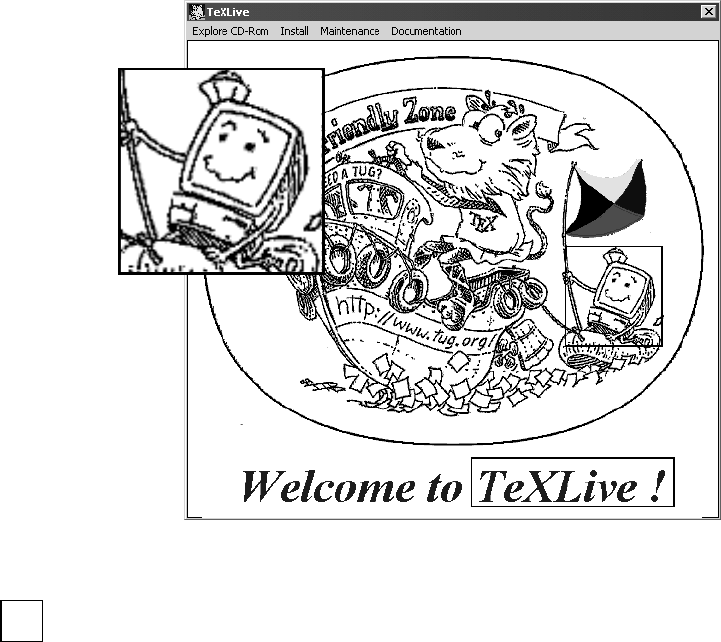
160 Chapter 6. Graphics Inclusion and Color
6.1.5 Superimposing images
h
h
h
h
h
h
h
h
h
h
h
h
h
h
h
h
h
h
h
h
h
h
h
`
`
`
`
`
`
`
`
`
`
`
`
`
`
`
`
`
`
H
H
H
H
H
H
H
H
H
H
H
H
H
H
H
H
H
H
a
a
a
a
a
a
a
a
a
a
a
a
a
a
a
a
a
a
a
a
a
a
a
Blow-Up
Figure 6.1: An embellished image file
Sometimes it is desired to superimpose one image file over part of another,
!say to add an inset in a corner. Or one may want to add text elements, or even
lines and arrows pointing to some feature in the image. One might even want
to make some area of the image into a link to another document. The picture
environment described in Section 13.1 can be used to allow exact placement of
such objects.
For example, in the figure on this page, we embellish the T
EXLive welcome
image from Figure B.1 on page 383 by adding a blow-up of a small section,
pointing a labeled arrow to it, and making the area around the text ‘T
EXLive!’ into
a link. We do this with the following input:
\setlength{\unitlength}{0.01\linewidth}
\setlength{\fboxsep}{0pt}
\setlength{\fboxrule}{1.5pt}
\begin{picture}(80,80)
\thicklines
\put(0,0){\includegraphics[width=.8\linewidth]{texlive}}
\put(57,26){\framebox(14.2,14.6){}}
\drawline(57,26)(-10,36.7)

6.1. The graphics packages 161
\drawline(71.2,26)(20.5,36.7)
\drawline(71.2,40.6)(20.5,67.2)
\drawline(57,40.6)(-10,67.2)
\put(-10,37){\fbox{\includegraphics[width=.3\linewidth,
viewport=390 180 490 280,clip]{texlive}}}
\put(-9,19){\vector(1,4){4}}
\put(-9,18){\makebox(0,0)[t]{\large Blow-Up}}
\put(43,2){\hyperlink{info}{\makebox(30,7){}}}
\end{picture}
Here the unit length for the picture placement has been set to 1/100 of the
current line width \linewidth, so we can conveniently use 100 units for the full
width. The picture environment reserves a space of 80×80 units; the image
file texlive is placed at the lower left corner (location 0,0) and set to a width
of 80% of \linewidth. We then draw a framed box around a portion of this
image, and then add that portion as a second image (selected with viewport
and clipped) as a blow-up. The \drawline commands (from the epic package)
join the corners of the original and blown-up areas. The order here is important
since later images overwrite the earlier ones. Then we add an arrow (\vector)
and the text ‘Blow-up’ (with \makebox). Finally, the \hyperlink command from
the hyperref package turns the 30×7 unit area around the text ‘T
EXLive!’ into a
active link to the target named info.
One can also place objects outside of the reserved picture area, so arrows
could be added pointing from the main text to some part of an image. This is
more appropriate for the production of slides (Chapter 15) where one wants rigid
control over the relative locations of graphics and text.
6.1.6 How importation can go wrong
In order to understand better what can go wrong when a graphics file is imported,
!and to know what to do about it, it is important to realize how the interplay
between L
A
T
EX and the driver program functions.
L
A
T
EX has no idea what is in the graphics file; for it, the figure is simply a box
of a given height, width, and depth, as indeed are all the characters that L
A
T
EX
processes. The information on the graphic’s natural size is somehow obtained,
either by information in the graphics file itself, or through the optional entries
in the \includegraphics command or equivalent. After scaling and rotating,
L
A
T
EX knows the final size that it must reserve in the output text for the figure.
What is then written to the .dvi file is the name of the graphics file and
information on how it should be transformed. Just how this information is
coded depends on the graphics driver selected. When the printer driver program
processes the .dvi file, it interprets these special instructions, reads in the
specified graphics file, performs the transformations, and places the result where
L
A
T
EX has said it should go. The end result is that the area inside the designated
bounding box coincides with the box that L
A
T
EX has reserved for it. If the bounding
box information is incorrect, the figure is obviously going to be misplaced.
162 Chapter 6. Graphics Inclusion and Color
PostScript output
Graphics inclusion was originally developed for PostScript graphics adhering to
the encapsulated specification that was designed to allow PostScript code to be
included within another PostScript file. Tomas Rokicki and his dvips driver broke
the ground in this field and thus established the standards. It is for that reason
that we place so much emphasis on PostScript graphics here. Encapsulated
PostScript files may not contain any commands that reset the whole graphics
page, and furthermore, they must contain a comment line of the form
%%BoundingBox: llx lly urx ury
giving the coordinates of the lower left and upper right corners of the bounding
box. The units are never specified, always being big points.
PDF output
Today PDF is an important alternative to PostScript, and the pdfT
EX program
(Section 10.2.3) is the most convenient way to produce it with L
A
T
EX. However,
pdfT
EX is not only a replacement for the classical T
EX program, producing identical
output, it also combines the functionality of a DVI-to-PDF driver. Thus no
intermediate .dvi file is generated at all, with the .pdf file being generated
directly from the L
A
T
EX source file in one operation. This has consequences for
graphics inclusion with pdfT
EX. First of all, the number of allowed graphics
formats is increased: images may be PNG (.png files), JPEG (.jpg or .jpeg files),
TIFF (.tif or.tiff files) or even a single image in a one-page PDF file. Ironically,
PostScript images are absolutely out! Secondly, the concept of bounding box does
not really apply to these formats, since they have a natural size anyway. The
viewport option should therefore be used to make a cutout from the original
rather than bb.
An alternative method of obtaining PDF output is to employ the true DVI-
to-PDF driver, dvipdfm, written by Mark A. Wicks. In this case, a .dvi file is
produced as usual (with the graphics option dvipdfm), and then the PDF output
is generated with this conversion program. The same set of graphics formats is
allowed as for pdfT
EX, for much the same reasons.
The third method would be to generate DVI, then PostScript, and then convert
it to PDF. As far as the graphics are concerned, this is the same as PostScript.
Having pointed out how the importation takes place, we can now discuss
what can go wrong along this chain of processes.
Problems with importation: pdfT
E
X
The single most common error when importing a graphics file with pdfT
EX
is that it does not exist in one of the permitted formats. Many users who
are used to using classical T
EX with PostScript simply switch to pdfT
EX
and are astonished to get the error message:
! LaTeX Error: Unknown graphics extension: .eps.
As explained above, pdfT
EX cannot handle PostScript files, so the graphics
must be converted to, or regenerated in, another format.
6.1. The graphics packages 163
The above error message will appear only if one has specified the full
name of the graphics file including the extension .eps. If the extension
is absent, which we recommend, the error message will report that the
file cannot be found. This means that it cannot be found with any of the
allowed extensions. It might very well be that it exists with the extension
.eps, but since that is not allowed for pdfT
EX, it will not be sought.
To maintain flexibility, one can have the same graphics file available
both as an .eps and as a .pdf file. Leaving the extension off in the
\includegraphics command means one does not need to make any
changes to the file name when switching between regular T
EX and pdfT
EX.
Problems with importation: PostScript
The most common problems encountered when importing encapsulated
PostScript files are listed here.
No bounding box. If the bounding box information is totally missing
from the graphics file, L
A
T
EX issues the error message
! LaTeX Error: Cannot determine size of graphic
in ... (no BoundingBox).
The solution is to determine the bounding box coordinates somehow
(see next point) and to include them, either in the \includegraphics
command, or by editing the graphics file itself. However, if there
really is no bounding box information in the file, it is unlikely to con-
form to the encapsulated standard and will cause other problems.
The placement is incorrect. Both L
A
T
EX and the driver process without
error messages, but the figure is either displaced from the expected
position, or is far too small.
Most likely the bounding box information is incorrect. Many appli-
cations that produce PostScript files are too lazy to calculate the true
bounding box, or they think they are generating a whole page with
a figure somewhere in the middle. In either case, the bounding box
corresponds to the full page even though the printed figure occupies
only a portion of it.
Find the true bounding box by one of the following methods:
1. Print the figure, mark the lower left and upper right corners
of the box containing the figure, and measure their distances
from the left and bottom edges. Enter these distances in the
\includegraphics command, or edit the PostScript file. In the
latter case, convert to big points.
Difficulties with this are that some encapsulated PostScript files
cannot be printed on their own, and that the left and bottom

164 Chapter 6. Graphics Inclusion and Color
edges of the paper need not be the exact lines from which the
printer really measures.
2. Include the figure in a short L
A
T
EX file such as
\setlength{\fboxsep}{-\fboxrule}
\fbox{\includegraphics{test.eps}}
and print the output. The apparent bounding box appears as
a framed box. Measure the true bounding box relative to the
left and bottom edges of the apparent one, and enter the values
in the \includegraphics command with the viewport= key.
If necessary, scale the figure down to fit on the page, but then
remember to increase the measurements by the same scale
factor.
3. Use the GhostView program to fix up the bounding box, either
automatically or manually. This is the most convenient method
if you have this utility for viewing and manipulating PostScript
files.
Immovable graphic. It does not shift, nor scale nor rotate, no matter what
is specified. In this case, it violates the encapsulated PostScript rules
and contains some global plotting commands. Graphics produced
by word processing programs are notorious for this. Often the
offending command is setpagedevice.
There is little that can be done to correct this, other than trying to re-
generate the graphics file with an option for encapsulated PostScript.
Judicious editing can remove the troublesome lines, but this could
result in the file becoming totally unreadable.
6.1.7 Configuring graphics importation
Although the graphics syntax has been standardized, and most of the driver-
!specific coding hidden in the .def files, there are still a number of items that
must be set up for any particular installation and operating system. These are
most conveniently placed in the local configuration file graphics.cfg which is
read in if it is present.
Many installations come with a ready-made configuration file, so there may
not be any need to make up your own. On the other hand, you may want to edit
or replace it for you own purposes.
Default driver
The choice of driver option must always be given, but a local default can be
specified in the configuration file. For example, if dvips is the standard graphics
driver, you may add
6.1. The graphics packages 165
\ExecuteOptions{dvips}
to graphics.cfg and you do not need to give the option dvips when loading
graphics or graphicx. You may still specify any other graphics driver option if
you wish.
Many supplied configuration files go further and determine whether pdfT
EX
is activated or not; if so, the default graphics option is set to pdftex, otherwise
to dvips.
The rest of the configuring commands in this section can be issued either in
the graphics.cfg file, or in the document.
Search path for graphics files
One can specify the directories where L
A
T
EX is to look for graphics files with
\graphicspath{dir list}
where dir list is a list of directory names, each enclosed in brackets { }, with no
other separator. The syntax of the local operating system must be used. Without
this command, L
A
T
EX searches for graphics files in the same directories as for all
other T
EX files. Example,
\graphicspath{{figs/}{eps/}} for Unix, DOS, Windows
\graphicspath{{:figs:}{:eps:}} for Macintosh
\graphicspath{{[.figs]}{[.eps]}} for VMS
Note: The Unix syntax works even with DOS and Windows, since the normal
backslash in the directory names must be replaced by a slash /to avoid looking
like a command name.
Default extensions
A list of default extensions for the graphics files can be defined with
\DeclareGraphicsExtensions{ext list}
This means that only the root name of the file must be given and L
A
T
EX will
attempt to find it by attaching all the possible extensions. For PostScript drivers,
the ext list is usually set to .eps,.ps. At our installation, we also include the
non-standard extension.psc. Note that the above command does not add to the
list of extensions but rewrites it anew; if you wish to add to the list, you must
include all the allowed extensions in the one declaration.
Graphics types
Defining the extensions is only part of the task: one must also associate each
extension with a graphics type so that L
A
T
EX knows how to process it. PostScript
recognizes only one type, eps, encapsulated PostScript, but there do exist other
types such as bmp and pcx for other drivers. For the non-standard.psc extension
above, we must also give
\DeclareGraphicsRule{.psc}{eps}{}{}
to inform L
A
T
EX that this extension belongs to type eps. The other two (empty)
arguments specify that the bounding box information is to be read from the file
itself, and that no other program needs to be applied to the file.

166 Chapter 6. Graphics Inclusion and Color
Compressing graphics files
Since PostScript files are often extremely large, it makes sense to try to compress
them with either the zip or gzip programs. In such a case, the .eps file is
replaced by a file with extension.zip, or.eps.gz, or.eps-gz. Two problems now
arise: first, L
A
T
EX cannot read such files to obtain the bounding box information,
and secondly, the driver needs to unpack such a file to include it in the final
output. This can be accomplished with, for example,
\DeclareGraphicsRule{.eps.gz}{eps}{.eps.bb}{‘gunzip -c #1}
which establishes the graphics type as eps, with the bounding box information in
the file of the same name and extension.eps.bb, and that the operating system
command gunzip -c must be applied to the file (represented as #1). The single
quote ‘is required to indicate a system command. The %%BoundingBox line of
the original file must be copied and stored in the.eps.bb file.
Such decompression rules are system dependent and thus need to be con-
figured for the local installation. For example, under the VMS operating system,
the gzip program produces files with extension .eps-gz and decompression
is performed with gzip -d rather than with gunzip. The corresponding rule
becomes
\DeclareGraphicsRule{.eps-gz}{eps}{.bb}{‘gzip -d -c #1}
6.2 Adding color
The color package accepts the same driver options listed on page 154
for the graphics package. In addition, it also recognizes the options:
monochrome
to convert all color commands to black and white, for previewers
that cannot handle color;
dvipsnames
makes the named color model of dvips (Section 6.2.1) available
to other drivers;
nodvipsnames
disables the named model for dvips, to save memory;
usenames
loads all the named colors as defined ones; again, see Section 6.2.1
for details.
A local configuration file color.cfg can be set up in the same way as for
!the graphics package. The default driver option is specified in exactly the same
way as in Section 6.1.7.
Colors are specified either by a defined name, or by the form
[model]{specs}

6.2. Adding color 167
where model is one of rgb (red, green, blue), cmyk (cyan, magenta, yellow,
black), gray, or named. The specs is a list of numbers from 0 to 1 giving the
strengths of the components in the model. Thus [rgb]{1,0,0} defines
red, [cmyk]{0,0,1,0} yellow. The gray model takes only one number.
The named model accesses colors by internal names that were originally
built into the dvips driver, but which may now be used by some other
drivers too. This model is described in Section 6.2.1.
A color can be defined with
\definecolor{name}{model}{specs}
and then the name may be used in all the following color commands.
Certain colors are automatically predefined for all drivers: red,green,
blue,yellow,cyan,magenta,black,white.
In the following color commands, col spec is either the name of a
defined color, like {blue}, or [model]{spec}, like [rgb]{0,1,0}.
\pagecolor col spec sets the background color for the current and
following pages;
\color col spec is a declaration to switch to setting text in the given
color;
\textcolor col spec{text}sets the text of its argument in the given
color;
\colorbox col spec{text}sets its argument in a box with the given color
as background;
\fcolorbox col spec1 col spec2{text}like \colorbox, with a frame of
col spec1 around a box of background color col spec2; the two spec-
ifications must either both be defined ones, or both use the same
model, which is given only once; for example, \fcolorbox{red}
{green}{Text} sets ‘Text’ in the current text color on a green back-
ground with a red frame;
\normalcolor switches to the color that was active at the end of the
preamble. Thus placing a \color command in the preamble can
change the standard color for the whole document. This is the
equivalent to \normalfont for font selection.
Normally one would try to define all the colors needed as names for the
col spec entries. This simplifies changing the color definition everywhere
should fine-tuning be required after the initial printed results are seen.
The same color definition can produce quite different effects on different
printers. Even the display on the monitor is no reliable guide as to how
the output will appear on paper.

168 Chapter 6. Graphics Inclusion and Color
6.2.1 The named color model
One very useful color model is called named and is based on the 68
predefined internal colors of the dvips PostScript driver. Sample names
are BurntOrange or DarkOrchid. This model can be activated for other
drivers with the option dvipsnames, in which case one can define colors
as, for example
\definecolor{titlecol}{named}{DarkOrchid}
The color titlecol can then be used as col spec in the various color
commands.
The named colors can be defined with their own names if one invokes
the option usenames, which effectively declares
\definecolor{BurntOrange}{named}{BurntOrange}
and so on, for all 68 colors.
It is possible to generate a palette of the named colors by processing
the following short L
A
T
EX file and sending the output to the desired printer.
\documentclass[12pt,a4paper]{article}
\usepackage[dvipsnames]{color}
\usepackage{multicol}
\pagestyle{empty}
\setlength{\oddsidemargin}{0pt}
\setlength{\textwidth}{16cm}
\setlength{\textheight}{22cm}
\setlength{\parindent}{0pt}
\setlength{\parskip}{0pt}
\begin{document}
\renewcommand*{\DefineNamedColor}[4]{%
\textcolor[named]{#2}{\rule{7mm}{7mm}}\quad
\texttt{#2}\strut\\}
\begin{center}\Large Named colors in \texttt{dvipsnam.def}
\end{center}
\begin{multicols}{3}
\input{dvipsnam.def}
\end{multicols}
\end{document}
Remember, each printer can reproduce the colors differently, so it is
important to test this table with every color printer that might be used.
Exercise 6.3: Copy the above lines to a file named palette.tex or copy it from
the enclosed CD from \books\Kopka_and_Daly\. Process it and view the output
on a color monitor or send it to a color printer.

7
Floating tables and
figures
Whether a figure is imported with \includegraphics (Chapter 6) or
produced with the picture environment of Chapter 13, it is inserted in
the text where the drawing or importing commands are issued, coming
between the previous and following texts. This can present the same
difficulties as for tables, described in Section 4.8.5: if the figure is so
high that it no longer fits on the current page, that page is prematurely
terminated and the figure is placed at the top of the next page, with too
much empty space left on the original page.
In Section 4.8.5 we mention how this problem is solved for tables. Here
we now give a complete description of the float procedures that apply to
both figures and tables.
7.1 Float placement
L
A
T
EX does make it possible to float figures and tables, together with their
headlines and captions, to an appropriate location without interrupting
the text. This is invoked with the environments
\begin{figure}[where]figure \end{figure}
\begin{figure*}[where]figure \end{figure*}
\begin{table}[where]table \end{table}
\begin{table*}[where]table \end{table*}
The *-forms apply only to the two-column page format and insert the
figure or table across both columns instead of the normal single column.
They function exactly the same as the standard forms when the page
format is single column.
In the above syntax, figure and table are the texts for the contents of the
float, either a picture or tabular environment, or an \includegraphics
command, together with a possible \caption command, as described
later in Section 7.4.
169
170 Chapter 7. Floating tables and figures
The argument where specifies the allowed locations for the figure or
table. There are several possibilities so that where consists of from zero
to four letters with the following meanings:
hhere: the float may appear at that point in the text where the
environment is typed in; this is not permitted for the *-form; see
also the here package and the Hparameter, page 178;
ttop: the float may appear at the top of the current page, provided
there is enough room for both it and the previous text; if this is not
the case, it is added at the top of the next page; the subsequent text
continues on the current page until the next normal page break; (for
two-column format, read column in place of page);
bbottom: the float may be placed at the bottom of the page; the
subsequent text continues until the room left on the current page
is just enough for the float; if there is already insufficient room, the
float will be put at the bottom of the next page; this is not permitted
for the *-form;
ppage: the float may be put on a special page (or column) containing
only figures and/or tables;
!used together with any combination of the other letters, suspends
all the spacing and number restrictions described in Section 7.3.
The argument values may be combined to allow several possibilities. If
none is given, L
A
T
EX assumes the standard combination tbp.
The placement arguments permit certain possibilities for locating the
float, but the actual insertion takes place at the earliest possible point in
accordance with the following rules:
•no float appears on a page prior to that where it is defined;
•figures and tables are output in the order in which they were defined
in the text, so that no float appears before a previously defined float
of the same type; figures and tables may, however, be mixed in their
output sequence; in two-column format, the double column *-floats
may also appear out of sequence;
•floats will be located only at one of the allowed positions given by
the placement argument where; without an argument, the standard
combination tbp is used;
•unless the !is included in where, the positioning obeys the limita-
tions of the style parameters described in Section 7.3;
•for the combination ht, the argument htakes priority; the float is
inserted at the point of its definition even if there is enough room
for it at the top of the page.

7.3. Style parameters for floats 171
When any of the commands \clearpage,\cleardoublepage, or
\end{document} is given, all floats that have not yet been output will
be printed on a separate page or column regardless of their placement
arguments.
Sometimes L
A
T
EX gets stuck on a float which holds up the entire queue
Package:
after-
page until the end of the document. One way to clear the queue is to issue
\clearpage right after the troublesome float. However, that would in-
sert a new page at that point, something that may not be desired. The
package afterpage in the tools collection (Section B.5.4) provides the
command \afterpage which executes its argument at the end of the
current page. Thus \afterpage{\clearpage} solves this problem by
delaying the \clearpage command until the actual page break.
7.2 Postponing floats
Occasionally one wants to prevent floats from appearing on a certain
page, for example at the top of a title page. (L
A
T
EX automatically corrects
that case.) However, there are other situations where a float should be
suppressed temporarily. One might want it at the top of a page, but not
before the start of the section that refers to it. The command
\suppressfloats[loc]
sees to it that for the current page only no further floats of the specified
placement loc should appear. If the optional loc is omitted, all floats are
suppressed; otherwise loc may be either tor b, but not both.
Note that \suppressfloats does not suppress all floats for the cur-
rent page, but only further ones that come between the issuing of this
command and the end of the page. Thus it is still possible for floats from
a previous section to appear on the page.
Alternatively, the package flafter (Section B.5.3) may be loaded to
Package:
flafter ensure that all floats appear only after their position in the text.
The command \suppressfloats and the location parameter !are
attempts to give the author more control over the sometimes capricious
actions of float placement.
7.3 Style parameters for floats
There are a number of style parameters that influence the placement of floats,
!which may be altered by the user as desired.
topnumber
The maximum number of floats that may appear at the top of a page.
bottomnumber
The maximum number of floats that may appear at the bottom of a
page.
172 Chapter 7. Floating tables and figures
totalnumber
The maximum number of floats that may appear on any page regardless
of position.
dbltopnumber
The same as topnumber but for floats that extend over both columns
in two-column page format.
The above parameters are all counters and may be reset to new values with
the command \setcounter{ctr}{num}, where ctr is the name of the counter
and num the new value that it is to take on.
\topfraction
A decimal number that specifies what fraction of the page may be used
for floats at the top.
\bottomfraction
A decimal number that specifies what fraction of the page may be used
for floats at the bottom.
\textfraction
The fraction of a page that must be filled with text. This is a minimum,
so that the fraction available for floats, whether top or bottom, can
never be more than 1−\textfraction.
\floatpagefraction
The smallest fraction of a float page that is to be filled with floats before
a new page is called.
\dbltopfraction
The same as \topfraction but for double column floats in two-column
page format.
\dblfloatpagefraction
The same as \floatpagefraction but for double column floats in
two-column page format.
These style parameters are altered with \renewcommand{cmd}{frac}where
cmd stands for the parameter name and frac for the new decimal value, which
in every case must be less than 1.
\floatsep
The vertical spacing between floats appearing either at the top or at the
bottom of a page.
\textfloatsep
The vertical spacing between floats and text, for both top and bottom
floats.
\intextsep
The vertical spacing above and below a float that appears in the middle
of a text page with the hplacement argument.
\dblfloatsep
The same as \floatsep but for double column floats in two-column
page format.
\dbltextfloatsep
The same as \textfloatsep but for double column floats in two-
column page format.
7.4. Float captions 173
This group of style declarations are rubber lengths that may be changed with
the \setlength command (Section 2.4.2).
\topfigrule
A command that is executed after a float at the top of a page. It may be
used to add a rule to separate the float from the main text. Whatever it
adds must have zero height.
\botfigrule
Similar to \topfigrule, but is executed before a float that appears at
the bottom of a page.
\dblfigrule
Similar to \topfigrule, but for double column floats.
These three commands normally do nothing, but they may be redefined if
necessary. For example, to add a rule of thickness 0.4 pt below a top float,
\renewcommand{\topfigrule}{\vspace*{-3pt}
\rule{\columnwidth}{0.4pt}\vspace{2.6pt} }
Because of the negative argument in \vspace*, the total vertical spacing is zero,
as required.
All the one-column style parameters also function within the two-column
page format, but they apply only to floats that fill up one column.
If the style parameters are set to new values within the preamble, they apply
from the first page onwards. However, if they are changed within a document,
they do not take effect until the next page.
7.4 Float captions
A figure caption or table title is produced with the command
\caption[short title]{caption text}
inside the figure or table environment. The caption text is the text that
is printed with the float and may be fairly long. The short title is optional
and is the text that appears in the list of figures or tables (Section 3.4.4).
If it is missing, it is set equal to caption text. The short title should be
given if the caption text is longer than about 300 characters, or if it is
more than one line long.
In the table environment, the \caption command generates a title of
the form ‘Table n:caption text’, and in the figure environment ‘Figure n:
caption text’, where nis a sequential number that is automatically incre-
mented. In document class article, the figures and tables are numbered
from 1 through to the end of the document. For the report and book
classes, they are numbered within each chapter in the form c.n, where c
is the current chapter number and nis the sequential number reset to 1 at
the start of each chapter. Figures and tables are numbered independently
of one another.
174 Chapter 7. Floating tables and figures
Table 7.1: Computer Center Budget for 2004
Nr. Item 51505 52201 53998 Total
1.1 Maintenance 130 000 15 000 145 000
1.2 Network costs 5 000 23 000 28 000
1.3 Repairs 25 000 6 000 31 000
1.4 Expendables 68 000 68 000
1. Total 160 000 74 000 38 000 272 000
The \caption command may be omitted if numbering is unwanted,
since any text included in the float environment will accompany the
contents. The advantages of \caption over simple text are the automatic
numbering and entries in the lists of figures and tables. However, a
manual entry in these lists may be made as described in Section 3.4.4
using
\addcontentsline and \addtocontents
Atitle, or headline, is produced with \caption when the command
comes at the beginning of the material in the float environment: the
number and text are printed above the table or figure. A caption is added
below the object if the command comes after all the other float commands.
In other words, the \caption is just another item within the float and
whether its text appears at the top (as title) or below (as caption) depends
on how the user places it.
The caption text will be centered if it is shorter than one line, otherwise
it is set as a normal paragraph. The total width may be adjusted to that of
the table or figure by placing the command inside a parbox or minipage.
For example,
\parbox{width}{\caption{caption text}}
The following demonstrations contain further examples of how text,
table, and picture commands may be combined in floats.
7.5 Float examples
The first two tables are produced with the following texts:
\begin{table} \caption{Computer Center Budget for 2004}
\begin{tabular}{|l|l||r|r|r|r|} ... ... \end{tabular}
\end{table}
(This text was typed in before the last paragraph of the previous section. The
second table is entered here in the current text.)
7.5. Float examples 175
Table 7.2: Estimates for 2004. A continuation of the previous budget is
no longer practical since, with the installation of the new computing system
in 2003, the operating conditions have been completely overhauled.
Nr. Item 51505 52201 53998 Total
1.1 Maintenance 240 000 240 000
1.2 Line costs 12 000 8 000 36 000 56 000
1.3 Training 50 000 50 000
1.4 Expansion 80 000 3 000 83 000
1.5 Expendables 42 000 42 000
1. Total 332 000 53 000 86 000 471 000
\begin{table}
\caption{\textbf{Estimates for 2004} \emph{A continuation...}}
\begin{tabular}{|l|l||r|r|r|r|} ... ... ... \end{tabular}
\end{table}
Because the placement argument is missing from the table environ-
ments, the standard values tbp are used. The first was placed at the
top on the facing page because it was typed in early enough (during the
last section) that there was still room for it there. Then the command
\suppressfloats (Section 7.2) was issued to prevent any more floats
appearing on the same page. The second table is therefore forced to float
to the top of this page.
Narrow figures or tables may be set beside each other, as shown in
the following example (which appears at the bottom of this page). (The
picture environment is explained in Chapter 13.)
\begin{figure}[b]
\setlength{\unitlength}{1cm}
\begin{minipage}[t]{5.0cm}
\begin{picture}(5.0,2.5) ... ... \end{picture}\par
\caption{Left}
\end{minipage}
Space for Left Figure
?
2.5 cm
6
5.0 cm -
Figure 7.1: Left
Space for Right Figure
?
3.0 cm
6
6.0 cm -
Figure 7.2: Right

176 Chapter 7. Floating tables and figures
\hfill
\begin{minipage}[t]{6.0cm}
\begin{picture}(6.0,3.0) ... ... \end{picture}\par
\caption{Right}
\end{minipage}
\end{figure}
The two figures along with their captions are each set in a minipage
environment of widths 5 and 6 cm. The minipages are separated from one
another by an \hfill space. The positioning argument thas the effect
that the minipages are aligned along their first lines (Section 4.7.3). The
entire structure within the figure environment floats as a single entity.
The question might now arise as to why, since the two figures have
unequal heights and are supposedly aligned vertically along their top
lines, their bottom edges are at the same level. The explanation is that
apicture environment establishes an LR box (Section 4.7.1) to contain
all the picture commands, and that is viewed by L
A
T
EX as a single line of
output text with the baseline at the bottom edge of the picture. In both
minipages, the picture environment is the first entry and is therefore
the first logical line of text. It is these baselines that are taken for the
vertical alignment of the minipages.
If the two pictures were to be aligned along their top edges, it would be
necessary to include a dummy first line (Section 4.7.4) in each minipage
before the picture environments. This could be something like \mbox{},
for example.
The application of box commands within a float permits completely
free positioning. If the caption text is to appear, say, beside the table or
figure, instead of above or below it, the objects may be put into minipages
or parboxes with suitable alignment arguments. Here is an example:
\begin{table}[b]
\centerline{\bfseries Results and Seat Distribution of the...}
\mbox{\small
\begin{minipage}[b]{7.7cm}
Results and Seat Distribution of the 2003 General Election
140 186
60 42
Pros
Cons
Ups
Downs
Seat Distribution
in the Assembly of
2004–2006
Results:
2003 General
Election
Party Votes %
Pros 15 031 287 37.7
Cons 12 637 418 31.7
Ups 6 499 210 16.3
Downs 4 486 514 11.3
Others 1 201 078 3.0

7.6. References to figures and tables in text 177
\begin{minipage}[t]{4.4cm}
\mbox{}\\ \setlength{\unitlength}{0.75cm}
\begin{picture}(5.75,5.0) ... ... ... \end{picture}
\end{minipage} \hfill
\parbox[t]{3.2cm}{\makebox[0cm]{}\\{\bfseries Seat ...} ...}
\end{minipage}
\hspace{-3cm}
\begin{minipage}[b]{7cm}
\parbox[b]{2.5cm}{{\bfseries Results:}\\ General Election..}
\hfill
\begin{tabular}[b]{|l||r|r|} ... ... \end{tabular}
\end{minipage} }
\end{table}
Here the vertical boxes are nested inside one another. The left side, consisting
!of graphics and a title at the upper right, is contained in a minipage of width
7.7 cm, in which the picture is in another minipage of width 4.4 cm while the text
is in a parbox of width 3.2 cm. Both are aligned with the top lines. A dummy line
containing \mbox{} (Section 4.7.4) is added before the first picture to provide
a top line with which the second parbox can be aligned.
The right-hand side consists of a minipage of width 7 cm, shifted to the left
by 3 cm, aligned with the left-hand minipage along the bottom lines. It contains
a parbox of width 2.5 cm for the text as well as a table, which is automatically a
vertical box. Both of these are aligned with the bottom lines.
7.6 References to figures and tables in text
The automatic numbering of tables and figures has the consequence that
the author does not know the numbers at the time of writing. Since he
or she would like to be able to refer to these objects by number, as ‘see
Figure 3’ or ‘Table 5 illustrates’, another means of referencing must be
found. It is not sufficient to keep track of the number of \caption calls
that have been made, since the document may not be written in the order
in which it finally appears, and new figures or tables may be inserted
during revision, or some removed.
These problems are solved with the L
A
T
EX cross-reference system, de-
scribed in more detail in Section 9.2.1. The basic commands are
\label{name} \ref{name}
which assign a keyword name to the figure or table number that may be
used as reference in the text. The keyword name may be any combination
of letters, numbers or symbols. The assignment is made with the \label
command given anywhere within the caption text of the \caption com-
mand; in the main text, the command \ref inserts the number that is
associated with its keyword.
This is best shown with an example. The budget table on page 174
was actually written as

178 Chapter 7. Floating tables and figures
\caption{\label{budget04} Computer Center ... }
so that Table \ref{budget04} produces ‘Table 7.1’ when used in the
main text.
There is a second referencing command \pageref to generate the
page number where the referenced object is to be found. For example, a
few lines up, the input text on page \pageref{budget04} was used to
create the text ‘. . . on page 174’.
7.7 Some float packages
7.7.1 Placing a float right here
The float placement parameter h, described on page 170, only permits a
Package:
here float to be placed at the current location, it does not force it to appear
there. With Frank Mittelbach’s package here, an additional parameter H
is provided which places the float immediately where it appears in the
source text. If there is not enough room for it on the current page, a
\pagebreak command is first issued. This will most likely lead to an ugly
page break.
7.7.2 Flowing text around a float
The package floatflt by Mats Dahlgren (based on the earlier and now
Package:
floatflt obsolete floatfig by Thomas Kneser) permits one to mix text and floats
side by side, with the text flowing around the float at the end, as in the
next paragraph.
A figure is placed within \begin{floatingfigure}[pos]{wth}
Figure commands with or without a
\caption command
\end{floatingfigure}
the text as shown in the box
at the right. Here pos de-
termines on which side the
figure is to appear; it may
be r(right), l(left), p(right
for odd, left for even pages), or v(like punless a package option is given,
in which case, it is used). The mandatory argument wth is the width
of the figure itself; in fact, some additional space will be included for a
border between text and figure. It is advisable to include a \centering
command at the start of the figure material.
The material in the floatingfigure environment need not actually
be a figure. In the above example, some boxed text in a minipage was
used for demonstration purposes. However, if the \caption command
is included in the environment, then a figure number will be printed, in
sequence with those of the regular figure environment.
Rather than giving the pos parameter each time, one can specify a
default value as an option when loading the package with \usepackage:

7.7. Some float packages 179
rflt (right), lflt (left), or vflt (variable, i.e. p). If no option is given, the
default is vflt.
To include a table with text,
\begin{floatingtable}[pos]{
\begin{tabular}{table specs}
table entries
\end{tabular}}
Optional \caption command
\end{floatingtable}
the usage is slightly different, as
shown at the left. That is, the en-
tire table appears in place of the
wth for a figure, and only the cap-
tion in placed in the environment
itself.
Both these environments are
to be placed at the start of the paragraph that is to flow around the figure
or table. The flowing cannot start in the middle of a paragraph.
There is some very tricky coding to get the flowing text to work prop-
erly, and needless to say, there are many things that can go wrong. Please
read the accompanying manual for more details.
7.7.3 Defining new floats and styles
For authors who are not satisfied with the standard float style, or who
Package:
float need additional floating environments, we recommend the float package
by Anselm Lingnau. With this package, one defines a new float type with
\newfloat{name}{loc}{ext}[within]
where name is the name of the new float environment, loc is the default
placement letters (selection of tbhpH), ext is the extension of the file
containing the list of this float type, and the optional within is the name
of a counter (e.g., chapter) within which the numbering is reset.
For example, to define a plate environment that behaves just like
figure but which is numbered separately as Plate xxx, with the numbers
reset within each chapter, give
\newfloat{plate}{p}{lop}[chapter]
\floatname{plate}{Plate}
The first line defines the new environment, with default placement on a
float page. The second states that the captions associated with this float
are to start with the word ‘Plate’; without this, they would be labeled as
‘plate’, the same as the environment name itself.
The information for the list of plates is stored in a file with extension
.lop, in the same way that the list of figures is in a file with extension
.lof (Section 3.4.4). This list is printed by reading in this file with the
command
\listof{plate}{List of Plates}
where ‘List of Plates’ is the list title.
The default placement parameters for any float environment, including
the standard figure and table ones, can be redefined with
180 Chapter 7. Floating tables and figures
\floatplacement{name}{loc}
The float package also defines 4 float styles:
plain much like standard L
A
T
EX except the caption is always below the
float contents;
plaintop
like plain but with the caption always above the contents;
boxed in which the contents are in a framed box with the caption below
it;
ruled with the caption above, and with rules above, below, and between
caption and float contents.
One selects a float style by issuing \floatstyle{style}, where style is
one of the above possibilities. The style then applies to all new float
environments defined with \newfloat, until a new style is issued.
Note: the style selection affects the subsequent float definitions, not
the float environments that are then used. To change the float style for
the standard figure and table floats, issue
\floatstyle{ruled}
\restylefloat{figure}
\restylefloat{table}
The float package also contains the Hplacement parameter for ‘here
and I mean it’, so it is not necessary to include the here package with it.

8
User Customizations
L
A
T
EX allows the user to define his or her own commands and environments.
However, since these make extensive use of the L
A
T
EX counters and lengths,
we will first present a more detailed discussion of these objects and how
they may be manipulated.
8.1 Counters
8.1.1 L
A
T
E
X counters
L
A
T
EX manages a number of counters by giving them initial values at the
start and by changing these values when certain commands are called.
Most of these counters have the same name as the commands that alter
them:
part chapter paragraph figure enumi
section subparagraph table enumii
subsection page footnote enumiii
subsubsection equation mpfootnote enumiv
The meanings of most of these counters are obvious from their names
and need no further explanation. The counters enumi ... enumiv refer to
the four levels of the enumerate environment (Sections 4.3.4 and 4.3.5),
while the counter mpfootnote controls the footnote numbering within
the minipage environment (Section 4.10.4).
The value of a counter is an integer number, usually non-negative. A
command may output several numbers at once: the current \subsection
command outputs 8.1.1, which addresses three counters in all. For exam-
ple, the \subsection command increments the value of the subsection
counter by one, and prints the values of the chapter,section, and
subsection counters, separated by periods. At the same time, this com-
mand sets the subsubsection counter to zero.
181
182 Chapter 8. User Customizations
8.1.2 User-defined counters
The user may create new counters with the command
\newcounter{counter name}[in counter]
where counter name is the name of the newly established counter. This
may be any combination of letters that is not already the name of an
existing counter. Thus none of the names of the L
A
T
EX counters listed
above may be used as counter name nor any name of a previously defined
user counter.
The optional argument in counter is the name of another counter
that already exists (L
A
T
EX or user defined) and has the effect that the newly
defined counter is reset to zero whenever in counter is incremented by one
of the commands \stepcounter or \refstepcounter (see below). For
example, the subsection counter is reset to zero whenever the section
counter is incremented.
The \newcounter command may not appear in any file that is read in
with the \include command (Section 9.1.2). It is therefore best to put all
\newcounter commands into the preamble.
8.1.3 Changing counter values
Every counter, whether L
A
T
EX or user defined, has an initial value of zero;
this can be altered with the following commands:
\setcounter{counter}{num}
This command is self-explanatory: the specified counter is as-
signed the integer value num.
\addtocounter{counter}{num}
With this command, the value of the counter is increased by the
integer num, which may be positive or negative.
\stepcounter{counter}
The value of the counter is increased by one, and at the same
time all its sub-counters (that is, those that have this counter as
their in counter) are reset to zero (see above).
\refstepcounter{counter}
This command has the same effect as \stepcounter but also
makes counter the current counter for the cross-referencing com-
mand \label (see Section 9.2.1).
This last command may be applied, for example, within the figure
or table environments when the \caption command is missing and yet
there is to be a reference in the text to the figure or table number using the
\ref command. Then \refstepcounter{figure} or \refstepcounter
{table} is given within that float environment to bring the corresponding
8.1. Counters 183
counter to the right value and to allow that value to be assigned a keyword
with the \label command (Section 9.2.1).
The value of a counter may be treated as a number with the command
\value{counter}
which does not change the value at all. This command is mostly used
in connection with \setcounter or \addtocounter. For example, if the
user-defined counter mypage has been created, it may be set to the same
value as the page counter page by giving \setcounter{mypage}{\value
{page}}.
8.1.4 Printing counter values
The numerical value in a counter can be printed with the commands
\arabic{counter}as an Arabic number,
\Roman{counter}as a capital Roman numeral,
\roman{counter}as a lower case Roman numeral,
\alph{counter}as a lower case letter,
\Alph{counter}as a capital letter,
\fnsymbol{counter}as a footnote symbol.
For the commands \alph and \Alph, the numbers 1. . . 26 correspond to
the letters a...zand A. . . Z. It is up to the user to ensure that the counter
value lies within this range. For \fnsymbol, the numbers 1. . . 9 are output
as the symbols * † ‡ § ¶ ** †† ‡‡. Here again, the user must
take care that the counter does not reach a value of 10 or more.
For each counter, a command of the form
\thecounter
is also available, consisting of \the immediately followed by the name
of that counter, such as \thepage. This type of command is initially
identical to \arabic{counter}, but may redefined to be composed of
several counter commands. In the document classes book and report,
for example, the command \thesection is defined in terms of both the
chapter and section numbers: \arabic{chapter}.\arabic{section}.
Here is the result of printing \thesection at this point: 8.1.
The automatic printing of counter values such as the page, equation,
or sectioning numbers is accomplished by means of calls to the appro-
priate \thecounter commands. If a different format for some automatic
numbering is desired, say alphabetical equation numbers, the definition
of the corresponding \thecounter command can be altered using the
methods described in Section 8.3.
Exercise 8.1: Take your standard exercise.tex file and print out the final values
of the L
A
T
EX counters with \arabic{counter}commands at the end. Change some
the values with the \setcounter and \addtocounter commands and print the
values out once more.

184 Chapter 8. User Customizations
8.2 Lengths
It has been constantly pointed out in all the descriptions of the length
parameters such as \parskip or \textwidth that new values may be
assigned with the \setlength command. Some of these parameters
expect rubber length values that may stretch or shrink. These are mainly
parameters that produce vertical spacing. The types of length units,
both fixed and rubber, are described in detail in Section 2.4. This will
not be repeated here, but rather additional commands for assigning and
handling lengths are discussed in this section.
The standard L
A
T
EX method for assigning a value to a length parameter
is with the command
\setlength{\length cmd}{length spec}
where length spec may be a length specification (with units) or another
length parameter. In the latter case, \length cmd takes on the current
value of that other parameter. Thus with \setlength{\rightmargin}
{\leftmargin} the right-hand margin in a list environment is set to
the same value as that of the left-hand margin.
Lengths may be increased with
\addtolength{\length cmd}{length spec}
which adds length spec to the value of the length parameter \length cmd.
A negative value for length spec decreases \length cmd by that amount.
Once again, another length parameter may be used for length spec, with or
without a preceding minus sign, and its value will be added or subtracted.
A decimal number just before a length parameter multiplies its value by
that quantity: 0.5\textwidth means half the width of the text column
and 2\parskip twice the inter-paragraph spacing.
With the command
\settowidth{\length cmd}{text}
the length parameter \length cmd is set equal to the natural length of a
piece of text.
Similarly the commands
\settoheight{\length cmd}{text}
\settodepth{\length cmd}{text}
set the \length cmd equal to the height and depth of the text above and
below the baseline, respectively.
Finally, the command
\stretch{decimal num}
yields a rubber length that is decimal num times as stretchable as \fill
(Section 2.4.2).
A user-defined length parameter is created with

8.3. User-defined commands 185
\newlength{\new len cmd}
which establishes \new len cmd as a length with a value of 0pt. All the
above commands may be used to manipulate its value further.
The command
!\addvspace{length spec}
inserts extra vertical spacing of the amount length spec at that point where it
appears. If more than one such command is given, the total inserted spacing will
be that of the largest argument and not the sum of them all. This command may
only be given between paragraphs. Its application for user-defined commands
and environments lies in the generation of structures that should behave like
paragraphs.
8.3 User-defined commands
New commands may be defined or redefined under L
A
T
EX with the com-
mands
\newcommand{\com name}[narg][opt]{def }
\renewcommand{\com name}[narg][opt]{def }
The first version is used to define a command \com name that does not
yet exist. Its name may be any combination of letters that do not form
the name of another command. The second version redefines an already
existing command \com name. In both cases, an error message is printed
if the incorrect variant is called. The first optional argument narg is a
number between 1 and 9 specifying how many arguments the new or
altered command is to have. A second optional argument opt gives the
default value for an optional argument that the new command may take.
The actual definition of the command is contained in the text def.
8.3.1 Commands without arguments
We will first illustrate the use of the \newcommand without the optional
argument [narg]. This form is applied when a fixed combination of
L
A
T
EX or user commands is to be repeated frequently as a command with
its own name. For example, the structure x1, . . . , xn, called an x-vector,
often occurs in mathematical formulas and is formed in math mode with
x_1,\ldots,x_n. Typing
\newcommand{\xvec}{x_1,\ldots,x_n}
creates a new command named \xvec that may be called and used just
like any other command. When called, it inserts the sequence of text and
commands, in this case x_1,\ldots,x_n, into the current text exactly as

186 Chapter 8. User Customizations
if one had typed it oneself. In fact, this is precisely what happens: when
\xvec is called, it is its definition that goes into the L
A
T
EX processing.
Since the new command \xvec contains a math command (the sub-
script command ), it may only be called within math mode. Thus $\xvec$
is required to produce x1, . . . , xnin text mode. It might therefore seem a
good idea to include the switching to math mode in the definition itself,
as
\newcommand{\xvec}{$x_1,\ldots,x_n$}
Now \xvec yields x1, . . . ,xn. However, this command may only be applied
in text and never in math mode. There is a trick to enable the command
to be called in both modes: define it as
\newcommand{\xvec}{\ensuremath{x_1,\ldots,x_n}}
Now both \xvec and $\xvec$ are allowed, both with the same result.
The above text mode example was actually written as \xvec{}, since
T
EX treats it as a command without arguments, terminating its name with
the first non-letter that it finds. If this character is a blank, it only ends
the command name and does not insert interword spacing (Section 2.1).
Thus \xvec and ... produces ‘x1, . . . , xnand . . . ’ without any spacing
between. This problem is solved by adding a space command \or the
empty structure {} after the command name, in this case as \xvec\ or
\xvec{}.
It would also have been possible to include the blank in the definition of
\xvec, as {\ensuremath{x_1,\ldots,x_n} }. Now the blank following
the command name is still removed, but the command itself inserts one
to make up for it. However, this is not recommended practice since this
‘programmed’ blank will always be present, even when some punctuation
or other symbol directly follows the command.
A better solution is provided by the xspace package in the tools
Package:
xspace collection (Section B.5.4). With this package, one adds the command
\xspace at the end of a definition where a space may appear:
\newcommand{\xvec}{\ensuremath{x_1,\ldots,x_n}\xspace}
This command prints a blank unless it is followed by punctuation, in
which case it does nothing.
The different versions of the above example were all illustrated with
the command \newcommand, although in fact this command may only be
used once to initiate a user-defined command that does not already exist.
Once \xvec has been created, a revised definition can only be given with
the command \renewcommand. This was indeed done with the second
and subsequent definitions of \xvec.
Following this example, the user may employ \newcommand (or alter-
natively \renewcommand) to combine any set of commands and text to
form a command under a new name that may then be called whenever

8.3. User-defined commands 187
necessary. In this way, a considerable amount of typing can be avoided
and the possibility of error reduced, especially for complex mathematical
structures.
If it is not known whether or not a command with the chosen name
already exists, one may use instead
\providecommand{\com name}[narg][opt]{def }
which has the same syntax as \newcommand and \renewcommand. The
difference is that if the command already exists, the new definition will
be ignored. The opposite effect (overwriting the current definition of a
command without knowing if it already exists) can be achieved by first
calling \providecommand to ensure the command exists, and then issuing
the true definition with \renewcommand. However, this should be done
only with great care!
Exercise 8.2: Define the commands \iint,\iiint,
and \idotsint, to make the multiple integrals shown
at the right as displayed formulas, or as the following
text formulas: RR,RRR,R···RZZ ZZZ Z···Z
Exercise 8.3: Change the \thechapter,\thesection, and \thesubsection
commands so that for the document classes book and report the chapter num-
bering is done with capital letters, such as B, the section numbering with capital
Roman numerals after the chapter letter, in the form B–III, and the subsection
numbering with lower case Roman numerals following a comma: B–III,v.
Hint: the original versions of these commands in book and report are defined
as
\newcommand{\thechapter}{\arabic{chapter}}
\newcommand{\thesection}{\thechapter.\arabic{section}}
\newcommand{\thesubsection}{\thesection.\arabic{subsection}}
Now apply \renewcommand to make the required changes.
8.3.2 Commands with arguments
In addition to the vector x1, . . . , xn, there are equivalent vectors y1, . . . , yn
and z1, . . . , znin mathematics. It would be possible to define commands
\yvec and \zvec following the pattern for \xvec. However, it is also pos-
sible to define a generalized vector command and to specify the variable
part as an argument. In the present example, the variable part is the letter
x,y, or z. A command with one variable part is created with the optional
argument [1]. For example,
\newcommand{\avec}[1]{\ensuremath{#1_1,\ldots,#1_n}}
defines the general vector command \avec{arg}. Calling \avec{x} yields
x1, . . . , xnwhile invoking \avec{y} prints out y1, . . . , yn. The character

188 Chapter 8. User Customizations
#1 in the command definition is a dummy argument representing the text
of arg that replaces all occurrences of #1 when the command is called.
By imagining an xor a yat each location of the #1 in the definition, the
desired structures in each case can be recognized.
The digit 1 in the dummy argument #1 seems at first to be rather
pointless. In fact, for a command with only one argument it really has
no meaning. However, its function becomes more obvious for commands
with multiple arguments. Let us say, for example, that we want a command
to generate structures such as u1, . . . , umas well as v1, . . . , vn. This
requires two arguments, one to specify the letter u,v, etc., and a second
to determine the last subscript n,m, and so on. Such a command is
created with
\newcommand{\anvec}[2]{\ensuremath{#1_1,\ldots,#1_#2}}
and invoked as \anvec{u}{n} for u1, . . . , unand as \anvec{v}{m} for
u1, . . . , um. The optional argument [2] for \newcommand says that the
command being defined contains two arguments; in the definition part,
#1 is replaced by the first argument and #2 by the second. By imagining
uor vin place of #1 and nor mwhere #2 stands, one can see how the
command \anvec{arg1}{arg2}operates.
This pattern may be carried on for even more arguments. With
\newcommand{\subvec}[3]{\ensuremath{#1_#2,\ldots,#1_#3}}
a command \subvec is defined with three arguments. It should be clear
from the definition that calling \subvec{a}{i}{j} produces ai, . . . , aj.
A command argument that consists of only a single character need not be
!put into curly brackets { } but may be given directly. If it is the first argument,
it must be separated from the command name with a blank, as usual. Thus the
sequence \subvec aik is the same as \subvec{a}{i}{k}, and \subvec x1n
produces the same structure x1, . . . , xnas our first user-defined example \xvec.
Arguments must be enclosed in curly brackets { } when they contain more
than one character, since the brackets indicate that the contents are to be treated
as a unit. Thus \subvec{A}{ij}{lk} prints out Aij, . . . , Alk. The three replace-
ment arguments are Afor #1,ij for #2, and lk for #3.
Why does \subvec{A}{ij}{lk} produce Aij, . . . , Alkand not the expected
result Aij, . . . , Alk? The answer is that, although the arguments within curly
brackets are set as units into the definition text, the brackets themselves are
not. The command text after replacement is \ensuremath{A_ij,\ldots,A_lk}
so that only the first characters following the subscript symbols _are actually
lowered. In order that both letters be lowered, they must be seen as a unit within
the command text, that is as A_{ij},...,A_{lk}. This may be achieved with
the \subvec command by including an extra set of brackets in the arguments:
\subvec{A}{{ij}}{{lk}}. A better solution, however, is to put the brackets in
the definition to begin with:
\renewcommand{\subvec}[3]{\ensuremath{#1_{#2},\ldots,#1_{#3}}}
which will always produce the desired result with only a single set of brackets
per argument: \subvec{A}{ij}{lk} prints Aij, . . . , Alk.

8.3. User-defined commands 189
8.3.3 Commands with an optional argument
As we have seen, many L
A
T
EX commands may take optional arguments, including
!the command \newcommand itself. It is also possible to define user commands
with one optional argument. The advantage of this is that, although an argument
is provided, in most applications it will usually take some standard value that
need not be given explicitly.
As an example, the user-defined vector command \subvec in the last section
has three arguments, for the letter and for the first and last subscripts. However,
it may be that the letter is normally x, so it makes sense to include it as an
optional argument, which is to be specified only for a different letter. This is
accomplished with
\renewcommand{\subvec}[3][x]
{\ensuremath{#1_{#2},\ldots,#1_{#3}}}
The difference between this and the previous definition is the addition of [x]
after the [3] argument. This states that the first of the three arguments is to be
optional, and its standard value is x. Now \subvec{i}{j} prints xi, . . . , xjwhile
\subvec[a]{1}{n} produces a1, . . . , an.
There may only be one optional argument in the user-defined command, and
it will always be the first one, the #1 in the definition.
8.3.4 Additional examples of user-defined commands
In the above explanation of user-defined commands, a very simple case
of a vector structure was taken as an example. We would now like to
demonstrate some more complex situations, in which counters, lengths,
and even some special T
EX commands are applied.
Example 1: In Section 5.4.6, the T
EX commands \atop and \choose were
presented as useful mathematical commands even for L
A
T
EX applications.
Unfortunately, the syntax of these commands deviates considerably from
that of the similar L
A
T
EX command \frac. However,
\newcommand{\latop}[2]{{#1\atop#2}} and
\newcommand{\lchoose}[2]{{#1\choose#2}}
define two commands \latop and \lchoose that yield the same results
with a syntax like that of L
A
T
EX: \latop{upper}{lower}.
Example 2: The command \defbox{sample text}is to set a box width
equal to the length of the text sample text. A subsequent call to the
command \textbox{text}centers text within a frame with the same
width as sample text.
\newlength{\wdth}
\newcommand{\defbox}[1]{\settowidth{\wdth}{#1}}
\newcommand{\textbox}[1]{\framebox[\wdth]{#1}}
190 Chapter 8. User Customizations
First, a new length parameter \wdth is created, then \defbox is defined
so that \wdth is set equal to the length of its argument (Section 8.2), and
finally \textbox makes a framed box of that same width containing its
argument, centered. (Do not name the length parameter \width, for this
already exists, Section 4.7.5.)
as wide as this text\\
\defbox{as wide as this text}\textbox{}\\
\textbox{text}\\
\textbox{longer text}
as wide as this text
text
longer text
Example 3: A footnote command \myftnote is to be created that behaves
as the normal command \footnote{text}in putting text into a footnote,
but instead of using numbers as the marker, it should take the symbols
∗ † ‡ § ¶ ∗∗ †† ‡‡ one after the other, starting again with the symbol ∗
on each new page. First a new counter must be established that will be
reset to zero every time the page counter is incremented. This is done
with (see Section 8.1.2)
\newcounter{myfn}[page]
making a user-defined counter myfn that is set to zero every time the
page counter is incremented.∗Next the command
\renewcommand{\thefootnote}{\fnsymbol{footnote}}
redefines the footnote marker to be that symbol in the sequence given
by the counter footnote (Sections 4.10.2 and 8.1.4). Now the actual new
footnote command can be constructed with
\newcommand{\myftnote}[1]{\setcounter{footnote}{\value{myfn}}%
\footnote{#1}\stepcounter{myfn}}
yielding the desired results. The user-defined command \myftnote pos-
sesses one argument, which is passed to the L
A
T
EX\footnote command
after the L
A
T
EX counter footnote has been set equal to the value of the
user counter myfn. Once the command \footnote has been executed,
the counter myfn is then incremented by one with \stepcounter{myfn}.
This counter, however, is reset to zero whenever the page counter is
incremented, that is, whenever a new page begins.
The footnote on the previous page was generated with the command
\myftnote as described. It is now used here†and again here‡, demon-
strating how the symbols have been reset on a new page.
Example 4: A command \alpheqn is to be set up so that once it has been
called, the subsequent equations will all have the same number but be
∗Actually the page counter is not incremented exactly at the end of the page; L
A
T
EX reads
in the whole paragraph before it decides if and where a page break should occur. This can
cause problems with resetting the myfn counter near the top of a page.
†another footnote
‡and yet another footnote

8.3. User-defined commands 191
followed by letters a,b, . . . , separated by a hyphen ‘-’ from the number.
The command \reseteqn restores the numbering scheme to its original
style. Thus a sequence of equation numbers could be 4, 5, 6-a, 6-b, 7.
\newcounter{saveeqn}
\newcommand{\alpheqn}{\setcounter{saveeqn}{\value{equation}}%
\stepcounter{saveeqn}\setcounter{equation}{0}%
\renewcommand{\theequation}
{\mbox{\arabic{saveeqn}-\alph{equation}}}}
\newcommand{\reseteqn}{\setcounter{equation}{\value{saveeqn}}%
\renewcommand{\theequation}{\arabic{equation}}}
The example should be easy to comprehend with the help of the com-
mands and counters in Section 8.1. The current value of counter equation
is saved in the counter saveeqn and then incremented, while equation
itself is set to zero. The form of the equation marker, \theequation, is
redefined using these two counters. The equation numbering routines will
operate on equation as usual, leaving saveeqn unchanged. The resetting
command \reseteqn puts the value of saveeqn back into equation and
restores the definition of \theequation.
This example is only appropriate for the document class article. For
report and book, the definition of \theequation is
\arabic{chapter}.\arabic{equation}
The necessary modifications are left as an exercise for the user.
The \mbox command in the first \renewcommand{\theequation} defining
!the combined equation number is necessary because the result will be printed
in math mode, where the hyphen ‘-’ is interpreted as a binary operator (minus
sign) with extra spacing between it and its two ‘operands’, \arabic{saveeqn}
and \alph{equation}. Thus 6 −awould be output instead of 6-a. The \mbox
command causes a temporary switch out of math into text mode.
Example 5: In Section 5.4.10, the international standards for mathemat-
ical typesetting are outlined, in which tensor and matrix variables should
be set in a sans serif typeface, preferably italic or slanted. The math
alphabet command \mathsf accomplishes this only for an upright font.
The solution is to create a new math alphabet \mathsfsl for use in a
\tensor command.
\DeclareMathAlphabet{\mathsfsl}{OT1}{cmss}{m}{sl}
\newcommand{\tensor}[1]{\mathsfsl{#1}}
The NFSS system of font attributes is presented in Section A.1, and the
\DeclareMathAlphabet command is explained in Section A.3.3.
The Computer Modern sans serif fonts do not possess an italic form
which is why the slanted shape is taken instead. If one were to select
italic with {i} in place of {sl}, L
A
T
EX would automatically substitute the
slanted version.
192 Chapter 8. User Customizations
In Section 5.4.10, several new commands are suggested to simplify
typing math according to the ISO standard. These are:
\newcommand{\me}{\mathrm{e}}
\newcommand{\mi}{\mathrm{i}}
\newcommand{\dif}{\mathrm{d}}
\renewcommand{\vec}[1]{\boldsymbol{#1}}
These permit the constants e, i, and differential operator d to be printed
upright, and not italic. The redefinition of the \vec command requires
the AMSmath package amsbsy, either directly or as part of the amsmath
package (Chapter 12).
Here one could also include the abbreviation for the electron volt,
mentioned on page 30, and its multiples:
\newcommand{\eV}{\mbox{e\hspace{-.12em}V}}
\newcommand{\keV}{\mbox{k\eV}}
\newcommand{\MeV}{\mbox{M\eV}}
If these commands are used frequently in many different documents,
we recommend saving them in a separate file, say isomath.tex, to be
input at the start of those documents, with \input{isomath}.
Exercise 8.4: Define L
A
T
EX commands \Lbrack and \Lbrace in the same manner
as in Example 1 for \latop and \lchoose corresponding to the T
EX commands
\brack and \brace. These T
EX commands behave as \choose from Section 5.4.6
except that they enclose their contents in square brackets [\Lbrack] or curly
braces {\Lbrace}. (Note that the names \lbrack and \lbrace are already
defined and so should not be used for these commands.)
Exercise 8.5: Generalize Example 4 with a command \vareqn{num}{type}to
make the subsequent equation numbers have the value num followed by a running
number in square brackets printed as \alph ...\Roman, as given by the argument
type. For example, 33[A], 33[B], would result from calling \vareqn{33}{\Alph}.
Exercise 8.6: Generalize the integral commands in Ex-
ercise 8.2 to include an argument to represent the area
of integration set centered below the entire symbol.
Thus \iint{(D)},\iiint{V}, and \idotsint{G}
should produce:
ZZ
(D) ZZ
VZ Z···Z
G
Hint: the second command can be made simply with a subscript on the middle
integral (but see \limits in Section 5.2.5). For the other two, negative horizontal
shifting of the subscripted symbol is needed using \hspace{-..}.
Exercise 8.7: The \tensor command defined in Example 5 above sets tensor
variables in a slanted, sans serif font. If matrices are to be set instead in an
upright, sans serif font, define a command \mtrx to produce this.
Note: do not name this command \matrix because that already exists to produce
matrices, not their variable names.
8.3. User-defined commands 193
8.3.5 Conditional text
Practiced T
EX users will be familiar with the conditional commands that
Package:
ifthen are available, both for T
EX and L
A
T
EX. However, their usage is not always
straightforward and often requires extensive knowledge of T
EX’s deeper
principles. Leslie Lamport has provided a package named ifthen, ex-
tended by David Carlisle, which not only simplifies their application, but
also gives them a L
A
T
EX syntax.
The package is loaded as usual with the command
\usepackage{ifthen}
in the preamble. It then makes available the two commands \ifthenelse
and \whiledo, which have the following syntaxes:
\ifthenelse{test}{then text}{else text}
\whiledo{test}{do text}
In both cases, test is a logical statement (explained below); for the first
command, then text or else text is inserted into the text depending on
whether test is trueor false. For the second command, the do text is
inserted (executed) as long as test evaluates to true. (The do text must
alter the inputs to test or it will never stop!) The texts may also contain
commands, or even define or redefine commands.
There are four types of basic logical statements which may be com-
bined to form more complicated ones.
Testing numbers
To compare two numbers or commands that evaluate to numbers, simply
put one of the relational operators <,=, or >between them, which stand
for less than,equals, and greater than, respectively. The value of a
counter may be tested by putting its name as the argument of the \value
command. Examples:
\newcommand{\three}{3}
\ifthenelse {\three = 3} {O.K.} {What?}
\ifthenelse {\value{page} < 100 }
{Page xx} {Page xxx}
The first case prints ‘O.K.’ since \three is equal to 3; in the second
case Page xx is printed if the current page number is less than 100, else
Page xxx. (The blanks above are added for clarity, since spaces between
arguments are always ignored.)
Whether a number is even or odd can be tested with \isodd
\ifthenelse {\isodd{\value{page}}
{odd} {even}
194 Chapter 8. User Customizations
Testing text
To test if two commands evaluate to the same piece of text, or if a
command is defined as a certain string of text, use
\equal{string1}{string2}
where string1 and string2 are texts or commands that reduce to text. For
example, with
\ifthenelse {\equal{\name}{Fred}} {Frederick} {??}
the text Frederick is inserted if \name has been defined to be Fred (with
\newcommand), otherwise two question marks are printed.
Testing lengths
Another logical statement compares two lengths.
\lengthtest{relation}
where relation consists of two lengths or length commands separated by
a relational operator <,=, or >. For example,
\newlength{\horiz} \newlength{\vert}
\newlength{\min}
.......
\ifthenelse {\lengthtest{\horiz > \vert}}
{\setlength{\min}{\vert}} {\setlength{\min}{\horiz}
sets \min to be the smaller of \horiz and \vert.
Testing switches
Aboolean switch is a parameter that is either trueor false, also called
aflag. Three commands exist to handle them:
\newboolean{string}creates a new switch
\setboolean{string}{value}assigns a value true or false
\boolean{string}tests its value
The last of these is used as test in \ifthenelse and \whiledo.
There are a number of internal L
A
T
EX switches that may also be tested
(but never reset!). The most useful of these are @twoside and @twocolumn
for checking if two-side or two-column modes are active. Since they
contain the character @, they may only be used inside a class or package
file (Appendix D).
8.4. User-defined environments 195
Combining logical statements
Any of the above logical statements may be combined to form a more
complex statement by means of the logical operators
\and \or \not \( \)
which should be straightforward to anyone familiar with boolean logic.
For example, to set \textwidth to 10 cm if two-column mode is active or
if \paperwidth is greater than 15 cm and the page counter is below 100,
\ifthenelse {\lengthtest{\textwidth > 10cm} \or
\( \lengthtest{\paperwidth > 15cm} \and
\value{page} < 100 \) }
{\setlength{\textwidth}{10cm}} {}
will accomplish this.
Such conditionals are fairly complicated, and they are most appropri-
ate for defining new commands that may have alternative actions, or for
including in package and class files (Appendix D).
A relatively simple example: suppose one is uncertain whether British
or American spelling is wanted by the publisher. One can write the
document with both included in the text, with a switch in the preamble
to make the final selection.
\newboolean{US}
\setboolean{US}{true} %For American spelling
%\setboolean{US}{false} %For British spelling
\newcommand{\USUK}[2]{\ifthenelse{\boolean{US}}{#1}{#2}}
Now \USUK is a command that prints its first or second argument accord-
ing to the setting of the flag US. Thus in the text one may write
... the \USUK{color}{colour} of music ...
which will yield American spelling if \setboolean{US}{true} has been
specified, otherwise the British version. In fact, different sections of the
work could have different spelling simply by changing the value of the
switch at the appropriate point.
As an example of \whiledo: one wishes to write some text ntimes,
where both the text and nare to be variable.
\newcounter{mycount}
\newcommand{\replicate}[2]{\setcounter{mycount}{#1}
\whiledo{\value{mycount}>0}{#2\addtocounter{mycount}{-1}}}
Now \replicate{30}{?} will print 30 question marks.
8.4 User-defined environments
Environments may be created or changed with the commands

196 Chapter 8. User Customizations
\newenvironment{env name}[narg][opt]{beg def }{end def }
\renewenvironment{env name}[narg][opt]{beg def }{end def }
where the arguments have the following meanings:
env name: the name of the environment; for \newenvironment, it may
not be the same as any existing environment or command name,
whether L
A
T
EX or user-defined. For \renewenvironment, on the other
hand, there must already be an environment bearing this name. Any
changes to L
A
T
EX environments should only be undertaken if the user
knows what he or she is doing.
narg: a number between 1 and 9 that states how many arguments the
environment is to have; if the optional argument narg is omitted,
the environment is to have no arguments.
opt: the default text for the first argument (#1) if it is to be optional; this
behaves the same as for \(re)newcommand (page 185).
beg def: the initial text to be inserted when \begin{env name}is called;
if this text contains entries of the form #n, with n=1, . . .,narg, then
when the environment is started with the call
\begin{env name}{arg 1}...{arg n}...
each occurrence of #nwithin beg def is replaced by the text of the
argument arg n.
end def: the final text that is inserted when \end{env name}is called;
here the dummy arguments #nare not allowed since they are only
to appear in the beg def text.
8.4.1 Environments without arguments
Just as for user-defined commands, environments without the optional
argument narg will be illustrated first. A user-defined environment named
sitquote is created with
\newenvironment{sitquote}{\begin{quote}\small
\itshape}{\end{quote}}
which sets the text appearing between \begin{sitquote} text \end
{sitquote} in the typeface \small\itshape, and indented on both
sides from the main margins, as demonstrated here.
In this case, beg def consists of the command sequence \begin{quote}
\small\itshape while end def is simply \end{quote}. Now the call
\begin{sitquote} text \end{sitquote} is the same as
\begin{quote}\small\itshape text \end{quote}
8.4. User-defined environments 197
which produces the desired result.
This example does not appear to be very practical since the same
effect can be achieved with less typing by adding \small\itshape at
the beginning of the quote environment. However, it is more consistent
with the concept of logical markup introduced in Section 1.2.2. This
special quotation environment may be used throughout the document
without worrying about its typographical details, which are specified in
its definition located in the document preamble. Doing it this way not
only ensures consistency, it also simplifies any substitution that may be
demanded later by a typographical expert.
Let us expand the previous example somewhat as follows:
\newcounter{com}
\newenvironment{comment}
{\noindent\slshape Comment:\begin{quote}\small\itshape}
{\stepcounter{com}\hfill(\arabic{com})\end{quote}}
where now beg def contains the text and commands
\noindent\slshape Comment:\begin{quote}\small\itshape
and end def is
\stepcounter{com}\hfill(\arabic{com})\end{quote}
where com is a user counter created by the \newcounter command. Now
since the command \begin{comment} inserts the text beg def at the start
of the environment and \end{comment} the text end def at the finish, it
should be clear that
\begin{comment} This is a comment.
Comments should ...
... in round parentheses.
\end{comment}
will generate the following type of structure:
Comment:
This is a comment. Comments should be preceded by the word Com-
ment: the text being in a small, italic typeface, indented on both sides
from the main margins. Each comment receives a running comment
number at the lower right in round parentheses. (1)
The user should examine the sequence of commands with the re-
placement text of this example to see precisely what the effect of this
environment is. Two weaknesses should become apparent: what would
happen if \begin{comment} were called in the middle of a line of text
without a blank line before, and what would happen if the last line of the
comment text were so long that there was no more room for the running
comment number on the same line?
The following revision removes these two problems:

198 Chapter 8. User Customizations
\renewenvironment{comment}
{\begin{sloppypar}\noindent\slshape Comment:
\begin{quote}\small\itshape}
{\stepcounter{com}\hspace*{\fill}(\arabic{com})\end{quote}
\end{sloppypar}}
With the \begin{sloppypar} command, the call to the environment
always starts a new paragraph in which no overfull line can occur upon
line breaking. If the comment number does not fit on the last line of
text, a new line begins with the number right justified because of the
command \hspace*{\fill}. Again the user should examine carefully
just what is inserted into the processing between the \begin{comment}
and the \end{comment}.
8.4.2 Environments with arguments
Passing arguments over to an environment is carried out exactly as for
commands. As an example, the comment environment will be modified so
that the name of the person making the comment is added after the word
Comment:, and this name will be an argument when the environment is
invoked.
\renewenvironment{comment}[1]
{\begin{sloppypar}\noindent\slshape Comment: #1
\begin{quote}\small\itshape}
{\stepcounter{com}\hspace*{\fill}(\arabic{com})%
\end{quote}\end{sloppypar}}
The text
\begin{comment}{Helmut Kopka} This is a modified ...
... environment argument \end{comment}
now produces
Comment: Helmut Kopka
This is a modified comment. Comments should be preceded by the
word Comment:, followed by the name of the commenter, with the text
of the comment being in a small, italic typeface, indented on both sides
from the main margins. Each comment receives a running comment
number at the lower right in round parentheses. The name of the
commenter is transferred as an environment argument. (2)
This example will now be modified once again by interchanging the
comment number and the name of the commenter. Placing the running
number after the word Comment: is no problem, for it is simply necessary
to insert those commands from {end def }at the location of the #1 dummy
argument. However, putting the symbol #1 where the comment number
used to be will produce an error message during the L
A
T
EX processing since

8.4. User-defined environments 199
this violates the syntax of the \newenvironment command: ‘No dummy
arguments shall appear within the {end def}.’ If the dummy argument
comes after \begin{quote}, the name will be printed at the wrong place,
at the beginning of the comment text.
There is a trick to solve this problem:
\newsavebox{\comname}
\renewenvironment{comment}[1]
{\begin{sloppypar}\noindent\stepcounter{com}\slshape
Comment \arabic{com}\sbox{\comname}{#1}
\begin{quote}\small\itshape}
{\hspace*{\fill}\usebox{\comname}\end{quote}\end{sloppypar}}
The commands \newsavebox,\sbox, and \usebox are all described in
Section 4.7.1. Here \comname is the name of a box that has been created
with \newsavebox, in which the first argument, the commenter’s name,
is stored. With this new definition, a comment now appears as follows:
Comment 3
In this form, every comment is assigned a sequential number after
the word Comment. The comment text appears as before, while the
name of the commenter is entered as the environment argument and
is placed at the right of the last line. Helmut Kopka
The implementation of more than one argument for environments is
the same as for commands and needs no further explanation.
8.4.3 Environments with an optional argument
Similarly, environments may be defined with an optional argument, just
as commands. To take our last example once more, if we feel that most
comments will be made by Helmut Kopka, we could alter the first line of
the definition to
\renewenvironment{comment}[1][Helmut Kopka]{..}{..}
Now it is only necessary to specify the name of the commenter if it is
someone else. With
\begin{comment}[Patrick W. Daly]More than ...
... appropriate.\end{comment}
we obtain
Comment 4
More than one person may want to make a comment, but perhaps
one person makes more than others do. An optional argument for the
name is then appropriate. Patrick W. Daly
200 Chapter 8. User Customizations
Exercise 8.8: Extend the definition of the comment environment so that a page
break cannot occur either between the heading ‘Comment n’ and the comment
text or between the comment text and the commenter’s name.
Exercise 8.9: Create a new environment making use of the minipage environ-
ment, to be named varpage and possessing one argument that is a sample text
to determine the width of the minipage. The call
\begin{varbox}{‘As wide as this sample text’}
...................\end{varbox}
should pack the enclosed text into a minipage that has a width equal to that of
the text ‘As wide as this sample text’.
Hint: a user-defined length parameter must first be established, say \varwidth.
See Section 8.2 for details on assigning lengths to text widths.
Exercise 8.10: Generate an environment named varlist with two arguments
that behaves as a generalization of the sample list in Section 4.4.3. The first
argument is to be the item word that is printed on each call to \item; the second
is the numbering style of the item numeration. For example, with the call
\begin{varlist}{Sample}{\Alph} . . . . . \end{varlist}
every \item command within the environment should produce the sequence
‘Sample A’, ‘Sample B’, . . . . The indentation should be 1 cm larger than the width
of the item word, which itself should be left justified within the label box.
Hint: once again a user-defined length, say \itemwidth, is necessary for this
solution. After the length of the item word has been stored with \settowidth,
the indentation may be set with
\setlength{\leftmargin}{\itemwidth}
to be equal to the width of the item word, and then with
\addtolength{\leftmargin}{1cm}
to be 1 cm larger. Length assignments for \labelwidth and \labelsep may be
similarly set to appropriate values.
All further details may be obtained from Section 4.4.
8.5 Some comments on user-defined structures
8.5.1 Reusing sets of definitions
User definitions are created to alter page formats, to reorganize the doc-
ument layout, to invent new structures, and to define shortcuts. That
is, they either directly specify typographical elements like the text width,
or indicate how new or existing logical elements are to be rendered ty-
pographically. As such, they belong in the preamble, where they can be
conveniently redefined as needed, effecting the entire document.
Once a set of user definitions has been established, what is the best
way to reuse them? There are several possibilities:

8.5. Some comments on user-defined structures 201
1. Write a new class file based on an existing one, incorporating the
your own changes. This should be reserved for major changes to the
layout or document organization, which will be used very frequently.
2. Write your definitions to a package file with the extension.sty to be
loaded with the \usepackage command. You can take advantage of
special package features, like internal commands and options.
3. Write the definitions to a file with the extension.tex and load it with
\input{filename}. No extra features are possible, and the file can
be loaded anywhere within the source file.
4. Just copy the definitions from one source file to the next.
Methods 1 and 2 are more sophisticated, and should be considered for
user definitions that have a wide generality. They are explained in Ap-
pendix D. Method 3 is perfectly good for a personal collection of shortcut
commands, or common (re)definitions that are applied to many docu-
ments. By having one depository for all such customizations, it is easier
to maintain them centrally.
Finally method 4 is applicable for a short list of uncomplicated defini-
tions.
8.5.2 Unwanted spaces
Occasionally user-defined structures generate spacing where none was
expected, or more spacing than was desired. This is almost always due
to blanks or new lines in the definition, included only to improve the
legibility of the input text but interpreted as spacing when the structure
is invoked.
For example, if the %character had been left out of the first line of the
\myftnote definition on page 190, a new line would have been added to
the command text at that point, and converted into a blank. This blank
would be inserted between the previous word which should receive the
footnote marker and the call to the \footnote command that actually
generates the marker, with the result that it would be displaced from that
word (for example, wrong ∗instead of right∗).
At this point we should like to point out that many L
A
T
EX commands are
!invisible, in that they do not produce any text at the point where they are called.
If such an invisible command is given separated by blanks from the surrounding
text, it is possible that two blanks will appear.
For example \rule{0pt}{0pt} produces
‘For example produces’ twice the interword spacing between ‘example’ and
‘produces’. Invisible commands without arguments do not present this problem
since the trailing blank acts solely as a command name terminator and disappears.
Furthermore, the following L
A
T
EX commands and environments always remove the
subsequent blanks even when arguments are present.
202 Chapter 8. User Customizations
\pagebreak \linebreak \label \glossary \vspace figure
\nopagebreak \nolinebreak \index \marginpar table
8.5.3 Identical command and counter names
In the previous examples a number of counters were introduced for
application to specific commands or environments, such as myfn for the
command \myfootnote on page 190, or com for the environment comment
on page 197. In these cases, the counter and the corresponding command
or environment were given different names. This was not necessary:
counters may have a name that is identical to that of a command or
environment. L
A
T
EX knows from the context whether the name refers to a
counter or to a command/environment.
The different names were chosen in the examples in order to avoid
confusion for the beginner. In fact, it is reasonable to give a counter the
same name as the command or environment with which it is coupled, a
practice that L
A
T
EX itself constantly employs (Section 8.1.1). In the above-
mentioned examples, the counters could just as easily have been named
myfootnote and comment to emphasize their interdependence with the
command and environment of the same names.
8.5.4 Scope of user definitions
User structures that are defined within the preamble are valid for the
entire document. Command and environment definitions that are made
inside an environment remain in effect only until its end. Even their
names are unknown to L
A
T
EX outside the environment in which they were
defined. Thus if they are to be defined once again in another environment,
it is \newcommand or \newenvironment that must be used and not the
\renew versions.
For command and environment names that have been globally defined,
that is, in the preamble, all further new definitions of these names must
be made with the \renew version. However, these subsequent definitions
will apply only locally within the environment in which they are declared;
outside, the previous global definitions will be valid once more.
The same applies to structure definitions within nested environments.
A definition in the outer environment is effective within all inner ones, but
a new definition must be made at the deeper levels with \renewcommand
or \renewenvironment. On leaving the inner environment, the new
definition will no longer be operative, but rather the old one will be
re-established.
Warning: Structures that have been created with \newsavebox or with
\newcounter are globally defined. If they are given within an environ-
ment, their definitions remain effective even outside that environment.
Similarly \setcounter functions globally, although \savebox does not.

8.5. Some comments on user-defined structures 203
Local definitions are really not to be recommended. It is far better to
place all user definitions at the beginning, in the preamble, where they
are most easily visible. A local redefinition of a standard command can
lead to puzzling effects that are hard for others, or even for the author,
to trace down. Of course, some special effects might just be wanted.
8.5.5 Order of definitions
User-defined structures may be nested within one another. If one user
definition contains another user-defined structure, it is often the case that
the inner one has already been defined. However, this is not necessary.
User definitions may contain other user structures that are defined after-
wards. What is important is that the other structure is defined before the
first command is invoked.
For example, a normal sequence of definitions would be
\newcommand{\A}{defa}
\newcommand{\B}{defb}
\newcommand{\C}{\A \B}
where \C is defined in terms of \A and \B. However, it is also permissible
to write
\newcommand{\C}{\A \B}
normal text, but without calling \C
\newcommand{\B}{defb}
\newcommand{\A}{defa}
further text with any number of calls to \A,\B and \C
8.5.6 Nested definitions
User definitions may be nested inside one another. A structure such as
!\newcommand{\outer}{{\newcommand{\inner}...}}
is permissible. The command that is defined with the name {\inner}is valid
and known only within the command {\outer}, according to the remarks on the
scope of definitions on the facing page. Although the T
EX macros make copious
use of nested command definitions to limit the lifetime of temporary commands,
it is not recommended to nest L
A
T
EX definitions excessively since it is too easy
to lose track of the bracketing. A forgotten bracket pair will produce an error
message on the second call to the outer command, since the inner definition still
exists as a leftover from the first call. Nevertheless, here is an example:
\newcommand{\twentylove}
{{\newcommand{\fivelove}
{{{\newcommand{\onelove}
{I love \LaTeX!}%
\onelove\ \onelove\ \onelove\ \onelove\ \onelove}}}
\fivelove\\ \fivelove\\ \fivelove\\ \fivelove}}

204 Chapter 8. User Customizations
The entry My opinion of \LaTeX:\\ \twentylove now produces:
My opinion of L
A
T
EX:
I love L
A
T
EX! I love L
A
T
EX! I love L
A
T
EX! I love L
A
T
EX! I love L
A
T
EX!
I love L
A
T
EX! I love L
A
T
EX! I love L
A
T
EX! I love L
A
T
EX! I love L
A
T
EX!
I love L
A
T
EX! I love L
A
T
EX! I love L
A
T
EX! I love L
A
T
EX! I love L
A
T
EX!
I love L
A
T
EX! I love L
A
T
EX! I love L
A
T
EX! I love L
A
T
EX! I love L
A
T
EX!
Indenting the lines of the definition, as shown above, can help to keep track of
the nesting levels; each line of the same level starts in the same column, ignoring
braces.
If both the inner and outer definitions are to be provided with arguments,
!the symbols for the inner and outer dummy arguments must be distinguished.
The symbols for the inner definition are ##1 ... ##9, while those for the outer
one are the normal #1 ... #9. For example:
\newcommand{\thing}[1]{{\newcommand{\color}[2]{The ##1 is ##2.}
\color{#1}{red} \color{#1}{green} \color{#1}{blue}}}
The entry The colors of the objects are\\
\thing{dress}\\ \thing{book}\\ \thing{car} produces
The colors of the objects are
The dress is red. The dress is green. The dress is blue.
The book is red. The book is green. The book is blue.
The car is red. The car is green. The car is blue.
The separate definition and calling as in Section 8.5.5 is easier to follow and
would be:
\newcommand{\thing[1]}{\color{#1}{red} \color{#1}{green}
\color{#1}{blue}
\newcommand{\color}[2]{The #1 is #2.}
If one were ever to go to a third level of definitions, the dummy arguments
!are given as ####1 ...####9. And for the fourth level one writes 8 #signs!
Part II
Beyond the Basics

9
Document
Management
This chapter describes those features of L
A
T
EX that justify the subtitle
of Leslie Lamport’s original books, ‘A Document Preparation System’.
Whereas in the previous chapters we have concentrated more on markup,
logical and typographical, we now present topics that are essential for
producing large, complex documents in an efficient manner. The sub-
jects included here are the splitting of a document into several files,
selective processing of parts of a document, cross-references to sections,
figures, and equations, automated production of bibliographies, indices,
and glossaries.
9.1 Processing parts of a document
As often pointed out, a L
A
T
EX document consists of a preamble and the
actual text part. Short documents, such as those that a beginner might
have, are written to a single file by means of a text editor, and might be
corrected after the first trial printing. As the user gathers experience and
confidence, the L
A
T
EX documents will rapidly expand in length until one is
faced with the task of producing an entire book of more than a hundred
pages.
Such long documents could theoretically be kept in one file, although
that would make the whole operation increasingly clumsy. The file editor
functions less efficiently on longer files and the L
A
T
EX processing takes
correspondingly more time. A better idea is to split the work into several
files which L
A
T
EX then merges during the processing.
9.1.1 The \input command
The contents of another file may be read into a L
A
T
EX document with the
command
\input{filename}
207

208 Chapter 9. Document Management
where the name of the other file is filename.tex. It is only necessary to
specify the full name of the file if the extension is something other than
.tex. During the L
A
T
EX processing, the text contained in this second file
is read in at that location in the first file where the command is given.
The result of the \input command is the same as if the contents
of the file filename.tex had been typed into the document file at that
position. The command may be given anywhere in the document, either
in the preamble or within the text part.
Since the \input command may be given in the preamble, it is possible
to put the whole preamble text itself into a separate file. The actual L
A
T
EX
processing file could even be reduced to simply \begin{document} ...
\end{document} with a number of \input commands. A preamble
file makes sense if one has a series of documents all of the same type
requiring a common preamble. This also simplifies any later change to
the specifications that must be made in all the documents. Different
preamble files may be prepared for various types of processing and may
then be selected with \input{proc type}.
A file that is read in by means of the \input command may also
contain further \input commands. The nesting depth is limited only by
the capacities of the computer.
In order to obtain a listing of all extra files read in, give the command
\listfiles
in the preamble. The list appears both on the computer monitor and in
the transcript file, at the end of the processing run. The version numbers
and any other loading information are also printed. This provides a check
as to which files have been input. See Section D.2.9 for a demonstration.
Exercise 9.1: Put the preamble of your standard exercise file exercise.tex into
a separate file preamble.tex. Split the text part into three files exer1.tex,
exer2.tex, and exer3.tex. What should the main file now contain to ensure
that L
A
T
EX processes the whole exercise text?
9.1.2 The \include command
Splitting the document into several files may be practical for writing and
editing, but when the files are merged with the \input commands, it is
still the entire document that is processed. Even if only one file contains
a small correction, all files will be read in and processed once again. It
would therefore be desirable to be able to reprocess only the one corrected
file.
One rough-and-ready method is to write a temporary main file contain-
ing only the preamble (which may be read in) and an \input command to
read in that specific file. The disadvantage is that all automatic numbering
of page numbers, sections, figures, equations, etc. will start from 1, since

9.1. Processing parts of a document 209
all the information from the previous files will be missing. Furthermore,
all cross-references from other files will be absent.
A much better method is to employ the L
A
T
EX command
\include{filename}
which is only allowed within the text part of the document, together with
\includeonly{file list}
in the preamble, containing a list file list of those files that are to be read
in. The file names are separated by commas and the extension.tex is left
off.
If filename is in the file list, or if \includeonly is missing from the
preamble, the command \include{filename}is identical to
\clearpage \input{filename} \clearpage
However, if filename is not contained within the file list,\include is
equivalent to \clearpage and the file contents are not read in. However,
an auxiliary .aux file is read in that sets all the counters and cross-
referencing information for that file.
Since \include always begins a new page, the document must be split
into files at those points where a new page occurs, such as between chap-
ters. Furthermore, \include commands may not be nested: they may
only appear in the main processing file. However, an \input command
may be given within a file that is \included.
The great advantage of the \include command is that the additional
information about page, section, and equation numbers will be supplied
by the .aux files that are read in in place of the .tex files so that the
selective processing takes place with the correct values of these counters.
Cross-reference information from the other files is also available so that
the \ref and \pageref commands (Section 9.2.1) yield the correct results.
All these values will have been determined during a previous processing
of the entire document.
If the changes in the file that is being selectively processed lead to an
increase or reduction in the number of pages, the following files will also
have to be reprocessed to correct their page numbers. The same is true if
sections are added or removed, or if the number of equations, footnotes,
figures, etc. is altered.
For example, suppose file 3ends on page 17, but after the selective
processing it now extends to page 22. The following file 4 still begins on
page 18, and all further files also have their original starting page numbers.
If file 4 is now selectively processed, it will receive the correct number for
its first page, 23, based on the stored information in the revised file 3. So
far so good. However, if instead file 6 were to be selectively processed
right after file 3, it would receive its starting page number from file 5,
which has not yet been corrected and would be in error by 5. The same
210 Chapter 9. Document Management
applies to all other structure counters. Their correct values can only be
guaranteed when the files have been reprocessed in their proper order.
In spite of these restrictions, the \include command is extremely use-
ful for large documents, saving considerable computation time. Longer
documents are normally written and edited in many stages. The \include
command permits one to reprocess selective alterations in a short time,
even if the numbering systems temporarily go awry. This can be re-
paired later on with a complete reprocessing of the entire document, by
deactivating the \includeonly command in the preamble.
A file that is read in with \include may not contain any \newcounter
declarations. This is not much of a restriction, since they should normally
be given in the preamble.
For example, each chapter of a book might be written to a separate
file with names chap1.tex,chap2.tex, . . . . The processing file itself
contains the text
\documentclass{book}
................
\includeonly{...}
\begin{document}
\frontmatter
\include{toc}
\mainmatter
\include{chap1}
\include{chap2}
...
\backmatter
\include{back}
\end{document}
where the file toc.tex contains only commands for the title page, table
of contents, and other listings:
\begin{titlepage} ... \end{titlepage}
\tableofcontents \listoftables \listoffigures
and back.tex those for bibliography and index:
\bibliography{..}
\printindex
The chapters to be processed are selected by adding them to the argument
of \includeonly, not by changing the \include commands, which must
always be present to ensure that all the .aux are input every time. For
example, by giving \includeonly{toc,chap3} one processes the table
of contents and chapter 3.
9.1. Processing parts of a document 211
9.1.3 Monitor input and output
There are times when it is desirable that L
A
T
EX write a message to the
computer monitor during processing. This can be achieved with the
command
\typeout{message}
where message stands for the text that is to appear on the monitor. This
text is printed when the L
A
T
EX processing reaches this command. It is also
written to the transcript file, but does not appear in the processed output.
If message contains a user-defined command, it will be interpreted
and its translation appears on the monitor. The same thing applies to
L
A
T
EX commands. This could have dire consequences if the commands,
either user or L
A
T
EX, are not really printable. To print the command name
literally, precede it with the command \protect.
The command
\typein[\com name]{message}
also writes the message text to the monitor, but then it waits for the
user to enter a line of text from the keyboard, terminated by typing the
returnkey. If the optional argument \com name is missing, the line of
text is inserted directly into the processing. In this way, one could, for
example, reuse the same text for a letter for several addressees, entering
the name each time from the keyboard. Suppose the text contains
Dear \typein{Name:}\\ ...
then what appears on the monitor is:
Name:
\@typein=
At this point, one enters the name of the
recipient. If on successive processings
‘George’, ‘Fred’, and ‘Mary’ are entered, the
result will be a set of identical letters dif-
fering only in their salutations as ‘Dear
George’, ‘Dear Fred’, and ‘Dear Mary’.
If the \typein command contains the optional argument \com name,
this is treated the same as
\typeout{message} \newcommand{\com name}{entered definition}
In this case the definition is stored under the command name \com name
interactively and may be invoked and executed in the rest of the document
like any other L
A
T
EX command.
With some experience in L
A
T
EX methodology, it soon becomes obvi-
ous that interactive processing with the \typein command can be very
practical. For example, if the preamble contains
\typein[\files]{Which files?}
\includeonly{\files}

212 Chapter 9. Document Management
the following appears on the monitor:
Which files?
\files=
Now L
A
T
EX waits for the user to type in the
names of one or more files (separated by
commas) to be processed. This avoids hav-
ing to modify the main processing file with
an editor every time.
A similar procedure may be employed when a form letter is to be sent
to various recipients. One can enter the name and address and even the
salutation interactively. Complete forms may be processed by L
A
T
EX in this
way, with the entries being made from the keyboard.
Warning: The \typein command may not be used as the argument of
another L
A
T
EX command! It may, however, be given in environments such
as minipage.
Exercise 9.2: Change the main file from Exercise 9.1 so that the files exer1.tex,
exer2.tex, and exer3.tex may be read in with the \include command. Ar-
range that you can determine interactively which of the files is to be processed.
Exercise 9.3: Generate output of the form
Certificate
Olympic Spring Games
Walterville 1992
Finger Wrestling
Gold A. T. Glitter AUR 7999.9 Points
Silver S. Lining ARG 7777.7 Points
Bronze H. D. Tarnish CUP 7250.0 Points
so that the following enquiries appear on the monitor one after the other
Message Command=Input
Sport: \@typein = Finger Wrestling
Unit: \unit = Points
Gold: \@typein = A. T. Glitter
Country: \@typein = AUR
Value: \@typein = 7999.9
Silver: \@typein = S. Lining
... ... = ...
and the appropriate entries are made interactively. The third column contains
the answers necessary to produce the above sample output. Repeat the program
with different entries. Let your imagination run wild.
9.2. In-text references 213
9.2 In-text references
In a longer text, one often wants to refer to other chapters, sections,
tables, and figures, or to pages where some other description has been
given. One also needs an index of certain keywords that occur throughout
the document. In the days before electronic text processing, such cross-
references and indices meant an enormous amount of extra work for
the author or secretary. Today the computer can alleviate much of this
burden.
In the old days, referring to earlier parts of the text by page number
was tedious but feasible. Referencing future parts that had not yet been
written had to be limited to section numbers since the page numbers were
not yet known, or space had to be left for the page number to be entered
at a later date.
The production of a book is usually a progressive and constantly
shifting process. The manuscript may not necessarily be written in the
order in which it is to appear, and even once the initial draft version is
finished, there will be major changes due to new considerations by the
author or to knowledgeable advice from reviewers. Revisions, deletions,
and insertions of entire sections or even chapters are commonplace, not
to mention possible reordering of parts of the text.
L
A
T
EX relegates all the problems associated with such major alterations
to the past. No matter what changes the author makes, the information
necessary for the cross-references and keyword index is stored for use at
any point in the text.
9.2.1 Cross-references
As already pointed out in several places, the command
\label{marker}
is used to store the current value of the relevant counter (section,
equation, etc.) at that point in the text, which may then be referred
to at other places. The value is assigned to the key marker, which may be
any combination of letters, numbers, and characters, even those that are
normally special symbols.
The page number on which the \label command was issued can be
printed with
\pageref{marker}
at any point earlier or later in the document.
If the \label command is given after a sectioning command, or within
an equation,eqnarray, or enumerate environment, or inside the ar-
gument of a \caption within the figure or table environments, the
command

214 Chapter 9. Document Management
\ref{marker}
prints the number of that section, equation, figure, table, or enumeration
that was current when marker was defined, and in the correct format.
For enumerate, the same number is printed as is generated by the \item
command where the \label appeared. Reference may also be made
to theorem-like structures created by a \newtheorem command if the
\label is given within the text of that theorem command. For example,
a\label with marker text bo-wei was issued in the text of the Bolzano–
Weierstrass theorem on page 80:
\begin{theorem}[Balzano--Weierstrass]
\label{bo-wei}...\end{theorem}
so that the input text
Theorem˜\ref{bo-wei} on page˜\pageref{bo-wei}
generates the output ‘Theorem 1 on page 80’. Similarly, the input text
for Table˜\ref{budget04} on page˜\pageref{budget04},
see also Section˜\ref{sec:figref}
produces ‘for Table 7.1 on page 174, see also Section 7.6’, since that
section contains the marker \label{sec:figref}.
Note that the counter whose value is stored by the \label command
depends on the context in which the command is given. This is normally
fairly self-evident. Within regular text, it will be the counter and its value
for the last issued sectioning command, which might not be immediately
visible. Therefore, when reference to a section number is desired, it is
best to place the \label command immediately after the appropriate
sectioning command, or even within its argument, as part of the title text.
This is in fact the recommended method. Put the \label command within
the body of the text only when you want to refer to the page number at
that point.
A list of all label markers, their translations, and page numbers may
be produced by processing the file lablst.tex, provided with the L
A
T
EX
installation.
9.2.2 How cross-referencing works
It is useful to know how the cross-referencing information is managed. What the
!\label command actually does is to write the key name together with the current
value of the appropriate counter(s) and the current page number to an auxiliary
file with the root name of the document file plus the extension.aux. The \ref and
\pageref commands obtain their information from this.aux file, which is read
in at the beginning of the next processing by the \begin{document} command.
The same situation as for the table of contents (Section 3.4.2) also applies here:
on the first run, the.aux file does not exist so that no cross-reference information
9.2. In-text references 215
can be output; instead the information is gathered and written to a new.aux file
at the end of the run. A warning message is printed at the end if the auxiliary
information has changed and a new run is necessary.
If selective processing is being done with \includeonly and a set of \include
commands, then an.aux file exists for each included files, as well as for the main
source file. These.aux files are read in on every processing run, whether or not
the corresponding .tex file is input. In this way, counter and cross-referencing
information for the entire document is maintained even when only parts of it are
processed.
9.2.3 Referencing parts of other documents
It is possible to refer to the marker keys in another L
A
T
EX document by
Package:
xr means of David Carlisle’s xr package, which is part of the tools collection
(Section B.5.4). With
\externaldocument{filename}
all the keys in the specified file become available in the current docu-
ment, to be printed with \ref{key}as usual. Difficulties arise if there
are duplicate key names in any of the external or current files. To cir-
cumvent this problem, an optional argument can be given, for example
as \externaldocument[x-]{filename}, in which case all the markers in
the external file will be prefixed with x-. Thus the external key intro is
referred to with \ref{x-intro}.
9.2.4 Smart referencing: the varioref package
When the object being referenced is so close that you know it will be
Package:
varioref on the same or adjacent page, you very likely will want to alter the text
accordingly. However, it might later switch from ‘same’ to ‘adjacent’ after
another revision and you will have to change that text once more. The
tools package varioref by Frank Mittelbach does this for you. It defines
a command \vref{key}which is almost the same as ‘\ref{key}on page
\pageref{key}.’ However, if \label{key}is on the current, previous,
or next page, it prints appropriate text. Thus depending on the relative
locations, Fig. \vref{f1} automatically produces one of
Fig. 5 when \label on same page,
Fig. 5 on the preceding page on previous page,
Fig. 5 on the next page on following page,
Fig. 5 on the facing page on opposite page with twoside option,
Fig. 5 on page 24 when two or more pages away.
The command \vpageref prints only the page part of the text, or ‘on
this page’ if \label{key}is on the current page. It may also take one or
two optional arguments: the texts for the current page and non-current
pages. For example, the example \vpageref[above]{f1} prints one of
216 Chapter 9. Document Management
the example above when \label on same page,
the example on the previous page on following page,
the example on page 24 when two of more pages away,
while the \vpageref[above example][example]{f1} outputs one of:
the above example when \label on same page,
the example on the next page on the following page,
the example on page 24 when two of more pages away.
A range of numbers and pages can be produced with the command
\vrefrange, which takes two mandatory arguments, both label keys. It
prints text like ‘5 to 7 on pages 212–214’, or ‘5 to 7 on the next page’, and
so on. It takes one optional argument, the text to print when both labels
are on the current page.
The page part of \vrefrange only is printed with \vpagerefrange,
which also takes two mandatory (label key) arguments and one optional
(text) one. If both labels are on the same page, it behaves like \vpageref;
the optional argument is printed if both are on the current page.
Since English text is automatically printed by the above commands,
they would not be very useful for documents, say, in Italian. The varioref
package therefore accepts all the language options recognized by the
babel system (Chapter 11) to reprogram the texts. With the option
italian, one will get texts like in questa pagina for ‘on this page’ and
nella pagina precedente for ‘on the preceding page’, and so on.
All the texts are stored in special commands which can be redefined
by the user:
\reftextbefore previous but non-facing page
\reftextfacebefore previous but facing page
\reftextafter next but non-facing page
\reftextfaceafter next but facing page
\reftextfaraway{key}more than one page away
\reftextpagerange{key1}{key2}page range of 2 labels
\reftextlabelrange{key1}{key2}range of 2 different labels.
The last three must be redefined with 1 or 2 arguments, as
\renewcommand{\reftextfaraway}[1]{on page \pageref{#1}}
\renewcommand{\reftextpagerange}[2]{on pages \pageref{#1}%
--\pageref{#2}}
\renewcommand{\reftextlabelrange}[2]{\ref{#1} to \ref{#2}}
There is also \vreftextvario{text1}{text2}to provide altering texts
for the above commands, so that the same text is not printed every time.
9.3 Bibliographies
Academic publications normally include a list of references, or bibliogra-
phy, containing the names of other works that are cited within the text

9.3. Bibliographies 217
by means of a running number. This is the system supported by stan-
dard L
A
T
EX, described in the next section. The alternative citation method,
with author name and year of publication, can be achieved with various
extension packages, as described in Section 9.3.4).
Often the bibliography has not been finalized before the main text is
started. Especially for numerical bibliographies, it would be a great nui-
sance to have to go through the whole text and change all the numbering
every time something was added to the bibliography. Therefore L
A
T
EX is
programmed not only to format the bibliography but also to keep track
of its alterations and additions in order to modify the references in the
text automatically.
The bibliography is generated most conveniently and efficiently from
a general database with the help of the BIBT
EX program that should be part
of the L
A
T
EX installation. How to prepare such databases is explained in
Chapter 14. The advantages of a database is that its entries can be reused
again and again for all future documents, while the formatting style in
each bibliography listing can vary according to the requirements of each
document. One can, however, write it by hand without BIBT
EX.
9.3.1 Bibliography by hand
The actual bibliography, whether created by BIBT
EX or by hand, is placed
inside the environment
\begin{thebibliography}{sample label}
entries
\end{thebibliography}
The individual entries in the bibliography each begin with the command
\bibitem[label]{key}entry text
Without the optional argument label,\bibitem produces a running num-
ber in square brackets as the label for the reference in the text. With
label, one can give whatever indicator one wishes, such as an abbreviation
of the author’s name, or an arbitrary reference number. The mandatory
argument key is a reference key, much like that for the cross-referencing
\label command (page 213), which is used to make the actual citation
in the main text. The key name can be made up of any combination of
letters, numbers, and symbols except commas.
The bibliography information itself is contained in entry text, such as
‘author, title, publisher, year, edition, page numbers’, possibly in various
typefaces. The output text will be indented after the first line by a width
equal to that of the sample label, so this should be as large as the longest
label in the bibliography. For the standard application with running
numbers, sample label should be a dummy number with as many digits
218 Chapter 9. Document Management
as the largest label (for example 99 if there are more than 10 but less than
100 entries).
For bibliographies with author–year citations (Section 9.3.4) the entries
in the thebibliography are the same, except that the optional label must
be present, taking a special form that will transfer the author and year
texts to the citation commands.
A sample (numerical) thebibliography environment could look as
follows:
\begin{thebibliography}{99}
\bibitem{lamport} Leslie Lamport. \textsl{\LaTeX\ -- A Document
Preparation System}, 2nd edition. Addison-Wesley,
Reading, MA, 1994
.........
\bibitem{knuth} Donald E. Knuth. \textsl{Computers and
Typesetting Vol.\ A--E}. Addison-Wesley,
Reading, MA, 1986
\bibitem[6a]{knuth:a} Vol A: \textsl{The {\TeX}book}, 1986
.........
\bibitem[6e]{knuth:e} Vol E: \textsl{Computer Modern
Typefaces}, 1986
\end{thebibliography}
Here lamport,knuth, and knuth:a have been chosen as keys. The
sample label is given as 99 since a two-digit number produces sufficient
indentation for the standard form of \bibitem. The entry with the key
knuth is the sixth in the list and thus it automatically receives the label
[6]; in order for its sub-entries knuth:a ... knuth:e to be printed as [6a]
. . . [6e], it is necessary to set their optional label arguments to 6a ... 6e.
(Yes, this does violate the automatic labeling system.)
The bibliography is normally printed near the end of the document
by placing the thebibliography environment at the desired location.
For document classes book and report, the word Bibliography appears
as an unnumbered chapter title at the beginning, whereas for article
the word References is written as an unnumbered section heading. The
above sample bibliography appears as:
[1] Leslie Lamport. L
A
T
EX – A Document Preparation System, 2nd edition.
Addison-Wesley Co., Inc., Reading, MA, 1994
.........
[6] Donald E. Knuth. Computers and Typesetting Vol. A–E. Addison-Wesley Co.,
Inc., Reading, MA, 1986
[6a] Vol A: The T
EXbook, 1986
.........
[6e] Vol E: Computer Modern Typefaces, 1986
Exercise 9.4: Produce a bibliography with the thebibliography environment,
with a label consisting of the first three letters of the author’s name followed

9.3. Bibliographies 219
by the last digits of the year of publication. If the same author has more than
one work in a given year, add a running letter to distinguish them, for example
knu86c, knu86d. With such labels, it is appropriate to make the reference keys
the same as the labels. The indentation depth should be 1.5 cm.
Note: The indentation depth is determined by the argument sample label in the
thebibliography environment. This is usually a dummy text with the right
width. This width can be given precisely with \hspace{width}.
Exercise 9.5: Copy the thebibliography environment from the above exercise
to the end of your standard exercise file (but ahead of the \end{document}
command). Refer to the entries in the bibliography by inserting \cite commands
into your text. Make sure that the key in the \cite command is written exactly
as in the \bibitem command in the thebibliography environment.
9.3.2 Bibliography with BIBT
E
X
Bibliographic databases and the BIBT
EX program are fully described in
Chapter 14. Here we just review the essential aspects for the L
A
T
EX source
file.
•All the information for the literature references is placed in one or
more databases. Each entry is given an identifying key (the key in
the \bibitem argument) which is the handle to refer to it.
•In the source text, citations to the references are made with various
commands like \cite,\citet,\citep, taking the key as argument.
•The bibliography style must be specified somewhere in the document
with \bibliographystyle{bib style}; the bib style determines how
the bibliography is to be formatted; the basic style is plain for
numerical citations, or plainnat with the natbib package.
•Give the command \bibliography{database}where the bibliogra-
phy is to appear; database is a list of all databases to be searched.
•Process the source file with L
A
T
EX; run BIBT
EX and then L
A
T
EX twice.
BIBT
EX writes a bibliography following the formatting specifications of
bib style into a thebibliography environment, storing it in a file with
extension.bbl; this file is input by the \bibliography command.
9.3.3 Numerical citations
Standard L
A
T
EX can only handle numerical bibliographies and citations. In
this case, the citation in the text is made with the command
\cite[extra]{key}
220 Chapter 9. Document Management
where key is the reference key that appears in the \bibitem command.
With the sample bibliography on page 218, the source text
For additional information about \LaTeX\ and \TeX\ see
\cite{lamport} and \cite{knuth,knuth:a}.
yields: For additional information about L
A
T
EX and T
EX see [1] and [6, 6a].
If the optional argument extra is included in the \cite command, this
text is added after the label(s) but still inside the square brackets.
The creation of a bibliographic database is described in
\cite[Appendix B]{lamport}, while the program \BibTeX\
itself is explained in \cite[pages 74, 75]{lamport}.
The creation of a bibliographic database is described in [1, Appendix B],
while the program BIBT
EX itself is explained in [1, pages 74, 75].
9.3.4 Author–year bibliographies with natbib
An alternative bibliographic citation style, used in this book and in many
scientific journals, makes reference to other published works by citing
the author’s name and year of publication. In this case, the entries in the
bibliographic listing are not numbered. The citation itself may be either
parenthetical [Jones et al., 1999] or textual, as shown by Jones et al. [1999].
There may be some variations within this style: for example, in this book
parentheses are used in place of square brackets and the name is left in
normal type. None of this is supported by standard L
A
T
EX, but rather by
additional packages.
There are a number of packages developed to deal with this situation,
each requiring a different syntax for the optional label argument in the
\bibitem command in order to transfer the author and year information
to the citation commands. And each has its own bibliography style (.bst)
file to allow BIBT
EX to accomplish this.
The natbib package by Patrick W. Daly is the most universal of these,
Package:
natbib being compatible with the \bibitem syntaxes, and thus with the.bst files,
of other author–year packages such as apalike,chicago, and harvard,
to name just a few. Furthermore, natbib can even produce numerical
or superscript citations as well, and will also function with the standard
(numerical) bibliography styles and \bibitem syntax, albeit only with
numerical citations.
Furthermore, natbib is integrated with the hyperref package (Sec-
tion 10.2.4) to make citations into automatic links to the bibliographic
entry.
The author–year \bibitem
The required natbib form of the ‘optional’ label argument to \bibitem
within the thebibliography environment is
9.3. Bibliographies 221
\bibitem [short(year)long] {key}...
where short is the short author list (e.g. Jones et al.) and long is an
optional full author list. A sample bibliography might be:
\begin{thebibliography}{99}
\bibitem[James et al.(2001)James, Jones, and Smith]{JAM01}
P. R. James, F. J. Jones, and R. T. Smith, ... 2001.
\bibitem[Jones et al.(1999)Jones, Baker, and Toms]{JON99}
F. J. Jones, H. P. Baker, and W. V. Toms, ... 1999.
\bibitem[Jones et al.(2000a)Jones, Toms, and Baker]{JON00}
F. J. Jones, W. V. Toms, and H. P. Baker, ... 2000a.
\bibitem[Jones et al.(2000b)Jones, Toms, and Baker]{JON00b}
F. J. Jones, W. V. Toms, and H. P. Baker, ... 2000b
\end{thebibliography}
Such bibliographies will be automatically produced by BIBT
EX when a
bibliography style is invoked with the \bibliographystyle command
that is compatible with natbib. Three such .bst files are provided with
natbib, as substitutes for 3 of the 4 basic BIBT
EX styles: plainnat,
unsrtnat, and abbrvnat (Section 14.1). However, many others also exist
as contributions for specific publishers and journals.
Author–year citations
There is a flexible citation syntax permitting parenthetical (\citep) and
textual (\citet) citations, with the abbreviated or full author list, with
optional notes both before and after the citations. For example,
\citet{JON99} ⇒Jones et al., (1999)
\citet[pg.˜22]{JON99} ⇒Jones et al., (1999, pg. 22)
\citep{JON99} ⇒(Jones et al., 1999)
\citep[pg.˜22]{JON99} ⇒(Jones et al., 1999, pg. 22)
\citep[e.g.][]{JON99} ⇒(e.g. Jones et al., 1999)
\citep[e.g.][pg.˜22]{JON99} ⇒(e.g. Jones et al., 1999, pg. 22)
\citet*{JON99} ⇒Jones, Baker, and Toms (1999)
\citep*{JON00} ⇒(Jones, Toms, and Baker, 2000)
The citation punctuation (type of brackets, points between multiple cita-
tions, dates, and so on) can be selected by options when loaded, specified
by declarations, or programmed to be associated with the bibliography
style. See below.
Multiple citations are available as usual, with compression of repeated
authors:
\citet{JON99,JAM01} ⇒Jones et al. (1999); James et al. (2001)
\citep{JON99,JAM01} ⇒(Jones et al., 1999; James et al., 2001)
\citep{JON99,JON00} ⇒(Jones et al., 1999, 2000a)
\citep{JON00,JON00b} ⇒(Jones et al., 2000a,b)
222 Chapter 9. Document Management
In numerical citation mode, the command \citep behaves like the
standard \cite command, printing the reference’s number in brackets,
while \citet gives the authors’ names followed by the reference’s number.
This is textual citation in numerical mode, allowing the author to use the
same syntax for both citation modes.
\citet{JON99} ⇒Jones et al. [21]
\citet[pg.˜22]{JON99} ⇒Jones et al. [21, pg. 22]
\citep{JON99} ⇒[21]
\citep[pg.˜22]{JON99} ⇒[21, pg. 22]
\citep[e.g.][]{JON99} ⇒[e.g. 21]
\citep[e.g.][pg.˜22]{JON99} ⇒[e.g. 21, pg. 22]
\citep{JON00,JON00b} ⇒[21, 32]
The commands \citeauthor{key}and \citeyear{key}print just
the author names and year, respectively; a starred version \citeauthor
prints the full author list.
There also exist capitalized variants of these citation commands,
\Citet, etc., for use at the beginning of a sentence, when the first author
name begins with something like ‘von’.
\citet{delaM89} has shown ... ⇒de la Mar has shown . . .
\Citet{delaM89} has shown ... ⇒De la Mar has shown . . .
Package options
Many aspects of formatting the citations can be controlled by options
specified when loading natbib with the \usepackage command:
round citations in round parentheses (default);
square citations in square brackets;
curly citations in curly braces;
angle citations in angle brackets;
colon to separate multiple citations with semicolons (default);
comma to use commas as separators;
authoryear
for author–year citations (default);
numbers
for numerical citations;
super for superscripted numerical citations;
9.3. Bibliographies 223
sectionbib
puts the bibliography in a section instead a chapter; for use with
the chapterbib package (Section 9.3.5);
sort orders multiple citations into the sequence in which they appear
in the list of references;
sort&compress
as sort but in addition multiple numerical citations are com-
pressed if possible (as 3–6, 15);
longnamesfirst
makes the first citation of any reference the equivalent of the
starred variant (full author list) and subsequent citations normal
(abbreviated list).
Note: natbib defaults to author–year citations, but if any single \bibitem
command does not conform to any of the recognized author–year syn-
taxes, it will switch automatically to numerical citations.
Further customizations
There are several formatting commands in natbib that may be (re)defined
by the author to achieve special effects in the bibliography, such as font
or spacing between entries. In standard L
A
T
EX, these are all fixed.
\bibsection
can be redefined to the desired sectioning command for intro-
ducing the list of references. This is normally \section* or
\chapter*.
\bibpreamble
is printed after the bibliography heading but before the actual
list of references; is normally undefined, but can be defined to
insert any desired leading text.
\bibfont
can be a font declaration, e.g. \small to apply to the whole list
of references; is normally undefined.
\citenumfont
can be a font declaration or command like \itshape or \textit
for formatting numerical citations; normally undefined.
\bibnumfmt
is a command with an argument to format the numbers in the
list of references; the default definition is [#1].
224 Chapter 9. Document Management
\bibhang
is the indentation after the first line of each reference; change
this with the \setlength command.
\bibsep
is the vertical spacing between references; change this with the
\setlength command.
There are many other customization possibilities and specialized fea-
tures to natbib which can be found in the supplied documentation (pro-
cess natbib.dtx if it not already provided as a.dvi or.pdf file) or in the
short summary natnotes.tex.
9.3.5 Multiple bibliographies
In standard L
A
T
EX, with or without BIBT
EX, there can only be one bibliogra-
Package:
chapter-
bib phy per document. However, it is not uncommon for a book to consist of
independent chapters, each with its own bibliography and local citations.
The chapterbib package by Donald Arseneau solves this problem. It
requires that the document be broken up into individual source files that
are read into the main file with the \include command of Section 9.1.2.
Each such file must contain its own thebibliography environment, or its
own \bibliographystyle and \bibliography commands if BIBT
EX is to
be used. The citation commands will work locally within each file. Even
if the same reference appears in several bibliographies, with a different
number each time, the citations will refer to the one in the local file.
One must process BIBT
EX individually on each of the separate files,
creating a series of.bbl files. Then the document is reprocessed with L
A
T
EX,
at least twice; the.bbl files are read in by the individual \bibliography
commands.
If you cannot make use of the \include commands because you do
not want each file to begin on a new page, you can still localize the
bibliographies and their citations with the cbunit environment. This
does not work with BIBT
EX, however. In that case, you must still put the
bibliographic units into separate files, and then read them in with the
\cbinput{file}command. Set the package option draft when loading
chapterbib, process with L
A
T
EX, process each file with BIBT
EX, remove the
draft option, process with L
A
T
EX at least twice.
With classes book and report, the bibliography is placed in an un-
numbered chapter; this is undesirable if each chapter is to have its own
bibliography. In this case, add the package option sectionbib to change
the bibliography to an unnumbered section instead.
The chapterbib package is compatible with natbib except for the
sectionbib option. The two packages clash on their redefinitions of bib-
liography. In this case, add the option to natbib instead of to chapterbib.

9.4. Keyword index 225
9.4 Keyword index
L
A
T
EX itself does not produce a keyword index automatically as it does a
table of contents, but it can prepare input data for the MakeIndex program
(Section 9.4.3) that does generate such an index, in a form that L
A
T
EX can
use on a later run.
9.4.1 The index environment
A keyword index is formatted in the environment
\begin{theindex} index entries \end{theindex}
which switches to a two-column page format with a running head INDEX.
The first page of the index carries the heading Index in the same size as
a chapter heading for the book and report document classes, and as a
section heading for the article class. (More precisely, the actual word
printed is contained in the command \indexname which may be redefined
for other languages.) The individual entries are made with commands
\item \subitem \subsubitem and \indexspace
followed by the keywords and their page numbers. For example,
commands, 18
arguments, 19, 101
multiple, 103, 104
replacement symbol, 20
as environments, 42
used as arguments for sec-
tioning commands, 41, 42
displayed text, 21–32
\item commands, 18
\subitem arguments, 19, 101
\subsubitem multiple, 103, 104
\subsubitem replacement symbol, 20
\subitem as environments, 42
\subitem used as arguments for
sectioning commands, 41, 42
\indexspace
\item displayed text, 21--32
If the text entry is too long for one line, it is broken and continued on
the next line, indented deeper than all other lines, as in the above example
‘used as argument for sectioning commands, 41, 42’. The command
\indexspace leaves a blank line in the index.
9.4.2 Preparing the index entries
The theindex environment only sets up a suitable format for the index.
The entries themselves, as well as their page numbers, are generated by
the MakeIndex program described in Section 9.4.3. This program requires
input information from the L
A
T
EX file in the form of unsorted keywords
and page numbers. The author enters this information in the text file
with the command
\index{index entry}

226 Chapter 9. Document Management
where index entry is the text to be entered into the index. It may con-
tain any combination of letters, numbers, and symbols including even
command characters and blanks. This means that even commands may
be included in the index entry, such as \index{\LaTeX\ logo}. Even
the one command that may otherwise never be used as an argument,
\verb, may be included. However, if index entry does contain a com-
mand, \index may not be used as an argument of another command.
Normally all the \index commands are ignored by L
A
T
EX and do abso-
lutely nothing. They are activated only when the preamble contains the
command
\makeindex
in which case, a file with the document’s root name plus the extension
.idx is opened. Now the \index commands write index entry and the
current page number to this file in the form
\indexentry{index entry}{pagenumber}
It is this .idx file that is the input to the MakeIndex program. There are
special symbols that may be used in the index entry to indicate main and
subitems and other refinements.
The MakeIndex program expects the \index entries to be of one of
the three forms:
\index{main entry}
\index{main entry!sub entry}
\index{main entry!sub entry!sub sub entry}
The individual main and sub-entries may contain any combination of
characters with the exceptions of !,@, and |. The exclamation point is the
divider between the various entry fields. If the \index command contains
only a main entry, this will become the text for an \item command. The
main entries will be in alphabetical order.
If the \index command contains a main and a sub-entry, the text
sub entry will be assigned to a \subitem command underneath the cor-
responding main entry. The texts for the \subitem will also be in alpha-
betical order. Similarly the text of a sub sub entry will appear following
a\subsubitem command, alphabetically ordered, below the appropriate
sub entry text.
The main and sub-entries may also contain special characters and even
L
A
T
EX commands that are to be neglected during alphabetization. This is
indicated by an entry of the form lex entry@print entry, in which lex entry
is used for the alphabetical ordering while print entry is the actual text
to be output. For example, in the keyword index in this book, which was
generated with MakeIndex, all the command names appear as input text
and are ordered without the preceding \character. These entries were
made in the text as \index{put@\verb=\put=}.

9.4. Keyword index 227
An entry may be terminated with the character sequences |( or |)
to designate the beginning and end of a range of page numbers. For
example,
\index{table|(} on page 95
\index{table|)} on page 110
produces the entry ‘table’ with page numbers given as 95–110.
Instead of having the page number printed after the entry, a reference
may be made to another index entry. For example, with
\index{space|see{blank}}
\index{table|seealso{array}}
the entries ‘space, see blank’ and ‘table, see also array’ are made in the
index.
The three characters !,@, and |therefore have special functions for
the MakeIndex program. In order to print these characters literally as
text without their functions, the quote character "must precede them.
For example, "! represents a literal exclamation point and not the entry
divider.
The quote character itself is thus a fourth special symbol and must be
entered literally as "". However, there is a special rule in MakeIndex syntax
that says a quote character preceded by a backslash will be interpreted
as part of a command: thus \" may be used to put a German umlaut in
an entry (as in \index{Knappen, J\"org}). This special rule can lead to
additional problems at times: in this book the index entry \! had to be
typed as "\"!.
It is possible to specify varying fonts for the page number. For example,
in the index of this book, page numbers are set in bold face to indicate
the page where a command is defined or first explained. This is achieved
with an entry of the form
\index{blank} on page 11, and
\index{blank|textbf} on page 22
which in the second case puts the page number for this entry as the
argument of a command \textbf. The line in the theindex environment
becomes
\item blank, 11, \textbf{22}
Note: The vertical bar in the \index entry is not a typing error, but
must replace the backslash as the L
A
T
EX command symbol under these
circumstances.
There is a file idx.tex in the L
A
T
EX installation, which can improve the read-
!ability of the .idx files. By processing the idx.tex file (that is, calling latex
idx), the user is prompted for the name of the.idx file to list:

228 Chapter 9. Document Management
After the root name of the.idx file has
********************************
* Enter idx file’s first Name. *
********************************
\filename=
been entered from the keyboard, a two-
column page format is output contain-
ing the index entry texts listed under
page headings of the form Page n. No
further information is obtained through such a formatted listing, but it is far
easier to work with than a straightforward output of the.idx file alone.
Even if the \index commands have no effect without the \makeindex com-
mand in the preamble, it is a good idea to include them in the text from the initial
development of the document. The \makeindex command can be included later
when the final version of the document is ready. At this point, the MakeIndex
program can be run to produce the theindex environment from the data in the
.idx file just as BIBT
EX produces thebibliography environments. This tool is
described in the next section.
The L
A
T
EX installation also contains the package showidx, which prints
Package:
showidx the index entries from the \index commands as marginal notes, beginning
at the top of the page on which they occur. This is useful for going through
a preliminary version of the document to check that all index entries are
really on the proper page or whether additional entries have to be made.
If showidx is used, it is a good idea to increase the width of the marginal
note box with the declaration \marginparwidth (Section 4.10.6) in the
preamble. Unfortunately, the present book format is not suitable for such
a demonstration.
9.4.3 Running MakeIndex
The tiresome drudgery of making up the theindex environment for a
keyword index can be dispensed with if the program MakeIndex is avail-
able. This program was written by Pehong Chen with the support of
Leslie Lamport. We will give only an abbreviated description of its use
here. More details are in the documentation accompanying the program
package.
The program MakeIndex processes the.idx file, producing as output
another file with the root name of the document and the extension.ind,
containing the complete theindex environment. It is run by clicking the
appropriate icon in the editor shell, or from a command line with
makeindex root name.idx or simply makeindex root name
A subsequent L
A
T
EX processing outputs the index at the location of
Package:
makeidx the \printindex command which, together with the \see command, is
defined in the package makeidx. Thus the production of an index in this
way requires the package file makeidx to be loaded with the \usepackage
command.
The alphabetical ordering of MakeIndex normally follows the standard
ascii code, first symbols, then digits, and finally letters, where upper case
comes before lower case. Blanks are included as symbols. There are a
9.4. Keyword index 229
number of options that allow these rules to be changed. How the options
are invoked when the program is called depends on the computer type,
but we assume here a hyphen preceding the option letter, as in
makeindex -g -l root name
The most important options are:
-l Letter ordering: blanks are ignored when sorting;
-c Compress blanks: multiple and leading blanks are removed as
they are in normal L
A
T
EX;
-g German ordering: following the German rules in which symbols
precede letters (lower before upper case) which precede numbers;
the sequences "a,"o,"u, and "s (the codes for ¨
a,¨
o,¨
u, and ß
in the usual L
A
T
EX adaptations for German) are treated as though
they were ae,oe,ue, and ss, which is standard German practice;
-s Style specification: allows the name of an index formatting file
to be included to redefine the functioning of MakeIndex.
The -s option reads in an index style file containing commands to
define both the input and output of the MakeIndex program. For example,
it is possible to change the special symbols !,@,|, and "so that different
characters execute their functions and they themselves revert to being
pure text.
The style-defining file consists of a list of pairs in the form keyword at-
tribute. The attribute is either one character in single quotes (for example,
’z’), or a character string in double quotes (for example, "a string").
The most important keywords, together with their default definitions, are:
quote ’"’ defines the quote symbol;
level ’!’ defines the entry separation symbol;
actual ’@’ defines the lexical switch symbol;
encap ’|’ defines the dummy command symbol for page formatting.
There are many more keywords for defining complicated output struc-
tures. These are described in the documentation that should be included
with the MakeIndex program package.
The file makeindex.tex contains a short manual by Leslie Lamport
(but without mentioning style definitions).

230 Chapter 9. Document Management
9.4.4 Glossary
A ‘glossary’ is a special index of terms and phrases alphabetically ordered
together with their explanations. To help set up a glossary, L
A
T
EX offers
the commands
\makeglossary in the preamble and
\glossary{glossary entry}in the text part
which function just like the commands for making up a keyword index.
The entries are written to a file with extension .glo after the command
\makeglossary has been given in the preamble. The form of these file
entries from each \glossary command is
\glossaryentry{glossary entry}{pagenumber}
The information the .glo file can be used to establish a glossary.
However, there is no equivalent to the theindex environment for a glos-
sary, but a recommended structure is the description environment
(Section 4.3.3) or a special list environment (Section 4.4).

10
PostScript and PDF
PostScript is a printing and plotting language developed by the Adobe
Systems Inc. Unlike the printing instructions for other types of printers,
the PostScript code may be written to an ascii file, viewed on a com-
puter monitor, put online, downloaded, included in emails. It therefore
represents a type of electronic paper.
It is also a programming language, and thus offers enormous possibil-
ities for including special effects that cannot easily be inserted with other
output formats. Several packages exist to exploit these, packages which
are then limited to PostScript output. However, the PostScript advantages
are so attractive that this can be justified.
Portable Document Format, PDF, is another Adobe product, a successor
to PostScript, inheriting many of it properties. However, PDF includes
many features to make it applicable to true electronic documents: internal
and external links, bookmarks, animation, encryption, etc., features that
have no correspondence in paper. It represents a revolutionary new type
of information medium.
PostScript has played a very important role in the development of
L
A
T
EX, setting the standards for graphics inclusion, and offering additional
font families over the standard Computer Modern set. Now PDF carries
on that tradition. With the pdfT
EX program, PDF is actually married to T
EX
and thus to L
A
T
EX.
In the next sections we describe the generation of PostScript output
with L
A
T
EX, the usage of PostScript (type 1) fonts, and then the production
of PDF output with all its bells and whistles.
10.1 L
A
T
E
X and PostScript
PostScript output is best produced with the dvips driver program written
by Tomas Rokicki, available with most T
EX installations. It is this very
powerful and flexible program that has set the standard for DVI conversion
programs.
231
232 Chapter 10. PostScript and PDF
Its two most significant features are the inclusion of graphics as encap-
sulated PostScript images, as described in Chapter 6, and the capability of
making use of PostScript fonts in place of the Computer Modern ones (Sec-
tion G.5). There are also enhanced drawing capabilities, as demonstrated
in Sections 13.2.2 and 13.3.2.
10.1.1 The dvips driver
The dvips driver program operates on the DVI result from T
EX, with or
without L
A
T
EX, to generate PostScript output, which may be written to a
file or sent directly to a printer. One either clicks the appropriate icon in
the editor shell, or issues the command from a command line prompt:
dvips myfile
to process myfile.dvi and generate myfile.ps. (The L
A
T
EX source text
was of course in myfile.tex.) The PostScript file may be viewed with
a PostScript viewer like GhostView or sent to a PostScript printer, or
included in an email.
There are many options that may be included in the command line,
appearing between dvips and the file name. For example, to output five
pages only starting at the 10th, sending them to a file named p5-15.ps,
give
dvips -p 10 -n 5 -o p5-15 myfile
You may also specify the first (-p) and last (-l) page numbers, whether
only odd (-A) or even (-B) pages are to be printed, or in reverse order (-r).
The page numbers with -p and -l refer to the actual page numbers in
the document, or rather to its first occurrence. Hence -p 8 might start
with page viii rather than page 8. Specifying -p =8 will start with the 8th
page, regardless of its actual number. The list of options can be printed
to the monitor with dvips --help.
One useful option is t landscape to rotate the output into landscape
mode, which should be done if the document has been processed with
the landscape option in \documentclass. However, dvips has another
way of accomplishing this: add the driver-specific command
\special{landscape}
in the source text itself and dvips will automatically print in landscape
mode.
The output is written to a file with the same root name as the input,
but with extension .ps, unless the option -o filename is given. To send
the output directly to a printer, specify that printer as the output ‘file’, as
-o \lpt1. Beware, if that printer is not a PostScript printer, it will simply
output the PostScript code directly as text, something that normally uses
a considerable amount of paper.
10.1. L
A
T
E
X and PostScript 233
A full manual for dvips should be available as dvips.ps or dvips.pdf;
otherwise the source file dvips.tex can be processed (with T
EX, not L
A
T
EX!).
The program is configured to the local installation by means of a file
config.ps that should be located in texmf\dvips\config. This sets
up certain parameters for the default printer, as well as various paper
formats, indicating which is to be the default (European A4 or American
letter). This can be overridden with -t a4 or -t letter. Another
important configuration item is a list of font mapping files (Section 10.1.3),
to associate T
EX font names with actual PostScript fonts and their files.
Additional configuration files are usually provided, for specific print-
ers or other font mappings, all with the name config plus a different
extension. They may be invoked on the command line with the option
-P plus extension. For example, config.cx contains lines for a generic
PostScript printer with resolution of 300 dpi; with -P cx, this file is input,
overriding the default values in config.ps. Another example for adding
PostScript fonts is given in Section 10.1.3.
Of course, the dvips driver manages not only PostScript fonts but
also the standard T
EX pixel fonts generated by the METAFONT program
(Section G.3). These bitmaps are stored in .pk files that need to be
generated for the desired printer, size, and resolution. Originally, the
user had to ensure that they were present before the driver program
could address them. Fortunately, dvips has revolutionized this process
by calling METAFONT itself if the needed.pk files are missing.
However, it is the use of PostScript fonts that make dvips especially
interesting. We describe in some detail how they are integrated into
the T
EX/L
A
T
EX system in the next sections since almost all of this applies
equally well to PDF output.
10.1.2 Invoking PostScript fonts
Under the New Font Selection Scheme of Appendix A, it is relatively
simple to invoke the PostScript fonts, provided that the font definition
.fd files are provided. These are normally to be found in the directory
psnfss in the standard installations. It also contains packages for the 35
standard PostScript fonts, plus those for a number of other commercially
available fonts. These packages are actually quite simple; for example,
the times.sty file contains only four lines, which are listed on page 379.
All these packages do is redefine the three font families, \rmdefault,
\sfdefault,\ttdefault and the bold face default attribute \bfdefault.
The packages for the 35 standard fonts, and the three assignments
that they make, are listed in Table 10.1 on the next page. (The 35 fonts
include italic and bold variants of these.)
These packages are only meaningful when the resulting DVI output is
to be transformed with dvips to PostScript or PDF files, or when the L
A
T
EX
source is to be processed with pdfT
EX to generate PDF directly. Other
234 Chapter 10. PostScript and PDF
Table 10.1: The psnfss packages and their fonts
Package \rmfamily \sffamily \ttfamily
times.sty Times-Roman Helvetica Courier
palatino.sty Palatino Helvetica Courier
newcent.sty NewCenturySchlbk AvantGarde Courier
bookman.sty Bookman AvantGarde Courier
avant.sty AvantGarde
helvet.sty Helvetica
drivers can only handle the T
EX pixel fonts described in Appendix G (also
known as type 3 fonts). Some drivers, in particular the monitor previewers
xdvi and windvi, will also invoke programs to generate the bitmap .pk
files from the PostScript.pfb source files.
Why bother to use these packages when dvips is capable of including
the pixel fonts just as well? The answer is that the standard PostScript
fonts are well known from other applications, and there are additional
commercially available fonts in PostScript format; they therefore offer a
wider choice than simply the traditional Computer Modern fonts that are
limited to T
EX and L
A
T
EX.
Furthermore, although the pixel fonts can be included in PDF output,
the results viewed on the monitor are simply atrocious. They are slow
to draw and appear very fuzzy. (They do print all right, however.) PDF
should make use of PostScript fonts exclusively. In Section G.6 we explain
how the standard Computer Modern and Extended Modern fonts are now
available in PostScript encoding, especially for this need.
10.1.3 Installing PostScript fonts
The packages listed in the previous section invoke the PostScript fonts by means
!of the NFSS system, provided they have been properly included in the installation.
This means that the following files must be present:
.tfm the font metric files for both the virtual and raw fonts;
.fd the NFSS font definition files associating the font attributes to precise
virtual font names; these and the.tfm files are the only ones read by L
A
T
EX
itself;
.vf virtual font files that instruct the DVI driver how to produce the characters;
usually this refers to characters in a real font with different encoding;
.map mapping files that tell the dvips driver the true internal names of the real
fonts, plus any re-encodings or distortions that must be undertaken.

10.1. L
A
T
E
X and PostScript 235
The.map files are a feature of dvips that has been taken over by pdfT
EX and
other programs that make use of PostScript fonts. It translates the L
A
T
EX names
for the fonts into the internal names used by PostScript itself. For example, the
line
ptmr8r Times-Roman "TeXBase1Encoding ReEncodeFont" <8r.enc
says that the font known to L
A
T
EX as ptm8r is really the Times-Roman font.
Furthermore, the text in quotes is also inserted into the PostScript output; in this
case, it is a command to state that the symbol assignments (the encoding) should
be that of the TeXBase1Encoding vector. The definition of this encoding vector
is to be found in the file 8r.enc, which must also be inserted, since it is not part
of basic PostScript.
Note that type 1 fonts are essentially a collection of symbols identified by
name, whereas application programs like L
A
T
EX address characters by positional
number. It is the encoding vector that associates those numbers with symbol
names for the benefit of the application. However, they are not intrinsic to the
font itself.
For fonts other than the 35 standard ones included in every PostScript output
device, additional files must also be input. For example
hlhr8r LucidaBright "TeXBase1Encoding ReEncodeFont"
<8r.enc <hlhr8a.pfb
says that the file hlhr8a.pfb must also be inserted into the PostScript output,
containing the drawing instructions for the LucidaBright font.
The .map files are listed in the config.ps file that configures dvips. Often
there is a single mapping file named psfonts.map, included with the line
p psfonts.map
in config.ps, or individual mapping files are listed, as
p psnfss.map
p +pazo.map
p + ....
prefixed with a +sign after the first one.
In some cases, the map file listings are also included in additional config files,
such as config.cms for the PostScript versions of the standard Computer Modern
fonts. If these are not already contained in config.ps or in psfonts.map, they
may be added on the dvips command line with the option -P cms. Other families
of PostScript fonts can be included in the same manner.
10.1.4 Long road from input code to output character
Let us illustrate with an example how L
A
T
EX translates an input character with
!given font attributes into a particular symbol in a specific font. Suppose we have
the following attributes (Section A.1):
Encoding: OT1 Family: ptm Series: bShape: sl
236 Chapter 10. PostScript and PDF
The encoding and family indicate the font definition file that associates these
attributes with real font names, in this case ot1ptm.fd. In that file, one finds
this set of attributes to be assigned to font ptmbo7t; this is the Berry name for
Times-BoldOblique, 7-bit-text (Tables G.2 and G.3 on pages 504 and 505).
Our sample input code is \AE; according to file ot1enc.def, this corresponds
to character 29 in the OT1 encoding. L
A
T
EX thus writes instructions to the .dvi
file to output the symbol in position 29 of font ptmbo7t. And with that, L
A
T
EX is
finished with its part of the operation.
The next step is to process the .dvi file with the dvips driver. When this
program searches for a font, it first looks in the map files, then it seeks the .vf
virtual font files, and finally it tries to find it as a .pk pixel file. In our case, it
discovers the virtual font ptmbo7t.vf, which tells the driver that character 29 is
to be symbol 198 of font ptmbo8r. This is the same basic font but with 8-bit-raw
encoding. Again dvips searches for this next font, and finds it in a mapping file,
containing the line
ptmbo8r Times-Bold ".167 SlantFont TeXBase1Encoding
ReEncodeFont" <8r.enc
This tells the driver that it is to use the font with the internal name Times-
Bold slanted by a factor 0.167 and encoded according to the TeXBase1Encoding
encoding vector. The file 8r.enc must also be copied into the output.
Finally, the output .ps file is sent to a PostScript printer or other PostScript
interpreter. The specified encoding vector indicates that character 198 is the
symbol with the internal name AE, which is then printed from the Times-Bold
font, distorted as required. The long road has come full circle.
10.2 Portable Document Format (PDF)
In 1993, Adobe Systems Inc. published the Portable Document Format, or
PDF, as a page-oriented format for electronic documents. As a successor
to PostScript, which is also an Adobe creation, it combines fixed textual
contents with hypertext elements, compression methods, and security
measures. It corresponds to true electronic publishing with a fixed layout
but still with hardcopy possibilities. Compared to PostScript files, the PDF
output is considerably smaller, especially when graphics are included.
Today it is considered the ideal medium for storage and transmitting
large documents electronically in final format.
10.2.1 Producing PDF output
Adobe has made the PDF specification public and freely available so
that anyone is entitled to write software to produce and to read files
in this format. They have also made available a free reader program,
Acrobat Reader, so it is hardly worthwhile writing another one, at least not
commercially. (Ghostscript can also interpret PDF as well as PostScript.)
10.2. Portable Document Format 237
Where Adobe makes its money is in the sales of programs to produce
and manipulate PDF files. Of these, the main ones are:
•Acrobat Distiller to convert PostScript into PDF, and
•Acrobat program to modify existing PDF files.
In the latter case, ‘modification’ means adding links, changing colors,
including navigational aids, and inserting notes; it does not mean altering
the actual textual content in any way.
Today most graphical and text processing programs are capable of
generating PDF output. For the L
A
T
EX user, there are three routes that
may be taken to produce PDF output. The obvious one is.tex →.dvi →
.ps →.pdf using dvips to generate the PostScript and then Distiller or
Ghostscript to create the PDF file.
The other two methods are to employ a DVI-to-PDF driver, or the pdfT
EX
program to go directly to PDF, by-passing the intermediate DVI output.
We describe each of these in the next sections.
Used on their own, all of these methods produce a simple PDF file
containing nothing more than the text itself, a sort of electronic paper.
The hypertext features that make an electronic document really live can
be added automatically with the help of the hyperref package described
in Section 10.2.4.
10.2.2 The dvipdfm driver
The driver program dvipdfm by Mark A. Wicks is the equivalent of dvips
for PDF output. As its name implies, it converts DVI to PDF output. (The
msuffix is to distinguish it from a previously announced dvipdf program
that never came to fruition.)
Graphics input can be included with the graphics or graphicx pack-
ages (Section 6.1) by specifying the option dvipdfm. The allowed graphics
formats are JPEG, PNG, and PDF.
The program is called from a command line with
dvipdfm myfile
to convert myfile.dvi to myfile.pdf. As for dvips, there are many
options that may be included. It is best to read the provided manual in
dvipdfm.pdf or dvipdfm.dvi, or produce it by processing dvipdfm.tex
with T
EX.
The configuration is set up by means of a file named config in the
dvipdfm directory. This is set up similarly to the config.ps file for
dvips, including the list of mapping files, although these have a different
syntax to those of dvips.
Hypertext features and other PDF additions can be added with the
hyperref package (Section 10.2.4).
238 Chapter 10. PostScript and PDF
10.2.3 The pdfT
E
X program
The most direct method of getting PDF output is to process the L
A
T
EX file
with pdfT
EX, a variation on the T
EX program developed by H`
an Thˆ
e
´Th`
anh.
The following points should be noted:
•pdfT
EX behaves just like the regular T
EX program unless the declara-
tion \pdfoutput=1 is issued before the first page is output; in this
case, it generates PDF instead of DVI output and activates many new
T
EX-like commands for including PDF features.
•Since pdfT
EX combines the functionality of both the T
EX program
and a DVI driver, it must be able to deal with fonts in the way that a
driver program would. Originally this meant that it could only handle
PostScript type 1 fonts, but now it can also cope with METAFONT
bitmap fonts (type 3) as well as TrueType fonts. The bitmap fonts
however look very bad when viewed, but this is a viewer problem.
•When started, the program reads a configuration file pdftex.cfg
which can set many parameters, as such page size, offsets, PDF
compression level, and specifies the names of font mapping files.
It may also set the default output to PDF, avoiding having to set
\pdfoutput in the source text.
•The font map files are identical to those used by dvips (page 236);
they relate the T
EX name for the font to various characteristics,
encoding scheme, true name, and specify the file containing the
character drawing instructions.
•New T
EX-like commands exist to include PDF features, like compres-
sion level, page attributes, document information, opening setup,
forms, annotations, links, bookmarks, and article threads.
•Graphics can be included in PNG, TIFF, or JPEG formats; PDF files
may be inserted provided they contain only a single page without
any fonts or bitmaps. The graphics packages (Section 6.1) support
pdfT
EX by means of a pdftex graphics option.
To run pdfT
EX with L
A
T
EX (often referred to as pdfL
A
T
EX), it is necessary
to generate a L
A
T
EX format (Section B.1.3) using pdfT
EX instead of T
EX, with
the -ini option, renaming the resulting latex.fmt to pdflatex.fmt; it
is then called with the command
pdftex &pdflatex
Most installations contain a command pdflatex that translates to this
combination. The editor shell should also have an icon that invokes this
command.
10.2. Portable Document Format 239
We do not describe the new T
EX-like commands to add PDF features
to the output, preferring to use the L
A
T
EX-like commands of the hyperref
package. For information on the intrinsic new pdfT
EX commands, see The
L
A
T
EX Web Companion (Goossens and Rahtz, 1999), which also explains the
hyperref package in detail. The pdfT
EX manual should also be available
on your system under texmf\doc\pdftex\ in various formats.
So which of the above methods is to be recommended? The PostScript
+ Distiller is the most inelegant, involving two intermediate steps (DVI
and PS) and requires purchasing the Distiller program. Alternatively one
can use the free GhostView program for the conversion to PDF, but one
still has the intermediate steps. And if one selects this route, one must be
certain that dvips uses the PostScript version of the Computer Modern
fonts, by setting up the mapping files accordingly.
The dvipdfm program is in the original spirit of T
EX, that uses DVI
as a universal intermediate format for all outputs. Purists might tend
to respect this ideal. After all, no one ever considered rewriting T
EX to
produce PostScript output directly. That said, one must consider that T
EX
was invented in the days when no one printer specification dominated
the field. Today, PDF is much more than a printer format; it is the means
of representing documents electronically. That alone would not justify
preferring pdfT
EX over a DVI-to-PDF converter, nor would the fact that
it saves a processing step; the deciding argument is that pdfT
EX has
established itself as reliable, robust, and flexible.
In the end, it is likely a question of which program one is more
comfortable with, and which one has given the better results for the
particular user.
10.2.4 The hyperref package
Sebastian Rahtz has written an ambitious package hyperref to add au-
Package:
hyperref tomatic hypertext links to L
A
T
EX documents that are intended to become
HTML (using L
A
T
EX2HTML, Section E.1.1 or T
EX4ht, Section E.1.2) or PDF
files (using any of the methods described above). Not only do all internal
cross-references link to their reference points, citations are also linked to
the list of references, table of contents to the section headings, and index
listings to the original text. Additional links to external documents are
possible by means of a single syntax for all types of output. And it does
this with a uniform syntax even though all the conversion methods have
their own syntaxes.
Because this package redefines many aspects of the L
A
T
EX kernel and
of many other packages, it should always be loaded as the very last one
to be sure that it has the final word.
It is especially for PDF output, whether by means of PostScript plus
Distiller, with dvipdfm, or directly with pdfT
EX, that this package is ex-
tremely useful. Figure 10.1 on the next page gives an example of such a
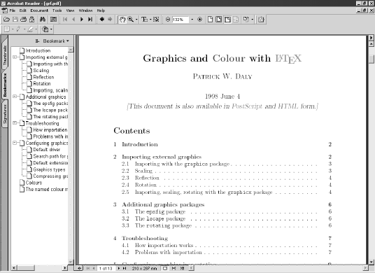
240 Chapter 10. PostScript and PDF
Figure 10.1: Output produced by pdfT
EX with the hyperref package for
automatic links, with an outline list at the left.
PDF file, where it should be noted that the table of content entries are all
links to their sections, as are the entries in the left-hand outline, which is
also generated automatically. The package provides L
A
T
EX-like commands
for the PDF features.
Before we go any further, we should explain certain terms that are
used below.
Links are indicated as a piece of text in a different color, or surrounded by
a frame, or may be an image, which when clicked cause the viewer
to jump to another document or some other place in the current
document.
Anchors (also called targets) are the destinations for links. They are pro-
vided with an identifying name so that the link can find them. Some
anchors are meant only for internal linking within the document,
while others are visible from outside.
Thumbnails are small images of the pages that are displayed in a thumb-
nail window by the viewer. They may be used to locate a certain
page more quickly, especially if it has an obviously different appear-
ance because of a figure it contains. Double clicking the page image
causes the viewer to jump to that page.
Bookmarks are special links to places in the document, associated with
aview, usually meaning a zoom factor, or a specification like ‘fit
10.2. Portable Document Format 241
page to width of window’. The bookmark window displays all these,
and by double clicking them, one jumps to that location and view.
Bookmarks are ordered within a tree, with sub-bookmarks and so
on. The bookmark display may have the tree opened or closed.
Outline is the usual use for bookmarks, building a table of contents, or
outline, for the whole document. The word ‘outline’ is used here,
but the PDF viewers refer to ‘bookmarks’. The latter if really far
more general.
Options for hyperref
There are a large number of parameters that may be configured for the
package, either as options in the \usepackage command, or with the
\hypersetup command, or with a configuration file. An example of
setting options with the first method is:
\usepackage[pdftex,
pdftitle={Graphics and Color with LaTeX},
pdfauthor={Patrick W Daly},
pdfsubject={Importing images and use of color in LaTeX},
pdfkeywords={LaTeX, graphics, color},
pdfpagemode=UseOutlines,
bookmarks,bookmarksopen,
pdfstartview=FitH,
colorlinks,linkcolor=blue,citecolor=blue,
urlcolor=red,
]
{hyperref}
Options that take a value are given with an equals sign and the value;
for multiple values, or text, the values must be placed within curly braces,
as shown in the example. Options that are either true or false are
simply given (to make them true) or equated to false. Options may also
be given with the \hypersetup command, as for example:
\hypersetup{colorlinks, linkcolor=blue}
Values that are colors must be a name of a defined color, as explained
in Section 6.2; the name must be defined before it is first used. However,
some color values must be the three numbers of the rgb model. The
colors of link borders may only be given as rgb. The hyperref package
automatically loads the color package if colorlinks is given.
One option must specify the driver name for which the output is
intended; in the above example this is pdftex, but other possibilities are:
dvipdf dvipdfm dvips dvipsone dviwindo hypertex
latex2html pdftex tex4ht textures vtex
242 Chapter 10. PostScript and PDF
The option hypertex is not for any particular driver, but rather for any
that conforms to the HyperT
EX guidelines, such as dvips. There is also a
draft option that turns off all hypertext features.
The next four options in the example (pdftitle–pdfkeywords) are
entries for the PDF document information stored in the file and displayed
only when the viewer shows the document summary. The complete set of
such options is:
pdfauthor pdfcreator pdfkeywords
pdfproducer pdfsubject pdftitle
The standard paper size options of Section 3.1.1 are all recognized
and one of them must be given, either as an option to hyperref or as a
global option in the \documentclass command. This is necessary to set
up the size of the PDF page. Reminder, these are:
a4paper a5paper b5paper
executivepaper legalpaper letterpaper
Here is a list of all of the remaining options, with default value in
brackets.
4(false) use Acrobat 4 features;
anchorcolor
(black) set color of anchors (targets of internal links);
backref
(false) adds links in the bibliography back to the citation; with
pagebackref, a list of pages is added to the bibliography, each
being a link back to the citation;
baseurl
determines the prefix for URLs given with \href;
bookmarks
(true) make bookmarks out of sectioning commands;
bookmarksnumbered
(false) include section numbers in bookmark text;
bookmarksopen
(false) start document with bookmarks tree opened;
bookmarksopenlevel
(max) the level to which bookmarks are opened;
bookmarkstype
(toc) specifies which ‘contents’ file used for bookmarks;
breaklinks
(false) allows link text to break over lines;
10.2. Portable Document Format 243
citebordercolor
(010) the color of the border around citations;
citecolor
(green) color of citation links when colorlinks given;
colorlinks
(false, but true for tex4ht and dviwindo) link and anchor
texts are to be colored, according to color specifications for the
various types of links; without this, link text is surrounded by a
frame;
debug (false) output diagnostic messages;
draft (false) turn off all hyperlinking;
extension
(dvi) default extension of linked files using the xr package (Sec-
tion 9.2.3); the package tries to guess whether the file specified
by \externaldocument should be.dvi or.pdf; with PDF output,
the viewer will open that external file and switch to it;
filebordercolor
(0 .5 .5) color of the border around file links;
filecolor
(cyan) color of file links when colorlinks given;
frenchlinks
(false) use small caps instead of color for links;
hyperfigures
(false) make figures into hyperlinks;
hyperindex
(true) make index entries into links back to referenced text;
hypertexnames
(true) use guessable (obvious) names for links;
implicit
(true) redefine L
A
T
EX internal commands;
linkbordercolor
(100) color of the border around links;
linkcolor
(red) color of link text when colorlinks given;
linktocpage
(false) the page numbers in the table of contents (or list of
figures/tables) are the links, rather than the text itself;
244 Chapter 10. PostScript and PDF
menubordercolor
(100) color of the border around Acrobat menu links;
menucolor
(red) color for Acrobat menu links when colorlinks given;
naturalnames
(false) use L
A
T
EX-computed names for links;
nesting
(false) links are allowed to be nested, although none of the
existing drivers support this;
pageanchor
(true) an anchor (target) is placed automatically on every page,
something that is necessary of the table of contents is to act as
links;
pagebackref
(false) adds to each entry in the bibliography a list of page
numbers linked to their citations;
pagebordercolor
(110) color of the border around page links;
pagecolor
(red) color of page links when colorlinks given;
pdfborder
(001, but 000with colorlinks) width of the border around
links in PDF files; the first two numbers are always zero, the third
is the line thickness in points;
pdfcenterwindow
(false) positions the document window in the center of the
computer monitor when the PDF file is opened;
pdffitwindow
(false) resizes the document window to fit the first page when
the PDF file is opened;
pdfhighlight
(/I) determines how the Acrobat menu buttons behave when
clicked; /I for inverse, /N for none, /O for outline, /P inset
highlighting;
pdfmenubar
(true) makes the menu bar in the PDF viewer visible;
pdfnewwindow
(false) a new window is opened when the PDF viewer switches
to another file;
10.2. Portable Document Format 245
pdfpagelayout
(SinglePage) determines the page layout for the PDF viewer;
other values are OneColumn (all pages in a continuous column),
TwoColumnLeft (two columns, with odd numbers on the left),
TwoColumnRight (two columns, with odd numbers on the right);
pdfpagemode
(None) determines initial display in the PDF viewer; other val-
ues are UseThumbs (show thumbnails), UseOutline (show book-
marks), FullScreen (no tool or menu bars, window is full screen);
pdfpagescrop
a set of four numbers determining the crop box when the the
PDF file is opened, similar to a bounding box;
pdfpagetransition
(R) determines how the pages are changed; possible values are
Split (like opening a curtain), Blinds (like Venetian blinds), Box
(a rectangle opens from the center), Wipe (vertical line moves
across page), Dissolve (old page dissolves into new), Glitter
(variation on dissolve), R(replace); additional parameters can be
added where appropriate: /Dm (with Split and Blinds) followed
by /H (horizontal) or /V (vertical), /Di (with Wipe and Glitter)
followed by 90,180,270 for the direction of motion, /M (with
Split and Box) followed by /I (inwards), /O (outwards); see
page 344 for a simplified interface to this feature;
pdfstartpage
(1) the first page number to be displayed when the PDF file is
opened;
pdfstartview
(Fit) determines the initial view when the PDF file is opened;
takes values of Fit (fit page to window), FitH (fit to width), FitV
(fit to height), FitB (fit to bounding box), FitBH (fit to bounding
box width), FitBV (fit to bounding box height), XYZ (no change);
pdftoolbar
(true) makes the tool bar in the PDF viewer visible;
pdfview
(XYZ) determines the page view when a link moves to a new page;
takes same values as pdfstartview;
pdfwindowui
(true) makes the user interface elements (bookmarks, thumb-
nails) in the PDF viewer available; if false, they are permanently
switched off;
246 Chapter 10. PostScript and PDF
plainpages
(true) makes the anchors for the pages to be their Arabic form; if
false, the page anchors are as the page numbers are formatted,
highly recommended if the document contains both Roman and
Arabic page numbers;
raiselinks
(false) with the hypertex driver, makes the border around links
the actual height of their contents, rather than the current base-
line separation;
runbordercolor
(0 .7 .7) color of the border around ‘run’ links;
unicode
(false) enables Unicode encoded PDF strings;
urlbordercolor
(011) color of the border around URL links;
urlcolor
(magenta) color of URL links when colorlinks given;
verbose
(false) issues many extra messages.
Using a configuration file
Very often a user will find that he or she needs the same set of options in
almost every document. Rather than issuing that set again and again, it is
possible to prepare a configuration file named hyperref.cfg containing
a\hypersetup command with all the option settings that one normally
wants. One effectively resets the default values. Any settings in the L
A
T
EX
source text itself will override those defaults.
The hyperref.cfg file must be located somewhere where it will always
be found by the L
A
T
EX processing. It might very well be that a file of that
name already exists, and will be read in in preference to yours. To check
just which location is being used, examine the transcript.log file for the
full path name, and then edit that version of hyperref.cfg.
Linking commands
The main purpose of the hyperref package is to add the automatic links
between cross-referencing commands and tables of contents. However,
it also enables access to PDF features with L
A
T
EX-style commands. One
of these is the ability to add manual links within the file and to other
documents, locally or on the Web. The commands to achieve this are:

10.2. Portable Document Format 247
\hyperbaseurl{url pre}
sets a prefix for all external URLs specified by other commands,
so that the common part of a set of URLs need only be given
once; this is the same as the baseurl option, but can be changed
within the document;
\href{url}{text}
makes text into a link to the full URL given by url prefixed with
the current base URL; special characters like #and &can be type
in url directly;
\hyperimage{url}{image url}
inserts the image referenced by image url;
\hyperdef{category}{name}{text}
establishes text as a target (anchor) with name category.name;
\hyperref{url}{category}{name}{text}
makes text a link to url#category.name;
an alternate syntax is \hyperref[key]{text}to make text an
internal link to the location marked with \label{key};
\hypertarget{name}{text}
establishes text as an internal target (anchor) with the name
#name;
\hyperlink{name}{text}
makes text a link to the internal target #name.
The cross-referencing commands \ref{key}and \pageref{key}(Sec-
tion 9.2.1) automatically create links to the corresponding \label{key}
location. As pointed out above, one can also create a manual link with
\hyperref[key]{text}.
The hyperref package also provides starred versions \ref* and
\pageref* which function as the regular ones but without creating a
link.
Adding Acrobat buttons
An electronic document is active, as indicated by the links within it for
jumping to other sections. But it is also possible to insert other types of
‘actions’, in the form of buttons which, when clicked, do something, like
flipping to the next page, opening another document, or even quitting.
The hyperref package can add such functionality for the Acrobat
viewers, by means of the command
\Acrobatmenu{action}{text}

248 Chapter 10. PostScript and PDF
Table 10.2: Actions available from the Acrobat menus (after Goossens
and Rahtz, 1999, page 48)
Acrobat Menu Available options for \Acrobatmenu
File Open, Close, Scan, Save, SaveAs, Optimizer:SaveAsOpt,
Print, PageSetup, Quit
File→Import ImportImage, ImportNotes, AcroForm:ImportFDF
File→Export ExportNotes, AcroForm:ExportFDF
File→DocProps GeneralInfo, OpenInfo, FontsInfo, SecurityInfo,
Weblink:Base, AutoIndex:DocInfo
Edit Undo, Cut, Copy, Paste, Clear, SelectAll, Ole:CopyFile,
TouchUp:TextAttributes, TouchUp:FitTextToSelection,
TouchUp:ShowLineMarkers,
TouchUp:ShowCaptureSuspects, TouchUp:FindSuspect,
Properties
Edit→Prefs GeneralPrefs, NotePrefs, FullScreenPrefs,Weblink:Prefs,
AcroSearch:Preferences(Windows)or,
AcroSearch:Prefs(Mac), Cpt:Capture
Edit→Search AcroSrch:Query, AcroSrch:Indexes, AcroSrch:Results,
AcroSrch:Assist, AcroSrch:PrevDoc, AcroSrch:PrevHit,
AcroSrch:NextHit, AcroSrch:NextDoc
Edit→Fields AcroForm:Duplicate, AcroForm:TabOrder
Document Cpt:CapturePages, AcroForm:Actions, CropPages,
RotatePages, InsertPages, ExtractPages, ReplacePages,
DeletePages, NewBookmark, SetBookmarkDest,
CreateAllThumbs, DeleteAllThumbs
View ActualSize, FitVisible, FitWidth, FitPage, ZoomTo,
FullScreen, FirstPage, PrevPage, NextPage, LastPage,
GoToPage, GoBack, GoForward, SinglePage, OneColumn,
TwoColumns, ArticleThreads, PageOnly, ShowBookmarks,
ShowThumbs
Tools Hand, ZoomIn, ZoomOut, SelectText, SelectGraphics, Note,
Link, Thread, AcroForm:Tool, Acro Movie:MoviePlayer,
TouchUp:TextTool, Find, FindAgain, FindNextNote,
CreateNotesFile
Window ShowHideToolBar, ShowHideMenuBar, ShowHideClipboard,
Cascade, TileHorizontal, TileVertical, CloseAll
Help HelpUserGuide, HelpTutorial, HelpExchange, HelpScan,
HelpCapture, HelpPDFWriter, HelpDistiller, HelpSearch,
HelpCatalog, HelpReader,Weblink:Home
Help(Windows) About
10.2. Portable Document Format 249
where text becomes a button to execute action when clicked. Of course,
text can be more than mere text, it is often a graphics that really does
look like a button.
The actions available are those provided by the Acrobat and Acrobat
Reader programs. These are not documented by Adobe, but are listed in
Table 10.2 on the facing page, which is taken from Goossens and Rahtz
(1999), who credit Merz (1998) for having figured them out. These actions
are therefore specific to these viewers only, and may change with later
versions. They may all be executed by the viewers themselves, by means
of pull-down menus in the menu bar, indicated in the left column of
Table 10.2.
The main purpose of this command is to set up navigational controls
on each page of a document that is meant essentially for screen viewing.
The regular tool bar may be turned off, which is why the document
itself must provide it. This is best put into a footline, and that is most
conveniently done with the fancyhdr package (Section 3.2.2).
\documentclass[a4paper]{article}
\usepackage{fancyhdr}
\usepackage[pdftex,colorlinks,
pdftoolbar=false,pdfmenubar=false,
pdfwindowui=false,
pdfpagemode=FullScreen,
]{hyperref}
\pagestyle{fancy}
\cfoot{\navbar}
\newcommand{\navbar}{%
\Acrobatmenu{FirstPage}{$\Leftarrow$}
\Acrobatmenu{PrevPage}{$\leftarrow$}
\Acrobatmenu{NextPage}{$\rightarrow$}
\Acrobatmenu{LastPage}{$\Rightarrow$}
\Acrobatmenu{Close}{$\bullet$}
}
The above produces a footline containing
⇐←→⇒•
(by default in red) as clickable buttons to jump to the first page, to the
previous page, to the next page, to the last page, respectively. And clicking
the bullet •closes the document. Of course, it looks even better if icons
are made up and inserted with \includegraphics.

11
Multilingual L
A
T
E
X
The original versions of T
EX and L
A
T
EX were set up for the English language,
American variant. The built-in hyphenation patterns were for English
only, and several English words such as ‘Figure’ and ‘Bibliography’ were
included explicitly in certain commands. This in fact violates the rules
of good programming which forbid doing anything explicitly. In Europe,
L
A
T
EX users quickly made customizations for their particular languages.
The adaptation for German, german.sty, is a set of macros from many
contributors collected together by H. Partl of the Technical University of
Vienna, and has become the standard for the German-speaking T
EX Users
Group (DANTE). It contains some facilities for other languages, including
French and English.
The key to the german package and other language adaptations is
the fact that the standard L
A
T
EX document styles (and later classes for
L
A
T
EX 2ε) had been altered so that explicit English words in the output were
replaced by reprogrammable command names. These names had become
standardized among European users for application to all languages. The
modified L
A
T
EX version by J. Schrod from Darmstadt was known as IL
A
T
EX,
for International L
A
T
EX. These names and their standard English values
are to be found on page 459.
As of December 1, 1991, these naming features became part of the L
A
T
EX
standard. They represent good programming practice, since they allow
even English-speaking users to change certain titles easily, for example
‘Abstract’ into ‘Summary’ or ‘Contents’ into ‘Table of Contents’. Naturally,
they were taken over, and extended upon, by L
A
T
EX 2ε.
Another important feature for multilingual usage is the T
EX\language
counter which allows more than one set of hyphenation patterns to be
stored in the format with initex (Section B.1.3). Different patterns are
activated by setting \language to the appropriate number. This is now
standard for all T
EX version over 3.0, which should now be universal.
Individual language packages such as german maintained by Bernd
Raichle and french by Bernard Gaulle have now been superseded to a
large extent today by the universal multilanguage system: babel.
251
252 Chapter 11. Multilingual L
A
T
E
X
11.1 The babel system
The babel system has been developed by Johannes Braams at the Dutch
PTT Research Laboratories. Its main purpose is to provide a standard
means of switching languages with a flexible method for loading the
hyphenation patterns. It has been written to work with both T
EX and
L
A
T
EX.
The three main requirements for a single language adaptation are:
translation of the explicit English words, special commands to simplify
certain features of that language, and selection of the appropriate hyphen-
ation patterns. To these babel adds: removal of the special commands
and testing for the current language. The language-specific files must
conform to the babel selection command structure. The concept of ‘di-
alects’ is also included, that is, two ‘languages’ that share a common set
of hyphenation patterns. Examples are German and Austrian as well as
British and US English, which only differ in the form of the dates.
At present, the babel package contains definition files for the following
languages (more can be added at any time):
Afrikaans, Bahasa, Basque, Breton, Bulgarian, Catalan, Croatian,
Czech, Danish, Dutch, English, Esperanto, Estonian, Finnish, French,
Galician, German, Greek, Hebrew, Hungarian, Icelandic, Irish Gaelic,
Italian, Latin, Lower Sorbian, North Sami, Norwegian, Polish, Por-
tuguese, Romanian, Russian, Scottish Gaelic, Spanish, Slovakian,
Slovenian, Swedish, Serbian, Turkish, Ukrainian, Upper Sorbian,
Welsh
The necessary definition files are delivered with the installation. The
hyphenation patterns for the various languages must be obtained from
another source, however. For most of these files, there are no special
commands for accents or punctuation: they only redefine the naming
commands for those words that normally print English text.
The german.sty package has been a great inspiration for babel. How-
ever, because of the name conflict, it was necessary to create a new
germanb.sty (and ngermanb.sty for the new German grammar rules) for
babel applications, which contains the same set of special commands,
but with a few babel additions. Similarly, the babel French file had to be
named frenchb.sty to distinguish it from the existing french.sty.
To exploit the babel features most fully, one should produce a L
A
T
EX
format (Section B.1.3) that incorporates it directly. To this end, the
hyphen.cfg supplied with babel must be used with the language.dat
file configured for the local languages and hyphenation patterns that are
to be pre-loaded. Only in this way can one conveniently get the right word
division for each language.
Alternatively, one can use a normal L
A
T
EX format and load babel as
a regular package, as illustrated below. The switching of hyphenation
11.1. The babel system 253
patterns will then be questionable.
The babel files
The babel installation provides the following files for its implementation:
babel.def contains some of the basic macros for running babel, and
must be loaded by the first language file read in; the remain-
ing macros are either already in the format itself (loaded from
hyphen.cfg) or read in from switch.def;babel.def determines
which is the case and reacts accordingly;
switch.def contains the additional babel macros, to be read in if these
macros are not already stored in the L
A
T
EX format;
hyphen.cfg contains the same macro definitions as in switch.def, plus
some more that are to be run by initex; if this file is available during
the creation of the L
A
T
EX format (Section B.1.3), these macros are
built into that format and file switch.def is not necessary at run
time;
babel.sty is a master package that loads the language files specified as
options;
language.dat contains a list of languages and the file names of their
hyphenation patterns; this file is read in by hyphen.cfg during
the initex run; it is the only file that may (must!) be edited for the
particular installation (Section 11.2);
esperant.ldf... the language definition files.
esperant.sty... compatibility files that read in the.ldf files.
Invoking babel
The babel package is loaded with the desired languages as options:
\usepackage[english,esperanto]{babel}
Alternatively, the language names may be used as global options, some-
thing that is recommended if there are other packages that take the
languages as options, as
\documentclass[english,esperanto]{article}
\usepackage{babel,varioref}
In both cases, the last named language is the one that is immediately
active.
The recognized language names that may be used as options are:

254 Chapter 11. Multilingual L
A
T
E
X
afrikaans
bahasa
basque
breton
bulgarian
catalan
croatian
czech
danish
dutch
english
=USenglish
=american
=UKenglish
=british
=canadian
esperanto
estonian
finnish
french
=francais
=canadien
=acadian
galician
german
=germanb
=ngerman
=austrian
=naustrian
greek
=polutoniko-
greek
hebrew
magyar
=hungarian
icelandic
irish
italian
latin
lowersorbian
samin
norsk
=nynorsk
polish
portuges
=portuguese
=brazilian
=brazil
romanian
russian
scottish
spanish
slovak
slovene
swedish
serbian
turkish
ukrainian
uppersorbian
welsh
Those names preceded by =are synonyms for the language option
above them. (The equals sign is not part of the option name.) For
example, both hungarian and magyar load the file magyar.ldf.
If the babel package is loaded, all it does is read in the specified lan-
guage packages; they in turn read in babel.def and possibly switch.def
(if its macros are not already in the format).
Language switching commands
The normal user needs to know very little about the babel internal oper-
ations. The new high-level user commands are:
\selectlanguage{language}
\begin{otherlanguage}{language}text \end{otherlanguage}
\begin{otherlanguage*}{language}text \end{otherlanguage*}
\foreignlanguage{language}{text}
\iflanguage{language}{yes text}{no text}
The \selectlanguage command and the otherlanguage environment
are two ways to switch to another language, with all its features and trans-
lations. The \foreignlanguage command and the otherlanguage* en-
vironment also switch to language but without the translations or date
changes; they are meant for setting short sections of text in a language
different from the regular one.
The \iflanguage executes yes text if language is current otherwise
no text.
In addition, \languagename contains the name of the currently se-
lected language.
Of course, each language definition file can also have its own special
commands to assist typing accented and special characters. For example,

11.1. The babel system 255
in German, one may type "a as a shorthand for \"a. To find out what
special commands are available for each language, and any other spe-
cial considerations, one must read the documentation for that language.
Documentation should be found in the texmf\doc\tex\generic\babel
directory, or you can process the desired language.dtx file in the texmf\
source\tex\generic\babel directory. (These paths might be different
on your system.)
Contents of a language definition file
Although one does not normally need to know anything about how the
switching mechanism functions, we will outline it here for the interested
user.
Two additional internal babel commands are:
\addlanguage{lang num}and
\adddialect{lang num 1}{lang num 2}
where lang num is an internal language number for specifying the set of
hyphenation patterns. The command \addlanguage sets its argument
equal to the next available language number. The form of lang num used
in babel is \l@language; for example, \l@english. This command is
executed on those language names listed in language.dat during the
initex run. The command \adddialect sets the first argument equal to
the second so that the two languages make use of the same set of hy-
phenation patterns. For example, in english.ldf there is the command
\adddialect{\l@american}{\l@english}.
A language definition file must provide four commands:
\captionslang to redefine the naming commands like \tablename
(see Section D.4.1);
\datelang to define \today (see Section D.4.2);
\extraslang to define any language-specific commands;
\noextraslang to remove the language-specific commands.
If the language lang is not one of those with prestored hyphenation
patterns in the current format file (that is, if \l@lang is undefined), it is
set to be a ‘dialect’ of language number 0.
Finally, the language definition file calls \selectlanguage{lang}to
activate that language. This is accomplished by
•calling \language\l@lang to select the set of hyphenation patterns,
•invoking \originalTeX in order to remove any existing language-
specific commands,
•activating \captionslang,\datelang, and \extraslang to invoke
the language-specific names, date, and commands,
256 Chapter 11. Multilingual L
A
T
E
X
•redefining \originalTeX to be \noextraslang so that the next
language switch will remove those features specific to lang.
11.2 Contents of the language.dat file
As has been mentioned before, with T
EX version 3.0 and later it is possible
to store more than one set of hyphenation patterns in the format file.
The counter \language is used to switch between them by setting it to a
different number.
However, there is no standard to dictate which languages belong to
which numbers. If a package were to assume a certain ordering, it would
most certainly function incorrectly at installations other than the one
for which it was designed. The babel system invokes a more reliable
procedure.
During the production of the format by initex (Section B.1.3), the file
hyphen.cfg is input, which in turn reads in language.dat, the only file
to be tailored to the local installation. This file contains a list of languages
to add as well as the name of the file with the hyphenation patterns and
the name of any additional file to be included. It also indicates names of
dialects that use the same hyphenations by prefixing the name with an
equals sign. For example, if language.dat contains
=USenglish
american ushyphen.tex
english ukhyphen.tex
=UKenglish
=british
french frhyphen.tex
german dehypht.tex
ngerman dehyphn.tex
the hyphenation patterns stored in files ushyphen.tex,ukhyphen.tex,
frhyphen.tex,dehypht.tex, and dehyphn.tex are loaded under the
language numbers 0 to 4 respectively, and \l@american,\l@english,
\l@french,\@german, and \l@ngerman are defined as numbers 0 through
4 for use with the \selectlanguage command. Languages \l@USenglish
and \l@UKenglish are synonyms for the current language, in this case 0
and 1, respectively. Similarly \l@british is identical to \l@UKenglish.

12
Math Extensions with
AMS-L
A
T
E
X
The American Mathematical Society, AMS, has supported the develop-
ment and usage of T
EX since its first release. It in fact owns the T
EX logo
as a registered trademark.
Shortly after T
EX 82 became available, the AMSproduced a macro
package for generating a special format amstex, described in The Joy
of T
EXby Spivak (1986). The macros in this AMS-T
EX complement the
mathematical typesetting features of Plain T
EX by adding additional ones
and simplifying others.
However, AMS-T
EX is not a documentation preparation system like
L
A
T
EX, describing the logical layout of a document by means of markup
commands, but rather is simply an extension to Plain T
EX.
The great popularity of T
EX as a text formatting program is due primar-
ily to the availability of L
A
T
EX as a user-friendly interface to the underlying
T
EX machinery. Many authors therefore asked the AMSto provide L
A
T
EX
with the same mathematical features as in AMS-T
EX. The AMS-L
A
T
EX
project was thus launched in 1987, with version 1.0 completed three
years later by Frank Mittelbach and Rainer Sch¨
opf, together with Michael
Downes of the AMS.AMS-L
A
T
EX has been fully converted to L
A
T
EX 2εwith
version 1.2 in 1996.
The AMS-L
A
T
EX collection consists of three parts: packages for ex-
tending mathematical typesetting, extra classes for articles and books
published by the AMS, and supplemental fonts for additional symbols,
math alphabets, and Cyrillic fonts.
In the next sections, we give an overview of the math extensions avail-
able in the package amsmath; a more detailed user’s manual is delivered
with the collection, in the file amsldoc.tex. How to invoke the additional
fonts is described below in Section 12.4, or in the AMS-supplied manual
found in the file amsfndoc.tex. The extra classes will not be described in
this book; AMSauthors should refer to the instructions in the document
instr-l.tex provided with AMS-L
A
T
EX.
257

258 Chapter 12. Math Extensions with AMS-L
A
T
E
X
12.1 Invoking AMS-L
A
T
E
X
If the \documentclass statement at the beginning of the L
A
T
EX document
Package:
amsmath selects one of the AMSclasses amsbook,amsart, or amsproc, then most
of the AMS-L
A
T
EX features are loaded automatically. These features may
still be employed with other classes by including the main extension
package amsmath by means of
\usepackage[options]{amsmath}
in the document’s preamble. The list of allowable options is described
below in Section 12.2.8.
The amsmath package defines many of the new math typesetting fea-
tures itself, but it also loads a number of other packages from the AMS-
L
A
T
EX collection that contain further extensions, such as amsopn,amstext,
and amsbsy. These packages could be loaded separately without amsmath
if only their limited features are wanted. On the other hand, the packages
amscd and amsthm are not included in amsmath and must be loaded ex-
plicitly if their features are desired. Simply add their names to the list of
packages in \usepackage.
The following Section 12.2 describes the new commands and environ-
ments made available with amsmath and its associated packages. We call
these the standard features of AMS-L
A
T
EX. Further extensions added by
other packages are explained afterwards.
The examples in this chapter employ the user-defined commands \mi,\me,
!and \dif defined in Section 5.4.10 for printing upright i, e, and d in math mode.
12.2 Standard features of AMS-L
A
T
E
X
This relatively long section presents those standard features of AMS-L
A
T
EX
that are activated by loading the amsmath package, or by selecting one of
the AMSclasses amsart,amsbook, or amsproc.
12.2.1 Additional font switching commands
Standard L
A
T
EX provides the math alphabet commands \mathcal,\mathrm,
Package:
amsbsy \mathbf,\mathsf,\mathit,\mathtt for changing fonts within math
mode (Section 5.4.2). With AMS-L
A
T
EX, one may also use the commands
\boldsymbol{symbol}and \pmb{symbol}
to print symbol in a bold face, provided there is an appropriate bold
font for it. Whereas the command \mathbf sets only Latin letters,
numbers, and Greek upper case letters in bold, these commands also
affect math symbols and Greek lower case letters. Compare the re-
sult of $\mathbf{\nabla\times V\,d\sigma}$ (∇ ×V dσ) with that

12.2. Standard features of AMS-L
A
T
E
X 259
of $\boldsymbol{\nabla\times V\,d\sigma}$ (∇ × V dσ). With the
standard L
A
T
EX command \mathbf, only the letters Vand dappear bold,
while the other characters remain in normal weight. Not only that, these
letters are upright, and not italic as required by international standards.
With \boldsymbol, all symbols are bold and italic.
Those symbols for which no bold face font exists will remain in normal
weight with the \boldsymbol command. Such symbols are, for example,
those that come in two sizes (Section 5.3.7) like P,R,S, and so on. The
command \pmb (poor man’s bold) simulates a bold face even for these
symbols by printing them several times slightly displaced. The result of
$\pmb{\sum\;\int\;\bigcup}$ is PRS
PRS
PRS.
These commands are defined in the package amsbsy, which may be
loaded separately without amsmath.
A short piece of normal text can be given within a formula with
Package:
amstext
\text{short text}
In contrast to \mbox{short text}for standard L
A
T
EX, the \text command
switches font size correctly when used as superscripts and subscripts.
Thus .._{\text{Word}} sets Word lower and changes to \scriptstyle
font size. To achieve the same effect in standard L
A
T
EX, the font size must
be given explicitly, as .._{\mbox{\scriptstyle Word}}. Furthermore,
the name \text is more precise than \mbox.
This command is defined in the package amstext. Like amsbsy, it may
be loaded on its own without amsmath if none of the other AMS-L
A
T
EX
features are wanted.
Another command to insert normal text inside a displayed equation is
\intertext{insert text}
The insert text is inserted as a left-justified line of text between those
of the formula. The alignment of the formula lines remains unaffected,
something that is not guaranteed if one closes the displayed equation,
inserts text and reopens the equation. For example:
(x +iy)(x −iy) =x2−ixy +ixy −i2y2
=y2+y2since i2= −1 is true.
On the other hand
(x +iy)2=x2+2ixy +i2y2=x2+2ixy −y2
(x −iy)2=x2−2ixy +i2y2=x2−2ixy −y2
\begin{align*}
(x+\mi y)(x-\mi y) & = xˆ2 - \mi xy + \mi xy - \mi ˆ2yˆ2\\
& = yˆ2 + yˆ2\quad\text{since}\quad \mi ˆ2=-1
\quad\text{is true.}\\
260 Chapter 12. Math Extensions with AMS-L
A
T
E
X
\intertext{On the other hand}
(x +\mi y)ˆ2 & = xˆ2 + 2\mi xy +\mi ˆ2yˆ2 = xˆ2 + 2\mi xy-yˆ2\\
(x -\mi y)ˆ2 & = xˆ2 - 2\mi xy +\mi ˆ2yˆ2 = xˆ2 - 2\mi xy-yˆ2
\end{align*}
The alignment of the lines on the first equals sign is maintained through
the interruption with the line of text ‘On the other hand’. The environment
align (Section 12.2.6) is one of several new ones provided by AMS-L
A
T
EX to
replace the standard L
A
T
EX environment eqnarray. Note that \intertext
may only be issued immediately after the \\ for starting a new line.
12.2.2 Multiple mathematical symbols
Mathematical formulas often require the same symbol to appear several
times, such as multiple integral signs, or symbols and arrows to be stacked
above or below a mathematical expression. Usually the distances between
these symbols depends on the mathematical meaning, something that
L
A
T
EX cannot automatically recognize. AMS-L
A
T
EX provides a number of
structures to help the user find the right spacing without tedious trial and
error.
Multiple integrals
With AMS-L
A
T
EX, the commands \iint,\iiint,\iiiint, and \idotsint
output multiple integrals, with upper and lower limits being added in the
usual manner. In text formulas, they are printed as RR,RRR,RRRR,R···R,
while in displayed formulas, they appear as
ZZ
S
f (x, y) dS\[ \iint\limits_S f(x,y)\,\dif S \]
ZZZ
V
f (x, y, z) dV\[ \iiint\limits_V f(x,y,z)\,\dif V\]
ZZZZ
G
f (x, y, z, t) dG\[ \iiiint\limits_G f(x,y,z,t)
\,\dif G \]
Z···Z
U
f(x1, . . . , xk)dU\[ \idotsint\limits_U
f(x_1,\ldots,x_k)\,\dif U \]
whereby the command \limits may be left off if the option intlimits
has been specified when amsmath was loaded (see Section 12.2.8).
12.2. Standard features of AMS-L
A
T
E
X 261
Multiline limits
One often needs multiline limits or indices for summations, as in the
examples below.
∆p1p2···pn−k
q1q2···qn−kX
k0,k1,...≥0
k0+k1+···=0
a0k0a1k1···
AMS-L
A
T
EX provides a command \substack for this purpose, with syntax
\substack{1st line\\2nd line\\...\\ last line}
where the command must immediately follow the ˆor _shifting com-
mands, and be entirely enclosed in curly braces { }. The index for the
left-hand example above was generated with
\Delta_{\substack{p_1p_2\cdots p_{n-k}\\q_1q_2\cdots q_{n-k}}}
The lines of text printed by \substack are centered horizontally, as
is apparent in the right-hand example above. This was produced with
\[ \sum_{\substack{k_0,k_1,\ldots\ge0\\ k_0+\k_1+
\cdots=0}}a_{0k_0} a_{1k_1}\cdots \]
On the other hand, the environment subarray offers more control over
the horizontal alignment:
\begin{subarray}{pos}1st line\\2nd line\\...\\ last line
\end{subarray}
The argument pos may be cfor centered, or lfor left-justified lines.
X
i∈Λ
i<j<n
P(i, j) \[ \sum_{\begin{subarray}{l} i\in\Lambda\\
i<j<n \end{subarray}} P(i,j) \]
Special limits
To add a differential prime sign to a summation symbol without a lower
limit, like PEn, in a displayed formula, one can easily give
\[ \sum\nolimits’ E_n \] XEn
However, if there to be an upper limit as well, the prime can only be
added with much fiddling. The \sideset command simplifies this task
considerably.
∞
X
n=0
(2n+1)E2n+1
\[ \sideset{}{’}\sum_{n=0}ˆ\infty
(2n+1) E_{2n+1} \]
The complete syntax for this command is:
262 Chapter 12. Math Extensions with AMS-L
A
T
E
X
\sideset{pre}{post}\symbol
where pre and post are the superscripts and subscript commands to be
added before and after the \symbol, respectively. They must contain
raising and lowering operators ˆand _.
The product symbol Qis given daggers above and asterisks
below with \sideset{_\dagˆ*}{_\dagˆ*}\prod, as shown
at the right.
∗
†Y∗
†
Additional shifting commands are
\overset{char}{\symbol}and \underset{char}{\symbol}
which place the arbitrary char above or below the \symbol in the size
appropriate for superscripts and subscripts. Thus $\overset{*}{X}$
produces ∗
Xand $\underset{*}{X}$ yields X
∗.
Extended arrows
The amsmath package provides a number of commands to produce extra
long arrows for combining with mathematical expressions. The com-
mands
\overleftarrow{expr} \underleftarrow{expr}
\overrightarrow{expr} \underrightarrow{expr}
\overleftrightarrow{expr} \underleftrightarrow{expr}
produce lengthened arrows pointing left and right, as well as double
arrows above and below the mathematical expression expr.
−−−−→
ABCD =AB
−→ +BC
−→ +CD
−−→
←−−−−
ABCD =DC
←−− +CB
←− +BA
←−
←−−−→
ABCD =DCAB
←−−−→
\begin{eqnarray*}
\overrightarrow{ABCD} & = &
\underrightarrow{AB} +
\underrightarrow{BC} +
\underrightarrow{CD} \\
\overleftarrow{ABCD} & = &
\underleftarrow{DC} ...
\end{eqnarray*}
The lower arrows are actually too close to the expression, as is seen on
the right-hand side of the last example. This should also be the case for
all the other examples with a lower arrow, except that we have added a
strut to push them down somewhat:
\underrightarrow{\rule[-2pt]{0pt}{2pt}AB} ... and
\underleftarrow{\rule[-2pt]{0pt}{2pt}DC} ...
A smaller font size will be used for the arrows when they appear in
exponents, indices, superscripts, and subscripts:
12.2. Standard features of AMS-L
A
T
E
X 263
Z−−−→
0.2πr dϕ =2πr \int_{\overrightarrow{0.2\pi}}
r\,d\varphi = 2\pi r
There are two more commands for horizontal arrows of variable length:
\xleftarrow[below]{above} \xrightarrow[below]{above}
which place the mandatory above in superscript size over the arrow, and
the optional below in subscript size beneath it.
An+µ−1
←−−−−− Bn±i−1
−−−−→
TC\[ A \xleftarrow{n+\mu-1} B
\xrightarrow[T]{n\pm i-1} C \]
The package amscd (Section 12.3.2) offers further possibilities for
combining arrows and text.
Stacked accents
Attempting to place multiple accents over a character with standard L
A
T
EX,
say with $\hat{\hat{A}}$, results in a misplacement: ˆ
ˆ
A. The same
applies to the other mathematical accents commands \check,\breve,
\acute,\grave,\tilde,\bar,\vec,\dot, and \ddot (Section 5.3.9).
The amsmath package provides a set of math accent commands with the
same names but capitalized,
\Hat \Breve \Grave \Bar \Dot
\Check \Acute \Tilde \Vec \Ddot
which can be safely combined with one another for the expected results:
$\Hat{\Hat{A}}$,$\Breve{\Bar{B}}$ and $\Tilde{\Tilde{C}}$
produce ˆ
ˆ
A,˘
¯
B, and ˜
˜
C.
Three or four dots in a row over a symbol are often used for time
derivatives of third and fourth order. They can be placed with the com-
mands
\dddot{sym}and \ddddot{sym}
In this way ...
uand ....
uare produced with $\dddot{u}$ and $\ddddot{u}$.
Continuation dots
In standard L
A
T
EX, one has the commands \ldots and \cdots for printing
three continuation dots, either on the baseline or raised to the center of
the line. AMS-L
A
T
EX offers a number of additional possibilities. The most
general of these is the \dots command which adjusts the vertical height
according to the symbol that follows it. If this is an equals sign or binary
operator, such as +or −, the dots are raised, as with \cdots, otherwise
they are on the baseline, as with \ldots.

264 Chapter 12. Math Extensions with AMS-L
A
T
E
X
$a_0+a_1+\dots+a_n$ =⇒ a0+a1+ ···+ an
$a_0,a_1,\dots,a_n$ =⇒ a0, a1, . . . , an
If the continuation dots come at the end of a formula, there is no following
symbol to determine the height of the dots. In this case, one must
manually indicate the height by means of one of the commands \dotsc
(comma), \dotsb (binary), \dotsm (multiplication), or \dotsi (integral).
The \dotsc is to be used with commas, so $A_1,A_2,\dotsc$ pro-
duces A1, A2, . . . ; the \dotsb sets them for a binary operator, thus
$A_1+A_2+\dotsb$ yields A1+A2+···; the command \dotsm is actually
identical to \dotsb, but it is logically meant to be applied to multiplica-
tion, $A_1A_2\dotsm$ makes A1A2···; finally \dotsi places the dots at
the mean height of an adjacent integral sign.
\[ \int_{A_1}\int_{A_2}\dotsi \] ZA1ZA2···
12.2.3 Fractions
The T
EX fraction commands \atop,\choose, and others may be allowed
in standard L
A
T
EX, but not in AMS-L
A
T
EX. With the amsmath package, only
those fraction commands described here may be used.
Basic fraction commands
In addition to the regular L
A
T
EX command \frac{over}{under},AMS-
L
A
T
EX provides the commands \tfrac and \dfrac with the same syn-
tax. These are effectively the same as \frac but with the font set to
\textstyle or \displaystyle, respectively (Section 5.5.2). We demon-
strate their effects with some examples from the AMS-L
A
T
EX user’s manual.
\[ \frac{1}{k}\log_2 c(f)\qquad
\tfrac{1}{k}\log_2 c(f)\qquad
\sqrt{\frac{1}{k}\log_2 c(f)}\qquad
\sqrt{\dfrac{1}{k}\log_2 c(f)} \]
1
klog2c(f) 1
klog2c(f) s1
klog2c(f) s1
klog2c(f)
Binomial expressions
A binomial expression looks something like a fraction, but is enclosed in
round parentheses and is missing the horizontal rule. The basic command
in the amsmath package is
\binom{over}{under}

12.2. Standard features of AMS-L
A
T
E
X 265
which functions in the same way as \frac and the other fraction com-
mands.
\[ \binom{n+1}{k} = \binom{n}{k}
+ \binom{n}{k-1 \] n+1
k!= n
k!+ n
k−1!
Similarly there are the commands \tbinom and \dbinom analogous to
\tfrac and \dfrac.
User-defined fractions
The amsmath package provides a powerful tool for defining fraction-like
structures:
\genfrac{left brk}{right brk}{thickness}{mathsize}{over}{under}
where left brk and right brk are the parenthesis characters on the left and
right, thickness is the thickness of the horizontal line, and {mathsize}is
a number 0–3 representing the math sizes \displaystyle,\textstyle,
\scriptstyle, and \scriptscriptstyle, respectively. The last two
arguments, over and under, are the texts in the two parts of the fraction,
the same arguments as in \frac and \binom.
If the thickness is left blank, the standard thickness for L
A
T
EX fractions
is used. If mathsize is empty, the font size is determined automatically
by the normal rules in Section 5.5.2.
Rather than repeating \genfrac with the same first four arguments
time and again, one should define new fraction commands with it. For
example, the following definitions are given in amsmath.sty:
\newcommand{\frac}[2]{\genfrac{}{}{}{}{#1}{#2}}
\newcommand{\dfrac}[2]{\genfrac{}{}{}{0}{#1}{#2}}
\newcommand{\tfrac}[2]{\genfrac{}{}{}{1}{#1}{#2}}
\newcommand{\binom}[2]{\genfrac{(}{)}{0pt}{}{#1}{#2}
As a further example, consider the redefinition of the command \frac
\renewcommand{\frac}[3][]{\genfrac{}{}{#1}{}{#2}{#3}}
in which the line thickness is now an optional first argument; without this
optional argument, the command behaves as normal. Thus
\[ \binom{n}{m} =
\frac[2pt]{n!}{M!(n-m)!} \]
yields n
m!=n!
M!(n −m)!
Continued fractions
Continued fractions can be made in AMS-L
A
T
EX with the command
\cfrac[pos]{over}{under}
whereby the denominator under may contain further \cfrac commands.
266 Chapter 12. Math Extensions with AMS-L
A
T
E
X
\[ a_0 + \cfrac{1}{a_1 + \cfrac{1}{a_2 +
\cfrac{1}{a_3 + \cfrac{1}{a_4 +
\dotsb }}}} \]
produces
a0+1
a1+1
a2+1
a3+1
a4+···
If the optional argument pos is missing, the numerator over is centered
on the horizontal rule; otherwise it may take values of lor rto left or
right justify the numerator.
12.2.4 Matrices
Standard L
A
T
EX possesses the environment array for producing arrays
and matrices. The amsmath package provides the additional environments
pmatrix,bmatrix,Bmatrix,vmatrix, and Vmatrix, which automatically
add the enclosing braces (), [], {},| | and around the array, and in the
right size. For completeness, there is also a matrix environment with no
braces.
In contrast to the standard array environment (Section 4.8.1), these
matrix environments do not require an explicit column specification as
argument. By default, up to 10 centered columns may be used without
any argument. (This maximum number may be changed by giving the
special counter MaxMatrixCols a new value with either \setcounter
or \addtocounter.) Otherwise the matrix environments are used in the
same way as the array environment.
The following example is taken from Section 5.4.3 on page 134 and is
recast here using AMS-L
A
T
EX constructs.
(1,2,...,n)
X
p1<p2<···<pn−k
∆p1p2...pn−k
p1p2...pn−kX
q1<q2<···<qk
aq1q1aq1q2. . . aq1qk
aq2q1aq2q2. . . aq2qk
...................
aqkq1aqkq2. . . aqkqk
\[ \sum_{p_1<p_2<\dots<p_{n-k}}ˆ{(1,2,\dots,n)}
\Delta_{\substack{p_1p_2\dots p_{n-k}\\p_1p_2
\dots p_{n-k}}}
\sum_{q_1<q_2<\dots<q_k}
\begin{vmatrix}
a_{q_1q_1} & a_{q_1q_2} & \dots & a_{q_1q_k}\\
a_{q_2q_1} & a_{q_2q_2} & \dots & a_{q_2q_k}\\
12.2. Standard features of AMS-L
A
T
E
X 267
\hdotsfor[2.0]{4}\\
a_{q_kq_1} & a_{q_kq_2} & \dots & a_{q_kq_k}
\end{vmatrix} \]
Comparing this input text with that on page 134, one sees that it
is simpler and easier to follow. The only new command used here is
\hdotsfor which has the syntax
\hdotsfor[stretch]{n}
and which prints a continuous line of dots through ncolumns. The
optional argument stretch is a multiplicative number to increase the dot
density, being 1.0 by default.
\[ \begin{matrix} a & b & c & d & e\\
x & \hdotsfor{3} & z
\end{matrix} \]
a b c d e
x . . . . . . . . . z
Compare the standard dot spacing above with that from \hdotsfor[2.0]
in the previous example.
The initial letter of each of the xmatrix environments indicates the
type of braces that enclose it: pmatrix for (round) parentheses, bmatrix
for (square) brackets, Bmatrix for (curly) braces, vmatrix for vertical
lines, and Vmatrix for double vertical lines. They appear as
r s t
u v w
x y z
r s t
u v w
x y z
r s t
u v w
x y z
r s t
u v w
x y z
r s t
u v w
x y z
r s t
u v w
x y z
where each matrix has been produced with
\[ \begin{xmatrix}r&s&t\\u&v&w\\x&y&z
\end{xmatrix} \]
where xmatrix is set to matrix,pmatrix,bmatrix,Bmatrix,vmatrix,
and Vmatrix one after the other.
To generate a small array within a text formula, one can apply the
smallmatrix environment. In this way a b c
e m r can be made with
$ \bigl( \begin{smallmatrix} a & b & c\\ e & m & r
\end{smallmatrix} \bigr) $
12.2.5 User extensions and fine adjustments
Function names
Standard L
A
T
EX recognizes a number of preprogrammed function names
Package:
amsopn (Section 5.3.8) that are printed in math made by placing a backslash in

268 Chapter 12. Math Extensions with AMS-L
A
T
E
X
front of that name: arccos, arcsin, arctan, arg, cos, cosh, cot, coth, csc,
deg, det, dim, exp, gcd, hom, inf, ker, lg, lim, liminf, limsup, ln, log, max,
min, Pr, sec, sin, sinh, sup, tan, tanh. Not only do these names appear in
an upright font, as is required for function names, but the spacing with
adjacent parts of the mathematical expression is adjusted automatically.
AMS-L
A
T
EX provides some more function names, as variations on the
standard \lim name:
\varlimsup lim \varinjlim lim
−−→
\varliminf lim \varprojlim lim
←−−
These functions may take on limits with the raising and lowering operators
ˆand _; for example \varliminf_{n\to\infty} for limn→∞.
It is also possible to define new function names with the same font
and spacing properties as the predefined ones. The command
\DeclareMathOperator{\cmd}{name}
which may only be issued in the preamble, before \begin{document},
defines a command \cmd that prints the function name name. For
example, to define a function name \doit, give
\DeclareMathOperator{\doit}{doit}
and then $A=3\doitˆ2(B)$ yields A=3 doit2(B). Note that superscripts
and subscripts are printed beside the operator; if they are to be printed
as limits, that is, above and below the operator in displayed math mode,
use the *-form to define them. For example:
\DeclareMathOperator*{\Lim}{lim}
\[ \Lim_{n\to-\infty}ˆ{n\to+\infty}\]
n→+∞
lim
n→−∞
The name text need not be identical to the command name. In par-
ticular, it may contain special characters not allowed in command names.
Modulo expressions are printed in standard L
A
T
EX with \bmod and
\pmod commands, and are complemented in AMS-L
A
T
EX by \mod and
\pod. The possibilities are:
z≡x+ymod n2
z≡x+y (mod n2)
z≡x+ymod n2
z≡x+y (n2)
z \equiv x+y \bmod{nˆ2}
z \equiv x+y \pmod{nˆ2}
z \equiv x+y \mod{nˆ2}
z \equiv x+y \pod{nˆ2}
The automatic parentheses are missing with \mod, while with \pod the
name ‘mod’ is omitted. Furthermore, \pmod is redefined for text formulas
to reduce the preceding space: $y\pmod{a+b}$:y (mod a+b).
The \DeclareMathOperator command and additional function names
are defined in the amsopn package, which may be loaded on its own with-
out amsmath.
12.2. Standard features of AMS-L
A
T
E
X 269
Fine-tuning roots
The positioning of an index to a root sign is not always ideal under
standard L
A
T
EX. In β
√k, for example, the βcould be somewhat higher and
shifted slightly to the right. The AMS-L
A
T
EX commands
\leftroot{shift} \uproot{shift}
cause such manual displacements, where shift is a number specifying
the size in small, internal units. Negative numbers represent a shift in
the opposite direction. Compare the above standard result with that of
$\sqrt[\leftroot{-1}\uproot{3}\beta]{k}$:β
√k.
The size of the root sign depends on its contents. If they hang below
the baseline, the root sign extends lower down than for contents that have
no depth. Note the differences between √x,√y, and √z. Some publishers
want all root signs be at the same height, as √x+√y+√z. This is accom-
plished with the T
EX command \smash which places its argument in a box
of zero height and depth. The AMS-L
A
T
EX version of this command allows
an optional argument bor tto zero only the depth or height, respectively.
The above example is produced with $\sqrt{\smash[b]{y}}$. The op-
tion bis taken because we want only the depth to be ignored, not the
height of the letter y.
Spacing adjustment
With standard L
A
T
EX, there are a number of commands to fine-tune the
spacing in a math formula (Section 5.5.1). These are \, \: \; \quad and
\qquad for increasing amounts of positive spacing, and \! for negative
spacing. With the amsmath package, the first three still exist, but may
also be called with the more obvious names \thinspace,\medspace, and
\thickspace. There is also \negthinspace as an alias for \!.
The complete set of spacing commands are summarized in the table
below taken from the AMS-L
A
T
EX manual.
Short Command Short Command
form name Demo form name Demo
\, \thinspace \! \negthinspace
\: \medspace \negmedspace
\; \thickspace \negthickspace
\quad
\qquad
The general math spacing command is
\mspace{mu}
which inserts space in mathematical spacing units ‘mu’ (=1/18 em). For
example, \mspace{-9mu} puts in negative spacing of 1/2 em.
270 Chapter 12. Math Extensions with AMS-L
A
T
E
X
Vertical bars
In standard L
A
T
EX, the commands |and \| are used for single and double
vertical bars, |and . However, these symbols are often used as delimiters
(that is, like braces) in which case different spacing requirements are
needed. In particular, a distinction must be made between the left and
right delimiter in expressions like |a|and v. The L
A
T
EX commands are
only appropriate for single appearances, like p|qor f (t, x)|t=0.
The amsmath package defines the delimiter commands \lvert,\rvert
for a single bar, and \lVert,\rVert for a double bar. They are useful for
defining commands that set their arguments in such delimiters, as
\newcommand{\abs}[1]{\lvert#1\rvert}
\newcommand{\norm}[1]{\lVert#1\rVert}
Now $\abs{a}$ produces |a|, and $\norm{v}$ v.
A similar recommendation can be made for the standard commands
\langle and \rangle. By defining
\newcommand{\mean}[1]{\langle#1\rangle}
one gives $\mean{x}$ to generate x, rather than $<x>$ which produces
< x >.
Boxed formulas
A formula may be placed in a box with the command
\boxed{formula}
For example,
\[ \boxed{\int_0ˆ\infty f(x)\,\dif x \approx
\sum_{i=1}ˆn w_i \meˆ{x_i} f(x_i)} \]
produces Z∞
0
f (x) dx≈
n
X
i=1
wiexif(xi)
12.2.6 Multiline equations
Equations consisting of several lines which are horizontally aligned at set
points, such as the equals sign, can be generated in standard L
A
T
EX with
the eqnarray and eqnarray* environments (Section 5.4.7). Many authors
consider these to be far too limited for publications with complicated
multiline equations. AMS-L
A
T
EX therefore provides a range of further
alignment environments for formulas extending over a single line:
align gather falign multline alignat split
12.2. Standard features of AMS-L
A
T
E
X 271
With the exception of split, all exist in a standard and a *-form. As for
eqnarray, the standard form adds an automatic equation number to each
line, while the *-form does not. The standard L
A
T
EXequation environment
for single line formulas is also available in AMS-L
A
T
EX in a *-form. It may
be used in combination with multiline environments.
Common features of alignment environments
All the alignment, or multiline, environments switch to math mode at the
start and back to text mode at the end, except for split which must
be called in math mode. A new line is forced in the formula with the
\\ command, as usual; an optional argument \\[len]can be added to
increase the line spacing by len, again as usual.
The automatic numbering with the standard forms can be suppressed
for single lines by adding \notag before the \\ line break. Alternatively,
the line can be given a desired marker with \tag{mark}. For example,
with \tag{$\dag$}, the marker is (†). Using the *-form instead, the
marker text is printed without the parentheses.
The vertical position of the equation number or marker can be adjusted
with the command
\raisetag{len}
which moves the marker upwards by len for that line only. A negative
value moves it downwards.
The multline environment
The multline environment is a variant of the equation environment for
single formulas that are too long for one line. The line breaks occur where
the user forces them with the \\ command. The first line is left justified,
the last right justified, and lines in between are centered. However, if the
option fleqn has been given, all the lines appear left justified.
The equation number, if present, appears at the right of the last line
by default or if the option reqno has been selected; if the option leqno
has been chosen, the number is placed at the left of the first line. (See
Section 12.2.8 for the amsmath options.)
It is possible to shift individual lines fully to the left or right with
the commands \shoveleft{formula}and \shoveright{formula}. The
entire formula text for that line, except the terminating \\, is placed in
their arguments.
The left and right margins for the formula are set by the length par-
ameter \multlinegap which is initially 10 pt. This may be altered by the
user with the \setlength or \addtolength commands.
272 Chapter 12. Math Extensions with AMS-L
A
T
E
X
An equation with five lines could be broken to look as follows:
First line — left justified
Second line — horizontally centered
Third line — pushed to the left
Fourth line — pushed to the right
Last line — right justified (12.1)
\begin{multline}
\framebox[.75\columnwidth]{First line --- left justified}\\
\framebox[.6\columnwidth]{Second line --- horizontally
centered}\\
\shoveleft{\framebox[.6\columnwidth]{Third line --- pushed
to the left}}\\
\shoveright{\framebox[.6\columnwidth]{Fourth line --- pushed
to the right}}\\
\framebox[.75\columnwidth]{Last line --- right justified}
\end{multline}
A real equation would contain mathematical expressions and not the
\framebox commands in the above demonstration.
The split environment
Like multline, the split environment is meant for a single equation
that does not fit on one line. Line breaks are again forced with the \\
command; the difference is that in each line there is an alignment marker
&such that the lines are horizontally positioned to line up the markers.
The split environment does not switch into math mode, nor does it
produce an equation number. It is intended to be applied within another
math environment, such as equation or gather. This is why there is an
equation* environment in AMS-L
A
T
EX.
The equation number, if present, is provided by the outer environment.
It is applied to the entire multiline formula, which by default, or with the
option centertags, is centered on the group of lines. With the option
tbtags, it is placed either at the left of the last line, or at the right of the
first line, depending on the further options leqno and reqno, respectively.
(See Section 12.2.8.)
Hc=1
2n
n
X
l=0
(−1)l(k −l)p−2X
l1+···+lp=l
p
Y
i=1 ni
li!
×[(k −l) −(ki−li)]ki−li×h(k −l)2−
p
X
j=1
(ki−li)2i(12.2)

12.2. Standard features of AMS-L
A
T
E
X 273
\begin{equation}\begin{split}
H_c&=\frac{1}{2n}\sum_{l=0}ˆn (-1)ˆl (k-l)ˆ{p-2}
\sum_{l_1+\dots+l_p=l} \prod_{i=1}ˆp \binom{n_i}{l_i}\\
&\quad\times[(k-l) - (k_i-l_i)]ˆ{k_i-l_i}\times
\Bigl[(k-l)ˆ2 - \sum_{j=1}ˆp (k_i-l_i)ˆ2\Bigr]
\end{split}\end{equation}
The alignment has been chosen to be just before the equals sign. The
second line begins with the alignment marker &so that the equation
continues below the =in the first line. A \quad has been inserted so
that the ×is not immediately below the equals sign. Alternatively, one
could place the &after the =and dispense with \quad in the second line.
However, the above is more suitable when there are continuation lines
beginning with =. Note the centered equation number at the right.
The gather environment
The gather environment switches to math mode, centering each of its
formula lines without any alignment. The formula lines are separated by
\\ commands. Each line receives an equation number, unless the *-form
has been used, or \notag has been issued in that line.
1
2+2
34
+3
49
+··· + n
n+1n2
+··· = ∞
X
n=1n
n+1n2
(12.3)
converges since lim
n→∞
n
sn
n+1n2
=lim
n→∞
1
1+1
n
n
=1
e<1
root condition
2+3
4+4
9+··· + n+1
n2+··· = ∞
X
n=1
n+1
n2(12.4)
diverges since Z∞
c
x+1
x2dx=ln x−1
x∞
c= ∞ (integral condition)
\begin{gather}
\frac{1}{2} + \left(\frac{2}{3}\right)ˆ4 + \left(\frac{3}{4}
\right)ˆ9 + \dots + \left(\frac{n}{n+1}\right)ˆ{nˆ2} + \dotsb
= \sum_{n=1}ˆ\infty \left(\frac{n}{n+1}\right)ˆ{nˆ2} \\
\text{converges since}\quad\lim_{n\to\infty}
\sqrt[n]{\left(\frac{n}{n+1}\right)ˆ{nˆ2}} = \lim_{n\to\infty}
\left(\frac{1}{1 + \dfrac{1}{n}}\right)ˆn = \frac{1}{\me} < 1
\tag*{root condition}\\
2 + \frac{3}{4} + \frac{4}{9} + \dots + \frac{n+1}{nˆ2} +
\dotsb = \sum_{n=1}ˆ\infty \frac{n+1}{nˆ2}\\
\text{diverges since}\quad\int_cˆ\infty \frac{x+1}{xˆ2}\,
274 Chapter 12. Math Extensions with AMS-L
A
T
E
X
\dif x = \left[ \ln x -\frac{1}{x}\right]_cˆ\infty = \infty
\tag{integral condition}
\end{gather}
Note the use of \tag and \notag (page 271) to add text as markers to the
second and fourth lines.
The align environment
The align environment is intended for multiple equations with horizontal
alignment, usually on an equals sign or equivalent. New lines are indicated
with \\ as usual. Each line is split into aligned columns such that the first
column is right justified against the &character, the second left justified;
the third column is right justified against the third &, the fourth column
left justified again, and so on. This is the same as an array environment
with column specification {rl rl rl ...}.
(xn)=nxn−1(ex)=ex(sin x)=cos x
1
xn= − n
xn+1(ax)=axln a (cos x)= −sin x
n
√x=1
nn
√xn−1(ln x)=1
x(tan x)=1
cos2x
(logax)=1
xln a(cot x)= − 1
sin2x
\begin{align*}
\left(xˆn\right)’ &= nxˆ{n-1} & \left(\meˆx\right)’ &= \meˆx &
(\sin x)’ &= \cos x \\
\left(\frac{1}{xˆn}\right)’ &= -\frac{n}{xˆ{n+1}} &
\left(aˆx\right)’ &= aˆx\ln a & (\cos x)’ &= -\sin x\\
\left(\sqrt[n]{x}\right)’ &= \frac{1}{n\sqrt[n]{xˆn -1}} &
(\ln x)’ &= \frac{1}{x} & (\tan x)’
&= \frac{1}{\cosˆ2 x}\\
& & (\log_a x)’ &= \frac{1}{x\ln a} & (\cot x)’
&= -\frac{1}{\sinˆ2 x}
\end{align*}
The align* environment is used here to prevent the lines from being
numbered, something that is not appropriate for such a collection of
formulas. The alignment within each of the three column pairs is on the
equals sign. The input for the last line begins with a double && to produce
an empty column pair.
Occasionally a set of formulas is to be aligned on several equals signs
in one line, as in the equations below for the volume V, inertial moment Iz,
and mass Mof an arbitrary body, in Cartesian, cylindrical, and spherical
coordinates. In this case, the second and third parts are separated by a

12.2. Standard features of AMS-L
A
T
E
X 275
double && so that the left-hand sides of these column pairs are empty:
the equals signs are always on an odd-numbered alignment marker.
V=Z
V
dv=ZZZdxdydz=ZZZρdxdρdφ
=ZZZr2sin θdrdθdφ(12.5)
Iz=Z
V
ρ2dv=ZZZ(x2+y2)dxdydz=ZZZρ3dzdρdφ
=ZZZr4sin3θdrdθdφ(12.6)
M=Z
V
δdv=ZZZδdxdydz=ZZZδρ dzdρdφ
=ZZZδr2sin θdrdθdφ(12.7)
\begin{align}
V &= \int\limits_V\dif v &&= \iiint\dif x\,\dif y\,\dif z
&&= \iiint \rho\,\dif x\,\dif \rho\,\dif \phi \notag \\
&&&&&= \iiint rˆ2 \sin\theta\,\dif r\,\dif\theta\,\dif\phi\\
I_z &= \int\limits_V \rhoˆ2\,\dif v &&=\iiint(xˆ2 + yˆ2)
\,\dif x\,\dif y\,\dif z
&&= \iiint \rhoˆ3\,\dif z\,\dif \rho\,\dif \phi \notag \\
&&&&&= \iiint rˆ4\sinˆ3\theta\,\dif r\,\dif\theta\,\dif\phi\\
M &= \int\limits_V \delta\,\dif v &&= \iiint \delta
\,\dif x\,\dif y\,\dif z
&&= \iiint \delta\rho\,\dif z\,\dif\rho\,\dif\phi\notag \\
&&&&&=\iiint\delta rˆ2\sin\theta\,\dif r\,\dif\theta\,\dif\phi
\end{align}
There are two variations on the align environment, falign and
alignat. The first has exactly the same syntax as align but it inserts
so much spacing between the column pairs that the entire line is filled
out. The alignat environment is just the opposite: no spacing is in-
serted automatically between the column pairs. It must take the number
of column pairs as a mandatory argument, but otherwise the syntax of
the contents is the same as that for align. The example above with the
volume, inertial moment, and mass of a body could just as well have been
given with
\begin{alignat}{3} formula text \end{alignat}
(In fact, this is precisely what was done in order to fit it within the line
width of this book.)
If one or more columns are empty, as in this example, it is possible
to control their widths precisely in the alignat environment by adding
276 Chapter 12. Math Extensions with AMS-L
A
T
E
X
explicit spacing between the two &characters in one of the lines. See
Section 5.5.1 for spacing in math mode.
In summary, for the align environment and its variants, the first,
third, fifth, etc. &characters are alignment markers, while the second,
fourth, sixth, etc. are column pair separators.
Nested alignment environments
We have already pointed out on page 272 how the split environment
is to be placed inside an equation environment. The same is true for
the environments aligned and gathered, which may be used as building
blocks within formulas. Their contents and behavior are otherwise the
same as their related environments.
Both of these environments take an optional argument pos
\begin{aligned}[pos]lines \end{aligned}
\begin{gathered}[pos]lines \end{gathered}
which takes values of tor bto determine the vertical alignment (top or
bottom) when they appear beside other elements. When no pos is given,
they are centered. In this way
α=aa
β=bbbbb
γ=g
versus δ=dd
η=eeeeee
ϕ=f
versus
s=x+y
d=u−v−w
p=x◦y
is produced with
\begin{equation*}
\begin{aligned} \alpha&=aa\\ \beta&=bbbbb\\ \gamma&=g
\end{aligned}
\qquad\text{versus}\qquad
\begin{aligned}[t] \delta&=dd\\ \eta&=eeeeee\\ \varphi&=f
\end{aligned}
\qquad\text{versus}\qquad
\begin{gathered}[b] s= x+y\\ d= u - v - w\\ p = x\circ y
\end{gathered}
\end{equation*}
The cases environment
Although it is possible with standard L
A
T
EX to produce structures of the
form
Pr−j=(0 if r−jis odd,
r!(−1)(r−j)/2if r−jis even. (12.8)
12.2. Standard features of AMS-L
A
T
E
X 277
as demonstrated by a similar example in Section 5.4.1 on page 132, the
AMS-L
A
T
EXcases environment allows a simpler input:
\begin{equation}
P_{r-j}=\begin{cases} 0 & \text{if $r-j$ is odd,}\\
r!\,(-1)ˆ{(r-j)/2} & \text{if $r-j$ is even.}
\end{cases}
\end{equation}
There may be more than two cases in the environment, as in the
example reproduced here from page 132:
y=
−1 : x < 0
0 : x=0
+1 : x > 0
\[ y = \begin{cases} -1 &:\quad x<0\\
\hfill 0 &:\quad x=0\\ +1 &:\quad x>0
\end{cases} \]
12.2.7 Equation numbering
Numbering hierarchy
With the standard L
A
T
EX classes book and report, equations are given
a double number with the chapter designation and then a sequential
number starting at 1 for each new chapter. For the article class, the
equations are numbered sequentially throughout the work.
With the amsmath package, it is possible to alter this hierarchy. For
example, if an article is to have the equations numbered within each
section, with the section number, give
\numberwithin{equation}{section}
to redefine the equation numbers to include the section number and to
make the equation counter reset every time the section counter is incre-
mented. This is as though the equation counter had been created with
\newcounter{equation}[section] (Section 8.1.2), something which the
user cannot normally bring about. Furthermore, \theequation is rede-
fined to be \thesection.\arabic{equation}, something that is in the
user’s power but which is not much use if the equation counter is never
reset.
Subnumbering equations
On page 190 we give an example of how equations may be subnumbered,
that is, the main equation number stays the same and a letter is appended
to it, as 1.8a, 1.8b, 1.8c . . . . The amsmath package provides this feature
with the subequations environment. Numbered equations appearing
within
\begin{subequations} ... \end{subequations}
278 Chapter 12. Math Extensions with AMS-L
A
T
E
X
will all have the same main number which is one more than that of the
previous one, with sequential, lower case letters attached.
Within the environment, the equation counter refers to the subnum-
ber, that is, to the letters, while the main number is to be found in the
parentequation counter. To change the format of the subnumber, say
to 1.8-A, 1.8-B, . . . , give
\begin{subequations}
\renewcommand{\theequation}
{\theparentequation-\Alph{equation}}
...
\end{subequations}
Referencing equation numbers
The L
A
T
EX cross-reference system is described in Section 9.2.1 and works
exactly the same way with AMS-L
A
T
EX: when \label{marker}is issued in
a mathematical formula that receives an automatic equation number, that
number can be printed anywhere in the text with \ref{marker}, where
marker is arbitrary text to identify that equation.
The amsmath package adds a command \eqref{marker}to print the
equation number in parentheses, as it appears beside the math formula.
For example, the cases equation on page 276 is referred to as equation 12.8
with \ref, or as equation (12.8) with \eqref.
If \label is given immediately after the start of a subequations envi-
ronment, the corresponding \ref commands will print the main equation
number without the extra letter. In this way one can refer to the en-
tire group of equations. Later \label commands are associated with
individual equation lines and reference them with the letters.
Page breaks within multiline formulas
Unlike the standard L
A
T
EXeqnarray environment, the AMS-L
A
T
EX multiline
math environments do not normally allow any page breaks to occur within
them. The idea is that the author should have more control over where
such breaks may occur. To allow or force a page break within a multiline
equation, one gives
\displaybreak[num]
just before the line breaking command \\. Here the optional num has
the same meaning as for the standard \pagebreak command (page 33):
without it, a new page is forced, but it may take values of 0–4 to allow
a break with increasing degree of encouragement, whereby 4 also forces
the page break.
Alternatively, one can issue \allowdisplaybreaks in the document
preamble to allow L
A
T
EX to break pages automatically within multiline
12.2. Standard features of AMS-L
A
T
E
X 279
formulas as necessary. This command too takes an optional argument
num with possible values between 0 and 4 which make it progressively
easier for automatic page breaks to occur.
Once \allowdisplaybreaks has been given in the preamble, it is still
possible to suppress page breaks within a formula by ending an equation
line with \\* instead of with \\.
12.2.8 Package options for amsmath
The main amsmath package for AMS-L
A
T
EX recognizes a number of options
that may be given when it is loaded with
\usepackage[options]{amsmath}
They are listed here as pairs with opposing effects. The member of
each pair that is assumed if neither is given, the default, is indicated by
underlining.
centertags |tbtags The equation number for a split environment
(page 272) is centered vertically by default. With tbtags, it is placed
either to the left of the first line or to the right of the last line,
depending on the side on which numbers are to appear.
sumlimits |nosumlimits In displayed formulas, initial and final limits
appear below and above the Psign with the sumlimits option. With
nosumlimits, they are placed beside the sign, raised and lowered
with the usual ˆand _characters.
Other symbols that are affected by these options are PQ`SU
TFWVJNand L. On the other hand, integral signs are not
influenced by them.
sumlimits
∞
X
n=0
1
2n=2;
m−1
Y
i=0
n−i=n!
(n −m)!nosumlimits
X∞
n=0
1
2n=2; Ym−1
i=0n−i=n!
(n −m)!
The input text is the same for both of the above cases.
intlimits |nointlimits Integral signs normally have their limits at
the side; these options allow them to be placed above and below as
for summations.
intlimits
a
Z
0pa2−x2dx=
1
Z
0
a2q1−sin2td sin t=a2
π/2
Z
0
cos2tdt=πa2
4
280 Chapter 12. Math Extensions with AMS-L
A
T
E
X
nointlimits
Za
0pa2−x2dx=Z1
0
a2q1−sin2td sin t=a2Zπ/2
0
cos2tdt=πa2
4
where again the input text is the same for both cases. As a reminder,
the standard L
A
T
EX treatment of limits on integral signs is the same
as for nointlimits.
namelimits |nonamelimits The function names \det,\gcd,\inf,
\lim,\liminf,\limsup \max,\min,\Pr, and \sup frequently take
lower limits which normally appear below the name in displayed
formulas. With nonamelimits, they are placed at the lower right.
namelimits
lim
x→∞ 1+1
xx
=e=2.7182 . . .
nonamelimits
limx→∞ 1+1
xx
=e=2.7182 . . .
The above options determine the standard placement of limits for the
entire document. It is still possible to change the behavior in any particular
case with the \limits and \nolimits commands, as in normal L
A
T
EX.
The remaining package options select the side for equation numbers
and the horizontal positioning of equations.
leqno |reqno The standard location for equation numbers is on the
right side, at the margin; with leqno, they are placed on the left side
of the equation.
fleqn With this option, all displayed equations are printed flush left, set
off from the left margin by an amount \mathindent. Without this
option, equations are centered. (This is like the fleqn class option
for the standard classes, page 39.)
12.3 Further AMS-L
A
T
E
X packages
The AMS-L
A
T
EX packages described in this section must be loaded explic-
itly if their features are to be exploited. Unlike the amsbsy and amstext
packages, they are not loaded automatically with amsmath. They may,
however, be used on their own, independently of the main package.
12.3.1 Extended theorem declarations
The amsthm package offers many additional possibilities for generating
Package:
amsthm theorem-like declarations described for standard L
A
T
EX in Section 4.5.
As for standard L
A
T
EX, a new theorem declaration is created with a
statement like

12.3. Further AMS-L
A
T
E
X packages 281
\newtheorem{com}{Comment}
where the first argument is the name of the theorem type (here com) and
the second is the title that is printed when the theorem declaration is
invoked. For example,
\begin{com}
Theorem declarations can have any name.
\end{com}
produces the declaratory text
Comment 1. Theorem declarations can have any name.
In addition to the two mandatory arguments, the \newtheorem com-
mand may have one of two optional ones. The complete syntax is
\newtheorem{type}[num like]{title}
or
\newtheorem{type}{title}[in counter]
where num like is the name of an existing theorem-like declaration which
is to be numbered in the same sequence as type, and in counter is a
counter name like chapter or section to reset the numbers of the type
declarations.
All this is standard L
A
T
EX so far. The amsthm package adds the following
features.
•A\newtheorem* is provided that defines an unnumbered theorem
structure.
•Three predefined theorem styles are available:
plain in which the title and number are in bold face and the text
italic;
definition with title and number in bold face and the text in
normal font;
remark for title and number in italic and the text normal.
The desired style is activated by first issuing \theoremstyle{style};
all subsequent \newtheorem statements will have this style until a
new one is activated.
•A\swapnumbers can be issued to cause all following new theorem
types to have the numbers appear before the title, as 1 Comment.
•New theorem styles may be defined by the user by means of a
\newtheoremstyle command, or additional predefined styles may
be loaded with package options. Since this is fairly specialized and
complex, it is best to examine the example file thmtest.tex or read
the documentation in amsthm.dtx.

282 Chapter 12. Math Extensions with AMS-L
A
T
E
X
•Aproof environment is available for presenting short proofs. It is
an unnumbered structure with the title Proof. The text is terminated
automatically with the Q.E.D. symbol . This symbol may be altered
by redefining the command \qedsymbol; it may be printed at any
time by issuing \qed.
The amsthm package has much in common with Frank Mittelbach’s
theorem package in the tools collection of Section B.5.4.
12.3.2 Commutative diagrams
Package:
amscd The extra AMS-L
A
T
EX package amscd
makes it easier to generate commutative
diagrams like the one here at the right.
SWΛ⊗Tj
−−−−→ T
y
yEnd P
(S ⊗T)/I (Z ⊗T )/J
These diagrams are created within the CD environment using some
additional arrow commands. These bear the rather unusual names @>>>
@<<< @AAA and @VVV for arrows pointing right, left, upwards, and down-
wards, respectively.The command @= draws a horizontal double rule, a
lengthened equals sign.
Any text or symbols between the first and second >or <characters will
appear above the horizontal arrow in \scriptstyle font. Similarly, any
text or symbols between the second and third characters will be printed
below the arrow.
For vertical arrows, text or symbols between the first and second Aor
Vare placed to the left; those between the second and third to the right,
again in \scriptstyle.
The above example diagram, which is taken from the AMS-L
A
T
EX man-
ual amsldoc.tex, was produced with
\[ \begin{CD}
Sˆ{\mathcal{W}_\Lambda}\otimes T @>j>> T\\
@VVV @VV{\End P}V\\
(S\otimes T)/I @= (Z\otimes T)/J
\end{CD} \]
The command \End to print the function name ‘End’ is not standard. It
must be previously defined with \DeclareMathOperator{\End}{End}
(see page 268).
12.3.3 References with upref package
Normally the numbers printed with the \ref and \pageref commands
Package:
upref are in the current font, whether that be bold, italic, or upright. In order
to ensure that the numbers are always upright, load the extra AMS-L
A
T
EX
package upref.
12.4. The AMSfonts 283
12.4 The AMSfonts
The AMSmakes a number of fonts available to complement the regular
Computer Modern fonts provided with the standard T
EX/L
A
T
EX installation.
They include extra math alphabets, supplemental CM bold math italic and
symbol fonts in smaller sizes than 10 pt, Cyrillic fonts, and additional
symbol fonts.
In the next sections we describe these various fonts and how to take
advantage of them.
12.4.1 Extra CM math fonts
Standard T
EX installations of Computer Modern fonts provide bold math
italic cmmib10, the bold symbols cmbsy10, and math extensions cmex10
fonts only in 10 pt size, as indicated by the suffix 10 to their names. The
AMShas supplemented these with versions in sizes 5–9 pt.
cmmib5 cmmib6 cmmib7 cmmib8 cmmib9
cmbsy5 cmbsy6 cmbsy7 cmbsy8 cmbsy9
cmex7 cmex8 cmex9
The small caps font cmcsc10 is also given companions cmcsc8 and
cmcsc9.
The normal L
A
T
EX installation automatically assumes that these fonts
are on the system and incorporates them into the necessary NFSS font
definition files. Substitutions will be made if they are missing.
12.4.2 Cyrillic fonts
The AMSCyrillic fonts were originally used in reviews of books published
in Russian and other Slavic languages in which the titles were to be
rendered in the original language. In 1988, the Humanities and Arts
Computing Center of the University of Washington redesigned them for
general purpose Slavic studies, adding the pre-Revolutionary and accented
letters. The overall appearance was also greatly enhanced (see Layout 8 on
page 497).
These fonts all bear the prefix wncy, followed by the style designation
r(upright), b(bold), i(italic), sc (small caps), or ss (upright sans serif),
and the design size in points.
The best way to enable the Cyrillic fonts is simply to select font
encoding OT2 under NFSS, as illustrated in Section A.2 on page 371. The
.fd (font definition) files for the Cyrillic fonts have been so set up that the
other font attributes fully parallel those of the Latin fonts. This means
wncyr10 has all the same attributes as cmr10, except for the encoding:
family cmr, shape n, series m. (Of course, if the CM fonts are not the
284 Chapter 12. Math Extensions with AMS-L
A
T
E
X
current standard ones, it will require more than just selecting the OT2
encoding to activate these Cyrillic fonts.)
The layout of the Cyrillic fonts has been chosen in such a way that
the input text may be entered following the regular English transliteration
scheme. Thus Cyrillic Sis in position 83 where Latin S is normally
situated. Typing S when a Cyrillic font is active outputs the correct
equivalent S. Numerals and punctuation are to be found in the standard
locations and so may be typed in as usual. ‘Sankt-Peterburg 10?’ is
thus generated by {\cyr Sankt-Peterburg 10?}.
Since the Cyrillic alphabet possesses more letters than the Latin, many
of them must be transliterated with multi-letter combinations. These are
automatically programmed into the fonts using T
EX’s ligature system. For
example, Ch is treated as a ligature for symbol 81 Qjust as fi is for fiin a
Latin font. This means that multi-letter transliterations are simply typed
in. The input for ‘Hruwev’ is {\cyr Khrushchev}, where Kh →Hand
shch →w. The transliteration scheme is that for English; other languages
have their own systems to reproduce the original pronunciation. For
example, ‘Gorbaqv’ is Gorbatschow in German, Gorbaciov in Italian, and
Gorbachev in English. These other schemes do not work with these fonts.
Not all letters can be produced so automatically (for example, the in
Gorbaqv) and for this reason the AMSprovides a file cyracc.def con-
taining macro definitions for accented letters and other special features,
such as the hard and soft signs. When these macros are given in a Latin
font, additional transliteration symbols appear.
12.4.3 Euler fonts
The fonts known as the Euler collection, named after the eighteenth-
century mathematician Leonhard Euler, have been collected from various
sources by the AMS. They include a ‘blackboard’ font, representing a
professor’s handwriting on a blackboard, a Fraktur or Gothic font, and a
script font. Their main purpose in mathematics is to be a substitute for
the CM calligraphic math alphabets.
To use the blackboard characters, one must load the package amsfonts
Package:
amsfonts (which is included automatically with the amssymb package) and then em-
ploy the math alphabet command \mathbb. Thus $\mathbb{A B C ..}$
produces
ABCDEFGHIJKLNMOPQRSTUVWXYZ
The package eucal redefines the \mathcal command to use the Euler
Package:
eucal script characters in place of the CM calligraphic letters. If this package
is loaded with the option mathscr, the command \mathcal is left un-
changed and instead \mathscr is defined to invoke these letters. In this
case, $\mathscr{A B C ..}$ produces
12.4. The AMSfonts 285
ABCDEFGHIJKLNMOPQRSTUVWXYZ
Finally, the package eufrak defines the math alphabet command
Package:
eufrak \mathfrak, with which $\mathfrak{A B C ..}$ yields
ABCDEFGHIJKLNMOPQRSTUVWXYZ
This math alphabet is also enabled with the amsfonts package.
12.4.4 Extra math symbols
The set of symbols in the CM math symbol fonts by no means exhausts the
fantasies of active mathematicians. To overcome this deficiency, the AMS
has produced two fonts, msam10 and msbm10, containing only symbols,
arrows, and the blackboard characters. They are also available in sizes
5–9 pt. Since these fonts originated in the days when T
EX could only
handle 128 characters in any font, that is exactly how many they contain.
Today, they could be combined into one font of 256 characters.
Two packages permit access to this treasure trove of hieroglyphs:
amsfonts enables the \mathbb math alphabet command for the black-
board characters, and defines those symbol names which are other-
wise only provided in the latexsym package (Section 5.3.3).
amssymb is the more convenient package, which loads amsfonts and then
defines names for all the symbols in the two fonts.
For example,
\[ \circlearrowright \Cup \lessapprox \lll \varpropto \because
\circeq \vDash \blacktriangle \sphericalangle \]
∝∵
All the symbols and their associated names from the amssymb package
are to be found in Tables H.20–H.26 on pages 599–601.

13
Drawing with L
A
T
E
X
The inclusion of graphical material from other programs is treated in
Chapter 6. Such ‘foreign’ files do add some complications (which are
greatly reduced today with L
A
T
EX 2ε) and can cause portability problems.
What would be desirable is a means to do graphics with L
A
T
EX itself so that
the source text file is fully self-contained.
Standard L
A
T
EX does contain the means to make somewhat primitive
drawings on its own. The word ‘primitive’ should not be considered
derogatory, for simple building blocks are the basic units for construct-
ing very complicated, sophisticated structures. They are also useful for
superimposing imported graphics or for adding embellishments to them,
as demonstrated in Section 6.1.5.
This chapter describes the intrinsic L
A
T
EX drawing capabilities, and then
explains some extensions that are available to enhance them.
Many more possibilities exist for adding specialized diagrams, from
chemistry, to music, to chess positions. These are described in detail in
The L
A
T
EX Graphics Companion by Goossens et al. (1997).
13.1 The picture environment
13.1.1 Picture coordinates
The picture building blocks can only be put in place once a coordinate
system has been established for that picture. This consists of a reference
point or origin, and two mutually perpendicular coordinate axes, as well
as a length unit for the coordinates. The origin is the lower left corner
of the picture and the axes are its lower and left edges. These edges are
referred to as the x-axis (lower) and y-axis (left).
Once the unit of length (UL) has been specified, every point within the
picture area can be uniquely referred to with two decimal numbers: the
first is the number of length units along the x-axis, the second the number
along the y-axis.
287

288 Chapter 13. Drawing with L
A
T
E
X
The coordinate numbers are generally positive, meaning that the point
lies to the right and above the reference point. Since this point is the
lower left corner of the picture, all other points should be more to the
right and higher than it. However, negative values are also possible. A
negative x value (a negative number for the first member of a coordinate
pair) defines a point left of the origin, while a negative y value (the second
member of the pair is negative) specifies a point below the reference point.
-
6
y-axis
x-axis
rUL
-
origin
q(1.8,1.4)
1.8
1.4
-
6
x
y
negative coordinate values
sUL
-
r
r
rr
(3.0,2.0)
(−2.2,1.8)
(−1.8,−0.8) (2.5,−1.0)
The unit length is selected with the command
\setlength{\unitlength}{length}
In the left-hand example above, the unit length was set to a value of
1.5 cm with the command \setlength{\unitlength}{1.5cm}. The
point (1.8,1.4) then lies 1.8 times the unit length (=2.7 cm) to the right,
and 1.4 times (=2.1 cm) above the origin. In the right-hand example, the
unit length is set to 1 cm.
The unit of length is normally set to a convenient size such as 1 cm,
1 mm, or 1 in and the picture is built up accordingly. Once it has been
completed, it is possible to rescale the whole thing simply by changing
the value of the length unit. A picture that was originally designed with
\unitlength set to 1 cm can be enlarged by a factor 1.2 by redefining its
length unit to be 1.2 cm.
13.1.2 The picture environment
Pictures are constructed within the picture environment which is started
with
\begin{picture}(x dimen,y dimen)
picture commands
\end{picture}

13.1. The picture environment 289
where (x dimen,y dimen)is a pair of numbers that specifies the size
(dimensions) of the picture in the x-direction (horizontal) and y-direction
(vertical). This pair of numbers is enclosed in round parentheses! The
unit of length is that previously selected by \unitlength.
\setlength{\unitlength}{1.5cm}
\begin{picture}(4,5) ... ... ... \end{picture}
produces a picture that is 4 length units wide and 5 units high. Since the
length unit has been set to 1.5 cm, the actual size is 6 cm wide and 7.5 cm
high.
Picture commands are those commands described below that are used
to produce and position the individual picture elements. These are the
only commands that are allowed within the picture environment, other
than font style and size declarations (Section 4.1) and the line thickness
commands \thicklines and \thinlines. These last determine which
of the two available line thicknesses will become current for drawing
lines: one may switch back and forth as one pleases. Initially thin lines
are active.
The value of the parameter \unitlength must not be altered within
the picture environment, for it must remain the same for the entire
picture. It may, however, be changed between pictures.
If the \unitlength specification together with the picture environ-
ment are enclosed within another environment, such as \begin{center}
... \end{center}, then that value of \unitlength is valid only until
the end of the environment. A picture environment without a preceding
\unitlength command uses the standard value of 1 pt.
13.1.3 The positioning commands
Picture elements are generated and positioned by means of the two com-
mands \put and \multiput, which have the syntaxes:
\put(x,y){pic elem}
\multiput(x,y)(∆x,∆y){num}{pic elem}
The pic elem is one of the picture element commands described in the next
section. The arguments (x,y)are the placement coordinates, designating
the location of the picture element within the picture coordinate system,
in units of \unitlength. If this is 1 cm, then (2.5,3.6) means that the
element is to be positioned 2.5 cm to the right and 3.6 cm above the lower
left corner of the picture.
The \multiput command generates the same picture element num
times, moving it (∆x,∆y)each time. Thus the element is drawn at
(x, y),(x+∆x, y +∆y),
(x+2∆x, y +2∆y), . . . up to
(x+[num −1]∆x, y +[num −1]∆y)
290 Chapter 13. Drawing with L
A
T
E
X
The coordinate pair (x,y)is incremented by (∆x,∆y)for each succes-
sive placement. The values of the incrementing pair may be positive or
negative.
Thus \multiput(2.5,3.6)(0.5,-0.6){5}{pic elem}produces the
pic elem a total of five times, first at the location (2.5,3.6) and then at
(3.0,3.0), (3.5,2.4), (4.0,1.8), and finally (4.5,1.2).
Note that the numbers for the coordinate and increment pairs are given
in round parentheses (,)and that the two numbers within each pair
are separated by a comma. The num and pic elem entries, on the other
hand, are enclosed in curly brackets { } as usual.
Warning: Since the comma separates the two numbers in a coordinate
pair, it may not be used in place of a decimal point. For coordinate entries,
decimal numbers must be written with a period, not a comma.
13.1.4 Picture element commands
Text within pictures
The simplest picture element of all is a piece of text, positioned at the
desired location within the picture. This is accomplished by putting text
in place of pic elem in the \put or \multiput command.
(1.8,1.2)
An arrow The arrow points to the location (1.8,1.2). The com-
mand \put(1.8,1.2){An arrow} inserts the text
‘An arrow’ so that its lower left corner is at the
specified position.
The text as picture element may also be packed into a \parbox or a
minipage environment, and the reference point for the coordinate entry
in the \put command depends on the positioning arguments of that box:
\parbox[b]{..}{..}
Reference point is the
lower left corner of the
last line in the parbox.
\parbox{32mm}{...}
For a standard parbox,
the reference point is
the vertical center of the
left edge.
\parbox[t]{..}{..}
Reference point is the
lower left corner of the
top line in the parbox.
7
Exercise 13.1: Produce a picture 100 mm wide and 50 mm high with \unitlength
equal to 1 mm. Place the given texts at the following locations: (0,0) ‘The First
Picture’, (90,47) ‘upper left’, (70,40) ‘somewhere upper right’, and put a parbox
of width 60 mm at (25,25) containing ‘A separate exercise file with the name
picture.tex should be created for the exercises in this Chapter.’
Exercise 13.2: Repeat the picture processing with a value of 1.5 mm for
\unitlength, and with positioning arguments tand bfor the parbox.
13.1. The picture environment 291
Picture boxes—rectangles
The box commands \framebox,\makebox, and \savebox (Section 4.7.1)
are available in the picture environment but with an extended syntax. In
addition, there is another box command \dashbox:
\makebox(x dimen,y dimen)[pos]{text}
\framebox(x dimen,y dimen)[pos]{text}
\dashbox{dash len}(x dimen,y dimen)[pos]{text}
The dimensional pair (x dimen,y dimen)defines the width and height
of the rectangular box in units of \unitlength. The positioning argument
pos determines how the text is located within the box. It may take on
values:
[t] top The input text appears—centered horizontally—below the up-
per edge of the box.
[b] bottom The input text appears—centered horizontally—above the
lower edge of the box.
[l] left The input text begins—centered vertically—at the left edge of
the box.
[r] right The input text ends—centered vertically—at the right edge of
the box.
[s] stretch The input text is stretched horizontally to fill up the box,
and centered vertically.
Without the optional argument pos, the input text is centered vertically
and horizontally within the box.
These positional values may be combined two at a time:
[tl] top left The text appears at the upper left.
[tr] top right The text appears at the upper right.
[bl] bottom left The text appears at the lower left.
[br] bottom right The text appears at the lower right.
The order of the values is unimportant: tl has the same effect as lt.
These box commands are to be used as pic elem in the placement
commands \put and \multiput. The box is so placed that its lower left
corner is at the position given by the coordinate pair in the placement
command.
\put(1.5,1.2){\framebox(2.5,1.2){center}}
292 Chapter 13. Drawing with L
A
T
E
X
(1.5,1.2)
center
2.5 UL
- ?
6
1.2 UL
The arrow indicates the point (1.5,1.2) which
is the position of the lower left corner of
the rectangle with width 2.5 units and height
1.2 units. The text ‘center’ is centered both
horizontally and vertically. UL = 0.8 cm.
The effect of the text positioning argument is made clear with the
following examples (UL = 1 cm):
top center
bot. left
center right
center stretch
@
@I @
@I
@
@R
@
@R
(0.0,1.95) (3.0,1.95)
(3.0,3.2)
(2.0,0.3)
\put(0.0,1.95){\framebox(2,1.0)
[t]{top center}}
\put(3.0,1.95){\framebox(2,0.8)
[lb]{bot. left}}
\put(3.0,3.2){\framebox(2,0.6)
[r]{center right}}
\put(2.0,0.3){\framebox(2,0.6)
[s]{stretch\hfill center}}
The picture element \makebox is exactly the same as the \framebox
command but without the rectangular frame. It is most often employed
with the dimensional pair (0,0) in order to place text at a desired location.
(See Section 4.7.1 for the effect of zero width boxes on the enclosed text.)
center center
top right
bot center
flush left
@
@R
(2.0,0.5)
?
(3.0,1.6)
6
(4.0,1.0)
-
(2.0,2.8) \put(3,1.6){\makebox(0,0){center center}}
\put(2,0.5){\makebox(0,0)[tr]{top right}}
\put(4,1.0){\makebox(0,0)[b]{bot center}}
\put(2,2.8){\makebox(0,0)[l]{flush left}}
The combination [lb] positions the text in exactly
the same way as simply typing the text in as pic elem
without a box, as shown on page 290.
The picture element \dashbox also produces a framed box, but with
adashed line around it. The argument dash len specifies the dash length.
\put(1.0,0.75){\dashbox{0.2}(4,1){dashed frame}}
dashed frame
*
(1.0,0.75)
A dashed frame looks best when both the height
and width are a multiple of the dash length.
Even in the above picture box commands, the entered text may be put
into a vertical box (\parbox or minipage). Since vertical boxes themselves
possess an optional positioning argument bor t, which must not conflict
with that of the picture box, the following rule must be observed:
If a picture box command contains the positioning argument
bor t, then the same value must be applied to the enclosed
vertical box. If the picture box command has no positioning
argument or only ror l, then the vertical box must be used in
the standard (no argument) form.
13.1. The picture environment 293
The positioning argument of a picture box has the same effect on the
enclosed vertical box as it does on a line of text, in that the whole box is
treated as a single unit.
Exercise 13.3: Reproduce the organization table below with the boxes and
included text but without the horizontal and vertical lines and arrows. These
will be part of the next exercise.
Hint: first draw the boxes on a piece of squared paper so that the edges of the
boxes lie on the printed rules. Select the unit of length to be the rule spacing
of the paper. Take as the origin the lower left corner of an imaginary frame
surrounding the entire diagram.
Directorate
Managing Director
Scientific
Advisors Trustees
Science Administration Technical Head
Projects Services Stores Phys. Plant Workshops Labs
Project
working
groups
Project
hardware
construction
including
general
services
Orders
Receiving
Customs
Library
Computer
facilities
Development
Analysis
Theory
Project planning and
managing
Personnel
Bookkeeping
Staff planning
Drafting
- -
6
-
Straight lines
In the picture environment, L
A
T
EX can draw straight lines of any length,
horizontally and vertically as well as at a limited number of angles. The
syntax for this picture element reads
\line(∆x,∆y){length}
For horizontal and vertical lines, length specifies how long the line is to be
in length units. For lines at an angle, it has a somewhat more complicated
meaning, as is explained below. The line begins at that spot given by the
placement coordinates in the \put or \multiput command.
(0,0) @
@R
(7.5,0)
\thicklines
\put(0,0){\line(1,0){6}}
\put(0,0){\line(0,1){1}}
\put(6,0){\line(0,1){0.5}}
The angle at which the line is drawn is given by the slope pair (∆x,∆y).
The slope pair (1,0), in which ∆x=1 and ∆y=0, produces a horizontal
line, while the pair (0,1) leads to a vertical line. This is illustrated in the
above example.
In general (∆x,∆y) has the following meaning:
294 Chapter 13. Drawing with L
A
T
E
X
6
-
y
x
-
∆x
?
6
∆y
qq
A
Beginning at a point A on the line and mov-
ing a distance ∆xin the x direction (horizon-
tally), ∆yis the distance one must move in
the y direction (vertically) in order to rejoin
the line.
By specifying a slope pair (∆x,∆y), a line is
drawn at just that angle to fulfill the above
conditions.
As mentioned already, the number of different slopes available is
limited. This is because ∆xand ∆ymay only take on values according to
certain rules:
1. The number must be a whole integer (negative or positive).
2. Only the values 0, 1, . . . , 6 are allowed.
3. The two numbers in the pair may not contain a common divisor.
Pairs such as (3.5,1.2) (rule 1) and (7,0) (rule 2) are thus forbidden.
Similarly (2,2) and (3,6) are invalid pairs by rule 3, since both numbers
in the first pair are divisible by 2, and those in the second by 3. The
same angles are achieved with the pairs (1,1) and (1,2) respectively.
In all there are 25 allowed slope pairs, including (1,0) for horizontal
and (0,1) for vertical lines, as one can verify by writing down all the
possibilities.
In addition, the numbers in the slope pair may be positive or negative,
for example, (0,-1),(-2,-5). A negative ∆xin the above diagram means
motion to the left, and a negative ∆yis for motion downwards. Thus
\put(2,3){\line(0,-1){2.5}} draws a line starting at point (2,3) and
going 2.5 length units vertically downwards.
6
-
y
x
q
q
-
∆x=26
?
∆y=−1
-
len =3.5
HHHHHHHH
H
For lines at an angle, the argument length
determines the projected distance along
the x-axis. This is made clearer with
the help of the diagram on the left.
\put(1.0,2.75){\line(2,-1){3.5}}
If one draws dashed lines straight down
from the two end points, then that part of
the x-axis between them is the projection
of the line on to the x-axis.
Sloping lines must have a minimum length of about 10 pt or 3.5 mm,
otherwise a warning is issued and no line is drawn.
Arrows
The arrow picture element is made with the command
13.1. The picture environment 295
\vector(∆x,∆y){length}
which functions exactly the same as the \line command as far as the
arguments and their limitations are concerned. The command draws a line
from the placement location given in the \put or \multiput command
and places an arrow head at the end.
Just as for lines, arrows too must have a length of at least 10 pt or
3.5 mm. Rules 1–3 apply to ∆xand ∆yas well, with the further restriction
that the allowed numbers are limited to 0, 1, . . . , 4. This makes a total of
13 possible angles for arrows, not counting changes in sign.
QQQQQQQQ
Qs
\begin{picture}(5,2)\thicklines
\put(5,0){\vector(-1,0){5}}
\put(0,0){\vector(1,1){2}}
\put(2,2){\vector(3,-2){3}}
\end{picture}
Exercise 13.4: Complete the diagram in Exer-
cise 13.3 by including the missing horizontal and
vertical lines and arrows.
Exercise 13.5: Generate the figure at the right.
The corner points are (0,5), (0,10), (5,15), (10,15),
(15,10), (15,5), (10,0), and (5,0) and the length unit
is 0.1 inch.
HHHHHHH
H
@@@
@
A
A
A
A
A
A
A
A
@
@
@
@
@
@
@
@
B
B
B
B
B
B
B
B
B
B
B
A
A
A
A
A
A
A
A
@
@
@
@
@
@
@
@
P
P
P
P
P
P
P
P
P
P
P@
@
@
@
H
H
H
H
H
H
H
H
H
H
H
H
H
H
H
H
Circles
The circle picture element is produced with the commands
\circle{diameter}
\circle*{diameter}
With the *-form of the command, a solid filled-in circle is printed rather
than just an outline as for the standard form. Only certain sizes are
available so L
A
T
EX selects the one closest to the specified diameter entry.
If the size is too small, a warning is output to the monitor and no circle
is printed.
u
"!
#
6}
\begin{picture}(3,1.6)
\put(1,1){\circle*{0.2}}
\put(1,1){\circle{1.2}}
\put(1,1){\vector(0,1){0.6}}
\put(2.5,1){\circle*{0.5}}
\end{picture}
The placement location in the corresponding \put command refers to the
center of the circle.
296 Chapter 13. Drawing with L
A
T
E
X
Ovals and rounded corners
The term oval is used here to mean a rectangle whose corners have been
replaced by quarter circles; the largest possible radius is chosen for the
circles such that the sides join together smoothly. The command to
produce them is
\oval(x dimen,y dimen)[part]
The placement location in the corresponding \put command refers to the
center of the oval.
\put(3.0,0.75){\oval(4.0,1.5)}
?
6
-
1.5 UL
4 UL
q(3.0,0.75)
Here we have set the values x dimen = 4.0
UL and y dimen = 1.5 UL, whereby the unit
length UL has been selected to be 0.8 cm.
The center of the oval is at the placement co-
ordinates in the \put command, at (3.0,0.75).
The optional argument part takes on values t,b,l, or r, for making
half ovals.
3.5 UL
q(3.25,1.0)
[r]
q
(1.75,1.0)
[l] ?
6
(1.2 UL)
-
3.5 UL
q
[t]
(1.75,2.6)
-
3.5 UL
?
1.2 UL
1.2 UL
6
q
(1.75,4.2)
[b] \put(1.75,4.2){\oval(3.5,1.2)[b]}
\put(1.75,2.6){\oval(3.5,1.2)[t]}
\put(1.75,1.0){\oval(3.5,1.2)[l]}
\put(3.25,1.2){\oval(3.5,1.2)[r]}
The width and height specifications for half
ovals are always those of the entire figure
even though only part of it is being drawn.
Similarly, the placement coordinates in the
corresponding \put command refer to the
center of the complete oval. (Unit length
here is UL = 1 cm.)
The argument part may also be one of the combinations tl,tr,bl, or
br to generate a quarter oval. The order of the two letters is unimportant,
so that lt,rt,lb, and rb are equally valid.
q
(1.0,1.5)
[bl]
q
(3.5,1.5)
[br]
1 UL
2 UL
6
q
(2.0,2.5)
[tl]
q(2.5,2.5)
[tr]
?
1 UL
3 UL -\put(2.0,2.5){\oval(3.0,1.0)[tl]}
\put(2.5,2.5){\oval(3.0,1.0)[tr]}
\put(1.0,1.5){\oval(1.0,2.0)[bl]}
\put(3.5,1.5){\oval(1.0,2.0)[br]}
Once again the size specifications refer to the
entire oval and not just to the part that is drawn,
and the placement coordinates in the \put com-
mand refer to the center of the complete oval.
Quarter and half circles may also be drawn as partial ovals with equal
width and height, but only up to a certain size. The following examples

13.1. The picture environment 297
demonstrate that sections of circles are possible up to a size of about
1.5 cm.
' $
#
q
"
q#
q
q!
q
\put(2.0,1.0){\oval(4.0,4.0)[t]}
\put(2.0,1.0){\oval(1.5,1.5)[t]}
\put(0.75,0.75){\oval(1.5,1.5)[bl]}
\put(1.75,0.0){\oval(1.5,1.5)[tl]}
\put(2.25,0.0){\oval(1.5,1.5)[tr]}
\put(3.25,0.75){\oval(1.5,1.5)[br]}
Sections of ovals may be combined with other picture elements. The
placement coordinates in the \put command, however, require some
serious consideration to get them positioned properly.
?
?
r
-
q(2.75,0.5)
\put(0.5,2.5){\oval(1.0,1.0)[t]}
\put(0.0,2.5){\vector(0,-1){2.5}}
\put(1.0,2.5){\vector(0,-1){1.5}}
\put(0.5,2.5){\circle*{0.1}}
\put(2.5,0.5){\line(0,1){2.5}}
\put(2.75,0.5){\oval(0.5,0.5)[bl]}
\put(2.75,0.25){\vector(1,0){1.25}}
In all the above examples, the centers of the ovals have been marked
with a black dot to indicate where they are. They are not normally a part
of the \oval picture element.
Exercise 13.6: Although the object
pictured here is very offensive, it
does make an excellent exercise for
the picture environment.
Hint: sizing and positioning can be
worked out best by overlaying the
illustration with transparent graph
paper.
m mr r
uuuuuuuuu
uuuuuuuu
@
@
E
E
UL=1 mm
Vertically stacked text
It is sometimes necessary to write text vertically in a diagram, as in
the example here at the right. This is carried out with the command
\shortstack[pos]{col}
The positioning argument can take on values l,r, or c. The standard
is cfor centered. The command is similar to a tabular environment
with only one column. The text is entered as col, each row being
separated from the next by \\.
y
–
a
x
i
s
The \shortstack command is most frequently implemented for plac-
ing short lines of text inside a framed box, or for stacking single letters
298 Chapter 13. Drawing with L
A
T
E
X
vertically. The individual rows are separated from each other with the
smallest possible vertical spacing. This means that rows with letters
sticking up or down (like hand y) will have larger apparent gaps between
them than rows without such letters. Adding \strut to each line, as in
the third example, equalizes the vertical spacing.
This
spacing
leaves
some
room
for
help
Not
really
the
best
for words
at all
A strut
in each
line
is better
L
e
t
t
e
r
s
b
e
s
t
*
*
*
6
(1.0,0.5) (3.0,0.5) (5.0,0.5) (8.0,0.8) (9.0,1.2)
The placement coordinates of the corresponding \put command refer
to the lower left corner of an imaginary box that contains the vertically
stacked text. The first of the above texts is left justified, the second
centered, and the third right justified. The last two on the right are
centered. They were entered with
\put(1.0,0.5){\shortstack[l]{This\\spacing\\leaves\\some\\...}}
\put(3.0,0.5){\shortstack{Not\\really\\the\\best\\ ...}}
\put(5.0,0.5){\shortstack[r]{A strut\strut\\in each\strut\\...}}
\put(8.0,0.8){\shortstack{L\\e\\t\\t\\e\\r\\s}}
\put(9.0,1.2){\shortstack{b\\e\\s\\t}}
The \shortstack command may also be used outside of the picture
environment within normal text. One possible application is for marginal
notes, as in Section 4.10.5.
Framed text
The \framebox command generates a frame of a predetermined size in
which text may be inserted at various positions (page 291). In text mode,
there is the command \fbox for drawing a frame around text that fits
it exactly (Section 4.7.1). This command is also available in the picture
environment.
The amount of spacing between the box frame and the enclosed text is
given by the parameter \fboxsep. The placement of an \fbox by means
of the \put command occurs in an unexpected manner, as shown below:
\begin{picture}(5,2)
\setlength{\fboxsep}{0.25cm}
\put(0,0){\framebox(5,2){}}
\put(1,1){\fbox{fitted frame}}
\end{picture}
fitted frame
(1,1)
The additional frame spacing is often unwanted in a diagram, espe-
cially if the frame surrounds a picture object rather than text. In this
case, the command
13.1. The picture environment 299
\frame{pic elem}
is used instead. The placement coordinate of the \put command then
refers to the lower left corner as usual.
\put(0.0,0.5){\frame{TEXT}}
\put(1.5,0.0){\frame{\shortstack{W\\O\\R\\D}}}
TEXT
W
O
R
D
The contents of the \frame command can be any of the previous
picture elements, and need not be merely text. However, in many cases
the output comes out wrong.
\put(0,0){\frame{\vector(1,1){1.0}}}
\put(2,0){\frame{\circle{1.0}}}
The first example produces the correct result, while the second has
failed. In such cases, one can try putting the picture object inside a
\makebox of suitable size and positioning as argument for the \frame
command. However, it would then make more sense to use the \framebox
command itself in place of \frame{\makebox...}.
Curved lines
Curved lines may be drawn in the picture environment with the com-
mands
\qbezier[num](x1,y1)(x2,y2)(x3,y3)
which draw a quadratic B´
ezier curve from point (x1, y1)to (x3, y3)with
(x2, y2)as the extra B´
ezier point. The curve is actually drawn as num +1
dots. The number of points num is an optional argument; if it is omitted,
its value will be calculated to produce a solid-looking line.
The meaning of the extra point can
be illustrated with the example at
the right. The input is
\begin{picture}(40,20)
\qbezier(0,0)(20,20)(40,10)
\end{picture} pppppppppppppppppppppppppppppppppppppppp
r
rr
(40,10)
(20,20)
(0,0)
The curve is drawn from (0,0) to (40,10) such that the tangents at the
endpoints (the dotted lines) intersect at the extra B´
ezier point (20,20).
Another way of stating this is that, as one moves from the first to the
third point, one begins by heading directly towards the second point, and
on arrival at the destination, one is moving directly away from that second
point again. The dotted lines in the above example, which are not drawn
by the \bezier functions, illustrate this.
A dotted curve may be drawn by specifying the number of points num;
some experimentation may be required to get just the right effect.
300 Chapter 13. Drawing with L
A
T
E
X
Line thickness
There is a choice of two line thicknesses for the picture elements \circle,
\oval, and \vector, as well as for sloping lines. These may be selected
with
\thicklines or \thinlines
Each of these declarations remains in effect until countermanded by a
call to the other one, or until the end of the environment in which it was
invoked. Initially, \thinlines is in effect.
The thickness of the horizontal and vertical lines may be set with the
declaration
\linethickness{thickness}
to any desired size. The argument thickness is a positive length speci-
fication. With \linethickness{1.5mm}, all subsequent horizontal and
vertical lines will have a thickness of 1.5 mm.
Since frame boxes are constructed out of horizontal and vertical lines,
the command \linethickness also affects the \framebox and \dashbox
commands.
Saving parts of pictures
It is possible to store a combination of picture elements as a sub-picture
under a certain name, and to recall the whole set as often as one wants
without having to reissue the individual commands every time.
First each sub-picture must have a name reserved for it with
\newsavebox{\sub pic name}
which creates a box with the name \sub pic name for storing the picture.
Afterwards, the sub-picture is saved with
\savebox{\sub pic name}(x dimen,y dimen)[pos]{sub pic}
where the arguments (x dimen,y dimen)and pos have the same meaning
as for \makebox on page 291.
If the picture commands sub pic are simply a piece of text, this com-
mand is exactly the same as the \makebox command except that the text
is not printed but stored under the name \sub pic name. The sub pic
may be set down anywhere within the main picture as a separate picture
element.
\usebox{\sub pic name}
\newsavebox{\sub}
\savebox{\sub}(2,1)[br]{\small Sub-Pic}
....
\put(0.7,0.0){\frame{\usebox{\sub}}}
\put(3.0,1.0){\frame{\usebox{\sub}}} ?
6
1 UL
-
2 UL
Sub-Pic
Sub-Pic
13.1. The picture environment 301
This example may not seem very practical, since the \savebox and
\usebox commands could have been replaced by a \framebox together
with \multiput to achieve the same result with even less effort. However,
the main advantage of these two commands is not for multiple setting of
text, but rather for more complex sub pic compositions.
It should be pointed out that a \savebox command may be given
outside of the picture environment, and even within the preamble. Such
a sub-picture is then available in all picture environments throughout
the document. However, if a \savebox is defined within an environment,
it keeps its contents only until that environment comes to an end.
The picture elements inside a \savebox will be sized according to the
value of \unitlength in effect at the time that the box is constructed. It
will not be rescaled by a later change in \unitlength.
13.1.5 Making graph paper
The package graphpap adds a new command for drawing gridded paper:
Package:
graphpap
\graphpaper[num](x,y)(lx,ly)
which places a grid with its lower left corner at (x,y), which is lx units
wide and ly units high. Grid lines are drawn for every num units, with
every fifth one thicker and labeled. If num is not specified, it is assumed
to be 10. All arguments must be integers, not decimal fractions. For
example, \graphpaper(50,50)(200,100) produces
50 100 150 200 250
50
100
150
(50,50)
@@
@R
UL=0.3 mm
Exercise 13.7: Produce a sheet of graph paper 10 cm by 15 cm with 2 mm
separation between the lines. This sheet may be used to determine the positioning
of picture elements when planning a new diagram.
13.1.6 Shifting a picture environment
The generalized syntax of the picture environment contains a further
coordinate pair as an optional argument
302 Chapter 13. Drawing with L
A
T
E
X
\begin{picture}(x dimen,y dimen)(x offset,y offset)
picture commands \end{picture}
In this form, (x offset,y offset)specifies the coordinates of the lower
left corner. This means that for all \put commands in the environment,
the amounts x offset and y offset are effectively subtracted from the place-
ment coordinates, so that the entire picture is shifted by x offset to the
left and by y offset downwards.
13.2 Extended pictures
13.2.1 The epic package
With the intention of adding some higher level commands and creating
Package:
epic a more user-friendly interface to the picture environment, Sunil Podar
released his epic package, adding new features and enhancements. One
idea is to be able to draw multiple objects relative to each other, with
only a limited number of absolute coordinates, making reuse and shifting
much easier. Another goal is to simplify the drawing of lines.
This code was originally written for L
A
T
EX 2.09, but functions just as
well as a L
A
T
EX 2εpackage. Thus it is implemented with
\usepackage{epic}
It makes the following new commands available to the user:
\multiputlist \matrixput \grid
\dottedline \dashline \drawline
\jput \picsquare \putfile
as well as the environments:
dottedjoin dashjoin drawjoin
The \multiputlist command is a variation on the regular \multiput
command; rather than placing the same element in several locations, it
puts different elements at regularly spaced intervals.
\multiputlist(x,y)(∆x,∆y)[pos]{Obj1, Obj2, . . . , ObjN }
places the Npicture elements Obj1, . . . , ObjN at (x,y),(x+∆x,y+∆y),
and so on. They are actually put into a series of \makebox(0,0)[pos]{},
so that the optional pos argument specifies the location of the element
relative to the plotted point (Section 13.1.4). The elements in the list are
separated by commas, so they must be enclosed in {} if they themselves
contain commas.
The \matrixput command is the 2-D equivalent of \multiput, creat-
ing an array of a single picture element. Its syntax is:

13.2. Extended pictures 303
\matrixput(x,y)(∆x1,∆y1){n1}(∆x2,∆y2){n2}{Obj}
Thus, \matrixput(0,0)(3,5){3}(10,0){5}{\circle{1.5}} produces
ccccc
ccccc
ccccc
The \grid command is similar to the \graphpaper command, but it
will also optionally label the axes.
\grid(width,height)(∆width,∆height)[X0,Y0]
draws a grid of size width×height, with grid lines at intervals ∆width
and ∆height. If the optional argument is given, the grid lines are labeled
starting at X0,Y0, which must be integers, incremented by ∆width and
∆height, which must also be integers in this case. The \grid command
must be placed inside a \put command to specify its lower left corner:
\put(0,0){\grid...}.
A set of points can be joined by a dotted line with the command
\dottedline[dot char]{dot gap}(x1,y1)(x2,y2)...(xn,yn)
where dot gap is the spacing (in \unitlength units) between the dots
and dot char is the character used for the dot; if it not specified, the
\picsquare (see below) is used by default, a small square. A near solid
line can be achieved by making dot gap very small, but this could cause
T
EX to run out of memory.
To join a set of points with a dashed line, one uses
\dashline[stretch]{dash len}{dot gap}(x1,y1)(x2,y2)...(xn,yn)
where dash len is the length of the dashes (in \unitlength units), which
are constructed as a series of dots to produce a solid looking dash. If the
optional dot gap is given, then the dashes are made as a series of dots
with that separation. The optional stretch is a number between −100 and
infinity. If it is 0 or missing, the number of dashes is chosen so that
the gaps between them are the same length as the dashes; if stretch is
positive, the number of dashes is increased by stretch percent; if negative,
it is reduced by that amount. With various combinations of stretch and
dot gap, different dash patterns can be produced.
To draw a solid-looking line through a set of points, one uses
\drawline[stretch](x1,y1)(x2,y2)...(xn,yn)
which draws the lines as a series of line segments using the L
A
T
EX line
fonts. Since these have a limited number of angles, the result can appear
fairly jagged. By increasing the optional stretch factor (again a percent),
more segments are used and the appearance is improved; by decreasing
it, the line can begin to look dashed.
As an example of these three line drawing commands,
304 Chapter 13. Drawing with L
A
T
E
X
\begin{picture}(100,13)
\dottedline[.]{3}(0,0)(10,10)(20,0)
\dashline{3}(30,0)(40,10)(50,0)
\drawline(60,0)(70,10)(80,0)
\end{picture}
produces
....... .....@@@
For each of the three line drawing commands, there is a corresponding
environment, named dottedjoin,dashjoin, and drawjoin, each taking
the same set of optional and mandatory arguments as the commands,
except for the set of coordinates. Within these environments, one gives
a set of \jput commands, which behaves exactly like the regular \put,
except that all its elements are joined by the selected line type. For
example,
\begin{picture}(100,13)
\begin{dottedjoin}{2}
\jput(0,0){\circle{3}}
\jput(20,8){\makebox(0,0){\Large$\star$}}
\jput(40,3){\makebox(0,0){\small Finish}}
\end{dottedjoin}
\begin{dashjoin}[20]{3}
\jput(55,3){}
\jput(70,10){\oval(10,5)}
\jput(80,0){\circle*{2}}
\end{dashjoin}
\end{picture}
produces:
h
............
Finish
............
u
Real life data curves are generated by other software programs. These
results can be imported into the picture environment by storing them
in a data file, named say mycurve.put and then issuing
\putfile{mycurve.put}{\picsquare}
The data file contains a list of x y coordinates, one pair per line, with
possible comments beginning with %as usual. The \putfile command
places its second argument at all the points listed in the data file.
The default dot character for plotting all lines is the \picsquare, a
black square that scales with the current line thickness. A different dot
character may be used with \putfile if one wishes. It is also possible to
specify the dot character for \dottedline, but the default is \picsquare.
13.2. Extended pictures 305
The default values for the optional stretch argument in \dashline and
\drawline are initially 0, but may be changed at any time by redefining
(with \renewcommand)\dashlinestretch and \drawlinestretch, re-
spectively. This makes it possible to revise a whole set of curves with one
command, rather than manually changing each one.
13.2.2 The eepic package
The epic commands are still subject to many of the limitations of the
Package:
eepic picture environment: limited number of slopes for lines, limited line
thicknesses, restrictions on circle sizes. This is because the picture
environment uses L
A
T
EX fonts to ‘draw’ inclined lines and circles, making
the results portable to all output devices.
The eepic package, by Conrad Kwok repairs these problems by em-
ploying graphic commands executed by the DVI driver itself. They are
transmitted to the .dvi file by \special commands, which are driver-
specific. Thus greater flexibility is achieved, but at the price of loss
of portability. The package is therefore most suitable for use with the
PostScript dvips driver, as well as with the previewers xdvi and windvi.
It does not work with pdfT
EX, unfortunately; on the other hand, it has no
problems with dvipdfm.
However, eepic not only recodes the features of epic, it also adds
some additional functionality. If one wishes to invoke these extra features
with a driver that does not recognize the graphics \specials, one can use
the emulation package eepicemu instead. A comparison of the results
with these two packages is shown in Figure 13.1 on the next page.
In either case, one must load epic with one of eepic or eepicemu:
\usepackage{epic,eepic} or \usepackage{epic,eepicemu}
The following standard picture elements are modified by the eepic
package:
\line(∆x,∆y){length}(page 293) where ∆xand ∆ymay take on any
positive or negative integer values, and not just those between ±6.
\circle{diameter}(page 295) may have any value for diameter; the
same for \circle*.
\oval (page 296) may have the maximum diameter of the corners set to
any value; this is stored in the length \maxovaldiam which the user
may change; the default value is 40 pt.
Similarly, all the extra commands from epic package are also revised
internally. The restrictions on slopes never apply directly to them, but
lines of arbitrary slope are drawn with little segments at the nearest
available slope, or as series of dots, requiring much computer time and
306 Chapter 13. Drawing with L
A
T
E
X
Figure 13.1: Comparison of results using the true eepic drawing func-
tions (top) and those with the emulation in eepicemu (bottom). (This
example is taken from the eepic user’s manual.)
overloading the output file. With eepic, these lines are drawn more
efficiently.
Additional features added by eepic (and eepicemu, even if they do
not work very well):
\allinethickness{dimen}
sets the line thickness to dimen for all picture elements, including
circles, ovals, splines, not just for straight lines;
\Thicklines
sets thickness of straight lines to 1.5 times that of \thicklines;
\path(x1,y1)(x2,y2)...(xn,yn)
is a fast version of \drawline, without the stretch option; a solid
line is always drawn;
\spline(x1,y1)(x2,y2)...(xn,yn)
draws a curve from the first to last point, with intermediate
points as control points;
\ellipse(xdiam,y diam)
draws an ellipse with horizontal and vertical sizes x diam,y diam
respectively; there is also *-form to produce a solid ellipse;
\arc{diameter}{start}{end}
draws the arc of a circle with diameter (in \unitlength units)
from angle start to end, in radians, clockwise from 0 pointing
to the right; start must be from 0 to 2π, and end from start to
start+2π.
13.3. Other drawing packages 307
13.3 Other drawing packages
13.3.1 The X
Y
-pic package
As indicated at the beginning of this chapter, an exhaustive description of
many other specialized packages, for drawing or using METAFONT fonts,
can be found in The L
A
T
EX Graphics Companion by Goossens et al. (1997).
Most of these are designed for T
EX in general, but will also work with L
A
T
EX.
We mention two of these here just to show the possibilities.
The X
Y
-pic package can carry out general drawing entirely with extra
METAFONT fonts, making it fully portable among all output drivers. The
fonts are also available in type 1 coding (Section G.6) so that the package
works just as well with PDF output. It was created by Kristoffer H. Rose
and then extended by Ross Moore and others.
Even an overview of X
Y
-pic is beyond the scope of this book. We rec-
ommend the supplied User’s Guide and more extensive Reference Manual
both to be found in texmf\doc\generic\xypic. The descriptions and
illustrations in Chapter 5 of Goossens et al. (1997) are especially helpful.
To give a flavor of the syntax in X
Y
-pic, we give the following examples:
\xymatrix{
U \ar@/_/[ddr]_y \ar@/ˆ/[drr]ˆx \ar@{.>}[dr]|-{(x,y)} \\
& X \times_Z Y \ar[d]ˆq \ar[r]_p & X \ar[d]_r \\
& Y \ar[r]ˆg & Z}
\xy /r1.5pc/:,+<5pc,3pc>*+{P};p
@(,+(2,2)*{+}@+, +(2,-2)*{+}@+
,+(2,2)*{+}@+, +(2,0)*+{C}="C"
,*\qspline{},"C",**\crvs{.}
,@i @)\endxy
that produce the diagrams:
U
y
x
%%
(x,y)
##
X×ZY
q
p//X
r
Yg//Z
P
+
+
+C
___
The first example, with \xymatrix, organizes its contents in rows and
columns, not dissimilar to the tabular environment. In this case, the
first row contains Uin the first column, and the rest are empty; the second
row has an empty first column (starts with &, the column separator) while
the next two columns contain X \times_Z Y and X; the third row also
has an empty first column, with entries Yand Zin the remaining columns.
Everything else describes how these nodes are connected. For example,
308 Chapter 13. Drawing with L
A
T
E
X
\ar@/_/[ddr]_y means ‘draw an arrow, curving down to the node located
two down and one right, and subscript it with y.’ And so on for the other
connections.
The second example, with \xy...\endxy gives more complicated draw-
ing instructions, placing objects at given coordinates, joining them with
arrows, lines, curves. As can be seen from both of these examples, it takes
some practice to learn the syntax and to exploit X
Y
-pic fully.
13.3.2 PSTricks
In Chapter 10 we describe how the PostScript language plays a very im-
portant role in T
EX and L
A
T
EX by making a wide spectrum of fonts available
to complement the original Computer Modern fonts. But PostScript is
also a powerful plotting language. It was in order to exploit the PostScript
possibilities directly that Timothy van Zandt wrote the PSTricks package
for direct use within T
EX, and thus within L
A
T
EX.
Actually PSTricks consists of over a dozen packages. The complete
functionality may be loaded with the package pstricks, or the individual
packages may loaded singly. (Since PSTricks is really a T
EX utility, the L
A
T
EX
package pstricks.sty does nothing more than load the pstricks.tex
file containing the actual code.) Some of these packages are:
pst-3d 3-D drawing
pst-blur adding blurred shadows
pst-char stroking and filling character paths
pst-coil coil and zigzag objects
pst-eps export objects to EPS files
pst-fill adds \psboxfill command
pst-gr3d drawing 3-D grids
pst-grad gradient color fills
pst-lens simulating effect of a lens
pst-node placing and joining nodes
pst-osci emulating oscilloscopes
pst-plot plotting data
pst-poly drawing polygrams
pst-slpe improvement on pst-grad
pst-text setting text along a path
pst-tree tree commands
As with X
Y
-pic, it is beyond the scope of this book on document pro-
duction with L
A
T
EX to describe the extensive plotting features of PSTricks.
We refer to Goossens et al. (1997), Chapter 4 for a description of most of
these packages (some have been added since then) and otherwise to the
supplied manuals and documentation to be found in texmf\generic\
source\pstricks.

14
Bibliographic
Databases and BIBT
E
X
In academic publications, a bibliography or list of references is standard
procedure. In Section 9.3 we describe how a bibliography can be formatted
with the thebibliography environment and how its entries are referred
to within the text. Often authors find that they are constantly referring to
the same publications in most of their own papers. Similarly, researchers
working in the same field will frequently be referring to the same set of
papers. This means that many of the entries in the thebibliography
environment will be repeated from one work to the next, or even among
co-workers at one institute.
It would be very useful if the bibliographic entries could be stored in
one database file once and for all to be available for all documents with
a list of references in that field. Such a database system is possible with
the BIBT
EX program supplied with the L
A
T
EX installation. The information
about the various publications is stored in one or more files with the
extension .bib. For each publication there is a key that identifies it, and
which may be used in the text document to refer to it. Such a file is called
abibliographic database.
14.1 The BIBT
E
X program
BIBT
EX is an auxiliary program to L
A
T
EX that automatically constructs a
bibliography for a L
A
T
EX document by searching one or more databases.
To this end, the L
A
T
EX file must contain the command
\bibliography{database1, database2, . . . }
at that point in the text where the bibliography is to appear. Here the
argument database1, database2, . . . is a list of root names, separated by
commas, of the bibliographic database files that are to be searched. The
extension.bib is not explicitly written.
Reference can be made to a publication in one of the databases at any
place in the text with the commands
309
310 Chapter 14. Bibliographic Databases and BIBT
E
X
\cite{key}
\citep{key}
\citet{key}
as is explained in Sections 9.3.3 and 9.3.4. The key is the database identi-
fier for that publication, which of course the user must know beforehand.
After the first L
A
T
EX processing, the BIBT
EX program must be run either by
clicking the appropriate icon in the editor shell, or from a command line
with bibtex plus the root name of the L
A
T
EX file. Supposing this source
file name is comets.tex, the call
bibtex comets
produces a new file with the name comets.bbl, containing the extracted
information for those publications for which there was a \cite refer-
ence, packaged in a thebibliography environment to be input into the
document on the next L
A
T
EX run.
Occasionally the bibliography is to include publications that were not
referenced in the text. These may be added with the command
\nocite{key}
given anywhere within the main document. It produces no text at all
but simply informs BIBT
EX that this reference is also to be put into the
bibliography. With \nocite{*},every entry in all the databases will be
included, something that is useful when producing a list of all entries and
their keys.
After running BIBT
EX to make up the.bbl file, it is necessary to process
L
A
T
EXat least twice to establish both the bibliography and the in-text refer-
ence labels. The bibliography will be printed where the \bibliography
command is issued; it in fact inputs the.bbl file.
The formatting of the bibliography may be selected with the declara-
tion
\bibliographystyle{style}
which may be issued anywhere in the document. Its only function is to
inform BIBT
EX what bibliography style file (.bst) is to be loaded to deter-
mine the resulting format. Many contributed.bst files exist, designed for
specific journals and publishing houses, and it is possible to create one’s
own (Section 14.3). However, the supplied standard ones for numerical
citation only are:
plain The entries in the bibliography are ordered alphabetically; each
is assigned a running number in square brackets as the in-text
reference marker, printed where the \cite commands are issued.
unsrt The entries are ordered according to their first references by the
\cite and \nocite commands. The entry for the first \cite

14.2. Creating a bibliographic database 311
receives the number 1, that of the next \cite with a different
key the number 2, and so on. The markings and listings are
otherwise the same as for plain.
alpha The ordering in the bibliography is the same as for plain but the
markers are an abbreviation of the author’s name plus year of
publication. A reference to Smith (1987) would appear as [Smi87]
instead.
abbrv The ordering and marking are the same as for plain, but the
bibliographic listing is shortened by abbreviating first names,
months, and journal names.
For author–year citations and the natbib package (Section 9.3.4),
there exist the bibliographic styles plainnat,unsrtnat, and abbrvnat,
producing the same bibliography format as the corresponding standard
styles, but with natbib compatibility.
14.2 Creating a bibliographic database
Creating a bibliographic database might seem like more work than typing
up a list of references with the thebibliography environment; the great
advantage is that the entries need to be included in the database once
and only once and are then available for all future publications. Even
if a different bibliography style is demanded in later works, all the in-
formation is already on hand in the database for BIBT
EX to write a new
thebibliography environment in another format. In fact, we feel that
even for a single document, it is simpler to make an entry into the database
than to adhere to the very precise and fiddly requirements of a literature
list, especially regarding punctuation and positioning of the authors’ ini-
tials. The database entry proceeds very quickly and easily if one has a
generalized template, as illustrated in Section 14.2.6.
The entries in a bibliographic database are of the form
@BOOK{knuth:86a,
AUTHOR = "Donald E. Knuth",
TITLE = {The \TeX{}book},
EDITION = "third",
PUBLISHER = "Addison--Wesley",
ADDRESS = {Reading, Massachusetts},
YEAR = 1986
}
The first word, prefixed with @, determines the entry type, as explained
in the next section. The entry type is followed by the reference information
for that entry enclosed in curly braces { }. The very first entry is the key
312 Chapter 14. Bibliographic Databases and BIBT
E
X
for the whole reference by which it is referred to in the \cite command.
In the above example this is knuth:86a. The key may be any combination
of letters, numerals, and symbols, except commas. The actual reference
information is then entered in various fields, separated from one another
by commas. Each field consists of a field name, an = sign, with optional
spaces on either side, and the field text. The field names shown above are
AUTHOR,TITLE,PUBLISHER,ADDRESS, and YEAR. The field text must be
enclosed either in curly braces or in double quotation marks. However,
if the text consists solely of a number, as for YEAR above, the braces or
quotation marks may be left off.
For each entry type, certain fields are required, others are optional, and
the rest are ignored. These are listed with the descriptions of the various
entry types below. If a required field is omitted, an error message will
occur during the BIBT
EX run. Optional fields will have their information
included in the bibliography if they are present, but they need not be
there. Ignored fields are useful for including extra information in the
database that will not be output, such as a comment or an abstract of the
paper. Ignored fields might also be ones that are used by other database
programs.
The general syntax for entries in the bibliographic database reads
@entry type{key,
field name = {field text},
....
field name = {field text} }
The names of the entry types as well as the field names may be written
in capitals or lower case letters, or in a combination of both. Thus @BOOK,
@book, and @bOOk are all acceptable variations.
The outermost pair of braces for the entire entry may be either curly
braces { }, as illustrated, or parentheses ( ). In the latter case, the
general syntax reads
@entry type(key, ... ... )
However, the field text may only be enclosed within curly braces {...} or
double quotation marks "..." as shown in the example above.
14.2.1 The entry types
The following is a list of the standard entry types in alphabetical order,
with a brief description of the types of works for which they are appli-
cable, together with the required and optional fields that they take. The
meanings of the fields are explained in the next section.
@article Entry for an article from a journal or magazine.
required fields author,title,journal,year.
optional fields volume,number,pages,month,note.
14.2. Creating a bibliographic database 313
@book Entry for a book with a definite publisher.
required fields author or editor,title,publisher,year.
optional fields volume or number,series,address,edition,
month,note.
@booklet Entry for a printed and bound work without the name of a
publisher or sponsoring organization.
required fields title.
optional fields author,howpublished,address,month,year,
note.
@conference Is the same as @inproceedings below.
@inbook Entry for a part (chapter, section, certain pages) of a book.
required fields author or editor,title,chapter and/or
pages,publisher,year.
optional fields volume or number,series,type,address,
edition,month,note.
@incollection Entry for part of a book that has its own title.
required fields author,title,booktitle,publisher,year.
optional fields editor,volume or number,series,type,
chapter,pages,address,edition,month,
note.
@inproceedings Entry for an article in conference proceedings.
required fields author,title,booktitle,year.
optional fields editor,volume or number,series,pages,
address,month,organization,publisher,
note.
@manual Entry for technical documentation.
required fields title.
optional fields author,organization,address,edition,
month,year,note.
@mastersthesis Entry for a Master’s thesis.
required fields author,title,school,year.
optional fields type,address,month,note.
@misc Entry for a work that does not fit under any of the others.
required fields none.
optional fields author,title,howpublished,month,year,
note.
@phdthesis Entry for a PhD thesis.
required fields author,title,school,year.
optional fields type,address,month,note.

314 Chapter 14. Bibliographic Databases and BIBT
E
X
@proceedings Entry for conference proceedings.
required fields title,year.
optional fields editor,volume or number,series,address,
month,organization,publisher,note.
@techreport Entry for a report published by a school or other institution,
usually as part of a series.
required fields author,title,institution,year.
optional fields type,number,address,month,note.
@unpublished Entry for an unpublished work with an author and title.
required fields author,title,note.
optional fields month,year.
Each entry type may also have the optional fields key and crossref.
The former provides additional information for alphabetizing the entries,
especially when the author information is missing. The author informa-
tion is normally found in the author field but may also be in the editor
or even organization fields. This key field has nothing to do with the
key for identifying the entry in the \cite command. The crossref field
gives the key for another entry in the database that shares many of the
information fields, as illustrated in Section 14.2.3.
14.2.2 The fields
The fields that may be used within a bibliographic entry are listed below
together with their meanings. They are always given in the form:
field name ={field text}or
field name ="field text"
address
The address of the publisher or other institution. For major
publishing houses, it is sufficient to give just the city. For smaller
publishers, giving the full address is recommended.
annote An annotation that may be used by non-standard bibliography
styles to produce an annotated bibliography. The standard BIBT
EX
styles ignore it.
author The name(s) of the author(s) as described in Section 14.2.4.
booktitle
The title of a book when only part of it is being cited. See
Section 14.2.4 for special considerations on capitalization.
chapter
A chapter or section number.
14.2. Creating a bibliographic database 315
crossref
The key of another entry in the database that shares many of the
same field entries. See Section 14.2.3.
edition
The edition of a book, usually written in full and capitalized,
as ‘Second’. The standard styles will change it to lower case as
necessary.
editor The name(s) of the editor(s) as described in Section 14.2.4. If
there is also an author field, then this gives the editor of the
book or collection in which the citation appears.
howpublished
States anything unusual about the method of publishing. Should
be capitalized. Example: ‘Privately published’.
institution
The name of the sponsoring institution for a technical report.
journal
The name of a journal or magazine. Abbreviations are provided
for the most common ones (see Section 14.2.5).
key An addition for alphabetizing purposes when the author infor-
mation is missing. This is not the same as the key for identifying
the entry to a \cite command.
month The month in which the work was published or, if unpublished,
when it was written. Abbreviations exist in the form of the first
three letters of the (English) names.
note Any additional information that should be added. Capitalize the
first letter.
number The number of a journal, magazine, technical report, or work in
a series. Journals are usually identified by volume and number;
technical reports are issued a number by the institution; books
in series sometimes have a number given to them.
organization
The sponsoring organization for a conference or a manual.
pages A page number or a range of pages, in the form 32,41,58 or
87--101 or 68+. The last form indicates page 68 and following
pages. A single hyphen given for a range will be converted by
the standard styles to the double hyphen to produce a dash, as
‘87–101’.
publisher
The publisher’s name.
316 Chapter 14. Bibliographic Databases and BIBT
E
X
school The name of the academic institution where a thesis was written.
series The name of a series or set of books. When citing a book from
a series, the title field gives the name of the book itself while
the optional series specifies the title of whole set.
title The title of the work, obeying the capitalization rules listed in
Section 14.2.4.
type The type of technical report, for example, ‘Research Note’.
url The universal resource locator, or Internet address, for online
documents; this is not standard but supplied by more modern
bibliography styles.
volume The volume number of a journal or multi-volume book.
year The year in which the work was published or, if unpublished, in
which it was written. It should normally consist of four numerals,
such as 1993.
Additional field names may be included, which BIBT
EX will simply
ignore. For example, to add the abstract of an article in the database,
abstract = {text of an abstract}
This can be of use in other applications as well as for database manage-
ment.
14.2.3 Cross-referencing fields
If many entries in the bibliographic database share a common set of field
information, such as for a number of works all appearing in the same
conference proceedings, it is possible to refer to another entry containing
that common set with the crossref field. For example,
@INPROCEEDINGS{xyz-1,
crossref = {xyz-proceedings},
author = {J. S. Jones},
title = {The First Results from the {Appleville Experiment}},
pages = {34--38} }
.............
@PROCEEDINGS{xyz-proceedings,
editor = {C. H. Kelvin},
title = {Proceedings of the First Conference on the
{Appleville Experiment}},
booktitle = {Proceedings of the First Conference on the
{Appleville Experiment}}
year = 1991 }
14.2. Creating a bibliographic database 317
The first entry, with key xyz-1, is to obtain all its missing fields from
the second entry, by means of the crossref field referring to the entry
with key xyz-proceedings. The missing fields are editor,booktitle,
and year, those that are common to all articles in the conference pro-
ceedings. Note that booktitle is an ignored field for @PROCEEDINGS but
needs to be included here since it is required for @INPROCEEDINGS.
If an entry is referred to by two or more other entries, then it too will
be included in the bibliography, even though its key never appeared as
the argument of a \cite or \nocite command.
In order for this system to function properly, the entry that is referred
to must appear in the database(s) after all those that refer to it. It is
therefore recommended to put all such referenced entries at the end of
the database. Cross-references may not be nested.
14.2.4 Special field formats
There are some special rules for entering the texts to the fields author,
editor,title, and booktitle. BIBT
EX will process names, putting sur-
names first, abbreviating given names with initials, and so on, according
to the instructions in the style file. Thus it is important that the program
knows what is a given name and what a surname. Similarly for titles, cap-
italization may change depending on style and/or entry type, so BIBT
EX
must know what words are always capitalized.
Names
The names in the author and editor fields may be typed in either in
the form {Given Names Surname}or as {Surname, Given Names}. That
is, BIBT
EX assumes that if there is no comma the last capitalized name is
the surname, or family name; otherwise what comes before the comma is
taken to be the surname. Thus the name texts "John George Harrison"
and "Harrison, John George" are equivalent for Mr J. G. Harrison.
However, if a person has a double surname, without a separating hyphen,
the second form must be employed, or the double name must be enclosed
in braces, as
"San Martino, Maria" or "Maria {San Martino}"
for Ms M. San Martino.
Auxiliary words to a surname that are not capitalized, such as von or
de, may be entered in either form:
"Richard von Mannheim" or "von Mannheim, Richard"
"Walter de la Maire" or "de la Maire, Walter"
Anything enclosed in braces will be treated as a single item, something
that is used in ambiguous cases, or when the name contains a comma or
the word and. An example is
318 Chapter 14. Bibliographic Databases and BIBT
E
X
"{Harvey and Sons, Ltd}"
If the name contains a Junior or some other addition, it must be
entered {Surname, Junior, Given Name}, for example as
"Ford, Jr, Henry" or "Ford, III, Henry"
However, if there is to be no comma, then the Jr must be treated as part
of a double surname, something that is not recommended at all:
"{Filmore Jr}, Charles" or "Charles {Filmore Jr}"
Accents within a name formed with a backslash command should
be enclosed in braces with the backslash as the first character after the
opening brace. In this way, the alphabetization and the formation of labels
with the alpha bibliography style will function properly. For example,
author = "Kurt G{\"o}del",
year = 1931
will produce the label [G¨
od31] as desired. The accent text must not be
enclosed any deeper than shown here.
Accents should be formed with the backslash command for most
generality. Some language modifications have shorthands for accented
letters (like "a instead of \"a for German) but these should be avoided in
the database to ensure that the results will be universally understood.
Hyphenated first names are properly abbreviated. Thus "Jean-Paul
Sartre" becomes ‘J.-P. Sartre’.
If an author or editor field is to contain more than one name, the
names are separated by the word and. For example,
author = "Helmut Kopka and Daly, Patrick William" or
AUTHOR = {Peter C. Barnes and Tolman, Paul and Mary Smith}
If the and is actually part of the name, the whole name must be enclosed
in braces, as pointed out above.
Do not insert any ˜characters between names or initials; BIBT
EX will
do this automatically as it deems fit.
If only initials are given for the authors given names, insert a blank be-
tween them, as P. W. Daly, not P.W. Daly. The latter will be interpreted
as a single given name and will be abbreviated as ‘P. Daly’
If the author list is too long to type in all the names, it may be
terminated with and others. This will be converted to the form of et al.
prescribed in the style file.
Titles
The capitalization of the title depends on the bibliography style: usually
book titles are capitalized while article titles are not. The text in the fields

14.2. Creating a bibliographic database 319
title and booktitle should be written in the capitalized form so that
BIBT
EX can change to lower case as required.
The general rules for capitalizing titles in English state that the first
word of the title, the first word after a colon, and all other words are
capitalized except articles and unstressed prepositions and conjunctions.
For example:
title="The Right Way to Learn: A Short-Cut to a Successful Life"
Words that are always to be capitalized, such as proper nouns, must
be enclosed in braces. It is sufficient to enclose only the letter that must
be capitalized. The two following examples are equivalent:
title = "The {Giotto} Mission to Comet {Halley}" or
TITLE = {The {G}iotto Mission to Comet {H}alley}
14.2.5 Abbreviations
It is always possible to use an abbreviation in the field text in place of
actual text. Some abbreviations, such as the names of the months and
some standard journal names, are already available, and the user is free
to define new ones for his or her personal use.
The name of an abbreviation consists of any combination of letters,
numbers, and symbols except
"#%’(),={}
An abbreviation is defined with the command
@string{abbrev name = {text}} or
@string(abbrev name = {text})
where abbrev name stands for the name of the abbreviation and text is
the replacement text. For example, if the abbreviation
@string{JGR = {Journal of Geophysical Research}}
has been defined, the following two field statements are identical:
journal = JGR
journal = {Journal of Geophysical Research}
The name of the abbreviation is not enclosed in braces or double quotes,
otherwise the name itself will be interpreted literally as the field text. In
both the @string command and the name of the abbreviation, the case
of the letters is unimportant. The above abbreviation could just as well
be defined as
@STRING{jgr = {Journal of Geophysical Research}}
or @StrinG{jGr = {Journal of Geophysical Research}}
320 Chapter 14. Bibliographic Databases and BIBT
E
X
and it may be referred to in the fields as JGR,JGr,JgR,Jgr,jGR,jGr,jgR
or jgr.
Abbreviations may be concatenated with the symbol #between them.
Thus after giving
@string{yrbk = {Institute Yearbook}}
this abbreviation may be combined with other abbreviations and text, as
in
title = "Max-Planck˜" # yrbk # 2000
to produce ‘Max-Planck Institute Yearbook 2000’.
Standard abbreviations exist for the months of the year, the names
consisting of the first three letters of the name, as jan,feb, etc. These
are actually included within the .bst file, and can change their defini-
tion for styles intended for other languages. However, the name of the
abbreviation remains the same, the first 3 letters of the English name.
Further predefined abbreviations are available (in the .bst file) for
some standard journal names. Those produced with custom-bib are
especially extensive. See Section 14.3.
The @string commands may be issued anywhere in the database
between two bibliographic entries, but must already be defined before
they are used. Therefore, it makes most sense to insert all the abbreviation
definitions at the beginning of the database file.
14.2.6 Using a template
Typing in the text for bibliographic entries into a database might seem to
be rather complicated since there are so many things to remember, such
as which fields are required and which are optional, what their formats
are, and so on. One way to simplify this task is to make up templates
for the most common entry types that you use. A template is basically a
complete entry with all the fields left blank. It is stored in a separate file
on its own, to be inserted into the database file whenever a new entry of
that type is to be made. Then the field texts are written in.
An appropriate template for the entry type @article could be
@ARTICLE{<key>,
AUTHOR = {},
TITLE = {},
YEAR = {},
JOURNAL = {},
volume = {},
number = {},
month = {},
pages = {},
14.3. Customizing bibliography styles 321
note = {}
}
in which the <key> is a reminder that the keyword is to go here, the
required fields come first and are capitalized, while the optional fields are
in lower case.
Finally, we mention that BIBT
EX has been written by Oren Patashnik,
Stanford University, in close association with Leslie Lamport. The BIBT
EX
installation should contain the two files btxdoc.tex and btxhak.tex for
additional information about BIBT
EX. In particular, btxhak.tex contains
instructions for writing bibliographic style files. Process these files with
L
A
T
EX, if the resulting.dvi or.pdf files are not already there.
14.3 Customizing bibliography styles
It seems that every journal and publishing house has its own set of rules
for formatting bibliographies. The differences are really minor, such as
whether to use commas or colons here, or to put volume numbers in bold
or italic typeface. Nevertheless, in spite of this triviality, the rules are
rigid for each house.
Standard L
A
T
EX provides only four bibliography styles, and their dif-
ferences have more to do with sorting and labeling than with such fussy
details. It is possible to design one’s own .bst file, by modifying ex-
isting ones; however, this requires a knowledge of the peculiar BIBT
EX
programming language, something that puzzles even experienced L
A
T
EX
users. There are some 50.bst files in the BIBT
EX directories of the T
EX file
servers, and probably many more in contributed L
A
T
EX directories. Each
is designed for a specific journal and there is no guarantee that it would
be accepted by another one. What is a user to do if his or her publisher
demands a certain format that just is not to be found? How can one seek
a given format anyway among those offered?
Some help can be found in the custom-bib application written by
Patrick W. Daly. The heart of this package is a generic (or master) bibliog-
raphy style merlin.mbs containing alternative coding for a multitude of
different bibliographic features or options. It is processed with the Doc-
Strip program which is capable of including alternative coding according
to selected options (see Section D.7.1).
Because of the large number of options offered (well over 100), a menu-
guided interface is provided, called makebst.tex. When processed under
T
EX or L
A
T
EX, this ‘program’ first asks which .mbs file is to be read, and
then interactively constructs a DocStrip batch job to produce the selected
bibliographic features according to menu information contained in the
.mbs file itself. This means that there could be a number of .mbs files
322 Chapter 14. Bibliographic Databases and BIBT
E
X
to choose from, each one explaining its set of options to the user via
makebst.
Support for other languages is provided by means of additional.mbs
files, one for each language, which contain the translations for such words
as volume,editor,edition, and so on.
Some of the features provided by the supplied generic bibliographic
style file are:
•numerical or author–year citations; in the latter case, one may also
choose which \bibitem style is to be used;
•order of references: by citation order, alphabetical by all authors,
alphabetic by author–year label;
•format of authors’ names: first name plus surname, initials plus
surname, surname plus initials, reversed initials only for first author,
and more;
•number of author names to include before giving et al.;
•typeface to be used for the author names;
•position of date, parentheses or brackets around the year;
•format of volume, number, and pages for journals;
•capitalization of article titles as sentence or title style;
•whether to use the word and or an ampersand &;
•placement of commas with the word and;
•whether to abbreviate editor,volume,chapter, etc.;
•first and last page numbers or only first;
•optional addition of shorthand designations of common journal
names;
•and much more.
Abbreviations for many journal names in physics, optics, and geo-
physics can be provided in those .bst files produced by custom-bib,
which then may be used in BIBT
EX databases. It is unfortunate that these
are to be found in the .bst files themselves, which means that they may
not be universally present. Which ones are present depends on the op-
tions chosen by the producer of the style file. The file shorthnd.tex in
the custom-bib installation lists all the current possible abbreviations.
(Actually, it is generated by running L
A
T
EX on shorthnd.ins, which then
produces the most current list from the existing .mbs files.) To check
what any particular .bst file contains, open it and look for the MACRO
commands.

15
Presentation Material
So far we have been assuming that the output of a L
A
T
EX project is to
be printed paper or an electronic document looking like printed paper
displayed on the computer monitor.
Another important type of output is presentation material, the visual
support displayed in front of an audience during an oral presentation.
Traditionally, this consisted of a set of slides to the projected onto a
screen, but in more recent times this has been replaced by viewgraphs
(or transparencies) and an overhead projector, giving the speaker much
more interactive control over the presentation. However, the truly modern
presentation is done electronically, with the entire presentation stored in
a computer directly connected to the projector; there are no slides to fall
out of the cassette, or be inserted the wrong way around, no viewgraphs
to spill out onto the floor. The only thing that can go wrong is that
the computer refuses the connection, needs rebooting, or the necessary
display program is missing. Such teething problems are occurring less
frequently now that this form of presentation is becoming standard.
In spite of the change in medium away from the 2 ×2 pieces of
film, a computer presentation is still called a slide show, a term which
today presupposes the electronic medium. We will use the word slide
more generally to mean a page of text and/or graphics for presentation,
whether it is to be printed on paper and then photographically rendered
to film or transparency, or to be directly projected from the computer.
The preparation of such a slide with L
A
T
EX is much the same regardless
of the final projection method; direct projection does offer additional
features which we also address.
We start this chapter with the standard L
A
T
EX method for slide prepara-
tion, the slides class, and then describe the far more advanced seminar
class (Section 15.2). The latter is especially suitable for interesting PDF
electronic presentations. We then illustrate pdfscreen (Section 15.3), a
package designed more for documents meant for electronic viewing but
which can also produce slides. Finally we show in Section 15.4 how PDF
presentations may be enhanced with the help of an additional program.
323
324 Chapter 15. Presentation Material
15.1 Slide production with SLIT
E
X
The term SLIT
EXwas used in the old L
A
T
EX 2.09 system to indicate a
separate specialized version of L
A
T
EX for producing projection material.
This awkward and cumbersome device was needed then because of the
way fonts were hardwired into the formats. With L
A
T
EX 2ε, this is no longer
necessary, and the entire functionality is now found within the slides
class, considerably streamlined over the obsolete version, running under
regular L
A
T
EX, or pdfL
A
T
EX. The word SLIT
EX therefore should be retired,
but since is is a nifty expression, we will continue to use it to distinguish
the slides class, which is considerably different from article and the
other standard classes.
15.1.1 The slides class
A slide is meant to be projected before an audience and is therefore
something quite different from a sheet of paper to be read held in the
hand. One could of course make up the text for slides with the normal
L
A
T
EX commands, but there would be problems getting the font size right,
arranging overlays, making sure that the text does not change pages
unexpectedly, and the question of whether book-style fonts are suitable
for projection. The L
A
T
EX class slides attempts to solve these.
A different set of fonts is used by this class, ones in which the lower
case letters are relatively larger than in the normal fonts, and with a much
bigger base size. This has the effect of limiting the amount of text that fits
on one page/slide, but this is in fact very good practice for presentation
material. The text really should be restricted to keywords and abbreviated
sentences. A full page of normal text projected on to a screen will not be
read by the audience.
One is not obliged to use the built-in fonts; one may still select other
(sans serif) font packages, such as helvet for Helvetica (Section 10.1.2)
as one pleases. They will be used in larger sizes than usual.
Slides should also make use of color. The original SLIT
EX had a com-
plicated method for producing color overlays (in black and white, to be
copied in color) which now is totally eliminated from the slides class.
Instead, one simply makes use of the color package of Section 6.2.
Most of the formatting commands of regular L
A
T
EX may be used with
slides, except for the page breaking and sectioning commands. The
special features that are unique to this class are described in the next
sections.
15.1.2 The slide environments
The source file for producing slides is structured much the same as that
for a normal document, except that it is the slides class that is invoked
15.1. Slide production with SLIT
E
X 325
as
\documentclass{slides}
preamble text
\begin{document}
slide text
\end{document}
If colors are wanted the color package of Section 6.2 must be added, for
example as
\usepackage[pdftex]{color}
(You will have to specify your own driver as the option here, or rely on the
local configuration to give it automatically, as is usually the case.)
The preamble may contain global specifications, for changing the paper
size or selecting a page style, as usual. It may not contain any printable
material.
Any text that appears after \begin{document} but before the special
slide environments described below is output to an unnumbered leading
page that comes before any slides. This may serve as a cover page for the
slides.
There are three environments available for organizing different parts
of a slide: the main slide itself, possible overlays, and additional notes to
the slide.
Slides
A slide or viewgraph is created by means of the environment
\begin{slide} text and commands \end{slide}
The contents of a slide environment may be any text that one pleases.
Note that the slides class makes use of its own set of character fonts.
The standard font in the normal size is roughly equivalent to the L
A
T
EX sans
serif font \sffamily in the size \LARGE. All the regular font commands
and declarations of Section 4.1 are available, along with the other display
and list environments of Chapter 4. However, there can be no page
breaks within the environment, for the entire text is expected to fit on
one page (slide or viewgraph). The successive slide environments will be
numbered consecutively. If the page should overflow, a warning message
is printed.
Any color commands from the color package may be employed, if
that package has been loaded.
Overlays
An overlay is an addition to a slide that can be laid on top of it to fill
in certain gaps. The idea is to create suspense during a presentation, by
326 Chapter 15. Presentation Material
filling in some key words a few minutes later, or to be able to replace
some text by alternatives.
The slides class generates overlays with the overlay environment,
which functions exactly the same as the slide environment, except that
the numbering is done as a sub-number of the last slide. Thus the overlays
following slide 6 are numbered 6-a, 6-b, and so on.
\begin{overlay} text and commands \end{overlay}
The slide environment for a viewgraph that is to have overlays must
come before the overlay environments that go with it. Both the slide
and overlay should contain identical texts, except that certain parts are
printed in ‘invisible’ ink by means of the two declarations
\invisible and \visible
These two commands function just like font declarations. They may be
set within curly braces {} to limit their scope, or used to apply to the
whole environment. Normally, in the slide, a few words might be made
invisible, while in the corresponding overlay,\invisible is declared
at the start and only those words that were blanked out in the slide are
made visible. This may be seen in the sample on page 329.
Note: the \invisible command does not work with fonts other than
the default ones, nor with pdfT
EX. However, for pdfT
EX, there are better
methods to achieve the same results (Section 15.4.1).
One application for overlays is to present alternative text. One might,
for example, show a table of cost estimates, with the figures on an overlay.
By exchanging this overlay for another, new numbers that can be achieved
by certain procedural changes may be fitted into the same table.
Notes
During a presentation, it is often necessary to refer to a list of keywords
or other notes between the actual projected slides. The slides class has
the note environment for producing such reminders for the speaker.
\begin{note} text \end{note}
Like the overlays, notes are sub-numbered with respect to the previous
slide, but with numbers instead of letters. Following slide 4, notes are
numbered 4-1, 4-2, and so on.
15.1.3 Further features
Page styles
The L
A
T
EX command \pagestyle{style}may also be used with the slides
class. The following styles are available:

15.1. Slide production with SLIT
E
X 327
plain All slides, overlays, and notes have their number at the lower
right corner.
headings
The same as plain except that if the clock option is selected
(see below), a time marker is printed in the lower left corner of
the notes. This is the default page style.
empty The sheets are printed with no page numbers.
In normal L
A
T
EX, the command \pagestyle is issued in the preamble
and is valid for the whole document. Individual pages may be given a
different style by means of the \thispagestyle command which remains
in effect for only one page. This command should not be employed within
one of the environments, but rather a new \pagestyle command may be
given outside of the slide,overlay, and note environments.
Timing notes
The option clock can be selected with \documentclass; it activates two
additional commands:
\settime{secs}
\addtime{secs}
and prints the time in minutes at the bottom of each note. In this way, the
notes contain a reminder of how far advanced the presentation should be
at that point. The value of the time marker is set and incremented with
the above two commands, which take a number in seconds as argument.
The initial value of the timer is 0.
Selective slide processing
During the construction of a slide show, one is likely to spend considerable
time working on individual slides, ignoring the others for the time being.
Complicated slides need to be corrected, processed, and viewed. One can
speed this up by selecting only a few slides for processing, by placing the
command
\onlyslides{slide list}
in the preamble. The slide list stands for a list of slide numbers in
ascending order, for example, 2,5,9-12,15, specifying the slides, or
range of slides, that are to be processed.
Non-existent slide numbers may also appear in the slide list. If the
slide file contains, say, 20 slides, the command \onlyslides{1,18-999}
will allow only slides 1 and 18–20 to be processed. Any overlays that
belong to these slides will also be output.
Finally, the command

328 Chapter 15. Presentation Material
\onlynotes{note list}
in the preamble limits the notes that are output to those listed in note list.
Supposing that slide 5 has three note environments associated with it,
\onlynotes{5} arranges that only the note pages 5-1, 5-2, and 5-3 are
printed.
The \onlyslides and \onlynotes commands function similarly to
the command \includeonly described in Section 9.1.2. An interactive
means of selecting slides and notes to process may be set up exactly as
illustrated in Section 9.1.3 with the \typein command:
\typein[\slides]{Which slides to do?}
\onlyslides{\slides}
During processing, the message ‘Which slides to do?’ is typed to the
monitor, and the user replies with the desired slide numbers. A similar
scheme may be set up for \onlynotes.
A sample slide file
An example of input text with the slides class, with a leading page,
overlay, and note, and using the clock option, is given here. The four-
page result is shown on the opposite page.
\documentclass[a4paper,clock]{slides}
\begin{document}
\begin{center}\Large\bfseries
Sample Viewgraphs
\end{center}
\begin{slide}
\begin{center}\large Advantages of \texttt{slides}\end{center}
\begin{itemize}
\item Uses special fonts
\item Forces key words instead of long text
\invisible
\item Supports color layers
\visible
\end{itemize}
Color commands may be used {\invisible as color layers}
\end{slide}
\begin{overlay}
\invisible
\begin{center}\large Advantages of \texttt{slides}\end{center}

15.1. Slide production with SLIT
E
X 329
The Leading Page The Slide Page
1
Sample
Viewgraphs
Advantages of
slides
•Uses special fonts
•Forces key words in-
stead of long text
Color commands may be
used
The Overlay Page The Note Page
1-a 1-1
5 min
•Supports color layers
as color layers
Add the overlay only for
L
A
T
E
X 2.09
330 Chapter 15. Presentation Material
\begin{itemize}
\item Uses special fonts
\item Forces key words instead of long text
\visible
\item Supports color layers
\invisible
\end{itemize}
Color commands may be used {\visible as color layers}
\end{overlay}
\addtime{300}
\begin{note}
Add the overlay only for \LaTeX˜2.09
\end{note}
\end{document}
15.2 Slide production with seminar
The slides class of the previous section some basic support for the
production of presentation material. To improve on this, Timothy van
Zandt has written the seminar class with many additional features. This
was originally meant as a ‘main style’ for L
A
T
EX 2.09, but has been upgraded
to a L
A
T
EX 2εclass file by Sebastian Rahtz with fixes by David Carlisle and
Denis Girou. They only changed the interfacing so that it would work as
a class file, leaving the functionality untouched.
Unfortunately, the supplied manual for seminar (sem-user.tex) has
not been updated, and is still couched in the language of L
A
T
EX 2.09; in
particular it confuses packages and ‘style options’. We will try to correct
this here.
If seminar is being used for PDF output, as for an electronic pre-
sentation, it is vital to include Sebastian Rahtz’ hyperref package (Sec-
tion 10.2.4), which detects the presence of seminar and adjusts the PDF
page sizes accordingly. This should be done even if no other hyperref
features are utilized. There are some other refinements to make seminar
function smoothly with pdfT
EX, explained in Section 15.2.7.
15.2.1 Overview
The seminar class is loaded as usual with
\documentclass[options]{seminar}
Here we summarize its main features which differ from SLIT
EX.
15.2. Slide production with seminar 331
•The slide material is put into the slide environment, for landscape
slides, and in slide* for portrait slides.
•Regular Roman fonts are used, but this can be changed. The op-
tions semhelv and semlcmss switch to sans serif family with the
PostScript Helvetica and the standard SLIT
EX fonts, respectively.
•Regular font sizes are used, with default 10 pt as usual. However,
the slide text is magnified on output to make it more suitable for
projection; the magnification factor can be set, but the default is a
factor of 2, so the effective default font size is 20 pt.
•A slide is started automatically when the current one is full, or may
be forced with the \newslide command; the entire slide show could
therefore be contained within a single slide environment.
•There is a choice of framing style for the slide text; the framing may
be turned off with \slideframe{none} in the preamble.
•Everything outside of the slide or slide* environments counts as
note text. The notes are printed on separate pages, numbered n.1,
n.2, . . . , for those following slide number n.
•The options slidesonly,notes, and notesonly control whether
only the slides, both slides and notes, or only the notes are printed.
By default, both are printed.
•With the article option (not to be confused with the class of the
same name), the slide show is printed in miniature form, 2 per page,
appropriate for reviewing or as a handout. There is a notesonly*
option to be used with article to indicate the missing slides.
We now explain these features in more detail.
15.2.2 Magnification and lengths
Rather than using enlarged fonts as does SLIT
EX, seminar works with
‘normal’ sizes, which are then magnified at output. One can set the
magnification step with \slidesmag{num}in the preamble, where num
is an integer between −5 and 9. Step 0 is one-to-one, and each step
indicates an additional factor of 1.2. The default is step 4 (factor 2).
By default, the basic font size is 10 pt, but this may be altered with
the usual options 11pt and 12pt. All these are magnified on output. The
font size can be changed at any point in the document with \ptsize{pt},
where pt can be one of 8, 9, 10, 11, 12, 14, or 17. If this is given within a
slide environment, it applies only within that environment.
332 Chapter 15. Presentation Material
The article option produces a handout, with 2 slides per page, using a
separate magnification which is set with \articlemag{num}; the default
step is 0, no magnification.
The output magnification applies to all sizes and lengths. This means,
any lines drawn with \rule or spaces inserted with \hspace or \vspace
are also magnified if they specify absolute units like pt or in. The size of
the slide itself remains unchanged by the magnification, since the purpose
is only to increase the size of the contents relative to the slide. To set
lengths to values that remain fixed relative to the slide dimensions, use
\setslidelength and \addtoslidelength in place of \setlength and
\addtolength. For example,
\newlength{\fixed}
\setslidelength{\fixed}{3in}
\addtoslidelength{\fixed}{1cm}
\rule{1pt}{\fixed}
draws a line of height 1 pt ×magnification and of fixed length 3 in + 1 cm.
For the article output, there are also the corresponding commands
\setartlength and \addtoartlength
The following length commands are slide lengths (do not magnify) and
may be used wherever a length is required:
\semcm 1 centimeter
\semin 1 inch
\textwidth width of the text area
\textheight height of the text area
\linewidth current width of text
These are particularly useful with the \includegraphics command and
its options width= and height=.
15.2.3 Landscape and portrait slides
In contrast to SLIT
EX, the seminar class allows landscape and portrait
slides to be mixed. However, there are several aspects that need to be
considered.
The slide and slide* environments determine whether the contents
should be in landscape or portrait slides, but the actual placement will
only be correct when it agrees with the orientation of the entire document,
as specified by the options landscape and portrait. That means, when
the landscape option is chosen, the landscape slides will be properly for-
matted, but the portrait ones not. The reverse applies with the portrait
option. What one must do is to print the landscape and portrait slides sep-
arately, each with the appropriate option, and with the \landscapeonly
or \portraitonly command in the preamble.
15.2. Slide production with seminar 333
When using the dvips driver, one can print the landscape and portrait
slides together by including the option semrot, which ensures that the
portrait slides are rotated into the landscape orientation. The entire
document (slide show) can be printed in one go. The portrait sheets
are then manually rotated to the correct orientation. This would not be
acceptable for a PDF electronic presentation, where one wants the two
orientations to be mixed in one file, with the text always upright. Another
solution for pdfT
EX is given is Section 15.2.7.
When printing both orientations together with the semrot option, the
head and footlines will not normally be rotated with the text for portrait
slides. This can be corrected by issuing \rotateheaderstrue. In this
way, the output is the same as when one prints landscape and portrait
slides separately.
Selecting landscape orientation in itself does not force the output
printer to go into landscape mode; it only sets the page dimensions so
that the text is written along the longer side. The printer is informed
about the landscape intentions either by a switch when the file is sent to
it, or by an option to the DVI driver. Again, dvips can get around this, as
explained on page 232. Using seminar and dvips, one should define
\renewcommand{\printlandscape}{\special{landscape}}
to allow the class to instruct the printer to go landscape when necessary.
This also avoids the warning message on processing that the output must
be printed in landscape mode.
15.2.4 Slide formatting
Here we describe the various ways to control the size, layout, and other
formatting aspects of the slides.
Slide size
By default, the paper size is American letter size, 11 ×8.5 in, and the
slide dimensions (slide writing area) are 8.5×6.3 in. By specifying the
a4 option the paper size becomes 29.7×21 cm and the slide dimensions
22.2×15.2 cm. (The a4paper option exists, but may cause an error.)
The slide size may be altered temporarily as optional arguments to
the slide and slide* environments, as for example,
\begin{slide}[10cm,7cm]
\begin{slide*}[7cm,10cm]
Both of the above produce a slide 10 cm wide and 7 cm high.

334 Chapter 15. Presentation Material
Margins
Normally the material within a slide is centered vertically. The declaration
commands
\centerslidefalse and \centerslidetrue
turns this centering off and on, respectively. Without centering, the text
is pushed to the top of the slide.
The text is left justified by default, with a ragged right margin. This
can be changed with
\raggedslides[len]
where len is the maximum space between the end of the line and the right
margin. Omitting len produces a ragged right margin, while a value of 0 pt
yields right justification; giving 2 em, say, creates a semi-ragged margin.
The margins between the slide area and the edge of the page are set
with the commands
\slideleftmargin \sliderightmargin
\slidetopmargin \slidebottommargin
which are all set initially to 0.6 in. Since these are commands, not lengths,
they must be changed with \renewcommand.
Framing
The slide area can be framed, the default being a rectangular box like that
produced by \fbox (which is exactly what it is). The frame style can be
chosen with
\slideframe[cmds]{style}
The possible values for style are plain (the default) or none. The optional
cmds are settings to adjust the frame parameters, such as \fboxrule
and \fboxsep. By including the fancybox package, one also has shadow,
double,oval, and Oval as allowed values for style, with their correspond-
ing parameters (Section 4.7.9).
All frames make use of the lengths
\slideframewidth and \slideframesep
for the frame thickness and separation from text. These may only be
altered (with \setlength) outside the \slideframe command; in the
optional cmds, one must alter \fboxrule and \fboxsep directly.
It is possible to define one’s own frame style with
\newslideframe{new style}[cmds]{\box cmd{#1}}

15.2. Slide production with seminar 335
where new style is the name of the new style (for use with \slideframe),
cmds are box parameter settings, and \box cmd is a box command, like
\fbox or \shadowbox.
There is a semcolor option for seminar, but this is not based on
the L
A
T
EXcolor package, but depends on PostScript and the dvips driver.
With the color package, one can make use of the \color and \textcolor
commands for setting text in color, as well as \colorbox and \fcolorbox
for colored boxes and \pagecolor to color the whole page (page 167).
Two examples for defining color frame styles are
\newslideframe{gplain}{\fcolorbox{green}{white}{#1}}
\newslideframe{rshadow}[\color{red}]%
{\shadowbox{\color{black}#1\color{red}}}
The first makes use of the color frame box command \fcolorbox, while
the second shows a trick to combine color commands with \shadowbox,
which normally prints a black shadow box. The two \color{red} com-
mands ensure all sides of the box are in red, while the \color{black}#1
puts the box’s contents in black.
Page styles
Page styles determine how the running head and footlines appear on each
page, just as in normal text. The regular L
A
T
EX page style of Section 3.2
(plain,empty,myheadings, and headings) are all available, and the
default is plain, with the page/slide number centered in the footline. A
different page style may be selected with \pagestyle{style}at any time,
or with \thispagestyle{style}for just the current page.
There is also an additional page style align that puts +marks at the
four corners.
You can define your own page styles with
\newpagestyle{style}{headline}{footline}
\renewpagestyle{style}{headline}{footline}
which is preferable to using the styles in the fancyhdr package of Sec-
tion 3.2.2 since that cannot handle the magnified lengths correctly. For
example, to define a page style with a centered text in the head, and a
footline with a text at the left and the slide number at the right, give
\newpagestyle{mystyle}%
{\hfill Report\hfill}%
{March 20, 2004\hfill\thepage}
Note here that \thepage prints the number for the current page, whereas
\theslide and \thenote refer to the latest slide and note numbers
respectively; \thepage is always set to whichever of them is being printed.
336 Chapter 15. Presentation Material
Font commands can be included in the new definitions, but one should
be aware that the commands \slideheadfont and \slidefootfont are
always inserted into the head and footlines. These are defined to be
\scriptsize, but may be redefined by the user.
It is possible to select different page styles for the slides and notes.
The \pagestyle command sets the style for both (as well as for the
article output) while \slidepagestyle applies only to slides.
Page breaking
Unlike SLIT
EX where each slide environment generates a single slide (and
warnings if it is too big), the seminar package allows the text to break
naturally into multiple slides just as normal text does into pages. A new
slide may be forced with \newslide.
You can add some extra tolerance for the page breaking by specifying
\extraslideheight{len}
where len is the additional height allowed before a break in automatically
inserted. By setting this to be large, automatic page breaks never occur,
and the user has full control, either with \newslide or by ending the
environment. Setting it to 0 pt causes pages to be broken as for regular
text. The default is 10 pt.
15.2.5 Selective output
One can select to output just the slides, or just the notes, or both, by
adding one of the options slidesonly,notesonly, or notes to the
\documentclass command. There is also a notesonly* option to print
the notes alone in article output but with indicators for the slides.
A problem arises if slidesonly has been selected. Any global specifi-
cations issued after \begin{document} and outside of a slide environ-
ment will be ignored. One might want to redefine parameters in this way;
including them inside the slide environment makes the changes local to
that one environment. To avoid this, such global commands should be
placed inside a allversions* environment. (If you actually want to in-
clude text and not just non-printing specifications, use the allversions
environment instead.)
Just as for SLIT
EX, one can output selected slides or notes. This is useful
during development of the slide show, when one may spend much time
designing a complicated slide and is constantly processing it to see the
results; this can become tediously slow if the other, completed, slides are
also complicated or include large graphics files. As for SLIT
EX (page 327),
the \onlyslides{list}command in the preamble ensures that only those
slides whose numbers are included in list are processed. However, there
is also a \notslides{list}command to exclude those slides in list.
15.2. Slide production with seminar 337
The list a set of numbers in any order, separated by commas, or a
range with a hyphen. It is even possible to include \ref commands
for slides containing the corresponding \label, something that is very
useful during development when the slide numbers are yet finalized. For
example,
\onlyslides{4,2,\ref{sum},10-999}
outputs slides 2, 4, the slide containing \label{sum}, and all from 10 to
999. Non-existent numbers are ignored, so 10-999 really means ‘10 to
the end’, unless there really are so many slides in this show.
15.2.6 Additional features
Counters
The seminar class provides all the standard L
A
T
EX counters (Section 8.1)
as well as slide and note counters, the values of which are printed with
\theslide and \thenote. The page number is printed with \thepage,
which is set to whichever of the others is current, or to the true page
number for article output.
The footnote counter is the only one that is reset to 1 for each new
slide. If you want other counters to be reset too, say equation, specify
this with
\slidereset{list}or \addtoslidereset{list}
where list is a comma-separated list of counters. The first command
overwrites the existing list of counters, the second adds to it.
The note environment
As an alternative to note pages being generated by all text outside of the
slide environment, one can issue \noxcomment in the preamble, or select
option noxcomment in \documentclass, and then place all the notes in
\begin{note} ...\end{note} environments.
Overlays
Overlays for slides can be produced by including the options semlayer
and semcolor. These make use of PostScript coding and therefore only
work with the dvips driver or equivalent.
The \overlay{n}indicates that the following text is to appear on
overlay n; it remains in effect until the current scope is ended, at the end
of the environment or {..} group, or when another \overlay command
is issued.
338 Chapter 15. Presentation Material
Overlays are not so useful for a PDF electronic presentation. Instead,
one creates the same effect by building the page successively. A method
of doing this is explained in Section 15.4.1.
Adding a background image
Slide shows are made more effective with the use of color, and with a
background pattern or picture. A background color can be added with
the \pagecolor command from the color package.
However, even more effective is a background image. If this is a
graphics file named mybg.png, one can insert it as a background to all
slides with the following trick. This does require the fancybox package
for the \fancyput command.
\newlength\bgwidth
\newlength\bgheight
\ifportrait
\setslidelength{\bgwidth}{\paperwidth}
\setslidelength{\bgheight}{\paperheight}
\else
\setslidelength{\bgwidth}{\paperheight}
\setslidelength{\bgheight}{\paperwidth}
\fi
\ifarticle\else
\fancyput(-1\semin,1\semin){\raisebox{-\bgheight}
{\includegraphics[totalheight=\bgheight,
width=\bgwidth]{mybg.png}}}
\fi
What this does is first to define and set two new lengths, \bgwidth
and \bgheight, to be the non-magnified size of the full page, for the
current orientation. The \fancyput command places its contents on each
page, relative to a point 1 in from the upper left corner; with the above
coordinates, it is shifted exactly to the upper left corner. The graphics
is inserted here, shifted down by the page height, and expanded/shrunk
to fit the page exactly. One must design the graphics correctly so that
any distortion is minimal. The \ifarticle construction prevents the
background image from being included with article output.
This should work with any type of output, PostScript or PDF or other.
Of course, the type of graphics file must conform to those allowed by the
DVI driver. For PostScript, it must be an.eps file, not.png.
See also page 345 for an alternative means of adding background
images.
15.2. Slide production with seminar 339
Local configuration
The seminar class reads in the file seminar.con if it exists. This gives
the user the chance to write all the specifications and new definitions that
he or she always employs to this file, to have them automatically included
in every seminar source file.
15.2.7 Using pdfT
E
X with seminar
Although the seminar class originated in the pre-L
A
T
EX 2εdays, and many
of its extra features are coded for PostScript and the dvips driver without
the modern graphics and color packages, there is no problem using it
with today’s L
A
T
EX and those packages. This is particularly true for PDF
output.
However, with pdfT
EX itself, there are some extra length parameters
\pdfpagewidth and \pdfpageheight which need to be properly set to
get the output right. This is most simply guaranteed by including the
hyperref package (Section 10.2.4) even if no other of its features is
needed.
Another difficulty arises if landscape and portrait slides are mixed.
If the goal is only to print to paper or transparencies, then the two
orientations may be processed and output separately, as explained above.
However, for an electronic presentation, this would be most inconvenient.
Certainly the ability to mix the two orientations is highly desirable.
The following code makes this possible. It revises the slide* envi-
ronment to interchange the PDF page dimensions, so that a true portrait
page is produced. (This is not possible with printed output where a single
print job must have a fixed orientation.)
\@ifundefined{pdfoutput}{\endinput}{%
\ifcase\pdfoutput \endinput \fi}
\newcommand*{\pdf@revpage}{%
\@tempdima=\pdfpagewidth
\pdfpagewidth=\pdfpageheight
\pdfpageheight=\@tempdima
\@tempdima=\paperwidth
\paperwidth=\paperheight
\paperheight=\@tempdima
}
\ifarticle \pdf@revpage \fi
\renewcommand{\printlandscape}{}
\expandafter\let\expandafter\slide@str
\csname slide*\endcsname
\@namedef{slide*}{\pdf@revpage\slide@str}
340 Chapter 15. Presentation Material
Store this in a file named sempdftx.sty, which can then be loaded with
\usepackage. It is programmed to do nothing if pdfT
EX is not being
used. Alternatively, add a line \RequirePackage{sempdftx} to the local
configuration file seminar.con to load it on every seminar run.
Note: This file can be copied from the enclosed CD in the directory
\books\Kopka_and_Daly\, where a version of seminar.con is also avail-
able.
15.3 Electronic documents for screen viewing
Strictly speaking, this section is not about presentation material that is
to be projected before an audience, but rather about documents that are
deliberately intended to be read from a computer monitor. These have
other requirements from printable documents: the page shape should be
more like a monitor (that is, landscape instead of portrait) and navigation
aids should be included especially if the viewer’s regular tool bars have
been switched off. And of course, internal links should be present, as
well as links to external web sites and documents.
The pdfscreen package by C. V. Radhakrishnan is an effort to fulfill
Package:
pdf-
screen these requirements. But it is more flexible than that, for it also allows
the entire document to be output in traditional print format. And it even
contains a slide environment for making projection material, so it does
indeed belong to this chapter.
The supplied manual can be found in texmf\doc\latex\pdfscreen,
in print and screen versions. The source file manual.tex can serve as a
good example of how to use the package. Figure 15.2 on the opposite page
demonstrates what a title page can look like, complete with navigation
panel which appears on every page.
Parameters for pdfscreen
This package should be loaded with the article class and with the
hyperref package. In fact, it should be considered to be an extension to
hyperref. And it should be loaded last, right after hyperref.
The options that may be invoked with the \usepackage command are
screen to generate the output in the screen version, for online reading;
print to generate the print version of the output;
panelleft
to place the navigation panel at the left;
panelright
to place the navigation panel at the right;
15.3. Electronic documents for screen viewing 341
Figure 15.2: Title page of a pdfscreen document
nopanel
to suppress the navigation panel;
paneltoc
to include a table of contents in the navigation panel;
nocfg to ignore any local configuration file;
sectionbreak
to insert a new page at the start of sections.
In addition one can specify various color schemes for the panel and
its buttons. Possible color options are bluelace,blue,gray,orange,
palegreen, and chocolate. Also all the babel language options (Chap-
ter 11) are recognized, for labeling the navigation buttons, although only
15 are actually supported; the others default to English.
There are additional parameters that must be set by declarations:
\emblema{image}
to set the name of the graphics file used for the logo in the
navigation panel;
342 Chapter 15. Presentation Material
\urlid{url}
to set the web address (URL) of the home page button in the
navigation panel;
\screensize{height}{width}
to set the dimensions of the screen; since there are no defaults,
this must be given;
\margins{left}{right}{top}{bottom}
to set the margins for the document; again there are no defaults,
so this must be given.
The navigation panel
The navigation panel appears on each page and contains the buttons for
changing pages and linking to the author’s home page. A default panel is
provided, but the user may redesign it as he or she pleases, by redefining
the \panel command. For example,
\renewcommand{\panel}{\colorbox{panelbackground}
{\begin{minipage}[t][\paperheight][b]{\panelwidth}
.....
\Acrobatmenu{FirstPage}
{\addButton{.2in}{$\blacktriangleleft$}}
.....
\end{minipage}}}
Here the \Acrobatmenu command is from the hyperref package (see
page 247) while \panelwidth and \addButton are from pdfscreen. The
\panelwidth length is by default 15% of the screen width, and can be
redefined. The \addButton{wth}{text}creates a button of width wth
containing text. In the above example, clicking the button executes the
viewer command to go to the first page.
There is also a command
\imageButton{wth}{ht}{image}
to insert the graphics file image as a button of width wth and height ht.
A row of small navigation buttons can be turned on at the bottom of
the page with \bottombuttons and turned off with \nobottombuttons.
Background image
A graphics file can be inserted as background for the whole page with
\overlay{image}, or a uniform background color can be selected with
\backgroundcolor{color}.
The navigation panel has as background that color previously defined
as panelbackground, which the user may alter. Otherwise, the graphics
15.4. Special effects with PDF 343
file image may be inserted as the panel background with the command
\paneloverlay{image}.
Making slides
There is a slide environment that places its contents centered vertically
within a box the full size of the text area.
Local configuration
Any settings that you want to use for all documents with pdfscreen may
be written to a file named pdfscreen.cfg, which is read in on loading if
present.
Controlling print or screen output
The entire file can be processed either as a document to be printed in the
traditional way, or as an electronic document for reading on a monitor.
This is switched by the options print and screen when loading the
package.
Text and specifications that are meant exclusively for one output ver-
sion must be enclosed in print or screen environments. This is espe-
cially important for the \screensize and \margins commands, which
are inappropriate in print mode.
Other packages loaded
The pdfscreen package makes heavy use of several other packages, which
it loads automatically. These must then also be installed on the system:
hyperref
comment
truncate
graphicx
color
colortbl
calc
amssymb
amsbsy
shortvrb
fancybox
15.4 Special effects with PDF
There are many fancy features that one expects today from an electronic
presentation: sounds and animation, text dancing in from the sides, fade
overs, and possibly fireworks. A PDF file can include many of these.
The pdfT
EX program cannot (yet) generate these directly, but there is an
auxiliary program called PPower4, written in Java by Klaus Guntermann
and Christian Spannagel. This is a post-processor designed to take as
input a PDF file specially prepared with pdfT
EX with some extra packages,
and to create a new PDF file with the additional tricks.
344 Chapter 15. Presentation Material
For example, in order to build up a page containing an itemized list,
such that each item should pop up one at a time, one adds a \pause
command after each item, runs pdfT
EX, and processes the output with
PPower4. It splits the page up into several pages, each one containing
the text up to the next \pause. By stepping through these pages, the
presenter ‘constructs’ the one slide before the eyes of the audience. In
fact, PPower4 can do much more, making a very sophisticated electronic
slide show from pure L
A
T
EX input.
The PPower4 program and the necessary L
A
T
EX support packages are
on the T
EXLive CD, but the latest versions can be obtained from http://
www-sp.iti.informatik.tu-darmstadt.de/software/ppower4/. At
the time of writing, it is still under development, but is already very
impressive.
15.4.1 The PPower4 packages
The PPower4 post-processor is run with only two parameters: the names of
the input and output files. There are no additional adjustments, controls,
or options at processing time. Everything of that sort has already been
placed in the L
A
T
EX source text itself with the help of supplied packages.
These instructional commands add comments to the resulting PDF file,
which may be viewed and printed as normal. It is the post-processor that
reads these comments and uses them as instructions for making up the
new output file.
Here we describe these packages and the marker commands that they
enable. The use of the hyperref package is presupposed, since many
effects can be achieved directly with it.
Page transitions
Transitions from one page to another can be done in various ways to catch
attention. The simplest is the plain replacement: the old page vanishes,
the new one appears. Others involve effects that look like blinds opening,
or like a box opening from or towards the center, or dissolving from one
to the other. These can be set with the hyperref package with the option
pdfpagetransition (page 245) or set to a different effect anywhere in
the document by giving
\hypersetup{pdfpagetransition={pars}}
where pars are the required parameters for the desired transition.
Marc van Dongen has prepared a file pagetrans.tex, available with
the PPower4 collection, that defines simpler commands to execute the
above. (If this were renamed pagetrans.sty, it would be a package and
could be loaded with \usepackage but as is, it must be included with the
\input command.) These commands are:
15.4. Special effects with PDF 345
\Replace pages are simply replaced, the default;
\Dissolve one page ‘dissolves’ into the other in a mosaic fashion;
\VBlinds several horizontal lines sweep vertically across the screen, like
Venetian blinds;
\HBlinds same as \VBlinds, but vertical lines move horizontally;
\HOSplit two vertical lines sweep horizontally out from the center;
\HISplit as above, but the lines move into the center;
\VOSplit two horizontal lines sweep vertically out from the center;
\VISplit as above, but the lines move into the center;
\OBox a box opens out from the center;
\IBox a box sweeps into the center;
\Wipe{angle}a single line sweeps across the screen in the direction given
by angle, which can be 0 (left to right), 90 (bottom to top), 180 (right
to left), 270 (top to bottom);
\pageTransitionGlitter{angle}like \Dissolve but in a band that
moves across the screen in the direction angle, which can be 0 (left
to right), 270 (bottom to top), 315 (upper left to lower right).
We stress again, these declarations are simplifications of the hyperref
commands, and function without PPower4 post-processing. Once given,
they remain in effect for all pages until a new transition command is
declared.
Adding a background
We have already seen in Section 15.2.6 how a background image may be
added with the help of the fancybox package, and how a solid background
color can be set with the color package.
These and other effects can also be achieved with the background
Package:
back-
ground package supplied with PPower4. This package provides the commands
\hpagecolor[color1]{color2}and
\vpagecolor[color1]{color2}
that cause the background color to blend from color1 to color2 horizon-
tally or vertically. If the optional color1 is omitted, it is the intensity
of color2 that changes across the page. Both colors must be defined by
the color package command \definecolor, or be one of the predefined
colors. This effect requires post-processing with PPower4!
346 Chapter 15. Presentation Material
The package can also add background images, without PPower4 post-
processing, if it is loaded with the option bgadd. This then includes the
commands
\bgadd{image}and \bgaddcenter{image}
to place image at the upper left corner or centered on the page. The
image is an \includegraphics command with appropriate scaling to fit
the page. These commands may be issued more than once to add further
elements to the background. They may all be removed with \bgclear.
Note: The addition of background elements to the pages requires that
the package eso-pic also be installed.
Building a page successively
The electronic equivalent to overlays is the successive building of a page
Package:
pause of text. The PPower4 pause package introduces the \pause command
that places markers in the PDF output which PPower4 then uses to break
the page at that point, and to start a new page containing the previous
contents plus whatever comes up to the next \pause or end of page. This
works for both pdfT
EX and dvipdfm.
For example, we could build a numbered list with
We proceed as follows:
\begin{enumerate}
\item We write the list source text.\pause
\item We add the pause markers.\pause
\item We run pdf\TeX.\pause
\item We run PPower4.\pause
\end{enumerate}
And there we have it!
The first PDF file generated will have a single page with a small colored
block where each \pause command appears. (This may be suppressed if
the package is loaded with the nomarkers option.) The resulting PDF file
after post-processing will have 5 pages in place of this one, each one with
an additional item. As the presenter steps through the pages, each new
line appears to be added to a single page, until the full page is complete.
Building with transitions
Rather than having the new line simply popping up out of nowhere, one
can select the type of page transition at any step by giving a modified
\pause with the name of one of the transition declarations from page 344.
For example \pauseHBlinds is the same as \pause plus \HBlinds ex-
cept that the transitions between main pages are not affected. Note that
15.4. Special effects with PDF 347
\pauseReplace is the default, causing the new text simply to appear.
These remain in effect for the following \pause breaks until counter-
manded.
There is a \pauseGlitter{angle}command as the equivalent to
\pageTransitionGlitter{angle}, but all others just attach the dec-
laration name to \pause.
Building with levels
Even more sophistication can be added by assigning level numbers to the
chunks of text between the \pause markers. In this way the page can be
built up in any order, parts can be made to disappear or to be replaced,
and the footline text at the bottom of the page can be visible from the
beginning.
The level number corresponds to the sequence number of the views
of the built-up page. Thus a chunk of text (that which comes between
\pause commands) with level nwill first appear in view n. By default, the
level number starts at 1 and increases by 1 for each \pause. To ensure
that the page footline is at level 1, we can write the last line of the above
example as
And there we have it!\pause\pauselevel{=1}
The \pauselevel command sets the level number for the chunk in
which it is located. There are several possibilities for its argument.
{=n}sets the level number absolutely to n;
{=+n}increases it by n; bear in mind that the preceding \pause has
already incremented it by 1;
{=-n}decreases it by n;
{=n-d}sets level number to nand makes the change in level
number with \pause to be −d; this would be done with say
{=10 -1} to make the chunks numbered backwards from 10,
causing the page to be built from the bottom up;
{:m}sets the maximum level to m; at higher levels, the text van-
ishes; with {=3 :4} the chunk is visible only at levels 3 and 4;
the :mmay also be set relatively as {:+m}or {:-m}.
It is also possible to give multiple level specifications, as
\pause\pauselevel{=2 :2, =5 :6}Text\pause
to cause ‘Text’ to appear at level 2, to vanish for 3 and 4, and to reappear
only for 5 and 6.
The level number may not be less than 1. Zero and negative numbers
are treated as 1.
348 Chapter 15. Presentation Material
With some tricky playing around with level numbers and with the T
EX
overlap commands \rlap and \llap, it is possible to get text or images
to be replaced. The two must be made to overlap, but at different level
numbers. For example:
We now \rlap{alter}change this word
We now
\pause\pauselevel{=1 :1}\rlap{alter}\pause
change\pause\pauselevel{=1}
this word
The first line shows the text without the \pause markers, in which ‘alter’
overlaps to the right over ‘change’. The next lines show the same text with
levels inserted: ‘alter’ belongs to level 1, and disappears after 1; ‘change’
belongs to 2 (automatic increment), and the remaining text is set back to
level 1.
Highlighting instead of building
An alternative to building the page by pieces is to highlight the section of
text being discussed. In this mode, the entire page is visible, but printed
in a dull color, like gray, while the chunk of text at the current level is in
a bright color. When switching to the next view (level), that text becomes
dull, and the next chunk brightens.
To get this to work, one must inform PPower4 what the normal and
highlight colors are to be, and one must further indicate what text should
actually change. Clearly certain parts of the page are to remain as they
always are, at least the head and footlines, and possible titles. This is
done with
\pausecolors{textclr}{dullclr}{highclr}
where textclr is a dummy color that is not otherwise being used. Only text
indicated in this color will participate in the highlighting. For example
\pausecolors{cyan}{gray}{red} ...
This is the \textcolor{cyan}{text to be highlighted}
by the ...
The ‘text to be highlighted’ will normally appear in gray, but will turn
red for that view corresponding to its level number. And only for that
view! At the next view, it returns to gray. Note that the color cyan never
appears; it is only a marker for PPower4. (Well, it does appear in the first
PDF output, before post-processing.)
The highlighting mode is activated with \pausehighlight which
makes all text at all levels visible, but with this color switching feature.
The build mode can be reactivated with \pausebuild. In build mode, the
15.4. Special effects with PDF 349
color switching still takes place, but the text does not appear until the
right view is reached. It will be highlighted only for this first view.
One can add the word highlight to the argument of \pauselevel to
indicate a chunk that should always be visible even in build mode, and
which participates in the color switching. In highlight mode, this has no
effect.
Linking to first view
Making an internal link with the hyperref commands \hypertarget and
Package:
pp4link \hyperlink (page 247) causes the target to be on the completed built up
page, on the last view. However, one probably wants to link to the first
view, before the page is built up. The pp4link package can assist here. It
defines the commands
\toplink{name}{text}and \toptarget{name}
to establish text as a link to the target name.
This package tries to load hyperref on its own, without any options. If
you try loading hyperref afterwards, with options, you will get a message
about conflicting options and the options will be ignored. Therefore, load
pp4link after hyperref.
16
Letters
In addition to the three standard L
A
T
EX document classes, there is a fourth
one named letter for formatting correspondence. As provided, this
class is intended for private letters without any frills such as letterheads
or business reference codes. However, local modifications are possible.
We first present the standard L
A
T
EXletter class, and then demonstrate
how a house style can be written using our own institute style as an exam-
ple. As always, it is highly recommended that each of these modifications
be given its own file name so that letter.cls refers only to the provided
L
A
T
EX version.
16.1 The L
A
T
E
Xletter class
The letter document class is meant for writing letters. A single input
file may contain the text for more than one letter and recipient, all from
the same sender. Address labels may also be printed automatically if
one wishes. Most of the normal L
A
T
EX commands function as usual within
the letter class. One exception, however, is the sectioning commands,
which will lead to the error message ! Undefined control sequence
when issued. It actually makes little sense to try to divide a letter up into
chapters, sections, etc. On the other hand, there are a number of special
commands that may be applied only within this style.
The input text for a letter begins as for every L
A
T
EX document with
\documentclass[options]{letter}
in which all the options listed in Section 3.1 may be given for options
except for twocolumn and titlepage which hardly make any sense within
a letter.
Every letter must contain the name and address of the sender, which
are set for all the letters in one file by including the commands
\address{sender address}
\signature{sender name}or \name{sender name}
351

352 Chapter 16. Letters
in the preamble. The sender address normally consists of several lines,
separated by \\ commands, as in the example
\address{Max-Planck-Institut f\"ur Aeronomie\\
Max-Planck-Str.\ 2\\
D--37191 Katlenburg--Lindau\\Germany}
The entry in the \name command will be used in the return address in the
letterhead, if such has been programmed. The entry in the \signature
command will be printed at the end of the letter below the space left
blank for the writer’s signature. If \signature has not been specified,
the \name entry is inserted here instead. This allows a more formal
\name to be used for the return address and a different form, perhaps
with multiple lines, for the signature, as in
\name{Prof.\ M.\ Ostmann}
\signature{Martin Ostmann\\Project Leader}
When the above commands are issued in the preamble, they remain valid
for all the letters in the document, except for those letters that contain
new versions of these commands. Thus one letter might have a different
\signature from the others. The scope of these entries extends only to
the end of the environment in which they were called (see Section 8.5.4).
Two other sender entries are possible in standard L
A
T
EXletter class.
They are intended to be employed in local modifications for a house style.
The idea is that if \address is not called, the preprogrammed company
letterhead which might also contain the sender’s room and/or telephone
number is generated. Thus the commands
\location{room number}and \telephone{tel number}
are provided. In the standard letter class, the entries room number and
tel number are printed at the bottom of the first page only if \address is
not issued.
The preamble may also contain the \pagestyle command with the
usual entries plain,empty, or headings. The first is the default, putting
the page number centered at the bottom of all pages after the first. The
headings page style adds the recipient’s name, the date, and page number
in a line at the top of all pages after the first.
After the preamble commands, the actual text begins as in all L
A
T
EX
files with the command \begin{document}. The text consists of one or
more letters, each enclosed in a letter environment with the syntax:
\begin{letter}{recipient}text of letter \end{letter}
where recipient stands for the name and address of the recipient, divided
into several lines separated by \\ commands.
\begin{letter}{Mr Donald J. Burns\\
Ontario Institute of Physics\\

16.1. The L
A
T
E
Xletter class 353
41 Adelaide St.\\
London, Ontario\\Canada N4R 3X5}
The text of letter normally begins with the command \opening and
ends with \closing, between which the body of the letter appears, mixed
with whatever L
A
T
EX commands are desired. The syntax of these two
commands is
\opening{dear}
\closing{regards}
where dear is the salutation, such as Dear Mr Tibs, and regards stands
for the terminating text, for example Yours sincerely,. The \opening
command could also contain other text, for example a subject entry line,
with the true salutation as part of the following body text.
L
A
T
EX places the sender’s name and address in the upper right corner
of the first page with the current date set right justified below it. Then the
recipient’s name and address appear at the left margin, followed by the
salutation and the body of the letter. The letter ends with the terminating
text and the sender’s name or signature left justified from the center of
the line with sufficient vertical space between them for the handwritten
signature.
After the \closing, a number of other commands may appear as part
of the letter. One is \cc to produce a copy distribution list:
\cc{name1 \\ name2 \\ ... }
The text ‘cc:’ (or more correctly, the text defined in \ccname) is printed
at the left margin, followed by an indented list of names of the copy
recipients.
The second additional command is \encl for making a list of enclo-
sures:
\encl{enclosure1 \\ enclosure2 \\ ... }
The word ‘encl:’ (actually the text in \enclname) is printed at the left
margin and then the list of enclosures.
Finally, the command \ps may be used to add a postscript after the
signature. The command itself does not generate any text, nor does it
take an argument. The postscript text is everything located between the
\ps and \end{letter} commands.
Normally the letter is dated automatically with the current date. How-
ever, if it is desired that the letter be back-dated, or that the date be
otherwise fixed in the text, it may be set with
\date{date text}
in which case date text appears where the current date would be placed.
A letter file may contain any number of letter environments, one per
letter. As stated already, when \address,\name, and \signature have

354 Chapter 16. Letters
A sample letter produced with the standard letter class.
Max–Planck–Institut f¨
ur Aeronomie
Max–Planck-Str. 2
D-37191 Katlenburg–Lindau
Germany
September 8, 2003
T
EXproof Ltd
P. O. Box 123
9876 Wordtown
Textland
Dear Sir;
We are most pleased to be able to answer your request for information about the
use of L
A
T
EX for general text processing at a scientific institute.
1. After some initial trepidation on the part of the secretarial staff, which was
mainly due to the first experience with a non-WYSIWYG text system, the
system is now fully accepted and appreciated.
2. Much to the surprise of many secretaries, they find that they are able to set
the most complicated mathematical formulas in a reasonably short time
without difficulties. The same applies to the production of detailed tables.
3. Creating cross-references and keyword indices no longer causes horror,
even when the author is well known for demanding constant changes.
4. Finally, the high quality appearance of the output has assisted in winning
acceptance for L
A
T
EX in our house.
An additional positive note is the ability to write business letters readily, making
use of the letter class provided with L
A
T
EX. In our institute, we have designed a
special version to print our own letterhead, saving the need to have special letter
paper printed.
Yours truly,
Patrick W. Daly
encl: Listing of our mpletter.cls
Sample output
cc: H. Kopka
B. Wand

16.1. The L
A
T
E
Xletter class 355
been specified in the preamble, they remain in force for all the letters in
the file. It is possible to alter any one or more of these sender entries
by reissuing the command within one of the letters, before the \opening
command, but then this change is valid solely for that letter. If both \name
and \signature have been declared, it is the latter that is printed below
the signature space.
The first page contains no page number. Subsequent pages have either
a centered page number at the bottom (default) or a heading line with
recipient, date, and page number at the top (page style headings).
The sample letter on the facing page was generated with the following
input text.
\documentclass[a4paper,11pt]{letter}
\name{Dr P. W. Daly}
\address{Max--Planck--Institut f\"ur Aeronomie\\
Max--Planck--Str.\ 2\\
D-37191 Katlenburg--Lindau\\Germany}
\signature{Patrick W. Daly}
\date{September 8, 2003}
\begin{document}
\begin{letter}{\TeX proof Ltd\\P.\,O. Box 123\\
9876 Wordtown\\Textland}
\opening{Dear Sir;}
We are most pleased to be able to answer your request for
information about the use of \LaTeX{} for general text
processing at a scientific institute.
\begin{enumerate}
\item
After some initial trepidation on the part of the secretarial
...............................
in winning acceptance for \LaTeX{} in our house.
\end{enumerate}
An additional positive note is the ability to write business
...............................
special paper printed.
\closing{Yours truly,}
\encl{Listing of our \texttt{mpletter.cls}\\Sample output}
\cc{H. Kopka\\B. Wand}
\end{letter}
\end{document}
By adding the command \makelabels in the preamble, the user can
print out address stickers after all the letters have been output. The
entries for the addresses are taken from the recipients’ names and ad-
dresses in the argument to the letter environment. The standard L
A
T
EX
letter class is designed for a page of labels 4 1
4×2 inches, ordered in
two columns. This could be altered for other formats. An address sticker
356 Chapter 16. Letters
without a corresponding letter may be printed by including an empty
letter environment of the form
\begin{letter}{recipient}\end{letter}
16.2 A house letter style
The sample letter above demonstrates the possibilities of the standard
L
A
T
EXletter class. The height and width of the text may easily be altered
with appropriate declarations in the preamble. The use of explicit English
words and date style is no problem for other languages since they are all
contained in special commands that can be redefined.
The letter class has been designed so that if the \address command
is omitted, a company letterhead will be printed instead. This presup-
poses that the file has been reprogrammed at the local installation for
this purpose. Each employee using this house letter style will have certain
personal entries to make, such as his or her room and/or telephone num-
ber. These commands have been provided for in the standard letter
class.
We have such a house letter style at our institute which we will illustrate
here. However, it was found necessary to add some more personal entries,
such as ‘Our Ref.’, ‘Your Ref.’, and email addresses. In addition, a command
to print out ‘Subject:’ has also been added.
To distinguish our local house style from that of standard L
A
T
EX, we have
named it mpletter. It contains most of the features of letter, since it in
fact reads in that class file and then makes its alterations and additions.
The \address command is not necessary, since all letters are printed with
the institute letterhead, including its address. The recipient’s name and
address are taken from the argument of the letter environment and are
vertically centered in the space provided in the letterhead.
The writer’s name and telephone extension are entered with
\name{author}and \telephone{ext number}
which, if given in the preamble, apply to all the letters in the file. If
different letters have other authors, these commands must be made in
the appropriate letter environment before the \opening command. New
entry commands specific to mpletter are
\yref{your code}
\ymail{your date}
\myref{our code}
\subject{subj text}
which produce the words
Your Ref.:, Your letter of :, Our Ref.:, Subject:
16.2. A house letter style 357
MAX–PLANCK–INSTITUT F¨
UR AERONOMIE Max–Planck–Str. 2
Katlenburg–Lindau
GERMANY
MPI f¨ur Aeronomie, D–37191 Katlenburg–Lindau
Mr George Murphy
35 Waterville Rd.
Centertown, Middlesex
United Kingdom
Dr P. W. Daly
Tel.: 05556–401–279
Email:
daly @ linmpi.mpg.de
May 10, 2003
Your Ref.: GFM/sdf Your letter from: April 28, 2003 Our Ref.: PWD/sib
Subject: L
A
T
EX information
Dear George,
Thank you for your inquiry about the latest version of the L
A
T
EX installation and
additional packages.
The entire T
EX installation, with binaries and of course L
A
T
EX, along with a large
number of contributed packages, is distributed annually by the T
EX Users Group,
on their T
EXlive CD.
I am sending you a copy of the current version of this CD, as you requested.
In a separate directory named bibtex you will find the special bibliography
formatting package files mentioned in ‘A Guide to L
A
T
EX’. I hope you will find
these of use.
Do not hesitate to get in touch with me again if you have any further questions
about the installation or running of the package.
Regards,
Patrick W. Daly
encl: 1 CD-ROM with T
EXlive contents
cc: H. Kopka
Telephone 05556–401– 1
Telefax 05556–401– 240
Telex 9 65 527 aerli
Bank
Kreis–Sparkasse Northeim
41 104 449 (BLZ 262 500 01)
Train Station
Northeim
(Han.)

358 Chapter 16. Letters
properly positioned under the letterhead together with the corresponding
text argument. If any of these commands are missing, their text will not
appear in the letter.
Since ours is a German institute, there is an option german that trans-
lates all these words into their German equivalents. The entry commands
have the same names, however.
As in the standard letter class, the current date is printed automati-
cally, but may be changed to any desired text with the command
\date{date text}
if one wishes to back-date a letter or to fix the dating within the letter file
itself. This is often handy if one only keeps electronic copies of the letters
for the record. Otherwise, when a hard copy is run off months later, it
will appear with the new current date and not with the original one.
The entry author that is given as the argument to the \name command
appears in the letterhead as the name of the sender. It will also appear
below the space left for the signature, unless it is overridden by the
\signature command that specifies an alternative form of the name for
this purpose.
The sample letter on the previous page has been generated with our
house style, using the following input text.
\documentclass[12pt]{mpletter}
\name{Dr P. W. Daly} \signature{Patrick W. Daly}
\myref{PWD/sib}
\date{May 10, 2003}
\subject{\LaTeX{} information}
\telephone{279} \internet{daly}
\ymail{April 28, 2003} \yref{GFM/sdf}
\begin{document}
\begin{letter}{%
Mr George Murphy\\35 Waterville Rd.\\
Centertown, Middlesex\\United Kingdom}
\opening{Dear George,}
Thank you for your inquiry about the latest version
of the \LaTeX{} installation and additional packages.
..........................
Do not hesitate to get in touch with me again if you
have any further questions about the installation or
running of the package.
\closing{Regards,}
\encl{1 CD-ROM with \TeX{}live contents}
\cc{H. Kopka}
\end{letter}
\end{document}
16.3. A model letter customization 359
The first page of our institute letter appears as shown, without a page
number. If the text must continue beyond one page, the next page will
have the heading
MAX–PLANCK–INSTITUT F¨
UR AERONOMIE
To Mr George Murphy May 10, 1998 Page 2
The recipient’s name that appears in this heading is taken from the first
line of the recipient argument in the \begin{letter}. This argument
is split up by the L
A
T
EX processing so that the first line is contained in
the command \toname, and the rest of the lines in \toaddress. The
words ‘To’ and ‘Page’ are in the standard commands \headtoname and
\pagename, and may be changed by an appropriate language adaptation
option as shown in Section D.4.2.
16.3 A model letter customization
Adapting the letter.cls class file to the requirements of a company
style should present few difficulties to an experienced L
A
T
EX programmer.
Even a normal user may be able to make the necessary changes with the
help of the example in this section.
We present here the class file mpletter.cls that was used to produce
the sample letter on page 357. It makes heavy use of the L
A
T
EX program-
ming features described in Appendix D. In order to understand it, one
should be familiar with Section D.2. It will not be necessary to make
any changes to the file letter.cls itself, since all modifications are in a
separate class file that inputs the original.
The new class file is to be called mpletter.cls. It begins by specifying
the T
EX format that it requires, and by identifying itself.
\NeedsTeXFormat{LaTeX2e}
\ProvidesClass{mpletter}
It will be necessary to execute conditionals, so we will need the ifthen
package described in Section 8.3.5. We will want a flag to decide if the
letter is to be in German or not, determined by an option. Create the flag
and define the option german to set it.
\RequirePackage{ifthen}
\newboolean{@german}
\setboolean{@german}{false}
\DeclareOption{german}{\setboolean{@german}{true}}
All other options that are valid in the standard letter class will also
be accepted here, so simply pass them on to that class with the default
option. Then process all options before loading letter itself with the
a4paper option. We only have A4 paper in our institute.
360 Chapter 16. Letters
\DeclareOption*{\PassOptionsToClass{\CurrentOption}{letter}}
\ProcessOptions
\LoadClass[a4paper]{letter}
This completes the preliminaries. So far, we have read in the standard
letter class, along with the package ifthen, and defined a new option
that is not present in the original class. Otherwise, all options and
functions are unchanged, so far.
We now define the new ‘name’ commands to contain language-sensitive
text, such as ‘Subject’, which are not provided for in the basic class. The
actual definitions will be executed by two commands \englishnames and
\germannames.
\newcommand{\englishnames}{%
\newcommand{\yrefname}{\textsl{Your Ref.}}
\newcommand{\ymailname}{\textsl{Your letter from}}
\newcommand{\myrefname}{\textsl{Our Ref.}}
\newcommand{\subjectname}{\textsl{Subject}}
\newcommand{\telephonename}{Telephone}
\newcommand{\stationname}{Train Station}
\newcommand{\germanname}{GERMANY}
\newcommand{\telcode}{[49]-5556-401}
\newcommand{\postcode}{D--37191}
}
\newcommand{\germannames}{%
.....................
\newcommand{\telcode}{(05556) 401}
\newcommand{\postcode}{37191}
}
\ifthenelse{\boolean{@german}}
{\RequirePackage{german}\germannames}{\englishnames}
The last lines test whether the flag @german has been set (by the option
german), and if so, the package german is loaded, and the German names
are defined, otherwise the English names. The package german already
translates the standard names commands \toname,\headtoname, and
\pagename, so they are not included in \germannames.
Having settled the language problem, we now attack those commands
for entering extra information in the header. Each of these stores its
text argument in an internal command for future use. First the internal
storage commands must be created.
\newcommand{\@yref}{} \newcommand{\@ymail}{}
\newcommand{\@myref}{} \newcommand{\@subject}{}
\newcommand{\@internet}{}
\newcommand{\yref}[1]{\renewcommand{\@yref}{\yrefname: #1}}
16.3. A model letter customization 361
\newcommand{\ymail}[1]{\renewcommand{\@ymail}{\ymailname: #1}}
\newcommand{\myref}[1]{\renewcommand{\@myref}{\myrefname: #1}}
\newcommand{\subject}[1]{\renewcommand{\@subject}
{\subjectname: #1}}
\newcommand{\internet}[1]{\renewcommand{\@internet}{#1}}
\newcommand{\INTERNET}{@linmpi.mpg.de}
Set the dimensions of the text on the page and its margins. These
numbers are appropriate for A4 paper (which does make the a4paper
option superfluous).
\setlength{\textheight}{215mm} \setlength{\textwidth}{160mm}
\setlength{\oddsidemargin}{0pt} \setlength{\evensidemargin}{0pt}
\setlength{\topmargin}{-20pt} \setlength{\headheight}{12pt}
\setlength{\headsep}{35pt}
The next step is to define some fixed fonts that are needed for the
letterhead. We refer to the fonts with their explicit NFSS attributes; in
this case they are all Computer Modern sans serif fonts in various sizes.
These fonts will not change if totally different families are used for the
body of the letter.
\DeclareFixedFont{\xviisf}{OT1}{cmss}{m}{n}{17}
\DeclareFixedFont{\xsf}{OT1}{cmss}{m}{n}{10}
\DeclareFixedFont{\viiisf}{OT1}{cmss}{m}{n}{8}
The letterhead itself is divided into two fields, the left one containing
the institute name in large letters, the right one the address in a smaller
font. Below the first horizontal line, the left field displays the name and
address of the recipient, positioned to fit in the window of an envelope, and
the right one has the personal data of the letter writer, name, extension,
computer address. The widths of these fields are established.
\newlength{\leftfield} \setlength{\leftfield}{117mm}
\newlength{\rightfield} \setlength{\rightfield}{43mm}
The total width of these two fields equals 160 mm, which is the same as
\textwidth.
Next, we place the institute name and address in several saved boxes.
\newsavebox{\FIRM} \newsavebox{\firmaddress}
\newsavebox{\firm} \newsavebox{\firmreturn}
\sbox{\FIRM}
{\parbox[t]{\leftfield}
{\xviisf MAX--PLANCK--INSTITUT F\"UR AERONOMIE}}
\sbox{\firm}
{\xsf MAX--PLANCK--INSTITUT F\"UR AERONOMIE}
\sbox{\firmreturn}
362 Chapter 16. Letters
{\viiisf\underline{MPI f\"ur Aeronomie,
\postcode{} Katlenburg--Lindau}}
\sbox{\firmaddress}
{\parbox[t]{\rightfield}{\viiisf\baselineskip10pt
Max--Planck--Stra{\ss}e 2\\
\postcode{} Katlenburg--Lindau\\\germanname}}
Using these boxes as building blocks, we put together the actual head and
foot of the letterhead page in two further save boxes.
\newsavebox{\firmhead} \newsavebox{\firmfoot}
\sbox{\firmhead}
{\parbox{\textwidth}{\usebox{\FIRM}\raisebox{6pt}
{\usebox{\firmaddress}}\\[3pt] \rule{\textwidth}{1pt}}}
\sbox{\firmfoot}
{\parbox{\textwidth}{\rule{\textwidth}{0.6pt}\\[5pt]
\viiisf\setlength{\baselineskip}{12pt}%
\begin{tabular}[t]{@{}ll}
\underline{\telephonename} & \telcode-1\\
\underline{Telefax} & \telcode-240\\
\underline{Telex} & 9\,65\,527 aerli
\end{tabular}\hfill
\begin{tabular}[t]{l}
\underline{Bank}\\
Kreis--Sparkasse Northeim\\
41\,104\,449 (BLZ 262\,500\,01)
\end{tabular}\hfill
\begin{tabular}[t]{l@{}}
\underline{\stationname}\\
Northeim\\
(Han.)
\end{tabular} }}
The box \firmhead is fairly clear: it is a \parbox of width \textwidth
containing the boxes \FIRM and \firmaddress side by side, with a line
below. The foot \firmfoot is also a \parbox of the same width, but
containing three columns of general institute information, set in tabular
environments.
It now remains to have the head and foot boxes placed on the first
page. In the letter class, there is a special page style named firstpage
that is always invoked for the first page of a letter. This must be redefined.
\renewcommand{\ps@firstpage}
{\setlength{\headheight}{41pt}\setlength{\headsep}{25pt}%
\renewcommand{\@oddhead}{\usebox{\firmhead}}%
\renewcommand{\@oddfoot}{\raisebox{-20pt}[0pt]
{\usebox{\firmfoot}}}%
16.3. A model letter customization 363
\renewcommand{\@evenhead}{}\renewcommand{\@evenfoot}{}}
This page style must (re)define the commands \@oddhead and \@oddfoot,
which are always inserted at the top and bottom of odd pages, to place
our special \firmhead and \firmfoot. The even pages are unimportant,
since the first page is always odd. It is necessary to enlarge \headheight
and \headsep to allow the big boxes to fit in.
Subsequent pages are set with the headings or plain page styles. We
want to modify the former to include the firm address once more.
\renewcommand{\ps@headings}
{\setlength{\headheight}{41pt}%
\renewcommand{\@oddhead}
{\parbox{\textwidth}{\usebox{\firm}\\[5pt]
\slshape \headtoname{} \toname\hfill\@date\hfill
\pagename{} \thepage\\
\rule[3pt]{\textwidth}{1pt}}}
\renewcommand{\@oddfoot}{}
\renewcommand{\@evenhead}{\@oddhead}
\renewcommand{\@evenfoot}{\@oddfoot}}
One small problem remains: the first time one of these page style
commands is executed, the head and foot commands may not yet exist,
causing \renewcommand to complain. We ensure that they are there at
the start by predefining them with \providecommand (Section 8.3.1).
\providecommand{\@evenhead}{}\providecommand{\@oddhead}{}
\providecommand{\@evenfoot}{}\providecommand{\@oddfoot}{}
Now make headings the active page style.
\pagestyle{headings}
There is only one last thing to do, and that is to redefine the opening
command that prints the recipient’s address and the salutation. We add
a bit more, including the personal data of the sender, as well as the
reference information. The address goes in the left field, the personal
data to the right. The references go in a line below the rule, followed by
the subject line. These entries are tested first, and are only included if
they are not blank. Several stored entry commands used here are part
of the standard letter class, such as \toname and \toaddress. The
\@date entry is either \today or whatever text was stored with \date.
\renewcommand{\opening}[1]{\thispagestyle{firstpage}%
\parbox[t]{\leftfield}
{\usebox{\firmreturn}\\
\parbox[b][3.5cm][c]{\leftfield}{\toname\\\toaddress}}%
\parbox[t]{\rightfield}
{\fromname
\ifthenelse{\equal{\telephonenum}{}}
{}{\\ Tel.: \telcode-\telephonenum}
364 Chapter 16. Letters
\ifthenelse{\equal{\@internet}{}}
{}{\\{\viiisf Email: \@internet\INTERNET}}
\\[5mm] \@date}
\par
\rule{\textwidth}{0.6pt}
\makebox[\leftfield][l]
{\ifthenelse{\equal{\@yref}{}}
{\@ymail}{\@yref\hfill\@ymail\hfill}}
\@myref\par
\ifthenelse{\equal{\@subject}{}}
{}{\@subject\par}
\vspace{2\parskip} #1 \par\nobreak}
The result of this formatting can be seen on page 357. It should be
possible to modify the coding as needed for other organizations without
too much difficulty.
The field for the recipient’s name and address has been positioned so
that it will appear in the address window of an envelope when properly
folded. The smaller return address will also be visible through this
window. The printing of extra address stickers is thus superfluous.
As an exercise, the user should design a document class pletter for writing
personal letters. With the tips for formatting company letters, it should not be
difficult to add a letterhead of the form
Sheila Joan McDonald Tel.: 234-9871
31 Maple Drive
Willowtown
Hint: The name has been printed with the font cmdunh10 scaled \magstep4,
declared with \newfont. Such a pletter class must remain in the personal
directories of the user at a computer center. It would be rather embarrassing if
everyone made use of the same personal letterhead.
Appendices

A
The New Font Selection
Scheme (NFSS)
When T
EX and L
A
T
EX were invented, the fonts available for them were very
limited in number. For this reason, the original L
A
T
EX had an inflexible
system of defining the fonts that were to be used, since it was not obvious
that one might want to change them. The association between the high-
level font commands such as \large and \bf and the external font name
that is ultimately selected was rigidly fixed internally.
Today there are many additional fonts available, some of which should
be used alongside the standard CM fonts, and others that should replace
them altogether. For example, the Cyrillic fonts of Section 12.4.2 should be
added parallel to the Latin fonts, but to make them operate automatically
under the L
A
T
EX size commands was a complex procedure. (We know:
we have done it!) Similarly, installing PostScript fonts involved calling
intricate interface macros.
Another problem was the behavior of the font style and size com-
mands. As explained in Section F.2.1, each of the font declarations \rm,
\bf,\sc,\sl,\it,\sf, and \tt activates a particular font in the current
size, overriding the previous declaration. One can select either a bold or
an italic font, but there is no way to select a bold, italic one. Furthermore,
selecting a new size automatically switches to \rm, an upright, Roman,
medium font. That is, the attributes cannot be selected independently of
each other.
In 1989 Frank Mittelbach and Rainer Sch¨
opf proposed a New Font
Selection Scheme (NFSS) for L
A
T
EX and a preliminary test package was
ready in early 1990. A second release (NFSS2) was published mid-1993
with many substantial changes. With the official release of L
A
T
EX 2εin
June 1994, NFSS became firmly entrenched in the new standard. The new
font declarations and commands are described in Sections 4.1.3 and 4.1.4.
Here we explain the usage in more detail; in Section A.3 we describe how
new sets of fonts may be installed.
367
368 Appendix A. The New Font Selection Scheme (NFSS)
A.1 Font attributes under NFSS
According to the NFSS scheme, every character set can be classified by
five attributes called encoding,family,series,shape, and size, which may
be selected with the commands
\fontencoding{encode} \fontfamily{fam} \fontseries{wt wth}
\fontshape{form}and \fontsize{sz}{line sp}
The encode attribute was new to the second release of NFSS. It specifies
the layout of the characters within the font. Possible values for it are listed
in Table A.1. It is unlikely that one would want to change encoding within
a document, except to activate Cyrillic fonts perhaps. This feature is more
for L
A
T
EX programmers to install new fonts on the system.
Table A.1: The NFSS encoding schemes
Encoding Description Sample Font Page
OT1 Original text fonts from Knuth cmr10 492
OT2 Univ. Washington Cyrillic fonts wncyr10 497
T1 The Cork (DC/EC) fonts ecrm1000 500
OML T
EX math letter fonts cmmi10 495
OMS T
EX math symbol fonts cmsy10 495
OMX T
EX math extended fonts cmex10 496
UUnknown coding — —
The argument fam in \fontfamily denotes a basic set of font proper-
ties. For the Computer Modern fonts, listed in Section G.2.2, all the serif
fonts belong to the family cmr. The family cmss includes all the sans
serif fonts while cmtt contains the typewriter fonts. A number of special
decorative fonts are the only members of their families. Table A.3 on
page 370 lists the CM fonts according to the family and other attributes.
Note: The font attribute family has no relationship to the primitive
T
EX concept of the same name. A T
EX family consists of three fonts of
different sizes for use in math formulas as normal characters, and first-
and second-level indices.
The argument wt wth in \fontseries designates the weight (=bold-
ness) and width of the characters. These are specified by 1 to 4 letters as
shown in Table A.2 on the opposite page.
The argument for \fontseries{wt wth}consists of the letter or let-
ters for the weight, followed by those for the width. Thus ebsc indicates
weight extrabold and width semicondensed while bx means weight bold
and width expanded. The letter mis omitted when combined with any
non-normal weight or width; if both are to be normal, it is sufficient to
give malone.

A.1. Font attributes under NFSS 369
Table A.2: The NFSS series attributes
Weight class Width class
Ultralight ul Ultracondensed 50% uc
Extralight el Extracondensed 62.5% ec
Light lCondensed 75% c
Semilight sl Semicondensed 87.5% sc
Medium (normal) mMedium 100% m
Semibold sb Semiexpanded 112.5% sx
Bold bExpanded 125% x
Extrabold eb Extraexpanded 150% ex
Ultrabold ub Ultraexpanded 200% ux
In \fontshape, the argument form is one of the letter combinations
n,it,sl, or sc for selecting normal (or upright), italic, slanted, or small
caps.
The \fontsize attribute command takes two arguments, the first sz
being the point size of the font (without the dimension pt explicitly given)
and the second line sp being the vertical spacing from one baseline to the
next. The second argument becomes the new value of \baselineskip
(Section 3.2.4). For example, \fontsize{12}{15} selects a font size of
12 pt with interline spacing of 15 pt. (The second argument may be given
a dimension, such as 15pt, but pt is assumed if no dimension is stated.)
Once all five attributes have been set, the font itself is selected with
the command \selectfont. The new feature here is that the various
attributes are independent of one another. Changing one of them does
not alter the others. For example, if the selection
\fontfamily{cmr} \fontseries{bx} \fontshape{n} \fontsize{12}{15}
has been made for an upright, bold, expanded, Roman font of size 12 pt
and interline spacing 15 pt, then when \fontfamily{cmss} is later se-
lected for a sans serif font, the attributes weight and width bx, form n,
and size 12(15pt) remain in effect when the next \selectfont is issued.
Alternatively, all attributes but the size may be specified and the font
activated immediately with the command
\usefont{code}{family}{series}{shape}
The table on the next page (by F. Mittelbach and R. Sch¨
opf) lists the
classification of the Computer Modern character sets according to the
attributes \fontfamily,\fontseries, and \fontshape. That there are
so many attribute combinations without a corresponding CM font may
appear to be a weakness in the NFSS system, but it must be recalled that
it is designed for the future. It may also be employed with the PostScript
370 Appendix A. The New Font Selection Scheme (NFSS)
Table A.3: Attributes of the Computer Modern fonts
Series Shape(s) Examples of external names
Computer Modern Roman — (\fontfamily{cmr})
m n, it, sl, sc, u cmr10, cmti10, cmsl10, cmcsc10,
cmu10
bx n, it, sl cmbx10, cmbxti10, cmbxsl10
b n cmb10
Computer Modern Sans Serif — (\fontfamily{cmss})
m n, sl cmss10, cmssi10
bx n cmssbx10
sbc n cmssdc10
Computer Modern Typewriter — (\fontfamily{cmtt})
m n, it, sl, sc cmtt10, cmitt10, cmsltt10,
cmtcsc10
fonts, which are becoming ever more popular, to exploit their complete
variability.
Formally it is possible to set any combination of attributes; however,
there may not exist any font matching all the attributes selected. If that is
the case, then when \selectfont is called, L
A
T
EX issues a warning stating
which font has been activated in its place. The font size attribute of
the \fontsize command may normally take on values of 5, 6, 7, 8, 9,
10, 10.95, 12, 14.4, 17.28, 20.74, and 24.88, but other values may also
be added. The second argument, the interline spacing, may take on any
value since it is not something intrinsic to the font itself.
With the \begin{document} command, L
A
T
EX sets the five attributes to
certain preset default values. These are normally standard encoding OT1,
family cmr, medium series m, normal shape n, and the base size selected.
The user may change these initial values within the preamble, or they
might be set differently by a special option, say when a PostScript font
has been selected.
A.2 Simplified font selection
The attribute commands \fontencoding,\fontfamily,\fontseries,
\fontshape, and \fontsize, together with the command \selectfont,
are the basic tools in the New Font Selection Scheme. The user need not
A.2. Simplified font selection 371
employ these commands directly, but rather may make use of the higher-
level declarations presented in Sections 4.1.2 and 4.1.3. In fact, a font
declaration like \itshape is defined as \fontshape{it}\selectfont.
The high-level commands to select font sizes are:
\tiny (5pt)\normalsize (10pt)\LARGE (17.28pt)
\scriptsize (7pt)\large (12pt)\huge (20.74pt)
\footnotesize (8pt)\Large (14.4pt)\Huge (24.88pt)
\small (9pt)
The sizes listed for the commands are those when 10pt (the default) has
been selected as the basic size option in the \documentclass command;
for 11pt and 12pt, they will all scale accordingly.
The family declarations and their standard family attribute values are:
\rmfamily (cmr)\sffamily (cmss)\ttfamily (cmtt)
which are the three Computer Modern families, Roman, Sans Serif, and
Typewriter (Section G.2.2).
The series declarations and their initial attribute values are:
\mdseries (m)\bfseries (bx)
meaning that only a medium and a bold extended series are provided as
standard.
Finally, the shape declarations and their attribute values are:
\upshape (n)\itshape (it)
\slshape (sl)\scshape (sc)
to select upright, slanted,italic, and Small Caps.
Note that there are no high-level declarations for the encoding attri-
butes. This is because there is normally no need to change encoding
within a document. An exception might be to use Cyrillic fonts (coding
OT2), in which case one could define
\newcommand{\cyr}{\fontencoding{OT2}\selectfont}
\newcommand{\lat}{\fontencoding{OT1}\selectfont}
to be able to switch back and forth more conveniently.
The family, shape, and series attributes may be reset to their standard
values at any time with the \normalfont command, which also activates
that font in the current size.
For each of the above font attribute declarations there is also a cor-
responding font command (Section 4.1.4) that sets its argument in that
font. Thus \textit{text} is almost the same as {\itshape text}, the
only difference being that the command also contains the italic correction
automatically. The complete list of such commands is:
372 Appendix A. The New Font Selection Scheme (NFSS)
Family: \textrm \textsf \texttt
Series: \textmd \textbf
Shape: \textup \textit \textsl \textsc
Other: \emph \textnormal
The \emph command is described in Section 4.1.1; \textnormal sets its
argument in \normalfont.
A.3 Installing fonts with NFSS
In this section, we wish to elaborate on the internal workings of NFSS,
showing how a set of attributes are associated with a particular font and
how special symbols are assigned to their proper positions within various
encoding schemes.
A.3.1 Default attribute values
We implied in Section A.2 that the font attribute declarations like \itshape
are defined as \fontshape{it}\selectfont, whereas in fact they make
use of certain default attributes. Thus the true definition of \itshape is
\fontshape{\itdefault}\selectfont
The default commands available are
Family: \rmdefault \sfdefault \ttdefault
Series: \mddefault \bfdefault
Shape: \updefault \itdefault \sldefault \scdefault
It is \itdefault that is defined to be the attribute it.
It is also necessary to define the standard attributes chosen when
the command \normalfont is issued. These are contained in the four
defaults
\encodingdefault \familydefault \seriesdefault
\shapedefault
All this may sound like a complicated route linking the high-level
commands to a particular font. However, it does provide flexibility and
modularity. The author only needs to know that three families, two series,
and four shapes are available, and does not care what they really are. A
programmer defines these with the defaults at a lower level.
An example of how all the standard fonts may be replaced by PostScript
ones, by simply redefining the three family defaults, is shown on page 379.
Such redefinitions are much simpler than trying to alter the font decla-
rations themselves, including \normalfont. Those definitions are in fact
much more complex than implied here, whereas the default commands
really are as simple as indicated.

A.3. Installing fonts with NFSS 373
A.3.2 Defining font commands
There are a number of commands available for defining new font declarations
!and commands. These are intended mainly for L
A
T
EX package programmers but
may be used in a normal document as well.
\DeclareFixedFont{\cmd}{code}{family}{series}{shape}{size}
defines \cmd to be a declaration that selects the font of the specified attributes.
It is rigidly fixed in all attributes. This is equivalent to \newfont except that the
font is determined by attributes and not by name.
\DeclareTextFontCommand{\cmd}{font specs}
defines \cmd to be a font command that sets its argument according to font specs.
This command is used internally to define all the font commands like \textbf,
which is defined with font specs as \bfseries.
\DeclareOldFontCommand{\cmd}{text specs}{math specs}
defines \cmd to be a font declaration that may be used in math mode in the
manner of L
A
T
EX 2.09: as a declaration, not a command. It is useful for defining
commands to be compatible with the old version, but should be avoided. For
example, \it is defined with
\DeclareOldFontCommand{\it}{\normalfont\itshape}{\mathit}
A.3.3 Mathematical alphabets
The font that has been activated for text processing does not influence
the characters and their fonts in math mode, since special mathematical
symbol fonts are used for this purpose. If a formula is to appear in
bold face, the command \boldmath (Section 5.4.9) must be issued, which
remains in effect until it is countermanded by \unboldmath. Both of
these declarations must be made outside of math mode.
These commands may still be employed in the same way under NFSS.
However, the internal math font selection command is
\mathversion{vers name}
in which the argument vers name currently takes on values normal and
bold. The declarations \unboldmath and \boldmath are defined in terms
of this command. It is planned that special package files will become
available to allow additional sets of math symbols.
On the other hand, mathematical alphabet commands may be issued
within math mode itself, to set letters as symbols in particular fonts
(Section 5.4.2):
\mathrm \mathcal \mathnormal \mathbf \mathsf \mathit \mathtt
These are all commands operating on arguments rather than declarations,
unlike the L
A
T
EX 2.09 equivalents.
New math font alphabets may be defined by the user. For example, to
define a slanted math font \mathsl, give
374 Appendix A. The New Font Selection Scheme (NFSS)
\DeclareMathAlphabet{\mathsl}{OT1}{cmr}{m}{sl}
which means that the new math font command \mathsl selects that font
in family cmr with weight mand shape sl, which, with the normal font
definitions, is font cmsl in the appropriate size. However, this font will
be selected in all math versions, whereas it would be more suitable if a
bold font were selected when \mathversion{bold} is in effect. This is
accomplished by adding to the definition of \mathsl
\SetMathAlphabet{\mathsl}{bold}{OT1}{cmr}{bx}{sl}
which redefines \mathsl exceptionally for math version bold to be a font
with weight bx. For the normal font definitions, this is cmbxsl in the
current size.
New math versions can be created with
\DeclareMathVersion{vers name}
and the fonts belonging to it are determined by issuing \Set... com-
mands for each math alphabet or symbol font.
A.3.4 Mathematical symbol fonts
Mathematical symbols must be defined in a totally different manner from text
!characters: they bear a command name (like \alpha), may come from various
fonts, behave differently depending on type, and can appear in different sizes.
Under L
A
T
EX 2.09, the symbol names were fixed to the Computer Modern math
fonts, but NFSS offers more flexibility for additional (or replacement) symbol
fonts.
A symbol font name is declared with the command
\DeclareSymbolFont{sym fnt name}{code}{family}{series}{shape}
which associates the name sym fnt name with the given set of attributes. This
name is not a command, but rather an internal designation for use in defining
symbols. The selected font is valid for all versions, but if a different font is to be
associated with the same name under other versions,
\SetSymbolFont{sym fnt name}{version}{code}{family}{series}{shape}
may be used to redefine sym fnt name for that one version.
The standard L
A
T
EX setup declares
\DeclareSymbolFont{operators}{OT1}{cmr}{m}{n}
\DeclareSymbolFont{letters}{OML}{cmm}{m}{it}
\DeclareSymbolFont{symbols}{OMS}{cmsy}{m}{n}
\DeclareSymbolFont{largesymbols}{OMX}{cmex}{m}{n}
the sequence of which is important for reasons that are built deeply into T
EX
itself.
Once the symbol font names have been defined, they may be used to construct
math alphabets and various types of symbols.

A.3. Installing fonts with NFSS 375
\DeclareSymbolFontAlphabet{\math alph}{sym fnt name}
defines \math alph to be a math alphabet based on the font with the internal name
sym fnt name. This command is to be preferred over \DeclareMathAlphabet if
a symbol font exists with the proper attributes for the math alphabet.
The primary command for defining symbols is
\DeclareMathSymbol{\symbol}{type}{sym fnt name}{pos}
which makes \symbol print the symbol in position pos of font sym fnt name. The
pos is a number, in decimal (10), octal (’12) or hexadecimal ("0A) representation.
The type specifies the functionality of the symbol and is one of
\mathord an ordinary symbol
\mathop a large operator like P
\mathbin a binary operator like ×
\mathrel a relational operator like ≥
\mathopen an opening bracket like {
\mathclose a closing bracket like }
\mathpunct punctuation
\mathalpha an alphabetic character
Math alphabet commands operate only on the symbols of type \mathalpha;
other types always produce the same symbol, for a given math version, within all
math alphabets.
Similarly, math accent commands are established with
\DeclareMathAccent{\cmd}{type}{sym fnt name}{pos}
where type is either \mathord or \mathalpha; in the latter case, the symbol
changes with the math alphabet.
Math delimiters and radicals can appear in two different sizes. They are set
up with
\DeclareMathDelimiter{\cmd}{type}{sym fnt1}{pos1}{sym fnt2}{pos2}
\DeclareMathRadical {\cmd} {sym fnt1}{pos1}{sym fnt2}{pos2}
which define \cmd to print the smaller variant from position pos1 of font sym fnt1
and the larger from position pos2 of sym fnt2.
The sizes have not been specified in any of the above math declarations. This
is because there are normally four different sizes available, depending on the
math style, as explained in Section 5.5.2. However, these sizes must somehow be
specified. This is done with
\DeclareMathSizes{text}{math text}{script}{sscript}
where the four arguments are numbers giving a point size. When the normal
text font is size text pt, \textstyle will be in math text size, \scriptstyle in
script, and \scriptscriptstyle in sscript size. For example,
\DeclareMathSizes{10}{10}{7}{5}
All the \Declare... and \Set... commands may only be called in the
preamble.

376 Appendix A. The New Font Selection Scheme (NFSS)
A.3.5 Addressing the attribute values
In some programming situations, it is necessary to make use of the current values
!of the attributes without knowing what they are. These are stored in the internal
commands
\f@encoding \f@shape \tf@size
\f@family \f@size \sf@size
\f@series \f@baselineskip \ssf@size
The values of these commands should never be changed directly. However, they
may be used to test if they possess a certain value. Since they all contain the
character @in their names, they may only be used in class or package files, and
not in the main document file.
A.3.6 Defining fonts under NFSS
Under NFSS, fonts are specified within a document by giving the attributes
required and then calling \selectfont. How is the set of font attributes
then associated with a particular external font name such as those found
in Appendix G? This is done by means of font definition commands which
are usually stored in files with extensions.def and.fd.
First the declaration
\DeclareFontEncoding{code}{text set}{math set}
sets up a new encoding attribute named code; whenever a text font of
this encoding is selected, text set is executed in order to redefine accent
commands or other things that are coding dependent; similarly math set
is called for every math alphabet of this encoding. It is possible to define
default text set and math set with
\DeclareFontEncodingDefaults{text set}{math set}
This allows general text and math mode settings to be declared with this
command, while more specialized ones, which are executed afterwards,
appear in \DeclareFontEncoding.
If no font can be found for the specified attributes,
\DeclareFontSubstitution{code}{family}{series}{shape}
declares the values of the attributes that should be substituted; substi-
tutions are made in order of shape,series, then family; the encoding is
never substituted. If even this fails to find a valid font, then
\DeclareErrorFont{code}{family}{series}{shape}{size}
determines which font is to be used as a last resort.
A new family with a specified encoding scheme is established with
\DeclareFontFamily{code}{family}{option}

A.3. Installing fonts with NFSS 377
where option is a set of commands that may be executed every time a font
of this family and encoding is selected.
The main font-defining declaration that associates external font names
with font attributes is
\DeclareFontShape{code}{family}{series}{shape}
{font def }{option}
where option is additional commands that are executed when one of these
fonts is selected.
The font def contains a series of size/font associations, each consist-
ing of a size part, a function, an optional argument, and a font argument.
For example,
\DeclareFontShape{OT1}{cmr}{m}{n}
{ <5> <6> <7> <8> <9> <10> <12> gen * cmr
<10.95> cmr10
<14.4> cmr12
<17.28> <20.74> <24.88> cmr17}{}
states that the medium series, normal shape members of the cmr family
are to be represented by external fonts cmr5 ... cmr12 for sizes 5–12 pt,
by cmr10 scaled to 10.95 pt for sizes near 11 pt, and so on. If the specified
size is not present, the nearest size within certain limits is taken instead.
The size part consists of numbers in angle brackets, representing point
sizes. The brackets may also contain ranges, as <-10> means all sizes
up to, but excluding, 10 pt, <10-14> means 10 pt to less than 14 pt, and
<24-> indicates 24 pt and higher. The possible functions are:
(empty) loads the named font scaled to the requested point size; if an
optional argument in square brackets precedes the font name, it
acts as an additional scaling factor;
<11> [.95] cmr10 would load cmr10 scaled to 95% of 11 pt;
gen * generates the font name by appending the point size to the font
argument;
<12> gen * cmr loads cmr12;
genb * generates the font name by appending the point size times 100
to the font argument (for DC and EC fonts, page 501);
<14.4> genb * ecss loads ecss1440;
sub * substitutes a different font whose attributes are given in the font
argument as fam/ser/shp;
<-> sub * cmtt/m/n this is best used when there is no font
of the required attributes; a message is output to the monitor and
to the transcript file;
378 Appendix A. The New Font Selection Scheme (NFSS)
subf * is like the empty function, but issues a warning that an explicit
substitute font has been loaded;
fixed * loads the specified font at its normal size, ignoring the size part;
if an optional argument is given, it is the point size to which the font
is scaled, as in
<10> fixed * [11] cmr12 which loads cmr12 at 11 pt when
10 pt is requested.
All the above functions may be preceded by an sto suppress messages
to the monitor. Thus silent sub * is ssub *, and silent empty is s *.
As another example, consider the definition of bold, italic, typewriter,
for which there is no font in the Computer Modern collection:
\DeclareFontShape{OT1}{cmtt}{bx}{it}{
<-> ssub * cmtt/m/it }{}
This substitutes (silently) for all sizes (<->) the medium italic typewriter
attributes. Which fonts those are is determined by a \DeclareFontShape
command with those attributes.
The font definition commands may be issued in a package file, or even
in the document itself. However, the normal procedure is to store each of
the \DeclareFontEncoding commands in a file named codeenc.def (for
example, ot1enc.def for the OT1 encoding), and to place the commands
\DeclareFontFamily and \DeclareFontShape in a file whose name
consists of the encoding and family designations plus the extension.fd.
For example, the shape specifications for encoding OT1 and family cmr are
to be found in ot1cmr.fd. When a coding and family combination that is
not already defined is selected, L
A
T
EX tries to find the appropriate .fd file
for input. It is therefore not necessary to input such files explicitly, for
they are loaded automatically as required.
However, it is important that the encoding be declared beforehand. If
Package:
fontenc it is not already known in the current format, \DeclareFontEncoding
must be issued, either explicitly, or by loading the codeenc.def file. One
way to do this is to invoke the standard package fontenc, as for example
\usepackage[OT2,T1]{fontenc}
where the desired codings are listed as options in square brackets, the
last of which is made current.
The normal user will never need to worry about such problems. How-
ever, L
A
T
EX programmers will find things considerably easier for them.
For example, to install PostScript fonts under NFSS is almost trivial. The
common PostScript fonts are already defined as separate families in .fd
files of their own; for example, ot1ptm.fd associates PostScript Times
fonts to a family named ptm. A package to activate these fonts is supplied
under the name times.sty containing essentially the lines

A.3. Installing fonts with NFSS 379
\renewcommand{\rmdefault}{ptm}
\renewcommand{\sfdefault}{phv}
\renewcommand{\ttdefault}{pcr}
\renewcommand{\bfdefault}{b}
This makes Times ptm the default Roman family, invoked with the com-
mand \rmfamily, Helvetica phv the default sans serif family (called by
\sffamily), and Courier pcr the default typewriter family (activated by
\ttfamily). The default attribute for bold face is defined to be binstead
of the regular bx, since bold extended is not provided by these fonts.
Another two examples of the usefulness of NFSS are the Cyrillic fonts
of the University of Washington (Section 12.4.2) and the extended EC fonts
with the Cork encoding (Section G.4.3). Both of these may be activated
within a document simply by selecting another encoding, OT2 for Cyrillic,
T1 for the EC fonts. (These encodings must first be declared, for example
with the fontenc package as illustrated on the facing page.)
A.3.7 Encoding commands
In L
A
T
EX, special characters and accents are addressed by means of commands,
!such as \O to print the Scandinavian letter Ø. The position of this character in
the font tables depends on the encoding (character 31 in OT1 and 216 in T1), so
that it is necessary to redefine all such symbol commands when the encoding is
altered. This is carried out with the help of certain encoding commands, which
normally appear in the codeenc.def file along with the \DeclareFontEncoding
command.
To define a command that functions differently in the various encodings,
\ProvideTextCommand{\cmd}{code}[narg][opt]{def }
\DeclareTextCommand{\cmd}{code}[narg][opt]{def }
are available and behave just like \providecommand and \newcommand except
\cmd has the definition def only when the encoding code is active. Thus \cmd
may have different definitions for each encoding.
\DeclareTextSymbol{\cmd}{code}{pos}
defines \cmd to print the character in the font position pos when encoding code
is active.
\DeclareTextAccent{\cmd}{code}{pos}
defines \cmd to be an accent command, using the character in font position pos
as the accent symbol, when encoding code is active.
\DeclareTextComposite{\cmd}{code}{letter}{pos}
\DeclareTextCompositeCommand{\cmd}{code}{letter}{def }
define the action of command \cmd followed by the single letter either to print the
character in font position pos or to execute the definition def. These declarations
are most useful with the T1 encoding, where many accented letters are separate
380 Appendix A. The New Font Selection Scheme (NFSS)
symbols on their own (Section G.4.3). Thus \’{e} in OT1 prints an acute accent
(character 19) over the letter e, while in T1, it prints the single character in
position 233. This behavior is achieved with
\DeclareTextAccent{\’}{OT1}{19}
\DeclareTextComposite{\’}{T1}{e}{233}
The command must already have been defined for the encoding, either with
\DeclareTextAccent or with \DeclareTextCommand; in the latter case, it must
be defined to take a single argument.
All of the above definition commands create new commands for a specific
encoding. If the defined commands are invoked in some other encoding, an
error message is issued. Default definitions may be provided for all unspecified
encodings with
\DeclareTextCommandDefault{\cmd}[narg][opt]{def }
\ProvideTextCommandDefault{\cmd}[narg][opt]{def }
\DeclareTextAccentDefault{\cmd}{code}
\DeclareTextSymbolDefault{\cmd}{code}
where the first two create a default definition that applies to all unspecified
encodings, while the second two declare which encoding is to be taken as the
default.

B
The L
A
T
E
X Clockwork
In this appendix, we describe how the T
EX program and L
A
T
EX files are
installed, how they are organized, what their roles are. Throughout this
book we have given examples of contributed packages, but here we list
those packages and other files that belong to the ‘kernel’, the essential
installation. In Section B.6, we explain how L
A
T
EX ticks, what happens
during a processing run, and what all the various file types mean.
B.1 Installing L
A
T
E
X
We explain first L
A
T
EX installations in general before looking at the particu-
lar one provided on the enclosed T
EXLive CD.
B.1.1 T
E
X implementations
One must have the T
EX program and its auxiliaries (METAFONT, font files)
before L
A
T
EX can be set up on top of it. Installing T
EX is a somewhat
daunting experience, but thankfully it need not be done very often and
there are many ready-to-run implementations available for practically
every computer operating system. These can be obtained from CTAN
under the directory systems (Figure B.4 on page 390) or from the T
EX
Users Group (www.tug.org).
The system delivered with the T
EXLive CD is that developed by Karl
Berry known generically as Web2c. This name derives from the fact that it
converts Donald Knuth’s original T
EX source files from his Web language
(no relation to the World Wide Web) into the C programming language for
subsequent compilation with a C compiler. The teT
EX implementation, by
Thomas Esser, applies Web2c to Unix machines, while Fabrice Popineau’s
fpT
EX is the Win32 (Windows 95, 98, NT, 2000, XP) version.
Another excellent T
EX implementation for Windows is MikT
EX by Chris-
tian Schenk, available from CTAN under systems/win32/miktex/.
381
382 Appendix B. The L
A
T
E
X Clockwork
The implementation for DOS, emT
EX by Eberhardt Mattes is still avail-
able from CTAN, but is no longer appropriate for modern PCs. We used
to produce the first two editions of this book and found it superb for its
time.
Commercial packages for T
EX also exist, offering graphics display of
the output while you type: for Windows (Y&Y Inc., www.YandY.com/) and
Textures for Macintosh (Blue Sky Research, www.bluesky.com/). A ‘what-
you-see-is-what-you-get’ T
EX system is Scientific Workplace, which can be
purchased from MacKichan Software Research (www.tcisoft.com/).
It should be stressed that the T
EX and pdfT
EX programs in all the
above implementations are identical (for the same version number). They
provide ready-to-run executable programs from the same source code,
which are necessarily different for different computer types. There are
also minor variations as to how the programs are run.
The L
A
T
EX files are all ascii so they are fully compatible with all systems.
One uses the already installed T
EX or pdfT
EX program to generate the L
A
T
EX
formats (Section B.1.3). Even this task is normally done for you by the
above implementations.
A graphics interface to T
EX and L
A
T
EX is not absolutely essential, but
today it is almost unthinkable to do without one. This is an editor program
for writing and managing the L
A
T
EX source files, and calling the various
programs (L
A
T
EX, BIBT
EX, MakeIndex) and invoking viewers by clicking icons.
For Unix, the emacs is normally used for this; for Windows, the two editor
programs mentioned in Section 1.6.2, Winshell and WinEdt can be highly
recommended.
B.1.2 The T
E
XLive CD
The T
EX Users Group, TUG issues a set of CDs each year to its members
containing the latest T
EX and L
A
T
EX installations, with executable files for
Win32, Linux, Macintosh, and all known flavors of Unix. As of the 7th issue
in 2002, it was necessary to split the contents over 2 CDs, separating the
Unix versions from the others. Each CD is otherwise complete, missing
only the executables of the other one.
The T
EXLive CDs are maintained by Sebastian Rahtz who has kindly
agreed to allow the CD for Windows, Linux, Mackintosh to be included with
this book, as it stands in June 2003. It thus corresponds to something
between the 7th and 8th regular issues.
The startup window in Figure B.1 appears when the CD is inserted into
your computer. If the autorun function does not work, you can run the
autorun.exe program directly from the CD.
You then proceed with the installation by clicking Install on the upper
bar. You then follow the instructions on the various pages that then
appear, making selections as you go. One choice is whether to install
to run from the CD, or to install to the hard disk. In the former case,

B.1. Installing L
A
T
E
X 383
Figure B.1: The T
EXLive welcome
you have the entire installation available with little lost of storage, but
will need to have the CD mounted in the player whenever you run L
A
T
EX.
Processing time will also be slower.
If you elect to install only part of the system to hard disk, you may still
add further packages and support programs later by clicking maintenance.
Or you may run texsetup --maintenance which does the same thing
bypassing the Welcome window. Running texsetup --help produces a
list of all the options.
You may also click Documentation→View TexLive doc to open the
instruction manual for T
EXLive, with details for all systems. (Or you
can go directly to \texmf\doc\tldoc\english\ and select live.pdf or
live.html.)
Documentation for most of the packages and collections are available
on the CD under \texmf\doc\..., if the author has provided a descrip-
tion. We often refer to such manuals throughout this book, indicating
more precisely where they are to be found. By clicking Documenta-
tion→Run TeXDocTK, you may open a documentation browser (Figure B.2)
to assist finding descriptions for any module.
The T
EXLive installation program will do all the housekeeping for you,

384 Appendix B. The L
A
T
E
X Clockwork
Figure B.2: The T
EXLive documentation browser
placing files in the right directories, setting up font mapping files, and
generating the formats. However, there might still be times when you
want or have to do some of this yourself. This we explain in the next
sections.
B.1.3 Making the L
A
T
E
X format
Adding or updating L
A
T
EX on to an existing T
EX installation by hand is
relatively straight forward. One must obtain the source files, which
on T
EXLive are located at \texmf\source\latex\base\ or on CTAN
at tex-archive/macros/latex/base/. At CTAN, instruction files with
extension .txt are available for the various implementations, such as
miktex.txt and web2ctex.txt, as well as the general instruction file
install.txt.
These source files are a set of packed files consisting of a large number
of .dtx files, the integrated source and documentation files. These are
unpacked by running initex on the batch job file unpack.ins. This
generates the necessary.cls,.sty,.clo, and other files. It also constructs
the fundamental file latex.ltx which is needed to produce the format
file. On CTAN, the unpacked files are already provided in a parallel
directory unpacked.
The next step should be to run initex on the latex.ltx file to produce
the L
A
T
EX format latex. However, before doing that, there are a number
of configuration aspects to be considered. At several points during the
processing, certain files are read in, but if a file of the same name but
extension .cfg exists, it is loaded instead. It is this device that permits
one to configure the final format for local conditions or desires. The
possible configuration files are:
texsys.cfg offers the possibility of adding some very machine-specific
adjustments for older versions of T
EX or for some peculiarities of
the T
EX installation; information is to be found in the specific .txt
file, or in ltdirchk.dtx;
B.1. Installing L
A
T
E
X 385
fonttext.cfg is loaded in place of fonttext.ltx if it is present; this
defines the fonts that are to be available for processing text; details
can be found in fontdef.dtx;
fontmath.cfg is loaded in place of fontmath.ltx if it is present; this is
the equivalent of fonttext.cfg for math fonts;
preload.cfg is loaded in place of preload.ltx if it is present; this
determines which fonts are preloaded into the format; a number of
other preload files may be extracted from preload.dtx, any one
of which may be renamed to.cfg to be implemented;
hyphen.cfg is loaded in place of hyphen.ltx if it is present; this spec-
ifies the hyphenation patterns and their assignments; by default,
the patterns in hyphen.tex are loaded into language 0; the babel
system provides such a configuration file (Section 11.1) which must
be used if babel is to be incorporated into the format, in which case,
language.dat must be tailored to local requirements.
The only configuration file that you are likely to want to change is
hyphen.cfg, especially if you are going to be using L
A
T
EX for languages
other than American English.
Once any configuration files have been set up and located where T
EX
can read them, initex may be run on latex.ltx with
initex latex.ltx or
tex -ini latex.ltx
The resulting latex.fmt must be placed where format files are read.
For fpT
EX as installed by T
EXLive, this is in texmf-var\web2c\. Other
unpacked files must be moved to texmf\tex\latex\base\; these are
latexbug.tex,testpage.tex,lablst.tex,idx.tex,nfssfont.tex,
small2e.tex,sample2e.tex, and docstrip.tex,
and all files with extensions.cls,.clo,.sty,.fd,.def, and.cfg.
Files with extension.ist are moved to texmf\makeindex\base\.
To make up the L
A
T
EX format with pdfT
EX, run instead
pdfinitex -fmt=pdflatex latex.ltx or
pdftex -ini -fmt=pdflatex latex.ltx
This processes latex.ltx base file once more, but names the result-
ing format file pdflatex.fmt rather than latex.fmt. This is necessary
because the format files may only be used with the program that gen-
erated them, so the two must be distinguished even though they both
are essentially the same thing. Move this format too to the format file
directory.
The actual commands to invoke T
EX or pdfT
EX with L
A
T
EX (what we
normally call ‘running L
A
T
EX or pdfL
A
T
EX’) are
386 Appendix B. The L
A
T
E
X Clockwork
tex &latex
pdftex &pdflatex
meaning ‘run the T
EX or pdfT
EX program with the specified format file’.
The system should have shortcuts named latex and pdflatex that trans-
late to the above.
The web2c system, for which fpT
EX is the Win32 implementation, has
a different method. It stores all the necessary configuration informa-
tion in a file named texmf.cnf located in the texmf\web2c directory.
This sets up environments according to the name of the program being
run, and in particular, adds the format name automatically for a T
EX-like
program. Thus a T
EX program named latex will use the latex.fmt for-
mat file if none is specified. However, there is no real program named
latex, so on Unix systems, an alias with this name is established to
point to the tex executable program. On Win32, the actual T
EX executable
code is in a dynamic link library tex.dll and very small files named
tex.exe,latex.exe exist to use this one library. These .exe files are
in fact identical, and are really only there to ensure that different for-
mats are invoked automatically when they are called. Similarly, there are
pdftex.dll,pdftex.exe, and pdflatex.exe. If any additional formats
are ever needed for these programs, one only needs to copy one of these
.exe files to the new name.
B.1.4 Updating the database
T
EX works with a very large number of files, for classes, packages, fonts,
formats, and so on. A set of environments are used to indicate where the
program should search for these files. With web2c, these are all defined
in the texmf.cnf configuration file mentioned above. The user normally
does not have to worry about this. However, to speed up the search,
a database is prepared giving the exact location of all the files in the
search paths. This database will be created and updated automatically if
installation programs are used, such as that for T
EXLive.
If the user should add a new package or fonts collection by hand,
without going through an installation program, it will be necessary to
update this database. Under web2c (and fpT
EX), this is carried out with
the command
mktexlsr
Under MikT
EX, one must run
configure --update-fndb
or click ‘refresh now’ in the MikT
EX options program.
It is not necessary to update the database if existing files are being
replaced. It is only the names and locations of the files that go into the
database, not their actual versions or sizes.
B.3. T
E
X directory structure 387
B.2 Obtaining the Adobe euro fonts
As pointed out in Section 2.5.8, the type 1 euro currency symbol fonts
from Adobe Systems Inc. that are used with the europs and eurosans
packages cannot be distributed on CDs like T
EXLive, nor on CTAN, since
Adobe reserves the exclusive right to distribution, even though free of
charge. T
EXLive and CTAN do provide all other files needed, like the font
metric.tfm and font definition.fd files.
You can obtain the Adobe euro.pfb files from www.adobe.com/type/
eurofont.html, downloading the appropriate file for your computer type.
They must be unpacked (on Windows, for example, you just execute the
downloaded eurofont.exe) and then rename them as follows:
Windows PostScript T
EX
_1______.PFB EuroSans-Regular zpeurs.pfb
_1I_____.PFB EuroSans-Italic zpeuris.pfb
_1B_____.PFB EuroSans-Bold zpeubs.pfb
_1BI____.PFB EuroSans-BoldItalic zpeubis.pfb
_3______.PFB EuroSerif-Regular zpeur.pfb
_3I_____.PFB EuroSerif-Italic zpeuri.pfb
_3B_____.PFB EuroSerif-Bold zpeub.pfb
_3BI____.PFB EuroSerif-BoldItalic zpeubi.pfb
_2______.PFB EuroMono-Regular zpeurt.pfb
_2I_____.PFB EuroMono-Italic zpeurit.pfb
_2B_____.PFB EuroMono-Bold zpeubt.pfb
_2BI____.PFB EuroMono-BoldItalic zpeubit.pfb
The first column is the name as unpacked on Windows, the second the
internal PostScript name, and the third, the name used by T
EX. The
.pfb files must be renamed to those in the third column, and placed in
texmf\fonts\type1\adobe\euro (or better in texmf-local).
The font map file zpeu.map must also be added to the lists of font maps
for dvips,dvipdfm, and pdfT
EX (Section 10.1.3). The T
EXLive installation
does all this for you; you only need to get and store the.pfb files.
B.3 T
E
X directory structure
The T
EX system, of which L
A
T
EX is only one part, albeit a large one, requires
a very large number of files, for fonts, formats, classes, packages, bibli-
ographies, and much more. Section B.6 lists the types of files and their
extensions, at least for what concerns L
A
T
EX. Other flavors of T
EX have
their own types in addition.
388 Appendix B. The L
A
T
E
X Clockwork
texmf
bibtex dvipdfm fonts metafont source
doc dvips makeindex pdftex tex
pk source tfm type1 vf
generic latex plain
babel config dvips hyphen amsfonts base config
base hyperref natbib psnfss tools
Figure B.3: The TDS directory tree
In the early days, anyone setting up a T
EX installation would try to
create order of some sort by distributing the files into different directories
(also called folders) according to their functions. However, everyone had
their own ideas how to do this. Thus changing from one installation to
another required a totally new road map.
The T
EX Users Group, TUG, commissioned a working group to prepare
a recommended standard, which published its results in 1994. The
latest version of this paper is on T
EXLive at \texmf\doc\tds\ in various
formats. The T
EX Directory Structure (TDS) described there can only be a
recommendation, but it is fairly universally followed today. The T
EXLive
CD certainly conforms to it.
Figure B.3 offers an overview of TDS. The top directory is named texmf,
to demonstrate that it holds the entire T
EX and METAFONT systems.
This may not be the absolute top directory on any installation. For
example, if you install to a Windows hard disk, you might find it in
\program files\texlive\texmf. Furthermore, there might be parallel
directories named texmf-var (where the system writes files it creates,
like font.pk files) and texmf-local for any private packages you install
yourself. The idea is to keep the main texmf tree intact, to let the T
EXLive
installation program manage it. These parallel trees should have the same
structure, but may be incomplete.
The subdirectories under texmf are the main classification of the
subsequent files, sorted mainly by program, such as BIBT
EX (Section 14.1),
B.4. The CTAN server 389
dvipdfm (Section 10.2.2), dvips (Section 10.1.1), MakeIndex (Section 9.4.3),
METAFONT (Section G.3), and pdfT
EX (Section 10.2.3). Others are
doc containing documentation of all sorts; its subdirectories are similarly
structured to those under tex; most of the documentation files that
we have referred to in this book are to be found here;
fonts is subdivided according to the types of files explained in Sec-
tion G.1: pk for the pixel files (these usually go into texmf-var),
tfm for the font metric files, vf for virtual font files, source for the
METAFONT.mf sources, type1 for the.pfb or.pfa PostScript outline
font files; the contents of each of these directories are further sorted
by supplier (adobe,public, . . . ), and then by font family (times,
cm, . . . );
source contains the delivery files for packages and collections; for L
A
T
EX,
these are the.dtx and.ins files, found under latex\base; similarly
for packages, such as latex\geometry containing geometry.dtx
and geometry.ins; these are not needed any more once installed;
the subdirectories under source mirror those under tex;
tex is the main directory for files directly related to T
EX; some of its
subdirectories are
generic for files that apply to all T
EX applications, like hyphenation
patterns;
latex for all the L
A
T
EX related files; this is further subdivided into
directories for individual packages; only a handful are shown in
the figure; base contains the fundamental L
A
T
EX files, the kernel;
plain for Plain T
EX, which is often just called T
EX (Section 1.3.2).
This directory structure allows a user to locate documentation, source,
running files for a package, collection, program, on all installations. The
documentation and source files can readily be removed, or not copied
at all from the CD, since they play no role during the processing. This
structure makes it easy to remove such unnecessary branches of the tree.
B.4 The CTAN server
The easiest way to obtain the L
A
T
EX software not available on the T
EXLive
CD is via one of the network servers supported by various educational
institutions. They also provide the most up-to-date standard L
A
T
EX instal-
lation, T
EX extensions, programs for running T
EX, collections of drivers for
different printers, hyphenation patterns for other languages, etc. Such a
server is a treasure trove for the dedicated T
EX and L
A
T
EX user.
390 Appendix B. The L
A
T
E
X Clockwork
tex-archive
fonts support macros
latex2html tex4ht
amsfonts cm ec latex latex latex209
required base unpacked contrib
supported other
amslatex babel cyrillic graphics psnfss tools
language
hyphenations
psfonts
doc
systems
msdos win32
Figure B.4: Partial directory tree of CTAN servers
There are three main network servers for T
EX and L
A
T
EX located in the
United States, Great Britain, and Germany, forming the Comprehensive T
EX
Archive Network, CTAN. They are not only kept up to date but also reg-
ularly exchange contributions among themselves. They are all reachable
on the Internet.
Country Internet address
USA ftp://ctan.tug.org/tex-archive/
UK ftp://ftp.tex.ac.uk/tex-archive/
Germany ftp://ftp.dante.de/tex-archive/
In addition, there are many full and partial mirrors of these sites. See the
TUG home page, http://www.tug.org, for details.
The directory structure is the same for all three servers. A sketch of
the main parts of the directory tree is presented in Figure B.4.
The latest version of the L
A
T
EX source files may be found under the
subdirectories base or unpacked, where in the latter the files are already
unpacked and latex.ltx is ready. The L
A
T
EX extensions and general style
files that have been contributed by other users are located in the subdirec-
tory contrib/supported, with each contribution in a subdirectory of its
own. Extensions offered by the L
A
T
EX3 Team are found in the required
subdirectory, which include babel,graphics,tools, and so on.
B.5. Additional standard files 391
B.5 Additional standard files
Throughout this book we have pointed out and explained many con-
tributed packages that expand L
A
T
EX functionality. However, there are a
number of service documents, additional classes, and packages that are
delivered with the basic L
A
T
EX installation, found in texmf\tex\latex\
base\. We list them all here, although some have been mentioned in other
sections.
B.5.1 Special documents
The standard installation includes a number of special ‘documents’, files
with the.tex extension. These are:
small2e.tex a short sample document;
sample2e.tex a longer sample document;
lablst.tex (Section 9.2.1) for printing out all the cross-reference labels,
with translations and page numbers; it asks interactively the name
of the document that is to be so listed;
idx.tex (Section 9.4) lists all the \index entries for a document, or-
dered in two columns, by page; it asks interactively the name of the
document that is to be so listed;
testpage.tex to test the positioning of the text on a page; this is more a
test of the printer driver, to make sure that the margins are correct
and that the scaling comes out properly;
nfssfont.tex is a document to print out a font table, sample text, and
various other tests; it asks for the name of the font interactively; the
command \help prints out a list of commands that can be given;
docstrip.tex (Section D.7.1) this is more a program than a document; it
is the basic tool for unpacking operating files from their documented
source files; it not only removes comments, but also includes alter-
native coding depending on various options.
B.5.2 Extra classes
In addition to the standard classes that have already been discussed (book,
report,article,letter) the standard installation also contains
proc for producing camera-ready copy of conference proceedings; it is a
variant of the two-column article class; it contains one extra com-
mand: \copyrightspace, which leaves blank space at the bottom
of the first column for typing in a copyright notice;
392 Appendix B. The L
A
T
E
X Clockwork
minimal a bare-bones class for testing and debugging;
slides (Section 15.1) the former SLIT
EX, for producing presentation ma-
terial;
ltxdoc (Section D.7.2) to produce class and package documentation.
B.5.3 Standard packages
The standard packages, some of which are described elsewhere, are:
alltt (Section 4.9.1) enables the alltt environment which is much like
verbatim except that \ { } behave as normal; this means that
commands included in the text are executed and not printed literally;
doc (Section D.7.2) provides many special features for documenting L
A
T
EX
packages;
exscale allows the mathematical symbols that appear in different sizes
to scale with the font size option given in the \documentclass
command; normally the size of these symbols is fixed, independent
of the basic size of the text;
flafter (Section 7.2, page 171) ensures that floating objects (figures and
tables) do not appear before their position in the text;
fontenc (Section A.3.6, page 378) declares font encodings by loading
their.def files; the names of the encodings are listed as options;
graphpap (Section 13.1.5) provides the command \graphpaper which
produces coordinate grids in the picture environment;
ifthen (Section 8.3.5) allows text or command definitions depending on
the state of various conditionals; one may test the state of a boolean
switch, the value of a counter or length, or the text definition of a
command;
inputenc (Section D.5) allows a L
A
T
EX document file to be prepared with
a system-dependent input encoding scheme for special characters;
latexsym loads the 11 special L
A
T
EX symbols in the lasy fonts (Sec-
tion G.2.2), which were part of L
A
T
EX 2.09; this file is automatically
read in in compatibility mode;
makeidx (Section 9.4.3) provides the commands that may be used with
the MakeIndex program to generate a keyword index;
showidx (Section 9.4) makes the \index entries visible by printing them
as marginal notes;
B.5. Additional standard files 393
shortvrb (Section 4.9.1) provides the commands \MakeShortVerb and
\DeleteShortVerb, to designate (and remove) a certain character
as the equivalent of \verb for printing literal text. The character,
preceded by a backslash, is given as an argument to these com-
mands. After \MakeShortVerb{\|} has been issued, |\cmd{x}| is
equivalent to \verb|\cmd{x}|, producing \cmd{x};
syntonly provides the command \syntaxonly which, when given in the
preamble, suppresses all output to the .dvi file, but continues to
issue errors and warnings; the job runs about four times faster than
normal; this is used to check the processing when output is not
immediately needed;
t1enc makes the T1 font encoding (Section G.4.3) the standard, for use
with DC or EC fonts;
textcomp makes the special symbols in the text companion fonts avail-
able in text mode (Section G.4.4);
tracefnt is a diagnostic tool for checking NFSS font selections; the
options given with \usepackage control its action:
errorshow suppresses all warnings and information messages to
the monitor, which are still sent to the transcript file; only error
messages are printed to the monitor;
warningshow prints warnings and error messages on the monitor;
this behavior is much the same as when the package is not used
at all;
infoshow (default option) sends font selection information to the
monitor, which is normally only written to the transcript file;
debugshow writes considerably more information to the transcript
file about every change of font; can produce a very large tran-
script;
pausing turns all warnings into error messages so that processing
temporarily stops, awaiting user response;
loading shows the loading of external fonts.
B.5.4 The tools packages
The members of the L
A
T
EX3 Team, as individuals, have written a number
of packages that they collectively make available; these are to be found in
the texmf\tex\latex\tools\ directory. Although contributions, they
are considered to be part of the standard installation.
Many of these have been described elsewhere in this book, but we list
them all here.
394 Appendix B. The L
A
T
E
X Clockwork
afterpage (Section 7.1 on page 171) permits commands to be saved
and executed at the end of the current page. This is use-
ful for forcing stubborn floats to be output right away, with
\afterpage{\clearpage}. If \clearpage were issued directly,
a new page would be inserted at that point. With \afterpage, the
command is reserved until the end of the page.
array (Section 4.8.4 on page 106) is a re-implementation of the tabular
and array environments with several additional features.
bm permits individual math symbols to be printed in bold face with
command \bm{\sym}. Thus $\alpha + \bm{\beta}$ produces
α+βwithout recourse to the \boldmath command which would
set the whole formula in bold face. There is also a command
\DeclareBoldMathCommand{\name}{\sym}that defines \name to
be \bm{\sym}.
calc re-implements the counter and length commands to allow ‘normal’
arithmetic with them, such as
\setlength{\mylen}{3cm + \textwidth}
\setcounter{page}{\value{section} * 3}
\parbox{\linewidth / \real{1.6}}{...}
Note that the arithmetical expressions can be used not only to set
values but also as arguments to commands and environments.
dcolumn (Section 4.8.4) requires the array package; it allows decimal
point alignment in the tabular tables.
delarray (Section 4.8.4) requires the array package; it permits large
bracketing symbols to be put around array environments, for mak-
ing matrices of various sorts.
enumerate (Section 4.3.5, page 74) re-implements the enumerate envi-
ronment so that an optional argument determines the numeration
style.
fileerr.dtx when unpacked, produces a set of small files that may
be used to reply to T
EX when a file is not found; this makes the
responses similar to those for error messages; the files are named
h.tex,e.tex,s.tex, and x.tex; thus, replying xreturnloads the
last one, which terminates the input.
fontsmpl is a package to output a sample text, accents, and special char-
acters for a given font; with the accompanying file fontsmpl.tex, a
family such as cmr can be printed with all attributes and encodings.
ftnright puts footnotes in the right-hand column in two-column mode.

B.5. Additional standard files 395
hhline requires the array package; allows more flexibility in putting
horizontal rules in tables.
indentfirst (Section 3.2.4 on page 46) indents the first paragraph of
sections, which normally are not indented.
layout (Section 3.2.5 on page 47) defines the command \layout which
draws a diagram of the current page format, with the values of the
parameters printed.
longtable (Section 4.8.4 on page 108) makes tables that extend over
several pages, with breaks occurring automatically.
multicol (Section 3.2.8) introduces the environment multicols which
switches to multi-column output without a page break either before
or after. It is called with
\begin{multicols}{num cols}[header text][pre space]
Text set in num cols columns
\end{multicols}
The optional header text is printed in a single column across the top
of the multi-column part. A \newpage is issued only if the remaining
space on the current page is less than a certain value, stored in
the length \premulticols; the optional length argument pre space
overrides this value if given. Similarly the length \postmulticols
determines whether a new page is inserted at the end of the multi-
column text. Column separation and possible rule are set by the
standard L
A
T
EX lengths \columnsep and \columnseprule as for the
\twocolumn command. The text in the multi-column format is
balanced; that is, the columns are all equally long.
showkeys prints out all the cross-reference keys defined by \label and
\bibitem and used by \ref,\pageref, and \cite; these are mar-
ginal and interlinear notes for a draft only, to check the cross-
referencing.
somedefs allows only selected commands to be defined in a package,
depending on options in \usepackage.
tabularx (Section 4.8.4) defines a tabularx environment which is like
tabular*, a table of desired width, except that it is the column
widths that expand and not the intercolumn spacing.
theorem provides extensions to the \newtheorem command for more
flexible ‘theorem-like’ environments; it is very similar to the AMS
amsthm package (Section 12.3.1).

396 Appendix B. The L
A
T
E
X Clockwork
varioref (Section 9.2.4) defines \vref and \vpageref commands, anal-
ogous to \ref and \pageref, which check if the referenced object is
only one page away, and if so, print text like ‘on the previous page’;
the actual text printed can alternate between two variants.
verbatim (Section 4.9.1) is a re-implementation of the verbatim environ-
ment that prevents memory overflow for long texts; it also defines a
command \verbatiminput to input a file and to print its contents
literally, as well as a comment environment for a block comment in
the input text.
xr (Section 9.2.3) is a package to allow \ref to cross-reference \label
commands from other documents.
xspace (Section 8.3.1 on page 186) contains a device to fix the problem
of command names swallowing up the blank that follows them; thus
the command \PS defined as
\newcommand{\PS}{PostScript\xspace}
may be used as \PS file without having to terminate the \PS
command with \or {}.
B.6 The various L
A
T
E
X files
A number of different files are used during the L
A
T
EX processing: some
are read in while others are created to store information for the next run.
They all consist of two parts:
root name.extension
For every L
A
T
EX document, there is a main file, whose root name is used
when the program L
A
T
EX is called. It normally possesses the extension
.tex, as do any other files that it might read in with \input or \include
commands. (If they have a different extension, it must be given explicitly.)
The other files that are created during a L
A
T
EX processing run normally
have the same root name as the main file but a variety of different exten-
sions, depending on their functions. If the main file contains \include
commands, there will be additional files created having the same root
names as the included.tex files but with the extension.aux.
Some of these files are created with every L
A
T
EX run, whereas oth-
ers appear only when certain L
A
T
EX commands have been issued, such
as \tableofcontents or \makeindex. The .aux files as well as those
produced by special L
A
T
EX commands may be suppressed by including
the command \nofiles in the preamble. This command is useful if a
document is being constantly corrected and reprocessed, so that the in-
formation in the special files is not yet finalized and may therefore be
B.6. The various L
A
T
E
X files 397
dispensed with. Files created at the T
EX level of processing will always be
generated.
Other extensions describe files that contain formatting information,
or additional instructions (coding), or databases. The root part of these
file names is not associated with any document file. An example of this
type is the article.cls file that defines the article class.
The rest of this section contains a list of the L
A
T
EX file extensions with
a short description of the role they play in the L
A
T
EX processing.
.aux This is the auxiliary file written by L
A
T
EX, containing information for
cross-references as well as some commands necessary for the table
of contents and other lists. There will be one .aux file created (or
re-created) for the main file, in addition to one for every file read in
by an \include command.
The auxiliary.aux files may be suppressed by issuing \nofiles in
the preamble.
.bbl This file is not created by L
A
T
EX, but by the program BIBT
EX. It has
the same root name as the main file. BIBT
EX actually only reads the
.aux file for its information. The.bbl file is read into the next L
A
T
EX
processing run by the command \bibliography and produces the
list of literature references.
.bib Bibliographic databases have the extension.bib. BIBT
EX reads them
to extract the information it needs to generate the .bbl file. The
root name describes the database and not (necessarily) any text
file. The database name is included in the text by means of the
\bibliography command.
.blg This is the transcript file from a BIBT
EX run. The root name is the
same as that of the input file.
.bst This is a bibliography style file that is used as input to BIBT
EX to
determine the format of the bibliography. The name of the .bst
file is included in the text by means of the \bibliographystyle
command.
.cfg Some classes permit local configurations for paper size or other
requirements by putting specifications into a .cfg file of the same
root name as the class. The ltxdoc class (Section D.7.2) is one of
these.
.clo This is a class option file, containing the coding for certain options
that might apply to more than one class. There is no special
command to input them.
.cls This is a class file, defining the overall format of the document. It
is read in by the \documentclass command. A .cls file may also
be input from another one with the \LoadClass command.
398 Appendix B. The L
A
T
E
X Clockwork
.def Additional definition files of various types carry the .def exten-
sion. Examples are t1enc.def (to define the T1 encoding) and
latex209.def (for compatibility mode between L
A
T
EX 2εand 2.09).
.dtx These are documented source files for the L
A
T
EX installation. If a.dtx
file is processed directly, the documentation is printed. This is an
explanatory manual and/or a detailed description of the coding. The
class, package,.ltx,.fd or other file(s) are extracted by processing
the.dtx file with DocStrip (Section D.7.1), usually by running L
A
T
EX
or T
EX on a supplied.ins file.
.dvi This is the T
EX output file, containing the processed text in a for-
mat that is independent of the output printer, hence a ‘device-
independent’ file. It too is generated by every T
EX process run and
cannot be suppressed by \nofiles.
The.dvi file must be further processed by a printer driver program
that converts it into the special commands for the desired output
device (printer).
.fd Files containing the NFSS commands associating external font names
with font attributes (Section A.3.6) are font description files. The
root names consist of the encoding and family designations, such
as ot1cmr.fd. When a font of a given family is requested for the
first time, the corresponding .fd file is automatically read in, if it
exists.
.fdd Documented sources for .fd files have the extension.fdd, and are
nothing more than a special type of.dtx file. They may be processed
for the documentation, or have the.fd files extracted by DocStrip.
.fmt This extension belongs to a T
EXformat file that has been created
with the special program initex (Section B.1.3). Format files contain
all the basic instructions in a compact coding for quick loading.
L
A
T
EX is nothing less than T
EX run with the format latex.fmt. (Plain
T
EX uses the format file plain.fmt.)
.glo This file is only generated when the command \makeglossary
exists in the preamble. It has the same root name as the main
file and contains only \glossaryentry commands that have been
produced by \glossary commands in the input text. This file will
be suppressed in spite of the presence of \makeglossary if the
command \nofiles is issued in the preamble.
.gls This file is the glossary equivalent of the.ind file. It too is generated
by the MakeIndex program, but with the .glo file as input. The
input and output extensions must be explicitly given. There are no
standard L
A
T
EX commands to read in the.gls file. The doc package
uses it to record a change history.
B.6. The various L
A
T
E
X files 399
.idx This file is only generated when the command \makeindex exists
in the preamble. It has the same root name as the main file and
contains only \indexentry commands that have been produced by
\index commands in the input text. This file will be suppressed in
spite of the presence of \makeindex if the command \nofiles is
issued in the preamble.
.ilg This is the transcript file from a MakeIndex run. The root name is
the same as that of the input file.
.ind This file is generated by the MakeIndex program, with the.idx file as
input. It is read in by the \printindex command which is defined
by the makeidx package. It contains a theindex environment, built
up from the entries in the input file.
.ins To facilitate the DocStrip run on a.dtx file, the necessary commands
(and options) are put into an installation file. The extraction is
then accomplished simply by processing (with T
EX or L
A
T
EX) the
appropriate.ins file.
.ist This is an index style file, containing style settings for MakeIndex.
The root name reflects the style and has no relationship to any text
file. For the doc package, the files gind.ist and gglo.ist are
provided for specialized index formatting.
.lof This file contains the information for the list of figures. It behaves
exactly like the .toc file except that it is opened by the command
\listoffigures instead of by \tableofcontents.
.log This is the transcript file, containing the protocol of the T
EX pro-
cessing run, that is, all the messages that were sent to the monitor
during the run as well as additional information that can be of use
to T
EX experts when errors occur. This file is always generated, even
when \nofiles has been issued.
.lot This file contains the information for the list of tables. It behaves
exactly like the .toc file except that it is opened by the command
\listoftables instead of by \tableofcontents.
.ltx For L
A
T
EX installation, certain files that are inputs to the initex pro-
gram bear the extension .ltx. They form the basis for generating
the format latex.fmt. The main such file is named latex.ltx.
.mf METAFONT source files (Sections G.1 and G.3) contain drawing in-
structions for the characters in a font. The METAFONT program
converts these to bitmap.pk files in a given size and resolution for
DVI driver programs.
400 Appendix B. The L
A
T
E
X Clockwork
.pk Packed pixel, or bitmap, files (Section G.1) contain images of the
characters in a font. These are read in by the DVI drivers to print
the characters either on paper or on the computer monitor.
.sty This is a package file, to be loaded with \usepackage. A package
contains additional L
A
T
EX commands to define new features or alter
existing ones. It should not produce any printable text. It may be
input by another package with the command \RequirePackage.
.tex The file containing the user’s input text should have the extension
.tex. For every L
A
T
EX document there is at least one.tex file. If there
is only one.tex file, it is also the main file that determines the root
name of all the others. If there are \input or \include commands
within the input text, there are other files belonging to the document
with different root names but all with the extension.tex. The main
file is the one whose name appears when the program L
A
T
EX is called.
It contains the highest level \input commands and is the only file
that may have \include commands.
.tfm T
EX font metric files (Section G.1) contain all the font information
that T
EX needs to process a document: height, width, depth of
each letter, ligature information, italic correction, and so on. The
only thing that is missing is what the character looks like. This is
provided by.pk files.
.toc This file contains the information for the table of contents. The com-
mand \tableofcontents reads in the.toc file, if it exists, and then
outputs the table of contents. At the same time, a new.toc file is
opened where all the contents information for the current process-
ing run is written. This .toc file is closed by the \end{document}
command, so that if the L
A
T
EX run is interrupted before completion,
the.toc file is lost.
A.toc file is only generated if the document contains the command
\tableofcontents and if the \nofiles command has not been
issued. It has the same root name as the main file.
.vf Virtual font files (Section G.1) are read in in place of.pk files for fonts
that do not really exist independently. For each character, there are
instructions for the driver program, usually to take character nn
from real font xx.

C
Error Messages
Errors are bound to be made at times during the preparation of a long
L
A
T
EX document. The mistakes can be of various kinds, from simple typing
errors for command names to forgetting that some commands must be
paired or giving an incorrect syntax for a complicated command.
Errors during the L
A
T
EX processing produce a list of messages on the
monitor, which appear totally incomprehensible to the beginner. Even the
advanced user can have difficulty figuring out a particular error message.
However, these messages contain information about fundamental struc-
tures that can aid an experienced T
EX programmer to see much deeper
into the heart of the problem.
In addition, the error messages contain useful information even for
the beginner. It is the purpose of this chapter to explain some of these
messages that can be of assistance to non-programmers.
Error messages are written both to the computer monitor and to the
processing transcript file, with extension .log. Examine this file if the
messages on the monitor went by too fast.
C.1 Basic structure of error messages
Error messages have two sources: those from L
A
T
EX and those from the
underlying T
EX program. The L
A
T
EX messages are often followed by T
EX
messages since L
A
T
EX operates at a higher level.
C.1.1 T
E
X error messages
We start with a simple error as an example.
\documentclass{article}
\begin{document}
The last words appear in \txetbf{bold face}.
\end{document}
401
402 Appendix C. Error Messages
Here the command \textbf has been mistakenly typed as \txetbf. Dur-
ing the processing, L
A
T
EX assumes that the user wants to invoke a T
EX
command \txetbf. Since L
A
T
EX does not know the T
EX commands, it
passes this text on to T
EX, which then decides that there is no such com-
mand in its repertoire. The following error message is written to the
monitor:
! Undefined control sequence.
l.3 The last words appear in \txetbf
{bold face}.
?
The program stops at this point and waits for a response from the user.
This message can be understood even by beginners. It consists of an error
indicator that starts with an exclamation point !. Here the indicator is:
! Undefined control sequence, meaning that an unknown command
name (control sequence) was the cause of the error. Next comes a pair of
text lines, the first of which is prefixed with l.3, meaning that the error
occurred in ‘line 3’ of the input text. The error itself was encountered
at the last symbol printed in this upper line. The lower line shows the
continuation of the input line being processed when the error was found,
here the words {bold face}. Before continuing, T
EX waits for a reaction
from the user, as indicated by the question mark in the last line of the
message.
Entering another ?and returnas response produces the following
information:
Type <return> to proceed, S to scroll future error messages,
R to run without stopping, Q to run quietly,
I to insert something, E to edit your file,
1 or ... or 9 to ignore next 1 to 9 tokens of input,
H for help, X to quit
?
This is a list of the possible user responses:
1. return: simply typing the return key tells T
EX to continue process-
ing after making an attempt to handle the error according to some
preprogrammed rules. In the case of an unknown command name,
the error treatment is to ignore it.
2. Sscroll mode: T
EX continues the processing, writing further error
messages to the monitor as they are encountered, but without stop-
ping for a user response. This is as though returnwere pressed
after all subsequent errors.
3. Rrun mode: T
EX continues processing as with S, but does not even
stop as it would in scroll mode if the file named in an \input or
\include command is missing.
C.1. Basic structure of error messages 403
4. Qquiet mode: the same as with Rexcept that no further error
messages are printed to the monitor. They are, however, written to
the.log file.
5. Iinsert: the mistake can be corrected by inserting the proper text.
T
EX puts the line of text entered from the keyboard into the pro-
cessing in place of the error and then continues. Such a correction
applies only to the processing: the original text in the .tex file is
unchanged and must be altered with an editor. Typing in I\stop
brings the program to a halt with the current page in the.dvi file.
6. 1 ...: entering a number less than 100 will delete that many char-
acters and commands from the subsequent text. The program then
stops to await further response from the user.
7. Hhelp: an extended account of the problem is printed to the monitor,
which is more informative than the brief error indicator and which
may contain tips for relieving the error.
8. Xexit: The T
EX processing is halted at this point. The current page
does not appear in the.dvi file.
9. Eedit: The process is halted as with Xand a message is printed
saying on which line of which file the error occurred. For some
implementations, the editor may actually be called automatically,
going directly to the faulty line.
The above response letters may be typed in either in capitals or in lower
case. The response does not take effect until after returnis pressed.
Typing Hor hfor help on the previous sample error message produces
the text:
The control sequence at the end of the top line
of your error message was never \def’ed. If you have
misspelled it (e.g., ‘\hobx’), type ‘I’ and the correct
spelling (e.g., ‘I\hbox’). Otherwise just continue
and I’ll forget about whatever was undefined.
?
The error is described in more detail: the command name at the end
of the upper line is unknown; if this is simply a typing error, enter the
proper text with the Iresponse, in this case I\textbf. Otherwise, press
returnand the faulty command will be ignored. The line of text will
be processed as though it had been The last word appears in bold
face. Of course, no bold face can actually appear.
The basic structure of a T
EX error message is summarized as:
Every error message begins with an error indicator, marked by a !at the
beginning of the first line. The indicator text is a brief description of the

404 Appendix C. Error Messages
problem. Following are one or more lines of input text. The last symbol
of the first of these lines is the one that has caused T
EX to stop and print
the error message. The last line contains the text or commands that are
the next to be processed. T
EX waits for a response from the user. If
that response is the typing of an Hfor help, a more detailed description,
with possible tips, is printed to the monitor, and T
EX waits for a further
response.
C.1.2 L
A
T
E
X error messages
As an example of a text with a L
A
T
EX error, we take
\documentclass{article}
\begin{document}
\begin{qoute}\slshape
Text indented at both ends
\end{quote}
\end{document}
Here the call \begin{quote} was incorrectly typed as qoute. The L
A
T
EX
processing writes the error message:
! LaTeX Error: Environment qoute undefined.
See the LaTeX manual or LaTeX Companion for explanation.
Type H <return> for immediate help.
...
l.3 \begin{qoute}
\slshape
?
The first line of this message states that L
A
T
EX itself discovered this error,
with a brief error indicator, in this case Environment qoute undefined.
All L
A
T
EX error messages begin with a line like this, followed by a reference
to the L
A
T
EX manuals for detailed explanation (which is also to be found
in Section C.3 of this book). The third line of text is a reminder that the
response Hreturnwill also type additional clarification.
The line of three dots ... indicates that there are more lines of internal
!coding that have been suppressed. Sometimes it is desirable to look deeper
behind the error message, especially for practiced T
EXperts who know how to
interpret them. In this case, L
A
T
EX can be made to output the missing lines of
coding by setting
\setcounter{errorcontextlines}{num}
where num is the number of levels a macro will be decoded on an error. By
default, num = −1. The knowledgeable user can set it to 99 to get more lines
than he or she will ever likely to want.
C.1. Basic structure of error messages 405
The next pair of lines shows just where the processing was halted
when the error was detected. As for T
EX messages, the current input
line of text is broken at the error, with the processed part on the first
line, here \begin{qoute}, and the remainder on the next line. Here this
remainder is \slshape. The line indicator l.3 (small letter L, not number
one) shows on which line (3) of the input file the error was found.
L
A
T
EX now awaits a response from the user. Typing Hreturnyields
the additional information:
Your command was ignored.
Type I <command> <return> to replace it with another command,
or <return> to continue without it.
?
This means the last command in the upper line of the pair beginning with
l.3 has not been read into the processing. The mistake may thus be
corrected for the current process run only with I\begin{quote} return.
The misspelling will still be in the text file, though, and needs to be
removed by an editor run later.
However, if the processing is continued by simply pressing return,
then \begin{qoute} is ignored, as though this text were not in the
source file. This leads directly to another error when the command
\end{quote} is encountered, since now the matching \begin{quote}
command is missing. The actual text of this second error message is:
! LaTeX Error: \begin{document} ended by \end{quote}.
See the LaTeX manual or LaTeX Companion for explanation.
Type H <return> for immediate help.
...
l.5 \end{quote}
?
The message again contains the standard L
A
T
EX announcement, with error
indicator, in the first line, followed by a reference to the manuals, and an
invitation to type Hfor help. The error indicator in this case is
\begin{document} ended by \end{qoute}.
This arises because when L
A
T
EX encountered \end{quote}, it checked the
name of the current environment. Since \begin{quote} was missing,
the matching \begin command is the \begin{document} statement,
producing a mismatched \begin...\end pair.
The last pair of lines again shows just how far the processing had
occurred before the error was detected. In this case, the whole of the
current line has already been taken in, so the remainder line is blank.
406 Appendix C. Error Messages
The response Hreturnat this point leads to the same message as
for the first error. A correction with an Ientry will not do any good since
the missing \begin{quote} can no longer be inserted ahead of the en-
vironment text. Entering I\begin{quote} will replace the \end{quote}
with \begin{quote}, but that does not solve the real problem. The best
response now is to type returnso that the command \end{quote} is
ignored and the processing continues.
Now both the faulty \begin{qoute} and correct \end{quote} com-
mands are removed and the processing takes place as if the quote envi-
ronment had never been in the input text at this point.
If the typing error qoute had been made in the \end instead of in the
\begin command, the error message would have been:
! LaTeX Error: \begin{quote} on input line 3 ended by \end{qoute}
See the LaTeX manual or LaTeX Companion for explanation.
Type H <return> for immediate help.
...
l.5 \end{qoute}
?
The previous explanations should be enough for the user to understand
what is now being said. The error indicator here is
\begin{quote} on input line 3 ended by \end{qoute}
and the last pair of lines indicate that the problem is in line 5 and that the
troublesome command is \end{qoute}. The obvious thing to do now, and
the Hmessage encourages this conclusion, is to make a correction with
I\end{quote}. However, now a new message appears on the monitor:
! Extra \endgroup.
<recently read> \endgroup
l.5 \end{qoute}
?
With the exception of the last pair beginning with l.5, this makes no
sense at all. The error indicator ! Extra \endgroup is seemingly mean-
ingless. That this is a T
EX error message and not a L
A
T
EX one is hardly any
compensation.
The frustrated user is not really to blame. The response was perfectly
reasonable even if it was wrong. Only experience could say that the
best action at that point was to have just pressed return. The quote
environment is closed off anyway, although any special actions associated
with \end{quote} would be left off.
The help message at this point is

C.1. Basic structure of error messages 407
Things are pretty mixed up, but I think the worst is over.
This is at least encouraging, and the user should not lose heart. The best
thing is to just keep on pressing returnto get through the run.
We give here two recommendations for choosing a response, one spe-
cific and one general. The specific one is:
If a false environment name appears in a \begin command, the proper
correction of the error is
I\begin{right name}
If the misspelling has occurred in the \end command, the best way
to handle this mistake is just to press return. The environment will
be closed and any local declarations or definitions will be terminated.
However, if there are any commands to be executed or text to be printed
by the \end command, these will be missing.
The general recommendation is
If the user knows how to correct the error with the help of the error
message, this should be done with
Icorrection
Otherwise, one may give returnand wait and see what happens. Even
if more peculiar (T
EX) error messages appear, one can keep on pressing
returnuntil the processing is finally at an end. The following print-
out should indicate where the mistake was.
Instead of continually pressing return, one may also enter S,R, or Q
and returnto speed up the error treatment (Section C.1.1). Here, as
with the simple returnentry, the faulty commands are not just ignored.
T
EX attempts to treat them by making assumptions about what the user
wanted to do at this spot. Only when this is no longer possible will T
EX
ignore the command completely. For example, if the indicator reads
\begin{environment} ended by \end{environment}
there was at least a \begin command with a valid environment name
earlier. It could be assumed that the name of the environment in the \end
command is wrong. L
A
T
EX thus tries to execute this command using the
name of the current environment.
C.1.3 Error messages from T
E
X macros
The majority of T
EX commands and practically all the L
A
T
EX commands
are so-called T
EX macros. These are combinations of primitive commands
grouped together under a new command name, by which they may be
408 Appendix C. Error Messages
called as a unit. T
EX macros are structures similar to those that may
be defined by the L
A
T
EX command \newcommand. Up to nine arguments
may be passed to them, just as for L
A
T
EX commands. However, the cor-
responding T
EX commands for generating macros are more general than
\newcommand.
In fact, of the approximately 900 Plain T
EX commands available, only
300 are primitives, or fundamental commands. The remaining 600 are
macros. If an error occurs within a macro, the other commands within it
may also be affected.
Here is an example for clarification. The command \centerline is a
macro defined as
\def\centerline#1{\@@line{\hss#1\hss}}
in which \@@line is itself a macro while \hss is a T
EX primitive, a rubber
length that can be infinitely stretched or shrunk. To avoid leading the
user into the murky depths of T
EX commands, we will simply point out
that the above macro definition is more or less equivalent to the L
A
T
EX
command sequence
\newcommand{\centerline}[1]{\makebox[\textwidth][c]{#1}}
Now take the following sample input text
\documentclass{article}
\begin{document}
\centerline{This is an \invalid command}
\end{document}
in which a \has been placed before the word invalid, making a false
command named \invalid. During the L
A
T
EX processing, the following
T
EX error message appears:
! Undefined control sequence.
<argument> This is an \invalid
command
l.3 \centerline{This is an \invalid command}
?
This T
EX message is now a bit more understandable. The error indicator
is the same as for the example in Section C.1.1:
! Undefined control sequence.
The following pair of lines claim that the error was recognized after the
‘command’ \invalid was processed, and that the next piece of text to be
read in is the word command. At the same time, the <argument> at the
beginning of the upper line says that this text is the argument of some
other command.
The next pair of lines are familiar: the error occurred in line 3 of the
input text, after the entire line, command and argument, had been read
in for processing.
C.2. Some sample errors 409
C.2 Some sample errors
C.2.1 Error propagation
The example with the incorrect \begin{qoute} environment showed that
a simple response with the returnkey led to a second error message
in spite of the fact that the \end{quote} command that produced it was
correct. That one wrongly corrected error leads to further errors is more
often the rule than the exception.
Let us look at the input text
\documentclass{article}
\begin{document}
\begin{itemie}
\item This is the first point in the list
\item And here comes the second
\end{itemize}
\end{document}
The only mistake in this text is the misspelled environment name itemie
in place of itemize. The L
A
T
EX processing first produces the same error
message as for the incorrect quote environment earlier:
! LaTeX Error: Environment itemie undefined.
See the LaTeX manual or LaTeX Companion for explanation.
Type H <return> for immediate help.
...
l.3 \begin{itemie}
?
At this point, entering returnleads to a new error messages:
! LaTeX Error: Lonely \item--perhaps a missing list environment.
See the LaTeX manual or LaTeX Companion for explanation.
Type H <return> for immediate help.
...
l.4 \item T
his is the first point in the list
?
What has happened here is that without the \begin command, the \item
has been issued outside of a list environment, where it is rather meaning-
less. (Actually it is defined to print the above error message!) It is now
too late to try to insert the missing start of the itemize environment.
Typing Hreturnfor help yields
410 Appendix C. Error Messages
Try typing <return> to proceed.
If that doesn’t work, type X <return> to quit.
?
Following this advice and pressing return, one obtains the same er-
ror message once again, but this time on line 5, for the second \item
command. Persevering further and pressing returnonce again, one is
presented with
! LaTeX Error: \begin{document} ended by \end{itemize}.
See the LaTeX manual or LaTeX Companion for explanation.
Type H <return> for immediate help.
...
l.6 \end{itemize}
?
The itemize environment has now come to its end, but since it was
never properly started, L
A
T
EX complains about a mismatch of \begin
and \end commands. Now at last, typing another returnleads to a
proper continuation of the processing. Of course the itemized text will be
incorrectly formatted, but the rest of the document will not be affected.
In this example, a single mistake in the input text generated three
further error messages. This is by no means unusual. Some L
A
T
EX errors
can produce hundreds of such successive errors. It is even possible that
the chain of errors never ceases and that the processing never advances.
In this case, there is nothing else to do but to terminate the program.
This should be done with the entry I\stop after the next error message.
It may be necessary to give it several times before it takes effect. If this
does not work, that is, if the same message appears every time, then the
response Xreturnwill halt the program immediately.
It is better to stop the program with I\stop than with X, since then
the output will include the last page being processed. This can be of
assistance in trying to deduce what the source of the error was.
The final lesson of this section is simply: even when faced with a host
of error messages, don’t panic! Continue to press the returnkey to
advance the processing.
Pressing Sreturninstead will produce the same set of error mes-
sages on the monitor but without waiting for a user response in between
(Section C.1.1).
C.2.2 Typical fatal errors
Occasionally it may happen that a user forgets to include one of the com-
mands \documentclass or \begin{document}, or the entire preamble.
C.2. Some sample errors 411
The last can easily occur when a L
A
T
EX file is to be read in with \input or
\include, but is mistakenly entered directly with the L
A
T
EX program call.
If a file with the text
This file has no preamble.
is put directly into the L
A
T
EX processing, the following message appears
on the monitor:
! LaTeX Error: Missing \begin{document}.
See the LaTeX manual or LaTeX Companion for explanation.
Type H <return> for immediate help.
...
l.1 T
his file has no preamble.
?
with the accompanying help message after typing Hreturn:
You’re in trouble here. Try typing <return> to proceed.
If that doesn’t work, type X <return> to quit.
?
One sees from the error message that L
A
T
EX has discovered a mistake
on reading the very first letter of the text. The help message is also not
very encouraging. There is no point trying to continue the processing
with return. Rather one should stop it with Xor Eright away, since
nothing useful can be achieved here.
Even when the above example file contains the environment
\begin{document}
This file has no preamble.
\end{document}
it is not possible to carry out a proper processing. The T
EX error message
now printed is
! LaTeX Error: The font size command \normalsize is not defined:
there is probably something wrong with the class file.
See the LaTeX manual or LaTeX Companion for explanation.
Type H <return> for immediate help.
...
l.1 \begin{document}
?
412 Appendix C. Error Messages
The error indicator is rather peculiar since the command \normalsize
never appears in the input. Only the last two lines of this message are
easily understood. They state that the error was recognized on line 1
after \begin{document} was read in. The fact that this is the text of the
first line is enough to show that no meaningful processing can take place,
since the mandatory \documentclass command that must precede it is
missing.
Here again there is no choice but to halt the program with Xor E, since
a continuation of the processing would be meaningless.
(The reason for the strange error indicator is that many formatting
parameters are initiated by the \begin{document} statement, including
the standard font. It is here that \normalfont is called internally, and
that command must be defined in the class file, which is missing. Other
initiating commands are defined in the L
A
T
EX format itself, and so they do
not cause this error.)
If the name of the document class is wrongly typed, say as
\documentclass{fred}
the following message appears:
! LaTeX Error: File ‘fred.cls’ not found.
Type X to quit or <RETURN> to proceed,
or enter new name. (Default extension: cls)
Enter file name:
This message should be fairly clear: the program is looking for a file with
the name fred.cls but cannot find it, so would the user be so kind as to
enter an alternative name. If the new name has the same extension as that
requested (.cls), it need not be explicitly given. In this case, the name of
any standard L
A
T
EX class, such as article,report,book, or letter, may
be typed in, as well as that of any additional classes that you might have
access to. Of course, it should be the class for which the document was
written.
This same error message is printed whenever a file is to be read in that
cannot be found on the system. The issuing command may be \input,
\include, or \usepackage. If the file sought really does exist, perhaps
it is not located where T
EX is looking for files. Usually there is a system
parameter set by the installation to point T
EX to its files. If your file is
somewhere else, you can trying entering its full name, with directory or
path designations.
If L
A
T
EX is asking for a file that you know does not exist, or which is
totally unknown to you, you will want to halt the processing right away
or tell L
A
T
EX to skip the silly file. At this point, you have a problem.
L
A
T
EX insists on a valid file name. Typing Xreturnonly produces the

C.2. Some sample errors 413
message once again, this time stating that it cannot find the file x.ext.
Some installations provide a dummy file named null.tex, while one of
the extension packages available (Section B.5.4) offers a set of files named
after the standard response letters x.tex,e.tex,r.tex,h.tex,s.tex
to emulate the responses to normal error messages.
Emergency stop: sometimes one reaches a situation where the program
cannot be halted after an error, even with I\stop or X. In such a case, one
has to apply the operating system’s program interrupt, usually CTRL Z.
C.2.3 Mathematical errors
Surprisingly few errors occur as a result of incorrect application of math-
ematical formula commands themselves, even for a user with only a little
experience. More often, the errors in mathematical formulas are fiddly
ones such as forgetting a closing brace }or neglecting to switch back
to text mode. Another type of common error is to use a symbol in text
mode that may only appear in math mode. We will point out a few typical
examples here.
One wants to produce the text: ‘The price is $3.50 and the order
number is type sample’, and types the input text:
The price is $3.50 and the order number is type_sample.
This text contains two errors, such that the first cancels the second one:
the $sign is the math mode switch for generating formulas within text
(Section 5.1). The proper way to write a true dollar sign in text is as \$.
Instead, in the sample text, the $alone switches to math mode, setting
everything that follows as a formula. However, the closing switch-back $
is missing, something that T
EX will first notice at the end of the current
paragraph.
! Missing $ inserted.
<inserted text>
$
l.4
?
If returnis simply pressed as a response, T
EX inserts a $at this point.
For our sample text, this would be at the end of the text before the blank
line. This means that the text from the first $to the end of the paragraph
will be set as a text formula:
The price is 3.50andtheor dernumberistypesample.
This output should show the user right away what went wrong. Near
the end of the line, there is a letter sprinted as an index. This is the
second error in the example. The underbar character _is only permitted
414 Appendix C. Error Messages
in math mode and should have been typed here as \_. However, after
the first $had switched (incorrectly) into math mode, the _sign became
allowed, with the result that the following letter swas lowered.
If we now correct the text by replacing the $sign with \$, then the _
symbol is no longer in math mode, producing the error message:
! Missing $ inserted.
<inserted text>
$
l.5 ...ice is \$3.50 and the order number is type_
sample.
?
Pressing returnhere tells T
EX to recover from the error by inserting
the apparently missing $sign at this point before the math command
_. The processing continues, and at some place before the end of the
current paragraph, T
EX will notice again that the closing $is not present.
The same error message is printed as in the first case. The processing
goes on with another returnresponse, with the result:
The price is $3.50 and the order number is typesample.
In all three cases, asking for more help with Hwould type to the monitor:
I’ve inserted a begin-math/end-math symbol since I think
you left one out. Proceed, with fingers crossed.
The last sentence above is just what we recommend for mathematical
error messages: keep on pressing returnor Sto get through to the end
of the processing, and then look at the printed output to find the mistake.
C.2.4 Errors from multi-file texts
If the document text is split over many files that are to be read in with
\input or \include commands, the line number in the error message
refers to the file currently being read. A response with Ereturnwill call
the editor program and open that file, going to the indicated line where
the error was recognized. With the other responses, the editor has to be
called separately, with the faulty file explicitly named.
It is possible to determine which file was being processed at the time
of the error by examining the processing messages or the.log file. As the
files are opened for reading, T
EX writes an opening parenthesis (and the
name of the file to the monitor and to the transcript.log file. When the
file is closed, a closing parenthesis )is printed. Output page numbers
are similarly written to both the monitor and transcript file in square
brackets. For example, if the monitor shows the processing messages
C.3. List of L
A
T
E
X error messages 415
..(myfile.tex [1] [2] [3] (part1.tex [4] [5]) (part2.tex [6] [7]
! Undefined control sequence
l.999 \finish
?
this can be interpreted as follows: a file myfile.tex was being read, and
after pages 1, 2, and 3 had been output, the file part1.tex was read in with
an \input or \include command inside the file myfile.tex. Pages 4
and 5 were output and part1.tex was closed, after which another file
part2.tex was opened for input. An error was discovered in line 999 of
this file. If this error is corrected from the keyboard, or if the processing
is otherwise continued, the monitor messages proceed as
[8] [9]) [10]
! Too many }’s
l.217 \em sample}
The closing parenthesis after page 9 indicates that the file part2.tex has
been closed. The next error is on page 10 in the main file myfile.tex,
since there is no closing )for it. The error was discovered on line 217 of
this file.
C.3 List of L
A
T
E
X error messages
The L
A
T
EX error messages are listed here, divided into general, package, or
font error messages. Within each group, they are ordered alphabetically
according to the error indicators. A description of the possible causes
and solutions is also given.
C.3.1 General L
A
T
E
X error messages
The following error messages are those not involving font selection or
definition, nor any of the special features for L
A
T
EX programming class
and package files (Appendix D).
! LaTeX Error: ... undefined.
The argument of a \renewcommand or \renewenvironment has not been
previously defined. The corresponding \new... command should be
used instead.
! LaTeX Error: \< in mid line.
The command \< in a tabbing environment occurred in the middle of
a line. This command may only appear at the beginning of a line (Sec-
tion 4.6.3).
416 Appendix C. Error Messages
! LaTeX Error: Bad \line or \vector argument.
The first argument of a \line or \vector command specifies the angle
of the line or arrow. This message states that the selected angle entries
are invalid. See pages 293–294.
! LaTeX Error: Bad math environment delimiter.
L
A
T
EX has encountered a math switch command in the wrong mode: either
a\[ or \( command in math mode or the corresponding \] or \) in
normal text mode. Either the math switches have been improperly paired
or some braces {...} are incorrect.
! LaTeX Error: \begin{...} on input line ... ended by \end{...}.
L
A
T
EX has encountered an \end command without a corresponding \begin
of the same name. This may be due to a typing mistake in the name of the
environment, or to the omission of a previous \end command. A good
way to avoid this error is always to enter the \end command immediately
after the \begin, inserting the actual environment text with the editor in
between the two. This is especially useful for long, nested environments.
It also reduces the risk of typing the environment name incorrectly in the
\end command.
! LaTeX Error: Can be used only in preamble.
Many commands may only be called within the preamble. These include
\documentclass,\usepackage,\nofiles,\includeonly,\makeindex,
\makeglossary, and several others. Certain commands that only have
meaning within class or package files, such as \ProvidesClass and
\ProvidesPackage (Section D.2.1), as well as many \Declare.. and
\Set.. commands are also only allowed in the preamble. If one of these
commands is issued after \begin{document}, this message is printed.
! LaTeX Error: Command ... invalid in math mode.
A command has been issued in math mode that only makes sense in
text mode, such as \item or \circle. The font declarations \itshape,
\bfseries, and so on, also produce this error in math mode, since the
math alphabet commands \mathit,\mathbf should be used instead.
! LaTeX Error: Command ... already defined.
The user has tried to redefine an existing structure with one
of \newenvironment,\newcommand,\newtheorem,\newsavebox,
\newfont,\newlength,\newcounter, or \DeclareMathAlphabet.
Either a different name must be selected or, in the case of commands
and environments, the \renew... version must be employed. (Note that
when an environment named sample is defined, the commands \sample
and \endsample are also created.)
C.3. List of L
A
T
E
X error messages 417
! LaTeX Error: Command ... undefined in encoding ....
The specified command has been defined with \DeclareTextCommand
for a certain NFSS encoding (say OT1) but was executed while another
encoding (for example T1) for which there is no definition was active.
! LaTeX Error: Counter too large.
A counter that is to be printed as a letter contains a value greater than 26.
! LaTeX Error: Environment ... undefined.
L
A
T
EX has encountered a \begin command with an unknown environment
name. This is probably due to a typing mistake. It may be corrected
during the processing with the response Ifollowed by the correct name.
(This does not alter the source file, where the error remains.)
! LaTeX Error: File ‘...’ not found
Type X to quit or <RETURN> to proceed,
or enter new name. (Default extension: ...)
Enter file name:.
A file is to be loaded with one of the inputting commands, but it cannot
be found. You may type a new file name, or quit, or proceed without it.
If the file name has been given correctly, and it does exist, maybe it is
not located where L
A
T
EX looks for files. Make sure that it is in one of the
right directories. The user is offered a chance to type in an alternative,
or correctly typed, name via the keyboard. Type in the file name, with
optional extension, and press return. L
A
T
EX proposes a default extension
that is the same as that requested. There is no default for the main part
of the file name.
! LaTeX Error: Float(s) lost.
Afigure or table environment or a \marginpar command was given
within a vertical box (\parbox or minipage environment), or these struc-
tures were issued within a L
A
T
EX command that uses vertical boxes inter-
nally, such as a footnote. This error is first recognized by L
A
T
EX when a
page is output so that the actual cause could be many lines earlier in the
text. A number of tables, figures, or marginal notes may have been lost
as a result, but certainly not the one that triggered the problem.
! LaTeX Error: Illegal character in array arg.
Atabular or array environment contains an unknown column format-
ting character (see Section 4.8.1) or the formatting entry in the second
argument of a \multicolumn command is wrong.
! LaTeX Error: \include cannot be nested.
An attempt has been made to call \include from a file that has already
418 Appendix C. Error Messages
been read in by an \include command. All \include commands must
be issued in the main file (Section 9.1.2).
! LaTeX Error: LaTeX2e command ... in LaTeX 2.09 document.
This error occurs if a L
A
T
EX 2εcommand is used in compatibility mode
(Appendix F), that is, if the document uses \documentstyle instead of
\documentclass. These can be \LaTeXe,\usepackage,\ensuremath,
the lrbox environment, as well as the new syntax for adding an optional
argument with \newcommand and \newenvironment.
! LaTeX Error: Lonely \item--perhaps a missing list environment.
An \item command has been given outside of a list environment (Sec-
tion 4.3). Either the environment name has been misspelled in the \begin
command and not corrected by keyboard entry, or the \begin command
has been forgotten.
! LaTeX Error: Missing @-exp in array arg.
The column formatting argument of a tabular or array environment
contains an @symbol without the necessary following text in curly braces
{ } that must go with it (Section 4.8.1 for @-expressions), or the same
thing occurs in the second argument of a \multicolumn command.
! LaTeX Error: Missing begin{document}.
Either the \begin{document} command has been forgotten or there is
printable text inside the preamble of the document. In the latter case,
there could be a declaration with incorrect syntax, such as a command
argument without curly braces { } or a command name without the
backslash \character.
! LaTeX Error: Missing p-arg in array arg.
The column formatting argument of a tabular or array environment
contains a psymbol without the necessary width specification that must
go with it (Section 4.8.1), or the same thing occurs in the second argument
of a \multicolumn command.
! LaTeX Error: No counter ‘...’ defined.
A\setcounter or \addtocounter command was called that referred
to a counter name that does not exist. Most likely the name was typed
incorrectly. If this error occurs while an .aux file is being read and if
the name of the counter is indeed correct, the defining \newcounter
command was probably given outside of the preamble. Therefore it is
highly recommended always to give the \newcounter commands inside
the preamble. (If the other L
A
T
EX counter commands are used with an
undefined counter name, a long list of funny T
EX error messages appears.)

C.3. List of L
A
T
E
X error messages 419
! LaTeX Error: No \title given.
The \maketitle command has been given before \title has been de-
clared.
! LaTeX Error: Not in outer par mode.
Afigure or table environment or a \marginpar command was given
within math mode or inside a vertical box (\parbox or minipage envi-
ronment). In the first case, the math switch-back command was probably
forgotten.
! LaTeX Error: Page height already too large.
The command \enlargethispage is trying to extend the vertical size of
the page, which L
A
T
EX already considers too large.
! LaTeX Error: \pushtabs and \poptabs don’t match.
The number of \poptabs commands in a tabbing environment does not
agree with the number of previous \pushtabs given (Section 4.6.4).
! LaTeX Error: Something’s wrong--perhaps a missing \item.
The most likely cause of this error is that the text in a list environment
(list,itemize,enumerate, or description) does not begin with an
\item command. It will also occur if thebibliography environment is
given without the argument {sample label}(Section 9.3).
! LaTeX Error: Suggested extra height (...) dangerously large.
The command \enlargethispage is trying to extend the vertical size of
the page more than L
A
T
EX considers reasonable.
! LaTeX Error: Tab overflow.
The last \= command in a tabbing environment exceeded the maximum
number of tab stops allowed by L
A
T
EX.
! LaTeX Error: There’s no line here to end.
The command \newline or \\ has been issued after a \par or blank line
where it makes no sense. If additional vertical space is to be inserted
here, this should be done with a \vspace command.
! LaTeX Error: This may be a LaTeX bug.
This message states that L
A
T
EX is fully confused. This could be the result
of a previous error after which the user response was to press return. In
this case, the processing should be brought to a halt with I\stop or Xor E
and the earlier error corrected. It is also possible, although unlikely, that
there is a bug in the L
A
T
EX program itself. If this is the first error message
420 Appendix C. Error Messages
in the processing, and the text seems otherwise to be satisfactory, the
file should be saved and submitted to the computing center for further
investigation.
! LaTeX Error: Too deeply nested.
Too many list environments (description,itemize,enumerate, or list)
have been nested inside one another. The maximum depth of such nesting
is dependent on the installation but should always be at least four.
! LaTeX Error: Too many columns in eqnarray environment.
The eqnarray environment may only have three columns per line. You
may have forgotten to start a new row with \\, or have placed an extra &
in the line.
! LaTeX Error: Too many unprocessed floats.
This error may occur if there are too many \marginpar commands on one
page. However, it is more likely that L
A
T
EX is retaining more figure and
table floats than it can hold. This happens if too many such float objects
have been given before they can be output (Chapter 7). In this case, the
last figure or table should be added later in the text. Another cause could
be that the figure or table cannot be located on a normal text page, but
rather on a special float page at the end of the text or after a \clearpage
or \cleardoublepage command. Since the output sequence of figures
and tables will be the same as that with which they were input, one such
float can block the entire queue. A \clearpage or \cleardoublepage
command can free the blockage.
! LaTeX Error: Undefined tab position.
A\>,\+,\-, or \< command in a tabbing environment has tried to move
to a tabulator stop that does not exist (Section 4.6).
! LaTeX Error: \verb ended by end of line.
The text of an in-line verbatim command \verb+...+ extends over more
than one line of text. This is forbidden in order to catch a common error:
the missing terminating character. Make sure that the entire text between
the initial and terminating characters is all on one input line.
! LaTeX Error: \verb illegal in command argument.
The \verb command may not be used in the argument of any other
command, except \index and \glossary. It may not be used within
section titles or footnotes, for example.
C.3. List of L
A
T
E
X error messages 421
C.3.2 L
A
T
E
X package errors
The special programming commands for handling class and package files
(Appendix D) have their own set of error messages. If one of these features
issues a serious error, there is often little the user can do about it other
than report the problem to the author of the file. On the other hand,
some errors are due to the improper use of the file or of the options that
it provides.
Often classes and packages contain their own error or warning mes-
sages with text and meanings that are peculiar to them. These are indi-
cated as such, along with the name of the class or package that issued
them. For example, the package mypack could print the error
Package mypack Error: cannot mix options ‘good’
(mypack) and ‘bad’.
A help message should also be available when His typed. Obviously,
such error (and warning) messages cannot be explained here, since they
depend entirely on the package in question.
! LaTeX Error: \LoadClass in package file.
A package file has called \LoadClass, which it is not allowed to do. A
class file can only be loaded from another class file.
! LaTeX Error: Option clash for package ....
The specified package has been requested a second time with a different
set of options. A package file will only be loaded once and a second
attempt will be ignored. Thus, if two \usepackage or \RequirePackage
commands load the same package with different options, there is a con-
flict. Try to arrange for a consistent set. Typing Hfor help after this
message will print out the two sets of options.
! LaTeX Error: \RequirePackage or \LoadClass in Options Section.
These two commands may not appear in the definition of a class or
package option made with the \DeclareOption command. Instead, the
option should set some flag or other indicator that is later tested before
calling the command in question.
! LaTeX Error: This file needs format ‘...’ but this is ‘...’.
The \NeedsTeXFormat command specifies a different format from the
one being used. The format is the prestored set of instructions that
determine what type of T
EX is being run. For L
A
T
EX 2ε, the format name
specified must be LaTeX2e. This file cannot be processed at all with the
current format in use.
422 Appendix C. Error Messages
! LaTeX Error: Two \documentclass or \documentstyle commands.
A document may contain only one \documentclass or \documentstyle
command. If you can only see one in the main document file, check that
other files being loaded do not contain an offending second one.
! LaTeX Error: Two \LoadClass commands.
The class file contains more than one \LoadClass command, something
that is not allowed. The class file has been improperly written.
! LaTeX Error: Unknown option ‘...’ for package ‘...’.
An option has been specified with \usepackage but it is not defined
for that package. Check the instructions for the package or look for a
misprint.
! LaTeX Error: \usepackage before \documentclass.
The \usepackage command may not appear before \documentclass. A
class file must be loaded before any packages.
C.3.3 L
A
T
E
X font errors
The following error messages occur when defining or selecting fonts with
the New Font Selection Scheme (Appendix A). Some of these messages
indicate that the fonts have not been properly set up, in which case the
font description files may be corrupted or contain mistakes. In either
case, the system manager must see that a proper set of files are installed.
! LaTeX Error: ... allowed only in math mode.
A math alphabet command such as \mathbf has been used in text mode.
Perhaps a $has been forgotten.
! LaTeX Error: Command ‘...’ not defined as a math alphabet.
The name of a non-existent math alphabet has been specified in one of
the \Set.. or \Declare.. commands that take a math alphabet name as
argument. The math alphabet name must be declared with the command
\DeclareMathVersion before it may be used.
! LaTeX Error: Command ... not provided in base LaTeX2e.
A number of symbols that were part of the basic L
A
T
EX 2.09, but not in T
EX,
are no longer automatically included in L
A
T
EX 2ε. Add one of the packages
latexsym or amsfonts to include them.
! LaTeX Error: \DeclareTextComposite used on inappropriate
command ....
\DeclareTextComposite (Section A.3.7) is used to redefine an existing
C.3. List of L
A
T
E
X error messages 423
accenting command to print a single character for a certain encoding. If
the accenting command does not already exist, this message is issued.
! LaTeX Error: Encoding scheme ‘...’ unknown.
A font declaration or selection command that refers to a non-existent
encoding scheme has been issued. There is probably a typing error
involved here.
! LaTeX Error: Font family ‘...+...’ unknown.
A\DeclareFontShape command has been issued for a font encoding
and family combination that has not been previously declared by means
of a \DeclareFontFamily command (Section A.3.6).
! LaTeX Error: Font ... not found.
The font with the specified attributes could not be found, nor could an
adequate substitution be made. The font defined by \DeclareErrorFont
is used instead.
! LaTeX Error: Math alphabet identifier ... is undefined
in math version ‘...’.
A math alphabet (Section A.3.3) that has not been defined for the current
math version has been invoked. This means that the alphabet has been
created by \DeclareMathAlphabet with an empty shape attribute, but
no \SetMathAlphabet declaration has been given to define it for the
selected math version.
! LaTeX Error: Math version ‘...’ is not defined.
The name of a non-existent math version has been specified in one of the
\Set... or \Declare... commands that take a math version name as ar-
gument. The version name must be declared with \DeclareMathVersion
before it may be used.
! LaTeX Error: Not a command name: ‘...’.
The first argument of \DeclareMathAccent must be a command name,
like \acute. Most likely the backslash \character has been forgotten.
! LaTeX Error: Symbol font ‘...’ not defined.
The name of a non-existent symbol font has been specified in one of
the \Set.. or \Declare.. commands that take a symbol font name as
argument. The font name must be declared with \DeclareSymbolFont
before it may be used as a symbol font.
424 Appendix C. Error Messages
! LaTeX Error: The font size command \normalsize is not defined:
there is probably something wrong with class file.
It is necessary for class files to define \normalsize, the basic size of stan-
dard text in the document. If the class file does not do this, if it only
defines \@normalsize, then it must be repaired. This message also ap-
pears if \documentclass is missing, for an empty class file is clearly a
faulty one.
! LaTeX Error: This NFSS system isn’t set up properly.
Something is wrong with the font descriptions in the.fd files, or there is
no valid font declared by \DeclareErrorFont. This is a serious problem,
to be reported to the system manager.
! LaTeX Error: Too many math alphabets used in version ....
There is a limit of 16 math alphabets possible, a number set by T
EX itself.
Any additional math alphabet definitions are ignored.
! LaTeX Error: Unknown symbol font ‘...’.
The name of a non-existent symbol font has been used as argument to
the command \DeclareSymbolFontAlphabet. The font name must first
be declared with \DeclareSymbolFont before it may be used.
C.4 T
E
X error messages
This section contains a list of some of the most common T
EX error mes-
sages, ordered alphabetically according to the error indicator, together
with a brief description of the possible cause. Each one begins with an
exclamation point only.
! Counter too large.
As a T
EX error, this message refers to a footnote marked either with letters
or symbols in which the counter has exceeded a value of 26 or 9. It may
also occur if there are too many \thanks commands on a title page.
! Double subscript.
A mathematical formula contains two subscripts for the same variable,
for example, x_2_3 or x_{2}_{3}. The proper way to produce x23is with
x_{2_3} or x_{2_{3}} (Section 5.2.2).
! Double superscript.
A mathematical formula contains two superscripts for the same variable,
for example, xˆ2ˆ3 or xˆ{2}ˆ{3}. The proper way to produce x23is with
xˆ{2ˆ3} or xˆ{2ˆ{3}} (Section 5.2.2).

C.4. T
E
X error messages 425
! Extra alignment tab has been changed to \cr.
A line in a tabular or array environment contains more &commands
than there are columns defined. The error is probably due to a forgotten
\\ at the end of the previous line.
! Extra }, or forgotten .
In math mode, either an opening brace {has been left off or an extra
closing brace }has been included by mistake. Another possibility is that
a math mode switch command such as $,\[, or \( has been forgotten.
! Font ... not loaded: Not enough room left.
The text processing requires more character fonts to be loaded than T
EX
can handle owing to memory limitations. If certain parts of the document
need different fonts, you can try to split it up and to process the parts
separately.
! Illegal parameter number in definition of ....
This error message is probably due to a \newcommand,\newenvironment,
\renewcommand, or \renewenvironment command in which the substitu-
tion character #has been applied incorrectly. This character may appear
within the defining text only in the form #n, where nis a number between
1 and the number of arguments specified in the command. Otherwise
the character #may only appear in the definition as \#. This error may
also arise if the substitution character is applied within the last argument
{end def }(Section 8.4).
! Illegal unit of measure (pt inserted).
If this error message comes right after another error with the message
! Missing number, treated as zero.
the problem lies with this previous error (see below). Otherwise, the
mistake is that T
EX expects a length specification at this point but has
only been given a number without a length unit. This occurs most often
when a length is to be set to zero and 0has been typed in instead of 0mm or
0pt. If this is the case, then responding with returnproduces the right
result since for a zero value any unit specification is all right. This error
may also occur if a length specification has been completely forgotten.
! Misplaced alignment tab character &.
The single character command &has been given in normal text outside of
the tabular and array environments. Possibly the intention was to print
&, in which case \& should be typed. This may still be achieved during
the processing by responding with I\& to the error message.

426 Appendix C. Error Messages
! Missing control sequence inserted.
This error is most likely caused by a \newcommand,\renewcommand,
\newlength, or \newsavebox command in which the backslash \is miss-
ing from the first argument. Pressing returnas response will complete
the processing correctly since T
EX assumes a backslash is missing and
inserts it.
! Missing number, treated as zero.
This error is most likely due to a L
A
T
EX command that expects a number or
length as argument, which is missing. It may also occur when a command
that takes an optional argument is followed by text beginning with [.
Finally another cause can be a \protect command preceding a length or
\value command.
! Missing { inserted.
! Missing } inserted.
T
EX is totally confused when either of these error indicators is written.
The line number printed will probably not be where the source of the
error is to be found, which is a missing opening or closing brace. If the
error is not obvious, continue the processing by pressing returnand try
to deduce where it might be from the printed output.
! Missing inserted.
Most likely a symbol or command that may only appear in math mode
was used in normal text. Recall that all those commands described in
Chapter 5 are only allowed in math mode unless otherwise stated. If
an \mbox command is inserted within a math formula, its argument has
temporarily exited from math to normal text mode. The message may
also occur if a blank line appears within a math formula, signalling a new
paragraph and the end of the formula without the necessary $sign.
! Not a letter.
The word list in a \hyphenation command contains a character that is
not recognized as a letter, such as an accent command like \’{e}. Such
words can only be hyphenated by explicitly inserting the hyphenation
possibilities (Sections 2.8.1 and 2.8.2).
! Paragraph ended before ... was complete.
The argument of a command contains a blank line or a \par command,
something that is not allowed. Probably a closing brace }has been
omitted.
! TeX capacity exceeded, sorry [...].
T
EX sets up various storage buffers in the computer memory to carry out
C.4. T
E
X error messages 427
the text processing. This message appears when one of these buffers is
full and can no longer be used. The name of the buffer and its maximum
size are printed in the square brackets of the error indicator. With this
message, the T
EX processing is terminated. The source of this problem is
hardly ever due to insufficient memory, no matter how much complicated
text is being processed, but rather to an error in the text itself. The
methods described in Section C.6 may be applied to try to detect the true
error.
The following descriptions of the various buffers should help to decide
whether the storage capacity allotted to T
EX really is too small and to
explain what one might do to correct this.
buffer size The problem here can be that the text in the argument of a sec-
tioning, \caption,\addcontentsline, or \addtocontents command is
too long. The message then normally appears when the \end{document}
command is processed, but may also arise at one of \tableofcontents,
\listoffigures, or \listoftables. The way to avoid this is to use the
optional argument for the short form of the heading text (Sections 3.3.3
and 7.4). Indeed, such a long entry in the table of contents is a nuisance
anyway and should be shortened. After the correction has been made in the
input text, the previous L
A
T
EX.aux file must be deleted before reprocessing.
This problem can occur on a PC if a word processing program has been
used to generate the input text instead of a text editor. Some of these
programs put an entire paragraph into a single line even though the text
on the monitor is broken up into lines.
exception dictionary The list of hyphenation exceptions that have been en-
tered with the \hyphenation commands has become too large. Words
used less frequently should be removed and their possible word divisions
indicated explicitly with the \- command.
hash size The source file contains too many command definitions or uses too
many cross-reference markers. This does not mean that the input text
really needs all these commands, for it may be that the user has developed
a large collection of private commands that are stored in a single file and
read into every document, whether they are all applicable or not.
input stack size An overflow of this buffer is probably due to a mistake in a
command definition. For example, the command defined with
\newcommand{\com}{One more \com}
produces One more {One more {...One more \com}...}} going on for
ever, since it continually calls itself. Actually, it does not go on for ever,
but only until this buffer is full.
main memory size This buffer contains the text for the page currently being
processed. It also overflows if a recursively defined command has been
called. However, the more usual reasons are: (1) a large number of very
complicated commands have been defined on one page; (2) there are too
428 Appendix C. Error Messages
many \index or \glossary commands on one page; (3) the page itself is
too complex to fit within the allotted buffer space.
The solution to the first two situations is clear: reduce the number of
command definitions and/or \index and \glossary commands on that
page. In the third case, the cause might be a long tabbing,tabular,
array, or picture environment, or a stuck float (figure or table) waiting
for an output command.
To find out whether the memory overflow is really due to an overly com-
plex page, add the command \clearpage just before the spot where the
overflow occurs. If the error message no longer appears on the next pro-
cessing run, then this page was indeed too complicated for T
EX. However,
if the overflow still persists, the error is probably a mistake in the input
text. If necessary, it may have to be located with the method explained in
Section C.6.
If the page really is too complex for the T
EX processing, it must be simplified.
However, first recall that the entire last paragraph is processed before that
page is output, even if the page break occurs near the beginning of the
paragraph. Introducing a \newpage may solve the problem and should
be tried out before attempting a tedious restructuring of the text. If the
error is due to a stuck figure or table, it might be alleviated by moving the
float object to later in the text, or by changing the positioning argument
(Section 7.1). If the whole text is not yet complete, one can try giving
\clearpage for now in order to clear the blocked floats and then decide
on a better ordering when the text is finalized.
pool size Most likely there are too many command definitions and/or labels,
or their names are too long. Try shortening the names. This error may
also occur if a closing right brace }has been forgotten in the argument
of a counter command such as \setcounter or in a \newenvironment or
\newtheorem command.
save size This buffer overflows when commands, environments, and the scope
of declarations are nested too deeply. For example, if the argument of a
\multiput command contains a picture environment, which in turn pos-
sesses a \footnotesize declaration with another \multiput command,
and so on. Such a nesting must be simplified, unless the real problem
is a forgotten closing brace }that merely makes the structure appear so
complex.
! Text line contains an invalid character.
The input text contains a strange symbol that T
EX does not recognize.
This could be a problem with the editor itself, that it is inserting extra
characters. If an examination of the source file does not reveal the strange
symbol, consult the computing center for help.
! Undefined control sequence.
Every T
EX user encounters this error message at some point. It is usually
C.5. Warnings 429
the result of an incorrectly typed command name. It may be amended
during the processing by responding with Iand the proper name of the
command, plus return. This does not alter the source file, which must
be corrected separately after the L
A
T
EX run. If the command name has
been entered correctly in a L
A
T
EX command, it may be that it was issued
in an improper environment where it is not allowed (that is, not defined
there).
! Use of ... doesn’t match its definition.
If ‘...’ is the name of a L
A
T
EX command, it is likely that one of the
picture commands from Sections 13.1.3 and 13.1.4 has been called with
the wrong syntax for its arguments. If the name is \@array, there is a
faulty @-expression (Section 4.8.1) in a tabular or array environment.
Possibly a fragile command was given in the @-expression without the
\protect command preceding it.
! You can’t use ‘macro parameter #’ in ... mode.
The special symbol #has been used in normal text. Probably there should
have been a \# in order to print # itself. This can be corrected during the
processing with the response I\# and return.
C.5 Warnings
T
EX and L
A
T
EX errors both bring the processing run to a temporary stop and
wait for a reaction from the user, or they may halt the program completely.
Warnings, on the other hand, merely inform the user that the processed
output may contain some faults that he or she might want to correct.
Warnings appear on the monitor along with the page number where they
occur, without the program coming to a stop. They are also written to
the .log file where they may be examined after the L
A
T
EX processing and
possible printing. Warnings may be issued either by L
A
T
EX or by T
EX itself.
C.5.1 General L
A
T
E
X warnings
L
A
T
EX warnings are indicated by the words ‘LaTeX Warning:’ at their start,
followed by the warning message itself.
LaTeX Warning: Citation ‘...’ on page ... undefined on
input line ....
The key in a \cite or other citation command has not yet been defined
with a corresponding \bibitem command (Section 9.3). If this message
does not disappear on the next run, then the bibliography is missing
430 Appendix C. Error Messages
that defining \bibitem entry, either because BIBT
EX has not been run, or
because that reference is not in any of the specified databases.
LaTeX Warning: Command ... has changed.
Check if current package is valid.
The \CheckCommand statement is used to test if a given command has a
certain definition. This warning is issued if the test fails. This is used to
be sure that a given package is doing what the programmer thinks it is
doing.
LaTeX Warning: Float too large for page by ..pt on input line...
A float (figure or table environment) is too big to fit on the page. It will
be printed anyway, but will extend beyond the normal page margins.
LaTeX Warning: ‘h’ float specifier changed to ‘ht’.
The float placement specifier ‘h’ for ‘here’ (Section 7.1) does not really
mean exactly at the location of the float environment. It will be placed
‘here’ only if there is enough room remaining on the page for it, otherwise
it appears at the top of the next available page. This message is a reminder
of this fact.
LaTeX Warning: inputting ‘...’ instead of obsolete ‘...’.
Some packages written for L
A
T
EX 2.09 explicitly input certain files, such
as article.sty, that have a new equivalent with a different name (in
this case article.cls). Dummy files with the old names that issue this
message and input the right file are provided.
LaTeX Warning: Label ‘...’ multiply defined.
Two \label or \bibitem commands have defined keys with the same
name (Sections 9.2.1 and 9.3). Even after the correction has been made,
this message will be printed once more to the monitor since the informa-
tion that led to it is to be found in the .aux file from the last processing
run. On the run after that, it should be gone.
LaTeX Warning: Label(s) may have changed.
Rerun to get cross-references right.
The printed outputs from the \ref,\pageref, and \cite commands may
be incorrect since their values have been altered during the processing.
L
A
T
EX must be run once more so that the right values are used.
LaTeX Warning: Marginpar on page ... moved.
A marginal note on the given page has been shifted downwards to prevent
it from being too close to another one. This means that it will not be beside
the line of text where the \marginpar command was actually given.
C.5. Warnings 431
LaTeX Warning: No \author given.
The \maketitle command has been issued without a previous \author
command. Unlike a missing \title command, this is not an error, but
merely peculiar. The warning is printed just in case you did mean to
specify an author.
LaTeX Warning: Optional argument of \twocolumn too tall on page.
The \twocolumn command (Section 3.2.7) starts a new page and switches
to two-column formatting. The text in the optional argument is printed
in one wide column above the double column text. If that text is too large
to fit onto one page, this warning is printed.
LaTeX Warning: \oval, \circle, or \line size unavailable on
input line ....
The size specified for an \oval,\circle, or slanted \line command in
apicture environment is too small for L
A
T
EX to print.
LaTeX Warning: Reference ‘...’ on page ... undefined on
input line ....
The marker name in a \ref or \pageref command has not been defined
by a \label command in the previous processing run (Section 9.2.1).
If this message does not disappear on the next run, the corresponding
\label command is missing.
LaTeX Warning: Text page ... contains only floats.
This message points out that the float style parameters (Section 7.3) have
excluded any regular text from appearing on the specified page. This is
not necessarily bad, but you might want to check that page visually.
LaTeX Warning: There were multiply-defined labels.
This message is printed at the end of the L
A
T
EX run if there were any
\label or \bibitem commands that used the same marker name more
than once. A warning is also printed near the beginning of the run for
each repeated marker name.
LaTeX Warning: There were undefined references.
This message is printed at the end of the L
A
T
EX run if there were any \ref
or \pageref commands whose markers had not been defined during a
previous run. A warning is also printed earlier for each undefined marker
used. If it does not disappear on the next run, then the corresponding
\label is missing, maybe due to a typing error in the marker text.
432 Appendix C. Error Messages
C.5.2 L
A
T
E
X package warnings
The class and package warnings are those that check the names and
versions of the loaded files against those requested, or the use of options,
or whether the filecontents environment has written some text to a
file. The commands involved are described in Section D.2.9.
Classes and packages can also issue their own warnings which are
peculiar to them. These cannot be listed here, since they depend entirely
on the class or package itself.
LaTeX Warning: File ‘...’ already exists on the system.
Not generating it from this source.
The filecontents environment is not extracting text from the main file
because it has discovered a file of the same name already on the system.
LaTeX Warning: Unused global option(s):.
Options specified in the \documentclass statement are global, meaning
they can apply to the class and/or to any following packages. However,
if no class or package recognizes any of these options, this warning is
printed, followed by a list of the unused options.
LaTeX Warning: Writing file ‘...’.
The filecontents environment (Section D.2.9) is extracting text out of
the main file and writing it to a file of the given name.
LaTeX Warning: You have requested class/package ‘...’,
but the class/package provides ‘...’.
The name of the class or package as given by its internal identifying
command \ProvidesClass or \ProvidesPackage does not agree with
the file that was read in with \usepackage or \RequirePackage.
LaTeX Warning: You have requested, on input line ..., version
‘...’ of class/package ...,
but only version ‘...’ is available.
The date of a class or package file, as given by its internal identifying
command \ProvidesClass or \ProvidesPackage, is earlier than that
asked for by the \usepackage or \RequirePackage command. The class
or package may not have all the features that the inputting file expects.
LaTeX Warning: You have requested release ‘...’ of LaTeX,
but only release ‘...’ is available.
The date of your L
A
T
EX version is earlier than that specified for some input
file in a \NeedsTeXFormat command (Section D.2.1). Your L
A
T
EX may not
provide all the features needed by that file.
C.5. Warnings 433
C.5.3 L
A
T
E
X font warnings
Font warnings are those involving the NFSS commands (Appendix A). They
are indicated by the text: LaTeX Font Warning: plus the warning text.
LaTeX Font Warning: Command ... invalid in math mode.
A command that should only appear in text mode has been given in math
mode. The command is simply ignored. The commands \mathversion,
\boldmath,\unboldmath, and \em lead to this message. There are other
commands that produce an error message with the same text.
LaTeX Font Warning: Command \tracingfonts not provided.
(Font) Use the ‘tracefnt’ package.
(Font) Command found: on input line ....
The font tracing diagnostic tool \tracingfonts may only be used if the
tracefnt package (page 393) has been loaded. Otherwise, this command
is ignored.
LaTeX Font Warning: Encoding ‘...’ has changed to ‘...’ for
(Font) symbol font ‘...’ in the math version ‘...’.
To make use of the specified symbol font in the given math version, it was
necessary to change the font encoding temporarily.
LaTeX Font Warning: Font shape ‘...’in size <...> not available
(Font) size <...> substituted.
No font has been defined for the size and shape requested, so a substitute
size is used instead.
LaTeX Font Warning: Font shape ‘...’ undefined
(Font) using ‘...’ instead.
The shape attribute that has been requested is unknown, or has not been
defined, so a substitute shape will be used instead.
C.5.4 T
E
X warnings
A T
EX warning is recognized by the fact that it is not an error message
(not prefixed with !) and that the processing is not halted. The most
common T
EX warnings are:
Overfull \hbox ....
T
EX could not break this line in a reasonable way so part of it will extend
into the right margin. The rest of the information in the message can be
of assistance.

434 Appendix C. Error Messages
For example, with the complete warning message
!Overfull \hbox (17.2122pt too wide) in paragraph at lines 4--6
[]\OT1/cmr/m/n/10 If T[]X can-not find an ap-pro-pri-ate
spot to di-vide a word at the end of the line, as right
here aaaaaaaaaaaaaaaaaaaaaaaaaa
one knows that the line is about 17.2 pt (6 mm) too long and extends this amount
into the right-hand margin. The line is part of the paragraph in lines 4 to 6. The
font used is designated by its attributes \OT1\cmr/m/n/10. The text of the prob-
lem line is If ... ... right here aaaaaaaaaaaaaaaaaaaaaaaaaa. Possi-
ble word divisions are shown with hyphens, such as di-vide. The last word
cannot be divided, which is the cause of the problem.
A way around this is to include some suggested hyphenations with the \-
command, such as aaaaaaaaa\-aaaaaaaaaaaaaa. Similarly, a \linebreak com-
mand before the problem word, or setting the whole paragraph in a sloppypar
environment, will get rid of this warning message.
If a badly broken line extends only a tiny bit into the right margin, say
1 pt or less, in most cases this will hardly be noticed and may be left as
it is. A sample output should be printed just to verify the appearance.
Overfull \vbox ....
This warning occurs very rarely. T
EX could not break the page properly
so that the text extends beyond the bottom of the page. More often T
EX
sets less text on a page than too much. Thus this warning arises only
when the page contains a very large vertical box, higher than the value of
\textheight, such as a long table.
Underfull \hbox ....
This is the opposite of the Overfull \hbox warning. It appears when
T
EX has filled a line right and left justified, but with so much interword
spacing that it considers the appearance to be undesirable. This is often
the result of a sloppypar environment, a \sloppy declaration, or a
\linebreak command. It may also come about after an inappropriate
application of a \\ or \newline command, such as two \\ commands
one after the other. The additional information in the warning message
contains the text of the badly formatted line plus an evaluation of the
‘badness’ of the word spacing.
If in the example of the Overfull \hbox a\linebreak is included in the
!text at the spot ..., as right\linebreak here, then the warning becomes
Underfull \hbox (badness 5504) in paragraph at lines 4--6
[]\OT1/cmr/m/n/10 If T[]X can-not find an ap-pro-pri-ate
spot to di-vide a word at the end of the line, as right
which states that the paragraph in lines 4 to 6 contains an output line in which
the interword spacing may be unacceptably wide. The text of this line reads If
... ..., as right and is set in the font \OT1/cmr/m/n/10. The evaluation
C.6. Search for subtle errors 435
badness 5504 is T
EX’s estimate of how unacceptable the spacing is: the smaller
this number the better.
Underfull \vbox ....
The page has been broken with head and foot justified, but T
EX judges
the amount of inter-paragraph spacing to be possibly unacceptable. The
badness number here corresponds to the quantity with the same name
from the Underfull \hbox warning.
C.6 Search for subtle errors
At some point or another you will encounter an error message for which
you cannot identify any cause, try as you may. For such devious errors,
we recommend the following search strategy:
1. Copy the file twice into a previous and a working copy (in addition
to the original, which remains untouched during this search).
2. In the working copy, find the outermost environment where the error
occurred and remove one or more inner environments. If there are
no inner environments, shorten the remaining text. Process the file
with L
A
T
EX once more.
3. If the error still occurs, copy the shortened working copy to the
previous copy and repeat step 2. If the outer environment in step
2 is \begin{document} ... \end{document}, the shortening may
be carried out by simply inserting \end{document} at some earlier
point.
4. If the error is no longer in the shortened working copy, copy the
previous copy back to the working copy. The error is still present in
this version. Remove less of the text than last time and repeat steps
2 to 4.
5. If the error is found to be in the next innermost environment, repeat
the procedure for this environment with steps 2 to 4.
With this strategy, the error may be localized to one command or to the
innermost environment with only a small remaining structure. If the
error still cannot be identified in spite of its being precisely localized,
seek help from a more experienced colleague or from the computing
center. However, it is normally possible to recognize the mistake once the
position of the error has been found.
It does happen that even though the error has been corrected, the same
error message appears on the next L
A
T
EX process run. This is because of
the internal transfer in information through the L
A
T
EX auxiliary files, which
436 Appendix C. Error Messages
are always one run behind on the current situation. For example, if there
is a mistake in one of the sectioning commands, then after it has been
eliminated, the faulty entry still exists in the .toc file. If the document
contains the \tableofcontents command, L
A
T
EX will read in that .toc
file on the next run, and issue the error message once more, since a new
.toc file is only created after a successful processing.
In this case, the .toc file should also be edited and the error re-
moved. If that is not possible, the file should be erased and the corrected
source file processed twice with L
A
T
EX. If the error was in \caption,
\addcontentsline, or \addtocontents, the same applies to the corre-
sponding.lof or.lot file.
Occasionally the.aux file itself must be erased to prevent an error in
it from being repeated even after the .tex file has been repaired. Here
one must be careful that the command \nofiles has not been given in
the preamble, for then a corrected .aux file will not be generated after a
further L
A
T
EX process run.

D
L
A
T
E
X Programming
In this appendix, we present the special commands that were designed
for class and package files, with several examples of useful packages. We
also explain the system for integrating documentation with coding in a
single file, the system used for the core L
A
T
EX files and standard packages.
D.1 Class and package files
D.1.1 The L
A
T
E
X concept, an open system
The wealth of contributed L
A
T
EX programming was probably never antici-
pated by Leslie Lamport when he released L
A
T
EX. It is now a fact of life,
and indeed one of the great strengths of the system. The L
A
T
EX Team
not only accommodates such ‘foreign’ extensions, it actually supports
and encourages them, as witnessed by the copious presentations of such
packages in The L
A
T
EX Companion (Goossens et al., 1994) as well as in this
book.
And this is the way it should be. The extensions have been written by
people who needed them, who realized that L
A
T
EX was missing something
vital for them. On the other hand, to add all of them to the basic L
A
T
EX
installation would overload it with features that 90% of the users would
never require. The philosophy now is that L
A
T
EX provides a fundamental
core, or kernel, which is extended first by the standard class files, and
then by the myriad of contributed packages and other classes.
It is the role of the L
A
T
EX Team to establish guidelines for programming,
to ensure that packages do not clash needlessly with the kernel, or with
each other, and to provide a basis of stability so that useful packages con-
tinue to operate through further updates to the kernel and the standard
classes. These L
A
T
EX features for class and package control, together with
a set of programming tools, offers an enhanced degree of reliability and
durability, both among packages and against future updates of the kernel.
437
438 Appendix D. L
A
T
E
X Programming
D.1.2 Levels of commands
There are a number of levels of commands with varying degrees of security
for the future:
user commands (highest level) described in this and the other manuals,
consisting of lower case letters, such as \texttt, are part of the
L
A
T
EX external definition to be supported forever;
class and package commands with longish names of mixed upper and
lower cases (like \NeedsTeXFormat) are intended mainly for pro-
grammers, and are also guaranteed; most are preamble-only com-
mands, but there is otherwise no real restriction to class and package
files;
internal L
A
T
E
X commands containing the character @in their names can
only be used in class and package files; they are not guaranteed
forever, although many of them are indispensable for special effects;
a programmer makes use of them at the risk that some day his or
her package may become obsolete;
low-level T
E
X commands also have names with lower case letters, and no
@; they should be safe against future evolution of L
A
T
EX, but even this
is not absolutely certain; they should be avoided where possible, as
explained below;
internal private commands are those used within a contributed class or
package file; it is recommended that they all be prefixed with some
upper case letters representing the package name and @in order to
avoid clashes with other packages; for example, \SK@cite, from the
showkeys package.
A question that confronts L
A
T
EX programmers is to what extent the
internal L
A
T
EX commands may be used in class and package files. There is
always a danger that such commands may vanish in later versions, since
they have never been documented in the official books (Lamport, 1985,
1994; Goossens et al., 1994). Like the T
EX commands discussed in the
next section, their use cannot be forbidden, but one must be aware that a
certain degree of risk will accompany them.
The guidelines issued by the L
A
T
EX Team strongly recommend employ-
ing the high-level L
A
T
EX commands whenever possible.
•Use \newcommand and \renewcommand instead of \def; if one of
the T
EX defining commands must be used, because a template is
required, or because it must be \gdef or \xdef, issue a dummy
\newcommand beforehand to test for a name clash. If it is unim-
portant whether the command name already exists, issue a dummy
D.1. Class and package files 439
\providecommand followed by \renewcommand. The ability to de-
fine commands with one optional argument at the high level removes
one reason for wanting to reach down to the lower ones.
•Use \newenvironment and \renewenvironment instead of defining
\myenv and \endmyenv.
•Assign values to lengths and glues (rubber lengths) with the
\setlength command, rather than by simply equating.
•Avoid the T
EX box commands \setbox,\hbox, and \vbox; use in-
stead \sbox,\mbox,\parbox and the like. With the extra L
A
T
EX
optional arguments, the need for the T
EX equivalents is greatly di-
minished, and the L
A
T
EX versions are far more transparent. Moreover,
the L
A
T
EX boxes will function properly with the color package, while
the others are unpredictable.
•Issue error and warning messages with \PackageError and
\PackageWarning rather than with \@latexerr or \@warning; the
former also inform the user of the source of the message, instead
of labeling them all as L
A
T
EX messages.
•There is no suggestion that one should exclusively use the
\ifthenelse command from the ifthen package (Section 8.3.5)
in place of the T
EX conditionals. It seems that this package is offered
to simplify employing conditionals, in a manner more consistent
with L
A
T
EX syntax. Although most of the examples in this book use
it rather than the T
EX versions, we never employ it ourselves in our
own programming.
Adhering to these and similar rules will help ensure that a package will
remain fit through future extensions of the L
A
T
EX kernel.
D.1.3 T
E
X commands
Why should primitive T
EX commands be shunned? To define commands
with \def rather than \newcommand must be just as good, and is often
unavoidable. Is there really a chance that it might be removed from a
future L
A
T
EX version? The primitives are the building blocks on which all
flavors of L
A
T
EX are constructed. Surely they must remain!
This is not really the point. The primitive T
EX commands form the
bedrock of any format, and anything defined with them will always do
exactly what the programmer expected. However, the equivalent L
A
T
EX
tools could actually do more as time goes on. The \newcommand checks
for name clashes with existing commands, for example. It might even be
possible that a debugging device that keeps track of all redefinitions could
be added later; any commands defined with \def would be excluded from
440 Appendix D. L
A
T
E
X Programming
such a scheme. Even now there is something like this to keep track of all
files input with middle and high-level commands.
Another example of how low-level programming can go astray is the
case of robust commands. Many commands are intrinsically fragile,
meaning that they are prematurely interpreted when used as arguments
of other commands, but they may be made robust by prefixing them with
\protect. In L
A
T
EX 2.09, several fragile commands were defined to be
robust by including the \protect in the definition, as for the L
A
T
EX logo
command:
\def\LaTeX{\protect\p@LaTeX}
\def\p@LaTeX{...}
The true definition is in the internal \p@LaTeX, not the external \LaTeX.
Since the original definition for the logo actually possessed some flaws,
several packages included an improved version. Those that simply rede-
fined \LaTeX itself made the command fragile; those that were cleverer
only redefined \p@LaTeX, with the result that they are totally left behind
in L
A
T
EX 2ε, where commands are made robust in a completely different
(and much better) manner. (Incidentally, the internal definition of the
L
A
T
EX logo today has been greatly improved.)
In spite of the desirability of employing only official L
A
T
EX commands,
there are many occasions when either the internal L
A
T
EX commands or the
T
EX primitives just must be used. The risk of future incompatibility must
be taken in order to have a workable package now. However, one should
not take this risk lightly, where a high-level equivalent is available.
D.2 L
A
T
E
X programming commands
All the commands described in this section are new to L
A
T
EX 2ε. They
are not essential to class and package files, but they do extend their
usefulness and guarantee that they are employed properly.
D.2.1 File identification
Three commands test that the external environment in which the class or
package has been inserted is correct. The first of these is
\NeedsTeXFormat{format}[version]
The first statement in a class or package should be the declaration of
the T
EX format needed. Although there are existing formats with other
names, only the one named LaTeX2e actually recognizes this statement.
All others will immediately issue the error message
! Undefined control sequence.
D.2. L
A
T
E
X programming commands 441
l.1 \NeedsTeXFormat
{LaTeX2e}
which all by itself is fairly informative.
What is perhaps of more use is the optional version argument, which
must contain the date of issue in the form yyyy/mm/dd. If a package
makes use of features that were introduced in a certain version, its date
should be given, so that if it is used with an earlier version of L
A
T
EX 2ε, a
warning is printed. For example, the command \DeclareRobustCommand
did not exist in the preliminary test release of L
A
T
EX 2ε, but was first
introduced with the official release of June 1, 1994. Thus any package
containing this command should begin with
\NeedsTeXFormat{LaTeX2e}[1994/06/01]
The form of the date is important, including the zeros and slashes.
This declaration is not limited to class and package files: it may also
be issued at the start of the document itself to ensure that it is processed
with the right L
A
T
EX. It must, however, be given in the preamble.
The next two commands identify the class or package file itself:
\ProvidesClass{class}[version]
\ProvidesPackage{package}[version]
In both cases, the version consists of three parts: date, version number,
and additional information. The date is in the same format as above,
while the version number can be any designation without blanks, and the
additional information is text with or without blanks. An example is
\ProvidesPackage{shortpag}[1995/03/24 v1.4 (F. Barnes)]
Only the date part is actually checked by L
A
T
EX against the date specified in
the calling \usepackage command. The version number and additional
information are printed out if \listfiles has been requested. However,
the above format is necessary for the \GetFileInfo command in the doc
package (Section D.7.2).
Both the \documentclass and \usepackage commands (as well as
\LoadClass and \RequirePackage) may take an optional argument to
specify the earliest acceptable release date for the class/package. For
example, with
\documentclass[12pt]{article}[1995/01/01]
if the article class file loaded contains
\ProvidesClass{article}[1994/07/13 v1.2u
Standard LaTeX document class]
a warning message is printed. The same procedure applies to the com-
mands \usepackage and \ProvidesPackage.

442 Appendix D. L
A
T
E
X Programming
This system of version checking allows a document to insist that
suitable versions of the class and package files are loaded. It assumes,
however, that all later versions are fully compatible with earlier ones.
There is a further identifying command for general files, those to be
loaded with \input.
\ProvidesFile{file name}[version]
There is no checking of the name or version in this case, but both pieces
of information will be printed by \listfiles.
D.2.2 Loading further classes and packages
In the main document file, classes are read in by means of the initializing
\documentclass command, and packages with \usepackage. Within
class and package files, the commands
\LoadClass[options]{class}[version]
\RequirePackage[options]{package}[version]
\LoadClassWithOptions{class}[version]
\RequirePackageWithOptions{package}[version]
must be used instead. The first allows one class file to load another, with
selected options, if desired; the second permits class and package files to
load other packages. Only one \LoadClass command may appear within
any class file; it may not be called from a package file. Neither command
may be invoked in the document file. The packages argument may be a
list of several package names, separated by commas.
The ...WithOptions variants load the class or package with all those
options that were specified for the current one, something that is often
required.
How the optional version arguments interact with the corresponding
\Provides.. command has been explained in the previous section; how
the options argument is treated is described below.
D.2.3 Processing options
Both classes and packages may take options which are defined with
\DeclareOption{option}{code}
where option is the name of the option and code is the set of instructions
that it is to execute. Internally, a command named \ds@option is created.
Often the code does nothing more than set flags, or input an option
file. (\RequirePackage may not be used within the option code!) Two
examples from article.cls are
\DeclareOption{fleqn}{\input{fleqn.clo}}
\DeclareOption{twocolumn}{\setboolean{\@twocolumn}{true}}

D.2. L
A
T
E
X programming commands 443
A default option is defined with \DeclareOption*, which takes no option
name, specifying the code to be executed for all requested options that
are undefined.
There are two special commands that may be used only within the
code of the default option definition:
\CurrentOption contains the name of the option being processed;
\OptionNotUsed declares \CurrentOption to be unprocessed.
For example, to have a class file emulate L
A
T
EX 2.09 behavior where all
undefined options load a.sty file of the same name, define
\DeclareOption*{\InputIfFileExists{\CurrentOption.sty}%
{}{\OptionNotUsed}}
which first checks if there is a.sty file of the requested name, and if not
declares the option to be unused. Requested options that have not been
used (processed) are listed in a warning message.
The options are then processed with the commands
\ExecuteOptions{option list}
\ProcessOptions
\ProcessOptions*
where \ExecuteOptions calls those commands defined for the options
in option list. This is normally done to establish certain options as being
present by default. \ProcessOptions executes all the requested options
in the order in which they were defined and then removes them from the
list. Options are therefore executed only once by this command. The
*-version is similar, except that the options are executed in the order
requested.
It is also possible to transfer options to a class or package file with
\PassOptionsToClass{options}{class name}
\PassOptionsToPackage{options}{package name}
where options is a list of valid options recognized by the specified class
or package file. These commands may be used within the definition of
other options. The class or package named must later be loaded with
\LoadClass or \RequirePackage.
If the default options for class and package files have not been altered
by \DeclareOption*, the standard procedure for handling options that
have been requested but are undefined is
•all options requested in the \documentclass statement are desig-
nated global; they are considered to apply to all subsequent pack-
ages, but not to classes loaded with \LoadClass; if they are not
defined in the class, no error or warning is issued;
444 Appendix D. L
A
T
E
X Programming
•all options requested with other commands, including \LoadClass
and the \PassOptionsTo.., are local; if they are not defined in that
class or package, an error is issued;
•if there global options that are defined in neither the class nor any
of the packages, a warning is issued;
•options, global and local, are executed in the order in which they are
defined in the class and packages, unless \ProcessOptions* has
been called in which case they are executed in the order in which
they are listed.
D.2.4 Deferred processing
Sometimes, to achieve certain special effects or to avoid possible conflicts
with other packages, it is desirable to have some commands executed
at the end of the package or class, or at the beginning or end of the
document. This can be accomplished with
\AtEndOfClass{cmds}
\AtEndOfPackage{cmds}
\AtBeginDocument{cmds}
\AtEndDocument{cmds}
The first two store away cmds to be carried out at the end of the class
or package file. They can be used by local configuration files that are
read in at the beginning, but contain modifications that should be made
at the end so that they are not overwritten by the defaults. The last two
declarations store away the cmds to be executed with \begin{document}
and \end{document} respectively. All of these may be issued more than
once, in which case the cmds are processed in the order in which they
were issued.
The cmds stored with \AtBeginDocument are inserted into the pro-
cessing stream effectively within the preamble, but after the command
\begin{document} has done almost everything else that it does. Thus
the cmds may be considered to be part of the main body but preamble-only
commands are also allowed.
D.2.5 Robust commands
Commands may actually be fragile, meaning that if they are used in the
arguments of other commands, they could be prematurely interpreted,
causing unexpected problems. This happens with moving arguments,
those that appear somewhere else other than where they were given: in
the table of contents and in running headlines. Complex commands with
conditionals or redefinitions are likely to be fragile.

D.2. L
A
T
E
X programming commands 445
Many intrinsic commands in L
A
T
EX 2.09 were fragile, and it was neces-
sary to precede them with \protect when they appeared in the argument
of a \section command, for example. In this case, the command name
is transferred rather than its translation. Some commands could be made
robust using the trick shown on page 440 for the \LaTeX command itself.
In today’s L
A
T
EX, almost all regular commands are robust. However, the
commands a user may define with \newcommand,\renewcommand, and
\providecommand (Section 8.3) may very well be fragile. Alternatively,
one can define the commands with
\DeclareRobustCommand{\com name}[narg][opt]{def }
which has the same syntax as the other defining commands. If the com-
mand to be defined already exists, a message is written to the transcript
file, and the old definition is overwritten.
Another command with the same syntax simply checks the current
definition of \com name:
\CheckCommand{\com name}[narg][opt]{def }
and issues a warning message if the actual definition is not the same
as def, with the same number of arguments, and so on. This is used
to ensure that the state of the system is as one expects, and that no
previously loaded packages have altered some important definition.
Both \DeclareRobustCommand and \CheckCommand may be called at
any point in the document.
D.2.6 Commands with ‘short’ arguments
Normally, the arguments to user-defined commands are allowed to contain
new paragraphs, with the \par command or with a blank line. In T
EX
jargon, these commands are said to be ‘long’. This is not the standard
behavior for commands created with the T
EX\def command, where the
arguments must be short in order to act as a test for forgotten closing
braces.
With the version from December 1, 1994, L
A
T
EX provides *-forms of all
the defining commands:
\newcommand* \renewcommand*
\newenvironment* \renewenvironment*
\providecommand*
\DeclareRobustCommand* \CheckCommand*
which create user-defined commands with ‘short’ arguments in the same
way as does \def.
It is recommended that one should almost always take the *-version
of these defining commands, unless there is some very good reason to
expect that the possible arguments may be ‘long’, that is, contain new
paragraphs. Long arguments should be the exception, not the rule.

446 Appendix D. L
A
T
E
X Programming
D.2.7 Issuing errors and warnings
Classes and packages may be programmed to issue their own error mes-
sages and warnings. This is useful to indicate which file is responsible
for the message.
Error messages are generated with
\ClassError{class name}{error text}{help}
\PackageError{package name}{error text}{help}
where error text is the message printed to the monitor and to the tran-
script file, and help is additional text printed after the user responds with
H. If the texts contain command names that are to be printed literally,
they must be preceded by \protect; spaces are generated with \space,
and new lines with \MessageBreak. For example,
\PackageError{ghost}{%
The \protect\textwidth\space is too large\MessageBreak
for the paper you have selected}
{Use a smaller width.}
produces the error message
! Package ghost Error: The \textwidth is too large
(ghost) for the paper you have selected.
See the ghost package documentation for explanation.
Type H <return> for immediate help.
Typing Hreturnproduces
Use a smaller width.
after which L
A
T
EX halts again to wait for a response as described in Sec-
tion C.1.
Warnings may also be issued from classes and packages in a similar
way. The difference is that there is no help text, and the processing does
not stop for a response. The line number of the input file where the
warning occurred may be optionally suppressed.
\ClassWarning{class name}{warning text}
\ClassWarningNoLine{class name}{warning text}
\PackageWarning{package name}{warning text}
\PackageWarningNoLine{package name}{warning text}
For example, with the warning
\PackageWarning{ghost}
{This text is haunted}
one obtains the message
Package ghost Warning: This text is haunted on input line 20.

D.2. L
A
T
E
X programming commands 447
and the processing continues. Warnings may be split into several lines
with the \MessageBreak command, just like error texts.
Two last commands of this type are
\ClassInfo{class name}{info text}
\PackageInfo{package name}{info text}
which write their texts only to the transcript file, and not to the monitor.
They are otherwise just like the corresponding NoLine warnings.
D.2.8 Inputting files
Files other than classes and packages may also be input, in which case it
is often desirable to make sure that they exist beforehand. Or, alternative
actions might be taken depending on the existence of a certain file. These
goals are met with
\IfFileExists{file name}{true}{false}
\InputIfFileExists{file name}{true}{false}
Both these commands test for the presence of the specified file name in
the area that L
A
T
EX is looking for files, and execute true if it is found,
otherwise false. In addition, \InputIfFileExists reads in that file after
executing true.
These commands are not restricted to the preamble, nor to class or
package files. In fact, the regular \input command is defined in terms of
them.
Many special classes make use of these commands to read in a local
configuration file. For example, the class ltxdoc contains
\InputIfFileExists{ltxdoc.cfg}
{\typeout{Local config file ltxdoc.cfg used}}
{}
just before \ProcessOptions is called. This allows one to have a local
configuration that might specify
\PassOptionsToClass{a4paper}{article}
for a European installation, without altering the files that are processed
with the ltxdoc class.
D.2.9 Checking files
Although not really part of programming, two L
A
T
EX features to keep track
of input files are described here. The first of these, already mentioned in
Section 9.1.1, is the command
\listfiles

448 Appendix D. L
A
T
E
X Programming
which may be given in the preamble, even before \documentclass. It
causes a list of all input files to be printed at the end of the processing,
along with their version and release data. In this way, one has a record
of just which files were included, something that may be of use when
deciding to send a document file to another installation for processing
there. Since any non-standard files may also have to be included, these
may be more readily identified from such a listing.
For example, the simple document file
\documentclass{article}
\usepackage{ifthen}
\listfiles
\begin{document}
\input{mymacros}
This is \te.
\end{document}
produces the listing
*File List*
article.cls 2001/04/21 v1.4e Standard LaTeX document class
size10.clo 2001/04/21 v1.4e Standard LaTeX file (size option)
ifthen.sty 2001/05/26 v1.1c Standard LaTeX ifthen package
mymacros.tex
***********
In this case, the local file mymacros.tex contains no version information
because it is missing a \ProvidesFile command.
What should one do if a local file, such as mymacros.tex above, is
needed for the processing of a document file that is to be sent elsewhere?
One could send it along with the main file, but that requires giving the
recipient more instructions on what to do. Or, its contents could simply
be included in the main file, for shipping purposes. For a package file,
this is not so easy, since internal commands containing the @sign would
cause trouble, and the options would not be handled properly. For this
purpose, we have the environment
\begin{filecontents}{file name}
file contents
\end{filecontents}
which may only appear at the very beginning of the document, before the
\documentclass command. It tests to see if there is a file on the system
with the name file name, and if not, it writes its contents literally to a file
of that name. This may be a package file that is subsequently input with
\usepackage. In this way, the missing non-standard files can be ported
together with the main document file.
If we extend the above simple example by including at the very start

D.2. L
A
T
E
X programming commands 449
\begin{filecontents}{mymacros}
\newcommand{\te}{the end}
\end{filecontents}
the newly written file mymacros.tex contains
%% LaTeX2e file ‘mymacros’
%% generated by the ‘filecontents’ environment
%% from source ‘mydoc’ on 2003/01/31.
%%
\newcommand{\te}{the end}
Note that the filecontents environment adds some comment lines
to explain where the new file came from. If this is undesirable, the
filecontents* environment may be used instead.
D.2.10 Useful internal commands
Notwithstanding the guidelines in Section D.1.2 that recommend avoiding internal
!L
A
T
EX commands, there are a number that are fairly fundamental, and indeed form
many of the building blocks of the L
A
T
EX kernel and many standard packages. Since
they are still internal commands, they are not guaranteed for all future updates.
However, if they were to vanish, many of the interesting extension packages
provided by the L
A
T
EX Team itself would have to be drastically overhauled. We
merely present them briefly here for the sake of the bolder user.
\@namedef{cmd}{def }
\@nameuse{cmd}
define and execute a command named \cmd, where the backslash is not included
in the command name. This name may contain any characters, even those
normally forbidden in command names.
\@ifundefined{cmd}{true}{false}
executes true if the command \cmd does not exist, else false. Again, the backslash
is not included in cmd, and any characters may appear in the command name.
This test is often used to define commands conditionally, a task that has been
taken over by \providecommand. It may also be employed to determine whether
the main class is article-like or not: \@ifundefined{chapter}{..}{..} tests
for the existence of the \chapter command.
\@ifnextcharchar{true}{false}
tests if the next character is char, and if so, executes true, else false. This
command is traditionally used to define commands with optional arguments,
where char is [. The extended syntax of \newcommand offers a high-level means
of achieving this.
\@ifstar{true}{false}

450 Appendix D. L
A
T
E
X Programming
tests if the next character is a star *, and if so, executes true, else false. It is used
to define *-forms of commands and environments, something that still cannot
be done at the high level.
\@for \obj := \list \do {cmds}
where \list is a command that is defined to be a list of elements separated by
commas, and \obj is successively set equal to each of these elements while the
code cmds is executed once for each element. For example,
\newcommand{\set}{start,middle,end}
\@for \xx:=\set \do {This is the \xx. }
prints ‘This is the start. This is the middle. This is the end.’
D.2.11 Useful T
E
X commands
Many of the most sophisticated features of L
A
T
EX and its packages can only be
!programmed with the help of Plain T
EX commands. These are described not only
in The T
EXbook (Knuth, 1986a), but also in the excellent reference manual by
Eijkhout (1992), T
EX by Topic, a T
EXnician’s Reference.
We do not intend this book to a manual for T
EX; nevertheless, there are a few
common T
EX commands that appear in many packages, and even in the examples
to follow. A brief description of what they do will aid the understanding of these
codings. A true T
EXpert or T
EXnician can skip this section altogether.
\def\cmd#1#2..{definition}
is the standard defining command in T
EX. It is the equivalent of \newcommand*
except that there is no check for name clashes, and the arguments are specified
differently. For example, a command \Exp to write scientific notation can be
defined as
\def\Exp#1#2{\ensuremath{#1\times10ˆ{#2}}}
or as \newcommand*{\Exp}[2]{\ensuremath{#1\times10ˆ{#2}}}
In both cases, \Exp{1.1}{4} produces 1.1×10⁴. However, \def can go further:
it can put the arguments in a template, such as
\def\Exp#1(#2){\ensuremath{#1\times10ˆ{#2}}}
to allow the more convenient notation \Exp1.1(4), something that cannot be
produced with \newcommand. The \def command is often used when a command
is to be defined without knowing (or caring) whether its name already exists, or
when a template is needed.
\gdef \edef \xdef
are variations on \def: the first makes a global definition, valid even outside the
current environment or {..} bracketing; the second is an expanded definition,
such that any commands in it have their meanings and not the command itself
inserted in the definition; the last is a combination of the other two, expanded
and global.
D.3. Sample packages 451
\noexpand \expandafter
control the expansion of commands in definitions and execution. Any commands
in the definition part of \edef are expanded (their meanings inserted) unless
they have \noexpand before them. The opposite is achieved with \expandafter,
which jumps over the following command, expands the next one, and then
executes the one skipped. This is very deep T
EXnology, and is best illustrated by
an example with the \Exp command defined above.
\newcommand*{\mynums}{1.1(4)} \expandafter\Exp\mynums
is identical to \Exp1.1(4), whereas \Exp\mynums is not; \mynums is expanded
to 1.1(4) before \Exp is executed.
\let\cmd a = \cmd b or \let\cmd a\cmd b
makes \cmd a take on the current meaning of \cmd b. This is often employed
to save the current meaning of a command before redefining it, possibly using
the older meaning too.
\relax
does absolutely nothing, but it is often inserted in places where something should
be but nothing is wanted.
\ifcond true code \else false code \fi
is the form of a T
EX conditional. There are too many variations on the condition
cond to explain here, but one common application is the equivalent of the L
A
T
EX
boolean switch commands:
\newif\ifflag =\newboolean{flag}
\flagtrue =\setboolean{flag}{true}
\flagfalse =\setboolean{flag}{false}
\ifflag ..\else..\fi =\ifthenelse{\boolean{flag}}{..}{..}
For those who are used to it, the T
EX form is more compact, but does not conform
to the general L
A
T
EX style of doing things.
\ifcase num text 0 \or text 1 \or ...\fi
executes one of the text num according to the value of num.
\endinput
terminates the current file being input. This is not really necessary, but it is
considered good programming to end all files this way. The main document file
does not need it since \end{document} has the same effect.
D.3 Sample packages
We present here some demonstration packages to illustrate the program-
ming commands of the previous section. These packages are not trivial
and are all useful in their own right, even though their functionality is
covered by others described in this book.
452 Appendix D. L
A
T
E
X Programming
D.3.1 Modifying the text page size
The standard L
A
T
EX classes set the text size parameters \textwidth and
\textheight according to the size option specified in \documentclass,
such as a4paper or legalpaper. They also adjust the margins so that the
text is centered both horizontally and vertically. The value of \textwidth
is restricted, however, so that there are at most 60–70 characters per line,
this being considered optimal by the rules of typography.
Often one wants to ignore this limitation and use the paper to its
maximum extent. The geometry package from Section 3.2.6 does this
and much more. Here we present a simpler package for this single
function.
The fullpage package presented here uses the values of \paperwidth
and \paperheight, which have been set according to the paper size
option, to produce a margin of one inch on all sides. It even considers
what the page style is so that room for head and footlines may be taken
into account. Optionally, it may set an even narrower margin of 1.5 cm.
Before proceeding, it might be useful to review the page format par-
ameters shown in the figures on pages 48 and 602.
The package file begins by stating that it needs L
A
T
EX 2εand by iden-
tifying itself. The package information contains the date in prescribed
form, the version number, and additionally the initials of the author. The
ifthen package is then loaded since conditionals will be required.
\NeedsTeXFormat{LaTeX2e}
\ProvidesPackage{fullpage}[2002/02/15 1.1 (PWD)]
\RequirePackage{ifthen}
Next the options are prepared. These are to be in and cm for margins
of 1 in and 1.5 cm respectively (1 cm is really too narrow). A special length
is used to store the margin value. This is a private, internal command,
conforming to the convention mentioned on page 438.
\newlength{\FP@margin}
\DeclareOption{in}{\setlength{\FP@margin}{1in}}
\DeclareOption{cm}{\setlength{\FP@margin}{1.5cm}}
Furthermore, the four standard page styles are also to be option names.
They will set two internal boolean switches and the page style.
\newboolean{FP@plain}
\newboolean{FP@empty}
\DeclareOption{plain}{\setboolean{FP@plain}{true}
\setboolean{FP@empty}{false}
\pagestyle{plain}}
\DeclareOption{empty}{\setboolean{FP@plain}{true}
\setboolean{FP@empty}{true}
\pagestyle{empty}}
\DeclareOption{headings}{\setboolean{FP@plain}{false}
D.3. Sample packages 453
\setboolean{FP@empty}{false}
\pagestyle{headings}}
\DeclareOption{myheadings}{\setboolean{FP@plain}{false}
\setboolean{FP@empty}{false}
\pagestyle{myheadings}}
Finally, the default set of options is executed, and then the selected
options are processed, in this case, in the order specified. The reason for
this is that if more than one page style has been given, the last one should
dominate.
\ExecuteOptions{in,plain}
\ProcessOptions*
Now the calculation can begin. First, for plain and empty, there are no
headlines, so set the relevant parameters to zero. This is when FP@plain
is true. Then set the space reserved for the footline to zero for the
empty page style (FP@empty is true). For headings and myheadings,
this space is maintained since these styles normally have a plain page
(with footline) on the first page.
\ifthenelse{\boolean{FP@plain}}
{\setlength{\headheight}{0pt}
\setlength{\headsep}{0pt}}{}
\ifthenelse{\boolean{FP@empty}}
{\setlength{\footskip}{0pt}}{}
With all the margins and headline and footline spacings set, the actual
calculation can be made. Recall that the driver program leaves a 1 inch
margin at the left and above, which must be subtracted from \topmargin
and \oddsidemargin.
\setlength{\textwidth}{\paperwidth}
\addtolength{\textwidth}{-2\FP@margin}
\setlength{\oddsidemargin}{\FP@margin}
\addtolength{\oddsidemargin}{-1in}
\setlength{\evensidemargin}{\oddsidemargin}
\setlength{\textheight}{\paperheight}
\addtolength{\textheight}{-\headheight}
\addtolength{\textheight}{-\headsep}
\addtolength{\textheight}{-\footskip}
\addtolength{\textheight}{-2\FP@margin}
\setlength{\topmargin}{\FP@margin}
\addtolength{\topmargin}{-1in}
Remember that \paperheight and \paperwidth are set to the full dimen-
sions of the paper by the paper size option. If this is wrongly specified,
of course, the final result will be incorrect.
This completes the coding for the package file fullpage.sty. An
example of how it might be invoked is
454 Appendix D. L
A
T
E
X Programming
\documentclass[a4paper,12pt]{article}
\usepackage[headings]{fullpage}
......
D.3.2 Redesigning the head and footlines
Something that is often demanded by L
A
T
EX users is the possibility of
altering the head and footlines that appear on each page. Standard L
A
T
EX
does provide a limited number of page styles (Section 3.2) but these are
not always sufficient. The most flexible of them is the myheadings page
style which allows the author to determine the text of the running heads
with \markright and \markboth. However, the general format, including
font style and placement of the page number, is still fixed by L
A
T
EX.
The fancyhdr package by Piet van Oostrum (Section 3.2.2) solves all
this very nicely for most cases. Nevertheless we present this example to
show how it is done internally, and to illustrate how some other special
effects can be achieved.
We wish to modify the headline for documentation of large projects
requiring particular information in the running head. Apart from a short
version of the title and the section and page numbers, they might demand
the document serial number, date, and version number. It would be useful
to have a generalized documentation page style that allows these entries
to be specified outside of the page style definition itself.
Since this coding is only feasible for the article class, we will create
a new class, called dochead, that inputs article.cls and then defines
a new page style. Actually this class could contain many other special
features of which our new page style is only one.
Again we start by declaring the T
EX version that we need (release 4
from December 1, 1995), and by identifying the class file.
\NeedsTeXFormat{LaTeX2e}[1995/12/01]
\ProvidesClass{dochead}[2002/04/27 1.5 (PWD)]
This class has no options of its own, passing all specified ones on to
the underlying article class by means of the \LoadClassWithOptions
command, which only became available with release 4.
\LoadClassWithOptions{article}
Now come the commands that are used to enter the four pieces of
information for the headline: short title, date, serial number, and ver-
sion. Each of these commands stores its argument in an internal \DH@
command, each of which is initially set to be empty. Finally, the entering
commands are declared to be allowed only in the preamble, since it would
be disastrous if they were called after the main text had started.
\newcommand*{\DocTitle}[1] {\renewcommand*{\DH@title}{#1}}
\newcommand*{\DocDate}[1] {\renewcommand*{\DH@date}{#1}}
D.3. Sample packages 455
\newcommand*{\DocNumber}[1]
{\renewcommand*{\DH@number}{\MakeUppercase{#1}}}
\newcommand*{\DocVersion}[1]{\renewcommand*{\DH@version}{#1}}
\newcommand*{\DH@title}{} \newcommand*{\DH@date}{}
\newcommand*{\DH@number}{} \newcommand*{\DH@version}{}
\@onlypreamble{\DocTitle} \@onlypreamble{\DocDate}
\@onlypreamble{\DocNumber} \@onlypreamble{\DocVersion}
The \@onlypreamble command is an internal L
A
T
EX one.
Note: The commands \MakeUppercase and \MakeLowercase (not used
here) set the case of their arguments. The former is used here to ensure
that the document number always appears in upper case letters.
We now define the new page style, dochead, which means we must cre-
ate a command \ps@dochead, to be executed by \pagestyle{dochead}.
What this command must do is redefine the four internals \@oddhead,
\@evenhead,\@oddfoot, and \@evenfoot. We make the footlines empty,
and the even and odd headlines identical. That headline is to be a mini-
page, the full width of the page, containing a table with the relevant
document information.
\newcommand*{\ps@dochead}{%
\renewcommand*{\@oddhead}{%
\begin{minipage}{\textwidth}\normalfont
\begin{tabular*}{\textwidth}{@{}l@{\extracolsep{\fill}}%
l@{\extracolsep{0pt}:˜}l@{}}%
\DH@number & Version & \DH@version \\
\DH@title & Section & \thesection \\
Date:˜\DH@date & Page & \thepage
\end{tabular*}\vspace{0.5ex} \rule{\textwidth}{0.6pt}%
\end{minipage}}
\renewcommand*{\@evenhead}{\@oddhead}
\renewcommand*{\@oddfoot}{}
\renewcommand*{\@evenfoot}{}
}
\pagestyle{dochead}
The last line activates the new page style.
It is also necessary to increase the size of \headheight and \headsep
because our headline is much higher than normal. We pick a height of 3.5
times a regular line.
\setlength{\headheight}{3.5\baselineskip}
\setlength{\headsep}{3em}
We now add a further refinement. Such documentation normally wants
the pages to be numbered within the sections. Therefore, we want to
redefine the command \thepage which prints the page number from
the page counter (Section 8.1.4), and we need to modify the \section
command to start a new page and to reset the page counter. This is done
by storing the current definition of \section and then redefining it.

456 Appendix D. L
A
T
E
X Programming
\let\DH@section=\section
\renewcommand*{\thepage}{\thesection-\arabic{page}}
\renewcommand*{\section}{\newpage\setcounter{page}{1}\DH@section}
Notice that the new \section command calls the old one now stored in
our own internal command \DH@section.
If the above is written to a file named dochead.cls, the following
source text could be used to invoke it:
\documentclass[12pt,a4paper]{dochead}
\DocTitle{Spacecraft Cleanliness}
\DocNumber{Esa--xy--123}
\DocDate{2003 Feb 26}
\DocVersion{4.2}
\begin{document}
................
The headline on the fourth page of Section 3 would then appear as below.
ESA–XY–123 Version: 4.2
Spacecraft Cleanliness Section: 3
Date: 2003 Feb 26 Page : 3-4
With this example as a model, it should not be difficult to create similar
headlines for other applications with different entries.
D.3.3 Reprogramming the sectioning commands
Another aspect of L
A
T
EX formatting that one might want to alter is the
appearance of the sectioning titles. The fonts used, as well as their sizes
and the spacing around them, are all rigidly set in the class files. We know
users who feel so frustrated by the predefined sectioning that they type
in their own by hand, including the numbers, something that completely
violates the L
A
T
EX concept of logical markup.
In fact, all the sectioning commands from \section to \subparagraph
are defined by means of a generalized internal section command with the
following syntax:
\@startsection{sec-name}{level}{indent}{pre-skip} {post-skip}
{style}*[short title]{title}
where both the *and [short title]are optional. A command like \section
is defined to be \@startsection with all the arguments up to and in-
cluding style; the remaining optional *,short title, and title are given
as arguments to \section itself (Section 3.3.3). The meanings of these
arguments are:
D.3. Sample packages 457
sec-name: the name of the section level, for example subsubsection;
this name is used to select the appropriate counter and to enter the
title correctly in the table of contents and page headlines;
level: is the number in the sectioning hierarchy as described on page 56,
1 for \section, 2 for \subsection ...;
indent: is the amount of indentation from the left margin;
pre-skip: is a rubber length, the absolute value of which is the space in-
serted above the title; if this is negative, the first paragraph following
the section title is not indented;
post-skip: is a rubber length; if positive, it is the space inserted below
the title; if negative, its absolute value is the space between the title
and the subsequent run-in text;
style: font declarations issued when printing the section title, such as
\bfseries and \Large;
*: optional; if present, the section counter is not incremented, the section
is not numbered, no entry is made in the table of contents;
short title: optional alternative text for the table of contents and page
headline; may only be given if the *is absent;
title: the text printed as the section title; if short title is missing, this text
is also entered in the table of contents and page headline.
The font style of the title is determined by the declarations in style;
these must be declarations, like \bfseries, and not commands with
arguments like \textbf. However, with the release from June 1, 1996,
the last item in the style list may indeed be a command with an argument.
This permits something like \bfseries\MakeUppercase to force the title
to be bold face capital letters.
Rubber lengths with generous stretch and shrink should be given for
pre-skip and post-skip to allow L
A
T
EX more freedom in avoiding bad page
breaks.
The section number is written with the command \@seccntformat
that takes one argument, the name of the sectioning counter (sec-name
above) that is to be printed. This may be redefined for special effects, as
illustrated in the example below.
Since both \@startsection and \@seccntformat contain @, they are
internal commands that can only be used in a class or package file. We
give here a brief package, mysects.sty, which redefines all the sectioning
commands. The values of pre-skip and post-skip are those in the standard
article.cls.
458 Appendix D. L
A
T
E
X Programming
\NeedsTeXFormat{LaTeX2e}[1996/06/01]
\ProvidesPackage{mysects}[2003/03/21 v2.1 (PWD)]
The date of the fifth L
A
T
EX release is specified because we want to use a
command in the font styles. We start with the \section command which
is to be centered, \Large and upper case.
\renewcommand{\section}{\@startsection {section}{1}{0pt}%
{-3.5ex plus -1ex minus -.2ex}%
{2.3ex plus.2ex}%
{\centering\normalfont\Large\MakeUppercase}}
The subsections and subsubsection titles are in small caps and bold
slanted fonts respectively.
\renewcommand{\subsection}{\@startsection{subsection}{2}{20pt}%
{-3.25ex plus -1ex minus -.2ex}%
{1.5ex plus .2ex}%
{\normalfont\large\scshape}}
\renewcommand{\subsubsection}{\@startsection{subsubsection}{3}%
{10pt}%
{-3.25ex plus -1ex minus -.2ex}%
{1.5ex plus .2ex}%
{\normalfont\normalsize\bfseries\slshape}}
The paragraph and subparagraph titles are to be run-in types (negative
post-skip).
\renewcommand{\paragraph}{\@startsection{paragraph}{4}{0pt}%
{3.25ex plus 1ex minus.2ex}%
{-1em}%
{\normalfont\normalsize\underline}}
\renewcommand{\subparagraph}{\@startsection{subparagraph}{5}%
{\parindent}%
{3.25ex plus 1ex minus .2ex}%
{-1em}%
{\normalfont\normalsize\itshape}}
Finally, redefine the section numbers to have a period after them.
\renewcommand{\@seccntformat}[1]{\@nameuse{the#1}.\quad}
As an example of output with mysects, consider the short document:
\documentclass{article}
\usepackage{mysects}
\setcounter{secnumdepth}{3}
\begin{document}
\section{Historical Outline}
\subsection{Medieval Life}
\subsubsection{The Role of the Priest}
\paragraph{In the Church}

D.4. Changing preprogrammed text 459
The priest fulfills several functions.
\subparagraph{At the Altar}
Here the priest was master of ceremonies.
\end{document}
which produces output:
1. HISTORICAL OUTLINE
1.1. Medieval Life
1.1.1. The Role of the Priest
In the Church The priest fulfills several functions.
At the Altar Here the priest was master of ceremonies.
Because the counter secnumdepth was set to 3, numbering only goes to
the third level.
D.4 Changing preprogrammed text
D.4.1 Changing explicit names
There are a number of titles that appear automatically in L
A
T
EX, such
as ‘Contents’, ‘Bibliography’, ‘Chapter’. For works in languages other
than English, it is necessary that they be replaced by their translations.
And even in English, an author might prefer say ‘Summary’ in place
of ‘Abstract’. All such explicit words are to be found in certain name
commands that may be redefined as one pleases.
These name commands are not defined in the basic L
A
T
EX format it-
self, but rather in the various class files, as they are needed. Thus
\chaptername exists only in classes book and report, but not in article.
This means, if a package were to redefine the word ‘Chapter’ for all classes,
it must do so with something like
\providecommand*{\chaptername}{}
\renewcommand*{\chaptername}{Chapitre}
The standard set of name commands and their initial values are:
(defined in book,report, and article classes)
\contentsname {Contents}
\listfigurename {List of Figures}
\listtablename {List of Tables}
\indexname {Index}
\figurename {Figure}
\tablename {Table}
460 Appendix D. L
A
T
E
X Programming
\partname {Part}
\appendixname {Appendix}
(defined in book and report classes)
\chaptername {Chapter}
\bibname {Bibliography}
(defined in article class)
\abstractname {Abstract}
\refname {References}
(defined in letter class)
\ccname {cc}
\enclname {encl}
\pagename {Page}
\headtoname {To}
(defined in makeidx package)
\seename {see}
\alsoname {see also}
(defined only in certain packages)
\prefacename {Preface}
\glossaryname {Glossary}
\proofname {Proof}
The redefinition of these name commands is a fundamental part of
the multilingual babel system (Chapter 11). The commands are not re-
defined directly but rather by means of certain \captionslanguage such
as \captionsgerman and \captionsenglish that allow for convenient
switching back and forth between different languages. For example,
\newcommand*{\captionsgerman}{%
\renewcommand*{\contentsname}{Inhaltsverzeichnis}
...
\renewcommand*{alsoname}{siehe auch}}
D.4.2 The date
The \today command for the current date is another one that outputs
explicit English words. Its standard definition conforms to the American
style of giving dates, that is ‘January 15, 2004’. If one wants to redefine
this, either for the British style (15th January 2004), or for another lan-
guage altogether, the best method is to follow the example of the other
names commands: do not redefine \today directly, but create commands
that allow one to switch back and forth.
For example, we can define \dateUSenglish and \dateenglish mak-
ing use of the internal T
EX counters \year,\month,\day and the T
EX
D.5. Direct typing of special letters 461
\ifcase command (page 451).
\newcommand*{\dateUSenglish}{\renewcommand*{\today}{%
\ifcase\month \or
January\or February\or March\or April\or May\or June\or
July\or August\or September\or October\or November\or
December\fi \space\number\day, \number\year}}
\newcommand*{\dateenglish}{\renewcommand*{\today}{%
\number\day \ifcase\day \or
st\or nd\or rd\or th\or th\or th\or th\or th\or th\or th\or
th\or th\or th\or th\or th\or th\or th\or th\or th\or th\or
st\or nd\or rd\or th\or th\or th\or th\or th\or th\or th\or
st\fi\space \ifcase\month \or
January\or February\or March\or April\or May\or June\or
July\or August\or September\or October\or November\or
December\fi \space\number\year}}
Definitions for other languages can be modeled after these examples.
D.5 Direct typing of special letters
In Section 2.5.9, we explained the inputenc package that permits direct
Package:
inputenc typing of accented and special letters, provided one has an appropriate
keyboard and display font. For example, on a German keyboard set
up for Windows, typing the key marked ‘ß’ inserts character 223, which
is displayed on the author’s monitor as the ‘eszet’ letter for which the
regular L
A
T
EX input is \ss. The source file however, receives only the
code number 223, which L
A
T
EX would normally reject as unknown. The
inputenc package with the ansinew option tells it that character 223 is
to be treated as \ss. This will have the same result even if the file is
displayed on a monitor set up for a different coding.
Table D.1 lists the current set of encoding options for the package.
Others may be added in the future. For each of these options, there is
corresponding .def file defining the extended characters with the com-
mands
\DeclareInputText{pos}{text}or
\DeclareInputMath{pos}{math}
which assign text or math coding to the character pos. For example,
latin1.def contains
\DeclareInputText{223}{\ss}
to translate the input character code 223 to the L
A
T
EX command \ss.
Some T
EX installations automatically contain such conversions for their
own local input coding scheme; files written under such a system without
462 Appendix D. L
A
T
E
X Programming
Table D.1: Input coding schemes for inputenc package
ascii 7-bit ascii encoding, characters 32–127 only
latin1 ISO Latin-1 encoding (Western Europe)
latin2 ISO Latin-2 encoding (Eastern Europe)
latin3 ISO Latin-3 encoding (Catalan, Esperanto, Galacian, Maltese)
latin4 ISO Latin-4 encoding (Scandinavian, Greenland Inuit, Lappish)
latin5 ISO Latin-5 encoding (Turkish)
latin9 ISO Latin-9 encoding (with euro symbol)
decmulti DEC Multinational encoding
cp850 IBM 850 code page (Western Europe)
cp852 IBM 852 code page (Eastern Europe)
cp437 IBM 437 code page (North America)
cp437de Variant on 437, with German ß replacing Greek βin position 225
cp865 IBM 865 code page (Scandinavia)
applemac Macintosh encoding
next NeXt encoding
ansinew Windows ANSI encoding
cp1252 Windows 1252 code page (same as ansinew)
cp1250 Windows 1250 code page, for Central and Eastern Europe
the inputenc package will be processed correctly on their own system,
but will generate garbage on another one. Thus this package should
always be added when special symbols are directly typed in, especially if
there is any possibility that the file may be processed on another computer
system.
D.6 Alternatives for special symbols
A number of symbols in the text fonts cannot be addressed explicitly, but
only as ligatures, for example ¿as ?‘. Other symbols that one might want
in text are only available in math mode. L
A
T
EX provides some \text..
commands, listed in Table D.2 on the opposite page, to print these and
other characters directly.
D.7 Managing code and documentation
This section describes two additional advanced features for maintaining
L
A
T
EX code and its documentation. There is no need to employ these at
all, for any home-written packages and classes will function just as well
without them. They do add a degree of sophistication and security, by
tracing the history of the code’s development, and by including the current
documentation within the code itself. Here ‘documentation’ means both
the user’s manual and the programmer’s description of what each step of

D.7. Managing code and documentation 463
Table D.2: Alternative commands for special symbols in text mode
Command Symbol Replaces
Ligatures
\textemdash —---
\textendash –--
\textexclamdown ¡!‘
\textquestiondown ¿?‘
\textquotedblleft “‘‘
\textquotedblright ”’’
\textquoteleft ‘‘
\textquoteright ’’
Math symbols
\textbullet •$\bullet$
\textperiodcentered ·$\cdot$
\textbackslash \$\setminus$
\textbar |$|$
\textless <$<$
\textgreater >$>$
Miscellaneous
\textvisiblespace \verb*+ +
\textasciicircum ˆ\verb+ˆ+
\textasciitilde ˜\verb+˜+
\textsuperscript{123} 123 $ˆ{123}$
Special symbols
\textcompwordmark (ligature break)
\textregistered ®
\texttrademark ™
\textcircled{x} x
○
the code is doing.
The L
A
T
EX installation files are written in this way. There are about 40
such files that are processed with the DocStrip utility (next Section) to
extract the code from these files and merge it into one file latex.ltx.
The documentation for each contributory file can be viewed alone, or a
giant document can be created for the entire set. On the other hand,
the standard class files, with much common coding, along with their
option files, are all extracted from the one file classes.dtx, with a single
documentation.
More practically, many packages are provided as.dtx files containing
the package code plus user manual and programmer’s documentation. A
DocStrip batch job with extension.ins is also given, which when processed
by L
A
T
EX (or Plain T
EX for that matter) extracts the actual .sty file, along
with a drive.drv file. L
A
T
EXing the driver file generates the documentation.
This is usually superfluous since the.dtx file itself is so constructed that
464 Appendix D. L
A
T
E
X Programming
it behaves like a driver file. However, the .drv file can be edited by the
user to select, say, just the user manual and to suppress the programmer
notes.
The next sections describe first the extraction program DocStrip, which
can be used for many other applications as well (e.g. custom-bib, Sec-
tion 14.3), and then the integrated documentation scheme in the following
section.
D.7.1 The DocStrip utility
Since the T
EX program is a programming as well as a text formatting
language, it can be exploited to provide a number of utility ‘programs’ to
manipulate files. Such programs are immediately portable: if you have
T
EX, you can run them. One example of such a program is the DocStrip
utility for extracting functioning code out of one or more source files
containing documentation, as comments. The program was originally
written by Frank Mittelbach and further developed by Johannes Braams,
Denys Duchier, Marcin Woli´
nski, and Mark Wooding.
The basic idea was to copy one file to another leaving off all the
comment lines. From this simple concept came two additional features
that extended the application of DocStrip: alternative lines of coding
could be selectively suppressed or included depending on options chosen
at processing time; and multiple files, or modules, could be input to form
a single output file. This means that one source file can be the home
of several different L
A
T
EX packages, and that a single package file can be
constructed out of many different components, as for the main L
A
T
EX file
latex.ltx mentioned above.
Running interactively
The simplest way of running DocStrip on a file is to invoke it with T
EX (or
L
A
T
EX, but T
EX is faster), as
tex docstrip
which produces the response
**********************************************************
* This program converts documented macro-files into fast *
* loadable files by stripping off (nearly) all comments! *
**********************************************************
****************************************************
* First type the extension of your input file(s): *
\infileext=
****************************************************
D.7. Managing code and documentation 465
One replies by entering the input extension (usually .dtx); then one is
asked in turn for the output extension, the options wanted, and finally,
for the root name of the file(s) to be processed. Execution follows.
There are some limitations to this method, since the input and output
files have the same root name, differing only in the extension, and initial
and final comments added to the output are fixed. The more flexible
means of running the utility is with a batch job.
Running as a batch job
ADocStrip batch job is a file containing instructions for the utility. For
example, suppose the fullpage package illustrated in Section D.3.1 is
put into a documented source file called fullpage.dtx, and the actual
package file fullpage.sty is to be extracted with the option package,
while a documentation driver file fullpage.drv is obtained with option
driver; the batch file, named fullpage.ins, could look like
\input docstrip
\preamble
This is a stripped version of the original file.
\endpreamble
\postamble
This is the end of the stripped file.
\endpostamble
\declarepreamble\predriver
This is a documentation driver file.
\endpreamble
\declarepostamble\postdriver
End of documentation driver file.
\endpostamble
\keepsilent
\askforoverwritefalse
\generate{\file{fullpage.sty}{\from{fullpage.dtx}{package}}
\file{fullpage.drv}{\usepreamble\predriver
\usepostamble\postdriver
\from{fullpage.dtx}{driver}}
}
\endbatchfile
The first and last lines are vital: first the file docstrip.tex is loaded,
defining all the special DocStrip commands; then after the instructions
have been executed, \endbatchfile ensures an orderly termination.
466 Appendix D. L
A
T
E
X Programming
The commands \preamble and \postamble allow one to insert ex-
planatory comments at the beginning and end of the extracted file.
The preamble is often a copyright notice and/or a caveat that the ex-
tracted file should never be distributed without the source. Additional
labeled pre- and postambles may be declared with \declarepreamble
and \declarepostamble, and activated with declarations \usepreamble
and \usepostamble.
The instructions \keepsilent and \askforoverwritefalse are op-
tional. The former suppresses processing information during the run
while the latter turns off the warning that an existing file may be over-
written.
The main command is \generate which specifies the files to be created
with a series of \file commands, each taking two arguments: the name of
the new file and a list of instructions for its production. These instructions
can be declarations like \keepsilent or \usepreamble, but the main one
is the command \from. This again takes two arguments: the name of the
input file and a list of the options to be applied. In the above example,
each generated file has only a single input source, but multiple input files
are possible with a series of \from commands.
The created fullpage.sty file now contains
%%
%% This is file ‘fullpage.sty’,
%% generated with the docstrip utility.
%%
%% The original source files were:
%%
%% fullpage.dtx (with options: ‘package’)
%% This is a stripped version of the original file.
%% Copyright (C) 1994 Patrick W. Daly
\NeedsTeXFormat{LaTeX2e}
......................
\addtolength{\topmargin}{-1in}
%% This is the end of the stripped file.
%%
%% End of file ‘fullpage.sty’.
It is possible to have a master batch job to process individual ones, in
which case the master must input them with \batchinput, and not with
\input.
Rules for removing lines
The \generate and \file commands cause the input file(s) to be trans-
ferred to the output file, line by line, according to the following rules:
1. any lines beginning with a single %sign are removed;
D.7. Managing code and documentation 467
2. any lines beginning with double %% signs are retained;
3. any line beginning with %<opt> (or %<+opt>) will have the rest of its
text transferred if opt is one of the selected options; otherwise it is
removed;
4. any line beginning with %<!opt> (or %<-opt>) will have the rest of its
text transferred if opt is not one of the selected options; otherwise
it is removed;
5. all lines between %<*opt> and %</opt> are retained or removed
depending on whether opt is a selected option or not.
Options can be combined logically, negated, and grouped:
a&b (aand b);
a|b (aor b);
!a (not a);
(a|b)&c (cand one of aor b)
For more information on DocStrip, see the documentation which can
be obtained by processing docstrip.dtx with L
A
T
EX.
D.7.2 Documenting L
A
T
E
X coding
The documenting of software products is extremely important: it provides
on the one hand a manual for the user, and on the other details about
the coding for the programmer. The original L
A
T
EX styles, as well as the
basic latex.tex file, were heavily commented by Leslie Lamport, but only
with straightforward normal text. It was Frank Mittelbach’s doc package
that first allowed sophisticated, integrated documentation of the source
codes.
By integrated documentation, we mean that the descriptions and the
coding are to be found merged together in a single source file. Thus
two processes are necessary, one to extract the actual coding on its own
(the DocStrip utility of Section D.7.1) and another to print the documen-
tation (the doc package). The basic idea behind this package is that the
comments are in fact regular L
A
T
EX text, with some extra features to allow
automatic indexing and to record the program’s development. The coding
itself appears in a special type of verbatim environment.
The documentation is produced by running a special driver file through
L
A
T
EX. Such a driver for a source file named fullpage.dtx would be, in
its simplest form,
\documentclass{article}
\usepackage{doc}
\begin{document}
\DocInput{fullpage.dtx}
\end{document}

468 Appendix D. L
A
T
E
X Programming
The \DocInput command reads in the specified file, but it first alters the
function of the %character from ‘comment’ to ‘do nothing’. This means
all comment lines in fullpage.dtx become real text to be processed!
We describe some of the extra features that the doc package makes
available for the ‘comments’ in the .dtx files, illustrated by an example,
the source file fullpage.dtx for the fullpage package presented in
Section D.3.1. As usual, a more complete manual can be acquired by
processing doc.dtx.
The description part
The documentation consists of two parts: the description, which is a
manual for the end user, and the coding, a detailed explanation of how
the software works, including the lines of code themselves. It is possible
to suppress the coding part and to print only the description by issuing
\OnlyDescription
in the preamble.
Special commands for the description part are:
\DescribeMacro{\macro name}
\DescribeEnvironment{env name}
which are placed at the start of the text that illustrates a new high-level
command (macro) or environment. These commands do two things: they
place the macro or environment name in a marginal note at that location
(for easy reference when reading) and they insert an entry in the index.
Because documentation needs to use the \verb command frequently
for printing input text, some abbreviations are provided with
\MakeShortVerb{\c}and \DeleteShortVerb{\c}
which first turn the character cinto shorthand for \verbc, and then re-
store its normal use. For example, after \MakeShortVerb{\|},|\mycom|
prints \mycom. (These commands can be made available for any document
by loading the package shortvrb, which is actually extracted from the
doc package.)
If the comment character %has been deactivated, how can one put
comments into the documentation text? One way is to make use of the
T
EX conditional \iffalse to form a block, or meta comment, as
% \iffalse
% These lines are ignored even when the
% percent character is inactive
% \fi
The other method is to use ˆˆA in place of %, a special doc feature.
The description part is terminated with

D.7. Managing code and documentation 469
\StopEventually{final text}
where final text is to appear at the very end of the article; if only the
description part is printed, final text is printed immediately and the
documentation is ended.
The coding part
The coding part should normally contain the more specialized material
that is of no interest to the everyday user. The special commands that
may be used here are
\begin{macro}{\macro name}text and code \end{macro}
\begin{environment}{env name}text and code \end{environment}
both of which again insert a marginal note and make an entry in the index.
They also organize any \changes commands, as explained below.
The most important environment in the coding part is macrocode,
which prints its contents as in verbatim, optionally with a code line
number. The form of this environment is somewhat special:
\begin{macrocode}
lines of code
\end{macrocode}
The four spaces before the \end{macrocode} are obligatory; those before
the \begin are not necessary, but it is good practice to insert them for
symmetry. This environment also counts all the backslashes within it for
a checksum test, and makes an index entry for every command name that
it finds. So it is something more than a mere verbatim environment!
The coding part is brought to an end with
\Finale
which carries out the checksum test and prints the stored final text from
\StopEventually. There may actually be more text following it, which
is only printed when both description and coding parts are output.
Index of macros and record of changes
The doc package makes automatic entries into an index by means of
the two \Describexxx commands and the two environments presented
above. As well, all commands that appear in the coding are indexed.
However, the indexing is turned on only if one of
\CodelineIndex or \PageIndex
is given in the preamble. The first references the indexed commands to
the number of the code line where they appear, the second to the page
470 Appendix D. L
A
T
E
X Programming
number. In the second case, the code lines are not numbered, unless the
declaration \CodelineNumbered is also issued.
Since not all commands in the coding really need to be indexed, espe-
cially those that are part of standard L
A
T
EX and T
EX, the command
\DoNotIndex{list of command names}
is given, often repeatedly, near the beginning, to exempt the listed com-
mands from being indexed.
The automatic indexing of all the commands in the code slows down
the processing considerably. Once the index.idx file has been produced,
future runs do not need to repeat this effort (unless there have been
changes to the code). The command
\DisableCrossrefs
will suppress this indexing, but it may be countermanded by an earlier
\EnableCrossrefs which neutralizes the disabling command.
The text of the index is generated from the .idx data file by the
MakeIndex program (Section 9.4.3), which must be run with the special
indexing style gind.ist as
makeindex -s gind.ist filename
The indexing style file gind.ist can be extracted from doc.dtx.
To print the index, the command
\PrintIndex
is placed where it should appear. Often this is part of the final text in
\StopEventually. An up-to-date index can only appear after MakeIndex
has been run between two L
A
T
EX processings.
A record of changes to the software can be made by inserting
\changes{version}{date}{text}
throughout the documentation, in both the description and coding parts.
To form the change history list, the command
\RecordChanges
must be placed in the preamble. This enables the change entries to be
placed in a glossary file, which is then processed by MakeIndex as
makeindex -s gglo.ist -o filename.gls filename.glo
(The indexing style file gglo.ist is also extracted from doc.dtx.) The
change history is then printed in the documentation where
\PrintChanges
is located, again often as part of final text. The texts of the \changes
commands are ordered, first by version number, then by the name of the
macro or environment in which they appear.
D.7. Managing code and documentation 471
Integrity tests
If the source file is to be sent over electronic networks, there is a danger
that it might be corrupted or truncated. Two tests are possible to check
for this. By placing
\CheckSum{num}
near the start of the documentation (before the coding anyway), all the
backslashes in the macrocode environments will be added up, and the
total compared with the number num by the \Finale command. If
num=0, the true total will be printed on the monitor; otherwise, if the
sum does not agree with num, an error is printed, with the two values.
The other test checks that the character set has not been corrupted by
passing through computer systems with different character codes.
\CharacterTable
{Upper-case \A\B\C\D\E\F\G\H. . .
.....
. . . . . Tilde \˜}
The argument must agree exactly with that expected by doc (except for
inactive %signs and multiple spaces). It should be copied from the
doc.sty or doc.dtx files.
Obtaining the file information
File information may be obtained with the command
\GetFileInfo{filename}
which defines \filename,\filedate,\fileversion, and \fileinfo
from the optional release information to be found in the \Providesxxx
command identifying the specified file (Section D.2.1). The idea is that
the .dtx file should contain this information once, and only once, but it
needs to be known to print it in the title of the article. These \filexxx
commands may be used for this purpose. The release information must
conform to the sequence date, blank, version, blank, text.
The ltxdoc class
A special class called ltxdoc is provided to assist running the doc pack-
age. It invokes the article class with the doc package, and then issues
commands
\AtBeginDocument{\MakeShortVerb{\|}}
\CodelineNumbered
\DisableCrossrefs
472 Appendix D. L
A
T
E
X Programming
and defines a number of other useful commands for aiding the documen-
tation. See the description by processing ltxdoc.dtx. It also provides for
local configuration: if ltxdoc.cfg exists, it is read in. This can pass paper
size or other formatting options to article, issue \OnlyDescription
by means of \AtBeginDocument, and so on.
A sample.dtx file
To illustrate these features, we show part of the source file fullpage.dtx.
The initial lines ensure that all the files that can be extracted from it (the
package .sty and the documentation driver .drv) receive their proper
identifying commands. The date and version information appears only
once, but is transferred to both extracted files.
% \iffalse (This is a meta-comment)
%% Copyright (C) 1994 Patrick W. Daly
\NeedsTeXFormat{LaTeX2e}
%<*dtx>
\ProvidesFile {fullpage.dtx}
%</dtx>
%<package>\ProvidesPackage{fullpage}
%<driver>\ProvidesFile{fullpage.drv}
% \fi
%\ProvidesFile{fullpage}
[2002/02/15 1.1 (PWD)]
It is the last \ProvidesFile{fullpage} that enables the proper func-
tioning of \GetFileInfo; the first one is only a dummy to absorb the
information line when the.dtx file is read directly.
Next, the driver part is given. This is what L
A
T
EX sees when it processes
the file directly.
%\iffalse
%<*driver>
\documentclass[a4paper,11pt]{article}
\usepackage{doc}
\EnableCrossrefs
\RecordChanges
\CodelineIndex
\begin{document}
\DocInput{fullpage.dtx}
\end{document}
%</driver>
%\fi
Now the checksum and list of commands that are not to be indexed
are given, followed by the start of the article.
% \CheckSum{73}
% \DoNotIndex{\addtolength,\boolean,\ExecuteOptions,\ifthenelse}
D.7. Managing code and documentation 473
% \DoNotIndex{\newboolean,\newlength,\ProcessOptions}
% \DoNotIndex{\RequirePackage,\setboolean,\setlength}
% \changes{1.0}{1994 Feb 15}{Initial version}
% \changes{1.1}{2002 Feb 15}{Next revision}
% \GetFileInfo{fullpage}
% \title{\bfseries A Package to Set Margins to Full Page}
% \author{Patrick W. Daly}
% \date{This paper describes package \texttt{\filename}\\
% version \fileversion, from \filedate}
% \maketitle
% \MakeShortVerb{\|}
%
% \section{Purpose}
% To set a uniform margin of one inch or 1.5˜cm on all four
%......
We advance to the end of the description and start of the coding part.
% \StopEventually{\PrintIndex\PrintChanges}
%
% \section{The Coding}
% The first thing is to read in the \texttt{ifthen} package,
% if it is not already there.
% \begin{macrocode}
%<*package>
\RequirePackage{ifthen}
% \end{macrocode}
%
% \begin{macro}{\DeclareOption}
% \begin{macro}{\FP@margin}
% Define the options with help of the length |\FP@margin|. The
% options |in| and |cm| select the actual margin size.
% \begin{macrocode}
\newlength{\FP@margin}
\DeclareOption{in}{\setlength{\FP@margin}{1in}}
\DeclareOption{cm}{\setlength{\FP@margin}{1.5cm}}
% \end{macrocode}
% \end{macro}
The end of the file finishes the coding and calls \Finale.
.......
\setlength{\topmargin}{\FP@margin}
\addtolength{\topmargin}{-1in}
%</package>
% \end{macrocode}
% \end{macro}\end{macro}
% \Finale

E
L
A
T
E
X and World Wide
Web
Today it is no longer sufficient to produce professional-looking printed
output on paper; one has to be able to get it online as well, that is, make
it available in electronic form of some kind. To some extent, PostScript
output fulfills this requirement in that it may be considered electronic
paper. However, as we point out in Section 15.3, true electronic documents
are something quite different.
The Internet used to be a nice, quiet neighborhood where academics
could exchange simple, plain text emails or obtain known files by FTP, until
it was invaded by the rowdy World Wide Web with its corporate identities,
slick advertising, energetic yuppies, anarchists, and revolutionaries. In
other words, it went cosmopolitan. It is here in this glittering marketplace
that electronic documents have to compete for attention.
An electronic document is not something that is simply sent to a
printer or leisurely viewed on a monitor: it is interactive, in that it guides
the reader to other parts of itself or to other documents located anywhere
else on the Web. With these links, the viewer can jump to other relevant
passages with a mere mouse click. Colored illustrations are naturally
part of such documents, but so are sounds and movies, as well as means
of sending feedback to the author. This is a totally new medium for
information exchange, more radical than the Gutenberg revolution from
handwritten manuscripts to printed books.
In Section 1.2 we explain the structural similarities between L
A
T
EX and
the Web languages HTML and XML. Here we point out the possibilities for
conversion from L
A
T
EX to the others, and then how T
EX can be used as an
engine to render XML documents in L
A
T
EX formats. Detailed descriptions of
the conversion programs are to be found in the supplied documentation,
and in the L
A
T
EX Web Companion (Goossens and Rahtz, 1999). This topic
is far too extensive to be dealt with in this book.
475
476 Appendix E. L
A
T
E
X and World Wide Web
E.1 Converting to HTML
E.1.1 The L
A
T
E
X2HTML program
The L
A
T
EX2HTML translator, written by Nikos Drakos with additions by a
large number of contributors, is a comprehensive Perl script that converts
a L
A
T
EX source file into HTML with the help of several other programs,
notably L
A
T
EX itself, dvips, Ghostscript, and the netpbm library of graphics
utilities.
When L
A
T
EX2HTML processes a L
A
T
EX file, it creates a new subdirectory
with the same name as that file, to which it writes the resulting HTML
output and any generated images as .gif files. The program interprets
the L
A
T
EX input text in the same way as L
A
T
EX itself does, but instead of
producing typesetting instructions in the .dvi file, it writes appropriate
HTML code to an .html file. For example, \section{Introduction} is
interpreted as <H1>Introduction</H1> for the output.
This means that L
A
T
EX2HTML is essentially duplicating the L
A
T
EX pro-
cessing, an enormous undertaking. Since the document classes contain
varying commands or have common ones behaving differently, there must
be Perl scripts for each one (article.perl, and so on) to program these
commands properly. Additional packages loaded with \usepackage can
also define new commands, or alter the functionality of existing ones;
the translator must be informed about these by means of corresponding
Perl scripts. For example, the natbib package described in Section 9.3.4
defines citation commands \citet and \citep, which need to be made
available to L
A
T
EX2HTML in a file natbib.perl. Most of the tools packages
of Section B.5.4 are included as Perl scripts, as are many other popular
contributed packages. In other words, the entire L
A
T
EX2HTML installation
must mirror the L
A
T
EX one.
This process is somewhat simplified by the fact that both formats
are markup languages written in pure typewriter text. However, this
similarity soon reaches its limits with the many L
A
T
EX features not available
in HTML, such as complex math, included figures, cross-referencing. In
the other direction, HTML exhibits hyperlinks, both internally and to
external documents, something not provided by normal L
A
T
EX.
L
A
T
EX2HTML attempts to reproduce math with the limited HTML pos-
sibilities, but failing that, formulas are handled the same as figures and
other environments that cannot be directly rendered: they are converted
to GIF image files along the route.tex →.dvi →.ps →.pbm →.gif, which
are then included in the HTML file as in-line images.
Cross-references and citations are automatically provided with hyper-
links to their targets; the keyword index also links back to the text. Other
features of HTML can be included by means of special commands defined
in the html.sty package. For example:
•explicit hyperlinks, internal and external
E.1. Converting to HTML 477
•conditional text for the HTML or L
A
T
EX versions only
•raw HTML code
•segmentation of the HTML output
•finer image control
•...
This package thus provides the L
A
T
EX writer with a more convenient in-
terface for producing hypertext documents; furthermore, the same doc-
ument can still be processed with L
A
T
EX to generate the ‘paper’ version at
any time. The conditional text mentioned above allows the electronic and
paper versions to exhibit some differences.
L
A
T
EX2HTML is available on the CTAN servers (Figure B.4 on page 390)
under the support directory. It can also be downloaded from the
L
A
T
EX2HTML home page http://cbl.leeds.ac.uk/nikos/tex2html/
doc/latex2html/latex2html.html, where more information as well as
a manual can be obtained.
E.1.2 The T
E
X4ht program
An alternative program is that by Eitan M. Gurari, called T
EX4ht. It pro-
duces much the same results as L
A
T
EX2HTML, but by a different route.
Rather than trying to interpret the L
A
T
EX input text itself, it processes
instead the.dvi file to extract the HTML output. It is therefore applicable
both to L
A
T
EX and Plain T
EX, as its name implies.
In reality, it is not as simple as that. Since the DVI output is normally
only a list of typesetting instructions, containing no logical markup infor-
mation at all, it is necessary to process the L
A
T
EX input with the matching
TeX4ht.sty package that redefines all the regular L
A
T
EX commands to
write appropriate code to the.dvi file. This is accomplished by means of
the \special command, a basic T
EX command for writing instructions to
a particular DVI driver. In this case the driver is the T
EX4ht program; no
other driver will be able to process this.dvi file.
The T
EX4ht processor writes the HTML output according to various
options specified in the L
A
T
EX input. For example, the HTML output can be
segmented by chapters or sections, tables of contents may be added to
each segment, links are automatically established for cross-references. As
with L
A
T
EX2HTML, manual links to external documents or internal points
can be made, raw HTML coding included, explicit images included. It
is also possible to turn off the HTML conversion in order to produce a
normal .dvi file; conditional input for whether HTML is on or off is also
available.
Any symbols, tables, equations, or imported figures that cannot be
directly rendered in HTML are written to a new DVI file, with extension
478 Appendix E. L
A
T
E
X and World Wide Web
.idv, one item per page. Finally, a log file is written containing conversion
instructions for each such object; this file is so constructed as to act as
a script, or batch job, for creating GIF images. Just how this conversion
is realized and how the instructions are formatted depend on the local
installation and can be configured by the user. However, the usual route is
something like.idv →.ps (dvips)→.ppm (Ghostscript) →.gif (pbm). An
example of T
EX4ht output with a GIF representation of a math equation
can be seen in Figure E.1 on page 482.
Since T
EX4ht needs to redefine all the L
A
T
EX markup commands, one
could argue that it too is duplicating L
A
T
EX just like L
A
T
EX2HTML. To some
extent this is true, although there is a very important difference: it is only
the markup, not the formatting commands, that needs to be massaged.
Most classes and additional packages will need no extra configuring to
be processed by T
EX4ht. A package like natbib which adds new citation
commands \citet and \citep will totally confuse L
A
T
EX2HTML without
the additional Perl script natbib.perl, whereas under T
EX4ht these com-
mands will produce the correct output text in the HTML file without any
additional definitions. (However, the automatic links between the cita-
tions and list of references will be missing, since this is a markup feature,
but the printed text will be all right.)
T
EX4ht is available from the T
EXLive CD, or from http://www.cis.
ohio-state.edu/˜gurari/TeX4ht/mn.html.
L
A
T
EX2HTML and T
EX4ht are only two examples of procedures for creat-
ing HTML output from L
A
T
EX. In both cases, one should not try to convert
arbitrary L
A
T
EX files, but should view them as means of producing normal
L
A
T
EX and HTML output from a common source file. This source file must
be constructed accordingly, possibly with conditional texts for the two
outputs, with manual hyperlinks, formatting options for HTML, and so
on.
The use of GIF bitmap images for rendering items not readily available
in HTML, while producing the visual features on screen, does not allow
these objects to be searched for or otherwise further processed. Such
images also do not participate in automatic font size changes and other
Web manipulations.
E.2 The Extensible Markup Language: XML
It has long been recognized that HTML has many severe limitations. Its
simplicity may have been responsible for its rapid rise in popularity, but
that simplicity also restricts it to the type of documents for which it was
originally intended. Today the Web is offering much more than at the
beginning, with databases, search engines, data verification. HTML is not
programmable, so that browser suppliers have found it necessary to add
additional features of their own, which only function with their browser.
E.2. The Extensible Markup Language: XML 479
Standardization is thus destroyed.
What is needed is a means of adding new features to an HTML file
so that the browser can be informed of what they mean. This would be
like adding new features to a L
A
T
EX file by means of a package. It is to
this end that the Web Consortium began the development in 1996 of the
Extensible Markup Language, or XML.
However, XML is not so much a language as a specification for defin-
ing languages in a standard manner. An XML interpreter must be able
to determine whether an XML document conforms to the general rules
(mainly that all tags are properly closed), in which case it is considered
to be well-formed, and to the specific syntax of the tags that it uses (as
defined in a DTD, Document Type Definition), in which case it is also valid.
There remains the question of how those tags are to be rendered (how
are sections formatted, what to do with cross references, how to include
graphics), which is relegated to style sheets documented in the Extensible
Stylesheet Language, XSL. Here we have true separation between content
and format, between logical and typographical markup.
If all this sounds overwhelming, it is! Furthermore, the DTDs are
considered to be too cumbersome and various alternatives have been
developed, themselves conforming to XML (which the DTDs do not). This
whole area is in transition, but the rewards will be high when a reliable
standard for electronic data exchange is achieved. Data in this sense is
very generic, and includes textual documents. We recommend the books
by (Marchal, 2000) and (Williamson, 2001); or one can check the Web
Consortium home page http://www.w3.org/.
E.2.1 XML and L
A
T
E
X
What does all this have to do with L
A
T
EX? Just as the similarity between
L
A
T
EX and HTML allow relative easy conversion, so does the essential
similarity with XML. The T
EX4ht system has already done the real work of
converting L
A
T
EX structure into HTML tags; it is therefore simply a matter
of changing the output for each of those tags, something that is put into
corresponding configuration files.
Since XML itself is not a language with defined tags, how do we know
what those tags are to be? Here we rely on existing DTDs for textual
documents. These can be the DocBook DTD developed for software user
manuals and other computer documentation, or the TEI DTD, the Text
Encoding Initiative meant essentially for general text, including images
and sounds.
The T
EX4ht collection on the T
EXLive CD includes configurations for
producing XML output from L
A
T
EX for both of these DTDs. The preamble
to the L
A
T
EX source file should then include
\usepackage[html]{tex4ht} for HTML output
480 Appendix E. L
A
T
E
X and World Wide Web
\usepackage[xhtml,docbook]{tex4ht} for XML, DocBook output
\usepackage[xhtml,tei]{tex4ht} for XML, TEI output
One might ask why does the author not write an XML file directly as
the source document? First, one might very well want to convert older
documents recorded in L
A
T
EX to XML. Secondly, one might find it simpler
to write in L
A
T
EX (not everyone agrees) since no one would write an XML
file by hand (everyone agrees) but would rely on some application to do it
behind the scenes. Certainly L
A
T
EX source text is easier to read, even when
intersperse with commands, than an XML file.
E.2.2 MathML and L
A
T
E
X
One of the strengths of T
EX and thus L
A
T
EX over other text processing
systems is the ability to handle mathematics in a way that is acceptable to
mathematicians. HTML has never been able to even begin to compete in
this area. The only way conversion programs like L
A
T
EX2HTML and T
EX4ht
can render equations like that in Figure E.1 is to convert it to an image
file. This is hardly a satisfactory solution.
The MathML project attempts to define an XML language to encode
mathematics. We refer to chapter 8 of the L
A
T
EX Web Companion (Goossens
and Rahtz, 1999) for a description. T
EX4ht can produce output in MathML
by specifying
\usepackage[xhtml,mathml]{tex4ht}
Symbols that do not exists in the browser fonts will still be converted to
image files, but instructions are inserted to carry out the placement for
fractions and superscripts and subscripts. Unfortunately, most browsers
do not recognize MathML (yet). Again, once this becomes established
there will be a standard for recording and exchanging documents with
complex mathematics.
E.2.3 Rendering XML with T
E
X/L
A
T
E
X
Another role that L
A
T
EX, or more properly the T
EX program, can play in the
XML world, is to translate it to a form that can be viewed or printed as a
finished document. This is known as rendering.
David Carlisle has written macros in a file xmltex.tex to act as an
XML parser for output in T
EX or L
A
T
EX. Sebastian Rahtz has written an
additional macro package PassiveT
EX, to incorporate an XSL style sheet
for the TEI DTD into xmltex. With this combination, one can produce DVI
or PDF output from a TEI-coded XML file.
There are a number of ways of going about this. The simplest is to
write a ‘wrapper’ file for processing document.xml as
E.3. The techexplorer Hypermedia Browser 481
\def\xmlfile{document.xml}
\input xmltex.tex
and then to process this with either L
A
T
EX or pdfL
A
T
EX. The PassiveT
EX
macros will be found automatically, if they are on the system.
Another means is to generate an xmltex format, as described in Sec-
tion B.1.3. This would be done with
initex &latex xmltex.tex or
tex -ini &latex xmltex.tex
to generate a format named xmltex.fmt. One can then invoke it with
tex &xmltex document.xml
or simply with xmltex document.xml if an alias or batch file for the
command xmltex has been defined to equate to the real command.
Instead of using the T
EX program, one can also make use of pdfT
EX
instead, to generate PDF instead of DVI output.
E.3 The techexplorer Hypermedia Browser
A completely different approach to Web viewing of T
EX and L
A
T
EX docu-
ments is offered by the IBM techexplorer Hypermedia Browser, a plug-in
for Netscape Navigator and Microsoft Internet Explorer under Windows.
When properly installed, it is launched automatically within the parent
browser window when one opens a file with one of the extensions .tex,
.bbl,.ltx,.latex, or.tcx.
The techexplorer interprets the T
EX and L
A
T
EX commands directly
and displays the results on the monitor. The original page height and
line width are ignored, the paragraphs being fitted to the size of the win-
dow as is normal for any browser. Fonts, tables, environments, but most
importantly mathematics are reproduced very well. Figure E.1 on the
next page demonstrates a single formula represented by both T
EX4ht and
techexplorer. Even user commands defined with \def and \newcommand
are recognized, provided they occur within the same file. However, no
external packages may be loaded, nor are the class files accepted. (Both
\usepackage and \documentclass are simply ignored.)
Hypertext features can be included with additional T
EX-like commands
that establish internal and external links, pop-up menus, multiple-file
documents (segmentation) with automatic links between them, and in-
clusion of images. In other words, a techexplorer document can have
the full range of hypertext features of HTML. Here one must make the
same comment as for L
A
T
EX2HTML and T
EX4ht: it is not primarily intended
for viewing arbitrary L
A
T
EX documents, but rather for preparing hypertext
Web pages by means of T
EX or L
A
T
EX. The only problem here is that most
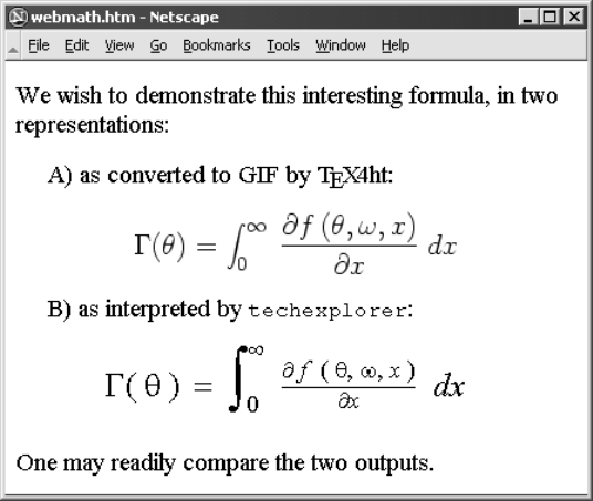
482 Appendix E. L
A
T
E
X and World Wide Web
Figure E.1: Example of a math formula represented by T
EX4ht (as a GIF
image of the original L
A
T
EX output) and by techexplorer rendering.
Internet users will probably not have techexplorer installed, so that
they will only be presented with the input text, and not its rendering.
One additional application of techexplorer which is not available
to the other programs is to embed T
EX commands, especially mathemat-
ics, inside a regular HTML file. If the commands are stored in a file
formula.tex, they could be embedded with
<EMBED SRC="formula.tex" WIDTH=300 HEIGHT=70>
or they can be entered directly as
<EMBED TYPE="application/x-techexplorer"
TEXDATA="$$\Gamma(\theta)=\int_0ˆ\infty\;
\frac{\partial f\,(\theta,\omega,x)}
{\partial x}\; dx$$" WIDTH=300 HEIGHT=70>
The result, shown in the lower part of Figure E.1, is a very acceptable
display of the math formula in the middle of an HTML file. (This file was
generated by T
EX4ht from a L
A
T
EX file, with the above techexplorer text
included as raw HTML code.)
The techexplorer is obtainable from http://www.software.ibm.
com/enetwork/techexplorer. It comes in a free introductory version,
as well as in a professional version for a nominal charge.

F
Obsolete L
A
T
E
X
Since 1994, L
A
T
EX 2εhas replaced L
A
T
EX 2.09 as the official version. Al-
though the newer version is backward compatible with the previous one,
this is only to allow older source files written for L
A
T
EX 2.09 to be processed
under L
A
T
EX 2ε; it is not intended that newer files should make use of the
obsolete syntax.
Human nature being conservative as it is, many authors continued to
use the commands they were familiar with, even today. The purpose of
this chapter is to explain those commands for users who may come across
such legacy documents, and to indicate to traditional L
A
T
EX users which
commands they should no longer be employing. It is not meant to be a
guide for using L
A
T
EX 2.09!
At first sight, the differences seem very slight indeed. In fact, the
real changes are mainly internal, allowing packages to be handled more
systematically and fonts to be dealt with in a more flexible manner. The
advantages of L
A
T
EX 2εfor class and package writers are considerable, as
explained in Appendix D. Regular users benefit indirectly by being able
to employ these extensions, and by being able to activate fonts other than
the original Computer Modern families.
F.1 The 2.09 preamble
As for L
A
T
EX 2ε, the document preamble in L
A
T
EX 2.09 contains overall
specifications for the entire document, including general layout.
F.1.1 Style instead of class
L
A
T
EX 2.09 works with style rather than class files, so the first command in
the source file is
\documentstyle[options]{style}
483
484 Appendix F. Obsolete L
A
T
E
X
rather than \documentclass. Possible values for style are article,
report,book, or any other main style files that might exist locally. These
styles may have various options associated with them, like 11pt,twoside,
and so on, which can be listed in the set of options. Not all the options
available with the L
A
T
EX 2εclass files are recognized by the style files.
The options list has an additional function in L
A
T
EX 2.09: for any option
in the list that is not recognized by the style file, a file with that name and
extension.sty is loaded, if it exists. The original idea of this mechanism
was to allow certain options applicable to all styles to have the common
coding stored in an extra file, rather than repeating it within each main
style file. It was this that later led to the concept of packages.
There is no \usepackage command in L
A
T
EX 2.09; packages can only
be loaded with the options list, and no options may be specified for the
packages.
To start a document with the article style and 12pt option, with the
parskip and makeidx packages, one gives
\documentstyle[12pt,parskip,makeidx]{article}
F.1.2 Compatibility mode
L
A
T
EX 2εis designed to be able to process older L
A
T
EX documents with
exactly the same output as with L
A
T
EX 2.09. To do this, it recognizes the
\documentstyle command which switches it into compatibility mode,
changing the functionality of many L
A
T
EX 2εfeatures. For example, the
\usepackage command becomes inoperable, issuing an error message.
With a true L
A
T
EX 2.09 installation, the above \documentstyle exam-
ple would load the files article.sty,parskip.sty, and makeidx.sty.
Under L
A
T
EX 2ε, in compatibility mode, it first tries to load the main style
as a class file with the extension .cls, in this case article.cls, but if
that fails, it then looks for the extension.sty. This is to handle local main
style files that have no class file equivalent. The packages parskip.sty
and makeidx.sty are loaded as well. However, they too may recognize
the compatibility mode and behave differently as they would with regular
L
A
T
EX 2ε.
F.2 Font selection
The other major difference between the two versions is font selection.
The New Font Selection Scheme (NFSS) and font attributes described in
Section 4.1.3 are missing in L
A
T
EX 2.09, as are the font commands \textbf,
\texttt, and so on, and the font attribute declarations such as \bfseries
and \ttfamily. (They are still available even in L
A
T
EX 2εcompatibility
mode.)
F.3. Obsolete means obsolete 485
F.2.1 Old font declarations
In L
A
T
EX 2.09, only the two-letter font declarations that originally came
from Plain T
EX are possible.
\rm Roman \it Italic \sc Small Caps
\bf Bold face \sl Slanted \sf Sans Serif
\tt Typewriter
These are all declarations, changing the font until another font declaration
is given, or until the current environment is ended. They are normally
used as {\bf bold face} to yield bold face.
The emphasizing declaration \em also belongs to this group, but it has
been taken over as part of L
A
T
EX 2εproper.
These old declarations have a different behavior from that of their
NFSS counterparts: they rigidly select a particular font instead of altering
only one attribute, but retaining the current size. Compare:
{\sl slanted {\bf bold}} ⇒slanted bold
{\slshape slanted {\bfseries bold}} ⇒slanted bold
It is not possible to obtain slanted or italic bold face with L
A
T
EX 2.09 even
though such fonts are available.
These two-letter declarations are also retained in the standard L
A
T
EX 2ε
classes, and not just in compatibility mode. Note carefully that wording:
they are not part of L
A
T
EX 2εitself, but are only included as part of the
standard class files. This means other class files might not provide them,
or that they might even be removed in some later version (although this
is most unlikely). Therefore, their use is not to be encouraged at all.
F.2.2 Font size declarations
In L
A
T
EX 2.09, the font size declarations also reset all the other font at-
tributes (Section 4.1.3) to their defaults, that is, Roman, upright, medium
weight. By contrast, in L
A
T
EX 2ε, these attributes remain unchanged. Com-
pare the results of {\sl slanted {\Large larger}}:
L
A
T
EX 2.09: slanted larger
L
A
T
EX 2ε:slanted larger
In L
A
T
EX 2εcompatibility mode, the size declarations behave as they do in
L
A
T
EX 2.09.
F.3 Obsolete means obsolete
Many features have been added to L
A
T
EX 2ε, and a number of commands
have been given extended syntax, in the form of additional optional argu-
ments. We have no intention of indicating them anymore in this book as
486 Appendix F. Obsolete L
A
T
E
X
this is a manual for the newer version only. (Previous editions did make
a distinction.)
Apart from the restrictions pointed out in the above sections, all of
the L
A
T
EX 2εfeatures will work in compatibility mode. Nevertheless, we
stress once more, compatibility mode is only intended for the processing
of older source files. Every effort has been undertaken to ensure that the
results are identical to those of a processing with the true L
A
T
EX 2.09 itself.
Compatibility mode (\documentstyle in place of \documentclass)
issues a very strong warning:
Entering LaTeX 2.09 COMPATIBILITY MODE
*************************************************************
!!WARNING!! !!WARNING!! !!WARNING!! !!WARNING!!
This mode attempts to provide an emulation of the LaTeX 2.09
author environment so that OLD documents can be successfully
processed. It should NOT be used for NEW documents!
New documents should use Standard LaTeX conventions and start
with the \documentclass command.
Compatibility mode is UNLIKELY TO WORK with LaTeX 2.09 style
files that change any internal macros, especially not with
those that change the FONT SELECTION or OUTPUT ROUTINES.
Therefore such style files MUST BE UPDATED to use
Current Standard LaTeX: LaTeX2e.
If you suspect that you may be using such a style file, which
is probably very, very old by now, then you should attempt to
get it updated by sending a copy of this error message to the
author of that file.
*************************************************************
Take this message seriously, and stick to \documentclass.

G
T
E
X Fonts
Computers work exclusively with numbers, or more precisely, only with
bits which may be interpreted as numbers. They do not know the differ-
ence between the letter A and an apple, or that either even exists. For text
processing, all symbols, both input and output, need to be represented
as numbers somehow. The association between number and symbol is
called the encoding or layout. The latter term derives from the common
method of illustrating the encoding in the form of a table.
Encoding tables are by no means standard. The standard ascii scheme
is just one of several, and it is limited to 7 bits, or 128 characters. There
are 8-bit (256 characters) versions as well, in fact, a large number exist,
tailored to different computer systems and languages. The question of
coding the input for L
A
T
EX documents with more than 7 bits are addressed
in Sections 2.5.9 and D.5.
In this appendix, we look at how the underlying T
EX program deals
with output fonts, their nomenclature, and their encoding tables.
G.1 Font metrics and bitmaps
When T
EX decides to output character nn in a particular font, all it needs
to know is how much room to leave for it. T
EX does not care what the
character looks like, for that is the task of the DVI driver afterwards.
Information about the characters in each font are stored in various
files, all bearing the root name of the font but with different extensions.
This information is divided into files that contain only the sizes of each
symbol, and those with the actual drawing or image data.
.tfm T
EX font metric files are the only font files read in by T
EX itself.
They contain the sizes of the characters, such as width, height, and
depth. For slanted fonts, they also possess the ‘italic correction’
for each letter. Furthermore, they specify for which letter combi-
nations a different spacing is required, such as AV instead of AV,
487
488 Appendix G. T
E
X Fonts
or for which a ligature is available. Finally, the .tfm files provide
information about the slope of the characters (zero for an unslanted
font), the standard word spacing and its stretch and shrinkage, the
width of the em and quad spacings, and the spacings at the end
of a sentence. Mathematical and symbol fonts require even more
information which is also included in their.tfm files.
.pk Compressed pixel files contain bitmaps (images) of the symbols in
each font, in one size and one resolution. The DVI driver program
uses these to send the output to a printer or previewer. These files
are normally generated automatically by the METAFONT program
(Section G.3) as needed.
Since these files might exist several times for a given font, in dif-
ference sizes or resolutions, many installations distinguish them
by adding the resolution to the extension, as cmr10.300pk or
cmr10.600pk for 300 and 600 dpi versions, respectively. On sys-
tems that cannot support extensions with more than three charac-
ters, both files are named cmr10.pk but are stored in directories
dpi300 and dpi600.
Font magnification is achieved by selecting an appropriate resolu-
tion. If cmr10 is to be printed on a 300 dpi printer at double its
normal size, the 600 dpi version is used instead.
.mf METAFONT source files contain the drawing instructions for each
of the fonts. These are not read by the DVI driver but rather by the
METAFONT program which converts them into .pk bitmap files at
the required size and resolution.
.vf Virtual font files are an alternative to .pk files. Instead of having
bitmaps for each character, they contain instructions that refer to
characters in different, real fonts, or that tell the driver to draw a
black box and issue a warning message (that the character does not
exist, for example).
Virtual fonts are normally associated with PostScript fonts and are
therefore described in Section G.5. However, there is no reason for
them not to be used with bitmap fonts as well.
G.2 Computer Modern fonts
When Donald E. Knuth invented the T
EX program, he also provided it with
an extensive set of character fonts, which he named Computer Modern,
rather than relying on the fonts available on any given printer. At that
time, the printer fonts were not so good, and certainly were not uniform.
G.2. Computer Modern fonts 489
With the supplied fonts, T
EX could produce identical, high-quality results
on all printers.
L
A
T
EX, of course, has inherited these fonts, so that they have almost
become a trademark for documents produced by T
EX or L
A
T
EX. This is not
really necessary, for L
A
T
EX need not be married to any particular set of
fonts, especially with the New Font Selection Scheme (Appendix A) which
simplifies font installation enormously. The main fonts used in this book,
for example, are Lucida Bright, Lucida Sans, and Lucida Sans Typewriter,
designed by Bigelow & Holmes and distributed by Y&Y Inc.
G.2.1 Font families
Typography is the study and classification of typefaces, something that
goes back to Gutenberg’s invention of movable type (not of the printing
press, which was invented by the Chinese) five and a half centuries ago.
Since that time, many families of fonts have been created, bearing classical
names like Baskerville, Garamond, Univers, etc. Each member of such a
family has the same overall design, or basic look, but vary by being slanted,
italic, bold, or thin; and of course, they come in different sizes.
Font families are classified according to certain criteria that often
determine to what use they will be put.
Serif fonts: are those that have little horizontal lines, or serifs, at their
edges, to guide the eye better. Experience has shown these to be
best for general reading, and so they are regularly used for the main
body of text. The NFSS terminology refers to these as Roman fonts.
Sans serif fonts: are those that are lacking any serifs. Such fonts with
their starker appearance are often employed for titling or headlining.
Compare sans serif with regular text.
Fixed fonts: are those with a uniform letter width, something that has
evolved from the typewriter and has been carried over to computer
listings. Classically, such fonts have no business in book printing,
where proportional fonts (the letter iis narrower than m) have always
dominated.
Decorative fonts: are ones that stand out because of some unusual char-
acteristic. They are intended to catch attention and to attract the
eye. Such families are not complete, with a full range of shapes and
widths, and are employed mostly by advertising.
Mathematical fonts: are collections of special symbols needed for math-
ematical works. Their further classification cannot be compared to
that of text fonts at all.
490 Appendix G. T
E
X Fonts
A book designer must decide what kinds of typeface families are
needed. He or she might decide on a Roman (serifed) font for the main
body, a sans serif one for headlines, and then, if it is a book containing
computer code, select a fixed font for setting those parts. Finally, symbol
fonts will be needed if the work contains mathematical sections.
The Computer Modern set of fonts provides all these classes of fami-
lies. However, since they were produced before the NFSS attribute system
of classification was established, the CM font nomenclature does not con-
form perfectly with this scheme. The NFSS system frees the user from
having to think about the CM font names, for specifying the attributes is
sufficient. Of course, the NFSS installation must provide the font defini-
tion .fd files which translate any set of attributes into a real font name,
or into some acceptable substitute.
G.2.2 Classification of CM fonts
All the T
EX font names begin with the letters cm, which stands for ‘Com-
puter Modern’, followed by one to four letters describing the style of font,
and finally one or two digits specifying the design size in points. This is
the root name of the font which must be given in the \newfont command
(Section 4.1.5) if it is to be activated directly.
The CM fonts can be classified as text, math, decorative, or other
special symbol fonts, as described in the rest of this section. Each type of
font has an encoding scheme shown in the accompanying layout tables.
Text fonts
The Computer Modern fonts appropriate for straightforward text can be
classified into the three families Roman, sans serif, and typewriter. Within
each of these families there are upright, slanted, italic, small caps, and
bold variants.
Table G.1 presents the names of these fonts together with the NFSS
family/series/shape assignments from Appendix A. They all have the
same coding (OT1). The *in each name is the design size specification
which takes on values of 5,6,7,8,9,10,12,17. Only cmr* is available
in all these sizes, while some are only to be found in size 10. (This table
contains much the same information as in Table A.3 on page 370 but in a
different form.)
One sees several apparent inconsistencies in these font names, such
as cmti* for the italic upright font. Why is this not cmri*? The answer
is that this is a text italic font, as opposed to the math italic font cmmi*
described below. These inconsistences have arisen because the CM fonts
were not created with the NFSS classification system in mind, since that
was established a decade later.

G.2. Computer Modern fonts 491
Table G.1: Computer Modern text fonts
Roman Sans serif Typewriter
Family= cmr cmss cmtt
Style Series/shape
Upright m/n cmr* cmss* cmtt*
” slanted m/sl cmsl* cmssi* cmsltt*
” italic m/it cmti* —cmitt*
” small caps m/sc cmcsc* —cmtcsc*
Bold b/m cmb* — —
Bold extended bx/m cmbx* cmssbx* —
” ” slanted bx/sl cmbxsl* — —
” ” italic bx/it cmbxti* — —
Further inconsistencies exist in the encoding schemes for the CM text
fonts. They are all nominally OT1, but there are slight deviations among
them. The proper OT1 encoding is displayed in Layout 1 on the next page
for font cmr10. The text italic fonts are identical to the upright ones,
except that the dollar sign in position 36 is replaced by the pound sign
(Layout 3 for cmti10). The slanted fonts, on the other hand, are exactly
the same as the upright ones. Other deviations are to be found in the
small caps (Layout 2) and all the typewriter fonts (Layout 4).
Math fonts
The Computer Modern fonts provide three types of mathematical fonts,
each with its own encoding scheme.
The mathematical italic fonts cmmi* contain Latin and Greek letters,
in upper and lower case, plus a number of extra symbols. Since variable
names in formulas are set in italics, these are basically italic fonts. The
encoding scheme is designated OML, for old math letters, and is displayed
in Layout 5. It is available in design sizes 5–12 pt in normal weight, but
only in 10 pt size in bold face, cmmib10. These fonts are used for the
letters math alphabet of Section A.3.4.
Symbol fonts cmsy* provide the rest of the math symbols for formulas,
except for those that appear in variable sizes. The encoding scheme is
named OMS for old math symbols and is shown in Layout 6. It comes in
sizes 5–10 pt in normal weight, and in 10 pt size in bold face, cmbsy10.
The symbols math alphabet uses these fonts.
Variable sized symbols are to be found in the font cmex10, with encod-
ing OMX, for old math extension. Layout 7 illustrates this set. There is no
bold version of this font. It belongs to the largesymbols math alphabet
of Section A.3.4.
492 Appendix G. T
E
X Fonts
0 1 2 3 4 5 6 7
’00x Γ0∆1Θ2Λ3Ξ4Π5Σ6Υ7
’01x Φ8Ψ9Ω10 ff11 fi12 fl13 ffi14 ffl15
’02x ı16 17 `18 ´19 ˇ20 ˘21 ¯22 ˚23
’03x ¸24 ß25 æ26 œ27 ø28 Æ29 Œ30 Ø31
’04x 32 !33 ”34 #35 $36 %37 &38 ’39
’05x (40 )41 *42 +43 ,44 -45 .46 /47
’06x 048 149 250 351 452 553 654 755
’07x 856 957 :58 ;59 ¡60 =61 ¿62 ?63
’10x @64 A65 B66 C67 D68 E69 F70 G71
’11x H72 I73 J74 K75 L76 M77 N78 O79
’12x P80 Q81 R82 S83 T84 U85 V86 W87
’13x X88 Y89 Z90 [91 “92 ]93 ˆ94 ˙95
’14x ‘96 a97 b98 c99 d100 e101 f102 g103
’15x h104 i105 j106 k107 l108 m109 n110 o111
’16x p112 q113 r114 s115 t116 u117 v118 w119
’17x x120 y121 z122 –123 —124 ˝125 ˜126 ¨127
Font Layout 1: The character font cmr10. This is the standard character
assignment for the OT1 encoding scheme.
0 1 2 3 4 5 6 7
’00x Γ0∆1Θ2Λ3Ξ4Π5Σ6Υ7
’01x Φ8Ψ9Ω10 ↑11 ↓12 '13 ¡14 ¿15
’02x ı16 17 `18 ´19 ˇ20 ˘21 ¯22 ˚23
’03x ¸24 ß25 æ26 œ27 ø28 Æ29 Œ30 Ø31
’04x 32 !33 ”34 #35 $36 %37 &38 ’39
’05x (40 )41 *42 +43 ,44 -45 .46 /47
’06x 048 149 250 351 452 553 654 755
’07x 856 957 :58 ;59 <60 =61 >62 ?63
’10x @64 A65 B66 C67 D68 E69 F70 G71
’11x H72 I73 J74 K75 L76 M77 N78 O79
’12x P80 Q81 R82 S83 T84 U85 V86 W87
’13x X88 Y89 Z90 [91 “92 ]93 ˆ94 ˙95
’14x ‘96 a97 b98 c99 d100 e101 f102 g103
’15x h104 i105 j106 k107 l108 m109 n110 o111
’16x p112 q113 r114 s115 t116 u117 v118 w119
’17x x120 y121 z122 –123 —124 ˝125 ˜126 ¨127
Font Layout 2: The character font cmcsc10. The differences from Lay-
out 1 are symbols 11–15, 25, 60, and 62. The ligatures that normally
appear in 11–15 have been replaced by some extra symbols.

G.2. Computer Modern fonts 493
0 1 2 3 4 5 6 7
’00x Γ0∆1Θ2Λ3Ξ4Π5Σ6Υ7
’01x Φ8Ψ9Ω10 ff11 fi12 fl13 ffi14 ffl15
’02x ı16 17 `18 ´19 ˇ20 ˘21 ¯22 ˚23
’03x ¸24 ß25 æ26 œ27 ø28 Æ29 Œ30 Ø31
’04x 32 !33 ”34 #35 £36 %37 &38 ’39
’05x (40 )41 *42 +43 ,44 -45 .46 /47
’06x 048 149 250 351 452 553 654 755
’07x 856 957 :58 ;59 ¡60 =61 ¿62 ?63
’10x @64 A65 B66 C67 D68 E69 F70 G71
’11x H72 I73 J74 K75 L76 M77 N78 O79
’12x P80 Q81 R82 S83 T84 U85 V86 W87
’13x X88 Y89 Z90 [91 “92 ]93 ˆ94 ˙95
’14x ‘96 a97 b98 c99 d100 e101 f102 g103
’15x h104 i105 j106 k107 l108 m109 n110 o111
’16x p112 q113 r114 s115 t116 u117 v118 w119
’17x x120 y121 z122 –123 —124 ˝125 ˜126 ¨127
Font Layout 3: The character font cmti10. The only difference from
Layout 1 is symbol 36 (£instead of $). All other text italic fonts
have this same pattern.
01234567
’00x Γ0∆1Θ2Λ3Ξ4Π5Σ6Υ7
’01x Φ8Ψ9Ω10 ↑11 ↓12 '13 ¡14 ¿15
’02x ı16 17 `18 ´19 ˇ20 ˘21 ¯22 ˚23
’03x ¸24 ß25 æ26 œ27 ø28 Æ29 Œ30 Ø31
’04x 32 !33 "34 #35 $36 %37 &38 ’39
’05x (40 )41 *42 +43 ,44 -45 .46 /47
’06x 048 149 250 351 452 553 654 755
’07x 856 957 :58 ;59 <60 =61 >62 ?63
’10x @64 A65 B66 C67 D68 E69 F70 G71
’11x H72 I73 J74 K75 L76 M77 N78 O79
’12x P80 Q81 R82 S83 T84 U85 V86 W87
’13x X88 Y89 Z90 [91 \92 ]93 ^94 _95
’14x ‘96 a97 b98 c99 d100 e101 f102 g103
’15x h104 i105 j106 k107 l108 m109 n110 o111
’16x p112 q113 r114 s115 t116 u117 v118 w119
’17x x120 y121 z122 {123 |124 }125 ~126 ¨127
Font Layout 4: The character font cmtt10. All tt fonts are set up with
the same pattern. The differences from Layout 1 lie in symbols 11–
15, 60, 62, 92, 123, 124, and 125. Furthermore, the italic typewriter
fonts also have £in place of $.
494 Appendix G. T
E
X Fonts
The term old in these encoding names refers to the original encoding
as introduced by Donald Knuth, in the same way that the text encoding
OT1 indicated the old, or original, text encoding with 128 characters per
font. The new encoding schemes contain 256 characters. For text, the
encoding is named T1 (Section G.4.3); such extended math fonts do not
yet exist.
The extra AMSfonts in Section 12.4.1 add additional bold face sizes
for cmmib* and cmbsy* as well as some more sizes for cmex*.
Decorative fonts
Three families of decorative or special fonts are available in a single design
size and limited attributes. They all exhibit OT1 encoding.
cmfr Funny Roman family, consists of two fonts, cmff10 leaning to the left
and cmfi10 which leans to the right. Both are series mwith shapes n
and it respectively.
cmfib Fibonacci family, contains one font cmfib8 derived from the Fi-
bonacci series of numbers. It has series mand shape n.
cmdunh Dunhill family, with one font cmdunh10 with series mand shape
n. This font is demonstrated in the sample letterhead on page 364.
Logo fonts
The fonts logo8,logo9,logo10,logosl10, and logobf10 contain only
the nine letters A, E, F, M, N, O, P, S, and T, for generating the logos
METAFONT METAFONT METAFONT
METAPOST METAPOST METAPOST
The L
A
T
E
Xlasy fonts
As an extension of the cmsy* fonts for mathematical symbols, L
A
T
EX pro-
Package:
latexsym
amsfonts vides some additional symbols with the font lasy* in design sizes 5–10 pt.
It contains the 15 symbols: ()*+0123;<=.
These symbols are not defined unless one of the packages latexsym
or amsfonts has been loaded.
Fonts for making pictures
The special picture elements for use in the L
A
T
EXpicture environment are
stored in fonts named line10,lcircle10,linew10, and lcirclew10.
The first two are used for lines, ovals, and circles when \thinlines is
in effect. The sloping lines and arrow heads are to be found in line10
G.2. Computer Modern fonts 495
0 1 2 3 4 5 6 7
’00x Γ0∆1Θ2Λ3Ξ4Π5Σ6Υ7
’01x Φ8Ψ9Ω10 α11 β12 γ13 δ14 15
’02x ζ16 η17 θ18 ι19 κ20 λ21 µ22 ν23
’03x ξ24 π25 ρ26 σ27 τ28 υ29 φ30 χ31
’04x ψ32 ω33 ε34 ϑ35 36 37 ς38 ϕ39
’05x 40 41 42 43 44 45 46 47
’06x 48 49 50 51 52 53 54 55
’07x 56 57 .58 ,59 <60 /61 >62 63
’10x ∂64 A65 B66 C67 D68 E69 F70 G71
’11x H72 I73 J74 K75 L76 M77 N78 O79
’12x P80 Q81 R82 S83 T84 U85 V86 W87
’13x X88 Y89 Z90 91 92 93 94 95
’14x 96 a97 b98 c99 d100 e101 f102 g103
’15x h104 i105 j106 k107 l108 m109 n110 o111
’16x p112 q113 r114 s115 t116 u117 v118 w119
’17x x120 y121 z122 ı123 124 ℘125 126 127
Font Layout 5: The font cmmi10. This corresponds to the OML encoding
scheme, as does cmmib10. It contains lower case Greek letters in
positions 11–39 and math symbols in 40–47, 60–64, and 123–127.
0 1 2 3 4 5 6 7
’00x −0·1×2∗3÷45±6∓7
’01x ⊕89⊗10 11 12 13 ◦14 •15
’02x 16 ≡17 ⊆18 ⊇19 ≤20 ≥21 22 23
’03x ∼24 ≈25 ⊂26 ⊃27 28 29 ≺30 31
’04x ←32 →33 ↑34 ↓35 ↔36 %37 &38 '39
’05x ⇐40 ⇒41 ⇑42 ⇓43 ⇔44 -45 .46 ∝47
’06x 048 ∞49 ∈50 351 452 553 654 755
’07x ∀56 ∃57 ¬58 ∅59 <60 =61 >62 ⊥63
’10x ℵ64 A65 B66 C67 D68 E69 F70 G71
’11x H72 I73 J74 K75 L76 M77 N78 O79
’12x P80 Q81 R82 S83 T84 U85 V86 W87
’13x X88 Y89 Z90 ∪91 ∩92 ]93 ∧94 ∨95
’14x `96 a97 b98 c99 d100 e101 {102 }103
’15x h104 i105 |106 k107 l108 m109 \110 o111
’16x √112 q113 ∇114 ∫115 t116 u117 v118 w119
’17x §120 †121 ‡122 ¶123 ♣124 ♦125 ♥126 ♠127
Font Layout 6: The font cmsy10. The cmsy fonts, adhering to the OMS
encoding scheme, contain many math symbols as well as the cal-
ligraphic letters A...Zin positions 65–90. The bold face version
cmbsy10 is set up on the same pattern.

496 Appendix G. T
E
X Fonts
0 1 2 3 4 5 6 7
’00x 01234567
’01x 8910 11 12 13 14 15
’02x 16 17 18 19 20 21 22 23
’03x 24 25 26 27 28 29 30 31
’04x 32 !33 "34 #35 $36 %37 &38 '39
’05x (40 )41 *42 +43 ,44 -45 .46 /47
’06x 48 49 50 51 52 53 54 55
’07x 56 57 58 59 60 61 62 63
’10x 64 65 66 67 D68 E69 F70 G71
’11x H72 I73 J74 K75 L76 M77 N78 O79
’12x P80 Q81 R82 S83 T84 U85 V86 W87
’13x X88 Y89 Z90 [91 \92 ]93 ^94 _95
’14x `96 a97 b98 c99 d100 e101 f102 g103
’15x h104 i105 j106 k107 l108 m109 n110 o111
’16x p112 q113 r114 s115 t116 u117 v118 w119
’17x x120 y121 z122 {123 |124 }125 ~126 127
Font Layout 7: The font cmex10, containing the mathematical symbols
that appear in varying sizes. This is the OMX encoding scheme.

G.3. The METAFONT program 497
0 1 2 3 4 5 6 7
’00x Nj0Lj1234567
’01x nj8lj910 11 12 13 14 15
’02x 16 17 18 19 20 21 22 23
’03x 24 25 26 27 28 29 30 31
’04x ¨32 !33 ”34 #35 $36 %37 ´38 ’39
’05x (40 )41 *42 +43 ,44 -45 .46 /47
’06x 048 149 250 351 452 553 654 755
’07x 856 957 :58 ;59 «60 ı61 »62 ?63
’10x ˘64 A65 B66 C67 D68 E69 F70 G71
’11x H72 I73 J74 K75 L76 M77 N78 O79
’12x P80 Q81 R82 S83 T84 U85 V86 W87
’13x X88 Y89 Z90 [91 “92 ]93 ^94 _95
’14x ‘96 a97 b98 c99 d100 e101 f102 g103
’15x h104 i105 j106 k107 l108 m109 n110 o111
’16x p112 q113 r114 s115 t116 u117 v118 w119
’17x x120 y121 z122 –123 —124 }125 ~126 127
Font Layout 8: The character font wncyr10, one of the Cyrillic fonts from
the University of Washington. Its coding scheme is designated OT2.
while the circles and oval segments (Section 13.1.4) are in lcircle10.
The second pair of fonts with the added wcontain thicker lines, for use
with \thicklines.
G.2.3 AMSCyrillic fonts
The Cyrillic fonts that are part of the amsfonts collection are described in
Section 12.4.2. They conform to the font encoding scheme OT2, displayed
in Layout 8. They are available as upright (wncyr*), bold (wncyb*), small
caps (wncysc*), and upright sans serif (wncyss*) fonts. As for the CM
fonts, *represents the design size in points.
The NFSS system assigns these fonts to families cmr and cmss; that is,
they are treated as members of the Computer Modern set. This is not as
absurd as it sounds since they are intended to be used with the CM fonts.
G.3 The METAFONT program
METAFONT is a program for designing and developing character fonts,
written by Donald E. Knuth as a companion to his T
EX program (Knuth,
1986c, 1986d, 1986e). It is this program that made the uniform high
quality typographic output possible for T
EX at a time when most printers
had their own built-in fonts of varying standards.
498 Appendix G. T
E
X Fonts
The printer driver programs have the task of converting the DVI output
from T
EX into instruction code for a particular printer. To do this, they
need to know how to print each of the symbols used in the document.
These symbols are represented as a set of black and white dots (pixels)
that is adjusted to the output resolution. Clearly to produce the letter A
in a given size at 600 dpi (dots per inch) requires many more dots than at
150 dpi (16 times). This information is contained in the corresponding
.pk files, in compressed format.
However, designing fonts as a set of dots, and that for any number of
resolutions, and taking into account idiosyncrasies of individual printers,
is an impossible task. Rather, the fonts are defined with.mf files, contain-
ing instructions on how to draw the symbols with a pen of a given shape.
This is the most general definition, describing the ideal form. METAFONT
then translates this ideal into the practical realization, the pixels, for any
specified resolution. Aspects of the various printers, such as relative pixel
size and shape, may also be included, so that the resulting patterns are
both resolution and printer dependent. The font metric.tfm files are also
produced in this process.
Today it is hardly necessary for most users to know anything more
about METAFONT other than that it exists. The drivers and previewers
are now so constructed that when they notice that the required .pk file
is missing, they invoke METAFONT themselves to generate it. In this way
the collection of pixel files grows as needed and includes only those that
are actually used. (Originally huge sets of pixel files had to be supplied
to cover every remote possibility.)
Another reason for the decline in the awareness of METAFONT is
the increasing use of the type 1 fonts for PostScript and PDF output
(Chapter 10).
Donald Knuth has announced that he wishes to withdraw from any
further development of either of these programs, being prepared merely to
correct any definite errors they may contain. To emphasize this decision,
he will from now on give version numbers to T
EX that converge to π
(3.14159. . . ) and to METAFONT that approach the value of e (2.71828. . . ).
At present, T
EX is at version 3.14159 and METAFONT at 2.718. As a
consequence of this decision, any further major developments to these
two programs, such as undertaken by user groups, will be under new
names, since Knuth has kept the copyright to the existing names.
G.4 Extended Computer fonts
The Computer Modern fonts were developed in the early days of T
EX when
it could only handle 128 characters per font. The modern T
EX program
can deal with 256 characters in each font, requiring a new set of standard
fonts to exploit this feature.
G.4. Extended Computer fonts 499
G.4.1 Limitations and deficiencies of the CM fonts
Most of the diacritical marks (accents) used in European languages written
with the Latin alphabet are contained in, or may be generated by, T
EX’s
Computer Modern (CM) fonts. A basic set of naked accents is available
for combination with other letters, such as the acute accent ´ with the
letter eto make ´
e. Other combinations may be constructed for diacritical
marks that are not predefined in T
EX or L
A
T
EX.
Fashioning diacritical characters as a combination of letters and special
symbols has one great disadvantage for the T
EX processing: words con-
taining such characters cannot take part in the automatic word division
since the hyphenation patterns include only pure letters. The accented
letters, such as those in German and French and most other languages,
must be treated as single characters in the hyphenation patterns, and
must appear as single letters in the character set.
In addition to diacritical characters, a number of special letters are
employed in some European languages, such as ß, Æ, æ, Œ, œ, Ø, and
ø, which are provided in standard T
EX with the CM fonts (Section 2.5.6).
However, other special letters, such as Ŋ, ŋ, Þ, þ, and ð, are missing
completely and cannot be easily constructed from existing ones.
G.4.2 The Cork proposal
At the 1990 International T
EX Conference in Cork, Ireland, an extension of
the Latin alphabet and its assignments within the 256 character positions
was proposed and accepted. This extension includes the majority of
special and diacritical letters as single characters for many languages
written with the Latin alphabet. Hyphenation patterns for such languages
may include the special and diacritical letters as single letters for optimal
word division by T
EX and L
A
T
EX.
Character fonts conforming to the Cork scheme are to bear the iden-
tifying letters ec in their names for ‘Extended Computer’ in place of the
cm for ‘Computer Modern’.
G.4.3 The realization of EC fonts
The Cork proposal for extending the T
EX fonts to 256 characters was first
implemented by Norbert Schwarz, who produced an initial set of META-
FONT source files. He also selected the designation dc to emphasize that
this was a preliminary realization of the EC fonts. Some work was still
needed to fine-tune the design of several symbols.
After issuing versions 1.2 and 1.3 of the DC fonts in 1995 and 1996,
J¨
org Knappen released the first set of true EC fonts in January, 1997. Font
Layout 9 presents his font ecrm1000, the extended version of cmr10. The
EC fonts are now considered to be stable in that neither their encoding

500 Appendix G. T
E
X Fonts
0 1 2 3 4 5 6 7
’00x `0´1ˆ2˜3¨4˝5˚6ˇ7
’01x ˘8¯9˙10 ¸11 ˛12 ‚13 ‹14 ›15
’02x “16 ”17 „18 «19 »20 –21 —22 23
’03x ‰24 ı25 26 ff27 fi28 fl29 ffi30 ffl31
’04x 32 !33 "34 #35 $36 %37 &38 ’39
’05x (40 )41 *42 +43 ,44 -45 .46 /47
’06x 048 149 250 351 452 553 654 755
’07x 856 957 :58 ;59 <60 =61 >62 ?63
’10x @64 A65 B66 C67 D68 E69 F70 G71
’11x H72 I73 J74 K75 L76 M77 N78 O79
’12x P80 Q81 R82 S83 T84 U85 V86 W87
’13x X88 Y89 Z90 [91 \92 ]93 ^94 _95
’14x ‘96 a97 b98 c99 d100 e101 f102 g103
’15x h104 i105 j106 k107 l108 m109 n110 o111
’16x p112 q113 r114 s115 t116 u117 v118 w119
’17x x120 y121 z122 {123 |124 }125 ~126 127
’20x Ă128 Ą129 Ć130 Č131 Ď132 Ě133 Ę134 Ğ135
’21x Ĺ136 Ľ137 Ł138 Ń139 Ň140 Ŋ141 Ő142 Ŕ143
’22x Ř144 Ś145 Š146 Ş147 Ť148 Ţ149 Ű150 Ů151
’23x Ÿ152 Ź153 Ž154 Ż155 IJ156 İ157 đ158 §159
’24x ă160 ą161 ć162 č163 ď164 ě165 ę166 ğ167
’25x ĺ168 ľ169 ł170 ń171 ň172 ŋ173 ő174 ŕ175
’26x ř176 ś177 š178 ş179 ť180 ţ181 ű182 ů183
’27x ÿ184 ź185 ž186 ż187 ij188 ¡189 ¿190 £191
’30x À192 Á193 Â194 Ã195 Ä196 Å197 Æ198 Ç199
’31x È200 É201 Ê202 Ë203 Ì204 Í205 Î206 Ï207
’32x Ð208 Ñ209 Ò210 Ó211 Ô212 Õ213 Ö214 Œ215
’33x Ø216 Ù217 Ú218 Û219 Ü220 Ý221 Þ222 223
’34x à224 á225 â226 ã227 ä228 å229 æ230 ç231
’35x è232 é233 ê234 ë235 ì236 í237 î238 ï239
’36x ð240 ñ241 ò242 ó243 ô244 õ245 ö246 œ247
’37x ø248 ù249 ú250 û251 ü252 ý253 þ254 ß255
Font Layout 9: The extended font ecrm1000 with T1 encoding.
G.4. Extended Computer fonts 501
nor their metrics (the .tfm files) will be changed in future. Thus their
behavior as far as T
EX and L
A
T
EX are concerned is finalized. The actual
printed characters might be modified slightly in later updates.
The EC font names are of the form ecxxnnnn, where xx represents two
letters specifying the font characteristics, and nnnn the design size in
hundredths of points. Thus ecrm1000 is the upright Roman font in size
10 points.
The METAFONT source files are available for the following extended
fonts (without the size specification):
ecrm
ecbx
ecbl
ecrb
ecrb
ecti
ecui
ecbi
eccc
ecxc
ecsc
ecoc
ecci
ectt
ecit
ecvt
ecvi
ecvi
ectc
ecst
ecss
ecsi
ecsx
ecso
ecdh
Comparing these with the root names of the CM fonts from Table G.1 on
page 491, one may easily recognize the correspondence. For example,
ecbx* is the extended bold font corresponding to the CM font cmbx*.
It is intended that the EC fonts should exist in most design sizes.
The present distribution contains almost all the fonts in sizes from 5 to
35.83 pt, that is, with size specifications:
0500 0600 0700 0800 0900 1000 1095
1200 1440 1728 2074 2488 2986 3583
In contrast to the CM text fonts which exhibit differences in the symbol
assignments among them, as illustrated in Layouts 1–4, the EC fonts all
have exactly the same encoding scheme, as presented in Layout 9.
The EC fonts are now part of the standard L
A
T
EX installations.
A parallel set of fonts called text companion, or TC, fonts is also pro-
vided. These contain special symbols for text that are normally found in
the CM math fonts, if at all, such as currency symbols and degree signs.
These fonts are still somewhat experimental so that the symbol assign-
ments are not yet stable. The current contents are shown in Layout 10.
G.4.4 Invoking the EC and TC fonts
The EC fonts correspond to the NFSS encoding scheme T1 (Section A.1).
The simplest way to activate them is to place
\usepackage[T1]{fontenc}
in the preamble of the document. All this really does is to make T1
the standard encoding by redefining \encodingdefault to be T1, and
it loads the file t1enc.def which redefines the accent and special letter
commands by means of the encoding commands of Section A.3.7.

502 Appendix G. T
E
X Fonts
0 1 2 3 4 5 6 7
’00x 01234567
’01x 8910 ¸11 ˛12 13 14 15
’02x 16 17 18 19 20 21 22 23
’03x ←24 →25 26 27 28 29 30 31
’04x 32 33 34 35 $36 37 38 '39
’05x 40 41 ∗42 43 ,44 45 .46 ⁄47
’06x 48 49 50 51 52 53 54 55
’07x 56 57 58 59 〈60 −61 〉62 63
’10x 64 65 66 67 68 69 70 71
’11x 72 73 74 75 76 77 78 ○79
’12x 80 81 82 83 84 85 86 Ω87
’13x 88 89 90 91 92 93 ↑94 ↓95
’14x 96 97 98 99 100 101 102 103
’15x 104 105 106 107 108 109 ♪110 111
’16x 112 113 114 115 116 117 118 119
’17x 120 121 122 123 124 125 126 127
’20x 128 129 130 131 †132 ‡133 134 ‰135
’21x •136 137 138 139 ƒ140 ₡141 142 143
’22x 144 145 ₤146 147 148 149 ₫150 ™151
’23x 152 153 154 №155 156 ℮157 ◦158 159
’24x 160 161 ¢162 £163 ¤164 ¥165 ¦166 §167
’25x 168 ©169 ª170 171 ¬172 173 ®174 175
’26x °176 ±177 ²178 ³179 180 µ181 ¶182 ·183
’27x 184 ¹185 º186 √187 ¼188 ½189 ¾190 €191
’30x 192 193 194 195 196 197 198 199
’31x 200 201 202 203 204 205 206 207
’32x 208 209 210 211 212 213 ×214 215
’33x 216 217 218 219 220 221 222 223
’34x 224 225 226 227 228 229 230 231
’35x 232 233 234 235 236 237 238 239
’36x 240 241 242 243 244 245 ÷246 247
’37x 248 249 250 251 252 253 254 255
Font Layout 10: The text companion font tcrm1000 with the TS1 encod-
ing scheme.
G.5. PostScript fonts 503
To obtain access to the symbols in the TC fonts, one can load the
Package:
textcomp textcomp package, which not only redefines several existing symbol com-
mands, it also adds many new ones. For example, \copyright, which is
normally defined to be \textcircle{c}, is changed to print character
169 from an appropriate TC font. Character 191 is the symbol for the Eu-
ropean currency unit, the euro, printed with \texteuro; however, better
ways of producing it are presented in Section 2.5.8.
G.4.5 Special character commands
Inspecting Font Layout 9, one notices that the EC fonts contain not only
many single characters that are formed out of two CM symbols (like ¨
A =
A + ¨) but also several characters that have no correspondence in the CM
font layout at all. The first type is accommodated by internally redefining
the action of accent and special character commands. The second set
requires new commands that are recognized only when the T1 encoding
is active. These are
the ogonek accent \k{o}:o
˛
special letters \DH =Ð\DJ =Ð\NG =Ŋ\TH =Þ
\dh =ð\dj =đ\ng =ŋ\th =þ
special symbols \guillemotleft =«\guillemotright =»
\guilsinglleft =‹\guilsinglright =›
\quotedblbase =„\quotesinglbase =‚
\textquotedbl ="
When issued in OT1 encoding, these commands print an error message.
Note: The \guillemotleft and \guillemotright are not misprints
even though the proper word for the French quotations marks is guillemet.
The PostScript fonts contain these erroneous names for these symbols
and this mistake has propagated to such an extent that it can never be
removed from all the software that includes it. A guillemot is in fact an
Arctic bird, not a French quotation mark.
G.5 PostScript fonts
PostScript fonts, also known as outline or type 1 fonts, are treated exactly
the same way as the METAFONT fonts as far as L
A
T
EX is concerned: during
the processing, a.tfm file is read in for each font specifying the character
sizes and other properties. This is all that L
A
T
EX needs to know, for it is
the task of the driver program to print the actual character that fills the
reserved space.
The driver makes use of the virtual font mechanism, which means that
what L
A
T
EX sees are actually artificial fonts that do not really exist on their
504 Appendix G. T
E
X Fonts
own. There are.tfm files for these fonts, so the L
A
T
EX processing proceeds
as normal. What the driver then does is to read a .vf file instead of the
pixel.pk files. The instructions in the virtual font file tell the driver how
to create each character: they may be drawn, taken from other fonts,
or distorted. This is how PostScript slanted and small caps fonts are
emulated, for such fonts do not exist in the ‘raw’ form. See Section 10.1.4
for example of how this works.
Even the font layout can be redesigned with virtual fonts. The raw
PostScript fonts have an encoding scheme that conforms to neither OT1
nor T1, but which is used as a pool of symbols for constructing virtual
fonts that do conform to these schemes. In particular, the Computer
Modern fonts contain upper case Greek letters in the first 11 slots (Layout 1
on page 492) which are to be found in the PostScript symbol font only.
The virtual font ptmr7t conforms to this by taking its characters from
both the raw Times-Roman and Symbol fonts.
G.5.1 Naming scheme for PostScript fonts
In order to be compatible with all possible operating systems, it is nec-
essary to reduce the names of the PostScript font files to a maximum of
eight characters. This makes for an extremely abbreviated and cryptic
nomenclature.
The most commonly used scheme is that of Karl Berry. Here, the first
letter of the name specifies the supplier of the font, for example pfor
Adobe (stands for PostScript), or hfor Bigelow & Holmes, who designed
the Lucida fonts used in this book, or mfor Monotype, or lfor Linotype,
and so on.
Table G.2: Root names of the 35 standard PostScript fonts
pagd AvantGarde-Demi phvrrn Helvetica-Narrow
pagdo AvantGarde-DemiOblique phvron Helvetica-Narrow-Oblique
pagk AvantGarde-Book pncb NewCenturySchlbk-Bold
pagko AvantGarde-BookOblique pncbi NewCenturySchlbk-BoldItalic
pbkd Bookman-Demi pncr NewCenturySchlbk-Roman
pbkdi Bookman-DemiItalic pncri NewCenturySchlbk-Italic
pbkl Bookman-Light pplb Palatino-Bold
pbkli Bookman-LightItalic pplbi Palatino-BoldItalic
pcrb Courier-Bold pplr Palatino-Roman
pcrbo Courier-BoldOblique pplri Palatino-Italic
pcrr Courier psyr Symbol
pcrro Courier-Oblique ptmb Times-Bold
phvb Helvetica-Bold ptmbi Times-BoldItalic
phvbo Helvetica-BoldOblique ptmr Times-Roman
phvbrn Helvetica-Narrow-Bold ptmri Times-Italic
phvbon Helvetica-Narrow-BoldOblique pzcmi ZapfChancery-MediumItalic
phvr Helvetica pzdr ZapfDingbats
phvro Helvetica-Oblique

G.6. Computer Modern as PostScript fonts 505
Table G.3: A selection of the encoding suffixes in the Berry nomenclature
Suffix Encoding NFSS designation Page
7t 7-bit T
EX text encoding OT1 492
7m T
EX math italics encoding OML 495
7v T
EX math extension encoding OMX 496
7y T
EX math symbols encoding OMS 495
8t 8-bit Cork encoding T1 500
8a Adobe standard encoding
8r TeXBase1Encoding
A two-letter typeface code follows the supplier letter, such as tm for
Times-Roman. Next come various letters to specify weight, for example
rfor regular (upright Roman) or bfor bold, and variant, like ifor italic,
ofor oblique (slanted). Next come a number plus letter to indicate the
encoding scheme, followed by possible width code letters. The Berry
names for the 35 standard PostScript fonts that should be loaded in every
printer are listed in Table G.2 on the facing page, without the encoding
suffixes.
The most important encoding suffixes for our purposes are listed in
Table G.3. The 7-bit encodings have already been explained in Section G.2.2
and shown in Layouts 1, 5–7, while the 8t or T1 scheme is to be found in
Layout 9 in Section G.4.3.
The other 8-bit schemes listed in Table G.3 are the raw encoding, 8r,
and the Adobe standard encoding, 8a, which is the default for most type 1
fonts if no re-encoding is specified. This scheme plays absolutely no role
in the NFSS installation for PostScript fonts.
Virtual fonts ptmr7t and ptmr8t are both constructed from the same
raw font ptmr8r, differing only in the character assignments. There are
also raw fonts that are modifications of the basic fonts. For example,
ptmro8t is an oblique Times-Roman virtual font, based on ptmro8r, the
raw version. However, there is no such font in the repertoire of Table G.2.
This pseudo font is generated by applying a PostScript slanting operation
to Times-Roman, as demonstrated in Section 10.1.4.
G.6 Computer Modern as PostScript fonts
The traditional pixel fonts produced by METAFONT have served us well
in the days when the emphasis was on printed paper output. Even
for PostScript output, the pixel fonts are acceptable for online viewing.
However, they become very tedious when included in PDF output for
506 Appendix G. T
E
X Fonts
viewing: they appear very fuzzy and require a long time to draw. For
this reason, PDF output, whether produced with pdfT
EX, dvipdfm, or
converted from PostScript, should use type 1 fonts exclusively. To this
end, the Computer Modern fonts themselves have been converted to type 1
fonts.
The first such undertaking was carried out by Basil Malyshev whose
set of font files are known as bakoma. However, the set that is more
often used today is the result of a joint project of Y&Y Inc. and Blue
Sky Research. Originally part of their commercial T
EX installations, these
fonts are now available free of charge. They are included on the T
EXLive
CD under texmf\fonts\type1\bluesky\ in several subdirectories as
.pfb files. They bear the same names and have the same font metrics
as the corresponding pixel fonts (Appendix G) and therefore do not need
any additional .tfm files. However, one must also get the mapping file
bsr.map from texmf\dvips\bluesky\ and add it to the list of mapping
files in config.ps.
The Bluesky fonts are incomplete in that certain less often used
fonts are missing in some sizes. One can either include the map file
bsr-interpolated.map, which substitutes the missing sizes with the
nearest approximation, or employ the bakoma fonts that fill the gaps,
with the map file bakomaextra.map. The T
EXLive CD does not include the
complete bakoma set, but only those fonts that are missing in the Bluesky
ensemble.
Together Bluesky and bakoma provide PostScript-encoded versions for
all the Computer Modern fonts described in Section G.2, for text, math,
symbols, decoration, pictures, along with the additional AMSfonts for
additional symbols and Cyrillic. However, these are only for the OT1
encoding with 128 characters per font.
A more recent effort to apply PostScript to the Extended Computer (EC)
fonts with the T1 encoding has been successfully completed by Vladimir
Volovich with his cm-super collection. Each of the basic.pfb files contains
from 468 to 585 characters, which by means of encoding vectors and
mapping files can be used to emulate all the fonts in Section G.4, including
the text companion fonts with TS1 encoding, and many other additional
encoding schemes. They were generated from the original METAFONT .mf
source files and should therefore produce exactly the same results as the
corresponding pixel fonts.
To use them, one must install the cm-super package from the T
EXLive
CD, which copies the .pfb files from \texmf\fonts\type1\cm-super\
and the mapping and encoding files from \texmf\dvips\cm-super\.
The metric.tfm files are the same as those for the pixel files and so need
not be provided extra.
H
Command Summary
This appendix contains a brief description of all the L
A
T
EX commands,
in alphabetical (ascii) order, neglecting the leading backslash \\, along
with some T
EX commands that have been explained in this book. In the
following section, the commands are presented in their logical grouping
in a number of tables and figures.
H.1 Brief description of the L
A
T
E
X commands
For each command in the following summary, the section and page number
is given where it is introduced and described in detail. The numbers are
shown in the form: ‘(Section) – Page’: for example (2.5.1) – 13 means
‘Section 2.5.1, page 13’. If these numbers are missing, then the command
has not been presented in the book but is only mentioned here.
The following notations may be added to the commands:
[m] those permitted in math mode only;
[a] those belonging to AMS-L
A
T
EX;
[p] those allowed only in the preamble.
\. . . . . . . . . . . . . . . . . . . . . . . (2.1), (2.7.1) – 19, 29
Normal space between words after a command without arguments
or after a period that is not the end of a sentence.
!...........................(9.4.2)–226
Field separation character within the \index command. For example:
with \index{command!fragile} one produces an index sub-entry
‘fragile’ under the main entry ‘command’.
!‘ produces ¡ . . . . . . . . . . . . . . . . . . . . . . (2.5.6) – 24
\! [m] .........................(5.5.1)–145
In math mode, a negative space of −1/6 quad: xx\!x =xxx.
507

508 Appendix H. Command Summary
". . . . . . . . . . . . . . . . (2.5.2), (9.4.2), (14.2) – 23, 227, 311
1. In normal text, this produces the double closing quote ”.
2. Literal sign for MakeIndex, in order to print one of the special
characters !,@,|, or ". Example: \index{"!} to enter character
!without it being interpreted as a separation character.
3. Delimiter for a text field in BIBT
EX. Example:
AUTHOR = "Donald E. Knuth".
\" ............................(2.5.7)–24
Produces an umlaut accent: \"{a} =¨
a.
#. . . . . . . . . . . . . . . . . . . . . . (8.3.2), (8.4.2) – 187, 198
Argument replacement character in a user-defined command or en-
vironment.
## ..........................(8.5.6)–204
Replacement character for an internal argument within a nested user-
defined command or environment.
\# ............................(2.5.4)–23
Command to produce a hash symbol: \# = #.
............................(5.1)–119
Toggle character for switching between text and in-line math modes.
On the first appearance (text to math) it behaves the same as \(
or \begin{math}, while the second call (math to text) is as \) or
\end{math}.
\$ ...........................(2.5.4)–23
Command to produce a dollar sign: \$ =$.
%............................ (4.11)–118
Comment character. The rest of the line of text following %is ignored
by the T
EX processing.
\% ............................(2.5.4)–23
Command to produce a percent sign: \% = %.
&.............................(4.8.1)–97
Indicates a new column in array and tabular environments.
\& ............................(2.5.4)–23
Command to produce an ampersand symbol: \& = &.
\’ . . . . . . . . . . . . . . . . . . . . . . (2.5.7), (4.6.4) – 24, 83
1. Command to produce an acute accent: \’a =´
a.
H.1. Brief description of the L
A
T
E
X commands 509
2. Within the tabbing environment, a command to jump to the
end of the current column.
( ) . . . . . . . . . . . . . . . . . . . . (13.1.2), (14.2) – 289, 312
For a picture command in picture environment, specifies a coordi-
nate pair. In BIBT
EX, an alternative form for the outermost grouping
of the entry type.
\( ............................(5.1)–119
Switches from text to in-line math mode to produce formulas within
a line of text. It functions the same as \begin{math} and as a $sign
in text mode.
\) ............................(5.1)–119
Switches back from in-line math mode to text mode. It functions the
same as \end{math} and as a $sign in math mode.
\+ ............................(4.6.3)–82
Within the tabbing environment, increments the left margin by one
tab stop (moves it to the right).
\, . . . . . . . . . . . . . . . . . . . . . . (2.7.1), (5.5.1) – 29, 145
Small space, the size of 1/6 quad, for use in text and math mode:
xx\,x =xx x.
-.............................(2.5.3)–23
As -, produces the hyphen - for compound words and word division,
as --, the en dash –, and as ---, the em dash —.
\- . . . . . . . . . . . . . . . . . . . . . . (2.8.1), (4.6.3) – 35, 82
1. Denotes possible word division. If a word contains at least one
\- the normal word division rules are suspended for that word
and division may occur only at those locations.
2. Within the tabbing environment, decrements the left margin
by one tap stop (moves it to the left).
\. ............................(2.5.7)–24
Command to produce a dot accent: \.o =˙
o.
\/ ...........................(2.5.10)–26
Command to break up ligatures: shelf\/ful = shelfful.
\: [m] .........................(5.5.1)–145
In math mode, a medium space, the size of 2/9 quad: xx\:x =xx x.
\; [m] .........................(5.5.1)–145
In math mode, a large space, the size of 5/18 quad: xx\;x =xx x.
510 Appendix H. Command Summary
\< ............................(4.6.3)–82
Within the tabbing environment, moves to the left by one tab stop.
\= . . . . . . . . . . . . . . . . . . . . . . (2.5.7), (4.6.1) – 24, 81
1. Command to produce a macron accent: \=o =¯
o.
2. Within the tabbing environment, sets a tab stop at the current
position within the line.
\> ............................(4.6.1)–81
Within the tabbing environment, moves right to the next tab stop.
?‘ produces ¿ . . . . . . . . . . . . . . . . . . . . . . (2.5.6) – 24
@. . . . . . . . . . . . . . . . . . . . . . (9.4.2), (14.2) – 226, 311
1. In MakeIndex, separates an entry in an \index command into
a lexical (for alphabetization) and printing part. Example:
\index{sum@$\sum$} means that the entry appears in the in-
dex at the location of the word ‘sum’ but what is printed is the
summation sign P.
2. In BIBT
EX, denotes the entry type. Example: @BOOK indicates that
the following literature entries correspond to those of a book.
\@ ............................(2.7.1)–29
Extra space at the end of a sentence ending with a capital letter.
[ ] ........................... (2.1)–18
After commands or environment calls, specifies an optional argu-
ment.
\[ ............................(5.1)–120
Switches from text mode to displayed math mode for putting
a formula on a line by itself. Has the same effect as
\begin{displaymath} or $$ in text mode.
\\[space]........................(2.7.2)–31
Ends the current line (without right justifying it). The optional ar-
gument [space]inserts additional vertical spacing of length space
before the next line.
\\*[space]........................(2.7.2)–31
The same as \\ but prevents a page break from occurring between
the current and next line.
\] ............................(5.1)–120
Switches back from displayed math mode to text mode. Has the
same effect as \end{displaymath} or $$ in math mode.

H.1. Brief description of the L
A
T
E
X commands 511
ˆ[m] ..........................(5.2.2)–121
Exponents and superscripts in equations: xˆ2 =x2,xˆ{-2n} =
x−2n.
\ˆ ............................(2.5.7)–24
Command to produce a circumflex accent: \ˆo =ˆ
o.
_[m] ..........................(5.2.2)–121
Subscripts in equations: a_n =an,a_{i,j,k} =ai,j,k.
\_ ............................(2.5.4)–23
Command to produce the underbar sign: t\_v = t v.
\‘ . . . . . . . . . . . . . . . . . . . . . . (2.5.7), (4.6.4) – 24, 83
1. Command to produce a grave accent: \‘o =`
o.
2. Within the tabbing environment, pushes the following text up
against the right margin of the line.
{ } . . . . . . . . . . . . . . . . . (2.1), (2.2), (14.2) – 18, 20, 311
1. After a command or environment call, specifies a mandatory
argument.
2. Grouping a section of text to create a nameless environment.
3. In BIBT
EX, delimiting the name of an entry type, as well as an
alternative delimiter for the text field.
\{ produces a left curly brace: \{ ={. . . . . . . . . . (2.5.4) – 23
|[m] produces |. . . . . . . . . . . . . . (5.3.4), (5.4.1) – 126, 132
|............................(9.4.2)–227
In MakeIndex, the command character within a \index command.
1. After the command \newcommand{\ii}[1]{\textit{#1}}
has been defined, \index{entry|ii} produces the page num-
ber for ‘entry’ in the index in italic type.
2. The cross-reference command \see from makeidx.sty can be
invoked with \index{bison|see{buffalo}} to produce cross-
references within the index.
\| [m] produces ...................(5.3.6)–127
\} produces a right curly brace: \} =}. . . . . . . . . . (2.5.4) – 23
˜.............................(2.7.1)–29
A normal space between words, but without the possibility that the
line will be broken there. Example: Prof.˜Jones ensures that ‘Prof.’
and ‘Jones’ both remain on the same line.
\˜ ............................(2.5.7)–24
Command to produce a tilde accent: \˜n =˜
n.
512 Appendix H. Command Summary
\a= ...........................(4.6.4)–83
Produces a macron accent within tabbing environment: \a=o =¯
o.
\a’ ...........................(4.6.4)–83
Produces an acute accent within tabbing environment: \a’o =´
o.
\a‘ ...........................(4.6.4)–83
Produces a grave accent within tabbing environment: \a‘o =`
o.
\AA produces ˚
A......................(2.5.6)–24
\aa produces ˚
a ......................(2.5.6)–24
\abovedisplayskip [m] . . . . . . . . . . . . . . . . (5.5.4) – 149
Vertical space between a long displayed equation and the preceding
line of text. A new value may be assigned with the \setlength
command:
\setlength{\abovedisplayskip}{10pt plus2pt minus5pt}
\abovedisplayshortskip [m] . . . . . . . . . . . . . (5.5.4) – 149
Vertical space between a short displayed equation and the preceding
line of text. A new value may be assigned with the \setlength
command as in the above example.
\abstractname ....................(D.4.1)–460
Command containing the heading for the abstract. In English, this is
‘Abstract’ but may be altered for adaptation to other languages.
\acute{x}[m] .....................(5.3.9)–129
Acute accent over math variable x:\acute{a} =´
a
\Acute{x}[m][a] . . . . . . . . . . . . . . . . . . . (12.2.2) – 263
With the amsmath package, can be used like \acute, but with multiple
AMS-L
A
T
EX math accents the positioning will be correct.
\addcontentsline{file}{format}{entry}. . . (3.4.3), (3.4.4) – 59, 60
Manual addition of entry into the list file.toc,.lof, or.lot, according
to the value of file, to be formatted as the heading of a sectioning
command, as given by format, for example
\addcontentsline{toc}{section}{References}
\address{sender}................... (16.1)–351
In the letter document class, enters the sender’s address. Multiple
lines in sender are separated by \\.
\addtime{secs}................... (15.1.3)–327
In the slides class, if the option clock has been selected, a time
marker, in minutes, appears at the bottom of the notes. This com-
mand adds the specified number of seconds to the marker. See also
\settime.

H.1. Brief description of the L
A
T
E
X commands 513
\addtocontents{file}{entry}. . . . . . . . (3.4.3), (3.4.4) – 59, 60
Manual addition of entry into the list file.toc,.lof, or.lot, according
to the value of file. Example:
\addtocontents{lof}{\protect\newpage}
\addtocounter{counter}{number}. . . . . . . . . . (8.1.3) – 182
Adds number to the current value of the number stored in counter.
\addtolength{length name}{length}. . . . . . . . . . (8.2) – 184
Adds the quantity length to the current value of the length command
\length name.
\addvspace{length}...................(8.2)–185
Inserts vertical spacing of amount length between paragraphs at the
point where the command is given. If other vertical spacing exists,
the total will not exceed length.
\AE produces Æ . . . . . . . . . . . . . . . . . . . . . . (2.5.6) – 24
\ae produces æ . . . . . . . . . . . . . . . . . . . . . . (2.5.6) – 24
\aleph [m] produces ℵ.................(5.3.6)–127
\allowdisplaybreaks[num][p][a] . . . . . . . . . . (12.2.7) – 278
With the amsmath package, allows automatic page breaks to occur
within multiline math formulas. If num is present, it takes a value
of 0–4 to increase the ease with which page breaks occur. Without
this command, a manual page break can be made at the end of any
formula line with \displaybreak.
\Alph{counter}....................(8.1.4)–183
Prints the current value of counter as a capital letter.
\alph{counter}....................(8.1.4)–183
Prints the current value of counter as a lower case letter.
\alpha [m] produces α.................(5.3.1)–125
\alsoname .......................(D.4.1)–460
Command for use in the makeidx package. It prints the text for a
command \seealso. In English, this is ‘see also’ but may be altered
for adaptation to other languages.
\amalg [m] produces .................(5.3.3)–125
\and ...........................(3.3.1)–53
Used to separate author names within the \author command for
generating a title page with \maketitle.
\angle [m] produces ∠.................(5.3.6)–127
\appendixname ....................(D.4.1)–460
Command containing the heading for the appendix. In English, this
is ‘Appendix’ but may be altered for adaptation to other languages.
514 Appendix H. Command Summary
\approx [m] produces ≈................(5.3.4)–126
\arabic{counter}...................(8.1.4)–183
Prints the current value of counter as an Arabic number.
\arccos [m] ......................(5.3.8)–128
Command to produce the function name ‘arccos’ in equations.
\arcsin [m] ......................(5.3.8)–128
Command to produce the function name ‘arcsin’ in equations.
\arctan [m] ......................(5.3.8)–128
Command to produce the function name ‘arctan’ in equations.
\arg [m] ........................(5.3.8)–128
Command to produce the function name ‘arg’ in equations.
\arraycolsep ......................(4.8.2)–98
Half the width of the intercolumn spacing in the array environment.
Value is assigned with the L
A
T
EX command \setlength:
\setlength{\arraycolsep}{3mm}
\arrayrulewidth ....................(4.8.2)–98
The thickness of vertical and horizontal lines in the array and
tabular environments. Its value is assigned to a length with
\setlength:
\setlength{\arrayrulewidth}{0.5mm}
\arraystretch .....................(4.8.2)–98
Factor to change the spacing between lines in a table, normal value
being 1. Spacing is multiplied by this factor, which is set to a new
value with \renewcommand{\arraystretch}{factor}.
\ast [m] produces ∗..................(5.3.3)–125
\asymp [m] produces .................(5.3.4)–126
\AtBeginDocument{code}[p] . . . . . . . . . . . . . . (D.2.4) – 444
Stores the code to be inserted into the processing stream when
\begin{document} is executed. Commands that are only allowed in
the preamble may be part of code. A package might include coding
in this way to ensure that it is not overwritten by another package.
\AtEndDocument{code}[p] . . . . . . . . . . . . . . . (D.2.4) – 444
Stores the code to be inserted into the processing stream when
\end{document} is executed. A package might include coding in
this way to have additional features printed automatically at the end
of the document.
H.1. Brief description of the L
A
T
E
X commands 515
\AtEndOfClass{code}[p] . . . . . . . . . . . . . . . (D.2.4) – 444
Stores the code to be inserted into the processing stream when the
current class file has finished being read. May only be given in a class
file, or in another file that is read by a class file. May be used by a
local configuration file to overwrite defaults in the class file itself.
\AtEndOfPackage{code}[p] . . . . . . . . . . . . . . (D.2.4) – 444
Stores the code to be inserted into the processing stream when the
current package file has finished being read. May only be given in a
package file, or in another file that is read by a package file. May be
used by a local configuration file to overwrite defaults in the package
file itself.
\author{name}.....................(3.3.1)–53
Enters the author name(s) for a title page produced by the
\maketitle command.
\b{x}..........................(2.5.7)–24
Command to produce an underbar accent: \b{o} = o
¯.
\backmatter .......................(3.3.5)–57
In the book class, introduces the material that comes at the end
(bibliography, index) by turning off the chapter numbering of the
\chapter command.
\backslash [m] produces \. . . . . . . . . . . . . . . (5.3.6) – 127
\bar{x}[m] ......................(5.3.9)–129
Macron accent over the math variable x:\bar{a} =¯
a.
\Bar{x}[m][a] . . . . . . . . . . . . . . . . . . . . (12.2.2) – 263
With the amsmath package, can be used like \bar, but with multiple
AMS-L
A
T
EX math accents the positioning will be correct.
\baselineskip .....................(3.2.4)–46
Interline spacing within a paragraph. Every font has its own internal
line spacing. A new value (a rubber length) may be assigned with
\setlength:
\setlength{\baselineskip}{12pt plus2pt minus1pt}
\baselinestretch . . . . . . . . . . . . . . (3.2.4), (4.1.2) – 46, 63
A factor with the normal value of 1 by which the internal length
\baselineskip is multiplied to produce the actual interline spacing.
May be changed with:
\renewcommand{\baselinestretch}{factor}
The new value takes effect after the next change in font size!
516 Appendix H. Command Summary
\begin{envrnmnt}.................... (2.2)–19
Start of an environment with the name envrnmnt. This command
must be coupled with \end{envrnmt}to terminate the environment.
The environment name in both these commands must be identical.
\begin{abstract} ....................(3.3.2)–55
Start of the environment abstract to produce an abstract. With
document class article, font size \small and the quotation en-
vironment are selected. With report, the abstract appears on a
separate page with normal font size and line width. In both cases,
the heading Abstract is centered above the text.
\begin{align} [a] . . . . . . . . . . . . . . . . . . (12.2.6) – 274
With the amsmath package, switches to displayed math mode to pro-
duce a set of aligned equations. Line are terminated by \\ commands.
The lines are split into columns aligned on the first, third, fifth . . . &
characters. Each line receives an equation number unless the *-form
of the environment has been selected.
\begin{alignat}{num}[a] . . . . . . . . . . . . . (12.2.6) – 275
Is the same as the align environment except that no spacing is
inserted automatically between the column pairs. The argument num
is the number of column pairs = (1+n&)/2 where n&is the number
of &signs in one row. Explicit spacing may be placed between column
pairs, especially if the left part of that pair is otherwise empty.
\begin{aligned}[pos][m][a] . . . . . . . . . . . . (12.2.6) – 276
With the amsmath package, is like the align environment but is
used as an element within math mode. The optional argument pos
determines the vertical positioning relative to neighboring elements:
tor bfor top or bottom, no argument for centering.
\begin{appendix} ....................(3.3.4)–57
Start of the environment appendix to produce an appendix. The
main section counter is reset to zero and its numbering appears as
capital letters.
\begin{array}[pos]{col}[m] . . . . . . . . (4.8.1), (5.4.3) – 95, 134
Start of the environment array to produce matrices and arrays in
math mode. The column definition col contains a formatting charac-
ter for each column. Thus \begin{array}{lcr} produces an array
with three columns: one left justified, one centered, and one right
justified. The optional parameter pos determines how the array is
aligned vertically with text outside it on the same line: twith the top
line, bwith the bottom line, while the default is with the center. See
also \begin{tabular}
\begin{center} .....................(4.2.1)–67
Start of the environment center. Each line of text terminated by \\
appears centered. See also \centering.

H.1. Brief description of the L
A
T
E
X commands 517
\begin{command name}................. (2.2)–20
Most declaration commands, such as the font styles and sizes, can be
used as environment names. For example, \begin{small} switches
to font size \small until the countercommand \end{small} is given.
\begin{alltt} ....................(4.9.1)–111
When the alltt package has been loaded, this environment prints
out original text in typewriter typeface, maintaining line breaks, spe-
cial symbols, and so on, except for \{}which function as usual.
This allows commands to be executed within the typewriter text.
\begin{bmatrix} [m][a] . . . . . . . . . . . . . . . (12.2.4) – 266
Like the matrix environment, but enclosed in square brackets [].
\begin{Bmatrix} [m][a] . . . . . . . . . . . . . . . (12.2.4) – 266
Like the matrix environment, but enclosed in curly braces { }.
\begin{cases} [m][a] . . . . . . . . . . . . . . . . (12.2.6) – 277
With the amsmath package, writes math expressions on several lines,
terminated by \\, in left-justified columns, separated by &, with a
curly brace enclosing all lines at the left, the whole being centered
vertically.
\begin{description} ..................(4.3.3)–70
Start of the environment description to produce an indented list
with labels. The label text is the argument label in the command
\item[label].
\begin{displaymath} ..................(5.1)–120
Switches from text to displayed math mode for producing a formula
on a line by itself. Functions the same as \[.
\begin{document} ....................(1.5.2)–12
Start of the outermost environment of a text document. This com-
mand terminates the preamble. It is obligatory for every L
A
T
EX doc-
ument, as is its counterpart \end{document} for ending the docu-
ment.
\begin{enumerate} ...................(4.3.2)–70
Start of the environment enumerate to produce a numbered, in-
dented listing. The style of numbering depends on the depth of
nesting; at the first level, it consists of a running Arabic number that
is incremented with each call to \item.
\begin{eqnarray} [m] . . . . . . . . . . . . . . . . . (5.4.7) – 138
Switches from text to displayed math mode to produce a set of equa-
tions or a multiline formula in the form of a three-column table {rcl}.
The individual lines of the formula are ended with the command \\;
the fields within a line are separated by &characters. Each line is
given a sequential equation number unless the command \nonumber
appears within it.

518 Appendix H. Command Summary
\begin{eqnarray*} [m] . . . . . . . . . . . . . . . . (5.4.7) – 138
Is the same as the eqnarray environment except that no equation
numbers are printed.
\begin{equation} [m] ..................(5.1)–120
Switches from text to displayed math mode to produce a formula on
a line by itself, including an automatic sequential equation number.
\begin{falign} [a] . . . . . . . . . . . . . . . . . (12.2.6) – 275
With the amsmath package, is the same as the align environment
except that spacing is inserted between the column pairs to fill up
the entire line.
\begin{figure}[loc]..................(7.1)–169
Float environment for entering text for a figure. The optional ar-
gument loc can be any combination of the letters h,t,b, and pto
determine the various positioning possibilities. Default is tbp. The
character !may additionally be given to ignore all float spacing and
number restrictions set by the float style parameters.
\begin{figure*}[loc]..................(7.1)–169
The same as the figure environment except that the figure is inserted
over the width of two columns when the option twocolumn or the
command \twocolumn has been selected. The standard form figure
will only fill the width of one column.
\begin{filecontents}{file name}[p] . . . . . . . . . (D.2.9) – 448
An environment that may be given only before \documentclass, it
writes its lines literally to a file of the specified name, if that file does
not already exist. It also adds comment lines stating its source. In
this way, non-standard files may be included in the main document
file for shipment to other installations. If a file with the stated name
already exists, it is not overwritten, but a warning message is issued.
\begin{filecontents*}{file name}[p] . . . . . . . . (D.2.9) – 448
Is the same as the filecontents environment, except that no com-
ment lines are written to the file. The file will contain exactly the
contents of the environment, and nothing more.
\begin{flushleft} ...................(4.2.2)–67
Start of the flushleft environment in which each line of text is
left justified, that is, it begins flush with the left margin but is not
expanded to match the right edge. The equivalent declaration is
\raggedright.
\begin{flushright} ..................(4.2.2)–67
Start of the flushright environment in which each line of text is
right justified, that is, the right-hand side is flush with the right
margin, but the line is not expanded to start exactly at the left edge.
The equivalent declaration is \raggedleft.

H.1. Brief description of the L
A
T
E
X commands 519
\begin{gather} [a] . . . . . . . . . . . . . . . . . (12.2.6) – 273
With the amsmath package, switches to displayed math mode to
produce several lines of equations, all centered with no alignment.
Lines are terminated by \\ commands. Each line receives an equation
number, unless the *-form of the environment has been selected.
\begin{gathered}[pos][m][a] . . . . . . . . . . . . (12.2.6) – 276
With the amsmath package, is like the gather environment but is
used as an element within math mode. The optional argument pos
determines the vertical positioning relative to neighboring elements:
tor bfor top or bottom, no argument for centering.
\begin{itemize} ....................(4.3.1)–69
Start of the itemize environment for producing labeled, indented
listings. The type of label depends on the depth of nesting; at the
first level it is a •generated by each \item command.
\begin{longtable} ..................(4.8.4)–108
With the longtable package, begins a table with the same syntax as
tabular but which will continue to other pages as necessary. The
head and footlines on the continued pages can be specified, termi-
nated with \endhead,\endfirsthead,\endfoot,\endlastfoot.
\begin{letter}{recipient}. . . . . . . . . . . . . . (16.1) – 352
Start of a letter with the document class letter. Name and address
of the recipient are given within the second pair of brackets; lines of
text within this argument are ended with the command \\.
\begin{list}{standard label}{list decl}. . . . . . . . . (4.4) – 74
Start of a generalized list environment. The label is defined by
standard label, which is generated by each \item command. The
desired list declarations are contained in list decl (see page 75).
\begin{lrbox}{\boxname}...............(4.7.1)–87
Functions in a way similar to the command \sbox, except that it is the
text of the environment that is stored in the LR box named \boxname,
which has previously been created with \newsavebox{\boxname}.
The contents of the box may be printed as often as desired with
\usebox{\boxname}.
\begin{math} ......................(5.1)–119
Switches from text to in-line math mode to produce formulas within
a line of text. This environment has the same effect as \( or $in text
mode.
\begin{matrix} [m][a] . . . . . . . . . . . . . . . . (12.2.4) – 266
With the amsmath package, is the same as the array environment
except that the column specifier argument may be omitted, without
520 Appendix H. Command Summary
which up to 10 centered columns may be entered. This maximum
may be changed with the counter MaxMatrixCols. The environments
pmatrix,bmatrix,Bmatrix,vmatrix, and Vmatrix function the
same as matrix but are enclosed in braces (), [], {},| | and ,
respectively.
\begin{minipage}[pos][height][inner pos]{width}
. . . . . . . . . . . . . . . . . . . . . . . . (4.7.3), (4.7.5) – 88, 90
Environment to format text within a ‘minipage’ of width width. Its ver-
tical positioning with respect to the surrounding text is determined
by the optional argument pos:tfor alignment with its top line, b
with its bottom line, and centered with no argument. The other two
optional arguments are: height to give the total height, and inner pos
to specify how the text is to be positioned inside it. Possible values
are tfor top, bfor bottom, cfor centered, and sto be stretched
out to fill the whole vertical space. The default is the value of the
external positioning pos option. The height argument may contain
the parameters \height,\depth,\width, and \totalheight.
\begin{multicols}{num cols}[header][pre space]
. . . . . . . . . . . . . . . . . . . . . . . . (3.2.8), (B.5.4) – 51, 395
This environment is provided by the multicol package in the tools
collection (Section B.5.4). It switches to printing the text in num cols
columns, with header printed in one column across the top. A new
page is inserted only if the remaining space on the current page
is less than \premulticols or the optional argument pre space.
A new page is inserted at the end if the remaining space is less
than \postmulticols. The columns on the last page are balanced.
Column separation and rule are set by the lengths \columnsep and
\columnseprule.
With the starred version multicols*, the columns of text are not
balanced on the last page of the environment.
\begin{multline} [a] . . . . . . . . . . . . . . . . (12.2.6) – 271
With the amsmath package, switches to displayed math mode to
produce a single equation over several lines. Line breaks are forced
by \\ commands. The first line is to the far left, the last to the right, all
others centered. With \shoveleft{form}and \shoveright{form},
single lines consisting of form may be pushed to the left or right.
The single equation number appears at the right of the last line, or at
the left of the first line, depending on class options reqno (default)
and leqno, respectively. With the *-form of the environment, the
equation number is suppressed.
\begin{note} .................... (15.1.2)–326
In slides class, the environment for producing a note for the current
slide. Notes are numbered with the current slide number followed
by a hyphen and running number, for example 8-1, 8-2, etc.
H.1. Brief description of the L
A
T
E
X commands 521
\begin{overlay} .................. (15.1.2)–325
In slides class, the environment for producing an overlay for the
current slide. Overlays are numbered with the current slide number
followed by a lower case letter, for example 3-a, 3-b, etc. See also
\begin{slide}.
\begin{picture}(x dimen,y dimen). . . . . . . . . (13.1.2) – 288
Environment to generate a picture with the width x dimen and height
y dimen, where the unit of length has previously been specified by
the declaration \unitlength.
\begin{picture}(x dimen,y dimen)(x offset,y offset)(13.1.6) – 301
Most general form of the call to the picture environment. The
picture is displaced to the left by x offset and downwards by y offset.
\begin{pmatrix} [m][a] . . . . . . . . . . . . . . . (12.2.4) – 266
Like the matrix environment, but enclosed in round parentheses ().
\begin{quotation} ...................(4.2.3)–67
Start of the quotation environment in which text is indented on
both sides relative to the normal page margins. Paragraphs within
the environment are marked with an additional indentation of the
first line.
\begin{quote} .....................(4.2.3)–67
The same as the quotation environment except that the first line
of a paragraph is not indented but instead additional line spacing
comes between paragraphs.
\begin{slide} . . . . . . . . . . . . . (15.1.2), (15.2.1) – 325, 331
In slides and seminar classes, the main environment for producing
a slide.
\begin{sloppypar} ...................(2.8.3)–36
Inside this environment word spacings are allowed to stretch more
generously than usual so that paragraphs are broken up into lines
with fewer word divisions. See also \sloppy. The countercommand
is \fussy.
\begin{split} [m][a] . . . . . . . . . . . . . . . . (12.2.6) – 272
With the amsmath package, is used within a math environment such
as equation to write a formula over several lines. Line breaks are
forced with \\ commands and the lines are horizontally aligned
on the &alignment marker. Any equation number is generated by
the outer environment. It is either centered with the class option
centertags (default) or with tbtags it appears at the right of the
last line, or at the left of the first line, depending on class options
reqno (default) and leqno, respectively.
522 Appendix H. Command Summary
\begin{subarray}{pos}{1st line\\..\\last line}[m][a] (12.2.2) – 261
With the amsmath package, sets multiline text for superscripts and
subscripts, like \substack, but the parameter pos may take on values
cor lfor centered or left-justified lines.
\begin{subequations} [a] . . . . . . . . . . . . . . (12.2.7) – 277
With the amsmath package, numbers equations within it with a fixed
main number and sequence of lower case letters attached, as 7a, 7b,
7c, . . . .
\begin{tabbing} ....................(4.6.1)–81
Start of the tabbing environment in which special tabbing commands
become operational: \= sets a tab stop, \> jumps to the next stop,
\< goes back a stop, \\ terminates and starts a new line, \+ sets the
left margin one tab stop further, \- moves the left margin back one
stop.
\begin{table}[loc]. . . . . . . . . . . . . (4.8.5), (7.1) – 109, 169
Float environment for entering text for a table. The optional argument
loc can be any combination of the letters h,t,b, and pto determine
the various positioning possibilities. Default is tbp. The character
!may additionally be given to ignore all float spacing and number
restrictions set by the float style parameters.
\begin{table*}[loc]..................(7.1)–169
The same as the table environment except that the table is inserted
over the width of two columns when the option twocolumn or the
command \twocolumn has been selected. The standard form table
will only fill the width of one column.
\begin{tabular}[pos]{cols}. . . . . . . . . . . . . . (4.8.1) – 95
Start of the tabular environment for producing tables. The ar-
gument cols contains a formatting character for each column in the
table: cfor centered text, lfor left, rfor right justification, or p{wd}
for a column of width wd in which the text may extend over several
lines.
When the entry @{text}appears between any two of the above column
formatting characters, text is inserted in every row between those two
columns. Where the character |appears, a vertical line is drawn in
every row.
The optional argument pos specifies how the table is to be vertically
aligned with the surrounding text: with no argument, it is centered,
otherwise with tthe top line, with bthe bottom line is aligned with
the external baseline.
The text entries of the individual columns are separated by &and the
rows are terminated by \\.

H.1. Brief description of the L
A
T
E
X commands 523
\begin{tabular*}{width}[pos]{cols}. . . . . . . . . . (4.8.1) – 95
The same as \begin{tabular} except that the total width of the
table is given by the argument width. This may only be achieved
successfully if there is rubber spacing between the columns. This
may be added with @{\extracolsep\fill} somewhere within the
cols format definition.
\begin{thebibliography}{sample label}. . . . . . . (9.3.1) – 217
Environment to generate a list of literature references. The sam-
ple label is the longest reference marker that will appear. Each entry
in the bibliography starts with the command \bibitem which prints
the marker for that entry; lines after the first are indented by an
amount equal to the width of sample label.
\begin{theindex} ...................(9.4.1)–225
Environment to produce a keyword index in two-column format.
Entries are made with the \item,\subitem,\subsubitem, or
\indexspace commands.
\begin{theorem type}[extra title]. . . . . . . . . . . . (4.5) – 80
Environment to invoke a theorem-like structure that has previously
been defined by the user with the \newtheorem command. The name
of the environment, theorem type, something like theorem or axiom,
is the first argument of the \newtheorem command. The extra title
is text that added after the name and number of the structure in ()
parentheses.
\begin{titlepage} ...................(3.3.1)–52
Environment to produce a title page without a page number. The
user has total control over the composition of this page.
\begin{trivlist} ....................(4.4.5)–79
Environment to generate a trivial list without a sample label and
list declarations. The parameters \leftmargin,\labelwidth, and
\itemsep are all set to 0 pt while \listparindent =\parindent
and \parsep =\parskip.
\begin{verbatim} ....................(4.9)–110
Environment to print out source text, that is, as from a typewriter.
Blank lines, line breaking, and commands are all output literally
without any interpretation or formatting.
\begin{verbatim*} ...................(4.9)–110
The same as the verbatim environment except that blanks are
printed as to make them visible.
\begin{verse} .....................(4.2.4)–68
Environment for setting rhymes, poems, verses, etc. Stanzas are
separated by blank lines, individual lines by the \\ command.

524 Appendix H. Command Summary
\begin{vmatrix} [m][a] . . . . . . . . . . . . . . . (12.2.4) – 266
Like the matrix environment, but enclosed in vertical lines | |.
\begin{Vmatrix} [m][a] . . . . . . . . . . . . . . . (12.2.4) – 266
Like the matrix environment, but enclosed in double vertical lines
.
\belowdisplayskip [m] . . . . . . . . . . . . . . . . (5.5.4) – 149
Vertical spacing between a long displayed formula and the following
text. A new value may be assigned with the \setlength command:
\setlength{\belowdisplayskip}{\abovedisplayskip}
sets \belowdisplayskip to the same value as \abovedisplayskip.
See further examples under \abovedisplayskip.
\belowdisplayshortskip [m] . . . . . . . . . . . . . (5.5.4) – 149
Vertical spacing between a short displayed formula and the following
text. Value is set with the \setlength command as in the above
example.
\beta [m] produces β..................(5.3.1)–125
\bfdefault ......................(A.3.1)–372
This command defines the series attribute that is selected with the
\bfseries command. It may be redefined with \renewcommand:
\renewcommand{\bfdefault}{b}
\bfseries . . . . . . . . . . . . . . . . . . (4.1.3), (A.2) – 64, 371
This declaration switches to a font in the current family and shape,
but with the bold series attribute.
\bibitem[label]{key}entry text . . . . . . (9.3.1), (9.3.4) – 217, 221
Command to enter the text for a literature reference in the
thebibliography environment. The reference word key is used
in the main body of the text with citation commands to refer to this
entry. In standard L
A
T
EX, the bibliography list will be sequentially
numbered, except for those entries with an optional label, in which
case label replaces the number. In author–year bibliographies, the
label must have a special form to transfer author and year texts to
the citation commands.
\bibliography{file list}. . . . . . . . . . (9.3.2), (14.1) – 219, 309
For producing a bibliography with the aid of the BIBT
EX program;
file list is the root name of one or more files containing the literature
databases to be searched.
\bibliographystyle{style}. . . . . . . . (9.3.2), (14.1) – 219, 310
In conjunction with the BIBT
EX program, this command selects the
style in which the bibliography entries are to be written. Choices for
style are plain,unsrt,alpha, and abbrv, or plainnat,unsrtnat,
abbrvnat with natbib. Many other contributed styles also exist.

H.1. Brief description of the L
A
T
E
X commands 525
\bibname .......................(D.4.1)–460
Command containing the heading for the bibliography in book and
report document classes. In English, this is ‘Bibliography’ but may
be altered for adaptation to other languages.
\bigbr symbol [m] ...................(5.5.3)–148
A bracket symbol larger than normal, but smaller than \Big. Exam-
ple: \big(.
\Bigbr symbol [m] ...................(5.5.3)–148
A bracket symbol larger than \big, but smaller than \bigg. Example:
\Big[.
\bigcap [m] produces T................(5.3.7)–128
\bigcirc [m] produces . . . . . . . . . . . . . . . (5.3.3) – 125
\bigcup [m] produces S................(5.3.7)–128
\biggbr symbol [m] . . . . . . . . . . . . . . . . . . (5.5.3) – 148
A bracket symbol larger than \Big, but smaller than \Bigg. Example:
\bigg|.
\Biggbr symbol [m] . . . . . . . . . . . . . . . . . . (5.5.3) – 148
The largest bracket symbol. Example: \Bigg\langle.
\bigodot [m] produces J. . . . . . . . . . . . . . . (5.3.7) – 128
\bigoplus [m] produces L. . . . . . . . . . . . . . . (5.3.7) – 128
\bigotimes [m] produces N. . . . . . . . . . . . . . (5.3.7) – 128
\bigtriangledown [m] produces . . . . . . . . . . . (5.3.3) – 125
\bigtriangleup [m] produces . . . . . . . . . . . . (5.3.3) – 125
\bigskip ........................(2.7.3)–32
Inserts large vertical spacing of the amount \bigskipamount. See
also \medskip and \smallskip.
\bigskipamount
Standard value for the amount of vertical spacing that is inserted
with the command \bigskip. May be changed with the \setlength
command:
\setlength{\bigskipamount}{5ex plus1.5ex minus2ex}
\bigsqcup [m] produces F. . . . . . . . . . . . . . . (5.3.7) – 128
\biguplus [m] produces U. . . . . . . . . . . . . . . (5.3.7) – 128
\bigvee [m] produces W................(5.3.7)–128
\bigwedge [m] produces V. . . . . . . . . . . . . . . (5.3.7) – 128
\binom{over}{under}[m][a] . . . . . . . . . . . . . (12.2.3) – 264
With the amsmath package, prints a binomial expression:
\[\binom{n}{k}\] yields n
k!.

526 Appendix H. Command Summary
\bmod [m] . . . . . . . . . . . . . . . . (5.3.8), (12.2.5) – 129, 268
Command to produce the function name ‘mod’ in the form
a\bmod b =amod b
\boldmath .......................(5.4.9)–143
Switches to bold face for math mode. This command must be given
in text mode, however, before going into math mode. To set only part
of a formula in bold face, use \mbox{\boldmath$...$} to return
temporarily to text mode.
\boldsymbol{symbol}[m][a] . . . . . . . . . . . . . (12.2.1) – 258
When one of the packages amsmath or amsbsy has been loaded, this
command prints symbol in bold face. Unlike \mathbf, it also affects
math symbols and lower case Greek letters.
\bot [m] produces ⊥..................(5.3.6)–127
\botfigrule .......................(7.3)–173
A command that is executed before a float at the bottom of a page.
It is normally defined to do nothing, but may be redefined to add a
rule between the float and the main text. It must not add any net
vertical spacing.
\renewcommand{\botfigrule}{\vspace*{-.4pt}
\rule{\columnwidth}{.4pt}}
\bottomfraction ....................(7.3)–172
Maximum fraction of a page that may be taken up by floats at the
bottom. May be set to a new value with:
\renewcommand{\bottomfraction}{decimal frac}.
bottomnumber ......................(7.3)–171
Maximum number of floats that may appear at the bottom of a page.
Set to a new number with \setcounter{bottomnumber}{num}.
\bowtie [m] produces ................(5.3.4)–126
\Box [m] produces ..................(5.3.3)–125
\boxed{formula}[m][a] . . . . . . . . . . . . . . . (12.2.5) – 270
With the amsmath package, sets the mathematical formula in a box.
\breve{x}[m] .....................(5.3.9)–129
Breve accent over the math variable x:\breve{a} =˘
a.
\Breve{x}[m][a] . . . . . . . . . . . . . . . . . . . (12.2.2) – 263
With the amsmath package, can be used like \breve, but with multiple
AMS-L
A
T
EX math accents the positioning will be correct.
\bullet [m] produces •................(5.3.3)–125
\c{x}..........................(2.5.7)–24
Produces a cedilla under x:\c{C} = C¸.
H.1. Brief description of the L
A
T
E
X commands 527
\cap [m] produces ∩..................(5.3.3)–125
\caption[short form]{caption text}. . . . . . . . . . . (7.4) – 173
Produces a numbered title or caption with the text caption text within
the float environments figure or table. The short form is the
abbreviated text appearing in the list of figures or tables, which is
the same as the caption text if it is omitted.
\captionslanguage . . . . . . . . . . . . (D.4.1), (11.1) – 459, 255
A command used in several language adaptations to redefine the
headings of special sections such as ‘Chapter’ and ‘Contents’. It
occurs in packages like german as well as in the babel system. This
command is normally part of the definition of the \selectlanguage
command.
\cc{list}........................ (16.1)–353
Command within document class letter to generate ‘cc:’, copies,
followed by a list of names list at the end of the letter.
\ccname ........................(D.4.1)–460
Command in the letter document class containing the word to be
printed by the \cc command. In English, this is ‘cc’ but may be
altered for adaptation to other languages.
\cdot [m] produces ·..................(5.3.3)–125
\cdots [m] produces ··· ................(5.2.6)–123
\centering .......................(4.2.1)–67
Declaration to switch to centered lines of text, each input line being
terminated by \\. See also \begin{center}.
\centerline{text}....................(4.2.1)–67
An additional T
EX command that sets text centered on a horizontal
line by itself.
\cfrac[pos]{over}{under}[m][a] . . . . . . . . . . (12.2.3) – 265
With the amsmath package, produces a continued fraction. The op-
tional argument pos may be lor rto have the numerator left or right
justified on the horizontal rule, otherwise it is centered.
\chapter[short title]{title}................(3.3.3)–55
Starts a new chapter on a new page, with an automatic sequential
chapter number and title as header. If the optional short title is given,
it appears in place of title in the table of contents and in the running
head at the top of the pages.
\chapter*{title}.....................(3.3.3)–55
Starts a new chapter on a new page, with title as header, but without a
chapter number. The entry does not appear in the table of contents.
528 Appendix H. Command Summary
\chaptername .....................(D.4.1)–460
Command containing the chapter heading. In English, this is ‘Chap-
ter’ but may be altered for adaptation to other languages.
\check{x}[m] .....................(5.3.9)–129
H´
aˇ
cek accent over the math variable x:\check{a} =ˇ
a.
\Check{x}[m][a] . . . . . . . . . . . . . . . . . . . (12.2.2) – 263
With the amsmath package, can be used like \check, but with multiple
AMS-L
A
T
EX math accents the positioning will be correct.
\CheckCommand{\com name}[narg][opt]{def }. . . . . (D.2.5) – 445
Tests that the current definition of \com name is as expected. If not,
an error message is issued. This is used to ensure that important
commands have not been altered by other packages.
\chi [m] produces χ..................(5.3.1)–125
\circ [m] produces ◦..................(5.3.3)–125
\circle{diameter}................. (13.1.4)–295
Picture element command to produce a circle with diameter diameter
in the picture environment. To be used as an argument in a \put
or \multiput command.
\circle*{diameter}................. (13.1.4)–295
Like \circle but produces a solid circle, filled in black.
\cite[note]{key}. . . . . . . . . . . . . (9.3.3), (14.1) – 219, 310
Literature citation using the identifier key to produce a reference
label in the text. The optional note text is included with the label.
\citep[pre-note][post-note]{key}. . . . . . . . . . . (9.3.4) – 221
With the natbib package, inserts a parenthetical literature citation
as ‘[Jones et al., 1999]’, using the identifier key. The optional note
texts are included within the parentheses, before and after; if only
one is present, it is a post-note. In numerical citation mode, the
citation number is printed as ‘[21]’, just as with the standard \cite
command. Multiple keys may be given.
\citet{key}......................(9.3.4)–221
With the natbib package, inserts an in-text literature citation as
‘Jones et al. [1999]’, using the identifier key. In numerical citation
mode, it prints the author’s name before the citation number, as
‘Jones et al. [21]’.
\ClassError{class name}{error text}{help}[p] . . . . . (D.2.7) – 446
Writes an error message error text to the monitor and transcript file,
labeled with the class name, and halts processing, waiting for a user
response as for a L
A
T
EX error. If Hreturnis typed, the help text is
printed. Both error text and help may contain \MessageBreak for a
new line, \space for a forced space, and \protect before commands
that are to have their names printed literally and not interpreted.

H.1. Brief description of the L
A
T
E
X commands 529
\ClassInfo{class name}{info text}[p] . . . . . . . . . (D.2.7) – 447
Is like \ClassWarningNoLine except that the text info text is only
written to the transcript file, and not to the monitor.
\ClassWarning{class name}{warning text}[p] . . . . . (D.2.7) – 446
Writes warning text to the monitor and transcript file, labeled with
the class name and the current line number of the input file. Pro-
cessing continues. The warning text is formatted in the same way as
that for \ClassError.
\ClassWarningNoLine{class name}{warning text}[p] . . (D.2.7) – 446
Is like \ClassWarning except that the current line number of the
input file is not printed.
\cleardoublepage ....................(2.7.4)–34
Ends the current page and outputs all unprocessed floats on to one
or more float pages. The next page will be a right-hand one, with an
odd page number.
\clearpage .......................(2.7.4)–33
Ends the current page and outputs all unprocessed floats on to one
or more float pages.
\cline{n-m}......................(4.8.1)–97
In tabular environment, produces a horizontal rule from the begin-
ning of column nto the end of column m. Example: \cline{2-5}.
\closing{regards}................... (16.1)–353
End of the text in the letter environment; regards stands for the
desired terminating text.
\clubsuit [m] produces ♣. . . . . . . . . . . . . . . (5.3.6) – 127
\color col spec ......................(6.2)–167
A command made available with the color package. It is a declaration
that switches the color in which the text is printed to that specified.
It remains in effect until the end of the current environment or until
countermanded by another \color command. The col spec is either
the name of a color defined (or predefined) by \definecolor or
of the form [model]{specs}, where the arguments have the same
meaning as they do for \definecolor. Examples:
\color[rgb]{0.5,0.5,0} \color{magenta}
\colorbox col spec{text}.................(6.2)–167
A command made available with the color package. The text is set
in an LR box with the specified color as the background color. The
col spec is the same as for \color.

530 Appendix H. Command Summary
\columnsep .......................(3.1.1)–40
Declaration for the amount of intercolumn spacing in two-column
page formatting. May be changed with the \setlength command:
\setlength{\columnsep}{1pt}
\columnseprule .....................(3.1.1)–40
Declaration for the thickness of the vertical rule separating the
columns in two-column page formatting. Value is set with the
\setlength command:
\setlength{\columnseprule}{1pt}
\cong [m] produces .................(5.3.4)–126
\contentsline{sec type}{\numberline{sec num}title text}{page}
Command that appears in the .toc file for every entry in the table
of contents, which is read when the \tableofcontents command
is given. Such commands may be altered or added to the.toc file by
means of the text editor. The entry sec type stands for the sectioning
level, such as section, while sec num is its number (for example,
2.3) and page is the page number where the entry appears.
\contentsname ....................(D.4.1)–459
Command containing the heading for the table of contents. In En-
glish, this is ‘Contents’ but may be altered for adaptation to other
languages.
\coprod [m] produces `................(5.3.7)–128
\copyright produces ©.................(2.5.5)–23
\cos [m] ........................(5.3.8)–128
Command to produce the function name ‘cos’ in formulas.
\cosh [m] .......................(5.3.8)–128
Command to produce the function name ‘cosh’ in formulas.
\cot [m] ........................(5.3.8)–128
Command to produce the function name ‘cot’ in formulas.
\coth [m] .......................(5.3.8)–128
Command to produce the function name ‘coth’ in formulas.
\csc [m] ........................(5.3.8)–128
Command to produce the function name ‘csc’ in formulas.
\cup [m] produces ∪..................(5.3.3)–125
\CurrentOption [p] . . . . . . . . . . . . . . . . . . (D.2.3) – 443
A command that may only be used in the definition of options,
especially for default options. It contains the name of the option
being processed.

H.1. Brief description of the L
A
T
E
X commands 531
\d{x}..........................(2.5.7)–24
Produces a ‘dot under’ accent: \d{o} = o
..
\dag produces †......................(2.5.5)–23
\dagger [m] produces †................(5.3.3)–125
\dashbox{dash}(x dimen,y dimen)[pos]{text}. . . (13.1.4) – 291
Picture element command to produce a dashed frame with width
x dimen and height y dimen, using a dash length of dash in the
picture environment. Without the optional pos, the contents text
are centered within the frame, otherwise they are positioned at the
left (l), right (r), top (t), or bottom (b), or a combination thereof, such
as lt. This command is used as an argument in a \put or \multiput
command.
\dashv [m] produces .................(5.3.6)–127
\date{date text}. . . . . . . . . . . . . . . (3.3.1), (16.1) – 52, 353
1. The command \maketitle normally prints the current date on
the title page. The declaration \date will replace the date with
whatever text is given in date text.
2. Prints the text date text instead of the automatic current date
in a letter.
\datelanguage ..................... (11.1)–255
A command used in several language adaptations to redefine the
\today command according to the requirements of language. It oc-
curs in german package as well as in the babel system. It may also be
used for ‘dialects’, such a \dateUSenglish and \dateenglish. This
command is normally part of the definition of the \selectlanguage
command.
\dblfigrule .......................(7.3)–173
A command that is executed after a two-column float at the top of a
page. It is normally defined to do nothing, but may be redefined to
add a rule between the float and the main text. It must not add any
net vertical spacing.
\renewcommand{\dblfigrule}{\vspace*{-.4pt}
\rule{\textwidth}{.4pt}}
\dblfloatpagefraction .................(7.3)–172
For two-column page formatting, the fraction of a float page that
must be filled with floats before a new page is called. A new value is
assigned with
\renewcommand{\dblfloatpagefraction}{decimal frac}
\dbinom{over}{under}[m][a] . . . . . . . . . . . . (12.2.3) – 264
With the amsmath package, produces a binomial as \binom does, but
in \displaystyle size.

532 Appendix H. Command Summary
\dblfloatsep ......................(7.3)–172
For two-column page formatting, the vertical spacing between floats
that extend over both columns. A new value is set with the
\setlength command:
\setlength{\dblfloatsep}{12pt plus 2pt minus 4pt}
\dbltextfloatsep ....................(7.3)–172
For two-column page formatting, the vertical spacing between floats
extending over both columns at the top of the page and the following
text. A new value is set with the \setlength command.
\dbltopfraction ....................(7.3)–172
For two-column page formatting, the maximum fraction of a page that
may be occupied at the top by floats extending over both columns.
A new value is assigned with
\renewcommand{\dbltopfraction}{decimal frac}.
dbltopnumber ......................(7.3)–172
For two-column page formatting, the maximum number of floats that
may appear at the top of a page extending over both columns. A new
value is assigned with
\setcounter{dbltopnumber}{num}.
\ddag produces ‡.....................(2.5.5)–23
\ddagger [m] produces ‡................(5.3.3)–125
\dddot{x}[m][a] . . . . . . . . . . . . . . . . . . . (12.2.2) – 263
With the amsmath package, a triple dot accent in math formulas:
\dddot{a} =...
a.
\ddddot{x}[m][a] . . . . . . . . . . . . . . . . . . (12.2.2) – 263
With the amsmath package, a four-dot accent in math formulas:
\ddddot{a} =....
a.
\ddot{x}[m]......................(5.3.9)–129
A double dot accent in mathematical formulas: \ddot{a} =¨
a.
\Ddot{x}[m][a] . . . . . . . . . . . . . . . . . . . (12.2.2) – 263
With the amsmath package, can be used like \ddot, but with multiple
AMS-L
A
T
EX math accents the positioning will be correct.
\ddots [m] produces ...................(5.2.6)–123
\DeclareErrorFont{code}{fam}{ser}{shp}{sz}[p] . . (A.3.6) – 376
If no valid font can be found, even after substituting the attributes
as given by \DeclareFontSubstitution, the font declared with this
command is selected as a last resort.

H.1. Brief description of the L
A
T
E
X commands 533
\DeclareFixedFont{\cmd}{code}{fam}{ser}{shp}{sz}[p]
.............................(A.3.2)–373
Defines \cmd to be a font declaration that selects a font with the
fixed attributes given in the definition.
\DeclareFontEncoding{code}{text set}{math set}[p] . (A.3.6) – 376
Declares code to be the name of a new encoding scheme; text set is a
set of commands that is to be executed when switching to text mode,
math set a set for math mode.
\DeclareFontEncodingDefaults{text set}{math set}[p] (A.3.6) – 376
Declares the sets of commands to be executed by all encodings when
switching to text and math modes; the additional commands specific
to each encoding are executed afterwards.
\DeclareFontFamily{code}{fam}{opt}[p] . . . . . . (A.3.6) – 376
Declares fam to be a new font family with the encoding code; the
encoding must previously have been declared. The commands in opt
are executed every time this family is selected.
\DeclareFontShape{code}{fam}{ser}{shp}{def }{opt}[p]
.............................(A.3.6)–377
Associates external font names with the given font attribute values;
the actual definition def relates font sizes to font names, as explained
on page 377. The commands in opt are executed every time this shape
is selected.
\DeclareFontSubstitution{code}{fam}{ser}{shp}[p] (A.3.6) – 376
Declares the font attributes that are to be substituted in case there
is no valid font corresponding to the set of attributes selected. The
order of substitution is shape,series, and family; the encoding is
never substituted.
\DeclareGraphicsExtensions{ext list}[p] . . . . . . . (6.1.7) – 165
Establishes the list of default extensions for graphics files that can be
imported with the \includegraphics command and the graphics
or graphicx packages; ext list is a comma-separated list of file ex-
tensions, such as .eps,.ps.
\DeclareGraphicsRule{ext}{type}{bb}{cmd}[p] . . . (6.1.7) – 165
Associates a graphics file extension ext with a graphics file type and a
file extension (bb) where the bounding box information is to be read,
and an operating command (cmd) that is to be executed on the file
to make it available for importation. For example
\DeclareGraphicsRule{.eps.gz}{eps}
{.eps.bb}{‘gunzip -c #1}
Here the command must be prefixed with ‘and #1 represents the
name of the file to be processed.

534 Appendix H. Command Summary
\DeclareMathAccent{\cmd}{type}{sym fnt}{pos}[p] . (A.3.4) – 375
Declares \cmd to be a math accent command, printed with the char-
acter in position pos of the symbol font with the internal name
sym fnt. The type is either \mathord or \mathalpha; in the latter
case the symbol changes with math alphabet.
\DeclareMathAlphabet{\cmd}{code}{fam}{ser}{shp}[p]
.............................(A.3.3)–373
Defines \cmd to be a math alphabet for setting letters in math mode;
the font selected in all math versions is that with the specified font at-
tributes. If a different font is to be invoked for certain math versions,
they are defined individually with \SetMathAlphabet afterwards.
However, if the shape attribute is left empty, the alphabet command
is indeed created, but remains undefined in all versions, requiring an
explicit \SetMathAlphabet declaration for each one.
\DeclareMathDelimiter{\cmd}{type}{sym fnt1}{pos1}
{sym fnt2}{pos2}[p] . . . . . . . . . . . . . . (A.3.4) – 375
Declares \cmd to be a math delimiter in two sizes: the smaller
variant is the character in position pos1 of the symbol font with the
internal name sym fnt1, while the larger is from position pos2 of font
sym fnt2.
\DeclareMathOperator{\cmd}{name}[p][a] . . . . . (12.2.5) – 268
With the amsopn or amsmath packages, defines \cmd to be a math
mode command to print the text name as a function name in an
upright font with appropriate spacing. With the *-form, the raising
and lowering operators ˆand _produce limits, above or below the
name.
\DeclareMathRadical{\cmd}{sym fnt1}{pos1}
{sym fnt2}{pos2}[p] . . . . . . . . . . . . . . (A.3.4) – 375
Declares \cmd to be a math radical symbol: the smaller variant is the
character in position pos1 of the symbol font with the internal name
sym fnt1, while the larger is from position pos2 of font sym fnt2.
\DeclareMathSizes{text}{math text}{script}{sscript}[p] (A.3.4) – 375
Sets the point sizes for the three math styles \textstyle,
\scriptstyle, and \scriptscriptstyle when the text is being
printed in point size text. The unit pt is not included.
\DeclareMathSymbol{\symbol}{type}{sym fnt}{pos}[p] (A.3.4) – 375
Declares \symbol to be a command that prints the character in posi-
tion pos with the symbol font with the internal name sym fnt. This
same symbol is printed in all math alphabets, but may be different
for other math versions if the symbol font has been \Set... to have
different attributes in that math version.

H.1. Brief description of the L
A
T
E
X commands 535
\DeclareMathVersion{ver}[p] . . . . . . . . . . . . (A.3.3) – 374
Declares ver to be a new math version for math alphabets and
symbol fonts. Initially, the version will use those fonts defined
by \Declare... commands, which may be redefined for this math
version with appropriate \Set... commands.
\DeclareOldFontCommand{\cmd}{text specs}{math specs}[p]
.............................(A.3.2)–373
Defines \cmd to be a font declaration that invokes text specs in text
mode, and math specs in math mode. The new command behaves in
math mode as a 2.09 font declaration, although math specs must be
a math font command without its argument. It is meant to define
commands to be compatible with L
A
T
EX 2.09 and should generally be
avoided.
\DeclareOption{option}{code}[p] . . . . . . . . . . . (D.2.3) – 442
In a class or package file, this command defines the set of commands
(code) that is to be associated with the given option. These commands
are executed when \ExecuteOptions or \ProcessOptions is called.
After the latter, all definitions are erased, to save memory. The code
is internally stored in a command named \ds@option.
\DeclareOption*{code}[p] . . . . . . . . . . . . . . . (D.2.3) – 442
In a class or package file, this command defines the default set of
commands that is associated with every undefined option. Special
commands that may be used within code are \CurrentOption (the
name of the option) and \OptionNotUsed. Example:
\DeclareOption*{\InputIfFileExists
{\CurrentOption.sty}{}{\OptionNotUsed}}
\DeclareRobustCommand{\cmd}[narg][opt]{def }. . . (D.2.5) – 445
Defines or redefines the command \cmd in the same way as
\newcommand except that the result is robust: it may be used in
the argument of another command without a \protect command
before it.
\DeclareRobustCommand*{\cmd}[narg][opt]{def }. . (D.2.6) – 445
The same as \DeclareRobustCommand except that the arguments to
\cmd must be ‘short’, not containing any new paragraphs.
\DeclareSymbolFont{sym fnt}{code}{fam}{ser}{shp}[p]
.............................(A.3.4)–374
Declares the math font with the given attributes to be a symbol font
that may be addressed by other commands with the name sym fnt.
The symbol font applies to all math versions unless redefined with a
\SetSymbolFont command.

536 Appendix H. Command Summary
\DeclareSymbolFontAlphabet{\cmd}{sym fnt}[p] . . (A.3.4) – 375
Defines \cmd to be a math alphabet that uses the font declared with
a\DeclareSymbolFont command to have the internal name sym fnt.
This is preferred over \DeclareMathAlphabet if there is a defined
symbol font with the necessary attributes for the math alphabet.
\DeclareTextAccent{\cmd}{code}{pos}[p] . . . . . . (A.3.7) – 379
Defines \cmd to be an accent command when encoding code is active;
it uses the symbol in font position pos as the accent.
\DeclareTextAccentDefault{\cmd}{code}[p] . . . . (A.3.7) – 380
Declares the default encoding that is to be taken if the accent com-
mand \cmd is called in an encoding for which it is not explicitly
defined.
\DeclareTextCommand{\cmd}{code}[narg][opt]{def }[p]
.............................(A.3.7)–379
Defines \cmd in the same way as \newcommand except the definition
is only valid when encoding code is active.
\DeclareTextCommandDefault{\cmd}[narg][opt]{def }[p]
.............................(A.3.7)–380
Creates a default definition for the command \cmd for all encodings
for which it is not explicitly defined.
\DeclareTextComposite{\cmd}{code}{let}{pos}[p] . (A.3.7) – 379
Defines \cmd followed by the letter let to be the single character in
font position pos when encoding code is active. It thus defines the
action of accent commands in T1 encoding when the accented letter
exists as a separate symbol. For example:
\DeclareTextComposite{\’}{T1}{e}{233}
The command must already have been defined for the encoding
with either \DeclareTextAccent or \DeclareTextCommand (with
one argument).
\DeclareTextCompositeCommand{\cmd}{code}{let}{def }[p]
.............................(A.3.7)–379
Is the same as \DeclareTextComposite except that any definition
may be assigned to the command/letter combination, and not just a
single symbol.
\DeclareTextFontCommand{\cmd}{font specs}[p] . . . (A.3.2) – 373
Defines \cmd to be a text font command that sets its argument with
the font spec specifications. Example:
\DeclareTextFontCommand{\textbf}{\bfseries}
\DeclareTextSymbol{\cmd}{code}{pos}[p] . . . . . . (A.3.7) – 379
Defines \cmd to print the symbol in font position pos when encoding
code is active.
H.1. Brief description of the L
A
T
E
X commands 537
\DeclareTextSymbolDefault{\cmd}{code}[p] . . . . (A.3.7) – 380
Declares the default encoding that is to be taken if the symbol com-
mand \cmd is called in an encoding for which it is not explicitly
defined.
\definecolor{name}{model}{specs}. . . . . . . . . . (6.2) – 167
A command made available with the color package. It associates
the name of a color (name) with the specifications specs according
to a certain model. Possible values for model are rgb (red, green,
blue), cmyk (cyan, magenta, yellow, black), gray, and named. In each
case, specs is a comma-separated list of numbers between 0 and 1
specifying the strength of the relevant component. In the case of the
named model, specs is an internal name for the color that is known
by the driver program. Examples:
\definecolor{litegrn}{cmyk}{0.25,0,0.75.0}
\definecolor{brown}{named}{RawSienna}
A number of colors are predefined in all color drivers: red,green,
blue,yellow,cyan,magenta,black, and white.
\deg [m] ........................(5.3.8)–128
Command to produce the function name ‘deg’ in formulas.
\DeleteShortVerb{\c}. . . . . . . . . . . . (4.9.1, B.5.3) – 111, 393
When the standard package shortvrb has been loaded, this com-
mand counteracts the effects of a previous \MakeShortVerb{\c},
allowing the character cto have its original meaning once more.
\Delta [m] produces ∆.................(5.3.1)–125
\delta [m] produces δ.................(5.3.1)–125
\depth ..........................(4.7.1)–86
A length parameter equal to the depth of a box (baseline to bottom); it
may only be used in the width specification of \makebox,\framebox,
or \savebox, or in the height specification of a \parbox or minipage
environment.
\framebox[20\depth]{text}
\det [m] ........................(5.3.8)–128
Command to produce the function name ‘det’ in formulas. Can be
combined with a lower limit by means of the subscript command.
\dfrac{numerator}{denominator}[m][a] . . . . . . . (12.2.3) – 264
With the amsmath package, produces a fraction as \frac does, but
in \displaystyle size.
\DH ..........................(G.4.5)–503
When T1 encoding is active, prints the character Ð.
538 Appendix H. Command Summary
\dh ..........................(G.4.5)–503
When T1 encoding is active, prints the character ð.
\Diamond [m] produces ♦. . . . . . . . . . . . . . . (5.3.3) – 125
\diamond [m] produces ................(5.3.3)–125
\diamondsuit [m] produces ♦. . . . . . . . . . . . . (5.3.6) – 127
\dim [m] ........................(5.3.8)–128
Command to produce the function name ‘dim’ in formulas.
\discretionary{before}{after}{without}. . . . . . . . (2.8.1) – 35
Hyphenation suggestion within a word. The word may be divided
such that before is at the end of one line, and after at the start of the
next line. If no division occurs, without is printed.
\displaybreak[num][m][a] . . . . . . . . . . . . . (12.2.7) – 278
With the amsmath package, allows a manual page break in a multiline
math formula when given just before \\; if num is present, it takes
on values of 0–4 with increasing encouragement for a break, where 4
is the same as no value, a forced page break. Automatic page breaks
are impossible in multiline formulas unless \allowdisplaybreaks
has been issued in the preamble.
\displaystyle [m] . . . . . . . . . . . . . . . . . . (5.5.2) – 146
Switches to font size \displaystyle as the active font within a math
formula.
\div [m] produces ÷..................(5.3.3)–125
\DJ ..........................(G.4.5)–503
When T1 encoding is active, prints the character Ð.
\dj ..........................(G.4.5)–503
When T1 encoding is active, prints the character đ.
\documentclass[options]{class}[version][p] . . . . . . (3.1) – 37
Normally the first command in a L
A
T
EX document, determining the
overall characteristics. Standard values for class are:
article,report,book,letter, and slides
of which only one may be selected. In addition, various options may
be chosen, their names separated by commas. Possibilities are:
10pt,11pt,12pt,
letterpaper,legalpaper,executivepaper,
a4paper,a5paper,b5paper,landscape,
onecolumn,twocolumn,
oneside,twoside,
notitlepage,titlepage,
leqno,fleqn,openbib,
draft,final
H.1. Brief description of the L
A
T
E
X commands 539
These and any additional options are all global, meaning that they
also apply to any packages specified with a following \usepackage
command.
The optional version is a date, given in the form yyyy/mm/dd, as for
example 1994/08/01. If the date of the class file read in is earlier
than this, a warning message is printed.
\doublebox{text}....................(4.7.9)–94
With the fancybox package, is a variant of \fbox, drawing a doubled
box around text; the thicknesses and separation of the lines depend
on the length \fboxrule.
\dot{x}[m] ......................(5.3.9)–129
A dot accent in mathematical formulas: \dot{a} =˙
a.
\Dot{x}[m][a] . . . . . . . . . . . . . . . . . . . . (12.2.2) – 263
With the amsmath package, can be used like \dot, but with multiple
AMS-L
A
T
EX math accents the positioning will be correct.
\doteq [m] produces .
=.................(5.3.4)–126
\dotfill ........................(2.7.1)–30
Fills up the space in a line with a dotted leader: . . . . . . . = \dotfill.
\dots produces . . . . . . . . . . . . . . . . . . . . . . (5.2.6) – 123
\dots [m][a] . . . . . . . . . . . . . . . . . . . . . (12.2.2) – 264
With the amsmath package, places continuation dots in math mode
automatically at a height determined by the following symbol.
\dotsb [m][a] produces dots for binary operator: ··· . (12.2.2) – 264
\dotsc [m][a] produces dots for commas: . . . . . . . . (12.2.2) – 264
\dotsi [m][a] produces dots for integral signs: ··· . . (12.2.2) – 264
\dotsm [m][a] produces dots for multiplication: ··· . . (12.2.2) – 264
\doublerulesep .....................(4.8.2)–98
The distance between double rules inside the tabular and array
environments. New value assigned with \setlength outside of the
environment.
\Downarrow [m] produces ⇓. . . . . . . . . . . . . . (5.3.5) – 127
\downarrow [m] produces ↓. . . . . . . . . . . . . . . (5.3.5) – 127
\ell [m] produces ..................(5.3.6)–127
\em ...........................(4.1.1)–62
This declaration switches to an emphatic font, one that has the
current family and series, but with a different shape attribute. It
normally toggles between an upright and an italic shape.
540 Appendix H. Command Summary
\emph{text}.......................(4.1.1)–62
This command sets its argument in an emphatic font, one that has
the current family and series, but with a different shape attribute. It
normally toggles between an upright and an italic shape.
\emptyset [m] produces ∅. . . . . . . . . . . . . . . (5.3.6) – 127
\encl{enclosures}................... (16.1)–353
Command in the document class letter to add the word ‘encl:’ with
the list enclosures at the end of a letter. For International L
A
T
EX, the
actual word printed is contained in the command \enclname.
\enclname .......................(D.4.1)–460
Command in the letter document class containing the word to be
printed by the \encl command. In English, this is ‘encl’ but may be
altered for adaptation to other languages.
\end{environment}................... (2.2)–19
Command to terminate an environment started with a command
\begin{environment}.
\endfirsthead ....................(4.8.4)–108
Within the longtable environment of the longtable package, this
command ends those specifications that are to be added to the top
of the table (the head) on the first page only.
\endfoot .......................(4.8.4)–108
Within the longtable environment of the longtable package, this
command ends those specifications that are to be added at the bottom
of the table (the foot) before it is continued to other pages.
\endhead .......................(4.8.4)–108
Within the longtable environment of the longtable package, this
command ends those specifications that are to be added to the top
of the table (the head) when it is continued to other pages.
\endlastfoot .....................(4.8.4)–108
Within the longtable environment of the longtable package, this
command ends those specifications that are to be added at the bottom
of the table (the foot) on the last page.
\enlargethispage{size}.................(2.7.4)–34
The \textheight parameter is temporarily increased by the length
size, in order to improve a bad page break. On the following pages,
\textheight will have its normal value once more.
\enlargethispage* ...................(2.7.4)–34
Is the same as \enlargethispage except that any additional spacing
between the lines is removed as necessary to maximize the amount
of text on the page.

H.1. Brief description of the L
A
T
E
X commands 541
\ensuremath{math cmds}. . . . . . . . . . . . . . . (8.3.1) – 186
Sets math cmds in math mode; may be called in both text and math
modes. Its main use is to define new commands that require math
mode but can be called from either mode.
\epsilon [m] produces ................(5.3.1)–125
\eqref{marker}[a] . . . . . . . . . . . . . . . . . (12.2.7) – 278
With the amsmath package, is a variation on the \ref command,
and prints the equation number defined with \label{marker}in
parentheses, as (5.6).
\equiv [m] produces ≡.................(5.3.4)–126
\eta [m] produces η..................(5.3.1)–125
\euro ..........................(2.5.8)–25
With the eurosym package, prints the euro symbol efrom the eu-
rosym METAFONT fonts. With the eurosans package, it prints the
symbol from the Adobe (PostScript) euro fonts. In both cases, the
symbol is sans serif but changes to bold face or slanted to match the
current font.
\EUR ...........................(2.5.8)–25
With the europs package, prints the euro symbol €from the Adobe
(PostScript) euro fonts, such that it matches the font family and other
attributes. \EURofc prints the invariable symbol €.
\evensidemargin ....................(3.2.5)–48
Sets the left margin for the even-numbered pages. It is effective in
the document class book and, when the option twoside has been
selected, in the other classes. A new value is assigned with the
\setlength command:
\setlength{\evensidemargin}{2.5cm}
\ExecuteOptions{option list}[p] . . . . . . . . . . . . (D.2.3) – 443
In a class or package file, this command executes all the option
definitions in option list. This is normally invoked just prior to
\ProcessOptions to establish certain options as default.
\exists [m] produces ∃................(5.3.6)–127
\exp [m] ........................(5.3.8)–128
Command to produce the function name ‘exp’ in formulas.
\extracolsep{extra width}...............(4.8.1)–96
Tabular command for setting extra spacing between all the following
columns in a table. This command is inserted as an @-expression
into the column definition field of the tabular environment:
\begin{tabular}{lr@{\extracolsep{2.5mm}}lcr}
542 Appendix H. Command Summary
\fbox{text}produces a frame around text . . . . . . . . (4.7.1) – 86
\fancypage{cmds1}{cmds2}...............(4.7.9)–95
With the fancybox package, places a framed box around the contents
of all subsequent pages; cmds1 exclude the head and footlines, cmds2
includes them. The arguments set box parameters like \fboxrule
but must end with a box command like \shadowbox. Usually one set
of cmds is left blank.
\fboxrule ........................(4.7.8)–93
The line thickness for the frames drawn by \fbox and \framebox
commands. A new value is assigned with the \setlength command:
\setlength{\fboxrule}{1pt}
\fboxsep ........................(4.7.8)–93
The distance between the frame and text in the \fbox and \framebox
commands. A new value is assigned with the \setlength command:
\setlength{\fboxsep}{1mm}
\fcolorbox col spec1 col spec2{text}. . . . . . . . . . . (6.2) – 167
A command made available with the color package. Like \colorbox,
the text is set in an LR box with the col spec2 as the background color,
but with a frame of color col spec1 around it. The col specs are either
both defined names or employ the same model. Examples:
\fcolorbox[rgb]{1,0,0}{0,1,0}{Text}
\fcolorbox{red}{green}{Text}
\figurename ......................(D.4.1)–459
Command containing the name for a figure caption. In English, this
is ‘Figure’ but may be altered for adaptation to other languages.
\fill ..........................(2.4.2)–22
A rubber length with a natural size of zero that can stretch to any
size necessary to fill up the horizontal or vertical space available.
\flat [m] produces ..................(5.3.6)–127
\floatpagefraction ..................(7.3)–172
The fraction of a float page that must be filled with floats before a
new page is called. A new value is assigned with
\renewcommand{\floatpagefraction}{decimal frac}
\floatsep ........................(7.3)–172
The vertical spacing between floats that appear at the top or bottom
of a page. A new value is set with the \setlength command:
\setlength{\floatsep}{12pt plus 2pt minus 4pt}
\flushbottom ......................(3.2.5)–48
A declaration that puts vertical spacing between paragraphs so that
the last line on every page is at the same position. Standard for the
book document class and for the twoside option.
H.1. Brief description of the L
A
T
E
X commands 543
\fnsymbol{counter}..................(8.1.4)–183
Prints the current value of the given counter as a ‘footnote symbol’:
*† ‡ § ¶ ** †† ‡‡
\fontencoding{enc}..................(A.1)–368
This command selects the font encoding scheme. Possible values of
enc are OT1 for the standard and T1 for the Cork encodings. Other
values are also possible.
\fontfamily{fam}...................(A.1)–368
This command selects the ‘family’ of fonts. Possible values of fam
for standard L
A
T
EX with the Computer Modern fonts are cmr,cmss,
cmtt, and cmfi.
\fontseries{ser}....................(A.1)–368
This command selects the ‘series’ of fonts within a ‘family’. Possible
values of ser for standard L
A
T
EX are m(medium) and bx (bold extended).
\fontshape{form}....................(A.1)–368
This command selects the ‘shape’ of fonts. Possible values of form are
n(normal), it (italic), sl (slanted), sc (small caps), and u(‘unslanted’
italic).
\fontsize{sz}{line sp}.................(A.1)–368
This command selects the font size. The argument sz specifies the
size of the characters in points (without the dimension pt) and line sp
determines the value of the interline spacing (\baselineskip), with
an explicit dimension. Example: \fontsize{12}{14pt}.
\footnote[num]{footnote text}. . . . . (4.10.1), (4.10.2) – 112, 114
Produces a footnote containing the text footnote tex. The optional
argument num will be used as the footnote number in place of the
next number in the automatic sequence.
\footnotemark[num]. . . . . . . . . . . . . . . . (4.10.3) – 114
Produces a footnote marker in the current text. The optional argu-
ment num will be used as the footnote number in place of the next
number in the automatic sequence. May be used within structures
where \footnote is not normally permitted, such as LR boxes, tables,
math formulas.
\footnoterule ................... (4.10.6)–118
This is an internal command to produce the horizontal rule between
the regular text on a page and the footnote text at the bottom. May
be changed with, e.g.,
\renewcommand{\footnoterule}
{\rule{wdth}{hght}\vspace{-hght}}
544 Appendix H. Command Summary
\footnotesep .................... (4.10.6)–117
The vertical spacing between two footnotes. A new value is assigned
with the \setlength command:
\setlength{\footnotesep}{6.5pt}
\footnotesize .....................(4.1.2)–62
Switches to the font size \footnotesize, which is smaller than
\small but larger than \scriptsize.
\footnotetext[num]{footnote text}. . . . . . . . . (4.10.3) – 114
Produces a footnote with the text footnote text but without generat-
ing a marker in the current text. The marker that is used for the
footnote itself at the bottom of the page derives from the current
value of the counter footnote, which remains unchanged, or from
the value of the optional argument num. This command may be used
together with the \footnotemark command to insert footnotes into
structures where they are otherwise not allowed, such as LR boxes,
tables, and math formulas. The \footnotetext command must be
given outside of that structure.
\footskip ........................(3.2.5)–48
The distance from the bottom edge of the text body to the lower edge
of the footline. A value is assigned with the \setlength command:
\setlength{\footskip}{25pt}
\forall [m] produces ∀................(5.3.6)–127
\foreignlanguage{language}{text}. . . . . . . . . . (11.1) – 254
In the babel system, sets a short text in the selected language.
\frac{numerator}{denominator}[m] . . . . . . . . . (5.2.3) – 122
Math command for generating fractions.
\frame{text}..................... (13.1.4)–298
Produces a frame without any intervening spacing around text.
Mainly used as a picture element in a \put or \multiput command
within the picture environment.
\framebox[width][pos]{text}} . . . . . . . . . . . . . (4.7.1) – 86
Produces a frame of width width around text. By default, the text is
centered within the frame, but may be left or right justified by giving
the optional argument pos as lor r. It may also have the value s, to
stretch the text to the given width.
\framebox(xdimen,y dimen)[pos]{text}. . . . . . (13.1.4) – 291
Picture element command to produce a frame of width x dimen and
height y dimen within the picture environment. Without the op-
tional argument pos, the text is centered vertically and horizontally.

H.1. Brief description of the L
A
T
E
X commands 545
The text may be left or right justified, and/or aligned at the top or
bottom, by setting pos to a combination of the letters l,r,t, and b,
such as tr for top, right; pos may also contain sto stretch the text
to the full width. The command is to be used as the argument of a
\put or \multiput command.
\frenchspacing .....................(2.7.1)–29
After this command has been given, no additional horizontal spacing
is inserted at the end of a sentence. The countercommand is
\nonfrenchspacing.
\frontmatter ......................(3.3.5)–57
In the book class, introduces the material that comes at the beginning
(preface, table of contents) by turning off the chapter numbering of
the \chapter command and switching to Roman numbers for the
pagination.
\frown [m] produces .................(5.3.4)–126
\fussy ..........................(2.8.3)–36
Countercommand of \sloppy that allows larger interword spacings
than normal. After \fussy has been given, the normal spacings apply
once more.
\Gamma [m] produces Γ.................(5.3.1)–125
\gamma [m] produces γ.................(5.3.1)–125
\gcd [m] ........................(5.3.8)–128
Command to produce the function name ‘gcd’ in formulas. A lower
limit may be given as a subscript.
\ge [m] produces ≥...................(5.3.4)–126
\genfrac{left}{right}{thkns}{mathsz}{over}{under}[m][a]
............................ (12.2.3)–265
With the amsmath package, produces a generalized fraction with
delimiters left and right, line thickness thkns, math font size mathsz
0–3, and with over on top of under. If mathsz is empty, the sizing is
automatic.
\geq [m] produces ≥..................(5.3.4)–126
\gets [m] produces ←.................(5.3.5)–127
\gg [m] produces ..................(5.3.4)–126
\glossary{glossary entry}. . . . . . . . . . . . . . . (9.4.4) – 230
Write a \glossaryentry command to the.glo file if \makeglossary
has been issued in the preamble; else it does nothing.
\glossaryentry{glossary entry}{page number}. . . . (9.4.4) – 230
The form in which the entry is written to the .glo file by the
\glossary command.
546 Appendix H. Command Summary
\graphpaper[num](x,y)(lx,ly). . . . . . . . . . . (13.1.5) – 301
A command added with the graphpap package for use in the picture
environment. It plots a labeled grid system with the lower left corner
at (x,y),lx wide and ly high. Grid lines are drawn every num units,
with the fifth ones thicker. If num is not specified, it is assumed to
be 10. All arguments must be integers, not decimal fractions.
\grave{x}[m] .....................(5.3.9)–129
A grave accent over the math variable x:\grave{a} =`
a.
\Grave{x}[m][a] . . . . . . . . . . . . . . . . . . . (12.2.2) – 263
With the amsmath package, can be used like \grave, but with multiple
AMS-L
A
T
EX math accents the positioning will be correct.
\guillemotleft ....................(G.4.5)–503
When T1 encoding is active, prints the symbol «.
\guillemotright ...................(G.4.5)–503
When T1 encoding is active, prints the symbol ».
\guilsinglleft ....................(G.4.5)–503
When T1 encoding is active, prints the symbol ‹.
\guilsinglright ...................(G.4.5)–503
When T1 encoding is active, prints the symbol ›.
\H{x}..........................(2.5.7)–24
Hungarian double acute accent: \H{o} =˝
o.
\hat{x}[m] ......................(5.3.9)–129
Circumflex over the math variable x:\hat{a} =ˆ
a.
\Hat{x}[m][a] . . . . . . . . . . . . . . . . . . . . (12.2.2) – 263
With the amsmath package, can be used like \hat, but with multiple
AMS-L
A
T
EX math accents the positioning will be correct.
\hbar [m] produces .................(5.3.6)–127
\headheight .......................(3.2.5)–48
The height of the head at the top of each page. A new value is
assigned with the \setlength command:
\setlength{\headheight}{25pt}
\headsep ........................(3.2.5)–48
Vertical spacing between the lower edge of the page head and the
top of the main text. A new value is assigned with the \setlength
command:
\setlength{\headsep}{0.25in}

H.1. Brief description of the L
A
T
E
X commands 547
\headtoname ......................(D.4.1)–460
Command in the letter document class containing the text that
precedes the recipient’s name in the headline after the first page.
In English, this is ‘To’ but may be altered for adaptation to other
languages.
\heartsuit [m] produces ♥. . . . . . . . . . . . . . (5.3.6) – 127
\height .........................(4.7.1)–86
A length parameter equal to the natural height of a box (distance from
the baseline to the top); it may only be used in the width specification
of \makebox,\framebox, or \savebox, or in the height specification
of a \parbox or a minipage environment.
\framebox[6\height]{text}
\hfill ..........................(2.7.1)–30
A horizontal rubber spacing with a natural length of zero that can
be stretched to any value. Used to fill up a horizontal line with blank
spacing. This command is an abbreviation for \hspace{\fill}.
\hline ..........................(4.8.1)–97
Produces a horizontal line in the array and tabular environments
over the width of the entire table.
\hoffset .........................602,603
Horizontal offset of the output page from the printer border set by
the printer driver. This printer border is normally 1 inch from the
left edge of the paper. The standard value of \hoffset is 0 pt so
that the left reference margin of the page is identical with the printer
margin. A new value is assigned with the \setlength command:
\setlength{\hoffset}{-1in}
\hom [m] ........................(5.3.8)–128
Command to produce the function name ‘hom’ in formulas.
\hookleftarrow [m] produces ←. . . . . . . . . . . . (5.3.5) – 127
\hookrightarrow [m] produces →. . . . . . . . . . . (5.3.5) – 127
\hrulefill .......................(2.7.1)–30
Fills up the space in a line with a rule: =\hrulefill.
\hspace{width}.....................(2.7.1)–29
Produces horizontal spacing of length width. It is ignored if it occurs
at the beginning or end of a line.
\hspace*{width}....................(2.7.1)–29
Produces horizontal spacing of length width even at the beginning or
end of a line.
548 Appendix H. Command Summary
\huge ..........................(4.1.2)–62
Switches to the font size \huge, which is smaller than \Huge but
larger than \LARGE.
\Huge ..........................(4.1.2)–62
Switches to the largest font size available \Huge, which is larger than
\huge.
\hyperlink{name}{link}. . . . . . . . . . . . . . (10.2.4) – 247
With the hyperref package, makes the contents of link to be a link to
the target with the name name, established with the \hypertarget
command. The link may be text, a symbol, or a graphics loaded with
\includegraphics. The link is framed with a colored box, unless
the option colorlinks has been set to true, in which case the link
is set in a text color determined by the option linkcolor.
\hypertarget{name}{text}. . . . . . . . . . . . . (10.2.4) – 247
With the hyperref package, prints the text argument as normal, but
makes it a target for internal links, named name. The text may be
empty.
\hypersetup{key = value, . . . }. . . . . . . . . . . . (10.2.4) – 241
With the hyperref package, allows parameters (key) to be assigned
values (value); the parameters may also be set as options in the
\usepackage loading command, by with \hypersetup, these values
may be changed within the document. The list of possible keys and
values is given on pages 242–246.
\hyphenation{hyphenation list}[p] . . . . . . . . . . . (2.8.2) – 35
Sets up a list of hyphenation exceptions. The hyphenation list con-
sists of a collection of words containing hyphens at the places where
word division may occur: hy-phen-a-tion per-mit-ted.
\i produces ı . . . . . . . . . . . . . . . . . . . . . . . (2.5.7) – 24
\idotsint [m][a] produces R···R. . . . . . . . . . . (12.2.2) – 260
\iff [m] produces ⇐⇒ .................(5.3.5)–127
\IfFileExists{file name}{true}{false}. . . . . . . . (D.2.8) – 447
Tests if the file file name can be found in the places where L
A
T
EX looks
for files; if so, the code true is executed; otherwise, false. This is like
\InputIfFileExists except the file is not input.
\iflanguage{language}{yes text}{no text}. . . . . . (11.1) – 254
In the multilingual babel system, tests if language is the currently
selected language and, if so, executes yes text, otherwise no text.
H.1. Brief description of the L
A
T
E
X commands 549
\[ifthen]ifthenelse{test}{then text}{else text}. . . . . (8.3.5) – 193
A conditional command available when the standard package ifthen
has been loaded. If the logical statement test evaluates to true
then then text is inserted, otherwise else text. The logical state-
ment may be relational (two numbers with one of <=>be-
tween them), an even–odd test (\isodd{number}), a comparison
of two texts (\equal{text1}{text2}), a comparison of two lengths
(\lengthtest{length1 op length2},op is one of < = >), or a test
of a boolean switch (\boolean{switch}). Switches are created with
\newboolean{switch}and set with \setboolean{switch}{value},
where value is true or false. Logical statements may be combined
with logical operators \and,\or, and \not, and grouped with \( and
\).
\Im [m] produces ...................(5.3.6)–127
\imath [m] produces ı.................(5.3.6)–127
\in [m] produces ∈...................(5.3.4)–126
\include{file}.....................(9.1.2)–209
Inserts the contents of the file with the root name file and extension
.tex into the current text at the point where the command appears.
A new page is always started! Together with \includeonly, this
command allows portions of the document to be processed as though
the rest of the text were present.
\includegraphics[llx,lly][urx,ury]{file name}. . . . . (6.1.2) – 155
A command made available with the graphics package that imports
external graphics stored in the file file name. The coordinates of the
bounding box are given by llx,lly (lower left corner) and by urx,ury
(upper right corner). It is the contents of this bounding box that
are used for further manipulation: scaling, rotating. It is also the
(manipulated) bounding box that is used to reserve space in the text;
any graphics that extend beyond the limits of this box will also be
printed, but overlapping any other material that may be beside it.
The bounding box coordinates may have units attached to them; the
default units are big points bp (72 per inch).
If the bounding box coordinates are omitted, the information is
obtained in some other manner, depending on the type of graphics
file. For an encapsulated PostScript file, this information is taken
from the graphics file itself.
If llx and lly are not specified, they are assumed to be 0. That is, if
only one set of optional coordinates are given, they refer to the upper
right corner.
\includegraphics*[llx,lly][urx,ury]{file name}. . . . (6.1.2) – 155
The same as \includegraphics except that any graphics extending
beyond the bounding box are not included: the figure is clipped.

550 Appendix H. Command Summary
\includegraphics[key=value,...]{file name}. . . . . (6.1.3) – 157
With the graphicx package, this command has a different syntax in
which the scaling, rotating, clipping are effected through key=value
pairs, like width=7cm,angle=90,scale=.5.
\includeonly{file list}[p] . . . . . . . . . . . . . . . (9.1.2) – 209
Only those files whose names are in file list, separated by commas,
will be read in by the \include commands. The \include commands
for other file names are ignored. Nevertheless, all the auxiliary files
are read in so that the page and section numbers will be correct, as
are the cross-reference markers.
\indent .........................(3.2.4)–46
The first line of the next paragraph is to be indented.
\index{index entry}. . . . . . . . . . . . (9.4.2), (9.4.2) – 225, 226
Writes a \indexentry command to the .idx file if the \makeindex
command has been issued in the preamble; otherwise it does nothing.
The MakeIndex program (Section 9.4.3) can process this file if the
entries are in the forms
\index{main entry}
\index{main entry!sub entry}
\index{main entry!sub entry!sub sub entry}
making up a theindex environment with the entries alphabetically
ordered and organized with \item,\subitem, and \subsubitem
commands.
\indexentry{index entry}{page number}. . . . . . . (9.4.2) – 226
The form in which the entry is written to the.idx file by the \index
command.
\indexname ......................(D.4.1)–459
Command containing the heading for the index. In English, this is
‘Index’ but may be altered for adaptation to other languages.
\indexspace ......................(9.4.1)–225
Command within theindex environment to produce a blank line.
\inf [m] ........................(5.3.8)–128
Command to produce the function name ‘inf’ in formulas. A lower
limit may be set as a subscript.
\infty [m] produces ∞.................(5.3.6)–127
\intertext{insert text}[m][a] . . . . . . . . . . . . (12.2.1) – 259
When the package amsmath is loaded, this command inserts text as
a left-justified line between lines of an equation, without affecting
their horizontal alignment.

H.1. Brief description of the L
A
T
E
X commands 551
\input{file}......................(9.1.1)–207
Inserts the contents of the file with the root name file and extension
.tex into the current text at the point where the command appears.
The file that is read in may also contain further \input commands.
\InputIfFileExists{file name}{true}{false}. . . . . (D.2.8) – 447
Tests if the file file name can be found in the places where L
A
T
EX
looks for files; if so, the code true is executed and the file is input;
otherwise, false is executed.
\int [m] produces R..................(5.2.5)–123
\iint [m][a] produces RR . . . . . . . . . . . . . . . (12.2.2) – 260
\iiint [m][a] produces RRR . . . . . . . . . . . . . . (12.2.2) – 260
\iiiint [m][a] produces RRRR . . . . . . . . . . . . . (12.2.2) – 260
\intextsep .......................(7.3)–172
The vertical spacing between floats in the middle of a page and the
surrounding text. A new value is assigned with the \setlength
command:
\setlength{\intextsep}{10pt plus2pt minus3pt}
\invisible ..................... (15.1.2)–326
In slides class, a declaration that makes the following text be printed
in ‘invisible ink’, that is, it takes up as much space as though it were
there. It remains in effect until the end of the environment, or end of
the curly braces, in which it was issued, or until \visible is given.
It is used for making overlays.
\iota [m] produces ι..................(5.3.1)–125
\itdefault ......................(A.3.1)–372
This command defines the shape attribute that is selected with the
\itshape command. It may be redefined with \renewcommand:
\renewcommand{\itdefault}{it}
\item[label]. . . . . . . . . . . . . . . . . . (4.3), (4.4.1) – 69, 74
Produces a label and the start of an item text in a list environment.
Without the optional argument, the label is generated according to
the type of environment, for example numbers for the enumerate
environment. The optional argument inserts label in place of this
standard item label.
\item .........................(9.4.1)–225
Produces a main entry in theindex environment.
\itemindent .......................(4.4.2)–77
The amount by which the label and the text of the first line after each
\item is indented in a list environment. The standard value is 0 pt,
but a new value may be assigned with the \setlength command:
\setlength{\itemindent}{1em}
552 Appendix H. Command Summary
\itemsep ........................(4.4.2)–75
The amount of vertical spacing in addition to \parsep that is inserted
between the \item texts in a list environment. A new value may be
assigned with the \setlength command:
\setlength{\itemsep}{2pt plus1pt minus1pt}
\itshape . . . . . . . . . . . . . . . . . . (4.1.3), (A.2) – 64, 371
This declaration switches to a font in the current family and series,
but with the italic shape attribute.
\j produces . . . . . . . . . . . . . . . . . . . . . . . (2.5.7) – 24
\jmath [m] produces .................(5.3.6)–127
\Join [m] produces .................(5.3.6)–127
\jot ..........................(5.5.4)–149
The amount of vertical spacing between the formula lines of an
eqnarray or eqnarray* environment. Standard value is 3 pt. A new
value may be assigned with the \setlength command:
\setlength{\jot}{4.5pt}
\k{x}.........................(G.4.5)–503
When T1 encoding is active, prints the ogonek accent \k{A} =Ą.
\kappa [m] produces κ.................(5.3.1)–125
\ker [m] ........................(5.3.8)–128
Command to produce the function name ‘ker’ in formulas.
\kill ..........................(4.6.2)–82
Removes the preceding sample line in a tabbing environment that
was given only to set the tabs and not to be printed at this point.
\L produces Ł . . . . . . . . . . . . . . . . . . . . . . (2.5.6) – 24
\l produces ł . . . . . . . . . . . . . . . . . . . . . . . (2.5.6) – 24
\label{marker}....................(9.2.1)–213
Sets a marker in the text at this position with the name marker.
It may be referred to either earlier or later in the document with
the command \ref{marker}to output the counter that was then
current, such as the section, equation, or figure number, or with the
command \pageref{marker}to print the page number where the
marker was set.
\labelenum n......................(4.3.5)–73
A set of commands to produce the standard labels for the nesting
levels of the enumerate environments, where nis one of i,ii,iii,
or iv. For example,
\renewcommand{\labelenumii}{\arabic{enumii}.)}
changes the standard labels of the second-level enumerate environ-
ment to be 1.), 2.), etc.
H.1. Brief description of the L
A
T
E
X commands 553
\labelitem n......................(4.3.5)–73
A set of commands to produce the standard labels for the nesting
levels of the itemize environments, where nis one of i,ii,iii, or
iv. For example,
\renewcommand{\labelitemi}{$\Rightarrow$}
changes the standard labels of the outermost itemize environment
to ⇒.
\labelsep ........................(4.4.2)–77
In a list environment, the distance between the label box and the
list text. A new value is assigned with the \setlength command:
\setlength{\labelsep}{5pt}
\labelwidth .......................(4.4.2)–77
In a list environment, the width of the box reserved for the label. A
new value is assigned with the \setlength command:
\setlength{labelwidth}{2.2cm}
\Lambda [m] produces Λ................(5.3.1)–125
\lambda [m] produces λ................(5.3.1)–125
\langle [m] produces .................(5.4.1)–132
\language{num}................... (11.1)–255
In T
EX versions 3.0 and later, the set of hyphenation patterns number
num is made active. The patterns must be previously loaded into
the format file by an initex run in which \language{num}was given
before those patterns were read in.
\large ..........................(4.1.2)–62
Switches to the font size \large, which is smaller than \Large but
larger than \normalsize.
\Large ..........................(4.1.2)–62
Switches to the font size \Large, which is smaller than \LARGE but
larger than \large.
\LARGE ..........................(4.1.2)–62
Switches to the font size \LARGE, which is smaller than \huge but
larger than \Large.
\LaTeX produces L
A
T
EX................... (2.1)–18
\LaTeXe produces L
A
T
EX 2ε................. (2.1)–19
\lceil [m] produces .................(5.4.1)–132
\ldots produces . . . . . . . . . . . . . . . . . . . . . (5.2.6) – 123
\le [m] produces ≤...................(5.3.4)–126
\leadsto [m] produces . . . . . . . . . . . . . . . (5.3.5) – 127
554 Appendix H. Command Summary
\leftlbrack [m] ....................(5.4.1)–131
Adjusts the size of the bracket symbol lbrack to fit the height of
the formula between the \left ... \right pair. For example,
\left[. If there is to be no matching bracket, the \left and \right
commands must still be given to specify the part of the formula to
be sized, but the missing bracket is given as a period (for example,
\right.).
\Leftarrow [m] produces ⇐. . . . . . . . . . . . . . (5.3.5) – 127
\leftarrow [m] produces ←. . . . . . . . . . . . . . (5.3.5) – 127
\leftharpoondown [m] produces . . . . . . . . . . . (5.3.5) – 127
\leftharpoonup [m] produces . . . . . . . . . . . . (5.3.5) – 127
\lefteqn [m] .....................(5.4.7)–140
A command inside the eqnarray environment that outputs its ar-
gument as though it had zero width, thus having no effect on the
column widths. It is used mainly for the first row of a multi-row
formula.
\leftmargin .......................(4.4.2)–76
In a list environment, the amount by which the left edge of the text
is indented relative to the surrounding text. A new value is assigned
with the \setlength command. For nested list environments,
different values for the indentation can be specified by adding i
...vi to the declaration name, such as
\setlength{\leftmarginiii}{0.5cm}
Seealso ...................... (4.3.4)–71.
\Leftrightarrow [m] produces a. . . . . . . . . . . (5.3.5) – 127
\leftrightarrow [m] produces ↔. . . . . . . . . . . (5.3.5) – 127
\leftroot{shift}[m][a] . . . . . . . . . . . . . . . (12.2.5) – 269
With the amsmath package, used in the index to a \sqrt command
to shift it slightly to the left. The shift is a number specifying how
many units to move it. Example:
\sqrt[\leftroot{-1}\uproot{3}\beta]{k}
\leq [m] produces ≤..................(5.3.4)–126
\lfloor [m] produces ................(5.4.1)–132
\lg [m].........................(5.3.8)–128
Command to produce the function name ‘lg’ in formulas.
\lhd [m] produces ..................(5.3.3)–125
\lim [m] ........................(5.3.8)–128
Command to produce the function name ‘lim’ in formulas. A lower
limit may be set as a subscript.
\liminf [m] ......................(5.3.8)–128
Command to produce the function name ‘lim inf’ in formulas. A
lower limit may be set as a subscript.
H.1. Brief description of the L
A
T
E
X commands 555
\limits [m] . . . . . . . . . . . . . . . . (5.2.5), (5.3.7) – 123, 128
Places the upper and lower limits above and below the appropriate
symbols where these would normally go just after them.
\limsup [m] ......................(5.3.8)–128
Command to produce the function name ‘lim sup’ in formulas. A
lower limit may be set as a subscript.
\line(∆x,∆y){length}. . . . . . . . . . . . . . . (13.1.4) – 293
A picture element command within a picture environment for draw-
ing horizontal and vertical lines of any length as well as slanted lines
at a limited number of angles. For horizontal and vertical lines, the
length argument is the actual length in units of \unitlength. For
slanted lines, length is the length of the projection on to the x-axis
(horizontal displacement). The slope is determined by the (∆x, ∆y)
arguments, which take on integral values such that −6≤∆x≤6
and −6≤∆y≤6. This command is the argument of a \put or
\multiput command.
\linebreak[n].....................(2.7.2)–31
A recommendation to break the line of text at this point such that
it fills the horizontal space available (left and right justified). The
urgency of the recommendation is given by the integral number
nbetween 0 and 4, with the higher numbers meaning a stronger
recommendation. A value of 4 is the same as the command without
the optional argument and means an obligatory line break.
\linethickness{thickness}. . . . . . . . . . . . . (13.1.4) – 300
Sets the thickness of the horizontal and vertical lines in the picture
environment. The argument thickness is a length specification with
units, for example, 1.2mm.
\linewidth .......................(3.2.5)–47
A length that is set to the current text line width, whether in one
column of a two-column page, in a minipage or parbox. This must
never be changed, but is used when that width is needed, say to set
the width of an included graphics with
\includegraphics[width=0.8\linewidth]{..}
\listfigurename ...................(D.4.1)–459
Command containing the heading for the list of figures. In English,
this is ‘List of Figures’ but may be altered for adaptation to other
languages.
\listfiles [p] . . . . . . . . . . . . . . . (9.1.1), (D.2.9) – 208, 447
When given in the preamble, causes a list of all files read in during
the processing to be printed to the monitor and to the transcript file
at the end of the run. The list includes version number, date, and
any additional information entered with one of the \Provides...
commands.
556 Appendix H. Command Summary
\listoffigures .....................(3.4.4)–59
Produces a list of figures with the entries from all the \caption
commands in figure environments.
\listoftables .....................(3.4.4)–59
Produces a list of tables with the entries from all the \caption
commands in table environments.
\listparindent .....................(4.4.2)–77
Depth of indentation for the first line of a paragraph inside a list
environment. A new value may be assigned with the \setlength
command:
\setlength{\listparindent}{1em}
\listtablename ....................(D.4.1)–459
Command containing the heading for the list of tables. In English,
this is ‘List of Tables’ but may be altered for adaptation to other
languages.
\ll [m] produces ..................(5.3.4)–126
\ln [m].........................(5.3.8)–128
Command to produce the function name ‘ln’ in formulas.
\LoadClass[options]{class}[version][p] . . . . . . . . (D.2.2) – 442
This command may only be invoked within a class file to load another
class file. It may only be called once within any class file. The file
loaded must have the extension .cls. Any options specified in the
\documentclass command are not passed over as global options.
The optional version is a date, given in the form yyyy/mm/dd, as for
example 1994/08/01. If the date of the class file is earlier than this,
a warning message is printed.
\LoadClassWithOptions{class}[version][p] . . . . . . (D.2.2) – 442
Like \LoadClass except all the currently specified options are auto-
matically passed to class.
\location{number}.................. (16.1)–352
In the letter document class, enters the sender’s room number. In
the standard L
A
T
EXletter class, number is only output if \address
has not been called. It is intended to be used in company letterheads.
\log [m] ........................(5.3.8)–128
Command to produce the function name ‘log’ in formulas.
H.1. Brief description of the L
A
T
E
X commands 557
\Longleftarrow [m] produces ⇐= . . . . . . . . . . . (5.3.5) – 127
\longleftarrow [m] produces ←− . . . . . . . . . . . (5.3.5) – 127
\Longleftrightarrow [m] produces ⇐⇒ . . . . . . . . (5.3.5) – 127
\longleftrightarrow [m] produces ←→ . . . . . . . . (5.3.5) – 127
\longmapsto [m] produces −→ . . . . . . . . . . . . . (5.3.5) – 127
\Longrightarrow [m] produces =⇒ . . . . . . . . . . . (5.3.5) – 127
\longrightarrow [m] produces −→ . . . . . . . . . . . (5.3.5) – 127
\lq produces ‘, identical to the ‘symbol.
\lvert [m][a] produces |(left delimiter) . . . . . . . . (12.2.5) – 270
\lVert [m][a] produces (left delimiter) . . . . . . . . (12.2.5) – 270
\mainmatter .......................(3.3.5)–57
In the book class, introduces the main body of text after the front
matter, by resetting the page numbering to 1 with Arabic numbers,
and by reactivating the chapter numbering with the \chapter com-
mand. It undoes the effects of \frontmatter.
\makebox[width][pos]{text}...............(4.7.1)–86
Produces a box of width width containing text centered horizontally,
unless pos is given to specify that it is to be left (l) or right (r)
justified. It may also have the value s, to stretch the text to width.
\makebox(x dimen,y dimen)[pos]{text}. . . . . . . (13.1.4) – 291
Picture element command to produce a box of width x dimen and
height y dimen within the picture environment. Without the op-
tional argument pos, the text is centered vertically and horizontally.
The text may be left or right justified, and/or aligned at the top or
bottom, by setting pos to a combination of the letters l,r,t, and b,
such as tr for top, right; pos may also contain sto stretch the text
to the full width. The command is used as the argument of a \put
or \multiput command.
\makeglossary [p] ...................(9.4.4)–230
Command to activate the \glossary commands in the text.
\makeindex [p].....................(9.4.2)–226
Command to activate the \index commands in the text.
\makelabel{text}....................(4.4.1)–75
An internal command that is called by the \item command to pro-
duce the actual label text within a list environment.
\makelabels ...................... (16.1)–355
Produces address labels in the letter document class using the
entries from the \begin{letter} environment.
\MakeLowercase{text cmd}. . . . . . . . . . . . . . (D.3.2) – 455
Converts text cmd (text and commands) to lower case.

558 Appendix H. Command Summary
\MakeShortVerb{\c}. . . . . . . . . . . . . (4.9.1, B.5.3) – 111, 393
When the standard package shortvrb has been loaded, this com-
mand makes the character ca shorthand form for \verbc: every-
thing that appears between two occurrences of cis printed literally,
in typewriter type. With \DeleteShortVerb{\c}, the character is
restored to its normal meaning. Example: \MakeShortVerb{\|}
\maketitle .......................(3.3.1)–54
Produces a title page using entries in the \author and \title com-
mands, and optionally those in the \date and \thanks commands.
\MakeUppercase{text cmd}. . . . . . . . . . . . . . (D.3.2) – 455
Converts text cmd (text and commands) to upper case.
\mapsto [m] produces → ................(5.3.5)–127
\marginpar[left text]{right text}. . . . . . . . . . . (4.10.5) – 117
Produces a marginal note at the right of the text containing right text.
With two-sided formatting, the marginal note goes into the left margin
on the even pages, in which case the optional left text will be written
instead. For two-column text, the marginal notes always go into the
‘outer’ margin, and again left text will be used for the left margin.
\marginparpush ................... (4.10.6)–118
The minimum vertical separation between two marginal notes. A
new value may be assigned with the \setlength command.
\marginparsep ................... (4.10.6)–118
The spacing between the edge of the text and a marginal note. A new
value may be assigned with the \setlength command.
\marginparwidth .................. (4.10.6)–118
The width of the box reserved for marginal notes. A new value may
be assigned with the \setlength command.
\markboth{left head}{right head}. . . . . . . . . . . . (3.2.1) – 43
Sets the text entries for the left and right page headlines in two-
sided formatting when the page style myheadings has been selected,
or when the automatic entries of page style headings are to be
changed.
\markright{head}....................(3.2.1)–43
Sets the text entry for the page headline when the page style
myheadings has been selected, or when the automatic entry of page
style headings is to be manually changed. In two-sided formatting,
only the right headline is set with this command.
\mathbf{text}[m] . . . . . . . . . . . . . (5.4.2), (A.3.3) – 133, 373
This command sets text in a bold font (\bfseries) within math
mode. Spaces are ignored as usual.
H.1. Brief description of the L
A
T
E
X commands 559
\mathcal{text}[m] . . . . . . . (5.3.2), (5.4.2), (A.3.3) – 125, 133, 373
This command sets text in calligraphic letters within math mode:
$\mathcal{ABC}$ =ABC.
\mathindent .......................(3.1.1)–40
The indentation of displayed formulas from the left margin when the
option fleqn has been selected. A new value may be assigned with
the \setlength command:
\setlength{\mathindent}{25pt}
\mathit{text}[m] . . . . . . . . . . . . . (5.4.2), (A.3.3) – 133, 373
This command sets text in a text italic font (\itshape) within math
mode. It differs from \mathnormal in that the spacing between the
letters is as in regular text. Compare mathit and mathnormal.
\mathnormal{text}[m] . . . . . (5.3.1), (5.4.2), (A.3.3) – 125, 133, 373
This command sets text in the normal (italic) math font within math
mode. In this font, capital Greek letters are also set in italics:
$\Gamma\mathnormal{\Gamma}$ =ΓΓ.
\mathring{x}[m] ...................(5.3.9)–129
A ring accent in mathematical formulas: \mathring{a} =˚
a.
\mathrm{text}[m] . . . . . . . . . . . . . (5.4.2), (A.3.3) – 133, 373
This command sets text in a Roman font (\rmfamily) within math
mode. Spaces are ignored as usual.
\mathsf{text}[m] . . . . . . . . . . . . . (5.4.2), (A.3.3) – 133, 373
This command sets text in a sans serif font (\sffamily) within math
mode. Spaces are ignored as usual.
\mathtt{text}[m] . . . . . . . . . . . . . (5.4.2), (A.3.3) – 133, 373
This command sets text in a typewriter font (\ttfamily) within math
mode. Spaces are ignored as usual.
\mathversion{ver}..................(A.3.3)–373
Selects the current math version. Possible values are bold and
normal; new values may be created with the \DeclareMathVersion
command.
\max [m] ........................(5.3.8)–128
Command to produce the function name ‘max’ in formulas. A lower
limit may be set as a subscript.
\mbox{text}produces an LR box around text . . . . . . . (4.7.1) – 86
\mddefault ......................(A.3.1)–372
This command defines the series attribute that is selected with the
\mdseries command. It may be redefined with \renewcommand:
\renewcommand{\mddefault}{m}
560 Appendix H. Command Summary
\mdseries . . . . . . . . . . . . . . . . . . (4.1.3), (A.2) – 64, 371
This declaration switches to a font in the current family and shape,
but with the medium series attribute.
\medskip ........................(2.7.3)–32
Inserts large vertical spacing of the amount \medskipamount. See
also \bigskip and \smallskip.
\medskipamount
Standard value for the amount of vertical spacing that is inserted
with the command \medskip. May be changed with the \setlength
command:
\setlength{\medskipamount}{3ex plus1ex minus1ex}
\medspace [m][a] . . . . . . . . . . . . . . . . . . . (12.2.5) – 269
With the amsmath package, this is an alias for \:, a medium space in
a math formula.
\MessageBreak ....................(D.2.7)–446
Forces a new line in the texts of error, warning, and information mes-
sages. These are the only places where it may be invoked, otherwise
it does nothing.
\mho [m] produces ..................(5.3.6)–127
\mid [m] produces |..................(5.3.4)–126
\min [m] ........................(5.3.8)–128
Command to produce the function name ‘min’ in formulas. A lower
limit may be set as a subscript.
\mod{arg}[m][a] . . . . . . . . . . . . . . . . . . . (12.2.5) – 268
With the amsopn or amsmath packages, command to produce the
function name ‘mod’ in formulas in the form:
y\mod{a+b} =ymod a+b
\models [m] produces ................(5.3.4)–126
\mp [m] produces ∓...................(5.3.3)–125
\mspace{mu}[m][a] . . . . . . . . . . . . . . . . . (12.2.5) – 269
With the amsmath package, inserts spacing in math formulas; mu is
a math space in units of mu (=1/18 em): \mspace{-4mu}.
\mu [m] produces µ...................(5.3.1)–125
\multicolumn{n}{col}{text}...............(4.8.1)–97
Merges the next ncolumns in the array and tabular environments,
formatting the text entry text according to the single column defini-
tion col, which may be l,c,ras well as |.

H.1. Brief description of the L
A
T
E
X commands 561
\multiput(x,y)(∆x,∆y){n}{pic elem}. . . . . . . (13.1.3) – 289
Multiple positioning command in the picture environment. The
object pic elem is placed ntimes, at (x, y),(x+∆x, y +∆y), . . . (x +
(n −1)∆x, y +(n −1)∆y).
\multlinegap [m][a] . . . . . . . . . . . . . . . . . (12.2.6) – 271
A length that determines the left and right margins of formulas
produced with the AMS-L
A
T
EXmultline environment; initial value is
10 pt but may be reset by the user.
\nabla [m] produces ∇.................(5.3.6)–127
\name{sender}..................... (16.2)–356
In the letter document class, enters the sender’s name.
\natural [m] produces ................(5.3.6)–127
\nearrow [m] produces ................(5.3.5)–127
\NeedsTeXFormat{format}[version][p] . . . . . . . . (D.2.1) – 440
Declares the T
EX format that is necessary for processing the file. This
should be the first statement in the file. At the moment, the only
legitimate value for format is LaTeX2e. The version, if included, must
be given as a date in the form yyyy/mm/dd, specifying the earliest
possible release date of the format that is consistent with all the
features employed in the file. Example:
\NeedsTeXFormat{LaTeX2e}[1994/06/01]
\neg [m] produces ¬..................(5.3.6)–127
\negmedspace [m][a] . . . . . . . . . . . . . . . . . (12.2.5) – 269
With the amsmath package, this inserts a negative medium space in a
math formula.
\negthickspace [m][a] . . . . . . . . . . . . . . . . (12.2.5) – 269
With the amsmath package, this inserts a negative thick space in a
math formula.
\negthinspace [m][a] . . . . . . . . . . . . . . . . (12.2.5) – 269
With the amsmath package, this is an alias for \!, a negative thin
space in a math formula.
\neq [m] produces ≠..................(5.3.4)–127
\newboolean{switch}.................(8.3.5)–194
Requires the standard L
A
T
EX package ifthen. Creates a
new boolean switch. The value of the switch is set with
\setboolean{switch}{value}, where value is true or false. Its
value is tested with \boolean{switch}, which may be used as a logi-
cal statement in the test part of \ifthenelse and \whiledo.

562 Appendix H. Command Summary
\newcommand{com name}[narg][opt]{def }. . . . . . . (8.3) – 185
Defines a user command with the name \com name to be def. The
first optional argument narg ≤9 specifies how many variable ar-
guments the command is to have, which appear in the def as the
replacement characters #1 to #narg. If the second optional argu-
ment is present, the first argument of the new command is optional,
and takes on the value opt if it is not explicitly given.
\newcommand*{com name}[narg][opt]{def }. . . . . . (D.2.6) – 445
The same as \newcommand except that the arguments to \com name
must be ‘short’, not containing any new paragraphs.
\newcounter{counter name}[in counter]. . . . . . . (8.1.2) – 182
Establishes a new counter with the name counter name. The optional
argument in counter is the name of an existing counter which, when
incremented, resets the new counter to zero; that is, the new counter
is a sub-counter of in counter.
\newenvironment{env name}[narg][opt]{beg def }{end def }
..............................(8.4)–195
Defines a user environment with the name env name which has the
\begin definition beg def and the \end definition end def. The
optional argument narg ≤9 specifies how many variable arguments
the environment is to have, which appear in the beg def as the
replacement characters #1 to #narg. If the second optional argument
is present, the first argument of the \begin command is optional,
and takes on the value opt if it is not explicitly given.
\newenvironment*{env name}[narg][opt]{beg def }{end def }
.............................(D.2.6)–445
The same as \newenvironment except that the arguments to
\begin{env name}must be ‘short’, not containing any new para-
graphs.
\newfont{\font cmd}{\font name scaled size}. . . . . (4.1.5) – 66
Establishes the relation between the font file name file name mag-
nified by the scaling factor size and a font selection command
\font cmd. After \font cmd has been called, \baselineskip, the
interline spacing, still has its previous value.
\newlength{\length cmd}................(8.2)–185
Creates a new length command with the name \length cmd and
initializes it to 0 pt. New values may be assigned as for all length
commands with the \setlength command:
\setlength{\length cmd}{length}
The quantity length must have units (cm,pt, etc.) and may be a
rubber length.
H.1. Brief description of the L
A
T
E
X commands 563
\newline ........................(2.7.2)–31
Terminates and starts a line of text without right justifying it.
\newpage ........................(2.7.4)–33
Terminates and starts a new page, leaving the rest of the page blank.
\newsavebox{\boxname}................(4.7.1)–87
Creates a storage box with the name \boxname in which LR boxes
may be saved with the \savebox command.
\newtheorem{type}[num like]{title}
\newtheorem{type}{title}[in ctr]. . . . . . . . . . . . (4.5) – 80
Defines a new theorem-like environment named type which when
called prints a theorem declaration with the name title in bold face,
followed by an automatic sequential number, and the actual text of
the environment in italic. The optional argument num like is the
name of another theorem structure which is to share the same num-
bering counter. The other optional argument in ctr is the name of a
sectioning counter, such as chapter, which is to reset the theorem
counter every time it is incremented. That is, the theorem counter is
a sub-counter of in ctr. Only one of the optional arguments may be
given.
\NG ..........................(G.4.5)–503
When T1 encoding is active, prints the character Ŋ.
\ng ..........................(G.4.5)–503
When T1 encoding is active, prints the character ŋ.
\ni [m] produces ...................(5.3.4)–126
\nocite{key}..................... (14.1)–310
The entry in the literature database with the keyword key will be
included in the bibliography without any citation (reference) in the
text. With \nocite{*},all entries in all databases will be included.
\nofiles [p] .......................(B.6)–396
Issued in the preamble, this command suppresses the output of the
auxiliary files.aux,.glo,.idx,.lof,.lot, and.toc.
\noindent ........................(3.2.4)–46
The first line of the next paragraph will not be indented.
\nolimits [m] .....................(5.3.7)–128
Places the upper and lower limits after the appropriate symbols where
these would normally go just above or below them.
564 Appendix H. Command Summary
\nolinebreak[n]....................(2.7.2)–32
A recommendation not to break the line of text at this point. The
urgency of the recommendation is given by the integral number
nbetween 0 and 4, with the higher numbers meaning a stronger
recommendation. A value of 4 is the same as the command without
the optional argument and means absolutely no line break here.
\nonfrenchspacing ...................(2.7.1)–29
Countermands \frenchspacing, switching back to the standard for-
matting in which extra word spacing is inserted at the end of a
sentence.
\nonumber [m] .....................(5.4.7)–139
The formula line in an eqnarray environment in which this command
appears will not contain an equation number.
\nopagebreak[n]....................(2.7.4)–33
A recommendation not to break the page at this point. The urgency of
the recommendation is given by the integral number nbetween 0 and
4, with the higher numbers meaning a stronger recommendation. A
value of 4 is the same as the command without the optional argument
and means absolutely no page break here.
\normalcolor ......................(6.2)–167
A command that normally does nothing. However, if the color
package has been loaded, it resets the color for text to be the color
that was in effect at the end of the preamble, normally black. A
\color command in the preamble can alter this ‘standard’ color.
This command is called by many internal L
A
T
EX macros, to reset
the text color when printing headlines and headings. Other packages
should also use it so that they are consistent with the color package.
\normalfont . . . . . . . . . . . . . . . . . (4.1.3), (A.2) – 65, 371
This declaration switches to the font with the default family, shape,
and series attributes.
\normalmarginpar .................. (4.10.5)–117
Countermands \reversemarginpar, switching back to the standard
placement of marginal notes in the ‘outer’ margin.
\normalsize .......................(4.1.2)–62
Switches to the font size \normalsize, the size selected by the
option in the \documentclass or \documentstyle commands. It is
smaller than \large but larger than \small.
\not [m] ........................(5.3.4)–127
Changes the following comparison symbol into its negative counter-
part:
\not\cong =
H.1. Brief description of the L
A
T
E
X commands 565
\notag{mark}[m][a] . . . . . . . . . . . . . . . . . (12.2.6) – 271
Within one of the AMS-L
A
T
EX alignment environments, suppresses
the automatic equation number.
\notin [m] produces ∉.................(5.3.4)–127
\nu [m] produces ν...................(5.3.1)–125
\numberwithin{ctr}{in ctr}[a] . . . . . . . . . . . (12.2.7) – 277
With the amsmath package, redefines the counter ctr to be a sub-
counter of in ctr, meaning it is reset every time in ctr is incremented.
The value of in ctr is printed with that of ctr. This is normally used
to make equations in an article to be numbered within sections:
\numberwithin{equation}{section}
\nwarrow [m] produces ................(5.3.5)–127
\O produces Ø . . . . . . . . . . . . . . . . . . . . . . (2.5.6) – 24
\o produces ø . . . . . . . . . . . . . . . . . . . . . . . (2.5.6) – 24
\oddsidemargin .....................(3.2.5)–48
Sets the left margin for the odd-numbered pages in document class
book or when the option twoside has been selected for other classes.
In all other cases, it sets the left margin for all pages. A new value is
assigned with the \setlength command:
\setlength{\evensidemargin}{1.5cm}
\odot [m] produces .................(5.3.3)–125
\OE produces Π. . . . . . . . . . . . . . . . . . . . . . (2.5.6) Р24
\oe produces œ . . . . . . . . . . . . . . . . . . . . . . (2.5.6) – 24
\oint [m] produces H..................(5.3.7)–128
\Omega [m] produces Ω.................(5.3.1)–125
\omega [m] produces ω.................(5.3.1)–125
\ominus [m] produces ................(5.3.3)–125
\onecolumn .......................(3.2.7)–51
Starts a new page and switches from two-column to one-column page
formatting.
\onlynotes{note nums}. . . . . . . . . . . . . . . (15.1.3) – 327
In slides class, a command to be issued in the preamble to generate
only those notes whose numbers appear in note nums. The command
behaves the same as \onlyslides for slides.
\onlyslides{slide nums}. . . . . . . . . . . . . . (15.1.3) – 327
In slides class, a command to be issued in the preamble to generate
only those slides whose numbers appear in slide nums. The numbers
are separated by commas, and may include a range with a hyphen:
\onlyslides{4,10-13,23}.

566 Appendix H. Command Summary
\opening{dear}.................... (16.1)–353
In the letter environment of the letter class, this sets the
form of the salutation at the start of the letter text; for example,
\opening{Dear George,}.
\oplus [m] produces ⊕.................(5.3.3)–125
\OptionNotUsed [p] . . . . . . . . . . . . . . . . . . (D.2.3) – 443
A command that may only be used in the definition of options,
especially default options. It declares the \CurrentOption to be
unprocessed. This is used if the processing of a default option
should fail, say because some file is missing. L
A
T
EX is then informed
that this requested option is still outstanding.
\oslash [m] produces ................(5.3.3)–125
\otimes [m] produces ⊗................(5.3.3)–125
\oval(xdimen,y dimen)[part]. . . . . . . . . . . (13.1.4) – 296
Picture element command to produce an oval with width x dimen
and height y dimen in the picture environment. The optional part
argument may take on values of t,b,l, and rto draw only the top,
bottom, left, or right halves of the oval. A combination of these
values may be given to draw only a quarter of the oval, such as tl
or lt for the top left part. To be used as an argument in a \put or
\multiput command.
\ovalbox{text}.....................(4.7.9)–94
With the fancybox package, is a variant of \fbox, drawing a framed
box with round corners around text; the thickness of the lines is
given by \thinlines.
\Ovalbox{text}.....................(4.7.9)–94
With the fancybox package, is the same as \ovalbox but the thick-
ness of the lines is given by \thicklines.
\overbrace{sub form}[m] . . . . . . . . . . . . . . . (5.4.4) – 136
Produces a horizontal curly brace over the math formula sub form.
Any following superscript will be placed centered above the horizon-
tal brace.
\overbrace{a+b} =z }| {
a+b
\overbrace{x+y+z}ˆ{\xi\eta\zeta} =
ξηζ
z }| {
x+y+z
\overleftarrow{expr}[m][a] . . . . . . . . . . . . (12.2.2) – 262
With the amsmath package, places a long leftwards pointing arrow
over the mathematical expression expr.
\overleftrightarrow{expr}[m][a] . . . . . . . . . (12.2.2) – 262
With the amsmath package, places a long double arrow over the
mathematical expression expr.

H.1. Brief description of the L
A
T
E
X commands 567
\overline{sub form}[m] . . . . . . . . . . . . . . . (5.4.4) – 136
Produces a horizontal bar over the math formula sub form:
\overline{a-b} =a−b
\overrightarrow{expr}[m][a] . . . . . . . . . . . . (12.2.2) – 262
With the amsmath package, places a long rightwards pointing arrow
over the mathematical expression expr.
\overset{char}{\symbol}[m][a] . . . . . . . . . . . (12.2.2) – 262
With the amsmath package, places char over the math symbol \symbol
in superscript size.
\P produces ¶.......................(2.5.5)–23
\PackageError{pkg name}{error text}{help}[p] . . . . (D.2.7) – 446
Writes an error message error text to the monitor and transcript file,
labeled with the package name, and halts processing, waiting for a
user response as for a L
A
T
EX error. If Hreturnis typed, the help text is
printed. Both error text and help may contain \MessageBreak for a
new line, \space for a forced space, and \protect before commands
that are to have their names printed literally and not interpreted.
\PackageInfo{pkg name}{info text}[p] . . . . . . . . (D.2.7) – 447
Is like \PackageWarningNoLine except that the text info text is only
written to the transcript file, and not to the monitor.
\PackageWarning{pkg name}{warn text}[p] . . . . . . (D.2.7) – 446
Writes warn text to the monitor and transcript file, labeled with
the package name and the current line number of the input file.
Processing continues. The warn text is formatted in the same way as
that for \PackageError.
\PackageWarningNoLine{pkg name}{warn text}[p] . . (D.2.7) – 446
Is like \PackageWarning except that the current line number of the
input file is not printed.
\pagebreak[n].....................(2.7.4)–33
A recommendation to break the page at this point. The urgency of
the recommendation is given by the integral number nbetween 0 and
4, with the higher numbers meaning a stronger recommendation. A
value of 4 is the same as the command without the optional argument
and means an obligatory page break.
\pagecolor col spec ...................(6.2)–167
A command made available with the color package. Sets the back-
ground color starting with the current page. All following pages have
the same background color until \pagecolor is called once more.
The col spec is the same as for \color.
568 Appendix H. Command Summary
\pagename .......................(D.4.1)–460
Command in the letter document class containing the text for page
numbers after the first page. In English, this is ‘Page’ but may be
altered for adaptation to other languages.
\pagenumbering{style}.................(3.2.3)–45
Determines the style of the page numbering and resets the page
counter to 1. Possible values for style are: arabic,roman,Roman,
alph, and Alph.
\pageref{marker}...................(9.2.1)–213
Prints the number of the page where marker has been set by a
\label{marker}command.
\pagestyle{style}[p] .................. (3.2)–42
Determines the page style, that is, the contents of the head and
footlines on every page. Possible values for style are: plain,empty,
headings, and myheadings.
\path{directory}....................(4.9.2)–112
With the url package, prints directory literally, in typewriter font,
with line breaks after non-letters, without hyphens. It functions
much the same as the \url command, but is logically distinct since
it is encoding something different.
\paperheight ......................(3.2.5)–48
The total height of the page as specified by the page size option in
the \documentclass command line. With the default lettersize
option, this is 11 in; with a4paper, it is 29.7 cm. The additional
option landscape interchanges the values of \paperwidth and
\paperheight.
\paperwidth .......................(3.2.5)–48
The total width of the page as specified by the page size option in
the \documentclass command line. With the default lettersize
option, this is 8.5 in; with a4paper, it is 21 cm. The additional
option landscape interchanges the values of \paperwidth and
\paperheight.
\par ...........................(2.5.1)–23
Ends the current paragraph and begins a new one. This command is
equivalent to a blank line.
\paragraph[short title]{title}. . . . . . . . . . . . . . (3.3.3) – 55
The second last command in the sectioning hierarchy, coming be-
tween \subsubsection and \subparagraph. It formats title with
the current sub-subsection number and an automatic sequential para-
graph number. If the optional short title is given, it appears in place
of title in the table of contents.

H.1. Brief description of the L
A
T
E
X commands 569
\paragraph*{title}....................(3.3.3)–55
The same as \paragraph but without a number or an entry in the
table of contents.
\parallel [m] produces . . . . . . . . . . . . . . . (5.3.4) – 126
\parbox[pos][height][inner pos]{width}{text}(4.7.3), (4.7.5) – 88, 90
Produces a vertical box of width width in which text is set in lines
that are left and right justified to this width. The vertical positioning
with respect to the surrounding text is determined by the optional
argument pos:tfor alignment with its top line, bwith its bottom
line, and centered with no argument. The two additional optional
arguments: height to give the total height, and inner pos to specify
how the text is to be positioned inside it. Possible values are tfor top,
bfor bottom, cfor centered, and sto be stretched out to fill the whole
vertical space. The default is the value of the external positioning pos
option. The height argument may contain the parameters \height,
\depth,\width, and \totalheight.
\parindent .......................(3.2.4)–46
The amount of indentation for the first line of a paragraph. A new
value may be assigned with the \setlength command:
\setlength{\parindent}{1.5em}
\parsep .........................(4.4.2)–76
The vertical spacing between paragraphs within a list environment.
A new value may be assigned with the \setlength command:
\setlength{\parsep}{2pt plus1pt minus1pt}
\parskip ........................(3.2.4)–46
The vertical spacing between paragraphs. A new value may be as-
signed with the \setlength command:
\setlength{\parskip}{3pt plus1pt minus2pt}
\part[short title]{title}.................(3.3.3)–55
The highest command in the sectioning hierarchy. It begins a new
‘Part’ with an automatic sequential part number and the heading
title. The following sectioning numbers are not influenced by the
part number. If the optional short title is given, it appears in place of
title in the table of contents.
\part*{title}.......................(3.3.3)–55
The same as \part but without a number or an entry in the table of
contents.
\partial [m] produces ∂................(5.3.6)–127
\partname .......................(D.4.1)–460
Command containing the part heading. In English, this is ‘Part’ but
may be altered for adaptation to other languages.
570 Appendix H. Command Summary
\partopsep .......................(4.4.2)–75
The additional vertical spacing at the beginning and/or end of a listing
when a blank line precedes or follows the environment commands.
A new value may be assigned with the \setlength command:
\setlength{\partopsep}{2pt plus1pt minus1pt}
\PassOptionsToClass{options}{class}[p] . . . . . . . (D.2.3) – 443
Assigns the options in the list options to the specified class file, which
is later loaded with \LoadClass. This command must be called from
a class file, or from another file input by a class file. It may be used in
the definition of options, or in a configuration file to activate options.
\PassOptionsToPackage{options}{package}[p] . . . . (D.2.3) – 443
Assigns the options in the list options to the specified package file,
which is later loaded with \RequirePackage. This command may be
called from a class or package file. It may be used in the definition
of options, or in a configuration file to activate certain options.
\perp [m] produces ⊥.................(5.3.4)–126
\Phi [m] produces Φ..................(5.3.1)–125
\phi [m] produces φ..................(5.3.1)–125
\Pi [m] produces Π...................(5.3.1)–125
\pi [m] produces π...................(5.3.1)–125
\pm [m] produces ±...................(5.3.4)–126
\pmb{symbol}[m][a] . . . . . . . . . . . . . . . . . (12.2.1) – 258
When one of the packages amsmath or amsbsy has been loaded, this
command prints symbol in simulated bold face. This is done by
printing it several times slightly displaced.
\pmod{arg}[m] . . . . . . . . . . . . . (5.3.8), (12.2.5) – 129, 268
Command to produce the function name ‘mod’ in formulas in the
form:
y\pmod{a+b} =y (mod a+b)
\pod{arg}[m][a] . . . . . . . . . . . . . . . . . . . (12.2.5) – 268
With the amsopn or amsmath packages, command to produce the
function name ‘mod’ in formulas in the form:
y\pod{a+b} =y (a +b)
\poptabs ........................(4.6.4)–83
Restores the last set of tabular stops in the tabbing environment
that has been saved with \pushtabs.
\pounds produces £....................(2.5.5)–23
\Pr [m].........................(5.3.8)–128
Command to produce the function name ‘Pr’ in formulas. A lower
limit may be set as a subscript.
H.1. Brief description of the L
A
T
E
X commands 571
\prec [m] produces ≺.................(5.3.4)–126
\preceq [m] produces ................(5.3.4)–126
\prime [m] produces (identical to the ’symbol) . . . . (5.3.6) – 127
\printindex ......................(9.4.3)–228
A command defined in the makeidx.sty file that generates theindex
environment after the program MakeIndex has processed the.idx file.
\ProcessOptions [p] . . . . . . . . . . . . . . . . . . (D.2.3) – 443
In a class or package file, this command processes the requested
options by executing the \ds@ commands for each one in the order
in which they were defined. The \ds@ commands are then erased.
\ProcessOptions* [p] . . . . . . . . . . . . . . . . . (D.2.3) – 443
This is the same as \ProcessOptions except that the \ds@ com-
mands are executed in the order in which the options were requested.
\prod [m] produces Q.................(5.3.7)–128
\propto [m] produces ∝................(5.3.4)–126
\protect .......................(D.2.5)–445
Fragile commands may be used in moving arguments when they are
preceded by the \protect command. Example:
\section{The \protect\pounds{} Sign}.
\providecommand{\com name}[narg][opt]{def }. . . (8.3.1) – 187
The same as \newcommand except that if a command with the name
\com name already exists, the new definition is ignored.
\providecommand*{\com name}[narg][opt]{def }. . . (D.2.6) – 445
The same as \providecommand except that the arguments to
\com name must be ‘short’, not containing any new paragraphs.
\ProvidesClass{class}[version][p] . . . . . . . . . . (D.2.1) – 441
At the beginning of a class file, this statement declares the name of
the class and its version, to be checked against the name and version
in the \documentclass or \LoadClass command that input it. The
version specification, if present, consists of three parts: date, version
number, and additional information. Example:
\ProvidesClass{thesis}[1995/01/25 v3.8 U of Saigon]
\ProvidesFile{file name}[version]. . . . . . . . . . (D.2.1) – 442
At the beginning of a general file, this statement declares its name
and version. No checking is done when the file is read in with
\input, but the information is printed out if \listfiles has been
activated. This command is not limited to the preamble as the other
\Provides.. commands are.

572 Appendix H. Command Summary
\ProvidesPackage{class}[version][p] . . . . . . . . . (D.2.1) – 441
At the beginning of a package file, this statement declares the name
of the package and its version, to be checked against the name and
version in the \usepackage or \RequirePackage command that
input it. The version specification, if present, consists of three parts:
date, version number, and additional information. Example:
\ProvidesPackage{notes}[1995/02/13 1.2 G. Smith]
\ProvideTextCommand{\cmd}{code}[narg][opt]{def }[p]
.............................(A.3.7)–379
Defines \cmd in the same way as \providecommand except the def-
inition is only valid when encoding code is active. If the command
\cmd is already defined for that encoding, it is not redefined.
\ProvideTextCommandDefault{\cmd}{code}[narg][opt]{def }[p]
.............................(A.3.7)–380
Is the same as \DeclareTextCommandDefault except that if a default
encoding definition already exists for \cmd, then no redefinition
occurs and the previous definition is retained.
\ps text ........................ (16.1)–353
Adds a postscript to a letter in the letter document class.
\Psi [m] produces Ψ..................(5.3.1)–125
\psi [m] produces ψ..................(5.3.1)–125
\pushtabs ........................(4.6.4)–83
Saves the current set of tabulator stops in the tabbing environment.
It may be recalled with the \poptabs command.
\put(x,y){pic elem}................. (13.1.3)–289
The positioning command within a picture environment. The pic-
ture element pic elem is placed with its reference point at the location
(x, y).
\qbezier[num](x1,y1)(x2,y2)(x3,y3). . . . . . (13.1.4) – 299
This command can be given within the picture environment to
draw a quadratic B´
ezier curve from point (x1,y1)to (x3,y3), using
(x2,y2)as the extra B´
ezier point. The curve is drawn as num +
1 dots if the optional argument num is given, otherwise num is
calculated automatically to produce a solid line. It is the same as
\bezier except that num is optional.
\quad ..........................(2.7.1)–30
Inserts horizontal spacing of size 1 em.
\qquad ..........................(2.7.1)–30
Inserts horizontal spacing of size 2 em.
H.1. Brief description of the L
A
T
E
X commands 573
\quotedblbase ....................(G.4.5)–503
When T1 encoding is active, prints the symbol „.
\quotesinglbase ...................(G.4.5)–503
When T1 encoding is active, prints the symbol ‚.
\r{x}..........................(2.5.7)–24
Produces a circle accent: \r{o} =˚
o.
\raggedbottom .....................(3.2.5)–48
The standard page formatting for article,report, and letter
document classes when the twoside option has not been selected.
The spacing between paragraphs is fixed so that the last line will vary
from page to page. The opposite command is \flushbottom.
\raggedleft .......................(4.2.2)–67
After this declaration, the lines of text will only be right justified and
the left margin will be uneven. The individual lines are terminated
by \\. See also \begin{flushright}.
\raggedright ......................(4.2.2)–67
After this declaration, the lines of text will only be left justified and
the right margin will be uneven. The individual lines are terminated
by \\. See also \begin{flushleft}.
\raisebox{lift}[height][depth]{text}. . . . . . . . . . (4.7.2) – 87
An LR box containing text is raised an amount lift above the current
baseline. If lift is negative, the box is lowered. The optional argu-
ments state that it is to be treated as though it extended by height
above and by depth below the baseline regardless of its true extents.
\raisetag{len}[m][a] . . . . . . . . . . . . . . . . (12.2.6) – 271
Within one of the AMS-L
A
T
EX alignment environments, raises the
equation number or marker by len above its normal position.
\rangle [m] produces .................(5.4.1)–132
\rceil [m] produces .................(5.4.1)–132
\Re [m] produces ..................(5.3.6)–127
\ref{marker}.....................(9.2.1)–213
Prints the number of the section, equation, figure, or table where
marker has been set by a \label{marker}command.
\reflectbox{text}...................(6.1.2)–156
A command made available with the graphics package that reflects
the contents text as an LR box such that left and right are reversed.

574 Appendix H. Command Summary
\refname .......................(D.4.1)–460
Command containing the heading for the bibliography in article
document class. In English, this is ‘References’ but may be altered
for adaptation to other languages.
\refstepcounter{counter}. . . . . . . . . . . . . . (8.1.3) – 182
Increases the value of the number stored in counter by one, the same
as \stepcounter, but also makes the specified counter the relevant
one for the \label–\ref cross-referencing commands.
\renewcommand{com name}[narg][opt]{def }. . . . . . (8.3) – 185
The same as \newcommand except that the command \com name
must already exist, otherwise an error message is printed.
\renewcommand*{com name}[narg][opt]{def }. . . . (D.2.6) – 445
The same as \renewcommand except that the arguments to
\com name must be ‘short’, not containing any new paragraphs.
\renewenvironment{env}[narg][opt]{beg}{end}. . . . (8.4) – 195
The same as \newenvironment except that the environment env
must already exist, otherwise an error message is printed.
\renewenvironment*{env}[narg][opt]{beg}{end}. . (D.2.6) – 445
The same as \renewenvironment except that the arguments to
\begin{env}must be ‘short’, not containing any new paragraphs.
\RequirePackage[options]{packages}[version][p] . . . (D.2.2) – 442
This command is the equivalent of \usepackage within a class or
package file. It loads one or more package files with the extension
.sty. More than one package may be specified in packages, the names
being separated by commas. Any options listed will be applied to all
packages. Furthermore, any options listed in the \documentclass
command will also be applied to the package files.
The optional version is a date, given in the form yyyy/mm/dd, as for
example 1994/08/01. If the date of the package file is earlier than
this, a warning message is printed.
\RequirePackageWithOptions{package}[version][p] . (D.2.2) – 442
Like \RequirePackage except all the currently specified options are
automatically passed to package.
\resizebox{h length}{v length}{text}. . . . . . . . . (6.1.2) – 156
A command made available with the graphics package that scales
the contents text as an LR box such that the horizontal size becomes
h length and the vertical size v length. If either size is given as !, the
one scale factor is applied to both dimensions.

H.1. Brief description of the L
A
T
E
X commands 575
\resizebox*{h length}{v length}{text}. . . . . . . . . (6.1.2) – 156
The same as \resizebox except that the vertical size v length refers
to the total height plus depth of the LR box.
\reversemarginpar ................. (4.10.5)–117
Changes the placement of marginal notes from the standard (right
or ‘outer’ margin) to the opposite side. Can be countermanded with
\normalmarginpar.
\rfloor [m] produces .................(5.4.1)–132
\rhd [m] produces ..................(5.3.3)–125
\rho [m] produces ρ..................(5.3.1)–125
\rightrbrack [m]....................(5.4.1)–131
Adjusts the size of the bracket symbol rbrack to fit the height of
the formula between the \left ... \right pair. For example,
\right]. If there is to be no matching bracket, the \left and
\right commands must still be given to specify the part of the
formula to be sized, but the missing bracket is given as a period (for
example, \left.).
\Rightarrow [m] produces ⇒. . . . . . . . . . . . . . (5.3.5) – 127
\rightarrow [m] produces →. . . . . . . . . . . . . . (5.3.5) – 127
\rightharpoondown [m] produces . . . . . . . . . . (5.3.5) – 127
\rightharpoonup [m] produces . . . . . . . . . . . (5.3.5) – 127
\rightleftharpoons [m] produces z. . . . . . . . . (5.3.5) – 127
\rightmargin ......................(4.4.2)–76
In a list environment, the amount by which the right edge of the
text is indented relative to the right side of the surrounding text.
Standard value is 0 pt. A new value is assigned with the \setlength
command:
\setlength{\rightmargin}{0.5cm}
\rmdefault ......................(A.3.1)–372
This command defines the family attribute that is selected with the
\rmfamily command. It may be redefined with \renewcommand:
\renewcommand{\rmdefault}{ptm}
\rmfamily . . . . . . . . . . . . . . . . . . (4.1.3), (A.2) – 64, 371
This declaration switches to a font in the current series and shape,
but with the Roman family attribute.
\Roman{counter}....................(8.1.4)–183
Prints the current value of the counter as an upper case Roman
numeral.
\roman{counter}....................(8.1.4)–183
Prints the current value of the counter as a lower case Roman numeral.

576 Appendix H. Command Summary
\rotatebox{angle}{text}................(6.1.2)–156
A command made available with the graphics package that rotates
the contents text as an LR box through the angle expressed in de-
grees. The rotation is counterclockwise about the left-hand end of
the baseline of the box.
\rq produces ’, identical to the ’symbol.
\rule[lift]{width}{height}...............(4.7.6)–91
Produces a black rectangle of width width and height height, raised
above the baseline by an amount lift, if this optional argument is given.
A value of ‘0 pt’ for either the width or height creates an invisible
horizontal or vertical strut that may be used to make spacing.
\rvert [m][a] produces |(right delimiter) . . . . . . . (12.2.5) – 270
\rVert [m][a] produces (right delimiter) . . . . . . . (12.2.5) – 270
\S produces §.......................(2.5.5)–23
\SS produces SS, the upper case version of \ss, ß . . . . . (2.5.6) – 24
\savebox{\boxname}[width][pos]{text}. . . . . . . . (4.7.1) – 87
Functions the same as the \makebox command except that the box
contents are not output but saved under the name \boxname, which
has been previously defined with \newsavebox. The box may be
set any place in the text as often as desired with the command
\usebox{\boxname}.
\savebox{\boxname}(x dim,y dim)[pos]{sub pic}. (13.1.4) – 300
In the picture environment, a sub-picture sub pic may be stored as
a box of width x dim and height y dim under the name \boxname,
which has been previously defined with \newsavebox. The pos ar-
gument functions as it does for the picture \makebox. The box
may be set any place in the picture environment with the command
\usebox{\boxname}.
\sb produces a subscript, identical to the _symbol.
\sbox{\boxname}{text}.................(4.7.1)–87
Stores text in an LR box named \boxname that has previously been
created with \newsavebox{\boxname}. The contents of the box may
be printed as often as desired with \usebox{\boxname}.
\scalebox{h scale}[v scale]{text}. . . . . . . . . . . (6.1.2) – 156
A command made available with the graphics package that scales
the contents text as an LR box with the horizontal factor h scale
and optionally with the (different) vertical factor v scale. If v scale is
missing, it is the same as h scale.
\scdefault ......................(A.3.1)–372
This command defines the shape attribute that is selected with the
\scshape command. It may be redefined with \renewcommand:
\renewcommand{\scdefault}{sc}
H.1. Brief description of the L
A
T
E
X commands 577
\scriptscriptstyle [m] . . . . . . . . . . . . . . . (5.5.2) – 146
Switches to font size \scriptscriptstyle as the active font inside
a math formula.
\scriptsize .......................(4.1.2)–62
Switches to the font size \scriptsize, which is smaller than
\footnotesize but larger than \tiny.
\scriptstyle [m] ...................(5.5.2)–146
Switches to font size \scriptstyle as the active font inside a math
formula.
\scshape . . . . . . . . . . . . . . . . . . (4.1.3), (A.2) – 64, 371
This declaration switches to a font in the current family and series,
but with the Caps and Small Caps shape attribute.
\searrow [m] produces ................(5.3.5)–127
\sec [m] ........................(5.3.8)–128
Command to produce the function name ‘sec’ in formulas.
\section[short title]{title}................(3.3.3)–55
Begins a new section, formatting title with the current chapter number
(book and report classes only) and an automatic sequential section
number. If the optional short title is given, it appears in place of title
in the table of contents and the running head at the top of the pages.
\section*{title}.....................(3.3.3)–55
The same as \section but without a number or an entry in the table
of contents.
\see{reference}....................(9.4.2)–227
A command defined in the makeidx package for use with the MakeIn-
dex program. It is called within an \index command to refer to
another entry in the keyword index as ‘see reference’. Given in the
form:
\index{entry|see{reference}}
Note: the above text is correct with |in place of \for |see.
\seealso{reference}..................(9.4.2)–227
Like \see, but will print the text ‘see also reference’ in the index.
More precisely, it prints the text stored in the command \alsoname.
Requires the makeidx package.
\seename .......................(D.4.1)–460
A command defined in the package makeidx containing the text for
the command \see. In English, this is ‘see’ but may be altered for
adaptation to other languages.

578 Appendix H. Command Summary
\selectfont .......................(A.1)–369
Activates the font with the current set of attributes, making it the
current font in which text is set. It should normally follow an attribute
selection command. Example:
\fontshape{sl}\selectfont
\selectlanguage{language}. . . . . . . . . . . . . (11.1) – 255
Command in multi-language packages such as german and in the
babel system for changing the language. The names of titles, the
form of the date command \today, special language-specific com-
mands, and the hyphenation patterns are all changed. Example:
\selectlanguage{english}
\setboolean{switch}{value}. . . . . . . . . . . . . . (8.3.5) – 194
Requires the standard L
A
T
EX package ifthen. Sets the value of
a boolean switch to trueor false, depending on value, which
must be true or false. The switch must have been created with
\newboolean{switch}. Its value is tested with \boolean{switch},
which may be used as a logical statement in the test part of
\ifthenelse and \whiledo.
\setcounter{counter}{value}. . . . . . . . . . . . . (8.1.3) – 182
Assigns the integral number value to the counter counter.
\setlength{\length cmd}{length spec}. . . . . . . . . (8.2) – 184
The length command with the name \length cmd is assigned the
length value length spec, which may be a fixed or rubber length.
See also . . . . . . . . . . . . . . . . . (2.4.1), (2.4.2) – 21, 21
\SetMathAlphabet{\cmd}{ver}{code}{fam}{ser}{shp}[p]
.............................(A.3.3)–373
Defines the math alphabet that has been declared with
\DeclareMathAlphabet to take the specified font attributes in the
math version ver.
\setminus [m] produces \. . . . . . . . . . . . . . . (5.3.3) – 125
\SetSymbolFont{sym fnt}{ver}{code}{fam}{ser}{shp}[p]
.............................(A.3.4)–374
Defines the symbol font that has been declared with
\DeclareSymbolFont to take the specified font attributes in the
math version ver.
\settime{secs}................... (15.1.3)–327
In the slides class, if the option clock has been selected, a time
marker, in minutes, appears at the bottom of the notes. This com-
mand sets the internal timer to the specified number of seconds. See
also \addtime.

H.1. Brief description of the L
A
T
E
X commands 579
\settodepth{\length cmd}{text}. . . . . . . . . . . . (8.2) – 184
The length command with the name \length cmd is assigned a value
equal to the depth of text below the baseline.
\settoheight{\length cmd}{text}. . . . . . . . . . . . (8.2) – 184
The length command with the name \length cmd is assigned a value
equal to the height of text above the baseline.
\settowidth{\length cmd}{text}. . . . . . . . . . . . (8.2) – 184
The length command with the name \length cmd is assigned a value
equal to the length of text as it would be set in an LR box.
\sfdefault ......................(A.3.1)–372
This command defines the family attribute that is selected with the
\sffamily command. It may be redefined with \renewcommand:
\renewcommand{\sfdefault}{phv}
\sffamily . . . . . . . . . . . . . . . . . . (4.1.3), (A.2) – 64, 371
This declaration switches to a font in the current series and shape,
but with the sans serif family attribute.
\shadowbox{text}....................(4.7.9)–94
With the fancybox package, is a variant of \fbox, drawing a shad-
owed box around text; the thickness of the shadow is given by the
length \shadowsize.
\sharp [m] produces .................(5.3.6)–127
\shortstack[pos]{text}. . . . . . . . . . . . . . . (13.1.4) – 297
Formats the text into a single column, where the individual
rows are terminated by \\. The optional positioning argument
pos takes on values of lor rto set the text left or right justified,
otherwise it is centered. Example:
\shortstack{aa\\bbb\\cc\\x\\yy\\zzz}
aa
bbb
cc
x
yy
zzz
\sideset{pre}{post}\symbol [m][a] . . . . . . . . . (12.2.2) – 262
With the amsmath package, places superscripts and subscripts snugly
before (pre) and after (post) the math symbol \symbol. Example:
$\sideset{_\dagˆ*}{_\dagˆ*}\prod$ yields ∗
†Y∗
†
\Sigma [m] produces Σ.................(5.3.1)–125
\sigma [m] produces σ.................(5.3.1)–125
\signature{name}.................. (16.1)–351
In the letter document class, supplies the name of the writer that
should go below the signature if this is different from the entry in
\name.

580 Appendix H. Command Summary
\sim [m] produces ∼..................(5.3.4)–126
\simeq [m] produces .................(5.3.4)–126
\sin [m] ........................(5.3.8)–128
Command to produce the function name ‘sin’ in formulas.
\sinh [m] .......................(5.3.8)–128
Command to produce the function name ‘sinh’ in formulas.
\sldefault ......................(A.3.1)–372
This command defines the shape attribute that is selected with the
\slshape command. It may be redefined with \renewcommand:
\renewcommand{\sldefault}{sl}
\sloppy .........................(2.8.3)–36
After this command has been given, word spacings are allowed to
stretch more generously than usual so that paragraphs are broken up
into lines with fewer word divisions. It is countermanded by \fussy.
See also \begin{sloppypar}.
\slshape . . . . . . . . . . . . . . . . . . (4.1.3), (A.2) – 64, 371
This declaration switches to a font in the current family and series,
but with the slanted shape attribute.
\small ..........................(4.1.2)–62
Switches to the font size \small, which is smaller than \normalsize
but larger than \footnotesize.
\smallskip .......................(2.7.3)–32
Inserts large vertical spacing of amount \smallskipamount. See also
\medskip and \bigskip.
\smallskipamount
Standard value for the amount of vertical spacing that is inserted with
the command \smallskip. May be changed with the \setlength
command:
\setlength{\smallskipamount}{1ex plus0.5ex minus0.3ex}
\smash[pos]{text}[m][a] . . . . . . . . . . . . . . . (12.2.5) – 269
With the amsmath package, this T
EX command acquires an optional
argument pos that may be bor t, to effectively zero the depth or
height of the text. With no pos, both height and depth are zeroed.
\smile [m] produces .................(5.3.4)–126
\sp produces a superscript, identical to the ˆsymbol.
\spadesuit [m] produces ♠. . . . . . . . . . . . . . (5.3.6) – 127
\sqcap [m] produces .................(5.3.3)–125
\sqcup [m] produces .................(5.3.3)–125
\sqrt[n]{arg}[m]...................(5.2.4)–122
Basic math command to produce a root sign. The height and length
of the sign are made to fit the contents arg. The optional argument
nis the degree of the root: \sqrt[3]{2} =3
√2, \sqrt{2} =√2.

H.1. Brief description of the L
A
T
E
X commands 581
\sqsubset [m] produces . . . . . . . . . . . . . . . (5.3.4) – 126
\sqsubseteq [m] produces . . . . . . . . . . . . . . (5.3.4) – 126
\sqsupset [m] produces . . . . . . . . . . . . . . . (5.3.4) – 126
\sqsupseteq [m] produces . . . . . . . . . . . . . . (5.3.4) – 126
\ss produces ß . . . . . . . . . . . . . . . . . . . . . . (2.5.6) – 24
\stackrel{upper}{lower}[m] . . . . . . . . . . . . . (5.4.5) – 137
Places one mathematical symbol upper on top of another lower, such
that the upper one appears in a smaller typeface:
\stackrel{\alpha}{\longrightarrow} =α
−→
\star [m] produces .................(5.3.3)–125
\stepcounter{counter}................(8.1.3)–182
Increases the value of the number stored in counter by one.
\stretch{decimal num}.................(8.2)–184
A rubber length with a natural value of 0 pt but with a stretchability
that is decimal num times that of \fill.
\subitem{sub entry}..................(9.4.1)–225
In theindex environment, a command to produce a second-level
entry after an \item command.
\subparagraph[short title]{title}. . . . . . . . . . . . . (3.3.3) – 55
The last command in the sectioning hierarchy, coming after
\paragraph. It formats title with the current paragraph number
and an automatic sequential sub-paragraph number. If the optional
short title is given, it appears in place of title in the table of contents.
\subparagraph*{title}..................(3.3.3)–55
The same as \subparagraph but without a number or an entry in
the table of contents.
\subsection[short title]{title}. . . . . . . . . . . . . . (3.3.3) – 55
The command in the sectioning hierarchy that comes between the
\section and \subsubsection. It formats title with the current
section number and an automatic sequential subsection number. If
the optional short title is given, it appears in place of title in the table
of contents.
\subsection*{title}...................(3.3.3)–55
The same as \subsection but without a number or an entry in the
table of contents.
\substack{1st line\\..\\last line}[m][a] . . . . . . . (12.2.2) – 261
With the amsmath package, produces centered multiline indices or
limits; it must immediately follow ˆor _and be enclosed in { }.

582 Appendix H. Command Summary
\subsubitem{sub sub entry}. . . . . . . . . . . . . . (9.4.1) – 225
In theindex environment, a command to produce a third-level entry
under a \subitem command.
\subsubsection[short form]{title}. . . . . . . . . . . (3.3.3) – 55
The command in the sectioning hierarchy coming between
\subsection and \paragraph. It formats title with the current sub-
section number and an automatic sequential sub-subsection number.
If the optional short title is given, it appears in place of title in the
table of contents.
\subsubsection*{title}.................(3.3.3)–55
The same as \subsubsection but without a number or an entry in
the table of contents.
\subset [m] produces ⊂................(5.3.4)–126
\subseteq [m] produces ⊆. . . . . . . . . . . . . . . (5.3.4) – 126
\succ [m] produces .................(5.3.4)–126
\succeq [m] produces ................(5.3.4)–126
\sum [m] produces P..................(5.2.5)–123
\sup [m] ........................(5.3.8)–128
Command to produce the function name ‘sup’ in formulas. A lower
limit may be set as a subscript.
\suppressfloats[loc]..................(7.2)–171
Any floats given between this command and the end of the current
page will be suspended at least until the next page. If the optional loc
is given as one of tor b(not both), only floats with that placement
parameter are suspended.
\supset [m] produces ⊃................(5.3.4)–126
\supseteq [m] produces ⊇. . . . . . . . . . . . . . . (5.3.4) – 126
\surd [m] produces √.................(5.3.6)–127
\swarrow [m] produces ................(5.3.5)–127
\symbol{n}.......................(4.1.6)–66
Produces the symbol in the current character font that is stored
under the internal number n.
\t{xy}..........................(2.5.7)–24
Produces a ‘tie-after’ accent over two letters: \t{oo} =
oo.
\tabbingsep .......................(4.6.4)–83
Determines the spacing between the text ltext and the current tabular
stop when ltext\’ is given in a tabbing environment. A new value
may be assigned with the \setlength command.

H.1. Brief description of the L
A
T
E
X commands 583
\tabcolsep .......................(4.8.2)–98
Determines the half-column spacing in the tabular environment. A
new value may be assigned with the \setlength command:
\setlength{\tabcolsep}{3mm}
\tableofcontents ....................(3.4.2)–58
Prints the table of contents from information in the sectioning com-
mands and additional entries.
\tablename ......................(D.4.1)–459
Command containing the name for a table caption. In English, this
is ‘Table’ but may be altered for adaptation to other languages.
\tabularnewline[len]..................(4.8.1)–98
Terminates a row in the tabular or array environments, adding
vertical spacing len if it is specified. This is equivalent to \\[len]
except that there is no ambiguity as to whether it is terminating a
row in the table or a line of text within a column entry. If something
like \raggedright is given in the last column, then this command
must be used in place of \\.
\tag{mark}[m][a] . . . . . . . . . . . . . . . . . . (12.2.6) – 271
Within one of the AMS-L
A
T
EX alignment environments, prints mark
in place of the equation number, in parentheses. The *-form prints
it without parentheses.
\tan [m] ........................(5.3.8)–128
Command to produce the function name ‘tan’ in formulas.
\tanh [m] .......................(5.3.8)–128
Command to produce the function name ‘tanh’ in formulas.
\tau [m] produces τ..................(5.3.1)–125
\tbinom{over}{under}[m][a] . . . . . . . . . . . . (12.2.3) – 264
With the amsmath package, produces a binomial as \binom does, but
in \textstyle size.
\telephone{number}. . . . . . . . . . . . (16.1), (16.2) – 352, 356
In the letter document class, enters the sender’s telephone number.
In the standard L
A
T
EXletter.sty,number is only output if \address
has not been called. It is intended to be used in company letter styles
such as mpletter.
\TeX produces T
EX .................... (2.1)–19
\text{short text}[m][a] . . . . . . . . . . . . . . . (12.2.1) – 259
When one of the packages amsmath or amstext has been loaded, this
command prints short text as normal text within a math formula. If
used in subscripts or superscripts, automatic sizing takes place.

584 Appendix H. Command Summary
\textsym name .....................(D.6)–462
An alternative means to produce certain special symbols that
otherwise are only available in math mode or through ligature
combinations:
\textbullet (•); \textemdash (—); \textendash (–);
\textexclamdown (¡); \textperiodcentered (·);
\textquestiondown (¿); \textquotedblleft (“);
\textquotedblright (”); \textquoteleft (‘); \textquoteright
(’); \textvisiblespace ( )
\textasciicircum (ˆ); \textasciitilde (˜); \textbackslash (\);
\textbar (|); \textgreater (>); \textless (<)
\textbf{text}......................(4.1.4)–65
This command sets its argument in a font in the current family
and shape, but with the bold series attribute. It is equivalent to
{\bfseries text}.
\textcircled{char}...................(D.6)–462
Produces the specified character in a circle: \textcircled{s} =s
○.
\textcolor col spec{text}................(6.2)–167
A command made available with the color package. The text is set
in the specified color. The col spec is the same as for \color.
\textcompwordmark ...................(D.6)–462
Prints an invisible character that may be used to break ligatures:
f\textcompwordmark i = fi
\textfloatsep .....................(7.3)–172
The vertical spacing between floats at the top of the page and the
following text or between text and floats at the bottom of the page.
A new value is set with the \setlength command.
\setlength{\textfloatsep}{20pt plus 2pt minus 4pt}
\textfraction .....................(7.3)–172
The minimum fraction of a page containing text and floats that must
be filled with text. A new value is set with
\renewcommand{\textfraction}{decimal frac}
\textheight .......................(3.2.5)–48
The total height reserved for the text on each page, excluding head
and footlines. A new value may be assigned with the \setlength
command:
\setlength{\textheight}{45\baselineskip}
H.1. Brief description of the L
A
T
E
X commands 585
\textit{text}......................(4.1.4)–65
This command sets its argument in a font in the current family
and series, but with the italic shape attribute. It is equivalent to
{\itshape text}.
\textmd{text}......................(4.1.4)–65
This command sets its argument in a font in the current family and
shape, but with the medium series attribute. It is equivalent to
{\mdseries text}.
\textnormal{text}....................(4.1.3)–65
This command sets its argument in the font with the default family,
series, and shape attributes. It is equivalent to {\normalfont text}.
\textquotedbl ....................(G.4.5)–503
When T1 encoding is active, prints the symbol ".
\textregistered produces ®. . . . . . . . . . . . . (D.6) – 462
\textrm{text}......................(4.1.4)–65
Sets text in a font in the current series and shape, but with the Roman
family attribute. It is equivalent to {\rmfamily text}.
\textsc{text}......................(4.1.4)–65
Sets text in a font in the current family and series, but with the Caps
and Small Caps shape attribute. It is equivalent to {\scshape text}.
\textsf{text}......................(4.1.4)–65
Sets text in a font in the current series and shape, but with the sans
serif family attribute. It is equivalent to {\sffamily text}.
\textsl{text}......................(4.1.4)–65
Sets text in a font in the current family and series, but with the slanted
shape attribute. It is equivalent to {\slshape text}.
\textstyle [m] ....................(5.5.2)–146
Switches to font size \textstyle inside a math formula.
\textsuperscript{char}................(D.6)–462
Produces a superscript in the current text, rather than math, font:
\textsuperscript{12} =12.
\texttrademark produces ™..............(D.6)–462
\texttt{text}......................(4.1.4)–65
Sets text in a font in the current series and shape, but with the
typewriter family attribute. It is equivalent to {\ttfamily text}.
\textup{text}......................(4.1.4)–65
Sets text in a font in the current family and series, but with the
upright shape attribute. It is equivalent to {\upshape text}.

586 Appendix H. Command Summary
\textwidth .......................(3.2.5)–48
The total width reserved for the text on a page. For two-column
formatting, this is the width of both columns plus the gap between
them. A new value may be assigned with the \setlength command.
\tfrac{numerator}{denominator}[m][a] . . . . . . . (12.2.3) – 264
With the amsmath package, produces a fraction as \frac does, but
in \textstyle size.
\TH ..........................(G.4.5)–503
When T1 encoding is active, prints the character Þ.
\th ..........................(G.4.5)–503
When T1 encoding is active, prints the character þ.
\thanks{footnote text}..................(3.3.1)–54
Produces a footnote to an author’s name on the title page when
\maketitle is called.
\thecounter ......................(8.1.4)–183
Internal commands for formatting and printing counter values, mak-
ing possible use of other counters. For example, \thesubsection
might be defined to be \thesection.\roman{subsection}. A new
definition may be made with \renewcommand{\thecounter}{def }.
\Theta [m] produces Θ.................(5.3.1)–125
\theta [m] produces θ.................(5.3.1)–125
\thicklines ..................... (13.1.4)–300
In the picture environment, this command sets all the sloping lines
and arrows, circles, and ovals to be drawn with thicker than normal
lines.
\thickspace [m][a] . . . . . . . . . . . . . . . . . . (12.2.5) – 269
With the amsmath package, this is an alias for \;, a thick space in a
math formula.
\thinlines ..................... (13.1.4)–300
In the picture environment, resets the line thickness for sloping
lines and arrows, circles, and ovals back to the standard value after
\thicklines has been given.
\thinspace [m][a] . . . . . . . . . . . . . . . . . . (12.2.5) – 269
With the amsmath package, this is an alias for \,, a thin space in a
math formula.
\thisfancypage{cmds1}{cmds2}. . . . . . . . . . . . (4.7.9) – 95
With the fancybox package, places a framed box around the contents
of the current page only; cmds1 exclude the head and footlines, cmds2
includes them. The arguments set box parameters like \fboxrule
but must end with a box command like \shadowbox. Usually one set
of cmds is left blank.

H.1. Brief description of the L
A
T
E
X commands 587
\thispagestyle{style}................. (3.2)–42
Changes the page style for the current page only. Possible values for
style are: plain,empty,headings, and myheadings.
\tilde{x}[m] .....................(5.3.9)–129
Produces a tilde (squiggle) over the math variable x:\tilde{a} =
˜
a.
\Tilde{x}[m][a] . . . . . . . . . . . . . . . . . . . (12.2.2) – 263
With the amsmath package, can be used like \tilde, but with multiple
AMS-L
A
T
EX math accents the positioning will be correct.
\tiny ..........................(4.1.2)–62
Switches to the smallest font size available \tiny, smaller than
\scriptsize.
\times [m] produces ×.................(5.3.3)–125
\title{text}.......................(3.3.1)–52
Enters the text for the title page that is produced by \maketitle.
\to [m] produces →..................(5.3.5)–127
\today . . . . . . . . . . . . . . . . . . . (2.5.11), (D.4.2) – 27, 461
Prints the current date in the American fashion. This form may be
changed to British or to that of other languages by redefining the
command with the help of the internal T
EX commands \day,\month,
and \year.
\top [m] produces ..................(5.3.6)–127
\topfigrule .......................(7.3)–173
A command that is executed after a float at the top of a page. It is
normally defined to do nothing, but may be redefined to add a rule
between the float and the main text. It must not add any net vertical
spacing.
\renewcommand{\topfigrule}{\vspace*{-.4pt}
\rule{\columnwidth}{.4pt}}
\topfraction ......................(7.3)–172
The maximum fraction of a page that may be occupied at the top by
floats at the top of the page. A new value is assigned with
\renewcommand{\topfraction}{decimal frac}
\topmargin .......................(3.2.5)–48
The size of the margin from the top of the page to the page head. A
new value may be assigned by the \setlength command:
\setlength{topmargin}{0.5in}
588 Appendix H. Command Summary
topnumber ........................(7.3)–171
The maximum number of floats that may appear at the top of a page.
A new value is assigned with:
\setcounter{topnumber}{num}
\topsep . . . . . . . . . . . . . . . . . . . (4.4.2), (5.5.4) – 75, 149
The extra vertical spacing, in addition to \parskip, inserted at the
beginning and end of a listing environment. When document class
option fleqn has been chosen, it is also inserted at the beginning
and end of displayed math formulas. A new value may be assigned
with the \setlength command:
\setlength{\topsep}{4pt plus2pt minus2pt}
\topskip ........................(3.2.5)–48
The vertical distance from the top of the page body to the baseline
of the first line of text. A new value may be assigned with the
\setlength command:
\setlength{\topskip}{12pt}
\totalheight ......................(4.7.1)–86
A length parameter equal to the total natural height of a box (height
plus depth); it may only be used in the width specification of
\makebox,\framebox, or \savebox, or in the height specification of
a\parbox or a minipage environment.
\framebox[6\totalheight]{text}
totalnumber .......................(7.3)–172
The total number of floats that may appear on a page regardless of
their positions. A new value is assigned with:
\setcounter{totalnumber}{num}
\triangle [m] produces . . . . . . . . . . . . . . . (5.3.6) – 127
\triangleleft [m] produces . . . . . . . . . . . . . (5.3.3) – 125
\triangleright [m] produces . . . . . . . . . . . . (5.3.3) – 125
\ttdefault ......................(A.3.1)–372
This command defines the family attribute that is selected with the
\ttfamily command. It may be redefined with \renewcommand:
\renewcommand{\ttdefault}{pcr}
\ttfamily . . . . . . . . . . . . . . . . . . . (4.1.3), A.2) – 64, 371
This declaration switches to a font in the current series and shape,
but with the typewriter family attribute.
\twocolumn[text]....................(3.2.7)–51
Begins a new page and switches to two-column page format. The
optional text is set in one column extending over the two columns.
H.1. Brief description of the L
A
T
E
X commands 589
\typein[\cmd]{message}. . . . . . . . . . . . . . . (9.1.3) – 211
Prints the message to the monitor and stops the program, waiting for
a reply from the user. The text of the response is assigned to the L
A
T
EX
command named \@typein, or to \cmd if the optional argument has
been given. After the return key is pressed, the processing continues.
The typed-in text is inserted in place of \@typein if the optional
argument was not given, otherwise it may be inserted as one pleases
with the \cmd command.
\typeout{message}..................(9.1.3)–211
Prints the message to the monitor and continues the processing. The
message is also written to the.log file.
\u{x}..........................(2.5.7)–24
Produces a breve accent: \u{o} =˘
o.
\unboldmath ......................(5.4.9)–143
Countermands the \boldmath command. It must be given outside
of the math mode. Afterwards, formulas are set in standard ‘math
italics’ once more.
\underbrace{sub form}[m] . . . . . . . . . . . . . . (5.4.4) – 136
Produces a horizontal curly brace beneath the math formula
sub form. Any following subscript will be placed centered below
the horizontal brace.
\underbrace{a+b}:a+b
| {z }
\underbrace{x+y+z}_{\xi\eta\zeta}:x+y+z
| {z }
ξηζ
\underleftarrow{expr}[m][a] . . . . . . . . . . . . (12.2.2) – 262
With the amsmath package, places a long leftwards pointing arrow
beneath the mathematical expression expr.
\underleftrightarrow{expr}[m][a] . . . . . . . . . (12.2.2) – 262
With the amsmath package, places a long double arrow beneath the
mathematical expression expr.
\underline{text}...................(5.4.4)–136
Underlines the text in both math and normal text modes:
\underline{Text} = Text.
\underrightarrow{expr}[m][a] . . . . . . . . . . . (12.2.2) – 262
With the amsmath package, places a long rightwards pointing arrow
beneath the mathematical expression expr.
590 Appendix H. Command Summary
\underset{char}{\symbol}[m][a] . . . . . . . . . . (12.2.2) – 262
With the amsmath package, places char below the math symbol
\symbol in subscript size.
\unitlength ..................... (13.1.1)–288
Defines the unit of length for the following picture environments.
A value is assigned with the \setlength command:
\setlength{\unitlength}{1.2cm}
\unlhd [m] produces .................(5.3.3)–125
\unrhd [m] produces .................(5.3.3)–125
\Uparrow [m] produces ⇑................(5.3.5)–127
\uparrow [m] produces ↑................(5.3.5)–127
\updefault ......................(A.3.1)–372
This command defines the shape attribute that is selected with the
\upshape command. It may be redefined with \renewcommand:
\renewcommand{\updefault}{n}
\Updownarrow [m] produces ~
. . . . . . . . . . . . . (5.3.5) – 127
\updownarrow [m] produces x
y. . . . . . . . . . . . . (5.3.5) – 127
\uplus [m] produces .................(5.3.3)–125
\upshape . . . . . . . . . . . . . . . . . . (4.1.3), (A.2) – 64, 371
This declaration switches to a font in the current family and series,
but with the upright shape attribute.
\Upsilon [m] produces Υ................(5.3.1)–125
\upsilon [m] produces υ................(5.3.1)–125
\uproot{shift}[m][a] . . . . . . . . . . . . . . . . . (12.2.5) – 269
With the amsmath package, used in the index to a \sqrt command to
shift it slightly upwards. The shift is a number specifying how many
units to move it. Example:
\sqrt[\leftroot{-1}\uproot{3}\beta]{k}
\url{address}.....................(4.9.2)–112
With the url package, prints address literally, normally in typewriter
font, with line breaks after non-letters, without hyphens. Intended
for Internet and email addresses. With the hyperref package, ad-
dress becomes an active link in a PDF file. The address argument
may be delimited either by curly braces as usual, or by some other
character, as is done with \verb. Examples:
\url{w_smith@xyz.com} or \url|w_smith@xyz.com|
\urlstyle{style}...................(4.9.2)–112
With the url package, sets the typeface for subsequent \url com-
mands, where style is one of tt,rm,sf, or same, for typewriter,
Roman, sans serif, or unchanged font, respectively.

H.1. Brief description of the L
A
T
E
X commands 591
\usebox{boxname}...................(4.7.1)–87
Inserts into the text the contents of the box that was saved with the
\sbox or \savebox command under the name \boxname, which has
been previously created with the \newsavebox command.
\usecounter{counter}..................(4.4.1)–75
Command in the list environment that specifies which counter is to
be employed in the standard labels with the \item commands. This
counter is incremented by one with each \item call.
\usefont{code}{fam}{ser}{shp}. . . . . . . . . . . . . (A.1) – 369
Activates the font with the given set of attributes in the current size.
Is equivalent to selecting the given font attributes and then calling
\selectfont.
\usepackage[options]{packages}[version][p] . . . . . . (3.1.2) – 41
Loads one or more package files containing additional L
A
T
EX or T
EX
definitions. The files have the extension.sty. More than one package
may be specified in packages, the names being separated by commas.
Any options listed will be applied to all packages. Furthermore, any
options listed in the \documentclass command will also be applied
to the package files.
The optional version is a date, given in the form yyyy/mm/dd, as for
example 1994/08/01. If the date of the package file is earlier than
this, a warning message is printed.
Example:
\usepackage{bezier,ifthen}[1994/06/01]
\v{x}..........................(2.5.7)–24
Produces h´
aˇ
cek accent: \v{o} =ˇ
o.
\value{counter}....................(8.1.3)–183
The current value of the number stored in counter for use with com-
mands that require a number. It does not output this number. For ex-
ample, \setcounter{counter1}{\value{counter2}} sets counter1
to the same value as that of counter2.
\varepsilon [m] produces ε. . . . . . . . . . . . . . (5.3.1) – 125
\varinjlim [m][a] produces ‘lim
−−→’ in formulas . . . . . (12.2.5) – 268
\varliminf [m][a] produces ‘lim’ in formulas . . . . . (12.2.5) – 268
\varlimsup [m][a] produces ‘lim’ in formulas . . . . . (12.2.5) – 268
\varphi [m] produces ϕ................(5.3.1)–125
\varpi [m] produces .................(5.3.1)–125
\varprojlim [m][a] produces ‘lim
←−− ’ in formulas . . . . (12.2.5) – 268
\varrho [m] produces ................(5.3.1)–125
\varsigma [m] produces ς. . . . . . . . . . . . . . . (5.3.1) – 125

592 Appendix H. Command Summary
\vartheta [m] produces ϑ. . . . . . . . . . . . . . . (5.3.1) – 125
\vdash [m] produces .................(5.3.6)–127
\vdots [m] produces .
.
. .................(5.2.6)–123
\vec{x}[m] ......................(5.3.9)–129
A vector symbol over the variable x:\vec{a} =
a.
\Vec{x}[m][a] . . . . . . . . . . . . . . . . . . . . (12.2.2) – 263
With the amsmath package, can be used like \vec, but with multiple
AMS-L
A
T
EX math accents the positioning will be correct.
\vector(∆x,∆y){length}. . . . . . . . . . . . . . (13.1.4) – 295
A picture element command within a picture environment for draw-
ing horizontal and vertical arrows of any length as well as slanted
arrows at a limited number of angles. For horizontal and verti-
cal arrows, the length argument is the actual length in units of
\unitlength. For slanted arrows, length is the length of the pro-
jection on to the x-axis (horizontal displacement). The slope is de-
termined by the (∆x, ∆y) arguments, which take on integral values
such that −4≤∆x≤4 and −4≤∆y≤4. This command is the
argument of a \put or \multiput command.
\vee [m] produces ∨..................(5.3.3)–125
\verb|source text|....................(4.9)–110
Everything that comes between the |...| symbols is output in the
typewriter font exactly as is with no interpretation of special symbols
or commands. Any symbol other than *may be used as the switch
character, illustrated here as |, as long as it does not appear in
source text.
\verb*|source text|...................(4.9)–110
The same as \verb except that blanks are made visible with the
symbol .
\vfill ..........................(2.7.3)–32
A vertical rubber spacing with a natural length of zero that can be
stretched to any value. Used to fill up parts of a page with blank
spacing. This command is an abbreviation for \vspace{\fill}.
\visible ...................... (15.1.2)–326
In slides class, a declaration that countermands a previous
\invisible command, making text printed again. It remains in
effect until the end of the environment, or end of the curly braces,
in which it was issued, or until \invisible is given. It is used for
making overlays.
\vline ..........................(4.8.1)–97
Prints a vertical rule within the column entry of a table in the tabular
environment.

H.1. Brief description of the L
A
T
E
X commands 593
\voffset .........................602,603
Vertical offset of the output page from the printer border set by the
printer driver. This printer border is normally 1 inch from the top
edge of the paper. The standard value of \voffset is 0 pt so that the
top reference margin of the page is identical with the printer margin.
A new value is assigned with the \setlength command:
\setlength{\voffset}{-1in}
\vpageref[current][non-current]{key}. . . . . . . . (9.2.4) – 215
With the varioref package, this is equivalent to on page
\pageref{key}, unless \label{key}is on the current or adjacent
page, in which case appropriate text is automatically substituted,
e.g., ‘on the next page’. The first optional argument is inserted for
the current page, the second for other pages.
\vref{key}......................(9.2.4)–215
With the varioref package, this is equivalent to \ref{key} on page
\pageref{key}, unless \label{key}is on the current or adjacent
page, in which case appropriate text is automatically substituted for
the page specification, e.g., ‘on the next page’.
\vspace{height}.....................(2.7.3)–32
Produces vertical spacing of length height. It is ignored if it occurs
at the beginning or end of a page.
\vspace*{height}....................(2.7.3)–32
Produces vertical spacing of length height even at the beginning or
end of a page.
\wedge [m] produces ∧.................(5.3.3)–125
\whiledo{test}{do text}................(8.3.5)–193
A conditional command available when the standard package ifthen
has been loaded. The do text is inserted repeatedly as long as
the logical statement test evaluates to true. The logical state-
ment may be relational (two numbers with one of <=>be-
tween them), an even–odd test (\isodd{number}), a comparison
of two texts (\equal{text1}{text2}), a comparison of two lengths
(\lengthtest{length1 op length2},op is one of < = >), or a test
of a boolean switch (\boolean{switch}). Switches are created with
\newboolean{switch}and set with \setboolean{switch}{value},
where value is true or false. Logical statements may be combined
with logical operators \and,\or, and \not, and grouped with \( and
\).
\widehat{xyz}[m]...................(5.3.9)–129
Produces a wide \hat symbol over several characters:
\widehat{xyz} =Å
xyz.
594 Appendix H. Command Summary
\widetilde{xyz}[m] . . . . . . . . . . . . . . . . . (5.3.9) – 129
Produces a wide \tilde symbol over several characters:
\widetilde{xyz} =Ç
xyz.
\width ..........................(4.7.1)–86
A length parameter equal to the natural width of a box; it may
only be used in the width specification of \makebox,\framebox, or
\savebox, or in the height specification of a \parbox or a minipage
environment.
\framebox[2\width]{text}
\wp [m] produces ℘...................(5.3.6)–127
\wr [m] produces ...................(5.3.3)–125
\Xi [m] produces Ξ...................(5.3.1)–125
\xi [m] produces ξ...................(5.3.1)–125
\xleftarrow[below]{above}[m][a] . . . . . . . . . (12.2.2) – 262
With the amsmath package, draws leftward pointing arrow with above
printed over it in superscript size, and optionally below beneath it in
subscript size.
\xrightarrow[below]{above}[m][a] . . . . . . . . . (12.2.2) – 262
With the amsmath package, draws rightward pointing arrow with
above printed over it in superscript size, and optionally below be-
neath it in subscript size.
\zeta [m] produces ζ.................(5.3.1)–125
H.2. Summary tables and figures 595
H.2 Summary tables and figures
Table H.1 Font attribute commands (4.1.3) – p. 64.
\rmfamily \textrm{text}Roman
\sffamily \textsf{text}sans serif
\ttfamily \texttt{text} typewriter
\upshape \textup{text}upright
\itshape \textit{text}italic
\slshape \textsl{text}slanted
\scshape \textsc{text}Small Caps
\mdseries \textmd{text}medium
\bfseries \textbf{text}bold face
Table H.2 Math alphabet commands (5.4.2) – p. 133.
\mathrm{text}Roman
\mathsf{text}sansserif
\mathnormal{text}normal
\mathtt{text} typewriter
\mathit{text}italic
\mathbf{text}boldface
\mathcal{text}CAL
Table H.3 Font sizes (4.1.2) – p. 62.
\tiny smallest
\scriptsize very small
\footnotesize smaller
\small small
\normalsize normal
\large large
\Large larger
\LARGE even larger
\huge still larger
\Huge largest
Table H.4 L
A
T
EX 2.09 font declarations (F.2.1) – p. 485.
\rm Roman \it Italic \sc Small Caps
\bf Bold Face \sl Slanted \sf Sans Serif
\tt Typewriter \mit Γ ΠΦ \cal CAL

596 Appendix H. Command Summary
Table H.5 Dimensions (2.4.1) – p. 21.
mm millimeter bp big point (1 in = 72 bp)
cm centimeter dd (1157 dd = 1238 pt)
in inch (1 in = 2.54 cm) cc cicero (1 cc = 12 dd)
pt point (1 in = 72.27 pt) sp (1 pt = 65536 sp)
pc pica (1 pc = 12 pt)
em The current width of a capital M
ex The current height of the letter x
Table H.6 Accents (2.5.7) – p. 24.
`
o =\‘{o} ´
o=\’{o} ˆ
o=\ˆ{o} ¨
o=\"{o} ˜
o=\˜{o}
¯
o =\={o} ˙
o=\.{o} ˘
o=\u{o} ˇ
o=\v{o} ˝
o=\H{o}
oo=\t{oo} o¸=\c{o} o
.=\d{o} o
¯=\b{o} ˚
o=\r{o}
Table H.7 Special letters from other languages (2.5.6) – p. 24.
œ={\oe} Œ={\OE} æ={\ae} Æ={\AE} ˚
a={\aa} ˚
A ={\AA} ¡ =!‘
ø ={\o} Ø ={\O} ł ={\l} Ł ={\L} ß={\ss} SS={\SS} ¿=?‘
Table H.8 Special symbols (2.5.5) – 23.
†\dag §\S ©\copyright ‡\ddag ¶\P £\pounds
Table H.9 Command symbols (2.5.4) – 23.
$\$ %\% {\{ \_ &\& #\# }\}
Table H.10 Greek letters (5.3.1) – p. 125.
Lower case letters
α\alpha θ\theta ooτ\tau
β\beta ϑ\vartheta π\pi υ\upsilon
γ\gamma ι\iota \varpi φ\phi
δ\delta κ\kappa ρ\rho ϕ\varphi
\epsilon λ\lambda \varrho χ\chi
ε\varepsilon µ\mu σ\sigma ψ\psi
ζ\zeta ν\nu ς\varsigma ω\omega
η\eta ξ\xi
Upper case letters
Γ\Gamma Λ\Lambda Σ\Sigma Ψ\Psi
∆\Delta Ξ\Xi Υ\Upsilon Ω\Omega
Θ\Theta Π\Pi Φ\Phi
H.2. Summary tables and figures 597
Table H.11 Binary operation symbols (5.3.3) – p. 125.
±\pm ∩\cap ◦\circ \bigcirc
∓\mp ∪\cup •\bullet \Box
×\times \uplus \diamond ♦\Diamond
÷\div \sqcap \lhd \bigtriangleup
·\cdot \sqcup \rhd \bigtriangledown
∗\ast ∨\vee \unlhd \triangleleft
\star ∧\wedge \unrhd \triangleright
†\dagger ⊕\oplus \oslash \\setminus
‡\ddagger \ominus \odot \wr
\amalg ⊗\otimes
Table H.12 Relational symbols (5.3.4) – p. 126.
≤\le \leq ≥\ge \geq ≠\neq ∼\sim
\ll \gg .
=\doteq \simeq
⊂\subset ⊃\supset ≈\approx \asymp
⊆\subseteq ⊇\supseteq \cong \smile
\sqsubset \sqsupset ≡\equiv \frown
\sqsubseteq \sqsupseteq ∝\propto \bowtie
∈\in \ni ≺\prec \succ
\vdash \dashv \preceq \succeq
\models ⊥\perp \parallel \| |\mid |
Table H.13 Negated relational symbols (5.3.4) – p. 127.
<\not< >\not> = \not=
≤ \not\le ≥ \not\ge ≡ \not\equiv
≺ \not\prec \not\succ ∼ \not\sim
\not\preceq \not\succeq \not\simeq
⊂ \not\subset ⊃ \not\supset ≈ \not\approx
⊆ \not\subseteq ⊇ \not\supseteq \not\cong
\not\sqsubseteq \not\sqsupseteq \not\asymp
∈ \not\in ∉\notin
Table H.14 Brackets (5.4.1) – p. 132.
(())\lfloor \rfloor
[[]]\lceil \rceil
{\{ }\} \langle \rangle
||\| ↑\uparrow ⇑\Uparrow
//\\backslash ↓\downarrow ⇓\Downarrow
x
y\updownarrow ~
\Updownarrow
598 Appendix H. Command Summary
Table H.15 Arrows (5.3.5) – p. 127.
←\leftarrow \gets ←− \longleftarrow ↑\uparrow
⇐\Leftarrow ⇐= \Longleftarrow ⇑\Uparrow
→\rightarrow \to −→ \longrightarrow ↓\downarrow
⇒\Rightarrow =⇒ \Longrightarrow ⇓\Downarrow
↔\leftrightarrow ←→\longleftrightarrow x
y\updownarrow
a\Leftrightarrow ⇐⇒\Longleftrightarrow ~
\Updownarrow
→ \mapsto −→ \longmapsto \nearrow
←\hookleftarrow →\hookrightarrow \searrow
\leftharpoonup \rightharpoonup \swarrow
\leftharpoondown \rightharpoondown \nwarrow
z\rightleftharpoons \leadsto
Table H.16 Miscellaneous symbols (5.3.6) – p. 127.
ℵ\aleph \prime ∀\forall \Box
\hbar ∅\emptyset ∃\exists ♦\Diamond
ı\imath ∇\nabla ¬\neg \triangle
\jmath √\surd \flat ♣\clubsuit
\ell ∂\partial \natural ♦\diamondsuit
℘\wp \top \sharp ♥\heartsuit
\Re ⊥\bot \| ♠\spadesuit
\Im \vdash ∠\angle \Join
\mho \dashv \\backslash ∞\infty
The underlined commands in Tables H.11, H.12, H.15, and H.16 can only be used
in L
A
T
EX 2εif one of the packages latexsym or amsfonts has been loaded.
Table H.17 Mathematical symbols in two sizes (5.3.7) – p. 128.
PX\sum T\\bigcap JK\bigodot
RZ\int S[\bigcup NO\bigotimes
HI\oint FG\bigsqcup LM\bigoplus
QY\prod W_\bigvee U]\biguplus
`a\coprod V^\bigwedge
Table H.18 Function names (5.3.8) – p. 128.
\arccos \cosh \det \inf \limsup \Pr \tan
\arcsin \cot \dim \ker \ln \sec \tanh
\arctan \coth \exp \lg \log \sin
\arg \csc \gcd \lim \max \sinh
\cos \deg \hom \liminf \min \sup

H.2. Summary tables and figures 599
Table H.19 Math accents (5.3.9) – p. 129.
ˆ
a\hat{a} ˘
a\breve{a} `
a\grave{a} ¯
a\bar{a}
ˇ
a\check{a} ´
a\acute{a} ˜
a\tilde{a}
a\vec{a}
˙
a\dot{a} ¨
a\ddot{a} ˚
a\mathring{a}
The following symbols are made available with the package amssymb.
Table H.20 AMSarrows
⇢\dashrightarrow ⇠\dashleftarrow
⇔\leftleftarrows n\leftrightarrows
j\Lleftarrow #\twoheadleftarrow
(\leftarrowtail ?\looparrowleft
y\leftrightharpoons \curvearrowleft
\circlearrowleft ↖\Lsh
r\upuparrows v\upharpoonleft
x\downharpoonleft \multimap
\leftrightsquigarrow ⇒\rightrightarrows
m\rightleftarrows ⇒\rightrightarrows
m\rightleftarrows %\twoheadrightarrow
)\rightarrowtail @\looparrowright
z\rightleftharpoons \curvearrowright
\circlearrowright ↗\Rsh
t\downdownarrows u\upharpoonright
w\downharpoonright \rightsquigarrow
Negated arrows
2\nleftarrow 3\nrightarrow
f\nLeftarrow h\nRightarrow
4\nleftrightarrow g\nLeftrightarrow
Table H.21 AMSbinary operation symbols
\dotplus \smallsetminus
\Cap \Cup
\barwedge \veebar
\doublebarwedge \boxminus
\boxtimes \boxdot
\boxplus \divideontimes
\ltimes \rtimes
\leftthreetimes \rightthreetimes
\curlywedge \curlyvee
\circleddash \circledast
\circledcirc á\centerdot
\intercal
600 Appendix H. Command Summary
Table H.22 AMSGreek and Hebrew letters
F\digamma \varkappa
\beth \daleth ג\gimel
Table H.23 AMSdelimiters
[\ulcorner \\urcorner ]\llcorner ^\lrcorner
Table H.24 AMSrelational symbols
\leqq \leqslant
\eqslantless \lesssim
\lessapprox \approxeq
\lessdot \lll
≶\lessgtr \lesseqgtr
\lesseqqgtr \doteqdot
\risingdotseq ≒\fallingdotseq
\backsim \backsimeq
\subseteqq \Subset
\sqsubset \preccurlyeq
\curlyeqprec \precsim
\precapprox \vartriangleleft
\trianglelefteq \vDash
\Vvdash \smallsmile
\smallfrown \bumpeq
\Bumpeq \geqq
\geqslant \eqslantgtr
\gtrsim \gtrapprox
\gtrdot \ggg
≷\gtrless \gtreqless
\gtreqqless \eqcirc
\circeq \triangleq
∼\thicksim ≈\thickapprox
\supseteqq \Supset
\sqsupset \succcurlyeq
\curlyeqsucc \succsim
\succapprox \vartriangleright
\trianglerighteq \Vdash
\shortmid \shortparallel
\between \pitchfork
∝\varpropto \blacktriangleleft
∴\therefore \backepsilon
\blacktriangleright ∵\because

H.2. Summary tables and figures 601
Table H.25 AMSnegated relational symbols
≮\nless \nleq
Ö\nleqslant Ø\nleqq
Ú\lneq Ü\lneqq
Þ\lvertneqq à\lnsim
ã\lnapprox å\nprec
ç\npreceq ë\precnsim
í\precnapprox \nsim
ô\nshortmid ö\nmid
ø\nvdash ù\nvDash
ï\ntriangleleft ñ\ntrianglelefteq
È\nsubseteq ⊊\subsetneq
Ð\varsubsetneq Î\subsetneqq
Ò\varsubsetneqq ≯\ngtr
\ngeq ×\ngeqslant
Ù\ngeqq Û\gneq
Ý\gneqq ß\gvertneqq
â\gnsim ä\gnapprox
æ\nsucc è\nsucceq
è\nsucceq ì\succnsim
î\succnapprox \ncong
õ\nshortparallel ÷\nparallel
ù\nvDash û\nVDash
ð\ntriangleright ò\ntrianglerighteq
É\nsupseteq Ë\nsupseteqq
⊋\supsetneq Ñ\varsupsetneq
Ï\supsetneqq Ó\varsupsetneqq
Table H.26 Miscellaneous AMSsymbols
\hbar \hslash
\vartriangle \triangledown
\square ♦\lozenge
\circledS ∠\angle
\measuredangle \nexists
\mho \Finv
\Game k\Bbbk
\backprime \varnothing
\blacktriangle \blacktriangledown
\blacksquare \blacklozenge
«\bigstar \sphericalangle
\complement ∂\eth
\diagup \diagdown
602 Appendix H. Command Summary
-?
h
v?
6
\voffset
Head
?
6
\headheight
?
\topmargin
?
\headsep
Body
Foot ?
\footskip
6
?
-
\textwidth
\textheight
-r
L
L
\oddsidemargin
\evensidemargin
?
\topskip
First line of text
Normal
marg.
note
?
6
r
\marginparpush
-r
\marginparwidth
-
\marginparsep
Marg.
note,
odd
pages
Marg.
note,
even
pages
Rev.
marg.
note
- \hoffset
\topfraction×\textheight
\bottomfraction×\textheight
6
?
6
?
Max. space for floats at bottom
Max. space for floats at top
\textfraction×\textheight
Min. space for text
when floats are present
?
6
Figure H.1 Single column page format
(3.2.5), p. 48 – (4.10.6), p. 118 – (7.3), p. 172.
H.2. Summary tables and figures 603
-?
h
v?
6
\voffset
Head
?
6
\headheight
?
\topmargin
?
\headsep
Left column Right column
Foot ?
\footskip
6
?
-
\textwidth
\textheight
\columnwidth
-
-
\columnsep
- \columnseprule
(line thickness)
-r
L
L
\oddsidemargin
\evensidemargin
?
\topskip
First line of text
Marg.
note,
right
column
?
6
r
\marginparpush
-r
\marginparwidth
-
\marginparsep
Marg.
note,
left
column
- \hoffset
\dbltopfraction×
\textheight
Max. space for floats
extending over
two columns
?
6
Reserved space for floats
within one column as for
the single column format
Figure H.2 Double column page format
(3.2.5), p. 48 – (3.1.1), p. 40 – (4.10.6), p. 118 – (7.3), p. 172.
604 Appendix H. Command Summary
Remarks on the page format figures
The reference margins in the L
A
T
EX processing are shifted from the logical
margins by the amounts \hoffset and \voffset. These in turn are
displaced from the physical margins by hand vin the DVI driver. The
default values for \hoffset and \voffset are 0 pt, so that the reference
margins are equal to the logical ones. The usual values for hand vare
1 inch. Thus the logical page margins on the left and at the top are shifted
1 inch from the physical edge of the paper. The user may alter this by
changing the values of \hoffset and \voffset.
L
A
T
EX 2εrecognizes the parameters \paperwidth and \paperheight
which contain the full dimensions of the paper, including the 1 inch
margins. These are set by the paper size option to the class specification.
The parameter \footheight was specified but never used in L
A
T
EX 2.09;
it has been dropped from L
A
T
EX 2ε.
Preceding text
Item 1
Paragraph 1
Label
Item 1
Paragraph 2
Item 2
Label
Following text
6
?
6
?
6
?
6
?
-
-
-
-
-
\topsep + \parskip [+ \partopsep]
\topsep + \parskip [+ \partopsep]
\labelsep
\labelwidth
\leftmargin
\listparindent \parsep
\rightmargin
\itemsep + \parsep
-
\itemindent
Figure H.3 Format of the list environment (4.4.2) – p. 75.
Note 1: The default values for the three parameters \itemindent,
\listparindent,\rightmargin are 0 pt.
Note 2: The default values in the trivlist environment are 0 pt for
\itemindent,\leftmargin,\rightmargin, and \labelwidth; on
the other hand, \parsep and \listparindent are assigned the
respective values of \parskip and \parindent.
Bibliography
Abrahams P. W., with Hargreaves K. A. and Berry K. (1990). T
EX for the
Impatient. Reading MA: Addison-Wesley
Beccari, C. (1997). Typesetting mathematics for science and technology
according to ISO 31/XI. TUGboat,18(1), 39–48
Botway L. and Biemesderfer C. (1985). L
A
T
EX Command Summary . Provi-
dence RI: T
EX Users Group
Eijkhout V. (1992). T
EX by Topic, a T
EXnician’s Reference. Harlow: Addison-
Wesley
Flynn P. (1995). HTML & T
EX: Making them sweat. TUGboat,16(2), 146–150
Haralambous Y. and Rahtz S. (1995). L
A
T
EX, hypertext and PDF, or the entry
of T
EX into the world of hypertext. TUGboat,16(2), 162–173
Goossens M. and Saarela J. (1995). From L
A
T
EX to HTML and back. TUGboat,
16(2), 174–214
Goossens M., Mittelbach F. and Samarin A. (1994). The L
A
T
EX Companion.
Reading MA: Addison-Wesley
Goossens M., Rahtz S. and Mittelbach F. (1997). The L
A
T
EX Graphics Com-
panion. Reading MA: Addison-Wesley
Goossens M. and Rahtz S. (1999). The L
A
T
EX Web Companion. Reading MA:
Addison-Wesley
Knuth D. E. (1986a). The T
EXbook, Computers and Typesetting, Vol. A.
Reading MA: Addison-Wesley
Knuth D. E. (1986b). T
EX: The Program, Computers and Typesetting, Vol. B.
Reading MA: Addison-Wesley
Knuth D. E. (1986c). The METAFONT book, Computers and Typesetting,
Vol. C. Reading MA: Addison-Wesley
Knuth D. E. (1986d). METAFONT: The Program, Computers and Typeset-
ting, Vol. D. Reading MA: Addison-Wesley
605
606 BIBLIOGRAPHY
Knuth D. E. (1986e). Computer Modern Typefaces, Computers and Type-
setting, Vol. E. Reading MA: Addison-Wesley
Kopka H. (1994). L
A
T
EX, Band 1, eine Einf¨
uhrung. Bonn: Addison-Wesley
Kopka H. (1995). L
A
T
EX, Band 2, Erg¨
anzungen, mit einer Einf¨
uhrung in
METAFONT. Bonn: Addison-Wesley
Kopka H. (1997). L
A
T
EX, Band 3, Erweiterungen. Bonn: Addison-Wesley
Lamport L. (1985). L
A
T
EX—A Document Preparation System. Reading MA:
Addison-Wesley
Lamport L. (1994). L
A
T
EX—A Document Preparation System, 2nd edn. for
L
A
T
EX 2ε. Reading MA: Addison-Wesley
Marchal, B. XML by Example. Indianapolis IN: Que-Programming
Merz T. (1997). PostScript & Acrobat/PDF. Berlin: Springer-Verlag
Merz T. (1998). Web Publishing with Acrobat/PDF. Berlin: Springer-Verlag
Rokicki T. (1985). Packed (PK) font file format. TUGboat,6(3), 115–20
Reckdahl, K. (1996a). Using EPS graphics in L
A
T
EX 2εdocuments, part 1:
The graphics and graphicx packages. TUGboat,17(1), 43–53
Reckdahl K. (1996b). Using EPS graphics in L
A
T
EX 2εdocuments, part 2:
Floating figures, boxed figures, captions, and math in figures. TUGboat,
17(3), 288–310
Samuel A. L. (1985). First Grade T
EX: A Beginner’s T
EX Manual. Providence,
RI: T
EX Users Group
Schwarz N. (1990). Introduction to T
EX. Reading MA: Addison-Wesley
Snow W. (1992). T
EX for the Beginner. Reading MA: Addison-Wesley
Sojka P., Th`
anh H. T. and Zlatuˇ
ska J. The joy of T
EX2PDF—Acrobatics with
an alternative to DVI format. TUGboat,17(3), 244–251
Spivak M. (1986). The Joy of T
EX. Providence RI: American Mathematical
Society
Taylor P. (1996). Computer typesetting or electronic publishing? New
trends in scientific publication. TUGboat,17(4), 367–381
Urban M. (1986). An Introduction to L
A
T
EX. Providence RI: T
EX Users Group
Williamson, H. A. XML from A to Z. Redmond WA: Redmond Technology
Press
Index
For purposes of alphabetization, the backslash character \is ignored at the start
of an entry. Otherwise, the ordering is by the ascii sequence.
Bold page numbers indicate the place where the command or concept is in-
troduced, explained, or defined. Slanted page numbers refer to the Command
Summary, Appendix H.
The keyword index is set up with main and two sub-entries. If a keyword cannot
be found as a main entry, one should try to find it as a sub-entry to some more
general term. Such major topics are
AMS-L
A
T
EX, bibliographic database, bibliography, box, command, command
(user-defined), cross-reference, error messages, exercises, file types, float,
fonts, footnote, formula, hyphenation, L
A
T
EX, L
A
T
EX counters, letter, line
breaking, lists, package, page breaking, page formatting, page numbering,
page style, picture, PostScript, programming, sectioning, seminar, slides,
spacing, style parameter, symbols, tabbing, table, table examples, T
EX, text.
!(MakeIndex), 226,507
\!,145, 269, 507
!‘,24,507
"(BIBT
EX), 311, 508
"(MakeIndex), 227,508
",23,508
\" (¨ accent), 24,508
##,204,508
\#,23, 425, 508
#, 17, 187, 425, 429, 508
$$, 120
\$, 17, 23, 27, 28, 413, 508
$, 17, 120, 413, 425, 426, 508
\%,23, 27, 28, 118, 508
%, 17, 22, 60, 111, 118,508
\&,23,508
&, 17, 97, 139, 272, 274, 425, 508
\’ (tabbing), 83,508
’’,23
’,23
\’ (´ accent), 24,508
((BIBT
EX), 312,509
\(,119, 416, 425, 509
(,132,509
((picture), 289,509
)(BIBT
EX), 312,509
\),119, 416, 509
),132,509
)(picture), 289,509
\+ (tabbing), 82, 84, 420, 509
\,,29, 123, 144, 145, 269, 509
\- (tabbing), 82, 84, 420, 509
\- (hyphenation), 35, 40, 427, 434,
509
-,23,509
--,23,509
---,23,509
\. (˙ accent), 24,509
\/,26,509
/,132
\:,145, 269, 509
\;,145, 269, 509
\< (tabbing), 82, 415, 420, 510
\= (tabbing), 81, 82, 83, 419, 510
607

608 INDEX
\= (¯ accent), 24,510
\> (tabbing), 81, 82–4, 420, 510
?‘,24,510
@(BIBT
EX), 312–14, 510
@(MakeIndex), 226,510
\@, 29, 510
@-expression, 96, 101, 110
\@date, 363
\@evenfoot, 362, 455
\@evenhead, 362, 455
\@for, 450
\@ifnextchar, 449
\@ifstar, 449
\@ifundefined, 449
\@latexerr, 439
\@namedef, 449
\@nameuse, 449, 458
\@oddfoot, 362, 455
\@oddhead, 362, 455
\@onlypreamble, 455
\@seccntformat, 457
\@startsection, 456
\@warning, 439
\[,120, 124, 416, 425, 510,549
[,18, 132, 426, 510
\\,31, 32, 53, 67, 68, 81, 84, 97, 99,
104, 271, 297, 352, 419,
425, 434, 510
\\*,31, 279, 510
\],120, 124, 416, 510
],18, 132, 510
\ˆ,23
ˆ, 17, 121, 123, 424, 511
\ˆ (ˆ accent), 24,511
\_,23, 414, 511
_, 17, 121, 123, 413, 424, 511
\‘ (tabbing), 83,511
‘,23
‘‘,23
\‘ (` accent), 24,511
{, 17, 18, 312, 425, 511
\{,23, 120, 132, 511
|,126, 132, 270, 511
|(MakeIndex), 227,511
\|,126, 127, 132, 270, 511
\| (table), 96
}, 17, 18, 312, 425, 426, 428, 511
\},23, 120, 132, 511
˜, 17, 22, 28, 511
\˜ (˜ accent), 24,511
10pt option, 38, 61
11pt option, 38, 61
12pt option, 38, 61, 456
8r.enc, 235, 236
\,22, 28, 507
\a’ (tabbing), 83,512
a4paper option, 38, 359, 447, 452,
456
a5paper option, 38
\a= (tabbing), 83,512
\a‘ (tabbing), 83,512
\AA,24,512
\aa,24,512
abbrv bibliography style, 311
abbrvnat bibliography style, 221,
311
\abovedisplayshortskip,149,512
\abovedisplayskip,149,512
Abrahams, P. W., 605
abstract, 55
abstract environment, 55,516
\abstractname,460,512
accents
in tabbing environment, 83
in other languages, 24
mathematical, 129
Acrobat, 16, 236, 237, 242, 247, 249
Acrobat Distiller, 237, 239
\Acrobatmenu (hyperref), 247, 342
\acute,129, 263, 512
\Acute (AMS), 263,512
\addButton (pdfscreen), 342
\addcontentsline,59, 60, 174,
427, 436, 512
\adddialect (babel), 255
\addlanguage (babel), 255
\address,351, 352, 353, 356, 512
\addtime (slides), 327,512
\addtoartlength (seminar), 332
\addtocontents,59, 60, 174, 427,
436, 513
\addtocounter, 21, 110, 115, 182,
183, 418, 513
\addtolength,184, 200, 453, 513
\addtoslidelength (seminar), 332
\addtoslidereset (seminar), 337
INDEX 609
\addvspace,185,513
Adobe Systems Inc., 25, 231, 236,
249, 387, 504
\AE,24,513
\ae,24,513
Afrikaans, 252
afterpage package, 171, 394
\aleph,127,513
align environment (AMS), 270,
274,516
align page style (seminar), 335
alignat environment (AMS), 270,
275,516
aligned environment (AMS), 276,
516
\allinethickness (eepic), 306
\allowdisplaybreaks (AMS), 278,
513
alltt environment, 111, 392, 517
alltt package, 111, 392
allversions* environment
(seminar), 336
\Alph, 73, 114, 183, 278, 513
\alph, 73, 114, 183, 191, 192, 513
alpha bibliography style, 311
\alpha,125,513
alphabetic page numbering, 45
\alsoname,460,513
\amalg,126,513
American Mathematical Society,
151, 257
American spelling, 195
amsart class, 258
amsbook class, 258
amsbsy package, 144, 192, 258–9
amscd package, 258, 263, 282
amsfndoc.tex, 257
amsfonts package, 126, 284–5,
422, 494
AMS-L
A
T
EX, 257–85
\Acute,263,512
align environment, 270, 274,
516
alignat environment, 270,
275,516
aligned environment, 276,
516
\allowdisplaybreaks,278,
513
arrows, extended, 262
\Bar,263,515
\binom,264,525
binomials, 264
Bmatrix environment, 266,
517
bmatrix environment, 266,
517
\boldsymbol, 144, 258,526
\boxed, 142, 270,526
\Breve,263,526
cases environment, 277,517
CD environment, 282
\cfrac,265,527
\Check,263,528
CM fonts, 283
commutative diagrams, 282
Cyrillic fonts, 283, 497
\dbinom,265,531
\ddddot,263,532
\dddot,263,532
\Ddot,263,532
\DeclareMathOperator,268,
282, 534
\dfrac,264,537
\displaybreak,278,538
\Dot,263,539
dots, 263
\dots,263,539
\dotsb,264,539
\dotsc,264,539
\dotsi,264,539
\dotsm,264,539
\eqref,278,541
equation* environment, 272
falign environment, 270,
275,518
fonts, 283–5
fractions, 264
continued, 265
user-defined, 265
function names, 267
defining, 268
gather environment, 270,
273,519
gathered environment, 276,
519
\genfrac,265,545
\Grave,263,546
610 INDEX
\Hat,263,546
\hdotsfor,267
\idotsint,260,548
\iiiint,260,551
\iiint,260,551
\iint,260,551
\intertext,259,550
\leftroot,269,554
limits
multiline, 261
special, 261
\lVert,270,557
\lvert,270,557
math symbols, 285
\mathbb, 284
matrix, 266
matrix environment, 266,519
\medspace,269,560
\mod,268,560
\mspace,269,560
multiline equations, 270–7
page breaks, 278
multiple integrals, 260
multline environment, 270,
271,520
\multlinegap,271,561
\negmedspace,269,561
\negthickspace,269,561
\negthinspace,269,561
\notag,271,565
\numberwithin,277,565
options, 279
\overleftarrow,262,566
\overleftrightarrow,262,
566
\overrightarrow,262,567
\overset,262,567
pmatrix environment, 266,
521
\pmb,258,570
\pod,268,570
\raisetag,271
roots, 269
\rVert,270,576
\rvert,270,576
\shoveleft,271
\shoveright,271
\sideset,262,579
smallmatrix environment,
267
\smash,269,580
split environment, 270, 272,
276, 521
subarray environment, 261,
522
subequations environment,
277,522
\substack,261,581
\tag,271,573,583
\tbinom,265,583
\text,259,583
\tfrac,264,586
theorems, 280
\theoremstyle, 281
\thickspace,269,586
\thinspace,269,586
\Tilde,263,587
\underleftarrow,262,589
\underleftrightarrow,262,
589
\underrightarrow,262,589
\underset,262,590
upright references, 282
\uproot,269,590
\varinjlim,268,591
\varliminf,268,591
\varlimsup,268,591
\varprojlim,268,591
\Vec,263,592
vertical bars, 270
Vmatrix environment, 266,
524
vmatrix environment, 266,
524
\xleftarrow,263,594
\xrightarrow,263,594
amsldoc.tex, 257, 282
amsmath package, 192, 258
amsopn package, 258, 267–8
amsproc class, 258
amssymb package, 284, 285
AMS-T
EX, 257
amstex format, 257
amstext package, 258–9
amsthm package, 81, 258, 280–2,
395
\and,53,513
INDEX 611
\angle,127,513
ANSI coding, 26, 462
apalike package, 220
appendix, 57
appendix environment, 516
\appendix,57
\appendixname,460,513
Apple Macintosh coding, 26, 462
\approx,126,514
Arabic page numbering, 45
\arabic, 73, 75, 77, 78, 114, 183,
191, 277, 514
\arc (eepic), 306
\arccos,128,514
\arcsin,128,514
\arctan,128,514
\arg,128,514
argument, command, 18
array environment, 95, 107, 134,
146, 147, 149, 150, 266,
394, 417, 418, 425, 428,
429, 516
array package, 107, 394
\arraycolsep,98,149,514
\arrayrulewidth,98,514
arrays, 133–6
\arraystretch,98,514
arrows, 127
extended (AMS), 262
Arseneau, Donald, 112, 224
article class, 37, 41, 55, 113, 131,
173, 191, 218, 225, 277,
391, 397, 454, 459, 471
article.cls, 397, 430
article.sty (L
A
T
EX 2.09), 430
\articlemag (seminar), 332
ascii, 5, 14, 17, 228, 231, 382, 487
\askforoverwritefalse (DocStrip),
465
\ast,126,514
\asymp,126,514
\AtBeginDocument,444, 472, 514
\AtEndDocument,444,514
\AtEndOfClass,444,515
\AtEndOfPackage,444,515
\atop (T
EX), 137, 146, 147, 189
attributes, font, 64–5, 368–72
defaults, 372
\author,52, 53, 54, 69, 431, 515
.aux file, 209, 210, 214, 396, 397,
418, 427, 430, 436
auxiliary file, 214
avant package, 234
AvantGarde, PostScript font, 234,
504
axioms, 80
b5paper option, 38
\b (
¯accent), 24,515
babel package, 252–6
babel.def (babel), 253
babel, multilingual L
A
T
EX, 216,
252–6, 385, 460
background package, 345–6
\backgroundcolor (pdfscreen),
342
\backmatter,57, 210, 515
\backslash,127, 132, 515
Bahasa, 252
bakoma fonts, 506
bakomaextra.map, 506
\bar,129, 263, 515
\Bar (AMS), 263,515
Barroca, Leonor, 159
baseline, 46, 63
\baselineskip, 63, 362, 369, 515
\baselinestretch,46, 47, 63, 515
Basque, 252
\batchinput (DocStrip), 466
.bbl file, 219, 224, 310, 397
Beccari, Claudio, 605
\begin, 19, 64, 416–18, 516
\belowdisplayshortskip,149,524
\belowdisplayskip,149,524
Berry naming scheme, 504
Berry, Karl, 381, 504, 605
\beta,125,524
\bf (L
A
T
EX 2.09), 65, 367, 485
\bfdefault, 233, 372,524
\bfseries, 19, 20, 64, 371, 416, 524
\bgadd (background), 346
\bgaddcenter (background), 346
\bgclear (background), 346
.bib file, 309, 397
\bibitem,217, 219–21, 322, 395,
429–31, 524
bibliographic database, 219, 309–21
abbreviations, 320
612 INDEX
creating, 311
cross-referencing, 316, 317
entry type, 311, 312, 314
field, 312
abbreviations, 319
ignored, 312
list of, 314, 316
names, 317, 318
optional, 312, 314
required, 312, 314
special formats, 317
titles, 318, 319
journal abbreviations, 322
structure, 311
template, 311, 320
bibliography, 216
abbrv, 311
abbrvnat, 221, 311
alpha, 311
author–year style, 220–4
BIBT
EX, 217, 219, 224, 309–21
customizing, 223, 321–2
entry, 217
format, see style
multiple, 224
numerical, 219
open style, 39
plain, 219, 310
plainnat, 219, 221, 311
reference in text, 219, 310
style, 219, 221, 310
unsrt, 310
unsrtnat, 221, 311
\bibliography, 210, 219, 224, 309,
310, 397, 524
\bibliographystyle, 219, 221,
224, 310, 397, 524
\bibname,460,525
BIBT
EX, 15, 217, 219, 224, 309–21,
382, 388, 397, 430
writing styles for, 321
Biemesderfer, C., 605
\Big (T
EX), 148, 525
\big (T
EX), 148, 525
\bigcap,128,525
\bigcirc,126,525
\bigcup,128,525
\Bigg (T
EX), 148, 525
\bigg (T
EX), 148, 525
\bigodot,128,525
\bigoplus,128,525
\bigotimes,128,525
\bigskip,33,525
\bigskipamount,525
\bigsqcup,128,525
\bigtriangledown,126,525
\bigtriangleup,126,525
\biguplus,128,525
\bigvee,128,525
\bigwedge,128,525
binary operator symbols, 125
\binom (AMS), 264,525
binomial coefficient, 137, 264
blank, 11, 22
after command, 19, 22, 27, 186
at beginning of line, 22, 29
forced, 22
multiple, 11, 22
protected, 22, 29
rubber, 30
suppression of, 22
blank line for new paragraph, 22
.blg file, 397
Blue Sky Research, 382, 506
bm package, 144, 394
\bm, 144, 394
Bmatrix environment (AMS), 266,
517
bmatrix environment (AMS), 266,
517
\bmod,129, 268, 526
body, 47
bold face in formulas, 143, 394
\boldmath,143, 144, 150, 151, 373,
394, 433, 526
\boldsymbol (AMS), 144, 258,526
book class, 37, 41, 55, 57, 113, 130,
173, 183, 187, 191, 218,
224, 225, 277, 391, 459
bookman package, 234
Bookman, PostScript font, 234, 504
\boolean (ifthen), 194, 195, 360,
451, 453
\bot,127,526
\botfigrule,173,526
bottom margin, 48
\bottombuttons (pdfscreen), 342
\bottomfraction,172,526
INDEX 613
bottomnumber,171,526
Botway, L., 605
\bowtie,126,526
box, 85–94
calling, 87
framed, 86
lowering, 87
LR, 85, 87
nested, 92
paragraph, 85
parbox, 88
positioning
horizontal, 86
vertical, 88, 89, 92
raising, 87
rule, 85, 91
saving, 87
style parameters, 93
T
EX primitive, 85
vertical, 88
\Box,126, 127, 526
boxed formula, 142, 270
\boxed (AMS), 142, 270,526
bp (big point), 21, 155, 158
Braams, Johannes, 252, 464
\brace (T
EX), 192
\brack (T
EX), 192
bracket symbol, see symbols
Breton, 252
\breve,129, 263, 526
\Breve (AMS), 263,526
British spelling, 195
bsr-interpolated.map, 506
bsr.map, 506
.bst file, 220, 221, 310, 321, 397
btxdoc.tex, 321
btxhak.tex, 321
Bulgarian, 252
\bullet,126,526
\c (¸ accent), 24,526
calc package, 394
calligraphic letters, 125, 284
\cap,126,527
\caption, 60, 108, 169, 173, 174,
177, 178, 182, 213, 427,
436, 527
\captionslang (non-standard), 255,
460, 527
Carlisle, David, 154, 159, 193, 215,
330, 480
cases environment (AMS), 277,
517
Catalan, 252, 462
catalogue.html, 13
\cbinput (chapterbib), 224
cbunit environment (chapterbib),
224
\cc,353,527
cc (cicero), 21
\ccname, 353, 460,527
CD environment (AMS), 282
\cdot,126,527
\cdots,123, 134, 137, 263, 527
center environment, 67, 69, 79, 98,
176, 289, 516
centered text, 67
centering and indenting, 67–9
\centering,67, 69, 79, 178, 458,
527
\centerline (T
EX), 67, 176, 408, 527
\centerslidefalse (seminar), 334
\centerslidetrue (seminar), 334
centertags option, 272, 279
.cfg file, 253, 384, 385, 397, 472
\cfoot (fancyhdr), 44
\cfrac (AMS), 265,527
\changes (doc), 470
chapter counter, 57, 181, 183
chapter opening page, 39
\chapter, 44, 55, 58, 449, 527
\chapter*,55,527
chapterbib package, 224
\chaptername,460,528
character spacing, see spacing
character specification, 66
decimal, 66
hexadecimal, 66
octal, 66
\CharacterTable (doc), 471
\chead (fancyhdr), 44
\check,129, 263, 528
\Check (AMS), 263,528
\CheckCommand, 430, 445,528
\CheckCommand*, 445
\CheckSum (doc), 471
chemical formulas, 143
Chen, Pehong, 228
614 INDEX
\chi,125,528
chicago package, 220
Chinese, 6
\choose (T
EX), 137, 146, 147, 189,
192
\circ,126,528
\circle, 416
\circle (eepic), 305
\circle (picture), 295, 299, 300,
431, 528
\circle* (eepic), 305
\circle* (picture), 295,528
\cite,219, 310, 312, 314, 395, 429,
430, 528
\citeauthor (natbib), 222
\citep (natbib), 219, 221, 310, 528
\Citet (natbib), 222
\citet (natbib), 219, 221, 310, 528
\citeyear (natbib), 222
\ClassError,446,528
classes.dtx, 463
\ClassInfo,447,529
\ClassWarning,446,529
\ClassWarningNoLine,446,529
Clausen, Joern, 25
\cleardoublepage,34, 171, 420,
529
\clearpage,34, 84, 171, 209, 420,
428, 529
forbidden, 84
\cline,97, 102, 106, 529
.clo file, 384, 385, 397
\closing,353,529
.cls file, 384, 385, 398, 484
\clubsuit,127,529
cm (centimeter), 21
cm-super fonts, 506
\CodelineIndex (doc), 469
\CodelineNumbered (doc), 470
Codepages, IBM, 26, 462
color package, 153, 166, 324, 325,
335, 338, 345, 439
\color (color), 167, 335, 529
color.cfg, 166
\colorbox (color), 167, 335, 529
colors, 166–8
column breaking, 34
column separation
two-column pages, 40
column separation symbol, 97, 139
\columnsep,40, 51, 52, 395, 530
\columnseprule,40, 52, 395, 530
\columnwidth,51, 173
command
*-form, 18
distinguishing from text, 11
followed by blank, 19, 186
invisible, 201
levels, 438
multi-character, 17
name, 17
single character, 17
syntax, 18
two-character, 17
command characters, printing of,
23
command, user-defined, 185–92
examples
T
EX as L
A
T
EX, 189
equation numbering, 190
footnotes, 190
framing text, 189
followed by blank, 186
for math and text, 186
general comments, 200
nested, 204
order of, 203
scope of, 202
global, 202
local, 202
storing, 200
unwanted spacing, 201
with arguments, 187, 188
calling, 188
with optional argument, 189
without arguments, 185, 187
calling, 186
comment, 118
character, 118
comment environment (verbatim),
111, 118, 396
commenting out, 118
compatibility mode, 392, 398, 418,
484
Comprehensive T
EX Archive
Network, see CTAN
compressed graphics files, 166
INDEX 615
Computer Modern fonts, 8, 64, 283,
369, 488–97, 499
PostScript version, 235, 505
conditional text, 193
config.cms, 235
config.ps, 233, 235
configuration file, local
color, 166
graphics, 164
hyperref, 246
hyphen, 253, 385
L
A
T
EX installation, 384
ltxdoc, 397, 447, 472
pdfscreen, 343
seminar, 339, 340
configuring L
A
T
EX, 384
\cong,126,530
constant, see formula
\contentsline,530
\contentsname,459,530
continued fraction, 146, 149, 265
continuing dots, 123, 263
\coprod,128,530
copyright sign, 23, 503
\copyright,23, 503, 530
\copyrightspace, 391
\cornersize (fancybox), 94
\cos,128,530
\cosh,128,530
\cot,128,530
\coth,128,530
counter value, 183
multiple printing, 183
printing, 183
counter, L
A
T
EX, see L
A
T
EX counter
counter, user-defined, 182
auto. reset, 182
changing, 182
creation, 182
incrementing, 182
setting, 182
Courier, PostScript font, 234, 379,
504
Croatian, 252
cross-reference, 213–16
external document, 215
to bibliography, 219
to counters, 182, 213
to equations, 131, 139, 213,
278
to figures, 177, 213
to lists, 213
to pages, 213
to sections, 56, 213
to tables, 177, 213
to text, 213
to theorems, 213
variable, 215
\csc,128,530
CTAN, 381, 389
\cup,126,530
\CurrentOption, 359, 443,530
cyracc.def, 284
Cyrillic fonts, 6, 283, 379, 497
transliteration, 284
Czech, 252
\d (.accent), 24,531
\dag,23,531
dagger, 23
\dagger,126,531
Dahlgren, Mats, 178
Daly, Patrick W., 220, 321
Danish, 252
DANTE, German-speaking T
EX
Users, 251
dash, 23
as hyphen, 23
as minus sign, 23
\dashbox (picture), 291, 292, 300,
531
dashjoin environment (epic), 302,
304
\dashline (epic), 302, 303
\dashlinestretch (epic), 305
\dashv,126, 127, 531
database, see bibliographic
database
\date,52, 54, 69, 353, 358, 363, 531
\datelang (non-standard), 255, 461,
531
.dat file, 253
\day (T
EX), 27, 460
\dbinom (AMS), 265,531
\dblfigrule,173,531
\dblfloatpagefraction,172,531
\dblfloatsep,172,532
616 INDEX
\dbltextfloatsep,172,532
\dbltopfraction,172,532
dbltopnumber,172,532
DC fonts, see EC fonts
dcolumn package, 107, 394
dd (didˆ
ot), 21
\ddag,23,532
\ddagger,126,532
\ddddot (AMS), 263,532
\dddot (AMS), 263,532
\ddot,129, 263, 532
\Ddot (AMS), 263,532
\ddots,123,532
de Boer, Ingo H., 15
DEC Multinational coding, 462
declaration, 20
local, 20
scope of, 20
\DeclareBoldMathCommand (bm),
394
\DeclareErrorFont,376, 423, 424,
532
\DeclareFixedFont, 66, 361, 373,
533
\DeclareFontEncoding,376, 378,
379, 533
\DeclareFontEncodingDefaults,
376,533
\DeclareFontFamily,376, 378,
423, 533
\DeclareFontShape,377, 378, 423,
533
\DeclareFontSubstitution,376,
533
\DeclareGraphicsExtensions
(graphics), 165,533
\DeclareGraphicsRule
(graphics), 165,533
\DeclareInputMath (inputenc),
461
\DeclareInputText (inputenc),
461
\DeclareMathAccent,375, 423, 534
\DeclareMathAlphabet, 191, 374,
375, 416, 423, 534
\DeclareMathDelimiter,375,534
\DeclareMathOperator (AMS),
268, 282, 534
\DeclareMathRadical,375,534
\DeclareMathSizes,375,534
\DeclareMathSymbol,375,534
\DeclareMathVersion,374, 422,
423, 535
\DeclareOldFontCommand,373,535
\DeclareOption, 359, 421, 442,535
\DeclareOption*, 359, 443,535
\declarepostamble (DocStrip), 465
\declarepreamble (DocStrip), 465
\DeclareRobustCommand,445,535
\DeclareRobustCommand*,445,535
\DeclareSymbolFont,374, 423,
424, 535
\DeclareSymbolFontAlphabet,
375, 424, 536
\DeclareTextAccent,379,536
\DeclareTextAccentDefault,380,
536
\DeclareTextCommand,379, 417,
536
\DeclareTextCommandDefault,
380,536
\DeclareTextComposite,379, 422,
536
\DeclareTextCompositeCommand,
379,536
\DeclareTextFontCommand,373,
536
\DeclareTextSymbol,379,536
\DeclareTextSymbolDefault,380,
537
\def (T
EX), 439, 445, 450
.def file, 153, 253, 376, 378, 379,
385, 392, 398
\definecolor (color), 167, 345,
537
\deg,128,537
dehyphn.tex, 256
dehypht.tex, 256
delarray package, 108, 394
\DeleteShortVerb (shortvrb),
111, 393, 468, 537
\Delta,125,537
\delta,125,537
\depth,86, 90, 537
\DescribeEnvironment (doc), 468
\DescribeMacro (doc), 468
description environment, 69, 70,
74, 79, 230, 419, 420, 517
INDEX 617
design size, 501
\det,128, 129, 280, 537
determinant, 133–6
\dfrac (AMS), 264,537
\DH,503,537
\dh,503,538
diacritical marks, see accents
\Diamond,126, 127, 538
\diamond,126,538
\diamondsuit,127,538
\dim,128,538
\DisableCrossrefs (doc), 470
\discretionary,35,538
\displaybreak (AMS), 278,538
displayed formula, 119
displayed text
centered, 67
indented, 67
left or right justified, 67
nested, 68
displaymath environment, 120,
517
\displaystyle, 142, 146, 150, 264,
538
\div,126,538
\DJ,503,538
\dj,503,538
doc package, 392, 399, 441, 467–73
doc.dtx, 468
DocBook DTD, 479
\DocInput, 467
DocStrip, 321, 398, 464–7
docstrip.dtx, 467
docstrip.tex, 385, 391, 465
document class, 37
options, 120
document environment, 12,517
Document Type Definition, 479
document, major subdivisions,
52–7
documentation
browser, 383
integrated, 463, 467
with doc, 467–73
documentation of packages, 13
\documentclass,12,37, 41, 398,
416, 422, 443, 538
\documentstyle (L
A
T
EX 2.09), 418,
422, 483
dollar sign, 23, 27
\DoNotIndex (doc), 470
\dot,129, 263, 539
\Dot (AMS), 263,539
\doteq,126,539
\dotfill,30, 84, 86, 135, 539
\dots,124,539
\dots (AMS), 263,539
\dotsb (AMS), 264,539
\dotsc (AMS), 264,539
\dotsi (AMS), 264,539
\dotsm (AMS), 264,539
dottedjoin environment (epic),
302, 304
\dottedline (epic), 302, 303
double dagger, 23
\doublebox (fancybox), 94,539
\doublerulesep,98,539
\Downarrow,127, 132, 539
\downarrow,127, 132, 539
Downes, Michael, 257
draft option, 39
Drakos, Nikos, 476
drawjoin environment (epic), 302,
304
\drawline (epic), 161, 302, 303
\drawlinestretch (epic), 305
driver, printer, 15, 153, 389, 391,
398, 453, 488, 497
.drv file, 463, 464
DTD, 479
DocBook, 479
TEI, 479, 480
.dtx file, 13, 384, 389, 398, 463, 465
Duchier, Denys, 464
Dutch, 252
.dvi file, 14, 27, 153, 161, 236, 305,
393, 403, 477
dvipdf, graphics option, 154
dvipdfm, PDF driver, 162, 237, 305,
346, 387, 389
dvipdfm, graphics option, 154, 237
dvips, graphics option, 154
dvips, printer driver, 15, 162, 167,
168, 231, 236, 305, 332,
333, 335, 337, 387, 389,
476
dvipsone, graphics option, 154
dviwin, graphics option, 154
618 INDEX
e.tex, 394, 413
EC fonts, 393, 499–503
calling, 501
character assignments, 500
special character commands,
503
with NFSS, 379
\edef (T
EX), 450
eepic package, 305–6
eepicemu package, 305
Eijkhout, Victor, 450, 605
electron volt, symbol, 30, 192
electronic documents, 340, 475
electronic projection, 323
electronic publishing, 236
\ell,127,539
\ellipse (eepic), 306
ellipsis, 123
\else (T
EX), 451
em dash, 23
\em, 20, 62, 65, 433, 485, 539
em, 21
emacs, 382
email addresses, 112
\emblema (pdfscreen), 341
\emph,62, 65, 372, 540
empty page style, 42, 327, 335, 352,
452
\emptyset,127,540
emT
EX for DOS, 382
emtex, graphics option, 154
en dash, 23
\EnableCrossrefs (doc), 470
encapsulated PostScript, see
PostScript
\encl,353,540
\enclname, 353, 460,540
encoding, see font
encoding commands in NFSS, 379
encoding scheme
OML, 491, 495
OMS, 491, 495
OMX, 491, 496
OT1, 490, 492, 506
OT2, 283, 497
T1,500, 501, 503, 506
TS1,502, 506
encoding, font attribute, 368
\encodingdefault,372, 501
end of line, as a blank, 22
\end, 19, 64, 416, 540
\endbatchfile (DocStrip), 465
\end{document},12,517
\endfirsthead (longtable), 108,
540
\endfoot (longtable), 108,540
\endhead (longtable), 108,540
\endinput (T
EX), 451
\endlastfoot (longtable), 108,
540
\endpostamble (DocStrip), 465
\endpreamble (DocStrip), 465
English, 252
english.ldf, 255
\enlargethispage,34, 419, 540
\enlargethispage*,34,540
\ensuremath,186, 187, 188, 418,
450, 541
enumerate environment, 69, 70,
71, 72, 74, 79, 213, 394,
419, 420, 517
enumerate package, 74, 394
enumncounter, 73, 181
environment, 19, 516
command name as, 20, 517
global, 20
math, 119
nameless, 20, 62, 63
environment environment (doc),
469
environment, user-defined, 195–200
general comments, 200
scope of, 202
global, 202
local, 202
storing, 200
with arguments, 198, 199
calling, 198
with optional argument, 199
without arguments, 196, 197
calling, 196
epic package, 302–5
.eps file, 155
epsf package, 159
\epsf (epsfig), 159
epsfig package, 159
\epsfig (epsfig), 159
\epsfxsize (epsfig), 159
INDEX 619
\epsfysize (epsfig), 159
\epsilon,125,541
eqnarray environment, 120, 138,
142, 213, 270, 420, 517
eqnarray* environment, 120, 138,
142, 270, 518
\eqref (AMS), 278,541
\equal (ifthen), 194, 363
equation, see formula
equation counter, 181, 277
equation environment, 120, 124,
213, 271, 276, 518
equation number, 120, 271
changing hierarchy, 277
right or left, 39, 120, 131, 271
subnumbered, 277
user-defined, 191
vertically centered, 142, 272
equation* environment (AMS),
272
equations, set of, 133–6
\equiv,126,541
error messages
basic structure for T
EX, 403
continue program, 402
emergency stop, 413
error indicator, 402
error line, 402, 405
from L
A
T
EX, 404–7
from T
EX, 401–4
from T
EX macros, 407
going to deeper levels, 404
list
hard-to-find errors, 435
L
A
T
EX font errors, 422–4
L
A
T
EX font warnings, 433
L
A
T
EX general errors, 415–20
L
A
T
EX general warnings,
429–31
L
A
T
EX package errors, 421–2
L
A
T
EX package warnings, 432
T
EX, 424–9
T
EX warnings, 433–5
mathematical, 413, 414
multi-file, 414
propagation, 409–10
stop program
with I\stop, 403, 410
with editor, 403
with X, 403, 410
unknown file name, 412, 417
user response
call editor, 403
continue program, 402
correction, 403
deletion, 403
help, 403
recommendation, 407
errorcontextlines counter, 404
eso-pic package, 346
Esperanto, 252, 462
Esser, Thomas, 381
Estonian, 252
\eta,125,541
eucal package, 284–5
eufrak package, 285
\EUR (europs), 25,541
euro symbol, 24–5, 387, 462, 503
PostScript fonts, 25, 387
\euro (eurosym), 25, 28, 541
\EURofc (europs), 25,541
eurofont.exe, 387
European Commission, 25
European paper sizes, 12
europs package, 25, 387
eurosans package, 25, 387
eurosym package, 25, 28
\evensidemargin,48, 49, 361, 453,
541
ex, 21
\ExecuteOptions, 165, 443, 453,
541
executivepaper option, 38
exercises
Chapter 2, 27, 28
Chapter 3, 40, 45, 47–9, 54, 57,
58, 60
Chapter 4, 68, 69, 72, 74, 78,
84, 93, 103, 105, 110, 111,
116, 118
Chapter 5, 121, 124, 129, 130,
132, 135–7, 141, 149, 150
Chapter 6, 157, 159, 168
Chapter 8, 183, 187, 192, 200
Chapter 9, 208, 212, 218, 219
Chapter 13, 290, 293, 295,
297, 301
\exists,127,541
620 INDEX
\exp,128,541
\expandafter (T
EX), 451
explicit names, changing, 459
exponents, 121
exscale package, 392
Extended Computer fonts, see EC
fonts
\externaldocument (xr), 215, 243
\extracolsep,96, 110, 455, 541
\extrarowheight (array), 107
\extraslang (non-standard), 255
\extraslideheight (seminar), 336
\f@baselineskip, 376
\f@encoding, 376
\f@family, 376
\f@series, 376
\f@shape, 376
\f@size, 376
Fairbairns, Robin, 47
falign environment (AMS), 270,
275,518
family, font attribute, 64, 368
\familydefault,372
fancy page style, 43
fancybox package, 94–5, 334, 338,
345
\fancyfoot (fancyhdr), 44
fancyhdr package, 43–5, 249, 335,
454
\fancyhead (fancyhdr), 44
\fancyhf (fancyhdr), 44
\fancypage (fancybox), 95, 542
\fancypagestyle (fancyhdr), 45
\fancyput (fancybox), 338
\fbox,86, 92–4, 115, 142, 334, 542
\fbox (picture), 298
\fboxrule,93, 94, 164, 334, 542
\fboxsep,93, 94, 164, 298, 334, 542
\fcolorbox (color), 167, 335, 542
.fdd file, 398
.fd file, 233, 234, 283, 376, 378,
385, 398, 424, 490
\fi (T
EX), 451
figure, see float
figure counter, 181
figure caption, see float, caption
figure environment, 60, 108, 169,
173, 182, 213, 417, 419,
430, 518
figure* environment, 169,518
\figurename,459,542
figures, list of, 59
file
including, 448
inputting safely, 447
listing, 447
transcript, 14, 50, 208, 211,
399, 401, 447
file transfer protocol, see FTP
file types
.aux, 209, 210, 214, 396, 397,
418, 427, 430, 436
.bbl, 219, 224, 310, 397
.bib, 309, 397
.blg, 397
.bst, 220, 221, 310, 321, 397
.cfg, 253, 384, 385, 397, 472
.clo, 384, 385, 397
.cls, 384, 385, 398, 484
.dat, 253
.def, 153, 253, 376, 378, 379,
385, 392, 398
.drv, 463, 464
.dtx, 13, 384, 389, 398, 463,
465
.dvi, 14, 27, 153, 161, 236,
305, 393, 403, 477
.eps, 155
.fdd, 398
.fd, 233, 234, 283, 376, 378,
385, 398, 424, 490
.fmt, 398
.gif, 476
.glo, 230, 398, 470
.gls, 399, 470
.gz, 166
.html, 476
.idv, 478
.idx, 226–8, 399, 470
.ilg, 399
.ind, 228, 399
.ins, 389, 399, 463
.ist, 385, 399, 470
.jpeg, 162
.jpg, 162
.ldf, 253
.lof, 59, 179, 399, 436
INDEX 621
.log, 14, 246, 399, 401, 403,
414, 429
.lot, 59, 399, 436
.map, 234
.mbs, 321, 322
.mf, 389, 400, 488, 498, 506
.pbm, 476
.pdf, 162, 237
.pfa, 389
.pfb, 234, 389, 506
.pk, 233, 234, 236, 388, 400,
488, 498, 504
.png, 162
.ppm, 478
.ps, 232, 236
.sty, 9, 12, 41, 384, 385, 463,
484
.tcx, 481
.tex, 14, 17, 208, 209, 391,
396, 400, 403, 436
.tfm, 234, 400, 487, 498, 503,
506
.tiff, 162
.tif, 162
.toc, 59, 400, 436
.txt, 384
.vf, 234, 236, 400, 488, 504
.zip, 166
\file (DocStrip), 465
filecontents environment, 432,
448,518
filecontents* environment, 449,
518
\filedate (doc), 471
fileerr.dtx, 394
\fileinfo (doc), 471
\filename (doc), 471
\fileversion (doc), 471
\fill,22, 30, 32, 96, 110, 184, 455,
542
filler, with dots, rules, spacing, 30
final option, 39
\Finale (doc), 469, 473
Finnish, 252
\firsthline (array), 107
firstpage page style, 362
fixed length, 21
flafter package, 171, 392
\flat,127,542
fleqn option, 39, 120, 124, 149,
271, 280
float, 110, 169–77
caption, 173
width, 174
causing buffer overflow, 428
double columns, 169
examples, 109, 174–7
figure title, 173
head and foot text, 109
numbering, 173
placement, 109, 169–71
style parameter, 171
table title, 173
float package, 179–80
floatfig package, see floatflt
floatflt package, 178–9
floatingfigure environment, 178
floatingtable environment, 179
\floatname (float), 179
\floatpagefraction,172,542
\floatplacement (float), 180
\floatsep,172,542
\floatstyle (float), 180
\flushbottom,48,542
flushleft environment, 67, 79,
518
flushright environment, 67, 79,
518
\flushright, 117
Flynn, Peter, 605
.fmt file, 398
\fnsymbol, 114, 183, 190, 543
font
slides class, 324
amsfonts, 283–5
attribute, 64–5, 368–72
defaults, 372
encoding, 368
family, 64, 368
internals, 376
series, 64, 368
shape, 64, 368
size, 64, 369
bitmaps, 488
character assignment
cmcsc10 (small caps), 492
cmex10 (var. symbols), 496
cmmi10 (math text), 495
622 INDEX
cmr10 (standard), 492
cmsy10 (math symbols), 495
cmti10 (text italic), 493
cmtt10 (typewriter), 493
EC fonts, 500
TC fonts, 502
wncyr10 (Cyrillic), 497
classification, 489
commands, 65, 370
Computer Modern, 8, 64, 283,
369, 488–97, 499
Cyrillic, 283, 379, 497
decorative, 494
design size, 501
EC, 393, 499–503
calling, 501
with NFSS, 379
encoding, 487
euro, PostScript, 25, 387
eurosym, 25
extended, 498–503
Extended Computer, see EC
families, 489
file names, 490
L
A
T
EX, 65, 494
L
A
T
EX 2.09 commands, 485
line spacing for additional, 562
loading, 66
logos, 494
magnification, 66
math, 491
symbols, 374
math alphabets, 133, 258, 373
NFSS, 367–72, 376–9
pixel, 8
PostScript, 233–6, 378, 503–5
standard, 65, 367
standard line spacing, 63
TC, 24, 393, 501
text, 490
TrueType, 238
type 1, 8, 25, 231, 238, 387,
498, 503
type 3, 8, 234, 238
virtual, 488, 503
font definition files, 236, 376, 398
font environment, 64
font size, 62
changing, 62, 367
class option, 37
declarations, 63
in formulas, 146
standard line spacing, 63
font size commands (L
A
T
EX 2.09),
485
font style commands (L
A
T
EX 2.09),
485
fontenc package, 378–9, 392, 501
\fontencoding,368, 370, 543
\fontfamily,368, 369, 370, 543
fontmath.cfg, 385
fontmath.ltx, 385
\fontseries,368, 369, 370, 543
\fontshape,368, 369, 370, 372, 543
\fontsize,368, 369, 370, 543
fontsmpl package, 394
fonttext.cfg, 385
fonttext.ltx, 385
foot, 42, 44, 47, 50, 85, 249, 335,
347, 362, 435, 453
customizing, 43, 454
\footheight (L
A
T
EX 2.09), 604
footnote, 112–16
change markers, 114
forbidden mode, 114
in minipages, 113, 115
in tables, 116
marker without text, 114
non-standard, 113
standard, 113
forbidden, 113
standard marker, 113
style parameter, 117
text external to forbidden
mode, 114
footnote counter, 113, 181, 190
\footnote,112, 113, 114, 116, 543
\footnotemark,114, 115, 543
\footnoterule,118,543
\footnotesep,117,544
\footnotesize,63, 371, 428, 544
\footnotetext, 110, 114, 115, 544
\footrulewidth (fancyhdr), 44
\footskip,48, 50, 453, 544
\forall,127,544
\foreignlanguage (babel), 254,
544
format file, 6, 384, 398, 440
INDEX 623
formula, 119
arrays, 133–6, 266
blanks within, 120
bold face in, 143, 258, 394
chemical, 143
constants, 120
continued fraction, 146, 149,
265
continuing dots, 123, 263
displayed, 119
centered, 39, 120, 280
flush left, 39, 120, 280
indented, 40
ellipsis, 123
exponent, 121
extra T
EX commands, 137
fine-tuning, 145–8
bracket sizing, 148
font size, 146–7
horizontal spacing, 145, 269
font size in, 146
detailed, 147
simplified, 146
fraction, 122
framed, 142
function names, 128, 267
Greek letters, 125
horizontal spacing, 145, 269
in text, 119
index, 121
integral, 123
limits
for 2 sizes, 128
multiline, 261
positioning, 123, 128
with functions, 129
lowering in, 121
math style parameters, 148
matrix, 133–6, 266
multiline, 120, 138–41
bracket sizing, 140, 148
breaking, 138
centered, 138
column separation, 138
left part, 140
numbered, 139
page breaks, 278
with AMS, 270–7
numbered, 120
overbrace, 136
overlining, 136
raising in, 121
root, 122, 269
side-by-side, 142
subnumbered, 277
summation, 123
symbols in, see symbols
text within, 133, 259
underbrace, 136
underlining, 136
variables, 120
fpT
EX for Windows, 381, 385
\frac,122, 146, 189, 264, 544
fractions, 122
with AMS, 264
fragile commands, 440, 444
\frame, 299, 300, 544
\framebox,86, 90, 93, 94, 106, 189,
272, 300, 544
\framebox (picture), 291, 292, 298,
544
framed formulas, see boxed
formula
framed table, 100
framed text, 86
French, 252
french package, 251
\frenchspacing,29,545
frhyphen.tex, 256
\from (DocStrip), 465
\fromname, 363
\frontmatter,57, 210, 545
\frown,126,545
ftnright package, 394
FTP, 475
fullpage package, 452, 465
function names, 128
defining, 268
with AMS, 267
\fussy,36,545
Galician, 252, 462
\Gamma,125,545
\gamma,125,545
gather environment (AMS), 270,
273,519
gathered environment (AMS),
276,519
624 INDEX
Gaulle, Bernard, 251
\gcd,128, 129, 280, 545
\gdef (T
EX), 450
\ge,126,545
\generate (DocStrip), 465
\genfrac (AMS), 265,545
geometry package, 49–51, 452
\geq,126,545
German, 252
spelling reform, 35
german package, 251, 252, 360
\GetFileInfo (doc), 441, 471, 472
\gets,127,545
\gg,126,545
gglo.ist, 399, 470
Ghostscript, 236, 476
GhostView, 164, 232, 239
GIF images, 476, 478
.gif file, 476
gind.ist, 399, 470
Girou, Denis, 330
.glo file, 230, 398, 470
glossary, 230
\glossary,230, 398, 420, 428, 545
\glossaryentry,230, 398, 545
\glossaryname,460
.gls file, 399, 470
Goossens, M., 605
graphics
importing files, 154
rotation, 156
scaling, 156
graphics package, 153, 155–7
graphics.cfg, 164
\graphicspath (graphics), 165
graphicx package, 157–9
graphpap package, 301, 392
\graphpaper, 392
\graphpaper (graphpap), 301,546
\grave,129, 263, 546
\Grave (AMS), 263,546
Greek, 252
Greek letters, 125
grfguide.tex, 154
\grid (epic), 302, 303
\guillemotleft,503,546
\guillemotright,503,546
\guilsinglleft,503,546
\guilsinglright,503,546
Guntermann, Klaus, 343
Gurari, Eitan M., 477
.gz file, 166
gzip program, 166
h.tex, 394, 413
\H (˝ accent), 24,546
Haralambous, Y., 605
Hargreaves, K. A., 605
harvard package, 220
\hat,129,546
\Hat (AMS), 263,546
\hbar,127,546
\hbox (T
EX), 439
\hdotsfor (AMS), 267
head, 42, 44, 47, 50, 85, 335, 362,
435, 453
customizing, 43, 454
right page, 43
\headheight,48, 50, 361, 363, 453,
455, 546
heading, 43
left page, 43
setting values, 47
headings page style, 42, 44, 55, 58,
327, 335, 352, 363, 452
\headrulewidth (fancyhdr), 44
\headsep,48, 50, 361, 363, 453,
455, 546
\headtoname, 359, 360, 363, 460,
547
\heartsuit,127,547
Hebrew, 252
\height,86, 90, 547
helvet package, 234
Helvetica, PostScript font, 234, 324,
379, 504
here package, 178
\hfill,30, 32, 77, 84, 88, 89, 117,
142, 149, 176, 362, 547
hhline package, 395
\hline,97, 100, 102, 103, 106, 547
\hoffset (T
EX), 547,604
\hom,128,547
\hookleftarrow,127,547
\hookrightarrow,127,547
\hpagecolor (background), 345
\href (hyperref), 247
\hrulefill,30, 84, 91, 547
INDEX 625
\hspace,29, 30, 82, 96, 105, 106,
110, 332, 547
\hspace*,29, 82, 547
\hss (T
EX), 408
HTML, 3–5, 9, 476–8
html package, 476
.html file, 476
\Huge,63, 371, 548
\huge,63, 371, 548
Hungarian, 252
\hyperbaseurl (hyperref), 247
\hyperdef (hyperref), 247
\hyperimage (hyperref), 247
\hyperlink (hyperref), 161, 247,
349, 548
hyperref package, 112, 161, 220,
239–49, 330, 339, 340,
344
\hyperref (hyperref), 247
hyperref.cfg, 246
\hypersetup (hyperref), 241, 246,
344, 548
\hypertarget (hyperref), 247, 349,
548
hyphen, 23
hyphen.cfg, 252, 256, 385
babel, 253
hyphen.ltx, 385
hyphen.tex, 385
hyphenation, 34, 427
exception list, 35
in other languages, 499
manual, 35
multilingual, 36, 251, 256
other languages, 389
overfull \hbox, 434
turning off, 36
with accents, 426
\hyphenation,36, 426, 427, 548
\i,24,548
Icelandic, 252
\idotsint (AMS), 260,548
.idv file, 478
idx.tex, 227, 385, 391
.idx file, 226–8, 399, 470
\if (T
EX), 451
\ifcase (T
EX), 451, 461
\iff,127,548
\iffalse (T
EX), 468
\IfFileExists,447,548
\iflanguage (babel), 254, 548
ifthen package, 193–5, 359, 392,
439, 452
\ifthenelse (ifthen), 193, 195,
360, 363, 439, 451, 453
\iiiint (AMS), 260,551
\iiint (AMS), 260,551
\iint (AMS), 260,551
.ilg file, 399
\Im,127,549
\imageButton (pdfscreen), 342
\imath,127, 129, 549
importing graphics files, 154–66
compressed, 166
configuring, 164
problems, 161
\in,126,549
in (inch), 21
\include, 182, 209, 210, 212, 215,
224, 396, 397, 402, 411,
412, 414, 415, 417, 549
\includegraphics, 156, 159–61,
163, 164, 169, 249, 332,
346
\includegraphics (graphics),
155,549
\includegraphics (graphicx),
157,550
\includegraphics* (graphics),
156,549
\includegraphics* (graphicx),
159
\includeonly,209, 210, 211, 215,
328, 416, 550
including one file in another, 448
\indent,46,550
indentfirst package, 46, 395
index of keywords, 225–8
\index,225, 226, 228, 391, 392,
399, 420, 428, 550
\indexentry,226, 399, 550
\indexname, 225, 459,550
\indexspace,225,550
.ind file, 228, 399
indices, 121
\inf,128, 129, 280, 550
\infty,127,550
626 INDEX
initex, 6, 251, 253, 256, 384, 398
input coding, 26, 461
\input, 192, 201, 207, 208, 209,
396, 402, 411, 412, 414,
415, 442, 447, 551
nested, 208
inputenc package, 26, 392, 461–2
\InputIfFileExists,447,551
.ins file, 389, 399, 463
install.txt, 384
instr-l.tex, 257
\int,123,128,551
integral sign, 123
Internet, 9, 316, 390, 475, 590
giving addresses, 112
\intertext (AMS), 259,550
\intextsep,172,551
intlimits option, 260, 279
Inuit, 462
invisible commands, 201
\invisible (slides), 326,551
\iota,125,551
Irish Gaelic, 252
ISO math standards, 144
ISO-Latin codings, 462
\isodd (ifthen), 193
.ist file, 385, 399, 470
\it (L
A
T
EX 2.09), 367, 373, 485
Italian, 252
italic correction, 62, 65, 487
\itdefault,372,551
\item, 69, 70, 73–5, 77, 78, 200, 214,
225, 409, 416, 418, 419,
551
\item[option],71, 72, 79, 551
\itemindent,77, 79, 551,604
itemize environment, 69, 70, 71,
72, 74, 79, 419, 420, 519
\itemsep,76, 77, 552,604
\itshape,64, 371, 372, 416, 458,
552
\j,24,552
Japanese, 6
\jmath,127, 129, 552
\Join,127,552
\jot,149,552
JPEG images, 162, 237, 238
.jpeg file, 162
.jpg file, 162
\jput (epic), 302, 304
justification, 28, 34
\k (˛accent), 503, 552
\kappa,125,552
\keepsilent (DocStrip), 465
\ker,128,552
keyboard input, 211
keyboard symbols, 120
\kill,82,552
Knappen, J¨
org, 499
Kneser, Thomas, 178
Knuth, Donald E., 6, 7, 119, 151,
218, 381, 488, 494, 497,
605
Kopka, Helmut, 606
Kwok, Conrad, 305
\L,24,552
\l,24,552
label
for bibliography, see
bibliography entry
for lists, see list labels
\label, 56, 131, 139, 177, 182, 183,
213, 247, 278, 395, 396,
430, 431, 552
\labelenumn,73,552
\labelitemn,73,553
\labelsep,77, 200, 553,604
\labelwidth,77, 79, 200, 553,604
lablst.tex, 214, 385, 391
\Lambda,125,553
\lambda,125,553
Lamport, Leslie, 7, 8, 75, 193, 207,
218, 228, 229, 321, 437,
467, 606
landscape environment (lscape),
159
landscape option, 38, 232
\landscapeonly (seminar), 332
\langle,132, 270, 553
language.dat, 252, 256, 385
language.dat (babel), 253
\language (T
EX), 36, 251, 255, 256,
553
\languagename (babel), 254
languages
INDEX 627
accents and special letters, 24
babel, 252
Lappish, 462
\LARGE,63, 325, 371, 553
\Large,63, 371, 458, 553
\large,63, 367, 371, 553
\lasthline (array), 107
L
A
T
EX
compatibility with 2.09, 392,
398, 418, 484
files, 12, 396–400
fonts, 61–6
installing, 381–6
logo, 18
sources, 389
version 3, 8
L
A
T
EX counters
enumn, 73, 181
chapter,57, 181, 183
equation, 181, 277
errorcontextlines, 404
figure, 181
footnote, 113, 181, 190
MaxMatrixCols (AMS), 266
mpfootnote,115, 181
page, 45, 181, 183, 190, 195
paragraph,57, 181
part,57, 181
secnumdepth,56, 58, 458
section,57, 181, 183, 277
subparagraph,57, 181
subsection,57, 181
subsubsection,57, 181
table, 181
tocdepth,58
latex format, 14, 384, 398
\LaTeX,18, 440, 553
latex.fmt, 385, 398
latex.ltx, 384, 390, 399, 463
latex.tex, 467
L
A
T
EX 2.09, 7, 9, 46, 65, 153, 159,
324, 330, 373, 374, 392,
422, 430, 440, 443, 445,
483–6
latex209.def, 398
L
A
T
EX2HTML translator, 476, 480
L
A
T
EX3 Project, 3, 8
latexbug.tex, 385
\LaTeXe,19, 418, 553
L
A
T
EX error messages, see error
messages
latexsym package, 126, 285, 392,
422, 494
Latin, 252
layout package, 47, 395
\lceil,132,553
.ldf file, 253
\ldots,123, 137, 263, 553
\le,126,553
\leadsto,127,553
left margin, 48, 50
two-sided, 48
\left, 108, 131, 134, 137, 140, 553
\Leftarrow,127,554
\leftarrow,127,554
\lefteqn,140,554
\leftharpoondown,127,554
\leftharpoonup,127,554
\leftmargin,76, 77, 79, 80, 554,
604
\leftmarginn, 80, 554
\leftmark, 44
\Leftrightarrow,127,554
\leftrightarrow,127,554
\leftroot (AMS), 269,554
legalpaper option, 38
length, 21, 184
0 value, 21
fixed, 21
rubber, see rubber lengths
setting, see \setlength
units of, 21
zero, 21
length, user-defined, 184
\lengthtest (ifthen), 194
\leq,126,554
leqno option, 39, 120, 131, 271,
272, 280
\let (T
EX), 451
letter, 351–64
closing, 353
commands
forbidden, 351
local, 356
standard, 351–6
distribution list, 353
enclosures, 353
house style, 356–64
628 INDEX
L
A
T
EX standard, 351–6
letterhead, company, 356–64
postscript, 353
recipient name and address,
352
reference entry, 356
return name and address, 351
salutation, 353
stickers, 356
subject entry, 356
letter class, 37, 351, 391, 460
letter environment, 352, 356, 519
letter.cls, 359
letterhead, 352, 356
letterpaper option, 38
\lfloor,132,554
\lfoot (fancyhdr), 44
\lg,128,554
\lhd,126,554
\lhead (fancyhdr), 44
ligatures, 26, 488
breaking of, 26
Cyrillic, 284
\lim,128, 129, 268, 280, 554
\liminf,128, 129, 280, 554
\limits, 123, 128, 260, 280, 555
\limsup,128, 129, 280, 555
line breaking
discouraged, 32
encouraged, 31
forced, 31
with justification, 31
suppressed, 29, 32
with centered text, 67
with extra space, 31
with left justification, 67
with right justification, 67
line width, 48, 50
\line (eepic), 305
\line (picture), 293, 294, 295, 416,
431, 555
line, black, see rules
\linebreak,31, 33, 434, 555
\linethickness,300,555
\linewidth,47, 51, 158, 161, 332,
555
Lingnau, Anselm, 179
list environment, 74, 77–80, 230,
419, 420, 519
list labels, 69
changing style, 72
in lists, 74
list markers, see list labels
list of references, see bibliography
\listfigurename,459,555
\listfiles, 208, 441, 442, 447,555
listings, 69–74
\listof (float), 179
\listoffigures,59, 210, 399, 427,
556
\listoftables,59, 210, 399, 427,
556
\listparindent,76, 79, 556,604
lists, 74–80
format diagram, 76
nested, 71, 72, 79
numbered, 75
standard label, 74
style parameters, 75
trivial, 79
user’s environment, 78
\listtablename,459,556
literal text, printing, 110, 393
live.pdf, 383
\ll,126,556
\llap (T
EX), 348
\ln,128,556
\LoadClass, 359, 398, 421, 422,
442, 443, 556
\LoadClassWithOptions,442, 454,
556
\location, 352, 556
.lof file, 59, 179, 399, 436
\log,128,556
.log file, 14, 246, 399, 401, 403,
414, 429
\Longleftarrow,127,557
\longleftarrow,127,557
\Longleftrightarrow,127,557
\longleftrightarrow,127,557
\longmapsto,127,557
\Longrightarrow, 117, 127,557
\longrightarrow,127,557
longtable environment
(longtable), 108,519
longtable package, 108, 395
.lot file, 59, 399, 436
Lower Sorbian, 252
INDEX 629
lowering text, see text
lowering, in formulas, see formula
\lq (T
EX), 557
LR box, 85, 87
lrbox environment, 87, 418, 519
lscape package, 159
ltxdoc class, 392, 397, 447, 471
ltxdoc.cfg, 472
ltxdoc.dtx, 472
\lVert (AMS), 270,557
\lvert (AMS), 270,557
LyX, 15
Macintosh, see Apple
macro environment (doc), 469
macrocode environment (doc), 469
\mainmatter,57, 210, 557
\makebox,86, 90, 364, 557
\makebox (picture), 161, 291, 292,
299, 300, 557
makebst.tex, 321
\makeglossary,230, 398, 416, 557
makeidx package, 228, 392, 399,
460
MakeIndex, 15, 228–9, 382, 389,
392, 399, 470, 550
options, 229
style file, 229
\makeindex,226, 228, 396, 399,
416, 557
makeindex.tex, 229
\makelabel,75, 77, 557
\makelabels,355,557
\MakeLowercase,455,557
\MakeShortVerb (shortvrb), 111,
393, 468, 558
\maketitle, 52–4, 54, 69, 419, 431,
558
\MakeUppercase,455, 457, 458, 558
Maltese, 462
Malyshev, Basil, 506
.map file, 234
\mapsto,127,558
Marchal, B., 606
margin, 48–50
margin mark, 116
marginal notes, 116–18
\marginpar, 116, 117, 417, 419,
420, 430, 558
\marginparpush,118,558
\marginparsep, 50, 118,558
\marginparwidth, 50, 118, 228, 558
\margins (pdfscreen), 342
\markboth,43, 454, 558
\markright,43, 58, 454, 558
markup, 4–5, 11, 14, 17, 197, 207
logical, 5, 7, 61, 112, 456, 479
typographical, 4, 28, 479
markup languages, 4
math accents, 129
math alphabets, 133, 258, 373
math environment, 119,519
math equation, see formula
math fine-tuning, 145–8
bracket sizing, 148
font size, 146–7
horizontal spacing, 145, 269
with AMS, 269
math formula, see formula
math mode, 119
math standards, 144
math style parameters, 148
math symbols, see symbols
math variable, see formula
math version, 373
\mathalpha, 375
\mathbb (AMS), 284
\mathbf,133, 143, 258, 373, 416,
422, 558
\mathbin, 375
\mathcal,125, 133, 258, 284, 373,
559
\mathclose, 375
\mathfrak, 285
\mathindent, 40, 120, 124, 142,
149, 280, 559
\mathit,133, 258, 373, 416, 559
MathML, 480
\mathnormal, 125, 133, 373, 559
\mathop, 375
\mathopen, 375
\mathord, 375
\mathpunct, 375
\mathrel, 375
\mathring,129,559
\mathrm, 123, 133, 143, 144, 258,
373, 559
mathscr option, 284
630 INDEX
\mathscr, 284
\mathsf,133, 144, 258, 373, 559
\mathtt,133, 258, 373, 559
\mathversion,373, 433, 559
matrix, 133–6
small in text formulas, 138
with AMS, 266
matrix environment (AMS), 266,
519
\matrixput (epic), 302, 303
Mattes, Eberhardt, 382
\max,128, 129, 280, 559
MaxMatrixCols counter (AMS),
266
\mbox, 32, 86, 87, 90, 133, 144, 150,
151, 426, 439, 559
.mbs file, 321, 322
\mddefault,372,559
\mdseries,64, 371, 560
\medskip,33,560
\medskipamount,560
\medspace (AMS), 269,560
merlin.mbs, 321
Merz, Thomas, 606
\MessageBreak, 446, 447, 560
messages, error, see error messages
messages, processing, see
processing messages
METAFONT, 6, 8, 233, 389, 488,
494, 497–9, 501
.mf file, 389, 400, 488, 498, 506
\mho,127,560
\mid,126,560
MikT
EX for Windows, 381, 386
miktex.txt, 384
\min,128, 129, 280, 560
minimal class, 392
minipage environment, 88, 89, 90,
92, 93, 113, 142, 200, 212,
290, 292, 417, 419, 455,
520
minus sign, 23
minus,22, 47, 77
Mittelbach, Frank, 8, 51, 178, 215,
257, 282, 367, 464, 467,
605
mm (millimeter), 21
\mod (AMS), 268,560
mode
left-to-right, 86
math, 119
paragraph, 88
\models,126,560
monitor input/output, 211
\month (T
EX), 27, 460
Moore, Ross, 307, 605
\mp,126,560
mpfootnote counter, 115, 181
\mspace (AMS), 269,560
\mu,125,560
multi-file text, 207
merging, 207
selective processing, 208
multicol package, 51–2, 395
multicols environment, 51, 395,
520
multicols* environment, 52
\multicolumn,97, 101–3, 106, 151,
417, 418, 560
multiline formula, 120, 138, 270–7
multilingual L
A
T
EX, 251–6
\multiput (picture), 289, 290, 291,
293, 295, 428, 561
\multiputlist (epic), 302
multline environment (AMS), 270,
271,520
\multlinegap (AMS), 271,561
myheadings page style, 42, 45, 58,
335, 452, 454
\nabla,127,561
name commands, 459
\name,351, 352, 353, 355, 356, 358,
561
nameless environment, 20, 62, 63
namelimits option, 280
natbib package, 219–24, 476
natnotes.tex, 224
\natural,127,561
\nearrow,127,561
\NeedsTeXFormat, 359, 421, 432,
438, 440, 454, 561
\neg,127,561
negation symbols, 126
\negmedspace (AMS), 269,561
\negthickspace (AMS), 269,561
\negthinspace (AMS), 269,561
\neq,126,561
INDEX 631
netpbm library, 476
network servers, 390
New Font Selection Scheme, see
NFSS, see NFSS
\newboolean (ifthen), 194, 195,
359, 451, 452, 561
newcent package, 234
NewCenturySchlbk, PostScript font,
234, 504
\newcolumntype (array), 107
\newcommand, 25, 185, 202, 416,
418, 425, 426, 438, 449,
562
\newcommand*, 445, 562
\newcounter, 21, 75, 77, 182, 190,
203, 416, 418, 562
not with \include, 210
\newenvironment, 78, 196, 202,
416, 418, 425, 439, 562
\newenvironment*, 445, 562
\newfloat (float), 179
\newfont,66, 364, 373, 416, 562
\newif (T
EX), 451
\newlength, 21, 185, 361, 416, 426,
562
\newline, 31, 32, 419, 434, 563
\newpage,33, 34, 60, 84, 108, 428,
563
forbidden, 84
\newpagestyle (seminar), 335
\newsavebox, 21, 87, 106, 199, 203,
300, 361, 416, 426, 563
\newslide (seminar), 331, 336
\newslideframe (seminar), 334
\newtheorem,80, 81, 214, 395, 416,
563
\newtheorem (amsthm), 281
\newtheorem* (amsthm), 281
\newtheoremstyle (amsthm), 281
NeXt coding, 462
NFSS, 9, 64, 367–80, 398, 484, 489
EC fonts, 379
encoding commands, 379
font attributes, 64–5, 368–72
defaults, 372
font definition, 376–9
installing, 372–80
nfssfont.tex, 385, 391
\NG,503,563
\ng,503,563
\ni,126,563
\nobottombuttons (pdfscreen),
342
\nobreak, 364
\nocite,310,563
\noexpand (T
EX), 451
\noextraslang (non-standard), 255
\nofiles,396, 397–400, 416, 436,
563
\noindent,46,563
nointlimits option, 279
\nolimits,128, 280, 563
\nolinebreak,32, 33, 564
nonamelimits option, 280
\nonfrenchspacing,29,564
\nonumber,139, 142, 564
\nopagebreak,33,564
\normalcolor (color), 167,564
\normalfont,65, 167, 371, 455,
458, 564
\normalmarginpar,117,564
\normalsize,63, 371, 412, 424,
458, 564
North Sami, 252
Norwegian, 252
nosumlimits option, 279
\not,126,564
\notag (AMS), 271,565
note environment (seminar), 337
note environment (slides), 326,
520
\notin,126,565
notitlepage option, 39
\noxcomment (seminar), 337
\nu,125,565
null.tex, 413
numbering in lists, 75
\numberwithin (AMS), 277,565
\nwarrow,127,565
\O,24, 379, 565
\o,24,565
\oddsidemargin,48, 50, 361, 453,
565
\odot,126,565
\OE,24,565
\oe,24,565
ogonek accent, 503
632 INDEX
\oint,128,565
\Omega,125,565
\omega,125,565
\ominus,126,565
OML encoding, 491, 495
OMS encoding, 491, 495
OMX encoding, 491, 496
one-column page formatting
for single pages, 51
onecolumn option, 38
\onecolumn,51,565
oneside option, 38
\OnlyDescription (doc), 468, 472
\onlynotes (slides), 328,565
\onlyslides (seminar), 336
\onlyslides (slides), 327,565
Oostrum, Piet van, 43, 454
openany option, 39
openbib option, 39
\opening,353, 355, 356, 363, 566
openright option, 39
\oplus,126,566
\OptionNotUsed,443,566
options
defining, 442
global, 42, 443
local, 42, 444
processing, 443
to classes, 37
to packages, 41
\or (T
EX), 451
\originalTeX (babel), 255
\oslash,126,566
OT1 encoding, 490, 492, 506
ot1cmr.fd, 378, 398
ot1enc.def, 236, 378
ot1ptm.fd, 236
OT2 encoding, 283, 497
otherlanguage environment
(babel), 254
otherlanguage* environment
(babel), 254
\otimes,126,566
outline fonts, see type 1 fonts
\oval (eepic), 305
\oval (picture), 296, 297, 300, 431,
566
\Ovalbox (fancybox), 94,566
\ovalbox (fancybox), 94,566
\overbrace,136,566
overbraces in formulas, 136
Overfull \hbox warning, 433
Overfull \vbox warning, 434
overlapping text, 86, 160, 348
overlay environment (slides),
326,521
\overlay (pdfscreen), 342
\overlay (seminar), 337
\overleftarrow (AMS), 262,566
\overleftrightarrow (AMS), 262,
566
\overline,136,567
overlining, 136
\overrightarrow (AMS), 262,567
\overset (AMS), 262,567
oztex, graphics option, 154
\P,23,567
package, 8, 9, 12, 13, 41
afterpage, 171, 394
alltt, 111, 392
amsbsy, 144, 192, 258–9
amscd, 258, 263, 282
amsfonts, 126, 284–5, 422,
494
amsmath, 192, 258
amsopn, 258, 267–8
amssymb, 284, 285
amstext, 258–9
amsthm, 81, 258, 280–2, 395
apalike, 220
array, 107, 394
avant, 234
babel, 252–6
background, 345–6
bm, 144, 394
bookman, 234
calc, 394
chapterbib, 224
chicago, 220
color, 153, 166, 324, 325,
335, 338, 345, 439
dcolumn, 107, 394
delarray, 108, 394
doc, 392, 399, 441, 467–73
documentation, 13
eepic, 305–6
eepicemu, 305
INDEX 633
enumerate, 74, 394
epic, 302–5
epsf, 159
epsfig, 159
eso-pic, 346
eucal, 284–5
eufrak, 285
europs, 25, 387
eurosans, 25, 387
eurosym, 25, 28
exscale, 392
fancybox, 94–5, 334, 338, 345
fancyhdr, 43–5, 249, 335, 454
flafter, 171, 392
float, 179–80
floatfig,see floatflt
floatflt, 178–9
fontenc, 378–9, 392, 501
fontsmpl, 394
french, 251
ftnright, 394
fullpage, 452, 465
geometry, 49–51, 452
german, 251, 252, 360
graphics, 153, 155–7
graphicx, 157–9
graphpap, 301, 392
harvard, 220
helvet, 234
here, 178
hhline, 395
html, 476
hyperref, 112, 161, 220,
239–49, 330, 339, 340,
344
ifthen, 193–5, 359, 392, 439,
452
indentfirst, 46, 395
inputenc, 26, 392, 461–2
latexsym, 126, 285, 392, 422,
494
layout, 47, 395
longtable, 108, 395
lscape, 159
makeidx, 228, 392, 399, 460
multicol, 51–2, 395
natbib, 219–24, 476
newcent, 234
palatino, 234
parskip, 46–7
pause, 346–9
pdfscreen, 340–3
pp4link, 349
pstricks, 308
rotating, 159
sempdftx, 340
shortvrb, 111, 393
showidx, 228, 392
showkeys, 395
somedefs, 395
standard, 392
syntonly, 393
t1enc, 393
tabularx, 107, 395
TeX4ht, 477
textcomp, 24–5, 393, 503
theorem, 81, 282, 395
times, 234
tracefnt, 393, 433
upref, 282
url, 112
varioref, 215–16, 253, 396
verbatim, 111, 118, 396
with options, 41
xr, 215, 243, 396
xspace, 186, 396
\PackageError, 439, 446,567
\PackageInfo,447,567
packages, catalogue of, 13
\PackageWarning, 439, 446,567
\PackageWarningNoLine,446,567
page breaking, 33
discouraged, 33
encouraged, 33
forced, 33
with justification, 33
two columns, 34
two-sided, 34
with tabbing, 84
with figures and tables, 34
page counter, 45, 181, 183, 190,
195
page format, 47
diagrams, 48
full page, 452–4
one-column, 48, 51
one-sided, 38
setting values, 47
634 INDEX
two-column, 38, 51
two-sided, 38, 50
with geometry, 49–51
page numbering
alphabetic, 45
Arabic, 45
changing, 45
in heading, 42
Roman numerals, 20, 45
setting, 45
suppression of, 42
page style
align (seminar), 335
customizing, 43, 454
empty,42, 327, 335, 352, 452
fancy,43
firstpage, 362
headings,42, 44, 55, 58, 327,
335, 352, 363, 452
myheadings,42, 45, 58, 335,
452, 454
plain,42, 45, 327, 335, 352,
363, 452
in letters, 352
page transitions, PDF, 245, 344
\pagebreak,33, 34, 84, 178, 278,
567
no effect, 84
\pagecolor (color), 167, 335, 338,
567
\PageIndex (doc), 469
\pagename, 359, 360, 363, 460,568
\pagenumbering, 20, 21, 45, 58, 60,
568
\pageref, 56, 178, 209, 213, 214,
247, 282, 395, 396, 430,
431, 568
\pageref* (hyperref), 247
\pagestyle,42, 58, 326, 327, 335,
352, 452, 455, 568
pagetrans.tex, 344
pagination, see page numbering
palatino package, 234
Palatino, PostScript font, 234, 504
\paneloverlay (pdfscreen), 343
\panelwidth (pdfscreen), 342
paper size, option, 38
\paperheight,48, 50, 452, 453,
568,604
\paperwidth,48, 50, 195, 452, 453,
568,604
\par,23, 364, 419, 426, 445, 568
paragraph, 11
box, 85, 88
paragraph counter, 57, 181
paragraph character, 23
paragraph termination
with blank line, 11
with \par, 23
\paragraph,55,568
\paragraph*,55,569
paragraphing
extra line space, 11, 22, 46
indentation, 11, 46
after section command, 46
setting, 20, 46
suppression of, 46
\parallel,126,569
\parbox,88, 89, 90, 92, 142, 151,
174, 290, 292, 362, 417,
419, 439, 569
\parindent, 20, 46, 79, 569
\parsep,76, 77, 79, 569,604
parskip package, 46–7
\parskip, 22, 46, 79, 184, 364, 569,
604
part counter, 57, 181
\part,55,569
\part*,55,569
\partial,127,569
Partl, H., 46, 251
\partname,460,569
\partopsep,75,570,604
PassiveT
EX, 480
\PassOptionsToClass, 359, 443,
570
\PassOptionsToPackage,443,570
Patashnik, Oren, 321
\path,568
\path (eepic), 306
\path (url), 112
pause package, 346–9
\pause (pause), 346
\pausebuild (pause), 348
\pausecolors (pause), 348
\pausehighlight (pause), 348
\pauselevel (pause), 347
.pbm file, 476
INDEX 635
pc (pica), 21
pctex32, graphics option, 154
pctexhp, graphics option, 154
pctexps, graphics option, 154
pctexwin, graphics option, 154
PDF, 3, 8, 9, 16, 162–3, 231, 236–9,
242–6, 307, 338, 339, 480,
481, 498
slide show, 323, 330, 333, 338
with PostScript fonts, 234, 505
with PPower4, 343
.pdf file, 162, 237
pdfL
A
T
EX, 238, 324
pdflatex format, 238, 385
pdflatex.fmt, 385
\pdfoutput, 238
\pdfpageheight (pdfT
EX), 339
\pdfpagewidth (pdfT
EX), 339
pdfscreen package, 340–3
pdfT
EX, 6, 16, 238–9, 305, 346, 385,
387, 389, 481
graphics inclusion, 162–3
with seminar, 339
pdftex, graphics option, 154, 238
pdftex.cfg, 238
pdftex.dll, 386
Perl, 476
\perp,126,570
.pfa file, 389
.pfb file, 234, 389, 506
\Phi,125,570
\phi,125,570
\Pi,125,570
\pi,125,570
\picsquare (epic), 302, 304
picture
arrow, 294
allowed slopes, 295
min. length, 295
box, 291–3
dashed, 291, 292
examples, 291, 292
framed, 291
parbox inside, 292
positioning argument, 291
unframed, 291, 292
with text, 291
circle, 295
filled, 295
open, 295
commands, 289–300
coordinate system, 287
curves, 299
elements, 289
arrow, 294
box, 291–3
circle, 295
half circle, 297
line, 294
oval, 296
positioning, 289
quarter circles, 297
repeated, 289
text, 290
floating, see float
framed text, 298
half circles, 297
length unit, 287, 288
limited command set, 289
line, 294
allowed slopes, 293, 294
min. length, 294
sloping, 293
vertical, 293
line thickness, 289, 300
multiline text, 290
ref. point, 290
oval, 296
examples, 296, 297
positioning, 287
positioning commands, 289
quarter circles, 297
saving, 300
shifting, 301
superimposing images, 160
vertical text, 297
x-axis, 287
y-axis, 287
picture environment, 93, 160,
175, 288, 289, 295, 298,
302, 428, 431, 521
with offset, 301
pixel fonts, 8
.pk file, 233, 234, 236, 388, 400,
488, 498, 504
plain bibliography style, 219, 310
plain format, 398
636 INDEX
plain page style, 42, 45, 327, 335,
352, 363, 452
plain.fmt, 398
plainnat bibliography style, 219,
221, 311
Plain T
EX, 7, 398, 408
plus,22, 47, 77, 78
\pm,126,570
pmatrix environment (AMS), 266,
521
\pmb (AMS), 258,570
\pmod, 129, 268, 570
PNG images, 162, 237, 238
.png file, 162
\pod (AMS), 268,570
Podar, Sunil, 302
poetry, 68
pointers, 127
Polish, 252
Popineau, Fabrice, 381
\poptabs,83, 84, 419, 570
Portable Document Format, see PDF
\portraitonly (seminar), 332
Portuguese, 252
\postamble (DocStrip), 465
PostScript, 3, 15, 64, 154, 162, 163,
231–6, 239, 308, 335, 337,
338, 367, 370, 475, 498
compressing, 166
driver, 153, 154, 162, 165, 168,
231
encapsulated, 153, 155, 162–5,
232
euro fonts, 25, 387
fonts, 233–6, 238, 239, 331,
369, 372, 378, 389, 503–5
installing, 234
printer, 232, 236, 305
T
EX fonts, 235, 505
under NFSS, 233, 378
viewer, 164, 232, 305
pound sign, 23, 27, 28, 570
\pounds,23, 27, 570
pp4link package, 349
.ppm file, 478
PPower4, 343–9
\Pr,128, 129, 280, 570
preamble, 12, 208
\preamble (DocStrip), 465
\prec,126,571
\preceq,126,571
\prefacename,460
preload.cfg, 385
preload.ltx, 385
presentation material, see slides
\prime,127,571
print environment (pdfscreen),
343
\PrintChanges (doc), 470
printer driver, 15, 153, 389, 391,
398, 453, 488, 497
\PrintIndex (doc), 470
\printindex, 210, 228, 399, 571
\printlandscape (seminar), 333
proc class, 391
processing messages, 399, 414
\ProcessOptions, 359, 443, 447,
571
\ProcessOptions*,443, 444, 453,
571
\prod,128, 137, 571
programming L
A
T
EX, 437–51
deferred coding, 444
durability, 440
error messages, 446
examples
custom headline, 454–6
customized letter, 359–64
full page, 452–4
sectioning, 456–9
file checking, 440–2
guidelines, 438
loading files, 442
options, 442–4
portability, 437
robust commands, 444
warnings, 446
proof environment (amsthm), 282
\proofname,460
\propto,126,571
\protect, 211, 426, 429, 440, 445,
446, 535, 571
protected space, 22, 29, 144
protocol, see transcript file
\providecommand,187, 363, 439,
449, 571
\providecommand*, 445, 571
INDEX 637
\ProvidesClass, 359, 416, 432,
441, 454, 571
\ProvidesFile,442, 448, 472, 571
\ProvidesPackage, 416, 432, 441,
572
\ProvideTextCommand,379,572
\ProvideTextCommandDefault,
380,572
\ps,353,572
.ps file, 232, 236
\psfig (epsfig), 159
psfonts.map, 235
\Psi,125,572
\psi,125,572
psnfss, PostScript support, 233
PSTricks, 308
pstricks package, 308
pt (point), 21
\ptsize (seminar), 331
\pushtabs,83, 84, 419, 572
\put (picture), 161, 289, 290–9,
302, 572
\putfile (epic), 302, 304
\qbezier,299,572
\qed (amsthm), 282
\qedsymbol (amsthm), 282
\qquad,30, 124, 269, 572
\quad,30, 124, 269, 273, 572
quotation environment, 61, 67,
68, 79, 521
quotation marks, 23, 29
French, 503
quote environment, 19, 61, 67, 68,
79, 197, 521
\quotedblbase,503,573
\quotesinglbase,503,573
r.tex, 413
\r (˚ accent), 24,573
Radhakrishnan, C. V., 340
\raggedbottom,48,573
\raggedleft,67,573
\raggedright,67,573
\raggedslides (seminar), 334
Rahtz, Sebastian, 154, 159, 239,
330, 382, 480, 605
Raichle, Bernd, 251
\raisebox,87, 88, 92, 102, 104,
362, 573
\raisetag (AMS), 271
raising text, see text
raising, in formulas, see formula
\rangle,132, 270, 573
\rceil,132,573
\Re,127,573
Reckdahl, Keith, 606
\RecordChanges (doc), 470
\ref, 56, 131, 139, 177, 182, 209,
214, 247, 278, 282, 395,
396, 430, 431, 573
\ref* (hyperref), 247
reference, cross, see cross-reference
references, list of, see bibliography
\reflectbox (graphics), 156,573
\refname,460,574
\refstepcounter,182,574
\reftext...(varioref), 216
relational symbols, 126
\relax (T
EX), 451
\renewcommand, 44, 185, 202, 415,
425, 426, 438, 574
\renewcommand*, 445, 574
\renewenvironment,196, 203, 415,
425, 439, 574
\renewenvironment*, 445, 574
\renewpagestyle (seminar), 335
report class, 37, 41, 55, 113, 130,
173, 183, 187, 191, 218,
224, 225, 277, 391, 459
reqno option, 271, 272, 280
\RequirePackage, 400, 421, 432,
442,574
\RequirePackageWithOptions,
442,574
\resizebox (graphics), 156,574
\resizebox* (graphics), 575
\restylefoat (float), 180
\reversemarginpar,117,575
\rfloor,132,575
\rfoot (fancyhdr), 44
\rhd,126,575
\rhead (fancyhdr), 44
\rho,125,575
\right, 108, 131, 134, 137, 140, 575
\Rightarrow, 74, 127,575
\rightarrow,127,575
638 INDEX
\rightharpoondown,127,575
\rightharpoonup,127,575
\rightleftharpoons,127,575
\rightmargin,76, 77, 79, 575,604
\rightmark, 44
\rlap (T
EX), 348
\rm (L
A
T
EX 2.09), 367, 485
\rmdefault, 233, 372, 379, 575
\rmfamily,64, 371, 379, 575
robust commands, 440, 445
Rokicki, Tomas, 159, 162, 231, 606
Roman page numbering, 45, 58, 60
\Roman, 73, 75, 114, 183, 192, 575
\roman, 73, 114, 183,575
Romanian, 252
roots, 122, 269
Rose, Kristoffer H., 307
rotate environment (rotating),
159
\rotatebox (graphics), 156,576
\rotatebox (graphicx), 159
\rotateheaderstrue (seminar),
333
rotating graphics and text, 156
rotating package, 159
Rowley, Chris, 8
\rq (T
EX), 576
rubber lengths, 21, 22, 30, 32, 46,
77, 85, 149, 173, 184, 457
rule box, 85
\rule, 18, 91, 106, 116, 173, 332,
362, 364, 455, 576
rules
horizontal, 91
vertical, 91
Russian, 252, 283
\rVert (AMS), 270,576
\rvert (AMS), 270,576
\S,23,576
s.tex, 394, 413
Saarela, J., 605
Samarin, A., 605
sample2e.tex, 385, 391
Samuel, Arthur L., 606
\savebox,87, 93, 203, 576
\savebox (picture), 300,576
\sb (T
EX), 576
\sbox,87, 93, 106, 199, 361, 439,
576
\sc (L
A
T
EX 2.09), 367, 485
\scalebox (graphics), 156,576
scaling graphics and text, 156
\scdefault,372,576
Schenk, Christian, 381
Schmidt, Walter, 25
Sch¨
opf, Rainer, 8, 257, 367
Schrod, J., 251
Schwarz, Norbert, 499, 606
Scientific Workplace, 382
Scottish Gaelic, 252
screen environment (pdfscreen),
343
\screensize (pdfscreen), 342
\scriptscriptstyle,146, 375, 577
\scriptsize,63, 371, 577
\scriptstyle,146, 282, 375, 577
\scshape,64, 371, 577
\searrow,127,577
\sec,128,577
secnumdepth counter, 56, 58, 458
section counter, 57, 181, 183, 277
\section, 44, 55, 58, 113, 455, 577
\section*,55,577
sectioning
*-form, 55, 56
hierarchy, 55
numbering, 55
depth of, 56
secnumdepth,57
suppression of, 55
title, 55
short form, 58
sectioning commands, 55
redefining, 456
\see,227, 228, 577
\seealso,227,577
\seename,460,577
\selectfont,369, 370, 372, 376,
578
selective file processing, 208
controlling, 210, 212
\selectlanguage (babel), 254, 256,
578
sem-user.tex, 330
\semcm (seminar), 332
\semin (seminar), 332
INDEX 639
seminar
\addtoartlength, 332
\addtoslidelength, 332
\addtoslidereset, 337
\articlemag, 332
\centerslidefalse, 334
\centerslidetrue, 334
\extraslideheight, 336
\landscapeonly, 332
\newpagestyle, 335
\newslide, 331, 336
\newslideframe, 334
\noxcomment, 337
\onlyslides, 336
\overlay, 337
\portraitonly, 332
\printlandscape, 333
\ptsize, 331
\raggedslides, 334
\renewpagestyle, 335
\rotateheaderstrue, 333
\semcm, 332
\semin, 332
\setartlength, 332
\setslidelength, 332
\slidebottommargin, 334
\slidefootfont, 336
\slideframe, 331, 334
\slideframesep, 334
\slideframewidth, 334
\slideheadfont, 336
\slideleftmargin, 334
\slidepagestyle, 336
\slidereset, 337
\sliderightmargin, 334
\slidesmag, 331
\slidetopmargin, 334
\thenote, 335, 337
\theslide, 335, 337
seminar class, 330–40
seminar.con, 339, 340
sempdftx package, 340
sempdftx.sty, 340
Serbian, 252
series, font attribute, 64, 368
\seriesdefault,372
servers, see network servers
\setartlength (seminar), 332
\setboolean (ifthen), 194, 359,
451, 452, 578
\setbox (T
EX), 439
\setcounter, 21, 182, 183, 203,
418, 578
\setlength, 20–2, 75, 83, 173, 184,
200, 439, 578
\SetMathAlphabet,374, 423, 578
\setminus,126,578
\setslidelength (seminar), 332
\SetSymbolFont,374,578
\settime (slides), 327,578
\settodepth,184,579
\settoheight,184,579
\settowidth,184, 189, 200, 579
\sf (L
A
T
EX 2.09), 367, 485
\sf@size, 376
\sfdefault, 233, 372, 379, 579
\sffamily,64, 66, 325, 371, 379,
579
\shadowbox (fancybox), 94, 335,
579
\shadowsize (fancybox), 94, 579
shape, font attribute, 64, 368
\shapedefault,372
\sharp,127,579
shorthnd.tex, 322
\shortstack,297, 298, 299, 579
shortvrb package, 111, 393
\shoveleft (AMS), 271
\shoveright (AMS), 271
showidx package, 228, 392
showkeys package, 395
\sideset (AMS), 262,579
sideways environment (rotating),
159
\Sigma,125,579
\sigma,125,579
\signature,351, 352, 353, 358, 579
\sim,126,580
\simeq,126,580
Simonic, Aleksander, 15
\sin,128,580
\sinh,128,580
size, font attribute, 64, 369
\sl (L
A
T
EX 2.09), 367, 485
\sldefault,372,580
slide environment (seminar), 331,
332, 521
640 INDEX
slide environment (slides), 325,
521
slide* environment (seminar),
331, 332
\slidebottommargin (seminar),
334
\slidefootfont (seminar), 336
\slideframe (seminar), 331, 334
\slideframesep (seminar), 334
\slideframewidth (seminar), 334
\slideheadfont (seminar), 336
\slideleftmargin (seminar), 334
\slidepagestyle (seminar), 336
\slidereset (seminar), 337
\sliderightmargin (seminar), 334
slides, 323–40
leading page, 325
notes, 326
overlays, 325–6
page styles, 326
selective processing, 327
special environments, 325–6
timing notes, 327
slides class, 324–30, 392
\slidesmag (seminar), 331
\slidetopmargin (seminar), 334
SLIT
EX, see slides
\sloppy,36, 88, 434, 580
sloppypar environment, 36, 198,
434, 521
Slovakian, 252
Slovenian, 252
\slshape,64, 78, 199, 363, 371, 580
small environment, 110, 517
\small, 19, 63, 371, 580
small2e.tex, 385, 391
smallmatrix environment (AMS),
267
\smallskip,33,580
\smallskipamount,580
\smash (AMS), 269,580
\smile,126,580
Snow, W., 606
Sojka, Petr, 606
somedefs package, 395
source file, 5, 6
source text, 4, 11, 14, 17
\sp (T
EX), 580
space, see blank
\space, 446
spacing
character, 29
French spacing, 29
horizontal, 29, 30
line
local change, 32
standard, 63
manual adjustment, 28
paragraph, 11, 22, 46
unwanted, 201
vertical, 31–3
rubber, 32
word, 28
after period, 29
after punctuation, 28
\spadesuit,127,580
Spanish, 252
Spannagel, Christian, 343
special characters, 23
special letters in other languages,
24
\special (T
EX), 153, 232, 305, 477
spelling, American or British, 195
Spivak, Michael, 257
\spline (eepic), 306
split environment (AMS), 270,
272, 276, 521
\sqcap,126,580
\sqcup,126,580
\sqrt,122, 269, 580
\sqsubset,126,581
\sqsubseteq,126,581
\sqsupset,126,581
\sqsupseteq,126,581
square root sign, 122
\SS,24,576
\ss,24,581
\ssf@size, 376
\stackrel,137,581
\star,126,581
\stepcounter, 110, 115, 182,581
\StopEventually (doc), 469
\stretch,184,581
strut, 92, 103, 105
\strut, 298
.sty file, 9, 12, 41, 384, 385, 463,
484
style files (L
A
T
EX 2.09), 483
INDEX 641
style parameter
float, 171
footnote, 117
frame box, 93
lists, 75
marginal note, 118
math, 148
table, 98
subarray environment (AMS),
261,522
subequations environment
(AMS), 277,522
\subitem,225, 226, 581
subparagraph counter, 57, 181
\subparagraph,55,581
\subparagraph*,55,581
subscript, 121
subsection counter, 57, 181
\subsection, 44, 55, 181, 581
\subsection*,55,581
\subset,126,582
\subseteq,126,582
\substack (AMS), 261,581
\subsubitem,225, 226, 582
subsubsection counter, 57, 181
\subsubsection,55,582
\subsubsection*,55,582
\succ,126,582
\succeq,126,582
\sum,123,128, 137, 582
sumlimits option, 279
summation sign, 123
\sup,128, 129, 280, 582
superscript, 121
\suppressfloats,171, 175, 582
\supset,126,582
\supseteq,126,582
\surd,127,582
Sutor, Robert, 605
\swapnumbers (amsthm), 281
\swarrow,127,582
Swedish, 252
switch.def (babel), 253
\symbol, 66, 88, 582
symbols
above one another, 137, 261
alternative commands, 462
arrows, 127, 262, 282
binary operators, 125
brackets, 131
automatic size, 131
invisible, 132
manual sizing, 148
multiline equations, 140,
148, 276
direct input, 26, 461
integral, 123, 260
keyboard, 120
letters
calligraphic, 125, 284
Greek, 125
limits, 128, 261
miscellaneous, 127
negation, 126
pointers, 127
relational, 126
summation, 123
two sizes, 128
\syntaxonly (syntonly), 393
syntonly package, 393
T1 encoding, 500, 501, 503, 506
t1enc package, 393
t1enc.def, 398, 501
\t (accent), 24,582
tab stop, 81
tabbing, 81–5
accents in, 83
additional commands, 83
backwards, 82
end of line, 81
left margin, 82
setting, 82
nesting, 84
page breaking, 84
sample line, 82
setting stops, 81
storing, 83
tabbing environment, 81, 83, 84,
415, 419, 420, 428, 522
\tabbingsep,83,582
\tabcolsep,98, 106, 583
table, 95–110
column alignment, 101
on decimals, 107
construction, 95–8
@-expression, 96, 101, 110
column formatting, 96
642 INDEX
column repetition, 96
column separation, 97
horizontal line, 97
math arrays, 133–6
merging columns, 97, 101
paragraph column, 96, 104
row end, 97
vertical line, 96, 97
vertical positioning, 95
examples, see table examples
extension packages, 106, 394
floating, see float, 169
footnotes inside, 116
intercolumn spacing, 96
math, 133–6
multi-page, 108
multipage, 108
numbering, see float, caption
setting width, 96, 107
style parameter, 98
title, see float
table counter, 181
table environment, 60, 108–10,
169, 173, 182, 213, 417,
419, 430, 522
table examples, 98–106
@-expression, 110
changing fonts, 102
column alignment, 101
column format, 99
empty box, 105
floating, 110
framed, 100
horizontal line, 100, 102
math arrays, 133–6
merging columns, 101
paragraph column, 104
line breaking, 105
row termination, 99
setting widths, 110
text between columns, 101
unframed, 99
vertical line, 99, 102, 106
with all table features, 106
table of contents, 55, 58
automatic entries, 58
for figures, 59
for tables, 59
level of entry, 58
tocdepth, 58
manual entry, 59
printing, 58
table* environment, 169,522
\tablename, 255, 459,583
\tableofcontents,58, 60, 210,
396, 400, 427, 436, 583
tables, list of, 59
tabular environment, 10, 95, 99,
102, 107, 116, 179, 297,
362, 394, 417, 418, 425,
428, 429, 522
tabular* environment, 95, 107,
110, 395, 455, 523
\tabularnewline,98, 105, 583
tabularx environment, 107, 395
tabularx package, 107, 395
tabulator, see tabbing
\tag (AMS), 271,573,583
\tan,128,583
\tanh,128,583
\tau,125,583
Taylor, Philip, 606
\tbinom (AMS), 265,583
tbtags option, 272, 279
TC fonts, 24, 501
tcidvi, graphics option, 154
.tcx file, 481
TDS, T
EX Directory Structure, 388
techexplorer Hypermedia
Browser, 481
TEI DTD, 479, 480
\telephone, 352, 356,583
testpage.tex, 385, 391
teT
EX for Unix, 381
T
EX
logo, 19
T
EX, 6, 398
implementations, 381
T
EX commands, 438
adjusting bracket sizes, 148
allowed, 450–1
\atop,137, 146, 147, 189
avoiding, 439
\Big, 148, 525
\big, 148, 525
\Bigg, 148, 525
\bigg, 148, 525
\brace, 192
INDEX 643
\brack, 192
\centerline, 67, 176, 408, 527
\choose,137, 146, 147, 189,
192
\day, 27, 460
\def, 439, 445, 450
\edef, 450
\else, 451
\endinput, 451
\expandafter, 451
\fi, 451
forbidden, 137
\gdef, 450
\hbox, 439
\hoffset,547,604
\hss, 408
\if, 451
\ifcase, 451, 461
\iffalse, 468
\language, 36, 251, 255, 256,
553
\let, 451
\llap, 348
\lq,557
\month, 27, 460
\newif, 451
\noexpand, 451
\or, 451
\relax, 451
\rlap, 348
\rq,576
\sb,576
\setbox, 439
\sp,580
\special, 153, 232, 305, 477
\vbox, 439
\voffset,593,604
\xdef, 450
\year, 27, 460
\TeX,19,583
tex.dll, 386
T
EX4ht program, 477, 479, 480
TeX4ht package, 477
T
EX error messages, see error
messages
.tex file, 14, 17, 208, 209, 391, 396,
400, 403, 436
T
EXLive, 3, 13, 15, 160, 344, 381–9,
478, 479, 506
texmf.cnf, 386
texsys.cfg, 384
text
commands in text, 11
comments in, 118
components, 11
framed, 86
in formulas, 133
literal, printing, 110, 393
lowering, 87
math, 119
merging, 207
multiple files, 207
overlapping, 86
raising, 87
selective processing, 208
underlining, 136
vertically stacked, 297
width calculation, 184
text companion fonts, 24, 393, 501,
506
text editor, 4, 17
text formula, 119
text height, 48, 50
\textsymbol, 463, 584
\text (AMS), 259,583
\textbf,65, 372, 373, 584
\textcircled,463,584
\textcolor (color), 167, 335, 584
textcomp package, 24–5, 393, 503
\textcompwordmark,463,584
\texteuro,25
\texteuro (textcomp), 503
\textfloatsep,172,584
\textfraction,172,584
\textheight,48, 50, 332, 361, 434,
452, 453, 584
\textit,65, 372, 585
\textmd,65, 372, 585
\textnormal,65, 372, 585
\textquotedbl,503,585
\textregistered,463,585
\textrm,65, 372, 585
\textsc,65, 372, 585
\textsf, 25, 65, 372, 585
\textsl, 44, 65, 372, 585
\textstyle, 137, 146, 264, 375, 585
\textsuperscript,463,585
\texttrademark,463,585
644 INDEX
\texttt,65, 88, 372, 585
\textup,65, 372, 585
Textures, 382
textures, graphics option, 154
\textwidth, 21, 48, 50, 184, 195,
332, 361, 452, 453, 455,
586
\tf@size, 376
.tfm file, 234, 400, 487, 498, 503,
506
\tfrac (AMS), 264,586
\TH,503,586
\th,503,586
Th`
anh, H`
an Thˆ
e
´, 16, 238, 606
\thanks,54, 424, 586
\the,586
\thecounter, 183, 586
thebibliography environment,
217, 220, 221, 224, 228,
309, 311, 419, 523
\thechapter, 187
\theequation, 191, 277
\thefootnote,113, 116, 190
Theiling, Henrik, 25
theindex environment, 225, 228,
399, 523
\thenote (seminar), 335, 337
theorem environment, 80,523
theorem package, 81, 282, 395
theorems, 80
with AMS, 280
\theoremstyle (AMS), 281
\thepage, 44, 183, 335, 363, 455
\thesection, 183, 187, 277
\theslide (seminar), 335, 337
\thesubsection, 187
\Theta,125,586
\theta,125,586
\Thicklines (eepic), 306
\thicklines (picture), 94, 289,
293, 300, 497, 586
\thickspace (AMS), 269,586
\thinlines (picture), 94, 289, 300,
494, 586
\thinspace (AMS), 269,586
\thisfancypage (fancybox), 95,
586
\thispagestyle, 21, 43, 327, 335,
363, 587
thmtest.tex, 281
.tif file, 162
TIFF images, 162, 238
.tiff file, 162
\tilde,129, 263, 587
\Tilde (AMS), 263,587
times package, 234
\times,126,587
Times-Roman, PostScript font, 234,
379, 504
times.sty, 378
\tiny,63, 371, 587
title
of sections, 55
of table, see float
title page, 39, 52
free format, 54
standard format, 52
\title,52, 53, 54, 69, 419, 431, 587
titlepage environment, 52, 54,
69, 210, 523
titlepage option, 39, 54, 55, 351
\to,127,587
\toaddress, 359, 363
tocdepth counter, 58
.toc file, 59, 400, 436
\today, 27, 28, 36, 255, 363, 460,
587
\toname, 359, 360, 363
top margin, 48, 50
\top,127,587
\topfigrule,173,587
\topfraction,172,587
\toplink (pp4link), 349
\topmargin,48, 50, 361, 453, 587
topnumber,171,588
\topsep,75,149,588,604
\topskip,48,588
\toptarget (pp4link), 349
\totalheight,86, 90, 588
totalnumber,172,588
tracefnt package, 393, 433
transcript file, 14, 50, 399, 401
transliteration, Cyrillic, 284
\triangle,127,588
\triangleleft,126,588
\triangleright,126,588
trivial lists, 79
trivlist environment, 79,523
INDEX 645
truetex, graphics option, 154
TrueType fonts, 238
TS1 encoding, 502, 506
\tt (L
A
T
EX 2.09), 65, 367, 485
\ttdefault, 233, 372, 379, 588
\ttfamily,64, 371, 379, 588
TUG, T
EX Users Group, 3, 382, 388
Turkish, 252, 462
turn environment (rotating), 159
\turnbox (rotating), 159
two-column page formatting, 38
column dividing rule, 40
column separation, 40
for single pages, 51
two-sided page formatting, 38, 50
left margin, 48
twocolumn option, 34, 38, 40, 51,
116, 117, 351
\twocolumn, 34, 51, 395, 431, 588
twoside option, 34, 38, 43, 44, 49,
50, 58, 116, 117
.txt file, 384
typefaces, see fonts
\typein,211, 212, 328, 589
\typeout,211,589
type 1 fonts, 8, 25, 231, 238, 387,
498, 503
type 3 fonts, 8, 234, 238
\u (˘ accent), 24,589
ukhyphen.tex, 256
Ukrainian, 252
Umeki, Hideo, 49
\unboldmath,143, 373, 433, 589
\underbrace,136,589
underbraces in formulas, 136
Underfull \hbox warning, 434
Underfull \vbox warning, 435
\underleftarrow (AMS), 262,589
\underleftrightarrow (AMS),
262,589
\underline,136, 362, 458, 589
underlining, 136
\underrightarrow (AMS), 262,589
\underset (AMS), 262,590
\unitlength (picture), 288, 289,
290, 590
units of length, 21
Unix, 381
\unlhd,126,590
unpack.ins, 384
\unrhd,126,590
unsrt bibliography style, 310
unsrtnat bibliography style, 221,
311
\Uparrow,127, 132, 590
\uparrow,127, 132, 590
\updefault,372,590
\Updownarrow,127,590
\updownarrow,127,590
\uplus,126,590
Upper Sorbian, 252
upref package, 282
\uproot (AMS), 269,590
\upshape,64, 371, 590
\Upsilon,125,590
\upsilon,125,590
Urban, Michael, 606
url package, 112
\url (url), 112,590
\urldef (url), 112
\urlid (pdfscreen), 342
\urlstyle (url), 112, 590
\usebox,87, 93, 106, 199, 300, 362,
591
\usecounter,75, 77, 78, 591
\usefont,369,591
\usepackage, 12, 24, 41, 42, 201,
222, 395, 412, 416, 418,
421, 422, 432, 441, 591
\usepostamble (DocStrip), 465
\usepreamble (DocStrip), 465
ushyphen.tex, 256
\v (ˇ accent), 24,591
\value,183, 191, 193, 195, 426, 591
van Dongen, Marc, 344
van Zandt, Timothy, 94, 308, 330
\varepsilon,125,591
variable, math, see formula
\varinjlim (AMS), 268,591
varioref package, 215–16, 253,
396
\varliminf (AMS), 268,591
\varlimsup (AMS), 268,591
\varphi,125,591
\varpi,125,591
\varprojlim (AMS), 268,591
646 INDEX
\varrho,125,591
\varsigma,125,591
\vartheta,125,591
\vbox (T
EX), 439
\vdash,126, 127, 592
\vdots,123,592
\vec,129, 144, 263, 592
\Vec (AMS), 263,592
\vector (picture), 161, 295, 299,
300, 416, 592
\vee,126,592
\verb,110, 393, 420, 592
\verb*,110,592
verbatim environment, 110, 467,
523
in verbatim package, 111, 396
verbatim package, 111, 118, 396
verbatim* environment, 110,523
\verbatiminput (verbatim), 111,
396
verse, 68
verse environment, 61, 68, 79, 523
version, math, 373
.vf file, 234, 236, 400, 488, 504
\vfill,32,592
viewgraphs, see slides
virtual fonts, 488, 503
\visible (slides), 326,592
\vline,97, 106, 592
Vmatrix environment (AMS), 266,
524
vmatrix environment (AMS), 266,
524
\voffset (T
EX), 593,604
Volovich, Vladimir, 506
\vpagecolor (background), 345
\vpageref (varioref), 215, 396,
593
\vpagerefrange (varioref), 216
\vref (varioref), 215, 396, 593
\vrefrange (varioref), 216
\vspace,32, 92, 332, 364, 419, 455,
593
\vspace*,32, 69, 173, 593
vtex, graphics option, 154
Washington, University, 283
Web Consortium, 479
Web2c T
EX, 381
web2ctex.txt, 384
\wedge,126,593
Welsh, 252
what-you-see-is-what-you-get, 4,
382
\whiledo (ifthen), 193, 195, 593
Wicks, Mark A., 162, 237
\widehat,593
\widetilde,594
\width,86, 90, 594
Williams, Graham, 13
Williamson, H. A., 606
Windows, 381
Windows coding, 26, 462
windvi previewer, 154, 234, 305
WinEdt, 15, 382
WinShell, 15, 382
Woli´
nski, Marcin, 464
Wooding, Mark, 464
word division, see hyphenation
word spacing, see spacing
World Wide Web, 4, 8, 9, 475–82
\wp,127,594
\wr,126,594
x.tex, 394, 413
\xdef (T
EX), 450
xdvi previewer, 15, 154, 234, 305
\Xi,125,594
\xi,125,594
\xleftarrow (AMS), 263,594
XML, 3, 5, 10, 478–81
xmltex format, 481
xmltex.tex, 480
xr package, 215, 243, 396
\xrightarrow (AMS), 263,594
XSL, 5, 479
xspace package, 186, 396
X
Y
-pic, 307
Y&Y, 382, 489, 506
\year (T
EX), 27, 460
\zeta,125,594
zip program, 166
.zip file, 166
Zlatuˇ
ska, Jiˇ
r
´
ı, 606
