Guide To Programming And Algorithms Using R
User Manual:
Open the PDF directly: View PDF ![]() .
.
Page Count: 185 [warning: Documents this large are best viewed by clicking the View PDF Link!]
- Guide to Programming and Algorithms Using R
- Chapter 1: Introduction
- Chapter 2: Loops
- Chapter 3: Recursions
- Chapter 4: Complexity of Programs and Algorithms
- Chapter 5: Accuracy Issues
- Chapter 6: Sorting
- Chapter 7: Solutions of Linear Systems of Equations
- Chapter 8: File Processing
- Chapter 9: Suggested Mini Projects
- Bibliography
- Index


Özgür Ergül
Electrical and Electronics Engineering
Middle East Technical University
Ankara, Turkey
ISBN 978-1-4471-5327-6 ISBN 978-1-4471-5328-3 (eBook)
DOI 10.1007/978-1-4471-5328-3
Springer London Heidelberg New York Dordrecht
Library of Congress Control Number: 2013945190
© Springer-Verlag London 2013
This work is subject to copyright. All rights are reserved by the Publisher, whether the whole or part of
the material is concerned, specifically the rights of translation, reprinting, reuse of illustrations, recitation,
broadcasting, reproduction on microfilms or in any other physical way, and transmission or information
storage and retrieval, electronic adaptation, computer software, or by similar or dissimilar methodology
now known or hereafter developed. Exempted from this legal reservation are brief excerpts in connection
with reviews or scholarly analysis or material supplied specifically for the purpose of being entered
and executed on a computer system, for exclusive use by the purchaser of the work. Duplication of
this publication or parts thereof is permitted only under the provisions of the Copyright Law of the
Publisher’s location, in its current version, and permission for use must always be obtained from Springer.
Permissions for use may be obtained through RightsLink at the Copyright Clearance Center. Violations
are liable to prosecution under the respective Copyright Law.
The use of general descriptive names, registered names, trademarks, service marks, etc. in this publication
does not imply, even in the absence of a specific statement, that such names are exempt from the relevant
protective laws and regulations and therefore free for general use.
While the advice and information in this book are believed to be true and accurate at the date of pub-
lication, neither the authors nor the editors nor the publisher can accept any legal responsibility for any
errors or omissions that may be made. The publisher makes no warranty, express or implied, with respect
to the material contained herein.
Printed on acid-free paper
Springer is part of Springer Science+Business Media (www.springer.com)
www.it-ebooks.info


Preface
Computer programming is one of fundamental areas in engineering. As comput-
ers have permeated our modern lives, it has been increasingly more attractive to
write programs to make these machines work for us. Only a couple of decades ago,
a computer course was the first time that a student met with a computer. Today,
a standard first-year undergraduate student has at least ten years of experience on
using programs and diverse software on their desktops, laptops, and smart phones.
But, interestingly, when it comes to writing programs in addition to using them,
programming courses and materials considered in those mandatory practical hours
remain as “difficult stuff” for many students, who are even experts in using their
technological gadgets.
There are extremely many books in computer programming, some of which are
excellent sources for teaching and learning programming and related concepts. Pro-
gramming would be incomplete without explaining underlying algorithms. Hence,
most of these books also cover algorithmic techniques for solving problems, which
are usually accompanied by some coding techniques using a programming language
or pseudocodes. I am also using various books in my own courses. Some of them
contain hundreds of pages with nice discussions on programming and algorithms.
On the other hand, I have witnessed that, when they have trouble to understand
a concept or a part of material, many students prefer internet, such as discussion
boards, rather than their books. Their responses to my question, i.e., why they are
not willing to follow their books, has forced me to write this one, not to replace
other texts in this area, but to support them via an introductory material that many
student find quite easy to follow.
My discussions with students have often led to the same point that they admit
what they find difficult while programming. I have found interesting that students
are actually very successful to understand some critical concepts, such as recursion,
that many lecturers and instructors consider difficult. On the other hand, they are
struggling on implementing algorithms and writing their own programs because of
some common mistakes. These “silly” mistakes, as called by students themselves,
are not written in books, and they are difficult to solve since programming environ-
ments do not provide sufficient feedback on their mistakes. My reaction has been
collecting these common mistakes and including them in course materials that have
significantly boosted student performance. This book also contains such faulty pro-
grams written by students along with discussions for better programming.
vii
www.it-ebooks.info

viii Preface
When it comes to the point where I need to tell what is special about this book,
I would describe it as a simple, concise, and short material that may be suitable for
introductory programming courses. Some of the discussions in the text may be found
as “stating the obvious” by many lecturers and instructors, but in fact, I have col-
lected them from my discussions with students, and they actually include answers
to those questions that students are often embarrassed to ask. I have also filtered
topics such that only threshold concepts, which are major barriers in learning com-
puter programming, are considered in this book. I believe that higher-level topics
can easily be understood once the topics focused in this book are covered.
This book contains nine chapters. The first chapter is an introduction, where we
start with simple examples to understand programming and algorithms. The second
and third chapters present two important concepts of programming, namely loops
and recursions. We consider various example programs, including those with mis-
takes that are commonly experienced by beginners. In the fourth chapter, we focus
on the efficiency of programs and algorithms. This topic is unfortunately omitted or
skipped fast in some programming courses and books, but in fact, it is required to
understand why we are programming. Another important aspect, i.e., accuracy, is
focused in the fifth chapter. A major topic in computer programming, namely, sort-
ing is discussed in the sixth chapter, followed by the seventh chapter that is devoted
to linear systems of equations. In the eighth chapter, we briefly discuss file process-
ing, i.e., investigating and modifying simple files. Finally, the last chapter presents
some mini projects that students may enjoy while programming.
As the title of this book suggests, all programs given in this book are written in
the R language. This is merely a choice, which is supported by some of its favor-
able properties, such as being freely available and easy to use. Even though a single
language is used throughout the book, no strict assumptions have been made so that
all discussions are also valid for other programming languages. Except the last one,
each chapter ends with a set of exercises that needs to be completed for fully under-
standing the given topics because programming and algorithms cannot be learned
without evaluating, questioning, and discussing the material in an active manner via
hands-on practices.
Enjoy it!
Özgür Ergül
Ankara, Turkey
www.it-ebooks.info

Contents
1 Introduction ................................ 1
1.1 Programming Concept ........................ 1
1.2 Example: An Omelette-Cooking Algorithm ............. 2
1.3 Common Properties of Computer Programs ............. 4
1.4 Programming in R Using Functions . . ............... 4
1.4.1 Working with Conditional Statements ............ 6
1.5 SomeConventions.......................... 7
1.6 Conclusions ............................. 9
1.7 Exercises............................... 9
2 Loops ................................... 13
2.1 Loop Concept ............................ 13
2.1.1 Example:1-NormwithForStatement............ 13
2.1.2 Example:1-NormwithWhileStatement .......... 16
2.1.3 Example:FindingtheFirstZero............... 19
2.1.4 Example:InfinityNorm................... 22
2.2 Nested Loops ............................ 23
2.2.1 Example: Matrix–Vector Multiplication ........... 23
2.2.2 Example:Closest-PairProblem............... 26
2.3 Iteration Concept . . . ........................ 28
2.3.1 Example: Number of Terms for e.............. 28
2.3.2 Example:GeometricSeries ................. 30
2.3.3 Example: Babylonian Method . ............... 30
2.4 Conclusions ............................. 32
2.5 Exercises............................... 32
3 Recursions ................................. 35
3.1 Recursion Concept . . ........................ 35
3.1.1 Example: Recursive Calculation of 1-Norm ......... 35
3.1.2 Example: Fibonacci Numbers . ............... 40
3.1.3 Example:Factorial...................... 41
3.2 Using Recursion for Solving Problems ............... 42
3.2.1 Example: Highest Common Factor ............. 42
3.2.2 Example: Lowest Common Multiple ............ 43
3.2.3 Example: Towers of Hanoi . . ............... 45
ix
www.it-ebooks.info

xContents
3.2.4 Example: Binary Search ................... 49
3.2.5 Example: Sequence Generation ............... 51
3.2.6 Example: Determinant .................... 53
3.3 Proof by Induction . . ........................ 54
3.4 Conclusions ............................. 56
3.5 Exercises............................... 56
4 Complexity of Programs and Algorithms ................ 59
4.1 ComplexityofPrograms....................... 60
4.1.1 Example: Inner Product ................... 60
4.2 Order of Complexities ........................ 62
4.2.1 OrderNotation........................ 63
4.2.2 Example: Revisiting Inner Product ............. 65
4.2.3 Example: Revisiting Infinity Norm ............. 66
4.2.4 Example: Revisiting Matrix–Vector Multiplication ..... 67
4.3 Shortcuts for Finding Orders of Programs .............. 69
4.3.1 Example: Matrix–Matrix Multiplication .......... 70
4.4 Complexity and Order of Recursive Programs and Algorithms . . . 71
4.4.1 Example: Revisiting Binary Search ............. 74
4.4.2 Example: Revisiting Sequence Generation ......... 75
4.5 OrdersofVariousAlgorithms.................... 76
4.5.1 Example:TravelingSalesmanProblem........... 78
4.5.2 Fibonacci Numbers ..................... 78
4.5.3 BinomialCoefficients .................... 80
4.6 Conclusions ............................. 83
4.7 Exercises............................... 84
5 Accuracy Issues .............................. 87
5.1 Evaluating Mathematical Functions at Difficult Points . . ..... 87
5.2 Polynomial Evaluation ........................ 91
5.2.1 Horner’sAlgorithm ..................... 92
5.2.2 Accuracy of Polynomial Evaluation ............. 94
5.3 Matrix–Matrix Multiplications ................... 95
5.4 Conclusions ............................. 97
5.5 Exercises............................... 97
6 Sorting ................................... 99
6.1 Bubble Sort Algorithm ........................100
6.2 InsertionSortAlgorithm.......................104
6.3 QuickSort..............................109
6.4 Comparisons.............................112
6.5 Conclusions .............................114
6.6 Exercises...............................114
7 Solutions of Linear Systems of Equations ...............117
7.1 Overview of Linear Systems of Equations .............117
7.2 Solutions of Triangular Systems ...................120
www.it-ebooks.info

Contents xi
7.2.1 Forward Substitution .....................121
7.2.2 Backward Substitution ....................123
7.3 GaussianElimination ........................124
7.3.1 ElementaryRowOperations.................124
7.3.2 StepsoftheGaussianElimination..............126
7.3.3 Implementation .......................127
7.4 LUFactorization...........................128
7.5 Pivoting ...............................132
7.6 FurtherTopics ............................136
7.6.1 Banded Matrices .......................136
7.6.2 CholeskyFactorization ...................139
7.6.3 Gauss–JordanElimination..................141
7.6.4 Determinant . ........................142
7.6.5 InvertingMatrices......................142
7.7 Conclusions .............................143
7.8 Exercises...............................144
8 File Processing ..............................149
8.1 InvestigatingFiles ..........................149
8.2 ModifyingFiles ...........................154
8.3 Working with Multiple Files .....................157
8.4 InformationOutputs.........................161
8.5 Conclusions .............................162
8.6 Exercises...............................162
9 Suggested Mini Projects .........................165
9.1 ProgrammingTraffic.........................165
9.1.1 PreliminaryWork ......................165
9.1.2 MainWork1.........................167
9.1.3 MainWork2.........................168
9.1.4 MainWork3.........................170
9.2 SortingWords ............................171
9.2.1 PreliminaryWork ......................171
9.2.2 MainWork1.........................173
9.2.3 MainWork2.........................173
9.3 DesigningSystems..........................174
9.3.1 PreliminaryWork ......................174
9.3.2 MainWork1.........................176
9.3.3 MainWork2.........................176
Bibliography ..................................179
Index ......................................181
www.it-ebooks.info

1
Introduction
This introductory chapter starts with the programming concept, where we discuss
various aspects of programs and algorithms. We consider a simple omelette-cooking
algorithm to understand the basic principles of programming. Then, we list the com-
mon properties of computer programs, followed by some notes on programming in
R, particularly by using the function concept. Finally, matrices and vectors, as well
as their representations in R, are briefly discussed.
1.1 Programming Concept
Acomputer program is a sequence of commands and instructions to effectively
solve a given problem. Such a problem may involve calculations, data processing,
or both. Each computer program is based on an underlying procedure called algo-
rithm. An algorithm may be implemented in different ways, leading to different pro-
grams using the same procedure. We follow this convention throughout this book,
where an algorithm refers to a list of procedures, whereas a program refers to its
implementation as a code.
A computer program is usually written by humans and executed by computers,
as the name suggests. For the solution of a given problem, there are usually several
programs and algorithms available. Some of them can be better than others consid-
ering the efficiency and/or accuracy of results. These two aspects should be defined
now.
•Efficiency often refers to the speed of programs and algorithms. For example,
one can measure the time spent for the solution of a given problem. The shorter
the duration (processing time), the better the efficiency of the program and algo-
rithm used. Note that this (being faster) is quite a relative definition that involves
comparisons of multiple programs and algorithms. In some cases, memory re-
quired for the solution of a problem can be included in the definition of the effi-
ciency. In such a case, using less memory is favorable, and a program/algorithm
using relatively small amount of memory is called to be efficient. For both speed
and memory usage, the efficiency of a program/algorithm naturally depends on
its inputs.
Ö. Ergül, Guide to Programming and Algorithms Using R,
DOI 10.1007/978-1-4471-5328-3_1,
© Springer-Verlag London 2013
1
www.it-ebooks.info

2 1 Introduction
•When a program/algorithm is used, the aim is usually to get a set of results
called outputs. Depending on the problem, outputs can be letters, words, or
numbers. Accuracy is often an issue when dealing with numerical outputs. Since
programs are implemented on computers, numerical results may not be exact,
i.e., they involve errors. This is not because programs are incorrect, but because
computers use floating-point representations of numbers, leading to rounding
errors. Although being negligible one by one, rounding errors tend to accu-
mulate and become visible in outputs. A program/algorithm that produces less
error is called more accurate than other programs/algorithms that produce more
errors. Obviously, similar to efficiency, accuracy is a relative property. But it
is common to call a program/algorithm stable when it produces consistently
accurate results under different circumstances, i.e., for different inputs.
When comparing programs and algorithms, there are usually tradeoffs between effi-
ciency and accuracy. Hence, one may need to investigate a set of possible programs
and algorithms in detail to choose the best of them for given requirements. This is
also the main motivation in programming.
1.2 Example: An Omelette-Cooking Algorithm
Assume that we would like to write an algorithm for cooking a simple omelette and
implement it as a program. As opposed to standard ones, these are to be executed
by humans. Let us simply list the basic steps.
•Gather eggs, crack them in a cup.
•Useaforktomixthem.
•Add salt, mix again.
•Pour butter onto a pan.
•Put the heat on. Wait until the butter melts.
•Pour the egg mixture onto the pan.
•Wait until there is no liquid visible.
This list can be considered as a program, since it is a sequence of commands and
instructions to effectively solve the omelette-cooking problem. Note that dividing
the third item into two parts as
•Add salt.
•Mix again.
would lead to another program, even though the algorithm (the underlying proce-
dure) would not change.
For this program to work smoothly, we need a cup, a fork, a pan, and heat. Under
normal circumstances, these items do not change. Hence, they can be called the
constants of the program. Of course, we can use a bowl instead of a cup to mix eggs.
This is perfectly allowed, but constants are considered to be fixed in the content of
the program, and changing them means modifying the program itself. Hence, using
a bowl instead of a cup would be writing another program, which could be more
suitable in some cases, e.g., for large numbers of eggs. Such a modification can
be minor (using bowl instead of cup) or major (adding pepper after salt). Making
www.it-ebooks.info

1.2 Example: An Omelette-Cooking Algorithm 3
modifications on purpose to change a program, in accordance with new needs or to
make it better, can be simply interpreted as programming.
In addition to the constants defined above, we need eggs, salt, and butter in or-
der to cook an omelette. These can be considered as the inputs of the program.
These items and their properties tend to change in every execution. For example,
the size of eggs will be different from omelette to omelette, but the program above
(including constants) remains the same. Note that this is actually the idea behind
programming: Programs are written while considering that they will be required
and used for different inputs. Types and numbers of inputs are included in the pro-
cess of programming and often chosen by the programmer who writes the program.
In our case, one might consider the number of eggs as an input, which could be used
to determine whether a cup or a bowl is required. This would probably extend the
applicability of the program to more general cases.
Finally, in the program above, the omelette is the result, hence the output. Out-
puts and their properties (for example, the taste of the omelette in our case) depend
on both constants and inputs, as well as operations performed in the program in
accordance with the instructions given.
Now let us try to implement the omelette-cooking algorithm in a more systematic
way. In this case, we use some signs to define operations. Let us also list constants,
inputs, and outputs clearly. From now on, we use a different font to distin-
guish program texts from normal texts.
Constants: cup, fork, heat, pan
Inputs: eggs,salt,butter
•egg_mixture = eggs →cup
•egg_mixture = fork >egg mixture
•egg_mixture = egg mixture +salt
•pan_content = butter →pan
•pan_content = pan_content +heat
•pan_content = pan_content +egg_mixture
•omelette = pan_content +heat
Output: omelette
In this format, →represents crack/add/pour, >represents apply/use, +repre-
sents add/mix (including heating), and =represents update operations. Even though
these are defined arbitrarily here, each programming language has its own set of
rules and operations for writing programs.
Note how the steps are written in the revised format, especially using
egg_mixture and pan_content. These two items are called the variables
of the program. They vary depending on the inputs. The variable egg_mixture
is first obtained by cracking eggs into cup. It is then updated by using fork and
adding salt. The variable pan_content is first obtained by pouring butter
into pan. It is then updated by adding heat and pouring egg_mixture,fol-
lowed by adding further heat to produce the output, i.e., omelette. Similar to
constants, but as opposed to inputs and outputs, variables of a program are not seen
and may not be known by its users.
www.it-ebooks.info

4 1 Introduction
1.3 Common Properties of Computer Programs
It is now convenient to list some common properties of computer programs.
•Programs are usually written by humans and executed by computers. Hence,
a program should be clear, concise, and direct.
•Programs are usually lists of consecutive steps. Hence, it is expected that a pro-
gram has a flow in a certain direction, usually from top to bottom.
•Programs have well-defined initiations (where to start) and terminations (where
to stop and extract output).
•Programs have well-defined constants, inputs, outputs, and variables.
•Programs are written by using a finite set of operations defined by programming
languages. Any new operation can be written using default operations provided
by the language.
•Each item (scalar, vector, or matrix) in a program should be well defined.
In the above, “well-defined” refers to something unambiguous that can be defined
and interpreted uniquely.
Obviously, programs directly depend on the programming language used, i.e.,
commands and operations provided by the language. But there are some common
operations defined in all programming languages (with minor changes in styles and
programming rules, i.e., syntax). These can be categorized as follows:
•Basic algebraic operations, e.g., addition, subtraction, multiplication, and divi-
sion.
•Equality, assign, and inequality (in conditional statements).
•Some special operations, e.g., absolute value, floor/ceil, powers.
•Boolean operations, e.g., and, or.
•Input/output operations, e.g., read, write, print, return, list, plot.
•Loop statements, e.g., for, while, do.
•Conditional statements, e.g., if, else.
•Termination statements, e.g., end, stop.
In addition to various operations, programming languages provide many built-in
functions that can be used to implement algorithms and write programs.
1.4 Programming in R Using Functions
In this book, all programs are written by using the R language, which is freely
available at
http://www.r-project.org/
This website also includes manuals and many notes on using R. Note that this book
is not an R guide; but we use this flexible language as a tool to implement algo-
rithms and to employ the resulting programs effectively for solving problems. All
programs investigated in this book can easily be rewritten by using other program-
ming languages since the underlying algorithms remain the same.
www.it-ebooks.info

1.4 Programming in R Using Functions 5
We write programs as functions in R. This is because functions perfectly fit into
the aims of programming, especially for writing reusable codes. A function in R has
the following structure:
function_name = function(input1_name,input2_name,...){
some operations
some more operations
return(output_name)
}
In the above, the names of the function (function_name), inputs
(input1_name, etc.), and output (output_name) are selected by the program-
mer. Each function is written for a specific purpose to be performed by various
operations. These operations produce the output, which is finally extracted from the
function using return or any other output statement.
Once a function is written in the R editor, it can be saved with the name
function_name.R
to be used later. In order to use the function, we need to identify it in the R workspace
as
source("function_name.R")
after the working directory is set to the one where the file exists. Then, the function
can be executed simply by writing its name with appropriate inputs as
myoutput_name = function_name(myinput1_name,myinput2_name,...)
which stores the output in myoutput_name. Calling the function as
function_name(myinput1_name,myinput2_name,...)
also works, where the output is printed out rather than stored.
A function can be interpreted as a closed box where inputs are entering and
outputs are leaving. Users interact with a function only through inputs and out-
puts. Therefore, constants and variables used inside a function are not defined out-
side. Similarly, input and output names, e.g., input1_name,input2_name, and
output_name above, are considered to be defined inside the function, and they
are not available with the same names outside. This is the reason why we use my-
input1_name,myinput2_name, and myoutput_name above to distinguish
them from those used in the function.
The next subsection presents some examples that can be considered as warm-up
routines before writing and investigating more complicated functions in the next
chapters.
www.it-ebooks.info

6 1 Introduction
1.4.1 Working with Conditional Statements
Let us write a simple program that gives the letter “a” if the input is 1 and the letter
“b” if the input is 2. Let the name of the program be giveletter. We can use
conditional statements to handle different cases.
R Program: Print Some Letters (Original)
01 giveletter = function(thenumber){
02 if (thenumber == 1){
03 theletter = "a"
04 }
05 if (thenumber == 2){
06 theletter = "b"
07 }
08 return(theletter)
09 }
After writing and saving the program above as giveletter.R, we can identify it as
source("giveletter.R")
and use it as
giveletter(2)
that prints out “b” since the input is 2.
In the program above, theletter is the output, which is defined only inside the
function. For example, if one writes theletter in the workspace, R should give
an error (if it is not also defined outside by mistake). Similarly, the input thenum-
ber is defined only inside the function. In order to use the program, one can also
write
mynumber = 2
giveletter(mynumber)
where mynumber is defined outside the function. Moreover, using
mynumber = 2
myletter = giveletter(mynumber)
stores the result “b”inmyletter, which is also defined outside the function. In
this context, mynumber and myletter can be considered as variables of the R
workspace, even though they are used for input/output.
Computer programs are often restricted to a range of inputs. For example, the
program above do not return an output if the input is 3. It may not be fair to ex-
pect from programmers to consider all cases (including user mistakes), but some-
times, such a limitation can be considered as a poor programming. Along this di-
rection, the program above can easily be improved by handling “other” cases as
follows.
www.it-ebooks.info

1.5 Some Conventions 7
R Program: Print Some Letters (Revised)
01 giveletter = function(thenumber){
02 if (thenumber == 1){
03 theletter = "a"
04 }
05 else if (thenumber == 2){
06 theletter = "b"
07 }
08 else{
09 theletter = " "
10 }
11 return(theletter)
12 }
The revised program returns the space character if the input is neither 1 nor 2. Note
that, in such a case, the original program gives an error and does not produce any
useful feedback to the user. If the input is not a number (as a mistake), the revised
program also gives an error, which may further be handled with additional checks in
the program, if desired. Obviously, for any program, there is a tradeoff between the
applicability and simplicity that must be considered carefully by the programmer.
Once a function is written, it can also be used inside another function, provided
that it is defined in the R workspace. This increases the reusability of functions
and creates a flexible implementation environment, where complicated functions
are constructed by using more basic functions. Note that the R language has also
many built-in functions that can be used easily when writing programs.
1.5 Some Conventions
Finally, we list some mathematical conventions that are used throughout this book
with the corresponding syntax in R.
A∈Rm×nrepresents a matrix involving a total of m×nreal numbers arranged
in mrows and ncolumns. For example,
⎡
⎣
123
456
789
⎤
⎦
is a 3 ×3 matrix involving nine elements. This matrix can be defined in R as
A = matrix(c(1,4,7,2,5,8,3,6,9),nrow=3,ncol=3)
Here, c(1,4,7,2,5,8,3,6,9) defines an array of numbers in R. This array is
used to construct the matrix, where the numbers are arranged columnwise. Some-
times, it may be easier to arrange numbers rowwise, e.g., by using
A = matrix(c(1,2,3,4,5,6,7,8,9),nrow=3,ncol=3,"byrow"="true")
that produces the same matrix in R.
www.it-ebooks.info

8 1 Introduction
If a matrix has only one column, it is called a vector, e.g., v∈Rnrepresents a
vector of nelements. For example, ⎡
⎣
1
4
7⎤
⎦
is a vector of three elements, which can be defined in R as
v = matrix(c(1,4,7),nrow=3,ncol=1)
In mathematical point of view, we always consider column vectors (elements ar-
ranged as columns) rather than row vectors. If a vector has only one element, i.e., if
it is just a single number, we simply call it a scalar.
The R language provides a great flexibility in defining vectors and matrices. For
example,
v = matrix(c(1,4,7,10),ncol=1)
defines a vector of four elements, whereas
v = matrix(c(1,4,7,10),nrow=16)
defines a vector of 16 elements with 1, 4, 7, and 10 are repeated four times. Similarly,
A = matrix(0,nrow=16,ncol=16)
defines a 16 ×16 matrix involving a total of 256 zeros.
Let Abe an m×nmatrix. Then, A[m, n]represents its element located at the
mth row and nth column. We can also define a submatrix Bby selecting some rows
and columns of Aas
B=A[k1:k2,l
1:l2].
Specifically, the matrix Babove contains rows of Afrom k1to k2and columns of
Afrom l1to l2. Selecting k2=k1=k,wehave
B=A[k1:k1,l
1:l2]=A[k,l1:l2],
where Bis a row vector involving l2−l1+1 elements from the kth row of A.
Similarly, selecting l2=l1=lleads to
B=A[k1:k2,l
1:l1]=A[k1:k2,l],
where Bis a column vector involving k2−k1+1 elements from the lth column
of A. In R, elements of matrices are accessed and used similar to the mathematical
expressions above. For example,
B = A[k1:k2,l1:l2]
means that some rows and columns of a matrix Aare selected and stored in another
matrix B.
www.it-ebooks.info

1.6 Conclusions 9
1.6 Conclusions
Computer programs are written for solving problems on computers. Each program
has input(s) and output(s) and is based on an algorithm that describes the proce-
dure to attack and solve a given problem. Efficiency and accuracy are two aspects
that should be considered carefully when implementing algorithms and writing pro-
grams. In addition to inputs and outputs, programs often contain constants and vari-
ables that are not visible to users. Each of these items (inputs, outputs, constants,
and variables) can be a scalar, vector, or matrix.
In the next chapters, we will consider R programs written as functions to solve
various practical problems. In addition to correct versions, we will investigate incor-
rect and poor programs that contain possible mistakes and limitations to be avoided
along the direction of good programming.
1.7 Exercises
1. Do the following list of operations in the R workspace:
i=5
j=6
k=i+j
print(k)
j=j+2
k=k+j
print(k)
k=k
*k
print(k)
Observe how the value of k(via outputs of the print statements) changes.
2. Write the following program, which finds and returns the larger one of two given
numbers:
R Program: Find and Print the Larger Number (Original)
01 givelarger = function(i,j){
02 if (i >j){
03 thelarger = i
04 }
05 else{
06 thelarger = j
07 }
08 return(thelarger)
09 }
Test your program (after saving and sourcing it) for various inputs, such as
givelarger(3,-4)
3. Write the following program, which also finds and returns the larger one of two
given numbers:
www.it-ebooks.info

10 1 Introduction
R Program: Find and Print the Larger Number (Revised)
01 givelarger = function(i,j){
02 if (i >j){
03 return(i)
04 }
05 else{
06 return(j)
07 }
08 }
Test your program (after saving and sourcing it) for various inputs, such as
givelarger(3,-4)
4. Write an improved program that finds and returns the larger one of two given
numbers. As opposed to the programs in Exercises 2 and 3, the program should
print “the numbers are equal” and return nothing if the inputs are equal. Test your
program (after saving and sourcing it) for various inputs.
5. Use the built-in function atan of R to compute tan−1(−1),tan
−1(0), and
tan−1(1).
6. In addition to various built-in functions, the R language has many built-in con-
stants. Do the following list of operations in the R workspace:
print(pi)
pi = 3
print(pi)
As shown in this example, user variables can overwrite the built-in constants, but
this should be avoided. Following the operations above, try
rm(pi)
print(pi)
and observe that the variable pi is removed so that print(pi) gives again the
value of the built-in constant. One can also use “Clear Workspace” in the R menu to
remove all user-defined objects.
7. Write the following original program, which returns “a” or “b” depending on the
input:
www.it-ebooks.info

1.7 Exercises 11
R Program: Print Some Letters (Original)
01 giveletter = function(thenumber){
02 if (thenumber == 1){
03 theletter = "a"
04 }
05 if (thenumber == 2){
06 theletter = "b"
07 }
08 return(theletter)
09 }
Try the program for an input that leads to an error, e.g.,
giveletter(3)
Explain why the program does not work for such a case. Consider adding the line
theletter = " "
before the conditional statements. Retry the program and explain how it works.
8. Create a 4 ×3 matrix in the R workspace as
A = matrix(c(1,2,3,4,5,6,7,8,9,10,11,12),nrow=4,"byrow"="true")
Then, access to different elements of the matrix as follows:
A[1,1:3]
A[1:4,2]
A[3,3]
Also, try A[11],A[20],A[5,4],A[1,1,1] and explain what happens in each
case.
www.it-ebooks.info

2
Loops
Aloop is a sequence of instructions, which are required to be executed more than
once on purpose. They are initiated by loop statements (for or while) and termi-
nated by termination statements (simply }or sometimes break). Different kinds
of loops can be found in almost all practical programs. In this chapter, we con-
sider writing loops and using them for solving various problems. In addition to cor-
rect versions, we focus on possible mistakes when writing and implementing loops.
Nested loops are also considered for practical purposes, such as matrix–vector mul-
tiplications. Finally, we study the iteration concept, which is based on using loops
for achieving a convergence.
2.1 Loop Concept
We first consider simple examples involving basic problems and their solutions us-
ing loops.
2.1.1 Example: 1-Norm with For Statement
Consider the calculation of the 1-norm of a given vector v∈Rn, i.e.,
v1=
n
i=1|v[i]|.
The vector has nelements. The most trivial algorithm to compute the 1-norm can
be described as follows:
•Initialize a sum value as zero.
•Add the absolute value of the first element to the sum value.
•Add the absolute value of the second element (if n>2) to the sum value.
•...
•Add the absolute value of the last element to the sum value.
•Return the sum value.
Ö. Ergül, Guide to Programming and Algorithms Using R,
DOI 10.1007/978-1-4471-5328-3_2,
© Springer-Verlag London 2013
13
www.it-ebooks.info

14 2 Loops
Obviously, there is a repetition (adding the absolute value of an element), which can
be expressed as a loop. The following R program can be written along this direction:
R Program: Calculation of 1-Norm Using For (Original)
01 onenorm_for = function(v){
02 sumvalue = 0
03 for (i in 1:length(v)){
04 sumvalue = sumvalue + abs(v[i])
05 }
06 return(sumvalue)
07 }
In this program, we are simply performing addition operations, which could be writ-
ten as
sumvalue = 0 + abs(v[1]) + abs(v[2]) + abs(v[3]) + ...
where abs is a built-in function (command) in R. But, instead of writing all addition
operations, we use a for loop. This is because of two major reasons:
•We would like to write a general program, where the input vector vmay have
different numbers of elements.
•Even if the input size is fixed, we are probably unable to write all summation
operations one by one if the number of elements in vis large.
When the for loop is used above, the operations inside the loop, i.e.,
sumvalue = sumvalue + abs(v[i])
are repeated for ntimes. This is due to the expression
i in 1:length(v)
in the for statement, which indicates that the variable iwill change from 1 to
length(v). Here, length(v) is an R command that gives the number of ele-
ments in v. The value of the 1-norm is stored in a scalar variable sumvalue, which
is returned whenever the loop finishes. The line
sumvalue = 0
is required to make sure that this scalar is well defined before starting the loop.
At this stage, lets consider some modifications with possible mistakes. In the
following program, the loop is constructed correctly, but sumvalue is not updated
in accordance with the 1-norm.
R Program: Calculation of 1-Norm Using For (Incorrect)
01 onenorm_for = function(v){
02 sumvalue = 0
03 for (i in 1:length(v)){
04 sumvalue = sumvalue + abs(v[1])
05 }
06 return(sumvalue)
07 }
www.it-ebooks.info

2.1 Loop Concept 15
Specifically, instead of adding the absolute values of the elements in v, just the
absolute value of the first element is added for ntimes. Hence, the result (output) is
n
i=1|v[1]|=n|v[1]|,
which is simply ntimes the absolute value of the first element, rather than the 1-
norm of the vector.
An example to a correct but poor programming is as follows:
R Program: Calculation of 1-Norm Using For (Restricted)
01 onenorm_for = function(v){
02 sumvalue = 0
03 for (i in 1:10){
04 sumvalue = sumvalue + abs(v[i])
05 }
06 return(sumvalue)
07 }
In this case, the loop and update operations are written correctly, but the number of
elements is fixed to 10. The programmer may be sure that the number of elements
in input vectors to be considered and handled via this program is always 10. But,
why not to make it more general without too much effort?
The following correct program is quite similar to the original one, but the number
of elements is defined as a variable n:
R Program: Calculation of 1-Norm Using For (Correct)
01 onenorm_for = function(v){
02 sumvalue = 0
03 n = length(v)
04 for (i in 1:n){
05 sumvalue = sumvalue + abs(v[i])
06 }
07 return(sumvalue)
08 }
In some cases, adding some variables may lead to neater expressions. In the example
above, the programmer may find
for (i in 1:n){
neater than the original expression
for (i in 1:length(v)){
In addition, in computer programs, it is common to use a variable more than once,
and using an extra line n = length(v) may prevent repetitive call of the same
function, i.e., length in this case.
The following is another correct version, where the variable sumvalue is ini-
tialized as the absolute value of the first element:
www.it-ebooks.info

16 2 Loops
R Program: Calculation of 1-Norm Using For (Correct)
01 onenorm_for = function(v){
02 sumvalue = abs(v[1])
03 n = length(v)
04 for (i in 2:n){
05 sumvalue = sumvalue + abs(v[i])
06 }
07 return(sumvalue)
08 }
Note that the loop is constructed as
i in 2:n
instead of
i in 1:n
to avoid adding the first element twice. As opposed to the previous examples, this
program assumes that the vector has at least two elements, i.e., n>1.
2.1.2 Example: 1-Norm with While Statement
Another program to calculate the 1-norm of a given vector is shown below. Com-
pared to the previous programs, the for loop is replaced with a while loop. Even
though a different program is implemented now, the underlying algorithm remains
the same, i.e., the 1-norm of a vector is calculated by adding the absolute values of
its elements one by one.
R Program: Calculation of 1-Norm Using While (Original)
01 onenorm_while = function(v){
02 sumvalue = 0
03 i=1
04 while (i <=length(v)){
05 sumvalue = sumvalue + abs(v[i])
06 i=i+1
07 }
08 return(sumvalue)
09 }
Note the following specific commands due to the structure of the while statement:
•The variable iis initialized as 1 before the loop.
•In addition to the update of the variable sumvalue, the variable iis incre-
mented inside the loop as i=i+1.
www.it-ebooks.info

2.1 Loop Concept 17
These are because the while statement indicates only a condition for stopping the
loop whereas no information is provided for the initialization or incrementation, as
opposed to the for statement, where all possible values of the variable iare clearly
defined.
Again, let us consider some modifications with possible mistakes. In the follow-
ing program, the incrementation i=i+1is performed at an incorrect place:
R Program: Calculation of 1-Norm Using While (Incorrect)
01 onenorm_while = function(v){
02 sumvalue = 0
03 i=1
04 while (i <=length(v)){
05 i=i+1
06 sumvalue = sumvalue + abs(v[i])
07 }
08 return(sumvalue)
09 }
This means that the result (output) is
v1=
n+1
i=2|v[i]|
instead of the 1-norm of the vector. This expression is mathematically invalid,
whereas the program is not expected to give the correct answer (1-norm of the vec-
tor). On the other hand, the behavior of the program is actually unpredictable since
the program tries to access to the (n +1)th element of a vector of nelements. In our
case (using R), this probably leads to a not-a-number (NaN) result, but in practice,
it is possible that a junk number in memory is extracted by coincidence leading to
an incorrect result at the end.
Another incorrect program, where the incrementation of iis forgotten, is as fol-
lows:
R Program: Calculation of 1-Norm Using While (Incorrect)
01 onenorm_while = function(v){
02 sumvalue = 0
03 i=1
04 while (i <=length(v)){
05 sumvalue = sumvalue + abs(v[i])
06 }
07 return(sumvalue)
08 }
This simple mistake leads to the famous infinite loop. Since iis not incremented,
the condition in the while statement is always satisfied. Hence, the program con-
tinues infinitely (at least in theory!), adding the absolute value of the first element
repetitively. This is a very serious problem.
www.it-ebooks.info

18 2 Loops
Consider now the following example, where the initialization of iis forgotten:
R Program: Calculation of 1-Norm Using While (Incorrect)
01 onenorm_while = function(v){
02 sumvalue = 0
03 while (i <=length(v)){
04 sumvalue = sumvalue + abs(v[i])
05 i=i+1
06 }
07 return(sumvalue)
08 }
This is again a case where the behavior of the program is unpredictable. The variable
iis simply undefined before the while statement; hence, we probably get an error
indicating that this variable is not found. But, more dangerously, it is possible that
iis actually defined (probably incorrectly) in the R workspace before this program
is used. In such a case, one may expect that the program gives an incorrect result or
a not-a-number (NaN).
A common mistake in loops is mixing for and while statements, such as the
loop in the following incorrect program.
R Program: Calculation of 1-Norm Using For (Incorrect)
01 onenorm_for = function(v){
02 sumvalue = 0
03 i=1
04 for (i in 1:length(v)){
05 sumvalue = sumvalue + abs(v[i])
06 i=i+1
07 }
08 return(sumvalue)
09 }
There are two mistakes in this program. The harmless one is the initialization
i=1, which is actually not required since a for loop is used and this statement
already defines the initial value of i. However, the second mistake, i.e.,
i=i+1
inside the loop, is very dangerous. This is because the loop variable ithat should be
controlled by the for statement is modified inside the loop. Luckily, R can handle
this by omitting the update inside the loop. But, using some other languages, such a
mistake may lead to an erratic behavior that is difficult to control. In general, loop
variables should not be modified or used for other purposes, except proper increase
or decrease commands in while loops.
Finally, the following is a nice and correct variation, where the vector elements
are accessed in a reversed order:
www.it-ebooks.info

2.1 Loop Concept 19
R Program: Calculation of 1-Norm Using While (Correct)
01 onenorm_while = function(v){
02 sumvalue = 0
03 i = length(v)
04 while (i >=1){
05 sumvalue = sumvalue + abs(v[i])
06 i=i-1
07 }
08 return(sumvalue)
09 }
Note how iis initialized and updated inside the loop, whereas the condition of the
while statement is constructed accordingly.
2.1.3 Example: Finding the First Zero
Lets assume that we would like to find the location of the first zero element of a
vector v∈Rn. First, consider the following program using a for statement:
R Program: Finding the First Zero Using For (Original)
01 findzero_for = function(v){
02 for (i in 1:length(v)){
03 if (v[i] == 0){
04 return(i)
05 }
06 }
07 }
Similar to the previous examples, the elements of the vector are accessed from 1
to n. But, interestingly, the return statement is placed inside the loop. This is
because whenever we find a zero element, we would like to stop (there is no need to
go on) and return the index of this element. Note that this condition is checked by
the if statement as
if (v[i] == 0){
while the variable iis changed from 1 to n.
The program above does not return anything if there is no any zero in the vector
being considered. Even though printing noting would be a good indication for the
absence of a zero, one may desire a kind of warning message to be printed in this
special case. In fact, it is quite easy to do this as follows:
www.it-ebooks.info

20 2 Loops
R Program: Finding the First Zero Using For (Correct)
01 findzero_for = function(v){
02 for (i in 1:length(v)){
03 if (abs(v[i]) == 0){
04 return(i)
05 }
06 }
07 return("Vector does not contain zero element!")
08 }
We only added a single line
return("Vector does not contain zero element!")
just after the end of the loop without any extra condition. This is sufficient because
we know that, if there is a zero, the program returns its index and stops immediately
at line 04. Hence, line 07 is never executed if there is a zero in the vector. Otherwise
(if there is no zero in the vector), the loop ends without any return operation, and
line 07 is executed next to print out the desired warning.
The algorithm for finding the first zero can also be implemented using a while
statement. Consider the following:
R Program: Finding the First Zero Using While (Incorrect)
01 findzero_while = function(v){
02 i=1
03 while (v[i] !=0){
04 i=i+1
06 }
07 return(i)
08 }
In this program, we start by setting the variable ito 1. Then, it is incremented as
i=i+1
while the element being considered, i.e., v[i], is not zero. This also means that the
loop stops (hence, iis not incremented any further) whenever the element is zero
and the condition
v[i] !=0
is not satisfied. The final value of iis returned as the index of the first zero element.
The program above looks good, but unfortunately it suffers from a serious prob-
lem. When there is no zero element in the input vector v, the loop tries to con-
tinue even after the last element is checked. Then, the loop attempts to access to the
(n +1)th element of the vector, which leads to an error. This is quite different from
printing nothing, and the program above can be considered as incorrect.
www.it-ebooks.info

2.1 Loop Concept 21
As a remedy, one can insert an additional condition to stop the while loop
when all elements are considered but no zero is found. In other words, the loop
variable ishould not be allowed to become larger than length(v) whether the
vector contains zero or not. Consider the following updated program:
R Program: Finding the First Zero Using While (Incorrect)
01 findzero_while = function(v){
02 i=1
03 while (v[i] != 0&&i<=length(v)){
04 i=i+1
06 }
07 return(i)
08 }
Note that the combined expression
v[i] !=0&&i<=length(v)
means that both two conditions, i.e., v[i] !=0and i<=length(v), need to
be satisfied in order to while loop continues. This program is much better than the
previous one since the additional condition in the while statement, i.e.,
i<=length(v)
stops the loop whenever the value of iexceeds the length of v. Unfortunately, even
though it does not give any run-time error, this program is also incorrect. A problem
occurs again in the special case, i.e., where there is no zero. Specifically, if there is
no zero in the vector v,thevalueof(n +1)is returned incorrectly as the index of
the first zero element. In fact, the program should return nothing or print a warning
message to indicate that no zero is found. Hence, we need to add a conditional
statement as follows:
R Program: Finding the First Zero Using While (Correct)
01 findzero_while = function(v){
02 i=1
03 while (v[i] !=0&&i<=length(v)){
04 i=i+1
05 }
06 if (i <=length(v)){
07 return(i)
08 }
09 else{
10 return("Vector does not contain zero element!")
11 }
12 }
The final program above is correct, but it looks more complicated that the corre-
sponding program (including the warning message) using a for loop. In many
cases, depending on the problem and algorithm, using for or while might be
www.it-ebooks.info

22 2 Loops
easier than the other, even though the resulting programs have almost the same effi-
ciency.
2.1.4 Example: Infinity Norm
Consider the calculation of the ∞-norm of a given vector v∈Rn, i.e.,
v∞=max
1≤i≤n|v[i]|.
As the formula states, the ∞-form of a vector is the maximum of the absolute values
of its elements. The following program, which checks the absolute values of all
elements one by one using a for loop, is suitable for finding the ∞-norm:
R Program: Calculation of Infinity-Norm (Original)
01 infinitynorm = function(v){
02 maxvalue = 0
03 for (i in 1:length(v)){
04 if (abs(v[i]) >maxvalue){
05 maxvalue = abs(v[i])
06 }
07 }
08 return(maxvalue)
09 }
In this program, the elements of the vector vis considered from 1 to n. Inside the
loop, there is an if statement to compare the absolute value of the element being
considered with the variable maxvalue. At any instance, this variable, i.e., max-
value, stores the largest absolute value of the elements that have been considered
so far. Then, if the absolute value of the element being considered is larger than
maxvalue, this variable should be updated as
maxvalue = abs(v[i])
accordingly. A program without a conditional statement, such as the following one,
would be incorrect:
R Program: Calculation of Infinity-Norm (Incorrect)
01 infinitynorm = function(v){
02 maxvalue = 0
03 for (i in 1:length(v)){
04 maxvalue = abs(v[i])
05 }
06 return(maxvalue)
07 }
The program above returns nothing but the absolute value of the last element of the
input vector v.
www.it-ebooks.info

2.2 Nested Loops 23
We have seen different programs to calculate two different norms of a given
vector. At this stage, the following question may arise: Is there any better way to
calculate these norms instead of writing these programs? In fact, the answer is yes.
For example, consider the following command for the ∞-norm:
max(abs(v))
It is just a single line, and there is even no need to put this command in a function
format. Alternative, if vis correctly defined as a column vector, using
norm(v,"I")
also works. These examples show that, before attempting to write any program, it
is usually better to check whether the programming language (which is R in our
case) already provides the desired function or not. For example, using R, there is a
norm function, which can be used as above, not only for the ∞-norm, but also for
some other norms in mathematics. In addition to saving time for programming, these
built-in functions (programmed by the language developers) are generally more ef-
ficient (e.g., faster) than those written by users. Of course, no language can provide
all functions required. Hence, in real life, computer programs often involve multiple
contributions, where user functions and built-in functions are used together appro-
priately.
2.2 Nested Loops
There is no limitation in putting a loop inside another loop. In such a nested struc-
ture, however, the loop variables should be used very carefully, and they should not
be mixed. In addition, one should keep in mind that nested loops can be computa-
tionally expensive, while they may be implemented if no alternative exists.
2.2.1 Example: Matrix–Vector Multiplication
Consider the multiplication of a matrix A∈Rm×nwith a vector x∈Rn.Ify=Ax,
we have
y[i]=
n
j=1
A[i, j]x[j]
for i=1,2,...,m. Hence, a code segment to obtain an element of ycan be
sumvalue = 0
n = ncol(A)
for (j in 1:n){
sumvalue = sumvalue + A[i,j]*x[j]
}
y[i] = sumvalue
In this code, the command n = ncol(A) gives the number of columns in the
input matrix A. We set the value of the variable sumvalue to 0 and update it inside
the loop by adding the multiplication of a matrix element with the corresponding
www.it-ebooks.info

24 2 Loops
element of the input vector x. When the loop finishes, the final value of sumvalue
is stored in y. Note that the variable i, which corresponds to the index of the output
vector, is assumed to be constant at this stage.
The code segment above should be repeated for all elements of the output vec-
tor y, i.e., for different values of i. Therefore, we need this loop to be placed inside
another loop as shown in the following program:
R Program: Matrix–Vector Multiplication (Original)
01 matvecmult = function(A,x){
02 m = nrow(A)
03 n = ncol(A)
04 y = matrix(0,nrow=m)
05 for (i in 1:m){
06 sumvalue = 0
07 for (j in 1:n){
08 sumvalue = sumvalue + A[i,j]*x[j]
09 }
10 y[i] = sumvalue
11 }
12 return(y)
13 }
In this program, the command nrow(A) gives the number of rows in the input
matrix A. This value is stored in the variable m, similar to the number of columns
that is stored in n. Note that different variables, i.e., iand j, are used for the outer
and inner loops, respectively.
In the program above, the variable sumvalue is reinitialized as zero before each
inner loop. Having said this, the following program is incorrect:
R Program: Matrix–Vector Multiplication (Incorrect)
01 matvecmult = function(A,x){
02 m = nrow(A)
03 n = ncol(A)
04 y = matrix(0,nrow=m)
05 sumvalue = 0
06 for (i in 1:m){
07 for (j in 1:n){
08 sumvalue = sumvalue + A[i,j]*x[j]
09 }
10 y[i] = sumvalue
11 }
12 return(y)
13 }
Using this program, where sumvalue is initialized only once outside the loops,
only the first element of ycan be calculated correctly. Then, the variable sumvalue
contains accumulated contributions from earlier calculations leading to incorrect
values in the other elements, i.e., from y[2] to y[m].
www.it-ebooks.info

2.2 Nested Loops 25
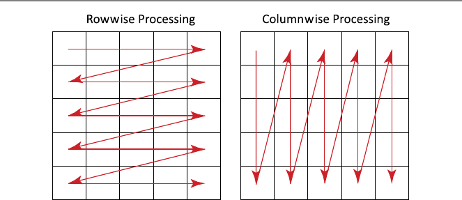
When there are nested loops, their order is always an issue to be considered by
the programmer. In the original matrix–vector multiplication program, the outer and
inner loops are constructed for the rows and columns of the matrix A, respectively.
Specifically, the variable of the outer loop irepresents the rows of A, whereas the
variable of the inner loop jrepresents its columns. This is called a rowwise process-
ing of the matrix, because the matrix is accessed row by row, e.g., first all elements
in the first row are considered, second all elements in the second row are considered,
etc. A columnwise processing is also possible, corresponding to a switch of the outer
and inner loops in the program.
The nested loops are best switched when there is no operation between them
(i.e., no operation inside the outer loop and outside the inner loop). In the original
program, line 05, i.e.,
sumvalue = 0
is between two loops. Therefore, before attempting to write a matrix–vector mul-
tiplication with the matrix accessed columnwise, we can modify the original algo-
rithm slightly by removing the variable sumvalue:
R Program: Matrix–Vector Multiplication (Correct)
01 matvecmult = function(A,x){
02 m = nrow(A)
03 n = ncol(A)
04 y = matrix(0,nrow=m)
05 for (i in 1:m){
06 for (j in 1:n){
07 y[i] = y[i] + A[i,j]*x[j]
08 }
09 }
10 return(y)
11 }
This program works correctly since the output vector yis initialized as zero in line
04. Moreover, it is now convenient to switch the loops to obtain a columnwise pro-
cessing of the input matrix as follows:
R Program: Matrix–Vector Multiplication (Correct)
01 matvecmult = function(A,x){
02 m = nrow(A)
03 n = ncol(A)
04 y = matrix(0,nrow=m)
05 for (j in 1:n){
06 for (i in 1:m){
07 y[i] = y[i] + A[i,j]*x[j]
08 }
09 }
10 return(y)
11 }
www.it-ebooks.info
26 2 Loops
Fig. 2.1 Rowwise and columnwise processing of a matrix
Note how the elements of the matrix Aare now used columnwise. As an example,
Fig. 2.1 illustrates rowwise and columnwise processing of a 5 ×5 matrix.
For the matrix–vector multiplication programs demonstrated above, one should
also note how the elements of the input and output vectors are used. In the rowwise
processing, the input vector xis traced repetitively, whereas the output vector yis
traced only once. This is reversed in the columnwise partitioning, where the input
vector xis traced once, while the output vector yis traced repetitively.
2.2.2 Example: Closest-Pair Problem
Consider the following problem. Given npoints in the two-dimensional space, i.e.,
(xk,y
k)for k=1,2,...,n, find the two closest points. As a brute-force approach,
where all possible solutions are considered, we can compute the distance between
each pair. Then, the minimum of these distances can be selected. We can follow
this approach, but instead of storing the distance values between all pairs, we may
compute them on-the-fly and compare with a variable minimumdistance, which
is simply the minimum distance encountered so far. After considering all possible
pairs, this variable and the corresponding index information can be returned as the
outputs. Along this direction, the following program can be written:
www.it-ebooks.info

2.2 Nested Loops 27
R Program: Finding the Closest Pair (Original)
01 findclosest = function(x,y){
02 n = length(x)
03 minimumdistance = sqrt((x[1]-x[2])∧2+(y[1]-y[2])∧2)
04 ibackup = 1
05 jbackup = 2
06 for (i in 1:(n-1)){
07 for (j in (i+1):n){
08 distance = sqrt((x[i]-x[j])∧2+(y[i]-y[j])∧2)
09 if (distance <minimumdistance){
10 minimumdistance = distance
11 ibackup = i
12 jbackup = j
13 }
14 }
15 }
16 list(minimumdistance,ibackup,jbackup)
17 }
The inputs of this program are vectors xand ythat store the xand ycoordinates
of the given points, respectively. Both vectors have nelements, where nis stored
in a variable n. Initially, the variable minimumdistance is set to the distance
between the first and second points as
minimumdistance = sqrt((x[1]-x[2])∧2+(y[1]-y[2])∧2)
To keep the track of the pair with the minimum distance, we also use the variables
ibackup and jbackup, which are initially set to 1 and 2, respectively. After these
initializations, we have two for loops to select different points and to compute the
distances between them. In the outer loop, the variable ichanges from 1 to n−1.
In the inner loop, the variable jchanges from the value of i+1 to n. This way, all
possible pairs are considered without any duplication as the value of iis always
smaller than the value of j.
Inside the loops, the distance between the ith and jth points is calculated as
distance = sqrt((x[i]-x[j])∧2+(y[i]-y[j])∧2)
This value is then compared with the variable minimumdistance, which stores
the minimum distance up to that point. If distance is smaller than mini-
mumdistance, then minimumdistance should be updated accordingly, as
well as the indices, i.e.,
minimumdistance = distance
ibackup = i
jbackup = j
Finally, note that, instead of a return statement, we use
list(ibackup,jbackup,minimumdistance)
at the end of the program to print out the minimum distance and the indices of the
corresponding points.
www.it-ebooks.info

28 2 Loops
Fig. 2.2 The closest pair
among 10 points
As an example, Fig. 2.2 depicts 10 points on the x–yplane, and the closest pair
found by using the program above.
2.3 Iteration Concept
In a broad sense, an iterative procedure is a process of repeating a set of instruc-
tions to approach a target. Each repetition is called an iteration, and the output of
an iteration is the input of the next iteration. Hence, each iteration depends on all
previous iterations. The aim in performing iterations is to converge to a steady state,
but divergence is not uncommon in many iterative solutions.
2.3.1 Example: Number of Terms for e
Assume that we would like to find the number of terms in the expression
e=∞
i=0
1
i!≈
n
i=0
1
i!
to approximate the value of ewith a given error threshold. The following iterative
program can be used for this purpose:
www.it-ebooks.info
2.3 Iteration Concept 29
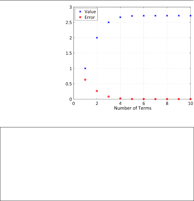
Fig. 2.3 Convergence of the
series to the value of e
R Program: Finding the Number of Terms for e(Original)
01 numberoftermsfore = function(desirederror){
02 refvalue = exp(1)
03 term = 1
04 sumvalue = 1 / factorial(term-1)
05 while (abs((refvalue-sumvalue)/refvalue) >desirederror){
06 term = term + 1
07 sumvalue = sumvalue + 1/factorial(term-1)
08 }
09 return(term)
10 }
In this program, the variable term represents the number of terms used in the series.
After this variable is incremented inside the while loop, a new term is added into
the series as
sumvalue = sumvalue + 1/factorial(term-1)
where factorial is the built-in R function for the factorial. Hence, the variable
sumvalue is updated in each repetition, and the loop continues while the relative
error is larger than the desired value represented by the scalar input desireder-
ror. This comparison can be seen in the while statement as
while (abs((refvalue-sumvalue)/refvalue) >desirederror){
where abs((refvalue-sumvalue)/refvalue) is the relative error. Note
that the reference value is obtained by using the built-in function of R, i.e., exp(1).
Figure 2.3 depicts how the variable sumvalue approaches e, and the error is
reduced to zero as the number of terms increases. In other words, sumvalue con-
verges to e, whereas the error converges to zero.
www.it-ebooks.info

30 2 Loops
2.3.2 Example: Geometric Series
Lets consider another iterative procedure, where the number of terms in the infinite
geometric series
1
1−x=∞
i=0
xi≈
n
i=0
xi,|x|<1,
is to be found again for a given error criteria. The following program can be used:
R Program: Finding the Number of Terms in the Geometric Series (Original)
01 numberoftermsingeo = function(x,desirederror){
02 refvalue = 1/(1−x)
03 term = 1
04 sumvalue = x∧(term−1)
05 while (abs((refvalue-sumvalue)/refvalue) >desirederror){
06 term = term + 1
07 sumvalue = sumvalue + x∧(term−1)
08 }
09 return(term)
10 }
In this case, the program has two inputs, i.e., xand desirederror. This program
works fine when the variable x, corresponding to the value of xin the formula
above, fits into the definition of the geometric series. In other words, a convergence
is achieved if the absolute value of the input xis smaller than 1. Otherwise, no
convergence occurs, since the geometric series becomes mathematically invalid.
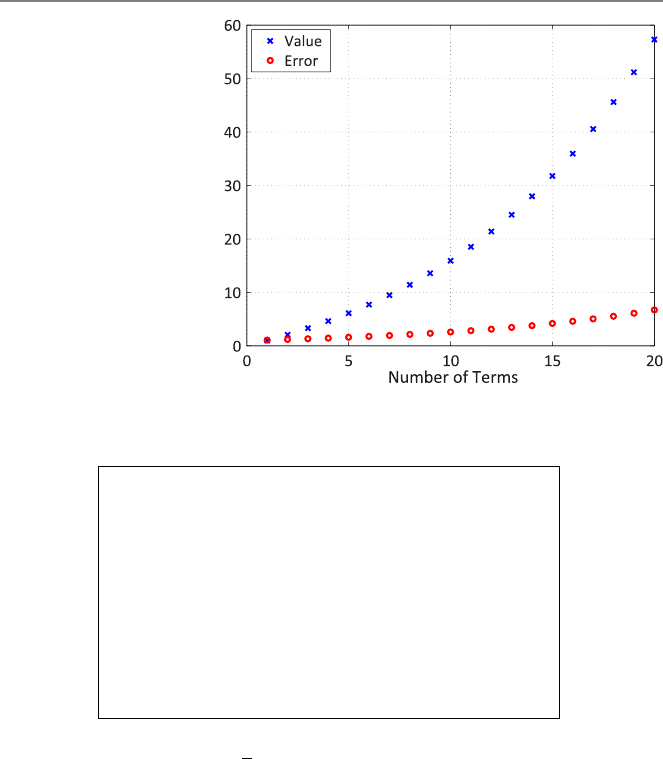
As an example, Fig. 2.4 depicts the variable sumvalue and the corresponding
error with respect to the number of terms when the program is used for xequal to
1.01. The value of sumvalue does not converge to any value, whereas the error
increases unboundedly as the iterations go on. Hence, in this example, convergence
is not achieved, and iterations diverge. Note that, for those faulty values of x,the
algorithm above never stops (infinite loop occurs), which may be considered as a
poor programming.
2.3.3 Example: Babylonian Method
Let us write an iterative program using the Babylonian method, i.e.,
xn+1=0.5(xn+5/xn),
to approximate the square root of 5 with 0.001 error. We can start with x0=2
and assume that the “exact” value of √5 is not available. Hence, we stop iterations
when the values in two consecutive iterations are sufficiently close to each other,
i.e., |xn+1−xn|<0.001. The proposed algorithm can be implemented as follows.
www.it-ebooks.info
2.3 Iteration Concept 31
Fig. 2.4 Divergence of the
geometric series for x=1.01
R Program: Babylonian Method for Square-Root of 5 (Original)
01 babylonianforsqrtfive = function(){
02 xold = 2
03 xnew = 0.5*(xold + 5/xold)
04 while (abs(xnew-xold) > 0.001){
05 print(xold)
06 xold = xnew
07 xnew = 0.5*(xold + 5/xold)
08 }
09 return(xnew)
10 }
This is a quite special program for a specific purpose; there is no input, but the output
is the approximate value of √5. In addition, the history of iterations is printed out
by using print(xold) in line 05. There are two variables to keep the values of x.
These are the old value xold and the new value xnew. The variable xold is ini-
tially set to 2, whereas the variable xnew is calculated by using the formula above.
The iterative process is constructed by using a while statement, which compares
the absolute difference of xold and xnew with the target error 0.001. In the loop,
xold is updated by simply copying xnew, whereas xnew is recalculated using the
formula again. Note that the order of these updates (first xold using xnew, then
xnew using the new value) is important.
If the program above is implemented and used, we get the steps of the iterative
procedure in the R workspace as
2
2.25
2.236068
www.it-ebooks.info

32 2 Loops
where the final value 2.236068 is the required approximation of √5. In other words,
the approximate value of √5 converges to 2.236068.
2.4 Conclusions
Loops are among the basics of computer programming, in which instructions are
often need to be repeated. For example, iterative procedures where iterations are
carried out to achieve convergence can easily be implemented using loops. All pro-
gramming languages, including R, provide special statements to construct loops.
Two types of loop statements are common:
•for-type statements, where the possible values of the loop variable are clearly
defined.
•while-type statements, where the continuation criteria are clearly defined, but
the loop variable needs to be initialized and incremented manually.
Depending on the problem and the solution algorithm, one of the types may be
easier to use than the other.
Loops are very beneficial, but they can easily be written incorrectly. Programmers
need to check how loops behave under different circumstances, especially to avoid
infinite loops, whereas extra conditions may be required to control special cases.
2.5 Exercises
1. Write a program using a for statement to compute the 1-norm of a given vector
v∈Rn. Apply the program to an example vector as
onenorm_for(matrix(c(4,5,4,3,-1,3,4,5,-4,2),ncol=1))
2. Consider the original program for the geometric series. How the program can be
changed in order to avoid infinite loop for faulty values of x?
3. Write a program to calculate the 2-norm of a given vector v∈Rn, i.e.,
v2=
n
i=1
(v[i])2,
using a for or while loop. Apply it to an example vector as
twonorm(matrix(c(5,4,1,6,7,8,-4,15,-2,4),ncol=1))
Compare your result with the value given by the built-in function of R, i.e.,
norm(matrix(c(5,4,1,6,7,8,-4,15,-2,4),ncol=1),"E")
www.it-ebooks.info

2.5 Exercises 33
4. Write a program that calculates the sum of cubes of positive integers from 1 to n
for a given value of n, i.e.,
n
i=1
i3.
Check your code against the direct formula
n
i=1
i3=n(n +1)
22
for different values of n, such as n=3, n=30, and n=300.
5. Write an R program that counts the number of zeros of a given vector v∈Rn.
Apply the program to an example vector as
countzeros(matrix(c(4,0,3,0,0,3,-4,0,5,0),ncol=1))
6. Write a program that finds the smallest element of a given vector v∈Rn. Apply
the program to three different vectors as
findminimum(matrix(c(4,0,3,0,0,3,-4,0,5,0),ncol=1))
findminimum(matrix(c(4,2,3,5,6,3,4,1,5,2),ncol=1))
findminimum(matrix(c(-4,-2,-3,-5,-6,-3,-4,-1,-5,-2),ncol=1))
Check that your program works correctly with −4, 1, and −6 outputs, respectively.
7. Write a program that finds the two farthest points among npoints in the two-
dimensional space, i.e., (xk,y
k)for k=1,2,...,n. Apply the program to an exam-
ple problem as
x = matrix(c(1,4,3,-2,-3),ncol=1)
y = matrix(c(2,-2,2,2,-1),ncol=1)
findfarthest(x,y)
8. Write a program that calculates the sine function using its Taylor-series expan-
sion, i.e.,
sin x=x−x3
3!+x5
5!−x7
7!+···= ∞
i=0
(−1)ix2i+1
(2i+1)!≈
n
i=0
(−1)ix2i+1
(2i+1)!.
The input of the program should be the value of xin terms of radians and the num-
ber of added terms n. The output should be the approximate value of sinx. Test your
code for x=π/3 and n=1,2,3,4,.... How many terms are required for six dig-
its of accuracy? Perform similar tests for x=4π/3 and x=7π/2. Compare your
results for different values of x.
www.it-ebooks.info

3
Recursions
Arecursion is a repeating process, where a statement is used inside itself. An inter-
esting example to recursion is the experiment when two mirrors are placed parallel
to each other so that nested images are formed infinitely. Recursive algorithms are
very useful in computer programming, and in many cases, the most efficient pro-
gram to solve a given problem involves a recursive structure. In this chapter, we
again start with simple examples to implement recursions, along with some possi-
ble mistakes. Then, we see how recursions can be used effectively to solve more
complex problems. Finally, we study a very important concept, namely proof by
induction, which is a mathematical tool to analyze and understand recursive expres-
sions.
3.1 Recursion Concept
Efficient or not, most of the programs can be rewritten using a recursion. Neverthe-
less, we should be very careful when writing recursive programs, particularly when
terminating recursions. In programming, we do not want recursions go infinitely.
3.1.1 Example: Recursive Calculation of 1-Norm
Consider again the calculation of the 1-norm of a given vector v∈Rn, i.e.,
v1=
n
i=1|v[i]|.
The vector has nelements. A recursive algorithm to compute the 1-norm can be
described as follows:
•If the vector has more than one element, divide it into two smaller vectors. Then,
the 1-norm of the vector equals the sum of the 1-norms of the smaller vectors.
Ö. Ergül, Guide to Programming and Algorithms Using R,
DOI 10.1007/978-1-4471-5328-3_3,
© Springer-Verlag London 2013
35
www.it-ebooks.info

36 3 Recursions
•If the vector has only one element, its 1-norm is the absolute value of the ele-
ment.
The first item defines the recursion. Specifically, computing the 1-norm of a vector
requires computing the 1-norms of two smaller vectors. In mathematical point of
view, the equality that we are using here is
n
i=1|v[i]|=
m
i=1|v[i]|+
n
i=m+1|v[i]|,
where 1 ≤m<n. This can also be written as
v1=v[1:m]1+v[m+1:n]1,
where the definition of the 1-norm in terms of itself is clearly visible. It should
be emphasized that this nice property of the 1-norm allows us to write a recursive
algorithm.
The second item in the algorithm above defines how we can terminate the recur-
sion. Any vector with more than one element can be divided into two vectors, but
we need to think again whenever we get a vector with only one element. For this
special case, we simply have
v1=|v[1]|,
which means that the 1-norm of the vector is the absolute value of the element.
At this stage, it may be useful to define how to divide a multielement vector into
two smaller vectors. A nice selection would be m≈n/2, which can be interpreted as
the vector is divided into two vectors of almost equal sizes. It can be shown that this
choice leads to the most efficient program, since less recursion steps are required to
divide the vector into one-element pieces. On the other hand, we need to consider
how to define an approximation to the half of n. For an even n,m=n/2 works. For
an odd n, however, m=n/2 is not meaningful as there is no such a fractional index.
To avoid this, one can use m=n/2, where · is the floor operation.
Based on the discussions above, we can write the complete formula for our re-
cursion as
v1=v[1:m]1+v[m+1:n]1for m=n/2if n>1,
|v[1]| if n=1.
With the help of this formula, the following R program can be written:
www.it-ebooks.info

3.1 Recursion Concept 37
R Program: Recursive Calculation of 1-Norm (Original)
01 onenormrecursive = function(v){
02 if (length(v) >1){
03 sum1 = onenormrecursive(v[1:floor(length(v)/2)])
04 sum2 = onenormrecursive(v[(floor(length(v)/2)+1):length(v)])
05 sumvalue = sum1 + sum2
06 }
07 else{
08 sumvalue = abs(v[1])
09 }
10 return(sumvalue)
11 }
Note how an if statement is used to distinguish two different cases. For n>1,
i.e., when the vector being considered has more than one element, we divide it into
two parts, evaluate the 1-norms of these smaller vectors, and then combine these 1-
norms to get the 1-norm of the vector. Interestingly, we do not directly compute the
1-norms of the smaller vectors. In fact, we just use the program that we are currently
writing! These are performed by three lines as
sum1 = onenormrecursive(v[1:floor(length(v)/2)])
sum2 = onenormrecursive(v[(floor(length(v)/2)+1):length(v)])
sumvalue = sum1 + sum2
by employing the program onenormrecursive in itself. When the vector being
considered has only one element, the only line being executed is
sumvalue = abs(v[1])
as required.
To improve its readability, the recursive program can be rewritten as follows:
R Program: Recursive Calculation of 1-Norm (Correct)
01 onenormrecursive = function(v){
02 n=length(v)
03 m=floor(n/2)
04 if (n >1){
05 sum1 = onenormrecursive(v[1:m])
06 sum2 = onenormrecursive(v[(m+1):n])
07 sumvalue = sum1 + sum2
08 }
09 else{
10 sumvalue = abs(v[1])
11 }
12 return(sumvalue)
13 }
In this program, the number of elements and the partitioning point are stored in
variables nand m, respectively.
www.it-ebooks.info
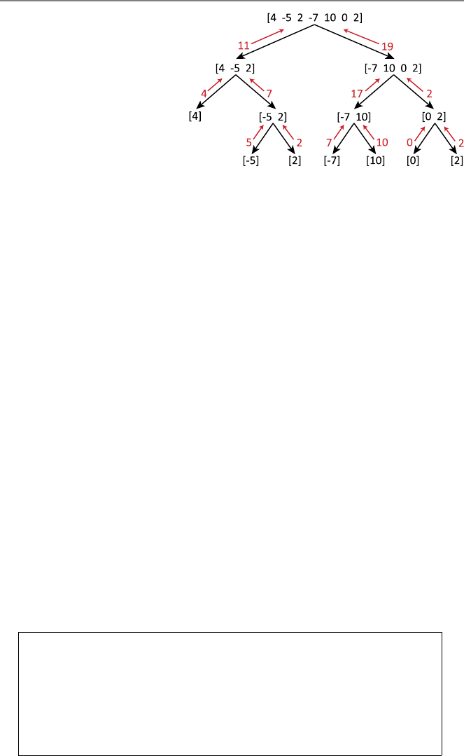
38 3 Recursions
Fig. 3.1 Recursive
calculation of the 1-norm of a
simple vector
Each person has her/his own way of understanding recursion, but one common
method is to construct a tree structure using simple examples. For the program
above, consider the vector
v=[4−52−7100 −2]
involving seven elements. Figure 3.1 depicts a tree structure on how the 1-norm of
this vector is calculated recursively. In this figure, we observe the partitioning of
vectors into smaller vectors until the number of elements is reduced to only one.
Combinations of outputs from bottom to top lead to the final output 11 +19 =30,
which is the 1-norm of v.
The efficiency of a recursive program is often related to the depth of recursion,
which can be defined as the number of levels in a tree structure associated with a
solution using a recursive program. For the recursive calculation of the 1-norm with
equally divided vectors, the depth of recursion is approximately n/2 if the initial
vector has nelements.
One of the common confusions in recursive programming is regarding variables.
For example, using the program above, what is the value of nif the program calls
itself and smaller vectors are considered repetitively? A correct answer would be
that nis the number of elements in any vector being considered. As the recursion
continues, multiple nvalues appear, but they are not mixed since variable values
are locally defined within functions and each call of the function means a new n.
This can be seen easily if a print statement like print(n) is placed in the program
above.
Now, let us see some possible mistakes that can be done in writing recursive
programs. Consider the following:
R Program: Recursive Calculation of 1-Norm (Incorrect)
01 onenormrecursive = function(v){
02 if (length(v) >1){
03 sum1 = onenormrecursive(v[1:floor(length(v)/2)])
04 sum2 = onenormrecursive(v[(floor(length(v)/2)+1):length(v)])
05 sumvalue = sum1 + sum2
06 }
07 return(sumvalue)
08 }
www.it-ebooks.info

3.1 Recursion Concept 39
In this program, the termination condition is forgotten. Therefore, as the recursion
continues and whenever a vector with only one element is encountered (note that this
eventually happens for any initial vector), the program tries to return sumvalue,
which is not defined. Therefore, the program stops with an error.
In the following one, there is not even a condition defined:
R Program: Recursive Calculation of 1-Norm (Incorrect)
01 onenormrecursive = function(v){
02 sum1 = onenormrecursive(v[1:floor(length(v)/2)])
03 sum2 = onenormrecursive(v[(floor(length(v)/2)+1):length(v)])
04 sumvalue = sum1 + sum2
05 return(sumvalue)
06 }
Since there is no condition and termination, one may expect that this program runs
infinitely, especially due to the line
sum2 = onenormrecursive(v[(floor(length(v)/2)+1):length(v)])
To understand what actually happens, consider a vector vwith only one element,
i.e., n=1. Then, m=n/2=0 and m+1=1, which means that the program
is executed with the same input vector (through line 03) again and again. Luckily,
the R environment automatically detects infinite recursions, and the program above
stops immediately with an error indicating this particular problem.
The following can be considered as an example to a poor programming:
R Program: Recursive Calculation of 1-Norm (Poor)
01 onenormrecursive = function(v){
02 if (length(v) >1){
03 sum1 = onenormrecursive(v[1:1])
04 sum2 = onenormrecursive(v[2:length(v)])
05 sumvalue = sum1 + sum2
06 }
07 else{
08 sumvalue = abs(v[1])
09 }
10 return(sumvalue)
11 }
In this case, the vector considered is not divided equally, but instead, it is divided
into a vector of only one element and another vector containing the rest. Hence,
vectors are not divided effectively in this program. It can be shown that, using this
program, the depth of the recursion is n(rather than n/2) if the initial vector has n
elements.
www.it-ebooks.info

40 3 Recursions
3.1.2 Example: Fibonacci Numbers
Fibonacci numbers starting from 1 can be written as
1,1,2,3,5,8,13,21,34,55,...,
where each number (except for the first two numbers) is the sum of two previous
numbers. This recurrence relation can be written as
f(i)=f(i−1)+f(i−2), i > 2,
with conditions f(1)=1 and f(2)=1. Then, the following recursive program can
be written to find the ith Fibonacci number:
R Program: Recursive Calculation of ith Fibonacci Number (Original)
01 fiborecursive = function(i){
02 if (i <=2){
03 value = 1
04 }
05 else{
06 value1 = fiborecursive(i-1)
07 value2 = fiborecursive(i-2)
08 value = value1 + value2
09 }
10 return(value)
11 }
The program simply returns 1 if the variable icorresponding to the value of iis
smaller than or equal to 2. Otherwise, the program itself is called twice; one for
i-1 and the other for i-2. Then, the results of these calls are added together to get
the ith Fibonacci number.
In the program above, we do not have to define variables to store intermediate
values. Hence, the program can easily be shortened as follows:
R Program: Recursive Calculation of ith Fibonacci Number (Correct)
01 fiborecursive = function(i){
02 if (i <=2){
03 value = 1
04 }
05 else{
06 value = fiborecursive(i-1) + fiborecursive(i-2)
07 }
08 return(value)
09 }
On the R side, this program is not very different from the original one. The original
three lines are replaced with line 06, i.e.,
value = fiborecursive(i-1) + fiborecursive(i-2)
www.it-ebooks.info

3.1 Recursion Concept 41
When this line is executed, the function is first called for i-1 and i-2. The results
of these calls are stored by R, but they are not available as variables to the user.
Their summation, however, is assigned to the variable value, which is returned as
the output of the program.
Many programmers are keen to shorten their programs for practical purposes. As
an example, the program above can be further shortened as follows:
R Program: Recursive Calculation of ith Fibonacci Number (Correct)
01 fiborecursive = function(i){
02 if (i <=2){
03 return(1)
04 }
05 else{
06 return(fiborecursive(i-1)+fiborecursive(i-2))
07 }
08 }
In this case, the sum fiborecursive(i-1)+fiborecursive(i-2) is re-
turned without even storing it in any variable. Since the outputting is carried inside
the if statement, two return statements are required for different conditions,
even though only one of them is executed depending on the value of the variable i.
Along this direction, the following program is incorrect and leads to the infinite-
recursion error.
R Program: Recursive Calculation of ith Fibonacci Number (Incorrect)
01 fiborecursive = function(i){
02 return(fiborecursive(i-1)+fiborecursive(i-2))
03 }
3.1.3 Example: Factorial
The factorial of a number can easily be calculated using a recursive algorithm. Even
though there is a built-in function factorial in R, we consider this as a good
example of recursion. Writing the factorial operation as
i!=i×(i −1)×(i −2)×···×1,
we note the recurrence relation i!=i×(i −1)!and the termination condition 0!=1,
which can be used to write the following program:
www.it-ebooks.info

42 3 Recursions
R Program: Recursive Calculation of Factorial (Original)
01 factorialrecursive = function(i){
02 if (i == 0){
03 value = 1
04 }
05 else{
06 value = i*factorialrecursive(i-1)
07 }
08 return(value)
09 }
Similar to the previous examples, this program can be shortened by removing the
variable value as follows:
R Program: Recursive Calculation of Factorial (Correct)
01 factorialrecursive = function(i){
02 if (i == 0){
03 return(1)
04 }
05 else{
06 return(i*factorialrecursive(i-1))
07 }
08 }
Note that the multiplication i*factorialrecursive(i-1)) needs to be per-
formed before the return operation, but this is performed implicitly by R without
any intermediate value (variable) available to the user.
3.2 Using Recursion for Solving Problems
Up to this point, we have seen how to construct a recursive approach and write
recursive programs to solve a given problem. In this section, we consider some
problems, which can be solved most naturally by recursive algorithms.
3.2.1 Example: Highest Common Factor
Let a nonnegative integer (natural number) i∈Nbe factorized as i=a×b, where
a,b ∈N.Bothaand bare called factors of i. Each natural number ihas a set of
factors including at least 1 and itself. Then, the highest common factor (HCF) of a
set of natural numbers {i1,i
2,...,i
m}is defined as the largest integer, which is the
factor of all numbers in the set.
The highest common factor of two numbers can be obtained by a recursive algo-
rithm, namely, a recursive version of the Euclidean algorithm. The Euclidean algo-
rithm is based on the following observation. If HCF{i, j }is the highest common fac-
www.it-ebooks.info

3.2 Using Recursion for Solving Problems 43
tor of iand j, where i≥j, it is also the highest common factor of (i −j)and j.Note
that if i=a×HCF{i, j }and j=b×HCF{i, j}, then (i −j)=(a −b)×HCF{i, j }.
Based on the discussion above, the following program can be written:
R Program: Finding HCF Using Recursive Euclidean Algorithm (Original)
01 hcfeuclidean = function(i,j){
02 if (j == 0){
03 hcfvalue = i
04 }
05 else{
06 k=i%%j
07 hcfvalue = hcfeuclidean(j,k)
08 }
09 return(hcfvalue)
10 }
First, assume that the first input iis greater than or equal to the second input j.
As described above, the smaller integer can be subtracted from the larger integer
without changing their HCF. This idea is used in line 06 as
k=i%%j
where the built-in modulus function %% is used. Specifically, in this line, the modu-
lus function is used to subtract a multiple of jfrom i. Instead of a single subtraction,
the modulus function (corresponding to one or multiple subtractions) is used so that
the resulting value k=i%%jis always smaller than j. This can be interpreted
as jis repetitively subtracted from iuntil a smaller integer is obtained. Then, the
program calls itself with the new inputs jand k, where the former is the larger
integer now.
Interestingly, this program works correctly even when the first input iis smaller
than the second input j. If this is the case, the modulus operation in line 06 returns
iwithout subtracting anything. Then, the program calls itself (in line 07) as
hcfvalue = hcfeuclidean(j,i)
where the inputs are switched without any change in their values. In other words, if
the first input is smaller, then the program automatically switches the inputs in the
first call of the recursion.
In the program above, the recursion is controlled by an if statement. In any call
of this program, if the smaller integer is zero, then the output is the other integer (see
line 03). Note that, as a recursion continues and integers are subtracted from each
other, this condition occurs eventually, leading to the termination of the recursion.
3.2.2 Example: Lowest Common Multiple
The lowest common multiple (LCM) of two positive integers iand jis defined as
the smallest integer that is the multiple of both iand j. In other words, LCM{i, j }=
a×iand LCM{i, j}=b×jsuch that aand bare the smallest possible integers.
www.it-ebooks.info

44 3 Recursions
The lowest common multiple of two numbers is related to their highest common
factor as
LCM{i, j}= i×j
HCF{i, j}.
Hence, the following program can be used to easily find the lowest common mul-
tiple. Even though it involves a single command (other than the function definition
and the return line), we write it as a function to use later:
R Program: Finding LCM Using HCF (Original)
01 lcmusinghcf = function(i,j){
02 lcmvalue = i*j / hcfeuclidean(i,j)
03 return(lcmvalue)
04 }
Now, let us consider the lowest common multiple of a set of positive integers
{i1,i
2,...,i
n}. We note that
LCM{i1,i
2,...,i
n}=LCM{i1,LCM{i2,...,i
n}}.
In other words, the lowest common multiple can be defined recursively using itself.
The following program can be written following this strategy:
R Program: Finding LCM of a Vector of Numbers (Original)
01 lcmvector = function(v){
02 n = length(v)
03 if (n == 2){
04 lcmvalue = lcmusinghcf(v[1],v[2])
05 }
06 else{
07 j = lcmvector(v[2:n])
08 lcmvalue = lcmusinghcf(v[1],j)
09 }
10 return(lcmvalue)
11 }
The input of this program is a vector vthat contains positive integers whose lowest
common multiple is to be found. If there are only two elements in this vector, the
program lcmusinghcf is called directly using these elements, i.e., v[1] and
v[2], in line 04. This (having two elements) is also the termination case of the
recursion. For more than two elements, lines 07 and 08 are performed, which can
be described as follows.
•Line 07: Find the lowest common multiple of elements from v[2] to v[n].
This is where the program calls itself.
www.it-ebooks.info
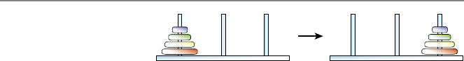
3.2 Using Recursion for Solving Problems 45
Fig. 3.2 Towers of Hanoi
involving four disks
•Line 08: The output (the lowest common multiple of all elements) is the lowest
common multiple of the first element and the result of line 07. The program
lcmusinghcf can be used here since there are only two numbers (the first
element and the result of line 07).
Note how a recursive program lcmvector uses another recursive program
hcfeuclidean with an interface lcmusinghcf between them. In computer
science, implementations usually involve multiple programs and code segments in-
teracting with each other, as in this particular case.
3.2.3 Example: Towers of Hanoi
A very famous set of problems that can be solved recursively is Towers of Hanoi. As
depicted in Fig. 3.2, the puzzle involves three rods and a given number of (originally
eight but four in this example) disks that can slide on the rods. Initially, the disks
are stacked in one of the rods (source rod on the left) based on their sizes, i.e., from
the smallest on the top to the largest on the bottom leading to a conical shape. The
aim is to transfer the entire stack to another rod (destination rod on the right), again
resulting in a conical shape. There is also a buffer rod in the middle to facilitate the
movements. The rules are as follows:
•Only one disk may be moved at a time.
•Each move involves taking a disk on the top of a stack and putting it on the top
of another stack.
•A disk cannot be placed on a smaller disk.
A particular aim is to perform the transfer of the stack with a minimum number of
movements.
Initially, the solution of the puzzle may not seem trivial, but in fact, it is easy
using a recursive approach. Consider the version depicted in Fig. 3.2 involving four
disks. The following observations can be made:
•For the solution of the problem, the largest disk on the source (left) rod is even-
tually moved to the destination (right) rod.
•In order to perform this movement, other three disks should reside on the buffer
(middle) rod with a conical shape. Specifically, this is the only scenario that
such a movement can be done based on the given rules.
•Then, the solution of the original problem involves the solution of a similar
(smaller) problem, where the smaller three rods are transferred from the source
(left) rod to the buffer (middle) rod and then, from the buffer (middle) rod to the
destination (left) rod.
Obviously, the items above describe a recursive process. In order to solve the prob-
lem involving four disks, we need to solve a subproblem involving three disks twice.
Similarly, the solution of a three-disk problem requires the solution of a smaller
www.it-ebooks.info

46 3 Recursions
problem involving only two disks. Now, lets write all operations one by one and
construct the recursive structure.
•Solution for four disks (transfer from a source to a destination):
– Step 1: Move the smaller three disks from the source rod to the buffer rod.
(Perform the solution of this subproblem as described below.)
– Step 2: Move the largest disk (among four disks) to the destination rod.
– Step 3: Move the smaller three disks from the buffer rod to the destination
rod. (Perform the solution of this subproblem as described below.)
•Solution for three disks (transfer from a source to a destination):
– Step 1: Move the smaller two disks from the source rod to the buffer rod.
(Perform the solution of this subproblem as described below.)
– Step 2: Move the largest disk (among three disks) to the destination rod.
– Step 3: Move the smaller two disks from the buffer rod to the destination
rod. (Perform the solution of this subproblem as described below.)
•Solution for two disks (transfer from a source to a destination):
– Step 1: Move the smaller disk from the source rod to the buffer rod.
– Step 2: Move the larger disk to the destination rod.
– Step 3: Move the smaller disk from the buffer rod to the destination rod.
In the solutions described above, the terms “source”, “buffer”, and “destination” are
redefined for each problem. In other words, each problem and its solution always
involve a transfer of rods from the source rod to the destination rod while using the
buffer rod. Hence, one need to be very careful when calling the recursive function
since, for example, the buffer rod for the parent problem can be the source rod or
destination rod for the subproblem.
A pseudocode for the solution of Towers of Hanoi with arbitrary numbers of
disks can be written as follows:
Pseudocode: Solution of Towers of Hanoi
01 towersofhanoi = function(n,sourcerod,bufferrod,destinationrod){
02 if (n == 0){
03 do nothing
04 }
05 else{
06 towersofhanoi(n-1,sourcerod,destinationrod,bufferrod)
07 move from sourcerod to destinationrod
06 towersofhanoi(n-1,bufferrod,sourcerod,destinationrod)
08 }
10 }
The orders of the rods in the recursive calls should be particularly noted, in accor-
dance with the discussion above.
Figure 3.3 depicts the solution of a four-disk problem, which requires a total
of 15 movements. At this stage, we can find the minimum number of movements
required to solve any given number of disks. This way, we can set the optimality
criteria before solving the problem for large numbers of disks.
www.it-ebooks.info
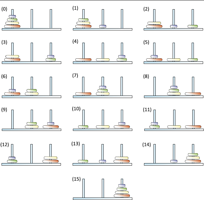
3.2 Using Recursion for Solving Problems 47
Fig. 3.3 The solution of Towers of Hanoi involving four disks
Consider the solution of Towers of Hanoi with ndisks. As detailed above, such
a solution requires two smaller solutions involving n−1 disks, in addition to a
movement of the largest disk. Hence, one can write
f(n)=2f(n−1)+1,
where frepresents the number of movements. Unsurprisingly, the number of move-
ments is a recursive function, i.e., a function defined by using itself. In fact, recursive
programs and algorithms often have recursive costs (here the number of movements
can be interpreted as the cost). For the termination of the recurrence relation, one
can also add f(0)=0, so that f(1)=1 is the number of movements for the trivial
one-disk problem.
www.it-ebooks.info

48 3 Recursions
Table 3.1 Number of
movements required to solve
Towers of Hanoi involving n
disks
Number of disks (n) Number of movements (2n−1)
00
11
23
37
415
531
10 1023
20 1,048,575
30 1,073,741,823
40 1,099,511,627,775
50 1,125,899,906,842,623
In order to find an explicit expression for the recursive function above, we can
use the recurrence relation to derive a sequence of equations. First, note that f(n)=
2f(n−1)+1 means f(n−1)=2f(n−2)+1forn≥2. Then,
f(n)=2f(n−1)+1
=2(2f(n−2)+1)+1
=4f(n−2)+2+1.
Similarly, for n≥3,
f(n)=8f(n−3)+4+2+1.
It appears that, considering an arbitrarily large n,wehave
f(n)=2n−1f(1)+2n−2+···+8+4+2+1,
which can be rewritten as
f(n)=2n−1+2n−2+···+8+4+2+1=
n−1
i=0
2i
since f(1)=1. Evaluating the summation, we get
f(n)=
n−1
i=0
2i=1−2n
1−2=2n−1
as the explicit expression, which is valid for all values of n≥0.
Table 3.1 lists the number of movements to solve Towers of Hanoi with respect
to the number of disks n.
www.it-ebooks.info
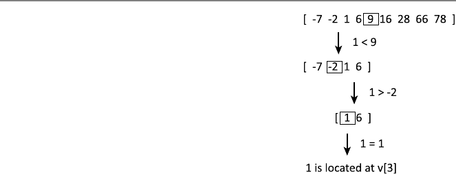
3.2 Using Recursion for Solving Problems 49
Fig. 3.4 Recursive
binary-search algorithm
applied to a simple vector
Obviously, the number of movements grows rapidly (exponentially to be more
specific). To formally prove that f(n)=2n−1 is the direct formula for the recursion
f(n)=2f(n−1)+1, we need proof by induction, which is considered in the last
section of this chapter.
3.2.4 Example: Binary Search
Consider a recursive binary-search algorithm, which finds the position of a given
number in a vector v∈Rninvolving sorted numbers:
•Take the vector, as well as a lower index and a higher index. The number is to
be searched between these lower and higher indices.
•Take the number in the middle of the range between the lower and higher in-
dices. If it is the one that we are looking for, then the algorithm stops by return-
ing its index.
•If the number that we are searching is smaller than the middle element, the
algorithm is restarted by considering the smaller elements (from the lower index
to the middle index, excluding the middle index).
•If the number that we are searching is larger than the middle element, the algo-
rithm is restarted by considering the larger elements (from the middle index to
the higher index, excluding the middle index).
This is called a recursive binary-search algorithm, since it is based on recursively
dividing the vector into two smaller vectors until the number is found. It is of course
possible to find the searched element by scanning all elements of the given vec-
tor, but the binary-search algorithm is much more efficient than a direct scan, as
discussed in Chap. 4.
As an example, consider a simple vector of nine elements
v=[−7,−2,1,6,9,16,28,66,78]
and assume that we are searching the number 1 (located at v[3]) in it. Note that, as an
important requirement for the proposed algorithm working correctly, the numbers
in the vector are sorted in the ascending order. Figure 3.4 depicts a tree structure on
how the number is searched and found.
www.it-ebooks.info

50 3 Recursions
In the first step, the middle element is v[5]=9. Since 1 <9, the search continues
in v[1:4]. In the second step, the middle element is v[2]=−2. Since 1 >−2,
the search continues in v[3:4]. In the third and final step, the middle element is
v[3]=1, which is the number that we are searching. Hence, its index, i.e., 3, is
returned as the final result of the search.
We also need to consider what happens when the number that we are searching
does not exist in the vector. As shown in the example above, the binary-search algo-
rithm is based on systematically limiting the range of elements that we are looking
so that the required number is found after a number of steps. Therefore, as the recur-
sion continues, we expect that the lower and higher indices approach to each other.
If, at some step, the higher index is smaller than the lower index, it can be claimed
that the number is not found and the algorithm must stop.
Considering the discussion above, the following program can be written. The
inputs of this program are the vector v, the number that we are searching thenum-
ber, and lower/higher indices of the search lowerindex and higherindex.
In the initial call of this program, lowerindex is set to 1, while higherindex
is set to nto consider all elements of the vector.
R Program: Recursive Binary Search (Original)
01 binarysearchrecursive = function(v,thenumber,lowerindex,higherindex){
02 if (lowerindex >higherindex){
03 print("The number is not found!")
04 }
05 else{
06 middleindex = lowerindex + floor((higherindex-lowerindex)/2)
07 if (v[middleindex] == thenumber){
08 return(middleindex)
09 }
10 else if (v[middleindex] <thenumber){
11 binarysearchrecursive(v,thenumber,middleindex+1,higherindex)
12 }
13 else if (v[middleindex] >thenumber){
14 binarysearchrecursive(v,thenumber,lowerindex,middleindex-1)
15 }
16 }
17 }
The program starts with an if statement to compare lowerindex and high-
erindex.Iflowerindex is larger than higherindex, then the program stops
and prints a warning message to indicate that the number is not found in the vector;
this is the termination point of the recursion. Otherwise, the program may continue.
The variable middleindex is calculated in line 06 as
middleindex = lowerindex + floor((higherindex-lowerindex)/2)
which is followed by the comparison of the middle element v[middleindex]
with the number to be found, i.e., thenumber. The program returns middlein-
dex, if the equality in line 07 holds. Otherwise, the program itself is called with a
new search range that is determined according to the value of v[middleindex]
with respect to thenumber.
www.it-ebooks.info

3.2 Using Recursion for Solving Problems 51
3.2.5 Example: Sequence Generation
Assume that we would like to list all words with nletters. For simplicity, these
words contain only “a” and “b”, but we would like to find all possible combinations
whether the word is meaningful or not. The following recursive algorithm can be
used for this purpose:
•Put “a” as the first letter. Then, solve the problem for n−1 letters if n>1 and
add the result next to “a”.
•Put “b” as the first letter. Then, solve the problem for n−1 letters if n>1 and
add the result next to “b”.
•Combine the two items above for the complete list.
Obviously, the solution of the problem (listing words) for nletters depends on the
solution of the problem (listing words) for n−1 letters. Hence, this is a recursive
algorithm.
In order to write the recursive program, we use two combination operations, i.e.,
rbind for rowwise combinations and cbind for columnwise combinations. Re-
sults are stored as matrices. For nletters, we expect 2ndifferent words. As an ex-
ample, if n=3, the words to be listed are “aaa”, “aab”, “aba”, “abb”, “baa”, “bab”,
“bba”, and “bbb”, which can be written as a matrix, i.e.,
⎡
⎢
⎢
⎢
⎢
⎢
⎢
⎢
⎢
⎢
⎢
⎣
aaa
aab
aba
abb
baa
bab
bba
bbb
⎤
⎥
⎥
⎥
⎥
⎥
⎥
⎥
⎥
⎥
⎥
⎦
.
The proposed recursive algorithm described above can be implemented shortly as
follows:
R Program: Generate Words With a and b (Original)
01 generateab = function(n){
02 if (n >0){
03 v = rbind(matrix("a",nrow=2∧(n-1)),matrix("b",nrow=2∧(n-1)))
04 return(noquote(cbind(v,rbind(generateab(n-1),generateab(n-1)))))
05 }
06 }
The program above is very compact and it contains few lines, but each line should
be investigated carefully to understand how such a program generates and prints all
words with nletters.
First, lets focus on line 03. This line initializes a vector vwith 2nelements. The
first half of these elements are the character “a”, whereas the second half are the
character “b”. Note that the commands
matrix("a",nrow=2∧(n-1))
www.it-ebooks.info

52 3 Recursions
and
matrix("b",nrow=2∧(n-1))
generate vectors of 2n−1elements, which are then combined using rbind and
stored in v. As an example, if n=3, one can expect that vcontains
⎡
⎢
⎢
⎢
⎢
⎢
⎢
⎢
⎢
⎢
⎣
a
a
a
a
b
b
b
b
⎤
⎥
⎥
⎥
⎥
⎥
⎥
⎥
⎥
⎥
⎦
.
In line 04, the function itself is called twice with an input of n-1, i.e.,
generateab(n-1)
We expect that the results of these calls are identical matrices involving 2n−1rows
and n−1 columns containing the solution for the input n−1. These matrices are
combined using rbind as
rbind(generateab(n-1),generateab(n-1))
leading to a matrix with 2nrows. As an example, if n=3, rbind above is expected
to create the matrix ⎡
⎢
⎢
⎢
⎢
⎢
⎢
⎢
⎢
⎢
⎣
aa
ab
ba
bb
aa
ab
ba
bb
⎤
⎥
⎥
⎥
⎥
⎥
⎥
⎥
⎥
⎥
⎦
.
Finally, the result of rbind is combined columnwise with v(prepared as discussed
above) as
cbind(v,rbind(generateab(n-1),generateab(n-1)))
which is the desired output to be returned. Before returning, we use the built-in
noquote command to omit quotation marks in the output.
In the program above, the if statement is particularly important to terminate the
recursion appropriately. For any input n>1, the program calls itself with smaller
inputs. When n=1, line 03 generates a vector of two elements containing “a” and
“b”. At this stage, there is nothing to add after these letters; therefore, the calls with
a smaller input (n=0) should return nothing. This is precisely controlled by the
if statement in line 02, which guarantees that the program neither calls itself nor
returns anything when n=0.
One way to improve the program above is storing the result of generateab(n-
1)) and using it twice, rather than calling the function twice. This does not change
www.it-ebooks.info

3.2 Using Recursion for Solving Problems 53
Fig. 3.5 Producing A1jfrom
Afor the calculation of the
determinant
the depth of recursion (that is n) but improves the efficiency by reducing the number
of function calls.
3.2.6 Example: Determinant
Determinant is an important quantity for square matrices, and there are various
ways, including a recursive approach, to calculate this quantity. Using a recursive
approach, the determinant of an arbitrary square matrix A∈Rn×ncan be written as
det(A) =A[1,1]det(A11)+···+A[1,j](−1)1+jdet(A1j)
+···+A[1,n](−1)1+ndet(A1n),
where A1jrepresent an (n −1)×(n −1)matrix obtained by deleting the first
row and the jth column of A. Figure 3.5 presents an illustration of producing A1j
from A.
The recursive formula above is valid when n>1. For n=1, det(A) =A[1,1],
i.e., the determinant is simply the value of the single element. Based on the recur-
rence relation and the termination condition, the following program can be written:
R Program: Recursive Calculation of Determinant (Original)
01 determinantrecursive = function(A){
02 n = nrow(A)
03 if (n == 1){
04 value = A[1,1]
05 }
06 else{
07 value = 0
08 for (j in (1:n)){
09 if (j == 1){
10 A1j = matrix(A[2:n,2:n],nrow=n-1)
11 }
12 else if (j == n){
13 A1j = matrix(A[2:n,1:(n-1)],nrow=n-1)
14 }
15 else{
16 A1j = cbind(A[2:n,1:(j-1)],A[2:n,(j+1):n])
17 }
18 value1 = determinantrecursive(A1j)
19 value2 = A[1,j]*(-1)∧(j+1)
20 value = value + value1*value2
21 }
22 }
23 return(value)
24 }
www.it-ebooks.info

54 3 Recursions
If the matrix has more than one element, the for loop (lines 08–21) is executed.
For each value of the variable jfrom 1 to n, the first row and the jth column are
removed from the original matrix. Removing the first row is relatively easy, but
removing the jth column requires a careful consideration of three different cases
via conditional statements. When the value of jis 1 and the first column is to be
removed, we have
A1j = matrix(A[2:n,2:n],nrow=n-1)
where the column index is 2:n to indicate that the columns of Afrom 2 to nare
selected. Similarly, when the value of jis nand the last column is to be removed,
we have
A1j = matrix(A[2:n,1:(n-1)],nrow=n-1)
where the column index is now 1:(n-1). For all other values of jfrom 2 to
n−1, removing the jth column requires the selection of two submatrices, i.e.,
A[2:n,1:(j-1)] and A[2:n,(j+1):n], and then their columnwise combi-
nation as
A1j = cbind(A[2:n,1:(j-1)],A[2:n,(j+1):n])
Whenever the submatrix A1j is obtained, its determinant is calculated by using the
program itself as
value1 = determinantrecursive(A1j)
which is multiplied with
value2 = A[1,j]*(-1)∧(j+1)
in accordance with the formula of the determinant. The multiplication is then added
to the output value, which is returned after all jvalues are considered.
Even though the program above is relatively simple compared to some other
methods for calculating the determinant, it is very expensive. Specifically, its time
complexity is O(n!), where nrepresents the size of the matrix. Therefore, the de-
terminant of a matrix is usually calculated with more efficient methods, such as the
LU factorization, especially when the matrix is large. Nevertheless, the procedure
above is a good example on the application of a recursive algorithm to solve a prac-
tical problem.
3.3 Proof by Induction
Proof by induction is a powerful tool in mathematics to prove various statements,
including recurrence relations. In many cases, recursive formulas need to be con-
verted into direct formulas, which can be performed heuristically and then, proven
via induction. An induction is based on two simple rules:
(1) Show that the statement is true for the most initial value or case, e.g., for 0 or
1 or another value.
www.it-ebooks.info

3.3 Proof by Induction 55
(2) Assuming that the statement is true in general (e.g., for n), show that it is also
true for the incremental case (e.g., for n+1).
Although the rules are simple, there are many useful statements that can be proven
by induction.
As an example, consider the formula
m
i=1
i=m(m +1)
2,
which can be proven by induction as follows. First, consider the initial case m=1.
For this value of m,wehave
1
i=1
i=1×2
2=1,
and the statement is true. Next, assume that the statement is true for m=n, i.e.,
n
i=1
i=n(n +1)
2
is given. Then, considering the incremental case m=(n +1),wehave
n+1
i=1
i=
n
i=1
i+(n +1)=n(n +1)
2+(n +1)=n2+3n+2
2=(n +1)(n +2)
2.
Hence,
n+1
i=1
i=(n +1)(n +2)
2,
and the statement is true for m=(n +1)(if it is true for m=n). This completes the
proof.
Now, consider the recurrence relation
f(m)=f(m−1)+a
with initial condition f(1)=a. First, we can find the direct formula heuristically.
Starting with f(2)=f(1)+a=a+a=2a,wehavef(3)=f(2)+a=2a+
a=3a,f(4)=f(3)+a=3a+a=4a, etc. Hence, f(m)=ma seems to be the
direct formula for this sequence, but we need induction to prove it. The initial case
f(1)=ais already given, and the formula is satisfied for m=1. We also note that
f(n+1)=f(n)+ausing the recursive formula. Consequently, if f(n)=na, then
f(n+1)=na +a=(n+1)a, which fits into the direct formula, proving its validity.
As another example, consider the recurrence relation
f(m)=a×f(m−1)
www.it-ebooks.info

56 3 Recursions
with f(0)=1. Note that f(1)=a×f(0)=a,f(2)=a×f(1)=a2,f(3)=
a×f(2)=a3, etc. Hence, f(m)=amseems to be the direct formula, which can
be proven again by induction. First, we note that the rule is valid for the initial case
m=0, i.e., f(0)=a0=1 is already given. Then, using the recursive formula and
assuming that f(n)=anis correct, we have f(n+1)=a×f(n)=a×an=an+1,
showing that the direct formula is valid.
Finally, consider the recurrence relation
f(m)=m×f(m−1)
with f(0)=1. Note that f(1)=1×f(0)=1, f(2)=2×f(1)=2, and f(3)=
3×f(2)=6. Hence, f(m)=m!seems to be the direct formula. To prove this, we
first note that the rule is valid for m=0, i.e., f(0)=1 is given and correct. Then,
using the recursive relation, we write f(n+1)=(n +1)f (n).Iff(n)=n!, then
f(n+1)=(n +1)n!=(n +1)!, so that the direct formula is proven to be correct.
As demonstrated in the examples above, the equivalence of a recursive formula
and a direct formula can be shown rigorously via proof by induction. The cost of
a recursive algorithm often has a recurrence relation, which needs to be converted
into a direct expression to assess the algorithm.
3.4 Conclusions
Recursions can be very useful in computer programming. For many problems, the
most natural and/or efficient solutions are provided by recursive programs and al-
gorithms. Some examples presented in this chapter are finding the highest common
factor and lowest common multiple of a set of integers, Towers of Hanoi, binary
search, sequence generation, and computing determinants of matrices. As presented
in the next chapters, binomial coefficients can be calculated recursively, and one of
the most efficient sorting algorithms, namely the quick sort algorithm, is also based
on a recursive structure.
Despite their favorable properties, one should be very careful when implement-
ing recursive algorithms since they can easily go out of control. All recursive struc-
tures require termination conditions that must be placed accordingly into programs.
Constructing tree structures using simple examples can be very useful when un-
derstanding and writing recursive programs. Such a tree structure may also provide
some information on the efficiency of a recursive program by showing the depth of
recursion in terms of inputs.
3.5 Exercises
1. Write a recursive program that calculates the ith Fibonacci number. Test your
code for i=10, i=20, i=30, and i=40. Describe roughly how the processing
time changes when igets larger?
www.it-ebooks.info

3.5 Exercises 57
2. Write a recursive program that calculates the factorial of a given number i. Check
your code for i=10, i=20, i=30, and i=40 against the built-in function fac-
torial in R. What is the largest ithat your program returns a number?
3. Write a recursive program to compute the sum of squares of first nintegers. For
this purpose, you may use
n
i=1
i2=
n−1
i=1
i2+n2
for n>1. Hence, the recursive formula to be programmed is f(n)=f(n−1)+n2,
where f(1)=1. Test your code for some values of n. Note that the direct formula
(that can be used as a reference) is
n
i=1
i2=n(n +1)(2n+1)
6.
4. Write a recursive program that finds the highest common factor of two nonnega-
tive integers iand jusing the Euclidean algorithm. Test your code for the following
pairs of (i, j ):(3,2),(4,2),(40,24),(120,45), and (540,56).
5. Write a recursive program that finds the lowest common multiple of two positive
integers iand j, employing the program of the previous question. Test your code
for the following pairs of (i, j):(12,27),(16,28),(14,15),(7,13),(8,48).
6. Write a recursive program that finds the lowest common multiple of a vector of
positive integers, employing the program of the previous question. Test your pro-
gram for a vector ⎡
⎢
⎢
⎢
⎢
⎣
700
50
4
3
2
⎤
⎥
⎥
⎥
⎥
⎦.
7. Write a recursive program to compute the number of movements to solve Towers
of Hanoi involving ndisks using f(n) =2f(n −1)+1, where f(1)=1. Test
your code for some values of n. Note that the direct formula (that can be used as a
reference) is f(n)=2n−1.
8. What is the determinant of an n×ndiagonal matrix A(A[i, j ]=0ifi= j)?
How the recursive program given in this chapter works for diagonal matrices? How
would you change it for a more efficient calculation of the determinant of a diagonal
matrix?
www.it-ebooks.info

4
Complexity of Programs and Algorithms
As briefly discussed in the previous chapters, there are usually several algorithms
to solve a given problem. For example, the 1-norm of a vector can be calculated
using a loop (for or while, depending on programming) or a recursion. Hence,
for any problem, it is essential to compare different algorithms in terms of efficiency
(processing time and memory requirement) and/or accuracy.
In order to compare the efficiency of programs and algorithms, we need to ana-
lyze them by estimating or measuring their time and/or memory costs. Estimations
are as important as measurements because we often need to know the cost of a pro-
gram before writing and using it. In addition, we would like to know the cost when
different computers are used, rather than relying on a measurement on a specific
computer. Consequently, it is not surprising that calculating the costs of programs
and algorithms has become a major area in computer science.
Today, performances of computers are usually expressed by an important quan-
tity, namely, floating-point operations per second (FLOPS). This is simply the num-
ber of floating-point operations that can be performed in one second. A floating-
point operation can be defined as a basic operation, e.g., addition, subtraction, mul-
tiplication, or division, applied to floating-point representations of numbers in com-
puters. Hence, to estimate the time cost of a computer program (and hence the under-
lying algorithm), it would be convenient to count the number of floating-point oper-
ations in it. On the other hand, this would be an incomplete estimation since other
kinds of operations, such as conditional statements, loop statements, and equalities
are ignored. Estimation of the memory cost is usually easier, since one can count the
number of scalars and elements in vectors and matrices. But, the memory require-
ment depends on how the numbers are represented, e.g., single precision or double
precision.
In this chapter, we use a systematic approach to understand and estimate costs
of programs and algorithms. First, we start with a rigorous analysis by counting
each operation and each piece of storage in programs. When these costs are stated
as functions of input sizes (and sometimes input values), the resulting expressions
are called time and memory complexities. Then, we simplify these expressions using
asymptotic techniques, leading to a very important concept, namely, the order.After
Ö. Ergül, Guide to Programming and Algorithms Using R,
DOI 10.1007/978-1-4471-5328-3_4,
© Springer-Verlag London 2013
59
www.it-ebooks.info

60 4 Complexity of Programs and Algorithms
some practice, we derive shortcuts to explore the costs of programs. Finally, we
study the costs of recursive programs, followed by some discussions on orders of
various programs and algorithms.
4.1 Complexity of Programs
In our rigorous analysis for the time complexity, we count all lines and operations
one by one, except the following cases:
•First lines (function definitions) and output lines (e.g., return) are not
counted.
•Lines including only {and }are not counted.
•Conditional statements else and else if are assumed to be connected to
the associated if statements, and hence they are not counted.
These rules are defined for simplification purposes, and they are not critical, as will
be revealed later.
For the memory complexity, we consider all items (inputs, outputs, constants,
variables) and count all elements (scalars and all elements in vectors and matrices).
4.1.1 Example: Inner Product
Consider the calculation of the inner product of two given vectors vand w∈Rn.
Their inner product is defined as
v·w=
n
i=1
v[i]w[i].
The following program can be used for this purpose:
R Program: Calculation of Inner Product (Original)
01 innerproduct = function(v,w){
02 sumvalue = 0
03 for (i in 1:length(v)){
04 sumvalue = sumvalue + v[i]*w[i]
05 }
06 return(sumvalue)
07 }
Now, let us calculate the time cost of this program in terms of n(input size). Except
the first and last three lines, we need to work on each line separately. First, consider
line 02,
sumvalue = 0
www.it-ebooks.info

4.1 Complexity of Programs 61
This is simply setting the variable sumvalue to zero. We do not know how many
seconds this operation requires, and in fact, it depends on the computer that we are
employing this program. Hence, the only thing we can do is writing the required
time for the execution of this line as T02.
Line 03 is a for statement
for (i in 1:length(v)){
that can be interpreted as the variable iis incremented one by one and compared
to the maximum allowed value length(v). Hence, this line is executed for n+1
times with one additional step required for a final comparison to terminate the loop.
Then, the overall time required is (n +1)T03, where T03 is the time for a single
execution of the line, depending again on the computer.
Finally, line 04,
sumvalue = sumvalue + v[i]*w[i]
is executed for ntimes since it is inside the loop, and the overall time required for
this line is nT04.
Combining all contributions from line 02 to line 04, we obtain the time complex-
ity of the program as
Tall =T02 +(n +1)T03 +nT04 =n(T03 +T04)+T02 +T03.
The final equality is particularly important, since one can deduce that Tall ≈n(T03 +
T04)when nis large.
Next, let us calculate the memory cost of the program. The program requires the
storage of the scalars iand sumvalue, as well as the vectors vand wof size n.
Then, the memory complexity should be
Mall =nMr+nMr+Mr+Mr=(2n+2)Mr,
where Mris the memory required for a real number. Note that Mall ≈2nMrfor
large values of n.
At this stage, assume that we would like to write a slightly better program to cal-
culate the inner product of two vectors. Since the inner product is not defined when
the vectors have different numbers of elements, we modify the previous program as
follows:
R Program: Calculation of Inner Product With Check (Original)
01 innerproductwithcheck = function(v,w){
02 if (length(v) == length(w)){
03 sumvalue = 0
04 for (i in 1:length(v)){
05 sumvalue = sumvalue + v[i]*w[i]
06 }
07 return(sumvalue)
08 }
09 else{
10 print("Vectors must have the same length!")
11 }
12 }
www.it-ebooks.info

62 4 Complexity of Programs and Algorithms
Now, it is not trivial to find the time complexity of this program since it depends on
the inputs vand w. Specifically, if these vectors have different lengths, the program
cannot calculate the inner product, and it only prints the warning message in line
10. In this case, the program is quite fast and efficient, although there is not any
useful output. On the other hand, when vand whave the same length, the program
calculates the inner product that should require significantly longer time and slightly
more memory. This situation is called the worst case, i.e., the scenario when the
inputs are difficult so that the program requires the longest possible time and/or the
largest amount of memory. For the program above, the worst case occurs when the
vectors have the same length and the inner product is to be calculated.
When finding the complexity of a program, it is possible to construct the analysis
on a best-case scenario, a worst-case scenario, or an average-case scenario. But, in
order to obtain strict upper bounds for the processing time and memory, it is usually
essential to carry out a worst-case analysis. Considering the worst-case scenario for
the program above, the time complexity is
Tall =T02 +T03 +(n +1)T04 +nT05 =n(T04 +T05)+T02 +T03 +T04,
which is almost the same as the time complexity of the previous program. The only
difference is the additional time required for the new conditional statement in line
02. Since no new variable is added to the program, the memory complexity is exactly
the same as before, i.e., it is
Mall =(2n+2)Mr.
4.2 Order of Complexities
When investigating programs and algorithm, long expressions for time and memory
complexities are often replaced with their orders. There are three important reasons:
•Expressions for time and memory complexities include input sizes. Hence, they
are useful to estimate the required processing time and memory for given inputs.
On the other hand, there are still unknown quantities, such as the actual time in
seconds to execute a line or the actual memory in bytes to store a real number.
These can be, of course, measured on any computer. However, those values ob-
tained on a computer depend on its capabilities, e.g., its processors. Hence, they
may not be very useful if a program is employed on another computer, which
has not been used before. Including computer specifications as parameters also
complicates the comparisons of programs.
•When comparing programs and assessing their efficiency, it is usually required
to know their performances for large input sizes. This is because the efficiency
of a program is not critical for small inputs, i.e., when the processing time and
required memory are already negligible. Instead, we would like to know what
happens when the input size gets larger and the program needs to deal with large
data structures.
www.it-ebooks.info

4.2 Order of Complexities 63
•Since an algorithm can be programmed in different ways, computing the exact
cost of a program includes unnecessary details such as the time required to
execute one or more extra lines, conditional statements, etc. Rather than these
relatively unimportant information on the programming style or similar small
variations, we are more interested in the efficiency of underlying algorithms.
These items above motivate an asymptotic analysis to find the order of a given com-
plexity.
In the literature, the complexity of a program may refer to a detailed expression
or its asymptotic order. But, the complexity of an algorithm usually refers to its
order.
4.2.1 Order Notation
Let us first construct the mathematical basis for the asymptotic analysis. Let f(n)
and g(n) be two functions for n∈R. Then,
f(n)=O(g(n)) as n→∞
if and only if there exist positive real numbers Cland Chand a real number n0such
that
Cl|g(n)|≤|f(n)|≤Ch|g(n)|for all n>n
0.
This expression, i.e., f(n)=O(g(n)), is known as the big-theta notation and can be
read as “f(n)is in the order of g(n).” The aim is to represent the behavior of f(n)
when ngets larger.
Using the definition above immediately leads to two combination methods. Let
f1(n) =O(g1(n)) and f2(n) =O(g2(n)) be positive functions. It can be shown that
•f1(n)f2(n) =O(g1(n)g2(n)), and
•f1(n) +f2(n) =O(g1(n) +g2(n)).
Hence, in practice, order expressions can be combined easily. These equalities, as
well as the original definition itself, can be used to simplify complex expressions and
to find their orders. Also note that, in programming, nis defined as an integer, and
time and memory complexities of programs and algorithms are positive functions
by default.
As an example, consider a polynomial function
f(n)=aknk+ak−1nk−1+ak−2nk−2+···+a1n+a0,
where the coefficients alfor 0 ≤l≤kare all positive. For n≥1,
nk≥nk−1≥nk−2≥···≥n≥1,
leading to
aknk≤f(n)≤aknk+ak−1nk+ak−2nk+···+a1nk+a0nk
www.it-ebooks.info
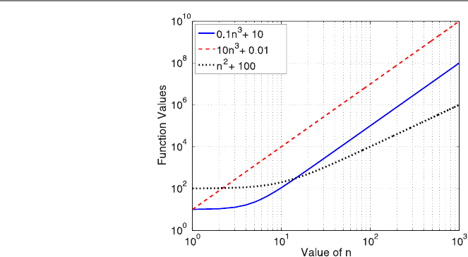
64 4 Complexity of Programs and Algorithms
Fig. 4.1 Some functions in a
log–log plot
or
aknk≤f(n)≤nk(ak+ak−1+ak−2+···+a1+a0).
Then, letting Cl=akand Ch=(ak+ak−1+ak−2+···+a1+a0),wehave
Clnk≤f(n)≤Chnk.
The last inequality fits into the definition of the order, and we have f(n)=O(nk).
Now, consider the following functions and their orders:
•f1(n) =0.1n3+10 =O(n3)
•f2(n) =10n3+0.01 =O(n3)
•f3(n) =n2+100 =O(n2)
These functions are depicted in Fig. 4.1 in a log–log plot, i.e., when xand y
axis values of the plot increase logarithmically. These types of plots are useful since
functions with different orders can be compared easily. Specifically, in a log–log
plot, scaling a function corresponds a shift in the ydirection, whereas the slope of
a curve represents its power. In this example, both f1and f2have the same order,
i.e., O(n3). This means that both functions behave like n3since this term dominates
as ngoes to infinity. In Fig. 4.1, this behavior is visible since both functions have
the same slope. Note that the order does not indicate anything about the constant in
front of the dominant term. These constants (0.1 for f1and 10 for f2) are visible as
a difference in the ydirection for large values of n. As opposed to others, the order
of f3is n2, leading to a lower slope for this function. In other words, since its order
is smaller, this function has lower values compared to f1and f2for sufficiently
large values of n. As also shown in Fig. 4.1, different functions may have different
behaviors for small values of n, but while analyzing algorithms, we are interested in
behaviors and comparisons when nis large.
Following the discussion above, different functions (e.g., complexities) can be
compared in the context of order as follows:
www.it-ebooks.info

4.2 Order of Complexities 65
•If a function f1(n) has a higher order than f2(n),f1(n) is larger than f2(n) for
sufficiently large values of n. When comparing two programs or algorithms, the
one with a lower order can be said to be more efficient than the other.
•If two functions f1(n) and f2(n) have the same order, the constants of the dom-
inant terms are required to compare the functions for large values of n. Note that
this is not possible if only the order is available. Programs and algorithms hav-
ing the same order are often said to have the same efficiency, even though the
constants, if available, may provide more precise (but less critical) information.
When finding orders of programs and algorithms from their complexities, we usu-
ally use shortcuts without using the formal definition detailed above. The strategy is
finding the most significant term (e.g., with the highest power of n) and omitting its
constant. When doing this, we should keep in mind that this is not an approximation
and there is in fact an underlying procedure as described above.
Before working on shortcuts, we emphasize that the formal definition is always
available if we are not sure about the most significant term in a given expression.
Consider the following two functions:
•f1(n) =2n+3log
2(n) =O(n)
•f2(n) =3n+4nlog2(n) =O(n log2n)
For the first example, log2(n) < n for n>1, and hence 2n≤f1(n) ≤5nfor n>1.
Therefore, f1(n) =O(n). For the second example, log2(n) > 1forn>2, and hence
4nlog2(n) ≤f2(n) ≤7nlog2(n) for n>2. Therefore, f2(n) =O(n log2n).
When discussing orders, the base of a logarithm is often omitted. This is because
all logarithms are the same in the context of order. In other words,
O(log2n) =O(log3n) =O(log4n) =···.
Hence, for the second function above, one can write f2(n) =O(n log n).
4.2.2 Example: Revisiting Inner Product
Consider the following program to calculate again the inner product of two vectors
of size n:
R Program: Calculation of Inner Product (Revisited)
01 innerproduct = function(v,w){
02 sumvalue = 0
03 n = length(v)
04 for (i in 1:n){
05 sumvalue = sumvalue + v[i]*w[i]
06 }
07 return(sumvalue)
08 }
It can be shown that the time complexity of this program is
Tall =n(T04 +T05)+T02 +T03 +T04,
www.it-ebooks.info

66 4 Complexity of Programs and Algorithms
which depends on the value of n. Considering the most significant term, i.e., n(T04 +
T05), we conclude that
Tall =O(n).
Similarly,
Mall =(2n+3)Mr=O(n).
Hence, the time and memory complexities of this program and algorithm (comput-
ing the inner product by multiplying elements and adding them) are of order n.
4.2.3 Example: Revisiting Infinity Norm
Now, lets consider the calculation of the ∞-norm of a given vector v∈Rn:
R Program: Calculation of Infinity-Norm (Revisited)
01 infinitynorm = function(v){
02 maxvalue = 0
03 n = length(v)
04 for (i in 1:n){
05 if (abs(v[i]) >maxvalue){
06 maxvalue = abs(v[i])
07 }
08 }
09 return(maxvalue)
10 }
It can be shown that, in the worst case, the time complexity of this program is
Tall =n(T04 +T05 +T06)+T02 +T03 +T04.
Note that the values of T02,T03,T04,T05, and T06 are not the same as those used
before. Considering the variables maxvalue,n,i, as well as the input vector v,
the memory complexity is
Mall =(n +3)Mr.
Considering the significant terms involving n, the time and memory complexities of
this program are also O(n).
According to our analysis, the complexity (both time and memory) of calculat-
ing the inner product is O(n). This means that when ngets larger, the cost of the
program increases linearly. For example, increasing the value of nby a factor of two
(approximately) increases the processing time and memory by factors of two. The
complexity of the infinite norm is also O(n), but this does not mean that the two pro-
grams (and the corresponding algorithms) have precisely the same cost. This only
indicates that the cost of the infinite norm is also linear, i.e., increasing the value of
nby a factor of two (approximately) increases the processing time and memory by
factors of two.
www.it-ebooks.info

4.2 Order of Complexities 67
4.2.4 Example: Revisiting Matrix–Vector Multiplication
Consider the multiplication of a matrix A∈Rm×nwith a vector x∈Rnusing the
program below.
R Program: Matrix-Vector Multiplication (Revisited)
01 matvecmult = function(A,x){
02 m = nrow(A)
03 n = ncol(A)
04 y = matrix(0,nrow=m)
05 for (i in 1:m){
06 sumvalue = 0
07 for (j in 1:n){
08 sumvalue = sumvalue + A[i,j]*x[j]
09 }
10 y[i] = sumvalue
11 }
12 return(y)
13 }
Lets first find the time cost of this program. Lines 02 to 04 are executed only once.
Hence, we can start by adding the time required for these lines as
Tall =T02 +T03 +T04 +···.
Line 05 is a for statement, which is executed for m+1 times, including a final
check of the variable i, leading to
Tall =T02 +T03 +T04 +(m +1)T05 +···.
In addition, lines 06 and 10 are inside this loop and executed for mtimes, which can
be added as
Tall =T02 +T03 +T04 +(m +1)T05 +mT06 +mT10 +···.
At this stage, we need to focus on the inner loop. Line 07 is a for statement, which
is executed for n+1 times for each i. Hence, this line is executed for a total of
m(n +1)times, leading to
Tall =T02 +T03 +T04 +(m +1)T05 +mT06 +mT10 +m(n +1)T07 +···.
Finally, the contribution of line 08 can be added as
Tall =T02 +T03 +T04 +(m +1)T05 +mT06 +mT10 +m(n +1)T07 +mnT08.
Rearranging the terms, we obtain a final expression for the time complexity as
Tall =mn(T07 +T08)+m(T05 +T06 +T07 +T10)+T02 +T03 +T04 +T05.
www.it-ebooks.info

68 4 Complexity of Programs and Algorithms
Table 4.1 Itemsusedinthe
matrix–vector multiplication
program
Item Type Number of elements
AInput mn
xInput n
yOutput m
mVariable 1
nVariable 1
sumvalue Variable 1
As opposed to the previous examples, the time complexity of the matrix–vector
multiplication involves two variables, i.e., the number of rows mand the number
of columns n. In order to find the order of this complexity, we again take the most
significant term so that
Tall =O(mn).
For the memory complexity of the matrix–vector multiplication, let us make a
simple table (Table 4.1) showing all items used in the program.
Adding all contributions, we have
Mall =mn +n+m+3=O(mn).
Both time and memory complexities of the matrix–vector multiplication are
O(mn). Different cases can be considered now:
•When m≈n, i.e., when the numbers of columns and rows are nearly the same,
O(mn) =O(n2), which can be interpreted as the complexity of the matrix–
vector multiplication has a quadratic order.
•When mis constant, O(mn) =O(n). In this case, the cost of the matrix–vector
multiplication is investigated as the number of columns is increased, i.e., the
matrix becomes wider and wider. Note that, having a very large mdoes not
change the order, as long as it is defined as a constant.
•When nis constant, O(mn) =O(m). In this case, the cost of the matrix–vector
multiplication is investigated as the number of rows are increased, i.e., the ma-
trix becomes longer and longer. Again note that a very large ndoes not change
the order as long as it is defined as a constant.
•When m=1orn=1, the matrix–vector multiplication reduces into an inner
product of two vectors. In these cases, the complexity is O(n) or O(m), de-
pending on which one is considered as a constant.
As a demonstration, Table 4.2 lists the results of an experiment using the matrix–
vector multiplication program for square matrices with different sizes. Since we
performing time measurements and inputs/outputs are not critical (provided that the
program works smoothly), we select all elements of the matrices and input vectors
as unity. The measurements are performed for n=100, n=200, n=400, n=
800, and n=1600. Table 4.2 shows the processing time in seconds, which can be
measured using the built-in system.time function of R. We also list the increase
rate, i.e., the ratio between the processing times in consecutive runs, for n≥100.
www.it-ebooks.info

4.3 Shortcuts for Finding Orders of Programs 69
Table 4.2 Measurements for
matrix–vector multiplications
with square matrices
nProcessing time (seconds) Increase rate
100 0.038 –
200 0.127 3.34
400 0.651 5.13
800 2.650 4.07
1600 10.482 3.96
It can be observed that the increase rate approaches 4 as ngets larger. Hence, this
experiment confirms our analysis, which states that the order of the matrix–vector
multiplication is O(n2). Specifically, for large values of n, we expect that doubling
the value of nshould increase the processing time by 22=4 times. This is clearly
visible in Table 4.2.
In the experiment above, the increase rate is quite different from 4 when nis
small. There are two reasons for this:
•As analyzed before, the time complexity of the program is
Tall =mn(T07 +T08)+m(T05 +T06 +T07 +T10)+T02 +T03 +T04 +T05,
which becomes
Tall =n2(T07 +T08)+n(T05 +T06 +T07 +T10)+T02 +T03 +T04 +T05
for m=n. Obviously, in addition to the most significant term with n2, there are
other terms (e.g., with n), whose contributions are visible for small values of n.
•When the execution of a program is faster, the time measurement is less reliable
since a shorter processing time is to be measured. All time measurements are
contaminated by some factors, such as out-of-control system programs running
on the same computer, but this contamination becomes more visible in shorter
durations.
Nevertheless, we need to emphasize again that measurements are not critical for
small values of n, i.e., when processing times are short and tolerable, and when
their accurate prediction is not needed.
4.3 Shortcuts for Finding Orders of Programs
When the order of a complexity is found from its full expression, the most dominant
term is extracted, and its constant is omitted to obtain a simplified expression. Then,
the following question arises: Can we find a way to derive the order directly from
the program without finding and simplifying the full expression for the complexity?
The answer is positive, provided that we investigate the given program carefully to
find out critical lines (for processing time) and critical items (for memory).
www.it-ebooks.info

70 4 Complexity of Programs and Algorithms
As an example, consider the following program for the multiplication of a matrix
A∈Rm×nwith a vector x∈Rn.
R Program: Matrix–Vector Multiplication (Revisited)
01 matvecmult = function(A,x){
02 m = nrow(A)
03 n = ncol(A)
04 y = matrix(0,nrow=m)
05 for (i in 1:m){
06 sumvalue = 0
07 for (j in 1:n){
08 sumvalue = sumvalue + A[i,j]*x[j]
09 }
10 y[i] = sumvalue
11 }
12 return(y)
13 }
To find the order of the time complexity, we find a line that is inside all loops and
executed more than others. For the program above, line 08, i.e.,
sumvalue = sumvalue + A[i,j]*x[j]
fits into this definition. Then, we find how many times this critical line is executed.
Since line 08 is inside an outer loop (ifrom 1 to m) and an inner loop (jfrom
1ton), it is executed for a total of mn times. Omitting all constants and smaller
terms that may arise at this stage, the number of times that the line is executed
corresponds to the order of the time complexity. There is no such extra term in mn,
and hence one can immediately conclude that the time complexity of the matrix–
vector multiplication is O(mn).
Note that, in the program above, one can also select line 07 as a critical line. This
line is executed for m(n +1)=mn +mtimes. But, omitting mcompared to mn,
we again reach the same expression, i.e., O(mn), for the time complexity.
To find the order of the memory complexity, we find the item (input, output, vari-
able, or constant) that has the largest number of elements. For the program above,
this item is the matrix A, which has a total of mn elements. Therefore, the memory
complexity of the matrix–vector multiplication is also O(mn).
4.3.1 Example: Matrix–Matrix Multiplication
Consider now the multiplication of two matrices A∈Rm×nand B∈Rn×p:
www.it-ebooks.info

4.4 Complexity and Order of Recursive Programs and Algorithms 71
R Program: Matrix–Matrix Multiplication (Original)
01 matmatmult = function(A,B){
02 m = nrow(A)
03 n = ncol(A)
04 p = ncol(B)
05 C = matrix(0,nrow=m,ncol=p)
06 for (i in 1:m){
07 for (j in 1:p){
08 sumvalue = 0
09 for (k in 1:n){
10 sumvalue = sumvalue + A[i,k]*B[k,j]
11 }
12 C[i,j] = sumvalue
13 }
14 }
15 return(C)
16 }
To find the order of the time complexity, we note that line 10 is a critical line. This
line is executed for mp n times, and hence the time complexity is O(mpn).Forthe
memory complexity, we need to consider three major matrices, i.e., A,B, and C.
These matrices involve mn,np , and mp elements, respectively. Considering that m,
n, and pcan be arbitrary, we conclude that the memory complexity is O(mn +np +
mp ) in general. Using these expressions for square matrices, i.e., for m=p=n,the
time and memory complexities of the matrix–matrix multiplication are O(n3)and
O(n2), respectively. Note that, for the memory complexity in this case, we have
O(n2+n2+n2)=O(3n2)=O(n2).
When p=1, both the time and memory complexities of the matrix–matrix multipli-
cation are O(mn), which is consistent with our previous analysis for the complexity
of the matrix–vector multiplication. Another special case occurs when m=1 and
n=1, corresponding to the inner product of two vectors of size p, with O(p) time
and memory complexities.
4.4 Complexity and Order of Recursive Programs
and Algorithms
Up to now, we have seen how to estimate costs of various programs and algorithms.
We also discussed some shortcuts to derive orders by finding critical lines and their
repetitions. On the other hand, problems arise when considering recursive programs
and algorithms. Unsurprisingly, the cost of a recursive program or algorithm also
has a recursive expression, which needs to be solved to get an explicit (direct) ex-
pression.
As an example, lets consider the recursive calculation of the 1-norm of a given
vector v∈Rnusing the following program:
www.it-ebooks.info

72 4 Complexity of Programs and Algorithms
R Program: Recursive Calculation of 1-Norm (Revisited)
01 onenormrecursive = function(v){
02 if (length(v) >1){
03 sum1 = onenormrecursive(v[1:floor(length(v)/2)])
04 sum2 = onenormrecursive(v[(floor(length(v)/2)+1):length(v)])
05 sumvalue = sum1 + sum2
06 }
07 else{
08 sumvalue = abs(v[1])
09 }
10 return(sumvalue)
11 }
In order to simplify the analysis of the time complexity, assume that n=2afor an
integer a(hence a=log2n). Considering that line 02 (connected to line 07) and line
05 are executed, in addition to two calls of the program itself (with smaller vectors
of n/2=2a−1elements), we have
Tall(2a)=T02 +T05 +2Tall(2a−1)or Tall(n) =T02 +T05 +2Tall(n/2)
for the time complexity. Then, we obtain a recurrence relation as Tall(n) =C+
2Tall(n/2), where C=T02 +T05 is a constant (does not depend on n). Note that
the processing times required for lines 03 and 04 are both Tall(n/2), which is the
time required to execute the function itself for vectors of size n/2. Some extra time
may be required as the numerical results of function calls are assigned to variables
sum1 and sum2. Specifically, the assignments in lines 03 and 04 may have some
contributions in the overall time complexity. But, such an extra time is constant (say
Tadd), and the final recurrence relation still holds, i.e., we have
Tall(n) =C+2Tall(n/2)
for some constant C=T02 +T05 +Tadd. Considering large values of n, one can
write a sequence of equations as
Tall(n) =C+2Tall(n/2)
=C+2(C +2Tall(n/4)) =C+2C+4Tall(n/4)
=C+2C+4(C +2Tall(n/8)) =C+2C+4C+8Tall(n/8)
.
.
.
=C+2C+4C+8C+···+n
2CTall(2)
=C+2C+4C+8C+···+n
2C+nTall(1)
=C+2C+4C+8C+···+n
2C+n(T02 +T08)
=C
a−1
i=0
2i+nD,
www.it-ebooks.info

4.4 Complexity and Order of Recursive Programs and Algorithms 73
where D=T02 +T08 represents the processing time when the input vector has
only one element. Evaluating the final summation, we get the order of the time
complexity as
Tall(n) =1−2a
1−2C+nD =nC +nD −C=O(n).
The analysis of the memory complexity of a recursive algorithm is slightly tricky.
One needs to separate the memory used for the initial input, because it is allocated
just once. For the program above, putting vaside, we have the recurrence relation
Mothers(n) =C+2Mothers(n/2),
where Caccounts for the scalar variables. An analysis similar to the one above leads
to Mothers(n) =O(n). Combining this with the memory for the input, we have
Mall(n) =Minput(n) +Mothers(n) =O(n) +Mothers(n) =O(n) +O(n) =O(n)
as the memory complexity of the program.
Now, consider the following program with some modifications on the original
one:
R Program: Recursive Calculation of 1-Norm (Inefficient)
01 onenormrecursive = function(v){
02 if (length(v) >1){
03 w = v[1:floor(length(v)/2)]
04 z = v[(floor(length(v)/2)+1):length(v)]
05 sum1 = onenormrecursive(w)
06 sum2 = onenormrecursive(z)
07 sumvalue = sum1 + sum2
08 }
09 else{
10 sumvalue = abs(v[1])
11 }
12 return(sumvalue)
13 }
In this program, the input vector vis explicitly divided into two vectors wand z
to be used when the program is called. Unfortunately, this means extra memory in
each recursion step. To be specific, we have
Mothers(n) =C+nD +2Mothers(n/2),
leading to the sequence
Mothers(n) =C+nD +2Mothers(n/2)
=C+nD +2(C +nD/2+2Mothers(n/4))
=C+2C+2nD +4Mothers(n/4)
www.it-ebooks.info

74 4 Complexity of Programs and Algorithms
.
.
.
=C+2C+4C+8C+···+n
2C+anD +nMothers(1)
=C
a−1
i=0
2i+(n log2n)D +nE
=nC −C+(n log2n)D +nE
=O(n log2n).
Combining this result with the memory for the initial input vector, we have
Mall(n) =O(n) +Mothers(n) =O(n) +O(n log2n) =O(n log2n) =O(n log n)
as the memory complexity of the program. Hence, the program above has a higher
memory complexity than the original one, i.e., it is more inefficient, even though
both programs are based on the same recursive algorithm. As shown in this example,
memory used for some new variables may accumulate in a recursive program, even
leading to increase in the order of the memory complexity.
4.4.1 Example: Revisiting Binary Search
Let us consider the recursive binary-search algorithm and revisit the following pro-
gram, which finds the position of a given number in a vector v∈Rninvolving sorted
numbers.
R Program: Recursive Binary Search (Revisited)
01 binarysearchrecursive = function(v,thenumber,lowerindex,higherindex){
02 if (lowerindex >higherindex){
03 print("The number is not found!")
04 }
05 else{
06 middleindex = lowerindex + floor((higherindex-lowerindex)/2)
07 if (v[middleindex] == thenumber){
08 return(middleindex)
09 }
10 else if (v[middleindex] <thenumber){
11 binarysearchrecursive(v,thenumber,middleindex+1,higherindex)
12 }
13 else if (v[middleindex] >thenumber){
14 binarysearchrecursive(v,thenumber,lowerindex,middleindex-1)
15 }
16 }
17 }
Assume that the input vector vhas n=2aelements for an integer a. Considering
the worst-case scenario, the searched number thenumber is not found in the first
step. Hence, the same algorithm is called again for a vector of size n/2=2a−1.
Before this second call, however, line 02 (connected to line 05), line 06, and line
www.it-ebooks.info

4.4 Complexity and Order of Recursive Programs and Algorithms 75
07 (connected to lines 10 and 13) are executed. Then, we can write the overall time
complexity as
Tall(2a)=T02 +T06 +T07 +Tall(2a−1)or Tall(n) =T02 +T06 +T07 +Tall(n/2).
For large values of n, a sequence of equations can be written as
Tall(n) =C+Tall(n/2)
=2C+Tall(n/4)
=3C+Tall(n/8)
.
.
.
where Cis a constant (does not depend on n).
According to the worst-case scenario, the search does not end until lowindex
equals highindex so that the recursion cannot continue any further. Considering
all steps, the time complexity of the program can be written as
Tall(n) =aC +Tall(n/2a)=log2(n)C +Tall(1).
At this stage, the program stops if the searched number is found. On the other hand,
it is possible that the number does not exist in the vector. In this case, line 02 (fol-
lowed by line 03) is executed once more, but this is not significant in terms of the
time cost, and we have Tall(1)=O(1). Consequently,
Tall(n) =O(log2(n)) =O(log n),
which means that the time complexity of the recursive binary search has a logarith-
mic order. Note that, despite its logarithmic time complexity, the program above has
O(n) memory complexity since the input vhas nelements to be stored.
4.4.2 Example: Revisiting Sequence Generation
Consider the recursive program below, which can be used to list all words with n
letters (either “a” and “b”).
R Program: Generate Words With a and b (Revisited)
01 generateab = function(n){
02 if (n >0){
03 v = rbind(matrix("a",nrow=2∧(n-1)),matrix("b",nrow=2∧(n-1)))
04 return(noquote(cbind(v,rbind(generateab(n-1),generateab(n-1)))))
05 }
06 }
www.it-ebooks.info

76 4 Complexity of Programs and Algorithms
The output of this program is a matrix of 2n×nelements. For finding the time
complexity, we need to analyze lines 03 and 04 carefully. The time complexity of
line 03 depends on the value of nsince two vectors of size 2n−1are combined
using rbind. We may assume that rbind (and cbind) operations involve com-
binations of two data structures, where one of them (e.g., smaller one) is moved
in memory. Hence, T03 =t032n−1, where t03 is a constant. In line 04, the program
itself is called twice with input n-1. Outputs of these calls are matrices of size
2n−1×(n −1). These matrices are combined using rbind with a time complexity
of T04a=t04a(n −1)2n−1. Then, the resulting 2n×(n −1)matrix is combined with
a vector of 2nelements using cbind, which has T04b=t04b2ntime complexity.
Considering all contributions, we obtain
Tall(n) =t032n−1+t04a(n −1)2n−1+t04b2n+2Tall(n −1)
or
Tall(n) =(C +nD)2n+2Tall(n −1),
where
C=t03/2−t04a/2+t04band D=t04a/2.
Using the expression above, one can obtain
Tall(n) =2n
n−1
i=0
(C +(n −i)D) =(C +nD/2+n2D/2)2n
or
Tall(n) =O(n22n)=O(2p(n)),
where p(n) =n+2log
2n. Hence, the time complexity of the sequence generation
has an exponential order, as discussed in the next setion. Carrying out a similar
analysis, it can be shown that the memory complexity of the program above also
has an exponential order.
4.5 Orders of Various Algorithms
As we analyzed in this chapter, the inner product of two vectors and the computation
of the infinite norm of a vector have O(n) time and memory complexities, whereas
the matrix–vector multiplication has O(n2)complexity for square matrices. Simi-
larly, for n×nsquare matrices, the matrix–matrix multiplication has O(n3)time
complexity and O(n2)memory complexity. Therefore, all these programs and algo-
rithms have polynomial orders, since n,n2, and n3are polynomials.
In general, a program or algorithm has a polynomial order if its complexity is
O(nk)for some constant k>0, where nis the input size. As special cases, k=1,
k=2, and k=3 correspond to the linear, quadratic, and cubic orders, respectively.
Note that the case k=0 is not considered as a polynomial order since O(n0)=O(1)
indicates another family of programs and algorithms with constant orders.
www.it-ebooks.info
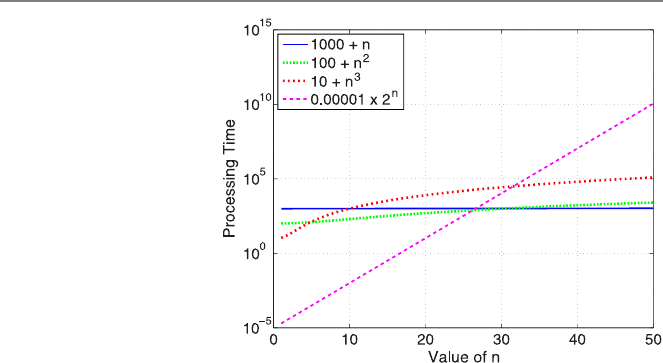
4.5 Orders of Various Algorithms 77
Fig. 4.2 Processing time as a
function of input size for four
hypothetical algorithms
In addition to those with polynomial orders, there are many programs and al-
gorithms with logarithmic and exponential orders. A program or algorithm has a
logarithmic order if its complexity is O(logn) and has an exponential order if its
complexity is O(2p(n)), where p(n) is a polynomial or any function of polynomial
order. Similar to the base of the logarithm, the base of the exponential term is not
important, but it is often selected as 2. Examples are the recursive binary search with
a logarithmic time complexity and recursive sequence generation with exponential
time and memory complexities.
In general, programs and algorithms with exponential complexities are consid-
ered as expensive, and, if possible, they are avoided (replaced with inexpensive pro-
grams and algorithms). Despite this usual warning, there is no a common criterion
to directly judge the complexity, and in fact, the assessment of the efficiency often
depends on the application area. For example, the Gaussian elimination with O(n3)
time complexity is a major tool in linear algebra, but it is often considered to be
expensive. Therefore, it is replaced with iterative methods and fast algorithms for
large nvalues that are encountered in many practical problems.
As a demonstration, Fig. 4.2 depicts the processing time for four hypothetical
programs with different orders. The time complexities of the programs are given as
1000+n, 100+n2,10+n3, and 0.00001×2n. Note that the yaxis has a logarithmic
scale, but the xaxis has not. We observe that, for small values of n, the slowest and
the fastest programs are the first and the fourth, respectively. However, as the value
of nincreases, the cost of the fourth program increases rapidly (exponentially), and
this program becomes the slowest one among four programs for large values of n.
Similar comparisons can be made between other programs. Usually, solutions of
small problems are not critical, and performances of programs for small input sizes
are not important. On the other hand, as the input size increases and solutions be-
come difficult, we need to find the most efficient programs, and this information can
be obtained by analyzing complexities and orders of programs and algorithms.
www.it-ebooks.info

78 4 Complexity of Programs and Algorithms
4.5.1 Example: Traveling Salesman Problem
A famous problem in computer science is the traveling salesman problem, which
can be solved by using many different algorithms with different costs. The problem
can be described as follows. A salesman should visit a total of ncities starting from
one of them. Each city should be visited only once. What is the sequence of cities,
which leads to the shortest route? It should be noted that choosing the nearest city
in each step does not necessarily gives the shortest route overall.
Now, let us consider the brute-force solution based on testing all possible an-
swers. In the first step, there are a total of n−1 cities that the salesman can go.
Then, she/he can visit one of n−2 cities in the second step, one of n−3 cities in
the third step, etc. Considering all n−1 steps, one can conclude that there are
(n −1)×(n −2)×(n −3)×···×2×1=(n −1)!
different choices for the trip. These possible trips can be directly compared with
each other and the one with the shortest route can be found. The complexity of this
algorithm is clearly O(n!), i.e., it has a factorial order, which is even worse than the
exponential order.
4.5.2 Fibonacci Numbers
Let us consider the calculation of the ith Fibonacci number. One can use the recur-
rence relation
f(i)=f(i−1)+f(i−2), i > 2,
with conditions f(1)=1 and f(2)=1 to write the following program:
R Program: Recursive Calculation of nth Fibonacci Number (Revisited)
01 fiborecursive = function(i){
02 if (i <=2){
03 return(1)
04 }
05 else{
06 return(fiborecursive(i-1)+fiborecursive(i-2))
07 }
08 }
Even though this program seems quite compact and natural (using the definition of
the Fibonacci numbers), it is expensive. The time complexity can be written as
Tall(i) =C+2Tall(i −1),
www.it-ebooks.info

4.5 Orders of Various Algorithms 79
where Cis a constant. Note that, in this example, iis not the input size, and the time
complexity depends on the value of the input irather than its size. To find a direct
formula for the time cost, a sequence of equations can be derived as
Tall(i) =C+2Tall(i −1)
=C+2(C +2Tall(i −2)) =C+2C+4Tall(i −2)
=C+2C+4(C +2Tall(i −3)) =C+2C+4C+8Tall(i −3)
.
.
.
=C+2C+4C+8C+···+2i−2C+2i−1Tall(1)
=C+2C+4C+8C+···+2i−2C+2i−1T02
=C
i−2
j=0
2j+2i−1T02
=2i−1C−C+2i−1T02,
which leads to
Tall(i) =O(2i).
Hence, the time complexity of recursively calculating the ith Fibonacci number has
an exponential order.
In order to understand why the simple program above is so expensive, consider
the calculation of the 7th Fibonacci number, i.e., f(7)=f(6)+f(5), which re-
quires f(6)and f(5). On the other hand, f(6)=f(5)+f(4), which means that
f(5)is calculated twice to find f(7). Similarly, f(4)is calculated three times, f(3)
is calculated four times, etc. These duplications in the calculations grow rapidly,
leading to an exponential order.
As mentioned in Chap. 3, the cost of a recursive program is often related to the
depth of the recursion. On the other hand, the cost may not be directly proportional
to the depth, as the cost per recursion level may also change. For the program above,
the depth of the recursion is O(i). But, the cost is doubled from a level to the next
level, which leads to an exponential complexity overall.
Following the discussion above, a more efficient algorithm to calculate the ith
Fibonacci number can be proposed. In such an algorithm, the Fibonacci numbers
from 1 to ican be calculated using the expression f(i)=f(i−1)+f(i−2)in a
loop, rather than a recursion. A program using a for loop can be written as follows:
www.it-ebooks.info

80 4 Complexity of Programs and Algorithms
R Program: Iterative Calculation of the nth Fibonacci Number (Original)
01 fiboiterative = function(i){
02 if (i <=2){
03 value = 1
04 }
05 else{
06 value1 = 1
07 value2 = 1
08 for (j in 3:i){
09 value = value1 + value2
10 value1 = value2
11 value2 = value
12 }
13 }
14 return(value)
15 }
In this program, the variables value1 and value2 store the values of two con-
secutive Fibonacci numbers. For each value of jfrom 3 to i, the values of these
variables are updated appropriately. Specifically, value2 is copied to value1,
whereas value2 is updated as the sum of value1 and value2 from the previ-
ous step. This way, when the loop finishes,
value = value1 + value2
gives the ith Fibonacci number.
In the program above, lines 09–11 can be considered as critical lines, which are
executed for i−2 times. Therefore, the time complexity of this program is O(i),
which is much better than the exponential complexity of the recursive program and
algorithm. Moreover, the memory complexity is O(1)since only a couple of scalar
variables are used. Finally, this program can be considered as a kind of iterative
procedure since each iteration depends on previous iterations. In this context, the
program converges to the ith Fibonacci number, whereas no divergence is expected.
Once again, we emphasize that programs and algorithms need to be compared
extensively in terms of efficiency and/or accuracy. Even for very simple problems,
some programs and algorithms can be much better than others.
4.5.3 Binomial Coefficients
Consider the computation of the binomial coefficient
b(i, j ) =i
j=i!
j!(i −j)!.
Obviously, this quantity can easily be calculated by using the factorial as follows:
www.it-ebooks.info

4.5 Orders of Various Algorithms 81
R Program: Finding Binomial Coefficients Using Factorial (Original)
01 binomialusingfactorial = function(i,j){
02 value = factorial(i) / ( factorial(j)*factorial(i-j))
03 return(value)
04 }
However, this program is unstable. For example, consider the calculation of
200
199=200!
199!(200 −199)!=200.
Using a standard computer, the program above cannot do this! This is because both
199! and 200! are very large numbers and they cannot be represented properly in R.
Hence, the program cannot provide any useful output, although it should be simply
200. Specifically, this instability can be observed when factorials of the inputs i
and jare very large. In order to overcome this problem, a more stable program is
required.
First, let us consider the Pascal triangle, which directly provides the binomial
coefficients. First seven lines of the triangle are as follows:
1
11
121
1331
14641
1 5 10 10 5 1
1 6 15 20 15 6 1
Each number in a line is the sum of two numbers in the previous line. This way, the
Pascal triangle consists of the binomial coefficients, where the coefficient b(i, j )
resides at (j +1)th position of the (i +1)th line. For example, check the value of
b(6,3)=6
3=20
residing at the 4th position in the 7th line.
The Pascal triangle provides the required recursion to obtain the binomial coeffi-
cients. Specifically, we have
b(i, j ) =b(i −1,j −1)+b(i −1,j)
www.it-ebooks.info

82 4 Complexity of Programs and Algorithms
with b(0,0)=1, leading to the following stable program.
R Program: Finding Binomial Coefficients Using the Pascal Triangle (Original)
01 binomialpascal = function(i,j){
02 if (j = 0){
03 value = 1
04 }
05 else if (i == j){
06 value = 1
07 else{
10 value = binomialpascal(i-1,j-1) + binomialpascal(i-1,j)
11 }
12 return(value)
13 }
Although this program (and the underlying algorithm based on the Pascal triangle)
is more stable than the previous program (and the underlying algorithm based on
factorials), it is very expensive, particularly for the coefficients at the middle of the
Pascal triangle. For example, if j≈i/2, then the time complexity of the program
above is O(2i). Hence, we need better programs and algorithms for both efficient
and stable computations of the binomial coefficients.
In order to derive a new algorithm, one can use the expression of the binomial
coefficients and perform cancellations to arrive at
b(i, j ) =i
j=i!
j!(i −j)!=i×(i −1)×(i −2)×···×(i −j+1)
j×(j −1)×(j −2)×···×1.
Factorization of the final equality leads to
b(i, j ) =i
jb(i −1,j −1).
This is a very useful recurrence relation that can be implemented as follows:
R Program: Finding Binomial Coefficients Recursively (Original)
01 binomialrecursive = function(i,j){
02 if (j == 0){
03 value = 1
04 }
05 else{
08 value = (i/j)*binomialrecursive(i-1,j-1)
09 }
10 return(value)
11 }
Similar to the previous program using the Pascal triangle, this program is quite
stable. In addition, as a very important advantage, the program above is extremely
efficient with only O(j ) time complexity.
www.it-ebooks.info

4.6 Conclusions 83
Table 4.3 Programs/algorithms to compute binomial coefficients
Program/Algorithm Time complexity Behavior for large i
Using Factorial O(i) Unstable
Using the Pascal’s Triangle O(2i)if j≈i/2Stable
Recursive O(j ) Stable
Although less important, the program using the recurrence relation is even bet-
ter than the program using the Pascal’s triangle in terms of stability. The binomial
coefficients are often generalized as
b(i, j ) =0ifi<j.
Using the programs above for such a case, only the third (using the recurrence re-
lation) may give zero, while the first (using factorials) returns a not-a-number error,
and the second (using Pascal’s triangle) suffers from an infinite recursion. Hence,
if such a case may occur in an application, the first and second programs need to
be improved via conditional statements, whereas the program using the recurrence
relation does not require any modification.
Finally, we summarize the programs/algorithms to compute the binomial coeffi-
cients in Table 4.3. Among three different methods, only the recursive version pro-
vides both efficient and stable computations. For the solution of a given problem,
the programmers often need to search for the most efficient and most stable/accurate
programs and algorithms. In some cases, as in the computation of the binomial coef-
ficients, it may be possible to find a nice algorithm, whose implementation exhibits
both efficiency and stability. In some cases, however, the programmer may need to
choose between efficiency and stability/accuracy, depending on the application and
user needs.
4.6 Conclusions
For a given problem, it is essential to compare different programs and algorithms in
terms of efficiency and/or accuracy. Efficiency refers to the speed of programs and
algorithms, as well as to the amount of memory required by them. For both speed
and memory usage, the efficiency of a program/algorithm naturally depends on its
inputs.
This chapter is devoted to estimating processing time and memory costs of com-
puter programs. For a given program, a rigorous approach can be followed by count-
ing each operation and each piece of storage to find the complexity of the program
as well as the underlying algorithm. At the same time, we are more interested in
the efficiency of programs when input sizes/values are large so that time and mem-
ory costs are significant. This leads to an asymptotic analysis to find orders from
complexities and to use the resulting neat expressions for assessing the efficiency of
implementations. This chapter also discusses some shortcuts to calculate the orders
of programs and algorithms by finding critical lines and items in the codes.
www.it-ebooks.info

84 4 Complexity of Programs and Algorithms
4.7 Exercises
1. Write a program that calculates the inner product of two given vectors vand
w∈Rnusing a loop. Test your program for various small vectors. Then, use your
program and measure the processing time for vectors of different sizes as
system.time(innerproduct(matrix(1,nrow=10000),matrix(1,nrow=10000)))
system.time(innerproduct(matrix(1,nrow=40000),matrix(1,nrow=40000)))
system.time(innerproduct(matrix(1,nrow=160000),matrix(1,nrow=160000)))
system.time(innerproduct(matrix(1,nrow=640000),matrix(1,nrow=640000)))
Hence, fill the following table and show that the time complexity of your program is
O(n). Based on your measurements, estimate the time required for the inner product
of two vectors of size n=640,000,000.
nProcessing time (seconds) Increase rate
10,000 –
40,000
160,000
640,000
2. Using your time measurement for n=640,000 in Question 1, estimate how many
floating-point operations can be performed per second, assuming that a summation
and multiplication is one floating-point operation. This will give a rough idea on
how powerful the computer that you employ your program on.
3. Write a program that multiplies a matrix A∈Rm×nwith a vector x∈Rn.Test
your program for various small matrices and vectors. Then, use your program and
measure the processing time for matrices and vectors of different sizes as
system.time(matvecmult(matrix(1,nrow=100,ncol=100),matrix(1,nrow=100)))
system.time(matvecmult(matrix(1,nrow=200,ncol=200),matrix(1,nrow=200)))
system.time(matvecmult(matrix(1,nrow=400,ncol=400),matrix(1,nrow=400)))
system.time(matvecmult(matrix(1,nrow=800,ncol=800),matrix(1,nrow=800)))
Hence, fill the following table and show that the time complexity of your program
is O(n2).
nProcessing time (seconds) Increase rate
100 –
200
400
800
www.it-ebooks.info

4.7 Exercises 85
4. Write a program that multiplies two matrices A∈Rm×nand B∈Rn×p.Test
your program for various small matrices. Then, use your program and measure the
processing time for 50 ×50 and 100 ×100 matrices as
A=matrix(1,nrow=50,ncol=50)
B=matrix(1,nrow=50,ncol=50)
system.time(matmatmult(A,B))
A=matrix(1,nrow=100,ncol=100)
B=matrix(1,nrow=100,ncol=100)
system.time(matmatmult(A,B))
Show that your measurements fit into the theoretical complexity, i.e., O(n3).
5. Write a recursive program that lists all words with nletters containing “a” and
“b”. Test your program for n=4, n=5, and n=6. Then, use your program and
measure the processing time for larger values of nas
system.time(generateab(10))
system.time(generateab(11))
system.time(generateab(12))
system.time(generateab(13))
system.time(generateab(14))
system.time(generateab(15))
Hence, fill the following table and show that the time complexity of your program
has an exponential order.
nProcessing time (seconds) Increase rate
10 –
11
12
13
14
15
Based on your measurements, estimate the time required for generating and listing
all words with n=30 letters.
6. Write a program that calculates the ith Fibonacci number using a loop. Test your
code for i=10, i=20, i=30, i=40. How the processing time changes when
igets larger, especially compared to the recursive program that you implemented
before? Also find the 1000th Fibonacci number using your program, displaying it
approximately.
7. Write a program that calculates the binomial coefficients using the Pascal triangle.
The inputs should be the indices of the coefficient, i.e., iand jin
b(i, j ) =i
j=i!
j!(i −j)!.
www.it-ebooks.info

86 4 Complexity of Programs and Algorithms
Measure the time required to find the binomial coefficients b(16,8),b(18,9),
b(20,10), and b(22,11). For these cases, where j=i/2, how quickly does the
time increase with respect to i?
8. Write a program that calculates the binomial coefficients using the improved re-
cursive formula
b(i, j ) =i
jb(i −1,j −1).
Measure the time required to find various binomial coefficients. How fast your pro-
gram is, especially compared to the program using the Pascal triangle?
www.it-ebooks.info

5
Accuracy Issues
When comparing programs and algorithms, both two aspects, i.e., efficiency and ac-
curacy, should be considered together. In many cases, accuracy is not critical, such
as when outputs are not numeric or they are simply integers. However, it becomes
an important issue to assess the accuracy of results when a program contains numer-
ical computations involving real numbers leading to rounding errors. In some cases,
rounding errors tend to accumulate and/or be amplified, leading to significantly in-
accurate outputs. This short chapter presents some of these interesting cases, along
with short discussions of well-known techniques to avoid such accuracy problems.
5.1 Evaluating Mathematical Functions at Difficult Points
Consider the mathematical function
f(x)=1−cos x
x2
defined for x∈R. First, let us write an R program to plot this function in any given
range x∈[xmin,x
max]by sampling at n+1 points.
R Program: Evaluate f(x) = (1-cos x)/x∧2 (Original)
01 evaluatefunction1 = function(xmin,xmax,n){
02 x = c(0)
03 f = c(0)
05 for (i in (0:n)){
06 x[i+1] = xmin + i*(xmax-xmin)/n
07 f[i+1] = (1-cos(x[i+1]))/(x[i+1])∧2
08 }
09 plot(x,f,type="l",col="blue",xlab="x",ylab="function")
10 }
Using this program for xmin =−1, xmax =1, and n=100 as
evaluatefunction1(-1,1,100)
Ö. Ergül, Guide to Programming and Algorithms Using R,
DOI 10.1007/978-1-4471-5328-3_5,
© Springer-Verlag London 2013
87
www.it-ebooks.info
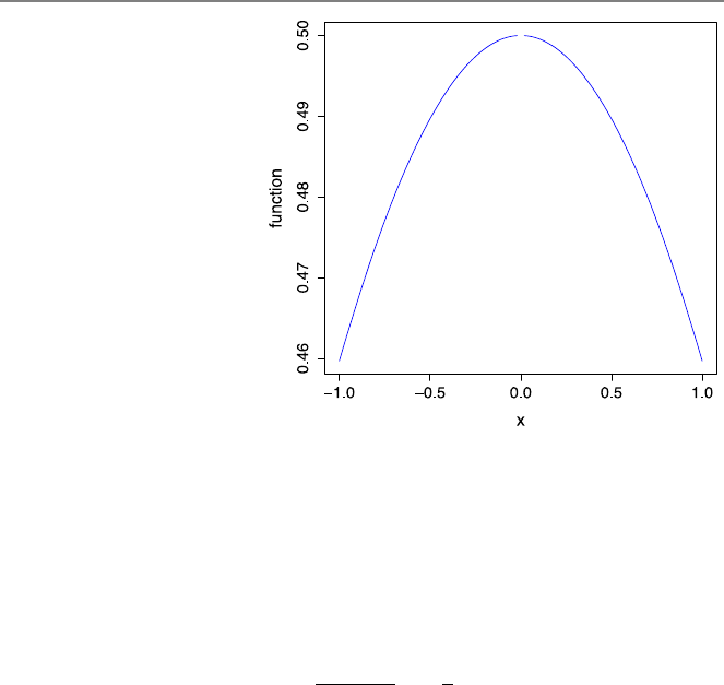
88 5 Accuracy Issues
Fig. 5.1 Plot of the function
f(x)=(1−cos x)/x2in the
[−1,1]range
generates the plot depicted in Fig. 5.1. Note that using the built-in curve function
of R (without writing any program) as
curve((1-cos(x))/(x)∧2,from=-1,to=1)
would generate a similar plot. In any case, the plot seems fine, except at around
x=0, where the line is discontinuous. Note that the mathematical function is in
fact continuous everywhere, including x=0 with the value of
lim
x→01−cosx
x2=1
2.
Unfortunately, the evaluation of the function at around x=0 is problematic using
the floating-point arithmetic.
To further investigate the behavior of the function at around x=0, we can use
the program above as
evaluatefunction1(-10∧-7,10∧-7,200)
to generate the zoomed plot depicted in Fig. 5.2. In addition to a persistent disconti-
nuity at x=0, other accuracy problems are clearly visible in this plot. Specifically,
the value of the function in this range should be close to 0.5, but we observe incor-
rect values oscillating between 0 and 1.
The discontinuities in Figs. 5.1 and 5.2 are due to the fact that (1−cosx) =0
and x2=0forx=0. Therefore, as the function is evaluated at x=0, we have 0/0
that leads to a not-a-number (NaN) in R. On the other hand, the accuracy problems
that become visible when evaluating the function f(x)=(1−cos x)/x2at around
x=0 are due to rounding errors. When xis close to 0, cos xis close to 1 and
(1−cosx) is close to zero. Unfortunately, when this subtraction, i.e., one minus
cosx, is performed using floating-point arithmetic, it contains rounding errors. This
is because the exact representation of 1−cosxrequires more digits (possibly infinite
www.it-ebooks.info
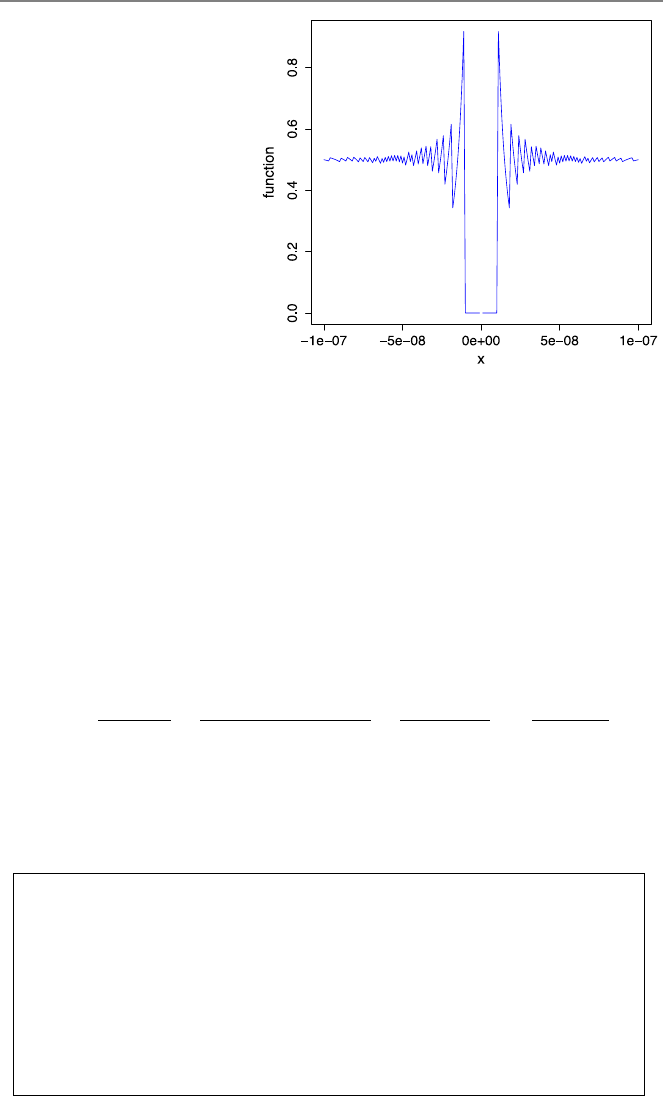
5.1 Evaluating Mathematical Functions at Difficult Points 89
Fig. 5.2 Plot of the function
f(x)=(1−cos x)/x2in the
[−10−7,10−7]range
numbers of digits) after the decimal point than allowed on the computer, and hence,
some of the “insignificant” digits have to be omitted. The resulting rounding errors
are small, but they are amplified as the result of the subtraction is divided by x2,
which is also small when xis close to 0. Note that this term (x2) also contains
rounding errors itself. Consequently, rounding errors significantly contaminate the
numerical value of the function when xis small.
Rounding errors often affect the evaluation of functions at critical points. Dif-
ferent strategies can be used to avoid such errors. If possible, the expression of the
given function should be replaced with a more stable one via analytical manipula-
tions. Using the identity
cosx=1−2sin
2(x/2)
for the function above, we have
f(x)=1−cos x
x2=1−(1−2sin
2(x/2))
x2=2sin
2(x/2)
x2=sin2(x/2)
x2/2,
which is much more stable than the original one since it does not contain any diffi-
cult subtraction. It only contains a small value divided by another small value, but
there is no any amplification of rounding errors to generate significantly incorrect
results at the end. Considering this, the following R program can be written:
R Program: Evaluate f(x) = (sin∧2(x/2))/(x∧2/2) (Original)
01 evaluatefunction2 = function(xmin,xmax,n){
02 x = c(0)
03 f = c(0)
05 for (i in (0:n)){
06 x[i+1] = xmin + i*(xmax-xmin)/n
07 f[i+1] = (sin(x[i+1]/2))∧2/((x[i+1])∧2/2)
08 }
09 plot(x,f,type="l",col="blue",xlab="x",ylab="function")
10 }
www.it-ebooks.info
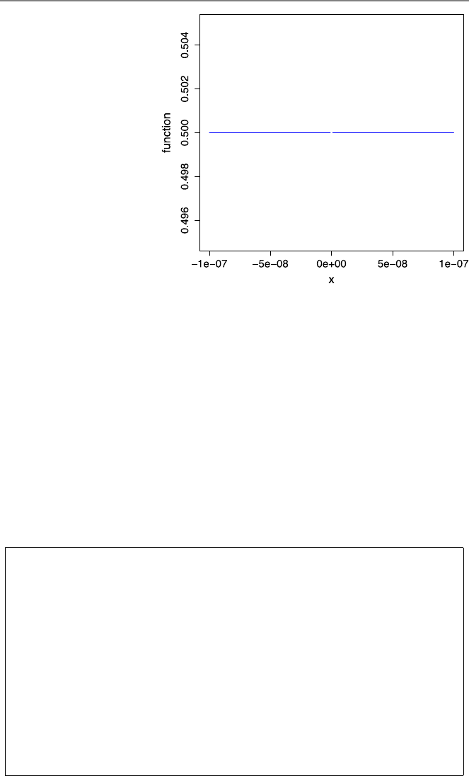
90 5 Accuracy Issues
Fig. 5.3 Plot of the function
f(x)=(sin2(x/2))/(x2/2)
in the [−10−7,10−7]range
Figure 5.3 depicts a revised plot in the [−10−7,10−7]range. It can be observed that
large oscillations due to rounding errors disappear using the new expression. This
plot confirms the improved stability of the modified expression of the function, as
described above.
In Fig. 5.3, the discontinuity at x=0 is still visible because, even using the
improved formula, we still have 0/0. In fact, this case occurs whenever x2is less
than the smallest positive floating-point number that can be represented. So, the
problem is not limited to a “single” point. In order to handle these cases, it is useful
to divide the evaluation of the function into different parts. Specifically, for very
small or zero values of x, one can use f(x)=1/2, which is the limit value of the
function. Along this direction, the program can be revised as follows:
R Program: Evaluate f(x) = (sin∧2(x/2))/(x∧2/2) With Check (Original)
01 evaluatefunction2withcheck = function(xmin,xmax,n,epsilon){
02 x = c(0)
03 f = c(0)
04 for (i in (0:n)){
05 x[i+1] = xmin + i*(xmax-xmin)/n
06 if (abs(x[i+1]) >epsilon){
07 f[i+1] = (sin(x[i+1]/2))∧2/((x[i+1])∧2/2)
08 }
09 else{
10 f[i+1] = 1/2
11 }
12 }
13 plot(x,f,type="l",col="blue",xlab="x",ylab="function")
14 }
www.it-ebooks.info

5.2 Polynomial Evaluation 91
Fig. 5.4 Plot of the function
f(x)=(sin2(x/2))/(x2/2)
in the [−10−7,10−7]range
using a check around 1/2
In this program, epsilon is an input to control the evaluation of the function.
Specifically, when xis in the range [−,]for a small number , the value of the
function is set to 1/2 without attempting to evaluate the formula. Using this program
as
evaluatefunction2withcheck(-10∧-7,10∧-7,200,10∧-10)
generates the plot in Fig. 5.4, where no problem is visible at around the critical
point.
5.2 Polynomial Evaluation
Polynomials are finite expressions involving constants, variables, and their powers
(with nonnegative integer exponents) combined with basic operations, i.e., addition,
subtraction, multiplication, and division. In this book, we consider polynomials with
a single variable xthat can be written in the form of
p(x) =
n
i=0
aixi=a0+a1x+a2x2+···+anxn,
where aifor i=0,1,...,n are constants (coefficients). This polynomial has a de-
gree of n, which is simply the largest exponent. In general, a polynomial of degree
nhas n+1 terms, but one or some of its coefficients can be zero.
Given a polynomial p(x), it may be desired to compute its value at x=x0, which
is called polynomial evaluation. A direct way to do this is just inserting the value of
x0into the polynomial expression. Such a direct program can be written as follows:
www.it-ebooks.info

92 5 Accuracy Issues
R Program: Direct Polynomial Evaluation (Original)
01 polyeval = function(a,x0){
02 n = length(a) - 1
03 polyvalue = a[1]
04 for (j in (1:n)){
05 polyvalue = polyvalue + a[j+1]*(x0)∧j
06 }
07 return(polyvalue)
08 }
The first input of the algorithm is vector aof size n+1 that includes the coefficients
of the polynomial, i.e., a0in a[1],a1in a[2], etc. The second input x0 is the
value at which the polynomial is evaluated. Considering a critical line (line 05), the
time complexity of this program is O(n), even though the power (x0)∧jis often
considered to be an expensive operation, compared to a floating-point operation.
The polynomial evaluation program using the direct approach can easily be im-
proved by storing the powers of x0in each step. Such an improved program can be
written as follows:
R Program: Improved Direct Polynomial Evaluation (Original)
01 polyevalimproved = function(a,x0){
02 n = length(a) - 1
03 polyvalue = a[1]
04 powersofx0 = 1
05 for (j in (1:n)){
06 powersofx0 = x0*powersofx0
07 polyvalue = polyvalue + a[j+1]*powersofx0
08 }
09 return(polyvalue)
10 }
In this program, the powers of x0arestoredinavariablepowersofx0, which
is updated and used for each term of the polynomial. It is often assumed that the
improved program is faster than the original one since it does not contain any power
operation. Nevertheless, a single line (line 05 in the original program) is replaced
with two new lines (lines 06 and 07 in the improved program), which may ac-
tually increase the processing time depending on the computer. For reducing the
processing time, one may consider the Horner’s algorithm, as detailed in the next
subsection.
5.2.1 Horner’s Algorithm
The Horner’s algorithm is an efficient method for polynomial evaluation. It is based
on rewriting a polynomial
p(x) =a0+a1x+a2x2+···+anxn
www.it-ebooks.info

5.2 Polynomial Evaluation 93
as follows. First, we note that
p(x) =p0=a0+xp1(x),
where p1(x) =a1+a2x+···+anxn−1is a polynomial of order n−1. Similarly,
p1(x) =a1+xp2(x),
where p2(x) =a2+a3x+···+anxn−2. This way, we define a sequence of poly-
nomials
pj(x) =aj+xpj+1(x)
for j=0,1,...,n and pn+1(x) =0.
Now, assume that we would like to evaluate the polynomial at x=x0. Consider-
ing the sequence of polynomials as defined above, we have
yn=an
yn−1=an−1+x0yn
yn−2=an−2+x0yn−1
.
.
.
yj=aj+x0yj+1
.
.
.
y1=a1+x0y2
y0=a0+x0y1,
where y0=p0(x0)=p(x0). Note that we trace the polynomial in reverse order,
i.e., from nto 0. This sequence of evaluations has a recursive structure, but it is
commonly implemented via a loop, as in the following program:
R Program: Polynomial Evaluation With Horner’s Algorithm (Original)
01 polyevalhorner = function(a,x0){
02 n = length(a) - 1
03 polyvalue = a[n+1]
04 for (j in (1:n)){
05 polyvalue = a[n+1-j] + x0*polyvalue
06 }
07 return(polyvalue)
08 }
Similar to the previous ones, the time complexity of this program is O(n). Hence,
the order is the same (linear) for all polynomial evaluation programs. On the other
hand, the program using the Horner’s algorithm contains a single line inside the loop
and no power operation, so that it is expected to be faster than the direct evaluation
programs. Considering the operations inside the loops, such a speedup in the pro-
cessing time is limited to two, whereas smaller speedup values are usually observed
in practical cases due to fixed lines, such as the for statement, in all programs.
www.it-ebooks.info

94 5 Accuracy Issues
5.2.2 Accuracy of Polynomial Evaluation
Polynomial evaluation programs usually encounter accuracy problems when the
value of the polynomial is close to zero. This is similar to the evaluation of functions
at critical points, where rounding errors are responsible for inaccurate results. As an
example, consider the evaluation of p(x) =(x −2)10 at x=2.01. This polynomial
can be rewritten as
p(x) =1024 −5120x+11520x2−15360x3+13440x4−8064x5
+3360x6−960x7+180x8−20x9+x10.
Then, using our programs as
a=c(1024,-5120,11520,-15360,13440,-8064,3360,-960,180,-20,1)
polyeval(a,2.01)
polyevalimproved(a,2.01)
polyevalhorner(a,2.01)
we obtain inconsistent results, i.e.,
3.683454e-11
-7.048584e-12
-2.182787e-11
In fact, all these results are incorrect, since p(2.01)=(2.01 −2)10 =10−20.Ob-
viously, using the polynomial evaluation programs, rounding errors become sig-
nificant as large numbers are added and subtracted to obtain a small result. Even
though all final results are small (around 10−11) and close to zero, they may be am-
plified if these results are to be used somewhere else. Using the factored form, i.e.,
p(x) =(x −2)10, however, we simply take the power of a small number, which is
reliable and less prone to rounding errors.
As a further example, we consider the evaluation of a simple polynomial, i.e.,
p(x) =(x −1)3=x3−3x2+3x−1,
at around x=1. In order to evaluate the polynomial at multiple points using the
Horner’s algorithm, the following program can be used:
R Program: Using Horner’s Algorithm At Multiple Points (Original)
01 polyevalhornermultiple = function(a,xmin,xmax,n){
02 x = c(0)
03 y = c(0)
04 for (i in (0:n)){
05 x[i+1] = xmin + i*(xmax-xmin)/n
06 y[i+1] = polyevalhorner(a,x[i+1])
07 }
08 plot(x,y,type="l",col="blue",xlab="x",ylab="function")
09 }
www.it-ebooks.info
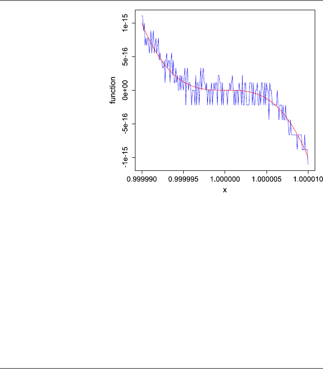
5.3 Matrix–Matrix Multiplications 95
Fig. 5.5 Plot of the
polynomial
p(x) =(x −1)3=x3−3x2+
3x−1inthe
[0.99999,1.00001]range
when it is evaluated by using
the Horner’s algorithm
(oscillatory) and the factored
form (smooth)
In the above, the program polyevalhorner is used as a function at npoints in
the range [xmin,x
max], which are indicated by the inputs xmin,xmax, and n.The
polynomial coefficients are again provided by an input vector a. Using the program
above as
polyevalhornermultiple(c(1,-3,3,-1),0.99999,1.00001,200)
one may obtain the oscillatory curve depicted in Fig. 5.5. The correct values of the
polynomial are also plotted using the factored form p(x) =(x −1)3, leading to
the smooth curve in the same figure. We observe that the Horner’s algorithm suffers
from rounding errors that are clearly visible at around the critical point x=1, where
the value of the polynomial is close to zero.
5.3 Matrix–Matrix Multiplications
Up to now, we have seen various cases where rounding errors may significantly
affect numerical outputs. In these cases, where functions and polynomials are eval-
uated at critical points, large numbers are added or subtracted from each other to
generate small values. These small values may also be amplified, e.g., via divisions
by other small quantities, leading to very inaccurate outputs. In this section, we con-
sider similar effects of rounding errors in matrix operations, where these errors even
change the characteristics of the resulting matrices.
Consider the 3 ×2matrix
A=⎡
⎣
11
0
0⎤
⎦,
www.it-ebooks.info

96 5 Accuracy Issues
where is a small number. As discussed in Chap. 7, linear systems involving such
a matrix with more rows than columns are called overdetermined. One way to solve
an overdetermined system is multiplying it with the transpose of the matrix such
that the system becomes square. For the matrix above, we have
ATA=10
10⎡
⎣
11
0
0⎤
⎦=1+21
11+2.
Unfortunately, this multiplication is prone to inaccuracy problems when is very
small such that 1 +2is rounded to unity.
As an example, let be 10−10. In R, we can define the matrix as
epsilon = 10^-10
A = matrix(c(1,epsilon,0,1,0,epsilon),nrow=3)
which is correctly represented as
1e+00 1e+00
1e-10 0e+00
0e+00 1e-10
Then, we can multiply the matrix with its transpose using the built-in functions t
(for transpose) and %*%(for matrix–matrix multiplication) as
B = t(A)%*%A
But, the result of the multiplication, i.e., B, is represented in R as
11
11
where 2is lost (i.e., rounded to zero), and 1 +2is rounded to unity. This is a
very serious problem since the matrix involving only ones is rank deficient and the
resulting system does not have a unique solution. This type of rounding errors are
commonly encountered in matrix operations, which can be interpreted as loss of in-
formation considering that matrices usually represent some underlying phenomena
in physical life. Similar to the previous examples, a remedy is to modify the solution
algorithm, e.g., using factorization methods to solve overdetermined systems rather
than matrix–matrix multiplications.
Finally, consider the inner product of two vectors, i.e.,
v=⎡
⎣
1
−1⎤
⎦and w=⎡
⎣
1
1⎤
⎦,
which is equal to 2.Again,ifis small, the result is prone to disastrous effects of
rounding errors. For example, using
epsilon = 10^-10
v = c(1,epsilon,-1)
w = c(1,epsilon,1)
t(v)%*%w
we obtain zero in R. Similar to the previous example, 2is rounded to zero.
www.it-ebooks.info

5.4 Conclusions 97
5.4 Conclusions
Rounding errors become important when a program contains numerical computa-
tions involving real numbers. Errors are introduced as numbers are rounded using
floating-point arithmetic. These errors are small, but they may accumulate and/or
be amplified, so that outputs may become significantly inaccurate. As shown in this
chapter, evaluations of functions and polynomials are prone to stability problems at
some critical points. Similarly, matrix–matrix multiplications are interesting exam-
ples where rounding errors may change the overall characteristics of output matri-
ces. In Chapter 7, we discuss pivoting as an important tool to avoid rounding errors
arising in elimination and factorization methods for linear systems of equations.
5.5 Exercises
1. Consider the following simple example to demonstrate rounding errors. Choose
a sufficiently small number, e.g., =10−20. Try the following in the R workspace:
epsilon = 10^-20
epsilon+1-1
epsilon+(1-1)
Explain why the result is different for the second and third lines.
2. This exercise shows how an analytical manipulation may improve the evaluation
of a function at around a critical point. Consider the function
f(x)=exp(2x) −1
exp(x) −1.
Plot the function in the x∈[−1,1]range using the built-in function of R as
curve((exp(2*x)-1)/(exp(x)-1),from=-1,to=1)
to see the problem at x=0. Then, try
curve((exp(2*x)-1)/(exp(x)-1),from=-10∧-7,to=10∧-7)
to see inaccuracy problems around this critical point. Then, manipulate the function
by factorizing the numerator as
exp(2x) −1=(exp(x) −1)(exp(x) +1)
followed by a cancellation. Show that the revised formula behaves well around
x=0.
3. This exercise shows how handling special cases may improve the evaluation of a
function around a critical point. Write a program called evaluatefunctionsinc
www.it-ebooks.info

98 5 Accuracy Issues
that plots the sinc function
f(x)=sin x
x
in a desired range x∈[xmin,x
max]using a total of nsamples. The inputs of the
program should be xmin,xmax, and n. Use your function as
evaluatefunctionsinc(-10,10,100)
to observe the discontinuity at x=0. Also try
evaluatefunctionsinc(-10∧-20,10∧-20,100)
to see that the discontinuity problem persists at x=0. Then, modify your program
by adding an extra input epsilon such that the limit value of the function, i.e.,
lim
x→0f(x)=1,
is used in a given narrow range x∈[−,]. Use your revised program as
evaluatefunctionsincwithcheck(-10∧-20,10∧-20,100,10∧-30)
to observe that the inaccuracy problem at x=0 is solved.
4. Write an R program that evaluates a given polynomial at a desired point directly.
(Use the improved version given in this chapter). Use your program to evaluate
p(x) =−8+x+2x2−6x3+4x4+5x5+x6
at x=−2.
5. Write an R program that evaluates a given polynomial at a desired point using the
Horner’s algorithm. Use your program to evaluate
p(x) =−8+x+2x2−6x3+4x4+5x5+x6
at x=−2.
6. Describe how the Horner’s algorithm works when a polynomial is to be evaluate
at x0=0. Suggest a modification in the original program to handle this special case
more efficiently.
www.it-ebooks.info

6
Sorting
Sorting is a very important concept in computer science. Given a vector of num-
bers, the aim is to reorder the elements so that they appear in accordance with a
desired rule, i.e., increasing or decreasing order. There are extremely many applica-
tions where sorted vectors are required for efficiency. It is also essential to sort the
elements efficiently, and it is not surprising that diverse algorithms and their imple-
mentations have been (and still being) proposed in the literature for this purpose.
Among many of them, in this chapter, we focus on three algorithms, namely, the
bubble sort algorithm, the insertion sort algorithm, and the quick sort algorithm. The
bubble sort algorithm is one of the most trivial algorithms that was analyzed decades
ago. The insertion sort algorithm is another simple one, which can be used to sort
small vectors efficiently. Although both algorithms are important sorting tools, they
are barely alternative to the quick sort algorithm, which has been the most popular
sorting algorithm due to its superior efficiency.
In this chapter, we consider three algorithms separately and analyze them in de-
tail. We use these algorithms to sort the elements of vectors in increasing order.
When investigating their computational complexity, sorting algorithms are usually
tested under various circumstances. Specifically, as opposed to what we do in the
previous chapters, we consider a best case, a worst case, and an average case sepa-
rately for each sorting program/algorithm when estimating its time complexity. For
example, in the best case for bubble sort and insertion sort algorithms, we assume
that the input vector is already sorted, hence sorting is not actually required. For
these algorithms, the worst case occurs when the input vector is reversely sorted,
i.e., the elements of the input vector are sorted in the decreasing order. An average-
case analysis is usually more tricky, but we use some heuristic approaches and try to
understand the programs and algorithms under normal circumstances. For the quick
sort algorithm, we use completely different analysis methods since this algorithm
has a different structure. As opposed to the time complexity, the memory complex-
ity of a sorting program/algorithm is usually fixed and does not depend on different
cases.
Ö. Ergül, Guide to Programming and Algorithms Using R,
DOI 10.1007/978-1-4471-5328-3_6,
© Springer-Verlag London 2013
99
www.it-ebooks.info

100 6 Sorting
6.1 Bubble Sort Algorithm
The bubble sort algorithm is a straightforward sorting algorithm based on direct
comparisons of elements. Let a∈Rnbe a vector of nelements to be sorted. The
bubble sort algorithm starts by comparing a[1]and a[2].Ifa[1]is greater than
a[2], then they are swapped. Next, a[2]and a[3]are compared, and swapped if
required. When all consecutive elements in the vector are processed, the algorithm
starts another step by going back to the first element of the vector. The vector is
processed until no change is required in any step.
For a better understanding of the algorithm, consider an example vector
[5,−3,4,6,3,1]. Operations and modifications on the vector in different steps of
the algorithm can be written as follows.
•Step 1: [5,−3,4,6,3,1]→[−3,5,4,6,3,1]→[−3,4,5,6,3,1]
→[−3,4,5,6,3,1]→[−3,4,5,3,6,1]→[−3,4,5,3,1,6]
•Step 2: [−3,4,5,3,1,6]→[−3,4,5,3,1,6]→[−3,4,5,3,1,6]
→[−3,4,3,5,1,6]→[−3,4,3,1,5,6]→[−3,4,3,1,5,6]
•Step 3: [−3,4,3,1,5,6]→[−3,4,3,1,5,6]→[−3,3,4,1,5,6]
→[−3,3,1,4,5,6]→[−3,3,1,4,5,6]→[−3,3,1,4,5,6]
•Step 4: [−3,3,1,4,5,6]→[−3,3,1,4,5,6]→[−3,1,3,4,5,6]
→[−3,1,3,4,5,6]→[−3,1,3,4,5,6]→[−3,1,3,4,5,6]
•Step 5: [−3,1,3,4,5,6]→[−3,1,3,4,5,6]→[−3,1,3,4,5,6]
→[−3,1,3,4,5,6]→[−3,1,3,4,5,6]→[−3,1,3,4,5,6]
Step 5 does not involve any swap operation, and hence it is the last step. At the end
of this step, the elements of the vector are sorted as [−3,1,3,4,5,6]. Figure 6.1
depicts the application of the bubble sort algorithm to this example vector and the
elements of the vector at different steps. In this figure, the elements compared are
shown as opaque, whereas other elements are transparent. The status of the vector
at the end of each step is also shown.
The bubble sort algorithm is so inefficient that it is not even mentioned in most
of the computer science courses. As we will see later, even the misplacement of
a single element in an almost sorted vector leads to O(n2)time complexity using
the bubble sort algorithm. The problem lies in the fact that any unsorted vector
needs to be traced for O(n) times (so there are O(n) steps), whereas each step
requires O(n) comparisons, leading to the quadratic overall complexity of the al-
gorithm. In other words, the bubble sort algorithm requires a total of O(n2)com-
parisons between nelements, unless the given vector is already sorted. Along this
direction, a more efficient sorting algorithm should have a lower number of com-
parisons with a reduced number of steps or number of comparisons per step or
both.
Following the discussion above, the bubble sort algorithm can be implemented
as follows:
www.it-ebooks.info
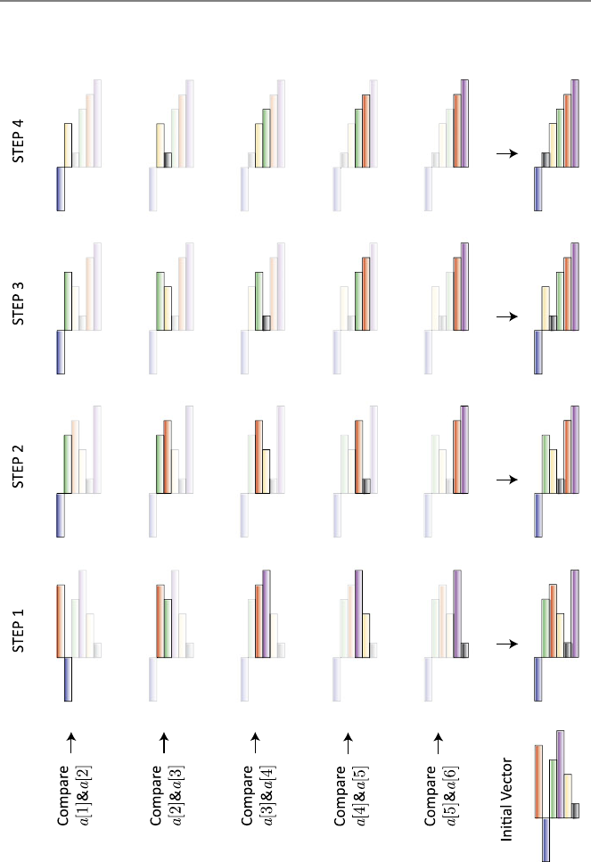

102 6 Sorting
R Program: Bubble Sort (Original)
01 bubblesort = function(a){
02 n = length(a)
03 swap = 1
04 while (swap == 1){
05 swap = 0
06 for (i in (1:(n-1))){
07 if (a[i] >a[i+1]){
08 abackup = a[i]
09 a[i] = a[i+1]
10 a[i+1] = abackup
11 swap = 1
12 }
13 }
14 }
15 return(a)
16 }
The input of this program is a vector athat contains nelements to be sorted. The
output is the same vector with sorted elements. Therefore, this is an in-place pro-
gram, i.e., operations are carried out on a single vector, which is both input and
output, and no significant memory is used in addition to this vector.
In the program above, the variable swap is used to represent whether any swap
operation is performed or not in a step. Note that no swap operation in a step of
the bubble sort algorithm means that the vector has been sorted and the program
can stop. Initially, swap is set to one to indicate that the program must work on the
vector. The sorting steps are performed by using a while loop, which continues
if swap is one. At any step (inside the loop), swap is immediately set to zero
since it can be switched to one only if there is a swap operation in the current step.
A variable to keep the track of a status (in this case, having a swap or not) is called
aflag.
The implementation of each step is a for loop, where the elements of the vec-
tor aare compared and swapped if necessary, in accordance with the bubble sort
algorithm. Specifically, choosing a value for the variable i, the elements a[i] and
a[i+1] are compared. If a[i] is greater than a[i+1], then they need to be
swapped as follows:
abackup = a[i]
a[i+1] = abackup
a[i] = a[i+1]
In addition to the swap operation, the flag is set to one to indicate that a swap op-
eration has been done and more steps may be required in the bubble sort algorithm.
Note that we are using a backup variable abackup to facilitate the swap operations.
Having said this, the following would be incorrect:
a[i+1] = a[i]
a[i] = a[i+1]
www.it-ebooks.info

6.1 Bubble Sort Algorithm 103
Using this pair of lines, both a[i] and a[i+1] would be the same at the end,
whereas the original a[i+1] is completely lost.
The bubble sort program above can easily be improved with the following ob-
servation. The largest element is located at the last position and it does not move
after the first step. In other words, it is “locked.” Hence, one does not need to check
and compare a[n-1] and a[n] after the first step since they should not require a
swap later. Similarly, the second largest element is located in the correct position,
i.e., at the (n −1)th position, and does not move after the second step, etc. Based on
these, some unnecessary checks can be avoided, leading to the following improved
program:
R Program: Improved Bubble Sort (Original)
01 bubblesortimproved = function(a){
02 n = length(a)
03 swap = 1
04 step = 1
05 while (swap == 1){
06 swap = 0
07 if (step <n){
08 for (i in (1:(n-step))){
09 if (a[i] >a[i+1]){
10 abackup = a[i]
11 a[i] = a[i+1]
12 a[i+1] = abackup
13 swap = 1
14 }
15 }
16 }
17 step = step + 1
18 }
19 return(a)
20 }
In the for loop of this program, ichanges from 1 to n-step rather than 1 to
n-1. Here, the variable step is the index of the step, which is initially set to one
and incremented at the end of each step as
step = step + 1
This way, unnecessary comparisons described above are easily avoided.
Now, let us calculate the cost of the improved bubble sort program. The memory
complexity of the program is O(n) considering the input vector a. On the other
hand, the time complexity depends on the elements of the input vector, and we need
consider each case separately.
•Best Case: In the best case, i.e., when the vector is already sorted, only one
step is performed, and no swap is required. In this case, lines 09–13 can be
considered as critical lines, which are executed for n−1 times since the value
of step is one. Therefore, Tbest
all =O(n).
www.it-ebooks.info

104 6 Sorting
•Worst Case: In the worst case, i.e., when the vector is reversely sorted, n−1
steps are required, whereas each comparison requires a swap. Then, the critical
lines 09–13 are executed from 1 to n-step, where step changes from 1 to
n−1. Therefore, we have
Tworst
all =C
n−1
s=1
(n −s) =C
n−1
s=1
s=Cn(n −1)
2=O(n2),
where Cis a constant.
•Almost the Best Case: In order to understand the performance of the improved
bubble sort program under normal circumstances, we consider almost the best
case, where the initial vector is correctly sorted except the smallest element.
Let the smallest element be located at the last (nth) position instead of the first
position. Then, there should be again n−1 steps, even though each step involves
only a single swap operation. Hence, in this case, lines 10–13 are executed once
per step, but line 09 is executed from 1 to n-step (as in the worst case),
becoming a critical line. Therefore, we have
Talmost-best
all =C
n−1
s=1
(n −s) =O(n2),
where Cis a constant. Even though the sorting is significantly faster compared
to the worst case (because lines 10–13 are executed once per step), the time
complexity is still O(n2).
•Average Case: The improved bubble sort program requires O(n2)processing
time, even when a single element is misplaced in the initially sorted vector.
This also means that, except for the best case, i.e., when the entire vector is
already sorted, the improved bubble sort program has O(n2)time complexity,
including all average cases. Therefore,
Taverage
all =O(n2).
Due to its relatively high time complexity, the bubble sort algorithm is rarely used
in real-life applications. In the next subsections, we consider the insertion sort and
quick sort algorithms that are more efficient and used in practice.
6.2 Insertion Sort Algorithm
The insertion sort is another simple algorithm, which is based on direct compar-
isons of elements. Let abe a vector of nelements to be sorted. The insertion sort
algorithm starts by comparing a[2]with a[1]and swapping them if required. This
operation is exactly the same as the first operation of the bubble sort algorithm. But
then, a[3]is compared with both a[2]and a[1]to make sure that it is inserted in the
www.it-ebooks.info

6.2 Insertion Sort Algorithm 105
correct position. The algorithm continues by inserting a[4],a[5], etc., in the cor-
rect positions considering the elements with smaller indices that are already sorted.
Hence, as opposed to the bubble sort algorithm, the vector is traced only once, but
each element (except a[2]) is compared with more than one element to be inserted
in the correct position.
Let us apply the insertion sort to the example vector a=[5,−3,4,6,3,1].
•Insertion of a[2]:[5,−3,4,6,3,1]→[−3,5,4,6,3,1]
•Insertion of a[3]:[−3,5,4,6,3,1]→[−3,4,5,6,3,1]→[−3,4,5,6,3,1]
•Insertion of a[4]:[−3,4,5,6,3,1]→[−3,4,5,6,3,1]
•Insertion of a[5]:[−3,4,5,6,3,1]→[−3,4,5,3,6,1]→[−3,4,3,5,6,1]
→[−3,3,4,5,6,1]→[−3,3,4,5,6,1]
•Insertion of a[6]:[−3,3,4,5,6,1]→[−3,3,4,5,1,6]→[−3,3,4,1,5,6]
→[−3,3,1,4,5,6]→[−3,1,3,4,5,6]
→[−3,1,3,4,5,6]
Figure 6.2 illustrates the elements of the example vector in different steps of the
insertion sort algorithm. Theoretically, the insertion of a[i]should require (i −1)
comparisons, but as shown in this example (i.e., insertion of a[4]), further com-
parisons can be avoided if a comparison does not require a swap. In other words,
the number of comparisons depends on the values of the elements that are already
sorted, as well as the element to be inserted.
The advantage of the insertion sort algorithm over the bubble sort algorithm may
not be obvious without a detailed analysis. For a vector of nelements, there should
be a total of n−1 insertions (can be considered as steps), while each insertion
requires O(n) comparisons in average. In fact, as presented below, the average-case
time complexity of the insertion sort algorithm is O(n2), similar to that of the bubble
sort algorithm. Nevertheless, the insertion sort algorithm becomes very efficient for
nearly sorted vectors, which require several comparisons per step, leading to a linear
overall complexity.
Based on the discussion above, the insertion sort algorithm can be implemented
as follows:
www.it-ebooks.info
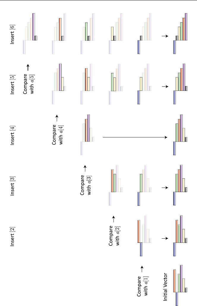

6.2 Insertion Sort Algorithm 107
R Program: Insertion Sort (Original)
01 insertionsort = function(a){
02 n = length(a)
03 for (i in (2:n)){
04 for (j in (1:(i-1))){
05 if (a[i-j] >a[i-j+1]){
06 abackup = a[i-j]
07 a[i-j] = a[i-j+1]
08 a[i-j+1] = abackup
09 }
10 else{
11 break
12 }
13 }
14 }
15 return(a)
16 }
The input/output of this program is again a vector a, which contains nelements.
In the program, the outer loop is constructed for the insertion steps with the variable
ichanging from 2 to n. Choosing a value for iand the element to be inserted
(initially at the ith position), maximum i-1 comparisons are required. Therefore,
in the inner loop, the variable jchanges from 1to i-1. Comparisons are executed
in line 05 as
if (a[i-j] >a[i-j+1]){
Note that the element to be inserted may move in each comparison, and hence com-
parisons are made between (i −j)th and (i −j+1)th elements above. In any
comparison, if the element a[i-j] is greater than the element a[i-j+1],they
are swapped. Otherwise, the break command in line 11 is executed, which im-
mediately ends the inner loop. This is essential to avoid unnecessary comparisons.
Because, if a[i-j] is not greater than a[i-j+1], the element to be inserted,
which is now located at (i −j+1)th position, is already in the correct place, and it
should not move any further.
The memory complexity of the insertion sort program above is O(n) and it is an
in-place program. For the time complexity, we again consider different cases.
•Best Case: In the best case, i.e., when the vector is already sorted, the if state-
ment
a[i-j] >a[i-j+1]
never holds. Hence, the inner for loop is broken immediately when jis one.
Considering line 05 as a critical line, which is executed for (n −1)times due to
the outer loop, we have
Tbest
all =O(n).
www.it-ebooks.info

108 6 Sorting
•Worst case: In the worst case, i.e., when the vector is reversely sorted, the con-
ditional statement [i-j] >a[i-j+1] always holds, and each comparison
requires a swap. In other words, break is never executed. In this case, lines
05–08 can be considered to be critical to derive the time complexity as
Tworst
all =C
n
i=2
(i −1)=C
n−1
i=1
i=Cn(n −1)
2=O(n2),
where Cis a constant. In the above, the summation represents the outer loop,
whereas i−1 is the cost due to the inner loop for a given i.
•Almost the Best Case: Consider almost the best case, where the initial vector is
correctly sorted except the smallest element, which is located at the last (nth)
position. This means that, for the elements from a[2] to a[n-1], the inner
loop is immediately broken. For these elements, line 05 is critical, which is
executed for (n −1)times. On the contrary, for the last element, i.e., a[n],
break is never executed. For this element, lines 05–08 are critical, which are
executed for (n −1)times since jchanges from 1to i-1 when the value of i
is n. Considering all contributions, we have
Talmost-best
all =C(n −1)+D(n −1)=O(n),
where Cand Dare constants. Obviously, for this case, the insertion sort algo-
rithm is more efficient than the bubble sort algorithm.
•Average Case: We do not have a quick conclusion for the average time com-
plexity of the insertion sort program/algorithm since it has O(n) complexity
for almost the best case. In order to analyze the program in an average case,
consider the inner loop
for (j in (1:(i-1))){
running from 1to i-1 with a possible break. In the best case, this loop always
breaks whenever jis 1 since any element to be inserted is already located in the
correct position. In the worst case, however, the loop always continues without
any break from 1to i-1 since all elements to be inserted should move to the
first position. Then, in an average case, we can assume that the loop continues
up to approximately half of iand then breaks. Hence, the time complexity can
be written as
Taverage
all =C
n
i=2
(i/2−1)=O(n2),
which means that we again have a quadratic order in average.
As a result, the insertion sort algorithm performs well for almost sorted vectors, but
its time complexity is O(n2)in average cases. Due to this high time complexity, the
insertion sort algorithm is rarely used, only when the input vector is small and/or
nearly sorted.
www.it-ebooks.info

6.3 Quick Sort 109
Fig. 6.3 Application of the
quick sort algorithm to the
vector [5,−3,4,6,3,1]
6.3 Quick Sort
The quick sort algorithm is a well-known and popular method, which is commonly
used in many applications. Its popularity is due to its lower time complexity, which
is O(n logn) in average.
Let abe a vector of nelements to be sorted. The quick sort algorithm starts by
choosing a pivot element a[p]. The vector is reordered so that all elements smaller
than a[p] have smaller indices and all elements larger than a[p] have larger in-
dices. After this reordering, the pivot is in its correct position (say, at a[r]), but this
is not necessarily true for the other elements. Then, the quick sort algorithm contin-
ues recursively by considering the smaller vectors a[1:r-1] and a[r+1:n] and
applying the same operations on them.
Consider the application of the quick sort algorithm to an example vector involv-
ing six elements, e.g., a=[5,−3,4,6,3,1]. As a rule to choose the pivot, we can
use p=n/2, where · represents the floor operation. Then, the algorithm works
as depicted in Fig. 6.3. Note that as the recursion continues, vectors with one ele-
ment arise, and no further sorting is required for them. This condition, i.e., having
one element, can be considered as the termination condition for the recursion.
The quick sort algorithm with the pivoting strategy p=n/2can be imple-
mented as follows:
www.it-ebooks.info

110 6 Sorting
R Program: Quick Sort (Original)
01 quicksort = function(a){
02 n = length(a)
03 if (n >1){
04 p = floor(n/2)
05 pivot = a[p]
06 asmaller = c()
07 alarger = c()
08 for (i in (1:n)){
09 if (i != p){
10 if (a[i] <= pivot){
11 asmaller = rbind(asmaller,a[i])
12 }
13 else{
14 alarger = rbind(a[i],alarger)
15 }
16 }
17 }
18 asmaller = quicksort(asmaller)
19 alarger = quicksort(alarger)
20 a = rbind(asmaller,a[p],alarger)
21 }
22 return(a)
23 }
This program is not in-place since we allocate two new vectors, namely, asmaller
and alarger, to collect the elements that are smaller and larger, respectively, than
the pivot. Then, the memory requirement can be written as
Mall(n) =C+nD +Mall(ns)+Mall(nl),
where Cand Dare constants. In the above, nsand nlrepresent the numbers of
elements in asmaller and alarger vectors, respectively. Therefore, ns+nl=
(n −1), but their values depend on the input vector.
Now let us consider the worst-case scenario for the program above. As opposed
to the other sorting programs and algorithms, the worst case of the quick sort pro-
gram/algorithm is not the case where the input vector is reversely sorted. Instead,
the value of the pivot compared to the other elements is the critical factor. Specif-
ically, the worst case happens when the pivot is either the smallest or the largest
element by “coincidence.” Considering the latter, all elements other than the pivot
are collected in asmaller, whereas alarger has no element. In other words,
ns=n−1, nl=0, and
Mall(n) =C+nD +Mall(n −1).
Assuming that this worst-case selection occurs in all steps of the recursion, we have
Mworst
all (n) =C+nD +Mworst
all (n −1),
www.it-ebooks.info

6.3 Quick Sort 111
which can be solved to arrive at
Mworst
all (n) =O(n2)
as the worst-case memory requirement.
For the quick sort algorithm, the best case happens when the value of the pivot
is perfect such that nearly half of the elements are smaller than the pivot. Conse-
quently, ns=n/2−1, nl=n−n/2, and
Mall(n) =C+nD +Mall(n/2−1)+Mall(n −n/2).
Assuming that this best-case selection occurs in all steps of the recursion, we obtain
Mbest
all (n) =O(n logn)
as the best-case memory requirement.
It should be noted that there are also improved (in-place) implementations of
the quick sort algorithm that require only O(log n) extra memory other than for the
input vector, leading to Mbest
all (n) =O(n) +O(logn) =O(n), but they are out of the
scope of this book.
Now, let us investigate the time complexity of the quick sort program in detail.
•Best Case: In the best case, i.e., where pivots are chosen perfectly in all steps,
the processing time can be written as
Tbest
all (n) =C+nD +Tbest
all (n/2−1)+Tbest
all (n −n/2),
leading to
Tbest
all (n) =O(n logn),
similar to the best-case memory.
•Worst case: In the worst case, i.e., where pivots are extremum (minimum or
maximum) elements in all steps, the processing time can be written as
Tworst
all (n) =C+nD +Tworst
all (n −1),
leading to
Tworst
all (n) =O(n2),
similar to the worst-case memory.
•Average case: In general, choosing the best or worst pivot in all steps of the
recursion has a very low probability. In the best case, input vectors are divided
equally into pairs of vectors. In the worst case, all elements (except the pivots)
are collected in one vector. Along this direction, in order to consider different
possibilities between the best and worst selections of pivots, one can write
Taverage
all (n) =C+nD +1
n/2
n/2
i=1Taverage
all (n −i) +Taverage
all (i −1),
www.it-ebooks.info

112 6 Sorting
where different values of iaccounts for different possible splits. A rigorous
analysis of this formula leads to
Tall(n) =O(n log n)
as the average time complexity of the quick sort program.
To sum up, the time complexity of the quick sort program is O(n logn) in average.
This low complexity is an important advantage of the quick-sort algorithm over
other sorting algorithms in the literature.
As a demonstration, Fig. 6.4 depicts the application of the quick sort program to
a vector of 2500 elements. First, we generate a random vector and its plot as
v = rnorm(2500,0,10)
plot(v,col="blue",xlab="Index",ylab="Element Values")
Then, we apply the quick sort program and plot the resulting vector as
w = quicksort(v)
plot(w,col="blue",xlab="Index",ylab="Element Values")
It can be observed that the elements are nicely ordered using the quick sort program,
verifying its correct implementation.
6.4 Comparisons
Table 6.1 lists the time complexity of the three sorting algorithms considered in
this chapter. In the worst-case scenarios, all algorithms have O(n2)complexity. In
the average cases, however, the quick sort algorithm with O(n logn) complexity
is more efficient than others. Its low average-time complexity is the reason why the
quick sort algorithm is preferred in many real-life applications. If the initial vector is
known to be almost sorted, then the insertion sort algorithm (with O(n) complexity)
may be used instead of the quick sort algorithm, but this requires a priori knowledge
on the vector, and the gain in the processing time may not be very critical.
When comparing complexities, it is relatively easier to understand polynomial
orders. For example, if an algorithm has a quadratic time complexity, increasing
the input size twice increases the processing time by 22=4 times for large inputs.
However, if an algorithm has a logarithmic time complexity, i.e., O(log n),itisdiffi-
cult to estimate the increase in the processing time when the input size is increased,
e.g., twice. The ignored base of the logarithm also leads to confusions. For a more
correct interpretation, one may consider that the input size is squared (rather than
multiplied), which leads to twofold increase in the processing time if the algorithm
has a logarithmic complexity.
In order to understand O(n log n), consider that nis very large, which is in fact an
assumption that is already made for the asymptotic analysis. For a large n, increasing
the input size to 2nleads to an almost twofold increase in the processing time, since
the lognterm contributes a little. This term can add a twofold increase only when
the input size is increased to a very large value, i.e., n2. But, in the case of such a
www.it-ebooks.info
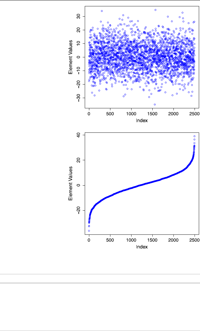
6.4 Comparisons 113
Fig. 6.4 Application of the
quick sort program to a vector
of random elements
Table 6.1 Comparison of three sorting algorithms in terms of the processing time
Algorithm Bubble sort Insertion sort Quick sort
Worst-Case Scenario Reversely sorted Reversely sorted Worst pivots
Worst Case O(n2)O(n2)O(n2)
Average Case O(n2)O(n2)O(n log n)
Best-Case Scenario Already sorted Already sorted Best pivots
Almost Best Case O(n2)O(n) O(n log n)
Best Case O(n) O(n) O(n log n)
www.it-ebooks.info

114 6 Sorting
big jump from nto n2, the time is already squared due to the nterm. Therefore,
O(n logn) can be considered as a linear-like complexity, which behaves like O(n)
but being slightly larger. This is the reason why this expression is usually called
linearithmic.
6.5 Conclusions
Sorting is one of the important problems in computer science since sorted vectors
are required in many application areas. Given a numeric vector of nelements, it is
desirable to sort its elements as fast as possible. Among many of them, the quick sort
algorithm is coming forward as an efficient method with O(n log n) time complex-
ity in average. This algorithm is based on recursively dividing vectors into smaller
vectors such that the number of comparisons required to sort a given vector is dras-
tically reduced from O(n2)to O(n log n). In this chapter, for comparisons, we also
focus on the bubble sort and insertion sort algorithms, but it should be emphasized
that these algorithms are rarely used in real life as they have O(n2)time complexity
for an average vector. If the vector is almost sorted, the insertion sort algorithm may
have a linear O(n) time complexity, which is mathematically better than the com-
plexity of the quick sort algorithm. Nevertheless, for large vectors, the quick sort
algorithm has a linear-like complexity that reduces a need for an alternative algo-
rithm even when the vector is almost sorted. The quick sort algorithm is extremely
popular, and its alternative implementations (such as in-place, optimized, and using
pivoting strategies) can be found in the literature.
6.6 Exercises
1. Write a program that sorts a given vector using the improved bubble sort algo-
rithm. The input should be a vector of nelements. The output should be the same
vector with sorted elements. Test your program for a small vector as
bubblesortimproved(matrix(c(50,-3,1,6,12,10,0,-40,1,5,8,1),ncol=1))
to make sure that it works correctly. Then, measure the time required to sort random
vectors of 500, 1000, and 2000 elements as
system.time(bubblesortimproved(matrix(rnorm(500,0,1),ncol=1)))
system.time(bubblesortimproved(matrix(rnorm(1000,0,1),ncol=1)))
system.time(bubblesortimproved(matrix(rnorm(2000,0,1),ncol=1)))
Investigate the timing results in terms of the time complexity of the program.
2. Write a program that sorts a given vector using the insertion sort algorithm. The
input should be a vector of nelements. The output should be the same vector with
sorted elements. Test your program for a small vector as
insertionsort(matrix(c(50,-3,1,6,12,10,0,-40,1,5,8,1),ncol=1))
www.it-ebooks.info

6.6 Exercises 115
to make sure that it works correctly. Then, measure the time required to sort random
vectors of 500, 1000, and 2000 elements as
system.time(insertionsort(matrix(rnorm(500,0,1),ncol=1)))
system.time(insertionsort(matrix(rnorm(1000,0,1),ncol=1)))
system.time(insertionsort(matrix(rnorm(2000,0,1),ncol=1)))
Investigate the timing results in terms of the time complexity of the program.
3. Use your insertion sort program to perform the following experiment. First, create
a vector of 500 almost-sorted elements as
v = insertionsort(matrix(rnorm(500,0,1),ncol=1))
v[500] = -100
Note that the last element of the vector is set to −100, which is (most probably)
misplaced. Then, measure the time required to sort the vector as
system.time(insertionsort(v))
Repeat the experiment for vectors of size 1000 and 2000 to investigate the time
complexity of the program for almost sorted vectors.
4. Write a program that sorts a given vector using the quick sort algorithm with
p=n/2pivoting. The input should be a vector of nelements. The output should
be the same vector with sorted elements. Test your program for a small vector as
quicksort(matrix(c(50,-3,1,6,12,10,0,-40,1,5,8,1),ncol=1))
to make sure that it works correctly. Then, measure the time required to sort random
vectors of 1000, 2000, 10,000, and 20,000 elements as
system.time(quicksort(matrix(rnorm(1000,0,1),ncol=1)))
system.time(quicksort(matrix(rnorm(2000,0,1),ncol=1)))
system.time(quicksort(matrix(rnorm(10000,0,1),ncol=1)))
system.time(quicksort(matrix(rnorm(20000,0,1),ncol=1)))
Investigate the timing results in terms of the time complexity of the program.
5. Consider a modified quick sort program/algorithm, where the pivot is selected as
the first element of the vector. Describe the disadvantages of the program/algorithm
when the input vector is almost sorted.
www.it-ebooks.info

7
Solutions of Linear Systems of Equations
Linear systems of equations are important components in many basic areas, such as
biology, chemistry, computer science, economics, engineering, and physics. Math-
ematical modeling of real-life scenarios often leads to linear systems of equations,
whose solutions are required to understand the underlying phenomena. Solution
techniques for linear systems have been developed for decades under the name of
linear algebra. It is also common to approximate nonlinear systems with linear ones
in order to benefit the advanced methods in this area.
7.1 Overview of Linear Systems of Equations
A linear system of equations is a collection of linear equations involving a set of
variables. As an example, consider the linear equation
x+2y=4
involving two variables, i.e., xand y. As depicted in Fig. 7.1, this equation repre-
sents a line in the two-dimensional space. Now, consider another equation
x−y=1
involving the same variables. This equation corresponds to another line. If we would
like to consider the two equations at the same time, we may write it in a matrix
equation (linear system) form as
12
1−1x
y=4
1.
The linear system above can be interpreted as “two equations with two unknowns.”
Solution of such a system is relatively easy by a direct substitution. For exam-
ple, using the first equation, we have x=4−2y, which can be inserted into the
second equation to get 4 −2y−y=1or−3y=−3. Hence, y=1 and x=
Ö. Ergül, Guide to Programming and Algorithms Using R,
DOI 10.1007/978-1-4471-5328-3_7,
© Springer-Verlag London 2013
117
www.it-ebooks.info
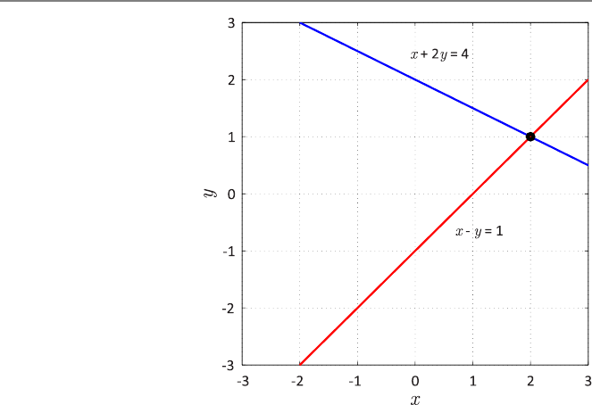
118 7 Solutions of Linear Systems of Equations
Fig. 7.1 Lines corresponding
to x+2y=4andx−y=1,
intersecting at (x, y) =(2,1)
4−2y=2. In other words, (x, y) =(2,1)is the solution to the linear system. As
depicted in Fig. 7.1, the solution actually corresponds to the intersection of the two
lines describing the two equations.
In general, we have nequations involving nunknowns, where n>2. Such linear
systems can be difficult to solve by a direct substitution. Nevertheless, we are able
to derive systematic ways and techniques to solve large matrix equations involving
large numbers of unknowns. Geometric interpretations of large linear systems can
be difficult, but this does not prevent us to solve them by abstracting each equation
as an (n −1)-dimensional “line” in the n-dimensional space.
Before going into further details of the solution techniques, it is useful to cate-
gorize linear systems of equations to understand them and their possible solutions.
Assume that we have mequations involving nunknowns, i.e.,
a11x1+a12x2+... +a1nxn=b1,
a21x1+a22x2+... +a2nxn=b2,
a31x1+a32x2+... +a3nxn=b3,
.
.
..
.
..
.
..
.
.....
.
..
.
..
.
..
.
.
am1x1+am2x2+... +amnxn=bm.
Then, in the matrix form, we have
⎡
⎢
⎢
⎢
⎢
⎢
⎣
a11 a12 ... a
1n
a21 a22 ... a
2n
a31 a32 ... a
3n
.
.
..
.
.....
.
.
am1am2... a
mn
⎤
⎥
⎥
⎥
⎥
⎥
⎦
⎡
⎢
⎢
⎢
⎢
⎢
⎣
x1
x2
x3
.
.
.
xn
⎤
⎥
⎥
⎥
⎥
⎥
⎦=⎡
⎢
⎢
⎢
⎢
⎢
⎣
b1
b2
b3
.
.
.
bm
⎤
⎥
⎥
⎥
⎥
⎥
⎦
.
www.it-ebooks.info

7.1 Overview of Linear Systems of Equations 119
Depending on the values of mand n, we have three different cases.
(1) If m=n, then the number of equations is equal to the number of unknowns.
Such a system is called a square system, considering that the matrix has a
square shape with equal numbers of rows and columns.
(2) If m>n, then there are more equations than unknowns. Such a system is
called an overdetermined system.
(3) If m<n, then there are more unknowns than equations. Such a system is
called an underdetermined system.
In this book, we will mainly consider square systems (m=n).
The values of mand ndo not give a complete information about the solution. We
again have three different cases.
(1) Unique Solution: A system may have a unique solution. Only square and
overdetermined systems may have unique solutions.
(2) Infinitely Many Solutions: A system may have infinitely many solutions. Such
a system can be square, underdetermined, or overdetermined.
(3) No Solution: A system may have no solution. Such a system can be square,
underdetermined, or overdetermined.
Hence, a square system may have a unique solution, infinitely many solutions, or no
solution.
Let us now consider various square systems with different properties.
•12
1−1x
y=4
1
is a square system with a unique solution (x, y) =(2,1).
•12
24
x
y=4
8
is a square system with infinitely many solutions. For example, inserting x=
4−2yinto second equation, we obtain 2(4−2y) +4y=8or8=8, which is
always correct, independently of the values of xand y. This is because these
two equations are linearly dependent, i.e., one of them can be obtained from the
other and vice versa. In this example, the second equation is obtained via mul-
tiplying the first equation by two. Hence, it does not provide a new information
regarding the variables xand y. Geometrically, both equations correspond to
the same line in the two-dimensional space. Hence, their intersection is also the
same line involving infinitely many points (solutions).
•12
24
x
y=4
4
is a square system with no solution. For example, inserting x=4−2yinto sec-
ond equation, we obtain 2(4−2y)+4y=4or8=4, which is always incorrect
for any values of xand y. Geometrically, these equations correspond to two
parallel lines in the two-dimensional space. Hence, they do not intersect and
there is not any point (solution) that is on the both lines at the same time.
Geometric interpretations of the systems defined above with infinitely many solu-
tions and no solution are illustrated in Fig. 7.2.
www.it-ebooks.info
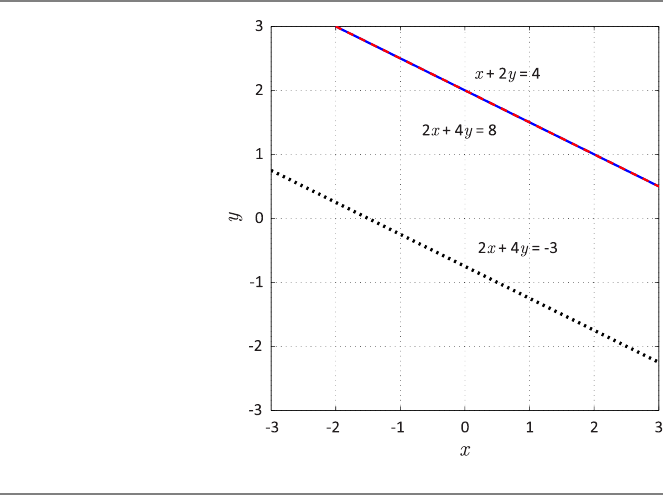
120 7 Solutions of Linear Systems of Equations
Fig. 7.2 Lines corresponding
to x+2y=4, 2x+4y=8,
and 2x+4y=−3
7.2 Solutions of Triangular Systems
Solution of a general n×nmatrix equation involves two main stages.
(1) Modify the matrix equation (using elimination or factorization) such that it
becomes easier to solve.
(2) Apply substitution systematically to solve for unknowns.
We first consider the second stage and focus on solution methods for simple matrix
equations, namely, triangular systems.
An n×nlower-triangular matrix
L=⎡
⎢
⎢
⎢
⎢
⎢
⎣
l11 00... 0
l21 l22 0... 0
l31 l32 l33 ... 0
.
.
..
.
..
.
.....
.
.
ln1ln2ln3... l
nn
⎤
⎥
⎥
⎥
⎥
⎥
⎦
has zero elements above the diagonal, i.e., L[i, j ]=0forj>i.Ann×nupper-
triangular matrix
U=⎡
⎢
⎢
⎢
⎢
⎢
⎣
u11 u12 u13 ... u
1n
0u22 u23 ... u
2n
00u33 ... u
3n
.
.
..
.
..
.
.....
.
.
000... u
nn
⎤
⎥
⎥
⎥
⎥
⎥
⎦
www.it-ebooks.info

7.2 Solutions of Triangular Systems 121
has zero elements below the diagonal, i.e., U[i, j ]=0fori>j. A matrix, which
is both lower and upper triangular, is called diagonal since such a matrix may have
nonzero elements only on the diagonal, i.e.,
D=⎡
⎢
⎢
⎢
⎢
⎢
⎣
d11 00... 0
0d22 0... 0
00d33 ... 0
.
.
..
.
..
.
.....
.
.
000... d
nn
⎤
⎥
⎥
⎥
⎥
⎥
⎦
.
Matrix equations involving diagonal matrices are trivial to solve. For example, if
D⎡
⎢
⎢
⎢
⎢
⎢
⎣
x1
x2
x3
.
.
.
xn
⎤
⎥
⎥
⎥
⎥
⎥
⎦=⎡
⎢
⎢
⎢
⎢
⎢
⎣
b1
b2
b3
.
.
.
bn
⎤
⎥
⎥
⎥
⎥
⎥
⎦
,
one can find that ⎡
⎢
⎢
⎢
⎢
⎢
⎣
x1
x2
x3
.
.
.
xn
⎤
⎥
⎥
⎥
⎥
⎥
⎦=⎡
⎢
⎢
⎢
⎢
⎢
⎣
b1/d11
b2/d22
b3/d33
.
.
.
bn/dnn
⎤
⎥
⎥
⎥
⎥
⎥
⎦
.
Matrix equations involving lower-triangular and upper-triangular matrices can be
solved via forward and backward substitutions, respectively.
7.2.1 Forward Substitution
Consider a matrix equation involving an n×nlower-triangular matrix, i.e.,
⎡
⎢
⎢
⎢
⎢
⎢
⎣
l11 00... 0
l21 l22 0... 0
l31 l32 l33 ... 0
.
.
..
.
..
.
.....
.
.
ln1ln2ln3... l
nn
⎤
⎥
⎥
⎥
⎥
⎥
⎦
⎡
⎢
⎢
⎢
⎢
⎢
⎣
x1
x2
x3
.
.
.
xn
⎤
⎥
⎥
⎥
⎥
⎥
⎦=⎡
⎢
⎢
⎢
⎢
⎢
⎣
b1
b2
b3
.
.
.
bn
⎤
⎥
⎥
⎥
⎥
⎥
⎦
.
The first equation can be written as
l11x1+0x2+0x3+···+0xn=b1
or
l11x1=b1,
www.it-ebooks.info

122 7 Solutions of Linear Systems of Equations
leading to
x1=b1/l11.
In other words, the first equation can be solved without using the other equations.
Let us consider the second equation now. Omitting the multiplications with zeros,
we have
l21x1+l22x2=b2
or
x2=(b2−x1l21)/ l22.
Obviously, the value of x2depends on the value of x1. Also note that the value of x1
is found above and already available for the calculation of x2. Similarly, using the
third equation, we get
x3=(b3−x1l31 −x2l32)/ l33,
where x1and x2are available and can be used to find x3. In general,
xi=(bi−x1li1−x2li2−···−x(i−1)li(i−1))/ lii
for 3 <i≤n. Based on these, one can write the following program for the forward
substitution:
R Program: Forward Substitution (Original)
01 forwardsub = function(L,b){
02 x = c(0)
03 n = nrow(L)
04 for (i in (1:n)){
05 x[i] = b[i]
06 if (i >1){
07 for (j in (1:(i-1))){
08 x[i] = x[i] - L[i,j]*x[j]
09 }
10 }
11 x[i] = x[i]/L[i,i]
12 }
13 return(cbind(x))
14 }
Note that we use cbind to return the solution as a column vector.
The time complexity of the program above can easily be found by noting that
line 08 is a critical line. This line is executed for
n
i=2
(i −1)=
n−1
i=1
i=n(n −1)
2=n2/2−n/2
www.it-ebooks.info

7.2 Solutions of Triangular Systems 123
times, leading to O(n2)time complexity. In the above, the summation accounts for
the outer loop (where the loop variable ichanges from 1 to n, while line 08 is not
executed when iequals 1), and i−1 stands for the number of executions for a
given idue to the inner loop. The memory complexity of the forward substitution
program is also O(n2), considering the storage of the matrix L.
7.2.2 Backward Substitution
Consider a matrix equation involving an n×nupper-triangular matrix, i.e.,
⎡
⎢
⎢
⎢
⎢
⎢
⎣
u11 u12 u13 ... u
1n
0u22 u23 ... u
2n
00u33 ... u
3n
.
.
..
.
..
.
.....
.
.
000... u
nn
⎤
⎥
⎥
⎥
⎥
⎥
⎦
⎡
⎢
⎢
⎢
⎢
⎢
⎣
x1
x2
x3
.
.
.
xn
⎤
⎥
⎥
⎥
⎥
⎥
⎦=⎡
⎢
⎢
⎢
⎢
⎢
⎣
b1
b2
b3
.
.
.
bn
⎤
⎥
⎥
⎥
⎥
⎥
⎦
.
The last (nth) equation can be written as
unnxn=bn,
leading to
xn=bn/unn.
In other words, the last equation can be solved without using the other equations.
Finding the value of xn, one can consider the (n −1)th equation to compute x(n−1)
as
x(n−1)=(b(n−1)−xnu(n−1)n)/u(n−1)(n−1).
Similarly,
x(n−2)=(b(n−2)−x(n−1)u(n−2)(n−1)−xnu(n−2)n)/u(n−2)(n−2).
In general,
xi=(bi−x(i+1)ui(i+1)−x(i+2)ui(i+2)−···−xnui,n)/uii
for 1 ≤i<(n−2). Note that the procedure is very similar to the forward substitu-
tion, but we only process the matrix in the backward direction from the last row to
the first row. Such an algorithm can be implemented as follows:
www.it-ebooks.info

124 7 Solutions of Linear Systems of Equations
R Program: Backward Substitution (Original)
01 backwardsub = function(U,b){
02 x = c(0)
03 n = nrow(U)
04 for (i in (n:1)){
05 x[i] = b[i]
06 if (i <n){
07 for (j in ((i+1):n)){
08 x[i] = x[i] - U[i,j]*x[j]
09 }
10 }
11 x[i] = x[i]/U[i,i]
12 }
13 return(cbind(x))
14 }
In the program above, note that the index of outer loop, i.e.,
for (i in (n:1)){
changes in a reverse order from nto 1. Line 08 is again a critical line and is executed
for n2/2−n/2 times, leading to O(n2)time complexity.
Both forward and backward substitution methods fail when one of the diagonal
elements of the matrix is zero. This is due to the fact that such a matrix is singular,
and in fact, the underlying linear system does not have any solution. An attempt
of substitution to such a system leads to a divide-by-zero error, leading to infinite
elements in the solution vector.
7.3 Gaussian Elimination
Triangular systems are easy to solve using forward and backward substitutions. Un-
fortunately, most of the systems derived in real-life applications involve nontriangu-
lar matrices, whose solutions require more than substitution. For those systems, one
can apply the Gaussian elimination to modify the matrix equation so that the matrix
becomes upper triangular (alternatively lower triangular).
7.3.1 Elementary Row Operations
The Gaussian elimination is based on two types of elementary row operations, i.e.,
replacement and permutation. Consider the ith and jth rows of an n×nmatrix A,
where i=j.
•Replacement: Replace the ith row with a combination of the ith and jth rows,
i.e.,
A[i, :]+αA[j,:]→A[i, :].
www.it-ebooks.info

7.3 Gaussian Elimination 125
•Permutation: Swap the ith and jth rows, i.e.,
A[i, :]↔A[j,:].
Replacement can be sufficient to convert a general matrix into an upper-triangular
form. Permutation is required for pivoting, as described later. In any case, all op-
erations that are applied to the matrix should also be applied to the right-hand-side
vector for consistency. This is particularly required to avoid changing the solution
by elementary row operations. A systematic technique to apply same operations to
a matrix and a right-hand-side vector is to combine (augment) them before elimina-
tion.
As an example, consider the following 3 ×3 matrix equation Ax =b:
⎡
⎣
21−2
3−14
1−22
⎤
⎦⎡
⎣x1
x2
x3⎤
⎦=⎡
⎣
1
11
6⎤
⎦.
Before applying replacement operations, we augment the matrix and the right-hand-
side vector as
{A|b}=⎡
⎣
21−2|1
3−14|11
1−22|6⎤
⎦.
Next, we eliminate the elements in the first column below the diagonal, i.e.,
A[2,1]=3 and A[3,1]=1, using A[1,1]=2. In order to eliminate A[2,1],we
can multiply the first row with 3/2 and subtract it from the second row. This can be
written as
{A|b}[2,:]−(3/2){A|b}[1,:]→{A|b}[2,:]
leading to
⎡
⎣
21−2|1
3−14|11
1−22|6⎤
⎦→⎡
⎣
21−2|1
0−5/27|19/2
1−22|6⎤
⎦.
As a result of the replacement operation, A[2,1]becomes zero. But, note that, the
other elements in the same row, including b[2], are also modified for consistency.
In order to eliminate A[3,1]using A[1,1], we multiply the first row with 1/2
and subtract it from the third row, i.e.,
{A|b}[3,:]−(1/2){A|b}[1,:]→{A|b}[3,:],
leading to
⎡
⎣
21−2|1
0−5/27|19/2
1−22|6⎤
⎦→⎡
⎣
21−2|1
0−5/27|19/2
0−5/23|11/2⎤
⎦.
www.it-ebooks.info

126 7 Solutions of Linear Systems of Equations
At this stage, all elements in the first column, except A[1,1], are zero. Hence, the
matrix becomes “similar” to an upper-triangular matrix. However, we should con-
tinue and eliminate all terms below the diagonal. Specifically, we should now con-
sider the second column and eliminate A[3,2]. On the other hand, we cannot use
A[1,2]for this purpose. Because such a replacement operation involving the first
row would create a nonzero element at A[3,1]and ruin our previous efforts. A better
strategy is to use A[2,2]to eliminate A[3,2]with the replacement operation
{A|b}[3,:]−{A|b}[2,:]→{A|b}[3,:].
This leads to
⎡
⎣
21−2|1
0−5/27|19/2
0−5/23|11/2⎤
⎦→⎡
⎣
21−2|1
0−5/27|19/2
00−4|−4⎤
⎦.
The final expression can be rewritten as a matrix equation, i.e.,
⎡
⎣
21−2
0−5/27
00−4⎤
⎦⎡
⎣x1
x2
x3⎤
⎦=⎡
⎣
1
19/2
−4⎤
⎦,
where the matrix is now upper triangular. Note that the matrix equation changes but
the system does not change by elementary row operations. In fact, we still consider
the same system with the same solution. The final matrix equation can be solved via
a backward substitution, and we obtain the solution as
⎡
⎣x1
x2
x3⎤
⎦=⎡
⎣
2
−1
1⎤
⎦.
Note that this solution satisfies both the triangular matrix equation and the original
matrix equation.
7.3.2 Steps of the Gaussian Elimination
Consider a general n×nmatrix equation Ax =b, i.e.,
⎡
⎢
⎢
⎢
⎢
⎢
⎣
a11 a12 a13 ... a
1n
a21 a22 a23 ... a
2n
a31 a32 a33 ... a
3n
.
.
..
.
..
.
.....
.
.
an1an2an3... a
nn
⎤
⎥
⎥
⎥
⎥
⎥
⎦
⎡
⎢
⎢
⎢
⎢
⎢
⎣
x1
x2
x3
.
.
.
xn
⎤
⎥
⎥
⎥
⎥
⎥
⎦=⎡
⎢
⎢
⎢
⎢
⎢
⎣
b1
b2
b3
.
.
.
bn
⎤
⎥
⎥
⎥
⎥
⎥
⎦
.
Steps of the Gaussian elimination can be listed as follows.
•Step 0: Augment the matrix and the right-hand-side vector, i.e., form {A|b}.
•Step 1: Eliminate the elements in the first column using the first row.
www.it-ebooks.info

7.3 Gaussian Elimination 127
– Eliminate a21 using a11.
{A|b}[2,:]−m21{A|b}[1,:]→{A|b}[2,:] (m21 =a21/a11)
– Eliminate a31 using a11.
{A|b}[3,:]−m31{A|b}[1,:]→{A|b}[3,:] (m31 =a31/a11)
–...
– Eliminate an1using a11.
{A|b}[n, :]−mn1{A|b}[1,:]→{A|b}[n, :] (mn1=an1/a11)
•Step 2: Eliminate the elements in the second column using the second row.
– Eliminate a32 using a22.
{A|b}[3,:]−m32{A|b}[2,:]→{A|b}[3,:] (m32 =a32/a22)
– Eliminate a42 using a22.
{A|b}[4,:]−m42{A|b}[2,:]→{A|b}[4,:] (m42 =a42/a22)
–...
– Eliminate an2using a22.
{A|b}[n, :]−mn2{A|b}[2,:]→{A|b}[n, :] (mn2=an2/a22)
•...
•Step k: Eliminate the elements in the kth column using the kth row.
•...
•Step (n −1): Eliminate the elements in the (n −1)th column using the (n −1)th
row.
The operations listed above should be performed consecutively by considering the
fact that the matrix elements are updated at each step. We also note that each elim-
ination operation involves a multiplier mik =aik/akk for k<i≤n. Following the
Gaussian elimination described above, the system becomes upper triangular that can
be solved via a backward substitution.
7.3.3 Implementation
Based on the steps described above, we are now ready to implement the Gaussian
elimination algorithm:
www.it-ebooks.info

128 7 Solutions of Linear Systems of Equations
R Program: Gaussian Elimination (Original)
01 gaussianelimination = function(Ab){
02 n = nrow(Ab)
03 for (k in (1:(n-1))){
04 for (i in ((k+1):n)){
05 mik = Ab[i,k]/Ab[k,k]
06 Ab[i,k] = 0
07 for (j in ((k+1):(n+1))){
08 Ab[i,j] = Ab[i,j] - mik*Ab[k,j]
09 }
10 }
11 }
12 return(Ab)
13 }
In the program above, the input is an n×(n +1)matrix Ab that includes the com-
bination (augmentation) of the n×nmatrix and the right-hand-side vector. The
output is the same matrix, including an n×nupper-triangular matrix and the mod-
ified right-hand-side vector. For the time complexity of the program, we note that
line 08 is a critical line. This line is inside three loops and executed for a total of
n−1
k=1
(n −k)(n −k+1)
times. Inserting k=n−kabove, we have
n−1
k=1
(n −k)(n −k+1)=
n−1
k=1
k(k+1)=
n−1
k=1
(k)2+
n−1
k=1
k
=n(n −1)(2n−1)
6+n(n −1)
2.
Therefore, the time complexity of the Gaussian elimination program/algorithm is
O(n3). Despite this cubic time complexity, the memory complexity of the Gaussian
elimination is O(n2), considering the storage for the matrix Ab.
7.4 LU Factorization
The Gaussian elimination is an important technique for the solution of matrix equa-
tions. Another popular technique is the LU factorization, which is based on the
decomposition of matrices into lower-triangular (L) and upper-triangular (U) parts,
i.e.,
A=LU.
www.it-ebooks.info

7.4 LU Factorization 129
Consider a matrix equation Ax =binvolving a square matrix A. Inserting the LU
factorization of the matrix (after it is found), we obtain
LUx =b,
which can be rewritten as
Ly =b,
where
Ux =y.
Hence, if the LU factorization of a matrix can be found, then the solution of the
related system requires only a forward substitution (to solve Ly =b), followed by a
backward substitution (to solve Ux =y).
LU factorization is directly related to the Gaussian elimination. Specifically, the
Gaussian elimination can be considered as a process to convert the initial matrix
into an upper-triangular one, i.e.,
A→U.
The resulting matrix Ucan be chosen as the upper-triangular matrix in the LU
factorization. Then, it can be shown that
L=⎡
⎢
⎢
⎢
⎢
⎢
⎣
100... 0
m21 10... 0
m31 m32 1... 0
.
.
..
.
..
.
.....
.
.
mn1mn2mn3... 1
⎤
⎥
⎥
⎥
⎥
⎥
⎦
.
Specifically, the corresponding lower-triangular matrix Lconsists of the multipliers
mik (for k<i≤n) used during the Gaussian elimination and ones on the diagonal.
Based on the discussion above, a program for the LU factorization can be written
as follows. Note the similarities between this program and the Gaussian elimination
program.
www.it-ebooks.info

130 7 Solutions of Linear Systems of Equations
R Program: LU Factorization (Original)
01 lufactorization = function(A){
02 n = nrow(A)
03 L = matrix(0,nrow=n,ncol=n)
04 for (k in (1:(n-1))){
05 for (i in ((k+1):n)){
06 L[i,k] = A[i,k]/A[k,k]
07 A[i,k] = 0
08 for (j in ((k+1):n)){
09 A[i,j] = A[i,j] - L[i,k]*Ab[k,j]
10 }
11 }
12 }
13 for (k in (1:n)){
14 L[k,k] = 1
15 }
16 return(cbind(L,A))
17 }
In this program, the input is an n×nmatrix Ato be factorized. The output is an
n×2nmatrix containing the lower-triangular and upper-triangular matrices of the
factorization. Similar to the Gaussian elimination, the time and memory complexi-
ties of the LU factorization are O(n3)and O(n2), respectively.
Although the LU factorization is directly related to the Gaussian elimination,
there is a distinct advantage of the LU factorization when multiple right-hand-side
vectors are involved in the solution of a problem. In many real-life applications, a
set of linear systems involving the same matrix but different right-hand-side vectors
is derived. Using the Gaussian elimination, each linear system should be solved
separately. Using the LU factorization, however, only one factorization is sufficient.
Following the factorization, forward and backward substitutions can be performed
efficiently (with O(n2)complexity) for each right-hand-side vector.
Consider again a 3 ×3 matrix equation Ax =b,
⎡
⎣
21−2
3−14
1−22
⎤
⎦⎡
⎣x1
x2
x3⎤
⎦=⎡
⎣
1
11
6⎤
⎦.
As shown before, matrix Acan be converted into an upper triangular matrix via a
Gaussian elimination, i.e.,
A→⎡
⎣
21−2
0−5/27
00−4⎤
⎦,
www.it-ebooks.info

7.4 LU Factorization 131
using the multipliers m21 =3/2, m31 =1/2, and m32 =1. Hence, the LU factoriza-
tion of Acan be written as
⎡
⎣
21−2
3−14
1−22
⎤
⎦=⎡
⎣
100
3/210
1/211
⎤
⎦⎡
⎣
21−2
0−5/27
00−4⎤
⎦.
Following this factorization, we need to apply the forward and backward substi-
tutions to solve the system. First, consider the forward substitution for the lower-
triangular system
⎡
⎣
100
3/210
1/211
⎤
⎦⎡
⎣y1
y2
y3⎤
⎦=⎡
⎣
1
11
6⎤
⎦,
which leads to ⎡
⎣y1
y2
y3⎤
⎦=⎡
⎣
1
19/2
−4⎤
⎦.
Using this result, we apply the backward substitution for the upper-triangular system
⎡
⎣
21−2
0−5/27
00−4⎤
⎦⎡
⎣x1
x2
x3⎤
⎦=⎡
⎣
1
19/2
−4⎤
⎦,
leading to
⎡
⎣x1
x2
x3⎤
⎦=⎡
⎣
2
−1
1⎤
⎦
as the solution of the overall system.
We underline that, following the factorization, the factors can be used to solve
for any right-hand side vector. For example, consider
b=⎡
⎣−9
3
4⎤
⎦.
Applying forward and backward substitutions as described above gives
x=⎡
⎣−2
−1
2⎤
⎦
as the solution for this right-hand-side vector.
www.it-ebooks.info

132 7 Solutions of Linear Systems of Equations
7.5 Pivoting
The Gaussian elimination (hence, the LU factorization) fails when the diagonal ele-
ment of the matrix at any step is zero. This is because the multiplier
mik = Ab[i,k]/Ab[k,k]
becomes infinite when Ab[k,k] is zero. On the other hand, this does not mean that
the system has no solution. In fact, in most cases, the system does have a solution (if,
at the same time, the matrix is not upper or lower triangular). But, the elimination
fails just because the diagonal element is zero. In order to solve this issue, a well-
known strategy is pivoting. Specifically, the partial pivoting technique can be used
to avoid simple failures in the Gaussian elimination.
The Gaussian elimination without pivoting is based on a type of elementary row
operations, namely replacement. Another type of elementary row operations, which
is the key for the partial pivoting, is permutation. A permutation operation can be
described simply as swapping pairs of rows. Note that, when a permutation is ap-
plied to the augmented matrix, the solution of the system does not change. Hence,
such an operation is allowed anytime during the Gaussian elimination.
The idea in the partial pivoting is as follows. If the diagonal element used in the
kth step (Ab[k,k]) is zero, then the kth row can be swapped with another row
such that the diagonal element becomes nonzero. Along this direction, the row to
be swapped should be selected carefully. Specifically, in order to avoid ruining the
previous elimination steps, the row to be swapped should be below the kth row.
This way, zero elements created in the previous steps remain unchanged, and the
elimination can be maintained as desired.
The partial pivoting described above may also be useful to increase the accuracy
of the Gaussian elimination. In general, a diagonal element Ab[k,k] can be very
small such that the corresponding multipliers mik are large numbers. Note that this
may not be possible to detect at the beginning since matrix elements are updated
during the elimination and such a small Ab[k,k] can be encountered at any step.
Using large multipliers is totally safe if the Gaussian elimination is performed ex-
actly, i.e., without any rounding errors. On computers, however, floating-point rep-
resentation of numbers can lead to disastrous effects when small diagonal elements
are used to generate large multipliers so that rounding errors are amplified. Partial
pivoting is useful to avoid these inaccuracies since small diagonal elements (i.e., not
only zeros) can be replaced with larger ones by swapping rows appropriately.
Although there can be different strategies for the partial pivoting, we present the
most basic one here. Consider the kth step of the elimination. We would like to
eliminate the elements in the kth column (below the diagonal element) using the kth
row. Before the elimination, we check all elements below the diagonal and find the
largest one (called pivot) among them. Then, the kth row is swapped with the pivot
row before the elimination operations.
A program for the Gaussian elimination with partial pivoting can be written as
follows:
www.it-ebooks.info

7.5 Pivoting 133
R Program: Gaussian Elimination With Partial Pivoting (Original)
01 gaussianeliminationpartial = function(Ab){
02 n = nrow(Ab)
03 for (k in (1:(n-1))){
04 pivotindex = k
05 for (i in ((k+1):n)){
06 if (abs(Ab[i,k]) >abs(Ab[pivotindex,k])){
07 pivotindex = i
08 }
09 }
10 if (pivotindex != k){
11 for (j in (k:(n+1))){
12 buffer = Ab[k,j]
13 Ab[k,j] = Ab[pivotindex,j]
14 Ab[pivotindex,j] = buffer
15 }
16 }
17 for (i in ((k+1):n)){
18 mik = Ab[i,k]/Ab[k,k]
19 Ab[i,k] = 0
20 for (j in ((k+1):(n+1))){
21 Ab[i,j] = Ab[i,j] - mik*Ab[k,j]
22 }
23 }
24 }
25 return(Ab)
26 }
This program is the same as the Gaussian elimination program without pivoting,
except lines 04–09 (finding the pivot) and lines 10–16 (swapping the rows). Note
that, when swapping the rows, jvalues that represent column indices start from k
instead of 1, i.e.,
for (j in (k:(n+1))){
since the elements from 1 to k-1 in the swapped rows are zero due to the previous
elimination steps.
Now, let us consider the additional time cost due to the partial pivoting. Consid-
ering the worst case, i.e., where swapping is required and the pivot is located in the
last row in each step, we have
Tadd =(n −1)T04 +T05
n−1
k=1
(n −k+1)+(T06 +T07)
n−1
k=1
(n −k)
+(n −1)T10 +T11
n−1
k=1
(n −k+3)+(T12 +T13 +T14)
n−1
k=1
(n −k+2).
Evaluating the summations, we obtain
Tadd =O(n2).
www.it-ebooks.info

134 7 Solutions of Linear Systems of Equations
Consequently, considering the O(n3)time complexity of the Gaussian elimination
without pivoting, the additional cost due to the partial pivoting is negligible when
nis large. In other words, the Gaussian eliminations with and without partial piv-
oting have almost the same cost for large systems. Therefore, the partial pivoting is
commonly used in Gaussian elimination codes since it prevents unnecessary break-
downs due to zero diagonal elements and increases the stability against rounding
errors.
The partial pivoting can also be used in the LU factorization. Such a decomposi-
tion can be written as
PA=LU,
where Land Uare lower and upper triangular matrices, respectively. Due to the
partial pivoting, in general, these matrices are not the same as the matrices Land
Usatisfying A=LU . Because, the effect of swapping rows is represented by a
matrix Pthat premultiplies Aso that A=LU =P−1LU. In this case, Pis called
the permutation matrix, which involves a single unity element in each row (or each
column) other than zeros.
Lets consider again a 3 ×3 matrix equation Ax =b,
⎡
⎣
21−2
3−14
1−22
⎤
⎦⎡
⎣x1
x2
x3⎤
⎦=⎡
⎣
1
11
6⎤
⎦.
Augmenting the matrix and the right-hand-side vector, we have
{A|b}=⎡
⎣
21−2|1
3−14|11
1−22|6⎤
⎦.
Considering the first column of {A|b}, we note that A[2,1]=3 is the pivot. Hence,
we swap the first and the second rows as
⎡
⎣
21−2|1
3−14|11
1−22|6⎤
⎦→⎡
⎣
3−14|11
21−2|1
1−22|6⎤
⎦.
Next, we eliminate the elements in the first column below the diagonal. The required
replacement operations are
{A|b}[2,:]−(2/3){A|b}[1,:]→{A|b}[2,:]
and
{A|b}[3,:]−(1/3){A|b}[1,:]→{A|b}[3,:],
www.it-ebooks.info

7.5 Pivoting 135
Table 7.1 Processing Times (in seconds) required for applying the Gaussian elimination to matrix
equations of various sizes
Matrix size Without pivoting With pivoting Difference
50 ×50 0.269 0.280 0.011
100 ×100 2.054 2.171 0.117
200 ×200 16.990 17.548 0.558
leading to
⎡
⎣
3−14|11
21−2|1
1−22|6⎤
⎦→⎡
⎣
3−14|11
05/3−14/3|−19/3
0−5/32/3|7/3⎤
⎦.
In the next step, the pivot is A[2,2]=5/3 since |A[2,2]|=|A[3,2]| and there is no
need to swap the rows. To eliminate the element in the second column, i.e., A[3,2],
the required replacement operation is
{A|b}[3,:]+{A|b}[2,:]→{A|b}[3,:],
leading to
⎡
⎣
3−14|11
05/3−14/3|−19/3
0−5/32/3|7/3⎤
⎦→⎡
⎣
3−14|11
05/3−14/3|−19/3
00 −4|−4⎤
⎦.
Finally, the backward substitution can be used to solve the system to obtain
⎡
⎣x1
x2
x3⎤
⎦=⎡
⎣
2
−1
1⎤
⎦.
Considering the steps of the Gaussian elimination with partial pivoting for this
example, the corresponding LU factorization can be written as
⎡
⎣
010
100
001
⎤
⎦⎡
⎣
21−2
3−14
1−22
⎤
⎦=⎡
⎣
100
2/310
1/3−11
⎤
⎦⎡
⎣
3−14
05/3−14/3
00 −4⎤
⎦,
where the permutation matrix (that premultiplies the system matrix) is designed for
swapping rows 1 and 2 without changing the third row.
Table 7.1 presents time measurements with the Gaussian elimination programs
described in this chapter. Matrix equations involving random elements are generated
and used to measure the time required for eliminations. It is clearly visible that the
additional time required for the partial pivoting is negligible, compared to the overall
O(n3)time required for the Gaussian elimination.
www.it-ebooks.info

136 7 Solutions of Linear Systems of Equations
7.6 Further Topics
7.6.1 Banded Matrices
The Gaussian elimination and the LU factorization are basic methods for the so-
lution of matrix equations involving general matrices. On the other hand, some
matrices have special properties that can be exploited to improve their solutions.
As an example, consider an n×nbanded matrix Awith bandwidth p<n, where
p=2k+1fork>0. Note that, by definition,
A[i, j]=0if|i−j|>k.
Then, the Gaussian elimination (or the LU factorization) can be performed more
efficiently by considering that some elements are already zero and they are not re-
quired to be eliminated.
Tridiagonal matrices with bandwidths p=3(i.e.,k=1 in the formula above)
are important examples of banded matrices. Consider a system Ax =binvolving an
n×ntridiagonal matrix, i.e.,
⎡
⎢
⎢
⎢
⎢
⎢
⎢
⎢
⎢
⎢
⎣
a11 a12 00... 00
a21 a22 a23 0... 00
0a32 a33 a34 ... 00
00a43 a44 ... 00
.
.
..
.
..
.
..
.
.....
.
..
.
.
0000... a
(n−1)(n−1)a(n−1)n
0000... a
n(n−1)ann
⎤
⎥
⎥
⎥
⎥
⎥
⎥
⎥
⎥
⎥
⎦
⎡
⎢
⎢
⎢
⎢
⎢
⎢
⎢
⎢
⎢
⎣
x1
x2
x3
x4
.
.
.
xn−1
xn
⎤
⎥
⎥
⎥
⎥
⎥
⎥
⎥
⎥
⎥
⎦
=
⎡
⎢
⎢
⎢
⎢
⎢
⎢
⎢
⎢
⎢
⎣
b1
b2
b3
b4
.
.
.
bn−1
bn
⎤
⎥
⎥
⎥
⎥
⎥
⎥
⎥
⎥
⎥
⎦
.
Using the Gaussian elimination, the first step is to eliminate the elements in the
first column using the first row. However, for a tridiagonal matrix, we do not have
to deal with whole rows and columns. In fact, in the first step, there is only one
nonzero element to be eliminated in the second row, i.e., a21. In addition, only one
element of the matrix, i.e., a22, needs an update while eliminating a21. Hence, we
can write the first step as
m21 =a21/a11,
a22 −m21a12 →a22,
b2−m21b1→b2,
followed by a21 =0.
Next, in the second step, a32 is required to be eliminated using the updated value
of a22. The only element of the matrix that requires to be updated in this elimination
step is a33, and we have
www.it-ebooks.info

7.6 Further Topics 137
m32 =a32/a22,
a33 −m32a23 →a33,
b3−m32b2→b3,
followed by a32 =0.
It can be derived that, for a tridiagonal matrix, the elimination in the kth step
(where k<n) can be written as
m(k+1)k =a(k+1)k/akk,
a(k+1)(k+1)−m(k+1)kak(k+1)→a(k+1)(k+1),
b(k+1)−m(k+1)kbk→b(k+1),
followed by a(k+1)k =0.
Hence, at the (n −1)th step, we have
mn(n−1)=an(n−1)/a(n−1)(n−1),
ann −mn(n−1)a(n−1)n →ann,
bn−mn(n−1)b(n−1)→bn,
followed by an(n−1)=0.
Considering the discussion above, a program of Gaussian elimination for tridi-
agonal matrices can be written as follows:
R Program: Gaussian Elimination for Tridiagonal Matrices (Original)
01 gaussianeliminationtridiagonal = function(Ab){
02 n = nrow(Ab)
03 for (k in (1:(n-1))){
04 multiplier = Ab[k+1,k]/Ab[k,k]
05 Ab[k+1,k] = 0
06 Ab[k+1,k+1] = Ab[k+1,k+1] - multiplier*Ab[k,k+1]
07 Ab[k+1,n+1] = Ab[k+1,n+1] - multiplier*Ab[k,n+1]
08 }
09 return(Ab)
10 }
In this program, the input is an n×(n +1)matrix Ab that includes the combination
of the n×nmatrix (that must be tridiagonal) and the right-hand-side vector. The
output is the same matrix, including an n×nupper-triangular matrix (again tridiag-
onal) and the modified right-hand-side vector. The time complexity of the program
above is only O(n). Hence, compared to the ordinary Gaussian elimination with
O(n3)complexity, this program is extremely efficient for large values of n.
Following Gaussian elimination, the solution of a matrix equation requires a
backward substitution, which can also be improved for tridiagonal matrices. Con-
sider an n×nmatrix equation involving an upper-triangular and tridiagonal matrix,
www.it-ebooks.info

138 7 Solutions of Linear Systems of Equations
i.e.,
⎡
⎢
⎢
⎢
⎢
⎢
⎢
⎢
⎢
⎢
⎣
u11 u12 00... 00
0u22 u23 0... 00
00u33 u34 ... 00
000u44 ... 00
.
.
..
.
..
.
..
.
.....
.
..
.
.
0000... u
(n−1)(n−1)u(n−1)n
0000... 0unn
⎤
⎥
⎥
⎥
⎥
⎥
⎥
⎥
⎥
⎥
⎦
⎡
⎢
⎢
⎢
⎢
⎢
⎢
⎢
⎢
⎢
⎣
x1
x2
x3
x4
.
.
.
xn−1
xn
⎤
⎥
⎥
⎥
⎥
⎥
⎥
⎥
⎥
⎥
⎦
=
⎡
⎢
⎢
⎢
⎢
⎢
⎢
⎢
⎢
⎢
⎣
b1
b2
b3
b4
.
.
.
bn−1
bn
⎤
⎥
⎥
⎥
⎥
⎥
⎥
⎥
⎥
⎥
⎦
.
Note that there are only two nonzero elements per row, except the last row with
only one element unn. The required operations in the backward substitution can be
written as
xn=bn/unn,
xn−1=(bn−1−u(n−1)nxn)/u(n−1)(n−1),
xn−2=(bn−2−u(n−2)(n−1)x(n−1))/u(n−2)(n−2),
.
.
.
x1=(b1−u12x2)/u11.
The program can be written as follows:
R Program: Backward Substitution for Tridiagonal Matrices (Original)
01 backwardsubtridiagonal = function(U,b){
02 x = c(0)
03 n = nrow(U)
04 for (i in (n:1)){
05 x[i] = b[i]
06 if (i <n){
07 x[i] = x[i] - U[i,i+1]*x[i+1]
08 }
09 x[i] = x[i]/U[i,i]
10 }
11 return(cbind(x))
12 }
As opposed to the ordinary backward substitution program (with O(n2)complex-
ity), the time complexity of this program is O(n). As a result, the solution of an
n×nsystem involving a tridiagonal matrix requires O(n) processing time overall.
Both programs above are superior to the corresponding programs for ordinary
matrices in terms of the processing time. However, the memory complexity is the
same, and it is O(n2)for all programs. This is because, storing a matrix and a right-
hand-side vector requires O(n2)space. On the other hand, it is possible to store
the elements of a tridiagonal matrix in a vector of O(n) elements by omitting zero
www.it-ebooks.info

7.6 Further Topics 139
elements. This would reduce the memory down to O(n) at the cost of some indexing
operations to use the matrix elements properly.
7.6.2 Cholesky Factorization
Consider an n×nreal matrix A. The matrix is called positive definite if
xTAx > 0
for all nonzero vectors xwith real elements. It can be shown that, if Ais symmetric
and positive definite, then it can be factorized as
A=LLT,
where Lis a lower-triangular matrix with positive diagonal elements. This is called
the Cholesky factorization, which is a common technique to solve matrix equations
involving symmetric positive-definite matrices.
Let Abe a symmetric positive-definite matrix with a Cholesky factorization as
⎡
⎢
⎢
⎢
⎢
⎢
⎣
a11 a21 ... a
n1
a21 a22 ... a
n2
a31 a32 ... a
n3
.
.
..
.
.....
.
.
an1an2... a
nn
⎤
⎥
⎥
⎥
⎥
⎥
⎦
=⎡
⎢
⎢
⎢
⎢
⎢
⎣
l11 00... 0
l21 l22 0... 0
l31 l32 l33 ... 0
.
.
..
.
..
.
.....
.
.
ln1ln2ln3... l
nn
⎤
⎥
⎥
⎥
⎥
⎥
⎦
⎡
⎢
⎢
⎢
⎢
⎢
⎣
l11 l21 l31 ... l
n1
0l22 l32 ... l
n2
00l33 ... l
n3
.
.
..
.
..
.
.....
.
.
000... l
nn
⎤
⎥
⎥
⎥
⎥
⎥
⎦
.
Considering the multiplication of the two matrices (particularly omitting the zero
elements), we have
a11 =(l11)2→l11 =(a11)1/2.
Hence, l11 can be calculated just by using a11. We also note that
aj1=l11lj1
or
lj1=aj1/l11,j=2,3,...,n.
Next, the nonzero elements in the second column of Lcan be calculated as
l22 =a22 −l2
211/2,
followed by
lj2=(aj2−lj1l21)/ l22,j=3,4,...,n.
www.it-ebooks.info

140 7 Solutions of Linear Systems of Equations
In general, for 2 ≤i≤n, one can derive
lii =aii −
i−1
k=1
l2
ik1/2
and
lji =aji −
i−1
k=1
ljkliklii,j=(i +1), (i +2),...,n,
to compute the other elements of the factor L.
At this stage, we can write a program for the Cholesky factorization as below.
In this program, the input is an n×nmatrix Ato be factorized. The output is an
n×nmatrix including the lower-triangular matrix of the factorization. Note that the
upper-triangular part can be obtained via a simple transpose operation.
R Program: Cholesky Factorization (Original)
01 choleskyfactorization = function(A){
02 n = nrow(A)
03 L = matrix(0,nrow=n,ncol=n)
04 for (i in (1:n)){
05 L[i,i] = A[i,i]
06 if (i >1){
07 for (k in (1:(i-1))){
08 L[i,i] = L[i,i] - L[i,k]*L[i,k]
09 }
10 }
11 L[i,i] = (L[i,i])∧(1/2)
12 if (i <n){
13 for (j in ((i+1):n)){
14 L[j,i] = A[j,i]
15 if (i >1){
16 for (k in (1:(i-1))){
17 L[j,i] = L[j,i] - L[j,k]*L[i,k]
18 }
19 }
20 L[j,i] = L[j,i]/L[i,i]
21 }
22 }
23 }
24 return(L)
25 }
Similar to the LU factorization (and the Gaussian elimination), the time complexity
of the Cholesky factorization is O(n3). For a detailed analysis, however, consider
a critical line 17, which is executed for
n−1
i=2
(i −1)(n −i) =n
n−1
i=2
i−
n−1
i=2
i2−n
n−1
i=2
1+
n−1
i=2
i
www.it-ebooks.info

7.6 Further Topics 141
times. Evaluating the summations, we get
n−1
i=2
(i −1)(n −i) ≈n3
6.
Comparing the last expression with the cost of the LU factorization or the Gaussian
elimination, it can be seen that the time complexity is halved by using the Cholesky
factorization (even though its order is the same, O(n3)). For this reason, if a sys-
tem involves a symmetric positive-definite matrix, the Cholesky factorization can
be preferred over the LU factorization.
7.6.3 Gauss–Jordan Elimination
Using the Gaussian elimination on a matrix makes it upper triangular so that it can
be solved via a backward substitution. On the other hand, it is possible to convert the
same matrix into a diagonal one and perform a simple solution involving a diagonal
matrix. This process, which is quite similar to the ordinary Gaussian elimination, is
called the Gauss–Jordan elimination. A program can be written as follows:
R Program: Gauss–Jordan Elimination (Original)
01 gaussjordanelimination = function(Ab){
02 n = nrow(Ab)
03 for (k in (1:n))){
04 if (k >1){
05 for (i in (1:(k-1))){
06 mik = Ab[i,k]/Ab[k,k]
07 Ab[i,k] = 0
08 for (j in ((k+1):(n+1))){
09 Ab[i,j] = Ab[i,j] - mik*Ab[k,j]
10 }
11 }
12 }
13 if (k <n){
14 for (i in ((k+1):n)){
15 mik = Ab[i,k]/Ab[k,k]
16 Ab[i,k] = 0
17 for (j in ((k+1):(n+1))){
18 Ab[i,j] = Ab[i,j] - mik*Ab[k,j]
19 }
20 }
21 }
22 }
23 return(Ab)
24 }
Note that, as opposed to the Gaussian elimination, this program has two inner loops.
The loop
for (i in (1:(k-1))){
is for eliminating elements under the diagonal, whereas the loop
www.it-ebooks.info

142 7 Solutions of Linear Systems of Equations
for (i in ((k+1):n)){
is for eliminating those above the diagonal. Consequently, the cost of the elimination
is doubled, compared to the Gaussian elimination program. Therefore, the Gauss–
Jordan elimination is preferred only when obtaining a diagonal matrix is essential,
e.g., when inverting matrices as discussed below.
7.6.4 Determinant
Determinant is an important quantity for square matrices. For example, a system
involving a square matrix has a unique solution if and only if its determinant is
nonzero. As discussed in Chap. 3, the determinant of a matrix can be calculated
recursively, but this is an expensive method with O(n!)time complexity. A better
way is to calculate the determinant via the LU factorization as follows.
Consider the LU decomposition of an n×nsquare matrix A=LU .Usingthe
properties of the determinant, we have
det(A) =det(L) det(U).
The determinant of a triangular matrix is the multiplication of its diagonal elements.
Hence,
det(A) =det(U) =
n
i=1
U[i, i],
noting that the diagonal elements in Lare unity, i.e., det(L) =1. Considering the
LU factorization, the time complexity of this method is O(n3), which is much better
than the O(n!)complexity of the recursive method.
7.6.5 Inverting Matrices
Matrix equations can be solved by inverting matrices. Consider a system Ax =b,
where Ais an n×nmatrix with nonzero determinant. The solution can be written
as
x=A−1b,
where A−1is an n×nmatrix, which is the inverse of A.
In this book, we focus on how to solve matrix equations using the Gaussian
elimination or the LU factorization. In fact, matrices are rarely inverted since the
Gaussian elimination and the LU factorization are available to solve linear systems,
and direct methods (such as the Cramer’s rule) are expensive and/or unstable. If the
inverse of a matrix must be found, one can still use the Gaussian elimination, the
LU factorization, or the Gauss–Jordan elimination.
www.it-ebooks.info

7.7 Conclusions 143
Let Abe an n×nmatrix to be inverted and consider a linear system of equations
in the form of
AX =I,
where Iis the n×nidentity matrix, and Xis an n×nmatrix with unknown ele-
ments. We note that, if Ahas an inverse, then A−1=X. The overall system above
can be considered as nsystems
Axi=ei,i=1,2,...,n,
where xiand eiare the columns of Xand I, respectively. When the vectors xi
are solved using the Gaussian elimination or the LU factorization, one can obtain
X=A−1as the inverse matrix.
Using the Gauss–Jordan elimination is particularly suitable for inverting matri-
ces. Consider an n×2naugmented matrix [A|I]. Using the Gauss–Jordan elimina-
tion, we have
[A|I]→[D|DA−1],
where Dis a diagonal matrix. The rows of the resulting augmented matrix can be
further scaled as
[D|DA−1]→[D−1D|D−1DA−1]=[I|A−1],
and the inverse of the matrix becomes available in the second part of the final result.
7.7 Conclusions
Since they are used to model real-life scenarios, linear systems of equations are
extremely important in many application areas. Their solutions are also important,
especially on computers that can handle large matrix equations. The Gaussian elim-
ination and the LU factorization are two famous (and related) methods to solve
such equations involving dense matrices. Both methods rely on the fact that trian-
gular matrix equations are easy to solve by substitution and it is possible to con-
vert dense matrix equations into triangular matrix equations via elimination. Both
methods are commonly used with partial pivoting to avoid numerical problems due
to null diagonal elements and rounding errors. The Gaussian elimination and the
LU factorization can also be improved for different systems (e.g., those involving
banded matrices), whereas alternative methods become available for special cases
(e.g., symmetric positive-definite matrices). In the last chapter, we consider the de-
sign of simple systems using matrix equations and their solutions.
www.it-ebooks.info

144 7 Solutions of Linear Systems of Equations
7.8 Exercises
1. Consider an overdetermined system involving three equations and two unknowns
as ⎡
⎣
21
−14
−2a32 ⎤
⎦x1
x2=⎡
⎣
1
−5
0⎤
⎦.
Find the value of a32 such that the system has a unique solution.
2. Consider an underdetermined system involving two equations and three un-
knowns as
12−1
48a23 ⎡
⎣x1
x2
x3⎤
⎦=1
−5.
Find the value of a23 such that the system has no solution.
3. Consider a square system involving three equations and three unknowns as
⎡
⎣
1−23
2−14
4−2a33 ⎤
⎦⎡
⎣x1
x2
x3⎤
⎦=⎡
⎣
7
12
b3⎤
⎦.
•Suggest values for a33 and b3such that the system has infinitely many solutions.
•Suggest values for a33 and b3such that the system has no solution.
•Suggest values for a33 and b3such that the system has a unique solution.
4. Write a program that performs forward substitution to solve any system involving
a lower triangular matrix. The inputs should be an n×nlower triangular matrix L
and a right-hand-side vector b. The output should be the solution vector xin Lx =b.
Test your code for the following matrix equations:
•⎡
⎣
50 0
2−30
42−4⎤
⎦⎡
⎣x1
x2
x3⎤
⎦=⎡
⎣
5
8
−12⎤
⎦
•⎡
⎢
⎢
⎣
2000
−2300
1−48 0
−301−2
⎤
⎥
⎥
⎦⎡
⎢
⎢
⎣
x1
x2
x3
x4
⎤
⎥
⎥
⎦=⎡
⎢
⎢
⎣
2
−8
9
−9
⎤
⎥
⎥
⎦
5. Write a program that performs backward substitution to solve any system in-
volving an upper triangular matrix. The inputs should be an n×nupper triangular
matrix Uand a right-hand-side vector b. The output should be the solution vector x
in Ux =b. Test your code for the following matrix equations:
www.it-ebooks.info

7.8 Exercises 145
•⎡
⎣−24 2
0−35
00−2⎤
⎦⎡
⎣x1
x2
x3⎤
⎦=⎡
⎣
4
−21
6⎤
⎦
•⎡
⎢
⎢
⎣
1−52 9
02−3−1
00 7−2
00 0−4
⎤
⎥
⎥
⎦⎡
⎢
⎢
⎣
x1
x2
x3
x4
⎤
⎥
⎥
⎦=⎡
⎢
⎢
⎣
5
5
−6
−12
⎤
⎥
⎥
⎦
6. Write a program that performs the Gaussian elimination without pivoting to solve
a given system involving an n×nmatrix Aand a right-hand-side vector b.The
input should be the n×(n +1)augmented matrix [A|b]. The output should be the
same augmented matrix after elimination. Test your code for the following matrix
equations:
•⎡
⎣
4−1−7
21−3
−12 4
⎤
⎦⎡
⎣x1
x2
x3⎤
⎦=⎡
⎣
0
−2
1⎤
⎦
•⎡
⎣
14 7
25 8
36−9⎤
⎦⎡
⎣x1
x2
x3⎤
⎦=⎡
⎣
1
2
3⎤
⎦
•⎡
⎣
1−21
202
101
⎤
⎦⎡
⎣x1
x2
x3⎤
⎦=⎡
⎣−2
4
2⎤
⎦
•⎡
⎣
123
242
−421
⎤
⎦⎡
⎣x1
x2
x3⎤
⎦=⎡
⎣
1
2
3⎤
⎦
What can be said about the solution of the third and fourth matrix equations consid-
ering the corresponding outputs?
7. Measure the time required to apply the Gaussian elimination to a system of 50
equations involving random elements as
Ab = matrix(rnorm(50^2+50),nrow=50)
system.time(gaussianelimination(Ab))
Repeat your measurement for n=100 and n=200, and analyze your timing results.
8. Write a program that finds the LU factorization of a given matrix without pivoting.
The input should be an n×nmatrix A. The outputs should be the factors Land U
in A=LU . Test your code for the following matrices:
www.it-ebooks.info

146 7 Solutions of Linear Systems of Equations
•A=⎡
⎣
4−1−7
21−3
−12 4
⎤
⎦
•A=⎡
⎣
1−21
202
101
⎤
⎦
•A=⎡
⎢
⎢
⎣
1−31 1
114−4
−1322
2−82 1
⎤
⎥
⎥
⎦
9. Suggest and write an in-place program that performs LU factorization without
allocating any extra memory (other than scalars). Note that the lower and upper
triangular parts can be put in a single matrix while omitting the diagonal (involving
unity elements) of the lower triangular factor.
10. Write a program that performs the Gaussian elimination with partial pivoting to
solve a given system involving an n×nmatrix Aand a right-hand-side vector b.
The input should be the n×(n +1)augmented matrix [A|b]. The output should
be the same augmented matrix after elimination. Test your code for the following
matrix equations:
•⎡
⎣
003
−202
120
⎤
⎦⎡
⎣x1
x2
x3⎤
⎦=⎡
⎣
1
2
3⎤
⎦
•⎡
⎣
01−2
20−1
−24 0
⎤
⎦⎡
⎣x1
x2
x3⎤
⎦=⎡
⎣
0
5
2⎤
⎦
•⎡
⎣
123
242
−421
⎤
⎦⎡
⎣x1
x2
x3⎤
⎦=⎡
⎣
1
2
3⎤
⎦
11. Measure the time required to apply the Gaussian elimination with partial pivot-
ing to a system of 50 equations involving random elements as
Ab = matrix(rnorm(50^2+50),nrow=50)
system.time(gaussianeliminationpartial(Ab))
Repeat your measurement for n=100 and n=200 and analyze your timing results.
Compare with your previous results obtained by using the Gaussian elimination
without pivoting. Also, based on your measurement for n=200, estimate the time
that would be required to apply the Gaussian elimination with partial pivoting to a
system with n=2000 and n=20000.
www.it-ebooks.info

7.8 Exercises 147
12. Write a program that applies Gaussian elimination for tridiagonal matrices. Also
implement the backward substitution for tridiagonal matrices and use your programs
to solve the system
⎡
⎢
⎢
⎢
⎢
⎢
⎢
⎣
110000
123000
033400
003450
000456
000056
⎤
⎥
⎥
⎥
⎥
⎥
⎥
⎦
⎡
⎢
⎢
⎢
⎢
⎢
⎢
⎣
x1
x2
x3
x4
x5
x6
⎤
⎥
⎥
⎥
⎥
⎥
⎥
⎦=⎡
⎢
⎢
⎢
⎢
⎢
⎢
⎣
1
2
3
4
5
6
⎤
⎥
⎥
⎥
⎥
⎥
⎥
⎦
.
13. Write a program that finds the Cholesky factorization of a given positive-definite
matrix. Apply your program to factorize
⎡
⎣
132
3107
279
⎤
⎦.
The Cholesky factorization immediately fails if A[1,1]=0. What does this mean?
14. Using your LU factorization program (Question 8), find the determinant of the
matrix ⎡
⎣
12−1
1−21
2−11
⎤
⎦.
Check your result using the built-in function of R as
det(matrix(c(1,1,2,2,-2,-1,-1,1,1),nrow=3))
www.it-ebooks.info

8
File Processing
As we described in the first chapter, a computer program is written to effectively
solve a given problem, which may involve calculations, data processing, or both. In
general, given a code segment, it may not be easy to separate calculations and data
processing. For example, the computation of the 1-norm of a given vector can be
considered as processing the given vector (data processing) and adding the absolute
values of its elements (calculations). On the other hand, some applications (such
as sorting) can be considered as mostly data processing, whereas others (such as
finding Fibonacci numbers) can be considered as mostly calculations.
In this chapter, we focus on file processing, i.e., processing files for given pur-
poses, which can be considered as data processing. Specifically, we write and ana-
lyze programs to investigate and modify files. As opposed to many other problems in
computer science, file processing is usually very dependent on the syntax of the pro-
gramming language. Some languages, such as R, provide many higher-level func-
tions that can easily be used to perform complex input/output operations, whereas
others may need more programmer efforts. In this chapter, we attack only some ba-
sic problems, whose solutions can easily be performed using different programming
languages.
As shown below, we consider files that contain numbers or some texts. Dealing
with texts means that we may get a constant, a variable, an input, or an output con-
taining a character or a set of characters rather than numbers. In computer science,
such nonnumeric items are commonly called as strings. Strings can also be collected
in vectors, leading to vectors of strings.
8.1 Investigating Files
Consider a file intro.txt, which contains the following text:
Ö. Ergül, Guide to Programming and Algorithms Using R,
DOI 10.1007/978-1-4471-5328-3_8,
© Springer-Verlag London 2013
149
www.it-ebooks.info

150 8 File Processing
A computer program is a sequence of commands and instructions to
effectively solve a given problem. Such a problem may involve
calculations, data processing, or both. Each computer program is
based on an underlying procedure called algorithm. An algorithm
may be implemented in different ways, leading to different
programs using the same procedure. We follow this convention
throughout this book, where an algorithm refers to a list of
procedures whereas a program refers to its implementation as a
code.
As the first exercise, let us write a program that counts the number of words in a
text file, i.e., intro.txt in this case. The algorithm is based on splitting the text into
strings at spaces and counting the number of resulting partitions. This can easily be
done using built-in functions of R as follows:
R Program: Counting Words in a Text File (Original)
01 countwords = function(){
02 v = scan("intro.txt","",quiet=TRUE)
03 print(paste("The file has",length(v),"words."))
04 }
This short program starts by reading the file intro.txt as
v = scan("intro.txt","",quiet=TRUE)
using the scan command of R. In the above, quiet=TRUE is required option-
ally to avoid any message from scan that normally prints out the number of items
scanned. By using an equality above, we assign the scanned words into a vector v.
Hence, we easily split the text and put the words into a vector. The length of this
vector gives the number of words in the file. Hence, using the program as
countwords()
we get an output like
"The file has 79 words."
Note that we use the paste command to combine the items to be printed.
The program above does not have any input and is written to count the number
of words in a fixed file, namely, intro.txt, which must exist in the program directory.
Alternatively, a general program for reading any text file can be written as follows:
R Program: Counting Words in a General Text File (Original)
01 countwordsgeneral = function(filename){
02 v = scan(filename,"",quiet=TRUE)
03 print(paste("The file has",length(v),"words."))
04 }
www.it-ebooks.info

8.1 Investigating Files 151
Here, the name of the file to be read is provided as an input string filename,
which is then used in the scan command. For example, this program can be used
as
countwordsgeneral("intro.txt")
to find the number of words in intro.txt. Note that both programs above give an error
if the file to be read does not exist in the working directory.
Next, consider the following program, which reads words from a file and writes
them as separate lines into another file. When doing this, we also would like to
remove punctuation marks, i.e., “.” and “,”, from the words.
R Program: Partitioning a Text into Words (Original)
01 partitiontextgeneral = function(inputfile,outputfile){
02 v = scan(inputfile,"",quiet=TRUE)
03 w = unlist(strsplit(v,"[.,]+"))
04 write(w,outputfile,sep="",append=FALSE)
05 }
In the above, the vector vagain contains the words of a given text. After forming
this vector, the punctuation marks are removed as
w = unlist(strsplit(v,"[.,]+"))
where the resulting punctuation-free words are stored in w. Finally, this vector is
written into an output file whose name is the input string outputfile.Usingthe
program above for the file intro.txt as
partitiontextgeneral("intro.txt","wordsofintro.txt")
creates a new file wordsofintro.txt that contains the words as
A
computer
program
is
a
sequence
of
commands
and
instructions
to
effectively
solve
a
given
problem
Such
.
.
.
Note that each word is written as a separate line without any punctuation marks.
www.it-ebooks.info

152 8 File Processing
Depending on the application, text files can be processed in many different ways.
For example, after partitioning a given text into words, one can easily omit the one-
letter words “A” and “a” while writing the words into the output file. Consider the
following program for this purpose:
R Program: Partitioning a Text into Words Omitting A (Original)
01 partitiontextgeneralomit = function(inputfile,outputfile){
02 v = scan(inputfile,"",quiet=TRUE)
03 w = unlist(strsplit(v,"[.,]+"))
04 for (i in 1:length(w)){
05 if ((w[i] != "a") && (w[i] != "A")){
06 write(w[i],outputfile,sep="",append=TRUE)
07 }
08 }
09 }
In this program, the words stored in vector ware written manually one by one into
the selected output file. In order to omit the one-letter words, a conditional statement
is used as
if ((w[i] != "a") && (w[i] != "A")){
which holds when the ith element of wis neither “a” nor “A”. If this is the case, then
write(w[i],outputfile,sep="",append=TRUE)
is used to write w[i] into the output file. Consequently, using the program as
partitiontextgeneralomit("intro.txt","wordsofintro_noa.txt")
creates a file wordsofintro_noa.txt containing only non-a-words of intro.txt.
In the final program above, append=TRUE is used in the write statement,
considering that the words in vector wneed to be written in the same file one by
one. Here, setting append to TRUE means that a letter w[i] should be written
into the file as a new line without deleting previous lines. Hence, one needs to be
careful when employing this program for multiple times. For example, using
partitiontextgeneralomit("intro.txt","wordsofintro_noa.txt")
partitiontextgeneralomit("intro.txt","wordsofintro_noa.txt")
partitiontextgeneralomit("intro.txt","wordsofintro_noa.txt")
where the function is called three times for the same file names, produces an output
file wordsofintro_noa.txt that contains the list of words repeated for three times. Of
course, appending may actually be desired, for example, if some words in different
input files are required to be collected in a single output file, e.g., as
partitiontextgeneralomit("intro1.txt","wordsofintro_noa.txt")
partitiontextgeneralomit("intro2.txt","wordsofintro_noa.txt")
partitiontextgeneralomit("intro3.txt","wordsofintro_noa.txt")
www.it-ebooks.info

8.1 Investigating Files 153
where intro1.txt, intro2.txt, and intro3.txt are different input files. But, in general,
programmers need to be careful while setting the append flag in write state-
ments.
Another issue that must be considered carefully when processing files is regard-
ing the choice of input and output files. In general, output files should be different
than input files to avoid mixing output and input data. In fact, if there are no storage
limitations, it is not uncommon to use different files as input and output, even when
the program can work using a single file. A good reason for such an effort to use
separate files may be a need for keeping the input file to use later, while the output
file is produced safely. On the other hand, using the same file as both input and out-
put may be preferred, especially when the main purpose is modifying a given file
rather than processing it.
Next, consider the following program that finds the longest word in a given text
file:
R Program: Finding the Longest Word in a Text File (Original)
01 findlongestword = function(filename){
02 v = scan(filename,"",quiet=TRUE)
03 w = unlist(strsplit(v,"[.,]+"))
04 maxwordlength = 0
05 longestword = ""
06 for (i in 1:length(w)){
07 wordlength = nchar(w[i])
08 if (wordlength > maxwordlength){
09 longestword = w[i]
10 maxwordlength = wordlength
11 }
12 }
13 print(paste(longestword,"has",maxwordlength,"letters."))
14 }
Similar to the previous programs, this program needs an input file whose name is
specified by the input string filename. After reading a given file and processing
its words by removing punctuation marks, a for loop is constructed to go through
the words and to find the longest one. Hence, the loop variable ichanges from
1tolength(w), where wis the vector containing the words. Before the loop,
the variables maxwordlength and longestword, which store the maximum
word length and the corresponding word, respectively, are set to 0 and “”. These
variables are updated inside the loop whenever any considered word w[i] is the
longest word encountered so far. This is checked by an if statement in line 08.
Note that the number of letters in a string can easily be found by using the built-in
function nchar. After the loop is completed, the final values of maxwordlength
and longestword are printed out as a message. For example, using the program
for intro.txt as
findlongestword("intro.txt")
leads to an output like
www.it-ebooks.info

154 8 File Processing
"implementation has 14 letters."
This means that the word “implementation” with 14 letters is the longest one in
intro.txt.
Next, assume that we would like to analyze the text in a given input file by creating
a histogram for all word lengths. Specifically, we would like to create a plot for the
number of letters in a given set of words. Consider the following program for this
purpose:
R Program: Checking Word Lengths in a Text File (Original)
01 checkwordlengths = function(filename){
02 v = scan(filename,"",quiet=TRUE)
03 w = unlist(strsplit(v,"[.,]+"))
04 z=0
05 maxwordlength = 0
06 longestword = ""
07 for (i in 1:length(w)){
08 wordlength = nchar(w[i])
09 if (wordlength > maxwordlength){
10 longestword = w[i]
11 maxwordlength = wordlength
12 }
13 z[i] = wordlength
14 }
15 hist(z,breaks=maxwordlength)
16 }
Using this program for intro.txt creates a plot such as the one shown in Fig. 8.1.In
this figure, the number of words is plotted with respect to the word length from 1 to
14. For example, there are a total of 11 words with three letters. In order to create
such a plot, we use
hist(z,breaks=maxwordlength)
where zis a vector that contains the length of each word, and maxwordlength
is the number of letters in the longest word. The vector zis filled via a for loop by
considering the words in a given text one by one. The value of maxwordlength
is determined by the same loop using a procedure that is similar to one in the pre-
vious program. In fact, except the output statements, there are only two differences
between the program above and the previous one. These are the initialization of the
vector zin line 04 and setting the ith element of this vector in line 13.
8.2 Modifying Files
In the previous section, we consider programs to process a given file to produce an
output, e.g., another file, a print, or a plot. In this section, we focus on modifying
(updating) files for some purposes. Hence, for these programs, input and output are
the same file. Using R, modifying a file is relatively easy since reading and writing
commands are very flexible and gives the programmer many options via flags. In
www.it-ebooks.info

8.2 Modifying Files 155
Fig. 8.1 A histogram of
words in the file intro.txt
some other languages and platforms, using the same item both as an input and as an
output may not be feasible or reliable. In such a case, the output can be created as a
new file, which is then used to replace the input file via a copy–paste in the system
level.
To demonstrate some file modifications that can be programmed, we consider
a file primes.txt that contains prime numbers in the ascending order with possible
jumps. Each number is written as a separate line, e.g.,
2
3
5
7
11
19
23
71
.
.
.
Our aim is to keep and update this file by inserting and deleting numbers.
First, assume that we would like to insert a new number to the file. The following
program can be used for this purpose:
www.it-ebooks.info

156 8 File Processing
R Program: Inserting a Number into a File (Original)
01 insertnumber = function(newnumber){
02 v = strtoi(scan("primes.txt","",quiet=TRUE))
03 n = length(v)
04 for (i in 1:n){
05 if (newnumber == v[i]){
06 print("The number is already in the list!")
07 break
08 }
09 if (newnumber <v[i]){
10 w = c(v[1:(i-1)],newnumber,v[i:n])
11 write(w,"primes.txt",ncolumn=1,sep="",append=FALSE)
12 print("The file is updated!")
13 break
14 }
15 }
16 }
The program starts by reading the file primes.txt and putting the existing numbers
into a vector v. Since the scan command of R creates strings or vectors of strings,
conversions into integers are required via a built-in function strtoi. Hence, the
vector vcontains integers, i.e., prime numbers. Also note that the numbers in the
file are assumed to be sorted in the ascending order. This way, any new number can
be inserted in its correct place. The number to be inserted is stored in an input called
newnumber. The program is based on comparing this number with those already
exist in the file. Hence a for loop is constructed from 1 to n, where nis the length
of the vector, i.e., the number of integers in the original text file. If the number to be
inserted is equal to one of the numbers in v, the program prints a warning message
(indicating that the number is already in the list) and the loop is broken without any
modification on the file. Otherwise, the loop continues (hence the loop variable iis
incremented) until the number to be inserted (newnumber) is smaller than the ith
element (v[i]). This way, we find the correct location where the new number is to
be inserted. The insertion is performed by simply using
w = c(v[1:(i-1)],newnumber,v[i:n])
and creating a new vector wusing the numbers in vas well as the new number. This
vector is finally written back into the file primes.txt as
write(w,"primes.txt",ncolumn=1,sep="",append=FALSE)
where append=FALSE is used to overwrite the file. Once the file is written, there
is no need to maintain the loop; hence, a break command is used after a message
is printed out to indicate the successful insertion.
As an example, if primes.txt contains 2,3,5,7,11,19,..., then using the pro-
gram above as
insertnumber(13)
updates the file by inserting a new line, i.e., 13, between 11 and 19.
www.it-ebooks.info

8.3 Working with Multiple Files 157
Next, we consider the following program that can be used to delete a number
from the file primes.txt:
R Program: Deleting a Number from a File (Original)
01 deletenumber = function(thenumber){
02 v = strtoi(scan("primes.txt","",quiet=TRUE))
03 n = length(v)
04 checkflag = 0
05 for (i in 1:n){
06 if (thenumber == v[i]){
07 w = c(v[1:(i-1)],v[(i+1):n])
08 write(w,"primes.txt",ncolumn=1,sep="",append=FALSE)
09 print("The number is deleted!")
10 checkflag = 1
11 break
12 }
13 }
14 if (checkflag == 0){
15 print("The number is not found!")
16 }
17 }
Similar to the previous program, this program starts by reading the file and storing
the numbers in a vector v. Then, a for loop is constructed to go over these numbers
and find the number to be deleted that is given by the input string thenumber.
Once the number is found at the ith location, a new vector is created as
w = c(v[1:(i-1)],v[(i+1):n])
where wis nothing but the vector vexcept v[i].Afterwis formed, it is written
into primes.txt with append=FALSE so that the file is overwritten. After the write
operation, a break command is used to avoid unnecessary checks. But, before the
loop is broken, a flag checkflag is set to one. This flag is used to check whether
the given number is deleted or not, and it is initialized as zero (indicating not deleted)
before the loop because it is quite possible that the number to be deleted is not in the
text file and the delete operation cannot be done. After the loop finishes, naturally
or via break, checkflag is controlled, and a warning message is printed out if its
value is zero, i.e., if the number is not found.
8.3 Working with Multiple Files
Considering different applications, it is quite common for a program to have multi-
ple input and/or output files. In this section, we focus on simple programs with two
input files, whose contents are compared with each other.
www.it-ebooks.info

158 8 File Processing
Consider two files including different numbers. We assume that, in both files,
each number is written as a separate line and there is no repetition, while the num-
bers are not necessarily sorted (i.e., they are in mixed order). Our aim is to compare
the numbers in these files and to find the total number of matches between the two
sets. A simple algorithm for this purpose can be comparing the numbers one by one
and printing out the number of matches once all comparisons are made. Hence, the
following program can be used:
R Program: Comparing Numbers in Two Different Files (Original)
01 comparenumbers = function(filename1,filename2){
02 v = strtoi(scan(filename1,"",quiet=TRUE))
03 w = strtoi(scan(filename2,"",quiet=TRUE))
04 n = length(v)
05 m = length(w)
06 numberofmatches = 0
07 for (i in 1:n){
08 vnumber = v[i]
09 for (j in 1:m){
10 wnumber = w[j]
11 if (vnumber == wnumber){
12 numberofmatches = numberofmatches + 1
13 }
14 }
15 }
16 print(paste("Length of the first file:",n))
17 print(paste("Length of the second file:",m))
18 print(paste("Number of matches:",numberofmatches))
19 }
The program starts by reading two files with names filename1 and filename2
that are given as inputs. The lengths of the files are stored in nand m. Then, a
nested loop structure is used where the outer and inner loops are constructed for
the numbers in the first and second files, respectively. If a number in the first file
(vnumber) is the same as a number in the second file (wnumber), then a variable
numberofmatches is incremented by one. Note that this variable is set to zero
before the loops. Once the loops are completed, the lengths of the files and the
number of matches are printed out (lines 16–18).
In the program above, it is quite possible to swap the loops so that the numbers
in the first/second file can be considered in the outer/inner loop. Such a swap leads
to the following program:
www.it-ebooks.info

8.3 Working with Multiple Files 159
R Program: Comparing Numbers in Two Different Files (Revised)
01 comparenumbers = function(filename1,filename2){
02 v = strtoi(scan(filename1,"",quiet=TRUE))
03 w = strtoi(scan(filename2,"",quiet=TRUE))
04 n = length(v)
05 m = length(w)
06 numberofmatches = 0
07 for (j in 1:m){
08 wnumber = w[j]
09 for (i in 1:n){
10 vnumber = v[i]
11 if (wnumber == vnumber){
12 numberofmatches = numberofmatches + 1
13 }
14 }
15 }
16 print(paste("Length of the first file:",n))
17 print(paste("Length of the second file:",m))
18 print(paste("Number of matches:",numberofmatches))
19 }
The programs above have almost the same efficiency, except a minor difference due
to different numbers of executions of lines 08, i.e.,
vnumber = v[i]
and
wnumber = w[j]
in the first and second programs, respectively. Since these lines are not critical (only
being inside the outer loop), one can expect that the programs work with the same
processing time for large files.
The matching programs above have O(nm) time complexities, where nand m
are file sizes, i.e., the numbers of elements in input files. Hence, for m≈n,the
processing time grows quadratically in terms of n. On the other hand, since it is
assumed that input files contain numbers without any duplication, one can find faster
ways to compare them and find the number of matches. For example, one can use
the binary-search algorithm presented in Chap. 3. Specifically, given two files, each
number in one of the files can be searched in the other one in logarithmic time. Then,
for files of nnumbers, this leads to a total of
n×O(logn) =O(n logn)
time for searching/finding all numbers. In order to apply the binary-search algo-
rithm, however, the searched vector should include sorted elements. Hence, before
searching numbers, sorting is required that can be performed efficiently via the quick
sort algorithm described in Chap. 6.
Considering the discussion above, the following program can be written for an
efficient number matching between two files:
www.it-ebooks.info

160 8 File Processing
R Program: Comparing Numbers in Two Different Files Efficiently (Original)
01 comparenumberswithbs = function(filename1,filename2){
02 v = strtoi(scan(filename1,"",quiet=TRUE))
03 w = strtoi(scan(filename2,"",quiet=TRUE))
04 w = quicksort(w)
05 n = length(v)
06 m = length(w)
07 numberofmatches = 0
08 for (i in 1:n){
09 vnumber = v[i]
10 indexinfo = binarysearchrecursivemod(w,vnumber,1,m)
11 if (indexinfo != 0){
12 numberofmatches = numberofmatches + 1
13 }
14 }
15 print(paste("Length of the first file:",n))
16 print(paste("Length of the second file:",m))
17 print(paste("Number of matches:",numberofmatches))
18 }
Similar to the previous programs, the vectors vand wcontain numbers in
filename1 and filename2, respectively. But, once wis formed, it is sorted
as
w = quicksort(w)
where we use the quick sort program presented in Chap. 6. As opposed to the previ-
ous programs, a single loop is constructed over the elements of v. Given an element
vnumber, it is searched inside was
indexinfo = binarysearchrecursivemod(w,vnumber,1,m)
where indexinfo is the index of the searched number in w. For the binary search,
we use a modified version as follows:
R Program: Recursive Binary Search (Revised)
01 binarysearchrecursivemod = function(v,thenumber,lowerindex,higherindex){
02 if (lowerindex >higherindex){
03 return(0)
04 }
05 else{
06 middleindex = lowerindex + floor((higherindex-lowerindex)/2)
07 if (v[middleindex] == thenumber){
08 return(middleindex)
09 }
10 else if (v[middleindex] <thenumber){
11 binarysearchrecursive(v,thenumber,middleindex+1,higherindex)
12 }
13 else if (v[middleindex] >thenumber){
14 binarysearchrecursive(v,thenumber,lowerindex,middleindex-1)
15 }
16 }
17 }
www.it-ebooks.info

8.4 Information Outputs 161
Using the modified version of the binary search, line 10 of the main program returns
zero if the number being searched is not found in the vector. Hence, following a
search, the conditional statement
if (indexinfo != 0){
is used to check whether the number is found (indexinfo is a positive number)
or not (indexinfo is zero).
Using the programs above and the quick sort program in Chap. 6, two files con-
taining nnumbers can be compared in a total of O(n log n) time in average. This
can be interpreted as a great reduction in the time complexity of number matching,
considering the quadratic time complexity of the program based on direct compar-
isons.
8.4 Information Outputs
In some cases, output files are generated for information purposes, e.g., to keep
records of runtime parameters such as timings or messages that are normally printed
out. In R, such files can easily be generated using the built-in sink command,
which directs the workspace into an output file. As an example, consider the follow-
ing program that measures the processing time of matrix–vector multiplications for
various random matrices and vectors of different sizes.
R Program: Checking Matrix–Vector Multiplication Time (Original)
01 checkmatvectime = function(infofile){
02 sink(infofile)
03 for (i in 1:5){
04 n = 100*i
05 A = matrix(rnorm(n*n,0,1),nrow=n)
06 x = matrix(rnorm(n,0,1),nrow=n)
07 print(paste("For n =",n,", system time is"))
08 print(system.time(matvecmult(A,x)))
09 }
10 sink()
11 print("Measurements are completed!")
12 }
For the matrix–vector multiplication in line 08, we use matvecmult presented in
Chap. 4. The matrices and vectors are generated randomly in lines 05 and 06 as
A = matrix(rnorm(n*n,0,1),nrow=n)
and
x = matrix(rnorm(n,0,1),nrow=n)
respectively, where ntakes values from 100 to 500. Using this program as
checkmatvectime("matvecinfo.txt")
www.it-ebooks.info

162 8 File Processing
creates a file matvecinfo.txt, which contains the outputs of lines 07 and 08. Specifi-
cally, the file contains five messages (due to print in line 07) and five timing outputs
(due to system.time in line 08), leading to a total of 15 lines. These items, which
are normally shown on the workspace, are written into a file since
sink(infofile)
is used before the loop. Here, infofile is a string input that specifies the file
name. Finally, due to the sink command in line 10 without any input, the file is
detached (but not deleted). Hence, the print command in line 11 leads to the message
“Measurements are completed!” that appears on the workspace rather than the file.
8.5 Conclusions
As opposed to some other applications, file processing is quite dependent on the
syntax of the programming language and requires it less algorithmic efforts. Hence,
such programs implemented using a programming language may not be easily ex-
tended to other languages. Nevertheless, some common strategies need to be devel-
oped to investigate, process, and modify files. In some cases, multiple input and out-
put files must be considered, while items in these files need to be processed quickly
for efficient programming. One of the suggested projects in the final chapter re-
quires some practices that require combinations of file processing, data processing,
and computations, as commonly encountered in real-life applications.
8.6 Exercises
1. Write a program that investigates any given text file and prints out the total num-
ber of letters (i.e., characters other than spaces and punctuation marks). Test your
program for various files.
2. Write a program that investigates any given text file and prints out the number of
words starting with letter “a” or “A”. Test your program for various files.
3. Write a program that investigates any given text file, selects words starting with
letter “a’ or “A”, and writes the selected words into another file. Test your program
for various files.
4. Write a program that investigates any given text file and generates a histogram
for the number of words in sentences. Test your program for various files.
5. Write a program that modifies any given file containing numbers (in separate
lines) by deleting some of its lines. Specifically, the program should delete the 2nd,
4th, 6th, . . . lines, while keeping the 1st, 3rd, 5th, ... lines. Test your program for
various files.
www.it-ebooks.info

8.6 Exercises 163
6. Write a program that mixes two given files containing numbers (in separate lines)
into a single output file. Specifically, the program should read lines from the first
and second files (input files) in a mixed order (i.e., one from the first file and the
next from the second file) and write them into a third file (output file). Test your
program for various files.
7. Use the sink command as sink("mycomputations.txt") to create a file.
Then, perform some simple operations, such as additions and multiplications of
numbers. Finally, use sink() to detach the file. Investigate the file by opening it
in a text editor.
www.it-ebooks.info

9
Suggested Mini Projects
This final chapter presents three mini projects suggested for better understand-
ing of programming and some related concepts. In the first project, simple one-
dimensional traffics are modeled based on given rules. In addition to some conver-
gence analysis, processing times are measured and compared with theoretical esti-
mations. The second project is related to sorting via the quick-sort algorithm. By
writing some interface programs, we sort words in the alphabetical order. Finally,
the third project focuses on linear systems of equations and their solutions with the
Gaussian elimination. For the implementation of all projects, each student needs to
select an id-number (can be derived from or be the same as her/his student number)
involving nine digits, e.g., 200912345.
9.1 Programming Traffic
The aim of this project is to practice writing, testing, and modifying simple algo-
rithms and their implementations. We consider one-dimensional traffic problems,
whose solutions require iterations and analysis of convergence. We also measure
the complexity of programs and algorithms and compare timing results with our
estimations.
9.1.1 Preliminary Work
A one-dimensional traffic problem involves a one-way road of length n. We consider
various roads with different lengths, assuming that nis a multiple of nine. Hence,
choose an id-number with nine digits, e.g., 200912345.
Now, assume that we would like to initialize a traffic on a road of length 2 ×
9=18. First, we write the id-number twice in a vector, i.e.,
v0=[2,0,0,9,1,2,3,4,5,2,0,0,9,1,2,3,4,5].
Ö. Ergül, Guide to Programming and Algorithms Using R,
DOI 10.1007/978-1-4471-5328-3_9,
© Springer-Verlag London 2013
165
www.it-ebooks.info
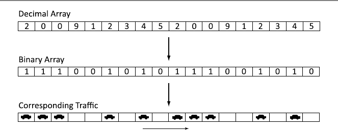
166 9 Suggested Mini Projects
Fig. 9.1 An example to generate and interpret a traffic on a road of length 18
This is the decimal vector that represents the traffic. Then, we convert this vector
into a binary vector by using 1 for even numbers and 0 for odd numbers. Hence, the
corresponding binary vector is
b0=[1,1,1,0,0,1,0,1,0,1,1,1,0,0,1,0,1,0].
Finally, this binary vector is converted into a meaningful traffic scenario. Specifi-
cally, the value 1 indicates that a car exists in a cell, whereas the value 0 indicates
that the cell is empty. Note that there are a total of ncells, either empty or full (i.e.,
occupied by a car). Figure 9.1 depicts how to generate and interpret a traffic on a
road of length 18.
A traffic that we generate as above is an initial (t=0) condition, and we would
like to see what happens in the next time steps, i.e., t=1,2,3,.... We assume that
the traffic flows from left to right with the following simple rules:
•A car can move to the next cell (cell on the right) if the next cell is empty.
•A car cannot move to the next cell (cell on the right) if the next cell is full.
•A car in the last cell disappears in the next time step.
Before writing a program, it is essential to define the rules in an appropriate format.
Since we are interested in the traffic on the road, the rules can be rewritten for each
cell such that a decision chart in Table 9.1 is formed. In this decision chart, the
status of the ith cell (1 <i<n) at time t+1 is written depending on the status
of the (i −1)th, ith, and (i +1)th cells at time t. For example, if bt[i−1]=1,
bt[i]=0, and bt[i+1]=1 and as the time is incremented from tto t+1, the car
at the (i −1)th cell moves to the ith cell, and we have bt+1[i]=1.
Table 9.1 clearly describes the evolution of the traffic as the time goes on. How-
ever, we can easily simplify it by investigating the values in detail. For example,
consider bt[i]=0 (rows 1, 2, 5, and 6). In this case, we note that bt+1[i]=bt[i−1].
This is because if the ith cell is empty at time t, its status at time t+1 directly de-
pends on the status of the previous cell at time t. Specifically, if the previous cell is
empty, then there is no car to move to the ith cell, and the ith cell remains empty. If
the previous cell is occupied by a car, however, that car moves to the ith cell at time
t+1. More importantly, all these movements do not depend on the status of the
www.it-ebooks.info

9.1 Programming Traffic 167
Table 9.1 Decision chart for
the one-dimensional traffic bt[i−1]bt[i]bt[i+1]bt+1[i]
0000
0010
0100
0111
1001
1011
1100
1111
Table 9.2 Short decision
chart for the one-dimensional
traffic
bt[i]bt+1[i]
0bt[i−1]
1bt[i+1]
Table 9.3 Short decision
chart for the first cell bt[1]bt+1[1]
00
1bt[2]
Table 9.4 Short decision
chart for the last cell bt[n]bt+1[n]
0bt[n−1]
10
(i +1)th cell. By using this type of approaches, one can obtain the short decision
chart in Table 9.2.
The decision chart in Table 9.2 (as well as in Table 9.1)isvalidfor1<i<nbut
not for i=1 and i=n. At these boundary cells, separate rules listed in Tables 9.3
and 9.4 must be applied.
Figure 9.2 shows the evolution of the example binary vector from t=0tot=1
and t=1tot=2, as well as the corresponding traffic at t=2.
9.1.2 Main Work 1
(1) Write a program (an R function called initroad) that generates a binary
vector representing a traffic on a road of length 9m, given the value of m.
The program should generate the vector in accordance with the selected id-
number. The output of the program should be this binary vector. Test your
program for different values of m.
www.it-ebooks.info
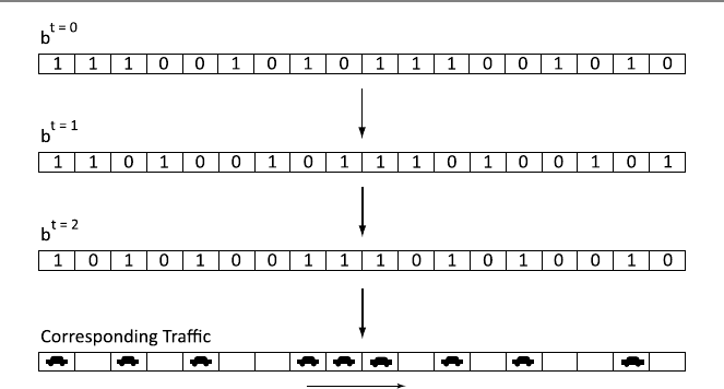
168 9 Suggested Mini Projects
Fig. 9.2 Evolution of the traffic in Fig. 9.1 from t=0tot=2
(2) Write a program (an R function called modifyroad) that modifies a given
binary vector according to the decision charts derived in the preliminary work.
Specifically, the program should take a binary vector representing a traffic as
input. The output should be another binary vector representing the traffic in
the next time step. Test your program for various vectors.
(3) Write a program (an R function called countroad) that counts the number
of ones in a given binary vector. Hence, the output of the program should be
the number of ones. Test your program for various vectors.
(4) Using your programs, perform the following experiment:
(a) Generate a binary vector representing a traffic on a road of length 90
(m=10).
(b) Modify the binary vector and find the status of the traffic at t=
1,2,3,.... Each time step can be considered as an iteration. Perform
iterations until the whole road is empty.
(c) Record the total number of cars at each time step in a file.
(d) Using the output file, make a plot displaying the number of cars as a
function of time steps and observe how the number of cars decays to
zero.
An example plot is shown in Fig. 9.3.
9.1.3 Main Work 2
Consider again one-dimensional traffic problems while the rules at the boundary
cells are changed. Specifically, if there exists a car in the last cell, then, instead of
simply disappearing, it reenters the road from the first cell (if the first cell is already
empty) in the next time step. The decision charts for the boundary cells can be
revised as listed in Tables 9.5 and 9.6.
www.it-ebooks.info
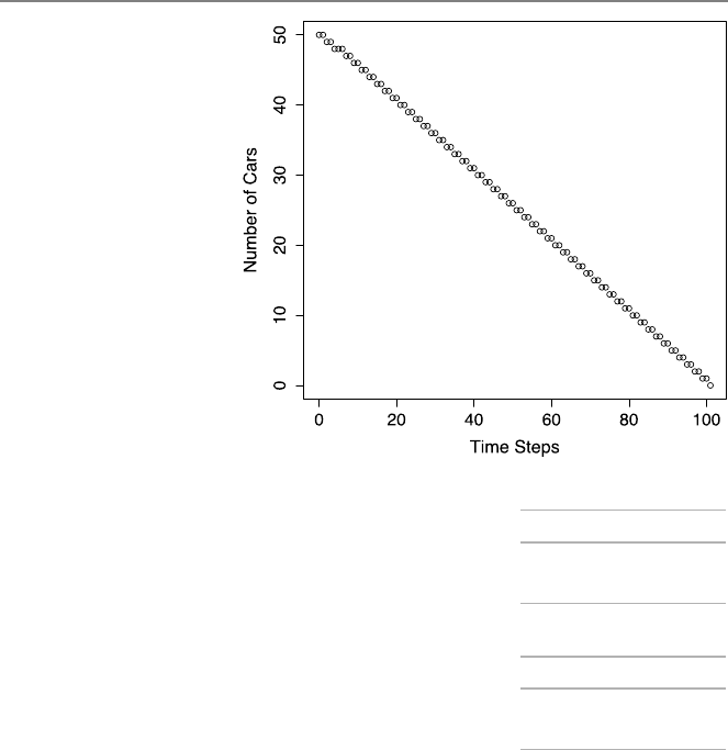
9.1 Programming Traffic 169
Fig. 9.3 Number of cars
versus time steps
Table 9.5 Revised decision
chart for the first cell bt[1]bt+1[1]
0bt[n]
1bt[2]
Table 9.6 Revised decision
chart for the last cell bt[n]bt+1[n]
0bt[n−1]
1bt[1]
(1) Write a program (an R function called modifyroad2) that modifies a given
binary vector according to the revised rules. Similar to the original program,
the program should take a binary vector representing a traffic as input. The
output should be another binary vector representing the traffic in the next time
step. Test your program for various vectors.
(2) Write a program (an R function called compareroads) that compares two
given binary vectors and returns the number cells with different values (zero in
a vector and one in the other). Test your program for various pairs of vectors.
(3) Using your programs, perform the following experiment.
(a) Generate a binary vector representing a traffic on a road of length 90
(m=10).
(b) Modify the binary vector and find the status of the traffic at t=
1,2,3,.... Each time step can be considered as an iteration. Perform
a total of 10 iterations.
(c) Record the number of modified cells at each time step in a file.
www.it-ebooks.info
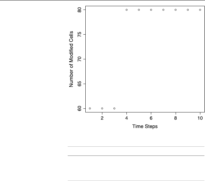
170 9 Suggested Mini Projects
Fig. 9.4 Number of modified
cells versus time steps
Table 9.7 Processing times
required for modifying roads
of different lengths
mMeasured (seconds) Expected (seconds)
1000 0.040 –
2000 0.077 2 ×0.040 =0.080
4000 0.158 4 ×0.040 =0.160
(d) Using the output file, make a plot displaying the number of modified
cells as a function of time steps and observe how the number of modified
cells converges to a value (traffic speed) that depends on the number of
empty cells on the road.
An example plot is shown in Fig. 9.4.
9.1.4 Main Work 3
Consider the solution of one-dimensional traffic problems with the revised rules.
(1) Find the order of the modification program theoretically.
(2) Generate a binary vector representing a traffic on a road of length 9000 (m=
1000). Modify the binary vector and record the time required for this.
(3) Repeat items 1 and 2 for m=2000.
(4) Repeat items 1 and 2 for m=4000.
(5) Analyze your measurements (processing times for m=1000, m=2000, and
m=4000) considering the theoretical order of the modification program.
A sample set of measurements is shown in Table 9.7.
www.it-ebooks.info

9.2 Sorting Words 171
Table 9.8 Conversion of the word “program” to an integer
Letters p r o g r a m
Integers 16 18 15 7 18 1 13
Multiplier 276275274273272271270
Multiplication 6198727824 258280326 7971615 137781 13122 27 13
9.2 Sorting Words
In this project, we write and test some practical programs for reordering a given list
of words according to the alphabetic order. For this purpose, we implement conver-
sion functions between words and numbers, as well as the quick sort algorithm for
the efficient sorting of numbers.
9.2.1 Preliminary Work
There can be different strategies to convert words to numbers and numbers to words.
A valid conversion must be a one-to-one map between words and numbers, i.e., each
word should correspond to a unique number and vice versa. In this project, we use a
simple technique based on converting each letter to its order in the English alphabet.
For example, “a” corresponds to 1, “b” corresponds to 2, “c” corresponds to 3, etc.
To further simplify the conversion, we will assume that a word can have maximum
seven letters.
As an example, consider the word “program” to be converted into a number. Ac-
cording to the alphabet, the numbers corresponding to the letters in “program” are
16 (for p), 18 (for r), 15 (for o), 7 (for g), 18 (for r), 1 (for a), and 13 (for m),
respectively. In order to obtain a unique integer representation for “program”, we
multiply the first number corresponding to the first letter with 276, the second num-
ber corresponding to the second letter with 275, the third number corresponding to
the third letter with 274, the fourth number corresponding to the fourth letter with
273, the fifth number corresponding to the fifth letter with 272, the sixth number
corresponding to the sixth letter with 271, and the seventh number corresponding to
the seventh letter with 270=1. Then, we add the results of these multiplications to
find the integer representation of the word. The operations performed for “program”
are listed in Table 9.8. Note that “program” is uniquely represented by
6198727824+258280326+7971615+137781+13122 +27 +13 =6465130708,
and no other word with seven letters is represented by the same integer.
The conversion described above also works well for words with less than seven
letters. For example, consider the two-letter word “go”. This word can be considered
as a seven-letter word “go ”, with five spaces added at the end. When converting
into numbers, the space character corresponds to the zero value. Since “g” and “o”
www.it-ebooks.info

172 9 Suggested Mini Projects
are the 7th and 15th letters of the alphabet, the integer for the word “go” can be
found as
7×276+15×275+0×274+0×273+0×272+0×271+0×270=2927177028,
which is again a unique representation.
A conversion from words to numbers can be meaningful only when a reverse con-
version exists. Specifically, a method to convert numbers back to words is required.
Using the technique above, the reverse conversion can be described as follows. For
a given integer i, apply the steps consecutively.
•The number corresponding to the first letter can be found as i/276, where ·
represents the floor operation. In other words, i/276is the order of the first
letter in the alphabet.
•Do i=i−i/276×276. If the result is greater than zero, then there is a second
letter, and its order in the alphabet is i/275.
•Do i=i−i/275×275. If the result is greater than zero, then there is a third
letter, and its order in the alphabet is i/274.
•Do i=i−i/274×274. If the result is greater than zero, then there is a fourth
letter, and its order in the alphabet is i/273.
•Do i=i−i/273×273. If the result is greater than zero, then there is a fifth
letter, and its order in the alphabet is i/272.
•Do i=i−i/272×272. If the result is greater than zero, then there is a sixth
letter, and its order in the alphabet is i/271.
•Do i=i−i/271×271. If the result is greater than zero, then there is a seventh
letter, and its order in the alphabet is i/270=i.
As an example, lets apply this algorithm to i=6465130708. It can be found that
i/276=16, and we continue as follows:
•i=i−16 ×276=266402884 and i/275=18.
•i=i−18 ×275=8122558 and i/274=15.
•i=i−15 ×274=150943 and i/273=7.
•i=i−7×273=13162 and i/272=18.
•i=i−18 ×272=40 and i/271=1.
•i=i−1×271=13 and i/270=13.
Hence, the numbers corresponding to the letters are {16,18,15,7,18,1,13}, and the
represented word is “program”.
Next, consider the integer i=2927177028. One can find that i/276=7. Up-
dating as
i=i−i/276×276=215233605,
the next value is i/275=15. Then, the next update, i.e.,
i−i/275×275=0,
leads to a zero value. Hence, after this point, there is no need to continue. The
numbers are {7,15,0,0,0,0,0}, and the corresponding word is “go ”.
www.it-ebooks.info

9.2 Sorting Words 173
9.2.2 Main Work 1
(1) Write a program (an R function called charactertointeger) that con-
verts a given letter from “a” to “z” to an integer from 1 to 26. The program
should take a string of one character as an input. The output should be an in-
teger (1–26) depending on the order of the letter in the English alphabet. The
program should return zero for the space character.
(2) Write a program (an R function called wordtointeger) that converts a
given word to an integer using the rules described in the preliminary work.
The program should take a string of seven letters and give an integer (unique
representation of the word) as the output. The program should use char-
actertointeger implemented in item 1. Test your program for various
words with different lengths.
(3) Write a program (an R function called integertocharacter) that con-
verts a given integer 1 to 26 to a letter from “a” to “z”. The program should
take an integer as an input. The output should be a string of one character
depending on the integer (order in the English alphabet). The program should
return the space character for a zero input.
(4) Write a program (an R function called integertoword) that converts a
given integer to a word using the rules described in the preliminary work.
The program should take an integer as an input. The output should be a
string of seven characters. The program should use integertocharac-
ter implemented in item 3. Test your program for various integers, including
2972915217, 4876069590, 2461131702, 3321154924.
9.2.3 Main Work 2
(1) Generate/write a file of 100 words. The file should be readable in the R en-
vironment. Each word should be written as a new line, i.e., the file should
contain 100 lines. Each word should contain maximum seven letters. If a
word contains less than seven letters, space characters should be added at the
end.
(2) Write a program that sorts the elements of a given vector using the quick
sort algorithm. Specifically, the program should take a vector of integers
as an input. The output should be another or the same vector with sorted
elements (in the ascending order). Use p=n/2as the pivoting strat-
egy. Test your function for various vectors with different sizes and ele-
ments.
(3) Using your programs, perform the following.
(a) Read the data file including 100 words. Put the words into a vector
(“word vector”) of 100 elements.
(b) Convert each word in the “word vector” into an integer. Put the integers
into a vector (“number vector”) of 100 elements.
(c) Sort the “number vector” using the quick sort algorithm. Generate a
“sorted number vector”.
www.it-ebooks.info

174 9 Suggested Mini Projects
(d) Convert each integer in the “sorted number vector” into a word. Put the
words into a vector (“sorted word vector”) of 100 elements.
(e) Write the words in the “sorted word vector” into a data file. Open the
data file generated by the script. Investigate the file carefully and make
sure that words in the input data file are sorted correctly according to
the alphabetic order.
9.3 Designing Systems
In this project, we focus on writing programs to solve linear systems of equations.
Specifically, we consider the Gaussian elimination without pivoting and with partial
pivoting to solve matrix equations. Solutions can be interpreted as inputs that are
required to generate a given set of outputs from a linear system.
9.3.1 Preliminary Work
Consider a linear system involving ninputs and noutputs as depicted in Fig. 9.5.
This system may represent a real-life instrument, such as a linear electronic circuit,
where the inputs and outputs are electrical signals.
In this project, we consider relatively small linear systems involving 9 ×9ma-
trix equations. The matrix elements will be determined by using an id-number as
follows. Let the id-number be 200912345. Then, the first row of the matrix consists
of 2, 0, 0, 9, 1, 2, 3, 4, and 5, respectively. The next row involves the same num-
bers with a shift to the right, i.e., 5, 2, 0, 0, 9, 1, 2, 3, 4. Note that the last element
in the first row is moved to the beginning of the sequence in the second row. The
subsequent rows are formed similarly with regular shifts, leading to a 9 ×9matrix
as
A=
⎡
⎢
⎢
⎢
⎢
⎢
⎢
⎢
⎢
⎢
⎢
⎢
⎢
⎣
200912345
520091234
452009123
345200912
234520091
123452009
912345200
091234520
009123452
⎤
⎥
⎥
⎥
⎥
⎥
⎥
⎥
⎥
⎥
⎥
⎥
⎥
⎦
.
We consider matrix equations involving the matrix derived above (as well as a mod-
ified version) and different right-hand-side vectors.
The aim of the project is as follows. We would like to design a system that can
provide a predetermined set of outputs in a controllable manner. Since the matrix el-
ements are determined as above, the matrix representing the system is already fixed.
However, one can control the output by adjusting the input. Hence, our purpose is
www.it-ebooks.info
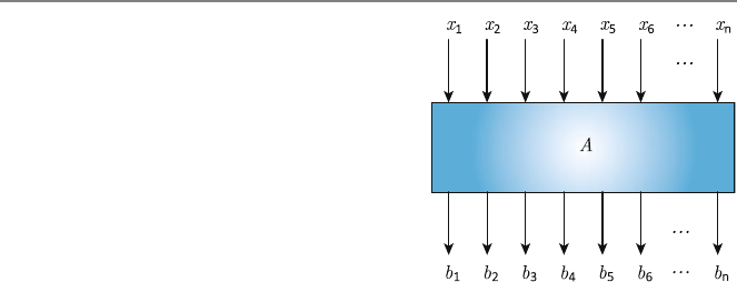
9.3 Designing Systems 175
Fig. 9.5 A system involving
ninputs and noutputs
to find the required set of inputs to obtain a given set of outputs. This requires the
solution of the matrix equations involving the matrix above.
As an example, assume that we would like to find the input values for an output
vector
b(1)=
⎡
⎢
⎢
⎢
⎢
⎢
⎢
⎢
⎢
⎢
⎢
⎢
⎢
⎣
1
0
0
0
0
0
0
0
0
⎤
⎥
⎥
⎥
⎥
⎥
⎥
⎥
⎥
⎥
⎥
⎥
⎥
⎦
.
Solving the matrix equation
Ax(1)=b(1)
gives
x(1)=
⎡
⎢
⎢
⎢
⎢
⎢
⎢
⎢
⎢
⎢
⎢
⎢
⎢
⎣
−3.99
−7.93
−8.39
5.72
0.25
5.89
7.52
4.00
1.30
⎤
⎥
⎥
⎥
⎥
⎥
⎥
⎥
⎥
⎥
⎥
⎥
⎥
⎦
×10−2
with three digits of accuracy. In other words, x(1)is the input required to produce
b(1)as the output. Matrix equations involving a 9 ×9 matrix and a few right-hand-
side vectors can be solved by using the Gaussian elimination. Note that, for larger
matrices, the LU factorization would be better since a single decomposition of a
matrix is sufficient for all solutions with different right-hand-side vectors.
www.it-ebooks.info

176 9 Suggested Mini Projects
9.3.2 Main Work 1
(1) Write a program (an R function called gaussianelimination) that per-
forms the Gaussian elimination without pivoting. Specifically, the program
should take n×(n +1)augmented matrix (including the matrix and the right-
hand-side vector) as an input. The output should be the same augmented ma-
trix after the Gaussian elimination is applied, i.e., an upper-triangular matrix
and the corresponding (modified) right-hand-side vector. Test your program
for various matrix equations.
(2) Write a program (an R function called backwardsub) that performs back-
ward substitution. Specifically, the program should take an n×nupper-
triangular matrix and a right-hand-side vector (they can be augmented, if de-
sired) as inputs. The output should be the solution vector. Test your function
for various matrix equations.
(3) Using your programs, perform the following.
(a) Generate a matrix equation involving a 9×9 matrix. The matrix elements
should be determined as described in the preliminary work. Select an
arbitrary right-hand-side vector involving only ones and zeros.
(b) Apply the Gaussian elimination without pivoting to the matrix equation.
(c) Apply the backward substitution to find the solution of the matrix equa-
tion.
(d) Print out the solution. Note that it contains the input values required to
generate the desired output values.
(e) Check the solution by multiplying it with the matrix and comparing the
result with the right-hand-side vector. Is there any error? Why?
9.3.3 Main Work 2
(1) Write a program (an R function called gaussianelimination
partial) that performs the Gaussian elimination with partial pivoting.
Specifically, the program should take n×(n +1)augmented matrix (including
the matrix and the right-hand-side vector) as an input. The output should be the
same augmented matrix after the Gaussian elimination with partial pivoting
is applied, i.e., an upper-triangular matrix and the corresponding (modified)
right-hand-side vector. Test your program for various matrix equations.
(2) Using your programs, perform the following.
(a) Generate a matrix equation involving a 9×9 matrix. The matrix ele-
ments should be determined as described in the preliminary work, but
with the following modification: Set the diagonal elements to zero. Use
the right-hand-side vector that you use in Main Work 1.
(b) Apply the Gaussian elimination without pivoting to the matrix equation.
(c) Apply the backward substitution to find the solution of the matrix equa-
tion.
(d) Print out the solution. What happened?
www.it-ebooks.info

9.3 Designing Systems 177
(3) Using your programs, perform the following.
(a) Generate a matrix equation involving a 9×9 matrix. The matrix elements
should be determined as described in the preliminary work, but with the
following modification: Set the diagonal elements to zero. Use the right-
hand-side vector that you use in Main Work 1.
(b) Apply the Gaussian elimination with partial pivoting to the matrix equa-
tion.
(c) Apply the backward substitution to find the solution of the matrix equa-
tion.
(d) Print out the solution. Note that it contains the input values required to
generate the desired output values.
(e) Check the solution by multiplying it with the matrix and comparing the
result with the right-hand-side vector. Is there any error? Why?
www.it-ebooks.info

Bibliography
1. Aho AV, Hopcroft JE, Ullman JD (1974) The design and analysis of computer algorithms.
Addison-Wesley, Reading
2. Dijkstra EW (1976) A discipline of programming. Prentice Hall, New York
3. Wirth N (1976) Algorithms +data structures =programs. Prentice Hall, New York
4. Aho AV, Ullman JD, Hopcroft JE (1983) Data structures and algorithms. Addison-Wesley,
Reading
5. Roberts ES (1986) Thinking recursively. Wiley, New York
6. Shackelford RL (1997) Introduction to computing and algorithms. Addison-Wesley, Read-
ing
7. Bentley J (1999) Programming Pearls. Addison-Wesley, Reading
8. Lafore R (2002) Data structures and algorithms in Java. Sams, Indianapolis
9. Johnsonbaugh R, Schaefer M (2003) Algorithms. Prentice Hall, New York
10. Skiena SS, Revilla M (2003) Programming challenges. Springer, Berlin
11. Lee RCT, Tseng SS, Chang RC, Tsai YT (2005) Introduction to the design and analysis of
algorithms. McGraw-Hill, New York
12. Kleinberg J, Tardos E (2005) Algorithm design. Addison-Wesley, Reading
13. Dasgupta S, Papadimitriou C, Vazirani U (2006) Algorithms. McGraw-Hill, New York
14. Levitin A (2006) Introduction to the design and analysis of algorithms. Addison-Wesley,
Reading
15. McConnell J (2007) Analysis of algorithms. Jones & Bartlett, Boston
16. Sedgewick R, Wayne K (2007) Introduction to programming in Java: an interdisciplinary
approach. Addison-Wesley, Reading
17. Skiena SS (2008) The algorithm design manual. Springer, Berlin
18. Heineman GT, Pollice G, Selkow S (2008) Algorithms in a nutshell. O’Reilly Media, Se-
bastopol
19. Wang W (2008) Beginning programming all-in-one desk reference for dummies. For Dum-
mies, New York
20. Cormen TH, Leiserson CE, Rivest RL, Stein C (2009) Introduction to algorithms. MIT
Press, Cambridge
21. Soltys M (2009) An introduction to the analysis of algorithms. World Scientific, Singapore
22. Shen A (2010) Algorithms and programming. Springer, Berlin
23. Bird R (2010) Pearls of functional algorithm design. Cambridge University Press, Cam-
bridge
24. Knuth DE (2011) The art of computer programming. Addison-Wesley, Reading
25. Sedgewick R, Wayne K (2011) Algorithms. Addison-Wesley, Reading
26. Karumanchi N (2011) Data structures and algorithms made easy: data structure and algo-
rithmic puzzles. CreateSpace, New York
27. Shaffer CA (2011) Data structures and algorithm analysis in Java. Dover, New York
Ö. Ergül, Guide to Programming and Algorithms Using R,
DOI 10.1007/978-1-4471-5328-3,
© Springer-Verlag London 2013
179
www.it-ebooks.info

180 Bibliography
28. Chivers I, Sleightholme J (2012) Introduction to programming with Fortran: with coverage
of Fortran 90, 95, 2003, 2008 and 77. Springer, Berlin
29. Crawley MJ (2012) The R book. Wiley, New York
30. Sedgewick R, Flajolet P (2013) An introduction to the analysis of algorithms. Addison-
Wesley, Reading
www.it-ebooks.info

Index
Symbols
1-norm, 13,35,71
2-norm, 32
∞-norm, 22,66
A
Accuracy, 2,87
Algorithm, 1
B
Babylonian method, 30
Backward substitution, 123,138
Banded matrices, 136
Binary search, 49,74
Binomial coefficients, 80
Break, 13,107,156
Bubble sort, 100
C
Cholesky factorization, 139
Closest pair, 26
Column-wise, 25,54
Complexity, 59,63
Computer program, 1
Conditional statement, 6
Constant, 2
D
Depth of recursion, 38
Determinant, 53,142
E
Efficiency, 1,59,77
Euclidean algorithm, 42
F
Fibonacci numbers, 40,78
Floating point, 2,59,88,132
For, 13
Forward substitution, 121
Function, 4
G
Gauss–Jordan elimination, 141,143
Gaussian elimination, 124,137
Geometric series, 30
H
Highest common factor, 42
Horner’s algorithm, 92
I
Infinite loop, 17
Inner product, 60,76,96
Input, 3
Insertion sort, 104
Iterative procedure, 28,80
L
Linear systems of equations, 117
Loop, 13
Lowest common multiple, 43
LU factorization, 128,130,142
M
Matrix, 7
Matrix–matrix multiplication, 70,76,95
Matrix–vector multiplication, 23,67,69,76
N
Nested loop, 23,158
Not-a-number, 17,83,88
O
Order, 59,62,69,71,76
Output, 2
P
Pascal’s triangle, 81
Pivoting, 132
Polynomial evaluation, 91
Programming, 1
Proof by induction, 54
Ö. Ergül, Guide to Programming and Algorithms Using R,
DOI 10.1007/978-1-4471-5328-3,
© Springer-Verlag London 2013
181
www.it-ebooks.info

