Guide To Elliptic Curve Cryptography Eclliptic
User Manual:
Open the PDF directly: View PDF ![]() .
.
Page Count: 332 [warning: Documents this large are best viewed by clicking the View PDF Link!]
- Guide to Elliptic Curve Cryptography
- Contents
- List of Algorithms
- List of Tables
- List of Figures
- Acronyms
- Preface
- 1 Introduction and Overview
- 2 Finite Field Arithmetic
- 3 Elliptic Curve Arithmetic
- 4 Cryptographic Protocols
- 5 Implementation Issues
- A Sample Parameters
- B ECC Standards
- C Software Tools
- Bibliography
- Index

Guide to Elliptic
Curve Cryptography
Darrel Hankerson
Alfred Menezes
Scott Vanstone
Springer
Guide
to
Elliptic Curve Cryptography
Springer
New
York
Berlin
Heidelberg
Hong Kong
London
Milan
Paris
Tokyo
Darrel
Hankerson
Alfred
Menezes
Scott
Vanstone
Guide
to
Elliptic
Curve Cryptography
With
38
Illustrations
Springer
Darrel
Hankcrsnn
Department
of
Mathematics
Auburn
University
Auhuni,
Al.
.36849-5107.
USA
hankedr"1
auburn,
cdu
Scott
Vanslone
Depart
menl
of
Combinatorics
and
Oplimi/.alion
University
of
Waterloo
Waterloo,
Ontario.
N2L 3Gl
Canada
xavansUK"1
LI
Waterloo.ea
Alfred
Menezes
Departmet
of
Combinatories
and
Optimization
University
of
Waterloo
Waterloo.
Ontario,
N2L 3G1
Canada
ajmeneze@uwaterloo.ca
library of
Congress
Calaloging-in-Publication
Data
Hankerson.
Darrel
R.
Guide
to
elliptic
curve
cryptography
/
Darrel
Hankerson,
Alfred
J.
Menezes,
Scott
Vanstone.
p. cm.
Includes
bibliographical
references
and
index.
ISBN
0-387-95273-X
(alk.
paper)
1.
Computer
securiiy.
2.
PuMic
key
cryptography.
I.
Vunsionc,
Scott
A,
11.
Mene/.es.
A. J.
(Alfred J,), 1965- III.
Title,
QA76.9.A25H37
2003
005.8'(2-dc22 2003059137
ISBN
0-387-95273-X
Printed
un
acid-free paper.
(c)
2004
Springer-Verlag
New
York, Inc.
All
riglils
reserved.
This
work
may not Ix1
translated
or
copied
in
wimle
or in pan
without
the
written
permission
ol'I
he
puhlishi-r
I
Springer-VL-rlag
New
York, Inc.,
175
I-'ifth
Avenue,
New
York,
NY
10010,USA
J,
except
for brief
excerpts
in
connection
with
reviews
or
scholarly
analysis.
Use in
connection
with
any
form
of
information
storage
and
reltrieval,
electronic adaption, computer software,
or by
similar
or
dissimilar methodology
now
known
01
hereafter
developed
is
forbidden.
The use in
this
publication
of
trade
names, trademarks, service marks,
and
similar terms, even
if
they
are not
identified
as
such,
is not to be
taken
as an
expression
of
opinion
as to
whedier
or not
they
are
subject
to
proprietary
rights.
Printed
m the
United
States
of
America. (HAM)
987654321
SPIN 10832297
Springer-Vcrlag
is a
part
of '
Springer
science+Business
Media
springeronline.com
Contents
List of Algorithms ix
List of Tables xiv
List of Figures xvi
Acronyms xvii
Preface xix
1 Introduction and Overview 1
1.1 Cryptographybasics .......................... 2
1.2 Public-keycryptography ........................ 6
1.2.1 RSAsystems .......................... 6
1.2.2 Discretelogarithmsystems................... 8
1.2.3 Elliptic curve systems ..................... 11
1.3 Why elliptic curve cryptography? . . . ................. 15
1.4 Roadmap ................................ 19
1.5 Notesandfurtherreferences ...................... 21
2 Finite Field Arithmetic 25
2.1 Introduction to finite fields ....................... 25
2.2 Primefieldarithmetic.......................... 29
2.2.1 Addition and subtraction . . . ................. 30
2.2.2 Integer multiplication ...................... 31
2.2.3 Integersquaring ........................ 34
2.2.4 Reduction............................ 35
2.2.5 Inversion ............................ 39
2.2.6 NISTprimes .......................... 44
vi Contents
2.3 Binaryfieldarithmetic ......................... 47
2.3.1 Addition ............................ 47
2.3.2 Multiplication . . . ....................... 48
2.3.3 Polynomial multiplication . . ................. 48
2.3.4 Polynomial squaring ...................... 52
2.3.5 Reduction............................ 53
2.3.6 Inversionanddivision ..................... 57
2.4 Optimalextensionfieldarithmetic ................... 62
2.4.1 Addition and subtraction . . . ................. 63
2.4.2 Multiplication and reduction . ................. 63
2.4.3 Inversion ............................ 67
2.5 Notesandfurtherreferences ...................... 69
3 Elliptic Curve Arithmetic 75
3.1 Introduction to elliptic curves ...................... 76
3.1.1 SimplifiedWeierstrassequations................ 78
3.1.2 Grouplaw............................ 79
3.1.3 Grouporder........................... 82
3.1.4 Groupstructure......................... 83
3.1.5 Isomorphismclasses ...................... 84
3.2 Pointrepresentationandthegrouplaw................. 86
3.2.1 Projectivecoordinates ..................... 86
3.2.2 The elliptic curve y2=x3+ax +b.............. 89
3.2.3 The elliptic curve y2+xy =x3+ax2+b........... 93
3.3 Point multiplication ........................... 95
3.3.1 Unknown point . . ....................... 96
3.3.2 Fixedpoint ........................... 103
3.3.3 Multiple point multiplication . ................. 109
3.4 Koblitz curves . . ............................ 114
3.4.1 The Frobenius map and the ring Z[τ]............. 114
3.4.2 Point multiplication ....................... 119
3.5 Curves with efficiently computable endomorphisms . . . ....... 123
3.6 Point multiplication using halving . . ................. 129
3.6.1 Pointhalving .......................... 130
3.6.2 Performingpointhalvingefficiently.............. 132
3.6.3 Point multiplication ....................... 137
3.7 Point multiplication costs . ....................... 141
3.8 Notesandfurtherreferences ...................... 147
Contents vii
4 Cryptographic Protocols 153
4.1 The elliptic curve discrete logarithm problem . ............ 153
4.1.1 Pohlig-Hellmanattack ..................... 155
4.1.2 Pollard’srhoattack....................... 157
4.1.3 Index-calculusattacks ..................... 165
4.1.4 Isomorphismattacks ...................... 168
4.1.5 Relatedproblems........................ 171
4.2 Domainparameters........................... 172
4.2.1 Domainparametergenerationandvalidation ......... 173
4.2.2 Generating elliptic curves verifiably at random . ....... 175
4.2.3 Determining the number of points on an elliptic curve . . . . 179
4.3 Keypairs ................................ 180
4.4 Signatureschemes ........................... 183
4.4.1 ECDSA............................. 184
4.4.2 EC-KCDSA .......................... 186
4.5 Public-keyencryption.......................... 188
4.5.1 ECIES ............................. 189
4.5.2 PSEC .............................. 191
4.6 Keyestablishment............................ 192
4.6.1 Station-to-station........................ 193
4.6.2 ECMQV ............................ 195
4.7 Notesandfurtherreferences ...................... 196
5 Implementation Issues 205
5.1 Softwareimplementation........................ 206
5.1.1 Integerarithmetic........................ 206
5.1.2 Floating-pointarithmetic.................... 209
5.1.3 SIMDandfieldarithmetic ................... 213
5.1.4 Platformmiscellany ...................... 215
5.1.5 Timings............................. 219
5.2 Hardwareimplementation ....................... 224
5.2.1 Designcriteria ......................... 226
5.2.2 Fieldarithmeticprocessors................... 229
5.3 Secureimplementation ......................... 238
5.3.1 Poweranalysisattacks ..................... 239
5.3.2 Electromagneticanalysisattacks................ 244
5.3.3 Errormessageanalysis..................... 244
5.3.4 Faultanalysisattacks...................... 248
5.3.5 Timingattacks ......................... 250
5.4 Notesandfurtherreferences ...................... 250
viii Contents
A Sample Parameters 257
A.1 Irreducible polynomials . . ....................... 257
A.2 Elliptic curves . . ............................ 261
A.2.1 Random elliptic curves over Fp................ 261
A.2.2 Random elliptic curves over F2m................ 263
A.2.3 Koblitz elliptic curves over F2m................ 263
B ECC Standards 267
C Software Tools 271
C.1 General-purposetools.......................... 271
C.2 Libraries................................. 273
Bibliography 277
Index 305
List of Algorithms
1.1 RSAkeypairgeneration .......................... 7
1.2 BasicRSAencryption............................ 7
1.3 BasicRSAdecryption............................ 7
1.4 BasicRSAsignaturegeneration ...................... 8
1.5 BasicRSAsignatureverification...................... 8
1.6 DLdomainparametergeneration...................... 9
1.7 DLkeypairgeneration ........................... 9
1.8 BasicElGamalencryption ......................... 10
1.9 BasicElGamaldecryption ......................... 10
1.10DSAsignaturegeneration.......................... 11
1.11DSAsignatureverification ......................... 11
1.12 Elliptic curve key pair generation ...................... 14
1.13 Basic ElGamal elliptic curve encryption . ................. 14
1.14 Basic ElGamal elliptic curve decryption . ................. 14
2.5 Multiprecision addition ........................... 30
2.6 Multiprecision subtraction . . ....................... 30
2.7 Addition in Fp............................... 31
2.8 Subtraction in Fp.............................. 31
2.9 Integer multiplication (operand scanning form) . . ............ 31
2.10 Integer multiplication (product scanning form) . . . ............ 32
2.13Integersquaring............................... 35
2.14Barrettreduction .............................. 36
2.17 Montgomery exponentiation (basic) . . . ................. 38
2.19ExtendedEuclideanalgorithmforintegers................. 40
2.20 Inversion in FpusingtheextendedEuclideanalgorithm.......... 40
2.21Binarygcdalgorithm ............................ 41
2.22 Binary algorithm for inversion in Fp.................... 41
2.23 Partial Montgomery inversion in Fp.................... 42
x List of Algorithms
2.25 Montgomery inversion in Fp........................ 43
2.26Simultaneousinversion........................... 44
2.27 Fast reduction modulo p192 =2192 −264 −1................ 45
2.28 Fast reduction modulo p224 =2224 −296 +1................ 45
2.29 Fast reduction modulo p256 =2256 −2224 +2192 +296 −1 ........ 46
2.30 Fast reduction modulo p384 =2384 −2128 −296 +232 −1......... 46
2.31 Fast reduction modulo p521 =2521 −1................... 46
2.32 Addition in F2m............................... 47
2.33 Right-to-left shift-and-add field multiplication in F2m........... 48
2.34 Right-to-left comb method for polynomial multiplication . . ....... 49
2.35 Left-to-right comb method for polynomial multiplication . . ....... 50
2.36 Left-to-right comb method with windows of width w........... 50
2.39 Polynomial squaring ............................ 53
2.40 Modular reduction (one bit at a time) . . . ................. 53
2.41 Fast reduction modulo f(z)=z163 +z7+z6+z3+1........... 55
2.42 Fast reduction modulo f(z)=z233 +z74 +1................ 55
2.43 Fast reduction modulo f(z)=z283 +z12 +z7+z5+1 .......... 56
2.44 Fast reduction modulo f(z)=z409 +z87 +1................ 56
2.45 Fast reduction modulo f(z)=z571 +z10 +z5+z2+1 .......... 56
2.47 Extended Euclidean algorithm for binary polynomials ........... 58
2.48 Inversion in F2musingtheextendedEuclideanalgorithm ......... 58
2.49 Binary algorithm for inversion in F2m................... 59
2.50 Almost Inverse Algorithm for inversion in F2m............... 60
2.54 Reduction modulo M=Bn−c....................... 64
2.59OEFinversion................................ 69
3.21 Point doubling (y2=x3−3x+b,Jacobiancoordinates) ......... 91
3.22 Point addition (y2=x3−3x+b,affine-Jacobiancoordinates) ...... 91
3.23 Repeated point doubling (y2=x3−3x+b, Jacobian coordinates) . . . . . 93
3.24 Point doubling (y2+xy=x3+ax2+b,a∈{0,1}, LD coordinates) . . . . . 94
3.25 Point addition (y2+xy=x3+ax2+b,a∈{0,1}, LD-affine coordinates) . . 95
3.26 Right-to-left binary method for point multiplication ............ 96
3.27 Left-to-right binary method for point multiplication ............ 97
3.30ComputingtheNAFofapositiveinteger.................. 98
3.31 Binary NAF method for point multiplication ................ 99
3.35 Computing the width-wNAFofapositiveinteger............. 100
3.36 Window NAF method for point multiplication . . . ............ 100
3.38 Sliding window method for point multiplication . . ............ 101
3.40 Montgomery point multiplication (for elliptic curves over F2m)...... 103
3.41 Fixed-base windowing method for point multiplication . . . ....... 104
3.42 Fixed-base NAF windowing method for point multiplication ....... 105
3.44 Fixed-base comb method for point multiplication . ............ 106
List of Algorithms xi
3.45 Fixed-base comb method (with two tables) for point multiplication . . . . 106
3.48 Simultaneous multiple point multiplication ................. 109
3.50Jointsparseform .............................. 111
3.51InterleavingwithNAFs........................... 112
3.61 Computing the TNAF of an element in Z[τ]................ 117
3.62 Division in Z[τ]............................... 118
3.63 Rounding off in Z[τ]............................ 118
3.65 Partial reduction modulo δ=(τ m−1)/(τ −1).............. 119
3.66 TNAF method for point multiplication on Koblitz curves . . ....... 119
3.69 Computing a width-wTNAF of an element in Z[τ]............ 123
3.70 Window TNAF point multiplication method for Koblitz curves ...... 123
3.74 Balanced length-two representation of a multiplier . ............ 127
3.77 Point multiplication with efficiently computable endomorphisms . . . . . 129
3.81Pointhalving ................................ 131
3.85 Solve x2+x=c(basicversion) ...................... 133
3.86 Solve x2+x=c.............................. 134
3.91 Halve-and-add w-NAF (right-to-left) point multiplication . . ....... 138
3.92 Halve-and-add w-NAF (left-to-right) point multiplication . . ....... 139
4.3 Pollard’srhoalgorithmfortheECDLP(singleprocessor)......... 159
4.5 ParallelizedPollard’srhoalgorithmfortheECDLP ............ 161
4.14Domainparametergeneration........................ 174
4.15Explicitdomainparametervalidation.................... 175
4.17 Generating a random elliptic curve over a prime field Fp......... 176
4.18 Verifying that an elliptic curve over Fpwas randomly generated . . . . . 176
4.19 Generating a random elliptic curve over a binary field F2m........ 177
4.21 Verifying that an elliptic curve over F2mwas randomly generated . . . . . 177
4.22 Generating a random elliptic curve over an OEF Fpm........... 178
4.23 Verifying that an elliptic curve over Fpmwas randomly generated . . . . . 178
4.24Keypairgeneration............................. 180
4.25Publickeyvalidation ............................ 181
4.26Embeddedpublickeyvalidation ...................... 181
4.29ECDSAsignaturegeneration........................ 184
4.30ECDSAsignatureverification ....................... 184
4.36EC-KCDSAsignaturegeneration...................... 187
4.37EC-KCDSAsignatureverification ..................... 187
4.42ECIESencryption.............................. 189
4.43ECIESdecryption.............................. 190
4.47PSECencryption .............................. 191
4.48PSECdecryption .............................. 191
4.50Station-to-stationkeyagreement ...................... 194
4.51ECMQVkeyagreement........................... 195
xii List of Algorithms
5.3 Most significant bit first (MSB) multiplier for F2m............. 230
5.4 Least significant bit first (LSB) multiplier for F2m............. 231
5.5 Digit-serial multiplier for F2m....................... 234
5.6 Inversion in F2m(modd) . . . ....................... 237
5.7 SPA-resistant left-to-right binary point multiplication ........... 242
5.8 RSA-OAEPencryption........................... 246
5.9 RSA-OAEPdecryption........................... 247
A.1 Testing a polynomial for irreducibility . . ................. 258
List of Tables
1.1 RSA,DLandECkeysizesforequivalentsecuritylevels ......... 19
2.1 OEFexampleparameters.......................... 62
2.2 ComputationaldetailsforinversioninOEFs................ 68
2.3 ComputationaldetailsforinversioninOEFs................ 68
3.1 Admissible orders of elliptic curves over F37 ................ 83
3.2 Isomorphism classes of elliptic curves over F5............... 85
3.3 Operation counts for arithmetic on y2=x3−3x+b........... 92
3.4 Operation counts for arithmetic on y2+xy =x3+ax2+b........ 96
3.5 Point addition cost in sliding versus window NAF methods . ....... 102
3.6 Operation counts for computing kP+lQ ................. 113
3.7 Operation counts in comb and interleaving methods ............ 113
3.8 Koblitz curves with almost-prime group order . . . ............ 115
3.9 Expressions for αu(for the Koblitz curve E0) ............... 121
3.10 Expressions for αu(for the Koblitz curve E1) ............... 122
3.11 Operation counts for point multiplication (random curve over F2163 ) . . . 140
3.12 Point multiplication costs for P-192 . . . ................. 143
3.13 Point multiplication costs for B-163 and K-163 . . ............ 145
3.14 Point multiplication timings for P-192, B-163, and K-163 . . ....... 146
5.1 Partial history and features of the Intel IA-32 family of processors . . . . 207
5.2 Instruction latency/throughput for Pentium II/III vs Pentium 4 ...... 208
5.3 Timingsforfieldarithmetic(binaryvsprimevsOEF)........... 220
5.4 Timingsforbinaryfieldarithmetic..................... 221
5.5 Timingsforprimefieldarithmetic ..................... 221
5.6 Multiplication and inversion times ..................... 222
5.7 Multiplication times for the NIST prime p224 =2224 −296 +1 ...... 224
5.8 Priorities for hardware design criteria . . ................. 229
5.9 Operation counts for inversion via multiplication in binary fields . . . . . 238
xiv List of Tables
A.1 Irreducible binary polynomials of degree m,2≤m≤300. . ....... 259
A.2 Irreducible binary polynomials of degree m, 301 ≤m≤600. ....... 260
A.3 NIST-recommended random elliptic curves over prime fields. ....... 262
A.4 NIST-recommended random elliptic curves over binary fields. ...... 264
A.5 NIST-recommended Koblitz curves over binary fields. ........... 265
B.1 ECCstandardsanddraftstandards ..................... 268
B.2 URLs for standards bodies and working groups. . . ............ 268
List of Figures
1.1 Basiccommunicationsmodel........................ 2
1.2 Symmetric-keyversuspublic-keycryptography .............. 4
2.1 Representingaprime-fieldelementasanarrayofwords.......... 29
2.2 Depth-2 splits for 224-bit integers (Karatsuba-Ofman multiplication) . . . 33
2.3 Depth-2 splits for 192-bit integers (Karatsuba-Ofman multiplication) . . . 34
2.4 Representingabinary-fieldelementasanarrayofwords ......... 47
2.5 Right-to-left comb method for polynomial multiplication . . ....... 49
2.6 Left-to-right comb method for polynomial multiplication . . ....... 49
2.7 Left-to-right comb method with windows of width w........... 51
2.8 Squaring a binary polynomial . ....................... 52
2.9 Reduction of a word modulo f(z)=z163 +z7+z6+z3+1........ 54
3.1 ECDSA support modules . . . ....................... 75
3.2 Elliptic curves over the real numbers . . . ................. 77
3.3 Geometric addition and doubling of elliptic curve points . . ....... 80
3.4 Montgomery point multiplication ...................... 103
3.5 Fixed-base comb method for point multiplication . ............ 107
3.6 The exponent array in Lim-Lee combing methods . ............ 108
3.7 Simultaneous point multiplication accumulation step ........... 109
3.8 InterleavingwithNAFs........................... 112
4.1 IllustrationofPollard’srhoalgorithm ................... 158
4.2 IllustrationofparallelizedPollard’srhoalgorithm............. 162
5.1 Splitting of a 64-bit floating-point number ................. 211
5.2 Hierarchy of operations in elliptic curve cryptographic schemes ...... 226
5.3 Elliptic curve processor architecture . . . ................. 227
5.4 Most significant bit first (MSB) multiplier for F25............. 231
5.5 Least significant bit first (LSB) multiplier for F25............. 232
xvi List of Figures
5.6 MSB multiplier with fixed reduction polynomial . . ............ 232
5.7 MSB multiplier for fields F2mwith 1 ≤m≤10 .............. 233
5.8 MSB multiplier for fields F25,F27,andF210 ................ 234
5.9 Multiplicand in a 2-digit multiplier for F25................. 235
5.10 A 2-digit multiplier for F25......................... 235
5.11 Squaring circuit for F27with fixed reduction polynomial . . ....... 236
5.12CMOSlogicinverter ............................ 239
5.13 Power trace for a sequence of addition and double operations ....... 240
5.14 Power trace for SPA-resistant elliptic curve operations ........... 241
5.15OAEPencodingfunction .......................... 246
5.16OAEPdecodingfunction .......................... 247
Acronyms
AES Advanced Encryption Standard
AIA Almost Inverse Algorithm
ANSI American National Standards Institute
ASIC Application-Specific Integrated Circuit
BEA Binary Extended Algorithm
DES Data Encryption Standard
DH Diffie-Hellman
DHP Diffie-Hellman Problem
DL Discrete Logarithm
DLP Discrete Logarithm Problem
DPA Differential Power Analysis
DSA Digital Signature Algorithm
DSS Digital Signature Standard
ECC Elliptic Curve Cryptography
ECDDHP Elliptic Curve Decision Diffie-Hellman Problem
ECDH Elliptic Curve Diffie-Hellman
ECDHP Elliptic Curve Diffie-Hellman Problem
ECDLP Elliptic Curve Discrete Logarithm Problem
ECDSA Elliptic Curve Digital Signature Algorithm
ECIES Elliptic Curve Integrated Encryption Scheme
EC-KCDSA Elliptic Curve Korean Certificate-based Digital Signature Algorithm
ECMQV Elliptic Curve Menezes-Qu-Vanstone
EEA Extended Euclidean Algorithm
FIPS Federal Information Processing Standards
FPGA Field-Programmable Gate Array
gcd Greatest Common Divisor
GHS Gaudry-Hess-Smart
GMR Goldwasser-Micali-Rivest
HCDLP Hyperelliptic Curve Discrete Logarithm Problem
xviii Acronyms
HMAC Hash-based Message Authentication Code
IEC International Electrotechnical Commission
IEEE Institute of Electrical and Electronics Engineers
IFP Integer Factorization Problem
ISO International Organization for Standardization
JSF Joint Sparse Form
KDF Key Derivation Function
KEM Key Encapsulation Mechanism
LD L´opez-Dahab
MAC Message Authentication Code
NAF Non-Adjacent Form
NESSIE New European Schemes for Signatures, Integrity and Encryption
NFS Number Field Sieve
NIST National Institute of Standards and Technology
OEF Optimal Extension Field
PKI Public-Key Infrastructure
PSEC Provably Secure Elliptic Curve encryption
RSA Rivest-Shamir-Adleman
SEC Standards for Efficient Cryptography
SECG Standards for Efficient Cryptography Group
SHA-1 Secure Hash Algorithm (revised)
SIMD Single-Instruction Multiple-Data
SPA Simple Power Analysis
SSL Secure Sockets Layer
STS Station-To-Station
TLS Transport Layer Security
TNAF τ-adic NAF
VLSI Very Large Scale Integration
Preface
The study of elliptic curves by algebraists, algebraic geometers and number theorists
dates back to the middle of the nineteenth century. There now exists an extensive liter-
ature that describes the beautiful and elegant properties of these marvelous objects. In
1984, Hendrik Lenstra described an ingenious algorithm for factoring integers that re-
lies on properties of elliptic curves. This discovery prompted researchers to investigate
other applications of elliptic curves in cryptography and computational number theory.
Public-key cryptography was conceived in 1976 by Whitfield Diffie and Martin Hell-
man. The first practical realization followed in 1977 when Ron Rivest, Adi Shamir and
Len Adleman proposed their now well-known RSA cryptosystem, in which security is
based on the intractability of the integer factorization problem. Elliptic curve cryptog-
raphy (ECC) was discovered in 1985 by Neal Koblitz and Victor Miller. Elliptic curve
cryptographic schemes are public-key mechanisms that provide the same functional-
ity as RSA schemes. However, their security is based on the hardness of a different
problem, namely the elliptic curve discrete logarithm problem (ECDLP). Currently
the best algorithms known to solve the ECDLP have fully exponential running time,
in contrast to the subexponential-time algorithms known for the integer factorization
problem. This means that a desired security level can be attained with significantly
smaller keys in elliptic curve systems than is possible with their RSA counterparts.
For example, it is generally accepted that a 160-bit elliptic curve key provides the same
level of security as a 1024-bit RSA key. The advantages that can be gained from smaller
key sizes include speed and efficient use of power, bandwidth, and storage.
Audience This book is intended as a guide for security professionals, developers, and
those interested in learning how elliptic curve cryptography can be deployed to secure
applications. The presentation is targeted to a diverse audience, and generally assumes
no more than an undergraduate degree in computer science, engineering, or mathemat-
ics. The book was not written for theoreticians as is evident from the lack of proofs for
mathematical statements. However, the breadth of coverage and the extensive surveys
of the literature at the end of each chapter should make it a useful resource for the
researcher.
xx Preface
Overview The book has a strong focus on efficient methods for finite field arithmetic
(Chapter 2) and elliptic curve arithmetic (Chapter 3). Next, Chapter 4 surveys the
known attacks on the ECDLP, and describes the generation and validation of domain
parameters and key pairs, and selected elliptic curve protocols for digital signature,
public-key encryption and key establishment. We chose not to include the mathemat-
ical details of the attacks on the ECDLP, or descriptions of algorithms for counting
the points on an elliptic curve, because the relevant mathematics is quite sophisticated.
(Presenting these topics in a readable and concise form is a formidable challenge post-
poned for another day.) The choice of material in Chapters 2, 3 and 4 was heavily
influenced by the contents of ECC standards that have been developed by accred-
ited standards bodies, in particular the FIPS 186-2 standard for the Elliptic Curve
Digital Signature Algorithm (ECDSA) developed by the U.S. government’s National
Institute for Standards and Technology (NIST). Chapter 5 details selected aspects of
efficient implementations in software and hardware, and also gives an introduction to
side-channel attacks and their countermeasures. Although the coverage in Chapter 5
is admittedly narrow, we hope that the treatment provides a glimpse of engineering
considerations faced by software developers and hardware designers.
Acknowledgements We gratefully acknowledge the following people who provided
valuable comments and advice: Mike Brown, Eric Fung, John Goyo, Rick Hite, Rob
Lambert, Laurie Law, James Muir, Arash Reyhani-Masoleh, Paul Schellenberg, Adrian
Tang, Edlyn Teske, and Christof Zalka. A special thanks goes to Helen D’Souza, whose
artwork graces several pages of this book. Thanks also to Cindy Hankerson and Sherry
Shannon-Vanstone for suggestions on the general theme of “curves in nature” rep-
resented in the illustrations. Finally, we would like to thank our editors at Springer,
Wayne Wheeler and Wayne Yuhasz, for their continued encouragement and support.
Updates, errata, and our contact information are available at our web site: http://
www.cacr.math.uwaterloo.ca/ecc/. We would greatly appreciate that readers inform us
of the inevitable errors and omissions they may find.
Darrel R. Hankerson, Alfred J. Menezes, Scott A. Vanstone
Auburn & Waterloo
July 2003

CHAPTER 1
Introduction and Overview
Elliptic curves have a rich and beautiful history, having been studied by mathematicians
for over a hundred years. They have been used to solve a diverse range of problems. One
example is the congruent number problem that asks for a classification of the positive
integers occurring as the area of some right-angled triangle, the lengths of whose sides
are rational numbers. Another example is proving Fermat’s Last Theorem which states
that the equation xn+yn=znhas no nonzero integer solutions for x,yand zwhen the
integer nis greater than 2.
In 1985, Neal Koblitz and Victor Miller independently proposed using elliptic curves
to design public-key cryptographic systems. Since then an abundance of research has
been published on the security and efficient implementation of elliptic curve cryptogra-
phy. In the late 1990’s, elliptic curve systems started receiving commercial acceptance
when accredited standards organizations specified elliptic curve protocols, and private
companies included these protocols in their security products.
The purpose of this chapter is to explain the advantages of public-key cryptography
over traditional symmetric-key cryptography, and, in particular, to expound the virtues
of elliptic curve cryptography. The exposition is at an introductory level. We provide
more detailed treatments of the security and efficient implementation of elliptic curve
systems in subsequent chapters.
We begin in §1.1 with a statement of the fundamental goals of cryptography and
a description of the essential differences between symmetric-key cryptography and
public-key cryptography. In §1.2, we review the RSA, discrete logarithm, and ellip-
tic curve families of public-key systems. These systems are compared in §1.3 in which
we explain the potential benefits offered by elliptic curve cryptography. A roadmap for
the remainder of this book is provided in §1.4. Finally, §1.5 contains references to the
cryptographic literature.
2 1. Introduction and Overview
1.1 Cryptography basics
Cryptography is about the design and analysis of mathematical techniques that enable
secure communications in the presence of malicious adversaries.
Basic communications model
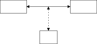
In Figure 1.1, entities A(Alice) and B(Bob) are communicating over an unsecured
channel. We assume that all communications take place in the presence of an adversary
E(Eve) whose objective is to defeat any security services being provided to Aand B.
E
AB
unsecured channel
Figure 1.1. Basic communications model.
For example, Aand Bcould be two people communicating over a cellular telephone
network, and Eis attempting to eavesdrop on their conversation. Or, Acould be the
web browser of an individual ˜
Awho is in the process of purchasing a product from
an online store ˜
Brepresented by its web site B. In this scenario, the communications
channel is the Internet. An adversary Ecould attempt to read the traffic from Ato B
thus learning ˜
A’s credit card information, or could attempt to impersonate either ˜
Aor
˜
Bin the transaction. As a third example, consider the situation where Ais sending
an email message to Bover the Internet. An adversary Ecould attempt to read the
message, modify selected portions, or impersonate Aby sending her own messages
to B. Finally, consider the scenario where Ais a smart card that is in the process
of authenticating its holder ˜
Ato the mainframe computer Bat the headquarters of a
bank. Here, Ecould attempt to monitor the communications in order to obtain ˜
A’s
account information, or could try to impersonate ˜
Ain order to withdraw funds from
˜
A’s account. It should be evident from these examples that a communicating entity
is not necessarily a human, but could be a computer, smart card, or software module
acting on behalf of an individual or an organization such as a store or a bank.
Security goals
Careful examination of the scenarios outlined above reveals the following fundamental
objectives of secure communications:
1. Confidentiality: keeping data secret from all but those authorized to see
it—messages sent by Ato Bshould not be readable by E.
1.1. Cryptography basics 3
2. Data integrity: ensuring that data has not been altered by unauthorized means—
Bshould be able to detect when data sent by Ahas been modified by E.
3. Data origin authentication: corroborating the source of data—Bshould be able
to verify that data purportedly sent by Aindeed originated with A.
4. Entity authentication: corroborating the identity of an entity—Bshould be
convinced of the identity of the other communicating entity.
5. Non-repudiation: preventing an entity from denying previous commitments or
actions—when Breceives a message purportedly from A, not only is Bcon-
vinced that the message originated with A,butBcan convince a neutral third
party of this; thus Acannot deny having sent the message to B.
Some applications may have other security objectives such as anonymity of the
communicating entities or access control (the restriction of access to resources).
Adversarial model
In order to model realistic threats faced by Aand B, we generally assume that the
adversary Ehas considerable capabilities. In addition to being able to read all data
transmitted over the channel, Ecan modify transmitted data and inject her own data.
Moreover, Ehas significant computational resources at her disposal. Finally, com-
plete descriptions of the communications protocols and any cryptographic mechanisms
deployed (except for secret keying information) are known to E. The challenge to cryp-
tographers is to design mechanisms to secure the communications in the face of such
powerful adversaries.
Symmetric-key cryptography
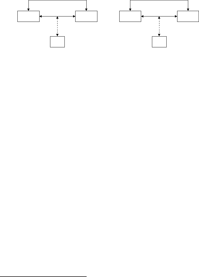
Cryptographic systems can be broadly divided into two kinds. In symmetric-key
schemes, depicted in Figure 1.2(a), the communicating entities first agree upon keying
material that is both secret and authentic. Subsequently, they may use a symmetric-key
encryption scheme such as the Data Encryption Standard (DES), RC4, or the Advanced
Encryption Standard (AES) to achieve confidentiality. They may also use a message au-
thentication code (MAC) algorithm such as HMAC to achieve data integrity and data
origin authentication.
For example, if confidentiality were desired and the secret key shared by Aand B
were k,thenAwould encrypt a plaintext message musing an encryption function ENC
and the key kand transmit the resulting ciphertext c=ENCk(m)to B. On receiving c,
Bwould use the decryption function DEC and the same key kto recover m=DECk(c).
If data integrity and data origin authentication were desired, then Aand Bwould first
agree upon a secret key k,afterwhichAwould compute the authentication tag t=
MACk(m)of a plaintext message musing a MAC algorithm and the key k.Awould
then send mand tto B. On receiving mand t,Bwould use the MAC algorithm and
the same key kto recompute the tag t=MACk(m)of mand accept the message as
having originated from Aif t=t.
4 1. Introduction and Overview
E
AB
unsecured channel
secret and authenticated channel
(a) Symmetric-key cryptography
E
AB
unsecured channel
authenticated channel
(b) Public-key cryptography
Figure 1.2. Symmetric-key versus public-key cryptography.
Key distribution and management The major advantage of symmetric-key cryptog-
raphy is high efficiency; however, there are significant drawbacks to these systems.
One primary drawback is the so-called key distribution problem—the requirement for
a channel that is both secret and authenticated for the distribution of keying material.
In some applications, this distribution may be conveniently done by using a physi-
cally secure channel such as a trusted courier. Another way is to use the services of an
on-line trusted third-party who initially establishes secret keys with all the entities in
a network and subsequently uses these keys to securely distribute keying material to
communicating entities when required.1Solutions such as these may be well-suited to
environments where there is an accepted and trusted central authority, but are clearly
impractical in applications such as email over the Internet.
A second drawback is the key management problem—in a network of Nentities,
each entity may have to maintain different keying material with each of the other N−1
entities. This problem can be alleviated by using the services of an on-line trusted third-
party that distributes keying material as required, thereby reducing the need for entities
to securely store multiple keys. Again, however, such solutions are not practical in
some scenarios. Finally, since keying material is shared between two (or more) entities,
symmetric-key techniques cannot be used to devise elegant digital signature schemes
that provide non-repudiation services. This is because it is impossible to distinguish
between the actions taken by the different holders of a secret key.2
Public-key cryptography
The notion of public-key cryptography, depicted in Figure 1.2(b), was introduced in
1975 by Diffie, Hellman and Merkle to address the aforementioned shortcomings
1This approach of using a centralized third-party to distribute keys for symmetric-key algorithms
to parties as they are needed is used by the Kerberos network authentication protocol for client/server
applications.
2Digital signatures schemes can be designed using symmetric-key techniques; however, these schemes
are generally impractical as they require the use of an on-line trusted third party or new keying material for
each signature.
1.1. Cryptography basics 5
of symmetric-key cryptography. In contrast to symmetric-key schemes, public-key
schemes require only that the communicating entities exchange keying material that
is authentic (but not secret). Each entity selects a single key pair (e,d)consisting of a
public key e, and a related private key d (that the entity keeps secret). The keys have the
property that it is computationally infeasible to determine the private key solely from
knowledge of the public key.
Confidentiality If entity Awishes to send entity Ba confidential message m, she ob-
tains an authentic copy of B’s public key eB, and uses the encryption function ENC of a
public-key encryption scheme to compute the ciphertext c=ENCeB(m).Athen trans-
mits cto B, who uses the decryption function DEC and his private key dBto recover the
plaintext: m=DECdB(c). The presumption is that an adversary with knowledge only
of eB(but not of dB) cannot decrypt c. Observe that there are no secrecy requirements
on eB. It is essential only that Aobtain an authentic copy of eB—otherwise Awould
encrypt musing the public key eEof some entity Epurporting to be B,andmwould
be recoverable by E.
Non-repudiation Digital signature schemes can be devised for data origin authenti-
cation and data integrity, and to facilitate the provision of non-repudiation services.
An entity Awould use the signature generation algorithm SIGN of a digital signature
scheme and her private key dAto compute the signature of a message: s=SIGNdA(m).
Upon receiving mand s, an entity Bwho has an authentic copy of A’s public key eA
uses a signature verification algorithm to confirm that swas indeed generated from
mand dA.SincedAis presumably known only by A,Bis assured that the message
did indeed originate from A. Moreover, since verification requires only the non-secret
quantities mand eA, the signature sfor mcan also be verified by a third party who
could settle disputes if Adenies having signed message m. Unlike handwritten sig-
natures, A’s signature sdepends on the message mbeing signed, preventing a forger
from simply appending sto a different message mand claiming that Asigned m.
Even though there are no secrecy requirements on the public key eA, it is essential
that verifiers should use an authentic copy of eAwhen verifying signatures purportedly
generated by A.
In this way, public-key cryptography provides elegant solutions to the three problems
with symmetric-key cryptography, namely key distribution, key management, and the
provision of non-repudiation. It must be pointed out that, although the requirement
for a secret channel for distributing keying material has been eliminated, implement-
ing a public-key infrastructure (PKI) for distributing and managing public keys can
be a formidable challenge in practice. Also, public-key operations are usually signifi-
cantly slower than their symmetric-key counterparts. Hence, hybrid systems that benefit
from the efficiency of symmetric-key algorithms and the functionality of public-key
algorithms are often used.
The next section introduces three families of public-key cryptographic systems.
6 1. Introduction and Overview
1.2 Public-key cryptography
In a public-key cryptographic scheme, a key pair is selected so that the problem of
deriving the private key from the corresponding public key is equivalent to solving
a computational problem that is believed to be intractable. Number-theoretic prob-
lems whose intractability form the basis for the security of commonly used public-key
schemes are:
1. The integer factorization problem, whose hardness is essential for the security of
RSA public-key encryption and signature schemes.
2. The discrete logarithm problem, whose hardness is essential for the security of
the ElGamal public-key encryption and signature schemes and their variants such
as the Digital Signature Algorithm (DSA).
3. The elliptic curve discrete logarithm problem, whose hardness is essential for the
security of all elliptic curve cryptographic schemes.
In this section, we review the basic RSA, ElGamal, and elliptic curve public-key en-
cryption and signature schemes. We emphasize that the schemes presented in this
section are the basic “textbook” versions, and enhancements to the schemes are re-
quired (such as padding plaintext messages with random strings prior to encryption)
before they can be considered to offer adequate protection against real attacks. Never-
theless, the basic schemes illustrate the main ideas behind the RSA, discrete logarithm,
and elliptic curve families of public-key algorithms. Enhanced versions of the basic
elliptic curve schemes are presented in Chapter 4.
1.2.1 RSA systems
RSA, named after its inventors Rivest, Shamir and Adleman, was proposed in 1977
shortly after the discovery of public-key cryptography.
RSA key generation
An RSA key pair can be generated using Algorithm 1.1. The public key consists of a
pair of integers (n,e)where the RSA modulus n is a product of two randomly generated
(and secret) primes pand qof the same bitlength. The encryption exponent e is an
integer satisfying 1 <e<φand gcd(e,φ) =1whereφ=(p−1)(q−1). The private
key d, also called the decryption exponent, is the integer satisfying 1 <d<φ and
ed ≡1(mod φ). It has been proven that the problem of determining the private key d
from the public key (n,e)is computationally equivalent to the problem of determining
the factors pand qof n; the latter is the integer factorization problem (IFP).

1.2. Public-key cryptography 7
Algorithm 1.1 RSA key pair generation
INPUT: Security parameter l.
OUTPUT: RSA public key (n,e)and private key d.
1. Randomly select two primes pand qof the same bitlength l/2.
2. Compute n=pq and φ=(p−1)(q−1).
3. Select an arbitrary integer ewith 1 <e<φand gcd(e,φ)=1.
4. Compute the integer dsatisfying 1 <d<φand ed ≡1(mod φ).
5. Return(n,e,d).
RSA encryption scheme
RSA encryption and signature schemes use the fact that
med ≡m(mod n)(1.1)
for all integers m. The encryption and decryption procedures for the (basic) RSA
public-key encryption scheme are presented as Algorithms 1.2 and 1.3. Decryption
works because cd≡(me)d≡m(mod n), as derived from expression (1.1). The se-
curity relies on the difficulty of computing the plaintext mfrom the ciphertext c=
memod nand the public parameters nand e. This is the problem of finding eth roots
modulo nand is assumed (but has not been proven) to be as difficult as the integer
factorization problem.
Algorithm 1.2 Basic RSA encryption
INPUT: RSA public key (n,e), plaintext m∈[0,n−1].
OUTPUT: Ciphertext c.
1. Compute c=memod n.
2. Return(c).
Algorithm 1.3 Basic RSA decryption
INPUT: RSA public key (n,e),RSAprivatekeyd, ciphertext c.
OUTPUT: Plaintext m.
1. Compute m=cdmod n.
2. Return(m).
RSA signature scheme
The RSA signing and verifying procedures are shown in Algorithms 1.4 and 1.5. The
signer of a message mfirst computes its message digest h=H(m)using a crypto-
graphic hash function H,wherehserves as a short fingerprint of m. Then, the signer

8 1. Introduction and Overview
uses his private key dto compute the eth root sof hmodulo n:s=hdmod n. Note that
se≡h(mod n)from expression (1.1). The signer transmits the message mand its sig-
nature sto a verifying party. This party then recomputes the message digest h=H(m),
recovers a message digest h=semod nfrom s, and accepts the signature as being
valid for mprovided that h=h. The security relies on the inability of a forger (who
does not know the private key d) to compute eth roots modulo n.
Algorithm 1.4 Basic RSA signature generation
INPUT: RSA public key (n,e),RSAprivatekeyd, message m.
OUTPUT: Signature s.
1. Compute h=H(m)where His a hash function.
2. Compute s=hdmod n.
3. Return(s).
Algorithm 1.5 Basic RSA signature verification
INPUT: RSA public key (n,e), message m, signature s.
OUTPUT: Acceptance or rejection of the signature.
1. Compute h=H(m).
2. Compute h=semod n.
3. If h=hthen return(“Accept the signature”);
Else return(“Reject the signature”).
The computationally expensive step in any RSA operation is the modular exponenti-
ation, e.g., computing memod nin encryption and cdmod nin decryption. In order to
increase the efficiency of encryption and signature verification, one can select a small
encryption exponent e; in practice, e=3ore=216 +1 is commonly chosen. The de-
cryption exponent dis of the same bitlength as n. Thus, RSA encryption and signature
verification with small exponent eare significantly faster than RSA decryption and
signature generation.
1.2.2 Discrete logarithm systems
The first discrete logarithm (DL) system was the key agreement protocol proposed
by Diffie and Hellman in 1976. In 1984, ElGamal described DL public-key encryp-
tion and signature schemes. Since then, many variants of these schemes have been
proposed. Here we present the basic ElGamal public-key encryption scheme and the
Digital Signature Algorithm (DSA).

1.2. Public-key cryptography 9
DL key generation
In discrete logarithm systems, a key pair is associated with a set of public domain
parameters (p,q,g). Here, pis a prime, qis a prime divisor of p−1, and g∈[1,p−1]
has order q(i.e., t=qis the smallest positive integer satisfying gt≡1(mod p)).
Aprivatekeyisanintegerxthat is selected uniformly at random from the interval
[1,q−1](this operation is denoted x∈R[1,q−1]), and the corresponding public key
is y=gxmod p. The problem of determining xgiven domain parameters (p,q,g)and
yis the discrete logarithm problem (DLP). We summarize the DL domain parameter
generation and key pair generation procedures in Algorithms 1.6 and 1.7, respectively.
Algorithm 1.6 DL domain parameter generation
INPUT: Security parameters l,t.
OUTPUT: DL domain parameters (p,q,g).
1. Select a t-bit prime qand an l-bit prime psuch that qdivides p−1.
2. Select an element gof order q:
2.1 Select arbitrary h∈[1,p−1]and compute g=h(p−1)/qmod p.
2.2 If g=1thengotostep2.1.
3. Return( p,q,g).
Algorithm 1.7 DL key pair generation
INPUT: DL domain parameters (p,q,g).
OUTPUT: Public key yand private key x.
1. Select x∈R[1,q−1].
2. Compute y=gxmod p.
3. Return(y,x).
DL encryption scheme
We present the encryption and decryption procedures for the (basic) ElGamal public-
key encryption scheme as Algorithms 1.8 and 1.9, respectively. If yis the intended
recipient’s public key, then a plaintext mis encrypted by multiplying it by ykmod p
where kis randomly selected by the sender. The sender transmits this product c2=
mykmod pand also c1=gkmod pto the recipient who uses her private key to
compute
cx
1≡gkx ≡yk(mod p)
and divides c2by this quantity to recover m. An eavesdropper who wishes to recover
mneeds to calculate ykmod p. This task of computing ykmod pfrom the domain pa-
rameters (p,q,g),y,andc1=gkmod pis called the Diffie-Hellman problem (DHP).

10 1. Introduction and Overview
The DHP is assumed (and has been proven in some cases) to be as difficult as the
discrete logarithm problem.
Algorithm 1.8 Basic ElGamal encryption
INPUT: DL domain parameters (p,q,g), public key y, plaintext m∈[0,p−1].
OUTPUT: Ciphertext (c1,c2).
1. Select k∈R[1,q−1].
2. Compute c1=gkmod p.
3. Compute c2=m·ykmod p.
4. Return(c1,c2).
Algorithm 1.9 Basic ElGamal decryption
INPUT: DL domain parameters (p,q,g),privatekeyx, ciphertext (c1,c2).
OUTPUT: Plaintext m.
1. Compute m=c2·c−x
1mod p.
2. Return(m).
DL signature scheme
The Digital Signature Algorithm (DSA) was proposed in 1991 by the U.S. National
Institute of Standards and Technology (NIST) and was specified in a U.S. Government
Federal Information Processing Standard (FIPS 186) called the Digital Signature Stan-
dard (DSS). We summarize the signing and verifying procedures in Algorithms 1.10
and 1.11, respectively.
An entity Awith private key xsigns a message by selecting a random integer kfrom
the interval [1,q−1], and computing T=gkmod p,r=Tmod qand
s=k−1(h+xr)mod q(1.2)
where h=H(m)is the message digest. A’s signature on mis the pair (r,s).Toverify
the signature, an entity must check that (r,s)satisfies equation (1.2). Since the verifier
knows neither A’s private key xnor k, this equation cannot be directly verified. Note,
however, that equation (1.2) is equivalent to
k≡s−1(h+xr)(mod q). (1.3)
Raising gto both sides of (1.3) yields the equivalent congruence
T≡ghs−1yrs−1(mod p).
The verifier can therefore compute Tand then check that r=Tmod q.

1.2. Public-key cryptography 11
Algorithm 1.10 DSA signature generation
INPUT: DL domain parameters (p,q,g),privatekeyx, message m.
OUTPUT: Signature (r,s).
1. Select k∈R[1,q−1].
2. Compute T=gkmod p.
3. Compute r=Tmod q.Ifr=0thengotostep1.
4. Compute h=H(m).
5. Compute s=k−1(h+xr)mod q.Ifs=0thengotostep1.
6. Return(r,s).
Algorithm 1.11 DSA signature verification
INPUT: DL domain parameters (p,q,g), public key y, message m, signature (r,s).
OUTPUT: Acceptance or rejection of the signature.
1. Verify that rand sare integers in the interval [1,q−1]. If any verification fails
then return(“Reject the signature”).
2. Compute h=H(m).
3. Compute w=s−1mod q.
4. Compute u1=hwmod qand u2=rwmod q.
5. Compute T=gu1yu2mod p.
6. Compute r=Tmod q.
7. If r=rthen return(“Accept the signature”);
Else return(“Reject the signature”).
1.2.3 Elliptic curve systems
The discrete logarithm systems presented in §1.2.2 can be described in the abstract
setting of a finite cyclic group. We introduce some elementary concepts from group
theory and explain this generalization. We then look at elliptic curve groups and show
how they can be used to implement discrete logarithm systems.
Groups
An abelian group (G,∗)consists of a set Gwith a binary operation ∗:G×G→G
satisfying the following properties:
(i) (Associativity)a∗(b∗c)=(a∗b)∗cfor all a,b,c∈G.
(ii) (Existence of an identity) There exists an element e∈Gsuch that a∗e=e∗a=a
for all a∈G.
(iii) (Existence of inverses) For each a∈G, there exists an element b∈G, called the
inverse of a, such that a∗b=b∗a=e.
(iv) (Commutativity)a∗b=b∗afor all a,b∈G.
12 1. Introduction and Overview
The group operation is usually called addition (+) or multiplication (·). In the first in-
stance, the group is called an additive group, the (additive) identity element is usually
denoted by 0, and the (additive) inverse of ais denoted by −a. In the second instance,
the group is called a multiplicative group, the (multiplicative) identity element is usu-
ally denoted by 1, and the (multiplicative) inverse of ais denoted by a−1. The group is
finite if Gis a finite set, in which case the number of elements in Gis called the order
of G.
For example, let pbe a prime number, and let Fp={0,1,2,..., p−1}denote the set
of integers modulo p.Then(Fp,+), where the operation +is defined to be addition of
integers modulo p, is a finite additive group of order pwith (additive) identity element
0. Also, (F∗
p,·),whereF∗
pdenotes the nonzero elements in Fpand the operation ·is
defined to be multiplication of integers modulo p, is a finite multiplicative group of
order p−1 with (multiplicative) identity element 1. The triple (Fp,+,·)is a finite field
(cf. §2.1), denoted more succinctly as Fp.
Now, if Gis a finite multiplicative group of order nand g∈G, then the smallest
positive integer tsuch that gt=1 is called the order of g;suchatalways exists and
is a divisor of n.Thesetg={gi:0≤i≤t−1}of all powers of gis itself a group
under the same operation as G, and is called the cyclic subgroup of G generated by
g. Analogous statements are true if Gis written additively. In that instance, the order
of g∈Gis the smallest positive divisor tof nsuch that tg =0, and g={ig :0≤
i≤t−1}. Here, tg denotes the element obtained by adding tcopies of g.IfGhas an
element gof order n,thenGis said to be a cyclic group and gis called a generator of
G.
For example, with the DL domain parameters (p,q,g)defined as in §1.2.2, the mul-
tiplicative group (F∗
p,·)is a cyclic group of order p−1. Furthermore, gis a cyclic
subgroup of order q.
Generalized discrete logarithm problem
Suppose now that (G,·)is a multiplicative cyclic group of order nwith generator g.
Then we can describe the discrete logarithm systems presented in §1.2.2 in the setting
of G. For instance, the domain parameters are gand n, the private key is an integer
xselected randomly from the interval [1,n−1], and the public key is y=gx.The
problem of determining xgiven g,nand yis the discrete logarithm problem in G.
In order for a discrete logarithm system based on Gto be efficient, fast algo-
rithms should be known for computing the group operation. For security, the discrete
logarithm problem in Gshould be intractable.
Now, any two cyclic groups of the same order nare essentially the same; that is,
they have the same structure even though the elements may be written differently. The
different representations of group elements can result in algorithms of varying speeds
for computing the group operation and for solving the discrete logarithm problem.
1.2. Public-key cryptography 13
The most popular groups for implementing discrete logarithm systems are the cyclic
subgroups of the multiplicative group of a finite field (discussed in §1.2.2), and cyclic
subgroups of elliptic curve groups which we introduce next.
Elliptic curve groups
Let pbe a prime number, and let Fpdenote the field of integers modulo p.Anelliptic
curve E over Fpis defined by an equation of the form
y2=x3+ax +b,(1.4)
where a,b∈Fpsatisfy 4a3+27b2≡ 0(mod p).Apair(x,y),wherex,y∈Fp,isa
point on the curve if (x,y)satisfies the equation (1.4). The point at infinity, denoted by
∞, is also said to be on the curve. The set of all the points on Eis denoted by E(Fp).
For example, if Eis an elliptic curve over F7with defining equation
y2=x3+2x+4,
then the points on Eare
E(F7)={∞,(0,2), (0,5), (1,0), (2,3), (2,4), (3,3), (3,4), (6,1), (6,6)}.
Now, there is a well-known method for adding two elliptic curve points (x1,y1)and
(x2,y2)to produce a third point on the elliptic curve (see §3.1). The addition rule re-
quires a few arithmetic operations (addition, subtraction, multiplication and inversion)
in Fpwith the coordinates x1,y1,x2,y2. With this addition rule, the set of points E(Fp)
forms an (additive) abelian group with ∞serving as the identity element. Cyclic sub-
groups of such elliptic curve groups can now be used to implement discrete logarithm
systems.
We next illustrate the ideas behind elliptic curve cryptography by describing an
elliptic curve analogue of the DL encryption scheme that was introduced in §1.2.2.
Such elliptic curve systems, and also the elliptic curve analogue of the DSA signature
scheme, are extensively studied in Chapter 4.
Elliptic curve key generation
Let Ebe an elliptic curve defined over a finite field Fp.LetPbe a point in E(Fp),and
suppose that Phas prime order n. Then the cyclic subgroup of E(Fp)generated by P
is
P={∞,P,2P,3P,...,(n−1)P}.
The prime p, the equation of the elliptic curve E, and the point Pand its order n,are
the public domain parameters. A private key is an integer dthat is selected uniformly
at random from the interval [1,n−1], and the corresponding public key is Q=dP.

14 1. Introduction and Overview
The problem of determining dgiven the domain parameters and Qis the elliptic curve
discrete logarithm problem (ECDLP).
Algorithm 1.12 Elliptic curve key pair generation
INPUT: Elliptic curve domain parameters (p,E,P,n).
OUTPUT: Public key Qand private key d.
1. Select d∈R[1,n−1].
2. Compute Q=dP.
3. Return(Q,d).
Elliptic curve encryption scheme
We present the encryption and decryption procedures for the elliptic curve analogue
of the basic ElGamal encryption scheme as Algorithms 1.13 and 1.14, respectively. A
plaintext mis first represented as a point M, and then encrypted by adding it to kQ
where kis a randomly selected integer, and Qis the intended recipient’s public key.
The sender transmits the points C1=kP and C2=M+kQ to the recipient who uses
her private key dto compute
dC1=d(kP)=k(dP)=kQ,
and thereafter recovers M=C2−kQ. An eavesdropper who wishes to recover M
needs to compute kQ. This task of computing kQ from the domain parameters, Q,and
C1=kP, is the elliptic curve analogue of the Diffie-Hellman problem.
Algorithm 1.13 Basic ElGamal elliptic curve encryption
INPUT: Elliptic curve domain parameters (p,E,P,n), public key Q, plaintext m.
OUTPUT: Ciphertext (C1,C2).
1. Represent the message mas a point Min E(Fp).
2. Select k∈R[1,n−1].
3. Compute C1=kP.
4. Compute C2=M+kQ.
5. Return(C1,C2).
Algorithm 1.14 Basic ElGamal elliptic curve decryption
INPUT: Domain parameters (p,E,P,n),privatekeyd, ciphertext (C1,C2).
OUTPUT: Plaintext m.
1. Compute M=C2−dC1, and extract mfrom M.
2. Return(m).
1.3. Why elliptic curve cryptography? 15
1.3 Why elliptic curve cryptography?
There are several criteria that need to be considered when selecting a family of public-
key schemes for a specific application. The principal ones are:
1. Functionality. Does the public-key family provide the desired capabilities?
2. Security. What assurances are available that the protocols are secure?
3. Performance. For the desired level of security, do the protocols meet performance
objectives?
Other factors that may influence a decision include the existence of best-practice stan-
dards developed by accredited standards organizations, the availability of commercial
cryptographic products, patent coverage, and the extent of existing deployments.
The RSA, DL and EC families introduced in §1.2 all provide the basic functional-
ity expected of public-key cryptography—encryption, signatures, and key agreement.
Over the years, researchers have developed techniques for designing and proving the
security of RSA, DL and EC protocols under reasonable assumptions. The fundamental
security issue that remains is the hardness of the underlying mathematical problem that
is necessary for the security of all protocols in a public-key family—the integer factor-
ization problem for RSA systems, the discrete logarithm problem for DL systems, and
the elliptic curve discrete logarithm problem for EC systems. The perceived hardness
of these problems directly impacts performance since it dictates the sizes of the domain
and key parameters. That in turn affects the performance of the underlying arithmetic
operations.
In the remainder of this section, we summarize the state-of-the-art in algorithms
for solving the integer factorization, discrete logarithm, and elliptic curve discrete
logarithm problems. We then give estimates of parameter sizes providing equivalent
levels of security for RSA, DL and EC systems. These comparisons illustrate the ap-
peal of elliptic curve cryptography especially for applications that have high security
requirements.
We begin with an introduction to some relevant concepts from algorithm analysis.
Measuring the efficiency of algorithms
The efficiency of an algorithm is measured by the scarce resources it consumes. Typi-
cally the measure used is time, but sometimes other measures such as space and number
of processors are also considered. It is reasonable to expect that an algorithm consumes
greater resources for larger inputs, and the efficiency of an algorithm is therefore de-
scribed as a function of the input size. Here, the size is defined to be the number of bits
needed to represent the input using a reasonable encoding. For example, an algorithm
for factoring an integer nhas input size l=log2n+1 bits.
Expressions for the running time of an algorithm are most useful if they are inde-
pendent of any particular platform used to implement the algorithm. This is achieved
by estimating the number of elementary operations (e.g., bit operations) executed. The

16 1. Introduction and Overview
(worst-case) running time of an algorithm is an upper bound, expressed as a function
of the input size, on the number of elementary steps executed by the algorithm. For ex-
ample, the method of trial division which factors an integer nby checking all possible
factors up to √nhas a running time of approximately √n≈2l/2division steps.
It is often difficult to derive exact expressions for the running time of an algorithm.
In these situations, it is convenient to use “big-O” notation. If fand gare two positive
real-valued functions defined on the positive integers, then we write f=O(g)when
there exist positive constants cand Lsuch that f(l)≤cg(l)for all l≥L. Informally,
this means that, asymptotically, f(l)grows no faster than g(l)to within a constant
multiple. Also useful is the “little-o” notation. We write f=o(g)if for any positive
constant cthere exists a constant Lsuch that f(l)≤cg(l)for l≥L. Informally, this
means that f(l)becomes insignificant relative to g(l)for large values of l.
The accepted notion of an efficient algorithm is one whose running time is bounded
by a polynomial in the input size.
Definition 1.15 Let Abe an algorithm whose input has bitlength l.
(i) Ais a polynomial-time algorithm if its running time is O(lc)for some constant
c>0.
(ii) Ais an exponential-time algorithm if its running time is not of the form O(lc)
for any c>0.
(iii) Ais a subexponential-time algorithm if its running time is O(2o(l)),andAis not
a polynomial-time algorithm.
(iv) Ais a fully-exponential-time algorithm if its running time is not of the form
O(2o(l)).
It should be noted that a subexponential-time algorithm is also an exponential-time al-
gorithm and, in particular, is not a polynomial-time algorithm. However, the running
time of a subexponential-time algorithm does grow slower than that of a fully-
exponential-time algorithm. Subexponential functions commonly arise when analyzing
the running times of algorithms for factoring integers and finding discrete logarithms.
Example 1.16 (subexponential-time algorithm)LetAbe an algorithm whose input is
an integer nor a small set of integers modulo n(so the input size is O(log2n)).Ifthe
running time of Ais of the form
Ln[α, c]=Oe(c+o(1))(logn)α(log log n)1−α
where cis a positive constant and αis a constant satisfying 0 <α<1, then Ais
a subexponential-time algorithm. Observe that if α=0thenLn[0,c]is a polyno-
mial expression in log2n(so Ais a polynomial-time algorithm), while if α=1then
Ln[1,c]is fully-exponential expression in log2n(so Ais a fully-exponential-time algo-
rithm). Thus the parameter αis a good benchmark of how close a subexponential-time
algorithm is to being efficient (polynomial-time) or inefficient (fully-exponential-time).

1.3. Why elliptic curve cryptography? 17
Solving integer factorization and discrete logarithm problems
We briefly survey the state-in-the-art in algorithms for the integer factorization, discrete
logarithm, and elliptic curve discrete logarithm problems.
Algorithms for the integer factorization problem Recall that an instance of the in-
teger factorization problem is an integer nthat is the product of two l/2-bit primes; the
input size is O(l)bits. The fastest algorithm known for factoring such nis the Number
Field Sieve (NFS) which has a subexponential expected running time of
Ln[1
3,1.923].(1.5)
The NFS has two stages: a sieving stage where certain relations are collected, and a
matrix stage where a large sparse system of linear equations is solved. The sieving
stage is easy to parallelize, and can be executed on a collection of workstations on the
Internet. However, in order for the sieving to be efficient, each workstation should have
a large amount of main memory. The matrix stage is not so easy to parallelize, since
the individual processors frequently need to communicate with one another. This stage
is more effectively executed on a single massively parallel machine, than on a loosely
coupled network of workstations.
As of 2003, the largest RSA modulus factored with the NFS was a 530-bit (160-
decimal digit) number.
Algorithms for the discrete logarithm problem Recall that the discrete logarithm
problem has parameters pand qwhere pis an l-bit prime and qis a t-bit prime divisor
of p−1; the input size is O(l)bits. The fastest algorithms known for solving the dis-
crete logarithm problem are the Number Field Sieve (NFS) which has a subexponential
expected running time of
Lp[1
3,1.923],(1.6)
and Pollard’s rho algorithm which has an expected running time of
πq
2.(1.7)
The comments made above for the NFS for integer factorization also apply to the NFS
for computing discrete logarithms. Pollard’s rho algorithm can be easily parallelized
so that the individual processors do not have to communicate with each other and only
occasionally communicate with a central processor. In addition, the algorithm has only
very small storage and main memory requirements.
The method of choice for solving a given instance of the DLP depends on the sizes
of the parameters pand q, which in turn determine which of the expressions (1.6)
and (1.7) represents the smaller computational effort. In practice, DL parameters are

18 1. Introduction and Overview
selected so that the expected running times in expressions (1.6) and (1.7) are roughly
equal.
As of 2003, the largest instance of the DLP solved with the NFS is for a 397-bit
(120-decimal digit) prime p.
Algorithms for the elliptic curve discrete logarithm problem Recall that the
ECDLP asks for the integer d∈[1,n−1]such that Q=dP,wherenis a t-bit prime,
Pis a point of order non an elliptic curve defined over a finite field Fp,andQ∈P.
If we assume that n≈p, as is usually the case in practice, then the input size is O(t)
bits. The fastest algorithm known for solving the ECDLP is Pollard’s rho algorithm
(cf. §4.1) which has an expected running time of
√πn
2.(1.8)
The comments above concerning Pollard’s rho algorithm for solving the ordinary
discrete logarithm problem also apply to solving the ECDLP.
As of 2003, the largest ECDLP instance solved with Pollard’s rho algorithm is for
an elliptic curve over a 109-bit prime field.
Key size comparisons
Estimates are given for parameter sizes providing comparable levels of security for
RSA, DL, and EC systems, under the assumption that the algorithms mentioned above
are indeed the best ones that exist for the integer factorization, discrete logarithm, and
elliptic curve discrete logarithm problems. Thus, we do not account for fundamental
breakthroughs in the future such as the discovery of significantly faster algorithms or
the building of a large-scale quantum computer.3
If time is the only measure used for the efficiency of an algorithm, then the param-
eter sizes providing equivalent security levels for RSA, DL and EC systems can be
derived using the running times in expressions (1.5), (1.6), (1.7) and (1.8). The pa-
rameter sizes, also called key sizes, that provide equivalent security levels for RSA,
DL and EC systems as an 80-, 112-, 128-, 192- and 256-bit symmetric-key encryption
scheme are listed in Table 1.1. By a security level of kbits we mean that the best algo-
rithm known for breaking the system takes approximately 2ksteps. These five specific
security levels were selected because they represent the amount of work required to per-
form an exhaustive key search on the symmetric-key encryption schemes SKIPJACK,
Triple-DES, AES-Small, AES-Medium, and AES-Large, respectively.
The key size comparisons in Table 1.1 are somewhat unsatisfactory in that they are
based only on the time required for the NFS and Pollard’s rho algorithms. In particular,
the NFS has several limiting factors including the amount of memory required for
3Efficient algorithms are known for solving the integer factorization, discrete logarithm, and elliptic curve
discrete logarithm problems on quantum computers (see the notes on page 196). However, it is still unknown
whether large-scale quantum computers can actually be built.

1.4. Roadmap 19
Security level (bits)
80 112 128 192 256
(SKIPJACK) (Triple-DES) (AES-Small) (AES-Medium) (AES-Large)
DL parameter q
EC parameter n160 224 256 384 512
RSA modulus n
DL modulus p1024 2048 3072 8192 15360
Table 1.1. RSA, DL and EC key sizes for equivalent security levels. Bitlengths are given for
the DL parameter
q
and the EC parameter
n
, and the RSA modulus
n
and the DL modulus
p
,
respectively.
the sieving stage, the size of the matrix, and the difficulty in parallelizing the matrix
stage, while these factors are not present in the analysis of Pollard’s rho algorithm. It
is possible to provide cost-equivalent key sizes that take into account the full cost of
the algorithms—that is, both the running time as well as the cost to build or otherwise
acquire the necessary hardware. However, such costs are difficult to estimate with a
reasonable degree of precision. Moreover, recent work has shown that the full cost
of the sieving and matrix stages can be significantly reduced by building customized
hardware. It therefore seems prudent to take a conservative approach and only use time
as the measure of efficiency for the NFS and Pollard’s rho algorithms.
The comparisons in Table 1.1 demonstrate that smaller parameters can be used in
elliptic curve cryptography (ECC) than with RSA and DL systems at a given security
level. The difference in parameter sizes is especially pronounced for higher security
levels. The advantages that can be gained from smaller parameters include speed (faster
computations) and smaller keys and certificates. In particular, private-key operations
(such as signature generation and decryption) for ECC are many times more efficient
than RSA and DL private-key operations. Public-key operations (such as signature ver-
ification and encryption) for ECC are many times more efficient than for DL systems.
Public-key operations for RSA are expected to be somewhat faster than for ECC if a
small encryption exponent e(such as e=3ore=216 +1) is selected for RSA. The
advantages offered by ECC can be important in environments where processing power,
storage, bandwidth, or power consumption is constrained.
1.4 Roadmap
Before implementing an elliptic curve system, several selections have to be made
concerning the finite field, elliptic curve, and cryptographic protocol:
1. a finite field, a representation for the field elements, and algorithms for
performing field arithmetic;
20 1. Introduction and Overview
2. an elliptic curve, a representation for the elliptic curve points, and algorithms for
performing elliptic curve arithmetic; and
3. a protocol, and algorithms for performing protocol arithmetic.
There are many factors that can influence the choices made. All of these must be
considered simultaneously in order to arrive at the best solution for a particular appli-
cation. Relevant factors include security considerations, application platform (software
or hardware), constraints of the particular computing environment (e.g., processing
speed, code size (ROM), memory size (RAM), gate count, power consumption), and
constraints of the particular communications environment (e.g., bandwidth, response
time).
Not surprisingly, it is difficult, if not impossible, to decide on a single “best” set of
choices. For example, the optimal choices for a workstation application can be quite
different from the optimal choices for a smart card application. The purpose of this
book is to provide security practitioners with a comprehensive account of the vari-
ous implementation and security considerations for elliptic curve cryptography, so that
informed decisions of the most suitable options can be made for particular applications.
The remainder of the book is organized as follows. Chapter 2 gives a brief intro-
duction to finite fields. It then presents algorithms that are well-suited for software
implementation of the arithmetic operations in three kinds of finite fields—prime fields,
binary fields and optimal extension fields.
Chapter 3 provides a brief introduction to elliptic curves, and presents different
methods for representing points and for performing elliptic curve arithmetic. Also
considered are techniques for accelerating the arithmetic on Koblitz curves and other
elliptic curves admitting efficiently-computable endomorphisms.
Chapter 4 describes elliptic curve protocols for digital signatures, public-key en-
cryption and key establishment, and considers the generation and validation of domain
parameters and key pairs. The state-of-the-art in algorithms for solving the elliptic
curve discrete logarithm problem are surveyed.
Chapter 5 considers selected engineering aspects of implementing elliptic curve
cryptography in software and hardware. Also examined are side-channel attacks
where an adversary exploits information leaked by cryptographic devices, including
electromagnetic radiation, power consumption, and error messages.
The appendices present some information that may be useful to implementors. Ap-
pendix A presents specific examples of elliptic curve domain parameters that are
suitable for cryptographic use. Appendix B summarizes the important standards that
describe elliptic curve mechanisms. Appendix C lists selected software tools that are
available for performing relevant number-theoretic calculations.
1.5. Notes and further references 21
1.5 Notes and further references
§1.1
Popular books on modern cryptography include those of Schneier [409], Menezes, van
Oorschot and Vanstone [319], Stinson [454], and Ferguson and Schneier [136]. These
books describe the basic symmetric-key and public-key mechanisms outlined in §1.1
including symmetric-key encryption schemes, MAC algorithms, public-key encryp-
tion schemes, and digital signature schemes. Practical considerations with deploying
public-key cryptography on a large scale are discussed in the books of Ford and Baum
[145], Adams and Lloyd [2], and Housley and Polk [200].
§1.2
The notion of public-key cryptography was introduced by Diffie and Hellman [121] and
independently by Merkle [321]. A lucid account of its early history and development is
given by Diffie [120]; for a popular narrative, see Levy’s book [290]. Diffie and Hell-
man presented their key agreement algorithm using exponentiation in the multiplicative
group of the integers modulo a prime, and described public-key encryption and digital
signature schemes using generic trapdoor one-way functions. The first concrete real-
ization of a public-key encryption scheme was the knapsack scheme of Merkle and
Hellman [322]. This scheme, and its many variants that have been proposed, have been
shown to be insecure.
The RSA public-key encryption and signature schemes are due to Rivest, Shamir and
Adleman [391].
ElGamal [131] was the first to propose public-key encryption and signature schemes
based on the hardness of the discrete logarithm problem. The Digital Signature Algo-
rithm, specified in FIPS 186 [139], was invented by Kravitz [268]. Smith and Skinner
[443], Gong and Harn [176], and Lenstra and Verheul [283] showed, respectively, how
the elements of the subgroup of order p+1ofF∗
p2, the subgroup of order p2+p+1
of F∗
p3, and the subgroup of order p2−p+1ofF∗
p6, can be compactly represented. In
their systems, more commonly known as LUC, GH, and XTR, respectively, subgroup
elements have representations that are smaller than the representations of field elements
by factors of 2, 1.5 and 3, respectively.
Koblitz [250] and Miller [325] in 1985 independently proposed using the group of
points on an elliptic curve defined over a finite field to devise discrete logarithm cryp-
tographic schemes. Two books devoted to the study of elliptic curve cryptography
are those of Menezes [313] and Blake, Seroussi and Smart [49] published in 1993
and 1999, respectively. The books by Enge [132] and Washington [474] focus on the
mathematics relevant to elliptic curve cryptography.
Other applications of elliptic curves include the integer factorization algorithm of
Lenstra [285] which is notable for its ability to quickly find any small prime factors
of an integer, the primality proving algorithm of Goldwasser and Kilian [173], and the
22 1. Introduction and Overview
pseudorandom bit generators proposed by Kaliski [233]. Koyama, Maurer, Okamoto
and Vanstone [267] showed how elliptic curves defined over the integers modulo a
composite integer ncould be used to design RSA-like cryptographic schemes where
the order of the elliptic curve group is the trapdoor. The hardness of factoring nis
necessary for these schemes to be secure, and hence nshould be the same bitlength
as the modulus used in RSA systems. The work of several people including Kuro-
sawa, Okada and Tsujii [273], Pinch [374], Kaliski [236] and Bleichenbacher [52] has
shown that these elliptic curve analogues offer no significant advantages over their RSA
counterparts.
There have been many other proposals for using finite groups in discrete logarithm
cryptographic schemes. These include the group of units of the integers modulo a com-
posite integer by McCurley [310], the jacobian of a hyperelliptic curve over a finite field
by Koblitz [251], the jacobian of a superelliptic curve over a finite field by Galbraith,
Paulus and Smart [157], and the class group of an imaginary quadratic number field by
Buchmann and Williams [80]. Buchmann and Williams [81] (see also Scheidler, Buch-
mann and Williams [405]) showed how a real quadratic number field which yields a
structure that is ‘almost’ a group can be used to design discrete logarithm schemes.
Analogous structures for real quadratic congruence function fields were studied by
Scheidler, Stein and Williams [406], and M¨uller, Vanstone and Zuccherato [336].
§1.3
The number field sieve (NFS) for factoring integers was first proposed by Pollard [380],
and is described in the book edited by Lenstra and Lenstra [280]. Cavallar et al. [87]
report on their factorization using the NFS of a 512-bit RSA modulus.
Pollard’s rho algorithm is due to Pollard [379]. The number field sieve (NFS) for com-
puting discrete logarithms in prime fields was proposed by Gordon [178] and improved
by Schirokauer [408]. Joux and Lercier [228] discuss further improvements that were
used in their computation in 2001 of discrete logarithms in a 397-bit (120-decimal
digit) prime field. The fastest algorithm for computing discrete logarithms in binary
fields is due to Coppersmith [102]. The algorithm was implemented by Thom´e [460]
who succeeded in 2001 in computing logarithms in the 607-bit field F2607 .
The Certicom ECCp-109 challenge [88] was solved in 2002 by a team of contribu-
tors led by Chris Monico. The method used was the parallelized version of Pollard’s
rho algorithm as proposed by van Oorschot and Wiener [463]. The ECCp-109 chal-
lenge asked for the solution of an ECDLP instance in an elliptic curve defined over a
109-bit prime field. The effort took 549 days and had contributions from over 10,000
workstations on the Internet.
The equivalent key sizes for ECC and DSA parameters in Table 1.1 are from FIPS 186-
2 [140] and NIST Special Publication 800-56 [342]. These comparisons are generally
in agreement with those of Lenstra and Verheul [284] and Lenstra [279], who also
consider cost-equivalent key sizes. Customized hardware designs for lowering the full
1.5. Notes and further references 23
cost of the matrix stage were proposed and analyzed by Bernstein [41], Wiener [481],
and Lenstra, Shamir, Tomlinson and Tromer [282]. Customized hardware designs for
lowering the full cost of sieving were proposed by Shamir [421] (see also Lenstra
and Shamir [281]), Geiselmann and Steinwandt [169], and Shamir and Tromer [423].
Shamir and Tromer [423] estimate that the sieving stage for a 1024-bit RSA modulus
can be completed in less than a year by a machine that would cost about US $10 million
to build, and that the matrix stage is easier.
§1.4
Readers can stay abreast of the latest developments in elliptic curve cryptography and
related areas by studying the proceedings of the annual cryptography conferences
including ASIACRYPT, CRYPTO, EUROCRYPT, INDOCRYPT, the Workshop on
Cryptographic Hardware and Embedded Systems (CHES), the International Workshop
on Practice and Theory in Public Key Cryptography (PKC), and the biennial Algorith-
mic Number Theory Symposium (ANTS). The proceedings of all these conferences are
published by Springer-Verlag in their Lecture Notes in Computer Science series, and
are conveniently available online at http://link.springer.de/link/service/series/0558/.
Another important repository for the latest research articles in cryptography is the
Cryptology ePrint Archive website at http://eprint.iacr.org/.
This page intentionally left blank

CHAPTER 2
Finite Field Arithmetic
The efficient implementation of finite field arithmetic is an important prerequisite in
elliptic curve systems because curve operations are performed using arithmetic op-
erations in the underlying field. §2.1 provides an informal introduction to the theory
of finite fields. Three kinds of fields that are especially amenable for the efficient
implementation of elliptic curve systems are prime fields, binary fields, and optimal
extension fields. Efficient algorithms for software implementation of addition, subtrac-
tion, multiplication and inversion in these fields are discussed at length in §2.2, §2.3,
and §2.4, respectively. Hardware implementation is considered in §5.2 and chapter
notes and references are provided in §2.5.
2.1 Introduction to finite fields
Fields are abstractions of familiar number systems (such as the rational numbers Q,the
real numbers R, and the complex numbers C) and their essential properties. They con-
sist of a set Ftogether with two operations, addition (denoted by +) and multiplication
(denoted by ·), that satisfy the usual arithmetic properties:
(i) (F,+)is an abelian group with (additive) identity denoted by 0.
(ii) (F\{0},·)is an abelian group with (multiplicative) identity denoted by 1.
(iii) The distributive law holds: (a+b)·c=a·c+b·cfor all a,b,c∈F.
If the set Fis finite, then the field is said to be finite.
This section presents basic facts about finite fields. Other properties will be presented
throughout the book as needed.
26 2. Finite Field Arithmetic
Field operations
AfieldFis equipped with two operations, addition and multiplication. Subtraction of
field elements is defined in terms of addition: for a,b∈F,a−b=a+(−b)where
−bis the unique element in Fsuch that b+(−b)=0(−bis called the negative of b).
Similarly, division of field elements is defined in terms of multiplication: for a,b∈F
with b= 0, a/b=a·b−1where b−1is the unique element in Fsuch that b·b−1=1.
(b−1is called the inverse of b.)
Existence and uniqueness
The order of a finite field is the number of elements in the field. There exists a finite
field Fof order qif and only if qis a prime power, i.e., q=pmwhere pis a prime
number called the characteristic of F,andmis a positive integer. If m=1, then Fis
called a prime field.Ifm≥2, then Fis called an extension field. For any prime power
q, there is essentially only one finite field of order q; informally, this means that any
two finite fields of order qare structurally the same except that the labeling used to
represent the field elements may be different (cf. Example 2.3). We say that any two
finite fields of order qare isomorphic and denote such a field by Fq.
Prime fields
Let pbe a prime number. The integers modulo p, consisting of the integers
{0,1,2,..., p−1}with addition and multiplication performed modulo p, is a finite
field of order p. We shall denote this field by Fpand call pthe modulus of Fp.Forany
integer a,amod pshall denote the unique integer remainder r,0≤r≤p−1, obtained
upon dividing aby p; this operation is called reduction modulo p.
Example 2.1 (prime field F29) The elements of F29 are {0,1,2,...,28}. The following
are some examples of arithmetic operations in F29.
(i) Addition: 17 +20 =8since37mod29=8.
(ii) Subtraction: 17 −20 =26 since −3 mod 29 =26.
(iii) Multiplication: 17 ·20 =21 since 340 mod 29 =21.
(iv) Inversion: 17−1=12 since 17 ·12 mod 29 =1.
Binary fields
Finite fields of order 2mare called binary fields or characteristic-two finite fields.One
way to construct F2mis to use a polynomial basis representation. Here, the elements
of F2mare the binary polynomials (polynomials whose coefficients are in the field
F2={0,1})ofdegreeatmostm−1:
F2m={am−1zm−1+am−2zm−2+···+a2z2+a1z+a0:ai∈{0,1}}.
2.1. Introduction to finite fields 27
An irreducible binary polynomial f(z)of degree mis chosen (such a polynomial exists
for any mand can be efficiently found; see §A.1). Irreducibility of f(z)means that
f(z)cannot be factored as a product of binary polynomials each of degree less than
m. Addition of field elements is the usual addition of polynomials, with coefficient
arithmetic performed modulo 2. Multiplication of field elements is performed modulo
the reduction polynomial f (z). For any binary polynomial a(z),a(z)mod f(z)shall
denote the unique remainder polynomial r(z)of degree less than mobtained upon long
division of a(z)by f(z); this operation is called reduction modulo f (z).
Example 2.2 (binary field F24) The elements of F24are the 16 binary polynomials of
degree at most 3:
0z2z3z3+z2
1z2+1z3+1z3+z2+1
zz
2+zz
3+zz
3+z2+z
z+1z2+z+1z3+z+1z3+z2+z+1.
The following are some examples of arithmetic operations in F24with reduction
polynomial f(z)=z4+z+1.
(i) Addition: (z3+z2+1)+(z2+z+1)=z3+z.
(ii) Subtraction: (z3+z2+1)−(z2+z+1)=z3+z. (Note that since −1=1inF2,
we have −a=afor all a∈F2m.)
(iii) Multiplication: (z3+z2+1)·(z2+z+1)=z2+1since
(z3+z2+1)·(z2+z+1)=z5+z+1
and
(z5+z+1)mod (z4+z+1)=z2+1.
(iv) Inversion: (z3+z2+1)−1=z2since (z3+z2+1)·z2mod (z4+z+1)=1.
Example 2.3 (isomorphic fields) There are three irreducible binary polynomials of de-
gree 4, namely f1(z)=z4+z+1, f2(z)=z4+z3+1and f3(z)=z4+z3+z2+z+1.
Each of these reduction polynomials can be used to construct the field F24; let’s call
the resulting fields K1,K2and K3. The field elements of K1,K2and K3are the same
16 binary polynomials of degree at most 3. Superficially, these fields appear to be dif-
ferent, e.g., z3·z=z+1inK1,z3·z=z3+1inK2,andz3·z=z3+z2+z+1in
K3. However, all fields of a given order are isomorphic—that is, the differences are
only in the labeling of the elements. An isomorphism between K1and K2may be con-
structed by finding c∈K2such that f1(c)≡0(mod f2)and then extending z→ c
to an isomorphism ϕ:K1→K2; the choices for care z2+z,z2+z+1, z3+z2,and
z3+z2+1.
28 2. Finite Field Arithmetic
Extension fields
The polynomial basis representation for binary fields can be generalized to all exten-
sion fields as follows. Let pbeaprimeandm≥2. Let Fp[z]denote the set of all
polynomials in the variable zwith coefficients from Fp.Let f(z),thereduction poly-
nomial, be an irreducible polynomial of degree min Fp[z]—such a polynomial exists
for any pand mand can be efficiently found (see §A.1). Irreducibility of f(z)means
that f(z)cannot be factored as a product of polynomials in Fp[z]each of degree less
than m. The elements of Fpmare the polynomials in Fp[z]of degree at most m−1:
Fpm={am−1zm−1+am−2zm−2+···+a2z2+a1z+a0:ai∈Fp}.
Addition of field elements is the usual addition of polynomials, with coefficient arith-
metic performed in Fp. Multiplication of field elements is performed modulo the
polynomial f(z).
Example 2.4 (an extension field)Letp=251 and m=5. The polynomial f(z)=z5+
z4+12z3+9z2+7 is irreducible in F251[z]and thus can serve as reduction polynomial
for the construction of F2515, the finite field of order 2515. The elements of F2515are
the polynomials in F251[z]of degree at most 4.
The following are some examples of arithmetic operations in F2515.Leta=123z4+
76z2+7z+4andb=196z4+12z3+225z2+76.
(i) Addition: a+b=68z4+12z3+50z2+7z+80.
(ii) Subtraction: a−b=178z4+239z3+102z2+7z+179.
(iii) Multiplication: a·b=117z4+151z3+117z2+182z+217.
(iv) Inversion: a−1=109z4+111z3+250z2+98z+85.
Subfields of a finite field
A subset kof a field Kis a subfield of Kif kis itself a field with respect to the
operations of K. In this instance, Kis said to be an extension field of k. The subfields
of a finite field can be easily characterized. A finite field Fpmhas precisely one subfield
of order plfor each positive divisor lof m; the elements of this subfield are the elements
a∈Fpmsatisfying apl=a. Conversely, every subfield of Fpmhas order plfor some
positive divisor lof m.
Bases of a finite field
The finite field Fqncan be viewed as a vector space over its subfield Fq. Here, vectors
are elements of Fqn, scalars are elements of Fq, vector addition is the addition operation
in Fqn, and scalar multiplication is the multiplication in Fqnof Fq-elements with Fqn-
elements. The vector space has dimension nand has many bases.

2.2. Prime field arithmetic 29
If B={b1,b2,...,bn}is a basis, then a∈Fqncan be uniquely represented by an n-
tuple (a1,a2,...,an)of Fq-elements where a=a1b1+a2b2+···+anbn. For example,
in the polynomial basis representation of the field Fpmdescribed above, Fpmis an m-
dimensional vector space over Fpand {zm−1,zm−2,...,z2,z,1}is a basis for Fpmover
Fp.
Multiplicative group of a finite field
The nonzero elements of a finite field Fq, denoted F∗
q, form a cyclic group under
multiplication. Hence there exist elements b∈F∗
qcalled generators such that
F∗
q={bi:0≤i≤q−2}.
The order of a∈F∗
qis the smallest positive integer tsuch that at=1. Since F∗
qis a
cyclic group, it follows that tis a divisor of q−1.
2.2 Prime field arithmetic
This section presents algorithms for performing arithmetic in the prime field Fp. Algo-
rithms for arbitrary primes pare presented in §2.2.1–§2.2.5. The reduction step can be
accelerated considerably when the modulus phas a special form. Efficient reduction
algorithms for the NIST primes such as p=2192 −264 −1 are considered in §2.2.6.
The algorithms presented here are well suited for software implementation. We as-
sume that the implementation platform has a W-bit architecture where Wis a multiple
of 8. Workstations are commonly 64- or 32-bit architectures. Low-power or inexpen-
sive components may have smaller W, for example, some embedded systems are 16-bit
and smartcards may have W=8. The bits of a W-bit word Uare numbered from 0 to
W−1, with the rightmost bit of Udesignated as bit 0.
The elements of Fpare the integers from 0 to p−1. Let m=log2pbe the
bitlength of p,andt=m/Wbe its wordlength. Figure 2.1 illustrates the case
where the binary representation of a field element ais stored in an array A=(A[t−
1],...,A[2],A[1],A[0])of tW-bit words, where the rightmost bit of A[0]is the least
significant bit.
A[t−1]··· A[2]A[1]A[0]
Figure 2.1. Representation of
a∈Fp
as an array
A
of
W
-bit words. As an integer,
a=2(t−1)WA[t−1]+···+22WA[2]+2WA[1]+A[0]
.
Hardware characteristics may favour approaches different from those of the al-
gorithms and field element representation presented here. §5.1.1 examines possible
bottlenecks in multiplication due to constraints on hardware integer multipliers and

30 2. Finite Field Arithmetic
the cost of propagating carries. §5.1.2 briefly discusses the use of floating-point hard-
ware commonly found on workstations, which can give substantial improvement in
multiplication times (and uses a different field element representation). Similarly,
single-instruction multiple-data (SIMD) registers on some processors can be employed;
see §5.1.3. Selected timings for field operations appear in §5.1.5.
2.2.1 Addition and subtraction
Algorithms for field addition and subtraction are given in terms of corresponding al-
gorithms for multi-word integers. The following notation and terminology is used. An
assignment of the form “(ε, z)←w” for an integer wis understood to mean
z←wmod 2W,and
ε←0ifw∈[0,2W), otherwise ε←1.
If w=x+y+εfor x,y∈[0,2W)and ε∈{0,1},thenw=ε2W+zand εis called the
carry bit from single-word addition (with ε=1 if and only if z<x+ε). Algorithm 2.5
performs addition of multi-word integers.
Algorithm 2.5 Multiprecision addition
INPUT:Integersa,b∈[0,2Wt).
OUTPUT:(ε, c)where c=a+bmod 2Wt and εis the carry bit.
1. (ε, C[0])←A[0]+B[0].
2. For ifrom 1 to t−1do
2.1 (ε, C[i])←A[i]+B[i]+ε.
3. Return(ε, c).
On processors that handle the carry as part of the instruction set, there need not
be any explicit check for carry. Multi-word subtraction (Algorithm 2.6) is similar to
addition, with the carry bit often called a “borrow” in this context.
Algorithm 2.6 Multiprecision subtraction
INPUT:Integersa,b∈[0,2Wt).
OUTPUT:(ε, c)where c=a−bmod 2Wt and εis the borrow.
1. (ε, C[0])←A[0]−B[0].
2. For ifrom 1 to t−1do
2.1 (ε, C[i])←A[i]−B[i]−ε.
3. Return(ε, c).

2.2. Prime field arithmetic 31
Modular addition ((x+y)mod p) and subtraction ((x−y)mod p) are adapted di-
rectly from the corresponding algorithms above, with an additional step for reduction
modulo p.
Algorithm 2.7 Addition in Fp
INPUT: Modulus p, and integers a,b∈[0,p−1].
OUTPUT:c=(a+b)mod p.
1. Use Algorithm 2.5 to obtain (ε, c)where c=a+bmod 2Wt and εis the carry
bit.
2. If ε=1, then subtract pfrom c=(C[t−1],...,C[2],C[1],C[0]);
Else if c≥pthen c←c−p.
3. Return(c).
Algorithm 2.8 Subtraction in Fp
INPUT: Modulus p, and integers a,b∈[0,p−1].
OUTPUT:c=(a−b)mod p.
1. Use Algorithm 2.6 to obtain (ε, c)where c=a−bmod 2Wt and εis the borrow.
2. If ε=1, then add pto c=(C[t−1],...,C[2],C[1],C[0]).
3. Return(c).
2.2.2 Integer multiplication
Field multiplication of a,b∈Fpcan be accomplished by first multiplying aand bas
integers, and then reducing the result modulo p. Algorithms 2.9 and 2.10 are elemen-
tary integer multiplication routines which illustrate basic operand scanning and product
scanning methods, respectively. In both algorithms, (UV)denotes a (2W)-bit quantity
obtained by concatenation of W-bit words Uand V.
Algorithm 2.9 Integer multiplication (operand scanning form)
INPUT:Integersa,b∈[0,p−1].
OUTPUT:c=a·b.
1. Set C[i]←0for0≤i≤t−1.
2. For ifrom 0 to t−1do
2.1 U←0.
2.2 For jfrom 0 to t−1 do:
(UV)←C[i+j]+A[i]·B[j]+U.
C[i+j]←V.
2.3 C[i+t]←U.
3. Return(c).

32 2. Finite Field Arithmetic
The calculation C[i+j]+A[i]·B[j]+Uat step 2.2 is called the inner product
operation. Since the operands are W-bit values, the inner product is bounded by 2(2W−
1)+(2W−1)2=22W−1 and can be represented by (UV).
Algorithm 2.10 is arranged so that the product c=ab is calculated right-to-left. As in
the preceding algorithm, a (2W)-bit product of W-bit operands is required. The values
R0,R1,R2,U,andVare W-bit words.
Algorithm 2.10 Integer multiplication (product scanning form)
INPUT:Integersa,b∈[0,p−1].
OUTPUT:c=a·b.
1. R0←0, R1←0, R2←0.
2. For kfrom 0 to 2t−2do
2.1 For each element of {(i,j)|i+j=k,0≤i,j≤t−1}do
(UV)←A[i]·B[j].
(ε, R0)←R0+V.
(ε, R1)←R1+U+ε.
R2←R2+ε.
2.2 C[k]←R0,R0←R1,R1←R2,R2←0.
3. C[2t−1]←R0.
4. Return(c).
Note 2.11 (implementing Algorithms 2.9 and 2.10) Algorithms 2.9 and 2.10 are writ-
ten in a form motivated by the case where a W-bit architecture has a multiplication
operation giving a 2W-bit result (e.g., the Intel Pentium or Sun SPARC). A common
exception is illustrated by the 64-bit Sun UltraSPARC, where the multiplier produces
the lower 64 bits of the product of 64-bit inputs. One variation of these algorithms splits
aand binto (W/2)-bit half-words, but accumulates in W-bit registers. See also §5.1.3
for an example concerning a 32-bit architecture which has some 64-bit operations.
Karatsuba-Ofman multiplication
Algorithms 2.9 and 2.10 take O(n2)bit operations for multiplying two n-bit integers. A
divide-and-conquer algorithm due to Karatsuba and Ofman reduces the complexity to
O(nlog23). Suppose that n=2land x=x12l+x0and y=y12l+y0are 2l-bit integers.
Then
xy =(x12l+x0)(y12l+y0)
=x1·y122l+[(x0+x1)·(y0+y1)−x1y1−x0·y0]2l+x0y0
and xy can be computed by performing three multiplications of l-bit integers (as op-
posed to one multiplication with 2l-bit integers) along with two additions and two

2.2. Prime field arithmetic 33
subtractions.1For large values of l, the cost of the additions and subtractions is in-
significant relative to the cost of the multiplications. The procedure may be applied
recursively to the intermediate values, terminating at some threshold (possibly the word
size of the machine) where a classical or other method is employed.
For integers of modest size, the overhead in Karatsuba-Ofman may be significant.
Implementations may deviate from the traditional description in order to reduce the
shifting required (for multiplications by 2land 22l) and make more efficient use of
word-oriented operations. For example, it may be more effective to split on word
boundaries, and the split at a given stage may be into more than two fragments.
Example 2.12 (Karatsuba-Ofman methods) Consider multiplication of 224-bit values
xand y, on a machine with word size W=32. Two possible depth-2 approaches are in-
dicated in Figure 2.2. The split in Figure 2.2(a) is perhaps mathematically more elegant
224
}
}
}
}A
A
A
A
112
0
0
0112
0
0
0
56 56 56 56
(a) n/2 split
224
~
~
~
~@
@
@
@
96
0
0
0128
0
0
0
32 64 64 64
(b) split on word boundary
Figure 2.2. Depth-2 splits for 224-bit integers. The product
xy
using (a) has three
112×112
multiplications, each performed using three
56×56
multiplications. Using (b),
xy
has a
96×96
(split as a
32×32
and two
64×64
)andtwo
128×128
multiplications (each generating three
64×64
multiplies).
and may have more reusable code compared with that in Figure 2.2(b). However, more
shifting will be required (since the splits are not on word boundaries). If multiplication
of 56-bit quantities (perhaps by another application of Karatsuba-Ofman) has approxi-
mately the same cost as multiplication of 64-bit values, then the split has under-utilized
the hardware capabilities since the cost is nine 64-bit multiplications versus one 32-bit
and eight 64-bit multiplications in (b). On the other hand, the split on word boundaries
in Figure 2.2(b) has more complicated cross term calculations, since there may be carry
to an additional word. For example, the cross terms at depth 2 are of the form
(x0+x1)(y0+y1)−x1y1−x0y0
where x0+x1and y0+y1are 57-bit in (a) and 65-bit in (b). Split (b) costs somewhat
more here, although (x0+x1)(y0+y1)can be managed as a 64×64 mulitply followed
by two possible additions corresponding to the high bits.
1The cross term can be written (x0−x1)(y1−y0)+x0y0+x1y1which may be useful on some platforms
or if it is known a priori that x0≥x1and y0≤y1.

34 2. Finite Field Arithmetic
192
=
=
=
=
96
-
-
-96
-
-
-
32 64 32 64
(a) binary split
192
u
u
u
u
uI
I
I
I
I
64
-
-
-64
1
1
164
-
-
-
32 32 32 32 32 32
(b) 3-way split at depth 1
192
~
~
~
~@
@
@
@
96
/
/
/96
/
/
/
32 32 32 32 32 32
(c) 3-way split at depth 2
Figure 2.3. Depth-2 splits for 192-bit integers. The product
xy
using (a) has three
96×96
mul-
tiplications. Each is performed with a
32×32
and two
64×64
(each requiring three
32×32
)
multiplications, for a total of 21 multiplications of size
32×32
. Using (b) or (c), only 18
multiplications of size
32×32
are required.
As a second illustration, consider Karatsuba-Ofman applied to 192-bit integers,
again with W=32. Three possible depth-2 approaches are given in Figure 2.3. In
terms of 32×32 multiplications, the split in Figure 2.3(a) will require 21, while (b) and
(c) use 18. The basic idea is that multiplication of 3l-bit integers x=x222l+x12l+x0
and y=y222l+y12l+y0can be done as
xy =(x222l+x12l+x0)·(y222l+y12l+y0)
=x2y224l+(x2y1+x1y2)23l+(x2y0+x0y2+x1y1)22l
+(x1y0+x0y1)2l+x0y0
=x2·y224l+[(x2+x1)·(y2+y1)−x2y2−x1·y1]23l
+[(x2+x0)·(y2+y0)−x2y2−x0·y0+x1y1]22l
+[(x1+x0)·(y1+y0)−x1y1−x0y0]2l+x0y0
for a total of six multiplications of l-bit integers.
The performance of field multiplication is fundamental to mechanisms based on
elliptic curves. Constraints on hardware integer multipliers and the cost of carry propa-
gation can result in significant bottlenecks in direct implementations of Algorithms 2.9
and 2.10. As outlined in the introductory paragraphs of §2.2, Chapter 5 discusses
alternative strategies applicable in some environments.
2.2.3 Integer squaring
Field squaring of a∈Fpcan be accomplished by first squaring aas an integer, and then
reducing the result modulo p. A straightforward modification of Algorithm 2.10 gives
the following algorithm for integer squaring, reducing the number of required single-

2.2. Prime field arithmetic 35
precision multiplications by roughly half. In step 2.1, a (2W+1)-bit result (ε,UV)is
obtained from multiplication of the (2W)-bit quantity (UV)by 2.
Algorithm 2.13 Integer squaring
INPUT:Integera∈[0,p−1].
OUTPUT:c=a2.
1. R0←0, R1←0, R2←0.
2. For kfrom 0 to 2t−2do
2.1 For each element of {(i,j)|i+j=k,0≤i≤j≤t−1}do
(UV)←A[i]·A[j].
If (i<j)then do: (ε, UV)←(UV)·2, R2←R2+ε.
(ε, R0)←R0+V.
(ε, R1)←R1+U+ε.
R2←R2+ε.
2.2 C[k]←R0,R0←R1,R1←R2,R2←0.
3. C[2t−1]←R0.
4. Return(c).
The multiplication by 2 in step 2.1 may be implemented as two single-precision
shift-through-carry (if available) or as two single-precision additions with carry. The
step can be rewritten so that each output word C[k]requires at most one multiplication
by 2, at the cost of two additional accumulators and an associated accumulation step.
2.2.4 Reduction
For moduli pthat are not of special form, the reduction zmod pcan be an expen-
sive part of modular multiplication. Since the performance of elliptic curve schemes
depends heavily on the speed of field multiplication, there is considerable incentive to
select moduli, such as the NIST-recommended primes of §2.2.6, that permit fast reduc-
tion. In this section, we present only the reduction method of Barrett and an overview
of Montgomery multiplication.
The methods of Barrett and Montgomery are similar in that expensive divisions
in classical reduction methods are replaced by less-expensive operations. Barrett re-
duction can be regarded as a direct replacement for classical methods; however, an
expensive modulus-dependent calculation is required, and hence the method is ap-
plicable when many reductions are performed with a single modulus. Montgomery’s
method, on the other hand, requires transformations of the data. The technique can be
effective when the cost of the input and output conversions is offset by savings in many
intermediate multiplications, as occurs in modular exponentiation.
Note that some modular operations are typically required in a larger framework such
as the signature schemes of §4.4, and the moduli involved need not be of special form.
In these instances, Barrett reduction may be an appropriate method.

36 2. Finite Field Arithmetic
Barrett reduction
Barrett reduction (Algorithm 2.14) finds zmod pfor given positive integers zand p.
In contrast to the algorithms presented in §2.2.6, Barrett reduction does not exploit any
special form of the modulus p. The quotient z/pis estimated using less-expensive
operations involving powers of a suitably-chosen base b(e.g., b=2Lfor some Lwhich
may depend on the modulus but not on z). A modulus-dependent quantity b2k/p
must be calculated, making the algorithm suitable for the case that many reductions are
performed with a single modulus.
Algorithm 2.14 Barrett reduction
INPUT:p,b≥3, k=logbp+1, 0 ≤z<b2k,andµ=b2k/p.
OUTPUT:zmod p.
1. q←z/bk−1·µbk+1.
2. r←(zmod bk+1)−(q·pmod bk+1).
3. If r<0thenr←r+bk+1.
4. While r≥pdo: r←r−p.
5. Return(r).
Note 2.15 (correctness of Algorithm 2.14)Letq=z/p;thenr=zmod p=z−qp.
Step 1 of the algorithm calculates an estimate qto qsince
z
p=z
bk−1·b2k
p·1
bk+1.
Note that
0≤q=z
bk−1·µ
bk+1≤z
p=q.
The following argument shows that q−2≤q≤q;thatis,qis a good estimate for q.
Define
α=z
bk−1−z
bk−1,β=b2k
p−b2k
p.
Then 0 ≤α, β < 1and
q= z
bk−1+αb2k
p+β
bk+1
≤z
bk−1·µ
bk+1+z
bk−1+b2k
p+1
bk+1.

2.2. Prime field arithmetic 37
Since z<b2kand p≥bk−1, it follows that
z
bk−1+b2k
p+1≤(bk+1−1)+bk+1+1=2bk+1
and
q≤z
bk−1·µ
bk+1+2=q+2.
The value rcalculated in step 2 necessarily satisfies r≡z−qp (mod bk+1)with
|r|<bk+1. Hence 0 ≤r<bk+1and r=z−qp mod bk+1after step 3. Now, since
0≤z−qp <p,wehave
0≤z−qp≤z−(q−2)p<3p.
Since b≥3and p<bk,wehave3p<bk+1. Thus 0 ≤z−qp<bk+1,andsor=z−qp
after step 3. Hence, at most two subtractions at step 4 are required to obtain 0 ≤r<p,
and then r=zmod p.
Note 2.16 (computational considerations for Algorithm 2.14)
(i) A natural choice for the base is b=2Lwhere Lis near the word size of the
processor.
(ii) Other than the calculation of µ(which is done once per modulus), the divisions
required are simple shifts of the base-brepresentation.
(iii) Let z=z/bk−1. Note that zand µhave at most k+1 base-bdigits. The
calculation of qin step 1 discards the k+1 least-significant digits of the product
zµ. Given the base-brepresentations z=z
ibiand µ=µjbj, write
zµ=
2k
l=0
i+j=l
z
iµj
wl
bl
where wlmay exceed b−1. If b≥k−1, then k−2
l=0wlbl<bk+1and hence
0≤zµ
bk+1−
2k
l=k−1
wlbl
bk+1=
k−2
l=0
wlbl
bk+1<1.
It follows that 2k
l=k−1wlblbk+1underestimates qby at most 1 if b≥k−
1. At most k+2
2+k=(k2+5k+2)/2 single-precision multiplications (i.e.,
multiplications of values less than b) are required to find this estimate for q.
(iv) Only the k+1 least significant digits of q·pare required at step 2. Since p<bk,
the k+1 digits can be obtained with k+1
2+ksingle-precision multiplications.

38 2. Finite Field Arithmetic
Montgomery multiplication
As with Barrett reduction, the strategy in Montgomery’s method is to replace division
in classical reduction algorithms with less-expensive operations. The method is not ef-
ficient for a single modular multiplication, but can be used effectively in computations
such as modular exponentiation where many multiplications are performed for given
input. For this section, we give only an overview (for more details, see §2.5).
Let R>pwith gcd(R,p)=1. Montgomery reduction produces zR−1mod pfor an
input z<pR. We consider the case that pis odd, so that R=2Wt may be selected and
division by Ris relatively inexpensive. If p=−p−1mod R,thenc=zR−1mod p
may be obtained via
c←(z+(zpmod R)p)/R,
if c≥pthen c←c−p,
with t(t+1)single-precision multiplications (and no divisions).
Given x∈[0,p),letx=xR mod p. Note that (xy)R−1mod p=(xy)Rmod p;that
is, Montgomery reduction can be used in a multiplication method on representatives x.
We define the Montgomery product of xand yto be
Mont(x,y)=xyR−1mod p=xyR mod p.(2.1)
A single modular multiplication cannot afford the expensive transformations x→x=
xR mod pand x→ xR
−1mod p=x; however, the transformations are performed
only once when used as part of a larger calculation such as modular exponentiation, as
illustrated in Algorithm 2.17.
Algorithm 2.17 Montgomery exponentiation (basic)
INPUT: Odd modulus p,R=2Wt,p=−p−1mod R,x∈[0,p),e=(el,...,e0)2.
OUTPUT:xemod p.
1. x←xR mod p,A←Rmod p.
2. For ifrom ldownto0do
2.1 A←Mont(A,A).
2.2 If ei=1thenA←Mont(A,x).
3. Return(Mont(A,1)).
As a rough comparison, Montgomery reduction requires t(t+1)single-precision
multiplications, while Barrett (with b=2W)usest(t+4)+1, and hence Montgomery
methods are expected to be superior in calculations such as general modular expo-
nentiation. Both methods are expected to be much slower than the direct reduction
techniques of §2.2.6 for moduli of special form.
2.2. Prime field arithmetic 39
Montgomery arithmetic can be used to accelerate modular inversion methods that
use repeated multiplication, where a−1is obtained as ap−2mod p(since ap−1≡1
(mod p)if gcd(a,p)=1). Elliptic curve point multiplication (§3.3) can benefit from
Montgomery arithmetic, where the Montgomery inverse discussed in §2.2.5 may also
be of interest.
2.2.5 Inversion
Recall that the inverse of a nonzero element a∈Fp, denoted a−1mod por simply a−1
if the field is understood from context, is the unique element x∈Fpsuch that ax =1
in Fp, i.e., ax ≡1(mod p). Inverses can be efficiently computed by the extended
Euclidean algorithm for integers.
The extended Euclidean algorithm for integers
Let aand bbe integers, not both 0. The greatest common divisor (gcd) of aand b,
denoted gcd(a,b), is the largest integer dthat divides both aand b. Efficient algorithms
for computing gcd(a,b)exploit the following simple result.
Theorem 2.18 Let aand bbe positive integers. Then gcd(a,b)=gcd(b−ca,a)for
all integers c.
In the classical Euclidean algorithm for computing the gcd of positive integers aand
bwhere b≥a,bis divided by ato obtain a quotient qand a remainder rsatisfying
b=qa +rand 0 ≤r<a. By Theorem 2.18, gcd(a,b)=gcd(r,a). Thus, the problem
of determining gcd(a,b)is reduced to that of computing gcd(r,a)where the arguments
(r,a)are smaller than the original arguments (a,b). This process is repeated until one
of the arguments is 0, and the result is then immediately obtained since gcd(0,d)=d.
The algorithm must terminate since the non-negative remainders are strictly decreasing.
Moreover, it is efficient because the number of division steps can be shown to be at most
2kwhere kis the bitlength of a.
The Euclidean algorithm can be extended to find integers xand ysuch that ax +by =
dwhere d=gcd(a,b). Algorithm 2.19 maintains the invariants
ax1+by1=u,ax2+by2=v, u≤v.
The algorithm terminates when u=0, in which case v=gcd(a,b)and x=x2,y=y2
satisfy ax +by =d.

40 2. Finite Field Arithmetic
Algorithm 2.19 Extended Euclidean algorithm for integers
INPUT: Positive integers aand bwith a≤b.
OUTPUT:d=gcd(a,b)and integers x,ysatisfying ax +by =d.
1. u←a,v←b.
2. x1←1, y1←0, x2←0, y2←1.
3. While u= 0do
3.1 q←v/u,r←v−qu,x←x2−qx1,y←y2−qy
1.
3.2 v←u,u←r,x2←x1,x1←x,y2←y1,y1←y.
4. d←v,x←x2,y←y2.
5. Return(d,x,y).
Suppose now that pis prime and a∈[1,p−1], and hence gcd(a,p)=1. If Al-
gorithm 2.19 is executed with inputs (a,p), the last nonzero remainder rencountered
in step 3.1 is r=1. Subsequent to this occurrence, the integers u,x1and y1as up-
dated in step 3.2 satisfy ax1+py1=uwith u=1. Hence ax1≡1(mod p)and so
a−1=x1mod p. Note that y1and y2are not needed for the determination of x1.These
observations lead to Algorithm 2.20 for inversion in Fp.
Algorithm 2.20 Inversion in Fpusing the extended Euclidean algorithm
INPUT:Primepand a∈[1,p−1].
OUTPUT:a−1mod p.
1. u←a,v←p.
2. x1←1, x2←0.
3. While u= 1do
3.1 q←v/u,r←v−qu,x←x2−qx1.
3.2 v←u,u←r,x2←x1,x1←x.
4. Return(x1mod p).
Binary inversion algorithm
A drawback of Algorithm 2.20 is the requirement for computationally expensive divi-
sion operations in step 3.1. The binary inversion algorithm replaces the divisions with
cheaper shifts (divisions by 2) and subtractions. The algorithm is an extended version
of the binary gcd algorithm which is presented next.
Before each iteration of step 3.1 of Algorithm 2.21, at most one of uand vis odd.
Thus the divisions by 2 in steps 3.1 and 3.2 do not change the value of gcd(u,v).In
each iteration, after steps 3.1 and 3.2, both uand vare odd and hence exactly one of
uand vwill be even at the end of step 3.3. Thus, each iteration of step 3 reduces the
bitlength of either uor vby at least one. It follows that the total number of iterations
of step 3 is at most 2kwhere kis the maximum of the bitlengths of aand b.

2.2. Prime field arithmetic 41
Algorithm 2.21 Binary gcd algorithm
INPUT: Positive integers aand b.
OUTPUT:gcd(a,b).
1. u←a,v←b,e←1.
2. While both uand vare even do: u←u/2, v←v/2, e←2e.
3. While u= 0do
3.1 While uis even do: u←u/2.
3.2 While vis even do: v←v/2.
3.3 If u≥vthen u←u−v;elsev←v−u.
4. Return(e·v).
Algorithm 2.22 computes a−1mod pby finding an integer xsuch that ax +py =1.
The algorithm maintains the invariants
ax1+py1=u,ax2+py2=v
where y1and y2are not explicitly computed. The algorithm terminates when u=1or
v=1. In the former case, ax1+py1=1 and hence a−1=x1mod p. In the latter case,
ax2+py2=1anda−1=x2mod p.
Algorithm 2.22 Binary algorithm for inversion in Fp
INPUT:Primepand a∈[1,p−1].
OUTPUT:a−1mod p.
1. u←a,v←p.
2. x1←1, x2←0.
3. While (u= 1andv= 1) do
3.1 While uis even do
u←u/2.
If x1is even then x1←x1/2; else x1←(x1+p)/2.
3.2 While vis even do
v←v/2.
If x2is even then x2←x2/2; else x2←(x2+p)/2.
3.3 If u≥vthen: u←u−v,x1←x1−x2;
Else: v←v−u,x2←x2−x1.
4. If u=1 then return(x1mod p); else return(x2mod p).
A division algorithm producing b/a=ba−1mod pcan be obtained directly from the
binary algorithm by changing the initialization condition x1←1tox1←b. The running
times are expected to be the same, since x1in the inversion algorithm is expected to be
full-length after a few iterations. Division algorithms are discussed in more detail for
binary fields (§2.3) where the lower cost of inversion relative to multiplication makes
division especially attractive.

42 2. Finite Field Arithmetic
Algorithm 2.22 can be converted to a two-stage inversion method that first finds
a−12kmod pfor some integer k≥0 and then solves for a−1. This alternative is sim-
ilar to the almost inverse method (Algorithm 2.50) for inversion in binary fields, and
permits some optimizations not available in a direct implementation of Algorithm 2.22.
The basic method is outlined in the context of the Montgomery inverse below, where
the strategy is particularly appropriate.
Montgomery inversion
As outlined in §2.2.4, the basic strategy in Montgomery’s method is to replace modular
reduction zmod pby a less-expensive operation zR−1mod pfor a suitably chosen R.
Montgomery arithmetic can be regarded as operating on representatives x=xRmod p,
and is applicable in calculations such as modular exponentiation where the required
initial and final conversions x→ xand x→ xR
−1mod p=xare an insignificant
portion of the overall computation.
Let p>2 be an odd (but possibly composite) integer, and define n=log2p.
The Montgomery inverse of an integer awith gcd(a,p)=1isa−12nmod p. Algo-
rithm 2.23 is a modification of the binary algorithm (Algorithm 2.22), and computes
a−12kmod pfor some integer k∈[n,2n].
Algorithm 2.23 Partial Montgomery inversion in Fp
INPUT: Odd integer p>2, a∈[1,p−1],andn=log2p.
OUTPUT: Either “not invertible” or (x,k)where n≤k≤2nand x=a−12kmod p.
1. u←a,v←p,x1←1, x2←0, k←0.
2. While v>0do
2.1 If vis even then v←v/2, x1←2x1;
else if uis even then u←u/2, x2←2x2;
else if v≥uthen v←(v −u)/2, x2←x2+x1,x1←2x1;
else u←(u−v)/2, x1←x2+x1,x2←2x2.
2.2 k←k+1.
3. If u= 1 then return(“not invertible”).
4. If x1>pthen x1←x1−p.
5. Return(x1,k).
For invertible a, the Montgomery inverse a−12nmod pmay be obtained from the
output (x,k)by k−nrepeated divisions of the form:
if xis even then x←x/2; else x←(x+p)/2. (2.2)
Compared with the binary method (Algorithm 2.22) for producing the ordinary inverse,
Algorithm 2.23 has simpler updating of the variables x1and x2, although k−nof the
more expensive updates occur in (2.2).

2.2. Prime field arithmetic 43
Note 2.24 (correctness of and implementation considerations for Algorithm 2.23)
(i) In addition to gcd(u,v) =gcd(a,p), the invariants
ax1≡u2k(mod p)and ax2≡−v2k(mod p)
are maintained. If gcd(a,p)=1, then u=1andx1≡a−12k(mod p)at the last
iteration of step 2.
(ii) Until the last iteration, the conditions
p=vx1+ux2,x1≥1,v≥1,0≤u≤a,
hold, and hence x1,v∈[1,p]. At the last iteration, x1←2x1≤2p;ifgcd(a,p)=
1, then necessarily x1<2pand step 4 ensures x1<p. Unlike Algorithm 2.22,
the variables x1and x2grow slowly, possibly allowing some implementation
optimizations.
(iii) Each iteration of step 2 reduces the product uvby at least half and the sum u+v
by at most half. Initially u+v=a+pand uv=ap,andu=v=1 before the final
iteration. Hence (a+p)/2≤2k−1≤ap, and it follows that 2n−2<2k−1<22n
and n≤k≤2n.
Montgomery arithmetic commonly selects R=2Wt ≥2nfor efficiency and uses
representatives x=xR mod p. The Montgomery product Mont(x,y)of xand yis as
defined in (2.1). The second stage (2.2) can be modified to use Montgomery multipli-
cation to produce a−1mod por a−1Rmod p(rather than a−12nmod p) from a,or
to calculate a−1Rmod pwhen Algorithm 2.23 is presented with arather than a.Al-
gorithm 2.25 is applicable in elliptic curve point multiplication (§3.3) if Montgomery
arithmetic is used with affine coordinates.
Algorithm 2.25 Montgomery inversion in Fp
INPUT: Odd integer p>2, n=log2p,R2mod p,anda=aR mod pwith
gcd(a,p)=1.
OUTPUT:a−1Rmod p.
1. Use Algorithm 2.23 to find (x,k)where x=a−12kmod pand n≤k≤2n.
2. If k<Wt then
2.1 x←Mont(x,R2)=a−12kmod p.
2.2 k←k+Wt.{Now, k>Wt.}
3. x←Mont(x,R2)=a−12kmod p.
4. x←Mont(x,22Wt−k)=a−1Rmod p.
5. Return(x).
The value a−1R≡R2/(aR)(mod p)may also be obtained by a division algorithm
variant of Algorithm 2.22 with inputs R2mod pand a. However, Algorithm 2.25 may
have implementation advantages, and the Montgomery multiplications required are
expected to be relatively inexpensive compared to the cost of inversion.

44 2. Finite Field Arithmetic
Simultaneous inversion
Field inversion tends to be expensive relative to multiplication. If inverses are required
for several elements, then the method of simultaneous inversion finds the inverses with
a single inversion and approximately three multiplications per element. The method is
based on the observation that 1/x=y(1/xy)and 1/y=x(1/xy), which is generalized
in Algorithm 2.26 to kelements.
Algorithm 2.26 Simultaneous inversion
INPUT:Primepand nonzero elements a1,...,akin Fp
OUTPUT: Field elements a−1
1,...,a−1
k,whereaia−1
i≡1(mod p).
1. c1←a1.
2. For ifrom 2 to kdo: ci←ci−1aimod p.
3. u←c−1
kmod p.
4. For ifrom kdownto 2 do
4.1 a−1
i←uci−1mod p.
4.2 u←uaimod p.
5. a−1
1←u.
6. Return(a−1
1,...,a−1
k).
For kelements, the algorithm requires one inversion and 3(k−1)multiplications,
along with kelements of temporary storage. Although the algorithm is presented in
the context of prime fields, the technique can be adapted to other fields and is superior
to kseparate inversions whenever the cost of an inversion is higher than that of three
multiplications.
2.2.6 NIST primes
The FIPS 186-2 standard recommends elliptic curves over the five prime fields with
moduli:
p192 =2192 −264 −1
p224 =2224 −296 +1
p256 =2256 −2224 +2192 +296 −1
p384 =2384 −2128 −296 +232 −1
p521 =2521 −1.
These primes have the property that they can be written as the sum or difference of a
small number of powers of 2. Furthermore, except for p521, the powers appearing in
these expressions are all multiples of 32. These properties yield reduction algorithms
that are especially fast on machines with wordsize 32.

2.2. Prime field arithmetic 45
For example, consider p=p192 =2192 −264 −1, and let cbe an integer with 0 ≤
c<p2.Let
c=c52320 +c42256 +c32192 +c22128 +c1264 +c0(2.3)
be the base-264 representation of c, where each ci∈[0,264 −1]. We can then reduce
the higher powers of 2 in (2.3) using the congruences
2192 ≡264 +1(mod p)
2256 ≡2128 +264 (mod p)
2320 ≡2128 +264 +1(mod p).
We thus obtain
c≡c52128 +c5264 +c5
+c42128 +c4264
+c3264 +c3
+c22128 +c1264 +c0(mod p).
Hence, cmodulo pcan be obtained by adding the four 192-bit integers c52128 +c5264 +
c5,c42128 +c4264,c3264 +c3and c22128 +c1264 +c0, and repeatedly subtracting p
until the result is less than p.
Algorithm 2.27 Fast reduction modulo p192 =2192 −264 −1
INPUT:Anintegerc=(c5,c4,c3,c2,c1,c0)in base 264 with 0 ≤c<p2
192.
OUTPUT:cmod p192.
1. Define 192-bit integers:
s1=(c2,c1,c0),s2=(0,c3,c3),
s3=(c4,c4,0),s4=(c5,c5,c5).
2. Return(s1+s2+s3+s4mod p192).
Algorithm 2.28 Fast reduction modulo p224 =2224 −296 +1
INPUT:Anintegerc=(c13,...,c2,c1,c0)in base 232 with 0 ≤c<p2
224.
OUTPUT:cmod p224.
1. Define 224-bit integers:
s1=(c6,c5,c4,c3,c2,c1,c0),s2=(c10,c9,c8,c7,0,0,0),
s3=(0,c13,c12,c11,0,0,0),s4=(c13,c12,c11,c10,c9,c8,c7),
s5=(0,0,0,0,c13,c12,c11).
2. Return(s1+s2+s3−s4−s5mod p224).

46 2. Finite Field Arithmetic
Algorithm 2.29 Fast reduction modulo p256 =2256 −2224 +2192 +296 −1
INPUT:Anintegerc=(c15,...,c2,c1,c0)in base 232 with 0 ≤c<p2
256.
OUTPUT:cmod p256.
1. Define 256-bit integers:
s1=(c7,c6,c5,c4,c3,c2,c1,c0),
s2=(c15,c14,c13,c12,c11,0,0,0),
s3=(0,c15,c14,c13,c12,0,0,0),
s4=(c15,c14,0,0,0,c10,c9,c8),
s5=(c8,c13,c15,c14,c13,c11,c10,c9),
s6=(c10,c8,0,0,0,c13,c12,c11),
s7=(c11,c9,0,0,c15,c14,c13,c12),
s8=(c12,0,c10,c9,c8,c15,c14,c13),
s9=(c13,0,c11,c10,c9,0,c15,c14).
2. Return(s1+2s2+2s3+s4+s5−s6−s7−s8−s9mod p256).
Algorithm 2.30 Fast reduction modulo p384 =2384 −2128 −296 +232 −1
INPUT:Anintegerc=(c23,...,c2,c1,c0)in base 232 with 0 ≤c<p2
384.
OUTPUT:cmod p384.
1. Define 384-bit integers:
s1=(c11,c10,c9,c8,c7,c6,c5,c4,c3,c2,c1,c0),
s2=(0,0,0,0,0,c23,c22,c21,0,0,0,0),
s3=(c23,c22,c21,c20,c19,c18,c17,c16,c15,c14,c13,c12),
s4=(c20,c19,c18,c17,c16,c15,c14,c13,c12,c23,c22,c21),
s5=(c19,c18,c17,c16,c15,c14,c13,c12,c20,0,c23,0),
s6=(0,0,0,0,c23,c22,c21,c20,0,0,0,0),
s7=(0,0,0,0,0,0,c23,c22,c21,0,0,c20),
s8=(c22,c21,c20,c19,c18,c17,c16,c15,c14,c13,c12,c23),
s9=(0,0,0,0,0,0,0,c23,c22,c21,c20,0),
s10 =(0,0,0,0,0,0,0,c23,c23,0,0,0).
2. Return(s1+2s2+s3+s4+s5+s6+s7−s8−s9−s10 mod p384).
Algorithm 2.31 Fast reduction modulo p521 =2521 −1
INPUT:Anintegerc=(c1041,...,c2,c1,c0)in base 2 with 0 ≤c<p2
521.
OUTPUT:cmod p521.
1. Define 521-bit integers:
s1=(c1041,...,c523,c522,c521),
s2=(c520,...,c2,c1,c0).
2. Return(s1+s2mod p521).

2.3. Binary field arithmetic 47
2.3 Binary field arithmetic
This section presents algorithms that are suitable for performing binary field arith-
metic in software. Chapter 5 includes additional material on use of single-instruction
multiple-data (SIMD) registers found on some processors (§5.1.3), and on design con-
siderations for hardware implementation (§5.2.2). Selected timings for field operations
appear in §5.1.5.
We assume that the implementation platform has a W-bit architecture where Wis
a multiple of 8. The bits of a W-bit word Uare numbered from 0 to W−1, with the
rightmost bit of Udesignated as bit 0. The following standard notation is used to denote
operations on words Uand V:
U⊕Vbitwise exclusive-or
U&Vbitwise AND
Uiright shift of Uby ipositions with the ihigh-order bits set to 0
Uileft shift of Uby ipositions with the ilow-order bits set to 0.
Let f(z)be an irreducible binary polynomial of degree m, and write f(z)=
zm+r(z). The elements of F2mare the binary polynomials of degree at most m−1.
Addition of field elements is the usual addition of binary polynomials. Multiplication is
performed modulo f(z). A field element a(z)=am−1zm−1+···+a2z2+a1z+a0is as-
sociated with the binary vector a=(am−1,...,a2,a1,a0)of length m.Lett=m/W,
and let s=Wt −m. In software, amay be stored in an array of tW-bit words:
A=(A[t−1],...,A[2],A[1],A[0]), where the rightmost bit of A[0]is a0,andthe
leftmost sbits of A[t−1]are unused (always set to 0).
A[t−1]A[1]A[0]
am−1···a(t−1)W··· a2W−1···aW+1aWaW−1···a1a0
s
Figure 2.4. Representation of
a∈F2m
as an array
A
of
W
-bit words. The
s=tW −m
highest
order bits of
A[t−1]
remain unused.
2.3.1 Addition
Addition of field elements is performed bitwise, thus requiring only tword operations.
Algorithm 2.32 Addition in F2m
INPUT: Binary polynomials a(z)and b(z)of degrees at most m−1.
OUTPUT:c(z)=a(z)+b(z).
1. For ifrom 0 to t−1do
1.1 C[i]←A[i]⊕B[i].
2. Return(c).

48 2. Finite Field Arithmetic
2.3.2 Multiplication
The shift-and-add method (Algorithm 2.33) for field multiplication is based on the
observation that
a(z)·b(z)=am−1zm−1b(z)+···+a2z2b(z)+a1zb(z)+a0b(z).
Iteration iin the algorithm computes zib(z)mod f(z)and adds the result to the
accumulator cif ai=1. If b(z)=bm−1zm−1+···+b2z2+b1z+b0,then
b(z)·z=bm−1zm+bm−2zm−1+···+b2z3+b1z2+b0z
≡bm−1r(z)+(bm−2zm−1+···+b2z3+b1z2+b0z)(mod f(z)).
Thus b(z)·zmod f(z)can be computed by a left-shift of the vector representation of
b(z), followed by addition of r(z)to b(z)if the high order bit bm−1is 1.
Algorithm 2.33 Right-to-left shift-and-add field multiplication in F2m
INPUT: Binary polynomials a(z)and b(z)of degree at most m−1.
OUTPUT:c(z)=a(z)·b(z)mod f(z).
1. If a0=1thenc←b;elsec←0.
2. For ifrom 1 to m−1do
2.1 b←b·zmod f(z).
2.2 If ai=1thenc←c+b.
3. Return(c).
While Algorithm 2.33 is well-suited for hardware where a vector shift can be per-
formed in one clock cycle, the large number of word shifts make it less desirable
for software implementation. We next consider faster methods for field multiplication
which first multiply the field elements as polynomials (§2.3.3 and §2.3.4), and then
reduce the result modulo f(z)(§2.3.5).
2.3.3 Polynomial multiplication
The right-to-left comb method (Algorithm 2.34) for polynomial multiplication is based
on the observation that if b(z)·zkhas been computed for some k∈[0,W−1],then
b(z)·zWj+kcan be easily obtained by appending jzero words to the right of the vector
representation of b(z)·zk. Algorithm 2.34 processes the bits of the words of Afrom
right to left, as shown in Figure 2.5 when the parameters are m=163, W=32. The
following notation is used: if C=(C[n],...,C[2],C[1],C[0])is an array, then C{j}
denotes the truncated array (C[n],...,C[j+1],C[j]).

2.3. Binary field arithmetic 49
←−−−−
A[0]a31 ··· a2a1a0
A[1]a63 ··· a34 a33 a32
A[2]a95 ··· a66 a65 a64
A[3]a127 ··· a98 a97 a96
A[4]a159 ··· a130 a129 a128
A[5]a162 a161 a160
Figure 2.5. The right-to-left comb method (Algorithm 2.34) processes the columns of the expo-
nent array for
a
right-to-left. The bits in a column are processed from top to bottom. Example
parameters are
W=32
and
m=163
.
Algorithm 2.34 Right-to-left comb method for polynomial multiplication
INPUT: Binary polynomials a(z)and b(z)of degree at most m−1.
OUTPUT:c(z)=a(z)·b(z).
1. C←0.
2. For kfrom 0 to W−1do
2.1 For jfrom 0 to t−1do
If the kth bit of A[j]is 1 then add Bto C{j}.
2.2 If k= (W−1)then B←B·z.
3. Return(C).
The left-to-right comb method for polynomial multiplication processes the bits of a
from left to right as follows:
a(z)·b(z)=···(am−1b(z)z+am−2b(z))z+am−3b(z)z+···+a1b(z)z+a0b(z).
Algorithm 2.35 is a modification of this method where the bits of the words of Aare
processed from left to right. This is illustrated in Figure 2.6 when m=163, W=32
are the parameters.
−−−−→
a31 ··· a2a1a0A[0]
a63 ··· a34 a33 a32 A[1]
a95 ··· a66 a65 a64 A[2]
a127 ··· a98 a97 a96 A[3]
a159 ··· a130 a129 a128 A[4]
a162 a161 a160 A[5]
Figure 2.6. The left-to-right comb method (Algorithm 2.35) processes the columns of the expo-
nent array for
a
left-to-right. The bits in a column are processed from top to bottom. Example
parameters are
W=32
and
m=163
.

50 2. Finite Field Arithmetic
Algorithm 2.35 Left-to-right comb method for polynomial multiplication
INPUT: Binary polynomials a(z)and b(z)of degree at most m−1.
OUTPUT:c(z)=a(z)·b(z).
1. C←0.
2. For kfrom W−1downto0do
2.1 For jfrom 0 to t−1do
If the kth bit of A[j]is 1 then add Bto C{j}.
2.2 If k= 0thenC←C·z.
3. Return(C).
Algorithms 2.34 and 2.35 are both faster than Algorithm 2.33 since there are fewer
vector shifts (multiplications by z). Algorithm 2.34 is faster than Algorithm 2.35 since
the vector shifts in the former involve the t-word array B(which can grow to size t+1),
while the vector shifts in the latter involve the 2t-word array C.
Algorithm 2.35 can be accelerated considerably at the expense of some storage over-
head by first computing u(z)·b(z)for all polynomials u(z)of degree less than w,and
then processing the bits of A[j]wat a time. The modified method is presented as Al-
gorithm 2.36. The order in which the bits of aare processed is shown in Figure 2.7
when the parameters are M=163, W=32, w=4.
Algorithm 2.36 Left-to-right comb method with windows of width w
INPUT: Binary polynomials a(z)and b(z)of degree at most m−1.
OUTPUT:c(z)=a(z)·b(z).
1. Compute Bu=u(z)·b(z)for all polynomials u(z)of degree at most w−1.
2. C←0.
3. For kfrom (W/w) −1 downto 0 do
3.1 For jfrom 0 to t−1do
Let u=(uw−1,...,u1,u0),whereuiis bit (wk+i)of A[j].
Add Buto C{j}.
3.2 If k= 0thenC←C·zw.
4. Return(C).
As written, Algorithm 2.36 performs polynomial multiplication—modular reduction
for field multiplication is performed separately. In some situations, it may be advanta-
geous to include the reduction polynomial fas an input to the algorithm. Step 1 may
then be modified to calculate ub mod f, which may allow optimizations in step 3.
Note 2.37 (enhancements to Algorithm 2.36) Depending on processor characteristics,
one potentially useful variation of Algorithm 2.36 exchanges shifts for additions and
table lookups. Precomputation is split into ltables; for simplicity, we assume l|w.Ta-
ble i,0≤i<l, consists of values Bv,i=v(z)ziw/lb(z)for all polynomials vof degree

2.3. Binary field arithmetic 51
−−−−→
a31 a30 a29 a28 ··· a3a2a1a0A[0]
a63 a62 a61 a60 ··· a35 a34 a33 a32 A[1]
a95 a94 a93 a92 ··· a67 a66 a65 a64 A[2]
a127 a126 a125 a124 ··· a99 a98 a97 a96 A[3]
a159 a158 a157 a156 ··· a131 a130 a129 a128 A[4]
a162 a161 a160 A[5]
←−−−−− w−−−−−→ ←−−−−− w−−−−−→
Figure 2.7. Algorithm 2.36 processes columns of the exponent array for
a
left-to-right. The
entries within a width
w
column are processed from top to bottom. Example parameters are
W=32
,
m=163
,and
w=4
.
less than w/l. Step 3.1 of Algorithm 2.36 is modified to calculate Bu=l−1
i=0Bui,i
where u=(uw−1,...,u0)=(ul−1,...,u0)and uihas w/lbits. As an example, Al-
gorithm 2.36 with w=4 has 16 elements of precomputation. The modified algorithm
with parameters w=8andl=4 has the same amount of precomputation (four tables
of four points each). Compared with the original algorithm, there are fewer iterations
at step 3 (and hence fewer shifts at step 3.2); however, step 3.1 is more expensive.
The comb methods are due to L´opez and Dahab, and are based on the observation
that the exponentiation methods of Lim and Lee can be adapted for use in binary fields.
§3.3.2 discusses Lim-Lee methods in more detail in the context of elliptic curve point
multiplication; see Note 3.47.
Karatsuba-Ofman multiplication
The divide-and-conquer method of Karatsuba-Ofman outlined in §2.2.2 can be directly
adapted for the polynomial case. For example,
a(z)b(z)=(A1zl+A0)(B1zl+B0)
=A1B1z2l+[(A1+A0)(B1+B0)+A1B1+A0B0]zl+A0B0
where l=m/2and the coefficients A0,A1,B0,B1are binary polynomials in zof
degree less than l. The process may be repeated, using table-lookup or other methods
at some threshold. The overhead, however, is often sufficient to render such strategies
inferior to Algorithm 2.36 for mof practical interest.
Note 2.38 (implementing polynomial multiplication) Algorithm 2.36 appears to be
among the fastest in practice for binary fields of interest in elliptic curve methods,
provided that the hardware characteristics are targeted reasonably accurately. The code
produced by various C compilers can differ dramatically in performance, and compilers
can be sensitive to the precise form in which the algorithm is written.

52 2. Finite Field Arithmetic
The contribution by Sun Microsystems Laboratories (SML) to the OpenSSL project
in 2002 provides a case study of the compromises chosen in practice. OpenSSL is
widely used to provide cryptographic services for the Apache web server and the
OpenSSH secure shell communication tool. SML’s contribution must be understood in
context: OpenSSL is a public and collaborative effort—it is likely that Sun’s proprietary
code has significant enhancements.
To keep the code size relatively small, SML implemented a fairly generic polynomial
multiplication method. Karatsuba-Ofman is used, but only on multiplication of 2-word
quantities rather than recursive application. At the lowest level of multiplication of
1-word quantities, a simplified Algorithm 2.36 is applied (with w=2, w=3, and
w=4 on 16-bit, 32-bit, and 64-bit platforms, respectively). As expected, the result
tends to be much slower than the fastest versions of Algorithm 2.36. In our tests on Sun
SPARC and Intel P6-family hardware, the Karatsuba-Ofman method implemented is
less efficient than use of Algorithm 2.36 at the 2-word stage. However, the contribution
from SML may be a better compromise in OpenSSL if the same code is used across
platforms and compilers.
2.3.4 Polynomial squaring
Since squaring a binary polynomial is a linear operation, it is much faster than mul-
tiplying two arbitrary polynomials; i.e., if a(z)=am−1zm−1+···+a2z2+a1z+a0,
then
a(z)2=am−1z2m−2+···+a2z4+a1z2+a0.
The binary representation of a(z)2is obtained by inserting a 0 bit between consecutive
bits of the binary representation of a(z)as shown in Figure 2.8. To facilitate this pro-
cess, a table Tof size 512 bytes can be precomputed for converting 8-bit polynomials
into their expanded 16-bit counterparts. Algorithm 2.39 describes this procedure for
the parameter W=32.
am−1
}}{
{
{
{
{
{
{
{
{
{
am−2
··· a1
1
1
1
1
1
1
1
1a0
!!
C
C
C
C
C
C
C
C
C
C
0am−10am−20··· 0a10a0
Figure 2.8. Squaring a binary polynomial
a(z)=am−1zm−1+···+a2z2+a1z+a0
.

2.3. Binary field arithmetic 53
Algorithm 2.39 Polynomial squaring (with wordlength W=32)
INPUT: A binary polynomial a(z)of degree at most m−1.
OUTPUT:c(z)=a(z)2.
1. Precomputation. For each byte d=(d7,...,d1,d0), compute the 16-bit quantity
T(d)=(0,d7,...,0,d1,0,d0).
2. For ifrom 0 to t−1do
2.1 Let A[i]=(u3,u2,u1,u0)where each ujis a byte.
2.2 C[2i]←(T(u1), T(u0)),C[2i+1]←(T(u3), T(u2)).
3. Return(c).
2.3.5 Reduction
We now discuss techniques for reducing a binary polynomial c(z)obtained by multi-
plying two binary polynomials of degree ≤m−1, or by squaring a binary polynomial
of degree ≤m−1. Such polynomials c(z)have degree at most 2m−2.
Arbitrary reduction polynomials
Recall that f(z)=zm+r(z),wherer(z)is a binary polynomial of degree at most
m−1. Algorithm 2.40 reduces c(z)modulo f(z)one bit at a time, starting with the
leftmost bit. It is based on the observation that
c(z)=c2m−2z2m−2+···+cmzm+cm−1zm−1+···+c1z+c0
≡(c2m−2zm−2+···+cm)r(z)+cm−1zm−1+···+c1z+c0(mod f(z)).
The reduction is accelerated by precomputing the polynomials zkr(z),0≤k≤W−1.
If r(z)is a low-degree polynomial, or if f(z)is a trinomial, then the space requirements
are smaller, and furthermore the additions involving zkr(z)in step 2.1 are faster. The
following notation is used: if C=(C[n],...,C[2],C[1],C[0])is an array, then C{j}
denotes the truncated array (C[n],...,C[j+1],C[j]).
Algorithm 2.40 Modular reduction (one bit at a time)
INPUT: A binary polynomial c(z)of degree at most 2m−2.
OUTPUT:c(z)mod f(z).
1. Precomputation. Compute uk(z)=zkr(z),0≤k≤W−1.
2. For ifrom 2m−2downtomdo
2.1 If ci=1then
Let j=(i−m)/Wand k=(i−m)−Wj.
Add uk(z)to C{j}.
3. Return(C[t−1],...,C[1],C[0]).
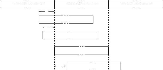
54 2. Finite Field Arithmetic
If f(z)is a trinomial, or a pentanomial with middle terms close to each other, then
reduction of c(z)modulo f(z)can be efficiently performed one word at a time. For
example, suppose m=163 and W=32 (so t=6), and consider reducing the word
C[9]of c(z)modulo f(z)=z163 +z7+z6+z3+1. The word C[9]represents the
polynomial c319z319 +···+c289z289 +c288z288.Wehave
z288 ≡z132 +z131 +z128 +z125 (mod f(z)),
z289 ≡z133 +z132 +z129 +z126 (mod f(z)),
.
.
.
z319 ≡z163 +z162 +z159 +z156 (mod f(z)).
By considering the four columns on the right side of the above congruences, we see that
reduction of C[9]can be performed by adding C[9]four times to C, with the rightmost
bit of C[9]added to bits 132, 131, 128 and 125 of C; this is illustrated in Figure 2.9.
3
⊕
⊕
⊕
⊕
C[9]
C[9]
C[9]
C[5]C[4]C[3]
4
3
C[9]
c160
c191 c159 c128 c127 c96
Figure 2.9. Reducing the 32-bit word
C[9]
modulo
f(z)=z163 +z7+z6+z3+1
.
NIST reduction polynomials
We next present algorithms for fast reduction modulo the following reduction
polynomials recommended by NIST in the FIPS 186-2 standard:
f(z)=z163 +z7+z6+z3+1
f(z)=z233 +z74 +1
f(z)=z283 +z12 +z7+z5+1
f(z)=z409 +z87 +1
f(z)=z571 +z10 +z5+z2+1.

2.3. Binary field arithmetic 55
These algorithms, which assume a wordlength W=32, are based on ideas similar to
those leading to Figure 2.9. They are faster than Algorithm 2.40 and furthermore have
no storage overhead.
Algorithm 2.41 Fast reduction modulo f(z)=z163 +z7+z6+z3+1 (with W=32)
INPUT: A binary polynomial c(z)of degree at most 324.
OUTPUT:c(z)mod f(z).
1. For ifrom10downto6do {Reduce C[i]z32imodulo f(z)}
1.1 T←C[i].
1.2 C[i−6]←C[i−6]⊕(T29).
1.3 C[i−5]←C[i−5]⊕(T4)⊕(T3)⊕T⊕(T3).
1.4 C[i−4]←C[i−4]⊕(T28)⊕(T29).
2. T←C[5]3. {Extract bits 3–31 of C[5]}
3. C[0]←C[0]⊕(T7)⊕(T6)⊕(T3)⊕T.
4. C[1]←C[1]⊕(T25)⊕(T26).
5. C[5]←C[5]& 0x7. {Clear the reduced bits of C[5]}
6. Return (C[5],C[4],C[3],C[2],C[1],C[0]).
Algorithm 2.42 Fast reduction modulo f(z)=z233 +z74 +1 (with W=32)
INPUT: A binary polynomial c(z)of degree at most 464.
OUTPUT:c(z)mod f(z).
1. For ifrom15downto8do {Reduce C[i]z32imodulo f(z)}
1.1 T←C[i].
1.2 C[i−8]←C[i−8]⊕(T23).
1.3 C[i−7]←C[i−7]⊕(T9).
1.4 C[i−5]←C[i−5]⊕(T1).
1.5 C[i−4]←C[i−4]⊕(T31).
2. T←C[7]9. {Extract bits 9–31 of C[7]}
3. C[0]←C[0]⊕T.
4. C[2]←C[2]⊕(T10).
5. C[3]←C[3]⊕(T22).
6. C[7]←C[7]& 0x1FF. {Clear the reduced bits of C[7]}
7. Return (C[7],C[6],C[5],C[4],C[3],C[2],C[1],C[0]).

56 2. Finite Field Arithmetic
Algorithm 2.43 Fast reduction modulo f(z)=z283 +z12 +z7+z5+1 (with W=32)
INPUT: A binary polynomial c(z)of degree at most 564.
OUTPUT:c(z)mod f(z).
1. For ifrom17downto9do {Reduce C[i]z32imodulo f(z)}
1.1 T←C[i].
1.2 C[i−9]←C[i−9]⊕(T5)⊕(T10)⊕(T12)⊕(T17).
1.3 C[i−8]←C[i−8]⊕(T27)⊕(T22)⊕(T20)⊕(T15).
2. T←C[8]27. {Extract bits 27–31 of C[8]}
3. C[0]←C[0]⊕T⊕(T5)⊕(T7)⊕(T12).
4. C[8]←C[8]& 0x7FFFFFF. {Clear the reduced bits of C[8]}
5. Return (C[8],C[7],C[6],C[5],C[4],C[3],C[2],C[1],C[0]).
Algorithm 2.44 Fast reduction modulo f(z)=z409 +z87 +1 (with W=32)
INPUT: A binary polynomial c(z)of degree at most 816.
OUTPUT:c(z)mod f(z).
1. For ifrom25downto13do {Reduce C[i]z32imodulo f(z)}
1.1 T←C[i].
1.2 C[i−13]←C[i−13]⊕(T7).
1.3 C[i−12]←C[i−12]⊕(T25).
1.4 C[i−11]←C[i−11]⊕(T30).
1.5 C[i−10]←C[i−10]⊕(T2).
2. T←C[12]25. {Extract bits 25–31 of C[12]}
3. C[0]←C[0]⊕T.
4. C[2]←C[2]⊕(T¡¡23).
5. C[12]←C[12]& 0x1FFFFFF. {Clear the reduced bits of C[12]}
6. Return (C[12],C[11],...,C[1],C[0]).
Algorithm 2.45 Fast reduction modulo f(z)=z571 +z10 +z5+z2+1 (with W=32)
INPUT: A binary polynomial c(z)of degree at most 1140.
OUTPUT:c(z)mod f(z).
1. For ifrom35downto18do {Reduce C[i]z32imodulo f(z)}
1.1 T←C[i].
1.2 C[i−18]←C[i−18]⊕(T5)⊕(T7)⊕(T10)⊕(T15).
1.3 C[i−17]←C[i−17]⊕(T27)⊕(T25)⊕(T22)⊕(T17).
2. T←C[17]27. {Extract bits 27–31 of C[17]}
3. C[0]←C[0]⊕T⊕(T2)⊕(T5)⊕(T10).
4. C[17]←C[17]& 0x7FFFFFFF. {Clear the reduced bits of C[17]}
5. Return (C[17],C[16],...,C[1],C[0]).
2.3. Binary field arithmetic 57
2.3.6 Inversion and division
In this subsection, we simplify the notation and denote binary polynomials a(z)by a.
Recall that the inverse of a nonzero element a∈F2mis the unique element g∈F2msuch
that ag =1inF2m,thatis,ag ≡1(mod f). This inverse element is denoted a−1mod
for simply a−1if the reduction polynomial fis understood from context. Inverses
can be efficiently computed by the extended Euclidean algorithm for polynomials.
The extended Euclidean algorithm for polynomials
Let aand bbe binary polynomials, not both 0. The greatest common divisor (gcd) of a
and b, denoted gcd(a,b), is the binary polynomial dof highest degree that divides both
aand b. Efficient algorithms for computing gcd(a,b)exploit the following polynomial
analogue of Theorem 2.18.
Theorem 2.46 Let aand bbe binary polynomials. Then gcd(a,b)=gcd(b−ca,a)
for all binary polynomials c.
In the classical Euclidean algorithm for computing the gcd of binary polynomials a
and b, where deg(b)≥deg(a),bis divided by ato obtain a quotient qand a remainder
rsatisfying b=qa +rand deg(r)<deg(a). By Theorem 2.46, gcd(a,b)=gcd(r,a).
Thus, the problem of determining gcd(a,b)is reduced to that of computing gcd(r,a)
where the arguments (r,a)have lower degrees than the degrees of the original argu-
ments (a,b). This process is repeated until one of the arguments is zero—the result is
then immediately obtained since gcd(0,d)=d. The algorithm must terminate since the
degrees of the remainders are strictly decreasing. Moreover, it is efficient because the
number of (long) divisions is at most kwhere k=deg(a).
In a variant of the classical Euclidean algorithm, only one step of each long division
is performed. That is, if deg(b)≥deg(a)and j=deg(b)−deg(a), then one computes
r=b+zja. By Theorem 2.46, gcd(a,b)=gcd(r,a). This process is repeated until a
zero remainder is encountered. Since deg(r)<deg(b), the number of (partial) division
stepsisatmost2kwhere k=max{deg(a), deg(b)}.
The Euclidean algorithm can be extended to find binary polynomials gand h
satisfying ag +bh =dwhere d=gcd(a,b). Algorithm 2.47 maintains the invariants
ag1+bh1=u
ag2+bh2=v.
The algorithm terminates when u=0, in which case v=gcd(a,b)and ag2+bh2=d.

58 2. Finite Field Arithmetic
Algorithm 2.47 Extended Euclidean algorithm for binary polynomials
INPUT: Nonzero binary polynomials aand bwith deg(a)≤deg(b).
OUTPUT:d=gcd(a,b)and binary polynomials g,hsatisfying ag +bh =d.
1. u←a,v←b.
2. g1←1, g2←0, h1←0, h2←1.
3. While u= 0do
3.1 j←deg(u)−deg(v).
3.2 If j<0 then: u↔v,g1↔g2,h1↔h2,j←−j.
3.3 u←u+zjv.
3.4 g1←g1+zjg2,h1←h1+zjh2.
4. d←v,g←g2,h←h2.
5. Return(d,g,h).
Suppose now that fis an irreducible binary polynomial of degree mand the nonzero
polynomial ahas degree at most m−1 (hence gcd(a,f)=1). If Algorithm 2.47 is
executed with inputs aand f, the last nonzero uencountered in step 3.3 is u=1. After
this occurrence, the polynomials g1and h1, as updated in step 3.4, satisfy ag1+fh
1=
1. Hence ag1≡1(mod f)and so a−1=g1. Note that h1and h2are not needed for the
determination of g1. These observations lead to Algorithm 2.48 for inversion in F2m.
Algorithm 2.48 Inversion in F2musing the extended Euclidean algorithm
INPUT: A nonzero binary polynomial aof degree at most m−1.
OUTPUT:a−1mod f.
1. u←a,v←f.
2. g1←1, g2←0.
3. While u= 1do
3.1 j←deg(u)−deg(v).
3.2 If j<0 then: u↔v,g1↔g2,j←−j.
3.3 u←u+zjv.
3.4 g1←g1+zjg2.
4. Return(g1).
Binary inversion algorithm
Algorithm 2.49 is the polynomial analogue of the binary algorithm for inversion in
Fp(Algorithm 2.22). In contrast to Algorithm 2.48 where the bits of uand vare
cleared from left to right (high degree terms to low degree terms), the bits of uand
vin Algorithm 2.49 are cleared from right to left.

2.3. Binary field arithmetic 59
Algorithm 2.49 Binary algorithm for inversion in F2m
INPUT: A nonzero binary polynomial aof degree at most m−1.
OUTPUT:a−1mod f.
1. u←a,v←f.
2. g1←1, g2←0.
3. While (u= 1andv= 1) do
3.1 While zdivides udo
u←u/z.
If zdivides g1then g1←g1/z;elseg1←(g1+f)/z.
3.2 While zdivides vdo
v←v/z.
If zdivides g2then g2←g2/z;elseg2←(g2+f)/z.
3.3 If deg(u)>deg(v) then: u←u+v,g1←g1+g2;
Else: v←v+u,g2←g2+g1.
4. If u=1 then return(g1); else return(g2).
The expression involving degree calculations in step 3.3 may be replaced by a sim-
pler comparison on the binary representations of the polynomials. This differs from
Algorithm 2.48, where explicit degree calculations are required in step 3.1.
Almost inverse algorithm
The almost inverse algorithm (Algorithm 2.50) is a modification of the binary inversion
algorithm (Algorithm 2.49) in which a polynomial gand a positive integer kare first
computed satisfying
ag ≡zk(mod f).
A reduction is then applied to obtain
a−1=z−kgmod f.
The invariants maintained are
ag1+fh
1=zku
ag2+fh
2=zkv
for some h1,h2that are not explicitly calculated.

60 2. Finite Field Arithmetic
Algorithm 2.50 Almost Inverse Algorithm for inversion in F2m
INPUT: A nonzero binary polynomial aof degree at most m−1.
OUTPUT:a−1mod f.
1. u←a,v←f.
2. g1←1, g2←0, k←0.
3. While (u= 1andv= 1) do
3.1 While zdivides udo
u←u/z,g2←z·g2,k←k+1.
3.2 While zdivides vdo
v←v/z,g1←z·g1,k←k+1.
3.3 If deg(u)>deg(v) then: u←u+v,g1←g1+g2.
Else: v←v+u,g2←g2+g1.
4. If u=1theng←g1;elseg←g2.
5. Return(z−kgmod f).
The reduction in step 5 can be performed as follows. Let l=min{i≥1|fi=1},
where f(z)=fmzm+···+f1z+f0.LetSbe the polynomial formed by the lrightmost
bits of g.ThenSf +gis divisible by zland T=(Sf +g)/zlhas degree less than m;
thus T=gz−lmod f. This process can be repeated to finally obtain gz−kmod f.The
reduction polynomial fis said to be suitable if lis above some threshold (which may
depend on the implementation; e.g., l≥Wis desirable with W-bit words), since then
less effort is required in the reduction step.
Steps 3.1–3.2 are simpler than those in Algorithm 2.49. In addition, the g1and
g2appearing in these algorithms grow more slowly in almost inverse. Thus one can
expect Algorithm 2.50 to outperform Algorithm 2.49 if the reduction polynomial is
suitable, and conversely. As with the binary algorithm, the conditional involving degree
calculations may be replaced with a simpler comparison.
Division
The binary inversion algorithm (Algorithm 2.49) can be easily modified to perform
division b/a=ba−1. In cases where the ratio I/Mof inversion to multiplication costs
is small, this could be especially significant in elliptic curve schemes, since an elliptic
curve point operation in affine coordinates (see §3.1.2) could use division rather than
an inversion and multiplication.
Division based on the binary algorithm To obtain b/a, Algorithm 2.49 is modified
at step 2, replacing g1←1 with g1←b. The associated invariants are
ag1+fh
1=ub
ag2+fh
2=vb.
2.3. Binary field arithmetic 61
On termination with u=1, it follows that g1=ba−1. The division algorithm is
expected to have the same running time as the binary algorithm, since g1in Algo-
rithm 2.49 goes to full-length in a few iterations at step 3.1 (i.e., the difference in
initialization of g1does not contribute significantly to the time for division versus
inversion).
If the binary algorithm is the inversion method of choice, then affine point operations
would benefit from use of division, since the cost of a point double or addition changes
from I+2Mto I+M.(Iand Mdenote the time to perform an inversion and a multi-
plication, respectively.) If I/Mis small, then this represents a significant improvement.
For example, if I/Mis 3, then use of a division algorithm variant of Algorithm 2.49
provides a 20% reduction in the time to perform an affine point double or addition.
However, if I/M>7, then the savings is less than 12%. Unless I/Mis very small, it
is likely that schemes are used which reduce the number of inversions required (e.g.,
halving and projective coordinates), so that point multiplication involves relatively few
field inversions, diluting any savings from use of a division algorithm.
Division based on the extended Euclidean algorithm Algorithm 2.48 can be trans-
formed to a division algorithm in a similar fashion. However, the change in the
initialization step may have significant impact on implementation of a division algo-
rithm variant. There are two performance issues: tracking of the lengths of variables,
and implementing the addition to g1at step 3.4.
In Algorithm 2.48, it is relatively easy to track the lengths of uand vefficiently
(the lengths shrink), and, moreover, it is also possible to track the lengths of g1and
g2. However, the change in initialization for division means that g1goes to full-length
immediately, and optimizations based on shorter lengths disappear.
The second performance issue concerns the addition to g1at step 3.4. An imple-
mentation may assume that ordinary polynomial addition with no reduction may be
performed; that is, the degrees of g1and g2never exceed m−1. In adapting for division,
step 3.4 may be less-efficiently implemented, since g1is full-length on initialization.
Division based on the almost inverse algorithm Although Algorithm 2.50 is similar
to the binary algorithm, the ability to efficiently track the lengths of g1and g2(in addi-
tion to the lengths of uand v) may be an implementation advantage of Algorithm 2.50
over Algorithm 2.49 (provided that the reduction polynomial fis suitable). As with
Algorithm 2.48, this advantage is lost in a division algorithm variant.
It should be noted that efficient tracking of the lengths of g1and g2(in addition to the
lengths of uand v) in Algorithm 2.50 may involve significant code expansion (perhaps
t2fragments rather than the tfragments in the binary algorithm). If the expansion
cannot be tolerated (because of application constraints or platform characteristics), then
almost inverse may not be preferable to the other inversion algorithms (even if the
reduction polynomial is suitable).

62 2. Finite Field Arithmetic
2.4 Optimal extension field arithmetic
Preceding sections discussed arithmetic for fields Fpmin the case that p=2 (binary
fields) and m=1 (prime fields). As noted on page 28, the polynomial basis repre-
sentation in the binary field case can be generalized to all extension fields Fpm, with
coefficient arithmetic performed in Fp.
For hardware implementations, binary fields are attractive since the operations in-
volve only shifts and bitwise addition modulo 2. The simplicity is also attractive for
software implementations on general-purpose processors; however the field multipli-
cation is essentially a few bits at a time and can be much slower than prime field
arithmetic if a hardware integer multiplier is available. On the other hand, the arith-
metic in prime fields can be more difficult to implement efficiently, due in part to the
propagation of carry bits.
The general idea in optimal extension fields is to select p,m, and the reduction poly-
nomial to more closely match the underlying hardware characteristics. In particular,
the value of pmay be selected to fit in a single word, simplifying the handling of carry
(since coefficients are single-word).
Definition 2.51 An optimal extension field (OEF) is a finite field Fpmsuch that:
1. p=2n−cfor some integers nand cwith log2|c|≤n/2; and
2. an irreducible polynomial f(z)=zm−ωin Fp[z]exists.
If c∈{±1},thentheOEFissaidtobeofType I (pis a Mersenne prime if c=1); if
ω=2, the OEF is said to be of Type II.
Type I OEFs have especially simple arithmetic in the subfield Fp, while Type II
OEFs allow simplifications in the Fpmextension field arithmetic. Examples of OEFs
are given in Table 2.1.
p f parameters Type
27+3z13 −5n=7,c=−3,m=13,ω=5 —
213 −1z13 −2n=13,c=1,m=13,ω=2I, II
231 −19 z6−2n=31,c=19,m=6,ω=2II
231 −1z6−7n=31,c=1,m=6,ω=7 I
232 −5z5−2n=32,c=5,m=5,ω=2II
257 −13 z3−2n=57,c=13,m=3,ω=2II
261 −1z3−37 n=61,c=1,m=3,ω=37 I
289 −1z2−3n=89,c=1,m=2,ω=3 I
Table 2.1. OEF example parameters. Here,
p=2n−c
is prime, and
f(z)=zm−ω∈Fp[z]
is
irreducible over
Fp
. The field is
Fpm=Fp[z]/( f)
of order approximately
2mn
.
The following results can be used to determine if a given polynomial f(z)=zm−ω
is irreducible in Fp[z].
2.4. Optimal extension field arithmetic 63
Theorem 2.52 Let m≥2beanintegerandω∈F∗
p. Then the binomial f(z)=zm−ω
is irreducible in Fp[z]if and only if the following two conditions are satisfied:
(i) each prime factor of mdivides the order eof ωin F∗
p, but not (p−1)/e;
(ii) p≡1(mod 4)if m≡0(mod 4).
If the order of ωas an element of F∗
pis p−1, then ωis said to be primitive.Itis
easily verified that conditions (i) and (ii) of Theorem 2.52 are satisfied if ωis primitive
and m|(p−1).
Corollary 2.53 If ωis a primitive element of F∗
pand m|(p−1),thenzm−ωis
irreducible in Fp[z].
Elements of Fpmare polynomials
a(z)=am−1zm−1+···+a2z2+a1z+a0
where the coefficients aiare elements of Fp. We next present algorithms for performing
arithmetic operations in OEFs. Selected timings for field operations appear in §5.1.5.
2.4.1 Addition and subtraction
If a(z)=m−1
i=0aiziand b(z)=m−1
i=0biziare elements of Fpm,then
a(z)+b(z)=
m−1
i=0
cizi,
where ci=(ai+bi)mod p;thatis, pis subtracted whenever ai+bi≥p. Subtraction
of elements of Fpmis done similarly.
2.4.2 Multiplication and reduction
Multiplication of elements a,b∈Fpmcan be done by ordinary polynomial multiplica-
tion in Z[z](i.e., multiplication of polynomials having integer coefficients), along with
coefficient reductions in Fpand a reduction by the polynomial f. This multiplication
takes the form
c(z)=a(z)b(z)=m−1
i=0
aizim−1
j=0
bjzj
≡
2m−2
k=0
ckzk≡cm−1zm−1+
m−2
k=0
(ck+ωck+m)zk(mod f(z))

64 2. Finite Field Arithmetic
where
ck=
i+j=k
aibjmod p.
Karatsuba-Ofman techniques may be applied to reduce the number of Fpmultiplica-
tions. For example,
a(z)b(z)=(A1zl+A0)(B1zl+B0)
=A1B1z2l+[(A1+A0)(B1+B0)−A1B1−A0B0]zl+A0B0
where l=m/2and the coefficients A0,A1,B0,B1are polynomials in Fp[z]of
degree less than l. The process may be repeated, although for small values of mit may
be advantageous to consider splits other than binary. The analogous case for prime
fields was discussed in §2.2.2.
Reduction in
F
F
Fp
The most straightforward implementation performs reductions in Fpfor every addi-
tion and multiplication encountered during the calculation of each ck. The restriction
log2|c|≤n/2 means that reduction in the subfield Fprequires only a few simple op-
erations. Algorithm 2.54 performs reduction of base-Bnumbers, using only shifts,
additions, and single-precision multiplications.
Algorithm 2.54 Reduction modulo M=Bn−c
INPUT:Abase B, positive integer x, and modulus M=Bn−cwhere cis an l-digit
base-Bpositive integer for some l<n.
OUTPUT:xmod M.
1. q0←x/Bn,r0←x−q0Bn.{x=q0Bn+r0with r0<Bn}
2. r←r0,i←0.
3. While qi>0do
3.1 qi+1←qic/Bn.{qic=qi+1Bn+ri+1with ri+1<Bn}
3.2 ri+1←qic−qi+1Bn.
3.3 i←i+1, r←r+ri.
4. While r≥Mdo: r←r−M.
5. Return(r).
Note 2.55 (implementation details for Algorithm 2.54)
(i) If l≤n/2andxhas at most 2nbase-Bdigits, Algorithm 2.54 executes step 3.1
at most twice (i.e., there are at most two multiplications by c).
(ii) As an alternative, the quotient and remainder may be folded into xat each stage.
Steps 1–4 are replaced with the following.

2.4. Optimal extension field arithmetic 65
1. While x≥Bn
1.1 Write x=vBn+uwith u<Bn.
1.2 x←cv+u.
2. If x≥Mthen x←x−M.
(iii) Algorithm 2.54 can be modified to handle the case M=Bn+cfor some posi-
tive integer c<Bn−1: in step 3.3, replace r←r+riwith r←r+(−1)iri,and
modifystep4toalsoprocessthecaser<0.
For OEFs, Algorithm 2.54 with B=2 may be applied, requiring at most two multi-
plications by cin the case that x<22n.Whenc=1 (a type I OEF) and x≤(p−1)2,
the reduction is given by:
write x=2nv+u;x←v+u;ifx≥pthen x←x−p.
Type I OEFs are attractive in the sense that Fpmultiplication (with reduction) can be
done with a single multiplication and a few other operations. However, the reductions
modulo pare likely to contribute a significant amount to the cost of multiplication in
Fpm, and it may be more efficient to employ a direct multiply-and-accumulate strategy
to decrease the number of reductions.
Accumulation and reduction
The number of Fpreductions performed in finding the product c(z)=a(z)b(z)in
Fpmcan be decreased by accumulation strategies on the coefficients of c(z).Since
f(z)=zm−ω, the product can be written
c(z)=a(z)b(z)≡
2m−2
k=0
ckzk≡
m−1
k=0
ckzk+ω
2m−2
k=m
ckzk−m
≡
m−1
k=0k
i=0
aibk−i+ω
m−1
i=k+1
aibk+m−i
c
k
zk(mod f(z)).
If the coefficient c
kis calculated as an expression in Z(i.e., as an integer without
reduction modulo p), then c
kmod pmay be performed with a single reduction (rather
than mreductions). The penalty incurred is the multiple-word operations (additions
and multiplication by ω) required in accumulating the terms of c
k.
In comparison with the straightforward reduce-on-every-operation strategy, it should
be noted that complete reduction on each Fpoperation may not be necessary; for exam-
ple, it may suffice to reduce the result to a value which fits in a single word. However,
frequent reduction (to a single word or value less than 2n) is likely to be expensive,
especially if a “carry” or comparison must be processed.
66 2. Finite Field Arithmetic
Depending on the value of p, the multiply-and-accumulate strategy employs two or
three registers for the accumulation (under the assumption that pfits in a register). The
arithmetic resembles that commonly used in prime-field implementations, and multipli-
cation cost in Fpmis expected to be comparable to that in a prime field Fqwhere q≈pm
and which admits fast reduction (e.g., the NIST-recommended primes in §2.2.6).
For the reduction c
kmod p, note that
c
k≤(p−1)2+ω(m−1)( p−1)2=(p−1)2(1+ω(m−1)).
If p=2n−cis such that
log2(1+ω(m−1)) +2log2|c|≤n,(2.4)
then reduction can be done with at most two multiplications by c.Asanexample,if
p=228 −165 and f(z)=z6−2, then
log2(1+ω(m−1)) +2log2|c|=log211 +2log2165 <n=28
and condition (2.4) is satisfied.
If accumulation is in a series of registers each of size Wbits, then selecting p=
2n−cwith n<Wallows several terms to be accumulated in two registers (rather
than spilling into a third register or requiring a partial reduction). The example with
p=228 −165 is attractive in this sense if W=32. However, this strategy competes
with optimal use of the integer multiply, and hence may not be effective if it requires
use of a larger mto obtain a field of sufficient size.
Example 2.56 (accumulation strategies) Consider the OEF defined by p=231 −1and
f(z)=z6−7, on a machine with wordsize W=32. Since this is a Type I OEF, subfield
reduction is especially simple, and a combination of partial reduction with accumula-
tion may be effective in finding c
kmod p. Although reduction into a single register
after each operation may be prohibitively expensive, an accumulation into two registers
(with some partial reductions) or into three registers can be employed.
Suppose the accumulator consists of two registers. A partial reduction may be per-
formed on each term of the form aibjby writing aibj=232v+uandthen2v+uis
added to the accumulator. Similarly, the accumulator itself could be partially reduced
after the addition of a product aibj.
If the accumulator is three words, then the partial reductions are unnecessary, and a
portion of the accumulation involves only two registers. On the other hand, the mul-
tiplication by ω=7 and the final reduction are slightly more complicated than in the
two-register approach.
The multiply-and-accumulate strategies also apply to field squaring in Fpm. Squaring
requires a total of m+m
2=m(m+1)/2 integer multiplications (and possibly m−1
multiplications by ω). The cost of the Fpreductions depends on the method; in partic-
ular, if only a single reduction is used in finding c
k, then the number of reductions is
the same as for general multiplication.

2.4. Optimal extension field arithmetic 67
2.4.3 Inversion
Inversion of a∈Fpm,a= 0, finds a polynomial a−1∈Fpmsuch that aa−1≡1
(mod f). Variants of the Euclidean Algorithm have been proposed for use with OEFs.
However, the action of the Frobenius map along with the special form of fcan be used
to obtain an inversion method that is among the fastest. The method is also relatively
simple to implement efficiently once field multiplication is written, since only a few
multiplications are needed to reduce inversion in Fpmto inversion in the subfield Fp.
Algorithm 2.59 computes
a−1=(ar)−1ar−1mod f(2.5)
where
r=pm−1
p−1=pm−1+···+p2+p+1.
Since (ar)p−1≡1(mod pm), it follows that ar∈Fp. Hence a suitable algorithm may
be applied for inversion in Fpin order to compute the term (ar)−1in (2.5).
Efficient calculation of ar−1=apm−1+···+pin (2.5) is performed by using properties
of the Frobenius map ϕ:Fpm→Fpmdefined by ϕ(a)=ap.ElementsofFpare fixed
by this map. Hence, if a=am−1zm−1+···+a2z2+a1z+a0,then
ϕi:a→ am−1z(m−1)pi+···+a1zpi+a0mod f.
To reduce the powers of zmodulo f, write a given nonnegative integer eas e=qm +r,
where q=e/mand r=emod m.Since f(z)=zm−ω, it follows that
ze=zqm+r≡ωqzr(mod f(z)).
Notice that ϕi(a)is somewhat simpler to evaluate if p≡1(mod m). By Theorem 2.52,
every prime factor of mdivides p−1. Necessarily, if mis square free, the condition
p≡1(mod m)holds. The results are collected in the following theorem.
Theorem 2.57 (action of Frobenius map iterates) Given an OEF with p=2n−cand
f(z)=zm−ω, let the Frobenius map on Fpmbe given by ϕ:a→ apmod f.
(i) The ith iterate of ϕis the map
ϕi:a→
m−1
j=0
ajωjpi/mzjpimod m.
(ii) If mis square-free, then p≡1(mod m)and hence jpimod m=jfor all 0 ≤
j≤m−1.

68 2. Finite Field Arithmetic
The values ze≡ωe/mzemod m(mod f(z)) may be precomputed for e=jpiof
interest, in which case ϕi(a)may be evaluated with only m−1 multiplications in Fp.
Use of an addition chain then efficiently finds ar−1in equation (2.5) using a few field
multiplications and applications of ϕi.
Example 2.58 (calculating ar−1) The OEF defined by p=231 −1and f(z)=z6−7
has r−1=p5+p4+···+p. We may calculate ar−1using the sequence indicated in
Table 2.2 (an addition-chain-like method) for m=6. Evaluation of ϕand ϕ2uses the
precomputed values in Table 2.3 obtained from Theorem 2.57.
m=3m=5m=6
T←apT1←apT1←ap
T←Ta=ap+1T1←T1a=ap+1T2←T1a=ap+1
ar−1←Tp=ap2+pT2←Tp2
1=ap3+p2T3←Tp2
2=ap3+p2
T1←T1T2=ap3+p2+p+1T2←T3T2=ap3+p2+p+1
ar−1←Tp
1T2←Tp2
2=ap5+p4+p3+p2
ar−1←T2T1
Cost: 1M+2ϕCost: 2M+3ϕCost: 3M+3ϕ
Table 2.2. Computation of
ar−1
for
r=pm−1
p−1
,
m∈{3,5,6}
. The final row indicates the cost in
Fpm
multiplications (
M
) and applications of an iterate of the Frobenius map (
ϕ
).
zjp ≡ωjp/mzj(mod f)zjp2≡ωjp2/mzj(mod f)
zp≡1513477736z z p2≡1513477735z
z2p≡1513477735z2z2p2≡634005911z2
z3p≡2147483646z3≡−1z3z3p2≡1z3
z4p≡634005911z4z4p2≡1513477735z4
z5p≡634005912z5z5p2≡634005911z5
Table 2.3. Precomputation for evaluating
ϕi
,
i∈{1,2}
, in the case
p=231 −1
and
f(z)=z6−7
(cf. Example 2.58). If
a=a5z5+···+a1z+a0∈Fp6
,then
ϕi(a)=api≡5
j=0ajωjpi/mzj
(mod f)
.
In general, if w(x)is the Hamming weight of the integer x,thenar−1can be
calculated with
t1(m)=log2(m−1)+w(m−1)−1

2.5. Notes and further references 69
multiplications in Fpm,and
t2(m)=
t1(m)+1,modd,
j=log2(m−1)+1,m=2jfor some j,
log2(m−1)+w(m)−1,otherwise,
applications of Frobenius map iterates. Since t2(m)≤t1(m)+1, the time for calculating
ar−1with m>2 is dominated by the multiplications in Fpm(each of which is much
more expensive than the m−1 multiplications in Fpneeded for evaluation of ϕi).
Algorithm 2.59 OEF inversion
INPUT:a∈Fpm,a= 0.
OUTPUT: The element a−1∈Fpmsuch that aa−1≡1(mod f).
1. Use an addition-chain approach to find ar−1,wherer=(pm−1)/( p−1).
2. c←ar=ar−1a∈Fp.
3. Obtain c−1such that cc−1≡1(mod p)via an inversion algorithm in Fp.
4. Return(c−1ar−1).
Note 2.60 (implementation details for Algorithm 2.59)
(i) The element cin step 2 of Algorithm 2.59 belongs to Fp. Hence, only arith-
metic contributing to the constant term of ar−1aneed be performed (requiring
mmultiplications of elements in Fpand a multiplication by ω).
(ii) Since c−1∈Fp, the multiplication in step 4 requires only mFp-multiplications.
(iii) The running time is dominated by the t1(m)multiplications in Fpmin finding
ar−1, and the cost of the subfield inversion in step 3.
The ratio I/Mof field inversion cost to multiplication cost is of fundamental interest.
When m=6, Algorithm 2.59 will require significantly more time than the t1(6)=3
multiplications involved in finding ar−1, since the time for subfield inversion (step 3)
will be substantial. However, on general-purpose processors, the ratio is expected to be
much smaller than the corresponding ratio in a prime field Fqwhere q≈pm.
2.5 Notes and further references
§2.1
For an introduction to the theory of finite fields, see the books of Koblitz [254] and
McEliece [311]. A more comprehensive treatment is given by Lidl and Niederreiter
[292].
70 2. Finite Field Arithmetic
§2.2
Menezes, van Oorshot, and Vanstone [319] concisely cover algorithms for ordinary
and modular integer arithmetic of practical interest in cryptography. Knuth [249] is
a standard reference. Koc¸ [258] describes several (modular) multiplication methods,
including classical and Karatsuba-Ofman, a method which interleaves multiplication
with reduction, and Montgomery multiplication.
The decision to base multiplication on operand scanning (Algorithm 2.9) or product
scanning (Algorithm 2.10) is platform dependent. Generally speaking, Algorithm 2.9
has more memory accesses, while Algorithm 2.10 has more complex control code
unless loops are unrolled. Comba [101] compares the methods in detail for 16-bit In-
tel 80286 processors, and the unrolled product-scanning versions were apparently the
inspiration for the “comba” routines in OpenSSL.
Scott [416] discusses multiplication methods on three 32-bit Intel IA-32 processors
(the 80486, Pentium, and Pentium Pro), and provides experimental results for mod-
ular exponentiation with multiplication based on operand scanning, product scanning
(Comba’s method), Karatsuba-Ofman with product scanning, and floating-point hard-
ware. Multiplication with features introduced on newer IA-32 processors is discussed
in §5.1.3. On the Motorola digital signal processor 56000, Duss´e and Kaliski [127]
note that extraction of Uin the inner loop of Algorithm 2.9 is relatively expensive.
The processor has a 56-bit accumulator but only signed multiplication of 24-bit quan-
tities, and the product scanning approach in Montgomery multiplication is reportedly
significantly faster.
The multiplication method of Karatsuba-Ofman is due to Karatsuba and Ofman [239].
For integers of relatively small size, the savings in multiplications is often insufficient in
Karatsuba-Ofman variants to make the methods competitive with optimized versions
of classical algorithms. Knuth [249] and Koc¸ [258] cover Karatsuba-Ofman in more
detail.
Barrett reduction (Algorithm 2.14) is due to Barrett [29]. Bosselaers, Govaerts, and
Vandewalle [66] provide descriptions and comparative results for classical reduction
and the reduction methods of Barrett and Montgomery. If the transformations and pre-
computation are excluded, their results indicate that the methods are fairly similar in
cost, with Montgomery reduction fastest and classical reduction likely to be slightly
slower than Barrett reduction. These operation count comparisons are supported by
implementation results on an Intel 80386 in portable C. De Win, Mister, Preneel and
Wiener [111] report that the difference between Montgomery and Barrett reduction was
negligible in their implementation on an Intel Pentium Pro of field arithmetic in Fpfor
a 192-bit prime p.
Montgomery reduction is due to Montgomery [330]. Koc¸, Acar, and Kaliski [260]
analyze five Montgomery multiplication algorithms. The methods were identified as
having a separate reduction phase or reduction integrated with multiplication, and
2.5. Notes and further references 71
according to the general form of the multiplication as operand-scanning or product-
scanning. Among the algorithms tested, they conclude that a “coarsely integrated
operand scanning” method (where a reduction step follows a multiplication step at each
index of an outer loop through one of the operands) is simplest and probably best for
general-purpose processors. Koc¸ and Acar [259] extend Montgomery multiplication to
binary fields.
The binary gcd algorithm (Algorithm 2.21) is due to Stein [451], and is analyzed by
Knuth [249]. Bach and Shallit [23] provide a comprehensive analysis of several gcd
algorithms. The binary algorithm for inversion (Algorithm 2.22) is adapted from the
corresponding extended gcd algorithm.
Lehmer [278] proposed a variant of the classical Euclidean algorithm which replaces
most of the expensive multiple-precision divisions by single-precision operations. The
algorithm is examined in detail by Knuth [249], and a slight modification is analyzed
by Sorenson [450]. Durand [126] provides concise coverage of inversion algorithms
adapted from the extended versions of the Euclidean, binary gcd, and Lehmer algo-
rithms, along with timings for RSA and elliptic curve point multiplication on 32-bit
RISC processors (for smartcards) from SGS-Thomson. On these processors, Lehmer’s
method showed significant advantages, and in fact produced point multiplication times
faster than was obtained with projective coordinates.
Algorithm 2.23 for the partial Montgomery inverse is due to Kaliski [234]. De Win,
Mister, Preneel and Wiener [111] report that an inversion method based on this algo-
rithm was superior to variations of the extended Euclidean algorithm (Algorithm 2.19)
in their tests on an Intel Pentium Pro, although details are not provided. The generaliza-
tion in Algorithm 2.25 is due to Savas and Koc¸ [403]; a similar algorithm is provided
for finding the usual inverse.
Simultaneous inversion (Algorithm 2.26) is attributed to Montgomery [331], where the
technique was suggested for accelerating the elliptic curve method (ECM) of factoring.
Cohen [99, Algorithm 10.3.4] gives an extended version of Algorithm 2.26, presented
in the context of ECM.
The NIST primes (§2.2.6) are given in the Federal Information Processing Standards
(FIPS) publication 186-2 [140] on the Digital Signature Standard, as part of the recom-
mended elliptic curves for US Government use. Solinas [445] discusses generalizations
of Mersenne numbers 2k−1 that permit fast reduction (without division); the NIST
primes are special cases.
§2.3
Algorithms 2.35 and 2.36 for polynomial multiplication are due to L´opez and Dahab
[301]. Their work expands on “comb” exponentiation methods of Lim and Lee [295].
Operation count comparisons and implementation results (on Intel family and Sun Ul-
traSPARC processors) suggest that Algorithm 2.36 will be significantly faster than
72 2. Finite Field Arithmetic
Algorithm 2.34 at relatively modest storage requirements. The multiple-table variants
in Note 2.37 are essentially described by L´opez and Dahab [301, Remark 2].
The OpenSSL contribution by Sun Microsystems Laboratories mentioned in Note 2.38
is authored by Sheueling Chang Shantz and Douglas Stebila. Our notes are based in
part on OpenSSL-0.9.8 snapshots. A significant enchancement is discussed by Weimer-
skirch, Stebila, and Chang Shantz [478]. Appendix C has a few notes on the OpenSSL
library.
The NIST reduction polynomials (§2.3.5) are given in the Federal Information Pro-
cessing Standards (FIPS) publication 186-2 [140] on the Digital Signature Standard, as
part of the recommended elliptic curves for US Government use.
The binary algorithm for inversion (Algorithm 2.49) is the polynomial analogue of
Algorithm 2.22. The almost inverse algorithm (Algorithm 2.50) is due to Schroeppel,
Orman, O’Malley, and Spatscheck [415]; a similar algorithm (Algorithm 2.23) in the
context of Montgomery inversion was described by Kaliski [234].
Algorithms for field division were described by Goodman and Chandrakasan [177],
Chang Shantz [90], Durand [126], and Schroeppel [412]. Inversion and division algo-
rithm implementations are especially sensitive to compiler differences and processor
characteristics, and rough operation count analysis can be misleading. Fong, Hanker-
son, L´opez and Menezes [144] discuss inversion and division algorithm considerations
and provide comparative timings for selected compilers on the Intel Pentium III and
Sun UltraSPARC.
In a normal basis representation, elements of F2mare expressed in terms of a basis
of the form {β,β2,β22,...,β2m−1}. One advantage of normal bases is that squaring of
a field element is a simple rotation of its vector representation. Mullin, Onyszchuk,
Vanstone and Wilson [337] introduced the concept of an optimal normal basis in or-
der to reduce the hardware complexity of multiplying field elements in F2mwhose
elements are represented using a normal basis. Hardware implementations of the arith-
metic in F2musing optimal normal bases are described by Agnew, Mullin, Onyszchuk
and Vanstone [6] and Sunar and Koc¸ [456].
Normal bases of low complexity, also known as Gaussian normal bases, were further
studied by Ash, Blake and Vanstone [19]. Gaussian normal bases are explicitly de-
scribed in the ANSI X9.62 standard [14] for the ECDSA. Experience has shown that
optimal normal bases do not have any significant advantages over polynomial bases for
hardware implementation. Moreover, field multiplication in software for normal basis
representations is very slow in comparison to multiplication with a polynomial basis;
see Reyhani-Masoleh and Hasan [390] and Ning and Yin [348].
§2.4
Optimal extension fields were introduced by Bailey and Paar [25, 26]. Theorem 2.52 is
from Lidl and Niederreiter [292, Theorem 3.75]. Theorem 2.57 corrects [26, Corollary
2.5. Notes and further references 73
2]. The OEF construction algorithm of [26] has a minor flaw in the test for irreducibil-
ity, leading to a few incorrect entries in their table of Type II OEFs (e.g, z25 −2 is not
irreducible when p=28−5). The inversion method of §2.4.3 given by Bailey and Paar
is based on Itoh and Tsujii [217]; see also [183].
Lim and Hwang [293] give thorough coverage to various optimization strategies and
provide useful benchmark timings on Intel and DEC processors. Their operation count
analysis favours a Euclidean algorithm variant over Algorithm 2.59 for inversion. How-
ever, rough operation counts at this level often fail to capture processor or compiler
characteristics adequately, and in subsequent work [294] they note that Algorithm 2.59
appears to be significantly faster in implementation on Intel Pentium II and DEC
Alpha processors. Chung, Sim, and Lee [97] note that the count for the number of
required Frobenius-map applications in inversion given in [26] is not necessarily min-
imal. A revised formula is given, along with inversion algorithm comparisons and
implementation results for a low-power Samsung CalmRISC 8-bit processor with a
math coprocessor.
This page intentionally left blank
CHAPTER 3
Elliptic Curve Arithmetic
Cryptographic mechanisms based on elliptic curves depend on arithmetic involving the
points of the curve. As noted in Chapter 2, curve arithmetic is defined in terms of un-
derlying field operations, the efficiency of which is essential. Efficient curve operations
are likewise crucial to performance.
Figure 3.1 illustrates module framework required for a protocol such as the El-
liptic Curve Digital Signature Algorithm (ECDSA, discussed in §4.4.1). The curve
arithmetic not only is built on field operations, but in some cases also relies on big
number and modular arithmetic (e.g., τ-adic operations if Koblitz curves are used;
see §3.4). ECDSA uses a hash function and certain modular operations, but the
computationally-expensive steps involve curve operations.
Curve arithmetic
Field arithmetic
Big number and
Elliptic Curve Digital Signature Algorithm
(Protocols, Chapter 4)
Random number
generation modular arithmetic (Chapter 3)
(Chapter 2)
Figure 3.1. ECDSA support modules.
76 3. Elliptic Curve Arithmetic
§3.1 provides an introduction to elliptic curves. The group operations of addition
and doubling for the points on an elliptic curve are given, along with fundamental
structure and other properties. §3.2 presents projective-coordinate representations (and
associated point addition and doubling algorithms), of principal interest when field
inversion is expensive relative to field multiplication. §3.3 discusses strategies for point
multiplication, the operation which dominates the execution time of schemes based on
elliptic curves.
The methods in §3.4, §3.5, and §3.6 are related in the sense that they all exploit en-
domorphisms of the elliptic curve to reduce the cost of doubling in point multiplication.
§3.4 discusses the special Koblitz curves, which allow point doubling for curves over
F2to be replaced by inexpensive field squaring operations. §3.5 examines a broader
class of elliptic curves which admit endomorphisms that can be used efficiently to re-
duce the number of doublings in point multiplication. Strategies in §3.6 for elliptic
curves over binary fields replace most point doublings by a potentially faster halving
operation. §3.7 contains operation count comparisons for selected point multiplication
methods. §3.8 concludes with chapter notes and references.
3.1 Introduction to elliptic curves
Definition 3.1 An elliptic curve E over a field K is defined by an equation
E:y2+a1xy+a3y=x3+a2x2+a4x+a6(3.1)
where a1,a2,a3,a4,a6∈Kand =0, where is the discriminant of Eand is defined
as follows:
=−d2
2d8−8d3
4−27d2
6+9d2d4d6
d2=a2
1+4a2
d4=2a4+a1a3
d6=a2
3+4a6
d8=a2
1a6+4a2a6−a1a3a4+a2a2
3−a2
4.
(3.2)
If Lis any extension field of K, then the set of L-rational points on Eis
E(L)={(x,y)∈L×L:y2+a1xy+a3y−x3−a2x2−a4x−a6=0}∪{∞}
where ∞is the point at infinity.
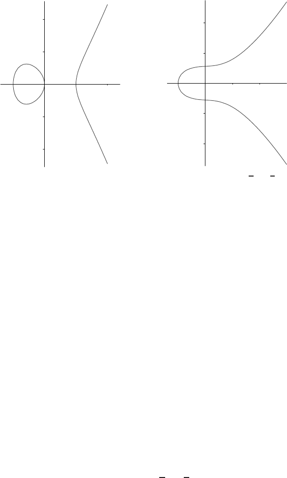
3.1. Introduction to elliptic curves 77
–2
–1
0
1
2
2x
y
(a) E1:y2=x3−x
–4
–2
0
2
4
12 x
y
(b) E2:y2=x3+1
4x+5
4
Figure 3.2. Elliptic curves over
R
.
Remark 3.2 (comments on Definition 3.1)
(i) Equation (3.1) is called a Weierstrass equation.
(ii) We say that Eis defined over K because the coefficients a1,a2,a3,a4,a6of its
defining equation are elements of K. We sometimes write E/Kto emphasize
that Eis defined over K,andKis called the underlying field. Note that if Eis
defined over K,thenEis also defined over any extension field of K.
(iii) The condition = 0 ensures that the elliptic curve is “smooth”, that is, there are
no points at which the curve has two or more distinct tangent lines.
(iv) The point ∞is the only point on the line at infinity that satisfies the projective
form of the Weierstrass equation (see §3.2).
(v) The L-rational points on Eare the points (x,y)that satisfy the equation of
the curve and whose coordinates xand ybelong to L. The point at infinity is
considered an L-rational point for all extension fields Lof K.
Example 3.3 (elliptic curves over R) Consider the elliptic curves
E1:y2=x3−x
E2:y2=x3+1
4x+5
4
defined over the field Rof real numbers. The points E1(R)\{∞}and E2(R)\{∞}are
graphed in Figure 3.2.

78 3. Elliptic Curve Arithmetic
3.1.1 Simplified Weierstrass equations
Definition 3.4 Two elliptic curves E1and E2defined over Kand given by the
Weierstrass equations
E1:y2+a1xy+a3y=x3+a2x2+a4x+a6
E2:y2+a1xy+a3y=x3+a2x2+a4x+a6
are said to be isomorphic over K if there exist u,r,s,t∈K,u=0, such that the change
of variables
(x,y)→(u2x+r,u3y+u2sx +t)(3.3)
transforms equation E1into equation E2. The transformation (3.3) is called an
admissible change of variables.
A Weierstrass equation
E:y2+a1xy+a3y=x3+a2x2+a4x+a6
defined over Kcan be simplified considerably by applying admissible changes of vari-
ables. The simplified equations will be used throughout the remainder of this book. We
consider separately the cases where the underlying field Khas characteristic different
from 2 and 3, or has characteristic equal to 2 or 3.
1. If the characteristic of Kis not equal to 2 or 3, then the admissible change of
variables
(x,y)→x−3a2
1−12a2
36 ,y−3a1x
216 −a3
1+4a1a2−12a3
24
transforms Eto the curve
y2=x3+ax +b(3.4)
where a,b∈K. The discriminant of this curve is =−16(4a3+27b2).
2. If the characteristic of Kis 2, then there are two cases to consider. If a1= 0, then
the admissible change of variables
(x,y)→a2
1x+a3
a1
,a3
1y+a2
1a4+a2
3
a3
1
transforms Eto the curve
y2+xy =x3+ax2+b(3.5)
where a,b∈K. Such a curve is said to be non-supersingular (cf. Definition 3.10)
and has discriminant =b.Ifa1=0, then the admissible change of variables
(x,y)→(x+a2,y)

3.1. Introduction to elliptic curves 79
transforms Eto the curve
y2+cy =x3+ax +b(3.6)
where a,b,c∈K. Such a curve is said to be supersingular (cf. Definition 3.10)
and has discriminant =c4.
3. If the characteristic of Kis 3, then there are two cases to consider. If a2
1=−a2,
then the admissible change of variables
(x,y)→x+d4
d2
,y+a1x+a1
d4
d2+a3,
where d2=a2
1+a2and d4=a4−a1a3, transforms Eto the curve
y2=x3+ax2+b(3.7)
where a,b∈K. Such a curve is said to be non-supersingular and has
discriminant =−a3b.Ifa2
1=−a2, then the admissible change of variables
(x,y)→(x,y+a1x+a3)
transforms Eto the curve
y2=x3+ax +b(3.8)
where a,b∈K. Such a curve is said to be supersingular and has discriminant
=−a3.
3.1.2 Group law
Let Ebe an elliptic curve defined over the field K.Thereisachord-and-tangent rule
for adding two points in E(K)to give a third point in E(K). Together with this addition
operation, the set of points E(K)forms an abelian group with ∞serving as its identity.
It is this group that is used in the construction of elliptic curve cryptographic systems.
The addition rule is best explained geometrically. Let P=(x1,y1)and Q=(x2,y2)
be two distinct points on an elliptic curve E. Then the sum R,ofPand Q,isdefined
as follows. First draw a line through Pand Q; this line intersects the elliptic curve at
a third point. Then Ris the reflection of this point about the x-axis. This is depicted in
Figure 3.3(a).
The double R,ofP, is defined as follows. First draw the tangent line to the elliptic
curve at P. This line intersects the elliptic curve at a second point. Then Ris the
reflection of this point about the x-axis. This is depicted in Figure 3.3(b).
Algebraic formulas for the group law can be derived from the geometric description.
These formulas are presented next for elliptic curves Eof the simplified Weierstrass
form (3.4) in affine coordinates when the characteristic of the underlying field Kis not
2 or 3 (e.g., K=Fpwhere p>3 is a prime), for non-supersingular elliptic curves Eof
the form (3.5) over K=F2m, and for supersingular elliptic curves Eof the form (3.6)
over K=F2m.
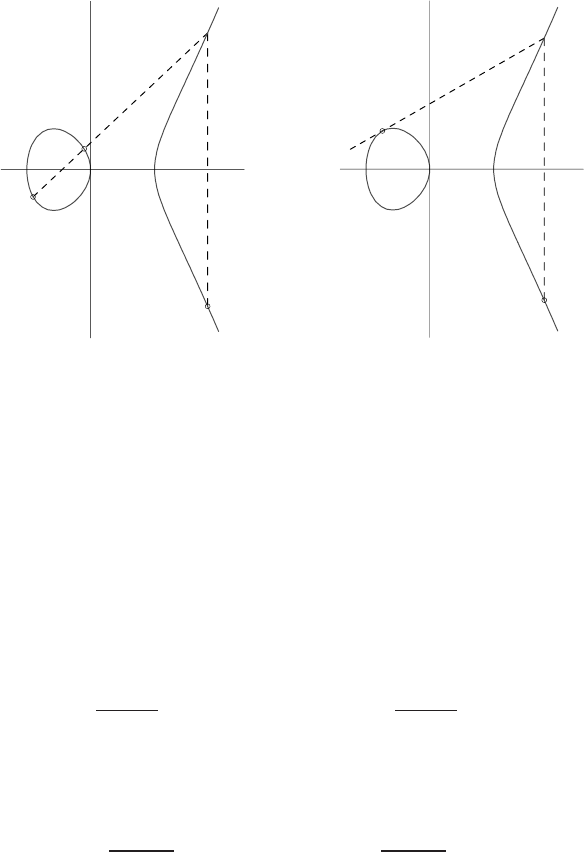
80 3. Elliptic Curve Arithmetic
R=(x3,y3)
x
y
P=(x1,y1)
Q=(x2,y2)
(a) Addition: P+Q=R.
R=(x3,y3)
x
y
P=(x1,y1)
(b) Doubling: P+P=R.
Figure 3.3. Geometric addition and doubling of elliptic curve points.
Group law for
E/K:y2=x3+ax +b
,char
(K)= 2,3
1. Identity.P+∞=∞+P=Pfor all P∈E(K).
2. Negatives.IfP=(x,y)∈E(K),then(x,y)+(x,−y)=∞. The point (x,−y)
is denoted by −Pand is called the negative of P; note that −Pis indeed a point
in E(K).Also,−∞ = ∞.
3. Point addition.LetP=(x1,y1)∈E(K)and Q=(x2,y2)∈E(K),whereP=
±Q.ThenP+Q=(x3,y3),where
x3=y2−y1
x2−x12
−x1−x2and y3=y2−y1
x2−x1(x1−x3)−y1.
4. Point doubling.LetP=(x1,y1)∈E(K),whereP=−P.Then2P=(x3,y3),
where
x3=3x2
1+a
2y12
−2x1and y3=3x2
1+a
2y1(x1−x3)−y1.
Example 3.5 (elliptic curve over the prime field F29)Letp=29, a=4, and b=20,
and consider the elliptic curve
E:y2=x3+4x+20
defined over F29. Note that =−16(4a3+27b2)=−176896 ≡ 0(mod 29),soEis
indeed an elliptic curve. The points in E(F29)are the following:

3.1. Introduction to elliptic curves 81
∞(2,6)(4,19)(8,10)(13,23)(16,2)(19,16)(27,2)
(0,7)(2,23)(5,7)(8,19)(14,6)(16,27)(20,3)(27,27)
(0,22)(3,1)(5,22)(10,4)(14,23)(17,10)(20,26)
(1,5)(3,28)(6,12)(10,25)(15,2)(17,19)(24,7)
(1,24)(4,10)(6,17)(13,6)(15,27)(19,13)(24,22)
Examples of elliptic curve addition are (5,22)+(16,27)=(13,6),and2(5,22)=
(14,6).
Group law for non-supersingular
E/F
F
F2m:y2+xy=x3+ax2+b
1. Identity.P+∞=∞+P=Pfor all P∈E(F2m).
2. Negatives.If P=(x,y)∈E(F2m),then(x,y)+(x,x+y)=∞. The point
(x,x+y)is denoted by −Pand is called the negative of P; note that −Pis
indeed a point in E(F2m).Also,−∞ = ∞.
3. Point addition.LetP=(x1,y1)∈E(F2m)and Q=(x2,y2)∈E(F2m),where
P=±Q.ThenP+Q=(x3,y3),where
x3=λ2+λ+x1+x2+aand y3=λ(x1+x3)+x3+y1
with λ=(y1+y2)/(x1+x2).
4. Point doubling.LetP=(x1,y1)∈E(F2m),whereP=−P.Then2P=(x3,y3),
where
x3=λ2+λ+a=x2
1+b
x2
1
and y3=x2
1+λx3+x3
with λ=x1+y1/x1.
Example 3.6 (non-supersingular elliptic curve over F24) Consider the finite field F24
as represented by the reduction polynomial f(z)=z4+z+1 (cf. Example 2.2). An
element a3z3+a2z2+a1z+a0∈F24is represented by the bit string (a3a2a1a0)of
length 4; for example, (0101)represents z2+1. Let a=z3,b=z3+1, and consider
the non-supersingular elliptic curve
E:y2+xy =x3+z3x2+(z3+1)
defined over F24. The points in E(F24)are the following:
∞(0011,1100)(1000,0001)(1100,0000)
(0000,1011)(0011,1111)(1000,1001)(1100,1100)
(0001,0000)(0101,0000)(1001,0110)(1111,0100)
(0001,0001)(0101,0101)(1001,1111)(1111,1011)
(0010,1101)(0111,1011)(1011,0010)
(0010,1111)(0111,1100)(1011,1001)
Examples of elliptic curve addition are (0010,1111)+(1100,1100)=(0001,0001),
and 2(0010,1111)=(1011,0010).

82 3. Elliptic Curve Arithmetic
Group law for supersingular
E/F
F
F2m:y2+cy=x3+ax +b
1. Identity.P+∞=∞+P=Pfor all P∈E(F2m).
2. Negatives.IfP=(x,y)∈E(F2m),then(x,y)+(x,y+c)=∞. The point
(x,y+c)is denoted by −Pand is called the negative of P; note that −Pis
indeed a point in E(F2m).Also,−∞ = ∞.
3. Point addition.LetP=(x1,y1)∈E(F2m)and Q=(x2,y2)∈E(F2m),where
P=±Q.ThenP+Q=(x3,y3),where
x3=y1+y2
x1+x22
+x1+x2and y3=y1+y2
x1+x2(x1+x3)+y1+c.
4. Point doubling.LetP=(x1,y1)∈E(F2m),whereP=−P.Then2P=(x3,y3),
where
x3=x2
1+a
c2
and y3=x2
1+a
c(x1+x3)+y1+c.
3.1.3 Group order
Let Ebe an elliptic curve defined over Fq. The number of points in E(Fq), denoted
#E(Fq), is called the order of Eover Fq. Since the Weierstrass equation (3.1) has
at most two solutions for each x∈Fq, we know that #E(Fq)∈[1,2q+1]. Hasse’s
theorem provides tighter bounds for #E(Fq).
Theorem 3.7 (Hasse)LetEbe an elliptic curve defined over Fq.Then
q+1−2√q≤#E(Fq)≤q+1+2√q.
The interval [q+1−2√q,q+1+2√q]is called the Hasse interval. An alternate
formulation of Hasse’s theorem is the following: if Eis defined over Fq,then#E(Fq)=
q+1−twhere |t|≤2√q;tis called the trace of Eover Fq.Since2
√qis small relative
to q,wehave#E(Fq)≈q.
The next result determines the possible values for #E(Fq)as Eranges over all
elliptic curves defined over Fq.
Theorem 3.8 (admissible orders of elliptic curves)Letq=pmwhere pis the charac-
teristic of Fq. There exists an elliptic curve Edefined over Fqwith #E(Fq)=q+1−t
if and only if one of the following conditions holds:
(i) t≡ 0(mod p)and t2≤4q.
(ii) mis odd and either (a) t=0; or (b) t2=2qand p=2; or (c) t2=3qand p=3.
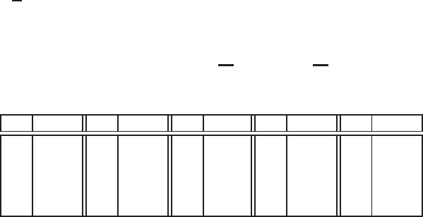
3.1. Introduction to elliptic curves 83
(iii) mis even and either (a) t2=4q;or(b)t2=qand p≡ 1(mod 3);or(c)t=0
and p≡ 1(mod 4).
A consequence of Theorem 3.8 is that for any prime pand integer tsatisfying
|t|≤2√p, there exists an elliptic curve Eover Fpwith #E(Fp)=p+1−t.This
is illustrated in Example 3.9.
Example 3.9 (orders of elliptic curves over F37)Letp=37. Table 3.1 lists, for each
integer nin the Hasse interval [37 +1−2√37,37 +1+2√37], the coefficients (a,b)
of an elliptic curve E:y2=x3+ax +bdefined over F37 with #E(F37)=n.
n(a,b)n(a,b)n(a,b)n(a,b)n(a,b)
26 (5,0) 31 (2,8) 36 (1,0) 41 (1,16) 46 (1,11)
27 (0,9) 32 (3,6) 37 (0,5) 42 (1,9) 47 (3,15)
28 (0,6) 33 (1,13) 38 (1,5) 43 (2,9) 48 (0,1)
29 (1,12) 34 (1,18) 39 (0,3) 44 (1,7) 49 (0,2)
30 (2,2) 35 (1,8) 40 (1,2) 45 (2,14) 50 (2,0)
Table 3.1. The admissible orders
n=#E(F37)
of elliptic curves
E:y2=x3+ax +b
defined
over
F37
.
The order #E(Fq)can be used to define supersingularity of an elliptic curve.
Definition 3.10 Let pbe the characteristic of Fq. An elliptic curve Edefined over Fq
is supersingular if pdivides t,wheretis the trace. If pdoes not divide t,thenEis
non-supersingular.
If Eis an elliptic curve defined over Fq,thenEis also defined over any extension
Fqnof Fq. The group E(Fq)of Fq-rational points is a subgroup of the group E(Fqn)
of Fqn-rational points and hence #E(Fq)divides #E(Fqn).If#E(Fq)is known, then
#E(Fqn)can be efficiently determined by the following result.
Theorem 3.11 Let Ebe an elliptic curve defined over Fq,andlet#E(Fq)=q+1−t.
Then #E(Fqn)=qn+1−Vnfor all n≥2, where {Vn}is the sequence defined
recursively by V0=2, V1=t,andVn=V1Vn−1−qVn−2for n≥2.
3.1.4 Group structure
Theorem 3.12 describes the group structure of E(Fq).WeuseZnto denote a cyclic
group of order n.
Theorem 3.12 (group structure of an elliptic curve)LetEbe an elliptic curve defined
over Fq.ThenE(Fq)is isomorphic to Zn1⊕Zn2where n1and n2are uniquely
determined positive integers such that n2divides both n1and q−1.
84 3. Elliptic Curve Arithmetic
Note that #E(Fq)=n1n2.Ifn2=1, then E(Fq)is a cyclic group. If n2>1, then
E(Fq)is said to have rank 2.Ifn2is a small integer (e.g., n=2,3 or 4), we sometimes
say that E(Fq)is almost cyclic.Sincen2divides both n1and q−1, one expects that
E(Fq)is cyclic or almost cyclic for most elliptic curves Eover Fq.
Example 3.13 (group structure) The elliptic curve E:y2=x3+4x+20 defined over
F29 (cf. Example 3.5) has #E(F29)=37. Since 37 is prime, E(F29)is a cyclic group
and any point in E(F29)except for ∞is a generator of E(F29). The following shows
that the multiples of the point P=(1,5)generate all the points in E(F29).
0P=∞ 8P=(8,10)16P=(0,22)24P=(16,2)32P=(6,17)
1P=(1,5)9P=(14,23)17P=(27,2)25P=(19,16)33P=(15,2)
2P=(4,19)10P=(13,23)18P=(2,23)26P=(10,4)34P=(20,26)
3P=(20,3)11P=(10,25)19P=(2,6)27P=(13,6)35P=(4,10)
4P=(15,27)12P=(19,13)20P=(27,27)28P=(14,6)36P=(1,24)
5P=(6,12)13P=(16,27)21P=(0,7)29P=(8,19)
6P=(17,19)14P=(5,22)22P=(3,28)30P=(24,7)
7P=(24,22)15P=(3,1)23P=(5,7)31P=(17,10)
Example 3.14 (group structure) Consider F24as represented by the reduction polyno-
mial f(z)=z4+z+1. The elliptic curve E:y2+xy =x3+z3x2+(z3+1)defined
over F24has #E(F24)=22 (cf. Example 3.6). Since 22 does not have any repeated fac-
tors, E(F24)is cyclic. The point P=(z3,1)=(1000,0001)has order 11; its multiples
are shown below.
0P=∞ 3P=(1100,0000)6P=(1011,1001)9P=(1001,0110)
1P=(1000,0001)4P=(1111,1011)7P=(1111,0100)10P=(1000,1001)
2P=(1001,1111)5P=(1011,0010)8P=(1100,1100)
3.1.5 Isomorphism classes
Recall the definition of isomorphic elliptic curves (Definition 3.4). The relation of iso-
morphism is an equivalence relation on the set of elliptic curves defined over a finite
field K. If two elliptic curves E1and E2are isomorphic over K, then their groups
E1(K)and E2(K)of K-rational points are also isomorphic. However, the converse is
not true (cf. Examples 3.16 and 3.17). We present some results on the isomorphism
classes of elliptic curves defined over finite fields of characteristic not equal to 2 or 3,
and for non-supersingular elliptic curves defined over binary fields.
Theorem 3.15 (isomorphism classes of elliptic curves)LetK=Fqbe a finite field
with char(K)= 2,3.

3.1. Introduction to elliptic curves 85
(i) The elliptic curves
E1:y2=x3+ax +b(3.9)
E2:y2=x3+ax +b(3.10)
defined over Kare isomorphic over Kif and only if there exists u∈K∗such that
u4a=aand u6b=b.Ifsuchauexists, then the admissible change of variables
(x,y)→(u2x,u3y)
transforms equation (3.9) into equation (3.10).
(ii) The number of isomorphism classes of elliptic curves over Kis 2q+6, 2q+2,
2q+4, 2q,forq≡1,5,7,11 (mod 12)respectively.
Example 3.16 (isomorphism classes of elliptic curves over F5) Table 3.2 lists the 12
isomorphism classes of elliptic curves over F5. Note that if the groups E1(Fq)and
E2(Fq)of Fq-rational points are isomorphic, then this does not imply that the elliptic
curves E1and E2are isomorphic over Fq. For example, the elliptic curves E1:y2=
x3+1andE2:y2=x3+2 are not isomorphic over F5,butE1(F5)and E2(F5)both
have order 6 and therefore both groups are isomorphic to Z6.
Isomorphism #E(F5)Group structure
class of E(F5)
{y2=x3+1,y2=x3+4}6Z6
{y2=x3+2,y2=x3+3}6Z6
{y3=x3+x}4Z2⊕Z2
{y3=x3+2x}2Z2
{y3=x3+3x}10 Z10
{y3=x3+4x}8Z4⊕Z2
{y2=x3+x+1,y2=x3+x+4}9Z9
{y2=x3+x+2,y2=x3+x+3}4Z4
{y2=x3+2x+1,y2=x3+2x+4}7Z7
{y2=x3+3x+2,y2=x3+3x+3}5Z5
{y2=x3+4x+1,y2=x3+4x+4}8Z8
{y2=x3+4x+2,y2=x3+4x+3}3Z3
Table 3.2. Isomorphism classes of elliptic curves
E
over
F5
.
Example 3.17 Let p=73. It is easy to verify using Theorem 3.15 that the elliptic
curves
E1:y2=x3+25x
E2:y2=x3+53x+55
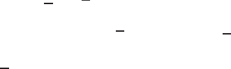
86 3. Elliptic Curve Arithmetic
defined over Fpare not isomorphic over Fp. However, the groups E1(Fpm)and
E2(Fpm)of Fpm-rational points are isomorphic for every m≥1.
Theorem 3.18 (isomorphism classes of elliptic curves over a binary field)LetK=
F2mbe a binary field.
(i) The non-supersingular elliptic curves
E1:y2+xy =x3+ax2+b(3.11)
E2:y2+xy =x3+ax2+b(3.12)
defined over Kare isomorphic over Kif and only if b=band Tr(a)=Tr(a),
where Tr is the trace function (see Definition 3.78). If these conditions are satis-
fied, then there exists s∈F2msuch that a=s2+s+a, and the admissible change
of variables
(x,y)→(x,y+sx)
transforms equation (3.11) into equation (3.12).
(ii) The number of isomorphism classes of non-supersingular elliptic curves over
Kis 2m+1−2. Let γ∈F2msatisfy Tr(γ ) =1. A set of representatives of the
isomorphism classes is
{y2+xy =x3+ax2+b|a∈{0,γ},b∈F∗
2m}.
(iii) The order #E(F2m)of the non-supersingular elliptic curve E:y2+xy =x3+
γx2+bis divisible by 2. If Tr(γ ) =0, then #E(F2m)is divisible by 4.
3.2 Point representation and the group law
Formulas for adding two elliptic points were presented in §3.1 for the elliptic curves
y2=x3+ax +bdefined over a field Kof characteristic that is neither 2 nor 3, and for
y2+xy =x3+ax2+bdefined over a binary field K. For both curves, the formulas
for point addition (i.e., adding two distinct finite points that are not negatives of each
other) and point doubling require a field inversion and several field multiplications.
If inversion in Kis significantly more expensive than multiplication, then it may be
advantageous to represent points using projective coordinates.
3.2.1 Projective coordinates
Let Kbe a field, and let cand dbe positive integers. One can define an equivalence
relation ∼on the set K3\{(0,0,0)}of nonzero triples over Kby
(X1,Y1,Z1)∼(X2,Y2,Z2)if X1=λcX2,Y1=λdY2,Z1=λZ2for some λ∈K∗.
3.2. Point representation and the group law 87
The equivalence class containing (X,Y,Z)∈K3\{(0,0,0)}is
(X:Y:Z)={(λcX,λ
dY,λZ):λ∈K∗}.
(X:Y:Z)is called a projective point,and(X,Y,Z)is called a representative of (X:
Y:Z). The set of all projective points is denoted by P(K). Notice that if (X,Y,Z)∈
(X:Y:Z)then (X:Y:Z)=(X:Y:Z); that is, any element of an equivalence
class can serve as its representative. In particular, if Z= 0, then (X/Zc,Y/Zd,1)is a
representative of the projective point (X:Y:Z), and in fact is the only representative
with Z-coordinate equal to 1. Thus we have a 1-1 correspondence between the set of
projective points
P(K)∗={(X:Y:Z):X,Y,Z∈K,Z= 0}
and the set of affine points
A(K)={(x,y):x,y∈K}.
The set of projective points
P(K)0={(X:Y:Z):X,Y,Z∈K,Z=0}
is called the line at infinity since its points do not correspond to any of the affine points.
The projective form of Weierstrass equation (3.1) of an elliptic curve Edefined over
Kis obtained by replacing xby X/Zcand yby Y/Zd, and clearing denominators.
Now, if (X,Y,Z)∈K3\{(0,0,0)}satisfies the projective equation then so does any
(X,Y,Z)∈(X:Y:Z). Therefore it makes sense to say that the projective point
(X:Y:Z)lies on E. We thus have a 1-1 correspondence between the affine points in
A(K)that lie on Eand the projective points in P(K)∗that lie on E. The projective
points in P(K)0which lie on Eare the points at infinity on E.
Example 3.19 (standard projective coordinates)Letc=1andd=1. Then the
projective form of the Weierstrass equation
E:y2+a1xy+a3y=x3+a2x2+a4x+a6
defined over Kis
Y2Z+a1XYZ +a3YZ2=X3+a2X2Z+a4XZ2+a6Z3.
The only point on the line at infinity that also lies on Eis (0:1:0). This projective
point corresponds to the point ∞in Definition 3.1.
Formulas that do not involve field inversions for adding and doubling points in pro-
jective coordinates can be derived by first converting the points to affine coordinates,
then using the formulas from §3.1 to add the affine points, and finally clearing denom-
inators. Also of use in point multiplication methods (see §3.3) is the addition of two
points in mixed coordinates—where the two points are given in different coordinate
systems.

88 3. Elliptic Curve Arithmetic
Example 3.20 (addition formulas using Jacobian coordinates)Letc=2andd=3.
The projective point (X:Y:Z),Z= 0, corresponds to the affine point (X/Z2,Y/Z3).
The projective form of the Weierstrass equation
E:y2=x3+ax +b
defined over Kis
Y2=X3+aXZ4+bZ6.
The point at infinity ∞corresponds to (1:1:0), while the negative of (X:Y:Z)is
(X:−Y:Z).
Point doubling.LetP=(X1:Y1:Z1)∈E, and suppose that P=−P.SinceP=
(X1/Z2
1:Y1/Z3
1:1), we can use the doubling formula for Ein affine coordinates to
compute 2P=(X
3:Y
3:1), obtaining
X
3=
3X2
1
Z4
1+a
2Y1
Z3
1
2
−2X1
Z2
1=(3X2
1+aZ4
1)2−8X1Y2
1
4Y2
1Z2
1
and
Y
3=
3X2
1
Z4
1+a
2Y1
Z3
1
&X1
Z2
1−X
3'−Y1
Z3
1=3X2
1+aZ4
1
2Y1Z1&X1
Z2
1−X
3'−Y1
Z3
1
.
To eliminate denominators in the expressions for X
3and Y
3,wesetX3=X
3·Z2
3and
Y3=Y
3·Z3
3where Z3=2Y1Z1, and obtain the following formulas for computing
2P=(X3:Y3:Z3)in Jacobian coordinates:
X3=(3X2
1+aZ4
1)2−8X1Y2
1
Y3=(3X2
1+aZ4
1)(4X1Y2
1−X3)−8Y4
1
Z3=2Y1Z1.
(3.13)
By storing some intermediate elements, X3,Y3and Z3can be computed using six field
squarings and four field multiplications as follows:
A←Y2
1,B←4X1·A,C←8A2,D←3X2
1+a·Z4
1,
X3←D2−2B,Y3←D·(B−X3)−C,Z3←2Y1·Z1.
Point addition using mixed Jacobian-affine coordinates.LetP=(X1:Y1:Z1)∈E,
Z1=0, and Q=(X2:Y2:1), and suppose that P=±Q.SinceP=(X1/Z2
1:Y1/Z3
1:

3.2. Point representation and the group law 89
1), we can use the addition formula for Ein affine coordinates to compute P+Q=
(X
3:Y
3:1), obtaining
X
3=
Y2−Y1
Z3
1
X2−X1
Z2
1
2
−X1
Z2
1−X2=&Y2Z3
1−Y1
(X2Z2
1−X1)Z1'2
−X1
Z2
1−X2
and
Y
3=
Y2−Y1
Z3
1
X2−X1
Z2
1
&X1
Z2
1−X
3'−Y1
Z3
1=&Y2Z3
1−Y1
(X2Z2
1−X1)Z1'&X1
Z2
1−X
3'−Y1
Z3
1
.
To eliminate denominators in the expressions for X
3and Y
3,wesetX3=X
3·Z2
3
and Y3=Y
3·Z3
3where Z3=(X2Z2
1−X1)Z1, and obtain the following formulas for
computing P+Q=(X3:Y3:Z3)in Jacobian coordinates:
X3=(Y2Z3
1−Y1)2−(X2Z2
1−X1)2(X1+X2Z2
1)
Y3=(Y2Z3
1−Y1)(X1(X2Z2
1−X1)2−X3)−Y1(X2Z2
1−X1)3
Z3=(X2Z2
1−X1)Z1.
(3.14)
By storing some intermediate elements, X3,Y3and Z3can be computed using three
field squarings and eight field multiplications as follows:
A←Z2
1,B←Z1·A,C←X2·A,D←Y2·B,E←C−X1,
F←D−Y1,G←E2,H←G·E,I←X1·G,
X3←F2−(H+2I), Y3←F·(I−X3)−Y1·H,Z3←Z1·E.
3.2.2 The elliptic curve
y2=x3+ax+b
This subsection considers coordinate systems and addition formulas for the elliptic
curve E:y2=x3+ax +bdefined over a field Kwhose characteristic is neither 2 nor
3. Several types of projective coordinates have been proposed.
1. Standard projective coordinates.Herec=1andd=1. The projective point
(X:Y:Z),Z= 0, corresponds to the affine point (X/Z,Y/Z). The projective
equation of the elliptic curve is
Y2Z=X3+aXZ2+bZ3.
The point at infinity ∞corresponds to (0:1:0), while the negative of (X:Y:Z)
is (X:−Y:Z).
90 3. Elliptic Curve Arithmetic
2. Jacobian projective coordinates.Herec=2andd=3. The projective point
(X:Y:Z),Z= 0, corresponds to the affine point (X/Z2,Y/Z3).The projective
equation of the elliptic curve is
Y2=X3+aXZ4+bZ6.
The point at infinity ∞corresponds to (1:1:0), while the negative of (X:Y:Z)
is (X:−Y:Z). Doubling and addition formulas were derived in Example 3.20.
If a=−3, the expression 3X2
1+aZ4
1that occurs in the doubling formula (3.13)
can be computed using only one field multiplication and one field squaring since
3X2
1−3Z4
1=3(X1−Z2
1)·(X1+Z2
1).
Henceforth, we shall assume that the elliptic curve y2=x3+ax +bhas a=−3.
Theorem 3.15 confirms that the selection is without much loss of generality.
Point doubling can be further accelerated by using the fact that 2Y1appears sev-
eral times in (3.13) and trading multiplications by 4 and 8 for divisions by 2. The
revised doubling formulas are:
A←3(X1−Z2
1)·(X1+Z2
1), B←2Y1,Z3←B·Z1,C←B2,
D←C·X1,X3←A2−2D,Y3←(D−X3)·A−C2/2.
The point doubling and point addition procedures for the case a=−3aregiven
in Algorithms 3.21 and 3.22 where an effort was made to minimize the number
of temporary variables Ti. The algorithms are written in terms of basic field op-
erations; however, specialized routines consisting of integrated basic operations
may be advantageous (see §5.1.2 for a concrete example when floating-point
hardware is used).
3. Chudnovsky coordinates. Here the Jacobian point (X:Y:Z)is represented
as (X:Y:Z:Z2:Z3). The redundancy in this representation is beneficial in
some point multiplication methods where additions are performed in projective
coordinates.

3.2. Point representation and the group law 91
Algorithm 3.21 Point doubling (y2=x3−3x+b, Jacobian coordinates)
INPUT:P=(X1:Y1:Z1)in Jacobian coordinates on E/K:y2=x3−3x+b.
OUTPUT:2P=(X3:Y3:Z3)in Jacobian coordinates.
1. If P=∞then return(∞).
2. T1←Z2
1.{T1←Z2
1}
3. T2←X1−T1.{T2←X1−Z2
1}
4. T1←X1+T1.{T1←X1+Z2
1}
5. T2←T2·T1.{T2←X2
1−Z4
1}
6. T2←3T2.{T2←A=3(X1−Z2
1)(X1+Z2
1)}
7. Y3←2Y1.{Y3←B=2Y1}
8. Z3←Y3·Z1.{Z3←BZ1}
9. Y3←Y2
3.{Y3←C=B2}
10. T3←Y3·X1.{T3←D=CX1}
11. Y3←Y2
3.{Y3←C2}
12. Y3←Y3/2. {Y3←C2/2}
13. X3←T2
2.{X3←A2}
14. T1←2T3.{T1←2D}
15. X3←X3−T1.{X3←A2−2D}
16. T1←T3−X3.{T1←D−X3}
17. T1←T1·T2.{T1←(D−X3)A}
18. Y3←T1−Y3.{Y3←(D−X3)A−C2/2}
19. Return(X3:Y3:Z3).
Algorithm 3.22 Point addition (y2=x3−3x+b, affine-Jacobian coordinates)
INPUT:P=(X1:Y1:Z1)in Jacobian coordinates, Q=(x2,y2)in affine coordinates
on E/K:y2=x3−3x+b.
OUTPUT:P+Q=(X3:Y3:Z3)in Jacobian coordinates.
1. If Q=∞then return(X1:Y1:Z1).
2. If P=∞then return(x2:y2:1).
3. T1←Z2
1.{T1←A=Z2
1}
4. T2←T1·Z1.{T2←B=Z1A}
5. T1←T1·x2.{T1←C=X2A}
6. T2←T2·y2.{T2←D=Y2B}
7. T1←T1−X1.{T1←E=C−X1}
8. T2←T2−Y1.{T2←F=D−Y1}
9. If T1=0then
9.1 If T2=0 then use Algorithm 3.21 to compute
(X3:Y3:Z3)=2(x2:y2:1)and return(X3:Y3:Z3).
9.2 Else return(∞).
10. Z3←Z1·T1.{Z3←Z1E}

92 3. Elliptic Curve Arithmetic
11. T3←T2
1.{T3←G=E2}
12. T4←T3·T1.{T4←H=E3}
13. T3←T3·X1.{T3←I=X1G}
14. T1←2T3.{T1←2I}
15. X3←T2
2.{X3←F2}
16. X3←X3−T1.{X3←F2−2I}
17. X3←X3−T4.{X3←F2−(H+2I)}
18. T3←T3−X3.{T3←I−X3}
19. T3←T3·T2.{T3←F(I−X3)}
20. T4←T4·Y1.{T4←Y1H}
21. Y3←T3−T4.{Y3←F(I−X3)−Y1H}
22. Return(X3:Y3:Z3).
The field operation counts for point addition and doubling in various coordinate
systems are listed in Table 3.3. The notation C1+C2→C3means that the points
to be added are in C1coordinates and C2coordinates, while their sum is expressed
in C3coordinates; for example, J+A→Jis an addition of points in Jacobian and
affine coordinates, with result in Jacobian coordinates. We see that Jacobian coordi-
nates yield the fastest point doubling, while mixed Jacobian-affine coordinates yield
the fastest point addition. Also useful in some point multiplication algorithms (see
Note 3.43) are mixed Jacobian-Chudnovsky coordinates and mixed Chudnovsky-affine
coordinates for point addition.
Doubling General addition Mixed coordinates
2A→A1I,2M,2S A +A→A1I,2M,1S J +A→J8M,3S
2P→P7M,3S P +P→P12M,2S J +C→J11M,3S
2J→J4M,4S J +J→J12M,4S C +A→C8M,3S
2C→C5M,4S C +C→C11M,3S
Table 3.3. Operation counts for point addition and doubling on
y2=x3−3x+b
.
A=
affine,
P=
standard projective,
J=
Jacobian,
C=
Chudnovsky,
I=
inversion,
M=
multiplication,
S=
squaring.
Repeated doublings
If consecutive point doublings are to be performed, then Algorithm 3.23 may be slightly
faster than repeated use of the doubling formula. By working with 2Yuntil the final
step, only one division by 2 is required. A field addition in the loop is eliminated by
calculating 3(X−Z2)(X+Z2)as 3(X2−W),whereW=Z4is computed at the first
doubling and then updated according to W←WY4before each subsequent doubling.

3.2. Point representation and the group law 93
Algorithm 3.23 Repeated point doubling (y2=x3−3x+b, Jacobian coordinates)
INPUT:P=(X:Y:Z)in Jacobian coordinates on E/K:y2=x3−3x+b,andan
integer m>0.
OUTPUT:2
mPin Jacobian coordinates.
1. If P=∞then return(P).
2. Y←2Y,W←Z4.
3. While m>0 do:
3.1 A←3(X2−W),B←XY2.
3.2 X←A2−2B,Z←ZY.
3.3 m←m−1. If m>0thenW←WY4.
3.4 Y←2A(B−X)−Y4.
4. Return(X,Y/2,Z).
In mconsecutive doublings, Algorithm 3.23 trades m−1 field additions, m−1divi-
sions by two, and a multiplication for two field squarings (in comparison with repeated
applications of Algorithm 3.21). The strategy can be adapted to the case where a=−3,
saving two field squarings in each of m−1 doublings.
3.2.3 The elliptic curve
y2+xy=x3+ax2+b
This subsection considers coordinate systems and addition formulas for the non-
supersingular elliptic curve E:y2+xy =x3+ax2+bdefined over a binary field
K. Several types of projective coordinates have been proposed.
1. Standard projective coordinates.Herec=1andd=1. The projective point
(X:Y:Z),Z= 0, corresponds to the affine point (X/Z,Y/Z). The projective
equation of the elliptic curve is
Y2Z+XYZ =X3+aX2Z+bZ3.
The point at infinity ∞corresponds to (0:1:0), while the negative of (X:Y:Z)
is (X:X+Y:Z).
2. Jacobian projective coordinates.Herec=2andd=3. The projective point
(X:Y:Z),Z= 0, corresponds to the affine point (X/Z2,Y/Z3).The projective
equation of the elliptic curve is
Y2+XYZ =X3+aX2Z2+bZ6.
The point at infinity ∞corresponds to (1:1:0), while the negative of (X:Y:Z)
is (X:X+Y:Z).
3. L´
opez-Dahab (LD) projective coordinates.Herec=1andd=2. The projec-
tive point (X:Y:Z),Z= 0, corresponds to the affine point (X/Z,Y/Z2).The

94 3. Elliptic Curve Arithmetic
projective equation of the elliptic curve is
Y2+XYZ =X3Z+aX2Z2+bZ4.
The point at infinity ∞corresponds to (1:0:0), while the negative of (X:Y:Z)
is (X:X+Y:Z). Formulas for computing the double (X3:Y3:Z3)of (X1:
Y1:Z1)are
Z3←X2
1·Z2
1,X3←X4
1+b·Z4
1,Y3←bZ4
1·Z3+X3·(aZ3+Y2
1+bZ4
1).
Formulas for computing the sum (X3:Y3:Z3)of (X1:Y1:Z1)and (X2:Y2:1)
are
A←Y2·Z2
1+Y1,B←X2·Z1+X1,C←Z1·B,D←B2·(C+aZ2
1),
Z3←C2,E←A·C,X3←A2+D+E,F←X3+X2·Z3,
G←(X2+Y2)·Z2
3,Y3←(E+Z3)·F+G.
The point doubling and point addition procedures when a∈{0,1}are given in
Algorithms 3.24 and 3.25 where an effort was made to minimize the number of
temporary variables Ti. Theorem 3.18(ii) confirms that the restriction a∈{0,1}
is without much loss of generality.
Algorithm 3.24 Point doubling (y2+xy=x3+ax2+b,a∈{0,1}, LD coordinates)
INPUT:P=(X1:Y1:Z1)in LD coordinates on E/K:y2+xy =x3+ax2+b.
OUTPUT:2P=(X3:Y3:Z3)in LD coordinates.
1. If P=∞then return(∞).
2. T1←Z2
1.{T1←Z2
1}
3. T2←X2
1.{T2←X2
1}
4. Z3←T1·T2.{Z3←X2
1Z2
1}
5. X3←T2
2.{X3←X4
1}
6. T1←T2
1.{T1←Z4
1}
7. T2←T1·b.{T2←bZ4
1}
8. X3←X3+T2.{X3←X4
1+bZ4
1}
9. T1←Y2
1.{T1←Y2
1}
10. If a=1thenT1←T1+Z3.{T1←aZ3+Y2
1}
11. T1←T1+T2.{T1←aZ3+Y2
1+bZ4
1}
12. Y3←X3·T1.{Y3←X3(aZ3+Y2
1+bZ4
1)}
13. T1←T2·Z3.{T1←bZ4
1Z3}
14. Y3←Y3+T1.{Y3←bZ4
1Z3+X3(aZ3+Y2
1+bZ4
1)}
15. Return(X3:Y3:Z3).

3.3. Point multiplication 95
Algorithm 3.25 Point addition (y2+xy=x3+ax2+b,a∈{0,1}, LD-affine coordinates)
INPUT:P=(X1:Y1:Z1)in LD coordinates, Q=(x2,y2)in affine coordinates on
E/K:y2+xy =x3+ax2+b.
OUTPUT:P+Q=(X3:Y3:Z3)in LD coordinates.
1. If Q=∞then return(P).
2. If P=∞then return(x2:y2:1).
3. T1←Z1·x2.{T1←X2Z1}
4. T2←Z2
1.{T2←Z2
1}
5. X3←X1+T1.{X3←B=X2Z1+X1}
6. T1←Z1·X3.{T1←C=Z1B}
7. T3←T2·y2.{T3←Y2Z2
1}
8. Y3←Y1+T3.{Y3←A=Y2Z2
1+Y1}
9. If X3=0then
9.1 If Y3=0 then use Algorithm 3.24 to compute
(X3:Y3:Z3)=2(x2:y2:1)and return(X3:Y3:Z3).
9.2 Else return(∞).
10. Z3←T2
1.{Z3←C2}
11. T3←T1·Y3.{T3←E=AC}
12. If a=1thenT1←T1+T2.{T1←C+aZ2
1}
13. T2←X2
3.{T2←B2}
14. X3←T2·T1.{X3←D=B2(C+aZ2
1)}
15. T2←Y2
3.{T2←A2}
16. X3←X3+T2.{X3←A2+D}
17. X3←X3+T3.{X3←A2+D+E}
18. T2←x2·Z3.{T2←X2Z3}
19. T2←T2+X3.{T2←F=X3+X2Z3}
20. T1←Z2
3.{T1←Z2
3}
21. T3←T3+Z3.{T3←E+Z3}
22. Y3←T3·T2.{Y3←(E+Z3)F}
23. T2←x2+y2.{T2←X2+Y2}
24. T3←T1·T2.{T3←G=(X2+Y2)Z2
3}
25. Y3←Y3+T3.{Y3←(E+Z3)F+G}
26. Return(X3:Y3:Z3).
The field operation counts for point addition and doubling in various coordinate
systems are listed in Table 3.4.
3.3 Point multiplication
This section considers methods for computing kP,wherekis an integer and Pis a
point on an elliptic curve Edefined over a field Fq. This operation is called point mul-

96 3. Elliptic Curve Arithmetic
Coordinate system General addition General addition Doubling
(mixed coordinates)
Affine V+M—V+M
Standard projective 13M12M7M
Jacobian projective 14M10M5M
L´opez-Dahab projective 14M8M4M
Table 3.4. Operation counts for point addition and doubling on
y2+xy =x3+ax2+b
.
M=
multiplication,
V=
division (see §2.3.6).
tiplication or scalar multiplication, and dominates the execution time of elliptic curve
cryptographic schemes (see Chapter 4). The techniques presented do not exploit any
special structure of the curve. Point multiplication methods that take advantage of ef-
ficiently computable endomorphisms on some special curves are considered in §3.4,
§3.5, and §3.6. §3.3.1 covers the case where Pis not known a priori. In instances
where Pis fixed, for example in ECDSA signature generation (see §4.4.1), point mul-
tiplication algorithms can exploit precomputed data that depends only on P(and not on
k); algorithms of this kind are presented in §3.3.2. Efficient techniques for computing
kP+lQ are considered in §3.3.3. This operation, called multiple point multiplication,
dominates the execution time of some elliptic curve cryptographic schemes such as
ECDSA signature verification (see §4.4.1).
We will assume that #E(Fq)=nh where nis prime and his small (so n≈q), P
and Qhave order n, and multipliers such as kare randomly selected integers from
the interval [1,n−1]. The binary representation of kis denoted (kt−1,...,k2,k1,k0)2,
where t≈m=log2q.
3.3.1 Unknown point
Algorithms 3.26 and 3.27 are the additive versions of the basic repeated-square-and-
multiply methods for exponentiation. Algorithm 3.26 processes the bits of kfrom right
to left, while Algorithm 3.27 processes the bits from left to right.
Algorithm 3.26 Right-to-left binary method for point multiplication
INPUT:k=(kt−1,...,k1,k0)2,P∈E(Fq).
OUTPUT:kP.
1. Q←∞.
2. For ifrom 0 to t−1do
2.1 If ki=1thenQ←Q+P.
2.2 P←2P.
3. Return(Q).

3.3. Point multiplication 97
Algorithm 3.27 Left-to-right binary method for point multiplication
INPUT:k=(kt−1,...,k1,k0)2,P∈E(Fq).
OUTPUT:kP.
1. Q←∞.
2. For ifrom t−1downto0do
2.1 Q←2Q.
2.2 If ki=1thenQ←Q+P.
3. Return(Q).
The expected number of ones in the binary representation of kis t/2≈m/2, whence
the expected running time of Algorithm 3.27 is approximately m/2 point additions and
mpoint doublings, denoted m
2A+mD.(3.15)
Let Mdenote a field multiplication, Sa field squaring, and Ia field inversion. If affine
coordinates (see §3.1.2) are used, then the running time expressed in terms of field
operations is
2.5mS+3mM+1.5mI (3.16)
if Fqhas characteristic >3, and
3mM+1.5mI (3.17)
if Fqis a binary field.
Suppose that Fqhas characteristic >3. If mixed coordinates (see §3.2.2) are used,
then Qis stored in Jacobian coordinates, while Pis stored in affine coordinates.
Thus the doubling in step 2.1 can be performed using Algorithm 3.21, while the addi-
tion in step 2.2 can be performed using Algorithm 3.22. The field operation count of
Algorithm 3.27 is then
8mM+5.5mS+(1I+3M+1S)(3.18)
(one inversion, three multiplications and one squaring are required to convert back to
affine coordinates).
Suppose now that Fqis a binary field. If mixed coordinates (see §3.2.3) are used,
then Qis stored in LD projective coordinates, while Pcan be stored in affine coordi-
nates. Thus the doubling in step 2.1 can be performed using Algorithm 3.24, and the
addition in step 2.2 can be performed using Algorithm 3.25. The field operation count
of Algorithm 3.27 is then
8.5mM+(2M+1I)(3.19)
(one inversion and two multiplications are required to convert back to affine
coordinates).

98 3. Elliptic Curve Arithmetic
Non-adjacent form (NAF)
If P=(x,y)∈E(Fq)then −P=(x,x+y)if Fqis a binary field, and −P=(x,−y)
if Fqhas characteristic >3. Thus subtraction of points on an elliptic curve is just as
efficient as addition. This motivates using a signed digit representation k =l−1
i=0ki2i,
where ki∈{0,±1}. A particularly useful signed digit representation is the non-adjacent
form (NAF).
Definition 3.28 Anon-adjacent form (NAF) of a positive integer kis an expression
k=l−1
i=0ki2iwhere ki∈{0,±1},kl−1= 0, and no two consecutive digits kiare
nonzero. The length of the NAF is l.
Theorem 3.29 (properties of NAFs)Letkbe a positive integer.
(i) khas a unique NAF denoted NAF(k).
(ii) NAF(k)has the fewest nonzero digits of any signed digit representation of k.
(iii) The length of NAF(k)is at most one more than the length of the binary
representation of k.
(iv) If the length of NAF(k)is l,then2
l/3<k<2l+1/3.
(v) The average density of nonzero digits among all NAFs of length lis approxi-
mately 1/3.
NAF(k)can be efficiently computed using Algorithm 3.30. The digits of NAF(k)are
generated by repeatedly dividing kby 2, allowing remainders of 0 or ±1. If kis odd,
then the remainder r∈{−1,1}is chosen so that the quotient (k−r)/2 is even—this
ensures that the next NAF digit is 0.
Algorithm 3.30 Computing the NAF of a positive integer
INPUT: A positive integer k.
OUTPUT:NAF(k).
1. i←0.
2. While k≥1do
2.1 If kis odd then: ki←2−(kmod 4),k←k−ki;
2.2 Else: ki←0.
2.3 k←k/2, i←i+1.
3. Return(ki−1,ki−2,...,k1,k0).
Algorithm 3.31 modifies the left-to-right binary method for point multiplication (Al-
gorithm 3.27) by using NAF(k)instead of the binary representation of k. It follows
from (iii) and (v) of Theorem 3.29 that the expected running time of Algorithm 3.31 is
approximately m
3A+mD.(3.20)

3.3. Point multiplication 99
Algorithm 3.31 Binary NAF method for point multiplication
INPUT: Positive integer k,P∈E(Fq).
OUTPUT:kP.
1. Use Algorithm 3.30 to compute NAF(k)=l−1
i=0ki2i.
2. Q←∞.
3. For ifrom l−1downto0do
3.1 Q←2Q.
3.2 If ki=1thenQ←Q+P.
3.3 If ki=−1thenQ←Q−P.
4. Return(Q).
Window methods
If some extra memory is available, the running time of Algorithm 3.31 can be decreased
by using a window method which processes wdigits of kat a time.
Definition 3.32 Let w≥2 be a positive integer. A width-wNAF of a positive integer k
is an expression k=l−1
i=0ki2iwhere each nonzero coefficient kiis odd, |ki|<2w−1,
kl−1= 0, and at most one of any wconsecutive digits is nonzero. The length of the
width-wNAF is l.
Theorem 3.33 (properties of width-wNAFs)Letkbe a positive integer.
(i) khas a unique width-wNAF denoted NAFw(k).
(ii) NAF2(k)=NAF(k).
(iii) The length of NAFw(k)is at most one more than the length of the binary
representation of k.
(iv) The average density of nonzero digits among all width-wNAFs of length lis
approximately 1/(w +1).
Example 3.34 (width-wNAFs)Letk=1122334455. We denote a negative integer −c
by c. The binary representation of kand the width-wNAFs of kfor 2 ≤w≤6are:
(k)2=1000 01011 100101 0111011011110111
NAF2(k)=1000 10100 101010 1000100100001001
NAF3(k)=1000 00300 100100 3000100100001001
NAF4(k)=1000 01000 700005 0007000700010007
NAF5(k)=10000150000 90000011000000900000009
NAF6(k)=1000 00000230000011000000900000009
NAFw(k)can be efficiently computed using Algorithm 3.35, where kmods 2wde-
notes the integer usatisfying u≡k(mod 2w)and −2w−1≤u<2w−1. The digits

100 3. Elliptic Curve Arithmetic
of NAFw(k)are obtained by repeatedly dividing kby 2, allowing remainders rin
[−2w−1,2w−1−1].Ifkis odd and the remainder r=kmods 2wis chosen, then
(k−r)/2 will be divisible by 2w−1, ensuring that the next w−1 digits are zero.
Algorithm 3.35 Computing the width-wNAF of a positive integer
INPUT: Window width w, positive integer k.
OUTPUT:NAF
w(k).
1. i←0.
2. While k≥1do
2.1 If kis odd then: ki←kmods 2w,k←k−ki;
2.2 Else: ki←0.
2.3 k←k/2, i←i+1.
3. Return(ki−1,ki−2,...,k1,k0).
Algorithm 3.36 generalizes the binary NAF method (Algorithm 3.31) by using
NAFw(k)instead of NAF(k). If follows from (iii) and (iv) of Theorem 3.33 that the
expected running time of Algorithm 3.36 is approximately
(1D+(2w−2−1)A)+*m
w+1A+mD+.(3.21)
Algorithm 3.36 Window NAF method for point multiplication
INPUT: Window width w, positive integer k,P∈E(Fq).
OUTPUT:kP.
1. Use Algorithm 3.35 to compute NAFw(k)=l−1
i=0ki2i,
2. Compute Pi=iP for i∈{1,3,5,...,2w−1−1}.
3. Q←∞.
4. For ifrom l−1downto0do
4.1 Q←2Q.
4.2 If ki= 0 then:
If ki>0thenQ←Q+Pki;
Else Q←Q−P−ki.
5. Return(Q).
Note 3.37 (selection of coordinates) The number of field inversions required can be
reduced by use of projective coordinates for the accumulator Q. If inversion is suffi-
ciently expensive relative to field multiplication, then projective coordinates may also
be effective for Pi. Chudnovsky coordinates (§3.2.2) for curves over prime fields elim-
inate inversions in precomputation at the cost of less-efficient Jacobian-Chudnovsky
mixed additions in the evaluation phase.

3.3. Point multiplication 101
The window NAF method employs a “sliding window” in the sense that Algorithm
3.35 has a width-wwindow, moving right-to-left, skipping consecutive zero entries
after a nonzero digit kiis processed. As an alternative, a sliding window can be used
on the NAF of k, leading to Algorithm 3.38. The window (which has width at most w)
moves left-to-right over the digits in NAF(k), with placement so that the value in the
window is odd (to reduce the required precomputation).
Algorithm 3.38 Sliding window method for point multiplication
INPUT: Window width w, positive integer k,P∈E(Fq).
OUTPUT:kP.
1. Use Algorithm 3.30 to compute NAF(k)=l−1
i=0ki2i.
2. Compute Pi=iP for i∈{1,3,...,2(2w−(−1)w)/3−1}.
3. Q←∞,i←l−1.
4. While i≥0do
4.1 If ki=0thent←1, u←0;
4.2 Else: find the largest t≤wsuch that u←(ki,...,ki−t+1)is odd.
4.3 Q←2tQ.
4.4 If u>0thenQ←Q+Pu;elseifu<0thenQ←Q−P−u.
4.5 i←i−t.
5. Return(Q).
The average length of a run of zeros between windows in the sliding window method
is
ν(w) =4
3−(−1)w
3·2w−2.
It follows that the expected running time of Algorithm 3.38 is approximately
*1D+2w−(−1)w
3−1A++m
w+ν(w) A+mD.(3.22)
Note 3.39 (comparing sliding window and window NAF methods)Foragivenw,the
sliding window method allows larger values in a window compared with those appear-
inginawidth-wNAF. This translates to a higher cost for precomputation (roughly
2w/3 in step 2 of Algorithm 3.38 versus 2w/4 point operations in step 2 of Algo-
rithm 3.36) in the sliding window method, but fewer point operations in the main loop
(m/(w +ν(w)) versus m/(w +1)). If the comparison is on point operations, then the
window NAF method will usually result in fewer point additions (when the optimum w
is selected for each method) for mof interest. To make a more precise comparison, the
coordinate representations (driven by the cost of field inversion versus multiplication)
must be considered.
As an example, consider the NIST binary curves and suppose that the inverse to mul-
tiplication ratio is I/M=8. Affine coordinates are used in precomputation, while the

102 3. Elliptic Curve Arithmetic
points m=163 m=233 m=283 m=409 m=571
wWN SW WN SW WN SW WN SW WN SW WN SW
211442 442 626 626 762 762 1098 1098 1530 1530
323340 318 484 438 580 526 836 750 1156 1038
445296 298 408 402 488 474 688 666 952 914
5811296 310 384 398 456 462 624 622 840 822
616 21 344 386 424 458 480 514 624 650 808 834
Table 3.5. Point addition cost in sliding versus window NAF methods, when
I/M=8
. “points”
denotes the number the points stored in the precomputation stage. “WN” denotes the window
NAF method (Algorithm 3.36). “SW” denotes the sliding window method (Algorithm 3.38).
main loop uses mixed projective-affine additions. Table 3.5 shows the expected cost
of point additions in each method. Note that there will also be mpoint doublings with
each method, so the difference in times for point multiplication will be even smaller
than Table 3.5 suggests. If there are constraints on the number of points that can be
stored at the precomputation phase, then the difference in precomputation may decide
the best method. For example, if only three points can be stored, then the sliding win-
dow method will be preferred, while storage for four points will favour the window
NAF method. The differences are fairly small however; in the example, use of w=3
(two and three points of precomputation, respectively) for both methods will favour
sliding window, but gives only 7–10% reduction in point addition cost over window
NAF.
Montgomery’s method
Algorithm 3.40 for non-supersingular elliptic curves y2+xy =x3+ax2+bover
binary fields is due to L´opez and Dahab, and is based on an idea of Montgomery.
Let Q1=(x1,y1)and Q2=(x2,y2)with Q1=±Q2.LetQ1+Q2=(x3,y3)and
Q1−Q2=(x4,y4). Then using the addition formulas (see §3.1.2), it can be verified
that
x3=x4+x2
x1+x2+x2
x1+x22
.(3.23)
Thus, the x-coordinate of Q1+Q2can be computed from the x-coordinates of Q1,
Q2and Q1−Q2. Iteration jof Algorithm 3.40 for determining kP computes the x-
coordinates only of Tj=[lP,(l+1)P],wherelis the integer represented by the j
leftmost bits of k.ThenTj+1=[2lP,(2l+1)P]or [(2l+1)P,(2l+2)P]if the (j+
1)st leftmost bit of kis 0 or 1, respectively, as illustrated in Figure 3.4. Each iteration
requires one doubling and one addition using (3.23). After the last iteration, having
computed the x-coordinates of kP =(x1,y1)and (k+1)P=(x2,y2),they-coordinate
of kP can be recovered as:
y1=x−1(x1+x)[(x1+x)(x2+x)+x2+y]+y.(3.24)

3.3. Point multiplication 103
(kt−1kt−2···kt−j
kt−(j+1)
kt−(j+2)···k1k0)2P
↓↓
[lP,(l+1)P]→ [2lP,lP+(l+1)P],if kt−(j+1)=0
[lP+(l+1)P,2(l+1)P],if kt−(j+1)=1
Figure 3.4. One iteration in Montgomery point multiplication. After
j
iterations, the
x
-coordinates of
lP
and
(l+1)P
are known for
l=(kt−1···kt−j)2
. Iteration
j+1
re-
quires a doubling and an addition to find the
x
-coordinates of
lP
and
(l+1)P
for
l=(kt−1···kt−(j+1))2
.
Equation (3.24) is derived using the addition formula for computing the x-coordinate
x2of (k+1)Pfrom kP =(x1,y1)and P=(x,y).
Algorithm 3.40 is presented using standard projective coordinates (see §3.2.1); only
the X-andZ-coordinates of points are computed in steps 1 and 2. The approximate
running time is
6mM+(1I+10M). (3.25)
One advantage of Algorithm 3.40 is that it does not have any extra storage require-
ments. Another advantage is that the same operations are performed in every iteration
of the main loop, thereby potentially increasing resistance to timing attacks and power
analysis attacks (cf. §5.3).
Algorithm 3.40 Montgomery point multiplication (for elliptic curves over F2m)
INPUT:k=(kt−1,...,k1,k0)2with kt−1=1, P=(x,y)∈E(F2m).
OUTPUT:kP.
1. X1←x,Z1←1, X2←x4+b,Z2←x2.{Compute (P,2P)}
2. For ifrom t−2downto0do
2.1 If ki=1then
T←Z1,Z1←(X1Z2+X2Z1)2,X1←xZ1+X1X2TZ
2.
T←X2,X2←X4
2+bZ4
2,Z2←T2Z2
2.
2.2 Else
T←Z2,Z2←(X1Z2+X2Z1)2,X2←xZ2+X1X2Z1T.
T←X1,X1←X4
1+bZ4
1,Z1←T2Z2
1.
3. x3←X1/Z1.
4. y3←(x+X1/Z1)[(X1+xZ1)(X2+xZ2)+(x2+y)(Z1Z2)](xZ1Z2)−1+y.
5. Return(x3,y3).
3.3.2 Fixed point
If the point Pis fixed and some storage is available, then the point multiplication
operation kP can be accelerated by precomputing some data that depends only on P.

104 3. Elliptic Curve Arithmetic
For example, if the points 2P,22P,...,2t−1Pare precomputed, then the right-to-left
binary method (Algorithm 3.26) has expected running time (m/2)A(all doublings are
eliminated).1
Fixed-base windowing methods
Brickell, Gordon, McCurley and Wilson proposed the following refinement to the sim-
ple method of precomputing every multiple 2iP.Let(Kd−1,...,K1,K0)2wbe the
base-2wrepresentation of k,whered=t/w,andletQj=i:Ki=j2wiPfor each j,
1≤j≤2w−1. Then
kP =
d−1
i=0
Ki(2wiP)=
2w−1
j=1j
i:Ki=j
2wiP=
2w−1
j=1
jQj
=Q2w−1+(Q2w−1+Q2w−2)+···+(Q2w−1+Q2w−2+···+Q1).
Algorithm 3.41 is based on this observation. Its expected running time is approximately
(2w+d−3)A(3.26)
where d=t/wand t≈m.
Algorithm 3.41 Fixed-base windowing method for point multiplication
INPUT: Window width w,d=t/w,k=(Kd−1,...,K1,K0)2w,P∈E(Fq).
OUTPUT:kP.
1. Precomputation. Compute Pi=2wiP,0≤i≤d−1.
2. A←∞,B←∞.
3. For jfrom 2w−1 downto 1 do
3.1 For each ifor which Ki=jdo: B←B+Pi.{Add Qjto B}
3.2 A←A+B.
4. Return( A).
Algorithm 3.42 modifies Algorithm 3.41 by using NAF(k)instead of the binary
representation of k. In Algorithm 3.42, NAF(k)is divided into {0,±1}-strings Kieach
of the same length w:
NAF(k)=Kd−1···K1K0.
Since each Kiis in non-adjacent form, it represents an integer in the interval [−I,I]
where I=(2w+1−2)/3ifwis even, and I=(2w+1−1)/3ifwis odd. The expected
running time of Algorithm 3.42 is approximately
2w+1
3+d−2A(3.27)
where d=(t+1)/w.
1Recall the following notation: tis the bitlength of k,andm=log2q. Also, we assume that t≈m.

3.3. Point multiplication 105
Algorithm 3.42 Fixed-base NAF windowing method for point multiplication
INPUT: Window width w, positive integer k,P∈E(Fq).
OUTPUT:kP.
1. Precomputation. Compute Pi=2wiP,0≤i≤(t+1)/w.
2. Use Algorithm 3.30 to compute NAF(k)=l−1
i=0ki2i.
3. d←l/w.
4. By padding NAF(k)on the left with 0s if necessary, write (kl−1,...,k1,k0)=
Kd−1···K1K0where each Kiis a {0,±1}-string of length d.
5. If wis even then I←(2w+1−2)/3; else I←(2w+1−1)/3.
6. A←∞,B←∞.
7. For jfrom Idownto1do
7.1 For each ifor which Ki=jdo: B←B+Pi.{Add Qjto B}
7.2 For each ifor which Ki=−jdo: B←B−Pi.{Add −Qjto B}
7.3 A←A+B.
8. Return( A).
Note 3.43 (selection of coordinates) If field inversion is sufficiently expensive, then
projective coordinates will be preferred for one or both of the accumulators Aand
Bin Algorithms 3.41 and 3.42. In the case of curves over prime fields, Table 3.3 shows
that Chudnovsky coordinates for Band Jacobian coordinates for Ais the preferred
selection if projective coordinates are used, in which case Algorithm 3.42 has mixed
Chudnovsky-affine additions at steps 7.1 and 7.2, and mixed Jacobian-Chudnovsky
addition at step 7.3.
Fixed-base comb methods
Let d=t/w. In the fixed-base comb method (Algorithm 3.44), the binary represen-
tation of kis first padded on the left with dw−t0s, and is then divided into wbit
strings each of the same length dso that
k=Kw−1···K1K0.
The bit strings Kjare written as rows of an exponent array
K0
.
.
.
Kw
.
.
.
Kw−1
=
K0
d−1··· K0
0
.
.
.
.
.
.
Kw
d−1··· Kw
0
.
.
..
.
.
Kw−1
d−1··· Kw−1
0
=
kd−1··· k0
.
.
.
.
.
.
k(w+1)d−1··· kwd
.
.
..
.
.
kwd−1··· k(w−1)d

106 3. Elliptic Curve Arithmetic
whose columns are then processed one at a time. In order to accelerate the computation,
the points
[aw−1,...,a2,a1,a0]P=aw−12(w−1)dP+···+a222dP+a12dP+a0P
are precomputed for all possible bit strings (aw−1,...,a1,a0).
Algorithm 3.44 Fixed-base comb method for point multiplication
INPUT: Window width w,d=t/w,k=(kt−1,...,k1,k0)2,P∈E(Fq).
OUTPUT:kP.
1. Precomputation. Compute [aw−1,...,a1,a0]Pfor all bit strings (aw−1,...,
a1,a0)of length w.
2. By padding kon the left with 0s if necessary, write k=Kw−1···K1K0,
where each Kjis a bit string of length d.LetKj
idenote the ith bit of Kj.
3. Q←∞.
4. For ifrom d−1 downto 0 do
4.1 Q←2Q.
4.2 Q←Q+[Kw−1
i,...,K1
i,K0
i]P.
5. Return(Q).
The expected running time of Algorithm 3.44 is
2w−1
2wd−1A+(d−1)D.(3.28)
For w>2, Algorithm 3.44 has approximately the same number of point additions
as point doubles in the main loop. Figure 3.5 illustrates the use of a second table of
precomputation in Algorithm 3.45, leading to roughly half as many point doubles as
point additions.
Algorithm 3.45 Fixed-base comb method (with two tables) for point multiplication
INPUT: Window width w,d=t/w,e=d/2,k=(kt−1,...,k0)2,P∈E(Fq).
OUTPUT:kP.
1. Precomputation. Compute [aw−1,...,a1,a0]Pand 2e[aw−1,...,a1,a0]Pfor all
bit strings (aw−1,...,a1,a0)of length w.
2. By padding kon the left with 0s if necessary, write k=Kw−1···K1K0,
where each Kjis a bit string of length d.LetKj
idenote the ith bit of Kj.
3. Q←∞.
4. For ifrom e−1 downto 0 do
4.1 Q←2Q.
4.2 Q←Q+[Kw−1
i,...,K1
i,K0
i]P+2e[Kw−1
i+e,...,K1
i+e,K0
i+e]P.
5. Return(Q).
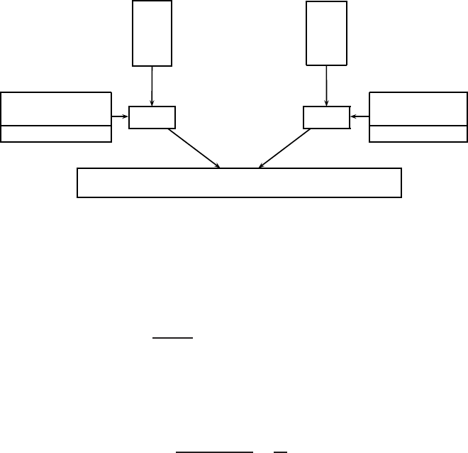
3.3. Point multiplication 107
w×dexponent array
−−−−−−−−−−−−→
K0
d−1···
.
.
.
Kw−1
d−1···
K0
i+e
.
.
.
Kw−1
i+e
··· K0
eK0
e−1···
.
.
.
.
.
.
··· Kw−1
eKw−1
e−1···
K0
i
.
.
.
Kw−1
i
··· K0
0
.
.
.
··· Kw−1
0
Precomp
(2w−1elements)
2e[aw−1,...,a0]P
lookup lookup
Precomp
(2w−1elements)
[aw−1,...,a0]P
Q←2Q+2e[Kw−1
i+e,...,K0
i+e]P+[Kw−1
i,...,K0
i]P
Figure 3.5. One iteration in Algorithm 3.45. The
w×d
exponent array is processed left-to-right in
e=d/2
iterations to find
kP
. Precomputation finds
[aw−1,...,a0]P
and
2e[aw−1,...,a0]P
for all
w
-bit values
(aw−1,...,a0)
,where
[aw−1,...,a0]=aw−12(w−1)d+···+a12d+a0
.
The expected running time of Algorithm 3.45 is approximately
2w−1
2w2e−1A+(e−1)D.(3.29)
For a fixed w, Algorithm 3.45 requires twice as much storage for precomputation as
Algorithm 3.44. For a given amount of precomputation, Algorithm 3.45 is expected to
outperform Algorithm 3.44 whenever
2w−1(w −2)
2w−w−1≥A
D,
where wis the window width used in Algorithm 3.44 (and hence width w−1isused
with Algorithm 3.45). As an example, LD coordinates in the binary field case give
A/D≈2, requiring (roughly) w≥6 in Algorithm 3.44 in order for the two-table
method to be superior. For the NIST curves over prime fields, A/D≈1.4 with Jacobian
coordinates and S=.8M, requiring w≥4.
Note 3.46 (Algorithm 3.45 with simultaneous addition) If storage for an additional e
points (which depend on k) can be tolerated, then the values
Ti←[Kw−1
i,...,K1
i,K0
i]P+2e[Kw−1
i+e,...,K1
i+e,K0
i+e]P,0≤i<e,
at step 4.2 of Algorithm 3.45 can be determined in a (data-dependent) precomputation
phase. The strategy calculates the points Tiin affine coordinates, using the method of
simultaneous inversion (Algorithm 2.26) to replace an expected e=(1−1/2w)2efield
inverses with one inverse and 3(e−1)field multiplications.
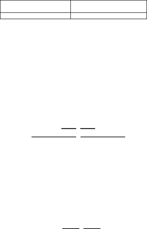
108 3. Elliptic Curve Arithmetic
If Qis maintained in projective coordinates, then emixed-coordinate additions at
step 4.2 are replaced by esimultaneous additions in the new precomputation phase.
With the coordinates discussed in §3.2, this translates into the following approximate
field operation counts.
eadditions in E(F2m)eadditions in E(Fpm),p>3
mixed-coordinate simultaneous mixed-coordinate simultaneous
8eMI+(5e−3)M8eM+3eSI+(5e−3)M+eS
For curves of practical interest from §3.2 over fields where I/Mis expected to be small
(e.g., binary fields and OEFs), a roughly 15% reduction in point multiplication time is
predicted.
Note 3.47 (comb methods) Algorithms 3.44 and 3.45 are special cases of exponen-
tiation methods due to Lim and Lee. For given parameters wand v,at-bit integer
kis written as an exponent array of w×dbits where d=t/w, as illustrated
in Figure 3.6. A typical entry Kw
vconsists of the e=d/vbits of kgiven by
Kw
v=(kl+e−1,...,kl+1,kl)where l=dw+ev(with zeros replacing some entries
if v=v−1andvd).
w
K0
v−1··· (K0
v,e−1,...,K0
v,0)··· K0
0
.
.
..
.
..
.
.
Kw
v−1··· (Kw
v,e−1,...,Kw
v,0)··· Kw
0
.
.
..
.
..
.
.
Kw−1
v−1··· (Kw−1
v,e−1,...,Kw−1
v,0
e=d/vbits
)··· Kw−1
0
d=t/wbits
Figure 3.6. The exponent array in Lim-Lee combing methods. Given parameters
w
and
v
,a
t
-bit
integer
k
is written as a
w×d
bit array for
d=t/w
.Entries
Kw
v
have
e=d/v
bits.
If Kwdenotes the integer formed from the bits in row w,then
kP =
w−1
w=0
Kw2dwP=
w−1
w=0v−1
v=0
Kw
v2ev2dwP
=
w−1
w=0
v−1
v=0e−1
e=0
Kw
v,e2e2ev2dwP
=
e−1
e=0
2ev−1
v=02evw−1
w=0
Kw
v,e2dwP
P[v][Kv,e]
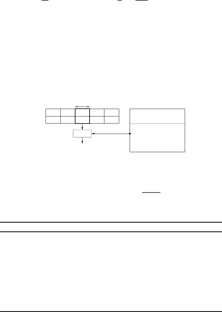
3.3. Point multiplication 109
where v(2w−1)points P[v][u]for v∈[0,v−1]and u∈[1,2w−1]are precomputed.
A point multiplication algorithm based on this method is expected to require approxi-
mately e−1≈t
wv −1 point doublings and (t
w−1)2w−1
2wpoint additions. Algorithms
3.44 and 3.45 are the cases v=1andv=2, respectively.
3.3.3 Multiple point multiplication
One method to potentially speed the computation of kP +lQ is simultaneous multiple
point multiplication (Algorithm 3.48), also known as Shamir’s trick.Ifkand lare t-bit
numbers, then their binary representations are written in a 2×tmatrix known as the
exponent array.Givenwidthw,thevaluesiP+jQ are calculated for 0 ≤i,j<2w.
At each of t/wsteps, the accumulator receives wdoublings and an addition from the
table of values iP+jQ determined by the contents of a 2×wwindow passed over the
exponent array; see Figure 3.7.
lookup
P
Q
R←2wR+(KiP+LiQ)
Li
Ki
··· L0
K0
···
···
wbits
kP =
lQ =
(2w−1)P+(2w−1)Q
0P+1Q
.
.
.
(22w−1 points)
Precomputation
Ld−1···Kd−1
Figure 3.7. Simultaneous point multiplication accumulation step.
Algorithm 3.48 has an expected running time of approximately
*(3·22(w−1)−2w−1−1)A+(22(w−1)−2w−1)D++*22w−1
22wd−1A+(d−1)w D+,
(3.30)
and requires storage for 22w−1 points.
Algorithm 3.48 Simultaneous multiple point multiplication
INPUT: Window width w,k=(kt−1,...,k0)2,l=(lt−1,...,l0)2,P,Q∈E(Fq).
OUTPUT:kP+lQ.
1. Compute iP+jQfor all i,j∈[0,2w−1].
2. Write k=(Kd−1,...,K1,K0)and l=(Ld−1,...,L1,L0)where each Ki,Liis
a bitstring of length w,andd=t/w.
3. R←∞.
4. For ifrom d−1 downto 0 do
4.1 R←2wR.
4.2 R←R+(KiP+LiQ).
5. Return(R).

110 3. Elliptic Curve Arithmetic
Algorithm 3.48 can be improved by use of a sliding window. At each step, place-
ment of a window of width at most wis such that the right-most column is nonzero.
Precomputation storage is reduced by 22(w−1)−1 points. The improved algorithm is
expected to have t/(w +(1/3)) point additions in the evaluation stage, a savings of
approximately 9% (in evaluation stage additions) compared with Algorithm 3.48 for
w∈{2,3}.
Joint sparse form
If kand lare each written in NAF form, then the expected number of zero columns in
the exponent array increases, so that the expected number of additions in the evaluation
stage of a suitably modified Algorithm 3.48 (processing one column at a time) is 5t/9.
The expected number of zero columns can be increased by choosing signed binary
expansions of kand ljointly. The joint sparse form (JSF) exponent array of positive
integers kand lis characterized by the following properties.
1. At least one of any three consecutive columns is zero.
2. Consecutive terms in a row do not have opposite signs.
3. If kj+1kj= 0thenlj+1= 0andlj=0. If lj+1lj= 0thenkj+1= 0andkj=0.
The representation has minimal weight among all joint signed binary expansions,
where the weight is defined to be the number of nonzero columns.
Example 3.49 (joint sparse form) The following table gives exponent arrays for k=
53 and l=102.
binary NAF joint sparse form
k=53 011010101 0−101 01100−10−1−1
l=102 110011010−1010−10110 10−10
weight 6 8 5
If Algorithm 3.48 is modified to use JSF, processing a single column in each itera-
tion, then t/2 additions (rather than 5t/9 using NAFs) are required in the evaluation
stage. Algorithm 3.50 finds the joint sparse form for integers k1and k2. Although it
is written in terms of integer operations, in fact only simple bit arithmetic is required;
for example, evaluation modulo 8 means that three bits must be examined, and ki/2
discards the rightmost bit.

3.3. Point multiplication 111
Algorithm 3.50 Joint sparse form
INPUT: Nonnegative integers k1and k2, not both zero.
OUTPUT:JSF(k2,k1), the joint sparse form of k1and k2.
1. l←0, d1←0, d2←0.
2. While (k1+d1>0ork2+d2>0)do
2.1 1←d1+k1,2←d2+k2.
2.2 For ifrom 1 to 2 do
If iis even then u←0;
Else
u←imods 4.
If i≡±3(mod 8)and 3−i≡2(mod 4)then u←−u.
ki
l←u.
2.3 For ifrom 1 to 2 do
If 2di=1+ki
lthen di←1−di.
ki←ki/2.
2.4 l←l+1.
3. Return JSF(k2,k1)=k1
l−1,...,k1
0
k2
l−1,...,k2
0.
Interleaving
The simultaneous and comb methods process multiple point multiplications using
precomputation involving combinations of the points. Roughly speaking, if each pre-
computed value involves only a single point, then the associated method is known as
interleaving.
In the calculation of kjPjfor points Pjand integers kj, interleaving allows dif-
ferent methods to be used for each kjPj, provided that the doubling step can be done
jointly. For example, width-wNAF methods with different widths can be used, or some
point multiplications may be done by comb methods. However, the cost of the doubling
is determined by the maximum number of doublings required in the methods for kjPj,
and hence the benefits of a comb method may be lost in interleaving.
Algorithm 3.51 is an interleaving method for computing v
j=1kjPj, where a width-
wjNAF is used on kj. Points iP
jfor odd i<2wj−1are calculated in a precomputation
phase. The expansions NAFwj(kj)are processed jointly, left to right, with a single
doubling of the accumulator at each stage; Figure 3.8 illustrates the case v=2. The
algorithm has an expected running time of approximately
*|{j:wj>2}|D+
v
j=1
(2wj−2−1)A++*max
1≤j≤vljD+
v
j=1
lj
wj+1A+(3.31)
where ljdenotes the length of NAFwj(kj), and requires storage for v
j=12wj−2points.
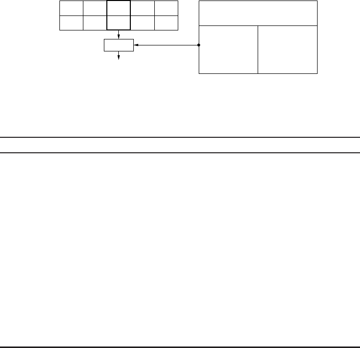
112 3. Elliptic Curve Arithmetic
lookup
P2
Q←2Q+k1
iP1+k2
iP2
k2
i··· k2
0
k2P2=
(2w2−1−1)P2
1P1
3P1.
.
.
3P2
1P2
(2w1−2+2w2−2points)
.
.
.
(2w1−1−1)P1
Precomputation
k1
t··· k1
i··· k1
0
k2
t···
P1
k1P1=
NAFwj(kj)
Figure 3.8. Computing
k1P1+k2P2
using interleaving with NAFs. The point multiplication
accumulation step is shown for the case
v=2
points. Scalar
kj
is written in width-
wj
NAF
form.
Algorithm 3.51 Interleaving with NAFs
INPUT:v,integerskj, widths wjand points Pj,1≤j≤v.
OUTPUT:v
j=1kjPj
1. Compute iP
jfor i∈{1,3,...,2wj−1−1},1≤j≤v.
2. Use Algorithm 3.30 to compute NAFwj(kj)=lj−1
i=0kj
i2i,1≤j≤v.
3. Let l=max{lj:1≤j≤v}.
4. Define kj
i=0forlj≤i<l,1≤j≤v.
5. Q←∞.
6. For ifrom l−1downto0do
6.1 Q←2Q.
6.2 For jfrom 1 to vdo
If kj
i= 0then
If kj
i>0thenQ←Q+kj
iPj;
Else Q←Q−kj
iPj.
7. Return(Q).
Note 3.52 (comparison with simultaneous methods) Consider the calculation of kP +
lQ,wherekand lare approximately the same bitlength. The simultaneous sliding and
interleaving methods require essentially the same number of point doublings regardless
of the window widths. For a given w, simultaneous sliding requires 3 ·22(w−1)points
of storage, and approximately t/(w +(1/3)) point additions in the evaluation stage,
while interleaving with width 2w+1onkand width 2won lrequires the same amount
of storage, but only (4w+3)t/(4w2+5w+2)<t/(w +(1/2)) additions in evalua-
tion. Interleaving may also be preferable at the precomputation phase, since operations
involving a known point Pmay be done in advance (encouraging the use of a wider
width for NAFw(k)), in contrast to the joint computations required in the simultaneous
method. Table 3.6 compares operation counts for computing kP +lQ in the case that
P(but not Q) is known in advance.

3.3. Point multiplication 113
In the case that storage for precomputation is limited to four points (including P
and Q), interleaving with width-3 NAFs or use of the JSF give essentially the same
performance, with interleaving requiring one or two more point doublings at the pre-
computation stage. Table 3.6 gives some comparative results for small window sizes.
method wstorage additions doubles
Alg 3.48 1 3 1 +3t/4≈1+.75tt
Alg 3.48 2 15 9 +15t/32 ≈9+.47t2+t
Alg 3.48 with sliding 2 12 9 +3t/7≈9+.43t2+t
Alg 3.48 with NAF 4 2 +5t/9≈2+.56tt
Alg 3.48 with JSF 4 2 +t/2≈2+.5tt
interleave with 3-NAF 3,32+21+t/2≈1+.5t1+t
interleave with 5-NAF & 4-NAF 5,48+43+11t/30 ≈3+.37t1+t
Table 3.6. Approximate operation counts for computing
kP+lQ
,where
k
and
l
are
t
-bit integers.
The precomputation involving only
P
is excluded.
Interleaving can be considered as an alternative to the comb method (Algo-
rithm 3.44) for computing kP. In this case, the exponent array for kis processed using
interleaving (Algorithm 3.51), with kjgiven by k=w
j=1kj2(j−1)dand points Pj
given by Pj=2(j−1)dP,1≤j≤w,wheredis defined in Algorithm 3.44. Table 3.7
compares the comb and interleaving methods for fixed storage.
method rows storage additions doubles
comb 2 3 3t/8≈.38tt/2
interleave (3,3)24 t/4≈.25tt/2
comb 4 15 15t/64 ≈.23tt/4
comb (two-table) 3 14 7t/24 ≈.29tt/6
interleave (4,4,4,4)416 t/4≈.25tt/4
interleave (4,4,4,3,3)51611t/50 ≈.22tt/5
comb 5 31 31t/160 ≈.19tt/5
comb (two-table) 4 30 15t/64 ≈.23tt/8
interleave (5,5,5,4,4)532 9t/50 ≈.18tt/5
interleave (5,5,4,4,4,4)63217t/90 ≈.19tt/6
Table 3.7. Approximate operation counts in comb and interleaving methods for computing
kP
,
P
known in advance. The bitlength of
k
is denoted by
t
. The interleaving methods list the widths
used on each row in calculating the NAF.
114 3. Elliptic Curve Arithmetic
3.4 Koblitz curves
Koblitz curves, also known as anomalous binary curves, are elliptic curves defined over
F2. The primary advantage of these curves is that point multiplication algorithms can be
devised that do not use any point doublings. The material in this section is closely based
on the detailed paper by Solinas [446] which contains proofs of facts and analyses of
algorithms presented.
Definition 3.53 Koblitz curves are the following elliptic curves defined over F2:
E0:y2+xy =x3+1
E1:y2+xy =x3+x2+1.
In cryptographic protocols, one uses the group E0(F2m)or E1(F2m)of F2m-rational
points for some extension field F2m.Leta∈{0,1}. For each proper divisor lof m,
Ea(F2l)is a subgroup of Ea(F2m)and hence #Ea(F2l)divides #Ea(F2m). In particular,
since #E0(F2)=4and#E1(F2)=2, #E0(F2m)is a multiple of 4 and #E1(F2m)is a
multiple of 2.
Definition 3.54 A Koblitz curve Eahas almost-prime group order over F2mif
#Ea(F2m)=hn where nis prime and
h=24ifa=0
2ifa=1.
his called the cofactor.
We shall assume throughout the remainder of this section that Eais a Koblitz curve
with almost-prime group order #Ea(F2m). Observe that #Ea(F2m)can only be almost
prime if mis a prime number. The group orders #Ea(F2m)can be efficiently computed
using Theorem 3.11. Table 3.8 lists the extension degrees m∈[100,600], and Koblitz
curves Eafor which #Ea(F2m)is almost prime.
3.4.1 The Frobenius map and the ring
Z
Z
Z[τ]
Definition 3.55 Let Eabe a Koblitz curve. The Frobenius map τ:Ea(F2m)→
Ea(F2m)is defined by
τ(∞)=∞,τ(x,y)=(x2,y2).
The Frobenius map can be efficiently computed since squaring in F2mis relatively
inexpensive (see §2.3.4). It is known that
(τ 2+2)P=µτ (P)for all P∈Ea(F2m),

3.4. Koblitz curves 115
mCurve Prime factorization of #Ea(F2m)
101 E12·1267650600228230886142808508011
103 E022·2535301200456459535862530067069
107 E022·40564819207303335604363489037809
107 E12·81129638414606692182851032212511
109 E12·324518553658426701487448656461467
113 E12·5192296858534827627896703833467507
131 E022·680564733841876926932320129493409985129
163 E12·5846006549323611672814741753598448348329118574063
233 E022·3450873173395281893717377931138512760570940988862252126\
328087024741343
239 E022·2208558830972980411979121875928648149482165613217098488\
87480219215362213
277 E022·6070840288205403346623318458823496583257511049878650876\
4884175561891622165064650683
283 E022·3885337784451458141838923813647037813284811733793061324\
295874997529815829704422603873
283 E12·7770675568902916283677847627294075626569631244830993521\
422749282851602622232822777663
311 E12·2085924839766513752338888384931203236916703635071711166\
739891218584916354726654294825338302183
331 E12·2187250724783011924372502227117621365353169430893227643\
447010306711358712586776588594343505255614303
347 E12·1433436634993794694756763059563804337997853118230175657\
28537420307240763803325774115493723193900257029311
349 E022·2866873269987589389513526119127608675995706236460351478\
84067443354153078762511899035960651549018775044323
359 E12·5871356456934583069723701491973342568439206372270799668\
11081824609485917244124494882365172478748165648998663
409 E022·3305279843951242994759576540163855199142023414821406096\
4232439502288071128924919105067325845777745801409636659\
0617731358671
571 E022·1932268761508629172347675945465993672149463664853217499\
3286176257257595711447802122681339785227067118347067128\
0082535146127367497406661731192968242161709250355573368\
5276673
Table 3.8. Koblitz curves
Ea
with almost-prime group order
#Ea(F2m)
and
m∈[100,600]
.

116 3. Elliptic Curve Arithmetic
where µ=(−1)1−aand τl(P)denotes the l-fold application of τto P. Hence the
Frobenius map can be regarded as a complex number τsatisfying
τ2+2=µτ ;(3.32)
we choose τ=(µ +√−7)/2. Let Z[τ]denote the ring of polynomials in τwith integer
coefficients. It now makes sense to multiply points in Ea(F2m)by elements of the ring
Z[τ]:iful−1τl−1+···+u1τ+u0∈Z[τ]and P∈Ea(F2m),then
(ul−1τl−1+···+u1τ+u0)P=ul−1τl−1(P)+···+u1τ(P)+u0P.(3.33)
The strategy for developing an efficient point multiplication algorithm for Koblitz
curves is to find, for a given integer k, a “nice” expression of the form k=l−1
i=0uiτi,
and then use (3.33) to compute kP. Here, “nice” means that lis relatively small and
the nonzero digits uiare small (e.g., ±1) and sparse.
Since τ2=µτ −2, every element αin Z[τ]can be expressed in canonical form
α=a0+a1τwhere a0,a1∈Z.
Definition 3.56 The norm of α=a0+a1τ∈Z[τ]is the (integer) product of αand its
complex conjugate. Explicitly,
N(a0+a1τ)=a2
0+µa0a1+2a2
1.
Theorem 3.57 (properties of the norm function)
(i) N(α) ≥0forallα∈Z[τ]with equality if and only if α=0.
(ii) 1 and −1 are the only elements of Z[τ]having norm 1.
(iii) N(τ ) =2andN(τ −1)=h.
(iv) N(τ m−1)=#Ea(F2m)and N((τ m−1)/(τ −1)) =n.
(v) The norm function is multiplicative; that is, N(α1α2)=N(α1)N(α2)for all
α1,α
2∈Z[τ].
(vi) Z[τ]is a Euclidean domain with respect to the norm function. That is, for any
α, β ∈Z[τ]with β=0, there exist κ,ρ ∈Z[τ](not necessarily unique) such that
α=κβ +ρand N(ρ) < N(β).
τ
-adic non-adjacent form (TNAF)
It follows from Theorem 3.57 that any positive integer kcan be written in the form
k=l−1
i=0uiτiwhere each ui∈{0,±1}.Suchaτ-adic representation can be obtained
by repeatedly dividing kby τ; the digits uiare the remainders of the division steps. This
procedure is analogous to the derivation of the binary representation of kby repeated
division by 2. In order to decrease the number of point additions in (3.33), it is desirable
to obtain a τ-adic representation for kthat has a small number of nonzero digits. This
can be achieved by using the τ-adic NAF, which can be viewed as a τ-adic analogue of
the ordinary NAF (Definition 3.28).

3.4. Koblitz curves 117
Definition 3.58 Aτ-adic NAF or TNAF of a nonzero element κ∈Z[τ]is an expression
κ=l−1
i=0uiτiwhere each ui∈{0,±1},ul−1=0, and no two consecutive digits uiare
nonzero. The length of the TNAF is l.
Theorem 3.59 (properties of TNAFs)Letκ∈Z[τ],κ= 0.
(i) κhas a unique TNAF denoted TNAF(κ).
(ii) If the length l(κ) of TNAF(κ) is greater than 30, then
log2(N(κ)) −0.55 <l(κ) < log2(N(κ)) +3.52.
(iii) The average density of nonzero digits among all TNAFs of length lis
approximately 1/3.
TNAF(κ) can be efficiently computed using Algorithm 3.61, which can be viewed
as a τ-adic analogue of Algorithm 3.30. The digits of TNAF(κ) are generated by re-
peatedly dividing κby τ, allowing remainders of 0 or ±1. If κis not divisible by τ,
then the remainder r∈{−1,1}is chosen so that the quotient (κ −r)/τ is divisible by
τ, ensuring that the next TNAF digit is 0. Division of α∈Z[τ]by τand τ2is easily
accomplished using the following result.
Theorem 3.60 (division by τand τ2in Z[τ])Letα=r0+r1τ∈Z[τ].
(i) αis divisible by τif and only if r0is even. If r0is even, then
α/τ =(r1+µr0/2)−(r0/2)τ.
(ii) αis divisible by τ2if and only if r0≡2r1(mod 4).
Algorithm 3.61 Computing the TNAF of an element in Z[τ]
INPUT:κ=r0+r1τ∈Z[τ].
OUTPUT:TNAF(κ).
1. i←0.
2. While r0= 0orr1= 0do
2.1 If r0is odd then: ui←2−(r0−2r1mod 4),r0←r0−ui;
2.2 Else: ui←0.
2.3 t←r0,r0←r1+µr0/2, r1←−t/2, i←i+1.
3. Return(ui−1,ui−2,...,u1,u0).
To compute kP, one can find TNAF(k)using Algorithm 3.61 and then use (3.33).
By Theorem 3.59(ii), the length of TNAF(k)is approximately log2(N(k)) =2log2k,
which is twice the length of NAF(k). To circumvent the problem of a long TNAF,
notice that if γ≡k(mod τm−1)then kP =γPfor all P∈Ea(F2m). This follows
because
(τ m−1)(P)=τm(P)−P=P−P=∞.

118 3. Elliptic Curve Arithmetic
It can also be shown that if ρ≡k(mod δ) where δ=(τ m−1)/(τ −1),thenkP =
ρPfor all points Pof order nin Ea(F2m). The strategy now is to find ρ∈Z[τ]of
as small norm as possible with ρ≡k(mod δ), and then use TNAF(ρ) to compute
ρP. Algorithm 3.62 finds, for any α, β ∈Z[τ]with β= 0, a quotient κ∈Z[τ]and
a remainder ρ∈Z[τ]with α=κβ +ρand N(ρ) as small as possible. It uses, as a
subroutine, Algorithm 3.63 for finding an element of Z[τ]that is “close” to a given
complex number λ0+λ1τwith λ0,λ
1∈Q.
Algorithm 3.62 Division in Z[τ]
INPUT:α=a0+a1τ∈Z[τ],β=b0+b1τ∈Z[τ]with β= 0.
OUTPUT:κ=q0+q1τ,ρ=r0+r1τ∈Z[τ]with α=κβ +ρand N(ρ) ≤4
7N(β).
1. g0←a0b0+µa0b1+2a1b1,
2. g1←a1b0−a0b1.
3. N←b2
0+µb0b1+2b2
1.
4. λ0←g0/N,λ1←g1/N.
5. Use Algorithm 3.63 to compute (q0,q1)←Round(λ0,λ
1).
6. r0←a0−b0q0+2b1q1,
7. r1←a1−b1q0−b0q1−µb1q1.
8. κ←q0+q1τ,
9. ρ←r0+r1τ.
10. Return(κ,ρ).
Algorithm 3.63 Rounding off in Z[τ]
INPUT: Rational numbers λ0and λ1.
OUTPUT:Integersq0,q1such that q0+q1τis close to complex number λ0+λ1τ.
1. For ifrom 0 to 1 do
1.1 fi←λi+1
2,ηi←λi−fi,hi←0.
2. η←2η0+µη1.
3. If η≥1then
3.1 If η0−3µη1<−1thenh1←µ;elseh0←1.
Else
3.2 If η0+4µη1≥2thenh1←µ.
4. If η<−1then
4.1 If η0−3µη1≥1thenh1←−µ;elseh0←−1.
Else
4.2 If η0+4µη1<−2thenh1←−µ.
5. q0←f0+h0,q1←f1+h1.
6. Return(q0,q1).
Definition 3.64 Let α, β ∈Z[τ]with β= 0. Then αmod βis defined to be the output
ρ∈Z[τ]of Algorithm 3.62.

3.4. Koblitz curves 119
Algorithm 3.62 for computing ρ=kmod δis cumbersome to implement on some
platforms because it requires two multiprecision integer divisions (in step 4). Algo-
rithm 3.65 computes an element ρ≡k(mod δ) without the expensive multiprecision
integer divisions. We write ρ=kpartmod δ. Solinas proved that l(ρ) ≤m+aand if
C≥2thenl(ρ)≤m+a+3. However, it is still possible that l(ρ)is significantly
bigger than l(ρ). This is not a concern in practice since the probability that ρ= ρ
is less than 2−(C−5)—hence selection of a sufficiently large Censures ρ=ρwith
overwhelming probability.
Algorithm 3.65 Partial reduction modulo δ=(τ m−1)/(τ −1)
INPUT:k∈[1,n−1],C≥2, s0=d0+µd1,s1=−d1,whereδ=d0+d1τ.
OUTPUT:ρ=kpartmod δ.
1. k←k/2a−C+(m−9)/2.
2. Vm←2m+1−#Ea(F2m).
3. For ifrom 0 to 1 do
3.1 g←si·k.j←Vm·g/2m.
3.2 λi←(g+j)/2(m+5)/2+1
2/2C.
4. Use Algorithm 3.63 to compute (q0,q1)←Round(λ0,λ
1).
5. r0←k−(s0+µs1)q0−2s1q1,r1←s1q0−s0q1.
6. Return(r0+r1τ).
3.4.2 Point multiplication
Algorithm 3.66 is an efficient point multiplication method that incorporates the ideas
of the preceding subsection. Since the length of TNAF(ρ)is approximately m,and
since its density is expected to be about 1/3, Algorithm 3.66 has an expected running
time of approximately m
3A.(3.34)
Algorithm 3.66 TNAF method for point multiplication on Koblitz curves
INPUT:Integerk∈[1,n−1],P∈E(F2m)of order n.
OUTPUT:kP.
1. Use Algorithm 3.65 to compute ρ=kpartmod δ.
2. Use Algorithm 3.61 to compute TNAF(ρ)=l−1
i=0uiτi.
3. Q←∞.
4. For ifrom l−1downto0do
4.1 Q←τQ.
4.2 If ui=1thenQ←Q+P.
4.3 If ui=−1thenQ←Q−P.
5. Return(Q).
120 3. Elliptic Curve Arithmetic
Window methods
If some extra memory is available, the running time of Algorithm 3.66 can be de-
creased by deploying a window method which processes wdigits of ρat a time. This
is achieved by using a width-wTNAF, which can be viewed as a τ-adic analogue of
the ordinary width-wNAF (Definition 3.32).
Theorem 3.67 Let {Uk}be the integer sequence defined by U0=0, U1=1, Uk+1=
µUk−2Uk−1for k≥1.
(i) U2
k−µUk−1Uk+2U2
k−1=2k−1for all k≥1.
(ii) Let tk=2Uk−1U−1
kmod 2kfor k≥1. (Since Ukis odd for each k≥1, U−1
kmod
2kdoes indeed exist.) Then t2
k+2≡µtk(mod 2k)for all k≥1.
From (3.32) and Theorem 3.67(ii), it follows that the map φw:Z[τ]→Z2winduced
by τ→ twis a surjective ring homomorphism with kernel {α∈Z[τ]:τwdivides α}.
Moreover, a set of distinct representatives of the equivalence classes of Z[τ]modulo
τwis {0,±1,±2,±3,...,±(2w−1−1), −2w−1},ofwhich{±1,±3,...,±(2w−1−1)}
are not divisible by τ.
Definition 3.68 Let w≥2 be a positive integer. Define αi=imod τwfor i∈
{1,3,5,...,2w−1−1}.Awidth-wTNAF of a nonzero element κ∈Z[τ]is an expres-
sion κ=l−1
i=0uiτiwhere each ui∈{0,±α1,±α3,...,±α2w−1−1},ul−1= 0, and at
most one of any wconsecutive digits is nonzero. The length of the width-wTNAF is l.
Note that TNAF2(κ) =TNAF(κ). Tables 3.9 and 3.10 list the αu’s for a∈{0,1}
and 3 ≤w≤6. The expressions given for each αuhas at most two terms that involve
powers of τand other αu’s. TNAF(αu)=(ul−1,...,u1,u0)is understood to mean
l−1
i=0uiτi. Most of the entries in the last columns of the tables were obtained from
the TNAF; a few exceptions were made where use of the TNAF is less efficient. With
these expressions, each αuPcan be computed using at most one elliptic curve addition
operation.
TNAFw(ρ) can be efficiently computed using Algorithm 3.69. In Algorithm 3.69,
kmods 2wdenotes the integer usatisfying u≡k(mod 2w)and −2w−1≤u<2w−1.
The digits of TNAFw(ρ) are obtained by repeatedly dividing ρby τ, allowing remain-
ders γin {0,±α1,±α3...,±α2w−1−1}.Ifρis not divisible by τand the remainder
chosen is αuwhere u=φw(ρ) mods 2w,then(ρ −αu)/τ will be divisible by τw−1,
ensuring that the next w−1 digits are 0.

3.4. Koblitz curves 121
wu u mod τwTNAF(umod τw) αu
3 1 1 (1)1
3τ+1(−1,0,−1) τ +1
4 1 1 (1)1
3−τ−3(1,0,−1) τ 2−1
5−τ−1(1,0,1) τ 2+1
7−τ+1(1,0,0,−1) τ 3−1
5 1 1 (1)1
3−τ−3(1,0,−1) τ 2−1
5−τ−1(1,0,1) τ 2+1
7−τ+1(1,0,0,−1) τ 3−1
9−2τ−3(1,0,1,0,0,1) τ 3α5+1
11 −2τ−1(−1,0,−1,0,−1)−τ2α5−1
13 −2τ+1(−1,0,−1,0,1)−τ2α5+1
15 3τ+1(1,0,0,0,−1) τ 2α5−α5
6 1 1 (1)1
3 3 (−1,0,0,1,0,−1) τ 2α25 −1
5 5 (−1,0,0,1,0,1) τ 2α25 +1
7−2τ−5(1,0,1,0,0,−1)−τ3α27 −1
9−2τ−3(1,0,1,0,0,1)−τ3α27 +1
11 −2τ−1(−1,0,−1,0,−1) τ 2α27 −1
13 −2τ+1(−1,0,−1,0,1) τ 2α27 +1
15 3τ+1(1,0,0,0,−1)−τ2α27 +α27
17 3τ+3(1,0,0,0,1)−τ2α27 +α29
19 3τ+5(1,0,0,−1,0,1,0,−1)−τ2α3−1
21 −4τ−3(−1,0,1,0,1) τ 2α29 +1
23 τ−3(−1,0,0,−1)−τ3−1
25 τ−1(−1,0,0,1)−τ3+1
27 τ+1(−1,0,−1)−τ2−1
29 τ+3(−1,0,1)−τ2+1
31 τ+5(−1,0,0,0,0,−1) τ 2α25 +α27
Table 3.9. Expressions for
αu=umod τw
for
a=0
and
3≤w≤6
.

122 3. Elliptic Curve Arithmetic
wu u mod τwTNAF(umod τw) αu
3 1 1 (1)1
3−τ+1(−1,0,−1)−τ+1
4 1 1 (1)1
3τ−3(1,0,−1) τ 2−1
5τ−1(1,0,1) τ 2+1
7τ+1(−1,0,0,−1)−τ3−1
5 1 1 (1)1
3τ−3(1,0,−1) τ 2−1
5τ−1(1,0,1) τ 2+1
7τ+1(−1,0,0,−1)−τ3−1
9 2τ−3(−1,0,−1,0,0,1)−τ3α5+1
11 2τ−1(−1,0,−1,0,−1)−τ2α5−1
13 2τ+1(−1,0,−1,0,1)−τ2α5+1
15 −3τ+1(1,0,0,0,−1) τ 2α5−α5
6 1 1 (1)1
3 3 (1,0,0,1,0,−1) τ 2α25 −1
5 5 (1,0,0,1,0,1) τ 2α25 +1
7 2τ−5(−1,0,−1,0,0,−1) τ 3α27 −1
9 2τ−3(−1,0,−1,0,0,1) τ 3α27 +1
11 2τ−1(−1,0,−1,0,−1) τ 2α27 −1
13 2τ+1(−1,0,−1,0,1) τ 2α27 +1
15 −3τ+1(1,0,0,0,−1)−τ2α27 +α27
17 −3τ+3(1,0,0,0,1)−τ2α27 +α29
19 −3τ+5(−1,0,0,−1,0,1,0,−1)−τ2α3−1
21 4τ−3(−1,0,1,0,1) τ 2α29 +1
23 −τ−3(1,0,0,−1) τ 3−1
25 −τ−1(1,0,0,1) τ 3+1
27 −τ+1(−1,0,−1)−τ2−1
29 −τ+3(−1,0,1)−τ2+1
31 −τ+5(1,0,0,0,0,−1) τ 2α25 +α27
Table 3.10. Expressions for
αu=umod τw
for
a=1
and
3≤w≤6
.

3.5. Curves with efficiently computable endomorphisms 123
Algorithm 3.69 Computing a width-wTNAF of an element in Z[τ]
INPUT:w,tw,αu=βu+γuτfor u∈{1,3,5,...,2w−1−1},ρ=r0+r1τ∈Z[τ].
OUTPUT:TNAF
w(ρ).
1. i←0.
2. While r0= 0orr1= 0do
2.1 If r0is odd then
u←r0+r1twmods 2w.
If u>0thens←1; else s←−1, u←−u.
r0←r0−sβu,r1←r1−sγu,ui←sαu.
2.2 Else: ui←0.
2.3 t←r0,r0←r1+µr0/2, r1←−t/2, i←i+1.
3. Return(ui−1,ui−2,...,u1,u0).
Algorithm 3.70 is an efficient point multiplication algorithm that uses the width-w
TNAF. Since the expected length of TNAF(ρ)is m, and since its density is expected
to be about 1/(w +1), Algorithm 3.70 has an expected running time of approximately
2w−2−1+m
w+1A.(3.35)
Algorithm 3.70 Window TNAF point multiplication method for Koblitz curves
INPUT: Window width w,integerk∈[1,n−1],P∈E(F2m)of order n.
OUTPUT:kP.
1. Use Algorithm 3.65 to compute ρ=kpartmod δ.
2. Use Algorithm 3.69 to compute TNAFw(ρ)=l−1
i=0uiτi.
3. Compute Pu=αuP,foru∈{1,3,5,...,2w−1−1}.
4. Q←∞.
5. For ifrom l−1downto0do
5.1 Q←τQ.
5.2 If ui= 0 then:
Let ube such that αu=uior α−u=−ui.
If u>0thenQ←Q+Pu;
Else Q←Q−P−u.
6. Return(Q).
3.5 Curves with efficiently computable endomorphisms
The Frobenius map (Definition 3.55) is an example of an endomorphism of an elliptic
curve. This section presents a general technique for accelerating point multiplication on
elliptic curves that have efficiently computable endomorphisms. While the technique
124 3. Elliptic Curve Arithmetic
does not yield a speedup that is as dramatic as achieved in §3.4 for Koblitz curves
(where all the point doublings are replaced by much faster applications of the Frobe-
nius map), it can be used to accelerate point multiplication on a larger class of curves
including some elliptic curves over large prime fields. Roughly speaking, if the endo-
morphism can be computed in no more time than it takes to perform a small number of
point doublings, then the technique eliminates about half of all doublings and reduces
the point multiplication time by roughly 33%.
Endomorphisms of elliptic curves
Let Ebe an elliptic curve defined over a field K. The set of all points on Ewhose
coordinates lie in any finite extension of Kis also denoted by E.Anendomorphism φ
of Eover Kis a map φ:E→Esuch that φ(∞)=∞and φ(P)=(g(P), h(P)) for
all P∈E,wheregand hare rational functions whose coefficients lie in K.Thesetof
all endomorphisms of Eover Kforms a ring, called the endomorphism ring of Eover
K. An endomorphism φis also a group homomorphism, that is,
φ(P1+P2)=φ(P1)+φ(P2)for all P1,P2∈E.
The characteristic polynomial of an endomorphism φis the monic polynomial f(X)
of least degree in Z[X]such that f(φ) =0, that is, f(φ)( P)=∞for all P∈E.IfEis
a non-supersingular elliptic curve, then the characteristic polynomial of φhas degree 1
or 2.
Example 3.71 (endomorphisms of elliptic curves)
(i) Let Ebe an elliptic curve defined over Fq. For each integer m,themultiplication
by m map [m]:E→Edefined by
[m]:P→ mP
is an endomorphism of Edefined over Fq. A special case is the negation map
defined by P→−P. The characteristic polynomial of [m]is X−m.
(ii) Let Ebe an elliptic curve defined over Fq. Then the q-th power map φ:E→E
defined by
φ:(x,y)→ (xq,yq), φ :∞→∞
is an endomorphism of Edefined over Fq, called the Frobenius endomorphism.
The characteristic polynomial of φis X2−tX+q,wheret=q+1−#E(Fq).
(iii) Let p≡1(mod 4)be a prime, and consider the elliptic curve
E:y2=x3+ax
defined over Fp.Leti∈Fpbe an element of order 4. Then the map φ:E→E
defined by
φ:(x,y)→ (−x,iy), φ :∞→∞
3.5. Curves with efficiently computable endomorphisms 125
is an endomorphism of Edefined over Fp. Note that φ(P)can be computed
using only one multiplication. The characteristic polynomial of φis X2+1.
(iv) Let p≡1(mod 3)be a prime, and consider the elliptic curve
E:y2=x3+b
defined over Fp.Letβ∈Fpbe an element of order 3. Then the map φ:E→E
defined by
φ:(x,y)→ (βx,y), φ :∞→∞
is an endomorphism of Edefined over Fp. Note that φ(P)can be computed
using only one multiplication. The characteristic polynomial of φis X2+X+1.
Note 3.72 (integer representation of an endomorphism) Suppose now that Eis an el-
liptic curve defined over the finite field Fq. Suppose also that #E(Fq)is divisible by
aprimen,andthatn2does not divide #E(Fq).ThenE(Fq)contains exactly one
subgroup of order n; let this subgroup be Pwhere P∈E(Fq)has order n.Ifφis
an endomorphism of Edefined over Fq,thenφ(P)∈E(Fq)and hence φ(P)∈P.
Suppose that φ(P)=∞. Then we can write
φ(P)=λPfor some λ∈[1,n−1].
In fact λis a root modulo nof the characteristic polynomial of φ.
Example 3.73 (the elliptic curve P-160) Consider the elliptic curve
E:y2=x3+3
defined over the 160-bit prime field Fp,where
p=2160 −229233
=1461501637330902918203684832716283019655932313743.
Since p≡1(mod 3), the curve is of the type described in Example 3.71(iv). The group
of Fp-rational points on Ehas prime order
#E(Fp)=n=1461501637330902918203687013445034429194588307251.
An element of order 3 in Fpis
β=771473166210819779552257112796337671037538143582
and so the map φ:E→Edefined by φ:∞→∞and φ:(x,y)→ (βx,y)is an
endomorphism of Edefined over Fp. The solution
λ=903860042511079968555273866340564498116022318806
to the equation λ2+λ+1≡0(mod n)has the property that φ(P)=λPfor all P∈
E(Fp).

126 3. Elliptic Curve Arithmetic
Accelerating point multiplication
The strategy for computing kP,wherek∈[0,n−1], is the following. First write
k=k1+k2λmod n(3.36)
where the integers k1and k2are of approximately half the bitlength of k.Suchan
expression is called a balanced length-two representation of k.Since
kP =k1P+k2λP
=k1P+k2φ(P), (3.37)
kP can be obtained by first computing φ(P)and then using simultaneous multiple
point multiplication (Algorithm 3.48) or interleaving (Algorithm 3.51) to evaluate
(3.37). Since k1and k2are of half the bitlength of k, half of the point doublings are
eliminated. The strategy is effective provided that a decomposition (3.36) and φ(P)
can be computed efficiently.
Decomposing a multiplier
We describe one method for obtaining a balanced length-two representation of the
multiplier k. For a vector v=(a,b)∈Z×Z,define
f(v) =a+bλmod n.
The idea is to first find two vectors, v1=(a1,b1)and v2=(a2,b2)in Z×Zsuch that
1. v1and v2are linearly independent over R;
2. f(v1)=f(v2)=0; and
3. v1and v2have small Euclidean norm (i.e., ||v1||=3a2
1+b2
1≈√n, and similarly
for v2).
Then, by considering (k,0)as a vector in Q×Q, we can use elementary linear algebra
to write
(k,0)=γ1v1+γ2v2,where γ1,γ
2∈Q.
If we let c1=γ1and c2=γ2,wherexdenotes the integer closest to x,then
v=c1v1+c2v2is an integer-valued vector close to (k,0)such that f(v) =0. Thus
the vector u=(k,0)−vhas small norm and satisfies f(u)=k. It follows that the
components k1,k2of uare small in absolute value and satisfy k1+k2λ≡k(mod n).
The independent short vectors v1and v2satisfying f(v1)=f(v2)=0 can be found
by applying the extended Euclidean algorithm (Algorithm 2.19) to nand λ. The algo-
rithm produces a sequences of equations sin+tiλ=riwhere s0=1, t0=0, r0=n,
s1=0, t1=1, r1=λ. Furthermore, it is easy to show that the remainders riare strictly
decreasing and non-negative, that |ti|<|ti+1|for i≥0, and that |si|<|si+1|and

3.5. Curves with efficiently computable endomorphisms 127
ri−1|ti|+ri|ti−1|=nfor i≥1. Now, let lbe the greatest index for which rl≥√n.Then
it can be easily verified that v1=(rl+1,−tl+1)satisfies f(v1)=0and||v1|| ≤ √2n,
and that v2=(rl,−tl)(and also v2=(rl+2,−tl+2)) is linearly independent of v1and
satisfies f(v2)=0. Heuristically, we would expect v2to have small norm. Thus v1and
v2satisfy conditions 1–3 above. For this choice of v1,v2,wehaveγ1=b2k/nand
γ2=−b1k/n. The method for decomposing kis summarized in Algorithm 3.74.
Algorithm 3.74 Balanced length-two representation of a multiplier
INPUT:Integersn,λ,k∈[0,n−1].
OUTPUT:Integersk1,k2such that k=k1+k2λmod nand |k1|,|k2|≈√n.
1. Run the extended Euclidean algorithm (Algorithm 2.19) with inputs nand λ.The
algorithm produces a sequence of equations sin+tiλ=riwhere s0=1, t0=0,
r0=n,s1=0, t1=1, r1=λ, and the remainders riand are non-negative and
strictly decreasing. Let lbe the greatest index for which rl≥√n.
2. Set (a1,b1)←(rl+1,−tl+1).
3. If (r2
l+t2
l)≤(r2
l+2+t2
l+2)then set (a2,b2)←(rl,−tl);
Else set (a2,b2)←(rl+2,−tl+2).
4. Compute c1=b2k/nand c2=−b1k/n.
5. Compute k1=k−c1a1−c2a2and k2=−c1b1−c2b2.
6. Return(k1,k2).
Example 3.75 (balanced length-two representation of a multiplier k) Consider the
elliptic curve P-160 defined in Example 3.73. In the notation of Algorithm 3.74 we
have
(rl,tl)=(2180728751409538655993509,−186029539167685199353061)
(rl+1,tl+1)=(788919430192407951782190,602889891024722752429129)
(rl+2,tl+2)=(602889891024722752429129,−1391809321217130704211319)
(a1,b1)=(788919430192407951782190,−602889891024722752429129)
(a2,b2)=(602889891024722752429129,1391809321217130704211319).
Now, let
k=965486288327218559097909069724275579360008398257.
We obtain
c1=919446671339517233512759,c2=398276613783683332374156
and
k1=−98093723971803846754077,k2=381880690058693066485147.

128 3. Elliptic Curve Arithmetic
Example 3.76 (balanced representation for special parameters) The elliptic curve can
be chosen so that the parameters k1and k2may be obtained with much less effort than
that required by Algorithm 3.74. For example, consider the curve
E:y2=x3−2
over Fp,where p=2390 +3 is prime and, as in Example 3.71(iv), satisfies p≡1
(mod 3). The group of Fp-rational points on Ehas order
#E(Fp)=2390 −2195 +7=63n
where nis prime. If
λ=2195 −2
3and β=2389 +2194 +1,
then βis an element of order 3 in Fp,λsatisfies λ2+λ+1≡0(mod n),andλ(x,y)=
(βx,y)for all (x,y)in the order-nsubgroup of E(Fp).
Suppose now that P=(x,y)is in the order-nsubgroup of E(Fp),andk∈[0,n−1]
is a multiplier. To find a balanced length-two representation of k, write k=2195k
2+k
1
for k
1<2195.Then
kP =(2195k
2+k
1)P=((3λ+2)k
2+k
1)P=(2k
2+k
1
k1
)P+3k
2
k2
λP
=k1(x,y)+k2(βx,y).
The method splits a multiplier k<nof approximately 384 bits into k1and k2where
each is approximately half the bitlength of k. Finally, note that the cost of calculating
βx=(2389 +2194 +1)xis less than a field multiplication.
Point multiplication algorithm
Given an elliptic curve Edefined over a finite field Fqwith a suitable endomorphism
φ, Algorithm 3.77 calculates the point multiplication kP using the decomposition
k=k1+k2λmod nand interleaving k1P+k2φ(P). The expected running time is
approximately
*|{j:wj>2}|D+
2
j=1
(2wj−2−1)A+Ck+Cφ++*D+
2
j=1
1
wj+1A+t
2(3.38)
where tis the bitlength of n,kjis written with a width-wjNAF, Ckdenotes the cost of
the decomposition of k,andCφis the cost of finding φ(P). The storage requirement is
2w1−2+2w2−2points.

3.6. Point multiplication using halving 129
Since v1and v2do not depend on k, it is possible to precompute estimates for b1/n
and −b2/nfor use in step 4 of Algorithm 3.74. In this case, only steps 4–6 of Algo-
rithm 3.74 must be performed, and hence the cost Ckis insignificant in the overall point
multiplication.
Algorithm 3.77 Point multiplication with efficiently computable endomorphisms
INPUT:Integerk∈[1,n−1],P∈E(Fq), window widths w1and w2,andλ.
OUTPUT:kP.
1. Use Algorithm 3.74 to find k1and k2such that k=k1+k2λmod n.
2. Calculate P2=φ(P),andletP1=P.
3. Use Algorithm 3.30 to compute NAFwj(|kj|)=lj−1
i=0kj,i2ifor j=1,2.
4. Let l=max{l1,l2}and define kj,i=0forlj≤i<l,1≤j≤2.
5. If kj<0, then set kj,i←−kj,ifor 0 ≤i<lj,1≤j≤2.
6. Compute iP
jfor i∈{1,3,...,2wj−1−1},1≤j≤2.
7. Q←∞.
8. For ifrom l−1downto0do
8.1 Q←2Q.
8.2 For jfrom 1 to 2 do
If kj,i= 0then
If kj,i>0thenQ←Q+kj,iPj;
Else Q←Q−|kj,i|Pj.
9. Return(Q).
3.6 Point multiplication using halving
Point multiplication methods based on point halving share strategy with τ-adic meth-
ods on Koblitz curves (§3.4) in the sense that point doubling is replaced by a potentially
faster operation. As with the efficiently computable endomorphisms in §3.5, the im-
provement is not as dramatic as that obtained with methods for Koblitz curves, although
halving applies to a wider class of curves.
Point halving was proposed independently by E. Knudsen and R. Schroeppel. We
restrict our attention to elliptic curves Eover binary fields F2mdefined by the equation
y2+xy =x3+ax2+b
where a,b∈F2m,b= 0. To simplify the exposition, we assume that Tr(a)=1(cf.
Theorem 3.18).2We further assume that mis prime and that the reduction polynomials
2The algorithms presented in this section can be modified for binary curves with Tr(a)=0; however,
they are more complicated than the case where Tr(a)=1.
130 3. Elliptic Curve Arithmetic
are trinomials or pentanomials. These properties are satisfied by the five random curves
over binary fields recommended by NIST in the FIPS 186-2 standard (see §A.2.2).
Let P=(x,y)be a point on Ewith P=−P. From §3.1.2, the (affine) coordinates
of Q=2P=(u,v) can be computed as follows:
λ=x+y/x(3.39)
u=λ2+λ+a(3.40)
v=x2+u(λ +1). (3.41)
Affine point doubling requires one field multiplication and one field division. With
projective coordinates and a∈{0,1}, point doubling can be done in four field multipli-
cations. Point halving is the following operation: given Q=(u,v), compute P=(x,y)
such that Q=2P. Since halving is the reverse operation of doubling, the basic idea for
halving is to solve (3.40) for λ, (3.41) for x, and finally (3.39) for y.
When Gis a subgroup of odd order nin E, point doubling and point halving are
automorphisms of G. Therefore, given a point Q∈G, one can always find a unique
point P∈Gsuch that Q=2P. §3.6.1 and §3.6.2 describe an efficient algorithm for
point halving in G. In §3.6.3, point halving is used to obtain efficient halve-and-add
methods for point multiplication in cryptographic schemes based on elliptic curves
over binary fields.
3.6.1 Point halving
The notion of trace plays a central role in deriving an efficient algorithm for point
halving.
Definition 3.78 The trace function on F2mis the function Tr :F2m→F2mdefined by
Tr(c)=c+c2+c22+···+c2m−1.
Lemma 3.79 (properties of the trace function)Letc,d∈F2m.
(i) Tr(c)=Tr(c2)=Tr(c)2; in particular, Tr(c)∈{0,1}.
(ii) Trace is linear; that is, Tr(c+d)=Tr(c)+Tr(d).
(iii) If (u,v)∈G,thenTr(u)=Tr(a).
Property (iii) follows from (3.40) because
Tr(u)=Tr(λ2+λ+a)=Tr(λ)2+Tr(λ) +Tr(a)=Tr(a).
Given Q=(u,v)∈G, point halving seeks the unique point P=(x,y)∈Gsuch that
Q=2P. The first step of halving is to find λ=x+y/xby solving the equation
λ2+
λ=u+a(3.42)

3.6. Point multiplication using halving 131
for
λ. An efficient algorithm for solving (3.42) is presented in §3.6.2. Let
λdenote the
solution of (3.42) obtained from this algorithm. It is easily verified that λ∈{
λ,
λ+1}.
If Tr(a)=1, the following result can be used to identify λ.
Theorem 3.80 Let P=(x,y), Q=(u,v) ∈Gbe such that Q=2P, and denote λ=
x+y/x.Let
λbe a solution to (3.42), and t=v+u
λ. Suppose that Tr(a)=1. Then
λ=λif and only if Tr(t)=0.
Proof: Recall from (3.41) that x2=v+u(λ +1). By Lemma 3.79(iii), we get Tr(x)=
Tr(a)since P=(x,y)∈G. Thus,
Tr(v +u(λ +1)) =Tr(x2)=Tr(x)=Tr(a)=1.
Hence, if
λ=λ+1, then Tr(t)=Tr(v +u(λ +1)) =1 as required. Otherwise, we must
have
λ=λ, which gives Tr(t)=Tr(v +uλ) =Tr(v +u((λ +1)+1)). Since the trace
function is linear,
Tr(v +u((λ +1)+1)) =Tr(v +u(λ +1)) +Tr(u)=1+Tr(u)=0.
Hence, we conclude that
λ=λif and only if Tr(t)=0.
Theorem 3.80 suggests a simple algorithm for identifying λin the case that Tr(a)=
1. We can then solve x2=v+u(λ +1)for the unique root x. §3.6.2 presents efficient
algorithms for finding traces and square roots in F2m. Finally, if needed, y=λx+x2
may be recovered with one field multiplication.
Let the λ-representation of a point Q=(u,v) be (u,λQ),where
λQ=u+v
u.
Given the λ-representation of Qas the input to point halving, we may compute tin
Theorem 3.80 without converting to affine coordinates since
t=v+u
λ=uu+u+v
u+u
λ=u(u+λQ+
λ).
In point multiplication, repeated halvings may be performed directly on the λ-
representation of a point, with conversion to affine only when a point addition is
required.
Algorithm 3.81 Point halving
INPUT:λ-representation (u,λQ)or affine representation (u,v) of Q∈G.
OUTPUT:λ-representation (x,λP)of P=(x,y)∈G,whereQ=2P.
1. Find a solution
λof
λ2+
λ=u+a.
2. If the input is in λ-representation, then compute t=u(u+λQ+
λ);
else, compute t=v+u
λ.
3. If Tr(t)=0, then λP←
λ,x←√t+u;
else λP←
λ+1, x←√t.
4. Return (x,λP).

132 3. Elliptic Curve Arithmetic
3.6.2 Performing point halving efficiently
Point halving requires a field multiplication and three main steps: (i) computing the
trace of t; (ii) solving the quadratic equation (3.42); and (iii) computing a square
root. In a normal basis, field elements are represented in terms of a basis of the form
{β,β2,...,β2m−1}. The trace of an element c=ciβ2i=(c0,c1,...,cm−1)is given by
Tr(c)=ci. The square root computation is a left rotation: √c=(c1,...,cm−1,c0).
Squaring is a right rotation, and x2+x=ccan be solved bitwise. These operations
are expected to be inexpensive relative to field multiplication. However, field multi-
plication in software for normal basis representations is very slow in comparison to
multiplication with a polynomial basis. Conversion between polynomial and normal
bases at each halving appears unlikely to give a competitive method, even if signifi-
cant storage is used. For these reasons, we restrict our discussion to computations in a
polynomial basis representation.
Computing the trace
Let c=m−1
i=0cizi∈F2m, with ci∈{0,1}, represented as the vector c=(cm−1,...,c0).
A primitive method for computing Tr(c)uses the definition of trace, requiring m−1
field squarings and m−1 field additions. A much more efficient method makes use of
the property that the trace is linear:
Tr(c)=Trm−1
i=0
cizi=
m−1
i=0
ciTr(zi).
The values Tr(zi)may be precomputed, allowing the trace of an element to be found
efficiently, especially if Tr(zi)=0formosti.
Example 3.82 (computing traces of elements in F2163 ) Consider F2163 with reduction
polynomial f(z)=z163 +z7+z6+z3+1. A routine calculation shows that Tr(zi)=1
if and only if i∈{0,157}.Asexamples,Tr(z160 +z46)=0, Tr(z157 +z46)=1, and
Tr(z157 +z46 +1)=0.
Solving the quadratic equation
The first step of point halving seeks a solution xof a quadratic equation of the form
x2+x=cover F2m. The time performance of this step is crucial in obtaining an
efficient point halving.
Definition 3.83 Let mbe an odd integer. The half-trace function H :F2m→F2mis
defined by
H(c)=
(m−1)/2
i=0
c22i.

3.6. Point multiplication using halving 133
Lemma 3.84 (properties of the half-trace function)Letmbe an odd integer.
(i) H(c+d)=H(c)+H(d)for all c,d∈F2m.
(ii) H(c)is a solution of the equation x2+x=c+Tr(c).
(iii) H(c)=H(c2)+c+Tr(c)for all c∈F2m.
Let c=m−1
i=0cizi∈F2mwith Tr(c)=0; in particular, H(c)is a solution of x2+
x=c. A simple method for finding H(c)directly from the definition requires m−1
squarings and (m−1)/2 additions. If storage for {H(zi):0≤i<m}is available, then
Lemma 3.84(i) may be applied to obtain
H(c)=Hm−1
i=0
cizi=
m−1
i=0
ciH(zi).
However, this requires storage for mfield elements, and the associated method requires
an average of m/2 field additions.
Lemma 3.84 can be used to significantly reduce the storage required as well as the
time needed to solve the quadratic equation. The basic strategy is to write H(c)=
H(c)+swhere chas fewer nonzero coefficients than c.Foreveni, note that
H(zi)=H(zi/2)+zi/2+Tr(zi).
Algorithm 3.85 is based on this observation, eliminating storage of H(zi)for all even
i. Precomputation builds a table of (m−1)/2fieldelementsH(zi)for odd i,andthe
algorithm is expected to have approximately m/4 field additions at step 4. The terms
involving Tr(zi)and H(1)have been discarded, since it suffices to produce a solution
s∈{H(c), H(c)+1}of x2+x=c.
Algorithm 3.85 Solve x2+x=c(basic version)
INPUT:c=m−1
i=0cizi∈F2mwhere mis odd and Tr(c)=0.
OUTPUT: A solution sof x2+x=c.
1. Precompute H(zi)for odd i,1≤i≤m−2.
2. s←0.
3. For ifrom (m−1)/2downto1do
3.1 If c2i=1 then do: c←c+zi,s←s+zi.
4. s←s+
(m−1)/2
i=1
c2i−1H(z2i−1).
5. Return(s).
Further improvements are possible by use of Lemma 3.84 together with the reduction
polynomial f(z).Letibe odd, and define jand sby
m≤2ji=m+s<2m.

134 3. Elliptic Curve Arithmetic
The basic idea is to apply Lemma 3.84(iii) jtimes, obtaining
H(zi)=H(z2ji)+z2j−1i+···+z4i+z2i+zi+jTr(zi). (3.43)
Let f(z)=zm+r(z),wherer(z)=zb+···+zb1+1and0<b1<···<b<m.Then
H(z2ji)=H(zsr(z)) =H(zs+b)+H(zs+b−1)+···+H(zs+b1)+H(zs).
Thus, storage for H(zi)may be exchanged for storage of H(zs+e)for e∈{0,b1,...,b}
(some of which may be further reduced). The amount of storage reduction is limited
by dependencies among elements H(zi).
If degr<m/2, the strategy can be applied in an especially straightforward fashion
to eliminate some of the storage for H(zi)in Algorithm 3.85. For m/2<i<m−degr,
H(zi)=H(z2i)+zi+Tr(zi)
=H(r(z)z2i−m)+zi+Tr(zi)
=H(z2i−m+b+···+z2i−m+b1+z2i−m)+zi+Tr(zi).
Since 2i−m+degr<i, the reduction may be applied to eliminate storage of H(zi)for
odd i,m/2<i<m−degr.Ifdegris small, Algorithm 3.86 requires approximately
m/4 elements of storage.
Algorithm 3.86 Solve x2+x=c
INPUT:c=m−1
i=0cizi∈F2mwhere mis odd and Tr(c)=0, and reduction polynomial
f(z)=zm+r(z).
OUTPUT: A solution sof x2+x=c.
1. Precompute H(zi)for i∈I0∪I1,whereI0and I1consist of the odd integers in
[1,(m−1)/2]and [m−degr,m−2], respectively.
2. s←0.
3. For each odd i∈((m−1)/2,m−degr), processed in decreasing order, do:
3.1 If ci=1 then do: c←c+z2i−m+b+···+z2i−m,s←s+zi.
4. For ifrom (m−1)/2 downto 1 do:
4.1 If c2i=1 then do: c←c+zi,s←s+zi.
5. s←s+
i∈I0∪I1
ciH(zi).
6. Return(s).
The technique may also reduce the time required for solving the quadratic equation,
since the cost of reducing each H(zi)may be less than the cost of adding a precom-
puted value of H(zi)to the accumulator. Elimination of the even terms (step 4) can be
implemented efficiently. Processing odd terms (as in step 3) is more involved, but will
be less expensive than a field addition if only a few words must be updated.
3.6. Point multiplication using halving 135
Example 3.87 (Algorithm 3.86 for the field F2163 ) Consider F2163 with reduction poly-
nomial f(z)=z163 +z7+z6+z3+1. Step 3 of Algorithm 3.86 begins with i=155.
By Lemma 3.84,
H(z155)=H(z310)+z155 +Tr(z155)
=H(z147z163)+z155
=H(z147(z7+z6+z3+1)) +z155.
If c155 =1, then z154 +z153 +z150 +z147 is added to c,andz155 is added to s.Inthis
fashion, storage for H(zi)is eliminated for i∈{83,85,...,155}, the odd integers in
((m−1)/2,m−degr).
Algorithm 3.86 uses 44 field elements of precomputation. While this is roughly half
that required by the basic algorithm, it is not minimal. For example, storage for H(z51)
may be eliminated, since
H(z51)=H(z102)+z51 +Tr(z51)
=H(z204)+z102 +z51 +Tr(z102)+Tr(z51)
=H(z163z41)+z102 +z51
=H(z48 +z47 +z44 +z41)+z102 +z51
which corresponds to equation (3.43) with j=2. The same technique eliminates stor-
age for H(zi),i∈{51,49,...,41}. Similarly, if (3.43) is applied with i=21 and j=3,
then
H(z21)=H(z12 +z11 +z8+z5)+z84 +z42 +z21.
Note that the odd exponents 11 and 5 are less than 21, and hence storage for H(z21)
may be eliminated.
In summary, the use of (3.43) with j∈{1,2,3}eliminates storage for odd val-
ues of i∈{21,41,...,51,83,...,155}, and a corresponding algorithm for solving the
quadratic equation requires 37 elements of precomputation. Further reductions are pos-
sible, but there are some complications since the formula for H(zi)involves H(zj)for
j>i.Asanexample,
H(z23)=H(z28 +z27 +z24 +z21)+z92 +z46 +z23
and storage for H(z23)may be exchanged for storage on H(z27). These strategies
reduce the precomputation to 30 field elements, significantly less than the 44 used in
Algorithm 3.86. In fact, use of
zn=z157+n+zn+1+zn−3+zn−6
together with the previous techniques reduces the storage to 21 field elements H(zi)for
i∈{157,73,69,65,61,57,53,39,37,33,29,27,17,15,13,11,9,7,5,3,1}.However,

136 3. Elliptic Curve Arithmetic
this final reduction comes at a somewhat higher cost in required code compared with
the 30-element version.
Experimentally, the algorithm for solving the quadratic equation (with 21 or 30 ele-
ments of precomputation) requires approximately 2/3 the time of a field multiplication.
Special care should be given to branch misprediction factors (§5.1.4) as this algorithm
performs many bit tests.
Computing square roots in
F
F
F2m
The basic method for computing √c,wherec∈F2m, is based on the little theorem of
Fermat: c2m=c.Then√ccan be computed as √c=c2m−1, requiring m−1 squarings.
A more efficient method is obtained from the observation that √ccan be expressed in
terms of the square root of the element z.Letc=m−1
i=0cizi∈F2m,ci∈{0,1}.Since
squaring is a linear operation in F2m, the square root of ccan be written as
√c=m−1
i=0
cizi2m−1
=
m−1
i=0
ci(z2m−1)i.
Splitting cinto even and odd powers, we have
√c=
(m−1)/2
i=0
c2i(z2m−1)2i+
(m−3)/2
i=0
c2i+1(z2m−1)2i+1
=
(m−1)/2
i=0
c2izi+
(m−3)/2
i=0
c2i+1z2m−1zi
=
ieven
cizi
2+√z
iodd
cizi−1
2.
This reveals an efficient method for computing √c: extract the two half-length vectors
ceven =(cm−1,...,c4,c2,c0)and codd =(cm−2,...,c5,c3,c1)from c(assuming mis
odd), perform a field multiplication of codd of length m/2with the precomputed
value √z, and finally add this result with ceven. The computation is expected to require
approximately half the time of a field multiplication.
In the case that the reduction polynomial fis a trinomial, the computation of √c
can be further accelerated by the observation that an efficient formula for √zcan be
derived directly from f.Let f(z)=zm+zk+1 be an irreducible trinomial of degree
m,wherem>2isprime.
Consider the case that kis odd. Note that 1 ≡zm+zk(mod f(z)). Then multiplying
by zand taking the square root, we get
√z≡zm+1
2+zk+1
2(mod f(z)).

3.6. Point multiplication using halving 137
Thus, the product √z·codd requires two shift-left operations and one modular
reduction.
Now suppose kis even. Observe that zm≡zk+1(mod f(z)). Then dividing by
zm−1and taking the square root, we get
√z≡z−m−1
2(zk
2+1)(mod f(z)).
In order to compute z−smodulo f(z),wheres=m−1
2, one can use the congruences
z−t≡zk−t+zm−t(mod f(z)) for 1 ≤t≤kfor writing z−sas a sum of few pos-
itive powers of z. Hence, the product √z·codd can be performed with few shift-left
operations and one modular reduction.
Example 3.88 (square roots in F2409 ) The reduction polynomial for the NIST recom-
mended finite field F2409 is the trinomial f(z)=z409 +z87 +1. Then, the new formula
for computing the square root of c∈F2409 is
√c=ceven +z205 ·codd +z44 ·codd mod f(z).
Example 3.89 (square roots in F2233 ) The reduction polynomial for the NIST recom-
mended finite field F2233 is the trinomial f(z)=z233 +z74 +1. Since k=74 is even,
we have √z=z−116 ·(z37 +1)mod f(z). Note that z−74 ≡1+z159 (mod f(z))
and z−42 ≡z32 +z191 (mod f(z)). Then one gets that z−116 ≡z32 +z117 +z191
(mod f(z)). Hence, the new method for computing the square root of c∈F2233 is
√c=ceven +(z32 +z117 +z191)(z37 +1)·codd mod f(z).
Compared to the standard method of computing square roots, the proposed technique
eliminates the need of storage and replaces the required field multiplication by a faster
operation. Experimentally, finding a root in Example 3.89 requires roughly 1/8the
time of a field multiplication.
3.6.3 Point multiplication
Halve-and-add variants of the point multiplication methods discussed in §3.3 replace
most point doublings with halvings. Depending on the application, it may be necessary
to convert a given integer k=(kt−1,...,k0)2for use with halving-based methods. If k
is defined by
k≡k
t−1/2t−1+···+k
2/22+k
1/2+k
0(mod n)
then kP =t−1
i=0k
i/2iP; i.e., (k
t−1,...,k
0)is used by halving-based methods. This
can be generalized to width-wNAF.

138 3. Elliptic Curve Arithmetic
Lemma 3.90 Let t
i=0k
i2ibe the w-NAF representation of 2t−1kmod n.Then
k≡
t−1
i=0
k
t−1−i
2i+2k
t(mod n).
Proof: We have 2t−1k≡t
i=0k
i2i(mod n).Sincenis prime, the congruence can be
divided by 2t−1to obtain
k≡
t
i=0
k
i
2t−1−i≡
t−1
i=0
k
t−1−i
2i+2k
t(mod n).
Algorithm 3.91 presents a right-to-left version of the halve-and-add method with the
input 2t−1kmod nrepresented in w-NAF. Point halving occurs on the input Prather
than on accumulators. Note that the coefficient k
tis handled separately in step 2 as it
corresponds to the special term 2k
tin k. The expected running time is approximately
(step4cost)+(t/(w +1)−2w−2)A+tH (3.44)
where Hdenotes a point halving and Ais the cost of a point addition when one of
the inputs is in λ-representation. If projective coordinates are used for Qi, then the
additions in steps 3.1 and 3.2 are mixed-coordinate. Step 4 may be performed by con-
version of Qito affine (with cost I+(5·2w−2−3)Mif inverses are obtained by a
simultaneous method), and then the sum is obtained by interleaving with appropriate
signed-digit representations of the odd multipliers i. The cost of step 4 for 2 ≤w≤5is
approximately w−2 point doublings and 0, 2, 6, or 16 point additions, respectively.3
Algorithm 3.91 Halve-and-add w-NAF (right-to-left) point multiplication
INPUT: Window width w,NAF
w(2t−1kmod n)=t
i=0k
i2i,P∈G.
OUTPUT:kP.(Note:k=k
0/2t−1+···+k
t−2/2+k
t−1+2k
tmod n.)
1. Set Qi←∞for i∈I={1,3,...,2w−1−1}.
2. If k
t=1thenQ1=2P.
3. For ifrom t−1 downto 0 do:
3.1 If k
i>0thenQk
i←Qk
i+P.
3.2 If k
i<0thenQ−k
i←Q−k
i−P.
3.3 P←P/2.
4. Q←i∈IiQi.
5. Return(Q).
3Knuth suggests calculating Qi←Qi+Qi+2for ifrom 2w−1−3 to 1, and then the result is given by
Q1+2i∈I\{1}Qi. The cost is comparable in the projective point case.

3.6. Point multiplication using halving 139
Consider the case w=2. The expected running time of Algorithm 3.91 is then ap-
proximately (1/3)tA
+tH. If affine coordinates are used, then a point halving costs
approximately 2M, while a point addition costs 2M+Vsince the λ-representation of
Pmust be converted to affine with one field multiplication. It follows that the field op-
eration count with affine coordinates is approximately (8/3)tM+(1/3)tV.However,
if Qis stored in projective coordinates, then a point addition requires 9M. The field op-
eration count of a mixed-coordinate Algorithm 3.91 with w=2 is then approximately
5tM+(2M+I).
Algorithm 3.92 is a left-to-right method. Point halving occurs on the accumula-
tor Q, whence projective coordinates cannot be used. The expected running time is
approximately
(D+(2w−2−1)A)+(t/(w +1)A+tH). (3.45)
Algorithm 3.92 Halve-and-add w-NAF (left-to-right) point multiplication
INPUT: Window width w,NAF
w(2t−1kmod n)=t
i=0k
i2i,P∈G.
OUTPUT:kP.(Note:k=k
0/2t−1+···+k
t−2/2+k
t−1+2k
tmod n.)
1. Compute Pi=iP,fori∈{1,3,5,...,2w−1−1}.
2. Q←∞.
3. For ifrom 0 to t−1do
3.1 Q←Q/2.
3.2 If k
i>0thenQ←Q+Pk
i.
3.3 If k
i<0thenQ←Q−P−k
i.
4. If k
t=1thenQ←Q+2P.
5. Return(Q).
Analysis
In comparison to methods based on doubling, point halving looks best when I/Mis
small and kP is to be computed for Pnot known in advance. In applications, the
operations kP and kP +lQ with Pknown in advance are also of interest, and this
section provides comparative results. The concrete example used is the NIST random
curve over F2163 (§A.2.2), although the general conclusions apply more widely.
Example 3.93 (double-and-add vs. halve-and-add) Table 3.11 provides an operation
count comparison between double-and-add and halve-and-add methods for the NIST
random curve over F2163 . For the field operations, the assumption is that I/M=8and
that a field division has cost I+M.
The basic NAF halving method is expected to outperform the w-NAF doubling
methods. However, the halving method has 46 field elements of precomputation. In
contrast, Algorithm 3.36 with w=4 (which runs in approximately the same time as
with w=5) requires only six field elements of extra storage.

140 3. Elliptic Curve Arithmetic
Storage Point Field operations (H=2M,I/M=8)
Method (field elts) operations affine projective
NAF, doubling
(Algorithm 3.36) 0 163D+54A217(M+V)=2173 1089M+I=1097
NAF, halving
(Algorithm 3.91) 46 163H+54A435M+54V=924 817M+I=825
5-NAF, doubling
(Algorithm 3.36) 14 [D+7A]+163D+27A198(M+V)=1982 879M+8V+I=959
4-NAF, halving
(Algorithm 3.91) 55 [3D+6A]+163H+30A— 671M+2I=687
5-NAF, halving
(Algorithm 3.92) 60 [D+7A]+163H+27A388M+35V=705 —
Table 3.11. Point and field operation counts for point multiplication for the NIST random curve
over
F2163
. Halving uses 30 field elements of precomputation in the solve routine, and 16 el-
ements for square root.
A=A+M
, the cost of a point addition when one of the inputs is in
λ
-representation. Field operation counts assume that a division
V
costs
I+M
.
The left-to-right w-NAF halving method requires that the accumulator be in affine
coordinates, and point additions have cost 2M+V(since a conversion from λ-
representation is required). For sufficiently large I/M, the right-to-left algorithm
will be preferred; in the example, Algorithm 3.91 with w=2 will outperform
Algorithm 3.92 at roughly I/M=11.
For point multiplication kP where Pis not known in advance, the example case in
Table 3.11 predicts that use of halving gives roughly 25% improvement over a similar
method based on doubling, when I/M=8.
The comparison is unbalanced in terms of storage required, since halving was per-
mitted 46 field elements of precomputation in the solve and square root routines. The
amount of storage in square root can be reduced at tolerable cost to halving; significant
storage (e.g., 21–30 elements) for the solve routine appears to be essential. It should
be noted, however, that the storage for the solve and square root routines is per field. In
addition to the routines specific to halving, most of the support for methods based on
doubling will be required, giving some code expansion.
Random curves vs. Koblitz curves The τ-adic methods on Koblitz curves (§3.4)
share strategy with halving in the sense that point doubling is replaced by a less-
expensive operation. In the Koblitz curve case, the replacement is the Frobenius map
τ:(x,y)→ (x2,y2), an inexpensive operation compared to field multiplication. Point
multiplication on Koblitz curves using τ-adic methods will be faster than those based
on halving, with approximate cost for kP given by
2w−2−1+t
w+1A+t·(cost of τ)
when using a width-wτ-adic NAF in Algorithm 3.70. To compare with Table 3.11,
assume that mixed coordinates are used, w=5, and that field squaring has approximate

3.7. Point multiplication costs 141
cost M/6. In this case, the operation count is approximately 379M, significantly less
than the 687Mrequired by the halving method.
Known point vs. unknown point In the case that Pis known in advance (e.g., signa-
ture generation in ECDSA) and storage is available for precomputation, halving loses
some of its performance advantages. For our case, and for relatively modest amounts
of storage, the single-table comb method (Algorithm 3.44) is among the fastest and can
be used to obtain meaningful operation count comparisons. The operation counts for
kP using methods based on doubling and halving are approximately
t
wD+2w−1
2wAand t
wH+2w−1
2wA,
respectively. In contrast to the random point case, roughly half the operations are point
additions. Note that the method based on doubling may use mixed-coordinate arith-
metic (in which case D=4M,A=8M, and there is a final conversion to affine),
while the method based on halving must work in affine coordinates (with H=2Mand
A=V+2M). If V=I+M, then values of tand wof practical interest give a thresh-
old I/Mbetween 7 and 8, above which the method based on doubling is expected to
be superior (e.g., for w=4andt=163, the threshold is roughly 7.4).
Simultaneous multiple point multiplication In ECDSA signature verification, the
computationally expensive step is a calculation kP +lQ where only Pis known in
advance. If interleaving (Algorithm 3.51) is used with widths w1and w2, respectively,
then the expected operation count for the method based on doubling is approximately
[D+(2w2−2−1)A]+t4D+1
w1+1+1
w2+1A5
where the precomputation involving Pis not included. (The expected count for the
method using halving can be estimated by a similar formula; however, a more precise
estimate must distinguish the case where consecutive additions occur, since the cost is
A+V+Mrather than 2A.)
For sufficiently large I/M, the method based on doubling will be superior; in Ex-
ample 3.93, this occurs at roughly I/M=11.7. When I/Mis such that halving is
preferred, the difference is less pronounced than in the case of a random point mul-
tiplication kP, due to the larger number of point additions relative to halvings. Note
that the interleaving method cannot be efficiently converted to a right-to-left algorithm
(where w1=w2=2), since the halving or doubling operation would be required on
two points at each step.
3.7 Point multiplication costs
Selection of point multiplication algorithms is complicated by platform characteris-
tics, coordinate selection, memory and other constraints, security considerations (§5.3),
142 3. Elliptic Curve Arithmetic
and interoperability requirements. This section presents basic comparisons among al-
gorithms for the NIST-recommended curves P-192 (over the prime field Fp192 for
p192 =2192 −264 −1) and B-163 and K-163 (random and Koblitz curves over the
binary field F2163 =F2[z]/(z163 +z7+z6+z3+1)). The general assumptions are that
inversion in prime fields is expensive relative to multiplication, a modest amount of
storage is available for precomputation, and costs for point arithmetic can be estimated
by considering only field multiplications, squarings, and inversions.
The execution times of elliptic curve cryptographic schemes are typically dominated
by point multiplications. Estimates for point multiplication costs are presented for three
cases: (i) kP where precomputation must be on-line; (ii) kP for Pknown in advance
and precomputation may be off-line; and (iii) kP +lQ where only the precomputation
for Pmay be done off-line. The latter two cases are motivated by protocols such as
ECDSA, where signature generation requires a calculation kP where Pis fixed, and
signature verification requires a calculation kP +lQ where Pis fixed and Qis not
known a priori.
Estimates are given in terms of curve operations (point additions Aand point dou-
bles D), and the corresponding field operations (multiplications Mand inversions
I). The operation counts are roughly what are obtained using the basic approxima-
tions presented with the algorithms; however, the method here considers the coordinate
representations used in precomputation and evaluation stages, and various minor opti-
mizations. On the other hand, the various representations for the scalars are generally
assumed to be of full length, overestimating some counts. Nevertheless, the estimation
method is sufficiently accurate to permit meaningful comparisons.
Estimates for P-192
Table 3.12 presents rough estimates of costs in terms of elliptic curve operations and
field operations for point multiplication methods for P-192, under the assumption that
field inversion has the cost of roughly 80 field multiplications. The high cost of inver-
sion encourages the use of projective coordinates and techniques such as simultaneous
inversion. Most of the entries involving projective coordinates are not very sensitive to
the precise value of I/M, provided that it is not dramatically smaller.
For point multiplication kP where precomputation must be done on-line, the cost
of point doubles limits the improvements of windowing methods over the basic NAF
method. The large inverse to multiplication ratio gives a slight edge to the use of
Chudnovsky over affine in precomputation for window NAF. Fixed-base methods are
significantly faster (even with only a few points of storage), where the precomputation
costs are excluded and the number of point doubles at the evaluation stage is greatly re-
duced. The cost of processing Qin the multiple point methods for kP+lQ diminishes
the usefulness of techniques that reduce the number of point doubles for known-point
multiplication. On the other hand, the cost of kP +lQ is only a little higher than the
cost for unknown-point multiplication.

3.7. Point multiplication costs 143
Points EC operations Field operations
Method Coordinates wstored A D M I Totala
Unknown point (k P, on-line precomputation)
Binary affine – 0 95 191 977 286 23857
(Algorithm 3.27) Jacobian-affine – 0 95 191 2420 12500
Binary NAF affine – 0 63 191 886 254 21206
(Algorithm 3.31) Jacobian-affine – 0 63 191 2082 12162
Window NAF Jacobian-affine 4 3 41 193 1840 4b2160
(Algorithm 3.36) Jacobian-Chudnovsky 5 7 38 192 1936 12016
Fixed base (k P, off-line precomputation)
Interleave
(Algorithm 3.51) Jacobian-affine 3,3 347 95 1203 11283
Windowing
(Algorithm 3.41)
Chudnovsky-affine &
Jacobian-Chudnovsky 538 37c+30d0801 1881
Windowing NAF
(Algorithm 3.42)
Chudnovsky-affine &
Jacobian-Chudnovsky 538 38c+20d0676 1756
Comb
(Algorithm 3.44) Jacobian-affine 530 37 38 675 1755
Comb 2-table
(Algorithm 3.45) Jacobian-affine 429 44 23 638 1718
Multiple point multiplication (k P +lQ)
Simultaneous
(Algorithm 3.48f)
Jacobian-affine &
Jacobian-Chudnovsky 210 91 192 2592 12672
Simultaneous JSF
(Alg. 3.48 & 3.50) Jacobian-affine – 2 97 191 2428 2b2588
Interleave
(Algorithm 3.51)
Jacobian-affine &
Jacobian-Chudnovsky 6,5 22 32e+34d192 2226 12306
aTotal cost in field multiplications assuming field inversions have cost I=80M.
bSimultaneous inversion used in precomputation. cC+A→C.dJ+C→J.eJ+A→J.
fSliding window variant.
Table 3.12. Rough estimates of point multiplication costs for the NIST curve over
Fp192
for prime
p192 =2192 −264 −1
. The unknown point methods for
kP
include the cost of precomputation,
while fixed base methods do not. Multiple point methods find
kP +lQ
where precomputation
costs involving only
P
are excluded. Field squarings are assumed to have cost
S=.85M
.
The entry for kP by interleaving when Pis fixed is understood to mean that Algo-
rithm 3.51 is used with inputs v=2, P1=P,P2=2dP, and half-length scalars k1
and k2defined by k=2dk2+k1where d=t/2. Width-3 NAFs are found for each
of k1and k2. An alternative with essentially the same cost uses a simultaneous method
(Algorithm 3.48) modified to process a single column of the joint sparse form (Algo-
rithm 3.50) of k1and k2at each step. This modified “simultaneous JSF” algorithm is
referenced in Table 3.12 for multiple point multiplication.
144 3. Elliptic Curve Arithmetic
Estimates for B-163 and K-163
Table 3.13 presents rough estimates of costs in terms of elliptic curve operations and
field operations for point multiplication methods for NIST random and Koblitz curves
(B-163 and K-163) over the binary field F2163 =F2[z]/(z163 +z7+z6+z3+1).The
estimates for TNAF algorithms are for K-163, while the other estimates are for B-163.
The choice of algorithm and coordinate representations are sensitive to the ratio of
field inversion to multiplication times, since the ratio is typically much smaller than
for prime fields. Further, a small ratio encourages the development of a fast division
algorithm for affine point arithmetic.
Estimates are presented for the cases I/M=5andI/M=8 under the assumptions
that field division Vhas approximate cost I+M(i.e., division is roughly the same
cost as inversion followed by multiplication), and that field squarings are inexpensive
relative to multiplication. The assumptions and cases considered are motivated by re-
ported results on common hardware and experimental evidence in §5.1.5. Note that if
V/M≤7, then affine coordinates will be preferred over projective coordinates in point
addition, although projective coordinates are still preferred in point doubling unless
V/M≤3.
As discussed for P-192, the cost of the point doubling limits the improvements of
windowing methods over the basic NAF method for B-163. However, the case is dif-
ferent for Koblitz curves, where doublings have been replaced by inexpensive field
squarings. The squarings are not completely free, however, and the estimations for the
TNAF algorithms include field squarings that result from applications of the Frobenius
map τunder the assumption that a squaring has approximate cost S≈M/7.
Methods based on point halving (§3.6) have been included in the unknown-point
case, with the assumption that a halving has cost approximately 2M. The predicted
times are significantly better than those for B-163, but significantly slower than times
for τ-adic methods on the special Koblitz curves. Note, however, that the storage listed
for halving-based methods ignores the (fixed) field elements used in the solve and
square root rotines. Similarly, it should be noted that the TNAF routines require support
for the calculation of τ-adic NAFs.
Fixed-base methods are significantly faster (even with only a few points of storage),
where the precomputation costs are excluded and the number of point doubles (for B-
163) at the evaluation stage is greatly reduced. As with P-192, the cost of processing
Qin the multiple point methods for kP +lQ in B-163 diminishes the usefulness of
techniques that reduce the number of point doubles for known-point multiplication. The
case differs for the Koblitz curve, since field squarings replace most point doublings.
The discussion for P-192 clarifies the meaning of the entry for kP by interleaving
when Pis fixed. The JSF method noted in the entries for kP +lQ has essentially the
same cost and could have been used. The entry for interleaving with TNAFs is obtained
by adapting the interleaving algorithm to process TNAFs.

3.7. Point multiplication costs 145
Points EC operations Field operationsa
Method Coordinates wstored A D M I I/M=5I/M=8
Unknown point (k P, on-line precomputation)
Binary affine 0 0 81 162 486 243 1701 2430
(Algorithm 3.27) projective 0 0 81 162 1298 11303 1306
Binary NAF affine 0 0 54 162 432 216 1512 2160
(Algorithm 3.31) projective 0 0 54 162 1082 11087 1090
Window NAF affine 4 3 35 163 396 198 1386 1980
(Algorithm 3.36) projective 4 3 3b+32 163 914 5939 954
Montgomery affine – 0 162c162d328 325 1953 2928
(Algorithm 3.40) projective – 0 162c162d982 1987 990
Halving w-NAF affine 5 7 7+27e1+163f423 35 598 705
(Alg. 3.91 & 3.92) projective 4 3 6+30e3+163f671 2681 687
TNAF affine – 0 54 0g154 54 424 586
(Algorithm 3.66) projective – 0 54 0g503 1508 511
Window TNAF affine 5 7 34 0g114 34 284 386
(Algorithm 3.70) projective 5 7 7b+27 0g301 8341 365
Fixed base (k P, off-line precomputation)
Interleave affine 3,3 341 81 244 122 854 1220
(Algorithm 3.51) projective 3,3 341 81 654 1659 662
Windowing affine 532 61 0122 61 427 610
(Algorithm 3.41) projective 532 31+30h0670 1 – 678
Windowing NAF affine 532 52 0104 52 364 520
(Algorithm 3.42) projective 532 32+20h0538 1 – 546
Comb affine 530 31 32 126 63 441 630
(Algorithm 3.44) projective 530 31 32 378 1383 386
Window TNAF affine 615 23 0g92 23 207 276
(Algorithm 3.70) projective 615 23 0g255 1260 263
Multiple point multiplication (k P +lQ)
Simultaneous JSF affine – 2 83 162 490 245 1715 2450
(Alg. 3.48 & 3.50) projective – 2 83 162 1302 31317 1326
Simultaneous affine 210 78 163 482 241 1687 2410
(Algorithm 3.48i) projective 210 78 163 1222 11 1277 1310
Interleave affine 6,4 18 60 163 448 224 1568 2240
(Algorithm 3.51) projective 6,4 18 60 163 1114 51139 1154
Interleave TNAF affine 6,5 22 59 0g164 59 459 636
(Alg. 3.51 & 3.69) projective 6,5 22 59 0g501 8541 565
aRight columns give costs in terms of field multiplications for I/M=5andI/M=8, resp.
bAffine. cAddition via (3.23). dx-coordinate only. eCost A+M.fHalvings; estimated cost 2M.
gField ops include applications of τwith S=M/7. hP+P→P.iSliding window variant.
Table 3.13. Rough estimates of point multiplication costs for the NIST curves over
F2163 =F2[z]/(z163 +z7+z6+z3+1)
. The unknown point methods for
kP
include the cost of
precomputation, while fixed base methods do not. Multiple point methods find
kP +lQ
where
precomputation costs involving only
P
are excluded. Precomputation is in affine coordinates.

146 3. Elliptic Curve Arithmetic
NIST Field Pentium III (800 MHz)
curve Method mult Mnormalized Mµs
Unknown point (k P, on-line precomputation)
P-192 5-NAF (Algorithm 3.36, w=5) 2016 2016 975
B-163 4-NAF (Algorithm 3.36, w=4) 954 2953 1475
B-163 Halving (Algorithm 3.91, w=4) 687 2126 1050
K-163 5-TNAF (Algorithm 3.70, w=5) 365 1130 625
Fixed base (k P, off-line precomputation)
P-192 Comb 2-table (Algorithm 3.45, w=4) 718 718 325
B-163 Comb (Algorithm 3.44, w=5) 386 1195 575
K-163 6-TNAF (Algorithm 3.70, w=6) 263 814 475
Multiple point multiplication (k P +lQ)
P-192 Interleave (Algorithm 3.51, w=6,5) 2306 2306 1150
B-163 Interleave (Algorithm 3.51, w=6,4) 1154 3572 1800
K-163 Interleave TNAF (Alg. 3.51 & 3.69, w=6,5) 565 1749 1000
Table 3.14. Point multiplication timings on an 800 MHz Intel Pentium III using general-purpose
registers.
M
is the estimated number of field multiplications under the assumption that
I/M=80
and
I/M=8
in the prime and binary fields, resp. The normalization gives equivalent P-192 field
multiplications for this implementation.
Summary
The summary multiplication counts in Tables 3.12 and 3.13 are not directly compa-
rable, since the cost of field multiplication can differ dramatically between prime and
binary fields on a given platform and between implementations. Table 3.14 gives field
multiplication counts and actual execution times for a specific implementation on an
800 MHz Intel Pentium III. The ratio of binary to prime field multiplication times in
this particular case is approximately 3.1 (see §5.1.5), and multiplication counts are
normalized in terms of P-192 field multiplications.
As a rough comparison, the times show that unknown-point multiplications were
significantly faster in the Koblitz (binary) case than for the random binary or prime
curves, due to the inexpensive field squarings that have replaced most point doubles.
In the known point case, precomputation can reduce the number of point doubles, and
the faster prime field multiplication gives P-192 the edge. For kP+lQ where only the
precomputation for kP may be off-line, the times for K-163 and P-192 are comparable,
and significantly faster than the corresponding time given for B-163.
The execution times for methods on the Koblitz curve are longer than predicted, in
part because the cost of finding τ-adic NAFs is not represented in the estimates (but is
included in the execution times). Algorithms 3.63 and 3.65 used in finding τ-adic NAFs
were implemented with the “big number” routines from OpenSSL (see Appendix C).
Note also that limited improvements in the known-point case for the Koblitz curve may
3.8. Notes and further references 147
be obtained via interleaving (using no more precomputation storage than granted to the
method for P-192).
There are several limitations of the comparisons presented here. Only general-
purpose registers were used in the implementation. Workstations commonly have
special-purpose registers that can be employed to speed field arithmetic. In particular,
the Pentium III has floating-point registers which can accelerate prime field arithmetic
(see §5.1.2), and single-instruction multiple-data (SIMD) registers that are easily har-
nessed for binary field arithmetic (see §5.1.3). Although all Pentium family processors
havea32×32 integer multiplier giving a 64-bit result, multiplication with general-
purpose registers on P6 family processors such as the Pentium III is faster than on
earlier Pentium or newer Pentium 4 processors. The times for P-192 may be less
competitive compared with Koblitz curve times on platforms where hardware inte-
ger multiplication is weaker or operates on fewer bits. For the most part, we have not
distinguished between storage for data-dependent items and storage for items that are
fixed for a given field or curve. The case where a large amount of storage is available
for precomputation in known-point methods is not addressed.
3.8 Notes and further references
§3.1
A brief introduction to elliptic curves can be found in Chapter 6 of Koblitz’s book [254].
Intermediate-level textbooks that provide proofs of many of the basic results used in
elliptic curve cryptography include Charlap and Robbins [92, 93], Enge [132], Silver-
man and Tate [433], and Washington [474]. The standard advanced-level reference on
the theory of elliptic curves are the two books by Silverman [429, 430].
Theorem 3.8 is due to Waterhouse [475]. Example 3.17 is from Wittmann [484].
§3.2
Chudnovsky and Chudnovsky [96] studied four basic models of elliptic curves in-
cluding: (i) the Weierstrass model y2+a1xy +a3y=x3+a2x2+a4x+a6used
throughout this book; (ii) the Jacobi model y2=x4+ax2+b; (iii) the Jacobi form
which represents the elliptic curve as the intersection of two quadrics x2+y2=1and
k2x2+z2=1; and (iv) the Hessian form x3+y3+z3=Dxyz. Liardet and Smart [291]
observed that the rules for adding and doubling points in the Jacobi form are the same,
thereby potentially increasing resistance to power analysis attacks. Joye and Quisquater
[231] showed that this property also holds for the Hessian form, and concluded that the
addition formulas for the Hessian form require fewer field operations than the addi-
tion formulas for the Jacobi form (12 multiplications versus 16 multiplications). Smart
[442] observed that the symmetry in the group law on elliptic curves in Hessian form
can be exploited to parallelize (to three processors) the addition and doubling of points.
148 3. Elliptic Curve Arithmetic
Note that since the group of Fq-rational points on an elliptic curve in Hessian form de-
fined over Fqmust contain a point of order 3, the Hessian form cannot be used for
the elliptic curves standardized by NIST. Elliptic curves in Hessian form were studied
extensively by Frium [151].
Chudnovsky coordinates were proposed by Chudnovsky and Chudnovsky [96]. The
different combinations for mixed coordinate systems were compared by Cohen, Miyaji
and Ono [100]. Note that their modified Jacobian coordinates do not yield any speedups
over (ordinary) Jacobian coordinates in point addition and doubling for elliptic curves
y2=x3+ax +bwith a=−3; however, the strategy is useful in accelerating repeated
doublings in Algorithm 3.23. Lim and Hwang [293] choose projective coordinates cor-
responding to (X/Z2,Y/2Z3); the division by 2 is eliminated, but point addition then
requires two more field additions.
LD coordinates were proposed by L´opez and Dahab [300]. The formulas reflect an
improvement due to Lim and Hwang [294] and Al-Daoud, Mahmod, Rushdan, and
Kilicman [10] resulting in one fewer multiplication (and one more squaring) in mixed-
coordinate point addition.
If field multiplication is via a method similar to Algorithm 2.36 with a data-dependent
precomputation phase, then King [246] suggests organizing the point arithmetic to
reduce the number of such precomputations (i.e., a table of precomputation may be
used more than once). Depending on memory constraints, a single preserved table of
precomputation is used, or multiple and possibly larger tables may be considered.
Algorithm 3.23 for repeated doubling is an example of an improvement possible when
combinations of point operations are performed. An improvement of this type is sug-
gested by King [246] for the point addition and doubling formulas given by L´opez and
Dahab [300]. A field multiplication can be traded for two squarings in the calculation
of 2(P+Q), since the value X3Z3required in the addition may be used in the subse-
quent doubling. The proposal by Eisentr¨ager, Lauter, and Montgomery [129] is similar
in the sense that a field multiplication is eliminated in the calculation of 2P+Qin
affine coordinates (by omitting the calculation of the y-coordinate of the intermediate
value P+Qin 2P+Q=(P+Q)+P).
§3.3
The right-to-left binary method is described in Knuth [249], along with the gen-
eralization to an m-ary method. Cohen [99] discusses right-to-left and left-to-right
algorithms with base 2k. Gordon [179] provides a useful survey of exponentiation
methods. Menezes, van Oorschot, and Vanstone [319] cover exponentiation algorithms
of practical interest in more generality than presented here.
The density result in Theorem 3.29 is due to Morain and Olivos [333]. The window
NAF method (Algorithms 3.36 and 3.35) is from Solinas [446], who remarks that
“More elaborate window methods exist (see [179]), but they can require a great deal of
initial calculation and seldom do much better than the technique presented here.”

3.8. Notes and further references 149
M¨oller [329] presents a fractional window technique that generalizes the sliding win-
dow and window NAF approaches. The method has more flexibility in the amount of
precomputation, of particular interest when memory is constrained (see Note 3.39). For
window width w>2 and given odd parameter v≤2w−1−3, the fractional window rep-
resentation has average density 1/(w +1+v+1
2w−1); the method is fractional in the sense
that the effective window size has increased by v+1
2w−1compared with the width-wNAF.
Algorithm 3.40 is due to L´opez and Dahab [299], and is based on an idea of Mont-
gomery [331]. Okeya and Sakurai [359] extended this work to elliptic curves over finite
fields of characteristic greater than three.
The fixed-base windowing method (Algorithm 3.41) is due to Brickell, Gordon, Mc-
Curley, and Wilson [72]. Gordon [179] cites the papers of de Rooij [109] and Lim
and Lee [295] for vector addition chain methods that address the “observation that the
BGMW method tends to use too much memory.” Special cases of the Lim-Lee method
[295] appear in Algorithms 3.44 and 3.45; the general method is described in Note
3.47.
The use of simultaneous addition in Note 3.46 for Lim-Lee methods is described
by Lim and Hwang [294]. An enhancement for combing parameter v>2(seeNote
3.47) is given which reduces the number of inversions from v−1 in a straightforward
generalization to log2v(with v/2eelements of temporary storage).
“Shamir’s trick” (Algorithm 3.48) for simultaneous point multiplication is attributed
by ElGamal [131] to Shamir. The improvement with use of a sliding window is due
to Yen, Laih, and Lenstra [487]. The joint sparse form is from Solinas [447]. Proos
[383] generalizes the joint sparse form to any number of integers. A related “zero col-
umn combing” method is also presented, generalizing the Lim-Lee method with signed
binary representations to increase the number of zero columns in the exponent array.
The improvement (for similar amounts of storage) depends on the relative costs of
point addition and doubling and the amount of storage for precomputation; if additions
have the same cost as doubles, then the example with 160-bit kand 32 points or less
of precomputation shows approximately 10% decrease in point operations (excluding
precomputation) in calculating kP.
Interleaving (Algorithm 3.51) is due to Gallant, Lambert, and Vanstone [160] and
M¨oller [326]. M¨oller [329] notes that the interleaving approach for kP where kis
split and then w-NAFs are found for the fragments can “waste” part of each w-NAF. A
window NAF splitting method is proposed, of particular interest when wis large. The
basic idea is to calculate the w-NAF of kfirst, and then split.
§3.4
Koblitz curves are so named because they were first proposed for cryptographic use
by Koblitz [253]. Koblitz explained how a τ-adic representation of an integer kcan be
used to eliminate the point doubling operations when computing kP for a point Pon a
150 3. Elliptic Curve Arithmetic
Koblitz curve. Meier and Staffelbach [312] showed how a short τ-adic representation
of kcan be obtained by first reducing kmodulo τm−1inZ[τ]. TNAFs and width-
wTNAFs were introduced by Solinas [444]. The algorithms were further developed
and analyzed in the extensive article by Solinas [446]. Park, Oh, Lee, Lim and Sung
[370] presented an alternate method for obtaining short τ-adic representations. Their
method reduces the length of the τ-adic representation by about log2h, and thus offers
a significant improvement only if the cofactor his large.
Some of the techniques for fast point multiplication on Koblitz curves were extended to
elliptic curves defined over small binary fields (e.g., F22,F23,F24and F25)byM¨uller
[334], and to elliptic curves defined over small extension fields of odd characteristic
by Koblitz [256] and Smart [439]. G¨unther, Lange and Stein [185] proposed gener-
alizations for point multiplication in the Jacobian of hyperelliptic curves of genus 2,
focusing on the curves y2+xy =x5+1andy2+xy =x5+x2+1 defined over F2.
Their methods were extended by Choie and Lee [94] to hyperelliptic curves of genus
2, 3 and 4 defined over finite fields of any characteristic.
§3.5
The method for exploiting efficiently computable endomorphisms to accelerate point
multiplication on elliptic curves is due to Gallant, Lambert and Vanstone [160], who
also presented Algorithm 3.74 for computing a balanced length-two representation of
a multiplier. The P-160 curve in Example 3.73 is from the wireless TLS specification
[360]. Example 3.76 is due to Solinas [447].
Sica, Ciet and Quisquater [428] proved that the vector v2=(a2,b2)in Algorithm 3.74
has small norm. Park, Jeong, Kim and Lim [368] presented an alternate method for
computing balanced length-two representations and proved that their method always
works. Their experiments showed that the performances of this alternate decomposition
method and of Algorithm 3.74 are the same in practice. Another method was proposed
by Kim and Lim [242]. The Gallant-Lambert-Vanstone method was generalized to bal-
anced length-mmultipliers by M¨uller [335] and shown to be effective for speeding up
point multiplication on certain elliptic curves defined over optimal extensions fields.
Generalizations to hyperelliptic curves having efficiently computable endomorphisms
were proposed by Park, Jeong and Lim [369].
Ciet, Lange, Sica, and Quisquater [98] extend the technique of τ-adic expansions on
Koblitz curves to curves over prime fields having an endomorphism φwith norm ex-
ceeding 1. In comparison with the Gallant-Lambert-Vanstone method, approximately
(log2n)/2 point doubles in the calculation of kP are replaced by twice as many appli-
cations of φ. A generalization of the joint sparse form (§3.3.3) to a φ-JSF is given for
endomorphism φhaving characteristic polynomial x2±x+2.
3.8. Notes and further references 151
§3.6
Point halving was proposed independently by Knudsen [247] and Schroeppel [413].
Additional comparisons with methods based on doubling were performed by Fong,
Hankerson, L´opez and Menezes [144].
The performance advantage of halving methods is clearest in the case of point multi-
plication kP where Pis not known in advance, and smaller inversion to multiplication
ratios generally favour halving. Knudsen’s analysis [247] gives halving methods a 39%
advantage for the unknown point case, under the assumption that I/M≈3. Fong, Han-
kerson, L´opez and Menezes [144] suggest that this ratio is too optimistic on common
SPARC and Pentium platforms, where the fastest times give I/M>8. The larger ratio
reduces the advantage to approximately 25% in the unknown-point case under a similar
analysis; if Pis known in advance and storage for a modest amount of precomputation
is available, then methods based on halving are inferior. For kP +lQ where only P
is known in advance, the differences between methods based on halving and methods
based on doubling are smaller, with halving methods faster for ratios I/Mcommonly
reported.
Algorithm 3.91 partially addresses the challenge presented in Knudsen [247] to de-
rive “an efficient halving algorithm for projective coordinates.” While the algorithm
does not provide halving on a projective point, it does illustrate an efficient windowing
method with halving and projective coordinates, especially applicable in the case of
larger I/M. Footnote 3 concerning the calculation of Qis from Knuth [249, Exercise
4.6.3-9]; see also M¨oller [326, 329].
§3.7
Details of the implementation used for Table 3.14 appear in §5.1.5. In short, only
general-purpose registers were used, prime field arithmetic is largely in assembly, and
binary field arithmetic is entirely in C except for a one-line fragment used in polynomial
degree calculations. The Intel compiler version 6 along with the Netwide Assembler
(NASM) were used on an Intel Pentium III running the Linux 2.2 operating system.
The 32-bit Intel Pentium III is roughly categorized as workstation-class, along with
other popular processors such as the DEC Alpha (64-bit) and Sun SPARC (32-bit and
64-bit) family. Lim and Hwang [293, 294] give extensive field and curve timings for
the Intel Pentium II and DEC Alpha, especially for OEFs. Smart [440] provides com-
parative timings on a Sun UltraSPARC IIi and an Intel Pentium Pro for curves over
prime, binary, and optimal extension fields. The NIST curves are the focus in Hanker-
son, L´opez, and Menezes [189] and Brown, Hankerson, L´opez, and Menezes [77], with
field and curve timings on an Intel Pentium II. De Win, Mister, Preneel, and Wiener
[111] compare ECDSA to DSA and RSA signature algorithms, with timings on an Intel
Pentium Pro. Weimerskirch, Stebila, and Chang Shantz [478] discuss implementations
for binary fields that handle arbitrary field sizes and reduction polynomials; timings are
given on a Pentium III and for 32- and 64-bit code on a Sun UltraSPARC III.
152 3. Elliptic Curve Arithmetic
Special-purpose hardware commonly available on workstations can dramatically speed
operations. Bernstein [43] gives timings for point multiplication on the NIST curve
over Fpfor p=2224 −296 +1 using floating-point hardware on AMD, DEC, Intel, and
Sun processors at http://cr.yp.to/nistp224/timings.html. §5.1 provides an overview of
the use of floating-point and SIMD hardware.

CHAPTER 4
Cryptographic Protocols
This chapter describes some elliptic curve-based signature, public-key encryption, and
key establishment schemes. §4.1 surveys the state-of-the-art in algorithms for solving
the elliptic curve discrete logarithm problem, whose intractability is necessary for the
security of all elliptic curve cryptographic schemes. Also discussed briefly in §4.1 are
the elliptic curve analogues of the Diffie-Hellman and decision Diffie-Hellman prob-
lems whose hardness is assumed in security proofs for some protocols. §4.2 and §4.3
consider the generation and validation of domain parameters and key pairs for use in
elliptic curve protocols. The ECDSA and EC-KCDSA signature schemes, the ECIES
and PSEC public-key encryption schemes, and the STS and ECMQV key establish-
ment schemes are presented in §4.4, §4.5, and §4.6, respectively. Extensive chapter
notes and references are provided in §4.7.
4.1 The elliptic curve discrete logarithm problem
The hardness of the elliptic curve discrete logarithm problem is essential for the
security of all elliptic curve cryptographic schemes.
Definition 4.1 The elliptic curve discrete logarithm problem (ECDLP) is: given an
elliptic curve Edefined over a finite field Fq, a point P∈E(Fq)of order n, and a point
Q∈P, find the integer l∈[0,n−1]such that Q=lP. The integer lis called the
discrete logarithm of Q to the base P, denoted l=logPQ.
The elliptic curve parameters for cryptographic schemes should be carefully cho-
sen in order to resist all known attacks on the ECDLP. The most na¨ıve algorithm for
solving the ECDLP is exhaustive search whereby one computes the sequence of points

154 4. Cryptographic Protocols
P,2P,3P,4P,... until Qis encountered. The running time is approximately nsteps
in the worst case and n/2 steps on average. Therefore, exhaustive search can be cir-
cumvented by selecting elliptic curve parameters with nsufficiently large to represent
an infeasible amount of computation (e.g., n≥280). The best general-purpose attack
known on the ECDLP is the combination of the Pohlig-Hellman algorithm and Pol-
lard’s rho algorithm, which has a fully-exponential running time of O(√p)where pis
the largest prime divisor of n. To resist this attack, the elliptic curve parameters should
be chosen so that nis divisible by a prime number psufficiently large so that √psteps
is an infeasible amount of computation (e.g., p>2160). If, in addition, the elliptic curve
parameters are carefully chosen to defeat all other known attacks (see §4.1.4), then the
ECDLP is believed to be infeasible given the state of today’s computer technology.
It should be noted that there is no mathematical proof that the ECDLP is intractable.
That is, no one has proven that there does not exist an efficient algorithm for solving
the ECDLP. Indeed, such a proof would be extremely surprising. For example, the non-
existence of a polynomial-time algorithm for the ECDLP would imply that P =NP thus
settling one of the fundamental outstanding open questions in computer science.1Fur-
thermore, there is no theoretical evidence that the ECDLP is intractable. For example,
the ECDLP is not known to be NP-hard,2anditisnotlikelytobeproventobeNP-hard
since the decision version of the ECDLP is known to be in both NP and co-NP.3
Nonetheless, some evidence for the intractability of the ECDLP has been gath-
ered over the years. First, the problem has been extensively studied by researchers
since elliptic curve cryptography was first proposed in 1985 and no general-purpose
subexponential-time algorithm has been discovered. Second, Shoup has proven a lower
bound of √nfor the discrete logarithm problem in generic groups of prime order n,
where the group elements are random bit strings and one only has access to the group
operation through a hypothetical oracle. While Shoup’s result does not imply that the
ECDLP is indeed hard (since the elements of an elliptic curve group have a mean-
ingful and non-random representation), it arguably offers some hope that the discrete
logarithm problem is hard in some groups.
The Pohlig-Hellman and Pollard’s rho algorithms for the ECDLP are presented in
§4.1.1 and §4.1.2, respectively. In §4.1.3, we survey the attempts at devising general-
purpose subexponential-time attacks for the ECDLP. Isomorphism attacks attempt to
reduce the ECDLP to the DLP in an isomorphic group for which subexponential-time
1Pis the complexity class of decision (YES/NO) problems with polynomial-time algorithms. NP is the
complexity class of decision problems whose YES answers can be verified in polynomial-time if one is
presented with an appropriate proof. While it can readily be seen that P ⊆NP, it is not known whether
P=NP.
2A problem is NP-hard if all NP problems polynomial-time reduce to it. NP-hardness of a problem is
considered evidence for its intractability since the existence of a polynomial-time algorithm for the problem
would imply that P =NP.
3co-NP is the complexity class of decision problems whose NO answers can be verified in polynomial-
time if one is presented with an appropriate proof. It is not known whether NP =co-NP. However, the
existence of an NP-hard decision problem that is in both NP and co-NP would imply that NP =co-NP.

4.1. The elliptic curve discrete logarithm problem 155
(or faster) algorithms are known. These attacks include the Weil and Tate pairing at-
tacks, attacks on prime-field-anomalous curves, and the Weil descent methodology.
While the mathematics behind these isomorphism attacks is quite sophisticated, the
cryptographic implications of the attacks can be easily explained and there are simple
countermeasures known for verifying that a given elliptic curve is immune to them. For
these reasons, we have chosen to restrict the presentation of the isomorphism attacks
in §4.1.4 to the cryptographic implications and countermeasures, and have excluded
the detailed mathematical descriptions of the attacks. Finally, §4.1.5 considers two
problems of cryptographic interest that are related to the ECDLP, namely the elliptic
curve Diffie-Hellman problem (ECDHP) and the elliptic curve decision Diffie-Hellman
problem (ECDDHP).
4.1.1 Pohlig-Hellman attack
The Pohlig-Hellman algorithm efficiently reduces the computation of l=logPQto
the computation of discrete logarithms in the prime order subgroups of P. It follows
that the ECDLP in Pis no harder than the ECDLP in its prime order subgroups.
Hence, in order to maximize resistance to the Pohlig-Hellman attack, the elliptic curve
parameters should be selected so that the order nof Pis divisible by a large prime. We
now outline the Pohlig-Hellman algorithm.
Suppose that the prime factorization of nis n=pe1
1pe2
2···per
r. The Pohlig-Hellman
strategy is to compute li=lmod pei
ifor each 1 ≤i≤r, and then solve the system of
congruences
l≡l1(mod pe1
1)
l≡l2(mod pe2
2)
.
.
.
l≡lr(mod per
r)
for l∈[0,n−1]. (The Chinese Remainder Theorem guarantees a unique solution.) We
show how the computation of each lican be reduced to the computation of eidiscrete
logarithms in the subgroup of order piof P. To simplify the notation, we write pfor
piand efor ei. Let the base-prepresentation of libe
li=z0+z1p+z2p2+···+ze−1pe−1
where each zi∈[0,p−1]. The digits z0,z1,...,ze−1are computed one at a time as
follows. We first compute P0=(n/p)Pand Q0=(n/p)Q. Since the order of P0is p,
we have
Q0=n
pQ=ln
pP=lP
0=z0P0.

156 4. Cryptographic Protocols
Hence z0=logP0Q0can be obtained by solving an ECDLP instance in P0.Next,we
compute Q1=(n/p2)(Q−z0P).Wehave
Q1=n
p2(Q−z0P)=n
p2(l−z0)P=(l−z0)n
p2P
=(z0+z1p−z0)n
p2P=z1n
pP=z1P0.
Hence z1=logP0Q1can be obtained by solving an ECDLP instance in P0.In
general, if the digits z0,z1,...,zt−1have been computed, then zt=logP0Qt,where
Qt=n
pt+1Q−z0P−z1pP−z2p2P−···−zt−1pt−1P.
Example 4.2 (Pohlig-Hellman algorithm for solving the ECDLP) Consider the ellip-
tic curve Edefined over F7919 by the equation:
E:y2=x3+1001x+75.
Let P=(4023,6036)∈E(F7919). The order of Pis
n=7889 =73·23.
Let Q=(4135,3169)∈P. We wish to determine l=logPQ.
(i) We first determine l1=lmod 73. We write l1=z0+z17+z272and compute
P0=7223P=(7801,2071)
Q0=7223Q=(7801,2071)
and find that Q0=P0; hence z0=1. We next compute
Q1=7·23(Q−P)=(7285,14)
and find that Q1=3P0; hence z1=3. Finally, we compute
Q2=23(Q−P−3·7P)=(7285,7905)
and find that Q2=4P0; hence z2=4. Thus l1=1+3·7+4·72=218.
(ii) We next determine l2=lmod 23. We compute
P0=73P=(7190,7003)
Q0=73Q=(2599,759)
and find that Q0=10P0; hence l2=10.
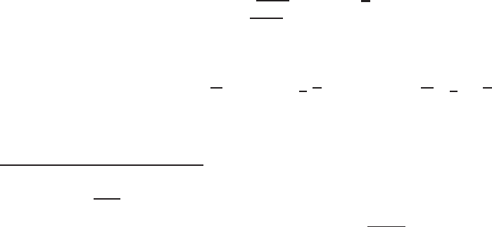
4.1. The elliptic curve discrete logarithm problem 157
(iii) Finally, we solve the pair of congruences
l≡218 (mod 73)
l≡10 (mod 23)
and obtain l=4334.
For the remainder of §4.1, we will assume that the order nof Pis prime.
4.1.2 Pollard’s rho attack
The main idea behind Pollard’s rho algorithm is to find distinct pairs (c,d)and
(c,d)of integers modulo nsuch that
cP+dQ=cP+dQ.
Then
(c−c)P=(d −d)Q=(d −d)lP
and so
(c−c)≡(d −d)l(mod n).
Hence l=logPQcan be obtained by computing
l=(c−c)(d −d)−1mod n.(4.1)
Ana¨ıve method for finding such pairs (c,d)and (c,d)is to select random in-
tegers c,d∈[0,n−1]and store the triples (c,d,cP +dQ)in a table sorted by third
component until a point cP+dQ is obtained for a second time—such an occurrence is
called a collision. By the birthday paradox,4the expected number of iterations before
a collision is obtained is approximately √πn/2≈1.2533√n. The drawback of this
algorithm is the storage required for the √πn/2triples.
Pollard’s rho algorithm finds (c,d)and (c,d)in roughly the same expected time
as the na¨ıve method, but has negligible storage requirements. The idea is to define
an iterating function f :P→Pso that given X∈Pand c,d∈[0,n−1]with
X=cP+dQ, it is easy to compute X=f(X)and c,d∈[0,n−1]with X=cP+dQ.
Furthermore, fshould have the characteristics of a random function.
The following is an example of a suitable iterating function. Let {S1,S2,...,SL}be
a “random” partition of Pinto Lsets of roughly the same size. Typical values for the
4Suppose that an urn has nballs numbered 1 to n. The balls are randomly drawn, one at a time with
replacement, from the urn. Then the expected number of draws before some ball is drawn for the second time
is approximately √πn/2. If n=365 and the balls represent different days of the year, then the statement
can be interpreted as saying that the expected number of people that have to be gathered in a room before
one expects at least two of them to have the same birthday is approximately √π365/2≈24. This number is
surprisingly small and hence the nomenclature “birthday paradox.”
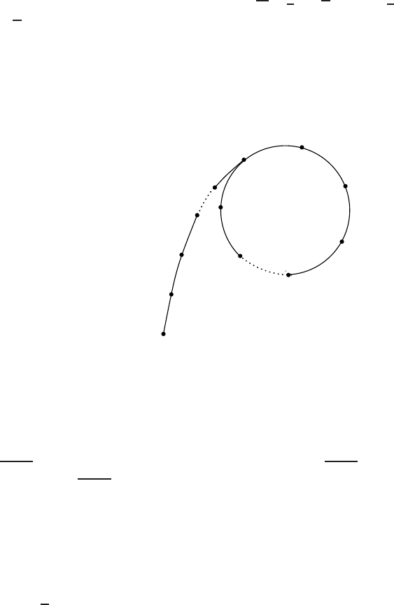
158 4. Cryptographic Protocols
number of branches L are 16 and 32. For example, if L=32 then a point X∈Pcan
be assigned to Sjif the five least significant bits of the x-coordinate of Xrepresent the
integer j−1. We write H(X)=jif X∈Sjand call Hthe partition function. Finally,
let aj,bj∈R[0,n−1]for 1 ≤j≤L.Then f:P→Pis defined by
f(X)=X+ajP+bjQwhere j=H(X).
Observe that if X=cP +dQ,then f(X)=X=cP +dQ where c=c+ajmod n
and d=d+bjmod n.
Now, any point X0∈Pdetermines a sequence {Xi}i≥0of points where Xi=
f(Xi−1)for i≥1. Since the set Pis finite, the sequence will eventually collide
and then cycle forever; that is, there is a smallest index tfor which Xt=Xt+sfor
some s≥1, and then Xi=Xi−sfor all i≥t+s(see Figure 4.1). Here, tis called
X1
X3
Xt+s+2
Xt+2
Xt+1
Xt+s+3
Xt+4
Xt+s−2
Xt−1
Xt+3
Xt+s+1
Xt+s
Xt
Xt+s+4
X2
X0
Xt+s−1
Figure 4.1.
ρ
-like shape of the sequence
{Xi}
in Pollard’s rho algorithm, where
t=
tail length
and
s=
cycle length.
the tail length and sis called the cycle length of the sequence. If fis assumed to be
a random function, then the sequence is expected to first collide after approximately
√πn/2 terms. Moreover, the expected tail length is t≈√πn/8 and the expected cycle
length is s≈√πn/8.
A collision, that is, points Xi,Xjwith Xi=Xjand i= j, can be found using
Floyd’s cycle-finding algorithm wherein one computes pairs (Xi,X2i)of points for
i=1,2,3... until Xi=X2i. After computing a new pair, the previous pair can be
discarded; thus the storage requirements are negligible. The expected number kof such
pairs that have to be computed before Xi=X2iis easily seen to satisfy t≤k≤t+
s. In fact, assuming that fis a random function, the expected value of kis about
1.0308√n, and hence the expected number of elliptic curve group operations is about

4.1. The elliptic curve discrete logarithm problem 159
3√n. The complete algorithm is presented as Algorithm 4.3. Note that the probability
of the algorithm terminating with failure (i.e., d=d in step 7) is negligible.
Algorithm 4.3 Pollard’s rho algorithm for the ECDLP (single processor)
INPUT:P∈E(Fq)of prime order n,Q∈P.
OUTPUT: The discrete logarithm l=logPQ.
1. Select the number Lof branches (e.g., L=16 or L=32).
2. Select a partition function H:P→{1,2,...,L}.
3. For jfrom 1 to Ldo
3.1 Select aj,bj∈R[0,n−1].
3.2 Compute Rj=ajP+bjQ.
4. Select c,d∈R[0,n−1]and compute X=cP+dQ.
5. Set X ←X,c←c,d ←d.
6. Repeat the following:
6.1 Compute j=H(X).
Set X←X+Rj,c←c+ajmod n,d←d+bjmod n.
6.2 For ifrom 1 to 2 do
Compute j=H(X).
Set X ←X +Rj,c←c +ajmod n,d ←d +bjmod n.
Until X=X.
7. If d=d then return(“failure”);
Else compute l=(c−c)(d −d)−1mod nand return(l).
Example 4.4 (Pollard’s rho algorithm for solving the ECDLP) Consider the elliptic
curve defined over F229 by the equation:
E:y2=x3+x+44.
The point P=(5,116)∈E(F229)has prime order n=239. Let Q=(155,166)∈P.
We wish to determine l=logPQ.
We select the partition function H:P→{1,2,3,4}with L=4 branches:
H(x,y)=(xmod 4)+1,
and the four triples
[a1,b1,R1]=[79,163,(135,117)]
[a2,b2,R2]=[206,19,(96,97)]
[a3,b3,R3]=[87,109,(84,62)]
[a4,b4,R4]=[219,68,(72,134)].
The following table lists the triples (c,d,X)and (c,d,X)computed in Algo-
rithm 4.3 for the case (c,d)=(54,175)in step 4.

160 4. Cryptographic Protocols
Iteration cdXc d X
–54 175 ( 39,159) 54 175 ( 39,159)
134 4 (160, 9) 113 167 (130,182)
2113 167 (130,182) 180 105 ( 36, 97)
3200 37 ( 27, 17) 0 97 (108, 89)
4180 105 ( 36, 97) 46 40 (223,153)
520 29 (119,180) 232 127 (167, 57)
60 97 (108, 89) 192 24 ( 57,105)
779 21 ( 81,168) 139 111 (185,227)
846 40 (223,153) 193 0 (197, 92)
926 108 ( 9, 18) 140 87 (194,145)
10 232 127 (167, 57) 67 120 (223,153)
11 212 195 ( 75,136) 14 207 (167, 57)
12 192 24 ( 57,105) 213 104 ( 57,105)
The algorithm finds
192P+24Q=213P+104Q,
and hence
l=(192 −213)·(104 −24)−1mod 239 =176.
Parallelized Pollard’s rho attack
Suppose now that Mprocessors are available for solving an ECDLP instance. A na¨ıve
approach would be to run Pollard’s rho algorithm independently on each processor
(with different randomly chosen starting points X0) until any one processor terminates.
A careful analysis shows that the expected number of elliptic curve operations per-
formed by each processor before one terminates is about 3√n/M. Thus the expected
speedup is only by a factor of √M.
Van Oorschot and Wiener proposed a variant of Pollard’s rho algorithm that yields a
factor Mspeedup when Mprocessors are employed. The idea is to allow the sequences
{Xi}i≥0generated by the processors to collide with one another. More precisely, each
processor randomly selects its own starting point X0, but all processors use the same
iterating function fto compute subsequent points Xi. Thus, if the sequences from two
different processors ever collide, then, as illustrated in Figure 4.2, the two sequences
will be identical from that point on.
Floyd’s cycle-finding algorithm finds a collision in the sequence generated by a sin-
gle processor. The following strategy enables efficient finding of a collision in the
sequences generated by different processors. An easily testable distinguishing property
of points is selected. For example, a point may be distinguished if the leading tbits of
its x-coordinate are zero. Let θbe the proportion of points in Phaving this distin-
guishing property. Whenever a processor encounters a distinguished point, it transmits
the point to a central server which stores it in a sorted list. When the server receives the
same distinguished point for the second time, it computes the desired discrete logarithm

4.1. The elliptic curve discrete logarithm problem 161
via (4.1) and terminates all processors. The expected number of steps per processor be-
fore a collision occurs is (√πn/2)/M. A subsequent distinguished point is expected
after 1/θ steps. Hence the expected number of elliptic curve operations performed by
each processor before a collision of distinguished points is observed is
1
Mπn
2+1
θ,(4.2)
and this parallelized version of Pollard’s rho algorithm achieves a speedup that is lin-
ear in the number of processors employed. Observe that the processors do not have
to communicate with each other, and furthermore have limited communications with
the central server. Moreover, the total space requirements at the central server can be
controlled by careful selection of the distinguishing property. The complete algorithm
is presented as Algorithm 4.5. Note that the probability of the algorithm terminating
with failure (i.e., d=d in step 7) is negligible.
Algorithm 4.5 Parallelized Pollard’s rho algorithm for the ECDLP
INPUT:P∈E(Fq)of prime order n,Q∈P.
OUTPUT: The discrete logarithm l=logPQ.
1. Select the number Lof branches (e.g., L=16 or L=32).
2. Select a partition function H:P→{1,2,...,L}.
3. Select a distinguishing property for points in P.
4. For jfrom 1 to Ldo
4.1 Select aj,bj∈R[0,n−1].
4.2 Compute Rj=ajP+bjQ.
5. Each of the Mprocessors does the following:
5.1 Select c,d∈R[0,n−1]and compute X=cP+dQ.
5.2 Repeat the following:
If Xis distinguished then send (c,d,X)to the central server.
Compute j=H(X).
Set X←X+Rj,c←c+ajmod n,andd←d+bjmod n.
Until the server receives some distinguished point Yfor the second time.
6. Let the two triples associated with Ybe (c,d,Y)and (c,d,Y).
7. If d=d then return(“failure”);
Else compute l=(c−c)(d −d)−1mod nand return(l).
Speeding Pollard’s rho algorithm using automorphisms
Let ψ:P→Pbe a group automorphism, where P∈E(Fq)has order n.We
assume that ψcan be computed very efficiently—significantly faster than a point ad-
dition. Suppose that ψhas order t,thatis,tis the smallest positive integer such that
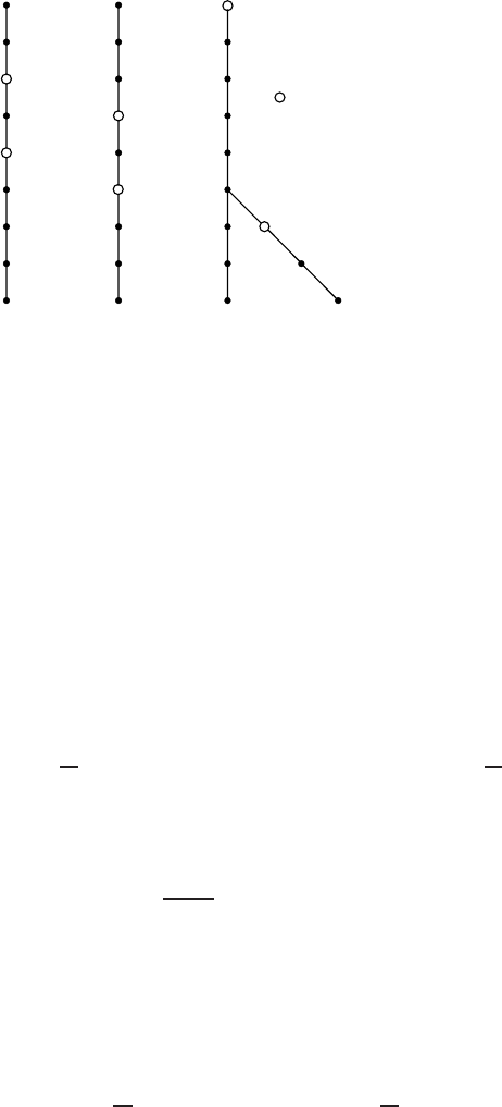
162 4. Cryptographic Protocols
X
Y
Processor 3 Processor 4Processor 1 Processor 2
distinguished
points
Figure 4.2. Sequences generated by the parallelized Pollard’s rho algorithm. The sequences gen-
erated by processors 3 and 4 first collide at
X
. The algorithm reports the collision at
Y
,thefirst
subsequent distinguished point.
ψt(R)=Rfor all R∈P. The relation ∼on Pdefined by
R1∼R2if and only if R1=ψj(R2)for some j∈[0,t−1]
is an equivalence relation. The equivalence class [R]containing a point R∈Pis
[R]={R,ψ(R), ψ 2(R),...,ψl−1(R)},
where lis the smallest positive divisor of tsuch that ψl(R)=R.
The idea behind the speedup is to modify the iterating function fso that it is defined
on the equivalence classes (rather than just on the points in P). To achieve this, we
define a canonical representative Rfor each equivalence class [R]. For example, Rmay
be defined to be the point in [R]whose x-coordinate is the smallest when considered as
an integer (with ties broken by selecting the point with a smaller y-coordinate). Then,
we can define an iterating function gon the canonical representatives by
g(R)=f(R).
Suppose now that we know the integer λ∈[0,n−1]such that
ψ(P)=λP.
Then, since ψis a group automorphism, we have that ψ(R)=λRfor all R∈P.
Thus, if we know integers aand bsuch that X=aP +bQ, then we can efficiently
compute integers aand bsuch that X=aP+bQ. Namely, if X=ψj(X),then
a=λjamod nand b=λjbmod n.
4.1. The elliptic curve discrete logarithm problem 163
The function gcan now be used as the iterating function in the parallelized Pollard’s
rho algorithm. The initial point in a sequence is X
0=X0where X0=a0P+b0Q
and a0,b0∈R[0,n−1]. Subsequent terms of the sequence are computed iteratively:
X
i=g(X
i−1)for i≥1. If most equivalence classes have size t, then the search space
has size approximately n/t(versus nif equivalence classes are not employed) and thus
the expected running time of the modified parallelized Pollard’s rho algorithm is
1
Mπn
2t+1
θ,(4.3)
a speedup by a factor of √tover (4.2).
Example 4.6 (using the negation map) The negation map ψ(P)=−Phas order 2 and
possesses the requisite properties described above. Thus, the parallelized Pollard’s rho
algorithm that uses equivalence classes under the negation map has an expected running
time of √πn
2M+1
θ.(4.4)
This is a speedup by a factor of √2 over (4.2) and is applicable to all elliptic curves.
Example 4.7 (speeding Pollard’s rho algorithm for Koblitz curves) Recall from §3.4
that a Koblitz curve Ea(where a∈{0,1}) is an elliptic curve defined over F2.The
Frobenius map τ:Ea(F2m)→Ea(F2m),definedbyτ(∞)=∞and τ(x,y)=(x2,y2),
is also a group automorphism of order mand can be computed efficiently since squar-
ing is a cheap operation in F2m.IfP∈Ea(F2m)has prime order nsuch that n2does
not divide #Ea(F2m),thenτ(P)∈Pand hence τis also a group automorphism of
P.Letµ=(−1)1−a. It follows from Note 3.72 that one of the two solutions λto the
modular equation
λ2−µλ +2≡0(mod n)
satisfies τ(P)=λP. Thus, τhas the requisite properties, and parallelized Pollard’s
rho algorithm that uses equivalence classes under the Frobenius map has an expected
running time of
1
Mπn
2m+1
θ.
Furthermore, the parallelized Pollard’s rho algorithm can exploit both the Frobenius
map and the negation map to achieve an expected running time of
1
2Mπn
m+1
θ.(4.5)
for Koblitz curves, a speedup by a factor of √2mover (4.2).

164 4. Cryptographic Protocols
Example 4.8 (solving a 113-bit ECDLP instance on the Internet)LetEbe an elliptic
curve defined over a prime field Fp,andletP∈E(Fp)have prime order n. Suppose
also that both pand nare 113-bit primes. Elliptic curves with these parameters would
offer roughly the same security as provided by 56-bit DES. Assume that we have M=
10,000 computers available on the Internet to solve an instance of the ECDLP in P,
and that each computer can perform one iteration (of step 5.2 of Algorithm 4.5) in
10 microseconds. If we select the distinguishing property so that θ=2−30, then the
expected number of iterations performed by each computer before the logarithm is
found is approximately
√π2113
2·10000 +230 ≈9.03 ×10¹³.
Hence, the expected running time before the logarithm is found is about 1045 days, or
threeyears.Sincethex-coordinate and associated (c,d)pair of a distinguished point
can be stored in 12 32-bit words, the total space required for storing the distinguished
points at the central server is about
12θ√πn
2words ≈3.8 Gigabytes.
One concludes from these calculations that while solving a 113-bit ECDLP requires
significant resources, 113-bit ECC provides adequate security only for low-security
short-term applications.
Multiple logarithms
We show how the distinguished points stored during the solution of one ECDLP in-
stance in Pusing (parallelized) Pollard’s rho algorithm can be used to accelerate
the solution of other ECDLP instances in P. This property is relevant to the secu-
rity of elliptic curve cryptographic systems because users typically share elliptic curve
parameters E,Fq,P, and select their own public keys Q∈P. Thus, if one or more
private keys can be found using Pollard’s rho algorithm, then finding other private keys
becomes progressively easier.
Suppose that l=logPQhas been computed. For each stored triple (c,d,X)as-
sociated to distinguished points Xencountered during the computation, the integer
s=c+dl mod nsatisfies X=sP. Similarly, the integers rj=aj+bjlmod nsatisfy
Rj=rjPfor 1 ≤j≤L. Now, to compute l=logPQwhere Q∈P, each proces-
sor computes the terms Yiof a random sequence with starting point Y0=c
0P+d
0Q
where c
0,d
0∈R[0,n−1],andthesame iterating function fas before. For each dis-
tinguished point Yencountered in the new sequences, a triple (c,d,Y)such that
Y=cP+dQis sent to the central server. A collision can occur between two new
sequences or between a new sequence and an old one. In the former case, we have
cP+dQ=cP+dQ,

4.1. The elliptic curve discrete logarithm problem 165
whence l=(c−c)(d −d)−1mod n. In the latter case, we have
cP+dQ=sP,
whence l=(s−c)(d)−1mod n.
The distinguished points collected during the first two ECDLP computations can
similarly be used for the computation of the third ECDLP computation, and so on. The
expected number Wkof random walk steps before kECDLP instances are iteratively
solved in the manner described has been shown to be
Wk≈T
k−1
i=02i
i
4i,
where Tis the expected number of random walk steps to solve a single ECDLP in-
stance. Thus, solving the second, third, and fourth ECDLP instances take only 50%,
37%, 31%, respectively, of the time to solve the first instance.
Concerns that successive ECDLP computations become easier can be addressed by
ensuring that the elliptic curve parameters are chosen so that the first ECDLP instance
is infeasible to solve.
4.1.3 Index-calculus attacks
Index-calculus algorithms are the most powerful methods known for computing dis-
crete logarithms in some groups including the multiplicative group F∗
qof a finite field,
the jacobian JC(Fq)of a hyperelliptic curve Cof high genus gdefined over a finite
field Fq, and the class group of an imaginary quadratic number field. It is natural then
to ask whether index-calculus methods can lead to subexponential-time algorithms for
the ECDLP.
We begin by outlining the index-calculus method in the general setting of an arbitrary
cyclic group and illustrate how the method can be adapted to the multiplicative group of
a prime field or binary field. We then explain why the natural ways to extend the index-
calculus methods to elliptic curve groups are highly unlikely to yield subexponential-
time algorithms for the ECDLP.
The main idea behind index-calculus methods
Let Gbe a cyclic group of order ngenerated by α. Suppose that we wish to find logαβ
for β∈G. The index-calculus method is the following.
1. Factor base selection. Choose a subset S={p1,p2,..., pt}of G, called the fac-
tor base, such that a “significant” proportion of elements in Gcan be efficiently
expressed as a product of elements from S. The choice of Swill depend on the
characteristics of the particular group G.

166 4. Cryptographic Protocols
2. Compute logarithms of elements in S. Select random integers k∈[0,n−1]until
αkcan be written as a product of elements in S:
αk=
t
6
i=1
pci
i,where ci≥0.(4.6)
Taking logarithms to the base αof both sides of (4.6) yields a linear equation
where the unknowns are the logarithms of factor base elements:
k≡
t
i=1
cilogαpi(mod n). (4.7)
This procedure is repeated until slightly more than tsuch equations have been
obtained. The resulting linear system of equations can then be solved to obtain
logαpifor 1 ≤i≤t.
3. Compute logαβ. Select random integers kuntil αkβcan be written as a product
of elements in S:
αkβ=
t
6
i=1
pdi
i,where di≥0.(4.8)
Taking logarithms to the base αof both sides of (4.8) yields the desired logarithm
of β:
logαβ=−k+
t
i=1
dilogαpimod n.(4.9)
The running time of the index-calculus algorithm depends critically on the choice
of the factor base S. There is also a trade-off in the size tof S.Largertare preferred
because then the probability of a random group element factoring over Sis expected to
be larger. On the other hand, smaller tare preferred because then the number of linear
equations that need to be collected is smaller. The optimum choice of tdepends on the
proportion of elements in Gthat factor over S.
Consider now the case G=F∗
p, the multiplicative group of a prime field. The ele-
ments of F∗
pcan be regarded as the integers in [1,p−1]. There is a natural choice for S,
namely the prime numbers ≤Bfor some bound B. An element of F∗
pfactors over Sif it
is B-smooth, that is, all its prime factors are ≤B. The optimal factor base size depends
on the distribution of B-smooth integers in [1,p−1], and yields a subexponential-time
algorithm for the DLP in F∗
p. The fastest variant of this algorithm is the number field
sieve (NFS) and has an expected running time of Lp[1
3,1.923].
Consider next the case G=F∗
2m, the multiplicative group of a binary field. The el-
ements of F∗
2mcan be regarded as the nonzero binary polynomials of degree less than
m. Hence there is a natural choice for S, namely the irreducible binary polynomials of
degree ≤Bfor some bound B. An element of F∗
2mfactors over Sif it is B-smooth,

4.1. The elliptic curve discrete logarithm problem 167
that is, all its irreducible factors have degree ≤B. The optimal factor base size depends
on the distribution of B-smooth polynomials among the binary polynomials of degree
≤B, and yields a subexponential-time algorithm for the DLP in F∗
2m. The fastest vari-
ant of this algorithm is Coppersmith’s algorithm and has an expected running time of
L2m[1
3,c]for some constant c<1.587.
Failure of index-calculus attacks on the ECLDP
Suppose that we wish to solve instances of the ECDLP in E(Fp)where E:y2=
x3+ax +bis an elliptic curve defined over the prime field Fp. For simplicity, suppose
that E(Fp)has prime order so that E(Fp)=Pfor some P∈E(Fp). The most natural
index-calculus approach would first lift E to a curve
Edefined over the field Qof
rational numbers, that is, to a curve
E:y2=x3+ax +
bwhere a,
b∈Qand a=
amod pand b=
bmod p. Then, the lift of a point R ∈E(Fp)is a point
R∈
E(Q)
whose coordinates reduce modulo pto those of R. This lifting process is analogous
to the ones used in the index-calculus method described above for computing discrete
logarithms in F∗
pand F∗
2m, where elements of F∗
pare “lifted” to integers in Z,and
elements of F∗
2mare “lifted” to polynomials in F2[z].
The celebrated Mordell-Weil Theorem states that the group structure of
E(Q)is
Etors ×Zr,whereEtors is the set of points in
E(Q)of finite order, and ris a non-
negative integer called the rank of
E. Furthermore, a theorem of Mazur states that
Etors has small size—in fact #Etors ≤16. Thus a natural choice for the factor base is a
set of points P1,P2,...,Prsuch that
P1,
P2,...,
Prare linearly independent in
E(Q).
Relations of the form (4.6) can then be found by selecting multiples kP of Pin E(Fp)
until the lift 7
kP can be written as an integer linear combination of the basis points in
E(Q):
7
kP =c1
P1+c2
P2+···+cr
Pr.
Then, reducing the coordinates of the points modulo pyields a desired relation
kP =c1P1+c2P2+···+crPr
in E(Fp).
There are two main reasons why this index-calculus approach is doomed to fail. The
first is that no one knows how to efficiently lift points in E(Fp)to
E(Q). Certainly, for
a lifting procedure to be feasible, the lifted points should have small height. (Roughly
speaking, the height of a point
P∈
E(Q)is the number of bits needed to write down the
coordinates of
P.) However, it has been proven (under some reasonable assumptions)
that the number of points of small height in any elliptic curve
E(Q)is extremely small,
so that only an insignificant proportion of points in E(Fp)can possibly be lifted to
points of small height in
E(Q)—this is the second reason for unavoidable failure of
this index-calculus approach.
For the ECDLP in elliptic curves Eover non-prime fields Fq, one could consider
lifting Eto an elliptic curve over a number field, or to an elliptic curve over a function
168 4. Cryptographic Protocols
field. These approaches are also destined to fail for the same reasons as for the prime
field case.
Of course there may be other ways of applying the index-calculus methodology
for solving the ECDLP. Thus far, no one has found an approach that yields a general
subexponential-time (or better) algorithm for the ECDLP.
4.1.4 Isomorphism attacks
Let Ebe an elliptic curve defined over a finite field Fq,andletP∈E(Fq)have prime
order n.LetGbe a group of order n.Sincenis prime, Pand Gare both cyclic and
hence isomorphic. If one could efficiently compute an isomorphism
ψ:P→G,(4.10)
then ECDLP instances in Pcould be efficiently reduced to instances of the DLP in
G. Namely, given Pand Q∈P,wehave
logPQ=logψ(P)ψ(Q). (4.11)
Isomorphism attacks reduce the ECDLP to the DLP in groups Gfor which
subexponential-time (or faster) algorithms are known. These attacks are special-
purpose in that they result in ECDLP solvers that are faster than Pollard’s rho algorithm
only for special classes of elliptic curves. The isomorphism attacks that have been
devised are the following:
(i) The attack on prime-field-anomalous curves reduces the ECDLP in an elliptic
curve of order pdefined over the prime field Fpto the DLP in the additive group
F+
pof integers modulo p.
(ii) In the case gcd(n,q)=1, the Weil and Tate pairing attacks establish an isomor-
phism between Pand a subgroup of order nof the multiplicative group F∗
qkof
some extension field Fqk.
(iii) The GHS Weil descent attack attempts to reduce the ECDLP in an elliptic curve
defined over a binary field F2mto the DLP in the jacobian of a hyperelliptic curve
defined over a proper subfield of F2m.
Since a polynomial-time algorithm is known for solving the DLP in F+
p, and since
subexponential-time algorithms are known for the DLP in the multiplicative group of a
finite field and for the jacobian of high-genus hyperelliptic curves, these isomorphism
attacks can have important implications to the security of elliptic curve cryptographic
schemes. We next discuss the cryptographic implications of and countermeasures to
these attacks.
Attack on prime-field-anomalous curves
An elliptic curve Edefined over a prime field Fpis said to be prime-field-anomalous
if #E(Fp)=p. The group E(Fp)is cyclic since it has prime order, and hence E(Fp)
4.1. The elliptic curve discrete logarithm problem 169
is isomorphic to the additive group F+
pof integers modulo p.Now,theDLPinF+
pis
the following: given p,a∈F+
p,a= 0, and b∈F+
p,findl∈[0,p−1]such that la ≡b
(mod p).Sincel=ba−1mod p,theDLPinF+
pcan be efficiently solved by using the
extended Euclidean algorithm (Algorithm 2.20) to compute a−1mod p.
In 1997, Araki, Satoh, Semaev and Smart showed than an isomorphism
ψ:E(Fp)→F+
p
can be efficiently computed for prime-field-anomalous elliptic curves. Consequently,
the ECDLP in such curves can be efficiently solved and hence these elliptic curves
must not be used in cryptographic protocols. Since it is easy to determine whether an
elliptic curve Eover a prime field Fpis prime-field-anomalous (by checking whether
#E(Fp)=p), the Araki-Satoh-Semaev-Smart attack can easily be circumvented in
practice.
Weil and Tate pairing attacks
Suppose now that the prime order nof P∈E(Fq)satisfies gcd(n,q)=1. Let kbe the
smallest positive integer such that qk≡1(mod n); the integer kis the multiplicative
order of qmodulo nand therefore is a divisor of n−1. Since ndivides qk−1, the
multiplicative group F∗
qkof the extension field Fqkhas a unique subgroup Gof order n.
The Weil pairing attack constructs an isomorphism from Pto Gwhen the additional
constraint n(q−1)is satisfied, while the Tate pairing attack constructs an isomor-
phism between Pand Gwithout requiring this additional constraint. The integer kis
called the embedding degree.
For most elliptic curves one expects that k≈n. In this case the Weil and Tate pairing
attacks do not yield an efficient ECDLP solver since the finite field Fqkhas exponential
size relative to the size of the ECDLP parameters. (The ECDLP parameters have size
O(log q)bits, while elements of Fqkhave size O(klog q)bits.) However, some special
elliptic curves do have small embedding degrees k. For these curves, the Weil and
Tate pairing reductions take polynomial time. Since subexponential-time algorithms
are known for the DLP in F∗
qk, this results in a subexponential-time algorithm for the
ECDLP in these special elliptic curves.
The special classes of elliptic curves with small embedding degree include super-
singular curves (Definition 3.10) and elliptic curves of trace 2 (with #E(Fq)=q−1).
These curves have k≤6 and consequently should not be used in the elliptic curve
protocols discussed in this book unless the underlying finite field is large enough so
that the DLP in F∗
qkis considered intractable. We note that constructive applications
have recently been discovered for supersingular elliptic curves, including the design of
identity-based public-key encryption schemes (see page 199 for references).
To ensure that an elliptic curve Edefined over Fqis immune to the Weil and Tate
pairing attacks, it is sufficient to check that n, the order of the base point P∈E(Fq),
does not divide qk−1forallsmallkfor which the DLP in F∗
qkis considered tractable.
If n>2160, then it suffices to check this condition for all k∈[1,20].

170 4. Cryptographic Protocols
Weil descent
Suppose that Eis a non-supersingular elliptic curve defined over a binary field K=
F2m, and suppose that #E(F2m)=nh where nis prime and his small (e.g., h=2or
h=4). In 1998, Frey proposed using Weil descent to reduce the ECDLP in E(F2m)
to the DLP in the jacobian variety of a curve of larger genus defined over a proper
subfield k=F2lof K.Letd=m/l. In Frey’s method, referred to as the Weil descent
attack methodology, one first constructs the so-called Weil restriction WK/kof scalars
of E,whichisad-dimensional abelian variety over k. One then attempts to find a curve
Cdefined over kin WK/ksuch that (i) there are algorithms for solving the DLP in the
jacobian JC(k)of Cover kthat are faster than Pollard’s rho method; and (ii) ECDLP
instances in E(K)can be efficiently mapped to DLP instances in JC(k).
Gaudry, Hess and Smart (GHS) showed how the Weil restriction WK/kcan be in-
tersected with n−1 hyperplanes to eventually obtain a hyperelliptic curve Cof genus
gdefined over kfrom an irreducible component in the intersection. Furthermore, they
gave an efficient algorithm that (in most cases) reduces ECDLP instances in E(K)
to instances of the hyperelliptic curve discrete logarithm problem (HCDLP) in JC(k).
Now, the Enge-Gaudry index-calculus algorithm for the HCDLP in a genus-ghyper-
elliptic curve over Fqhas a subexponential expected running time of Lqg[√2]bit
operations for g/log q→∞. Thus, provided that gis not too large, the GHS attack
yields a subexponential-time algorithm for the original ECDLP.
It was subsequently shown that the GHS attack fails for all cryptographically inter-
esting elliptic curves over F2mfor all prime m∈[160,600]. Note that such fields have
only one proper subfield, namely F2. In particular, it was shown that the hyperelliptic
curves Cproduced by the GHS attack either have genus too small (whence JC(F2)is
too small to yield any non-trivial information about the ECDLP in E(F2m)), or have
genus too large (g≥216 −1, whence the HCDLP in JC(F2)is infeasible using known
methods for solving the HCDLP). The GHS attack has also been shown to fail for all
elliptic curves over certain fields F2mwhere m∈[160,600]is composite; such fields
include F2169 ,F2209 and F2247 .
However, the GHS attack is effective for solving the ECDLP in some elliptic curves
over F2mwhere m∈[160,600]is composite. For example, the ECDLP in approxi-
mately 294 of the 2162 isomorphism classes of elliptic curves over F2161 can be solved
in about 248 steps by using the GHS attack to reduce the problem to an instance of
the HCDLP in a genus-8 hyperelliptic curve over the subfield F223 . Since Pollard’s rho
method takes roughly 280 steps for solving the ECDLP in cryptographically interesting
elliptic curves over F2161 , the GHS attack is deemed to be successful for the 294 elliptic
curves.
Let F2m,wherem∈[160,600]is composite, be a binary field for which the GHS
attack exhibits some success. Then the proportion of elliptic curves over F2mthat suc-
cumb to the GHS attack is relatively small. Thus, if one selects an elliptic curve over
F2mat random, then there is a very high probability that the elliptic curve will resist
the GHS attack. However, failure of the GHS attack does not imply failure of the Weil

4.1. The elliptic curve discrete logarithm problem 171
descent attack methodology—there may be other useful curves which lie on the Weil
restriction that were not constructed by the GHS method. Thus, to account for poten-
tial future developments in the Weil descent attack methodology, it seems prudent to
altogether avoid using elliptic curves over F2mwhere mis composite.
4.1.5 Related problems
While hardness of the ECDLP is necessary for the security of any elliptic curve cryp-
tographic scheme, it is generally not sufficient. We present some problems related to
the ECDLP whose hardness is assumed in the security proofs for some elliptic curve
protocols. All these problems can be presented in the setting of a general cyclic group,
however we restrict the discussion to elliptic curve groups.
Elliptic curve Diffie-Hellman problem
Definition 4.9 The (computational) elliptic curve Diffie-Hellman problem (ECDHP)
is: given an elliptic curve Edefined over a finite field Fq, a point P∈E(Fq)of order
n, and points A=aP,B=bP ∈P, find the point C=abP.
If the ECDLP in Pcan be efficiently solved, then the ECDHP in Pcan also be
efficiently solved by first finding afrom (P,A)and then computing C=aB. Thus the
ECDHP is no harder than the ECDLP. It is not known whether the ECDHP is equally
as hard as the ECDLP; that is, no one knows how to efficiently solve the ECDLP given
a (hypothetical) oracle that efficiently solves the ECDHP. However, the equivalence of
the ECDLP and ECDHP has been proven in some special cases where the ECDLP is
believed to be hard, for example when nis prime and all the prime factors of n−1are
small. The strongest evidence for the hardness of the ECDHP comes from a result of
Boneh and Lipton who proved (under some reasonable assumptions about the distribu-
tion of smooth integers in a certain interval) that if nis prime and the ECDLP cannot be
solved in Ln[1
2,c]subexponential time (for some constant c), then the ECDHP cannot
be solved in Ln[1
2,c−2]subexponential time. Further evidence for the hardness of the
ECDHP comes from Shoup’s lower bound of √nfor the Diffie-Hellman problem in
generic groups of prime order n.
Elliptic curve decision Diffie-Hellman problem
The ECDHP is concerned with computing the Diffie-Hellman secret point abP given
(P,aP,bP). For the security of some elliptic curve protocols, it may be necessary
that an adversary does not learn any information about abP. This requirement can
be formalized by insisting that the adversary cannot distinguish abP from a random
element in P.

172 4. Cryptographic Protocols
Definition 4.10 The elliptic curve decision Diffie-Hellman problem (ECDDHP) is:
given an elliptic curve Edefined over a finite field Fq, a point P∈E(Fq)of order
n, and points A=aP,B=bP,andC=cP ∈P, determine whether C=abP or,
equivalently, whether c≡ab (mod n).
If the ECDHP in Pcan be efficiently solved, then the ECDDHP in Pcan also
be efficiently solved by first finding C=abP from (P,A,B)and then comparing C
with C. Thus the ECDDHP is no harder than the ECDHP (and also the ECDLP). The
only hardness result that has been proved for ECDDHP is Shoup’s lower bound of √n
for the decision Diffie-Hellman problem in generic groups of prime order n.
4.2 Domain parameters
Domain parameters for an elliptic curve scheme describe an elliptic curve Edefined
over a finite field Fq, a base point P∈E(Fq), and its order n. The parameters should
be chosen so that the ECDLP is resistant to all known attacks. There may also be other
constraints for security or implementation reasons. Typically, domain parameters are
shared by a group of entities; however, in some applications they may be specific to
each user. For the remainder of this section we shall assume that the underlying field is
either a prime field (§2.2), a binary field (§2.3), or an optimal extension field (§2.4).
Definition 4.11 Domain parameters D =(q,FR,S,a,b,P,n,h)are comprised of:
1. The field order q.
2. An indication FR (field representation) of the representation used for the
elements of Fq.
3. A seed S if the elliptic curve was randomly generated in accordance with
Algorithm 4.17, Algorithm 4.19, or Algorithm 4.22.
4. Two coefficients a,b∈Fqthat define the equation of the elliptic curve Eover
Fq(i.e., y2=x3+ax +bin the case of a prime field or an OEF, and y2+xy =
x3+ax2+bin the case of a binary field).
5. TwofieldelementsxPand yPin Fqthat define a finite point P=(xP,yP)∈
E(Fq)in affine coordinates. Phas prime order and is called the base point.
6. The order n of P.
7. The cofactor h =#E(Fq)/n.
Security constraints In order to avoid the Pohlig-Hellman attack (§4.1.1) and Pol-
lard’s rho attack (§4.1.2) on the ECDLP, it is necessary that #E(Fq)be divisible by
a sufficiently large prime n. At a minimum, one should have n>2160.Havingfixed
an underlying field Fq, maximum resistance to the Pohlig-Hellman and Pollard’s rho
4.2. Domain parameters 173
attacks is attained by selecting Eso that #E(Fq)is prime or almost prime,thatis,
#E(Fq)=hn where nis prime and his small (e.g., h=1,2,3or4).
Some further precautions should be exercised to assure resistance to isomorphism
attacks (§4.1.4). To avoid the attack on prime-field-anomalous curves, one should ver-
ify that #E(Fq)=q. To avoid the Weil and Tate pairing attacks, one should ensure that
ndoes not divide qk−1forall1≤k≤C,whereCis large enough so that the DLP
in F∗
qCis considered intractable (if n>2160 then C=20 suffices). Finally, to ensure
resistance to the Weil descent attack, one may consider using a binary field F2monly if
mis prime.
Selecting elliptic curves verifiably at random A prudent way to guard against at-
tacks on special classes of curves that may be discovered in the future is to select the
elliptic curve E at random subject to the condition that #E(Fq)is divisible by a large
prime. Since the probability that a random curve succumbs to one of the known special-
purpose isomorphism attacks is negligible, the known attacks are also prevented. A
curve can be selected verifiably at random by choosing the coefficients of the defining
elliptic curve as the outputs of a one-way function such as SHA-1 according to some
pre-specified procedure. The input seed Sto the function then serves as proof (under
the assumption that SHA-1 cannot be inverted) that the elliptic curve was indeed gen-
erated at random. This provides some assurance to the user of the elliptic curve that
it was not intentionally constructed with hidden weaknesses which could thereafter be
exploited to recover the user’s private keys.
4.2.1 Domain parameter generation and validation
Algorithm 4.14 is one way to generate cryptographically secure domain parameters—
all the security constraints discussed above are satisfied. A set of domain parameters
can be explicitly validated using Algorithm 4.15. The validation process proves that
the elliptic curve in question has the claimed order and resists all known attacks on
the ECDLP, and that the base point has the claimed order. An entity who uses elliptic
curves generated by untrusted software or parties can use validation to be assured that
the curves are cryptographically secure.
Sample sets of domain parameters are provided in §A.2.
Note 4.12 (restrictions on n and L in Algorithms 4.14 and 4.15)
(i) Since nis chosen to satisfy n>2L, the condition L≥160 in the input of
Algorithm 4.14 ensures that n>2160.
(ii) The condition L≤log2qensures that 2L≤qwhence an elliptic curve E
over Fqwith order #E(Fq)divisible by an L-bit prime should exist (recall that
#E(Fq)≈q). In addition, if q=2mthen Lshould satisfy L≤log2q−1
because #E(F2m)is even (cf. Theorem 3.18(iii)).

174 4. Cryptographic Protocols
(iii) The condition n>4√qguarantees that E(Fq)has a unique subgroup of order
nbecause #E(Fq)≤(√q+1)2by Hasse’s Theorem (Theorem 3.7) and so n2
does not divide #E(Fq). Furthermore, since hn =#E(Fq)must lie in the Hasse
interval, it follows that there is only one possible integer hsuch that #E(Fq)=
hn, namely h=(√q+1)2/n.
Note 4.13 (selecting candidate elliptic curves) In Algorithm 4.14, candidate elliptic
curves Eare generated verifiably at random using the procedures specified in §4.2.2.
The orders #E(Fq)can be determined using the SEA point counting algorithm for the
prime field or OEF case, or a variant of Satoh’s point counting algorithm for the binary
field case (see §4.2.3). The orders #E(Fq)of elliptic curves Eover Fqare roughly
uniformly distributed in the Hasse interval [q+1−2√q,q+1+2√q]if Fqis a prime
field or an OEF, and roughly uniformly distributed among the even integers in the Hasse
interval if Fqis a binary field. Thus, one can use estimates of the expected number of
primes in the Hasse interval to obtain fairly accurate estimates of the expected number
of elliptic curves tried until one having prime or almost-prime order is found. The
testing of candidate curves can be accelerated by deploying an early-abort strategy
which first uses the SEA algorithm to quickly determine #E(Fq)modulo small primes
l, rejecting those curves where #E(Fq)is divisible by l. Only those elliptic curves
which pass these tests are subjected to a full point counting algorithm.
An alternative to using random curves is to select a subfield curve or a curve using
the CM method (see §4.2.3). Algorithm 4.14 can be easily modified to accommodate
these selection methods.
Algorithm 4.14 Domain parameter generation
INPUT: A field order q, a field representation FR for Fq, security level Lsatisfying
160 ≤L≤log2qand 2L≥4√q.
OUTPUT: Domain parameters D=(q,FR,S,a,b,P,n,h).
1. Select a,b∈Fqverifiably at random using Algorithm 4.17, 4.19 or 4.22 if Fqis
a prime field, binary field, or OEF, respectively. Let Sbe the seed returned. Let
Ebe y2=x3+ax +bin the case Fqis a prime field or an OEF, and y2+xy =
x3+ax2+bin the case Fqis a binary field.
2. Compute N=#E(Fq)(see §4.2.3).
3. Verify that Nis divisible by a large prime nsatisfying n>2L. If not, then go to
step 1.
4. Verify that ndoes not divide qk−1for1≤k≤20. If not, then go to step 1.
5. Verify that n= q.Ifnot,thengotostep1.
6. Set h←N/n.
7. Select an arbitrary point P∈E(Fq)and set P=hP. Repeat until P=∞.
8. Return(q,FR,S,a,b,P,n,h).

4.2. Domain parameters 175
Algorithm 4.15 Explicit domain parameter validation
INPUT: Domain parameters D=(q,FR,S,a,b,P,n,h).
OUTPUT: Acceptance or rejection of the validity of D.
1. Verify that qis a prime power (q=pmwhere pis prime and m≥1).
2. If p=2thenverifythatmis prime.
3. Verify that FR is a valid field representation.
4. Verify that a,b,xP,yP(where P=(x,y)) are elements of Fq(i.e., verify that
they are of the proper format for elements of Fq).
5. Verify that aand bdefine an elliptic curve over Fq(i.e., 4a3+27b2=0forfields
with p>3, and b= 0 for binary fields).
6. If the elliptic curve was randomly generated then
6.1 Verify that Sis a bit string of length at least lbits, where lis the bitlength
of the hash function H.
6.2 Use Algorithm 4.18 (for prime fields), Algorithm 4.21 (for binary fields)
or Algorithm 4.23 (for OEFs) to verify that aand bwere properly derived
from S.
7. Verify that P=∞.
8. Verify that Psatisfies the elliptic curve equation defined by a,b.
9. Verify that nis prime, that n>2160,andthatn>4√q.
10. Verify that nP =∞.
11. Compute h=(√q+1)2/nand verify that h=h.
12. Verify that ndoes not divide qk−1for1≤k≤20.
13. Verify that n= q.
14. If any verification fails then return(“Invalid”); else return(“Valid”).
4.2.2 Generating elliptic curves verifiably at random
Algorithms 4.17, 4.19 and 4.22 are specifications for generating elliptic curves
verifiably at random over prime fields, binary fields, and OEFs, respectively. The corre-
sponding verification procedures are presented as Algorithms 4.18, 4.21 and 4.23. The
algorithms for prime fields and binary fields are from the ANSI X9.62 standard.
Note 4.16 (explanation of the parameter r in Algorithms 4.17 and 4.22) Suppose that
Fqis a finite field of characteristic >3. If elliptic curves E1:y2=x3+a1x+b1
and E2:y2=x3+a2x+b2defined over Fqare isomorphic over Fqand satisfy
b1=0(sob2= 0), then a3
1/b2
1=a3
2/b2
2. The singular elliptic curves, that is, the curves
E:y2=x3+ax +bfor which 4a3+27b2=0inFq, are precisely those which ei-
ther have a=0andb=0, or a3/b2=−27/4. If r∈Fqwith r= 0andr=−27/4,
then there are precisely two isomorphism classes of curves E:y2=x3+ax +bwith
a3/b2=rin Fq. Hence, there are essentially only two choices for (a,b)in step 10
of Algorithms 4.17 and 4.22. The conditions r= 0andr=−27/4 imposed in step 9

176 4. Cryptographic Protocols
of both algorithms ensure the exclusion of singular elliptic curves. Finally, we men-
tion that this method of generating curves will never produce the elliptic curves with
a=0, b= 0, nor the elliptic curves with a= 0, b=0. This is not a concern because
such curves constitute a negligible fraction of all elliptic curves, and therefore are un-
likely to ever be generated by any method which selects an elliptic curve uniformly at
random.
Generating random elliptic curves over prime fields
Algorithm 4.17 Generating a random elliptic curve over a prime field Fp
INPUT:Aprimep>3, and an l-bit hash function H.
OUTPUT: A seed S,anda,b∈Fpdefining an elliptic curve E:y2=x3+ax +b.
1. Set t←log2p,s←(t−1)/l,v←t−sl.
2. Select an arbitrary bit string Sof length g≥lbits.
3. Compute h=H(S),andletr0be the bit string of length vbits obtained by taking
the vrightmost bits of h.
4. Let R0be the bit string obtained by setting the leftmost bit of r0to 0.
5. Let zbe the integer whose binary representation is S.
6. For ifrom 1 to sdo:
6.1 Let sibe the g-bit binary representation of the integer (z+i)mod 2g.
6.2 Compute Ri=H(si).
7. Let R=R0R1···Rs.
8. Let rbe the integer whose binary representation is R.
9. If r=0orif4r+27 ≡0(mod p)then go to step 2.
10. Select arbitrary a,b∈Fp, not both 0, such that r·b2≡a3(mod p).
11. Return(S,a,b).
Algorithm 4.18 Verifying that an elliptic curve over Fpwas randomly generated
INPUT:Prime p>3, l-bit hash function H, seed Sof bitlength g≥l,anda,b∈Fp
defining an elliptic curve E:y2=x3+ax +b.
OUTPUT: Acceptance or rejection that Ewas generated using Algorithm 4.17.
1. Set t←log2p,s←(t−1)/l,v←t−sl.
2. Compute h=H(S),andletr0be the bit string of length vbits obtained by taking
the vrightmost bits of h.
3. Let R0be the bit string obtained by setting the leftmost bit of r0to 0.
4. Let zbe the integer whose binary representation is S.
5. For ifrom 1 to sdo:
5.1 Let sibe the g-bit binary representation of the integer (z+i)mod 2g.
5.2 Compute Ri=H(si).
6. Let R=R0R1···Rs.
7. Let rbe the integer whose binary representation is R.
8. If r·b2≡a3(mod p)then return(“Accept”); else return(“Reject”).

4.2. Domain parameters 177
Generating random elliptic curves over binary fields
Algorithm 4.19 Generating a random elliptic curve over a binary field F2m
INPUT: A positive integer m,andanl-bit hash function H.
OUTPUT: Seed S,anda,b∈F2mdefining an elliptic curve E:y2+xy =x3+ax2+b.
1. Set s←(m−1)/l,v←m−sl.
2. Select an arbitrary bit string Sof length g≥lbits.
3. Compute h=H(S),andletb0be the bit string of length vbits obtained by taking
the vrightmost bits of h.
4. Let zbe the integer whose binary representation is S.
5. For ifrom 1 to sdo:
5.1 Let sibe the g-bit binary representation of the integer (z+i)mod 2g.
5.2 Compute bi=H(si).
6. Let b=b0b1···bs.
7. If b=0thengotostep2.
8. Select arbitrary a∈F2m.
9. Return(S,a,b).
Note 4.20 (selection of a in Algorithm 4.19) By Theorem 3.18(ii) on the isomorphism
classes of elliptic curves over F2m, it suffices to select afrom {0,γ}where γ∈F2m
satisfies Tr(γ ) =1. Recall also from Theorem 3.18(iii) that #E(F2m)is always even,
while if a=0then#E(F2m)is divisible by 4.
Algorithm 4.21 Verifying that an elliptic curve over F2mwas randomly generated
INPUT: Positive integer m,l-bit hash function H, seed Sof bitlength g≥l,anda,b∈
F2mdefining an elliptic curve E:y2+xy =x3+ax2+b.
OUTPUT: Acceptance or rejection that Ewas generated using Algorithm 4.19.
1. Set s←(m−1)/l,v←m−sl.
2. Compute h=H(S),andletb0be the bit string of length vbits obtained by taking
the vrightmost bits of h.
3. Let zbe the integer whose binary representation is S.
4. For ifrom 1 to sdo:
4.1 Let sibe the g-bit binary representation of the integer (z+i)mod 2g.
4.2 Compute bi=H(si).
5. Let b=b0b1···bs.
6. If b=bthen return(“Accept”); else return(“Reject”).

178 4. Cryptographic Protocols
Generating random elliptic curves over OEFs
Algorithm 4.22 Generating a random elliptic curve over an OEF Fpm
INPUT:Aprime p>3, reduction polynomial f(x)∈Fp[x]of degree m,andanl-bit
hash function H.
OUTPUT: A seed S,anda,b∈Fpmdefining an elliptic curve E:y2=x3+ax +b.
1. Set W←log2p,t←W·m,s←(t−1)/l,v←t−sl.
2. Select an arbitrary bit string Sof length g≥lbits.
3. Compute h=H(S),andletT0be the bit string of length vbits obtained by
taking the vrightmost bits of h.
4. Let zbe the integer whose binary representation is S.
5. For ifrom 1 to sdo:
5.1 Let sibe the g-bit binary representation of the integer (z+i)mod 2g.
5.2 Compute Ti=H(si).
6. Write T0T1···Ts=Rm−1···R1R0where each Riis a W-bit string.
7. For each i,0≤i≤m−1, let ri=Rimod p,whereRidenotes the integer whose
binary representation is Ri.
8. Let rbe the element (rm−1,...,r1,r0)in the OEF defined by pand f(x).
9. If r=0orif4r+27 =0inFpmthen go to step 2.
10. Select arbitrary a,b∈Fpm, not both 0, such that r·b2=a3in Fpm.
11. Return(S,a,b).
Algorithm 4.23 Verifying that an elliptic curve over Fpmwas randomly generated
INPUT:Primep>3, reduction polynomial f(x)∈Fp[x]of degree m,l-bit hash func-
tion H, seed Sof bitlength g≥l,anda,b∈Fpmdefining an elliptic curve
E:y2=x3+ax +b.
OUTPUT: Acceptance or rejection that Ewas generated using Algorithm 4.22.
1. Set W←log2p,t←W·m,s←(t−1)/l,v←t−sl.
2. Compute h=H(S),andletT0be the bit string of length vbits obtained by
taking the vrightmost bits of h.
3. Let zbe the integer whose binary representation is S.
4. For ifrom 1 to sdo:
4.1 Let sibe the g-bit binary representation of the integer (z+i)mod 2g.
4.2 Compute Ti=H(si).
5. Write T0T1···Ts=Rm−1···R1R0where each Riis a W-bit string.
6. For each i,0≤i≤m−1, let ri=Rimod p,whereRidenotes the integer whose
binary representation is Ri.
7. Let rbe the element (rm−1,...,r1,r0)in the OEF defined by pand f(x).
8. If r·b2=a3in Fpmthen return(“Accept”); else return(“Reject”).

4.2. Domain parameters 179
4.2.3 Determining the number of points on an elliptic curve
As discussed in the introduction to §4.2, the order #E(Fq)of an elliptic curve Eused
in a cryptographic protocol should satisfy some constraints imposed by security con-
siderations. Thus, determining the number of points on an elliptic curve is an important
ingredient of domain parameter generation. A na¨ıve algorithm for point counting is to
find, for each x∈Fq, the number of solutions y∈Fqto the Weierstrass equation for
E. This method is clearly infeasible for field sizes of cryptographic interest. In prac-
tice, one of the following three techniques is employed for selecting an elliptic curve
of known order.
Subfield curves Let q=pld ,whered>1. One selects an elliptic curve Edefined
over Fpl, counts the number of points in E(Fpl)using a na¨ıve method, and then easily
determines #E(Fq)using Theorem 3.11. The group used for the cryptographic applica-
tion is E(Fq). Since the elliptic curve Eis defined over a proper subfield Fplof Fq,itis
called a subfield curve. For example, Koblitz curves studied in §3.4 are subfield curves
with p=2andl=1. Since #E(Fplc )divides #E(Fq)for all divisors cof dand an
elliptic curve of prime or almost-prime order is desirable, lshould be small (preferably
l=1) and dshould be prime.
The complex-multiplication (CM) method In this method, one first selects an order
Nthat meets the required security constraints, and then constructs an elliptic curve with
that order. For elliptic curves over prime fields, the CM method is also called the Atkin-
Morain method; for binary fields it is called the Lay-Zimmer method. The CM method
is very efficient provided that the finite field order qand the elliptic curve order N=
q+1−tare selected so that the complex multiplication field Q(8t2−4q)has small
class number. Cryptographically suitable curves over 160-bit fields can be generated in
one minute on a workstation. In particular, the CM method is much faster than the best
algorithms known for counting the points on randomly selected elliptic curves over
prime fields and OEFs. For elliptic curves over binary fields, the CM method has been
superseded by faster point counting algorithms (see below).
Since the ECDLP is not known to be any easier for elliptic curves having small class
number, elliptic curves generated using the CM method appear to offer the same level
of security as those generated randomly.
Point counting In 1985, Schoof presented the first polynomial-time algorithm
for computing #E(Fq)for an arbitrary elliptic curve E. The algorithm computes
#E(Fq)mod lfor small prime numbers l, and then determines #E(Fq)using the Chi-
nese Remainder Theorem. It is inefficient in practice for values of qof practical interest,
but was subsequently improved by several people including Atkin and Elkies resulting
in the so-called Schoof-Elkies-Atkin (SEA) algorithm. The SEA algorithm, which is the
best algorithm known for counting the points on arbitrary elliptic curves over prime
fields or OEFs, takes a few minutes for values of qof practical interest. Since it can

180 4. Cryptographic Protocols
very quickly determine the number of points modulo small primes l, it can be used in
an early-abort strategy to quickly eliminate candidate curves whose orders are divisible
by a small prime number.
In 1999, Satoh proposed a fundamentally new method for counting the number of
points over finite fields of small characteristic. Variants of Satoh’s method, including
the Satoh-Skjernaa-Taguchi (SST) and the Arithmetic Geometric Mean (AGM) algo-
rithms, are extremely fast for the binary field case and can find cryptographically
suitable elliptic curves over F2163 in just a few seconds on a workstation.
4.3 Key pairs
An elliptic curve key pair is associated with a particular set of domain parameters
D=(q,FR,S,a,b,P,n,h). The public key is a randomly selected point Qin the
group Pgenerated by P. The corresponding private key is d=logPQ. The entity
Agenerating the key pair must have the assurance that the domain parameters are
valid (see §4.2). The association between domain parameters and a public key must
be verifiable by all entities who may subsequently use A’s public key. In practice,
this association can be achieved by cryptographic means (e.g., a certification authority
generates a certificate attesting to this association) or by context (e.g., all entities use
the same domain parameters).
Algorithm 4.24 Key pair generation
INPUT: Domain parameters D=(q,FR,S,a,b,P,n,h).
OUTPUT: Public key Q,privatekeyd.
1. Select d∈R[1,n−1].
2. Compute Q=dP.
3. Return(Q,d).
Observe that the problem of computing a private key dfrom the public key Qis pre-
cisely the elliptic curve discrete logarithm problem. Hence it is crucial that the domain
parameters Dbe selected so that the ECDLP is intractable. Furthermore, it is important
that the numbers dgenerated be “random” in the sense that the probability of any par-
ticular value being selected must be sufficiently small to preclude an adversary from
gaining advantage through optimizing a search strategy based on such probability.
Public key validation
The purpose of public key validation is to verify that a public key possesses certain
arithmetic properties. Successful execution demonstrates that an associated private key
logically exists, although it does not demonstrate that someone has actually computed
the private key nor that the claimed owner actually possesses it. Public key validation is

4.3. Key pairs 181
especially important in Diffie-Hellman-based key establishment protocols where an en-
tity Aderives a shared secret kby combining her private key with a public key received
from another entity B, and subsequently uses kin some symmetric-key protocol (e.g.,
encryption or message authentication). A dishonest Bmight select an invalid public
key in such a way that the use of kreveals information about A’s private key.
Algorithm 4.25 Public key validation
INPUT: Domain parameters D=(q,FR,S,a,b,P,n,h), public key Q.
OUTPUT: Acceptance or rejection of the validity of Q.
1. Verify that Q=∞.
2. Verify that xQand yQare properly represented elements of Fq(e.g., integers in
the interval [0,q−1]if Fqis a prime field, and bit strings of length mbits if Fq
is a binary field of order 2m).
3. Verify that Qsatisfies the elliptic curve equation defined by aand b.
4. Verify that nQ =∞.
5. If any verification fails then return(“Invalid”); else return(“Valid”).
There may be much faster methods for verifying that nQ =∞than performing an
expensive point multiplication nQ. For example, if h=1 (which is usually the case for
elliptic curves over prime fields that are used in practice), then the checks in steps 1, 2
and 3 of Algorithm 4.25 imply that nQ =∞. In some protocols the check that nQ =∞
may be omitted and either embedded in the protocol computations or replaced by the
check that hQ =∞. The latter check guarantees that Qis not in a small subgroup of
E(Fq)of order dividing h.
Algorithm 4.26 Embedded public key validation
INPUT: Domain parameters D=(q,FR,S,a,b,P,n,h), public key Q.
OUTPUT: Acceptance or rejection of the (partial) validity of Q.
1. Verify that Q=∞.
2. Verify that xQand yQare properly represented elements of Fq(e.g., integers in
the interval [0,q−1]if Fqis a prime field, and bit strings of length mbits if Fq
is a binary field of order 2m).
3. Verify that Qlies on the elliptic curve defined by aand b.
4. If any verification fails then return(“Invalid”); else return(“Valid”).
Small subgroup attacks
We illustrate the importance of the checks in public key validation by describing a
small subgroup attack on a cryptographic protocol that is effective if some checks are
not performed. Suppose that an entity A’s key pair (Q,d)is associated with domain
parameters D=(q,FR,S,a,b,P,n,h). In the one-pass elliptic curve Diffie-Hellman
182 4. Cryptographic Protocols
(ECDH) protocol, a second entity Bwho has authentic copies of Dand Qselects
r∈R[1,n−1]and sends R=rP to A.Athen computes the point K=dR, while
Bcomputes the same point K=rQ.BothAand Bderive a shared secret key k=
KDF(K), where KDF is some key derivation function. Note that this key establishment
protocol only provides unilateral authentication (of Ato B), which may be desirable
in some applications such as the widely deployed SSL protocol where the server is
authenticated to the client but not conversely. We suppose that Aand Bsubsequently
use the key kto authenticate messages for each other using a message authentication
code algorithm MAC.
Suppose now that Aomits the check that nQ =∞in public key validation (step 4
in Algorithm 4.25). Let lbe a prime divisor of the cofactor h. In the small subgroup
attack, Bsends to Aa point Rof order l(instead of a point in the group Pof order n).
Acomputes K=dR and k=KDF(K).SinceRhas order l,Kalso has order l(unless
d≡0(mod l)in which case K=∞). Thus K=dlRwhere dl=dmod l.Now,when
Asends to Ba message mand its authentication tag t=MACk(m),Bcan repeatedly
select l∈[0,l−1]until t=MACk(m)where k=KDF(K)and K=lR—then
dl=lwith high probability. The expected number of trials before Bsucceeds is l/2.
Bcan repeat the attack with different points Rof pairwise relatively prime orders
l1,l2,...,ls, and combine the results using the Chinese Remainder Theorem to obtain
dmod l1l2···ls.Ifhis relatively large, then Bcan obtain significant information about
A’s private key d, and can perhaps then deduce all of dby exhaustive search.
In practice, his usually small (e.g., h=1,2 or 4) in which case the small subgroup
attack described above can only determine a very small number of bits of d.Wenext
describe an attack that extends the small subgroup attack to elliptic curves different
from the one specified in the domain parameters.
Invalid-curve attacks
The main observation in invalid-curve attacks is that the usual formulae for adding
points on an elliptic curve Edefined over Fqdo not involve the coefficient b(see
§3.1.2). Thus, if Eis any elliptic curve defined over Fqwhose reduced Weierstrass
equation differs from E’s only in the coefficient b, then the addition laws for Eand E
are the same. Such an elliptic curve Eis called an invalid curve relative to E.
Suppose now that Adoes not perform public key validation on points it receives
in the one-pass ECDH protocol. The attacker Bselects an invalid curve Esuch that
E(Fq)contains a point Rof small order l, and sends Rto A.Acomputes K=dR and
k=KDF(R). As with the small subgroup attack, when Asends Ba message mand its
tag t=MACk(m),Bcan determine dl=dmod l. By repeating the attack with points
R(on perhaps different invalid curves) of relatively prime orders, Bcan eventually
recover d.
The simplest way to prevent the invalid-curve attacks is to check that a received point
does indeed lie on the legitimate elliptic curve.
4.4. Signature schemes 183
4.4 Signature schemes
Signatures schemes are the digital counterparts to handwritten signatures. They can be
used to provide data origin authentication, data integrity, and non-repudiation. Signa-
ture schemes are commonly used by trusted certification authorities to sign certificates
that bind together an entity and its public key.
Definition 4.27 Asignature scheme consists of four algorithms:
1. A domain parameter generation algorithm that generates a set Dof domain
parameters.
2. A key generation algorithm that takes as input a set Dof domain parameters and
generates key pairs (Q,d).
3. A signature generation algorithm that takes as input a set of domain parameters
D,aprivatekeyd, and a message m, and produces a signature .
4. A signature verification algorithm that takes as input the domain parameters D,
a public key Q, a message m, and a purported signature , and accepts or rejects
the signature.
We assume that the domain parameters Dare valid (see §4.2) and that the public key
Qis valid and associated with D(see §4.3). The signature verification algorithm al-
ways accepts input (D,Q,m,)if was indeed generated by the signature generation
algorithm with input (D,d,m).
The following notion of security of a signature scheme is due to Goldwasser, Micali
and Rivest (GMR).
Definition 4.28 A signature scheme is said to be secure (or GMR-secure)ifitisex-
istentially unforgeable by a computationally bounded adversary who can mount an
adaptive chosen-message attack. In other words, an adversary who can obtain signa-
tures of any messages of its choosing from the legitimate signer is unable to produce a
valid signature of any new message (for which it has not already requested and obtained
a signature).
This security definition is a very strong one—the adversary is afforded tremendous
powers (access to a signing oracle) while its goals are very weak (obtain the signature of
any message not previously presented to the signing oracle). It can be argued that this
notion is too strong for some applications—perhaps adversaries are unable to obtain
signatures of messages of their choice, or perhaps the messages whose signatures they
are able to forge are meaningless (and therefore harmless) within the context of the
application. However, it is impossible for the designer of a signature scheme intended
for widespread use to predict the precise abilities of adversaries in all environments
in which the signature scheme will be deployed. Furthermore, it is impossible for the
designer to formulate general criteria to determine which messages will be considered

184 4. Cryptographic Protocols
“meaningful.” Therefore, it is prudent to design signature schemes that are secure under
the strongest possible notion of security—GMR-security has gained acceptance as the
“right” one.
Two standardized signature schemes are presented, ECDSA in §4.4.1, and EC-
KCDSA in §4.4.2.
4.4.1 ECDSA
The Elliptic Curve Digital Signature Algorithm (ECDSA) is the elliptic curve analogue
of the Digital Signature Algorithm (DSA). It is the most widely standardized elliptic
curve-based signature scheme, appearing in the ANSI X9.62, FIPS 186-2, IEEE 1363-
2000 and ISO/IEC 15946-2 standards as well as several draft standards.
In the following, Hdenotes a cryptographic hash function whose outputs have
bitlength no more than that of n(if this condition is not satisfied, then the outputs
of Hcan be truncated).
Algorithm 4.29 ECDSA signature generation
INPUT: Domain parameters D=(q,FR,S,a,b,P,n,h),privatekeyd, message m.
OUTPUT: Signature (r,s).
1. Select k∈R[1,n−1].
2. Compute kP =(x1,y1)and convert x1to an integer x1.
3. Compute r=x1mod n.Ifr=0thengotostep1.
4. Compute e=H(m).
5. Compute s=k−1(e+dr)mod n.Ifs=0thengotostep1.
6. Return(r,s).
Algorithm 4.30 ECDSA signature verification
INPUT: Domain parameters D=(q,FR,S,a,b,P,n,h), public key Q, message m,
signature (r,s).
OUTPUT: Acceptance or rejection of the signature.
1. Verify that rand sare integers in the interval [1,n−1]. If any verification fails
then return(“Reject the signature”).
2. Compute e=H(m).
3. Compute w=s−1mod n.
4. Compute u1=ewmod nand u2=rwmod n.
5. Compute X=u1P+u2Q.
6. If X=∞then return(“Reject the signature”);
7. Convert the x-coordinate x1of Xto an integer x1; compute v=x1mod n.
8. If v=rthen return(“Accept the signature”);
Else return(“Reject the signature”).

4.4. Signature schemes 185
Proof that signature verification works If a signature (r,s)on a message mwas
indeed generated by the legitimate signer, then s≡k−1(e+dr)(mod n). Rearranging
gives
k≡s−1(e+dr)≡s−1e+s−1rd ≡we+wrd ≡u1+u2d(mod n).
Thus X=u1P+u2Q=(u1+u2d)P=kP,andsov=ras required.
Security notes
Note 4.31 (security proofs for ECDSA) In order for ECDSA to be GMR-secure, it is
necessary that the ECDLP in Pbe intractable, and that the hash function Hbe cryp-
tographically secure (preimage resistant and collision resistant). It has not been proven
that these conditions are also sufficient for GMR-security. ECDSA has, however, been
proven GMR-secure in the generic group model (where the group Pis replaced by
a generic group) and under reasonable and concrete assumptions about H. While a
security proof in the generic group model does not imply security in the real world
where a specific group such as an elliptic curve group is used, it arguably inspires some
confidence in the security of ECDSA.
Note 4.32 (rationale for security requirements on the hash function)IfHis not pre-
image resistant, then an adversary Emay be able to forge signatures as follows. E
selects an arbitrary integer land computes ras the x-coordinate of Q+lP reduced
modulo n.Esets s=rand computes e=rl mod n.IfEcan find a message msuch
that e=H(m),then(r,s)is a valid signature for m.
If His not collision resistant, then Ecan forge signatures as follows. She first finds
two different messages mand msuch that H(m)=H(m). She then asks Ato sign m;
the resulting signature is also valid for m.
Note 4.33 (rationale for the checks on r and s in signature verification) Step1ofthe
ECDSA signature verification procedure checks that rand sare integers in the interval
[1,n−1]. These checks can be performed very efficiently, and are prudent measures
in light of known attacks on related ElGamal signature schemes which do not perform
these checks. The following is a plausible attack on ECDSA if the check r= 0 (and,
more generally, r≡ 0(mod n)) is not performed. Suppose that Ais using the elliptic
curve y2=x3+ax +bover a prime field Fp,wherebis a quadratic residue modulo
p, and suppose that Auses a base point P=(0,√b)of prime order n. (It is plausible
that all entities may select a base point with zero x-coordinate in order to minimize the
size of domain parameters.) An adversary can now forge A’s signature on any message
mof its choice by computing e=H(m). It can readily be checked that (r=0,s=e)
is a valid signature for m.
186 4. Cryptographic Protocols
Note 4.34 (security requirements for per-message secrets) The per-message secrets k
in ECDSA signature generation have the same security requirements as the private key
d.IfanadversaryElearns a single per-message secret kthat Aused to generate a
signature (r,s)on some message m,thenEcan recover A’s private key since
d=r−1(ks −e)mod n(4.12)
where e=H(m)(see step 5 of ECDSA signature generation). Furthermore, Howgrave-
Graham and Smart have shown that if an adversary somehow learns a few (e.g., five)
consecutive bits of per-message secrets corresponding to several (e.g., 100) signed
messages, then the adversary can easily compute the private key. These observations
demonstrate that per-message secrets must be securely generated, securely stored, and
securely destroyed after they have been used.
Note 4.35 (repeated use of per-message secrets) The per-message secrets kshould be
generated randomly. In particular, this ensures that per-message secrets never repeat,
which is important because otherwise the private key dcan be recovered. To see this,
suppose that the same per-message secret kwas used to generate ECDSA signatures
(r,s1)and (r,s2)on two messages m1and m2.Thens1≡k−1(e1+dr)(mod n)and
s2≡k−1(e2+dr)(mod n),wheree1=H(m1)and e2=H(m2).Thenks1≡e1+dr
(mod n)and ks2≡e2+dr (mod n). Subtraction gives k(s1−s2)≡e1−e2(mod n).
If s1≡ s2(mod n), which occurs with overwhelming probability, then
k≡(s1−s2)−1(e1−e2)(mod n).
Thus an adversary can determine k, and then use (4.12) to recover d.
4.4.2 EC-KCDSA
EC-KCDSA is the elliptic curve analogue of the Korean Certificate-based Dig-
ital Signature Algorithm (KCDSA). The description presented here is from the
ISO/IEC 15946-2 standard.
In the following, Hdenotes a cryptographic hash function whose outputs are bit
strings of length lH. The bitlength of the domain parameter nshould be at least lH.
hcert is the hash value of the signer’s certification data that should include the signer’s
identifier, domain parameters, and public key. The signer’s private key is an integer
d∈R[1,n], while her public key is Q=d−1P(instead of dP which is the case with
all other protocols presented in this book). This allows for the design of signature
generation and verification procedures that do not require performing a modular in-
version. In contrast, ECDSA signature generation and verification respectively require
the computation of k−1mod nand s−1mod n.

4.4. Signature schemes 187
Algorithm 4.36 EC-KCDSA signature generation
INPUT: Domain parameters D=(q,FR,S,a,b,P,n,h),privatekeyd, hashed certifi-
cation data hcert, message m.
OUTPUT: Signature (r,s).
1. Select k∈R[1,n−1].
2. Compute kP =(x1,y1).
3. Compute r=H(x1).
4. Compute e=H(hcert,m).
5. Compute w=r⊕eand convert wto an integer w.
6. If w≥nthen w←w−n.
7. Compute s=d(k−w) mod n.Ifs=0thengotostep1.
8. Return(r,s).
Algorithm 4.37 EC-KCDSA signature verification
INPUT: Domain parameters D=(q,FR,S,a,b,P,n,h), public key Q, hashed certifi-
cation data hcert, message m, signature (r,s).
OUTPUT: Acceptance or rejection of the signature.
1. Verify that the bitlength of ris at most lHand that sis an integer in the interval
[1,n−1]. If any verification fails then return(“Reject the signature”).
2. Compute e=H(hcert,m).
3. Compute w=r⊕eand convert wto an integer w.
4. If w≥nthen w←w−n.
5. Compute X=sQ+wP.
6. Compute v=H(x1)where x1is the x-coordinate of X.
7. If v=rthen return(“Accept the signature”);
Else return(“Reject the signature”).
Proof that signature verification works If a signature (r,s)on a message mwas
indeed generated by the legitimate signer, then s≡d(k−w) (mod n). Rearranging
gives k≡sd−1+w(mod n). Thus X=sQ+wP=(sd−1+w)P=kP,andsov=r
as required.
Note 4.38 (use of hcert) In practice, hcert can be defined to be the hash of the signer’s
public-key certificate that should include the signer’s identity, domain parameters, and
public key. Prepending hcert to the message mprior to hashing (i.e., when computing
e=H(hcert,m)) can provide resistance to attacks based on manipulation of domain
parameters.
Note 4.39 (security proofs for EC-KCDSA) KCDSA, which operates in a prime-order
subgroup Sof the multiplicative group of a finite field, has been proven GMR-secure
under the assumptions that the discrete logarithm problem in Sis intractable and that
the hash function His a random function. Actually, if different hash functions H1
188 4. Cryptographic Protocols
and H2are used in steps 3 and 4, respectively, of the signature generation procedure,
then the security proof assumes that H1is a random function and makes the weaker
assumption that H2is collision resistant.
A security proof for a protocol that makes the assumption that hash functions em-
ployed are random functions is said to hold in the random oracle model. Such proofs
do not imply that the protocol is secure in the real world where the hash function is not
a random function. Nonetheless, such security proofs do offer the assurance that the
protocol is secure unless an adversary can exploit properties of the hash functions that
distinguish them from random functions.
The security proof for KCDSA extends to the case of EC-KCDSA if the operation
in step 3 of signature generation is replaced by r=H(x1,y1).
4.5 Public-key encryption
Public-key encryption schemes can be used to provide confidentiality. Since they are
considerably slower than their symmetric-key counterparts, they are typically used only
to encrypt small data items such as credit card numbers and PINs, and to transport
session keys which are subsequently used with faster symmetric-key algorithms for
bulk encryption or message authentication.
Definition 4.40 Apublic-key encryption scheme consists of four algorithms:
1. A domain parameter generation algorithm that generates a set Dof domain
parameters.
2. A key generation algorithm that takes as input a set Dof domain parameters and
generates key pairs (Q,d).
3. An encryption algorithm that takes as input a set of domain parameters D,a
public key Q, a plaintext message m, and produces a ciphertext c.
4. A decryption algorithm that takes as input the domain parameters D,aprivate
key d, a ciphertext c, and either rejects cas invalid or produces a plaintext m.
We assume Dis valid (see §4.2) and that Qis valid and associated with D(see §4.3).
The decryption algorithm always accepts (D,d,c)and outputs mif cwas indeed
generated by the encryption algorithm on input (D,Q,m).
The following notion of security of a public-key encryption scheme is due to
Goldwasser, Micali, Rackoff and Simon.
Definition 4.41 A public-key encryption scheme is said to be secure if it is indis-
tinguishable by a computationally bounded adversary who can mount an adaptive
chosen-ciphertext attack. In other words, an adversary who selects two plaintext mes-
sages m1and m2(of the same length) and is then given the ciphertext cof one of them
is unable to decide with non-negligible advantage whether cis the encryption of m1

4.5. Public-key encryption 189
or m2. This is true even though the adversary is able to obtain the decryptions of any
ciphertexts (different from the target ciphertext c) of its choosing.
This security definition is a very strong one—the adversary is unable to do better
than guess whether cis the encryption of one of two plaintext messages m1and m2
that the adversary itself chose even when it has access to a decryption oracle. Indis-
tinguishability against adaptive chosen-ciphertext attacks has gained acceptance as the
“right” notion of security for public-key encryption schemes.
Another desirable security property is that it should be infeasible for an adversary
who is given a valid ciphertext cto produce a different valid ciphertext csuch that the
(unknown) plaintext messages mand mare related in some known way; this security
property is called non-malleability. It has been proven that a public-key encryption
scheme is indistinguishable against adaptive chosen-ciphertext attacks if and only if it
is non-malleable against adaptive chosen-ciphertext attacks.
4.5.1 ECIES
The Elliptic Curve Integrated Encryption Scheme (ECIES) was proposed by Bellare
and Rogaway, and is a variant of the ElGamal public-key encryption scheme. It has
been standardized in ANSI X9.63 and ISO/IEC 15946-3, and is in the IEEE P1363a
draft standard.
In ECIES, a Diffie-Hellman shared secret is used to derive two symmetric keys k1
and k2.Keyk1is used to encrypt the plaintext using a symmetric-key cipher, while key
k2is used to authenticate the resulting ciphertext. Intuitively, the authentication guards
against chosen-ciphertext attacks since the adversary cannot generate valid ciphertexts
on her own. The following cryptographic primitives are used:
1. KDF is a key derivation function that is constructed from a hash function H.
If a key of lbits is required then KDF(S)is defined to be the concatenation of
the hash values H(S,i),whereiis a counter that is incremented for each hash
function evaluation until lbits of hash values have been generated.
2. ENC is the encryption function for a symmetric-key encryption scheme such as
the AES, and DEC is the decryption function.
3. MAC is a message authentication code algorithm such as HMAC.
Algorithm 4.42 ECIES encryption
INPUT: Domain parameters D=(q,FR,S,a,b,P,n,h), public key Q, plaintext m.
OUTPUT: Ciphertext (R,C,t).
1. Select k∈R[1,n−1].
2. Compute R=kP and Z=hkQ.IfZ=∞then go to step 1.
3. (k1,k2)←KDF(xZ,R),wherexZis the x-coordinate of Z.
4. Compute C=ENCk1(m)and t=MACk2(C).
5. Return(R,C,t).

190 4. Cryptographic Protocols
Algorithm 4.43 ECIES decryption
INPUT: Domain parameters D=(q,FR,S,a,b,P,n,h),privatekeyd, ciphertext
(R,C,t).
OUTPUT: Plaintext mor rejection of the ciphertext.
1. Perform an embedded public key validation of R(Algorithm 4.26). If the
validation fails then return(“Reject the ciphertext”).
2. Compute Z=hd R.IfZ=∞then return(“Reject the ciphertext”).
3. (k1,k2)←KDF(xZ,R),wherexZis the x-coordinate of Z.
4. Compute t=MACk2(C).Ift= tthen return(“Reject the ciphertext”).
5. Compute m=DECk1(C).
6. Return(m).
Proof that decryption works If ciphertext (R,C,t)was indeed generated by the
legitimate entity when encrypting m,then
hdR =hd(kP)=hk(dP)=hkQ.
Thus the decryptor computes the same keys (k1,k2)as the encryptor, accepts the ci-
phertext, and recovers m.
Security notes
Note 4.44 (security proofs for ECIES) ECIES has been proven secure (in the sense of
Definition 4.41) under the assumptions that the symmetric-key encryption scheme and
MAC algorithm are secure, and that certain non-standard (but reasonable) variants of
the computational and decision Diffie-Hellman problems are intractable. These Diffie-
Hellman problems involve the key derivation function KDF.
Note 4.45 (public key validation) The shared secret point Z=hd R is obtained by
multiplying the Diffie-Hellman shared secret dkP by h. This ensures that Zis a point in
the subgroup P. Checking that Z=∞in step 2 of the decryption procedure confirms
that Zhas order exactly n. This, together with embedded key validation performed in
step 1, provides resistance to the small subgroup and invalid-curve attacks described in
§4.3 whereby an attacker learns information about the receiver’s private key by sending
invalid points R.
Note 4.46 (inputs to the key derivation function) The symmetric keys k1and k2are de-
rived from the x-coordinate xZof the Diffie-Hellman shared secret Zas well as the
one-time public key Rof the sender. Inclusion of Ras input to KDF is necessary
because otherwise the scheme is malleable and hence also not indistinguishable. An
adversary could simply replace Rin the ciphertext (R,C,t)by −Rthus obtaining
another valid ciphertext with the same plaintext as the original ciphertext.

4.5. Public-key encryption 191
4.5.2 PSEC
Provably Secure Encryption Curve scheme (PSEC) is due to Fujisaki and Okamoto.
The version we present here is derived by combining PSEC-KEM, a key encapsula-
tion mechanism,andDEM1,adata encapsulation mechanism, that are described in
the ISO 18033-2 draft standard. PSEC-KEM has also been evaluated by NESSIE and
CRYPTREC.
The following cryptographic primitives are used in PSEC:
1. KDF is a key derivation function that is constructed from a hash function.
2. ENC is the encryption function for a symmetric-key encryption scheme such as
the AES, and DEC is the decryption function.
3. MAC is a message authentication code algorithm such as HMAC.
Algorithm 4.47 PSEC encryption
INPUT: Domain parameters D=(q,FR,S,a,b,P,n,h), public key Q, plaintext m.
OUTPUT: Ciphertext (R,C,s,t).
1. Select r∈R{0,1}l,wherelis the bitlength of n.
2. (k,k1,k2)←KDF(r),wherekhas bitlength l+128.
3. Compute k=kmod n.
4. Compute R=kP and Z=kQ.
5. Compute s=r⊕KDF(R,Z).
6. Compute C=ENCk1(m)and t=MACk2(C).
7. Return(R,C,s,t).
Algorithm 4.48 PSEC decryption
INPUT: Domain parameters D=(q,FR,S,a,b,P,n,h),privatekeyd, ciphertext
(R,C,s,t).
OUTPUT: Plaintext mor rejection of the ciphertext.
1. Compute Z=dR.
2. Compute r=s⊕KDF(R,Z).
3. (k,k1,k2)←KDF(r),wherekhas bitlength l+128.
4. Compute k=kmod n.
5. Compute R=kP.
6. If R= Rthen return(“Reject the ciphertext”).
7. Compute t=MACk2(C).Ift= tthen return(“Reject the ciphertext”).
8. Compute m=DECk1(C).
9. Return(m).
192 4. Cryptographic Protocols
Proof that decryption works If ciphertext (R,C,s,t)was indeed generated by the
legitimate entity when encrypting m,thendR =d(kP)=k(dP)=kQ. Thus the de-
cryptor computes the same keys (k,k1,k2)as the encryptor, accepts the ciphertext, and
recovers m.
Note 4.49 (security proofs for PSEC) PSEC has been proven secure (in the sense of
Definition 4.41) under the assumptions that the symmetric-key encryption and MAC
algorithms are secure, the computational Diffie-Helman problem is intractable, and the
key derivation function is a random function.
4.6 Key establishment
The purpose of a key establishment protocol is to provide two or more entities commu-
nicating over an open network with a shared secret key. The key may then be used in a
symmetric-key protocol to achieve some cryptographic goal such as confidentiality or
data integrity.
Akey transport protocol is a key establishment protocol where one entity creates
the secret key and securely transfers it to the others. ECIES (see §4.5.1) can be con-
sidered to be a two-party key transport protocol when the plaintext message consists
of the secret key. A key agreement protocol is a key establishment protocol where all
participating entities contribute information which is used to derive the shared secret
key. In this section, we will consider two-party key agreement protocols derived from
the basic Diffie-Hellman protocol.
Security definition A key establishment protocol should ideally result in the sharing
of secret keys that have the same attributes as keys that were established by people who
know each other and meet in a secure location to select a key by repeatedly tossing a
fair coin. In particular, subsequent use of the secret keys in a cryptographic protocol
should not in any way reduce the security of that protocol. This notion of security has
proved very difficult to formalize. Instead of a formal definition, we present an informal
list of desirable security properties of a key establishment protocol.
Attack model A secure protocol should be able to withstand both passive attacks
where an adversary attempts to prevent a protocol from achieving its goals by merely
observing honest entities carrying out the protocol, and active attacks where an ad-
versary additionally subverts the communications by injecting, deleting, altering or
replaying messages. In order to limit the amount of data available for cryptanalytic at-
tack (e.g., ciphertext generated using a fixed session key in an encryption application),
each run of a key establishment protocol between two entities Aand Bshould produce
a unique secret key called a session key. The protocol should still achieve its goal in the
face of an adversary who has learned some other session keys.
4.6. Key establishment 193
Fundamental security goal The fundamental security goals of a key establishment
protocol are:
1. Implicit key authentication. A key establishment protocol is said to provide im-
plicit key authentication (of Bto A) if entity Ais assured that no other entity
aside from a specifically identified second entity Bcan possibly learn the value
of a particular session key. The property does not imply that Ais assured of B
actually possessing the key.
2. Explicit key authentication. A key establishment protocol is said to provide key
confirmation (of Bto A) if entity Ais assured that the second entity Bcan
compute or has actually computed the session key. If both implicit key authenti-
cation and key confirmation (of Bto A) are provided, then the key establishment
protocol is said to provide explicit key authentication (of Bto A).
Explicit key authentication of both entities normally requires three passes (messages
exchanged). For a two-party three-pass key agreement protocol, the main security goal
is explicit key authentication of each entity to the other.
Other desirable security attributes Other security attributes may also be desirable
depending on the application in which a key establishment protocol is employed.
1. Forward secrecy. If long-term private keys of one or more entities are compro-
mised, the secrecy of previous session keys established by honest entities should
not be affected.
2. Key-compromise impersonation resilience. Suppose A’s long-term private key is
disclosed. Clearly an adversary who knows this value can now impersonate A,
since it is precisely this value that identifies A. However, it may be desirable that
this loss does not enable an adversary to impersonate other entities to A.
3. Unknown key-share resilience. Entity Acannot be coerced into sharing a key
with entity Bwithout A’s knowledge, that is, when Abelieves the key is shared
with some entity C= B,and B(correctly) believes the key is shared with A.
We present two elliptic curve-based key agreement schemes, the STS protocol in
§4.6.1 and ECMQV in §4.6.2. Both these protocols are believed to provide explicit key
authentication and possess the security attributes of forward secrecy, key-compromise
impersonation resilience, and unknown key-share resilience.
4.6.1 Station-to-station
The station-to-station (STS) protocol is a discrete logarithm-based key agreement
scheme due to Diffie, van Oorschot and Wiener. We present its elliptic curve analogue
as described in the ANSI X9.63 standard.
In the following, D=(q,FR,S,a,b,P,n,h)are elliptic curve domain parameters,
KDF is a key derivation function (see §4.5.1), MAC is a message authentication code

194 4. Cryptographic Protocols
algorithm such as HMAC, and SIGN is the signature generation algorithm for a signa-
ture scheme with appendix such as ECDSA (see §4.4.1) or an RSA signature scheme. If
any verification in Protocol 4.50 fails, then the protocol run is terminated with failure.
Protocol 4.50 Station-to-station key agreement
GOAL:Aand Bestablish a shared secret key.
PROTOCOL MESSAGES:
A→B:A,RA
A←B:B,RB,sB=SIGNB(RB,RA,A),tB=MACk1(RB,RA,A)
A→B:sA=SIGNA(RA,RB,B),tA=MACk1(RA,RB,B)
1. Aselects kA∈R[1,n−1], computes RA=kAP, and sends A,RAto B.
2. Bdoes the following:
2.1 Perform an embedded public key validation of RA(see Algorithm 4.26).
2.2 Select kB∈R[1,n−1]and compute RB=kBP.
2.3 Compute Z=hkBRAand verify that Z=∞.
2.4 (k1,k2)←KDF(xZ),wherexZis the x-coordinate of Z.
2.5 Compute sB=SIGNB(RB,RA,A)and tB=MACk1(RB,RA,A).
2.6 Send B,RB,sB,tBto A.
3. Adoes the following:
3.1 Perform an embedded public key validation of RB(see Algorithm 4.26).
3.2 Compute Z=hkARBand verify that Z=∞.
3.3 (k1,k2)←KDF(xZ),wherexZis the x-coordinate of Z.
3.4 Verify that sBis B’s signature on the message (RB,RA,A).
3.5 Compute t=MACk1(RB,RA,A)and verify that t=tB.
3.6 Compute sA=SIGN A(RA,RB,B)and tA=MACk1(RA,RB,B).
3.7 Send sA,tAto B.
4. Bdoes the following:
4.1 Verify that sAis A’s signature on the message (RA,RB,B).
4.2 Compute t=MACk1(RA,RB,B)and verify that t=tA.
5. The session key is k2.
The shared secret is Z=hkAkBP, which is derived from the ephemeral (one-
time) public keys RAand RB. Multiplication by hand the check Z=∞ensure
that Zhas order nand therefore is in P. Successful verification of the signatures
sA=SIGNA(RA,RB,B)and sB=SIGNB(RB,RA,A)convinces each entity of the
identity of the other entity (since the signing entity can be identified by its public sign-
ing key), that the communications have not been tampered with (assuming that the
signature scheme is secure), and that the other entity knows the identity of the entity
with which it is communicating (since this identity is included in the signed message).
Successful verification of the authentication tags tAand tBconvinces each entity that
the other entity has indeed computed the shared secret Z(since computing the tags
requires knowledge of k1and therefore also of Z).

4.6. Key establishment 195
4.6.2 ECMQV
ECMQV is a three-pass key agreement protocol that has been been standardized in
ANSI X9.63, IEEE 1363-2000, and ISO/IEC 15946-3.
In the following, D=(q,FR,S,a,b,P,n,h)are elliptic curve domain parameters,
(QA,dA)is A’s key pair, (QB,dB)is B’s key pair, KDF is a key derivation function
(see §4.5.1), and MAC is a message authentication code algorithm such as HMAC. If
Ris an elliptic curve point then Ris defined to be the integer (xmod 2f/2)+2f/2
where xis the integer representation of the x-coordinate of R,and f=log2n+1
is the bitlength of n. If any verification in Protocol 4.51 fails, then the protocol run is
terminated with failure.
Protocol 4.51 ECMQV key agreement
GOAL:Aand Bestablish a shared secret key.
PROTOCOL MESSAGES:
A→B:A,RA
A←B:B,RB,tB=MACk1(2,B,A,RB,RA)
A→B:tA=MACk1(3,A,B,RA,RB)
1. Aselects kA∈R[1,n−1], computes RA=kAP, and sends A,RAto B.
2. Bdoes the following:
2.1 Perform an embedded public key validation of RA(see Algorithm 4.26).
2.2 Select kB∈R[1,n−1]and compute RB=kBP.
2.3 Compute sB=(kB+RBdB)mod nand Z=hsB(RA+RAQA), and verify
that Z=∞.
2.4 (k1,k2)←KDF(xZ),wherexZis the x-coordinate of Z.
2.5 Compute tB=MACk1(2,B,A,RB,RA).
2.6 Send B,RB,tBto A.
3. Adoes the following:
3.1 Perform an embedded public key validation of RB(see Algorithm 4.26).
3.2 Compute sA=(kA+RAdA)mod nand Z=hsA(RB+RBQB), and verify
that Z=∞.
3.3 (k1,k2)←KDF(xZ),wherexZis the x-coordinate of Z.
3.4 Compute t=MACk1(2,B,A,RB,RA)and verify that t=tB.
3.5 Compute tA=MACk1(3,A,B,RA,RB)and send tAto B.
4. Bcomputes t=MACk1(3,A,B,RA,RB)and verifies that t=tA.
5. The session key is k2.
Protocol 4.51 can be viewed as an extension of the ordinary Diffie-Hellman key
agreement protocol. The quantity
sA=(kA+RAdA)mod n
serves as an implicit signature for A’s ephemeral public key RA. It is a ‘signature’ in
the sense that the only person who can compute sAis A, and is ‘implicit’ in the sense

196 4. Cryptographic Protocols
that Bindirectly verifies its validity by using
sAP=RA+RAQA
when deriving the shared secret Z. Similarly, sBis an implicit signature for B’s
ephemeral public key RB. The shared secret is Z=hsAsBPrather than kAkBPas
would be the case with ordinary Diffie-Hellman; multiplication by hand the check
Z=∞ensure that Zhas order nand therefore is in P. Note that Zis derived us-
ing the ephemeral public keys (RAand RB) as well as the long-term public keys (QA
and QB) of the two entities. The strings “2” and “3” are included in the MAC inputs
in order to distinguish authentication tags created by the initiator Aand responder B.
Successful verification of the authentication tags tAand tBconvinces each entity that
the other entity has indeed computed the shared secret Z(since computing the tags
requires knowledge of k1and therefore also of Z), that the communications have not
been tampered with (assuming that the MAC is secure), and that the other entity knows
the identity of the entity with which it is communicating (since the identities are in-
cluded in the messages that are MACed). No formal proof of security is known for
Protocol 4.51.
4.7 Notes and further references
§4.1
The generic group model for proving lower bounds on the discrete logarithm problem
was developed by Nechaev [344] and Shoup [425]. The Pohlig-Hellman algorithm is
due to Pohlig and Hellman [376].
Although the ECDLP appears to be difficult to solve on classical computers, it is known
to be easily solvable on quantum computers (computational devices that exploit quan-
tum mechanical principles). In 1994, Shor [424] presented polynomial-time algorithms
for computing discrete logarithms and factoring integers on a quantum computer. The
ECDLP case was studied more extensively by Proos and Zalka [384] who devised
quantum circuits for performing the elliptic curve group law. Proos and Zalka showed
that a k-bit instance of the ECDLP can be efficiently solved on a K-qubit quantum
computer where K≈5k+8√k+5log2k(a qubit is the quantum computer analogue
of a classical bit). In contrast, Beauregard [31] showed that k-bit integers can be effi-
ciently factored on a K-qubit quantum computer where K≈2k. For example, 256-bit
instances of the ECDLP are roughly equally difficult to solve on classical computers
as 3072-bit instances of the integer factorization problem. However, the former can
be solved on a 1448-qubit quantum computer, while the latter seems to need a 6144-
qubit quantum computer. Thus, it would appear that larger quantum machines (which
presumably are more difficult to build) are needed to solve the integer factorization
problem than the ECDLP for problem instances that are roughly equally difficult to
solve on classical computers. The interesting question then is when or whether large-
scale quantum computers can actually be built. This is an area of very active research

4.7. Notes and further references 197
and much speculation. The most significant experimental result achieved thus far is the
7-qubit machine built by Vandersypen et al. [464] in 2001 that was used to factor the in-
teger 15 using Shor’s algorithm. It remains to be seen whether experiments such as this
can be scaled to factor integers and solve ECDLP instances that are of cryptographic
interest. The book by Nielsen and Chuang [347] is an excellent and extensive overview
of the field of quantum computing
Characteristics of random functions, including the expected tail length and the expected
cyclic length of sequences obtained from random functions, were studied by Flajolet
and Odlyzko [143]. The rho algorithm (Algorithm 4.3) for computing discrete loga-
rithms was invented by Pollard [379]. Pollard’s original algorithm used an iterating
function with three branches. Teske [458] provided experimental evidence that Pol-
lard’s iterating function did not have optimal random characteristics, and proposed the
iterating function used in Algorithm 4.3. Teske [458, 459] gave experimental and theo-
retical evidence that her iterating function very closely models a random function when
the number of branches is L=20.
Pollard’s rho algorithm can be accelerated by using Brent’s cycle finding algorithm
[70] instead of Floyd’s algorithm. This yields a reduction in the expected number of
group operations from 3√nto approximately 2√n. A method that is asymptotically
faster but has significant storage requirements was proposed by Sedgewick, Szymanski
and Yao [419].
The parallelized version of Pollard’s rho algorithm (Algorithm 4.5) is due to van
Oorschot and Wiener [463].
Gallant, Lambert and Vanstone [159] and Wiener and Zuccherato [482] independently
discovered the methods for speeding (parallelized) Pollard’s rho algorithm using auto-
morphisms. They also described techniques for detecting when a processor has entered
a short (and useless) cycle. These methods were generalized to hyperelliptic curves and
other curves by Duursma, Gaudry and Morain [128].
Silverman and Stapleton [434] were the first to observe that the distinguished points
encountered in Pollard’s rho algorithm during the solution of an ECDLP instance can
be used in the solution of subsequent ECDLP instances (with the same elliptic curve
parameters). The use of Pollard’s rho algorithm to iteratively solve multiple ECDLP
instances was analyzed by Kuhn and Struik [271]. Kuhn and Struik also proved that
the best strategy for solving any one of kgiven ECDLP instances is to arbitrarily select
one of these instances and devote all efforts to solving that instance.
Pollard’s kangaroo algorithm [379] (introduced under the name lambda method), was
designed to find discrete logarithms that are known to lie in an interval of length b.Its
expected running time is 3.28√bgroup operations and has negligible storage require-
ments. Van Oorschot and Wiener [463] presented a variant that has modest storage
requirements and an expected running time of approximately 2√bgroup operations.
They also showed how to parallelize the kangaroo method, achieving a speedup that

198 4. Cryptographic Protocols
is linear in the number of processors employed. The parallelized kangaroo method is
slower than the parallelized rho algorithm when no information is known a priori about
the discrete logarithm (i.e., b=n). It becomes faster when b<0.39n. The parallelized
kangaroo method was further analyzed by Pollard [381].
The arguments in §4.1.3 for failure of the index-calculus method for the ECDLP were
presented by Miller [325] and further elaborated by Silverman and Suzuki [432]. For
an excellent exposition of the failure of this and other attacks, see Koblitz [257].
Silverman [431] proposed an attack on the ECDLP that he termed xedni calculus.Given
an ECDLP instance (P,Q)on an elliptic curve Eover a prime field Fp, one first takes
r≤9 different integer linear combinations of Pand Qand lifts these rpoints to points
in the rational plane Q×Q. One then attempts to find an elliptic curve
Edefined over
Qthat passes through these points. (This procedure is the reverse of the index-calculus
method which first lifts the curve and then the points; hence the name “xedni”.) If
E(Q)
has rank <r, then an integer linear dependence relation among the rpoints can be
found thereby (almost certainly) yielding a solution to the original ECDLP. In order to
increase the probability that
E(Q)has rank <r, Silverman required that
Ebe chosen so
that #
E(Ft)is as small as possible for all small primes t,thatis,#E(Ft)≈t+1−2√t.
(The opposite conditions, #E(Ft)≈t+1+2√t, called Mestre conditions,werepro-
posed by Mestre [324] and have been successfully used to obtain elliptic curves over Q
of higher than expected rank.) Shortly after Silverman proposed xedni calculus, Koblitz
(see Appendix K of [431]) observed that xedni calculus could be adapted to solve both
the ordinary discrete logarithm problem and the integer factorization problem. Thus, if
the xedni-calculus attack were efficient, then it would adversely affect the security of
all the important public-key schemes. Fortunately (for proponents of public-key cryp-
tography), Jacobson, Koblitz, Silverman, Stein and Teske [222] were able to prove that
xedni calculus is ineffective asymptotically (as p→∞), and also provided convincing
experimental evidence that it is extremely inefficient for primes pof the sizes used in
cryptography.
Isomorphism attacks on prime-field-anomalous elliptic curves were discovered inde-
pendently by Satoh and Araki [401], Semaev [420] and Smart [438]. Semaev’s attack
was generalized by R¨uck [397] to the DLP in subgroups of order pof the jacobian
of an arbitrary curve (including a hyperelliptic curve) defined over a finite field of
characteristic p.
The Weil pairing and Tate pairing attacks are due to Menezes, Okamoto and Vanstone
[314], and Frey and R¨uck [150], respectively. Balasubramanian and Koblitz [27] proved
that the embedding degree kis large for most elliptic curves of prime order defined
over prime fields. The Tate pairing attack applies to the jacobian of any non-singular
irreducible curve over a finite field Fq(subject to the condition that the order nof the
base element satisfies gcd(n,q)=1). Galbraith [155] derived upper bounds k(g)on the
embedding degree kfor supersingular abelian varieties of dimension gover finite fields;
these varieties include the jacobians of genus-gsupersingular curves. The bounds were
4.7. Notes and further references 199
improved by Rubin and Silverberg [396]. Constructive applications of supersingular
curves (and bilinear maps in general) include the three-party one-round Diffie-Hellman
protocol of Joux [227], the identity-based public-key encryption scheme of Boneh and
Franklin [58, 59], the hierarchical identity-based encryption and signature schemes of
Horwitz and Lynn [199] and Gentry and Silverberg [170], the short signature scheme
of Boneh, Lynn and Shacham [62], the aggregate signature scheme of Boneh, Gentry,
Lynn and Shacham [60], the self-blindable certificate scheme of Verheul [472], and the
efficient provably secure signature scheme of Boneh, Mironov and Shoup [63].
Frey first presented the Weil descent attack methodology in his lecture at the ECC ’98
conference (see [149]). Frey’s ideas were further elaborated by Galbraith and Smart
[158]. The GHS attack was presented by Gaudry, Hess and Smart [167] (see also Hess
[196]). It was shown to fail for all cryptographically interesting elliptic curves over
F2mfor all prime m∈[160,600]by Menezes and Qu [315]. Jacobson, Menezes and
Stein [223] used the GHS attack to solve an actual ECDLP instance over F2124 by
first reducing it to an HCDLP instance in a genus-31 hyperelliptic curve over F24,
and then solving the latter with the Enge-Gaudry subexponential-time algorithm [163,
133]. Maurer, Menezes and Teske [304] completed the analysis of the GHS attack
by identifying and enumerating the isomorphism classes of elliptic curves over F2m
for composite m∈[160,600]that are most vulnerable to the GHS attack. Menezes,
Teske and Weng [318] showed that the fields F2m,wherem∈[185,600]is divisible
by 5, are weak for elliptic curve cryptography in the sense that the GHS attack can
be used to solve the ECDLP significantly faster than Pollard’s rho algorithm for all
cryptographically interesting elliptic curves over these fields.
Elliptic curves E1and E2defined over Fqnare said to be isogenous over Fqnif
#E1(Fqn)=#E2(Fqn). Galbraith, Hess and Smart [156] presented a practical algo-
rithm for explicitly computing an isogeny between two isogenous elliptic curves over
Fqn. They observed that their algorithm could be used to extend the effectiveness of the
GHS attack as follows. Given an ECDLP instance on some cryptographically interest-
ing elliptic curve E1over F2m, one can check if E1is isogenous to some elliptic curve
E2over F2mfor which the GHS reduction yields an easier HCDLP instance than E1.
One can then use an isogeny φ:E1→E2to map the ECDLP instance to an ECDLP
instance in E2(F2m)and solve the latter using the GHS attack. For example, in the case
m=155, we can expect that roughly 2104 out of the 2156 isomorphism classes of ellip-
tic curves over F2155 are isogeous to one of the approximately 232 elliptic curves over
F2155 originally believed to be susceptible to the GHS attack. Thus, the GHS attack
may now be effective on 2104 out of the 2156 elliptic curves over F2155 .
Arita [18] showed that some elliptic curves over finite fields F3mof characteristic three
may also be susceptible to the Weil descent attack. Diem [118, 119] has shown that
the GHS attack can be extended to elliptic curves over Fpmwhere p≥5isprime.
He concludes that his particular variant of the GHS attack will always fail when mis
prime and m≥11—that is, the discrete logarithm problem in the resulting higher-genus
200 4. Cryptographic Protocols
curves is intractable. However, he provide some evidence that the attack might suceed
for some elliptic curves when m=3,5 or 7. Further research and experimentation is
necessary before the cryptographic implications of Diem’s work are fully understood.
Den Boer [112] proved the equivalence of the discrete logarithm and Diffie-Hellman
problems in arbitrary cyclic groups of order nwhere φ(n)has no large prime factors
(φ(n)is the Euler phi function). These results were generalized by Maurer [305]; see
also Maurer and Wolf [307]. Boneh and Lipton [61] formulated problems in generic
fields (which they call black-box fields), and proved the result that hardness of the
ECDLP implies hardness of the ECDHP. Boneh and Shparlinski [64] proved that if the
ECDHP is hard in a prime-order subgroup P⊆E(Fp)of an elliptic curve Edefined
over a prime field Fp, then there does not exist an efficient algorithm that predicts the
least significant bit of either the x-coordinate or the y-coordinate of the Diffie-Hellman
secret point for most elliptic curves isomorphic to E. This does not exclude the ex-
istence of efficient prediction algorithms for each of the isomorphic elliptic curves.
Boneh and Shparlinski’s work provides some evidence that computing the least sig-
nificant bit of either the x-coordinate or the y-coordinate of the Diffie-Hellman secret
point abP from (P,aP,bP)is as hard as computing the entire point abP.
A comprehensive survey (circa 1998) of the decision Diffie-Hellman problem and its
cryptographic applications is given by Boneh [54]. Joux and Nguyen [229] (see also
Verheul [471]) give examples of supersingular elliptic curves for which the discrete
logarithm and Diffie-Hellman problems are equivalent (and not known to be solvable in
polynomial time), but for which the decision Diffie-Hellman problem can be efficiently
solved.
§4.2
Algorithms 4.14 and 4.15 (domain parameter generation and validation), and Algo-
rithms 4.17, 4.18, 4.19 and 4.21 (generation and verification of random elliptic curves
over prime fields and binary fields) are extracted from ANSI X9.62 [14]. Vaudenay
[467] studied the procedures for generating random elliptic curves and suggested some
enhancements. In particular, he proposed including the field order and representation
as input in the binary field case.
Lenstra [285] proved that the orders of elliptic curves over a prime field are roughly
uniformly distributed in the Hasse interval. Howe [201] extended Lenstra’s results to
obtain, for any finite field Fqand prime power lk, estimates for the probability that a
randomly selected elliptic curve over Fqhas order #E(Fq)divisible by lk. The early-
abort strategy was first studied by Lercier [287].
The complex multiplication method for prime fields is described by Atkin and Morain
[20] (see also Buchmann and Baier [79]), for binary fields by Lay and Zimmer [276],
and for optimal extension fields by Baier and Buchmann [24]. Weng [479] intro-
duced a CM method for generating hyperelliptic curves of genus 2 that are suitable
for cryptographic applications.
4.7. Notes and further references 201
Schoof’s algorithm [411], originally described for elliptic curves over finite fields over
odd characteristic, was adapted to the binary field case by Koblitz [252]. An extensive
treatment of Schoof’s algorithm [411] and its improvements by Atkin and Elkies (and
others) is given by Blake, Seroussi and Smart [49, Chapter VII]. Lercier and Morain
[289] and Izu, Kogure, Noro and Yokoyama [218] report on their implementations of
the SEA algorithm for the prime field case. The latter implementation on a 300 MHz
Pentium II counts the number of points on a 240-bit prime field in about 7.5 minutes,
and can generate an elliptic curve of prime order over a 240-bit prime field in about 3
hours. Extensions of Schoof’s algorithm to genus-2 hyperelliptic curves were studied
by Gaudry and Harley [166].
Satoh [400] presented his point counting algorithm for elliptic curves over finite fields
of small characteristic greater than five. It was extended to elliptic curves over binary
fields by Fouquet, Gaudry and Harley [146] and Skjernaa [436]. Many variants for
the binary field case have subsequently been proposed. A variant that has lower mem-
ory requirements was devised by Vercauteren, Preneel and Vandewalle [470]. Fouquet,
Gaudry and Harley [147] explore combinations with an early abort strategy for the
purpose of generating elliptic curves of almost-prime orders. The SST variant was pro-
posed by Satoh, Skjernaa and Taguchi [402]. The AGM method, developed by Mestre,
Harley and Gaudry is described by Gaudry [164] who also presents refinements and
comparisons of the AGM and SST algorithms. Gaudry reports that his modified-SST
algorithm can determine the number of points on randomly chosen elliptic curves over
F2163 and F2239 in 0.13 seconds and 0.40 seconds, respectively, on a 700 MHz Pen-
tium III. Further enhancements for binary fields having a Gaussian normal basis of
small type have been reported by Kim et al. [243], Lercier and Lubicz [288], and Harley
[192].
Another noteworthy algorithm is that of Kedlaya [240] for counting the points on hy-
perelliptic curves (of any genus) over finite fields of small odd characteristic. Kedlaya’s
algorithm was extended by Vercauteren [469] to hyperelliptic curve over binary fields,
by Gaudry and G¨urel [165] to superelliptic curves yr=f(x)over finite fields of small
characteristic different from r, and by Denef and Vercauteren [113] to Artin-Schreier
curves y2+xmy=f(x)over binary fields.
§4.3
The need for public key validation was evangelized by Johnson [224, 225] at various
standards meetings. Small subgroup attacks on discrete logarithm protocols are due
to Vanstone (as presented by Menezes, Qu and Vanstone [316]), van Oorschot and
Wiener [462], Anderson and Vaudenay [13], and Lim and Lee [296]. The invalid-curve
attacks are extensions of the small subgroup attacks to invalid curves, using the ideas
behind the differential fault attacks on elliptic curve schemes by Biehl, Meyer and
M¨uller [46]. Invalid-curve attacks were first described by Antipa, Brown, Menezes,
Struik and Vanstone [16] who also demonstrated their potential effectiveness on the
ECIES encryption scheme and the one-pass ECMQV key agreement protocol.
202 4. Cryptographic Protocols
§4.4
The concept of a signature scheme was introduced in 1976 by Diffie and Hellman [121].
The first signature scheme based on the discrete logarithm problem was proposed in
1984 by ElGamal [131]. There are many variants of ElGamal’s scheme including DSA,
KCDSA, and schemes proposed by Schnorr [410] and Okamoto [354]. The notion of
GMR-security (Definition 4.28) is due to Goldwasser, Micali and Rivest [175].
ECDSA is described by Johnson, Menezes and Vanstone [226]. An extensive security
analysis was undertaken by Brown [75] who proved the GMR-security of ECDSA in
the generic group model. Dent [114] demonstrated that security proofs in the generic
group model may not provide any assurances in practice by describing a signature
scheme that is provably secure in the generic group model but is provably insecure
when any specific group is used. Stern, Pointcheval, Malone-Lee and Smart [452] no-
ticed that ECDSA has certain properties that no longer hold in the generic group model,
further illustrating limitations of security proofs in the generic group model.
Howgrave-Graham and Smart [202] first showed that an adversary can efficiently re-
cover a DSA or ECDSA private key if she knows a few bits of each per-message secret
corresponding to some signed messages (see Note 4.34). Their attacks were formally
proven to work for DSA and ECDSA by Nguyen and Shparlinski [345, 346], and for
the Nyberg-Rueppel signature scheme by El Mahassni, Nguyen and Shparlinski [130].
R¨omer and Seifert [392] presented a variant of this attack on ECDSA.
EC-KCDSA was first described by Lim and Lee [297]. The description provided in
§4.4.2 is based on the ISO/IEC 15946-2 standard [212]. The random oracle model
was popularized by Bellare and Rogaway [37]. Canetti, Goldreich and Halevi [83]
presented public-key encryption and signature schemes which they proved are secure
in the random oracle model, but insecure for any concrete instantiation of the random
function. Their work demonstrates that caution must be exercised when assessing the
real-world security of protocols that have been proven secure in the random oracle
model. Pointcheval and Stern [378] and Brickell, Pointcheval, Vaudenay and Yung [73]
proved the security of several variants of DSA (and also ECDSA) in the random oracle
model. The security proofs do not appear to extend to DSA and ECDSA. The security
proof of KCDSA mentioned in Note 4.39 is due to Brickell, Pointcheval, Vaudenay and
Yung [73].
Signature schemes such as ECDSA and EC-KCDSA are sometimes called signature
schemes with appendix because the message mis a required input to the verification
process. Signature schemes with (partial) message recovery are different in that they
do not require the (entire) message as input to the verification algorithm. The message,
or a portion of it, is recovered from the signature itself. Such schemes are desirable in
environments where bandwidth is extremely constrained. The Pintsov-Vanstone (PV)
signature scheme [375] is an example of a signature scheme with partial message recov-
ery. It is based on a signature scheme of Nyberg and Rueppel [350] and was extensively
analyzed by Brown and Johnson [76] who provided security proofs under various as-
4.7. Notes and further references 203
sumptions. Another elliptic curve signature scheme providing partial message recovery
is that of Naccache and Stern [341].
§4.5
The notion of indistinguishability (also known as polynomial security) for public-
key encryption schemes (Definition 4.41) was conceived by Goldwasser and Micali
[174]. They also formalized the security notion of semantic security—where a com-
putationally bounded adversary is unable to obtain any information about a plaintext
corresponding to a given ciphertext—and proved that the two security notions are
equivalent (under chosen-plaintext attacks). The concept of non-malleability was
introduced by Dolev, Dwork and Naor [123, 124]. Rackoff and Simon [389] are usu-
ally credited for the requirement that these security properties hold under adaptive
chosen-ciphertext attacks. Bellare, Desai, Pointcheval and Rogaway [36] studied the
relationships between various security notions for public-key encryption schemes and
proved the equivalence of indistinguishability and non-malleability against adaptive
chosen-ciphertext attacks.
The security definitions are in the single-user setting where there is only one legitimate
entity who can decrypt data and the adversary’s goal is to compromise the security of
this task. Bellare, Boldyreva and Micali [35] presented security definitions for public-
key encryption in the multi-user setting. The motivation for their work was to account
forattackssuchasH˚astad’s attacks [195] whereby an adversary can easily recover
a plaintext mif the same m(or linearly related m) is encrypted for three legitimate
entities using the basic RSA encryption scheme with encryption exponent e=3. Note
that H˚astad’s attacks cannot be considered to defeat the security goals of public-key
encryption in the single-user setting where there is only one legitimate entity. Bellare,
Boldyreva and Micali proved that security in the single-user setting implies security in
the multi-user setting.
ECIES, a variant of the ElGamal public-key encryption scheme [131], was proposed by
Bellare and Rogaway [40]. Abdalla, Bellare and Rogaway [1] formulated three variants
of the computational and decision Diffie-Hellman problems whose intractability was
sufficient for the security of ECIES. Smart [441] adapted the proof to the generic group
model where the Diffie-Hellman intractability assumptions are replaced by the assump-
tion that the group is generic. Cramer and Shoup [106] proved the security of ECIES
in the random oracle model under the assumption that the ECDHP problem is hard
even if an efficient algorithm for the ECDDHP is known. Solving the Diffie-Hellman
problem given an oracle for the decision Diffie-Hellman problem is an example of a
gap problem, a notion introduced by Okamoto and Pointcheval [356].
PSEC is based on the work of Fujisaki and Okamoto [152]. Key encapsulation mecha-
nisms were studied by Cramer and Shoup [106]. PSEC-KEM, DEM1, and the security
proof of PSEC were presented by Shoup in ISO 18033-2 [215].
204 4. Cryptographic Protocols
Cramer and Shoup [105] presented a discrete logarithm-based public-key encryption
scheme that is especially notable because it was proven secure in a standard model
(i.e., not in idealized models such as the generic group or random oracle model).
The security proof assumes the intractability of the decision Diffie-Hellman problem
and makes reasonable assumptions about the hash function employed. An extension
of the scheme for encrypting messages of arbitrary lengths was proved secure by
Shoup [426] under the computational Diffie-Hellman assumption in the random oracle
model where the hash function is modeled as a random function. One drawback of the
Cramer-Shoup scheme is that the encryption and decryption procedures require more
group exponentiations (point multiplications in the elliptic curve case) than competing
schemes.
Some other notable discrete logarithm-based public-key encryption schemes are those
that can be derived from the general constructions of Pointcheval [377], and Okamoto
and Pointcheval [357]. These constructions convert any public-key encryption scheme
that is indistinguishable against passive attacks (such as the basic ElGamal scheme) to
one that is provably indistinguishable against adaptive chosen-ciphertext attacks in the
random oracle model.
§4.6
The Diffie-Hellman key agreement protocol was introduced in the landmark paper of
Diffie and Hellman [121]. Boyd and Mathuria [68] provide a comprehensive and up-
to-date treatment of key transport and key agreement protocols. See also Chapter 12
of Menezes, van Oorschot and Vanstone [319], and the survey of authenticated Diffie-
Hellman protocols by Blake-Wilson and Menezes [50].
The most convincing formal definition of a secure key establishment protocol is that of
Canetti and Krawczyk [84]; see also Canetti and Krawczyk [85].
The STS key agreement protocol (Protocol 4.50) is due to Diffie, van Oorschot and
Wiener [122]. Blake-Wilson and Menezes [51] presented some plausible unknown key-
share attacks on the STS protocol when the identity of the intended recipient is not
included in the messages that are signed and MACed. Protocols that are similar (but
not identical) to Protocol 4.50 were proven secure by Canetti and Krawczyk [84].
The ECMQV key agreement protocol (Protocol 4.51) was studied by Law, Menezes,
Qu, Solinas and Vanstone [275], who provide some heuristic arguments for its security
and also present a one-pass variant. Kaliski [237] described an unknown key-share
attack on a two-pass variant of the ECMQV protocol that does not provide key
confirmation. The three-pass Protocol 4.51 appears to resist this attack.
Many different authenticated Diffie-Hellman key agreement protocols have been pro-
posed and analyzed. Some well-known examples are the OAKLEY protocol of Orman
[363], the SKEME protocol of Krawczyk [269], and the Internet Key Exchange (IKE)
protocol due to Harkins and Carrell [190] and analyzed by Canetti and Krawczyk [85].

CHAPTER 5
Implementation Issues
This chapter introduces some engineering aspects of implementing cryptographic so-
lutions based on elliptic curves efficiently and securely in specific environments. The
presentation will often be by selected examples, since the material is necessarily
platform-specific and complicated by competing requirements, physical constraints and
rapidly changing hardware, inelegant designs, and different objectives. The coverage
is admittedly narrow. Our goal is to provide a glimpse of engineering considerations
faced by software developers and hardware designers. The topics and examples chosen
illustrate general principles or involve hardware or software in wide use.
Selected topics on efficient software implementation are presented in §5.1. Although
the coverage is platform-specific (and hence also about hardware), much of the mate-
rial has wider applicability. The section includes notes on use of floating-point and
single-instruction multiple-data (vector) operations found on common workstations to
speed field arithmetic. §5.2 provides an introduction to the hardware implementation
of finite field and elliptic curve arithmetic. §5.3 on secure implementation introduces
the broad area of side-channel attacks. Rather than a direct mathematical assault on
security mechanisms, such attacks attempt to glean secrets from information leaked
as a consequence of physical processes or implementation decisions, including power
consumption, electromagnetic radiation, timing of operations, fault analysis, and anal-
ysis of error messages. In particular, simple and differential power analysis have been
shown to be effective against devices such as smart cards where power consumption
can be accurately monitored. For such devices, tamper-proof packaging may be inef-
fective (or at least expensive) for protecting embedded secrets. The section discusses
some algorithmic countermeasures which can minimize or mitigate the effectiveness
of side-channel attacks, typically at the cost of some efficiency.
206 5. Implementation Issues
5.1 Software implementation
This section collects a few topics which involve platform-specific details to a greater
extent than earlier chapters. At this level, software implementation decisions are driven
by underlying hardware characteristics, and hence this section is also about hardware.
No attempt has been made to be comprehensive; rather, the coverage is largely by
example. For material which focuses on specific platforms, we have chosen the Intel
IA-32 family (commonly known as x86 processors, in wide use since the 1980s) and
the Sun SPARC family.
§5.1.1 discusses some shortcomings of traditional approaches for integer multiplica-
tion, in particular, on the Intel Pentium family processors. §5.1.2 and §5.1.3 present
an overview of technologies and implementation issues for two types of hardware
acceleration. Many common processors possess floating-point hardware that can be
used to implement prime field arithmetic. A fast method presented by Bernstein us-
ing floating-point methods is outlined in §5.1.2. §5.1.3 considers the single-instruction
multiple-data (SIMD) registers present on Intel and AMD processors, which can be
used to speed field arithmetic. The common MMX subset is suitable for binary field
arithmetic, and extensions on the Pentium 4 can be used to speed multiplication in
prime fields using integer operations rather than floating point methods. §5.1.4 consists
of miscellaneous optimization techniques and implementation notes, some of which
concern requirements, characteristics, flaws, and quirks of the development tools the
authors have used. Selected timings for field arithmetic are presented in §5.1.5.
5.1.1 Integer arithmetic
In “classical” implementations of field arithmetic for Fpwhere pis prime, the field
element ais represented as a series of W-bit integers 0 ≤ai<2W,whereWis the
wordsize on the target machine (e.g., W=32) and a=t−1
i=0ai2Wi. Schoolbook
multiplication uses various scanning methods, of which product scanning (Algo-
rithm 2.10) consecutively computes each output word of c=ab (and reduction is
done separately). A multiply-and-accumulate strategy with a three-register accumulator
(r2,r1,r0)consists primarily of t2repeated fragments of the form
(uv)←aibj
(ε,r0)←r0+v
(ε,r1)←r1+u+ε
r2←r2+ε
(5.1)
where (uv) is the 2W-bit product of aiand bjand εis the carry bit. Karatsuba-Ofman
techniques (see §2.2.2) reduce the number of multiplications and are faster asymp-
totically, but the overhead often makes such methods uncompetitive for field sizes of
practical interest.

5.1. Software implementation 207
Processor Year MHz Cache (KB) Selected features
386 1985 16 First IA-32 family processor with 32-bit
operations and parallel stages.
486 1989 25 L1: 8 Decode and execution units expanded in five
pipelined stages in the 486; processor is capable
of one instruction per clock cycle.
Pentium
Pentium MMX
1993
1997
60
166
L1: 16
L1: 32
Dual-pipeline: optimal pairing in U-V pipes
could give throughput of two instructions per
clock cycle. MMX added eight special-purpose
64-bit “multimedia” registers, supporting op-
erations on vectors of 1, 2, 4, or 8-byte
integers.
Pentium Pro
Pentium II
Celeron
Pentium III
1995
1997
1998
1999
150
233
266
500
L1: 16
L2: 256,512
L1: 32
L2: 256,512
L2: 0,128
L1: 32
L2: 512
P6 architecture introduced more sophisticated
pipelining and out-of-order execution. Instruc-
tions decoded to µ-ops, with up to three
µ-ops executed per cycle. Improved branch
prediction, but misprediction penalty much
larger than on Pentium. Integer multiplication
latency/throughput 4/1 vs 9/9 on Pentium. Pen-
tium II and newer have MMX; the III introduced
SSE extensions with 128-bit registers support-
ing operations on vectors of single-precision
floating-point values.
Pentium 4 2000 1400 L1: 8
L2: 256
NetBurst architecture runs at significantly
higher clock speeds, but many instructions have
worse cycle counts than P6 family processors.
New 12K µ-op “execution trace cache” mech-
anism. SSE2 extensions have double-precision
floating-point and 128-bit packed integer data
types.
Table 5.1. Partial history and features of the Intel IA-32 family of processors. Many variants
of a given processor exist, and new features appear over time (e.g., the original Celeron had no
cache). Cache comparisons are complicated by the different access speeds and mechanisms (e.g.,
newer Pentium IIIs use an advanced transfer cache with smaller level 1 and level 2 cache sizes).
To illustrate the considerations involved in evaluating strategies for multiplication,
we briefly examine the case for the Intel Pentium family of processors, some of which
appear in Table 5.1. The Pentium is essentially a 32-bit architecture, and said to be
“superscalar” as it can process instructions in parallel. The pipelining capability is eas-
iest to describe for the original Pentium, where there were two general-purpose integer
pipelines, and optimization focused on organizing code to keep both pipes filled subject
to certain pipelining constraints. The case is more complicated in the newer processors
of the Pentium family, which use more sophisticated pipelining and techniques such as

208 5. Implementation Issues
out-of-order execution. For the discussion presented here, only fairly general properties
of the processor are involved.
The Pentium possesses an integer multiplier that can perform a 32×32-bit multipli-
cation (giving a 64-bit result). However, there are only eight (mostly) general-purpose
registers, and the multiplication of interest is restrictive in the registers used. Of fun-
damental interest are instruction latency and throughput, some of which are given in
Table 5.2. Roughly speaking, latency is the number of clock cycles required before the
result of an operation may be used, and throughput is the number of cycles that must
pass before the instruction may be executed again.1Note that small latency and small
throughput are desirable under these definitions.
Instruction Pentium II/III Pentium 4
Integer add, xor,... 1 / 1 .5 / .5
Integer add, sub with carry 1 / 1 6–8 / 2–3
Integer multiplication 4 / 1 14–18 / 3–5
Floating-point multiply 5 / 2 7 / 2
MMX ALU 1 / 1 2 / 2
MMX multiply 3 / 1 8 / 2
Table 5.2. Instruction latency / throughput for the Intel Pentium II/III vs the Pentium 4.
Fragment (5.1) has two performance bottlenecks: the dependencies between instruc-
tions work against pipelining, and there is a significant latency period after the multiply
(especially on the Pentium 4). Strategies for improving field multiplication (e.g., by
reducing simultaneously) using general-purpose registers are constrained by the very
few such registers available, carry handling, and the restriction to fixed output regis-
ters for the multiplication of interest. Some useful memory move instructions can be
efficiently inserted into (5.1). On the Pentium II/III, it appears that no reorganization
of the code can make better use of the latency period after the multiply, and multipli-
cation of t-word integers requires an average of approximately seven cycles to process
each 32×32 multiplication. Code similar to fragment (5.1) will do much worse on the
Pentium 4.
Redundant representations The cost of carry handling can be reduced in some cases
by use of a different field representation. The basic idea is to choose W<Wand
represent elements as a=ai2Wiwhere |ai|may be somewhat larger than 2W−1
(and hence such representations are not unique, and more words may be required to
represent a field element). Additions, for example, may be done without any processing
of carry. For field multiplication, choosing Wso that several terms aibjin c=ab
may be accumulated without carrying into a third word may be desirable. Roughly
1Intel defines latency as the number of clock cycles that are required for the execution core to complete
all of the µops that form an IA-32 instruction, and throughput as the number of clock cycles required to
wait before the issue ports are free to accept the same instruction again. For many IA-32 instructions, the
throughput of an instruction can be significantly less than its latency.

5.1. Software implementation 209
speaking, this is the strategy discussed in the next section, where Wis such that the
approximately 2W-bit quantity aibjcan be stored in a single (wide) floating-point
register.
5.1.2 Floating-point arithmetic
The floating-point hardware present on many workstations can be used to perform inte-
ger arithmetic. The basic techniques are not new, although the performance benefits on
common hardware has perhaps not been fully appreciated. As in the preceding section,
the examples will be drawn primarily from the Intel Pentium family; however, much of
the discussion applies to other platforms.
A rational number of the form 2emwhere eand mare integers with |m|<2bis said to
be a b-bit floating-point number. Given a real number z,fp
b(z)denotes a b-bit floating-
point value close to zin the sense that |z−fpb(z)|≤2e−1if |z|≤2e+b.Ab-bit floating-
point value 2emis the desired approximation for |z|∈((2b+e−2e−1)/2,2b+e−2e−1);a
simple example in the case b=3 appears in the following table.
ez-interval 3-bit approximation max error
−1[2−1/8,4−1/4]2−1m=1a1.a01/4
0[4−1/4,8−1/2]20m=1a1a01/2
1[8−1/2,16 −1]21m=1a1a001
If zis a b-bit floating-point value, then z=fpb(z). Subject to constraints on the expo-
nents, floating-point hardware can find fpb(x±y)and fpb(xy)for b-bit floating-point
values xand y,wherebdepends on the hardware.
IEEE single- and double-precision floating-point formats consist of a sign bit s,
biased exponent e, and fraction f. A double-precision floating-point format
s e (11-bit exponent) f(52-bit fraction)
63 62 52 51 0
represents numbers z=(−1)s×2e−1023 ×1.f; the normalization of the significand
1.fincreases the effective precision to 53 bits.2Floating-point operations are some-
times described using the length of the significand, such as 53-bit for double precision.
The Pentium has eight floating-point registers, where the length of the significand is se-
lected in a control register. In terms of fpb, the Pentium has versions for b∈{24,53,64}
(corresponding to formats of size 32, 64, and 80 bits).
Coding with floating-point operations requires strategies that are not merely direct
translations of what is done in the classical case. The numbers are stored in different
formats, and it is not economical to repeatedly move between the formats. Bit opera-
tions that are convenient in integer format (e.g., extraction of specific bits) are generally
2A similar normalization occurs for 32-bit single-precision and the 80-bit double extended-precision
formats; however, the entire 64-bit significand is retained in extended-precision format.
210 5. Implementation Issues
clumsy (and slow) if attempted on values in floating point registers. On the other hand,
floating-point addition operates on more bits than addition with integer instructions if
W=32, and the extra registers are welcomed on register-poor machines such as the
Pentium. Multiplication latency is still a factor (in fact, it’s worse on the Pentium II/III
than for integer multiplication—see Table 5.2); however, there are more registers and
the requirement for specific register use is no longer present, making it possible to do
useful operations during the latency period.
A multiprecision integer multiplication can be performed by a combination of
floating-point and integer operations. If the input and output are in canonical (multi-
word integer) format, the method is not effective on Intel P6-family processors;
however, the longer latencies of the Pentium 4 encourage a somewhat similar strat-
egy using SIMD capabilities (§5.1.3), and the combination has been used on SPARC
processors.
Example 5.1 (SPARC multiplication) The SPARC (Scalable Processor ARChitecture)
specification is the basis for RISC (Reduced Instruction Set Computer) designs from
Sun Microsystems. Unlike the Pentium where an integer multiply instruction is avail-
able, the 32-bit SPARC-V7 processors had only a “multiply step” instruction MULScc,
and multiplication is essentially shift-and-add with up to 32 repeated steps.
The SPARC-V9 architecture extends V8 to include 64-bit address and data types, ad-
ditional registers and instructions, improved processing of conditionals and branching,
and advanced support for superscalar designs. In particular, the V7 and V8 multiply op-
erations are deprecated in favour of a new MULX instruction that produces the lower 64
bits of the product of 64-bit integers. In the Sun UltraSPARC, MULX is relatively slow
for generic 32×32 multiplication; worse, the instruction does not cooperate with the
superscalar design which can issue four instructions per cycle (subject to moderately
restrictive constraints).
Due to the limitations of MULX, the multiprecision library GNU MP (see Appendix
C) implements integer multiplication using floating-point registers on V9-compatible
processors. Multiplication of awith 64-bit bsplits ainto 32-bit half-words and binto
four 16-bit pieces, and eight floating-point multiplications are performed for each 64-
bit word of a. Pairs (four per word of a) of 48-bit partial products are summed using
floating-point addition; the remaining operations are performed after transfer to integer
form. On an UltraSPARC I or II, the 56 instructions in the main loop of the calculation
for ab (where 64-bits of aare processed per iteration and bis 64-bit) are said to execute
in 14 cycles (4 instructions per cycle).
The conversions between integer and floating-point formats on each field multipli-
cation allow floating-point variations to be inserted relatively painlessly into existing
code. However, more efficient curve arithmetic may be constructed if the number of
conversions can be minimized across curve operations.

5.1. Software implementation 211
Scalar multiplication for P-224
We outline a fast method due to Bernstein for performing elliptic curve point multi-
plication kP using floating-point hardware for the NIST-recommended curve over Fp
with p=2224 −296 +1. All of the performance improvements are in field arithmetic
(and in the organization of field operations in point doubling and addition). On the
Pentium, which can use a 64-bit significand, field elements were represented as
a=
i
ai2Wi=
7
i=0
ai228i
where |ai|is permitted to be somewhat larger than 227 (as outlined at the end of §5.1.1).
In comparison with the representation as a vector of 32-bit positive integers, this rep-
resentation is not unique, and an additional word is required. Field multiplication will
require more than 64 (floating-point) multiplications, compared with 49 in the classical
method. On the positive side, more registers are available, multiplication can occur on
any register, and terms aibjmay be directly accumulated in a register without any carry
handling.
Field arithmetic Field multiplication and (partial) reduction is performed simulta-
neously, calculating c=ab from most-significant to least-significant output word.
Portions of the code for computing the term ckare of the form
r2←i+j=kaibj
r1←fp64(r2+αk)−αk
r0←r2−r1
where riare floating-point registers and αk=3·290+28k. Roughly speaking, the ad-
dition and subtraction of αkis an efficient way to extract bits from a floating-point
number. Consider the case k=0 and that rounding is via round-to-nearest. If r2is a
64-bit floating-point value with |r2|<290,thenr1∈228Z,|r0|≤227,andr2=r0+r1.
Figure 5.1 shows the values for r1and r0when 0 ≤r2=v·228 +u<290 and the case
u=227 is handled by a “round-to-even” convention.
11 vu
91 89 28 27 0
←−− 64 bits −−→
u<227 u>227
or or
u=227 and veven u=227 and vodd
r1=v·228,r0=u r1=(v+1)228,r0=u−228
(a) α+r2=α+v·228 +u(b) r1=fp64(r2+α)−α,r0=r2−r1
Figure 5.1. Splitting of a 64-bit floating-point number
r2
for the case
0≤r2=v·228 +u<290
and
α=3·290
. The round-to-nearest convention is used, with round-to-even when
u=227
.

212 5. Implementation Issues
The r0and r1calculated for a given k>7 are folded into lower-order terms. The first
step finds r2=a7b7,andthenc14 =r0and c15 =r1.Letc
k=ck·2−28kand consider
ck=c
k·228k=c
k·228(k−8)2224
=c
k·228(k−8)(p+296 −1)
≡c
k·228(k−5)212 −c
k·228(k−8)(mod p).
This says that ck·2−128 is added to ck−5,andck·2−224 is subtracted from ck−8;for
example, c15 is folded into c10 and c7. The process eventually produces a partially
reduced product c=ab as a vector of eight floating-point values.
Curve arithmetic Bernstein’s point multiplication method for computing kP uses a
width-4 window method (without sliding), with an expected 3 +(15/16)(224/4)point
additions.3On the Pentium II/III, point multiplication required roughly 730,000 cy-
cles, significantly faster than other implementations reported in the literature. Most of
the improvement may be obtained by scheduling only field multiplication and squar-
ing. However, the point arithmetic was organized so that some operations could be
efficiently folded into field multiplication; for example, the field arithmetic for point
doubling (x2,y2,z2)=2(x1,y1,z1)is organized as
δ←z2
1,γ←y2
1β←x1γ, α←3(x1−δ)(x1+δ)
x2←α2−8β, z2←(y1+z1)2−γ−δ, y2←α(4β−x2)−8γ2
requiring three multiplications, five squarings, and seven reductions. Conversion of
the output to canonical form is expensive, but is done only at the end of the point
multiplication.
Programming considerations Except for a fragment to set the floating-point control
register, all of the code is in C. However, the scheduling and management of regis-
ters is processor-specific, and involves some of the same work necessary for assembly
language versions. There are also a number of requirements on the development tools.
It is essential that 80-bit extended-double registers not be unexpectedly spilled to 64-
bit doubles by the compiler. Typically, data must be aligned properly (e.g., on 8-byte
boundaries), and some environments do not manage this properly. Alignment for au-
tomatic variables may require extra steps. An alternate strategy using SIMD integer
capabilities is discussed in §5.1.3.
3The reference implementation processes kas k=55
i=0ki24iwhere −8≤ki<8. The precomputation
phase stores iP in Chudnovsky coordinates (X:Y:Z:Z2:Z3)for nonzero i∈[−8,8), requiring three point
squarings and three point doublings. The excessive storage is not essential for performance.
5.1. Software implementation 213
5.1.3 SIMD and field arithmetic
Single-instruction multiple-data (SIMD) capabilities perform operations in parallel on
vectors. In the Intel Pentium family (see Table 5.1), such hardware is present on all
but the original Pentium and the Pentium Pro. The features were initially known as
“MMX Technology” for the multimedia applications, and consisted of eight 64-bit
registers, operating on vectors with components of 1, 2, 4, or 8 bytes. The capabilities
were extended in subsequent processors: streaming SIMD (SSE) in the Pentium III
has 128-bit registers and single-precision floating-point arithmetic, and SSE2 extends
SSE to include double-precision floating-point and integer operations in the Pentium
4. Advanced Micro Devices (AMD) introduced MMX support on their K6 processor,
and added various extensions in newer chips.
In this section, we consider the use of SIMD capabilities on AMD and Intel proces-
sors to speed field arithmetic. The general idea is to use these special-purpose registers
to implement fast 64-bit operations on what is primarily a 32-bit machine. For binary
fields, the common MMX subset can be used to speed multiplication and inversion.
For prime fields, the SSE2 extensions (specific to the Pentium 4) provide an alternative
approach to the floating-point methods of §5.1.2.
Binary field arithmetic with MMX
The eight 64-bit MMX registers found on Pentium and AMD processors are relatively
easy to employ to speed operations in binary fields F2m. Although restrictive in the
functions supported, the essential shift and xor operations required for binary field
arithmetic are available. The strengths and shortcomings of the MMX subset for field
multiplication and inversion are examined in this section.
Na¨ıvely, the 64-bit registers should improve performance by a factor of 2 compared
with code using only general-purpose 32-bit registers. In practice, the results depend on
the algorithm and the coding method. Implementations may be a mix of conventional
and MMX code, and only a portion of the algorithm benefits from the wide registers.
Comparison operations produce a mask vector rather than setting status flags, and data-
dependent branching is not directly supported. The MMX registers cannot be used
to address memory. On the other hand, the Pentium has only eight general-purpose
registers, so effective use of the extra registers may contribute collateral benefits to
general register management. As noted in Table 5.2, there is no latency or throughput
penalty for use of MMX on the Pentium II/III; on the Pentium 4, scheduling will be of
more concern.
Field multiplication Comb multiplication (Algorithm 2.36) with reduction is effi-
ciently implemented with MMX. Consider the field F2163 , with reduction polynomial
f(z)=z163 +z7+z6+z3+1. The precomputation step 1 uses MMX, and the accumu-
lator Cis maintained in six MMX registers; processing of the input ais accomplished
with general-purpose registers. The algorithm adapts well to use of the wide registers,
214 5. Implementation Issues
since the operations required are simple xor and shifts, there are no comparisons on
MMX registers, and (for this case) the accumulator Ccan be maintained entirely in
registers. Field multiplication is roughly twice the speed of a traditional approach.
Field inversion For inversion, Algorithm 2.48 (a Euclidean Algorithm variant) was
implemented. In contrast to multiplication, the inversion algorithm requires some op-
erations which are less-efficiently implemented with MMX. A degree calculation is
required in step 3.1, and step 3.3 requires an extra register load since the shift is by a
non-constant value. Two strategies were tested. The first used MMX only on g1and g2,
applying conventional code to track the lengths of uand vand find degrees. The second
strategy obtained somewhat better performance by using MMX for all four variables.
Lengths of uand vwere tracked in 32-bit increments, in order to more efficiently
perform degree calculations (by extracting appropriate 32-bit halves and passing to
conventional code for degree). A factor 1.5 improvement was observed in comparison
with a non-MMX version.
Programming considerations Unlike the commitment required for use of floating-
point registers as described in §5.1.2, the use of MMX capabilities may be efficiently
isolated to specific routines such as field multiplication—other code in an elliptic
curve scheme could remain unchanged if desired. Implementation in C may be done
with assembly-language fragments or with intrinsics. Assembly-language coding al-
lows the most control over register allocation and scheduling, and was the method
used to implement Algorithm 2.36. Programming with intrinsics is somewhat similar
to assembly-language coding, but the compiler manages register allocation and can
perform optimizations. The inversion routines were coded with intrinsics.
Intel provides intrinsics with its compiler, and the features were added to gcc-3.1.
As in §5.1.2, data alignment on 8-byte boundaries is required for performance. The
MMX and floating point registers share the same address space, and there is a penalty
for switching from MMX operations to floating-point operations. Code targeted for
the Pentium 4 could use the SSE2 enhancements, which do not have the interaction
problem with the floating-point stack, and which have wider 128-bit vector operations.
SIMD and prime field arithmetic
The Pentium III has eight 128-bit SIMD registers, and SSE2 extensions on the Pentium
4 support operations on vectors of double-precision floating-point values and 64-bit
integers. In contrast to the floating-point implementation described in §5.1.2, use of
the integer SSE2 capabilities can be efficiently isolated to specific routines such as
field multiplication.
Multiplication in SSE2 hardware does not increase the maximum size of operands
over conventional instructions (32 bits in both cases, giving a 64-bit result); how-
ever, there are more registers which can participate in multiplication, the multiplication
latency is lower, and products may be accumulated with 64-bit operations. With con-
ventional code, handling carry is a bottleneck but is directly supported since arithmetic
5.1. Software implementation 215
operations set condition codes that can be conveniently used. The SSE2 registers are
not designed for this type of coding, and explicit tests for carry are expensive. Imple-
menting the operand-scanning multiplication of Algorithm 2.9 is straightforward with
scalar SSE2 operations, since the additions may be done without concern for carry. The
approach has two additions and a subsequent shift associated with each multiplication
in the inner product operation (UV)←C[i+j]+A[i]·B[j]+U. The total number
of additions and shifts can be reduced by adapting the product-scanning approach in
Algorithm 2.10 at the cost of more multiplications. To avoid tests for carry, one or both
of the input values are represented in the form a=ai2Wiwhere W<32 so that
products may be accumulated in 64-bit registers.
Example 5.2 (multiplication with SSE2 integer operations) Suppose inputs consist of
integers represented as seven 32-bit words (e.g., in P-224 discussed in §5.1.2). A scalar
implementation of Algorithm 2.9 performs 49 multiplications, 84 additions, and 49
shifts in the SSE2 registers. If the input is split into 28-bit fragments, then Algorithm
2.10 performs 64 multiplications, 63 additions, and 15 shifts to obtain the product as
16 28-bit fragments.
The multiprecision library GNU MP (see Appendix C) uses an operand-scanning
approach, with an 11-instruction inner loop. The code is impressively compact, and
generic in that it handles inputs of varying lengths. If the supplied testing harness is
used with parameters favourable to multiplication times, then timings are comparable
to those obtained using more complicated code. However, under more realistic tests, a
product-scanning method using code specialized to the 7-word case is 20% faster, even
though the input must be split into 28-bit fragments and the output reassembled into
32-bit words. A straightforward SSE2 integer implementation of multiplication on 7-
word inputs and producing 14-word output (32-bit words) requires approximately 325
cycles, less than half the time of a traditional approach (which is especially slow on the
Pentium 4 due to the instruction latencies in Table 5.2).
5.1.4 Platform miscellany
This section presents selected notes on optimization techniques and platform charac-
teristics, some of which are specific to development environments the authors have
used. Compiler-specific notes are restricted to those for the C programming language,
a common choice when a higher-level language is used. Even if implementation in
hand-crafted assembly (for performance) is planned, prototyping in a higher-level lan-
guage may speed development and comparisons of algorithms. In this case, it will be
desirable that the prototype provide meaningful benchmark and other information for
performance estimates of assembly-language versions.
Common optimization considerations
We present basic performance considerations and techniques with wide applicability.
216 5. Implementation Issues
Loop unrolling Among common strategies for improving performance, loop un-
rolling is one of the most basic and most profitable. Loops are expanded so that more
operations are done per iteration, reducing the number of instructions executed but
increasing code size. The longer sequences are generally better-optimized, especially
in the case of fully-unrolled loops. As an example, the comb multiplication in Algo-
rithm 2.36 can be done efficiently with an outer loop over the w-bit windows, and a
completely unrolled inner loop to perform addition and shifting.
Typically, user-specified options influence the amount of loop unrolling performed
by the compiler. At the current state of compiler technology, this automatic method
cannot replace programmer-directed efforts, especially when unrolling is combined
with coding changes that reduce data-dependencies.
Local data On register-poor machines such as the Intel Pentium, the consumption of
registers to address data can frustrate optimization efforts. Copying data to the stack
allows addressing to be done with the same register used for other local variables. Note
that the use of a common base register can result in longer instructions (on processors
such as the Pentium with variable-length instructions) as displacements increase.
Duplicated code For some algorithms, duplicating code or writing case-specific frag-
ments is effective. As an example, the Euclidean algorithm variants for inversion call
for repeated interchange of the contents of arrays holding field elements. This can
be managed by copying contents or interchanging pointers to the arrays; however,
faster performance may be obtained with separate code fragments which are essentially
identical except that the names of variables are interchanged.
Similarly, case-specific code fragments can be effective at reducing the number of
conditionals and other operations. The Euclidean algorithm variants, for example, have
arrays which are known a priori to grow or shrink during execution. If the lengths can
be tracked efficiently, then distinct code fragments can be written, and a transfer to the
appropriate fragment is performed whenever a length crosses a boundary. A somewhat
extreme case of this occurs with the Almost Inverse Algorithm 2.50, where two of the
variables grow and two shrink. If twords are used to represent a field element, then
t2length-specific fragments can be employed. In tests on the Intel Pentium and Sun
SPARC, this was in fact required for the algorithm to be competitive with Algorithm
2.48.
Use of “bail-out” strategies can be especially effective with code duplication. The
basic idea is to remove code which handles unlikely or contrived data, and transfer
execution to a different routine if such data is encountered. Such methods can have dis-
mal worst-case performance, but may optimize significantly better (in part, because less
code is required). The technique is effective in the Euclidean Algorithm 2.48, where
the “unlikely data” is that giving large shifts at step 3.3.
Duplicated and case-specific coding can involve significant code expansion. Plat-
form characteristics and application constraints may limit the use of such strategies.

5.1. Software implementation 217
Branch misprediction Conditional expressions can significantly degrade optimiza-
tions and performance, especially if the outcome is poorly-predicted. Branch prediction
in the Intel Pentium family, for example, was improved in the P6 processors, but the
cost of misprediction is in fact much higher. Care must be exercised when timing rou-
tines containing a significant number of conditional expressions. Timing by repeated
calls with the same data can give wildly misleading results if typical usage differs. This
is easily seen in OEF arithmetic if implemented in the natural way suggested by the
mathematics, and in the routine described in §3.6.2 for solving x2+x=cin binary
fields, since branch prediction will be very poor with realistic data.
Techniques to reduce the number of frequently-executed poorly-predicted condition-
als include algorithm changes, table-lookup, and specialized instructions. In the case
of OEF multiplication in §2.4.2, the natural method which performs many subfield op-
erations is replaced by an algorithm with fewer conditional expressions. Table-lookup
is a widely used method, which is effective if the size of the table is manageable.
(Table-lookup can eliminate code, so the combined code and table may require less
storage than the non-table version.) The method is effective in Algorithm 3.86 for
solving x2+x=c, eliminating conditionals at step 3 and processing multiple bits
concurrently. Finally, the specialized instructions are illustrated by the Pentium II or
later, which contain conditional move and other instructions eliminating branching at
the cost of some dependency between instructions.
Assembly coding Performance considerations, shortcuts, register allocation, and ac-
cess to platform features are often sufficiently compelling to justify coding critical
sections in assembler. If many platforms must be supported, coding entire routines
may involve significant effort—even within the same family of processors, different
scheduling may be required for best performance.
Consider the multiply-and-accumulate fragment (5.1). This is commonly coded in
assembler for two reasons: some compilers do not process the 2W-bit product from W-
bit input efficiently, and instructions that access the carry flag rather than explicit tests
for carry should be used. In longer fragments, it may also be possible to outperform the
compiler in register allocation.
Inline assembly, supported by some compilers, is especially desirable for inserting
short fragments. As an example, the Euclidean Algorithm 2.48 requires polynomial
degree calculations. A relatively fast method uses a binary search and table lookup,
once the nonzero word of interest is located. Some processors have instruction sets
from which a fast “bit scan” may be built: the Pentium has single instructions (bsr and
bsf ) for finding the position of the most or least significant bit in a word.4Similarly,
Sun suggests using a Hamming weight (population) instruction to build a fast bit scan
from the right for the SPARC. The GNU C and Intel compilers work well for inlining
such code, since it is possible to direct cooperation with surrounding code. In contrast,
4The number of cycles required by the bit scan instructions varies across the Pentium family. The floating
point hardware can be used to provide an alternative to bit scan.
218 5. Implementation Issues
the Microsoft compiler has only limited support for such cooperation, and can suffer
from poor register management.
Compiler characteristics and flaws
The remaining notes in this section are decidedly platform-specific. The compilers ref-
erenced are GNU C (gcc-2.95), Intel (6.0), Microsoft (6.0), and Sun Workshop (6U2),
producing 32-bit code for the Intel Pentium family and 32- or 64-bit code for the Sun
UltraSPARC.
Scalars vs arrays Some compilers will produce slower code when arrays are used
rather than scalars (even though the array indices are known at compile-time). Among
the compilers tested, GNU C exhibits this optimization weakness.
Instruction scheduling Compared with the Intel and Sun compilers, GNU C is
weaker at instruction scheduling on the Pentium and SPARC platforms, but can be
coerced into producing somewhat better sequences by relatively small changes to the
source. In particular, significantly different times were observed in tests with Algorithm
2.36 on SPARC with minor reorganizations of code. The Sun Workshop compiler is
less-sensitive to such changes, and generally produces faster code.
On the Intel processors, scheduling and other optimizations using general-purpose
registers are frustrated by the few such registers available. A common strategy is to
allow the frame pointer (ebp) to be used as a general-purpose register; in GNU C, this
is ‘-fomit-frame-pointer’.
Alignment Processors typically have alignment requirements on data (e.g., 32-bit in-
tegers appear on 4-byte boundaries), and unaligned accesses may fault or be slow. This
is of particular concern with double-precision floating-point values and data for SIMD
operations, since some environments do not manage the desired alignment properly.
It is likely that these shortcomings will be corrected in subsequent releases of the de-
velopment tools. Regardless, alignment for automatic (stack) variables may require
additional steps.
Flaws Despite the maturity of the compilers tested, it was relatively easy to uncover
weaknesses. For example, an apparent optimization flaw in the Sun Workshop compiler
was triggered by a small code change in the 64-bit implementation of Algorithm 2.36,
causing shifts by 4 to be processed as multiplication by 16, a much slower operation
on that platform. Workarounds include post-processing the assembler output or using
a weaker optimization setting.
Significant optimization problems were observed in the Microsoft compiler con-
cerning inlining of C code; in particular, multiplication in a short OEF routine would
sometimes be replaced by a function call. This bug results in larger and much slower
code. The widely-used Microsoft compiler produces code which is competitive with
that of the Intel compiler (provided no bugs are triggered). However, the limited ability
5.1. Software implementation 219
for inline assembler to cooperate with surrounding code is a design weakness compared
with that of GNU C or the Intel compilers, which have the additional advantage that
they can be used on Unix-like systems.
5.1.5 Timings
Selected field operation timings are presented for Intel Pentium family processors and
the Sun UltraSPARC, commonly used in workstations. The NIST recommended binary
and prime fields (§A.2) are the focus, although some data for an OEF (§2.4) is presented
for comparison.
It is acknowledged that timings can be misleading, and are heavily influenced by
the programmer’s talent and effort (or lack thereof), compiler selection, and the precise
method of obtaining the data. The timings presented here should be viewed with the
same healthy dose of skepticism prescribed for all such data. Nonetheless, timings are
essential for algorithm analysis, since rough operation counts are often insufficient to
capture platform characteristics. For the particular timings presented here, there has
generally been independent “sanity check” data available from other implementations.
Tables 5.3–5.5 give basic comparisons for the NIST recommended binary and prime
fields, along with a selected OEF. Inversion and multiplication times for binary fields
on two platforms appear in Table 5.6, comparing compilers, inversion algorithms, and
32-bit vs 64-bit code. The 64-bit code on the Intel Pentium III is via special-purpose
registers. These capabilities were extended in the Pentium 4, and Table 5.7 includes
timings for prime field multiplication via these registers along with an approach using
floating-point registers.
Field arithmetic comparisons
Timings for the smallest of the NIST recommended binary and prime fields, along
with an OEF, are presented in Table 5.3. Specifically, these are the binary field F2163
with reduction polynomial f(z)=z163 +z7+z6+z3+1, the prime field Fp192 with
p192 =2192 −264 −1, and the OEF Fp6with prime p=231 −1 and reduction poly-
nomial f(z)=z6−7. Realistic branch misprediction penalties are obtained using a
sequence of pseudo randomly generated field elements, and the timings include frame-
work overhead such as function calls. The Intel compiler version 6 along with the
Netwide Assembler (NASM) were used on an Intel Pentium III running the Linux 2.2
operating system.
Algorithms for binary fields were coded entirely in C except for a one-line assembler
fragment used in polynomial degree calculations in inversion. Assembly coding may
be required in prime fields and OEFs in order to use hardware multipliers producing
a 64-bit product from 32-bit input, and to directly access the carry bit, both of which
are essential to performance in conventional methods. The first of the Fp192 columns
in Table 5.3 gives timings for code written primarily in C. For most entries, a signifi-

220 5. Implementation Issues
F2163 Fp192 aFp192 F(231−1)6
Addition 0.04 0.18 0.07 0.06
Reduction
Fast reduction 0.11b0.25c0.11cN/A
Barrett reduction (Algorithm 2.14) N/A 1.55d0.49 N/A
Multiplication (including fast reduction) 1.30e0.57d,f 0.42f0.40g
Squaring (including fast reduction) 0.20h—0.36
i0.32g
Inversion 10.5j58.3k25.2k2.9l
I/M8.1 102.3 60.0 7.3
aCoded primarily in C. bAlgorithm 2.41. cAlgorithm 2.27. dUses a 32×32 multiply-and-add.
eAlgorithm 2.36. fAlgorithm 2.10. gExample 2.56. hAlgorithm 2.39.
iAlgorithm 2.13. jAlgorithm 2.48. kAlgorithm 2.22. lAlgorithm 2.59.
Table 5.3. Timings (in
µ
s) for field arithmetic on an 800 MHz Intel Pentium III. The binary field
F2163 =F2[z]/(z163 +z7+z6+z3+1)
and the prime field
Fp192
for
p192 =2192 −264 −1
are
from the NIST recommendations (§A.2). The rightmost column is the optimal extension field
Fp6=Fp[z]/(z6−7)
for prime
p=231 −1
.
cant penalty is seen relative to the timings with assembly. However, the multiplication
routine uses an in-line assembly fragment for a 32×32 multiply with a three-word ac-
cumulation. If reduction is excluded, the time is very close to that obtained with the
assembly language version, an indication that the Intel compiler handles insertion of
short in-line assembly fragments well.
Reduction Barrett reduction does not exploit the special form of the NIST prime, and
the entries can be interpreted as rough cost estimates of reduction with a random 192-bit
prime. In contrast to special primes, this estimate shows that reduction is now a very
significant part of field multiplication timings, encouraging the use of Montgomery
(§2.2.4) and other multiplication methods. Significant performance degradation in the
C version of the fast reduction algorithm is largely explained by the many conditionals
in the clumsy handling of carry.
OEF The OEF F(231−1)6in the rightmost column of Table 5.3 is roughly the same size
as Fp192 . The multiplication is accomplished with an accumulation method (Example
2.56) resembling the method used in Fp192 , and the resulting times are comparable. As
expected, inversion is significantly faster for the OEF.
NIST fields Tables 5.4 and 5.5 provide timings for the NIST recommended binary
and prime fields. Note that optimizations in the larger fields were limited to tech-
niques employed for F2163 and Fp192 . In particular, Karatsuba-Ofman methods were not
competitive in our tests on this platform for the smaller fields, but were not examined
carefully in the larger fields.

5.1. Software implementation 221
F2163 F2233 F2283 F2409 F2571
Addition 0.04 0.04 0.04 0.06 0.07
Reduction (Algorithms 2.41–2.45) 0.11 0.13 0.19 0.14 0.33
Multiplication (Algorithm 2.36) 1.30 2.27 2.92 5.53 10.23
Squaring (Algorithm 2.39) 0.20 0.23 0.32 0.31 0.56
Inversion (Algorithm 2.48) 10.5 18.6 28.2 53.9 96.4
I/M8.18.29.79.89.4
Table 5.4. Timings (in
µ
s) for binary field arithmetic on an 800 MHz Intel Pentium III, including
reduction to canonical form. The fields are from the NIST recommendations (§A.2) with reduc-
tion polynomials
z163 +z7+z6+z3+1
,
z233 +z74 +1
,
z283 +z12 +z7+z5+1
,
z409 +z87 +1
,
and
z571 +z10 +z5+z2+1
, respectively.
Fp192 Fp224 Fp256 Fp384 Fp521
Addition 0.07 0.07 0.08 0.10 0.10
Reduction (Algorithms 2.27–2.31) 0.11 0.12 0.30 0.38 0.20
Multiplication (Algorithm 2.10) 0.42 0.52 0.81 1.47 2.32
Squaring (Algorithm 2.13) 0.36 0.44 0.71 1.23 1.87
Inversion (Algorithm 2.22) 25.2 34.3 44.3 96.3 163.8
I/M60.0 70.0 54.7 65.5 70.6
Table 5.5. Timings (in
µ
s) for prime field arithmetic on an 800 MHz Intel Pentium III, in-
cluding reduction to canonical form. The fields are from the NIST recommendations (§A.2)
with
p192 =2192 −264 −1
,
p224 =2224 −296 +1
,
p256 =2256 −2224 +2192 +296 −1
,
p384 =2384 −2128 −296 +232 −1
,and
p521 =2521 −1
.
Multiplication and inversion in binary fields
In point multiplication on elliptic curves (§3.3), the cost of field inversion relative to
field multiplication is of particular interest. This section presents estimates of the ratio
for the NIST binary fields (where the ratio is expected to be relatively small) for two
platforms. The three inversion methods discussed in §2.3.6 are compared, along with
timings for 32-bit and 64-bit code. The results also show significant differences among
the compilers used.
Table 5.6 gives comparative timings on two popular platforms, the Intel Pentium III
and Sun UltraSPARC IIe. Both processors are capable of 32- and 64-bit operations,
although only the UltraSPARC is 64-bit. The 64-bit operations on the Pentium III are
via the single-instruction multiple-data (SIMD) registers, introduced on the Pentium
MMX (see Table 5.1). The inversion methods are the extended Euclidean algorithm
(EEA) in Algorithm 2.48, the binary Euclidean algorithm (BEA) in Algorithm 2.49,
and the almost inverse algorithm (AIA) in Algorithm 2.50. The example fields are
taken from the NIST recommendations, with reduction polynomials f(z)=z163 +
z7+z6+z3+1and f(z)=z233 +z74 +1. Both allow fast reduction, but only the latter
is favourable to the almost inverse algorithm. Field multiplication based on the comb

222 5. Implementation Issues
Pentium III (800 MHz) SPARC (500 MHz)
32-bit 64-bit 32-bit 64-bit
Algorithm gcc icc mmx gcc cc cc
Arithmetic in F2163
multiplication 1.8 1.3 .7 1.9 1.8 .9
Euclidean algorithm 10.9 10.5 7.1 21.4 14.8 —
binary Euclidean algorithm 20.7 16.0 — 16.8 14.9 10.6
almost inverse 16.4 15.2 — 22.6 15.2 —
I/M6.1 8.1 9.8 8.8 8.2 12.1
Arithmetic in F2233
multiplication 3.0 2.3 — 4.0 2.9 1.7
Euclidean algorithm 18.3 18.8 — 45.5 25.7 —
binary Euclidean algorithm 36.2 28.9 — 42.0 34.0 16.9
almost inverse 22.7 20.1 — 36.8 24.7 —
I/M6.1 8.2 — 9.2 8.5 9.9
Table 5.6. Multiplication and inversion times for the Intel Pentium III and Sun UltraSPARC IIe.
The compilers are GNU C 2.95 (gcc), Intel 6 (icc), and Sun Workshop 6U2 (cc). The 64-bit
“multimedia” registers were employed for the entries under “mmx.” Inversion to multiplication
(
I/M
) uses the best inversion time.
method (Algorithm 2.36) appears to be fastest on these platforms. A width-4 comb
was used, and the times include reduction. Other than the MMX code and a one-line
assembler fragment for EEA, algorithms were coded entirely in C.
Some table entries are as expected, for example, the relatively good times for almost
inverse in F2233 . Other entries illustrate the significant differences between platforms
or compilers on a single platform. Apparent inconsistencies remain in Table 5.6,
but we believe that the fastest times provide meaningful estimates of inversion and
multiplication costs on these platforms.
Division The timings do not make a very strong case for division using a modification
of the BEA (§2.3.6). For the 32-bit code, unless EEA or AIA can be converted to
efficiently perform division, then only the entry for F2163 on the SPARC supports use
of BEA-like division. Furthermore, the ratio I/Mis at least 8 in most cases, and hence
the savings from use of a division algorithm would be less than 10%. With such a ratio,
elliptic curve methods will be chosen to reduce the number of inversions, so the savings
on a point multiplication kP would be significantly less than 10%.
On the other hand, if affine-only arithmetic is in use in a point multiplication method
based on double-and-add, then a fast division would be especially welcomed even if
I/Mis significantly larger than 5. If BEA is the algorithm of choice, then division has
essentially the same cost as inversion.
Implementation notes General programming considerations for the implementations
used here are covered in §5.1.4. In particular, to obtain acceptable multiplication times
5.1. Software implementation 223
with gcc on the Sun SPARC, code was tuned to be more “gcc-friendly.” Limited tuning
for gcc was also performed on the inversion code. Optimizing the inversion code is te-
dious, in part because rough operation counts at this level often fail to capture processor
or compiler characteristics adequately.
Multimedia registers The Intel Pentium family (all but the original and the Pentium
Pro) and AMD processors possess eight 64-bit “multimedia” registers that were em-
ployed for the timings in the column marked “mmx.” Use of these capabilities for field
arithmetic is discussed in §5.1.3.
EEA Algorithm 2.48 requires polynomial degree calculations. On the SPARC, de-
gree was found by binary search and table lookup, once the nonzero word of interest
is located. On the Pentium, a bit scan instruction (bsr) that finds the position of the
most significant bit in a word was employed via in-line assembly, resulting in an
improvement of approximately 15% in inversion times.
The code tracks the lengths of uand vusing tfragments of similar code, each frag-
ment corresponding to the current “top” of uand v. Here, twas chosen to be the number
of words required to represent field elements.
BEA Algorithm 2.49 was implemented with a t-fragment split to track the lengths of
uand vefficiently. Rather than the degree calculation indicated in step 3.3, a simpler
comparison on the appropriate words was used.
AIA Algorithm 2.50 allows efficient tracking of the lengths of g1and g2(in addition
to the lengths of uand v). A total of t2similar fragments of code were used, a signif-
icant amount of code expansion unless tis small. As with BEA, a simple comparison
replaces the degree calculations. Note that only the reduction polynomial for F2233 is
favourable to the almost inverse algorithm.
Prime field multiplication methods
For prime fields, traditional approaches for field multiplication are often throttled by
limitations of hardware integer multipliers and carry propagation. Both the Ultra-
SPARC and the Pentium family processors suffer from such limitations. The Intel
Pentium 4 is in fact much slower (in terms of processor cycles) in some operations
than the preceding generation of Pentium processors. As an example, field multiplica-
tion in Fp224 using Algorithm 2.10 with code targeted at the Pentium II/III appears in
Table 5.5 (from a Pentium III) and Table 5.7 (from a Pentium 4). Despite a factor 2
clock speed advantage for the Pentium 4, the timing is in fact slower than obtained on
the Pentium III.
Karatsuba-Ofman Methods based on Karatsuba-Ofman do not appear to be com-
petitive with classical methods on the Pentium II/III for fields of this size. Table 5.7
includes times on the Pentium 4 using a depth-2 approach outlined in Example 2.12.

224 5. Implementation Issues
Multiplication in Fp224 Time (µs)
Classical integer (Algorithm 2.10) 0.62
Karatsuba-Ofman (Example 2.12) 0.82
SIMD (Example 5.2) 0.27
Floating-point (P-224 in §5.1.2) 0.20a
aExcludes conversion to/from canonical form.
Table 5.7. Multiplication in
Fp224
for the 224-bit NIST prime
p224 =2224 −296 +1
on a 1.7 GHz
Intel Pentium 4. The time for the floating-point version includes (partial) reduction to eight
floating-point values, but not to or from canonical form; other times include reduction.
The classical and the Karatsuba-Ofman implementations would benefit from additional
tuning specifically for the Pentium 4; regardless, both approaches will be inferior to the
methods using special-purpose registers discussed next.
Floating-point arithmetic A strategy with wide applicability involves floating-point
hardware commonly found on workstations. The basic idea, discussed in more detail in
§5.1.2, is to exploit fast floating-point capabilities to perform integer arithmetic using a
suitable field element representation. In applications such as elliptic curve point multi-
plication, the expensive conversions between integer and floating-point formats can be
limited to an insignificant portion of the overall computation, provided that the curve
operations are written to cooperate with the new field representation. This strategy is
outlined for the NIST recommended prime field Fp224 for p224 =2224 −296 +1in
§5.1.2. Timings for multiplication using a floating-point approach on the Pentium 4 are
presented in Table 5.7. Note that the time includes partial reduction to eight floating-
point values (each of size roughly 28 bits), but excludes the expensive conversion to
canonical reduced form.
SIMD Fast multiplication can also be built using the single-instruction multiple-data
(SIMD) registers on the Pentium 4. The common MMX subset was noted in the pre-
vious section for binary field arithmetic, and SSE2 extensions on the Pentium 4 are
suitable for integer operations on vectors of 64-bit integers. §5.1.3 discusses the spe-
cial registers in more detail. Compared with the floating-point approach, conversion
between the field representation used with the SIMD registers and canonical form is
relatively inexpensive, and insertion of SIMD code into a larger framework is rela-
tively painless. The time for the SIMD approach in Table 5.7 includes the conversions
and reduction to canonical form.
5.2 Hardware implementation
In some applications, a software implementation of an elliptic curve cryptographic
scheme at required security levels may not provide the desired performance levels.
In these cases it may be advantageous to design and fabricate hardware accelerators to
5.2. Hardware implementation 225
meet the performance requirements. This section gives an introduction to hardware im-
plementation of elliptic curve systems. The main design issues are discussed in §5.2.1.
Architectures for finite field processors are introduced in §5.2.2. We begin with an
overview of some basic concepts of hardware design.
Gate Agate is a small electronic circuit that modifies its inputs and produces a single
output. The most common gate has two inputs (but may have more). Gates com-
prise the basic building blocks of modern computing devices. The most common
gates are NOT (inverting its input), NAND (logical AND of two inputs followed
by inversion), NOR (logical OR of two inputs followed by inversion), and their
more costly cousins AND and OR. Gate count typically refers to the equivalent
numbers of 2-input NAND gates.
VLSI Very large scale integration (VLSI) refers to the building of circuits with gate
counts exceeding 10,000. A VLSI circuit starts with a description in VHDL,
Verilog, or other hardware-description languages that is compiled either into in-
formation needed to produce the circuit (known as synthesis) or into source code
to be run on general-purpose machines (known as a simulation). The design of
VLSI circuits involves a trade-off between circuit-delay caused by the speed of
signal propagation and power dissipation. Judicious layouts of the physical cir-
cuit affect both. Other tools available include layout editors to assist with block
placement and timing-analysis tools to tune the design. These custom designs
can be costly in terms of time, money and other resources.
FPGA Afield-programmable gate array (FPGA) consists of a number of logic blocks
each of which typically contains more than a single gate and interconnections
between them. These can be converted into circuits by judicious application
of power to close or open specific electrical paths. In essence, the FPGA is
programmed. The change is reversible, allowing circuits to be created and mod-
ified after manufacture (hence “field-programmable”). An FPGA can be large
with a sea of gates numbering 20,000 or more. FPGAs were originally in-
troduced as a means of prototyping but are increasingly being used to create
application-specific circuits that will often outperform binary code running on
generic processors. Programming is typically done with vendor-specific tools
similar to those used in creating VLSI circuits.
Gate Array Agate array consists of a regular array of logic blocks where each
logic block typically contains more than a single gate and also interconnections
between these blocks. Circuits are formed by judiciously fusing connections be-
tween blocks. This process is irreversible. With the advent of FPGAs that provide
considerably more flexibility, gate array technology seems to be used far less.
ASIC Application-specific integrated circuit (ASIC) is the terminology used in regard
to VLSI or gate array.
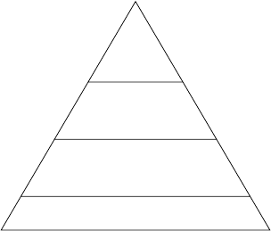
226 5. Implementation Issues
Multiplexor Amultiplexor is a multiple-input single-output device with a con-
troller that selects which input becomes the output. These devices provide the
conditional control of a circuit.
Pipelining Pipelining is a design feature that allows a second computation to begin
before the current computation is completed.
Parallel Processing Parallel processing is a technique that permits two or more
computations to happen simultaneously.
5.2.1 Design criteria
The operation that dominates the execution time of an elliptic curve cryptographic
protocol is point multiplication. Efficient implementation of point multiplication can
be separated into three distinct layers:
1. finite field arithmetic (Chapter 2);
2. elliptic curve point addition and doubling (§3.2); and
3. point multiplication technique (§3.3).
Accordingly, there is a hierarchy of operations involved in point multiplication with
point multiplication techniques near the top and the fundamental finite field arithmetic
at the base. The hierarchy, depicted in Figure 5.2, has been extended to the proto-
col level. For example, one could decide to implement ECDSA signature generation
(§4.4.1) entirely in hardware so that the only input to the device is the message to be
signed, and the only output is the signature for that message.
Protocols
Point
multiplication
Elliptic curve
addition and doubling
Finite field arithmetic
Figure 5.2. Hierarchy of operations in elliptic curve cryptographic schemes.
An important element of hardware design is to determine those layers of the hier-
archy that should be implemented in silicon. Clearly, finite field arithmetic must be
designed into any hardware implementation. One possibility is to design a hardware
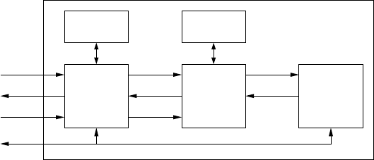
5.2. Hardware implementation 227
accelerator for finite field arithmetic only, and then use an off-the-shelf microprocessor
to perform the higher-level functions of elliptic curve point arithmetic. It is important to
note that an efficient finite field multiplier does not necessarily yield an efficient point
multiplier—all layers of the hierarchy need to be optimized.
Moving point addition and doubling and then point multiplication to hardware pro-
vides a more efficient ECC processor at the expense of more complexity. In all cases a
combination of both efficient algorithms and hardware architectures is required.
One approach to higher functionality is the processor depicted in Figure 5.3. Along
with program and data memory, the three main components are an arithmetic logic
unit (AU), an arithmetic unit controller (AUC), and a main controller (MC). The AU
performs the basic field operations of addition, squaring, multiplication, and inversion,
and is controlled by the AUC. The AUC executes the elliptic curve operations of point
addition and doubling. The MC coordinates and executes the method chosen for point
multiplication, and interacts with the host system.
memory
Program
memory
Program
control control
status status
command
MC AUC AU
control
status
command
data
HOST
SYSTEM
Figure 5.3. Elliptic curve processor architecture.
Let’s consider how a higher functionality processor might handle the computation
of kP for a randomly chosen integer k. The host commands the processor to generate
kP where the integer kand the (affine) coordinates of Pare provided by the host. The
integer kis loaded into the MC, and the coordinates of Pare loaded into the AU. The
MC instructs the AUC to do its initialization which may include converting the affine
coordinates of Pto projective coordinates needed by the point addition and doubling
formulae. The MC scans the bits of kand instructs the AUC to perform the appropriate
elliptic curve operations, which in turn instructs the AU to perform the appropriate
finite field operations. After all bits of kare processed, the MC instructs the AUC to
convert the result back to affine coordinates. The host reads the coordinates of kP
from the registers in the AU. Two important consequences of having two controllers
are the ability to permit parallel processing and pipelining of operations. The MC can
also use the data storage capability to implement algorithms that use precomputation
to compute kP more efficiently (see §3.3).
228 5. Implementation Issues
Criteria for selecting hardware designs
The following are some of the issues that have to considered in hardware design. It
should be emphasized that a good design demands a thorough understanding of the
target platform, operating environment, and performance and security requirements.
1. Cost is always a significant issue with hardware designers, and is driven by all
of the criteria that follow.
2. Hardware vs. software. Is there a compelling argument to choose a hardware
accelerator over a software implementation?
3. Throughput. A device that will be installed into a server will likely need to do
hundreds or thousands of elliptic curve operations per second whereas devices
designed for handheld computers will require only a small fraction of this.
4. Complexity. The more levels of the hierarchy that the device implements, the
more complex the circuitry becomes. This translates into more silicon area on a
custom VLSI device or a much larger FPGA. It will also result in higher cost.
5. Flexibility. Issues pertinent here include the ability of the device to perform
computations on curves over binary fields and prime fields.
6. Algorithm agility. Many cryptographic protocols require cryptographic algo-
rithms to be negotiated on a per-session basis (e.g., SSL). Reconfigurable
hardware might be an attractive feature provided that performance is not
significantly impacted.
7. Power consumption. Depending on the environment where the device will op-
erate, power consumption may or may not be a major issue. For example,
contactless smart cards are very constrained by the amount of power available
for cryptographic operations whereas a server can afford much higher power
consumption.
8. Security should always be paramount in any design consideration. If the device
is designed to perform only point additions and doublings, then it is activated
during a point multiplication kP by the bits associated with the random value k.
Without careful design of the overall architecture, bits of kcould be leaked by
side-channel attacks. Countermeasures to attacks based on timing, power analy-
sis, and electromagnetic radiation (see §5.3) should be considered based on the
environment in which the device will operate.
9. Overall system architecture. If the overall system has a microprocessor with
enough free cycles to handle protocol functionality above finite field arithmetic
(see Figure 5.2), then, depending on other criteria, this may be good reason to
design the device for finite field arithmetic only.
10. Implementation platform. A custom VLSI or gate array design or an FPGA
may be used. FPGAs typically have a high per unit cost versus VLSI and
gate array devices. Design costs are however significantly higher for VLSI
implementations.

5.2. Hardware implementation 229
11. Scalability. If it is desirable that the device can provide various levels of security
(for example by implementing all the NIST curves in §A.2), then one must design
the underlying finite field processor to accommodate variable field sizes.
The relative importance of these design criteria depends heavily on the application.
For example, cost is less of a concern if the hardware is intended for a high-end server
than if the hardware is intended for a low-end device such as a light switch. Table 5.8
lists design criteria priorities for these two extreme situations.
High-end device Low-end device
High priority Low priority High Priority Low priority
Throughput Cost Cost Throughput
Security Power consumption Hardware vs. software Flexibility
Scalability Complexity Complexity Algorithm agility
System architecture Power consumption Scalability
Implementation platform Security
Algorithm agility System architecture
Flexibility Implementation platform
Hardware vs. software
Table 5.8. Priorities for hardware design criteria.
5.2.2 Field arithmetic processors
This section describes hardware circuits for performing addition, multiplication, squar-
ing, and inversion operations in a binary field F2m. The operations in F2mare typically
easier to implement in hardware than their counterparts in prime fields Fpbecause bit-
wise addition in F2mdoes not have any carry propagation. Moreover, unlike the case of
F2m, squaring in Fpis roughly as costly as a general multiplication. As a consequence
of squaring being more expensive in Fpthan F2m, inversion using multiplication (as
described below for F2m)isslowerinFp.
Addition
Recall from §2.3.1 that addition of elements in a binary field F2mis performed bitwise.
There is no carry propagation, and hence addition in F2mis considerably simpler to
implement in hardware than addition in prime fields Fp.
Multiplication
We discuss the design of a hardware circuit to multiply elements in a binary field F2m.
We shall only consider the case where the elements of F2mare represented with respect
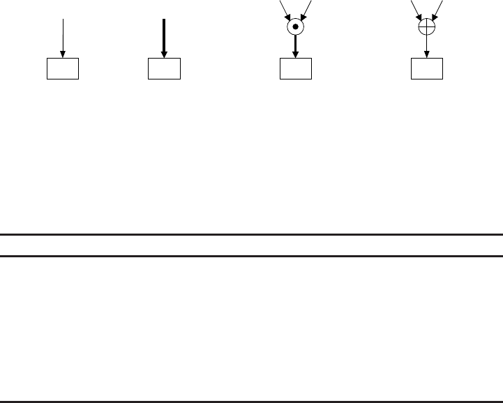
230 5. Implementation Issues
to a polynomial basis. If f(z)is the reduction polynomial, then we write
f(z)=zm+r(z), where degr≤m−1.
Moreover, if r(z)=rm−1zm−1+···+r2z2+r1z+r0, then we represent r(z)by the
binary vector
r=(rm−1,...,r2,r1,r0).
A multiplier is said to be bit-serial if it generates one bit of the product at each clock
cycle. It is digit-serial if it generates more than one bit of the product at each clock
cycle. We present bit-serial multipliers for the three cases:
(i) fixed field size with arbitrary reduction polynomial;
(ii) fixed field size with fixed reduction polynomial; and
(iii) variable field size (with arbitrary or fixed reduction polynomials).
We also describe a digit-serial multiplier for the fourth case:
(iv) fixed field size with fixed reduction polynomial.
In Figures 5.4–5.11, the following symbols are used to denote operations on bits A,
B,C:
C
A
C
A
C
BA
C
BA
C←AC←A⊕CC←C⊕(A&B)C←A⊕B
(i) Fixed field size with arbitrary reduction polynomial Algorithm 5.3, which mul-
tiplies a multiplicand a∈F2mand a multiplier b∈F2m, processes the bits of bfrom left
(most significant) to right (least significant). The multiplier, called a most significant
bit first (MSB) multiplier, is depicted in Figure 5.4 for the case m=5. In Figure 5.4
bis a shift register and cis a shift register whose low-end bit is tied to 0. An MSB
multiplier can perform a multiplication in F2min mclock cycles.
Algorithm 5.3 Most significant bit first (MSB) multiplier for F2m
INPUT:a=(am−1,...,a1,a0), b=(bm−1,...,b1,b0)∈F2m, and reduction polynomial
f(z)=zm+r(z).
OUTPUT:c=a·b.
1. Set c←0.
2. For ifrom m−1 downto 0 do
2.1 c←leftshift(c)+cm−1r.
2.2 c←c+bia.
3. Return(c).
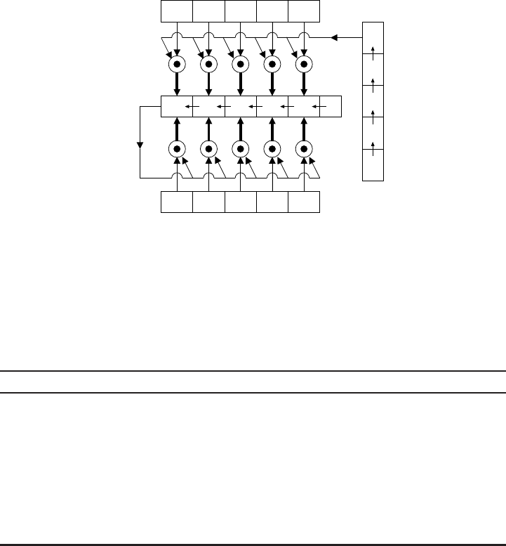
5.2. Hardware implementation 231
r0
r1
r3r2
c3c2c1c0
c4
a0
a1
a3a2
r4
a4
0
b
c
r
b2
b1
b0
a
b4
b3
Figure 5.4. Most significant bit first (MSB) multiplier for
F25
.
Algorithm 5.4, which multiplies a multiplicand a∈F2mand a multiplier b∈F2m,
processes the bits of bfrom right (least significant) to left (most significant). The
multiplier, called a least significant bit first (LSB) multiplier, is depicted in Figure 5.5.
Algorithm 5.4 Least significant bit first (LSB) multiplier for F2m
INPUT:a=(am−1,...,a1,a0), b=(bm−1,...,b1,b0)∈F2m, and reduction polynomial
f(z)=zm+r(z).
OUTPUT:c=a·b.
1. Set c←0.
2. For ifrom 0 to m−1do
2.1 c←c+bia.
2.2 a←leftshift(a)+am−1r.
3. Return(c).
One difference between the MSB and LSB multipliers is that the contents of two of
the four registers in Figure 5.4 are not altered during a multiplication, while three of
the four registers in Figure 5.5 are altered. In other words, the MSB multiplier only has
to clock two registers per clock cycle, as compared to three for the LSB multiplier.
(ii) Fixed field size with fixed reduction polynomial If the reduction polynomial
f(z)is fixed and is selected to be a trinomial or pentanomial, then the design of the
multiplier is significantly less complex since a register to hold the reduction polyno-
mial is no longer needed. Figure 5.6 illustrates an MSB multiplier for F25with fixed
reduction polynomial f(z)=z5+z2+1.
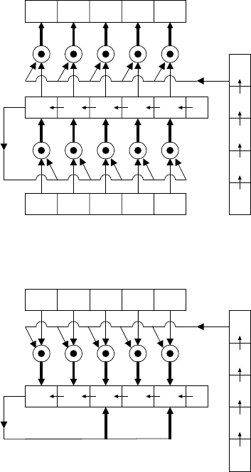
232 5. Implementation Issues
b
b2
b3
b4
b0
b1
r0
r1
r3r2
a3a2a1a0
a4
c0
c1
c3c2
r4
c4
a
r
c
0
Figure 5.5. Least significant bit first (LSB) multiplier for
F25
.
c3c2c1c0
c4
a0
a1
a3a2
a4
0
b
cb2
b1
b0
a
b4
b3
Figure 5.6. MSB multiplier with fixed reduction polynomial
f(z)=z5+z2+1
.
(iii) Variable field size The MSB multiplier in Figure 5.4 can be extended to multiply
elements in the fields F2mfor m∈{m1,m2,...,mt},wherem1<m2<···<mt. Each
register has length mt. Figure 5.7 illustrates an MSB multiplier that can implement
multiplication in any field F2mfor m∈{1,2,...,10}, and for any reduction polyno-
mial. Note that only the contents of registers band cchange at each clock cycle. The
controller loads the bits of a,band rfrom high-order to low-order and sets the unused
bits to 0. Although the unused cells are clocked, they consume little power since their
contents do not change.
The circuit can be simplified if each field has a fixed reduction polynomial, prefer-
ably a trinomial or a pentanomial. Figure 5.8 illustrates a variable field size MSB
multiplier for F25,F27,andF210 with the fixed reduction polynomials z5+z2+1,
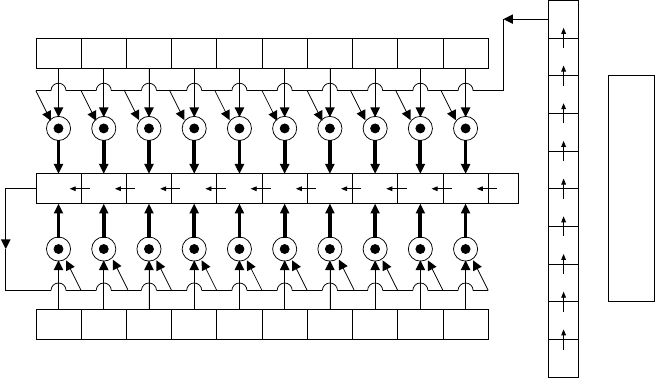
5.2. Hardware implementation 233
C
O
N
T
R
O
L
L
E
R
c
r
a
r1
r2
r4r3
c4c3c2c1
c5
a1
a2
a4a3
r5
a5
0000
0000
c0
0000
r0
a0
b1
b
b5
b4
b3
b2
b0
0
0
0
0
0
Figure 5.7. MSB multiplier for fields
F2m
with
1≤m≤10
. A multiplier for
F26
is shown.
z7+z+1, and z10 +z3+1, respectively. A multiplexor is used to select the desired
field. Loading registers and controlling the multiplexor is the function of the controller.
(iv) Digit-serial multiplier for fixed field size with fixed reduction polynomial We
consider multiplication of two elements aand bin F2mwhere the multiplier bis
expressed as a polynomial having l=m/kdigits
b=
l−1
i=0
Bizki,
where each digit Biis a binary polynomial of degree at most k−1. One way to express
the product a·bis the following:
a·b=a&l−1
i=0
Bizki'mod f(z)
=&l−1
i=0
Bi(azki mod f(z))'mod f(z)
where f(z)is the reduction polynomial for F2m. Algorithm 5.5 is a digit-serial
multiplier derived from this observation.
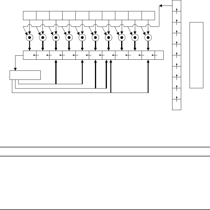
234 5. Implementation Issues
C
O
N
T
R
O
L
L
E
R
a
c3c2c1c0
c4
a0
a1
a3a2
a4
0000
0000
b0
0
b
b4
b3
b2
b1
0
0
0
0
Multiplexor
0
0
0
c
Figure 5.8. MSB multiplier for fields
F25
,
F27
,and
F210
with reduction polynomials
z5+z2+1
,
z7+z+1
,and
z10 +z3+1
. The multiplier for
F25
is shown.
Algorithm 5.5 Digit-serial multiplier for F2m
INPUT:a=m−1
i=0aizi∈F2m,b=l−1
i=0Bizki ∈F2m, reduction polynomial f(z).
OUTPUT:c=a·b.
1. Set c←0.
2. For ifrom 0 to l−1do
2.1 c←c+Bia.
2.2 a←a·zkmod f(z).
3. Return(cmod f(z)).
A hardware circuit for executing Algorithm 5.5 consists of a shift register to hold
the multiplicand a, another shift register to hold the multiplier b, and an accumulating
register (not a shift register) to hold c. The registers holding aand bare each mbits
in length, whereas cis (m+k−1)bits long. At the ith iteration, the content of ais
azki mod f(z). The product Bi·(azki mod f(z)) is called a digit multiplication.The
result of this digit multiplication is at most m+k−1 bits in length and is XORed into
the accumulator c. If the circuit can compute azki mod f(z)and Bi·(azki mod f(z))
in a single clock, then the entire multiplication can be completed in lclock cycles.
While the complexity of the circuit increases with k,ak-fold speedup for multiplication
can be achieved.
Figure 5.9 shows the aregister for a 2-digit multiplier for F25where the field is
defined by the reduction polynomial f(z)=z5+z2+1. In this example, we have
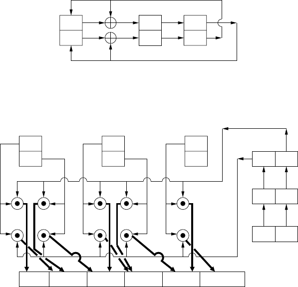
5.2. Hardware implementation 235
k=2andl=3. Figure 5.10 shows the circuit for digit multiplication excluding the
interconnect of Figure 5.9 and the interconnect on the cregister for the final reduction
modulo f(z). The final reduction interconnect will require multiplexors.
a1
a0a2
a3
a4
0
Figure 5.9. Circuit to compute
azki mod f(z)
,where
f(z)=z5+z2+1
and
k=2
.
b0
b2
c0c1c2c3c5
a0
a1
a2
a3
a4
b3
b1
b4
0
0
c4
Figure 5.10. A 2-digit multiplier for
F25
defined by
f(z)=z5+z2+1
.
Squaring
Squaring can of course be performed using any of the multipliers described above. If
the reduction polynomial f(z)is fixed and is a trinomial or a pentanomial, then it is
possible to design a circuit that will perform a squaring operation in a single clock
cycle (vs. mclock cycles for the bit-serial multipliers). Moreover, the squaring circuit
will add very little complexity to the multiplication circuit. A squaring circuit that takes
only one clock cycle is important when inversion is done by multiplication (see below).
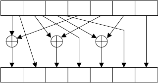
236 5. Implementation Issues
For example, consider the field F27with reduction polynomial f(z)=z7+z+1. If
a=a6z6+a5z5+a4z4+a3z3+a2z2+a1z+a0,then
c=a2
=a6z12 +a5z10 +a4z8+a3z6+a2z4+a1z2+a0
=(a6+a3)z6+a6z5+(a5+a2)z4+a5z3+(a4+a1)z2+a4z+a0.
A squaring circuit is illustrated in Figure 5.11.
c0
a0
a6a5
c1
c6c5
a2a1
a3
a4
c4c3c2
Figure 5.11. Squaring circuit for
F27
with fixed reduction polynomial
f(z)=z7+z+1
.
Inversion
The most difficult finite field operation to implement in hardware is inversion. There
are two basic types of inversion algorithms: those based on the extended Euclidean al-
gorithm and its variants (cf. §2.3.6), and those that use field multiplication. Inversion
by multiplication does not add significantly to the complexity of a hardware design, but
can severely impact performance if it is needed frequently. This is the reason why most
hardware (and for that matter software) designers prefer projective coordinates over
affine. Additional functionality must be incorporated into the controller but extensive
modifications to the core circuit are not required. If affine coordinates are preferred,
then inversion will undoubtedly be the bottleneck in performance thereby necessitating
an inversion circuit based on the extended Euclidean algorithm. Such a circuit will add
more complexity to both the core circuit and the controller. It seems that the added com-
plexity does not justify implementing inversion by the extended Euclidean algorithm,
and therefore we restrict our attention to inversion methods that use multiplication.
Let abe a nonzero element in F2m. Inversion by multiplication uses the fact that
a−1=a2m−2.(5.2)
Since 2m−2=m−1
i=12i,wehave
a−1=am−1
i=12i=
m−1
6
i=1
a2i.(5.3)

5.2. Hardware implementation 237
Thus, a−1can be computed by m−1 squarings and m−2 multiplications. We next
show how the number of multiplications can be reduced. First observe that
a−1=a2m−2=(a2m−1−1)2.
Hence a−1can be computed in one squaring once a2m−1−1has been evaluated. Now if
mis odd then
2m−1−1=(2(m−1)/2−1)(2(m−1)/2+1). (5.4)
If we let
b=a2(m−1)/2−1,
then by (5.4) we have
a2m−1−1=b·b2(m−1)/2.
Hence a2m−1−1can be computed with one multiplication and (m−1)/2 squarings once
bhas been evaluated. Similarly, if mis even then
2m−1−1=2(2m−2−1)+1=2(2(m−2)/2−1)(2(m−2)/2+1)+1.(5.5)
If we let
c=a2(m−2)/2−1,
then by (5.5) we have
a2m−1−1=a·c·c2(m−2)/22
.
Hence a2m−1−1can be computed with two multiplications and m/2 squarings once c
has been evaluated. This procedure can be repeated recursively to eventually compute
a−1. The total number of multiplications in this procedure can be shown to be
log2(m−1)+w(m−1)−1,(5.6)
where w(m−1)denotes the number of 1s in the binary representation of m−1,
while the total number of squarings is m−1. This inversion procedure is shown in
Algorithm 5.6 when mis odd.
Algorithm 5.6 Inversion in F2m(modd)
INPUT: Nonzero element a∈F2m.
OUTPUT:a−1.
1. Set A←a2,B←1, x←(m−1)/2.
2. While x= 0do
2.1 A←A·A2x.
2.2 If xis even then x←x/2;
Else B←B·A,A←A2,x←(x−1)/2.
3. Return(B).

238 5. Implementation Issues
Table 5.9 shows the number of squarings and multiplications needed to compute in-
verses in the NIST binary fields F2163 ,F2233 ,F2283 ,F2409 and F2571 using Algorithm 5.6.
The last squaring of Ain step 2.2 is not required, and therefore is not included in the
operation counts.
mlog2(m−1)w(m−1)multiplications squarings
163 7 3 9 162
233 7 4 10 232
283 8 4 11 282
409 8 4 11 408
571 9 5 13 570
Table 5.9. Operation counts for inversion in the binary fields
F2163
,
F2233
,
F2283
,
F2409
and
F2571
using Algorithm 5.6.
5.3 Secure implementation
When assessing the security of a cryptographic protocol, one usually assumes that the
adversary has a complete description of the protocol, is in possession of all public
keys, and is only lacking knowledge of the secret keys. In addition, the adversary may
have intercepted some data exchanged between the legitimate participants, and may
even have some control over the nature of this data (e.g., by selecting the messages
in a chosen-message attack on a signature scheme, or by selecting the ciphertext in
a chosen-ciphertext attack on a public-key encryption scheme). The adversary then
attempts to compromise the protocol goals by either solving an underlying problem
assumed to be intractable, or by exploiting some design flaw in the protocol.
The attacks considered in this traditional security model exploit the mathematical
specification of the protocol. In recent years, researchers have become increasingly
aware of the possibility of attacks that exploit specific properties of the implementation
and operating environment. Such side-channel attacks utilize information leaked dur-
ing the protocol’s execution and are not considered in traditional security models. For
example, the adversary may be able to monitor the power consumed or the electromag-
netic radiation emitted by a smart card while it performs private-key operations such
as decryption and signature generation. The adversary may also be able to measure
the time it takes to perform a cryptographic operation, or analyze how a cryptographic
device behaves when certain errors are encountered. Side-channel information may be
easy to gather in practice, and therefore it is essential that the threat of side-channel
attacks be quantified when assessing the overall security of a system.
It should be emphasized that a particular side-channel attack may not be a realistic
threat in some environments. For example, attacks that measure power consumption of
a cryptographic device can be considered very plausible if the device is a smart card
that draws power from an external, untrusted source. On the other hand, if the device
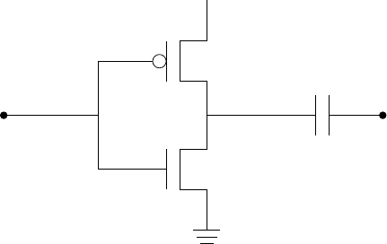
5.3. Secure implementation 239
is a workstation located in a secure office, then power consumption attacks are not a
significant threat.
The objective of this section is to provide an introduction to side-channel attacks
and their countermeasures. We consider power analysis attacks, electromagnetic anal-
ysis attacks, error message analysis, fault analysis, and timing attacks in §5.3.1, §5.3.2,
§5.3.3, §5.3.4, and §5.3.5, respectively. The countermeasures that have been proposed
are algorithmic, software-based, hardware-based, or combinations thereof. None of
these countermeasures are guaranteed to defeat all side-channel attacks. Furthermore,
they may slow cryptographic computations and have expensive memory or hardware
requirements. The efficient and secure implementation of cryptographic protocols on
devices such as smart cards is an ongoing and challenging research problem that
demands the attention of both cryptographers and engineers.
5.3.1 Power analysis attacks
CMOS (Complementary Metal-Oxide Semiconductor) logic is the dominant semicon-
ductor technology for microprocessors, memories, and application specific integrated
circuits (ASICs). The basic building unit in CMOS logic is the inverter, or NOT gate,
depicted in Figure 5.12. It consists of two transistors, one P-type and one N-type, that
P-type transistor
Vin
Supply Voltage
Ground
N-type transistor
Vout
capacitive
load
Figure 5.12. CMOS logic inverter.
serve as voltage-controlled switches. A high voltage signal is interpreted as a logical
‘1’, while a low voltage signal is interpreted as a logical ‘0’. If the input voltage Vin
is low, then the P-type transistor is conducting (i.e., the switch is closed) while the N-
type transistor is non-conducting; in this case, there is a path from the supply voltage to
the output and therefore Vout is high. Conversely, if Vin is high, then the P-type tran-
sistor is non-conducting while the N-type transistor is conducting; in this case, there
is a path from the output to the ground and therefore Vout is low. When the inverter
switches state, there is a short period of time during which both transistors conduct
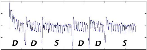
240 5. Implementation Issues
current. This causes a short circuit from the power supply to the ground. There is also
current flow when internal capacitive loads attached to the inverter’s output are charged
or discharged.
During a clock cycle, current flows through only a small proportion of the gates in a
CMOS device—those gates that are active during the execution of a particular instruc-
tion. Thus, the power consumed by the device can be expected to change continuously
as the device executes a complicated series of instructions.
If the power to the device is supplied at a constant voltage, then the power consumed
by the device is proportional to the flow of current. The current flow, and thus also the
power consumption, can be measured by placing a resistor in series with the power
supply and using an oscilloscope to measure the voltage difference across the resistor.
One can then plot a power trace, which shows the power consumed by the device
during each clock cycle.
The hypothesis behind power analysis attacks is that the power traces are correlated
to the instructions the device is executing as well as the values of the operands it is
manipulating. Therefore, examination of the power traces can reveal information about
the instructions being executed and contents of data registers. In the case that the device
is executing a secret-key cryptographic operation, it may then be possible to deduce the
secret key.
Simple power analysis
In simple power analysis (SPA) attacks, information about secret keying material is
deduced directly by examining the power trace from a single secret key operation.
Implementations of elliptic curve point multiplication algorithms are particularly vul-
nerable because the usual formulas for adding and doubling points are quite different
and therefore may have power traces which can readily be distinguished. Figure 5.13
shows the power trace for a sequence of addition (S) and double (D) operations on an
elliptic curve over a prime field. Points were represented using Jacobian coordinates
(see §3.2.1) whereby an addition operation takes significantly longer than a double
operation.
Figure 5.13. Power trace for a sequence of addition (S) and double (D) operations on an elliptic
curve over a prime field. Points were represented using Jacobian coordinates. The traces were
obtained from an SC140 DSP processor core.
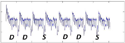
5.3. Secure implementation 241
Consider, for example, a device that performs a point multiplication kP during
ECDSA signature generation (Algorithm 4.29). Here, Pis a publicly-known elliptic
curve point and kis a secret integer. Recall that knowledge of a single per-message
secret kand the corresponding message and signature allows one to easily recover the
long-term private key (cf. Note 4.34). Suppose first that one of the binary methods for
point multiplication (Algorithms 3.26 and 3.27) is used. If examination of a power trace
of a point multiplication reveals the sequence of double and addition operations, then
one immediately learns the individual bits of k. Suppose now that a more sophisticated
point multiplication method is employed; for concreteness consider the binary NAF
method (Algorithm 3.31). If the power trace reveals the sequence of double and addi-
tion operations, then an adversary learns the digits of NAF(k)that are 0, which yields
substantial information about k.
Knowledge of how the algorithm is used and implementated facilitate SPA attacks.
Any implementation where the execution path is determined by the key bits has a
potential vulnerability.
Countermeasures Numerous techniques for resisting SPA attacks have been pro-
posed. These countermeasures involve modifications to the algorithms, software
implementations, hardware implementations, or combinations thereof. The effective-
ness of the countermeasures is heavily dependent on the characteristics of the hardware
platform, the operating environment, and the capabilities of the adversary, and must be
evaluated on a case-by-case basis. As an example, Figure 5.14 shows for the power
trace for a sequence of addition (S) and double (D) operations on an elliptic curve
over a prime field. Dummy operations were inserted in the algorithms for addition
and doubling in such a way that the sequence of elementary operations involved in
a doubling operation is repeated exactly twice in an addition operation. Compared to
Figure 5.13, it seems impossible to distinguish the addition and double operations by
casual inspection of the power trace in Figure 5.14.
Figure 5.14. Power trace for a sequence of addition (S) and double (D) operations on an elliptic
curve over a prime field. Points were represented using Jacobian coordinates. SPA resistance was
achieved by insertion of dummy operations in the addition and double algorithms (compare with
Figure 5.13). The traces were obtained from an SC140 DSP processor core.

242 5. Implementation Issues
None of the countermeasures that have been proposed are guaranteed to provide
adequate protection. It is also important to note that resistance to SPA attacks does not
guarantee resistance to other side-channel attacks such as differential power analysis
and electromagnetic analysis attacks. It is therefore impossible at present to provide
general recommendations for the best countermeasures to SPA attacks. Instead we just
give one example and list other methods in the Notes section starting on page 254.
Algorithm 5.7 is a modification of the left-to-right binary point multiplication
method to provide enhanced resistance to SPA attacks. Dummy operations are included
in the main loop so that the same basic elliptic curve operations (one double and one
addition) are performed in each iteration. Thus the sequence of double and additions
deduced from the power trace does not reveal any information about the bits of k.As
with most algorithmic countermeasures, the increased security comes at the expense of
slower performance.
Algorithm 5.7 SPA-resistant left-to-right binary point multiplication
INPUT:k=(kt−1,...,k1,k0)2,P∈E(Fq).
OUTPUT:kP.
1. Q0←∞.
2. For ifrom t−1downto0do
2.1 Q0←2Q0.
2.2 Q1←Q0+P.
2.3 Q0←Qki.
3. Return(Q0).
Differential power analysis
Differential power analysis (DPA) attacks exploit variations in power consumption that
are correlated to the data values being manipulated. These variations are typically much
smaller than those associated with different instruction sequences, and may be obfus-
cated by noise and measurement errors. Statistical methods are used on a collection of
power traces in order reduce the noice and strengthen the differential signals.
To launch a DPA attack, an adversary first selects an internal variable Vthat is en-
countered during the execution of the cryptographic operation and has the property that
knowledge of the input message mand a portion kof the unknown secret key deter-
mines the value of V. The determining function V=f(k,m)is called the selection
function. Let us assume for simplicity that Vis a single bit. The adversary collects a
number of power traces (e.g., a few thousand) from the device that performs the cryp-
tographic operation. She then makes a guess for k, and partitions the power traces into
two groups according to the predicted value of the bit V. The power traces in each
group are averaged, and the difference of the averages, called the differential trace,is
plotted. The idea is that the value of Vwill have some (possibly very small) influence
5.3. Secure implementation 243
on the power trace. Thus, if the guess for kis incorrect, then the partition of power
traces was essentially done randomly, and so one would expect the differential trace to
be flat. On the other hand, if the guess for kis correct then the two averaged power
traces will have some noticeable differences; one would expect the plot of the differ-
ential trace to be flat with spikes in regions influenced by V. This process is repeated
(using the same collection of power traces) until kis determined.
These ideas are illustrated in the following DPA attack on the SPA-resistant
point multiplication method of Algorithm 5.7. The attack demonstrates that SPA
countermeasures do not necessarily resist DPA attacks.
DPA attacks are generally not applicable to point multiplication in the signature
generation procedure for elliptic curve signature schemes such as ECDSA (Algo-
rithm 4.29) since the secret key kis different for each signature while the base point P
is fixed. However, the attacks can be mounted on point multiplication in elliptic curve
encryption and key agreement schemes. For example, for the point multiplication in
the ECIES decryption procedure (Algorithm 4.43), the multiplier is k=hd where dis
the long-term private key and his the cofactor, and the base point is P=Rwhere Ris
the point included in the ciphertext.
Suppose now that an adversary has collected the power traces as a cryptographic
device computed kP
1,kP
2,...,kP
rusing Algorithm 5.7. The adversary knows
P1,P2,...,Prand wishes to determine k.IfQ0=∞then the doubling operation in
step 2.1 is trivial and therefore can likely be distinguished from a non-trivial doubling
operation by examination of a single power trace. Thus, the attacker can easily de-
termine the leftmost bit of kthat is 1. Let us suppose that kt−1=1. The following
assignments are made in the first iteration of step 2 (with i=t−1): Q0←∞,Q1←P,
Q0←P. In the second iteration of step 2 (with i=t−2) the assignments are Q0←2P,
Q1←3P, and either Q0←2P(if kt−2=0) or Q0←3P(if kt−2=1). It follows that
the point 4Pis computed in a subsequent iteration if and only if kt−2=0. A position
in the binary representation of a point is selected, and the power traces are divided into
two groups depending on whether the selected bit of 4Piis 0 or 1. In the notation of
the generic description of DPA attacks, the key portion is k=kt−2,m=Pi,andthe
selection function fcomputes the selected bit of 4Pi. If the differential trace has some
noticeable spikes, then the adversary concludes that kt−2=0; otherwise kt−2=1. Once
kt−2has been determined, the adversary can similarly infer kt−3andsoon.
Countermeasures As is the case with SPA attacks, numerous techniques for resisting
DPA attacks have been proposed. Again, none of them are guaranteed to be sufficient
and their effectiveness must be evaluated on a case-by-case basis. These countermea-
sures are surveyed in the Notes section starting on page 254. Here we only present one
countermeasure that provides resistance to the particular DPA attack described above
for point multiplication.
Suppose that the field Fqhad characteristic >3, and suppose that mixed Jacobian-
affine coordinates (see §3.2.2) are used in Algorithm 5.7. Thus, the point Pis stored
in affine coordinates, while the points Q0and Q1are stored in Jacobian coordinates.
244 5. Implementation Issues
The first assignment of Q1is Q1←P;if P=(x,y)in affine coordinates, then Q1=
(x:y:1)in Jacobian coordinates. After this first assignment, the coordinates of Q1
are randomized to (λ2x,λ
3y,λ),whereλis a randomly selected nonzero element in
Fq, and the algorithm proceeds as before. The DPA attack described above is thwarted
because the adversary is unable to predict any specific bit of 4Pi(or other multiples of
Pi) in randomized Jacobian coordinates.
5.3.2 Electromagnetic analysis attacks
The flow of current through a CMOS device also induces electromagnetic (EM) emana-
tions. The EM signals can be collected by placing a sensor close to the device. As with
power analysis attacks, one can now analyze the EM signals in the hope that they reveal
information about the instructions being executed and contents of data registers. Simple
ElectroMagnetic Analysis (SEMA) attacks and Differential ElectroMagnetic Analysis
(DEMA) attacks, analogues of SPA and DPA attacks, can be launched. As with power
analysis attacks, these electromagnetic analysis (EMA) attacks are non-intrusive and
can be performed with relatively inexpensive equipment.
Since EM emanations may depend on the physical characteristics of the active gates,
a single EM sensor captures multiple EM signals of different types. These signals can
be separated and analyzed individually. This is unlike the case of power analysis attacks
where the power consumption measured is the single aggregation of power consumed
by all active units. Consequently, EMA attacks can potentially reveal more information
than power analysis attacks, and therefore constitute a more significant threat.
The most comprehensive study on EMA attacks was undertaken in 2002 by IBM
researchers Agrawal, Archambeault, Rao and Rohatgi, who conducted experiments on
several smart cards and a server containing an SSL accelerator. Their experiments pro-
vide convincing evidence that the output of a single wideband EM sensor consists of
multiple EM signals, each of which can encode somewhat different information about
the device’s state. Moreover, they succeeded in using EMA attacks to compromise the
security of some commercially available cryptographic devices that had built-in coun-
termeasures for resisting power analysis attacks, thus demonstrating that EMA attacks
can indeed be more powerful than power analysis attacks.
As with power analysis, EMA countermeasures could be hardware based (e.g., metal
layers to contain the EM emanations or circuit redesign to reduce the EM emanations)
or software based (e.g., use of randomization). The study of EMA attacks is relatively
new, and it remains to be seen which countermeasures prove to be the most effective.
5.3.3 Error message analysis
Another side channel that may be available to an adversary is the list of error messages
generated by the victim’s cryptographic device. Consider, for example, the decryption

5.3. Secure implementation 245
process of a public-key encryption scheme such as ECIES (see §4.5.1). A ciphertext
might be rejected as invalid because some data item encountered during decryption
is not of requisite form. In the case of ECIES decryption (Algorithm 4.43), a ci-
phertext (R,C,t)will be rejected if embedded public key validation of Rfails, or
if Z=hdR =∞, or if the authentication tag tis invalid. There are several ways in
which the adversary may learn the reason for rejection. For example, the error message
may be released by the protocol that used the encryption scheme, the adversary may
be able to access the error log file, or the adversary may be able to accurately time
the decryption process thereby learning the precise point of failure. An adversary who
learns the reason for rejection may be able to use this information to its advantage.
To illustrate this kind of side-channel attack, we consider Manger’s attack on the
RSA-OAEP encryption scheme. Manger’s attack is very effective, despite the fact that
RSA-OAEP has been proven secure (in the random oracle model). This supports the
contention that a cryptographic scheme that is secure in a traditional security model is
not necessarily secure when deployed in a real-world setting.
RSA-OAEP encryption scheme
RSA-OAEP is intended for the secure transport of short messages such as symmetric
session keys. It first formats the plaintext message using Optimal Asymmetric Encryp-
tion Padding (OAEP), and then encrypts the formatted message using the basic RSA
function. RSA-OAEP has been proven secure (in the sense of Definition 4.41) under
the assumption that the problem of finding eth roots modulo nis intractable, and that
the hash functions employed are random functions. The following notation is used in
the descriptions of the encryption and decryption procedures.
1. A’s RSA public key is (n,e),anddis A’s corresponding private key. The integer
nis kbytes in length. For example, if nis a 1024-bit modulus, then k=128.
2. His a hash function with l-byte outputs. For example, Hmay be SHA-1 in
which case l=20.
3. Pconsists of some encoding parameters.
4. padding consists of a string of 00 bytes (possibly empty) followed by a 01 byte.
5. Gis a mask generating function. It takes as input a byte string sand an output
length t, and generates a (pseudorandom) byte string of length tbytes. In prac-
tice, G(s,t)may be defined by concatenating successive hash values H(si),
for 0 ≤i≤t/l−1, and deleting any rightmost bytes if necessary.
The concatenation mof maskedS and maskedPM is a byte string of length k−1.
This ensures that the integer representation mof mis less than the modulus nwhich is
kbytes in length, and hence mcan be recovered from c.
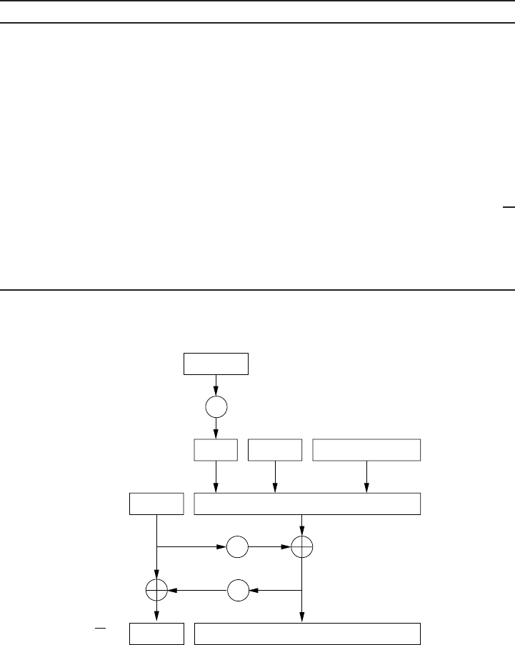
246 5. Implementation Issues
Algorithm 5.8 RSA-OAEP encryption
INPUT: RSA public key (n,e), message Mof length at most k−2−2lbytes.
OUTPUT: Ciphertext c.
1. Select a random seed Sof length lbytes.
2. Apply the OAEP encoding operation, depicted in Figure 5.15, with inputs S,P
and Mto obtain an integer m:
2.1 Form the padded message PM of length k−l−1 bytes by concatenating
H(P), a padding string of the appropriate length, and M.
2.2 Compute maskedPM =PM ⊕G(S,k−l−1).
2.3 Compute maskedS =S⊕G(maskedPM,l).
2.4 Concatenate the strings maskedS and maskedPM and convert the result m
to an integer m.
3. Compute c=memod n.
4. Return(c).
P
M
PM
padding
H
S
H(P)
G
G
maskedS maskedPM
m=
Figure 5.15. OAEP encoding function.
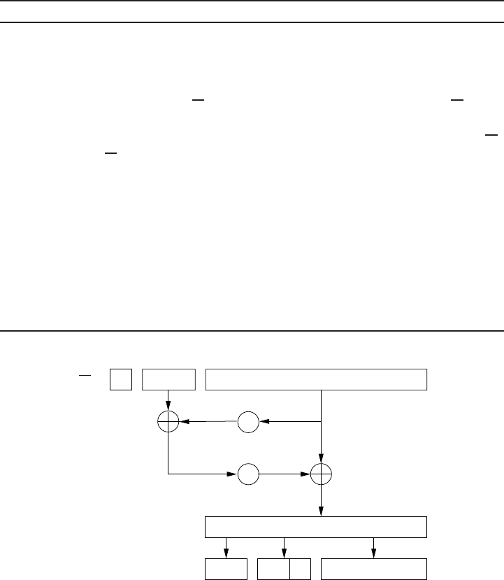
5.3. Secure implementation 247
Algorithm 5.9 RSA-OAEP decryption
INPUT: RSA public key (n,e),privatekeyd, ciphertext c.
OUTPUT: Plaintext Mor rejection of the ciphertext.
1. Check that c∈[0,n−1]; if not then return(“Reject the ciphertext”).
2. Compute m=cdmod n.
3. Convert mto a byte string mof length k.LetXdenote the first byte of m.
4. If X= 00 then return(“Reject the ciphertext”).
5. Apply the OAEP decoding operation, depicted in Figure 5.16 with inputs P,m:
5.1 Parse mto obtain X, a byte string maskedS of length l, and a byte string
maskedPM of length k−l−1.
5.2 Compute S=maskedS ⊕G(maskedPM,l).
5.3 Compute PM =maskedPM ⊕G(S,k−l−1).
5.4 Separate PM into a byte string Qconsisting of the first lbytes of PM,a
(possibly empty) byte string PS consisting of all consecutive zero bytes
following Q, a byte T, and a byte string M.
5.5 If T= 01 then return(“Reject the ciphertext”).
5.6 If Q= H(P)then return(“Reject the ciphertext”).
6. Return(M).
maskedPM
G
G
Q
PM
T
X
m=
M
maskedS
000000
Figure 5.16. OAEP decoding function.
Manger’s attack and countermeasures
A ciphertext c∈[0,n−1]may be invalid for several reasons: either X= 00 in step 4
of Algorithm 5.9, or T= 01 in step 5.5, or Q= H(P)in step 5.6. Manger’s attack
assumes that an adversary is able to ascertain whether X=00 in the case that cis found

248 5. Implementation Issues
to be invalid by the decryptor. The attack does not require the full power of a chosen-
ciphertext attack—the adversary does not need to learn the plaintexts corresponding to
ciphertexts of her choosing.
Suppose now that the adversary wishes to decrypt a target ciphertext cthat was
encrypted using A’s RSA key. Since cis valid, the adversary knows a priori that
m=cdmod nlies in the interval I=[0,28(k−1)−1]. The adversary selects cipher-
texts crelated to cin such a way that knowledge of whether the leftmost byte Xof
msatisfies X= 00 allows her to decrease the length of interval Iknown to contain m
by a factor (roughly) of 2. We will not present the technical details of how cis cho-
sen but only mention that this can be done very efficiently. After presenting about 8k
such ciphertexts cto Aand learning where the corresponding Xsatisfy X= 00, the
interval Iwill have only one integer in it, and adversary will thereby have recovered
mand can easily compute the plaintext M.Ifnis a 1024-bit integer, then only about
1024 interactions are required with the victim and hence the attack should be viewed
as being quite practical.
The attack can be prevented by ensuring that the decryption process returns identical
error messages if any of the three checks fail. Moreover, to prevent the possibility of
an adversary deducing the point of error by timing the decryption operation, the checks
in steps 4 and 5.5 of Algorithm 5.9 should be deferred until H(P)has been computed
and is being compared with Qin step 5.6.
5.3.4 Fault analysis attacks
Boneh, DeMillo and Lipton observed that if an error occurs while a cryptographic
device is performing a private-key operation, then the output of the cryptographic op-
eration may be incorrect and thereby provide exploitable information to an adversary.
Such errors may be introduced by non-malicious agents (e.g., hardware failures, soft-
ware bugs, or external noise) or may be induced by a malicious adversary who has
physical access to the device.
Fault analysis attacks generally do not pose a significant threat in practice. However,
if the environment in which cryptographic operations are being performed is conducive
to either non-malicious or induced errors, then suitable precautions should be taken.
These include verifying the result of a computation before exposing it, and using error-
control techniques to detect or correct data errors in internal memory.
We illustrate the basic ideas by presenting fault analysis attacks and countermeasures
on the RSA signature scheme.
RSA signature generation
Consider the FDH (Full Domain Hash) variant of the RSA signature scheme with
public key (n,e)and private key d. The signature of a message Mis
s=mdmod n,(5.7)
5.3. Secure implementation 249
where m=H(M)and His a hash function whose outputs are integers in the interval
[0,n−1]. The signature son Mis verified by computing m=H(M)and m=semod
n, and then checking that m=m.
In order to accelerate the signing operation (5.7), the signer computes
sp=mdpmod pand sq=mdqmod q,(5.8)
where pand qare the prime factors of n,dp=dmod (p−1),anddq=dmod (q−1).
Then the signature scan be computed as
s=asp+bsqmod n,
where aand bare integers satisfying
a≡21(mod p)
0(mod q)and b≡20(mod p)
1(mod q).
The integers dp,dq,aand bcan be precomputed by the signer. This signing procedure
is faster because the two modular exponentiations in (5.8) have exponents and moduli
that are half the bitlengths of the exponent and modulus in (5.7).
Suppose now that an error occurs during the computation of spand that no errors
occur during the computation of sq. In particular, suppose that sp≡ mdp(mod p)and
sq≡mdq(mod q). Thus
s≡ mdp(mod p)and s≡mdq(mod q)
whence
se≡ m(mod p)and se≡m(mod q).
It follows that
gcd(se−m,n)=q,(5.9)
and so an adversary who obtains the message representative mand the (incorrect)
signature scan easily factor nand thereafter compute the private key d.
One method for resisting this particular fault analysis attack on RSA signatures is to
incorporate some randomness in the formation of the message representative mfrom
the message Min such a way that an adversary cannot learn mfrom an erroneous
signature (and thus cannot evaluate the gcd in (5.9)). This property holds in the PSS
(Probabilistic Signature Scheme) variant of the RSA signature scheme. Note, however,
that there may exist other kinds of fault analysis attacks that are effective on PSS.
The simplest and most effective countermeasure is to insist that the device verify the
signature before transmission.
250 5. Implementation Issues
5.3.5 Timing attacks
The premise behind timing attacks is that the amount of time to execute an arithmetic
operation can vary depending on the value of its operands. An adversary who is capa-
ble of accurately measuring the time a device takes to execute cryptographic operations
(e.g., signature generation on a smart card) can analyze the measurements obtained to
deduce information about the secret key. Timing attacks are generally not as serious
a threat as power analysis attacks to devices such as smart cards because they typi-
cally require a very large number of measurements. However, recent work by Boneh
and Brumley has shown that timing attacks can be a concern even when launched
against a workstation running a protocol such as SSL with RSA over a local network
(where power analysis attacks may not be applicable). Thus, it is prudent that security
engineers consider resistance of their systems to timing attacks.
While experimental results on timing attacks on RSA and DES implementations
have been reported in the literature, there have not been any published reports on timing
attacks on implementations of elliptic curve systems. The attacks are expected to be
especially difficult to mount on elliptic curve signature schemes such as ECDSA since
a fresh per-message secret kis chosen each time the signature generation procedure is
invoked.
5.4 Notes and further references
§5.1
The features of the Intel IA-32 family of processors are described in [210]. References
for optimization techniques for the Pentium family of processors include the Intel man-
uals [208, 209] and Gerber [171]. SIMD capabilities of the AMD K6 processor are
detailed in [4]. Footnote 1 on instruction latency and throughput is from Intel [209].
The SPARC specification is created by the Architecture Committee of SPARC Interna-
tional (http://www.sparc.org), and is documented in Weaver and Germond [476]; see
also Paul [371]. The V9 design was preceded by the Texas Instruments and Sun Super-
SPARC and the Ross Technology HyperSPARC, both superscalar. Examples 5.1 and
5.2arebasedinpartonGNUMPversion4.1.2.
The fast implementations for finite field and elliptic curve arithmetic in P-224 using
floating-point operations described in §5.1.2 are due to Bernstein [42, 43]. Historical
information and references are provided in [42]. Required numerical analyses of the
proposed methods for P-224 were not complete as of 2002. Bernstein has announced
that “Fast point multiplication on the NIST P-224 elliptic curve” is expected to be
included in his forthcoming book on High-speed Cryptography.
Although SIMD is often associated with image and speech applications, Intel [209]
also suggests the use of such capabilities in “encryption algorithms.” Aoki and Lipmaa
5.4. Notes and further references 251
[17] evaluated the effectiveness of MMX-techniques on the AES finalists, noting that
MMX was particularly effective for Rijndael; see also Lipmaa’s [298] implementation
of the IDEA block cipher. In cross-platform code distributed for solving the Certi-
com ECC2K-108 Challenge [88] (an instance of the elliptic curve discrete logarithm
problem for a Koblitz curve over a 109-bit binary field), Robert Harley [191] provided
several versions of field multiplication routines. The MMX version was “about twice as
fast” as the version using only general-purpose registers. The Karatsuba-style approach
worked well for the intended target; however, the fastest versions of Algorithm 2.36
using only general-purpose registers were competitive in our tests.
Integer multiplication in Example 5.2 uses only scalar operations in the SSE2 in-
struction set. Moore [332] exploits vector capabilities of the 128-bit SSE2 registers
to perform two products simultaneously from 32-bit values in each 64-bit half of the
register. The method is roughly operand scanning, obtaining the matrix (aibj)of prod-
ucts of 29-bit values aiand bjin submatrices of size 4×4 (corresponding to values in
a pair of 128-bit registers). A shuffle instruction (pshufd) is used extensively to load a
register with four 32-bit components selected from a given register. Products are accu-
mulated, but “carry processing” is handled in a second stage. The supplied code adapts
easily to inputs of fairly general size; however, for the specific case discussed in Exam-
ple 5.2, the method was not as fast as a (fixed size) product-scanning approach using
scalar operations.
Of recent works that include implementation details and timings on common general-
purpose processors, the pair of papers by Lim and Hwang [293, 294] are noted for
the extensive benchmark data (on the Intel Pentium II and DEC Alpha), especially
for OEFs. Smart [440] compares representative prime, binary, and optimal extension
fields of approximately the same size, in the context of elliptic curve methods. Tim-
ings on a Sun UltraSPARC IIi and an Intel Pentium Pro are provided for field and
elliptic curve operations. Coding is in C++ with limited in-line assembly; a Karatsuba-
Ofman method with lookup tables for multiplication of polynomials of degree less
than 8 is used for the binary field. Hankerson, L´opez, and Menezes [189] and Brown,
Hankerson, L´opez, and Menezes [77] present an extensive study of software imple-
mentation for the NIST curves, with field and curve timings on an Intel Pentium II.
De Win, Mister, Preneel, and Wiener [111] compare ECDSA to DSA and RSA sig-
nature algorithms. Limited assembly on an Intel Pentium Pro was used for the prime
field; reduction is via Barrett. The binary field arithmetic follows Schroeppel, Orman,
O’Malley, and Spatscheck [415]; in particular, the almost inverse algorithm (Algorithm
2.50) is timed for two reduction trinomials, one of which is favourable to the almost
inverse method.
Implementors for constrained devices such as smartcards and handhelds face a dif-
ferent set of challenges and objectives. An introductory survey of smartcards with
cryptographic capabilities circa 1995 is given by Naccache and M’Ra¨ıhi [339]. Du-
rand [126] compares inversion algorithms for prime characteristic fields, and provides
252 5. Implementation Issues
timings for RSA decryption and elliptic curve point multiplication on RISC processors
from SGS-Thomson. Hasegawa, Nakajima, Matsui [194] implement ECDSA on a 16-
bit CISC M16C processor from Mitsubishi. Low memory consumption was paramount,
and elliptic curve point operations are written to use only two temporary variables.
The ECDSA implementation including SHA-1 required 4000 bytes. A prime of the
form p=e2a±1 is proposed for efficiency, where efits within a word (16 bits in
this case), and ais a multiple of the word size; in particular, p=65112 ·2144 −1
of 160 bits is used for the implementation. Itoh, Takenaka, Torii, Temma, and Kuri-
hara [216] implement RSA, DSA, and ECDSA on the Texas Instruments digital signal
processor TMS320C620. Pipelining improvements are proposed for a Montgomery
multiplication algorithm discussed in [260]. A consecutive doubling algorithm reduces
the number of field multiplications (with a method related to the modified Jacobian
coordinates in Cohen, Miyaji, and Ono [100]); field additions are also reduced under
the assumption that division by 2 has cost comparable to field addition (see §3.2.2).
Guajardo, Bl¨umel, Krieger, and Paar [182] target low-power and low-cost devices
based on the Texas Instruments MSP430x33x family of 16-bit RISC microcontrollers.
Implementation is over Fpfor prime p=2128 −297 −1, suitable for lower-security ap-
plications. Inversion is based on Fermat’s theorem, and the special form of the modulus
is used to reduce the amount of precomputation in a k-ary exponentiation method.
OEFs have been attractive for some constrained devices. Chung, Sim, and Lee [97]
discuss performance and implementation considerations for a low-power Samsung
CalmRISC 8-bit processor with a MAC2424 math coprocessor. The coprocessor op-
erates in 24-bit or 16-bit mode; the 16-bit mode was selected due to performance
restrictions. Timings are provided for field and curve operations over Fp10 with p=
216 −165 and reduction polynomial f(z)=z10 −2. Woodbury, Bailey, and Paar [486]
examine point multiplication on very low-cost Intel 8051 family processors. Only 256
bytes of RAM are available, along with slower external XRAM used for precomputa-
tion. Implementation is for a curve over the OEF F(28−17)17 with reduction polynomial
f(z)=217 −2, suitable for lower-security applications.
Personal Digital Assistants such as the Palm and RIM offerings have substantial mem-
ory and processing capability compared with the constrained devices noted above, but
are less powerful than common portable computers and have power and communication
bandwidth constraints. Weimerskirch, Paar, and Chang Shantz [477] present implemen-
tation results for the Handspring Visor with 2 MB of memory and a 16 MHz Motorola
Dragonball running the Palm OS. Timings are provided for the NIST recommended
random and Koblitz curves over F2163 .
§5.2
The elliptic curve processor architecture depicted in Figure 5.3 is due to Orlando and
Paar [361].
Beth and Gollmann [45] describe several circuits for F2mmultipliers including the
MSB and LSB versions, and ones that use normal and dual basis representations. The
5.4. Notes and further references 253
digit-serial multiplier (Algorithm 5.5) was proposed by Song and Parhi [449]. Algo-
rithm 5.6 for inversion in F2mis due to Itoh and Tsujii [217] (see also Agnew, Beth,
Mullin and Vanstone [5]). The algorithm is presented in the context of a normal basis
representation for the elements of F2m. Guajardo and Paar [183] adapted the algorithm
for inversion in general extension fields (including optimal extension fields) that use a
polynomial basis representation.
There are many papers that describe hardware implementations of elliptic curve opera-
tions. The majority of these papers consider elliptic curves over binary fields. Orlando
and Paar [361] proposed a scalable processor architecture suitable for the FPGA imple-
mentation of elliptic curve operations over binary fields. Multiplication is performed
with the digit-serial circuit proposed by Song and Parhi [449]. Timings are provided
for the field F2167 . Okada, Torii, Itoh and Takenaka [353] describe an FPGA imple-
mentation for elliptic curves over F2163 . Bednara et al. [32] (see also Bednara et al.
[33]) compared their FPGA implementations of elliptic curve operations over the field
F2191 with polynomial and normal basis representations. They concluded that a poly-
nomial basis multiplier will require fewer logic gates to implement than a normal
basis multiplier, and that Montgomery’s method (Algorithm 3.40) is preferred for point
multiplication.
The hardware design of Ernst, Jung, Madlener, Huss and Bl¨umel [134] uses the
Karatsuba-Ofman method for multiplying binary polynomials. Hardware designs
intended to minimize power consumption were considered by Goodman and Chan-
drakasan [177], and by Schroeppel, Beaver, Gonzales, Miller and Draelos [414]. Gura
et al. [186] designed hardware accelerators that permit any elliptic curve over any bi-
nary field F2mwith m≤255. Architectures that exploit subfields of a binary field were
studied by Paar and Soria-Rodriguez [365].
Hardware implementations of binary field arithmetic that use a normal basis repre-
sentation are described by Agnew, Mullin, Onyszchuk and Vanstone [6] (for the field
F2593 ), Agnew, Mullin and Vanstone [7] (for the field F2155 ), Gao, Shrivastava and So-
belman [162] (for arbitrary binary fields), and Leong and Leung [286] (for the fields
F2113 ,F2155 and F2173 ). The latter two papers include both the finite field operations and
the elliptic curve operations.
Koren’s book [266] is an excellent introduction to hardware architectures for perform-
ing the basic integer operations of addition, subtraction and multiplication. Orlando
and Paar [362] detail a scalable hardware architecture for performing elliptic curve
arithmetic over prime fields.
Savas¸, Tenca and Koc¸ [404] and Großsch¨adl [181] introduced scalable multipliers for
performing multiplication in both prime fields and binary fields. For both designs, the
unified multipliers require only slightly more area than for a multiplier solely for prime
fields. Multiplication in the Savas¸, Tenca and Koc¸ design is performed using Monto-
gomery’s technique (cf. §2.2.4), while Großsch¨adl’s design uses the more conventional
254 5. Implementation Issues
approach of accumulating partial products. Unified designs for Montgomery inversion
in both prime fields and binary fields were studied by Gutub, Tenca, Savas¸andKoc¸
[187]. An architecture with low power consumption for performing all operations in
both binary fields and prime fields was presented by Wolkerstorfer [485].
Bertoni et al. [44] present hardware architectures for performing multiplication in Fpm
where pis odd, with an emphasis on the case p=3; see also Page and Smart [366].
§5.3
Much of the research being conducted on side-channel attacks and their counter-
measures is presented at the conference on “Cryptographic Hardware and Embedded
Systems” that have been held annually since 1999. The proceedings of these confer-
ences are published by Springer-Verlag [262, 263, 261, 238]. Side-channel attacks do
not include exploitation of common programming and operational errors such as buffer
overflows, predictable random number generators, race conditions, and poor password
selection. For a discussion of the security implications of such errors, see the books by
Anderson [11] and Viega and McGraw [473].
SPA and DPA attacks were introduced in 1998 by Kocher, Jaffe and Jun [265]. Coron
[104] was the first to apply these attacks to elliptic curve cryptographic schemes, and
proposed the SPA-resistant method for point multiplication (Algorithm 5.7), and the
DPA-resistant method of randomizing projective coordinates. Oswald [364] showed
how a multiplier kcan be determined using the partial information gained about
NAF(k)from a power trace of an execution of the binary NAF point multiplication
method (Algorithm 3.31). Experimental results with power analysis attacks on smart
cards were reported by Akkar, Bevan, Dischamp and Moyart [9] and Messerges, Dab-
bish and Sloan [323], while those on a DSP processor core are reported by Gebotys
and Gebotys [168]. Figures 5.13 and 5.14 are taken from Gebotys and Gebotys [168].
Chari, Jutla, Rao and Rohatgi [91] presented some general SPA and DPA coun-
termeasures, and a formal methodology for evaluating their effectiveness. Proposals
for hardware-based defenses against power analysis attacks include using an internal
power source, randomizing the order in which instructions are executed (May, Muller
and Smart [308]), randomized register renaming (May, Muller and Smart [309]), and
using two capacitors, one of which is charged by an external power supply and the
other supplies power to the device (Shamir [422]).
One effective method for guarding against SPA attacks on point multiplication is to
employ elliptic curve addition formulas that can also be used for doubling. This ap-
proach was studied by Liardet and Smart [291] for curves in Jacobi form, by Joye and
Quisquater [231] for curves in Hessian form, and by Brier and Joye [74] for curves
in general Weierstrass form. Izu and Takagi [221] devised an active attack (not using
power analysis) on the Brier-Joye formula that can reveal a few bits of the private key
in elliptic curve schemes that use point multiplication with a fixed multiplier. Another
strategy for SPA resistance is to use point multiplication algorithms such as Coron’s
5.4. Notes and further references 255
(Algorithm 5.7) where the pattern of addition and double operations is independent
of the multiplier. Other examples are Montgomery point multiplication (see page 102
and also Okeya and Sakurai [358]), and the methods presented by M¨oller [327, 328],
Hitchcock and Montague [198], and Izu and Takagi [220]. The security and efficiency
of (improved versions) of the M¨oller [327] and Izu-Takagi [220] methods were care-
fully analyzed by Izu, M¨oller and Takagi [219]. Another approach taken by Trichina
and Bellezza [461] and Gebotys and Gebotys [168] is to devise formulas for the ad-
dition and double operations that have the same pattern of field operations (addition,
subtraction, multiplication and squaring).
Hasan [193] studied power analysis attacks on point multiplication for Koblitz curves
(see §3.4) and proposed some countermeasures which do not significantly degrade
performance.
Joye and Tymen [232] proposed using a randomly chosen elliptic curve isomorphic to
the given one, and a randomly chosen representation for the underlying fields, as coun-
termeasures to DPA attacks. Goubin [180] showed that even if point multiplication is
protected with an SPA-resistant method such as Algorithm 5.7 and a DPA-resistant
method such as randomized projective coordinates, randomized elliptic curve, or ran-
domized field representation, the point multiplication may still be vulnerable to a DPA
attack in situations where an attacker can select the base point (as is the case, for ex-
ample, with ECIES). Goubin’s observations highlight the difficulty in securing point
multiplication against power analysis attacks.
The potential of exploiting electromagnetic emanations has been known in military cir-
cles for a long time. For example, see the recently declassified TEMPEST document
written by the National Security Agency [343] that investigates different compromising
emanations including electromagnetic radiation, line conduction, and acoustic emis-
sions. The unclassified literature on attack techniques and countermeasures is also
extensive. For example, Kuhn and Anderson [272] discuss software-based techniques
for launching and preventing attacks based on deducing the information on video
screens from the electromagnetic radiations emitted. Loughry and Umphress [302] de-
scribe how optical radiation emitted from computer LED (light-emitting diodes) status
indicators can be analyzed to infer the data being processed by a device. Chapter 15 of
Anderson’s book [11] provides an excellent introduction to emission security. Exper-
imental results on electromagnetic analysis (EMA) attacks on cryptographic devices
such as smart cards and comparisons to power analysis attacks were first presented
by Quisquater and Samyde [386] and Gandolfi, Mourtel and Olivier [161]. The most
comprehensive unclassified study on EMA attacks to date is the work of Agrawal,
Archambeault, Rao and Rohatgi [8].
The first prominent example of side-channel attacks exploiting error messages was
Bleichenbacher’s 1998 attack [53] on the RSA encryption scheme as specified in
the PKCS#1 v1.5 standard [394]. This version of RSA encryption, which specifies a
method for formatting the plaintext message prior to application of the RSA function,
256 5. Implementation Issues
is widely deployed in practice including in the SSL protocol for secure web commu-
nications. For 1024-bit RSA moduli, Bleichenbacher’s attack enables an adversary to
obtain the decryption of a target ciphertext cby submitting about one million carefully-
chosen ciphertexts related to cto the victim and learning whether the ciphertexts were
rejected or not. The attack necessitated a patch to numerous SSL implementations. The
RSA-OAEP encryption scheme was proposed by Bellare and Rogaway [38] and proved
secure in the random oracle model by Shoup [427] and Fujisaki, Okamoto, Pointcheval
and Stern [153]. It has been included in many standards including the v2.2 update of
PKCS#1 [395]. Manger [303] presented his attack on RSA-OAEP in 2001. Vaude-
nay [466] described error message analysis attacks on symmetric-key encryption when
messages are first formatted by padding and then encrypted with a block cipher in CBC
mode.
Fault analysis attacks were first considered in 1997 by Boneh, DeMillo and Lipton
[56, 57], who described such attacks on the RSA signature scheme and the Fiat-Shamir
and Schnorr identification protocols. Bao et al. [28] presented fault analysis attacks on
the ElGamal, Schnorr and DSA signature schemes. The FDH and PSS variants of the
RSA signature scheme are due to Bellare and Rogaway [39], who proved their security
(in the sense of Definition 4.28) under the assumptions that finding eth roots modulo n
is intractable and that the hash functions employed are random functions. Fault anal-
ysis attacks on elliptic curve public-key encryption schemes were presented by Biehl,
Meyer and M¨uller [46]. Their attacks succeed if an error during the decryption process
produces a point that is not on the valid elliptic curve. The attacks can be prevented
by ensuring that points that are the result of a cryptographic calculation indeed lie on
the correct elliptic curve. Biham and Shamir [48] presented fault analysis attacks on
the DES symmetric-key encryption scheme. Anderson and Kuhn [12] discuss some
realistic ways of inducing transient faults, which they call glitches. More recently, Sko-
robogatov and Anderson [437] demonstrated that inexpensive equipment can be used
to induce faults in a smart card by illuminating specific transistors; they also propose
countermeasures to these optical fault induction attacks.
Timing attacks were introduced in 1996 by Kocher [264], who described attacks on
RSA modular exponentiation. Schindler [407] presented timing attacks on implementa-
tion of RSA exponentation that employ the Chinese Remainder Theorem. Experimental
results for an RSA implementation on a smart card were reported by Dhem et al. [117].
Timing attacks on DES that recover the Hamming weight of the secret key were de-
scribed by Hevia and Kiwi [197]. Brumley and Boneh [78] demonstrated that timing
attacks can reveal RSA private keys from an OpenSSL-based web server over a lo-
cal network. Canvel, Hiltgen, Vaudenay and Vuagnoux [86] devised timing attacks on
the CBC-mode encryption schemes used in SSL and TLS; their attacks can decrypt
commonly used ciphertext such as the encryption of a password.

APPENDIX A
Sample Parameters
This appendix presents elliptic curve domain parameters D=(q,FR,S,a,b,P,n,h)
that are suitable for cryptographic use; see §4.2 for a review of the notation. In §A.1,
an algorithm for testing irreducibility of a polynomial is presented. This algorithm can
be used to generate a reduction polynomial for representing elements of the finite field
Fpm. Also included in §A.1 are tables of irreducible binary polynomials that are rec-
ommended by several standards including ANSI X9.62 and ANSI X9.63 as reduction
polynomials for representing the elements of binary fields F2m. The 15 elliptic curves
recommended by NIST in the FIPS 186-2 standard for U.S. federal government use are
listed in §A.2.
A.1 Irreducible polynomials
A polynomial f(z)=amzm+···+a1z+a0∈Fp[z]of degree m≥1isirreducible
over Fpif f(z)cannot be factored as a product of polynomials in Fp[z]each of degree
less than m.Since f(z)is irreducible if and only if a−1
mf(z)is irreducible, it suffices to
only consider monic polynomials (i.e., polynomials with leading coefficient am=1).
For any prime pand integer m≥1, there exists at least one monic irreducible
polynomial of degree min Fp[z]. In fact, the exact number of such polynomials is
Np(m)=1
m
d|m
µ(d)pm/d,

258 A. Sample Parameters
where the summation index dranges over all positive divisors of m,andtheM¨
obius
function µis defined as follows:
µ(d)=
1,if d=1,
0,if dis divisible by the square of a prime,
(−1)l,if dis the product of ldistinct primes.
It has been shown that 1
2m≤Np(m)
pm≈1
m.
Thus, if polynomials in Fp[z]can be efficiently tested for irreducibility, then irreducible
polynomials of degree mcan be efficiently found by selecting random monic polyno-
mials of degree min Fp[z]until an irreducible one is found—the expected number of
trials is approximately m.
Algorithm A.1 is an efficient test for deciding irreducibility. It is based on the fact
that a polynomial f(z)of degree mis irreducible over Fpif and only if gcd(f(z), zpi−
z)=1 for each i,1≤i≤m
2.
Algorithm A.1 Testing a polynomial for irreducibility
INPUT:Aprimepand a polynomial f(z)∈Fp[z]of degree m≥1.
OUTPUT: Irreducibility of f(z).
1. u(z)←z.
2. For ifrom 1 to m
2do:
2.1 u(z)←u(z)pmod f(z).
2.2 d(z)←gcd(f(z), u(z)−z).
2.3 If d(z)= 1 then return(“reducible”).
3. Return(“irreducible”).
For each m,2≤m≤600, Tables A.1 and A.2 list an irreducible trinomial or pen-
tanomial f(z)of degree mover F2. The entries in the column labeled “T”arethe
degrees of the nonzero terms of the polynomial excluding the leading term zmand
the constant term 1. For example, T=krepresents the trinomial zm+zk+1, and
T=(k3,k2,k1)represents the pentanomial zm+zk3+zk2+zk1+1. The following cri-
teria from the ANSI X9.62 and ANSI X9.63 standards were used to select the reduction
polynomials:
(i) If there exists an irreducible trinomial of degree mover F2,then f(z)is the
irreducible trinomial zm+zk+1 for the smallest possible k.
(ii) If there does not exist an irreducible trinomial of degree mover F2,then f(z)
is the irreducible pentanomial zm+zk3+zk2+zk1+1forwhich(a)k3is the
smallest possible; (b) for this particular value of k3,k2is the smallest possible;
and (c) for these particular values of k3and k2,k1is the smallest possible.

A.1. Irreducible polynomials 259
m T m T m T m T m T m T
1−51 6,3,1101 7,6,1151 3201 14 251 7,4,2
2 1 52 3102 29 152 6,3,2202 55 252 15
3 1 53 6,2,1103 9153 1203 8,7,1253 46
4 1 54 9104 4,3,1154 15 204 27 254 7,2,1
5 2 55 7105 4155 62 205 9,5,2255 52
6 1 56 7,4,2106 15 156 9206 10,9,5256 10,5,2
7 1 57 4107 9,7,4157 6,5,2207 43 257 12
8 4,3,158 19 108 17 158 8,6,5208 9,3,1258 71
9 1 59 7,4,2109 5,4,2159 31 209 6259 10,6,2
10 360 1110 33 160 5,3,2210 7260 15
11 261 5,2,1111 10 161 18 211 11,10,8261 7,6,4
12 362 29 112 5,4,3162 27 212 105 262 9,8,4
13 4,3,163 1113 9163 7,6,3213 6,5,2263 93
14 564 4,3,1114 5,3,2164 10,8,7214 73 264 9,6,2
15 165 18 115 8,7,5165 9,8,3215 23 265 42
16 5,3,166 3116 4,2,1166 37 216 7,3,1266 47
17 367 5,2,1117 5,2,1167 6217 45 267 8,6,3
18 368 9118 33 168 15,3,2218 11 268 25
19 5,2,169 6,5,2119 8169 34 219 8,4,1269 7,6,1
20 370 5,3,1120 4,3,1170 11 220 7270 53
21 271 6121 18 171 6,5,2221 8,6,2271 58
22 172 10,9,3122 6,2,1172 1222 5,4,2272 9,3,2
23 573 25 123 2173 8,5,2223 33 273 23
24 4,3,174 35 124 19 174 13 224 9,8,3274 67
25 375 6,3,1125 7,6,5175 6225 32 275 11,10,9
26 4,3,176 21 126 21 176 11,3,2226 10,7,3276 63
27 5,2,177 6,5,2127 1177 8227 10,9,4277 12,6,3
28 178 6,5,3128 7,2,1178 31 228 113 278 5
29 279 9129 5179 4,2,1229 10,4,1279 5
30 180 9,4,2130 3180 3230 8,7,6280 9,5,2
31 381 4131 8,3,2181 7,6,1231 26 281 93
32 7,3,282 8,3,1132 17 182 81 232 9,4,2282 35
33 10 83 7,4,2133 9,8,2183 56 233 74 283 12,7,5
34 784 5134 57 184 9,8,7234 31 284 53
35 285 8,2,1135 11 185 24 235 9,6,1285 10,7,5
36 986 21 136 5,3,2186 11 236 5286 69
37 6,4,187 13 137 21 187 7,6,5237 7,4,1287 71
38 6,5,188 7,6,2138 8,7,1188 6,5,2238 73 288 11,10,1
39 489 38 139 8,5,3189 6,5,2239 36 289 21
40 5,4,390 27 140 15 190 8,7,6240 8,5,3290 5,3,2
41 391 8,5,1141 10,4,1191 9241 70 291 12,11,5
42 792 21 142 21 192 7,2,1242 95 292 37
43 6,4,393 2143 5,3,2193 15 243 8,5,1293 11,6,1
44 594 21 144 7,4,2194 87 244 111 294 33
45 4,3,195 11 145 52 195 8,3,2245 6,4,1295 48
46 196 10,9,6146 71 196 3246 11,2,1296 7,3,2
47 597 6147 14 197 9,4,2247 82 297 5
48 5,3,298 11 148 27 198 9248 15,14,10 298 11,8,4
49 999 6,3,1149 10,9,7199 34 249 35 299 11,6,4
50 4,3,2100 15 150 53 200 5,3,2250 103 300 5
Table A.1. Irreducible binary polynomials of degree
m
,
2≤m≤300
.

260 A. Sample Parameters
m T m T m T m T m T m T
301 9,5,2351 34 401 152 451 16,10,1501 5,4,2551 135
302 41 352 13,11,6402 171 452 6,5,4502 8,5,4552 19,16,9
303 1353 69 403 9,8,5453 15,6,4503 3553 39
304 11,2,1354 99 404 65 454 8,6,1504 15,14,6554 10,8,7
305 102 355 6,5,1405 13,8,2455 38 505 156 555 10,9,4
306 7,3,1356 10,9,7406 141 456 18,9,6506 23 556 153
307 8,4,2357 11,10,2407 71 457 16 507 13,6,3557 7,6,5
308 15 358 57 408 5,3,2458 203 508 9558 73
309 10,6,4359 68 409 87 459 12,5,2509 8,7,3559 34
310 93 360 5,3,2410 10,4,3460 19 510 69 560 11,9,6
311 7,5,3361 7,4,1411 12,10,3461 7,6,1511 10 561 71
312 9,7,4362 63 412 147 462 73 512 8,5,2562 11,4,2
313 79 363 8,5,3413 10,7,6463 93 513 26 563 14,7,3
314 15 364 9414 13 464 19,18,13 514 67 564 163
315 10,9,1365 9,6,5415 102 465 31 515 14,7,4565 11,6,1
316 63 366 29 416 9,5,2466 14,11,6516 21 566 153
317 7,4,2367 21 417 107 467 11,6,1517 12,10,2567 28
318 45 368 7,3,2418 199 468 27 518 33 568 15,7,6
319 36 369 91 419 15,5,4469 9,5,2519 79 569 77
320 4,3,1370 139 420 7470 9520 15,11,2570 67
321 31 371 8,3,2421 5,4,2471 1521 32 571 10,5,2
322 67 372 111 422 149 472 11,3,2522 39 572 12,8,1
323 10,3,1373 8,7,2423 25 473 200 523 13,6,2573 10,6,4
324 51 374 8,6,5424 9,7,2474 191 524 167 574 13
325 10,5,2375 16 425 12 475 9,8,4525 6,4,1575 146
326 10,3,1376 8,7,5426 63 476 9526 97 576 13,4,3
327 34 377 41 427 11,6,5477 16,15,7527 47 577 25
328 8,3,1378 43 428 105 478 121 528 11,6,2578 23,22,16
329 50 379 10,8,5429 10,8,7479 104 529 42 579 12,9,7
330 99 380 47 430 14,6,1480 15,9,6530 10,7,3580 237
331 10,6,2381 5,2,1431 120 481 138 531 10,5,4581 13,7,6
332 89 382 81 432 13,4,3482 9,6,5532 1582 85
333 2383 90 433 33 483 9,6,4533 4,3,2583 130
334 5,2,1384 12,3,2434 12,11,5484 105 534 161 584 14,13,3
335 10,7,2385 6435 12,9,5485 17,16,6535 8,6,2585 88
336 7,4,1386 83 436 165 486 81 536 7,5,3586 7,5,2
337 55 387 8,7,1437 6,2,1487 94 537 94 587 11,6,1
338 4,3,1388 159 438 65 488 4,3,1538 195 588 35
339 16,10,7389 10,9,5439 49 489 83 539 10,5,4589 10,4,3
340 45 390 9440 4,3,1490 219 540 9590 93
341 10,8,6391 28 441 7491 11,6,3541 13,10,4591 9,6,4
342 125 392 13,10,6442 7,5,2492 7542 8,6,1592 13,6,3
343 75 393 7443 10,6,1493 10,5,3543 16 593 86
344 7,2,1394 135 444 81 494 17 544 8,3,1594 19
345 22 395 11,6,5445 7,6,4495 76 545 122 595 9,2,1
346 63 396 25 446 105 496 16,5,2546 8,2,1596 273
347 11,10,3397 12,7,6447 73 497 78 547 13,7,4597 14,12,9
348 103 398 7,6,2448 11,6,4498 155 548 10,5,3598 7,6,1
349 6,5,2399 26 449 134 499 11,6,5549 16,4,3599 30
350 53 400 5,3,2450 47 500 27 550 193 600 9,5,2
Table A.2. Irreducible binary polynomials of degree
m
,
301 ≤m≤600
.
A.2. Elliptic curves 261
A.2 Elliptic curves
In the FIPS 186-2 standard, NIST recommended 15 elliptic curves of varying security
levels for U.S. federal government use. The curves are of three types:
(i) random elliptic curves over a prime field Fp;
(ii) random elliptic curves over a binary field F2m;and
(iii) Koblitz elliptic curves over a binary field F2m.
Their parameters are listed in §A.2.1, §A.2.2 and §A.2.3, respectively.
In the tables that follow, integers and polynomials are sometimes represented as
hexadecimal strings. For example, “0x1BB5” is the hexadecimal representation of the
integer 7093. The coefficients of the binary polynomial z13 +z11 +z5+z2+z+1form
a binary string “10100000100111” which has hexadecimal representation “0x2827”.
A.2.1 Random elliptic curves over
Fp
Table A.3 lists domain parameters for the five NIST-recommended randomly chosen
elliptic curves over prime fields Fp. The primes pwere specially chosen to allow for
very fast reduction of integers modulo p(see §2.2.6). The selection a=−3 for the co-
efficient in the elliptic curve equation was made so that elliptic curve points represented
in Jacobian projective coordinates could be added using one fewer field multiplication
(see §3.2.2). The following parameters are given for each curve:
pTheorderoftheprimefieldFp.
SThe seed selected to randomly generate the coefficients of the elliptic
curve using Algorithm 4.17.
rThe output of SHA-1 in Algorithm 4.17.
a,bThe coefficients of the elliptic curve y2=x3+ax +bsatisfying rb2≡a3
(mod p).
nThe (prime) order of the base point P.
hThe cofactor.
x,yThe xand ycoordinates of P.

262 A. Sample Parameters
P-192: p=2192 −264 −1, a=−3, h=1
S=
0x 3045AE6F C8422F64 ED579528 D38120EA E12196D5
r=
0x 3099D2BB BFCB2538 542DCD5F B078B6EF 5F3D6FE2 C745DE65
b=
0x 64210519 E59C80E7 0FA7E9AB 72243049 FEB8DEEC C146B9B1
n=
0x FFFFFFFF FFFFFFFF FFFFFFFF 99DEF836 146BC9B1 B4D22831
x=
0x 188DA80E B03090F6 7CBF20EB 43A18800 F4FF0AFD 82FF1012
y=
0x 07192B95 FFC8DA78 631011ED 6B24CDD5 73F977A1 1E794811
P-224: p=2224 −296 +1, a=−3, h=1
S=
0x BD713447 99D5C7FC DC45B59F A3B9AB8F 6A948BC5
r=
0x 5B056C7E 11DD68F4 0469EE7F 3C7A7D74 F7D12111 6506D031 218291FB
b=
0x B4050A85 0C04B3AB F5413256 5044B0B7 D7BFD8BA 270B3943 2355FFB4
n=
0x FFFFFFFF FFFFFFFF FFFFFFFF FFFF16A2 E0B8F03E 13DD2945 5C5C2A3D
x=
0x B70E0CBD 6BB4BF7F 321390B9 4A03C1D3 56C21122 343280D6 115C1D21
y=
0x BD376388 B5F723FB 4C22DFE6 CD4375A0 5A074764 44D58199 85007E34
P-256: p=2256 −2224 +2192 +296 −1, a=−3, h=1
S=
0x C49D3608 86E70493 6A6678E1 139D26B7 819F7E90
r=
0x 7EFBA166 2985BE94 03CB055C 75D4F7E0 CE8D84A9 C5114ABC AF317768 0104FA0D
b=
0x 5AC635D8 AA3A93E7 B3EBBD55 769886BC 651D06B0 CC53B0F6 3BCE3C3E 27D2604B
n=
0x FFFFFFFF 00000000 FFFFFFFF FFFFFFFF BCE6FAAD A7179E84 F3B9CAC2 FC632551
x=
0x 6B17D1F2 E12C4247 F8BCE6E5 63A440F2 77037D81 2DEB33A0 F4A13945 D898C296
y=
0x 4FE342E2 FE1A7F9B 8EE7EB4A 7C0F9E16 2BCE3357 6B315ECE CBB64068 37BF51F5
P-384: p=2384 −2128 −296 +232 −1, a=−3, h=1
S=
0x A335926A A319A27A 1D00896A 6773A482 7ACDAC73
r=
0x 79D1E655 F868F02F FF48DCDE E14151DD B80643C1 406D0CA1 0DFE6FC5 2009540A
495E8042 EA5F744F 6E184667 CC722483
b=
0x B3312FA7 E23EE7E4 988E056B E3F82D19 181D9C6E FE814112 0314088F 5013875A
C656398D 8A2ED19D 2A85C8ED D3EC2AEF
n=
0x FFFFFFFF FFFFFFFF FFFFFFFF FFFFFFFF FFFFFFFF FFFFFFFF C7634D81 F4372DDF
581A0DB2 48B0A77A ECEC196A CCC52973
x=
0x AA87CA22 BE8B0537 8EB1C71E F320AD74 6E1D3B62 8BA79B98 59F741E0 82542A38
5502F25D BF55296C 3A545E38 72760AB7
y=
0x 3617DE4A 96262C6F 5D9E98BF 9292DC29 F8F41DBD 289A147C E9DA3113 B5F0B8C0
0A60B1CE 1D7E819D 7A431D7C 90EA0E5F
P-521: p=2521 −1, a=−3, h=1
S=
0x D09E8800 291CB853 96CC6717 393284AA A0DA64BA
r=
0x 000000B4 8BFA5F42 0A349495 39D2BDFC 264EEEEB 077688E4 4FBF0AD8 F6D0EDB3
7BD6B533 28100051 8E19F1B9 FFBE0FE9 ED8A3C22 00B8F875 E523868C 70C1E5BF
55BAD637
b=
0x 00000051 953EB961 8E1C9A1F 929A21A0 B68540EE A2DA725B 99B315F3 B8B48991
8EF109E1 56193951 EC7E937B 1652C0BD 3BB1BF07 3573DF88 3D2C34F1 EF451FD4
6B503F00
n=
0x 000001FF FFFFFFFF FFFFFFFF FFFFFFFF FFFFFFFF FFFFFFFF FFFFFFFF FFFFFFFF
FFFFFFFA 51868783 BF2F966B 7FCC0148 F709A5D0 3BB5C9B8 899C47AE BB6FB71E
91386409
x=
0x 000000C6 858E06B7 0404E9CD 9E3ECB66 2395B442 9C648139 053FB521 F828AF60
6B4D3DBA A14B5E77 EFE75928 FE1DC127 A2FFA8DE 3348B3C1 856A429B F97E7E31
C2E5BD66
y=
0x 00000118 39296A78 9A3BC004 5C8A5FB4 2C7D1BD9 98F54449 579B4468 17AFBD17
273E662C 97EE7299 5EF42640 C550B901 3FAD0761 353C7086 A272C240 88BE9476
9FD16650
Table A.3. NIST-recommended random elliptic curves over prime fields.
A.2. Elliptic curves 263
A.2.2 Random elliptic curves over
F2m
Table A.4 lists domain parameters for the five NIST-recommended randomly chosen
elliptic curves over binary fields F2m. The extension degrees mare prime and were
selected so that there exists a Koblitz curve over F2mhaving almost-prime group or-
der (see §A.2.3). Algorithm 4.19 was used to generate the coefficient bof an elliptic
curve over F2mfrom the seed S. The output bof the algorithm was interpreted as
an element of F2mrepresented with respect to the Gaussian normal basis specified in
FIPS 186-2. A change-of-basis matrix was then used to transform bto a polynomial
basis representation—see FIPS 186-2 for more details. The following parameters are
given for each curve:
mThe extension degree of the binary field F2m.
f(z)The reduction polynomial of degree m.
SThe seed selected to randomly generate the coefficients of the elliptic
curve.
a,bThe coefficients of the elliptic curve y2+xy =x3+ax2+b.
nThe (prime) order of the base point P.
hThe cofactor.
x,yThe xand ycoordinates of P.
A.2.3 Koblitz elliptic curves over
F2m
Table A.5 lists domain parameters for the five NIST-recommended Koblitz curves over
binary fields. The binary fields F2mare the same as for the random curves in §A.2.2.
Koblitz curves were selected because point multiplication can be performed faster than
for the random curves (see §3.4). The following parameters are given for each curve:
mThe extension degree of the binary field F2m.
f(z)The reduction polynomial of degree m.
a,bThe coefficients of the elliptic curve y2+xy =x3+ax2+b.
nThe (prime) order of the base point P.
hThe cofactor.
x,yThe xand ycoordinates of P.

264 A. Sample Parameters
B-163: m=163, f(z)=z163 +z7+z6+z3+1, a=1, h=2
S=
0x 85E25BFE 5C86226C DB12016F 7553F9D0 E693A268
b=
0x 00000002 0A601907 B8C953CA 1481EB10 512F7874 4A3205FD
n=
0x 00000004 00000000 00000000 000292FE 77E70C12 A4234C33
x=
0x 00000003 F0EBA162 86A2D57E A0991168 D4994637 E8343E36
y=
0x 00000000 D51FBC6C 71A0094F A2CDD545 B11C5C0C 797324F1
B-233: m=233, f(z)=z233 +z74 +1, a=1, h=2
S=
0x 74D59FF0 7F6B413D 0EA14B34 4B20A2DB 049B50C3
b=
0x 00000066 647EDE6C 332C7F8C 0923BB58 213B333B 20E9CE42 81FE115F 7D8F90AD
n=
0x 00000100 00000000 00000000 00000000 0013E974 E72F8A69 22031D26 03CFE0D7
x=
0x 000000FA C9DFCBAC 8313BB21 39F1BB75 5FEF65BC 391F8B36 F8F8EB73 71FD558B
y=
0x 00000100 6A08A419 03350678 E58528BE BF8A0BEF F867A7CA 36716F7E 01F81052
B-283: m=283, f(z)=z283 +z12 +z7+z5+1, a=1, h=2
S=
0x 77E2B073 70EB0F83 2A6DD5B6 2DFC88CD 06BB84BE
b=
0x 027B680A C8B8596D A5A4AF8A 19A0303F CA97FD76 45309FA2 A581485A F6263E31
3B79A2F5
n=
0x 03FFFFFF FFFFFFFF FFFFFFFF FFFFFFFF FFFFEF90 399660FC 938A9016 5B042A7C
EFADB307
x=
0x 05F93925 8DB7DD90 E1934F8C 70B0DFEC 2EED25B8 557EAC9C 80E2E198 F8CDBECD
86B12053
y=
0x 03676854 FE24141C B98FE6D4 B20D02B4 516FF702 350EDDB0 826779C8 13F0DF45
BE8112F4
B-409: m=409, f(z)=z409 +z87 +1, a=1, h=2
S=
0x 4099B5A4 57F9D69F 79213D09 4C4BCD4D 4262210B
b=
0x 0021A5C2 C8EE9FEB 5C4B9A75 3B7B476B 7FD6422E F1F3DD67 4761FA99 D6AC27C8
A9A197B2 72822F6C D57A55AA 4F50AE31 7B13545F
n=
0x 01000000 00000000 00000000 00000000 00000000 00000000 000001E2 AAD6A612
F33307BE 5FA47C3C 9E052F83 8164CD37 D9A21173
x=
0x 015D4860 D088DDB3 496B0C60 64756260 441CDE4A F1771D4D B01FFE5B 34E59703
DC255A86 8A118051 5603AEAB 60794E54 BB7996A7
y=
0x 0061B1CF AB6BE5F3 2BBFA783 24ED106A 7636B9C5 A7BD198D 0158AA4F 5488D08F
38514F1F DF4B4F40 D2181B36 81C364BA 0273C706
B-571: m=571, f(z)=z571 +z10 +z5+z2+1, a=1, h=2
S=
0x 2aa058f7 3a0e33ab 486b0f61 0410c53a 7f132310
b=
0x 02F40E7E 2221F295 DE297117 B7F3D62F 5C6A97FF CB8CEFF1 CD6BA8CE 4A9A18AD
84FFABBD 8EFA5933 2BE7AD67 56A66E29 4AFD185A 78FF12AA 520E4DE7 39BACA0C
7FFEFF7F 2955727A
n=
0x 03FFFFFF FFFFFFFF FFFFFFFF FFFFFFFF FFFFFFFF FFFFFFFF FFFFFFFF FFFFFFFF
FFFFFFFF E661CE18 FF559873 08059B18 6823851E C7DD9CA1 161DE93D 5174D66E
8382E9BB 2FE84E47
x=
0x 0303001D 34B85629 6C16C0D4 0D3CD775 0A93D1D2 955FA80A A5F40FC8 DB7B2ABD
BDE53950 F4C0D293 CDD711A3 5B67FB14 99AE6003 8614F139 4ABFA3B4 C850D927
E1E7769C 8EEC2D19
y=
0x 037BF273 42DA639B 6DCCFFFE B73D69D7 8C6C27A6 009CBBCA 1980F853 3921E8A6
84423E43 BAB08A57 6291AF8F 461BB2A8 B3531D2F 0485C19B 16E2F151 6E23DD3C
1A4827AF 1B8AC15B
Table A.4. NIST-recommended random elliptic curves over binary fields.

A.2. Elliptic curves 265
K-163: m=163, f(z)=z163 +z7+z6+z3+1, a=1, b=1, h=2
n=
0x 00000004 00000000 00000000 00020108 A2E0CC0D 99F8A5EF
x=
0x 00000002 FE13C053 7BBC11AC AA07D793 DE4E6D5E 5C94EEE8
y=
0x 00000002 89070FB0 5D38FF58 321F2E80 0536D538 CCDAA3D9
K-233: m=233, f(z)=z233 +z74 +1, a=0, b=1, h=4
n=
0x 00000080 00000000 00000000 00000000 00069D5B B915BCD4 6EFB1AD5 F173ABDF
x=
0x 00000172 32BA853A 7E731AF1 29F22FF4 149563A4 19C26BF5 0A4C9D6E EFAD6126
y=
0x 000001DB 537DECE8 19B7F70F 555A67C4 27A8CD9B F18AEB9B 56E0C110 56FAE6A3
K-283: m=283, f(z)=z283 +z12 +z7+z5+1, a=0, b=1, h=4
n=
0x 01FFFFFF FFFFFFFF FFFFFFFF FFFFFFFF FFFFE9AE 2ED07577 265DFF7F 94451E06
1E163C61
x=
0x 0503213F 78CA4488 3F1A3B81 62F188E5 53CD265F 23C1567A 16876913 B0C2AC24
58492836
y=
0x 01CCDA38 0F1C9E31 8D90F95D 07E5426F E87E45C0 E8184698 E4596236 4E341161
77DD2259
K-409: m=409, f(z)=z409 +z87 +1, a=0, b=1, h=4
n=
0x 007FFFFF FFFFFFFF FFFFFFFF FFFFFFFF FFFFFFFF FFFFFFFF FFFFFE5F 83B2D4EA
20400EC4 557D5ED3 E3E7CA5B 4B5C83B8 E01E5FCF
x=
0x 0060F05F 658F49C1 AD3AB189 0F718421 0EFD0987 E307C84C 27ACCFB8 F9F67CC2
C460189E B5AAAA62 EE222EB1 B35540CF E9023746
y=
0x 01E36905 0B7C4E42 ACBA1DAC BF04299C 3460782F 918EA427 E6325165 E9EA10E3
DA5F6C42 E9C55215 AA9CA27A 5863EC48 D8E0286B
K-571: m=571, f(z)=z571 +z10 +z5+z2+1, a=0, b=1, h=4
n=
0x 02000000 00000000 00000000 00000000 00000000 00000000 00000000 00000000
00000000 131850E1 F19A63E4 B391A8DB 917F4138 B630D84B E5D63938 1E91DEB4
5CFE778F 637C1001
x=
0x 026EB7A8 59923FBC 82189631 F8103FE4 AC9CA297 0012D5D4 60248048 01841CA4
43709584 93B205E6 47DA304D B4CEB08C BBD1BA39 494776FB 988B4717 4DCA88C7
E2945283 A01C8972
y=
0x 0349DC80 7F4FBF37 4F4AEADE 3BCA9531 4DD58CEC 9F307A54 FFC61EFC 006D8A2C
9D4979C0 AC44AEA7 4FBEBBB9 F772AEDC B620B01A 7BA7AF1B 320430C8 591984F6
01CD4C14 3EF1C7A3
Table A.5. NIST-recommended Koblitz curves over binary fields.
This page intentionally left blank

APPENDIX B
ECC Standards
Cryptographic standards are important for two reasons: (i) to facilitate the widespread
use of cryptographically sound and well-specified techniques; and (ii) to promote in-
teroperability between different implementations. Interoperability is encouraged by
completely specifying the steps of the cryptographic schemes and the formats for
shared data such as domain parameters, keys and exchanged messages, and by limiting
the number of options available to the implementor.
This section describes the salient features of selected standards and draft standards
that describe elliptic curve mechanisms for signatures, encryption, and key establish-
ment. A summary is provided in Table B.1. Electronic copies of the standards can be
obtained online from the web sites listed in Table B.2. It should be noted that many of
these standards are updated periodically. Readers should consult the web sites for the
latest drafts.
American National Standards Institute (ANSI) The ANSI X9F subcommittee of
the ANSI X9 committee develops information security standards for the financial ser-
vices industry. Two elliptic curve standards have been completed: ANSI X9.62 which
specifies the ECDSA (§4.4.1), and ANSI X9.63 which specifies numerous elliptic
curve key agreement and key transport protocols including STS (§4.6.1), ECMQV
(§4.6.2), and ECIES (§4.5.1). The objective of these standards is to achieve a high
degree of security and interoperability. The underlying finite field is restricted to being
aprimefieldFpor a binary field F2m. The elements of F2mmay be represented using
a polynomial basis or a normal basis over F2. If a polynomial basis is desired, then the
reduction polynomial must be an irreducible trinomial, if one exists, and an irreducible
pentanomial otherwise. To facilitate interoperability, a specific reduction polynomial is
recommended for each field F2m; these polynomials of degree m,where2≤m≤600,
are listed in Tables A.1 and A.2. If a normal basis is desired, a specific Gaussian normal

268 B. ECC Standards
Standard Year Abbreviated Title Ref.
ANSI X9.62 1999 The elliptic curve digital signature algorithm [14]
ANSI X9.63 2001 Key agreement and key transport [15]
FIPS 186-2 2000 Digital signature standard (DSS) [140]
IEEE 1363-2000 2000 Standard specifications for public-key cryptography [204]
IEEE P1363a (draft) Amendment 1: Additional techniques [203]
ISO/IEC 15946-1 2002 Techniques based on elliptic curves–Part 1: General [211]
ISO/IEC 15946-2 2002 Part 2: Digital signatures [212]
ISO/IEC 15946-3 2002 Part 3: Key establishment [213]
ISO/IEC 15946-4 (draft) Part 4: Digital signatures giving message recovery [214]
ISO/IEC 18033-2 (draft) Encryption algorithms–Part 2: Asymmetric ciphers [215]
SEC 1 2000 Elliptic curve cryptography [417]
SEC 2 2000 Recommended elliptic curve domain parameters [418]
Table B.1. Selected standards and draft standards that specify cryptographic mechanisms based
on elliptic curves.
ANSI American National Standards Institute
http://www.ansi.org
X9 Standards for the Financial Services Industry
http://www.x9.org
IEEE Institute of Electrical and Electronics Engineers
http://www.ieee.org
P1363 Specifications for Public-Key Cryptography
http://grouper.ieee.org/groups/1363
ISO International Organization for Standardization
http://www.iso.ch
IEC International Electrotechnical Commission
http://www.iec.ch
SC 27 Information Technology – Security Techniques
http://www.din.de/ni/sc27
NIST National Institute of Standards and Technology
http://www.nist.gov
FIPS Federal Information Processing Standards
http://www.itl.nist.gov/fipspubs
SECG Standards for Efficient Cryptography Group
http://www.secg.org
SEC Standards for Efficient Cryptography documents
http://www.secg.org/secg docs.htm
NESSIE New European Schemes for Signatures, Integrity and Encryption
http://www.cryptonessie.org
IPA Information-technology Promotion Agency
http://www.ipa.go.jp/ipa-e/index-e.html
CRYPTREC Cryptographic Research and Evaluation Committee
http://www.ipa.go.jp/security/enc/CRYPTREC/index-e.html
Table B.2. URLs for standards bodies and working groups.
B. ECC Standards 269
basis is mandated. The primary security requirement is that the order nof the base point
Pshould be greater than 2160. The only hash function employed is SHA-1; however, it
is anticipated that ANSI X9.62 and X9.63 will be updated in the coming years to allow
for hash functions of varying output lengths.
National Institute of Standards and Technology (NIST) NIST is a non-regulatory
federal agency within the U.S. Commerce Department’s Technology Administration.
Included in its mission is the development of security-related Federal Information Pro-
cessing Standards (FIPS) intended for use by U.S. federal government departments.
The FIPS standards widely adopted and depolyed around the world include the Data
Encryption Standard (DES: FIPS 46), the Secure Hash Algorithms (SHA-1, SHA-256,
SHA-384 and SHA-512: FIPS 180-2 [138]), the Advanced Encryption Standard (AES:
FIPS 197 [141]), and Hash-based Message Authentication Code (HMAC: FIPS 198
[142]). FIPS 186-2, also known as the Digital Signature Standard (DSS), specifies the
RSA, DSA and ECDSA signature schemes. ECDSA is specified simply by reference
to ANSI X9.62 with a recommendation to use the 15 elliptic curves listed in §A.2.1,
§A.2.2 and §A.2.3. NIST is in the process of developing a recommendation [342] for
elliptic curve key establishment schemes that will include a selection of protocols from
ANSI X9.63.
Institute of Electrical and Electronics Engineers (IEEE) The IEEE P1363 work-
ing group is developing a suite of standards for public-key cryptography. The scope
of P1363 is very broad and includes schemes based on the intractability of inte-
ger factorization, discrete logarithm in finite fields, elliptic curve discrete logarithms,
and lattice-based schemes. The 1363-2000 standard includes elliptic curve signature
schemes (ECDSA and an elliptic curve analogue of a signature scheme due to Ny-
berg and Rueppel), and elliptic curve key agreement schemes (ECMQV and variants
of elliptic curve Diffie-Hellman (ECDH)). It differs fundamentally from the ANSI stan-
dards and FIPS 186-2 in that there are no mandated minimum security requirements
and there is an abundance of options. Its primary purpose, therefore, is to serve as a
reference for specifications of a variety of cryptographic protocols from which other
standards and applications can select. The 1363-2000 standard restricts the underlying
finite field to be a prime field Fpor a binary field F2m. The P1363a draft standard is an
addendum to 1363-2000. It contains specifications of ECIES and the Pintsov-Vanstone
signature scheme providing message recovery, and allows for extension fields Fpmof
odd characteristic including optimal extension fields (see §2.4).
International Organization for Standardization (ISO) ISO and the International
Electrotechnical Commission (IEC) jointly develop cryptographic standards within
the SC 27 subcommittee. ISO/IEC 15946 is a suite of elliptic curve cryptographic
standards that specifies signature schemes (including ECDSA and EC-KCDSA), key
establishment schemes (including ECMQV and STS), and digital signature schemes
providing message recovery. ISO/IEC 18033-2 provides detailed descriptions and se-
270 B. ECC Standards
curity analyses of various public-key encryption schemes including ECIES-KEM and
PSEC-KEM.
Standards for Efficient Cryptography Group (SECG) SECG is a consortium of
companies formed to address potential interoperability problems with cryptographic
standards. SEC 1 specifies ECDSA, ECIES, ECDH and ECMQV, and attempts to be
compatible with all ANSI, NIST, IEEE and ISO/IEC elliptic curve standards. Some
specific elliptic curves, including the 15 NIST elliptic curves, are listed in SEC 2.
New European Schemes for Signatures, Integrity and Encryption (NESSIE) The
NESSIE project was funded by the European Union’s Fifth Framework Programme.
Its main objective was to assess and select various symmetric-key primitives (block
ciphers, stream ciphers, hash functions, message authentication codes) and public-key
primitives (public-key encryption, signature and identification schemes). The elliptic
curve schemes selected were ECDSA and the key transport protocols PSEC-KEM and
ACE-KEM.
Cryptographic Research and Evaluation Committee (CRYPTREC) The Inform-
ation-technology Promotion Agency (IPA) in Japan formed the CRYPTREC committee
for the purpose of evaluating cryptographic protocols for securing the Japanese gov-
ernment’s electronic business. Numerous symmetric-key and public-key primitives are
being evaluated, including ECDSA, ECIES, PSEC-KEM and ECDH.

APPENDIX C
Software Tools
This appendix lists software tools of interest to practitioners and educators. The listing
is separated into two sections. §C.1 includes research and other tools, most of which
are fairly general-purpose and do not necessarily require programming. §C.2 entries
are more specialized or contain libraries to be used with programming languages such
as C. Generally speaking, §C.1 is of interest to those involved in education and with
prototyping, while developers may be primarily interested in §C.2. Researchers have
used packages from both sections. The descriptions provided are, for the most part,
adapted directly from those given by the package authors.
C.1 General-purpose tools
The entries in this section vary in capability and interface, with bc and calc as fairly
basic tools, and Maple, Mathematica, and MuPAD offering sophisticated graphics and
advanced user interfaces. Magma is significantly more specialized than tools such as
Mathematica, and has excellent support for elliptic curve operations such as point
counting. GAP and KANT/KASH can be regarded as the most specialized of the
packages in this section.
bc http://www.gnu.org
bc is a language that supports arbitrary precision numbers with interactive exe-
cution. There are some similarities in the syntax to the C programming language.
bc has the advantage of its wide availability and may be useful as a calculator
and in prototyping. Keith Matthews has written several bc programs in number
theory, http://www.numbertheory.org/gnubc/.
272 C. Software Tools
Calc http://www.gnu.org
Calc is an interactive calculator providing for easy large numeric calculations.
It can also be programmed for difficult or long calculations. Functions are pro-
vided for basic modular arithmetic. Calc, developed by David I. Bell and Landon
Curt Noll with contributions, is hosted on SourceForge, http://sourceforge.net/
projects/calc/.
GAP http://www.gap-system.org
GAP (Groups, Algorithms and Programming) is a system for computational
discrete algebra with particular emphasis on computational group theory. Ca-
pabilities include long integer and rational arithmetic, cyclotomic fields, finite
fields, residue class rings, p-adic numbers, polynomials, vectors and matrices,
various combinatorial functions, elementary number theory, and a wide variety
of list operations. GAP was developed at Lehrstuhl D f¨ur Mathematik, RWTH
Aachen, Germany beginning in 1986, and then transferred to the University of
St. Andrews, Scotland in 1997.
KANT/KASH http://www.math.tu-berlin.de/∼kant/kash.html
The Computational Algebraic Number Theory package is designed for sophis-
ticated computations in number fields and in global function fields. KASH is
the KAnt SHell, a front-end to KANT. Development is directed by Prof. Dr. M.
Pohst at the Technische Universit¨at Berlin.
Magma http://magma.maths.usyd.edu.au
The Magma Computational Algebra System “is a large, well-supported software
package designed to solve computationally hard problems in algebra, number
theory, geometry and combinatorics. It provides a mathematically rigorous en-
vironment for computing with algebraic, number-theoretic, combinatoric and
geometric objects.” In particular, there is extensive support for elliptic curve
operations.
Magma is produced and distributed by the Computational Algebra Group within
the School of Mathematics and Statistics of the University of Sydney. “While
Magma is a non-commercial system, we are required to recover all costs arising
from its distribution and support.”
Maple http://www.maplesoft.com
Maple is an advanced mathematical problem-solving and programming en-
vironment. The University of Waterloo’s Symbolic Computation Group (Wa-
terloo, Canada) initially developed the Maple symbolic technology. Maple is
commercial—historically, student and academic licensing has been relatively
generous.
C.2. Libraries 273
Mathematica http://www.wolfram.com
Mathematica is a general-purpose technical computing system, combining fast,
high-precision numeric and symbolic computation with easy-to-use data visu-
alization and programming capabilities. Wolfram Research, the developer of
Mathematica, was founded by Stephen Wolfram in 1987.
MuPAD http://www.mupad.de
MuPAD is a general-purpose computer algebra system for symbolic and numeri-
cal computations. Users can view the library code, implement their own routines
and data types easily, and can also dynamically link C/C++ compiled modules
for raw speed and flexibility.
MuPAD was originally developed by the MuPAD Research Group under di-
rection of Prof. B. Fuchssteiner at the University of Paderborn (Germany).
Free licenses are available; commercial versions can be obtained from SciFace
Software. Several books on MuPAD have been published, including the paper-
back MuPAD Tutorial: A version and platform independent introduction,byJ.
Gerhard, W. Oevel, F. Postel, and S. Wehmeier, Springer-Verlag, 2000.
C.2 Libraries
In contrast to most of the entries in §C.1, the packages in this section are more special-
ized. For example, some are libraries intended for programmers using languages such
as C or C++.
The most basic is GNU MP, a library supporting arbitrary-precision arithmetic
routines. It is recommended for its performance across many platforms. Crypto++
offers an extensive list of routines for cryptographic use, in an elegant C++ frame-
work. OpenSSL, MIRACL, and cryptlib are similarly ambitious. Developed from
SSLeay, OpenSSL is widely used in applications such as the Apache web server
and OpenSSH, and has also been used strictly for its big number routines. MIRACL
provides executables for elliptic curve point counting.
In addition to integer and polynomial arithmetic, LiDIA and NTL provide sophis-
ticated number-theoretic algorithms. Along with PARI-GP, these tools may be of
particular interest to researchers.
cryptlib http://www.cs.auckland.ac.nz/∼pgut001/cryptlib/
Although elliptic curve methods are not included, the cryptlib security toolkit
from Peter Gutmann is notable for its range of encryption, digital signature, key
and certificate management, and message security services, with support for a
wide variety of crypto hardware. In particular, cryptlib emphasizes ease of use
of high-level services such as SSH, SSL, S/MIME, and PGP. The big number
routines are from OpenSSL. The toolkit runs on a wide range of platforms, has a
274 C. Software Tools
dual-license for open source and commercial use, and substantial documentation
is available.
Crypto++ http://www.eskimo.com/∼weidai/cryptlib.html
Crypto++ is a free C++ library from Wei Dai for cryptography, and includes
ciphers, message authentication codes, one-way hash functions, public-key cryp-
tosystems, and key agreement schemes. The project is hosted on SourceForge,
http://sourceforge.net/projects/cryptopp/.
GNU MP http://www.swox.com/gmp/
GMP is a free library for arbitrary precision arithmetic, operating on signed in-
tegers, rational numbers, and floating point numbers. It focuses on speed rather
than simplicity or elegance.
Libgcrypt http://www.gnu.org/directory/security/libgcrypt.html
Libgcrypt is a general-purpose cryptographic library based on the code from
GnuPG (an OpenPGP compliant application). It provides functions for crypto-
graphic building blocks including symmetric ciphers, hash algorithms, MACs,
public key algorithms, large integers (using code derived from GNU MP), and
random numbers.
LiDIA http://www.informatik.tu-darmstadt.de/TI/LiDIA/
LiDIA is a C++ library for computational number theory which provides a col-
lection of highly optimized implementations of various multiprecision data types
and time-intensive algorithms. In particular, the library contains algorithms for
factoring and for point counting on elliptic curves. The developer is the LiDIA
Group at the Darmstadt University of Technology (Germany).
MIRACL http://indigo.ie/∼mscott/
The Multiprecision Integer and Rational Arithmetic C/C++ Library implements
primitives supporting symmetric-key and public-key methods, including elliptic
curve methods and point counting. Licensed through Shamus Software Ltd. (Ire-
land), it is “FREE for non-profit making, educational, or any non-commercial
use.”
NTL: A Library for doing Number Theory http://www.shoup.net/ntl/
NTL is a high-performance portable C++ library providing data structures and
algorithms for arbitrary length integers; for vectors, matrices, and polynomials
over the integers and over finite fields; and for arbitrary precision floating point
arithmetic. In particular, the library contains state-of-the-art implementations for
lattice basis reduction. NTL is maintained by Victor Shoup.
C.2. Libraries 275
OpenSSL http://www.openssl.org
The OpenSSL Project is a collaborative effort to develop a robust, full-featured,
and Open Source toolkit implementing the Secure Sockets Layer (SSL v2/v3)
and Transport Layer Security (TLS v1) protocols as well as a general-purpose
cryptography library. OpenSSL is based on the SSLeay library developed by
Eric A. Young and Tim J. Hudson.
PARI-GP http://www.parigp-home.de
PARI-GP is a computer-aided number theory package, consisting of a C library
and the programmable interactive gp calculator. Originally developed at Bor-
deaux by a team led by Henri Cohen, PARI-GP is now maintained by Karim
Belabas at the Universit´e Paris-Sud Orsay with many contributors.
This page intentionally left blank
Bibliography
[1] M. ABDALLA,M.BELLARE,AND P. ROGAWAY. The oracle Diffie-Hellman assump-
tions and an analysis of DHIES. Topics in Cryptology—CT-RSA 2001 (LNCS 2020)
[338], 143–158, 2001.
[2] C. ADAMS AND S. LLOYD.Understanding PKI: Concepts, Standards, and Deployment
Considerations. Addison-Wesley, 2nd edition, 2002.
[3] L. M. ADLEMAN AND M.-D. A. HUANG, editors. Algorithmic Number Theory—ANTS-
I, volume 877 of Lecture Notes in Computer Science. Springer-Verlag, 1994.
[4] ADVANCED MICRO DEVICES.AMD-K6 Processor Multimedia Technology, 2000.
Publication 20726, available from http://www.amd.com.
[5] G. AGNEW,T.BETH,R.MULLIN,AND S. VANSTONE. Arithmetic operations in
GF(2m).Journal of Cryptology, 6:3–13, 1993.
[6] G. AGNEW,R.MULLIN,I.ONYSZCHUK,AND S. VANSTONE. An implementation for
a fast public-key cryptosystem. Journal of Cryptology, 3:63–79, 1991.
[7] G. AGNEW,R.MULLIN,AND S. VANSTONE. An implementation of elliptic curve
cryptosystems over F2155 .IEEE Journal on Selected Areas in Communications, 11:804–
813, 1993.
[8] D. AGRAWAL,B.ARCHAMBEAULT,J.RAO,AND P. ROHATGI. The EM side-
channel(s). Cryptographic Hardware and Embedded Systems—CHES 2002 (LNCS 2523)
[238], 29–45, 2002.
[9] M. AKKAR,R.BEVAN,P.DISCHAMP,AND D. MOYART. Power analysis, what is now
possible... Advances in Cryptology—ASIACRYPT 2000 (LNCS 1976) [355], 489–502,
2000.
[10] E. AL-DAOUD,R.MAHMOD,M.RUSHDAN,AND A. KILICMAN. A new addition
formula for elliptic curves over GF(2n).IEEE Transactions on Computers, 51:972–975,
2002.
[11] R. ANDERSON.Security Engineering: A Guide to Building Dependable Distributed
Systems. Wiley, 2001.
[12] R. ANDERSON AND M. KUHN. Low cost attacks on tamper resistant devices. Security
Protocols 1997 (LNCS 1361) [95], 125–136, 1998.
[13] R. ANDERSON AND S. VAUDENAY. Minding your p’s and q’s. Advances in
Cryptology—ASIACRYPT ’96 (LNCS 1163) [245], 26–35, 1996.

278 Bibliography
[14] ANSI X9.62. Public Key Cryptography for the Financial Services Industry: The Elliptic
Curve Digital Signature Algorithm (ECDSA). American National Standards Institute,
1999.
[15] ANSI X9.63. Public Key Cryptography for the Financial Services Industry: Key
Agreement and Key Transport Using Elliptic Curve Cryptography. American National
Standards Institute, 2001.
[16] A. ANTIPA,D.BROWN,A.MENEZES,R.STRUIK,AND S. VANSTONE. Validation
of elliptic curve public keys. Public Key Cryptography—PKC 2003 (LNCS 2567) [116],
211–223, 2003.
[17] K. AOKI AND H. LIPMAA. Fast implementation of AES candidates. Third AES Can-
didate Conference (AES3), 2000. Available from http://csrc.nist.gov/encryption/aes/
round2/conf3/aes3conf.htm.
[18] S. ARITA. Weil descent of elliptic curves over finite fields of characteristic three.
Advances in Cryptology—ASIACRYPT 2000 (LNCS 1976) [355], 248–258, 2000.
[19] D. ASH,I.BLAKE,AND S. VANSTONE. Low complexity normal bases. Discrete
Applied Mathematics, 25:191–210, 1989.
[20] A. ATKIN AND F. MORAIN. Elliptic curves and primality proving. Mathematics of
Computation, 61:29–68, 1993.
[21] I. ATTALI AND T. JENSEN, editors. Smart Card Programming and Security, volume
2140 of Lecture Notes in Computer Science. International Conference on Research in
Smart Cards, E-smart 2001, Cannes, France, September 19-21, 2001, Springer-Verlag,
2001.
[22] D. AUCSMITH, editor. Information Hiding—IH ’98, volume 1525 of Lecture Notes in
Computer Science. Second International Workshop, IH’98, Portland, Oregon, April 1998,
Springer-Verlag, 1998.
[23] E. BACH AND J. SHALLIT.Algorithmic Number Theory, Volume I: Efficient Algorithms.
MIT Press, 1996.
[24] H. BAIER AND J. BUCHMANN. Elliptic curves of prime order over optimal extension
fields for use in cryptography. Progress in Cryptology—INDOCRYPT 2001 (LNCS 2247)
[367], 99–107, 2001.
[25] D. BAILEY AND C. PAAR. Optimal extension fields for fast arithmetic in public-key
algorithms. Advances in Cryptology—CRYPTO ’98 (LNCS 1462) [270], 472–485, 1998.
[26] . Efficient arithmetic in finite field extensions with application in elliptic curve
cryptography. Journal of Cryptology, 14:153–176, 2001.
[27] R. BALASUBRAMANIAN AND N. KOBLITZ. The improbability that an elliptic curve has
subexponential discrete log problem under the Menezes-Okamoto-Vanstone algorithm.
Journal of Cryptology, 11:141–145, 1998.
[28] F. BAO,H.DENG,Y.HAN,A.JENG,D.NARASIMHALU,AND T. NGAIR. Breaking
public key cryptosystems on tamper resistant devices in the presence of transient faults.
Security Protocols 1997 (LNCS 1361) [95], 115–124, 1998.
[29] P. BARRETT. Implementing the Rivest Shamir and Adleman public key encryption al-
gorithm on a standard digital signal processor. Advances in Cryptology—CRYPTO ’86
(LNCS 263) [351], 311–323, 1987.

Bibliography 279
[30] L. BATTEN AND J. SEBERRY, editors. Information Security and Privacy 2002, volume
2384 of Lecture Notes in Computer Science. 7th Australasian Conference, July 3-5, 2001,
Melbourne, Australia, Springer-Verlag, 2002.
[31] S. BEAUREGARD. Circuit for Shor’s algorithm using 2n+3 qubits. Quantum
Information and Computation, 3:175–185, 2003.
[32] M. BEDNARA,M.DALDRUP,J.SHOKROLLAHI,J.TEICH,AND J. VON ZUR GA-
THEN. Reconfigurable implementation of elliptic curve crypto algorithms. Proceedings
of the International Parallel and Distributed Processing Symposium (IPDPS 2002), 2002.
Available from http://computer.org/proceedings/ipdps/1573/workshops/1573toc.htm.
[33] . Tradeoff analysis of FPGA based elliptic curve cryptography. Proceedings of the
IEEE International Symposium on Circuits and Systems (ISCAS 2002), 2002.
[34] M. BELLARE, editor. Advances in Cryptology—CRYPTO 2000, volume 1880 of Lecture
Notes in Computer Science. 20th Annual International Cryptology Conference, Santa
Barbara, California, August 2000, Springer-Verlag, 2000.
[35] M. BELLARE,A.BOLDYREVA,AND S. MICALI. Public-key encryption in a multi-
user setting: Security proofs and improvements. Advances in Cryptology—EUROCRYPT
2000 (LNCS 1807) [382], 259–274, 2000.
[36] M. BELLARE,A.DESAI,D.POINTCHEVAL,AND P. ROGAWAY. Relations among no-
tions of security for public-key encryption schemes. Advances in Cryptology—CRYPTO
’98 (LNCS 1462) [270], 26–45, 1998.
[37] M. BELLARE AND P. ROGAWAY. Random oracles are practical: A paradigm for de-
signing efficient protocols. First ACM Conference on Computer and Communications
Security, 62–73. ACM Press, 1993.
[38] . Optimal asymmetric encryption. Advances in Cryptology—EUROCRYPT ’94
(LNCS 950) [110], 92–111, 1995.
[39] . The exact security of digital signatures — how to sign with RSA and Rabin.
Advances in Cryptology—EUROCRYPT ’96 (LNCS 1070) [306], 399–416, 1996.
[40] . Minimizing the use of random oracles in authenticated encryption schemes.
Information and Communications Security ’97 (LNCS 1334) [188], 1–16, 1997.
[41] D. BERNSTEIN. Circuits for integer factorization: A proposal. Preprint, 2001. Available
from http://cr.yp.to/papers.html.
[42] . Floating-point arithmetic and message authentication. Preprint, 2000. Available
from http://cr.yp.to/papers.html.
[43] . A software implementation of NIST P-224. Presentation at the 5th Workshop on
Elliptic Curve Cryptography (ECC 2001), University of Waterloo, October 29-31, 2001.
Slides available from http://cr.yp.to/talks.html.
[44] G. BERTONI,J.GUAJARDO,S.KUMAR,G.ORLANDO,C.PAAR,AND T. WOLLIN-
GER. Efficient GF(pm)arithmetic architectures for cryptographic applications. Topics
in Cryptology—CT-RSA 2003 (LNCS 2612) [230], 158–175, 2003.
[45] T. BETH AND D. GOLLMANN. Algorithm engineering for public key algorithms. IEEE
Journal on Selected Areas in Communications, 7:458–465, 1989.
[46] I. BIEHL,B.MEYER,AND V. M ¨
ULLER. Differential fault analysis on elliptic curve
cryptosystems. Advances in Cryptology—CRYPTO 2000 (LNCS 1880) [34], 131–146,
2000.

280 Bibliography
[47] E. BIHAM, editor. Advances in Cryptology—EUROCRYPT 2003, volume 2656 of
Lecture Notes in Computer Science. International Conference on the Theory and Appli-
cations of Cryptographic Techniques, Warsaw, Poland, May 4-8, 2003, Springer-Verlag,
2003.
[48] E. BIHAM AND A. SHAMIR. Differential fault analysis of secret key cryptosystems.
Advances in Cryptology—CRYPTO ’97 (LNCS 1294) [235], 513–525, 1997.
[49] I. BLAKE,G.SEROUSSI,AND N. SMART.Elliptic Curves in Cryptography. Cambridge
University Press, 1999.
[50] S. BLAKE-WILSON AND A. MENEZES. Authenticated Diffie-Hellman key agreement
protocols. Selected Areas in Cryptography—SAC ’98 (LNCS 1556) [457], 339–361,
1999.
[51] . Unknown key-share attacks on the station-to-station (STS) protocol. Public Key
Cryptography—PKC ’99 (LNCS 1560) [206], 154–170, 1999.
[52] D. BLEICHENBACHER. On the security of the KMOV public key cryptosystem.
Advances in Cryptology—CRYPTO ’97 (LNCS 1294) [235], 235–248, 1997.
[53] . Chosen ciphertext attacks against protocols based on the RSA encryption standard
PKCS #1. Advances in Cryptology—CRYPTO ’98 (LNCS 1462) [270], 1–12, 1998.
[54] D. BONEH. The decision Diffie-Hellman problem. Algorithmic Number Theory—ANTS-
III (LNCS 1423) [82], 48–63, 1998.
[55] , editor. Advances in Cryptology—CRYPTO 2003, volume 2729 of Lecture Notes
in Computer Science. 23rd Annual International Cryptology Conference, Santa Barbara,
California, August 17-21, 2003, Springer-Verlag, 2003.
[56] D. BONEH,R.DEMILLO,AND R. LIPTON. On the importance of checking crypto-
graphic protocols for faults. Advances in Cryptology—EUROCRYPT ’97 (LNCS 1233)
[154], 37–51, 1997.
[57] . On the importance of eliminating errors in cryptographic computations. Journal
of Cryptology, 14:101–119, 2001.
[58] D. BONEH AND M. FRANKLIN. Identity-based encryption from the Weil pairing.
Advances in Cryptology—CRYPTO 2001 (LNCS 2139) [241], 213–229, 2001.
[59] . Identity-based encryption from the Weil pairing. SIAM Journal on Computing,
32:586–615, 2003.
[60] D. BONEH,C.GENTRY,B.LYNN,AND H. SHACHAM. Aggregate and verifiably en-
crypted signatures from bilinear maps. Advances in Cryptology—EUROCRYPT 2003
(LNCS 2656) [47], 416–432, 2003.
[61] D. BONEH AND R. LIPTON. Algorithms for black-box fields and their application to
cryptography. Advances in Cryptology—CRYPTO ’96 (LNCS 1109) [255], 283–297,
1996.
[62] D. BONEH,B.LYNN,AND H. SHACHAM. Short signatures from the Weil pairing.
Advances in Cryptology—ASIACRYPT 2001 (LNCS 2248) [67], 514–532, 2001.
[63] D. BONEH,I.MIRONOV,AND V. S HOUP. A secure signature scheme from bilinear
maps. Topics in Cryptology—CT-RSA 2003 (LNCS 2612) [230], 98–110, 2003.
[64] D. BONEH AND I. SHPARLINSKI. On the unpredictability of bits of the elliptic curve
Diffie-Hellman scheme. Advances in Cryptology—CRYPTO 2001 (LNCS 2139) [241],
201–212, 2001.

Bibliography 281
[65] W. BOSMA, editor. Algorithmic Number Theory—ANTS-IV, volume 1838 of Lec-
ture Notes in Computer Science. 4th International Symposium, ANTS-IV, Leiden, The
Netherlands, July 2000, Springer-Verlag, 2000.
[66] A. BOSSELAERS,R.GOVAERTS,AND J. VANDEWALLE. Comparison of three modular
reduction functions. Advances in Cryptology—CRYPTO ’93 (LNCS 773) [453], 175–
186, 1994.
[67] C. BOYD, editor. Advances in Cryptology—ASIACRYPT 2001, volume 2248 of Lecture
Notes in Computer Science. 7th International Conference on the Theory and Application
of Cryptology and Information Security, Gold Coast, Australia, December 9-13, 2001,
Springer-Verlag, 2001.
[68] C. BOYD AND A. MATHURIA.Protocols for Key Establishment and Authentication.
Springer-Verlag, 2003.
[69] G. BRASSARD, editor. Advances in Cryptology–CRYPTO ’89, volume 435 of Lecture
Notes in Computer Science. Springer-Verlag, 1990.
[70] R. BRENT. An improved Monte Carlo factorization algorithm. BIT, 20:176–184, 1980.
[71] E. BRICKELL, editor. Advances in Cryptology—CRYPTO ’92, volume 740 of Lecture
Notes in Computer Science. 12th Annual International Cryptology Conference, Santa
Barbara, California, August 1992, Springer-Verlag, 1993.
[72] E. BRICKELL,D.GORDON,K.MCCURLEY,AND D. WILSON. Fast exponentiation
with precomputation. Advances in Cryptology—EUROCRYPT ’92 (LNCS 658) [398],
200–207, 1993.
[73] E. BRICKELL,D.POINTCHEVAL,S.VAUDENAY,AND M. YUNG. Design validations
for discrete logarithm based signature schemes. Public Key Cryptography—PKC 2000
(LNCS 1751) [207], 276–292, 2000.
[74] ´
E. BRIER AND M. JOYE. Weierstraß elliptic curves and side-channel attacks. Public Key
Cryptography—PKC 2002 (LNCS 2274) [340], 335–345, 2002.
[75] D. BROWN. Generic groups, collision resistance, and ECDSA. Cryptology ePrint
Archive: Report 2002/026. Available from http://eprint.iacr.org/2002/026/, February
2002.
[76] D. BROWN AND D. JOHNSON. Formal security proofs for a signature scheme with partial
message recovery. Topics in Cryptology—CT-RSA 2001 (LNCS 2020) [338], 126–142,
2001.
[77] M. BROWN,D.HANKERSON,J.L´
OPEZ,AND A. MENEZES. Software implementation
of the NIST elliptic curves over prime fields. Topics in Cryptology—CT-RSA 2001 (LNCS
2020) [338], 250–265, 2001.
[78] D. BRUMLEY AND D. BONEH. Remote timing attacks are practical. Proceedings of the
Twelfth USENIX Security Symposium. USENIX Association, 2003.
[79] J. BUCHMANN AND H. BAIER. Efficient construction of cryptographically strong elliptic
curves. Progress in Cryptology—INDOCRYPT 2000 (LNCS 1977) [393], 191–202, 2000.
[80] J. BUCHMANN AND H. WILLIAMS. A key-exchange system based on imaginary
quadratic fields. Journal of Cryptology, 1:107–118, 1988.
[81] . A key exchange system based on real quadratic fields. Advances in Cryptology–
CRYPTO ’89 (LNCS 435) [69], 335–343, 1990.

282 Bibliography
[82] J. BUHLER, editor. Algorithmic Number Theory—ANTS-III, volume 1423 of Lec-
ture Notes in Computer Science. Third International Symposium, ANTS-III, Portland,
Oregon, June 1998, Springer-Verlag, 1998.
[83] R. CANETTI,O.GOLDREICH,AND S. HALEVI. The random oracle methodology,
revisited. Proceedings of the 30th Annual ACM Symposium on Theory of Computing,
209–218, 1998.
[84] R. CANETTI AND H. KRAWCZYK. Analysis of key-exchange protocols and their use for
building secure channels. Advances in Cryptology—EUROCRYPT 2001 (LNCS 2045)
[372], 453–474, 2001.
[85] . Security analysis of IKE’s signature-based key-exchange protocol. Advances in
Cryptology—CRYPTO 2002 (LNCS 2442) [488], 143–161, 2002.
[86] B. CANVEL,A.HILTGEN,S.VAUDENAY,AND M. VUAGNOUX. Password interception
in a SSL/TLS channel. Advances in Cryptology—CRYPTO 2003 (LNCS 2729) [55],
583–599, 2003.
[87] S. CAVA L L A R ,B.DODSON,A.LENSTRA,W.LIOEN,P.MONTGOMERY,B.MURPHY,
H. TE RIELE,K.AARDAL,J.GILCHRIST,G.GUILLERM,P.LEYLAND,J.MARC-
HAND,F.MORAIN,A.MUFFETT,C.PUTNAM,C.PUTNAM,AND P. Z IMMERMANN.
Factorization of a 512-bit RSA modulus. Advances in Cryptology—EUROCRYPT 2000
(LNCS 1807) [382], 1–18, 2000.
[88] CERTICOM CORP. ECC Challenge. http://www.certicom.com/resources/ecc chall/
challenge.html, 1997.
[89] A. CHAN AND V. G LIGOR, editors. Information Security 2002, volume 2433 of Lecture
Notes in Computer Science. 5th International Conference, September 30 – October 23,
2002, Sao Paulo, Brazil, Springer-Verlag, 2002.
[90] S. CHANG SHANTZ. From Euclid’s GCD to Montgomery multiplication to the great
divide. Technical Report SMLI TR-2001-95, Sun Microsystems Laboratories, 2001.
[91] S. CHARI,C.JUTLA,J.RAO,AND P. ROHATGI. Towards sound approaches to counter-
act power-analysis attacks. Advances in Cryptology—CRYPTO ’99 (LNCS 1666) [480],
398–412, 1999.
[92] L. CHARLAP AND D. ROBBINS. An elementary introduction to elliptic curves. CRD
Expository Report 31, Center for Communications Research, Princeton, 1988.
[93] . An elementary introduction to elliptic curves II. CRD Expository Report 34,
Center for Communications Research, Princeton, 1990.
[94] Y. CHOIE AND J. LEE. Speeding up the scalar multiplication in the jacobians of hyper-
elliptic curves using frobenius map. Progress in Cryptology—INDOCRYPT 2002 (LNCS
2551) [317], 285–295, 2002.
[95] B. CHRISTIANSON,B.CRISPO,M.LOMAS,AND M. ROE, editors. Security Protocols
1997, volume 1361 of Lecture Notes in Computer Science. 5th International Workshop,
April 1997, Paris, France, Springer-Verlag, 1998.
[96] D. CHUDNOVSKY AND G. CHUDNOVSKY. Sequences of numbers generated by ad-
dition in formal groups and new primality and factoring tests. Advances in Applied
Mathematics, 7:385–434, 1987.
[97] J. CHUNG,S.SIM,AND P. L EE. Fast implementation of elliptic curve defined over
GF(pm)on CalmRISC with MAC2424 coprocessor. Cryptographic Hardware and
Embedded Systems—CHES 2000 (LNCS 1965) [263], 57–70, 2000.

Bibliography 283
[98] M. CIET,T.LANGE,F.SICA,AND J. QUISQUATER. Improved algorithms for
efficient arithmetic on elliptic curves using fast endomorphisms. Advances in
Cryptology—EUROCRYPT 2003 (LNCS 2656) [47], 388–400, 2003.
[99] H. COHEN.A Course in Computational Algebraic Number Theory. Springer-Verlag,
1993.
[100] H. COHEN,A.MIYAJI,AND T. ONO. Efficient elliptic curve exponentiation using mixed
coordinates. Advances in Cryptology—ASIACRYPT ’98 (LNCS 1514) [352], 51–65,
1998.
[101] P. COMBA. Exponentiation cryptosystems on the IBM PC. IBM Systems Journal,
29:526–538, 1990.
[102] D. COPPERSMITH. Fast evaluation of logarithms in fields of characteristic two. IEEE
Transactions on Information Theory, 30:587–594, 1984.
[103] , editor. Advances in Cryptology—CRYPTO ’95, volume 963 of Lecture Notes
in Computer Science. 15th Annual International Cryptology Conference, Santa Barbara,
California, August 1995, Springer-Verlag, 1995.
[104] J. CORON. Resistance against differential power analysis for elliptic curve cryptosys-
tems. Cryptographic Hardware and Embedded Systems—CHES ’99 (LNCS 1717) [262],
292–302, 1999.
[105] R. CRAMER AND V. S HOUP. A practical public key cryptosystem provably secure
against adaptive chosen ciphertext attack. Advances in Cryptology—CRYPTO ’98 (LNCS
1462) [270], 13–25, 1998.
[106] . Design and analysis of practical public-key encryption schemes secure against
adaptive chosen ciphertext attack. SIAM Journal on Computing, to appear.
[107] I. DAMG ˚
ARD, editor. Advances in Cryptology—EUROCRYPT ’90, volume 473 of
Lecture Notes in Computer Science. Workshop on the Theory and Application of
Cryptographic Techniques, Aarhus, Denmark, May 1990, Springer-Verlag, 1991.
[108] G. DAVID AND Y. F RANKEL, editors. Information Security 2001, volume 2200 of
Lecture Notes in Computer Science. 4th International Conference, October 1-3, 2001,
Malaga, Spain, Springer-Verlag, 2001.
[109] P. DE ROOIJ. Efficient exponentiation using precomputation and vector addition chains.
Advances in Cryptology—EUROCRYPT ’94 (LNCS 950) [110], 389–399, 1995.
[110] A. DESANTIS, editor. Advances in Cryptology—EUROCRYPT ’94, volume 950
of Lecture Notes in Computer Science. Workshop on the Theory and Application of
Cryptographic Techniques, Perugia, Italy, May 1994, Springer-Verlag, 1995.
[111] E. DE WIN,S.MISTER,B.PRENEEL,AND M. WIENER. On the performance of sig-
nature schemes based on elliptic curves. Algorithmic Number Theory—ANTS-III (LNCS
1423) [82], 252–266, 1998.
[112] B. DEN BOER. Diffie-Hellman is as strong as discrete log for certain primes. Advances
in Cryptology—CRYPTO ’88 (LNCS 403) [172], 530–539, 1990.
[113] J. DENEF AND F. VERCAUTEREN. An extension of Kedlaya’s algorithm to Artin-
Schreier curves in characteristic 2. Algorithmic Number Theory—ANTS-V (LNCS 2369)
[137], 308–323, 2002.
[114] A. DENT. Adapting the weaknesses of the random oracle model to the generic group
model. Advances in Cryptology—ASIACRYPT 2002 (LNCS 2501) [489], 100–109, 2002.

284 Bibliography
[115] Y. DESMEDT, editor. Advances in Cryptology—CRYPTO ’94, volume 839 of Lecture
Notes in Computer Science. 14th Annual International Cryptology Conference, Santa
Barbara, California, August 1994, Springer-Verlag, 1994.
[116] , editor. Public Key Cryptography—PKC 2003, volume 2567 of Lecture Notes in
Computer Science. 6th International Workshop on Practice and Theory in Public Key
Cryptography Miami, Florida, January 6-8, 2003, Springer-Verlag, 2003.
[117] J. DHEM,F.KOEUNE,P.LEROUX,P.MESTR ´
E,J.QUISQUATER,AND J. WILLEMS.
A practical implementation of the timing attack. Smart Card Research and Applications
(LNCS 1820) [387], 175–190, 2000.
[118] C. DIEM.A Study on Theoretical and Practical Aspects of Weil-Restriction of Varieties.
Ph.D. thesis, University of Essen, Germany, 2001.
[119] . The GHS-Attack in odd characteristic. Journal of the Ramanujan Mathematical
Society, 18:1–32, 2003.
[120] W. DIFFIE. The first ten years of public key cryptology. In Simmons [435], chapter 3,
135–175.
[121] W. DIFFIE AND M. HELLMAN. New directions in cryptography. IEEE Transactions on
Information Theory, 22:644–654, 1976.
[122] W. DIFFIE,P.VA N OORSCHOT,AND M. WIENER. Authentication and authenticated
key exchanges. Designs, Codes and Cryptography, 2:107–125, 1992.
[123] D. DOLEV,C.DWORK,AND M. NAOR. Non-malleable cryptography. Proceedings of
the 23rd Annual ACM Symposium on Theory of Computing, 542–552, 1991.
[124] . Non-malleable cryptography. SIAM Journal on Computing, 30:391–437, 2000.
[125] J. DOMINGO-FERRER,D.CHAN,AND A. WATS O N, editors. Smart Card Research
and Advanced Applications, volume 180 of IFIP International Federation for Informa-
tion Processing. Fourth Working Conference on Smart Card Research and Advanced
Applications (CARDIS 2000), Bristol, UK, September 20-22, 2000, Kluwer, 2000.
[126] A. DURAND. Efficient ways to implement elliptic curve exponentiation on a smart card.
Smart Card Research and Applications (LNCS 1820) [387], 357–365, 2000.
[127] S. DUSS´
E AND B. KALISKI. A cryptographic library for the Motorola DSP56000.
Advances in Cryptology—EUROCRYPT ’90 (LNCS 473) [107], 230–244, 1991.
[128] I. DUURSMA,P.GAUDRY,AND F. MORAIN. Speeding up the discrete log computation
on curves with automorphisms. Advances in Cryptology—ASIACRYPT ’99 (LNCS 1716)
[274], 103–121, 1999.
[129] K. EISENTR ¨
AGER,K.LAUTER,AND P. M ONTGOMERY. Fast elliptic curve arithmetic
and improved Weil pairing evaluation. Topics in Cryptology—CT-RSA 2003 (LNCS
2612) [230], 343–354, 2003.
[130] E. ELMAHASSNI,P.NGUYEN,AND I. SHPARLINSKI. The insecurity of
Nyberg-Rueppel and other DSA-like signature schemes with partially known nonces.
Cryptography and Lattices—CaLC 2001, volume 2146 of Lecture Notes in Computer
Science, 97–109. Springer-Verlag, 2001.
[131] T. ELGAMAL. A public key cryptosystem and a signature scheme based on discrete
logarithms. IEEE Transactions on Information Theory, 31:469–472, 1985.
[132] A. ENGE.Elliptic Curves and Their Applications to Cryptography: An Introduction.
Kluwer Academic Publishers, 1999.

Bibliography 285
[133] A. ENGE AND P. G AUDRY. A general framework for subexponential discrete logarithm
algorithms. Acta Arithmetica, 102:83–103, 2002.
[134] M. ERNST,M.JUNG,F.MADLENER,S.HUSS,AND R. BL¨
UMEL. A reconfigurable
system on chip implementation for elliptic curve cryptography over GF(2n).Crypto-
graphic Hardware and Embedded Systems—CHES 2002 (LNCS 2523) [238], 381–399,
2002.
[135] J. FEIGENBAUM, editor. Advances in Cryptology—CRYPTO ’91, volume 576 of Lecture
Notes in Computer Science. Springer-Verlag, 1992.
[136] N. FERGUSON AND B. SCHNEIER.Practical Cryptography. Wiley, 2003.
[137] C. FIEKER AND D. KOHEL, editors. Algorithmic Number Theory—ANTS-V, volume
2369 of Lecture Notes in Computer Science. 5th International Symposium, ANTS-V,
Sydney, Australia, July 2002, Springer-Verlag, 2002.
[138] FIPS 180-2. Secure Hash Standard. Federal Information Processing Standards
Publication 180-2, National Institute of Standards and Technology, 2002.
[139] FIPS 186. Digital Signature Standard (DSS). Federal Information Processing Standards
Publication 186, National Institute of Standards and Technology, 1994.
[140] FIPS 186-2. Digital Signature Standard (DSS). Federal Information Processing
Standards Publication 186-2, National Institute of Standards and Technology, 2000.
[141] FIPS 197. Advanced Encryption Standard (AES). Federal Information Processing
Standards Publication 197, National Institute of Standards and Technology, 2001.
[142] FIPS 198. HMAC – Keyed-Hash Message Authentication. Federal Information Pro-
cessing Standards Publication 198, National Institute of Standards and Technology,
2002.
[143] P. FLAJOLET AND A. ODLYZKO. Random mapping statistics. Advances in Cryptology
—EUROCRYPT ’89 (LNCS 434) [388], 329–354, 1990.
[144] K. FONG,D.HANKERSON,J.L
´
OPEZ,AND A. MENEZES. Field inversion and point
halving revisited. Technical Report CORR 2003-18, Department of Combinatorics and
Optimization, University of Waterloo, Canada, 2003.
[145] W. FORD AND M. BAUM.Secure Electronic Commerce: Building the Infrastructure for
Digital Signatures and Encryption. Prentice Hall, 2nd edition, 2000.
[146] M. FOUQUET,P.GAUDRY,AND R. HARLEY. An extension of Satoh’s algorithm and its
implementation. Journal of the Ramanujan Mathematical Society, 15:281–318, 2000.
[147] . Finding secure curves with the Satoh-FGH algorithm and an early-abort strategy.
Advances in Cryptology—EUROCRYPT 2001 (LNCS 2045) [372], 14–29, 2001.
[148] Y. FRANKEL, editor. Financial Cryptography—FC 2000, volume 1962 of Lecture Notes
in Computer Science. 4th International Conference, FC 2000, Anguilla, British West
Indies, February 2000, Springer-Verlag, 2001.
[149] G. FREY. Applications of arithmetical geometry to cryptographic constructions. Pro-
ceedings of the Fifth International Conference on Finite Fields and Applications,
128–161. Springer-Verlag, 2001.
[150] G. FREY AND H. R ¨
UCK. A remark concerning m-divisibility and the discrete logarithm
in the divisor class group of curves. Mathematics of Computation, 62:865–874, 1994.

286 Bibliography
[151] H. FRIUM. The group law on elliptic curves on Hesse form. Finite Fields with Appli-
cations to Coding Theory, Cryptography and Related Areas, 123–151. Springer-Verlag,
2002.
[152] E. FUJISAKI AND T. OKAMOTO. Secure integration of asymmetric and symmetric en-
cryption schemes. Advances in Cryptology—CRYPTO ’99 (LNCS 1666) [480], 537–554,
1999.
[153] E. FUJISAKI,T.OKAMOTO,D.POINTCHEVAL,AND J. STERN.RSA-OAEPisse-
cure under the RSA assumption. Advances in Cryptology—CRYPTO 2001 (LNCS 2139)
[241], 260–274, 2001.
[154] W. FUMY, editor. Advances in Cryptology—EUROCRYPT ’97, volume 1233 of Lecture
Notes in Computer Science. International Conference on the Theory and Application of
Cryptographic Techniques, Konstanz, Germany, May 1997, Springer-Verlag, 1997.
[155] S. GALBRAITH. Supersingular curves in cryptography. Advances in Cryptology—
ASIACRYPT 2001 (LNCS 2248) [67], 495–513, 2001.
[156] S. GALBRAITH,F.HESS,AND N. SMART. Extending the GHS Weil descent attack.
Advances in Cryptology—EUROCRYPT 2002 (LNCS 2332) [248], 29–44, 2002.
[157] S. GALBRAITH,S.PAULUS,AND N. SMART. Arithmetic on superelliptic curves.
Mathematics of Computation, 71:393–405, 2002.
[158] S. GALBRAITH AND N. SMART. A cryptographic application of Weil descent. Cryp-
tography and Coding, volume 1746 of Lecture Notes in Computer Science, 191–200.
Springer-Verlag, 1999.
[159] R. GALLANT,R.LAMBERT,AND S. VANSTONE. Improving the parallelized Pollard
lambda search on anomalous binary curves. Mathematics of Computation, 69:1699–
1705, 2000.
[160] . Faster point multiplication on elliptic curves with efficient endomorphisms.
Advances in Cryptology—CRYPTO 2001 (LNCS 2139) [241], 190–200, 2001.
[161] K. GANDOLFI,C.MOURTEL,AND F. OLIVIER. Electromagnetic analysis: concrete
results. Cryptographic Hardware and Embedded Systems—CHES 2001 (LNCS 2162)
[261], 251–261, 2001.
[162] L. GAO,S.SHRIVASTAVA,AND G. SOBELMAN. Elliptic curve scalar multiplier design
using FPGAs. Cryptographic Hardware and Embedded Systems—CHES ’99 (LNCS
1717) [262], 257–268, 1999.
[163] P. GAUDRY. An algorithm for solving the discrete log problem in hyperelliptic curves.
Advances in Cryptology—EUROCRYPT 2000 (LNCS 1807) [382], 19–34, 2000.
[164] . A comparison and a combination of SST and AGM algorithms for counting points
of elliptic curves in characteristic 2. Advances in Cryptology—ASIACRYPT 2002 (LNCS
2501) [489], 311–327, 2002.
[165] P. GAUDRY AND N. G ¨
UREL. An extension of Kedlaya’s point-counting algorithm to
superelliptic curves. Advances in Cryptology—ASIACRYPT 2001 (LNCS 2248) [67],
480–494, 2001.
[166] P. GAUDRY AND R. HARLEY. Counting points on hyperelliptic curves over finite fields.
Algorithmic Number Theory—ANTS-IV (LNCS 1838) [65], 313–332, 2000.
[167] P. GAUDRY,F.HESS,AND N. SMART. Constructive and destructive facets of Weil
descent on elliptic curves. Journal of Cryptology, 15:19–46, 2002.

Bibliography 287
[168] C. GEBOTYS AND R. GEBOTYS. Secure elliptic curve implementations: An analysis of
resistance to power-attacks in a DSP. Cryptographic Hardware and Embedded Systems—
CHES 2002 (LNCS 2523) [238], 114–128, 2002.
[169] W. GEISELMANN AND R. STEINWANDT. A dedicated sieving hardware. Public Key
Cryptography—PKC 2003 (LNCS 2567) [116], 267–278, 2003.
[170] C. GENTRY AND A. SILVERBERG. Hierarchical ID-based cryptography. Advances in
Cryptology—ASIACRYPT 2002 (LNCS 2501) [489], 548–566, 2002.
[171] R. GERBER.The Software Optimization Cookbook – High-Performance Recipes for the
Intel Architecture. Intel Press, 2002.
[172] S. GOLDWASSER, editor. Advances in Cryptology—CRYPTO ’88, volume 403 of Lecture
Notes in Computer Science. Springer-Verlag, 1990.
[173] S. GOLDWASSER AND J. KILIAN. Almost all primes can be quickly certified. Pro-
ceedings of the 18th Annual ACM Symposium on Theory of Computing, 316–329,
1986.
[174] S. GOLDWASSER AND S. MICALI. Probabilistic encryption. Journal of Computer and
System Sciences, 29:270–299, 1984.
[175] S. GOLDWASSER,S.MICALI,AND R. RIVEST. A digital signature scheme secure
against adaptive chosen-message attacks. SIAM Journal on Computing, 17:281–308,
1988.
[176] G. GONG AND L. HARN. Public-key cryptosystems based on cubic finite field
extensions. IEEE Transactions on Information Theory, 45:2601–2605, 1999.
[177] J. GOODMAN AND A. CHANDRAKASAN. An energy efficient reconfigurable public-key
cryptography processor architecture. Cryptographic Hardware and Embedded Systems—
CHES 2000 (LNCS 1965) [263], 175–190, 2000.
[178] D. GORDON. Discrete logarithms in GF(p)using the number field sieve. SIAM Journal
on Discrete Mathematics, 6:124–138, 1993.
[179] . A survey of fast exponentiation methods. Journal of Algorithms, 27:129–146,
1998.
[180] L. GOUBIN. A refined power-analysis attack on elliptic curve cryptosystems. Public Key
Cryptography—PKC 2003 (LNCS 2567) [116], 199–210, 2003.
[181] J. GROSSSCH ¨
ADL. A bit-serial unified multiplier architecture for finite fields GF(p)and
GF(2m).Cryptographic Hardware and Embedded Systems—CHES 2001 (LNCS 2162)
[261], 202–219, 2001.
[182] J. GUAJARDO,R.BL¨
UMEL,U.KRIEGER,AND C. PAAR. Efficient implementation of
elliptic curve cryptosystems on the TI MSP430x33x family of microcontrollers. Public
Key Cryptography—PKC 2001 (LNCS 1992) [244], 365–382, 2001.
[183] J. GUAJARDO AND C. PAAR. Itoh-Tsujii inversion in standard basis and its application
in cryptography and codes. Designs, Codes and Cryptography, 25:207–216, 2002.
[184] L. GUILLOU AND J. QUISQUATER, editors. Advances in Cryptology—EUROCRYPT
’95, volume 921 of Lecture Notes in Computer Science. International Conference on the
Theory and Application of Cryptographic Techniques, Saint-Malo, France, May 1995,
Springer-Verlag, 1995.

288 Bibliography
[185] C. G ¨
UNTHER,T.LANGE,AND A. STEIN. Speeding up the arithmetic on Koblitz curves
of genus two. Selected Areas in Cryptography—SAC 2000 (LNCS 2012) [455], 106–117,
2001.
[186] N. GURA,S.CHANG SHANTZ,H.EBERLE,D.FINCHELSTEIN,S.GUPTA,V.GUPTA,
AND D. STEBILA. An end-to-end systems approach to elliptic curve cryptography. Cryp-
tographic Hardware and Embedded Systems—CHES 2002 (LNCS 2523) [238], 349–365,
2002.
[187] A. GUTUB,A.TENCA,E.SAVA S¸, AND C. KOC¸ . Scalable and unified hardware to
compute Montgomery inverse in GF(p)and GF(2n).Cryptographic Hardware and
Embedded Systems—CHES 2002 (LNCS 2523) [238], 484–499, 2002.
[188] Y. HAN,T.OKAMOTO,AND S. QING, editors. Information and Communications
Security ’97, volume 1334 of Lecture Notes in Computer Science. First Inernational
Conference, November 11-14, 1997, Beijing, China, Springer-Verlag, 1997.
[189] D. HANKERSON,J.L
´
OPEZ,AND A. MENEZES. Software implementation of ellip-
tic curve cryptography over binary fields. Cryptographic Hardware and Embedded
Systems—CHES 2000 (LNCS 1965) [263], 1–24, 2000.
[190] D. HARKINS AND D. CARREL. The Internet Key Exchange (IKE). Internet Request for
Comments 2409, Available from http://www.ietf.org/rfc/rfc2409.txt, November 1998.
[191] R. HARLEY. The Elliptic Curve Discrete Logarithms Project. http://pauillac.inria.fr/
∼harley/ecdl/, 1997.
[192] . Asymptotically optimal p-adic point-counting. Contribution to the Number
Theory List, 2002.
[193] M. HASAN. Power analysis attacks and algorithmic approaches to their countermeasures
for Koblitz curve cryptosystems. IEEE Transactions on Computers, 50:1071–1083, 2001.
[194] T. HASEGAWA,J.NAKAJIMA,AND M. MATS U I. A practical implementation of elliptic
curve cryptosystems over GF(p)on a 16-bit microcomputer. Public Key Cryptography—
PKC ’98 (LNCS 1431) [205], 182–194, 1998.
[195] J. H ˚
ASTAD. Solving simultaneous modular equations of low degree. SIAM Journal on
Computing, 17:336–341, 1988.
[196] F. HESS. The GHS attack revisited. Advances in Cryptology—EUROCRYPT 2003
(LNCS 2656) [47], 374–387, 2003.
[197] A. HEVIA AND M. KIWI. Strength of two Data Encryption Standard implementations
under timing attacks. ACM Transactions on Information and System Security, 2:416–437,
1999.
[198] Y. HITCHCOCK AND P. M ONTAGUE. A new elliptic curve scalar multiplication algo-
rithm to resist simple power analysis. Information Security and Privacy 2002 (LNCS
2384) [30], 214–225, 2002.
[199] J. HORWITZ AND B. LYNN. Toward hierarchical identity-based encryption. Advances
in Cryptology—EUROCRYPT 2002 (LNCS 2332) [248], 466–481, 2002.
[200] R. HOUSLEY AND T. POLK.Planning for PKI: Best Practices Guide for Deploying
Public Key Infrastructure. Wiley, 2001.
[201] E. HOWE. On the group orders of elliptic curves over finite fields. Compositio
Mathematica, 85:229–247, 1993.

Bibliography 289
[202] N. HOWGRAVE-GRAHAM AND N. SMART. Lattice attacks on digital signature schemes.
Designs, Codes and Cryptography, 23:283–290, 2001.
[203] IEEE P1363A. Standard Specifications for Public-Key Cryptography—Amendment 1:
Additional Techniques, working draft 12bis, May 12 2003.
[204] IEEE STD 1363-2000. IEEE Standard Specifications for Public-Key Cryptography,
2000.
[205] H. IMAI AND Y. Z HENG, editors. Public Key Cryptography—PKC ’98, volume 1431 of
Lecture Notes in Computer Science. First International Workshop on Practice and Theory
in Public Key Cryptography, Pacifico Yokohama, Japan, February 1998, Springer-Verlag,
1998.
[206] , editors. Public Key Cryptography—PKC ’99, volume 1560 of Lecture Notes in
Computer Science. Second International Workshop on Practice and Theory in Public Key
Cryptography, Kamakura, Japan, March 1999, Springer-Verlag, 1999.
[207] , editors. Public Key Cryptography—PKC 2000, volume 1751 of Lecture Notes in
Computer Science. Third International Workshop on Practice and Theory in Public Key
Cryptosystems, Melbourne, Australia, January 2000, Springer-Verlag, 2000.
[208] INTEL CORPORATION.The Complete Guide to MMX Technology. McGraw-Hill,
1997. Contributing authors: D. Bistry, C. Delong, M. Gutman, M. Julier, M. Keith, L.
Mennemeier, M. Mittal, A. Peleg, and U. Weiser.
[209] .Intel Pentium 4 and Intel Xeon Processor Optimization Reference Manual, 2001.
Number 248966-04, available from http://developer.intel.com.
[210] .IA-32 Intel Architecture Software Developer’s Manual, Volume 1: Basic
Architecture, 2002. Number 245470-007, available from http://developer.intel.com.
[211] ISO/IEC 15946-1. Information Technology – Security Techniques – Cryptographic
Techniques Based on Elliptic Curves – Part 1: General, 2002.
[212] ISO/IEC 15946-2. Information Technology – Security Techniques – Cryptographic
Techniques Based on Elliptic Curves – Part 2: Digital Signatures, 2002.
[213] ISO/IEC 15946-3. Information Technology – Security Techniques – Cryptographic
Techniques Based on Elliptic Curves – Part 3: Key Establishment, 2002.
[214] ISO/IEC 15946-4. Information Technology – Security Techniques – Cryptographic
Techniques Based on Elliptic Curves – Part 4: Digital Signatures Giving Message
Recovery, draft 2003.
[215] ISO/IEC 18033-2. Information Technology – Security Techniques – Encryption
Algorithms – Part 2: Asymmetric Ciphers, draft 2002.
[216] K. ITOH,M.TAKENAKA,N.TORII,S.TEMMA,AND Y. K URIHARA. Fast implemen-
tation of public-key cryptography on a DSP TMS320C6201. Cryptographic Hardware
and Embedded Systems—CHES ’99 (LNCS 1717) [262], 61–72, 1999.
[217] T. ITOH AND S. TSUJII. A fast algorithm for computing multiplicative inverses in
GF(2m)using normal bases. Information and Computation, 78:171–177, 1988.
[218] T. IZU,J.KOGURE,M.NORO,AND K. YOKOYAMA. Efficient implementation of
Schoof’s algorithm. Advances in Cryptology—ASIACRYPT ’98 (LNCS 1514) [352],
66–79, 1998.

290 Bibliography
[219] T. IZU,B.M
¨
OLLER,AND T. TAKAGI. Improved elliptic curve multiplication meth-
ods resistant against side channel attacks. Progress in Cryptology—INDOCRYPT 2002
(LNCS 2551) [317], 296–313, 2002.
[220] T. IZU AND T. TAKAGI. A fast parallel elliptic curve multiplication resistant against side
channel attacks. Public Key Cryptography—PKC 2002 (LNCS 2274) [340], 280–296,
2002.
[221] . Exceptional procedure attack on elliptic curve cryptosystems. Public Key
Cryptography—PKC 2003 (LNCS 2567) [116], 224–239, 2003.
[222] M. JACOBSON,N.KOBLITZ,J.SILVERMAN,A.STEIN,AND E. TESKE.Analysisof
the xedni calculus attack. Designs, Codes and Cryptography, 20:41–64, 2000.
[223] M. JACOBSON,A.MENEZES,AND A. STEIN. Solving elliptic curve discrete logarithm
problems using Weil descent. Journal of the Ramanujan Mathematical Society, 16:231–
260, 2001.
[224] D. JOHNSON. Key validation. Research contribution to IEEE P1363. Available from
http://grouper.ieee.org/groups/1363/Research, 1997.
[225] . Public key validation: A piece of the PKI puzzle. Research contribution to IEEE
P1363. Available from http://grouper.ieee.org/groups/1363/Research, 2000.
[226] D. JOHNSON,A.MENEZES,AND S. VANSTONE. The elliptic curve digital signature
algorithm (ECDSA). International Journal of Information Security, 1:36–63, 2001.
[227] A. JOUX. A one round protocol for tripartite Diffie-Hellman. Algorithmic Number
Theory—ANTS-IV (LNCS 1838) [65], 385–393, 2000.
[228] A. JOUX AND R. LERCIER. Improvements to the general Number Field Sieve for discrete
logarithms in prime fields: A comparison with the Gaussian integer method. Mathematics
of Computation, 72:953–967, 2003.
[229] A. JOUX AND K. NGUYEN. Separating decision Diffie-Hellman from computational
Diffie-Hellman in cryptographic groups. Journal of Cryptology, to appear.
[230] M. JOYE, editor. Topics in Cryptology—CT-RSA 2003, volume 2612 of Lecture Notes
in Computer Science. The Cryptographer’s Track at the RSA Conference 2003, San
Francisco, California, April 13-17, 2003, Springer-Verlag, 2003.
[231] M. JOYE AND J. QUISQUATER. Hessian elliptic curves and side-channel attacks. Cryp-
tographic Hardware and Embedded Systems—CHES 2001 (LNCS 2162) [261], 402–410,
2001.
[232] M. JOYE AND C. TYMEN. Protections against differential analysis for elliptic curve
cryptography – an algebraic approach. Cryptographic Hardware and Embedded
Systems—CHES 2001 (LNCS 2162) [261], 377–390, 2001.
[233] B. KALISKI. One-way permutations on elliptic curves. Journal of Cryptology, 3:187–
199, 1991.
[234] . The Montgomery inverse and its applications. IEEE Transactions on Computers,
44:1064–1065, 1995.
[235] , editor. Advances in Cryptology—CRYPTO ’97, volume 1294 of Lecture Notes
in Computer Science. 17th Annual International Cryptology Conference, Santa Barbara,
California, August 1997, Springer-Verlag, 1997.
[236] . A chosen message attack on Demytko’s elliptic curve cryptosystem. Journal of
Cryptology, 10:71–72, 1997.

Bibliography 291
[237] . An unknown key-share attack on the MQV key agreement protocol. ACM
Transactions on Information and System Security, 4:275–288, 2001.
[238] B. KALISKI,C¸. KOC¸, AND C. PAAR, editors. Cryptographic Hardware and Embedded
Systems—CHES 2002, volume 2523 of Lecture Notes in Computer Science. Springer-
Verlag, 2002.
[239] A. KARATSUBA AND Y. O FMAN. Multiplication of multidigit numbers on automata.
Soviet Physics — Doklady, 7:595–596, 1963.
[240] K. KEDLAYA. Counting points on hyperelliptic curves using Monsky-Washnitzer
cohomology. Journal of the Ramanujan Mathematical Society, 16:323–338, 2001.
[241] J. KILIAN, editor. Advances in Cryptology—CRYPTO 2001, volume 2139 of Lecture
Notes in Computer Science. 21st Annual International Cryptology Conference, Santa
Barbara, California, August 19-23, 2001, Springer-Verlag, 2001.
[242] D. KIM AND S. LIM. Integer decomposition for fast scalar multiplication on elliptic
curves. Selected Areas in Cryptography—SAC 2002 (LNCS 2595) [349], 13–20, 2003.
[243] H. KIM,J.PARK,J.CHEON,J.PARK,J.KIM,AND S. HAHN. Fast elliptic curve point
counting using Gaussian normal basis. Algorithmic Number Theory—ANTS-V (LNCS
2369) [137], 292–207, 2002.
[244] K. KIM, editor. Public Key Cryptography—PKC 2001, volume 1992 of Lecture Notes
in Computer Science. 4th International Workshop on Practice and Theory in Public Key
Cryptosystems, Cheju Island, Korea, February 13-15, 2001, Springer-Verlag, 2001.
[245] K. KIM AND T. MAT S U M OT O, editors. Advances in Cryptology—ASIACRYPT ’96,vol-
ume 1163 of Lecture Notes in Computer Science. International Conference on the Theory
and Application of Cryptology and Information Security, Kyongju, Korea, November
1996, Springer-Verlag, 1996.
[246] B. KING. An improved implementation of elliptic curves over GF(2n)when using pro-
jective point arithmetic. Selected Areas in Cryptography—SAC 2001 (LNCS 2259) [468],
134–150, 2001.
[247] E. KNUDSEN. Elliptic scalar multiplication using point halving. Advances in
Cryptology—ASIACRYPT ’99 (LNCS 1716) [274], 135–149, 1999.
[248] L. KNUDSEN, editor. Advances in Cryptology—EUROCRYPT 2002, volume 2332 of
Lecture Notes in Computer Science. International Conference on the Theory and Appli-
cations of Cryptographic Techniques, Amsterdam, The Netherlands, April 28 – May 2,
2002, Springer-Verlag, 2002.
[249] D. KNUTH.The Art of Computer Programming—Seminumerical Algorithms. Addison-
Wesley, 3rd edition, 1998.
[250] N. KOBLITZ. Elliptic curve cryptosystems. Mathematics of Computation, 48:203–209,
1987.
[251] . Hyperelliptic cryptosystems. Journal of Cryptology, 1:139–150, 1989.
[252] . Constructing elliptic curve cryptosystems in characteristic 2. Advances in
Cryptology—CRYPTO ’90 (LNCS 537) [320], 156–167, 1991.
[253] . CM-curves with good cryptographic properties. Advances in Cryptology—
CRYPTO ’91 (LNCS 576) [135], 279–287, 1992.
[254] .A Course in Number Theory and Cryptography. Springer-Verlag, 2nd edition,
1994.

292 Bibliography
[255] , editor. Advances in Cryptology—CRYPTO ’96, volume 1109 of Lecture Notes
in Computer Science. 16th Annual International Cryptology Conference, Santa Barbara,
California, August 1996, Springer-Verlag, 1996.
[256] . An elliptic curve implementation of the finite field digital signature algorithm.
Advances in Cryptology—CRYPTO ’98 (LNCS 1462) [270], 327–337, 1998.
[257] . Good and bad uses of elliptic curves in cryptography. Moscow Mathematical
Journal, 2:693–715, 2002.
[258] C¸.K
OC¸ . High-speed RSA implementation. Technical Report TR-201, RSA Laboratories,
1994.
[259] C¸. K
OC¸AND T. ACAR. Montgomery multiplication in GF(2k).Designs, Codes and
Cryptography, 14:57–69, 1998.
[260] C¸. K
OC¸, T. ACAR,AND B. KALISKI. Analyzing and comparing Montgomery
multiplication algorithms. IEEE Micro, 16:26–33, 1996.
[261] C¸. K
OC¸, D. NACCACHE,AND C. PAAR, editors. Cryptographic Hardware and Em-
bedded Systems—CHES 2001, volume 2162 of Lecture Notes in Computer Science.
Springer-Verlag, 2001.
[262] C¸. K
OC¸AND C. PAAR, editors. Cryptographic Hardware and Embedded Systems—
CHES ’99, volume 1717 of Lecture Notes in Computer Science. Springer-Verlag, 1999.
[263] , editors. Cryptographic Hardware and Embedded Systems—CHES 2000, volume
1965 of Lecture Notes in Computer Science. Springer-Verlag, 2000.
[264] P. KOCHER. Timing attacks on implementations of Diffie-Hellman, RSA, DSS, and other
systems. Advances in Cryptology—CRYPTO ’96 (LNCS 1109) [255], 104–113, 1996.
[265] P. KOCHER,J.JAFFE,AND B. JUN. Differential power analysis. Advances in
Cryptology—CRYPTO ’99 (LNCS 1666) [480], 388–397, 1999.
[266] I. KOREN.Computer Arithmetic Algorithms. A.K. Peters, 2nd edition, 2002.
[267] K. KOYAMA,U.MAURER,T.OKAMOTO,AND S. VANSTONE. New public-key
schemes based on elliptic curves over the ring Zn.Advances in Cryptology—CRYPTO
’91 (LNCS 576) [135], 252–266, 1992.
[268] D. KRAVITZ. Digital signature algorithm. U.S. patent # 5,231,668, 1993.
[269] H. KRAWCZYK. SKEME: A versatile secure key exchange mechanism for internet. Pro-
ceedings of the Internet Society Symposium on Network and Distributed System Security,
114–127, 1996.
[270] , editor. Advances in Cryptology—CRYPTO ’98, volume 1462 of Lecture Notes
in Computer Science. 18th Annual International Cryptology Conference, Santa Barbara,
California, August 1998, Springer-Verlag, 1998.
[271] F. KUHN AND R. STRUIK. Random walks revisited: Extensions of Pollard’s rho algo-
rithm for computing multiple discrete logarithms. Selected Areas in Cryptography—SAC
2001 (LNCS 2259) [468], 212–229, 2001.
[272] M. KUHN AND R. ANDERSON. Soft tempest: Hidden data transmission using elec-
tromagnetic emanations. Information Hiding—IH ’98 (LNCS 1525) [22], 124–142,
1998.
[273] K. KUROSAWA,K.OKAKA,AND S. TSUJII. Low exponent attack against elliptic curve
RSA. Advances in Cryptology—ASIACRYPT ’94 (LNCS 917) [373], 376–383, 1995.

Bibliography 293
[274] K. LAM AND E. OKAMOTO, editors. Advances in Cryptology—ASIACRYPT ’99, volume
1716 of Lecture Notes in Computer Science. International Conference on the Theory
and Application of Cryptology and Information Security, Singapore, November 1999,
Springer-Verlag, 1999.
[275] L. LAW,A.MENEZES,M.QU,J.SOLINAS,AND S. VANSTONE. An efficient protocol
for authenticated key agreement. Designs, Codes and Cryptography, 28:119–134, 2003.
[276] G. LAY AND H. ZIMMER. Constructing elliptic curves with given group order over large
finite fields. Algorithmic Number Theory—ANTS-I (LNCS 877) [3], 250–263, 1994.
[277] P. LEE AND C. LIM, editors. Information Security and Cryptology 2002, volume 2587
of Lecture Notes in Computer Science. 5th International Conference, November 28-29,
2002, Seoul, Korea, Springer-Verlag, 2003.
[278] D. LEHMER. Euclid’s algorithm for large numbers. American Mathematical Monthly,
45:227–233, 1938.
[279] A. LENSTRA. Unbelievable security—matching AES security using public key systems.
Advances in Cryptology—ASIACRYPT 2001 (LNCS 2248) [67], 67–86, 2001.
[280] A. LENSTRA AND H. LENSTRA, editors. The Development of the Number Field Sieve.
Springer-Verlag, 1993.
[281] A. LENSTRA AND A. SHAMIR. Analysis and optimization of the TWINKLE factoring
device. Advances in Cryptology—EUROCRYPT 2000 (LNCS 1807) [382], 35–52, 2000.
[282] A. LENSTRA,A.SHAMIR,J.TOMLINSON,AND E. TROMER. Analysis of Bernstein’s
factorization circuit. Advances in Cryptology—ASIACRYPT 2002 (LNCS 2501) [489],
1–26, 2002.
[283] A. LENSTRA AND E. VERHEUL. The XTR public key system. Advances in Cryptology—
CRYPTO 2000 (LNCS 1880) [34], 1–19, 2000.
[284] . Selecting cryptographic key sizes. Journal of Cryptology, 14:255–293, 2001.
[285] H. LENSTRA. Factoring integers with elliptic curves. Annals of Mathematics, 126:649–
673, 1987.
[286] P. LEONG AND K. LEUNG. A microcoded elliptic curve processor using FPGA
technology. IEEE Transactions on VLSI Systems, 10:550–559, 2002.
[287] R. LERCIER. Finding good random elliptic curves for cryptosystems defined over F2n.
Advances in Cryptology—EUROCRYPT ’97 (LNCS 1233) [154], 379–392, 1997.
[288] R. LERCIER AND D. LUBICZ. Counting points on elliptic curves over finite fields of
small characteristic in quasi quadratic time. Advances in Cryptology—EUROCRYPT
2003 (LNCS 2656) [47], 360–373, 2003.
[289] R. LERCIER AND F. MORAIN. Counting the number of points on elliptic curves over
finite fields: strategies and performances. Advances in Cryptology—EUROCRYPT ’95
(LNCS 921) [184], 79–94, 1995.
[290] S. LEVY.Crypto: How the Code Rebels Beat the Government—Saving Privacy in the
Digital Age. Penguin Books, 2001.
[291] P. LIARDET AND N. SMART. Preventing SPA/DPA in ECC systems using the Jacobi
form. Cryptographic Hardware and Embedded Systems—CHES 2001 (LNCS 2162)
[261], 391–401, 2001.
[292] R. LIDL AND H. NIEDERREITER.Introduction to Finite Fields and Their Applications.
Cambridge University Press, revised edition, 1994.

294 Bibliography
[293] C. LIM AND H. HWANG. Fast implementation of elliptic curve arithmetic in GF(pn).
Public Key Cryptography—PKC 2000 (LNCS 1751) [207], 405–421, 2000.
[294] . Speeding up elliptic scalar multiplication with precomputation. Information
Security and Cryptology ’99 (LNCS 1787) [448], 102–119, 2000.
[295] C. LIM AND P. L EE. More flexible exponentiation with precomputation. Advances in
Cryptology—CRYPTO ’94 (LNCS 839) [115], 95–107, 1994.
[296] . A key recovery attack on discrete log-based schemes using a prime order
subgroup. Advances in Cryptology—CRYPTO ’97 (LNCS 1294) [235], 249–263, 1997.
[297] . A study on the proposed Korean digital signature algorithm. Advances in
Cryptology—ASIACRYPT ’98 (LNCS 1514) [352], 175–186, 1998.
[298] H. LIPMAA. IDEA: A cipher for multimedia architectures? Selected Areas in
Cryptography—SAC ’98 (LNCS 1556) [457], 248–263, 1999.
[299] J. L ´
OPEZ AND R. DAHAB. Fast multiplication on elliptic curves over GF(2m)without
precomputation. Cryptographic Hardware and Embedded Systems—CHES ’99 (LNCS
1717) [262], 316–327, 1999.
[300] . Improved algorithms for elliptic curve arithmetic in GF(2n).Selected Areas in
Cryptography—SAC ’98 (LNCS 1556) [457], 201–212, 1999.
[301] . High-speed software multiplication in F2m.Progress in Cryptology—INDO-
CRYPT 2000 (LNCS 1977) [393], 203–212, 2000.
[302] J. LOUGHRY AND D. UMPHRESS. Information leakage from optical emanations. ACM
Transactions on Information and System Security, 5:262–289, 2002.
[303] J. MANGER. A chosen ciphertext attack on RSA optimal asymmetric encryption padding
(OAEP) as standardized in PKCS #1 v2.0. Advances in Cryptology—CRYPTO 2001
(LNCS 2139) [241], 230–238, 2001.
[304] M. MAURER,A.MENEZES,AND E. TESKE. Analysis of the GHS Weil descent attack
on the ECDLP over characteristic two finite fields of composite degree. LMS Journal of
Computation and Mathematics, 5:127–174, 2002.
[305] U. MAURER. Towards the equivalence of breaking the Diffie-Hellman protocol and com-
puting discrete logarithms. Advances in Cryptology—CRYPTO ’94 (LNCS 839) [115],
271–281, 1994.
[306] , editor. Advances in Cryptology—EUROCRYPT ’96, volume 1070 of Lecture
Notes in Computer Science. International Conference on the Theory and Application of
Cryptographic Techniques, Saragossa, Spain, May 1996, Springer-Verlag, 1996.
[307] U. MAURER AND S. WOLF. The Diffie-Hellman protocol. Designs, Codes and
Cryptography, 19:147–171, 2000.
[308] D. MAY,H.MULLER,AND N. SMART. Non-deterministic processors. Information
Security and Privacy 2001 (LNCS 2119) [465], 115–129, 2001.
[309] . Random register renaming to foil DPA. Cryptographic Hardware and Embedded
Systems—CHES 2001 (LNCS 2162) [261], 28–38, 2001.
[310] K. MCCURLEY. A key distribution system equivalent to factoring. Journal of
Cryptology, 1:95–105, 1988.
[311] R. MCELIECE.Finite Fields for Computer Scientists and Engineers. Kluwer Academic
Publishers, 1987.

Bibliography 295
[312] W. MEIER AND O. STAFFELBACH. Efficient multiplication on certain nonsupersingular
elliptic curves. Advances in Cryptology—CRYPTO ’92 (LNCS 740) [71], 333–344, 1993.
[313] A. MENEZES.Elliptic Curve Public Key Cryptosystems. Kluwer Academic Publishers,
1993.
[314] A. MENEZES,T.OKAMOTO,AND S. VANSTONE. Reducing elliptic curve logarithms
to logarithms in a finite field. IEEE Transactions on Information Theory, 39:1639–1646,
1993.
[315] A. MENEZES AND M. QU. Analysis of the Weil descent attack of Gaudry, Hess and
Smart. Topics in Cryptology—CT-RSA 2001 (LNCS 2020) [338], 308–318, 2001.
[316] A. MENEZES,M.QU,AND S. VANSTONE. Key agreement and the need for
authentication. Presentation at PKS ’95, Toronto, Canada, November 1995.
[317] A. MENEZES AND P. S ARKAR, editors. Progress in Cryptology—INDOCRYPT 2002,
volume 2551 of Lecture Notes in Computer Science. Third International Conference on
Cryptology in India, Hyderabad, India, December 16-18, 2002, Springer-Verlag, 2002.
[318] A. MENEZES,E.TESKE,AND A. WENG. Weak fields for ECC. Cryptology ePrint
Archive: Report 2003/128. Available from http://eprint.iacr.org/2003/128/, June 2003.
[319] A. MENEZES,P.VA N OORSCHOT,AND S. VANSTONE.Handbook of Applied
Cryptography. CRC Press, 1996.
[320] A. MENEZES AND S. VANSTONE, editors. Advances in Cryptology—CRYPTO ’90,
volume 537 of Lecture Notes in Computer Science. Springer-Verlag, 1991.
[321] R. MERKLE. Secure communications over insecure channels. Communications of the
ACM, 21:294–299, 1978.
[322] R. MERKLE AND M. HELLMAN. Hiding information and signatures in trapdoor
knapsacks. IEEE Transactions on Information Theory, 24:525–530, 1978.
[323] T. MESSERGES,E.DABBISH,AND R. SLOAN. Examining smart-card security under the
threat of power analysis attacks. IEEE Transactions on Computers, 51:541–552, 2002.
[324] J. MESTRE. Formules explicites et minoration de conducteurs de vari´et´es alg´ebriques.
Compositio Mathematica, 58:209–232, 1986.
[325] V. MILLER. Use of elliptic curves in cryptography. Advances in Cryptology—CRYPTO
’85 (LNCS 218) [483], 417–426, 1986.
[326] B. M ¨
OLLER. Algorithms for multi-exponentiation. Selected Areas in Cryptography—
SAC 2001 (LNCS 2259) [468], 165–180, 2001.
[327] . Securing elliptic curve point multiplication against side-channel attacks.
Information Security 2001 (LNCS 2200) [108], 324–334, 2001.
[328] . Parallelizable elliptic curve point multiplication method with resistance against
side-channel attacks. Information Security 2002 (LNCS 2433) [89], 402–413, 2002.
[329] . Improved techniques for fast exponentiation. Information Security and
Cryptology 2002 (LNCS 2587) [277], 298–312, 2003.
[330] P. MONTGOMERY. Modular multiplication without trial division. Mathematics of
Computation, 44:519–521, 1985.
[331] . Speeding the Pollard and elliptic curve methods of factorization. Mathematics of
Computation, 48:243–264, 1987.

296 Bibliography
[332] S. MOORE. Using streaming SIMD extensions (SSE2) to perform big multiplications.
Application Note AP-941, Intel Corporation, 2000. Version 2.0, Order Number 248606-
001.
[333] F. MORAIN AND J. OLIVOS. Speeding up the computations on an elliptic curve using
addition-subtraction chains. Informatique Th´
eorique et Applications, 24:531–544, 1990.
[334] V. M ¨
ULLER. Fast multiplication on elliptic curves over small fields of characteristic two.
Journal of Cryptology, 11:219–234, 1998.
[335] . Efficient point multiplication for elliptic curves over special optimal exten-
sion fields. Public-Key Cryptography and Computational Number Theory, 197–207. de
Gruyter, 2001.
[336] V. M ¨
ULLER,S.VANSTONE,AND R. ZUCCHERATO. Discrete logarithm based
cryptosystems in quadratic function fields of characteristic 2. Designs, Codes and
Cryptography, 14:159–178, 1998.
[337] R. MULLIN,I.ONYSZCHUK,S.VANSTONE,AND R. WILSON. Optimal normal bases
in GF(pn).Discrete Applied Mathematics, 22:149–161, 1988/89.
[338] D. NACCACHE, editor. Topics in Cryptology—CT-RSA 2001, volume 2020 of Lecture
Notes in Computer Science. The Cryptographers’ Track at RSA Conference 2001, San
Francisco, California, April 8-12, 2001, Springer-Verlag, 2001.
[339] D. NACCACHE AND D. M’RA¨
IHI. Cryptographic smart cards. IEEE Micro, 16(3):14–
24, June 1996.
[340] D. NACCACHE AND P. PAILLIER, editors. Public Key Cryptography—PKC 2002,vol-
ume 2274 of Lecture Notes in Computer Science. 5th International Workshop on Practice
and Theory in Public Key Cryptosystems, Paris, France, February 2002, Springer-Verlag,
2002.
[341] D. NACCACHE AND J. STERN. Signing on a postcard. Financial Cryptography—FC
2000 (LNCS 1962) [148], 121–135, 2001.
[342] NAT I O NAL INSTITUTE OF STANDARDS AND TECHNOLOGY. NIST Special Publication
800-56: Recommendation on key establishment schemes, Draft 2.0. Available from http:
//csrc.nist.gov/CryptoToolkit/tkkeymgmt.html, January 2003.
[343] NAT I O NAL SECURITY AGENCY. NACSIM 5000 Tempest Fundamentals (U). Fort
George G. Meade, Maryland, USA. Available from http://cryptome.org/nacsim-5000.
htm.
[344] V. NECHAEV. Complexity of a determinate algorithm for the discrete logarithm problem.
Mathematical Notes, 55:165–172, 1994.
[345] P. NGUYEN AND I. SHPARLINSKI. The insecurity of the digital signature algorithm with
partially known nonces. Journal of Cryptology, 15:151–176, 2002.
[346] . The insecurity of the elliptic curve digital signature algorithm with partially
known nonces. Designs, Codes and Cryptography, to appear.
[347] M. NIELSEN AND I. CHUANG.Quantum Computation and Quantum Information.
Cambridge University Press, 2000.
[348] P. NING AND Y. Y IN. Efficient software implementation for finite field multiplication
in normal basis. Information and Communications Security 2001 (LNCS 2229) [385],
177–189, 2001.

Bibliography 297
[349] K. NYBERG AND H. HEYS, editors. Selected Areas in Cryptography—SAC 2002,vol-
ume 2595 of Lecture Notes in Computer Science. 9th Annual International Workshop, St.
John’s, Newfoundland, Canada, August 15-16, 2002, Springer-Verlag, 2003.
[350] K. NYBERG AND R. RUEPPEL. Message recovery for signature schemes based on the
discrete logarithm problem. Designs, Codes and Cryptography, 7:61–81, 1996.
[351] A. ODLYZKO, editor. Advances in Cryptology—CRYPTO ’86, volume 263 of Lecture
Notes in Computer Science. Springer-Verlag, 1987.
[352] K. OHTA AND D. PEI, editors. Advances in Cryptology—ASIACRYPT ’98, volume
1514 of Lecture Notes in Computer Science. International Conference on the Theory
and Application of Cryptology and Information Security, Beijing, China, October 1998,
Springer-Verlag, 1998.
[353] S. OKADA,N.TORII,K.ITOH,AND M. TAKENAKA. Implementation of elliptic curve
cryptographic coprocessor over GF(2m)on an FPGA. Cryptographic Hardware and
Embedded Systems—CHES 2000 (LNCS 1965) [263], 25–40, 2000.
[354] T. OKAMOTO. Provably secure and practical identification schemes and corresponding
signature schemes. Advances in Cryptology—CRYPTO ’92 (LNCS 740) [71], 31–53,
1993.
[355] , editor. Advances in Cryptology—ASIACRYPT 2000, volume 1976 of Lecture
Notes in Computer Science. 6th International Conference on the Theory and Application
of Cryptology and Information Security, Kyoto, Japan, December 2000, Springer-Verlag,
2000.
[356] T. OKAMOTO AND D. POINTCHEVAL. The gap-problems: A new class of problems for
the security of cryptographic schemes. Public Key Cryptography—PKC 2001 (LNCS
1992) [244], 104–118, 2001.
[357] . REACT: Rapid Enhanced-security Asymmetric Cryptosystem Transform. Topics
in Cryptology—CT-RSA 2001 (LNCS 2020) [338], 159–175, 2001.
[358] K. OKEYA AND K. SAKURAI. Power analysis breaks elliptic curve cryptosystems even
secure against the timing attack. Progress in Cryptology—INDOCRYPT 2000 (LNCS
1977) [393], 178–190, 2000.
[359] . Efficient elliptic curve cryptosystems from a scalar multiplication algorithm
with recovery of the y-coordinate on a Montgomery-form elliptic curve. Cryptographic
Hardware and Embedded Systems—CHES 2001 (LNCS 2162) [261], 126–141, 2001.
[360] OPEN MOBILE ALLIANCE LTD. Wireless Transport Layer Security. Version 06-Apr-
2001.
[361] G. ORLANDO AND C. PAAR. A high-performance reconfigurable elliptic curve proces-
sor for GF(2m).Cryptographic Hardware and Embedded Systems—CHES 2000 (LNCS
1965) [263], 41–56, 2000.
[362] . A scalable GF(p)elliptic curve processor architecture for programmable hard-
ware. Cryptographic Hardware and Embedded Systems—CHES 2001 (LNCS 2162)
[261], 348–363, 2001.
[363] H. ORMAN. The OAKLEY key determination protocol. Internet Request for Comments
2412, Available from http://www.ietf.org/rfc/rfc2412.txt, November 1998.
[364] E. OSWALD. Enhancing simple power-analysis attacks on elliptic curve cryptosystems.
Cryptographic Hardware and Embedded Systems—CHES 2002 (LNCS 2523) [238], 82–
97, 2002.

298 Bibliography
[365] C. PAAR AND P. SORIA-RODRIGUEZ. Fast arithmetic architectures for public-key al-
gorithms over Galois fields GF((2n)m).Advances in Cryptology—EUROCRYPT ’97
(LNCS 1233) [154], 363–378, 1997.
[366] D. PAGE AND N. SMART. Hardware implementation of finite fields of characteristic
three. Cryptographic Hardware and Embedded Systems—CHES 2002 (LNCS 2523)
[238], 529–539, 2002.
[367] C. PANDU RANGAN AND C. DING, editors. Progress in Cryptology—INDOCRYPT
2001, volume 2247 of Lecture Notes in Computer Science. Second International Confer-
ence on Cryptology in India, Chennai, India, December 16-20, 2001, Springer-Verlag,
2001.
[368] Y. PARK,S.JEONG,C.KIM,AND J. LIM. An alternate decomposition of an integer
for faster point multiplication on certain elliptic curves. Public Key Cryptography—PKC
2002 (LNCS 2274) [340], 323–334, 2002.
[369] Y. PARK,S.JEONG,AND J. LIM. Speeding up point multiplication on
hyperelliptic curves with efficiently-computable endomorphisms. Advances in
Cryptology—EUROCRYPT 2002 (LNCS 2332) [248], 197–208, 2002.
[370] Y. PARK,S.OH,J.L.S.LEE,AND M. SUNG. An improved method of multiplication
on certain elliptic curves. Public Key Cryptography—PKC 2002 (LNCS 2274) [340],
310–322, 2002.
[371] R. PAUL.SPARC Architecture, Assembly Language Programming, and C. Prentice Hall,
second edition, 2000.
[372] B. PFITZMANN, editor. Advances in Cryptology—EUROCRYPT 2001, volume 2045 of
Lecture Notes in Computer Science. International Conference on the Theory and Applica-
tion of Cryptographic Techniques, Innsbruck, Austria, May 6-10, 2001, Springer-Verlag,
2001.
[373] J. PIEPRZYK, editor. Advances in Cryptology—ASIACRYPT ’94, volume 917 of Lecture
Notes in Computer Science. 4th International Conference on the Theory and Applica-
tion of Cryptology, Wollongong, Australia, November/December 1994, Springer-Verlag,
1995.
[374] R. PINCH. Extending the Wiener attack to RSA-type cryptosystems. Electronics Letters,
31:1736–1738, 1995.
[375] L. PINTSOV AND S. VANSTONE. Postal revenue collection in the digital age. Financial
Cryptography—FC 2000 (LNCS 1962) [148], 105–120, 2001.
[376] S. POHLIG AND M. HELLMAN. An improved algorithm for computing logarithms over
GF(p)and its cryptographic significance. IEEE Transactions on Information Theory,
24:106–110, 1978.
[377] D. POINTCHEVAL. Chosen-ciphertext security for any one-way cryptosystem. Public
Key Cryptography—PKC 2000 (LNCS 1751) [207], 129–146, 2000.
[378] D. POINTCHEVAL AND J. STERN. Security arguments for digital signatures and blind
signatures. Journal of Cryptology, 13:361–396, 2000.
[379] J. POLLARD. Monte Carlo methods for index computation (mod p). Mathematics of
Computation, 32:918–924, 1978.
[380] . Factoring with cubic integers. In Lenstra and Lenstra [280], 4–10.

Bibliography 299
[381] . Kangaroos, monopoly and discrete logarithms. Journal of Cryptology, 13:437–
447, 2000.
[382] B. PRENEEL, editor. Advances in Cryptology—EUROCRYPT 2000, volume 1807 of Lec-
ture Notes in Computer Science. International Conference on the Theory and Application
of Cryptographic Techniques, Bruges, Belgium, May 2000, Springer-Verlag, 2000.
[383] J. PROOS. Joint sparse forms and generating zero columns when combing. Technical
Report CORR 2003-23, Department of Combinatorics and Optimization, University of
Waterloo, Canada, 2003.
[384] J. PROOS AND C. ZALKA. Shor’s discrete logarithm quantum algorithm for elliptic
curves. Quantum Information and Computation, 3:317–344, 2003.
[385] S. QING,T.OKAMOTO,AND J. ZHOU, editors. Information and Communications
Security 2001, volume 2229 of Lecture Notes in Computer Science. Third Inernational
Conference, November 13-16, 2001, Xian, China, Springer-Verlag, 2001.
[386] J. QUISQUATER AND D. SAMYDE. Electromagnetic analysis (EMA): Measures and
countermeasures for smart cards. Smart Card Programming and Security (LNCS 2140)
[21], 200–210, 2001.
[387] J. QUISQUATER AND B. SCHNEIER, editors. Smart Card Research and Applications,
volume 1820 of Lecture Notes in Computer Science. Third International Conference
(CARDIS’98), Louvain-la-Neuve, Belgium, September 14-16, 1998, Springer-Verlag,
2000.
[388] J. QUISQUATER AND J. VANDEWALLE, editors. Advances in Cryptology —
EUROCRYPT ’89, volume 434 of Lecture Notes in Computer Science. Workshop on the
Theory and Application of Cryptographic Techniques, Houthalen, Belgium, April 1989,
Springer-Verlag, 1990.
[389] C. RACKOFF AND D. SIMON. Non-interactive zero-knowledge proof of knowledge and
chosen ciphertext attack. Advances in Cryptology—CRYPTO ’91 (LNCS 576) [135],
433–444, 1992.
[390] A. REYHANI-MASOLEH AND M. HASAN. Fast normal basis multiplication using gen-
eral purpose processors. Selected Areas in Cryptography—SAC 2001 (LNCS 2259) [468],
230–244, 2001.
[391] R. RIVEST,A.SHAMIR,AND L. ADLEMAN. A method for obtaining digital signatures
and public-key cryptosystems. Communications of the ACM, 21:120–126, 1978.
[392] T. R ¨
OMER AND J. SEIFERT. Information leakage attacks against smart card implemen-
tations of the elliptic curve digital signature algorithm. Smart Card Programming and
Security (LNCS 2140) [21], 211–219, 2001.
[393] B. ROY AND E. OKAMOTO, editors. Progress in Cryptology—INDOCRYPT 2000,
volume 1977 of Lecture Notes in Computer Science. First International Conference in
Cryptology in India, Calcutta, India, December 2000, Springer-Verlag, 2000.
[394] RSA LABORATORIES. PKCS #1 v1.5: RSA Encryption Standard, November 1993.
[395] . PKCS #1 v2.1: RSA Cryptography Standard, June 2002.
[396] K. RUBIN AND A. SILVERBERG. The best and worst of supersingular abelian varieties
in cryptology. Advances in Cryptology—CRYPTO 2002 (LNCS 2442) [488], 336–353,
2002.

300 Bibliography
[397] H. R ¨
UCK. On the discrete logarithm in the divisor class group of curves. Mathematics
of Computation, 68:805–806, 1999.
[398] R. RUEPPEL, editor. Advances in Cryptology—EUROCRYPT ’92, volume 658 of Lecture
Notes in Computer Science. Workshop on the Theory and Application of Cryptographic
Techniques, Balatonf¨ured, Hungary, May 1992, Springer-Verlag, 1993.
[399] R. SAFAVI-NAINI, editor. Information Security and Privacy 2003, volume 2727 of
Lecture Notes in Computer Science. 8th Australasian Conference, July 9-11, 2003,
Wollongong, Australia, Springer-Verlag, 2003.
[400] T. SAT O H. The canonical lift of an ordinary elliptic curve over a prime field and its point
counting. Journal of the Ramanujan Mathematical Society, 15:247–270, 2000.
[401] T. SATOH AND K. ARAKI. Fermat quotients and the polynomial time discrete log al-
gorithm for anomalous elliptic curves. Commentarii Mathematici Universitatis Sancti
Pauli, 47:81–92, 1998.
[402] T. SAT O H,B.SKJERNAA,AND Y. TAGUCHI. Fast computation of canonical lifts of
elliptic curves and its application to point counting. Finite Fields and Their Applications,
9:89–101, 2003.
[403] E. SAVA S¸AND C¸. KOC¸ . The Montgomery inverse—revisited. IEEE Transactions on
Computers, 49:763–766, 2000.
[404] E. SAVA S¸, A. TENCA,AND C¸. KOC¸ . A scalable and unified multiplier architecture for
finite fields GF(p)and GF(2m).Cryptographic Hardware and Embedded Systems—
CHES 2000 (LNCS 1965) [263], 277–292, 2000.
[405] R. SCHEIDLER,J.BUCHMANN,AND H. WILLIAMS. A key-exchange protocol using
real quadratic fields. Journal of Cryptology, 7:171–199, 1994.
[406] R. SCHEIDLER,A.STEIN,AND H. WILLIAMS. Key-exchange in real quadratic
congruence function fields. Designs, Codes and Cryptography, 7:153–174, 1996.
[407] W. SCHINDLER. A timing attack against RSA with the Chinese Remainder Theorem.
Cryptographic Hardware and Embedded Systems—CHES 2000 (LNCS 1965) [263],
109–124, 2000.
[408] O. SCHIROKAUER. Discrete logarithms and local units. Philosophical Transactions of
the Royal Society of London A, 345:409–423, 1993.
[409] B. SCHNEIER.Applied Cryptography: Protocols, Algorithms, and Source Code in C.
Wiley, 2nd edition, 1996.
[410] C. SCHNORR. Efficient signature generation by smart cards. Journal of Cryptology,
4:161–174, 1991.
[411] R. SCHOOF. Elliptic curves over finite fields and the computation of square roots mod
p.Mathematics of Computation, 44:483–494, 1985.
[412] R. SCHROEPPEL. Automatically solving equations in finite fields. US Patent Application
No. 09/834,363, filed 12 April 2001.
[413] . Elliptic curves: Twice as fast! Presentation at the CRYPTO 2000 [34] Rump
Session, 2000.
[414] R. SCHROEPPEL,C.BEAVER,R.GONZALES,R.MILLER,AND T. DRAELOS.Alow-
power design for an elliptic curve digital signature chip. Cryptographic Hardware and
Embedded Systems—CHES 2002 (LNCS 2523) [238], 366–280, 2002.

Bibliography 301
[415] R. SCHROEPPEL,H.ORMAN,S.O’MALLEY,AND O. SPATSCHECK. Fast key ex-
change with elliptic curve systems. Advances in Cryptology—CRYPTO ’95 (LNCS 963)
[103], 43–56, 1995.
[416] M. SCOTT. Comparison of methods for modular exponentiation on 32-bit Intel 80x86
processors. Informal Draft 11 June 1996. Available from the MIRACL site http://indigo.
ie/∼mscott/.
[417] SEC 1. Standards for Efficient Cryptography Group: Elliptic Curve Cryptography.
Version 1.0, 2000.
[418] SEC 2. Standards for Efficient Cryptography Group: Recommended Elliptic Curve
Domain Parameters. Version 1.0, 2000.
[419] R. SEDGEWICK,T.SZYMANSKI,AND A. YAO. The complexity of finding cycles in
periodic functions. SIAM Journal on Computing, 11:376–390, 1982.
[420] I. SEMAEV. Evaluation of discrete logarithms in a group of p-torsion points of an elliptic
curve in characteristic p.Mathematics of Computation, 67:353–356, 1998.
[421] A. SHAMIR. Factoring large numbers with the TWINKLE device. Cryptographic
Hardware and Embedded Systems—CHES ’99 (LNCS 1717) [262], 2–12, 1999.
[422] . Protecting smart cards from passive power analysis with detached power supplies.
Cryptographic Hardware and Embedded Systems—CHES 2000 (LNCS 1965) [263], 71–
77, 2000.
[423] A. SHAMIR AND E. TROMER. Factoring large numbers with the TWIRL device.
Advances in Cryptology—CRYPTO 2003 (LNCS 2729) [55], 1–26, 2003.
[424] P. SHOR. Polynomial-time algorithms for prime factorization and discrete logarithms on
a quantum computer. SIAM Journal on Computing, 26:1484–1509, 1997.
[425] V. SHOUP. Lower bounds for discrete logarithms and related problems. Advances in
Cryptology—EUROCRYPT ’97 (LNCS 1233) [154], 256–266, 1997.
[426] . Using hash functions as a hedge against chosen ciphertext attack. Advances in
Cryptology—EUROCRYPT 2000 (LNCS 1807) [382], 275–288, 2000.
[427] . OAEP reconsidered. Journal of Cryptology, 15:223–249, 2002.
[428] F. SICA,M.CIET,AND J. QUISQUATER. Analysis of the Gallant-Lambert-Vanstone
method based on efficient endomorphisms: Elliptic and hyperelliptic curves. Selected
Areas in Cryptography—SAC 2002 (LNCS 2595) [349], 21–36, 2003.
[429] J. SILVERMAN.The Arithmetic of Elliptic Curves. Springer-Verlag, 1986.
[430] .Advanced Topics in the Arithmetic of Elliptic Curves. Springer-Verlag, 1994.
[431] . The xedni calculus and the elliptic curve discrete logarithm problem. Designs,
Codes and Cryptography, 20:5–40, 2000.
[432] J. SILVERMAN AND J. SUZUKI. Elliptic curve discrete logarithms and the index calculus.
Advances in Cryptology—ASIACRYPT ’98 (LNCS 1514) [352], 110–125, 1998.
[433] J. SILVERMAN AND J. TAT E.Rational Points on Elliptic Curves. Springer-Verlag, 1992.
[434] R. SILVERMAN AND J. STAPLETON. Contribution to the ANSI X9F1 working group,
1997.
[435] G. SIMMONS, editor. Contemporary Cryptology: The Science of Information Integrity.
IEEE Press, 1992.
[436] B. SKJERNAA. Satoh’s algorithm in characteristic 2. Mathematics of Computation,
72:477–487, 2003.

302 Bibliography
[437] S. SKOROBOGATOV AND R. ANDERSON. Optical fault induction analysis. Cryp-
tographic Hardware and Embedded Systems—CHES 2002 (LNCS 2523) [238], 2–12,
2002.
[438] N. SMART. The discrete logarithm problem on elliptic curves of trace one. Journal of
Cryptology, 12:193–196, 1999.
[439] . Elliptic curve cryptosystems over small fields of odd characteristic. Journal of
Cryptology, 12:141–151, 1999.
[440] . A comparison of different finite fields for elliptic curve cryptosystems. Computers
and Mathematics with Applications, 42:91–100, 2001.
[441] . The exact security of ECIES in the generic group model. Cryptography and Cod-
ing 2001, volume 2260 of Lecture Notes in Computer Science, 73–84. Springer-Verlag,
2001.
[442] . The Hessian form of an elliptic curve. Cryptographic Hardware and Embedded
Systems—CHES 2001 (LNCS 2162) [261], 118–125, 2001.
[443] P. SMITH AND C. SKINNER. A public-key cryptosystem and a digital signature system
based on the Lucas function analogue to discrete logarithms. Advances in Cryptology—
ASIACRYPT ’94 (LNCS 917) [373], 357–364, 1995.
[444] J. SOLINAS. An improved algorithm for arithmetic on a family of elliptic curves.
Advances in Cryptology—CRYPTO ’97 (LNCS 1294) [235], 357–371, 1997.
[445] . Generalized Mersenne numbers. Technical Report CORR 99-39, Department of
Combinatorics and Optimization, University of Waterloo, Canada, 1999.
[446] . Efficient arithmetic on Koblitz curves. Designs, Codes and Cryptography,
19:195–249, 2000.
[447] . Low-weight binary representations for pairs of integers. Technical Report
CORR 2001-41, Department of Combinatorics and Optimization, University of Waterloo,
Canada, 2001.
[448] J. SONG, editor. Information Security and Cryptology ’99, volume 1787 of Lecture Notes
in Computer Science. Second International Conference, December 9-10, 1999, Seoul,
Korea, Springer-Verlag, 2000.
[449] L. SONG AND K. PARHI. Low-energy digit-serial/parallel finite field multipliers. Journal
of VLSI Signal Processing, 19:149–166, 1998.
[450] J. SORENSON. An analysis of Lehmer’s Euclidean GCD algorithm. Proceedings of the
1995 International Symposium on Symbolic and Algebraic Computation, 254–258, 1995.
[451] J. STEIN. Computational problems associated with Racah algebra. Journal of
Computational Physics, 1:397–405, 1967.
[452] J. STERN,D.POINTCHEVAL,J.MALONE-LEE,AND N. SMART. Flaws in applying
proof methodologies to signature schemes. Advances in Cryptology—CRYPTO 2002
(LNCS 2442) [488], 93–110, 2002.
[453] D. STINSON, editor. Advances in Cryptology—CRYPTO ’93, volume 773 of Lecture
Notes in Computer Science. 13th Annual International Cryptology Conference, Santa
Barbara, California, August 1993, Springer-Verlag, 1994.
[454] .Cryptography: Theory and Practice. CRC Press, 2nd edition, 2002.

Bibliography 303
[455] D. STINSON AND S. TAVA R E S , editors. Selected Areas in Cryptography—SAC 2000,
volume 2012 of Lecture Notes in Computer Science. 7th Annual International Workshop,
Waterloo, Ontario, Canada, August 14-15, 2000, Springer-Verlag, 2001.
[456] B. SUNAR AND C¸. KOC¸ . An efficient optimal normal basis type II multiplier. IEEE
Transactions on Computers, 50:83–87, 2001.
[457] S. TAVA R E S A N D H. MEIJER, editors. Selected Areas in Cryptography—SAC ’98,vol-
ume 1556 of Lecture Notes in Computer Science. 5th Annual International Workshop,
Kingston, Ontario, Canada, August 1998, Springer-Verlag, 1999.
[458] E. TESKE. SpeedingupPollard’srhomethodfor computing discrete logarithms.
Algorithmic Number Theory—ANTS-III (LNCS 1423) [82], 541–554, 1998.
[459] . On random walks for Pollard’s rho method. Mathematics of Computation,
70:809–825, 2001.
[460] E. THOM ´
E. Computation of discrete logarithms in F2607 .Advances in Cryptology—
ASIACRYPT 2001 (LNCS 2248) [67], 107–124, 2001.
[461] E. TRICHINA AND A. BELLEZZA. Implementation of elliptic curve cryptography with
built-in counter measures against side channel attacks. Cryptographic Hardware and
Embedded Systems—CHES 2002 (LNCS 2523) [238], 98–113, 2002.
[462] P. VA N OORSCHOT AND M. WIENER. On Diffie-Hellman key agreement with short
exponents. Advances in Cryptology—EUROCRYPT ’96 (LNCS 1070) [306], 332–343,
1996.
[463] . Parallel collision search with cryptanalytic applications. Journal of Cryptology,
12:1–28, 1999.
[464] M. VANDERSYPEN,M.STEFFEN,G.BREYTA,C.YANNONI,M.SHERWOOD,AND
I. CHUANG. Experimental realization of Shor’s quantum factoring algorithm using
nuclear magnetic resonance. Nature, 414:883–887, 2001.
[465] V. VARADHARAJAN AND Y. M U, editors. Information Security and Privacy 2001,vol-
ume 2119 of Lecture Notes in Computer Science. 6th Australasian Conference, July
11-13, 2001, Sydney, Australia, Springer-Verlag, 2001.
[466] S. VAUDENAY. Security flaws induced by CBC padding—applications, to SSL, IPSEC,
WTLS... Advances in Cryptology—EUROCRYPT 2002 (LNCS 2332) [248], 534–545,
2002.
[467] . The security of DSA and ECDSA. Public Key Cryptography—PKC 2003 (LNCS
2567) [116], 309–323, 2003.
[468] S. VAUDENAY AND A. YOUSSEF, editors. Selected Areas in Cryptography—SAC 2001,
volume 2259 of Lecture Notes in Computer Science. 8th Annual International Workshop,
Toronto, Ontario, Canada, August 16-17, 2001, Springer-Verlag, 2001.
[469] F. VERCAUTEREN. Computing zeta functions of hyperelliptic curves over finite fields of
characteristic 2. Advances in Cryptology—CRYPTO 2002 (LNCS 2442) [488], 369–384,
2002.
[470] F. VERCAUTEREN,B.PRENEEL,AND J. VANDEWALLE. A memory efficient version
of Satoh’s algorithm. Advances in Cryptology—EUROCRYPT 2001 (LNCS 2045) [372],
1–13, 2001.

304 Bibliography
[471] E. VERHEUL. Evidence that XTR is more secure than supersingular elliptic curve cryp-
tosystems. Advances in Cryptology—EUROCRYPT 2001 (LNCS 2045) [372], 195–210,
2001.
[472] . Self-blindable credential certificates from the Weil pairing. Advances in
Cryptology—ASIACRYPT 2001 (LNCS 2248) [67], 533–551, 2001.
[473] J. VIEGA AND G. MCGRAW.Building Secure Software: How to Avoid Security Problems
the Right Way. Addison-Wesley, 2001.
[474] L. WASHINGTON.Elliptic Curves: Number Theory and Cryptography. CRC Press, 2003.
[475] W. WATERHOUSE. Abelian varieties over finite fields. Annales Scientifiques de l’ ´
Ecole
Normale Sup´
erieure, 4eS´
erie, 2:521–560, 1969.
[476] D. WEAVER AND T. GERMOND, editors. The SPARC Architecture Manual, Version 9.
Prentice Hall, 1994.
[477] A. WEIMERSKIRCH,C.PAAR,AND S. CHANG SHANTZ. Elliptic curve cryptography
on a Palm OS device. Information Security and Privacy 2001 (LNCS 2119) [465], 502–
513, 2001.
[478] A. WEIMERSKIRCH,D.STEBILA,AND S. CHANG SHANTZ. Generic GF(2m)arith-
metic in software and its application to ECC. Information Security and Privacy 2003
(LNCS 2727) [399], 79–92, 2003.
[479] A. WENG. Constructing hyperelliptic curves of genus 2 suitable for cryptography.
Mathematics of Computation, 72:435–458, 2003.
[480] M. WIENER, editor. Advances in Cryptology—CRYPTO ’99, volume 1666 of Lecture
Notes in Computer Science. 19th Annual International Cryptology Conference, Santa
Barbara, California, August 1999, Springer-Verlag, 1999.
[481] . The full cost of cryptanalytic attacks. Journal of Cryptology, to appear.
[482] M. WIENER AND R. ZUCCHERATO. Faster attacks on elliptic curve cryptosystems.
Selected Areas in Cryptography—SAC ’98 (LNCS 1556) [457], 190–200, 1999.
[483] H. WILLIAMS, editor. Advances in Cryptology—CRYPTO ’85, volume 218 of Lecture
Notes in Computer Science. Springer-Verlag, 1986.
[484] C. WITTMANN. Group structure of elliptic curves over finite fields. Journal of Number
Theory, 88:335–344, 2001.
[485] J. WOLKERSTORFER. Dual-field arithmetic unit for GF(p)and GF(2m).Cryptographic
Hardware and Embedded Systems—CHES 2002 (LNCS 2523) [238], 500–514, 2002.
[486] A. WOODBURY,D.BAILEY,AND C. PAAR. Elliptic curve cryptography on smart cards
without coprocessors. Smart Card Research and Advanced Applications [125], 71–92,
2000.
[487] S. YEN,C.LAIH,AND A. LENSTRA. Multi-exponentiation. IEE Proceedings—
Computers and Digital Techniques, 141:325–326, 1994.
[488] M. YUNG, editor. Advances in Cryptology—CRYPTO 2002, volume 2442 of Lecture
Notes in Computer Science. 22nd Annual International Cryptology Conference, Santa
Barbara, California, August 18-22, 2002, Springer-Verlag, 2002.
[489] Y. ZHENG, editor. Advances in Cryptology—ASIACRYPT 2002, volume 2501 of Lecture
Notes in Computer Science. 8th International Conference on the Theory and Applica-
tion of Cryptology and Information Security, Queenstown, New Zealand, December 1-5,
2002, Springer-Verlag, 2002.
Index
Symbols
O-notation (big-O), 16
o-notation (little-o), 16
Ln[α, c](subexponential notation), 16
Fq(finite field of order q), 26
F∗
q(multiplicative group of Fq), 29
Fp(prime field), 26
F2m(binary field), 26
Q(the rational numbers), 25
R(the real numbers), 25
Z(the integers), 63
⊕(bitwise exclusive-or), 47
& (bitwise AND), 47
i(right shift by ipositions), 47
i(left shift by ipositions), 47
∞(point at infinity), 76
E(L)(L-rational points on E), 76
ab(concatenation of strings a,b), 104
#S(cardinality of a set S), 82
A
Abelian group, 11
Access control, 3
Additive group, 12
Admissible change of variables, 78
Advanced Encryption Standard, see AES
Adversarial model, 3
AES, 3
Large, 18
Medium, 18
Small, 18
Affine coordinates, 79
Affine point, 87
AGM algorithm, 180, 201
Algorithm
exponential-time, 16
fully-exponential-time, 16
polynomial-time, 16
running time, 16
subexponential-time, 16
Alignment, 218
Almost cyclic, 84
Almost inverse algorithm, 59, 223
Almost prime, 114, 173
American National Standards Institute, see
ANSI
Anomalous binary curve, see Koblitz curve
Anonymity, 3
ANSI, 267
X9.62, 175, 184, 257, 258, 267
X9.63, 189, 193, 195, 257, 258, 267
ASIC, 225
B
Barrett reduction, 36, 70, 220
Base point, 172
Big-O notation, 16
Binary field, 26
addition, 47, 229
arithmetic with MMX, 213
division, 57, 222
inversion, 57, 221, 236
Karatsuba-Ofman multiplication, 51
multiplication, 48, 221, 229
polynomial multiplication, 48
polynomial squaring, 52
reduction, 53
squaring, 235
306 Index
timings, 219–223
Binary inversion algorithm
for binary fields, 58, 223
for prime fields, 40
Birthday paradox, 157
Bit-serial multiplier, 230
Bleichenbacher’s attack, 255
Branch misprediction, 217
C
Carry bit, 30
Certicom ECDLP challenge, 22
Characteristic, 26
Characteristic-two finite field, 26
Chudnovsky coordinates, 90, 148
CM method, 179
co-NP, 154
Cofactor, 114, 172
Collision, 157
Comb method
for point multiplication, 105–109
for polynomial multiplication, 48–51
Confidentiality, 2
Coordinates
affine, 79
Chudnovsky, 90, 148
Jacobian, 88, 90, 93
LD, 93, 148
projective, 86–89
Cost-equivalent key sizes, 19
Cramer-Shoup public-key encryption, 204
Cryptographic Research and Evaluation Com-
mittee, see CRYPTREC
CRYPTREC, 191, 270
Cyclic group, 12
generator, 12
Cyclic subgroup, 12
D
Data encapsulation mechanism, 191
Data Encryption Standard, 3
Data integrity, 3
Data origin authentication, 3
DES, 3
Differential power analysis, see DPA
Differential trace, 242
Diffie-Hellman problem, 10
Digit-serial multiplier, 230, 233
Digital Signature Algorithm (DSA), 10
Digital Signature Standard, 10
Discrete logarithm problem, 9
Discrete logarithm systems, 8–11
basic encryption scheme, 9
domain parameter generation, 9
key pair generation, 9
signature scheme, 10
Discriminant, 76
Distinguished point, 160
Division in binary fields, 60, 222
Domain parameters, 172–178, 257–263
generation, 174
validation, 175
DPA, 242, 254
DSA, 10
E
Early-abort strategy, 174, 180
EC-KCDSA, 186, 202
ECDLP, see elliptic curve discrete loga-
rithm problem
ECDSA, 184, 202
ECIES, 189, 203
ECMQV, 195, 204
Efficient algorithm, 15
Electromagnetic analysis attacks, 244, 255
ElGamal encryption, 10, 14
Elliptic curve, 13
admissible change of variables, 78
affine coordinates, 79
affine point, 87
Chudnovsky coordinates, 90, 148
definition, 76
discriminant, 76
double of points, 79
endomorphism, 124
group law, 79–82
group structure, 83
Hessian form, 147, 254
isogenous, 199
isomorphic, 78
isomorphism classes, 84–86
Jacobi form, 147, 254
Index 307
Jacobi model, 147
Jacobian coordinates, 88, 90, 93
LD coordinates, 93, 148
non-supersingular, 78, 83
order, 82
point, 13
point at infinity, 13, 76
projective point, 87
rational points, 76
selecting verifiably at random, 173
sum of points, 79
supersingular, 79, 83
trace, 82
underlying field, 77
Weierstrass equation, 77
Elliptic curve decision Diffie-Hellman prob-
lem, 172
Elliptic curve Diffie-Hellman problem, 171,
200
Elliptic curve discrete logarithm problem,
14, 153–172
GHS attack, 170, 199
index-calculus attack, 165
kangaroo algorithm, 197
Lambda method, 197
parallelized Pollard’s rho attack, 160
Pohlig-Hellman attack, 155
Pollard’s rho attack, 157, 197
prime-field-anomalous curves, 168, 198
Tate pairing attack, 169, 198
Weil descent attack, 170, 199
Weil pairing attack, 169, 198
xedni calculus, 198
Elliptic curve systems, 11–14
basic ElGamal encryption, 14
EC-KCDSA, 186
ECDSA, 184
ECIES, 189
ECMQV, 195
key pair generation, 14
PSEC, 191
station-to-station, 193
Embedding degree, 169
Endomorphism
definition of, 124
efficiently computable, 124–125, 150
point multiplication, 129
Frobenius, 124
ring, 124
Entity authentication, 3
Error message analysis, 244–248
Explicit key authentication, 193
Exponent array, 105, 109
Exponential-time algorithm, 16
Extended Euclidean algorithm
for integers, 39
for polynomials, 57, 223
Extension field, 26, 28
F
Factor base, 165
Fault analysis, 248, 256
Federal Information Processing Standards,
see FIPS
Field, 25
Finite field, 12, 25
binary, 26
characteristic, 26
extension, 26
isomorphic, 26
order, 26
prime, 26
primitive element, 63
subfield, 28
see also binary field, prime field,
optimal extension field
FIPS, see NIST
Floating-point arithmetic, 209–212, 224
Floyd’s cycle-finding algorithm, 158
Forward secrecy, 193
FPGA, 225
Frobenius map, 67, 114, 124
Fully-exponential-time algorithm, 16
G
Gate, 225
Gate array, 225
Gaussian normal basis, 72, 263
Generator, 12
Generic group, 154
GH, 21
GHS attack, 170, 199
308 Index
GMR-secure, 183
GNU MP (gmp), 210, 215, 274
Greatest common divisor
of integers, 39
of polynomials, 57
Group, 11
generic, 154
Group law, 79–82
H
Half-trace function, 132
Hasse interval, 82
Hasse’s Theorem, 82
Hessian form, 147, 254
HMAC, 3
Hyperelliptic curve, 22, 150, 165, 170, 201
Hyperelliptic curve discrete logarithm prob-
lem, 170
I
IEEE, 269
1363-2000, 184, 195, 269
P1363a, 189, 269
IKE, 204
Implicit key authentication, 193
Implicit signature, 195
Index-calculus attack, 165
Institute of Electrical and Electronics Engi-
neers, see IEEE
Integer
arithmetic with floating-point, 209,
224
Karatsuba-Ofman multiplication, 32
multiplication, 31, 206
reduction, 35
squaring, 34
Integer factorization problem, 6
Interleaving, 111
International Organization for Standardiza-
tion, see ISO/IEC
Invalid-curve attack, 182, 201
Inversion
in binary fields, 57, 221, 236
in optimal extension fields, 67
in prime fields, 39
Irreducible polynomial, 257
ISO/IEC, 269
15946-1, 268
15946-2, 184, 186, 268
15946-3, 189, 195, 268
15946-4, 268
18033-2, 269
Isogenous elliptic curves, 199
Isomorphic
elliptic curves, 78, 84–86
fields, 26
J
Jacobi form, 147, 254
Jacobi model, 147
Jacobian coordinates, 88, 90, 93
Joint sparse form, 110, 149
K
Kangaroo algorithm, 197
Karatsuba-Ofman multiplication
for integers, 32, 223
for polynomials, 51
Kedlaya’s algorithm, 201
Key agreement protocol, 192
see also key establishment
Key confirmation, 193
Key derivation function, 182, 189, 191
Key distribution problem, 4
Key encapsulation mechanism, 191
Key establishment, 192–196
ECMQV, 195, 204
IKE, 204
OAKLEY, 204
security, 192
SKEME, 204
station-to-station, 193, 204
Key management problem, 4
Key pair, 180–182
generation, 14, 180
validation, 180, 201
Key transport protocol, 192
see also key establishment
Key-compromise impersonation resilience,
193
Koblitz curve, 163, 263
almost-prime group order, 114
Index 309
TNAF, 117
TNAF method, 119
window TNAF method, 123
L
Lambda method, 197
Latency, 208
LD coordinates, 93, 148
Lehmer’s gcd algorithm, 71
Lim-Lee exponentiation method, 108
Line at infinity, 87
Little-o notation, 16
LSB multiplier, 231
LUC, 21
M
M¨obius function, 258
MAC, 3
Malleability, 189
Modulus, 26
Monic polynomial, 257
Montgomery
inversion, 42, 71, 254
multiplication, 38
point multiplication, 102, 255
reduction, 38, 70
Mordell-Weil Theorem, 167
MSB multiplier, 230
Multiplexor, 226
Multiplicative group, 12
N
NAF, 98
National Institute of Standards and Tech-
nology, see NIST
NESSIE, 191, 270
New European Schemes for Signatures, In-
tegrity and Encryption, see NESSIE
NIST, 269
FIPS 180-2, 269
FIPS 186, 10
FIPS 186-2, 184, 257, 261, 269
FIPS 197, 269
FIPS 198, 269
FIPS 46, 269
prime, 44, 220
reduction polynomial, 54, 220
Non-adjacent form (NAF), 98
Non-repudiation, 3
Non-supersingular, 78, 83
Normal basis, 72, 132, 253, 263
NP, 154
NP-hard, 154
Number Field Sieve, 17
O
OAKLEY, 204
OEF, see optimal extension field
OpenSSL, 52, 256, 275
see also SSL
Optical fault induction attack, 256
Optimal extension field
addition, 63
inversion, 67
multiplication, 63
reduction, 63
subtraction, 63
timings, 219–220
Type, 62
Optimal normal basis, 72
Order
of a field element, 29
of a finite field, 26
of a group, 12
of a group element, 12
of an elliptic curve, 82
P
Parallel processing, 226
Parallelized Pollard’s rho attack, 160
Pentanomial, 54, 130, 258
Pipelining, 226
Pohlig-Hellman attack, 155
Point, 13
double, 79
sum, 79
Point at infinity, 13, 76
Point counting algorithms, 179–180, 201
Point halving, 129–141, 151
halve-and-add, 137–141
Point multiplication, 95–113
binary NAF method, 99
310 Index
comparisons, 141–147
fixed-base comb method, 106
fixed-base NAF windowing method,
105
fixed-base windowing method, 104
halve-and-add, 137–141
interleaving, 111
left-to-right binary method, 97
Lim-Lee method, 108
right-to-left binary method, 96
sliding window method, 101
timings, 146–147
TNAF method, 119
window NAF method, 100
window TNAF method, 123
with efficiently computable endomor-
phisms, 129
Pollard’s rho attack, 17, 18, 157, 197
Polynomial
Karatsuba-Ofman multiplication, 51
multiplication, 48
reduction, 53
squaring, 52
Polynomial basis, 26
Polynomial security, 203
Polynomial-time algorithm, 16
Power analysis, 239–244
DPA, 242, 254
SPA, 240, 254
Power trace, 240
Prime field, 26
addition, 30
arithmetic with SIMD, 214, 224, 250
integer multiplication, 31
integer squaring, 34
inversion, 39
Karatsuba-Ofman multiplication, 32,
223
reduction, 35
subtraction, 30
timings, 219–220, 223–224
Prime-field-anomalous curve, 168, 198
Primitive element, 63
Program optimizations
assembly coding, 217
duplicated code, 216
loop unrolling, 216
Projective coordinates, see coordinates
Projective point, 87
PSEC, 191
Public key validation, 180, 201
Public-key cryptography, 4–5
Public-key encryption, 188–192
Cramer-Shoup, 204
ECIES, 189, 203
malleability, 189
polynomial security, 203
PSEC, 191
security, 188
semantic security, 203
Public-key infrastructure, 5
Q
Quadratic number field, 22, 165
Quantum computer, 196
Qubit, 196
R
Rational points, 76
RC4, 3
Reduction
Barrett, 36, 70, 220
Montgomery, 38, 70
polynomial, 27, 28
RSA, 6–8
basic encryption scheme, 6
basic signature scheme, 7
FDH, 248
key pair generation, 6
OAEP, 245, 256
PSS, 249
Running time, 16
S
Satoh’s algorithm, 180, 201
Scalar multiplication, see point multiplica-
tion
Schoof’s algorithm, 179, 201
SEA algorithm, 179, 201
SECG, 270
Security level, 18
Semantic security, 203
Index 311
Session key, 192
SHA-1, 173
Shamir’s trick, 109
Side-channel attack, 238–250
electromagnetic analysis, 244
error message analysis, 244–248
fault analysis, 248–249
optical fault induction, 256
power analysis, 239–244
timing, 250
Signature scheme
EC-KCDSA, 186, 202
ECDSA, 184, 202
security, 183
Signed digit representation, 98
SIMD, 213, 224, 250
Simple power analysis, see SPA
Simultaneous inversion, 44
Single-instruction multiple-data, see SIMD
SKEME, 204
SKIPJACK, 18
Small subgroup attack, 181, 201
SPA, 240, 254
SSL, 182, 228, 250, 256
see also OpenSSL
SST algorithm, 180, 201
Standards, 267–270
ANSI, 267
CRYPTREC, 191, 270
FIPS, 269
IEEE, 269
ISO/IEC, 269
NESSIE, 191, 270
NIST, 269
SECG, 270
Standards for Efficient Cryptography Group
(SECG), 270
Station-to-station protocol, 193, 204
STS, see station-to-station protocol
Subexponential-time algorithm, 16
Subfield, 28
Superelliptic curve, 22
Supersingular, 79, 83
Symmetric-key cryptography, 3–4
T
Tate pairing attack, 169, 198
Throughput, 208
Timing attack, 250, 256
TNAF, 117
Trace
function, 130
of an elliptic curve, 82
Trinomial, 53, 54, 130, 258
Triple-DES, 18
U
Underlying field, 77
Unknown key-share resilience, 193
V
VLSI, 225
W
Weierstrass equation, 77
Weil
descent attack, 170, 199
pairing attack, 169, 198
Width-w
NAF, 99
TNAF, 120
X
Xedni calculus, 198
XTR, 21
