HBase The Definitive Guide 2nd Edition
User Manual:
Open the PDF directly: View PDF ![]() .
.
Page Count: 667 [warning: Documents this large are best viewed by clicking the View PDF Link!]
- Copyright
- Table of Contents
- Foreword: Michael Stack
- Foreword: Carter Page
- Preface
- Chapter 1. Introduction
- Chapter 2. Installation
- Chapter 3. Client API: The Basics
- Chapter 4. Client API: Advanced Features
- Chapter 5. Client API: Administrative Features
- Chapter 6. Available Clients
- Chapter 7. Hadoop Integration
- Appendix A. Upgrade from Previous Releases

ISBN: 063-6-920-03394-3
[?]
HBase - The Definitive Guide - 2nd Edition, Second Edition
by Lars George
Copyright © 2010 Lars George. All rights reserved.
Printed in the United States of America.
Published by O’Reilly Media, Inc., 1005 Gravenstein Highway North, Sebastopol,
CA 95472.
O’Reilly books may be purchased for educational, business, or sales promotional
use. Online editions are also available for most titles (http://safaribookson
line.com). For more information, contact our corporate/institutional sales depart‐
ment: 800-998-9938 or <corporate@oreilly.com>.
Editor: Ann Spencer
Production Editor: FIX ME!
Copyeditor: FIX ME!
Proofreader: FIX ME!
Indexer: FIX ME!
Cover Designer: Karen Montgomery
Interior Designer: David Futato
Illustrator: Rebecca Demarest
January -4712: Second Edition
Revision History for the Second Edition:
2015-04-10 Early release revision 1
2015-07-07 Early release revision
See http://oreilly.com/catalog/errata.csp?isbn=0636920033943 for release details.
Nutshell Handbook, the Nutshell Handbook logo, and the O’Reilly logo are regis‐
tered trademarks of O’Reilly Media, Inc. !!FILL THIS IN!! and related trade dress
are trademarks of O’Reilly Media, Inc.
Many of the designations used by manufacturers and sellers to distinguish their
products are claimed as trademarks. Where those designations appear in this
book, and O’Reilly Media, Inc. was aware of a trademark claim, the designations
have been printed in caps or initial caps.
While every precaution has been taken in the preparation of this book, the publish‐
er and authors assume no responsibility for errors or omissions, or for damages re‐
sulting from the use of the information contained herein.
www.finebook.ir
Table of Contents
Foreword: Michael Stack. . . . . . . . . . . . . . . . . . . . . . . . . . ix
Foreword: Carter Page. . . . . . . . . . . . . . . . . . . . . . . . . . xiii
Preface. . . . . . . . . . . . . . . . . . . . . . . . . . . . . . . . . . . . . . xvii
1. Introduction. . . . . . . . . . . . . . . . . . . . . . . . . . . . . . . . . . 1
The Dawn of Big Data 1
The Problem with Relational Database Systems 7
Nonrelational Database Systems, Not-Only SQL or NoSQL? 10
Dimensions 13
Scalability 15
Database (De-)Normalization 16
Building Blocks 19
Backdrop 19
Namespaces, Tables, Rows, Columns, and Cells 21
Auto-Sharding 26
Storage API 28
Implementation 29
Summary 33
HBase: The Hadoop Database 34
History 34
Nomenclature 37
Summary 37
2. Installation. . . . . . . . . . . . . . . . . . . . . . . . . . . . . . . . . . 39
Quick-Start Guide 39
Requirements 43
Hardware 43
Software 51
Filesystems for HBase 67
Local 69
HDFS 70
iii
www.finebook.ir
S3 70
Other Filesystems 72
Installation Choices 73
Apache Binary Release 73
Building from Source 76
Run Modes 79
Standalone Mode 79
Distributed Mode 79
Configuration 85
hbase-site.xml and hbase-default.xml 87
hbase-env.sh and hbase-env.cmd 88
regionserver 88
log4j.properties 89
Example Configuration 89
Client Configuration 91
Deployment 92
Script-Based 92
Apache Whirr 94
Puppet and Chef 94
Operating a Cluster 95
Running and Confirming Your Installation 95
Web-based UI Introduction 96
Shell Introduction 98
Stopping the Cluster 99
3. Client API: The Basics. . . . . . . . . . . . . . . . . . . . . . . . . 101
General Notes 101
Data Types and Hierarchy 103
Generic Attributes 104
Operations: Fingerprint and ID 104
Query versus Mutation 106
Durability, Consistency, and Isolation 108
The Cell 112
API Building Blocks 117
CRUD Operations 122
Put Method 122
Get Method 146
Delete Method 168
Append Method 181
Mutate Method 184
Batch Operations 187
Scans 193
Introduction 193
The ResultScanner Class 199
Table of Contentsiv
www.finebook.ir
Scanner Caching 203
Scanner Batching 206
Slicing Rows 210
Load Column Families on Demand 213
Scanner Metrics 214
Miscellaneous Features 215
The Table Utility Methods 215
The Bytes Class 216
4. Client API: Advanced Features. . . . . . . . . . . . . . . . . . 219
Filters 219
Introduction to Filters 219
Comparison Filters 223
Dedicated Filters 232
Decorating Filters 252
FilterList 256
Custom Filters 259
Filter Parser Utility 269
Filters Summary 272
Counters 273
Introduction to Counters 274
Single Counters 277
Multiple Counters 278
Coprocessors 282
Introduction to Coprocessors 282
The Coprocessor Class Trinity 285
Coprocessor Loading 289
Endpoints 298
Observers 311
The ObserverContext Class 312
The RegionObserver Class 314
The MasterObserver Class 334
The RegionServerObserver Class 340
The WALObserver Class 342
The BulkLoadObserver Class 344
The EndPointObserver Class 344
5. Client API: Administrative Features. . . . . . . . . . . . . . 347
Schema Definition 347
Namespaces 347
Tables 350
Table Properties 358
Column Families 362
HBaseAdmin 375
Basic Operations 375
Table of Contents v
www.finebook.ir
Namespace Operations 376
Table Operations 378
Schema Operations 391
Cluster Operations 393
Cluster Status Information 411
ReplicationAdmin 422
6. Available Clients. . . . . . . . . . . . . . . . . . . . . . . . . . . . 427
Introduction 427
Gateways 427
Frameworks 431
Gateway Clients 432
Native Java 432
REST 433
Thrift 444
Thrift2 458
SQL over NoSQL 459
Framework Clients 460
MapReduce 460
Hive 460
Mapping Existing Tables 469
Mapping Existing Table Snapshots 473
Pig 474
Cascading 479
Other Clients 480
Shell 481
Basics 481
Commands 484
Scripting 497
Web-based UI 503
Master UI Status Page 504
Master UI Related Pages 521
Region Server UI Status Page 532
Shared Pages 551
7. Hadoop Integration. . . . . . . . . . . . . . . . . . . . . . . . . . 559
Framework 559
MapReduce Introduction 560
Processing Classes 562
Supporting Classes 575
MapReduce Locality 581
Table Splits 583
MapReduce over Tables 586
Preparation 586
Table as a Data Sink 603
Table of Contentsvi
www.finebook.ir
1. “Bigtable: A Distributed Storage System for Structured Data” by Fay Chang et al.
Foreword: Michael Stack
The HBase story begins in 2006, when the San Francisco-based start‐
up Powerset was trying to build a natural language search engine for
the Web. Their indexing pipeline was an involved multistep process
that produced an index about two orders of magnitude larger, on aver‐
age, than your standard term-based index. The datastore that they’d
built on top of the then nascent Amazon Web Services to hold the in‐
dex intermediaries and the webcrawl was buckling under the load
(Ring. Ring. “Hello! This is AWS. Whatever you are running, please
turn it off!”). They were looking for an alternative. The Google Bigta‐
ble paper1 had just been published.
Chad Walters, Powerset’s head of engineering at the time, reflects
back on the experience as follows:
Building an open source system to run on top of Hadoop’s Distribut‐
ed Filesystem (HDFS) in much the same way that Bigtable ran on
top of the Google File System seemed like a good approach be‐
cause: 1) it was a proven scalable architecture; 2) we could lever‐
age existing work on Hadoop’s HDFS; and 3) we could both contrib‐
ute to and get additional leverage from the growing Hadoop ecosys‐
tem.
After the publication of the Google Bigtable paper, there were on-
again, off-again discussions around what a Bigtable-like system on top
of Hadoop might look. Then, in early 2007, out of the blue, Mike Ca‐
farela dropped a tarball of thirty odd Java files into the Hadoop issue
tracker: “I’ve written some code for HBase, a Bigtable-like file store.
It’s not perfect, but it’s ready for other people to play with and exam‐
ix
www.finebook.ir
ine.” Mike had been working with Doug Cutting on Nutch, an open
source search engine. He’d done similar drive-by code dumps there to
add features such as a Google File System clone so the Nutch index‐
ing process was not bounded by the amount of disk you attach to a
single machine. (This Nutch distributed filesystem would later grow
up to be HDFS.)
Jim Kellerman of Powerset took Mike’s dump and started filling in the
gaps, adding tests and getting it into shape so that it could be commit‐
ted as part of Hadoop. The first commit of the HBase code was made
by Doug Cutting on April 3, 2007, under the contrib subdirectory. The
first HBase “working” release was bundled as part of Hadoop 0.15.0
in October 2007.
Not long after, Lars, the author of the book you are now reading,
showed up on the #hbase IRC channel. He had a big-data problem of
his own, and was game to try HBase. After some back and forth, Lars
became one of the first users to run HBase in production outside of
the Powerset home base. Through many ups and downs, Lars stuck
around. I distinctly remember a directory listing Lars made for me a
while back on his production cluster at WorldLingo, where he was em‐
ployed as CTO, sysadmin, and grunt. The listing showed ten or so
HBase releases from Hadoop 0.15.1 (November 2007) on up through
HBase 0.20, each of which he’d run on his 40-node cluster at one time
or another during production.
Of all those who have contributed to HBase over the years, it is poetic
justice that Lars is the one to write this book. Lars was always dog‐
ging HBase contributors that the documentation needed to be better if
we hoped to gain broader adoption. Everyone agreed, nodded their
heads in ascent, amen’d, and went back to coding. So Lars started
writing critical how-to’s and architectural descriptions in-between
jobs and his intra-European travels as unofficial HBase European am‐
bassador. His Lineland blogs on HBase gave the best description, out‐
side of the source, of how HBase worked, and at a few critical junc‐
tures, carried the community across awkward transitions (e.g., an im‐
portant blog explained the labyrinthian HBase build during the brief
period we thought an Ivy-based build to be a “good idea”). His lus‐
cious diagrams were poached by one and all wherever an HBase pre‐
sentation was given.
HBase has seen some interesting times, including a period of sponsor‐
ship by Microsoft, of all things. Powerset was acquired in July 2008,
and after a couple of months during which Powerset employees were
disallowed from contributing while Microsoft’s legal department vet‐
ted the HBase codebase to see if it impinged on SQLServer patents,
Foreword: Michael Stackx
www.finebook.ir
we were allowed to resume contributing (I was a Microsoft employee
working near full time on an Apache open source project). The times
ahead look promising, too, whether it’s the variety of contortions
HBase is being put through at Facebook—as the underpinnings for
their massive Facebook mail app or fielding millions of hits a second
on their analytics clusters—or more deploys along the lines of Ya‐
hoo!’s 1k node HBase cluster used to host their snapshot of Micro‐
soft’s Bing crawl. Other developments include HBase running on file‐
systems other than Apache HDFS, such as MapR.
But plain to me though is that none of these developments would have
been possible were it not for the hard work put in by our awesome
HBase community driven by a core of HBase committers. Some mem‐
bers of the core have only been around a year or so—Todd Lipcon,
Gary Helmling, and Nicolas Spiegelberg—and we would be lost
without them, but a good portion have been there from close to
project inception and have shaped HBase into the (scalable) general
datastore that it is today. These include Jonathan Gray, who gambled
his startup streamy.com on HBase; Andrew Purtell, who built an
HBase team at Trend Micro long before such a thing was fashionable;
Ryan Rawson, who got StumbleUpon—which became the main spon‐
sor after HBase moved on from Powerset/Microsoft—on board, and
who had the sense to hire John-Daniel Cryans, now a power contribu‐
tor but just a bushy-tailed student at the time. And then there is Lars,
who during the bug fixes, was always about documenting how it all
worked. Of those of us who know HBase, there is no better man quali‐
fied to write this first, critical HBase book.
—Michael Stack
HBase Project Janitor
Foreword: Michael Stack xi
www.finebook.ir
Foreword: Carter Page
In late 2003, Google had a problem: We were continually building our
web index from scratch, and each iteration was taking an entire
month, even with all the parallelization we had at our disposal. What’s
more the web was growing geometrically, and we were expanding into
many new product areas, some of which were personalized. We had a
filesystem, called GFS, which could scale to these sizes, but it lacked
the ability to update records in place, or to insert or delete new re‐
cords in sequence.
It was clear that Google needed to build a new database.
There were only a few people in the world who knew how to solve a
database design problem at this scale, and fortunately, several of
them worked at Google. On November 4, 2003, Jeff Dean and Sanjay
Ghemawat committed the first 5 source code files of what was to be‐
come Bigtable. Joined by seven other engineers in Mountain View and
New York City, they built the first version, which went live in 2004.
To this day, the biggest applications at Google rely on Bigtable: GMail,
search, Google Analytics, and hundreds of other applications. A Bigta‐
ble cluster can hold many hundreds of petabytes and serve over a ter‐
abyte of data each second. Even so, we’re still working each year to
push the limits of its scalability.
The book you have in your hands, or on your screen, will tell you all
about how to use and operate HBase, the open-source re-creation of
Bigtable. I’m in the unusual position to know the deep internals of
both systems; and the engineers who, in 2006, set out to build an open
source version of Bigtable created something very close in design and
behavior.
xiii
www.finebook.ir
My first experience with HBase came after I had been with the Bigta‐
ble engineering team in New York City. Out of curiosity, I attended a
HBase meetup in Facebook’s offices near Grand Central Terminal.
There I listened to three engineers describe work they had done in
what turned out to be a mirror world of the one I was familiar with. It
was an uncanny moment for me. Before long we broke out into ses‐
sions, and I found myself giving tips to strangers on schema design in
this product that I had never used in my life. I didn’t tell anyone I was
from Google, and no one asked (until later at a bar), but I think some
of them found it odd when I slipped and mentioned “tablets” and
“merge compactions”--alien nomenclature for what HBase refers to as
“regions” and “minor compactions”.
One of the surprises at that meetup came when a Facebook engineer
presented a new feature that enables a client to read snapshot data
directly from the filesystem, bypassing the region server. We had coin‐
cidentally developed the exact same functionality internally on Bigta‐
ble, calling it Offline Access. I looked into HBase’s history a little more
and realized that many of its features were developed in parallel with
similar features in Bigtable: replication, coprocessors, multi-tenancy,
and most recently, some dabbling in multiple write-ahead logs. That
these two development paths have been so symmetric is a testament
to both the logical cogency of the original architecture and the ingen‐
uity of the HBase contributors in solving the same problems we en‐
countered at Google.
Since I started following HBase and its community for the past year
and a half, I have consistently observed certain characteristics about
its culture. The individual developers love the academic challenge of
building distributed systems. They come from different companies,
with often competing interests, but they always put the technology
first. They show a respect for each other, and a sense of responsibility
to build a quality product for others to rely upon. In my shop, we call
that “being Googley.” Culture is critical to success at Google, and it
comes as little surprise that a similar culture binds the otherwise dis‐
parate group of engineers that built HBase.
I’ll share one last realization I had about HBase about a year after that
first meetup, at a Big Data conference. In the Jacob Javitz Convention
Center on the west side of Manhattan, I saw presentation after pre‐
sentation by organizations that had built data processing infrastruc‐
tures that scaled to insane levels. One had built its infrastructure on
Hadoop, another on Storm and Kafka, and another using the darling
of that conference, Spark. But there was one consistent factor, no
matter which data processing framework had been used or what prob‐
lem was being solved. Every brain-explodingly large system that need‐
Foreword: Carter Pagexiv
www.finebook.ir
ed a real database was built on HBase. The biggest timeseries archi‐
tectures? HBase. Massive geo data analytics? HBase. The UIDAI in In‐
dia, which stores biometrics for more than 600 million people? What
else but HBase. Presenters were saying, “I built a system that scaled
to petabytes and millions of operations per second!” and I was struck
by just how much HBase and its amazing ecosystem and contributors
had enabled these applications.
Dozens of the biggest technology companies have adopted HBase as
the database of choice for truly big data. Facebook moved its messag‐
ing system to HBase to handle billions of messages per day. Bloom‐
berg uses HBase to serve mission-critical market data to hundreds of
thousands of traders around the world. And Apple uses HBase to store
the hundreds of terabytes of voice recognition data that power Siri.
And you may wonder, what are the eventual limits? From my time on
the Bigtable team, I’ve seen that while the data keeps getting bigger,
we’re a long way from running out of room to scale. We’ve had to re‐
duce contention on our master server and our distributed lock server,
but theoretically, we don’t see why a single cluster couldn’t hold many
exabytes of data. To put it simply, there’s a lot of room to grow. We’ll
keep finding new applications for this technology for years to come,
just as the HBase community will continue to find extraordinary new
ways to put this architecture to work.
—Carter Page
Engineering Manager, Bigtable Team, Google
Foreword: Carter Page xv
www.finebook.ir
Preface
You may be reading this book for many reasons. It could be because
you heard all about Hadoop and what it can do to crunch petabytes of
data in a reasonable amount of time. While reading into Hadoop you
found that, for random access to the accumulated data, there is some‐
thing called HBase. Or it was the hype that is prevalent these days ad‐
dressing a new kind of data storage architecture. It strives to solve
large-scale data problems where traditional solutions may be either
too involved or cost-prohibitive. A common term used in this area is
NoSQL.
No matter how you have arrived here, I presume you want to know
and learn—like I did not too long ago—how you can use HBase in your
company or organization to store a virtually endless amount of data.
You may have a background in relational database theory or you want
to start fresh and this “column-oriented thing” is something that
seems to fit your bill. You also heard that HBase can scale without
much effort, and that alone is reason enough to look at it since you
are building the next web-scale system. And did I mention it is free
like Hadoop?
I was at that point in late 2007 when I was facing the task of storing
millions of documents in a system that needed to be fault-tolerant and
scalable while still being maintainable by just me. I had decent skills
in managing a MySQL database system, and was using the database
to store data that would ultimately be served to our website users.
This database was running on a single server, with another as a back‐
up. The issue was that it would not be able to hold the amount of data
I needed to store for this new project. I would have to either invest in
serious RDBMS scalability skills, or find something else instead.
xvii
www.finebook.ir
1. See the Bigtable paper for reference.
Obviously, I took the latter route, and since my mantra always was
(and still is) “How does someone like Google do it?” I came across Ha‐
doop. After a few attempts to use Hadoop, and more specifically
HDFS, directly, I was faced with implementing a random access layer
on top of it—but that problem had been solved already: in 2006, Goo‐
gle had published a paper titled “Bigtable”1 and the Hadoop develop‐
ers had an open source implementation of it called HBase (the
Hadoop Database). That was the answer to all my problems. Or so it
seemed…
These days, I try not to think about how difficult my first experience
with Hadoop and HBase was. Looking back, I realize that I would have
wished for this particular project to start today. HBase is now mature,
completed a 1.0 release, and is used by many high-profile companies,
such as Facebook, Apple, eBay, Adobe, Yahoo!, Xiaomi, Trend Micro,
Bloomberg, Nielsen, and Saleforce.com (see http://wiki.apache.org/
hadoop/Hbase/PoweredBy for a longer, though not complete list).
Mine was one of the very first clusters in production and my use case
triggered a few very interesting issues (let me refrain from saying
more).
But that was to be expected, betting on a 0.1x version of a community
project. And I had the opportunity over the years to contribute back
and stay close to the development team so that eventually I was hum‐
bled by being asked to become a full-time committer as well.
I learned a lot over the past few years from my fellow HBase develop‐
ers and am still learning more every day. My belief is that we are no‐
where near the peak of this technology and it will evolve further over
the years to come. Let me pay my respect to the entire HBase commu‐
nity with this book, which strives to cover not just the internal work‐
ings of HBase or how to get it going, but more specifically, how to ap‐
ply it to your use case.
In fact, I strongly assume that this is why you are here right now. You
want to learn how HBase can solve your problem. Let me help you try
to figure this out.
General Information
Before we get started a few general notes. More information about
the code examples and Hush, a complete HBase application used
throughout the book, can be found in (to come).
Prefacexviii
www.finebook.ir
HBase Version
This book covers the 1.0.0 release of HBase. This in itself is a very ma‐
jor milestone for the project, seeing HBase maturing over the years
where it is now ready to fall into a proper release cycle. In the past
the developers were free to decide the versioning and indeed changed
the very same a few times. More can be read about this throughout
the book, but suffice it to say that this should not happen again. (to
come) sheds more light on the future of HBase, while “History” (page
34) shows the past.
Moreover, there is now a system in place that annotates all external
facing APIs with a audience and stability level. In this book we only
deal with these classes and specifically with those that are marked
public. You can read about the entire set of annotations in (to come).
The code for HBase can be found in a few official places, for example
the Apache archive (http://s.apache.org/hbase-1.0.0-archive), which
has the release files as binary and source tarballs (aka compressed
file archives). There is also the source repository (http://s.apache.org/
hbase-1.0.0-apache) and a mirror on the popular GitHub site (https://
github.com/apache/hbase/tree/1.0.0). Chapter 2 has more on how to
select the right source and start from there.
Since this book was printed there may have been important updates,
so please check the book’s website at http://www.hbasebook.com in
case something does not seem right and you want to verify what is go‐
ing on. I will update the website as I get feedback from the readers
and time is moving on.
What is in this Book?
The book is organized in larger chapters, where Chapter 1 starts off
with an overview of the origins of HBase. Chapter 2 explains the intri‐
cacies of spinning up a HBase cluster. Chapter 3, Chapter 4, and
Chapter 5 explain all the user facing interfaces exposed by HBase,
continued by Chapter 6 and Chapter 7, both showing additional ways
to access data stored in a cluster and—though limited here—how to
administrate it.
The second half of the book takes you deeper into the topics, with (to
come) explaining how everything works under the hood (with some
particular deep details moved into appendixes). [Link to Come] ex‐
plains the essential need of designing data schemas correctly to gain
most out of HBase and introduces you to key design.
Preface xix
www.finebook.ir
For the operator of a cluster (to come) and (to come), as well as (to
come) do hold vital information to make their life easier. While operat‐
ing HBase is not rocket science, a good command of specific opera‐
tional skills goes a long way. (to come) discusses all aspects required
to operate a cluster as part of a larger (very likely well established) IT
landscape, which pretty much always includes integration into a com‐
pany wide authentication system.
Finally, (to come) discusses application patterns observed at HBase
users, those I know personally or have met at conferences over the
years. There are some use-cases where HBase works as-is out-of-the-
box. For others some care has to be taken ensuring success early on,
and you will learn about the distinction in due course.
Target Audience
I was asked once what the intended audience is for this book, as it
seemed to cover a lot but maybe not enough or too much? I am
squarely aiming at the HBase developer and operator (or the newfan‐
gled devops, especially found in startups). These are the engineers
that work at any size company, from large ones like eBay and Apple,
all the way to small startups that aim high, i.e. wanting to serve the
world. From someone who has never used HBase before, to the power
users that develop with and against its many APIs, I am humbled by
your work and hope to help you with this book.
On the other hand, it seemingly is not for the open-source contributor
or even committer necessarily, as there are many more intrinsic
things to know when working on the bowels of the beast-yet I believe
we all started as an API user first and hence I believe it is a great
source even for those rare folks.
What is New in the Second Edition?
The second edition has new chapters and appendices: (to come) was
added to tackle the entire topic of enterprise security setup and inte‐
gration. (to come) was added to give more real world use-case details,
along with selected case studies.
The code examples were updated to reflect the new HBase 1.0.0 API.
The repository (see (to come) for more) was tagged with “rev1” before
I started updating it, and I made sure that revision worked as well
against the more recent versions. It will not all compile and work
against 1.0.0 though since for example RowLocks were removed in
0.96. Please see Appendix A for more details on the changes and how
to migrate existing clients to the new API.
Prefacexx
www.finebook.ir

Conventions Used in This Book
The following typographical conventions are used in this book:
Italic
Indicates new terms, URLs, email addresses, filenames, file exten‐
sions, and Unix commands
Constant width
Used for program listings, as well as within paragraphs to refer to
program elements such as variable or function names, databases,
data types, environment variables, statements, and keywords
Constant width bold
Shows commands or other text that should be typed literally by
the user
Constant width italic
Shows text that should be replaced with user-supplied values or by
values determined by context
This icon signifies a tip, suggestion, or general note.
This icon indicates a warning or caution.
Using Code Examples
This book is here to help you get your job done. In general, you may
use the code in this book in your programs and documentation. You do
not need to contact us for permission unless you’re reproducing a sig‐
nificant portion of the code. For example, writing a program that uses
several chunks of code from this book does not require permission.
Selling or distributing a CD-ROM of examples from O’Reilly books
does require permission. Answering a question by citing this book and
quoting example code does not require permission. Incorporating a
significant amount of example code from this book into your product’s
documentation does require permission.
We appreciate, but do not require, attribution. An attribution usually
includes the title, author, publisher, and ISBN. For example: "HBase:
The Definitive Guide, Second Edition, by Lars George (O’Reilly). Copy‐
right 2015 Lars George, 978-1-491-90585-2.”
Preface xxi
www.finebook.ir

If you feel your use of code examples falls outside fair use or the per‐
mission given here, feel free to contact us at <permissions@oreil
ly.com>.
Safari® Books Online
Safari Books Online is an on-demand digital library that
lets you easily search over 7,500 technology and creative
reference books and videos to find the answers you need
quickly.
With a subscription, you can read any page and watch any video from
our library online. Read books on your cell phone and mobile devices.
Access new titles before they are available for print, and get exclusive
access to manuscripts in development and post feedback for the
authors. Copy and paste code samples, organize your favorites, down‐
load chapters, bookmark key sections, create notes, print out pages,
and benefit from tons of other time-saving features.
O’Reilly Media has uploaded this book to the Safari Books Online ser‐
vice. To have full digital access to this book and others on similar top‐
ics from O’Reilly and other publishers, sign up for free at http://
my.safaribooksonline.com.
How to Contact Us
Please address comments and questions concerning this book to the
publisher:
O’Reilly Media, Inc.
1005 Gravenstein Highway North
Sebastopol, CA 95472
800-998-9938 (in the United States or Canada)
707-829-0515 (international or local)
707-829-0104 (fax)
We have a web page for this book, where we list errata, examples, and
any additional information. You can access this page at:
http://shop.oreilly.com/product/0636920033943.do
The author also has a site for this book at:
http://www.hbasebook.com/
Prefacexxii
www.finebook.ir
To comment or ask technical questions about this book, send email to:
<bookquestions@oreilly.com>
For more information about our books, courses, conferences, and
news, see our website at http://www.oreilly.com.
Find us on Facebook: http://facebook.com/oreilly
Follow us on Twitter: http://twitter.com/oreillymedia
Watch us on YouTube: http://www.youtube.com/oreillymedia
Acknowledgments
I first want to thank my late dad, Reiner, and my mother, Ingrid, who
supported me and my aspirations all my life. You were the ones to
make me a better person.
Writing this book was only possible with the support of the entire
HBase community. Without that support, there would be no HBase,
nor would it be as successful as it is today in production at companies
all around the world. The relentless and seemingly tireless support
given by the core committers as well as contributors and the commu‐
nity at large on IRC, the Mailing List, and in blog posts is the essence
of what open source stands for. I stand tall on your shoulders!
Thank you to Jeff Hammerbacher to talk me into writing the book in
the first place, and also making the initial connections with the awe‐
some staff at O’Reilly.
Thank you to the committers, who included, as of this writing, Amita‐
nand S. Aiyer, Andrew Purtell, Anoop Sam John, Chunhui Shen, Devar‐
aj Das, Doug Meil, Elliott Clark, Enis Soztutar, Gary Helmling, Grego‐
ry Chanan, Honghua Feng, Jean-Daniel Cryans, Jeffrey Zhong, Jesse
Yates, Jimmy Xiang, Jonathan Gray, Jonathan Hsieh, Kannan Muthuk‐
karuppan, Karthik Ranganathan, Lars George, Lars Hofhansl, Liang
Xie, Liyin Tang, Matteo Bertozzi, Michael Stack, Mikhail Bautin, Nick
Dimiduk, Nicolas Liochon, Nicolas Spiegelberg, Rajeshbabu Chinta‐
guntla, Ramkrishna S Vasudevan, Ryan Rawson, Sergey Shelukhin,
Ted Yu, and Todd Lipcon; and to the emeriti, Mike Cafarella, Bryan
Duxbury, and Jim Kellerman.
I would like to extend a heartfelt thank you to all the contributors to
HBase; you know who you are. Every single patch you have contrib‐
uted brought us here. Please keep contributing!
Further, a huge thank you to the book’s reviewers. For the first edi‐
tion these were: Patrick Angeles, Doug Balog, Jeff Bean, Po Cheung,
Preface xxiii
www.finebook.ir
Jean-Daniel Cryans, Lars Francke, Gary Helmling, Michael Katzenel‐
lenbogen, Mingjie Lai, Todd Lipcon, Ming Ma, Doris Maassen, Camer‐
on Martin, Matt Massie, Doug Meil, Manuel Meßner, Claudia Nielsen,
Joseph Pallas, Josh Patterson, Andrew Purtell, Tim Robertson, Paul
Rogalinski, Joep Rottinghuis, Stefan Rudnitzki, Eric Sammer, Michael
Stack, and Suraj Varma.
The second edition was reviewed by: Lars Francke, Ian Buss, Michael
Stack, …
A special thank you to my friend Lars Francke for helping me deep
dive on particular issues before going insane. Sometimes a set of ex‐
tra eyes - and ears - is all that is needed to get over a hump or through
a hoop.
Further, thank you to anyone I worked or communicated with at
O’Reilly, you are the nicest people an author can ask for and in partic‐
ular, my editors Mike Loukides, Julie Steele, and Marie Beaugureau.
Finally, I would like to thank Cloudera, my employer, which generous‐
ly granted me time away from customers so that I could write this
book. And to all my colleagues within Cloudera, you are the most awe‐
somest group of people I have ever worked with. Rock on!
Prefacexxiv
www.finebook.ir
1. See, for example, “‘One Size Fits All’: An Idea Whose Time Has Come and Gone”)
by Michael Stonebraker and Uğur Çetintemel.
2. Information can be found on the project’s website. Please also see the excellent Ha‐
doop: The Definitive Guide (Fourth Edition) by Tom White (O’Reilly) for everything
you want to know about Hadoop.
Chapter 1
Introduction
Before we start looking into all the moving parts of HBase, let us
pause to think about why there was a need to come up with yet anoth‐
er storage architecture. Relational database management systems
(RDBMSes) have been around since the early 1970s, and have helped
countless companies and organizations to implement their solution to
given problems. And they are equally helpful today. There are many
use cases for which the relational model makes perfect sense. Yet
there also seem to be specific problems that do not fit this model very
well.1
The Dawn of Big Data
We live in an era in which we are all connected over the Internet and
expect to find results instantaneously, whether the question concerns
the best turkey recipe or what to buy mom for her birthday. We also
expect the results to be useful and tailored to our needs.
Because of this, companies have become focused on delivering more
targeted information, such as recommendations or online ads, and
their ability to do so directly influences their success as a business.
Systems like Hadoop2 now enable them to gather and process peta‐
bytes of data, and the need to collect even more data continues to in‐
1
www.finebook.ir
3. The quotes are from a presentation titled “Rethinking EDW in the Era of Expansive
Information Management” by Dr. Ralph Kimball, of the Kimball Group, available on‐
line. It discusses the changing needs of an evolving enterprise data warehouse mar‐
ket.
crease with, for example, the development of new machine learning
algorithms.
Where previously companies had the liberty to ignore certain data
sources because there was no cost-effective way to store all that infor‐
mation, they now are likely to lose out to the competition. There is an
increasing need to store and analyze every data point they generate.
The results then feed directly back into their e-commerce platforms
and may generate even more data.
In the past, the only option to retain all the collected data was to
prune it to, for example, retain the last N days. While this is a viable
approach in the short term, it lacks the opportunities that having all
the data, which may have been collected for months and years, offers:
you can build mathematical models that span the entire time range, or
amend an algorithm to perform better and rerun it with all the previ‐
ous data.
Dr. Ralph Kimball, for example, states3 that
Data assets are [a] major component of the balance sheet, replacing
traditional physical assets of the 20th century
and that there is a
Widespread recognition of the value of data even beyond traditional
enterprise boundaries
Google and Amazon are prominent examples of companies that realiz‐
ed the value of data early on and started developing solutions to fit
their needs. For instance, in a series of technical publications, Google
described a scalable storage and processing system based on com‐
modity hardware. These ideas were then implemented outside of Goo‐
gle as part of the open source Hadoop project: HDFS and MapReduce.
Hadoop excels at storing data of arbitrary, semi-, or even unstruc‐
tured formats, since it lets you decide how to interpret the data at
analysis time, allowing you to change the way you classify the data at
any time: once you have updated the algorithms, you simply run the
analysis again.
Hadoop also complements existing database systems of almost any
kind. It offers a limitless pool into which one can sink data and still
pull out what is needed when the time is right. It is optimized for large
Chapter 1: Introduction2
www.finebook.ir

4. Edgar F. Codd defined 13 rules (numbered from 0 to 12), which define what is re‐
quired from a database management system (DBMS) to be considered relational.
While HBase does fulfill the more generic rules, it fails on others, most importantly,
on rule 5: the comprehensive data sublanguage rule, defining the support for at
least one relational language. See Codd’s 12 rules on Wikipedia.
file storage and batch-oriented, streaming access. This makes analysis
easy and fast, but users also need access to the final data, not in batch
mode but using random access—this is akin to a full table scan versus
using indexes in a database system.
We are used to querying databases when it comes to random access
for structured data. RDBMSes are the most prominent systems, but
there are also quite a few specialized variations and implementations,
like object-oriented databases. Most RDBMSes strive to implement
Codd’s 12 rules,4 which forces them to comply to very rigid require‐
ments. The architecture used underneath is well researched and has
not changed significantly in quite some time. The recent advent of dif‐
ferent approaches, like column-oriented or massively parallel process‐
ing (MPP) databases, has shown that we can rethink the technology to
fit specific workloads, but most solutions still implement all or the ma‐
jority of Codd’s 12 rules in an attempt to not break with tradition.
Column-Oriented Databases
Column-oriented databases save their data grouped by columns.
Subsequent column values are stored contiguously on disk. This
differs from the usual row-oriented approach of traditional data‐
bases, which store entire rows contiguously—see Figure 1-1 for a
visualization of the different physical layouts.
The reason to store values on a per-column basis instead is based
on the assumption that, for specific queries, not all of the values
are needed. This is often the case in analytical databases in partic‐
ular, and therefore they are good candidates for this different
storage schema.
Reduced I/O is one of the primary reasons for this new layout, but
it offers additional advantages playing into the same category:
since the values of one column are often very similar in nature or
even vary only slightly between logical rows, they are often much
better suited for compression than the heterogeneous values of a
row-oriented record structure; most compression algorithms only
look at a finite window of data.
The Dawn of Big Data 3
www.finebook.ir

Specialized algorithms—for example, delta and/or prefix compres‐
sion—selected based on the type of the column (i.e., on the data
stored) can yield huge improvements in compression ratios. Better
ratios result in more efficient bandwidth usage.
Note, though, that HBase is not a column-oriented database in the
typical RDBMS sense, but utilizes an on-disk column storage format.
This is also where the majority of similarities end, because although
HBase stores data on disk in a column-oriented format, it is distinctly
different from traditional columnar databases: whereas columnar da‐
tabases excel at providing real-time analytical access to data, HBase
excels at providing key-based access to a specific cell of data, or a se‐
quential range of cells.
In fact, I would go as far as classifying HBase as column-family-
oriented storage, since it does group columns into families and within
each of those data is stored row-oriented. (to come) has much more on
the storage layout.
Chapter 1: Introduction4
www.finebook.ir
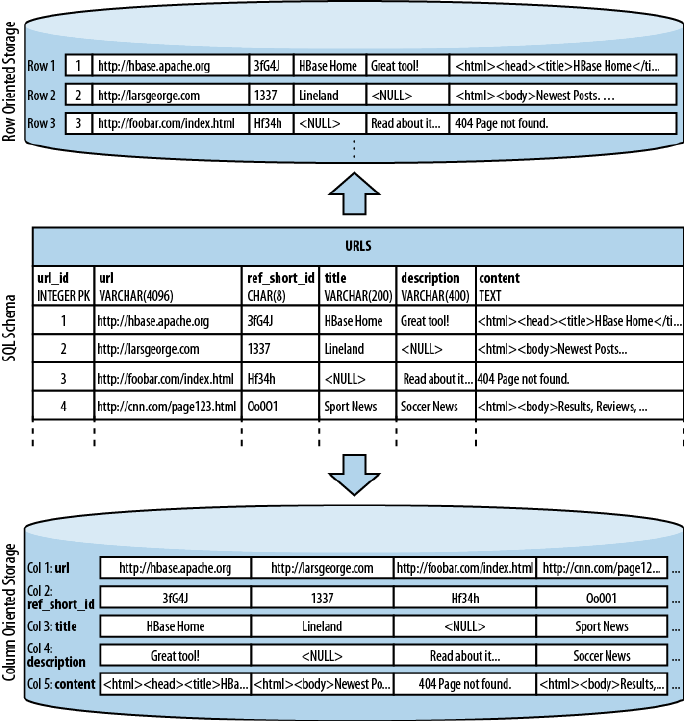
Figure 1-1. Column-oriented and row-oriented storage layouts
The speed at which data is created today is already greatly increased,
compared to only just a few years back. We can take for granted that
this is only going to increase further, and with the rapid pace of glob‐
alization the problem is only exacerbated. Websites like Google, Ama‐
zon, eBay, and Facebook now reach the majority of people on this
planet. The term planet-size web application comes to mind, and in
this case it is fitting.
The Dawn of Big Data 5
www.finebook.ir
5. See this note published by Facebook.
6. See this blog post, as well as this one, by the Facebook engineering team. Wall
messages count for 15 billion and chat for 120 billion, totaling 135 billion messages
a month. Then they also add SMS and others to create an even larger number.
7. Facebook uses Haystack, which provides an optimized storage infrastructure for
large binary objects, such as photos.
8. See this presentation, given by Facebook employee and HBase committer, Nicolas
Spiegelberg.
Facebook, for example, is adding more than 15 TB of data into its Ha‐
doop cluster every day5 and is subsequently processing it all. One
source of this data is click-stream logging, saving every step a user
performs on its website, or on sites that use the social plug-ins offered
by Facebook. This is an ideal case in which batch processing to build
machine learning models for predictions and recommendations is ap‐
propriate.
Facebook also has a real-time component, which is its messaging sys‐
tem, including chat, wall posts, and email. This amounts to 135+ bil‐
lion messages per month,6 and storing this data over a certain number
of months creates a huge tail that needs to be handled efficiently.
Even though larger parts of emails—for example, attachments—are
stored in a secondary system,7 the amount of data generated by all
these messages is mind-boggling. If we were to take 140 bytes per
message, as used by Twitter, it would total more than 17 TB every
month. Even before the transition to HBase, the existing system had
to handle more than 25 TB a month.8
In addition, less web-oriented companies from across all major indus‐
tries are collecting an ever-increasing amount of data. For example:
Financial
Such as data generated by stock tickers
Bioinformatics
Such as the Global Biodiversity Information Facility (http://
www.gbif.org/)
Smart grid
Such as the OpenPDC (http://openpdc.codeplex.com/) project
Sales
Such as the data generated by point-of-sale (POS) or stock/invento‐
ry systems
Chapter 1: Introduction6
www.finebook.ir
9. Short for Linux, Apache, MySQL, and PHP (or Perl and Python).
Genomics
Such as the Crossbow (http://bowtie-bio.sourceforge.net/crossbow/
index.shtml) project
Cellular services, military, environmental
Which all collect a tremendous amount of data as well
Storing petabytes of data efficiently so that updates and retrieval are
still performed well is no easy feat. We will now look deeper into some
of the challenges.
The Problem with Relational Database
Systems
RDBMSes have typically played (and, for the foreseeable future at
least, will play) an integral role when designing and implementing
business applications. As soon as you have to retain information about
your users, products, sessions, orders, and so on, you are typically go‐
ing to use some storage backend providing a persistence layer for the
frontend application server. This works well for a limited number of
records, but with the dramatic increase of data being retained, some
of the architectural implementation details of common database sys‐
tems show signs of weakness.
Let us use Hush, the HBase URL Shortener discussed in detail in (to
come), as an example. Assume that you are building this system so
that it initially handles a few thousand users, and that your task is to
do so with a reasonable budget—in other words, use free software.
The typical scenario here is to use the open source LAMP9 stack to
quickly build out a prototype for the business idea.
The relational database model normalizes the data into a user table,
which is accompanied by a url, shorturl, and click table that link to
the former by means of a foreign key. The tables also have indexes so
that you can look up URLs by their short ID, or the users by their
username. If you need to find all the shortened URLs for a particular
list of customers, you could run an SQL JOIN over both tables to get a
comprehensive list of URLs for each customer that contains not just
the shortened URL but also the customer details you need.
In addition, you are making use of built-in features of the database:
for example, stored procedures, which allow you to consistently up‐
The Problem with Relational Database Systems 7
www.finebook.ir
10. Short for Atomicity, Consistency, Isolation, and Durability. See “ACID” on Wikipe‐
dia.
11. Memcached is an in-memory, nonpersistent, nondistributed key/value store. See
the Memcached project home page.
date data from multiple clients while the database system guarantees
that there is always coherent data stored in the various tables.
Transactions make it possible to update multiple tables in an atomic
fashion so that either all modifications are visible or none are visible.
The RDBMS gives you the so-called ACID10 properties, which means
your data is strongly consistent (we will address this in greater detail
in “Consistency Models” (page 11)). Referential integrity takes care of
enforcing relationships between various table schemas, and you get a
domain-specific language, namely SQL, that lets you form complex
queries over everything. Finally, you do not have to deal with how da‐
ta is actually stored, but only with higher-level concepts such as table
schemas, which define a fixed layout your application code can refer‐
ence.
This usually works very well and will serve its purpose for quite some
time. If you are lucky, you may be the next hot topic on the Internet,
with more and more users joining your site every day. As your user
numbers grow, you start to experience an increasing amount of pres‐
sure on your shared database server. Adding more application servers
is relatively easy, as they share their state only with the central data‐
base. Your CPU and I/O load goes up and you start to wonder how
long you can sustain this growth rate.
The first step to ease the pressure is to add slave database servers
that are used to being read from in parallel. You still have a single
master, but that is now only taking writes, and those are much fewer
compared to the many reads your website users generate. But what if
that starts to fail as well, or slows down as your user count steadily in‐
creases?
A common next step is to add a cache—for example, Memcached.11
Now you can offload the reads to a very fast, in-memory system—how‐
ever, you are losing consistency guarantees, as you will have to inva‐
lidate the cache on modifications of the original value in the database,
and you have to do this fast enough to keep the time where the cache
and the database views are inconsistent to a minimum.
While this may help you with the amount of reads, you have not yet
addressed the writes. Once the master database server is hit too hard
with writes, you may replace it with a beefed-up server—scaling up
Chapter 1: Introduction8
www.finebook.ir

vertically—which simply has more cores, more memory, and faster
disks… and costs a lot more money than the initial one. Also note that
if you already opted for the master/slave setup mentioned earlier, you
need to make the slaves as powerful as the master or the imbalance
may mean the slaves fail to keep up with the master’s update rate.
This is going to double or triple the cost, if not more.
With more site popularity, you are asked to add more features to your
application, which translates into more queries to your database. The
SQL JOINs you were happy to run in the past are suddenly slowing
down and are simply not performing well enough at scale. You will
have to denormalize your schemas. If things get even worse, you will
also have to cease your use of stored procedures, as they are also sim‐
ply becoming too slow to complete. Essentially, you reduce the data‐
base to just storing your data in a way that is optimized for your ac‐
cess patterns.
Your load continues to increase as more and more users join your site,
so another logical step is to prematerialize the most costly queries
from time to time so that you can serve the data to your customers
faster. Finally, you start dropping secondary indexes as their mainte‐
nance becomes too much of a burden and slows down the database
too much. You end up with queries that can only use the primary key
and nothing else.
Where do you go from here? What if your load is expected to increase
by another order of magnitude or more over the next few months? You
could start sharding (see the sidebar titled “Sharding” (page 9)) your
data across many databases, but this turns into an operational night‐
mare, is very costly, and still does not give you a truly fitting solution.
You essentially make do with the RDBMS for lack of an alternative.
Sharding
The term sharding describes the logical separation of records into
horizontal partitions. The idea is to spread data across multiple
storage files—or servers—as opposed to having each stored con‐
tiguously.
The separation of values into those partitions is performed on
fixed boundaries: you have to set fixed rules ahead of time to
route values to their appropriate store. With it comes the inherent
difficulty of having to reshard the data when one of the horizontal
partitions exceeds its capacity.
Resharding is a very costly operation, since the storage layout has
to be rewritten. This entails defining new boundaries and then
The Problem with Relational Database Systems 9
www.finebook.ir

12. See “NoSQL” on Wikipedia.
horizontally splitting the rows across them. Massive copy opera‐
tions can take a huge toll on I/O performance as well as temporar‐
ily elevated storage requirements. And you may still take on up‐
dates from the client applications and need to negotiate updates
during the resharding process.
This can be mitigated by using virtual shards, which define a
much larger key partitioning range, with each server assigned an
equal number of these shards. When you add more servers, you
can reassign shards to the new server. This still requires that the
data be moved over to the added server.
Sharding is often a simple afterthought or is completely left to the
operator. Without proper support from the database system, this
can wreak havoc on production systems.
Let us stop here, though, and, to be fair, mention that a lot of compa‐
nies are using RDBMSes successfully as part of their technology
stack. For example, Facebook—and also Google—has a very large
MySQL setup, and for their purposes it works sufficiently. These data‐
base farms suits the given business goals and may not be replaced
anytime soon. The question here is if you were to start working on im‐
plementing a new product and knew that it needed to scale very fast,
wouldn’t you want to have all the options available instead of using
something you know has certain constraints?
Nonrelational Database Systems, Not-
Only SQL or NoSQL?
Over the past four or five years, the pace of innovation to fill that ex‐
act problem space has gone from slow to insanely fast. It seems that
every week another framework or project is announced to fit a related
need. We saw the advent of the so-called NoSQL solutions, a term
coined by Eric Evans in response to a question from Johan Oskarsson,
who was trying to find a name for an event in that very emerging, new
data storage system space.12
The term quickly rose to fame as there was simply no other name for
this new class of products. It was (and is) discussed heavily, as it was
also deemed the nemesis of “SQL"or was meant to bring the plague to
anyone still considering using traditional RDBMSes… just kidding!
Chapter 1: Introduction10
www.finebook.ir

The actual idea of different data store architectures for
specific problem sets is not new at all. Systems like Berke‐
ley DB, Coherence, GT.M, and object-oriented database
systems have been around for years, with some dating
back to the early 1980s, and they fall into the NoSQL
group by definition as well.
The tagword is actually a good fit: it is true that most new storage sys‐
tems do not provide SQL as a means to query data, but rather a differ‐
ent, often simpler, API-like interface to the data.
On the other hand, tools are available that provide SQL dialects to
NoSQL data stores, and they can be used to form the same complex
queries you know from relational databases. So, limitations in query‐
ing no longer differentiate RDBMSes from their nonrelational kin.
The difference is actually on a lower level, especially when it comes to
schemas or ACID-like transactional features, but also regarding the
actual storage architecture. A lot of these new kinds of systems do one
thing first: throw out the limiting factors in truly scalable systems (a
topic that is discussed in “Dimensions” (page 13)). For example, they
often have no support for transactions or secondary indexes. More im‐
portantly, they often have no fixed schemas so that the storage can
evolve with the application using it.
Consistency Models
It seems fitting to talk about consistency a bit more since it is
mentioned often throughout this book. On the outset, consistency
is about guaranteeing that a database always appears truthful to
its clients. Every operation on the database must carry its state
from one consistent state to the next. How this is achieved or im‐
plemented is not specified explicitly so that a system has multiple
choices. In the end, it has to get to the next consistent state, or re‐
turn to the previous consistent state, to fulfill its obligation.
Consistency can be classified in, for example, decreasing order of
its properties, or guarantees offered to clients. Here is an informal
list:
Strict
The changes to the data are atomic and appear to take effect
instantaneously. This is the highest form of consistency.
Nonrelational Database Systems, Not-Only SQL or NoSQL? 11
www.finebook.ir

13. See Eric Brewer’s original paper on this topic and the follow-up post by Coda Hale,
as well as this PDF by Gilbert and Lynch.
Sequential
Every client sees all changes in the same order they were ap‐
plied.
Causal
All changes that are causally related are observed in the same
order by all clients.
Eventual
When no updates occur for a period of time, eventually all up‐
dates will propagate through the system and all replicas will
be consistent.
Weak
No guarantee is made that all updates will propagate and
changes may appear out of order to various clients.
The class of system adhering to eventual consistency can be even
further divided into subtler sets, where those sets can also coex‐
ist. Werner Vogels, CTO of Amazon, lists them in his post titled
“Eventually Consistent”. The article also picks up on the topic of
the CAP theorem,13 which states that a distributed system can on‐
ly achieve two out of the following three properties: consistency,
availability, and partition tolerance. The CAP theorem is a highly
discussed topic, and is certainly not the only way to classify, but it
does point out that distributed systems are not easy to develop
given certain requirements. Vogels, for example, mentions:
An important observation is that in larger distributed scale sys‐
tems, network partitions are a given and as such consistency and
availability cannot be achieved at the same time. This means that
one has two choices on what to drop; relaxing consistency will al‐
low the system to remain highly available […] and prioritizing
consistency means that under certain conditions the system will
not be available.
Relaxing consistency, while at the same time gaining availability,
is a powerful proposition. However, it can force handling inconsis‐
tencies into the application layer and may increase complexity.
There are many overlapping features within the group of nonrelation‐
al databases, but some of these features also overlap with traditional
storage solutions. So the new systems are not really revolutionary, but
rather, from an engineering perspective, are more evolutionary.
Chapter 1: Introduction12
www.finebook.ir
14. See Brewer: “Lessons from giant-scale services.”, Internet Computing, IEEE (2001)
vol. 5 (4) pp. 46–55.
Even projects like Memcached are lumped into the NoSQL category,
as if anything that is not an RDBMS is automatically NoSQL. This cre‐
ates a kind of false dichotomy that obscures the exciting technical
possibilities these systems have to offer. And there are many; within
the NoSQL category, there are numerous dimensions you could use to
classify where the strong points of a particular system lie.
Dimensions
Let us take a look at a handful of those dimensions here. Note that
this is not a comprehensive list, or the only way to classify them.
Data model
There are many variations in how the data is stored, which include
key/value stores (compare to a HashMap), semistructured,
column-oriented, and document-oriented stores. How is your appli‐
cation accessing the data? Can the schema evolve over time?
Storage model
In-memory or persistent? This is fairly easy to decide since we are
comparing with RDBMSes, which usually persist their data to per‐
manent storage, such as physical disks. But you may explicitly
need a purely in-memory solution, and there are choices for that
too. As far as persistent storage is concerned, does this affect your
access pattern in any way?
Consistency model
Strictly or eventually consistent? The question is, how does the
storage system achieve its goals: does it have to weaken the con‐
sistency guarantees? While this seems like a cursory question, it
can make all the difference in certain use cases. It may especially
affect latency, that is, how fast the system can respond to read and
write requests. This is often measured in harvest and yield.14
Atomic read-modify-write
While RDBMSes offer you a lot of these operations directly (be‐
cause you are talking to a central, single server), they can be more
difficult to achieve in distributed systems. They allow you to pre‐
vent race conditions in multithreaded or shared-nothing applica‐
tion server design. Having these compare and swap (CAS) or
check and set operations available can reduce client-side complex‐
ity.
Nonrelational Database Systems, Not-Only SQL or NoSQL? 13
www.finebook.ir
Locking, waits, and deadlocks
It is a known fact that complex transactional processing, like two-
phase commits, can increase the possibility of multiple clients
waiting for a resource to become available. In a worst-case scenar‐
io, this can lead to deadlocks, which are hard to resolve. What kind
of locking model does the system you are looking at support? Can
it be free of waits, and therefore deadlocks?
Physical model
Distributed or single machine? What does the architecture look
like—is it built from distributed machines or does it only run on
single machines with the distribution handled client-side, that is,
in your own code? Maybe the distribution is only an afterthought
and could cause problems once you need to scale the system. And
if it does offer scalability, does it imply specific steps to do so? The
easiest solution would be to add one machine at a time, while shar‐
ded setups (especially those not supporting virtual shards) some‐
times require for each shard to be increased simultaneously be‐
cause each partition needs to be equally powerful.
Read/write performance
You have to understand what your application’s access patterns
look like. Are you designing something that is written to a few
times, but is read much more often? Or are you expecting an equal
load between reads and writes? Or are you taking in a lot of writes
and just a few reads? Does it support range scans or is it better
suited doing random reads? Some of the available systems are ad‐
vantageous for only one of these operations, while others may do
well (but maybe not perfect) in all of them.
Secondary indexes
Secondary indexes allow you to sort and access tables based on
different fields and sorting orders. The options here range from
systems that have absolutely no secondary indexes and no guaran‐
teed sorting order (like a HashMap, i.e., you need to know the
keys) to some that weakly support them, all the way to those that
offer them out of the box. Can your application cope, or emulate, if
this feature is missing?
Failure handling
It is a fact that machines crash, and you need to have a mitigation
plan in place that addresses machine failures (also refer to the dis‐
cussion of the CAP theorem in “Consistency Models” (page 11)).
How does each data store handle server failures? Is it able to con‐
tinue operating? This is related to the “Consistency model” dimen‐
sion discussed earlier, as losing a machine may cause holes in your
Chapter 1: Introduction14
www.finebook.ir

data store, or even worse, make it completely unavailable. And if
you are replacing the server, how easy will it be to get back to be‐
ing 100% operational? Another scenario is decommissioning a
server in a clustered setup, which would most likely be handled
the same way.
Compression
When you have to store terabytes of data, especially of the kind
that consists of prose or human-readable text, it is advantageous
to be able to compress the data to gain substantial savings in re‐
quired raw storage. Some compression algorithms can achieve a
10:1 reduction in storage space needed. Is the compression meth‐
od pluggable? What types are available?
Load balancing
Given that you have a high read or write rate, you may want to in‐
vest in a storage system that transparently balances itself while
the load shifts over time. It may not be the full answer to your
problems, but it may help you to ease into a high-throughput appli‐
cation design.
We will look back at these dimensions later on to see
where HBase fits and where its strengths lie. For now, let
us say that you need to carefully select the dimensions
that are best suited to the issues at hand. Be pragmatic
about the solution, and be aware that there is no hard and
fast rule, in cases where an RDBMS is not working ideally,
that a NoSQL system is the perfect match. Evaluate your
options, choose wisely, and mix and match if needed.
An interesting term to describe this issue is impedance
match, which describes the need to find the ideal solution
for a given problem. Instead of using a “one-size-fits-all”
approach, you should know what else is available. Try to
use the system that solves your problem best.
Scalability
While the performance of RDBMSes is well suited for transactional
processing, it is less so for very large-scale analytical processing. This
refers to very large queries that scan wide ranges of records or entire
tables. Analytical databases may contain hundreds or thousands of
terabytes, causing queries to exceed what can be done on a single
server in a reasonable amount of time. Scaling that server vertically—
that is, adding more cores or disks—is simply not good enough.
Nonrelational Database Systems, Not-Only SQL or NoSQL? 15
www.finebook.ir
15. See “FT 101” by Jim Gray et al.
16. The term DDI was coined in the paper “Cloud Data Structure Diagramming Techni‐
ques and Design Patterns” by D. Salmen et al. (2009).
What is even worse is that with RDBMSes, waits and deadlocks are in‐
creasing nonlinearly with the size of the transactions and concurrency
—that is, the square of concurrency and the third or even fifth power
of the transaction size.15 Sharding is often an impractical solution, as
it has to be done within the application layer, and may involve com‐
plex and costly (re)partitioning procedures.
Commercial RDBMSes are available that solve many of these issues,
but they are often specialized and only cover certain aspects. Above
all, they are very, very expensive. Looking at open source alternatives
in the RDBMS space, you will likely have to give up many or all rela‐
tional features, such as secondary indexes, to gain some level of per‐
formance.
The question is, wouldn’t it be good to trade relational features per‐
manently for performance? You could denormalize (see the next sec‐
tion) the data model and avoid waits and deadlocks by minimizing
necessary locking. How about built-in horizontal scalability without
the need to repartition as your data grows? Finally, throw in fault tol‐
erance and data availability, using the same mechanisms that allow
scalability, and what you get is a NoSQL solution—more specifically,
one that matches what HBase has to offer.
Database (De-)Normalization
At scale, it is often a requirement that we design schemas differently,
and a good term to describe this principle is Denormalization, Dupli‐
cation, and Intelligent Keys (DDI).16 It is about rethinking how data is
stored in Bigtable-like storage systems, and how to make use of it in
an appropriate way.
Part of the principle is to denormalize schemas by, for example, dupli‐
cating data in more than one table so that, at read time, no further ag‐
gregation is required. Or the related prematerialization of required
views, once again optimizing for fast reads without any further pro‐
cessing.
There is much more on this topic in [Link to Come], where you will
find many ideas on how to design solutions that make the best use of
the features HBase provides. Let us look at an example to understand
the basic principles of converting a classic relational database model
to one that fits the columnar nature of HBase much better.
Chapter 1: Introduction16
www.finebook.ir
17. Note, though, that this is provided purely for demonstration purposes, so the sche‐
ma is deliberately kept simple.
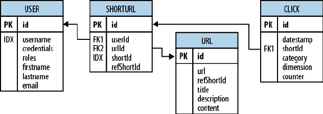
Consider the HBase URL Shortener, Hush, which allows us to map
long URLs to short URLs. The entity relationship diagram (ERD) can
be seen in Figure 1-2. The full SQL schema can be found in (to come).
17
Figure 1-2. The Hush schema expressed as an ERD
The shortened URL, stored in the shorturl table, can then be given to
others that subsequently click on it to open the linked full URL. Each
click is tracked, recording the number of times it was used, and, for
example, the country the click came from. This is stored in the click
table, which aggregates the usage on a daily basis, similar to a
counter.
Users, stored in the user table, can sign up with Hush to create their
own list of shortened URLs, which can be edited to add a description.
This links the user and shorturl tables with a foreign key relation‐
ship.
The system also downloads the linked page in the background, and ex‐
tracts, for instance, the TITLE tag from the HTML, if present. The en‐
tire page is saved for later processing with asynchronous batch jobs,
for analysis purposes. This is represented by the url table.
Every linked page is only stored once, but since many users may link
to the same long URL, yet want to maintain their own details, such as
the usage statistics, a separate entry in the shorturl is created. This
links the url, shorturl, and click tables.
It also allows you to aggregate statistics about the original short ID,
refShortId, so that you can see the overall usage of any short URL to
Nonrelational Database Systems, Not-Only SQL or NoSQL? 17
www.finebook.ir
map to the same long URL. The shortId and refShortId are the
hashed IDs assigned uniquely to each shortened URL. For example, in
http://hush.li/a23eg
the ID is a23eg.
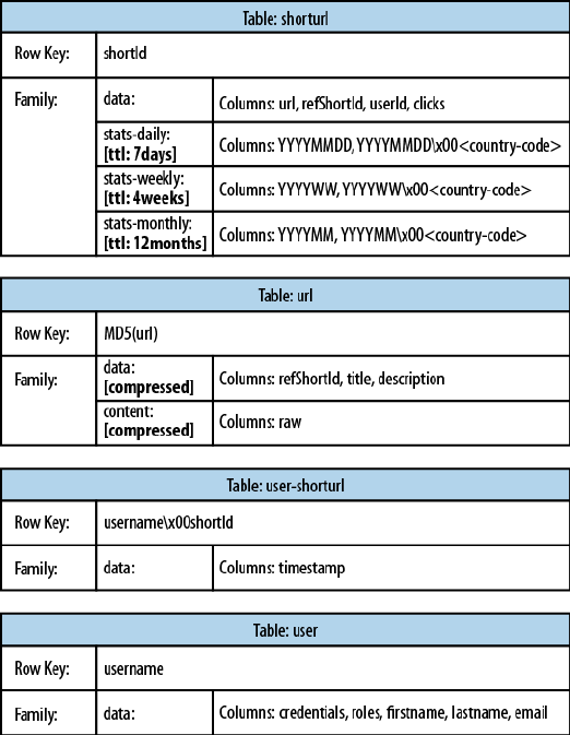
Figure 1-3 shows how the same schema could be represented in
HBase. Every shortened URL is stored in a table, shorturl, which al‐
so contains the usage statistics, storing various time ranges in sepa‐
rate column families, with distinct time-to-live settings. The columns
form the actual counters, and their name is a combination of the date,
plus an optional dimensional postfix—for example, the country code.
Figure 1-3. The Hush schema in HBase
Chapter 1: Introduction18
www.finebook.ir
The downloaded page, and the extracted details, are stored in the url
table. This table uses compression to minimize the storage require‐
ments, because the pages are mostly HTML, which is inherently ver‐
bose and contains a lot of text.
The user-shorturl table acts as a lookup so that you can quickly find
all short IDs for a given user. This is used on the user’s home page,
once she has logged in. The user table stores the actual user details.
We still have the same number of tables, but their meaning has
changed: the clicks table has been absorbed by the shorturl table,
while the statistics columns use the date as their key, formatted as
YYYYMMDD--for instance, 20150302--so that they can be accessed se‐
quentially. The additional user-shorturl table is replacing the for‐
eign key relationship, making user-related lookups faster.
There are various approaches to converting one-to-one, one-to-many,
and many-to-many relationships to fit the underlying architecture of
HBase. You could implement even this simple example in different
ways. You need to understand the full potential of HBase storage de‐
sign to make an educated decision regarding which approach to take.
The support for sparse, wide tables and column-oriented design often
eliminates the need to normalize data and, in the process, the costly
JOIN operations needed to aggregate the data at query time. Use of
intelligent keys gives you fine-grained control over how—and where—
data is stored. Partial key lookups are possible, and when combined
with compound keys, they have the same properties as leading, left-
edge indexes. Designing the schemas properly enables you to grow
the data from 10 entries to 10 billion entries, while still retaining the
same write and read performance.
Building Blocks
This section provides you with an overview of the architecture behind
HBase. After giving you some background information on its lineage,
the section will introduce the general concepts of the data model and
the available storage API, and presents a high-level overview on im‐
plementation.
Backdrop
In 2003, Google published a paper titled “The Google File System”.
This scalable distributed file system, abbreviated as GFS, uses a clus‐
ter of commodity hardware to store huge amounts of data. The filesys‐
tem handled data replication between nodes so that losing a storage
Building Blocks 19
www.finebook.ir
server would have no effect on data availability. It was also optimized
for streaming reads so that data could be read for processing later on.
Shortly afterward, another paper by Google was published, titled
“MapReduce: Simplified Data Processing on Large Clusters”. MapRe‐
duce was the missing piece to the GFS architecture, as it made use of
the vast number of CPUs each commodity server in the GFS cluster
provides. MapReduce plus GFS forms the backbone for processing
massive amounts of data, including the entire search index Google
owns.
What is missing, though, is the ability to access data randomly and in
close to real-time (meaning good enough to drive a web service, for
example). Another drawback of the GFS design is that it is good with a
few very, very large files, but not as good with millions of tiny files,
because the data retained in memory by the master node is ultimately
bound to the number of files. The more files, the higher the pressure
on the memory of the master.
So, Google was trying to find a solution that could drive interactive
applications, such as Mail or Analytics, while making use of the same
infrastructure and relying on GFS for replication and data availability.
The data stored should be composed of much smaller entities, and the
system would transparently take care of aggregating the small re‐
cords into very large storage files and offer some sort of indexing that
allows the user to retrieve data with a minimal number of disk seeks.
Finally, it should be able to store the entire web crawl and work with
MapReduce to build the entire search index in a timely manner.
Being aware of the shortcomings of RDBMSes at scale (see (to come)
for a discussion of one fundamental issue), the engineers approached
this problem differently: forfeit relational features and use a simple
API that has basic create, read, update, and delete (or CRUD) opera‐
tions, plus a scan function to iterate over larger key ranges or entire
tables. The culmination of these efforts was published in 2006 in a pa‐
per titled “Bigtable: A Distributed Storage System for Structured Da‐
ta”, two excerpts from which follow:
Bigtable is a distributed storage system for managing structured
data that is designed to scale to a very large size: petabytes of data
across thousands of commodity servers.
…a sparse, distributed, persistent multi-dimensional sorted map.
It is highly recommended that everyone interested in HBase read that
paper. It describes a lot of reasoning behind the design of Bigtable
and, ultimately, HBase. We will, however, go through the basic con‐
cepts, since they apply directly to the rest of this book.
Chapter 1: Introduction20
www.finebook.ir
HBase is implementing the Bigtable storage architecture very faithful‐
ly so that we can explain everything using HBase. (to come) provides
an overview of where the two systems differ.
Namespaces, Tables, Rows, Columns, and
Cells
First, a quick summary: the most basic unit is a column. One or more
columns form a row that is addressed uniquely by a row key. A num‐
ber of rows, in turn, form a table, and there can be many of them.
Each column may have multiple versions, with each distinct value con‐
tained in a separate cell. On a higher level, tables are grouped into
namespaces, which help, for example, with grouping tables by users
or application, or with access control.
This sounds like a reasonable description for a typical database, but
with the extra dimension of allowing multiple versions of each cells.
But obviously there is a bit more to it: All rows are always sorted lexi‐
cographically by their row key. Example 1-1 shows how this will look
when adding a few rows with different keys.
Example 1-1. The sorting of rows done lexicographically by their
key
hbase(main):001:0> scan 'table1'
ROW COLUMN+CELL
row-1 column=cf1:, timestamp=1297073325971 ...
row-10 column=cf1:, timestamp=1297073337383 ...
row-11 column=cf1:, timestamp=1297073340493 ...
row-2 column=cf1:, timestamp=1297073329851 ...
row-22 column=cf1:, timestamp=1297073344482 ...
row-3 column=cf1:, timestamp=1297073333504 ...
row-abc column=cf1:, timestamp=1297073349875 ...
7 row(s) in 0.1100 seconds
Note how the numbering is not in sequence as you may have expected
it. You may have to pad keys to get a proper sorting order. In lexico‐
graphical sorting, each key is compared on a binary level, byte by
byte, from left to right. Since row-1... is less than row-2..., no mat‐
ter what follows, it is sorted first.
Having the row keys always sorted can give you something like a pri‐
mary key index known from RDBMSes. It is also always unique, that
is, you can have each row key only once, or you are updating the same
row. While the original Bigtable paper only considers a single index,
HBase adds support for secondary indexes (see (to come)). The row
keys can be any arbitrary array of bytes and are not necessarily
human-readable.
Building Blocks 21
www.finebook.ir
18. You will see in “Column Families” (page 362) that the qualifier also may be left unset.
Rows are composed of columns, and those, in turn, are grouped into
column families. This helps in building semantical or topical bound‐
aries between the data, and also in applying certain features to them,
for example, compression, or denoting them to stay in-memory. All
columns in a column family are stored together in the same low-level
storage files, called HFile.
Column families need to be defined when the table is created and
should not be changed too often, nor should there be too many of
them. There are a few known shortcomings in the current implemen‐
tation that force the count to be limited to the low tens, though in
practice only a low number is usually needed anyways (see [Link to
Come] for details). The name of the column family must be composed
of printable characters, a notable difference from all other names or
values.
Columns are often referenced as family:qualifier pair with the quali
fier being any arbitrary array of bytes.18 As opposed to the limit on
column families, there is no such thing for the number of columns: you
could have millions of columns in a particular column family. There is
also no type nor length boundary on the column values.
Figure 1-4 helps to visualize how different rows are in a normal data‐
base as opposed to the column-oriented design of HBase. You should
think about rows and columns not being arranged like the classic
spreadsheet model, but rather use a tag metaphor, that is, information
is available under a specific tag.
Chapter 1: Introduction22
www.finebook.ir
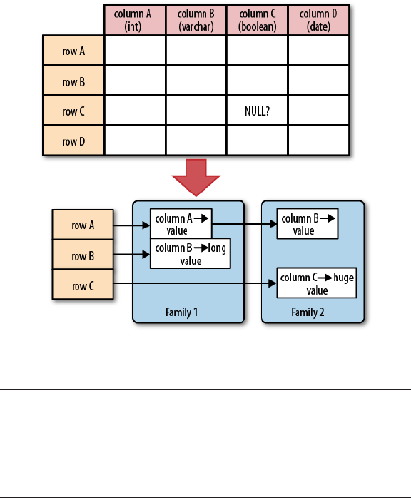
Figure 1-4. Rows and columns in HBase
The "NULL?" in Figure 1-4 indicates that, for a database
with a fixed schema, you have to store NULLs where there
is no value, but for HBase’s storage architectures, you
simply omit the whole column; in other words, NULLs are
free of any cost: they do not occupy any storage space.
All rows and columns are defined in the context of a table, adding a
few more concepts across all included column families, which we will
discuss shortly.
Every column value, or cell, either is timestamped implicitly by the
system or can be set explicitly by the user. This can be used, for exam‐
ple, to save multiple versions of a value as it changes over time. Dif‐
ferent versions of a cell are stored in decreasing timestamp order, al‐
lowing you to read the newest value first. This is an optimization
aimed at read patterns that favor more current values over historical
ones.
The user can specify how many versions of a value should be kept. In
addition, there is support for predicate deletions (see (to come) for the
concepts behind them) allowing you to keep, for example, only values
Building Blocks 23
www.finebook.ir

written in the past week. The values (or cells) are also just uninterpre‐
ted arrays of bytes, that the client needs to know how to handle.
If you recall from the quote earlier, the Bigtable model, as implement‐
ed by HBase, is a sparse, distributed, persistent, multidimensional
map, which is indexed by row key, column key, and a timestamp.
Putting this together, we can express the access to data like so:
(Table, RowKey, Family, Column, Timestamp) → Value
This representation is not entirely correct as physically it
is the column family that separates columns and creates
rows per family. We will pick this up in (to come) later on.
In a more programming language style, this may be expressed as:
SortedMap<
RowKey, List<
SortedMap<
Column, List<
Value, Timestamp
>
>
>
>
Or all in one line:
SortedMap<RowKey, List<SortedMap<Column, List<Value, Timestamp>>>>
The first SortedMap is the table, containing a List of column families.
The families contain another SortedMap, which represents the col‐
umns, and their associated values. These values are in the final List
that holds the value and the timestamp it was set, and is sorted really
descending by the timestamp component.
An interesting feature of the model is that cells may exist in multiple
versions, and different columns have been written at different times.
The API, by default, provides you with a coherent view of all columns
wherein it automatically picks the most current value of each cell.
Figure 1-5 shows a piece of one specific row in an example table.
Chapter 1: Introduction24
www.finebook.ir
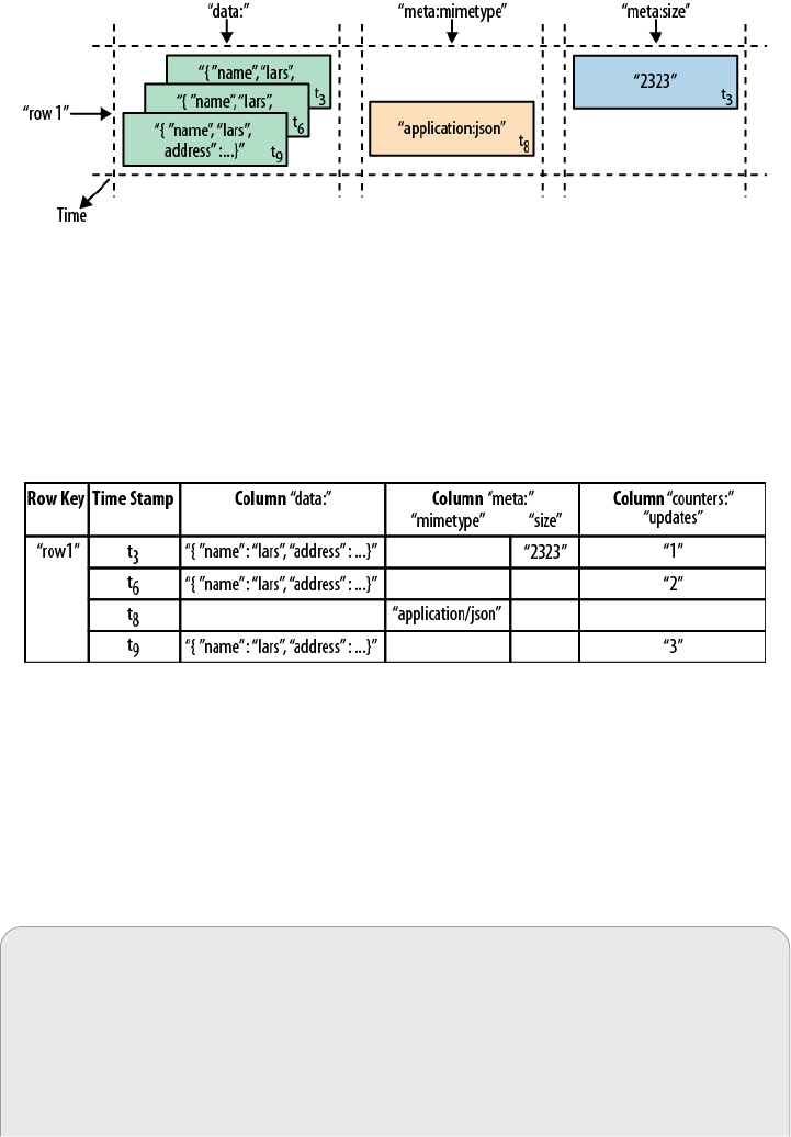
Figure 1-5. A time-oriented view into parts of a row
The diagram visualizes the time component using tn as the timestamp
when the cell was written. The ascending index shows that the values
have been added at different times. Figure 1-6 is another way to look
at the data, this time in a more spreadsheet-like layout wherein the
timestamp was added to its own column.
Figure 1-6. The same parts of the row rendered as a spreadsheet
Although they have been added at different times and exist in multiple
versions, you would still see the row as the combination of all columns
and their most current versions—in other words, the highest tn from
each column. There is a way to ask for values at (or before) a specific
timestamp, or more than one version at a time, which we will see a lit‐
tle bit later in Chapter 3.
The Webtable
The canonical use case of Bigtable and HBase is the webtable,
that is, the web pages stored while crawling the Internet.
The row key is the reversed URL of the page—for example,
org.hbase.www. There is a column family storing the actual HTML
code, the contents family, as well as others like anchor, which is
Building Blocks 25
www.finebook.ir

19. This was introduced in HBase 0.94.0. More on ACID guarantees and MVCC in (to
come).
used to store outgoing links, another one to store inbound links,
and yet another for metadata like the language of the page.
Using multiple versions for the contents family allows you to
store a few older copies of the HTML, and is helpful when you
want to analyze how often a page changes, for example. The time‐
stamps used are the actual times when they were fetched from
the crawled website.
Access to row data is atomic and includes any number of columns be‐
ing read or written to. The only additional guarantee is that you can
span a mutation across colocated rows atomically using region-local
transactions (see (to come) for details19). There is no further guaran‐
tee or transactional feature that spans multiple rows across regions,
or across tables. The atomic access is also a contributing factor to this
architecture being strictly consistent, as each concurrent reader and
writer can make safe assumptions about the state of a row. Using mul‐
tiversioning and timestamping can help with application layer consis‐
tency issues as well.
Finally, cells, since HBase 0.98, can carry an arbitrary set of tags.
They are used to flag any cell with metadata that is used to make deci‐
sions about the cell during data operations. A prominent use-case is
security (see (to come)) where tags are set for cells containing access
details. Once a user is authenticated and has a valid security token,
the system can use the token to filter specific cells for the given user.
Tags can be used for other things as well, and (to come) will explain
their application in greater detail.
Auto-Sharding
The basic unit of scalability and load balancing in HBase is called a
region. Regions are essentially contiguous ranges of rows stored to‐
gether. They are dynamically split by the system when they become
too large. Alternatively, they may also be merged to reduce their num‐
ber and required storage files (see (to come)).
Chapter 1: Introduction26
www.finebook.ir
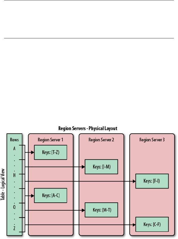
The HBase regions are equivalent to range partitions as
used in database sharding. They can be spread across
many physical servers, thus distributing the load, and
therefore providing scalability.
Initially there is only one region for a table, and as you start adding
data to it, the system is monitoring it to ensure that you do not exceed
a configured maximum size. If you exceed the limit, the region is split
into two at the middle key--the row key in the middle of the region—
creating two roughly equal halves (more details in (to come)).
Each region is served by exactly one region server, and each of these
servers can serve many regions at any time. Figure 1-7 shows how the
logical view of a table is actually a set of regions hosted by many re‐
gion servers.
Figure 1-7. Rows grouped in regions and served by different
servers
Building Blocks 27
www.finebook.ir

The Bigtable paper notes that the aim is to keep the re‐
gion count between 10 and 1,000 per server and each at
roughly 100 MB to 200 MB in size. This refers to the hard‐
ware in use in 2006 (and earlier). For HBase and modern
hardware, the number would be more like 10 to 1,000 re‐
gions per server, but each between 1 GB and 10 GB in
size.
But, while the numbers have increased, the basic principle
is the same: the number of regions per server, and their
respective sizes, depend on what can be handled suffi‐
ciently by a single server.
Splitting and serving regions can be thought of as autosharding, as of‐
fered by other systems. The regions allow for fast recovery when a
server fails, and fine-grained load balancing since they can be moved
between servers when the load of the server currently serving the re‐
gion is under pressure, or if that server becomes unavailable because
of a failure or because it is being decommissioned.
Splitting is also very fast—close to instantaneous—because the split
regions simply read from the original storage files until a compaction
rewrites them into separate ones asynchronously. This is explained in
detail in (to come).
Storage API
Bigtable does not support a full relational data model; instead, it
provides clients with a simple data model that supports dynamic
control over data layout and format […]
The API offers operations to create and delete tables and column fami‐
lies. In addition, it has functions to change the table and column fami‐
ly metadata, such as compression or block sizes. Furthermore, there
are the usual operations for clients to create or delete values as well
as retrieving them with a given row key.
A scan API allows you to efficiently iterate over ranges of rows and be
able to limit which columns are returned or the number of versions of
each cell. You can match columns using filters and select versions us‐
ing time ranges, specifying start and end times.
Chapter 1: Introduction28
www.finebook.ir
20. Region-local transactions, along with a row-key prefix aware split policy, were add‐
ed in HBase 0.94. See HBASE-5229.
21. Coprocessors were added to HBase in version 0.92.0.
On top of this basic functionality are more advanced features. The sys‐
tem has support for single-row and region-local20 transactions, and
with this support it implements atomic read-modify-write sequences
on data stored under a single row key, or multiple, colocated ones.
Cell values can be interpreted as counters and updated atomically.
These counters can be read and modified in one operation so that, de‐
spite the distributed nature of the architecture, clients can use this
mechanism to implement global, strictly consistent, sequential coun‐
ters.
There is also the option to run client-supplied code in the address
space of the server. The server-side framework to support this is
called coprocessors.21 The code has access to the server local data and
can be used to implement lightweight batch jobs, or use expressions
to analyze or summarize data based on a variety of operators.
Finally, the system is integrated with the MapReduce framework by
supplying wrappers that convert tables into input source and output
targets for MapReduce jobs.
Unlike in the RDBMS landscape, there is no domain-specific language,
such as SQL, to query data. Access is not done declaratively, but pure‐
ly imperatively through the client-side API. For HBase, this is mostly
Java code, but there are many other choices to access the data from
other programming languages.
Implementation
Bigtable […] allows clients to reason about the locality properties of
the data represented in the underlying storage.
The data is stored in store files, called HFiles, which are persistent
and ordered immutable maps from keys to values. Internally, the files
are sequences of blocks with a block index stored at the end. The in‐
dex is loaded when the HFile is opened and kept in memory. The de‐
fault block size is 64 KB but can be configured differently if required.
The store files provide an API to access specific values as well as to
scan ranges of values given a start and end key.
Building Blocks 29
www.finebook.ir

22. This is a simplification as newer HFile versions use a multilevel index, loading par‐
tial index blocks as needed. This adds to the latency, but once the index is cached
the behavior is back to what is described here.
Implementation is discussed in great detail in (to come).
The text here is an introduction only, while the full details
are discussed in the referenced chapter(s).
Since every HFile has a block index, lookups can be performed with a
single disk seek.22 First, the block possibly containing the given key is
determined by doing a binary search in the in-memory block index,
followed by a block read from disk to find the actual key.
The store files are typically saved in the Hadoop Distributed File Sys‐
tem (HDFS), which provides a scalable, persistent, replicated storage
layer for HBase. It guarantees that data is never lost by writing the
changes across a configurable number of physical servers.
When data is updated it is first written to a commit log, called a write-
ahead log (WAL) in HBase, and then stored in the in-memory mem‐
store. Once the data in memory has exceeded a given maximum value,
it is flushed as a HFile to disk. After the flush, the commit logs can be
discarded up to the last unflushed modification. While the system is
flushing the memstore to disk, it can continue to serve readers and
writers without having to block them. This is achieved by rolling the
memstore in memory where the new/empty one is taking the updates,
while the old/full one is converted into a file. Note that the data in the
memstores is already sorted by keys matching exactly what HFiles
represent on disk, so no sorting or other special processing has to be
performed.
Chapter 1: Introduction30
www.finebook.ir

We can now start to make sense of what the locality prop‐
erties are, mentioned in the Bigtable quote at the begin‐
ning of this section. Since all files contain sorted key/value
pairs, ordered by the key, and are optimized for block op‐
erations such as reading these pairs sequentially, you
should specify keys to keep related data together. Refer‐
ring back to the webtable example earlier, you may have
noted that the key used is the reversed FQDN (the domain
name part of the URL), such as org.hbase.www. The rea‐
son is to store all pages from hbase.org close to one an‐
other, and reversing the URL puts the most important part
of the URL first, that is, the top-level domain (TLD). Pages
under blog.hbase.org would then be sorted with those
from www.hbase.org--or in the actual key format,
org.hbase.blog sorts next to org.hbase.www.
Because store files are immutable, you cannot simply delete values by
removing the key/value pair from them. Instead, a delete marker (also
known as a tombstone marker) is written to indicate the fact that the
given key has been deleted. During the retrieval process, these delete
markers mask out the actual values and hide them from reading cli‐
ents.
Reading data back involves a merge of what is stored in the mem‐
stores, that is, the data that has not been written to disk, and the on-
disk store files. Note that the WAL is never used during data retrieval,
but solely for recovery purposes when a server has crashed before
writing the in-memory data to disk.
Since flushing memstores to disk causes more and more HFiles to be
created, HBase has a housekeeping mechanism that merges the files
into larger ones using compaction. There are two types of compaction:
minor compactions and major compactions. The former reduce the
number of storage files by rewriting smaller files into fewer but larger
ones, performing an n-way merge. Since all the data is already sorted
in each HFile, that merge is fast and bound only by disk I/O perfor‐
mance.
The major compactions rewrite all files within a column family for a
region into a single new one. They also have another distinct feature
compared to the minor compactions: based on the fact that they scan
all key/value pairs, they can drop deleted entries including their dele‐
tion marker. Predicate deletes are handled here as well—for example,
removing values that have expired according to the configured time-
to-live (TTL) or when there are too many versions.
Building Blocks 31
www.finebook.ir

23. For more information on Apache ZooKeeper, please refer to the official project
website.
This architecture is taken from LSM-trees (see (to come)).
The only difference is that LSM-trees are storing data in
multipage blocks that are arranged in a B-tree-like struc‐
ture on disk. They are updated, or merged, in a rotating
fashion, while in Bigtable the update is more coarse-
grained and the whole memstore is saved as a new store
file and not merged right away. You could call HBase’s ar‐
chitecture “Log-Structured Sort-and-Merge-Maps.” The
background compactions correspond to the merges in
LSM-trees, but are occurring on a store file level instead
of the partial tree updates, giving the LSM-trees their
name.
There are three major components to HBase: the client library, at
least one master server, and many region servers. The region servers
can be added or removed while the system is up and running to ac‐
commodate changing workloads. The master is responsible for assign‐
ing regions to region servers and uses Apache ZooKeeper, a reliable,
highly available, persistent and distributed coordination service, to fa‐
cilitate that task.
Apache ZooKeeper
ZooKeeper23 is a separate open source project, and is also part of
the Apache Software Foundation. ZooKeeper is the comparable
system to Google’s use of Chubby for Bigtable. It offers filesystem-
like access with directories and files (called znodes) that distribut‐
ed systems can use to negotiate ownership, register services, or
watch for updates.
Every region server creates its own ephemeral node in ZooKeep‐
er, which the master, in turn, uses to discover available servers.
They are also used to track server failures or network partitions.
Ephemeral nodes are bound to the session between ZooKeeper
and the client which created it. The session has a heartbeat keep‐
alive mechanism that, once it fails to report, is declared lost by
ZooKeeper and the associated ephemeral nodes are deleted.
HBase uses ZooKeeper also to ensure that there is only one mas‐
ter running, to store the bootstrap location for region discovery,
Chapter 1: Introduction32
www.finebook.ir
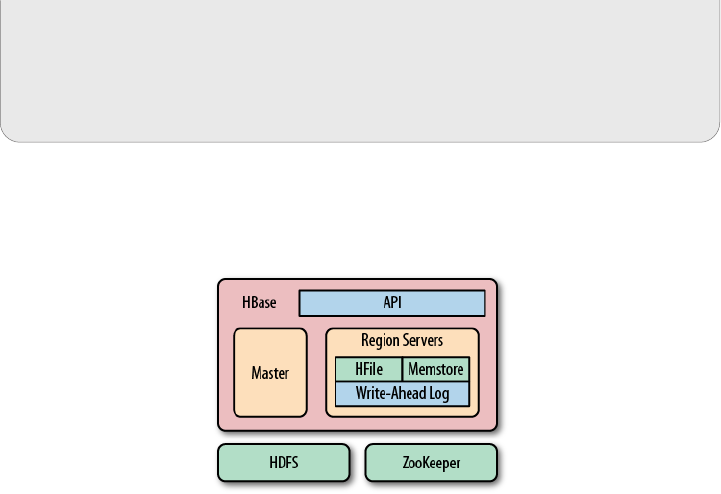
as a registry for region servers, as well as for other purposes. Zoo‐
Keeper is a critical component, and without it HBase is not opera‐
tional. This is facilitated by ZooKeeper’s distributed design using
an ensemble of servers and the Zab protocol to keep its state con‐
sistent.
Figure 1-8 shows how the various components of HBase are orches‐
trated to make use of existing system, like HDFS and ZooKeeper, but
also adding its own layers to form a complete platform.
Figure 1-8. HBase using its own components while leveraging ex‐
isting systems
The master server is also responsible for handling load balancing of
regions across region servers, to unload busy servers and move re‐
gions to less occupied ones. The master is not part of the actual data
storage or retrieval path. It negotiates load balancing and maintains
the state of the cluster, but never provides any data services to either
the region servers or the clients, and is therefore lightly loaded in
practice. In addition, it takes care of schema changes and other meta‐
data operations, such as creation of tables and column families.
Region servers are responsible for all read and write requests for all
regions they serve, and also split regions that have exceeded the con‐
figured region size thresholds. Clients communicate directly with
them to handle all data-related operations.
(to come) has more details on how clients perform the region lookup.
Summary
Billions of rows * millions of columns * thousands of versions = tera‐
bytes or petabytes of storage
— The HBase Project
Building Blocks 33
www.finebook.ir
24. Powerset is a company based in San Francisco that was developing a natural lan‐
guage search engine for the Internet. On July 1, 2008, Microsoft acquired Power‐
set, and subsequent support for HBase development was abandoned.
We have seen how the Bigtable storage architecture is using many
servers to distribute ranges of rows sorted by their key for load-
balancing purposes, and can scale to petabytes of data on thousands
of machines. The storage format used is ideal for reading adjacent
key/value pairs and is optimized for block I/O operations that can satu‐
rate disk transfer channels.
Table scans run in linear time and row key lookups or mutations are
performed in logarithmic order—or, in extreme cases, even constant
order (using Bloom filters). Designing the schema in a way to com‐
pletely avoid explicit locking, combined with row-level atomicity, gives
you the ability to scale your system without any notable effect on read
or write performance.
The column-oriented architecture allows for huge, wide, sparse tables
as storing NULLs is free. Because each row is served by exactly one
server, HBase is strongly consistent, and using its multiversioning can
help you to avoid edit conflicts caused by concurrent decoupled pro‐
cesses, or retain a history of changes.
The actual Bigtable has been in production at Google since at least
2005, and it has been in use for a variety of different use cases, from
batch-oriented processing to real-time data-serving. The stored data
varies from very small (like URLs) to quite large (e.g., web pages and
satellite imagery) and yet successfully provides a flexible, high-
performance solution for many well-known Google products, such as
Google Earth, Google Reader, Google Finance, and Google Analytics.
HBase: The Hadoop Database
Having looked at the Bigtable architecture, we could simply state that
HBase is a faithful, open source implementation of Google’s Bigtable.
But that would be a bit too simplistic, and there are a few (mostly sub‐
tle) differences worth addressing.
History
HBase was created in 2007 at Powerset24 and was initially part of the
contributions in Hadoop. Since then, it has become its own top-level
project under the Apache Software Foundation umbrella. It is avail‐
able under the Apache Software License, version 2.0.
Chapter 1: Introduction34
www.finebook.ir
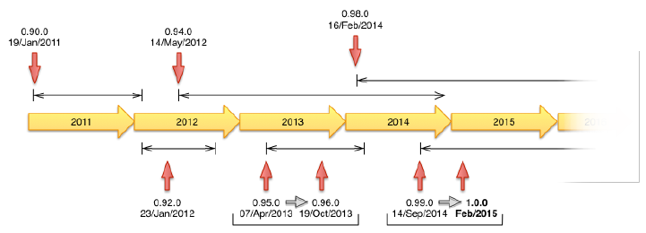
25. For an interesting flash back in time, see HBASE-287 on the Apache JIRA, the issue
tracking system. You can see how Mike Cafarella did a code drop that was then
quickly picked up by Jim Kellerman, who was with Powerset back then.
The project home page is http://hbase.apache.org/, where you can find
links to the documentation, wiki, and source repository, as well as
download sites for the binary and source releases.
Figure 1-9. The release timeline of HBase.
Here is a short overview of how HBase has evolved over time, which
Figure 1-9 shows in a timeline form:
November 2006
Google releases paper on Bigtable
February 2007
Initial HBase prototype created as Hadoop contrib25
October 2007
First "usable" HBase (Hadoop 0.15.0)
January 2008
Hadoop becomes an Apache top-level project, HBase becomes sub‐
project
October 2008
HBase 0.18.1 released
January 2009
HBase 0.19.0 released
September 2009
HBase 0.20.0 released, the performance release
HBase: The Hadoop Database 35
www.finebook.ir

26. Oh, the irony! Hadoop 1.0.0 was released on December 27th, 2011, which means
three years ahead of HBase.
May 2010
HBase becomes an Apache top-level project
June 2010
HBase 0.89.20100621, first developer release
January 2011
HBase 0.90.0 released, the durability and stability release
January 2012
HBase 0.92.0 released, tagged as coprocessor and security release
May 2012
HBase 0.94.0 released, tagged as performance release
October 2013
HBase 0.96.0 released, tagged as the singularity
February 2014
HBase 0.98.0 released
February 2015
HBase 1.0.0 released
Figure 1-9 shows as well how many months or years a release has
been—or still is—active. This mainly depends on the release managers
and their need for a specific major version to keep going.
Around May 2010, the developers decided to break with
the version numbering that used to be in lockstep with the
Hadoop releases. The rationale was that HBase had a
much faster release cycle and was also approaching a ver‐
sion 1.0 level sooner than what was expected from Ha‐
doop.26
To that effect, the jump was made quite obvious, going
from 0.20.x to 0.89.x. In addition, a decision was made to
title 0.89.x the early access version for developers and
bleeding-edge integrators. Version 0.89 was eventually re‐
leased as 0.90 for everyone as the next stable release.
Chapter 1: Introduction36
www.finebook.ir

Nomenclature
One of the biggest differences between HBase and Bigtable concerns
naming, as you can see in Table 1-1, which lists the various terms and
what they correspond to in each system.
Table 1-1. Differences in naming
HBase Bigtable
Region Tablet
RegionServer Tablet server
Flush Minor compaction
Minor compaction Merging compaction
Major compaction Major compaction
Write-ahead log Commit log
HDFS GFS
Hadoop MapReduce MapReduce
MemStore memtable
HFile SSTable
ZooKeeper Chubby
More differences are described in (to come).
Summary
Let us now circle back to “Dimensions” (page 13), and how these di‐
mensions can be used to classify HBase. HBase is a distributed, per‐
sistent, strictly consistent storage system with near-optimal write—in
terms of I/O channel saturation—and excellent read performance, and
it makes efficient use of disk space by supporting pluggable compres‐
sion algorithms that can be selected based on the nature of the data in
specific column families.
HBase extends the Bigtable model, which only considers a single in‐
dex, similar to a primary key in the RDBMS world, offering the server-
side hooks to implement flexible secondary index solutions. In addi‐
tion, it provides push-down predicates, that is, filters, reducing data
transferred over the network.
There is no declarative query language as part of the core implemen‐
tation, and it has limited support for transactions. Row atomicity and
read-modify-write operations make up for this in practice, as they cov‐
er many use cases and remove the wait or deadlock-related pauses ex‐
perienced with other systems.
HBase: The Hadoop Database 37
www.finebook.ir
27. Again I am simplifying here for the sake of being introductory. Later we will see
areas where tuning is vital and might seemingly go against what I am summarizing
here. See [Link to Come] for details.
HBase handles shifting load and failures gracefully and transparently
to the clients. Scalability is built in, and clusters can be grown or
shrunk while the system is in production. Changing the cluster does
not involve any complicated rebalancing or resharding procedure, and
is usually completely automated.27
Chapter 1: Introduction38
www.finebook.ir

1. See “Java” (page 58) for information of supported Java versions for older releases of
HBase.
Chapter 2
Installation
In this chapter, we will look at how HBase is installed and initially
configured. The first part is a quickstart section that gets you going
fast, but then shifts gears into proper planning and setting up of a
HBase cluster. Towards the end we will see how HBase can be used
from the command line for basic operations, such as adding, retriev‐
ing, and deleting data.
All of the following assumes you have the Java Runtime
Environment (JRE) installed. Hadoop and also HBase re‐
quire at least version 1.7 (also called Java 7)1, and the rec‐
ommended choice is the one provided by Oracle (formerly
by Sun), which can be found at http://www.java.com/down
load/. If you do not have Java already or are running into
issues using it, please see “Java” (page 58).
Quick-Start Guide
Let us get started with the “tl;dr” section of this book: you want to
know how to run HBase and you want to know it now! Nothing is eas‐
ier than that because all you have to do is download the most recent
binary release of HBase from the Apache HBase release page.
39
www.finebook.ir

2. Previous versions were shipped just as source archive and had no special postfix in
their name. The quickstart steps will still work though.
HBase is shipped as a binary and source tarball.2 Look for
bin or src in their names respectively. For the quickstart
you need the binary tarball, for example named
hbase-1.0.0-bin.tar.gz.
You can download and unpack the contents into a suitable directory,
such as /usr/local or /opt, like so:
$ cd /usr/local
$ wget http://archive.apache.org/dist/hbase/hbase-1.0.0/
hbase-1.0.0-bin.tar.gz
$ tar -zxvf hbase-1.0.0-bin.tar.gz
Setting the Data Directory
At this point, you are ready to start HBase. But before you do so,
it is advisable to set the data directory to a proper location. You
need to edit the configuration file conf/hbase-site.xml and set
the directory you want HBase—and ZooKeeper—to write to by as‐
signing a value to the property key named hbase.rootdir and
hbase.zookeeper.property.dataDir:
<?xml version="1.0"?>
<?xml-stylesheet type="text/xsl" href="configuration.xsl"?>
<configuration>
<property>
<name>hbase.rootdir</name>
<value>file:///<PATH>/hbase</value>
</property>
<property>
<name>hbase.zookeeper.property.dataDir</name>
<value>file:///<PATH>/zookeeper</value>
</property>
</configuration>
Replace <PATH> in the preceding example configuration file with a
path to a directory where you want HBase to store its data. By de‐
fault, hbase.rootdir is set to /tmp/hbase-${user.name}, which
could mean you lose all your data whenever your server or test
machine reboots because a lot of operating systems (OSes) clear
out /tmp during a restart.
Chapter 2: Installation40
www.finebook.ir

With that in place, we can start HBase and try our first interaction
with it. We will use the interactive shell to enter the status command
at the prompt (complete the command by pressing the Return key):
$ cd /usr/local/hbase-1.0.0
$ bin/start-hbase.sh
starting master, logging to \
/usr/local/hbase-1.0.0/bin/../logs/hbase-<username>-master-
localhost.out
$ bin/hbase shell
HBase Shell; enter 'help<RETURN>' for list of supported commands.
Type "exit<RETURN>" to leave the HBase Shell
Version 1.0.0, r6c98bff7b719efdb16f71606f3b7d8229445eb81, Sat Feb
14 19:49:22 PST 2015
hbase(main):001:0> status
1 servers, 0 dead, 2.0000 average load
This confirms that HBase is up and running, so we will now issue a
few commands to show that we can put data into it and retrieve the
same data subsequently.
It may not be clear, but what we are doing right now is
similar to sitting in a car with its brakes engaged and in
neutral while turning the ignition key. There is much more
that you need to configure and understand before you can
use HBase in a production-like environment. But it lets
you get started with some basic HBase commands and be‐
come familiar with top-level concepts.
We are currently running in the so-called Standalone
Mode. We will look into the available modes later on (see
“Run Modes” (page 79)), but for now it’s important to know
that in this mode everything is run in a single Java process
and all files are stored in /tmp by default—unless you did
heed the important advice given earlier to change it to
something different. Many people have lost their test data
during a reboot, only to learn that they kept the default
paths. Once it is deleted by the OS, there is no going back!
Let us now create a simple table and add a few rows with some data:
hbase(main):002:0> create 'testtable', 'colfam1'
0 row(s) in 0.2930 seconds
=> Hbase::Table - testtable
hbase(main):003:0> list
TABLE
testtable
Quick-Start Guide 41
www.finebook.ir
1 row(s) in 0.1920 seconds
=> ["testtable"]
hbase(main):004:0> put 'testtable', 'myrow-1', 'colfam1:q1',
'value-1'
0 row(s) in 0.1020 seconds
hbase(main):005:0> put 'testtable', 'myrow-2', 'colfam1:q2',
'value-2'
0 row(s) in 0.0410 seconds
hbase(main):006:0> put 'testtable', 'myrow-2', 'colfam1:q3',
'value-3'
0 row(s) in 0.0380 seconds
After we create the table with one column family, we verify that it ac‐
tually exists by issuing a list command. You can see how it outputs
the testtable name as the only table currently known. Subsequently,
we are putting data into a number of rows. If you read the example
carefully, you can see that we are adding data to two different rows
with the keys myrow-1 and myrow-2. As we discussed in Chapter 1, we
have one column family named colfam1, and can add an arbitrary
qualifier to form actual columns, here colfam1:q1, colfam1:q2, and
colfam1:q3.
Next we want to check if the data we added can be retrieved. We are
using a scan operation to do so:
hbase(main):007:0> scan 'testtable'
ROW COLUMN+CELL
myrow-1 column=colfam1:q1, timestamp=1425041048735,
value=value-1
myrow-2 column=colfam1:q2, timestamp=1425041060781,
value=value-2
myrow-2 column=colfam1:q3, timestamp=1425041069442,
value=value-3
2 row(s) in 0.2730 seconds
You can observe how HBase is printing the data in a cell-oriented way
by outputting each column separately. It prints out myrow-2 twice, as
expected, and shows the actual value for each column next to it.
If we want to get exactly one row back, we can also use the get com‐
mand. It has many more options, which we will look at later, but for
now simply try the following:
hbase(main):008:0> get 'testtable', 'myrow-1'
COLUMN CELL
colfam1:q1 timestamp=1425041048735, value=value-1
1 row(s) in 0.2220 seconds
Chapter 2: Installation42
www.finebook.ir
What is missing in our basic set of operations is to delete a value.
Again, the aptly named delete command offers many options, but for
now we just delete one specific cell and check that it is gone:
hbase(main):009:0> delete 'testtable', 'myrow-2', 'colfam1:q2'
0 row(s) in 0.0390 seconds
hbase(main):010:0> scan 'testtable'
ROW COLUMN+CELL
myrow-1 column=colfam1:q1, timestamp=1425041048735,
value=value-1
myrow-2 column=colfam1:q3, timestamp=1425041069442,
value=value-3
2 row(s) in 0.0620 seconds
Before we conclude this simple exercise, we have to clean up by first
disabling and then dropping the test table:
hbase(main):011:0> disable 'testtable'
0 row(s) in 1.4880 seconds
hbase(main):012:0> drop 'testtable'
0 row(s) in 0.5780 seconds
Finally, we close the shell by means of the exit command and return
to our command-line prompt:
hbase(main):013:0> exit
$ _
The last thing to do is stop HBase on our local system. We do this by
running the stop-hbase.sh script:
$ bin/stop-hbase.sh
stopping hbase.....
That is all there is to it. We have successfully created a table, added,
retrieved, and deleted data, and eventually dropped the table using
the HBase Shell.
Requirements
Not all of the following requirements are needed for specific run
modes HBase supports. For purely local testing, you only need Java,
as mentioned in “Quick-Start Guide” (page 39).
Hardware
It is difficult to specify a particular server type that is recommended
for HBase. In fact, the opposite is more appropriate, as HBase runs on
Requirements 43
www.finebook.ir

3. The naming of the processing daemon per node has changed between the former
MapReduce v1 and the newer YARN based framework.
many, very different hardware configurations. The usual description is
commodity hardware. But what does that mean?
For starters, we are not talking about desktop PCs, but server-grade
machines. Given that HBase is written in Java, you at least need sup‐
port for a current Java Runtime, and since the majority of the memory
needed per region server is for internal structures—for example, the
memstores and the block cache—you will have to install a 64-bit oper‐
ating system to be able to address enough memory, that is, more than
4 GB.
In practice, a lot of HBase setups are colocated with Hadoop, to make
use of locality using HDFS as well as MapReduce. This can significant‐
ly reduce the required network I/O and boost processing speeds. Run‐
ning Hadoop and HBase on the same server results in at least three
Java processes running (data node, task tracker or node manager3,
and region server) and may spike to much higher numbers when exe‐
cuting MapReduce or other processing jobs. All of these processes
need a minimum amount of memory, disk, and CPU resources to run
sufficiently.
It is assumed that you have a reasonably good understand‐
ing of Hadoop, since it is used as the backing store for
HBase in all known production systems (as of this writing).
If you are completely new to HBase and Hadoop, it is rec‐
ommended that you get familiar with Hadoop first, even
on a very basic level. For example, read the recommended
Hadoop: The Definitive Guide (Fourth Edition) by Tom
White (O’Reilly), and set up a working HDFS and MapRe‐
duce or YARN cluster.
Giving all the available memory to the Java processes is also not a
good idea, as most operating systems need some spare resources to
work more effectively—for example, disk I/O buffers maintained by Li‐
nux kernels. HBase indirectly takes advantage of this because the al‐
ready local disk I/O, given that you colocate the systems on the same
server, will perform even better when the OS can keep its own block
cache.
Chapter 2: Installation44
www.finebook.ir

4. See “Multi-core processor” on Wikipedia.
We can separate the requirements into two categories: servers and
networking. We will look at the server hardware first and then into
the requirements for the networking setup subsequently.
Servers
In HBase and Hadoop there are two types of machines: masters (the
HDFS NameNode, the MapReduce JobTracker or YARN Resource‐
Manager, and the HBase Master) and slaves (the HDFS DataNodes,
the MapReduce TaskTrackers or YARN NodeManagers, and the
HBase RegionServers). They do benefit from slightly different hard‐
ware specifications when possible. It is also quite common to use ex‐
actly the same hardware for both (out of convenience), but the master
does not need that much storage, so it makes sense to not add too
many disks. And since the masters are also more important than the
slaves, you could beef them up with redundant hardware components.
We will address the differences between the two where necessary.
Since Java runs in user land, you can run it on top of every operating
system that supports a Java Runtime—though there are recommended
ones, and those where it does not run without user intervention (more
on this in “Operating system” (page 51)). It allows you to select from a
wide variety of vendors, or even build your own hardware. It comes
down to more generic requirements like the following:
CPU
It makes little sense to run three or more Java processes, plus the
services provided by the operating system itself, on single-core
CPU machines. For production use, it is typical that you use multi‐
core processors.4 4 to 8 cores are state of the art and affordable,
while processors with 10 or more cores are also becoming more
popular. Most server hardware supports more than one CPU so
that you can use two quad-core CPUs for a total of eight cores.
This allows for each basic Java process to run on its own core
while the background tasks like Java garbage collection can be ex‐
ecuted in parallel. In addition, there is hyperthreading, which adds
to their overall performance.
As far as CPU is concerned, you should spec the master and slave
machines roughly the same.
Node type Recommendation
Master Dual 4 to 8+ core CPUs, 2.0-2.6 GHz
Slave Dual 4 to 10+ core CPUs, 2.0-2.6 GHz
Requirements 45
www.finebook.ir

HBase use-cases are mostly I/O bound, so having more cores will
help keep the data drives busy. On the other hand, higher clock
rates are not required (but do not hurt either).
Memory
The question really is: is there too much memory? In theory, no,
but in practice, it has been empirically determined that when us‐
ing Java you should not set the amount of memory given to a single
process too high. Memory (called heap in Java terms) can start to
get fragmented, and in a worst-case scenario, the entire heap
would need rewriting—this is similar to the well-known disk frag‐
mentation, but it cannot run in the background. The Java Runtime
pauses all processing to clean up the mess, which can lead to quite
a few problems (more on this later). The larger you have set the
heap, the longer this process will take. Processes that do not need
a lot of memory should only be given their required amount to
avoid this scenario, but with the region servers and their block
cache there is, in theory, no upper limit. You need to find a sweet
spot depending on your access pattern.
At the time of this writing, setting the heap of the region
servers to larger than 16 GB is considered dangerous.
Once a stop-the-world garbage collection is required, it
simply takes too long to rewrite the fragmented heap.
Your server could be considered dead by the master and
be removed from the working set.
This may change sometime as this is ultimately bound to
the Java Runtime Environment used, and there is develop‐
ment going on to implement JREs that do not stop the run‐
ning Java processes when performing garbage collections.
Another recent addition to Java is the G1 garbage collec‐
tor (”garbage first“), which is fully supported by Java 7 up‐
date 4 and later. It holds promises to run with much larger
heap sizes, as reported by an Intel engineering team in a
blog post. The majority of users at the time of writing are
not using large heaps though, i.e. with more than 16GB.
Test carefully!
Table 2-1 shows a very basic distribution of memory to specific
processes. Please note that this is an example only and highly de‐
Chapter 2: Installation46
www.finebook.ir

5. Setting up a production cluster is a complex thing, the examples here are given just
as a starting point. See the O’Reilly Hadoop Operations book by Eric Sammer for
much more details.
pends on the size of your cluster and how much data you put in,
but also on your access pattern, such as interactive access only or
a combination of interactive and batch use (using MapReduce). (to
come) will help showing various case-studies and how the memory
allocation was tuned.
Table 2-1. Exemplary memory allocation per Java process for a
cluster with 800 TB of raw disk storage space
Process Heap Description
Active NameNode 8 GB About 1 GB of heap for every 100 TB of raw
data stored, or per every million files/inodes
Standby NameNode 8 GB Tracks the Active NameNode and therefore
needs the same amount
ResourceManager 2 GB Moderate requirements
HBase Master 4 GB Usually lightly loaded, moderate requirements
only
DataNode 1 GB Moderate requirements
NodeManager 1 GB Moderate requirements
HBase RegionServer 12 GB Majority of available memory, while leaving
enough room for the operating system (for the
buffer cache), and for the Task Attempt
processes
Task Attempts 1 GB (ea.) Multiply by the maximum number you allow for
each
ZooKeeper 1 GB Moderate requirements
An exemplary setup could be as such: for the master machine, run‐
ning the Active and Standby NameNode, ResourceManager, Zoo‐
Keeper, and HBase Master, 24 GB of memory; and for the slaves,
running the DataNodes, NodeManagers, and HBase RegionServ‐
ers, 24 GB or more.5
Node type Minimal Recommendation
Master 24 GB
Slave 24 GB (and up)
Requirements 47
www.finebook.ir

6. See “RAID” on Wikipedia.
7. See “JBOD” on Wikipedia.
It is recommended that you optimize your RAM for the
memory channel width of your server. For example, when
using dual-channel memory, each machine should be con‐
figured with pairs of DIMMs. With triple-channel memory,
each server should have triplets of DIMMs. This could
mean that a server has 18 GB (9 × 2GB) of RAM instead of
16 GB (4 × 4GB).
Also make sure that not just the server’s motherboard sup‐
ports this feature, but also your CPU: some CPUs only sup‐
port dual-channel memory, and therefore, even if you put
in triple-channel DIMMs, they will only be used in dual-
channel mode.
Disks
The data is stored on the slave machines, and therefore it is those
servers that need plenty of capacity. Depending on whether you
are more read/write- or processing-oriented, you need to balance
the number of disks with the number of CPU cores available. Typi‐
cally, you should have at least one core per disk, so in an eight-
core server, adding six disks is good, but adding more might not
be giving you optimal performance.
RAID or JBOD?
A common question concerns how to attach the disks to the
server. Here is where we can draw a line between the master
server and the slaves. For the slaves, you should not use RAID,
6 but rather what is called JBOD.7 RAID is slower than separate
disks because of the administrative overhead and pipelined
writes, and depending on the RAID level (usually RAID 0 to be
able to use the entire raw capacity), entire data nodes can be‐
come unavailable when a single disk fails.
For the master nodes, on the other hand, it does make sense to
use a RAID disk setup to protect the crucial filesystem data. A
common configuration is RAID 1+0 (or RAID 10 for short).
For both servers, though, make sure to use disks with RAID
firmware. The difference between these and consumer-grade
Chapter 2: Installation48
www.finebook.ir

8. This assumes 100 IOPS per drive, and 100 MB/second per drive.
disks is that the RAID firmware will fail fast if there is a hard‐
ware error, and therefore will not freeze the DataNode in disk
wait for a long time.
Some consideration should be given regarding the type of drives—
for example, 2.5” versus 3.5” drives or SATA versus SAS. In gener‐
al, SATA drives are recommended over SAS since they are more
cost-effective, and since the nodes are all redundantly storing rep‐
licas of the data across multiple servers, you can safely use the
more affordable disks. On the other hand, 3.5” disks are more reli‐
able compared to 2.5” disks, but depending on the server chassis
you may need to go with the latter.
The disk capacity is usually 1 to 2 TB per disk, but you can also
use larger drives if necessary. Using from six to 12 high-density
servers with 1 TB to 2 TB drives is good, as you get a lot of storage
capacity and the JBOD setup with enough cores can saturate the
disk bandwidth nicely.
Node type Minimal Recommendation
Master 4 × 1 TB SATA, RAID 1+0 (2 TB usable)
Slave 6 × 1 TB SATA, JBOD
IOPS
The size of the disks is also an important vector to determine
the overall I/O operations per second (IOPS) you can achieve
with your server setup. For example, 4 × 1 TB drives is good
for a general recommendation, which means the node can sus‐
tain about 400 IOPS and 400 MB/second transfer throughput
for cold data accesses.8
What if you need more? You could use 8 × 500 GB drives, for
800 IOPS/second and near GigE network line rate for the disk
throughput per node. Depending on your requirements, you
need to make sure to combine the right number of disks to
achieve your goals.
Chassis
The actual server chassis is not that crucial, as most servers in a
specific price bracket provide very similar features. It is often bet‐
Requirements 49
www.finebook.ir

ter to shy away from special hardware that offers proprietary func‐
tionality and opt for generic servers so that they can be easily
combined over time as you extend the capacity of the cluster.
As far as networking is concerned, it is recommended that you use
a two- or four-port Gigabit Ethernet card—or two channel-bonded
cards. If you already have support for 10 Gigabit Ethernet or In‐
finiBand, you should use it.
For the slave servers, a single power supply unit (PSU) is suffi‐
cient, but for the master node you should use redundant PSUs,
such as the optional dual PSUs available for many servers.
In terms of density, it is advisable to select server hardware that
fits into a low number of rack units (abbreviated as “U”). Typically,
1U or 2U servers are used in 19” racks or cabinets. A considera‐
tion while choosing the size is how many disks they can hold and
their power consumption. Usually a 1U server is limited to a lower
number of disks or forces you to use 2.5” disks to get the capacity
you want.
Node type Minimal Recommendation
Master Gigabit Ethernet, dual PSU, 1U or 2U
Slave Gigabit Ethernet, single PSU, 1U or 2U
Networking
In a data center, servers are typically mounted into 19” racks or cabi‐
nets with 40U or more in height. You could fit up to 40 machines (al‐
though with half-depth servers, some companies have up to 80 ma‐
chines in a single rack, 40 machines on either side) and link them to‐
gether with a top-of-rack (ToR) switch. Given the Gigabit speed per
server, you need to ensure that the ToR switch is fast enough to han‐
dle the throughput these servers can create. Often the backplane of a
switch cannot handle all ports at line rate or is oversubscribed—in
other words, promising you something in theory it cannot do in reali‐
ty.
Switches often have 24 or 48 ports, and with the aforementioned
channel-bonding or two-port cards, you need to size the networking
large enough to provide enough bandwidth. Installing 40 1U servers
would need 80 network ports; so, in practice, you may need a stag‐
gered setup where you use multiple rack switches and then aggregate
to a much larger core aggregation switch (CaS). This results in a two-
tier architecture, where the distribution is handled by the ToR switch
and the aggregation by the CaS.
Chapter 2: Installation50
www.finebook.ir

9. There is more on this in Eric Sammer’s Hadoop Operations book, and in online
post, such as Facebook’s Fabric.
While we cannot address all the considerations for large-scale setups,
we can still notice that this is a common design pattern.9 Given that
the operations team is part of the planning, and it is known how much
data is going to be stored and how many clients are expected to read
and write concurrently, this involves basic math to compute the num‐
ber of servers needed—which also drives the networking considera‐
tions.
When users have reported issues with HBase on the public mailing list
or on other channels, especially regarding slower-than-expected I/O
performance bulk inserting huge amounts of data, it became clear
that networking was either the main or a contributing issue. This
ranges from misconfigured or faulty network interface cards (NICs) to
completely oversubscribed switches in the I/O path. Please make sure
that you verify every component in the cluster to avoid sudden opera‐
tional problems—the kind that could have been avoided by sizing the
hardware appropriately.
Finally, albeit recent improvements of the built-in security in Hadoop
and HBase, it is common for the entire cluster to be located in its own
network, possibly protected by a firewall to control access to the few
required, client-facing ports.
Software
After considering the hardware and purchasing the server machines,
it’s time to consider software. This can range from the operating sys‐
tem itself to filesystem choices and configuration of various auxiliary
services.
Most of the requirements listed are independent of HBase
and have to be applied on a very low, operational level.
You may have to advise with your administrator to get ev‐
erything applied and verified.
Operating system
Recommending an operating system (OS) is a tough call, especially in
the open source realm. In terms of the past seven or more years, it
seems there is a preference for using Linux with HBase. In fact, Ha‐
Requirements 51
www.finebook.ir

10. See HBASE-6814.
doop and HBase are inherently designed to work with Linux, or any
other Unix-like system, or with Unix. While you are free to run either
one on a different OS as long as it supports Java, they have only been
thoroughly tested with Unix-like systems. The supplied start and stop
scripts, more specifically, expect a command-line shell as provided by
Linux, Unix, or Windows.
Running on Windows
HBase running on Windows has not been tested before
0.96 to a great extent, therefore running a production in‐
stall of HBase on top of Windows is often not recommend‐
ed. There has been work done recently to add the necessa‐
ry scripts and other scaffolding to support Windows in
HBase 0.96 and later.10
Within the Unix and Unix-like group you can also differentiate be‐
tween those that are free (as in they cost no money) and those you
have to pay for. Again, both will work and your choice is often limited
by company-wide regulations. Here is a short list of operating systems
that are commonly found as a basis for HBase clusters:
CentOS
CentOS is a community-supported, free software operating system,
based on Red Hat Enterprise Linux (known as RHEL). It mirrors
RHEL in terms of functionality, features, and package release lev‐
els as it is using the source code packages Red Hat provides for its
own enterprise product to create CentOS-branded counterparts.
Like RHEL, it provides the packages in RPM format.
It is also focused on enterprise usage, and therefore does not
adopt new features or newer versions of existing packages too
quickly. The goal is to provide an OS that can be rolled out across
a large-scale infrastructure while not having to deal with short-
term gains of small, incremental package updates.
Fedora
Fedora is also a community-supported, free and open source oper‐
ating system, and is sponsored by Red Hat. But compared to RHEL
and CentOS, it is more a playground for new technologies and
strives to advance new ideas and features. Because of that, it has a
much shorter life cycle compared to enterprise-oriented products.
Chapter 2: Installation52
www.finebook.ir
11. DistroWatch has a list of popular Linux and Unix-like operating systems and main‐
tains a ranking by popularity.
An average maintenance period for a Fedora release is around 13
months.
The fact that it is aimed at workstations and has been enhanced
with many new features has made Fedora a quite popular choice,
only beaten by more desktop-oriented operating systems.11 For
production use, you may want to take into account the reduced life
cycle that counteracts the freshness of this distribution. You may
also want to consider not using the latest Fedora release, but trail‐
ing by one version to be able to rely on some feedback from the
community as far as stability and other issues are concerned.
Debian
Debian is another Linux-kernel-based OS that has software pack‐
ages released as free and open source software. It can be used for
desktop and server systems and has a conservative approach when
it comes to package updates. Releases are only published after all
included packages have been sufficiently tested and deemed sta‐
ble.
As opposed to other distributions, Debian is not backed by a com‐
mercial entity, but rather is solely governed by its own project
rules. It also uses its own packaging system that supports DEB
packages only. Debian is known to run on many hardware plat‐
forms as well as having a very large repository of packages.
Ubuntu
Ubuntu is a Linux distribution based on Debian. It is distributed as
free and open source software, and backed by Canonical Ltd.,
which is not charging for the OS but is selling technical support
for Ubuntu.
The life cycle is split into a longer- and a shorter-term release. The
long-term support (LTS) releases are supported for three years on
the desktop and five years on the server. The packages are also
DEB format and are based on the unstable branch of Debian:
Ubuntu, in a sense, is for Debian what Fedora is for RHEL. Using
Ubuntu as a server operating system is made more difficult as the
update cycle for critical components is very frequent.
Solaris
Solaris is offered by Oracle, and is available for a limited number
of architecture platforms. It is a descendant of Unix System V Re‐
lease 4, and therefore, the most different OS in this list. Some of
Requirements 53
www.finebook.ir

the source code is available as open source while the rest is closed
source. Solaris is a commercial product and needs to be pur‐
chased. The commercial support for each release is maintained for
10 to 12 years.
Red Hat Enterprise Linux
Abbreviated as RHEL, Red Hat’s Linux distribution is aimed at
commercial and enterprise-level customers. The OS is available as
a server and a desktop version. The license comes with offerings
for official support, training, and a certification program.
The package format for RHEL is called RPM (the Red Hat Package
Manager), and it consists of the software packaged in the .rpm file
format, and the package manager itself.
Being commercially supported and maintained, RHEL has a very
long life cycle of 7 to 10 years.
You have a choice when it comes to the operating system
you are going to use on your servers. A sensible approach
is to choose one you feel comfortable with and that fits in‐
to your existing infrastructure.
As for a recommendation, many production systems run‐
ning HBase are on top of CentOS, or RHEL.
Filesystem
With the operating system selected, you will have a few choices of file‐
systems to use with your disks. There is not a lot of publicly available
empirical data in regard to comparing different filesystems and their
effect on HBase, though. The common systems in use are ext3, ext4,
and XFS, but you may be able to use others as well. For some there
are HBase users reporting on their findings, while for more exotic
ones you would need to run enough tests before using it on your pro‐
duction cluster.
Note that the selection of filesystems is for the HDFS data
nodes. HBase is directly impacted when using HDFS as its
backing store.
Here are some notes on the more commonly used filesystems:
Chapter 2: Installation54
www.finebook.ir

12. See http://en.wikipedia.org/wiki/Ext3 on Wikipedia for details.
ext3
One of the most ubiquitous filesystems on the Linux operating sys‐
tem is ext312. It has been proven stable and reliable, meaning it is
a safe bet in terms of setting up your cluster with it. Being part of
Linux since 2001, it has been steadily improved over time and has
been the default filesystem for years.
There are a few optimizations you should keep in mind when using
ext3. First, you should set the noatime option when mounting the
filesystem of the data drives to reduce the administrative overhead
required for the kernel to keep the access time for each file. It is
not needed or even used by HBase, and disabling it speeds up the
disk’s read performance.
Disabling the last access time gives you a performance
boost and is a recommended optimization. Mount options
are typically specified in a configuration file called /etc/
fstab. Here is a Linux example line where the noatime op‐
tion is specified:
/dev/sdd1 /data ext3 defaults,noatime 0 0
Note that this also implies the nodiratime option, so no
need to specify it explicitly.
Another optimization is to make better use of the disk space pro‐
vided by ext3. By default, it reserves a specific number of bytes in
blocks for situations where a disk fills up but crucial system pro‐
cesses need this space to continue to function. This is really useful
for critical disks—for example, the one hosting the operating sys‐
tem—but it is less useful for the storage drives, and in a large
enough cluster it can have a significant impact on available stor‐
age capacities.
Requirements 55
www.finebook.ir

13. See this post on the Ars Technica website. Google hired the main developer of ext4,
Theodore Ts’o, who announced plans to keep working on ext4 as well as other Li‐
nux kernel features.
You can reduce the number of reserved blocks and gain
more usable disk space by using the tune2fs command-
line tool that comes with ext3 and Linux. By default, it is
set to 5% but can safely be reduced to 1% (or even 0%) for
the data drives. This is done with the following command:
tune2fs -m 1 <device-name>
Replace <device-name> with the disk you want to adjust—
for example, /dev/sdd1. Do this for all disks on which you
want to store data. The -m 1 defines the percentage, so
use -m 0, for example, to set the reserved block count to
zero.
A final word of caution: only do this for your data disk,
NOT for the disk hosting the OS nor for any drive on the
master node!
Yahoo! -at one point- did publicly state that it is using ext3 as its
filesystem of choice on its large Hadoop cluster farm. This shows
that, although it is by far not the most current or modern filesys‐
tem, it does very well in large clusters. In fact, you are more likely
to saturate your I/O on other levels of the stack before reaching
the limits of ext3.
The biggest drawback of ext3 is that during the bootstrap process
of the servers it requires the largest amount of time. Formatting a
disk with ext3 can take minutes to complete and may become a
nuisance when spinning up machines dynamically on a regular ba‐
sis—although that is not a very common practice.
ext4
The successor to ext3 is called ext4 (see http://en.wikipedia.org/
wiki/Ext4 for details) and initially was based on the same code but
was subsequently moved into its own project. It has been officially
part of the Linux kernel since the end of 2008. To that extent, it
has had only a few years to prove its stability and reliability. Nev‐
ertheless, Google has announced plans13 to upgrade its storage in‐
frastructure from ext2 to ext4. This can be considered a strong en‐
dorsement, but also shows the advantage of the extended filesys‐
tem (the ext in ext3, ext4, etc.) lineage to be upgradable in place.
Chapter 2: Installation56
www.finebook.ir
14. See http://en.wikipedia.org/wiki/Xfs on Wikipedia for details.
Choosing an entirely different filesystem like XFS would have
made this impossible.
Performance-wise, ext4 does beat ext3 and allegedly comes close
to the high-performance XFS. It also has many advanced features
that allow it to store files up to 16 TB in size and support volumes
up to 1 exabyte (i.e., 1018 bytes).
A more critical feature is the so-called delayed allocation, and it is
recommended that you turn it off for Hadoop and HBase use. De‐
layed allocation keeps the data in memory and reserves the re‐
quired number of blocks until the data is finally flushed to disk. It
helps in keeping blocks for files together and can at times write
the entire file into a contiguous set of blocks. This reduces frag‐
mentation and improves performance when reading the file subse‐
quently. On the other hand, it increases the possibility of data loss
in case of a server crash.
XFS
XFS14 became available on Linux at about the same time as ext3. It
was originally developed by Silicon Graphics in 1993. Most Linux
distributions today have XFS support included.
Its features are similar to those of ext4; for example, both have ex‐
tents (grouping contiguous blocks together, reducing the number
of blocks required to maintain per file) and the aforementioned de‐
layed allocation.
A great advantage of XFS during bootstrapping a server is the fact
that it formats the entire drive in virtually no time. This can signifi‐
cantly reduce the time required to provision new servers with
many storage disks.
On the other hand, there are some drawbacks to using XFS. There
is a known shortcoming in the design that impacts metadata oper‐
ations, such as deleting a large number of files. The developers
have picked up on the issue and applied various fixes to improve
the situation. You will have to check how you use HBase to deter‐
mine if this might affect you. For normal use, you should not have
a problem with this limitation of XFS, as HBase operates on fewer
but larger files.
Requirements 57
www.finebook.ir

15. See http://en.wikipedia.org/wiki/ZFS on Wikipedia for details
ZFS
Introduced in 2005, ZFS15 was developed by Sun Microsystems.
The name is an abbreviation for zettabyte filesystem, as it has the
ability to store 256 zettabytes (which, in turn, is 278, or 256 x 1021,
bytes) of data.
ZFS is primarily supported on Solaris and has advanced features
that may be useful in combination with HBase. It has built-in com‐
pression support that could be used as a replacement for the plug‐
gable compression codecs in HBase.
It seems that choosing a filesystem is analogous to choosing an oper‐
ating system: pick one that you feel comfortable with and that fits into
your existing infrastructure. Simply picking one over the other based
on plain numbers is difficult without proper testing and comparison. If
you have a choice, it seems to make sense to opt for a more modern
system like ext4 or XFS, as sooner or later they will replace ext3 and
are already much more scalable and perform better than their older
sibling.
Installing different filesystems on a single server is not
recommended. This can have adverse effects on perfor‐
mance as the kernel may have to split buffer caches to
support the different filesystems. It has been reported
that, for certain operating systems, this can have a devas‐
tating performance impact. Make sure you test this issue
carefully if you have to mix filesystems.
Java
It was mentioned in the note Note that you do need Java for HBase.
Not just any version of Java, but version 7, a.k.a. 1.7, or later-unless
you have an older version of HBase that still runs on Java 6, or 1.6.
The recommended choice is the one provided by Oracle (formerly by
Sun), which can be found at http://www.java.com/download/. Table 2-2
shows a matrix of what is needed for various HBase versions.
Table 2-2. Supported Java Versions
HBase Version JDK 6 JDK 7 JDK 8
1.0 no yes yesa
0.98 yes yes yesab
Chapter 2: Installation58
www.finebook.ir

HBase Version JDK 6 JDK 7 JDK 8
0.96 yes yes n/a
0.94 yes yes n/a
a Running with JDK 8 will work but is not well tested.
b Building with JDK 8 would require removal of the deprecated remove() method of the
PoolMap class and is under consideration. See HBASE-7608 for more information about
JDK 8 support.
In HBase 0.98.5 and newer, you must set JAVA_HOME on
each node of your cluster. The hbase-env.sh script pro‐
vides a mechanism to do this.
You also should make sure the java binary is executable and can be
found on your path. Try entering java -version on the command line
and verify that it works and that it prints out the version number indi‐
cating it is version 1.7 or later—for example, java version
"1.7.0_45". You usually want the latest update level, but sometimes
you may find unexpected problems (version 1.6.0_18, for example, is
known to cause random JVM crashes) and it may be worth trying an
older release to verify.
If you do not have Java on the command-line path or if HBase fails to
start with a warning that it was not able to find it (see Example 2-1),
edit the conf/hbase-env.sh file by commenting out the JAVA_HOME
line and changing its value to where your Java is installed.
Example 2-1. Error message printed by HBase when no Java exe‐
cutable was found
+======================================================================
+
| Error: JAVA_HOME is not set and Java could not be
found |
+----------------------------------------------------------------------
+
| Please download the latest Sun JDK from the Sun Java web
site |
| > http://java.sun.com/javase/downloads/
< |
|
|
| HBase requires Java 1.7 or lat‐
er. |
| NOTE: This script will find Sun Java whether you install using
the |
| binary or the RPM based instal‐
Requirements 59
www.finebook.ir

ler. |
+======================================================================
+
Hadoop
In the past HBase was bound very tightly to the Hadoop version it ran
with. This has changed due to the introduction of Protocol Buffer
based Remote Procedure Calls (RPCs). Table 2-3 summarizes the ver‐
sions of Hadoop supported with each version of HBase. Based on the
version of HBase, you should select the most appropriate version of
Hadoop. You can use Apache Hadoop, or a vendor’s distribution of Ha‐
doop—no distinction is made here. See (to come) for information
about vendors of Hadoop.
Hadoop 2.x is faster and includes features, such as short-
circuit reads, which will help improve your HBase random
read performance. Hadoop 2.x also includes important
bug fixes that will improve your overall HBase experience.
HBase 0.98 drops support for Hadoop 1.0 and deprecates
use of Hadoop 1.1 or later (all 1.x based versions). Finally,
HBase 1.0 does not support Hadoop 1.x at all anymore.
When reading Table 2-3, please note that the symbol means the com‐
bination is supported, while indicates it is not supported. A ? indi‐
cates that the combination is not tested.
Table 2-3. Hadoop version support matrix
HBase-0.92.x HBase-0.94.x HBase-0.96.x HBase-0.98.xaHBase-1.0.xb
Hadoop-0.20.205 ✓ ✗ ✗ ✗ ✗
Hadoop-0.22.x ✓ ✗ ✗ ✗ ✗
Hadoop-1.0.x ✗ ✗ ✗ ✗ ✗
Hadoop-1.1.x ? ✓ ✓ ? ✗
Hadoop-0.23.x ✗ ✓ ? ✗ ✗
Hadoop-2.0.x-
alpha ✗ ? ✗ ✗ ✗
Hadoop-2.1.0-
beta ✗ ? ✓ ✗ ✗
Hadoop-2.2.0 ✗ ? ✓ ✓ ?
Hadoop-2.3.x ✗ ? ✓ ✓ ?
Hadoop-2.4.x ✗ ? ✓ ✓ ✓
Hadoop-2.5.x ✗ ? ✓ ✓ ✓
Chapter 2: Installation60
www.finebook.ir

16. See HBASE-12241 and HBASE-6775 for background.
HBase-0.92.x HBase-0.94.x HBase-0.96.x HBase-0.98.xaHBase-1.0.xb
a Support for Hadoop 1.x is deprecated.
b Hadoop 1.x is not supported.
Because HBase depends on Hadoop, it bundles an instance of the Ha‐
doop JAR under its lib directory. The bundled Hadoop is usually the
latest available at the time of HBase’s release, and for HBase 1.0.0
this means Hadoop 2.5.1. It is important that the version of Hadoop
that is in use on your cluster matches what is used by HBase. Replace
the Hadoop JARs found in the HBase lib directory with the once you
are running on your cluster to avoid version mismatch issues. Make
sure you replace the JAR on all servers in your cluster that run HBase.
Version mismatch issues have various manifestations, but often the re‐
sult is the same: HBase does not throw an error, but simply blocks in‐
definitely.
The bundled JAR that ships with HBase is considered only
for use in standalone mode. Also note that Hadoop, like
HBase, is a modularized project, which means it has many
JAR files that have to go with each other. Look for all JARs
starting with the prefix hadoop to find the ones needed.
Hadoop, like HBase, is using Protocol Buffer based RPCs, so mixing
clients and servers from within the same major version should be fine,
though the advice is still to replace the HBase included version with
the appropriate one from the used HDFS version-just to be safe. The
Hadoop project site has more information about the compatibility of
Hadoop versions.
For earlier versions of HBase, please refer to the online reference
guide.
ZooKeeper
ZooKeeper version 3.4.x is required as of HBase 1.0.0. HBase makes
use of the multi functionality that is only available since version 3.4.0.
Additionally, the useMulti configuration option defaults to true in
HBase 1.0.0.16
Requirements 61
www.finebook.ir

SSH
Note that ssh must be installed and sshd must be running if you want
to use the supplied scripts to manage remote Hadoop and HBase dae‐
mons. A commonly used software package providing these commands
is OpenSSH, available from http://www.openssh.com/. Check with your
operating system manuals first, as many OSes have mechanisms to in‐
stall an already compiled binary release package as opposed to having
to build it yourself. On a Ubuntu workstation, for example, you can
use:
$ sudo apt-get install openssh-client
On the servers, you would install the matching server package:
$ sudo apt-get install openssh-server
You must be able to ssh to all nodes, including your local node, using
passwordless login. You will need to have a public key pair—you can
either use the one you already have (see the .ssh directory located in
your home directory) or you will have to generate one—and add your
public key on each server so that the scripts can access the remote
servers without further intervention.
The supplied shell scripts make use of SSH to send com‐
mands to each server in the cluster. It is strongly advised
that you not use simple password authentication. Instead,
you should use public key authentication-only!
When you create your key pair, also add a passphrase to
protect your private key. To avoid the hassle of being
asked for the passphrase for every single command sent to
a remote server, it is recommended that you use ssh-
agent, a helper that comes with SSH. It lets you enter the
passphrase only once and then takes care of all subse‐
quent requests to provide it.
Ideally, you would also use the agent forwarding that is
built in to log in to other remote servers from your cluster
nodes.
Domain Name Service
HBase uses the local hostname to self-report its IP address. Both for‐
ward and reverse DNS resolving should work. You can verify if the
setup is correct for forward DNS lookups by running the following
command:
Chapter 2: Installation62
www.finebook.ir
17. Public here means external IP, i.e. the one used in the LAN to route traffic to this
server.
$ ping -c 1 $(hostname)
You need to make sure that it reports the public17 IP address of the
server and not the loopback address 127.0.0.1. A typical reason for
this not to work concerns an incorrect /etc/hosts file, containing a
mapping of the machine name to the loopback address.
If your machine has multiple interfaces, HBase will use the interface
that the primary hostname resolves to. If this is insufficient, you can
set hbase.regionserver.dns.interface (see “Configuration” (page
85) for information on how to do this) to indicate the primary interface.
This only works if your cluster configuration is consistent and every
host has the same network interface configuration.
Another alternative is to set hbase.regionserver.dns.nameserver to
choose a different name server than the system-wide default.
Synchronized time
The clocks on cluster nodes should be in basic alignment. Some skew
is tolerable, but wild skew can generate odd behaviors. Even differ‐
ences of only one minute can cause unexplainable behavior. Run NTP
on your cluster, or an equivalent application, to synchronize the time
on all servers.
If you are having problems querying data, or you are seeing weird be‐
havior running cluster operations, check the system time!
File handles and process limits
HBase is a database, so it uses a lot of files at the same time. The de‐
fault ulimit -n of 1024 on most Unix or other Unix-like systems is in‐
sufficient. Any significant amount of loading will lead to I/O errors
stating the obvious: java.io.IOException: Too many open files.
You may also notice errors such as the following:
2010-04-06 03:04:37,542 INFO org.apache.hadoop.hdfs.DFSClient: Ex‐
ception
in createBlockOutputStream java.io.EOFException
2010-04-06 03:04:37,542 INFO org.apache.hadoop.hdfs.DFSClient:
Abandoning
block blk_-6935524980745310745_1391901
Requirements 63
www.finebook.ir

18. A useful document on setting configuration values on your Hadoop cluster is Aaron
Kimball’s “Configuration Parameters: What can you just ignore?”.
These errors are usually found in the logfiles. See (to
come) for details on their location, and how to analyze
their content.
You need to change the upper bound on the number of file descrip‐
tors. Set it to a number larger than 10,000. To be clear, upping the
file descriptors for the user who is running the HBase process is an
operating system configuration, not a HBase configuration. Also, a
common mistake is that administrators will increase the file descrip‐
tors for a particular user but HBase is running with a different user
account.
You can estimate the number of required file handles
roughly as follows: Per column family, there is at least one
storage file, and possibly up to five or six if a region is un‐
der load; on average, though, there are three storage files
per column family. To determine the number of required
file handles, you multiply the number of column families
by the number of regions per region server. For example,
say you have a schema of 3 column families per region and
you have 100 regions per region server. The JVM will open
3 × 3 × 100 storage files = 900 file descriptors, not count‐
ing open JAR files, configuration files, CRC32 files, and so
on. Run lsof -p REGIONSERVER_PID to see the accurate
number.
As the first line in its logs, HBase prints the ulimit it is seeing, as
shown in Example 2-2. Ensure that it’s correctly reporting the in‐
creased limit.18 See (to come) for details on how to find this informa‐
tion in the logs, as well as other details that can help you find—and
solve—problems with a HBase setup.
Example 2-2. Example log output when starting HBase
Fri Feb 27 13:30:38 CET 2015 Starting master on de1-app-mba-1
core file size (blocks, -c) 0
data seg size (kbytes, -d) unlimited
file size (blocks, -f) unlimited
max locked memory (kbytes, -l) unlimited
Chapter 2: Installation64
www.finebook.ir

max memory size (kbytes, -m) unlimited
open files (-n) 2560
pipe size (512 bytes, -p) 1
stack size (kbytes, -s) 8192
cpu time (seconds, -t) unlimited
max user processes (-u) 709
virtual memory (kbytes, -v) unlimited
2015-02-27 13:30:39,352 INFO [main] util.VersionInfo: HBase 1.0.0
...
You may also need to edit /etc/sysctl.conf and adjust the fs.file-
max value. See this post on Server Fault for details.
Example: Setting File Handles on Ubuntu
If you are on Ubuntu, you will need to make the following
changes.
In the file /etc/security/limits.conf add this line:
hadoop - nofile 32768
Replace hadoop with whatever user is running Hadoop and
HBase. If you have separate users, you will need two entries, one
for each user.
In the file /etc/pam.d/common-session add the following as the
last line in the file:
session required pam_limits.so
Otherwise, the changes in /etc/security/limits.conf won’t be
applied.
Don’t forget to log out and back in again for the changes to take
effect!
You should also consider increasing the number of processes allowed
by adjusting the nproc value in the same /etc/security/
limits.conf file referenced earlier. With a low limit and a server un‐
der duress, you could see OutOfMemoryError exceptions, which will
eventually cause the entire Java process to end. As with the file han‐
dles, you need to make sure this value is set for the appropriate user
account running the process.
Datanode handlers
A Hadoop HDFS data node has an upper bound on the number of files
that it will serve at any one time. The upper bound property is called
Requirements 65
www.finebook.ir

19. In previous versions of Hadoop this parameter was called dfs.datanode.max.xci
evers, with xciever being misspelled.
dfs.datanode.max.transfer.threads.19 Again, before doing any
loading, make sure you have configured Hadoop’s conf/hdfs-
site.xml file, setting the property value to at least the following:
<property>
<name>dfs.datanode.max.transfer.threads</name>
<value>10240</value>
</property>
Be sure to restart your HDFS after making the preceding
configuration changes.
Not having this configuration in place makes for strange-looking fail‐
ures. Eventually, you will see a complaint in the datanode logs about
the xcievers limit being exceeded, but on the run up to this one mani‐
festation is a complaint about missing blocks. For example:
10/12/08 20:10:31 INFO hdfs.DFSClient: Could not obtain block
blk_XXXXXXXXXXXXXXXXXXXXXX_YYYYYYYY from any node:
java.io.IOException:
No live nodes contain current block. Will get new block loca‐
tions from
namenode and retry...
Swappiness
You need to prevent your servers from running out of memory over
time. We already discussed one way to do this: setting the heap sizes
small enough that they give the operating system enough room for its
own processes. Once you get close to the physically available memory,
the OS starts to use the configured swap space. This is typically loca‐
ted on disk in its own partition and is used to page out processes and
their allocated memory until it is needed again.
Swapping—while being a good thing on workstations—is something to
be avoided at all costs on servers. Once the server starts swapping,
performance is reduced significantly, up to a point where you may not
even be able to log in to such a system because the remote access pro‐
cess (e.g., SSHD) is coming to a grinding halt.
HBase needs guaranteed CPU cycles and must obey certain freshness
guarantees—for example, to renew the ZooKeeper sessions. It has
been observed over and over again that swapping servers start to
Chapter 2: Installation66
www.finebook.ir

miss renewing their leases and are considered lost subsequently by
the ZooKeeper ensemble. The regions on these servers are redeployed
on other servers, which now take extra pressure and may fall into the
same trap.
Even worse are scenarios where the swapping server wakes up and
now needs to realize it is considered dead by the master node. It will
report for duty as if nothing has happened and receive a YouAreDea
dException in the process, telling it that it has missed its chance to
continue, and therefore terminates itself. There are quite a few implic‐
it issues with this scenario—for example, pending updates, which we
will address later. Suffice it to say that this is not good.
You can tune down the swappiness of the server by adding this line to
the /etc/sysctl.conf configuration file on Linux and Unix-like sys‐
tems:
vm.swappiness=5
You can try values like 0 or 5 to reduce the system’s likelihood to use
swap space.
Since Linux kernel version 2.6.32 the behavior of the
swappiness value has changed. It is advised to use 1 or
greater for this setting, not 0, as the latter disables swap‐
ping and might lead to random process termination when
the server is under memory pressure.
Some more radical operators have turned off swapping completely
(see swappoff on Linux), and would rather have their systems run
“against the wall” than deal with swapping issues. Choose something
you feel comfortable with, but make sure you keep an eye on this
problem.
Finally, you may have to reboot the server for the changes to take ef‐
fect, as a simple
sysctl -p
might not suffice. This obviously is for Unix-like systems and you will
have to adjust this for your operating system.
Filesystems for HBase
The most common filesystem used with HBase is HDFS. But you are
not locked into HDFS because the FileSystem used by HBase has a
Filesystems for HBase 67
www.finebook.ir

20. See “Uniform Resource Identifier” on Wikipedia.
pluggable architecture and can be used to replace HDFS with any oth‐
er supported system. In fact, you could go as far as implementing your
own filesystem—maybe even on top of another database. The possibili‐
ties are endless and waiting for the brave at heart.
In this section, we are not talking about the low-level file‐
systems used by the operating system (see “Filesystem”
(page 54) for that), but the storage layer filesystems.
These are abstractions that define higher-level features
and APIs, which are then used by Hadoop to store the da‐
ta. The data is eventually stored on a disk, at which point
the OS filesystem is used.
HDFS is the most used and tested filesystem in production. Almost all
production clusters use it as the underlying storage layer. It is proven
stable and reliable, so deviating from it may impose its own risks and
subsequent problems.
The primary reason HDFS is so popular is its built-in replication, fault
tolerance, and scalability. Choosing a different filesystem should pro‐
vide the same guarantees, as HBase implicitly assumes that data is
stored in a reliable manner by the filesystem. It has no added means
to replicate data or even maintain copies of its own storage files. This
functionality must be provided by the lower-level system.
You can select a different filesystem implementation by using a URI20
pattern, where the scheme (the part before the first “:”, i.e., the colon)
part of the URI identifies the driver to be used. Figure 2-1 shows how
the Hadoop filesystem is different from the low-level OS filesystems
for the actual disks.
Chapter 2: Installation68
www.finebook.ir
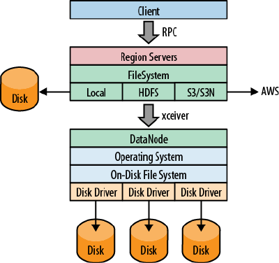
21. A full list was compiled by Tom White in his post “Get to Know Hadoop Filesys‐
tems”.
Figure 2-1. The filesystem negotiating transparently where data is
stored
You can use a filesystem that is already supplied by Hadoop: it ships
with a list of filesystems,21 which you may want to try out first. As a
last resort—or if you’re an experienced developer—you can also write
your own filesystem implementation.
Local
The local filesystem actually bypasses Hadoop entirely, that is, you do
not need to have a HDFS or any other cluster at all. It is handled all in
the FileSystem class used by HBase to connect to the filesystem im‐
plementation. The supplied ChecksumFileSystem class is loaded by
the client and uses local disk paths to store all the data.
The beauty of this approach is that HBase is unaware that it is not
talking to a distributed filesystem on a remote or colocated cluster,
but actually is using the local filesystem directly. The standalone
mode of HBase uses this feature to run HBase only. You can select it
by using the following scheme:
file:///<path>
Similar to the URIs used in a web browser, the file: scheme address‐
es local files.
Filesystems for HBase 69
www.finebook.ir

22. HBASE-11218 has the details.
23. See “Amazon S3” for more background information.
24. See “EC2” on Wikipedia.
Note that before HBase version 1.0.0 (and 0.98.3) there
was a rare problem with data loss, during very specific sit‐
uations, using the local filesystem. While this setup is just
for testing anyways, because HDFS or another reliable fil‐
esystem is used in production, you should still be careful.22
HDFS
The Hadoop Distributed File System (HDFS) is the default filesystem
when deploying a fully distributed cluster. For HBase, HDFS is the fil‐
esystem of choice, as it has all the required features. As we discussed
earlier, HDFS is built to work with MapReduce, taking full advantage
of its parallel, streaming access support. The scalability, fail safety,
and automatic replication functionality is ideal for storing files relia‐
bly. HBase adds the random access layer missing from HDFS and ide‐
ally complements Hadoop. Using MapReduce, you can do bulk im‐
ports, creating the storage files at disk-transfer speeds.
The URI to access HDFS uses the following scheme:
hdfs://<namenode>:<port>/<path>
S3
Amazon’s Simple Storage Service (S3)23 is a storage system that is pri‐
marily used in combination with dynamic servers running on Ama‐
zon’s complementary service named Elastic Compute Cloud (EC2).24
S3 can be used directly and without EC2, but the bandwidth used to
transfer data in and out of S3 is going to be cost-prohibitive in prac‐
tice. Transferring between EC2 and S3 is free, and therefore a viable
option. One way to start an EC2-based cluster is shown in “Apache
Whirr” (page 94).
The S3 FileSystem implementation provided by Hadoop supports
three different modes: the raw (or native) mode, the block-based
mode, and the newer AWS SDK based mode. The raw mode uses the
s3n: URI scheme and writes the data directly into S3, similar to the
local filesystem. You can see all the files in your bucket the same way
as you would on your local disk.
Chapter 2: Installation70
www.finebook.ir

25. See HADOOP-10400 and AWS SDK for details.
26. See this post for a more in-depth discussion on I/O performance on EC2.
The s3: scheme is the block-based mode and was used to overcome
S3’s former maximum file size limit of 5 GB. This has since been
changed, and therefore the selection is now more difficult—or easy:
opt for s3n: if you are not going to exceed 5 GB per file.
The block mode emulates the HDFS filesystem on top of S3. It makes
browsing the bucket content more difficult as only the internal block
files are visible, and the HBase storage files are stored arbitrarily in‐
side these blocks and strewn across them.
Both these filesystems share the fact that they use the external JetS3t
open source Java toolkit to do the actual heavy lifting. A more recent
addition is the s3a: scheme that replaces the JetS3t block mode with
an AWS SDK based one.25 It is closer to the native S3 API and can op‐
timize certain operations, resulting in speed ups, as well as integrate
better overall compared to the existing implementation.
You can select the filesystem using these URIs:
s3://<bucket-name>
s3n://<bucket-name>
s3a://<bucket-name>
What about EBS and ephemeral disk using EC2?
While we are talking about Amazon Web Services, you might won‐
der what can be said about EBS volumes vs. ephemeral disk
drives (aka instance storage). The former has proper persistency
across server restarts, something that instance storage does not
provide. On the other hand, EBS is connected to the EC2 instance
using a storage network, making it much more susceptible to la‐
tency fluctuations. Some posts recommend to only allocate the
maximum size of a volume and combine four of them in a RAID-0
group.
Instance storage also exposes more latency issues compared to
completely local disks, but is slightly more predictable.26 There is
still an impact and that has to be factored into the cluster design.
Not being persistent is one of the major deterrent to use ephemer‐
al disks, because losing a server will cause data to rebalance—
something that might be avoided by starting another EC2 instance
and reconnect an existing EBS volume.
Filesystems for HBase 71
www.finebook.ir

27. QFS used to be called CloudStore, which in turn was formerly known as the Kos‐
mos filesystem, abbreviated as KFS and the namesake of the original URI scheme.
28. Also check out the JIRA issue HADOOP-8885 for the details on QFS. Info about the
removal of KFS is found under HADOOP-8886.
Amazon recently added the option to use SSD (solid-state drive)
backed EBS volumes, for low-latency use-cases. This should be in‐
teresting for HBase setups running in EC2, as it supposedly
smoothes out the latency spikes incurred by the built-in write
caching of the EBS storage network. Your mileage may vary!
Other Filesystems
There are other filesystems, and one to mention is QFS, the Quantcast
File System.27 It is an open source, distributed, high-performance file‐
system written in C++, with similar features to HDFS. Find more in‐
formation about it at the Quantcast website.28
There are other file systems, for example the Azure filesystem, or the
Swift filesystem. Both use the native APIs of Microsoft Azure Blob
Storage and OpenStack Swift respectively allowing Hadoop to store
data in these systems. We will not further look into these choices, so
please carefully evaluate what you need given a specific use-case.
Note though that the majority of clusters in production today are
based on HDFS.
Wrapping up the Hadoop supported filesystems, Table 2-4 shows a list
of all the important choices. There are more supported by Hadoop,
but they are used in different ways and are therefore excluded here.
Table 2-4. A list of HDFS filesystem implementations
File System URI Scheme Description
HDFS hdfs: The original Hadoop Distributed
Filesystem
S3 Native s3n: Stores in S3 in a readable format for other
S3 users
S3 Block s3: Data is stored in proprietary binary blocks
in S3, using JetS3t
S3 Block (New) s3a: Improved proprietary binary block
storage, using the AWS API
Quantcast FS qfs: External project providing a HDFS
replacement
Chapter 2: Installation72
www.finebook.ir

File System URI Scheme Description
Azure Blob Storage wasb:aUses the Azure blob storage API to store
binary blocks
OpenStack Swift swift: Provides storage access for OpenStack’s
Swift blob storage
a There is also a wasbs: scheme for secure access to the blob storage.
Installation Choices
Once you have decided on the basic OS-related options, you must
somehow get HBase onto your servers. You have a couple of choices,
which we will look into next. Also see (to come) for even more options.
Apache Binary Release
The canonical installation process of most Apache projects is to down‐
load a release, usually provided as an archive containing all the re‐
quired files. Some projects, including HBase since version 0.95, have
separate archives for a binary and source release—the former intend‐
ed to have everything needed to run the release and the latter con‐
taining all files needed to build the project yourself.
Over the years the HBase packing has changed a bit, being modular‐
ized along the way. Due to the inherent external dependencies to Ha‐
doop, it also had to support various features and versions of Hadoop.
Table 2-5 shows a matrix with the available packages for each major
HBase version. Single means a combined package for source and bi‐
nary release components, Security indicates a separate—but also
source and binary combined—package for kerberized setups, Source
is just for source packages, same for Binary but here just for binary
packages for Hadoop 2.x and later. Finally, Hadoop 1 Binary and Ha‐
doop 2 Binary are both binary packages that are specific to the Ha‐
doop version targeted.
Table 2-5. HBase packaging evolution
Version Single Security Source Binary Hadoop 1
Binary Hadoop 2
Binary
0.90.0 ✓ ✗ ✗ ✗ ✗ ✗
0.92.0 ✓ ✓ ✗ ✗ ✗ ✗
0.94.0 ✓ ✓ ✗ ✗ ✗ ✗
0.96.0 ✗ ✗ ✓ ✗ ✓ ✓
0.98.0 ✗ ✗ ✓ ✗ ✓ ✓
1.0.0 ✗ ✗ ✓ ✓ ✗ ✗
Installation Choices 73
www.finebook.ir
29. Processes that are started and then run in the background to perform their task are
often referred to as daemons.
The table also shows that as of version 1.0.0 HBase will only support
Hadoop 2 as mentioned earlier. For more information on HBase relea‐
ses, you may also want to check out the Release Notes page. Another
interesting page is titled Change Log, and it lists everything that was
added, fixed, or changed in any form or shape for each released ver‐
sion.
You can download the most recent release of HBase from the Apache
HBase release page and unpack the contents into a suitable directory,
such as /usr/local or /opt, like so-shown here for version 1.0.0:
$ cd /usr/local
$ wget http://archive.apache.org/dist/hbase/hbase-1.0.0/
hbase-1.0.0-bin.tar.gz
$ tar -zxvf hbase-1.0.0-bin.tar.gz
Once you have extracted all the files, you can make yourself familiar
with what is in the project’s directory. The content may look like this:
$ cd hbase-1.0.0
$ ls -l
-rw-r--r-- 1 larsgeorge staff 130672 Feb 15 04:40 CHANGES.txt
-rw-r--r-- 1 larsgeorge staff 11358 Jan 25 10:47 LICENSE.txt
-rw-r--r-- 1 larsgeorge staff 897 Feb 15 04:18 NOTICE.txt
-rw-r--r-- 1 larsgeorge staff 1477 Feb 13 01:21 README.txt
drwxr-xr-x 31 larsgeorge staff 1054 Feb 15 04:21 bin
drwxr-xr-x 9 larsgeorge staff 306 Feb 27 13:37 conf
drwxr-xr-x 48 larsgeorge staff 1632 Feb 15 04:49 docs
drwxr-xr-x 7 larsgeorge staff 238 Feb 15 04:43 hbase-
webapps
drwxr-xr-x 115 larsgeorge staff 3910 Feb 27 13:29 lib
drwxr-xr-x 8 larsgeorge staff 272 Mar 3 22:18 logs
The root of it only contains a few text files, stating the license terms
(LICENSE.txt and NOTICE.txt) and some general information on how
to find your way around (README.txt). The CHANGES.txt file is a static
snapshot of the change log page mentioned earlier. It contains all the
changes that went into the current release you downloaded.
The remainder of the content in the root directory consists of other di‐
rectories, which are explained in the following list:
binThe bin--or binaries--directory contains the scripts supplied by
HBase to start and stop HBase, run separate daemons,29 or start
additional master nodes. See “Running and Confirming Your In‐
stallation” (page 95) for information on how to use them.
Chapter 2: Installation74
www.finebook.ir

conf
The configuration directory contains the files that define how
HBase is set up. “Configuration” (page 85) explains the contained
files in great detail.
docs
This directory contains a copy of the HBase project website, in‐
cluding the documentation for all the tools, the API, and the
project itself. Open your web browser of choice and open the
docs/index.html file by either dragging it into the browser,
double-clicking that file, or using the File→Open (or similarly
named) menu.
hbase-webapps
HBase has web-based user interfaces which are implemented as
Java web applications, using the files located in this directory.
Most likely you will never have to touch this directory when work‐
ing with or deploying HBase into production.
libJava-based applications are usually an assembly of many auxiliary
libraries, plus the JAR file containing the actual program. All of
these libraries are located in the lib directory. For newer versions
of HBase with a binary package structure and modularized archi‐
tecture, all HBase JAR files are also in this directory. Older ver‐
sions have one or few more JARs directly in the project root path.
logs
Since the HBase processes are started as daemons (i.e., they are
running in the background of the operating system performing
their duty), they use logfiles to report their state, progress, and op‐
tionally, errors that occur during their life cycle. (to come) ex‐
plains how to make sense of their rather cryptic content.
Initially, there may be no logs directory, as it is created
when you start HBase for the first time. The logging
framework used by HBase is creating the directory and
logfiles dynamically.
Since you have unpacked a binary release archive, you can now move
on to “Run Modes” (page 79) to decide how you want to run HBase.
Installation Choices 75
www.finebook.ir

Building from Source
This section is important only if you want to build HBase
from its sources. This might be necessary if you want to
apply patches, which can add new functionality you may
be requiring.
HBase uses Maven to build the binary packages. You therefore need a
working Maven installation, plus a full Java Development Kit (JDK)--
not just a Java Runtime as used in “Quick-Start Guide” (page 39).
You can download the most recent source release of HBase from the
Apache HBase release page and unpack the contents into a suitable
directory, such as /home/<username> or /tmp, like so-shown here for
version 1.0.0 again:
$ cd /usr/username
$ wget http://archive.apache.org/dist/hbase/hbase-1.0.0/
hbase-1.0.0-src.tar.gz
$ tar -zxvf hbase-1.0.0-src.tar.gz
Once you have extracted all the files, you can make yourself familiar
with what is in the project’s directory, which is now different from
above, because you have a source package. The content may look like
this:
$ cd hbase-1.0.0
$ ls -l
-rw-r--r-- 1 larsgeorge admin 130672 Feb 15 04:40 CHANGES.txt
-rw-r--r-- 1 larsgeorge admin 11358 Jan 25 10:47 LICENSE.txt
-rw-r--r-- 1 larsgeorge admin 897 Feb 15 04:18 NOTICE.txt
-rw-r--r-- 1 larsgeorge admin 1477 Feb 13 01:21 README.txt
drwxr-xr-x 31 larsgeorge admin 1054 Feb 15 04:21 bin
drwxr-xr-x 9 larsgeorge admin 306 Feb 13 01:21 conf
drwxr-xr-x 25 larsgeorge admin 850 Feb 15 04:18 dev-support
drwxr-xr-x 4 larsgeorge admin 136 Feb 15 04:42 hbase-
annotations
drwxr-xr-x 4 larsgeorge admin 136 Feb 15 04:43 hbase-
assembly
drwxr-xr-x 4 larsgeorge admin 136 Feb 15 04:42 hbase-
checkstyle
drwxr-xr-x 4 larsgeorge admin 136 Feb 15 04:42 hbase-client
drwxr-xr-x 4 larsgeorge admin 136 Feb 15 04:42 hbase-common
drwxr-xr-x 5 larsgeorge admin 170 Feb 15 04:43 hbase-
examples
drwxr-xr-x 4 larsgeorge admin 136 Feb 15 04:42 hbase-hadoop-
compat
drwxr-xr-x 4 larsgeorge admin 136 Feb 15 04:42 hbase-
Chapter 2: Installation76
www.finebook.ir
hadoop2-compat
drwxr-xr-x 4 larsgeorge admin 136 Feb 15 04:43 hbase-it
drwxr-xr-x 4 larsgeorge admin 136 Feb 15 04:42 hbase-prefix-
tree
drwxr-xr-x 5 larsgeorge admin 170 Feb 15 04:42 hbase-
protocol
drwxr-xr-x 4 larsgeorge admin 136 Feb 15 04:43 hbase-rest
drwxr-xr-x 4 larsgeorge admin 136 Feb 15 04:42 hbase-server
drwxr-xr-x 4 larsgeorge admin 136 Feb 15 04:43 hbase-shell
drwxr-xr-x 4 larsgeorge admin 136 Feb 15 04:43 hbase-
testing-util
drwxr-xr-x 4 larsgeorge admin 136 Feb 15 04:43 hbase-thrift
-rw-r--r-- 1 larsgeorge admin 86635 Feb 15 04:21 pom.xml
drwxr-xr-x 3 larsgeorge admin 102 May 22 2014 src
Like before, the root of it only contains a few text files, stating the li‐
cense terms (LICENSE.txt and NOTICE.txt) and some general infor‐
mation on how to find your way around (README.txt). The
CHANGES.txt file is a static snapshot of the change log page men‐
tioned earlier. It contains all the changes that went into the current
release you downloaded. The final, yet new file, is the Maven POM file
pom.xml, and it is needed for Maven to build the project.
The remainder of the content in the root directory consists of other di‐
rectories, which are explained in the following list:
binThe bin--or binaries--directory contains the scripts supplied by
HBase to start and stop HBase, run separate daemons, or start ad‐
ditional master nodes. See “Running and Confirming Your Installa‐
tion” (page 95) for information on how to use them.
conf
The configuration directory contains the files that define how
HBase is set up. “Configuration” (page 85) explains the contained
files in great detail.
hbase-webapps
HBase has web-based user interfaces which are implemented as
Java web applications, using the files located in this directory.
Most likely you will never have to touch this directory when work‐
ing with or deploying HBase into production.
logs
Since the HBase processes are started as daemons (i.e., they are
running in the background of the operating system performing
their duty), they use logfiles to report their state, progress, and op‐
tionally, errors that occur during their life cycle. (to come) ex‐
plains how to make sense of their rather cryptic content.
Installation Choices 77
www.finebook.ir

Initially, there may be no logs directory, as it is created
when you start HBase for the first time. The logging
framework used by HBase is creating the directory and
logfiles dynamically.
hbase-XXXXXX
These are the source modules for HBase, containing all the re‐
quired sources and other resources. They are structured as Maven
modules, which means allowing you to build them separately if
needed.
srcContains all the source for the project site and documentation.
dev-support
Here are some scripts and related configuration files for specific
development tasks.
The lib and docs directories as seen in the binary package above are
absent as you may have noted. Both are created dynamically-but in
other locations-when you compile the code. There are various build
targets you can choose to build them separately, or together, as
shown below. In addition, there is also a target directory once you
have built HBase for the first time. It holds the compiled JAR, site, and
documentation files respectively, though again dependent on the Mav‐
en command you have executed.
Once you have the sources and confirmed that both Maven and JDK
are set up properly, you can build the JAR files using the following
command:
$ mvn package
Note that the tests for HBase need more than one hour to complete. If
you trust the code to be operational, or you are not willing to wait, you
can also skip the test phase, adding a command-line switch like so:
$ mvn -DskipTests package
This process will take a few minutes to complete while creating the
target directory in the HBase project home directory. Once the build
completes with a Build Successful message, you can find the com‐
piled JAR files in the target directory. If you rather want to addition‐
ally build the binary package, you need to run this command:
$ mvn -DskipTests package assembly:single
Chapter 2: Installation78
www.finebook.ir
30. The pseudo-distributed versus fully distributed nomenclature comes from Hadoop.
With that archive you can go back to “Apache Binary Release” (page
73) and follow the steps outlined there to install your own, private re‐
lease on your servers. Finally, here the Maven command to build just
the site details, which is the website and documentation mirror:
$ mvn site
More information about building and contribute to HBase can be
found online.
Run Modes
HBase has two run modes: standalone and distributed. Out of the box,
HBase runs in standalone mode, as seen in “Quick-Start Guide” (page
39). To set up HBase in distributed mode, you will need to edit files in
the HBase conf directory.
Whatever your mode, you may need to edit conf/hbase-env.sh to tell
HBase which java to use. In this file, you set HBase environment vari‐
ables such as the heap size and other options for the JVM, the prefer‐
red location for logfiles, and so on. Set JAVA_HOME to point at the root
of your java installation. You can also set this variable in your shell
environment, but you would need to do this for every session you
open, and across all machines you are using. Setting JAVA_HOME in the
conf/hbase-env.sh is simply the easiest and most reliable way to do
that.
Standalone Mode
This is the default mode, as described and used in “Quick-Start Guide”
(page 39). In standalone mode, HBase does not use HDFS—it uses the
local filesystem instead—and it runs all HBase daemons and a local
ZooKeeper in the same JVM process. ZooKeeper binds to a well-known
port so that clients may talk to HBase.
Distributed Mode
The distributed mode can be further subdivided into pseudo-
distributed--all daemons run on a single node—and fully distributed--
where the daemons are spread across multiple, physical servers in the
cluster.30
Distributed modes require an instance of the Hadoop Distributed File
System (HDFS). See the Hadoop requirements and instructions for
Run Modes 79
www.finebook.ir

how to set up HDFS. Before proceeding, ensure that you have an ap‐
propriate, working HDFS installation.
The following subsections describe the different distributed setups.
Starting, verifying, and exploring of your install, whether a pseudo-
distributed or fully distributed configuration, is described in “Running
and Confirming Your Installation” (page 95). The same verification
steps apply to both deploy types.
Pseudo-distributed mode
A pseudo-distributed mode is simply a distributed mode that is run on
a single host. Use this configuration for testing and prototyping on
HBase. Do not use this configuration for production or for evaluating
HBase performance.
Once you have confirmed your HDFS setup, edit conf/hbase-
site.xml. This is the file into which you add local customizations and
overrides for the default HBase configuration values (see (to come) for
the full list, and “HDFS-Related Configuration” (page 87)). Point HBase
at the running Hadoop HDFS instance by setting the hbase.rootdir
property. For example, adding the following properties to your hbase-
site.xml file says that HBase should use the /hbase directory in the
HDFS whose name node is at port 9000 on your local machine, and
that it should run with one replica only (recommended for pseudo-
distributed mode):
<configuration>
...
<property>
<name>hbase.rootdir</name>
<value>hdfs://localhost:9000/hbase</value>
</property>
<property>
<name>dfs.replication</name>
<value>1</value>
</property>
...
</configuration>
In the example configuration, the server binds to local
host. This means that a remote client cannot connect.
Amend accordingly, if you want to connect from a remote
location.
The dfs.replication setting of 1 in the configuration assumes you
are also running HDFS in that mode. On a single machine it means
Chapter 2: Installation80
www.finebook.ir
you only have one DataNode process/thread running, and therefore
leaving the default of 3 for the replication would constantly yield
warnings that blocks are under-replicated. The same setting is also
applied to HDFS in its hdfs-site.xml file. If you have a fully dis‐
tributed HDFS instead, you can remove the dfs.replication setting
altogether.
If all you want to try for now is the pseudo-distributed mode, you can
skip to “Running and Confirming Your Installation” (page 95) for de‐
tails on how to start and verify your setup. See (to come) for informa‐
tion on how to start extra master and region servers when running in
pseudo-distributed mode.
Fully distributed mode
For running a fully distributed operation on more than one host, you
need to use the following configurations. In hbase-site.xml, add the
hbase.cluster.distributed property and set it to true, and point
the HBase hbase.rootdir at the appropriate HDFS name node and lo‐
cation in HDFS where you would like HBase to write data. For exam‐
ple, if your name node is running at a server with the hostname name
node.foo.com on port 9000 and you want to home your HBase in
HDFS at /hbase, use the following configuration:
<configuration>
...
<property>
<name>hbase.rootdir</name>
<value>hdfs://namenode.foo.com:9000/hbase</value>
</property>
<property>
<name>hbase.cluster.distributed</name>
<value>true</value>
</property>
...
</configuration>
In addition, a fully distributed mode requires that you modify the
conf/regionservers file. It lists all the hosts on which you want to
run HRegionServer daemons. Specify one host per line (this file in
HBase is like the Hadoop slaves file). All servers listed in this file will
be started and stopped when the HBase cluster start or stop scripts
are run. By default the file only contains the localhost entry, refer‐
ring back to itself for standalone and pseudo-distributed mode:
$ cat conf/regionservers
localhost
A distributed HBase setup also depends on a running ZooKeeper clus‐
ter. All participating nodes and clients need to be able to access the
Run Modes 81
www.finebook.ir

31. In versions before HBase 0.95 it was also possible to read an external zoo.cfg file.
This has been deprecated in HBASE-4072. The issue mentions hbase.con
fig.read.zookeeper.config to enable the old behavior for existing, older setups,
which is still available in HBase 1.0.0 though should not be used if possible.
32. For the full list of ZooKeeper configurations, see ZooKeeper’s zoo.cfg. HBase does
not ship with that file, so you will need to browse the conf directory in an appropri‐
ate ZooKeeper download.
running ZooKeeper ensemble. HBase, by default, manages a ZooKeep‐
er cluster (which can be as low as a single node) for you. It will start
and stop the ZooKeeper ensemble as part of the HBase start and stop
process. You can also manage the ZooKeeper ensemble independent
of HBase and just point HBase at the cluster it should use. To toggle
HBase management of ZooKeeper, use the HBASE_MANAGES_ZK vari‐
able in conf/hbase-env.sh. This variable, which defaults to true,
tells HBase whether to start and stop the ZooKeeper ensemble servers
as part of the start and stop commands supplied by HBase.
When HBase manages the ZooKeeper ensemble, you can specify the
ZooKeeper configuration options directly in conf/hbase-site.xml.31
You can set a ZooKeeper configuration option as a property in the
HBase hbase-site.xml XML configuration file by prefixing the Zoo‐
Keeper option name with hbase.zookeeper.property. For example,
you can change the clientPort setting in ZooKeeper by setting the
hbase.zookeeper.property.clientPort property. For all default val‐
ues used by HBase, including ZooKeeper configuration, see (to come).
Look for the hbase.zookeeper.property prefix.32
zoo.cfg Versus hbase-site.xml
Please note that the following information is applicable to versions
of HBase before 0.95, or when you enable the old behavior by set‐
ting hbase.config.read.zookeeper.config to true.
There is some confusion concerning the usage of zoo.cfg and
hbase-site.xml in combination with ZooKeeper settings. For
starters, if there is a zoo.cfg on the classpath (meaning it can be
found by the Java process), it takes precedence over all settings in
hbase-site.xml--but only those starting with the hbase.zookeep
er.property prefix, plus a few others.
There are some ZooKeeper client settings that are not read from
zoo.cfg but must be set in hbase-site.xml. This includes, for ex‐
ample, the important client session timeout value set with zoo
keeper.session.timeout. The following table describes the de‐
pendencies in more detail.
Chapter 2: Installation82
www.finebook.ir

Property zoo.cfg + hbase-
site.xml hbase-site.xml
only
hbase.zookeeper.quorum Constructed from serv
er.__n__ lines as specified in
zoo.cfg. Overrides any
setting in hbase-site.xml.
Used as specified.
hbase.zookeeper.property.* All values from zoo.cfg
override any value specified in
hbase-site.xml.
Used as specified.
zookeeper.* Only taken from hbase-
site.xml. Only taken from
hbase-
site.xml.
To avoid any confusion during deployment, it is highly recom‐
mended that you not use a zoo.cfg file with HBase, and instead
use only the hbase-site.xml file. Especially in a fully distributed
setup where you have your own ZooKeeper servers, it is not prac‐
tical to copy the configuration from the ZooKeeper nodes to the
HBase servers.
You must at least set the ensemble servers with the hbase.zookeep
er.quorum property. It otherwise defaults to a single ensemble mem‐
ber at localhost, which is not suitable for a fully distributed HBase
(it binds to the local machine only and remote clients will not be able
to connect).
There are three prefixes to specify ZooKeeper related properties:
zookeeper.
Specifies client settings for the ZooKeeper client used by the
HBase client library.
hbase.zookeeper
Used for values pertaining to the HBase client communicating to
the ZooKeeper servers.
hbase.zookeeper.properties.
These are only used when HBase is also managing the ZooKeeper
ensemble, specifying ZooKeeper server parameters.
How Many ZooKeepers Should I Run?
You can run a ZooKeeper ensemble that comprises one node only,
but in production it is recommended that you run a ZooKeeper en‐
semble of three, five, or seven machines; the more members an
ensemble has, the more tolerant the ensemble is of host failures.
Run Modes 83
www.finebook.ir

Also, run an odd number of machines, since running an even
count does not make for an extra server building consensus—you
need a majority vote, and if you have three or four servers, for ex‐
ample, both would have a majority with three nodes. Using an odd
number, larger than 3, allows you to have two servers fail, as op‐
posed to only one with even numbers.
Give each ZooKeeper server around 1 GB of RAM, and if possible,
its own dedicated disk (a dedicated disk is the best thing you can
do to ensure the ZooKeeper ensemble performs well). For very
heavily loaded clusters, run ZooKeeper servers on separate ma‐
chines from RegionServers, DataNodes, TaskTrackers, or Node‐
Managers.
For example, in order to have HBase manage a ZooKeeper quorum on
nodes rs{1,2,3,4,5}.foo.com, bound to port 2222 (the default is
2181), you must ensure that HBASE_MANAGES_ZK is commented out or
set to true in conf/hbase-env.sh and then edit conf/hbase-
site.xml and set hbase.zookeeper.property.clientPort and
hbase.zookeeper.quorum. You should also set hbase.zookeeper.prop
erty.dataDir to something other than the default, as the default has
ZooKeeper persist data under /tmp, which is often cleared on system
restart. In the following example, we have ZooKeeper persist to /var/
zookeeper:
Keep in mind that setting HBASE_MANAGES_ZK either way
implies that you are using the supplied HBase start
scripts. This might not be the case for a packaged distribu‐
tion of HBase (see (to come)). There are many ways to
manage processes and therefore there is no guarantee
that any setting made in hbase-env.sh, and hbase-
site.xml, are really taking affect. Please consult with you
distribution’s documentation ensuring you use the proper
approach.
<configuration>
...
<property>
<name>hbase.zookeeper.property.clientPort</name>
<value>2222</value>
</property>
<property>
<name>hbase.zookeeper.quorum</name>
<val‐
Chapter 2: Installation84
www.finebook.ir
ue>rs1.foo.com,rs2.foo.com,rs3.foo.com,rs4.foo.com,rs5.foo.com</
value>
</property>
<property>
<name>hbase.zookeeper.property.dataDir</name>
<value>/var/zookeeper</value>
</property>
...
</configuration>
To point HBase at an existing ZooKeeper cluster, one that is not man‐
aged by HBase, set HBASE_MANAGES_ZK in conf/hbase-env.sh to
false:
...
# Tell HBase whether it should manage it's own instance of Zookeep‐
er or not.
export HBASE_MANAGES_ZK=false
Next, set the ensemble locations and client port, if nonstandard, in
hbase-site.xml. When HBase manages ZooKeeper, it will start/stop
the ZooKeeper servers as a part of the regular start/stop scripts. If
you would like to run ZooKeeper yourself, independent of HBase start/
stop, do the following:
${HBASE_HOME}/bin/hbase-daemons.sh {start,stop} zookeeper
Note that you can use HBase in this manner to spin up a ZooKeeper
cluster, unrelated to HBase. Just make sure to set HBASE_MANAGES_ZK
to false if you want it to stay up across HBase restarts so that when
HBase shuts down, it doesn’t take ZooKeeper down with it.
For more information about running a distinct ZooKeeper cluster, see
the ZooKeeper Getting Started Guide. Additionally, see the ZooKeeper
wiki, or the ZooKeeper documentation for more information on Zoo‐
Keeper sizing.
Configuration
Now that the basics are out of the way (we’ve looked at all the choices
when it comes to selecting the filesystem, discussed the run modes,
and fine-tuned the operating system parameters), we can look at how
to configure HBase itself. Similar to Hadoop, all configuration param‐
eters are stored in files located in the conf directory. These are sim‐
ple text files either in XML format arranged as a set of properties, or
in simple flat files listing one option per line.
Configuration 85
www.finebook.ir

33. Be careful when editing XML files. Make sure you close all elements. Check your
file using a tool like xmllint, or something similar, to ensure well-formedness of
your document after an edit session.
For more details on how to modify your configuration files
for specific workloads refer to (to come).
Here a list of current configuration files, as available in HBase 1.0.0,
with the detailed description of each following in due course:
hbase-env.cmd and hbase-env.sh
Set up the working environment for HBase, specifying variables
such as JAVA_HOME. For Windows and Linux respectively.
hbase-site.xml
The main HBase configuration file. This file specifies configuration
options which override HBase’s default configuration.
backup-masters
This file is actually not present on a fresh install. It is a text file
that lists all the hosts which should have backup masters started
on.
regionservers
Lists all the nodes that are designated to run a region server in‐
stance.
hadoop-metrics2-hbase.properties
Specifies settings for the metrics framework integrated into each
HBase process.
hbase-policy.xml
In secure mode, this file is read and defines the authorization rules
for clients accessing the servers.
log4j.properties
Configures how each process logs its information using the Log4J
libraries.
Configuring a HBase setup entails editing the conf/hbase-env.{sh|
cmd} file containing environment variables, which is used mostly by
the shell scripts (see “Operating a Cluster” (page 95)) to start or stop a
cluster. You also need to add configuration properties to the XML
file33 conf/hbase-site.xml to, for example, override HBase defaults,
tell HBase what filesystem to use, and tell HBase the location of the
ZooKeeper ensemble.
Chapter 2: Installation86
www.finebook.ir

When running in distributed mode, after you make an edit to a HBase
configuration file, make sure you copy the content of the conf directo‐
ry to all nodes of the cluster. HBase will not do this for you.
There are many ways to synchronize your configuration
files across your cluster. The easiest is to use a tool like
rsync. There are many more elaborate ways, and you will
see a selection in “Deployment” (page 92).
We will now look more closely at each configuration file.
hbase-site.xml and hbase-default.xml
Just as in Hadoop where you add site-specific HDFS configurations to
the hdfs-site.xml file, for HBase, site-specific customizations go into
the file conf/hbase-site.xml. For the list of configurable properties,
see (to come), or view the raw hbase-default.xml source file in the
HBase source code at hbase-common/src/main/resources. The doc
directory also has a static HTML page that lists the configuration op‐
tions.
Not all configuration options are listed in hbase-
default.xml. Configurations that users would rarely
change do exist only in code; the only way to turn find
such configuration options is to read the source code it‐
self.
The servers always read the hbase-default.xml file first and subse‐
quently merge it with the hbase-site.xml file content—if present.
The properties set in hbase-site.xml always take precedence over
the default values loaded from hbase-default.xml.
Most changes here will require a cluster restart for HBase to notice
the change. However, there is a way to reload some specific settings
while the processes are running. See (to come) for details.
HDFS-Related Configuration
If you have made HDFS-related configuration changes on your Ha‐
doop cluster—in other words, properties you want the HDFS cli‐
Configuration 87
www.finebook.ir

ents to use as opposed to the server-side configuration—HBase
will not see these properties unless you do one of the following:
•Add a pointer to your $HADOOP_CONF_DIR to the HBASE_CLASS
PATH environment variable in hbase-env.sh.
•Add a copy of core-site.xml, hdfs-site.xml, etc. (or
hadoop-site.xml) or, better, symbolic links, under $
{HBASE_HOME}/conf.
• Add them to hbase-site.xml directly.
An example of such a HDFS client property is dfs.replication.
If, for example, you want to run with a replication factor of 5,
HBase will create files with the default of 3 unless you do one of
the above to make the configuration available to HBase.
When you add Hadoop configuration files to HBase, they will al‐
ways take the lowest priority. In other words, the properties con‐
tained in any of the HBase-related configuration files, that is, the
default and site files, take precedence over any Hadoop configura‐
tion file containing a property with the same name. This allows
you to override Hadoop properties in your HBase configuration
file.
hbase-env.sh and hbase-env.cmd
You set HBase environment variables in these files. Examples include
options to pass to the JVM when a HBase daemon starts, such as Java
heap size and garbage collector configurations. You also set options
for HBase configuration, log directories, niceness, SSH options, where
to locate process pid files, and so on. Open the file at conf/hbase-
env.{cmd,sh} and peruse its content. Each option is fairly well docu‐
mented. Add your own environment variables here if you want them
read when a HBase daemon is started.
regionserver
This file lists all the known region server names. It is a flat text file
that has one hostname per line. The list is used by the HBase mainte‐
nance script to be able to iterate over all the servers to start the re‐
gion server process. An example can be seen in “Example Configura‐
tion” (page 89).
Chapter 2: Installation88
www.finebook.ir

If you used previous versions of HBase, you may miss the
masters file, available in the 0.20.x line. It has been re‐
moved as it is no longer needed. The list of masters is now
dynamically maintained in ZooKeeper and each master
registers itself when started.
log4j.properties
Edit this file to change the rate at which HBase files are rolled and to
change the level at which HBase logs messages. Changes here will re‐
quire a cluster restart for HBase to notice the change, though log lev‐
els can be changed for particular daemons via the HBase UI. See (to
come) for information on this topic, and (to come) for details on how
to use the logfiles to find and solve problems.
Example Configuration
Here is an example configuration for a distributed 10-node cluster.
The nodes are named master.foo.com, host1.foo.com, and so on,
through node host9.foo.com. The HBase Master and the HDFS name
node are running on the node master.foo.com. Region servers run on
nodes host1.foo.com to host9.foo.com. A three-node ZooKeeper en‐
semble runs on zk1.foo.com, zk2.foo.com, and zk3.foo.com on the
default ports. ZooKeeper data is persisted to the directory /var/
zookeeper. The following subsections show what the main configura‐
tion files--hbase-site.xml, regionservers, and hbase-env.sh--found
in the HBase conf directory might look like.
hbase-site.xml
The hbase-site.xml file contains the essential configuration proper‐
ties, defining the HBase cluster setup.
<?xml version="1.0"?>
<?xml-stylesheet type="text/xsl" href="configuration.xsl"?>
<configuration>
<property>
<name>hbase.zookeeper.quorum</name>
<value>zk1.foo.com,zk2.foo.com,zk3.foo.com</value>
</property>
<property>
<name>hbase.zookeeper.property.dataDir</name>
<value>/var/zookeeper</value>
</property>
<property>
<name>hbase.rootdir</name>
<value>hdfs://master.foo.com:9000/hbase</value>
Configuration 89
www.finebook.ir
34. See HBASE-11804 for details.
</property>
<property>
<name>hbase.cluster.distributed</name>
<value>true</value>
</property>
</configuration>
regionservers
In this file, you list the nodes that will run region servers. In our exam‐
ple, we run region servers on all but the head node master.foo.com,
which is carrying the HBase Master and the HDFS NameNode.
host1.foo.com
host2.foo.com
host3.foo.com
host4.foo.com
host5.foo.com
host6.foo.com
host7.foo.com
host8.foo.com
host9.foo.com
hbase-env.sh
Here are the lines that were changed from the default in the supplied
hbase-env.sh file. We are setting the HBase heap to be 4 GB:
...
# export HBASE_HEAPSIZE=1000
export HBASE_HEAPSIZE=4096
...
Before HBase version 1.0 the default heap size was 1GB. This has
been changed34 in 1.0 and later to the default value of the JVM. This
usually amounts to one-fourth of the available memory, for example on
a Mac with Java version 1.7.0_45:
$ hostinfo | grep memory
Primary memory available: 48.00 gigabytes
$ java -XX:+PrintFlagsFinal -version | grep MaxHeapSize
uintx MaxHeapSize := 12884901888 {product}
You can see that the JVM reports a maximum heap of 12GB, which is
the mentioned one-fourth of the full 48GB.
Once you have edited the configuration files, you need to distribute
them across all servers in the cluster. One option to copy the content
of the conf directory to all servers in the cluster is to use the rsync
Chapter 2: Installation90
www.finebook.ir

command on Unix and Unix-like platforms. This approach and others
are explained in “Deployment” (page 92).
(to come) discusses the settings you are most likely to
change first when you start scaling your cluster.
Client Configuration
Since the HBase Master may move around between physical machines
(see (to come) for details), clients start by requesting the vital infor‐
mation from ZooKeeper—something visualized in (to come). For that
reason, clients require the ZooKeeper quorum information in a hbase-
site.xml file that is on their Java $CLASSPATH.
You can also set the hbase.zookeeper.quorum configura‐
tion key in your code. Doing so would lead to clients that
need no external configuration files. This is explained in
“Put Method” (page 122).
If you are configuring an IDE to run a HBase client, you could include
the conf/ directory in your class path. That would make the configu‐
ration files discoverable by the client code.
Minimally, a Java client needs the following JAR files specified in its
$CLASSPATH, when connecting to HBase, as retrieved with the HBase
shell mapredcp command (and some shell string mangling):
$ bin/hbase mapredcp | tr ":" "\n" | sed "s/\/usr\/local\/
hbase-1.0.0\/lib\///"
zookeeper-3.4.6.jar
hbase-common-1.0.0.jar
hbase-protocol-1.0.0.jar
htrace-core-3.1.0-incubating.jar
protobuf-java-2.5.0.jar
hbase-client-1.0.0.jar
hbase-hadoop-compat-1.0.0.jar
netty-all-4.0.23.Final.jar
hbase-server-1.0.0.jar
guava-12.0.1.jar
Run the same bin/hbase mapredcp command without any string man‐
gling to get a properly configured class path output, which can be fed
directly to an application setup. All of these JAR files come with HBase
and are usually postfixed with the a version number of the required
Configuration 91
www.finebook.ir
release. Ideally, you use the supplied JARs and do not acquire them
somewhere else because even minor release changes could cause
problems when running the client against a remote HBase cluster.
A basic example hbase-site.xml file for client applications might
contain the following properties:
<?xml version="1.0"?>
<?xml-stylesheet type="text/xsl" href="configuration.xsl"?>
<configuration>
<property>
<name>hbase.zookeeper.quorum</name>
<value>zk1.foo.com,zk2.foo.com,zk3.foo.com</value>
</property>
</configuration>
Deployment
After you have configured HBase, the next thing you need to do is to
think about deploying it on your cluster. There are many ways to do
that, and since Hadoop and HBase are written in Java, there are only
a few necessary requirements to look out for. You can simply copy all
the files from server to server, since they usually share the same con‐
figuration. Here are some ideas on how to do that. Please note that
you would need to make sure that all the suggested selections and ad‐
justments discussed in “Requirements” (page 43) have been applied—
or are applied at the same time when provisioning new servers.
Besides what is mentioned below, the much more common way these
days to deploy Hadoop and HBase is using a prepackaged distribution,
which are listed in (to come).
Script-Based
Using a script-based approach seems archaic compared to the more
advanced approaches listed shortly. But they serve their purpose and
do a good job for small to even medium-size clusters. It is not so much
the size of the cluster but the number of people maintaining it. In a
larger operations group, you want to have repeatable deployment pro‐
cedures, and not deal with someone having to run scripts to update
the cluster.
The scripts make use of the fact that the regionservers configuration
file has a list of all servers in the cluster. Example 2-3 shows a very
simple script that could be used to copy a new release of HBase from
the master node to all slave nodes.
Chapter 2: Installation92
www.finebook.ir
Example 2-3. Example Script to copy the HBase files across a clus‐
ter
#!/bin/bash
# Rsync's HBase files across all slaves. Must run on master. Assumes
# all files are located in /usr/local
if [ "$#" != "2" ]; then
echo "usage: $(basename $0) <dir-name> <ln-name>"
echo " example: $(basename $0) hbase-0.1 hbase"
exit 1
fi
SRC_PATH="/usr/local/$1/conf/regionservers"
for srv in $(cat $SRC_PATH); do
echo "Sending command to $srv...";
rsync -vaz --exclude='logs/*' /usr/local/$1 $srv:/usr/local/
ssh $srv "rm -fR /usr/local/$2 ; ln -s /usr/local/$1 /usr/local/$2"
done
echo "done."
Another simple script is shown in Example 2-4; it can be used to copy
the configuration files of HBase from the master node to all slave no‐
des. It assumes you are editing the configuration files on the master in
such a way that the master can be copied across to all region servers.
Example 2-4. Example Script to copy configurations across a clus‐
ter
#!/bin/bash
# Rsync's HBase config files across all region servers. Must run on
master.
for srv in $(cat /usr/local/hbase/conf/regionservers); do
echo "Sending command to $srv...";
rsync -vaz --delete --exclude='logs/*' /usr/local/hadoop/ $srv:/usr/
local/hadoop/
rsync -vaz --delete --exclude='logs/*' /usr/local/hbase/ $srv:/usr/
local/hbase/
done
echo "done."
The second script uses rsync just like the first script, but adds the --
delete option to make sure the region servers do not have any older
files remaining but have an exact copy of what is on the originating
server.
There are obviously many ways to do this, and the preceding examples
are simply for your perusal and to get you started. Ask your adminis‐
Deployment 93
www.finebook.ir
trator to help you set up mechanisms to synchronize the configuration
files appropriately. Many beginners in HBase have run into a problem
that was ultimately caused by inconsistent configurations among the
cluster nodes. Also, do not forget to restart the servers when making
changes. If you want to update settings while the cluster is in produc‐
tion, please refer to (to come).
Apache Whirr
Recently, we have seen an increase in the number of users who want
to run their cluster in dynamic environments, such as the public cloud
offerings by Amazon’s EC2, or Rackspace Cloud Servers, as well as in
private server farms, using open source tools like Eucalyptus or Open‐
Stack.
The advantage is to be able to quickly provision servers and run ana‐
lytical workloads and, once the result has been retrieved, to simply
shut down the entire cluster, or reuse the servers for other dynamic
workloads. Since it is not trivial to program against each of the APIs
providing dynamic cluster infrastructures, it would be useful to ab‐
stract the provisioning part and, once the cluster is operational, sim‐
ply launch the MapReduce jobs the same way you would on a local,
static cluster. This is where Apache Whirr comes in.
Whirr has support for a variety of public and private cloud APIs and
allows you to provision clusters running a range of services. One of
those is HBase, giving you the ability to quickly deploy a fully opera‐
tional HBase cluster on dynamic setups.
You can download the latest Whirr release from the project’s website
and find preconfigured configuration files in the recipes directory.
Use it as a starting point to deploy your own dynamic clusters.
The basic concept of Whirr is to use very simple machine images that
already provide the operating system (see “Operating system” (page
51)) and SSH access. The rest is handled by Whirr using services that
represent, for example, Hadoop or HBase. Each service executes
every required step on each remote server to set up the user ac‐
counts, download and install the required software packages, write
out configuration files for them, and so on. This is all highly customiz‐
able and you can add extra steps as needed.
Puppet and Chef
Similar to Whirr, there are other deployment frameworks for dedica‐
ted machines. Puppet by Puppet Labs and Chef by Opscode are two
such offerings.
Chapter 2: Installation94
www.finebook.ir

Both work similar to Whirr in that they have a central provisioning
server that stores all the configurations, combined with client soft‐
ware, executed on each server, which communicates with the central
server to receive updates and apply them locally.
Also similar to Whirr, both have the notion of recipes, which essential‐
ly translate to scripts or commands executed on each node. In fact, it
is quite possible to replace the scripting employed by Whirr with a
Puppet- or Chef-based process. Some of the available recipe packages
are an adaption of early EC2 scripts, used to deploy HBase to dynam‐
ic, cloud-based server. For Chef, you can find HBase-related examples
at http://cookbooks.opscode.com/cookbooks/hbase. For Puppet, please
refer to http://hstack.org/hstack-automated-deployment-using-puppet/
and the repository with the recipes at http://github.com/hstack/puppet
as a starting point. There are other such modules available on the In‐
ternet.
While Whirr solely handles the bootstrapping, Puppet and Chef have
further support for changing running clusters. Their master process
monitors the configuration repository and, upon updates, triggers the
appropriate remote action. This can be used to reconfigure clusters
on-the-fly or push out new releases, do rolling restarts, and so on. It
can be summarized as configuration management, rather than just
provisioning.
You heard it before: select an approach you like and
maybe even are familiar with already. In the end, they
achieve the same goal: installing everything you need on
your cluster nodes. If you need a full configuration man‐
agement solution with live updates, a Puppet- or Chef-
based approach—maybe in combination with Whirr for the
server provisioning—is the right choice.
Operating a Cluster
Now that you have set up the servers, configured the operating sys‐
tem and filesystem, and edited the configuration files, you are ready
to start your HBase cluster for the first time.
Running and Confirming Your Installation
Make sure HDFS is running first. Start and stop the Hadoop HDFS
daemons by running bin/start-dfs.sh over in the $HADOOP_HOME di‐
rectory. You can ensure that it started properly by testing the put and
Operating a Cluster 95
www.finebook.ir
35. Previous versions of HBase used port 60010 for the master and 60030 for the re‐
gion server respectively.
get of files into the Hadoop filesystem. HBase does not normally use
the YARN daemons. You only need to start them for actual MapRe‐
duce jobs, something we will look into in detail in Chapter 7.
If you are managing your own ZooKeeper, start it and confirm that it
is running, since otherwise HBase will fail to start.
Just as you started the standalone mode in “Quick-Start Guide” (page
39), you start a fully distributed HBase with the following command:
$ bin/start-hbase.sh
Run the preceding command from the $HBASE_HOME directory. You
should now have a running HBase instance. The HBase log files can
be found in the logs subdirectory. If you find that HBase is not work‐
ing as expected, please refer to (to come) for help finding the prob‐
lem.
Once HBase has started, see “Quick-Start Guide” (page 39) for infor‐
mation on how to create tables, add data, scan your insertions, and fi‐
nally, disable and drop your tables.
Web-based UI Introduction
HBase also starts a web-based user interface (UI) listing vital at‐
tributes. By default, it is deployed on the master host at port 16010
(HBase region servers use 16030 by default).35 If the master is run‐
ning on a host named master.foo.com on the default port, to see the
master’s home page you can point your browser at http://
master.foo.com:16010. Figure 2-2 is an example of how the resultant
page should look. You can find a more detailed explanation in “Web-
based UI” (page 503).
Chapter 2: Installation96
www.finebook.ir
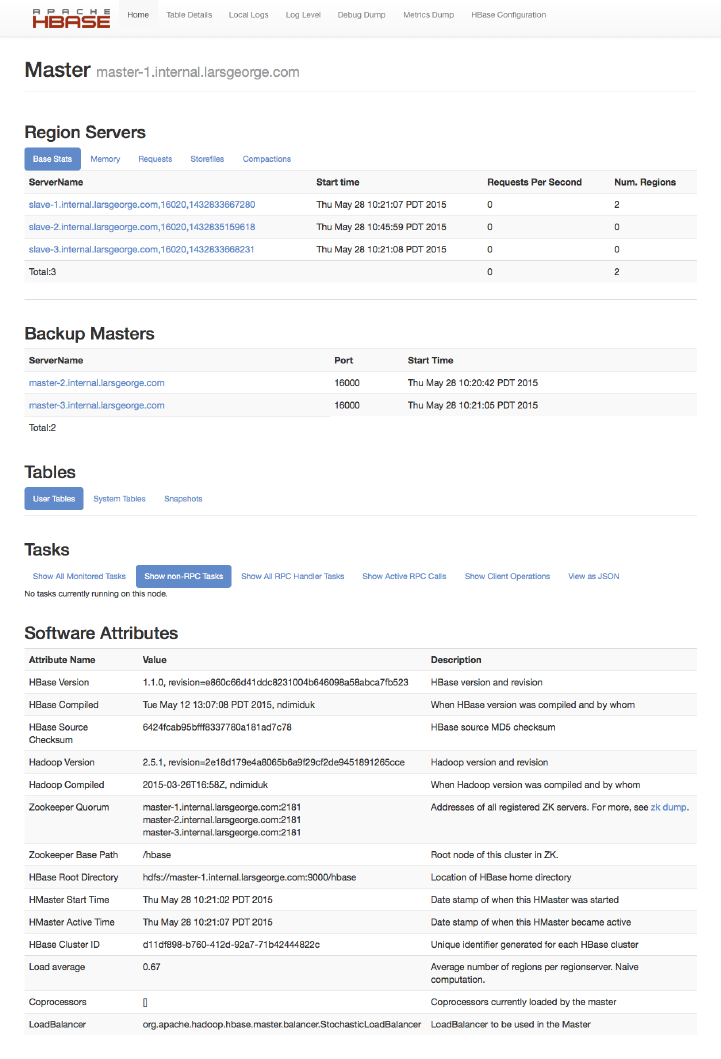
From this page you can access a variety of status information about
your HBase cluster. The page is separated into multiple sections. The
top part has the information about the available region servers, as
well as any optional backup masters. This is followed by the known
tables, system tables, and snapshots—these are tabs that you can se‐
lect to see the details you want.
The lower part shows the currently running tasks—if there are any--,
and again using tabs, you can switch to other details here, for exam‐
ple, the RPC handler status, active calls, and so on. Finally the bottom
of the page has the attributes pertaining to the cluster setup.
After you have started the cluster, you should verify that all the region
servers have registered themselves with the master and appear in the
appropriate table with the expected hostnames (that a client can con‐
nect to). Also verify that you are indeed running the correct version of
HBase and Hadoop.
Shell Introduction
You already used the command-line shell that comes with HBase when
you went through “Quick-Start Guide” (page 39). You saw how to cre‐
ate a table, add and retrieve data, and eventually drop the table.
The HBase Shell is (J)Ruby’s IRB with some HBase-related commands
added. Anything you can do in IRB, you should be able to do in the
HBase Shell. You can start the shell with the following command:
$ bin/hbase shell
HBase Shell; enter 'help<RETURN>' for list of supported commands.
Type "exit<RETURN>" to leave the HBase Shell
Version 1.0.0, r6c98bff7b719efdb16f71606f3b7d8229445eb81, Sat Feb
14 19:49:22 PST 2015
hbase(main):001:0>
Type help and then press Return to see a listing of shell commands
and options. Browse at least the paragraphs at the end of the help text
for the gist of how variables and command arguments are entered into
the HBase Shell; in particular, note how table names, rows, and col‐
umns, must be quoted. Find the full description of the shell in “Shell”
(page 481).
Since the shell is JRuby-based, you can mix Ruby with HBase com‐
mands, which enables you to do things like this:
hbase(main):001:0> create 'testtable', 'colfam1'
hbase(main):002:0> for i in 'a'..'z' do for j in 'a'..'z' do \
put 'testtable', "row-#{i}#{j}", "colfam1:#{j}", "#{j}" end end
Chapter 2: Installation98
www.finebook.ir
The first command is creating a new table named testtable, with one
column family called colfam1, using default values (see “Column Fam‐
ilies” (page 362) for what that means). The second command uses a Ru‐
by loop to create rows with columns in the newly created tables. It
creates row keys starting with row-aa, row-ab, all the way to row-zz.
Stopping the Cluster
To stop HBase, enter the following command. Once you have started
the script, you will see a message stating that the cluster is being
stopped, followed by “.” (period) characters printed in regular inter‐
vals (just to indicate that the process is still running, not to give you
any percentage feedback, or some other hidden meaning):
$ bin/stop-hbase.sh
stopping hbase...............
Shutdown can take several minutes to complete. It can take longer if
your cluster is composed of many machines. If you are running a dis‐
tributed operation, be sure to wait until HBase has shut down com‐
pletely before stopping the Hadoop daemons.
(to come) has more on advanced administration tasks—for example,
how to do a rolling restart, add extra master nodes, and more. It also
has information on how to analyze and fix problems when the cluster
does not start, or shut down.
Operating a Cluster 99
www.finebook.ir

Chapter 3
Client API: The Basics
This chapter will discuss the client APIs provided by HBase. As noted
earlier, HBase is written in Java and so is its native API. This does not
mean, though, that you must use Java to access HBase. In fact, Chap‐
ter 6 will show how you can use other programming languages.
General Notes
As noted in “HBase Version” (page xix), we are mostly
looking at APIs that are flagged as public regarding their
audience. See (to come) for details on the annotations in
use.
The primary client entry point to HBase is the Table interface in the
org.apache.hadoop.hbase.client package. It provides the user with
all the functionality needed to store and retrieve data from HBase, as
well as delete obsolete values and so on. It is retrieved by means of
the Connection instance that is the umbilical cord to the HBase
servers. Though, before looking at the various methods these classes
provide, let us address some general aspects of their usage.
All operations that mutate data are guaranteed to be atomic on a per-
row basis. This affects all other concurrent readers and writers of that
same row. In other words, it does not matter if another client or
thread is reading from or writing to the same row: they either read a
101
www.finebook.ir

1. The region servers use a multiversion concurrency control mechanism, implement‐
ed internally by the MultiVersionConsistencyControl (MVCC) class, to guarantee
that readers can read without having to wait for writers. Equally, writers do need
to wait for other writers to complete before they can continue.
consistent last mutation, or may have to wait before being able to ap‐
ply their change.1 More on this in (to come).
Suffice it to say for now that during normal operations and load, a
reading client will not be affected by another updating a particular
row since their contention is nearly negligible. There is, however, an
issue with many clients trying to update the same row at the same
time. Try to batch updates together to reduce the number of separate
operations on the same row as much as possible.
It also does not matter how many columns are written for the particu‐
lar row; all of them are covered by this guarantee of atomicity.
Finally, creating an initial connection to HBase is not without cost.
Each instantiation involves scanning the hbase:meta table to check if
the table actually exists and if it is enabled, as well as a few other op‐
erations that make this call quite heavy. Therefore, it is recommended
that you create a Connection instances only once and reuse that in‐
stance for the rest of the lifetime of your client application.
Once you have a connection instance you can retrieve references to
the actual tables. Ideally you do this per thread since the underlying
implementation of Table is not guaranteed to the thread-safe. Ensure
that you close all of the resources you acquire though to trigger im‐
portant house-keeping activities. All of this will be explained in detail
in the rest of this chapter.
The examples you will see in partial source code can be
found in full detail in the publicly available GitHub reposi‐
tory at https://github.com/larsgeorge/hbase-book. For de‐
tails on how to compile them, see (to come).
Initially you will see the import statements, but they will
be subsequently omitted for the sake of brevity. Also, spe‐
cific parts of the code are not listed if they do not immedi‐
ately help with the topic explained. Refer to the full source
if in doubt.
Chapter 3: Client API: The Basics102
www.finebook.ir

Data Types and Hierarchy
Before we delve into the actual operations and their API classes, let us
first see how the classes that we will use throughout the chapter are
related. There is some very basic functionality introduced in lower-
level classes, which surface in the majority of the data-centric classes,
such as Put, Get, or Scan. Table 3-1 list all of the basic data-centric
types that are introduced in this chapter.
Table 3-1. List of basic data-centric types
Type Kind Description
Get Query Retrieve previously stored data from a single row.
Scan Query Iterate over all or specific rows and return their data.
Put Mutation Create or update one or more columns in a single row.
Delete Mutation Remove a specific cell, column, row, etc.
Increment Mutation Treat a column as a counter and increment its value.
Append Mutation Attach the given data to one or more columns in a single row.
Throughout the book we will collectively refer to these classes as op‐
erations. Figure 3-1 shows you the hierarchy of the data-centric types
and their relationship to the more generic superclasses and inter‐
faces. Understanding them first will help use them throughout the en‐
tire API, and we save the repetitive mention as well. The remainder of
this section will discuss what these base classes and interfaces add to
each derived data-centric type.
Data Types and Hierarchy 103
www.finebook.ir
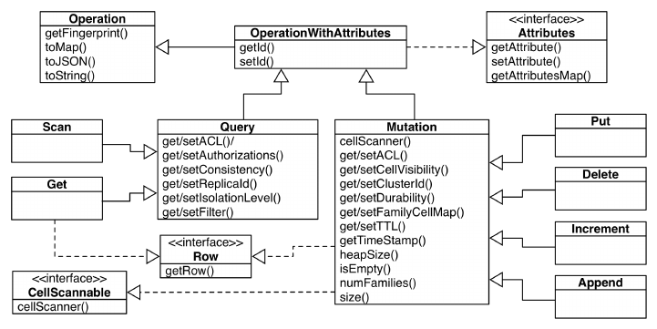
Figure 3-1. The class hierarchy of the basic client API data classes
Generic Attributes
One fundamental interface is Attributes, which introduces the fol‐
lowing methods:
Attributes setAttribute(String name, byte[] value)
byte[] getAttribute(String name)
Map<String, byte[]> getAttributesMap()
They provide a general mechanism to add any kind of information in
form of attributes to all of the data-centric classes. By default there
are no attributes set (apart from possibly internal ones) and a develop‐
er can make use of setAttribute() to add custom ones as needed.
Since most of the time the construction of a data type, such as Put, is
immediately followed by an API call to send it off to the servers, a val‐
id question is: where can I make use of attributes?
One thing to note is that attributes are serialized and sent to the serv‐
er, which means you can use them to inspect their value, for example,
in a coprocessor (see “Coprocessors” (page 282)). Another use-case is
the Append class, which uses the attributes to return information back
to the user after a call to the servers (see “Append Method” (page 181)).
Operations: Fingerprint and ID
Another fundamental type is the abstract class Operation, which adds
the following methods to all data types:
Chapter 3: Client API: The Basics104
www.finebook.ir

abstract Map<String, Object> getFingerprint()
abstract Map<String, Object> toMap(int maxCols)
Map<String, Object> toMap()
String toJSON(int maxCols) throws IOException
String toJSON() throws IOException
String toString(int maxCols)
String toString()
These were introduces when HBase 0.92 had the slow query logging
added (see (to come)), and help in generating useful information col‐
lections for logging and general debugging purposes. All of the latter
methods really rely on the specific implementation of toMap(int max
Cols), which is abstract in Operation. The Mutation class imple‐
ments it for all derived data classes in such a way as described in
Table 3-2. The default number of columns included in the output is 5
(hardcoded in HBase 1.0.0) when not specified explicitly.
In addition, the intermediate OperationWithAttributes class is ex‐
tending the above Operation class, implements the Attributes inter‐
face, and is adding the following methods, which are used in conjunc‐
tion:
OperationWithAttributes setId(String id)
String getId()
The ID is a client-provided value, which identifies the operation when
logged or emitted otherwise. For example, the client could set it to the
method name that is invoking the API, so that when the operation—
say the Put instance—is logged it can be determined which client call
is the root cause. Add the hostname, process ID, and other useful in‐
formation and it will be much easier to spot the culprit.
Table 3-2. The various methods to retrieve instance information
Method Description
getId() Returns what was set by the setId() method.
getFingerprint() Returns the list of column families included in the instance.
toMap(int maxCols) Compiles a list including fingerprint, column families with all
columns and their data, total column count, row key, and—if
set—the ID and cell-level TTL.
toMap() Same as above, but only for 5 columns.a
toJSON(int maxCols) Same as toMap(maxCols) but converted to JSON. Might fail
due to encoding issues.
toJSON() Same as above, but only for 5 columns.a
toString(int maxCols) Attempts to call toJSON(maxCols), but when it fails, falls back
to toMap(maxCols).
toString() Same as above, but only for 5 columns.a
Data Types and Hierarchy 105
www.finebook.ir

Method Description
a Hardcoded in HBase 1.0.0. Might change in the future.
The repository accompanying the book has an example named Finger
printExample.java which you can experiment with to see the finger‐
print, ID, and toMap() in action.
Query versus Mutation
Before we end with the final data types, there are a few more super‐
classes of importance. First the Row interface, which adds:
byte[] getRow()
The method simply returns the given row key of the instance. This is
implemented by the Get class, as it handles exactly one row. It is also
implemented by the Mutation superclass, which is the basis for all the
types that are needed when changing data. Additionally, Mutation im‐
plements the CellScannable interface to provide the following meth‐
od:
CellScanner cellScanner()
With it, a client can iterate over the returned cells, which we will
learn about in “The Cell” (page 112) very soon. The Mutation class also
has many other functions that are shared by all derived classes. Here
is a list of the most interesting ones:
Table 3-3. Methods provided by the Mutation superclass
Method Description
getACL()/setACL() The Access Control List (ACL) for this operation. See (to
come) for details.
getCellVisibility()/set
CellVisibility() The cell level visibility for all included cells. See (to come)
for details.
getClusterIds()/setClus
terIds() The cluster ID as needed for replication purposes. See (to
come) for details.
getDurability()/setDura
bility() The durability settings for the mutation. See “Durability,
Consistency, and Isolation” (page 108) for details.
getFamilyCellMap()/set
FamilyCellMap() The list of all cells per column family available in this
instance.
getTimeStamp() Retrieves the associated timestamp of the Put instance.
Can be optionally set using the constructor’s ts parameter.
If not set, may return Long.MAX_VALUE (also defined as
HConstants.LATEST_TIMESTAMP).
getTTL()/setTTL() Sets the cell level TTL value, which is being applied to all
included Cell instances before being persisted.
Chapter 3: Client API: The Basics106
www.finebook.ir

2. As of this writing, there is unfortunately a disparity in spelling in these methods.
Method Description
heapSize() Computes the heap space required for the current Put
instance. This includes all contained data and space
needed for internal structures.
isEmpty() Checks if the family map contains any Cell instances.
numFamilies() Convenience method to retrieve the size of the family map,
containing all Cell instances.
size() Returns the number of Cell instances that will be added
with this Put.
While there are many that you learn about at an opportune moment
later in the book (see the links provided above), there are also a few
that we can explain now and will not have to repeat them later, since
they are shared by most data-related types. First is the getFamily
CellMap() and setFamilyCellMap() pair. Mutations hold a list of col‐
umns they act on, and columns are represented as Cell instances
(“The Cell” (page 112) will introduce them properly). So these two meth‐
ods let you retrieve the current list of cells held by the mutation, or
set—or replace—the entire list in one go.
The getTimeStamp() method returns the instance-wide timestamp set
during instantiation, or via a call to setTimestamp()2 if present. Usu‐
ally the constructor is the common way to optionally hand in a time‐
stamp. What that timestamp means is different for each derived class.
For example, for Delete it sets a global filter to delete cells that are of
that version or before. For Put it is stored and applied to all subse‐
quent addColumn() calls when no explicit timestamp is specified with
it.
Another pair are the getTTL() and setTTL() methods, allowing the
definition of a cell-level time-to-live (TTL). They are useful for all mu‐
tations that add new columns (or cells, in case of updating an existing
column), and in fact for Delete the call to setTTL() will throw an ex‐
ception that the operation is unsupported. The getTTL() is to recall
what was set before, and by default the TTL is unset. Once assigned,
you cannot unset the value, so to disable it again, you have to set it to
Long.MAX_VALUE.
The size(), isEmpty(), and numFamilies() all return information
about what was added to the mutation so far, either using the addCol
umn(), addFamily() (and class specific variants), or setFamilyCell
Map(). size just returns the size of the list of cells. So if you, for ex‐
ample, added three specific columns, two to column family 1, and one
Data Types and Hierarchy 107
www.finebook.ir

to column family 2, you would be returned 3. isEmpty() compares
size() to be 0 and would return true in that case, false otherwise.
numFamilies() is keeping track of how many column families have
been addressed during the addColumn() and addFamily() calls. In
our example we would be returned 2 as we have used as many fami‐
lies.
The other larger superclass on the retrieval side is Query, which pro‐
vides a common substrate for all data types concerned with reading
data from the HBase tables. The following table shows the methods in‐
troduced:
Table 3-4. Methods provided by the Query superclass
Method Description
getAuthorizations()/setAuthoriza
tions() Visibility labels for the operation. See (to come)
for details.
getACL()/setACL() The Access Control List (ACL) for this operation.
See (to come) for details.
getFilter()/setFilter() The filters that apply to the retrieval operation.
See “Filters” (page 219) for details.
getConsistency()/setConsistency() The consistency level that applies to the
current query instance.
getIsolationLevel()/setIsolation
Level() Specifies the read isolation level for the
operation.
getReplicaId()/setReplicaId() Gives access to the replica ID that served the
data.
We will address the latter ones in “CRUD Operations” (page 122) and
“Durability, Consistency, and Isolation” (page 108), as well as in other
parts of the book as we go along. For now please note their existence
and once we make use of them you can transfer their application to
any other data type as needed. In summary, and to set nomenclature
going forward, we can say that all operations are either part of writing
data and represented by mutations, or they are part of reading data
and are referred to as queries.
Before we can move on, we first have to introduce another set of basic
types required to communicate with the HBase API to read or write
data.
Durability, Consistency, and Isolation
While we are still talking about the basic data-related types of the
HBase API, we have to go on a little tangent now, covering classes (or
enums) that are used in conjunction with the just mentioned methods
Chapter 3: Client API: The Basics108
www.finebook.ir

of Mutation and Query, or, in other words, that widely shared boiler‐
plate functionality found in all derived data types, such as Get, Put, or
Delete.
The first group revolves around durabilty, as seen, for example, above
in the setDurability() method of Mutation. Since it is part of the
write path, the durability concerns how the servers handle updates
sent by clients. The list of options provided by the implementing Dura
bility enumeration are:
Table 3-5. Durability levels
Level Description
USE_DEFAULT For tables use the global default setting, which is SYNC_WAL. For a
mutation use the table’s default value.
SKIP_WAL Do not write the mutation to the WAL.a
ASYNC_WAL Write the mutation asynchronously to the WAL.
SYNC_WAL Write the mutation synchronously to the WAL.
FSYNC_WAL Write the Mutation to the WAL synchronously and force the entries to
disk.b
a This replaces the setWriteToWAL(false) call from earlier versions of HBase.
b This is currently not supported and will behave identical to SYNC_WAL. See
HADOOP-6313.
WAL stands for write-ahead log, and is the central mecha‐
nism to keep data safe. The topic is explained in detail in
(to come).
There are some subtleties here that need explaining. For USE_DEFAULT
there are two places named, the table and the single mutation. We
will see in “Tables” (page 350) how tables are defined in code using the
HTableDescriptor class. For now, please note that this class also of‐
fers a setDurability() and getDurability() pair of methods. It de‐
fines the table-wide durability in case it is not overridden by a client
operation. This is where the Mutation comes in with its same pair of
methods: here you can specify a durability level different from the
table wide.
But what does durability really mean? It lets you decide how impor‐
tant your data is to you. Note that HBase is a complex distributed sys‐
tem, with many moving parts. Just because the client library you are
using accepts the operation does not imply that it has been applied, or
persisted even. This is where the durability parameter comes in. By
Data Types and Hierarchy 109
www.finebook.ir

3. Available since HBase 1.0 as part of HBASE-10070.
default HBase is using the SYNC_WAL setting, meaning data is written
to the underlying filesystem. This does not imply it has reached disks,
or another storage media, and in catastrophic circumstances-say the
entire rack or even data center loses power-you could lose data. This
is still the default as it strikes a performance balance and with the
proper cluster architecture it should be pretty much impossible to
happen.
If you do not trust your cluster design, or it out of your control, or you
have seen Murphy’s Law in action, you can opt for the highest durabil‐
ity guarantee, named FSYNC_WAL. It implies that the file system has
been advised to push the data to the storage media, before returning
success to the client caller. More on this is discussed later in (to
come).
As of this writing, the proper fsync support needed for
FSYNC_WAL is not implemented by Hadoop! Effectively this
means that FSYNC_WAL does the same currently as
SYNC_WAL.
The ASYNC_WAL defers the writing to an opportune moment, controlled
by the HBase region server and its WAL implementation. It has group
write and sync features, but strives to persist the data as quick as pos‐
sible. This is the second weakest durability guarantee. This leaves the
SKIP_WAL option, which simply means not to write to the write-ahead
log at all—fire and forget style! If you do not care losing data during a
server loss, then this is your option. Be careful, here be dragons!
This leads us to the read side of the equation, which is controlled by
two settings, first the consistency level, as used by the setConsisten
cy() and getConsistency() methods of the Query base class.3 It is
provided by the Consistency enumeration and has the following op‐
tions:
Table 3-6. Consistency Levels
Level Description
STRONG Strong consistency as per the default of HBase. Data is always current.
TIMELINE Replicas may not be consistent with each other, but updates are
guaranteed to be applied in the same order at all replicas. Data might
be stale!
Chapter 3: Client API: The Basics110
www.finebook.ir
4. This was introduced in HBase 0.94 as HBASE-4938.
The consistency levels are needed when region replicas are in use
(see (to come) on how to enable them). You have two choices here, ei‐
ther use the default STRONG consistency, which is native to HBase and
means all client operations for a specific set of rows are handled by
one specific server. Or you can opt for the TIMELINE level, which
means you instruct the client library to read from any server hosting
the same set of rows.
HBase always writes and commits all changes strictly serially, which
means that completed transactions are always presented in the exact
same order. You can slightly loosen this on the read side by trying to
read from multiple copies of the data. Some copies might lag behind
the authoritative copy, and therefore return some slightly outdated
data. But the great advantage here is that you can retrieve data faster
as you now have multiple replicas to read from.
Using the API you can think of this example (ignore for now the
classes you have not been introduced yet):
Get get = new Get(row);
get.setConsistency(Consistency.TIMELINE);
...
Result result = table.get(get);
...
if (result.isStale()) {
...
}
The isStale() method is used to check if we have retrieved data from
a replica, not the authoritative master. In this case it is left to the cli‐
ent to decide what to do with the result, in other words HBase will not
attempt to reconcile data for you. On the other hand, receiving stale
data, as indicated by isStale() does not imply that the result is out‐
dated. The general contract here is that HBase delivered something
from a replica region, and it might be current—or it might be behind
(in other words stale). We will discuss the implications and details in
later parts of the book, so please stay tuned.
The final lever at your disposal on the read side, is the isolation level4,
as used by the setIsolationLevel() and getIsolationLevel()
methods of the Query superclass.
Data Types and Hierarchy 111
www.finebook.ir

Table 3-7. Isolation Levels
Level Description
READ_COMMITTED Read only data that has been committed by the authoritative
server.
READ_UNCOMMITTED Allow reads of data that is in flight, i.e. not committed yet.
Usually the client reading data is expected to see only committed data
(see (to come) for details), but there is an option to forgo this service
and read anything a server has stored, be it in flight or committed.
Once again, be careful when applying the READ_UNCOMMITTED setting,
as results will vary greatly dependent on your write patterns.
We looked at the data types, their hierarchy, and the shared function‐
ality. There are more types we need to introduce you to before we can
use the API, so let us move to the next now.
The Cell
From your code you may have to work with Cell instances directly. As
you may recall from our discussion earlier in this book, these instan‐
ces contain the data as well as the coordinates of one specific cell. The
coordinates are the row key, name of the column family, column quali‐
fier, and timestamp. The interface provides access to the low-level de‐
tails:
getRowArray(), getRowOffset(), getRowLength()
getFamilyArray(), getFamilyOffset(), getFamilyLength()
getQualifierArray(), getQualifierOffset(), getQualifierLength()
getValueArray(), getValueOffset(), getValueLength()
getTagsArray(), getTagsOffset(), getTagsLength()
getTimestamp()
getTypeByte()
getSequenceId()
There are a few additional methods that we have not explained yet.
We will see those in (to come) and for the sake of brevity ignore their
use for the time being. Since Cell is just an interface, you cannot sim‐
ple create one. The implementing class, named KeyValue as of and up
to HBase 1.0, is private and cannot be instantiated either. The CellU
til class, among many other convenience functions, provides the nec‐
essary methods to create an instance for us:
static Cell createCell(final byte[] row, final byte[] family,
final byte[] qualifier, final long timestamp, final byte type,
final byte[] value)
static Cell createCell(final byte[] rowArray, final int rowOffset,
final int rowLength, final byte[] familyArray, final int family‐
Offset,
Chapter 3: Client API: The Basics112
www.finebook.ir
final int familyLength, final byte[] qualifierArray,
final int qualifierOffset, final int qualifierLength)
static Cell createCell(final byte[] row, final byte[] family,
final byte[] qualifier, final long timestamp, final byte type,
final byte[] value, final long memstoreTS)
static Cell createCell(final byte[] row, final byte[] family,
final byte[] qualifier, final long timestamp, final byte type,
final byte[] value, byte[] tags, final long memstoreTS)
static Cell createCell(final byte[] row, final byte[] family,
final byte[] qualifier, final long timestamp, Type type,
final byte[] value, byte[] tags)
static Cell createCell(final byte[] row)
static Cell createCell(final byte[] row, final byte[] value)
static Cell createCell(final byte[] row, final byte[] family,
final byte[] qualifier)
There are probably many you will never need, yet, there they are.
They also show what can be assigned to a Cell instance, and what can
be retrieved subsequently. Note that memstoreTS above as a parame‐
ter is synonymous with sequenceId, as exposed by the getter
Cell.getSequenceId(). Usually though, you will not have to explicitly
create the cells at all, they are created for you as you add columns to,
for example, Put or Delete instances. You can then retrieve them,
again for example, using the following methods of Query and Muta
tion respectively, as explained earlier:
CellScanner cellScanner()
NavigableMap<byte[], List<Cell>> getFamilyCellMap()
The data as well as the coordinates are stored as a Java byte[], that
is, as a byte array. The design behind this type of low-level storage is
to allow for arbitrary data, but also to be able to efficiently store only
the required bytes, keeping the overhead of internal data structures
to a minimum. This is also the reason that there is an Offset and
Length parameter for each byte array parameter. They allow you to
pass in existing byte arrays while doing very fast byte-level opera‐
tions. And for every member of the coordinates, there is a getter in
the Cell interface that can retrieve the byte arrays and their given
offset and length.
The CellUtil class has many more useful methods, which will help
the avid HBase client developer handle Cells with ease. For example,
you can clone every part of the cell, such as the row or value. Or you
can fill a ByteRange with each component. There are helpers to create
CellScanners over a given list of cell instance, do comparisons, or de‐
termine the type of mutation. Please consult the CellUtil class di‐
rectly for more information.
Data Types and Hierarchy 113
www.finebook.ir

There is one more field per Cell instance that is representing an addi‐
tional dimension for its unique coordinates: the type. Table 3-8 lists
the possible values. We will discuss their meaning a little later, but for
now you should note the different possibilities.
Table 3-8. The possible type values for a given Cell instance
Type Description
Put The Cell instance represents a normal Put operation.
Delete This instance of Cell represents a Delete operation, also known
as a tombstone marker.
DeleteFamilyVer
sion This is the same as Delete, but more broadly deletes all columns
of a column family matching a specific timestamp.
DeleteColumn This is the same as Delete, but more broadly deletes an entire
column.
DeleteFamily This is the same as Delete, but more broadly deletes an entire
column family, including all contained columns.
You can see the type of an existing Cell instance by, for example, us‐
ing the getTypeByte() method shown earlier, or using the CellU
til.isDeleteFamily(cell) and other similarly named methods. We
can combine the cellScanner() with the Cell.toString() to see the
cell type in human readable form as well. The following comes from
the CellScannerExample.java provided in the books online code
repository:
Example 3-1. Shows how to use the cell scanner
Put put = new Put(Bytes.toBytes("testrow"));
put.addColumn(Bytes.toBytes("fam-1"), Bytes.toBytes("qual-1"),
Bytes.toBytes("val-1"));
put.addColumn(Bytes.toBytes("fam-1"), Bytes.toBytes("qual-2"),
Bytes.toBytes("val-2"));
put.addColumn(Bytes.toBytes("fam-2"), Bytes.toBytes("qual-3"),
Bytes.toBytes("val-3"));
CellScanner scanner = put.cellScanner();
while (scanner.advance()) {
Cell cell = scanner.current();
System.out.println("Cell: " + cell);
}
The output looks like this:
Cell: testrow/fam-1:qual-1/LATEST_TIMESTAMP/Put/vlen=5/seqid=0
Cell: testrow/fam-1:qual-2/LATEST_TIMESTAMP/Put/vlen=5/seqid=0
Cell: testrow/fam-2:qual-3/LATEST_TIMESTAMP/Put/vlen=5/seqid=0
Chapter 3: Client API: The Basics114
www.finebook.ir

5. See “Unix time” on Wikipedia.
It prints out the meta information of the current Cell instances, and
has the following format:
<row-key>/<family>:<qualifier>/<version>/<type>/<value-length>/
<sequence-id>
Versioning of Data
A special feature of HBase is the possibility to store multiple ver‐
sions of each cell (the value of a particular column). This is
achieved by using timestamps for each of the versions and storing
them in descending order. Each timestamp is a long integer value
measured in milliseconds. It records the time that has passed
since midnight, January 1, 1970 UTC—also known as Unix time, or
Unix epoch.5 Most operating systems provide a timer that can be
read from programming languages. In Java, for example, you
could use the System.currentTimeMillis() function.
When you put a value into HBase, you have the choice of either
explicitly providing a timestamp (see the ts parameter above), or
omitting that value, which in turn is then filled in by the Region‐
Server when the put operation is performed.
As noted in “Requirements” (page 43), you must make sure your
servers have the proper time and are synchronized with one an‐
other. Clients might be outside your control, and therefore have a
different time, possibly different by hours or sometimes even
years.
As long as you do not specify the time in the client API calls, the
server time will prevail. But once you allow or have to deal with
explicit timestamps, you need to make sure you are not in for un‐
pleasant surprises. Clients could insert values at unexpected time‐
stamps and cause seemingly unordered version histories.
While most applications never worry about versioning and rely on
the built-in handling of the timestamps by HBase, you should be
aware of a few peculiarities when using them explicitly.
Here is a larger example of inserting multiple versions of a cell
and how to retrieve them:
hbase(main):001:0> create 'test', { NAME => 'cf1', VERSIONS =>
3 }
0 row(s) in 0.1540 seconds
Data Types and Hierarchy 115
www.finebook.ir

=> Hbase::Table - test
hbase(main):002:0> put 'test', 'row1', 'cf1', 'val1'
0 row(s) in 0.0230 seconds
hbase(main):003:0> put 'test', 'row1', 'cf1', 'val2'
0 row(s) in 0.0170 seconds
hbase(main):004:0> scan 'test'
ROW COLUMN+CELL
row1 column=cf1:, timestamp=1426248821749, val‐
ue=val2
1 row(s) in 0.0200 seconds
hbase(main):005:0> scan 'test', { VERSIONS => 3 }
ROW COLUMN+CELL
row1 column=cf1:, timestamp=1426248821749, val‐
ue=val2
row1 column=cf1:, timestamp=1426248816949, val‐
ue=val1
1 row(s) in 0.0230 seconds
The example creates a table named test with one column family
named cf1, and instructs HBase to keep three versions of each
cell (the default is 1). Then two put commands are issued with the
same row and column key, but two different values: val1 and
val2, respectively. Then a scan operation is used to see the full
content of the table. You may not be surprised to see only val2, as
you could assume you have simply replaced val1 with the second
put call.
But that is not the case in HBase. Because we set the versions to
3, you can slightly modify the scan operation to get all available
values (i.e., versions) instead. The last call in the example lists
both versions you have saved. Note how the row key stays the
same in the output; you get all cells as separate lines in the shell’s
output.
For both operations, scan and get, you only get the latest (also re‐
ferred to as the newest) version, because HBase saves versions in
time descending order and is set to return only one version by de‐
fault. Adding the maximum versions parameter to the calls allows
you to retrieve more than one. Set it to the aforementioned
Long.MAX_VALUE (or a very high number in the shell) and you get
all available versions.
The term maximum versions stems from the fact that you may
have fewer versions in a particular cell. The example sets VER
SIONS (a shortcut for MAX_VERSIONS) to “3”, but since only two are
stored, that is all that is shown.
Chapter 3: Client API: The Basics116
www.finebook.ir

Another option to retrieve more versions is to use the time range
parameter these calls expose. They let you specify a start and end
time and will retrieve all versions matching the time range. More
on this in “Get Method” (page 146) and “Scans” (page 193).
There are many more subtle (and not so subtle) issues with ver‐
sioning and we will discuss them in (to come), as well as revisit
the advanced concepts and nonstandard behavior in (to come).
Finally, there is the CellComparator class, forming the basis of
classes which compare given cell instances using the Java Comparator
pattern. One class is publicly available as an inner class of CellCompa
rator, namely the RowComparator. You can use this class to compare
cells by just their row component, in other words, the given row key.
An example can be seen in CellComparatorExample.java in the code
repository.
API Building Blocks
With this introduction of the underlying classes and their functionality
out of the way, we can resume to look at the basic client API. It is
(mostly) required for any of the following examples to connect to a
HBase instance, be it local, pseudo-distributed, or fully deployed on a
remote cluster. For that there are classes provided to establish this
connection and start executing the API calls for data manipulation.
The basic flow of a client connecting and calling the API looks like
this:
Configuration conf = HBaseConfiguration.create();
Connection connection = ConnectionFactory.createConnection(conf);
TableName tableName = TableName.valueOf("testtable");
Table table = connection.getTable(tableName);
...
Result result = table.get(get);
...
table.close();
connection.close();
There are a few classes introduced here in one swoop:
Configuration
This is a Hadoop class, shared by HBase, to load and provide the
configuration to the client application. It loads the details from the
configuration files explained in “hbase-site.xml and hbase-
default.xml” (page 87).
Data Types and Hierarchy 117
www.finebook.ir

ConnectionFactory
Provides a factory method to retrieve a Connection instance, con‐
figured as per the given configuration.
Connection
The actual connection. Create this instance only once per applica‐
tion and share it during its runtime. Needs to be closed when not
needed anymore to free resources.
TableName
Represents a table name with its namespace. The latter can be un‐
set and then points to the default namespace. The table name,
before namespaces were introduced into HBase, used to be just a
String.
Table
The lightweight, not thread-safe representation of a data table
within the client API. Create one per thread, and close it if not
needed anymore to free resources.
In practice you should take care of allocating the HBase client resour‐
ces in a reliable manner. You can see this from the code examples in
the book repository. Especially GetTryWithResourcesExample.java is
a good one showing how to make use of a newer Java 7 (and later)
construct called try-with-resources (refer to the online tutorial for
more info).
The remaining classes from the example will be explained as we go
through the remainder of the chapter, as part of the client API usage.
Accessing Configuration Files from Client Code
“Client Configuration” (page 91) introduced the configuration files
used by HBase client applications. They need access to the hbase-
site.xml file to learn where the cluster resides—or you need to
specify this location in your code.
Either way, you need to use an HBaseConfiguration class within
your code to handle the configuration properties. This is done us‐
ing one of the following static methods, provided by that class:
static Configuration create()
static Configuration create(Configuration that)
As you will see soon, the Example 3-2 is using create() to re‐
trieve a Configuration instance. The second method allows you
to hand in an existing configuration to merge with the HBase-
specific one.
Chapter 3: Client API: The Basics118
www.finebook.ir

When you call any of the static create() methods, the code be‐
hind it will attempt to load two configuration files, hbase-
default.xml and hbase-site.xml, using the current Java class
path.
If you specify an existing configuration, using create(Configura
tion that), it will take the highest precedence over the configu‐
ration files loaded from the classpath.
The HBaseConfiguration class actually extends the Hadoop Con
figuration class, but is still compatible with it: you could hand in
a Hadoop configuration instance and it would be merged just fine.
After you have retrieved an HBaseConfiguration instance, you
will have a merged configuration composed of the default values
and anything that was overridden in the hbase-site.xml configura‐
tion file—and optionally the existing configuration you have hand‐
ed in. You are then free to modify this configuration in any way
you like, before you use it with your Connection instances. For ex‐
ample, you could override the ZooKeeper quorum address, to
point to a different cluster:
Configuration config = HBaseConfiguration.create();
config.set("hbase.zookeeper.quorum",
"zk1.foo.com,zk2.foo.com");
In other words, you could simply omit any external, client-side
configuration file by setting the quorum property in code. That
way, you create a client that needs no extra configuration.
Resource Sharing
Every instance of Table requires a connection to the remote servers.
This is handled by the Connection implementation instance, acquired
using the ConnectionFactory as demonstrated in “API Building
Blocks” (page 117). But why not create a connection for every table
that you need in your application? Why is a good idea to create the
connection only once and then share it within your application? There
are good reasons for this to happen, because every connection does a
lot of internal resource handling, such as:
Share ZooKeeper Connections
As each client eventually needs a connection to the ZooKeeper en‐
semble to perform the initial lookup of where user table regions
are located, it makes sense to share this connection once it is es‐
tablished, with all subsequent client instances.
Data Types and Hierarchy 119
www.finebook.ir

Cache Common Resources
Every lookup performed through ZooKeeper, or the catalog tables,
of where user table regions are located requires network round-
trips. The location is then cached on the client side to reduce the
amount of network traffic, and to speed up the lookup process.
Since this list is the same for every local client connecting to a re‐
mote cluster, it is equally useful to share it among multiple clients
running in the same process. This is accomplished by the shared
Connection instance.
In addition, when a lookup fails—for instance, when a region was
split—the connection has the built-in retry mechanism to refresh
the stale cache information. This is then immediately available to
all other application threads sharing the same connection refer‐
ence, thus further reducing the number of network round-trips ini‐
tiated by a client.
There are no known performance implications for sharing
a connection, even for heavily multithreaded applications.
The drawback of sharing a connection is the cleanup: when you do not
explicitly close a connection, it is kept open until the client process ex‐
its. This can result in many connections that remain open to ZooKeep‐
er, especially for heavily distributed applications, such as MapReduce
jobs talking to HBase. In a worst-case scenario, you can run out of
available connections, and receive an IOException instead.
You can avoid this problem by explicitly closing the shared connec‐
tion, when you are done using it. This is accomplished with the
close() method provided by Connection. The call decreases an inter‐
nal reference count and eventually closes all shared resources, such
as the connection to the ZooKeeper ensemble, and removes the con‐
nection reference from the internal list.
Previous versions of HBase (before 1.0) used to handle connections
differently, and in fact tried to manage them for you. An attempt to
make usage of shared resources easier was the HTablePool, that
wrapped a shared connection to hand out shared table instances. All
of that was too cumbersome and error-prone (there are quite a few JI‐
RAs over the years documenting the attempts to fix connection man‐
agement), and in the end the decision was made to put the onus on
the client to manage them. That way the contract is clearer and if mis‐
use occurs, it is fixable in the application code.
Chapter 3: Client API: The Basics120
www.finebook.ir

6. See HBASE-6580, which introduced the getTable() in 0.98 and 0.96 (also backpor‐
ted to 0.94.11).
Especially the HTablePool was a stop-gap solution to reuse the older
HTable instances. This was superseded by the Connection.getTa
ble() call, returning a light-weight table implementation.6 Light-
weight here means that acquiring them is fast. In the past this was not
the case, so caching instances was the primary purpose of HTable
Pool. Suffice it to say, the API is much cleaner in HBase 1.0 and later,
so that following the easy steps described in this section should lead
to production grade applications with no late surprises.
One last note is the advanced option to hand in your own ExecutorSer
vice instance when creating the initial, shared connection:
static Connection createConnection(Configuration conf, ExecutorSer‐
vice pool)
throws IOException
The thread pool is needed to parallelize work across region servers for
example. One of the methods using this implicitly is the
Table.batch() call (see “Batch Operations” (page 187)), where opera‐
tions are grouped by server and executed in parallel. You are allowed
to hand in your own pool, but be diligent setting the pool to appropri‐
ate levels. If you do not use your own pool, but rely on the one created
for you, there are still configuration properties you can set to control
its parameters:
Table 3-9. Connection thread pool configuration parameters
Key Default Description
hbase.hconnec
tion.threads.max 256 Sets the maximum number of threads
allowed.
hbase.hconnec
tion.threads.core 256 Minimum number of threads to keep in
the pool.
hbase.hconnec
tion.threads.keepalivetime 60s Sets the amount in seconds to keep
excess idle threads alive.
If you use your own, or the supplied one is up to you. There are many
knobs (often only accessible by reading the code—hey, it is open-
source after all!) you could potentially turn, so as always, test careful‐
ly and evaluate thoroughly.
Data Types and Hierarchy 121
www.finebook.ir

CRUD Operations
The initial set of basic operations are often referred to as CRUD,
which stands for create, read, update, and delete. HBase has a set of
those and we will look into each of them subsequently. They are pro‐
vided by the Table interface, and the remainder of this chapter will
refer directly to the methods without specifically mentioning the con‐
taining interface again.
Most of the following operations are often seemingly self-explanatory,
but the subtle details warrant a close look. However, this means you
will start to see a pattern of repeating functionality so that we do not
have to explain them again and again.
Put Method
Most methods come as a whole set of variants, and we will look at
each in detail. The group of put operations can be split into separate
types: those that work on single rows, those that work on lists of rows,
and one that provides a server-side, atomic check-and-put. We will
look at each group separately, and along the way, you will also be in‐
troduced to accompanying client API features.
Region-local transactions are explained in (to come). They
still revolve around the Put set of methods and classes, so
the same applies.
Single Puts
The very first method you may want to know about is one that lets you
store data in HBase. Here is the call that lets you do that:
void put(Put put) throws IOException
It expects exactly one Put object that, in turn, is created with one of
these constructors:
Put(byte[] row)
Put(byte[] row, long ts)
Put(byte[] rowArray, int rowOffset, int rowLength)
Put(ByteBuffer row, long ts)
Put(ByteBuffer row)
Put(byte[] rowArray, int rowOffset, int rowLength, long ts)
Put(Put putToCopy)
You need to supply a row to create a Put instance. A row in HBase is
identified by a unique row key and—as is the case with most values in
Chapter 3: Client API: The Basics122
www.finebook.ir
7. Universally Unique Identifier; see http://en.wikipedia.org/wiki/Universal
ly_unique_identifier for details.
HBase—this is a Java byte[] array. You are free to choose any row
key you like, but please also note that [Link to Come] provides a whole
section on row key design (see (to come)). For now, we assume this
can be anything, and often it represents a fact from the physical world
—for example, a username or an order ID. These can be simple num‐
bers but also UUIDs7 and so on.
HBase is kind enough to provide us with a helper class that has many
static methods to convert Java types into byte[] arrays. Here a short
list of what it offers:
static byte[] toBytes(ByteBuffer bb)
static byte[] toBytes(String s)
static byte[] toBytes(boolean b)
static byte[] toBytes(long val)
static byte[] toBytes(float f)
static byte[] toBytes(int val)
...
For example, here is how to convert a username from string to
byte[]:
byte[] rowkey = Bytes.toBytes("johndoe");
Besides this direct approach, there are also constructor variants that
take an existing byte array and, respecting a given offset and length
parameter, copy the needed row key bits from the given array instead.
For example:
byte[] data = new byte[100];
...
String username = "johndoe";
byte[] username_bytes = username.getBytes(Charset.forName("UTF8"));
...
System.arraycopy(username_bytes, 0, data, 45, user‐
name_bytes.length);
...
Put put = new Put(data, 45, username_bytes.length);
Similarly, you can also hand in an existing ByteBuffer, or even an ex‐
isting Put instance. They all take the details from the given object.
The difference is that the latter case, in other words handing in an ex‐
isting Put, will copy everything else the class holds. What that might
be can be seen if you read on, but keep in mind that this is often used
to clone the entire object.
CRUD Operations 123
www.finebook.ir
8. In HBase versions before 1.0 these methods were named add(). They have been
deprecated in favor of a coherent naming convention with Get and other API
classes. “Migrate API to HBase 1.0.x” (page 635) has more info.
Once you have created the Put instance you can add data to it. This is
done using these methods:
Put addColumn(byte[] family, byte[] qualifier, byte[] value)
Put addColumn(byte[] family, byte[] qualifier, long ts, byte[] val‐
ue)
Put addColumn(byte[] family, ByteBuffer qualifier, long ts, Byte‐
Buffer value)
Put addImmutable(byte[] family, byte[] qualifier, byte[] value)
Put addImmutable(byte[] family, byte[] qualifier, long ts, byte[]
value)
Put addImmutable(byte[] family, ByteBuffer qualifier, long ts,
ByteBuffer value)
Put addImmutable(byte[] family, byte[] qualifier, byte[] value,
Tag[] tag)
Put addImmutable(byte[] family, byte[] qualifier, long ts, byte[]
value,
Tag[] tag)
Put addImmutable(byte[] family, ByteBuffer qualifier, long ts,
ByteBuffer value, Tag[] tag)
Put add(Cell kv) throws IOException
Each call to addColumn()8 specifies exactly one column, or, in combi‐
nation with an optional timestamp, one single cell. Note that if you do
not specify the timestamp with the addColumn() call, the Put instance
will use the optional timestamp parameter from the constructor (also
called ts), or, if also not set, it is the region server that assigns the
timestamp based on its local clock. If the timestamp is not set on the
client side, the getTimeStamp() of the Put instance will return
Long.MAX_VALUE (also defined in HConstants as LATEST_TIMESTAMP).
Note that calling any of the addXYZ() methods will internally create a
Cell instance. This is evident by looking at the other functions listed
in Table 3-10, for example getFamilyCellMap() returning a list of all
Cell instances for a given family. Similarly, the size() method simply
returns the number of cells contain in the Put instance.
There are copies of each addColumn(), named addImmutable(), which
do the same as their counterpart, apart from not copying the given
byte arrays. It assumes you do not modify the specified parameter ar‐
rays. They are more efficient memory and performance wise, but rely
on proper use by the client (you!). There are also variants that take an
Chapter 3: Client API: The Basics124
www.finebook.ir

9. This was changed in 1.0.0 from KeyValue. Cell is now the proper public API class,
while KeyValue is only used internally.
additional Tag parameter. You will learn about tags in (to come) and
(to come), but for now—we are in the basic part of the book after all—
we will ignore those.
The variant that takes an existing Cell9 instance is for advanced users
that have learned how to retrieve, or create, this low-level class. To
check for the existence of specific cells, you can use the following set
of methods:
boolean has(byte[] family, byte[] qualifier)
boolean has(byte[] family, byte[] qualifier, long ts)
boolean has(byte[] family, byte[] qualifier, byte[] value)
boolean has(byte[] family, byte[] qualifier, long ts, byte[] value)
They increasingly ask for more specific details and return true if a
match can be found. The first method simply checks for the presence
of a column. The others add the option to check for a timestamp, a
given value, or both.
There are more methods provided by the Put class, summarized in
Table 3-10. Most of them are inherited from the base types discussed
in “Data Types and Hierarchy” (page 103), so no further explanation
is needed here. All of the security related ones are discussed in (to
come).
Note that the getters listed in Table 3-10 for the Put class
only retrieve what you have set beforehand. They are rare‐
ly used, and make sense only when you, for example, pre‐
pare a Put instance in a private method in your code, and
inspect the values in another place or for unit testing.
Table 3-10. Quick overview of additional methods provided by the
Put class
Method Description
cellScanner() Provides a scanner over all cells available in this
instance.
getACL()/setACL() The ACLs for this operation (might be null).
getAttribute()/setAttri
bute() Set and get arbitrary attributes associated with this
instance of Put.
getAttributesMap() Returns the entire map of attributes, if any are set.
CRUD Operations 125
www.finebook.ir

Method Description
getCellVisibility()/set
CellVisibility() The cell level visibility for all included cells.
getClusterIds()/setCluster
Ids() The cluster IDs as needed for replication purposes.
getDurability()/setDurabil
ity() The durability settings for the mutation.
getFamilyCellMap()/setFami
lyCellMap() The list of all cells of this instance.
getFingerprint() Compiles details about the instance into a map for
debugging, or logging.
getId()/setId() An ID for the operation, useful for identifying the origin
of a request later.
getRow() Returns the row key as specified when creating the Put
instance.
getTimeStamp() Retrieves the associated timestamp of the Put
instance.
getTTL()/setTTL() Sets the cell level TTL value, which is being applied to
all included Cell instances before being persisted.
heapSize() Computes the heap space required for the current Put
instance. This includes all contained data and space
needed for internal structures.
isEmpty() Checks if the family map contains any Cell instances.
numFamilies() Convenience method to retrieve the size of the family
map, containing all Cell instances.
size() Returns the number of Cell instances that will be
applied with this Put.
toJSON()/toJSON(int) Converts the first 5 or N columns into a JSON format.
toMap()/toMap(int) Converts the first 5 or N columns into a map. This is
more detailed than what getFingerprint() returns.
toString()/toString(int) Converts the first 5 or N columns into a JSON, or map
(if JSON fails due to encoding problems).
Example 3-2 shows how all this is put together (no pun intended) into
a basic application.
Chapter 3: Client API: The Basics126
www.finebook.ir

The examples in this chapter use a very limited, but exact,
set of data. When you look at the full source code you will
notice that it uses an internal class named HBaseHelper. It
is used to create a test table with a very specific number
of rows and columns. This makes it much easier to com‐
pare the before and after.
Feel free to run the code as-is against a standalone HBase
instance on your local machine for testing—or against a
fully deployed cluster. (to come) explains how to compile
the examples. Also, be adventurous and modify them to
get a good feel for the functionality they demonstrate.
The example code usually first removes all data from a
previous execution by dropping the table it has created. If
you run the examples against a production cluster, please
make sure that you have no name collisions. Usually the
table is called testtable to indicate its purpose.
Example 3-2. Example application inserting data into HBase
import org.apache.hadoop.conf.Configuration;
import org.apache.hadoop.hbase.HBaseConfiguration;
import org.apache.hadoop.hbase.TableName;
import org.apache.hadoop.hbase.client.Connection;
import org.apache.hadoop.hbase.client.ConnectionFactory;
import org.apache.hadoop.hbase.client.Put;
import org.apache.hadoop.hbase.client.Table;
import org.apache.hadoop.hbase.util.Bytes;
import java.io.IOException;
public class PutExample {
public static void main(String[] args) throws IOException {
Configuration conf = HBaseConfiguration.create();
Connection connection = ConnectionFactory.createConnection(conf);
Table table = connection.getTable(TableName.valueOf("testta‐
ble"));
Put put = new Put(Bytes.toBytes("row1"));
put.addColumn(Bytes.toBytes("colfam1"), Bytes.toBytes("qual1"),
Bytes.toBytes("val1"));
put.addColumn(Bytes.toBytes("colfam1"), Bytes.toBytes("qual2"),
Bytes.toBytes("val2"));
table.put(put);
CRUD Operations 127
www.finebook.ir

table.close();
connection.close();
}
}
Create the required configuration.
Instantiate a new client.
Create put with specific row.
Add a column, whose name is “colfam1:qual1”, to the put.
Add another column, whose name is “colfam1:qual2”, to the put.
Store row with column into the HBase table.
Close table and connection instances to free resources.
This is a (nearly) full representation of the code used and every line is
explained. The following examples will omit more and more of the
boilerplate code so that you can focus on the important parts.
You can, once again, make use of the command-line shell (see “Quick-
Start Guide” (page 39)) to verify that our insert has succeeded:
hbase(main):001:0> list
TABLE
testtable
1 row(s) in 0.0400 seconds
hbase(main):002:0> scan 'testtable'
ROW COLUMN+CELL
row1 column=colfam1:qual1, timestamp=1426248302203,
value=val1
row1 column=colfam1:qual2, timestamp=1426248302203,
value=val2
1 row(s) in 0.2740 seconds
As mentioned earlier, either the optional parameter while creating a
Put instance called ts, short for timestamp, or the ts parameter for
the addColumn() etc. calls, allow you to store a value at a particular
version in the HBase table.
Client-side Write Buffer
Each put operation is effectively an RPC (“remote procedure call”)
that is transferring data from the client to the server and back. This is
OK for a low number of operations, but not for applications that need
to store thousands of values per second into a table.
Chapter 3: Client API: The Basics128
www.finebook.ir

10. This class replaces the functionality that used to be available via HTableInter
face#setAutoFlush(false) in HBase before 1.0.0.
The importance of reducing the number of separate RPC
calls is tied to the round-trip time, which is the time it
takes for a client to send a request and the server to send
a response over the network. This does not include the
time required for the data transfer. It simply is the over‐
head of sending packages over the wire. On average,
these take about 1ms on a LAN, which means you can han‐
dle 1,000 round-trips per second only.
The other important factor is the message size: if you send
large requests over the network, you already need a much
lower number of round-trips, as most of the time is spent
transferring data. But when doing, for example, counter
increments, which are small in size, you will see better
performance when batching updates into fewer requests.
The HBase API comes with a built-in client-side write buffer that col‐
lects put and delete operations so that they are sent in one RPC call to
the server(s). The entry point to this functionality is the BufferedMuta
tor class.10 It is obtained from the Connection class using one of
these methods:
BufferedMutator getBufferedMutator(TableName tableName) throws
IOException
BufferedMutator getBufferedMutator(BufferedMutatorParams params)
throws IOException
The returned BufferedMutator instance is thread-safe (note that
Table instances are not) and can be used to ship batched put and de‐
lete operations, collectively referred to as mutations, or operations,
again (as per the class hierarchy superclass, see “Data Types and Hi‐
erarchy” (page 103)). There are a few things to remember when using
this class:
1. You have to call close() at the very end of its lifecycle. This flush‐
es out any pending operations synchronously and frees resources.
2. It might be necessary to call flush() when you have submitted
specific mutations that need to go to the server immediately.
3. If you do not call flush() then you rely on the internal, asynchro‐
nous updating when specific thresholds have been hit—or close()
has been called.
CRUD Operations 129
www.finebook.ir

4. Any local mutation that is still cached could be lost if the applica‐
tion fails at that very moment.
The local buffer is not backed by a persistent storage, but
rather relies solely on the applications memory to hold the
details. If you cannot deal with operations not making it to
the servers, then you would need to call flush() before
signalling success to the user of your application—or for‐
feit the use of the local buffer altogether and use a Table
instance.
We will look into each of these requirements in more detail in this sec‐
tion, but first we need to further explain how to customize a Buffered
Mutator instance.
While one of the constructors is requiring the obvious table name to
send the operation batches to, the latter is a bit more elaborate. It
needs an instance of the BufferedMutatorParams class, holding not
only the necessary table name, but also other, more advanced param‐
eters:
BufferedMutatorParams(TableName tableName)
TableName getTableName()
long getWriteBufferSize()
BufferedMutatorParams writeBufferSize(long writeBufferSize)
int getMaxKeyValueSize()
BufferedMutatorParams maxKeyValueSize(int maxKeyValueSize)
ExecutorService getPool()
BufferedMutatorParams pool(ExecutorService pool)
BufferedMutator.ExceptionListener getListener()
BufferedMutatorParams listener(BufferedMutator.ExceptionListener
listener)
The first in the list is the constructor of the parameter class, asking
for the minimum amount of detail, which is the table name. Then you
can further get or set the following parameters:
WriteBufferSize
If you recall the heapSize() method of Put, inherited from the
common Mutation class, it is called internally to add the size of
the mutations you add to a counter. If this counter exceeds the val‐
ue assigned to WriteBufferSize, then all cached mutations are
sent to the servers asynchronously.
If the client does not set this value, it defaults to what is config‐
ured on the table level. This, in turn, defaults to what is set in the
Chapter 3: Client API: The Basics130
www.finebook.ir

configuration under the property hbase.client.write.buffer. It
defaults to 2097152 bytes in hbase-default.xml (and in the code
if the latter XML is missing altogether), or, in other words, to
2MB.
A bigger buffer takes more memory—on both the client
and server-side since the server deserializes the passed
write buffer to process it. On the other hand, a larger
buffer size reduces the number of RPCs made. For an esti‐
mate of server-side memory-used, evaluate the following
formula: hbase.client.write.buffer * hbase.region
server.handler.count * number of region servers.
Referring to the round-trip time again, if you only store
larger cells (say 1KB and larger), the local buffer is less
useful, since the transfer is then dominated by the transfer
time. In this case, you are better advised to not increase
the client buffer size.
The default of 2MB represents a good balance between RPC pack‐
age size and amount of data kept in the client process.
MaxKeyValueSize
Before an operation is allowed by the client API to be sent to the
server, the size of the included cells is checked against the MaxKey
ValueSize setting. If the cell exceeds the set limit, it is denied and
the client is facing an IllegalArgumentException("KeyValue
size too large") exception. This is to ensure you use HBase
within reasonable boundaries. More on this in [Link to Come].
Like above, when unset on the instance, this value is taken from
the table level configuration, and that equals to the value of the
hbase.client.keyvalue.maxsize configuration property. It is set
to 10485760 bytes (or 10MB) in the hbase-default.xml file, but
not in code.
Pool
Since all asynchronous operations are performed by the client li‐
brary in the background, it is required to hand in a standard Java
ExecutorService instance. If you do not set the pool, then a de‐
fault pool is created instead, controlled by hbase.hta
ble.threads.max, set to Integer.MAX_VALUE (meaning unlimi‐
ted), and hbase.htable.threads.keepalivetime, set to 60 sec‐
onds.
CRUD Operations 131
www.finebook.ir
Listener
Lastly, you can use a listener hook to be notified when an error oc‐
curs during the application of a mutation on the servers. For that
you need to implement a BufferedMutator.ExceptionListener
which provides the onException() callback. The default just
throws an exception when it is received. If you want to enforce a
more elaborate error handling, then the listener is what you need
to provide.
Example 3-3 shows the usage of the listener in action.
Example 3-3. Shows the use of the client side write buffer
private static final int POOL_SIZE = 10;
private static final int TASK_COUNT = 100;
private static final TableName TABLE = TableName.valueOf("testta‐
ble");
private static final byte[] FAMILY = Bytes.toBytes("colfam1");
public static void main(String[] args) throws Exception {
Configuration configuration = HBaseConfiguration.create();
BufferedMutator.ExceptionListener listener =
new BufferedMutator.ExceptionListener() {
@Override
public void onException(RetriesExhaustedWithDetailsException e,
BufferedMutator mutator) {
for (int i = 0; i < e.getNumExceptions(); i++) {
LOG.info("Failed to sent put: " + e.getRow(i));
}
}
};
BufferedMutatorParams params =
new BufferedMutatorParams(TABLE).listener(listener);
try (
Connection conn = ConnectionFactory.createConnection(configura‐
tion);
BufferedMutator mutator = conn.getBufferedMutator(params)
) {
ExecutorService workerPool = Executors.newFixedThread‐
Pool(POOL_SIZE);
List<Future<Void>> futures = new ArrayList<>(TASK_COUNT);
for (int i = 0; i < TASK_COUNT; i++) {
futures.add(workerPool.submit(new Callable<Void>() {
@Override
public Void call() throws Exception {
Put p = new Put(Bytes.toBytes("row1"));
p.addColumn(FAMILY, Bytes.toBytes("qual1"), Bytes.to‐
Bytes("val1"));
mutator.mutate(p);
// [...]
Chapter 3: Client API: The Basics132
www.finebook.ir
// Do work... Maybe call mutator.flush() after many edits
to ensure
// any of this worker's edits are sent before exiting the
Callable
return null;
}
}));
}
for (Future<Void> f : futures) {
f.get(5, TimeUnit.MINUTES);
}
workerPool.shutdown();
} catch (IOException e) {
LOG.info("Exception while creating or freeing resources", e);
}
}
}
Create a custom listener instance.
Handle callback in case of an exception.
Generically retrieve the mutation that failed, using the common
superclass.
Create a parameter instance, set the table name and custom
listener reference.
Allocate the shared resources using the Java 7 try-with-resource
pattern.
Create a worker pool to update the shared mutator in parallel.
Start all the workers up.
Each worker uses the shared mutator instance, sharing the same
backing buffer, callback listener, and RPC execuor pool.
Wait for workers and shut down the pool.
The try-with-resource construct ensures that first the mutator,
and then the connection are closed. This could trigger
exceptions and call the custom listener.
CRUD Operations 133
www.finebook.ir

Setting these values for every BufferedMutator instance
you create may seem cumbersome and can be avoided by
adding a higher value to your local hbase-site.xml con‐
figuration file—for example, adding:
<property>
<name>hbase.client.write.buffer</name>
<value>20971520</value>
</property>
This will increase the limit to 20 MB.
As mentioned above, the primary use case for the client write buffer is
an application with many small mutations, which are put and delete
requests. Especially the latter are very small, as they do not carry any
value: deletes are just the key information of the cell with the type set
to one of the possible delete markers (see “The Cell” (page 112) again
if needed).
Another good use case are MapReduce jobs against HBase (see Chap‐
ter 7), since they are all about emitting mutations as fast as possible.
Each of these mutations is most likely independent from any other
mutation, and therefore there is no good flush point. Here the default
BufferedMutator logic works quite well as it accumulates enough op‐
erations based on size and, eventually, ships them asynchronously to
the servers, while the job task continues to do its work.
The implicit flush or explicit call to the flush() method ships all the
modifications to the remote server(s). The buffered Put and Delete in‐
stances can span many different rows. The client is smart enough to
batch these updates accordingly and send them to the appropriate re‐
gion server(s). Just as with the single put() or delete() call, you do
not have to worry about where data resides, as this is handled trans‐
parently for you by the HBase client. Figure 3-2 shows how the opera‐
tions are sorted and grouped before they are shipped over the net‐
work, with one single RPC per region server.
Chapter 3: Client API: The Basics134
www.finebook.ir
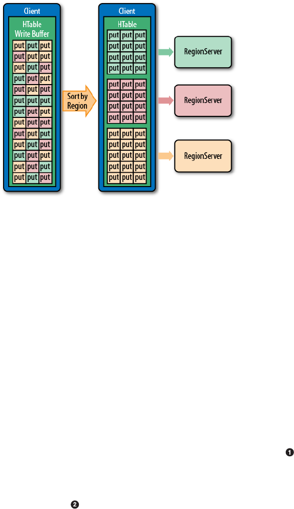
Figure 3-2. The client-side puts sorted and grouped by region serv‐
er
One note in regards to the executor pool mentioned above. It says that
it is controlled by hbase.htable.threads.max and is by default set to
Integer.MAX_VALUE, meaning unbounded. This does not mean that
each client sending buffered writes to the servers will create an end‐
less amount of worker threads. It really is creating only one thread
per region server. This scales with the number of servers you have,
but once you grow into the thousands, you could consider setting this
configuration property to some maximum, bounding it explicitly where
you need it.
Example 3-4 shows another example of how the write buffer is used
from the client API.
Example 3-4. Example using the client-side write buffer
TableName name = TableName.valueOf("testtable");
Connection connection = ConnectionFactory.createConnection(conf);
Table table = connection.getTable(name);
BufferedMutator mutator = connection.getBufferedMutator(name);
Put put1 = new Put(Bytes.toBytes("row1"));
put1.addColumn(Bytes.toBytes("colfam1"), Bytes.toBytes("qual1"),
Bytes.toBytes("val1"));
mutator.mutate(put1);
Put put2 = new Put(Bytes.toBytes("row2"));
put2.addColumn(Bytes.toBytes("colfam1"), Bytes.toBytes("qual1"),
CRUD Operations 135
www.finebook.ir
Bytes.toBytes("val2"));
mutator.mutate(put2);
Put put3 = new Put(Bytes.toBytes("row3"));
put3.addColumn(Bytes.toBytes("colfam1"), Bytes.toBytes("qual1"),
Bytes.toBytes("val3"));
mutator.mutate(put3);
Get get = new Get(Bytes.toBytes("row1"));
Result res1 = table.get(get);
System.out.println("Result: " + res1);
mutator.flush();
Result res2 = table.get(get);
System.out.println("Result: " + res2);
mutator.close();
table.close();
connection.close();
Get a mutator instance for the table.
Store some rows with columns into HBase.
Try to load previously stored row, this will print “Result:
keyvalues=NONE”.
Force a flush, this causes an RPC to occur.
Now the row is persisted and can be loaded.
This example also shows a specific behavior of the buffer that you may
not anticipate. Let’s see what it prints out when executed:
Result: keyvalues=NONE
Result: keyvalues={row1/colfam1:qual1/1426438877968/Put/vlen=4/
seqid=0}
While you have not seen the get() operation yet, you should still be
able to correctly infer what it does, that is, reading data back from the
servers. But for the first get() in the example, asking for a column
value that has had a previous matching put call, the API returns a
NONE value—what does that mean? It is caused by two facts, with the
first explained already above:
1. The client write buffer is an in-memory structure that is literally
holding back any unflushed records, in other words, nothing was
sent to the servers yet.
2. The get() call is synchronous and goes directly to the servers,
missing the client-side cached mutations.
Chapter 3: Client API: The Basics136
www.finebook.ir
You have to be aware of this percularity when designing applications
making use of the client buffering.
List of Puts
The client API has the ability to insert single Put instances as shown
earlier, but it also has the advanced feature of batching operations to‐
gether. This comes in the form of the following call:
void put(List<Put> puts) throws IOException
You will have to create a list of Put instances and hand it to this call.
Example 3-5 updates the previous example by creating a list to hold
the mutations and eventually calling the list-based put() method.
Example 3-5. Example inserting data into HBase using a list
List<Put> puts = new ArrayList<Put>();
Put put1 = new Put(Bytes.toBytes("row1"));
put1.addColumn(Bytes.toBytes("colfam1"), Bytes.toBytes("qual1"),
Bytes.toBytes("val1"));
puts.add(put1);
Put put2 = new Put(Bytes.toBytes("row2"));
put2.addColumn(Bytes.toBytes("colfam1"), Bytes.toBytes("qual1"),
Bytes.toBytes("val2"));
puts.add(put2);
Put put3 = new Put(Bytes.toBytes("row2"));
put3.addColumn(Bytes.toBytes("colfam1"), Bytes.toBytes("qual2"),
Bytes.toBytes("val3"));
puts.add(put3);
table.put(puts);
Create a list that holds the Put instances.
Add put to list.
Add another put to list.
Add third put to list.
Store multiple rows with columns into HBase.
A quick check with the HBase Shell reveals that the rows were stored
as expected. Note that the example actually modified three columns,
but in two rows only. It added two columns into the row with the key
row2, using two separate qualifiers, qual1 and qual2, creating two
uniquely named columns in the same row.
hbase(main):001:0> scan 'testtable'
ROW COLUMN+CELL
CRUD Operations 137
www.finebook.ir
row1 column=colfam1:qual1, timestamp=1426445826107,
value=val1
row2 column=colfam1:qual1, timestamp=1426445826107,
value=val2
row2 column=colfam1:qual2, timestamp=1426445826107,
value=val3
2 row(s) in 0.3300 seconds
Since you are issuing a list of row mutations to possibly many differ‐
ent rows, there is a chance that not all of them will succeed. This
could be due to a few reasons—for example, when there is an issue
with one of the region servers and the client-side retry mechanism
needs to give up because the number of retries has exceeded the con‐
figured maximum. If there is a problem with any of the put calls on
the remote servers, the error is reported back to you subsequently in
the form of an IOException.
Example 3-6 uses a bogus column family name to insert a column.
Since the client is not aware of the structure of the remote table—it
could have been altered since it was created—this check is done on
the server-side.
Example 3-6. Example inserting a faulty column family into HBase
Put put1 = new Put(Bytes.toBytes("row1"));
put1.addColumn(Bytes.toBytes("colfam1"), Bytes.toBytes("qual1"),
Bytes.toBytes("val1"));
puts.add(put1);
Put put2 = new Put(Bytes.toBytes("row2"));
put2.addColumn(Bytes.toBytes("BOGUS"), Bytes.toBytes("qual1"),
Bytes.toBytes("val2"));
puts.add(put2);
Put put3 = new Put(Bytes.toBytes("row2"));
put3.addColumn(Bytes.toBytes("colfam1"), Bytes.toBytes("qual2"),
Bytes.toBytes("val3"));
puts.add(put3);
table.put(puts);
Add put with non existent family to list.
Store multiple rows with columns into HBase.
The call to put() fails with the following (or similar) error message:
WARNING: #3, table=testtable, attempt=1/35 failed=1ops, last excep‐
tion: null \
on server-1.internal.foobar.com,65191,1426248239595, tracking \
started Sun Mar 15 20:35:52 CET 2015; not retrying 1 - final
failure
Exception in thread "main" \
org.apache.hadoop.hbase.client.RetriesExhaustedWithDetailsExcep‐
Chapter 3: Client API: The Basics138
www.finebook.ir

tion: \
Failed 1 action: \
org.apache.hadoop.hbase.regionserver.NoSuchColumnFamilyExcep‐
tion: \
Column family BOGUS does not exist in region \
testtable,,1426448152586.deecb9559bde733aa2a9fb1e6b42aa93. in
table \
'testtable', {NAME => 'colfam1', DATA_BLOCK_ENCODING => 'NONE', \
BLOOMFILTER => 'ROW', REPLICATION_SCOPE => '0', COMPRESSION =>
'NONE', \
VERSIONS => '1', TTL => 'FOREVER', MIN_VERSIONS => '0', \
KEEP_DELETED_CELLS => 'FALSE', BLOCKSIZE => '65536', \
IN_MEMORY => 'false', BLOCKCACHE => 'true'}
: 1 time,
The first three line state the request ID (#3), the table name (test
table), the attempt count (1/35) with number of failed operations
(1ops), and the last error (null), as well as the server name, and
when the asynchronous processing did start.
This is followed by the exception name, which usually is Retrie
sExhaustedWithDetailsException.
Lastly, the details of the failed operations are listed, here only
one failed (Failed 1 action) and it did so with a NoSuchColumnFami
lyException. The last line (: 1 time) lists how often it failed.
You may wonder what happened to the other, non-faulty puts in the
list. Using the shell again you should see that the two correct puts
have been applied:
hbase(main):001:0> scan 'testtable'
ROW COLUMN+CELL
row1 column=colfam1:qual1, timestamp=1426448152808,
value=val1
row2 column=colfam1:qual2, timestamp=1426448152808,
value=val3
2 row(s) in 0.3360 seconds
The servers iterate over all operations and try to apply them. The
failed ones are returned and the client reports the remote error using
the RetriesExhaustedWithDetailsException, giving you insight into
how many operations have failed, with what error, and how many
times it has retried to apply the erroneous modification. It is interest‐
ing to note that, for the bogus column family, the retry is automatical‐
ly set to 1 (see the NoSuchColumnFamilyException: 1 time), as this
is an error from which HBase cannot recover.
In addition, you can make use of the exception instance to gain access
to more details about the failed operation, and even the faulty muta‐
CRUD Operations 139
www.finebook.ir
tion itself. Example 3-7 extends the original erroneous example by in‐
troducing a special catch block to gain access to the error details.
Example 3-7. Special error handling with lists of puts
try {
table.put(puts);
} catch (RetriesExhaustedWithDetailsException e) {
int numErrors = e.getNumExceptions();
System.out.println("Number of exceptions: " + numErrors);
for (int n = 0; n < numErrors; n++) {
System.out.println("Cause[" + n + "]: " + e.getCause(n));
System.out.println("Hostname[" + n + "]: " + e.getHostname‐
Port(n));
System.out.println("Row[" + n + "]: " + e.getRow(n));
}
System.out.println("Cluster issues: " + e.mayHaveClusterIs‐
sues());
System.out.println("Description: " + e.getExhaustiveDescrip‐
tion());
}
Store multiple rows with columns into HBase.
Handle failed operations.
Gain access to the failed operation.
The output of the example looks like this (some lines are omitted for
the sake of brevity):
Mar 16, 2015 9:54:41 AM org.apache....client.AsyncProcess logNoRe‐
submit
WARNING: #3, table=testtable, attempt=1/35 failed=1ops, last excep‐
tion: \
null on srv1.foobar.com,65191,1426248239595, \
tracking started Mon Mar 16 09:54:41 CET 2015; not retrying 1 - fi‐
nal failure
Number of exceptions: 1
Cause[0]: org.apache.hadoop.hbase.regionserver.NoSuchColumnFami‐
lyException: \
org.apache.hadoop.hbase.regionserver.NoSuchColumnFamilyException:
Column \
family BOGUS does not exist in region \
testtable,,1426496081011.8be8f8bc862075e8bea355aecc6a5b16. in
table \
'testtable', {NAME => 'colfam1', DATA_BLOCK_ENCODING => 'NONE', \
BLOOMFILTER => 'ROW', REPLICATION_SCOPE => '0', COMPRESSION =>
'NONE', \
VERSIONS => '1', TTL => 'FOREVER', MIN_VERSIONS => '0', \
KEEP_DELETED_CELLS => 'FALSE', BLOCKSIZE => '65536', IN_MEMORY =>
Chapter 3: Client API: The Basics140
www.finebook.ir

'false', \
BLOCKCACHE => 'true'}
at org.apache.hadoop.hbase.regionserver.RSRpcServices.doBatch‐
Op(...)
...
Hostname[0]: srv1.foobar.com,65191,1426248239595
Row[0]: {"totalColumns":1,"families":{"BOGUS":[{ \
"timestamp":9223372036854775807,"tag":[],"qualifier":"qual1", \
"vlen":4}]},"row":"row2"}
Cluster issues: false
Description: exception from srv1.foobar.com,65191,1426248239595
for row2
org.apache.hadoop.hbase.regionserver.NoSuchColumnFamilyException:
\
org.apache.hadoop.hbase.regionserver.NoSuchColumnFamilyException: \
Column family BOGUS does not exist in region \
testtable,,1426496081011.8be8f8bc862075e8bea355aecc6a5b16. in
table '\
testtable', {NAME => 'colfam1', ... }
at org.apache.hadoop.hbase.regionserver.RSRpcServices.doBatch‐
Op(...)
...
at java.lang.Thread.run(...)
As you can see, you can ask for the number of errors incurred, the
causes, the servers reporting them, and the actual mutation(s). Here
we only have one that we triggered with the bogus column family
used. Interesting is that the exception also gives you access to the
overall cluster status to determine if there are larger problems at
play.
Table 3-11. Methods of the RetriesExhaustedWithDetailsExcep
tion class
Method Description
getCauses() Returns a summary of all causes for all failed
operations.
getExhaustiveDescription() More detailed list of all the failures that were
detected.
getNumExceptions() Returns the number of failed operations.
getCause(int i) Returns the exact cause for a given failed
operation.a
getHostnamePort(int i) Returns the exact host that reported the specific
error.a
CRUD Operations 141
www.finebook.ir

Method Description
getRow(int i) Returns the specific mutation instance that
failed.a
mayHaveClusterIssues() Allows to determine if there are wider problems
with the cluster.b
a Where i greater or equal to 0 and less than getNumExceptions().
b This is determined by all operations failing as do not retry, indicating that all servers
involved are giving up.
We already mentioned the MaxKeyValueSize parameter for the Buf
feredMutator before, and how the API ensures that you can only sub‐
mit operations that comply to that limit (if set). The same check is
done when you submit a single put, or a list of puts. In fact, there is
actually one more test done, which is that the mutation submitted is
not entirely empty. These checks are done on the client side, though,
and in the event of a violation the client is throwing an exception that
leaves the operations preceding the faulty one in the client buffer.
The list-based put() call uses the client-side write buffer—
in form of an internal instance of BatchMutator--to insert
all puts into the local buffer and then to call flush() im‐
plicitly. While inserting each instance of Put, the client
API performs the mentioned check. If it fails, for example,
at the third put out of five, the first two are added to the
buffer while the last two are not. It also then does not trig‐
ger the flush command at all. You need to keep inserting
put instances or call close() to trigger a flush of all cach‐
ed instances.
Because of this behavior of plain Table instances and their put(List)
method, it is recommended to use the BufferedMutator directly as it
has the most flexibility. If you read the HBase source code, for exam‐
ple the TableOutputFormat, you will see the same approach, that is
using the BufferedMutator for all cases a client-side write buffer is
wanted.
You need to watch out for another peculiarity using the list-based put
call: you cannot control the order in which the puts are applied on the
server-side, which implies that the order in which the servers are
called is also not under your control. Use this call with caution if you
have to guarantee a specific order—in the worst case, you need to cre‐
ate smaller batches and explicitly flush the client-side write cache to
Chapter 3: Client API: The Basics142
www.finebook.ir
enforce that they are sent to the remote servers. This also is only pos‐
sible when using the BufferedMutator class directly.
An example for updates that need to be controlled tightly are foreign
key relations, where changes to an entity are reflected in multiple
rows, or even tables. If you need to ensure a specific order these mu‐
tations are applied, you may have to batch them separately, to ensure
one batch is applied before another.
Finally, Example 3-8 shows the same example as in “Client-side Write
Buffer” (page 128) using the client-side write buffer, but using a list of
mutations, instead of separate calls to mutate(). This is akin to what
you just saw in this section for the list of puts. If you recall the ad‐
vanced usage of a Listener, you have all the tools to do the same list
based submission of mutations, but using the more flexible approach.
Example 3-8. Example using the client-side write buffer
List<Mutation> mutations = new ArrayList<Mutation>();
Put put1 = new Put(Bytes.toBytes("row1"));
put1.addColumn(Bytes.toBytes("colfam1"), Bytes.toBytes("qual1"),
Bytes.toBytes("val1"));
mutations.add(put1);
Put put2 = new Put(Bytes.toBytes("row2"));
put2.addColumn(Bytes.toBytes("colfam1"), Bytes.toBytes("qual1"),
Bytes.toBytes("val2"));
mutations.add(put2);
Put put3 = new Put(Bytes.toBytes("row3"));
put3.addColumn(Bytes.toBytes("colfam1"), Bytes.toBytes("qual1"),
Bytes.toBytes("val3"));
mutations.add(put3);
mutator.mutate(mutations);
Get get = new Get(Bytes.toBytes("row1"));
Result res1 = table.get(get);
System.out.println("Result: " + res1);
mutator.flush();
Result res2 = table.get(get);
System.out.println("Result: " + res2);
Create a list to hold all mutations.
Add Put instance to list of mutations.
Store some rows with columns into HBase.
CRUD Operations 143
www.finebook.ir

Try to load previously stored row, this will print “Result:
keyvalues=NONE”.
Force a flush, this causes an RPC to occur.
Now the row is persisted and can be loaded.
Atomic Check-and-Put
There is a special variation of the put calls that warrants its own sec‐
tion: check and put. The method signatures are:
boolean checkAndPut(byte[] row, byte[] family, byte[] qualifier,
byte[] value,
Put put) throws IOException
boolean checkAndPut(byte[] row, byte[] family, byte[] qualifier,
CompareFilter.CompareOp compareOp, byte[] value, Put put)
throws IOException
These calls allow you to issue atomic, server-side mutations that are
guarded by an accompanying check. If the check passes successfully,
the put operation is executed; otherwise, it aborts the operation com‐
pletely. It can be used to update data based on current, possibly relat‐
ed, values.
Such guarded operations are often used in systems that handle, for
example, account balances, state transitions, or data processing. The
basic principle is that you read data at one point in time and process
it. Once you are ready to write back the result, you want to make sure
that no other client has done the same already. You use the atomic
check to compare that the value is not modified and therefore apply
your value.
The first call implies that the given value has to be equal to the stored
one. The second call lets you specify the actual comparison operator
(explained in “Comparison Operators” (page 221)), which enables more
elaborate testing, for example, if the given value is equal or less than
the stored one. This is useful to track some kind of modification ID,
and you want to ensure you have reached a specific point in the cells
lifecycle, for example, when it is updated by many concurrent clients.
A special type of check can be performed using the check
AndPut() call: only update if another value is not already
present. This is achieved by setting the value parameter
to null. In that case, the operation would succeed when
the specified column is nonexistent.
Chapter 3: Client API: The Basics144
www.finebook.ir
The call returns a boolean result value, indicating whether the Put
has been applied or not, returning true or false, respectively.
Example 3-9 shows the interactions between the client and the server,
returning the expected results.
Example 3-9. Example application using the atomic compare-and-
set operations
Put put1 = new Put(Bytes.toBytes("row1"));
put1.addColumn(Bytes.toBytes("colfam1"), Bytes.toBytes("qual1"),
Bytes.toBytes("val1"));
boolean res1 = table.checkAndPut(Bytes.toBytes("row1"),
Bytes.toBytes("colfam1"), Bytes.toBytes("qual1"), null, put1);
System.out.println("Put 1a applied: " + res1);
boolean res2 = table.checkAndPut(Bytes.toBytes("row1"),
Bytes.toBytes("colfam1"), Bytes.toBytes("qual1"), null, put1);
System.out.println("Put 1b applied: " + res2);
Put put2 = new Put(Bytes.toBytes("row1"));
put2.addColumn(Bytes.toBytes("colfam1"), Bytes.toBytes("qual2"),
Bytes.toBytes("val2"));
boolean res3 = table.checkAndPut(Bytes.toBytes("row1"),
Bytes.toBytes("colfam1"), Bytes.toBytes("qual1"),
Bytes.toBytes("val1"), put2);
System.out.println("Put 2 applied: " + res3);
Put put3 = new Put(Bytes.toBytes("row2"));
put3.addColumn(Bytes.toBytes("colfam1"), Bytes.toBytes("qual1"),
Bytes.toBytes("val3"));
boolean res4 = table.checkAndPut(Bytes.toBytes("row1"),
Bytes.toBytes("colfam1"), Bytes.toBytes("qual1"),
Bytes.toBytes("val1"), put3);
System.out.println("Put 3 applied: " + res4);
Create a new Put instance.
Check if column does not exist and perform optional put
operation.
Print out the result, should be “Put 1a applied: true”.
Attempt to store same cell again.
Print out the result, should be “Put 1b applied: false” as the
column now already exists.
CRUD Operations 145
www.finebook.ir

Create another Put instance, but using a different column
qualifier.
Store new data only if the previous data has been saved.
Print out the result, should be “Put 2 applied: true” as the
checked column exists.
Create yet another Put instance, but using a different row.
Store new data while checking a different row.
We will not get here as an exception is thrown beforehand!
The output is:
Put 1a applied: true
Put 1b applied: false
Put 2 applied: true
Exception in thread "main" org.apache.hadoop.hbase.DoNotRetryIOEx‐
ception:
org.apache.hadoop.hbase.DoNotRetryIOException:
Action's getRow must match the passed row
...
The last call in the example did throw a DoNotRetryIOException error
because checkAndPut() enforces that the checked row has to match
the row of the Put instance. You are allowed to check one column and
update another, but you cannot stretch that check across row bound‐
aries.
The compare-and-set operations provided by HBase rely
on checking and modifying the same row! As with most
other operations only providing atomicity guarantees on
single rows, this also applies to this call. Trying to check
and modify two different rows will return an exception.
Compare-and-set (CAS) operations are very powerful, especially in
distributed systems, with even more decoupled client processes. In
providing these calls, HBase sets itself apart from other architectures
that give no means to reason about concurrent updates performed by
multiple, independent clients.
Get Method
The next step in a client API is to retrieve what was just saved. For
that the Table is providing you with the get() call and matching
classes. The operations are split into those that operate on a single
Chapter 3: Client API: The Basics146
www.finebook.ir
row and those that retrieve multiple rows in one call. Before we start
though, please note that we are using the Result class in passing in
the various examples provided. This class will be explained in “The
Result class” (page 159) a little later, so bear with us for the time being.
The code—and output especially—should be self-explanatory.
Single Gets
First, the method that is used to retrieve specific values from a HBase
table:
Result get(Get get) throws IOException
Similar to the Put class for the put() call, there is a matching Get
class used by the aforementioned get() function. A get() operation is
bound to one specific row, but can retrieve any number of columns
and/or cells contained therein. Therefore, as another similarity, you
will have to provide a row key when creating an instance of Get, using
one of these constructors:
Get(byte[] row)
Get(Get get)
The primary constructor of Get takes the row parameter specifying
the row you want to access, while the second constructor takes an ex‐
isting instance of Get and copies the entire details from it, effectively
cloning the instance. And, similar to the put operations, you have
methods to specify rather broad criteria to find what you are looking
for—or to specify everything down to exact coordinates for a single
cell:
Get addFamily(byte[] family)
Get addColumn(byte[] family, byte[] qualifier)
Get setTimeRange(long minStamp, long maxStamp) throws IOException
Get setTimeStamp(long timestamp)
Get setMaxVersions()
Get setMaxVersions(int maxVersions) throws IOException
The addFamily() call narrows the request down to the given column
family. It can be called multiple times to add more than one family.
The same is true for the addColumn() call. Here you can add an even
narrower address space: the specific column. Then there are methods
that let you set the exact timestamp you are looking for—or a time
range to match those cells that fall inside it.
Lastly, there are methods that allow you to specify how many versions
you want to retrieve, given that you have not set an exact timestamp.
By default, this is set to 1, meaning that the get() call returns the
most current match only. If you are in doubt, use getMaxVersions()
to check what it is set to. The setMaxVersions() without a parameter
CRUD Operations 147
www.finebook.ir
sets the number of versions to return to Integer.MAX_VALUE--which is
also the maximum number of versions you can configure in the col‐
umn family descriptor, and therefore tells the API to return every
available version of all matching cells (in other words, up to what is
set at the column family level).
As mentioned earlier, HBase provides us with a helper class named
Bytes that has many static methods to convert Java types into byte[]
arrays. It also can do the same in reverse: as you are retrieving data
from HBase—for example, one of the rows stored previously—you can
make use of these helper functions to convert the byte[] data back in‐
to Java types. Here is a short list of what it offers, continued from the
earlier discussion:
static String toString(byte[] b)
static boolean toBoolean(byte[] b)
static long toLong(byte[] bytes)
static float toFloat(byte[] bytes)
static int toInt(byte[] bytes)
...
Example 3-10 shows how this is all put together.
Example 3-10. Example application retrieving data from HBase
Configuration conf = HBaseConfiguration.create();
Connection connection = ConnectionFactory.createConnection(conf);
Table table = connection.getTable(TableName.valueOf("testta‐
ble"));
Get get = new Get(Bytes.toBytes("row1"));
get.addColumn(Bytes.toBytes("colfam1"), Bytes.toBytes("qual1"));
Result result = table.get(get);
byte[] val = result.getValue(Bytes.toBytes("colfam1"),
Bytes.toBytes("qual1"));
System.out.println("Value: " + Bytes.toString(val));
table.close();
connection.close();
Create the configuration.
Instantiate a new table reference.
Create get with specific row.
Add a column to the get.
Chapter 3: Client API: The Basics148
www.finebook.ir

Retrieve row with selected columns from HBase.
Get a specific value for the given column.
Print out the value while converting it back.
Close the table and connection instances to free resources.
If you are running this example after, say Example 3-2, you should get
this as the output:
Value: val1
The output is not very spectacular, but it shows that the basic opera‐
tion works. The example also only adds the specific column to re‐
trieve, relying on the default for maximum versions being returned set
to 1. The call to get() returns an instance of the Result class, which
you will learn about very soon in “The Result class” (page 159).
Using the Builder pattern
All of the data-related types and the majority of their add and set
methods support the fluent interface pattern, that is, all of these
methods return the instance reference and allow chaining of calls.
Example 3-11 show this in action.
Example 3-11. Creates a get request using its fluent interface
Get get = new Get(Bytes.toBytes("row1"))
.setId("GetFluentExample")
.setMaxVersions()
.setTimeStamp(1)
.addColumn(Bytes.toBytes("colfam1"), Bytes.toBytes("qual1"))
.addFamily(Bytes.toBytes("colfam2"));
Result result = table.get(get);
System.out.println("Result: " + result);
Create a new get using the fluent interface.
Example 3-11 showing the fluent interface should emit the following
on the console:
Before get call...
Cell: row1/colfam1:qual1/2/Put/vlen=4/seqid=0, Value: val1
Cell: row1/colfam1:qual1/1/Put/vlen=4/seqid=0, Value: val1
Cell: row1/colfam1:qual2/4/Put/vlen=4/seqid=0, Value: val2
Cell: row1/colfam1:qual2/3/Put/vlen=4/seqid=0, Value: val2
Cell: row1/colfam2:qual1/2/Put/vlen=4/seqid=0, Value: val1
Cell: row1/colfam2:qual1/1/Put/vlen=4/seqid=0, Value: val1
CRUD Operations 149
www.finebook.ir

Cell: row1/colfam2:qual2/4/Put/vlen=4/seqid=0, Value: val2
Cell: row1/colfam2:qual2/3/Put/vlen=4/seqid=0, Value: val2
Result: keyvalues={row1/colfam1:qual1/1/Put/vlen=4/seqid=0, row1/
colfam2:qual1/1/Put/vlen=4/seqid=0}
An interesting part of this is the result that is printed last. While the
example is adding the entire column family colfam2, it only prints a
single cell. This is caused by the setTimeStamp(1) call, which affects
all other selections. We essentially are telling the API to fetch “all
cells from column family #2 that have a timestamp equal or less than
1”.
The Get class provides additional calls, which are listed in Table 3-12
for your perusal. By now you should recognize many of them as inher‐
ited methods from the Query and Row superclasses.
Table 3-12. Quick overview of additional methods provided by the
Get class
Method Description
familySet()/getFamilyMap() These methods give you access to the column
families and specific columns, as added by the add
Family() and/or addColumn() calls. The family map
is a map where the key is the family name and the
value a list of added column qualifiers for this
particular family. The familySet() returns the Set of
all stored families, i.e., a set containing only the
family names.
getACL()/setACL() The Access Control List (ACL) for this operation. See
(to come) for details.
getAttribute()/setAttribute() Set and get arbitrary attributes associated with this
instance of Get.
getAttributesMap() Returns the entire map of attributes, if any are set.
getAuthorizations()/setAutho
rizations() Visibility labels for the operation. See (to come) for
details.
getCacheBlocks()/setCache
Blocks() Specify if the server-side cache should retain blocks
that were loaded for this operation.
setCheckExistenceOnly()/is
CheckExistenceOnly() Only check for existence of data, but do not return
any of it.
setClosestRowBefore()/isClo
sestRowBefore() Return all the data for the row that matches the
given row key exactly, or the one that immediately
precedes it.
getConsistency()/setConsisten
cy() The consistency level that applies to the current
query instance.
getFilter()/setFilter() The filters that apply to the retrieval operation. See
“Filters” (page 219) for details.
Chapter 3: Client API: The Basics150
www.finebook.ir

Method Description
getFingerprint() Compiles details about the instance into a map for
debugging, or logging.
getId()/setId() An ID for the operation, useful for identifying the
origin of a request later.
getIsolationLevel()/setIsola
tionLevel() Specifies the read isolation level for the operation.
getMaxResultsPerColumnFami
ly()/setMaxResultsPerColumn
Family()
Limit the number of cells returned per family.
getMaxVersions()/setMaxVer
sions() Override the column family setting specifying how
many versions of a column to retrieve.
getReplicaId()/setReplicaId() Gives access to the replica ID that should serve the
data.
getRow() Returns the row key as specified when creating the
Get instance.
getRowOffsetPerColumnFami
ly()/setRowOffsetPerColumnFam
ily()
Number of cells to skip when reading a row.
getTimeRange()/setTimeRange() Retrieve or set the associated timestamp or time
range of the Get instance.
setTimeStamp() Sets a specific timestamp for the query. Retrieve
with getTimeRange().a
numFamilies() Retrieves the size of the family map, containing the
families added using the addFamily() or addCol
umn() calls.
hasFamilies() Another helper to check if a family—or column—has
been added to the current instance of the Get class.
toJSON()/toJSON(int) Converts the first 5 or N columns into a JSON
format.
toMap()/toMap(int) Converts the first 5 or N columns into a map. This is
more detailed than what getFingerprint() returns.
toString()/toString(int) Converts the first 5 or N columns into a JSON, or
map (if JSON fails due to encoding problems).
a The API converts a value assigned with setTimeStamp() into a TimeRange instance
internally, setting it to the given timestamp and timestamp + 1, respectively.
CRUD Operations 151
www.finebook.ir

The getters listed in Table 3-12 for the Get class only re‐
trieve what you have set beforehand. They are rarely used,
and make sense only when you, for example, prepare a
Get instance in a private method in your code, and inspect
the values in another place or for unit testing.
The list of methods is long indeed, and while you have seen the inher‐
ited ones before, there are quite a few specific ones for Get that war‐
rant a longer explanation. In order, we start with setCacheBlocks()
and getCacheBlocks(), which controls how the read operation is han‐
dled on the server-side. Each HBase region server has a block cache
that efficiently retains recently accessed data for subsequent reads of
contiguous information. In some events it is better to not engage the
cache to avoid too much churn when doing completely random gets.
Instead of polluting the block cache with blocks of unrelated data, it is
better to skip caching these blocks and leave the cache undisturbed
for other clients that perform reading of related, co-located data.
The setCheckExistenceOnly() and isCheckExistenceOnly() combi‐
nation allows the client to check if a specific set of columns, or column
families are already existent. The Example 3-12 shows this in action.
Example 3-12. Checks for the existence of specific data
List<Put> puts = new ArrayList<Put>();
Put put1 = new Put(Bytes.toBytes("row1"));
put1.addColumn(Bytes.toBytes("colfam1"), Bytes.toBytes("qual1"),
Bytes.toBytes("val1"));
puts.add(put1);
Put put2 = new Put(Bytes.toBytes("row2"));
put2.addColumn(Bytes.toBytes("colfam1"), Bytes.toBytes("qual1"),
Bytes.toBytes("val2"));
puts.add(put2);
Put put3 = new Put(Bytes.toBytes("row2"));
put3.addColumn(Bytes.toBytes("colfam1"), Bytes.toBytes("qual2"),
Bytes.toBytes("val3"));
puts.add(put3);
table.put(puts);
Get get1 = new Get(Bytes.toBytes("row2"));
get1.addColumn(Bytes.toBytes("colfam1"), Bytes.toBytes("qual1"));
get1.setCheckExistenceOnly(true);
Result result1 = table.get(get1);
byte[] val = result1.getValue(Bytes.toBytes("colfam1"),
Bytes.toBytes("qual1"));
System.out.println("Get 1 Exists: " + result1.getExists());
Chapter 3: Client API: The Basics152
www.finebook.ir
System.out.println("Get 1 Size: " + result1.size());
System.out.println("Get 1 Value: " + Bytes.toString(val));
Get get2 = new Get(Bytes.toBytes("row2"));
get2.addFamily(Bytes.toBytes("colfam1"));
get2.setCheckExistenceOnly(true);
Result result2 = table.get(get2);
System.out.println("Get 2 Exists: " + result2.getExists());
System.out.println("Get 2 Size: " + result2.size());
Get get3 = new Get(Bytes.toBytes("row2"));
get3.addColumn(Bytes.toBytes("colfam1"), Bytes.to‐
Bytes("qual9999"));
get3.setCheckExistenceOnly(true);
Result result3 = table.get(get3);
System.out.println("Get 3 Exists: " + result3.getExists());
System.out.println("Get 3 Size: " + result3.size());
Get get4 = new Get(Bytes.toBytes("row2"));
get4.addColumn(Bytes.toBytes("colfam1"), Bytes.to‐
Bytes("qual9999"));
get4.addColumn(Bytes.toBytes("colfam1"), Bytes.toBytes("qual1"));
get4.setCheckExistenceOnly(true);
Result result4 = table.get(get4);
System.out.println("Get 4 Exists: " + result4.getExists());
System.out.println("Get 4 Size: " + result4.size());
Insert two rows into the table.
Check first with existing data.
Exists is “true”, while no cel was actually returned.
Check for an entire family to exist.
Check for a non-existent column.
Check for an existent, and non-existent column.
Exists is “true” because some data exists.
When executing this example, the output should read like the follow‐
ing:
Get 1 Exists: true
Get 1 Size: 0
Get 1 Value: null
Get 2 Exists: true
Get 2 Size: 0
Get 3 Exists: false
Get 3 Size: 0
CRUD Operations 153
www.finebook.ir

Get 4 Exists: true
Get 4 Size: 0
The one peculiar result is the last, you will be returned true for any of
the checks you added returning true. In the example we tested a col‐
umn that exists, and one that does not. Since one does, the entire
check returns positive. In other words, make sure you test very specif‐
ically for what you are looking for. You may have to issue multiple get
request (batched preferably) to test the exact coordinates you want to
verify.
Alternative checks for existence
The Table class has another way of checking for the existence of
data in a table, provided by these methods:
boolean exists(Get get) throws IOException
boolean[] existsAll(List<Get> gets) throws IOException;
You can set up a Get instance, just like you do when using the
get() calls of Table. Instead of having to retrieve the cells from
the remote servers, just to verify that something exists, you can
employ these calls because they only return a boolean flag. In
fact, these calls are just shorthand for using Get.setCheckExis
tenceOnly(true) on the included Get instance(s).
Using Table.exists(), Table.existsAll(), or
Get.setCheckExistenceOnly() involves the same lookup
semantics on the region servers, including loading file
blocks to check if a row or column actually exists. You only
avoid shipping the data over the network—but that is very
useful if you are checking very large columns, or do so
very frequently. Consider using Bloom filters to speed up
this process (see (to come)).
We move on to setClosestRowBefore() and isClosestRowBefore(),
offering some sort of fuzzy matching for rows. Presume you have a
complex row key design, employing compound data comprised of
many separate fields (see (to come)). You can only match data from
left to right in the row key, so again presume you have some leading
fields, but not more specific ones. You can ask for a specific row using
get(), but what if the requested row key is too specific and does not
exist? Without jumping the gun, you could start using a scan opera‐
tion, explained in “Scans” (page 193). For one of get calls you can in‐
Chapter 3: Client API: The Basics154
www.finebook.ir

stead use the setClosestRowBefore() method, setting this functional‐
ity to true. Example 3-13 shows the result:
Example 3-13. Retrieves a row close to the requested, if necessary
Get get1 = new Get(Bytes.toBytes("row3"));
get1.addColumn(Bytes.toBytes("colfam1"), Bytes.toBytes("qual1"));
Result result1 = table.get(get1);
System.out.println("Get 1 isEmpty: " + result1.isEmpty());
CellScanner scanner1 = result1.cellScanner();
while (scanner1.advance()) {
System.out.println("Get 1 Cell: " + scanner1.current());
}
Get get2 = new Get(Bytes.toBytes("row3"));
get2.addColumn(Bytes.toBytes("colfam1"), Bytes.toBytes("qual1"));
get2.setClosestRowBefore(true);
Result result2 = table.get(get2);
System.out.println("Get 2 isEmpty: " + result2.isEmpty());
CellScanner scanner2 = result2.cellScanner();
while (scanner2.advance()) {
System.out.println("Get 2 Cell: " + scanner2.current());
}
Get get3 = new Get(Bytes.toBytes("row2"));
get3.addColumn(Bytes.toBytes("colfam1"), Bytes.toBytes("qual1"));
get3.setClosestRowBefore(true);
Result result3 = table.get(get3);
System.out.println("Get 3 isEmpty: " + result3.isEmpty());
CellScanner scanner3 = result3.cellScanner();
while (scanner3.advance()) {
System.out.println("Get 3 Cell: " + scanner3.current());
}
Get get4 = new Get(Bytes.toBytes("row2"));
get4.addColumn(Bytes.toBytes("colfam1"), Bytes.toBytes("qual1"));
Result result4 = table.get(get4);
System.out.println("Get 4 isEmpty: " + result4.isEmpty());
CellScanner scanner4 = result4.cellScanner();
while (scanner4.advance()) {
System.out.println("Get 4 Cell: " + scanner4.current());
}
Attempt to read a row that does not exist.
Instruct the get() call to fall back to the previous row, if
necessary.
CRUD Operations 155
www.finebook.ir

Attempt to read a row that exists.
Read exactly a row that exists.
The output is interesting again:
Get 1 isEmpty: true
Get 2 isEmpty: false
Get 2 Cell: row2/colfam1:qual1/1426587567787/Put/vlen=4/seqid=0
Get 2 Cell: row2/colfam1:qual2/1426587567787/Put/vlen=4/seqid=0
Get 3 isEmpty: false
Get 3 Cell: row2/colfam1:qual1/1426587567787/Put/vlen=4/seqid=0
Get 3 Cell: row2/colfam1:qual2/1426587567787/Put/vlen=4/seqid=0
Get 4 isEmpty: false
Get 4 Cell: row2/colfam1:qual1/1426587567787/Put/vlen=4/seqid=0
The first call using the default Get instance fails to retrieve anything,
as it asks for a row that does not exist (row3, we assume the same two
rows exist from the previous example). The second adds a setCloses
tRowBefore(true) instruction to match the row exactly, or the closest
one sorted before the given row key. This, in our example, is row2,
shown to work as expected. What is surprising though is that the en‐
tire row is returned, not the specific column we asked for.
This is extended in get #3, which now reads the existing row2, but still
leaves the fuzzy matching on. We again get the entire row back, not
just the columns we asked for. In get #4 we remove the setCloses
tRowBefore(true) and get exactly what we expect, that is only the
column we have selected.
Finally, we will look at four methods in a row: getMaxResultsPerCo
lumnFamily(), setMaxResultsPerColumnFamily(), getRowOffsetPer
ColumnFamily(), and setRowOffsetPerColumnFamily(), as they all
work in tandem to allow the client to page through a wide row. The
former pair handles the maximum amount of cells returned by a get
request. The latter pair then sets an optional offset into the row.
Example 3-14 shows this as simple as possible.
Example 3-14. Retrieves parts of a row with offset and limit
Put put = new Put(Bytes.toBytes("row1"));
for (int n = 1; n <= 1000; n++) {
String num = String.format("%04d", n);
put.addColumn(Bytes.toBytes("colfam1"), Bytes.toBytes("qual" +
num),
Bytes.toBytes("val" + num));
}
table.put(put);
Get get1 = new Get(Bytes.toBytes("row1"));
get1.setMaxResultsPerColumnFamily(10);
Chapter 3: Client API: The Basics156
www.finebook.ir

Result result1 = table.get(get1);
CellScanner scanner1 = result1.cellScanner();
while (scanner1.advance()) {
System.out.println("Get 1 Cell: " + scanner1.current());
}
Get get2 = new Get(Bytes.toBytes("row1"));
get2.setMaxResultsPerColumnFamily(10);
get2.setRowOffsetPerColumnFamily(100);
Result result2 = table.get(get2);
CellScanner scanner2 = result2.cellScanner();
while (scanner2.advance()) {
System.out.println("Get 2 Cell: " + scanner2.current());
}
Ask for ten cells to be returned at most.
In addition, also skip the first 100 cells.
The output in abbreviated form:
Get 1 Cell: row1/colfam1:qual0001/1426592168066/Put/vlen=7/seqid=0
Get 1 Cell: row1/colfam1:qual0002/1426592168066/Put/vlen=7/seqid=0
...
Get 1 Cell: row1/colfam1:qual0009/1426592168066/Put/vlen=7/seqid=0
Get 1 Cell: row1/colfam1:qual0010/1426592168066/Put/vlen=7/seqid=0
Get 2 Cell: row1/colfam1:qual0101/1426592168066/Put/vlen=7/seqid=0
Get 2 Cell: row1/colfam1:qual0102/1426592168066/Put/vlen=7/seqid=0
...
Get 2 Cell: row1/colfam1:qual0109/1426592168066/Put/vlen=7/seqid=0
Get 2 Cell: row1/colfam1:qual0110/1426592168066/Put/vlen=7/seqid=0
This, on first sight, seems to make sense, we get ten columns (cells)
returned from column 1 to 10. For get #2 we get the same but skip
the first 100 columns, starting at 101 to 110. But that is not exactly
how these get options work, they really work on cells, not columns.
Example 3-15 extends the previous example to write each column
three times, creating three cells—or versions—for each.
Example 3-15. Retrieves parts of a row with offset and limit #2
for (int version = 1; version <= 3; version++) {
Put put = new Put(Bytes.toBytes("row1"));
for (int n = 1; n <= 1000; n++) {
String num = String.format("%04d", n);
put.addColumn(Bytes.toBytes("colfam1"), Bytes.toBytes("qual"
+ num),
Bytes.toBytes("val" + num));
}
System.out.println("Writing version: " + version);
table.put(put);
CRUD Operations 157
www.finebook.ir

Thread.currentThread().sleep(1000);
}
Get get0 = new Get(Bytes.toBytes("row1"));
get0.addColumn(Bytes.toBytes("colfam1"), Bytes.to‐
Bytes("qual0001"));
get0.setMaxVersions();
Result result0 = table.get(get0);
CellScanner scanner0 = result0.cellScanner();
while (scanner0.advance()) {
System.out.println("Get 0 Cell: " + scanner0.current());
}
Get get1 = new Get(Bytes.toBytes("row1"));
get1.setMaxResultsPerColumnFamily(10);
Result result1 = table.get(get1);
CellScanner scanner1 = result1.cellScanner();
while (scanner1.advance()) {
System.out.println("Get 1 Cell: " + scanner1.current());
}
Get get2 = new Get(Bytes.toBytes("row1"));
get2.setMaxResultsPerColumnFamily(10);
get2.setMaxVersions(3);
Result result2 = table.get(get2);
CellScanner scanner2 = result2.cellScanner();
while (scanner2.advance()) {
System.out.println("Get 2 Cell: " + scanner2.current());
}
Insert three versions of each column.
Get a column with all versions as a test.
Get ten cells, single version per column.
Do the same but now retrieve all versions of a column.
The output, in abbreviated form again:
Writing version: 1
Writing version: 2
Writing version: 3
Get 0 Cell: row1/colfam1:qual0001/1426592660030/Put/vlen=7/seqid=0
Get 0 Cell: row1/colfam1:qual0001/1426592658911/Put/vlen=7/seqid=0
Get 0 Cell: row1/colfam1:qual0001/1426592657785/Put/vlen=7/seqid=0
Get 1 Cell: row1/colfam1:qual0001/1426592660030/Put/vlen=7/seqid=0
Get 1 Cell: row1/colfam1:qual0002/1426592660030/Put/vlen=7/seqid=0
...
Get 1 Cell: row1/colfam1:qual0009/1426592660030/Put/vlen=7/seqid=0
Get 1 Cell: row1/colfam1:qual0010/1426592660030/Put/vlen=7/seqid=0
Chapter 3: Client API: The Basics158
www.finebook.ir
Get 2 Cell: row1/colfam1:qual0001/1426592660030/Put/vlen=7/seqid=0
Get 2 Cell: row1/colfam1:qual0001/1426592658911/Put/vlen=7/seqid=0
Get 2 Cell: row1/colfam1:qual0001/1426592657785/Put/vlen=7/seqid=0
Get 2 Cell: row1/colfam1:qual0002/1426592660030/Put/vlen=7/seqid=0
Get 2 Cell: row1/colfam1:qual0002/1426592658911/Put/vlen=7/seqid=0
Get 2 Cell: row1/colfam1:qual0002/1426592657785/Put/vlen=7/seqid=0
Get 2 Cell: row1/colfam1:qual0003/1426592660030/Put/vlen=7/seqid=0
Get 2 Cell: row1/colfam1:qual0003/1426592658911/Put/vlen=7/seqid=0
Get 2 Cell: row1/colfam1:qual0003/1426592657785/Put/vlen=7/seqid=0
Get 2 Cell: row1/colfam1:qual0004/1426592660030/Put/vlen=7/seqid=0
If we iterate over the same data, we get the same result (get #1 does
that). But as soon as we instruct the servers to return all versions, the
results change. We added a Get.setMaxVersions(3) (we could have
used setMaxVersions() without a parameter as well) and therefore
now iterate over all cells, reflected in what get #2 shows. We still get
ten cells back, but this time from column 1 to 4 only, with all versions
of the columns in between.
Be wary when using these get parameters, you might not get what you
expected initially. But they behave as designed, and it is up to the cli‐
ent application and the accompanying table schema to end up with
the proper results.
The Result class
The above examples implicitly show you that when you retrieve data
using the get() calls, you receive an instance of the Result class that
contains all the matching cells. It provides you with the means to ac‐
cess everything that was returned from the server for the given row
and matching the specified query, such as column family, column
qualifier, timestamp, and so on.
There are utility methods you can use to ask for specific results—just
as Example 3-10 used earlier—using more concrete dimensions. If you
have, for example, asked the server to return all columns of one spe‐
cific column family, you can now ask for specific columns within that
family. In other words, you need to call get() with just enough con‐
crete information to be able to process the matching data on the client
side. The first set of functions provided are:
byte[] getRow()
byte[] getValue(byte[] family, byte[] qualifier)
byte[] value()
ByteBuffer getValueAsByteBuffer(byte[] family, byte[] qualifier)
ByteBuffer getValueAsByteBuffer(byte[] family, int foffset, int
flength,
byte[] qualifier, int qoffset, int qlength)
boolean loadValue(byte[] family, byte[] qualifier, ByteBuffer dst)
throws BufferOverflowException
CRUD Operations 159
www.finebook.ir

11. Be wary as this might change in future versions.
boolean loadValue(byte[] family, int foffset, int flength, byte[]
qualifier,
int qoffset, int qlength, ByteBuffer dst) throws BufferOverflo‐
wException
CellScanner cellScanner()
Cell[] rawCells()
List<Cell> listCells()
boolean isEmpty()
int size()
You saw getRow() before: it returns the row key, as specified, for ex‐
ample, when creating the instance of the Get class used in the get()
call providing the current instance of Result. size() is returning the
number of Cell instances the server has returned. You may use this
call—or isEmpty(), which checks if size() returns a number greater
than zero—to check in your own client code if the retrieval call re‐
turned any matches.
The getValue() call allows you to get the data for a specific cell that
was returned to you. As you cannot specify what timestamp—in other
words, version—you want, you get the newest one. The value() call
makes this even easier by returning the data for the newest cell in the
first column found. Since columns are also sorted lexicographically on
the server, this would return the value of the column with the column
name (including family and qualifier) sorted first.
Some of the methods to return data clone the underlying
byte array so that no modification is possible. Yet others
do not and you have to take care not to modify the re‐
turned arrays—for your own sake.
The following methods do clone (which means they create
a copy of the byte array) the data before returning it to
the caller: getRow(), getValue(), value(), getMap(), get
NoVersionMap(), and getFamilyMap().11
There is another set of accessors for the value of available cells,
namely getValueAsByteBuffer() and loadValue(). They either cre‐
ate a new Java ByteBuffer, wrapping the byte array with the value, or
copy the data into a provided one respectively. You may wonder why
you have to provide the column family and qualifier name as a byte ar‐
ray plus specifying an offset and length into each of the arrays. The
assumption is that you may have a more complex array that holds all
Chapter 3: Client API: The Basics160
www.finebook.ir

of the data needed. In this case you can set the family and qualifier
parameter to the very same array, just pointing the respective offset
and length to where in the larger array the family and qualifier are
stored.
Access to the raw, low-level Cell instances is provided by the raw
Cells() method, returning the array of Cell instances backing the
current Result instance. The listCells() call simply converts the ar‐
ray returned by raw() into a List instance, giving you convenience by
providing iterator access, for example. The created list is backed by
the original array of KeyValue instances. The Result class also imple‐
ments the already discussed CellScannable interface, so you can iter‐
ate over the contained cells directly. The examples in the “Get Meth‐
od” (page 146) show this in action, for instance, Example 3-13.
The array of cells returned by, for example, rawCells() is
already lexicographically sorted, taking the full coordi‐
nates of the Cell instances into account. So it is sorted
first by column family, then within each family by qualifi‐
er, then by timestamp, and finally by type.
Another set of accessors is provided which are more column-oriented:
List<Cell> getColumnCells(byte[] family, byte[] qualifier)
Cell getColumnLatestCell(byte[] family, byte[] qualifier)
Cell getColumnLatestCell(byte[] family, int foffset, int flength,
byte[] qualifier, int qoffset, int qlength)
boolean containsColumn(byte[] family, byte[] qualifier)
boolean containsColumn(byte[] family, int foffset, int flength,
byte[] qualifier, int qoffset, int qlength)
boolean containsEmptyColumn(byte[] family, byte[] qualifier)
boolean containsEmptyColumn(byte[] family, int foffset, int
flength,
byte[] qualifier, int qoffset, int qlength)
boolean containsNonEmptyColumn(byte[] family, byte[] qualifier)
boolean containsNonEmptyColumn(byte[] family, int foffset, int
flength,
byte[] qualifier, int qoffset, int qlength)
By means of the getColumnCells() method you ask for multiple val‐
ues of a specific column, which solves the issue pointed out earlier,
that is, how to get multiple versions of a given column. The number
returned obviously is bound to the maximum number of versions you
have specified when configuring the Get instance, before the call to
get(), with the default being set to 1. In other words, the returned list
contains zero (in case the column has no value for the given row) or
CRUD Operations 161
www.finebook.ir

one entry, which is the newest version of the value. If you have speci‐
fied a value greater than the default of 1 version to be returned, it
could be any number, up to the specified maximum (see Example 3-15
for an example).
The getColumnLatestCell() methods are returning the newest cell of
the specified column, but in contrast to getValue(), they do not re‐
turn the raw byte array of the value but the full Cell instance instead.
This may be useful when you need more than just the value data. The
two variants only differ in one being more convenient when you have
two separate arrays only containing the family and qualifier names.
Otherwise you can use the second version that gives you access to the
already explained offset and length parameters.
The containsColumn() is a convenience method to check if there was
any cell returned in the specified column. Again, this comes in two
variants for convenience. There are two more pairs of functions for
this check, containsEmptyColumn() and containsNonEmptyCol
umns(). They do not only check that there is a cell for a specific col‐
umn, but also if that cell has no value data (it is empty) or has value
data (it is not empty). All of these contains checks internally use the
getColumnLatestCell() call to get the newest version of a column
cell, and then perform the check.
These methods all support the fact that the qualifier can
be left unspecified—setting it to null--and therefore
matching the special column with no name.
Using no qualifier means that there is no label to the col‐
umn. When looking at the table from, for example, the
HBase Shell, you need to know what it contains. A rare
case where you might want to consider using the empty
qualifier is in column families that only ever contain a sin‐
gle column. Then the family name might indicate its pur‐
pose.
There is a third set of methods that provide access to the returned da‐
ta from the get request. These are map-oriented and look like this:
NavigableMap<byte[], NavigableMap<byte[],
NavigableMap<Long, byte[]>>> getMap()
NavigableMap<byte[], NavigableMap<byte[], byte[]>> getNoVersion‐
Map()
NavigableMap<byte[], byte[]> getFamilyMap(byte[] family)
Chapter 3: Client API: The Basics162
www.finebook.ir

The most generic call, named getMap(), returns the entire result set
in a Java Map class instance that you can iterate over to access all the
values. This is different from accessing the raw cells, since here you
get only the data in a map, not any accessors or other internal infor‐
mation of the cells. The map is organized as such: family → qualifi
er → values. The getNoVersionMap() does the same while only in‐
cluding the latest cell for each column. Finally, the getFamilyMap()
lets you select the data for a specific column family only—but includ‐
ing all versions, if specified during the get call.
Use whichever access method of Result matches your access pattern;
the data has already been moved across the network from the server
to your client process, so it is not incurring any other performance or
resource penalties.
Finally, there are a few more methods provided, that do not fit into
the above groups
Table 3-13. Additional methods provided by Result
Method Description
create() There is a set of these static methods to help create Result
instances if necessary.
copyFrom() Helper method to copy a reference of the list of cells from one
instance to another.
compareResults() Static method, does a deep compare of two instance, down to
the byte arrays.
getExists()/setEx
ists() Optionally used to check for existence of cells only. See
Example 3-12 for an example.
getTotalSizeOf
Cells() Static method, summarizes the estimated heap size of all
contained cells. Uses Cell.heapSize() for each contained cell.
isStale() Indicates if the result was served by a region replica, not the
main one.
addResults()/get
Stats() This is used to return region statistics, if enabled (default is
false).
toString() Dump the content of an instance for logging or debugging. See
“Dump the Contents” (page 163).
Dump the Contents
All Java objects have a toString() method, which, when overrid‐
den by a class, can be used to convert the data of an instance into
a text representation. This is not for serialization purposes, but is
most often used for debugging.
CRUD Operations 163
www.finebook.ir

The Result class has such an implementation of toString(),
dumping the result of a read call as a string. Example 3-16 shows
a brief snippet on how it is used.
Example 3-16. Retrieve results from server and dump content
Get get = new Get(Bytes.toBytes("row1"));
Result result1 = table.get(get);
System.out.println(result1);
Result result2 = Result.EMPTY_RESULT;
System.out.println(result2);
result2.copyFrom(result1);
System.out.println(result2);
The output looks like this:
keyvalues={row1/colfam1:qual1/1426669424163/Put/vlen=4/seqid=0,
row1/colfam1:qual2/1426669424163/Put/vlen=4/seqid=0}
It simply prints all contained Cell instances, that is, calling
Cell.toString() respectively. If the Result instance is empty,
the output will be:
keyvalues=NONE
This indicates that there were no Cell instances returned. The
code examples in this book make use of the toString() method to
quickly print the results of previous read operations.
There is also a Result.EMPTY_RESULT field available, that returns a
shared and final instance of Result that is empty. This might be useful
when you need to return an empty result from for client code to, for
example, a higher level caller.
Chapter 3: Client API: The Basics164
www.finebook.ir

As of this writing, the shared EMPTY_RESULT is not read-
only, which means if you modify it, then the shared in‐
stance is modified for any other user of this instance. For
example:
Result result2 = Result.EMPTY_RESULT;
System.out.println(result2);
result2.copyFrom(result1);
System.out.println(result2);
Assuming we have the same result1 as shown in
Example 3-16 earlier, you get this:
keyvalues=NONE
keyvalues={row1/colfam1:qual1/1426672899223/Put/vlen=4/
seqid=0,
row1/colfam1:qual2/1426672899223/Put/vlen=4/
seqid=0}
Be careful!
List of Gets
Another similarity to the put() calls is that you can ask for more than
one row using a single request. This allows you to quickly and effi‐
ciently retrieve related—but also completely random, if required—da‐
ta from the remote servers.
As shown in Figure 3-2, the request may actually go to
more than one server, but for all intents and purposes, it
looks like a single call from the client code.
The method provided by the API has the following signature:
Result[] get(List<Get> gets) throws IOException
Using this call is straightforward, with the same approach as seen ear‐
lier: you need to create a list that holds all instances of the Get class
you have prepared. This list is handed into the call and you will be re‐
turned an array of equal size holding the matching Result instances.
Example 3-17 brings this together, showing two different approaches
to accessing the data.
CRUD Operations 165
www.finebook.ir

Example 3-17. Example of retrieving data from HBase using lists of
Get instances
byte[] cf1 = Bytes.toBytes("colfam1");
byte[] qf1 = Bytes.toBytes("qual1");
byte[] qf2 = Bytes.toBytes("qual2");
byte[] row1 = Bytes.toBytes("row1");
byte[] row2 = Bytes.toBytes("row2");
List<Get> gets = new ArrayList<Get>();
Get get1 = new Get(row1);
get1.addColumn(cf1, qf1);
gets.add(get1);
Get get2 = new Get(row2);
get2.addColumn(cf1, qf1);
gets.add(get2);
Get get3 = new Get(row2);
get3.addColumn(cf1, qf2);
gets.add(get3);
Result[] results = table.get(gets);
System.out.println("First iteration...");
for (Result result : results) {
String row = Bytes.toString(result.getRow());
System.out.print("Row: " + row + " ");
byte[] val = null;
if (result.containsColumn(cf1, qf1)) {
val = result.getValue(cf1, qf1);
System.out.println("Value: " + Bytes.toString(val));
}
if (result.containsColumn(cf1, qf2)) {
val = result.getValue(cf1, qf2);
System.out.println("Value: " + Bytes.toString(val));
}
}
System.out.println("Second iteration...");
for (Result result : results) {
for (Cell cell : result.listCells()) {
System.out.println(
"Row: " + Bytes.toString(
cell.getRowArray(), cell.getRowOffset(), cell.getRowL‐
ength()) +
" Value: " + Bytes.toString(CellUtil.cloneValue(cell)));
}
}
System.out.println("Third iteration...");
Chapter 3: Client API: The Basics166
www.finebook.ir

for (Result result : results) {
System.out.println(result);
}
Prepare commonly used byte arrays.
Create a list that holds the Get instances.
Add the Get instances to the list.
Retrieve rows with selected columns from HBase.
Iterate over results and check what values are available.
Iterate over results again, printing out all values.
Two different ways to access the cell data.
Assuming that you execute Example 3-5 just before you run
Example 3-17, you should see something like this on the command
line:
First iteration...
Row: row1 Value: val1
Row: row2 Value: val2
Row: row2 Value: val3
Second iteration...
Row: row1 Value: val1
Row: row2 Value: val2
Row: row2 Value: val3
Third iteration...
keyvalues={row1/colfam1:qual1/1426678215864/Put/vlen=4/seqid=0}
keyvalues={row2/colfam1:qual1/1426678215864/Put/vlen=4/seqid=0}
keyvalues={row2/colfam1:qual2/1426678215864/Put/vlen=4/seqid=0}
All iterations return the same values, showing that you have a number
of choices on how to access them, once you have received the results.
What you have not yet seen is how errors are reported back to you.
This differs from what you learned in “List of Puts” (page 137). The
get() call either returns the said array, matching the same size as the
given list by the gets parameter, or throws an exception.
Example 3-18 showcases this behavior.
Example 3-18. Example trying to read an erroneous column family
List<Get> gets = new ArrayList<Get>();
Get get1 = new Get(row1);
get1.addColumn(cf1, qf1);
gets.add(get1);
Get get2 = new Get(row2);
get2.addColumn(cf1, qf1);
gets.add(get2);
CRUD Operations 167
www.finebook.ir
Get get3 = new Get(row2);
get3.addColumn(cf1, qf2);
gets.add(get3);
Get get4 = new Get(row2);
get4.addColumn(Bytes.toBytes("BOGUS"), qf2);
gets.add(get4);
Result[] results = table.get(gets);
System.out.println("Result count: " + results.length);
Add the Get instances to the list.
Add the bogus column family get.
An exception is thrown and the process is aborted.
This line will never reached!
Executing this example will abort the entire get() operation, throw‐
ing the following (or similar) error, and not returning a result at all:
org.apache.hadoop.hbase.client.RetriesExhaustedWithDetailsExcep‐
tion:
Failed 1 action: NoSuchColumnFamilyException: 1 time,
servers with issues: 10.0.0.57:51640,
Exception in thread "main" \
org.apache.hadoop.hbase.client.RetriesExhaustedWithDetailsExcep‐
tion: \
Failed 1 action: \
org.apache.hadoop.hbase.regionserver.NoSuchColumnFamilyExcep‐
tion: \
Column family BOGUS does not exist in region \
testtable,,1426678215640.de657eebc8e3422376e918ed77fc33ba. \
in table 'testtable', {NAME => 'colfam1', ...}
at org.apache.hadoop.hbase.regionserver.HRegion.checkFami‐
ly(...)
at org.apache.hadoop.hbase.regionserver.HRegion.get(...)
...
One way to have more control over how the API handles partial faults
is to use the batch() operations discussed in “Batch Operations”
(page 187).
Delete Method
You are now able to create, read, and update data in HBase tables.
What is left is the ability to delete from it. And surely you may have
guessed by now that the Table provides you with a method of exactly
Chapter 3: Client API: The Basics168
www.finebook.ir
that name, along with a matching class aptly named Delete. Again
you have a few variants, one that takes a single delete, one that ac‐
cepts a list of deletes, and another that provides an atomic, server-
side check-and-delete. The following discusses them in that order.
Single Deletes
The variant of the delete() call that takes a single Delete instance is:
void delete(Delete delete) throws IOException
Just as with the get() and put() calls you saw already, you will have
to create a Delete instance and then add details about the data you
want to remove. The constructors are:
Delete(byte[] row)
Delete(byte[] row, long timestamp)
Delete(final byte[] rowArray, final int rowOffset, final int row‐
Length)
Delete(final byte[] rowArray, final int rowOffset, final int row‐
Length,
long ts)
Delete(final Delete d)
You need to provide the row you want to modify, and—optionally—a
specific version/timestamp to operate on. There are other variants to
create a Delete instance, where the next two do the same as the al‐
ready described first pair, with the difference that they allow you to
pass in a larger array, with accompanying offset and length parame‐
ter. The final variant allows you to hand in an existing delete instance
and copy all parameters from it.
Otherwise, you would be wise to narrow down what you want to re‐
move from the given row, using one of the following methods:
Delete addFamily(final byte[] family)
Delete addFamily(final byte[] family, final long timestamp)
Delete addFamilyVersion(final byte[] family, final long timestamp)
Delete addColumns(final byte[] family, final byte[] qualifier)
Delete addColumns(final byte[] family, final byte[] qualifier,
final long timestamp)
Delete addColumn(final byte[] family, final byte[] qualifier)
Delete addColumn(byte[] family, byte[] qualifier, long timestamp)
void setTimestamp(long timestamp)
You do have a choice to narrow in on what to remove using four types
of calls. First, you can use the addFamily() methods to remove an en‐
tire column family, including all contained columns. The next type is
addColumns(), which operates on exactly one column. The third type
is similar, using addColumn(). It also operates on a specific, given col‐
CRUD Operations 169
www.finebook.ir

umn only, but deletes either the most current or the specified version,
that is, the one with the matching timestamp.
Finally, there is setTimestamp(), and it allows you to set a timestamp
that is used for every subsequent addXYZ() call. In fact, using a De
lete constructor that takes an explicit timestamp parameter is just
shorthand to calling setTimestamp() just after creating the instance.
Once an instance wide timestamp is set, all further operations will
make use of it. There is no need to use the explicit timestamp parame‐
ter, though you can, as it has the same effect.
This changes quite a bit when attempting to delete the entire row, in
other words when you do not specify any family or column at all. The
difference is between deleting the entire row or just all contained col‐
umns, in all column families, that match or have an older timestamp
compared to the given one. Table 3-14 shows the functionality in a
matrix to make the semantics more readable.
The handling of the explicit versus implicit timestamps is
the same for all addXYZ() methods, and apply in the fol‐
lowing order:
1. If you do not specify a timestamp for the addXYZ()
calls, then the optional one from either the construc‐
tor, or a previous call to setTimestamp() is used.
2. If that was not set, then HConstants.LATEST_TIME
STAMP is used, meaning all versions will be affected by
the delete.
LATEST_TIMESTAMP is simply the highest value the version
field can assume, wich os Long.MAX_VALUE. Because the
delete affects all versions equal or less than the given
timestamp, this means LATEST_TIMESTAMP covers all ver‐
sions.
Table 3-14. Functionality matrix of the delete() calls
Method Deletes without
timestamp Deletes with timestamp
none Entire row, that is, all
columns, all versions. All versions of all columns in all column
families, whose timestamp is equal to or
older than the given timestamp.
addColumn() Only the latest version of
the given column; older
versions are kept.
Only exactly the specified version of the
given column, with the matching
Chapter 3: Client API: The Basics170
www.finebook.ir
Method Deletes without
timestamp Deletes with timestamp
timestamp. If nonexistent, nothing is
deleted.
addCol
umns() All versions of the given
column. Versions equal to or older than the given
timestamp of the given column.
addFamily() All columns (including all
versions) of the given
family.
Versions equal to or older than the given
timestamp of all columns of the given
family.
For advanced user there is an additional method available:
Delete addDeleteMarker(Cell kv) throws IOException
This call checks that the provided Cell instance is of type delete (see
Cell.getTypeByte() in “The Cell” (page 112)), and that the row key
matches the one of the current delete instance. If that holds true, the
cell is added as-is to the family it came from. One place where this is
used are such tools as Import. These tools read and deserialize entire
cells from an input stream (say a backup file or write-ahead log) and
want to add them verbatim, that is, no need to create another internal
cell instance and copy the data.
Example 3-19 shows how to use the single delete() call from client
code.
Example 3-19. Example application deleting data from HBase
Delete delete = new Delete(Bytes.toBytes("row1"));
delete.setTimestamp(1);
delete.addColumn(Bytes.toBytes("colfam1"), Bytes.to‐
Bytes("qual1"));
delete.addColumn(Bytes.toBytes("colfam1"), Bytes.to‐
Bytes("qual3"), 3);
delete.addColumns(Bytes.toBytes("colfam1"), Bytes.to‐
Bytes("qual1"));
delete.addColumns(Bytes.toBytes("colfam1"), Bytes.to‐
Bytes("qual3"), 2);
delete.addFamily(Bytes.toBytes("colfam1"));
delete.addFamily(Bytes.toBytes("colfam1"), 3);
table.delete(delete);
Create delete with specific row.
Set timestamp for row deletes.
CRUD Operations 171
www.finebook.ir

Delete the latest version only in one column.
Delete specific version in one column.
Delete all versions in one column.
Delete the given and all older versions in one column.
Delete entire family, all columns and versions.
Delete the given and all older versions in the entire column
family, i.e., from all columns therein.
Delete the data from the HBase table.
The example lists all the different calls you can use to parameterize
the delete() operation. It does not make too much sense to call them
all one after another like this. Feel free to comment out the various
delete calls to see what is printed on the console.
Setting the timestamp for the deletes has the effect of only matching
the exact cell, that is, the matching column and value with the exact
timestamp. On the other hand, not setting the timestamp forces the
server to retrieve the latest timestamp on the server side on your be‐
half. This is slower than performing a delete with an explicit time‐
stamp.
If you attempt to delete a cell with a timestamp that does not exist,
nothing happens. For example, given that you have two versions of a
column, one at version 10 and one at version 20, deleting from this
column with version 15 will not affect either existing version.
Another note to be made about the example is that it showcases cus‐
tom versioning. Instead of relying on timestamps, implicit or explicit
ones, it uses sequential numbers, starting with 1. This is perfectly val‐
id, although you are forced to always set the version yourself, since
the servers do not know about your schema and would use epoch-
based timestamps instead. Another example of using custom version‐
ing can be found in (to come).
The Delete class provides additional calls, which are listed in
Table 3-15 for your reference. Once again, many are inherited from
the superclasses, such as Mutation.
Table 3-15. Quick overview of additional methods provided by the
Delete class
Method Description
cellScanner() Provides a scanner over all cells available in this
instance.
getACL()/setACL() The ACLs for this operation (might be null).
Chapter 3: Client API: The Basics172
www.finebook.ir

Method Description
getAttribute()/setAttri
bute() Set and get arbitrary attributes associated with this
instance of Delete.
getAttributesMap() Returns the entire map of attributes, if any are set.
getCellVisibility()/set
CellVisibility() The cell level visibility for all included cells.
getClusterIds()/setCluster
Ids() The cluster IDs as needed for replication purposes.
getDurability()/setDurabil
ity() The durability settings for the mutation.
getFamilyCellMap()/setFami
lyCellMap() The list of all cells of this instance.
getFingerprint() Compiles details about the instance into a map for
debugging, or logging.
getId()/setId() An ID for the operation, useful for identifying the origin
of a request later.
getRow() Returns the row key as specified when creating the De
lete instance.
getTimeStamp() Retrieves the associated timestamp of the Delete
instance.
getTTL()/setTTL() Not supported by Delete, will throw an exception when
setTTL() is called.
heapSize() Computes the heap space required for the current De
lete instance. This includes all contained data and
space needed for internal structures.
isEmpty() Checks if the family map contains any Cell instances.
numFamilies() Convenience method to retrieve the size of the family
map, containing all Cell instances.
size() Returns the number of Cell instances that will be
applied with this Delete.
toJSON()/toJSON(int) Converts the first 5 or N columns into a JSON format.
toMap()/toMap(int) Converts the first 5 or N columns into a map. This is
more detailed than what getFingerprint() returns.
toString()/toString(int) Converts the first 5 or N columns into a JSON, or map
(if JSON fails due to encoding problems).
List of Deletes
The list-based delete() call works very similarly to the list-based
put(). You need to create a list of Delete instances, configure them,
and call the following method:
void delete(List<Delete> deletes) throws IOException
CRUD Operations 173
www.finebook.ir
Example 3-20 shows where three different rows are affected during
the operation, deleting various details they contain. When you run this
example, you will see a printout of the before and after states of the
delete. The output is printing the raw KeyValue instances, using Key
Value.toString().
Just as with the other list-based operation, you cannot
make any assumption regarding the order in which the de‐
letes are applied on the remote servers. The API is free to
reorder them to make efficient use of the single RPC per
affected region server. If you need to enforce specific or‐
ders of how operations are applied, you would need to
batch those calls into smaller groups and ensure that they
contain the operations in the desired order across the
batches. In a worst-case scenario, you would need to send
separate delete calls altogether.
Example 3-20. Example application deleting lists of data from
HBase
List<Delete> deletes = new ArrayList<Delete>();
Delete delete1 = new Delete(Bytes.toBytes("row1"));
delete1.setTimestamp(4);
deletes.add(delete1);
Delete delete2 = new Delete(Bytes.toBytes("row2"));
delete2.addColumn(Bytes.toBytes("colfam1"), Bytes.to‐
Bytes("qual1"));
delete2.addColumns(Bytes.toBytes("colfam2"), Bytes.to‐
Bytes("qual3"), 5);
deletes.add(delete2);
Delete delete3 = new Delete(Bytes.toBytes("row3"));
delete3.addFamily(Bytes.toBytes("colfam1"));
delete3.addFamily(Bytes.toBytes("colfam2"), 3);
deletes.add(delete3);
table.delete(deletes);
Create a list that holds the Delete instances.
Set timestamp for row deletes.
Delete the latest version only in one column.
Delete the given and all older versions in another column.
Delete entire family, all columns and versions.
Chapter 3: Client API: The Basics174
www.finebook.ir

12. For easier readability, the related details were broken up into groups using blank
lines.
Delete the given and all older versions in the entire column
family, i.e., from all columns therein.
Delete the data from multiple rows the HBase table.
The output you should see is:12
Before delete call...
Cell: row1/colfam1:qual1/2/Put/vlen=4/seqid=0, Value: val2
Cell: row1/colfam1:qual1/1/Put/vlen=4/seqid=0, Value: val1
Cell: row1/colfam1:qual2/4/Put/vlen=4/seqid=0, Value: val4
Cell: row1/colfam1:qual2/3/Put/vlen=4/seqid=0, Value: val3
Cell: row1/colfam1:qual3/6/Put/vlen=4/seqid=0, Value: val6
Cell: row1/colfam1:qual3/5/Put/vlen=4/seqid=0, Value: val5
Cell: row1/colfam2:qual1/2/Put/vlen=4/seqid=0, Value: val2
Cell: row1/colfam2:qual1/1/Put/vlen=4/seqid=0, Value: val1
Cell: row1/colfam2:qual2/4/Put/vlen=4/seqid=0, Value: val4
Cell: row1/colfam2:qual2/3/Put/vlen=4/seqid=0, Value: val3
Cell: row1/colfam2:qual3/6/Put/vlen=4/seqid=0, Value: val6
Cell: row1/colfam2:qual3/5/Put/vlen=4/seqid=0, Value: val5
Cell: row2/colfam1:qual1/2/Put/vlen=4/seqid=0, Value: val2
Cell: row2/colfam1:qual1/1/Put/vlen=4/seqid=0, Value: val1
Cell: row2/colfam1:qual2/4/Put/vlen=4/seqid=0, Value: val4
Cell: row2/colfam1:qual2/3/Put/vlen=4/seqid=0, Value: val3
Cell: row2/colfam1:qual3/6/Put/vlen=4/seqid=0, Value: val6
Cell: row2/colfam1:qual3/5/Put/vlen=4/seqid=0, Value: val5
Cell: row2/colfam2:qual1/2/Put/vlen=4/seqid=0, Value: val2
Cell: row2/colfam2:qual1/1/Put/vlen=4/seqid=0, Value: val1
Cell: row2/colfam2:qual2/4/Put/vlen=4/seqid=0, Value: val4
Cell: row2/colfam2:qual2/3/Put/vlen=4/seqid=0, Value: val3
Cell: row2/colfam2:qual3/6/Put/vlen=4/seqid=0, Value: val6
Cell: row2/colfam2:qual3/5/Put/vlen=4/seqid=0, Value: val5
Cell: row3/colfam1:qual1/2/Put/vlen=4/seqid=0, Value: val2
Cell: row3/colfam1:qual1/1/Put/vlen=4/seqid=0, Value: val1
Cell: row3/colfam1:qual2/4/Put/vlen=4/seqid=0, Value: val4
Cell: row3/colfam1:qual2/3/Put/vlen=4/seqid=0, Value: val3
Cell: row3/colfam1:qual3/6/Put/vlen=4/seqid=0, Value: val6
Cell: row3/colfam1:qual3/5/Put/vlen=4/seqid=0, Value: val5
Cell: row3/colfam2:qual1/2/Put/vlen=4/seqid=0, Value: val2
Cell: row3/colfam2:qual1/1/Put/vlen=4/seqid=0, Value: val1
Cell: row3/colfam2:qual2/4/Put/vlen=4/seqid=0, Value: val4
Cell: row3/colfam2:qual2/3/Put/vlen=4/seqid=0, Value: val3
Cell: row3/colfam2:qual3/6/Put/vlen=4/seqid=0, Value: val6
CRUD Operations 175
www.finebook.ir
Cell: row3/colfam2:qual3/5/Put/vlen=4/seqid=0, Value: val5
After delete call...
Cell: row1/colfam1:qual3/6/Put/vlen=4/seqid=0, Value: val6
Cell: row1/colfam1:qual3/5/Put/vlen=4/seqid=0, Value: val5
Cell: row1/colfam2:qual3/6/Put/vlen=4/seqid=0, Value: val6
Cell: row1/colfam2:qual3/5/Put/vlen=4/seqid=0, Value: val5
Cell: row2/colfam1:qual1/1/Put/vlen=4/seqid=0, Value: val1
Cell: row2/colfam1:qual2/4/Put/vlen=4/seqid=0, Value: val4
Cell: row2/colfam1:qual2/3/Put/vlen=4/seqid=0, Value: val3
Cell: row2/colfam1:qual3/6/Put/vlen=4/seqid=0, Value: val6
Cell: row2/colfam1:qual3/5/Put/vlen=4/seqid=0, Value: val5
Cell: row2/colfam2:qual1/2/Put/vlen=4/seqid=0, Value: val2
Cell: row2/colfam2:qual1/1/Put/vlen=4/seqid=0, Value: val1
Cell: row2/colfam2:qual2/4/Put/vlen=4/seqid=0, Value: val4
Cell: row2/colfam2:qual2/3/Put/vlen=4/seqid=0, Value: val3
Cell: row2/colfam2:qual3/6/Put/vlen=4/seqid=0, Value: val6
Cell: row3/colfam2:qual2/4/Put/vlen=4/seqid=0, Value: val4
Cell: row3/colfam2:qual3/6/Put/vlen=4/seqid=0, Value: val6
Cell: row3/colfam2:qual3/5/Put/vlen=4/seqid=0, Value: val5
The deleted original data is highlighted in the Before delete call…
block. All three rows contain the same data, composed of two column
families, three columns in each family, and two versions for each col‐
umn.
The example code first deletes, from the entire row, everything up to
version 4. This leaves the columns with versions 5 and 6 as the re‐
mainder of the row content.
It then goes about and uses the two different column-related add calls
on row2 to remove the newest cell in the column named col
fam1:qual1, and subsequently every cell with a version of 5 and older
—in other words, those with a lower version number—from col
fam1:qual3. Here you have only one matching cell, which is removed
as expected in due course.
Lastly, operating on row-3, the code removes the entire column family
colfam1, and then everything with a version of 3 or less from colfam2.
During the execution of the example code, you will see the printed
Cell details, using something like this:
System.out.println("Cell: " + cell + ", Value: " +
Bytes.toString(cell.getValueArray(), cell.getValueOffset(),
cell.getValueLength()));
Chapter 3: Client API: The Basics176
www.finebook.ir
By now you are familiar with the usage of the Bytes class, which is
used to print out the value of the Cell instance, as returned by the
getValueArray() method. This is necessary because the Cell.to
String() output (as explained in “The Cell” (page 112)) is not print‐
ing out the actual value, but rather the key part only. The toString()
does not print the value since it could be very large. Here, the exam‐
ple code inserts the column values, and therefore knows that these
are short and human-readable; hence it is safe to print them out on
the console as shown. You could use the same mechanism in your own
code for debugging purposes.
Please refer to the entire example code in the accompanying source
code repository for this book. You will see how the data is inserted
and retrieved to generate the discussed output.
What is left to talk about is the error handling of the list-based de
lete() call. The handed-in deletes parameter, that is, the list of De
lete instances, is modified to only contain the failed delete instances
when the call returns. In other words, when everything has succee‐
ded, the list will be empty. The call also throws the exception—if there
was one—reported from the remote servers. You will have to guard
the call using a try/catch, for example, and react accordingly.
Example 3-21 may serve as a starting point.
Example 3-21. Example deleting faulty data from HBase
Delete delete4 = new Delete(Bytes.toBytes("row2"));
delete4.addColumn(Bytes.toBytes("BOGUS"), Bytes.to‐
Bytes("qual1"));
deletes.add(delete4);
try {
table.delete(deletes);
} catch (Exception e) {
System.err.println("Error: " + e);
}
table.close();
System.out.println("Deletes length: " + deletes.size());
for (Delete delete : deletes) {
System.out.println(delete);
}
Add bogus column family to trigger an error.
Delete the data from multiple rows the HBase table.
Guard against remote exceptions.
Check the length of the list after the call.
Print out failed delete for debugging purposes.
CRUD Operations 177
www.finebook.ir
Example 3-21 modifies Example 3-20 but adds an erroneous delete de‐
tail: it inserts a BOGUS column family name. The output is the same as
that for Example 3-20, but has some additional details printed out in
the middle part:
Before delete call...
Cell: row1/colfam1:qual1/2/Put/vlen=4/seqid=0, Value: val2
Cell: row1/colfam1:qual1/1/Put/vlen=4/seqid=0, Value: val1
...
Cell: row3/colfam2:qual3/6/Put/vlen=4/seqid=0, Value: val6
Cell: row3/colfam2:qual3/5/Put/vlen=4/seqid=0, Value: val5
Deletes length: 1
Error: org.apache.hadoop.hbase.client.RetriesExhaustedWithDetail‐
sException: \
Failed 1 action: \
org.apache.hadoop.hbase.regionserver.NoSuchColumnFamilyExcep‐
tion: \
Column family BOGUS does not exist ...
...
: 1 time,
{"ts":9223372036854775807,"totalColumns":1,"families":{"BOGUS":[{ \
"timestamp":9223372036854775807,"tag":[],"qualifi‐
er":"qual1","vlen":0}]}, \
"row":"row2"}
After delete call...
Cell: row1/colfam1:qual3/6/Put/vlen=4/seqid=0, Value: val6
Cell: row1/colfam1:qual3/5/Put/vlen=4/seqid=0, Value: val5
...
Cell: row3/colfam2:qual3/6/Put/vlen=4/seqid=0, Value: val6
Cell: row3/colfam2:qual3/5/Put/vlen=4/seqid=0, Value: val5
As expected, the list contains one remaining Delete instance: the one
with the bogus column family. Printing out the instance—Java uses the
implicit toString() method when printing an object—reveals the in‐
ternal details of the failed delete. The important part is the family
name being the obvious reason for the failure. You can use this techni‐
que in your own code to check why an operation has failed. Often the
reasons are rather obvious indeed.
Finally, note the exception that was caught and printed out in the
catch statement of the example. It is the same RetriesExhausted
WithDetailsException you saw twice already. It reports the number
of failed actions plus how often it did retry to apply them, and on
which server. An advanced task that you will learn about in later chap‐
ters (for example (to come)) is how to verify and monitor servers so
that the given server address could be useful to find the root cause of
the failure. Table 3-11 had a list of available methods.
Chapter 3: Client API: The Basics178
www.finebook.ir
Atomic Check-and-Delete
You saw in “Atomic Check-and-Put” (page 144) how to use an atomic,
conditional operation to insert data into a table. There are equivalent
calls for deletes that give you access to server-side, read-modify-write
functionality:
boolean checkAndDelete(byte[] row, byte[] family, byte[] qualifier,
byte[] value, Delete delete) throws IOException
boolean checkAndDelete(byte[] row, byte[] family, byte[] qualifier,
CompareFilter.CompareOp compareOp, byte[] value, Delete delete)
throws IOException
You need to specify the row key, column family, qualifier, and value to
check before the actual delete operation is performed. The first call
implies that the given value has to equal to the stored one. The sec‐
ond call lets you specify the actual comparison operator (explained in
“Comparison Operators” (page 221)), which enables more elaborate test‐
ing, for example, if the given value is equal or less than the stored
one. This is useful to track some kind of modification ID, and you want
to ensure you have reached a specific point in the cells lifecycle, for
example, when it is updated by many concurrent clients.
Should the test fail, nothing is deleted and the call returns a false. If
the check is successful, the delete is applied and true is returned.
Example 3-22 shows this in context.
Example 3-22. Example application using the atomic compare-and-
set operations
Delete delete1 = new Delete(Bytes.toBytes("row1"));
delete1.addColumns(Bytes.toBytes("colfam1"), Bytes.to‐
Bytes("qual3"));
boolean res1 = table.checkAndDelete(Bytes.toBytes("row1"),
Bytes.toBytes("colfam2"), Bytes.toBytes("qual3"), null, de‐
lete1);
System.out.println("Delete 1 successful: " + res1);
Delete delete2 = new Delete(Bytes.toBytes("row1"));
delete2.addColumns(Bytes.toBytes("colfam2"), Bytes.to‐
Bytes("qual3"));
table.delete(delete2);
boolean res2 = table.checkAndDelete(Bytes.toBytes("row1"),
Bytes.toBytes("colfam2"), Bytes.toBytes("qual3"), null, de‐
lete1);
System.out.println("Delete 2 successful: " + res2);
Delete delete3 = new Delete(Bytes.toBytes("row2"));
delete3.addFamily(Bytes.toBytes("colfam1"));
CRUD Operations 179
www.finebook.ir

try{
boolean res4 = table.checkAndDelete(Bytes.toBytes("row1"),
Bytes.toBytes("colfam1"), Bytes.toBytes("qual1"),
Bytes.toBytes("val1"), delete3);
System.out.println("Delete 3 successful: " + res4);
} catch (Exception e) {
System.err.println("Error: " + e.getMessage());
}
Create a new Delete instance.
Check if column does not exist and perform optional delete
operation.
Print out the result, should be “Delete successful: false”.
Delete checked column manually.
Attempt to delete same cell again.
Print out the result, should be “Delete successful: true” since the
checked column now is gone.
Create yet another Delete instance, but using a different row.
Try to delete while checking a different row.
We will not get here as an exception is thrown beforehand!
Here is the output you should see:
Before delete call...
Cell: row1/colfam1:qual1/1/Put/vlen=4/seqid=0, Value: val1
Cell: row1/colfam1:qual2/2/Put/vlen=4/seqid=0, Value: val2
Cell: row1/colfam1:qual3/3/Put/vlen=4/seqid=0, Value: val3
Cell: row1/colfam2:qual1/1/Put/vlen=4/seqid=0, Value: val1
Cell: row1/colfam2:qual2/2/Put/vlen=4/seqid=0, Value: val2
Cell: row1/colfam2:qual3/3/Put/vlen=4/seqid=0, Value: val3
Delete 1 successful: false
Delete 2 successful: true
Error: org.apache.hadoop.hbase.DoNotRetryIOException: \
Action's getRow must match the passed row
...
After delete call...
Cell: row1/colfam1:qual1/1/Put/vlen=4/seqid=0, Value: val1
Cell: row1/colfam1:qual2/2/Put/vlen=4/seqid=0, Value: val2
Cell: row1/colfam2:qual1/1/Put/vlen=4/seqid=0, Value: val1
Cell: row1/colfam2:qual2/2/Put/vlen=4/seqid=0, Value: val2
Using null as the value parameter triggers the nonexistence test,
that is, the check is successful if the column specified does not exist.
Since the example code inserts the checked column before the check
Chapter 3: Client API: The Basics180
www.finebook.ir
is performed, the test will initially fail, returning false and aborting
the delete operation. The column is then deleted by hand and the
check-and-modify call is run again. This time the check succeeds and
the delete is applied, returning true as the overall result.
Just as with the put-related CAS call, you can only perform the check-
and-modify on the same row. The example attempts to check on one
row key while the supplied instance of Delete points to another. An
exception is thrown accordingly, once the check is performed. It is al‐
lowed, though, to check across column families—for example, to have
one set of columns control how the filtering is done for another set of
columns.
This example cannot justify the importance of the check-and-delete
operation. In distributed systems, it is inherently difficult to perform
such operations reliably, and without incurring performance penalties
caused by external locking approaches, that is, where the atomicity is
guaranteed by the client taking out exclusive locks on the entire row.
When the client goes away during the locked phase the server has to
rely on lease recovery mechanisms ensuring that these rows are even‐
tually unlocked again. They also cause additional RPCs to occur,
which will be slower than a single, server-side operation.
Append Method
Similar to the generic CRUD functions so far, there is another kind of
mutation function, like put(), but with a spin on it. Instead of creating
or updating a column value, the append() method does an atomic
read-modify-write operation, adding data to a column. The API method
provided is:
Result append(final Append append) throws IOException
And similar once more to all other API data manipulation functions so
far, this call has an accompanying class named Append. You create an
instance with one of these constructors:
Append(byte[] row)
Append(final byte[] rowArray, final int rowOffset, final int row‐
Length)
Append(Append a)
So you either provide the obvious row key, or an existing, larger array
holding that byte[] array as a subset, plus the necessary offset and
length into it. The third choice, analog to all the other data-related
types, is to hand in an existing Append instance and copy all its param‐
eters. Once the instance is created, you move along and add details of
the column you want to append to, using one of these calls:
CRUD Operations 181
www.finebook.ir
Append add(byte[] family, byte[] qualifier, byte[] value)
Append add(final Cell cell)
Like with Put, you must call one of those functions, or else a subse‐
quent call to append() will throw an exception. This does make sense
as you cannot insert or append to the entire row. Note that this is dif‐
ferent from Delete, which of course can delete an entire row. The
first provided method takes the column family and qualifier (the col‐
umn) name, plus the value to add to the existing. The second copies
all of these parameters from an existing cell instance. Example 3-23
shows the use of append on an existing and empty column.
Example 3-23. Example application appending data to a column in
HBase
Append append = new Append(Bytes.toBytes("row1"));
append.add(Bytes.toBytes("colfam1"), Bytes.toBytes("qual1"),
Bytes.toBytes("newvalue"));
append.add(Bytes.toBytes("colfam1"), Bytes.toBytes("qual2"),
Bytes.toBytes("anothervalue"));
table.append(append);
The output should be:
Before append call...
Cell: row1/colfam1:qual1/1/Put/vlen=8/seqid=0, Value: oldvalue
After append call...
Cell: row1/colfam1:qual1/1426778944272/Put/vlen=16/seqid=0,
Value: oldvaluenewvalue
Cell: row1/colfam1:qual1/1/Put/vlen=8/seqid=0, Value: oldvalue
Cell: row1/colfam1:qual2/1426778944272/Put/vlen=12/seqid=0,
Value: anothervalue
You will note in the output how we appended newvalue to the existing
oldvalue for qual1. We also added a brand new column with qual2,
that just holds the new value anothervalue. The append operation is
binary, as is all the value related functionality in HBase. In other
words, we appended two strings but in reality we appended two
byte[] arrays. If you use the append feature, you may have to insert
some delimiter to later parse the appended bytes into separate parts
again.
One special option of append() is to not return any data from the
servers. This is accomplished with this pair of methods:
Append setReturnResults(boolean returnResults)
boolean isReturnResults()
Usually, the newly updated cells are returned to the caller. But if you
want to send the append to the server, and you do not care about the
Chapter 3: Client API: The Basics182
www.finebook.ir

result(s) at this point, you can call setReturnResults(false) to omit
the shipping. It will then return null to you instead. The Append class
provides additional calls, which are listed in Table 3-16 for your refer‐
ence. Once again, many are inherited from the superclasses, such as
Mutation.
Table 3-16. Quick overview of additional methods provided by the
Append class
Method Description
cellScanner() Provides a scanner over all cells available in this
instance.
getACL()/setACL() The ACLs for this operation (might be null).
getAttribute()/setAttri
bute() Set and get arbitrary attributes associated with this
instance of Append.
getAttributesMap() Returns the entire map of attributes, if any are set.
getCellVisibility()/set
CellVisibility() The cell level visibility for all included cells.
getClusterIds()/setCluster
Ids() The cluster IDs as needed for replication purposes.
getDurability()/setDurabil
ity() The durability settings for the mutation.
getFamilyCellMap()/setFami
lyCellMap() The list of all cells of this instance.
getFingerprint() Compiles details about the instance into a map for
debugging, or logging.
getId()/setId() An ID for the operation, useful for identifying the origin
of a request later.
getRow() Returns the row key as specified when creating the Ap
pend instance.
getTimeStamp() Retrieves the associated timestamp of the Append
instance.
getTTL()/setTTL() Sets the cell level TTL value, which is being applied to
all included Cell instances before being persisted.
heapSize() Computes the heap space required for the current Ap
pend instance. This includes all contained data and
space needed for internal structures.
isEmpty() Checks if the family map contains any Cell instances.
numFamilies() Convenience method to retrieve the size of the family
map, containing all Cell instances.
size() Returns the number of Cell instances that will be
applied with this Append.
toJSON()/toJSON(int) Converts the first 5 or N columns into a JSON format.
CRUD Operations 183
www.finebook.ir

Method Description
toMap()/toMap(int) Converts the first 5 or N columns into a map. This is
more detailed than what getFingerprint() returns.
toString()/toString(int) Converts the first 5 or N columns into a JSON, or map (if
JSON fails due to encoding problems).
Mutate Method
Analog to all the other groups of operations, we can separate the mu‐
tate calls into separate ones. One difference is though that we do not
have a list based version, but single mutations and the atomic
compare-and-mutate. We will discuss them now in order.
Single Mutations
So far all operations had their specific method in Table and a specific
data-related type provided. But what if you want to update a row
across these operations, and doing so atomically. That is where the mu
tateRow() call comes in. It has the following signature:
void mutateRow(final RowMutations rm) throws IOException
The RowMutations based parameter is a container that accepts either
Put or Delete instance, and then applies both in one call to the
server-side data. The list of available constructors and methods for
the RowMutations class is:
RowMutations(byte[] row)
add(Delete)
add(Put)
getMutations()
getRow()
You create an instance with a specific row key, and then add any de‐
lete or put instance you have. The row key you used to create the Row
Mutations instance must match the row key of any mutation you add,
or else you will receive an exception when trying to add them.
Example 3-24 shows a working example.
Example 3-24. Modifies a row with multiple operations
Put put = new Put(Bytes.toBytes("row1"));
put.addColumn(Bytes.toBytes("colfam1"), Bytes.toBytes("qual1"),
4, Bytes.toBytes("val99"));
put.addColumn(Bytes.toBytes("colfam1"), Bytes.toBytes("qual4"),
4, Bytes.toBytes("val100"));
Delete delete = new Delete(Bytes.toBytes("row1"));
delete.addColumn(Bytes.toBytes("colfam1"), Bytes.to‐
Chapter 3: Client API: The Basics184
www.finebook.ir
Bytes("qual2"));
RowMutations mutations = new RowMutations(Bytes.toBytes("row1"));
mutations.add(put);
mutations.add(delete);
table.mutateRow(mutations);
The output should read like this:
Before delete call...
Cell: row1/colfam1:qual1/1/Put/vlen=4/seqid=0, Value: val1
Cell: row1/colfam1:qual2/2/Put/vlen=4/seqid=0, Value: val2
Cell: row1/colfam1:qual3/3/Put/vlen=4/seqid=0, Value: val3
After mutate call...
Cell: row1/colfam1:qual1/4/Put/vlen=5/seqid=0, Value: val99
Cell: row1/colfam1:qual1/1/Put/vlen=4/seqid=0, Value: val1
Cell: row1/colfam1:qual3/3/Put/vlen=4/seqid=0, Value: val3
Cell: row1/colfam1:qual4/4/Put/vlen=6/seqid=0, Value: val100
With one call did we update row1, with column name qual1, setting it
to a new value of val99. We also added a whole new column, named
qual4, with a value of val100. Finally, at the same time we removed
one column from the same row, namely column qual2.
Atomic Check-and-Mutate
You saw earlier, for example in “Atomic Check-and-Delete” (page
179), how to use an atomic, conditional operation to modify data in a
table. There are equivalent calls for mutations that give you access to
server-side, read-modify-write functionality:
public boolean checkAndMutate(final byte[] row, final byte[] fami‐
ly,
final byte[] qualifier, final CompareOp compareOp, final byte[]
value,
final RowMutations rm) throws IOException
You need to specify the row key, column family, qualifier, and value to
check before the actual list of mutations is applied. The call lets you
specify the actual comparison operator (explained in “Comparison
Operators” (page 221)), which enables more elaborate testing, for exam‐
ple, if the given value is equal or less than the stored one. This is use‐
ful to track some kind of modification ID, and you want to ensure you
have reached a specific point in the cells lifecycle, for example, when
it is updated by many concurrent clients.
Should the test fail, nothing is applied and the call returns a false. If
the check is successful, the mutations are applied and true is re‐
turned. Example 3-25 shows this in context.
CRUD Operations 185
www.finebook.ir

Example 3-25. Example using the atomic check-and-mutate opera‐
tions
Put put = new Put(Bytes.toBytes("row1"));
put.addColumn(Bytes.toBytes("colfam1"), Bytes.toBytes("qual1"),
4, Bytes.toBytes("val99"));
put.addColumn(Bytes.toBytes("colfam1"), Bytes.toBytes("qual4"),
4, Bytes.toBytes("val100"));
Delete delete = new Delete(Bytes.toBytes("row1"));
delete.addColumn(Bytes.toBytes("colfam1"), Bytes.to‐
Bytes("qual2"));
RowMutations mutations = new RowMutations(Bytes.toBytes("row1"));
mutations.add(put);
mutations.add(delete);
boolean res1 = table.checkAndMutate(Bytes.toBytes("row1"),
Bytes.toBytes("colfam2"), Bytes.toBytes("qual1"),
CompareFilter.CompareOp.LESS, Bytes.toBytes("val1"), muta‐
tions);
System.out.println("Mutate 1 successful: " + res1);
Put put2 = new Put(Bytes.toBytes("row1"));
put2.addColumn(Bytes.toBytes("colfam2"), Bytes.toBytes("qual1"),
4, Bytes.toBytes("val2"));
table.put(put2);
boolean res2 = table.checkAndMutate(Bytes.toBytes("row1"),
Bytes.toBytes("colfam2"), Bytes.toBytes("qual1"),
CompareFilter.CompareOp.LESS, Bytes.toBytes("val1"), muta‐
tions);
System.out.println("Mutate 2 successful: " + res2);
Check if the column contains a value that is less than “val1”.
Here we receive “false” as the value is equal, but not lesser.
Now “val1” is less than “val2” (binary comparison) and we
expect “true” to be printed on the console.
Update the checked column to have a value greater than what
we check for.
Here is the output you should see:
Before check and mutate calls...
Cell: row1/colfam1:qual1/1/Put/vlen=4/seqid=0, Value: val1
Cell: row1/colfam1:qual2/2/Put/vlen=4/seqid=0, Value: val2
Cell: row1/colfam1:qual3/3/Put/vlen=4/seqid=0, Value: val3
Cell: row1/colfam2:qual1/1/Put/vlen=4/seqid=0, Value: val1
Cell: row1/colfam2:qual2/2/Put/vlen=4/seqid=0, Value: val2
Chapter 3: Client API: The Basics186
www.finebook.ir

Cell: row1/colfam2:qual3/3/Put/vlen=4/seqid=0, Value: val3
Mutate 1 successful: false
Mutate 2 successful: true
After check and mutate calls...
Cell: row1/colfam1:qual1/4/Put/vlen=5/seqid=0, Value: val99
Cell: row1/colfam1:qual1/1/Put/vlen=4/seqid=0, Value: val1
Cell: row1/colfam1:qual3/3/Put/vlen=4/seqid=0, Value: val3
Cell: row1/colfam1:qual4/4/Put/vlen=6/seqid=0, Value: val100
Cell: row1/colfam2:qual1/4/Put/vlen=4/seqid=0, Value: val2
Cell: row1/colfam2:qual1/1/Put/vlen=4/seqid=0, Value: val1
Cell: row1/colfam2:qual2/2/Put/vlen=4/seqid=0, Value: val2
Cell: row1/colfam2:qual3/3/Put/vlen=4/seqid=0, Value: val3
Just as before, using null as the value parameter triggers the non‐
existence test, that is, the check is successful if the column specified
does not exist. Since the example code inserts the checked column be‐
fore the check is performed, the test will initially fail, returning false
and aborting the operation. The column is then updated by hand and
the check-and-modify call is run again. This time the check succeeds
and the mutations are applied, returning true as the overall result.
Different to the earlier examples is that the Example 3-25 is using a
LESS comparison for the check: it specifies a column and asks the
server to verify that the given value (val1) is less than the currently
stored value. They are exactly equal and therefore the test will fail.
Once the value is increased, the second test succeeds with the check
and proceeds as expected.
As with the put- or delete-related CAS call, you can only perform the
check-and-modify operation on the same row. The earlier
Example 3-22 did showcase this with a cross-row check. We omit this
here for the sake of brevity.
Batch Operations
You have seen how you can add, retrieve, and remove data from a
table using single or list-based operations, applied to a single row. In
this section, we will look at API calls to batch different operations
across multiple rows.
In fact, a lot of the internal functionality of the list-based
calls, such as delete(List<Delete> deletes) or
get(List<Get> gets), is based on the batch() call intro‐
duced here. They are more or less legacy calls and kept
for convenience. If you start fresh, it is recommended that
you use the batch() calls for all your operations.
Batch Operations 187
www.finebook.ir
The following methods of the client API represent the available batch
operations. You may note the usage of Row, which is the ancestor, or
parent class, for Get and all Mutation based types, such as Put, as ex‐
plained in “Data Types and Hierarchy” (page 103).
void batch(final List<? extends Row> actions, final Object[] re‐
sults)
throws IOException, InterruptedException
void batchCallback(final List<? extends Row> actions, final Ob‐
ject[] results,
final Batch.Callback<R> callback) throws IOException, Interrupte‐
dException
Using the same parent class allows for polymorphic list items, repre‐
senting any of the derived operations. It is equally easy to use these
calls, just like the list-based methods you saw earlier. Example 3-26
shows how you can mix the operations and then send them off as one
server call.
Be careful if you mix a Delete and Put operation for the
same row in one batch call. There is no guarantee that
they are applied in order and might cause indeterminate
results.
Example 3-26. Example application using batch operations
List<Row> batch = new ArrayList<Row>();
Put put = new Put(ROW2);
put.addColumn(COLFAM2, QUAL1, 4, Bytes.toBytes("val5"));
batch.add(put);
Get get1 = new Get(ROW1);
get1.addColumn(COLFAM1, QUAL1);
batch.add(get1);
Delete delete = new Delete(ROW1);
delete.addColumns(COLFAM1, QUAL2);
batch.add(delete);
Get get2 = new Get(ROW2);
get2.addFamily(Bytes.toBytes("BOGUS"));
batch.add(get2);
Object[] results = new Object[batch.size()];
try {
table.batch(batch, results);
} catch (Exception e) {
Chapter 3: Client API: The Basics188
www.finebook.ir
System.err.println("Error: " + e);
}
for (int i = 0; i < results.length; i++) {
System.out.println("Result[" + i + "]: type = " +
results[i].getClass().getSimpleName() + "; " + results[i]);
}
Create a list to hold all values.
Add a Put instance.
Add a Get instance for a different row.
Add a Delete instance.
Add a Get instance that will fail.
Create result array.
Print error that was caught.
Print all results and class types.
You should see the following output on the console:
Before batch call...
Cell: row1/colfam1:qual1/1/Put/vlen=4/seqid=0, Value: val1
Cell: row1/colfam1:qual2/2/Put/vlen=4/seqid=0, Value: val2
Cell: row1/colfam1:qual3/3/Put/vlen=4/seqid=0, Value: val3
Error: org.apache.hadoop.hbase.client.RetriesExhaustedWithDetail‐
sException: \
Failed 1 action: \
org.apache.hadoop.hbase.regionserver.NoSuchColumnFamilyExcep‐
tion: \
Column family BOGUS does not exist in ...
...
: 1 time,
Result[0]: type = Result; keyvalues=NONE
Result[1]: type = Result; keyvalues={row1/colfam1:qual1/1/Put/
vlen=4/seqid=0}
Result[2]: type = Result; keyvalues=NONE
Result[3]: type = NoSuchColumnFamilyException; \
org.apache.hadoop.hbase.regionserver.NoSuchColumnFamilyExcep‐
tion: \
org.apache.hadoop.hbase.regionserver.NoSuchColumnFamilyExcep‐
tion: \
Column family BOGUS does not exist in ...
...
After batch call...
Cell: row1/colfam1:qual1/1/Put/vlen=4/seqid=0, Value: val1
Cell: row1/colfam1:qual3/3/Put/vlen=4/seqid=0, Value: val3
Cell: row2/colfam2:qual1/4/Put/vlen=4/seqid=0, Value: val5
Batch Operations 189
www.finebook.ir

As with the previous examples, there is some wiring behind the print‐
ed lines of code that inserts a test row before executing the batch
calls. The content is printed first, then you will see the output from
the example code, and finally the dump of the rows after everything
else. The deleted column was indeed removed, and the new column
was added to the row as expected.
Finding the result of the Get operation requires you to investigate the
middle part of the output, that is, the lines printed by the example
code. The lines starting with Result[n]--with n ranging from zero to 3
—is where you see the outcome of the corresponding operation in the
batch parameter. The first operation in the example is a Put, and the
result is an empty Result instance, containing no Cell instances. This
is the general contract of the batch calls; they return a best match re‐
sult per input action, and the possible types are listed in Table 3-17.
Table 3-17. Possible result values returned by the batch() calls
Result Description
null The operation has failed to communicate with the remote server.
Empty Result Returned for successful Put and Delete operations.
Result Returned for successful Get operations, but may also be empty when
there was no matching row or column.
Throwable In case the servers return an exception for the operation it is returned
to the client as-is. You can use it to check what went wrong and maybe
handle the problem automatically in your code.
Looking through the returned result array in the console output you
can see the empty Result instances returned by the Put operation,
and printing keyvalues=NONE (Result[0]). The Get call also succee‐
ded and found a match, returning the Cell instances accordingly (Re
sult[1]). The Delete succeeded as well, and returned an empty Re
sult instance (Result[2]). Finally, the operation with the BOGUS col‐
umn family has the exception for your perusal (Result[3]).
When you use the batch() functionality, the included Put
instances will not be buffered using the client-side write
buffer. The batch() calls are synchronous and send the
operations directly to the servers; no delay or other inter‐
mediate processing is used. This is obviously different
compared to the put() calls, so choose which one you
want to use carefully.
Chapter 3: Client API: The Basics190
www.finebook.ir
All the operations are grouped by the destination region servers first
and then sent to the servers, just as explained and shown in
Figure 3-2. Here we send many different operations though, not just
Put instances. The rest stays the same though, including the note
there around the executor pool used and its upper boundary on num‐
ber of region servers (also see the hbase.htable.threads.max config‐
uration property). Suffice it to say that all operations are sent to all af‐
fected servers in parallel, making this very efficient.
In addition, all batch operations are executed before the results are
checked: even if you receive an error for one of the actions, all the
other ones have been applied. In a worst-case scenario, all actions
might return faults, though. On the other hand, the batch code is
aware of transient errors, such as the NotServingRegionException
(indicating, for instance, that a region has been moved), and is trying
to apply the action(s) multiple times. The hbase.client.retries.num
ber configuration property (by default set to 35) can be adjusted to in‐
crease, or reduce, the number of retries.
There are two different batch calls that look very similar. The code in
Example 3-26 makes use of the first variant. The second one allows
you to supply a callback instance (shared from the coprocessor pack‐
age, more in “Coprocessors” (page 282)), which is invoked by the client
library as it receives the responses from the asynchronous and paral‐
lel calls to the server(s). You need to implement the Batch.Callback
interface, which provides the update() method called by the library.
Example 3-27 is a spin on the original example, just adding the call‐
back instance—here implemented as an anonymous inner class.
Example 3-27. Example application using batch operations with
callbacks
List<Row> batch = new ArrayList<Row>();
Put put = new Put(ROW2);
put.addColumn(COLFAM2, QUAL1, 4, Bytes.toBytes("val5"));
batch.add(put);
Get get1 = new Get(ROW1);
get1.addColumn(COLFAM1, QUAL1);
batch.add(get1);
Delete delete = new Delete(ROW1);
delete.addColumns(COLFAM1, QUAL2);
batch.add(delete);
Get get2 = new Get(ROW2);
get2.addFamily(Bytes.toBytes("BOGUS"));
batch.add(get2);
Batch Operations 191
www.finebook.ir
Object[] results = new Object[batch.size()];
try {
table.batchCallback(batch, results, new Batch.Callback<Re‐
sult>() {
@Override
public void update(byte[] region, byte[] row, Result result) {
System.out.println("Received callback for row[" +
Bytes.toString(row) + "] -> " + result);
}
});
} catch (Exception e) {
System.err.println("Error: " + e);
}
for (int i = 0; i < results.length; i++) {
System.out.println("Result[" + i + "]: type = " +
results[i].getClass().getSimpleName() + "; " + results[i]);
}
Create a list to hold all values.
Add a Put instance.
Add a Get instance for a different row.
Add a Delete instance.
Add a Get instance that will fail.
Create result array.
Print error that was caught.
Print all results and class types.
You should see the same output as in the example before, but with the
additional information emitted from the callback implementation,
looking similar to this (further shortened for the sake of brevity):
Before delete call...
Cell: row1/colfam1:qual1/1/Put/vlen=4/seqid=0, Value: val1
Cell: row1/colfam1:qual2/2/Put/vlen=4/seqid=0, Value: val2
Cell: row1/colfam1:qual3/3/Put/vlen=4/seqid=0, Value: val3
Received callback for row[row2] ->
keyvalues=NONE
Received callback for row[row1] ->
keyvalues={row1/colfam1:qual1/1/Put/vlen=4/seqid=0}
Received callback for row[row1] ->
keyvalues=NONE
Error: org.apache.hadoop.hbase.client.RetriesExhaustedWithDetail‐
sException:
Failed 1 action:
...
: 1 time,
Chapter 3: Client API: The Basics192
www.finebook.ir
13. Scans are similar to nonscrollable cursors. You need to declare, open, fetch, and
eventually close a database cursor. While scans do not need the declaration step,
they are otherwise used in the same way. See “Cursors” on Wikipedia.
Result[0]: type = Result; keyvalues=NONE
Result[1]: type = Result; keyvalues={row1/colfam1:qual1/1/Put/
vlen=4/seqid=0}
Result[2]: type = Result; keyvalues=NONE
Result[3]: type = NoSuchColumnFamilyException;
org.apache.hadoop.hbase.regionserver.NoSuchColumnFamilyException:
...
After batch call...
Cell: row1/colfam1:qual1/1/Put/vlen=4/seqid=0, Value: val1
Cell: row1/colfam1:qual3/3/Put/vlen=4/seqid=0, Value: val3
Cell: row2/colfam2:qual1/4/Put/vlen=4/seqid=0, Value: val5
The update() method in our example just prints out the information it
has been given, here the row key and the result of the operation. Obvi‐
ously, in a more serious application the callback can be used to imme‐
diately react to results coming back from servers, instead of waiting
for all of them to complete. Keep in mind that the overall runtime of
the batch() call is dependent on the slowest server to respond,
maybe even to timeout after many retries. Using the callback can im‐
prove client responsiveness as perceived by its users.
Scans
Now that we have discussed the basic CRUD-type operations, it is
time to take a look at scans, a technique akin to cursors13 in database
systems, which make use of the underlying sequential, sorted storage
layout HBase is providing.
Introduction
Use of the scan operations is very similar to the get() methods. And
again, similar to all the other functions, there is also a supporting
class, named Scan. But since scans are similar to iterators, you do not
have a scan() call, but rather a getScanner(), which returns the ac‐
tual scanner instance you need to iterate over. The available methods
are:
ResultScanner getScanner(Scan scan) throws IOException
ResultScanner getScanner(byte[] family) throws IOException
ResultScanner getScanner(byte[] family, byte[] qualifier)
throws IOException
Scans 193
www.finebook.ir

The latter two are for your convenience, implicitly creating an in‐
stance of Scan on your behalf, and subsequently calling the getScan
ner(Scan scan) method.
The Scan class has the following constructors:
Scan()
Scan(byte[] startRow, Filter filter)
Scan(byte[] startRow)
Scan(byte[] startRow, byte[] stopRow)
Scan(Scan scan) throws IOException
Scan(Get get)
The difference between this and the Get class is immediately obvious:
instead of specifying a single row key, you now can optionally provide
a startRow parameter—defining the row key where the scan begins to
read from the HBase table. The optional stopRow parameter can be
used to limit the scan to a specific row key where it should conclude
the reading.
The start row is always inclusive, while the end row is ex‐
clusive. This is often expressed as [startRow, stopRow)
in the interval notation.
A special feature that scans offer is that you do not need to have an
exact match for either of these rows. Instead, the scan will match the
first row key that is equal to or larger than the given start row. If no
start row was specified, it will start at the beginning of the table. It
will also end its work when the current row key is equal to or greater
than the optional stop row. If no stop row was specified, the scan will
run to the end of the table.
There is another optional parameter, named filter, referring to a
Filter instance. Often, though, the Scan instance is simply created
using the empty constructor, as all of the optional parameters also
have matching getter and setter methods that can be used instead.
Like with the other data-related types, there is a convenience con‐
structor to copy all parameter from an existing Scan instance. There is
also one that does the same from an existing Get instance. You might
be wondering why: the get and scan functionality is actually the same
on the server side. The only difference is that for a Get the scan has to
include the stop row into the scan, since both, the start and stop row
are set to the same value. You will soon see that the Scan type has
more functionality over Get, but just because of its iterative nature. In
Chapter 3: Client API: The Basics194
www.finebook.ir

addition, when using this constructor based on a Get instance, the fol‐
lowing method of Scan will return true as well:
boolean isGetScan()
Once you have created the Scan instance, you may want to add more
limiting details to it—but you are also allowed to use the empty scan,
which would read the entire table, including all column families and
their columns. You can narrow down the read data using various
methods:
Scan addFamily(byte [] family)
Scan addColumn(byte[] family, byte[] qualifier)
There is a lot of similar functionality compared to the Get class: you
may limit the data returned by the scan by setting the column families
to specific ones using addFamily(), or, even more constraining, to on‐
ly include certain columns with the addColumn() call.
If you only need subsets of the data, narrowing the scan’s
scope is playing into the strengths of HBase, since data is
stored in column families and omitting entire families from
the scan results in those storage files not being read at all.
This is the power of column family-oriented architecture at
its best.
Scan has other methods that are selective in nature, here the first set
that center around the cell versions returned:
Scan setTimeStamp(long timestamp) throws IOException
Scan setTimeRange(long minStamp, long maxStamp) throws IOException
TimeRange getTimeRange()
Scan setMaxVersions()
Scan setMaxVersions(int maxVersions)
int getMaxVersions()
The setTimeStamp() method is shorthand for setting a time range
with setTimeRange(time, time + 1), both resulting in a selection of
cells that match the set range. Obviously the former is very specific,
selecting exactly one timestamp. getTimeRange() returns what was
set by either method. How many cells per column—in other words,
how many versions—are returned by the scan is controlled by setMax
Versions(), where one sets it to the given number, and the other to
all versions. The accompanying getter getMaxVersions() returns
what was set.
Scans 195
www.finebook.ir
The next set of methods relate to the rows that are included in the
scan:
Scan setStartRow(byte[] startRow)
byte[] getStartRow()
Scan setStopRow(byte[] stopRow)
byte[] getStopRow()
Scan setRowPrefixFilter(byte[] rowPrefix)
Using setStartRow() and setStopRow() you can define the same pa‐
rameters the constructors exposed, all of them limiting the returned
data even further, as explained earlier. The matching getters return
what is currently set (might be null since both are optional). The se
tRowPrefixFilter() method is shorthand to set the start row to the
value of the rowPrefix parameter and the stop row to the next key
that is greater than the current key: There is logic in place to incre‐
ment the binary key in such a way that it properly computes the next
larger value. For example, assume the row key is { 0x12, 0x23,
0xFF, 0xFF }, then incrementing it results in { 0x12, 0x24 }, since
the last two bytes were already at their maximum value.
Next, there are methods around filters:
Filter getFilter()
Scan setFilter(Filter filter)
boolean hasFilter()
Filters are a special combination of time range and row based selec‐
tors. They go even further by also adding column family and column
name selection support. “Filters” (page 219) explains them in full detail,
so for now please note that setFilter() assigns one or more filters to
the scan. The getFilter() call returns the current one—if set
before--, and hasFilter() lets you check if there is one set or not.
Then there are a few more specific methods provided by Scan, that
handle particular use-cases. You might consider them for advanced
users only, but they really are straight forward, so let us discuss them
now, starting of with:
Scan setReversed(boolean reversed)
boolean isReversed()
Scan setRaw(boolean raw)
boolean isRaw()
Scan setSmall(boolean small)
boolean isSmall()
The first pair enables the application to not iterate forward-only (as
per the aforementioned cursor reference) over rows, but do the same
in reverse. Traditionally, HBase only provided the forward scans, but
Chapter 3: Client API: The Basics196
www.finebook.ir
14. This was added in HBase 0.98, with HBASE-4811.
recent versions14 of HBase introduced the reverse option. Since data
is sorted ascending (see (to come) for details), doing a reverse scan in‐
volves some more involved processing. In other words, reverse scans
are slightly slower than forward scans, but alleviate the previous ne‐
cessity of building application-level lookup indexes for both directions.
Now you can do the same with a single one (we discuss this in (to
come)).
One more subtlety to point out about reverse scans is that the reverse
direction is per-row, but not within a row. You still receive each row in
a scan as if you were doing a forward scan, that is, from the lowest
lexicographically sorted column/cell ascending to the highest. Just
each call to next() on the scanner will return the previous row (or n
rows) to you. More on iterating over rows is discussed in “The Re‐
sultScanner Class” (page 199). Finally, when using reverse scans you al‐
so need to flip around any start and stop row value, or you will not
find anything at all (see Example 3-28). In other words, if you want to
scan, for example, row 20 to 10, you need to set the start row to 20,
and the stop row to 09 (assuming padding, and taking into considera‐
tion that the stop row specified is excluded from the scan).
The second pair of methods, lead by setRaw(), switches the scanner
into a special mode, returning every cell it finds. This includes deleted
cells that have not yet been removed physically, and also the delete
markers, as discussed in “Single Deletes” (page 169), and “The Cell”
(page 112). This is useful, for example, during backups, where you
want to move everything from one cluster to another, including de‐
leted data. Making this more useful is the HColumnDescriptor.set
KeepDeletedCells() method you will learn about in “Column Fami‐
lies” (page 362).
The last pair of methods deal with small scans. These are scans that
only ever need to read a very small set of data, which can be returned
in a single RPC. Calling setSmall(true) on a scan instance instructs
the client API to not do the usual open scanner, fetch data, and close
scanner combination of remote procedure calls, but do them in one
single call. There are also some server-side read optimizations in this
mode, so the scan is as fast as possible.
Scans 197
www.finebook.ir

What is the threshold to consider small scans? The rule of
thumb is, that the data scanned should ideally fit into one
data block. By default the size of a block is 64KB, but
might be different if customized cluster- or column family-
wide. But this is no hard limit, the scan might exceed a
single block.
The isReversed(), isRaw(), and isSmall() return true if the respec‐
tive setter has been invoked beforehand.
The Scan class provides additional calls, which are listed in Table 3-18
for your perusal. As before, you should recognize many of them as in‐
herited methods from the Query superclass. There are more methods
described separately in the subsequent sections, since they warrant a
longer explanation.
Table 3-18. Quick overview of additional methods provided by the
Scan class
Method Description
getACL()/setACL() The Access Control List (ACL) for this operation. See (to
come) for details.
getAttribute()/setAttri
bute() Set and get arbitrary attributes associated with this
instance of Scan.
getAttributesMap() Returns the entire map of attributes, if any are set.
getAuthorizations()/setAu
thorizations() Visibility labels for the operation. See (to come) for
details.
getCacheBlocks()/setCache
Blocks() Specify if the server-side cache should retain blocks
that were loaded for this operation.
getConsistency()/setConsis
tency() The consistency level that applies to the current query
instance.
getFamilies() Returns an array of all stored families, i.e., containing
only the family names (as byte[] arrays).
getFamilyMap()/setFamily
Map() These methods give you access to the column families
and specific columns, as added by the addFamily()
and/or addColumn() calls. The family map is a map
where the key is the family name and the value is a list
of added column qualifiers for this particular family.
getFilter()/setFilter() The filters that apply to the retrieval operation. See
“Filters” (page 219) for details.
getFingerprint() Compiles details about the instance into a map for
debugging, or logging.
Chapter 3: Client API: The Basics198
www.finebook.ir

Method Description
getId()/setId() An ID for the operation, useful for identifying the origin
of a request later.
getIsolationLevel()/setIso
lationLevel() Specifies the read isolation level for the operation.
getReplicaId()/setRepli
caId() Gives access to the replica ID that should serve the
data.
numFamilies() Retrieves the size of the family map, containing the
families added using the addFamily() or addColumn()
calls.
hasFamilies() Another helper to check if a family—or column—has
been added to the current instance of the Scan class.
toJSON()/toJSON(int) Converts the first 5 or N columns into a JSON format.
toMap()/toMap(int) Converts the first 5 or N columns into a map. This is
more detailed than what getFingerprint() returns.
toString()/toString(int) Converts the first 5 or N columns into a JSON, or map (if
JSON fails due to encoding problems).
Refer to the end of “Single Gets” (page 147) for an explanation of the
above methods, for example setCacheBlocks(). Others are explained
in “Data Types and Hierarchy” (page 103).
Once you have configured the Scan instance, you can call the Table
method, named getScanner(), to retrieve the ResultScanner in‐
stance. We will discuss this class in more detail in the next section.
The ResultScanner Class
Scans usually do not ship all the matching rows in one RPC to the cli‐
ent, but instead do this on a per-row basis. This obviously makes sense
as rows could be very large and sending thousands, and most likely
more, of them in one call would use up too many resources, and take a
long time.
The ResultScanner converts the scan into a get-like operation, wrap‐
ping the Result instance for each row into an iterator functionality. It
has a few methods of its own:
Result next() throws IOException
Result[] next(int nbRows) throws IOException
void close()
Scans 199
www.finebook.ir

15. This property was called hbase.regionserver.lease.period in earlier versions of
HBase.
You have two types of next() calls at your disposal. The close() call
is required to release all the resources a scan may hold explicitly.
Scanner Leases
Make sure you release a scanner instance as quickly as possible.
An open scanner holds quite a few resources on the server side,
which could accumulate to a large amount of heap space being oc‐
cupied. When you are done with the current scan call close(),
and consider adding this into a try/finally, or the previously ex‐
plained try-with-resources construct to ensure it is called, even
if there are exceptions or errors during the iterations.
The example code does not follow this advice for the sake of brevi‐
ty only.
Like row locks, scanners are protected against stray clients block‐
ing resources for too long, using the same lease-based mecha‐
nisms. You need to set the same configuration property to modify
the timeout threshold (in milliseconds):15
<property>
<name>hbase.client.scanner.timeout.period</name>
<value>120000</value>
</property>
You need to make sure that the property is set to a value that
makes sense for locks as well as the scanner leases.
The next() calls return a single instance of Result representing the
next available row. Alternatively, you can fetch a larger number of
rows using the next(int nbRows) call, which returns an array of up
to nbRows items, each an instance of Result and representing a
unique row. The resultant array may be shorter if there were not
enough rows left—or could even be empty. This obviously can happen
just before you reach—or are at—the end of the table, or the stop row.
Otherwise, refer to “The Result class” (page 159) for details on how to
make use of the Result instances. This works exactly like you saw in
“Get Method” (page 146).
Note that next() might return null if you exhaust the table. But
next(int nbRows) will always return a valid array to you. It might be
empty for the same reasons, but it is a valid array nevertheless.
Chapter 3: Client API: The Basics200
www.finebook.ir

Example 3-28 brings together the explained functionality to scan a
table, while accessing the column data stored in a row.
Example 3-28. Example using a scanner to access data in a table
Scan scan1 = new Scan();
ResultScanner scanner1 = table.getScanner(scan1);
for (Result res : scanner1) {
System.out.println(res);
}
scanner1.close();
Scan scan2 = new Scan();
scan2.addFamily(Bytes.toBytes("colfam1"));
ResultScanner scanner2 = table.getScanner(scan2);
for (Result res : scanner2) {
System.out.println(res);
}
scanner2.close();
Scan scan3 = new Scan();
scan3.addColumn(Bytes.toBytes("colfam1"), Bytes.toBytes("col-5")).
addColumn(Bytes.toBytes("colfam2"), Bytes.toBytes("col-33")).
setStartRow(Bytes.toBytes("row-10")).
setStopRow(Bytes.toBytes("row-20"));
ResultScanner scanner3 = table.getScanner(scan3);
for (Result res : scanner3) {
System.out.println(res);
}
scanner3.close();
Scan scan4 = new Scan();
scan4.addColumn(Bytes.toBytes("colfam1"),
Bytes.toBytes("col-5")).
setStartRow(Bytes.toBytes("row-10")).
setStopRow(Bytes.toBytes("row-20"));
ResultScanner scanner4 = table.getScanner(scan4);
for (Result res : scanner4) {
System.out.println(res);
}
scanner4.close();
Scan scan5 = new Scan();
scan5.addColumn(Bytes.toBytes("colfam1"), Bytes.toBytes("col-5")).
setStartRow(Bytes.toBytes("row-20")).
setStopRow(Bytes.toBytes("row-10")).
setReversed(true);
ResultScanner scanner5 = table.getScanner(scan5);
for (Result res : scanner5) {
System.out.println(res);
}
scanner5.close();
Scans 201
www.finebook.ir

Create empty Scan instance.
Get a scanner to iterate over the rows.
Print row content.
Close scanner to free remote resources.
Add one column family only, this will suppress the retrieval of
“colfam2”.
Use fluent pattern to add specific details to the Scan.
Only select one column.
One column scan that runs in reverse.
The code inserts 100 rows with two column families, each containing
100 columns. The scans performed vary from the full table scan, to
one that only scans one column family, then to another very restrictive
scan, limiting the row range, and only asking for two very specific col‐
umns. The final two limit the previous one to just a single column, and
the last of those two scans also reverses the scan order. The end of
the abbreviated output should look like this:
...
Scanning table #4...
keyvalues={row-10/colfam1:col-5/1427010030763/Put/vlen=8/seqid=0}
keyvalues={row-100/colfam1:col-5/1427010039565/Put/vlen=9/seqid=0}
...
keyvalues={row-19/colfam1:col-5/1427010031928/Put/vlen=8/seqid=0}
keyvalues={row-2/colfam1:col-5/1427010029560/Put/vlen=7/seqid=0}
Scanning table #5...
keyvalues={row-20/colfam1:col-5/1427010032053/Put/vlen=8/seqid=0}
keyvalues={row-2/colfam1:col-5/1427010029560/Put/vlen=7/seqid=0}
...
keyvalues={row-11/colfam1:col-5/1427010030906/Put/vlen=8/seqid=0}
keyvalues={row-100/colfam1:col-5/1427010039565/Put/vlen=9/seqid=0}
Once again, note the actual rows that have been matched. The lexico‐
graphical sorting of the keys makes for interesting results. You could
simply pad the numbers with zeros, which would result in a more
human-readable sort order. This is completely under your control, so
choose carefully what you need. Also note how the stop row is exclu‐
sive in the scan results, meaning if you really wanted all rows between
20 and 10 (for the reverse scan example), then specify row-20 as the
start and row-0 as the stop row. Try it yourself!
Chapter 3: Client API: The Basics202
www.finebook.ir

16. This was changed from 1 in releases before 0.96. See HBASE-7008 for details.
Scanner Caching
If not configured properly, then each call to next() would be a sepa‐
rate RPC for every row—even when you use the next(int nbRows)
method, because it is nothing else but a client-side loop over next()
calls. Obviously, this is not very good for performance when dealing
with small cells (see “Client-side Write Buffer” (page 128) for a discus‐
sion). Thus it would make sense to fetch more than one row per RPC if
possible. This is called scanner caching and is enabled by default.
There is a cluster wide configuration property, named hbase.cli
ent.scanner.caching, which controls the default caching for all
scans. It is set to 10016 and will therefore instruct all scanners to fetch
100 rows at a time, per RPC invocation. You can override this at the
Scan instance level with the following methods:
void setCaching(int caching)
int getCaching()
Specifying scan.setCaching(200) will increase the payload size to
200 rows per remote call. Both types of next() take these settings in‐
to account. The getCaching() returns what is currently assigned.
You can also change the default value of 100 for the entire
HBase setup. You do this by adding the following configu‐
ration key to the hbase-site.xml configuration file:
<property>
<name>hbase.client.scanner.caching</name>
<value>200</value>
</property>
This would set the scanner caching to 200 for all instances
of Scan. You can still override the value at the scan level,
but you would need to do so explicitly.
You may need to find a sweet spot between a low number of RPCs and
the memory used on the client and server. Setting the scanner cach‐
ing higher will improve scanning performance most of the time, but
setting it too high can have adverse effects as well: each call to
next() will take longer as more data is fetched and needs to be trans‐
ported to the client, and once you exceed the maximum heap the cli‐
ent process has available it may terminate with an OutOfMemoryExcep
tion.
Scans 203
www.finebook.ir
When the time taken to transfer the rows to the client, or
to process the data on the client, exceeds the configured
scanner lease threshold, you will end up receiving a lease
expired error, in the form of a ScannerTimeoutException
being thrown.
Example 3-29 showcases the issue with the scanner leases.
Example 3-29. Example timeout while using a scanner
Scan scan = new Scan();
ResultScanner scanner = table.getScanner(scan);
int scannerTimeout = (int) conf.getLong(
HConstants.HBASE_CLIENT_SCANNER_TIMEOUT_PERIOD, -1);
try {
Thread.sleep(scannerTimeout + 5000);
} catch (InterruptedException e) {
// ignore
}
while (true){
try {
Result result = scanner.next();
if (result == null) break;
System.out.println(result);
} catch (Exception e) {
e.printStackTrace();
break;
}
}
scanner.close();
Get currently configured lease timeout.
Sleep a little longer than the lease allows.
Print row content.
The code gets the currently configured lease period value and sleeps a
little longer to trigger the lease recovery on the server side. The con‐
sole output (abbreviated for the sake of readability) should look simi‐
lar to this:
Adding rows to table...
Current (local) lease period: 60000ms
Sleeping now for 65000ms...
Attempting to iterate over scanner...
org.apache.hadoop.hbase.client.ScannerTimeoutException: \
65017ms passed since the last invocation, timeout is currently
set to 60000
Chapter 3: Client API: The Basics204
www.finebook.ir
at org.apache.hadoop.hbase.client.ClientScanner.next(ClientS‐
canner.java)
at client.ScanTimeoutExample.main(ScanTimeoutExample.java:53)
...
Caused by: org.apache.hadoop.hbase.UnknownScannerException: \
org.apache.hadoop.hbase.UnknownScannerException: Name: 3915, al‐
ready closed?
at org.apache.hadoop.hbase.regionserver.RSRpcServices.scan(...)
...
Caused by: org.apache.hadoop.hbase.ipc.RemoteWithExtrasException( \
org.apache.hadoop.hbase.UnknownScannerException): \
org.apache.hadoop.hbase.UnknownScannerException: Name: 3915, al‐
ready closed?
at org.apache.hadoop.hbase.regionserver.RSRpcServices.scan(...)
...
Mar 22, 2015 9:55:22 AM org.apache.hadoop.hbase.client.ScannerCal‐
lable close
WARNING: Ignore, probably already closed
org.apache.hadoop.hbase.UnknownScannerException: \
org.apache.hadoop.hbase.UnknownScannerException: Name: 3915, al‐
ready closed?
at org.apache.hadoop.hbase.regionserver.RSRpcServices.scan(...)
...
The example code prints its progress and, after sleeping for the speci‐
fied time, attempts to iterate over the rows the scanner should pro‐
vide. This triggers the said timeout exception, while reporting the con‐
figured values. You might be tempted to add the following into your
code
Configuration conf = HBaseConfiguration.create()
conf.setLong(HConstants.HBASE_CLIENT_SCANNER_TIMEOUT_PERIOD,
120000)
assuming this increases the lease threshold (in this example, to two
minutes). But that is not going to work as the value is configured on
the remote region servers, not your client application. Your value is
not being sent to the servers, and therefore will have no effect. If you
want to change the lease period setting you need to add the appropri‐
ate configuration key to the hbase-site.xml file on the region servers
—while not forgetting to restart (or reload) them for the changes to
take effect!
The stack trace in the console output also shows how the ScannerTi
meoutException is a wrapper around an UnknownScannerException.
It means that the next() call is using a scanner ID that has since ex‐
pired and been removed in due course. In other words, the ID your cli‐
ent has memorized is now unknown to the region servers—which is
the namesake of the exception.
Scans 205
www.finebook.ir

Scanner Batching
So far you have learned to use client-side scanner caching to make
better use of bulk transfers between your client application and the
remote region’s servers. There is an issue, though, that was men‐
tioned in passing earlier: very large rows. Those—potentially—do not
fit into the memory of the client process, but rest assured that HBase
and its client API have an answer for that: batching. You can control
batching using these calls:
void setBatch(int batch)
int getBatch()
As opposed to caching, which operates on a row level, batching works
on the cell level instead. It controls how many cells are retrieved for
every call to any of the next() functions provided by the ResultScan
ner instance. For example, setting the scan to use setBatch(5) would
return five cells per Result instance.
When a row contains more cells than the value you used
for the batch, you will get the entire row piece by piece,
with each next Result returned by the scanner.
The last Result may include fewer columns, when the to‐
tal number of columns in that row is not divisible by what‐
ever batch it is set to. For example, if your row has 17 col‐
umns and you set the batch to 5, you get four Result in‐
stances, containing 5, 5, 5, and the remaining two columns
respectively.
The combination of scanner caching and batch size can be used to
control the number of RPCs required to scan the row key range select‐
ed. Example 3-30 uses the two parameters to fine-tune the size of
each Result instance in relation to the number of requests needed.
Example 3-30. Example using caching and batch parameters for
scans
private static void scan(int caching, int batch, boolean small)
throws IOException {
int count = 0;
Scan scan = new Scan()
.setCaching(caching)
.setBatch(batch)
.setSmall(small)
.setScanMetricsEnabled(true);
ResultScanner scanner = table.getScanner(scan);
Chapter 3: Client API: The Basics206
www.finebook.ir

for (Result result : scanner) {
count++;
}
scanner.close();
ScanMetrics metrics = scan.getScanMetrics();
System.out.println("Caching: " + caching + ", Batch: " + batch +
", Small: " + small + ", Results: " + count +
", RPCs: " + metrics.countOfRPCcalls);
}
public static void main(String[] args) throws IOException {
...
scan(1, 1, false);
scan(1, 0, false);
scan(1, 0, true);
scan(200, 1, false);
scan(200, 0, false);
scan(200, 0, true);
scan(2000, 100, false);
scan(2, 100, false);
scan(2, 10, false);
scan(5, 100, false);
scan(5, 20, false);
scan(10, 10, false);
...
}
Set caching and batch parameters.
Count the number of Results available.
Test various combinations.
The code prints out the values used for caching and batching, the
number of results returned by the servers, and how many RPCs were
needed to get them. For example:
Caching: 1, Batch: 1, Small: false, Results: 200, RPCs: 203
Caching: 1, Batch: 0, Small: false, Results: 10, RPCs: 13
Caching: 1, Batch: 0, Small: true, Results: 10, RPCs: 0
Caching: 200, Batch: 1, Small: false, Results: 200, RPCs: 4
Caching: 200, Batch: 0, Small: false, Results: 10, RPCs: 3
Caching: 200, Batch: 0, Small: true, Results: 10, RPCs: 0
Caching: 2000, Batch: 100, Small: false, Results: 10, RPCs: 3
Caching: 2, Batch: 100, Small: false, Results: 10, RPCs: 8
Caching: 2, Batch: 10, Small: false, Results: 20, RPCs: 13
Caching: 5, Batch: 100, Small: false, Results: 10, RPCs: 5
Caching: 5, Batch: 20, Small: false, Results: 10, RPCs: 5
Caching: 10, Batch: 10, Small: false, Results: 20, RPCs: 5
You can tweak the two numbers to see how they affect the outcome.
Table 3-19 lists a few selected combinations. The numbers relate to
Example 3-30, which creates a table with two column families, adds
Scans 207
www.finebook.ir

10 rows, with 10 columns per family in each row. This means there
are a total of 200 columns—or cells, as there is only one version for
each column—with 20 columns per row. The value in the RPCs column
also includes the calls to open and close a scanner for normal scans,
increasing the count by two for every such scan. Small scans currently
do not report their counts and appear as zero.
Table 3-19. Example settings and their effects
Caching Batch Results RPCs Notes
1 1 200 203 Each column is returned as a separate Result
instance. One more RPC is needed to realize the
scan is complete.
200 1 200 4 Each column is a separate Result, but they are all
transferred in one RPC (plus the extra check).
2 10 20 13 The batch is half the row width, so 200 divided by
10 is 20 Results needed. 10 RPCs (plus the
check) to transfer them.
5 100 10 5 The batch is too large for each row, so all 20
columns are batched. This requires 10 Result
instances. Caching brings the number of RPCs
down to two (plus the check).
5 20 10 5 This is the same as above, but this time the batch
matches the columns available. The outcome is
the same.
10 10 20 5 This divides the table into smaller Result
instances, but larger caching also means only two
RPCs are needed.
To compute the number of RPCs required for a scan, you need to first
multiply the number of rows with the number of columns per row (at
least some approximation). Then you divide that number by the small‐
er value of either the batch size or the columns per row. Finally, di‐
vide that number by the scanner caching value. In mathematical
terms this could be expressed like so:
RPCs = (Rows * Cols per Row) / Min(Cols per Row, Batch Size) /
Scanner Caching
Figure 3-3 shows how the caching and batching works in tandem. It
has a table with nine rows, each containing a number of columns. Us‐
ing a scanner caching of six, and a batch set to three, you can see that
three RPCs are necessary to ship the data across the network (the
dashed, rounded-corner boxes).
Chapter 3: Client API: The Basics208
www.finebook.ir
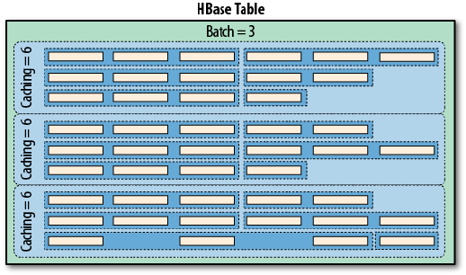
Figure 3-3. The scanner caching and batching controlling the num‐
ber of RPCs
The small batch value causes the servers to group three columns into
one Result, while the scanner caching of six causes one RPC to trans‐
fer six rows—or, more precisely, results--sent in the batch. When the
batch size is not specified but scanner caching is specified, the result
of the call will contain complete rows, because each row will be con‐
tained in one Result instance. Only when you start to use the batch
mode are you getting access to the intra-row scanning functionality.
You may not have to worry about the consequences of using scanner
caching and batch mode initially, but once you try to squeeze the opti‐
mal performance out of your setup, you should keep all of this in mind
and find the sweet spot for both values.
Finally, batching cannot be combined with filters that return true
from their hasFilterRow() method. Such filters cannot deal with par‐
tial results, in other words, the row being chunked into batches. It
needs to see the entire row to make a filtering decision. It might be
that the important column needed for that decision is not yet present.
Or, it could be that there have been batches of results sent to the cli‐
ent already, just to realize later that the entire row should have been
skipped.
Another combination disallowed is batching with small scans. The lat‐
ter are an optimization returning the entire result in one call, not in
further, smaller chunks. If you try to set the scan batching and small
scan flag together, you will receive an IllegalArgumentException ex‐
ception in due course.
Scans 209
www.finebook.ir
Slicing Rows
But wait, this is not all you can do with scans! There is more, and first
we will discuss the related slicing of table data using the following
methods:
int getMaxResultsPerColumnFamily()
Scan setMaxResultsPerColumnFamily(int limit)
int getRowOffsetPerColumnFamily()
Scan setRowOffsetPerColumnFamily(int offset)
long getMaxResultSize()
Scan setMaxResultSize(long maxResultSize)
The first four work together by allowing the application to cut out a
piece of each row selected, using an offset to start from a specific col‐
umn, and a max results per column family limit to stop returning data
once reached. The latter pair of functions allow to add (and retrieve)
an upper size limit of the data returned by the scan. It keeps a run‐
ning tally of the cells selected by the scan and stops returning them
once the size limit is exceeded. Example 3-31 shows this in action:
Example 3-31. Example using offset and limit parameters for scans
private static void scan(int num, int caching, int batch, int off‐
set,
int maxResults, int maxResultSize, boolean dump) throws IOExcep‐
tion {
int count = 0;
Scan scan = new Scan()
.setCaching(caching)
.setBatch(batch)
.setRowOffsetPerColumnFamily(offset)
.setMaxResultsPerColumnFamily(maxResults)
.setMaxResultSize(maxResultSize)
.setScanMetricsEnabled(true);
ResultScanner scanner = table.getScanner(scan);
System.out.println("Scan #" + num + " running...");
for (Result result : scanner) {
count++;
if (dump) System.out.println("Result [" + count + "]:" + re‐
sult);
}
scanner.close();
ScanMetrics metrics = scan.getScanMetrics();
System.out.println("Caching: " + caching + ", Batch: " + batch +
", Offset: " + offset + ", maxResults: " + maxResults +
", maxSize: " + maxResultSize + ", Results: " + count +
", RPCs: " + metrics.countOfRPCcalls);
}
public static void main(String[] args) throws IOException {
Chapter 3: Client API: The Basics210
www.finebook.ir
...
scan(1, 11, 0, 0, 2, -1, true);
scan(2, 11, 0, 4, 2, -1, true);
scan(3, 5, 0, 0, 2, -1, false);
scan(4, 11, 2, 0, 5, -1, true);
scan(5, 11, -1, -1, -1, 1, false);
scan(6, 11, -1, -1, -1, 10000, false);
...
}
The example’s hidden scaffolding creates a table with two column
families, with ten rows and ten columns in each family. The output,
abbreviated, looks something like this:
Scan #1 running...
Result [1]:keyvalues={row-01/colfam1:col-01/1/Put/vlen=9/seqid=0,
row-01/colfam1:col-02/2/Put/vlen=9/seqid=0,
row-01/colfam2:col-01/1/Put/vlen=9/seqid=0,
row-01/colfam2:col-02/2/Put/vlen=9/seqid=0}
...
Result [10]:keyvalues={row-10/colfam1:col-01/1/Put/vlen=9/seqid=0,
row-10/colfam1:col-02/2/Put/vlen=9/seqid=0,
row-10/colfam2:col-01/1/Put/vlen=9/seqid=0,
row-10/colfam2:col-02/2/Put/vlen=9/seqid=0}
Caching: 11, Batch: 0, Offset: 0, maxResults: 2, maxSize: -1,
Results: 10, RPCs: 3
Scan #2 running...
Result [1]:keyvalues={row-01/colfam1:col-05/5/Put/vlen=9/seqid=0,
row-01/colfam1:col-06/6/Put/vlen=9/seqid=0,
row-01/colfam2:col-05/5/Put/vlen=9/seqid=0,
row-01/colfam2:col-06/6/Put/vlen=9/seqid=0}
...
Result [10]:keyvalues={row-10/colfam1:col-05/5/Put/vlen=9/seqid=0,
row-10/colfam1:col-06/6/Put/vlen=9/seqid=0,
row-10/colfam2:col-05/5/Put/vlen=9/seqid=0,
row-10/colfam2:col-06/6/Put/vlen=9/seqid=0}
Caching: 11, Batch: 0, Offset: 4, maxResults: 2, maxSize: -1,
Results: 10, RPCs: 3
Scan #3 running...
Caching: 5, Batch: 0, Offset: 0, maxResults: 2, maxSize: -1,
Results: 10, RPCs: 5
Scan #4 running...
Result [1]:keyvalues={row-01/colfam1:col-01/1/Put/vlen=9/seqid=0,
row-01/colfam1:col-02/2/Put/vlen=9/seqid=0}
Result [2]:keyvalues={row-01/colfam1:col-03/3/Put/vlen=9/seqid=0,
row-01/colfam1:col-04/4/Put/vlen=9/seqid=0}
...
Result [31]:keyvalues={row-10/colfam1:col-03/3/Put/vlen=9/seqid=0,
row-10/colfam1:col-04/4/Put/vlen=9/seqid=0}
Scans 211
www.finebook.ir
Result [32]:keyvalues={row-10/colfam1:col-05/5/Put/vlen=9/seqid=0}
Caching: 11, Batch: 2, Offset: 0, maxResults: 5, maxSize: -1,
Results: 32, RPCs: 5
Scan #5 running...
Caching: 11, Batch: -1, Offset: -1, maxResults: -1, maxSize: 1,
Results: 10, RPCs: 13
Scan #6 running...
Caching: 11, Batch: -1, Offset: -1, maxResults: -1, maxSize: 10000,
Results: 10, RPCs: 5
The first scan starts at offset 0 and asks for a maximum of 2 cells, re‐
turning columns one and two. The second scan does the same but sets
the offset to 4, therefore retrieving the columns five to six. Note how
the offset really defines the number of cells to skip initially, and our
value of 4 causes the first four columns to be skipped.
The next scan, #3, does not emit anything, since we are only interes‐
ted in the metrics. It is the same as scan #1, but using a caching value
of 5. You will notice how the minimal amount of RPCs is 3 (open,
fetch, and close call for a non-small scanner). Here we see 5 RPCs that
have taken place, which makes sense, since now we cannot fetch our
10 results in one call, but need two calls with five results each, plus an
additional one to figure that there are no more rows left.
Scan #4 is combining the previous scans with a batching value of 2,
so up to two cells are returned per call to next(), but at the same
time we limit the amount of cells returned per column family to 5. Ad‐
ditionally combined with the caching value of 11 we see five RPCs
made to the server.
Finally, scan #5 and #6 are using setMaxResultSize() to limit the
amount of data returned to the caller. Just to recall, the scanner cach‐
ing is set as number of rows, while the max result size is specified in
bytes. What do we learn from the metrics (the rows are omitted as
both print the entire table) as printed in the output?
•We need to set the caching to 11 to fetch all ten rows in our exam‐
ple in one RPC. When you set it to 10 an extra RPC is incurred, just
to realize that there are no more rows.
•The caching setting is bound by the max result size, so in scan #5
we force the servers to return every row as a separate result, be‐
cause setting the max result size to 1 byte means we cannot ship
more than one row in a call. The caching is rendered useless.
Chapter 3: Client API: The Basics212
www.finebook.ir
17. This has been addressed with implicit row chunking in HBase 1.1.0 and later. See
HBASE-11544 for details.
•Even if we set the max result size to 1 byte, we still get at least
one row per request. Which means, for very large rows we might
still get under memory pressure.17
•The max result size should be set as an upper boundary that could
be computed as max result size = caching * average row size. The
idea is to fit in enough rows into the max result size but still en‐
sure that caching is working.
This is a rather involved section, showing you how to tweak many scan
parameters to optimize the communication with the region servers.
Like I mentioned a few times so far, your mileage may vary, so please
test this carefully and evaluate your options.
Load Column Families on Demand
Scans have another advanced feature, one that deserves a longer ex‐
planation: loading column families on demand. This is controlled by
the following methods:
Scan setLoadColumnFamiliesOnDemand(boolean value)
Boolean getLoadColumnFamiliesOnDemandValue()
boolean doLoadColumnFamiliesOnDemand()
This functionality is a read optimization, useful only for tables with
more than one column family, and especially then for those use-cases
with a dependency between data in those families. For example, as‐
sume you have one family with meta data, and another with a heavier
payload. You want to scan the meta data columns, and if a particular
flag is present in one column, you need to access the payload data in
the other family. It would be costly to include both families into the
scan if you expect the cardinality of the flag to be low (in comparison
to the table size). This is because such a scan would load the payload
for every row, just to then ignore it.
Enabling this feature with setLoadColumnFamiliesOnDemand(true) is
only half the of the preparation work: you also need a filter that imple‐
ments the following method, returning a boolean flag:
boolean isFamilyEssential(byte[] name) throws IOException
The idea is that the filter is the decision maker if a column family is
essential or not. When the servers scan the data, they first set up in‐
ternal scanners for each column family. If load column families on de‐
mand is enabled and a filter set, it calls out to the filter and asks it to
Scans 213
www.finebook.ir

decide if an included column family is to be scanned or not. The fil‐
ter’s isFamilyEssential() is invoked with the name of the family un‐
der consideration, before the column family is added, and must return
true to approve. If it returns false, then the column family is ignored
for now and loaded on demand later if needed.
On the other hand, you must add all column families to the scan, no
matter if they are essential or not. The framework will only consult the
filter about the inclusion of a family, if they have been added in the
first place. If you do not explicitly specify any family, then you are OK.
But as soon as you start using the addColumn() or addFamily() meth‐
ods of Scan, then you have to ensure you add the non-essential col‐
umns or families too.
Scanner Metrics
The Example 3-30 uses another feature of the scan class, allowing the
client to reason about the effectiveness of the operation. This is ac‐
complished with the following methods:
Scan setScanMetricsEnabled(final boolean enabled)
boolean isScanMetricsEnabled()
ScanMetrics getScanMetrics()
As shown in the example, you can enable the collection of scan met‐
rics by invoking setScanMetricsEnabled(true). Once the scan is
complete you can retrieve the ScanMetrics using the getScanMet
rics() method. The isScanMetricsEnabled() is a check if the collec‐
tion of metrics has been enabled previously. The returned ScanMet
rics instance has a set of fields you can read to determine what cost
the operation accrued:
Table 3-20. Metrics provided by the ScanMetrics class
Metric Field Description
countOfRPCcalls The total amount of RPC calls incurred by the scan.
countOfRemoteRPCcalls The amount of RPC calls to a remote host.
sumOfMillisSecBetweenNexts The sum of milliseconds between sequential next()
calls.
countOfNSRE Number of NotServingRegionException caught.
countOfBytesInResults Number of bytes in Result instances returned by the
servers.
countOfBytesInRemoteResults Same as above, but for bytes transferred from remote
servers.
countOfRegions Number of regions that were involved in the scan.
countOfRPCRetries Number of RPC retries incurred during the scan.
Chapter 3: Client API: The Basics214
www.finebook.ir

Metric Field Description
countOfRemoteRPCRetries Same again, but RPC retries for non-local servers.
In the example we are printing the countOfRPCcalls field, since we
want to figure out how many calls have taken place. When running the
example code locally the countOfRemoteRPCcalls would be zero, as
all RPC calls are made to the very same machine. Since scans are exe‐
cuted by region servers, and iterate over all regions included in the
selected row range, the metrics are internally collected region by re‐
gion and accumulated in the ScanMetrics instance of the Scan object.
While it is possible to call upon the metrics as the scan is taking place,
only at the very end of the scan you will see the final count.
Miscellaneous Features
Before looking into more involved features that clients can use, let us
first wrap up a handful of miscellaneous features and functionality
provided by HBase and its client API.
The Table Utility Methods
The client API is represented by an instance of the Table class and
gives you access to an existing HBase table. Apart from the major fea‐
tures we already discussed, there are a few more notable methods of
this class that you should be aware of:
void close()
This method was mentioned before, but for the sake of complete‐
ness, and its importance, it warrants repeating. Call close() once
you have completed your work with a table. There is some internal
housekeeping work that needs to run, and invoking this method
triggers this process. Wrap the opening and closing of a table into
a try/catch, or even better (on Java 7 or later), a try-with-
resources block.
TableName getName()
This is a convenience method to retrieve the table name. It is pro‐
vided as an instance of the TableName class, providing access to
the namespace and actual table name.
Configuration getConfiguration()
This allows you to access the configuration in use by the Table in‐
stance. Since this is handed out by reference, you can make
changes that are effective immediately.
Miscellaneous Features 215
www.finebook.ir
HTableDescriptor getTableDescriptor()
Each table is defined using an instance of the HTableDescriptor
class. You gain access to the underlying definition using getTable
Descriptor().
For more information about the management of tables using the ad‐
ministrative API, please consult “Tables” (page 350).
The Bytes Class
You saw how this class was used to convert native Java types, such as
String, or long, into the raw, byte array format HBase supports na‐
tively. There are a few more notes that are worth mentioning about
the class and its functionality. Most methods come in three variations,
for example:
static long toLong(byte[] bytes)
static long toLong(byte[] bytes, int offset)
static long toLong(byte[] bytes, int offset, int length)
You hand in just a byte array, or an array and an offset, or an array,
an offset, and a length value. The usage depends on the originating
byte array you have. If it was created by toBytes() beforehand, you
can safely use the first variant, and simply hand in the array and noth‐
ing else. All the array contains is the converted value.
The API, and HBase internally, store data in larger arrays using, for
example, the following call:
static int putLong(byte[] bytes, int offset, long val)
This call allows you to write the long value into a given byte array, at
a specific offset. If you want to access the data in that larger byte ar‐
ray you can make use of the latter two toLong() calls instead. The
length parameter is a bit of an odd one as it has to match the length
of the native type, in other words, if you try to convert a long from a
byte[] array but specify 2 as the length, the conversion will fail with
an IllegalArgumentException error. In practice, you should really
only have to deal with the first two variants of the method.
The Bytes class has support to convert from and to the following na‐
tive Java types: String, boolean, short, int, long, double, float,
ByteBuffer, and BigDecimal. Apart from that, there are some note‐
worthy methods, which are listed in Table 3-21.
Chapter 3: Client API: The Basics216
www.finebook.ir

18. See the Bytes documentation online.
Table 3-21. Overview of additional methods provided by the Bytes
class
Method Description
toStringBina
ry() While working very similar to toString(), this variant has an extra
safeguard to convert non-printable data into human-readable
hexadecimal numbers. Whenever you are not sure what a byte array
contains you should use this method to print its content, for
example, to the console, or into a logfile.
compareTo()/
equals() These methods allow you to compare two byte[], that is, byte
arrays. The former gives you a comparison result and the latter a
boolean value, indicating whether the given arrays are equal to each
other.
add()/head()/
tail() You can use these to combine two byte arrays, resulting in a new,
concatenated array, or to get the first, or last, few bytes of the given
byte array.
binarySearch() This performs a binary search in the given array of values. It
operates on byte arrays for the values and the key you are
searching for.
increment
Bytes() This increments a long value in its byte array representation, as if
you had used toBytes(long) to create it. You can decrement using a
negative amount parameter.
There is some overlap of the Bytes class with the Java-provided Byte
Buffer. The difference is that the former does all operations without
creating new class instances. In a way it is an optimization, because
the provided methods are called many times within HBase, while
avoiding possibly costly garbage collection issues.
For the full documentation, please consult the JavaDoc-based API doc‐
umentation.18
Miscellaneous Features 217
www.finebook.ir
Chapter 4
Client API: Advanced
Features
Now that you understand the basic client API, we will discuss the ad‐
vanced features that HBase offers to clients.
Filters
HBase filters are a powerful feature that can greatly enhance your ef‐
fectiveness when working with data stored in tables. You will find pre‐
defined filters, already provided by HBase for your use, as well as a
framework you can use to implement your own. You will now be intro‐
duced to both.
Introduction to Filters
The two prominent read functions for HBase are Table.get() and
Table.scan(), both supporting either direct access to data or the use
of a start and end key, respectively. You can limit the data retrieved
by progressively adding more limiting selectors to the query. These in‐
clude column families, column qualifiers, timestamps or ranges, as
well as version numbers.
While this gives you control over what is included, it is missing more
fine-grained features, such as selection of keys, or values, based on
regular expressions. Both classes support filters for exactly these rea‐
sons: what cannot be solved with the provided API functionality select‐
ing the required row or column keys, or values, can be achieved with
filters. The base interface is aptly named Filter, and there is a list of
219
www.finebook.ir
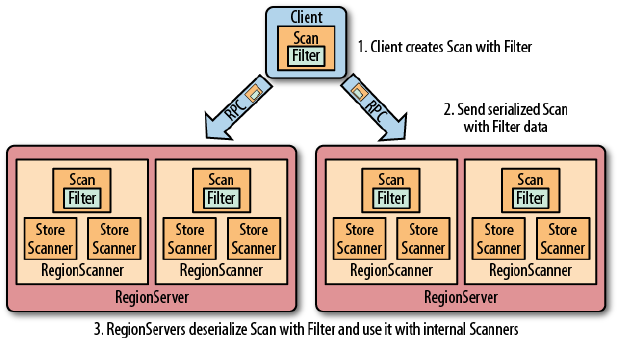
concrete classes supplied by HBase that you can use without doing
any programming.
You can, on the other hand, extend the Filter classes to implement
your own requirements. All the filters are actually applied on the serv‐
er side, also referred to as predicate pushdown. This ensures the most
efficient selection of the data that needs to be transported back to the
client. You could implement most of the filter functionality in your cli‐
ent code as well, but you would have to transfer much more data—
something you need to avoid at scale.
Figure 4-1 shows how the filters are configured on the client, then se‐
rialized over the network, and then applied on the server.
Figure 4-1. The filters created on the client side, sent through the
RPC, and executed on the server side
The Filter Hierarchy
The lowest level in the filter hierarchy is the Filter interface, and the
abstract FilterBase class that implements an empty shell, or skele‐
ton, that is used by the actual filter classes to avoid having the same
boilerplate code in each of them. Most concrete filter classes are di‐
rect descendants of FilterBase, but a few use another, intermediate
ancestor class. They all work the same way: you define a new instance
of the filter you want to apply and hand it to the Get or Scan instan‐
ces, using:
setFilter(filter)
Chapter 4: Client API: Advanced Features220
www.finebook.ir

While you initialize the filter instance itself, you often have to supply
parameters for whatever the filter is designed for. There is a special
subset of filters, based on CompareFilter, that ask you for at least
two specific parameters, since they are used by the base class to per‐
form its task. You will learn about the two parameter types next so
that you can use them in context.
Filters have access to the entire row they are applied to. This means
that they can decide the fate of a row based on any available informa‐
tion. This includes the row key, column qualifiers, actual value of a
column, timestamps, and so on. When referring to values, or compari‐
sons, as we will discuss shortly, this can be applied to any of these de‐
tails. Specific filter implementations are available that consider only
one of those criteria each.
While filters can apply their logic to a specific row, they have no state
and cannot span across multiple rows. There are also some scan relat‐
ed features—such as batching (see “Scanner Batching” (page 206))--
that counteract the ability of a filter to do its work. We will discuss
these limitations in due course below.
Comparison Operators
As CompareFilter-based filters add one more feature to the base Fil
terBase class, namely the compare() operation, it has to have a user-
supplied operator type that defines how the result of the comparison
is interpreted. The values are listed in Table 4-1.
Table 4-1. The possible comparison operators for CompareFilter-
based filters
Operator Description
LESS Match values less than the provided one.
LESS_OR_EQUAL Match values less than or equal to the provided one.
EQUAL Do an exact match on the value and the provided one.
NOT_EQUAL Include everything that does not match the provided value.
GREATER_OR_EQUAL Match values that are equal to or greater than the provided one.
GREATER Only include values greater than the provided one.
NO_OP Exclude everything.
The comparison operators define what is included, or excluded, when
the filter is applied. This allows you to select the data that you want as
either a range, subset, or exact and single match.
Filters 221
www.finebook.ir

Comparators
The second type that you need to provide to CompareFilter-related
classes is a comparator, which is needed to compare various values
and keys in different ways. They are derived from ByteArrayCompara
ble, which implements the Java Comparable interface. You do not
have to go into the details if you just want to use an implementation
provided by HBase and listed in Table 4-2. The constructors usually
take the control value, that is, the one to compare each table value
against.
Table 4-2. The HBase-supplied comparators, used with
CompareFilter-based filters
Comparator Description
LongComparator Assumes the given value array is a Java Long number and
uses Bytes.toLong() to convert it.
BinaryComparator Uses Bytes.compareTo() to compare the current with the
provided value.
BinaryPrefixComparator Similar to the above, but does a left hand, prefix-based
match using Bytes.compareTo().
NullComparator Does not compare against an actual value, but checks
whether a given one is null, or not null.
BitComparator Performs a bitwise comparison, providing a BitwiseOp
enumeration with AND, OR, and XOR operators.
RegexStringComparator Given a regular expression at instantiation, this comparator
does a pattern match on the data.
SubstringComparator Treats the value and table data as String instances and
performs a contains() check.
The last four comparators listed in Table 4-2—the NullCom
parator, BitComparator, RegexStringComparator, and
SubstringComparator—only work with the EQUAL and
NOT_EQUAL operators, as the compareTo() of these compa‐
rators returns 0 for a match or 1 when there is no match.
Using them in a LESS or GREATER comparison will yield er‐
roneous results.
Each of the comparators usually has a constructor that takes the com‐
parison value. In other words, you need to define a value you compare
each cell against. Some of these constructors take a byte[], a byte ar‐
ray, to do the binary comparison, for example, while others take a
String parameter—since the data point compared against is assumed
Chapter 4: Client API: Advanced Features222
www.finebook.ir

to be some sort of readable text. Example 4-1 shows some of these in
action.
The string-based comparators, RegexStringComparator
and SubstringComparator, are more expensive in compar‐
ison to the purely byte-based versions, as they need to
convert a given value into a String first. The subsequent
string or regular expression operation also adds to the
overall cost.
Comparison Filters
The first type of supplied filter implementations are the comparison
filters. They take the comparison operator and comparator instance as
described above. The constructor of each of them has the same signa‐
ture, inherited from CompareFilter:
CompareFilter(final CompareOp compareOp, final ByteArrayComparable
comparator)
You need to supply the comparison operator and comparison class for
the filters to do their work. Next you will see the actual filters imple‐
menting a specific comparison.
Please keep in mind that the general contract of the HBase filter API
means you are filtering out information—filtered data is omitted from
the results returned to the client. The filter is not specifying what you
want to have, but rather what you do not want to have returned when
reading data.
In contrast, all filters based on CompareFilter are doing the opposite,
in that they include the matching values. In other words, be careful
when choosing the comparison operator, as it makes the difference in
regard to what the server returns. For example, instead of using LESS
to skip some information, you may need to use GREATER_OR_EQUAL to
include the desired data points.
RowFilter
This filter gives you the ability to filter data based on row keys.
Example 4-1 shows how the filter can use different comparator instan‐
ces to get the desired results. It also uses various operators to include
the row keys, while omitting others. Feel free to modify the code,
changing the operators to see the possible results.
Filters 223
www.finebook.ir

Example 4-1. Example using a filter to select specific rows
Scan scan = new Scan();
scan.addColumn(Bytes.toBytes("colfam1"), Bytes.toBytes("col-1"));
Filter filter1 = new RowFilter(CompareFilter.Compar‐
eOp.LESS_OR_EQUAL,
new BinaryComparator(Bytes.toBytes("row-22")));
scan.setFilter(filter1);
ResultScanner scanner1 = table.getScanner(scan);
for (Result res : scanner1) {
System.out.println(res);
}
scanner1.close();
Filter filter2 = new RowFilter(CompareFilter.CompareOp.EQUAL,
new RegexStringComparator(".*-.5"));
scan.setFilter(filter2);
ResultScanner scanner2 = table.getScanner(scan);
for (Result res : scanner2) {
System.out.println(res);
}
scanner2.close();
Filter filter3 = new RowFilter(CompareFilter.CompareOp.EQUAL,
new SubstringComparator("-5"));
scan.setFilter(filter3);
ResultScanner scanner3 = table.getScanner(scan);
for (Result res : scanner3) {
System.out.println(res);
}
scanner3.close();
Create filter, while specifying the comparison operator and
comparator. Here an exact match is needed.
Another filter, this time using a regular expression to match the
row keys.
The third filter uses a substring match approach.
Here is the full printout of the example on the console:
Adding rows to table...
Scanning table #1...
keyvalues={row-1/colfam1:col-1/1427273897619/Put/vlen=7/seqid=0}
keyvalues={row-10/colfam1:col-1/1427273899185/Put/vlen=8/seqid=0}
keyvalues={row-100/colfam1:col-1/1427273908651/Put/vlen=9/seqid=0}
keyvalues={row-11/colfam1:col-1/1427273899343/Put/vlen=8/seqid=0}
keyvalues={row-12/colfam1:col-1/1427273899496/Put/vlen=8/seqid=0}
keyvalues={row-13/colfam1:col-1/1427273899643/Put/vlen=8/seqid=0}
keyvalues={row-14/colfam1:col-1/1427273899785/Put/vlen=8/seqid=0}
keyvalues={row-15/colfam1:col-1/1427273899925/Put/vlen=8/seqid=0}
Chapter 4: Client API: Advanced Features224
www.finebook.ir
keyvalues={row-16/colfam1:col-1/1427273900064/Put/vlen=8/seqid=0}
keyvalues={row-17/colfam1:col-1/1427273900202/Put/vlen=8/seqid=0}
keyvalues={row-18/colfam1:col-1/1427273900343/Put/vlen=8/seqid=0}
keyvalues={row-19/colfam1:col-1/1427273900484/Put/vlen=8/seqid=0}
keyvalues={row-2/colfam1:col-1/1427273897860/Put/vlen=7/seqid=0}
keyvalues={row-20/colfam1:col-1/1427273900623/Put/vlen=8/seqid=0}
keyvalues={row-21/colfam1:col-1/1427273900757/Put/vlen=8/seqid=0}
keyvalues={row-22/colfam1:col-1/1427273900881/Put/vlen=8/seqid=0}
Scanning table #2...
keyvalues={row-15/colfam1:col-1/1427273899925/Put/vlen=8/seqid=0}
keyvalues={row-25/colfam1:col-1/1427273901253/Put/vlen=8/seqid=0}
keyvalues={row-35/colfam1:col-1/1427273902480/Put/vlen=8/seqid=0}
keyvalues={row-45/colfam1:col-1/1427273903582/Put/vlen=8/seqid=0}
keyvalues={row-55/colfam1:col-1/1427273904633/Put/vlen=8/seqid=0}
keyvalues={row-65/colfam1:col-1/1427273905577/Put/vlen=8/seqid=0}
keyvalues={row-75/colfam1:col-1/1427273906453/Put/vlen=8/seqid=0}
keyvalues={row-85/colfam1:col-1/1427273907327/Put/vlen=8/seqid=0}
keyvalues={row-95/colfam1:col-1/1427273908211/Put/vlen=8/seqid=0}
Scanning table #3...
keyvalues={row-5/colfam1:col-1/1427273898394/Put/vlen=7/seqid=0}
keyvalues={row-50/colfam1:col-1/1427273904116/Put/vlen=8/seqid=0}
keyvalues={row-51/colfam1:col-1/1427273904219/Put/vlen=8/seqid=0}
keyvalues={row-52/colfam1:col-1/1427273904324/Put/vlen=8/seqid=0}
keyvalues={row-53/colfam1:col-1/1427273904428/Put/vlen=8/seqid=0}
keyvalues={row-54/colfam1:col-1/1427273904536/Put/vlen=8/seqid=0}
keyvalues={row-55/colfam1:col-1/1427273904633/Put/vlen=8/seqid=0}
keyvalues={row-56/colfam1:col-1/1427273904729/Put/vlen=8/seqid=0}
keyvalues={row-57/colfam1:col-1/1427273904823/Put/vlen=8/seqid=0}
keyvalues={row-58/colfam1:col-1/1427273904919/Put/vlen=8/seqid=0}
keyvalues={row-59/colfam1:col-1/1427273905015/Put/vlen=8/seqid=0}
You can see how the first filter did an exact match on the row key, in‐
cluding all of those rows that have a key, equal to or less than the giv‐
en one. Note once again the lexicographical sorting and comparison,
and how it filters the row keys.
The second filter does a regular expression match, while the third
uses a substring match approach. The results show that the filters
work as advertised.
FamilyFilter
This filter works very similar to the RowFilter, but applies the com‐
parison to the column families available in a row—as opposed to the
row key. Using the available combinations of operators and compara‐
tors you can filter what is included in the retrieved data on a column
family level. Example 4-2 shows how to use this.
Filters 225
www.finebook.ir
Example 4-2. Example using a filter to include only specific column
families
Filter filter1 = new FamilyFilter(CompareFilter.CompareOp.LESS,
new BinaryComparator(Bytes.toBytes("colfam3")));
Scan scan = new Scan();
scan.setFilter(filter1);
ResultScanner scanner = table.getScanner(scan);
for (Result result : scanner) {
System.out.println(result);
}
scanner.close();
Get get1 = new Get(Bytes.toBytes("row-5"));
get1.setFilter(filter1);
Result result1 = table.get(get1);
System.out.println("Result of get(): " + result1);
Filter filter2 = new FamilyFilter(CompareFilter.CompareOp.EQUAL,
new BinaryComparator(Bytes.toBytes("colfam3")));
Get get2 = new Get(Bytes.toBytes("row-5"));
get2.addFamily(Bytes.toBytes("colfam1"));
get2.setFilter(filter2);
Result result2 = table.get(get2);
System.out.println("Result of get(): " + result2);
Create filter, while specifying the comparison operator and
comparator.
Scan over table while applying the filter.
Get a row while applying the same filter.
Create a filter on one column family while trying to retrieve
another.
Get the same row while applying the new filter, this will return
“NONE”.
The output—reformatted and abbreviated for the sake of readability—
shows the filter in action. The input data has four column families,
with two columns each, and 10 rows in total.
Adding rows to table...
Scanning table...
keyvalues={row-1/colfam1:col-1/1427274088598/Put/vlen=7/seqid=0,
row-1/colfam1:col-2/1427274088615/Put/vlen=7/seqid=0,
row-1/colfam2:col-1/1427274088598/Put/vlen=7/seqid=0,
row-1/colfam2:col-2/1427274088615/Put/vlen=7/seqid=0}
keyvalues={row-10/colfam1:col-1/1427274088673/Put/vlen=8/seqid=0,
row-10/colfam1:col-2/1427274088675/Put/vlen=8/seqid=0,
row-10/colfam2:col-1/1427274088673/Put/vlen=8/seqid=0,
Chapter 4: Client API: Advanced Features226
www.finebook.ir
row-10/colfam2:col-2/1427274088675/Put/vlen=8/seqid=0}
...
keyvalues={row-9/colfam1:col-1/1427274088669/Put/vlen=7/seqid=0,
row-9/colfam1:col-2/1427274088671/Put/vlen=7/seqid=0,
row-9/colfam2:col-1/1427274088669/Put/vlen=7/seqid=0,
row-9/colfam2:col-2/1427274088671/Put/vlen=7/seqid=0}
Result of get(): keyvalues={
row-5/colfam1:col-1/1427274088652/Put/vlen=7/seqid=0,
row-5/colfam1:col-2/1427274088654/Put/vlen=7/seqid=0,
row-5/colfam2:col-1/1427274088652/Put/vlen=7/seqid=0,
row-5/colfam2:col-2/1427274088654/Put/vlen=7/seqid=0}
Result of get(): keyvalues=NONE
The last get() shows that you can (inadvertently) create an empty set
by applying a filter for exactly one column family, while specifying a
different column family selector using addFamily().
QualifierFilter
Example 4-3 shows how the same logic is applied on the column quali‐
fier level. This allows you to filter specific columns from the table.
Example 4-3. Example using a filter to include only specific column
qualifiers
Filter filter = new QualifierFilter(CompareFilter.Compar‐
eOp.LESS_OR_EQUAL,
new BinaryComparator(Bytes.toBytes("col-2")));
Scan scan = new Scan();
scan.setFilter(filter);
ResultScanner scanner = table.getScanner(scan);
for (Result result : scanner) {
System.out.println(result);
}
scanner.close();
Get get = new Get(Bytes.toBytes("row-5"));
get.setFilter(filter);
Result result = table.get(get);
System.out.println("Result of get(): " + result);
The output is the following (abbreviated again):
Adding rows to table...
Scanning table...
keyvalues={row-1/colfam1:col-1/1427274739258/Put/vlen=7/seqid=0,
row-1/colfam1:col-10/1427274739309/Put/vlen=8/seqid=0,
row-1/colfam1:col-2/1427274739272/Put/vlen=7/seqid=0,
row-1/colfam2:col-1/1427274739258/Put/vlen=7/seqid=0,
row-1/colfam2:col-10/1427274739309/Put/vlen=8/seqid=0,
Filters 227
www.finebook.ir

row-1/colfam2:col-2/1427274739272/Put/vlen=7/seqid=0}
...
keyvalues={row-9/colfam1:col-1/1427274739441/Put/vlen=7/seqid=0,
row-9/colfam1:col-10/1427274739458/Put/vlen=8/seqid=0,
row-9/colfam1:col-2/1427274739443/Put/vlen=7/seqid=0,
row-9/colfam2:col-1/1427274739441/Put/vlen=7/seqid=0,
row-9/colfam2:col-10/1427274739458/Put/vlen=8/seqid=0,
row-9/colfam2:col-2/1427274739443/Put/vlen=7/seqid=0}
Result of get(): keyvalues={
row-5/colfam1:col-1/1427274739366/Put/vlen=7/seqid=0,
row-5/colfam1:col-10/1427274739384/Put/vlen=8/seqid=0,
row-5/colfam1:col-2/1427274739368/Put/vlen=7/seqid=0,
row-5/colfam2:col-1/1427274739366/Put/vlen=7/seqid=0,
row-5/colfam2:col-10/1427274739384/Put/vlen=8/seqid=0,
row-5/colfam2:col-2/1427274739368/Put/vlen=7/seqid=0}
Since the filter asks for columns, or in other words column qualifiers,
with a value of col-2 or less, you can see how col-1 and col-10 are
also included, since the comparison—once again—is done lexicograph‐
ically (means binary).
ValueFilter
This filter makes it possible to include only columns that have a specif‐
ic value. Combined with the RegexStringComparator, for example,
this can filter using powerful expression syntax. Example 4-4 showca‐
ses this feature. Note, though, that with certain comparators—as ex‐
plained earlier—you can only employ a subset of the operators. Here a
substring match is performed and this must be combined with an
EQUAL, or NOT_EQUAL, operator.
Example 4-4. Example using the value based filter
Filter filter = new ValueFilter(CompareFilter.CompareOp.EQUAL,
new SubstringComparator(".4"));
Scan scan = new Scan();
scan.setFilter(filter);
ResultScanner scanner = table.getScanner(scan);
for (Result result : scanner) {
for (Cell cell : result.rawCells()) {
System.out.println("Cell: " + cell + ", Value: " +
Bytes.toString(cell.getValueArray(), cell.getValueOffset(),
cell.getValueLength()));
}
}
scanner.close();
Get get = new Get(Bytes.toBytes("row-5"));
get.setFilter(filter);
Result result = table.get(get);
Chapter 4: Client API: Advanced Features228
www.finebook.ir

for (Cell cell : result.rawCells()) {
System.out.println("Cell: " + cell + ", Value: " +
Bytes.toString(cell.getValueArray(), cell.getValueOffset(),
cell.getValueLength()));
}
Create filter, while specifying the comparison operator and
comparator.
Set filter for the scan.
Print out value to check that filter works.
Assign same filter to Get instance.
The output, confirming the proper functionality:
Adding rows to table...
Results of scan:
Cell: row-1/colfam1:col-4/1427275408429/Put/vlen=7/seqid=0, Value:
val-1.4
Cell: row-1/colfam2:col-4/1427275408429/Put/vlen=7/seqid=0, Value:
val-1.4
...
Cell: row-9/colfam1:col-4/1427275408605/Put/vlen=7/seqid=0, Value:
val-9.4
Cell: row-9/colfam2:col-4/1427275408605/Put/vlen=7/seqid=0, Value:
val-9.4
Result of get:
Cell: row-5/colfam1:col-4/1427275408527/Put/vlen=7/seqid=0, Value:
val-5.4
Cell: row-5/colfam2:col-4/1427275408527/Put/vlen=7/seqid=0, Value:
val-5.4
The example’s wiring code (hidden, see the online repository again)
set the value to row key + “.” + column number. The rows and col‐
umns start at 1. The filter is instructed to retrieve all cells that have a
value containing .4--aiming at the fourth column. And indeed, we see
that only column col-4 is returned.
DependentColumnFilter
Here you have a more complex filter that does not simply filter out da‐
ta based on directly available information. Rather, it lets you specify a
dependent column—or reference column—that controls how other col‐
umns are filtered. It uses the timestamp of the reference column and
includes all other columns that have the same timestamp. Here are
the constructors provided:
DependentColumnFilter(final byte[] family, final byte[] qualifier)
DependentColumnFilter(final byte[] family, final byte[] qualifier,
final boolean dropDependentColumn)
Filters 229
www.finebook.ir

DependentColumnFilter(final byte[] family, final byte[] qualifier,
final boolean dropDependentColumn, final CompareOp valueCompar‐
eOp,
final ByteArrayComparable valueComparator)
Since this class is based on CompareFilter, it also offers you to fur‐
ther select columns, but for this filter it does so based on their values.
Think of it as a combination of a ValueFilter and a filter selecting on
a reference timestamp. You can optionally hand in your own operator
and comparator pair to enable this feature. The class provides con‐
structors, though, that let you omit the operator and comparator and
disable the value filtering, including all columns by default, that is,
performing the timestamp filter based on the reference column only.
Example 4-5 shows the filter in use. You can see how the optional val‐
ues can be handed in as well. The dropDependentColumn parameter is
giving you additional control over how the reference column is han‐
dled: it is either included or dropped by the filter, setting this parame‐
ter to false or true, respectively.
Example 4-5. Example using a filter to include only specific column
families
private static void filter(boolean drop,
CompareFilter.CompareOp operator,
ByteArrayComparable comparator)
throws IOException {
Filter filter;
if (comparator != null) {
filter = new DependentColumnFilter(Bytes.toBytes("colfam1"),
Bytes.toBytes("col-5"), drop, operator, comparator);
} else {
filter = new DependentColumnFilter(Bytes.toBytes("colfam1"),
Bytes.toBytes("col-5"), drop);
}
Scan scan = new Scan();
scan.setFilter(filter);
// scan.setBatch(4); // cause an error
ResultScanner scanner = table.getScanner(scan);
for (Result result : scanner) {
for (Cell cell : result.rawCells()) {
System.out.println("Cell: " + cell + ", Value: " +
Bytes.toString(cell.getValueArray(), cell.getValueOffset(),
cell.getValueLength()));
}
}
scanner.close();
Get get = new Get(Bytes.toBytes("row-5"));
get.setFilter(filter);
Chapter 4: Client API: Advanced Features230
www.finebook.ir

Result result = table.get(get);
for (Cell cell : result.rawCells()) {
System.out.println("Cell: " + cell + ", Value: " +
Bytes.toString(cell.getValueArray(), cell.getValueOffset(),
cell.getValueLength()));
}
}
public static void main(String[] args) throws IOException {
filter(true, CompareFilter.CompareOp.NO_OP, null);
filter(false, CompareFilter.CompareOp.NO_OP, null);
filter(true, CompareFilter.CompareOp.EQUAL,
new BinaryPrefixComparator(Bytes.toBytes("val-5")));
filter(false, CompareFilter.CompareOp.EQUAL,
new BinaryPrefixComparator(Bytes.toBytes("val-5")));
filter(true, CompareFilter.CompareOp.EQUAL,
new RegexStringComparator(".*\\.5"));
filter(false, CompareFilter.CompareOp.EQUAL,
new RegexStringComparator(".*\\.5"));
}
Create the filter with various options.
Call filter method with various options.
This filter is not compatible with the batch feature of the
scan operations, that is, setting Scan.setBatch() to a
number larger than zero. The filter needs to see the entire
row to do its work, and using batching will not carry the
reference column timestamp over and would result in er‐
roneous results.
If you try to enable the batch mode nevertheless, you will
get an error:
Exception in thread "main" \
org.apache.hadoop.hbase.filter.IncompatibleFilterEx‐
ception: \
Cannot set batch on a scan using a filter that re‐
turns true for \
filter.hasFilterRow
at org.apache.hadoop.hbase.client.Scan.set‐
Batch(Scan.java:464)
...
The example also proceeds slightly differently compared to the earlier
filters, as it sets the version to the column number for a more reprodu‐
cible result. The implicit timestamps that the servers use as the ver‐
Filters 231
www.finebook.ir
sion could result in fluctuating results as you cannot guarantee them
using the exact time, down to the millisecond.
The filter() method used is called with different parameter combi‐
nations, showing how using the built-in value filter and the drop flag
is affecting the returned data set. Here the output of the first two fil
ter() call:
Adding rows to table...
Results of scan:
Cell: row-1/colfam2:col-5/5/Put/vlen=7/seqid=0, Value: val-1.5
Cell: row-10/colfam2:col-5/5/Put/vlen=8/seqid=0, Value: val-10.5
...
Cell: row-8/colfam2:col-5/5/Put/vlen=7/seqid=0, Value: val-8.5
Cell: row-9/colfam2:col-5/5/Put/vlen=7/seqid=0, Value: val-9.5
Result of get:
Cell: row-5/colfam2:col-5/5/Put/vlen=7/seqid=0, Value: val-5.5
Results of scan:
Cell: row-1/colfam1:col-5/5/Put/vlen=7/seqid=0, Value: val-1.5
Cell: row-1/colfam2:col-5/5/Put/vlen=7/seqid=0, Value: val-1.5
Cell: row-9/colfam1:col-5/5/Put/vlen=7/seqid=0, Value: val-9.5
Cell: row-9/colfam2:col-5/5/Put/vlen=7/seqid=0, Value: val-9.5
Result of get:
Cell: row-5/colfam1:col-5/5/Put/vlen=7/seqid=0, Value: val-5.5
Cell: row-5/colfam2:col-5/5/Put/vlen=7/seqid=0, Value: val-5.5
The only difference between the two calls is setting dropDependent
Column to true and false respectively. In the first scan and get out‐
put you see the checked column in colfam1 being omitted, in other
words dropped as expected, while in the second half of the output you
see it included.
What is this filter good for you might wonder? It is used where appli‐
cations require client-side timestamps (these could be epoch based, or
based on some internal global counter) to track dependent updates.
Say you insert some kind of transactional data, where across the row
all fields that are updated, should form some dependent update. In
this case the client could set all columns that are updated in one mu‐
tation to the same timestamp, and when later wanting to show the en‐
tity at a certain point in time, get (or scan) the row at that time. All
modifications from earlier (or later, or exact) changes are then
masked out (or included). See (to come) for libraries on top of HBase
that make use of such as schema.
Dedicated Filters
The second type of supplied filters are based directly on FilterBase
and implement more specific use cases. Many of these filters are only
Chapter 4: Client API: Advanced Features232
www.finebook.ir
really applicable when performing scan operations, since they filter
out entire rows. For get() calls, this is often too restrictive and would
result in a very harsh filter approach: include the whole row or noth‐
ing at all.
PrefixFilter
Given a row prefix, specified when you instantiate the filter instance,
all rows with a row key matching this prefix are returned to the client.
The constructor is:
PrefixFilter(final byte[] prefix)
Example 4-6 has this applied to the usual test data set.
Example 4-6. Example using the prefix based filter
Filter filter = new PrefixFilter(Bytes.toBytes("row-1"));
Scan scan = new Scan();
scan.setFilter(filter);
ResultScanner scanner = table.getScanner(scan);
for (Result result : scanner) {
for (Cell cell : result.rawCells()) {
System.out.println("Cell: " + cell + ", Value: " +
Bytes.toString(cell.getValueArray(), cell.getValueOffset(),
cell.getValueLength()));
}
}
scanner.close();
Get get = new Get(Bytes.toBytes("row-5"));
get.setFilter(filter);
Result result = table.get(get);
for (Cell cell : result.rawCells()) {
System.out.println("Cell: " + cell + ", Value: " +
Bytes.toString(cell.getValueArray(), cell.getValueOffset(),
cell.getValueLength()));
}
The output:
Results of scan:
Cell: row-1/colfam1:col-1/1427280142327/Put/vlen=7/seqid=0, Value:
val-1.1
Cell: row-1/colfam1:col-10/1427280142379/Put/vlen=8/seqid=0, Val‐
ue: val-1.10
...
Cell: row-1/colfam2:col-8/1427280142375/Put/vlen=7/seqid=0, Value:
val-1.8
Cell: row-1/colfam2:col-9/1427280142377/Put/vlen=7/seqid=0, Value:
val-1.9
Cell: row-10/colfam1:col-1/1427280142530/Put/vlen=8/seqid=0, Val‐
Filters 233
www.finebook.ir

ue: val-10.1
Cell: row-10/colfam1:col-10/1427280142546/Put/vlen=9/seqid=0, Val‐
ue: val-10.10
...
Cell: row-10/colfam2:col-8/1427280142542/Put/vlen=8/seqid=0, Val‐
ue: val-10.8
Cell: row-10/colfam2:col-9/1427280142544/Put/vlen=8/seqid=0, Val‐
ue: val-10.9
Result of get:
It is interesting to see how the get() call fails to return anything, be‐
cause it is asking for a row that does not match the filter prefix. This
filter does not make much sense when doing get() calls but is highly
useful for scan operations.
The scan also is actively ended when the filter encounters a row key
that is larger than the prefix. In this way, and combining this with a
start row, for example, the filter is improving the overall performance
of the scan as it has knowledge of when to skip the rest of the rows
altogether.
PageFilter
You paginate through rows by employing this filter. When you create
the instance, you specify a pageSize parameter, which controls how
many rows per page should be returned.
PageFilter(final long pageSize)
There is a fundamental issue with filtering on physically
separate servers. Filters run on different region servers in
parallel and cannot retain or communicate their current
state across those boundaries. Thus, each filter is required
to scan at least up to pageCount rows before ending the
scan. This means a slight inefficiency is given for the Page
Filter as more rows are reported to the client than nec‐
essary. The final consolidation on the client obviously has
visibility into all results and can reduce what is accessible
through the API accordingly.
The client code would need to remember the last row that was re‐
turned, and then, when another iteration is about to start, set the start
row of the scan accordingly, while retaining the same filter properties.
Because pagination is setting a strict limit on the number of rows to
be returned, it is possible for the filter to early out the entire scan,
Chapter 4: Client API: Advanced Features234
www.finebook.ir
once the limit is reached or exceeded. Filters have a facility to indi‐
cate that fact and the region servers make use of this hint to stop any
further processing.
Example 4-7 puts this together, showing how a client can reset the
scan to a new start row on the subsequent iterations.
Example 4-7. Example using a filter to paginate through rows
private static final byte[] POSTFIX = new byte[] { 0x00 };
Filter filter = new PageFilter(15);
int totalRows = 0;
byte[] lastRow = null;
while (true) {
Scan scan = new Scan();
scan.setFilter(filter);
if (lastRow != null) {
byte[] startRow = Bytes.add(lastRow, POSTFIX);
System.out.println("start row: " +
Bytes.toStringBinary(startRow));
scan.setStartRow(startRow);
}
ResultScanner scanner = table.getScanner(scan);
int localRows = 0;
Result result;
while ((result = scanner.next()) != null) {
System.out.println(localRows++ + ": " + result);
totalRows++;
lastRow = result.getRow();
}
scanner.close();
if (localRows == 0) break;
}
System.out.println("total rows: " + totalRows);
The abbreviated output:
Adding rows to table...
0: keyvalues={row-1/colfam1:col-1/1427280402935/Put/vlen=7/
seqid=0, ...}
1: keyvalues={row-10/colfam1:col-1/1427280403125/Put/vlen=8/
seqid=0, ...}
...
14: keyvalues={row-110/colfam1:col-1/1427280404601/Put/vlen=9/
seqid=0, ...}
start row: row-110\x00
0: keyvalues={row-111/colfam1:col-1/1427280404615/Put/vlen=9/
seqid=0, ...}
1: keyvalues={row-112/colfam1:col-1/1427280404628/Put/vlen=9/
seqid=0, ...}
...
14: keyvalues={row-124/colfam1:col-1/1427280404786/Put/vlen=9/
Filters 235
www.finebook.ir
seqid=0, ...}
start row: row-124\x00
0: keyvalues={row-125/colfam1:col-1/1427280404799/Put/vlen=9/
seqid=0, ...}
...
start row: row-999\x00
total rows: 1000
Because of the lexicographical sorting of the row keys by HBase and
the comparison taking care of finding the row keys in order, and the
fact that the start key on a scan is always inclusive, you need to add
an extra zero byte to the previous key. This will ensure that the last
seen row key is skipped and the next, in sorting order, is found. The
zero byte is the smallest increment, and therefore is safe to use when
resetting the scan boundaries. Even if there were a row that would
match the previous plus the extra zero byte, the scan would be cor‐
rectly doing the next iteration—because the start key is inclusive.
KeyOnlyFilter
Some applications need to access just the keys of each Cell, while
omitting the actual data. The KeyOnlyFilter provides this functionali‐
ty by applying the filter’s ability to modify the processed columns and
cells, as they pass through. It does so by applying some logic that con‐
verts the current cell, stripping out the data part. The constructors of
the filter are:
KeyOnlyFilter()
KeyOnlyFilter(boolean lenAsVal)
There is an optional boolean parameter, named lenAsVal. It is hand‐
ed to the internal conversion call as-is, controlling what happens to
the value part of each Cell instance processed. The default value of
false simply sets the value to zero length, while the opposite true
sets the value to the number representing the length of the original
value. The latter may be useful to your application when quickly iter‐
ating over columns, where the keys already convey meaning and the
length can be used to perform a secondary sort. (to come) has an ex‐
ample.
Example 4-8 tests this filter with both constructors, creating random
rows, columns, and values.
Example 4-8. Only returns the first found cell from each row
int rowCount = 0;
for (Result result : scanner) {
for (Cell cell : result.rawCells()) {
System.out.println("Cell: " + cell + ", Value: " + (
cell.getValueLength() > 0 ?
Bytes.toInt(cell.getValueArray(), cell.getValueOffset(),
Chapter 4: Client API: Advanced Features236
www.finebook.ir
cell.getValueLength()) : "n/a" ));
}
rowCount++;
}
System.out.println("Total num of rows: " + rowCount);
scanner.close();
}
public static void main(String[] args) throws IOException {
Configuration conf = HBaseConfiguration.create();
HBaseHelper helper = HBaseHelper.getHelper(conf);
helper.dropTable("testtable");
helper.createTable("testtable", "colfam1");
System.out.println("Adding rows to table...");
helper.fillTableRandom("testtable", /* row */ 1, 5, 0,
/* col */ 1, 30, 0, /* val */ 0, 10000, 0, true, "colfam1");
Connection connection = ConnectionFactory.createConnection(conf);
table = connection.getTable(TableName.valueOf("testtable"));
System.out.println("Scan #1");
Filter filter1 = new KeyOnlyFilter();
scan(filter1);
Filter filter2 = new KeyOnlyFilter(true);
scan(filter2);
The abbreviated output will be similar to the following:
Adding rows to table...
Results of scan:
Cell: row-0/colfam1:col-17/6/Put/vlen=0/seqid=0, Value: n/a
Cell: row-0/colfam1:col-27/3/Put/vlen=0/seqid=0, Value: n/a
...
Cell: row-4/colfam1:col-3/2/Put/vlen=0/seqid=0, Value: n/a
Cell: row-4/colfam1:col-5/16/Put/vlen=0/seqid=0, Value: n/a
Total num of rows: 5
Scan #2
Results of scan:
Cell: row-0/colfam1:col-17/6/Put/vlen=4/seqid=0, Value: 8
Cell: row-0/colfam1:col-27/3/Put/vlen=4/seqid=0, Value: 6
...
Cell: row-4/colfam1:col-3/2/Put/vlen=4/seqid=0, Value: 7
Cell: row-4/colfam1:col-5/16/Put/vlen=4/seqid=0, Value: 8
Total num of rows: 5
The highlighted parts show how first the value is simply dropped and
the value length is set to zero. The second, setting lenAsVal explicitly
to true see a different result. The value length of 4 is attributed to the
length of the payload, an integer of four bytes. The value is the ran‐
dom length of old value, here values between 5 and 9 (the fixed prefix
val- plus a number between 0 and 10,000).
Filters 237
www.finebook.ir

FirstKeyOnlyFilter
Even if the name implies KeyValue, or key only, this is
both a misnomer. The filter returns the first cell it finds in
a row, and does so with all its details, including the value.
It should be named FirstCellFilter, for example.
If you need to access the first column—as sorted implicitly by HBase—
in each row, this filter will provide this feature. Typically this is used
by row counter type applications that only need to check if a row ex‐
ists. Recall that in column-oriented databases a row really is com‐
posed of columns, and if there are none, the row ceases to exist.
Another possible use case is relying on the column sorting in lexico‐
graphical order, and setting the column qualifier to an epoch value.
This would sort the column with the oldest timestamp name as the
first to be retrieved. Combined with this filter, it is possible to retrieve
the oldest column from every row using a single scan. More interest‐
ingly, though, is when you reverse the timestamp set as the column
qualifier, and therefore retrieve the newest entry in a row in a single
scan.
This class makes use of another optimization feature provided by the
filter framework: it indicates to the region server applying the filter
that the current row is done and that it should skip to the next one.
This improves the overall performance of the scan, compared to a full
table scan. The gain is more prominent in schemas with very wide
rows, in other words, where you can skip many columns to reach the
next row. If you only have one column per row, there will be no gain
at all, obviously.
Example 4-9 has a simple example, using random rows, columns, and
values, so your output will vary.
Example 4-9. Only returns the first found cell from each row
Filter filter = new FirstKeyOnlyFilter();
Scan scan = new Scan();
scan.setFilter(filter);
ResultScanner scanner = table.getScanner(scan);
int rowCount = 0;
for (Result result : scanner) {
for (Cell cell : result.rawCells()) {
System.out.println("Cell: " + cell + ", Value: " +
Bytes.toString(cell.getValueArray(), cell.getValueOffset(),
cell.getValueLength()));
Chapter 4: Client API: Advanced Features238
www.finebook.ir
}
rowCount++;
}
System.out.println("Total num of rows: " + rowCount);
scanner.close();
The abbreviated output, showing that only one cell is returned per
row, confirming the filter’s purpose:
Adding rows to table...
Results of scan:
Cell: row-0/colfam1:col-10/19/Put/vlen=6/seqid=0, Value: val-76
Cell: row-1/colfam1:col-0/0/Put/vlen=6/seqid=0, Value: val-19
...
Cell: row-8/colfam1:col-10/4/Put/vlen=6/seqid=0, Value: val-35
Cell: row-9/colfam1:col-1/5/Put/vlen=5/seqid=0, Value: val-0
Total num of rows: 30
FirstKeyValueMatchingQualifiersFilter
This filter is an extension to the FirstKeyOnlyFilter, but instead of
returning the first found cell, it instead returns all the columns of a
row, up to a given column qualifier. If the row has no such qualifier,
all columns are returned. The filter is mainly used in the rowcounter
shell command, to count all rows in HBase using a distributed pro‐
cess.
The constructor of the filter class looks like this:
FirstKeyValueMatchingQualifiersFilter(Set<byte[]> qualifiers)
Example 4-10 sets up a filter with two columns to match. It also loads
the test table with random data, so you output will most certainly
vary.
Example 4-10. Returns all columns, or up to the first found refer‐
ence qualifier, for each row
Set<byte[]> quals = new HashSet<byte[]>();
quals.add(Bytes.toBytes("col-2"));
quals.add(Bytes.toBytes("col-4"));
quals.add(Bytes.toBytes("col-6"));
quals.add(Bytes.toBytes("col-8"));
Filter filter = new FirstKeyValueMatchingQualifiersFilter(quals);
Scan scan = new Scan();
scan.setFilter(filter);
ResultScanner scanner = table.getScanner(scan);
int rowCount = 0;
for (Result result : scanner) {
for (Cell cell : result.rawCells()) {
System.out.println("Cell: " + cell + ", Value: " +
Bytes.toString(cell.getValueArray(), cell.getValueOffset(),
Filters 239
www.finebook.ir
cell.getValueLength()));
}
rowCount++;
}
System.out.println("Total num of rows: " + rowCount);
scanner.close();
Here is the output on the console in an abbreviated form for one exe‐
cution:
Adding rows to table...
Results of scan:
Cell: row-0/colfam1:col-0/1/Put/vlen=6/seqid=0, Value: val-48
Cell: row-0/colfam1:col-1/4/Put/vlen=6/seqid=0, Value: val-78
Cell: row-0/colfam1:col-5/1/Put/vlen=6/seqid=0, Value: val-62
Cell: row-0/colfam1:col-6/6/Put/vlen=5/seqid=0, Value: val-6
Cell: row-10/colfam1:col-1/3/Put/vlen=6/seqid=0, Value: val-73
Cell: row-10/colfam1:col-6/5/Put/vlen=6/seqid=0, Value: val-11
...
Cell: row-6/colfam1:col-1/0/Put/vlen=6/seqid=0, Value: val-39
Cell: row-7/colfam1:col-9/6/Put/vlen=6/seqid=0, Value: val-57
Cell: row-8/colfam1:col-0/2/Put/vlen=6/seqid=0, Value: val-90
Cell: row-8/colfam1:col-1/4/Put/vlen=6/seqid=0, Value: val-92
Cell: row-8/colfam1:col-6/4/Put/vlen=6/seqid=0, Value: val-12
Cell: row-9/colfam1:col-1/5/Put/vlen=6/seqid=0, Value: val-35
Cell: row-9/colfam1:col-2/2/Put/vlen=6/seqid=0, Value: val-22
Total num of rows: 47
Depending on the random data generated we see more or less cells
emitted per row. The filter is instructed to stop emitting cells when
encountering one of the columns col-2, col-4, col-6, or col-8. For
row-0 this is visible, as it had one more column, named col-7, which
is omitted. row-7 has only one cell, and no matching qualifier, hence it
is included completely.
InclusiveStopFilter
The row boundaries of a scan are inclusive for the start row, yet exclu‐
sive for the stop row. You can overcome the stop row semantics using
this filter, which includes the specified stop row. Example 4-11 uses
the filter to start at row-3, and stop at row-5 inclusively.
Example 4-11. Example using a filter to include a stop row
Filter filter = new InclusiveStopFilter(Bytes.toBytes("row-5"));
Scan scan = new Scan();
scan.setStartRow(Bytes.toBytes("row-3"));
scan.setFilter(filter);
ResultScanner scanner = table.getScanner(scan);
for (Result result : scanner) {
System.out.println(result);
Chapter 4: Client API: Advanced Features240
www.finebook.ir

}
scanner.close();
The output on the console, when running the example code, confirms
that the filter works as advertised:
Adding rows to table...
Results of scan:
keyvalues={row-3/colfam1:col-1/1427282689001/Put/vlen=7/seqid=0}
keyvalues={row-30/colfam1:col-1/1427282689069/Put/vlen=8/seqid=0}
...
keyvalues={row-48/colfam1:col-1/1427282689100/Put/vlen=8/seqid=0}
keyvalues={row-49/colfam1:col-1/1427282689102/Put/vlen=8/seqid=0}
keyvalues={row-5/colfam1:col-1/1427282689004/Put/vlen=7/seqid=0}
FuzzyRowFilter
This filter acts on row keys, but in a fuzzy manner. It needs a list of
row keys that should be returned, plus an accompanying byte[] array
that signifies the importance of each byte in the row key. The con‐
structor is as such:
FuzzyRowFilter(List<Pair<byte[], byte[]>> fuzzyKeysData)
The fuzzyKeysData specifies the mentioned significance of a row key
byte, by taking one of two values:
0Indicates that the byte at the same position in the row key must
match as-is.
1Means that the corresponding row key byte does not matter and is
always accepted.
Example: Partial Row Key Matching
A possible example is matching partial keys, but not from left to
right, rather somewhere inside a compound key. Assuming a row
key format of <userId>_<actionId>_<year>_<month>, with fixed
length parts, where <userId> is 4, <actionId> is 2, <year> is 4,
and <month> is 2 bytes long. The application now requests all
users that performed certain action (encoded as 99) in January of
any year. Then the pair for row key and fuzzy data would be the
following:
row key
"????_99_????_01", where the "?" is an arbitrary character,
since it is ignored.
Filters 241
www.finebook.ir

fuzzy data
=
"\x01\x01\x01\x01\x00\x00\x00\x00\x01\x01\x01\x01\x00\x00\x00"
In other words, the fuzzy data array instructs the filter to find all
row keys matching "????_99_????_01", where the "?" will accept
any character.
An advantage of this filter is that it can likely compute the next match‐
ing row key when it comes to an end of a matching one. It implements
the getNextCellHint() method to help the servers in fast-forwarding
to the next range of rows that might match. This speeds up scanning,
especially when the skipped ranges are quite large. Example 4-12
uses the filter to grab specific rows from a test data set.
Example 4-12. Example filtering by column prefix
List<Pair<byte[], byte[]>> keys = new ArrayList<Pair<byte[],
byte[]>>();
keys.add(new Pair<byte[], byte[]>(
Bytes.toBytes("row-?5"), new byte[] { 0, 0, 0, 0, 1, 0 }));
Filter filter = new FuzzyRowFilter(keys);
Scan scan = new Scan()
.addColumn(Bytes.toBytes("colfam1"), Bytes.toBytes("col-5"))
.setFilter(filter);
ResultScanner scanner = table.getScanner(scan);
for (Result result : scanner) {
System.out.println(result);
}
scanner.close();
The example code also adds a filtering column to the scan, just to
keep the output short:
Adding rows to table...
Results of scan:
keyvalues={row-05/colfam1:col-01/1/Put/vlen=9/seqid=0,
row-05/colfam1:col-02/2/Put/vlen=9/seqid=0,
...
row-05/colfam1:col-09/9/Put/vlen=9/seqid=0,
row-05/colfam1:col-10/10/Put/vlen=9/seqid=0}
keyvalues={row-15/colfam1:col-01/1/Put/vlen=9/seqid=0,
row-15/colfam1:col-02/2/Put/vlen=9/seqid=0,
...
row-15/colfam1:col-09/9/Put/vlen=9/seqid=0,
row-15/colfam1:col-10/10/Put/vlen=9/seqid=0}
The test code wiring adds 20 rows to the table, named row-01 to
row-20. We want to retrieve all the rows that match the pattern row-?
Chapter 4: Client API: Advanced Features242
www.finebook.ir

5, in other words all rows that end in the number 5. The output above
confirms the correct result.
ColumnCountGetFilter
You can use this filter to only retrieve a specific maximum number of
columns per row. You can set the number using the constructor of the
filter:
ColumnCountGetFilter(final int n)
Since this filter stops the entire scan once a row has been found that
matches the maximum number of columns configured, it is not useful
for scan operations, and in fact, it was written to test filters in get()
calls.
ColumnPaginationFilter
This filter’s functionality is superseded by the slicing func‐
tionality explained in “Slicing Rows” (page 210), and pro‐
vided by the setMaxResultsPerColumnFamily() and se
tRowOffsetPerColumnFamily() methods of Scan, and Get.
Similar to the PageFilter, this one can be used to page through col‐
umns in a row. Its constructor has two parameters:
ColumnPaginationFilter(final int limit, final int offset)
It skips all columns up to the number given as offset, and then in‐
cludes limit columns afterward. Example 4-13 has this applied to a
normal scan.
Example 4-13. Example paginating through columns in a row
Filter filter = new ColumnPaginationFilter(5, 15);
Scan scan = new Scan();
scan.setFilter(filter);
ResultScanner scanner = table.getScanner(scan);
for (Result result : scanner) {
System.out.println(result);
}
scanner.close();
Running this example should render the following output:
Adding rows to table...
Results of scan:
keyvalues={row-01/colfam1:col-16/16/Put/vlen=9/seqid=0,
row-01/colfam1:col-17/17/Put/vlen=9/seqid=0,
Filters 243
www.finebook.ir

row-01/colfam1:col-18/18/Put/vlen=9/seqid=0,
row-01/colfam1:col-19/19/Put/vlen=9/seqid=0,
row-01/colfam1:col-20/20/Put/vlen=9/seqid=0}
keyvalues={row-02/colfam1:col-16/16/Put/vlen=9/seqid=0,
row-02/colfam1:col-17/17/Put/vlen=9/seqid=0,
row-02/colfam1:col-18/18/Put/vlen=9/seqid=0,
row-02/colfam1:col-19/19/Put/vlen=9/seqid=0,
row-02/colfam1:col-20/20/Put/vlen=9/seqid=0}
...
This example slightly changes the way the rows and col‐
umns are numbered by adding a padding to the numeric
counters. For example, the first row is padded to be
row-01. This also shows how padding can be used to get a
more human-readable style of sorting, for example—as
known from dictionaries or telephone books.
The result includes all 10 rows, starting each row at column 16 (off
set = 15) and printing five columns (limit = 5). As a side note, this
filter does not suffer from the issues explained in “PageFilter” (page
234), in other words, although it is distributed and not synchronized
across filter instances, there are no inefficiencies incurred by reading
too many columns or rows. This is because a row is contained in a sin‐
gle region, and no overlap to another region is required to complete
the filtering task.
ColumnPrefixFilter
Analog to the PrefixFilter, which worked by filtering on row key
prefixes, this filter does the same for columns. You specify a prefix
when creating the filter:
ColumnPrefixFilter(final byte[] prefix)
All columns that have the given prefix are then included in the result.
Example 4-14 selects all columns starting with col-1. Here we drop
the padding again, to get binary sorted column names.
Example 4-14. Example filtering by column prefix
Filter filter = new ColumnPrefixFilter(Bytes.toBytes("col-1"));
Scan scan = new Scan();
scan.setFilter(filter);
ResultScanner scanner = table.getScanner(scan);
for (Result result : scanner) {
System.out.println(result);
Chapter 4: Client API: Advanced Features244
www.finebook.ir

}
scanner.close();
The result of running this example should show the filter doing its job
as advertised:
Adding rows to table...
Results of scan:
keyvalues={row-1/colfam1:col-1/1/Put/vlen=7/seqid=0,
row-1/colfam1:col-10/10/Put/vlen=8/seqid=0,
...
row-1/colfam1:col-19/19/Put/vlen=8/seqid=0}
...
MultipleColumnPrefixFilter
This filter is a straight extension to the ColumnPrefixFilter, allowing
the application to ask for a list of column qualifier prefixes, not just a
single one. The constructor and use is also straight forward:
MultipleColumnPrefixFilter(final byte[][] prefixes)
The code in Example 4-15 adds two column prefixes, and also a row
prefix to limit the output.
Example 4-15. Example filtering by column prefix
Filter filter = new MultipleColumnPrefixFilter(new byte[][] {
Bytes.toBytes("col-1"), Bytes.toBytes("col-2")
});
Scan scan = new Scan()
.setRowPrefixFilter(Bytes.toBytes("row-1"))
.setFilter(filter);
ResultScanner scanner = table.getScanner(scan);
for (Result result : scanner) {
System.out.print(Bytes.toString(result.getRow()) + ": ");
for (Cell cell : result.rawCells()) {
System.out.print(Bytes.toString(cell.getQualifierArray(),
cell.getQualifierOffset(), cell.getQualifierLength()) + ",
");
}
System.out.println();
}
scanner.close();
Limit to rows starting with a specific prefix.
The following shows what is emitted on the console (abbreviated),
note how the code also prints out only the row key and column qualifi‐
ers, just to show another way of accessing the data:
Filters 245
www.finebook.ir
Adding rows to table...
Results of scan:
row-1: col-1, col-10, col-11, col-12, col-13, col-14, col-15,
col-16,
col-17, col-18, col-19, col-2, col-20, col-21, col-22, col-23,
col-24,
col-25, col-26, col-27, col-28, col-29,
row-10: col-1, col-10, col-11, col-12, col-13, col-14, col-15,
col-16,
col-17, col-18, col-19, col-2, col-20, col-21, col-22, col-23,
col-24,
col-25, col-26, col-27, col-28, col-29,
row-18: col-1, col-10, col-11, col-12, col-13, col-14, col-15,
col-16,
col-17, col-18, col-19, col-2, col-20, col-21, col-22, col-23,
col-24,
col-25, col-26, col-27, col-28, col-29,
row-19: col-1, col-10, col-11, col-12, col-13, col-14, col-15,
col-16,
col-17, col-18, col-19, col-2, col-20, col-21, col-22, col-23,
col-24,
col-25, col-26, col-27, col-28, col-29,
ColumnRangeFilter
This filter acts like two QualifierFilter instances working together,
with one checking the lower boundary, and the other doing the same
for the upper. Both would have to use the provided BinaryPrefixCom
parator with a compare operator of LESS_OR_EQUAL, and GREAT
ER_OR_EQUAL respectively. Since all of this is error-prone and extra
work, you can just use the ColumnRangeFilter and be done. Here the
constructor of the filter:
ColumnRangeFilter(final byte[] minColumn, boolean minColumnInclu‐
sive,
final byte[] maxColumn, boolean maxColumnInclusive)
You have to provide an optional minimum and maximum column quali‐
fier, and accompanying boolean flags if these are exclusive or inclu‐
sive. If you do not specify minimum column, then the start of table is
used. Same for the maximum column, if not provided the end of the
table is assumed. Example 4-16 shows an example using these param‐
eters.
Example 4-16. Example filtering by columns within a given range
Filter filter = new ColumnRangeFilter(Bytes.toBytes("col-05"),
true,
Bytes.toBytes("col-11"), false);
Scan scan = new Scan()
.setStartRow(Bytes.toBytes("row-03"))
Chapter 4: Client API: Advanced Features246
www.finebook.ir
.setStopRow(Bytes.toBytes("row-05"))
.setFilter(filter);
ResultScanner scanner = table.getScanner(scan);
for (Result result : scanner) {
System.out.println(result);
}
scanner.close();
The output is as follows:
Adding rows to table...
Results of scan:
keyvalues={row-03/colfam1:col-05/5/Put/vlen=9/seqid=0,
row-03/colfam1:col-06/6/Put/vlen=9/seqid=0,
row-03/colfam1:col-07/7/Put/vlen=9/seqid=0,
row-03/colfam1:col-08/8/Put/vlen=9/seqid=0,
row-03/colfam1:col-09/9/Put/vlen=9/seqid=0,
row-03/colfam1:col-10/10/Put/vlen=9/seqid=0}
keyvalues={row-04/colfam1:col-05/5/Put/vlen=9/seqid=0,
row-04/colfam1:col-06/6/Put/vlen=9/seqid=0,
row-04/colfam1:col-07/7/Put/vlen=9/seqid=0,
row-04/colfam1:col-08/8/Put/vlen=9/seqid=0,
row-04/colfam1:col-09/9/Put/vlen=9/seqid=0,
row-04/colfam1:col-10/10/Put/vlen=9/seqid=0}
In this example you can see the use of the fluent interface again to set
up the scan instance. It also limits the number of rows scanned (just
because).
SingleColumnValueFilter
You can use this filter when you have exactly one column that decides
if an entire row should be returned or not. You need to first specify
the column you want to track, and then some value to check against.
The constructors offered are:
SingleColumnValueFilter(final byte[] family, final byte[] qualifi‐
er,
final CompareOp compareOp, final byte[] value)
SingleColumnValueFilter(final byte[] family, final byte[] qualifi‐
er,
final CompareOp compareOp, final ByteArrayComparable compara‐
tor)
protected SingleColumnValueFilter(final byte[] family, final
byte[] qualifier,
final CompareOp compareOp, ByteArrayComparable comparator,
final boolean filterIfMissing, final boolean latestVersionOnly)
The first one is a convenience function as it simply creates a Binary
Comparator instance internally on your behalf. The second takes the
same parameters we used for the CompareFilter-based classes. Al‐
though the SingleColumnValueFilter does not inherit from the Com
Filters 247
www.finebook.ir

pareFilter directly, it still uses the same parameter types. The third,
and final constructor, adds two additional boolean flags, which, alter‐
natively, can be set with getter and setter methods after the filter has
been constructed:
boolean getFilterIfMissing()
void setFilterIfMissing(boolean filterIfMissing)
boolean getLatestVersionOnly()
void setLatestVersionOnly(boolean latestVersionOnly)
The former controls what happens to rows that do not have the col‐
umn at all. By default, they are included in the result, but you can use
setFilterIfMissing(true) to reverse that behavior, that is, all rows
that do not have the reference column are dropped from the result.
You must include the column you want to filter by, in other
words, the reference column, into the families you query
for—using addColumn(), for example. If you fail to do so,
the column is considered missing and the result is either
empty, or contains all rows, based on the getFilterIf
Missing() result.
By using setLatestVersionOnly(false)--the default is true--you can
change the default behavior of the filter, which is only to check the
newest version of the reference column, to instead include previous
versions in the check as well. Example 4-17 combines these features
to select a specific set of rows only.
Example 4-17. Example using a filter to return only rows with a
given value in a given column
SingleColumnValueFilter filter = new SingleColumnValueFilter(
Bytes.toBytes("colfam1"),
Bytes.toBytes("col-5"),
CompareFilter.CompareOp.NOT_EQUAL,
new SubstringComparator("val-5"));
filter.setFilterIfMissing(true);
Scan scan = new Scan();
scan.setFilter(filter);
ResultScanner scanner = table.getScanner(scan);
for (Result result : scanner) {
for (Cell cell : result.rawCells()) {
System.out.println("Cell: " + cell + ", Value: " +
Bytes.toString(cell.getValueArray(), cell.getValueOffset(),
cell.getValueLength()));
}
}
Chapter 4: Client API: Advanced Features248
www.finebook.ir
scanner.close();
Get get = new Get(Bytes.toBytes("row-6"));
get.setFilter(filter);
Result result = table.get(get);
System.out.println("Result of get: ");
for (Cell cell : result.rawCells()) {
System.out.println("Cell: " + cell + ", Value: " +
Bytes.toString(cell.getValueArray(), cell.getValueOffset(),
cell.getValueLength()));
}
The output shows how the scan is filtering out all columns from row-5,
since their value starts with val-5. We are asking the filter to do a
substring match on val-5 and use the NOT_EQUAL comparator to in‐
clude all other matching rows:
Adding rows to table...
Results of scan:
Cell: row-1/colfam1:col-1/1427279447557/Put/vlen=7/seqid=0, Value:
val-1.1
Cell: row-1/colfam1:col-10/1427279447613/Put/vlen=8/seqid=0, Val‐
ue: val-1.10
...
Cell: row-4/colfam2:col-8/1427279447667/Put/vlen=7/seqid=0, Value:
val-4.8
Cell: row-4/colfam2:col-9/1427279447669/Put/vlen=7/seqid=0, Value:
val-4.9
Cell: row-6/colfam1:col-1/1427279447692/Put/vlen=7/seqid=0, Value:
val-6.1
Cell: row-6/colfam1:col-10/1427279447709/Put/vlen=8/seqid=0, Val‐
ue: val-6.10
...
Cell: row-9/colfam2:col-8/1427279447759/Put/vlen=7/seqid=0, Value:
val-9.8
Cell: row-9/colfam2:col-9/1427279447761/Put/vlen=7/seqid=0, Value:
val-9.9
Result of get:
Cell: row-6/colfam1:col-1/1427279447692/Put/vlen=7/seqid=0, Value:
val-6.1
Cell: row-6/colfam1:col-10/1427279447709/Put/vlen=8/seqid=0, Val‐
ue: val-6.10
...
Cell: row-6/colfam2:col-8/1427279447705/Put/vlen=7/seqid=0, Value:
val-6.8
Cell: row-6/colfam2:col-9/1427279447707/Put/vlen=7/seqid=0, Value:
val-6.9
SingleColumnValueExcludeFilter
The SingleColumnValueFilter we just discussed is extended in this
class to provide slightly different semantics: the reference column, as
Filters 249
www.finebook.ir
handed into the constructor, is omitted from the result. In other
words, you have the same features, constructors, and methods to con‐
trol how this filter works. The only difference is that you will never get
the column you are checking against as part of the Result instance(s)
on the client side.
TimestampsFilter
When you need fine-grained control over what versions are included
in the scan result, this filter provides the means. You have to hand in a
List of timestamps:
TimestampsFilter(List<Long> timestamps)
As you have seen throughout the book so far, a version is a
specific value of a column at a unique point in time, deno‐
ted with a timestamp. When the filter is asking for a list of
timestamps, it will attempt to retrieve the column versions
with the matching timestamps.
Example 4-18 sets up a filter with three timestamps and adds a time
range to the second scan.
Example 4-18. Example filtering data by timestamps
List<Long> ts = new ArrayList<Long>();
ts.add(new Long(5));
ts.add(new Long(10));
ts.add(new Long(15));
Filter filter = new TimestampsFilter(ts);
Scan scan1 = new Scan();
scan1.setFilter(filter);
ResultScanner scanner1 = table.getScanner(scan1);
for (Result result : scanner1) {
System.out.println(result);
}
scanner1.close();
Scan scan2 = new Scan();
scan2.setFilter(filter);
scan2.setTimeRange(8, 12);
ResultScanner scanner2 = table.getScanner(scan2);
for (Result result : scanner2) {
System.out.println(result);
}
scanner2.close();
Add timestamps to the list.
Chapter 4: Client API: Advanced Features250
www.finebook.ir

Add the filter to an otherwise default Scan instance.
Also add a time range to verify how it affects the filter
Here is the output on the console in an abbreviated form:
Adding rows to table...
Results of scan #1:
keyvalues={row-1/colfam1:col-10/10/Put/vlen=8/seqid=0,
row-1/colfam1:col-15/15/Put/vlen=8/seqid=0,
row-1/colfam1:col-5/5/Put/vlen=7/seqid=0}
keyvalues={row-100/colfam1:col-10/10/Put/vlen=10/seqid=0,
row-100/colfam1:col-15/15/Put/vlen=10/seqid=0,
row-100/colfam1:col-5/5/Put/vlen=9/seqid=0}
...
keyvalues={row-99/colfam1:col-10/10/Put/vlen=9/seqid=0,
row-99/colfam1:col-15/15/Put/vlen=9/seqid=0,
row-99/colfam1:col-5/5/Put/vlen=8/seqid=0}
Results of scan #2:
keyvalues={row-1/colfam1:col-10/10/Put/vlen=8/seqid=0}
keyvalues={row-10/colfam1:col-10/10/Put/vlen=9/seqid=0}
...
keyvalues={row-98/colfam1:col-10/10/Put/vlen=9/seqid=0}
keyvalues={row-99/colfam1:col-10/10/Put/vlen=9/seqid=0}
The first scan, only using the filter, is outputting the column values for
all three specified timestamps as expected. The second scan only re‐
turns the timestamp that fell into the time range specified when the
scan was set up. Both time-based restrictions, the filter and the scan‐
ner time range, are doing their job and the result is a combination of
both.
RandomRowFilter
Finally, there is a filter that shows what is also possible using the API:
including random rows into the result. The constructor is given a pa‐
rameter named chance, which represents a value between 0.0 and
1.0:
RandomRowFilter(float chance)
Internally, this class is using a Java Random.nextFloat() call to ran‐
domize the row inclusion, and then compares the value with the
chance given. Giving it a negative chance value will make the filter ex‐
clude all rows, while a value larger than 1.0 will make it include all
rows. Example 4-19 uses a chance of 50%, iterating three times over
the scan:
Filters 251
www.finebook.ir
Example 4-19. Example filtering rows randomly
Filter filter = new RandomRowFilter(0.5f);
for (int loop = 1; loop <= 3; loop++) {
Scan scan = new Scan();
scan.setFilter(filter);
ResultScanner scanner = table.getScanner(scan);
for (Result result : scanner) {
System.out.println(Bytes.toString(result.getRow()));
}
scanner.close();
}
The random results for one execution looked like:
Adding rows to table...
Results of scan for loop: 1
row-1
row-10
row-3
row-9
Results of scan for loop: 2
row-10
row-2
row-3
row-5
row-6
row-8
Results of scan for loop: 3
row-1
row-3
row-4
row-8
row-9
Your results will most certainly vary.
Decorating Filters
While the provided filters are already very powerful, sometimes it can
be useful to modify, or extend, the behavior of a filter to gain addition‐
al control over the returned data. Some of this additional control is
not dependent on the filter itself, but can be applied to any of them.
This is what the decorating filter group of classes is about.
Chapter 4: Client API: Advanced Features252
www.finebook.ir

1. The various filter methods are discussed in “Custom Filters” (page 259).
Decorating filters implement the same Filter interface,
just like any other single-purpose filter. In doing so, they
can be used as a drop-in replacement for those filters,
while combining their behavior with the wrapped filter in‐
stance.
SkipFilter
This filter wraps a given filter and extends it to exclude an entire row,
when the wrapped filter hints for a Cell to be skipped. In other
words, as soon as a filter indicates that a column in a row is omitted,
the entire row is omitted.
The wrapped filter must implement the filterKeyValue()
method, or the SkipFilter will not work as expected.1
This is because the SkipFilter is only checking the re‐
sults of that method to decide how to handle the current
row. See Table 4-9 on page Table 4-9 for an overview of
compatible filters.
Example 4-20 combines the SkipFilter with a ValueFilter to first
select all columns that have no zero-valued column, and subsequently
drops all other partial rows that do not have a matching value.
Example 4-20. Example of using a filter to skip entire rows based
on another filter’s results
Filter filter1 = new ValueFilter(CompareFilter.Compar‐
eOp.NOT_EQUAL,
new BinaryComparator(Bytes.toBytes("val-0")));
Scan scan = new Scan();
scan.setFilter(filter1);
ResultScanner scanner1 = table.getScanner(scan);
for (Result result : scanner1) {
for (Cell cell : result.rawCells()) {
System.out.println("Cell: " + cell + ", Value: " +
Bytes.toString(cell.getValueArray(), cell.getValueOffset(),
cell.getValueLength()));
}
}
scanner1.close();
Filters 253
www.finebook.ir

Filter filter2 = new SkipFilter(filter1);
scan.setFilter(filter2);
ResultScanner scanner2 = table.getScanner(scan);
for (Result result : scanner2) {
for (Cell cell : result.rawCells()) {
System.out.println("Cell: " + cell + ", Value: " +
Bytes.toString(cell.getValueArray(), cell.getValueOffset(),
cell.getValueLength()));
}
}
scanner2.close();
Only add the ValueFilter to the first scan.
Add the decorating skip filter for the second scan.
The example code should print roughly the following results when you
execute it—note, though, that the values are randomized, so you
should get a slightly different result for every invocation:
Adding rows to table...
Results of scan #1:
Cell: row-01/colfam1:col-01/1/Put/vlen=5/seqid=0, Value: val-4
Cell: row-01/colfam1:col-02/2/Put/vlen=5/seqid=0, Value: val-4
Cell: row-01/colfam1:col-03/3/Put/vlen=5/seqid=0, Value: val-1
Cell: row-01/colfam1:col-04/4/Put/vlen=5/seqid=0, Value: val-3
Cell: row-01/colfam1:col-05/5/Put/vlen=5/seqid=0, Value: val-1
Cell: row-02/colfam1:col-01/1/Put/vlen=5/seqid=0, Value: val-1
Cell: row-02/colfam1:col-03/3/Put/vlen=5/seqid=0, Value: val-2
Cell: row-02/colfam1:col-04/4/Put/vlen=5/seqid=0, Value: val-4
Cell: row-02/colfam1:col-05/5/Put/vlen=5/seqid=0, Value: val-2
...
Cell: row-30/colfam1:col-01/1/Put/vlen=5/seqid=0, Value: val-2
Cell: row-30/colfam1:col-02/2/Put/vlen=5/seqid=0, Value: val-4
Cell: row-30/colfam1:col-03/3/Put/vlen=5/seqid=0, Value: val-4
Cell: row-30/colfam1:col-05/5/Put/vlen=5/seqid=0, Value: val-4
Total cell count for scan #1: 124
Results of scan #2:
Cell: row-01/colfam1:col-01/1/Put/vlen=5/seqid=0, Value: val-4
Cell: row-01/colfam1:col-02/2/Put/vlen=5/seqid=0, Value: val-4
Cell: row-01/colfam1:col-03/3/Put/vlen=5/seqid=0, Value: val-1
Cell: row-01/colfam1:col-04/4/Put/vlen=5/seqid=0, Value: val-3
Cell: row-01/colfam1:col-05/5/Put/vlen=5/seqid=0, Value: val-1
Cell: row-06/colfam1:col-01/1/Put/vlen=5/seqid=0, Value: val-4
Cell: row-06/colfam1:col-02/2/Put/vlen=5/seqid=0, Value: val-4
Cell: row-06/colfam1:col-03/3/Put/vlen=5/seqid=0, Value: val-4
Cell: row-06/colfam1:col-04/4/Put/vlen=5/seqid=0, Value: val-3
Cell: row-06/colfam1:col-05/5/Put/vlen=5/seqid=0, Value: val-2
...
Cell: row-28/colfam1:col-01/1/Put/vlen=5/seqid=0, Value: val-2
Chapter 4: Client API: Advanced Features254
www.finebook.ir
2. See Table 4-9 for an overview of compatible filters.
Cell: row-28/colfam1:col-02/2/Put/vlen=5/seqid=0, Value: val-1
Cell: row-28/colfam1:col-03/3/Put/vlen=5/seqid=0, Value: val-2
Cell: row-28/colfam1:col-04/4/Put/vlen=5/seqid=0, Value: val-4
Cell: row-28/colfam1:col-05/5/Put/vlen=5/seqid=0, Value: val-2
Total cell count for scan #2: 55
The first scan returns all columns that are not zero valued. Since the
value is assigned at random, there is a high probability that you will
get at least one or more columns of each possible row. Some rows will
miss a column—these are the omitted zero-valued ones.
The second scan, on the other hand, wraps the first filter and forces
all partial rows to be dropped. You can see from the console output
how only complete rows are emitted, that is, those with all five col‐
umns the example code creates initially. The total Cell count for each
scan confirms the more restrictive behavior of the SkipFilter var‐
iant.
WhileMatchFilter
This second decorating filter type works somewhat similarly to the
previous one, but aborts the entire scan once a piece of information is
filtered. This works by checking the wrapped filter and seeing if it
skips a row by its key, or a column of a row because of a Cell check.2
Example 4-21 is a slight variation of the previous example, using dif‐
ferent filters to show how the decorating class works.
Example 4-21. Example of using a filter to skip entire rows based
on another filter’s results
Filter filter1 = new RowFilter(CompareFilter.CompareOp.NOT_EQUAL,
new BinaryComparator(Bytes.toBytes("row-05")));
Scan scan = new Scan();
scan.setFilter(filter1);
ResultScanner scanner1 = table.getScanner(scan);
for (Result result : scanner1) {
for (Cell cell : result.rawCells()) {
System.out.println("Cell: " + cell + ", Value: " +
Bytes.toString(cell.getValueArray(), cell.getValueOffset(),
cell.getValueLength()));
}
}
scanner1.close();
Filter filter2 = new WhileMatchFilter(filter1);
Filters 255
www.finebook.ir
scan.setFilter(filter2);
ResultScanner scanner2 = table.getScanner(scan);
for (Result result : scanner2) {
for (Cell cell : result.rawCells()) {
System.out.println("Cell: " + cell + ", Value: " +
Bytes.toString(cell.getValueArray(), cell.getValueOffset(),
cell.getValueLength()));
}
}
scanner2.close();
Once you run the example code, you should get this output on the con‐
sole:
Adding rows to table...
Results of scan #1:
Cell: row-01/colfam1:col-01/1/Put/vlen=9/seqid=0, Value: val-01.01
Cell: row-02/colfam1:col-01/1/Put/vlen=9/seqid=0, Value: val-02.01
Cell: row-03/colfam1:col-01/1/Put/vlen=9/seqid=0, Value: val-03.01
Cell: row-04/colfam1:col-01/1/Put/vlen=9/seqid=0, Value: val-04.01
Cell: row-06/colfam1:col-01/1/Put/vlen=9/seqid=0, Value: val-06.01
Cell: row-07/colfam1:col-01/1/Put/vlen=9/seqid=0, Value: val-07.01
Cell: row-08/colfam1:col-01/1/Put/vlen=9/seqid=0, Value: val-08.01
Cell: row-09/colfam1:col-01/1/Put/vlen=9/seqid=0, Value: val-09.01
Cell: row-10/colfam1:col-01/1/Put/vlen=9/seqid=0, Value: val-10.01
Total cell count for scan #1: 9
Results of scan #2:
Cell: row-01/colfam1:col-01/1/Put/vlen=9/seqid=0, Value: val-01.01
Cell: row-02/colfam1:col-01/1/Put/vlen=9/seqid=0, Value: val-02.01
Cell: row-03/colfam1:col-01/1/Put/vlen=9/seqid=0, Value: val-03.01
Cell: row-04/colfam1:col-01/1/Put/vlen=9/seqid=0, Value: val-04.01
Total cell count for scan #2: 4
The first scan used just the RowFilter to skip one out of 10 rows; the
rest is returned to the client. Adding the WhileMatchFilter for the
second scan shows its behavior to stop the entire scan operation, once
the wrapped filter omits a row or column. In the example this is
row-05, triggering the end of the scan.
FilterList
So far you have seen how filters—on their own, or decorated—are do‐
ing the work of filtering out various dimensions of a table, ranging
from rows, to columns, and all the way to versions of values within a
column. In practice, though, you may want to have more than one fil‐
ter being applied to reduce the data returned to your client applica‐
tion. This is what the FilterList is for.
Chapter 4: Client API: Advanced Features256
www.finebook.ir

The FilterList class implements the same Filter inter‐
face, just like any other single-purpose filter. In doing so,
it can be used as a drop-in replacement for those filters,
while combining the effects of each included instance.
You can create an instance of FilterList while providing various pa‐
rameters at instantiation time, using one of these constructors:
FilterList(final List<Filter> rowFilters)
FilterList(final Filter... rowFilters)
FilterList(final Operator operator)
FilterList(final Operator operator, final List<Filter> rowFilters)
FilterList(final Operator operator, final Filter... rowFilters)
The rowFilters parameter specifies the list of filters that are as‐
sessed together, using an operator to combine their results. Table 4-3
lists the possible choices of operators. The default is MUST_PASS_ALL,
and can therefore be omitted from the constructor when you do not
need a different one. Otherwise, there are two variants that take a
List or filters, and another that does the same but uses the newer
Java vararg construct (shorthand for manually creating an array).
Table 4-3. Possible values for the FilterList.Operator enumeration
Operator Description
MUST_PASS_ALL A value is only included in the result when all filters agree to do so,
i.e., no filter is omitting the value.
MUST_PASS_ONE As soon as a value was allowed to pass one of the filters, it is included
in the overall result.
Adding filters, after the FilterList instance has been created, can be
done with:
void addFilter(Filter filter)
You can only specify one operator per FilterList, but you are free to
add other FilterList instances to an existing FilterList, thus creat‐
ing a hierarchy of filters, combined with the operators you need.
You can further control the execution order of the included filters by
carefully choosing the List implementation you require. For example,
using ArrayList would guarantee that the filters are applied in the
order they were added to the list. This is shown in Example 4-22.
Filters 257
www.finebook.ir
Example 4-22. Example of using a filter list to combine single pur‐
pose filters
List<Filter> filters = new ArrayList<Filter>();
Filter filter1 = new RowFilter(CompareFilter.CompareOp.GREAT‐
ER_OR_EQUAL,
new BinaryComparator(Bytes.toBytes("row-03")));
filters.add(filter1);
Filter filter2 = new RowFilter(CompareFilter.Compar‐
eOp.LESS_OR_EQUAL,
new BinaryComparator(Bytes.toBytes("row-06")));
filters.add(filter2);
Filter filter3 = new QualifierFilter(CompareFilter.Compar‐
eOp.EQUAL,
new RegexStringComparator("col-0[03]"));
filters.add(filter3);
FilterList filterList1 = new FilterList(filters);
Scan scan = new Scan();
scan.setFilter(filterList1);
ResultScanner scanner1 = table.getScanner(scan);
for (Result result : scanner1) {
for (Cell cell : result.rawCells()) {
System.out.println("Cell: " + cell + ", Value: " +
Bytes.toString(cell.getValueArray(), cell.getValueOffset(),
cell.getValueLength()));
}
}
scanner1.close();
FilterList filterList2 = new FilterList(
FilterList.Operator.MUST_PASS_ONE, filters);
scan.setFilter(filterList2);
ResultScanner scanner2 = table.getScanner(scan);
for (Result result : scanner2) {
for (Cell cell : result.rawCells()) {
System.out.println("Cell: " + cell + ", Value: " +
Bytes.toString(cell.getValueArray(), cell.getValueOffset(),
cell.getValueLength()));
}
}
scanner2.close();
And the output again:
Adding rows to table...
Results of scan #1 - MUST_PASS_ALL:
Cell: row-03/colfam1:col-03/3/Put/vlen=9/seqid=0, Value: val-03.03
Chapter 4: Client API: Advanced Features258
www.finebook.ir
Cell: row-04/colfam1:col-03/3/Put/vlen=9/seqid=0, Value: val-04.03
Cell: row-05/colfam1:col-03/3/Put/vlen=9/seqid=0, Value: val-05.03
Cell: row-06/colfam1:col-03/3/Put/vlen=9/seqid=0, Value: val-06.03
Total cell count for scan #1: 4
Results of scan #2 - MUST_PASS_ONE:
Cell: row-01/colfam1:col-01/1/Put/vlen=9/seqid=0, Value: val-01.01
Cell: row-01/colfam1:col-02/2/Put/vlen=9/seqid=0, Value: val-01.02
...
Cell: row-10/colfam1:col-04/4/Put/vlen=9/seqid=0, Value: val-10.04
Cell: row-10/colfam1:col-05/5/Put/vlen=9/seqid=0, Value: val-10.05
Total cell count for scan #2: 50
The first scan filters out a lot of details, as at least one of the filters in
the list excludes some information. Only where they all let the infor‐
mation pass is it returned to the client.
In contrast, the second scan includes all rows and columns in the re‐
sult. This is caused by setting the FilterList operator to
MUST_PASS_ONE, which includes all the information as soon as a single
filter lets it pass. And in this scenario, all values are passed by at least
one of them, including everything.
Custom Filters
Eventually, you may exhaust the list of supplied filter types and need
to implement your own. This can be done by either implementing the
abstract Filter class, or extending the provided FilterBase class.
The latter provides default implementations for all methods that are
members of the interface. The Filter class has the following struc‐
ture:
public abstract class Filter {
public enum ReturnCode {
INCLUDE, INCLUDE_AND_NEXT_COL, SKIP, NEXT_COL, NEXT_ROW,
SEEK_NEXT_USING_HINT
}
public void reset() throws IOException
public boolean filterRowKey(byte[] buffer, int offset, int
length)
throws IOException
public boolean filterAllRemaining() throws IOException
public ReturnCode filterKeyValue(final Cell v) throws IOException
public Cell transformCell(final Cell v) throws IOException
public void filterRowCells(List<Cell> kvs) throws IOException
public boolean hasFilterRow()
public boolean filterRow() throws IOException
public Cell getNextCellHint(final Cell currentKV) throws IOExcep‐
tion
public boolean isFamilyEssential(byte[] name) throws IOException
public void setReversed(boolean reversed)
Filters 259
www.finebook.ir

public boolean isReversed()
public byte[] toByteArray() throws IOException
public static Filter parseFrom(final byte[] pbBytes)
throws DeserializationException
}
The interface provides a public enumeration type, named ReturnCode,
that is used by the filterKeyValue() method to indicate what the ex‐
ecution framework should do next. Instead of blindly iterating over all
values, the filter has the ability to skip a value, the remainder of a col‐
umn, or the rest of the entire row. This helps tremendously in terms of
improving performance while retrieving data.
The servers may still need to scan the entire row to find
matching data, but the optimizations provided by the fil
terKeyValue() return code can reduce the work required
to do so.
Table 4-4 lists the possible values and their meaning.
Table 4-4. Possible values for the Filter.ReturnCode enumeration
Return code Description
INCLUDE Include the given Cell instance in the result.
INCLUDE_AND_NEXT_COL Include current cell and move to next column, i.e. skip all
further versions of the current.
SKIP Skip the current cell and proceed to the next.
NEXT_COL Skip the remainder of the current column, proceeding to the
next. This is used by the TimestampsFilter, for example.
NEXT_ROW Similar to the previous, but skips the remainder of the current
row, moving to the next. The RowFilter makes use of this
return code, for example.
SEEK_NEXT_USING_HINT Some filters want to skip a variable number of cells and use
this return code to indicate that the framework should use the
getNextCellHint() method to determine where to skip to. The
ColumnPrefixFilter, for example, uses this feature.
Most of the provided methods are called at various stages in the pro‐
cess of retrieving a row for a client—for example, during a scan opera‐
tion. Putting them in call order, you can expect them to be executed in
the following sequence:
hasFilterRow()
This is checked first as part of the read path to do two things: first,
to decide if the filter is clashing with other read settings, such as
Chapter 4: Client API: Advanced Features260
www.finebook.ir
scanner batching, and second, to call the filterRow() and filter
RowCells() methods subsequently. It also enforces to load the en‐
tire row before calling these methods.
filterRowKey(byte[] buffer, int offset, int length)
The next check is against the row key, using this method of the
Filter implementation. You can use it to skip an entire row from
being further processed. The RowFilter uses it to suppress entire
rows being returned to the client.
filterKeyValue(final Cell v)
When a row is not filtered (yet), the framework proceeds to invoke
this method for every Cell that is part of the current row being
materialized for the read. The ReturnCode indicates what should
happen with the current cell.
transfromCell()
Once the cell has passed the check and is available, the transform
call allows the filter to modify the cell, before it is added to the re‐
sulting row.
filterRowCells(List<Cell> kvs)
Once all row and cell checks have been performed, this method of
the filter is called, giving you access to the list of Cell instances
that have not been excluded by the previous filter methods. The De
pendentColumnFilter uses it to drop those columns that do not
match the reference column.
filterRow()
After everything else was checked and invoked, the final inspec‐
tion is performed using filterRow(). A filter that uses this func‐
tionality is the PageFilter, checking if the number of rows to be
returned for one iteration in the pagination process is reached, re‐
turning true afterward. The default false would include the cur‐
rent row in the result.
reset()
This resets the filter for every new row the scan is iterating over.
It is called by the server, after a row is read, implicitly. This ap‐
plies to get and scan operations, although obviously it has no ef‐
fect for the former, as `get()`s only read a single row.
filterAllRemaining()
This method can be used to stop the scan, by returning true. It is
used by filters to provide the early out optimization mentioned. If a
filter returns false, the scan is continued, and the aforementioned
methods are called. Obviously, this also implies that for get() op‐
erations this call is not useful.
Filters 261
www.finebook.ir

filterRow() and Batch Mode
A filter using filterRow() to filter out an entire row, or filter
RowCells() to modify the final list of included cells, must also
override the hasRowFilter() function to return true.
The framework is using this flag to ensure that a given filter is
compatible with the selected scan parameters. In particular, these
filter methods collide with the scanner’s batch mode: when the
scanner is using batches to ship partial rows to the client, the pre‐
vious methods are not called for every batch, but only at the ac‐
tual end of the current row.
Figure 4-2 shows the logical flow of the filter methods for a single
row. There is a more fine-grained process to apply the filters on a col‐
umn level, which is not relevant in this context.
Chapter 4: Client API: Advanced Features262
www.finebook.ir
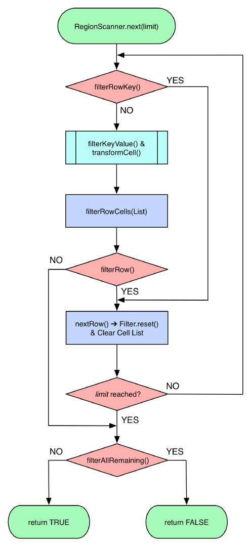

row
The Filter interface has a few more methods at its disposal.
Table 4-5 lists them for your perusal.
Table 4-5. Additional methods provided by the Filter class
Method Description
getNextCellHint() This method is invoked when the filter’s filterKeyValue()
method returns ReturnCode.SEEK_NEXT_USING_HINT. Use it to
skip large ranges of rows—if possible.
isFamilyEssential() Discussed in “Load Column Families on Demand” (page 213),
used to avoid unnecessary loading of cells from column
families in low-cardinality scans.
setReversed()/isRe
versed() Flags the direction the filter instance is observing. A reverse
scan must use reverse filters too.
toByteArray()/parse
From() Used to de-/serialize the filter’s internal state to ship to the
servers for application.
The reverse flag, assigned with setReversed(true), helps the filter to
come to the right decision. Here is a snippet from the PrefixFil
ter.filterRowKey() method, showing how the result of the binary
prefix comparison is reversed based on this flag:
...
int cmp = Bytes.compareTo(buffer, offset, this.prefix.length,
this.prefix, 0, this.prefix.length);
if ((!isReversed() && cmp > 0) || (isReversed() && cmp < 0)) {
passedPrefix = true;
}
...
Example 4-23 implements a custom filter, using the methods provided
by FilterBase, overriding only those methods that need to be
changed (or, more specifically, at least implement those that are
marked abstract). The filter first assumes all rows should be filtered,
that is, removed from the result. Only when there is a value in any col‐
umn that matches the given reference does it include the row, so that
it is sent back to the client. See “Custom Filter Loading” (page 268) for
how to load the custom filters into the Java server process.
Example 4-23. Implements a filter that lets certain rows pass
public class CustomFilter extends FilterBase {
private byte[] value = null;
private boolean filterRow = true;
public CustomFilter() {
Chapter 4: Client API: Advanced Features264
www.finebook.ir
super();
}
public CustomFilter(byte[] value) {
this.value = value;
}
@Override
public void reset() {
this.filterRow = true;
}
@Override
public ReturnCode filterKeyValue(Cell cell) {
if (CellUtil.matchingValue(cell, value)) {
filterRow = false;
}
return ReturnCode.INCLUDE;
}
@Override
public boolean filterRow() {
return filterRow;
}
@Override
public byte [] toByteArray() {
FilterProtos.CustomFilter.Builder builder =
FilterProtos.CustomFilter.newBuilder();
if (value != null) builder.setValue(ByteStringer.wrap(value));
return builder.build().toByteArray();
}
//@Override
public static Filter parseFrom(final byte[] pbBytes)
throws DeserializationException {
FilterProtos.CustomFilter proto;
try {
proto = FilterProtos.CustomFilter.parseFrom(pbBytes);
} catch (InvalidProtocolBufferException e) {
throw new DeserializationException(e);
}
return new CustomFilter(proto.getValue().toByteArray());
}
}
Set the value to compare against.
Reset filter flag for each new row being tested.
When there is a matching value, then let the row pass.
Always include, since the final decision is made later.
Filters 265
www.finebook.ir

3. For users of older, pre-Protocol Buffer based HBase, please see “Migrate Custom
Filters to post HBase 0.96” (page 640) for a migration guide.
Here the actual decision is taking place, based on the flag
status.
Writes the given value out so it can be send to the servers.
Used by the servers to establish the filter instance with the
correct values.
The most interesting part about the custom filter is the serialization
using Protocol Buffers (Protobuf, for short).3 The first thing to do is
define a message in Protobuf, which is done in a simple text file, here
named CustomFilters.proto:
option java_package = "filters.generated";
option java_outer_classname = "FilterProtos";
option java_generic_services = true;
option java_generate_equals_and_hash = true;
option optimize_for = SPEED;
message CustomFilter {
required bytes value = 1;
}
The file defines the output class name, the package to use during code
generation and so on. The next step is to compile the definition file in‐
to code. This is done using the Protobuf protoc tool.
The Protocol Buffer library usually comes as a source
package that needs to be compiled and locally installed.
There are also pre-built binary packages for many operat‐
ing systems. On OS X, for example, you can run the follow‐
ing, assuming Homebrew was installed:
$ brew install protobuf
You can verify the installation by running $ protoc --
version and check it prints a version number:
$ protoc --version
libprotoc 2.6.1
The online code repository of the book has a script bin/doprotoc.sh
that runs the code generation. It essentially runs the following com‐
mand from the repository root directory:
Chapter 4: Client API: Advanced Features266
www.finebook.ir
$ protoc -Ich04/src/main/protobuf --java_out=ch04/src/main/java \
ch04/src/main/protobuf/CustomFilters.proto
This will place the generated class file in the source directory, as
specified. After that you will be able to use the generated types in
your custom filter as shown in the example. Example 4-24 uses the
new custom filter to find rows with specific values in it, also using a
FilterList.
Example 4-24. Example using a custom filter
List<Filter> filters = new ArrayList<Filter>();
Filter filter1 = new CustomFilter(Bytes.toBytes("val-05.05"));
filters.add(filter1);
Filter filter2 = new CustomFilter(Bytes.toBytes("val-02.07"));
filters.add(filter2);
Filter filter3 = new CustomFilter(Bytes.toBytes("val-09.01"));
filters.add(filter3);
FilterList filterList = new FilterList(
FilterList.Operator.MUST_PASS_ONE, filters);
Scan scan = new Scan();
scan.setFilter(filterList);
ResultScanner scanner = table.getScanner(scan);
for (Result result : scanner) {
for (Cell cell : result.rawCells()) {
System.out.println("Cell: " + cell + ", Value: " +
Bytes.toString(cell.getValueArray(), cell.getValueOffset(),
cell.getValueLength()));
}
}
scanner.close();
Just as with the earlier examples, here is what should appear as out‐
put on the console when executing this example:
Adding rows to table...
Results of scan:
Cell: row-02/colfam1:col-01/1/Put/vlen=9/seqid=0, Value: val-02.01
Cell: row-02/colfam1:col-02/2/Put/vlen=9/seqid=0, Value: val-02.02
...
Cell: row-02/colfam1:col-06/6/Put/vlen=9/seqid=0, Value: val-02.06
Cell: row-02/colfam1:col-07/7/Put/vlen=9/seqid=0, Value: val-02.07
Cell: row-02/colfam1:col-08/8/Put/vlen=9/seqid=0, Value: val-02.08
...
Cell: row-05/colfam1:col-04/4/Put/vlen=9/seqid=0, Value: val-05.04
Cell: row-05/colfam1:col-05/5/Put/vlen=9/seqid=0, Value: val-05.05
Cell: row-05/colfam1:col-06/6/Put/vlen=9/seqid=0, Value: val-05.06
...
Filters 267
www.finebook.ir
Cell: row-05/colfam1:col-10/10/Put/vlen=9/seqid=0, Value: val-05.10
Cell: row-09/colfam1:col-01/1/Put/vlen=9/seqid=0, Value: val-09.01
Cell: row-09/colfam1:col-02/2/Put/vlen=9/seqid=0, Value: val-09.02
...
Cell: row-09/colfam1:col-09/9/Put/vlen=9/seqid=0, Value: val-09.09
Cell: row-09/colfam1:col-10/10/Put/vlen=9/seqid=0, Value: val-09.10
As expected, the entire row that has a column with the value matching
one of the references is included in the result.
Custom Filter Loading
Once you have written your filter, you need to deploy it to your HBase
setup. You need to compile the class, pack it into a Java Archive (JAR)
file, and make it available to the region servers. You can use the build
system of your choice to prepare the JAR file for deployment, and a
configuration management system to actually provision the file to all
servers. Once you have uploaded the JAR file, you have two choices
how to load them:
Static Configuration
In this case, you need to add the JAR file to the hbase-env.sh con‐
figuration file, for example:
# Extra Java CLASSPATH elements. Optional.
# export HBASE_CLASSPATH=
export HBASE_CLASSPATH="/hbase-book/ch04/target/hbase-book-
ch04-2.0.jar"
This is using the JAR file created by the Maven build as supplied
by the source code repository accompanying this book. It uses an
absolute, local path since testing is done on a standalone setup, in
other words, with the development environment and HBase run‐
ning on the same physical machine.
Note that you must restart the HBase daemons so that the
changes in the configuration file are taking effect. Once this is
done you can proceed to test the new filter.
Dynamic Loading
You still build the JAR file the same way, but instead of hardcoding
its path into the configuration files, you can use the cluster wide,
shared JAR file directory in HDFS that is used to load JAR files
from. See the following configuration property from the hbase-
default.xml file:
<property>
<name>hbase.dynamic.jars.dir</name>
<value>${hbase.rootdir}/lib</value>
</property>
Chapter 4: Client API: Advanced Features268
www.finebook.ir
The default points to ${hbase.rootdir}/lib, which usually re‐
solves to /hbase/lib/ within HDFS. The full path would be similar
to this example path: hdfs://master.foobar.com:9000/hbase/
lib. If this directory exists and contains files ending in .jar, then
the servers will load those files and make the contained classes
available. To do so, the files are copied to a local directory named
jars, located in a parent directory set again in the HBase default
properties:
<property>
<name>hbase.local.dir</name>
<value>${hbase.tmp.dir}/local/</value>
</property>
An example path for a cluster with a configured temporary directo‐
ry pointing to /data/tmp/ you will see the JAR files being copied
to /data/tmp/local/jars. You will see this directory again later
on when we talk about dynamic coprocessor loading in “Coproces‐
sor Loading” (page 289). The local JAR files are flagged to be deleted
when the server process ends normally.
The dynamic loading directory is monitored for changes, and will
refresh the JAR files locally if they have been updated in the
shared location.
Note that no matter how you load the classes and their containing
JARs, HBase is currently not able to unload a previously loaded class.
This means that once loaded, you cannot replace a class with the
same name. The only way short of restarting the server processes is to
add a version number to the class and JAR name to load the new one
by new name. This leaves the previous classes loaded in memory and
might cause memory issues after some time.
Filter Parser Utility
The client-side filter package comes with another helper class, named
ParseFilter. It is used in all the places where filters need to be de‐
scribed with text and then, eventually, converted to a Java class. This
happens in the gateway servers, such as for REST or Thrift. The
HBase Shell also makes use of the class allowing a shell user to speci‐
fy a filter on the command line, and then executing the filter as part of
a subsequent scan, or get, operation. The following executes a scan on
one of the earlier test tables (so your results may vary), adding a row
prefix and qualifier filter, using the shell:
hbase(main):001:0> scan 'testtable', \
{ FILTER => "PrefixFilter('row-2') AND QualifierFilter(<=,
'binary:col-2')" }
Filters 269
www.finebook.ir

ROW COLUMN+CELL
row-20 column=colfam1:col-0, timestamp=7, value=val-46
row-21 column=colfam1:col-0, timestamp=7, value=val-87
row-21 column=colfam1:col-2, timestamp=5, value=val-26
...
row-28 column=colfam1:col-2, timestamp=3, value=val-74
row-29 column=colfam1:col-1, timestamp=0, value=val-86
row-29 column=colfam1:col-2, timestamp=3, value=val-21
10 row(s) in 0.0170 seconds
What seems odd at first is the "binary:col-2" parameter. The second
part after the colon is the value handed into the filter. The first part is
the way the filter parser class is allowing you to specify a comparator
for filters based on CompareFilter (see “Comparators” (page 222)).
Here is a list of supported comparator prefixes:
Table 4-6. String representation of Comparator types
String Type
binary BinaryComparator
binaryprefix BinaryPrefixComparator
regexstring RegexStringComparator
substring SubstringComparator
Since a comparison filter also is requiring a comparison operation,
there is a way of expressing this in string format. The example above
uses "<=" to specify less than or equal. Since there is an enumeration
provided by the CompareFilter class, there is a matching pattern be‐
tween the string representation and the enumeration value, as shown
in the next table (also see “Comparison Operators” (page 221)):
Table 4-7. String representation of compare operation
String Type
< CompareOp.LESS
<= CompareOp.LESS_OR_EQUAL
> CompareOp.GREATER
>= CompareOp.GREATER_OR_EQUAL
= CompareOp.EQUAL
!= CompareOp.NOT_EQUAL
The filter parser supports a few more text based tokens that translate
into filter classes. You can combine filters with the AND and OR key‐
words, which are subsequently translated into FilterList instances
that are either set to MUST_PASS_ALL, or MUST_PASS_ONE respectively
Chapter 4: Client API: Advanced Features270
www.finebook.ir

(“FilterList” (page 256) describes this in more detail). An example
might be:
hbase(main):001:0> scan 'testtable', \
{ FILTER => "(PrefixFilter('row-2') AND ( \
QualifierFilter(>=, 'binary:col-2'))) AND (TimestampsFilter(1,
5))" }
ROW COLUMN+CELL
row-2 column=colfam1:col-9, timestamp=5, value=val-31
row-21 column=colfam1:col-2, timestamp=5, value=val-26
row-23 column=colfam1:col-5, timestamp=5, value=val-55
row-28 column=colfam1:col-5, timestamp=1, value=val-54
4 row(s) in 0.3190 seconds
Finally, there are the keywords SKIP and WHILE, representing the use
of a SkipFilter (see “SkipFilter” (page 253)) and WhileMatchFilter
(see “WhileMatchFilter” (page 255)). Refer to the mentioned sections
for details on their features.
hbase(main):001:0> scan 'testtable', \
{ FILTER => "SKIP ValueFilter(>=, 'binary:val-5') " }
ROW COLUMN+CELL
row-11 column=colfam1:col-0, timestamp=8, value=val-82
row-48 column=colfam1:col-3, timestamp=6, value=val-55
row-48 column=colfam1:col-7, timestamp=3, value=val-80
row-48 column=colfam1:col-8, timestamp=2, value=val-65
row-7 column=colfam1:col-9, timestamp=6, value=val-57
3 row(s) in 0.0150 seconds
The precedence of the keywords the parser understands is the follow‐
ing, listed from highest to lowest:
Table 4-8. Precedence of string keywords
Keyword Description
SKIP/WHILE Wrap filter into SkipFilter, or WhileMatchFilter instance.
AND Add both filters left and right of keyword to FilterList instance using
MUST_PASS_ALL.
OR Add both filters left and right of keyword to FilterList instance using
MUST_PASS_ONE.
From code you can invoke one of the following methods to parse a fil‐
ter string into class instances:
Filter parseFilterString(String filterString)
throws CharacterCodingException
Filter parseFilterString (byte[] filterStringAsByteArray)
throws CharacterCodingException
Filter parseSimpleFilterExpression(byte[] filterStringAsByteArray)
throws CharacterCodingException
Filters 271
www.finebook.ir

The parseSimpleFilterExpression() parses one specific filter in‐
stance, and is used mainly from within the parseFilterString()
methods. The latter handles the combination of multiple filters with
AND and OR, plus the decorating filter wrapping with SKIP and WHILE.
The two parseFilterString() methods are the same, one is taking a
string and the other a string converted to a byte[] array.
The ParseFilter class—by default—is only supporting the filters that
are shipped with HBase. The unsupported filters on top of that are
FirstKeyValueMatchingQualifiersFilter, FuzzyRowFilter, and Ran
domRowFilter (as of this writing). In your own code you can register
your own, and retrieve the list of supported filters using the following
methods of this class:
static Map<String, String> getAllFilters()
Set<String> getSupportedFilters()
static void registerFilter(String name, String filterClass)
Filters Summary
Table 4-9 summarizes some of the features and compatibilities related
to the provided filter implementations. The symbol means the feature
is available, while indicates it is missing.
Table 4-9. Summary of filter features and compatibilities between
them
Filter BatchaSkipbWhile-
MatchcListdEarly OuteGetsfScansg
RowFilter ✓ ✓ ✓ ✓ ✓ ✗ ✓
FamilyFilter ✓ ✓ ✓ ✓ ✗ ✓ ✓
QualifierFilter ✓ ✓ ✓ ✓ ✗ ✓ ✓
ValueFilter ✓ ✓ ✓ ✓ ✗ ✓ ✓
DependentColumn
Filter ✗ ✓ ✓ ✓ ✗ ✓ ✓
SingleColumnVa
lueFilter ✓ ✓ ✓ ✓ ✗ ✗ ✓
SingleColumnVa
lueExcludeFilter ✓ ✓ ✓ ✓ ✗ ✗ ✓
PrefixFilter ✓ ✗ ✓ ✓ ✓ ✗ ✓
PageFilter ✓ ✗ ✓ ✓ ✓ ✗ ✓
KeyOnlyFilter ✓ ✓ ✓ ✓ ✗ ✓ ✓
FirstKeyOnlyFil
ter ✓ ✓ ✓ ✓ ✗ ✓ ✓
Chapter 4: Client API: Advanced Features272
www.finebook.ir

Filter BatchaSkipbWhile-
MatchcListdEarly OuteGetsfScansg
FirstKeyValue
MatchingQuali
fiersFilter
✓ ✓ ✓ ✓ ✗ ✓ ✓
InclusiveStopFil
ter ✓ ✗ ✓ ✓ ✓ ✗ ✓
FuzzyRowFilter ✓ ✓ ✓ ✓ ✓ ✗ ✓
ColumnCountGet
Filter ✓ ✓ ✓ ✓ ✗ ✓ ✗
ColumnPagination
Filter ✓ ✓ ✓ ✓ ✗ ✓ ✓
ColumnPrefixFil
ter ✓ ✓ ✓ ✓ ✗ ✓ ✓
MultipleColumn
PrefixFilter ✓ ✓ ✓ ✓ ✗ ✓ ✓
ColumnRange ✓ ✓ ✓ ✓ ✗ ✓ ✓
TimestampsFilter ✓ ✓ ✓ ✓ ✗ ✓ ✓
RandomRowFilter ✓ ✓ ✓ ✓ ✗ ✗ ✓
SkipFilter ✓✓/✗a✓/✗h✓ ✗ ✗ ✓
WhileMatchFilter ✓✓/✗h✓/✗h✓ ✓ ✗ ✓
FilterList ✓/✗h✓/✗h✓/✗h✓✓/✗h✓ ✓
a Filter supports Scan.setBatch(), i.e., the scanner batch mode.
b Filter can be used with the decorating SkipFilter class.
c Filter can be used with the decorating WhileMatchFilter class.
d Filter can be used with the combining FilterList class.
e Filter has optimizations to stop a scan early, once there are no more matching rows
ahead.
f Filter can be usefully applied to Get instances.
g Filter can be usefully applied to Scan instances.
h Depends on the included filters.
Counters
In addition to the functionality we already discussed, HBase offers an‐
other advanced feature: counters. Many applications that collect sta‐
tistics—such as clicks or views in online advertising—were used to col‐
lect the data in logfiles that would subsequently be analyzed. Using
counters offers the potential of switching to live accounting, foregoing
the delayed batch processing step completely.
Counters 273
www.finebook.ir

Introduction to Counters
In addition to the check-and-modify operations you saw earlier, HBase
also has a mechanism to treat columns as counters. Otherwise, you
would have to lock a row, read the value, increment it, write it back,
and eventually unlock the row for other writers to be able to access it
subsequently. This can cause a lot of contention, and in the event of a
client process, crashing it could leave the row locked until the lease
recovery kicks in—which could be disastrous in a heavily loaded sys‐
tem.
The client API provides specialized methods to do the read-modify-
write operation atomically in a single client-side call. Earlier versions
of HBase only had calls that would involve an RPC for every counter
update, while newer versions started to add the same mechanisms
used by the CRUD operations—as explained in “CRUD Operations”
(page 122)--which can bundle multiple counter updates in a single
RPC.
Before we discuss each type separately, you need to have a few more
details regarding how counters work on the column level. Here is an
example using the shell that creates a table, increments a counter
twice, and then queries the current value:
hbase(main):001:0> create 'counters', 'daily', 'weekly', 'monthly'
0 row(s) in 1.1930 seconds
hbase(main):002:0> incr 'counters', '20150101', 'daily:hits', 1
COUNTER VALUE = 1
0 row(s) in 0.0490 seconds
hbase(main):003:0> incr 'counters', '20150101', 'daily:hits', 1
COUNTER VALUE = 2
0 row(s) in 0.0170 seconds
hbase(main):04:0> get_counter 'counters', '20150101', 'daily:hits'
COUNTER VALUE = 2
Every call to incr increases the counter by the given value (here 1).
The final check using get_counter shows the current value as expect‐
ed. The format of the shell’s incr command is as follows:
incr '<table>', '<row>', '<column>', [<increment-value>]
Initializing Counters
You should not initialize counters, as they are automatically as‐
sumed to be zero when you first use a new counter, that is, a col‐
umn qualifier that does not yet exist. The first increment call to a
Chapter 4: Client API: Advanced Features274
www.finebook.ir

new counter will set it to 1--or the increment value, if you have
specified one.
You can read and write to a counter directly, but you must use
Bytes.toLong()
to decode the value and
Bytes.toBytes(long)
for the encoding of the stored value. The latter, in particular, can
be tricky, as you need to make sure you are using a long number
when using the toBytes() method. You might want to consider
typecasting the variable or number you are using to a long explic‐
itly, like so:
byte[] b1 = Bytes.toBytes(1L)
byte[] b2 = Bytes.toBytes((long) var)
If you were to try to erroneously initialize a counter using the put
method in the HBase Shell, you might be tempted to do this:
hbase(main):001:0> put 'counters', '20150101', 'daily:clicks',
'1'
0 row(s) in 0.0540 seconds
But when you are going to use the increment method, you would
get this result instead:
hbase(main):013:0> incr 'counters', '20110101', 'dai
ly:clicks', 1
ERROR: org.apache.hadoop.hbase.DoNotRetryIOException: Attemp‐
ted to increment field that isn't 64 bits wide
at org.apache.hadoop.hbase.regionserver.HRegion.incre‐
ment(HRegion.java:5856)
at org.apache.hadoop.hbase.regionserver.RSRpcServices.in‐
crement(RSRpcServices.java:490)
...
That is not the expected value of 2! This is caused by the put call
storing the counter in the wrong format: the value is the character
1, a single byte, not the byte array representation of a Java long
value—which is composed of eight bytes.
You can also access the counter with a get call, giving you this result:
hbase(main):005:0> get 'counters', '20150101'
COLUMN CELL
daily:hits timestamp=1427485256567, value=
\x00\x00\x00\x00\x00\x00\x00\x02
1 row(s) in 0.0280 seconds
Counters 275
www.finebook.ir
This is obviously not very readable, but it shows that a counter is sim‐
ply a column, like any other. You can also specify a larger increment
value:
hbase(main):006:0> incr 'counters', '20150101', 'daily:hits', 20
COUNTER VALUE = 22
0 row(s) in 0.0180 seconds
hbase(main):007:0> get_counter 'counters', '20150101', 'daily:hits'
COUNTER VALUE = 22
hbase(main):008:0> get 'counters', '20150101'
COLUMN CELL
daily:hits timestamp=1427489182419, value=
\x00\x00\x00\x00\x00\x00\x00\x16
1 row(s) in 0.0200 seconds
Accessing the counter directly gives you the byte[] array representa‐
tion, with the shell printing the separate bytes as hexadecimal values.
Using the get_counter once again shows the current value in a more
human-readable format, and confirms that variable increments are
possible and work as expected.
Finally, you can use the increment value of the incr call to not only in‐
crease the counter, but also retrieve the current value, and decrease
it as well. In fact, you can omit it completely and the default of 1 is as‐
sumed:
hbase(main):009:0> incr 'counters', '20150101', 'daily:hits'
COUNTER VALUE = 23
0 row(s) in 0.1700 seconds
hbase(main):010:0> incr 'counters', '20150101', 'daily:hits'
COUNTER VALUE = 24
0 row(s) in 0.0230 seconds
hbase(main):011:0> incr 'counters', '20150101', 'daily:hits', 0
COUNTER VALUE = 24
0 row(s) in 0.0170 seconds
hbase(main):012:0> incr 'counters', '20150101', 'daily:hits', -1
COUNTER VALUE = 23
0 row(s) in 0.0210 seconds
hbase(main):013:0> incr 'counters', '20150101', 'daily:hits', -1
COUNTER VALUE = 22
0 row(s) in 0.0200 seconds
Using the increment value—the last parameter of the incr command
—you can achieve the behavior shown in Table 4-10.
Chapter 4: Client API: Advanced Features276
www.finebook.ir

Table 4-10. The increment value and its effect on counter incre‐
ments
Value Effect
greater than zero Increase the counter by the given value.
zero Retrieve the current value of the counter. Same as using the
get_counter shell command.
less than zero Decrease the counter by the given value.
Obviously, using the shell’s incr command only allows you to increase
a single counter. You can do the same using the client API, described
next.
Single Counters
The first type of increment call is for single counters only: you need to
specify the exact column you want to use. The methods, provided by
Table, are as such:
long incrementColumnValue(byte[] row, byte[] family, byte[] quali‐
fier,
long amount) throws IOException;
long incrementColumnValue(byte[] row, byte[] family, byte[] quali‐
fier,
long amount, Durability durability) throws IOException;
Given the coordinates of a column, and the increment amount, these
methods only differ by the optional durability parameter—which
works the same way as the Put.setDurability() method (see “Dura‐
bility, Consistency, and Isolation” (page 108) for the general discus‐
sion of this feature). Omitting durability uses the default value of Du
rability.SYNC_WAL, meaning the write-ahead log is active. Apart
from that, you can use them straight forward, as shown in
Example 4-25.
Example 4-25. Example using the single counter increment meth‐
ods
long cnt1 = table.incrementColumnValue(Bytes.toBytes("20110101"),
Bytes.toBytes("daily"), Bytes.toBytes("hits"), 1);
long cnt2 = table.incrementColumnValue(Bytes.toBytes("20110101"),
Bytes.toBytes("daily"), Bytes.toBytes("hits"), 1);
long current = table.incrementColumnValue(Bytes.to‐
Bytes("20110101"),
Bytes.toBytes("daily"), Bytes.toBytes("hits"), 0);
Counters 277
www.finebook.ir

long cnt3 = table.incrementColumnValue(Bytes.toBytes("20110101"),
Bytes.toBytes("daily"), Bytes.toBytes("hits"), -1);
Increase counter by one.
Increase counter by one a second time.
Get current value of the counter without increasing it.
Decrease counter by one.
The output on the console is:
cnt1: 1, cnt2: 2, current: 2, cnt3: 1
Just as with the shell commands used earlier, the API calls have the
same effect: they increment the counter when using a positive incre‐
ment value, retrieve the current value when using zero for the incre‐
ment, and decrease the counter by using a negative increment value.
Multiple Counters
Another way to increment counters is provided by the increment()
call of Table. It works similarly to the CRUD-type operations dis‐
cussed earlier, using the following method to do the increment:
Result increment(final Increment increment) throws IOException
You must create an instance of the Increment class and fill it with the
appropriate details—for example, the counter coordinates. The con‐
structors provided by this class are:
Increment(byte[] row)
Increment(final byte[] row, final int offset, final int length)
Increment(Increment i)
You must provide a row key when instantiating an Increment, which
sets the row containing all the counters that the subsequent call to in
crement() should modify. There is also the variant already known to
you that takes a larger array with an offset and length parameter to
extract the row key from. Finally, there is also the one you have seen
before, which takes an existing instance and copies all state from it.
Once you have decided which row to update and created the Incre
ment instance, you need to add the actual counters—meaning columns
—you want to increment, using these methods:
Increment addColumn(byte[] family, byte[] qualifier, long amount)
Increment add(Cell cell) throws IOException
The first variant takes the column coordinates, while the second is re‐
using an existing cell. This is useful, if you have just retrieved a
Chapter 4: Client API: Advanced Features278
www.finebook.ir

counter and now want to increment it. The add() call checks that the
given cell matches the row key of the Increment instance.
The difference here, as compared to the Put methods, is that there is
no option to specify a version—or timestamp—when dealing with in‐
crements: versions are handled implicitly. Furthermore, there is no
addFamily() equivalent, because counters are specific columns, and
they need to be specified as such. It therefore makes no sense to add
a column family alone.
A special feature of the Increment class is the ability to take an op‐
tional time range:
Increment setTimeRange(long minStamp, long maxStamp) throws IOEx‐
ception
TimeRange getTimeRange()
Setting a time range for a set of counter increments seems odd in
light of the fact that versions are handled implicitly. The time range is
actually passed on to the servers to restrict the internal get operation
from retrieving the current counter values. You can use it to expire
counters, for example, to partition them by time: when you set the
time range to be restrictive enough, you can mask out older counters
from the internal get, making them look like they are nonexistent. An
increment would assume they are unset and start at 1 again. The get
TimeRange() returns the currently assigned time range (and might be
null if not set at all).
Similar to the shell example shown earlier, Example 4-26 uses various
increment values to increment, retrieve, and decrement the given
counters.
Example 4-26. Example incrementing multiple counters in one row
Increment increment1 = new Increment(Bytes.toBytes("20150101"));
increment1.addColumn(Bytes.toBytes("daily"), Bytes.to‐
Bytes("clicks"), 1);
increment1.addColumn(Bytes.toBytes("daily"), Bytes.to‐
Bytes("hits"), 1);
increment1.addColumn(Bytes.toBytes("weekly"), Bytes.to‐
Bytes("clicks"), 10);
increment1.addColumn(Bytes.toBytes("weekly"), Bytes.to‐
Bytes("hits"), 10);
Result result1 = table.increment(increment1);
for (Cell cell : result1.rawCells()) {
System.out.println("Cell: " + cell +
" Value: " + Bytes.toLong(cell.getValueArray(), cell.getVa‐
lueOffset(),
Counters 279
www.finebook.ir

cell.getValueLength()));
}
Increment increment2 = new Increment(Bytes.toBytes("20150101"));
increment2.addColumn(Bytes.toBytes("daily"), Bytes.to‐
Bytes("clicks"), 5);
increment2.addColumn(Bytes.toBytes("daily"), Bytes.to‐
Bytes("hits"), 1);
increment2.addColumn(Bytes.toBytes("weekly"), Bytes.to‐
Bytes("clicks"), 0);
increment2.addColumn(Bytes.toBytes("weekly"), Bytes.to‐
Bytes("hits"), -5);
Result result2 = table.increment(increment2);
for (Cell cell : result2.rawCells()) {
System.out.println("Cell: " + cell +
" Value: " + Bytes.toLong(cell.getValueArray(),
cell.getValueOffset(), cell.getValueLength()));
}
Increment the counters with various values.
Call the actual increment method with the above counter
updates and receive the results.
Print the cell and returned counter value.
Use positive, negative, and zero increment values to achieve the
wanted counter changes.
When you run the example, the following is output on the console:
Cell: 20150101/daily:clicks/1427651982538/Put/vlen=8/seqid=0 Val‐
ue: 1
Cell: 20150101/daily:hits/1427651982538/Put/vlen=8/seqid=0 Value: 1
Cell: 20150101/weekly:clicks/1427651982538/Put/vlen=8/seqid=0 Val‐
ue: 10
Cell: 20150101/weekly:hits/1427651982538/Put/vlen=8/seqid=0 Value:
10
Cell: 20150101/daily:clicks/1427651982543/Put/vlen=8/seqid=0 Val‐
ue: 6
Cell: 20150101/daily:hits/1427651982543/Put/vlen=8/seqid=0 Value: 2
Cell: 20150101/weekly:clicks/1427651982543/Put/vlen=8/seqid=0 Val‐
ue: 10
Cell: 20150101/weekly:hits/1427651982543/Put/vlen=8/seqid=0 Value:
5
When you compare the two sets of increment results, you will notice
that this works as expected.
Chapter 4: Client API: Advanced Features280
www.finebook.ir

The Increment class provides additional methods, which are listed in
Table 4-11 for your reference. Once again, many are inherited from
the superclasses, such as Mutation (see “Query versus Mutation”
(page 106) again).
Table 4-11. Quick overview of additional methods provided by the
Increment class
Method Description
cellScanner() Provides a scanner over all cells available in this
instance.
getACL()/setACL() The ACLs for this operation (might be null).
getAttribute()/setAttri
bute() Set and get arbitrary attributes associated with this
instance of Increment.
getAttributesMap() Returns the entire map of attributes, if any are set.
getCellVisibility()/set
CellVisibility() The cell level visibility for all included cells.
getClusterIds()/setClus
terIds() The cluster IDs as needed for replication purposes.
getDurability()/setDura
bility() The durability settings for the mutation.
getFamilyCellMap()/setFa
milyCellMap() The list of all cells of this instance.
getFamilyMapOfLongs() Returns a list of Long instance, instead of cells (which get
FamilyCellMap() does), for what was added to this
instance so far. The list is indexed by families, and then
by column qualifier.
getFingerprint() Compiles details about the instance into a map for
debugging, or logging.
getId()/setId() An ID for the operation, useful for identifying the origin of
a request later.
getRow() Returns the row key as specified when creating the Incre
ment instance.
getTimeStamp() Not useful with Increment. Defaults to HConstants.LAT
EST_TIMESTAMP.
getTTL()/setTTL() Sets the cell level TTL value, which is being applied to all
included Cell instances before being persisted.
hasFamilies() Another helper to check if a family—or column—has been
added to the current instance of the Increment class.
heapSize() Computes the heap space required for the current Incre
ment instance. This includes all contained data and space
needed for internal structures.
isEmpty() Checks if the family map contains any Cell instances.
Counters 281
www.finebook.ir

Method Description
numFamilies() Convenience method to retrieve the size of the family
map, containing all Cell instances.
size() Returns the number of Cell instances that will be applied
with this Increment.
toJSON()/toJSON(int) Converts the first 5 or N columns into a JSON format.
toMap()/toMap(int) Converts the first 5 or N columns into a map. This is more
detailed than what getFingerprint() returns.
toString()/toString(int) Converts the first 5 or N columns into a JSON, or map (if
JSON fails due to encoding problems).
A non-Mutation method provided by Increment is:
Map<byte[], NavigableMap<byte[], Long>> getFamilyMapOfLongs()
The above Example 4-26 in the online repository shows how this can
give you access to the list of increment values of a configured Incre
ment instance. It is omitted above for the sake of brevity, but the on‐
line code has this available (around line number 40).
Coprocessors
Earlier we discussed how you can use filters to reduce the amount of
data being sent over the network from the servers to the client. With
the coprocessor feature in HBase, you can even move part of the com‐
putation to where the data lives.
We slightly go on a tangent here as far as interface audi‐
ence is concerned. If you refer back to “HBase Version”
(page xix) you will see how we, up until now, solely cov‐
ered Public APIs, that is, those that are annotated as be‐
ing public. For coprocessors we are now looking at an API
annotated as @InterfaceAudience.LimitedPrivate(HBa
seInterfaceAudience.COPROC), since it is meant for
HBase system developers. A normal API user will make
use of coprocessors, but most likely not develop them.
Coprocessors are very low-level, and are usually for very
experienced developers only.
Introduction to Coprocessors
Using the client API, combined with specific selector mechanisms,
such as filters, or column family scoping, it is possible to limit what
Chapter 4: Client API: Advanced Features282
www.finebook.ir

data is transferred to the client. It would be good, though, to take this
further and, for example, perform certain operations directly on the
server side while only returning a small result set. Think of this as a
small MapReduce framework that distributes work across the entire
cluster.
A coprocessor enables you to run arbitrary code directly on each re‐
gion server. More precisely, it executes the code on a per-region ba‐
sis, giving you trigger- like functionality—similar to stored procedures
in the RDBMS world. From the client side, you do not have to take
specific actions, as the framework handles the distributed nature
transparently.
There is a set of implicit events that you can use to hook into, per‐
forming auxiliary tasks. If this is not enough, you can also extend the
RPC protocol to introduce your own set of calls, which are invoked
from your client and executed on the server on your behalf.
Just as with the custom filters (see “Custom Filters” (page 259)), you
need to create special Java classes that implement specific interfaces.
Once they are compiled, you make these classes available to the
servers in the form of a JAR file. The region server process can instan‐
tiate these classes and execute them in the correct environment. In
contrast to the filters, though, coprocessors can be loaded dynamical‐
ly as well. This allows you to extend the functionality of a running
HBase cluster.
Use cases for coprocessors are, for instance, using hooks into row mu‐
tation operations to maintain secondary indexes, or implementing
some kind of referential integrity. Filters could be enhanced to be‐
come stateful, and therefore make decisions across row boundaries.
Aggregate functions, such as sum(), or avg(), known from RDBMSes
and SQL, could be moved to the servers to scan the data locally and
only returning the single number result across the network (which is
showcased by the supplied AggregateImplementation class).
Another good use case for coprocessors is access control.
The authentication, authorization, and auditing features
added in HBase version 0.92 are based on coprocessors.
They are loaded at system startup and use the provided
trigger-like hooks to check if a user is authenticated, and
authorized to access specific values stored in tables.
The framework already provides classes, based on the coprocessor
framework, which you can use to extend from when implementing
Coprocessors 283
www.finebook.ir
your own functionality. They fall into two main groups: endpoint and
observer. Here is a brief overview of their purpose:
Endpoint
Next to event handling there may be also a need to add custom op‐
erations to a cluster. User code can be deployed to the servers
hosting the data to, for example, perform server-local computa‐
tions.
Endpoints are dynamic extensions to the RPC protocol, adding
callable remote procedures. Think of them as stored procedures,
as known from RDBMSes. They may be combined with observer
implementations to directly interact with the server-side state.
Observer
This type of coprocessor is comparable to triggers: callback func‐
tions (also referred to here as hooks) are executed when certain
events occur. This includes user-generated, but also server-
internal, automated events.
The interfaces provided by the coprocessor framework are:
MasterObserver
This can be used to react to administrative or DDL-type opera‐
tions. These are cluster-wide events.
RegionServerObserver
Hooks into commands sent to a region server, and covers re‐
gion server-wide events.
RegionObserver
Used to handle data manipulation events. They are closely
bound to the regions of a table.
WALObserver
This provides hooks into the write-ahead log processing, which
is region server-wide.
BulkLoadObserver
Handles events around the bulk loading API. Triggered before
and after the loading takes place.
EndpointObserver
Whenever an endpoint is invoked by a client, this observer is
providing a callback method.
Observers provide you with well-defined event callbacks, for every
operation a cluster server may handle.
All of these interfaces are based on the Coprocessor interface to gain
common features, but then implement their own specific functionality.
Chapter 4: Client API: Advanced Features284
www.finebook.ir
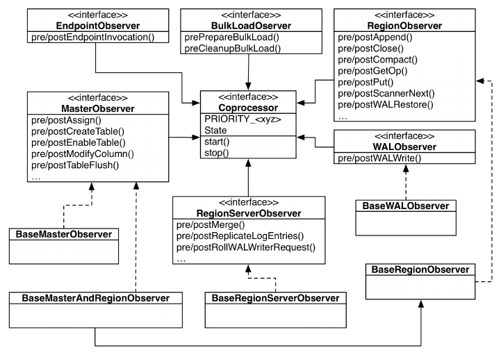
4. This was changed in the final 0.92 release (after the book went into print) from
enums to constants in HBASE-4048.
Finally, coprocessors can be chained, very similar to what the Java
Servlet API does with request filters. The following section discusses
the various types available in the coprocessor framework. Figure 4-3
shows an overview of all the classes we will be looking into.
Figure 4-3. The class hierarchy of the coprocessor related classes
The Coprocessor Class Trinity
All user coprocessor classes must be based on the Coprocessor inter‐
face. It defines the basic contract of a coprocessor and facilitates the
management by the framework itself. The interface provides two sets
of types, which are used throughout the framework: the PRIORITY
constants4, and State enumeration. Table 4-12 explains the priority
values.
Coprocessors 285
www.finebook.ir

Table 4-12. Priorities as defined by the Coprocessor.PRIORI
TY_<XYZ> constants
Name Value Description
PRIORITY_HIGHEST 0 Highest priority, serves as an upper boundary.
PRIORITY_SYSTEM 536870911 High priority, used for system coprocessors (Inte
ger.MAX_VALUE / 4).
PRIORITY_USER 1073741823 For all user coprocessors, which are executed
subsequently (Integer.MAX_VALUE / 2).
PRIORITY_LOWEST 2147483647 Lowest possible priority, serves as a lower boundary
(Integer.MAX_VALUE).
The priority of a coprocessor defines in what order the coprocessors
are executed: system-level instances are called before the user-level
coprocessors are executed.
Within each priority level, there is also the notion of a se‐
quence number, which keeps track of the order in which
the coprocessors were loaded. The number starts with
zero, and is increased by one thereafter.
The number itself is not very helpful, but you can rely on
the framework to order the coprocessors—in each priority
group—ascending by sequence number. This defines their
execution order.
Coprocessors are managed by the framework in their own life cycle.
To that effect, the Coprocessor interface offers two calls:
void start(CoprocessorEnvironment env) throws IOException
void stop(CoprocessorEnvironment env) throws IOException
These two methods are called when the coprocessor class is started,
and eventually when it is decommissioned. The provided Coprocessor
Environment instance is used to retain the state across the lifespan of
the coprocessor instance. A coprocessor instance is always contained
in a provided environment, which provides the following methods:
String getHBaseVersion()
Returns the HBase version identification string, for example
"1.0.0".
int getVersion()
Returns the version of the Coprocessor interface.
Chapter 4: Client API: Advanced Features286
www.finebook.ir

5. The use of HTableInterface is an API remnant from before HBase 1.0. For
HBase 2.0 and later this is changed to the proper `Table in
HBASE-12586.
Coprocessor getInstance()
Returns the loaded coprocessor instance.
int getPriority()
Provides the priority level of the coprocessor.
int getLoadSequence()
The sequence number of the coprocessor. This is set when the in‐
stance is loaded and reflects the execution order.
Configuration getConfiguration()
Provides access to the current, server-wide configuration.
HTableInterface getTable(TableName tableName)
HTableInterface getTable(TableName tableName, Executor
Service service)
Returns a Table implementation for the given table name. This al‐
lows the coprocessor to access the actual table data.5 The second
variant does the same, but allows the specification of a custom Ex
ecutorService instance.
Coprocessors should only deal with what they have been given by
their environment. There is a good reason for that, mainly to guaran‐
tee that there is no back door for malicious code to harm your data.
Coprocessor implementations should be using the getTa
ble() method to access tables. Note that this class adds
certain safety measures to the returned Table implemen‐
tation. While there is currently nothing that can stop you
from retrieving your own Table instances inside your cop‐
rocessor code, this is likely to be checked against in the
future and possibly denied.
The start() and stop() methods of the Coprocessor interface are in‐
voked implicitly by the framework as the instance is going through its
life cycle. Each step in the process has a well-known state. Table 4-13
lists the life-cycle state values as provided by the coprocessor inter‐
face.
Coprocessors 287
www.finebook.ir

Table 4-13. The states as defined by the Coprocessor.State enu‐
meration
Value Description
UNINSTALLED The coprocessor is in its initial state. It has no environment yet, nor is it
initialized.
INSTALLED The instance is installed into its environment.
STARTING This state indicates that the coprocessor is about to be started, that is,
its start() method is about to be invoked.
ACTIVE Once the start() call returns, the state is set to active.
STOPPING The state set just before the stop() method is called.
STOPPED Once stop() returns control to the framework, the state of the
coprocessor is set to stopped.
The final piece of the puzzle is the CoprocessorHost class that main‐
tains all the coprocessor instances and their dedicated environments.
There are specific subclasses, depending on where the host is used, in
other words, on the master, region server, and so on.
The trinity of Coprocessor, CoprocessorEnvironment, and Coproces
sorHost forms the basis for the classes that implement the advanced
functionality of HBase, depending on where they are used. They pro‐
vide the life-cycle support for the coprocessors, manage their state,
and offer the environment for them to execute as expected. In addi‐
tion, these classes provide an abstraction layer that developers can
use to easily build their own custom implementation.
Figure 4-4 shows how the calls from a client are flowing through the
list of coprocessors. Note how the order is the same on the incoming
and outgoing sides: first are the system-level ones, and then the user
ones in the order they were loaded.
Chapter 4: Client API: Advanced Features288
www.finebook.ir
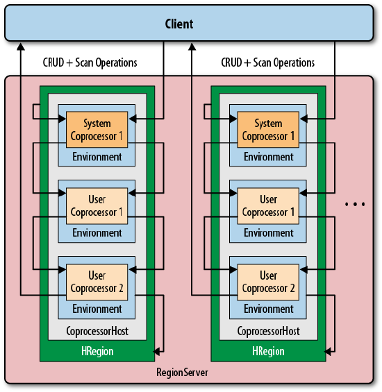
Figure 4-4. Coprocessors executed sequentially, in their environ‐
ment, and per region
Coprocessor Loading
Coprocessors are loaded in a variety of ways. Before we discuss the
actual coprocessor types and how to implement your own, we will talk
about how to deploy them so that you can try the provided examples.
You can either configure coprocessors to be loaded in a static way, or
load them dynamically while the cluster is running. The static method
uses the configuration files and table schemas, while the dynamic
loading of coprocessors is only using the table schemas.
There is also a cluster-wide switch that allows you to disable all copro‐
cessor loading, controlled by the following two configuration proper‐
ties:
hbase.coprocessor.enabled
The default is true and means coprocessor classes for system and
user tables are loaded. Setting this property to false stops the
Coprocessors 289
www.finebook.ir

servers from loading any of them. You could use this during test‐
ing, or during cluster emergencies.
hbase.coprocessor.user.enabled
Again, the default is true, that is, all user table coprocessors are
loaded when the server starts, or a region opens, etc. Setting this
property to false suppresses the loading of user table coproces‐
sors only.
Disabling coprocessors, using the cluster-wide configura‐
tion properties, means that whatever additional process‐
ing they add, your cluster will not have this functionality
available. This includes, for example, security checks, or
maintenance of referential integrity. Be very careful!
Loading from Configuration
You can configure globally which coprocessors are loaded when
HBase starts. This is done by adding one, or more, of the following to
the hbase-site.xml configuration file (but please, replace the exam‐
ple class names with your own ones!):
<property>
<name>hbase.coprocessor.master.classes</name>
<value>coprocessor.MasterObserverExample</value>
</property>
<property>
<name>hbase.coprocessor.regionserver.classes</name>
<value>coprocessor.RegionServerObserverExample</value>
</property>
<property>
<name>hbase.coprocessor.region.classes</name>
<value>coprocessor.system.RegionObserverExample,
coprocessor.AnotherCoprocessor</value>
</property>
<property>
<name>hbase.coprocessor.user.region.classes</name>
<value>coprocessor.user.RegionObserverExample</value>
</property>
<property>
<name>hbase.coprocessor.wal.classes</name>
<value>coprocessor.WALObserverExample, bar.foo.MyWALObserver</
value>
</property>
The order of the classes in each configuration property is important,
as it defines the execution order. All of these coprocessors are loaded
with the system priority. You should configure all globally active
Chapter 4: Client API: Advanced Features290
www.finebook.ir

classes here so that they are executed first and have a chance to take
authoritative actions. Security coprocessors are loaded this way, for
example.
The configuration file is the first to be examined as HBase
starts. Although you can define additional system-level
coprocessors in other places, the ones here are executed
first. They are also sometimes referred to as default copro‐
cessors.
Only one of the five possible configuration keys is read by
the matching CoprocessorHost implementation. For ex‐
ample, the coprocessors defined in hbase.coproces
sor.master.classes are loaded by the MasterCoprocesso
rHost class.
Table 4-14 shows where each configuration property is used.
Table 4-14. Possible configuration properties and where they are
used
Property Coprocessor Host Server Type
hbase.coprocessor.master.classes MasterCoprocessorHost Master Server
hbase.coprocessor.regionserv
er.classes
RegionServerCoprocessorHost Region Server
hbase.coprocessor.region.classes RegionCoprocessorHost Region Server
hbase.coprocessor.user.re
gion.classes
RegionCoprocessorHost Region Server
hbase.coprocessor.wal.classes WALCoprocessorHost Region Server
There are two separate properties provided for classes loaded into re‐
gions, and the reason is this:
hbase.coprocessor.region.classes
All listed coprocessors are loaded at system priority for every table
in HBase, including the special catalog tables.
hbase.coprocessor.user.region.classes
The coprocessor classes listed here are also loaded at system pri‐
ority, but only for user tables, not the special catalog tables.
Apart from that, the coprocessors defined with either property are
loaded when a region is opened for a table. Note that you cannot spec‐
ify for which user and/or system table, or region, they are loaded, or
Coprocessors 291
www.finebook.ir
in other words, they are loaded for every table and region. You need
to keep this in mind when designing your own coprocessors.
Be careful what you do as lifecycle events are triggered and your cop‐
rocessor code is setting up resources. As instantiating your coproces‐
sor is part of opening regions, any longer delay might be noticeable.
In other words, you should be very diligent to only do as light work as
possible during open and close events.
What is also important to consider is that when a coprocessor, loaded
from the configuration, fails to start, in other words it is throwing an
exception, it will cause the entire server process to be aborted. When
this happens, the process will log the error and a list of loaded (or
configured rather) coprocessors, which might help identifying the cul‐
prit.
Loading from Table Descriptor
The other option to define which coprocessors to load is the table de‐
scriptor. As this is per table, the coprocessors defined here are only
loaded for regions of that table—and only by the region servers host‐
ing these regions. In other words, you can only use this approach for
region-related coprocessors, not for master, or WAL-related ones. On
the other hand, since they are loaded in the context of a table, they
are more targeted compared to the configuration loaded ones, which
apply to all tables. You need to add their definition to the table de‐
scriptor using one of two methods:
1. Using the generic HTableDescriptor.setValue() with a specific
key, or
2. use the newer HTableDescriptor.addCoprocessor() method.
If you use the first method, you need to create a key that must start
with COPROCESSOR, and the value has to conform to the following for‐
mat:
[<path-to-jar>]|<classname>|[<priority>][|key1=value1,key2=val‐
ue2,...]
Here is an example that defines a few coprocessors, the first with
system-level priority, the others with user-level priorities:
'COPROCESSOR$1' => \
'hdfs://localhost:8020/users/leon/test.jar|coprocessor.Test|
2147483647'
'COPROCESSOR$2' => \
'/Users/laura/test2.jar|coprocessor.AnotherTest|1073741822'
'COPROCESSOR$3' => \
'/home/kg/advacl.jar|coprocessor.AdvancedAcl|1073741823|
Chapter 4: Client API: Advanced Features292
www.finebook.ir
keytab=/etc/keytab'
'COPROCESSOR$99' => '|com.foo.BarCoprocessor|'
The key is a combination of the prefix COPROCESSOR, a dollar sign as a
divider, and an ordering number, for example: COPROCESSOR$1. Using
the $<number> postfix for the key enforces the order in which the defi‐
nitions, and therefore the coprocessors, are loaded. This is especially
interesting and important when loading multiple coprocessors with
the same priority value. When you use the addCoprocessor() method
to add a coprocessor to a table descriptor, the method will look for the
highest assigned number and use the next free one after that. It starts
out at 1, and increments by one from there.
The value is composed of three to four parts, serving the following
purpose:
path-to-jar
Optional — The path can either be a fully qualified HDFS location,
or any other path supported by the Hadoop FileSystem class. The
second (and third) coprocessor definition, for example, uses a local
path instead. If left empty, the coprocessor class must be accessi‐
ble through the already configured class path.
If you specify a path in HDFS (or any other non-local file system
URI), the coprocessor class loader support will first copy the JAR
file to a local location, similar to what was explained in “Custom
Filters” (page 259). The difference is that the file is located in a
further subdirectory named tmp, for example /data/tmp/hbase-
hadoop/local/jars/tmp/. The name of the JAR is also changed to
a unique internal name, using the following pattern:
.<path-prefix>.<jar-filename>.<current-timestamp>.jar
The path prefix is usually a random UUID. Here a complete exam‐
ple:
$ $ ls -A /data/tmp/hbase-hadoop/local/jars/tmp/
.c20a1e31-7715-4016-8fa7-b69f636cb07c.hbase-book-ch04.jar.
1434434412813.jar
The local file is deleted upon normal server process termination.
classname
Required — This defines the actual implementation class. While the
JAR may contain many coprocessor classes, only one can be speci‐
fied per table attribute. Use the standard Java package name con‐
ventions to specify the class.
priority
Optional — The priority must be a number between the boundaries
explained in Table 4-12. If not specified, it defaults to Coproces
Coprocessors 293
www.finebook.ir

sor.PRIORITY_USER, in other words 1073741823. You can set any
priority to indicate the proper execution order of the coprocessors.
In the above example you can see that coprocessor #2 has a one-
lower priority compared to #3. This would cause #3 to be called
before #2 in the chain of events.
key=value
Optional — These are key/value parameters that are added to the
configuration handed into the coprocessor, and retrievable by call‐
ing CoprocessorEnvironment.getConfiguration() from, for ex‐
ample, the start() method. For example:
private String keytab;
@Override
public void start(CoprocessorEnvironment env) throws IOExcep‐
tion {
this.keytab = env.getConfiguration().get("keytab");
}
The above getConfiguration() call is returning the current server
configuration file, merged with any optional parameter specified in
the coprocessor declaration. The former is the hbase-site.xml,
merged with the provided hbase-default.xml, and all changes made
through any previous dynamic configuration update. Since this is then
merged with the per-coprocessor parameters (if there are any), it is
advisable to use a specific, unique prefix for the keys to not acciden‐
tally override any of the HBase settings. For example, a key with a
prefix made from the coprocessor class, plus its assigned value, could
look like this: com.foobar.copro.ReferentialIntegri
ty.table.main=production:users.
It is advised to avoid using extra whitespace characters in
the coprocessor definition. The parsing should take care of
all leading or trailing spaces, but if in doubt try removing
them to eliminate any possible parsing quirks.
The last coprocessor definition in the example is the shortest possible,
omitting all optional parts. All that is needed is the class name, as
shown, while retaining the dividing pipe symbols. Example 4-27 shows
how this can be done using the administrative API for HBase.
Example 4-27. Load a coprocessor using the table descriptor
public class LoadWithTableDescriptorExample {
Chapter 4: Client API: Advanced Features294
www.finebook.ir
public static void main(String[] args) throws IOException {
Configuration conf = HBaseConfiguration.create();
Connection connection = ConnectionFactory.createConnection(conf);
TableName tableName = TableName.valueOf("testtable");
HTableDescriptor htd = new HTableDescriptor(tableName);
htd.addFamily(new HColumnDescriptor("colfam1"));
htd.setValue("COPROCESSOR$1", "|" +
RegionObserverExample.class.getCanonicalName() +
"|" + Coprocessor.PRIORITY_USER);
Admin admin = connection.getAdmin();
admin.createTable(htd);
System.out.println(admin.getTableDescriptor(tableName));
admin.close();
connection.close();
}
}
Define a table descriptor.
Add the coprocessor definition to the descriptor, while omitting
the path to the JAR file.
Acquire an administrative API to the cluster and add the table.
Verify if the definition has been applied as expected.
Using the second approach, using the addCoprocessor() method pro‐
vided by the descriptor class, simplifies all of this, as shown in
Example 4-28. It will compute the next free coprocessor key using the
above rules, and assign the value in the proper format.
Example 4-28. Load a coprocessor using the table descriptor using
provided method
HTableDescriptor htd = new HTableDescriptor(tableName)
.addFamily(new HColumnDescriptor("colfam1"))
.addCoprocessor(RegionObserverExample.class.getCanonicalName(),
null, Coprocessor.PRIORITY_USER, null);
Admin admin = connection.getAdmin();
admin.createTable(htd);
Use fluent interface to create and configure the instance.
Use the provided method to add the coprocessor.
The examples omit setting the JAR file name since we assume the
same test setup as before, and earlier we have added the JAR file to
the hbase-env.sh file. With that, the coprocessor class is part of the
Coprocessors 295
www.finebook.ir
server class path and we can skip setting it again. Running the exam‐
ples against the assumed local, standalone HBase setup should emit
the following:
'testtable', {TABLE_ATTRIBUTES => {METADATA => { \
'COPROCESSOR$1' => '|coprocessor.RegionObserverExample|
1073741823'}}, \
{NAME => 'colfam1', DATA_BLOCK_ENCODING => 'NONE', BLOOMFILTER
=> 'ROW', \
REPLICATION_SCOPE => '0', VERSIONS => '1', COMPRESSION =>
'NONE', \
MIN_VERSIONS => '0', TTL => 'FOREVER', KEEP_DELETED_CELLS =>
'FALSE', \
BLOCKSIZE => '65536', IN_MEMORY => 'false', BLOCKCACHE =>
'true'}
The coprocessor definition has been successfully applied to the table
schema. Once the table is enabled and the regions are opened, the
framework will first load the configuration coprocessors and then the
ones defined in the table descriptor. The same considerations as men‐
tioned before apply here as well: be careful to not slow down the re‐
gion deployment process by long running, or resource intensive, oper‐
ations in your lifecycle callbacks, and avoid any exceptions being
thrown or the server process might be ended.
The difference here is that for table coprocessors there is a configura‐
tion property named hbase.coprocessor.abortonerror, which you
can set to true or false, indicating what you want to happen if an er‐
ror occurs during the initialization of a coprocessor class. The default
is true, matching the behavior of the configuration-loaded coproces‐
sors. Setting it to false will simply log the error that was encoun‐
tered, but move on with business as usual. Of course, the erroneous
coprocessor will neither be loaded nor be active.
Loading from HBase Shell
If you want to load coprocessors while HBase is running, there is an
option to dynamically load the necessary classes and containing JAR
files. This is accomplished using the table descriptor and the alter
call, provided by the administrative API (see “Table Operations” (page
378)) and exposed through the HBase Shell. The process is to updated
the table schema and then reload the table regions. The shell does
this in one call, as shown in the following example:
hbase(main):001:0> alter 'testqauat:usertable', \
'coprocessor' => 'file:///opt/hbase-book/hbase-book-
ch05-2.0.jar| \
coprocessor.SequentialIdGeneratorObserver|'
Updating all regions with the new schema...
1/11 regions updated.
Chapter 4: Client API: Advanced Features296
www.finebook.ir
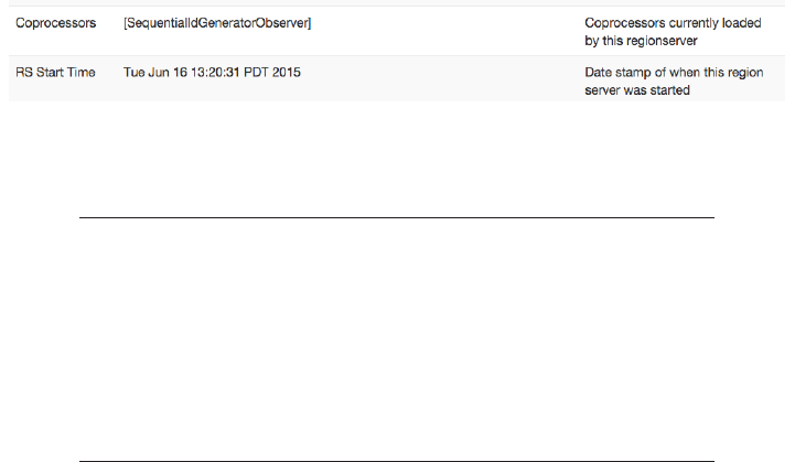
6/11 regions updated.
11/11 regions updated.
Done.
0 row(s) in 5.0540 seconds
hbase(main):002:0> describe 'testqauat:usertable'
Table testqauat:usertable is ENABLED
testqauat:usertable, {TABLE_ATTRIBUTES => {coprocessor$1 => \
'file:///opt/hbase-book/hbase-book-ch05-2.0.jar|coprocessor \
.SequentialIdGeneratorObserver|'}
COLUMN FAMILIES DESCRIPTION
{NAME => 'cf1', DATA_BLOCK_ENCODING => 'NONE', BLOOMFILTER =>
'ROW', \
REPLICATION_SCOPE => '0', COMPRESSION => 'NONE', VERSIONS =>
'1', \
TTL => 'FOREVER', MIN_VERSIONS => '0', KEEP_DELETED_CELLS =>
'FALSE', \
BLOCKSIZE => '65536', IN_MEMORY => 'false', BLOCKCACHE => 'true'}
1 row(s) in 0.0220 seconds
The second command uses describe to verify the coprocessor was
set, and what the assigned key for it is, here coprocessor$1. As for
the path used for the JAR file, keep in mind that it is considered the
source for the JAR file, and that it is copied into the local temporary
location before being loaded into the Java process as explained above.
You can use the region server UI to verify that the class has been
loaded successfully, by checking the Software Attributes section at
the end of the status page. In this table the is a line listing the loaded
coprocessor classes, as shown in Figure 4-5.
Figure 4-5. The Region Server status page lists the loaded copro‐
cessors
While you will learn more about the HBase Shell in
“Namespace and Data Definition Commands” (page 488), a
quick tip about using the alter command to add a table at‐
tribute: You can omit the METHOD => 'table_att' param‐
eter as shown above, because adding/setting a parameter
is the assumed default operation. Only for removing an at‐
tribute you have to explicitly specify the method, as shown
next when removing the previously set coprocessor.
Coprocessors 297
www.finebook.ir
Once a coprocessor is loaded, you can also remove them in the same
dynamic fashion, that is, using the HBase Shell to update the schema
and reload the affected table regions on all region servers in one sin‐
gle command:
hbase(main):003:0> alter 'testqauat:usertable', METHOD =>
'table_att_unset', \
NAME => 'coprocessor$1'
Updating all regions with the new schema...
2/11 regions updated.
8/11 regions updated.
11/11 regions updated.
Done.
0 row(s) in 4.2160 seconds
hbase(main):004:0> describe 'testqauat:usertable'
Table testqauat:usertable is ENABLED
testqauat:usertable
COLUMN FAMILIES DESCRIPTION
{NAME => 'cf1', DATA_BLOCK_ENCODING => 'NONE', BLOOMFILTER =>
'ROW', \
REPLICATION_SCOPE => '0', COMPRESSION => 'NONE', VERSIONS =>
'1', \
TTL => 'FOREVER', MIN_VERSIONS => '0', KEEP_DELETED_CELLS =>
'FALSE',
BLOCKSIZE => '65536', IN_MEMORY => 'false', BLOCKCACHE => 'true'}
1 row(s) in 0.0180 seconds
Removing a coprocessor requires to know its key in the table schema.
We have already retrieved that one earlier with the describe com‐
mand shown in the example. The unset (which removes the table sche‐
ma attribute) operation removes the key named coprocessor$1,
which was the said key we determined earlier. After all regions are re‐
loaded, we can use the describe command again to check if coproces‐
sor reference has indeed be removed, which is the case here.
Loading coprocessors using the dynamic table schema approach bears
the same burden as mention before: you cannot unload classes or JAR
files, therefore you may have to restart the region server process for
an update of the classes. You could work around for a limited amount
of time by versioning the class and JAR file names, but the loaded
classes may cause memory pressure eventually and force you to cycle
the processes.
Endpoints
The first of two major feature provided by the coprocessor framework
we are going to look at are endpoints. They solve a problem with mov‐
ing data for analytical queries, that would benefit from pre-calculating
Chapter 4: Client API: Advanced Features298
www.finebook.ir
intermediate results where the data resides, and just ship the results
back to the client. Sounds familiar? Yes, this is what MapReduce does
in Hadoop, that is, ship the code to the data, do the computation, and
persist the results.
An inherent feature of MapReduce is that it has intrinsic knowledge of
what data node is holding which block of information. When you exe‐
cute a job, the NameNode will instruct the scheduler to ship the code
to all nodes that contain data that is part of job parameters. With
HBase, we could run a client-side scan that ships all the data to the
client to do the computation. But at scale, this will not be efficient, be‐
cause the inertia of data exceeds the amount of processing performed.
In other words, all the time is spent in moving the data, the I/O.
What we need instead is the ability, just as with MapReduce, to ship
the processing to the servers, do the aggregation or any other compu‐
tation on the server-side, and only return the much smaller results
back to the client. And that, in a nutshell, is what Endpoints are all
about. You instruct the servers to load code with every region of a giv‐
en table, and when you need to scan the table, partially or completely,
it will call the server-side code, which then can scan the necessary da‐
ta where it resides: on the data servers.
Once the computation is completed, the results are shipped back to
the client, one result per region, and aggregated there for the final re‐
sult. For example, if you were to have 1,000 regions and 1 million col‐
umns, and you want to summarize the stored data, you would receive
1,000 decimal numbers on the client side—one for each region. This is
fast to aggregate for the final result. If you were to scan the entire
table using a purely client API approach, in a worst-case scenario you
would transfer all 1 million numbers to build the sum.
The Service Interface
Endpoints are implemented as an extension to the RPC protocol be‐
tween the client and server. In the past (before HBase 0.96) this was
done by literally extending the protocol classes. After the move to the
Protocol Buffer (Protobuf for short) based RPC, adding custom serv‐
ices on the server side was greatly simplified. The payload is serial‐
ized as a Protobuf message and sent from client to server (and back
again) using the provided coprocessor services API.
In order to provide an endpoint to clients, a coprocessor generates a
Protobuf implementation that extends the Service class. This service
can define any methods that the coprocessor wishes to expose. Using
the generated classes, you can communicate with the coprocessor in‐
stances via the following calls, provided by Table:
Coprocessors 299
www.finebook.ir
CoprocessorRpcChannel coprocessorService(byte[] row)
<T extends Service, R> Map<byte[],R> coprocessorService(final
Class<T> service,
byte[] startKey, byte[] endKey, final Batch.Call<T,R> callable)
throws ServiceException, Throwable
<T extends Service, R> void coprocessorService(final Class<T> ser‐
vice,
byte[] startKey, byte[] endKey, final Batch.Call<T,R> callable,
final Batch.Callback<R> callback) throws ServiceException, Throw‐
able
<R extends Message> Map<byte[], R> batchCoprocessorService(
Descriptors.MethodDescriptor methodDescriptor, Message request,
byte[] startKey, byte[] endKey, R responsePrototype)
throws ServiceException, Throwable
<R extends Message> void batchCoprocessorService(
Descriptors.MethodDescriptor methodDescriptor,
Message request, byte[] startKey, byte[] endKey, R responseProto‐
type,
Batch.Callback<R> callback) throws ServiceException, Throwable
Since Service instances are associated with individual regions within
a table, the client RPC calls must ultimately identify which regions
should be used in the service’s method invocations. Though regions
are seldom handled directly in client code and the region names may
change over time, the coprocessor RPC calls use row keys to identify
which regions should be used for the method invocations. Clients can
call Service methods against one of the following:
Single Region
This is done by calling coprocessorService() with a single row
key. This returns an instance of the CoprocessorRpcChannel class,
which directly extends Protobuf classes. It can be used to invoke
any endpoint call linked to the region containing the specified row.
Note that the row does not need to exist: the region selected is the
one that does or would contain the given key.
Ranges of Regions
You can call coprocessorService() with a start row key and an
end row key. All regions in the table from the one containing the
start row key to the one containing the end row key (inclusive) will
be used as the endpoint targets. This is done in parallel up to the
amount of threads configured in the executor pool instance in use.
Batched Regions
If you call batchCoprocessorService() instead, you still parallel‐
ize the execution across all regions, but calls to the same region
server are sent together in a single invocation. This will cut down
Chapter 4: Client API: Advanced Features300
www.finebook.ir

the number of network roundtrips, and is especially useful when
the expected results of each endpoint invocation is very small.
The row keys passed as parameters to the Table methods
are not passed to the Service implementations. They are
only used to identify the regions for endpoints of the re‐
mote calls. As mention, they do not have to actually exists,
they merely identify the matching regions by start and end
key boundaries.
Some of the table methods to invoke endpoints are using the Batch
class, which you have seen in action in “Batch Operations” (page 187)
before. The abstract class defines two interfaces used for Service in‐
vocations against multiple regions: clients implement Batch.Call to
call methods of the actual Service implementation instance. The in‐
terface’s call() method will be called once per selected region, pass‐
ing the Service implementation instance for the region as a parame‐
ter.
Clients can optionally implement Batch.Callback to be notified of the
results from each region invocation as they complete. The instance’s
void update(byte[] region, byte[] row, R result)
method will be called with the value returned by
R call(T instance)
from each region. You can see how the actual service type "T", and re‐
turn type "R" are specified as Java generics: they depend on the con‐
crete implementation of an endpoint, that is, the generated Java
classes based on the Protobuf message declaring the service, meth‐
ods, and their types.
Implementing Endpoints
Implementing an endpoint involves the following two steps:
1. Define the Protobuf service and generate classes
This specifies the communication details for the endpoint: it de‐
fines the RPC service, its methods, and messages used between
the client and the servers. With the help of the Protobuf compiler
the service definition is compiled into custom Java classes.
2. Extend the generated, custom Service subclass
Coprocessors 301
www.finebook.ir

You need to provide the actual implementation of the endpoint by
extending the generated, abstract class derived from the Service
superclass.
The following defines a Protobuf service, named RowCountService,
with methods that a client can invoke to retrieve the number of rows
and Cells in each region where it is running. Following Maven project
layout rules, they go into ${PROJECT_HOME}/src/main/protobuf, here
with the name RowCountService.proto:
option java_package = "coprocessor.generated";
option java_outer_classname = "RowCounterProtos";
option java_generic_services = true;
option java_generate_equals_and_hash = true;
option optimize_for = SPEED;
message CountRequest {
}
message CountResponse {
required int64 count = 1 [default = 0];
}
service RowCountService {
rpc getRowCount(CountRequest)
returns (CountResponse);
rpc getCellCount(CountRequest)
returns (CountResponse);
}
The file defines the output class name, the package to use during code
generation and so on. The last thing in step #1 is to compile the defi‐
nition file into code, which is accomplished by using the Protobuf pro
toc tool.
The Protocol Buffer library usually comes as a source
package that needs to be compiled and locally installed.
There are also pre-built binary packages for many operat‐
ing systems. On OS X, for example, you can run the follow‐
ing, assuming Homebrew was installed:
$ brew install protobuf
You can verify the installation by running $ protoc --
version and check it prints a version number:
$ protoc --version
libprotoc 2.6.1
Chapter 4: Client API: Advanced Features302
www.finebook.ir
The online code repository of the book has a script bin/doprotoc.sh
that runs the code generation. It essentially runs the following com‐
mand from the repository root directory:
$ protoc -Ich04/src/main/protobuf --java_out=ch04/src/main/java \
ch04/src/main/protobuf/RowCountService.proto
This will place the generated class file in the source directory, as
specified. After that you will be able to use the generated types. Step
#2 is to flesh out the generated code, since it creates an abstract
class for you. All the declared RPC methods need to be implemented
with the user code. This is done by extending the generated class,
plus merging in the Coprocessor and CoprocessorService interface
functionality. The latter two are defining the lifecycle callbacks, plus
flagging the class as a service. Example 4-29 shows this for the above
row-counter service, using the coprocessor environment provided to
access the region, and eventually the data with an InternalScanner
instance.
Example 4-29. Example endpoint implementation, adding a row
and cell count method.
public class RowCountEndpoint extends RowCounterProtos.RowCountService
implements Coprocessor, CoprocessorService {
private RegionCoprocessorEnvironment env;
@Override
public void start(CoprocessorEnvironment env) throws IOException {
if (env instanceof RegionCoprocessorEnvironment) {
this.env = (RegionCoprocessorEnvironment) env;
} else {
throw new CoprocessorException("Must be loaded on a table re‐
gion!");
}
}
@Override
public void stop(CoprocessorEnvironment env) throws IOException {
// nothing to do when coprocessor is shutting down
}
@Override
public Service getService() {
return this;
}
@Override
public void getRowCount(RpcController controller,
RowCounterProtos.CountRequest request,
RpcCallback<RowCounterProtos.CountResponse> done) {
Coprocessors 303
www.finebook.ir
RowCounterProtos.CountResponse response = null;
try {
long count = getCount(new FirstKeyOnlyFilter(), false);
response = RowCounterProtos.CountResponse.newBuilder()
.setCount(count).build();
} catch (IOException ioe) {
ResponseConverter.setControllerException(controller, ioe);
}
done.run(response);
}
@Override
public void getCellCount(RpcController controller,
RowCounterProtos.CountRequest request,
RpcCallback<RowCounterProtos.CountResponse> done) {
RowCounterProtos.CountResponse response = null;
try {
long count = getCount(null, true);
response = RowCounterProtos.CountResponse.newBuilder()
.setCount(count).build();
} catch (IOException ioe) {
ResponseConverter.setControllerException(controller, ioe);
}
done.run(response);
}
/**
* Helper method to count rows or cells.
* *
* @param filter The optional filter instance.
* @param countCells Hand in <code>true</code> for cell counting.
* @return The count as per the flags.
* @throws IOException When something fails with the scan.
*/
private long getCount(Filter filter, boolean countCells)
throws IOException {
long count = 0;
Scan scan = new Scan();
scan.setMaxVersions(1);
if (filter != null) {
scan.setFilter(filter);
}
try (
InternalScanner scanner = env.getRegion().getScanner(scan);
) {
List<Cell> results = new ArrayList<Cell>();
boolean hasMore = false;
byte[] lastRow = null;
do {
hasMore = scanner.next(results);
for (Cell cell : results) {
if (!countCells) {
Chapter 4: Client API: Advanced Features304
www.finebook.ir

if (lastRow == null || !CellUtil.matchingRow(cell, las‐
tRow)) {
lastRow = CellUtil.cloneRow(cell);
count++;
}
} else count++;
}
results.clear();
} while (hasMore);
}
return count;
}
}
Note how the FirstKeyOnlyFilter is used to reduce the number of
columns being scanned, in case of performing a row count operation.
For small rows, this will not yield much of an improvement, but for
tables with very wide rows, skipping all remaining columns (and more
so cells if you enabled multi-versioning) of a row can speed up the row
count tremendously.
You need to add (or amend from the previous examples)
the following to the hbase-site.xml file for the endpoint
coprocessor to be loaded by the region server process:
<property>
<name>hbase.coprocessor.user.region.classes</name>
<value>coprocessor.RowCountEndpoint</value>
</property>
Just as before, restart HBase after making these adjust‐
ments.
Example 4-30 showcases how a client can use the provided calls of
Table to execute the deployed coprocessor endpoint functions. Since
the calls are sent to each region separately, there is a need to summa‐
rize the total number at the end.
Example 4-30. Example using the custom row-count endpoint
public class EndpointExample {
public static void main(String[] args) throws IOException {
Configuration conf = HBaseConfiguration.create();
TableName tableName = TableName.valueOf("testtable");
Connection connection = ConnectionFactory.createConnection(conf);
Table table = connection.getTable(tableName);
try {
final RowCounterProtos.CountRequest request =
Coprocessors 305
www.finebook.ir
RowCounterProtos.CountRequest.getDefaultInstance();
Map<byte[], Long> results = table.coprocessorService(
RowCounterProtos.RowCountService.class,
null, null,
new Batch.Call<RowCounterProtos.RowCountService, Long>() {
public Long call(RowCounterProtos.RowCountService counter)
throws IOException {
BlockingRpcCallback<RowCounterProtos.CountResponse>
rpcCallback =
new BlockingRpcCallback<RowCounterProtos.CountRes‐
ponse>();
counter.getRowCount(null, request, rpcCallback);
RowCounterProtos.CountResponse response = rpcCall‐
back.get();
return response.hasCount() ? response.getCount() : 0;
}
}
);
long total = 0;
for (Map.Entry<byte[], Long> entry : results.entrySet()) {
total += entry.getValue().longValue();
System.out.println("Region: " + Bytes.toString(entry.get‐
Key()) +
", Count: " + entry.getValue());
}
System.out.println("Total Count: " + total);
} catch (Throwable throwable) {
throwable.printStackTrace();
}
}
}
Define the protocol interface being invoked.
Set start and end row key to “null” to count all rows.
Create an anonymous class to be sent to all region servers.
The call() method is executing the endpoint functions.
Iterate over the returned map, containing the result for each
region separately.
The code emits the region names, the count for each of them, and
eventually the grand total:
Before endpoint call...
Cell: row1/colfam1:qual1/2/Put/vlen=4/seqid=0, Value: val2
Cell: row1/colfam2:qual1/2/Put/vlen=4/seqid=0, Value: val2
...
Cell: row5/colfam1:qual1/2/Put/vlen=4/seqid=0, Value: val2
Cell: row5/colfam2:qual1/2/Put/vlen=4/seqid=0, Value: val2
Region: testtable,,1427209872848.6eab8b854b5868ec...a66e83ea822c.,
Chapter 4: Client API: Advanced Features306
www.finebook.ir

6. As of this writing, there is an error thrown when using null keys. See
HBASE-13417 for details.
Count: 2
Region: testtable,row3,1427209872848.3afd10e33044...8e071ce165ce.,
Count: 3
Total Count: 5
Example 4-31 slightly modifies the example to use the batch calls, that
is, where all calls to a region server are grouped and sent together,
for all hosted regions of that server.
Example 4-31. Example using the custom row-count endpoint in
batch mode
final CountRequest request = CountRequest.getDefaultInstance();
Map<byte[], CountResponse> results = table.batchCoprocessorSer‐
vice(
RowCountService.getDescriptor().findMethodByName("getRow‐
Count"),
request, HConstants.EMPTY_START_ROW, HConstants.EMPTY_END_ROW,
CountResponse.getDefaultInstance());
long total = 0;
for (Map.Entry<byte[], CountResponse> entry : results.entry‐
Set()) {
CountResponse response = entry.getValue();
total += response.hasCount() ? response.getCount() : 0;
System.out.println("Region: " + Bytes.toString(entry.get‐
Key()) +
", Count: " + entry.getValue());
}
System.out.println("Total Count: " + total);
The output is the same (the region name will vary for every execution
of the example, as it contains the time a region was created), so we
can refrain here from showing it again. Also, for such a small example,
and especially running on a local test rig, the difference of either call
is none. It will really show when you have many regions per server,
and the returned data is very small: only then the cost of the RPC
roundtrips are noticeable.
Example 4-31 does not use null for the start and end
keys, but rather HConstants.EMPTY_START_ROW and
HConstants.EMPTY_END_ROW, as provided by the API
classes. This is synonym to not specifying the keys at all.6
Coprocessors 307
www.finebook.ir
If you want to perform additional processing on the results, you can
further extend the Batch.Call code. This can be seen in
Example 4-32, which combines the row and cell count for each region.
Example 4-32. Example extending the batch call to execute multi‐
ple endpoint calls
final RowCounterProtos.CountRequest request =
RowCounterProtos.CountRequest.getDefaultInstance();
Map<byte[], Pair<Long, Long>> results = table.coprocessorSer‐
vice(
RowCounterProtos.RowCountService.class,
null, null,
new Batch.Call<RowCounterProtos.RowCountService, Pair<Long,
Long>>() {
public Pair<Long, Long> call(RowCounterProtos.RowCountSer‐
vice counter)
throws IOException {
BlockingRpcCallback<RowCounterProtos.CountResponse> row‐
Callback =
new BlockingRpcCallback<RowCounterProtos.CountRes‐
ponse>();
counter.getRowCount(null, request, rowCallback);
BlockingRpcCallback<RowCounterProtos.CountResponse> cell‐
Callback =
new BlockingRpcCallback<RowCounterProtos.CountRes‐
ponse>();
counter.getCellCount(null, request, cellCallback);
RowCounterProtos.CountResponse rowResponse = rowCall‐
back.get();
Long rowCount = rowResponse.hasCount() ?
rowResponse.getCount() : 0;
RowCounterProtos.CountResponse cellResponse = cellCall‐
back.get();
Long cellCount = cellResponse.hasCount() ?
cellResponse.getCount() : 0;
return new Pair<Long, Long>(rowCount, cellCount);
}
}
);
long totalRows = 0;
long totalKeyValues = 0;
for (Map.Entry<byte[], Pair<Long, Long>> entry : results.entry‐
Set()) {
totalRows += entry.getValue().getFirst().longValue();
totalKeyValues += entry.getValue().getSecond().longValue();
System.out.println("Region: " + Bytes.toString(entry.get‐
Chapter 4: Client API: Advanced Features308
www.finebook.ir
Key()) +
", Count: " + entry.getValue());
}
System.out.println("Total Row Count: " + totalRows);
System.out.println("Total Cell Count: " + totalKeyValues);
Running the code will yield the following output:
Region: testtable,,
1428306403441.94e36bc7ab66c0e535dc3c21d9755ad6., Count: {2,4}
Region: testta‐
ble,row3,1428306403441.720b383e551e96cd290bd4b74b472e11., Count:
{3,6}
Total Row Count: 5
Total KeyValue Count: 10
The examples so far all used the coprocessorService() calls to batch
the requests across all regions, matching the given start and end row
keys. Example 4-33 uses the single-row coprocessorService() call to
get a local, client-side proxy of the endpoint. Since a row key is speci‐
fied, the client API will route the proxy calls to the region—and to the
server currently hosting it—that contains the given key (again, regard‐
less of whether it actually exists or not: regions are specified with a
start and end key only, so the match is done by range only).
Example 4-33. Example using the proxy call of HTable to invoke an
endpoint on a single region
HRegionInfo hri = admin.getTableRegions(tableName).get(0);
Scan scan = new Scan(hri.getStartKey(), hri.getEndKey())
.setMaxVersions();
ResultScanner scanner = table.getScanner(scan);
for (Result result : scanner) {
System.out.println("Result: " + result);
}
CoprocessorRpcChannel channel = table.coprocessorService(
Bytes.toBytes("row1"));
RowCountService.BlockingInterface service =
RowCountService.newBlockingStub(channel);
CountRequest request = CountRequest.newBuilder().build();
CountResponse response = service.getCellCount(null, request);
long cellsInRegion = response.hasCount() ? response.get‐
Count() : -1;
System.out.println("Region Cell Count: " + cellsInRegion);
request = CountRequest.newBuilder().build();
response = service.getRowCount(null, request);
long rowsInRegion = response.hasCount() ? response.getCount() :
-1;
System.out.println("Region Row Count: " + rowsInRegion);
Coprocessors 309
www.finebook.ir
The output will be:
Result: keyvalues={row1/colfam1:qual1/2/Put/vlen=4/seqid=0,
row1/colfam1:qual1/1/Put/vlen=4/seqid=0,
row1/colfam2:qual1/2/Put/vlen=4/seqid=0,
row1/colfam2:qual1/1/Put/vlen=4/seqid=0}
Result: keyvalues={row2/colfam1:qual1/2/Put/vlen=4/seqid=0,
row2/colfam1:qual1/1/Put/vlen=4/seqid=0,
row2/colfam2:qual1/2/Put/vlen=4/seqid=0,
row2/colfam2:qual1/1/Put/vlen=4/seqid=0}
Region Cell Count: 4
Region Row Count: 2
The local scan differs from the numbers returned by the endpoint,
which is caused by the coprocessor code setting setMaxVersions(1),
while the local scan omits the limit and returns all versions of any cell
in that same region. It shows once more how careful you should be to
set these parameters to what is expected by the clients. If in doubt,
you could make the maximum version a parameter that is passed to
the endpoint through the Request implementation.
With the proxy reference, you can invoke any remote function defined
in your derived Service implementation from within client code, and
it returns the result for the region that served the request. Figure 4-6
shows the difference between the two approaches offered by copro
cessorService(): single and multi region coverage.
Chapter 4: Client API: Advanced Features310
www.finebook.ir
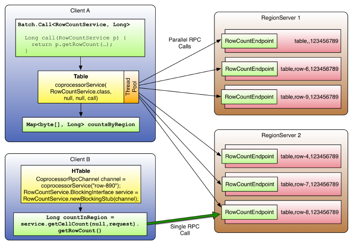
Figure 4-6. Coprocessor calls batched and executed in parallel,
and addressing a single region only
Observers
While endpoints somewhat reflect the functionality of database stored
procedures, the observers are akin to triggers. The difference to end‐
points is that observers are not only running in the context of a re‐
gion. They can run in many different parts of the system and react to
events that are triggered by clients, but also implicitly by servers
themselves. For example, when one of the servers is recovering a re‐
gion after another server has failed. Or when the master is taking ac‐
tions on the cluster state, etc.
Another difference is that observers are using pre-defined hooks into
the server processes, that is, you cannot add your own custom ones.
They also act on the server side only, with no connection to the client.
What you can do though is combine an endpoint with an observer for
region-related functionality, exposing observer state through a custom
RPC API (see Example 4-34).
Since you can load many observers into the same set of contexts, that
is, region, region server, master server, WAL, bulk loading, and end‐
Coprocessors 311
www.finebook.ir

points, it is crucial to set the order of their invocation chain appropri‐
ately. We discussed that in “Coprocessor Loading” (page 289), looking
into the priority and ordering dependent on how they are declared.
Once loaded, the observers are chained together and executed in that
order.
The ObserverContext Class
So far we have talked about the general architecture of coprocessors,
their super class, how they are loaded into the server process, and
how to implement endpoints. Before we can move on into the actual
observers, we need to introduce one more basic class. For the call‐
backs provided by the Observer classes, there is a special context
handed in as the first parameter to all calls: an instance of the Observ
erContext class. It provides access to the current environment, but al‐
so adds the interesting ability to indicate to the coprocessor frame‐
work what it should do after a callback is completed.
The observer context instance is the same for all coproces‐
sors in the execution chain, but with the environment
swapped out for each coprocessor.
Here are the methods as provided by the context class:
E getEnvironment()
Returns the reference to the current coprocessor environment. It
is paramterized to return the matching environment for a specific
coprocessor implementation. A RegionObserver for example
would be presented with an implementation instance of the Region
CoprocessorEnvironment interface.
void prepare(E env)
Prepares the context with the specified environment. This is used
internally only by the static createAndPrepare() method.
void bypass()
When your code invokes this method, the framework is going to
use your provided value, as opposed to what usually is returned by
the calling method.
void complete()
Indicates to the framework that any further processing can be
skipped, skipping the remaining coprocessors in the execution
chain. It implies that this coprocessor’s response is definitive.
Chapter 4: Client API: Advanced Features312
www.finebook.ir

boolean shouldBypass()
Used internally by the framework to check on the bypass flag.
boolean shouldComplete()
Used internally by the framework to check on the complete flag.
static <T extends CoprocessorEnvironment> ObserverCon
text<T> createAndPrepare(T env, ObserverContext<T> con
text)
Static function to initialize a context. When the provided context
is null, it will create a new instance.
The important context functions are bypass() and complete(). These
functions give your coprocessor implementation the option to control
the subsequent behavior of the framework. The complete() call influ‐
ences the execution chain of the coprocessors, while the bypass() call
stops any further default processing on the server within the current
observer. For example, you could avoid automated region splits like
so:
@Override
public void preSplit(ObserverContext<RegionCoprocessorEnvironment>
e) {
e.bypass();
e.complete();
}
There is a subtle difference between bypass and complete that needs
to be clarified: they are serving different purposes, with different ef‐
fects dependent on their usage. The following table lists the usual ef‐
fects of either flag on the current and subsequent coprocessors, and
when used in the pre or post hooks.
Table 4-15. Overview of bypass and complete, and their effects on
coprocessors
Bypass Complete Current - Pre Subsequent -
Pre Current -
Post Subsequent -
Post
✗ ✗ no effect no effect no effect no effect
✓ ✗ skip further
processing no effect no effect no effect
✗ ✓ no effect skip no effect skip
✓ ✓ skip further
processing skip no effect skip
Note that there are exceptions to the rule, that is, some pre hooks
cannot honor the bypass flag, etc. Setting bypass for post hooks usual‐
ly make no sense, since there is little to nothing left to bypass. Consult
Coprocessors 313
www.finebook.ir
7. See the RegionServer documentation.
8. Sometimes inconsistently named "c" instead.
the JavaDoc for each callback to learn if (and how) it honors the by‐
pass flag.
The RegionObserver Class
The first observer subclass of Coprocessor we will look into is the one
used at the region level: the RegionObserver class. For the sake of
brevity, all parameters and exceptions are omitted when referring to
the observer calls. Please read the online documentation for the full
specification.7 Note that all calls of this observer class have the same
first parameter (denoted as part of the “…” in the calls below), Observ
erContext<RegionCoprocessorEnvironment> ctx8, providing access
to the context instance. The context is explained in “The ObserverCon‐
text Class” (page 312), while the special environment class is ex‐
plained in “The RegionCoprocessorEnvironment Class” (page 328).
The operations can be divided into two groups: region life-cycle
changes and client API calls. We will look into both in that order, but
before we do, there is a generic callback for many operations of both
kinds:
enum Operation {
ANY, GET, PUT, DELETE, SCAN, APPEND, INCREMENT, SPLIT_REGION,
MERGE_REGION, BATCH_MUTATE, REPLAY_BATCH_MUTATE, COMPACT_REGION
}
postStartRegionOperation(..., Operation operation)
postCloseRegionOperation(..., Operation operation)
These methods in a RegionObserver are invoked when any of the pos‐
sible Operations listed is called. It gives the coprocessor the ability to
take invasive, or more likely, evasive actions, such as throwing an ex‐
ception to stop the operation from taking place altogether.
Handling Region Life-Cycle Events
While (to come) explains the region life-cycle, Figure 4-7 shows a sim‐
plified form.
Chapter 4: Client API: Advanced Features314
www.finebook.ir
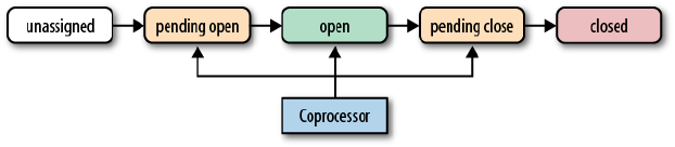
Figure 4-7. The coprocessor reacting to life-cycle state changes of
a region
The observers have the opportunity to hook into the pending open,
open, and pending close state changes. For each of them there is a set
of hooks that are called implicitly by the framework.
State: pending open
A region is in this state when it is about to be opened. Observing
coprocessors can either piggyback or fail this process. To do so,
the following callbacks in order of their invocation are available:
postLogReplay(...)
preOpen(...)
preStoreFileReaderOpen(...)
postStoreFileReaderOpen(...)
preWALRestore(...) / postWALRestore(...)
postOpen(...)
These methods are called just before the region is opened, before
and after the store files are opened in due course, the WAL being
replayed, and just after the region was opened. Your coprocessor
implementation can use them, for instance, to indicate to the
framework—in the preOpen() call—that it should abort the open‐
ing process. Or hook into the postOpen() call to trigger a cache
warm up, and so on.
The first event, postLogReplay(), is triggered dependent on what
WAL recovery mode is configured: distributed log splitting or log
replay (see (to come) and the hbase.master.distributed.log.re
play configuration property). The former runs before a region is
opened, and would therefore be triggering the callback first. The
latter opens the region, and then replays the edits, triggering the
callback after the region open event.
In both recovery modes, but again dependent on which is active,
the region server may have to apply records from the write-ahead
log (WAL). This, in turn, invokes the pre/postWALRestore() meth‐
ods of the observer. In case of using the distributed log splitting,
this will take place after the pending open, but just before the
Coprocessors 315
www.finebook.ir
open state. Otherwise, this is called after the open event, as edits
are replayed. Hooking into these WAL calls gives you fine-grained
control over what mutation is applied during the log replay pro‐
cess. You get access to the edit record, which you can use to in‐
spect what is being applied.
State: open
A region is considered open when it is deployed to a region server
and fully operational. At this point, all the operations discussed
throughout the book can take place; for example, the region’s in-
memory store could be flushed to disk, or the region could be split
when it has grown too large. The possible hooks are:
preFlushScannerOpen(...)
preFlush(...) / postFlush(...)
preCompactSelection(...) / postCompactSelection(...)
preCompactScannerOpen(...)
preCompact(...) / postCompact(...)
preSplit(...)
preSplitBeforePONR(...)
preSplitAfterPONR(...)
postSplit(...)
postCompleteSplit(...) / preRollBackSplit(...) / postRollBackS‐
plit(...)
This should be quite intuitive by now: the pre calls are executed
before, while the post calls are executed after the respective oper‐
ation. For example, using the preSplit() hook, you could effec‐
tively disable the built-in region splitting process and perform
these operations manually. Some calls are only available as pre-
hooks, some only as post-hooks.
The hooks for flush, compact, and split are directly linked to the
matching region housekeeping functions. There are also some
more specialized hooks, that happen as part of those three func‐
tions. For example, the preFlushScannerOpen() is called when the
scanner for the memstore (bear with me here, (to come) will ex‐
plain all the workings later) is set up. This is just before the actual
flush takes place.
Similarly, for compactions, first the server selects the files includ‐
ed, which is wrapped in coprocessor callbacks (postfixed Compact
Selection). After that the store scanners are opened and, finally,
the actual compaction happens.
For splits, there are callbacks reflecting current stage, with a par‐
ticular point-of-no-return (PONR) in between. This occurs, after
Chapter 4: Client API: Advanced Features316
www.finebook.ir

the split process started, but before any definitive actions have
taken place. Splits are handled like a transaction internally, and
when this transaction is about to be committed, the preSplitBe
forePONR() is invoked, and the preSplitAfterPONR() right after.
There is also a final completed or rollback call, informing you of
the outcome of the split transaction.
State: pending close
The last group of hooks for the observers is for regions that go into
the pending close state. This occurs when the region transitions
from open to closed. Just before, and after, the region is closed the
following hooks are executed:
preClose(..., boolean abortRequested)
postClose(..., boolean abortRequested)
The abortRequested parameter indicates why a region was
closed. Usually regions are closed during normal operation, when,
for example, the region is moved to a different region server for
load-balancing reasons. But there also is the possibility for a re‐
gion server to have gone rogue and be aborted to avoid any side
effects. When this happens, all hosted regions are also aborted,
and you can see from the given parameter if that was the case.
On top of that, this class also inherits the start() and stop() meth‐
ods, allowing the allocation, and release, of lifetime resources.
Handling Client API Events
As opposed to the life-cycle events, all client API calls are explicitly
sent from a client application to the region server. You have the op‐
portunity to hook into these calls just before they are applied, and just
thereafter. Here is the list of the available calls:
Table 4-16. Callbacks for client API functions
API Call Pre-Hook Post-Hook
Table.put() prePut(...) void postPut(...)
Table.checkAndPut() preCheckAndPut(...), pre
CheckAndPutAfterRow
Lock(...), prePut(...)
postPut(...), postCheckAnd
Put(...)
Table.get() preGetOp(...) void postGetOp(...)
Table.delete(),
Table.batch()
preDelete(...), prePrepareTi
meStampForDeleteVersion(...)
void postDelete(...)
Table.checkAndDe
lete()
preCheckAndDelete(...), pre
CheckAndDeleteAfterRow
Lock(...), preDelete(...)
postDelete(...), postCheck
AndDelete(...)
Coprocessors 317
www.finebook.ir

API Call Pre-Hook Post-Hook
Table.mutateRow() preBatchMutate(...), pre
Put(...)/preGetOp(...)
postBatchMutate(...), post
Put(...)/postGetOp(...),
postBatchMutateIndispensa
bly()
Table.append(),preAppend(...), preAppendAf
terRowLock()
postMutationBeforeW
AL(...), postAppend(...)
Table.batch() preBatchMutate(...), pre
Put(...)/preGetOp(...)/preDe
lete(...), prePrepareTimeS
tampForDeleteVersion(...)/
postPut(...)/postGe
tOp(...), postBatchMu
tate(...)
Table.checkAndMu
tate()
preBatchMutate(...) postBatchMutate(...)
Table.getScanner() preScannerOpen(...), preStor
eScannerOpen(...)
postInstantiateDelete
Tracker(...), postScanner
Open(...)
ResultScanner.next() preScannerNext(...) postScannerFilter
Row(...), postScanner
Next(...)
ResultScanner.close() preScannerClose(...) postScannerClose(...)
Table.increment(),
Table.batch()
preIncrement(...), preIncre
mentAfterRowLock(...)
postMutationBeforeW
AL(...), postIncre
ment(...)
Table.incrementColumn
Value()
preIncrementColumnValue(...) postIncrementColumnVal
ue(...)
Table.getClosestRowBe
fore()apreGetClosestRowBefore(...) postGetClosestRowBe
fore(...)
Table.exists() preExists(...) postExists(...)
completebulkload (tool) preBulkLoadHFile(...) postBulkLoadHFile(...)
a This API call has been removed in HBase 1.0. It will be removed in the coprocessor
API soon as well.
The table lists the events in calling order, separated by comma. When
you see a slash (“/”) instead, then the callback depends on the con‐
tained operations. For example, when you batch a put and delete in
one batch() call, then you would receive the pre/postPut() and pre/
postDelete() callbacks, for each contained instance. There are many
low-level methods, that allow you to hook into very essential processes
of HBase’s inner workings. Usually the method name should explain
the nature of the invocation, and with the parameters provided in the
online API documentation you can determine what your options are. If
all fails, you are an expert at this point anyways asking for such de‐
tails, presuming you can refer to the source code, if need be.
Chapter 4: Client API: Advanced Features318
www.finebook.ir
Example 4-34 shows another (albeit somewhat advanced) way of figur‐
ing out the call order of coprocessor methods. The example code com‐
bines a RegionObserver with a custom Endpoint, and uses an internal
list to track all invocations of any callback.
Example 4-34. Observer collecting invocation statistics.
@SuppressWarnings("deprecation") // because of API usage
public class ObserverStatisticsEndpoint
extends ObserverStatisticsProtos.ObserverStatisticsService
implements Coprocessor, CoprocessorService, RegionObserver {
private RegionCoprocessorEnvironment env;
private Map<String, Integer> stats = new LinkedHashMap<>();
// Lifecycle methods
@Override
public void start(CoprocessorEnvironment env) throws IOException {
if (env instanceof RegionCoprocessorEnvironment) {
this.env = (RegionCoprocessorEnvironment) env;
} else {
throw new CoprocessorException("Must be loaded on a table re‐
gion!");
}
}
...
// Endpoint methods
@Override
public void getStatistics(RpcController controller,
ObserverStatisticsProtos.StatisticsRequest request,
RpcCallback<ObserverStatisticsProtos.StatisticsResponse> done) {
ObserverStatisticsProtos.StatisticsResponse response = null;
try {
ObserverStatisticsProtos.StatisticsResponse.Builder builder =
ObserverStatisticsProtos.StatisticsResponse.newBuilder();
ObserverStatisticsProtos.NameInt32Pair.Builder pair =
ObserverStatisticsProtos.NameInt32Pair.newBuilder();
for (Map.Entry<String, Integer> entry : stats.entrySet()) {
pair.setName(entry.getKey());
pair.setValue(entry.getValue().intValue());
builder.addAttribute(pair.build());
}
response = builder.build();
// optionally clear out stats
if (request.hasClear() && request.getClear()) {
synchronized (stats) {
stats.clear();
}
}
Coprocessors 319
www.finebook.ir
} catch (Exception e) {
ResponseConverter.setControllerException(controller,
new IOException(e));
}
done.run(response);
}
/**
* Internal helper to keep track of call counts.
*
* @param call The name of the call.
*/
private void addCallCount(String call) {
synchronized (stats) {
Integer count = stats.get(call);
if (count == null) count = new Integer(1);
else count = new Integer(count + 1);
stats.put(call, count);
}
}
// All Observer callbacks follow here
@Override
public void preOpen(
ObserverContext<RegionCoprocessorEnvironment> observerContext)
throws IOException {
addCallCount("preOpen");
}
@Override
public void postOpen(
ObserverContext<RegionCoprocessorEnvironment> observerContext) {
addCallCount("postOpen");
}
...
}
This is combined with the code in Example 4-35, which then executes
every API call, followed by calling on the custom endpoint getStatis
tics(), which returns (and optionally clears) the collected invocation
list.
Example 4-35. Use an endpoint to query observer statistics
private static Table table = null;
private static void printStatistics(boolean print, boolean clear)
throws Throwable {
final StatisticsRequest request = StatisticsRequest
.newBuilder().setClear(clear).build();
Chapter 4: Client API: Advanced Features320
www.finebook.ir
Map<byte[], Map<String, Integer>> results = table.coprocessorSer‐
vice(
ObserverStatisticsService.class,
null, null,
new Batch.Call<ObserverStatisticsProtos.ObserverStatisticsSer‐
vice,
Map<String, Integer>>() {
public Map<String, Integer> call(
ObserverStatisticsService statistics)
throws IOException {
BlockingRpcCallback<StatisticsResponse> rpcCallback =
new BlockingRpcCallback<StatisticsResponse>();
statistics.getStatistics(null, request, rpcCallback);
StatisticsResponse response = rpcCallback.get();
Map<String, Integer> stats = new LinkedHashMap<String, Inte‐
ger>();
for (NameInt32Pair pair : response.getAttributeList()) {
stats.put(pair.getName(), pair.getValue());
}
return stats;
}
}
);
if (print) {
for (Map.Entry<byte[], Map<String, Integer>> entry : results.en‐
trySet()) {
System.out.println("Region: " + Bytes.toString(entry.get‐
Key()));
for (Map.Entry<String, Integer> call : entry.getValue().entry‐
Set()) {
System.out.println(" " + call.getKey() + ": " + call.get‐
Value());
}
}
System.out.println();
}
}
public static void main(String[] args) throws IOException {
Configuration conf = HBaseConfiguration.create();
Connection connection = ConnectionFactory.createConnection(conf);
HBaseHelper helper = HBaseHelper.getHelper(conf);
helper.dropTable("testtable");
helper.createTable("testtable", 3, "colfam1", "colfam2");
helper.put("testtable",
new String[]{"row1", "row2", "row3", "row4", "row5"},
new String[]{"colfam1", "colfam2"}, new String[]{"qual1",
"qual1"},
new long[]{1, 2}, new String[]{"val1", "val2"});
System.out.println("Before endpoint call...");
helper.dump("testtable",
new String[]{"row1", "row2", "row3", "row4", "row5"},
Coprocessors 321
www.finebook.ir
null, null);
try {
TableName tableName = TableName.valueOf("testtable");
table = connection.getTable(tableName);
System.out.println("Apply single put...");
Put put = new Put(Bytes.toBytes("row10"));
put.addColumn(Bytes.toBytes("colfam1"), Bytes.toBytes("qual10"),
Bytes.toBytes("val10"));
table.put(put);
printStatistics(true, true);
System.out.println("Do single get...");
Get get = new Get(Bytes.toBytes("row10"));
get.addColumn(Bytes.toBytes("colfam1"), Bytes.to‐
Bytes("qual10"));
table.get(get);
printStatistics(true, true);
...
} catch (Throwable throwable) {
throwable.printStackTrace();
}
}
The output then reveals how each API call is triggering a multitude of
callbacks, and different points in time:
Apply single put...
Region: testtable,,1428081747767.4fe07b3f06d5a2ed0ceb686aa0920b0b.
postStartRegionOperation: 1
- postStartRegionOperation-BATCH_MUTATE: 1
prePut: 1
preBatchMutate: 1
postBatchMutate: 1
postPut: 1
postBatchMutateIndispensably: 1
postCloseRegionOperation: 1
- postCloseRegionOperation-BATCH_MUTATE: 1
Do single get...
Region: testtable,,1428081747767.4fe07b3f06d5a2ed0ceb686aa0920b0b.
preGetOp: 1
postStartRegionOperation: 2
- postStartRegionOperation-SCAN: 2
preStoreScannerOpen: 1
postInstantiateDeleteTracker: 1
postCloseRegionOperation: 2
- postCloseRegionOperation-SCAN: 2
postGetOp: 1
Send batch with put and get...
Region: testtable,,1428081747767.4fe07b3f06d5a2ed0ceb686aa0920b0b.
Chapter 4: Client API: Advanced Features322
www.finebook.ir
preGetOp: 1
postStartRegionOperation: 3
- postStartRegionOperation-SCAN: 2
preStoreScannerOpen: 1
postInstantiateDeleteTracker: 1
postCloseRegionOperation: 3
- postCloseRegionOperation-SCAN: 2
postGetOp: 1
- postStartRegionOperation-BATCH_MUTATE: 1
prePut: 1
preBatchMutate: 1
postBatchMutate: 1
postPut: 1
postBatchMutateIndispensably: 1
- postCloseRegionOperation-BATCH_MUTATE: 1
Scan single row...
-> after getScanner()...
Region: testtable,,1428081747767.4fe07b3f06d5a2ed0ceb686aa0920b0b.
preScannerOpen: 1
postStartRegionOperation: 1
- postStartRegionOperation-SCAN: 1
preStoreScannerOpen: 2
postInstantiateDeleteTracker: 2
postCloseRegionOperation: 1
- postCloseRegionOperation-SCAN: 1
postScannerOpen: 1
-> after next()...
Region: testtable,,1428081747767.4fe07b3f06d5a2ed0ceb686aa0920b0b.
preScannerNext: 1
postStartRegionOperation: 1
- postStartRegionOperation-SCAN: 1
postCloseRegionOperation: 1
- postCloseRegionOperation-ANY: 1
postScannerNext: 1
preScannerClose: 1
postScannerClose: 1
-> after close()...
Region: testtable,,1428081747767.4fe07b3f06d5a2ed0ceb686aa0920b0b.
Scan multiple rows...
-> after getScanner()...
Region: testtable,,1428081747767.4fe07b3f06d5a2ed0ceb686aa0920b0b.
preScannerOpen: 1
postStartRegionOperation: 1
- postStartRegionOperation-SCAN: 1
preStoreScannerOpen: 2
postInstantiateDeleteTracker: 2
postCloseRegionOperation: 1
- postCloseRegionOperation-SCAN: 1
Coprocessors 323
www.finebook.ir
postScannerOpen: 1
-> after next()...
Region: testtable,,1428081747767.4fe07b3f06d5a2ed0ceb686aa0920b0b.
preScannerNext: 1
postStartRegionOperation: 1
- postStartRegionOperation-SCAN: 1
postCloseRegionOperation: 1
- postCloseRegionOperation-ANY: 1
postScannerNext: 1
preScannerClose: 1
postScannerClose: 1
-> after close()...
Region: testtable,,1428081747767.4fe07b3f06d5a2ed0ceb686aa0920b0b.
Apply single put with mutateRow()...
Region: testtable,,1428081747767.4fe07b3f06d5a2ed0ceb686aa0920b0b.
postStartRegionOperation: 2
- postStartRegionOperation-ANY: 2
prePut: 1
postCloseRegionOperation: 2
- postCloseRegionOperation-ANY: 2
preBatchMutate: 1
postBatchMutate: 1
postPut: 1
postBatchMutateIndispensably: 1
Apply single column increment...
Region: testtable,,1428081747767.4fe07b3f06d5a2ed0ceb686aa0920b0b.
preIncrement: 1
postStartRegionOperation: 4
- postStartRegionOperation-INCREMENT: 1
- postStartRegionOperation-ANY: 1
postCloseRegionOperation: 4
- postCloseRegionOperation-ANY: 1
preIncrementAfterRowLock: 1
- postStartRegionOperation-SCAN: 2
preStoreScannerOpen: 1
postInstantiateDeleteTracker: 1
- postCloseRegionOperation-SCAN: 2
postScannerFilterRow: 1
postMutationBeforeWAL: 1
- postMutationBeforeWAL-INCREMENT: 1
- postCloseRegionOperation-INCREMENT: 1
postIncrement: 1
Apply multi column increment...
Region: testtable,,1428081747767.4fe07b3f06d5a2ed0ceb686aa0920b0b.
preIncrement: 1
postStartRegionOperation: 4
- postStartRegionOperation-INCREMENT: 1
Chapter 4: Client API: Advanced Features324
www.finebook.ir
- postStartRegionOperation-ANY: 1
postCloseRegionOperation: 4
- postCloseRegionOperation-ANY: 1
preIncrementAfterRowLock: 1
- postStartRegionOperation-SCAN: 2
preStoreScannerOpen: 1
postInstantiateDeleteTracker: 1
- postCloseRegionOperation-SCAN: 2
postScannerFilterRow: 1
postMutationBeforeWAL: 2
- postMutationBeforeWAL-INCREMENT: 2
- postCloseRegionOperation-INCREMENT: 1
postIncrement: 1
Apply single incrementColumnValue...
Region: testtable,,1428081747767.4fe07b3f06d5a2ed0ceb686aa0920b0b.
preIncrement: 1
postStartRegionOperation: 4
- postStartRegionOperation-INCREMENT: 1
- postStartRegionOperation-ANY: 1
postCloseRegionOperation: 4
- postCloseRegionOperation-ANY: 1
preIncrementAfterRowLock: 1
- postStartRegionOperation-SCAN: 2
preStoreScannerOpen: 1
postInstantiateDeleteTracker: 1
- postCloseRegionOperation-SCAN: 2
postMutationBeforeWAL: 1
- postMutationBeforeWAL-INCREMENT: 1
- postCloseRegionOperation-INCREMENT: 1
postIncrement: 1
Call single exists()...
Region: testtable,,1428081747767.4fe07b3f06d5a2ed0ceb686aa0920b0b.
preExists: 1
preGetOp: 1
postStartRegionOperation: 2
- postStartRegionOperation-SCAN: 2
preStoreScannerOpen: 1
postInstantiateDeleteTracker: 1
postCloseRegionOperation: 2
- postCloseRegionOperation-SCAN: 2
postGetOp: 1
postExists: 1
Apply single delete...
Region: testtable,,1428081747767.4fe07b3f06d5a2ed0ceb686aa0920b0b.
postStartRegionOperation: 4
- postStartRegionOperation-DELETE: 1
- postStartRegionOperation-BATCH_MUTATE: 1
preDelete: 1
prePrepareTimeStampForDeleteVersion: 1
Coprocessors 325
www.finebook.ir
- postStartRegionOperation-SCAN: 2
preStoreScannerOpen: 1
postInstantiateDeleteTracker: 1
postCloseRegionOperation: 4
- postCloseRegionOperation-SCAN: 2
preBatchMutate: 1
postBatchMutate: 1
postDelete: 1
postBatchMutateIndispensably: 1
- postCloseRegionOperation-BATCH_MUTATE: 1
- postCloseRegionOperation-DELETE: 1
Apply single append...
Region: testtable,,1428081747767.4fe07b3f06d5a2ed0ceb686aa0920b0b.
preAppend: 1
postStartRegionOperation: 4
- postStartRegionOperation-APPEND: 1
- postStartRegionOperation-ANY: 1
postCloseRegionOperation: 4
- postCloseRegionOperation-ANY: 1
preAppendAfterRowLock: 1
- postStartRegionOperation-SCAN: 2
preStoreScannerOpen: 1
postInstantiateDeleteTracker: 1
- postCloseRegionOperation-SCAN: 2
postScannerFilterRow: 1
postMutationBeforeWAL: 1
- postMutationBeforeWAL-APPEND: 1
- postCloseRegionOperation-APPEND: 1
postAppend: 1
Apply checkAndPut (failing)...
-> success: false
Region: testtable,,1428081747767.4fe07b3f06d5a2ed0ceb686aa0920b0b.
preCheckAndPut: 1
postStartRegionOperation: 4
- postStartRegionOperation-ANY: 2
postCloseRegionOperation: 4
- postCloseRegionOperation-ANY: 2
preCheckAndPutAfterRowLock: 1
- postStartRegionOperation-SCAN: 2
preStoreScannerOpen: 1
postInstantiateDeleteTracker: 1
- postCloseRegionOperation-SCAN: 2
postCheckAndPut: 1
Apply checkAndPut (succeeding)...
-> success: true
Region: testtable,,1428081747767.4fe07b3f06d5a2ed0ceb686aa0920b0b.
preCheckAndPut: 1
postStartRegionOperation: 5
- postStartRegionOperation-ANY: 2
Chapter 4: Client API: Advanced Features326
www.finebook.ir
postCloseRegionOperation: 5
- postCloseRegionOperation-ANY: 2
preCheckAndPutAfterRowLock: 1
- postStartRegionOperation-SCAN: 2
preStoreScannerOpen: 1
postInstantiateDeleteTracker: 1
- postCloseRegionOperation-SCAN: 2
postScannerFilterRow: 1
- postStartRegionOperation-BATCH_MUTATE: 1
prePut: 1
preBatchMutate: 1
postBatchMutate: 1
postPut: 1
postBatchMutateIndispensably: 1
- postCloseRegionOperation-BATCH_MUTATE: 1
postCheckAndPut: 1
Apply checkAndDelete (failing)...
-> success: false
Region: testtable,,1428081747767.4fe07b3f06d5a2ed0ceb686aa0920b0b.
preCheckAndDelete: 1
postStartRegionOperation: 4
- postStartRegionOperation-ANY: 2
postCloseRegionOperation: 4
- postCloseRegionOperation-ANY: 2
preCheckAndDeleteAfterRowLock: 1
- postStartRegionOperation-SCAN: 2
preStoreScannerOpen: 1
postInstantiateDeleteTracker: 1
- postCloseRegionOperation-SCAN: 2
postCheckAndDelete: 1
Apply checkAndDelete (succeeding)...
-> success: true
Region: testtable,,1428081747767.4fe07b3f06d5a2ed0ceb686aa0920b0b.
preCheckAndDelete: 1
postStartRegionOperation: 7
- postStartRegionOperation-ANY: 2
postCloseRegionOperation: 7
- postCloseRegionOperation-ANY: 2
preCheckAndDeleteAfterRowLock: 1
- postStartRegionOperation-SCAN: 4
preStoreScannerOpen: 2
postInstantiateDeleteTracker: 2
- postCloseRegionOperation-SCAN: 4
postScannerFilterRow: 1
- postStartRegionOperation-BATCH_MUTATE: 1
preDelete: 1
prePrepareTimeStampForDeleteVersion: 1
preBatchMutate: 1
postBatchMutate: 1
postDelete: 1
Coprocessors 327
www.finebook.ir
postBatchMutateIndispensably: 1
- postCloseRegionOperation-BATCH_MUTATE: 1
postCheckAndDelete: 1
Apply checkAndMutate (failing)...
-> success: false
Region: testtable,,1428081747767.4fe07b3f06d5a2ed0ceb686aa0920b0b.
postStartRegionOperation: 4
- postStartRegionOperation-ANY: 2
postCloseRegionOperation: 4
- postCloseRegionOperation-ANY: 2
- postStartRegionOperation-SCAN: 2
preStoreScannerOpen: 1
postInstantiateDeleteTracker: 1
- postCloseRegionOperation-SCAN: 2
Apply checkAndMutate (succeeding)...
-> success: true
Region: testtable,,1428081747767.4fe07b3f06d5a2ed0ceb686aa0920b0b.
postStartRegionOperation: 8
- postStartRegionOperation-ANY: 4
postCloseRegionOperation: 8
- postCloseRegionOperation-ANY: 4
- postStartRegionOperation-SCAN: 4
preStoreScannerOpen: 2
postInstantiateDeleteTracker: 2
- postCloseRegionOperation-SCAN: 4
prePut: 1
preDelete: 1
prePrepareTimeStampForDeleteVersion: 1
postScannerFilterRow: 1
preBatchMutate: 1
postBatchMutate: 1
postPut: 1
postDelete: 1
postBatchMutateIndispensably: 1
Refer to the code for details, but the console output above is complete
and should give you guidance to identify the various callbacks, and
when they are invoked.
The RegionCoprocessorEnvironment Class
The environment instances provided to a coprocessor that is imple‐
menting the RegionObserver interface are based on the RegionCopro
cessorEnvironment class—which in turn is implementing the Copro
cessorEnvironment interface. The latter was discussed in “The Cop‐
rocessor Class Trinity” (page 285).
On top of the provided methods, the more specific, region-oriented
subclass is adding the methods described in Table 4-17.
Chapter 4: Client API: Advanced Features328
www.finebook.ir

9. The Java HBase classes are documented online.
Table 4-17. Specific methods provided by the RegionCoprocessor
Environment class
Method Description
getRegion() Returns a reference to the region the current observer is
associated with.
getRegionInfo() Get information about the region associated with the
current coprocessor instance.
getRegionServerServices() Provides access to the shared RegionServerServices
instance.
getSharedData() All the shared data between the instances of this
coprocessor.
The getRegion() call can be used to get a reference to the hosting
HRegion instance, and to invoke calls this class provides. If you are in
need of general information about the region, call getRegionInfo()
to retrieve a HRegionInfo instance. This class has useful functions
that allow to get the range of contained keys, the name of the region,
and flags about its state. Some of the methods are:
byte[] getStartKey()
byte[] getEndKey()
byte[] getRegionName()
boolean isSystemTable()
int getReplicaId()
...
Consult the online documentation to study the available list of calls. In
addition, your code can access the shared region server services in‐
stance, using the getRegionServerServices() method and returning
an instance of RegionServerServices. It provides many, very ad‐
vanced methods, and Table 4-18 list them for your perusal. We will
not be discussing all the details of the provided functionality, and in‐
stead refer you again to the Java API documentation.9
Table 4-18. Methods provided by the RegionServerServices class
abort() Allows aborting the entire server process, shutting
down the instance with the given reason.
addToOnlineRegions() Adds a given region to the list of online regions. This is
used for internal bookkeeping.
getCompactionRequest
er() Provides access to the shared CompactionRequestor
instance. This can be used to initiate compactions from
within the coprocessor.
Coprocessors 329
www.finebook.ir

abort() Allows aborting the entire server process, shutting
down the instance with the given reason.
getConfiguration() Returns the current server configuration.
getConnection() Provides access to the shared connection instance.
getCoordinatedStateMan
ager() Access to the shared state manager, gives access to the
TableStateManager, which in turn can be used to check on
the state of a table.
getExecutorService() Used by the master to schedule system-wide events.
getFileSystem() Returns the Hadoop FileSystem instance, allowing access
to the underlying file system.
getFlushRequester() Provides access to the shared FlushRequester instance.
This can be used to initiate memstore flushes.
getFromOnlineRegions() Returns a HRegion instance for a given region, must be
hosted by same server.
getHeapMemoryManager() Provides access to a manager instance, gives access to
heap related information, such as occupancy.
getLeases() Returns the list of leases, as acquired for example by client
side scanners.
getMetaTableLocator() The method returns a class providing system table related
functionality.
getNonceManager() Gives access to the nonce manager, which is used to
generate unique IDs.
getOnlineRegions() Lists all online regions on the current server for a given
table.
getRecoveringRegions() Lists all regions that are currently in the process of
replaying WAL entries.
getRegionServerAccount
ing() Provides access to the shared RegionServerAccounting
instance. It allows you to check on what the server
currently has allocated—for example, the global memstore
size.
getRegionsInTransitio
nInRS() List of regions that are currently in-transition.
getRpcServer() Returns a reference to the low-level RPC implementation
instance.
getServerName() The server name, which is unique for every region server
process.
getTableLockManager() Gives access to the lock manager. Can be used to acquire
read and write locks for the entire table.
getWAL() Provides access to the write-ahead log instance.
getZooKeeper() Returns a reference to the ZooKeeper watcher instance.
isAborted() Flag is true when abort() was called previously.
Chapter 4: Client API: Advanced Features330
www.finebook.ir
abort() Allows aborting the entire server process, shutting
down the instance with the given reason.
isStopped() Returns true when stop() (inherited from Stoppable) was
called beforehand.
isStopping() Returns true when the region server is stopping.
postOpenDeployTasks() Called by the region server after opening a region, does
internal housekeeping work.
registerService() Registers a new custom service. Called when server starts
and coprocessors are loaded.
removeFromOnlineRe
gions() Removes a given region from the internal list of online
regions.
reportRegionStateTran
sition() Triggers a report chain when a state change is needed for
a region. Sent to the Master.
stop() Stops the server gracefully.
There is no need of having to implement your own RegionObserver
class, based on the interface, you can use the BaseRegionObserver
class to only implement what is needed.
The BaseRegionObserver Class
This class can be used as the basis for all your observer-type copro‐
cessors. It has placeholders for all methods required by the RegionOb
server interface. They are all left blank, so by default nothing is done
when extending this class. You must override all the callbacks that
you are interested in to add the required functionality.
Example 4-36 is an observer that handles specific row key requests.
Example 4-36. Example region observer checking for special get
requests
public class RegionObserverExample extends BaseRegionObserver {
public static final byte[] FIXED_ROW = Bytes.toBytes("@@@GET‐
TIME@@@");
@Override
public void preGetOp(ObserverContext<RegionCoprocessorEnvironment>
e,
Get get, List<Cell> results) throws IOException {
if (Bytes.equals(get.getRow(), FIXED_ROW)) {
Put put = new Put(get.getRow());
put.addColumn(FIXED_ROW, FIXED_ROW,
Bytes.toBytes(System.currentTimeMillis()));
CellScanner scanner = put.cellScanner();
scanner.advance();
Cell cell = scanner.current();
results.add(cell);
Coprocessors 331
www.finebook.ir

}
}
}
Check if the request row key matches a well known one.
Create cell indirectly using a Put instance.
Get first cell from Put using the CellScanner instance.
Create a special KeyValue instance containing just the current
time on the server.
The following was added to the hbase-site.xml file to en‐
able the coprocessor:
<property>
<name>hbase.coprocessor.user.region.classes</name>
<value>coprocessor.RegionObserverExample</value>
</property>
The class is available to the region server’s Java Runtime
Environment because we have already added the JAR of
the compiled repository to the HBASE_CLASSPATH variable
in hbase-env.sh—see “Coprocessor Loading” (page 289)
for reference.
Do not forget to restart HBase, though, to make the
changes to the static configuration files active.
The row key @@@GETTIME@@@ is handled by the observer’s preGetOp()
hook, inserting the current time of the server. Using the HBase Shell
—after deploying the code to servers—you can see this in action:
hbase(main):001:0> get 'testtable', '@@@GETTIME@@@'
COLUMN CELL
@@@GETTIME@@@:@@@GETTIME@@@ timestamp=9223372036854775807, \
value=\x00\x00\x01L\x857\x9D\x0C
1 row(s) in 0.2810 seconds
hbase(main):002:0> Time.at(Bytes.toLong( \
"\x00\x00\x01L\x857\x9D\x0C".to_java_bytes) / 1000)
=> Sat Apr 04 18:15:56 +0200 2015
This requires an existing table, because trying to issue a get call to a
nonexistent table will raise an error, before the actual get operation is
executed. Also, the example does not set the bypass flag, in which
case something like the following could happen:
hbase(main):003:0> create 'testtable2', 'colfam1'
0 row(s) in 0.6630 seconds
Chapter 4: Client API: Advanced Features332
www.finebook.ir

=> Hbase::Table - testtable2
hbase(main):004:0> put 'testtable2', '@@@GETTIME@@@', \
'colfam1:qual1', 'Hello there!'
0 row(s) in 0.0930 seconds
hbase(main):005:0> get 'testtable2', '@@@GETTIME@@@'
COLUMN CELL
@@@GETTIME@@@:@@@GETTIME@@@ timestamp=9223372036854775807, \
value=\x00\x00\x01L\x85M\xEC{
colfam1:qual1 timestamp=1428165601622, value=Hel‐
lo there!
2 row(s) in 0.0220 seconds
A new table is created and a row with the special row key is inserted.
Subsequently, the row is retrieved. You can see how the artificial col‐
umn is mixed with the actual one stored earlier. To avoid this issue,
Example 4-37 adds the necessary e.bypass() call.
Example 4-37. Example region observer checking for special get
requests and bypassing further processing
if (Bytes.equals(get.getRow(), FIXED_ROW)) {
long time = System.currentTimeMillis();
Cell cell = CellUtil.createCell(get.getRow(), FIXED_ROW,
FIXED_ROW,
time, KeyValue.Type.Put.getCode(), Bytes.toBytes(time));
results.add(cell);
e.bypass();
}
Create cell directly using the supplied utility.
Once the special cell is inserted all subsequent coprocessors are
skipped.
You need to adjust the hbase-site.xml file to point to the
new example:
<property>
<name>hbase.coprocessor.user.region.classes</name>
<value>coprocessor.RegionObserverWithBypassExample</
value>
</property>
Just as before, please restart HBase after making these
adjustments.
As expected, and using the shell once more, the result is now differ‐
ent:
Coprocessors 333
www.finebook.ir

hbase(main):006:0> get 'testtable2', '@@@GETTIME@@@'
COLUMN CELL
@@@GETTIME@@@:@@@GETTIME@@@ timestamp=1428166075865, \
value=\x00\x00\x01L\x85T\xE5\xD9
1 row(s) in 0.2840 seconds
Only the artificial column is returned, and since the default get opera‐
tion is bypassed, it is the only column retrieved. Also note how the
timestamp of this column is 9223372036854775807--which is
Long.MAX_VALUE-- for the first example, and 1428166075865 for the
second. The former does not set the timestamp explicitly when it cre‐
ates the Cell instance, causing it to be set to HConstants.LAT
EST_TIMESTAMP (by default), and that is, in turn, set to Long.MAX_VAL
UE. The second example uses the CellUtil class to create a cell in‐
stance, which requires a timestamp to be specified (for the particular
method used, there are others that allow omitting it), and we set it to
the same server time as the value is set to.
Using e.complete() instead of the shown e.bypass() makes little dif‐
ference here, since no other coprocessor is in the chain. The online
code repository has an example that you can use to experiment with
either flag, and both together.
The MasterObserver Class
The second observer subclass of Coprocessor discussed handles all
possible callbacks the master server may initiate. The operations and
API calls are explained in Chapter 5, though they can be classified as
data-manipulation operations, similar to DDL used in relational data‐
base systems. For that reason, the MasterObserver class provides the
following hooks:
Table 4-19. Callbacks for master API functions
API Call Shell Call Pre-Hook Post-Hook
createTable() create preCreateTable(...),
preCreateTableHan
dler(...)
postCreateTable(...)
deleteTable(),
deleteTables()
drop preDeleteTable(...),
preDeleteTableHan
dler(...)
postDeleteTableHan
dler(...), postDele
teTable(...)
modifyTable() alter preModifyTable(...),
preModifyTableHan
dler(...)
postModifyTableHan
dler(...), postModi
fyTable(...)
modifyTable() alter preAddColumn(...),
preAddColumnHan
dler(...)
postAddColumnHan
dler(...), postAdd
Column(...)
Chapter 4: Client API: Advanced Features334
www.finebook.ir

API Call Shell Call Pre-Hook Post-Hook
modifyTable() alter preDeleteColumn(...),
preDeleteColumnHan
dler(...)
postDeleteColumnHan
dler(...), postDele
teColumn(...)
modifyTable() alter preModifyColumn(...),
preModifyColumnHan
dler(...)
postModifyColumnHan
dler(...), postModi
fyColumn(...)
enableTable(),
enableTables()
enable preEnableTable(...),
preEnableTableHan
dler(...)
postEnableTableHan
dler(...), postEna
bleTable(...)
disableTable(),
disableTables()
disable preDisableTable(...),
preDisableTableHan
dler(...)
postDisableTableHan
dler(...), postDisa
bleTable(...)
flush() flush preTableFlush(...) postTableFlush(...)
truncateTable() truncate preTruncateTa
ble(...), preTruncate
TableHandler(...)
postTruncateTableHan
dler(...), postTrun
cateTable(...)
move() move preMove(...) postMove(...)
assign() assign preAssign(...) postAssign(...)
unassign() unassign preUnassign(...) postUnassign(...)
offline() n/a preRegionOff
line(...)
postRegionOff
line(...)
balancer() balancer preBalance(...) postBalance(...)
setBalancerRun
ning()
balance_switch preBalanceS
witch(...)
postBalanceS
witch(...)
listTable
Names()
list preGetTable
Names(...)
postGetTable
Names(...)
getTableDescrip
tors(), listTa
bles()
list preGetTableDescrip
tors(...)
postGetTableDescrip
tors(...)
createName
space()
create_namespace preCreateName
space(...)
postCreateName
space(...)
deleteName
space()
drop_namespace preDeleteName
space(...)
postDeleteName
space(...)
getNamespaceDe
scriptor()
describe_name
space
preGetNamespaceDe
scriptor(...)
postGetNamespaceDe
scriptor(...)
listNamespaceDe
scriptors()
list_namespace preListNamespaceDe
scriptors(...)
postListNamespaceDe
scriptors(...)
modifyName
space()
alter_namespace preModifyName
space(...)
postModifyName
space(...)
cloneSnapshot() clone_snapshot preCloneSnap
shot(...)
postCloneSnap
shot(...)
Coprocessors 335
www.finebook.ir

API Call Shell Call Pre-Hook Post-Hook
deleteSnap
shot(), deleteS
napshots()
delete_snapshot,
delete_all_snap
shot
preDeleteSnap
shot(...)
postDeleteSnap
shot(...)
restoreSnap
shot()
restore_snapshot preRestoreSnap
shot(...)
postRestoreSnap
shot(...)
snapshot() snapshot preSnapshot(...) postSnapshot(...)
shutdown() n/a void preShut
down(...) n/aa
stopMaster() n/a preStopMaster(...) n/ab
n/a n/a preMasterInitializa
tion(...)
postStartMaster(...)
a There is no post hook, because after the shutdown, there is no longer a cluster to
invoke the callback.
b There is no post hook, because after the master has stopped, there is no longer a
process to invoke the callback.
Most of these methods are self-explanatory, since their name matches
the admin API function. They are grouped roughly into table and re‐
gion, namespace, snapshot, and server related calls. You will note that
some API calls trigger more than one callback. There are special pre/
postXYZHandler hooks, that indicate the asynchronous nature of the
call. The Handler instance is needed to hand off the work to an execu‐
tor thread pool. And as before, some pre hooks cannot honor the by‐
pass flag, so please, as before, read the online API reference carefully!
The MasterCoprocessorEnvironment Class
Similar to how the RegionCoprocessorEnvironment is enclosing a sin‐
gle RegionObserver coprocessor, the MasterCoprocessorEnviron
ment is wrapping MasterObserver instances. It also implements the
CoprocessorEnvironment interface, thus giving you, for instance, ac‐
cess to the getTable() call to access data from within your own im‐
plementation.
On top of the provided methods, the more specific, master-oriented
subclass adds the one method described in Table 4-20.
Table 4-20. Specific method provided by the MasterCoprocessorEn
vironment class
Method Description
getMasterServices() Provides access to the shared MasterServices instance.
Your code can access the shared master services instance, which ex‐
poses many functions of the Master admin API, as described in Chap‐
Chapter 4: Client API: Advanced Features336
www.finebook.ir

ter 5. For the sake of not duplicating the description of each, I have
grouped them here by purpose, but refrain from explaining them.
First are the table related calls:
createTable(HTableDescriptor, byte[][])
deleteTable(TableName)
modifyTable(TableName, HTableDescriptor)
enableTable(TableName)
disableTable(TableName)
getTableDescriptors()
truncateTable(TableName, boolean)
addColumn(TableName, HColumnDescriptor)
deleteColumn(TableName, byte[])
modifyColumn(TableName, HColumnDescriptor)
This is continued by namespace related methods:
createNamespace(NamespaceDescriptor)
deleteNamespace(String)
modifyNamespace(NamespaceDescriptor)
getNamespaceDescriptor(String)
listNamespaceDescriptors()
listTableDescriptorsByNamespace(String)
listTableNamesByNamespace(String)
Finally, Table 4-21 lists the more specific calls with a short descrip‐
tion.
Table 4-21. Methods provided by the MasterServices class
Method Description
abort() Allows aborting the entire server process, shutting down
the instance with the given reason.
checkTableModifiable() Convenient to check if a table exists and is offline so that
it can be altered.
dispatchMergingRe
gions() Flags two regions to be merged, which is performed on
the region servers.
getAssignmentManager() Gives you access to the assignment manager instance. It
is responsible for all region assignment operations, such
as assign, unassign, balance, and so on.
getConfiguration() Returns the current server configuration.
getConnection() Provides access to the shared connection instance.
getCoordinatedStateMan
ager() Access to the shared state manager, gives access to the
TableStateManager, which in turn can be used to check on
the state of a table.
getExecutorService() Used by the master to schedule system-wide events.
getMasterCoprocesso
rHost() Returns the enclosing host instance.
Coprocessors 337
www.finebook.ir

10. The Java HBase classes are documented online.
Method Description
getMasterFileSystem() Provides you with an abstraction layer for all filesystem-
related operations the master is involved in—for example,
creating directories for table files and logfiles.
getMetaTableLocator() The method returns a class providing system table related
functionality.
getServerManager() Returns the server manager instance. With it you have
access to the list of servers, live or considered dead, and
more.
getServerName() The server name, which is unique for every region server
process.
getTableLockManager() Gives access to the lock manager. Can be used to acquire
read and write locks for the entire table.
getZooKeeper() Returns a reference to the ZooKeeper watcher instance.
isAborted() Flag is true when abort() was called previously.
isInitialized() After the server process is operational, this call will return
true.
isServerShutdownHandler
Enabled() When an optional shutdown handler was set, this check
returns true.
isStopped() Returns true when stop() (inherited from Stoppable) was
called beforehand.
registerService() Registers a new custom service. Called when server starts
and coprocessors are loaded.
stop() Stops the server gracefully.
Even though I am listing all the master services methods, I will not be
discussing all the details on the provided functionality, and instead re‐
fer you to the Java API documentation once more.10
The BaseMasterObserver Class
Either you can base your efforts to implement a MasterObserver on
the interface directly, or you can extend the BaseMasterObserver
class instead. It implements the interface while leaving all callback
functions empty. If you were to use this class unchanged, it would not
yield any kind of reaction.
Adding functionality is achieved by overriding the appropriate event
methods. You have the choice of hooking your code into the pre and/or
post calls. Example 4-38 uses the post hook after a table was created
to perform additional tasks.
Chapter 4: Client API: Advanced Features338
www.finebook.ir
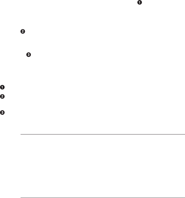
Example 4-38. Example master observer that creates a separate di‐
rectory on the file system when a table is created.
public class MasterObserverExample extends BaseMasterObserver {
@Override
public void postCreateTable(
ObserverContext<MasterCoprocessorEnvironment> ctx,
HTableDescriptor desc, HRegionInfo[] regions)
throws IOException {
TableName tableName = desc.getTableName();
MasterServices services = ctx.getEnvironment().getMasterServi‐
ces();
MasterFileSystem masterFileSystem = services.getMasterFileSys‐
tem();
FileSystem fileSystem = masterFileSystem.getFileSystem();
Path blobPath = new Path(tableName.getQualifierAsString() + "-
blobs");
fileSystem.mkdirs(blobPath);
}
}
Get the new table’s name from the table descriptor.
Get the available services and retrieve a reference to the actual
file system.
Create a new directory that will store binary data from the client
application.
You need to add the following to the hbase-site.xml file for
the coprocessor to be loaded by the master process:
<property>
<name>hbase.coprocessor.master.classes</name>
<value>coprocessor.MasterObserverExample</value>
</property>
Just as before, restart HBase after making these adjust‐
ments.
Once you have activated the coprocessor, it is listening to the said
events and will trigger your code automatically. The example is using
the supplied services to create a directory on the filesystem. A ficti‐
tious application, for instance, could use it to store very large binary
objects (known as blobs) outside of HBase.
Coprocessors 339
www.finebook.ir
11. As of this writing, there are discussions to remove—or at least disable—this func‐
tionality in future releases. See HBASE-11165 for details.
To trigger the event, you can use the shell like so:
hbase(main):001:0> create 'testtable3', 'colfam1'
0 row(s) in 0.6740 seconds
This creates the table and afterward calls the coprocessor’s postCrea
teTable() method. The Hadoop command-line tool can be used to
verify the results:
$ bin/hadoop dfs -ls
Found 1 items
drwxr-xr-x - larsgeorge supergroup 0 ... testtable3-
blobs
There are many things you can implement with the MasterObserver
coprocessor. Since you have access to most of the shared master re‐
sources through the MasterServices instance, you should be careful
what you do, as it can potentially wreak havoc.
Finally, because the environment is wrapped in an ObserverContext,
you have the same extra flow controls, exposed by the bypass() and
complete() methods. You can use them to explicitly disable certain
operations or skip subsequent coprocessor execution, respectively.
The BaseMasterAndRegionObserver Class
There is another, related base class provided by HBase, the BaseMas
terAndRegionObserver. It is a combination of two things: the BaseRe
gionObserver, as described in “The BaseRegionObserver Class” (page
331), and the MasterObserver interface:
public abstract class BaseMasterAndRegionObserver
extends BaseRegionObserver implements MasterObserver {
...
}
In effect, this is like combining the previous BaseMasterObserver and
BaseRegionObserver classes into one. This class is only useful to run
on the HBase Master since it provides both, a region server and mas‐
ter implementation. This is used to host the system tables directly on
the master.11 Otherwise the functionality of both have been described
above, therefore we can move on to the next coprocessor subclass.
The RegionServerObserver Class
You have seen how to run code next to regions, and within the master
processes. The same is possible within the region servers using the Re
Chapter 4: Client API: Advanced Features340
www.finebook.ir
gionServerObserver class. It exposes well-defined hooks that pertain
to the server functionality, that is, spanning many regions and tables.
For that reason, the following hooks are provided:
postCreateReplicationEndPoint(...)
Invoked after the server has created a replication endpoint (not to
be confused with coprocessor endpoints).
preMerge(...), postMerge(...)
Called when two regions are merged.
preMergeCommit(...), postMergeCommit(...)
Same as above, but with narrower scope. Called after preMerge()
and before postMerge().
preRollBackMerge(...), postRollBackMerge(...)
These are invoked when a region merge fails, and the merge trans‐
action has to be rolled back.
preReplicateLogEntries(...), postReplicateLogEntries(...)
Tied into the WAL entry replay process, allows special treatment
of each log entry.
preRollWALWriterRequest(...), postRollWALWriterRe
quest(...)
Wrap the rolling of WAL files, which will happen based on size,
time, or manual request.
preStopRegionServer(...)
This pre-only hook is called when the from Stoppable inherited
method stop() is called. The environment allows access to that
method on a region server.
The RegionServerCoprocessorEnvironment Class
Similar to how the MasterCoprocessorEnvironment is enclosing a sin‐
gle MasterObserver coprocessor, the RegionServerCoprocessorEn
vironment is wrapping RegionServerObserver instances. It also im‐
plements the CoprocessorEnvironment interface, thus giving you, for
instance, access to the getTable() call to access data from within
your own implementation.
On top of the provided methods, the specific, region server-oriented
subclass adds the one method described in Table 4-20.
Coprocessors 341
www.finebook.ir

Table 4-22. Specific method provided by the RegionServerCopro
cessorEnvironment class
Method Description
getRegionServerServices() Provides access to the shared RegionServerServices
instance.
We have discussed this class in “The RegionCoprocessorEnvironment
Class” (page 328) before, and refer you to Table 4-18, which lists the
available methods.
The BaseRegionServerObserver Class
Just with the other base observer classes you have seen, the BaseRe
gionServerObserver is an empty implementation of the RegionSer
verObserver interface, saving you time and effort to otherwise imple‐
ment the many callback methods. Here you can focus on what you
really need, and overwrite the necessary methods only. The available
callbacks are very advanced, and we refrain from constructing a sim‐
ple example at this point. Please refer to the source code if you need
to implement at this low level.
The WALObserver Class
The next observer class we are going to address is related to the
write-ahead log, or WAL for short. It offers a manageable list of call‐
backs, namely the following two:
preWALWrite(...), postWALWrite(...)
Wrap the writing of log entries to the WAL, allowing access to the
full edit record.
Since you receive the entire record in these methods, you can influ‐
ence what is written to the log. For example, an advanced use-case
might be to add extra cells to the edit, so that during a potential log
replay the cells could help fine tune the reconstruction process. You
could add information that trigger external message queueing, so that
other systems could react appropriately to the replay. Or you could
use this information to create auxiliary data upon seeing the special
cells later on.
The WALCoprocessorEnvironment Class
Once again, there is a specialized environment that is provided as part
of the callbacks. Here it is an instance of the WALCoprocessorEnviron
ment class. It also extends the CoprocessorEnvironment interface,
thus giving you, for instance, access to the getTable() call to access
data from within your own implementation.
Chapter 4: Client API: Advanced Features342
www.finebook.ir

On top of the provided methods, the specific, WAL-oriented subclass
adds the one method described in Table 4-23.
Table 4-23. Specific method provided by the WALCoprocessorEnvir
onment class
Method Description
getWAL() Provides access to the shared WAL instance.
With the reference to the WAL you can roll the current writer, in other
words, close the current log file and create a new one. You could also
call the sync() method to force the edit records into the persistence
layer. Here are the methods available from the WAL interface:
void registerWALActionsListener(final WALActionsListener listener)
boolean unregisterWALActionsListener(final WALActionsListener lis‐
tener)
byte[][] rollWriter() throws FailedLogCloseException, IOException
byte[][] rollWriter(boolean force) throws FailedLogCloseException,
IOException
void shutdown() throws IOException
void close() throws IOException
long append(HTableDescriptor htd, HRegionInfo info, WALKey key, WA‐
LEdit edits,
AtomicLong sequenceId, boolean inMemstore, List<Cell> memstor‐
eKVs)
throws IOException
void sync() throws IOException
void sync(long txid) throws IOException
boolean startCacheFlush(final byte[] encodedRegionName)
void completeCacheFlush(final byte[] encodedRegionName)
void abortCacheFlush(byte[] encodedRegionName)
WALCoprocessorHost getCoprocessorHost()
long getEarliestMemstoreSeqNum(byte[] encodedRegionName)
Once again, this is very low-level functionality, and at that point you
most likely have read large parts of the code already. We will defer
the explanation of each method to the online Java documentation.
The BaseWALObserver Class
The BaseWALObserver class implements the WALObserver interface.
This is mainly done to help along with a pending (as of this writing, for
HBase 1.0) deprecation process of other variants of the same callback
methods. You can use this class to implement your own, or implement
the interface directly.
Coprocessors 343
www.finebook.ir
The BulkLoadObserver Class
This observer class is used during bulk loading operations, as trig‐
gered by the HBase supplied completebulkload tool, contained in the
server JAR file. Using the Hadoop JAR support, you can see the list of
tools like so:
$ bin/hadoop jar /usr/local/hbase-1.0.0-bin/lib/hbase-
server-1.0.0.jar
An example program must be given as the first argument.
Valid program names are:
CellCounter: Count cells in HBase table
completebulkload: Complete a bulk data load.
copytable: Export a table from local cluster to peer cluster
export: Write table data to HDFS.
import: Import data written by Export.
importtsv: Import data in TSV format.
rowcounter: Count rows in HBase table
verifyrep: Compare the data from tables in two different clus‐
ters.
WARNING: It doesn't work for incrementColumnValues'd cells
since the
timestamp is changed after being appended to the log.
Once the completebulkload tool is run, it will attempt to move all
staged bulk load files into place (more on this in (to come), so for now
please bear with me). During that operation the available callbacks
are triggered:
prePrepareBulkLoad(...)
Invoked before the bulk load operation takes place.
preCleanupBulkLoad(...)
Called when the bulk load is complete and clean up tasks are per‐
formed.
Both callbacks cannot skip the default processing using the bypass
flag. They are merely invoked but their actions take no effect on the
further bulk loading process. The observer does not have its own envi‐
ronment, instead it uses the RegionCoprocessorEnvironment ex‐
plained in “The RegionCoprocessorEnvironment Class” (page 328).
The EndPointObserver Class
The final observer is equally manageable, since it does not employ its
own environment, but also shares the RegionCoprocessorEnviron
ment (see “The RegionCoprocessorEnvironment Class” (page 328)).
This makes sense, because endpoints run in the context of a region.
The available callback methods are:
Chapter 4: Client API: Advanced Features344
www.finebook.ir
preEndpointInvocation(...), postEndpointInvocation(...)
Whenever an endpoint method is called upon from a client, these
callbacks wrap the server side execution.
The client can replace (for the pre hook) or modify (for the post hook,
using the provided Message.Builder instance) the given Message in‐
stance to modify the outcome of the endpoint method. If an exception
is thrown during the pre hook, then the server-side call is aborted
completely.
Coprocessors 345
www.finebook.ir
1. Namespaces were added in 0.96. See HBASE-8408.
Chapter 5
Client API: Administrative
Features
Apart from the client API used to deal with data manipulation fea‐
tures, HBase also exposes a data definition-like API. This is similar to
the separation into DDL and DML found in RDBMSes. First we will
look at the classes required to define the data schemas and subse‐
quently see the API that makes use of it to, for example, create a new
HBase table.
Schema Definition
Creating a table in HBase implicitly involves the definition of a table
schema, as well as the schemas for all contained column families.
They define the pertinent characteristics of how—and when—the data
inside the table and columns is ultimately stored. On a higher level,
every table is part of a namespace, and we will start with their defin‐
ing data structures first.
Namespaces
Namespaces were introduced into HBase to solve the problem of or‐
ganizing many tables.1 Before this feature, you had a flat list of all
tables, including the system catalog tables. This—at scale—was caus‐
ing difficulties when you had hundreds and hundreds of tables. With
namespaces you can organize your tables into groups, where related
tables would be handled together. On top of that, namespaces allow to
347
www.finebook.ir
further abstract generic concepts, such as security. You can define ac‐
cess control on the namespace level to quickly apply the rules to all
comprised tables.
HBase creates two namespaces when it starts: default and hbase.
The latter is for the system catalog tables, and you should not create
your own tables in that space. Using the shell, you can list the name‐
spaces and their content like so:
hbase(main):001:0> list_namespace
NAMESPACE
default
hbase
2 row(s) in 0.0090 seconds
hbase(main):002:0> list_namespace_tables 'hbase'
TABLE
foobar
meta
namespace
3 row(s) in 0.0120 seconds
The other namespace, called default, is the one namespace that all
unspecified tables go into. You do not have to specify a namespace
when you generate a table. It will then automatically be added to the
default namespace on your behalf. Again, using the shell, here is
what happens:
hbase(main):001:0> list_namespace_tables 'default'
TABLE
0 row(s) in 0.0170 seconds
hbase(main):002:0> create 'testtable', 'colfam1'
0 row(s) in 0.1650 seconds
=> Hbase::Table - testtable
hbase(main):003:0> list_namespace_tables 'default'
TABLE
testtable
1 row(s) in 0.0130 seconds
The new table (testtable) was created and added to the default
namespace, since you did not specify one.
Chapter 5: Client API: Administrative Features348
www.finebook.ir

If you have run the previous examples, it may by that you
already have a table with that name. You will then receive
an error like this one using the shell:
ERROR: Table already exists: testtable!
You can either use another name to test with, or use the
disable 'testtable' and drop 'testtable' commands
to remove the table before moving on.
Since namespaces group tables, and their name being a fixed part of a
table definition, you are free to create tables with the same name in
different namespaces:
hbase(main):001:0> create_namespace 'booktest'
0 row(s) in 0.0970 seconds
hbase(main):002:0> create 'booktest:testtable', 'colfam1'
0 row(s) in 0.1560 seconds
=> Hbase::Table - booktest:testtable
hbase(main):003:0> create_namespace 'devtest'
0 row(s) in 0.0140 seconds
hbase(main):004:0> create 'devtest:testtable', 'colfam1'
0 row(s) in 0.1490 seconds
=> Hbase::Table - devtest:testtable
This example creates two namespaces, booktest and devtest, and
adds the table testtable to both. Applying the above list commands
is left for you to try, but you will see how the tables are now part of
the respective namespaces as expected. Dealing with namespace with‐
in your code revolves around the NamespaceDescriptor class, which
are constructed using the Builder pattern:
static Builder create(String name)
static Builder create(NamespaceDescriptor ns)
You either hand in a name for the new instance as a string, or an ex‐
isting NamespaceDescriptor instance, which also copies its configura‐
tion details. The returned Builder instance can then be used to add
further configuration details to the new namespace, and eventually
build the instance. Example 5-1 shows this in action:
Example 5-1. Example how to create a NamespaceDescriptor in
code
NamespaceDescriptor.Builder builder =
NamespaceDescriptor.create("testspace");
Schema Definition 349
www.finebook.ir

builder.addConfiguration("key1", "value1");
NamespaceDescriptor desc = builder.build();
System.out.println("Namespace: " + desc);
The result on the console:
Namespace: {NAME => 'testspace', key1 => 'value1'}
The class has a few more methods:
String getName()
String getConfigurationValue(String key)
Map<String, String> getConfiguration()
void setConfiguration(String key, String value)
void removeConfiguration(final String key)
String toString()
These methods are self-explanatory, they return the assigned name‐
space name, allow access to the configuration values, the entire list of
key/values, and retrieve the entire state as a string. The primary use
for this class is as part of admin API, explained in due course (see
Example 5-7).
Tables
Everything stored in HBase is ultimately grouped into one or more
tables. The primary reason to have tables is to be able to control cer‐
tain features that all columns in this table share. The typical things
you will want to define for a table are column families. The construc‐
tor of the table descriptor in Java looks like the following:
HTableDescriptor(final TableName name)
HTableDescriptor(HTableDescriptor desc)
You either create a table with a name or an existing descriptor. You
have to specify the name of the table using the TableName class (as
mentioned in “API Building Blocks” (page 117)). This allows you to
specify the name of the table, and an optional namespace with one pa‐
rameter. When you use the latter constructor, that is, handing in an
existing table descriptor, it will copy all settings and state from that
instance across to the new one.
A table cannot be renamed. The common approach to re‐
name a table is to create a new table with the desired
name and copy the data over, using the API, or a MapRe‐
duce job (for example, using the supplied copytable tool)
Chapter 5: Client API: Administrative Features350
www.finebook.ir
There are certain restrictions on the characters you can use to create
a table name. The name is used as part of the path to the actual stor‐
age files, and therefore has to comply with filename rules. You can lat‐
er browse the low-level storage system—for example, HDFS—to see
the tables as separate directories—in case you ever need to. The Ta
bleName class enforces these rules, as shown in Example 5-2.
Example 5-2. Example how to create a TableName in code
private static void print(String tablename) {
print(null, tablename);
}
private static void print(String namespace, String tablename) {
System.out.print("Given Namespace: " + namespace +
", Tablename: " + tablename + " -> ");
try {
System.out.println(namespace != null ?
TableName.valueOf(namespace, tablename) :
TableName.valueOf(tablename));
} catch (Exception e) {
System.out.println(e.getClass().getSimpleName() +
": " + e.getMessage());
}
}
public static void main(String[] args) throws IOException, Interrup‐
tedException {
print("testtable");
print("testspace:testtable");
print("testspace", "testtable");
print("testspace", "te_st-ta.ble");
print("", "TestTable-100");
print("tEsTsPaCe", "te_st-table");
print("");
// VALID_NAMESPACE_REGEX = "(?:[a-zA-Z_0-9]+)";
// VALID_TABLE_QUALIFIER_REGEX = "(?:[a-zA-Z_0-9][a-zA-
Z_0-9-.]*)";
print(".testtable");
print("te_st-space", "te_st-table");
print("tEsTsPaCe", "te_st-table@dev");
}
The result on the console:
Given Namespace: null, Tablename: testtable -> testtable
Given Namespace: null, Tablename: testspace:testtable -> test‐
space:testtable
Given Namespace: testspace, Tablename: testtable -> testspace:test‐
table
Schema Definition 351
www.finebook.ir

2. See “Database normalization” on Wikipedia.
3. We are brushing over region replicas here for the sake of a more generic view at
this point.
Given Namespace: testspace, Tablename: te_st-ta.ble ->
testspace:te_st-ta.ble
Given Namespace: , Tablename: TestTable-100 -> TestTable-100
Given Namespace: tEsTsPaCe, Tablename: te_st-table ->
tEsTsPaCe:te_st-table
Given Namespace: null, Tablename: -> IllegalArgumentException:
Table qualifier must not be empty
Given Namespace: null, Tablename: .testtable ->
IllegalArgumentException: Illegal first character at 0.
User-space table qualifiers can only start with 'alphanumeric
characters':
i.e. [a-zA-Z_0-9]: .testtable
Given Namespace: te_st-space, Tablename: te_st-table ->
IllegalArgumentException: Illegal character at 5. Namespaces
can
only contain 'alphanumeric characters': i.e. [a-zA-Z_0-9]: te_st-
space
Given Namespace: tEsTsPaCe, Tablename: te_st-table@dev ->
IllegalArgumentException: Illegal character code:64, <@> at 11.
User-space
table qualifiers can only contain 'alphanumeric characters':
i.e. [a-zA-Z_0-9-.]: te_st-table@dev
The class has many static helper methods, for example isLegalTable
QualifierName(), allowing you to check generated or user provided
names before passing them on to HBase. It also has getters to access
the names handed into the valueOf() method as used in the example.
Note that the table name is returned using the getQualifier() meth‐
od. The namespace has a matching getNamespace() method.
The column-oriented storage format of HBase allows you to store
many details into the same table, which, under relational database
modeling, would be divided into many separate tables. The usual data‐
base normalization2 rules do not apply directly to HBase, and there‐
fore the number of tables is usually lower, in comparison. More on
this is discussed in “Database (De-)Normalization” (page 16).
Although conceptually a table is a collection of rows with columns in
HBase, physically they are stored in separate partitions called re‐
gions. Figure 5-1 shows the difference between the logical and physi‐
cal layout of the stored data. Every region is served by exactly one re‐
gion server, which in turn serve the stored values directly to clients.3
Chapter 5: Client API: Administrative Features352
www.finebook.ir
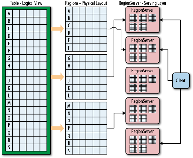
Figure 5-1. Logical and physical layout of rows within regions
Serialization
Before we move on to the table and its properties, there is something
to be said about the following specific methods of many client API
classes:
byte[] toByteArray()
static HTableDescriptor parseFrom(final byte[] bytes)
TableSchema convert()
static HTableDescriptor convert(final TableSchema ts)
Every communication between remote disjoint systems—for example,
the client talking to the servers, but also the servers talking with one
another—is done using the RPC framework. It employs the Google
Protocol Buffer (or Protobuf for short) library to serialize and deserial‐
ize objects (I am treating class instance and object as synonyms), be‐
fore they are passed between remote systems.
The above methods are invoked by the framework to write the object’s
data into the output stream, and subsequently read it back on the re‐
ceiving system. For that the framework calls toByteArray() on the
sending side, serializing the object’s fields, while the framework is
Schema Definition 353
www.finebook.ir
taking care of noting the class name and other details on their behalf.
Alternatively the convert() method in case of the HTableDescriptor
class can be used to convert the entire instance into a Protobuf class.
On the receiving server the framework reads the metadata, and will
create an instance using the static parseFrom() of the matching class.
This will read back the field data and leave you with a fully working
and initialized copy of the sending object. The same is achieved using
the matching convert() call, which will take a Protobuf object instead
of a low-level byte array.
All of this is based on protocol description files, which you can find in
the HBase source code. They are like the ones we used in Chapter 4
for custom filters and coprocessor endpoints—but much more elabo‐
rate. These protocol text files are compiled the same way when HBase
is build and the generated classes are saved into the appropriate
places in the source tree. The great advantage of using Protobuf over,
for example, Java Serialization, is that it is versioned and can evolve
over time. You can even upgrade a cluster while it is operational, be‐
cause an older (or newer) client can communicate with a newer (or
older) server.
Since the receiver needs to create the class using these generated
classes, it is implied that it must have access to the matching, com‐
piled class. Usually that is the case, as both the servers and clients are
using the same HBase Java archive file, or JAR. But if you develop
your own extensions to HBase—for example, the mentioned filters and
coprocessors—you must ensure that your custom class follows these
rules:
•It is available on both sides of the RPC communication channel,
that is, the sending and receiving processes.
•It implements the required Protobuf methods toByteArray() and
parseFrom().
As a client API developer, you should just acknowledge the underlying
dependency on RPC, and how it manifests itself. As an advanced de‐
veloper extending HBase, you need to implement and deploy your cus‐
tom code appropriately. “Custom Filters” (page 259) has an example
and further notes.
The RegionLocator Class
We could have discussed this class in “API Building Blocks” (page
117) but for the sake of complexity and the nature of the RegionLoca
tor, it is better to introduce you now to this class. As you recall from
“Auto-Sharding” (page 26) and other places earlier, a table is divided
Chapter 5: Client API: Administrative Features354
www.finebook.ir
into one to many regions, which are consecutive, sorted sets of rows.
They form the basis for HBase’s scalability, and the implicit sharding
(referred to as splitting) performed by the servers on your behalf is
one of the fundamental techniques offered by HBase.
Since you could choose the simple path and let the system deal with
all the region operations, there is seemingly no need to know more
about the regions behind a table. In practice though, this is not always
possible. There are times where you need to dig deeper and investi‐
gate the structure of a table, for example, what regions a table has,
what their boundaries are, and which specific region is serving a giv‐
en row key. For that, there are a few methods provided by the Region
Locator class, which always runs in a context of a specific table:
public HRegionLocation getRegionLocation(final byte[] row)
throws IOException
public HRegionLocation getRegionLocation(final byte[] row,
boolean reload) throws IOException
public List<HRegionLocation> getAllRegionLocations()
throws IOException
public byte[][] getStartKeys() throws IOException
public byte[][] getEndKeys() throws IOException
public Pair<byte[][], byte[][]> getStartEndKeys() throws IOExcep‐
tion
TableName getName()
The basic building blocks are the same as you know from the Table
usage, that is, you retrieve an instance from the shared connection by
specifying what table it should represent, and once you are done you
free its resources by invoking close():
Configuration conf = HBaseConfiguration.create();
Connection connection = ConnectionFactory.createConnection(conf);
TableName tn = TableName.valueOf(tableName);
RegionLocator locator = connection.getRegionLocator(tn);
Pair<byte[][], byte[][]> pair = locator.getStartEndKeys();
...
locator.close();
The various methods provided are used to retrieve either HRegionLoca
tion instances, or the binary start and/or end keys, of the table re‐
gions. Regions are specified with the start key inclusive, but the end
key exclusive. The primary reason is to be able to connect regions
contiguously, that it, without any gaps in the key space. The HRegion
Location is giving you access to region details, such as the server
currently hosting it, or the associated HRegionInfo object (explained
in “The RegionCoprocessorEnvironment Class” (page 328)):
Schema Definition 355
www.finebook.ir
HRegionInfo getRegionInfo()
String getHostname()
int getPort()
String getHostnamePort()
ServerName getServerName()
long getSeqNum()
String toString()
Example 5-8 uses many of these methods in the context of creating a
table in code.
Server and Region Names
There are two essential pieces of information that warrant a proper in‐
troduction: the server name and region name. They appear in many
places, such as the HBase Shell, the web-based UI, and both APIs, the
administrative and client API. Sometimes they are just emitted in hu‐
man readable form, which includes encoding unprintable characters
as codepoints. Other times, they are returned by functions such as get
ServerName(), or getRegionNameAsString() (provided by HRegionIn
fo), or are required as an input parameter to administrative API calls.
Example 5-3 creates a table and then locates the region that contains
the row Foo. Once the region is retrieved, the server name and region
name are printed.
Example 5-3. Shows the use of server and region names
TableName tableName = TableName.valueOf("testtable");
HColumnDescriptor coldef1 = new HColumnDescriptor("colfam1");
HTableDescriptor desc = new HTableDescriptor(tableName)
.addFamily(coldef1)
.setValue("Description", "Chapter 5 - ServerAndRegionNameExam‐
ple");
byte[][] regions = new byte[][] { Bytes.toBytes("ABC"),
Bytes.toBytes("DEF"), Bytes.toBytes("GHI"), Bytes.to‐
Bytes("KLM"),
Bytes.toBytes("OPQ"), Bytes.toBytes("TUV")
};
admin.createTable(desc, regions);
RegionLocator locator = connection.getRegionLocator(tableName);
HRegionLocation location = locator.getRegionLocation(Bytes.to‐
Bytes("Foo"));
HRegionInfo info = location.getRegionInfo();
System.out.println("Region Name: " + info.getRegionNameAs‐
String());
System.out.println("Server Name: " + location.getServerName());
The output for one execution of the code looked like:
Chapter 5: Client API: Administrative Features356
www.finebook.ir
Region Name: testtable,DEF,
1428681822728.acdd15c7050ec597b484b30b7c744a93.
Server Name: srv1.foobar.com,63360,1428669931467
The region name is a combination of table and region details (the start
key, and region creation time), plus an optional MD5 hash of the lead‐
ing prefix of the name, surrounded by dots (“.”):
<table name>,<region start key>,<region creation
time>[.<md5hash(prefix)>.]
In the example, "acdd15c7050ec597b484b30b7c744a93" is the MD5
hash of "testtable,DEF,1428681822728". The getEncodedName()
method of HRegionInfo returns just the hash, not the leading, reada‐
ble prefix. The hash itself is used when the system is creating the low‐
er level file structure within the storage layer. For example, the above
region hash is visible when listing the content of the storage directory
for HBase (this is explained in detail in (to come), for now just notice
the hash in the path):
$ bin/hdfs dfs -ls -R /hbase
drwxr-xr-x - larsgeorge supergroup 0 2015-04-10 18:03 \
/hbase/data/default/testtable/acdd15c7050ec597b484b30b7c744a93/
colfam1
The region creation timestamp is issued when a region is created, for
example when a table is created, or an existing region split. The dots
around the hash are mainly to identify the hash, and be able to parse
the text representation. There are times where the hash is not part of
the region name, and the missing ending dot makes this distinguisha‐
ble.
As for the server name, it is also a combination of various parts, in‐
cluding the host name of the machine:
<host name>,<RPC port>,<server start time>
The server start time is used to handle multiple processes on the same
physical machine, created over time. When a region server is stopped
and started again, the timestamp makes it possible for the HBase
Master to identify the new process on the same physical machine. It
will then move the old name, that is, the one with the lower time‐
stamp, into the list of dead servers. On the flip side, when you see a
server process reported as dead, make sure to compare the listed
timestamp with the current one of the process on that same server us‐
ing the same port. If the timestamp of the current process is newer
then all should be working as expected.
There is a class called ServerName that wraps the details into a conve‐
nient structure. Some API calls expect to receive an instance of this
Schema Definition 357
www.finebook.ir
4. Getters and setters in Java are methods of a class that expose internal fields in a
controlled manner. They are usually named like the field, prefixed with get and
set, respectively—for example, getName() and setName().
class, which can be created from scratch, though the practical ap‐
proach is to use the API to retrieve an existing instance, for example,
using the getServerName() method mentioned before.
Keep the two names in mind as you read through the rest of this chap‐
ter, since they appear quite a few times and it will make much more
sense now that you know about their structure and purpose.
Table Properties
The table descriptor offers getters and setters4 to set many options of
the table. In practice, a lot are not used very often, but it is important
to know them all, as they can be used to fine-tune the table’s perfor‐
mance. We will group the methods by the set of properties they influ‐
ence.
Name
The constructor already had the parameter to specify the table
name. The Java API has additional methods to access the name or
change it.
TableName getTableName()
String getNameAsString()
This method returns the table name, as set during the construction
of this instance. Refer to “Column Families” (page 362) for more de‐
tails, and Figure 5-2 for an example of how the table name is used
to form a filesystem path.
Column Families
This is the most important part of defining a table. You need to
specify the column families you want to use with the table you are
creating.
HTableDescriptor addFamily(final HColumnDescriptor family)
HTableDescriptor modifyFamily(final HColumnDescriptor family)
HColumnDescriptor removeFamily(final byte[] column)
HColumnDescriptor getFamily(final byte[] column)
boolean hasFamily(final byte[] familyName)
Set<byte[]> getFamiliesKeys()
HColumnDescriptor[] getColumnFamilies()
Collection<HColumnDescriptor> getFamilies()
You have the option of adding a family, modifying it, checking if it
exists based on its name, getting a list of all known families (in
Chapter 5: Client API: Administrative Features358
www.finebook.ir

various forms), and getting or removing a specific one. More on
how to define the required HColumnDescriptor is explained in
“Column Families” (page 362).
Maximum File Size
This parameter is specifying the maximum size a region within the
table should grow to. The size is specified in bytes and is read and
set using the following methods:
long getMaxFileSize()
HTableDescriptor setMaxFileSize(long maxFileSize)
Maximum file size is actually a misnomer, as it really is
about the maximum size of each store, that is, all the files
belonging to each column family. If one single column
family exceeds this maximum size, the region is split.
Since in practice, this involves multiple files, the better
name would be maxStoreSize.
The maximum size is helping the system to split regions when they
reach this configured limit. As discussed in “Building Blocks”
(page 19), the unit of scalability and load balancing in HBase is the
region. You need to determine what a good number for the size is,
though. By default, it is set to 10 GB (the actual value is
10737418240 since it is specified in bytes, and set in the default
configuration as hbase.hregion.max.filesize), which is good for
many use cases. We will look into use-cases in (to come) and show
how this can make a difference.
Please note that this is more or less a desired maximum size and
that, given certain conditions, this size can be exceeded and ac‐
tually be completely rendered without effect. As an example, you
could set the maximum file size to 1 GB and insert a 2 GB cell in
one row. Since a row cannot be split across regions, you end up
with a region of at least 2 GB in size, and the system cannot do
anything about it.
Memstore Flush Size
We discussed the storage model earlier and identified how HBase
uses an in-memory store to buffer values before writing them to
disk as a new storage file in an operation called flush. This param‐
eter of the table controls when this is going to happen and is speci‐
fied in bytes. It is controlled by the following calls:
long getMemStoreFlushSize()
HTableDescriptor setMemStoreFlushSize(long memstoreFlushSize)
Schema Definition 359
www.finebook.ir
As you do with the aforementioned maximum file size, you need to
check your requirements before setting this value to something
other than the default 128 MB (set as hbase.hregion.mem
store.flush.size to 134217728 bytes). A larger size means you
are generating larger store files, which is good. On the other hand,
you might run into the problem of longer blocking periods, if the
region server cannot keep up with flushing the added data. Also, it
increases the time needed to replay the write-ahead log (the WAL)
if the server crashes and all in-memory updates are lost.
Compactions
Per table you can define if the underlying storage files should be
compacted as part of the automatic housekeeping. Setting (and
reading) the flag is accomplished using these calls:
boolean isCompactionEnabled()
HTableDescriptor setCompactionEnabled(final boolean isEnable)
Split Policy
Along with specifying the maximum file size, you can further influ‐
ence the splitting of regions. When you specify a different split pol‐
icy class with the following methods, you override the system wide
setting configured with hbase.regionserver.region.split.poli
cy:
HTableDescriptor setRegionSplitPolicyClassName(String clazz)
String getRegionSplitPolicyClassName()
Region Replicas
Specify a value for the number of region replicas you want to have
for the current table. The default is 1, which means just the main
region. Setting it to 2, for example, adds a single additional replica
for every region of this table. This is controlled for the table de‐
scriptor via:
int getRegionReplication()
HTableDescriptor setRegionReplication(int regionReplication)
Durability
Controls on the table level how data is persisted in term of durabil‐
ity guarantees. We discussed this option in “Durability, Consisten‐
cy, and Isolation” (page 108), and you can set and retrieve the pa‐
rameter with these methods:
HTableDescriptor setDurability(Durability durability)
Durability getDurability()
Previous versions of HBase (before 0.94.7) used a boolean de‐
ferred log flush flag to switch between an immediate sync of the
WAL when data was written, or to a delayed one. This has been re‐
Chapter 5: Client API: Administrative Features360
www.finebook.ir
placed with the finer grained Durability class, that allows to indi‐
cate what a client wishes to happen during write operations. The
old setDeferredLogFlush(true) is replaced by the Durabili
ty.ASYNC_WAL option.
Read-only
By default, all tables are writable, but it may make sense to specify
the read-only option for specific tables. If the flag is set to true,
you can only read from the table and not modify it at all. The flag
is set and read by these methods:
boolean isReadOnly()
HTableDescriptor setReadOnly(final boolean readOnly)
Coprocessors
The listed calls allow you to configure any number of coprocessor
classes for a table. There are methods to add, check, list, and re‐
move coprocessors from the current table descriptor instance:
HTableDescriptor addCoprocessor(String className) throws IOEx‐
ception
HTableDescriptor addCoprocessor(String className, Path jarFile‐
Path,
int priority, final Map<String, String> kvs) throws IOExcep‐
tion
boolean hasCoprocessor(String className)
List<String> getCoprocessors()
void removeCoprocessor(String className)
Descriptor Parameters
In addition to those already mentioned, there are methods that let
you set arbitrary key/value pairs:
byte[] getValue(byte[] key)
String getValue(String key)
Map<ImmutableBytesWritable,ImmutableBytesWritable> getValues()
HTableDescriptor setValue(byte[] key, byte[] value)
HTableDescriptor setValue(final ImmutableBytesWritable key,
final ImmutableBytesWritable value)
HTableDescriptor setValue(String key, String value)
void remove(final String key)
void remove(ImmutableBytesWritable key)
void remove(final byte[] key)
They are stored with the table definition and can be retrieved if
necessary. You can use them to access all configured values, as all
of the above methods are effectively using this list to set their pa‐
rameters. Another use-case might be to store application related
metadata in this list, since it is persisted on the server and can be
read by any client subsequently. The schema manager in Hush
Schema Definition 361
www.finebook.ir

uses this to store a table description, which is handy in the HBase
web-based UI to learn about the purpose of an existing table.
Configuration
Allows you to override any HBase configuration property on a per
table basis. This is merged at runtime with the default values, and
the cluster wide configuration file. Note though that only proper‐
ties related to the region or table will be useful to set. Other, unre‐
lated keys will not be used even if you override them.
String getConfigurationValue(String key)
Map<String, String> getConfiguration()
HTableDescriptor setConfiguration(String key, String value)
void removeConfiguration(final String key)
Miscellaneous Calls
There are some calls that do not fit into the above categories, so
they are listed here for completeness. They allow you to check the
nature of the region or table they are related to, and if it is a sys‐
tem region (or table). They further allow you to convert the entire,
or partial state of the instance into a string for further use, for ex‐
ample, to print the result into a log file.
boolean isRootRegion()
boolean isMetaRegion()
boolean isMetaTable()
String toString()
String toStringCustomizedValues()
String toStringTableAttributes()
Column Families
We just saw how the HTableDescriptor exposes methods to add col‐
umn families to a table. Related to this is a class called HColumnDe
scriptor that wraps each column family’s settings into a dedicated
Java class. When using the HBase API in other programming languag‐
es, you may find the same concept or some other means of specifying
the column family properties.
The class in Java is somewhat of a misnomer. A more ap‐
propriate name would be HColumnFamilyDescriptor,
which would indicate its purpose to define column family
parameters as opposed to actual columns.
Chapter 5: Client API: Administrative Features362
www.finebook.ir
5. There are also some reserved names, that is, those used by the system to generate
necessary paths.
Column families define shared features that apply to all columns that
are created within them. The client can create an arbitrary number of
columns by simply using new column qualifiers on the fly. Columns
are addressed as a combination of the column family name and the
column qualifier (or sometimes also called the column key), divided by
a colon:
`family:qualifier`
The column family name must be composed of printable characters,
and cannot start with a colon (":"), or be completely empty.5 The
qualifier, on the other hand, can be composed of any arbitrary binary
characters. Recall the Bytes class mentioned earlier, which you can
use to convert your chosen names to byte arrays. The reason why the
family name must be printable is that the name is used as part of the
directory name by the lower-level storage layer. Figure 5-2 visualizes
how the families are mapped to storage files. The family name is add‐
ed to the path and must comply with filename standards. The advan‐
tage is that you can easily access families on the filesystem level as
you have the name in a human-readable format.
You should also be aware of the empty column qualifier. You can sim‐
ply omit the qualifier and specify just the column family name. HBase
then creates a column with the special empty qualifier. You can write
and read that column like any other, but obviously there is only one of
those, and you will have to name the other columns to distinguish
them. For simple applications, using no qualifier is an option, but it al‐
so carries no meaning when looking at the data—for example, using
the HBase Shell. You should get used to naming your columns and do
this from the start, because you cannot simply rename them later.
Schema Definition 363
www.finebook.ir
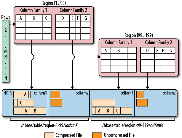
Figure 5-2. Column families mapping to separate storage files
Using the shell once again, we can try to create a column with no
name, and see what happens if we create a table with a column family
name that does not comply to the checks:
hbase(main):001:0> create 'testtable', 'colfam1'
0 row(s) in 0.1400 seconds
=> Hbase::Table - testtable
hbase(main):002:0> put 'testtable', 'row1', 'colfam1:', 'val1'
0 row(s) in 0.1130 seconds
hbase(main):003:0> scan 'testtable'
ROW COLUMN+CELL
row1 column=colfam1:, timestamp=1428488894611, val‐
ue=val1
1 row(s) in 0.0590 seconds
hbase(main):004:0> create 'testtable', 'col/fam1'
ERROR: Illegal character <47>. Family names cannot contain control
characters or colons: col/fam1
Here is some help for this command:
...
You can use the static helper method to verify the name:
Chapter 5: Client API: Administrative Features364
www.finebook.ir

static byte[] isLegalFamilyName(final byte[] b)
Use it in your program to verify user-provided input conforming to the
specifications that are required for the name. It does not return a
boolean flag, but throws an IllegalArgumentException when the
name is malformed. Otherwise, it returns the given parameter value
unchanged. The constructors taking in a familyName parameter,
shown below, uses this method internally to verify the given name; in
this case, you do not need to call the method beforehand.
A column family cannot be renamed. The common ap‐
proach to rename a family is to create a new family with
the desired name and copy the data over, using the API.
When you create a column family, you can specify a variety of parame‐
ters that control all of its features. The Java class has many construc‐
tors that allow you to specify most parameters while creating an in‐
stance. Here are the choices:
HColumnDescriptor(final String familyName)
HColumnDescriptor(final byte[] familyName)
HColumnDescriptor(HColumnDescriptor desc)
The first two simply take the family name as a String or byte[] ar‐
ray. There is another one that takes an existing HColumnDescriptor,
which copies all state and settings over from the given instance. In‐
stead of using the constructor, you can also use the getters and set‐
ters to specify the various details. We will now discuss each of them,
grouped by their purpose.
Name
Each column family has a name, and you can use the following
methods to retrieve it from an existing HColumnDescriptor in‐
stance:
byte[] getName();
String getNameAsString();
You cannot set the name, but you have to use these constructors to
hand it in. Keep in mind the requirement for the name to be print‐
able characters etc.
Schema Definition 365
www.finebook.ir

The name of a column family must not start with a “.” (pe‐
riod) and not contain “:” (colon), “/” (slash), or ISO control
characters, in other words, if its code is in the range
\u0000 through \u001F or in the range \u007F through
\u009F.
Maximum Versions
Per family, you can specify how many versions of each value you
want to keep. Recall the predicate deletion mentioned earlier
where the housekeeping of HBase removes values that exceed the
set maximum. Getting and setting the value is done using the fol‐
lowing API calls:
int getMaxVersions()
HColumnDescriptor setMaxVersions(int maxVersions)
The default value is 1, set by the hbase.column.max.version con‐
figuration property. The default is good for many use-cases, forc‐
ing the application developer to override the single version setting
to something higher if need be. For example, for a column storing
passwords, you could set this value to 10 to keep a history of previ‐
ously used passwords.
Minimum Versions
Specifies how many versions should always be kept for a column.
This works in tandem with the time-to-live, avoiding the removal of
the last value stored in a column. The default is set to 0, which dis‐
ables this feature.
int getMinVersions()
HColumnDescriptor setMinVersions(int minVersions)
Keep Deleted Cells
Controls whether the background housekeeping processes should
remove deleted cells, or not.
KeepDeletedCells getKeepDeletedCells()
HColumnDescriptor setKeepDeletedCells(boolean keepDeletedCells)
HColumnDescriptor setKeepDeletedCells(KeepDeletedCells keepDe‐
letedCells)
The used KeepDeletedCells type is an enumeration, having the
following options:
Table 5-1. The KeepDeletedCells enumeration
Value Description
FALSE Deleted cells are not retained.
Chapter 5: Client API: Administrative Features366
www.finebook.ir

Value Description
TRUE Deleted cells are retained until they are removed by other means such as
time-to-live (TTL) or the max number of versions. If no TTL is specified or
no new versions of delete cells are written, they are retained forever.
TTL Deleted cells are retained until the delete marker expires due to TTL. This
is useful when TTL is combined with the number of minimum versions,
and you want to keep a minimum number of versions around, but at the
same time remove deleted cells after the TTL.
The default is FALSE, meaning no deleted cells are kept during the
housekeeping operation.
Compression
HBase has pluggable compression algorithm support (you can find
more on this topic in (to come)) that allows you to choose the best
compression—or none—for the data stored in a particular column
family. The possible algorithms are listed in Table 5-2.
Table 5-2. Supported compression algorithms
Value Description
NONE Disables compression (default).
GZ Uses the Java-supplied or native GZip compression (which needs to be
installed separately).
LZO Enables LZO compression; must be installed separately.
LZ4 Enables LZ4 compression; must be installed separately.
SNAPPY Enables Snappy compression; binaries must be installed separately.
The default value is NONE--in other words, no compression is en‐
abled when you create a column family. When you use the Java API
and a column descriptor, you can use these methods to change the
value:
Compression.Algorithm getCompression()
Compression.Algorithm getCompressionType()
HColumnDescriptor setCompressionType(Compression.Algorithm
type)
Compression.Algorithm getCompactionCompression()
Compression.Algorithm getCompactionCompressionType()
HColumnDescriptor setCompactionCompressionType(Compression.Al‐
gorithm type)
Note how the value is not a String, but rather a Compression.Al
gorithm enumeration that exposes the same values as listed in
Table 5-2. Another observation is that there are two sets of meth‐
ods, one for the general compression setting and another for the
compaction compression setting. Also, each group has a getCom
Schema Definition 367
www.finebook.ir

6. After all, this is open source and a redundancy like this is often caused by legacy
code being carried forward. Please feel free to help clean this up and to contribute
back to the HBase project.
pression() and getCompressionType() (or getCompactionCom
pression() and getCompactionCompressionType(), respectively)
returning the same type of value. They are indeed redundant, and
you can use either to retrieve the current compression algorithm
type.6 As for compression versus compaction compression, the lat‐
ter defaults to what the former is set to, unless set differently.
We will look into this topic in much greater detail in (to come).
Encoding
Sets the encoding used for data blocks. If enabled, you can further
influence whether the same is applied to the cell tags. The API
methods involved are:
DataBlockEncoding getDataBlockEncoding()
HColumnDescriptor setDataBlockEncoding(DataBlockEncoding type)
These two methods control the encoding used, and employ the Dat
aBlockEncoding enumeration, containing the following options:
Table 5-3. Options of the DataBlockEncoding enumeration
Option Description
NONE No prefix encoding takes place (default).
PREFIX Represents the prefix compression algorithm, which removes
repeating common prefixes from subsequent cell keys.
DIFF The diff algorithm, which further compresses the key of
subsequent cells by storing only differences to previous keys.
FAST_DIFF An optimized version of the diff encoding, which also omits
repetitive cell value data.
PREFIX_TREE Trades increased write time latencies for faster read
performance. Uses a tree structure to compress the cell key.
In addition to setting the encoding for each cell key (and value da‐
ta in case of fast diff), cells also may carry an arbitrary list of tags,
used for different purposes, such as security and cell-level TTLs.
The following methods of the column descriptor allow you to fine-
tune if the encoding should also be applied to the tags:
HColumnDescriptor setCompressTags(boolean compressTags)
boolean isCompressTags()
The default is true, so all optional cell tags are encoded as part of
the entire cell encoding.
Chapter 5: Client API: Administrative Features368
www.finebook.ir

Block Size
All stored files in HBase are divided into smaller blocks that are
loaded during a get() or scan() operation, analogous to pages in
RDBMSes. The size of these blocks is set to 64 KB by default and
can be adjusted with these methods:
synchronized int getBlocksize()
HColumnDescriptor setBlocksize(int s)
The value is specified in bytes and can be used to control how
much data HBase is required to read from the storage files during
retrieval as well as what is cached in memory for subsequent ac‐
cess. How this can be used to optimize your setup can be found in
(to come).
There is an important distinction between the column fam‐
ily block size, or HFile block size, and the block size speci‐
fied on the HDFS level. Hadoop, and HDFS specifically, is
using a block size of—by default—128 MB to split up large
files for distributed, parallel processing using the YARN
framework. For HBase the HFile block size is—again by
default—64 KB, or one 2048th of the HDFS block size. The
storage files used by HBase are using this much more fine-
grained size to efficiently load and cache data in block op‐
erations. It is independent from the HDFS block size and
only used internally. See (to come) for more details, espe‐
cially (to come), which shows the two different block
types.
Block Cache
As HBase reads entire blocks of data for efficient I/O usage, it re‐
tains these blocks in an in-memory cache so that subsequent reads
do not need any disk operation. The default of true enables the
block cache for every read operation. But if your use case only ev‐
er has sequential reads on a particular column family, it is advisa‐
ble that you disable it to stop it from polluting the block cache by
setting the block cache-enabled flag to false. Here is how the API
can be used to change this flag:
boolean isBlockCacheEnabled()
HColumnDescriptor setBlockCacheEnabled(boolean blockCacheEna‐
bled)
There are other options you can use to influence how the block
cache is used, for example, during a scan() operation by calling
setCacheBlocks(false). This is useful during full table scans so
Schema Definition 369
www.finebook.ir
that you do not cause a major churn on the cache. See (to come)
for more information about this feature.
Besides the cache itself, you can configure the behavior of the sys‐
tem when data is being written, and store files being closed or
opened. The following set of methods define (and query) this:
boolean isCacheDataOnWrite()
HColumnDescriptor setCacheDataOnWrite(boolean value)
boolean isCacheDataInL1()
HColumnDescriptor setCacheDataInL1(boolean value)
boolean isCacheIndexesOnWrite()
HColumnDescriptor setCacheIndexesOnWrite(boolean value)
boolean isCacheBloomsOnWrite()
HColumnDescriptor setCacheBloomsOnWrite(boolean value)
boolean isEvictBlocksOnClose()
HColumnDescriptor setEvictBlocksOnClose(boolean value)
boolean isPrefetchBlocksOnOpen()
HColumnDescriptor setPrefetchBlocksOnOpen(boolean value)
Please consult (to come) and (to come) for details on how the block
cache works, what L1 and L2 is, and what you can do to speed up
your HBase setup. Note, for now, that all of these latter settings
default to false, meaning none of them is active, unless you ex‐
plicitly enable them for a column family.
Time-to-Live
HBase supports predicate deletions on the number of versions
kept for each value, but also on specific times. The time-to-live (or
TTL) sets a threshold based on the timestamp of a value and the
internal housekeeping is checking automatically if a value exceeds
its TTL. If that is the case, it is dropped during major compactions.
The API provides the following getters and setters to read and
write the TTL:
int getTimeToLive()
HColumnDescriptor setTimeToLive(int timeToLive)
The value is specified in seconds and is, by default, set to HConst
ants.FOREVER, which in turn is set to Integer.MAX_VALUE, or
2,147,483,647 seconds. The default value is treated as the special
case of keeping the values forever, that is, any positive value less
than the default enables this feature.
Chapter 5: Client API: Administrative Features370
www.finebook.ir

7. See “Bloom filter” on Wikipedia.
In-Memory
We mentioned the block cache and how HBase is using it to keep
entire blocks of data in memory for efficient sequential access to
data. The in-memory flag defaults to false but can be read and
modified with these methods:
boolean isInMemory()
HColumnDescriptor setInMemory(boolean inMemory)
Setting it to true is not a guarantee that all blocks of a family are
loaded into memory nor that they stay there. Think of it as a
promise, or elevated priority, to keep them in memory as soon as
they are loaded during a normal retrieval operation, and until the
pressure on the heap (the memory available to the Java-based
server processes) is too high, at which time they need to be dis‐
carded.
In general, this setting is good for small column families with few
values, such as the passwords of a user table, so that logins can be
processed very fast.
Bloom Filter
An advanced feature available in HBase is Bloom filters,7 allowing
you to improve lookup times given you have a specific access pat‐
tern (see (to come) for details). They add overhead in terms of
storage and memory, but improve lookup performance and read la‐
tencies. Table 5-4 shows the possible options.
Table 5-4. Supported Bloom Filter Types
Type Description
NONE Disables the filter.
ROW Use the row key for the filter (default).
ROWCOL Use the row key and column key (family+qualifier) for the filter.
As of HBase 0.96 the default is set to ROW for all column families of
all user tables (they are not enabled for the system catalog tables).
Because there are usually many more columns than rows (unless
you only have a single column in each row), the last option, ROW
COL, requires the largest amount of space. It is more fine-grained,
though, since it knows about each row/column combination, as op‐
posed to just rows keys.
Schema Definition 371
www.finebook.ir

The Bloom filter can be changed and retrieved with these calls,
taking or returning a BloomType enumeration, reflecting the above
options.
BloomType getBloomFilterType()
HColumnDescriptor setBloomFilterType(final BloomType bt)
Replication Scope
Another more advanced feature coming with HBase is replication.
It enables you to have multiple clusters that ship local updates
across the network so that they are applied to each other. By de‐
fault, replication is disabled and the replication scope is set to 0,
meaning it is disabled. You can change the scope with these func‐
tions:
int getScope()
HColumnDescriptor setScope(int scope)
The only other supported value (as of this writing) is 1, which ena‐
bles replication to a remote cluster. There may be more scope val‐
ues in the future. See Table 5-5 for a list of supported values.
Table 5-5. Supported Replication Scopes
Scope Constant Description
0 REPLICATION_SCOPE_LOCAL Local scope, i.e., no replication for this family
(default).
1 REPLICATION_SCOPE_GLOBAL Global scope, i.e., replicate family to a
remote cluster.
The full details can be found in (to come). Note how the scope is
also provided as a public constant in the API class HConstants.
When you need to set the replication scope in code it is advisable
to use the constants, as they are easier to read.
Encryption
Sets encryption related details. See (to come) for details. The fol‐
lowing API calls are at your disposal to set and read the encryption
type and key:
String getEncryptionType()
HColumnDescriptor setEncryptionType(String algorithm)
byte[] getEncryptionKey()
HColumnDescriptor setEncryptionKey(byte[] keyBytes)
Descriptor Parameters
In addition to those already mentioned, there are methods that let
you set arbitrary key/value pairs:
byte[] getValue(byte[] key)
String getValue(String key)
Chapter 5: Client API: Administrative Features372
www.finebook.ir
Map<ImmutableBytesWritable, ImmutableBytesWritable> getValues()
HColumnDescriptor setValue(byte[] key, byte[] value)
HColumnDescriptor setValue(String key, String value)
void remove(final byte[] key)
They are stored with the column definition and can be retrieved if
necessary. You can use them to access all configured values, as all
of the above methods are effectively using this list to set their pa‐
rameters. Another use-case might be to store application related
metadata in this list, since it is persisted on the server and can be
read by any client subsequently.
Configuration
Allows you to override any HBase configuration property on a per
column family basis. This is merged at runtime with the default
values, the cluster wide configuration file, and the table level set‐
tings. Note though that only properties related to the region or
table will be useful to set. Other, unrelated keys will not read even
if you override them.
String getConfigurationValue(String key)
Map<String, String> getConfiguration()
HColumnDescriptor setConfiguration(String key, String value)
void removeConfiguration(final String key)
Miscellaneous Calls
There are some calls that do not fit into the above categories, so
they are listed here for completeness. They allow you to retrieve
the unit for a configuration parameter, and get hold of the list of
all default values. They further allow you to convert the entire, or
partial state of the instance into a string for further use, for exam‐
ple, to print the result into a log file.
static Unit getUnit(String key)
static Map<String, String> getDefaultValues()
String toString()
String toStringCustomizedValues()
The only supported unit as of this writing is for TTL.
Example 5-4 uses the API to create a descriptor, set a custom and sup‐
plied value, and then print out the settings in various ways.
Example 5-4. Example how to create a HColumnDescriptor in code
HColumnDescriptor desc = new HColumnDescriptor("colfam1")
.setValue("test-key", "test-value")
.setBloomFilterType(BloomType.ROWCOL);
System.out.println("Column Descriptor: " + desc);
Schema Definition 373
www.finebook.ir
System.out.print("Values: ");
for (Map.Entry<ImmutableBytesWritable, ImmutableBytesWritable>
entry : desc.getValues().entrySet()) {
System.out.print(Bytes.toString(entry.getKey().get()) +
" -> " + Bytes.toString(entry.getValue().get()) + ", ");
}
System.out.println();
System.out.println("Defaults: " +
HColumnDescriptor.getDefaultValues());
System.out.println("Custom: " +
desc.toStringCustomizedValues());
System.out.println("Units:");
System.out.println(HColumnDescriptor.TTL + " -> " +
desc.getUnit(HColumnDescriptor.TTL));
System.out.println(HColumnDescriptor.BLOCKSIZE + " -> " +
desc.getUnit(HColumnDescriptor.BLOCKSIZE));
The output of Example 5-4 shows a few interesting details:
Column Descriptor: {NAME => 'colfam1', DATA_BLOCK_ENCODING =>
'NONE',
BLOOMFILTER => 'ROWCOL', REPLICATION_SCOPE => '0',
COMPRESSION => 'NONE', VERSIONS => '1', TTL => 'FOREVER',
MIN_VERSIONS => '0', KEEP_DELETED_CELLS => 'FALSE',
BLOCKSIZE => '65536', IN_MEMORY => 'false', BLOCKCACHE => 'true',
METADATA => {'test-key' => 'test-value'}}
Values: DATA_BLOCK_ENCODING -> NONE, BLOOMFILTER -> ROWCOL,
REPLICATION_SCOPE -> 0, COMPRESSION -> NONE, VERSIONS -> 1,
TTL -> 2147483647, MIN_VERSIONS -> 0, KEEP_DELETED_CELLS ->
FALSE,
BLOCKSIZE -> 65536, IN_MEMORY -> false, test-key -> test-value,
BLOCKCACHE -> true
Defaults: {CACHE_BLOOMS_ON_WRITE=false, CACHE_DATA_IN_L1=false,
PREFETCH_BLOCKS_ON_OPEN=false, BLOCKCACHE=true,
CACHE_INDEX_ON_WRITE=false, TTL=2147483647, DATA_BLOCK_ENCOD‐
ING=NONE,
BLOCKSIZE=65536, BLOOMFILTER=ROW, EVICT_BLOCKS_ON_CLOSE=false,
MIN_VERSIONS=0, CACHE_DATA_ON_WRITE=false, KEEP_DE‐
LETED_CELLS=FALSE,
COMPRESSION=none, REPLICATION_SCOPE=0, VERSIONS=1, IN_MEMO‐
RY=false}
Custom: {NAME => 'colfam1', BLOOMFILTER => 'ROWCOL',
METADATA => {'test-key' => 'test-value'}}
Units:
TTL -> TIME_INTERVAL
BLOCKSIZE -> NONE
Chapter 5: Client API: Administrative Features374
www.finebook.ir
The custom test-key property, with value test-value, is listed as
METADATA, while the one setting that was changed from the default,
the Bloom filter set to ROWCOL, is listed separately. The toStringCusto
mizedValues() only lists the changed or custom data, while the oth‐
ers print all. The static getDefaultValues() lists the default values
unchanged, since it is created once when this class is loaded and nev‐
er modified thereafter.
Before we move on, and as explained earlier in the context of the table
descriptor, the serialization functions required to send the configured
instances over RPC are also present for the column descriptor:
byte[] toByteArray()
static HColumnDescriptor parseFrom(final byte[] bytes) throws De‐
serializationException
static HColumnDescriptor convert(final ColumnFamilySchema cfs)
ColumnFamilySchema convert()
HBaseAdmin
Just as with the client API, you also have an API for administrative
tasks at your disposal. Compare this to the Data Definition Language
(DDL) found in RDBMSes—while the client API is more an analog to
the Data Manipulation Language (DML).
It provides operations to create tables with specific column families,
check for table existence, alter table and column family definitions,
drop tables, and much more. The provided functions can be grouped
into related operations; they’re discussed separately on the following
pages.
Basic Operations
Before you can use the administrative API, you will have to create an
instance of the Admin interface implementation. You cannot create an
instance directly, but you need to use the same approach as with
tables (see “API Building Blocks” (page 117)) to retrieve an instance
using the Connection class:
Configuration conf = HBaseConfiguration.create();
Connection connection = ConnectionFactory.createConnection(conf);
Admin admin = connection.getAdmin();
...
TableName[] tables = admin.listTableNames();
...
admin.close();
connection.close();
HBaseAdmin 375
www.finebook.ir

For the sake of brevity, this section omits the fact that
pretty much all methods may throw an IOException (or an
exception that inherits from it). The reason is usually a re‐
sult of a communication error between your client applica‐
tion and the remote servers, or an error that occurred on
the server-side and which was marshalled (as in wrapped)
into a client-side I/O error.
Handing in an existing configuration instance gives enough details to
the API to find the cluster using the ZooKeeper quorum, just like the
client API does. Use the administrative API instance for the operation
required and discard it afterward. In other words, you should not hold
on to the instance for too long. Call close() when you are done to
free any resources still held on either side of the communication.
The class implements the Abortable interface, adding the following
call to it:
void abort(String why, Throwable e)
boolean isAborted()
This method is called by the framework implicitly—for example, when
there is a fatal connectivity issue and the API should be stopped. You
should not call it directly, but rely on the system taking care of invok‐
ing it, in case of dire emergencies, that require a complete shutdown
—and possible restart—of the API instance.
The Admin class also exports these basic calls:
Connection getConnection()
void close()
The getConnection() returns the connection instance, and close()
frees all resources kept by the current Admin instance, as shown
above. This includes the connection to the remote servers.
Namespace Operations
You can use the API to create namespaces that subsequently hold the
tables assigned to them. And as expected, you can in addition modify
or delete existing namespaces, and retrieve a descriptor (see “Name‐
spaces” (page 347)). The list of API calls for these tasks are:
void createNamespace(final NamespaceDescriptor descriptor)
void modifyNamespace(final NamespaceDescriptor descriptor)
void deleteNamespace(final String name)
NamespaceDescriptor getNamespaceDescriptor(final String name)
NamespaceDescriptor[] listNamespaceDescriptors()
Chapter 5: Client API: Administrative Features376
www.finebook.ir
Example 5-5 shows these calls in action. The code creates a new
namespace, then lists the namespaces available. It then modifies the
new namespace by adding a custom property. After printing the de‐
scriptor it deletes the namespace, and eventually confirms the remov‐
al by listing the available spaces again.
Example 5-5. Example using the administrative API to create etc. a
namespace
Configuration conf = HBaseConfiguration.create();
Connection connection = ConnectionFactory.createConnection(conf);
Admin admin = connection.getAdmin();
NamespaceDescriptor namespace =
NamespaceDescriptor.create("testspace").build();
admin.createNamespace(namespace);
NamespaceDescriptor namespace2 =
admin.getNamespaceDescriptor("testspace");
System.out.println("Simple Namespace: " + namespace2);
NamespaceDescriptor[] list = admin.listNamespaceDescriptors();
for (NamespaceDescriptor nd : list) {
System.out.println("List Namespace: " + nd);
}
NamespaceDescriptor namespace3 =
NamespaceDescriptor.create("testspace")
.addConfiguration("Description", "Test Namespace")
.build();
admin.modifyNamespace(namespace3);
NamespaceDescriptor namespace4 =
admin.getNamespaceDescriptor("testspace");
System.out.println("Custom Namespace: " + namespace4);
admin.deleteNamespace("testspace");
NamespaceDescriptor[] list2 = admin.listNamespaceDescriptors();
for (NamespaceDescriptor nd : list2) {
System.out.println("List Namespace: " + nd);
}
The console output confirms what we expected to see:
Simple Namespace: {NAME => 'testspace'}
List Namespace: {NAME => 'default'}
List Namespace: {NAME => 'hbase'}
List Namespace: {NAME => 'testspace'}
Custom Namespace: {NAME => 'testspace', Description => 'Test Name‐
space'}
List Namespace: {NAME => 'default'}
List Namespace: {NAME => 'hbase'}
HBaseAdmin 377
www.finebook.ir
Table Operations
After the first set of basic and namespace operations, there is a group
of calls related to HBase tables. These calls help when working with
the tables themselves, not the actual schemas inside. The commands
addressing this are in “Schema Operations” (page 391).
Before you can do anything with HBase, you need to create tables.
Here is the set of functions to do so:
void createTable(HTableDescriptor desc)
void createTable(HTableDescriptor desc, byte[] startKey,
byte[] endKey, int numRegions)
void createTable(final HTableDescriptor desc, byte[][] splitKeys)
void createTableAsync(final HTableDescriptor desc, final byte[][]
splitKeys)
All of these calls must be given an instance of HTableDescriptor, as
described in detail in “Tables” (page 350). It holds the details of the
table to be created, including the column families. Example 5-6 uses
the simple variant of createTable() that just takes a table name.
Example 5-6. Example using the administrative API to create a
table
Configuration conf = HBaseConfiguration.create();
Connection connection = ConnectionFactory.createConnection(conf);
Admin admin = connection.getAdmin();
TableName tableName = TableName.valueOf("testtable");
HTableDescriptor desc = new HTableDescriptor(tableName);
HColumnDescriptor coldef = new HColumnDescriptor(
Bytes.toBytes("colfam1"));
desc.addFamily(coldef);
admin.createTable(desc);
boolean avail = admin.isTableAvailable(tableName);
System.out.println("Table available: " + avail);
Create a administrative API instance.
Create the table descriptor instance.
Create a column family descriptor and add it to the table
descriptor.
Call the createTable() method to do the actual work.
Check if the table is available.
Chapter 5: Client API: Administrative Features378
www.finebook.ir

Example 5-7 shows the same, but adds a namespace into the mix.
Example 5-7. Example using the administrative API to create a
table with a custom namespace
NamespaceDescriptor namespace =
NamespaceDescriptor.create("testspace").build();
admin.createNamespace(namespace);
TableName tableName = TableName.valueOf("testspace", "testtable");
HTableDescriptor desc = new HTableDescriptor(tableName);
HColumnDescriptor coldef = new HColumnDescriptor(
Bytes.toBytes("colfam1"));
desc.addFamily(coldef);
admin.createTable(desc);
The other createTable() versions have an additional—yet more ad‐
vanced—feature set: they allow you to create tables that are already
populated with specific regions. The code in Example 5-8 uses both
possible ways to specify your own set of region boundaries.
Example 5-8. Example using the administrative API to create a
table with predefined regions
private static Configuration conf = null;
private static Connection connection = null;
private static void printTableRegions(String tableName) throws IOEx‐
ception {
System.out.println("Printing regions of table: " + tableName);
TableName tn = TableName.valueOf(tableName);
RegionLocator locator = connection.getRegionLocator(tn);
Pair<byte[][], byte[][]> pair = locator.getStartEndKeys();
for (int n = 0; n < pair.getFirst().length; n++) {
byte[] sk = pair.getFirst()[n];
byte[] ek = pair.getSecond()[n];
System.out.println("[" + (n + 1) + "]" +
" start key: " +
(sk.length == 8 ? Bytes.toLong(sk) : Bytes.toStringBina‐
ry(sk)) +
", end key: " +
(ek.length == 8 ? Bytes.toLong(ek) : Bytes.toStringBina‐
ry(ek)));
}
locator.close();
}
public static void main(String[] args) throws IOException, Interrup‐
tedException {
conf = HBaseConfiguration.create();
connection = ConnectionFactory.createConnection(conf);
HBaseAdmin 379
www.finebook.ir

Admin admin = connection.getAdmin();
HTableDescriptor desc = new HTableDescriptor(
TableName.valueOf("testtable1"));
HColumnDescriptor coldef = new HColumnDescriptor(
Bytes.toBytes("colfam1"));
desc.addFamily(coldef);
admin.createTable(desc, Bytes.toBytes(1L), Bytes.toBytes(100L),
10);
printTableRegions("testtable1");
byte[][] regions = new byte[][] {
Bytes.toBytes("A"),
Bytes.toBytes("D"),
Bytes.toBytes("G"),
Bytes.toBytes("K"),
Bytes.toBytes("O"),
Bytes.toBytes("T")
};
HTableDescriptor desc2 = new HTableDescriptor(
TableName.valueOf("testtable2"));
desc2.addFamily(coldef);
admin.createTable(desc2, regions);
printTableRegions("testtable2");
}
Helper method to print the regions of a table.
Retrieve the start and end keys from the newly created table.
Print the key, but guarding against the empty start (and end)
key.
Call the createTable() method while also specifying the region
boundaries.
Manually create region split keys.
Call the crateTable() method again, with a new table name and
the list of region split keys.
Running the example should yield the following output on the console:
Printing regions of table: testtable1
[1] start key: , end key: 1
[2] start key: 1, end key: 13
[3] start key: 13, end key: 25
[4] start key: 25, end key: 37
[5] start key: 37, end key: 49
[6] start key: 49, end key: 61
[7] start key: 61, end key: 73
[8] start key: 73, end key: 85
[9] start key: 85, end key: 100
Chapter 5: Client API: Administrative Features380
www.finebook.ir
[10] start key: 100, end key:
Printing regions of table: testtable2
[1] start key: , end key: A
[2] start key: A, end key: D
[3] start key: D, end key: G
[4] start key: G, end key: K
[5] start key: K, end key: O
[6] start key: O, end key: T
[7] start key: T, end key:
The example uses a method of the RegionLocator implementation
that you saw earlier (see “The RegionLocator Class” (page 354)), get
StartEndKeys(), to retrieve the region boundaries. The first start and
the last end keys are empty, as is customary with HBase regions. In
between the keys are either the computed, or the provided split keys.
Note how the end key of a region is also the start key of the subse‐
quent one—just that it is exclusive for the former, and inclusive for the
latter, respectively.
The createTable(HTableDescriptor desc, byte[] startKey,
byte[] endKey, int numRegions) call takes a start and end key,
which is interpreted as numbers. You must provide a start value that
is less than the end value, and a numRegions that is at least 3: other‐
wise, the call will return with an exception. This is to ensure that you
end up with at least a minimum set of regions.
The start and end key values are subtracted and divided by the given
number of regions to compute the region boundaries. In the example,
you can see how we end up with the correct number of regions, while
the computed keys are filling in the range.
The createTable(HTableDescriptor desc, byte[][] splitKeys)
method used in the second part of the example, on the other hand, is
expecting an already set array of split keys: they form the start and
end keys of the regions created. The output of the example demon‐
strates this as expected. But take note how the first start key, and the
last end key are the default empty one (set to null), which means you
end up with seven regions, albeit having provided only six split keys.
HBaseAdmin 381
www.finebook.ir

The createTable() calls are, in fact, related. The createT
able(HTableDescriptor desc, byte[] startKey,
byte[] endKey, int numRegions) method is calculating
the region keys implicitly for you, using the
Bytes.split() method to use your given parameters to
compute the boundaries. It then proceeds to call the crea
teTable(HTableDescriptor desc, byte[][] split
Keys), doing the actual table creation.
Finally, there is the createTableAsync(HTableDescriptor desc,
byte[][] splitKeys) method that is taking the table descriptor, and
region keys, to asynchronously perform the same task as the createTa
ble() call.
Most of the table-related administrative API functions are
asynchronous in nature, which is useful, as you can send
off a command and not have to deal with waiting for a re‐
sult. For a client application, though, it is often necessary
to know if a command has succeeded before moving on
with other operations. For that, the calls are provided in
asynchronous—using the Async postfix—and synchronous
versions.
In fact, the synchronous commands are simply a wrapper
around the asynchronous ones, adding a loop at the end of
the call to repeatedly check for the command to have done
its task. The createTable() method, for example, wraps
the createTableAsync() method, while adding a loop that
waits for the table to be created on the remote servers be‐
fore yielding control back to the caller.
Once you have created a table, you can use the following helper func‐
tions to retrieve the list of tables, retrieve the descriptor for an exist‐
ing table, or check if a table exists:
HTableDescriptor[] listTables()
HTableDescriptor[] listTables(Pattern pattern)
HTableDescriptor[] listTables(String regex)
HTableDescriptor[] listTables(Pattern pattern, boolean includeSy‐
sTables)
HTableDescriptor[] listTables(String regex, boolean includeSysTa‐
bles)
HTableDescriptor[] listTableDescriptorsByNamespace(final String
name)
Chapter 5: Client API: Administrative Features382
www.finebook.ir
HTableDescriptor getTableDescriptor(final TableName tableName)
HTableDescriptor[] getTableDescriptorsByTableName(List<TableName>
tableNames)
HTableDescriptor[] getTableDescriptors(List<String> names)
boolean tableExists(final TableName tableName)
Example 5-6 uses the tableExists() method to check if the previous
command to create the table has succeeded. The listTables() re‐
turns a list of HTableDescriptor instances for every table that HBase
knows about, while the getTableDescriptor() method is returning it
for a specific one. Example 5-9 uses both to show what is returned by
the administrative API.
Example 5-9. Example listing the existing tables and their descrip‐
tors
Connection connection = ConnectionFactory.createConnection(conf);
Admin admin = connection.getAdmin();
HTableDescriptor[] htds = admin.listTables();
for (HTableDescriptor htd : htds) {
System.out.println(htd);
}
HTableDescriptor htd1 = admin.getTableDescriptor(
TableName.valueOf("testtable1"));
System.out.println(htd1);
HTableDescriptor htd2 = admin.getTableDescriptor(
TableName.valueOf("testtable10"));
System.out.println(htd2);
The console output is quite long, since every table descriptor is print‐
ed, including every possible property. Here is an abbreviated version:
Printing all tables...
'testtable1', {NAME => 'colfam1', DATA_BLOCK_ENCODING => 'NONE',
BLOOMFILTER
=> 'ROW', REPLICATION_SCOPE => '0', VERSIONS => '1', COMPRESSION
=> 'NONE',
MIN_VERSIONS => '0', TTL => 'FOREVER', KEEP_DELETED_CELLS =>
'FALSE',
BLOCKSIZE => '65536', IN_MEMORY => 'false', BLOCKCACHE => 'true'},
{NAME => 'colfam2', DATA_BLOCK_ENCODING => 'NONE', BLOOMFILTER =>
'ROW',
REPLICATION_SCOPE => '0', VERSIONS => '1', COMPRESSION => 'NONE',
MIN_VERSIONS => '0', TTL => 'FOREVER', KEEP_DELETED_CELLS =>
'FALSE',
BLOCKSIZE => '65536', IN_MEMORY => 'false', BLOCKCACHE => 'true'},
{NAME => 'colfam3', DATA_BLOCK_ENCODING => 'NONE', BLOOMFILTER =>
'ROW',
REPLICATION_SCOPE => '0', VERSIONS => '1', COMPRESSION => 'NONE',
HBaseAdmin 383
www.finebook.ir
MIN_VERSIONS => '0', TTL => 'FOREVER', KEEP_DELETED_CELLS =>
'FALSE',
BLOCKSIZE => '65536', IN_MEMORY => 'false', BLOCKCACHE => 'true'}
...
Exception in thread "main"
org.apache.hadoop.hbase.TableNotFoundException: testtable10
at org.apache.hadoop.hbase.client.HBaseAdmin.getTableDescrip‐
tor(...)
at admin.ListTablesExample.main(ListTablesExample.java:49)
...
The interesting part is the exception you should see being printed as
well. The example uses a nonexistent table name to showcase the fact
that you must be using existing table names—or wrap the call into a
try/catch guard, handling the exception more gracefully. You could
also use the tableExists() call, avoiding such exceptions being
thrown by first checking if a table exists. But keep in mind, HBase is a
distributed system, so just because you checked a table exists does
not mean it was already removed before you had a chance to apply the
next operation on it. In other words, using try/catch is advisable in
any event.
There are additional listTables() calls, which take a varying amount
of parameters. You can specify a regular expression filter either as a
string, or an already compiled Pattern instance. Furthermore, you
can instruct the call to include system tables by setting includeSysTa
bles to true, since by default they are excluded. Example 5-10 shows
these calls in use.
Example 5-10. Example listing the existing tables with patterns
HTableDescriptor[] htds = admin.listTables(".*");
htds = admin.listTables(".*", true);
htds = admin.listTables("hbase:.*", true);
htds = admin.listTables("def.*:.*", true);
htds = admin.listTables("test.*");
Pattern pattern = Pattern.compile(".*2");
htds = admin.listTables(pattern);
htds = admin.listTableDescriptorsByNamespace("testspace1");
The output is as such:
List: .*
testspace1:testtable1
testspace2:testtable2
testtable3
List: .*, including system tables
hbase:meta
hbase:namespace
testspace1:testtable1
Chapter 5: Client API: Administrative Features384
www.finebook.ir
testspace2:testtable2
testtable3
List: hbase:.*, including system tables
hbase:meta
hbase:namespace
List: def.*:.*, including system tables
testtable3
List: test.*
testspace1:testtable1
testspace2:testtable2
testtable3
List: .*2, using Pattern
testspace2:testtable2
List by Namespace: testspace1
testspace1:testtable1
The next set of list methods revolve around the names, not the entire
table descriptor we retrieved so far. The same can be done on the
table names alone, using the following calls:
TableName[] listTableNames()
TableName[] listTableNames(Pattern pattern)
TableName[] listTableNames(String regex)
TableName[] listTableNames(final Pattern pattern,
final boolean includeSysTables)
TableName[] listTableNames(final String regex,
final boolean includeSysTables)
TableName[] listTableNamesByNamespace(final String name)
Example 5-11 changes the previous example to use tables names, but
otherwise applies the same patterns.
Example 5-11. Example listing the existing tables with patterns
TableName[] names = admin.listTableNames(".*");
names = admin.listTableNames(".*", true);
names = admin.listTableNames("hbase:.*", true);
names = admin.listTableNames("def.*:.*", true);
names = admin.listTableNames("test.*");
Pattern pattern = Pattern.compile(".*2");
names = admin.listTableNames(pattern);
names = admin.listTableNamesByNamespace("testspace1");
The output is exactly the same and omitted here for the sake of brevi‐
ty. There is one more table information-related method available:
List<HRegionInfo> getTableRegions(final byte[] tableName)
List<HRegionInfo> getTableRegions(final TableName tableName)
HBaseAdmin 385
www.finebook.ir
This is similar to using the aforementioned RegionLocator (see “The
RegionLocator Class” (page 354)), but instead of returning the more
elaborate HRegionLocation details for each region of the table, this
call returns the slightly less detailed HRegionInfo records. The differ‐
ence is that the latter is just about the regions, while the former also
includes their current region server assignments.
After creating a table, you might also be interested to delete it. The
Admin calls to do so are:
void deleteTable(final TableName tableName)
HTableDescriptor[] deleteTables(String regex)
HTableDescriptor[] deleteTables(Pattern pattern)
Hand in a table name and the rest is taken care of: the table is re‐
moved from the servers, and all data deleted. The pattern based ver‐
sions of the call work the same way as shown for listTables() above.
Just be very careful not to delete the wrong table because of a wrong
regular expression pattern! The returned array for the pattern based
calls is a list of all tables where the operation failed. In other words, if
the operation succeeds, the returned list will be empty (but not null).
The is another related call, which does not delete the table itself, but
removes all data from it:
public void truncateTable(final TableName tableName,
final boolean preserveSplits)
Since a table might have grown and has been split across many re‐
gions, the preserveSplits flag is indicating what you want to have
happen with the list of these regions. The truncate call is really similar
to a disable and drop call, followed by a create operation, which recre‐
ates the table. At that point the preserveSplits flag decides if the
servers recreate the table with a single region, like any other new
table (which has no pre-split region list), or with all of its former re‐
gions.
But before you can delete a table, you need to ensure that it is first
disabled, using the following methods:
void disableTable(final TableName tableName)
HTableDescriptor[] disableTables(String regex)
HTableDescriptor[] disableTables(Pattern pattern)
void disableTableAsync(final TableName tableName)
Disabling the table first tells every region server to flush any uncom‐
mitted changes to disk, close all the regions, and update the system
tables to reflect that no region of this table is deployed to any servers.
The choices are again between doing this asynchronously, or synchro‐
nously, and supplying the table name in various formats for conve‐
Chapter 5: Client API: Administrative Features386
www.finebook.ir

nience. The returned list of descriptors for the pattern based calls is
listing all failed tables, that is, which were part of the pattern but
failed to disable. If all of them succeed to disable, the returned list will
be empty (but not null).
Disabling a table can potentially take a very long time, up
to several minutes. This depends on how much data is re‐
sidual in the server’s memory and not yet persisted to
disk. Undeploying a region requires all the data to be writ‐
ten to disk first, and if you have a large heap value set for
the servers this may result in megabytes, if not even giga‐
bytes, of data being saved. In a heavily loaded system this
could contend with other processes writing to disk, and
therefore require time to complete.
Once a table has been disabled, but not deleted, you can enable it
again:
void enableTable(final TableName tableName)
HTableDescriptor[] enableTables(String regex)
HTableDescriptor[] enableTables(Pattern pattern)
void enableTableAsync(final TableName tableName)
This call—again available in the usual flavors—reverses the disable
operation by deploying the regions of the given table to the active re‐
gion servers. Just as with the other pattern based methods, the re‐
turned array of descriptors is either empty, or contains the tables
where the operation failed.
Finally, there is a set of calls to check on the status of a table:
boolean isTableEnabled(TableName tableName)
boolean isTableDisabled(TableName tableName)
boolean isTableAvailable(TableName tableName)
boolean isTableAvailable(TableName tableName, byte[][] splitKeys)
Example 5-12 uses various combinations of the preceding calls to cre‐
ate, delete, disable, and check the state of a table.
Example 5-12. Example using the various calls to disable, enable,
and check that status of a table
Connection connection = ConnectionFactory.createConnection(conf);
Admin admin = connection.getAdmin();
TableName tableName = TableName.valueOf("testtable");
HTableDescriptor desc = new HTableDescriptor(tableName);
HColumnDescriptor coldef = new HColumnDescriptor(
HBaseAdmin 387
www.finebook.ir
Bytes.toBytes("colfam1"));
desc.addFamily(coldef);
admin.createTable(desc);
try {
admin.deleteTable(tableName);
} catch (IOException e) {
System.err.println("Error deleting table: " + e.getMessage());
}
admin.disableTable(tableName);
boolean isDisabled = admin.isTableDisabled(tableName);
System.out.println("Table is disabled: " + isDisabled);
boolean avail1 = admin.isTableAvailable(tableName);
System.out.println("Table available: " + avail1);
admin.deleteTable(tableName);
boolean avail2 = admin.isTableAvailable(tableName);
System.out.println("Table available: " + avail2);
admin.createTable(desc);
boolean isEnabled = admin.isTableEnabled(tableName);
System.out.println("Table is enabled: " + isEnabled);
The output on the console should look like this (the exception printout
was abbreviated, for the sake of brevity):
Creating table...
Deleting enabled table...
Error deleting table:
org.apache.hadoop.hbase.TableNotDisabledException: testtable
at org.apache.hadoop.hbase.master.HMaster.checkTableModifia‐
ble(...)
...
Disabling table...
Table is disabled: true
Table available: true
Deleting disabled table...
Table available: false
Creating table again...
Table is enabled: true
The error thrown when trying to delete an enabled table shows that
you either disable it first, or handle the exception gracefully in case
that is what your client application requires. You could prompt the
user to disable the table explicitly and retry the operation.
Also note how the isTableAvailable() is returning true, even when
the table is disabled. In other words, this method checks if the table is
physically present, no matter what its state is. Use the other two func‐
Chapter 5: Client API: Administrative Features388
www.finebook.ir

tions, isTableEnabled() and isTableDisabled(), to check for the
state of the table.
After creating your tables with the specified schema, you must either
delete the newly created table and recreate it to change its details, or
use the following method to alter its structure:
void modifyTable(final TableName tableName, final HTableDescriptor
htd)
Pair<Integer, Integer> getAlterStatus(final TableName tableName)
Pair<Integer, Integer> getAlterStatus(final byte[] tableName)
The modifyTable() call is only asynchronous, and there is no synchro‐
nous variant. If you want to make sure that changes have been propa‐
gated to all the servers and applied accordingly, you should use the
getAlterStatus() calls and loop in your client code until the schema
has been applied to all servers and regions. The call returns a pair of
numbers, where their meaning is summarized in the following table:
Table 5-6. Meaning of numbers returned by getAlterStatus() call
Pair Member Description
first Specifies the number of regions that still need to be updated.
second Total number of regions affected by the change.
As with the aforementioned deleteTable() commands, you must first
disable the table to be able to modify it. Example 5-13 does create a
table, and subsequently modifies it. It also uses the getAlterStatus()
call to wait for all regions to be updated.
Example 5-13. Example modifying the structure of an existing
table
Admin admin = connection.getAdmin();
TableName tableName = TableName.valueOf("testtable");
HColumnDescriptor coldef1 = new HColumnDescriptor("colfam1");
HTableDescriptor desc = new HTableDescriptor(tableName)
.addFamily(coldef1)
.setValue("Description", "Chapter 5 - ModifyTableExample: Origi‐
nal Table");
admin.createTable(desc, Bytes.toBytes(1L), Bytes.toBytes(10000L),
50);
HTableDescriptor htd1 = admin.getTableDescriptor(tableName);
HColumnDescriptor coldef2 = new HColumnDescriptor("colfam2");
htd1
.addFamily(coldef2)
.setMaxFileSize(1024 * 1024 * 1024L)
.setValue("Description",
"Chapter 5 - ModifyTableExample: Modified Table");
HBaseAdmin 389
www.finebook.ir
admin.disableTable(tableName);
admin.modifyTable(tableName, htd1);
Pair<Integer, Integer> status = new Pair<Integer, Integer>() {{
setFirst(50);
setSecond(50);
}};
for (int i = 0; status.getFirst() != 0 && i < 500; i++) {
status = admin.getAlterStatus(desc.getTableName());
if (status.getSecond() != 0) {
int pending = status.getSecond() - status.getFirst();
System.out.println(pending + " of " + status.getSecond()
+ " regions updated.");
Thread.sleep(1 * 1000l);
} else {
System.out.println("All regions updated.");
break;
}
}
if (status.getFirst() != 0) {
throw new IOException("Failed to update regions after 500 sec‐
onds.");
}
admin.enableTable(tableName);
HTableDescriptor htd2 = admin.getTableDescriptor(tableName);
System.out.println("Equals: " + htd1.equals(htd2));
System.out.println("New schema: " + htd2);
Create the table with the original structure and 50 regions.
Get schema, update by adding a new family and changing the
maximum file size property.
Disable and modify the table.
Create a status number pair to start the loop.
Loop over status until all regions are updated, or 500 seconds
have been exceeded.
Check if the table schema matches the new one created locally.
The output shows that both the schema modified in the client code
and the final schema retrieved from the server after the modification
are consistent:
50 of 50 regions updated.
Equals: true
New schema: 'testtable', {TABLE_ATTRIBUTES => {MAX_FILESIZE =>
'1073741824',
METADATA => {'Description' => 'Chapter 5 - ModifyTableExample:
Chapter 5: Client API: Administrative Features390
www.finebook.ir
Modified Table'}}, {NAME => 'colfam1', DATA_BLOCK_ENCODING =>
'NONE',
BLOOMFILTER => 'ROW', REPLICATION_SCOPE => '0', VERSIONS => '1',
COMPRESSION => 'NONE', MIN_VERSIONS => '0', TTL => 'FOREVER',
KEEP_DELETED_CELLS => 'FALSE', BLOCKSIZE => '65536', IN_MEMORY =>
'false', BLOCKCACHE => 'true'}, {NAME => 'colfam2', DA‐
TA_BLOCK_ENCODING
=> 'NONE', BLOOMFILTER => 'ROW', REPLICATION_SCOPE => '0', COM‐
PRESSION
=> 'NONE', VERSIONS => '1', TTL => 'FOREVER', MIN_VERSIONS =>
'0',
KEEP_DELETED_CELLS => 'FALSE', BLOCKSIZE => '65536', IN_MEMORY
=> 'false',
BLOCKCACHE => 'true'}
Calling the equals() method on the HTableDescriptor class com‐
pares the current with the specified instance and returns true if they
match in all properties, also including the contained column families
and their respective settings. It does not though compare custom set‐
tings, such as the used Description key, modified from the original to
the new value during the operation.
Schema Operations
Besides using the modifyTable() call, there are dedicated methods
provided by the Admin class to modify specific aspects of the current
table schema. As usual, you need to make sure the table to be modi‐
fied is disabled first. The whole set of column-related methods is as
follows:
void addColumn(final TableName tableName, final HColumnDescriptor
column)
void deleteColumn(final TableName tableName, final byte[] colum‐
nName)
void modifyColumn(final TableName tableName,
final HColumnDescriptor descriptor)
You can add, delete, and modify columns. Adding or modifying a col‐
umn requires that you first prepare a HColumnDescriptor instance, as
described in detail in “Column Families” (page 362). Alternatively, you
could use the getTableDescriptor() call to retrieve the current table
schema, and subsequently invoke getColumnFamilies() on the re‐
turned HTableDescriptor instance to retrieve the existing columns.
Otherwise, you supply the table name, and optionally the column
HBaseAdmin 391
www.finebook.ir

name for the delete calls. All of these calls are asynchronous, so as
mentioned before, caveat emptor.
Use Case: Hush
An interesting use case for the administrative API is to create and
alter tables and their schemas based on an external configuration
file. Hush is making use of this idea and defines the table and col‐
umn descriptors in an XML file, which is read and the contained
schema compared with the current table definitions. If there are
any differences they are applied accordingly. The following exam‐
ple has the core of the code that does this task:
Example 5-14. Creating or modifying table schemas using the
HBase administrative API
private void createOrChangeTable(final HTableDescriptor schema)
throws IOException {
HTableDescriptor desc = null;
if (tableExists(schema.getTableName(), false)) {
desc = getTable(schema.getTableName(), false);
LOG.info("Checking table " + desc.getNameAsString() +
"...");
final List<HColumnDescriptor> modCols =
new ArrayList<HColumnDescriptor>();
for (final HColumnDescriptor cd : desc.getFamilies()) {
final HColumnDescriptor cd2 = schema.getFamily(cd.get‐
Name());
if (cd2 != null && !cd.equals(cd2)) {
modCols.add(cd2);
}
}
final List<HColumnDescriptor> delCols =
new ArrayList<HColumnDescriptor>(desc.getFamilies());
delCols.removeAll(schema.getFamilies());
final List<HColumnDescriptor> addCols =
new ArrayList<HColumnDescriptor>(schema.getFamilies());
addCols.removeAll(desc.getFamilies());
if (modCols.size() > 0 || addCols.size() > 0 || del‐
Cols.size() > 0 ||
!hasSameProperties(desc, schema)) {
LOG.info("Disabling table...");
admin.disableTable(schema.getTableName());
if (modCols.size() > 0 || addCols.size() > 0 || del‐
Cols.size() > 0) {
for (final HColumnDescriptor col : modCols) {
LOG.info("Found different column -> " + col);
admin.modifyColumn(schema.getTableName(), col);
Chapter 5: Client API: Administrative Features392
www.finebook.ir

}
for (final HColumnDescriptor col : addCols) {
LOG.info("Found new column -> " + col);
admin.addColumn(schema.getTableName(), col);
}
for (final HColumnDescriptor col : delCols) {
LOG.info("Found removed column -> " + col);
admin.deleteColumn(schema.getTableName(), col.get‐
Name());
}
} else if (!hasSameProperties(desc, schema)) {
LOG.info("Found different table properties...");
admin.modifyTable(schema.getTableName(), schema);
}
LOG.info("Enabling table...");
admin.enableTable(schema.getTableName());
LOG.info("Table enabled");
getTable(schema.getTableName(), false);
LOG.info("Table changed");
} else {
LOG.info("No changes detected!");
}
} else {
LOG.info("Creating table " + schema.getNameAsString() +
"...");
admin.createTable(schema);
LOG.info("Table created");
}
}
Compute the differences between the XML based schema
and what is currently in HBase.
See if there are any differences in the column and table
definitions.
Alter the columns that have changed. The table was properly
disabled first.
Add newly defined columns.
Delete removed columns.
Alter the table itself, if there are any differences found.
In case the table did not exist yet create it now.
Cluster Operations
After the operations for the namespace, table, and column family
schemas within a table, there are a list of methods provided by the Ad
min implementation for operations on the regions and tables them‐
HBaseAdmin 393
www.finebook.ir

selves. They are used much more from an operator’s point of view, as
opposed to the schema functions, which will very likely be used by the
application developer. The cluster operations split into region, table,
and server operations, and we will discuss them in that order.
Region Operations
First are the region-related calls, that is, those concerned with the
state of a region. (to come) has the details on regions and their life cy‐
cle. Also, recall the details about the server and region name in “Serv‐
er and Region Names” (page 356), as many of the calls below will
need one or the other.
Many of the following operations are for advanced users,
so please handle with care.
List<HRegionInfo> getOnlineRegions(final ServerName sn)
Often you need to get a list of regions before operating on them,
and one way to do that is this method, which returns all regions
hosted by a given server.
void closeRegion(final String regionname, final String
serverName)
void closeRegion(final byte[] regionname, final String
serverName)
boolean closeRegionWithEncodedRegionName(final String en
codedRegionName, final String serverName)
void closeRegion(final ServerName sn, final HRegionInfo
hri)
Use these calls to close regions that have previously been de‐
ployed to region servers. Any enabled table has all regions en‐
abled, so you could actively close and undeploy one of those re‐
gions.
You need to supply the exact regionname as stored in the system
tables. Further, you may optionally supply the serverName param‐
eter, that overrides the server assignment as found in the system
tables as well. Some of the calls want the full name in text form,
others the hash only, while yet another is asking for objects encap‐
sulating the details.
Using this close call does bypass any master notification, that is,
the region is directly closed by the region server, unseen by the
master node.
Chapter 5: Client API: Administrative Features394
www.finebook.ir
void flush(final TableName tableName)
void flushRegion(final byte[] regionName)
As updates to a region (and the table in general) accumulate the
MemStore instances of the region servers fill with unflushed modifi‐
cations. A client application can use these synchronous methods to
flush such pending records to disk, before they are implicitly writ‐
ten by hitting the memstore flush size (see “Table Properties”
(page 358)) at a later time.
There is a method for flushing all regions of a given table, named
flush(), and another to flush a specific region, called flushRe
gion().
void compact(final TableName tableName)
void compact(final TableName tableName, final byte[] col
umnFamily)
void compactRegion(final byte[] regionName)
void compactRegion(final byte[] regionName, final byte[]
columnFamily)
void compactRegionServer(final ServerName sn, boolean ma
jor)
As storage files accumulate the system is compacting them in the
background to keep the number of files low. With these calls you
can explicitly trigger the same operation for an entire server, a
table, or one specific region. When you specify a column family
name, then the operation is applied to that family only. Setting the
major parameter to true promotes the region server-wide compac‐
tion to a major one.
The call itself is asynchronous, as compactions can potentially take
a long time to complete. Invoking these methods queues the
table(s), region(s), or column family for compaction, which is exe‐
cuted in the background by the server hosting the named region,
or by all servers hosting any region of the given table (see “Auto-
Sharding” (page 26) for details on compactions).
CompactionState getCompactionState(final TableName table
Name)
CompactionState getCompactionStateForRegion(final byte[]
regionName)
These are a continuation from the above, available to query the
status of a running compaction process. You either ask the status
for an entire table, or a specific region.
void majorCompact(TableName tableName)
void majorCompact(TableName tableName, final byte[] col
HBaseAdmin 395
www.finebook.ir
umnFamily)
void majorCompactRegion(final byte[] regionName)
void majorCompactRegion(final byte[] regionName, final
byte[] columnFamily)
These are the same as the compact() calls, but they queue the col‐
umn family, region, or table, for a major compaction instead. In
case a table name is given, the administrative API iterates over all
regions of the table and invokes the compaction call implicitly for
each of them.
void split(final TableName tableName)
void split(final TableName tableName, final byte[] split
Point)
void splitRegion(final byte[] regionName)
void splitRegion(final byte[] regionName, final byte[]
splitPoint)
Using these calls allows you to split a specific region, or table. In
case of the table-scoped call, the system iterates over all regions of
that table and implicitly invokes the split command on each of
them.
A noted exception to this rule is when the splitPoint parameter
is given. In that case, the split() command will try to split the
given region at the provided row key. In the case of using the
table-scope call, all regions are checked and the one containing
the splitPoint is split at the given key.
The splitPoint must be a valid row key, and—in case you use the
region specific method—be part of the region to be split. It also
must be greater than the region’s start key, since splitting a region
at its start key would make no sense. If you fail to give the correct
row key, the split request is ignored without reporting back to the
client. The region server currently hosting the region will log this
locally with the following message:
2015-04-12 20:39:58,077 ERROR [PriorityRpcServer.han‐
dler=4,queue=0,port=62255]
regionserver.HRegion: Ignoring invalid split
org.apache.hadoop.hbase.regionserver.WrongRegionException: Re‐
quested row out
of range for calculated split on HRegion testtable,,
1428863984023.
2d729d711208b37629baf70b5f17169c., startKey='', getEnd‐
Key()='ABC', row='ZZZ'
at org.apache.hadoop.hbase.regionserver.HRegion.check‐
Row(HRegion.java)
Chapter 5: Client API: Administrative Features396
www.finebook.ir
void mergeRegions(final byte[] encodedNameOfRegionA, fi
nal byte[] encodedNameOfRegionB, final boolean forcible)
This method allows you to merge previously split regions. The op‐
eration usually requires adjacent regions to be specified, but set‐
ting the forcible flag to true overrides this safety latch.
void assign(final byte[] regionName)
void unassign(final byte[] regionName, final boolean
force)
void offline(final byte[] regionName)
When a client requires a region to be deployed or undeployed from
the region servers, it can invoke these calls. The first would assign
a region, based on the overall assignment plan, while the second
would unassign the given region, triggering a subsequent automat‐
ic assignment. The third call allows you to offline a region, that is,
leave it unassigned after the call.
The force parameter set to true for unassign() means that a re‐
gion already marked to be unassigned—for example, from a previ‐
ous call to unassign()--is forced to be unassigned again. If force
were set to false, this would have no effect.
void move(final byte[] encodedRegionName, final byte[]
destServerName)
Using the move() call enables a client to actively control which
server is hosting what regions. You can move a region from its cur‐
rent region server to a new one. The destServerName parameter
can be set to null to pick a new server at random; otherwise, it
must be a valid server name, running a region server process. If
the server name is wrong, or currently not responding, the region
is deployed to a different server instead. In a worst-case scenario,
the move could fail and leave the region unassigned.
The destServerName must comply with the rules explained in
“Server and Region Names” (page 356), that is, it must have a
hostname, port, and timestamp component.
boolean setBalancerRunning(final boolean on, final
boolean synchronous)
boolean balancer()
The first method allows you to switch the region balancer on or
off. When the balancer is enabled, a call to balancer() will start
the process of moving regions from the servers, with more de‐
ployed to those with less deployed regions. (to come) explains how
this works in detail.
HBaseAdmin 397
www.finebook.ir

The synchronous flag allows to run the operation in said mode, or
in asynchronous mode when supplying false.
Example 5-15 assembles many of the above calls to showcase the ad‐
ministrative API and its ability to modify the data layout within the
cluster.
Example 5-15. Shows the use of the cluster operations
Connection connection = ConnectionFactory.createConnection(conf);
Admin admin = connection.getAdmin();
TableName tableName = TableName.valueOf("testtable");
HColumnDescriptor coldef1 = new HColumnDescriptor("colfam1");
HTableDescriptor desc = new HTableDescriptor(tableName)
.addFamily(coldef1)
.setValue("Description", "Chapter 5 - ClusterOperationExample");
byte[][] regions = new byte[][] { Bytes.toBytes("ABC"),
Bytes.toBytes("DEF"), Bytes.toBytes("GHI"), Bytes.to‐
Bytes("KLM"),
Bytes.toBytes("OPQ"), Bytes.toBytes("TUV")
};
admin.createTable(desc, regions);
BufferedMutator mutator = connection.getBufferedMutator(table‐
Name);
for (int a = 'A'; a <= 'Z'; a++)
for (int b = 'A'; b <= 'Z'; b++)
for (int c = 'A'; c <= 'Z'; c++) {
String row = Character.toString((char) a) +
Character.toString((char) b) + Character.toString((char)
c);
Put put = new Put(Bytes.toBytes(row));
put.addColumn(Bytes.toBytes("colfam1"), Bytes.to‐
Bytes("col1"),
Bytes.toBytes("val1"));
System.out.println("Adding row: " + row);
mutator.mutate(put);
}
mutator.close();
List<HRegionInfo> list = admin.getTableRegions(tableName);
int numRegions = list.size();
HRegionInfo info = list.get(numRegions - 1);
System.out.println("Number of regions: " + numRegions);
System.out.println("Regions: ");
printRegionInfo(list);
System.out.println("Splitting region: " + info.getRegionNameAs‐
String());
admin.splitRegion(info.getRegionName());
do {
Chapter 5: Client API: Administrative Features398
www.finebook.ir

list = admin.getTableRegions(tableName);
Thread.sleep(1 * 1000L);
System.out.print(".");
} while (list.size() <= numRegions);
numRegions = list.size();
System.out.println();
System.out.println("Number of regions: " + numRegions);
System.out.println("Regions: ");
printRegionInfo(list);
System.out.println("Retrieving region with row ZZZ...");
RegionLocator locator = connection.getRegionLocator(tableName);
HRegionLocation location =
locator.getRegionLocation(Bytes.toBytes("ZZZ"));
System.out.println("Found cached region: " +
location.getRegionInfo().getRegionNameAsString());
location = locator.getRegionLocation(Bytes.toBytes("ZZZ"), true);
System.out.println("Found refreshed region: " +
location.getRegionInfo().getRegionNameAsString());
List<HRegionInfo> online =
admin.getOnlineRegions(location.getServerName());
online = filterTableRegions(online, tableName);
int numOnline = online.size();
System.out.println("Number of online regions: " + numOnline);
System.out.println("Online Regions: ");
printRegionInfo(online);
HRegionInfo offline = online.get(online.size() - 1);
System.out.println("Offlining region: " + offline.getRegionNameAs‐
String());
admin.offline(offline.getRegionName());
int revs = 0;
do {
online = admin.getOnlineRegions(location.getServerName());
online = filterTableRegions(online, tableName);
Thread.sleep(1 * 1000L);
System.out.print(".");
revs++;
} while (online.size() <= numOnline && revs < 10);
numOnline = online.size();
System.out.println();
System.out.println("Number of online regions: " + numOnline);
System.out.println("Online Regions: ");
printRegionInfo(online);
HRegionInfo split = online.get(0);
System.out.println("Splitting region with wrong key: " + split.ge‐
tRegionNameAsString());
admin.splitRegion(split.getRegionName(), Bytes.to‐
Bytes("ZZZ")); // triggers log message
HBaseAdmin 399
www.finebook.ir
System.out.println("Assigning region: " + offline.getRegionNameAs‐
String());
admin.assign(offline.getRegionName());
revs = 0;
do {
online = admin.getOnlineRegions(location.getServerName());
online = filterTableRegions(online, tableName);
Thread.sleep(1 * 1000L);
System.out.print(".");
revs++;
} while (online.size() == numOnline && revs < 10);
numOnline = online.size();
System.out.println();
System.out.println("Number of online regions: " + numOnline);
System.out.println("Online Regions: ");
printRegionInfo(online);
System.out.println("Merging regions...");
HRegionInfo m1 = online.get(0);
HRegionInfo m2 = online.get(1);
System.out.println("Regions: " + m1 + " with " + m2);
admin.mergeRegions(m1.getEncodedNameAsBytes(),
m2.getEncodedNameAsBytes(), false);
revs = 0;
do {
list = admin.getTableRegions(tableName);
Thread.sleep(1 * 1000L);
System.out.print(".");
revs++;
} while (list.size() >= numRegions && revs < 10);
numRegions = list.size();
System.out.println();
System.out.println("Number of regions: " + numRegions);
System.out.println("Regions: ");
printRegionInfo(list);
Create a table with seven regions, and one column family.
Insert many rows starting from “AAA” to “ZZZ”. These will be
spread across the regions.
List details about the regions.
Split the last region this table has, starting at row key “TUV”.
Adds a new region starting with key “WEI”.
Loop and check until the operation has taken effect.
Retrieve region infos cached and refreshed to show the
difference.
Offline a region and print the list of all regions.
Chapter 5: Client API: Administrative Features400
www.finebook.ir

Attempt to split a region with a split key that does not fall into
boundaries. Triggers log message.
Reassign the offlined region.
Merge the first two regions. Print out result of operation.
Table Operations: Snapshots
The second set of cluster operations revolve around the actual tables.
These are low-level tasks that can be invoked from the administrative
API and be applied to the entire given table. The primary purpose is to
archive the current state of a table, referred to as snapshots. Here are
the admin API methods to create a snapshot for a table:
void snapshot(final String snapshotName, final TableName tableName)
void snapshot(final byte[] snapshotName, final TableName tableName)
void snapshot(final String snapshotName, final TableName tableName,
Type type)
void snapshot(SnapshotDescription snapshot)
SnapshotResponse takeSnapshotAsync(SnapshotDescription snapshot)
boolean isSnapshotFinished(final SnapshotDescription snapshot)
You need to supply a unique name for each snapshot, following the
same rules as enforced for table names. This is caused by snapshots
being stored in the underlying file system the same way as tables are,
though in a specific location (see (to come) for details). For example,
you could make use of the TableName.isLegalTableQualifierName()
method to verify if a given snapshot name is matching the require‐
ments. In addition, you have to name the table you want to perform
the snapshots on.
Besides the obvious snapshot calls asking for name and table, there
are a few more involved ones. The third call in the list above allows
you hand in another parameter, called type. It specifies the type of
snapshot you want to create, with the these choices being available:
Table 5-7. Choices available for snapshot types
Type Table
State Description
FLUSH Enabled This is the default and is used to force a flush operation on
online tables before the snapshot is taken.
SKIPFLUSH Enabled If you do not want to cause a flush to occur, you can use this
option to immediately snapshot all persisted files of a table.
DISABLED Disabled This option is not for normal use, but might be returned if a
snapshot was created on a disabled table.
HBaseAdmin 401
www.finebook.ir
The same enumeration is used for the objects returned by the listS
napshot() call, that is why the DISABLED value is a possible snapshot
type: it depends when you take the snapshot, that is, if the snapshot‐
ted table is enabled or disabled at that time. And obviously, if you
hand in a type of FLUSH or SKIPFLUSH on a disabled table they will
have no effect. On the contrary, the snapshot will go through and is
listed as DISABLED no matter what you have specified.
Once you have created one or more snapshot, you are able to retrieve
a list of the available snapshots using the following methods:
List<SnapshotDescription> listSnapshots()
List<SnapshotDescription> listSnapshots(String regex)
List<SnapshotDescription> listSnapshots(Pattern pattern)
The first call lists all snapshots stored, while the other two filter the
list based on a regular expression pattern. The output looks similar to
this, but of course depends on your cluster and what has been snap‐
shotted so far:
[name: "snapshot1"
table: "testtable"
creation_time: 1428924867254
type: FLUSH
version: 2
, name: "snapshot2"
table: "testtable"
creation_time: 1428924870596
type: DISABLED
version: 2]
Highlighted are the discussed types of each snapshot. The listSnap
shots() calls return a list of SnapshotDescription instances, which
give access to the snapshot details. There are the obvious getName()
and getTable() methods to return the snapshot and table name. In
addition, you can use getType() to get access to the highlighted snap‐
shot type, and getCreationTime() to retrieve the timestamp when
the snapshot was created. Lastly, there is getVersion() returning the
internal format version of the snapshot. This number is used to read
older snapshots with newer versions of HBase, so expect this number
to increase over time with major version of HBase. The description
class has a few more getters for snapshot details, such as the amount
of storage it consumes, and convenience methods to retrieve the de‐
scribed information in other formats.
When it is time to restore a previously taken snapshot, you need to
call one of these methods:
void restoreSnapshot(final byte[] snapshotName)
void restoreSnapshot(final String snapshotName)
Chapter 5: Client API: Administrative Features402
www.finebook.ir

void restoreSnapshot(final byte[] snapshotName,
final boolean takeFailSafeSnapshot)
void restoreSnapshot(final String snapshotName,
boolean takeFailSafeSnapshot)
Analogous, you specify a snapshot name, and the table is recreated
with the data contained in the snapshot. Before you can run a restore
operation on a table though, you need to disable it first. The restore
operation is essentially a drop operation, followed by a recreation of
the table with the archived data. You need to provide the table name
either as a string, or as a byte array. Of course, the snapshot has to
exist, or else you will receive an error.
The optional takeFailSafeSnapshot flag, set to true, will instruct the
servers to first perform a snapshot of the specified table, before re‐
storing the saved one. Should the restore operation fail, the failsafe
snapshot is restored instead. On the other hand, if the restore opera‐
tion completes successfully, then the failsafe snapshot is removed at
the end of the operation. The name of the failsafe snapshot is speci‐
fied using the hbase.snapshot.restore.failsafe.name configura‐
tion property, and defaults to hbase-failsafe-{snapshot.name}-
{restore.timestamp}. The possible variables you can use in the name
are:
Variable Description
{snapshot.name} The name of the snapshot.
{table.name} The name of the table the snapshot represents.
{restore.timestamp} The timestamp when the snapshot is taken.
The default value for the failsafe name ensures that the snapshot is
uniquely named, by adding the name of the snapshot that triggered its
creation, plus a timestamp. There should be no need to modify this to
something else, but if you want to you can using the above pattern
and configuration property.
You can also clone a snapshot, which means you are recreating the
table under a new name:
void cloneSnapshot(final byte[] snapshotName, final TableName ta‐
bleName)
void cloneSnapshot(final String snapshotName, final TableName ta‐
bleName)
Again, you specify the snapshot name in one or another form, but also
supply a new table name. The snapshot is restored in the newly
named table, like a restore would do for the original table.
Finally, removing a snapshot is accomplished using these calls:
HBaseAdmin 403
www.finebook.ir

void deleteSnapshot(final byte[] snapshotName)
void deleteSnapshot(final String snapshotName)
void deleteSnapshots(final String regex)
void deleteSnapshots(final Pattern pattern)
Like with the delete calls for tables, you can either specify an exact
snapshot by name, or you can apply a regular expression to remove
more than one in a single call. Just as before, be very careful what you
hand in, there is no coming back from this operation (as in, there is no
undo)! Example 5-16 runs these commands across a single original
table, that contains a single row only, named "row1":
Example 5-16. Example showing the use of the admin snapshot API
admin.snapshot("snapshot1", tableName);
List<HBaseProtos.SnapshotDescription> snaps = admin.listSnap‐
shots();
System.out.println("Snapshots after snapshot 1: " + snaps);
Delete delete = new Delete(Bytes.toBytes("row1"));
delete.addColumn(Bytes.toBytes("colfam1"), Bytes.to‐
Bytes("qual1"));
table.delete(delete);
admin.snapshot("snapshot2", tableName,
HBaseProtos.SnapshotDescription.Type.SKIPFLUSH);
admin.snapshot("snapshot3", tableName,
HBaseProtos.SnapshotDescription.Type.FLUSH);
snaps = admin.listSnapshots();
System.out.println("Snapshots after snapshot 2 & 3: " + snaps);
Put put = new Put(Bytes.toBytes("row2"))
.addColumn(Bytes.toBytes("colfam1"), Bytes.toBytes("qual10"),
Bytes.toBytes("val10"));
table.put(put);
HBaseProtos.SnapshotDescription snapshotDescription =
HBaseProtos.SnapshotDescription.newBuilder()
.setName("snapshot4")
.setTable(tableName.getNameAsString())
.build();
admin.takeSnapshotAsync(snapshotDescription);
snaps = admin.listSnapshots();
System.out.println("Snapshots before waiting: " + snaps);
System.out.println("Waiting...");
while (!admin.isSnapshotFinished(snapshotDescription)) {
Thread.sleep(1 * 1000);
Chapter 5: Client API: Administrative Features404
www.finebook.ir
System.out.print(".");
}
System.out.println();
System.out.println("Snapshot completed.");
snaps = admin.listSnapshots();
System.out.println("Snapshots after waiting: " + snaps);
System.out.println("Table before restoring snapshot 1");
helper.dump("testtable", new String[]{"row1", "row2"}, null,
null);
admin.disableTable(tableName);
admin.restoreSnapshot("snapshot1");
admin.enableTable(tableName);
System.out.println("Table after restoring snapshot 1");
helper.dump("testtable", new String[]{"row1", "row2"}, null,
null);
admin.deleteSnapshot("snapshot1");
snaps = admin.listSnapshots();
System.out.println("Snapshots after deletion: " + snaps);
admin.cloneSnapshot("snapshot2", TableName.valueOf("testtable2"));
System.out.println("New table after cloning snapshot 2");
helper.dump("testtable2", new String[]{"row1", "row2"}, null,
null);
admin.cloneSnapshot("snapshot3", TableName.valueOf("testta‐
ble3"));
System.out.println("New table after cloning snapshot 3");
helper.dump("testtable3", new String[]{"row1", "row2"}, null,
null);
Create a snapshot of the initial table, then list all available
snapshots next.
Remove one column and do two more snapshots, one without
first flushing, then another with a preceding flush.
Add a new row to the table and take yet another snapshot.
Wait for the asynchronous snapshot to complete. List the
snapshots before and after the waiting.
Restore the first snapshot, recreating the initial table. This
needs to be done on a disabled table.
Remove the first snapshot, and list the available ones again.
Clone the second and third snapshot into a new table, dump the
content to show the difference between the “skipflush” and
“flush” types.
HBaseAdmin 405
www.finebook.ir
The output (albeit a bit lengthy) reveals interesting things, please
keep an eye out for snapshot number #2 and #3:
Before snapshot calls...
Cell: row1/colfam1:qual1/2/Put/vlen=4/seqid=0, Value: val1
Cell: row1/colfam1:qual1/1/Put/vlen=4/seqid=0, Value: val1
...
Cell: row1/colfam2:qual3/6/Put/vlen=4/seqid=0, Value: val3
Cell: row1/colfam2:qual3/5/Put/vlen=4/seqid=0, Value: val3
Snapshots after snapshot 1: [name: "snapshot1"
table: "testtable"
creation_time: 1428918198629
type: FLUSH
version: 2
]
Snapshots after snapshot 2 & 3: [name: "snapshot1"
table: "testtable"
creation_time: 1428918198629
type: FLUSH
version: 2
, name: "snapshot2"
table: "testtable"
creation_time: 1428918200818
type: SKIPFLUSH
version: 2
, name: "snapshot3"
table: "testtable"
creation_time: 1428918200931
type: FLUSH
version: 2
]
Snapshots before waiting: [name: "snapshot1"
table: "testtable"
creation_time: 1428918198629
type: FLUSH
version: 2
, name: "snapshot2"
table: "testtable"
creation_time: 1428918200818
type: SKIPFLUSH
version: 2
, name: "snapshot3"
table: "testtable"
creation_time: 1428918200931
type: FLUSH
version: 2
]
Waiting...
Chapter 5: Client API: Administrative Features406
www.finebook.ir
.
Snapshot completed.
Snapshots after waiting: [name: "snapshot1"
table: "testtable"
creation_time: 1428918198629
type: FLUSH
version: 2
, name: "snapshot2"
table: "testtable"
creation_time: 1428918200818
type: SKIPFLUSH
version: 2
, name: "snapshot3"
table: "testtable"
creation_time: 1428918200931
type: FLUSH
version: 2
, name: "snapshot4"
table: "testtable"
creation_time: 1428918201570
version: 2
]
Table before restoring snapshot 1
Cell: row1/colfam1:qual1/1/Put/vlen=4/seqid=0, Value: val1
Cell: row1/colfam1:qual2/4/Put/vlen=4/seqid=0, Value: val2
...
Cell: row1/colfam2:qual3/5/Put/vlen=4/seqid=0, Value: val3
Cell: row2/colfam1:qual10/1428918201565/Put/vlen=5/seqid=0, Value:
val10
Table after restoring snapshot 1
Cell: row1/colfam1:qual1/2/Put/vlen=4/seqid=0, Value: val1
Cell: row1/colfam1:qual1/1/Put/vlen=4/seqid=0, Value: val1
...
Cell: row1/colfam2:qual3/6/Put/vlen=4/seqid=0, Value: val3
Cell: row1/colfam2:qual3/5/Put/vlen=4/seqid=0, Value: val3
Snapshots after deletion: [name: "snapshot2"
table: "testtable"
creation_time: 1428918200818
type: SKIPFLUSH
version: 2
, name: "snapshot3"
table: "testtable"
creation_time: 1428918200931
type: FLUSH
version: 2
, name: "snapshot4"
table: "testtable"
creation_time: 1428918201570
version: 2
HBaseAdmin 407
www.finebook.ir
]
New table after cloning snapshot 2
Cell: row1/colfam1:qual1/2/Put/vlen=4/seqid=0, Value: val1
Cell: row1/colfam1:qual1/1/Put/vlen=4/seqid=0, Value: val1
Cell: row1/colfam1:qual2/4/Put/vlen=4/seqid=0, Value: val2
...
Cell: row1/colfam2:qual3/6/Put/vlen=4/seqid=0, Value: val3
Cell: row1/colfam2:qual3/5/Put/vlen=4/seqid=0, Value: val3
New table after cloning snapshot 3
Cell: row1/colfam1:qual1/1/Put/vlen=4/seqid=0, Value: val1
Cell: row1/colfam1:qual2/4/Put/vlen=4/seqid=0, Value: val2
Cell: row1/colfam1:qual2/3/Put/vlen=4/seqid=0, Value: val2
...
Cell: row1/colfam2:qual3/6/Put/vlen=4/seqid=0, Value: val3
Cell: row1/colfam2:qual3/5/Put/vlen=4/seqid=0, Value: val3
Since we performed snapshot #2 while skipping flushes, we do not
see the preceding delete being applied: the delete has been applied to
the WAL and memstore, but not the store files yet. Snapshot #3 does
the same snapshot, but forces the flush to occur beforehand. The out‐
put in testtable2 and testtable3 confirm that the former still con‐
tains the deleted data, and the latter does not.
Some parting notes on snapshots:
•You can only have one snapshot or restore in progress per table. In
other words, if you have two separate tables, you can snapshot
them at the same time, but you cannot run two concurrent snap‐
shots on the same table—or run a snapshot while a restore is in
progress. The second operation would fail with an error message
(for example: "Rejected taking <snapshotname> because we
are already running another snapshot...").
•You can increase the snapshot concurrency from the default of 1
by setting a higher value with the hbase.snapshot.mas
ter.threads configuration property. The default means only one
snapshot operation runs at any given time in the entire cluster.
Subsequent operations would be queued and executed sequential‐
ly.
•Turning off snapshot support for the entire cluster is handled by
hbase.snapshot.enabled. It is set to true, that is, snapshot sup‐
port is enabled on a cluster installed with default values.
Chapter 5: Client API: Administrative Features408
www.finebook.ir
Server Operations
The third group of methods provided by the Admin interface address
the entire cluster. They are either generic calls, or very low-level oper‐
ations, so please again, be very careful with what you are doing.
ClusterStatus getClusterStatus()
The getClusterStatus() call allows you to retrieve an instance of
the ClusterStatus class, containing detailed information about
the cluster status. See “Cluster Status Information” (page 411) for
what you are provided with.
Configuration getConfiguration()
void updateConfiguration(ServerName server)
void updateConfiguration()
These calls allow the application to access the current configura‐
tion, and to reload that configuration from disk. The latter is done
for either all servers, when no parameter is specified, or one given
server only. You need to provide a server name, as discussed
throughout this chapter. Not all configuration properties are sup‐
ported as reloadable during the runtime of the servers. See (to
come) for a list of those that can be reloaded.
Using the getConfiguration() gives access to the client configu‐
ration instance, that is, what was loaded, or set later on, from disk.
Since HBase is a distributed system it is very likely that the client-
side settings are not the same as the server-side ones. And using
any of the set() methods of the returned Configuration instance
is just modifying the client-side settings. If you want to update the
servers, you need to deploy an updated hbase-site.xml to the
servers and invoke the updateConfiguration() call instead.
int getMasterInfoPort()
Returns the current web-UI port of the HBase Master. This value
is set with the hbase.master.info.port property, but might be
dynamically reassigned when the server starts.
int getOperationTimeout()
Returns the value set with the hbase.client.operation.timeout
property. It defines how long the client should wait for the servers
to respond, and defaulting to Integer.MAX_VALUE, that is, indefi‐
nitely.
void rollWALWriter(ServerName serverName)
Instructs the named server to close the current WAL file and cre‐
ate a new one.
HBaseAdmin 409
www.finebook.ir
boolean enableCatalogJanitor(boolean enable)
int runCatalogScan()
boolean isCatalogJanitorEnabled()
The HBase Master process runs a background housekeeping task,
the catalog janitor, which is responsible to clean up region opera‐
tion remnants. For example, when a region splits or is merged, the
janitor will clean up the left-over region details, including meta da‐
ta and physical files. By default, the task runs on every standard
cluster. You can use these calls to stop that task to run, invoke a
run manually with runCatalogScan(), and check the status of the
task.
String[] getMasterCoprocessors()
CoprocessorRpcChannel coprocessorService()
CoprocessorRpcChannel coprocessorService(ServerName sn)
Provides access to the list of coprocessors loaded into the master
process, and the RPC channel (which is derived from a Protobuf
superclass) for the active master, when not providing any parame‐
ter, or a given region server. See “Coprocessors” (page 282), and
especially “The Service Interface” (page 299), on how to make use
of the RPC endpoint.
void execProcedure(String signature, String instance,
Map<String, String> props)
byte[] execProcedureWithRet(String signature, String in
stance, Map<String, String> props)
boolean isProcedureFinished(String signature, String in
stance, Map<String, String> props)
HBase has a server-side procedure framework, which is used by,
for example, the master to distribute an operation across many or
all region servers. If a flush is triggered, the procedure represent‐
ing the flush operation is started on the cluster. There are calls to
do this as a one-off call, or with a built-in retry mechanism. The
latter call allows to retrieve the status of a procedure that was
started beforehand.
void shutdown()
void stopMaster()
void stopRegionServer(final String hostnamePort)
These calls either shut down the entire cluster, stop the master
server, or stop a particular region server only. Once invoked, the
affected servers will be stopped, that is, there is no delay nor a
way to revert the process.
Chapters (to come) and (to come) have more information on these ad‐
vanced—yet very powerful—features. Use with utmost care!
Chapter 5: Client API: Administrative Features410
www.finebook.ir

Cluster Status Information
When you query the cluster status using the Admin.getClusterSta
tus() call, you will be given a ClusterStatus instance, containing all
the information the master server has about the current state of the
cluster. Table 5-8 lists the methods of the ClusterStatus class.
Table 5-8. Overview of the information provided by the ClusterSta
tus class
Method Description
getAverageLoad() The total average number of regions per region server. This
is computed as number of regions/number of servers.
getBackupMasters() Returns the list of all known backup HBase Master servers.
getBackupMasters
Size() The size of the list of all known backup masters.
getBalancerOn() Provides access to the internal Boolean instance, reflecting
the balancer tasks status. Might be null.
getClusterId() Returns the unique identifier for the cluster. This is a UUID
generated when HBase starts with an empty storage
directory. It is stored in hbase.id under the HBase root
directory.
getDeadServerNames() A list of all server names currently considered dead. The
names in the collection are ServerName instances, which
contain the hostname, RPC port, and start code.
getDeadServers() The number of servers listed as dead. This does not contain
the live servers.
getHBaseVersion() Returns the HBase version identification string.
getLoad(ServerName
sn) Retrieves the status information available for the given
server name.
getMaster() The server name of the current master.
getMasterCoproces
sors() A list of all loaded master coprocessors.
getRegionsCount() The total number of regions in the cluster.
getRegionsInTransi
tion() Gives you access to a map of all regions currently in
transition, e.g., being moved, assigned, or unassigned. The
key of the map is the encoded region name (as returned by
HRegionInfo.getEncodedName(), for example), while the value
is an instance of RegionState.a
getRequestsCount() The current number of requests across all region servers in
the cluster.
getServers() The list of live servers. The names in the collection are Serv
erName instances, which contain the hostname, RPC port, and
start code.
HBaseAdmin 411
www.finebook.ir

Method Description
getServersSize() The number of region servers currently live as known to the
master server. The number does not include the number of
dead servers.
getVersion() Returns the format version of the ClusterStatus instance.
This is used during the serialization process of sending an
instance over RPC.
isBalancerOn() Returns true if the balancer task is enabled on the master.
toString() Converts the entire cluster status details into a string.
a See (to come) for the details.
Accessing the overall cluster status gives you a high-level view of
what is going on with your servers—as a whole. Using the getServ
ers() array, and the returned ServerName instances, lets you drill fur‐
ther into each actual live server, and see what it is doing currently.
See “Server and Region Names” (page 356) again for details on the
ServerName class.
Each server, in turn, exposes details about its load, by offering a Serv
erLoad instance, returned by the getLoad() method of the Cluster
Status instance. Using the aforementioned ServerName, as returned
by the getServers() call, you can iterate over all live servers and re‐
trieve their current details. The ServerLoad class gives you access to
not just the load of the server itself, but also for each hosted region.
Table 5-9 lists the provided methods.
Table 5-9. Overview of the information provided by the ServerLoad
class
Method Description
getCurrentCompactedKVs() The number of cells that have been compacted, while
compactions are running.
getInfoServerPort() The web-UI port of the region server.
getLoad() Currently returns the same value as getNumberOfRe
gions().
getMaxHeapMB() The configured maximum Java Runtime heap size in
megabytes.
getMemStoreSizeInMB() The total size of the in-memory stores, across all regions
hosted by this server.
getNumberOfRegions() The number of regions on the current server.
getNumberOfRequests() Returns the accumulated number of requests, and counts
all API requests, such as gets, puts, increments, deletes,
and so on.a
getReadRequestsCount() The sum of all read requests for all regions of this server.a
Chapter 5: Client API: Administrative Features412
www.finebook.ir

Method Description
getRegionServerCoproces
sors() The list of loaded coprocessors, provided as a string
array, listing the class names.
getRegionsLoad() Returns a map containing the load details for each hosted
region of the current server. The key is the region name
and the value an instance of the RegionsLoad class,
discussed next.
getReplicationLoadSink() If replication is enabled, this call returns an object with
replication statistics.
getReplicationLoad
SourceList() If replication is enabled, this call returns a list of objects
with replication statistics.
getRequestsPerSecond() Provides the computed requests per second value,
accumulated for the entire server.
getRootIndexSizeKB() The summed up size of all root indexes, for every storage
file, the server holds in memory.
getRsCoprocessors() The list of coprocessors in the order they were loaded.
Should be equal to getRegionServerCoprocessors().
getStorefileIndexSi
zeInMB() The total size in megabytes of the indexes—the block and
meta index, to be precise—across all store files in use by
this server.
getStorefiles() The number of store files in use by the server. This is
across all regions it hosts.
getStorefileSizeInMB() The total size in megabytes of the used store files.
getStores() The total number of stores held by this server. This is
similar to the number of all column families across all
regions.
getStoreUncompressedSi
zeMB() The raw size of the data across all stores in megabytes.
getTotalCompactingKVs() The total number of cells currently compacted across all
stores.
getTotalNumberOfRe
quests() Returns the total number of all requests received by this
server.a
getTotalStaticBloomSi
zeKB() Specifies the combined size occupied by all Bloom filters
in kilobytes.
getTotalStaticIndexSi
zeKB() Specifies the combined size occupied by all indexes in
kilobytes.
getUsedHeapMB() The currently used Java Runtime heap size in megabytes,
if available.
getWriteRequestsCount() The sum of all read requests for all regions of this server.a
hasMaxHeapMB() Check if the value with same name is available during the
accompanying getXYZ() call.
HBaseAdmin 413
www.finebook.ir

Method Description
hasNumberOfRequests() Check if the value with same name is available during the
accompanying getXYZ() call.
hasTotalNumberOfRe
quests() Check if the value with same name is available during the
accompanying getXYZ() call.
hasUsedHeapMB() Check if the value with same name is available during the
accompanying getXYZ() call.
obtainServerLoadPB() Returns the low-level Protobuf version of the current
server load instance.
toString() Converts the state of the instance with all above metrics
into a string for logging etc.
a Accumulated within the last hbase.regionserver.metrics.period
Finally, there is a dedicated class for the region load, aptly named Re
gionLoad. See Table 5-10 for the list of provided information.
Table 5-10. Overview of the information provided by the Region
Load class
Method Description
getCompleteSequenceId() Returns the last completed sequence ID for the region,
used in conjunction with the MVCC.
getCurrentCompactedKVs() The currently compacted cells for this region, while a
compaction is running.
getDataLocality() A ratio from 0 to 1 (0% to 100%) expressing the locality
of store files to the region server process.
getMemStoreSizeMB() The heap size in megabytes as used by the MemStore of
the current region.
getName() The region name in its raw, byte[] byte array form.
getNameAsString() Converts the raw region name into a String for
convenience.
getReadRequestsCount() The number of read requests for this region, since it was
deployed to the region server. This counter is not reset.
getRequestsCount() The number of requests for the current region.
getRootIndexSizeKB() The sum of all root index details help in memory for this
region, in kilobytes.
getStorefileIndexSizeMB() The size of the indexes for all store files, in megabytes,
for this region.
getStorefiles() The number of store files, across all stores of this region.
getStorefileSizeMB() The size in megabytes of the store files for this region.
getStores() The number of stores in this region.
Chapter 5: Client API: Administrative Features414
www.finebook.ir

Method Description
getStoreUncompressedSi
zeMB() The size of all stores in megabyte, before compression.
getTotalCompactingKVs() The count of all cells being compacted within this region.
getTotalStaticBloomSi
zeKB() The size of all Bloom filter data in kilobytes.
getTotalStaticIndexSi
zeKB() The size of all index data in kilobytes.
getWriteRequestsCount() The number of write requests for this region, since it
was deployed to the region server. This counter is not
reset.
toString() Converts the state of the instance with all above metrics
into a string for logging etc.
Example 5-17 shows all of the getters in action.
Example 5-17. Example reporting the status of a cluster
ClusterStatus status = admin.getClusterStatus();
System.out.println("Cluster Status:\n--------------");
System.out.println("HBase Version: " + status.getHBaseVersion());
System.out.println("Version: " + status.getVersion());
System.out.println("Cluster ID: " + status.getClusterId());
System.out.println("Master: " + status.getMaster());
System.out.println("No. Backup Masters: " +
status.getBackupMastersSize());
System.out.println("Backup Masters: " + status.getBackupMas‐
ters());
System.out.println("No. Live Servers: " + status.getServers‐
Size());
System.out.println("Servers: " + status.getServers());
System.out.println("No. Dead Servers: " + status.getDeadServ‐
ers());
System.out.println("Dead Servers: " + status.getDeadServer‐
Names());
System.out.println("No. Regions: " + status.getRegionsCount());
System.out.println("Regions in Transition: " +
status.getRegionsInTransition());
System.out.println("No. Requests: " + status.getRequestsCount());
System.out.println("Avg Load: " + status.getAverageLoad());
System.out.println("Balancer On: " + status.getBalancerOn());
System.out.println("Is Balancer On: " + status.isBalancerOn());
System.out.println("Master Coprocessors: " +
Arrays.asList(status.getMasterCoprocessors()));
System.out.println("\nServer Info:\n--------------");
for (ServerName server : status.getServers()) {
System.out.println("Hostname: " + server.getHostname());
HBaseAdmin 415
www.finebook.ir

System.out.println("Host and Port: " + server.getHostAndPort());
System.out.println("Server Name: " + server.getServerName());
System.out.println("RPC Port: " + server.getPort());
System.out.println("Start Code: " + server.getStartcode());
ServerLoad load = status.getLoad(server);
System.out.println("\nServer Load:\n--------------");
System.out.println("Info Port: " + load.getInfoServerPort());
System.out.println("Load: " + load.getLoad());
System.out.println("Max Heap (MB): " + load.getMaxHeapMB());
System.out.println("Used Heap (MB): " + load.getUsedHeapMB());
System.out.println("Memstore Size (MB): " +
load.getMemstoreSizeInMB());
System.out.println("No. Regions: " + load.getNumberOfRegions());
System.out.println("No. Requests: " + load.getNumberOfRe‐
quests());
System.out.println("Total No. Requests: " +
load.getTotalNumberOfRequests());
System.out.println("No. Requests per Sec: " +
load.getRequestsPerSecond());
System.out.println("No. Read Requests: " +
load.getReadRequestsCount());
System.out.println("No. Write Requests: " +
load.getWriteRequestsCount());
System.out.println("No. Stores: " + load.getStores());
System.out.println("Store Size Uncompressed (MB): " +
load.getStoreUncompressedSizeMB());
System.out.println("No. Storefiles: " + load.getStorefiles());
System.out.println("Storefile Size (MB): " +
load.getStorefileSizeInMB());
System.out.println("Storefile Index Size (MB): " +
load.getStorefileIndexSizeInMB());
System.out.println("Root Index Size: " + load.getRootIndexSi‐
zeKB());
System.out.println("Total Bloom Size: " +
load.getTotalStaticBloomSizeKB());
System.out.println("Total Index Size: " +
load.getTotalStaticIndexSizeKB());
System.out.println("Current Compacted Cells: " +
load.getCurrentCompactedKVs());
System.out.println("Total Compacting Cells: " +
load.getTotalCompactingKVs());
System.out.println("Coprocessors1: " +
Arrays.asList(load.getRegionServerCoprocessors()));
System.out.println("Coprocessors2: " +
Arrays.asList(load.getRsCoprocessors()));
System.out.println("Replication Load Sink: " +
load.getReplicationLoadSink());
System.out.println("Replication Load Source: " +
load.getReplicationLoadSourceList());
Chapter 5: Client API: Administrative Features416
www.finebook.ir

System.out.println("\nRegion Load:\n--------------");
for (Map.Entry<byte[], RegionLoad> entry :
load.getRegionsLoad().entrySet()) {
System.out.println("Region: " + Bytes.toStringBinary(en‐
try.getKey()));
RegionLoad regionLoad = entry.getValue();
System.out.println("Name: " + Bytes.toStringBinary(
regionLoad.getName()));
System.out.println("Name (as String): " +
regionLoad.getNameAsString());
System.out.println("No. Requests: " + regionLoad.getRequests‐
Count());
System.out.println("No. Read Requests: " +
regionLoad.getReadRequestsCount());
System.out.println("No. Write Requests: " +
regionLoad.getWriteRequestsCount());
System.out.println("No. Stores: " + regionLoad.getStores());
System.out.println("No. Storefiles: " + regionLoad.getStore‐
files());
System.out.println("Data Locality: " + regionLoad.getDataLo‐
cality());
System.out.println("Storefile Size (MB): " +
regionLoad.getStorefileSizeMB());
System.out.println("Storefile Index Size (MB): " +
regionLoad.getStorefileIndexSizeMB());
System.out.println("Memstore Size (MB): " +
regionLoad.getMemStoreSizeMB());
System.out.println("Root Index Size: " +
regionLoad.getRootIndexSizeKB());
System.out.println("Total Bloom Size: " +
regionLoad.getTotalStaticBloomSizeKB());
System.out.println("Total Index Size: " +
regionLoad.getTotalStaticIndexSizeKB());
System.out.println("Current Compacted Cells: " +
regionLoad.getCurrentCompactedKVs());
System.out.println("Total Compacting Cells: " +
regionLoad.getTotalCompactingKVs());
System.out.println();
}
}
Get the cluster status.
Iterate over the included server instances.
Retrieve the load details for the current server.
Iterate over the region details of the current server.
Get the load details for the current region.
HBaseAdmin 417
www.finebook.ir

On a standalone setup, and running the Performance Evalutation tool
(see (to come)) in parallel, you should see something like this:
Cluster Status:
--------------
HBase Version: 1.0.0
Version: 2
Cluster ID: 25ba54eb-09da-4698-88b5-5acdfecf0005
Master: srv1.foobar.com,63911,1428996031794
No. Backup Masters: 0
Backup Masters: []
No. Live Servers: 1
Servers: [srv1.foobar.com,63915,1428996033410]
No. Dead Servers: 2
Dead Servers: [srv1.foobar.com,62938,1428669753889, \
srv1.foobar.com,60813,1428991052036]
No. Regions: 7
Regions in Transition: {}
No. Requests: 56047
Avg Load: 7.0
Balancer On: true
Is Balancer On: true
Master Coprocessors: [MasterObserverExample]
Server Info:
--------------
Hostname: srv1.foobar.com
Host and Port: srv1.foobar.com:63915
Server Name: srv1.foobar.com,63915,1428996033410
RPC Port: 63915
Start Code: 1428996033410
Server Load:
--------------
Info Port: 63919
Load: 7
Max Heap (MB): 12179
Used Heap (MB): 1819
Memstore Size (MB): 651
No. Regions: 7
No. Requests: 56047
Total No. Requests: 14334506
No. Requests per Sec: 56047.0
No. Read Requests: 2325
No. Write Requests: 1239824
No. Stores: 7
Store Size Uncompressed (MB): 491
No. Storefiles: 7
Storefile Size (MB): 492
Storefile Index Size (MB): 0
Root Index Size: 645
Total Bloom Size: 644
Chapter 5: Client API: Administrative Features418
www.finebook.ir

Total Index Size: 389
Current Compacted Cells: 51
Total Compacting Cells: 51
Coprocessors1: []
Coprocessors2: []
Replication Load Sink: \
org.apache.hadoop.hbase.replication.ReplicationLoadSink@582a4aa3
Replication Load Source: []
Region Load:
--------------
Region: TestTable,,1429009449882.3696e9469bb5a83bd9d7d67f7db65843.
Name: TestTable,,1429009449882.3696e9469bb5a83bd9d7d67f7db65843.
Name (as String): TestTable,,
1429009449882.3696e9469bb5a83bd9d7d67f7db65843.
No. Requests: 248324
No. Read Requests: 0
No. Write Requests: 248324
No. Stores: 1
No. Storefiles: 1
Data Locality: 1.0
Storefile Size (MB): 89
Storefile Index Size (MB): 0
Memstore Size (MB): 151
Root Index Size: 116
Total Bloom Size: 128
Total Index Size: 70
Current Compacted Cells: 0
Total Compacting Cells: 0
Region: TestTable,00000000000000000000209715,1429009449882 \
.4be129aa6c8e3e00010f0a5824294eda.
Name: TestTable,00000000000000000000209715,1429009449882 \
.4be129aa6c8e3e00010f0a5824294eda.
Name (as String): TestTable,
00000000000000000000209715,1429009449882 \
.4be129aa6c8e3e00010f0a5824294eda.
No. Requests: 248048
No. Read Requests: 0
No. Write Requests: 248048
No. Stores: 1
No. Storefiles: 1
Data Locality: 1.0
Storefile Size (MB): 101
Storefile Index Size (MB): 0
Memstore Size (MB): 125
Root Index Size: 132
Total Bloom Size: 128
Total Index Size: 80
Current Compacted Cells: 0
Total Compacting Cells: 0
HBaseAdmin 419
www.finebook.ir
Region: TestTable,00000000000000000000419430,1429009449882 \
.08acdaa21909f0085d64c1928afbf144.
Name: TestTable,00000000000000000000419430,1429009449882 \
.08acdaa21909f0085d64c1928afbf144.
Name (as String): TestTable,
00000000000000000000419430,1429009449882 \
.08acdaa21909f0085d64c1928afbf144.
No. Requests: 247868
No. Read Requests: 0
No. Write Requests: 247868
No. Stores: 1
No. Storefiles: 1
Data Locality: 1.0
Storefile Size (MB): 101
Storefile Index Size (MB): 0
Memstore Size (MB): 125
Root Index Size: 133
Total Bloom Size: 128
Total Index Size: 80
Current Compacted Cells: 0
Total Compacting Cells: 0
Region: TestTable,00000000000000000000629145,1429009449882 \
.aaa91cddbfe2ed65bb35620f034f0c66.
Name: TestTable,00000000000000000000629145,1429009449882 \
.aaa91cddbfe2ed65bb35620f034f0c66.
Name (as String): TestTable,
00000000000000000000629145,1429009449882 \
.aaa91cddbfe2ed65bb35620f034f0c66.
No. Requests: 247971
No. Read Requests: 0
No. Write Requests: 247971
No. Stores: 1
No. Storefiles: 1
Data Locality: 1.0
Storefile Size (MB): 88
Storefile Index Size (MB): 0
Memstore Size (MB): 151
Root Index Size: 116
Total Bloom Size: 128
Total Index Size: 70
Current Compacted Cells: 0
Total Compacting Cells: 0
Region: TestTable,00000000000000000000838860,1429009449882 \
.5a4243a8d734836f4818f115370fc089.
Name: TestTable,00000000000000000000838860,1429009449882 \
.5a4243a8d734836f4818f115370fc089.
Name (as String): TestTable,
00000000000000000000838860,1429009449882 \
.5a4243a8d734836f4818f115370fc089.
No. Requests: 247453
Chapter 5: Client API: Administrative Features420
www.finebook.ir
No. Read Requests: 0
No. Write Requests: 247453
No. Stores: 1
No. Storefiles: 1
Data Locality: 1.0
Storefile Size (MB): 113
Storefile Index Size (MB): 0
Memstore Size (MB): 99
Root Index Size: 148
Total Bloom Size: 132
Total Index Size: 89
Current Compacted Cells: 0
Total Compacting Cells: 0
Region: hbase:meta,,1
Name: hbase:meta,,1
Name (as String): hbase:meta,,1
No. Requests: 2481
No. Read Requests: 2321
No. Write Requests: 160
No. Stores: 1
No. Storefiles: 1
Data Locality: 1.0
Storefile Size (MB): 0
Storefile Index Size (MB): 0
Memstore Size (MB): 0
Root Index Size: 0
Total Bloom Size: 0
Total Index Size: 0
Current Compacted Cells: 51
Total Compacting Cells: 51
Region: hbase:namespace,,
1428669937904.0cfcd0834931f1aa683c765206e8fc0a.
Name: hbase:namespace,,
1428669937904.0cfcd0834931f1aa683c765206e8fc0a.
Name (as String): hbase:namespace,,1428669937904 \
.0cfcd0834931f1aa683c765206e8fc0a.
No. Requests: 4
No. Read Requests: 4
No. Write Requests: 0
No. Stores: 1
No. Storefiles: 1
Data Locality: 1.0
Storefile Size (MB): 0
Storefile Index Size (MB): 0
Memstore Size (MB): 0
Root Index Size: 0
Total Bloom Size: 0
Total Index Size: 0
Current Compacted Cells: 0
Total Compacting Cells: 0
HBaseAdmin 421
www.finebook.ir

The region server process was restarted and therefore all
previous instance are now listed in the dead server list.
The example HBase Master coprocessor from earlier is still
loaded.
In this region all pending cells are compacted (51 out of 51).
Other regions have no currently running compactions.
Data locality is 100% since only one server is active, since this
test was run on a local HBase setup.
The data locality for newer regions might return "0.0" because none
of the cells have been flushed to disk yet. In general, when no infor‐
mation is available the call will return zero. But eventually you should
see the locality value reflect the respective ratio. The servers count all
blocks that belong to all store file managed, and divide the ones local
to the server by the total number of blocks. For example, if a region
has three column families, it has an equal amount of stores, namely
three. And if each holds two files with 2 blocks each, that is, four
blocks per store, and a total of 12 blocks, then if 6 of these blocks
were stored on the same physical node as the region server process,
then the ration would 0.5, or 50%. This assumes that the region serv‐
er is colocated with the HDFS data node, or else the locality would al‐
ways be zero.
ReplicationAdmin
HBase provides a separate administrative API for all replication pur‐
poses. Just to clarify, we are referring here to cluster-to-cluster repli‐
cation, not the aforementioned region replicas. The internals of clus‐
ter replication is explained in (to come), which means that we here
are mainly looking at the API side of it. If you want to fully understand
the inner workings, or one of the methods is unclear, then please refer
to the referenced section.
The class exposes one constructor, which can be used to create a con‐
nection to the cluster configured within the supplied configuration in‐
stance:
ReplicationAdmin(Configuration conf) throws IOException
Once you have created the instance, you can use the following meth‐
ods to set up the replication between the current and remote clusters:
void addPeer(String id, String clusterKey) throws ReplicationExcep‐
tion
void addPeer(String id, String clusterKey, String tableCFs)
void addPeer(String id, ReplicationPeerConfig peerConfig, Map<Ta‐
Chapter 5: Client API: Administrative Features422
www.finebook.ir

bleName,
? extends Collection<String>> tableCfs) throws ReplicationExcep‐
tion
void removePeer(String id) throws ReplicationException
void enablePeer(String id) throws ReplicationException
void disablePeer(String id) throws ReplicationException
boolean getPeerState(String id) throws ReplicationException
A peer is a remote cluster as far as the current cluster is concerned. It
is referenced by a unique ID, which is an arbitrary number, and the
cluster key. The latter comprises the following details from the peer’s
configuration:
<hbase.zookeeper.quorum>:<hbase.zookeeper.property.client‐
Port>:<zookeeper.znode.parent>
An example might be: zk1.foo.com,zk2.foo.com,zk3.foo.com:
2181:/hbase. There are three hostnames for the remote ZooKeeper
ensemble, the client port they are listening on, and the root path
HBase is storing its data in. This implies that the current cluster is
able to communicate with the listed remote servers, and the port is
not blocked by, for example, a firewall.
Peers can be added or removed, so that replication between clusters
are dynamically configurable. Once the relationship is established, the
actual replication can be enabled, or disabled, without having to re‐
move the peer details to do so. The enablePeer() method starts the
replication process, while the disablePeer() is stopping it for the
named peer. The getPeerState() lets you check the current state,
that is, is replication to the named peer active or not.
Note that both clusters need additional configuration
changes for replication of data to take place. In addition,
any column family from a specific table that should possi‐
bly be replicated to a peer cluster needs to have the repli‐
cation scope set appropriately. See Table 5-5 when using
the administrative API, and (to come) for the required
cluster wide configuration changes.
Once the relationship between a cluster and its peer are set, they can
be queried in various ways, for example, to determine the number of
peers, and the list of peers with their details:
int getPeersCount()
Map<String, String> listPeers()
Map<String, ReplicationPeerConfig> listPeerConfigs()
ReplicationPeerConfig getPeerConfig(String id)
ReplicationAdmin 423
www.finebook.ir
throws ReplicationException
List<HashMap<String, String>> listReplicated() throws IOException
We discussed how you have to enable the cluster wide replication sup‐
port, then indicate for every table which column family should be re‐
plicated. What is missing is the per peer setting that defines which of
the replicated families is send to which peer. In practice, it would be
unreasonable to ship all replication enabled column families to all
peer clusters. The following methods allow the definition of per peer,
per column family relationships:
String getPeerTableCFs(String id) throws ReplicationException
void setPeerTableCFs(String id, String tableCFs)
throws ReplicationException
void setPeerTableCFs(String id,
Map<TableName, ? extends Collection<String>> tableCfs)
void appendPeerTableCFs(String id, String tableCfs)
throws ReplicationException
void appendPeerTableCFs(String id,
Map<TableName, ? extends Collection<String>> tableCfs)
void removePeerTableCFs(String id, String tableCf)
throws ReplicationException
void removePeerTableCFs(String id,
Map<TableName, ? extends Collection<String>> tableCfs)
static Map<TableName, List<String>> parseTableCFsFromConfig(
String tableCFsConfig)
You can set and retrieve the list of replicated column families for a
given peer ID, and you can add to that list without replacing it. The
latter is done by the appendPeerTablesCFs() calls. Note how the ear‐
lier addPeer() is also allowing you to set the desired column families
as you establish the relationship. We brushed over it, since more ex‐
planation was needed.
The static parseTableCFsFromConfig() utility method is used inter‐
nally to parse string representations of the tables and their column
families into appropriate Java objects, suitable for further processing.
The setPeerTableCFs(String id, String tableCFs) for example is
used by the shell commands (see “Replication Commands” (page 496))
to hand in the table and column family details as text, and the utility
method parses them subsequently. The allowed syntax is:
<tablename>[:<column family>,<column family> ...] \
[;<tablename>[:<column family>,<column family> ...] ...]
Each table name is followed—optionally—by a colon, which in turn is
followed by a comma separated list of column family names that
should be part of the replication for the given peer. Use a semicolon
to separate more than one of such declarations within the same
string. Space between any of the parts should be handled fine, but
Chapter 5: Client API: Administrative Features424
www.finebook.ir
common advise is to not use any of them, just to avoid unnecessary
parsing issues. As noted, the column families are optional, if they are
not specified then all column families that are enabled to replicate
(that is, with a replication scope of 1) are selected to ship data to the
given peer.
Finally, when done with the replication related administrative API,
you should—as with any other API class—close the instance to free
any resources it may have accumulated:
void close() throws IOException
ReplicationAdmin 425
www.finebook.ir
Chapter 6
Available Clients
HBase comes with a variety of clients that can be used from various
programming languages. This chapter will give you an overview of
what is available.
Introduction
Access to HBase is possible from virtually every popular programming
language and environment. You either use the client API directly, or
access it through some sort of proxy that translates your request into
an API call. These proxies wrap the native Java API into other protocol
APIs so that clients can be written in any language the external API
provides. Typically, the external API is implemented in a dedicated
Java-based server that can internally use the provided Table client
API. This simplifies the implementation and maintenance of these
gateway servers.
On the other hand, there are tools that hide away HBase and its API
as much as possible. You talk to specific interface, or develop against
a set of libraries that generalize the access layer, for example, provid‐
ing a persistency layer with data access objects (DAOs). Some of these
abstractions are even active components themselves, acting like an
application server or middleware framework to implement data appli‐
cations that can talk to any storage backend. We will discuss these
various approaches in order.
Gateways
Going back to the gateway approach, the protocol between them and
their clients is driven by the available choices and requirements of the
remote client. An obvious choice is Representational State Transfer
427
www.finebook.ir
1. See “Architectural Styles and the Design of Network-based Software Architec‐
tures”) by Roy T. Fielding, 2000.
2. See the official SOAP specification online. SOAP—or Simple Object Access
Protocol--also uses HTTP as the underlying transport protocol, but exposes a differ‐
ent API for every service.
3. HBase used to also include a gateway server for Avro, but due to lack of interest
and support it was abandoned subsequently in HBase 0.96 (see HBASE-6553).
(REST),1 which is based on existing web-based technologies. The ac‐
tual transport is typically HTTP—which is the standard protocol for
web applications. This makes REST ideal for communicating between
heterogeneous systems: the protocol layer takes care of transporting
the data in an interoperable format.
REST defines the semantics so that the protocol can be used in a
generic way to address remote resources. By not changing the proto‐
col, REST is compatible with existing technologies, such as web
servers, and proxies. Resources are uniquely specified as part of the
request URI—which is the opposite of, for example, SOAP-based2 serv‐
ices, which define a new protocol that conforms to a standard.
However, both REST and SOAP suffer from the verbosity level of the
protocol. Human-readable text, be it plain or XML-based, is used to
communicate between client and server. Transparent compression of
the data sent over the network can mitigate this problem to a certain
extent.
As a result, companies with very large server farms, extensive band‐
width usage, and many disjoint services felt the need to reduce the
overhead and implemented their own RPC layers. One of them was
Google, which implemented the already mentioned Protocol Buffers.
Since the implementation was initially not published, Facebook devel‐
oped its own version, named Thrift.
They have similar feature sets, yet vary in the number of languages
they support, and have (arguably) slightly better or worse levels of en‐
coding efficiencies. The key difference with Protocol Buffers, when
compared to Thrift, is that it has no RPC stack of its own; rather, it
generates the RPC definitions, which have to be used with other RPC
libraries subsequently.
HBase ships with auxiliary servers for REST and Thrift.3 They are im‐
plemented as standalone gateway servers, which can run on shared or
dedicated machines. Since Thrift has its own RPC implementation, the
gateway servers simply provide a wrapper around them. For REST,
HBase has its own implementation, offering access to the stored data.
Chapter 6: Available Clients428
www.finebook.ir
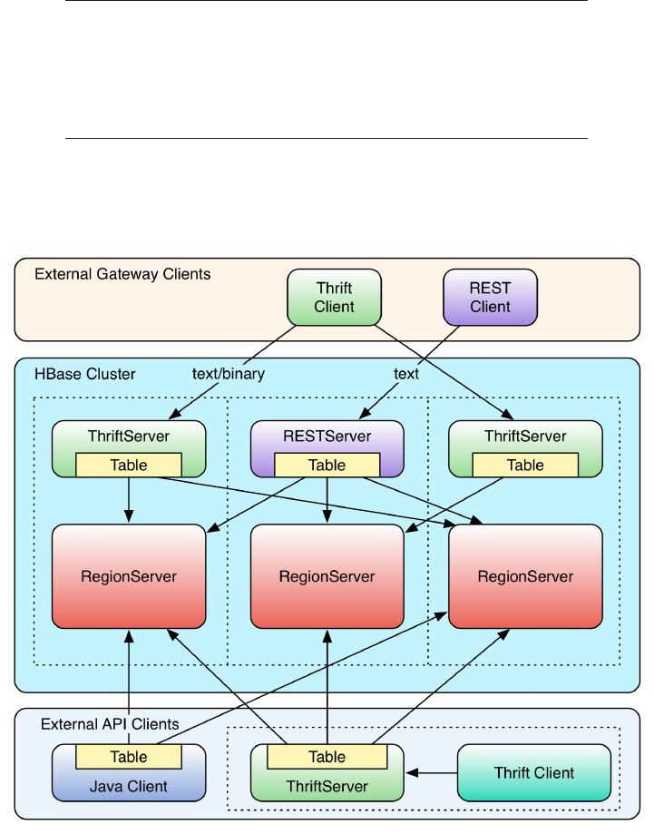
The supplied RESTServer actually supports Protocol Buf‐
fers. Instead of implementing a separate RPC server, it
leverages the Accept header of HTTP to send and receive
the data encoded in Protocol Buffers. See “REST” (page 433)
for details.
Figure 6-1 shows how dedicated gateway servers are used to provide
endpoints for various remote clients.
Figure 6-1. Clients connected through gateway servers
Internally, these servers use the common Table or BufferedMutator-
based client API to access the tables. You can see how they are start‐
ed on top of the region server processes, sharing the same physical
Introduction 429
www.finebook.ir

machine. There is no one true recommendation for how to place the
gateway servers. You may want to colocate them, or have them on
dedicated machines.
Another approach is to run them directly on the client nodes. For ex‐
ample, when you have web servers constructing the resultant HTML
pages using PHP, it is advantageous to run the gateway process on
the same server. That way, the communication between the client and
gateway is local, while the RPC between the gateway and HBase is us‐
ing the native protocol.
Check carefully how you access HBase from your client, to
place the gateway servers on the appropriate physical ma‐
chine. This is influenced by the load on each machine, as
well as the amount of data being transferred: make sure
you are not starving either process for resources, such as
CPU cycles, or network bandwidth.
The advantage of using a server as opposed to creating a new connec‐
tion for every request goes back to when we discussed “Resource
Sharing” (page 119)--you need to reuse connections to gain maximum
performance. Short-lived processes would spend more time setting up
the connection and preparing the metadata than in the actual opera‐
tion itself. The caching of region information in the server, in particu‐
lar, makes the reuse important; otherwise, every client would have to
perform a full row-to-region lookup for every bit of data they want to
access.
Selecting one server type over the others is a nontrivial task, as it de‐
pends on your use case. The initial argument over REST in compari‐
son to the more efficient Thrift, or similar serialization formats, shows
that for high-throughput scenarios it is advantageous to use a purely
binary format. However, if you have few requests, but they are large
in size, REST is interesting. A rough separation could look like this:
REST Use Case
Since REST supports existing web-based infrastructure, it will fit
nicely into setups with reverse proxies and other caching technolo‐
gies. Plan to run many REST servers in parallel, to distribute the
load across them. For example, run a server on every application
server you have, building a single-app-to-server relationship.
Thrift/Avro Use Case
Use the compact binary protocols when you need the best perfor‐
mance in terms of throughput. You can run fewer servers—for ex‐
Chapter 6: Available Clients430
www.finebook.ir
ample, one per region server—with a many-apps-to-server cardin‐
ality.
Frameworks
There is a long trend in software development to modularize and de‐
couple specific units of work. You might call this separation of respon‐
sibilities or other, similar names, yet the goal is the same: it is better
to build a commonly used piece of software only once, not having to
reinvent the wheel again and again. Many programming languages
have the concept of modules, in Java these are JAR files, providing
shared code to many consumers. One set of those libraries is for per‐
sistency, or data access in general. A popular choice is Hibernate, pro‐
viding a common interface for all object persistency.
There are also dedicated languages just for data manipulation, or such
that make this task as seamless as possible, so as not to distract form
the business logic. We will look into domain-specific languages (DSLs)
below, which cover these aspects. Another, newer trend is to also ab‐
stract away the application development, first manifested in platform-
as-a-service (PaaS). Here we are provided with everything that is
needed to write applications as quick as possible. There are applica‐
tion servers, accompanying libraries, databases, and so on.
With PaaS you still need to write the code and deploy it on they pro‐
vided infrastructure. The logical next step is to provide data access
APIs that an application can use with no further setup required. The
Google App Engine services is one of those, where you can talk to a
datastore API, that is provided as a library. It limits the freedom of an
application, but assuming the storage API is powerful enough, and im‐
posing no restrictions on the application developers creativity, it
makes deployment and management of applications much easier.
Hadoop is a very powerful and flexible system. In fact, any component
in Hadoop could be replaced, and you still have Hadoop, which is
more of an ideology than a collection of specific technologies. With
this flexibility and likely change comes the opposing wish of develop‐
ers to stay clear of any hard dependency. For that reason, it is appa‐
rent how a new kind of active framework is emerging. Similar to the
Google App Engine service, they provide a server component which
accepts applications being deployed into, and with abstracted inter‐
faces to underlying services, such as storage.
Interesting is that these kinds of frameworks, we will call them data
application servers, or data-as-a-service (DaaS), embrace the nature
of Hadoop, which is data first. Just like a smart phone, you install ap‐
plications that implement business use cases and run where the
Introduction 431
www.finebook.ir
shared data resides. There is no need to costly move large amounts of
data around to produce a result. With HBase as the storage engine,
you can expect these frameworks to make best use of many built-in
features, for example server-side coprocessors to push down selection
predicates and analytical functionality. One example here is Cask.
Common to libraries and frameworks is the notion of an abstraction
layer, be it a generic data API or DSL. This is also apparent with yet
another set of frameworks atop HBase, and other storage layers in
general, implementing SQL capabilities. We will discuss them in a
separate section below (see “SQL over NoSQL” (page 459)), so suffice it
to say that they provide a varying level of SQL conformity, allowing
access to data under the very popular idiom. Examples here are Impa‐
la, Hive, and Phoenix.
Finally, what is hard to determine is where some of these libraries and
frameworks really fit, as they can be employed on various backends,
some suitable for batch operations only, some for interactive use, and
yet other for both. The following will group them by that property,
though that means we may have to look at the same tool more than
ones. On the other hand, HBase is built for interactive access, but can
equally be used within long running batch processes, for example,
scanning analytical data for aggregation or model building. The
grouping therefore might be arbitrary, though helps with covering
both sides of the coin.
Gateway Clients
The first group of clients consists of the gateway kind, those that send
client API calls on demand, such as get, put, or delete, to servers.
Based on your choice of protocol, you can use the supplied gateway
servers to gain access from your applications. Alternatively, you can
employ the provided, storage specific API to implement generic, possi‐
bly hosted, data-centric solutions.
Native Java
The native Java API was discussed in Chapter 3 and Chapter 4. There
is no need to start any gateway server, as your client using Table or
BufferedMutator is directly communicating with the HBase servers,
via the native RPC calls. Refer to the aforementioned chapters to im‐
plement a native Java client.
Chapter 6: Available Clients432
www.finebook.ir
4. curl is a command-line tool for transferring data with URL syntax, supporting a
large variety of protocols. See the project’s website for details.
REST
HBase ships with a powerful REST server, which supports the com‐
plete client and administrative API. It also provides support for differ‐
ent message formats, offering many choices for a client application to
communicate with the server.
Operation
For REST-based clients to be able to connect to HBase, you need to
start the appropriate gateway server. This is done using the supplied
scripts. The following commands show you how to get the command-
line help, and then start the REST server in a non-daemonized mode:
$ bin/hbase rest
usage: bin/hbase rest start [--infoport <arg>] [-p <arg>] [-ro]
--infoport <arg> Port for web UI
-p,--port <arg> Port to bind to [default: 8080]
-ro,--readonly Respond only to GET HTTP method requests
[default:
false]
To run the REST server as a daemon, execute bin/hbase-daemon.sh
start|stop
rest [--infoport <port>] [-p <port>] [-ro]
$ bin/hbase rest start
^C
You need to press Ctrl-C to quit the process. The help stated that you
need to run the server using a different script to start it as a back‐
ground process:
$ bin/hbase-daemon.sh start rest
starting rest, logging to /var/lib/hbase/logs/hbase-larsgeorge-
rest-<servername>.out
Once the server is started you can use curl4 on the command line to
verify that it is operational:
$ curl http://<servername>:8080/
testtable
$ curl http://<servername>:8080/version
rest 0.0.3 [JVM: Oracle Corporation 1.7.0_51-24.51-b03] [OS: Mac
OS X \
10.10.2 x86_64] [Server: jetty/6.1.26] [Jersey: 1.9]
Gateway Clients 433
www.finebook.ir
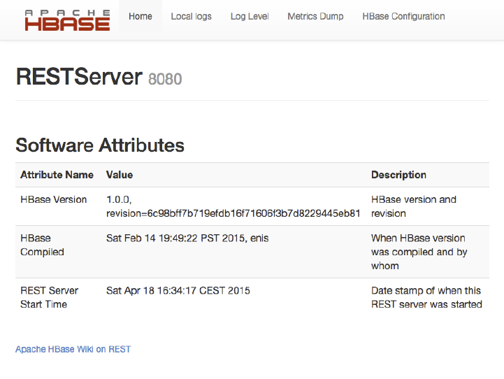
Retrieving the root URL, that is "/" (slash), returns the list of avail‐
able tables, here testtable. Using "/version" retrieves the REST
server version, along with details about the machine it is running on.
Alternatively, you can open the web-based UI provided by the REST
server. You can specify the port using the above mentioned --
infoport command line parameter, or by overriding the
hbase.rest.info.port configuration property. The default is set to
8085, and the content of the page is shown in Figure 6-2.
Figure 6-2. The web-based UI for the REST server
The UI has functionality that is common to many web-based UIs pro‐
vided by HBase. The middle part provides information about the serv‐
er and its status. For the REST server there is not much more but the
HBase version, compile information, and server start time. At the bot‐
tom of the page there is a link to the HBase Wiki page explaining the
REST API. At the top of the page there are links offering extra func‐
tionality:
Chapter 6: Available Clients434
www.finebook.ir

Home
Links to the Home page of the server.
Local logs
Opens a page that lists the local log directory, providing web-
based access to the otherwise inaccessible log files.
Log Level
This page allows to query and set the log levels for any class or
package loaded in the server process.
Metrics Dump
All servers in HBase track activity as metrics (see (to come)),
which can be accessed as JSON using this link.
HBase Configuration
Prints the current configuration as used by the server process.
See “Shared Pages” (page 551) for a deeper discussion on these shared
server UI links.
Stopping the REST server, when running as a daemon, involves the
same script, just replacing start with stop:
$ bin/hbase-daemon.sh stop rest
stopping rest..
The REST server gives you all the operations required to work with
HBase tables.
The current documentation for the REST server is avail‐
able online. Please refer to it for all the provided opera‐
tions. Also, be sure to carefully read the XML schemas
documentation on that page. It explains the schemas you
need to use when requesting information, as well as those
returned by the server.
You can start as many REST servers as you like, and, for example, use
a load balancer to route the traffic between them. Since they are
stateless—any state required is carried as part of the request—you
can use a round-robin (or similar) approach to distribute the load.
The --readonly, or -ro parameter switches the server into read-only
mode, which means it only responds to HTTP GET operations. Finally,
use the -p, or --port, parameter to specify a different port for the
server to listen on. The default is 8080. There are additional configura‐
Gateway Clients 435
www.finebook.ir

tion properties that the REST server is considering as it is started.
Table 6-1 lists them with default values.
Table 6-1. Configuration options for the REST server
Property Default Description
hbase.rest.dns.nameserver default Defines the DNS server used for
the name lookup.a
hbase.rest.dns.interface default Defines the network interface
that the name is associated
with.a
hbase.rest.port 8080 Sets the HTTP port the server
will bind to. Also settable per
instance with the -p and --port
command-line parameter.
hbase.rest.host 0.0.0.0 Defines the address the server
is listening on. Defaults to the
wildcard address.
hbase.rest.info.port 8085 Specifies the port the web-
based UI will bind to. Also
settable per instance using the
--infoport parameter.
hbase.rest.info.bindAddress 0.0.0.0 Sets the IP address the web-
based UI is bound to. Defaults
to the wildcard address.
hbase.rest.readonly false Forces the server into normal or
read-only mode. Also settable
by the --readonly, or -ro
options.
hbase.rest.threads.max 100 Provides the upper boundary of
the thread pool used by the
HTTP server for request
handlers.
hbase.rest.threads.min 2 Same as above, but sets the
lower boundary on number of
handler threads.
hbase.rest.connection.cleanup-
interval
10000 (10
secs) Defines how often the internal
housekeeping task checks for
expired connections to the
HBase cluster.
hbase.rest.connection.max-idletime 600000 (10
mins) Amount of time after which an
unused connection is
considered expired.
hbase.rest.support.proxyuser false Flags if the server should
support proxy users or not. This
Chapter 6: Available Clients436
www.finebook.ir

Property Default Description
is used to enable secure
impersonation.
a These two properties are used in tandem to look up the server’s hostname using the
given network interface and name server. The default value mean it uses whatever is
configured on the OS level.
The connection pool configured with the above cleanup task settings
is required since the server needs to keep a separate connection for
each authenticated user, when security is enabled. This also applies to
the proxy user settings, and both are explained in more detail in (to
come).
Supported Formats
Using the HTTP Content-Type and Accept headers, you can switch
between different formats being sent or returned to the caller. As an
example, you can create a table and row in HBase using the shell like
so:
hbase(main):001:0> create 'testtable', 'colfam1'
0 row(s) in 0.6690 seconds
=> Hbase::Table - testtable
hbase(main):002:0> put 'testtable', "\x01\x02\x03", 'col
fam1:col1', 'value1'
0 row(s) in 0.0230 seconds
hbase(main):003:0> scan 'testtable'
ROW COLUMN+CELL
\x01\x02\x03 column=colfam1:col1, timestamp=1429367023394, val‐
ue=value1
1 row(s) in 0.0210 seconds
This inserts a row with the binary row key 0x01 0x02 0x03 (in hexa‐
decimal numbers), with one column, in one column family, that con‐
tains the value value1.
Plain (text/plain)
For some operations it is permissible to have the data returned as
plain text. One example is the aforementioned /version operation:
$ curl -H "Accept: text/plain" http://<servername>:8080/version
rest 0.0.3 [JVM: Oracle Corporation 1.7.0_45-24.45-b08] [OS:
Mac OS X \
10.10.2 x86_64] [Server: jetty/6.1.26] [Jersey: 1.9]
On the other hand, using plain text with more complex return val‐
ues is not going to work as expected:
Gateway Clients 437
www.finebook.ir

5. The basic idea is to encode any unsafe or unprintable character code as “%” + AS‐
CII Code. Because it uses the percent sign as the prefix, it is also called percent en‐
coding. See the Wikipedia page on percent encoding for details.
$ curl -H "Accept: text/plain" \
http://<servername>:8080/testtable/%01%02%03/colfam1:col1
<html>
<head>
<meta http-equiv="Content-Type" content="text/html;
charset=ISO-8859-1"/>
<title>Error 406 Not Acceptable</title>
</head>
<body><h2>HTTP ERROR 406</h2>
<p>Problem accessing /testtable/%01%02%03/colfam1:col1. Reason:
<pre> Not Acceptable</pre></p>
<hr /><i><small>Powered by Jetty://</small></i><br/>
<br/>
...
<br/>
</body>
</html>
This is caused by the fact that the server cannot make any assump‐
tions regarding how to format a complex result value in plain text.
You need to use a format that allows you to express nested infor‐
mation natively.
The row key used in the example is a binary one, consist‐
ing of three bytes. You can use REST to access those bytes
by encoding the key using URL encoding,5 which in this
case results in %01%02%03. The entire URL to retrieve a
cell is then:
http://<servername>:8080/testtable/%01%02%03/
colfam1:col1
See the online documentation referred to earlier for the
entire syntax.
XML (text/xml)
When storing or retrieving data, XML is considered the default for‐
mat. For example, when retrieving the example row with no partic‐
ular Accept header, you receive:
$ curl http://<servername>:8080/testtable/%01%02%03/
colfam1:col1
Chapter 6: Available Clients438
www.finebook.ir
<?xml version="1.0" encoding="UTF-8" standalone="yes"?>
<CellSet>
<Row key="AQID">
<Cell column="Y29sZmFtMTpjb2wx" \
timestamp="1429367023394">dmFsdWUx</Cell>
</Row>
</CellSet>
The returned format defaults to XML. The column name and the
actual value are encoded in Base64, as explained in the online
schema documentation. Here is the respective part of the schema:
<element name="Row" type="tns:Row"></element>
<complexType name="Row">
<sequence>
<element name="key" type="base64Binary"></element>
<element name="cell" type="tns:Cell" maxOccurs="unbounded"
\
minOccurs="1"></element>
</sequence>
</complexType>
<element name="Cell" type="tns:Cell"></element>
<complexType name="Cell">
<sequence>
<element name="value" maxOccurs="1" minOccurs="1">
<simpleType><restriction base="base64Binary">
</simpleType>
</element>
</sequence>
<attribute name="column" type="base64Binary" />
<attribute name="timestamp" type="int" />
</complexType>
All occurrences of base64Binary are where the REST server re‐
turns the encoded data. This is done to safely transport the binary
data that can be contained in the keys, or the value. This is also
true for data that is sent to the REST server. Make sure to read
the schema documentation to encode the data appropriately, in‐
cluding the payload, in other words, the actual data, but also the
column name, row key, and so on.
A quick test on the console using the base64 command reveals the
proper content:
$ echo AQID | base64 -D | hexdump
0000000 01 02 03
$ echo Y29sZmFtMTpjb2wx | base64 -D
colfam1:col1
Gateway Clients 439
www.finebook.ir

$ echo dmFsdWUx | base64 -D
value1
This is obviously useful only to verify the details on the command
line. From within your code you can use any available Base64 im‐
plementation to decode the returned values.
JSON (application/json)
Similar to XML, requesting (or setting) the data in JSON simply re‐
quires setting the Accept header:
$ curl -H "Accept: application/json" \
http://<servername>:8080/testtable/%01%02%03/colfam1:col1
{
"Row": [{
"key": "AQID",
"Cell": [{
"column": "Y29sZmFtMTpjb2wx",
"timestamp": 1429367023394,
"$": "dmFsdWUx"
}]
}]
}
The preceding JSON result was reformatted to be easier to
read. Usually the result on the console is returned as a
single line, for example:
{"Row":[{"key":"AQID","Cell":[{"col‐
umn":"Y29sZmFtMTpjb2wx", \
"timestamp":1429367023394,"$":"dmFsdWUx"}]}]}
The encoding of the values is the same as for XML, that is, Base64
is used to encode any value that potentially contains binary data.
An important distinction to XML is that JSON does not have name‐
less data fields. In XML the cell data is returned between Cell
tags, but JSON must specify key/value pairs, so there is no immedi‐
ate counterpart available. For that reason, JSON has a special field
called "$" (the dollar sign). The value of the dollar field is the cell
data. In the preceding example, you can see it being used:
"$":"dmFsdWUx"
You need to query the dollar field to get the Base64-encoded data.
Chapter 6: Available Clients440
www.finebook.ir
Protocol Buffer (application/x-protobuf)
An interesting application of REST is to be able to switch encod‐
ings. Since Protocol Buffers have no native RPC stack, the HBase
REST server offers support for its encoding. The schemas are doc‐
umented online for your perusal.
Getting the results returned in Protocol Buffer encoding requires
the matching Accept header:
$ curl -H "Accept: application/x-protobuf" \
http://<servername>:8080/testtable/%01%02%03/colfam1:col1 |
hexdump -C
...
00000000 0a 24 0a 03 01 02 03 12 1d 12 0c 63 6f 6c 66 61 |.
$.........colfa|
00000010 6d 31 3a 63 6f 6c 31 18 a2 ce a7 e7 cc 29 22 06 |
m1:col1......)".|
00000020 76 61 6c 75 65 31 |
value1|
The use of hexdump allows you to print out the encoded message
in its binary format. You need a Protocol Buffer decoder to actually
access the data in a structured way. The ASCII printout on the
righthand side of the output shows the column name and cell value
for the example row.
Raw binary (application/octet-stream)
Finally, you can dump the data in its raw form, while omitting
structural data. In the following console command, only the data is
returned, as stored in the cell.
$ curl -H "Accept: application/octet-stream" \
http://<servername>:8080/testtable/%01%02%03/colfam1:col1 |
hexdump -C
00000000 76 61 6c 75 65 31 |
value1|
Gateway Clients 441
www.finebook.ir
Depending on the format request, the REST server puts
structural data into a custom header. For example, for the
raw get request in the preceding paragraph, the headers
look like this (adding -D- to the curl command):
HTTP/1.1 200 OK
Content-Length: 6
X-Timestamp: 1429367023394
Content-Type: application/octet-stream
The timestamp of the cell has been moved to the header as
X-Timestamp. Since the row and column keys are part of
the request URI, they are omitted from the response to
prevent unnecessary data from being transferred.
REST Java Client
The REST server also comes with a comprehensive Java client API. It
is located in the org.apache.hadoop.hbase.rest.client package.
The central classes are RemoteHTable and RemoteAdmin. Example 6-1
shows the use of the RemoteHTable class.
Example 6-1. Example of using the REST client classes
Cluster cluster = new Cluster();
cluster.add("localhost", 8080);
Client client = new Client(cluster);
RemoteHTable table = new RemoteHTable(client, "testtable");
Get get = new Get(Bytes.toBytes("row-30"));
get.addColumn(Bytes.toBytes("colfam1"), Bytes.toBytes("col-3"));
Result result1 = table.get(get);
System.out.println("Get result1: " + result1);
Scan scan = new Scan();
scan.setStartRow(Bytes.toBytes("row-10"));
scan.setStopRow(Bytes.toBytes("row-15"));
scan.addColumn(Bytes.toBytes("colfam1"), Bytes.toBytes("col-5"));
ResultScanner scanner = table.getScanner(scan);
for (Result result2 : scanner) {
System.out.println("Scan row[" + Bytes.toString(result2.ge‐
tRow()) +
"]: " + result2);
}
Set up a cluster list adding all known REST server hosts.
Chapter 6: Available Clients442
www.finebook.ir

Create the client handling the HTTP communication.
Create a remote table instance, wrapping the REST access into a
familiar interface.
Perform a get operation as if it were a direct HBase connection.
Scan the table, again, the same approach as if using the native
Java API.
Running the example requires that the REST server has been started
and is listening on the specified port. If you are running the server on
a different machine and/or port, you need to first adjust the value add‐
ed to the Cluster instance.
Here is what is printed on the console when running the example:
Adding rows to table...
Get result1:
keyvalues={row-30/colfam1:col-3/1429376615162/Put/vlen=8/seqid=0}
Scan row[row-10]:
keyvalues={row-10/colfam1:col-5/1429376614839/Put/vlen=8/seqid=0}
Scan row[row-100]:
keyvalues={row-100/colfam1:col-5/1429376616162/Put/vlen=9/
seqid=0}
Scan row[row-11]:
keyvalues={row-11/colfam1:col-5/1429376614856/Put/vlen=8/seqid=0}
Scan row[row-12]:
keyvalues={row-12/colfam1:col-5/1429376614873/Put/vlen=8/seqid=0}
Scan row[row-13]:
keyvalues={row-13/colfam1:col-5/1429376614891/Put/vlen=8/seqid=0}
Scan row[row-14]:
keyvalues={row-14/colfam1:col-5/1429376614907/Put/vlen=8/seqid=0}
Due to the lexicographical sorting of row keys, you will receive the
preceding rows. The selected columns have been included as expect‐
ed.
The RemoteHTable is a convenient way to talk to a number of REST
servers, while being able to use the normal Java client API classes,
such as Get or Scan.
The current implementation of the Java REST client is us‐
ing the Protocol Buffer encoding internally to communi‐
cate with the remote REST server. It is the most compact
protocol the server supports, and therefore provides the
best bandwidth efficiency.
Gateway Clients 443
www.finebook.ir

Thrift
Apache Thrift is written in C++, but provides schema compilers for
many programming languages, including Java, C++, Perl, PHP,
Python, Ruby, and more. Once you have compiled a schema, you can
exchange messages transparently between systems implemented in
one or more of those languages.
Installation
Before you can use Thrift, you need to install it, which is preferably
done using a binary distribution package for your operating system. If
that is not an option, you need to compile it from its sources.
HBase ships with pre-built Thrift code for Java and all the
included demos, which means that there should be no
need to install Thrift. You still will need the Thrift source
package, because it contains necessary code that the gen‐
erated classes rely on. You will see in the example below
(see “Example: PHP” (page 452)) how for some languages
that is required, while for others it may now.
Download the source tarball from the website, and unpack it into a
common location:
$ wget http://www.apache.org/dist/thrift/0.9.2/thrift-0.9.2.tar.gz
$ tar -xzvf thrift-0.9.2.tar.gz -C /opt
$ rm thrift-0.9.2.tar.gz
Install the dependencies, which are Automake, LibTool, Flex, Bison,
and the Boost libraries:
$ sudo apt-get install build-essential automake libtool flex bison
libboost
Now you can build and install the Thrift binaries like so:
$ cd /opt/thrift-0.9.2
$ ./configure
$ make
$ sudo make install
Alternative, on OS X you could, for example, use the Homebrew pack‐
age manager for installing the same like so:
$ brew install thrift
==> Installing dependencies for thrift: boost, openssl
...
Chapter 6: Available Clients444
www.finebook.ir

==> Summary
/usr/local/Cellar/thrift/0.9.2: 90 files, 5.4M
When installed, you can verify that everything succeeded by calling
the main thrift executable:
$ thrift -version
Thrift version 0.9.2
Once you have Thrift installed, you need to compile a schema into the
programming language of your choice. HBase comes with a schema
file for its client and administrative API. You need to use the Thrift bi‐
nary to create the wrappers for your development environment.
The supplied schema file exposes the majority of the API
functionality, but is lacking in a few areas. It was created
when HBase had a different API and that is noticeable
when using it. Newer features might be not supported yet,
for example the newer durability settings. See “Thrift2”
(page 458) for a replacement service, implementing the cur‐
rent HBase API verbatim.
Before you can access HBase using Thrift, though, you also have to
start the supplied ThriftServer.
Thrift Operations
Starting the Thrift server is accomplished by using the supplied
scripts. You can get the command-line help by adding the -h switch,
or omitting all options:
$ bin/hbase thrift
usage: Thrift [-b <arg>] [-c] [-f] [-h] [-hsha | -nonblocking |
-threadedselector | -threadpool] [--infoport <arg>] [-k
<arg>] [-m
<arg>] [-p <arg>] [-q <arg>] [-w <arg>]
-b,--bind <arg> Address to bind the Thrift server to.
[default:
0.0.0.0]
-c,--compact Use the compact protocol
-f,--framed Use framed transport
-h,--help Print help information
-hsha Use the THsHaServer This implies the
framed
transport.
--infoport <arg> Port for web UI
-k,--keepAliveSec <arg> The amount of time in secods to keep a
thread
alive when idle in TBoundedThreadPool‐
Gateway Clients 445
www.finebook.ir
Server
-m,--minWorkers <arg> The minimum number of worker threads for
TBoundedThreadPoolServer
-nonblocking Use the TNonblockingServer This implies
the
framed transport.
-p,--port <arg> Port to bind to [default: 9090]
-q,--queue <arg> The maximum number of queued requests in
TBoundedThreadPoolServer
-threadedselector Use the TThreadedSelectorServer This im‐
plies
the framed transport.
-threadpool Use the TBoundedThreadPoolServerThis is
the
default.
-w,--workers <arg> The maximum number of worker threads for
TBoundedThreadPoolServer
To start the Thrift server run 'bin/hbase-daemon.sh start thrift'
To shutdown the thrift server run 'bin/hbase-daemon.sh stop
thrift' or
send a kill signal to the thrift server pid
There are many options to choose from. The type of server, protocol,
and transport used is usually enforced by the client, since not all lan‐
guage implementations have support for them. From the command-
line help you can see that, for example, using the nonblocking server
implies the framed transport.
Using the defaults, you can start the Thrift server in non-daemonized
mode:
$ bin/hbase thrift start
^C
You need to press Ctrl-C to quit the process. The help stated that you
need to run the server using a different script to start it as a back‐
ground process:
$ bin/hbase-daemon.sh start thrift
starting thrift, logging to /var/lib/hbase/logs/ \
hbase-larsgeorge-thrift-<servername>.out
Stopping the Thrift server, running as a daemon, involves the same
script, just replacing start with stop:
$ bin/hbase-daemon.sh stop thrift
stopping thrift..
Once started either way, you can open the web-based UI provided by
the Thrift server. You can specify the port using the above listed --
infoport command line parameter, or by overriding the
hbase.thrift.info.port configuration property. The default is set to
9095, and the content of the page is shown in Figure 6-3.
Chapter 6: Available Clients446
www.finebook.ir
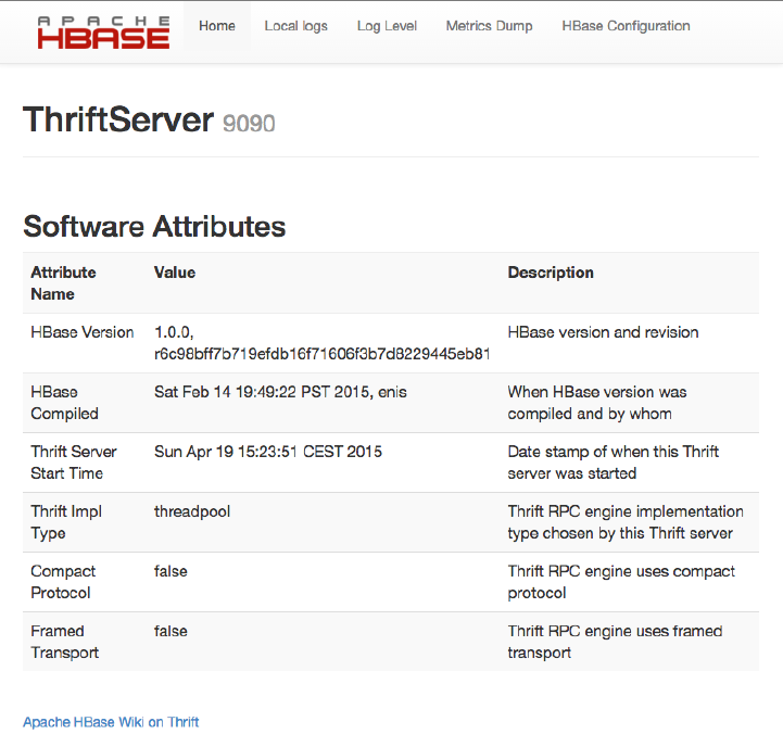
Figure 6-3. The web-based UI for the Thrift server
The UI has functionality that is common to many web-based UIs pro‐
vided by HBase. The middle part provides information about the serv‐
er and its status. For the Thrift server there is not much more but the
HBase version, compile information, server start time, and Thrift spe‐
cific details, such as the server type, protocol and transport options
configured. At the bottom of the page there is a link to the HBase Wiki
page explaining the Thrift API. At the top of the page there are links
offering extra functionality:
Home
Links to the Home page of the server.
Gateway Clients 447
www.finebook.ir

Local logs
Opens a page that lists the local log directory, providing web-
based access to the otherwise inaccessible log files.
Log Level
This page allows to query and set the log levels for any class or
package loaded in the server process.
Metrics Dump
All servers in HBase track activity as metrics (see (to come)),
which can be accessed as JSON using this link.
HBase Configuration
Prints the current configuration as used by the server process.
See “Shared Pages” (page 551) for a deeper discussion on these shared
server UI links.
The current documentation for the Thrift server is avail‐
able online (also see the package info). You should refer to
it for all the provided operations. It is also advisable to
read the provided $HBASE_HOME/hbase-thrift/src/main/
resources/org/apache/hadoop/hbase/thrift/
Hbase.thrift schema definition file for the authoritative
documentation of the available functionality.
The Thrift server provides you with all the operations required to
work with HBase tables. You can start as many Thrift servers as you
like, and, for example, use a load balancer to route the traffic between
them. Since they are stateless, you can use a round-robin (or similar)
approach to distribute the load. Use the -p, or --port, parameter to
specify a different port for the server to listen on. The default is 9090.
There are additional configuration properties that the Thrift server is
considering as it is started. Table 6-2 lists them with default values.
Table 6-2. Configuration options for the Thrift server
Property Default Description
hbase.thrift.dns.nameserver default Defines the DNS server
used for the name
lookup.a
hbase.thrift.dns.interface default Defines the network
interface that the name
is associated with.a
Chapter 6: Available Clients448
www.finebook.ir

Property Default Description
hbase.regionserver.thrift.port 9090 Sets the port the server
will bind to. Also
settable per instance
with the -p or --port
command-line
parameter.
hbase.regionserver.thrift.ipaddress 0.0.0.0 Defines the address the
server is listening on.
Defaults to the wildcard
address. Set with -b, --
bind per instance on the
command-line.
hbase.thrift.info.port 9095 Specifies the port the
web-based UI will bind
to. Also settable per
instance using the --
infoport parameter.
hbase.thrift.info.bindAddress 0.0.0.0 Sets the IP address the
web-based UI is bound
to. Defaults to the
wildcard address.
hbase.regionserver.thrift.server.type threadpool Sets the Thrift server
type in non-HTTP mode.
See below for details.
hbase.regionserver.thrift.compact false Enables the compact
protocol mode if set to
true. Default means
binary mode instead.
Also settable per
instance with -c, or --
compact.
hbase.regionserver.thrift.framed false Sets the transport mode
to framed. Otherwise
the standard transport is
used. Framed cannot be
used in secure mode.
When using the hsha or
nonblocking server type,
framed transport is
always used irrespective
of this configuration
property. Also settable
per instance with -f, or
--framed.
Gateway Clients 449
www.finebook.ir

Property Default Description
hbase.regionserv
er.thrift.framed.max_frame_size_in_mb
2097152 (2MB) The maximum frame
size when framed
transport mode is
enabled.
hbase.thrift.minWorkerThreads 16 Sets the minimum
amount of worker
threads to keep, should
be increased for
production use (for
example, to 200).
Settable on the
command-line with -m,
or --minWorkers.
hbase.thrift.maxWorkerThreads 1000 Sets the upper limit of
worker threads. Settable
on the command-line
with -w, or --workers.
hbase.thrift.maxQueuedRequests 1000 Maximum number of
request to queue when
workers are all busy.
Can be set with -q, and
--queue per instance.
hbase.thrift.threadKeepAliveTimeSec 60 (secs) Amount of time an
extraneous idle worker
is kept before it is
discarded. Also settable
with -k, or --
keepAliveSec.
hbase.regionserver.thrift.http false Flag that determines if
the server should run in
HTTP or native mode.
hbase.thrift.http_threads.max 100 Provides the upper
boundary of the thread
pool used by the HTTP
server for request
handlers.
hbase.thrift.http_threads.min 2 Same as above, but sets
the lower boundary on
number of handler
threads.
hbase.thrift.ssl.enabled false When HTTP mode is
enabled, this flag sets
the SSL mode.
hbase.thrift.ssl.keystore.store "" When SSL is enabled,
sets the key store file.
Chapter 6: Available Clients450
www.finebook.ir

Property Default Description
hbase.thrift.ssl.keystore.password null When SSL is enabled,
sets the password to
unlock the key store file.
hbase.thrift.ssl.keystore.keypassword null When SSL is enabled,
sets the password to
retrieve the keys from
the key store.
hbase.thrift.security.qop "" Can be one of auth,
auth-int, or auth-conf
to set the SASL quality-
of-protection (QoP). See
(to come) for details.
hbase.thrift.support.proxyuser false Flags if the server
should support proxy
users or not. This is
used to enable secure
impersonation.
hbase.thrift.kerberos.principal <hostname> Can be used to set the
Kerberos principal to
use in secure mode.
hbase.thrift.keytab.file "" Specifies the Kerberos
keytab file for secure
operation.
hbase.regionserver.thrift.coalesceIncre
ment
false Enables the coalesce
mode for increments,
which is a delayed,
batch increment
operation.
hbase.thrift.filters "" Loads filter classes into
the server process for
subsequent use.
hbase.thrift.connection.cleanup-
interval
10000 (10
secs) Defines how often the
internal housekeeping
task checks for expired
connections to the
HBase cluster.
hbase.thrift.connection.max-idletime 600000 (10
mins) Amount of time after
which an unused
connection is considered
expired.
a These two properties are used in tandem to look up the server’s hostname using the
given network interface and name server. The default value mean it uses whatever is
configured on the OS level.
Gateway Clients 451
www.finebook.ir
6. See this blog post for a comparison.
There a few choices for the server type in Thrift native mode (that is,
non-HTTP), which are:
nonblocking
Uses the TNonblockingServer class, which is based on Java NIO’s
non-blocking I/O, where the selector thread also process the actual
request. Settable per server instance with the -nonblocking pa‐
rameter.
hsha
Uses the THsHaServer class, implementing a Half-Sync/Half-Async
(HsHa) server. The difference to the non-blocking server is that it
has a single thread accepting connections, but a thread pool for
the processing workers. Settable per server instance with the -
hsha parameter.
threadedselector
Extends on the HsHa server by maintaining two thread pools, one
for network I/O (selection), and another for processing (workers).
Uses the TThreadedSelectorServer class. Settable per server in‐
stance with the -threadedselector parameter.
threadpool
Has a single thread to accept connections, which are then sched‐
uled to be worked on in an ExecutorService. Each connection is
dedicated to one client, therefore potentially many threads are
needed in highly concurrent setups. Uses the TBoundedThreadPool
Server class, which is a customized implementation of the Thrift
TThreadPoolServer class. Also settable per server instance with
the -threadpool parameter.
The default of type threadpool is a good choice for production use, as
it combines many proven techniques.6
Example: PHP
HBase not only ships with the required Thrift schema file, but also
with an example client for many programming languages. Here we
will enable the PHP implementation to demonstrate the required
steps.
Before we start though, a few notes:
•You need to enable PHP support for your web server! Follow your
server documentation to do so. On OS X, for example, you need to
Chapter 6: Available Clients452
www.finebook.ir
edit the /etc/apache2/httpd.conf and uncomment the following
line, and (re)start the server with $ sudo apachectl restart:
LoadModule php5_module libexec/apache2/libphp5.so
•HBase ships with a precompiled PHP Thrift module, so you are
free to skip the part below (that is, step #1) where we generate
the module anew. Either way should get you to the same result.
The code shipped with HBase is in the `hbase-examples
•The included DemoClient.php is not up-to-date, for example, it
tests with an empty row key, which is not allowed, and using a
non-UTF8 row key, which is allowed. Both checks fail, and you
need to fix the PHP file taking care of the changes.
• Apache Thrift has changed the layout of the PHP scaffolding files it
ships with. In earlier releases it only had a
$THRIFT_SRC_HOME/lib/php/src directory, while newer versions
have a ../src and ../lib folder.
Step 1
Optionally: The first step is to copy the supplied schema file and com‐
pile the necessary PHP source files for it:
$ cp -r $HBASE_HOME/hbase-thrift/src/main/resources/org/apache/ \
hadoop/hbase/thrift ~/thrift_src
$ cd thrift_src/
$ thrift -gen php Hbase.thrift
The call to thrift should complete with no error or other output on
the command line. Inside the thrift_src directory you will now find a
directory named gen-php containing the two generated PHP files re‐
quired to access HBase:
$ ls -l gen-php/Hbase/
total 920
-rw-r--r-- 1 larsgeorge staff 416357 Apr 20 07:46 Hbase.php
-rw-r--r-- 1 larsgeorge staff 52366 Apr 20 07:46 Types.php
If you decide to skip this step, you can copy the supplied, pre-
generated PHP files from the hbase-examples module in the HBase
source tree:
$ ls -lR $HBASE_HOME/hbase-examples/src/main/php
total 24
-rw-r--r-- 1 larsgeorge admin 8438 Jan 25 10:47 DemoClient.php
drwxr-xr-x 3 larsgeorge admin 102 May 22 2014 gen-php
/usr/local/hbase-1.0.0-src/hbase-examples/src/main/php/gen-php:
total 0
drwxr-xr-x 4 larsgeorge admin 136 Jan 25 10:47 Hbase
Gateway Clients 453
www.finebook.ir

/usr/local/hbase-1.0.0-src/hbase-examples/src/main/php/gen-php/
Hbase:
total 800
-rw-r--r-- 1 larsgeorge admin 366528 Jan 25 10:47 Hbase.php
-rw-r--r-- 1 larsgeorge admin 38477 Jan 25 10:47 Types.php
Step 2
The generated files require the Thrift-supplied PHP harness to be
available as well. They need to be copied into your web server’s docu‐
ment root directory, along with the generated files:
$ cd /opt/thrift-0.9.2
$ sudo mkdir $DOCUMENT_ROOT/thrift/
$ sudo cp src/*.php $DOCUMENT_ROOT/thrift/
$ sudo cp -r lib/Thrift/* $DOCUMENT_ROOT/thrift/
$ sudo mkdir $DOCUMENT_ROOT/thrift/packages
$ sudo cp -r ~/thrift_src/gen-php/Hbase $DOCUMENT_ROOT/thrift/pack
ages/
The generated PHP files are copied into a packages subdirectory, as
per the Thrift documentation, which needs to be created if it does not
exist yet.
The $DOCUMENT_ROOT in the preceding commands could
be /var/www, for example, on a Linux system using
Apache, or /Library/WebServer/Documents/ on an Apple
Mac OS X machine. Check your web server configuration
for the appropriate location.
HBase ships with a DemoClient.php file that uses the generated files
to communicate with the servers. This file is copied into the same
document root directory of the web server:
$ sudo cp $HBASE_HOME/hbase-examples/src/main/php/DemoClient.php
$DOCUMENT_ROOT/
You need to edit the DemoClient.php file and adjust the following
fields at the beginning of the file:
# Change this to match your thrift root
$GLOBALS['THRIFT_ROOT'] = 'thrift';
...
# According to the thrift documentation, compiled PHP thrift libra‐
ries should
# reside under the THRIFT_ROOT/packages directory. If these com‐
piled libraries
# are not present in this directory, move them there from gen-php/.
require_once( $GLOBALS['THRIFT_ROOT'].'/packages/Hbase/
Hbase.php' );
Chapter 6: Available Clients454
www.finebook.ir
7. As of this writing, the supplied DemoClient.php is slightly outdated, running into a
script error during evaluation. This results in not all of the included tests being exe‐
cuted. This is tracked in HBASE-13522.
...
$socket = new TSocket( 'localhost', 9090 );
...
Usually, editing the first line is enough to set the THRIFT_ROOT path.
Since the DemoClient.php file is also located in the document root di‐
rectory, it is sufficient to set the variable to thrift, that is, the direc‐
tory copied from the Thrift sources earlier.
The last line in the preceding excerpt has a hardcoded server name
and port. If you set up the example in a distributed environment, you
need to adjust this line to match your environment as well. After ev‐
erything has been put into place and adjusted appropriately, you can
open a browser and point it to the demo page. For example:
http://<webserver-address>/DemoClient.php
This should load the page and output the following details (abbrevi‐
ated here for the sake of brevity):7
scanning tables...
found: testtable
creating table: demo_table
column families in demo_table:
column: entry:, maxVer: 10
column: unused:, maxVer: 3
Starting scanner...
...
The same Demo Client client is also available in C++, Java, Perl,
Python, and Ruby. Follow the same steps to start the Thrift server,
compile the schema definition into the necessary language, and start
the client. Depending on the language, you will need to put the gener‐
ated code into the appropriate location first.
Example: Java
HBase already ships with the generated Java classes to communicate
with the Thrift server, though you can always regenerate them again
from the schema file. The book’s online code repository provides a
script to generate them directly within the example directory for this
chapter. It is located in the bin directory of the repository root path,
and is named dothrift.sh. It requires you to hand in the HBase
Thrift definition file, since that can be anywhere:
$ bin/dothrift.sh
Missing thrift file parameter!
Gateway Clients 455
www.finebook.ir

Usage: bin/dothrift.sh <thrift-file>
$ bin/dothrift.sh $HBASE_HOME/hbase-thrift/src/main/resources/org/
\
apache/hadoop/hbase/thrift/Hbase.thrift
compiling thrift: /usr/local/hbase-1.0.0-src/hbase-thrift/src/
main/ \
resources/org/apache/hadoop/hbase/thrift/Hbase.thrift
done.
After running the script, the generated classes can be found in the
ch06/src/main/java/org/apache/hadoop/hbase/thrift/ directory.
Example 6-2 uses these classes to communicate with the Thrift server.
Make sure the gateway server is up and running and listening on port
9090.
Example 6-2. Example using the Thrift generated client API
private static final byte[] TABLE = Bytes.toBytes("testtable");
private static final byte[] ROW = Bytes.toBytes("testRow");
private static final byte[] FAMILY1 = Bytes.toBytes("testFamily1");
private static final byte[] FAMILY2 = Bytes.toBytes("testFamily2");
private static final byte[] QUALIFIER = Bytes.toBytes
("testQualifier");
private static final byte[] COLUMN = Bytes.toBytes(
"testFamily1:testColumn");
private static final byte[] COLUMN2 = Bytes.toBytes(
"testFamily2:testColumn2");
private static final byte[] VALUE = Bytes.toBytes("testValue");
public static void main(String[] args) throws Exception {
TTransport transport = new TSocket("0.0.0.0", 9090, 20000);
TProtocol protocol = new TBinaryProtocol(transport, true, true);
Hbase.Client client = new Hbase.Client(protocol);
transport.open();
ArrayList<ColumnDescriptor> columns = new
ArrayList<ColumnDescriptor>();
ColumnDescriptor cd = new ColumnDescriptor();
cd.name = ByteBuffer.wrap(FAMILY1);
columns.add(cd);
cd = new ColumnDescriptor();
cd.name = ByteBuffer.wrap(FAMILY2);
columns.add(cd);
client.createTable(ByteBuffer.wrap(TABLE), columns);
ArrayList<Mutation> mutations = new ArrayList<Mutation>();
mutations.add(new Mutation(false, ByteBuffer.wrap(COLUMN),
ByteBuffer.wrap(VALUE), true));
mutations.add(new Mutation(false, ByteBuffer.wrap(COLUMN2),
Chapter 6: Available Clients456
www.finebook.ir
ByteBuffer.wrap(VALUE), true));
client.mutateRow(ByteBuffer.wrap(TABLE), ByteBuffer.wrap(ROW),
mutations, null);
TScan scan = new TScan();
int scannerId = client.scannerOpenWithScan(ByteBuff‐
er.wrap(TABLE),
scan, null);
for (TRowResult result : client.scannerGet(scannerId)) {
System.out.println("No. columns: " + result.getColumnsSize());
for (Map.Entry<ByteBuffer, TCell> column :
result.getColumns().entrySet()) {
System.out.println("Column name: " + Bytes.toString(
column.getKey().array()));
System.out.println("Column value: " + Bytes.toString(
column.getValue().getValue()));
}
}
client.scannerClose(scannerId);
ArrayList<ByteBuffer> columnNames = new ArrayList<ByteBuffer>();
columnNames.add(ByteBuffer.wrap(FAMILY1));
scannerId = client.scannerOpen(ByteBuffer.wrap(TABLE),
ByteBuffer.wrap(Bytes.toBytes("")), columnNames, null);
for (TRowResult result : client.scannerGet(scannerId)) {
System.out.println("No. columns: " + result.getColumnsSize());
for (Map.Entry<ByteBuffer, TCell> column :
result.getColumns().entrySet()) {
System.out.println("Column name: " + Bytes.toString(
column.getKey().array()));
System.out.println("Column value: " + Bytes.toString(
column.getValue().getValue()));
}
}
client.scannerClose(scannerId);
System.out.println("Done.");
transport.close();
}
Create a connection using the Thrift boilerplate classes.
Create two column descriptor instances.
Create the test table.
Insert a test row.
Scan with an instance of TScan. This is the most convenient
approach. Print the results in a loop.
Scan again, but with another Thrift method. In addition, set the
columns to a specific family only. Also print out the results in a
loop.
Gateway Clients 457
www.finebook.ir

Close the connection after everything is done.
The console output is:
No. columns: 2
Column name: testFamily1:testColumn
Column value: testValue
Column name: testFamily2:testColumn2
Column value: testValue
No. columns: 1
Column name: testFamily1:testColumn
Column value: testValue
Done.
Please consult the supplied classes, examples, and online documenta‐
tion for more details.
Thrift2
Since the client API of HBase was changed significantly in version
0.90, it is apparent in many places how the Thrift API is out of sync.
An effort was started to change this by implementing a new version of
the Thrift gateway server, named Thrift2. It mirrors the current client
API calls and therefore feels more natural to the HBase developers fa‐
miliar with the native, Java based API. On the other hand, unfortu‐
nately, it is still work in progress and is lacking various features.
Overall the Thrift2 server is used the same way as the original Thrift
server is, which means we can skip the majority of the explanation.
Read about the operations of the server in “Thrift Operations” (page
445). You can see all command line options running the thrift2 op‐
tion like so:
$ bin/hbase thrift2
usage: Thrift [-b <arg>] [-c] [-f] [-h] [-hsha | -nonblocking |
-threadpool] [--infoport <arg>] [-p <arg>]
-b,--bind <arg> Address to bind the Thrift server to. [de‐
fault:
0.0.0.0]
-c,--compact Use the compact protocol
-f,--framed Use framed transport
-h,--help Print help information
-hsha Use the THsHaServer. This implies the framed
transport.
--infoport <arg> Port for web UI
-nonblocking Use the TNonblockingServer. This implies
the framed
transport.
-p,--port <arg> Port to bind to [default: 9090]
-threadpool Use the TThreadPoolServer. This is the de‐
Chapter 6: Available Clients458
www.finebook.ir
fault.
To start the Thrift server run 'bin/hbase-daemon.sh start thrift2'
To shutdown the thrift server run 'bin/hbase-daemon.sh stop
thrift2' or
send a kill signal to the thrift server pid
Using the defaults, you can start the Thrift server in non-daemonized
mode:
$ bin/hbase thrift2 start
^C
You need to press Ctrl-C to quit the process. The help stated that you
need to run the server using a different script to start it as a back‐
ground process:
$ bin/hbase-daemon.sh start thrift2
starting thrift2, logging to /var/lib/hbase/logs/ \
hbase-larsgeorge-thrift2-<servername>.out
Stopping the Thrift server, running as a daemon, involves the same
script, just replacing start with stop:
$ bin/hbase-daemon.sh stop thrift2
stopping thrift2.
Once started either way, you can open the web-based UI provided by
the Thrift server, the same way as explained for the original Thrift
server earlier. Obviously, the main difference between Thrift2 and its
predecessor is the changes in API calls. Consult the Thrift service defi‐
nition file, that is, $HBASE_HOME/hbase-thrift/src/main/
resources/org/apache/hadoop/hbase/thrift/Hbase.thrift, for the
details on the provided services and data structures.
SQL over NoSQL
An interesting spin on NoSQL is the recent rise of SQL frameworks
that make HBase look like any other RDBMS: you have transactions,
indexes, referential integrity, and other well-known features—all atop
an inherently non-SQL system. These frameworks have varying levels
of integration, adding several service around HBase itself to re-add all
(or some) of the database relevant features. Some notable projects
are:
Phoenix
The most native integration into HBase is provided by the Apache
Phoenix project. It is available as open-source and under the
Apache ASF license. The framework uses many advanced features
to optimize generic SQL queries executed against HBase tables,
including coprocessors for secondary indexes, and filtering.
Gateway Clients 459
www.finebook.ir
Trafodion
Developed as open-source software by HP, Trafodion is a system
that combines existing database technology with HBase as the
storage layer.
Impala
Another open-source, and Apache licensed, project is Impala. Pri‐
mary built to perform interactive queries against data stored in
HDFS, it has the ability to directly access HBase tables too. Impala
shared
Hive with Tez/Spark
We will discuss Hive in detail in “Hive” (page 460), because original‐
ly it used the Hadoop batch framework to execute the data pro‐
cessing. With the option to replace MapReduce with other engines,
such as the more recent Tez or Spark, you can also run HiveQL
based queries interactively over HBase tables.
Framework Clients
After the more direct gateway clients, we are now going to talk about
the second class of clients, referred to collectively as frameworks.
They are offering a higher level of abstraction, usually in the form of a
domain specific language (DSL). This includes, for example, SQL, the
lingua franca of relational database system with external clients, and
also MapReduce, the original processing framework (and SDK) to
write and execute longer running batch jobs.
MapReduce
The Hadoop MapReduce framework is built to process petabytes of
data, in a reliable, deterministic, yet easy-to-program way. There are a
variety of ways to include HBase as a source and target for MapRe‐
duce jobs.
Native Java
The Java-based MapReduce API for HBase is discussed in Chapter 7.
Hive
The Apache Hive project offers a data warehouse infrastructure atop
Hadoop. It was initially developed at Facebook, but is now part of the
open source Hadoop ecosystem. Hive can be used to run structured
queries against HBase tables, which we will discuss now.
Chapter 6: Available Clients460
www.finebook.ir

8. See the Hive wiki for more details on storage handlers.
9. The Hive wiki has a full explanation of the HBase integration into Hive.
Introduction
Hive offers an SQL-like query language, called HiveQL, which allows
you to query the semistructured data stored in Hadoop. The query is
eventually turned into a processing job, traditionally MapReduce,
which is executed either locally or on a distributed cluster. The data is
parsed at job execution time and Hive employs a storage handler8 ab‐
straction layer that allows for data not to just reside in HDFS, but oth‐
er data sources as well. A storage handler transparently makes arbi‐
trarily stored information available to the HiveQL-based user queries.
Since version 0.6.0, Hive also comes with a handler for HBase.9 You
can define Hive tables that are backed by HBase tables or snapshots,
mapping columns between them and the query schema as required.
The row key can be exposed as one or more extra column when need‐
ed, supporting composite keys.
HBase Version Support
As of this writing, the latest release of Hive, version 1.2.1, in‐
cludes support for HBase 0.98.x. There is a problem using this
version with HBase 1.x, because a class signature has changed,
causing the HBase handler JAR shipped with Hive to throw a run‐
time exception when confronted with the HBase 1.x libraries:
15/07/03 04:38:09 [main]: ERROR exec.DDLTask: java.lang.NoSuch‐
MethodError: org.apache.hadoop.hbase.HTableDescriptor.addFami‐
ly(\
Lorg/apache/hadoop/hbase/HColumnDescriptor;)V
at org.apache.hadoop.hive.hbase.HBaseStorageHandler.pre‐
CreateTable(...)
at org.apache.hadoop.hive.metastore.HiveMetaStore‐
Client.createTable(...)
at org.apache.hadoop.hive.metastore.HiveMetaStore‐
Client.createTable(...)
The inly way currently to resolve this problem is to build Hive
from source, and update the HBase dependencies to 1.x in the
process. The steps are:
1. Clone the source repository of Hive
2. Edit the pom.xml, adjusting the used HBase version
3. Build Hive with final packaging option for Hadoop 2
Framework Clients 461
www.finebook.ir

4. Install this custom version of Hive
In more concrete steps, here are the shell commands:
$ git clone https://github.com/apache/hive.git
$ cd hive/
$ vi pom.xml
...
<hbase.hadoop1.version>0.98.9-hadoop1</hbase.hadoop1.version>
<hbase.hadoop2.version>1.1.0</hbase.hadoop2.version>
<!--hbase.hadoop2.version>0.98.9-hadoop2</
hbase.hadoop2.version-->
...
$ mvn clean install -Phadoop-2,dist -DskipTests
...
[INFO]
---------------------------------------------------------------------
[INFO] Building Hive HBase Handler 2.0.0-SNAPSHOT
[INFO]
---------------------------------------------------------------------
...
[INFO] --- maven-install-plugin:2.4:install (default-install)
@ \
hive-hbase-handler ---
[INFO] Installing /home/larsgeorge/hive/hbase-handler/target/ \
hive-hbase-handler-2.0.0-SNAPSHOT.jar to /home/lars‐
george/.m2/ \
repository/org/apache/hive/hive-hbase-handler/2.0.0-
SNAPSHOT/ \
hive-hbase-handler-2.0.0-SNAPSHOT.jar
...
[INFO]
---------------------------------------------------------------------
[INFO] Reactor Summary:
[INFO]
[INFO] Hive ............................................ SUC‐
CESS [ 8.843 s]
...
[INFO] Hive HBase Handler .............................. SUC‐
CESS [ 8.179 s]
...
[INFO] Hive Packaging .................................. SUC‐
CESS [01:02 min]
[INFO]
---------------------------------------------------------------------
[INFO] BUILD SUCCESS
[INFO]
---------------------------------------------------------------------
[INFO] Total time: 08:11 min
[INFO] Finished at: 2015-07-03T06:16:43-07:00
[INFO] Final Memory: 210M/643M
Chapter 6: Available Clients462
www.finebook.ir

[INFO]
---------------------------------------------------------------------
$ sudo tar -zxvf packaging/target/apache-hive-2.0.0-SNAPSHOT-
bin.tar.gz \
-C /opt/
The build process will take a while, since Maven needs to down‐
load all required libraries, and that depends on your Internet con‐
nection speed. Once the build is complete, you can start using the
HBase handler with the new version of HBase.
After you have installed Hive itself, you have to edit its configuration
files so that it has access to the HBase JAR file, and the accompanying
configuration. Modify $HIVE_CONF_DIR/hive-env.sh to contain these
lines, while using the appropriate paths for your installation:
# Set HADOOP_HOME to point to a specific hadoop install directory
HADOOP_HOME=/opt/hadoop
HBASE_HOME=/opt/hbase
# Hive Configuration Directory can be controlled by:
# export HIVE_CONF_DIR=
export HIVE_CONF_DIR=/etc/opt/hive/conf
export HIVE_LOG_DIR=/var/opt/hive/log
# Folder containing extra libraries required for hive compilation/
execution
# can be controlled by:
export HIVE_AUX_JARS_PATH=/usr/share/java/mysql-connector-
java.jar: \
$HBASE_HOME/lib/hbase-client-1.1.0.jar
You may have to copy the supplied $HIVE_CONF_DIR/hive-
env.sh.template file, and save it in the same directory,
but without the .template extension. Once you have copied
the file, you can edit it as described.
Also note that the used {HADOOP|HBASE}_HOME directories
for Hadoop and HBase need to be set to match your envi‐
ronment. The shown /opt/ parent directory is used
throughout the book for exemplary purposes.
Part of the Hive setup is to configure the metastore database, which is
then pointed to with the hive-site.xml, for example:
<?xml version="1.0" encoding="UTF-8" standalone="no"?>
<?xml-stylesheet type="text/xsl" href="configuration.xsl"?>
Framework Clients 463
www.finebook.ir
<configuration>
<property>
<name>javax.jdo.option.ConnectionURL</name>
<value>jdbc:mysql://master-2.internal.larsgeorge.com/meta‐
store_db</value>
</property>
<property>
<name>javax.jdo.option.ConnectionDriverName</name>
<value>com.mysql.jdbc.Driver</value>
</property>
<property>
<name>javax.jdo.option.ConnectionUserName</name>
<value>dbuser</value>
</property>
<property>
<name>javax.jdo.option.ConnectionPassword</name>
<value>dbuser</value>
</property>
<property>
<name>datanucleus.autoCreateSchema</name>
<value>false</value>
</property>
<property>
<name>hive.mapred.reduce.tasks.speculative.execution</name>
<value>false</value>
</property>
</configuration>
There is more work needed to get Hive working, including the cre‐
ation of the warehouse and temporary work directory within HDFS,
and so on. We refrain here to go into all the details, but refer you to
the aforementioned Hive wiki for all the details. Note that there is no
need for any extra processes to run for Hive to executed queries over
HBase (or HDFS). The Hive Metastore Server and Hive Server dae‐
mons are only needed for access to Hive by external clients.
Mapping Managed Tables
Once Hive is installed and operational, you can begin using the HBase
handler. First start the Hive command-line interface, create a native
Hive table, and insert data from the supplied example files:
Chapter 6: Available Clients464
www.finebook.ir

10. If you get an error starting the Hive CLI indicating an issue with JLine, please see
HIVE-8609. Hadoop 2.7.0 and later should work fine.
Should you run into issue with the commands shown, you
can start the Hive CLI overriding the logging level to print
details on the console using $ hive --hiveconf
hive.root.logger=INFO,console (or even DEBUG instead
of INFO, printing many more details).10
$ hive
...
hive> CREATE TABLE pokes (foo INT, bar STRING);
OK
Time taken: 1.835 seconds
hive> LOAD DATA LOCAL INPATH '/opt/hive/examples/files/kv1.txt' \
OVERWRITE INTO TABLE pokes;
Loading data to table default.pokes
Table default.pokes stats: [numFiles=1, numRows=0, totalSize=5812,
rawDataSize=0]
OK
Time taken: 2.695 seconds
This is using the pokes example table, as described in the Hive Get‐
ting Started guide, with two columns named foo and bar. The data
loaded is provided as part of the Hive installation, containing a key
and value field, separated by the Ctrl-A ASCII control code (hexadec‐
imal x01), which is the default for Hive:
$ head /opt/hive/examples/files/kv1.txt | cat -v
238^Aval_238
86^Aval_86
311^Aval_311
27^Aval_27
165^Aval_165
409^Aval_409
255^Aval_255
278^Aval_278
98^Aval_98
484^Aval_484
Next you create a HBase-backed table like so:
hive> CREATE TABLE hbase_table_1(key int, value string) \
STORED BY 'org.apache.hadoop.hive.hbase.HBaseStorageHandler' \
WITH SERDEPROPERTIES ("hbase.columns.mapping" = ":key,cf1:val") \
TBLPROPERTIES ("hbase.table.name" = "hbase_table_1");
OK
Time taken: 2.369 seconds
Framework Clients 465
www.finebook.ir
This DDL statement creates and maps a HBase table, defined using
the TBLPROPERTIES and SERDEPROPERTIES parameters, using the pro‐
vided HBase handler, to a Hive table named hbase_table_1. The
hbase.columns.mapping property has a special feature, which is map‐
ping the column with the name ":key" to the HBase row key. You can
place this special column to perform row key mapping anywhere in
your definition. Here it is placed as the first column, thus mapping the
values in the key column of the Hive table to be the row key in the
HBase table.
The hbase.table.name in the table properties is optional and only
needed when you want to use different names for the tables in Hive
and HBase. Here it is set to the same value, and therefore could be
omitted. It is particularly useful when the target HBase table is part of
a non-default namespace. For example, you could map the Hive
hbase_table_1 to a HBase table named "warehouse:table1", which
would place the table in the named warehouse namespace (you would
need to create that first of course, for example, using the HBase
Shell’s create_namespace command).
Loading the table from the previously filled pokes Hive table is done
next. According to the mapping, this will save the pokes.foo values in
the row key, and the pokes.bar data in the column cf1:val:
hive> INSERT OVERWRITE TABLE hbase_table_1 SELECT * FROM pokes;
Query ID = larsgeorge_20150704102808_6172915c-2053-473b-9554-
c9ea972e0634
Total jobs = 1
Launching Job 1 out of 1
Number of reduce tasks is set to 0 since there's no reduce operator
Starting Job = job_1433933860552_0036, Tracking URL = \
http://master-1.internal.larsgeorge.com:8088/ \
proxy/application_1433933860552_0036/
Kill Command = /opt/hadoop/bin/hadoop job -kill
job_1433933860552_0036
Hadoop job information for Stage-0: number of mappers: 1; \
number of reducers: 0
2015-07-04 10:28:23,743 Stage-0 map = 0%, reduce = 0%
2015-07-04 10:28:34,377 Stage-0 map = 100%, reduce = 0%, \
Cumulative CPU 3.43 sec
MapReduce Total cumulative CPU time: 3 seconds 430 msec
Ended Job = job_1433933860552_0036
MapReduce Jobs Launched:
Stage-Stage-0: Map: 1 Cumulative CPU: 3.43 sec \
HDFS Read: 15942 HDFS Write: 0 SUCCESS
Total MapReduce CPU Time Spent: 3 seconds 430 msec
OK
Time taken: 27.153 seconds
Chapter 6: Available Clients466
www.finebook.ir

11. Before YARN, using the original MapReduce framework, this variable was named
mapred.job.tracker and was set in the Hive CLI with SET mapred.job.track
er=local;.
This starts the first MapReduce job in this example. You can see how
the Hive command line prints out the parameters it is using. The job
copies the data from the HDFS-based Hive table into the HBase-
backed one. The execution time of around 30 seconds for this, and any
subsequent job shown, is attributed to the inherent work YARN and
MapReduce have to perform, which includes distributing the job JAR
files, spinning up the Java processes on the processing worker nodes,
and persist any intermediate results.
In certain setups, especially in the local, pseudo-
distributed mode, the Hive job may fail with an obscure er‐
ror message. Before trying to figure out the details, try
running the job in Hive local MapReduce mode. In the
Hive CLI enter:11
hive> SET mapreduce.framework.name=local;
The advantage is that you completely avoid the overhead
of and any inherent issue with the processing framework—
which means you have one less part to worry about when
debugging a failed Hive job.
Loading the data using a table to table copy as shown in the example
is good for limited amounts of data, as it uses the standard HBase cli‐
ent APIs, here with put() calls, to insert the data. This is not the most
efficient way to load data at scale, and you may want to look into bulk
loading of data instead (see below). Another, rather dangerous option
is to use the following parameter in the Hive CLI:
set hive.hbase.wal.enabled=false;
Be advised that this is effectively disabling the use of the write-ahead
log, your one place to keep data safe during server failures. In other
words, disabling the WAL is only advisable in very specific situations,
for example, when you do not worry about some data missing from the
table loading operation. On the other hand it removes one part of the
write process, and will certainly speed up loading data.
The following counts the rows in the pokes and hbase_table_1 tables
(the CLI output of the job details are omitted for the second and all
subsequent queries):
Framework Clients 467
www.finebook.ir
hive> SELECT COUNT(*) FROM pokes;
Query ID =
larsgeorge_20150705121407_ddc2ddfa-8cd6-4819-9460-5a88fdcf2639
Total jobs = 1
Launching Job 1 out of 1
Number of reduce tasks determined at compile time: 1
In order to change the average load for a reducer (in bytes):
set hive.exec.reducers.bytes.per.reducer=<number>
In order to limit the maximum number of reducers:
set hive.exec.reducers.max=<number>
In order to set a constant number of reducers:
set mapreduce.job.reduces=<number>
Starting Job = job_1433933860552_0045, Tracking URL = \
http://master-1.internal.larsgeorge.com:8088/proxy/ \
application_1433933860552_0045/
Kill Command = /opt/hadoop/bin/hadoop job -kill
job_1433933860552_0045
Hadoop job information for Stage-1: number of mappers: 1; \
number of reducers: 1
2015-07-05 12:14:21,938 Stage-1 map = 0%, reduce = 0%
2015-07-05 12:14:30,443 Stage-1 map = 100%, reduce = 0%, \
Cumulative CPU 2.08 sec
2015-07-05 12:14:40,017 Stage-1 map = 100%, reduce = 100%, \
Cumulative CPU 4.23 sec
MapReduce Total cumulative CPU time: 4 seconds 230 msec
Ended Job = job_1433933860552_0045
MapReduce Jobs Launched:
Stage-Stage-1: Map: 1 Reduce: 1 Cumulative CPU: 4.23 sec \
HDFS Read: 12376 HDFS Write: 4 SUCCESS
Total MapReduce CPU Time Spent: 4 seconds 230 msec
OK
500
Time taken: 33.268 seconds, Fetched: 1 row(s)
hive> SELECT COUNT(*) FROM hbase_table_1;
...
OK
309
Time taken: 46.218 seconds, Fetched: 1 row(s)
What is interesting to note is the difference in the actual count for
each table. They differ by more than 100 rows, where the HBase-
backed table is the shorter one. What could be the reason for this? In
HBase, you cannot have duplicate row keys, so every row that was
copied over, and which had the same value in the originating
pokes.foo column, is saved as the same row. This is the same as per‐
forming a SELECT DISTINCT on the source table:
hive> SELECT COUNT(DISTINCT foo) FROM pokes;
...
OK
Chapter 6: Available Clients468
www.finebook.ir
309
Time taken: 30.512 seconds, Fetched: 1 row(s)
This is now the same outcome and proves that the previous results are
correct. Finally, drop both tables, which also removes the underlying
HBase table:
hive> DROP TABLE pokes;
OK
Time taken: 0.85 seconds
hive> DROP TABLE hbase_table_1;
OK
Time taken: 3.132 seconds
hive> EXIT;
Mapping Existing Tables
You can also map an existing HBase table into Hive, or even map the
table into multiple Hive tables. This is useful when you have very dis‐
tinct column families, and querying them is done separately. This will
improve the performance of the query significantly, since it uses a
Scan internally, selecting only the mapped column families. If you
have a sparsely set family, this will only scan the much smaller files on
disk, as opposed to running a job that has to scan everything just to
filter out the sparse data.
Another reason to map unmanaged, existing HBase tables into Hive is
the ability to fine-tune the tables properties. For example, let’s create
a Hive table that is backed by a managed HBase table, using a non-
direct table name mapping, and subsequently use the HBase shell
with its describe command to print the table properties:
hive> CREATE TABLE dwitems(key int, value string) \
STORED BY 'org.apache.hadoop.hive.hbase.HBaseStorageHandler' \
WITH SERDEPROPERTIES ("hbase.columns.mapping" = ":key,cf1:val") \
TBLPROPERTIES ("hbase.table.name" = "warehouse:items");
OK
Time taken: 1.961 seconds
hbase(main):001:0> describe 'warehouse:items'
Table warehouse:items is ENABLED
warehouse:items
COLUMN FAMILIES DESCRIPTION
{NAME => 'cf1', DATA_BLOCK_ENCODING => 'NONE', BLOOMFILTER =>
'ROW', \
REPLICATION_SCOPE => '0', VERSIONS => '1', COMPRESSION =>
'NONE', \
MIN_VERSIONS => '0', TTL => 'FOREVER', KEEP_DELETED_CELLS =>
'FALSE', \
Framework Clients 469
www.finebook.ir
BLOCKSIZE => '65536', IN_MEMORY => 'false', BLOCKCACHE => 'true'}
1 row(s) in 0.2520 seconds
The managed table uses the properties provided by the cluster-wide
configuration, without the ability to override any of them from the
Hive CLI. This is very limiting in practice, so you would usually create
the table in the HBase shell first, and then map it into Hive as an ex‐
isting table. This requires the Hive EXTERNAL keyword, which is also
used in other places to access data stored in unmanaged Hive tables,
that is, those that are not under Hive’s control. The following example
first creates a namespace and table on the HBase side, and then a
mapping within Hive:
hbase(main):002:0> create_namespace 'salesdw'
0 row(s) in 0.0700 seconds
hbase(main):003:0> create 'salesdw:itemdescs', { NAME => 'meta',
VERSIONS => 5, \
COMPRESSION => 'Snappy', BLOCKSIZE => 8192 }, { NAME => 'data', \
COMPRESSION => 'GZ', BLOCKSIZE => 262144, BLOCKCACHE => 'false' }
0 row(s) in 1.3590 seconds
=> Hbase::Table - salesdw:itemdescs
hbase(main):004:0> describe 'salesdw:itemdescs'
Table salesdw:itemdescs is ENABLED
salesdw:itemdescs
COLUMN FAMILIES DESCRIPTION
{NAME => 'data', DATA_BLOCK_ENCODING => 'NONE', BLOOMFILTER =>
'ROW', \
REPLICATION_SCOPE => '0', VERSIONS => '1', COMPRESSION => 'GZ', \
MIN_VERSIONS => '0', TTL => 'FOREVER', KEEP_DELETED_CELLS =>
'FALSE', \
BLOCKSIZE => '262144', IN_MEMORY => 'false', BLOCKCACHE =>
'false'}
{NAME => 'meta', DATA_BLOCK_ENCODING => 'NONE', BLOOMFILTER =>
'ROW', \
REPLICATION_SCOPE => '0', VERSIONS => '5', COMPRESSION => 'SNAP‐
PY', \
MIN_VERSIONS => '0', TTL => 'FOREVER', KEEP_DELETED_CELLS =>
'FALSE', \
BLOCKSIZE => '8192', IN_MEMORY => 'false', BLOCKCACHE => 'true'}
2 row(s) in 0.0440 seconds
hive> CREATE EXTERNAL TABLE salesdwitemdescs(id string, \
title string, createdate string)
STORED BY 'org.apache.hadoop.hive.hbase.HBaseStorageHandler'
WITH SERDEPROPERTIES ("hbase.columns.mapping" = ":key, meta:ti
tle, meta:date")
TBLPROPERTIES("hbase.table.name" = "salesdw:itemdescs");
OK
Time taken: 0.33 seconds
Chapter 6: Available Clients470
www.finebook.ir
The example HBase table overwrites a few properties, for example,
the compression type and block sizes to use, based on the assumption
that the meta family is going to contain very small columns, while the
data family is holding a larger chunk of information. Before we are
going to look into further aspects of the Hive integration with HBase,
let us use the HBase Shell to insert some random data (see “Script‐
ing” (page 497) for details on how to use the Ruby based shell to its full
potential):
hbase(main):003:0> require 'date';
import java.lang.Long
import org.apache.hadoop.hbase.util.Bytes
def randomKey
rowKey = Long.new(rand * 100000).to_s
cdate = (Time.local(2011, 1,1) + rand * (Time.now.to_f - \
Time.local(2011, 1, 1).to_f)).to_i.to_s
recId = (rand * 10).to_i.to_s
rowKey + "|" + cdate + "|" + recId
end
1000.times do
put 'salesdw:itemdescs', randomKey, 'meta:title', \
('a'..'z').to_a.shuffle[0,16].join
end
0 row(s) in 0.0150 seconds
0 row(s) in 0.0070 seconds
...
0 row(s) in 0.0070 seconds
=> 1000
hbase(main):004:0> scan 'salesdw:itemdescs'
...
73240|1340109585|0 column=meta:title, timestamp=1436194770461,
value=owadqizytesfxjpk
7331|1320411151|5 column=meta:title, timestamp=1436194770291,
value=ygskbquxrhfpjdzl
73361|1333773850|1 column=meta:title, timestamp=1436194771546,
value=xvwpahoderlmkzyc
733|1322342049|7 column=meta:title, timestamp=1436194768921,
value=lxbewcargdkzhqnf
73504|1374527239|8 column=meta:title, timestamp=1436194773800,
value=knweopyzcfjmbxag
73562|1294318375|0 column=meta:title, timestamp=1436194770200,
value=cdhorqwgpatjvykx
73695|1415147780|1 column=meta:title, timestamp=1436194772545,
value=hjevgfwtscoiqxbm
73862|1358685650|7 column=meta:title, timestamp=1436194773488,
Framework Clients 471
www.finebook.ir

value=fephuajtyxsbcikn
73943|1324759091|0 column=meta:title, timestamp=1436194773597,
value=gvdentsxayhfrpoj
7400|1369244556|8 column=meta:title, timestamp=1436194774953,
value=hacgrvwbnfsieopy
74024|1363079462|3 column=meta:title, timestamp=1436194775155,
value=qsfjpabywuovmnrt...
Please note that for the row key this creates a compound key, that al‐
so varies in length. We will discuss how this can be mapped into Hive
next. The value for the meta:title column is randomized, for the sake
of simplicity. We can now query the table on the Hive side like so:
hive> SELECT * FROM salesdwitemdescs LIMIT 5;
hive> select * from salesdwitemdescs limit 5;
OK
10106|1415138651|1 wbnajpegdfiouzrk NULL
10169|1429568580|9 nwlujxsyvperhqac NULL
1023|1397904134|5 srcbzdyavlemoptq NULL
10512|1419127826|0 xnyctsefodmzgaju NULL
10625|1435864853|2 ysqovchlzwptibru NULL
Time taken: 0.239 seconds, Fetched: 5 row(s)
Finally, external tables are not deleted when the table is dropped from
inside Hive. It simply removes the metadata information about the
table.
Advanced Column Mapping Features
You have the option to map any HBase column directly to a Hive col‐
umn, or you can map an entire column family to a Hive MAP type. This
is useful when you do not know the column qualifiers ahead of time:
map the family and iterate over the columns from within the Hive
query instead.
HBase columns you do not map into Hive are not accessi‐
ble for Hive queries.
Since storage handlers work transparently for the higher-level layers
in Hive, you can also use any user-defined function (UDF) supplied
with Hive—or your own custom functions.
There are a few shortcomings in the current version, though:
No custom serialization
HBase only stores byte[] arrays, so Hive is simply converting
every column value to String, and serializes it from there. For ex‐
Chapter 6: Available Clients472
www.finebook.ir
ample, an INT column set to 12 in Hive would be stored as if using
Bytes.toBytes("12").
Check with the Hive project site to see if these features have since
been added.
Mapping Existing Table Snapshots
On top of mapping existing HBase tables into Hive, you can do the
same with HBase snapshots. You initially do the same things, that is,
define a table schema over a HBase table. This sets the table name us‐
ing the hbase.table.name property as shown above. When you exe‐
cute a query it is reading from the named table as expected. For read‐
ing from a snapshot instead, you have to set its name just before you
issue the same query as before, using the hive.hbase.snapshot.name
property interactively in the Hive shell. For example, first we snapshot
the previously created warehouse:itemdescs table, and then add an‐
other 1000 rows into it, bringing it to a total of 2000 rows:
hbase(main):005:0> snapshot 'salesdw:itemdescs', 'itemdescs-snap1'
0 row(s) in 0.7180 seconds
hbase(main):006:0> 1000.times do
put 'salesdw:itemdescs', randomKey, 'meta:title', \
('a'..'z').to_a.shuffle[0,16].join
end
...
0 row(s) in 0.0060 seconds
=> 1000
hbase(main):007:0> count 'salesdw:itemdescs'
Current count: 1000, row: 55291|1419780087|4
Current count: 2000, row: 999|1358386653|5
2000 row(s) in 0.6280 seconds
=> 2000
We can now assume that the snapshot itemdescs-snap1 has 1000
rows, while the live table has 2000. We switch to the Hive CLI and
confirm the table count next:
hive> SELECT COUNT(*) FROM salesdwitemdescs;
...
OK
2000
Time taken: 41.224 seconds, Fetched: 1 row(s)
Before we can use the snapshot, we have to switch to the HBase super
user (the one owning the HBase files in HDFS, here hadoop) to be able
to read the snapshot at all. This is explained in detail in “MapReduce
Framework Clients 473
www.finebook.ir
over Snapshots” (page 620), but suffice it to say that you have to exit the
Hive CLI and set a Hadoop variable to indicate the user like so:
$ export HADOOP_USER_NAME=hadoop
$ hive
Reading from a HBase snapshot requires the creation of a temporary
table structure somewhere in HDFS, which defaults to /tmp. You can
override this from within Hive’s shell using the hive.hbase.snap
shot.restoredir property, if you want to use a different path. Now
we are ready to query the snapshot, instead of the table:
hive> SET hive.hbase.snapshot.name=itemdescs-snap1;
//hive> SET hbase.bucketcache.ioengine=;
hive> SELECT COUNT(*) FROM salesdwitemdescs;
...
OK
1000
Time taken: 34.672 seconds, Fetched: 1 row(s)
As expected, we are returned a row count of 1000, matching the table
as it was when the snapshot was taken.
Block Load Data
Pig
The Apache Pig project provides a platform to analyze large amounts
of data. It has its own high-level query language, called Pig Latin,
which uses an imperative programming style to formulate the steps
involved in transforming the input data to the final output. This is the
opposite of Hive’s declarative approach to emulate SQL.
The nature of Pig Latin, in comparison to HiveQL, appeals to everyone
with a procedural programming background, but also lends itself to
significant parallelization. When it is combined with the power of Ha‐
doop and the MapReduce framework, you can process massive
amounts of data in reasonable time frames.
Version 0.7.0 of Pig introduced the LoadFunc/StoreFunc classes and
functionality, which allows you to load and store data from sources
other than the usual HDFS. One of those sources is HBase, imple‐
mented in the HBaseStorage class.
Pigs’ support for HBase includes reading and writing to existing
tables. You can map table columns as Pig tuples, which optionally in‐
clude the row key as the first field for read operations. For writes, the
first field is always used as the row key.
Chapter 6: Available Clients474
www.finebook.ir

12. Internally it uses the RowFilter class; see “RowFilter” (page 223).
13. The full details can be found on the Pig setup page.
The storage also supports basic filtering, working on the row level,
and providing the comparison operators explained in “Comparison
Operators” (page 221).12
Pig Installation
You should try to install the prebuilt binary packages for the oper‐
ating system distribution of your choice. If this is not possible, you
can download the source from the project website and build it lo‐
cally. For example, on a Linux-based system you could perform
the following steps.13
Download the source tarball from the website, and unpack it into
a common location:
$ wget http://www.apache.org/dist//pig/pig-0.8.1/
pig-0.8.1.tar.gz
$ tar -xzvf pig-0.8.1.tar.gz -C /opt
$ rm pig-0.8.1.tar.gz
Add the pig script to the shell’s search path, and set the PIG_HOME
environment variable like so:
$ export PATH=/opt/pig-0.8.1/bin:$PATH
$ export PIG_HOME=/opt/pig-0.8.1
After that, you can try to see if the installation is working:
$ pig -version
Apache Pig version 0.8.1
compiled May 27 2011, 14:58:51
You can use the supplied tutorial code and data to experiment with
Pig and HBase. You do have to create the table in the HBase Shell
first to work with it from within Pig:
hbase(main):001:0> create 'excite', 'colfam1'
Starting the Pig Shell, aptly called Grunt, requires the pig script. For
local testing add the -x local switch:
$ pig -x local
grunt>
Local mode implies that Pig is not using a separate MapReduce instal‐
lation, but uses the LocalJobRunner that comes as part of Hadoop. It
Framework Clients 475
www.finebook.ir

runs the resultant MapReduce jobs within the same process. This is
useful for testing and prototyping, but should not be used for larger
data sets.
You have the option to write the script beforehand in an editor of your
choice, and subsequently specify it when you invoke the pig script. Or
you can use Grunt, the Pig Shell, to enter the Pig Latin statements in‐
teractively. Ultimately, the statements are translated into one or more
MapReduce jobs, but not all statements trigger the execution. Instead,
you first define the steps line by line, and a call to DUMP or STORE will
eventually set the job in motion.
The Pig Latin functions are case-insensitive, though com‐
monly they are written in uppercase. Names and fields you
define are case-sensitive, and so are the Pig Latin func‐
tions.
The Pig tutorial comes with a small data set that was published by Ex‐
cite, and contains an anonymous user ID, a timestamp, and the search
terms used on its site. The first step is to load the data into HBase us‐
ing a slight transformation to generate a compound key. This is need‐
ed to enforce uniqueness for each entry:
grunt> raw = LOAD 'tutorial/data/excite-small.log' \
USING PigStorage('\t') AS (user, time, query);
T = FOREACH raw GENERATE CONCAT(CONCAT(user, '\u0000'), time),
query;
grunt> STORE T INTO 'excite' USING \
org.apache.pig.backend.hadoop.hbase.HBaseStorage('colfam1:query');
...
2011-05-27 22:55:29,717 [main] INFO org.apache.pig.backend.ha‐
doop. \
executionengine.mapReduceLayer.MapReduceLauncher - 100% complete
2011-05-27 22:55:29,717 [main] INFO org.apache.pig.tools.pig‐
stats.PigStats \
- Detected Local mode. Stats reported below may be incomplete
2011-05-27 22:55:29,718 [main] INFO org.apache.pig.tools.pig‐
stats.PigStats \
- Script Statistics:
HadoopVersion PigVersion UserId StartedAt FinishedAt
Features
0.20.2 0.8.1 larsgeorge 2011-05-27 22:55:22 2011-05-27
22:55:29 UNKNOWN
Success!
Chapter 6: Available Clients476
www.finebook.ir

Job Stats (time in seconds):
JobId Alias Feature Outputs
job_local_0002 T,raw MAP_ONLY excite,
Input(s):
Successfully read records from: "file:///opt/pig-0.8.1/tutorial/
data/excite-small.log"
Output(s):
Successfully stored records in: "excite"
Job DAG:
job_local_0002
You can use the DEFINE statement to abbreviate the long
Java package reference for the HBaseStorage class. For
example:
grunt> DEFINE LoadHBaseUser org.apache.pig.backend.ha‐
doop.hbase.HBaseStorage( \
'data:roles', '-loadKey');
grunt> U = LOAD 'user' USING LoadHBaseUser;
grunt> DUMP U;
...
This is useful if you are going to reuse the specific load or
store function.
The STORE statement started a MapReduce job that read the data from
the given logfile and copied it into the HBase table. The statement in
between is changing the relation to generate a compound row key—
which is the first field specified in the STORE statement afterward—
which is the user and time fields, separated by a zero byte.
Accessing the data involves another LOAD statement, this time using
the HBaseStorage class:
grunt> R = LOAD 'excite' USING \
org.apache.pig.backend.hadoop.hbase.HBaseStorage('colfam1:query',
'-loadKey') \
AS (key: chararray, query: chararray);
The parameters in the brackets define the column to field mapping, as
well as the extra option to load the row key as the first field in relation
R. The AS part explicitly defines that the row key and the col
fam1:query column are converted to chararray, which is Pig’s string
type. By default, they are returned as bytearray, matching the way
they are stored in the HBase table. Converting the data type allows
you, for example, to subsequently split the row key.
Framework Clients 477
www.finebook.ir
You can test the statements entered so far by dumping the content of
R, which is the result of the previous statement.
grunt> DUMP R;
...
Success!
...
(002BB5A52580A8ED970916150445,margaret laurence the stone angel)
(002BB5A52580A8ED970916150505,margaret laurence the stone angel)
...
The row key, placed as the first field in the tuple, is the concatenated
representation created during the initial copying of the data from the
file into HBase. It can now be split back into two fields so that the
original layout of the text file is re-created:
grunt> S = foreach R generate FLATTEN(STRSPLIT(key, '\u0000', 2))
AS \
(user: chararray, time: long), query;
grunt> DESCRIBE S;
S: {user: chararray, time: long, query: chararray}
Using DUMP once more, this time using relation S, shows the final re‐
sult:
grunt> DUMP S;
(002BB5A52580A8ED,970916150445,margaret laurence the stone angel)
(002BB5A52580A8ED,970916150505,margaret laurence the stone angel)
...
With this in place, you can proceed to the remainder of the Pig tutori‐
al, while replacing the LOAD and STORE statements with the preceding
code. Concluding this example, type in QUIT to finally exit the Grunt
shell:
grunt> QUIT;
$
Pig’s support for HBase has a few shortcomings in the current ver‐
sion, though:
No version support
There is currently no way to specify any version details when han‐
dling HBase cells. Pig always returns the most recent version.
Fixed column mapping
The row key must be the first field and cannot be placed anywhere
else. This can be overcome, though, with a subsequent FORE
ACH...GENERATE statement, reordering the relation layout.
Check with the Pig project site to see if these features have since been
added.
Chapter 6: Available Clients478
www.finebook.ir
Cascading
Cascading is an alternative API to MapReduce. Under the covers, it
uses MapReduce during execution, but during development, users
don’t have to think in MapReduce to create solutions for execution on
Hadoop.
The model used is similar to a real-world pipe assembly, where data
sources are taps, and outputs are sinks. These are piped together to
form the processing flow, where data passes through the pipe and is
transformed in the process. Pipes can be connected to larger pipe as‐
semblies to form more complex processing pipelines from existing
pipes.
Data then streams through the pipeline and can be split, merged,
grouped, or joined. The data is represented as tuples, forming a tuple
stream through the assembly. This very visually oriented model makes
building MapReduce jobs more like construction work, while abstract‐
ing the complexity of the actual work involved.
Cascading (as of version 1.0.1) has support for reading and writing
data to and from a HBase cluster. Detailed information and access to
the source code can be found on the Cascading Modules page (http://
www.cascading.org/modules.html).
Example 6-3 shows how to sink data into a HBase cluster. See the Git‐
Hub repository, linked from the modules page, for more up-to-date
API information.
Example 6-3. Using Cascading to insert data into HBase
// read data from the default filesystem
// emits two fields: "offset" and "line"
Tap source = new Hfs(new TextLine(), inputFileLhs);
// store data in a HBase cluster, accepts fields "num", "lower", and
"upper"
// will automatically scope incoming fields to their proper family‐
name,
// "left" or "right"
Fields keyFields = new Fields("num");
String[] familyNames = {"left", "right"};
Fields[] valueFields = new Fields[] {new Fields("lower"),
new Fields("upper") };
Tap hBaseTap = new HBaseTap("multitable", new HBaseScheme(keyFields,
familyNames, valueFields), SinkMode.REPLACE);
// a simple pipe assembly to parse the input into fields
// a real app would likely chain multiple Pipes together for more com‐
plex
Framework Clients 479
www.finebook.ir
// processing
Pipe parsePipe = new Each("insert", new Fields("line"),
new RegexSplitter(new Fields("num", "lower", "upper"), " "));
// "plan" a cluster executable Flow
// this connects the source Tap and hBaseTap (the sink Tap) to the
parsePipe
Flow parseFlow = new FlowConnector(properties).connect(source, hBase‐
Tap,
parsePipe);
// start the flow, and block until complete
parseFlow.complete();
// open an iterator on the HBase table we stuffed data into
TupleEntryIterator iterator = parseFlow.openSink();
while(iterator.hasNext()) {
// print out each tuple from HBase
System.out.println( "iterator.next() = " + iterator.next() );
}
iterator.close();
Cascading to Hive and Pig offers a Java API, as opposed to the
domain-specific languages (DSLs) provided by the others. There are
add-on projects that provide DSLs on top of Cascading.
Other Clients
There are other client libraries that allow you to access a HBase clus‐
ter. They can roughly be divided into those that run directly on the
Java Virtual Machine, and those that use the gateway servers to com‐
municate with a HBase cluster. Here are some examples:
Clojure
The HBase-Runner project (https://github.com/mudphone/hbase-
runner/) offers support for HBase from the functional program‐
ming language Clojure. You can write MapReduce jobs in Clojure
while accessing HBase tables.
JRuby
The HBase Shell is an example of using a JVM-based language to
access the Java-based API. It comes with the full source code, so
you can use it to add the same features to your own JRuby code.
HBql
HBql adds an SQL-like syntax on top of HBase, while adding the
extensions needed where HBase has unique features. See the
project’s website for details.
Chapter 6: Available Clients480
www.finebook.ir

HBase-DSL
This project gives you dedicated classes that help when formulat‐
ing queries against a HBase cluster. Using a builder-like style, you
can quickly assemble all the options and parameters necessary.
See its wiki online for more information.
JPA/JPO
You can use, for example, DataNucleus to put a JPA/JPO access
layer on top of HBase.
PyHBase
The PyHBase project offers a HBase client through the Avro gate‐
way server.
AsyncHBase
AsyncHBase offers a completely asynchronous, nonblocking, and
thread-safe client to access HBase clusters. It uses the native RPC
protocol to talk directly to the various servers. See the project’s
website for details.
Note that some of these projects have not seen any activi‐
ty for quite some time. They usually were created to fill a
need of the authors, and since then have been made pub‐
lic. You can use them as a starting point for your own
projects.
Shell
The HBase Shell is the command-line interface to your HBase clus‐
ter(s). You can use it to connect to local or remote servers and inter‐
act with them. The shell provides both client and administrative oper‐
ations, mirroring the APIs discussed in the earlier chapters of this
book.
Basics
The first step to experience the shell is to start it:
$ $HBASE_HOME/bin/hbase shell
HBase Shell; enter 'help<RETURN>' for list of supported commands.
Type "exit<RETURN>" to leave the HBase Shell
Version 1.0.0, r6c98bff7b719efdb16f71606f3b7d8229445eb81, \
Sat Feb 14 19:49:22 PST 2015
hbase(main):001:0>
Shell 481
www.finebook.ir

The shell is based on JRuby, the Java Virtual Machine-based imple‐
mentation of Ruby. More specifically, it uses the Interactive Ruby
Shell (IRB), which is used to enter Ruby commands and get an imme‐
diate response. HBase ships with Ruby scripts that extend the IRB
with specific commands, related to the Java-based APIs. It inherits the
built-in support for command history and completion, as well as all
Ruby commands.
There is no need to install Ruby on your machines, as
HBase ships with the required JAR files to execute the
JRuby shell. You use the supplied script to start the shell
on top of Java, which is already a necessary requirement.
Once started, you can type in help, and then press Return, to get the
help text (shown abbreviated):
hbase(main):001:0> help
HBase Shell, version 1.0.0,
r6c98bff7b719efdb16f71606f3b7d8229445eb81, \
Sat Feb 14 19:49:22 PST 2015
Type 'help "COMMAND"', (e.g. 'help "get"' -- the quotes are neces‐
sary) \
for help on a specific command.
Commands are grouped. Type 'help "COMMAND_GROUP"', (e.g. 'help
"general"') \
for help on a command group.
COMMAND GROUPS:
Group name: general
Commands: status, table_help, version, whoami
Group name: ddl
Commands: alter, alter_async, alter_status, create, describe,
disable, \
disable_all, drop, drop_all, enable, enable_all, exists,
get_table, \
is_disabled, is_enabled, list, show_filters
...
SHELL USAGE:
Quote all names in HBase Shell such as table and column names.
Commas
delimit command parameters. Type <RETURN> after entering a com‐
mand to
run it.
Dictionaries of configuration used in the creation and alteration
of tables
Chapter 6: Available Clients482
www.finebook.ir

are Ruby Hashes. They look like this:
...
As stated, you can request help for a specific command by adding the
command when invoking help, or print out the help of all commands
for a specific group when using the group name with the help com‐
mand. The optional command or group name has to be enclosed in
quotes.
You can leave the shell by entering exit, or quit:
hbase(main):002:0> exit
$
The shell also has specific command-line options, which you can see
when adding the -h, or --help, switch to the command:
$ $HBASE_HOME/bin/hbase shell -h
Usage: shell [OPTIONS] [SCRIPTFILE [ARGUMENTS]]
--format=OPTION Formatter for outputting results.
Valid options are: console, html.
(Default: console)
-d | --debug Set DEBUG log levels.
-h | --help This help.
Debugging
Adding the -d, or --debug switch, to the shell’s start command en‐
ables the debug mode, which switches the logging levels to DEBUG,
and lets the shell print out any backtrace information—which is
similar to stacktraces in Java.
Once you are inside the shell, you can use the debug command to
toggle the debug mode:
hbase(main):001:0> debug
Debug mode is ON
hbase(main):002:0> debug
Debug mode is OFF
You can check the status with the debug? command:
hbase(main):003:0> debug?
Debug mode is OFF
Without the debug mode, the shell is set to print only ERROR-level
messages, and no backtrace details at all, on the console.
Shell 483
www.finebook.ir
There is an option to switch the formatting being used by the shell. As
of this writing, only console is available, though, albeit the CLI help
(using -h for example) stating that html is supported as well. Trying
to set anything but console will yield an error message.
The shell start script automatically uses the configuration directory lo‐
cated in the same $HBASE_HOME directory. You can override the loca‐
tion to use other settings, but most importantly to connect to different
clusters. Set up a separate directory that contains an hbase-site.xml
file, with an hbase.zookeeper.quorum property pointing to another
cluster, and start the shell like so:
$ HBASE_CONF_DIR="/<your-other-config-dir>/" bin/hbase shell
Note that you have to specify an entire directory, not just the hbase-
site.xml file.
Commands
The commands are grouped into five different categories, represent‐
ing their semantic relationships. When entering commands, you have
to follow a few guidelines:
Quote Names
Commands that require a table or column name expect the name
to be quoted in either single or double quotes. Common advice is
to use single quotes.
Quote Values
The shell supports the output and input of binary values using a
hexadecimal—or octal—representation. You must use double
quotes or the shell will interpret them as literals.
hbase> get 't1', "key\x00\x6c\x65\x6f\x6e"
hbase> get 't1', "key\000\154\141\165\162\141"
hbase> put 't1', "test\xef\xff", 'f1:', "\x01\x33\x70"
Note the mixture of quotes: you need to make sure you use the
correct ones, or the result might not be what you had expected.
Text in single quotes is treated as a literal, whereas double-quoted
text is interpolated, that is, it transforms the octal or hexadecimal
values into bytes.
Comma Delimiters for Parameters
Separate command parameters using commas. For example:
hbase(main):001:0> get 'testtable', 'row-1', 'colfam1:qual1'
Chapter 6: Available Clients484
www.finebook.ir

Ruby Hashes for Properties
For some commands, you need to hand in a map with key/value
properties. This is done using Ruby hashes:
{'key1' => 'value1', 'key2' => 'value2', ...}
The keys/values are wrapped in curly braces, and in turn are sepa‐
rated by "=>" (the hash rocket, or fat comma). Usually keys are
predefined constants such as NAME, VERSIONS, or COMPRESSION, and
do not need to be quoted. For example:
hbase(main):001:0> create 'testtable', { NAME => 'colfam1', VER
SIONS => 1, \
TTL => 2592000, BLOCKCACHE => true }
Restricting Output
The get command has an optional parameter that you can use to
restrict the printed values by length. This is useful if you have
many columns with values of varying length. To get a quick over‐
view of the actual columns, you could suppress any longer value
being printed in full—which on the console can get unwieldy very
quickly otherwise.
In the following example, a very long value is inserted and subse‐
quently retrieved with a restricted length, using the MAXLENGTH
parameter:
hbase(main):001:0> put
'testtable','rowlong','colfam1:qual1','abcdefghijklmnopqrstuvw
xyzabcdefghi \
jklmnopqrstuvwxyzabcdefghijklmnopqrstuvwxyzabcdefghijklmnopqr
stuvwxyzabcde \
...
xyzabcdefghijklmnopqrstuvwxyzabcdefghijklmnopqrstuvwxyz'
hbase(main):018:0> get 'testtable', 'rowlong', MAXLENGTH => 60
COLUMN CELL
colfam1:qual1 timestamp=1306424577316, value=abcdefghijklm‐
nopqrstuvwxyzabc
The MAXLENGTH is counted from the start of the row, that is, it in‐
cludes the column name. Set it to the width (or slightly less) of
your console to fit each column into one line.
For any command, you can get detailed help by typing in help
'<command>'. Here is an example:
hbase(main):001:0> help 'status'
Show cluster status. Can be 'summary', 'simple', 'detailed', or
Shell 485
www.finebook.ir

'replication'. The
default is 'summary'. Examples:
hbase> status
hbase> status 'simple'
hbase> status 'summary'
hbase> status 'detailed'
hbase> status 'replication'
hbase> status 'replication', 'source'
hbase> status 'replication', 'sink'
The majority of commands have a direct match with a method provid‐
ed by either the client or administrative API. Next is a brief overview
of each command and the matching API functionality. They are grou‐
ped by their purpose, and aligned with how the shell groups the com‐
mand:
Table 6-3. Command Groups in HBase Shell
Group Description
general Comprises general commands that do not fit into any other category,
for example status.
configuration Some configuration properties can be changed at runtime, and
reloaded with these commands.
ddl Contains all commands for data-definition tasks, such as creating a
table.
namespace Similar to the former, but for namespace related operations.
dml Has all the data-maipulation commands, which are used to insert or
delete data, for example.
snapshots Tables can be saved using snapshots, which are created, deleted,
restored, etc. using commands from this group.
tools There are tools supplied with the shell that can help run expert-level,
cluster wide operations.
replication All replication related commands are within this group, for example,
adding a peer cluster.
security The contained commands handle security related tasks.
visibility labels These commands handle cell label related functionality, such as
adding or listing labels.
You can use any of the group names to get detailed help using the
same help '<groupname>' syntax, as shown above for the help of a
specific command. For example, typing in help ddl will print out the
full help text for the data-definition commands.
Chapter 6: Available Clients486
www.finebook.ir

General Commands
The general commands are listed in Table 6-4. They allow you, for ex‐
ample, to retrieve details about the status of the cluster itself, and the
version of HBase it is running.
Table 6-4. General Shell Commands
Command Description
status Returns various levels of information contained in the ClusterStatus
class. See the help to get the simple, summary, and detailed status
information.
version Returns the current version, repository revision, and compilation date of
your HBase cluster. See ClusterStatus.getHBaseVersion() in Table 5-8.
table_help Prints a help text explaining the usage of table references in the Ruby
shell.
whoami Shows the current OS user and group membership known to HBase about
the shell user.
Running status without any qualifier is the same as executing status
'summary', both printing the number of active and dead servers, as
well as the average load. The latter is the average number of regions
each region server holds. The status 'simple' prints out details
about the active and dead servers, which is their unique name, and for
the active ones also their high-level statistics, similar to what is shown
in the region server web-UI, containing the number of requests, heap
details, disk- and memstore information, and so on. Finally, the de‐
tailed version of the status is, in addition to the above, printing details
about every region currently hosted be the respective servers. See the
ClusterStatus class in “Cluster Status Information” (page 411) for
further details.
We will look into the features shown with table_help in “Scripting”
(page 497). The whoami command is particularly useful when the cluster
is running in secure mode (see (to come)). In non-secure mode the
output is very similar to running the id and whoami commands in a
terminal window, that is, they print out the ID of the current user and
associated groups:
hbase(main):001:0> whoami
larsgeorge (auth:SIMPLE)
groups: staff, ..., admin, ...
Another set of general commands are related to updating the server
configurations at runtime. Table 6-5 lists the available shell com‐
mands.
Shell 487
www.finebook.ir

Table 6-5. Configuration Commands
Commands Description
update_config Update the configuration for a particular server. The name must
be given as a valid server name.
update_all_config Updates all region servers.
You can use the status command to retrieve a list of servers, and
with those names invoke the update command. Note though, that you
need to slightly tweak the formatting of the emitted names: the com‐
ponents of a server name (as explained in “Server and Region Names”
(page 356)) are divided by commas, not colon or space. The following
example shows this used together:
hbase(main):001:0> status 'simple'
1 live servers
127.0.0.1:62801 1431177060772
...
Aggregate load: 0, regions: 4
hbase(main):002:0> update_config '127.0.0.1,62801,1431177060772'
0 row(s) in 0.1290 seconds
hbase(main):003:0> update_all_config
0 row(s) in 0.0560 seconds
Namespace and Data Definition Commands
The namespace group of commands provides the shell functionality
explained in “Namespaces” (page 347), which is handling the cre‐
ation, modification, and removal of namespaces. Table 6-6 lists the
available commands.
Table 6-6. Namespace Shell Commands
create_namespace Creates a namespace with the provided name.
drop_namespace Removes the namespace, which must be empty, that is, it
must not contain any tables.
alter_namespace Changes the namespace details by altering its configuration
properties.
describe_namespace Prints the details of an existing namespace.
list_namespace Lists all known namespaces.
list_namespace_tables Lists all tables contained in the given namespace.
The data definition commands are listed in Table 6-7. Most of them
stem from the administrative API, as described in Chapter 5.
Chapter 6: Available Clients488
www.finebook.ir

Table 6-7. Data Definition Shell Commands
Command Description
alter Modifies an existing table schema using modifyTable(). See “Schema
Operations” (page 391) for details.
alter_async Same as above, but returns immediately without waiting for the
changes to take effect.
alter_status Can be used to query how many regions have the changes applied to
them. Use this after making asynchronous alterations.
create Creates a new table. See the createTable() call in “Table Operations”
(page 378) for details.
describe Prints the HTableDescriptor. See “Tables” (page 350) for details. A
shortcut for this command is desc.
disable Disables a table. See “Table Operations” (page 378) and the disableTa
ble() method.
disable_all Uses a regular expression to disable all matching tables in a single
command.
drop Drops a table. See the deleteTable() method in “Table Operations”
(page 378).
drop_all Drops all matching tables. The parameter is a regular expression.
enable Enables a table. See the enableTable() call in “Table Operations”
(page 378) for details.
enable_all Using a regular expression to enable all matching tables.
exists Checks if a table exists. It uses the tableExists() call; see “Table
Operations” (page 378).
is_disabled Checks if a table is disabled. See the isTableDisabled() method in
“Table Operations” (page 378).
is_enabled Checks if a table is enabled. See the isTableEnabled() method in
“Table Operations” (page 378).
list Returns a list of all user tables. Uses the listTables() method,
described in “Table Operations” (page 378).
show_filters Lists all known filter classes. See “Filter Parser Utility” (page 269) for
details on how to register custom filters.
get_table Returns a table reference that can used in scripting. See “Scripting”
(page 497) for more information.
The commands ending in _all accept a regular expression that ap‐
plies the command to all matching tables. For example, assuming you
have one table in the system named test and using the catch-all regu‐
lar expression of ".*" you will see the following interaction:
hbase(main):001:0> drop_all '.*'
test
Shell 489
www.finebook.ir

Drop the above 1 tables (y/n)?
y
1 tables successfully dropped
hbase(main):002:0> drop_all '.*'
No tables matched the regex .*
Note how the command is confirming the operation before executing
it—better safe than sorry.
Data Manipulation Commands
The data manipulation commands are listed in Table 6-8. Most of them
are provided by the client API, as described in Chapters Chapter 3
and Chapter 4.
Table 6-8. Data Manipulation Shell Commands
Command Description
put Stores a cell. Uses the Put class, as described in “Put Method”
(page 122).
get Retrieves a cell. See the Get class in “Get Method” (page 146).
delete Deletes a cell. See “Delete Method” (page 168) and the Delete
class.
deleteall Similar to delete but does not require a column. Deletes an entire
family or row. See “Delete Method” (page 168) and the Delete
class.
append Allows to append data to cells. See “Append Method” (page 181)
for details.
incr Increments a counter. Uses the Increment class; see “Counters”
(page 273) for details.
get_counter Retrieves a counter value. Same as the get command but converts
the raw counter value into a readable number. See the Get class in
“Get Method” (page 146).
scan Scans a range of rows. Relies on the Scan class. See “Scans” (page
193) for details.
count Counts the rows in a table. Uses a Scan internally, as described in
“Scans” (page 193).
truncate Truncates a table, which is the same as executing the disable and
drop commands, followed by a create, using the same schema.
See “Table Operations” (page 378) and the truncateTable()
method for details.
truncate_pre
serve Same as the previous command, but retains the regions with their
start and end keys.
Chapter 6: Available Clients490
www.finebook.ir

Many of the commands have extensive optional parameters, please
make sure you consult their help within the shell. Some of the com‐
mands support visibility labels, which will be covered in (to come).
Formatting Binary Data
When printing cell values during a get operation, the shell implic‐
itly converts the binary data using the Bytes.toStringBinary()
method. You can change this behavior on a per column basis by
specifying a different formatting method. The method has to ac‐
cept a byte[] array and return a printable representation of the
value. It is defined as part of the column name, which is handed in
as an optional parameter to the get call:
<column family>[:<column qualifier>[:format method]]
For a get call, you can omit any column details, but if you do add
them, they can be as detailed as just the column family, or the
family and the column qualifier. The third optional part is the for‐
mat method, referring to either a method from the Bytes class, or
a custom class and method. Since this implies the presence of
both the family and qualifier, it means you can only specify a for‐
mat method for a specific column—and not for an entire column
family, or even the full row. Table 6-9 lists the two options with
examples.
Table 6-9. Possible Format Methods
Method Examples Description
Bytes Method toInt, toLong Refers to a known method from the
Bytes class.
Custom
Method c(CustomFormat
Class).format Specifies a custom class and method
converting byte[] to text.
The Bytes Method is simply shorthand for specifying the Bytes
class explicitly, for example, colfam:qual:c(org.apache.ha
doop.hbase.util.Bytes).toInt is the same as col
fam:qual:toInt. The following example uses a variety of com‐
mands to showcase the discussed:
hbase(main):001:0> create 'testtable', 'colfam1'
0 row(s) in 0.2020 seconds
=> Hbase::Table - testtable
hbase(main):002:0> incr 'testtable', 'row-1', 'colfam1:cnt1'
0 row(s) in 0.0580 seconds
Shell 491
www.finebook.ir

hbase(main):003:0> get_counter 'testtable', 'row-1', 'col
fam1:cnt1', 1
COUNTER VALUE = 1
hbase(main):004:0> get 'testtable', 'row-1', 'colfam1:cnt1'
COLUMN CELL
colfam1:cnt1 timestamp=..., value=
\x00\x00\x00\x00\x00\x00\x00\x01
1 row(s) in 0.0150 seconds
hbase(main):005:0> get 'testtable', 'row-1', { COLUMN => 'col
fam1:cnt1' }
COLUMN CELL
colfam1:cnt1 timestamp=..., value=
\x00\x00\x00\x00\x00\x00\x00\x01
1 row(s) in 0.0160 seconds
hbase(main):006:0> get 'testtable', 'row-1', \
{ COLUMN => ['colfam1:cnt1:toLong'] }
COLUMN CELL
colfam1:cnt1 timestamp=..., value=1
1 row(s) in 0.0050 seconds
hbase(main):007:0> get 'testtable', 'row-1', 'colfam1:cnt1:toL
ong'
COLUMN CELL
colfam1:cnt1 timestamp=..., value=1
1 row(s) in 0.0060 seconds
The example shell commands create a table, and increment a
counter, which results in a Long value of 1 stored inside the incre‐
ment column. When we retrieve the column we usually see the
eight bytes comprising the value. Since counters are supported by
the shell we can use the get_counter command to retrieve a
readable version of the cell value. The other option is to use a for‐
mat method to convert the binary value. By adding the :toLong
parameter, we instruct the shell to print the value as a human
readable number instead. The example commands also show how
{ COLUMN => 'colfam1:cnt1' } is the same as its shorthand
'colfam1:cnt1'. The former is useful when adding other options
to the column specification.
Snapshot Commands
These commands reflect the administrative API functionality ex‐
plained in “Table Operations: Snapshots” (page 401). They allow to
take a snapshot of a table, restore or clone it subsequently, list all
available snapshots, and more. The commands are listed in
Table 6-10.
Chapter 6: Available Clients492
www.finebook.ir

Table 6-10. Snapshot Shell Commands
Command Description
snapshot Creates a snapshot. Use the SKIP_FLUSH => true option to not
flush the table before the snapshot.
clone_snapshot Clones an existing snapshot into a new table.
restore_snapshot Restores a snapshot under the same table name as it was
created.
delete_snapshot Deletes a specific snapshot. The given name must match the
name of a previously created snapshot.
delete_all_snapshot Deletes all snapshots using a regular expression to match any
number of names.
list_snapshots Lists all snapshots that have been created so far.
Creating a snapshot lets you specify the mode like the API does, that
is, if you want to first force a flush of the table’s in-memory data (the
default behavior), or if you want to only snapshot the files that are al‐
ready on disk. The following example shows this using a test table:
hbase(main):001:0> create 'testtable', 'colfam1'
0 row(s) in 0.4950 seconds
=> Hbase::Table - testtable
hbase(main):002:0> for i in 'a'..'z' do \
for j in 'a'..'z' do put 'testtable', "row-#{i}#{j}", "col
fam1:#{j}", \
"#{j}" end end
0 row(s) in 0.0830 seconds
0 row(s) in 0.0070 seconds
...
hbase(main):003:0> count 'testtable'
676 row(s) in 0.1620 seconds
=> 676
hbase(main):004:0> snapshot 'testtable', 'snapshot1', \
{ SKIP_FLUSH => true }
0 row(s) in 0.4300 seconds
hbase(main):005:0> snapshot 'testtable', 'snapshot2'
0 row(s) in 0.3180 seconds
hbase(main):006:0> list_snapshots
SNAPSHOT TABLE + CREATION TIME
Shell 493
www.finebook.ir
snapshot1 testtable (Sun May 10 20:05:11 +0200 2015)
snapshot2 testtable (Sun May 10 20:05:18 +0200 2015)
2 row(s) in 0.0560 seconds
=> ["snapshot1", "snapshot2"]
hbase(main):007:0> disable 'testtable'
0 row(s) in 1.2010 seconds
hbase(main):008:0> restore_snapshot 'snapshot1'
0 row(s) in 0.3430 seconds
hbase(main):009:0> enable 'testtable'
0 row(s) in 0.1920 seconds
hbase(main):010:0> count 'testtable'
0 row(s) in 0.0130 seconds
=> 0
hbase(main):011:0> disable 'testtable'
0 row(s) in 1.1920 seconds
hbase(main):012:0> restore_snapshot 'snapshot2'
0 row(s) in 0.4710 seconds
hbase(main):013:0> enable 'testtable'
0 row(s) in 0.3850 seconds
hbase(main):014:0> count 'testtable'
676 row(s) in 0.1670 seconds
=> 676
Note how we took two snapshots, first one with the SKIP_FLUSH option
set, causing the table to not be flushed before the snapshot is created.
Since the table is new and not flushed at all yet, the snapshot will
have no data in it. The second snapshot is taken with the default flush‐
ing enabled, and subsequently we test both snapshots by recreating
the table in place with the restore_snapshot command. Using the
count command we test both and see how the first is indeed empty,
and the second contains the correct amount of rows.
Tool Commands
The tools commands are listed in Table 6-11. These commands are
provided by the administrative API; see “Cluster Operations” (page
393) for details. Many of these commands are very low-level, that is,
they may apply disruptive actions. Please make sure to carefully read
the shell help for each command to understand their impact.
Chapter 6: Available Clients494
www.finebook.ir

Table 6-11. Tools Shell Commands
Command Description
assign Assigns a region to a server. See “Cluster Operations” (page
393) and the assign() method.
balance_switch Toggles the balancer switch. See “Cluster Operations” (page
393) and the balanceSwitch() method.
balancer Starts the balancer. See “Cluster Operations” (page 393) and the
balancer() method.
close_region Closes a region. Uses the closeRegion() method, as described in
“Cluster Operations” (page 393).
compact Starts the asynchronous compaction of a region or table. Uses
compact(), as described in “Cluster Operations” (page 393).
compact_rs Compact all regions of a given region server. The optional
boolean flag decided between major and minor compactions.
flush Starts the asynchronous flush of a region or table. Uses flush(),
as described in “Cluster Operations” (page 393).
major_compact Starts the asynchronous major compaction of a region or table.
Uses majorCompact(), as described in “Cluster Operations” (page
393).
move Moves a region to a different server. See the move() call, and
“Cluster Operations” (page 393) for details.
split Splits a region or table. See the split() call, and “Cluster
Operations” (page 393) for details.
merge_region Merges two regions, specified as hashed names. The optional
boolean flag allows merging of non-subsequent regions.
unassign Unassigns a region. See the unassign() call, and “Cluster
Operations” (page 393) for details.
wal_roll Rolls the WAL, which means close the current and open a new
one.a
catalogjani
tor_run Runs the system catalog janitor process, which operates in the
background and cleans out obsolete files etc. See “Server
Operations” (page 409) for details.
catalogjani
tor_switch Toggles the system catalog janitor process, either enabling or
disabling it. See “Server Operations” (page 409) for details.
catalogjanitor_en
abled Returns the status of the catalog janitor background process.
See “Server Operations” (page 409) for details.
zk_dump Dumps the ZooKeeper details pertaining to HBase. This is a
special function offered by an internal class. The web-based UI of
the HBase Master exposes the same information.
trace Starts or stops a trace, using the HTrace framework. See (to
come) for details.
a Renamed from hlog_roll in earlier versions.
Shell 495
www.finebook.ir

Replication Commands
The replication commands are listed in Table 6-12, and are explained
in detail in “ReplicationAdmin” (page 422) and (to come).
Table 6-12. Replication Shell Commands
Command Description
add_peer Adds a replication peer.
remove_peer Removes a replication peer.
enable_peer Enables a replication peer.
disable_peer Disables a replication peer.
list_peers List all previously added peers.
list_replicated_tables Lists all tables and column families that have replication
enabled on the current cluster.
set_peer_tableCFs Sets specific column families that should be replicated to
the given peer.
append_peer_tableCFs Adds the given column families to the specified peer’s list of
replicated column families.
remove_peer_tableCFs Removes the given list of column families from the list of
replicated families for the given peer.
show_peer_tableCFs Lists the currently replicated column families for the given
peer.
Some commands have been removed recently, namely
start_replication and stop_replication (as of HBase
0.98.0 and 0.95.2, see HBASE-8861), and others added,
like the column families per table options (as of HBase
1.0.0 and 0.98.1, see HBASE-8751).
The majority of the commands expect a peer ID, to apply the respec‐
tive functionality to a specific peer configuration. You can add a peer,
remove it subsequently, enable or disable the replication for an exist‐
ing peer, and list all known peers or replicated tables. In addition, you
can set the desired column families per table per peer that should be
replicated. This only applies to column families with the replication
scope set to 1, and allows to limit which are shipped to a specific peer.
The remaining commands add column families to an exiting per table
per peer list, remove some or all from it, and list the current configu‐
ration.
The list_replicated_tables accepts an optional regular expression
that allows to filter the matching tables. It uses the listReplicated()
Chapter 6: Available Clients496
www.finebook.ir

method of the ReplicationAdmin class to retrieve the list first. It ei‐
ther prints all contained tables, or the ones matching the given ex‐
pression.
Security Commands
This group of commands can be split into two, first the access control
list, and then the visibility label related ones. With the former group
you can grant, revoke, and list the user permissions. Note though that
these commands are only applicable if the AccessController copro‐
cessor was enabled. See (to come) for all the details on these com‐
mands, how they work, and the required cluster configuration.
Table 6-13. Security Shell Commands
Command Description
grant Grant the named access rights to the given user.
revoke Revoke the previously granted rights of a given user.
user_permission Lists the current permissions of a user. The optional regular
expression filters the list.
The second group of security related commands address the cell-level
visibility labels, explained in (to come). Note again that you need some
extra configuration to make these work, here the addition of the Visi
bilityController coprocessor to the server processes.
Table 6-14. Visibility Label Shell Commands
Command Description
add_labels Adds a list of visibility labels to the system.
list_labels Lists all previously defined labels. An optional regular expression can
be used to filter the list.
set_auths Assigns the given list of labels to the provided user ID.
get_auths Returns the list of assigned labels for the given user.
clear_auths Removes all or only the specified list of labels from the named user.
set_visibility Adds a visibility expression to one or more cell.
Scripting
Inside the shell, you can execute the provided commands interactive‐
ly, getting immediate feedback. Sometimes, though, you just want to
send one command, and possibly script this call from the scheduled
maintenance system (e.g., cron or at). Or you want to send a com‐
mand in response to a check run in Nagios, or another monitoring
tool. You can do this by piping the command into the shell:
Shell 497
www.finebook.ir
$ echo "status" | bin/hbase shell
HBase Shell; enter 'help<RETURN>' for list of supported commands.
Type "exit<RETURN>" to leave the HBase Shell
Version 1.0.0, r6c98bff7b719efdb16f71606f3b7d8229445eb81, \
Sat Feb 14 19:49:22 PST 2015
status
1 servers, 2 dead, 3.0000 average load
Once the command is complete, the shell is closed and control is given
back to the caller. Finally, you can hand in an entire script to be exe‐
cuted by the shell at startup:
$ cat ~/hbase-shell-status.rb
status
$ bin/hbase shell ~/hbase-shell-status.rb
1 servers, 2 dead, 3.0000 average load
HBase Shell; enter 'help<RETURN>' for list of supported commands.
Type "exit<RETURN>" to leave the HBase Shell
Version 1.0.0, r6c98bff7b719efdb16f71606f3b7d8229445eb81, Sat Feb
14 19:49:22 PST 2015
hbase(main):001:0> exit
Once the script has completed, you can continue to work in the shell
or exit it as usual. There is also an option to execute a script using the
raw JRuby interpreter, which involves running it directly as a Java ap‐
plication. The hbase script sets up the class path to be able to use any
Java class necessary. The following example simply retrieves the list
of tables from the remote cluster:
$ cat ~/hbase-shell-status-2.rb
include Java
import org.apache.hadoop.hbase.HBaseConfiguration
import org.apache.hadoop.hbase.client.HBaseAdmin
import org.apache.hadoop.hbase.client.ConnectionFactory
conf = HBaseConfiguration.create
connection = ConnectionFactory.createConnection(conf)
admin = connection.getAdmin
tables = admin.listTables
tables.each { |table| puts table.getNameAsString() }
$ bin/hbase org.jruby.Main ~/hbase-shell-status-2.rb
testtable
Since the shell is based on JRuby’s IRB, you can use its built-in fea‐
tures, such as command completion and history. Enabling or configur‐
ing them is a matter of creating an .irbrc in your home directory,
which is read when the shell starts:
Chapter 6: Available Clients498
www.finebook.ir
$ cat ~/.irbrc
require 'irb/ext/save-history'
IRB.conf[:SAVE_HISTORY] = 100
IRB.conf[:HISTORY_FILE] = "#{ENV['HOME']}/.irb-save-history"
Kernel.at_exit do
IRB.conf[:AT_EXIT].each do |i|
i.call
end
end
This enables the command history to save across shell starts. The
command completion is already enabled by the HBase scripts. An ad‐
ditional advantage of the interactive interpreter is that you can use
the HBase classes and functions to perform, for example, something
that would otherwise require you to write a Java application. Here is
an example of binary output received from a Bytes.toBytes() call
that is converted into an integer value:
hbase(main):001:0>
org.apache.hadoop.hbase.util.Bytes.toInt( \
"\x00\x01\x06[".to_java_bytes)
=> 67163
Note how the shell encoded the first three unprintable characters as
hexadecimal values, while the fourth, the "[", was printed as a char‐
acter. Another example is to convert a date into a Linux epoch num‐
ber, and back into a human-readable date:
hbase(main):002:0> java.text.SimpleDateFormat.new("yyyy/MM/dd
HH:mm:ss"). \
parse("2015/05/12 20:56:29").getTime
=> 1431456989000
hbase(main):002:0> java.util.Date.new(1431456989000).toString
=> "Tue May 12 20:56:29 CEST 2015"
You can also add many cells in a loop—for example, to populate a
table with test data (which we used earlier but did not explain):
hbase(main):003:0> for i in 'a'..'z' do for j in 'a'..'z' do \
put 'testtable', "row-#{i}#{j}", "colfam1:#{j}", "#{j}" end end
A more elaborate loop to populate counters could look like this:
hbase(main):004:0> require 'date';
import java.lang.Long
import org.apache.hadoop.hbase.util.Bytes
(Date.new(2011, 01, 01)..Date.today).each { |x| put "testtable",
"daily", \
"colfam1:" + x.strftime("%Y%m%d"), Bytes.toBytes(Long.new(rand *
\
4000).longValue).to_a.pack("CCCCCCCC") }
Shell 499
www.finebook.ir

The shell’s JRuby code wraps many of the Java classes, such as Table
or Admin, into its own versions, making access to their functionality
more amenable. A result is that you can use these classes to your ad‐
vantage when performing more complex scripting tasks. If you exe‐
cute the table_help command you can access the built-in help text on
how to make use of the shell’s wrapping classes, and in particular the
table reference. You may have wondered up to now why the shell
sometimes responds with the ominous hash rocket, or fat comma,
when executing certain commands like create:
hbase(main):005:0> create 'testtable', 'colfam1'
0 row(s) in 0.1740 seconds
=> Hbase::Table - testtable
The create command really returns a reference to you, pointing to an
instance of Hbase:Table, which in turn references the newly created
testtable. We can make use of this reference by storing it in a vari‐
able and using the shell’s double tab feature to retrieve all the possi‐
ble functions it exposes:
You will have to remove the test table between these
steps, or keep adding new tables by adding a number post‐
fix, to prevent the (obvious) error message that the table
already exists. For the former, use disable 'testtable'
and drop 'testtable' to remove the table between these
steps, or to clean up from earlier test.
hbase(main):006:0> tbl = create 'testtable', 'colfam1'
0 row(s) in 0.1520 seconds
=> Hbase::Table - testtable
hbase(main):006:0> tbl. TAB TAB
...
tbl.append tbl.close
tbl.delete
tbl.deleteall tbl.describe
tbl.disable
...
tbl.help tbl.incr
tbl.name
tbl.put tbl.snapshot
tbl.table
...
The above is shortened and condensed for the sake of readability. You
can see though how the table Ruby class (here printed under its vari‐
Chapter 6: Available Clients500
www.finebook.ir
able name tbl) is exposing all of the shell commands with the same
name. For example, the put command really is a shortcut to the
table.put method. The table.help prints out the same as
table_help, and the table.table is the reference to the Java Table
instance. We will use the later to access the native API when no other
choice is left.
Another way to retrieve the same Ruby table reference is using the
get_table command, which is useful if the table already exists:
hbase(main):006:0> tbl = get_table 'testtable'
0 row(s) in 0.0120 seconds
=> Hbase::Table - testtable
Once you have the reference you can invoke any command using the
matching method, without having to enter the table name again:
hbase(main):007:0> tbl.put 'row-1', 'colfam1:qual1', 'val1'
0 row(s) in 0.0050 seconds
This inserts the given value into the named row and column of the test
table. The same way you can access the data:
hbase(main):008:0> tbl.get 'row-1'
COLUMN CELL
colfam1:qual1 timestamp=1431506646925, value=val1
1 row(s) in 0.0390 seconds
You can also invoke tbl.scan etc. to read the data. All the commands
that are table related, that is, they start with a table name as the first
parameter, should be available using the table reference syntax. Type
in tbl.help '<command>' to see the shell’s built-in help for the
command, which usually includes examples for the reference syntax
as well.
General administrative actions are also available directly on a table,
for example, enable, disable, flush, and drop by typing tbl.enable,
tbl.flush, and so on. Note that after dropping a table, your reference
to it becomes useless and further usage is undefined (and not recom‐
mended).
And lastly, another example around the custom serialization and for‐
matting. Assume you have saved Java objects into a table, and want to
recreate the instance on-the-fly, printing out the textual representa‐
tion of the stored object. As you have seen above, you can provide a
custom format method when retrieving columns with the get com‐
mand. In addition, HBase already ships with the Apache Commons
Lang artifacts to use the included SerializationUtils class. It has a
static serialize() and deserialize() method, which can handle any
Shell 501
www.finebook.ir
Java object that implements the Serializable interface. The follow‐
ing example goes deep into the bowls of the shell, since we have to
create our own Put instance. This is needed, because the provided put
shell command assumes the value is a string. For our example to
work, we need access to the raw Put class methods instead:
hbase(main):004:0> import org.apache.commons.lang.SerializationU
tils
=> Java::OrgApacheCommonsLang::SerializationUtils
hbase(main):002:0> create 'testtable', 'colfam1'
0 row(s) in 0.1480 seconds
hbase(main):003:0> p = org.apache.hadoop.hbase.client. \
Put.new("row-1000".to_java_bytes)
=> #<Java::OrgApacheHadoopHbaseClient::Put:0x6d6bc0eb>
hbase(main):004:0> p.addColumn("colfam1".to_java_bytes,
"qual1".to_java_bytes, \
SerializationUtils.serialize(java.util.ArrayList.new([1,2,3])))
=> #<Java::OrgApacheHadoopHbaseClient::Put:0x6d6bc0eb>
hbase(main):005:0> t.table.put(p)
hbase(main):006:0> scan 'testtable'
ROW COLUMN+CELL
row-1000 column=colfam1:qual1, timestamp=1431353253936, \
value=\xAC\xED\x00\x05sr\x00\x13java.util.ArrayListx\x81\xD2\x1D
\x99...
\x03sr\x00\x0Ejava.lang.Long;\x8B\xE4\x90\xCC\x8F#\xDF
\x02\x00\x01J...
\x10java.lang.Number\x86\xAC\x95\x1D\x0B\x94\xE0\x8B
\x02\x00\x00xp...
1 row(s) in 0.0340 seconds
hbase(main):007:0> get 'testtable', 'row-1000', \
'colfam1:qual1:c(SerializationUtils).deserialize'
COLUMN CELL
colfam1:qual1 timestamp=1431353253936, value=[1, 2, 3]
1 row(s) in 0.0360 seconds
hbase(main):008:0> p.addColumn("colfam1".to_java_bytes, \
"qual1".to_java_bytes, SerializationUtils.serialize( \
java.util.ArrayList.new(["one", "two", "three"])))
=> #<Java::OrgApacheHadoopHbaseClient::Put:0x6d6bc0eb>
hbase(main):009:0> t.table.put(p)
hbase(main):010:0> scan 'testtable'
ROW COLUMN+CELL
row-1000 column=colfam1:qual1, timestamp=1431353620544, \
value=\xAC\xED\x00\x05sr\x00\x13java.util.ArrayListx\x81\xD2\x1D
\x99 \
\xC7a\x9D\x03\x00\x01I\x00\x04sizexp\x00\x00\x00\x03w
Chapter 6: Available Clients502
www.finebook.ir
\x04\x00\x00\x00 \
\x03t\x00\x03onet\x00\x03twot\x00\x05threex
1 row(s) in 0.4470 seconds
hbase(main):011:0> get 'testtable', 'row-1000', \
'colfam1:qual1:c(SerializationUtils).deserialize'
COLUMN CELL
colfam1:qual1 timestamp=1431353620544, value=[one, two, three]
1 row(s) in 0.0190 seconds
First we import the already known (that is, they are already on the
class path of the HBase Shell) Apache Commons Lang class, and then
create a test table, followed by a custom Put instance. We set the put
instance twice, once with a serialized array list of numbers, and then
with an array list of strings. After each we call the put() method of
the wrapped Table instance, and scan the content to verify the serial‐
ized content.
After each serialization we call the get command, with the custom for‐
mat method pointing to the deserialize() method. It parses the raw
bytes back into a Java object, which is then printed subsequently.
Since the shell applies a toString() call, we see the original content
of the array list printed out that way, for example, [one, two,
three]. This confirms that we can recreate the serialized Java objects
(and even set it as shown) directly within the shell.
This example could be ported, for example, to Avro, so that you can
print the content of a serialized column value directly within the shell.
What is needed is already on the class path, including the Avro arti‐
facts. Obviously, this is getting very much into Ruby and Java itself.
But even with a little bit of programming skills in another language,
you might be able to use the features of the IRB-based shell to your
advantage. Start easy and progress from there.
Web-based UI
The HBase processes expose a web-based user interface (UI), which
you can use to gain insight into the cluster’s state, as well as the
tables it hosts. The majority of the functionality is read-only, but a few
selected operations can be triggered through the UI. On the other
hand, it is possible to get very detailed information, short of having to
resort to the full-fidelity metrics (see (to come)). It is therefore very
helpful to be able to navigate through the various UI components, be‐
ing able to quickly derive the current status, including memory usage,
number of regions, cache efficiency, coprocessor resources, and much
more.
Web-based UI 503
www.finebook.ir

14. This has changed from 60010 and 60030 in HBase 1.0 (see HBASE-10123 for de‐
tails). Version 1.0.0 of HBase had an odd state where the master would use the re‐
gion server ports for RPC, and the UI would redirect to a random port.
HBASE-13453 fixes this in 1.0.1 and later.
Master UI Status Page
HBase also starts a web-based information service of vital attributes.
By default, it is deployed on the master host at port 16010, while re‐
gion servers use 16030.14 If the master is running on a host named
master.foo.com on the default port, to see the master’s home page,
you can point your browser at http://master.foo.com:16010.
The ports used by the embedded information servers can
be set in the hbase-site.xml configuration file. The prop‐
erties to change are:
hbase.master.info.port
hbase.regionserver.info.port
Note that many of the information shown on the various status pages
are fed by the underlaying server metrics, as, for example, exposed by
the cluster information API calls explained in “Cluster Status Informa‐
tion” (page 411).
Main Page
The first page you will see when opening the master’s web UI is
shown in Figure 6-4. It consists of multiple sections that give you in‐
sight into the cluster status itself, the tables it serves, what the region
servers are, and so on.
Chapter 6: Available Clients504
www.finebook.ir

First we will look into the various parts of the page at a high level, fol‐
lowed by a more detailed description in the subsequent sections. The
details of the main Master UI page can be broken up into the follow‐
ing groups:
Shared Header
At the very top there is a header with hyperlinks that is shared by
many pages of the HBase UIs. They contain references to specific
subpages, such as Table Details, plus generic pages that dump
logs, let you set the logging levels, and dump debug, metric, and
configuration details.
Warnings
Optional — In case there are some issues with the current setup,
there are optional warning messages displayed at the very top of
the page.
Region Servers
Lists the actual region servers the master knows about. The table
lists the address, which you can click on to see more details. The
tabbed table is containing additional useful information about each
server, grouped by topics, such as memory, or requests.
Dead Region Servers
Optional — This section only appears when there are servers that
have previously been part of the cluster, but are now considered
dead.
Backup Masters
This section lists all configured and started backup master servers.
It is obviously empty if you have none of them.
Tables
Lists all the user and system tables HBase knows about. In addi‐
tion it also lists all known snapshots of tables.
Regions in Transition
Optional — Any region that is currently in change of its state is lis‐
ted here. If there is no region that is currently transitioned by the
system, then this entire section is omitted.
Tasks
The next group of details on the master’s main page is the list of
currently running tasks. Every internal operation performed by the
master, such as region or log splitting, is listed here while it is run‐
ning, and for another minute after its completion.
Chapter 6: Available Clients506
www.finebook.ir
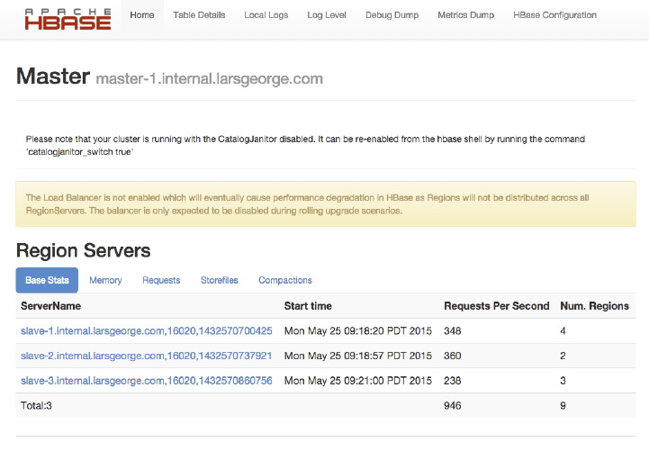
Software Attributes
You will find cluster-wide details in a table at the bottom of the
page. It has information on the version of HBase and Hadoop that
you are using, where the root directory is located, the overall load
average, and so on.
As mentioned above, we will discuss each of them now in that same
order in the next sections.
Warning Messages
As of this writing, there are three checks the Master UI page performs
and reports on, in case a violation is detected: the JVM version, as
well as the catalog janitor and balancer status. Figure 6-5 shows the
latter two of them.
Figure 6-5. The optional Master UI warnings section
There are certain Java JVM versions that are known to cause issues
when running as the basis for HBase. Again, as of this writing, there
only one tested for is 1.6.0_18, which was unstable. This might be ex‐
tended on on the future, if more troublesome Java versions are detec‐
ted. If the test is finding such a blacklisted JVM version a message is
Web-based UI 507
www.finebook.ir
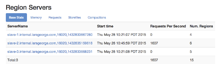
displayed at the very top of the page, just below the header, stating:
“Your current JVM version <version> is known to be unstable with
HBase. Please see the HBase wiki for details.”
The other two tests performed are more about the state of back‐
ground operations, the so-called chores. First the catalog janitor, ex‐
plained in “Server Operations” (page 409), which is required to keep a
HBase cluster clean. If you disable the janitor process with the API
call, or the shell command shown in “Tool Commands” (page 494),
you will see the message in the Master UI page as shown in the
screen shot. It reminds you to enable it again some time soon.
The check for the balancer status is very similar, as it checks if some‐
one has deactivated the background operation previously, and re‐
minds you to reenable it in the future — or else your cluster might get
skewed as region servers join or leave the collective.
Region Servers
The region server section of the Master UI page is divided into multi‐
ple subsections, represented as tabs. Each shows a set of information
pertaining to a specific topic. The first tab is named Base Stats and
comprises generic region server details, such as the server name (see
“Server and Region Names” (page 356) again for details), that also
acts as a hyperlink to the dedicated region server status page, ex‐
plained in “Region Server UI Status Page” (page 532). The screen shot
in Figure 6-6 lists three region servers, named slave-1 to slave-3.
The table also states, for each active regions server, the start time,
number of requests per second observed in the last few seconds (more
on the timing of metrics can be found in (to come)), and number of re‐
gions hosted.
Figure 6-6. The region server section on the master page - Base
Stats
Chapter 6: Available Clients508
www.finebook.ir
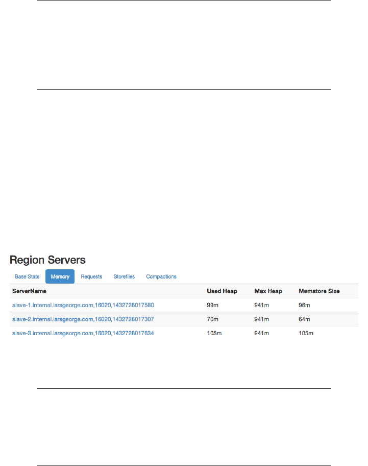
Please observe closely in the screen shot how there is one
server, namely slave-2, that seems to receive all the cur‐
rent requests only. This is—if sustained for a long time—
potentially a problem called hotspotting. We will use this
later to show you how to identify which table is causing
this imbalance.
The second tab contains memory related details. You can see the cur‐
rently used heap of the Java process, and the configured maximum
heap it may claim. The memstore size states the accumulated memory
occupied by all in-memory stores on each server. It can act as an indi‐
cator of how many writes you are performing, influenced by how many
regions are currently opened. As you will see in (to come), each table
is at least one region, and each region comprises one or more column
families, with each requiring a dedicated in-memory store. Figure 6-7
shows an example for our three current cluster with three region
servers.
Figure 6-7. The region server section on the master page - Memory
It is interesting to note that the used heap is close or even
equal to the memstore size, which is really only one com‐
ponent of the Java heap used. This can be attributed to the
size metrics being collected at different points in time and
should therefore only be used as an approximation.
The third tab, titled Requests, contains more specific information
about the current number of requests per second, and also the ob‐
served total read request and write request counts, accumulated
across the life time of the region server process. Figure 6-8 shows an‐
other example of the same three node cluster, but with an even usage.
Web-based UI 509
www.finebook.ir
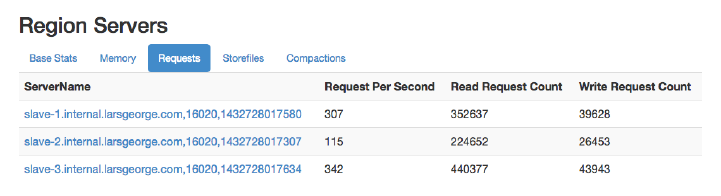
Figure 6-8. The region server section on the master page - Re‐
quests
The Storefiles tab, which is the number four, shows information about
the underlying store files of each server. The number of stores states
the total number of column families served by that server—since each
column family internally is represented as a store instance. The actual
number of files is the next column in the table. Once the in-memory
stores have filled up (or the dedicated heap for them is filled up) they
are flushed out, that is, written to disk in the store they belong to, cre‐
ating a new store file.
Since each store file is containing the actual cells of a table, they re‐
quire the most amount of disk space as far as HBase’s storage archi‐
tecture is concerned. The uncompressed size states their size before
any file compression is applied, but including any per-column family
encodings, such as prefix encoding. The storefile size column then
contains the actual file size on disk, that is, after any optional file com‐
pression has been applied.
Each file also stores various indexes to find the cells contained, and
these indexes require storage capacity too. The last two columns show
the size of the block and Bloom filter indices, as currently held in
memory for all open store files. Dependent on how you compress the
data, the size of your cells and file blocks, this number will vary. You
can use it as an indicator to estimate the memory needs for your serv‐
er processes after running your workloads for a while. Figure 6-9
shows an example.
Chapter 6: Available Clients510
www.finebook.ir
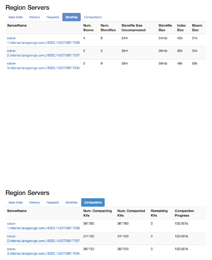
15. As a side note, you will find that the columns are titled with KV in them, an abbrevi‐
ation of KeyValue and synonym for cell. The latter is the official term as of HBase
version 1.0 going forward.
Figure 6-9. The region server section on the master page - Store‐
files
The final and fifth tab shows details about compactions, which are one
of the background housekeeping tasks a region server is performing
on your behalf.15 The table lists the number of current cells that have
been scheduled for compactions. The number of compacted cells trails
the former count, as each of them is processed by the server process.
The remaining cells is what is left of the scheduled cells, counting to‐
wards zero. Lastly, the compaction progress shows the scheduled ver‐
sus remaining as a percentage. Figure 6-10 shows that all compac‐
tions have been completed, that is, nothing is remaining and therefore
we reached 100% of the overall compaction progress.
Figure 6-10. The region server section on the master page - Com‐
pactions
Web-based UI 511
www.finebook.ir
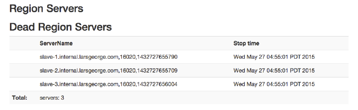
As a cluster is being written to, or compactions are triggered by API
or shell calls, the information in this table will vary. The percentage
will drop back down as soon as new cells are scheduled, and go back
to 100% as the background task is catching up with the compaction
queue.
Dead Region Servers
This is an optional section, which only appears if there is a server that
was active once, but is now considered inoperational, or dead.
Figure 6-11 shows an example, which has all three of our exemplary
slave servers with a now non-operational process. This might happen
if servers are restarted, or crash. In both cases the new process will
have a new, unique server name, containing the new start time.
Figure 6-11. The optional dead region server section on the master
page
If you have no such defunct process in your cluster, the entire section
will be omitted.
Backup Masters
The Master UI page further lists all the known backup masters. These
are HBase Master processes started on the other servers. While it
would be possible to start more than one Master on the same physical
machine, it is common to spread them across multiple servers, in case
the entire server becomes unavailable. Figure 6-12 shows an example
where two more backup masters have been started, on master-2 and
master-3.
Chapter 6: Available Clients512
www.finebook.ir
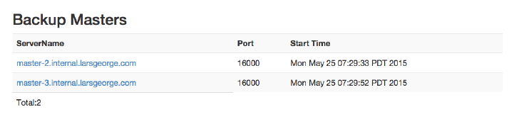
Figure 6-12. The backup master section on the Master page
The table has three columns, where the first has the hostname of the
server running the backup master process. The other two columns
state the port and start time of that process. Note that the port really
is the RPC port, not the one for the information server. The server
name acts as a hyperlink to that said information server though,
which means you can click on any of them to open the Backup Master
UI page, as shown in “Backup Master UI” (page 521).
Tables
The next major section on the Master UI page are the known tables
and snapshots, comprising user and system created ones. For that the
Tables section is split into three tabs: User Tables, System Tables, and
Snapshots.
User Tables
Here you will see the list of all tables known to your HBase cluster.
These are the ones you—or your users—have created using the
API, or the HBase Shell. The list has many columns that state, for
every user table, the namespace it belongs to, the name, region
count details, and a description. The latter gives you a printout of
the table descriptor, just listing the changed properties; see “Sche‐
ma Definition” (page 347) for an explanation of how to read them.
See Figure 6-13 for an example screen shot.
If you want more information about a user table, there are two op‐
tions. First, next to the number of user tables found, there is a link
titled Details. It takes you to another page that lists the same
tables, but with their full table descriptors, including all column
family descriptions as well. Second, the table names are links to
another page with details on the selected table. See “Table Infor‐
mation Page” (page 524) for an explanation of the contained informa‐
tion.
The region counts holds more information about how the regions
are distributed across the tables, or, in other words, how many re‐
Web-based UI 513
www.finebook.ir
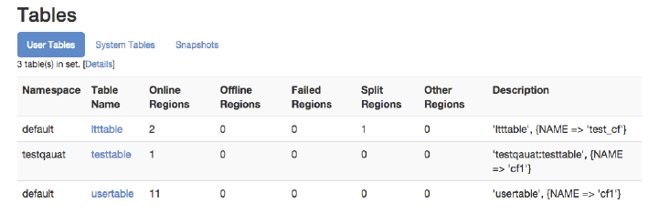
gions a table is divided into. The online regions lists all currently
active regions. The offline regions column should be always zero,
as otherwise a region is not available to serve its data. Failed re‐
gions is usually zero too, as it lists the regions that could not be
opened for some reason. See Figure 6-18 for an example showing
a table with a failed region.
Figure 6-13. The user tables
The split region count is the number of regions for which currently
a log splitting process is underway. They will eventually be opened
and move the count from this column into the online region one.
Lastly, there is an other regions counter, which lists the number of
regions in any other state from the previous columns. (to come)
lists all possible states, including the named and other ones ac‐
counted for here.
System Tables
This section list the all the catalog—or system—tables, usually
hbase:meta and hbase:namespace. There are additional, yet op‐
tional, tables, such as hbase:acl, hbase:labels, and hbase:quo
ta, which are created when the accompanying feature is enabled
or used for the first time. You can click on the name of the table to
see more details on the table regions—for example, on what server
they are currently hosted. As before with the user tables, see
“Table Information Page” (page 524) for more information. The final
column in the information table is a fixed description for the given
system table. Figure 6-14 is an example for a basic system table
list.
Chapter 6: Available Clients514
www.finebook.ir
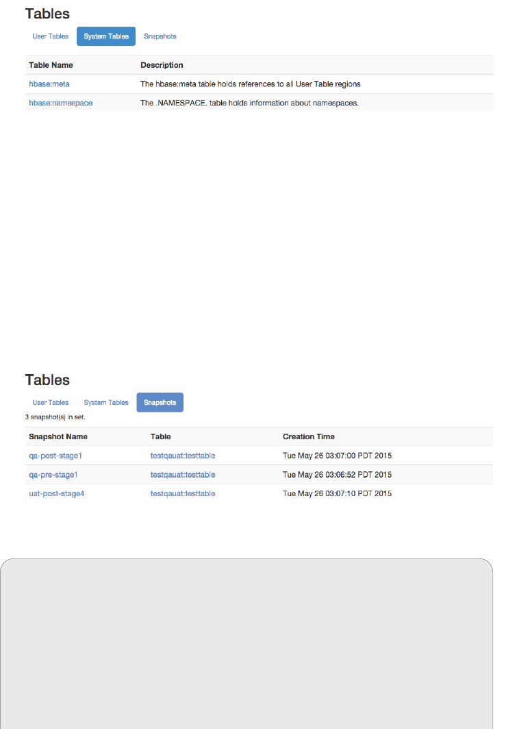
Figure 6-14. The system tables
Snapshots
The third and final tab available is listing all the known snapshots.
Figure 6-15 shows an example, with three different snapshots that
were taken previously. It lists the snapshot name, the table it was
taken from, and the creation time. The table name is a link to the
table details page, as already seen earlier, and explained in “Table
Information Page” (page 524). The snapshot name links to yet anoth‐
er page, which lists details about the snapshot, and also offers
some related operations directly from the UI. See “Snapshot”
(page 530) for details.
Figure 6-15. The list of known snapshots
Optional Table Fragmentation Information
There is a way to enable an additional detail about user and sys‐
tem tables, called fragmentation. It is enabled by adding the fol‐
lowing configuration property to the cluster configuration file,
that is, hbase_site.xml:
<property>
<name>hbase.master.ui.fragmentation.enabled</name>
<value>true</value>
</property>
Web-based UI 515
www.finebook.ir
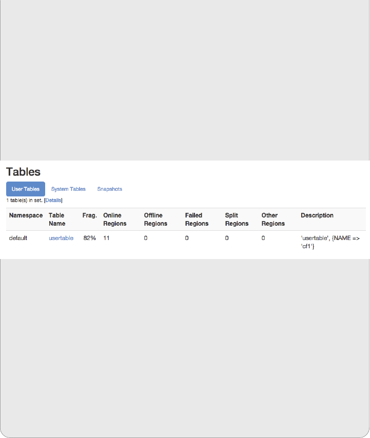
Once you have done so, the server will poll the storage file system
to check how many store files per store are currently present. If
each store only has one file, for example, after a major compac‐
tion of all tables, then the fragmentation amounts to zero. If you
have more than a single store file in a store, it is considered frag‐
mented. In other words, not the amount of files matters, but that
there is more than one. For example, if you have 10 stores and 5
have more than one file in them, then the fragmentation is 50%.
Figure 6-16 shows an example for a table with 11 regions, where
9 have more than one file, that is, 9 divided by 11, and results in
0.8181 rounded up to 82%.
Figure 6-16. The optional table fragmentation information
Once enabled, the fragmentation is added to the user and system
table information, and also to the list of software attributes at the
bottom of the page. The per-table information lists the fragmenta‐
tion for each table separately, while the one in the table at the end
of the page is summarizing the total fragmentation of the cluster,
that is, across all known tables.
A word of caution about this feature: it polls the file system details
on page load, which in a cluster under duress might increase the
latency of the UI page load. Because of this it is disabled by de‐
fault, and needs to be enabled explicitly.
Regions in Transition
As regions are managed by the master and region servers to, for ex‐
ample, balance the load across servers, they go through short phases
of transition. This applies to, for example, opening, closing, and split‐
ting a region. Before the operation is performed, the region is added
to the list of regions in transition, and once the operation is complete,
Chapter 6: Available Clients516
www.finebook.ir
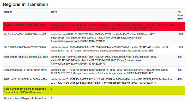
it is removed. (to come) describes the possible states a region can be
in.
When there is no region operation in progress, this section is omitted
completely. Otherwise it should look similar to the example in
Figure 6-17, listing the regions with their encoded name, the current
state, and the time elapsed since the transition process started. As of
this writing, there is a hard limit of 100 entries being shown only,
since this list could be very large for larger clusters. If that happens,
then a message like “<N> more regions in transition not shown”,
where <N> is the number of omitted entries.
Figure 6-17. The regions in transitions table
Usually the regions in transition should be appearing only briefly, as
region state transitioning is a short operation. In case you have an is‐
sue that persists, you may see a region stuck in transition for a very
long time, or even forever. If that is the case there is a threshold (set
by the hbase.metrics.rit.stuck.warning.threshold configuration
property and defaulting to one minute) that counts those regions in
excess regarding their time in the list. Figure 6-18 shows an example,
which was created by deliberately replacing a valid store file with one
that was corrupt. The server keeps trying to open the region for this
table, but will fail until an operator either deletes (or repairs) the file
in question.
Web-based UI 517
www.finebook.ir
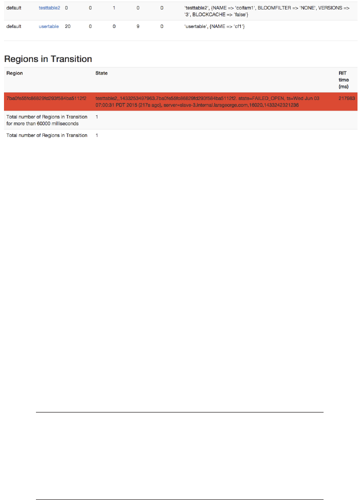
Figure 6-18. A failed region is stuck in the transition state
You will have noticed how the stuck region is counted in both summa‐
ry lines, the last two lines of the table. The screen shot also shows an
example of a region counted into the failed regions in the preceding
user table list. In any event, the row containing the oldest region in
the list (that is, the one with the largest RIT time) is rendered with a
red background color, while the first summary row at the bottom of
the table is rendered with a green-yellow background.
Tasks
HBase manages quite a few automated operations and background
tasks to keep the cluster healthy and operational. Many of these tasks
involve a complex set of steps to be run through, often across multi‐
ple, distributed set of servers. These tasks include, for example, any
region operation, such as opening and closing them, or splitting the
WAL files during a region recovery. The tasks save their state so that
they also can be recovered should the current server carrying out one
or more of the steps fail. The HBase UIs show the currently running
tasks and their state in the tasks section of their status pages.
The information about tasks applies to the UI status pages
for the HBase Master and Region Servers equally. In fact,
they share the same HTML template to generate the con‐
tent. The listed tasks though are dependent on the type of
server. For example, a get operation is only sent to the re‐
gion servers, not the master.
Chapter 6: Available Clients518
www.finebook.ir
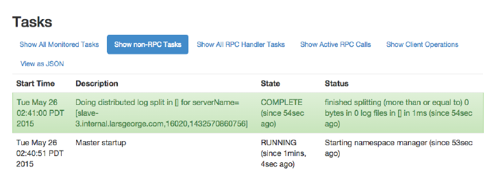
A row with a green background indicates a completed task, while all
other tasks are rendered with a white background. This includes en‐
tries that are currently running, or have been aborted. The latter can
happen when an operation failed due to an inconsistent state.
Figure 6-19 shows a completed and a running.
Figure 6-19. The list of currently running, general tasks on the
master
When you start a cluster you will see quite a few tasks show up and
disappear, which is expected, assuming they all turn green and age
out. Once a tasks is not running anymore, it will still be listed for 60
seconds, before it is removed from the UI.
The table itself starts out on the second tab, named non-RPC tasks. It
filters specific tasks from the full list, which is accessible on the first
tab, titled all monitored tasks. The next two tabs filter all RPC related
tasks, that is, all of them, or only the active ones respectively. The last
tab is named view as JSON and returns the content of the second tab
(the non-RPC tasks) as a JSON structure. It really is not a tab per-se
since it replaces the entire page with just the JSON output. Use the
browsers back to return to the UI page.
The difference between RPC and non-RPC tasks is their origin. The
former originate from a remote call, while the latter are something
triggered directly within the server process. Figure 6-20 shows two
RPC tasks, which also list their origin, that is, the remote client that
invoked the task. The previous screen shot in Figure 6-19 differs from
this one, as the displayed tasks are non-RPC ones, like the start of the
namespace manager, and therefore have no caller info.
Web-based UI 519
www.finebook.ir
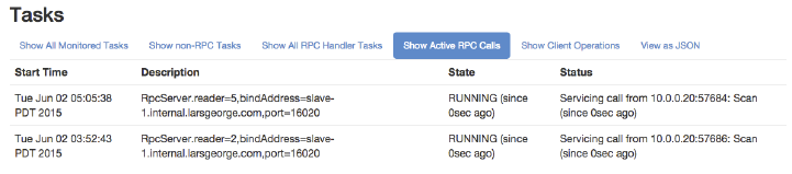
16. Recall that this should not be starting with /tmp, or you may lose your data during a
machine restart. Refer to “Quick-Start Guide” (page 39) for details.
Figure 6-20. The list of currently running RPC tasks on the master
Software Attributes
This section of the Master UI status page lists cluster wide settings,
such as the installed HBase and Hadoop versions, the root ZooKeeper
path and HBase storage directory16, and the cluster ID. The table lists
the attribute name, the current value, and a short description. Since
this page is generated on the current master, it lists what it assumes
to be the authoritative values. If you have some misconfiguration on
other servers, you may be misled by what you see here. Make sure
you cross-check the attributes and settings on all servers.
The table also lists the ZooKeeper quorum used, which has a link in its
description allowing you to see the information for your current
HBase cluster stored in ZooKeeper. “ZooKeeper page” (page 528) dis‐
cusses its content. The screen shot in Figure 6-21 shows the current
attributes of the test cluster used throughout this part of the book.
Chapter 6: Available Clients520
www.finebook.ir
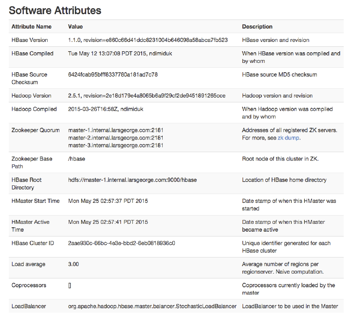
Figure 6-21. The list of attributes on the Master UI page
Master UI Related Pages
The following pages are related to the Master UI page, as they are di‐
rectly linked from it. This includes the detailed table, table informa‐
tion, and snapshot information pages.
Backup Master UI
If you have more than one HBase Master process started on your clus‐
ter (for more on how to do that see (to come)), then the active Master
UI will list them. Each of the server names is a link to the respective
backup master, providing its dedicated status page, as shown in
Figure 6-22. The content of each backup master is pretty much the
same, since they do nothing else but wait for a chance to take over the
Web-based UI 521
www.finebook.ir
lead. This happens of course only if the currently active master server
disappears.
At the top the page links to the currently active master, which makes
it easy to navigate back to the root of the cluster. This is followed by
the list of tasks, as explained in “Tasks” (page 518), though here we
will only ever see one entry, which is the long running tasks to wait
for the master to complete its startup—which is only happening in the
above scenario.
Chapter 6: Available Clients522
www.finebook.ir
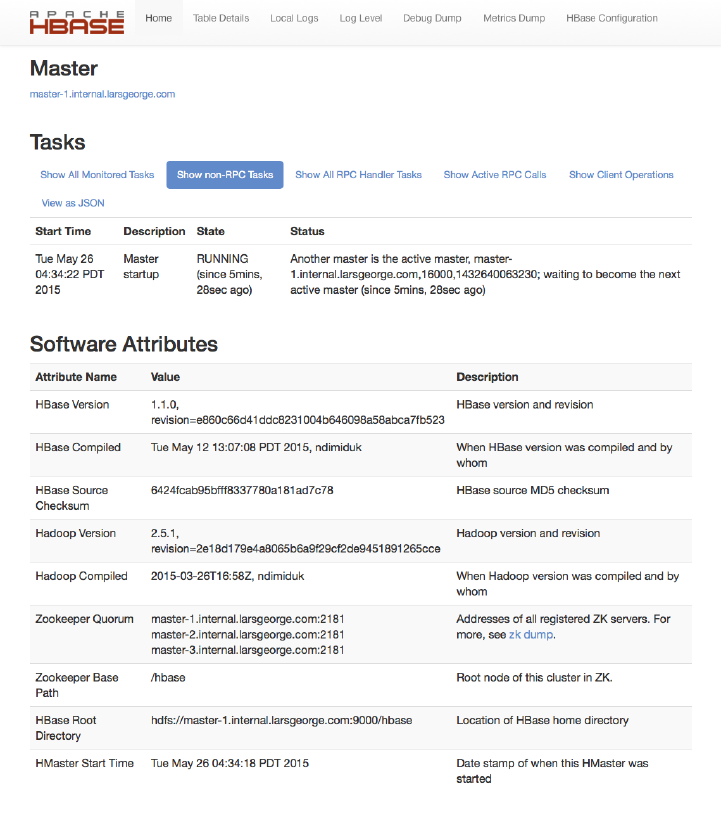
Figure 6-22. The backup master page
The page also lists an abbreviated list of software attributes. It is
missing any current values, such as the loaded coprocessors, or the
region load. These values are only accessible when the master process
is started fully and active. Otherwise you have seen the list of at‐
tributes before, in “Software Attributes” (page 520).
Web-based UI 523
www.finebook.ir
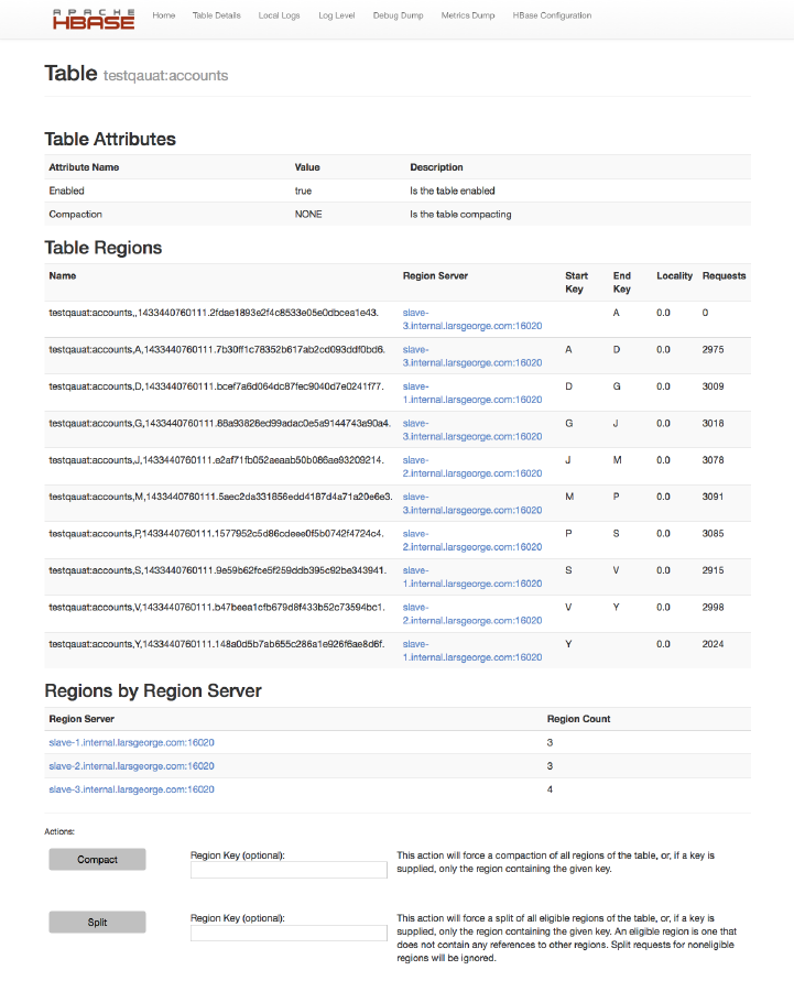
Table Attributes
Here you can find details about the table itself. First, it lists the
table status, that is, if it is enabled or not. See “Table Operations”
(page 378), and the disableTable() call especially. The boolean
value states whether the table is enabled, so when you see a true
in the Value column, this is the case. On the other hand, a value of
false would mean the table is currently disabled.
Second, the table shows if there are any compactions currently
running for this table. It either states NONE, MINOR, MAJOR, MA‐
JOR_AND_MINOR, or Unknown. The latter is rare but might show
when, for example, a table with a single region splits and no com‐
paction state is known to the Master for that brief moment. You
may wonder how a table can have a minor and major compaction
running at the same time, but recall how compactions are trig‐
gered per region, which means it is possible for a table with many
regions to have more than one being compacted (minor and/or ma‐
jor) at the same time.
Lastly, if you have the optional fragmentation information enabled,
as explained in “Optional Table Fragmentation Information” (page
515), you have a third line that lists the current fragmentation lev‐
el of the table.
Table Regions
This list can be rather large and shows all regions of a table. The
name column has the region name itself, and the region server col‐
umn has a link to the server hosting the region. Clicking on the
link takes you to the page explained in “Region Server UI Status
Page” (page 532).
+ The start key and end key columns show the region’s start and end
keys as expected. The locality column indicates, in terms of a percent‐
age, if the storage files are local to the server which needs it, or if
they are accessed through the network instead. See “Cluster Status
Information” (page 411) and the getDataLocality() call for details
+ Finally, the requests column shows the total number of requests, in‐
cluding all read (get, scan, etc.) and write (put, delete, etc.) opera‐
tions, since the region was deployed to the hosting server.
Regions by Region Server
The last group on the Table Information page lists which region
server is hosting how many regions of the selected table. This
number is usually distributed evenly across all available servers. If
not, you can use the HBase Shell or administrative API to initiate
the balancer, or use the move command to manually balance the
table regions (see “Cluster Operations” (page 393)).
Chapter 6: Available Clients526
www.finebook.ir
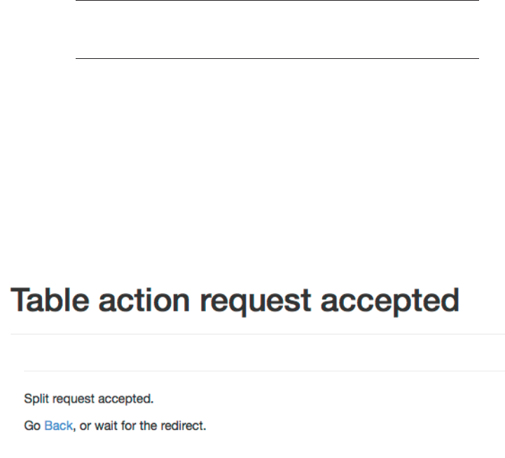
By default, the Table Information page also offers some actions that
can be used to trigger administrative operations on a specific region,
or the entire table. These actions can be hidden by setting the
hbase.master.ui.readonly configuration property to true. See
“Cluster Operations” (page 393) again for details about the actions,
and (to come) for information on when you want to use them. The
available operations are:
Compact
This triggers the compact functionality, which is asynchronously
running in the background. Specify the optional name of a region
to run the operation more selectively. The name of the region can
be taken from the table above, that is, the entries in the name col‐
umn of the Table Regions table.
Make sure to copy the entire region name as-is. This in‐
cludes the trailing "." (the dot)!
If you do not specify a region name, the operation is performed on
all regions of the table instead.
Split
Similar to the compact action, the split action triggers the split
command, operating on a table or region scope. Not all regions
may be splittable—for example, those that contain no, or very few,
cells, or one that has already been split, but which has not been
compacted to complete the process.
Once you trigger one of the operations, you will receive a confirma‐
tion page; for example, for a split invocation, you will see:
Web-based UI 527
www.finebook.ir
As directed, use the Back button of your web browser, or simply wait
a few seconds, to go back to the previous page, showing the table in‐
formation.
ZooKeeper page
This page shows the same information as invoking the zk_dump com‐
mand of the HBase Shell. It shows you the root directory HBase is us‐
ing inside the configured filesystem. You also can see the currently as‐
signed master, the known backup masters, which region server is
hosting the hbase:meta catalog table, the list of region servers that
have registered with the master, replication details, as well as Zoo‐
Keeper internal details. Figure 6-24 shows an exemplary output avail‐
able on the ZooKeeper page (abbreviated for the sake of space).
Chapter 6: Available Clients528
www.finebook.ir
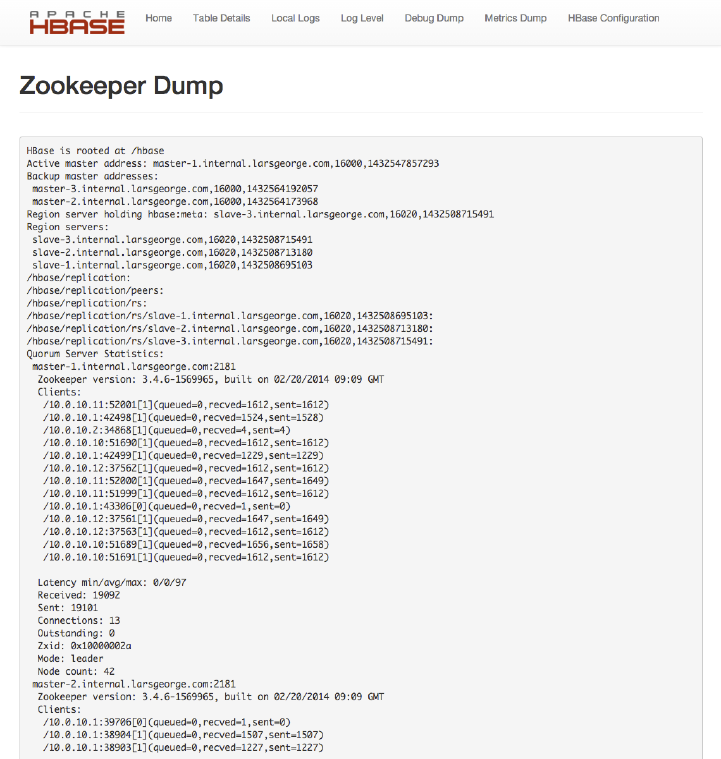
Figure 6-24. The ZooKeeper page, listing HBase and ZooKeeper
details
While you will rarely use this page, which is linked to from the Master
UI page, it is useful in case your cluster is unstable, or you need to re‐
assure yourself of its current configuration and state. The information
is very low-level in parts, but as you grow more accustomed to HBase
and how it is operated, the values reported might give you clues as to
what is happening inside the cluster.
Web-based UI 529
www.finebook.ir
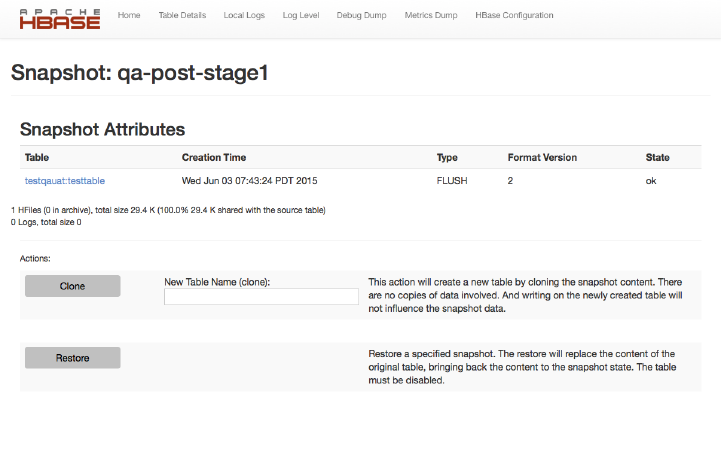
Snapshot
Every snapshot name, listed on the Master UI status page, is a link to
a dedicated page with information about the snapshot. Figure 6-25 is
an example screen shot, listing the table it was taken from (which is a
link back to the table information page), the creation time, the type of
snapshot, the format version, and state. You can refresh your knowl‐
edge about the meaning of each in “Table Operations: Snapshots”
(page 401).
Figure 6-25. The snapshot details page
The page also shows some information about the files involved in the
snapshot, for example:
36 HFiles (20 in archive), total size 250.9 M (45.3% 113.7 M
shared with the source table)
0 Logs, total size 0
Here we have 36 storage files in the snapshot, and 20 of those are al‐
ready replaced by newer files, which means they have been archived
to keep the snapshot consistent. Should you have had any severe is‐
sues with the cluster and experienced data loss, it might happen that
you see something similar to what Figure 6-26 shows. The snapshot is
corrupt because a file is missing (which I have manually removed to
Chapter 6: Available Clients530
www.finebook.ir
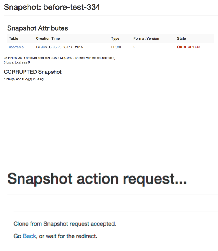
just to show you this screen shot—do not try this unless you know
what you are doing), as listed in the CORRUPTED Snapshot section of
the page.
Figure 6-26. A corrupt snapshot example
There are also actions you can perform—assuming you have not dis‐
abled them using the hbase.master.ui.readonly configuration prop‐
erty as explained—based on the currently displayed snapshot. You can
either clone the snapshot into a new table, or restore it by replacing
the originating table. Both actions will show a confirmation message
(or an error in case something is wrong, for example, when specifying
a non-existent namespace for a new table), similar to this:
More elaborate functionality is only available through the API, which
is mostly exposed through the HBase Shell (as mentioned, see “Table
Operations: Snapshots” (page 401)).
Web-based UI 531
www.finebook.ir
Region Server UI Status Page
The region servers have their own web-based UI, which you usually
access through the master UI, by clicking on the server name links
provided. You can access the page directly by entering
http://<region-server-address>:16030
into your browser (while making sure to use the configured port, here
using the default of 16030).
Main page
The main page of the region servers has details about the server, the
tasks it performs, the regions it is hosting, and so on. Figure 6-27
shows an example of this page.
Chapter 6: Available Clients532
www.finebook.ir
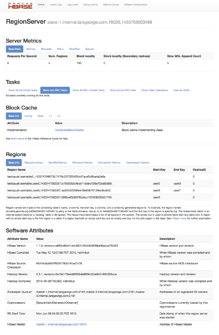
The page can be broken up into the following groups of distinct infor‐
mation, which we will—if they have not been explained before—dis‐
cuss in detail in the subsequent sections:
Server Metrics
First, there are statistics about the current state of the server, its
memory usage, number of requests observed, and more.
Tasks
The table lists all currently running tasks, as explained in “Tasks”
(page 518). The only difference is that region servers will work on
different tasks compared to the master. The former are concerned
about data and region operations, while the latter will manage the
region servers and WALs, among many other things.
Block Cache
When data is read from the storage files, it is loaded in blocks.
These are usually cached for subsequent use, speeding up the read
operations. The block cache has many configuration options, and
dependent on those this part of the region server page will vary in
its content.
Regions
Here you can see all the regions hosted by the currently selected
region server. The table has many tabs that contain basic informa‐
tion, as well as request, store file, compaction, and coprocessor
metrics.
Software Attributes
This group of information contains, for example, the version of
HBase you are running, when it was compiled, the ZooKeeper quo‐
rum used, server start time, and a link back to the active HBase
Master server. The content is self-explanatory, has a description
column, and is similar to what was explained in “Software At‐
tributes” (page 520).
Server Metrics
The first part on the status page of a region server relates to summary
statistics about the server itself. This includes the number of region it
holds, the memory used, client requests observed, number of store
files, WALs, and length of queues. Figure 6-28 combines them all into
one screen shot since they are all very short.
Chapter 6: Available Clients534
www.finebook.ir

17. As of this writing, covering version 1.1.0 of HBase, the “Slow WAL Append” value is
hardcoded to be zero.
Many of the values are backed by the server metrics
framework (see (to come)) and do refresh on a slower ca‐
dence. Even if you reload the page you will see changes
only every now and so often. The metrics update period is
set by the hbase.regionserver.metrics.period configu‐
ration property and defaults to 5 seconds. Metrics collec‐
tion is a complex process, which means that even with an
update every 5 seconds, there are some values which up‐
date at a slower rate. In other words, use the values dis‐
played with caution, as they might trail the actual current
values.
The first tab, named base stats, lists the most high level details, so
that you can have a quick glimpse at the overall state of the process.
It lists the requests per second, the number of region hosted, the
block locality percentage, the same for the replicas—if there are any--,
and the number of slow WAL append operations. The latter is trig‐
gered if writing to the write-ahead log is delayed for some reason
(most likely I/O pressure).17
Web-based UI 535
www.finebook.ir
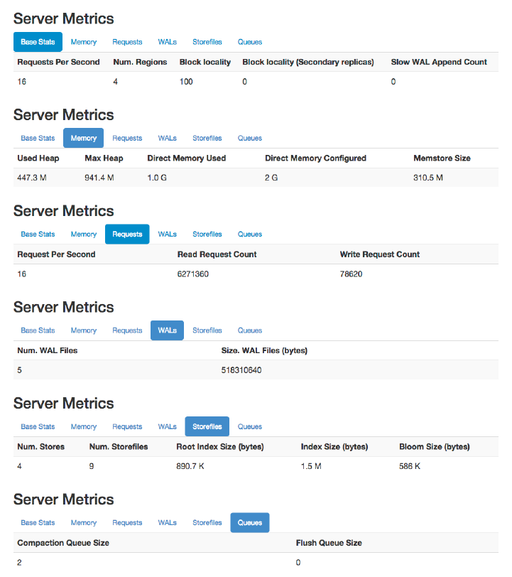
Figure 6-28. All tabs in the Server Metrics section
The second tab, titled memory, shows details of the currently used
memory, both on-heap and off-heap. If shows the current and maxi‐
mum configured Java heap, and the same for the off-heap memory,
called direct memory. All of these are configured in the cluster wide
hbase-env.sh configuration file for the Java process environment. The
tab also lists the current combined memory occupied by the all the in-
Chapter 6: Available Clients536
www.finebook.ir
memory stores hosted by this server. The region statistics further
down the page shows them separately.
The third tab is called requests and shows the combined, server-wide
number of requests per second served, and the total read and write
request count since the server started. The request per seconds are
over the configured time to collect metrics, which is explained in (to
come).
The tab named WALs lists write-ahead log metrics, here the number
of WALs this server is keeping around for recovery purposes. It also
lists the combined size of these files, as occupied on the underlying
storage system.
Next is the store files tab, which lists information about the actual
storage files. First the number of stores is stated, currently served by
this region server. Since a store can have zero to many storage files,
the next columns lists the number of store files, plus their combined
sizes regarding the various indices contained in them. There are the
root index, and the total index sizes, both addressing the block index
structure. The root index points to blocks in the overall block index,
and therefore is much smaller. Only the root index is kept in memory,
while the block index blocks are loaded and cached on demand. There
is also the Bloom filter, which—if enabled for the column family—is oc‐
cupying space in the persisted store files. The value state in the table
is the combined size as needed for all the store files together. Note
that it is cached on demand too, so not all of that space is needed in
memory.
The last and sixth tab titled queues lists the current size of the com‐
paction and flush queues. These are vital resources for a region serv‐
er, and a high as well as steadily increasing queue size indicates that
the server is under pressure and has difficulties to keep up with the
background housekeeping tasks.
Block Cache
The first tab, named base info, lists the selected cache implementation
class, as shown in Figure 6-29.
Web-based UI 537
www.finebook.ir
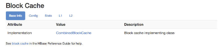
Figure 6-29. The base info of the Block Cache section
The block cache was configured as a combined cache, which uses the
purely in-memory LRU cache as L1 (first level) cache, and the bucket
cache as L2 (second level) cache (see (to come)). The LRU cache is set
to use %20 of the maximum Java heap, not the default 40%. The block
cache is configured as an off-heap cache, set to 1GB, using the follow‐
ing configuration settings:
<property>
<name>hbase.bucketcache.combinedcache.enabled</name>
<value>true</value>
</property>
<property>
<name>hfile.block.cache.size</name>
<value>0.2</value>
</property>
<property>
<name>hbase.bucketcache.ioengine</name>
<value>offheap</value>
</property>
<property>
<name>hbase.bucketcache.size</name>
<value>1024</value>
</property>
The next tab shows the cluster wide configuration values, regarding
the cache properties. Figure 6-30 is an example screen shot.
Chapter 6: Available Clients538
www.finebook.ir
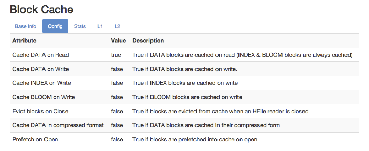
Figure 6-30. The configuration tab of the Block Cache section
These values are set with the following configuration properties (see
(to come) for the default values, their type, and description):
hfile.block.cache.size
hbase.rs.cacheblocksonwrite
hfile.block.index.cacheonwrite
hfile.block.bloom.cacheonwrite
hbase.rs.evictblocksonclose
hbase.block.data.cachecompressed
hbase.rs.prefetchblocksonopen
The first key, hfile.block.cache.size, sets the percentage used by
the LRU cache, and if it is set to 0% or less, the cache is completely
disabled. In practice it is very unlikely that you would ever go that far,
since without any caching the entire I/O is purely based on the back‐
ing storage. Even with SATA SSDs or PCIe flash memory cards, the in‐
cumbent x86-64 based architecture can operate on DRAM a magni‐
tude faster in comparison.
The majority of these options are turned off, which means you need to
deliberately turn them on within your cluster. See (to come) for an in-
depth discussion of cache configurations. The next tab is titled statis‐
tics, and shows the overall cache state. Since there are quite a few op‐
tions available to configure the block cache, that is, with L1 only, or
L1 and L2 together, the statistics combine the values if necessary.
Figure 6-31 shows an example.
Web-based UI 539
www.finebook.ir
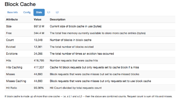
Figure 6-31. The statistics tab of the Block Cache section
As with many of the values the status pages show, you can access
them in various ways. Here, for example, you can also use the metrics
API, explained in (to come). The advantage of the web-based UI pages
is that they can nicely group the related attributes, format their value
human-readable, and add a short description for your perusal.
The screen shot was taken during a load test using YCSB (see (to
come)). After the test table was filled with random data, a subsequent
read load-test was executed (workload B or C). You might see with
some of the statistics the expected effect, for example, the L1 being
100% effective, because with a combined cache configuration, the L1
only caches index data, which fits easily into the in-memory space for
our test setup. This is also the reason that we decreased the dedicated
heap space allocated for the on-heap LRU cache—it is not needed and
the space can be used for other purposes. Figure 6-32 shows this on
the next tab, titled L1.
Chapter 6: Available Clients540
www.finebook.ir
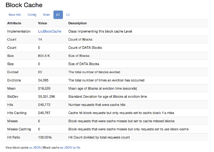
Figure 6-32. The L1 tab of the Block Cache section
The tab lists again many attributes, their values, and a short descrip‐
tion. From these values you can determine the amount of blocks cach‐
ed, divided into all blocks and data blocks respectively. Since we are
not caching data blocks in L1 with an active L2, the count states the
index blocks only. Same goes for the size of these blocks. There are
further statistics, such as the number of evicted blocks, and the num‐
ber of times an eviction check has run. The mean age and standard
deviation lets you determine how long blocks stay in the cache before
they are removed. This is related to the churn on the cache, because
the LRU cache evicts the oldest blocks first, and if these are relatively
young, you will have a high churn on the cache. The remaining num‐
bers state the hits (the total number, and only those that are part of
requests that had caching enabled), misses, and the ration between
them.
The L2 cache is more interesting in this example, as it does the heavy
lifting to cache all data blocks. Figure 6-33 shows the matching screen
shot in tab number five, labeled appropriately L2. It contains a list
similar to that of the L1 cache, showing attributes, their current val‐
ues, and a short description. The link in the first line of the table is
Web-based UI 541
www.finebook.ir
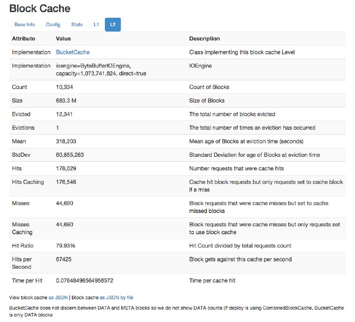
pointing to the online API documentation for the configured class,
here a BucketCache instance. You can further see the number of
blocks cached, their total size, the same eviction details as before, and
again the same for hits, misses, and the ratio. Some extra info here
are the hits per second and time per hit values. They show how
stressed the cache is and how quickly it can deliver contained blocks.
Figure 6-33. The L2 tab of the Block Cache section
When you switch the Block Cache section to the last tab, the L2 tab,
you will be presented with an additional section right below the Block
Cache one, named bucketcache buckets, listing all the buckets the
cache maintains, and for each the configured allocation size, and the
Chapter 6: Available Clients542
www.finebook.ir
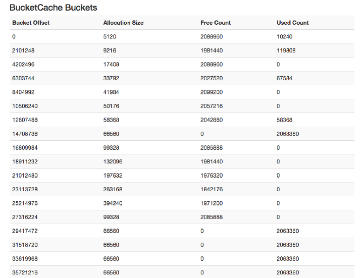
18. As of this writing, the labels are wrong for the BucketCache Buckets, the last two
columns are actually sizes, not counts. See HBASE-13861 for details.
size of the free and used blocks within.18 See Figure 6-34 for an exam‐
ple.
Figure 6-34. The extra bucket cache section
Since in this example the cache is configured to use 1GB of off-heap
memory, you see buckets spreading from offset 0, all the way close to
the maximum of 1073741824 bytes. The space is divided equally based
on the largest configured bucket size, and within each the space is
divided into blocks mentioned by the allocation size, which varies to
be flexible when it comes to assigning data to them. You can read
more about this in aforementioned (to come).
Lastly, the Block Cache section has an additional as JSON link on
some of the tabs, that lets you access the summary statistics as a
JSON structure. This can be done by opening the JSON as a web page,
Web-based UI 543
www.finebook.ir
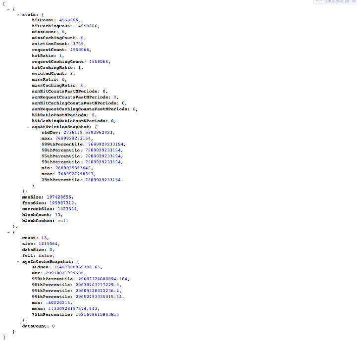
or as a direct download to your local machine (JSON by file option).
Figure 6-35 has an example JSON output.
Figure 6-35. Output of cache metrics as JSON
Regions
The next major information section on the region server’s web-based
UI status page is labeled Regions, listing specific metrics for every re‐
gion currently hosted by the server showing you its status page. It has
six tabs, with a lot of fine-grained data points, explained in order next.
First is the tab titled base info, showing you a brief overview of each
region. Figure 6-36 has an exemplary screen shot. You can see the re‐
gion name, the start and end keys, as well as the replica ID. The latter
Chapter 6: Available Clients544
www.finebook.ir
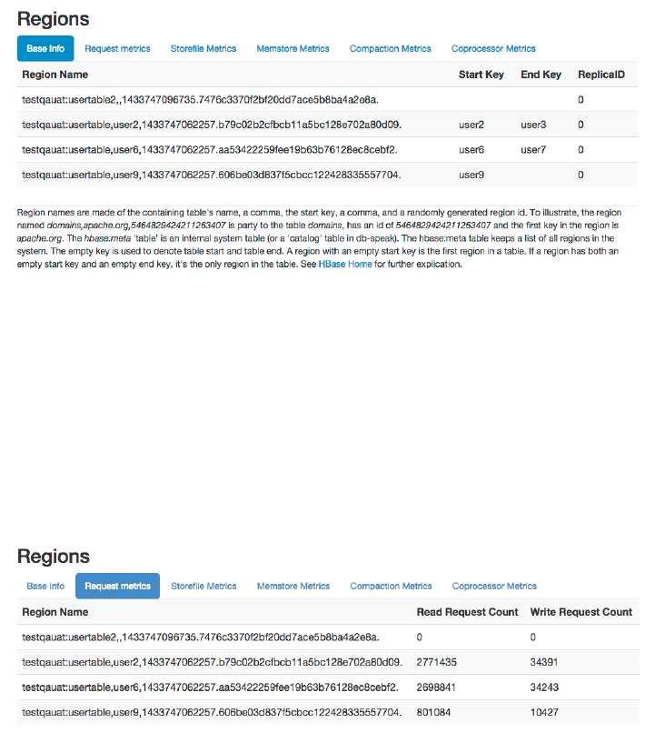
is a number different from zero if the region is a read replica. We will
look into this in (to come).
Figure 6-36. The regions details, basic information tab
The next tab, tab two titled request metrics, retains the region name
column—all further tabs do that, so they will not be mentioned again---
but then prints the total read request, and write request counts. These
are accumulated in-memory on the region server, that is, restarting
the server will reset the counters. Figure 6-37 shows a screen shot
where three tables of one table are busy, while the remaining one re‐
gion from another has not been used at all.
Figure 6-37. The regions details, request metrics tab
Then there is the storefile metrics tab, number three, which lists the
summary statistics about the store files contained in each region. Re‐
call that each store is equivalent to a column family, and each can
have zero (before anything was flushed) to many data files in them.
Web-based UI 545
www.finebook.ir
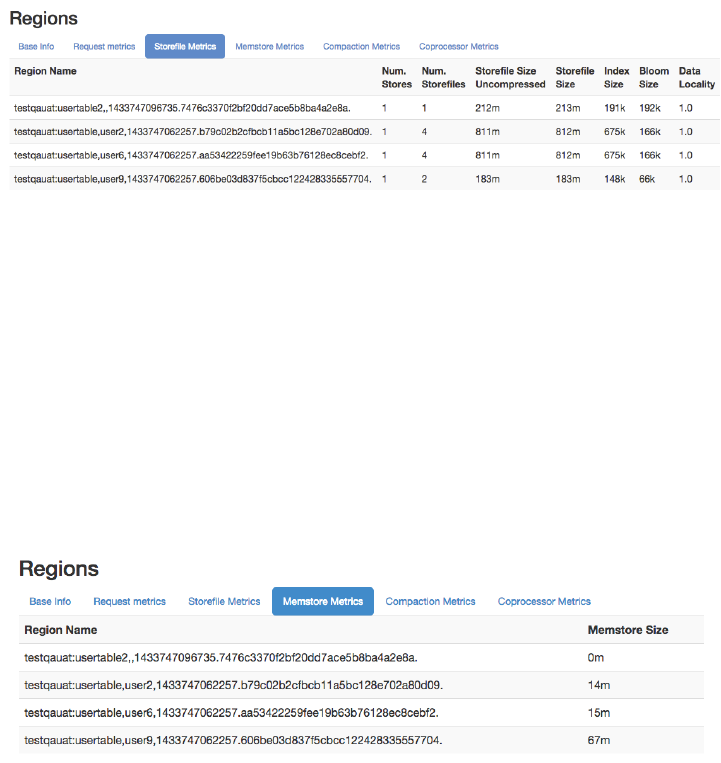
The page also lists the combined size of these files, both uncom‐
pressed and compressed, though the latter is optional and here we
see not much difference because of that (see (to come) to learn more
about compression of data). The next two columns state the block in‐
dex and Bloom filter size required by all the store files in the given re‐
gion. Lastly, you can see the data locality ratio, which is expressed as
a percentage from 0.0 to 1.0, meaning 0% to 100%. The screen shot in
Figure 6-38 shows the four regions with their respective store file
metrics.
Figure 6-38. The regions details, storefile metrics tab
The fourth tab, named memstore metrics, lists the accumulated, com‐
bined amount of memory occupied by the in-memory stores, that is,
the Java heap backed structures keeping the mutations (the put and
delete records) before they are written to disk. The default flush size
is 128MB, which means the sizes shown in this tab—assuming for a
second that you have only one memstore—should grow from 0m (zero
megabyte) to somewhere around 128m and then after being flushed in
the background drop back down to zero. If you have more than one
memstore then you should expect the upper boundary to be a multiple
of the flush size. Figure 6-39 shows an example.
Figure 6-39. The regions details, memstore metrics tab
Chapter 6: Available Clients546
www.finebook.ir
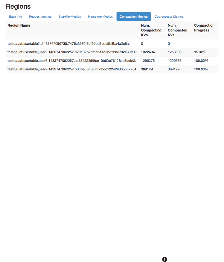
On tab five, the compaction metrics shows the summary statistics
about the cells currently scheduled for compaction, the number of
cells that has been already compacted, and a progress percentage.
The screen shot in Figure 6-40 shows an example.
Figure 6-40. The regions details, compaction metrics tab
Finally, the sixth tab, named coprocessor metrics, displays the time
spent in each coprocessor that was invoked for any hosted region. As
an example, the online code repository for this book includes a copro‐
cessor that does add a generated ID into each record that is written.
Example 6-4 shows the code, which, when you read it carefully, also
shows how the callback for prePut() is artificially delaying the call.
We just use this here to emulate a heavier processing task embedded
in a coprocessor.
Example 6-4. Adds a coprocessor local ID into the operation
private static String KEY_ID = "X-ID-GEN";
private byte[] family;
private byte[] qualifier;
private String regionName;
private Random rnd = new Random();
private int delay;
@Override
public void start(CoprocessorEnvironment e) throws IOException {
if (e instanceof RegionCoprocessorEnvironment) {
RegionCoprocessorEnvironment env = (RegionCoprocessorEnviron‐
ment) e;
Configuration conf = env.getConfiguration();
this.regionName = env.getRegionInfo().getEncodedName();
String family = conf.get("com.larsgeorge.copro.seqidgen.fami‐
ly", "cf1");
this.family = Bytes.toBytes(family);
Web-based UI 547
www.finebook.ir

String qualifier = conf.get("com.larsgeorge.copro.seqidg‐
en.qualifier",
"GENID");
this.qualifier = Bytes.toBytes(qualifier);
int startId = conf.getInt("com.larsgeorge.copro.seqidgen.star‐
tId", 1);
this.delay = conf.getInt("com.larsgeorge.copro.seqidgen.delay",
100);
env.getSharedData().putIfAbsent(KEY_ID, new AtomicInteger(star‐
tId));
} else {
LOG.warn("Received wrong context.");
}
}
@Override
public void stop(CoprocessorEnvironment e) throws IOException {
if (e instanceof RegionCoprocessorEnvironment) {
RegionCoprocessorEnvironment env = (RegionCoprocessorEnviron‐
ment) e;
AtomicInteger id = (AtomicInteger) env.getSharedDa‐
ta().get(KEY_ID);
LOG.info("Final ID issued: " + regionName + "-" + id.get());
} else {
LOG.warn("Received wrong context.");
}
}
@Override
public void prePut(ObserverContext<RegionCoprocessorEnvironment> e,
Put put,
WALEdit edit, Durability durability) throws IOException {
RegionCoprocessorEnvironment env = e.getEnvironment();
AtomicInteger id = (AtomicInteger) env.getSharedDa‐
ta().get(KEY_ID);
put.addColumn(family, qualifier, Bytes.toBytes(regionName + "-" +
id.incrementAndGet()));
try {
Thread.sleep(rnd.nextInt(delay));
} catch (InterruptedException e1) {
e1.printStackTrace();
}
}
Get environment and configuration instances.
Retrieve the settings passed into the configuration.
Set up generator if this has not been done yet on this region
server.
Chapter 6: Available Clients548
www.finebook.ir

Log the final number generated by this coprocessor.
Set the shared ID for this instance of put.
Sleep for 0 to “delay” milliseconds.
After compiling the project (see (to come)), the generated JAR file is
placed into the /opt/hbase-book directory on the test cluster used
throughout this section. We can then add the coprocessor to one of
the test tables, here one that is used with YCSB (see (to come)), so
that during a load test we can measure the impact of the callback. The
class is added using the HBase shell, and after running the load test, a
scan is performed to print the generated IDs—here a concatenation of
the encoded region name and a shared, continuously increasing ID:
hbase(main):001:0> alter 'testqauat:usertable', \
METHOD => 'table_att', 'coprocessor' => \
'file:///opt/hbase-book/hbase-book-ch05-2.0.jar| \
coprocessor.SequentialIdGeneratorObserver|'
Updating all regions with the new schema...
1/11 regions updated.
11/11 regions updated.
Done.
0 row(s) in 3.5360 seconds
hbase(main):002:0> scan 'testqauat:usertable', \
{ COLUMNS => [ 'cf1:GENID' ], LIMIT => 2 }
ROW COLUMN+CELL
user1000257404909208451 column=cf1:GENID, time‐
stamp=1433763441150, \
value=dcd5395044732242dfed39b09aa05c36-15853
user1000863415447421507 column=cf1:GENID, time‐
stamp=1433763396342, \
value=dcd5395044732242dfed39b09aa05c36-14045
2 row(s) in 4.5070 seconds
While running the load test using YCSB (workload A) the example
screen shot shown in Figure 6-41 was taken. Since the coprocessor
delays the processing between 1 and 100 milliseconds, you will find
the values in the execution time statistics column reflect that closely.
For every region every active coprocessor is listed, and for each you
will see the various timing details, showing minimum, average, and
maximum time observed. There is also a list of the 90th, 95th, and
99th percentile.
Web-based UI 549
www.finebook.ir
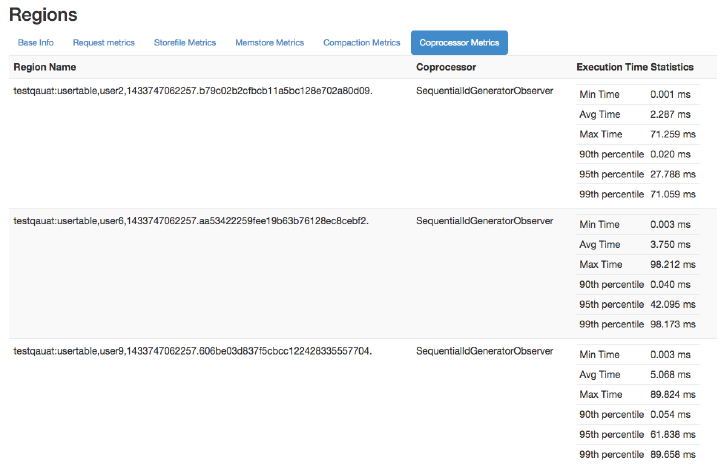
Figure 6-41. The regions details, coprocessor metrics tab
Software Attributes
This section of the Region Server UI status page lists cluster wide set‐
tings, such as the installed HBase and Hadoop versions, the ZooKeep‐
er quorum, the loaded coprocessor classes, and more. The table lists
the attribute name, the current value, and a short description. Since
this page is generated on the current region server, it lists what it as‐
sumes to be the authoritative values. If you have some misconfigura‐
tion on other servers, you may be misled by what you see here. Make
sure you cross-check the attributes and settings on all servers. The
screen shot in Figure 6-42 shows the current attributes of the test
cluster used throughout this part of the book.
Chapter 6: Available Clients550
www.finebook.ir
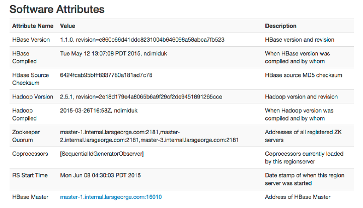
Figure 6-42. The list of attributes on the Region Server UI
Shared Pages
On the top of the master, region server, and table pages there are also
a few generic links that lead to subsequent pages, displaying or con‐
trolling additional details of your setup:
Local Logs
This link provides a quick way to access the logfiles without re‐
quiring access to the server itself. It firsts list the contents of the
log directory where you can select the logfile you want to see.
Click on a log to reveal its content. (to come) helps you to make
sense of what you may see. Figure 6-43 shows an example page.
Web-based UI 551
www.finebook.ir
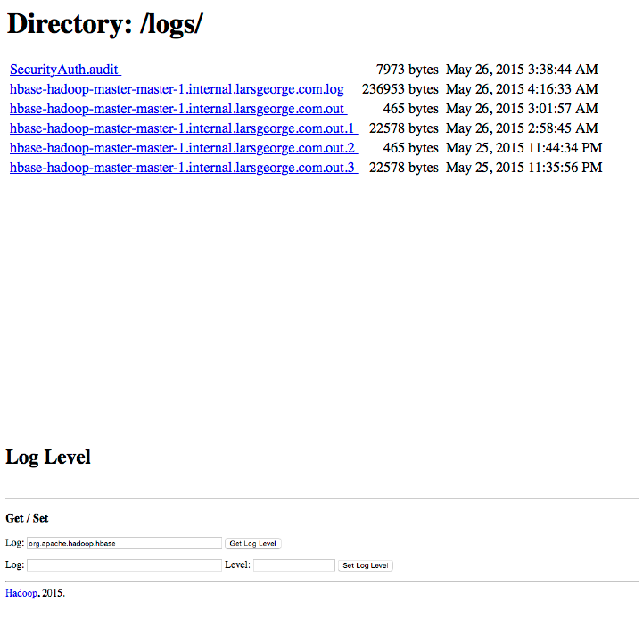
Figure 6-43. The Local Logs page
Log Level
This link leads you to a small form that allows you to retrieve and
set the logging levels used by the HBase processes. More on this is
provided in (to come). Figure 6-44 shows the form, already filled in
with org.apache.hadoop.hbase as the log hierarchy point to
check the level for.
Figure 6-44. The Log Level page
When you click on the Get Log Level button, you should see a re‐
sult similar to that shown in Figure 6-45.
Chapter 6: Available Clients552
www.finebook.ir
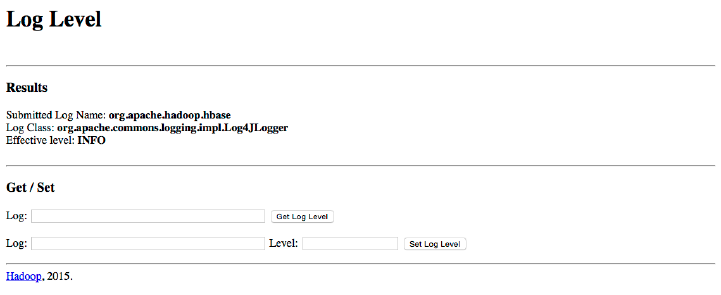
Figure 6-45. The Log Level Result page
Debug Dump
For debugging purposes, you can use this link to dump many de‐
tails of the current Java process, including the stack traces of the
running threads. You can find more details in (to come). The fol‐
lowing details are included, with the difference between HBase
Master and Region Server mentioned (the Master has a few more
sections listed in the debug page):
Version Info
Lists some of the information shown at the bottom of the status
pages, that is, the HBase and Hadoop version, and who com‐
piled them. See “Software Attributes” (page 520) or “Software
Attributes” (page 550).
Tasks
Prints all of the monitored tasks running on the server. Same
as explained in, for example, “Tasks” (page 518).
Servers
Master Only—Outputs the name and server load of each known
online region server (see “Cluster Status Information” (page
411) for details on the server load records).
Regions in Transition
Master Only—Lists the regions in transition, if there are any.
See “Regions in Transition” (page 516) for details.
Executors
Shows all the currently configured executor threads, working
on various tasks.
Web-based UI 553
www.finebook.ir
Stacks
Dumps the stack traces of all Java threads.
Configuration
Prints the configuration as loaded by the current server.
Recent Region Server Aborts
Master Only—Lists the reasons of the last region server aborts,
that is, the reasons why a slave server was abandoned or stop‐
ped.
Logs
The log messages of the server’s log are printed in this section.
Lists the last 100KBs, but can be changed per request by
adding the tailkb parameter with the desired number of kilo‐
bytes to the URL.
Region Server Queues
Shows detailed information about the compaction and flush
queues. This includes the different types of compaction entries
(small, or large), as well as splits, and region merges. Can be
disabled setting the hbase.regionserver.serv
let.show.queuedump configuration property to false.
Figure 6-46 shows an abbreviated example output for a region
server. The full pages are usually very long, as the majority of the
emitted information is very verbose.
Chapter 6: Available Clients554
www.finebook.ir
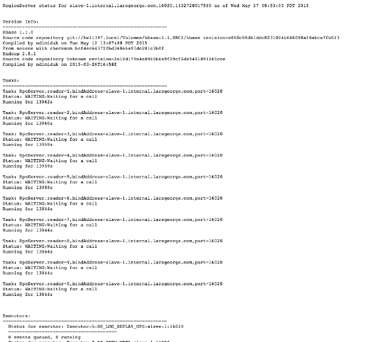
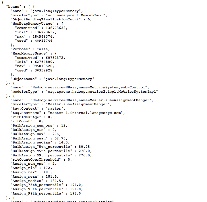
Figure 6-47. The Metrics Dump page
HBase Configuration
Last but not least, this shared link lets you output the current serv‐
er configuration as loaded by the process. This is not necessarily
what is on disk in the configuration directory, but what has been
loaded at process start time, and possibly modified by dynamically
reloading the configuration. Figure 6-48 is an example XML output
this link produces. Depending on your browser (here Chrome) the
rendering will vary.
Chapter 6: Available Clients556
www.finebook.ir
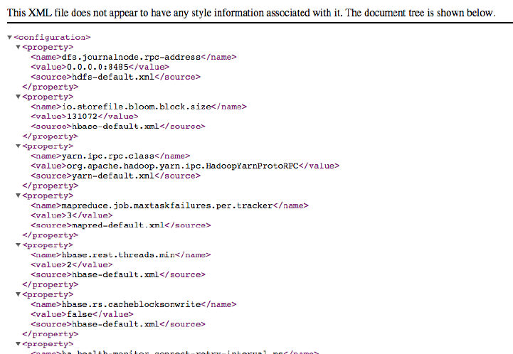
Figure 6-48. The HBase Configuration page
The web-based UI provided by the HBase servers is a good way to
quickly gain insight into the cluster, the hosted tables, the status of
regions and tables, and so on. The majority of the information can also
be accessed using the HBase Shell, but that requires console access
to the cluster.
You can use the UI to trigger selected administrative operations;
therefore, it might not be advisable to give everyone access to it: simi‐
lar to the shell, the UI should be used by the operators and adminis‐
trators of the cluster.
If you want your users to create, delete, and display their own tables,
you will need an additional layer on top of HBase, possibly using Thrift
or REST as the gateway server, to offer this functionality to end users.
Web-based UI 557
www.finebook.ir
Chapter 7
Hadoop Integration
Hadoop consists of two major components at heart: the file system
(HDFS) and the processing framework (YARN). We have discussed in
earlier chapters how HBase is using HDFS (if not configured other‐
wise) to keep the stored data safe, relying on the built-in replication of
data blocks, transparent checksumming, as well as access control and
security (the latter you will learn about in (to come)). In this chapter
we will look into how HBase is fitting nicely into the processing side of
Hadoop as well.
Framework
The primary purpose of Hadoop is to store data in a reliable and scala‐
ble manner, and in addition provide means to process the stored data
efficiently. That latter task is usually handed to YARN, which stands
for Yet Another Resource Negotiator, replacing the monolithic MapRe‐
duce framework in Hadoop 2.2. MapReduce is still present in Hadoop,
but was split into two parts: a resource management framework
named YARN, and a MapReduce application running on top of YARN.
The difference is that in the past (before Hadoop 2.2), MapReduce
was the only native processing framework in Hadoop. Now with YARN
you can execute any processing methodology, as long as it can be im‐
plement as a YARN application. MapReduce’s processing architecture
has been ported to YARN as MapReduce v2, and effectively runs the
same code as it always did. What became apparent though over time
is that there is a need for more complex processing, one that allows to
solve other classes of computational problems. One very common one
are iterative algorithms used in machine learning, with the prominent
example of Page Rank, made popular by Google’s search engine. The
559
www.finebook.ir
idea is to compute a graph problem that iterates over approximations
of solutions until a sufficiently stable one has been found.
MapReduce, with its two step, disk based processing model, is too rig‐
id for these types of problems, and new processing engines have been
developed to fit that gap. Apache Giraph, for example, can compute
graph workloads, based on the Bulk Synchronous Parallel (BSP) model
of distributed computation introduced by Leslie Valiant. Another is
Apache Spark, which is using a Directed Acyclic Graphs (DAG) based
engine, allowing the user to express many different algorithms, in‐
cluding MapReduce and iterative computations.
No matter how you use HBase with one of these processing engines,
the common approach is to use the Hadoop provided mechanisms to
gain access to data stored in HBase tables. There are shared classes
revolving around InputFormat and OutputFormat, which can (and
should) be used in a generic way, independent of how you process the
data. In other words, you can use MapReduce v1 (the one before Ha‐
doop 2.2 and YARN), MapReduce v2, or Spark, while all of them use
the same lower level classes to access data stored in HDFS, or HBase.
We will use the traditional MapReduce framework to explain these
classes, though their application in other frameworks is usually the
same. Before going into the application of HBase with MapReduce, we
will first have a look at the building blocks.
MapReduce Introduction
MapReduce as a process was designed to solve the problem of pro‐
cessing in excess of terabytes of data in a scalable way. There should
be a way to build such a system that increases in performance linearly
with the number of physical machines added. That is what MapRe‐
duce strives to do. It follows a divide-and-conquer approach by split‐
ting the data located on a distributed filesystem, or other data sour‐
ces, so that the servers (or rather CPUs, or, more modern, “cores”)
available can access these chunks of data and process them as fast as
they can. The problem with this approach is that you will have to con‐
solidate the data at the end. Again, MapReduce has this built right in‐
to it. Figure 7-1 gives a high-level overview of the process.
Chapter 7: Hadoop Integration560
www.finebook.ir
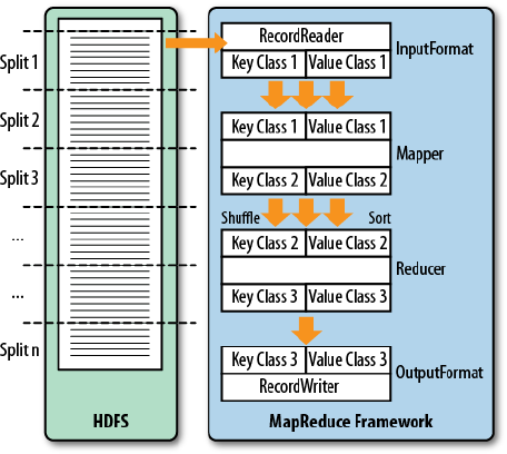
Figure 7-1. The MapReduce process
This (rather simplified) figure of the MapReduce process shows you
how the data is processed. The first thing that happens is the split,
which is responsible for dividing the input data into reasonably sized
chunks that are then processed by one server at a time. This splitting
has to be done in a somewhat smart way to make best use of available
servers and the infrastructure in general. In this example, the data
may be a very large log file that is divided into pieces of equal size.
This is good, for example, for Apache HTTP Server log files. Input da‐
ta may also be binary, though, in which case you may have to write
your own getSplits() method—but more on that shortly.
The basic principle of MapReduce (and a lot of other processing en‐
gines or frameworks) is to extract key/value pairs from the input data.
Depending on the processing engine, they might be called tuples, fea‐
ture vectors, or records, and so. MapReduce refers to them as records
(see The MapReduce counters showing the records processed),
though the idea is the same: we have data points that need to be pro‐
cessed. In MapReduce there is an extra emphasis on the key part of
each record, since it is used to route and group the values as part of
the processing algorithm. Each key and value also have a defined
type, which reflect their nature and makes processing less ambiguous.
As part of the setup of each MapReduce workflow, the job designer
has to assign the types to each key/value as it is passed through the
processing stages.
Framework 561
www.finebook.ir

The MapReduce counters showing the records processed.
...
Map-Reduce Framework
Map input records=289
Map output records=2157
Map output bytes=22735
Map output materialized bytes=10992
Input split bytes=137
Combine input records=2157
Combine output records=755
Reduce input groups=755
Reduce shuffle bytes=10992
Reduce input records=755
Reduce output records=755
...
Processing Classes
Figure 7-1 also shows you the classes that are involved in the Hadoop
implementation of MapReduce. Let us look at them and also at the
specific implementations that HBase provides in addition.
MapReduce versus Mapred, versus MapReduce v1 and
v2
Hadoop version 0.20.0 introduced a new MapReduce API. Its
classes are located in the package named mapreduce, while the
existing classes for the previous API are located in mapred. The
older API was deprecated and should have been dropped in ver‐
sion 0.21.0—but that did not happen. In fact, the old API was un‐
deprecated since the adoption of the new one was hindered by its
initial incompleteness.
HBase also has these two packages, which started to differ more
and more over time, with the new API being the actively support‐
ed one. This chapter will only refer to the new API, that is, when
you need to use the mapred package instead, you will have to re‐
place the respective classes. Some are named slightly different,
but fulfil the same purpose (for example, TableMap versus Table
Mapper). Yet others are not available in the older API, and would
need to be ported by manually. Most of the classes are self-
contained or have little dependencies, which means you can copy
them into your own source code tree and compile them with your
job archive file.
On the other hand—not to complicate matters presumably--, there
is the difference between MapReduce v1 and v2, mentioned earli‐
Chapter 7: Hadoop Integration562
www.finebook.ir
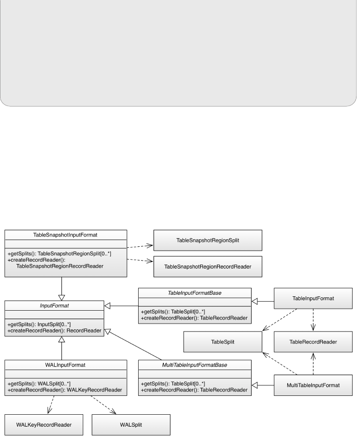
1. Note the switch of language here: sometimes Hadoop refers to the processed data
as records, sometimes as KeyValues. These are used interchangeably.
er. The differences in v1 and v2 are not the API, but their imple‐
mentations, with v1 being a single, monolithic framework, and v2
being an application executed by YARN. This change had no im‐
pact on the provided APIs by MapReduce, and both, v1 and v2, of‐
fer the mapreduce and mapred packages. Since YARN is the official
processing framework as of Hadoop 2.2 (released in 2013), and
since both expose the same API, this chapter will use YARN to ex‐
ecute the MapReduce examples.
InputFormat
The first hierarchy of classes to deal with is based on the InputFormat
class, shown in Figure 7-2. They are responsible for two things: first,
split the input data into chunks, and second, return a RecordReader
instance that defines the types of the key and value objects, and also
provides a nextKeyValue() method that is used to iterate over each
input record.1
Figure 7-2. The InputFormat hierarchy
Framework 563
www.finebook.ir

As far as HBase is concerned, there the following special implementa‐
tions:
TableInputFormat
This class is based on TableInputFormatBase, which implements
the majority of the functionality but remains abstract. TableInput
Format is used by many supplied examples, tools, and real MapRe‐
duce classes, as it provides the most generic functionality to iter‐
ate over data stored in a HBase table.
You either have to provide a Scan instance that you can prepare in
any way you want: specify start and stop keys, add filters, specify
the number of versions, and so on, or you have to hand in these pa‐
rameters separately and the framework will set up the Scan in‐
stance internally. See Table 7-1 for a list of all the basic proper‐
ties.
Table 7-1. The basic TableInputFormat configuration proper‐
ties
Property Description
hbase.mapreduce.inputtable Specifies the name of the table to read.
hbase.mapreduce.splittable Specifies an optional table to use for split
boundaries. This is useful when you are
preparing data for bulkload.
hbase.mapreduce.scan A fully configured, base-64 encoded scanner. All
other scan properties are ignored if this is
specified. See TableMapReduceUtil.convertScan
ToString(Scan) for more details.
hbase.mapre
duce.scan.row.start The optional start row key of the scan (see
Scan.setStartRow()).
hbase.mapre
duce.scan.row.stop The optional stop row key for the scan (see
Scan.setStopRow()).
hbase.mapreduce.scan.col
umn.family When given, specifies the column family to scan
(see Scan.addFamily()).
hbase.mapreduce.scan.col
umns Optional space character-delimited list of
columns to include in scan (see Scan.addCol
umn()).
hbase.mapreduce.scan.time
stamp Allows to set a specific timestamp for the scan to
return only those exact versions (see Scan.setTi
meStamp()).
hbase.mapreduce.scan.time
range.start/hbase.mapre
duce.scan.timerange.end
The starting and ending timestamp used to filter
columns with a specific range of versions (see
Scan.setTimeRange()). Both must be set to take
effect.
Chapter 7: Hadoop Integration564
www.finebook.ir

Property Description
hbase.mapreduce.scan.maxver
sions The maximum number of version to return (see
Scan.setMaxVersions()).
hbase.mapreduce.scan.cache
blocks Set to false to disable server-side caching of
blocks for this scan (see Scan.setCacheBlocks()).
hbase.mapreduce.scan.cache
drows The number of rows for caching that will be
passed to scanners (see Scan.setCaching()).
hbase.mapreduce.scan.batch
size Set the maximum number of values to return for
each call to next() (see Scan.setBatch()).
Some of these properties are assignable through dedicated setter
methods, for example, the setScan() or configureSplitTable()
calls. You will see examples of that in “Supporting Classes” (page
575) and “MapReduce over Tables” (page 586).
The TableInputFormat splits the table into proper blocks for you
and hands them over to the subsequent classes in the MapReduce
process. See “Table Splits” (page 583) for details on how the table is
split. The provided, concrete implementations of the inherited
getSplits() and createRecordReader() methods return the spe‐
cial TableSplit and TableRecordReader classes, respectively.
They wrap each region of a table into a split record, and return the
rows and columns as configured by the scan parameters.
MultiTableInputFormat
Since a TableInputFormat is only handling a single table with a
single scan instance, there is another class extending the same
idea to more than one table and scan, aptly named MultiTableIn
putFormat. It is only accepting a single configuration property,
named hbase.mapreduce.scans, which holds the configured scan
instance. Since the Configuration class used allows to specify the
same property more than once, you can add more than one into
the current job instance, for example:
List<Scan> scans = new ArrayList<Scan>();
Scan scan = new Scan();
scan.setAttribute(Scan.SCAN_ATTRIBUTES_TABLE_NAME,
Bytes.toBytes("prodretail:users"));
scans.add(scan);
scan = new Scan();
scan.setAttribute(Scan.SCAN_ATTRIBUTES_TABLE_NAME,
Bytes.toBytes("prodchannel:users"));
scan.setTimeRange(...);
scans.add(scan);
...
TableMapReduceUtil.initTableMapperJob(scans, ReportMap‐
Framework 565
www.finebook.ir
2. As of this writing, there is also a deprecated class named HLogInputFormat that on‐
ly differs from WALInputFormat in that it handles the equally deprecated HLogKey
class, as opposed to the newer WALKey.
per.class,
ImmutableBytesWritable.class, ImmutableBytesWritable.class,
job);
This uses an up until now unmentioned public constant, exposed
by the Scan class:
static public final String SCAN_ATTRIBUTES_TABLE_NAME = \
"scan.attributes.table.name";
It is needed for the MultiTableInputFormat to determine the
scanned tables. The previous TableInputFormat works the other
way around by explicitly setting the scanned table, because there
is only one. Here we assign the tables to the one or more scans
handed into the MultiTableInputFormat configuration, and then
let it iterate over those implicitely.
TableSnapshotInputFormat
This input format class allows you to read a previously taken table
snapshot. What has been omitted from the class diagram is the re‐
lationship to another class in the mapreduce package, the TableS
napshotInputFormatImpl. It is shared between the two API imple‐
mentations, and provides generic, API independent functionality.
For example, it wraps a special InputSplit class, which is then
further wrapped into a TableSnapshotRegionSplit class by the Ta
bleSnapshotInputFormat class. It also has the getSplits() meth‐
od that understands the layout of a snapshot within the HBase root
directory, and is able to wrap each contained region into a split in‐
stance. Since this is the same no matter which MapReduce API is
used, the functionality is implemented in the shared class.
The dedicated snapshot input format also has a setter named se
tInput() that allows you to assign the snapshot details. You can
access this method directly, or use the utility methods provided by
TableMapReduceUtil, explained in “Supporting Classes” (page 575).
The setInput() also asks for the name of a temporary directory,
which is used internally to restore the snapshot, before it is read
from. The user running the MapReduce job requires write permis‐
sions on this directory, or the job will fail. This implies that the di‐
rectory must be, for example, outside the HBase root directory.
WALInputFormat
If you ever need to read the binary write-ahead logs that HBase
generates, you can employ this class to access them.2 It is primari‐
Chapter 7: Hadoop Integration566
www.finebook.ir
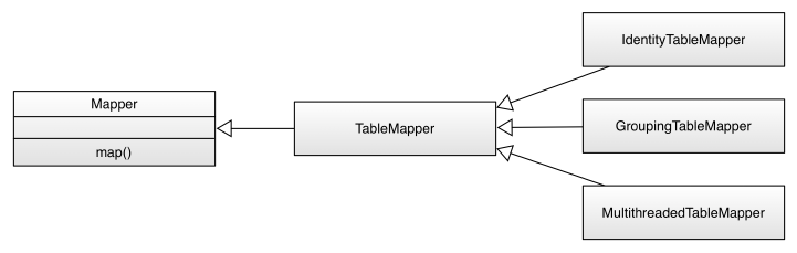
ly used by the WALPlayer class and tool to reply write-ahead logs
using MapReduce. Since WALs are rolled by default when they ap‐
proach the configured HDFS block size, it is not necessary to cal‐
culate splits. Instead, each WAL is mapped to one split. The only
exposed configuration properties for the WAL input format are:
public static final String START_TIME_KEY = "wal.start.time";
public static final String END_TIME_KEY = "wal.end.time";
They allow the user to specify which entries should be read from
the logs. Any record before the start, and after the end time will be
ignored. Of course, these properties are optional, and if not given
the entire logs are read and each record handed to the processing
function.
With all of these classes, you can always decide to create your own, or
extend the given ones and add your custom business logic as needed.
The supplied classes also provide methods (some have their Java
scope set as protected) that you can override to slightly change the
behavior without the need of implementing the same functionality
again. The classes ending Base are also a good starting point for your
own implementations, since they offer many features, and thus form
the basis for the provided concrete classes, and could do the same for
your own.
Mapper
The Mapper class(es) is for the next stage of the MapReduce process
and one of its namesakes (Figure 7-3). In this step, each record read
using the RecordReader is processed using the map() method.
Figure 7-1 also shows that the Mapper reads a specific type of key/
value pair, but emits possibly another type. This is handy for convert‐
ing the raw data into something more useful for further processing.
Figure 7-3. The Mapper hierarchy
Framework 567
www.finebook.ir
HBase provides the TableMapper class that enforces key class 1 to be
an ImmutableBytesWritable, and value class 1 to be a Result type—
since that is what the TableRecordReader and TableSnapshotRecor
dReader are returning. There are multiple implementations of derived
mapper classes available:
IdentityTableMapper
One subclass of the TableMapper is the IdentityTableMapper,
which is also a good example of how to add your own functionality
to the supplied classes. The TableMapper class itself does not im‐
plement anything but only adds the signatures of the actual key/
value pair classes. The IdentityTableMapper is simply passing on
the keys/values to the next stage of processing.
GroupingTableMapper
This is a special subclass that needs a list of columns before it can
be used. The mapper code checks each row it is given by the
framework in form of a Result instance, and if the given columns
exists, it creates a new key as a concatenation of all values as‐
signed to each named column. If any of the columns is missing in
the row the entire row is skipped.
You can set the key columns using the static initJob() method of
this class, or assign it to the following configuration property, pro‐
vided as a public constant in the mapper class:
public static final String GROUP_COLUMNS =
"hbase.mapred.groupingtablemap.columns";
The class expects the columns to be specified as a space
character-delimited string, for example "colfam1:col1 col
fam1:col2". If these columns are found in the row, the row key is
replaced by a space character-delimited new key, for example:
Input:
"row1" -> cf1:col1 = "val1", cf1:col2 = "val2", cf1:col3 =
"val3"
Output:
"val1 val2" -> cf1:col1 = "val1", cf1:col2 = "val2",
cf1:col3 = "val3"
The purpose of this change of the map output key value is the sub‐
sequent reduce phase, which receives key/values grouped based
on the key. The shuffle and sort steps of the MapReduce frame‐
work ensure that the records are sent to the appropriate Reducer
instance, which is usually another server somewhere in the clus‐
ter. By being able to group the rows using some column values you
Chapter 7: Hadoop Integration568
www.finebook.ir

can send related rows to a single reducer and therefore perform
some processing function across all of them.
MultiThreadedTableMapper
One of the basic principles of the MapReduce framework is that
the map and reduce functions are executed by a single thread,
which simplifies the implementation because there is no need to
take of thread-safety. Often—for performance reasons—class in‐
stances are reused to process data as fast as can be read from
disk, and not being slowed down by object instantiation. This is es‐
pecially true for very small data points.
On the other hand, sometimes the processing in the map function
is requiring an excessive amount of time, for example when data is
acquired from an external resource, over the network. An example
is a web crawling map function, which loads the URL from one
HBase table, retrieves the page over the Internet, and writes the
fetch content into another HBase table. In this case you mostly
wait for the external operation.
Since each map takes up a slot of the processing framework, it is
considered scarce, and is limited to what the scheduler is offering
to your job. In other words, you can only crawl the web so fast as
you receive processing capacities, but then wait for an external re‐
source most of the time. The MultiThreadedTableMapper is avail‐
able for exactly that reason, enabling you to turbo-charge your
map function by executing it in a parallel fashion using a thread
pool. The pool is controlled by the following configuration proper‐
ty, or the respective getter and setter:
public static final String NUMBER_OF_THREADS = \
"hbase.mapreduce.multithreadedmapper.threads";
public static int getNumberOfThreads(JobContext job)
public static void setNumberOfThreads(Job job, int threads)
Since you effectively bypass the number of threads as‐
signed to you by the scheduler and instead multiply that
number at your will, you must take not to exhaust any vital
resources in the process. For example, if you were to use
the multithreaded mapper implementation to just read
from, and/or write to HBase, you can easily overload the
disk I/O. Even with YARN using Linux control groups
(cgroups), or other such measures to guard system resour‐
ces, you have to be very careful.
Framework 569
www.finebook.ir
The number of threads to use is dependent on your external wait
time, for example, if you fetch web pages as per the example
above, you may want to gradually increase the thread pool to
reach CPU or network I/O saturation. The default size of the
thread pool is 10, which is conservative start point. Before you can
use the threaded class you need to assign the actual map function
to run. This is done using the following configuration property, or
again using the provided getter and setter methods:
public static final String MAPPER_CLASS = \
"hbase.mapreduce.multithreadedmapper.mapclass";
public static <K2, V2> Class<Mapper<ImmutableBytesWritable, Re‐
sult, K2, V2>> \
getMapperClass(JobContext job)
public static <K2, V2> void setMapperClass(Job job, \
Class<? extends Mapper<ImmutableBytesWritable, Result, K2,
V2>> cls)
The only difference to a normal map method is that you have to im‐
plement it in a thread-safe manner, just as any other Runnable
based Java thread executable. This implies that you cannot reuse
simple instance variables, unless they refer to an object that itself
is thread-safe as well.
Reducer
The Reducer stage and class hierarchy (Figure 7-4) is very similar to
the Mapper stage. This time we get the output of a Mapper class and
process it after the data has been shuffled and sorted.
In the implicit shuffle between the Mapper and Reducer stages, the in‐
termediate data is copied from different Map servers to the Reduce
servers and the sort combines the shuffled (copied) data so that the
Reducer sees the intermediate data as a nicely sorted set where each
unique key is now associated with all of the possible values it was
found with.
Chapter 7: Hadoop Integration570
www.finebook.ir
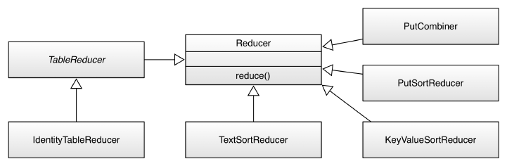
Figure 7-4. The Reducer hierarchy
There are again a set of derived classes available, though for direct
table operations there is only one: the TableReducer class. It has a
subclass called IdentityTableReducer, and all it does is make the
former abstract class a concrete, usable one. In other words, the basic
functionality of a Reducer based class is to pass on the data un‐
changed. If you want anything else, you need to implement your own.
Then there are a few more classes directly subclassing Reducer.
These are all needed for bulk loadiing data into HBase, as discussed in
(to come). Dependent on the type of data being loaded, one of TextSor
tReducer, PutSortReducer, or KeyValueSortReducer is used to emit
the bulk loader data in a sorted manner. The PutCombiner is an opti‐
mization used in the ImportTsv tool to combine many smaller puts in‐
to one larger one. This is close to the recommended Combiner usage
within Hadoop, reducing transfer of data between Mapper and Reduc
er instances during the shuffle phase. There could potentially be hun‐
dred or thousands of Put objects that would need to be serialized and
sent to the reducer process on a remote server. Combining these into
one does not reduce the size of the data, but reduces class overhead.
OutputFormat
The final stage is the OutputFormat class hierarchy (Figure 7-5), and
the job of these classes is to persist the data in various locations.
There are specific implementations that allow output to files, or to
HBase tables, and we are going to discuss each of them subsequently.
Framework 571
www.finebook.ir
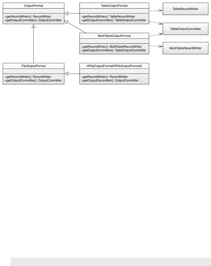
Figure 7-5. The OutputFormat hierarchy
TableOutputFormat
This class is the default output format for many MapReduce jobs
that need to write data back into HBase tables. It uses a TableRe
cordWriter to write the data into the specific HBase output table.
The latter uses a BufferedMutator instance to buffer writes be‐
fore sending them in batches to the servers. The provided write()
method expects to receive either a Put or a Delete instance, and
uses the BufferedMutator.mutate() method to persist them. If
you hand in something else, for example a Get or Increment in‐
stance an error is thrown instead. The close() method of the re‐
cord writer class closes the mutator, enforcing the flush of any
pending write operation to the servers.
It is important to note the cardinality as well. Although many Map
pers are handing records to many Reducers, only one OutputFor
mat instance takes the output records from its assigned Reducer
subsequently. It is the final class that handles the key/value pairs
and writes them to their final destination, this being a file or a
table. You need to configure the output format using the configu‐
ration properties shown in Table 7-2.
Table 7-2. The TableOutputFormat configuration properties
Property Description
hbase.mapred.outputta
ble The table to write into (required).
hbase.mapred.out
put.quorum Optional parameter to specify a peer cluster. Used to
specifying a remote cluster when copying between
hbase clusters (the source cluster is picked up from
hbase-site.xml).
Chapter 7: Hadoop Integration572
www.finebook.ir

Property Description
hbase.mapred.out
put.quorum.port Optional parameter to specify the peer cluster’s
ZooKeeper client port.
hbase.mapred.out
put.rs.class Optional specification of the RegionServer class name
of the peer cluster.
hbase.mapred.out
put.rs.impl Optional specification of the RegionServer
implementation name of the peer cluster.
These properties are exposed as public constants, allowing you to
refer to them as needed, or you can use, for example, the initTa
bleReducerJob() method of the TableMapReduceUtil helper class
to set the table name implicitly. The name of the output table must
be specified when the job is set up. Otherwise, the TableOutput
Format does not add much more complexity.
The four optional properties allow you to set up a job that reads
from one cluster—configured by the current configuration instance
—and write to another. The above initTableReducerJob() call
(one of the overloaded version) has facilities for assigning these
properties as well.
MultiTableOutputFormat
An extension to the direct TableOutputFormat is the ability to
write to more than one single output table. For that matter, the
dedicated MultiTableRecordWriter uses a need “trick” to coax in
the table name for every record emitted by the map or reduce
task: it defines the types of the writer as RecordWriter<Immutable
BytesWritable, Mutation>, using the key as the table name. Usu‐
ally the key is not needed for the HBase mutations to be written to
a table, as the name of the latter is set in the configuration of the
job. In fact, the TableOutputFormat with its TableRecordWriter
completely ignore the key, while simply persisting the handed in
put or delete object into the globally configured buffered mutator.
In other words, the change in usage is that a map or reduce task
needs to take care of what to emit by specifying the destination
table name, and the mutation (the put or delete). For example,
usually you would emit a mutation in a map or reduce method us‐
ing the TableOutFormat like so:
context.write(new ImmutableBytesWritable(rowkey), put);
Instead, you switch the key out to name the table instead:
context.write(new ImmutableBytesWritable(tableName), put);
Framework 573
www.finebook.ir

Internally the class uses a BufferedMutator instance for every
named table. In addition, the following constants are exposed by
the class:
public static final String WAL_PROPERTY = \
"hbase.mapreduce.multitableoutputformat.wal";
public static final boolean WAL_ON = true;
public static final boolean WAL_OFF = false;
They allow you to influence the durability settings for the write op‐
eration, as explained in “Durability, Consistency, and Isolation”
(page 108).
A few more general notes on the output formats and their supporting
classes:
1. The TableOutputCommitter class, used by both the above output
formats, is required for the Hadoop framework to do its job. For
HBase integration, this class is not needed. In fact, it is a dummy
and does not do anything. Other implementations of OutputFormat
do require a specific output committer, but for HBase an empty
implementation is all that is needed.
2. The BufferedMutator instances used have no explicit setter or
getter regarding their configuration. Instead, you have to set the
configuration properties influencing the buffered mutators before
you set up the MapReduce job. The settings will be passed into the
wrapping output formats through the job context. Table 7-3 lists
the properties with their default values. Especially the write buffer
should be tuned based on the use-case, where its size should ac‐
count for a decent amount of mutations to save on the batched net‐
work roundtrips.
Table 7-3. Important configuration settings influencing the Buffer
edMutator behavior
Property Default Description
hbase.cli
ent.write.buffer 2097152 (2MB) Configures the local write buffer in
bytes.
hbase.client.keyval
ue.maxsize 10485760
(10MB) Limits the maximum cell size a client
can write.
hbase.client.retries.num
ber 35 Number of retries before failing the
operation.
hbase.client.pause 100 (ms) Initial pause between retries.
Increases incrementally for retries.
hbase.rpc.timeout 60000 (1 min) The connection timeout for the
remote server call.
Chapter 7: Hadoop Integration574
www.finebook.ir
Finally, there is a third class of input format, which is not directly
based on OutputFormat, but FileOutputFormat instead. The reason to
rather extend FileOutputFormat is based on the built in features of
that class and the need to write HBase storage files, called HFile, di‐
rectly into the configured file storage layer, usually HDFS.
HFileOutputFormat/HFileOutputFormat2
This output format is used to stage HFile’s before they are loaded
into the tables, as explained in (to come). The difference between
these two classes is that the former is for the now deprecated Key
Value class, for legacy reasons, and the latter is for the newer
Cell classes. The class exposes a static, overloaded method named
configureIncrementalLoad() which simplifies setting up a Map‐
Reduce job using this output format.
Part of setting up the HFile specific RecordWriter is to set the ap‐
propriate table properties, including maximum file size, compres‐
sion format, Bloom filter type, the HFile block size, and block en‐
coding format. Many are optional, and will default to what the pro‐
vided hbase-site.xml file on the Java class path specifies. The
emitted Cell will define which column families are generated, thus
there is no need of specifying them explicitly. For the bulk load to
work, there are quite a few steps involved, for example, sorting
and routing the written Cells at a cluster-wide scale, using the To
talOrderPartitioner provided by Hadoop. This ensure that the
cells for a specific row all end up being written in the expected
sort-order by one reducer.
Supporting Classes
The MapReduce support comes with the TableMapReduceUtil class
that helps in setting up MapReduce jobs over HBase. It has static
methods that configure a job so that you can run it with HBase as the
source and/or the target. It also has other helper methods to configure
various aspects of working with the MapReduce framework. They can
be grouped as such:
Class Path Setup
There are two variants of the addDependencyJars() method, with
one finding all the containing JAR files given a list of classes. It
adds the found JAR files to the provided configuration instance us‐
ing the tmpjars property. This is honored by the MapReduce sys‐
tem which includes these JARs into the job setup using the Hadoop
distributed cache. In other words, you will not have to do anything
else to run the job.
Framework 575
www.finebook.ir
The method is powerful enough to work in development environ‐
ment, checking each named class file, and if it is not contained in a
JAR file already (that is, it was loaded from a JAR before the check
ran) it creates a JAR file on the fly and adds it to the configuration.
The temporary file is created using the File.createTempFile()
method, and used "hadoop-" as its name prefix. The location is set
by the test.build.dir configuration property, and defaults to tar
get/test-dir.
The second variant of the addDependencyJars() call just asks for a
Job instance, and adds all HBase and user JARs necessary for the
job execution, using the previous method. It looks at every class
named in the job configuration, for example, the mapper and re‐
ducer classes, and adds them to the job configuration. Implicitly it
calls a third class path related method named addHBaseDependen
cyJars(), which does the same for all HBase JARs a client may
possibly need. The end result is that all required JAR files, from
HBase or your own, are specified in the supplied configuration in‐
stance.
Lastly, the buildDependencyClasspath() method uses the
tmpjars property, retrieving all of the configured JARs, and re‐
turning a string suitable for an operating system specific search
path definition. For example, on Linux this may return something
of the following pattern: <path-to-jar>/<jarname1>.jar:<path-
to-jar>/<jarname2>.jar:.... It is using the path and directory
divider symbols configured for the platform it executes on.
Security Configuration
These calls allow you to set security credentials, but only do some‐
thing useful when security is enabled (see (to come)). There is in
itCredentials() which passes on the details about the config‐
ured Hadoop delegation tokens and configures the users creden‐
tials. This is done by authenticating and retrieving the valid tokens
to the job configuration. Before though the method also configures
the appropriate ZooKeeper properties within the configuration,
since it is needed to determine the unique cluster ID. Eventually
the method sends a request to the authentication coprocessor of
that cluster to retrieve the tokens, and assign them to the job con‐
figuration. This is done for the source and target cluster, if config‐
ured with the hbase.mapred.output.quorum property (as ex‐
plained in “OutputFormat” (page 571)).
The initCredentialsForCluster() always assumes an external
cluster, and asks for ZooKeeper quorum details explicitly. After
that it does the same thing, that is, it authenticates the user by
Chapter 7: Hadoop Integration576
www.finebook.ir
sending a request to the coprocessor, and adding the returned to‐
ken information to the job configuration.
Configure Table as Input
The initTableMapperJob() call comes in many variations. They
are essential in setting up MapReduce jobs where the HBase table
acts as in input to a Map instance. Here an example signature of
one variant:
public static void initTableMapperJob(String table, Scan scan,
Class<? extends TableMapper> mapper, Class<?> outputKeyClass,
Class<?> outputValueClass, Job job, boolean addDependency‐
Jars,
boolean initCredentials, Class<? extends InputFormat> input‐
FormatClass)
throws IOException
The calls add more or less details to the job configuration, so that
you can choose which is the most suitable to your task at hand. In
general, the calls do the following:
1. Configure the job with the given InputFormat class
2. If given, overwrite the output key and value class types
3. Assign the given mapper class to the job
4. Optionally, set the PutCombiner as combiner class, when the
output value type is Put
5. Merge the currently visible Hadoop and HBase configuration
into the job configuration
6. Set the given table name in the configuration
7. Serialize the configured Scan instance and assign it to the con‐
figuration
8. Overwrite the default Hadoop Writable based serialization
with a custom HBase one, based on Protobufs:
conf.setStrings("io.serializations", conf.get("io.seriali‐
zations"),
MutationSerialization.class.getName(),
ResultSerialization.class.getName(),
KeyValueSerialization.class.getName());
9. Optionally, call addDependencyJars() to add all JARs to the
class path
10. Optionally, set up the security credentials using initCreden
tials()
The mentioned Serialization classes are also part of the map
reduce package, and handle the conversion of mutations,
Framework 577
www.finebook.ir

query result, and cells in a platform independent manner, us‐
ing Google’s Protocol Buffers, and discussed in depth in “Seri‐
alization” (page 353). They are not used explicitly anywhere
else, so their implicit use by the initTableMapperJob() is
somewhat hidden. Especially if you do not use the utility meth‐
ods provided, you would need to set these classes manually, as
shown in the code excerpt above.
Configure Table as Output
The counterpart of the previous set of methods is this one, and it
configures a TableOutputFormat to use a HBase table as the tar‐
get for data emitted from the MapReduce job.
Keep in mind that the MapReduce OutputFormat is used
in combination with a single Reducer instance. In case of a
map-only job though the output format is called directly by
the map function.
The provided initTableReducerJob() call again comes in multiple
versions, offering fewer to more parameters. Here is the fully
specified variant for your perusal:
public static void initTableReducerJob(String table,
Class<? extends TableReducer> reducer, Job job,
Class partitioner, String quorumAddress, String serverClass,
String serverImpl, boolean addDependencyJars) throws IOExcep‐
tion
The following tasks are performed when invoking these methods:
1. Merge the currently visible Hadoop and HBase configuration
into the job configuration
2. Assign the given output format class to the job
3. If given, set the reducer class for the job
4. Set the output table name in the configuration
5. Overwrite the default Hadoop Writable based serialization
with a custom HBase one, based on Protobufs
6. Optionally, set the target cluster ZooKeeper quorum informa‐
tion
7. Optionally, assign the region server interface and implementa‐
tion class name
8. Set the output key type to ImmutableBytesWritable and out‐
put value type to Writable
Chapter 7: Hadoop Integration578
www.finebook.ir
9. Assign the given partitioner to the job
a. In case of the supplied HRegionPartioner, also limit the
number of reduce tasks to run to be not greater than the
number of regions in the output table
10. Optionally, call addDependencyJars() to add all JARs to the
class path
11. Set up the security credentials using initCredentials()
This is very similar to the above initTableMapperJob(), but
with a few difference to match the different purpose of writing
into a table, instead of reading from it. Again, if you decide not
to use this helper method, please study carefully what it does
and make sure you do everything required for your use-case as
well.
Configure Snapshot as Input
The supplied initTableSnapshotMapperJob() sets the name and
temporary directory required using the setInput() method of the
TableSnapshotInputFormat class, and then proceeds to invoke in
itTableMapperJob() while mostly passing on the parameters giv‐
en by the caller. It also assigns the TableSnapshotInputFormat as
the input format class for the job. One special function it performs
is to overrides any block cache configuration that could cause the
MapReduce task to exhaust its (usually scarce) resources.
Miscellaneous Tasks
The utility class TableMapReduceUtil has a few more generic
methods, which are called from the other helpers, or can be called
by your own code as necessary. The limitNumReduceTasks() en‐
sures the number of requested reduce tasks for the MapReduce
job does not exceed the number of available regions. setNumRedu
ceTasks(), on the other hand, sets the number of reduce tasks to
be the matching number of regions for the given table. This allows
you to set up a job where you have a single reduce task responsi‐
ble for exactly one region of the output table.
The already mentioned resetCacheConfig() overrides the cache
configuration for the sake of memory limitations. And setScanner
Caching() sets the hbase.client.scanner.caching property of
the job configuration to the given value. With that you can influ‐
ence for the particular job how many rows are fetched from the
servers in one RPC. It obviously overwrites any existing value, in‐
cluding the default value.
Framework 579
www.finebook.ir
There are a few more classes that are used implicitly but are required
for proper results.
HRegionPartitioner
As mentioned when we discussed the initTableReducerJob()
method of the TableMapReduceUtil utility class, this Hadoop Par
titioner implementation serves the purpose of routing the muta‐
tions to the TableOutputFormat handling a specific region of the
output table. It uses a RegionLocator instance configured with the
specified output table to decided where each put or delete has to
be send. Obviously, this implies to carefully pre-split a new table to
achieve proper load distribution across all region servers. If you
load into an existing table, it still is frugal to ensure the table has
enough regions to make, for example, the staging of the bulk load‐
ing efficient.
CellCreator
This class is used internally as part of the bulk loading process
with HFileOutputFormat, and more specifically the TextSortRe
ducer that receives the cells in text format and uses a parser to
separate out the details. Once the parsing is complete for a cell,
the CellCreator is used to convert the information into a Cell in‐
stance, which is then handed to the output format. Internally there
is also made use of the supplied VisibilityExpressionResolver
and DefaultVisibilityExpressionResolver classes, to convert
security information into cell tags.
JarFinder
The mentioned addDependencyJars() uses this helper class to
find, and optionally wrap development classes into JAR files, for
adding them to the job configuration.
SimpleTotalOrderPartitioner
You can use this class to distribute mutations in your own MapRe‐
duce jobs, based on a configurable key range. The range is speci‐
fied with the static setStartKey() and setEndKey() methods of
this class, where the end key must be exclusive, that is, at least
one byte greater than the biggest key you will use. It uses the Big
Decimal class to convert the specified keys into numbers, splitting
them into equally sized partitions using the Bytes.split() utility
method.
The package provides a few more classes, with one group serving the
bulk import feature discussed in (to come). The ImportTsv, TsvImpor
terMapper, TsvImporterTextMapper, and LoadIncrementalHFiles
classes are all used as part of that process. The remaining classes are
used in other HBase tools, explained in (to come).
Chapter 7: Hadoop Integration580
www.finebook.ir
MapReduce Locality
One of the more ambiguous things in Hadoop is block replication: it
happens automatically and you should not have to worry about it.
HBase relies on it to provide durability as it stores its files into the dis‐
tributed filesystem. Although block replication works completely
transparently, users sometimes ask how it affects performance.
This question usually arises when the user starts writing MapReduce
jobs against either HBase or Hadoop directly. Especially when larger
amounts of data are being stored in HBase, how does the system take
care of placing the data close to where it is needed? This concept is
referred to as data locality, and in the case of HBase using the Ha‐
doop File System (HDFS), users may have doubts as to whether it is
working.
First let us see how Hadoop handles this: the MapReduce documenta‐
tion states that tasks run close to the data they process. This is
achieved by breaking up large files in HDFS into smaller chunks, or
blocks, with a default setting of 128 MB. Each block is assigned to a
map task to process the contained data. This means larger block sizes
equal fewer map tasks to run as the number of mappers is driven by
the number of blocks that need processing.
Hadoop knows where blocks are located, and runs the map tasks di‐
rectly on the node that hosts the block. Since block replication en‐
sures that we have (by default) three copies on three different physi‐
cal servers, the framework has the choice of executing the code on
any of those three, which it uses to balance workloads. This is how it
guarantees data locality during the MapReduce process.
Back to HBase. Once you understand that Hadoop can process data
locally, you may start to question how this may work with HBase. As
discussed in (to come), HBase transparently stores files in HDFS. It
does so for the actual data files (HFile) as well as the logs (WAL). And
if you look into the code, it uses the Hadoop API call FileSystem.cre
ate(Path path) to create these files.
Framework 581
www.finebook.ir

If you do not co-share your cluster with Hadoop and
HBase, but instead employ a separate Hadoop as well as a
standalone HBase cluster, there is no data locality—there
can’t be. This is the same as running a separate MapRe‐
duce cluster that would not be able to execute tasks di‐
rectly on the data node. It is imperative for data locality to
have the Hadoop and HBase processes running on the
same cluster.
How does Hadoop figure out where data is located as HBase accesses
it? The most important factor is that HBase servers are not restarted
frequently and that they perform housekeeping on a regular basis.
These so-called compactions rewrite files as new data is added over
time. All files in HDFS, once written, are immutable (for all sorts of
reasons). Because of that, data is written into new files, and as their
number grows, HBase compacts them into another set of new, consoli‐
dated files.
And here is the kicker: HDFS is smart enough to put the data where it
is needed! It has a block placement policy in place that enforces all
blocks to be written first on a colocated server. The receiving data
node compares the server name of the writer with its own, and if they
match, the block is written to the local filesystem. Then a replica is
placed on a server within a remote rack, and another on a different
server in the remote rack—all assuming you have rack-awareness con‐
figured within HDFS. If not, the additional copies get placed on the
least loaded data node in the cluster.
If you have configured a higher replication factor, more replicas are
stored on distinct machines. The important factor here, though, is that
you now have a local copy of the block available. For HBase, this
means that if the region server stays up for long enough (which is
what you want), after a major compaction on all tables—which can be
invoked manually or is triggered by a configuration setting—it has the
files stored locally on the same host. The data node that shares the
same physical host has a copy of all data the region server requires. If
you are running a scan or get or any other use case, you can be sure
to get the best performance.
An issue to be aware of is region movements during load balancing, or
server failures. In that case, the data is no longer local, but over time
it will be once again. The master also takes this into consideration
when a cluster is restarted: it assigns all regions to the original region
Chapter 7: Hadoop Integration582
www.finebook.ir

3. This is not entirely true, the shared TableInputFormatBase class has a protected
method named includeRegionInSplit() which by default returns true. A custom
subclass could override the method and not include all regions belonging to the
configured scan.
servers. If one of them is missing, it has to fall back to the random re‐
gion assignment approach.
The HDFS balancer is another factor that potentially could
wreak havoc on block locality when run without the knowl‐
edge that HBase needs specific blocks to be kept on a spe‐
cific server. See HDFS-6133 for the feature required to
skip HBase blocks during balancer executions. It is avail‐
able in Hadoop 2.7 and later.
Table Splits
When running a MapReduce job in which you read from a table, you
are typically using the TableInputFormat. It fits into the framework
by overriding the required public methods getSplits() and createRe
cordReader(). Before a job is executed, the framework calls getS
plit() to determine how the data is to be separated into chunks, be‐
cause it sets the number of map tasks the job requires.
For HBase, the TableInputFormat uses the information about the
table it represents—based on the Scan instance you provided—to di‐
vide the table at region boundaries. Since it has no direct knowledge
of the effect of the optional filter, it uses the start and stop keys to
narrow down the number of regions. The number of splits, therefore,
is equal to all regions between the start and stop keys. If you do not
set the start and/or stop key, all are included.3
When the job starts, the framework is calling createRecordReader()
as many times as it has splits. It iterates over the splits and creates a
new TableRecordReader by calling createRecordReader() with the
current split. In other words, each TableRecordReader handles exact‐
ly one region, reading and mapping every row between the region’s
start and end keys.
The split also contains the server name hosting the region. This is
what drives locality for MapReduce jobs over HBase: the framework
checks the server name, and if a YARN worker node process is run‐
ning on the same machine, it will preferably run it on that server. Be‐
cause the region server is also colocated with the data node on that
Framework 583
www.finebook.ir

same node, the scan of the region will be able to retrieve all data from
the local disk.
When running MapReduce over HBase, it is strongly ad‐
vised that you turn off speculative execution mode. It will
only create more load on the same region and server, and
also works against locality: the speculative task is execut‐
ed on a different machine, and therefore will not have the
region server local, which is hosting the region. This re‐
sults in all data being sent over the network, adding nega‐
tively to the overall I/O load.
There are two more advanced features available while the table split‐
ting is performed: balancing for skewed tables, and shuffling the
splits:
Auto-balance Splits
The split function iterates over the regions in their natural order,
using their boundaries to set up the start and end of each split.
What it does not check by default is if all the region actually con‐
tain the same amount of data. This is where the auto-balance fea‐
ture comes in, controlled by the following configuration properties,
exposed by the TableInputFormatBase class:
public static final String MAPREDUCE_INPUT_AUTOBALANCE = \
"hbase.mapreduce.input.autobalance";
public static final String INPUT_AUTOBALANCE_MAXSKEWRATIO = \
"hbase.mapreduce.input.autobalance.maxskewratio";
public static final String TABLE_ROW_TEXTKEY =
"hbase.table.row.textkey";
Setting hbase.mapreduce.input.autobalance to true enables the
feature, triggering an additional check that is performed after the
usual split function has run. It consults the hbase.mapreduce.in
put.autobalance.maxskewratio property, defaulting to 3, to com‐
pare the size of each region against a skew ratio. First it computes
the average region size and multiplies that by the specified skew
ratio to determine the maximum skew threshold. It then iterates
over all regions checking if it exceeds the maximum skew thresh‐
old, and, if it does, separates it into two splits. In other words, now
two processing tasks will process one half of the larger region
each, instead of a single one doing all the work alone.
If the region size is less than the threshold, but greater than the
average size, it is added as-is. Should the region size be smaller
than the average, it attempts to combine this region plus all subse‐
Chapter 7: Hadoop Integration584
www.finebook.ir

quent one until it reaches (but not exceed) the maximum skew
threshold value. Here there will be one process function reading
more than one region. Obviously, this is counterproductive in re‐
gards to locality, as the combined split is retaining the locality in‐
formation of the first small region. The remaining regions fold into
the same split, and will most likely be read across the network—
unless coincidentally the subsequent region is colocated on the
same region server. You will need to weigh up the advantages of
splits being of similar size for a skewed table against the cost of
read some data over the network.
The hbase.table.row.textkey property is needed for those large
regions that are split in two, and helps the method to compute the
key that is in the middle of the start and end key of the region—
assuming the data within is distributed uniformly. The default is
true, which retains a human readable split key. If set to false, the
split is done on a binary level, which could result in non-printable
characters. Table 7-4 shows some examples.
Table 7-4. Example keys for auto-balanced splits
Start Key End Key Text Split Point
aaabcdefg aaafff Yes aaad
111000 1125790 Yes 111b
1110 1120 Yes 111_
{ 13, -19, 126, 127 } { 13, -19, 127, 0 } No { 13, -19, 127, -64 }
Set the text key flag appropriately for your use-case when you en‐
able the auto-balance functionality.
Shuffle Splits
The TableInputFormat class exposes another advanced property,
allowing you to shuffle the splits and therefore the map order:
public static final String SHUFFLE_MAPS = \
"hbase.mapreduce.inputtable.shufflemaps";
If set to true, this features runs after all the other split steps have
been performed. It takes the final list of splits and shuffles their
order. This is useful in the context of copying data from a table
with many regions to a table with much fewer regions. Since all
splits are initially ordered by their regions, which are subsequent,
it may cause the processing tasks to stress out the target region
server hosting the larger (in terms of key space) target region.
For example, assume you copy some data from a table with 100 re‐
gions to a table with 10 regions. Both have the same key space
Framework 585
www.finebook.ir
with the difference that in the target table a single region covers
the same key range as do 10 regions in the originating table. Also
assume we had 10 parallel processing tasks available, so now the
regions 1 to 10 would be read in parallel and written to the single
region covering the same key range. This would cause hotspotting,
and is discussed in detail in (to come).
The supplied CopyTable tool has a --shuffle option that allows
you to enable this feature.
MapReduce over Tables
The following sections will introduce you to using HBase in combina‐
tion with MapReduce. Before you can use HBase as a source or sink,
or both, for data processing jobs, you have to first decide how you
want to prepare the support by Hadoop.
Preparation
There are two vital steps required to execute MapReduce jobs:
1. Provide all necessary JAR files for the processing task to run.
2. Set all configuration parameters needed for the JARs to work as
expected.
Since running a MapReduce job needs classes from libraries not
shipped with Hadoop or the MapReduce framework, as well as their
configuration properties, you will need to make both available before
the job is executed. You have two choices: static preparation of all
task nodes, or dynamically supplying everything needed with the job
at submission time. We will discuss both in that order, but before we
do, there is the need of figuring out what has to be made available to
a processing job, no matter how it is provided.
Provision Libraries
Adding HBase support requires a fair amount of JAR files, comprising
HBase, ZooKeeper, and other supporting libraries. The best way to
figure out which classes are needed is employing the HBase command
line script like so:
$ hbase mapredcp | sed 's/:/\n/g'
...
/opt/hbase-1.1.0/lib/hbase-protocol-1.1.0.jar
/opt/hbase-1.1.0/lib/htrace-core-3.1.0-incubating.jar
/opt/hbase-1.1.0/lib/hbase-common-1.1.0.jar
/opt/hbase-1.1.0/lib/zookeeper-3.4.6.jar
Chapter 7: Hadoop Integration586
www.finebook.ir
/opt/hbase-1.1.0/lib/hbase-client-1.1.0.jar
/opt/hbase-1.1.0/lib/hbase-hadoop-compat-1.1.0.jar
/opt/hbase-1.1.0/lib/netty-all-4.0.23.Final.jar
/opt/hbase-1.1.0/lib/guava-12.0.1.jar
/opt/hbase-1.1.0/lib/protobuf-java-2.5.0.jar
/opt/hbase-1.1.0/lib/hbase-server-1.1.0.jar
The hbase shell script has two of these helper commands, classpath
and mapredcp. The difference is that the classpath command is print‐
ing all classes needed by HBase to operate, assuming you are on a
machine that is able to run any of the HBase processes. Included in
this list are:
• The HBase configuration directory, as set in $HBASE_CONF_DIR
•For the web applications (UIs), the directory containing hbase-
webapps (usually $HBASE_HOME)
•Optionally, if HBase is in a development environment, all Maven
dependencies
•All JAR files supplied by HBase, located in the $HBASE_HOME/lib
directory
•If available, all known Hadoop class path details, as returned by
hadoop classpath
•Any optional JAR file configured with $HBASE_CLASSPATH in the
hbase-env.sh configuration file
In addition, if there is a $HBASE_CLASSPATH_PREFIX variable defined,
its content is inserted at the very end, but before any other $CLASS
PATH content. This allows you to inject some dependencies that would
otherwise clash with the already included JAR files. Also, for the Ha‐
doop class path info to be set, you need to configure the $HA
DOOP_HOME variable, or otherwise ensure the hadoop script is accessi‐
ble to the hbase script.
As you can imagine, the resulting list is very long and most likely to
verbose. Instead, using the $hbase mapredcp command, you can re‐
trieve a minimal list of JARs needed for a client application, including
MapReduce jobs. What you might also note from the above is that the
classpath command includes the configuration directory, while the
mapredcp does not. We will discuss the difference next.
Setting Configuration Properties
For many libraries there is an option to provide custom configuration
files that modify, or fine tune, their behavior. This is also true for
HBase clients, which need to at least define the ZooKeeper quorum of
the cluster to contact. There are a few ways of doing that, for exam‐
MapReduce over Tables 587
www.finebook.ir
ple, set the property as a command line argument or in code, as
shown in “Fully distributed mode” (page 81) or “API Building Blocks”
(page 117). The most practical way is do have a local HBase configu‐
ration directory that contains a hbase-site.xml file with the Zoo‐
Keeper quorum set in it. You can also use this file then to set other
properties, such as number of retries for failed operations, or the con‐
nection timeout. Note that the servers already have such a directory,
and you could simply copy one over to the client to make it available
there.
Once you have a configuration directory, you usually assign its loca‐
tion to the $HBASE_CONF_DIR environment variable. The task is now to
make its content available to the job submission application, that is,
the job driver code. One of the first lines in that code is this:
Configuration conf = HBaseConfiguration.create();
The instantiation of the HBase configuration object triggers the load
of the HBase default values, and then the load of any custom hbase-
site.xml with settings that override the defaults. For that to work,
you must have the configuration directory on the class path of the job
driver application. As you have just seen, the hbase classpath com‐
mand does this for you, based on where $HBASE_CONF_DIR is pointing
to. For the hbase mapredcp command you will need to manually speci‐
fy the path as well, or it will not be known when the code executes.
Falling back to the default values will assume that the cluster is loca‐
ted at localhost, which is only good for local test setups.
Specifying the configuration properties is a matter of setting the $HA
DOOP_CLASSPATH to include the directory containing the hbase-
site.xml file. Once the job driver code runs, it uses the above code to
load the information, which is subsequently handed into the job con‐
text:
Job job = Job.getInstance(conf, "<job-name>");
This line merges the HBase configuration settings into the configura‐
tion stored inside the instantiated job. From here the MapReduce
framework will take care of serializing the properties and shipping
them with the job to the processing nodes. Once the tasks execute
there, the configuration is further merged with the one available on
the servers itself. This implies that you could also have HBase settings
available in the server-side configuration files, and thus be able to
omit them during the job submission. This is all part of the mentioned
deployment models, static or dynamic, which are explained now.
Chapter 7: Hadoop Integration588
www.finebook.ir

Static Provisioning
For a library that is used often, it can be useful to permanently install
its JAR file(s) locally on the YARN worker machines, that is, those ma‐
chines that run the MapReduce tasks. This is achieved by doing the
following:
1. Copy the JAR files into a common location on all nodes.
2. Add the JAR files with full location into the hadoop-env.sh config‐
uration file, into the $HADOOP_CLASSPATH variable:
# Extra Java CLASSPATH elements. Optional.
# export HADOOP_CLASSPATH="<extra_entries>:$HADOOP_CLASSPATH"
1. Restart all task trackers for the changes to be effective.
Obviously this technique is quite static, and every update (for exam‐
ple, to add new libraries, or update an existing one) requires a restart
of the processing daemons. If you decide to use this approach, edit the
hadoop-env.sh to contain, for example, the following:
export HADOOP_CLASSPATH="opt/hbase-1.1.0/lib/hbase-
protocol-1.1.0.jar: \
/opt/hbase-1.1.0/lib/htrace-core-3.1.0-incubating.jar:/opt/
hbase-1.1.0/ \
lib/hbase-common-1.1.0.jar:/opt/hbase-1.1.0/lib/
zookeeper-3.4.6.jar: \
/opt/hbase-1.1.0/lib/hbase-client-1.1.0.jar:/opt/hbase-1.1.0/
lib/ \
hbase-hadoop-compat-1.1.0.jar:/opt/hbase-1.1.0/lib/netty-
all-4.0.23. \
Final.jar:/opt/hbase-1.1.0/lib/guava-12.0.1.jar:/opt/hbase-1.1.0/
lib/ \
protobuf-java-2.5.0.jar:/opt/hbase-1.1.0/lib/hbase-
server-1.1.0.jar: \
$HADOOP_CLASSPATH"
Obviously the paths shown here are dependent on where HBase was
installed. If you have configured the $HBASE_HOME environment vari‐
able you could also use export
HADOOP_CLASSPATH="$HBASE_HOME/lib/hbase-
protocol-1.1.0.jar:... and so on, replacing the absolute path with
the variable instead.
Note that this fixes the versions of these globally provided
libraries to whatever is specified on the servers and in
their configuration files.
MapReduce over Tables 589
www.finebook.ir
The content of the $HADOOP_CLASSPATH is taken from the $hbase map
redcp output. You could even add this to the Hadoop configuration file
as an embedded command:
export HADOOP_CLASSPATH=$(hbase mapredcp):$HBASE_CONF_DIR:$HA‐
DOOP_CLASSPATH
This executes the HBase script (which of course needs to be available
when the Hadoop script is evaluated) every time the server processes
are started. It also adds the HBase configuration directory to the class
path, which was not done in the previous example. You will need to
decide based on your use-case, if you want to configure only one or
both statically. In practice, adding the HBase JARs and configuration
path to the server class path seems reasonable, as they often go to‐
gether.
The issue of locking into specific versions of required libraries can be
circumvented with the dynamic provisioning approach, explained
next.
Dynamic Provisioning
In case you need to provide different libraries to each job you want to
run, or you want to update the library versions along with your job
classes, then using the dynamic provisioning approach is more useful.
There are more than one way of deploying libraries dynamically along‐
side processing jobs: fat jars, using libjars, or adding dependencies
within the Java code, each discussed in order next.
Note that you still need to hand in the configuration files for a job to
succeed. This is accomplished by adding the HBase configuration di‐
rectory to the Hadoop class path during job submission, as explained
in “Preparation” (page 586). The easiest way is to interactively set the
class path environment variable Hadoop supports, and launch a job
like so:
$ export HADOOP_CLASSPATH=$(hbase mapredcp):$HBASE_CONF_DIR
$ hadoop jar ch07/target/hbase-book-ch07-2.0.jar ImportFromFile -t
testtable \
-i test-data.txt -c data:json
The other option to add the HBase configuration to the Hadoop envi‐
ronment was described above in the static provisioning section, that
is, you could edit the hadoop-env.sh file as mentioned. This can be
done on both the local client, or the remote processing servers. The
difference is that applying the edit locally will use the job submission
code to ship the configuration per job, while the server-side modifica‐
tion will apply to all jobs. You can still override settings using the job
submission process though.
Chapter 7: Hadoop Integration590
www.finebook.ir

Fat JARs
Hadoop’s JAR file support has a special feature: it reads all libraries
from an optional /lib directory contained in the job archive. You can
use this feature to generate so-called fat JAR files, as they ship not
just with the actual job code, but also with all libraries needed. This
results in considerably larger job JAR files, but on the other hand, rep‐
resents a complete, self-contained processing job.
Using Maven
The example code for this book uses Maven to build the JAR files
(see (to come)). Maven allows you to create the JAR files not just
with the example code, but also to build the enhanced fat JAR file
that can be deployed to the MapReduce framework as-is. This
avoids editing the server-side configuration files.
Maven has support for so-called profiles, which can be used to
customize the build process. The pom.xml for this chapter makes
use of this feature to add a fatjar profile that creates the re‐
quired /lib directory inside the final job JAR, and copies all re‐
quired libraries into it. For this to work properly, some of the de‐
pendencies need to be defined with a scope of provided so that
they are not included in the copy operation. This is done by
adding the appropriate tag to all libraries that are already avail‐
able on the server, for instance, the Hadoop JARs:
<dependency>
<groupId>org.apache.hadoop</groupId>
<artifactId>hadoop-mapreduce-client-core</artifactId>
<version>2.6.0</version>
<scope>provided</scope>
...
</dependency>
This is done in the parent POM file, located in the root directory of
the book repository, as well as inside the POM for the chapter, de‐
pending on where a dependency is added. One example is the
Apache Commons CLI library, which is also part of Hadoop.
The fatjar profile uses the Maven Assembly plug-in with an ac‐
companying src/main/assembly/job.xml file that specifies what
should, and what should not, be included in the generated target
JAR (for example, it skips the provided libraries). With the profile
in place, you can compile a lean JAR—one that only contains the
job classes—like so:
$ mvn package
MapReduce over Tables 591
www.finebook.ir

This will build a JAR that can be used to execute any of the includ‐
ed MapReduce, using the hadoop jar command:
$ hadoop jar ch07/target/hbase-book-ch07-2.0.jar
An example program must be given as the first argument.
Valid program names are:
AnalyzeData: Analyze imported JSON
ImportFromFile: Import from file
ImportFromFileWithDeps: Import from file (with dependencies)
ParseJson: Parse JSON into columns
ParseJson2: Parse JSON into columns (map only)
ParseJsonMulti: Parse JSON into multiple tables
The command will list all possible job names. It makes use of the
Hadoop ProgramDriver class, which is prepared with all known
job classes and their names. The Maven build takes care of adding
the custom Driver class—which is the one wrapping the Program
Driver instance—as the main class of the JAR file; hence, it is au‐
tomatically executed by the hadoop jar command.
Building a fat JAR only requires the addition of the profile name:
$ mvn package -Dfatjar
The generated JAR file has an added postfix to distinguish it, but
that is just a matter of taste (you can simply override the lean JAR
if you prefer, although I refrain from explaining it here):
$ hadoop jar ch07/target/hbase-book-ch07-2.0-job.jar
It behaves exactly like the lean JAR, and you can launch the same
jobs with the same parameters. The difference is that it includes
the required libraries, avoiding the configuration change on the
servers:
$ unzip -l ch07/target/hbase-book-ch07-2.0-job.jar
Archive: ch07/target/hbase-book-ch07-2.0-job.jar
Length Date Time Name
--------- ---------- ----- ----
0 06-28-2015 07:25 META-INF/
165 06-28-2015 07:25 META-INF/MANIFEST.MF
0 06-28-2015 07:25 mapreduce/
4876 06-28-2015 07:25 mapreduce/ImportJsonFrom‐
File.class
1699 06-28-2015 07:25 mapreduce/InvalidReducerOverride
\
$InvalidOverrideReduce.class
1042 06-28-2015 07:25 mapreduce/ImportFromFile$Coun‐
ters.class
...
0 06-28-2015 07:25 lib/
7912 06-27-2015 10:57 lib/hbase-book-common-2.0.jar
2556 06-27-2015 10:41 lib/hadoop-client-2.6.0.jar
Chapter 7: Hadoop Integration592
www.finebook.ir

3360985 06-27-2015 10:42 lib/hadoop-common-2.6.0.jar
2172168 06-27-2015 10:43 lib/guava-15.0.jar
792964 06-27-2015 10:41 lib/zookeeper-3.4.6.jar
67167 06-27-2015 10:41 lib/hadoop-auth-2.6.0.jar
32119 06-27-2015 10:42 lib/slf4j-api-1.7.10.jar
17035 06-27-2015 10:41 lib/hadoop-annotations-2.6.0.jar
1095441 06-27-2015 10:41 lib/hbase-client-1.0.0.jar
507776 06-27-2015 10:41 lib/hbase-common-1.0.0.jar
...
24409 06-27-2015 10:59 lib/log4j-over-slf4j-1.7.10.jar
44333 06-28-2015 07:25 lib/hbase-book-ch07-2.0.jar
16886830 05-14-2015 00:44 lib/jdk.tools-1.7.jar
--------- -------
39321170 59 files
Maven is not the only way to generate different job JARs; you can
also use Apache Ant, for example. What matters is not how you
build the JARs, but that they contain the necessary information
(either just the code, or the code and its required libraries).
Once you build a fat job JAR, you can set the configuration and submit
the job like so:
$ export HADOOP_CLASSPATH=$(hbase mapredcp):$HBASE_CONF_DIR
$ hadoop jar ch07/target/hbase-book-ch07-2.0-job.jar ImportFrom
File -t testtable \
-i test-data.txt -c data:json
Since all necessary JARs are shipped inside the job JAR, the process‐
ing nodes can run the tasks successfully without any further work.
Using “libjars”
Another way to dynamically provide the necessary libraries is the lib‐
jars feature of Hadoop’s MapReduce framework. When you create a
MapReduce job using the supplied GenericOptionsParser harness,
you get support for the libjars parameter for free. Here is the docu‐
mentation of the parser class:
public class GenericOptionsParser extends java.lang.Object
GenericOptionsParser is a utility to parse command line arguments
generic to the Hadoop framework. GenericOptionsParser recognizes
several standard command line arguments, enabling applications to
easily specify a namenode, a ResourceManager, additional configura‐
tion resources etc.
Generic Options
The supported generic options are:
-conf <configuration file> specify a configuration file
MapReduce over Tables 593
www.finebook.ir
-D <property=value> use value for given property
-fs <local|namenode:port> specify a namenode
-jt <local|resourcemanager:port> specify a ResourceManag‐
er
-files <comma separated list of files> specify comma sep‐
arated
files to be copied to the map reduce
cluster
-libjars <comma separated list of jars> specify comma sep‐
arated
jar files to include in the class‐
path.
-archives <comma separated list of archives> specify com‐
ma
separated archives to be unarchived on the compute
machines.
The general command line syntax is:
bin/hadoop command [genericOptions] [commandOptions]
...
The reason to carefully read the documentation is that it not only
states the libjars parameter, but also how and where to specify it on
the command line. Failing to add the libjars parameter properly will
result in the MapReduce job to fail. See “Debugging Job Submission
Problems” (page 596) for a detailed discussion on fixing submission er‐
rors.
The following command line example shows a job submission that first
sets up the required Hadoop class path, including all necessary JARs
and configuration files. It then proceeds to add the same list of JAR
files to the -libjars parameter, replacing all colon characters (“:”)
the mapredcp command emits with the necessary commas (“,”). This
will ensure all of the needed JARs are shipped with the job to the
worker nodes:
$ export HADOOP_CLASSPATH=$(hbase mapredcp):$HBASE_CONF_DIR
$ hadoop jar ch07/target/hbase-book-ch07-2.0.jar ImportFromFile \
-libjars $(hbase mapredcp | tr ':' ',') -t testtable \
-i test-data.txt -c data:json
...
15/06/28 13:12:28 INFO client.RMProxy: Connecting to ResourceManag‐
er \
at master-1.internal.larsgeorge.com/10.0.10.1:8032
15/06/28 13:12:31 INFO input.FileInputFormat: Total input paths to
process : 1
15/06/28 13:12:32 INFO mapreduce.JobSubmitter: number of splits:1
15/06/28 13:12:32 INFO mapreduce.JobSubmitter: Submitting tokens
for job: \
job_1433933860552_0018
Chapter 7: Hadoop Integration594
www.finebook.ir
15/06/28 13:12:32 INFO impl.YarnClientImpl: Submitted application \
application_1433933860552_0018
...
15/06/28 13:12:33 INFO mapreduce.Job: Running job:
job_1433933860552_0018
15/06/28 13:12:42 INFO mapreduce.Job: Job job_1433933860552_0018
running \
in uber mode : false
15/06/28 13:12:42 INFO mapreduce.Job: map 0% reduce 0%
15/06/28 13:12:51 INFO mapreduce.Job: map 100% reduce 0%
15/06/28 13:12:52 INFO mapreduce.Job: Job job_1433933860552_0018 \
completed successfully
15/06/28 13:12:52 INFO mapreduce.Job: Counters: 31
...
mapreduce.ImportFromFile$Counters
LINES=993
...
Adding Dependencies inside the Code
Finally, as discussed in “Supporting Classes” (page 575), the HBase
helper class TableMapReduceUtil comes with a set of methods that
you can use from your own code to dynamically provision additional
JAR and configuration files with your job:
static void addDependencyJars(Job job) throws IOException
static void addDependencyJars(Configuration conf, Class... classes)
throws IOException
The former uses the latter function to add all the necessary libraries
for HBase, ZooKeeper, job classes, and so on to the job configuration.
You can see in the source code of the ImportTsv class how this is
used:
public static Job createSubmittableJob(Configuration conf,
String[] args)
throws IOException, ClassNotFoundException {
Job job = null;
...
job = Job.getInstance(conf, jobName);
...
TableMapReduceUtil.addDependencyJars(job);
TableMapReduceUtil.addDependencyJars(job.getConfiguration(),
com.google.common.base.Function.class /* Guava used by TsvPars‐
er */);
...
return job;
}
The first call to addDependencyJars() adds the job and its necessary
classes, including the input and output format, the various key and
value types, and so on. The second call adds the Google Guava JAR,
which is needed on top of the others already added. Note how this
MapReduce over Tables 595
www.finebook.ir

method does not require you to specify the actual JAR file. It uses the
Java ClassLoader API and the supplied JarFinder utility class to de‐
termine the name of the JAR containing the class in question. This
might resolve to the same JAR, but that is irrelevant in this context.
It is important that you have access to these classes in your Java
CLASSPATH; otherwise, these calls will fail with a ClassNotFoundExcep
tion error, as discussed in “Debugging Job Submission Problems”
(page 596). You are still required to at least add the HADOOP_CLASSPATH
as shown above to the command line for an unprepared Hadoop setup,
or else you will not be able to run the job. In other words, the addDe
pendencyJars() is a programmatic way of omitting the -libjars pa‐
rameter on the job submission command line. Both do the same thing
though.
Which approach you take is your choice. The fat JAR has
the advantage of containing everything that is needed for
the job to run on a generic Hadoop setup. The other ap‐
proaches require at least a prepared class path.
As far as this book is concerned, for the sake of simplicity,
we will be using the fat JAR to build and launch MapRe‐
duce jobs.
Debugging Job Submission Problems
There are three types of issues to check first when submitting a Map‐
Reduce job and seeing them fail: the local class path, the remote class
path, and inclusion of JARs and/or configuration into the job task at‐
tempts. Before you can even submit a job, it has to load JAR files local‐
ly to set up the Hadoop and HBase environments. When you do not
add one or both of them to the Java class path, you see the following:
$ unset HADOOP_CLASSPATH
$ hadoop jar ch07/target/hbase-book-ch07-2.0.jar \
ImportFromFile -t testtable -i test-data.txt -c data:json
Exception in thread "main" java.lang.NoClassDefFoundError: \
org/apache/hadoop/hbase/HBaseConfiguration
at mapreduce.ImportFromFile.main(ImportFromFile.java:157)
...
at org.apache.hadoop.util.ProgramDriver.run(ProgramDriv‐
er.java:144)
at org.apache.hadoop.util.ProgramDriver.driver(ProgramDriv‐
er.java:152)
at mapreduce.Driver.main(Driver.java:28)
...
at org.apache.hadoop.util.RunJar.run(RunJar.java:221)
Chapter 7: Hadoop Integration596
www.finebook.ir
at org.apache.hadoop.util.RunJar.main(RunJar.java:136)
Caused by: java.lang.ClassNotFoundException: \
org.apache.hadoop.hbase.HBaseConfiguration
...
... 15 more
The submission fails to even set up the local application responsible
for lodging the job. The reason is clear, the HBase configuration class
is missing locally. Hadoop does not know about HBase (without any
extra measures, like the static deployment option mentioned above)
and therefore fails to start the Java application. This is fixed by adding
the libraries to the local $HADOOP_CLASSPATH environment variable, ei‐
ther within the currently running interactive shell, or by modifying the
hadoop-env.sh in use, as explained above.
The following sets the class path as a shell variable interactively, and
then submits the job again:
$ export HADOOP_CLASSPATH=$(hbase mapredcp)
$ hadoop jar ch07/target/hbase-book-ch07-2.0.jar \
ImportFromFile -t testtable -i test-data.txt -c data:json
15/06/28 05:12:34 INFO client.RMProxy: Connecting to ResourceManag‐
er at \
master-1.internal.larsgeorge.com/10.0.10.1:8032
15/06/28 05:12:35 INFO input.FileInputFormat: Total input paths to
process : 1
15/06/28 05:12:35 INFO mapreduce.JobSubmitter: number of splits:1
15/06/28 05:12:35 INFO mapreduce.JobSubmitter: Submitting tokens
for job: \
job_1433933860552_0010
15/06/28 05:12:36 INFO impl.YarnClientImpl: Submitted application \
application_1433933860552_0010
15/06/28 05:12:36 INFO mapreduce.Job: The url to track the job: \
http://master-1.internal.larsgeorge.com:8088/proxy/ \
application_1433933860552_0010/
15/06/28 05:12:36 INFO mapreduce.Job: Running job:
job_1433933860552_0010
15/06/28 05:12:49 INFO mapreduce.Job: Job job_1433933860552_0010
running \
in uber mode : false
15/06/28 05:12:49 INFO mapreduce.Job: map 0% reduce 0%
15/06/28 05:12:49 INFO mapreduce.Job: Job job_1433933860552_0010
failed \
with state FAILED due to: Application applica‐
tion_1433933860552_0010 \
failed 2 times due to AM Container for appat‐
tempt_1433933860552_0010_000002 \
exited with exitCode: 1
For more detailed output, check application tracking \
page:http://master-1.internal.larsgeorge.com:8088/proxy/ \
application_1433933860552_0010/Then, click on links to logs of
each attempt.
MapReduce over Tables 597
www.finebook.ir

Diagnostics: Exception from container-launch.
Container id: container_1433933860552_0010_02_000001
Exit code: 1
Stack trace: ExitCodeException exitCode=1:
at org.apache.hadoop.util.Shell.runCommand(Shell.java:538)
at org.apache.hadoop.util.Shell.run(Shell.java:455)
at org.apache.hadoop.util.Shell$ShellCommandExecutor.exe‐
cute(...)
at org.apache.hadoop.yarn.server.nodemanager.DefaultCon‐
tainer...
at org.apache.hadoop.yarn.server.nodemanager.containerman‐
ager...
at org.apache.hadoop.yarn.server.nodemanager.containerman‐
ager...
at java.util.concurrent.FutureTask.run(FutureTask.java:262)
at java.util.concurrent.ThreadPoolExecutor.runWork‐
er(ThreadPo...
at java.util.concurrent.ThreadPoolExecutor$Work‐
er.run(ThreadP...
at java.lang.Thread.run(Thread.java:745)
Container exited with a non-zero exit code 1
Failing this attempt. Failing the application.
15/06/28 05:12:49 INFO mapreduce.Job: Counters: 0
The issue is here that the submission clearly failed, stating that the
"container exited" and so on. But what happened? How can you figure
out what the true error is, since the root cause is apparently not re‐
ported? This is where YARN and its scripts help, they have a facility to
access the underlying, low-level logs on the command line:
The YARN UI is complex, making it difficult to find the
proper logs that hold the true cause of the failure. This is
caused by YARN delegating work to an ApplicationMas
ter, which then runs the actual MapReduce job. In addi‐
tion logs are available in YARN, the application master,
the MapReduce job, its task attempts, and the MapReduce
history server (if configured). Using the shell scripts in the
examples makes it slightly easier to see the errors, but
your mileage my vary. Both should get you to the same in‐
formation nevertheless.
$ yarn logs -applicationId application_1433933860552_0010
15/06/28 05:19:22 INFO client.RMProxy: Connecting to ResourceManag‐
er at \
master-1.internal.larsgeorge.com/10.0.10.1:8032
Chapter 7: Hadoop Integration598
www.finebook.ir
Container: container_1433933860552_0010_02_000001 on \
slave-1.internal.larsgeorge.com_53706
==========================================================================...
LogType:stderr
Log Upload Time:28-Jun-2015 05:12:50
LogLength:240
Log Contents:
...
LogType:stdout
Log Upload Time:28-Jun-2015 05:12:50
LogLength:0
Log Contents:
LogType:syslog
Log Upload Time:28-Jun-2015 05:12:50
LogLength:3112
Log Contents:
2015-06-28 05:13:06,563 INFO [main] org.apache.hadoop.mapre‐
duce.v2.app. \
MRAppMaster: Created MRAppMaster for application \
appattempt_1433933860552_0010_000002
...
2015-06-28 05:13:08,645 INFO [main] org.apache.hadoop.service. \
AbstractService: Service org.apache.hadoop.mapre‐
duce.v2.app.MRAppMaster \
failed in state INITED; cause: org.apache.hadoop.yarn.excep‐
tions. \
YarnRuntimeException: java.lang.RuntimeException: \
java.lang.ClassNotFoundException: Class org.apache.ha‐
doop.hbase.mapreduce \
.TableOutputFormat not found
org.apache.hadoop.yarn.exceptions.YarnRuntimeException: java.lang.
\
RuntimeException: java.lang.ClassNotFoundException: Class \
org.apache.hadoop.hbase.mapreduce.TableOutputFormat not found
at org.apache.hadoop.mapreduce.v2.app.MRAppMaster
$1.call(...)
...
Caused by: java.lang.RuntimeException: java.lang.ClassNotFoundEx‐
ception: \
Class org.apache.hadoop.hbase.mapreduce.TableOutputFormat not
found
...
The yarn logs command with the ID of the application prints the logs
captured from the task JVM, showing the root cause being the HBase
class TableOutputFormat missing. This is expected as we submitted a
job that needs these classes, but have not supplied them in any form.
The submission worked, since locally the class path is functional, but
on the remote servers it is not. We fix this using the -libjars param‐
eter interactively:
MapReduce over Tables 599
www.finebook.ir
$ hadoop jar ch07/target/hbase-book-ch07-2.0.jar \
ImportFromFile -libjars $(hbase mapredcp | tr ':' ',') -t testta
ble \
-i testdata.txt -c data:json
15/06/28 10:14:11 INFO client.RMProxy: Connecting to ResourceManag‐
er at \
master-1.internal.larsgeorge.com/10.0.10.1:8032
15/06/28 10:14:13 INFO input.FileInputFormat: Total input paths to
process : 1
15/06/28 10:14:13 INFO mapreduce.JobSubmitter: number of splits:1
15/06/28 10:14:14 INFO mapreduce.JobSubmitter: Submitting tokens
for job: \
job_1433933860552_0015
15/06/28 10:14:14 INFO impl.YarnClientImpl: Submitted application \
application_1433933860552_0015
15/06/28 10:14:14 INFO mapreduce.Job: The url to track the job: \
http://master-1.internal.larsgeorge.com:8088/proxy/ \
application_1433933860552_0015/
15/06/28 10:14:14 INFO mapreduce.Job: Running job:
job_1433933860552_0015
15/06/28 10:14:25 INFO mapreduce.Job: Job job_1433933860552_0015
running \
in uber mode : false
15/06/28 10:14:25 INFO mapreduce.Job: map 0% reduce 0%
15/06/28 10:14:52 INFO mapreduce.Job: map 100% reduce 0%
15/06/28 10:25:23 INFO mapreduce.Job: Task Id : \
attempt_1433933860552_0015_m_000000_0, Status : FAILED
AttemptID:attempt_1433933860552_0015_m_000000_0 Timed out after
600 secs
...
15/06/28 10:56:54 INFO mapreduce.Job: Job job_1433933860552_0015
failed \
with state FAILED due to: Task failed
task_1433933860552_0015_m_000000
Job failed as tasks failed. failedMaps:1 failedReduces:0
15/06/28 10:56:54 INFO mapreduce.Job: Counters: 9
Job Counters
Failed map tasks=4
Launched map tasks=4
Other local map tasks=3
Data-local map tasks=1
Total time spent by all maps in occupied slots
(ms)=20339752
Total time spent by all reduces in occupied slots (ms)=0
Total time spent by all map tasks (ms)=2542469
Total vcore-seconds taken by all map tasks=2542469
Total megabyte-seconds taken by all map tasks=2603488256
This now makes both class paths complete, locally and on the remote
servers. As discussed above, the -libjars parameter pulls the speci‐
fied JAR files into the job configuration, which then triggers the use of
Chapter 7: Hadoop Integration600
www.finebook.ir

the distributed cache to copy the JARs with the job submission to
every worker node. There are actually two ways of fixing this problem:
using -libjars on the command line, or use addDependencyJars()
within the code. Example 7-1 is amending the example we have
(without explaining it, which we will do in “Table as a Data Sink”
(page 603) though soon) used so far, adding a call to addDependency
Jars(). In doing so, we make the job set up the JARs on the remote
site the same way as the interactive -libjars does. Suffice it to say,
the job submits fine and passes the class path issue.
Example 7-1. MapReduce job that reads from a file and writes into
a table.
Job job = Job.getInstance(conf, "Import from file " + input +
" into table " + table);
job.setJarByClass(ImportFromFile2.class);
job.setMapperClass(ImportMapper.class);
job.setOutputFormatClass(TableOutputFormat.class);
job.getConfiguration().set(TableOutputFormat.OUTPUT_TABLE, table);
job.setOutputKeyClass(ImmutableBytesWritable.class);
job.setOutputValueClass(Writable.class);
job.setNumReduceTasks(0);
FileInputFormat.addInputPath(job, new Path(input));
TableMapReduceUtil.addDependencyJars(job);
Add dependencies to the configuration.
You can try for yourself using the following command, replacing the
driver parameter for the job with ImportFromFileWithDeps:
$ hadoop jar ch07/target/hbase-book-ch07-2.0.jar \
ImportFromFileWithDeps -t testtable -i test-data.txt -c data:json
But when you check the result of the earlier job shown above, it still
fails! This is attributed to the last piece of the puzzle, the HBase con‐
figuration. It is missing in the examples so far, and now since every‐
thing else is resolved we are stuck with connection issues, as appa‐
rent by the logs again:
$ yarn logs -applicationId application_1433933860552_0015
...
LogType:syslog
Log Upload Time:28-Jun-2015 10:57:00
LogLength:1019903
Log Contents:
...
2015-06-28 10:25:32,882 INFO [main] org.apache.zookeeper.ZooKeep‐
er: \
Initiating client connection, connectString=localhost:2181 \
sessionTimeout=90000 watcher=hconnection-0x5033d21
MapReduce over Tables 601
www.finebook.ir
e0x0, quorum=localhost:2181, baseZNode=/hbase
2015-06-28 10:25:32,921 INFO [main-SendThread(localhost:2181)] \
org.apache.zookeeper.ClientCnxn: Opening socket connection to
server \
localhost/127.0.0.1:2181. Will not attempt to
authenticate using SASL (unknown error)
2015-06-28 10:25:32,924 WARN [main-SendThread(localhost:2181)] \
org.apache.zookeeper.ClientCnxn: Session 0x0 for server null, un‐
expected \
error, closing socket connection and attempting reconnect
java.net.ConnectException: Connection refused
at sun.nio.ch.SocketChannelImpl.checkConnect(Native Method)
at sun.nio.ch.SocketChannelImpl.finishConnect(...)
at org.apache.zookeeper.ClientCnxnSocketNIO.doTran‐
sport(...)
at org.apache.zookeeper.ClientCnxn$SendThread.run(...)
...
2015-06-28 10:25:49,878 WARN [main] org.apache.hadoop.hbase.zoo‐
keeper. \
RecoverableZooKeeper: Possibly transient ZooKeeper, quorum=local‐
host:2181, \
exception=org.apache.zookeeper.KeeperException$ConnectionLossEx‐
ception: \
KeeperErrorCode = ConnectionLoss for /hbase/hbaseid
2015-06-28 10:25:49,878 ERROR [main] org.apache.hadoop.hbase.zoo‐
keeper. \
RecoverableZooKeeper: ZooKeeper exists failed after 4 attempts
2015-06-28 10:25:49,878 WARN [main] org.apache.hadoop.hbase.zoo‐
keeper. \
ZKUtil: hconnection-0x5033d21e0x0, quorum=localhost:2181, \
baseZNode=/hbase Unable to set watcher on znode (
/hbase/hbaseid)
org.apache.zookeeper.KeeperException$ConnectionLossException: \
KeeperErrorCode = ConnectionLoss for /hbase/hbaseid
at org.apache.zookeeper.KeeperException.create(...)
at org.apache.zookeeper.KeeperException.create(...)
at org.apache.zookeeper.ZooKeeper.exists(...)
at org.apache.hadoop.hbase.zookeeper.RecoverableZooKeep‐
er.exists(...)
at org.apache.hadoop.hbase.zookeeper.ZKUtil.checkEx‐
ists(...)
at org.apache.hadoop.hbase.zookeeper.ZKClusterId.readClus‐
terIdZNode(..
at org.apache.hadoop.hbase.client.ZooKeeperRegistry.get‐
ClusterId(...)
...
at org.apache.hadoop.security.UserGroupInforma‐
tion.doAs(UserGroupInformation.java:1628)
at org.apache.hadoop.mapred.YarnChild.main(YarnChild.java:
158)
2015-06-28 10:25:49,879 ERROR [main] org.apache.hadoop.hbase.zoo‐
keeper. \
Chapter 7: Hadoop Integration602
www.finebook.ir
ZooKeeperWatcher: hconnection-0x5033d21e0x0, quorum=localhost:
2181, \
baseZNode=/hbase Received unexpected KeeperException, re-
throwing exception
org.apache.zookeeper.KeeperException$ConnectionLossException: \
KeeperErrorCode = ConnectionLoss for /hbase/hbaseid
at org.apache.zookeeper.KeeperException.create(...)
at org.apache.zookeeper.KeeperException.create(...)
at org.apache.zookeeper.ZooKeeper.exists(...)
...
You can see the I/O errors logged, and above shows just a tiny ex‐
cerpt. In the logs there will be hundreds of them, since the connection
attempts are retried a few times before giving up eventually. The fix
needed is to add the HBase configuration directory to the local class
path, so that it can be found by the job submission application. For ex‐
ample:
$ export HADOOP_CLASSPATH=$(hbase mapredcp):$HBASE_CONF_DIR
This assumes the HBase configuration directory is specified in the
$HBASE_CONF_DIR environment variable. Equally, you could specify an
absolute path. The launcher application loads the configuration as
part of the HBaseConfiguration.create() call, which is usually one
of the first steps in setting up the job. Once loaded, the properties are
merged into the job configuration, which in turn is serialized and
shipped with the job submission.
Table as a Data Sink
Subsequently, we will go through various MapReduce jobs that use
HBase to read from, or write to, as part of the process. The first use
case explained is using HBase as a data sink. This is facilitated by the
TableOutputFormat class and demonstrated in Example 7-2.
MapReduce over Tables 603
www.finebook.ir

The example data used is based on the public RSS feed of‐
fered by Delicious. Arvind Narayanan used the feed to col‐
lect a sample data set, which he published on his blog.
There is no inherent need to acquire the data set, or cap‐
ture the RSS feed (http://feeds.delicious.com/v2/rss/
recent); if you prefer, you can use any other source, in‐
cluding JSON records. On the other hand, the Delicious
data set provides records that can be used nicely with
Hush: every entry has a link, user name, date, categories,
and so on.
The test-data.txt included in the book’s repository is a
small subset of the public data set. For testing, this subset
is sufficient, but you can obviously execute the jobs with
the full data set just as well.
The code, shown here in nearly complete form, includes some sort of
standard template, and the subsequent examples will not show these
boilerplate parts. This includes, for example, the command line pa‐
rameter parsing.
Example 7-2. MapReduce job that reads from a file and writes into
a table.
public class ImportFromFile {
public static final String NAME = "ImportFromFile";
public enum Counters { LINES }
static class ImportMapper
extends Mapper<LongWritable, Text, ImmutableBytesWritable, Muta‐
tion> {
private byte[] family = null;
private byte[] qualifier = null;
@Override
protected void setup(Context context)
throws IOException, InterruptedException {
String column = context.getConfiguration().get("conf.column");
byte[][] colkey = KeyValue.parseColumn(Bytes.toBytes(column));
family = colkey[0];
if (colkey.length > 1) {
qualifier = colkey[1];
}
}
@Override
public void map(LongWritable offset, Text line, Context context)
Chapter 7: Hadoop Integration604
www.finebook.ir

throws IOException {
try {
String lineString = line.toString();
byte[] rowkey = DigestUtils.md5(lineString);
Put put = new Put(rowkey);
put.addColumn(family, qualifier, Bytes.toBytes(lineString));
context.write(new ImmutableBytesWritable(rowkey), put);
context.getCounter(Counters.LINES).increment(1);
} catch (Exception e) {
e.printStackTrace();
}
}
}
private static CommandLine parseArgs(String[] args) throws ParseE‐
xception {
Options options = new Options();
Option o = new Option("t", "table", true,
"table to import into (must exist)");
o.setArgName("table-name");
o.setRequired(true);
options.addOption(o);
o = new Option("c", "column", true,
"column to store row data into (must exist)");
o.setArgName("family:qualifier");
o.setRequired(true);
options.addOption(o);
o = new Option("i", "input", true,
"the directory or file to read from");
o.setArgName("path-in-HDFS");
o.setRequired(true);
options.addOption(o);
options.addOption("d", "debug", false, "switch on DEBUG log lev‐
el");
CommandLineParser parser = new PosixParser();
CommandLine cmd = null;
try {
cmd = parser.parse(options, args);
} catch (Exception e) {
System.err.println("ERROR: " + e.getMessage() + "\n");
HelpFormatter formatter = new HelpFormatter();
formatter.printHelp(NAME + " ", options, true);
System.exit(-1);
}
return cmd;
}
public static void main(String[] args) throws Exception {
Configuration conf = HBaseConfiguration.create();
String[] otherArgs =
MapReduce over Tables 605
www.finebook.ir
new GenericOptionsParser(conf, args).getRemainingArgs();
CommandLine cmd = parseArgs(otherArgs);
String table = cmd.getOptionValue("t");
String input = cmd.getOptionValue("i");
String column = cmd.getOptionValue("c");
conf.set("conf.column", column);
Job job = Job.getInstance(conf, "Import from file " + input +
" into table " + table);
job.setJarByClass(ImportFromFile.class);
job.setMapperClass(ImportMapper.class);
job.setOutputFormatClass(TableOutputFormat.class);
job.getConfiguration().set(TableOutputFormat.OUTPUT_TABLE, table);
job.setOutputKeyClass(ImmutableBytesWritable.class);
job.setOutputValueClass(Writable.class);
job.setNumReduceTasks(0);
FileInputFormat.addInputPath(job, new Path(input));
System.exit(job.waitForCompletion(true) ? 0 : 1);
}
}
Define a job name for later use.
Define the mapper class, extending the provided Hadoop class.
The map() function transforms the key/value provided by the
InputFormat to what is needed by the OutputFormat.
The row key is the MD5 hash of the line to generate a random
key.
Store the original data in a column in the given table.
Parse the command line parameters using the Apache Commons
CLI classes. These are already part of HBase and therefore are
handy to process the job specific parameters.
Give the command line arguments to the generic parser first to
handle “-Dxyz” properties.
Define the job with the required classes.
This is a map only job, therefore tell the framework to bypass
the reduce step.
The code sets up the MapReduce job in its main() class by first pars‐
ing the command line, which determines the target table name and
column, as well as the name of the input file. This could be hardcoded
here as well, but it is good practice to write your code in a configura‐
ble way. The next step is setting up the job instance, assigning the
variable details from the command line, as well as all fixed parame‐
ters, such as class names. One of those is the mapper class, set to Im
Chapter 7: Hadoop Integration606
www.finebook.ir
portMapper. This class is located in the same source code file, imple‐
menting what should be done during the map phase of the job.
The main() code also assigns the output format class, which is the
aforementioned TableOutputFormat class. It is provided by HBase
and allows the job to easily write data into a table. The key and value
types needed by this class are implicitly fixed to ImmutableBytesWrit
able for the key, and Mutation for the value. Before you can execute
the job, you first have to create a target table, for example, using the
HBase Shell:
hbase(main):001:0> create 'testtable', 'data'
0 row(s) in 0.5330 seconds
Once the table is ready you can launch the job:
$ hdfs dfs -put ch07/test-data.txt .
$ export HADOOP_CLASSPATH=$(hbase mapredcp):$HBASE_CONF_DIR
$ hadoop jar ch07/target/hbase-book-ch07-2.0-job.jar ImportFrom
File \
-t testtable -i test-data.txt -c data:json
15/06/29 01:15:43 INFO client.RMProxy: Connecting to ResourceManag‐
er at \
master-1.internal.larsgeorge.com/10.0.10.1:8032
15/06/29 01:15:45 INFO input.FileInputFormat: Total input paths to
process : 1
15/06/29 01:15:45 INFO mapreduce.JobSubmitter: number of splits:1
15/06/29 01:15:45 INFO mapreduce.JobSubmitter: Submitting tokens
for job: \
job_1433933860552_0019
15/06/29 01:15:46 INFO impl.YarnClientImpl: Submitted application \
application_1433933860552_0019
15/06/29 01:15:46 INFO mapreduce.Job: The url to track the job: \
http://master-1.internal.larsgeorge.com:8088/proxy/ \
application_1433933860552_0019/
15/06/29 01:15:46 INFO mapreduce.Job: Running job:
job_1433933860552_0019
15/06/29 01:15:55 INFO mapreduce.Job: Job job_1433933860552_0019
running \
in uber mode : false
15/06/29 01:15:55 INFO mapreduce.Job: map 0% reduce 0%
15/06/29 01:16:04 INFO mapreduce.Job: map 100% reduce 0%
15/06/29 01:16:05 INFO mapreduce.Job: Job job_1433933860552_0019 \
completed successfully
15/06/29 01:16:05 INFO mapreduce.Job: Counters: 31
File System Counters
FILE: Number of bytes read=0
FILE: Number of bytes written=130677
FILE: Number of read operations=0
FILE: Number of large read operations=0
FILE: Number of write operations=0
HDFS: Number of bytes read=1015549
MapReduce over Tables 607
www.finebook.ir

HDFS: Number of bytes written=0
HDFS: Number of read operations=2
HDFS: Number of large read operations=0
HDFS: Number of write operations=0
Job Counters
Launched map tasks=1
Data-local map tasks=1
Total time spent by all maps in occupied slots
(ms)=61392
Total time spent by all reduces in occupied slots
(ms)=0
Total time spent by all map tasks (ms)=7674
Total vcore-seconds taken by all map tasks=7674
Total megabyte-seconds taken by all map
tasks=7858176
Map-Reduce Framework
Map input records=993
Map output records=993
Input split bytes=139
Spilled Records=0
Failed Shuffles=0
Merged Map outputs=0
GC time elapsed (ms)=48
CPU time spent (ms)=1950
Physical memory (bytes) snapshot=182571008
Virtual memory (bytes) snapshot=1618432000
Total committed heap usage (bytes)=173015040
mapreduce.ImportFromFile$Counters
LINES=993
File Input Format Counters
Bytes Read=1015410
File Output Format Counters
Bytes Written=0
The first command, hdfs dfs -put, stores the sample data in the
user’s home directory in HDFS. The second command sets up the
class path, and the third launches the job itself, which completes in a
short amount of time. The data is read using the default TextInputFor
mat, as provided by Hadoop and its MapReduce framework. This input
format can read text files that have newline characters at the end of
each line. For every line read, it calls the map() function of the de‐
fined mapper class. This triggers our ImportMapper.map() function.
As shown in Example 7-2, the ImportMapper defines two methods,
overriding the ones with the same name from the parent Mapper class.
Override Woes
It is highly recommended to add @Override annotations to your
methods, so that wrong signatures can be detected at compile
Chapter 7: Hadoop Integration608
www.finebook.ir

time. Otherwise, the implicit map() or reduce() methods might be
called and do an identity function. For example, consider this re
duce() method:
public void reduce(Writable key, Iterator<Writable> values,
Reducer.Context context) throws IOException, InterruptedEx‐
ception {
...
}
While this looks correct, it does not, in fact, override the reduce()
method of the Reducer class, but instead defines a new version of
the method. The MapReduce framework will silently ignore this
method and execute the default implementation as provided by
the Reducer class.
The reason is that the actual signature of the method is this:
protected void reduce(KEYIN key, Iterable<VALUEIN> values, \
Reducer.Context context) throws IOException, InterruptedEx‐
ception
This is a common mistake; the Iterable was erroneously replaced
by an Iterator class. This is all it takes to make for a new signa‐
ture. Adding the @Override annotation to an overridden method
in your code will make the compiler (and hopefully your back‐
ground compilation check of your IDE) throw an error—before you
run into what you might perceive as strange behavior during the
job execution. Adding the annotation to the previous example:
@Override
public void reduce(Writable key, Iterator<Writable> values,
Reducer.Context context) throws IOException, InterruptedEx‐
ception {
...
}
The IDE you are using should already display an error, but at a
minimum the compiler will report the mistake:
...
[INFO]
---------------------------------------------------------------------
[INFO] BUILD FAILURE
[INFO]
---------------------------------------------------------------------
...
[ERROR] Failed to execute goal org.apache.maven.plugins:maven-
compiler- \
plugin:3.2:compile (default-compile) on project hbase-book-
ch07: \
Compilation failure
MapReduce over Tables 609
www.finebook.ir

[ERROR] ch07/src/main/java/mapreduce/InvalidReducerOverr‐
ide.java:[14,5] \
method does not override or implement a method from a super‐
type
...
The setup() method of ImportMapper overrides the method called
once when the class is instantiated by the framework. Here it is used
to parse the given column into a column family and qualifier. The
map() of that same class is doing the actual work. As noted, it is called
for every row in the input text file, each containing a JSON record.
The code creates a HBase row key by using an MD5 hash of the line
content. It then stores the line content as-is in the provided column, ti‐
tled data:json.
The example makes use of the implicit write buffer set up by the Ta
bleOutputFormat class. The call to context.write() issues an inter‐
nal mutator.mutate() with the given instance of Put. The TableOut
putFormat takes care of calling close() when the job is complete—
saving the remaining data from the write buffer to the HBase target
table.
The map() method writes Put instances to store the input
data. You can also write Delete instances to delete data
from the target table. This is also the reason why the out‐
put value type of the job is set to Mutation, instead of the
explicit Put class.
The TableOutputFormat can (currently) only handle Put
and Delete instances. Passing anything else will raise an
IOException with the message set to "Pass a Delete or
a Put".
Finally, note how the job is just using the map phase, and no reduce is
needed. This is fairly typical with MapReduce jobs in combination with
HBase: since data is already stored in sorted tables, or the raw data
already has unique keys, you can avoid the more costly sort, shuffle,
and reduce phases in the process.
Table as a Data Source
After importing the raw data into the table, we can use the contained
data to parse the JSON records and extract information from it. This is
accomplished using the TableInputFormat class, the counterpart to
Chapter 7: Hadoop Integration610
www.finebook.ir

TableOutputFormat. It sets up a table as an input to the MapReduce
process. Example 7-3 makes use of the provided InputFormat sub‐
class.
Example 7-3. MapReduce job that reads the imported data and an‐
alyzes it.
static class AnalyzeMapper extends TableMapper<Text, IntWritable>
{
private JSONParser parser = new JSONParser();
private IntWritable ONE = new IntWritable(1);
@Override
public void map(ImmutableBytesWritable row, Result columns, Con‐
text context)
throws IOException {
context.getCounter(Counters.ROWS).increment(1);
String value = null;
try {
for (Cell cell : columns.listCells()) {
context.getCounter(Counters.COLS).increment(1);
value = Bytes.toStringBinary(cell.getValueArray(),
cell.getValueOffset(), cell.getValueLength());
JSONObject json = (JSONObject) parser.parse(value);
String author = (String) json.get("author");
context.write(new Text(author), ONE);
context.getCounter(Counters.VALID).increment(1);
}
} catch (Exception e) {
e.printStackTrace();
System.err.println("Row: " + Bytes.toStringBinary(row.get()) +
", JSON: " + value);
context.getCounter(Counters.ERROR).increment(1);
}
}
}
static class AnalyzeReducer
extends Reducer<Text, IntWritable, Text, IntWritable> {
@Override
protected void reduce(Text key, Iterable<IntWritable> values,
Context context) throws IOException, InterruptedException {
int count = 0;
for (IntWritable one : values) count++;
context.write(key, new IntWritable(count));
}
}
public static void main(String[] args) throws Exception {
...
MapReduce over Tables 611
www.finebook.ir

4. See the Hadoop wiki page for details.
Scan scan = new Scan();
if (column != null) {
byte[][] colkey = KeyValue.parseColumn(Bytes.toBytes(column));
if (colkey.length > 1) {
scan.addColumn(colkey[0], colkey[1]);
} else {
scan.addFamily(colkey[0]);
}
}
Job job = Job.getInstance(conf, "Analyze data in " + table);
job.setJarByClass(AnalyzeData.class);
TableMapReduceUtil.initTableMapperJob(table, scan, AnalyzeMap‐
per.class,
Text.class, IntWritable.class, job);
job.setReducerClass(AnalyzeReducer.class);
job.setOutputKeyClass(Text.class);
job.setOutputValueClass(IntWritable.class);
job.setNumReduceTasks(1);
FileOutputFormat.setOutputPath(job, new Path(output));
System.exit(job.waitForCompletion(true) ? 0 : 1);
}
Extend the supplied TableMapper class, setting your own output
key and value types.
Parse the JSON data, extract the author and count the
occurrence.
Extend a Hadoop Reducer class, assigning the proper types.
Count the occurrences and emit sum.
Create and configure a Scan instance.
Set up the table mapper phase using the supplied utility.
Configure the reduce phase using the normal Hadoop syntax.
This job runs as a full MapReduce process, where the map phase is
reading the JSON data from the input table, and the reduce phase is
aggregating the counts for every user. This is very similar to the Word
Count example4 that ships with Hadoop: the mapper emits counts of
ONE, while the reducer counts those up to the sum per key (which in
Example 7-3 is the Author). Executing the job on the command line is
done like so (leaving out the configuration of the $HADOOP_CLASSPATH
variable, for the sake of space, and assuming you have done so for the
previous example):
Chapter 7: Hadoop Integration612
www.finebook.ir
$ hadoop jar ch07/target/hbase-book-ch07-2.0-job.jar AnalyzeData \
-t testtable -c data:json -o analyze1
...
15/06/29 02:02:35 INFO client.RMProxy: Connecting to ResourceManag‐
er at \
master-1.internal.larsgeorge.com/10.0.10.1:8032
...
15/06/29 02:02:40 INFO mapreduce.JobSubmitter: number of splits:1
...
15/06/29 02:02:41 INFO mapreduce.Job: Running job:
job_1433933860552_0021
...
15/06/29 02:02:50 INFO mapreduce.Job: map 0% reduce 0%
15/06/29 02:03:02 INFO mapreduce.Job: map 100% reduce 0%
15/06/29 02:03:10 INFO mapreduce.Job: map 100% reduce 100%
15/06/29 02:03:11 INFO mapreduce.Job: Job job_1433933860552_0021 \
completed successfully
15/06/29 02:03:11 INFO mapreduce.Job: Counters: 53
...
mapreduce.AnalyzeData$Counters
COLS=993
ERROR=6
ROWS=993
VALID=987
...
The end result is a list of counts per author, and can be accessed from
the command line using, for example, the hdfs dfs -text command:
$ hdfs dfs -text analyze1/part-r-00000
10sr 1
13tohl 1
14bcps 1
21721725 1
2centime 1
33rpm 1
3sunset 1
52050361 1
6630nokia 1
...
The example also shows how to use the TableMapReduceUtil class,
with its static methods, to quickly configure a job with all the required
classes. Since the job also needs a reduce phase, the main() code
adds the Reducer classes as required, once again making implicit use
of the default value when no other is specified (in this case, the Tex
tOutputFormat class).
Obviously, this is a simple example, and in practice you will have to
perform more involved analytical processing. But even so, the tem‐
plate shown in the example stays the same: you read from a table, ex‐
MapReduce over Tables 613
www.finebook.ir

tract the required information, and eventually output the results to a
specific target.
Table as both Data Source and Sink
As already shown, the source or target of a MapReduce job can be a
HBase table, but it is also possible for a job to use HBase as both in‐
put and output. In other words, a third kind of MapReduce template
uses a table for the input and output types. This involves setting the
TableInputFormat and TableOutputFormat classes into the respec‐
tive fields of the job configuration. This also implies the various key
and value types, as shown before. Example 7-4 shows this in context.
Example 7-4. MapReduce job that parses the raw data into sepa‐
rate columns.
static class ParseMapper
extends TableMapper<ImmutableBytesWritable, Mutation> {
private JSONParser parser = new JSONParser();
private byte[] columnFamily = null;
@Override
protected void setup(Context context)
throws IOException, InterruptedException {
columnFamily = Bytes.toBytes(
context.getConfiguration().get("conf.columnfamily"));
}
@Override
public void map(ImmutableBytesWritable row, Result columns, Con‐
text context)
throws IOException {
context.getCounter(Counters.ROWS).increment(1);
String value = null;
try {
Put put = new Put(row.get());
for (Cell cell : columns.listCells()) {
context.getCounter(Counters.COLS).increment(1);
value = Bytes.toStringBinary(cell.getValueArray(),
cell.getValueOffset(), cell.getValueLength());
JSONObject json = (JSONObject) parser.parse(value);
for (Object key : json.keySet()) {
Object val = json.get(key);
put.addColumn(columnFamily, Bytes.toBytes(key.toString()),
Bytes.toBytes(val.toString()));
}
}
context.write(row, put);
context.getCounter(Counters.VALID).increment(1);
Chapter 7: Hadoop Integration614
www.finebook.ir

} catch (Exception e) {
e.printStackTrace();
System.err.println("Error: " + e.getMessage() + ", Row: " +
Bytes.toStringBinary(row.get()) + ", JSON: " + value);
context.getCounter(Counters.ERROR).increment(1);
}
}
}
public static void main(String[] args) throws Exception {
...
Scan scan = new Scan();
if (column != null) {
byte[][] colkey = KeyValue.parseColumn(Bytes.toBytes(column));
if (colkey.length > 1) {
scan.addColumn(colkey[0], colkey[1]);
conf.set("conf.columnfamily", Bytes.toStringBinary(col‐
key[0]));
conf.set("conf.columnqualifier", Bytes.toStringBinary(col‐
key[1]));
} else {
scan.addFamily(colkey[0]);
conf.set("conf.columnfamily", Bytes.toStringBinary(col‐
key[0]));
}
}
Job job = Job.getInstance(conf, "Parse data in " + input +
", write to " + output);
job.setJarByClass(ParseJson.class);
TableMapReduceUtil.initTableMapperJob(input, scan, ParseMap‐
per.class,
ImmutableBytesWritable.class, Put.class, job);
TableMapReduceUtil.initTableReducerJob(output,
IdentityTableReducer.class, job);
System.exit(job.waitForCompletion(true) ? 0 : 1);
}
Store the top-level JSON keys as columns, with their value set as
the column value.
Store the column family in the configuration for later use in the
mapper.
Setup map phase details using the utility method.
Configure an identity reducer to store the parsed data.
The example uses the utility methods to configure the map and reduce
phases, specifying the ParseMapper, which extracts the details from
the raw JSON, and an IdentityTableReducer to store the data in the
MapReduce over Tables 615
www.finebook.ir
target table. Note that both—that is, the input and output table—can
be the same. Launching the job from the command line can be done
like this:
$ hadoop jar ch07/target/hbase-book-ch07-2.0-job.jar ParseJson \
-i testtable -c data:json -o testtable
...
15/06/29 05:21:21 INFO impl.YarnClientImpl: Submitted application /
application_1433933860552_0022
...
15/06/29 05:21:21 INFO mapreduce.Job: Running job:
job_1433933860552_0022
...
15/06/29 05:21:31 INFO mapreduce.Job: map 0% reduce 0%
15/06/29 05:21:42 INFO mapreduce.Job: map 100% reduce 0%
15/06/29 05:21:53 INFO mapreduce.Job: map 100% reduce 100%
15/06/29 05:21:54 INFO mapreduce.Job: Job job_1433933860552_0022 \
completed successfully
15/06/29 05:21:54 INFO mapreduce.Job: Counters: 53
...
mapreduce.ParseJson$Counters
COLS=993
ERROR=6
ROWS=993
VALID=987
...
The percentages show that both the map and reduce phases have
been completed, and that the job overall completed subsequently. Us‐
ing the IdentityTableReducer to store the extracted data is not nec‐
essary, and in fact the same code with one additional line turns the
job into a map-only one. Example 7-5 shows the added line.
Example 7-5. MapReduce job that parses the raw data into sepa‐
rate columns (map phase only).
...
Job job = Job.getInstance(conf, "Parse data in " + input +
", write to " + output + "(map only)");
job.setJarByClass(ParseJson2.class);
TableMapReduceUtil.initTableMapperJob(input, scan, ParseMap‐
per.class,
ImmutableBytesWritable.class, Put.class, job);
TableMapReduceUtil.initTableReducerJob(output,
IdentityTableReducer.class, job);
job.setNumReduceTasks(0);
...
Running the job from the command line shows that the reduce phase
has been skipped:
Chapter 7: Hadoop Integration616
www.finebook.ir
$ hadoop jar ch07/target/hbase-book-ch07-1.0-job.jar ParseJson2 \
-i testtable -c data:json -o testtable
...
15/06/29 05:29:17 INFO mapreduce.Job: map 0% reduce 0%
15/06/29 05:29:29 INFO mapreduce.Job: map 100% reduce 0%
15/06/29 05:29:30 INFO mapreduce.Job: Job job_1433933860552_0023 \
completed successfully
...
The reduce stays at 0%, even when the job has completed. You can al‐
so use the Hadoop MapReduce UI to confirm that no reduce task have
been executed for this job. The advantage of bypassing the reduce
phase is that the job will complete much faster, since no additional
processing of the data by the framework is required. Both variations
of the ParseJson job performed the same work. The result can be
seen using the HBase Shell (omitting the repetitive row key output for
the sake of space):
hbase(main):001:0> scan 'testtable'
...
\xFB!Nn\x8F\x89}\xD8\x91+\xB9o9\xB3E\xD0
column=data:author, timestamp=1435580953962, value=bookrdr3
column=data:comments, timestamp=1435580953962,
value=http://delicious.com/url/409839abddbce807e4db07bf7d9cd7ad
column=data:guidislink, timestamp=1435580953962, value=false
column=data:id, timestamp=1435580953962,
value=http://delicious.com/url/
409839abddbce807e4db07bf7d9cd7ad#bookrdr3
...
column=data:link, timestamp=1435580953962,
value=http://sweetsassafras.org/2008/01/27/how-to-alter-a-wool-
sweater
...
column=data:updated, timestamp=1435580953962,
value=Mon, 07 Sep 2009 18:22:21 +0000
...
...
993 row(s) in 1.7070 seconds
The import makes use of the arbitrary column names supported by
HBase: the JSON keys are converted into qualifiers, and form new col‐
umns on the fly.
Custom Processing
You do not have to use any classes supplied by HBase to read and/or
write to a table. In fact, these classes are quite lightweight and only
act as helpers to make dealing with tables easier. Example 7-6 con‐
verts the previous example code to split the parsed JSON data into
two target tables. The link key and its value is stored in a separate
MapReduce over Tables 617
www.finebook.ir

table, named linktable, while all other fields are stored in the table
named infotable.
Example 7-6. MapReduce job that parses the raw data into sepa‐
rate tables.
static class ParseMapper
extends TableMapper<ImmutableBytesWritable, Writable> {
private Connection connection = null;
private BufferedMutator infoTable = null;
private BufferedMutator linkTable = null;
private JSONParser parser = new JSONParser();
private byte[] columnFamily = null;
@Override
protected void setup(Context context)
throws IOException, InterruptedException {
connection = ConnectionFactory.createConnection(
context.getConfiguration());
infoTable = connection.getBufferedMutator(TableName.valueOf(
context.getConfiguration().get("conf.infotable")));
linkTable = connection.getBufferedMutator(TableName.valueOf(
context.getConfiguration().get("conf.linktable")));
columnFamily = Bytes.toBytes(
context.getConfiguration().get("conf.columnfamily"));
}
@Override
protected void cleanup(Context context)
throws IOException, InterruptedException {
infoTable.flush();
linkTable.flush();
}
@Override
public void map(ImmutableBytesWritable row, Result columns, Con‐
text context)
throws IOException {
context.getCounter(Counters.ROWS).increment(1);
String value = null;
try {
Put infoPut = new Put(row.get());
Put linkPut = new Put(row.get());
for (Cell cell : columns.listCells()) {
context.getCounter(Counters.COLS).increment(1);
value = Bytes.toStringBinary(cell.getValueArray(),
cell.getValueOffset(), cell.getValueLength());
JSONObject json = (JSONObject) parser.parse(value);
for (Object key : json.keySet()) {
Object val = json.get(key);
if ("link".equals(key)) {
Chapter 7: Hadoop Integration618
www.finebook.ir
linkPut.addColumn(columnFamily, Bytes.toBytes(key.to‐
String()),
Bytes.toBytes(val.toString()));
} else {
infoPut.addColumn(columnFamily, Bytes.toBytes(key.to‐
String()),
Bytes.toBytes(val.toString()));
}
}
}
infoTable.mutate(infoPut);
linkTable.mutate(linkPut);
context.getCounter(Counters.VALID).increment(1);
} catch (Exception e) {
e.printStackTrace();
System.err.println("Error: " + e.getMessage() + ", Row: " +
Bytes.toStringBinary(row.get()) + ", JSON: " + value);
context.getCounter(Counters.ERROR).increment(1);
}
}
}
public static void main(String[] args) throws Exception {
...
conf.set("conf.infotable", cmd.getOptionValue("o"));
conf.set("conf.linktable", cmd.getOptionValue("l"));
...
Job job = Job.getInstance(conf, "Parse data in " + input +
", into two tables");
job.setJarByClass(ParseJsonMulti.class);
TableMapReduceUtil.initTableMapperJob(input, scan, ParseMap‐
per.class,
ImmutableBytesWritable.class, Put.class, job);
job.setOutputFormatClass(NullOutputFormat.class);
job.setNumReduceTasks(0);
System.exit(job.waitForCompletion(true) ? 0 : 1);
}
Create and configure both target tables in the setup() method.
Flush all pending commits when the task is complete.
Save parsed values into two separate tables.
Store table names in configuration for later use in the mapper.
Set the output format to be ignored by the framework.
You need to create two more tables, using, for example, the HBase
Shell:
hbase(main):001:0> create 'infotable', 'data'
hbase(main):002:0> create 'linktable', 'data'
MapReduce over Tables 619
www.finebook.ir
These two new tables will be used as the target tables for the current
example. Executing the job is done on the command line, and emits
the following output:
$ hadoop jar target/hbase-book-ch07-1.0-job.jar ParseJsonMulti \
-i testtable -c data:json -o infotable -l linktable
11/08/08 21:13:57 INFO mapred.JobClient: Running job:
job_201108081021_0033
11/08/08 21:13:58 INFO mapred.JobClient: map 0% reduce 0%
11/08/08 21:14:06 INFO mapred.JobClient: map 100% reduce 0%
11/08/08 21:14:08 INFO mapred.JobClient: Job complete:
job_201108081021_0033
...
So far, this is the same as the previous ParseJson examples. The dif‐
ference is the resulting tables, and their content. You can use the
HBase Shell and the scan command to list the content of each table
after the job has completed. You should see that the link table con‐
tains only the links, while the info table contains the remaining fields
of the original JSON.
Writing your own MapReduce code allows you to perform whatever is
needed during the job execution. You can, for example, read lookup
values from a different table while storing a combined result in yet an‐
other table. There is no limit as to where you read from, or where you
write to. The supplied classes are helpers, nothing more or less, and
serve well for a large number of use cases. If you find yourself limited
by their functionality, simply extend them, or implement generic Map‐
Reduce code and use the API to access HBase tables in any shape or
form.
MapReduce over Snapshots
Up to this point we have operated directly on active, live HBase
tables, either as a source, target, or both. An additional mode of oper‐
ation using the supplied input formats is to iterate over a table snap‐
shot instead. It allows you to freeze a table at a specific point in time,
and then iterate over its persisted content. This is useful for archival
purposes, or for analytical workloads that need to process subset of
the data, or while the table is not allowed to change while the process‐
ing is underway. You could copy a table, or disable all write opera‐
tions to it somehow, but by far the easiest way is to use the snapshot
API HBase provides (see “Table Operations: Snapshots” (page 401)
again for a refresher).
The utility class TableMapReduceUtil provides an easy to use helper
method for setting up the MapReduce job, named initTableSnapshot
MapperJob(). “Supporting Classes” (page 575) discussed this method
Chapter 7: Hadoop Integration620
www.finebook.ir

in more detail, but suffice it to say that all you have to do is provide an
existing snapshot name, and a writable location to stage the snapshot
as temporary table. The full signature of the method is:
public static void initTableSnapshotMapperJob(String snapshotName,
Scan scan, Class<? extends TableMapper> mapper,
Class<?> outputKeyClass, Class<?> outputValueClass, Job job,
boolean addDependencyJars, Path tmpRestoreDir) throws IOException
In addition, as with the other examples shown in this section, you can
set a specific mapper class to process the data, configure a Scan in‐
stance to limit and/or filter the data, set the output types, and option‐
ally add the necessary JAR file names to the job configuration. In fact,
this is very similar to a usual table as a data source approach, as
shown in “Table as a Data Source” (page 610). This is because all the
snapshot based input format does is create a temporary table from the
snapshot, and then iterate over it as if it is like any other normal table.
Well, at least in a nutshell. There is a lot going on behind the scenes,
that is, the snapshot information is read, the layout for the temporary
table created within the specified directory, the snapshot storage files
are linked into the temporary location, and then the processing can
begin. For the staging you need to have write access to both the tem‐
porary directory and the HBase root directory. This implies that you
need to run the MapReduce job using the snapshot backed input for‐
mat as the hbase user. In other words, this is an administrative opera‐
tion, and requires elevated privileges.
Splits are done at region boundaries, with the system trying to send
the tasks to the servers with the most storage files local. Keep in mind
that reading the low level store files might involve reading their un‐
derlying store blocks from HDFS across different machines. The Ta
bleSnapshotInputFormat first determines the locality of the store file
regarding the region they are in. Assuming there was one regin server
writing the data for a while, you should find at least one server—the
one with the region server and data node colocated—that has close, or
exactly, 100% locality. It also checks the remaining block replicas, us‐
ing a cutoff multiplier to include them into the list of preferred pro‐
cessing nodes. It is controlled by hbase.tablesnapshotinputfor
mat.locality.cutoff.multiplier, with a default value of 0.8 (80%),
with all regions passing that threshold to be included into the split lo‐
cality host list.
Favored Block Placement in HDFS
As of HDFS version 2.7.0 there is a feature allowing clients to
specify preferred nodes for block replica placement. This was add‐
MapReduce over Snapshots 621
www.finebook.ir

ed in HDFS-2576, and enables a DFS client to specify a list of host
names that are considered for replica placement. The matching
HBase work to support that is implemented in HBASE-4755, and
its related subtasks, such as HBASE-7942.
There is a second part to this feature, the balancers, both for
HDFS and HBase, need to honor the special block placement and
ensure they do not wreak havoc by moving blocks or regions to
the wrong servers. The JIRA issue for the HDFS side is
HDFS-6133. For HBase the work to enhance the load balancer
was done in HBASE-7932, which places the regions on the config‐
ured preferred nodes.
By default this feature is disabled, but can be switched on with
the hbase.master.loadbalancer.class configuration property,
setting it to org.apache.hadoop.hbase.master.balancer.Favor
edNodeLoadBalancer. The assignment of regions then follows the
Hadoop rack-awareness, optionally placing servers into racks, and
choosing random servers across those racks to create full region
copies. Given that all blocks of all files for a region are now loca‐
ted on more than one server, the cluster can reassign regions to
those preferred nodes while retaining the locality benefits. The
same advantage can be reaped by the TableSnapshotInputFor
mat, which can add the info to the splits returned by its getS
plits() method.
Example 7-7 shows an example that uses the earlier table with the im‐
ported test data in JSON format. Here we first snapshot the table, and
then iterate over it using a MapReduce job. The set up and execution
of the job is a bit different from before.
Example 7-7. MapReduce job that reads the data from a snapshot
and analyzes it.
Configuration conf = HBaseConfiguration.create();
String[] otherArgs =
new GenericOptionsParser(conf, args).getRemainingArgs();
CommandLine cmd = parseArgs(otherArgs);
if (cmd.hasOption("d")) conf.set("conf.debug", "true");
String table = cmd.getOptionValue("t");
long time = System.currentTimeMillis();
String tmpName = "snapshot-" + table + "-" + time;
String snapshot = cmd.getOptionValue("s", tmpName);
Path restoreDir = new Path(cmd.getOptionValue("b", "/tmp/" +
tmpName));
String column = cmd.getOptionValue("c");
String output = cmd.getOptionValue("o");
boolean cleanup = Boolean.valueOf(cmd.getOptionValue("x"));
Chapter 7: Hadoop Integration622
www.finebook.ir
...
Connection connection = ConnectionFactory.createConnection(conf);
Admin admin = connection.getAdmin();
LOG.info("Performing snapshot of table " + table + " as " + snap‐
shot);
admin.snapshot(snapshot, TableName.valueOf(table));
LOG.info("Setting up job");
Job job = Job.getInstance(conf, "Analyze data in snapshot " +
table);
job.setJarByClass(AnalyzeSnapshotData.class);
TableMapReduceUtil.initTableSnapshotMapperJob(snapshot, scan,
AnalyzeMapper.class, Text.class, IntWritable.class, job, true,
restoreDir);
TableMapReduceUtil.addDependencyJars(job.getConfiguration(),
JSONParser.class);
job.setReducerClass(AnalyzeReducer.class);
job.setOutputKeyClass(Text.class);
job.setOutputValueClass(IntWritable.class);
job.setNumReduceTasks(1);
FileOutputFormat.setOutputPath(job, new Path(output));
System.exit(job.waitForCompletion(true) ? 0 : 1);
if (cleanup) {
LOG.info("Cleaning up snapshot and restore directory");
admin.deleteSnapshot(snapshot);
restoreDir.getFileSystem(conf).delete(restoreDir, true);
}
admin.close();
connection.close();
Compute a name for the snapshot and restore directory, if not
specified otherwise.
Create a snapshot of the table.
Set up the snapshot mapper phase using the supplied utility.
Optionally clean up after the job is complete.
For this job to complete successfully, you need to do a few things dif‐
ferently:
1. Stage the class path with all HBase and project libraries, to fulfil
the dependency requirements.
2. Switch the user to the owner of the HBase files, here hadoop.
As explained above, since there is a need for the TableSnapshotInput
Format to write into the HBase root and temporary table directories,
MapReduce over Snapshots 623
www.finebook.ir
you need to switch the user executing the job. We do this by setting
the $HADOOP_USER_NAME environment variable to hadoop. Do not forget
to unset it at the end or your subsequent cluster interaction might be
affected!
We also need to stage the class path variable with more details, as
this job is needing additional, non-HBase (or Hadoop) libraries. Using
hbase classpath gives us all the HBase ones, more than the previous
hbase mapredcp call we used. This is caused by the TableSnapshotIn
putFormat to interact deeper with HBase and Hadoop, thus requiring
more libraries than the minimal set. In addition we add all the JAR
files that are part of the code repository build, using the mvn
dependency:build-classpath call triggering a Maven plugin that
emits all libraries needed. This includes the JSON libraries this exam‐
ple needs. An alternative approach would have been to use the fat jar
as done above, which includes the dependent JARs within the job jar.
In that case we would still have to use the hbase classpath output,
but not the additional Maven command.
$ export HADOOP_CLASSPATH=$(hbase classpath):$(mvn -f ch07/pom.xml
\
dependency:build-classpath | grep -v INFO)
$ export HADOOP_USER_NAME=hadoop
$ hadoop jar ch07/target/hbase-book-ch07-2.0.jar \
AnalyzeSnapshotData -t testtable -c data:json -o analyze2 -x
...
15/06/30 03:39:23 INFO mapreduce.AnalyzeSnapshotData: Performing
snapshot \
of table testtable as snapshot-testtable-1435660759657
15/06/30 03:39:24 INFO mapreduce.AnalyzeSnapshotData: Setting up
job
15/06/30 03:39:25 INFO snapshot.RestoreSnapshotHelper: \
region to add: 0be6bdf04700fa055129e69fff7790d2
15/06/30 03:39:25 INFO snapshot.RestoreSnapshotHelper: clone re‐
gion= \
0be6bdf04700fa055129e69fff7790d2 as
0be6bdf04700fa055129e69fff7790d2
15/06/30 03:39:25 INFO regionserver.HRegion: creating HRegion test‐
table \
HTD == 'testtable', {NAME => 'data', DATA_BLOCK_ENCODING =>
'NONE', \
BLOOMFILTER => 'ROW', REPLICATION_SCOPE => '0', VERSIONS => '1',
\
COMPRESSION => 'NONE', MIN_VERSIONS => '0', TTL => 'FOREVER', \
KEEP_DELETED_CELLS => 'FALSE', BLOCKSIZE => '65536', IN_MEMORY
=> 'false', \
BLOCKCACHE => 'true'} RootDir = \
/tmp/snapshot-testtable-1435660759657/
a2dd6a0c-0f1e-473f-8118-50028a88d945 \
Table name == testtable
Chapter 7: Hadoop Integration624
www.finebook.ir
15/06/30 03:39:25 INFO snapshot.RestoreSnapshotHelper: Adding HFi‐
leLink \
8b66d40caffd424099c21b7abbeda62c to table=testtable
15/06/30 03:39:25 INFO regionserver.HRegion: Closed \
testtable,,1435431398921.0be6bdf04700fa055129e69fff7790d2.
15/06/30 03:39:26 INFO client.RMProxy: Connecting to ResourceManag‐
er at \
master-1.internal.larsgeorge.com/10.0.10.1:8032
15/06/30 03:39:29 INFO mapreduce.JobSubmitter: number of splits:1
15/06/30 03:39:30 INFO mapreduce.JobSubmitter: Submitting tokens
for job: \
job_1433933860552_0026
15/06/30 03:39:30 INFO impl.YarnClientImpl: Submitted application \
application_1433933860552_0026
...
15/06/30 03:39:30 INFO mapreduce.Job: Running job:
job_1433933860552_0026
...
15/06/30 03:39:40 INFO mapreduce.Job: map 0% reduce 0%
15/06/30 03:39:50 INFO mapreduce.Job: map 100% reduce 0%
15/06/30 03:39:59 INFO mapreduce.Job: map 100% reduce 100%
15/06/30 03:40:00 INFO mapreduce.Job: Job job_1433933860552_0026 \
completed successfully
15/06/30 03:40:00 INFO mapreduce.Job: Counters: 53
...
mapreduce.AnalyzeSnapshotData$Counters
COLS=993
ERROR=6
ROWS=993
VALID=987
...
$ hdfs dfs -text analyze2/part-r-00000 | head -n 5
10sr 1
13tohl 1
14bcps 1
21721725 1
2centime 1
$ unset HADOOP_USER_NAME
Using the snapshot based input format requires write access to the
HBase root directory because it keeps reference of who is using what
snapshot files. While no data is copied to stage the temporary table,
and only links are created, you still have to allow write access to both
locations. If you miss to switch the user to the administrative one, you
will encounter errors like the one show here:
...
15/06/30 02:30:35 INFO regionserver.HRegion: Closed \
testtable,,1435431398921.0be6bdf04700fa055129e69fff7790d2.
MapReduce over Snapshots 625
www.finebook.ir
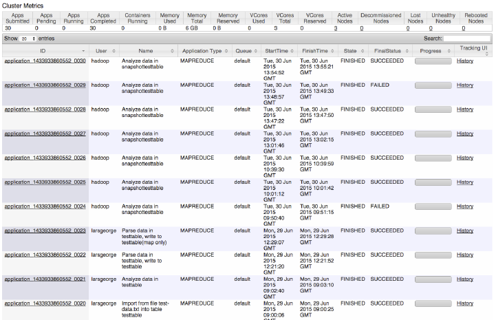
Exception in thread "main" java.io.IOException: \
java.util.concurrent.ExecutionException: \
org.apache.hadoop.security.AccessControlException: Permission
denied: \
user=larsgeorge, access=WRITE, \
inode="/hbase/archive/data/default":hadoop:supergroup:drwxr-xr-
x
at org.apache.hadoop.hdfs.server.namenode.FSPermission‐
Checker \
.checkFsPermission(FSPermissionChecker.java:271)
at org.apache.hadoop.hdfs.server.namenode.FSPermission‐
Checker....
...
Figure 7-6 shows the YARN main page with the applications list. You
can see how the earlier jobs were run as user larsgeorge, and then
the latter ones as hadoop using the approach shown above.
Figure 7-6. The class hierarchy of the basic client API data classes
An option to avoid write access to the HBase root is using the ExportS
napshot tool (see (to come)). Obviously, this tool has to copy the data
from the active or archive location into the target directory. At scale
this is a costly operation and should be carefully evaluated. Also, since
you copy into an arbitrary HDFS location, you are ultimately responsi‐
ble for managing that data. This includes keeping the files while jobs
Chapter 7: Hadoop Integration626
www.finebook.ir
are executing, and removing them when they are not required any‐
more.
Finally, another reason for using snapshots as a data source instead of
tables for MapReduce processing is that it avoids RPCs and other in‐
herent overhead of the server processes. This alone can speed up the
overall runtime of the job by a substantial margin. The JIRA adding
this input format class (see HBASE-8369) reports a factor of 5 to 6
times faster scanning performance for single scanners.
Bulk Loading Data
Instead of going through the API using put() calls to insert data—or
delete() to remove it subsequently--, especially when you need to
bootstrap a cluster with large amounts of existing data, you can also
stage and bulk load that data without going through the HBase
servers. This is a bit of a conundrum with HBase, as it is made for
small data points, and optimized for writes, with its sequential, Log-
Structured Merge Tree based architecture (more about this in (to
come)). Yet, the cost for maintaining said small data points is not neg‐
ligible. Filling the in-memory stores during write operation and flush‐
ing them subsequently, the compaction of data asynchronously in an
effort to keep the number of files in check, while handling explicit or
predicate deletes, is adding a non-trivial amount of noise to the sys‐
tem. Not to even speak of memory management pressure during in‐
tense writing, due to Java heap fragmentation. What if you could avoid
all of that, because you have the data already in some amenable for‐
mat and all you need doing is transform it into HBase data? That is ex‐
actly what bulk loading is: an ETL job that stages and loads the data
into HBase in its native format.
What is misleading here it to speak of loading data into HBase. What
really happens is that after the staging of the data in native HBase
store files, the so called HFiles, you atomically move them into the
HBase storage location, making them and the contained data immedi‐
ately available. Before you can do that though you have to do the stag‐
ing part, and that is an interesting one as well. Usually this is done by
a MapReduce job which extracts the records from the original data,
then converts them into Put or Delete instances, which are then stor‐
ed in HFiles. This implies sorting the data into rows and columns, ex‐
actly the way HBase would have done if you had used the client API.
And to complicate things, you often want to stage the store files in the
same layout as the target table is currently. You need to read the tar‐
get table’s region details, to separate the staged files in the same
granularity. Then once you complete the bulk load, you have to ensure
Bulk Loading Data 627
www.finebook.ir
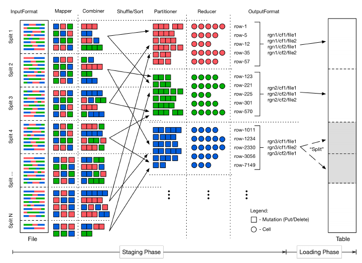
that this layout is still the same, which means if a region has split
since the initial region check, you may have to split the staged files
too to follow the new table layout. All of this is done by the supplied
ImportTsv and LoadIncrementalHFiles tools, as explained from an
operations side in (to come). Here we are going to look more into the
MapReduce integration, as it might help you stage other sources, or
create HFiles with a different processing framework, while using the
same principles, and output format classes.
Figure 7-7. The bulk loading process
The ImportTsv tool can be used as a template for the first phase of
bulk loading: the staging of data. Once this step has completed you
use the LoadIncrementalHFiles tool to do any final region split ad‐
justments, and then move the data files into place. Figure 7-7 shows a
high level view of how the bulk load process works. We will focus here
Chapter 7: Hadoop Integration628
www.finebook.ir

on the first phase, which employs many techniques to create the stag‐
ed data files:
The ImportTsv Helper Tool
The ImportTsv tool only supports inserting data into the table. In
other words, many used (and provided) classes are solely support‐
ing Put instances only. There is no inherent reason to extend the
idea to Deletes, but that has not been implemented yet. Adding
support for other mutations would not change the overall process.
The ImportTsv implementation has another special feature, it can
delay the creation of Put instances to coincide with the reduce
function—referred to as text-mode hereafter. In other words, in‐
stead of emitting Put objects from the mapper, then combining,
and shipping them to the reducer, you can keep the data in text
form and do the work at the end of the process. This was imple‐
mented in HBASE-8768 and available since HBase 0.98.0. You
need to enable that feature by overriding the mapper class using
the command line parameter:
-
Dimporttsv.mapper.class=org.apache.hadoop.hbase.mapre‐
duce.TsvImporterTextMapper
The tool will then switch out the appropriate classes as needed
during the job submission phase.
Read the Input Data
The first step is to read the original data, which is parsed into Put
or Delete (referred to collectively as mutation hereafter, for the
sake of simplicity) instance at the available granularity. This could
be one mutation for every column, or one for the entire row—all
dependent on what your input data looks like. You might even get
data for one row spread across the input files, which creates muta‐
tion instances at random times during the processing, spread
across random worker nodes in the cluster. All of these need to be
grouped subsequently.
The mapper is expected to emit the mutations as values, while the
row key of each mutation is used as the key for each record. This
will trigger the built-in shuffle and sorting functionality of the
MapReduce framework, grouping all mutations by row key. We
will see below how this is a boon and a bane (of sorts), since the
default hash function used to route the records would randomly
distribute them to matching reducer tasks. It would mean that the
Bulk Loading Data 629
www.finebook.ir
rows would not be contiguous across all partitions, but only within
each.
For ImportTsv see the TsvImporterMapper (or TsvImporterText
Mapper for text-mode) as an example mapper implementation.
Combine Mutations
As an optimization, we can combine the mutations for the same
row emitted by the same mapper task. We might not have the en‐
tire row on this server, but if we have more than one mutation for
a specific row, we can combine them into a single one, saving ob‐
ject overhead before the shuffle and sort take place.
Note that for ImportTsv this is provided by the PutCombiner class,
and only supports Put instances, as the name implies. The sup‐
plied class uses an implicit upper size boundary to not run into
memory pressure when combining puts. It is set to 1GB and can be
modified by setting the putcombiner.row.threshold property in
the configuration. For text-mode there is no combiner used.
Route Mutations
This is where we get the grouping of rows within region bound‐
aries working. The default hash partitioner class is replaced with
the TotalOrderPartitioner class, provided by Hadoop. It re‐
quires a list of partitions, based on user provided boundaries. For
bulk loading we use the target table’s region boundaries and hand
that list over to the special partitioner class. Any mutation that is
emitted is then send to the reducer handling the key subrange.
This also implies that we have to run as many reducers as we have
regions in the target table.
Sort Rows
There is not much that needs to be done for the rows to be sorted
within a region (or partition, both are used synonymously here), as
the MapReduce framework is taking care of that. This is one of the
fundamental tasks of the framework, sending the records to the
proper partition (based on the used partitioner implementation),
and the sorting them by their key component. This is why the key
type ImmutableBytesWritable is derived from the Hadoop Writa
bleComparable class, allowing for a natural sorting of records by
keys.
Sort Columns
While records are grouped and sorted by key, it leaves the associ‐
ated values to be ordered, that is, the mutations and the contained
columns forming a logical row in the resulting HBase table. The
PutSortReducer (or TextSortReducer for text-mode) class handles
Chapter 7: Hadoop Integration630
www.finebook.ir
this task, being provided with all mutations for a given row key, it
sorts the contained columns just like HBase would have done dur‐
ing an organic write operation using the client API.
The putsortreducer.row.threshold (or reducer.row.threshold
for text-mode) property, set to 1GB, defines an upper boundary to
avoid memory issues in extreme cases, with very memory intense
rows (those that contain many columns, or very large cells). The
output of the reducer are the actual columns (the cells) as the val‐
ue, and not a Put or Delete, while the key stays unchanged and
set as the row key. Figure 7-7 shows the difference by switching
from boxes to circles in the reducer step.
Write Files
The already discussed HFileOutputFormat2 class is responsible
for writing the actual storage files, that is, the HFiles. Its provided,
static helper method configureIncrementalLoad() can be used to
configure all the output format related aspects of the ETL job. This
includes setting the above reducer and partitioner classes (along
with its custom partition information), as well as the HFile related
properties, such as compression type, Bloom filter settings, block
sizes and encodings. Otherwise, the output format is honoring
many the usual storage related configuration properties, such as
hbase.hregion.max.filesize (set to 10GB by default) to specify
the maximum file size.
These are, from a generic viewpoint, all of the steps involved in stag‐
ing the bulk load data. The new HFiles are created in a temporary lo‐
cation, which needs to be set per staging job, and obviously requires
read and write access for the user running the job. For ImportTsv you
can specify the location on the command line, using the im
porttsv.bulk.output parameter. The mentioned LoadIncrementalH
Files utility performs the second stage of the bulk loading, by moving
the new files into the existing table directory, while ensuring any
short term region boundary changes are resolved in the process.
One caveat needs to be mentioned: loading potentially very large files
into a region can trigger splits right after the process completes. You
saw above that the staging process is creating files up to the maxi‐
mum configured size. If you already have storage files in the region,
you will trigger region splits if the combined new size of loaded files
plus existing ones exceeds the configured store maximum (which is
what the hbase.hregion.max.filesize really configures). This is OK
of course, because that is part of what makes HBase special, that is, it
does the housekeeping work for you asynchronously. On the other
hand, that again adds background I/O load to your cluster. It is advisa‐
Bulk Loading Data 631
www.finebook.ir
ble to calculate the sizes carefully, and maybe split regions at a slower
pace (say at off-peak times) before you do the loading.
Loading data into an existing table is a common exercise, and if that
table has a decent number of regions you will be able to efficiently
load data into them. This is attributed by the number of reducers
matching the number of regions, allowing for parallelizing the work
into as many concurrent tasks your MapReduce cluster can afford.
But what about a bootstrap process, that is, when you want to bulk
load new data in a not-yet-existent table? You can certainly use the
create shell command to quickly create a table, but that will only
have one region, and resulting into a single reducer task doing all the
data staging. Here is where presplitting a table comes in, discussed in
detail in (to come). Suffice it to say that you create a certain number
of regions at the time you create the table. These regions will be emp‐
ty, but then fill with data as it is being written to.
If presplitting a new table is the answer to avoid hotspotting on a sin‐
gle region for staging the bulk load, then how splits do you need? And
at what boundaries do you split them? This requires detailed knowl‐
edge of the key space, which you may not have when faced with an ar‐
bitrary set of input data. The common approach is to sample or parse
the data at least once, tracking the size of each record and building
equally sized partitions. This is only possible if you know where data
will eventually be located in the resulting table, and thus you may
have to run the same staging logic twice, once to determine the num‐
ber of regions and their boundaries based on size, and then again to
do the actual file staging. An alternative approach is to sample the im‐
port data first, trying to extrapolate the region sizes and count from
what you have access to. This is a common analytical task and not spe‐
cific to Hadoop or HBase. You need to calculate the possible error
rate to decide which sample rate works best for you. Either way, once
you have computed the split points based on the used row keys, you
hand this list into first the shell’s create command to presplit the new
table, and second the TotalOrderPartitioner, which will do the rest.
Chapter 7: Hadoop Integration632
www.finebook.ir

Appendix A
Upgrade from Previous
Releases
Upgrading HBase involves careful planning, especially when the clus‐
ter is currently in production. With the addition of rolling restarts (see
(to come)), it has become much easier to update HBase with no down‐
time.
Depending on the version of HBase you are using or up‐
grading to, you may need to upgrade the underlying Ha‐
doop version first so that it matches the required version
for the new version of HBase you are installing. Follow the
upgrade guide found on the Hadoop website.
Upgrading to HBase 0.90.x
Depending on the versions you are upgrading from, a different set of
steps might be necessary to update your existing cluster to a newer
version. The following subsections address the more common update
scenarios.
From 0.20.x or 0.89.x
This version of 0.90.x HBase can be started on data written by HBase
0.20.x or HBase 0.89.x, and there is no need for a migration step.
HBase 0.89.x and 0.90.x do write out the names of region directories
differently—they name them with an MD5 hash of the region name
633
www.finebook.ir
1. See “HBASE-3499 Users upgrading to 0.90.0 need to have their .META. table upda‐
ted with the right MEMSTORE_SIZE” (http://issues.apache.org/jira/browse/
HBASE-3499) for details.
rather than a Jenkins hash, which means that once you have started,
there is no going back to HBase 0.20.x.
Be sure to remove the hbase-default.xml file from your conf directory
when you upgrade. A 0.20.x version of this file will have suboptimal
configurations for HBase 0.90.x. The hbase-default.xml file is now
bundled into the HBase JAR and read from there. If you would like to
review the content of this file, you can find it in the src directory at
$HBASE_HOME/src/main/resources/hbase-default.xml or see (to
come).
Finally, if upgrading from 0.20.x, check your .META. schema in the
shell. In the past, it was recommended that users run with a 16 KB
MEMSTORE_FLUSHSIZE. Execute
hbase(main):001:0> scan '-ROOT-'
in the shell. This will output the current .META. schema. Check if the
MEMSTORE_FLUSHSIZE size is set to 16 KB (16384). If that is the case,
you will need to change this. The new default value is 64 MB
(67108864). Run the script $HBASE_HOME/bin/
set_meta_memstore_size.rb. This will make the necessary changes
to your .META. schema. Failure to run this change will cause your
cluster to run more slowly.1
Within 0.90.x
You can use a rolling restart during any of the minor upgrades. Simply
install the new version and restart the region servers using the proce‐
dure described in (to come).
Upgrading to HBase 0.92.0
No rolling restart is possible, as the wire protocol has changed be‐
tween versions. You need to prepare the installation in parallel, then
shut down the cluster and start the new version of HBase. No migra‐
tion is needed otherwise.
Appendix A: Upgrade from Previous Releases634
www.finebook.ir

Upgrading to HBase 0.98.x
Migrate API to HBase 1.0.x
TBD.
Table A-1. List of deprecated API methods and classes with their
replacement
Name Type Replacement Type
HTable Class Table Interface
HConnection Interface Connection Interface
HConnectionManager Class ConnectionFactory Class
HTableFactory Class ConnectionFactory.createCon
nection() Method
HTableInterface Interface Table Interface
HTablePool Class Connection.getTable() Method
<tablename> String TableName Class
HTable.getWriteToWAL() Method Table.getDurabilty() Method
HTable.setWriteToWAL() Method Table.setDurabilty() Method
HTable.getFamilyMap() Method Table.getFamilyCellMap() Method
HTable.setFamilyMap() Method Table.setFamilyCellMap() Method
Delete.deleteColumn() Method Delete.addColumn() Method
Delete.deleteColumns() Method Delete.addColumns() Method
Delete.deleteFamily() Method Delete.addFamily() Method
Delete.deleteFamilyVersion() Method Delete.addFamilyVersion() Method
Table.batch(List<? extends
Row>) Method Table.batch(List<? extends
Row>, Object[]) Method
Table.batchCallback(List<?
extends Row>, Callback<R>) Method Table.batchCallback(List<?
extends Row>, Object[], Call
back<R>)
Method
Batch.forMethod() Method dropped, no replacement n/a
Migrate Coprocessors to post HBase 0.96
Here are the steps needed to convert a Writable based coprocessor
implementation into a new Protocol Buffer based one. This is needed
since as of HBase 0.96 (nicknamed the Singularity) the entire RPC
communication has been replaced by a proper, versioned serialization
protocol. With that the old format is not acceptable anymore, and a
few changes had to take place. The following uses the RowCount exam‐
Upgrading to HBase 0.98.x 635
www.finebook.ir
ple from the first revision of the book, and how it was converted to the
new API.
Step 1
The first thing to do is to drop the custom protocol class in favor of a
Protocol Buffer definition. You can delete the entire class file that im‐
plements the protocol interface, which looks like this:
public interface RowCountProtocol extends CoprocessorProtocol {
long getRowCount() throws IOException;
long getRowCount(Filter filter) throws IOException;
long getKeyValueCount() throws IOException;
}
You need to create the replacement Protocol Buffer definition file, and
following Maven project layout rules, they go into $
{PROJECT_HOME}/src/main/protobuf, here with the name RowCount
Service.proto.
option java_package = "coprocessor.generated";
option java_outer_classname = "RowCounterProtos";
option java_generic_services = true;
option java_generate_equals_and_hash = true;
option optimize_for = SPEED;
message CountRequest {
}
message CountResponse {
required int64 count = 1 [default = 0];
}
service RowCountService {
rpc getRowCount(CountRequest)
returns (CountResponse);
rpc getCellCount(CountRequest)
returns (CountResponse);
}
The file defines the output class name, the package to use during code
generation and so on. The last thing in step #1 is to compile the defi‐
nition file into code. This is done using the Protocol Buffer protoc
tool, as described in more detail in “Custom Filters” (page 259). Exe‐
cuting the command-line compiler will place the generated class file
in the source directory, as specified.
Step 2
The next step is to convert Endpoint to new API, which involves re‐
moving the old custom RPC interface, and adding the new Protocol
Appendix A: Upgrade from Previous Releases636
www.finebook.ir

Buffer based one (see the RowCountEndpoint class in the code reposi‐
tory). The old way to integrate the custom calls looked like this:
public class RowCountEndpoint extends BaseEndpointCoprocessor
implements RowCountProtocol {
The new replaces the custom interface with the generated one from
step #1 above:
public class RowCountEndpoint extends RowCounterProtos.RowCountSer‐
vice
implements Coprocessor, CoprocessorService {
We also implement two more coprocessor related interface directly:
there is no BaseEndpointProcessor anymore. The Coprocessor and
CoprocessorService interfaces add vital lifecycle methods to our
class. We need the start() call to retrieve the coprocessor environ‐
ment like so:
@Override
public void start(CoprocessorEnvironment env) throws IOException {
if (env instanceof RegionCoprocessorEnvironment) {
this.env = (RegionCoprocessorEnvironment) env;
} else {
throw new CoprocessorException("Must be loaded on a table re‐
gion!");
}
}
In the past the boilerplate BaseEndpointProcessor gave us a getEn
vironment() method to retrieve the same. We now need to do this on
our own. On top of that we need to change the RPC call handlers,
where the old once simply implemented the custom RPC interface
methods:
@Override
public long getRowCount() throws IOException {
return getRowCount(new FirstKeyOnlyFilter());
}
In the new API style we have to add a bit more wiring, especially
around the marshalling of the result—or error—and how it is returned
to the framework (see the online documentation). Due to the use of
the Protocol Buffer library, we need to accept a request object and re‐
turn a response like so:
@Override
public void getCellCount(RpcController controller,
RowCounterProtos.CountRequest request,
RpcCallback<RowCounterProtos.CountResponse> done) {
RowCounterProtos.CountResponse response = null;
try {
long count = getCount(null, true);
Migrate API to HBase 1.0.x 637
www.finebook.ir
response = RowCounterProtos.CountResponse.newBuilder()
.setCount(count).build();
} catch (IOException ioe) {
ResponseConverter.setControllerException(controller, ioe);
}
done.run(response);
}
Custom RPC call with specific handler classes, such as the
controller, and request/response pair.
Call the internal helper to scan and summarize per region
aggregates as usual.
Hand in resulting count into the response wrapper.
Handle exceptions by wrapping the error and returning it via the
controller.
Apart from that there are more changes, unrelated to coprocessors,
that are required to make the old code work. For example, we need to
change from KeyValue to Cell types, and adjust how we do compari‐
sons. The new code looks very similar, but has a few slight changes:
try (
InternalScanner scanner = env.getRegion().getScanner(scan);
) {
List<Cell> results = new ArrayList<Cell>();
boolean hasMore = false;
byte[] lastRow = null;
do {
hasMore = scanner.next(results);
for (Cell cell : results) {
if (!countCells) {
if (lastRow == null || !CellUtil.matchingRow(cell, las‐
tRow)) {
lastRow = CellUtil.cloneRow(cell);
count++;
}
} else count++;
}
results.clear();
} while (hasMore);
}
Use of the new try-with-resource pattern to simplify resources
handling.
The new Cell interface is used to retrieve the data and iterate
over it.
Comparing changed to use the CellUtil.matchingRow() method,
for convenience.
Appendix A: Upgrade from Previous Releases638
www.finebook.ir

The byte array has to be memorized, use again the CellUtil
helper to clone the row key.
Apart from that, no further code changes on the server-side code were
necessary.
Step 3
From here you need to do the same as before, that is deploy the cop‐
rocessor as a JAR file on the servers, add the class name to the hbase-
site.xml file, add the JAR name to the class path in the hbase-env.sh
file, and restart the servers.
Step 4
Last step is invoking the server-side code. This is now client API code
that has to be adjusted. This is located in the EndpointExample class,
and looks like this for the old style API:
Map<byte[], Long> results = table.coprocessorExec(
RowCountProtocol.class, null, null,
new Batch.Call<RowCountProtocol, Long>() {
@Override
public Long call(RowCountProtocol counter) throws IOException {
return counter.getRowCount();
}
});
For the new one there are a few changes, analog to what we have
seen on the server-side code. There is more wiring for the Protocol
Buffer based RPC handling:
final RowCounterProtos.CountRequest request =
RowCounterProtos.CountRequest.getDefaultInstance();
Map<byte[], Long> results = table.coprocessorService(
RowCounterProtos.RowCountService.class, null, null,
new Batch.Call<RowCounterProtos.RowCountService, Long>() {
public Long call(RowCounterProtos.RowCountService counter)
throws IOException {
BlockingRpcCallback<RowCounterProtos.CountResponse> rpcCall‐
back =
new BlockingRpcCallback<RowCounterProtos.CountResponse>();
counter.getRowCount(null, request, rpcCallback);
RowCounterProtos.CountResponse response = rpcCallback.get();
return response.hasCount() ? response.getCount() : 0;
}
}
);
Create a request instance using the generated RPC class.
Migrate API to HBase 1.0.x 639
www.finebook.ir

Call the new coprocessorService() method (the older coprocessorEx
ec() has been removed).
Use the generated classes to paramterize the call.
Set up an RPC callback for the specific call and types.
Invoke the remote call.
Retrieve the response and, subsequently, the payload value (our
row count).
These are all the changes that were needed to run the existing exam‐
ple using the new API.
Migrate Custom Filters to post HBase 0.96
Here are the steps needed to convert a Writable based filter imple‐
mentation into a new Protocol Buffer based one. This is needed since
as of HBase 0.96 (nicknamed the Singularity) the entire RPC commu‐
nication has been replaced by a proper, versioned serialization proto‐
col. With that the old format is not acceptable anymore, and a few
changes had to take place. The following uses the CustomFilter ex‐
ample from the first revision of the book, and how it was converted to
the new API.
Step 1
First you need to create a Protocol Buffer definition, which covers all
the internal fields of the filter, setting its state. Following Maven
project layout rules, they go into ${PROJECT_HOME}/src/main/proto
buf, here with the name CustomFilters.proto. The content is the fol‐
lowing:
option java_package = "filters.generated";
option java_outer_classname = "FilterProtos";
option java_generic_services = true;
option java_generate_equals_and_hash = true;
option optimize_for = SPEED;
message CustomFilter {
required bytes value = 1;
}
The file defines the output class name, the package to use during code
generation and so on. The last thing in step #1 is to compile the defi‐
nition file into code. This is done using the Protocol Buffer protoc
tool, as described in more detail in “Custom Filters” (page 259). Exe‐
cuting the command-line compiler will place the generated class file
in the source directory, as specified.
Appendix A: Upgrade from Previous Releases640
www.finebook.ir
Step 2
Next step is the conversion of the existing, Writable based, serializa‐
tion methods, over to the new Protocal Buffer ones. For that we need
to change to methods, here the old version:
@Override
public void write(DataOutput dataOutput) throws IOException {
Bytes.writeByteArray(dataOutput, this.value);
}
@Override
public void readFields(DataInput dataInput) throws IOException {
this.value = Bytes.readByteArray(dataInput);
Both of those methods can be dropped, and are replaced by the fol‐
lowing two:
@Override
public byte [] toByteArray() {
FilterProtos.CustomFilter.Builder builder =
FilterProtos.CustomFilter.newBuilder();
if (value != null) builder.setValue(ByteStringer.wrap(value));
return builder.build().toByteArray();
}
public static Filter parseFrom(final byte[] pbBytes)
throws DeserializationException {
FilterProtos.CustomFilter proto;
try {
proto = FilterProtos.CustomFilter.parseFrom(pbBytes);
} catch (InvalidProtocolBufferException e) {
throw new DeserializationException(e);
}
return new CustomFilter(proto.getValue().toByteArray());
}
The look more complicated, but that is attributed to the Protocol
Buffer handling, which is not as hidden as the Writable version. The
toByteArray() serialized the filter fields inside a Protocol Buffer mes‐
sage. For that it creates a Builder instance that was generated in
step #1. The builder is then executed and the resulting byte array re‐
turned.
On the deserialization side the parseFrom() receives the byte array,
which is then parse by the generated code into a message instance.
The contained data is handed into the filter constructor, which is re‐
turned to the caller in due course.
Step 3
Migrate API to HBase 1.0.x 641
www.finebook.ir
From here you need to do the same as before, that is deploy the cop‐
rocessor as a JAR file on the servers, add the class name to the hbase-
site.xml file, add the JAR name to the class path in the hbase-env.sh
file, and restart the servers. See “Custom Filters” (page 259) for de‐
tails on the deployment options.
Step 4
Last step is invoking the filter as part of a read operation. This stays
the same as well as before, since we only adjusted the internal seriali‐
zation process, which is otherwise not exposed to the client. The us‐
age and rest of the filter implementation stays the same (see
Example 4-24 for an example).
Appendix 0: Upgrade from Previous Releases642
www.finebook.ir
